A.N. Shiryaev
Probability
Second Edition
Springer

N.-AvV
***«*.
"Order out of chaos"
(Courtesy of Professor A. T. Fomenko of the Moscow State University)

Preface to the Second Edition
In the Preface to the first edition, originally published in 1980, we mentioned
that this book was based on the author's lectures in the Department of
Mechanics and Mathematics of the Lomonosov University in Moscow,
which were issued, in part, in mimeographed form under the title
"Probability, Statistics, and Stochastic Processors, I, II" and published by that
University. Our original intention in writing the first edition of this book was to
divide the contents into three parts: probability, mathematical statistics, and
theory of stochastic processes, which corresponds to an outline of a three-
semester course of lectures for university students of mathematics. However,
in the course of preparing the book, it turned out to be impossible to realize
this intention completely, since a full exposition would have required too
much space. In this connection, we stated in the Preface to the first edition
that only probability theory and the theory of random processes with discrete
time were really adequately presented.
Essentially all of the first edition is reproduced in this second edition.
Changes and corrections are, as a rule, editorial, taking into account
comments made by both Russian and foreign readers of the Russian original and
of the English and German translations [Sll]. The author is grateful to all of
these readers for their attention, advice, and helpful criticisms.
In this second English edition, new material also has been added, as
follows: in Chapter III, §5, §§7-12; in Chapter IV, §5; in Chapter VII, §§8-10.
The most important addition is the third chapter. There the reader will
find expositions of a number of problems connected with a deeper study of
themes such as the distance between probability measures, metrization of
weak convergence, and contiguity of probability measures. In the same
chapter, we have added proofs of a number of important results on the rapidity of
convergence in the central limit theorem and in Poisson's theorem on the

Vlll
Preface to the Second Edition
approximation of the binomial by the Poisson distribution. These were
merely stated in the first edition.
We also call attention to the new material on the probability of large
deviations (Chapter IV, §5), on the central limit theorem for sums of
dependent random variables (Chapter VII, §8), and on §§9 and 10 of Chapter VII.
During the last few years, the literature on probability published in Russia
by Nauka has been extended by Sevastyanov [S10], 1982; Rozanov [R6],
1985; Borovkov [B4], 1986; and Gnedenko [G4], 1988. It appears that these
publications, together with the present volume, being quite different and
complementing each other, cover an extensive amount of material that is
essentially broad enough to satisfy contemporary demands by students in
various branches of mathematics and physics for instruction in topics in
probability theory.
Gnedenko's textbook [G4] contains many well-chosen examples,
including applications, together with pedagogical material and extensive surveys of
the history of probability theory. Borovkov's textbook [B4] is perhaps the
most like the present book in the style of exposition. Chapters 9 (Elements of
Renewal Theory), 11 (Factorization of the Identity) and 17 (Functional Limit
Theorems), which distinguish [B4] from this book and from [G4] and [R6],
deserve special mention. Rozanov's textbook contains a great deal of
material on a variety of mathematical models which the theory of probability and
mathematical statistics provides for describing random phenomena and their
evolution. The textbook by Sevastyanov is based on his two-semester course
at the Moscow State University. The material in its last four chapters covers
the minimum amount of probability and mathematical statistics required in
a one-year university program. In our text, perhaps to a greater extent than
in those mentioned above, a significant amount of space is given to set-
theoretic aspects and mathematical foundations of probability theory.
Exercises and problems are given in the books by Gnedenko and
Sevastyanov at the ends of chapters, and in the present textbook at the end
of each section. These, together with, for example, the problem sets by A. V.
Prokhorov and V. G. and N. G. Ushakov (Problems in Probability Theory,
Nauka, Moscow, 1986) and by Zubkov, Sevastyanov, and Chistyakov
(Collected Problems in Probability Theory, Nauka, Moscow, 1988) can be used by
readers for independent study, and by teachers as a basis for seminars for
students.
Special thanks to Harold Boas, who kindly translated the revisions from
Russian to English for this new edition.
Moscow
A. Shiryaev

Preface to the First Edition
This textbook is based on a three-semester course of lectures given by the
author in recent years in the Mechanics-Mathematics Faculty of Moscow
State University and issued, in part, in mimeographed form under the title
Probability, Statistics, Stochastic Processes, I, II by the Moscow State
University Press.
We follow tradition by devoting the first part of the course (roughly one
semester) to the elementary theory of probability (Chapter I). This begins
with the construction of probabilistic models with finitely many outcomes
and introduces such fundamental probabilistic concepts as sample spaces,
events, probability, independence, random variables, expectation,
correlation, conditional probabilities, and so on.
Many probabilistic and statistical regularities are effectively illustrated
even by the simplest random walk generated by Bernoulli trials. In this
connection we study both classical results (law of large numbers, local and
integral De Moivre and Laplace theorems) and more modern results (for
example, the arc sine law).
The first chapter concludes with a discussion of dependent random
variables generated by martingales and by Markov chains.
Chapters II-IV form an expanded version of the second part of the course
(second semester). Here we present (Chapter II) Kolmogorov's generally
accepted axiomatization of probability theory and the mathematical methods
that constitute the tools of modern probability theory (<r-algebras, measures
and their representations, the Lebesgue integral, random variables and
random elements, characteristic functions, conditional expectation with
respect to a <r-algebra, Gaussian systems, and so on). Note that two measure-
theoretical results—Caratheodory's theorem on the extension of measures
and the Radon-Nikodym theorem—are quoted without proof.

X
Preface to the First Edition
The third chapter is devoted to problems about weak convergence of
probability distributions and the method of characteristic functions for
proving limit theorems. We introduce the concepts of relative compactness
and tightness of families of probability distributions, and prove (for the
real line) Prohorov's theorem on the equivalence of these concepts.
The same part of the course discusses properties "with probability 1"
for sequences and sums of independent random variables (Chapter IV). We
give proofs of the "zero or one laws" of Kolmogorov and of Hewitt and
Savage, tests for the convergence of series, and conditions for the strong law
of large numbers. The law of the iterated logarithm is stated for arbitrary
sequences of independent identically distributed random variables with
finite second moments, and proved under the assumption that the variables
have Gaussian distributions.
Finally, the third part of the book (Chapters V-VIII) is devoted to random
processes with discrete parameters (random sequences). Chapters V and VI
are devoted to the theory of stationary random sequences, where "
stationary " is interpreted either in the strict or the wide sense. The theory of random
sequences that are stationary in the strict sense is based on the ideas of
ergodic theory: measure preserving transformations, ergodicity, mixing, etc.
We reproduce a simple proof (by A. Garsia) of the maximal ergodic theorem;
this also lets us give a simple proof of the BirkhofT-Khinchin ergodic theorem.
The discussion of sequences of random variables that are stationary in
the wide sense begins with a proof of the spectral representation of the
covariance fuction. Then we introduce orthogonal stochastic measures, and
integrals with respect to these, and establish the spectral representation of
the sequences themselves. We also discuss a number of statistical problems:
estimating the covariance function and the spectral density, extrapolation,
interpolation and filtering. The chapter includes material on the Kalman-
Bucy filter and its generalizations.
The seventh chapter discusses the basic results of the theory of martingales
and related ideas. This material has only rarely been included in traditional
courses in probability theory. In the last chapter, which is devoted to Markov
chains, the greatest attention is given to problems on the asymptotic behavior
of Markov chains with countably many states.
Each section ends with problems of various kinds: some of them ask for
proofs of statements made but not proved in the text, some consist of
propositions that will be used later, some are intended to give additional
information about the circle of ideas that is under discussion, and finally,
some are simple exercises.
In designing the course and preparing this text, the author has used a
variety of sources on probability theory. The Historical and Bibliographical
Notes indicate both the historial sources of the results and supplementary
references for the material under consideration.
The numbering system and form of references is the following. Each
section has its own enumeration of theorems, lemmas and formulas (with

Preface to the First Edition
XI
no indication of chapter or section). For a reference to a result from a
different section of the same chapter, we use double numbering, with the
first number indicating the number of the section (thus, (2.10) means formula
(10) of §2). For references to a different chapter we use triple numbering
(thus, formula (II.4.3) means formula (3) of §4 of Chapter II). Works listed
in the References at the end of the book have the form [L«], where L is a
letter and n is a numeral.
The author takes this opportunity to thank his teacher A. N. Kolmogorov,
and B. V. Gnedenko and Yu. V. Prokhorov, from whom he learned probability
theory and under whose direction he had the opportunity of using it. For
discussions and advice, the author also thanks his colleagues in the
Departments of Probability Theory and Mathematical Statistics at the Moscow
State University, and his colleagues in the Section on probability theory of the
Steklov Mathematical Institute of the Academy of Sciences of the U.S.S.R.
Moscow A. N. Shiryaev
Steklov Mathematical Institute
Translator's acknowledgement. I am grateful both to the author and to
my colleague, C. T. Ionescu Tulcea, for advice about terminology.
R. P. B.

Contents
Preface to the Second Edition vii
Preface to the First Edition ix
Introduction 1
CHAPTER I
Elementary Probability Theory 5
§1. Probabilistic Model of an Experiment with a Finite Number of
Outcomes 5
§2. Some Classical Models and Distributions 17
§3. Conditional Probability. Independence 23
§4. Random Variables and Their Properties 32
§5. The Bernoulli Scheme. I. The Law of Large Numbers 45
§6. The Bernoulli Scheme. II. Limit Theorems (Local,
De Moivre-Laplace, Poisson) 55
§7. Estimating the Probability of Success in the Bernoulli Scheme 70
§8. Conditional Probabilities and Mathematical Expectations with
Respect to Decompositions 76
§9. Random Walk. I. Probabilities of Ruin and Mean Duration in
Coin Tossing 83
§10. Random Walk. II. Reflection Principle. Arcsine Law 94
§11. Martingales. Some Applications to the Random Walk 103
§12. Markov Chains. Ergodic Theorem. Strong Markov Property 110
CHAPTER II
Mathematical Foundations of Probability Theory 131
§1. Probabilistic Model for an Experiment with Infinitely Many
Outcomes. Kolmogorov's Axioms 131

xiv Contents
§2. Algebras and a-algebras. Measurable Spaces 139
§3. Methods of Introducing Probability Measures on Measurable Spaces 151
§4. Random Variables. I. 170
§5. Random Elements 176
§6. Lebesgue Integral. Expectation 180
§7. Conditional Probabilities and Conditional Expectations with
Respect to a a-Algebra 212
§8. RandomVariables.il. 234
§9. Construction of a Process with Given Finite-Dimensional
Distribution 245
§10. Various Kinds of Convergence of Sequences of Random Variables 252
§11. The Hilbert Space of Random Variables with Finite Second Moment 262
§12. Characteristic Functions 274
§13. Gaussian Systems 297
CHAPTER III
Convergence of Probability Measures. Central Limit
Theorem 308
§1. Weak Convergence of Probability Measures and Distributions 308
§2. Relative Compactness and Tightness of Families of Probability
Distributions 317
§3. Proofs of Limit Theorems by the Method of Characteristic Functions 321
§4. Central Limit Theorem for Sums of Independent Random Variables. I.
The Lindeberg Condition 328
§5. Central Limit Theorem for Sums of Independent Random Variables. II.
Nonclassical Conditions 337
§6. Infinitely Divisible and Stable Distributions 341
§7. Metrizability of Weak Convergence 348
§8. On the Connection of Weak Convergence of Measures with Almost Sure
Convergence of Random Elements ("Method of a Single Probability
Space") 353
§9. The Distance in Variation between Probability Measures.
Kakutani-Hellinger Distance and Hellinger Integrals. Application to
Absolute Continuity and Singularity of Measures 359
§10. Contiguity and Entire Asymptotic Separation of Probability Measures 368
§11. Rapidity of Convergence in the Central Limit Theorem 373
§12. Rapidity of Convergence in Poisson's Theorem 376
CHAPTER IV
Sequences and Sums of Independent Random Variables 379
§1. Zero-or-One Laws 379
§2. Convergence of Series 384
§3. Strong Law of Large Numbers 388
§4. Law of the Iterated Logarithm 395
§5. Rapidity of Convergence in the Strong Law of Large Numbers and
in the Probabilities of Large Deviations 400

Contents
XV
CHAPTER V
Stationary (Strict Sense) Random Sequences and
Ergodic Theory 404
§1. Stationary (Strict Sense) Random Sequences. Measure-Preserving
Transformations 404
§2. Ergodicity and Mixing 407
§3. Ergodic Theorems 409
CHAPTER VI
Stationary (Wide Sense) Random Sequences. L2 Theory 415
§1. Spectral Representation of the Covariance Function 415
§2. Orthogonal Stochastic Measures and Stochastic Integrals 423
§3. Spectral Representation of Stationary (Wide Sense) Sequences 429
§4. Statistical Estimation of the Covariance Function and the Spectral
Density 440
§5. Wold's Expansion 446
§6. Extrapolation, Interpolation and Filtering 453
§7. The Kalman-Bucy Filter and Its Generalizations 464
CHAPTER VII
Sequences of Random Variables that Form Martingales 474
§1. Definitions of Martingales and Related Concepts 474
§2. Preservation of the Martingale Property Under Time Change at a
Random Time 484
§3. Fundamental Inequalities 492
§4. General Theorems on the Convergence of Submartingales and
Martingales 508
§5. Sets of Convergence of Submartingales and Martingales 515
§6. Absolute Continuity and Singularity of Probability Distributions 524
§7. Asymptotics of the Probability of the Outcome of a Random Walk
with Curvilinear Boundary 536
§8. Central Limit Theorem for Sums of Dependent Random Variables 541
§9. Discrete Version of Ito's Formula 554
§10. Applications to Calculations of the Probability of Ruin in Insurance 558
CHAPTER VIII
Sequences of Random Variables that Form Markov Chains 564
§1. Definitions and Basic Properties 564
§2. Classification of the States of a Markov Chain in Terms of
Arithmetic Properties of the Transition Probabilities p{$ 569
§3. Classification of the States of a Markov Chain in Terms of
Asymptotic Properties of the Probabilities p$ 573
§4. On the Existence of Limits and of Stationary Distributions 582
§5. Examples 587

Historical and Bibliographical Notes 596
References 603
Index of Symbols 609
Index 611

Introduction
The subject matter of probability theory is the mathematical analysis of
random events, i.e., of those empirical phenomena which—under certain
circumstance—can be described by saying that:
They do not have deterministic regularity (observations of them do not
yield the same outcome);
whereas at the same time
They possess some statistical regularity (indicated by the statistical
stability of their frequency).
We illustrate with the classical example of a "fair" toss of an "unbiased"
coin. It is clearly impossible to predict with certainty the outcome of each
toss. The results of successive experiments are very irregular (now "head,"
now "tail") and we seem to have no possibility of discovering any regularity
in such experiments. However, if we carry out a large number of
"independent" experiments with an "unbiased" coin we can observe a very definite
statistical regularity, namely that "head" appears with a frequency that is
"close" to^.
Statistical stability of a frequency is very likely to suggest a hypothesis
about a possible quantitative estimate of the "randomness" of some event A
connected with the results of the experiments. With this starting point,
probability theory postulates that corresponding to an event A there is a
definite number P(A), called the probability of the event, whose intrinsic
property is that as the number of "independent" trials (experiments)
increases the frequency of event A is approximated by P(A).
Applied to our example, this means that it is natural to assign the proba-

2
Introduction
bility \ to the event A that consists of obtaining "head" in a toss of an
"unbiased" coin.
There is no difficulty in multiplying examples in which it is very easy to
obtain numerical values intuitively for the probabilities of one or another
event. However, these examples are all of a similar nature and involve (so far)
undefined concepts such as "fair" toss, "unbiased" coin, "independence,"
etc.
Having been invented to investigate the quantitative aspects of
"randomness," probability theory, like every exact science, became such a science
only at the point when the concept of a probabilistic model had been clearly
formulated and axiomatized. In this connection it is natural for us to discuss,
although only briefly, the fundamental steps in the development of
probability theory.
Probability theory, as a science, originated in the middle of the seventeenth
century with Pascal (1623-1662), Fermat (1601-1655) and Huygens
(1629-1695). Although special calculations of probabilities in games of chance
had been made earlier, in the fifteenth and sixteenth centuries, by Italian
mathematicians (Cardano, Pacioli, Tartaglia, etc.), the first general methods
for solving such problems were apparently given in the famous
correspondence between Pascal and Fermat, begun in 1654, and in the first book on
probability theory, De Ratiociniis in Aleae Ludo (On Calculations in Games of
Chance), published by Huygens in 1657. It was at this time that the
fundamental concept of "mathematical expectation" was developed and theorems
on the addition and multiplication of probabilities were established.
The real history of probability theory begins with the work of James
Bernoulli (1654-1705), Ars Conjectandi (The Art of Guessing) published in
1713, in which he proved (quite rigorously) the first limit theorem of
probability theory, the law of large numbers; and of De Moivre (1667-1754),
Miscellanea Analytica Supplementum (a rough translation might be The
Analytic Method or Analytic Miscellany, 1730), in which the central limit
theorem was stated and proved for the first time (for symmetric Bernoulli
trials).
Bernoulli deserves the credit for introducing the "classical" definition of
the concept of the probability of an event as the ratio of the number of
possible outcomes of an experiment, that are favorable to the event, to the
number of possible outcomes.
Bernoulli was probably the first to realize the importance of considering
infinite sequences of random trials and to make a clear distinction between
the probability of an event and the frequency of its realization.
De Moivre deserves the credit for defining such concepts as independence,
mathematical expectation, and conditional probability.
In 1812 there appeared Laplace's (1749-1827) great treatise Theorie
Analytique des Probabilities (Analytic Theory of Probability) in which he
presented his own results in probability theory as well as those of his
predecessors. In particular, he generalized De Moivre's theorem to the general

Introduction
3
(unsymmetric) case of Bernoulli trials, and at the same time presented De
Moivre's results in a more complete form.
Laplace's most important contribution was the application of
probabilistic methods to errors of observation. He formulated the idea of
considering errors of observation as the cumulative results of adding a large number
of independent elementary errors. From this it followed that under rather
general conditions the distribution of errors of observation must be at least
approximately normal.
The work of Poisson (1781-1840) and Gauss (1777-1855) belongs to the
same epoch in the development of probability theory, when the center of the
stage was held by limit theorems. In contemporary probability theory we
think of Poisson in connection with the distribution and the process that
bear his name. Gauss is credited with originating the theory of errors and, in
particular, with creating the fundamental method of least squares.
The next important period in the development of probability theory is
connected with the names of P. L. Chebyshev (1821-1894), A. A. Markov
(1856-1922), and A. M. Lyapunov (1857-1918), who developed effective
methods for proving limit theorems for sums of independent but arbitrarily
distributed random variables.
The number of Chebyshev's publications in probability theory is not
large—four in all—but it would be hard to overestimate their role in
probability theory and in the development of the classical Russian school of that
subject.
"On the methodological side, the revolution brought about by Chebyshev
was not only his insistence for the first time on complete rigor in the proofs of
limit theorems,... but also, and principally, that Chebyshev always tried to
obtain precise estimates for the deviations from the limiting regularities that are
available for large but finite numbers of trials, in the form of inequalities that are
valid unconditionally for any number of trials."
(A. N. Kolmogorov [30])
Before Chebyshev the main interest in probability theory had been in the
calculation of the probabilities of random events. He, however, was the
first to realize clearly and exploit the full strength of the concepts of random
variables and their mathematical expectations.
The leading exponent of Chebyshev's ideas was his devoted student
Markov, to whom there belongs the indisputable credit of presenting his
teacher's results with complete clarity. Among Markov's own significant
contributions to probability theory were his pioneering investigations of
limit theorems for sums of independent random variables and the creation
of a new branch of probability theory, the theory of dependent random
variables that form what we now call a Markov chain.
"Markov's classical course in the calculus of probability and his original
papers, which are models of precision and clarity, contributed to the greatest
extent to the transformation of probability theory into one of the most significant

4
Introduction
branches of mathematics and to a wide extension of the ideas and methods of
Chebyshev."
(S. N. Bernstein [3])
To prove the central limit theorem of probability theory (the theorem
on convergence to the normal distribution), Chebyshev and Markov used
what is known as the method of moments. With more general hypotheses
and a simpler method, the method of characteristic functions, the theorem
was obtained by Lyapunov. The subsequent development of the theory has
shown that the method of characteristic functions is a powerful analytic
tool for establishing the most diverse limit theorems.
The modern period in the development of probability theory begins with
its axiomatization. The first work in this direction was done by S. N.
Bernstein (1880-1968), R. von Mises (1883-1953), and E. Borel (1871-1956).
A. N. Kolmogorov's book Foundations of the Theory of Probability appeared
in 1933. Here he presented the axiomatic theory that has become generally
accepted and is not only applicable to all the classical branches of probability
theory, but also provides a firm foundation for the development of new
branches that have arisen from questions in the sciences and involve infinite-
dimensional distributions.
The treatment in the present book is based on Kolmogorov's axiomatic
approach. However, to prevent formalities and logical subtleties from
obscuring the intuitive ideas, our exposition begins with the elementary theory of
probability, whose elementariness is merely that in the corresponding
probabilistic models we consider only experiments with finitely many
outcomes. Thereafter we present the foundations of probability theory in their
most general form.
The 1920s and '30s saw a rapid development of one of the new branches of
probability theory, the theory of stochastic processes, which studies families
of random variables that evolve with time. We have seen the creation of
theories of Markov processes, stationary processes, martingales, and limit
theorems for stochastic processes. Information theory is a recent addition.
The present book is principally concerned with stochastic processes with
discrete parameters: random sequences. However, the material presented
in the second chapter provides a solid foundation (particularly of a logical
nature) for the-study of the general theory of stochastic processes.
It was also in the 1920s and '30s that mathematical statistics became a
separate mathematical discipline. In a certain sense mathematical statistics
deals with inverses of the problems of probability: If the basic aim of
probability theory is to calculate the probabilities of complicated events under a
given probabilistic model, mathematical statistics sets itself the inverse
problem: to clarify the structure of probabilistic-statistical models by
means of observations of various complicated events.
Some of the problems and methods of mathematical statistics are also
discussed in this book. However, all that is presented in detail here is
probability theory and the theory of stochastic processes with discrete parameters.

CHAPTER I
Elementary Probability Theory
§1. Probabilistic Model of an Experiment with a
Finite Number of Outcomes
1. Let us consider an experiment of which all possible results are included
in a finite number of outcomes col9 ...,coN. We do not need to know the
nature of these outcomes, only that there are a finite number N of them.
We call colt ...,coN elementary events, or sample points, and the finite set
Q = {cox,..., coN},
the space of elementary events or the sample space.
The choice of the space of elementary events is theirs* step in formulating
a probabilistic model for an experiment. Let us consider some examples of
sample spaces.
Example 1. For a single toss of a coin the sample space Q consists of two
points:
ft = (H, T},
where H = "head" and T = "tail". (We exclude possibilities like "the coin
stands on edge," "the coin disappears," etc.)
Example 2. For n tosses of a coin the sample space is
Q = {co: co = (alt..., an), a{ = H or T}
and the general number N(Q) of outcomes is 2".

6
I. Elementary Probability Theory
Example 3. First toss a coin. If it falls "head" then toss a die (with six faces
numbered 1, 2, 3, 4, 5, 6); if it falls "tail", toss the coin again. The sample
space for this experiment is
Q = {HI, H2, H3, H4, H5, H6, TH, TT}.
We now consider some more complicated examples involving the
selection of n balls from an urn containing M distinguishable balls.
2. Example 4 (Sampling with replacement). This is an experiment in which
after each step the selected ball is returned again. In this case each sample of
n balls can be presented in the form (^,..., an), where at is the label of the
ball selected at the ith step. It is clear that in sampling with replacement
each at can have any of the M values 1, 2,..., M. The description of the
sample space depends in an essential way on whether we consider samples
like, for example, (4, 1, 2, 1) and (1, 4, 2, 1) as different or the same. It is
customary to distinguish two cases: ordered samples and unordered samples.
In the first case samples containing the same elements, but arranged
differently, are considered to be different. In the second case the order of
the elements is disregarded and the two samples are considered to be the
same. To emphasize which kind of sample we are considering, we use the
notation (^,..., a„) for ordered samples and [alt..., aj for unordered
samples.
Thus for ordered samples the sample space has the form
Q = {co: co = (fllf..., an), a{ = 1,..., M]
and the number of (different) outcomes is
N(Q) = Mn. (1)
If, however, we consider unordered samples, then
Q = {co: co = [fllf..., «„], a,- = 1,..., M}.
Clearly the number JV(Q) of (different) unordered samples is smaller than
the number of ordered samples. Let us show that in the present case
^(«) = CJ[f+II_l> (2)
where Clk = k\/\l\ (k - /)!] is the number of combinations of I elements,
'taken/cat a time.
We prove this by induction. Let N(M, n) be the number of outcomes of
interest. It is clear that when k < M we have
N(k, 1) = k = CI

§1. Probabilistic Model of an Experiment with a Finite Number of Outcomes 7
Now suppose that N(k, n) = C£+n_ x for k < M; we show that this formula
continues to hold when n is replaced by n + 1. For the unordered samples
[>!,..., an+1] that we are considering, we may suppose that the elements
are arranged in nondecreasing order: ax < a2 < • • • < an. It is clear that the
number of unordered samples with ax = 1 is N(M, n), the number with
ax = 2 is N(M — 1, n), etc. Consequently
N(M, n + 1) = N(M, n) + N(M - 1, n) + • • • + N(l, n)
= Cm+„_ x + CM_ i +„-i + • • • C„
— V^M + n ~" ^M + n-l) + ^M-l+n ~~ ^M-l+n-1^
+ ••■ + («:} -CD = C3,++\,;
here we have used the easily verified property
of the binomial coefficients.
Example 5 (Sampling without replacement). Suppose that n < M and that
the selected balls are not returned. In this case we again consider two
possibilities, namely ordered and unordered samples.
For ordered samples without replacement the sample space is
Q = {co: co = (fllf..., an), ak ^ au k ^ f, at = 1,..., M},
and the number of elements of this set (called permutations) is M(M — 1)---
(M — n + 1). We denote this by (M)„ or 4M and call it "the number of
permutations of M things, n at a time").
For unordered samples (called combinations) the sample space
Q = {co: co = [fllt..., flj, ak ^ ^, fc ^ f, 0i = 1,..., M}
consists of
JV(Q) = CM (3)
elements. In fact, from each unordered sample [alt...,aj consisting of
distinct elements we can obtain n! ordered samples. Consequently
N(Q)-n! = (M)n
and therefore
The results on the numbers of samples of n from an urn with M balls are
presented in Table 1.

8
I. Elementary Probability Theory
Table 1
M"
(M)„
Ordered
Cm + ii-1
cnM
Unordered
With
replacement
Without
replacement
^^^^.^^ Sample
Type ^\^^
For the case M = 3 and n = 2, the corresponding sample spaces are
displayed in Table 2.
Example 6 (Distribution of objects in cells). We consider the structure of
the sample space in the problem of placing n objects (balls, etc.) in M cells
(boxes, etc.). For example, such problems arise in statistical physics in
studying the distribution of n particles (which might be protons, electrons,...)
among M states (which might be energy levels).
Let the cells be numbered 1, 2,..., M, and suppose first that the objects
are distinguishable (numbered 1, 2,..., ri). Then a distribution of the n
objects among the M cells is completely described by an ordered set
(«!,..., an), where at is the index of the cell containing object i. However,
if the objects are indistinguishable their distribution among the M cells
is completely determined by the unordered set [al9...9 a„], where at is the
index of the cell into which an object is put at the ith step.
Comparing this situation with Examples 4 and 5, we have the following
correspondences:
(ordered samples) «-► (distinguishable objects),
(unordered samples) «-► (indistinguishable objects),
Table 2
(1,1) (1.2) (1,3)
(2,1) (2,2) (2,3)
(3,1) (3,2) (3,3)
(1,2) (1,3)
(2,1) (2,3)
(3,1) (3,2)
Ordered
[1,1] [2,2] [3,3]
[1,2] [1,3]
[2,3]
[1,2] [1,3]
[2,3]
Unordered
1 With
replacement i
Without
replacement
^^\SampIe
Type ^"\l

§1. Probabilistic Model of an Experiment with a Finite Number of Outcomes 9
by which we mean that to an instance of an ordered (unordered) sample of
n balls from an urn containing M balls there corresponds (one and only one)
instance of distributing n distinguishable (indistinguishable) objects among
M cells.
In a similar sense we have the following correspondences:
(sampling with replacement) *
(a cell may receive any number\
of objects I'
(sampling without replacement)
These correspondences generate others of the same kind
a cell may receive at most\
one object )
/an unordered sample in\
sampling without
replacement
(indistinguishable objects in the
problem of distribution among cells
when each cell may receive at
most one object
etc.; so that we can use Examples 4 and 5 to describe the sample space for
the problem of distributing distinguishable or indistinguishable objects
among cells either with exclusion (a cell may receive at most one object) or
without exclusion (a cell may receive any number of objects).
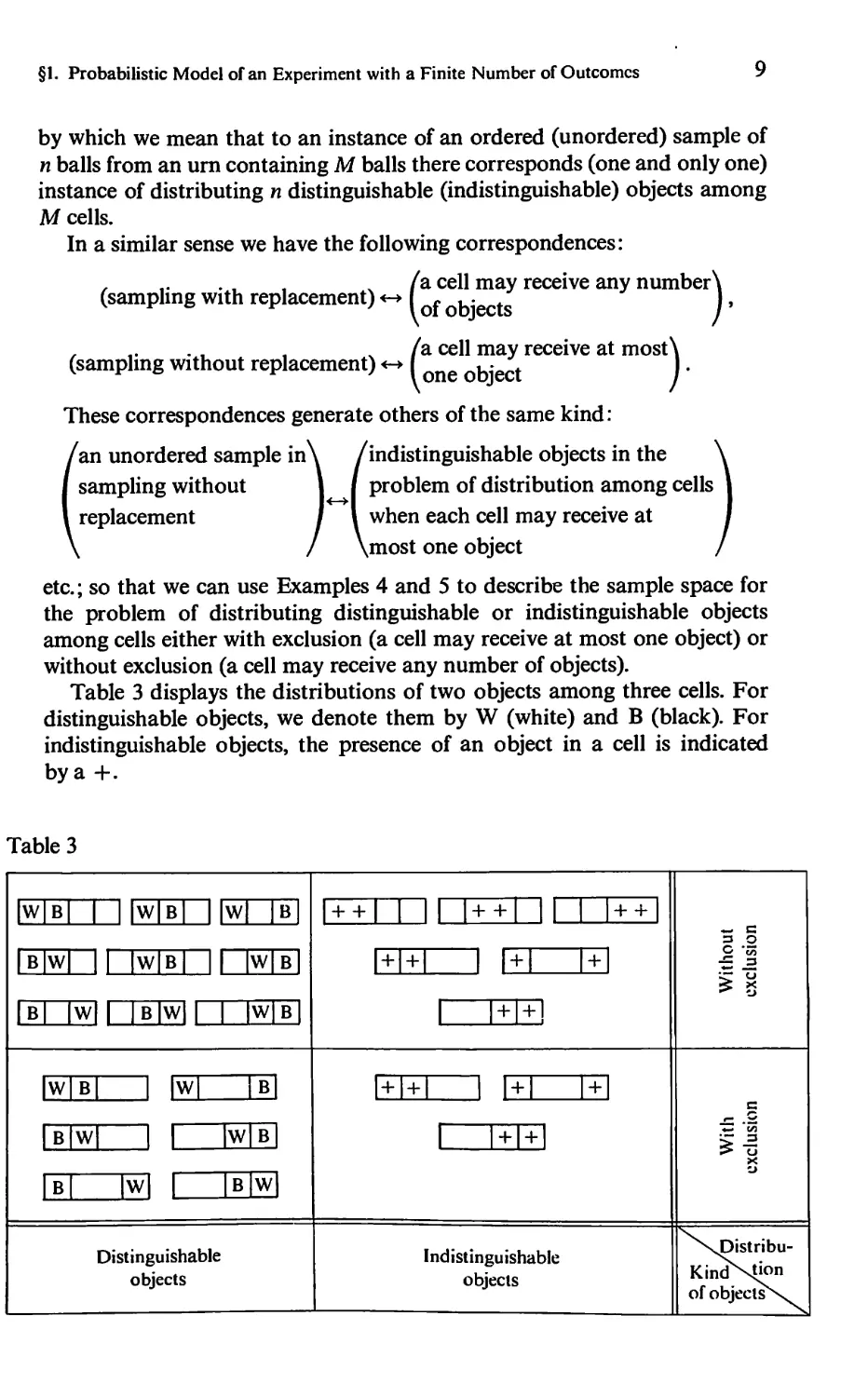
Table 3 displays the distributions of two objects among three cells. For
distinguishable objects, we denote them by W (white) and B (black). For
indistinguishable objects, the presence of an object in a cell is indicated
by a +.
Table 3
IWIBI I ||W|B| ||W| |B|
|b|w| II |w|b| II |w|b|
|B| |W|| IBIWM | |W|B|
IW|B| I |WJ L1J
|B|W| | 1 |W|B|
LbJ |W| 1 |B|W|
Distinguishable
objects
i + + i i ii i+ + i II
l+l+l 1 i+i
1 l±l±J
1 I+ + I
J±J
l+l+l I 1+J_
1 l+l+J
J+J
Indistinguishable
objects
w c
3 O
C "K
if
^sDistribu-
KindXtion
ofobjeclsN^^

10 I. Elementary Probability Theory
Table 4
N(Q) in the problem of placing n objects in M cells
^\^^ Kind of
^s"\v^^ objects
Distribution ^"\^^
Without exclusion
With exclusion
Distinguishable
objects
(Maxwell-
Boltzmann
statistics)
(M)„
Ordered
samples
Indistinguishable
objects
(Bose-
Einstein
statistics)
(Fermi-Dirac
statistics)
Unordered
samples
With
replacement
Without
replacement
^\Sample
Type^\|
N(Q) in the problem of choosing n balls from an urn
containing M balls
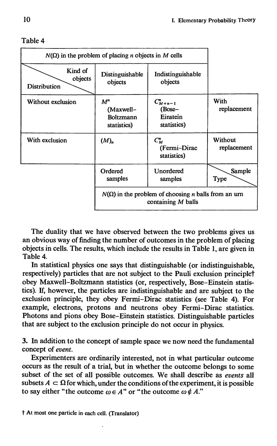
The duality that we have observed between the two problems gives us
an obvious way of finding the number of outcomes in the problem of placing
objects in cells. The results, which include the results in Table 1, are given in
Table 4.
In statistical physics one says that distinguishable (or indistinguishable,
respectively) particles that are not subject to the Pauli exclusion principle!
obey Maxwell-Boltzmann statistics (or, respectively, Bose-Einstein
statistics). If, however, the particles are indistinguishable and are subject to the
exclusion principle, they obey Fermi-Dirac statistics (see Table 4). For
example, electrons, protons and neutrons obey Fermi-Dirac statistics.
Photons and pions obey Bose-Einstein statistics. Distinguishable particles
that are subject to the exclusion principle do not occur in physics.
3. In addition to the concept of sample space we now need the fundamental
concept of event.
Experimenters are ordinarily interested, not in what particular outcome
occurs as the result of a trial, but in whether the outcome belongs to some
subset of the set of all possible outcomes. We shall describe as events all
subsets A c Q for which, under the conditions of the experiment, it is possible
to say either "the outcome co e A" or "the outcome co ¢ A"
t At most one particle in each cell. (Translator)

§1. Probabilistic Model of an Experiment with a Finite Number of Outcomes 11
For example, let a coin be tossed three times. The sample space Q consists
of the eight points
Q = {HHH, HHT,..., TTT}
and if we are able to observe (determine, measure, etc.) the results of all three
tosses, we say that the set
A = {HHH, HHT, HTH, THH}
is the event consisting of the appearance of at least two heads. If, however,
we can determine only the result of the first toss, this set A cannot be
considered to be an event, since there is no way to give either a positive or negative
answer to the question of whether a specific outcome co belongs to A.
Starting from a given collection of sets that are events, we can form new
events by means of statements containing the logical connectives "or,"
"and," and "not," which correspond in the language of set theory to the
operations "union," "intersection," and "complement."
If A and B are sets, their union, denoted by A u B, is the set of points that
belong either to A or to B:
A u B = {co e Q: co e A or co e B}.
In the language of probability theory, A u B is the event consisting of the
realization either of A or of B.
The intersection of A and Bt denoted by A n B, or by AB, is the set of
points that belong to both A and B:
A nB = {coeQ:coeA and coeB}.
The event A nB consists of the simultaneous realization of both A and B.
For example, if A = {HH, HT, TH} and B = {TT, TH, HT} then
AvB = {HH, HT, TH, TT} (= Q),
AnB = {TH, HT}.
If A is a subset of Q, its complement, denoted by A, is the set of points of
Q that do not belong to A.
If B\A denotes the difference of B and A (i.e. the set of points that belong
to B but not to A) then A = C1\A. In the language of probability, A is
the event consisting of the nonrealization of A. For example, if A =
{HH, HT, TH} then A = {TT}, the event in which two successive tails occur.
The sets A and A have no points in common and consequently A n A is
empty. We denote the empty set by 0. In probability theory, 0 is called an
impossible event. The set Q is naturally called the certain event.
When A and B are disjoint (AB = 0), the union A u B is called the
sum of A and B and written A + B.
If we consider a collection jtf0 of sets AgQwe may use the set-theoretic
operators u, n and \ to form a new collection of sets from the elements of

12
I. Elementary Probability Theory
s#0; these sets are again events. If we adjoin the certain and impossible
events Q and 0we obtain a collection $£ of sets which is an algebra, i.e. a
collection of subsets of Q for which
(1) Qe^,
(2) if A e sd, B e sd, the sets AvB,AnB,A\B also belong to s0.
It follows from what we have said that it will be advisable to consider
collections of events that form algebras. In the future we shall consider only
such collections.
Here are some examples of algebras of events:
(a) {Q, 0}, the collection consisting of Q and the empty set (we call this the
trivial algebra);
(b) {A, A, Q, 0}, the collection generated by A;
(c)i={/4:/4g Q}, the collection consisting of all the subsets of Q
(including the empty set 0).
It is easy to check that all these algebras of events can be obtained from the
following principle.
We say that a collection
® = {Dlt...,Dm}
of sets is a decomposition of Q, and call the Dt the atoms of the decomposition,
if the Dt are not empty, are pairwise disjoint, and their sum is Q:
Dt + ■ • • + D„ = Q.
For example, if Q consists of three points, Q = {1, 2, 3}, there are five
different decompositions:
Qx = {DJ with D1 = {1,2,3};
Q)2 = {/>!, D2} with £>! = {1, 2}, D2 = {3};
<2>3 = {Dlt D2} with Dx = {1, 3}, D2 = {2};
04 = {£>!, D2) with £>! = {2, 3}, D2 = {1};
^5 = {^i, D2, D3} with D, = {1}, D2 = {2}, D3 = {3}.
(For the general number of decompositions of a finite set see Problem 2.)
If we consider all unions of the sets in Q), the resulting collection of sets,
together with the empty set, forms an algebra, called the algebra induced by
3), and denoted by ol(3>). Thus the elements of ol(2>) consist of the empty set
together with the sums of sets which are atoms of 3).
Thus if Q) is a decomposition, there is associated with it a specific algebra
@ = ol(3)).
The converse is also true. Let ^ be an algebra of subsets of a finite space
Q. Then there is a unique decomposition 3) whose atoms are the elements of

§1. Probabilistic Model of an Experiment with a Finite Number of Outcomes 13
^, with @ = a(2>). In fact, let De@ and let D have the property that for
every B e 38 the set D n B either coincides with D or is empty. Then this
collection of sets D forms a decomposition 3) with the required property
a(^) = <%. In Example (a), Q) is the trivial decomposition consisting of the
single set Dx = Q; in (b), Q) = {/1, A}. The most fine-grained decomposition
3), which consists of the singletons {co,-}, w.efi, induces the algebra in
Example (c), i.e. the algebra of all subsets of Q.
Let ®x and S)2 be two decompositions. We say that 3)2 1S finer than ^i>
and write ^,<^2, if ol(3>x) c <x(^2).
Let us show that if Q consists, as we assumed above, of a finite number of
points (ol9..., coN, then the number N(sf) of sets in the collection sf is
equal to 2N. In fact, every nonempty set A e s# can be represented as A =
{co£l,..., coik}, where co£j. e Q, 1 < fr < N. With this set we associate the
sequence of zeros and ones
(0,...,0,1,0,...,0,1,...),
where there are ones in the positions iit...,ik and zeros elsewhere. Then
for a given k the number of different sets A of the form {cotl,..., coik} is the
same as the number of ways in which k ones (k indistinguishable objects)
can be placed in N positions (N cells). According to Table 4 (see the lower
right-hand square) we see that this number is CkN. Hence (counting the empty
set) we find that
JV(jO= 1 + Ch + •■• + CJJ = (1 + If = 2N.
4. We have now taken the first two steps in defining a probabilistic model
of an experiment with a finite number of outcomes: we have selected a sample
space and a collection $0 of subsets, which form an algebra and are called
events. We now take the next step, to assign to each sample point (outcome)
co.eQ,-, i = 1,..., N, a weight. This is denoted by p((Oi) and called the
probability of the outcome Wj; we assume that it has the following properties:
(a) 0 < p(cOi) < 1 (nonnegativity),
(b) pio^x) + • • • + p(coN) = 1 (normalization).
Starting from the given probabilities p(cOi) of the outcomes C0j, we define
the probability P(A) of any event A e s# by
P(A)= X pica,). (4)
U-.OieA]
Finally, we say that a triple
(Q, sf, P),
where Q = {a)u ..., coN}t s? is an algebra of subsets of O and
P = {P(A);Aetf}

14
I. Elementary Probability Theory
defines (or assigns) a probabilistic model, or a probability space, of experiments
with a (finite) space Q of outcomes and algebra s# of events.
The following properties of probability follow from (4):
P(0) = 0, (5)
P(0) = 1, (6)
P(A uB) = P(A) + P(B) - P(A n B). (7)
In particular, if A n B = 0, then
P(A + B) = P(A) + P(B) (8)
and
P(I) = 1 - P04). (9)
5. In constructing a probabilistic model for a specific situation, the
construction of the sample space Q and the algebra sf of events are ordinarily
not difficult. In elementary probability theory one usually takes the algebra
s# to be the algebra of all subsets of Q. Any difficulty that may arise is in
assigning probabilities to the sample points. In principle, the solution to this
problem lies outside the domain of probability theory, and we shall not
consider it in detail. We consider that our fundamental problem is not the
question of how to assign probabilities, but how to calculate the
probabilities of complicated events (elements of &#) from the probabilities of the
sample points.
It is clear from a mathematical point of view that for finite sample spaces
we can obtain all conceivable (finite) probability spaces by assigning non-
negative numbers pl9..., pN, satisfying the condition py + • • ■ + pN = 1, to
the outcomes au ..., coN.
The validity of the assignments of the numbers px,...,pN can, in specific
cases, be checked to a certain extent by using the law of large numbers
(which will be discussed later on). It states that in a long series of
"independent" experiments, carried out under identical conditions, the frequencies
with which the elementary events appear are "close" to their probabilities.
In connection with the difficulty of assigning probabilities to outcomes,
we note that there are many actual situations in which for reasons of
symmetry it seems reasonable to consider all conceivable outcomes as equally
probable. In such cases, if the sample space consists of points cou . .tcoN,
with N < oo, we put
p(Wl) = ... = p(coN) = 1/JV,
and consequently
P(A) = N(A)/N (10)

§1. Probabilistic Model of an Experiment with a Finite Number of Outcomes 15
for every event Aesf, where N(A) is the number of sample points in A.
This is called the classical method of assigning probabilities. It is clear that
in this case the calculation of P(A) reduces to calculating the number of
outcomes belonging to A. This is usually done by combinatorial methods,
so that combinatorics, applied to finite sets, plays a significant role in the
calculus of probabilities.
Example 7 (Coincidence problem). Let an urn contain M balls numbered
1, 2,..., M. We draw an ordered sample of size n with replacement. It is
clear that then
Q = {co:co = (fli,..., an), a{ = 1,:.., M}
and N(Q) = M". Using the classical assignment of probabilities, we consider
the M" outcomes equally probable and ask for the probability of the event
A = {co: co = (alt..., an\ at ^ ajt i ^ ;},
i.e., the event in which there is no repetition. Clearly N(A) = M(M — 1)---
(M — n + 1), and therefore
This problem has the following striking interpretation. Suppose that
there are n students in a class. Let us suppose that each student's birthday
is on one of 365 days and that all days are equally probable. The question
is, what is the probability Pn that there are at least two students in the class
whose birthdays coincide? If we interpret selection of birthdays as selection
of balls from an urn containing 365 balls, then by (11)
The following table lists the values of Pn for some values of n:
n
Pn
4
0.016
16
0.284
22
0.476
23
0.507
40
0.891
64
0.997
It is interesting to note that (unexpectedly!) the size of class in which there
is probability \ of finding at least two students with the same birthday is not
very large: only 23.
Example 8 (Prizes in a lottery). Consider a lottery that is run in the following
way. There are M tickets numbered 1, 2,..., M, of which n, numbered
1,..., n, win prizes (M > 2n). You buy n tickets, and ask for the probability
(P, say) of winning at least one prize.

16
I. Elementary Probability Theory
Since the order in which the tickets are drawn plays no role in the presence
or absence of winners in your purchase, we may suppose that the sample space
has the form
Q = {co: co = [al9..., a„], ak ^ alt k ^ /, ax = 1,..., M}.
By Table 1, N(Q) = CnM. Now let
A0 = {co:co = [alt..., aj, ak ^ at,k ^ 1,^ = n + 1 M}
be the event that there is no winner in the set of tickets you bought. Again
by Table 1, N(A0) = CnM_„. Therefore
P(^o)" Ct (M)n
\ M/\ M-l/ \ M-n + l)
and consequently
'■^■'-('-^-inl-firiTT)-
If M = h2 and n -> oo, then P(A0) -> e~l and
P_l _g-i «0.632.
The convergence is quite fast: for n = 10 the probability is already P = 0.670.
6. Problems
1. Establish the following properties of the operators n and u:
A \j B = B yj A, AB = BA (commutativity),
A u (B u C) = (A u B) u C, /1(#C) = (4£)C (associativity),
/l(# uQ^Bu/lC, /I u (BC) = U u #)(/1 u C) (distributivity),
Au A = A, AA = A (idempotency).
Show also that
AZTB = AnB, AB = AkjB.
2. Let Q contain N elements. Show that the number d(N) of different decompositions of
Q, is given by the formula
oo UN
WO-T'Itj. (12)
*=0 K-
(Hint: Show that
N-l
d(N) = £ C^_! d(k), where d(0) = 1,
*=o
and then verify that the series in (12) satisfies the same recurrence relation.)

§2. Some Classical Models and Distributions
17
3. For any finite collection of sets Alt...,Ant
P(AX u ■•■ u An) < P(At) + ■•■ + P(/t„).
4. Let A and B be events. Show that AB u BA is the event in which exactly one of A
and B occurs. Moreover,
P(AB u BA) = PU) + P(#) - 2P(/I#).
5. Let Al9..., i4„ be events, and define S0tSlt...,Sn as follows: S0 = 1,
Sr = I PUkl n ■•• n Akr), 1 < r < «,
where the sum is over the unordered subsets Jr = [kl9..., fcr] of {1,...,«}.
Let Bm be the event in which each of the events Alt ...tAn occurs exactly m times.
Show that
P(iU= £(-irmq"Sr.
In particular, for m = 0
P(B0)=l-S1+S2 ±Sn.
Show also that the probability that at least m of the events AX,...,A„ occur
simultaneously is
P(fl,) + — + P(Bn) = £ (-D'-Cri1^.
In particular, the probability that at least one of the events Alt..., A„ occurs is
HBi) + ••• + P(£„) = St - S2 + .-■ ± Sn.
§2. Some Classical Models and Distributions
1. Binomial distribution. Let a coin be tossed n times and record the results
as an ordered set (alt..., an), where at = 1 for a head ("success") and at = 0
for a tail ("failure"). The sample space is
Q = {co: co = (alt..., an), a( = 0, 1}.
To each sample point co = (alt..., an) we assign the probability
p(co) = p*y "z<\
where the nonnegative numbers p and g satisfy p + q = 1. In the first place,
we verify that this assignment of the weights p{co) is consistent. It is enough
to show that Y^oen P(w) = 1-
We consider all outcomes co = (al,...,an) for which £,-a{ = k, where
k = 0, 1,..., n. According to Table 4 (distribution of k indistinguishable

18
I. Elementary Probability Theory
ones in n places) the number of these outcomes is Ckn. Therefore
I Pico) = t CknPkqn~k = (p + qf = 1.
weCl fc = 0
Thus the space Q together with the collection &0 of all its subsets and the
probabilities P(/l) = Y,*>eA P(w)» A est, defines a probabilistic model. It is
natural to call this the probabilistic model for n tosses of a coin.
In the case n = 1, when the sample space contains just the two points
co = 1 ("success") and co = 0 ("failure"), it is natural to call p(l) = p the
probability of success. We shall see later that this model for n tosses of a
coin can be thought of as the result of n "independent" experiments with
probability p of success at each trial.
Let us consider the events
Ak = {co:co = (al9..., an), ax -\ + an = k}, k = 0, 1,..., n,
consisting of exactly k successes. It follows from what we said above that
P(Ak) = C*pY-\ (1)
and SU0 P04k) = 1.
The set of probabilities (P(/40),..., P(An)) is called the binomial
distribution (the number of successes in a sample of size n). This distribution plays an
extremely important role in probability theory since it arises in the most
diverse probabilistic models. We write Pn(k) = P(Ak), k = 0, 1,..., n.
Figure 1 shows the binomial distribution in the case p = \ (symmetric coin)
for « = 5,10,20.
We now present a different model (in essence, equivalent to the preceding
one) which describes the random walk of a "particle."
Let the particle start at the origin, and after unit time let it take a unit
step upward or downward (Figure 2).
Consequently after n steps the particle can have moved at most n units
up or n units down. It is clear that each path co of the particle is completely
specified by a set (a u ..., an), where at— +1 if the particle moves up at the
ith step, and a:— — 1 if it moves down. Let us assign to each path co the
weight p(co) = pvMqn-v«»)i where v(co) is the number of + Ts in the sequence
co = (a!,..., an), i.e. v(co) = [(^ H + an) + n]/2, and the nonnegative
numbers p and q satisfy p + q = 1.
Since ^,,^ p(co) = 1, the set of probabilities p(co) together with the space
Q of paths co = (alt ...,an) and its subsets define an acceptable probabilistic
model of the motion of the particle for n steps.
Let us ask the following question: What is the probability of the event Ak
that after n steps the particle is at a point with ordinate /c? This condition
is satisfied by those paths co for which v(co) — (n — v(co)) = k, i.e.
v(co) = -^-.

§2. Some Classical Models and Distributions
19
0.3 4-
0.2-1-
o.i 4-
0.3 4-
0.2 4-
0.1 4-
0 12 3 4 5
23456789 10
0.3 4-
0.2 4-
0.1 4-
/7 = 20
012345678910 20
Figure 1. Graph of the binomial probabilities P„(k) for n = 5,10,20.
The number of such paths (see Table 4) is C5,n+kl/2, and therefore
P(Ak) = c\?+kV2pln+kV2qln~kV2.
Consequently the binomial distribution (P(/4_n),..., P(/40),..., P(An))
can be said to describe the probability distribution for the position of the
particle after n steps.
Note that in the symmetric case (p = q = |) when the probabilities of
the individual paths are equal to 2"",
P(Ak) = C[n"+kl/2 • 2"".
Let us investigate the asymptotic behavior of these probabilities for large n.
If the number of steps is 2n, it follows from the properties of the binomial
coefficients that the largest of the probabilities P(Ak), \k\ < 2n, is
PUo) = Qn.2"2".
Figure 2

20
I. Elementary Probability Theory
-4-3-2-10 1 2 3 4
Figure 3. Beginning of the binomial distribution.
From Stirling's formula (see formula (6) in Section 4)
Consequently
2n"W
and therefore for large n
P04o) ~
y/nn
y/mi
Figure 3 represents the beginning of the binomial distribution for 2n
steps of a random walk (in contrast to Figure 2, the time axis is now directed
upward).
2. Multinomial distribution. Generalizing the preceding model, we now
suppose that the sample space is
Q = {co: co = («1,..., an)t at = blt..., br}t
where bu ..., br are given numbers. Let v^co) be the number of elements of
co = (alt..., an) that are equal to 6,-, i = 1,..., r9 and define the probability
of co by
where p( > 0 and px + h pr = 1. Note that
£p(co)= £ Cn(Ml,...,«r)p^--.p^,
<oeSl rni^,..., nP^0,i
l»U + ••• +nP = n >
where CB(ni,..., nr) is the number of (ordered) sequences (alt...,an) in
which by occurs nx times, ...,br occurs nr times. Since nl elements bt can
t The notation/(«) ~ g(n) means that f(n)/g(n) -> 1 as n -> oo.

§2. Some Classical Models and Distributions
21
be distributed into n positions in CJj1 ways; n2 elements b2 into n — nx
positions in CJj2_ni ways, etc., we have
Cn(nlt..., nr) = Cn"' • CnnLni ■ • • Cn"i(ni+... +np_l}
_ M-' (w — Hi)!
~~ ny! (n - ^i)! n2 ! (n - ^ - n2)!
n!
Therefore
£ P(w) = I „ |W'M|P"'"-P"r = (Pi + '•• + Pr)" = 1,
coett rn!^0 nP^O.i "1 • " * nr •
lni+ —+nP = n /
and consequently we have defined an acceptable method of assigning
probabilities.
Let
K, „P = {co: v^co) = nlf..., v£co) = «r}.
Then
P(4.t J = «11!,.... «r)p?« • • • Pr"-. (2)
The set of probabilities
{P(^1....,J}
is called the multinomial (or polynomial) distribution.
We emphasize that both this distribution and its special case, the binomial
distribution, originate from problems about sampling with replacement.
3. The multidimensional hypergeometric distribution occurs in problems that
involve sampling without replacement.
Consider, for example, an urn containing M balls numbered 1, 2,..., M,
where Mt balls have the color bl9 ..., Mr balls have the color br, and
Mj + • ■ • + Mr = M. Suppose that we draw a sample of size n < M without
replacement. The sample space is
D = {co: co = (au ..., an), ak^ at,k ^ lta: = 1,..., M}
and N(Q) = (M)„. Let us suppose that the sample points are equiprobable,
and find the probability of the event Bni „r in which nx balls have
color blt..., nr balls have color br, where nx + • • • + nr = n. It is easy to
show that
**(Bmi J = CJLnl9.... nr){My)ni • • • (Mr)„p,

22
I. Elementary Probability Theory
and therefore
p(B , N(Bni ,,)¾...¾ (3)
K ni nr) N(Q) CnM
The set of probabilities {P(Bm np)} is called the multidimensional
hypergeometric distribution. When r = 2 it is simply called the hypergeometric
distribution because its "generating function" is a hypergeometric function.
The structure of the multidimensional hypergeometric distribution is
rather complicated. For example, the probability
P(£n,„2) =-^7^, nx+n2 = n, Ml+M2 = M, (4)
contains nine factorials. However, it is easily established that if M -» oo
and Mj -> oo in such a way that MJM -» p (and therefore M2/M -> 1 — p)
then
p(5ni>n2)-Q+n2p^(i-pr. (5)
In other words, under the present hypotheses the hypergeometric
distribution is approximated by the binomial; this is intuitively clear since
when M and Mx are large (but finite), sampling without replacement ought
to give almost the same result as sampling with replacement.
Example. Let us use (4) to find the probability of picking six "lucky"
numbers in a lottery of the following kind (this is an abstract formulation of the
"sportloto," which is well known in Russia):
There are 49 balls numbered from 1 to 49; six of them are lucky (colored
red, say, whereas the rest are white). We draw a sample of six balls, without
replacement. The question is, What is the probability that all six of these
balls are lucky? Taking M = 49, Mx = 6, nx = 6, n2 = 0, we see that the
event of interest, namely
B6 o = {6 balls, all lucky}
has, by (4), probability
PtfW = t4~ * 7.2 x lO"8.
4. The numbers n! increase extremely rapidly with n. For example,
10! = 3,628,800,
15! = 1,307,674,368,000,
and 100! has 158 digits. Hence from either the theoretical or the
computational point of view, it is important to know Stirling's formula,
;GMa-
n\ = Jinn - exp -£ , 0 < 0n < 1, (6)

§3. Conditional Probability. Independence
23
whose proof can be found in most textbooks on mathematical analysis
(see also [69]).
5. Problems
1. Prove formula (5).
2. Show that for the multinomial distribution {P(y4ni,..., A„r)} the maximum
probability is attained at a point (/c,,...,/cr) that satisfies the inequalities npt — 1 <
kt < [n + r - l)pf, i = 1,..., r.
3. One-dimensional I sing model. Consider n particles located at the points 1,2,...,«.
Suppose that each particle is of one of two types, and that there are «, particles of the
first type and n2 of the second («, + n2 = «). We suppose that all n\ arrangements of
the particles are equally probable.
Construct a corresponding probabilistic model and find the probability of the
event A&mx x, m,2, m2\, m22) = {v, j = m,,,..., v22 = m22}t where vy is the number
of particles of type i following particles of type; (ij = 1, 2).
4. Prove the following inequalities by probabilistic reasoning:
£¢=2-,
fc = 0
£(02 = cn2n,
fc = 0
£ (- l)""kC* = Q_„ m > n + 1,
fc = 0
£ k(k - l)C^ = m(m - l)2m~2, m > 2.
fc = 0
§3. Conditional Probability. Independence
1. The concept of probabilities of events lets us answer questions of the
following kind: If there are M balls in an urn, Mj white and M2 black, what is
the probability P(A) of the event A that a selected ball is white? With the
classical approach, P(A) = MJM.
The concept of conditional probability, which will be introduced below,
lets us answer questions of the following kind: What is the probability that
the second ball is white (event B) under the condition that the first ball was
also white (event A)? (We are thinking of sampling without replacement.)
It is natural to reason as follows: if the first ball is white, then at the
second step we have an urn containing M — 1 balls, of which Mx — 1 are
white and M2 black; hence it seems reasonable to suppose that the
(conditional) probability in question is (Mi — 1)/(M — 1).

24
I. Elementary Probability Theory
We now give a definition of conditional probability that is consistent
with our intuitive ideas.
Let (Q, sf, P) be a (finite) probability space and A an event (i.e. A e sf).
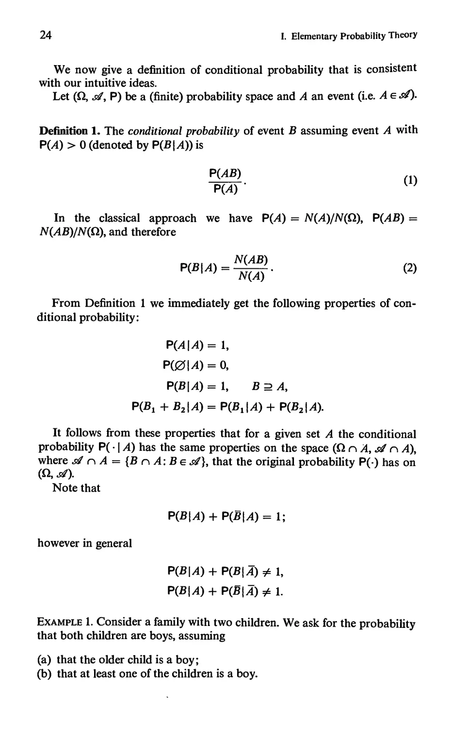
Definition 1. The conditional probability of event B assuming event A with
PG4) > 0 (denoted by P(B\A)) is
P(AB)
P(A) '
In the classical approach we have P(A) = N(A)/N(Q), P(AB) =
N(AB)/N(Q), and therefore
From Definition 1 we immediately get the following properties of
conditional probability:
P(A\A)= 1,
P(0M) = O,
P(B\A)=1, B^A,
P(B, + B2\A) = PifiM) + P(B2\A).
It follows from these properties that for a given set A the conditional
probability P( • | A) has the same properties on the space (ClnA,s/n A),
where sf n A = {B n A: B e sf}, that the original probability P(-) has on
(¾ ^).
Note that
however in general
P(B\A) + P(B\A) = 1;
P(B\A) + P(B\A) * 1,
P(B\A) + P(B\A) * 1.
Example 1. Consider a family with two children. We ask for the probability
that both children are boys, assuming
(a) that the older child is a boy;
(b) that at least one of the children is a boy.

§3. Conditional Probability. Independence
25
The sample space is
Q = {BB, BG, GB, GG},
where BG means that the older child is a boy and the younger is a girl, etc.
Let us suppose that all sample points are equally probable:
P(BB) = P(BG) = P(GB) = P(GG) = i
Let A be the event that the older child is a boy, and B, that the younger
child is a boy. Then A u B is the event that at least one child is a boy, and
AB is the event that both children are boys. In question (a) we want the
conditional probability P{AB\A), and in (b), the conditional probability
P{AB\A\jB).
It is easy to see that
"-"""•-igsfe-i-}-
2. The simple but important formula (3), below, is called the formula for
total probability. It provides the basic means for calculating the
probabilities of complicated events by using conditional probabilities.
Consider a decomposition Q) — {Alt..., An} with P04,) > 0, i = 1,..., n
(such a decomposition is often called a complete set of disjoint events). It
is clear that
and therefore
But
B = BAy + ••• + BAn
P{B) = £ P(BAd.
P(BAt) = P(B\AdP(Ad.
Hence we have the formula for total probability:
P(B) = £ PiB\AdP(A£ (3)
i=l
In particular, if 0 < P(A) < 1, then
P(B) = P(B\A)P(A) + P(B\A)P(A). (4)

26
I. Elementary Probability Theory
Example 2. An urn contains M balls, m of which are "lucky." We ask for the
probability that the second ball drawn is lucky (assuming that the result of
the first draw is unknown, that a sample of size 2 is drawn without
replacement, and that all outcomes are equally probable). Let A be the event that
the first ball is lucky, B the event that the second is lucky. Then
m(m — 1)
P{B\A) =
P{B\A) -
P{BA)
" P04)
P(BA)
" PiA)
M(M -
m
M
m(M -
M(M -
~~ M -
-J)
m)
m
m - r
and
M - 1
M ~
P(B) = P(B\A)P(A) + P{B\A)P{A)
m — \m m M — m m
M - 1 M M - 1 M M'
It is interesting to observe that P{A) is precisely m/M. Hence, when the
nature of the first ball is unknown, it does not affect the probability that the
second ball is lucky.
By the definition of conditional probability (with P(A) > 0),
P(AB) = P(B\A)P(A). (5)
This formula, the multiplication formula for probabilities, can be generalized
(by induction) as follows: If Al9..., An- x are events with P(Ay • • ■ An-1) > 0,
then
P(Al-..An) = P(Al)P(A2\Al)...P(An\Al---An.l) (6)
(here A1--An= A1nA2n--n An).
3. Suppose that A and B are events with P(A) > 0 and P(B) > 0. Then
along with (5) we have the parallel formula
P(AB) = P(A\B)P(B). (7)
From (5) and (7) we obtain Bayes's formula
P(A)P(B\A)
P(AlB)=P&)' (8)

§3. Conditional Probability. Independence
27
If the events Au...,An form a decomposition of Q, (3) and (8) imply
Bayes's theorem:
In statistical applications, Alt...,An {Ax + • • • + An = Q) are often
called hypotheses, and P04£) is called the a priori^ probability of At. The
conditional probability P(At\B) is considered as the a posteriori probability
of At after the occurrence of event B.
Example 3. Let an urn contain two coins: Au a fair coin with probability
j of falling H; and A2, a biased coin with probability \ of falling H. A coin is
drawn at random and tossed. Suppose that it falls head. We ask for the
probability that the fair coin was selected.
Let us construct the corresponding probabilistic model. Here it is natural
to take the sample space to be the set Q = {/^H, A {I, A2H, A2T}t which
describes all possible outcomes of a selection and a toss (A ^ means that
coin Ax was selected and fell heads, etc.) The probabilities p(co) of the various
outcomes have to be assigned so that, according to the statement of the
problem,
P(Al)=P(A2) = i
and
P(HM1) = i P(H\A2) = i
With these assignments, the probabilities of the sample points are uniquely
determined:
P(^1H) = i P(AlT) = l P(A2H)=l P(A2T)=i
Then by Bayes's formula the probability in question is
P(A {m_ P^PjHlAQ = 3
r^iin; p^p^j^) + p(A2)P(H\A2) 5'
and therefore
P042|H) = f.
4. In certain sense, the concept of independence, which we are now going to
introduce, plays a central role in probability theory: it is precisely this concept
that distinguishes probability theory from the general theory of measure
spaces.
t A priori: before the experiment; a posteriori: after the experiment.

28
I. Elementary Probability Theory
If A and B are two events, it is natural to say that B is independent of A
if knowing that A has occurred has no effect on the probability of B. In other
words, "B is independent of A" if
P{B\A) = P(B) (10)
(we are supposing that P(A) > 0).
Since
it follows from (10) that
P(AB) = P(A)P(B). (11)
In exactly the same way, if P(B) > 0 it is natural to say that" A is independent
ofB"if
P(A\B) = P(A).
Hence we again obtain (11), which is symmetric in A and B and still makes
sense when the probabilities of these events are zero.
After these preliminaries, we introduce the following definition.
Definition 2. Events A and B are called independent or statistically independent
(with respect to the probability P) if
P(AB) = P(A)P(B).
In probability theory it is often convenient to consider not only
independence of events (or sets) but also independence of collections of events (or
sets).
Accordingly, we introduce the following definition.
Definition 3. Two algebras sty and st2 of events (or sets) are called
independent or statistically independent (with respect to the probability P) if all pairs
of sets Ay and A2, belonging respectively to sty and st2, are independent.
For example, let us consider the two algebras
stx = {Ay, Ay, 0, CI} and st2 = {A2, A2, 0, Q},
where Ay and A2 are subsets of Q. It is easy to verify that sty and s#2 are
independent if and only if Ay and A2 are independent. In fact, the
independence of sty and s#2 means the independence of the 16 events Ay and A2,
Ay and A2,..., CI and CI. Consequently Ay and A2 are independent.
Conversely, if Ay and A2 are independent, we have to show that the other 15

§3. Conditional Probability. Independence
29
pairs of events are independent. Let us verify, for example, the independence
of A! and A2. We have
P{A,A2) = P04O - P{A,A2) = P{AX) - P{AX)P{A2)
= P(^1)(l-P(^2)) = P(^i)P(^2).
The independence of the other pairs is verified similarly.
5. The concept of independence of two sets or two algebras of sets can be
extended to any finite number of sets or algebras of sets.
Thus we say that the sets Au...,An are collectively independent or
statistically independent (with respect to the probability P) if for k = 1,..., n
and 1 < il < i2 < • • • < ik <, n
P(^V^lc) = P(^l)"P(^lc). (12)
The algebras s/l9...9 sf„ of sets are called independent or statistically
independent (with respect to the probability P) if all sets A „ ...,An belonging
respectively to jflt..., $£n are independent.
Note that pairwise independence of events does not imply their
independence. In fact if, for example, Q = {colt co2, co3, co4} and all outcomes are
equiprobable, it is easily verified that the events
A = {colt co2}, B = {cou co3}, C = {colt co4}
are pairwise independent, whereas
P(ABC) = i* (¾3 = P04)P(f*)P(C).
Also note that if
P(ABC) = P04)P(B)P(C)
for events A, B and C, it by no means follows that these events are pairwise
independent. In fact, let Q consist of the 36 ordered pairs (i,y), where ij =
1,2,..., 6 and all the pairs are equiprobable. Then if A = {(i,j):j = 1,2 or 5},
B = {(ij):j = 4, 5 or 6}, C = {(i,j): i+j = 9} we have
P(AB) = * * i = P(A)P(B),
P(AC) =£ ^ = P04)P(Q,
P(BQ =^ ** = P(B)P{C\
but also
P(^BC) = £=P04)P(f*)P(C).
6. Let us consider in more detail, from the point of view of independence,
the classical model (Q, sf, P) that was introduced in §2 and used as a basis
for the binomial distribution.

30
I. Elementary Probability Theory
In this model
Q = {co: co = (au ..., an), a-t = 0, 1}, st = {A: A c Q}
and
p{d) = p1 V"10'. (13)
Consider an event A £ Q. We say that this event depends on a trial at
time k if it is determined by the value ak alone. Examples of such events are
Ak = {co: ak = 1}, Ak = {co: ak = 0}.
Let us consider the sequence of algebras s/i9 sf2,..., s#„, where sdk =
{Ak, Ak, 0, Q} and show that under (13) these algebras are independent.
It is clear that
P04*)= I PM= I PsV"Zfl'
{o>'.ak=l) {toiak=l}
_ p y „01+ "+ak-i+ak+i + -+an
ifli ak-i,ak+i a„)
n— 1
x (n-l)-(a1 + -+flk-1+flk+1+-+fl„) _ p y Ql „1 in-1)-I _
£ = 0
and a similar calculation shows that P(Ak) = q and that, for k ^ 1,
P&MO = p2, P^,) = pq, P&kAd = «2.
It is easy to deduce from this that $£k and $£x are independent for k ^ /.
It can be shown in the same way that s/lt sf2t.. ■, .s/„ are independent.
This is the basis for saying that our model (Q, sf, P) corresponds to "n
independent trials with two outcomes and probability p of success." James
Bernoulli was the first to study this model systematically, and established
the law of large numbers (§5) for it. Accordingly, this model is also called
the Bernoulli scheme with two outcomes (success and failure) and probability
p of success.
A detailed study of the probability space for the Bernoulli scheme shows
that it has the structure of a direct product of probability spaces, defined
as follows.
Suppose that we are given a collection (Q1} @lt Pj),..., (Q„, ^n, P„) of
finite probability spaces. Form the space Q = Qj x Cl2 x • • - x Cl„ of points
co = (alt...t an\ where a{ e Qf. Let &0 = #t ® • • • ® @n be the algebra of
the subsets of Q that consists of sums of sets of the form
A = By x B2 x • • • x Bn
with BiG&t. Finally, for co = (al9 ...,an) take p(co) = Pi(ax)• • • pn(an) and
define P{A) for the set A = Bx x B2 x • - • x Bn by
P04)= I Pi(ai)"-P„(a„).
{aieBi a„eB„)

§3. Conditional Probability. Independence
31
It is easy to verify that P(0) = 1 and therefore the triple (O, sf, P) defines
a probability space. This space is called the direct product of the probability
spaces (Qlf @u PJ,..., (fK, ®n, Pn).
We note an easily verified property of the direct product of probability
spaces: with respect to P, the events
A, = {wiflieB!} ^ = {co:aneBn},
where Bt e &it are independent. In the same way, the algebras of subsets of O,
s0x = {Al:Al = {<D:aleBl},Ble@l},
sfn = {Am: An = {a>: aneBn}, Bne<2n}
are independent.
It is clear from our construction that the Bernoulli scheme
(O, jf, P) with O = {co: co = (alt..., an), a{ = 0 or 1}
s/ = {A:AcQ} and p(co) = p1 a'qn _s at
can be thought of as the direct product of the probability spaces (0£, 96 x, P,),
i = 1,2,..., n, where
0,.= (0,1), ^=((0),(1),0,0,.),
Pi({l» = P, Pi({0}) = q-
7. Problems
1. Give examples to show that in general the equations
P{B\A) + P(B\A) = 1,
P(B\A) + P(B\A) = 1
are false.
2. An urn contains M balls, of which M, are white. Consider a sample of size n. Let Bj
be the event that the ball selected at theyth step is white, and Ak the event that a sample
of size n contains exactly k white balls. Show that
P(Bj\Ak) = k/n
both for sampling with replacement and for sampling without replacement.
3. Let Ax,..., A„ be independent events. Then
\i=t / i=t
4. Let /4, A„ be independent events with P(A{) = pt. Then the probability P0
that neither event occurs is
^o= fid-Pi)-

32
I. Elementary Probability Theory
5. Let A and B be independent events. In terms of P(A) and P(B), find the probabilities
of the events that exactly k, at least k, and at most k of A and B occur (k — 0,1, 2).
6. Let event A be independent of itself, i.e. let A and A be independent. Show that
P(A) is either 0 or 1.
7. Let event A have P(/l) = 0 or 1. Show that A and an arbitrary event B are
independent.
8. Consider the electric circuit shown in Figure 4:
Figure 4
Each of the switches A, B, C, D, and E is independently open or closed with
probabilities p and q, respectively. Find the probability that a signal fed in at "input"
will be received at "output". If the signal is received, what is the conditional
probability that E is open?
§4. Random Variables and Their Properties
1. Let (Q, sf, P) be a probabilistic model of an experiment with a finite
number of outcomes, N(Q) < oo, where $£ is the algebra of all subsets of
Q. We observe that in the examples above, where we calculated the
probabilities of various events A e sf, the specific nature of the sample space Q was
of no interest. We were interested only in numerical properties depending
on the sample points. For example, we were interested in the probability of
some number of successes in a series of n trials, in the probability distribution
for the number of objects in cells, etc.
The concept "random variable," which we now introduce (later it will
be given a more general form) serves to define quantities that are subject to
"measurement" in random experiments.
Definition 1. Any numerical function £ = £(co) defined on a (finite) sample
space Q is called a (simple) random variable. (The reason for the term " simple "
random variable will become clear after the introduction of the general
concept of random variable in §4 of Chapter II.)

§4. Random Variables and Their Properties
33
Example 1. In the model of two tosses of a coin with sample space Q =
{HH, HT, TH, TT}, define a random variable f = f(co) by the table
0)
«w)
HH
2
HT
1
TH
1
TT
0
Here, from its very definition, £(co) is nothing but the number of heads in the
outcome co.
Another extremely simple example of a random variable is the indicator
(or characteristic function) of a set A e &0\
C = Uco),
where t
fl, coeA,
7^) = |o, co* A
When experimenters are concerned with random variables that describe
observations, their main interest is in the probabilities with which the
random variables take various values. From this point of view they are
interested, not in the distribution ofthe probability P over (Q, $t\ but in
its distribution over the range of a random variable. Since we are considering
the case when Q contains only a finite number of points, the range X of
the random variable £ is also finite. Let X = {xlt..., xm}, where the
(different) numbers xlt..., xm exhaust the values of f.
Let SC be the collection of all subsets of X, and let BeSC. We can also
interpret B as an event if the sample space is taken to be X, the set of values
of*
On (X, SC\ consider the probability P£(-) induced by £ according to the
formula
P£B) = P{co: £(co)eB}9 Be3C.
It is clear that the values of this probability are completely determined by
the probabilities
Pfrd = P{co: ¢(0,) = xj, XieX.
The set of numbers (P^),..., P^xm)} is called the probability
distribution of the random variable \.
t The notation 1(A) is also used. For frequently used properties of indicators see Problem 1.

34
I. Elementary Probability Theory
Example 2. A random variable £ that takes the two values 1 and 0 with
probabilities p ("success") and q ("failure"), is called a Bernoullit random
variable. Clearly
Pfr) = p*ql-X, x = 0, 1. (1)
A binomial (or binomially distributed) random variable £ is a random
variable that takes the n + 1 values 0, 1,..., n with probabilities
Pfc) = QpV"x, x = 0, 1,..., n. (2)
Note that here and in many subsequent examples we do not specify the
sample spaces (Q, $£, P), but are interested only in the values of the random
variables and their probability distributions.
The probabilistic structure of the random variables £ is completely
specified by the probability distributions {/^(x,), i — 1,..., m}. The concept
of distribution function, which we now introduce, yields an equivalent
description of the probabilistic structure of the random variables.
Definition 2. Let xeR1. The function
F£x) = P{co:t(cD)<x}
is called the distribution function of the random variable £.
Clearly
[i:xi<x)
and
Pfrd = Fficd - Ffic, -),
where F£x-) = limyTx F^OO-
If we suppose that xt < x2 < • • • < xm and put F^(x0) = 0, then
P&d = F&) - F«(x,_ 0, i =1,--., m.
The following diagrams (Figure 5) exhibit J^(x) and F^(x) for a binomial
random variable.
It follows immediately from Definition 2 that the distribution F^ = F^(x)
has the following properties:
(l)F,(-a)) = 0,F,(+oo)=l;
(2) F£x) is continuous on the right (F^(x+) = F^(x)) and piecewise constant.
t We use the terms "Bernoulli, binomial, Poisson, Gaussian,..., random variables" for what
are more usually called random variables with Bernoulli, binomial, Poisson, Gaussian,...,
distributions.

§4. Random Variables and Their Properties
35
***>.
Wj
I !
i
t
t—r
1 2
Figure 5
Along with random variables it is often necessary to consider random
vectors £ = (£ i,..., £,.) whose components are random variables. For
example, when we considered the multinomial distribution we were dealing
with a random vector v = (v^..., vr), where v,- = v,(co) is the number of
elements equal to bt9 i = 1,..., r, in the sequence co = (a l9 ..., a„).
The set of probabilities
P^xu ..., xr) = P{co: Mco) = xl9..., £r(co) = xr},
where x.-eA",-, the range of ££, is called the probability distribution of the
random vector £, and the function
F^Xi,..., xr) = P{co: f !(co) < xl9..., fr(co) < x,},
where xjeU1, is called the distribution function of the random vector £ =
(f 1,..., fr>
For example, for the random vector v = (v1}...,vr) mentioned above,
Pv(nu ..., nr) = Cn(nlt..., nr)p\l •••pn/
(see (2.2)).
2. Let £i,..., £r be a set of random variables with values in a (finite) set
X c Rl. Let SC be the algebra of subsets of A\

36
1. Elementary Probability Theory
Definition 3. The random variables f i,..., fr are said to be independent
(collectively independent) if
P{£1 = x1,...,£r = xr} = P{£1 = x1}...P{£r = xr}
for all Xi,..., xr e X; or, equivalently, if
PK16B1,...,4eBr} = P{^1eB1}-P{^eBr}
for all ^,..., Bre#".
We can get a very simple example of independent random variables
from the Bernoulli scheme. Let
Q = {co: co = (au ..., an\ at = 0, 1}, p(co) = pz V-1"'
and &(co) = at for co = (alt..., a„), i = 1,..., n. Then the random variables
f ii f 2» • • •, £„ are independent, as follows from the independence of the events
Ax — {co: ax = 1},..., An = {co: an = 1},
which was established in §3.
3. We shall frequently encounter the problem of finding the probability
distributions of random variables that are functions/(£l9..., £,.) of random
variables f i,..., fr. For the present we consider only the determination
of the distribution of a sum £ = ^ + r\ of random variables.
If ^ and »7 take values in the respective sets X = {xl9..., xk} and Y =
{.Vi» • • •»}>/}> the random variable £ = £ + r\ takes values in the set Z =
{z: z = x,- + yj, i = 1,..., fc;/ = 1,..., /}. Then it is clear that
P&) = P(C = z) = P{£ + r\ = z} = X P{£ = xlfi7 = y,.}.
{(i.j):x,+yj=z}
The case of independent random variables ^ and r\ is particularly
important. In this case
P{£ = xf> /7 = yj) = P{£ = x,}Pfe = yjh
and therefore
W = I PfrdPJyj) = I PfrdPfr - xf) (3)
for all z e Z, where in the last sum Pn{z — x,) is taken to be zero if z - xt ¢ Y.
For example, if £ and »7 are independent Bernoulli random variables,
taking the values 1 and 0 with respective probabilities p and q, then Z =
{0, 1, 2} and
Pf (0) = ^(0)^(0) = g2,
^c(l) = W^) + ^W) = 2pg,
Pf(2) = P.CDP.Ci) = p2.

§4. Random Variables and Their Properties
37
It is easy to show by induction that if f lt £2,..., £„ are independent
Bernoulli random variables with P{^ = 1} = p, P{^f = 0} = q, then the
random variable C = ^i + ••• + £„ has the binomial distribution
*c(*) = C£pV~*. fc = 0, 1,..., n. (4)
4. We now turn to the important concept of the expectation, or mean value,
of a random variable.
Let (Q, sd, P) be a (finite) probability space and ^ = £(co) a random
variable with values in the set X = {xlf..., xk}. If we put At — {coil; = x,},
i = 1,..., k, then £ can evidently be represented as
«g>) = £ X../04,.), (5)
i= 1
where the sets Ax,...,Ak form a decomposition of Q (i.e., they are pairwise
disjoint and their sum is Q; see Subsection 3 of §1).
Let Pi = P{£ = x,}. It is intuitively plausible that if we observe the values
of the random variable £ in "n repetitions of identical experiments", the
value xf ought to be encountered about ptn times, i = 1,..., k. Hence the
mean value calculated from the results of n experiments is roughly
1 *
- [nPi*i + • • • + np^J = £ Pi*i-
n (= i
This discussion provides the motivation for the following definition.
Definition 4. The expectation^ or mean value of the random variable ^ =
£*= l X|f 04i) is the number
E£ = I x£JW (6)
i=l
Since /1,- = {co: £(co) = x,} and P£x() = P(/l,), we have
E£ = £ x,.^). (7)
Recalling the definition of F^ = F^(x) and writing
AF^(x) = Ffic) - F£x -),
we obtain P£xt) = AF^x,) and consequently
E£ = £ x.-AF^x,). (8)
i= 1
t Also known as mathematical expectation, or expected value, or (especially in physics)
expectation value. (Translator)

38
I. Elementary Probability Theory
Before discussing the properties of the expectation, we remark that it is
often convenient to use another representation of the random variable £,
namely
/= 1
where Bl + • • • + Bt = Q, but some of the x's may be repeated. In this case
E£ can be calculated from the formula Yj=i x/P(5/)> which differs formally
from (5) because in (5) the x£ are all different. In fact,
£ x'jP(Bj) = Xi £ P(B;) = x,.P(^)
ij:x'j = xi) {j--xj = x,}
and therefore
5. We list the basic properties of the expectation:
(1) Ift>OthenEt>0.
(2) E(a£ + bn) = aE£ + ££»7, where a and fe are constants.
(3) Ift > r\ then E£ > En.
(4) |E£|<E|£|.
(5) If ^ and rj are independent, then E£n = E£ • E/7.
(6) (EI ^|)2 < E£2 -E?/2 (Cauchy-Bunyakovskii inequality).^
(7) //£ = /U) then E£ = P(,4).
Properties (1) and (7) are evident. To prove (2), let
« /
Then
a£ + bn = aX xJiAt n Bj) + b £ yjKAi ^ Bj)
«./ «./
= 1(^ + ^,^¾
«./
and
E(a£ + brj) = £ (ax, + b^OPUf n ^)
1./
I I
= flSxfPM,) + &5>jP(*/) = aEt + K17.
«' /
t Also known as the Cauchy-Schwarz or Schwarz inequality. (Translator)

§4. Random Variables and Their Properties
39
Property (3) follows from (1) and (2). Property (4) is evident, since
|E£h
<ZlxI-|P(^) = E|^|.
I > I
To prove (5) we note that
= E I XtyjHAt n Bj) = £ xiyJP{Ai n Bj)
«./ us
= I.xtyjP(AdPiBj)
i.j
= (l*|PW,)) • (l^PP*,)) = Ef-E*.
where we have used the property that for independent random variables the
events
At = {co: £(co) = x,} and Bj = {co: rj(co) = ^}
are independent: P(A{ n Bj) = P(Ai)P(Bj).
To prove property (6) we observe that
^ = ^/04,.), n2 = Y,y]m)
i J
and
E£2 = I x?PU,.), E/y2 = I tfPOtf.
Let Ef 2 > 0, E/y2 > 0. Put
<? = -^?. n-
v/E?' ' Ve?'
Since 2||^| < |2 + J72, we have 2E||/y| < E?2 + E/y2 = 2. Therefore
E||/7|<land(E|£7l)2<E£2-E/72.
However, if, say, E£2 = 0, this means that ££ xfP(At) = 0 and
consequently the mean value of £ is 0, and P{co: £(co) = 0} = 1. Therefore if at
least one of E£2 or Erj2 is zero, it is evident that E |^| = 0 and consequently
the Cauchy-Bunyakovskii inequality still holds.
Remark. Property (5) generalizes in an obvious way to any finite number of
random variables: if £u ..., £r are independent, then
The proof can be given in the same way as for the case r = 2, or by induction.

40
f. Elementary Probability Theory
Example 3. Let £ be a Bernoulli random variable, taking the values 1 and 0
with probabilities p and q. Then
E£=l.P{£=l}+0.P{£ = 0} = p.
Example 4. Let f „..., £„ be n Bernoulli random variables with Pfo = 1}
= p, P{& = 0} = q, p + g = 1. Then if
S„ = fi +■■• + «■
we find that
ESn = wp.
This result can be obtained in a different way. It is easy to see that ES„
is not changed if we assume that the Bernoulli random variables f i,..., f „
are independent. With this assumption, we have according to (4)
P(Sn = k) = C*pV-\ k = Q,l9...9n.
Therefore
ES„ = t *Ptf„ = *) = I *Ctpty"*
k = 0 k = 0
= npY ^ ~ ^! pfc-i0(n-i)-(k-i)
= npY (" ~ 1)! pVn-1)"' = «P.
However, the first method is more direct.
6. Let ^ = £,- x,-I(A,), where /1,- = {co: £(co) = xj, and <p = <p(£(co)) is a
function of £(co). If B, = {co: q>(£{co)) = j;,-}, then
j
and consequently
E? = Z,yjP(Bj) = ZyjP^j). (9)
j I
But it is also clear that
?(£(")) = 2>(x,-)/04,-).

§4. Random Variables and Their Properties
41
Hence, as in (9), the expectation of the random variable q> = <p(£) can be
calculated as
i
7. The important notion of the variance of a random variable £ indicates
the amount of scatter of the values of £ around E£.
Definition 5. The variance (also called the dispersion) of the random variable
£ (denoted by V£) is
V£ = E(£ - E£)2.
The number a = + yjv~£ is called the standard deviation.
Since
E(£ - E£)2 = E(£2 - 2* • E£ + (E£)2) = E£2 - (E£)2,
we have
V£ = E£2 - (E£)2.
Clearly V£ ^ 0. It follows from the definition that
M{a + b£) = fc2V<!;, where a and b are constants.
In particular, Ma = 0, V(fcf) = b2V£.
Let £ and r\ be random variables. Then
V« + n) = E((£ - EO + (//- E/7))2
= V£ + V/y + 2E(£ - E0fo - E/y).
Write
COv(£, /7) = E(£ - EQ(i7 - E/y).
This number is called the covariance of £ and rj. If V£ > 0 and V/7 > 0, then
cov(f, rfi
ptt*) =
v/wFv^
is called the correlation coefficient of £, and »7. It is easy to show (see Problem
7 below) that if p(£, rf) = ±1, then <!; and »7 are linearly dependent:
r\ = a£ + b,
with a > 0 if p(^, rf) = 1 and a < 0 if p(£, »7) = -1.
We observe immediately that if I, and r\ are independent, so are £, — E£
and n -En. Consequently by Property (5) of expectations,
cov(£, n) = Etf - EO • Efo - E/7) = 0.

42
I. Elementary Probability Theory
Using the notation that we introduced for covariance, we have
V(£ + ri) = V£ + V/y + 2cov(£, n); (10)
if £ and rj are independent, the variance of the sum ^ + rj is equal to the sum
of the variances,
V(£ + »y)= V£ + V17. (11)
It follows from (10) that (11) is still valid under weaker hypotheses than
the independence of ^ and rj. In fact, it is enough to suppose that £ and r\ are
uncorrelated, i.e. cov(£, r\) — 0.
Remark. If £ and r\ are uncorrelated, it does not follow in general that they
are independent. Here is a simple example. Let the random variable a take
the values 0, n/2 and n with probability 3. Then £ = sin a and r\ = cos a are
uncorrelated; however, they are not only stochastically dependent (i.e., not
independent with respect to the probability P):
P{£ = 1, rj = 1} = 0 * i = P{£ = l}P{i7 = 1},
but even functionally dependent: £2 + n2 = 1.
Properties (10) and (11) can be extended in the obvious way to any
number of random variables:
vf I fc) = I Vfc + 2 £ cov(&. y. (12)
V=i / 1 = 1 t>j
In particular, if f lf..., £„ are pairwise independent (pairwise uncorrelated
is sufficient), then
v(i&) = 1; vfc. (13)
Example 5. If £ is a Bernoulli random variable, taking the values 1 and 0
with probabilities p and q, then
V£ = E(£ - E£)2 = (£ - p)2 = (1 - p)2p + p2<? = M.
It follows that if f t,..., £„ are independent identically distributed Bernoulli
random variables, and S„ = f 1 + ■ • • + f„, then
VSn = npg. (14)
8. Consider two random variables ^ and r\. Suppose that only £ can be
observed. If £ and r\ are correlated, we may expect that knowing the value of £
allows us to make some inference about the values of the unobserved
variable n.
Any function f = /(£) of ^ is called an estimator for n. We say that an
estimator/* = /*(£) is best in the mean-square sense if
Eft -/*(£))2 = mf Eft -/(0)2.

§4. Random Variables and Their Properties
43
Let us show how to find a best estimator in the class of linear estimators
A(£) = a + b£. We consider the function g(a, b) = E{n - (a + H))2.
Differentiating g(a, b) with respect to a and b, we obtain
dg(atb)
= - 2E[»y - (a + fcC)],
da
dg(fl, ft)
at
= - 2EKn - (a + &©)a,
whence, setting the derivatives equal to zero, we find that the best mean-
square linear estimator is A*(£) = a* + fr*£, where
In other words,
a* = E„-6*E«, 6* =22^. (15)
A*© = E, + C-^«-Ef). (16)
The number E(rj — X*{^))2 is called the mean-square error of observation.
An easy calculation shows that it is equal to
cov2(& rj)
Consequently, the larger (in absolute value) the correlation coefficient
p(6 n) between £ and /7, the smaller the mean-square error of observation
A*. In particular, if |p(& n)\ = 1 then A* = 0 (cf. Problem 7). On the other
hand, if £ and n are uncorrelated (p(<^, n) = 0), then A*(£) = En, i.e. in the
absence of correlation between ^ and n the best estimate of n in terms of ^ is
simply En (cf. Problem 4).
9. Problems
1. Verify the following properties of indicators IA = /^(co):
/0 = 0, /« = 1, /,, + /*= 1,
Iaub = Ia + Ib ~ Iab-
The indicator of (J"=l At is 1 - f]?=i (1 — ^fX tne indicator of (J"=1 y4{ is
n?=i (1 _ JaX and the indicator of JJ=1 4£ is JJ=1 /^..
where /1 A J3 is the symmetric difference of /1 and J3, i.e. the set (A\B) u (J3\/4).

44
I. Elementary Probability Theory
2. Let £1,..., £,n be independent random variables and
f m:n = min(f,,..., f n), f max = max(f l5..., f n).
Show that
P{£ni„>x}= flP{^>^}.
i=t
P{£max<*} = flP{^<x}.
i=t
3. Let ¢,,..., £n be independent Bernoulli random variables such that
Pfo = 0} = 1 - A.A,
P{& = 1} = A.-A,
where A is a small number, A > 0, A,- > 0.
Show that
Ptfi + --- + ^=i} = ( Z A«)A + °<A2)'
P{^ + -- + ^n>l} = 0(A2).
4. Show that inf_00<fl<00 E(£ — a)2 is attained for a = E£ and consequently
inf E(£ - a)2 = V£.
— 00<fl<00
5. Let £ be a random variable with distribution function F£x) and let m, be a median
of F^x), i.e. a point such that
F^m,.-) < i < F4(m,).
Show that
inf E|£-af=E|£-mt.|.
— 0O<O< 00
6. Let P4(x) = P{£ = x) and F4(x) = P(£ < x}. Show that
^+tW = FA——)
for a > 0 and — oo < fc < oo. If y > 0, then
Ff<y) = ^+^) - J^-n/Jo + P&-yfy)-
Let f+ = max(f, 0). Then
{0, x < 0,
^(0), x = 0,
F^(x), x>0.

§5. The Bernoulli Scheme. I. The Law of Large Numbers
45
7. Let g and i/ be random variables with Vg > 0, Vi/ > 0, and let p = p(£, ly) be their
correlation coefficient. Show that \p\ < 1. If \p\ = 1, find constants a and b such
that i/ = ag + b. Moreover, if p = 1, then
17 - Eiy _ g - Eg
(and therefore a > 0), whereas if p = -1, then
i/ - Eiy _ g - Eg
(and therefore a < 0).
8. Let g and ly be random variables with Eg = Eiy = 0, Vg = Viy = 1 and correlation
coefficient p = p(Ji, ly). Show that
Emax(g2,iy2)<l+V1-P2-
9. Use the equation
(indicator of |J ,4,.) = jf[(l - IA(\
to deduce the formula P(J30) = 1 - St + S2 + - ■ • ± S„ from Problem 4 of §1.
10. Let gt,..., gn be independent random variables, (px = </>1(g1,..., gfc) and q>2 =
^2½¾ + ii•- • > €nX functions respectively of gt,..., gfc and gfc+lt..., gn. Show that the
random variables cpt and <p2 are independent.
11. Show that the random variables gt,..., gn are independent if and only if
Ftt *„(xi,.•.,*„) = F4l(x,) --^,,00
for all xlf..., xn, where F4l ^(x,,..., xn) = P{gt < xu -.., gn < *„}•
12. Show that the random variable g is independent of itself (i.e., g and g are
independent) if and only if g = const.
13. Under what hypotheses on g are the random variables g and sin g independent?
14. Let g and ly be independent random variables and ly # 0. Express the probabilities
of the events P{giy < z} and P{g/iy < z} in terms of the probabilities P4(x) and P^(y).
§5. The Bernoulli Scheme. I. The Law of
Large Numbers
1. In accordance with the definitions given above, a triple
(Q, s/, P) with Q = {co: co = (alf..., an), at = 0, 1},
is called a probabilistic model of n independent experiments with two
outcomes, or a Bernoulli scheme.

46
I. Elementary Probability Theory
In this and the next section we study some limiting properties (in a sense
described below) for Bernoulli schemes. These are best expressed in terms of
random variables and of the probabilities of events connected with them.
We introduce random variables ^,..., £n by taking £,(co) = ai9 i =
I,..., n, where co = (alt... t an). As we saw above, the Bernoulli variables
£,-(co) are independent and identically distributed:
P{£=l} = p, PK, = 0} = *, 1 = 1,...,11.
It is natural to think of £, as describing the result of an experiment at the
ith stage (or at time i).
Let us put S0(co) = 0 and
!£i + --- + &,
k= !,...,«.
As we found above, ESn = np and consequently
(1)
In other words, the mean value of the frequency of "success", i.e. SJn,
coincides with the probability p of success. Hence we are led to ask how much
the frequency SJn of success differs from its probability p.
We first note that we cannot expect that, for a sufficiently small s > 0
and for sufficiently large n, the deviation of SJn from p is less than £ for all
co, i.e. that
Sn(co)
In fact, when 0 < p < 1,
p{^=1}=p{^
< £, CO E CI.
(2)
1,...,6,= i} = p",
pp! = oj= P{^ =0,...,^ = 0} = q\
whence it follows that (2) is not satisfied for sufficiently small £ > 0.
We observe, however, that when n is large the probabilities of the events
{SJn = 1} and {SJn = 0} are small. It is therefore natural to expect that the
total probability of the events for which |[Sn(co)/n] - p\ > e will also be
small when n is sufficiently large.
We shall accordingly try to estimate the probability of the event
{co: \[Sn(co)/n\ — p\ > e}. For this purpose we need the following inequality,
which was discovered by Chebyshev.

§5. The Bernoulli Scheme. I. The Law of Large Numbers 47
Chebyshev's inequality. Let (Q, sf, P) be a probability space and £ = £(co) a
nonnegative random variable. Then
P{t > £} < E£/£ (3)
for all £ > 0.
Proof. We notice that
f = f/(£ > «) + £/(£ < £) > £/(£ > £) > e/(£ > £),
ator of A
ties of the expectation,
E£>£E/(£>£) = £P(£>£),
where 1(A) is the indicator of A.
Then, by the properties of the expectation
which establishes (3).
Corollary. //£ is any random variable, we have for £ > 0,
P{|£|>£}<E|£|/£,
P{|£|>£} = P{£2>£2}<E£2/£2, (4)
P{|£-E£|>£}<V£/£2.
In the last of these inequalities, take ^ = SJn. Then using (4.14), we obtain
\\ n | J £ « £ « £ «£
Therefore
W-'H
*»*' (5)
M£2 4rt£Z
from which we see that for large n there is rather small probability that the
frequency SJn of success deviates from the probability p by more than £.
For n > 1 and 0 < k < n, write
*>„(*) = cjpY-fc.
Then
IS
P<
P U 4 = I ^(*),
| J {fc:|(k/n)-p|^c}
and we have actually shown that
z pm* ™ *A. (6)

48
I. Elementary Probability Theory
Pn(k)k
1
np + ne
Figure 6
i.e. we have proved an inequality that could also have been obtained
analytically, without using the probabilistic interpretation.
It is clear from (6) that
-> oo. (7)
I PM-
[k:\(k(n)-p\*e)
o,
We can clarify this graphically in the following way. Let us represent the
binomial distribution (P„(/c), 0 < k < n} as in Figure 6.
Then as n increases the graph spreads out and becomes flatter. At the same
time the sum of Pn(k\ over k for which np — m< k < np 4- ne, tends to 1.
Let us think of the sequence of random variables S0, Slt...,Sn as the
path of a wandering particle. Then (7) has the following interpretation.
Let us draw lines from the origin of slopes kp, k(p + £), and k(p — e). Then
on the average the path follows the kp line, and for every £ > 0 we can say that
when n is sufficiently large there is a large probability that the point Sn
specifying the position of the particle at time n lies in the interval
[n(p — £), n(p + £)]; see Figure 7.
We would like to write (7) in the following form:
{|tH-£H'
(8)
Figure 7
k(p + e)
MP - e)

§5. The Bernoulli Scheme. I. The Law of Large Numbers
49
However, we must keep in mind that there is a delicate point involved
here. Indeed, the form (8) is really justified only if P is a probability on a
space (Q, s#) on which infinitely many sequences of independent Bernoulli
random variables £l9 £2,...,are defined. Such spaces can actually be
constructed and (8) can be justified in a completely rigorous probabilistic
sense (see Corollary 1 below, the end of §4, Chapter II, and Theorem 1, §9,
Chapter II). For the time being, if we want to attach a meaning to the analytic
statement (7), using the language of probability theory, we have proved only
the following.
Let (Q(n), st{n\ P(n)), n > 1, be a sequence of Bernoulli schemes such that
Q(n) = {co(n). ^(n, = (flw ^^ aW)t fljn) = ^ ^
sf™ = {A: A cQC)},
p(nVn)) = p£< 4*-W
and
S£n V>) = £? V}) + • • ■ + <&" Vn)),
where, for n < 1, ftn),..., fj0 are sequences of independent identically
distributed Bernoulli random variables.
Then
p(n))w(n):
^^-p\>e}= £ PJBQ-+Q. n-oo. (9)
n | J (k:\(k/n)-pUe)
Statements like (7)-(9) go by the name of James Bernoulli's law of large
numbers. We may remark that to be precise, Bernoulli's proof consisted in
establishing (7), which he did quite rigorously by using estimates for the
"tails" of the binomial probabilities Pn(k) (for the values of k for which
\{k/n) — p\>e). A direct calculation of the sum of the tail probabilities of
the binomial distribution Y,[k:\wn)-Pue) pnQ<) is rather difficult problem for
large n, and the resulting formulas are ill adapted for actual estimates of the
probability with which the frequencies Sjn differ from p by less than £.
Important progress resulted from the discovery by De Moivre (for p = j)
and then by Laplace (for 0 < p < 1) of simple asymptotic formulas for Pn(k)t
which led not only to new proofs of the law of large numbers but also to
more precise statements of both local and integral limit theorems, the essence
of which is that for large n and at least for k ~ np,
PM „ 1 e-(fc-"p)2/(2np,)j
yjlnnpq
and
{k:\{k/n)-p\se) ^/2ll J-*/HIpq

50
I. Elementary Probability Theory
2. The next section will be devoted to precise statements and proofs of these
results. For the present we consider the question of the real meaning of the
law of large numbers, and of its empirical interpretation.
Let us carry out a large number, say N, of series of experiments, each of
which consists of "n independent trials with probability p of the event C of
interest." Let S\Jn be the frequency of event C in the rth series and Ne the
number of series in which the frequency deviates from p by less than £:
NE is the number of Vs for which |(Sj/n) — p\ < £. Then
NJN ~ P£ (10)
where P£ = P{|(S»-p|<fi}.
It is important to emphasize that an attempt to make (10) precise inevitably
involves the introduction of some probability measure, just as an estimate for
the deviation ofSJn from p becomes possible only after the introduction of a
probability measure P.
3. Let us consider the estimate obtained above,
p{ft-pM= X p-(/c)-i' (11)
(J n I J lk:\ik/n)-p\>e) 4rt£
as an answer to the following question that is typical of mathematical
statistics: what is the least number n of observations that is guaranteed to
have (for arbitrary 0 < p < 1)
flf-'H*1-*
(12)
where a is a given number (usually small)?
It follows from (11) that this number is the smallest integer n for which
_1
' 4£2<X
»*T3Z- (1¾
For example, if a = 0.05 and e = 0.02, then 12 500 observations guarantee
that (12) will hold independently of the value of the unknown parameter p.
Later (Subsection 5, §6) we shall see that this number is much overstated;
this came about because Chebyshev's inequality provides only a very crude
upper bound for P{\(SJri) — p\ > e}.
4. Let us write
f \S„(w) I 1
C(n,£) = <co: -^^-p <£^.
From the law of large numbers that we proved, it follows that for every
e > 0 and for sufficiently large n, the probability of the set C(n, £) is close to
1. In this sense it is natural to call paths (realizations) co that are in C(n, £)
typical (or (n, £)-typical).

§5. The Bernoulli Scheme. I. The Law of Large Numbers
51
We ask the following question: How many typical realizations are there,
and what is the weight p(co) of a typical realization?
For this purpose we first notice that the total number N(Q) of points is 2",
and that if p = 0 or 1, the set of typical paths C(n, e) contains only the single
path (0,0,.... 0) or (1,1,..., 1). However, if p = £, it is intuitively clear that
"almost all" paths (all except those of the form (0,0,..., 0) or (1, 1,..., 1))
are typical and that consequently there should be about 2" of them.
It turns out that we can give a definitive answer to the question whenever
0 < p < 1; it will then appear that both the number of typical realizations
and the weights p(co) are determined by a function of p called the entropy.
In order to present the corresponding results in more depth, it will be
helpful to consider the somewhat more general scheme of Subsection 2 of
§2 instead of the Bernoulli scheme itself.
Let (pt, p2,..., pr) be a finite probability distribution, i.e. a set of nonnega-
tive numbers satisfying px + • • • 4- pr — 1. The entropy of this distribution is
H = ~ £ P.lnP.->
(14)
with 0 • In 0 = 0. It is clear that H > 0, and H = 0 if and only if every pi9
with one exception, is zero. The function /(x) = — x In x, 0 < x < 1, is
convex upward, so that, as know from the theory of convex functions,
/M + -+/(xf)
*f(±±^*y
Pi + ' ■ ' + Pr
.h,(» + ;"+»)-iT.
Consequently
r
H = - £ Pi\npi< -r
i=\
In other words, the entropy attains its largest value for px = • • • = pr = 1/r
(see Figure 8 for H = H(p) in the case r = 2).
If we consider the probability distribution (pu p2,..., pr) as giving the
probabilities for the occurrence of events AltA2,-.., Artsay, then it is quite
clear that the "degree of indeterminancy" of an event will be different for
H(pY
Figure 8. The function H(p) = -p In p - (1 - p)ln(l - p).

52
I. Elementary Probability Theory
different distributions. If, for example, px = 1, p2 = • • • = pr = 0, it is clear
that this distribution does not admit any indeterminacy: we can say with
complete certainty that the result of the experiment will be Ax. On the other
hand, if pt = • • • = pr = 1/r, the distribution has maximal indeterminacy,
in the sense that it is impossible to discover any preference for the occurrence
of one event rather than another.
Consequently it is important to have a quantitative measure of the
indeterminacy of different probability distributions, so that we may compare
them in this respect. The entropy successfully provides such a measure of
indeterminacy; it plays an important role in statistical mechanics and in many
significant problems of coding and communication theory.
Suppose now that the sample space is
Q = {co: co = (fllf..., fln), at = 1,..., r}
and that p(co) = p\l{to) • • • pvrAto), where v.(co) is the number of occurrences of i
in the sequence co, and (pl9..., pr) is a probability distribution.
For £ > 0 and n = 1, 2,..., let us put
C(n,£) = \co:
Vj(C0)
< e,
It is clear that
P(C(M,£))>
i-£p{
n
'}■
P. >£f.
and for sufficiently large n the probabilities P{\(\'i(co)/ri) — p,| > £} are
arbitrarily small when n is sufficiently large, by the law of large numbers
applied to the random variables
««)-{« %:". *=i «•
Hence for large n the probability of the event C(n, £) is close to 1. Thus, as in
the case n = 2, a path in C(n, £) can be said to be typical.
If all pi > 0, then for every coeQ.
K») = exp{-ni(-^lnPli)}.
Consequently if co is a typical path, we have
|i;(-^lnP,)-H|<-i|^>-PJlnft<-£i,„p,.
I*=l\ n / | fc=l | n | k=l
It follows that for typical paths the probability p(co) is close to e~"H and —
since, by the law of large numbers, the typical paths "almost" exhaust CI
when n is large—the number of such paths must be of order enH. These
considerations lead up to the following proposition.

§5. The Bernoulli Scheme. I. The Law of Large Numbers 53
Theorem (Macmillan). Let p, > 0, i = 1,..., r and 0 < £ < 1. Then there is
an n0 = n0(e; plt..., pr) swc/i that for all n> n0
(a) 6?n(H-£) < N(C(n, £0) < e"(H+£);
(b) e~n{H+t) < p(co) < e-nlH-£\ co e C(n, fil);
(c) P(C(h, fil)) = £ p(co) - 1, n - oo,
toeC(n.e„)
where
ex is the smaller of e and e/< — 2 £ In pk >.
Proof. Conclusion (c) follows from the law of large numbers. To establish
the other conclusions, we notice that if co e C(n, e) then
npk — e,n < vk(co) < npk + £^, k = 1,..., r,
and therefore
p{co) = exp{ -£ vk In pk) < exp{-n £ pk In pk - etn £ In pk}
<exp{-n(/f-i£)}.
Similarly
pico) > exp{- n(H + j£)}.
Consequently (b) is now established.
Furthermore, since
P(C(n, £0) ^: N(C(n, £0) • min pico),
toeC{n,£i)
we have
N(C(M'£l))- min p(co)<e-"(H+(1/2>£> '
and similarly
N(C(n, 8l» a-*<ML > P(C(«, £l)K"H-("2)0-
max p(co)
t»eC(n, Ei)
Since P(C(n, ^)) -> 1, n -> oo, there is an nx such that P(C(n, ^)) > 1 — £
for n > nu and therefore
NiCin, £l)) > (1 - £) expMH - J)}
= exp{n(H - £) + (infi + ln(l - £))}.

54
I. Elementary Probability Theory
Let n2 be such that
ine + ln(l - £) > 0.
for n> n2. Then when n > n0 = max(iii, n2) we have
This completes the proof of the theorem.
5. The law of large numbers for Bernoulli schemes lets us give a simple and
elegant proof of Weierstrass's theorem on the approximation of continuous
functions by polynomials.
Let/ = f(p) be a continuous function on the interval [0,1]. We introduce
the polynomials
b„(p) = i /(-) c*Py-\
*=o yv
which are called Bernstein polynomials after the inventor of this proof of
Weierstrass's theorem.
If £i,..., £n is a sequence of independent Bernoulli random variables
with P{£,- = 1} = p, P{£ = 0} = q and Sn = ^ + • • • + <L then
«©-
B„(P).
Since the function f = /(p), being continuous on [0, 1], is uniformly
continuous, for every £ > 0 we can find 5 > 0 such that | /(x) - f(y)\ < e
whenever |x - y\ < 3. It is also clear that the function is bounded: | /(x)| <,
M < oo.
Using this and (5), we obtain
i f(p) - bm\ = 11 [m - /(£)] c*pv-
< z \m-f(-n
+ I
{k:|(k/n)-p|>5}
m-f[-
Ctfq"-
Cknpkqn~
M
Hence
< £ + 2M z ckyq»-k <£+™=s +
[k:Ukirii-P\>5) 4«d 2nd
lim max | f(p) - Bn(p)\ = 0,
n-»oo 0<p^l
which is the conclusion of Weierstrass's theorem.

§6. The Bernoulli Scheme. II. Limit Theorems (Local, De Moivre-Laplace, Poisson) 55
6. Problems
1. Let ^ and i/ be random variables with correlation coefficient p. Establish the following
two-dimensional analog of Chebyshev's inequality:
P{|£ " E£| > ejvtor |i/ - Ei/| > e./Sh,} <i(l + yfT^p1).
(Hint: Use the result of Problem 8 of §4.)
2. Let f = f{x) be a nonnegative even function that is nondecreasing for positive x.
Then for a random variable £ with | £(co) \ < C,
f(Q /00
In particular, if f(x) = x2,
EE2 — e2 V£
qc2 <P{|g-Eg|>£}<-^.
3. Let £t,..., £n be a sequence of independent random variables with V££ < C. Then
l\ n n I J nez
(15)
(With the same reservations as in (8), inequality (15) implies the validity of the law of
large numbers in more general contexts than Bernoulli schemes.)
4. Let f lt..., £„ be independent Bernoulli random variables with P{& = 1} = p > 0,
P{£,- =—1} = 1 — p. Derive the following inequality of Bernstein: there is a number
a > 0 such that
||5l_(2p-l)|>£l<2c--2",
P<
where Sn = f t H h <!;„ and £ > 0.
§6. The Bernoulli Scheme. II. Limit Theorems
(Local, De Moivre-Laplace, Poisson)
1. As in the preceding section, let
Sn = £i +••• + &,.
Then
e|-* (1)
and by (4.14)
■(H'-f
(2)

56
I. Elementary Probability Theory
It follows from (1) that SJn ~ p, where the equivalence symbol ~ has been
given a precise meaning in the law of large numbers as the assertion
P{l(s„A0 - p| > e} -> 0. It is natural to suppose that, in a similar way, the
relation
ft
(3)
which follows from (2), can also be given a precise probabilistic meaning
involving, for example, probabilities of the form
- P
<x I— k xeR\
or equivalently
ii Tvs: I j
(since ES„ = np and VS„ = npq).
If, as before, we write
Pn(k) = C*pY
0 < k < n,
for n > 1, then
p{|^^h4= £ PM-
(4)
We set the problem of finding convenient asymptotic formulas, as n -> oo,
for Pn(k) and for their sum over the values of k that satisfy the condition on
the right-hand side of (4).
The following result provides an answer not only for these values of k
(that is, for those satisfying \k - np\ = 0(y/npq)) but also for those satisfying
\k-np\ = o{npqfl\
Local Limit Theorem. Let 0 < p < 1; then
1
Pnik) <
(k-np)2/(2npg)
y/2nnpq
uniformly for k such that \k — np\ = o(npq)2/3, i.e. as n -> oo
(5)
sup
[k:\k-np\<vin))
Pnik)
1 e-(fc-np)2/(2npq)
Jlnnpq
► 0,
where <p(ri) = o(npq)2'

§6. The Bernoulli Scheme. II. Limit Theorems (Local, De Moivre-Laplace, Poisson) 57
The proof depends on Stirling's formula (2.6)
n\ =j27ine-nnn(l + R(n)\
where R(ri) -> 0 as n -> oo.
Then if n -*■ oo, k -> oo, n — k -> oo, we have
'" fc!(n-fc)!
yfhtne~nnn 1 + R(n)
Jink • 2tt(« - fc) «"*** ■ e-t"-k>(« - fc)»-*(l + K(fr))(l + J*(n - k))
1 1 + fi(n, k,n-k)
fie m-r
where £ = £(n, k, n — k) is defined in an evident way and £ -> 0 as n -» oo,
fr -» oo, n — k -> oo.
Therefore
fei-f
Write p = k/n. Then
1 /n\k/\ n\n-k
J2nnp{\ - p)
w._4^©'(^)"-«»
= , 1 expiring + fn - fc)ln^ ^1-(1 + £)
= y 1 exp{.^lng+(l-^lnJ-|1j(l+£)
V2tt^(1 -/>) I |_" ^ \ n) \- p\ j
' ^2^(1 - p)
exp{-«H(p)}(l +£),
where
H(x) = xln- + (1 -x)\n\ -.
We are considering values of k such that |k - np\ = o(npq)2,3t and
consequently p — /? -> 0, n -> oo.

58
I. Elementary Probability Theory
Since, for 0 < x < 1,
x2 (1-x)2'
if we write H(p) in the form H(p + (p - p)) and use Taylor's formula, we
find that for sufficiently large n
H(p) = H(p) + H'(p)(P - p) + iH"(pKp - p)2 + OQp - p\3)
= \(~ + ^iP - P)2 + 0(\p - p\3).
Consequently
Pn(k) = I exJ- JLtf - pY + nO{\p - p|3)l(l + £)•
y/2nnp{\ - P) I 2pq J
Notice that
np)2
" ,* x2 n (k V (k
2pq 2pq \n J 2npq
Therefore
Pn(k) = 1 g-(fc-"p)2/(2np9)(1 + £/(n> fc> „ _ fc))>
V27wpg
3'(n, fc, n - fc) = (1 + £(n, fc, n - fc))exp{n OQp - p\3)} A*| _ ^
where
l+a'(
and, as is easily seen,
sup|£'(n, k, n — k)\ -> 0, n -> oo,
if the sup is taken over the values of k for which
\k — np\ < <p(ri), <p(n) = o(npq)213.
This completes the proof.

§6. The Bernoulli Scheme. II. Limit Theorems (Local, De Moivre-Laplace, Poisson) 59
Corollary. The conclusion of the local limit theorem can be put in thefollowing
equivalent form: For all xeR1 such that x = o(npq)lt6t and for np + Xyjnpq
an integer from the set {0,1 n},
Pninp + xjnpq) ~ e~x2'2t
yjlnnpq
i.e. as n -> oo,
sup
{x:|x|<0(n)}
Pn(np + Xy/npq)
1
yjlnnpq
-x2/2
(7)
(8)
where i]/(ri) = o(npq)1/6.
With the reservations made in connection with formula (5.8), we can
reformulate these results in probabilistic language in the following way:
P{Sn = k} ~ 1 e-ik-nP)2,{2nPq)t |fc _ npj = ofapq)2'3, (9)
yjlnnpq
p\Sn~np = A L
1 \/npq J ~ yfht
yjlnnpq
e-x2l\ x = o(npq)116.
(10)
(In the last formula np + Xyjnpq is assumed to have one of the values
0, 1,..., n.)
If we put tk = (k — np)/yfnpq and Atk = tk+l — tk = l/y/npq9 the
preceding formula assumes the form
(^-np = J _ ^-,^ h = 0(npq)m (11)
I yjnpq J yjln
It is clear that Atk = l/y/npq -> 0 and the set of points {tk} as it were
"fills" the real line. It is natural to expect that (11) can be used to obtain the
integral formula
I \fnpq J yJlnJa
— co < a < b < oo.
Let us now give a precise statement.
2. For — oo < a < fc < oo let
Pn(a,b-]= I Pn(np + XyfnTq\
where the summation is over those x for which np + Xyjnpq is an integer.

60
I. Elementary Probability Theory
It follows from the local theorem (see also (11)) that for all tk defined by
k = np + ffcx/npg and satisfying \tk\ < T < oo,
Pn(np + ^/¾ = -7= e"'2/2[1 + e('*' n)1 (12)
„"'2/2
/27T
where
sup \e(tk, n)\ -► 0, n -> 00. (13)
l'k|<T
Consequently, if a and!? are given so that — T < a <b < % then
= -^= f ^"x2/2 <** + Jtfte /7) + K<2)(fl, b\ (14)
where
a<tk^by/2n y/111 Ja
a<tk£b y/27l
From the standard properties of Riemann sums,
sup 1/^(^)1-0, n-00. (15)
-T<a<b£T
It also clear that
sup \R™(a9b)\
-T£a£b£T
< sup \e(tktn)\. £ -%e-*12
\tk\zT \tk\<T y/2n
< sup \e(tk,n)\
\'u\<T
x \-±= f e-*2'2 dx + sup 1¾¾ b)\\ - 0, (16)
Lv27lJ-T -T£a£b<T J
where the convergence of the right-hand side to zero follows from (15) and
from
-^L f e~x2'2 dx<-^=r e-*2'2 dx = 1, (17)
the value of the last integral being well known.

§6. The Bernoulli Scheme. II. Limit Theorems (Local, De Moivre-Laplace, Poisson) 61
We write
<D(x) =
1 f e-'2/2dt.
Then it follows from (14)-(16) that
sup | Pn(a, f] - (Otf?) - 0>(a))| - 0, n - oo. (18)
-T<a£b£T
We now show that this result holds for T = oo as well as for finite T. By
(17), corresponding to a given £ > 0 we can find a finite T = T(e) such that
-^=1 e-x2/2dx> 1 -i £.
(19)
According to (18), we can find an N such that for all n > N and T = T(s)
we have
sup | Pn(a, b] - WJb) - 0>(a))| < i £. (20)
-T£a<b£T
It follows from this and (19) that
P„(-7; T] > 1 - ±£,
and consequently
JU-oo, ^] + Pn(T, oo) < Jfi,
where Pn(- oo, T] = limsj^ Pn(S, T] and Pn(T, oo) = limstoo Pn(T, S].
Therefore for -oo < a < -T< T< b <> oo,
|pn(fl,!7]-4=r^x2/2^|
I v27C ^° I
<|pn(-x;r]-^Lf e-^2rfx
+ I P„(a, - T] - -^ f T e-*2'2 dx I + I Pn(T, « - -^= (V*1'2 <** I
I yj2nJa | | yjlnh |
< i£ + P„(- oo, - T] + -4= f ^""2/2 <** + Pn(Tt oo)
4 ^/2nJ-oo
By using (18) it is now easy to see that Pn(a, b] tends uniformly to d>(b) —
O(a) for — oo < a < b < oo.
Thus we have proved the following theorem.

62
I. Elementary Probability Theory
De Moivre-Laplace Integral Theorem. Let 0 < p < 1,
Pn(k) = CfcnPy-\ Pn(a,b-]= £ Pn(np + Xyfiti),
a<x£b
Then
sup Pn(a, f] - -^= f 6? ~x2/2 rfx - 0, n - oo. (21)
-oo<a<b<oo | yJ2>7l *° I
With the same reservations as in (5.8), (21) can be stated in probabilistic
language in the following'way:
I f Sn-ESn <b\--^= Ce-x2'2dxUo, n^co.
sup \P<a<—^=- J ^/¾^ |
-oo<a<b<oo| (. V*«Jn
It follows at once from this formula that
P{A <S^B}- \*(^S) - *fe?)l - 0, (22)
L V y/npq J \ yjnpq /J
as n -> oo, whenever —oo</l<B<oo.
Example. A true die is tossed 12 000 times. We ask for the probability P that
the number of 6's lies in the interval (1800,2100].
The required probability is
/l\*/5\ 12000-fc
"~ 2L £-120001/:
1800<fc;£2100 \°,
An exact calculation of this sum would obviously be rather difficult.
However, if we use the integral theorem we find that the probability P in
question is (n = 12 000, p = £, a = 1800, b = 2100)
Of2)00-2000) - of1?00"2000) = 0(,/6) - 0(-2^6)
Vl20004-f/ Vl2000.£-f/ W V
« 0(2.449) - 0(- 4.898) « 0.992,
where the values of 0(2.449) and 0(-4.898) were taken from tables of 0(x)
(this is the normal distribution function; see Subsection 6 below).
3. We have plotted a graph of Pn(np + Xy/npq) (with x assumed such that
np + Xy/ripq is an integer) in Figure 9.
Then the local theorem says that when x = o(npq)116, the curve
(l/y/27tnpq)e~x2t2 provides a close fit to Pn(np + x^/npq). On the other hand
the integral theorem says that Pn(a, b~\ = P{a^/npq < Sn — np < b^/npq} =
P{np + Oy/npq < Sn<np + byjnpq) is closely approximated by the integral
(1/7¾^2 dx.

§6. The Bernoulli Scheme. II. Limit Theorems (Local, De Moivre-Laplace, Poisson) 63
P„(np + Xy/npq)k
^X-
s
s
s
'
•s.
s.
1 c-x*n
Innpq
0
Figure 9
We write
™-«-«^ (=pfe?-})-
Then it follows from (21) that
sup |F„(x) - 0>(x)| -
-oo<Jf<oo
(23)
It is natural to ask how rapid the approach to zero is in (21) and (23),
as n -> oo. We quote a result in this direction (a special case of the Berry-
Esseen theorem: see §6 in Chapter III):
sup |F„(x)-
-oo<Jf^oo
*Mi <
p2 + q2
(24)
npq
It is important to recognize that the order of the estimate (1/y/npq)
cannot be improved; this means that the approximation of F„(x) by O(x)
can be poor for values of p that are close to 0 or 1, even when n is large. This
suggests the question of whether there is a better method of approximation
for the probabilities of interest when p or q is small, something better than
the normal approximation given by the local and integral theorems. In this
connection we note that for p = |, say, the binomial distribution {Pn(k)} is
symmetric (Figure 10). However, for small p the binomial distribution is
asymmetric (Figure 10), and hence it is not reasonable to expect that the
normal approximation will be satisfactory.
PJLk)
0.3-^
0.2 +
0.1 +
w
p = \t n = 10
b
0.3 +
0.2
0.1 +
*=*-
/rv P = hn= 10
K
v\
I
frn-
Figure 10

64
I. Elementary Probability Theory
4. It turns out that for small values of p the distribution known as the Poisson
distribution provides a good approximation to {P„(k)}.
Let
p^_ICnW-\ k = 0,l,...,n,
nK ' |0, fc = n + 1, n + 2,. .,
and suppose that p is a function p(n) of n.
Poisson's Theorem. Let p{n) -> 0, n -> oo, in swc/i a way that np(n) -> A,
wnere A > 0. Then for k =1,2,...,
PM-*nk9 n-oo, (25)
vvnere
"* = -Jp. ^ = 0,1,.... (26)
The proof is extremely simple. Since p(n) = (X/n) + o(l/n) by hypothesis,
for a given /c = 0, 1,... and sufficiently large n,
PM = Cknpkq»-k
But
n(n_l)...(n_fc + l)^ + 0^T
n(n-l)---(n-/c+ 1),., ,
= 7 \_X + o(l)J* -> AT, n -> oo,
and
which establishes (25).
The set of numbers {nk, k = 0, 1,...} defines the Poisson probability
distribution (nk > 0, Jj?=o ™k = 1)- Notice that all the (discrete) distributions
considered previously were concentrated at only a finite number of points.
The Poisson distribution is the first example that we have encountered of a
(discrete) distribution concentrated at a countable number of points.
The following result of Prokhorov exhibits the rapidity with which Pn(k)
converges to nk as n -> oo: if np(n) = X > 0, then
oo 2/1
£ | Pn(k) - nk | < — • min(2, X). (27)
^ = n n
(A proof of a somewhat weaker result is given in §12, Chapter III.)

§6. The Bernoulli Scheme. II. Limit Theorems (Local, De Moivre-Laplace, Poisson) 65
5. Let us return to the De Moivre-Laplace limit theorem, and show how it
implies the law of large numbers (with the same reservation that was made
in connection with (5.8)). Since
p{|^_pU8j = p{|^UeR
Un I J II yfim I VP4)
it is clear from (21) that when £ > 0
P\\--P <4--7= e-x2'2dx-+0,
till" I J v^J-*^
(28)
whence
■OH 4
n -> oo,
which is the conclusion of the law of large numbers.
From (28)
flc I ") 1 reyffipq
P\\--P <4 7=\ e-*2>2dx,
whereas Chebyshev's inequality yielded only
(29)
KIH-H-s-
It was shown at the end of §5 that Chebyshev's inequality yielded the estimate
1
n >
4e2a
for the number of observations needed for the validity of the inequality
p||—-p| <el > 1 -a.
■AH4
Thus with £ = 0.02 and a = 0.05, 12 500 observations were needed. We can
now solve the same problem by using the approximation (29).
We define the number k(a) by
{|!-p|s«}ai-*
"*2/2 dx = 1 - a.
Since £ ^/(n/pq) > 2fiN/n, if we define n as the smallest integer satisfying
2e^i > k(a) (30)
we find that
1½
n
(31)

66
I. Elementary Probability Theory
We find from (30) that the smallest integer n satisfying
guarantees that (31) is satisfied, and the accuracy of the approximation can
easily be established by using (24).
Taking £ = 0.02, a = 0.05, we find that in fact 2500 observations suffice,
rather than the 12 500 found by using ChebysheVs inequality. The values
of k(cx) have been tabulated. We quote a number of values of k(a) for various
values of a:
a
0.50
0.3173
0.10
0.05
0.0454
0.01
0.0027
m
0.675
1.000
1.645
1.960
2.000
2.576
3.000
6. The function
<*>(x) = -4= f e~t2'2 dt> (32)
yjlll J-00
which was introduced above and occurs in the De Moivre-Laplace integral
theorem, plays an exceptionally important role in probability theory. It is
known as the normal or Gaussian distribution on the real line, with the
(normal or Gaussian) density
0.67 1.96 2.58
Figure 11. Graph of the normal probability density <p(x).

§6. The Bernoulli Scheme. II. Limit Theorems (Local, De Moivre-Laplace, Poisson) 67
<D(x) = 4=r- Fe-y2'2 dy
Figure 12. Graph of the normal distribution <b(x).
We have already encountered (discrete) distributions concentrated on a
finite or countable set of points. The normal distribution belongs to another
important class of distributions that arise in probability theory. We have
mentioned its exceptional role; this comes about, first of all, because under
rather general hypotheses, sums of a large number of independent random
variables (not necessarily Bernoulli variables) are closely approximated by
the normal distribution (§4 of Chapter III). For the present we mention only
some of the simplest properties of <p(x) and €>(x), whose graphs are shown in
Figures 11 and 12.
The function <p(x) is a symmetric bell-shaped curve, decreasing very
rapidly with increasing |x|: thus <p(l) = 0.24197, <p(2) = 0.053991, <p(3) =
0.004432, <p(4) = 0.000134, <p(5) = 0.000016. Its maximum is attained at
x = 0 and is equal to (In)'1/2 « 0.399.
The curve <E(x) = (l/^/ln) ^-^e''2'2 dt approximates 1 very rapidly
as x increases: ¢(1) = 0.841345, ¢(2) = 0.977250, ¢(3) = 0.998650, ¢(4) =
0.999968, ¢(4, 5) = 0.999997.
For tables of <p(x) and ®(x), as well as of other important functions that
are used in probability theory and mathematical statistics, see [Al].
7. At the end of subsection 3, §5, we noticed that the upper bound for the
probability of the event {co: \(SJn) — p\ > £}, given by Chebyshev's
inequality, was rather crude. That estimate was obtained from Chebyshev's
inequality ?{X > e} < EX2/e2 for nonnegative random variables X > 0. We may,
however, use Chebyshev's inequality in the form
P{X>£} = P{X2k>£2k}<
EX2k
p2*
(33)
However, we can go further by using the "exponential form" of Chebyshev's

68
I. Elementary Probability Theory
inequality: if X > 0 and X > 0, this states that
?{X > £} = ?{exx > ex'} < Ee«x~s\ (34)
Since the positive number X is arbitrary, it is clear that
P{X>e}< inf Ee«x-S\ (35)
Let us see what the consequences of this approach are in the case when
X = SJntSn = ^+- + ^P{^=l) = p,P^i = 0) = qJ>l.
Let us set <p(X) = Ee**K Then
q>(k) = 1 - p + pex
and, under the hypothesis of the independence of f lf £2, -. •, £„,
E**" = [<p(A)]".
Therefore, (0 < a < 1)
•£4
, < juf £gA(Sn/n-a) _ jnf e-n[Aa/n-ln«>(A/n)]
= inf e~nfflS~ln «»(«)] = g-nsupa>0[as-ln ^(s)^ /3^
s>0
Similarly,
1i4
The function /(s) = as — log[l — p + pes~\ attains its maximum for
p ^ a ^ 1 at the point s0(f'(s0) = 0) determined by the equation
p(l-a)'
Consequently,
sup/(s) = H(a),
s>0
where
H(a) = aln- + (l-a)ln^—-
p 1 -p
is the function that was previously used in the proof of the local theorem
(subsection 1).
Thus, for p ^ a < 1
■{!-}
< e"nH(fl), (38)
and therefore, since H(p + x) > 2x2 and 0 ^ p + x ^ 1, we have, for £ > 0
and 0 < p ^ 1,

§6. The Bernoulli Scheme. II. Limit Theorems (Local, De Moivre- Laplace, Poisson) 69
P&-p>e\<e-2n£2. (39)
We can establish similarly that for a ^ p <, 1
pj^<flj<e-nH(fl), (40)
and consequently, for every £ > 0 and 0 < p < 1,
P&-p<-e\<e-2n£2. (41)
Therefore,
p||^-p|>£J<2e-2"£2. (42)
Hence, it follows that the number n3(a) of observations of the inequality
p{|^-p|<;£J>l-a, (43)
that are guaranteed to be satisfied for every p, 0 < p < 1, is determined by the
formula
[ln(2/<x)l
(44)
where [x] is the integral part of x. If we neglect "integral parts" and compare
n3(a) with nx(a) = [(4ae2)-1], we find that
"M L^oo, «i0.
a
It is clear from this that when a [ 0, an estimate of the smallest number of
observations needed that can be obtained from the exponential Chebyshev
inequality is more precise than the estimate obtained from the ordinary
Chebyshev inequality, especially for small a.
There is no difficulty in applying the formula
1 f00
?-y2/2dy 1^-tf"*2/2.
/27CX
to show that k2{<x) ~ 2 log(2/a) when a |0. Therefore,
^-1, «10.
Inequalities like (38)-(42) are known as inequalities for the probability of
large deviations. This terminology can be explained in the following way.

70
I. Elementary Probability Theory
The De Moivre-Laplace integral theorem makes it possible to estimate in
a simple way the probabilities of the events {\Sn — np\< Xy/n}
characterizing the "standard" deviation (up to order y/n) of Sn from np. Even the
inequalities (39), (41), and (42) provide an estimate of the probabilities of the
events {co: \Sn — np\ < xn}, describing deviations of order greater than yfn,
in fact of order n.
We shall continue the discussion of probabilities of large deviations, in
more general situations, in §5, chap. IV.
8. Problems
1. Let n = 100, p = i^, re» lfc» T5» T5- Using tables (for example, those in [Al]) of the
binomial and Poisson distributions, compare the values of the probabilities
P{10 < S.oo < 12}, P{20 < Sl00 < 22},
P{33 < Sl00 < 35}, P{40 < S.oo < 42},
P{50 < S.oo < 52}
with the corresponding values given by the normal and Poisson approximations.
2. Let p = 5 and Zn = 2Sn - n (the excess of l's over 0's in n trials). Show that
sup|y/^P{Z2n = j} - e-?i*n\ - 0, n - oo.
j
3. Show that the rate of convergence in Poisson's theorem is given by
k\ | n
§7. Estimating the Probability of Success
in the Bernoulli Scheme
1. In the Bernoulli scheme (Q, sf, P) with Q = {coico = (xu..., xn), xt =
0,1)}^ = A: A cQ),
P(cd) = p=*^-s*',
we supposed that p (the probability of success) was known.
Let us now suppose that p is not known in advance and that we want to
determine it by observing the outcomes of experiments; or, what amounts
to the same thing, by observations of the random variables £u ..., £Bf where
££co) = xt. This is a typical problem of mathematical statistics, and can be
formulated in various ways. We shall consider two of the possible
formulations: the problem of estimation and the problem of constructing confidence
intervals.
In the notation used in mathematical statistics, the unknown parameter
is denoted by 6, assuming a priori that 6 belongs to the set © = [0, 1]. We
say that the set (A s/, Pe; 6 e ©) with pe(co) = 6* *•(! - 0)"-£ *< is a probabil-
sup

§7. Estimating the Probability of Success in the Bernoulli Scheme
71
istic-statistical model (corresponding to " n independent trials " with
probability of "success" 0e©), and any function Tn = Tn(oS) with values in © is
called an estimator.
If Sn = f j + • • • + £„ and T* = Sjn, it follows from the law of large
numbers that T* is consistent, in the sense that (e > 0)
Pe{|7*-6>|>£}-0, n-oo. (1)
Moreover, this estimator is unbiased: for every 0
EeT* = 6>, (2)
where Ee is the expectation corresponding to the probability Pe.
The property of being unbiased is quite natural: it expresses the fact that
any reasonable estimate ought, at least "on the average," to lead to the
desired result. However, it is easy to see that T* is not the only unbiased
estimator. For example, the same property is possessed by every estimator
_ Mi + • • • + bnxn
n
where by + • • • + bn = n. Moreover, the law of large numbers (1) is also
satisfied by such estimators (at least if \bt\ < K < oo; see Problem 2, §3,
Chapter III) and so these estimators Tn are just as "good" as T*.
In this connection there arises the question of how to compare different
unbiased estimators, and which of them to describe as best, or optimal.
With the same meaning of "estimator," it is natural to suppose that an
estimator is better, the smaller its deviation from the parameter that is being
estimated. On this basis, we call an estimator fn efficient (in the class of
unbiased estimators 7^) if,
Vefn = infVeTn, 0 e©, (3)
where Ve Tn is the dispersion of Tn, i.e. Ee(Tn — 6)2.
Let us show that the estimator T*, considered above, is efficient. We have
/Sn\ yeSn "0(1 - 0) 0(1 - 0)
VeT* = Ve(— = -V = 2 = -• (4)
6 n \n) n2 n2 n
Hence to establish that T* is efficient, we have only to show that
Wv.r.a«LLS. (5)
This is obvious for 0 = 0 or 1. Let 0 e (0, 1) and
Pe(x,-) = 0^(1-0)1^.
It is clear that
pe(a>) = fl Pe(xd.

72
I. Elementary Probability Theory
Let us write
Le(ctf) = In pe(coi).
Then
Le(co) = In 0 - £ xt + ln(l - 0)£(1 - xt)
and
dLe(a>) _ £(*, - 0)
d0 0(1 - 0) '
Since
1 =Eel = £pe(a>),
CO
and since rn is unbiased,
0 = Eern = £rn(a>)Pe(co).
CO
After differentiating with respect to 0, we find that
Therefore
and by the Cauchy-Bunyakovskii inequality,
whence
^-^^- (6)
where
is known as Fisher's information.
From (6) we can obtain a special case of the Rao-Cramer inequality
for unbiased estimators Tn:
T'^mr (7>

§7. Estimating the Probability of Success in the Bernoulli Scheme 73
In the present case
0)]2 0(1 - I
which also establishes (5), from which, as we already noticed, there follows
the efficiency of the unbiased estimator T* = SJn for the unknown
parameter 0.
2. It is evident that, in considering T* as a pointwise estimator for 6, we have
introduced a certain amount of inaccuracy. It can even happen that the
numerical value of T* calculated from observations of xi,...,x„ differs
rather severely from the true value 0. Hence it would be advisable to
determine the size of the error.
It would be too much to hope that T*(co) differs little from the true value
6 for all sample points co. However, we know from the law of large numbers
that for every 3 > 0 and for sufficiently large n, the probability of the event
{|0 - T*(co)| > 3} will be arbitrarily small.
By Chebyshev's inequality
and therefore, for every X > 0,
ith Pe-proba
1 M1 -e)
If we take, for example, A = 3, then with Pe-probability greater than 0.8
(1 - (1/32) = | « 0.8889) the event
10 - T*| < 3
will be realized, and a fortiori the event
|0-T*|<-^=,
2y/n
since 0(1 - 0) < \.
Therefore
4" - ™ * iri=Pelr" - ir* *' *T*+Ma °-8888-
In other words, we can say with probability greater than 0.8888 that the exact
value of 6 is in the interval [T* - (3/2^), T* + (3/2^/¾]. This statement
is sometimes written in the symbolic form

74
I. Elementary Probability Theory
6^T*±—r (>88%),
where " >88 %" means "in more than 88 % of all cases."
The interval [T* - (3/2,/n), T* + (3/2^/n)] is an example of what are
called confidence intervals for the unknown parameter.
Definition. An interval of the form
»l(4 *2(0>)]
where ij/i(co) and ^2(w) ^re functions of sample points, is called a confidence
interval of reliability 1 — 3 (or of significance level 3) if
P*{*iM < 6 < ij/2(co)} > 1 - <5.
forall0e©.
The preceding discussion shows that the interval
X — 'Ll
T*-^=,T;+:
ijn" " 2jn~\
has reliability 1 — (1/A2). In point of fact, the reliability of this confidence
interval is considerably higher, since Chebyshev's inequality gives only
crude estimates of the probabilities of events.
To obtain more precise results we notice that
|co: |0 - T*\ < xj^^i = {co: ^(TJ, n) < 6 < ^(T*. n»,
where tyx = ^(T*, n) and i]/2 = ii/2(T%> n) are the roots of the quadratic
equation
(0-T*)2 = ^0(1-0),
which describes an ellipse situated as shown in Figure 13.
Figure 13

§7. Estimating the Probability of Success in the Bernoulli Scheme
75
Now let
1^*0(1 - 0) J
Then by (6.24)
1
sup|F2(x)-0>(x)| <
: y/nOO. - 0)
Therefore if we know a priori that
O<A<0<1-A<1,
where A is a constant, then
1
sup|Fg(x)-0>(x)|<-
and consequently
Pb{*i(T*, n) < 6< ij,2(T*, n)} = Po{|0 - T*\ < xlfXLJ>\
UMi - 6) J
> (20(A)- 1)- -^=.
Ay/n
Let X* be the smallest X for which
(20(A) -1)- -1= > 1 - 3*,
Ayjn
where 3* is a given significance level. Putting 3 = 3* — (2/Ay/n), we find
that X* satisfies the equation
<D(A)=l-i&
For large n we may neglect the term 2/A^/n and assume that X* satisfies
<D(A*) = l-is*.
In particular, if A* = 3 then 1 - 3* = 0.9973 .... Then with probability
approximately 0.9973
-"> (8)
or, after iterating and then suppressing terms of order 0(n~3/4), we obtain

76
I. Elementary Probability Theory
T* _ 3 /Tn*(l^ T*) < 0 < Tn* + 3 /^1
(9)
(10)
*(1 - T*)
Hence it follows that the confidence interval
L 2y/n 2y/n\
has (for large n) reliability 0.9973 (whereas Chebyshev's inequality only
provided reliability approximately 0.8889).
Thus we can make the following practical application. Let us carry out
a large number N of series of experiments, in each of which we estimate the
parameter 0 after n observations. Then in about 99.73 % of the N cases, in
each series the estimate will differ from the true value of the parameter by
at most 3/2^/n. (On this topic see also the end of §5.)
3. Problems
1. Let it be known a priori that 6 has a value in the set 0O S [0,1]. Construct an unbiased
estimator for 0, taking values only in 0O.
2. Under the hypotheses of the preceding problem, find an analog of the Rao-Cramer
inequality and discuss the problem of efficient estimators.
3. Under the hypotheses of the first problem, discuss the construction of confidence
intervals for 6.
§8. Conditional Probabilities and Mathematical
Expectations with Respect to Decompositions
1. Let (Q, sf, P) be a finite probability space and
9 = {Du...,Dk}
a decomposition of Q (Dt e sf, P(Z)£) > 0, i = 1,..., k, and Dy + • • • + Dk =
Q). Also let A be an event from sf and P(A\Dt) the conditional probability of
A with respect to Dt.
With a set of conditional probabilities {P(A\Dd, i = 1, • • -, k} we may
associate the random variable
tt(o>)= X P{A\DdlDl{w) (1)
(cf. (4.5)), that takes the values P(A\Dt) on the atoms of Z),-. To emphasize
that this random variable is associated specifically with the decomposition
% we denote it by
P(A\9) or P{A\S)){cd)

§8. Conditional Probabilities and Mathematical Expectations
77
and call it the conditional probability of the event A with respect to the
decomposition Q).
This concept, as well as the more general concept of conditional
probabilities with respect to a <r-algebra, which will be introduced later, plays an
important role in probability theory, a role that will be developed progressively
as we proceed.
We mention some of the simplest properties of conditional probabilities:
P(A + B\2>) = P(A\2>) + P(B\®)\ (2)
if Q) is the trivial decomposition consisting of the single set Q then
P04|O) = P(A). (3)
The definition of P(A\@) as a random variable lets us speak of its
expectation; by using this, we can write the formula (33) for total probability
in the following compact form:
EP(A\@) = P(A). (4)
In fact, since
P(A\@)= £ P{A\DtfDi(o>\
i= 1
then by the definition of expectation (see (4.5) and (4.6))
k k
EPiA\m = £ P(A\DdP(Dd = I P(ADd = P(A).
£=1 i=l
Now let r\ = rj(co) be a random variable that takes the values yu...,yk
with positive probabilities:
k
ri(co) = £ yjID.(co),
j=i
where D} = {co: rj(co) = j/J. The decomposition Q)^ = {/)^..., Dk} is called
the decomposition induced by rj. The conditional probability P(A\@,j) will
be denoted by P(A\n) or P(A\n\co\ and called the conditional probability
of A with respect to the random variable r\. We also denote by P(A\r\ =yj)
the conditional probability P(A\Dj), where Dj = {co: rj(co) = y$.
Similarly, if rjlt rj2,..., rjm are random variables and Bnuni nm is the
decomposition induced by rjlt rj2, . • •, r\m with atoms
Dyi,y2 ym = {co: ny(co) = yu..., rjm(co) = yj,
then P(A|Dnun ,J will be denoted by P(A\nu n2t..., rjm) and called the
conditional probability of A with respect to nu n2, •.., nm.
Example 1. Let £ and rj be independent identically distributed random
variables, each taking the values 1 and 0 with probabilities p and q. For k =
0, 1, 2, let us find the conditional probability P(£ + r\ = k\rj) of the event
A = {co:£ + n = k} with respect to rj.

78
I. Elementary Probability Theory
To do this, we first notice the following useful general fact: if £ and rj are
independent random variables with respective values x and y, then
P{Z + ri = z\rl = y)=P{Z,+y = z). (5)
In fact,
P(£ + rj = z, rj = y)
P(£ + fl=f\fl = y)-
Pfo = y)
P(£ + y = z,n = y) P(£ + y = z)PQ? = q)
p(ii = j') Pto = 3>)
= P« + y = z).
Using this formula for the case at hand, we find that
P« + n = k\rj) = P« + n = fc|iy = 0)/(,.0,(0)
+ PK + iy = *|ij = 1)/(,-1,(0))
= P« = k)I{„=0)(co) + P« = * - l}/h= i,(o»).
Thus
f «/{,-0,(0»), * = 0.
P« + 17 = *|i7) = I p/„-0j(o») + «/„- 1}(o)), * = 1, (6)
[p/{„=i,(o>), k = 2,
or equivalently
[¢(1 — if X k = 0,
P« + tf = *l*) = jp(l-ij) + OT, *=1, (7)
[PI. k = 2,
2. Let £ = £(co) be a random variable with values in the set X = {xl9..., x„} :
i
£ = £ XjIAj(co\ Aj = {co:£ = Xj}
and let B = {Du ..., Dk} be a decomposition. Just as we defined the
expectation of £ with respect to the probabilities P(Aj),j = 1,...,/.
E£ = I *,PG4A (8)
./=1
it is now natural to define the conditional expectation of £ with respect to B
by using the conditional probabilities P(A}\Q)\ j = 1,..., /. We denote
this expectation by E(£ | 3)) or E(£ | B) (co), and define it by the formula
E«|0)= £ x,-PC4,.| 0). (9)
y=i
According to this definition the conditional expectation E(^ | 3)) (co) is a
random variable which, at all sample points co belonging to the same atom

§8. Conditional Probabilities and Mathematical Expectations
79
P(-) —®-> E£
1(3.1)
P(-|D) (10) » E«|D)
(1)
(11)
P(-|0) (9) > E«|0)
Figure 14
D£, takes the same value £j=1 XjP^lZ),). This observation shows that the
definition of E(£|<2) could have been expressed differently. In fact, we could
first define E(£|Z>i), the conditional expectation of £ with respect to Dh by
E({\Dd = I XjPtAjm ( = ^jfy, (10)
and then define
Etf|0Xo>)= EE(^|A)/0<M (11)
i=l
(see the diagram in Figure 14).
It is also useful to notice that E(£\D) and E(^| 3)) are independent of the
representation of ^.
The following properties of conditional expectations follow immediately
from the definitions:
E(a£ + bri\3)) = c£(£| &) + bE(n| 3)\ a and b constants; (12)
E(£|Q) = E£; (13)
E(C| 3>) = C, C constant; (14)
if£ = IA(co) then
E(£|0) = PG4|0). (15)
The last equation shows, in particular, that properties of conditional
probabilities can be deduced directly from properties of conditional expectations.
The following important property generalizes the formula for total
probability (5):
EE(£|0) = E£. (16)
For the proof, it is enough to notice that by (5)
EE«| &) = E I XjPlAjl 9) = 2 x,EP04,.| 9) = £ x,P(^) = £¢.
./=1 ./=1 ./=1
Let 3) = {£>! Z)k} be a decomposition and rj = rj(co) sl random
variable. We say that rj is measurable with respect to this decomposition,

80
I. Elementary Probability Theory
or ^-measurable, if 0, =^ 0, i.e. rj = rj(coi) can be represented in the form
k
»7(fi>)= Z J^d.M'
i=l
where some yt might be equal. In other words, a random variable is
immeasurable if and only if it takes constant values on the atoms of 0.
Example 2. If Q) is the trivial decomposition, Q) = {O}, then rj fs
^-measurable if and only if rj = C, where C is a constant. Every random variable
rj is measurable with respect to Q)^.
Suppose that the random variable rj is ^-measurable. Then
E«ij|0) = uE«|0) (17)
and in particular
Efo|0) = ij (Eft 10,,) = *;). (18)
To establish (17) we observe that if £ = £j=1 x^-J^, then
f k
ft = Z Z Xjyi*AjDi
j=n=i
and therefore
E(ft|0) = Z I x^iPM^I®)
= Z Z ^y, Z WAjDADJIoJa)
j=n=i m=i
= Z Z x^PC^DJDOW©)
j=i i=i
= Z Z¥«P(^IW4 (19)
j=i «=i
On the other hand, since I2D. = /^ and IDt • /^ = 0, i ^ m, we obtain
ijEtf| 0) = ^Z yiW©)] • [Z XjPC^-l 0)1
= [Z yiW©)] • JE [z *;P04,-|z)m)l • /*»
= Z Z^^pc^iaO'/dM
.=1./=1
which, with (19), establishes (17).
We shall establish another important property of conditional expectations.
Let S)x and S>2 be two decompositions, with S>x =< S)2 (02 is "finer"

§8. Conditional Probabilities and Mathematical Expectations
81
than S){). Then
EffKI^I^J-EKI^t). (20)
For the proof, suppose that
Then if £ = £j= i xjIaj> we have
E«|02) = Z^.PC^I^),
y=i
and it is sufficient to establish that
E[PU;| 92)\ 9J = P(Aj\ ®x). (21)
Since
P(Aj\@2)= £ P(Aj\D2q)ID2q,
q=l
we have
E[PU^2)I^]= t P(AJ\D2q)P(D2q\3l)
9=1
= I P(^U>2«) jj£ P(D2q\Dlp)ID J
= I^/i PUyl^)P(/)2j/)ip)
p=l g=l
= Z W Z PU;l^2,)P(/)2j/)ip)
p=l {g:D2g = Dlp}
« PjAjD^) P(P2g)
£ ""',,:*>£,»„, P(C2,) P(Ol„)
m
= Z /Dlp-PU;|Z)ip) = PU;|^1),
p=l
which establishes (21).
When 3) is induced by the random variables i/i,..., iyft (0 = ^l7l ^),
the conditional expectation E^l^ „k) is denoted by E(£|>7i,..., rjk),
or E(£|»7i,...,»7fc)(G>), and is called the conditional expectation of £ with
respect torju...ink.
It follows immediately from the definition of E(£|>7) that if £ and rj are
independent, then
E(£k) = E£. (22)
From (18) it also follows that
E<ff |ff> — if- (23)

82 I. Elementary Probability Theory
Property (22) admits the following generalization. Let £ be independent
of Q) (i.e. for each Dt e <& the random variables £ and ID. are independent).
Then
E(£|0) = E£. (24)
As a special case of (20) we obtain the following useful formula:
Zm\ril,rJ2)\ril] = E(t\r,l). (25)
Example 3. Let us find E(£ + rj\ri) for the random variables £ and rj
considered in Example 1. By (22) and (23),
This result can also be obtained by starting from (8):
E(£ + rj\rj) = £ kP{£, +rj = k\rj) = p(l - rj) + qrj + 2prj = p + rj.
k=0
Example 4. Let £ and rj be independent and identically distributed random
variables. Then
E(£|£ + >7) = E07|£ + ,,)=£±^. (26)
In fact, if we assume for simplicity that £ and rj take the values 1,2,..., m,
we find (1 <, k <, m, 2 < I < 2m)
' P« + i| = 0 Ptf + * = /)
P« = /QPfo = / - k) _ P(rj = k)Pjt = l-k)
P(t + rj = l) Ptf + r, = 0
= Pfo = /c|^+ ^ = 0-
This establishes the first equation in (26). To prove the second, it is enough
to notice that
2E(£|£ + rj) = Etftf + 1,) + Efolf + I,) = E« + i||^ + rj) = £ + rj.
3. We have already noticed in §1 that to each decomposition Q) =
{£>!,..., Z)k} of the finite set Q there corresponds an algebra a{Qi) of subsets
of Q. The converse is also true: every algebra & of subsets of the finite space
Q generates a decomposition Q) {!% = ol{3>)). Consequently there is a one-
to-one correspondence between algebras and decompositions of a finite
space Q. This should be kept in mind in connection with the concept, which
will be introduced later, of conditional expectation with respect to the special
systems of sets called tr-algebras.
For finite spaces, the concepts of algebra and tr-algebra coincide. It will

§9. Random Walk. I. Probabilities of Ruin and Mean Duration in Coin Tossing 83
turn out that if & is an algebra, the conditional expectation E(£|«$) of a
random variable £ with respect to {% (to be introduced in §7 of Chapter II)
simply coincides with E(£ | Q)\ the expectation of £ with respect to the
decomposition Q) such that & = a( Q)\ In this sense we can, in dealing with
finite spaces in the future, not distinguish between E(£|^) and E(£|0),
understanding in each case that E(£|^) is simply defined to be E(£| Q)\
4. Problems
1. Give an example of random variables £ and i/ which are not independent but for
which
Etfl*) = E£
(a. (22).)
2. The conditional variance of £ with respect to <& is the random variable
V(£|0)=E[(£-E(£|0))2|0].
Show that
V£= EV(£|0) + VE(£|0).
3. Starting from (17), show that for every function f = f(rj) the conditional expectation
E(£|i/) has the property
E[/(f7)E(^)] = EK/M].
4. Let £ and i/ be random variables. Show that infy E(i/ - f(0)2 is attained for/*(£) =
E(i/10- (Consequently, the best estimator for i/ in terms of £, in the mean-square sense,
is the conditional expectation E(i/|£)).
5. Let f lt..., £n, t be independent random variables, where £,,..., £„ are identically
distributed and x takes the values 1, 2,..., n. Show that if St = ^, -\ h £r is the
sum of a random number of the random variables,
E(Sr|t) = tE£„ V(Sr|t) = tV£,
and
ESr = Et • E£„ VSr = Et • V^ + Vt • (E^)2.
6. Establish equation (24).
§9. Random Walk. I. Probabilities of Ruin and
Mean Duration in Coin Tossing
1. The value of the limit theorems of §6 for Bernoulli schemes is not just
that they provide convenient formulas for calculating probabilities P(S„ = k)
and P(A < Sn < B). They have the additional significance of being of a

84
I. Elementary Probability Theory
universal nature, i.e. they remain useful not only for independent Bernoulli
random variables that have only two values, but also for variables of much
more general character. In this sense the Bernoulli scheme appears as the
simplest model, on the basis of which we can recognize many probabilistic
regularities which are inherent also in much more general models.
In this and the next section we shall discuss a number of new probabilistic
regularities, some of which are quite surprising. The ones that we discuss are
again based on the Bernoulli scheme, although many results on the nature
of random oscillations remain valid for random walks of a more general
kind.
2. Consider the Bernoulli scheme (Q, $0, P), where Q = {co: co = (xlt..., xn),
X| = ±1}, s/ consists of all subsets of Q, and p{co) = p**»q»-*<>>\ v(a>) =
(£ x,- + n)/2. Let £(¢)) = x,, i = 1,..., n. Then, as we know, the sequence
<*!,..., <!;„ is a sequence of independent Bernoulli random variables,
Pft = i) = p, P(ft =-i) = g, p + * = i.
Let us put S0 = 0, Sk = <*! H h £k, 1 < k < n. The sequence S0,
Si,..., Sn can be considered as the path of the random motion of a particle
starting at zero. Here Sk+1 = Sk + £k, i.e. if the particle has reached the
point Sk at time k, then at time k + 1 it is displaced either one unit up (with
probability p) or one unit down (with probability q).
Let A and B be integers, A < 0 < B. An interesting problem about this
random walk is to find the probability that after n steps the moving particle
has left the interval (A, B). It is also of interest to ask with what probability
the particle leaves {A, E) at A or at B.
That these are natural questions to ask becomes particularly clear if we
interpret them in terms of a gambling game. Consider two players (first
and second) who start with respective bankrolls (-/4) and B. If £t =+1,
we suppose that the second player pays one unit to the first; if ££ = — 1, the
first pays the second. Then Sk = £t + • • • + £k can be interpreted as the
amount won by the first player from the second (if Sk < 0, this is actually
the amount lost by the first player to the second) after k turns.
At the instant k < n at which for the first time Sk = B (Sk = A) the
bankroll of the second (first) player is reduced to zero; in other words, that player
is ruined. (If k < n, we suppose that the game ends at time k, although the
random walk itself is well defined up to time n, inclusive.)
Before we turn to a precise formulation, let us introduce some notation.
Let x be an integer in the interval \_A, B~\ and for 0 < k < n let Sk = x + Sk,
*!:£ = min{0 < I < k: Sf = A or B}, (1)
where we agree to take t£ = k if A < Sf < B for all 0 < I < k.
For each k in 0 < k < n and x e [/4, B], the instant t£, called a stopping
time (see §11), is an integer-valued random variable defined on the sample
space Q (the dependence of t£ on Q is not explicitly indicated).

§9. Random Walk. 1. Probabilities of Ruin and Mean Duration in Coin Tossing 85
It is clear that for all / < k the set {co: xx = /} is the event that the random
walk {Sf, 0 < i < k], starting at time zero at the point x, leaves the interval
(A, B) at time /. It is also clear that when / < k the sets {co: xx = /, Sf = A}
and {co:xx = /, Sf ~ B} represent the events that the wandering particle
leaves the interval (A, B) at time / through A or B respectively.
For 0 < k < n, we write
■** = Z {co:r£=/,Sf = ,4},
0</<k
(2)
** = £ {co:iZ = /,Sf = £},
0</<k
and let
<xk(x) = P(^), /?k(x) = P(^)
be the probabilities that the particle leaves (A, B\ through A or B respectively,
during the time interval [0, fc]. For these probabilities we can find recurrent
relations from which we can successively determine a^x),..., a„(x) and
.0i(x),...,/?„(x).
Let, then, A < x < B. It is clear that a0(x) = fi0(x) = 0. Now suppose
1 < k < n. Then by (8.5),
A(x) = P&£) = P«|S? = * + DP(£i = 1)
+ PWIS? = x - l)P«i = -1)
= pP(@x\Sx = x + 1) + qP(@x\Sx = x - 1). (3)
We now show that
P{@xk\Sx = x + 1) = Pm±!), P(@xk\Sx = x - 1) = PiOi-1)-
To do this, we notice that <%* can be represented in the form
Of = {co: (x, x + <*!,..., x + <*! + - + ^6¾
where £k is the set of paths of the form
(x, x + xlt..., x + Xi + • • • xfc)
with xt = ± 1, which during the time [0, fr] first leave (A, B) at B (Figure 15).
We represent Bx in the form Bx'x+ 1 + Bxx~ \ where Bxx+1 and E^x~l
are the paths in Bx for which xx = +1 or xt = —1, respectively.
Notice that the paths (x, x + 1, x + 1 + x2,..., x + 1 + x2 + • • • + xk)
in Bx,x+ 1 are in one-to-one correspondence with the paths
(x + 1, x + 1 + x2,..., x + 1 + x2,..., x + 1 + x2 + • • • + xk)
in Bxt \. The same is true for the paths in Bxx~*. Using these facts, together
with independence, the identical distribution of ^,..., £k, and (8.6), we
obtain

86
I. Elementary Probability Theory
B
x
0
A
Figure 15. Example of a path from the set B%.
PWIS? = x + 1)
= PW|^ = 1)
= P{(*,x + {i,...,x + ^+... + WeBSI^ = l}
= P{(x + l,x + 1 + £2, ...,x + 1 + £2 + ••• + WeBJl}}
= P{(x + l,x + 1 + ^,...,x + 1 + £i + ••• + &-i)eflj£}}
= PW-1).
In the same way,
P(^|Sf = x - 1) = P(^:}).
Consequently, by (3) with x g (/1, £) and k ^ n,
ft(x) = Pft-i(x + 1) + «ft_ t(x - 1), (4)
where
/?,(B) = 1, 0,04) = 0, 0</<m. (5)
Similarly
ak(x) = pak_ t(x + 1) + gak_ t(x - 1) (6)
with
at(A) = 1, a,(B) = 0, 0 < I < n.
Since a0(x) = /J0(x) = 0,xe 04, B\ these recurrent relations can (at least
in principle) be solved for the probabilities
a^x),..., an(x) and ft(x),..., /?n(x).
Putting aside any explicit calculation of the probabilities, we ask for their
values for large n.
For this purpose we notice that since @$_xcz @$, k < n, we have
&_i(x) < /?k(x) ^ 1. It is therefore natural to expect (and this is actually

§9. Random Walk. I. Probabilities of Ruin and Mean Duration in Coin Tossing 87
the case; see Subsection 3) that for sufficiently large n the probability /?„(x)
will be close to the solution /J(x) of the equation
#x) = p«x + 1) + qfrx - 1) (7)
with the boundary conditions
KB) = 1, RA) = 0, (8)
that result from a formal approach to the limit in (4) and (5).
To solve the problem in (7) and (8), we first suppose that p ^ q. We see
easily that the equation has the two particular solutions a and b(q/p)x, where
a and b are constants. Hence we look for a solution of the form
«x) = a + b{qlp)x. (9)
Taking account of (8), we find that for A < x < B
m = Mr - (g/py m
M) (q/p)B-(q/Pr ( }
Let us show that this is the only solution of our problem. It is enough to
show that all solutions of the problem in (7) and (8) admit the
representation (9).
Let /?(x) be a solution with p(A) = 0, fi(B) = 1. We can always find
constants a and b such that
a + b{q/pY = hA\ a + b\q/p)A+ * = &4 + 1).
Then it follows from (7) that
p{A + 2) = a + bXqlp)A+2
and generally
Ax) = a + b(q/p)x. .
Consequently the solution (10) is the only solution of our problem.
A similar discussion shows that the only solution of
<x(x) = pa(x + 1) + q*(x - 1), x e (A, B) (11)
with the boundary conditions
a(A) = 1, ol(B) = 0 (12)
is given by the formula
If p = q = ^ the only solutions /?(x) and a(x) of (7), (8) and (11), (12) are
respectively
**-j£4 (14)
and

Elementary Probability Theory
«(*) =
(15)
We note that
a(x) + 0(x) = 1 (16)
forO <p < 1.
We call a(x) and /?(x) the probabilities of ruin for the first and second
players, respectively (when the first player's bankroll is x — A, and the second
player's is B — x) under the assumption of infinitely many turns, which of
course presupposes an infinite sequence of independent Bernoulli random
variables f lf £2,..., where ff = +1 is treated as a gain for the first player,
and f,- = -1 as a loss. The probability space (Q, s#, P) considered at the
beginning of this section turns out to be too small to allow such an infinite
sequence of independent variables. We shall see later that such a sequence
can actually be constructed and that /?(x) and a(x) are in fact the probabilities
of ruin in an unbounded number of steps.
We now take up some corollaries of the preceding formulas.
If we take A = 0,0 < x < B, then the definition of /?(x) implies that this
is the probability that a particle starting at x arrives at B before it reaches 0.
It follows from (10) and (14) (Figure 16) that
ix/B, p = q = i
Kx) = i MPT -1
{(1/P)B
r
p^q-
(17)
Now let q > p, which means that the game is unfavorable for the first
player, whose limiting probability of being ruined, namely a = a(0), is given
by
(Q/P)B ~ 1
(q/p)B ~ (q/p)A
Next suppose that the rules of the game are changed: the original bankrolls
of the players are still ( — A) and B, but the payoff for each player is now \,
Figure 16. Graph of /?(x), the probability that a particle starting from x reaches B
before reaching 0.

§9. Random Walk. I. Probabilities of Ruin and Mean Duration in Coin Tossing 89
rather than 1 as before. In other words, now let P(£,- = j) = p, P(& = —j) =
q. In this case let us denote the limiting probability of ruin for the first player
by a1/2. Then
„ (q/p)2B ~ 1
lt2-(q/p)2B-(q/p)2A'
and therefore
{q/p)B + 1
ail2~a\q/p)B^(q/p)A<°"
iiq>p.
Hence we can draw the following conclusion: if the game is unfavorable
to the first player (i.e.t q > p) then doubling the stake decreases the probability
of ruin.
3. We now turn to the question of how fast a„(x) and /?„(x) approach their
limiting values a(x) and J3(x).
Let us suppose for simplicity that x = 0 and put
an = <xn(0), ft = /?n(0), yn = 1 - (<x„ + ft).
It is clear that
yn = P{A <Sk<B,0<k<n},
where {A < Sk < B, 0 < k < n} denotes the event
fl {A<Sk<B}.
Osfc<n
Let n = rm, where r and m are integers and
Ci = £i+■•• + £«,
t2 = Sm+l + * • • + C,2m->
Cr = W- 1)+1 + "" + £rm-
Then if C = \A \ + B, it is easy to see that
{A< Sk < B, 1 < k < rm} s {|Cil < C,.... |C,I < Q,
and therefore, since Ci» • • •» C are independent and identically distributed,
yn < P{ICil < c,...,iu < c} = fl P{ic,| < c} = (P{|di < c}y. (18)
£= 1
We notice that V£i = w[l - (p - ¢)2]. Hence, for 0 < p < 1 and
sufficiently large m,
P{ICil<C}<£i, (19)
where ex < 1, since Vd < C2 if P(lf:| < C} - 1.

90
I. Elementary Probability Theory
If p = 0 or p = 1, then P{|Cil < C} = 0 for sufficiently large m, and
consequently (19) is satisfied for 0 < p ^ 1.
It follows from (18) and (19) that for sufficiently large n
yn < e", (2°)
where £ = e\lm < 1.
According to (16), a + )5 = 1. Therefore
(a - an) + (/? - ft) = yn,
and since a > a„, /? > ft, we have
0 < a - <xn < yn < £",
0 < P - ft < yn < £n, £ < 1.
There are similar inequalities for the differences a(x) — a„(x) and /?(x) — ft(x).
4. We now consider the question of the mean duration of the random walk.
Let mk(x) = Et£ be the expectation of the stopping time rk,k < n.
Proceeding as in the derivation of the recurrent relations for ft(x), we find that,
for x g 04, B),
mfc(x) = ErZ= £ /P(r£ = /)
l£/£fc
= I /• l>P(T£ = /|£! = 1) + «P« — f|«. = -1)]
l</<fc
= I I ■ [pPCtf-J =/-1) + «P(tfi{ = /-1)]
l£/<fc
= Z « + i)[pp(« = o + «pw-1 = 0]
0£/£fc-l
= pwfc_!(x +1) + gwfc-i(x - 1)
+ Z [pPW£i! =0 + sPttfi} = /)]
0</<fc-l
= pwfc_!(x +1) + qm^^x -1) + 1.
Thus, for x g (/1, £) and 0 < k < n, the functions wfc(x) satisfy the recurrent
relations
wfc(x) = 1 + pwfc-i(x +1) + qm^^x - 1), (21)
with w0(x) = 0. From these equations together with the boundary conditions
mk(A) = mk(B) = 0, (22)
we can successively find wii(x),..., mn(x).
Since wfc(x) < mk+l(x), the limit
w(x) = lim mn(x)

§9. Random Walk. I. Probabilities of Ruin and Mean Duration in Coin Tossing 91
exists, and by (21) it satisfies the equation
m{x) = 1 + pm{x +1) + qm{x - 1) (23)
with the boundary conditions
m(A) = m{B) = 0. (24)
To solve this equation, we first suppose that
m(x) < oo, x e (A, B). (25)
Then if p ^ q there is a particular solution of the form x/{q — p) and the
general solution (see (9)) can be written in the form
m(x) = —?— + a + b(-) .
Q-P \P/
Then by using the boundary conditions m(A) = m(B) = 0 we find that
m{x) = —!— (BP(x) + Aa(x) - x], (26)
p- q
where /?(x) and a(x) are defined by (10) and (13). If p = q = j, the general
solution of (23) has the form
m(x) = a + bx — x2,
and since m(A) = m(B) = 0 we have
m(x) = (B- x)(x - A). (27)
It follows, in particular, that if-the players start with equal bankrolls
(B= -A), then
m(0) = B2.
If we take B = 10, and suppose that each turn takes a second, then the
(limiting) time to the ruin of one player is rather long: 100 seconds.
We obtained (26) and (27) under the assumption that m(x) < oo, x g (A, B).
Let us now show that in fact m(x) is finite for all x g (A, B). We consider only
the case x = 0; the general case can be analyzed similarly.
Let p = q = j. We introduce the random variable STn defined in terms of
the sequence S0,SU...9S„ and the stopping time t„ = t£ by the equation
S*„= ISfc/{tn=fc}(co). (28)
*=o
The descriptive meaning of SXn is clear: it is the position reached by the
random walk at the stopping time t„. Thus, if t„ < n, then SXn = A or B;
ifrn = n, then/1 <SXn<B.

92
I. Elementary Probability Theory
Let us show that when p = q = i,
ESt„ = 0, (29)
ES?„ = Et„. (30)
To establish the first equation we notice that
ESt„ = Z ECSJ,,,,^)]
fc = 0
= I E[Sn/{tn=fc}(co)] + f E[(Sfc - Sn)I{Xn=k)(co)]
k=0 k=0
= ES„ + t EKSfc " Sn)I{Xn=k)(co)l (31)
fc = 0
where we evidently have ES„ = 0. Let us show that
I E[(S* " Sn)/{tn=fc}(co)] = 0.
*=o
To do this, we notice that {t„ > k} = {A < St < B,..., A < Sk < B}
when 0 < k < n. The event {A < Sx < B,..., A < Sk < B} can evidently
be written in the form
{co: (*!,...,&) eAkl (32)
where Ak is a subset of {— 1, +1}*. In other words, this set is determined by
just the values of £u ..., £k and does not depend on £k+ lt..., £„. Since
(T„ = k) = {T„ > k - 1}\{T„ > k},
this is also a set of the form (32). It then follows from the independence of
f i,..., f„ and from Problem 10 of §4 that the random variables Sn — Sk and
I{tn=k) are independent, and therefore
E[(S„ - Sfc)/{tn=fc}] = E[S„ - SJ ■ E/{tn=fc} = 0.
Hence we have established (29).
We can prove (30) by the same method:
ES?n = I ESfc2/{tn=fc} = t E([S„ + (Sk - Sn)]2/{tn=fc})
fc=0 fc=0
= I [ES„2/{tn=fc} + 2ES„(Sfc - Sn)I[tn=k)
fc = 0
+ E(S„ - Sk)2I{tn=k{] = ESn2 - £ E(S„ - Sfc)2/{tn=fc}
*=o
= „ _ £ („ _ k)P{Tn = k)=t kP(Tn = k) = ET„.
fc = 0 fc=0

§9. Random Walk. I. Probabilities of Ruin and Mean Duration in Coin Tossing 93
Thus we have (29) and (30) when p = q = j. For general p and q
(P + q = 1) it can be shown similarly that
EStn = (p-<z)-Ern, (33)
E[Stn-Tn.E^]2 = V^.ETn, (34)
where E^ = p - q, V^ = 1 - (p - q)2.
With the aid of the results obtained so far we can now show that
lim^^ mn(0) = m(0) < oo.
If p = q = ± then by (30)
Et„ < rnaxU2, B2). (35)
Ifp^g,thenby(33),
^max(U|,B)
ET"- \p~q\ ' (36>
from which it is clear that m(0) < oo.
We also notice that when p = q = \
Ern = ESl = ^2 • <xn + B2 ■ ft, + E[Sn2/u<Sn<B}]
and therefore
^2-an + B2-pn < Et„ < ^2-an + B2■ fin + max(^2,B2)-);n.
It follows from this and (20) that as n -> oo, Et„ converges with exponential
rapidity to
m(0) = 42a + B2fi = A2—^ - B2 ~^ = |^|.
There is a similar result when p ^ q:
aA + /?B
Et„ -* m(0) = , exponentially fast.
p- q
5. Problems
1. Establish the following generalizations of (33) and (34):
ES* = x + (p - q)Exxn,
E[SiS-t:.E{1]2 = V^.EtJ.
2. Investigate the limits of a(x), /?(x), and m(x) when the level A [ - oo.
3. Let p = q = % in the Bernoulli scheme. What is the order of E \Sn\ for large «?

94
I. Elementary Probability Theory
4. Two players each toss their own symmetric coins, independently. Show that the
probability that each has the same number of heads after n tosses is 2~ 2..2=0
Hence deduce the equation JJ=0 (C*)2 = Qn.
Let an be the first time when the number of heads for the first player coincides with
the number of heads for the second player (if this happens within n tosses; an = w + 1
if there is no such time). Find Emin(an, «).
§10. Random Walk. II. Reflection Principle.
Arcsine Law
1. As in the preceding section, we suppose that £lt £2, • • •, £2„ *s a sequence
of independent identically distributed Bernoulli random variables with
P(6 = 1) = P, P«, = -!) = «,
Sk = £t + • • • + £», 1 < k < 2«; S0 = 0.
We define
a2n = min{l < k < In: Sk = 0},
putting a2n = oo if Sk ^ 0 for 1 < fr < 2n.
The descriptive meaning of o2n is clear: it is the time of first return to
zero. Properties of this time are studied in the present section, where we
assume that the random walk is symmetric, i.e. p = q = \.
For 0 < k < n we write
"2* = P(S2k = 0), f2k = P(a2n = 2k). (1)
It is clear that w0 = 1 and
u2k = ^2k " 2
Our immediate aim is to show that for 1 < k < n the probability f2k is
given by
flk = 2^M2(fc-l)- (2)
It is clear that
{<r2n = 2/c} = {Sy ^0,S2 ^ 0,..., S2fc-! ^0,S2fc = 0}
for 1 < k < n, and by symmetry
fik = P{Si * 0,..., S2fc_ t * 0, S2k = 0}
= 2PIS! > 0,..., S2k. t > 0, S2k = 0}. (3)

§10. Random Walk. II. Reflection Principle. Arcsine Law
95
A sequence (S0,..., Sk) is called a path of length k; we denote by Lk(A)
the number of paths of length k having some specified property A. Then
and S2fc+1 = a2k+u ..., S2n = a2fc+1 + ■ • ■ + a2n)■ 2_2n
= 2L2fc(S! > 0,..., S2fc_ x > 0, S2fc = 0) • 2"2\ (4)
where the summation is over all sets (a2k+ u ..., a2n) with af = ±1.
Consequently the determination of the probability f2k reduces to
calculating the number of paths L^Si > 0,..., S2fc_ x > 0, S2k = 0).
Lemma 1. Let a and b be nonnegative integers, a — b > 0 and k = a + b.
Then
Lk(Sx > 0,..., S^ > 0, Sk = a - b) = ^=-^ C£. (5)
Proof. In fact,
Lfc(Sj > 0,..., Sk_ n > 0, Sk = a - b)
= Lk(Si = 1,S2 >0,..., Sfc_! >0,Sfc = fl-fe)
= Lfc(Si = 1, Sfc = a - b) - Lk(S1 = l,Sk = a-b;
and 3 i, 2 < i < fc - 1, such that Sf < 0). (6)
In other words, the number of positive paths (Slt S2,..., Sk) that originate
at (1, 1) and terminate at (k, a — b) is the same as the total number of paths
from (1, 1) to (k, a — b) after excluding the paths that touch or intersect the
time axis.*
We now notice that
Lk(Sx = 1, Sk = a - b\ 3 i, 2 < i < k - 1, such that S,- < 0)
= Lk(S1 = -l,Sk = a-b), (7)
i.e. the number of paths from a = (1,1) to (3 = (k, a — b\ neither touching
nor intersecting the time axis, is equal to the total number of paths that
connect a* = (1, — 1) with p. The proof of this statement, known as the
reflection principle, follows from the easily established one-to-one
correspondence between the paths A = (Sit ...,Sat Sa+ u ...,Sk) joining a and
/?, and paths B = (-Su ..., -Sa, Sa+U..., Sk) joining a* and /? (Figure 17);
a is the first point where A and B reach zero.
* A path (5,,..., Sk) is called positive (or nonnegative) if all St > 0 (5^ > 0); a path is said to
touch the time axis if Sj > 0 or else Sj < 0, for 1 <j<k> and there is an i, 1 < i < k, such
that Si = 0; and a path is said to intersect the time axis if there are two times i andj such that
St > 0 and Sj < 0.

96
I. Elementary Probability Theory
Figure 17. The reflection principle.
From (6) and (7) we find
Llfc(S1>a...>Slk_1>0>Slk = fl-Q
= msl = l,Sk = a-b)- US, = -l,Sk = a-b)
— W-l ~~ W-l — 7 ^fc>
which establishes (5).
Turning to the calculation of/"2*i we find that by (4) and (5) (with a = k,
b = k-l),
f2k = 2L2k{Sx > 0,..., S2k. t > 0, S2k = 0) ■ 2~2k
= ^2^.^ >a...,s2*-i = i)-2-2*
i ^ i
= 2-2"
2k
—£ Ck2k- 1 — ^ "2(fc- 1)-
Hence (2) is established.
We present an alternative proof of this formula, based on the following
observation. A straightforward verification shows that
_1_
2k
u2ik-l) — u2{k-l) ~ "2fc.
(8)
At the same time, it is clear that
{G2n = 2k} = {a2n > 2(k - l)}\>2n > 2k},
{a2n>2l} = {S1^0t...tS2l^0}
and therefore
{a2n = 2k} = {St # 0,..., S2(fc_ 1} * 0}\{S, * 0,..., S2k * 0}.
Hence
fik = P{Si ± 0,..., Sw_„ * 0} - PfSi * 0,..., S2fc * 0},

§10. Random Walk. II. Reflection Principle. Arcsine Law
97
Figure 18
and consequently, because of (8), in order to show that f2k = (l/2fr)w2(fc-i)
it is enough to show only that
L^S, * 0,..., S2k * 0) = L2k(S2k = 0). (9)
For this purpose we notice that evidently
L2k(Sl * 0,..., S2k * 0) = 2L2k{Sy > 0,..., S2k > 0).
Hence to verify (9) we need only establish that
2L2k(Sx > 0,..., S2k > 0) = L2fc(S! > 0,"..., S2k > 0) (10)
and
L2fc(S! > 0,..., S2k > 0) = L2k(S2k = 0). (11)
Now (10) will be established if we show that we can establish a one-to-one
correspondence between the paths A = (Slt..., S2k) for which at least one
Si = 0, and the positive paths B = (Slt..., S2k).
Let A = (Si,..., S2k) be a nonnegative path for which the first zero occurs
at the point a (i.e., Sa = 0). Let us construct the path, starting at (a, 2),
(Sa + 2, Sa+! + 2,..., S2k + 2) (indicated by the broken lines in Figure 18).
Then the path B = (Sl9..., Sfl_ i, Sa + 2,..., S2k + 2) is positive.
Conversely, let B = (S^ ..., S2fc) be a positive path and b the last instant
at which Sb = 1 (Figure 19). Then the path
A = (Sl,...,Sb,Sb+l-2,...,Sk-2)
Figure 19

98
I. Elementary Probability Theory
— m
Figure 20
is nonnegative. It follows from these constructions that there is a one-to-one
correspondence between the positive paths and the nonnegative paths with
at least one S£ = 0. Therefore formula (10) is established.
We now establish (11). From symmetry and (10) it is enough to show that
WSi > 0,..., S2k > 0) + L^Si > 0,..., S2k > 0 and 3 i,
1 < i < 2k, such that S, = 0) = L2k(S2k = 0).
The set of paths (S2k = 0) can be represented as the sum of the two sets
#! and #2> where ^x contains the paths (S0,..., S2k) that have just one
minimum, and #2 contains those for which the minimum is attained at at
least two points.
Let Cle<&l (Figure 20) and let y be the minimum point. We put the path
C\ = (S0, Si,..., S2k) in correspondence with the path C% obtained in the
following way (Figure 21). We reflect (S0, Slt..., S,) around the vertical
line through the point /, and displace the resulting path to the right and
upward, thus releasing it from the point (2/c, 0). Then we move the origin to
the point (/, — m). The resulting path C* will be positive.
In the same way, if C2 e <tf2 we can use the same device to put it into
correspondence with a nonnegative path C%.
A
•i^—I 1 1 1 1 1 1 1 ►
2k
Figure 21

§10. Random Walk. II. Reflection Principle. Arcsine Law
99
Conversely, let Cf = (Sx > 0,..., S2k > 0) be a positive path with
S2k = 2m (see Figure 21). We make it correspond to the path Cx that is
obtained in the following way. Let p be the last point at which Sp = m.
Reflect (Sp,..., S2m) with respect to the vertical line x = p and displace the
resulting path downward and to the left until its right-hand end coincides
with the point (0,0). Then we move the origin to the left-hand end of the
resulting path (this is just the path drawn in Figure 20). The resulting path
^i = (S0,...,S2fc) has a minimum at S2k = 0. A similar construction
applied to paths (St > 0,..., S2k > 0 and 3 i, 1 < i' <, 2k, with St = 0) leads
to paths for which there are at least two minima and S2k = 0. Hence we have
established a one-to-one correspondence, which establishes (11).
Therefore we have established (9) and consequently also the formula
flk = "2(fc- 1) - "2* = OWl^Cfc-l)-
By Stirling's formula
u2k = C2k-2~2k--^=, fc-*oo.
Therefore
1
J2k ~ 1= » K -* 00.
Hence it follows that the expectation of the first time when zero is reached,
namely
n
Emin(o-2„, 2n) = J] 2kP(a2n = 2k) + 2nu2n
* = i
= ZM2(fc-l) + 2""2n»
fc=l
can be arbitrarily large.
In addition, ^"=1 w2(fc-i) = °°» anc* consequently the limiting value of
the mean time for the walk to reach zero (in an unbounded number of steps)
is oo.
This property accounts for many of the unexpected properties of the
symmetric random walk that we have been discussing. For example, it
would be natural to suppose that after time 2n the number of zero net scores
in a game between two equally matched players (p = q = j), i.e. the number
of instants i at which S{ = 0, would be proportional to 2n. However, in fact
the number of zeros has order y/2n (see [Fl] and (15) in §9, Chapter VII).
Hence it follows, in particular, that, contrary to intuition, the "typical" walk
(S0, Sl9..., Sn) does not have a sinusoidal character (so that roughly half the
time the particle would be on the positive side and half the time on the negative
side), but instead must resemble a stretched-out wave. The precise formulation
of this statement is given by the arcsine law, which we proceed to investigate.

100
I. Elementary Probability Theory
2. Let P2fc.2„ be the probability that during the interval [0, 2n\ the particle
spends 2k units of time on the positive side.*
Lemma 2. Let u0 = 1 and 0 < k < n. Then
Plk,2n= u2k-u2n-2k (12)
Proof. It was shown above that f2k = u2ik-i) — w2*- Let us show that
k
"2fc= Z/2r-"2(fc-r)- (13)
Since {S2k = 0} c {a2n < 2k), we have
{S2k = 0} = {S2k = 0} n {a2n <2k}= £ {S2k = 0} n {a2n = 2/}.
i</<*
Consequently
u2k = P(S2k = 0) = £ P(S2fc = 0, a2n = 2/)
i<*<*
= Z P(S2fc = 0|<72fc = 2/)P(<72n = 2/).
i</<fc
But
P(S2fc = 0|<r2n = 2/) = P(S2fc = 0\St ± 0,..., S2/_t * 0, S2/ = 0)
= P(S2, + (£2/+1 + • ■ • + £2fc) = 0^ * 0,..., S,^ * 0, S2/ = 0)
= P(S2/ + (£2/+ ! + •■• + £2fc) = 0|S2/ = 0)
= P(£2*+i + ■•• + Z2k = 0) = P(S2(fc_0 = 0).
Therefore
"2*= Z P(S2(fc-0 = 0)P(t72n = 2/),
l£/£fc
which establishes (13).
We turn now to the proof of (12). It is obviously true for k = 0 and k = n.
Now let 1 < k < n — 1. If the particle is on the positive side for exactly 2k
instants, it must pass through zero. Let 2r be the time of first passage through
zero. There are two possibilities: either Sk > 0, k < 2r, or Sk < 0, k < 2r.
The number of paths of the first kind is easily seen to be
(l2 f2t)'2 Puk-r),2{n-r) = 2*2 ' f2r ' -^2(1:-r),2(n-r) •
* We say that the particle is on the positive side in the interval [m — 1, ni] if one, at least, of the
values S^-! and S„ is positive.

§10. Random Walk. II. Reflection Principle. Arcsine Law
101
The corresponding number of paths of the second kind is
1*2 "'jlr' ^2fc,2(n-r)*
Consequently, for 1 < k < n — 1,
1 k 1 k
Plk, 2n = X l_, J2r ' ^2(k - r), 2(n - r) + X X fir ' ^2fc. 2(n - r) • (14)
■^ r= 1 -^ r= 1
Let us suppose that P2*.2m = u2k • Uim-ik holds for m = 1,..., n — 1. Then
we find from (13) and (14) that
k k
Plk.2n — 2lhn-2k ' E fir ' ^2k-2r + 2M2fc ' zl, fir' "2n-2r-2fc
= 2li2n-2k ' u2k + 2**2* * u2n-2k = u2k'u2n-2k'
This completes the proof of the lemma.
Now let y(2n) be the number of time units that the particle spends on the
positive axis in the interval [0, 2ri]. Then, when x < 1,
lZ Zn J {fc,l/2<(2fc/2n)<x}
Since
""-^
as k -* oo, we have
1
Plk,2n — u2k ' M2(n-fc)
njHn - k)'
{k:l/2<(2k/2n)£x} ' {k:l/2<(2k/2n)^x}7m L»1\ H/l
as k -* oc and n — /fr -> oo.
Therefore
whence
^ 1 fx dt
E ^2k2n~- / ~»°. H-»00.
<(2k/2n)£x} ' 7T J 1/2 . A(l - 0
/ J •» 2fc,2n I /-t: r
{k: 1/2 <(2k/2n)£x} 7T J 1/2 ^y f (1 — f)
But, by symmetry,
E Plk, 2n -* 2
{fc:fc/n<l/2}

102
1. Elementary Probability Theory
and
1 fx dt 2 . r- !
1 , = - arcsm ux —. ?•
n Ji/2 ^O^T) *
Consequently we have proved the following theorem.
Theorem (Arcsine Law). The probability that the fraction of the time spent
by the particle on the positive side is at most x tends to In-1 arcsin y/x:
y\ Pik.in ~* 27T~! arcsin yfa (15)
{kik/nzx)
We remark that the integrand p{t) in the integral.
i f dt
*Jo Vf(l - 0
represents a U-shaped curve that tends to infinity as t -> 0 or 1.
Hence it follows that, for large n,
i.e., it is more likely that the fraction of the time spent by the particle on the
positive side is close to zero or one, than to the intuitive value \.
Using a table of arcsines and noting that the convergence in (15) is indeed
quite rapid, we find that
PJ2g) £0.024} *ai.
P{f>,0,},0,,
p{Zg> ^0.2^0.3,
p|2g)£0.65Uo.6.
Hence if, say, n = 1000, then in about one case in ten, the particle spends
only 24 units of time on the positive axis and therefore spends the greatest
amount of time, 976 units, on the negative axis.
3. Problems
1. How fast does Emin(a2n, 2w) -► oo as n -* oo?
2. Let t„ = min{l < k < n: Sk = 1}, where we take t„ = oo if Sk < 1 for 1 < k < n.
What is the limit of Emin(Tn, n) as n -> oo for symmetric (p = q = \) and for un-
symmetric (p # q) walks?

§11. Martingales. Some Applications to the Random Walk
103
§11. Martingales. Some Applications to the
Random Walk
1. The Bernoulli random walk discussed above was generated by a sequence
€ii. • •, €„ of independent random variables. In this and the next section we
introduce two important classes of dependent random variables, those that
constitute martingales and Markov chains.
The theory of martingales will be developed in detail in Chapter VII.
Here we shall present only the essential definitions, prove a theorem on the
preservation of the martingale property for stopping times, and apply this
to deduce the "ballot theorem." In turn, the latter theorem will be used for
another proof of proposition (10.5), which was obtained above by applying
the reflection principle.
2. Let (Q, sf, P) be a finite probability space and 3>x < 3>2 ^ * * • ^ @>n a
sequence of decompositions.
Definition 1. A sequence of random variables £l9..., £n is called a martingale
(with respect to the decomposition Q)x =< 3>2 ^ * • * ^ ^n) if
(1) £k is ^-measurable,
(2)E(£fc+1|<2fc) = £fc,l</c<H-l.
In order to emphasize the system of decompositions with respect to which
the random variables form a martingale, we shall use the notation
f = (&,0*)i ***,., (1)
where for the sake of simplicity we often do not mention explicitly that
1 < k < n.
When 3>k is induced by f t,..., f„, i.e.
@k = ®«i &.
instead of saying that £ = (£fc, 2>k) is a martingale, we simply say that the
sequence £ = (£fc) is a martingale.
Here are some examples of martingales.
Example 1. Let nu ..., rjn be independent Bernoulli random variables with
P(ifc = l)=P(ifc=-l) = i
Sk = rji + • • • + nk and Q)k = Qnx „k.
We observe that the decompositions 3)k have a simple structure:
Qx = {D+,D~},

104
I. Elementary Probability Theory
where
D+ = {(o: r]x = +1}, D~ = {cd: ^, = -1},
where
D++ = {w:^ = + 1,¾ = +1},...,/)-- = {w:>h= -1,¾ = -1).
etc.
It is also easy to see that ^,,...,^ = S>si sk-
Let us show that (Sk, 3)k) forms a martingale. In fact, Sk is ^-measurable,
and by (8.12), (8.18) and (8.24),
E(Sk+l\@k) = E(Sk + rik+1\@k)
= E(Sk\@k) + E(r}k+1\@k) = Sk + Erjk+l = Sk.
If we put S0 = 0 and take D0 = {Q}, the trivial decomposition, then the
sequence (Sfc, ^fc)0<*<n also forms a martingale.
Example 2. Let rjlt..., r]n be independent Bernoulli random variables with
Pixii = 1) = P. Pirii = -1)-0- If p # g, each of the sequences ^ = (&)
with
& = \j) . & = Sk - k(p - q\ where Sk = ^ + • • • + rjkt
is a martingale.
Example 3. Let »7 be a random variable, ®x =<•••=< 3>n, and
^ = E(^|^fc). (2)
Then the sequence £ = (£fc, £2fc) is a martingale. In fact, it is evident that
E{ri\S)k) is ^-measurable, and by (8.20)
E(£fc+1|£y = E[Efa|0k+1)£y = Efal^) = £k.
In this connection we notice that if ^ = (£fc, S)k) is any martingale, then
by (8.20)
& = E(&+i|0*) = E[E(^+2|^fc+1)|^fc]
= E(^+2l^) = -" = E(^|^fc). (3)
Consequently the set of martingales £ = (£k, 2>k) is exhausted by the
martingales of the form (2). (We note that for infinite sequences £ =
(£*> ^*)*>i this is, in general, no longer the case; see Problem 7 in §1 of
Chapter VII.)

§11. Martingales. Some Applications to the Random Walk
105
Example 4. Let nlt..., nn be a sequence of independent identically distributed
random variables, Sk = nx H + nkt and @>x = 2)Sn, S)2 = ^s„,sn_,» • • •»
Q)n = ^s„,s„-i s,- Let us show that the sequence £, = (£fc, 3)k) with
is a martingale. In the first place, it is clear that 3>k < @k+l and £k is Q)k-
measurable. Moreover, we have by symmetry, for; < n - k + 1,
E(nj\%) = E(rJl\^k) (4)
(compare (8.26)). Therefore
(n - k + l^Ciftl^^) = " I+1EfojW = E(S„_fc+1|0fc) = S„_fc+1,
./= i
and consequently
and it follows from Example 3 that £ = (£fc, ^fc) is a martingale.
Remark. From this martingale property of the sequence £ = (£fc, S)k)i^k^n,
it is clear why we will sometimes say that the sequence {Sk/k\^k^n forms a
reversed martingale. (Compare problem 6 in §1 of Chapter VII.)
Example 5. Let nu..., nn be independent Bernoulli random variables with
Pfoi= +l) = Pfoi =-1)-1,
Sk = rji H + »7*. Let /1 and B be integers, /1 < 0 < B. Then with 0 < X <
n/2, the sequence £ = (£fc, £2fc) with £2fc = £2Sl Sk and
tk = (cos X)~k expjufa - ^y^)l (5)
is a complex martingale (i.e., the real and imaginary parts of £fc form
martingales).
3. It follows from the definition of a martingale that the expectation E£fc is
the same for every k:
E& = E*!.
It turns out that this property persists if time k is replaced by a random
time.
In order to formulate this property we introduce the following definition.
Definition 2. A random variable t = t(co) that takes the values 1, 2,..., n is
called a stopping time (with respect to a decomposition (^fc)i<fc<„, Bx =<
@>i =^ ■ * ^ ^n) if. f°r ^ = 1, • • •, n, the random variable /{t=fc}(co) is
immeasurable.

106
I. Elementary Probability Theory
If we consider Q)k as the decomposition induced by observations for k
steps (for example, S>k = g>n „fc, the decomposition induced by the
variables nu..., nk), then the ^fc-measurability of I{T=k)(ca) means that the
realization or nonrealization of the event {t = k) is determined only by
observations for k steps (and is independent of the "future").
If 08k = o>(Q)k\ then the immeasurability of IlT=k)(co) is equivalent to the
assumption that
{r = k}e<%k. (6)
We have already introduced specific examples of stopping times: the times
t£, a2n introduced in §§9 and 10. Those times are special cases of stopping
times of the form
rA = min{0 <k <n:£ke A},
(7)
aA = min{0 < k < n: £k e A},
which are the times (respectively the first time after zero and the first time)
for a sequence £0, £lt..., £„ to attain a point of the set A.
4. Theorem 1. Let £ = (£fc, @>k\<k<n be a martingale and x a stopping time
with respect to the decomposition {S>k)\^k<n- Then
E«.|3i) = f i, (8)
where
¢.= 1 &/(.=«(*>) (9)
fc = l
and
Ef. = E^. (10)
Proof (compare the proof of (9.29)). Let D e Q)x. Using (3) and the properties
of conditional expectations, we find that
EfclP) = E(Ud)
KM } P(Z))
ZE[E(^n|^). /t.^./J
_1
1 "
= P(D) ?E^n'<*='>' ^
'p^ek./jO-ekjd),

§11. Martingales. Some Applications to the Random Walk
107
and consequently
E«t|®1) = E«,,|®1) = «1.
The equation E£t = E^ then follows in an obvious way.
This completes the proof of the theorem.
Corollary. For the martingale (Sk, @k)i<k<„ of Example 1, and any stopping
time t (with respect to (3>k)) we have the formulas
ESt = 0, ESt2 = Er, (11)
known as Wald's identities (cf (9.29) and (9.30); see also Problem 1 and
Theorem 3 in §2 of Chapter VII).
5. Let us use Theorem 1 to establish the following proposition.
Theorem 2 (Ballot Theorem). Let rjlt ...,rj„ be a sequence of independent
identically distributed random variables whose values are nonnegative integers,
Sfc = »7i + • • ■ + nk, 1 < k < n. Then
P{Sk < kfor allk,l<k< n\Sn} = 11 - ^ j , (12)
where a+ = max(a, 0).
Proof. On the set {co: Sn > n} the formula is evident. We therefore prove
(12) for the sample points at which Sn < n.
Let us consider the martingale £ = (£k, 3>k)i<k<n introduced in Example
4, with £k = Sn+1 _fc/(n + 1 - k) and ®k = 0Sn ~ _~k Sn.
We define
t = min{l <k <n:£k> 1},
taking t = n on the set {£k < 1 for all k such that 1 < k < n} =
{max1</<n(S//0 < 1}- It is clear that £t = £n = Si = 0 on this set, and
therefore
{max ^ < ll = {max ^ < 1, Sn < n] c {£ = 0}. (13)
Now let us consider those outcomes for which simultaneously
max, ^/<„(S//0 ^ 1 and Sn < n. Write a = n + 1 — t. It is easy to see that
a = max{l <k <n:Sk>k}
and therefore (since Sn < n) we have a < n, Sa > o, and Sa+l < a + 1.
Consequently na+1 = Sa+l - Sa < (a + 1) - a = 1, i.e. na+l = 0.
Therefore a <Sa = Sa+1 <o + 1, and consequently Sa = a and

108
I. Elementary Probability Theory
Therefore
{max ^1, Skills tf.= l}. (14)
From (13) and (14) we find that
| max ^ > 1, Sn < n\ = {£t = 1} n {Sn < n}.
Therefore, on the set {Sn < n}, we have
p{max 5» > i|Sl = pKt = i|SJ = £(£,1¾
where the last equation follows because £t takes only the two values 0 and 1.
Let us notice now that E(^t|Sn) = E^J^O, and (by Theorem 1)
E(ftl^i) = £i = sJn- Consequently, on the set {Sn < n} we have P{Sk < k
for all k such that 1 < k < n\Sn} = 1 - (SJn).
This completes the proof of the theorem.
We now apply this theorem to obtain a different proof of Lemma 1 of
§10, and explain why it is called the ballot theorem.
Let £ i,..., £„ be independent Bernoulli random variables with
PKi = 1)= P(&= -1) = i
Sk = £i + ••• + & and a, b nonnegative integers such that a — b > 0,
a + b = n. We are going to show that
P{Si > 0,..., Sn > 0|S„ = a - b} = ^-^. (15)
a + b
In fact, by symmetry,
P{S1>0,...,S„>0|S„ = a-&}
= P{Si <0,...,S„<0|S„ = -(fl-fc)}
= P{Sn + 1 < 1,..., Sn + n < n\Sn + n = n - (a - b)}
= Pf^ < 1,..., I/!+ ..- +I/,, <n|i71 + ••• + nn = n-(a-b)}
i-_b
L n J n a +
where we have put /7* = £fc + 1 and applied (12).
Now formula (10.5) follows from (15) in an evident way; the formula was
also established in Lemma 1 of §10 by using the reflection principle.

§11. Martingales. Some Applications to the Random Walk
109
Let us interpret f £ = +1 as a vote for candidate A and £t = — 1 as a vote
for B. Then Sk is the difference between the numbers of votes cast for A and
B at the time when k votes have been recorded, and
P{S! >0,...,Sn>0\Sn = a-b}
is the probability that A was always ahead of B, with the understanding that
A received a votes in all, B received b votes, and a — b > 0, a + b = n.
According to (15) this probability is (a - b)/n.
6. Problems
1. Let @)0 =^ ^, =^ • • • =^ 3)n be a sequence of decompositions with @)0 = {Q}, and let
t]k be ^-measurable variables, 1 < k < n. Show that the sequence f = (£fc, Qk) with
tk= Ifoi-EOfcUP,-,)]
is a martingale.
Z Let the random variables f|a fjfc satisfy E(»7fc 1^,,...,^.,) = 0. Show that the
sequence £ = (&), £fc£n with £, = »7, and
fc
Sfc+t = 5>*+i/i0h.---.1/1).
i=t
where yj are given functions, is a martingale.
3. Show that every martingale f = (&,£&*) has uncorrected increments: if a < b <
c < d then
cov<&-&,&-« = a
4. Let ^ = (£„...,^„) be a random sequence such that £fc is ^-measurable
{& =^ 30 2 ^ *"" ^ ^n)- Show that a necessary and sufficient condition for this
sequence to be a martingale (with respect to the system (^fc)) is that E£r = Ec, for
every stopping time t (with respect to (jS)k)). (The phrase "for every stopping time"
can be replaced by "for every stopping time that assumes two values.")
5. Show that if ^ = (^fc, @>k)x <*<„ is a martingale and t is a stopping time, then
£[£„/*=*,] = EKfc/,t=fc}]
for every k.
6. Let £ = (&, ^fc) and tj = (rjk, %) be two martingales, £, = 17, = 0. Show that
Ef„>7„ = £ E(& - &- tK^fc - %-1)
fc = 2
and in particular that
E£„2 = 1%-^.,)2.

110
I. Elementary Probability Theory
7. Let tju..., rjn be a sequence of independent identically distributed random variables
with Erji = 0. Show that the sequence £, = (£fc) with
_expA(^! +••• + t]k)
Cfc (EexpA^)"
is a martingale.
8. Let i/lt..., */„ be a sequence of independent identically distributed random variables
taking values in a finite set Y. Let f0(y) = P(r]l = y), y e F, and let /,(3;) be a non-
negative function with J]yGy /i(j>) = 1- Show that the sequence £ = (¾. ^J?) with
«- A, *,
- = /iO/i)---/iOh)
* Mm)—Mid*
is a martingale. (The variables £fc, known as likelihood ratios, are extremely important
in mathematical statistics.)
§12. Markov Chains. Ergodic Theorem.
Strong Markov Property
1. We have discussed the Bernoulli scheme with
Q={co:co = (x1,...,xn),xI = ai},
where the probability p(co) of each outcome is given by
p(co) = p(x1) -pCxJ, (1)
with p(x) = pxql~x. With these hypotheses, the variables £l9...,£n with
£i(co) = Xj are independent and identically distributed with
P«i = x) = ••• = P(£„ = x) = p(x), x = 0,1.
If we replace (1) by
p(co) = p1(x1)--pn(xn),
where p,(x) = pf(l - p,-), 0 < p,- < 1, the random variables f lf..., §„ are
still independent, but in general are differently distributed:
P«i = x) = Pl(x),.... P(£„ = x) = p„(x).
We now consider a generalization that leads to dependent random variables
that form what is known as a Markov chain.
Let us suppose that
Q = {co: co = (x0, xl9..., xn), x,- e X},

§12. Markov Chains. Ergodic Theorem. Strong Markov Property
111
where X is a finite set. Let there be given nonnegative functions p0(x),
Pi(x, y),.. -, pn(x, y) such that
IPo(x)=l,
(2)
Y,Pk(x>y)=l> fc=l,...,n; yeX.
yeX
For each co = (x0, xlt..., x„), put
p(co) = Po(x0)Pi(x0, xx) • • • P„(xn_x, xn). (3)
It is easily verified that J^e^ p(co) = 1, and consequently the set of numbers
p(co) together with the space Q and the collection of its subsets defines a
probabilistic model, which it is usual to call a model of experiments that form
a Markov chain.
Let us introduce the random variables £0, £lt..., £n with ^(co) = x,-. A
simple calculation shows that
P(£o = a) = p0(fl),
(4)
P(£o = «o» • • •» Zk = ak) = p0(a0)Pi(a0t ax) • • • pk(ak-lt ak).
We now establish the validity of the following fundamental property of
conditional probabilities:
P{&+i = ak+1\Zk = ak,...,t;0 = «o} = P{&+i =flfc+il^ = flfc} (5)
(under the assumption that P(£fc = akt..., £0 = a0) > 0).
By (4),
P{&+i = a*+il& = flfc,...,^o = flo}
_ p{&+1 = ak+1. • • •. £o = flo}
_ Po(Qq)Pi(Qq. ^l)• • • Pfc+ifofc. Qfc-n) _ „ , „ v
" Po(a0)--Pk(ak-1,ak) ~ *+!<*. W
In a similar way we verify
P{&+i = flfc+ilf* = «J = Pfc+ifcfc.flfc+i). (6)
which establishes (5).
Let Q)\ = Q)^ ^ be the decomposition induced by f0» •••»&» anc*
Then, in the notation introduced in §8, it follows from (5) that
P{&+1 = ak+l\Ot} = P{£fc + l = ak+1\tk} (7)
or
PKfc+i =ak+i\to, ■■■>&} = P{&+i =fl*+il&}.

112
I. Elementary Probability Theory
If we use the evident equation
P(AB\C) = P(A\BC)P(B\C),
we find from (7) that
P{Z„ = an,..., tk+l = ak + l\®l) = P{£„ = a,,..., &+l = ak+1\tk} (8)
or
P{£„ = «„,..., tk+l = ak+l\t0, ...,&} = P{£n = an,. ..,&+l =0fc+il6J.
(9)
This equation admits the following intuitive interpretation. Let us think
of £fc as the position of a particle "at present," (£0,..., £fc_ x) as the "past,"
and (^fc +!,..., 4) as the " future." Then (9) says that if the past and the present
are given, the future depends only on the present and is independent of how
the particle arrived at £fc, i.e. is independent of the past (£0,..., £fc_ j).
LetF = (fn = an,...,&+1 = ak+1), N = {& = ak},
B = {&-! = a*-i,...,fo = «o>-
Then it follows from (9) that
P(F|NB) = P(F|N),
from which we easily find that
P(FB | N) = P(F | N)P(B | N). (10)
In other words, it follows from (7) that for a given present N, the future F
and the past B are independent. It is easily shown that the converse also
holds: if (10) holds for all k = 0,1,..., n - 1, then (7) holds for every k = 0,
1,...,«- 1.
The property of the independence of future and past, or, what is the same
thing, the lack of dependence of the future on the past when the present is
given, is called the Markov property, and the corresponding sequence of
random variables £0,..., £„ is a Markov chain.
Consequently if the probabilities p(oj>) of the sample points are given by
(3), the sequence (£0,..., £n) with £{©) = x,- forms a Markov chain.
We give the following formal definition.
Definition. Let (Q, sf, P) be a (finite) probability space and let £ = (£0,..., £„)
be a sequence of random variables with values in a (finite) set X. If (7) is
satisfied, the sequence £ = (£0,..., £„) is called a (finite) Markov chain.
The set X is called the phase space or state space of the chain. The set of
probabilities (p„(x)), xeX, with p0(x) = P(£0 = x) is the initial distribution,
and the matrix ||pfc(x,y)\\, x, yeX, with p(x,y) = P{& = y\£k_l = x) is
the matrix of transition probabilities (from state x to state _y) at time
k = 1,..., n.

§12. Markov Chains. Ergodic Theorem. Strong Markov Property
113
When the transition probabilities pk(x, y) are independent of k, that is,
Pkfr, y) = p(x, y), the sequence £ = (£0,..., £„) is called a homogeneous
Markov chain with transition matrix ||p(x, y)\\.
Notice that the matrix ||p(x, y)\\ is stochastic: its elements are nonnegative
and the sum of the elements in each row is 1: ]£,, p(x, y) = l,xeX.
We shall suppose that the phase space X is a finite set of integers
(X = {0, 1,..., N}, X = {0, ± 1,..., ±N}, etc.), and use the traditional
notation pt = p0(i) and pi} = p(i,j).
It is clear that the properties of homogeneous Markov chains completely
determine the initial distributions p£ and the transition probabilities ptj. In
specific cases we describe the evolution of the chain, not by writing out the
matrix ||p£j|| explicitly, but by a (directed) graph whose vertices are the states
in X, and an arrow from state i to state j with the number p(j over it indicates
that it is possible to pass from point i to pointy with probability py. When
Pij = 0, the corresponding arrow is omitted.
Example 1. Let X = {0,1, 2} aitf
»PiJ= i o i).
\i o i/
The following graph corresponds to this matrix:
Here state 0 is said to be absorbing: if the particle gets into this state it remains
there, since p00 = 1. From state 1 the particle goes to the adjacent states 0
or 2 with equal probabilities; state 2 has the property that the particle remains
there with probability 3 and goes to state 0 with probability f.
Example 2. Let X = {0, ±1,..., ±N}, p0 = 1, pNN = P(-n)(-n) = 1, and,
for|i|<JV,
(p, ; = i+L
Pu=U J = i~U (11)
lo otherwise.

114
I. Elementary Probability Theory
The transitions corresponding to this chain can be presented graphically ii
the following way (N = 3):
This chain corresponds to the two-player game discussed earlier, when each
player has a bankroll N and at each turn the first player wins +1 from the
second with probability p, and loses (wins — 1) with probability q. If we
think of state i as the amount won by the first player from the second, then
reaching state N or — N means the ruin of the second or first player,
respectively.
In fact, if rjlt rj2,..., rj„ are independent Bernoulli random variables with
P(rji = +1) = p, P(^= -1) = q, So = 0 and Sk = ^ + ••• + rjk the
amounts won by the first player from the second, then the sequence S0,
Slt..., Sn is a Markov chain with p0 = 1 and transition matrix (11), since
P{S*+1 = J' |S* = **> $k-1 = h-1» • • •}
= P(S* + r}k+1 =j\Sk = ik,Sk.l = ifc_ x,...}
= P{Sk + rjk+l =j\Sk = ik} = P{,yfc+1 =; - ik}.
This Markov chain has a very simple structure:
Sfc+i-Sfc + fc+i. 0<k<n- 1,
where »ylf rj2,..., r\n is a sequence of independent random variables.
The same considerations show that if £0, 17^...,17,, are independent
random variables then the sequence f0» f 1» ■ • • i fn with
&+1 = /*(&, rjk+1), 0<k<n-l, (12)
is also a Markov chain.
It is worth noting in this connection that a Markov chain constructed in
this way can be considered as a natural probabilistic analog of a
(deterministic) sequence x = (x0,..., x„) generated by the recurrent equations
xk + l = fk(xk)-
We now give another example of a Markov chain of the form (12); this
example arises in queueing theory.
Example 3. At a taxi stand let taxis arrive at unit intervals of time (one at a
time). If no one is waiting at the stand, the taxi leaves immediately. Let rjk be
the number of passengers who arrive at the stand at time k, and suppose that
rjlt ...,rj„ are independent random variables. Let £k be the length of the

§12. Markov Chains. Ergodic Theorem. Strong Markov Property
115
waiting line at time k, £0 = 0. Then if £k = i, at the next time k + 1 the length
£k+x of the waiting line is equal to
. fa+i if'= 0,
In other words,
&+i = «* ~ 1)+ + f]k+l, 0<k<n-l,
where a+ = max(a, 0), and therefore the sequence £ = (£0,..., £„) is a
Markov chain.
Example 4. This example comes from the theory of branching processes. A
branching process with discrete times is a sequence of random variables
€o» €i» • • • > €n» where £k is interpreted as the number of particles in existence
at time k, and the process of creation and annihilation of particles is as
follows: each particle, independently of the other particles and of the
"prehistory" of the process, is transformed into j particles with probability pj,
j = 0, 1,..., M.
We suppose that at the initial time there is just one particle, £0 = 1. If at
time k there are £k particles (numbered 1, 2,..., £fc), then by assumption
£k+! is given as a random sum of random variables,
sjic + i — n\ t •• + */&>
where iff* is the number of particles produced by particle number i. It is
clear that if £k = 0 then £k+l = 0. If we suppose that all the random variables
nf\ k > 0, are independent of each other, we obtain
P{£*+i = **+il£fc = ifc> £*-i = '*-if-} = P(£fc+i = h+i\£k = '*}
= P{rf»+ --- + ^ = ^+1}.
It is evident from this that the sequence £0, f lf..., £„ is a Markov chain.
A particularly interesting case is that in which each particle either vanishes
with probability q or divides in two with probability p, p + q = 1. In this
case it is easy to calculate that
Pu = PWk+i =;l& = 0
is given by the formula
_ fc/'V'V-'72, J = 0,..., 2i,
j ~ (0 in all other cases.
2. Let ^ = (£fc, m, P) be a homogeneous Markov chain with starting vectors
(rows) m = (p^ and transition matrix H = ||p,v||. It is clear that
P« = P«i = ;lfo = /} = •■• = P{4 =714-1 = 0.

116 I. Elementary Probability Theory
We shall use the notation
p|? = P(& =;lfo = 0 (=PK*+i =;I6 = 0)
for the probability of a transition from state i to state y in fr steps, and
pf = P{&=./}
for the probability of finding the particle at pointy at time k. Also let
n(fc) = yf% Plk) = \\p{!}\\.
Let us show that the transition probabilities p\f satisfy the Kolmogorov-
Chapman equation
a
or, in matrix form,
p(k + l) _ p>(fc). p>(/) Q4\
The proof is extremely simple: using the formula for total probability
and the Markov property, we obtain
p!J+/> = P(£fc+/ =;|£0 = /) = £ P(&+/ = ;, & = <x|£0 = i)
a
= I *&♦, -;i& = <*)P(& = «16, = 0 = 1 p9p8?.
a a
The following two cases of (13) are particularly important:
the backward equation
pJT'-IiwB a?)
and the forward equation
pr"=np£% 06)
a
(see Figures 22 and 23). The forward and backward equations can be written
in the following matrix forms
P*fc+1> = [pW-tP, (17)
prfft+D = p.pw (18)

§12. Markov Chains. Ergodic Theorem. Strong Markov Property
117
1 /+1
Figure 22. For the backward equation.
Similarly, we find for the (unconditional) probabilities pf] that
(19)
or in matrix form
In particular,
(forward equation) and
|-|](fc+i) = n](fc).p.
ru<fc+i) _ r-|](i).p)(fc)
(backward equation). Since Pl l ] = IP, IIl x' = II, it follows from these equations
that
p><*> = p\ n(k) = n*.
Consequently for homogeneous Markov chains the fr-step transition
probabilities pj]p are the elements of the kth powers of the matrix IP, so that
many properties of such chains can be investigated by the methods of matrix
analysis.
0 k k+ 1
Figure 23. For the forward equation.

118
I. Elementary Probability Theory
Example 5. Consider a homogeneous Markov chain with the two states 0 and
1 and the matrix
ip = /Poo Poi\
\Pio Pn)
It is easy to calculate that
p.
and (by induction)
Pn
! _ / Poo + PoiPio Poi(Poo + Pn)\
\Pio(Poo + Pn) Pii + PoiPio j
1 /1-Pn l~Poo\
2 - Poo - Pn \1 - Pn 1 - Poo/
| (Poo + Pn - 1)" / 1-Poo -0-Poo)\
2-Poo-Pn \—(1 — Pn) 1-Pn /
(under the hypothesis that |p00 + pxl — 1| < 1).
Hence it is clear that if the elements of P satisfy |p00 + plt — 1| < 1 (in
particular, if all the transition probabilities p0- are positive), then as n -> oo
2 - Poo
and therefore
1 /1-P„ 1-Pcc\ (20)
o - Pn \1 - Pu 1 - Poo/
„(") = 1-P" Urn »<«> ^ X ~ P°°
lim * = o . " - lim rf? =
POO — Pi 1 n ^- POO — Pi 1
Consequently if |p00 + pu — 1| < 1, such a Markov chain exhibits
regular behavior of the following kind: the influence of the initial state on
the probability of finding the particle in one state or another eventually
becomes negligible (pj-^ approach limits n-r independent of i and forming a
probability distribution: n0 > 0, izx > 0, n0 + nt = 1); if also all p0- > 0
then 7r0 > 0 and TCj > 0.
3. The following theorem describes a wide class of Markov chains that have
the property called ergodicity: the limits n} = limn p0- not only exist, are
independent of i, and form a probability distribution (nj > 0, *£j nj — 1). but
also nj > 0 for all j (such a distribution ni is said to be ergodic).
Theorem 1 (Ergodic Theorem). Let P = ||p0|| be the transition matrix of a
chain with a finite state space X = {1, 2,..., N}.
(a) If there is an n0 such that
min pg0) > 0, (21)

§12. Markov Chains. Ergodic Theorem. Strong Markov Property
119
then there are numbers n^ ..., nN such that
j
and
pg> -+ tzj, n^co (23)
for every i e X.
(b) Conversely, if there are numbers nlt...,nN satisfying (22) and (23), there
is an n0 such that (21) holds.
(c) The numbers (nlt..., nN) satisfy the equations
*J = I.*aPaJ, J= I,- - N. (24)
a
mf = min p<f, Mf = max pg>.
i i
pB+i>-Zpi.p!?. (25)
Proof, (a) Let
Since
we have
ni
t?+ x> = min pg+ » = min £ pfapjy > min £ pfa min pg> = mjf >,
i i a i a a
whence mf* < n^n+1) and similarly MJn) > Mf+1}. Consequently, to establish
(23) it will be enough to prove that
Mf - my0 -> 0, n -► oo, ; = 1,..., N.
Let £ = minItJ- pgo) > 0. Then
p(.jo+n, = £ p(„0,p(n, = £ ^(no) _ £pjn>]p<n> + £ £ pjn>pg>
as a
-1 IMf*-»S?]p»+ «*■*.
a
But pS£0) - epJJ > 0; therefore
pjno + n) > mjn). £ [pjno) _ £pJn)-j + £p(2n) = mJn)(1 _ fi) + £pj2„)>
a
and consequently
m<no + n) > mjn)(1 _ £) + £pj2„)
In a similar way
Mjn0 + n) < Mjn)(1 _ fi) + fip(2n)
Combining these inequalities, we obtain
Mjn0 + n) _ mino + n) < (MJ„) _ rfn)) . (1 _ 8)

120
I. Elementary Probability Theory
and consequently
Mikno + n) _ mikn0 + n) < (MJ„) _ ^Jn)^ _ ^k j ^ k _ Q0>
Thus Mfp) - mf'* -> 0 for some subsequence np, np -> oo. But the
difference Mf - mf is monotonic in n, and therefore Mf] - mf] -> 0,
n -> oo.
If we put Uj = limn wj"*, it follows from the preceding inequalities that
IplJ* - wj| < MJn) - wjn) < (1 - e)[n/no*-1
for n> n0, that is, pi"* converges to its limit Uj geometrically (i.e., as fast as a
geometric progression).
It is also clear that ntf* > mfo) > £ > 0 for n > n0, and therefore nj > 0.
(b) Inequality (21) follows from (23) and (25).
(c) Equation (24) follows from (23) and (25).
This completes the proof of the theorem.
4. Equations (24) play a major role in the theory of Markov chains. A
nonnegative solution (nl,..., nN) satisfying £a na = 1 is said to be a stationary
or invariant probability distribution for the Markov chain with transition
matrix ||py||. The reason for this terminology is as follows.
Let us select an initial distribution (7^,..., nN) and take pj = nr Then
a
and in general pjn) = ny In other words, if we take (nl9..., nN) as the initial
distribution, this distribution is unchanged as time goes on, i.e. for any k
p«*=;) = p«o=;>. ./= 1,...,w.
Moreover, with this initial distribution the Markov chain ^ = (£, 11, P) is
really stationary: the joint distribution of the vector (£fc, 4+1, • • •, £*+/) is
independent of k for all I (assuming that k + I < n).
Property (21) guarantees both the existence of limits nj = lim p!"*, which
are independent of U and the existence of an ergodic distribution, i.e. one
with 7ij > 0. The distribution (7^,..., nN) is also a stationary distribution.
Let us now show that the set (nlt..., nN) is the only stationary distribution.
In fact, let (ftu ..., ftN) be another stationary distribution. Then
*] = Z *«p*j = • • • = Z *«p«j>
a a
and since pl"J -> 7c,- we have
*j = Z (¾' wj) = nj-
These problems will be investigated in detail in Chapter VIII for Markov
chains with countably many states as well as with finitely many states.

§12. Markov Chains. Ergodic Theorem. Strong Markov Property
121
We note that a stationary probability distribution (even unique) may
exist for a nonergodic chain. In fact, if
then
and consequently the limits lim pW do not exist. At the same time, the
system
n. = £ napajt j = 1, 2,
reduces to
of which the unique solution satisfying 7rt + n2 = 1 is (j, j).
We also notice that for this example the system (24) has the form
1*0 = ^o Poo + nlPlO-
ni = noPoi + ^lPllJ
from which, by the condition n0 = izx = 1, we find that the unique stationary
distribution (n0, n^ coincides with the one obtained above:
1-Pn 1 -Poo
TZq = - - —
2-Poo-Pn 2-Poo-Pu
We now consider some corollaries of the ergodic theorem.
Let A be a set of states, A c X and
ft
, xeA,
Consider
vM= ^n
which is the fraction of the time spent by the particle in the set A. Since
E[/x«*)lfo = Q = P(tkeA\Z0 = i) = EpSJ^p!^)),

122
I. Elementary Probability Theory
we have
n + 1 *=1o
and in particular
E[vu)(n)|{„ = .]=^|oP!?.
It is known from analysis (see also Lemma 1 in §3 of Chapter IV) that if
an -> a then (a0 + h an)/(n + 1) -> a, n -> oo. Hence if pj}* -> njt k -> oo,
then
Ev,y)(n) -> 7tif EVyl(n) -> nA, where tt^ = £ *;•
For ergodic chains one can in fact prove more, namely that the following
result holds for IA(t0),..., IA{£n\ ....
Law of Large Numbers. //£o> £i, • ..form a finite ergodic Markov chain, then
P{|v» - nA\ > £} ^ 0, n ^ oo, (26)
/or every s > 0 and every iniYia/ distribution.
Before we undertake the proof, let us notice that we cannot apply the
results of §5 directly to IA(£o), • • •» f >i(£n)> • • •» smce tnese variables are, in
general, dependent. However, the proof can be carried through along the
same lines as for independent variables if we again use Chebyshev's
inequality, and apply the fact that for an ergodic chain with finitely many
states there is a number p, 0 < p < 1, such that
\p^-nj\<C-pn. (27)
Let us consider states i and j (which might be the same) and show that,
for e > 0,
P{|vf» - nj\ > e\t0 = i} ^ 0, n -+ oo. (28)
By Chebyshev's inequality,
P{|v(,(«)-,^.16, = o <E<IV")~^0 = --}
Hence we have only to show that
E{|vw(n) - nj\2\Z0 = i}^0, n^ oo.

§12. Markov Chains. Ergodic Theorem. Strong Markov Property
123
A simple calculation shows that
E{|v{» - *,-|2l£o = '"> = (^TT)^'E{L?0(/°l(^) " ^Jh = '}
= . y y m^o
where
<° = E{[/ui«^w(«]lfo = <}
- tj-E[/U({*)lfo = 0 - «j-E[/u,«/)l{o = ']+ "|
-10-^-^-10--,-10 + ^.
s = min(fr, /) and * = \k — l\.
By (27),
p!;> = 7^ + £!;>, W$\<cP\
Therefore
K*'i < Ciiy + p'+ p* + p'x
where Cx is a constant. Consequently
V1 + XJ k = 0 / = 0 l/* + XJ fc = 0 / = 0
„ 4C, 2(ti + l) 8C,
^(n + 1)2' 1-p -(„ + l)(l-p)^0' "^°°-
Then (28) follows from this, and we obtain (26) in an obvious way.
5. In §9 we gave, for a random walk S0, Slt... generated by a Bernoulli
scheme, recurrent equations for the probability and the expectation of the
exit time at either boundary. We now derive similar equations for Markov
chains.
Let £ = (<!;0,..., <!;„) be a Markov chain with transition matrix ||p0-|| and
phase space X = {0, ± 1,..., ±N}. Let A and B be two integers, —N<
A < 0 < B < N, and xeX. Let 08k+ x be the set of paths (x0, xlt..., xk),
Xf e X, that leave the interval (/4, B) for the first time at the upper end, i.e.
leave (A, B) by going into the set (B, B + 1,..., N).
ForA<x<B, put
Wx) = P{«o We*l+I|{0 = x}.
In order to find these probabilities (for the first exit of the Markov chain
from (A, B) through the upper boundary) we use the method that was
applied in the deduction of the backward equations.

124
I. Elementary Probability Theory
We have
Wx) = P{«o,...,We^+1|fc = x}
= 2>*y-P{(£o, ...,^)e^fc+1|^0 = x,^=y}.
where, as is easily seen by using the Markov property and the homogeneity
of the chain,
= P{(x,y, £2,..., to e<%k+l\£0 = x, ^ = y}
aPfc{2 We*|{, = rf
Therefore
y
for /1 < x < B and 1 < k < n. Moreover, it is clear that
&(x) = 1, x = B, B + 1,..., N,
and
)5fc(x) = 0, x= -N,...,A
In a similar way we can find equations for afc(x), the probabilities for first
exit from (A9 B) through the lower boundary.
Let Tfc = min{0 < / < k: £, $ (A, B)}, where rk = k if the set {•} = 0.
Then the same method, applied to mk(x) = E(rfc |£0 = x), leads to the
following recurrent equations:
Wfc(x)= 1 +£lWjk-i(j>)Pxj,
y
(here 1 < k < n, A < x < B). We define
Wfc(x) = 0, x $ {A, B).
It is clear that if the transition matrix is given by (11) the equations for
afc(*)> Pk(x) and mk(x) become the corresponding equations from §9, where
they were obtained by essentially the same method that was used here.
These equations have the most interesting applications in the limiting
case when the walk continues for an unbounded length of time. Just as in §9,
the corresponding equations can be obtained by a formal limiting process
(k -+ oo).
By way of example, we consider the Markov chain with states {0, 1,..., B}
and transition probabilities
Poo = 1> Pbb = 1»

§12. Markov Chains. Ergodic Theorem. Strong Markov Property
and
(Pi > 0, j = i+ 1,
(Pi > 0, j = i+ 1,
U>0, j = i-l,
for 1 < i < B — 1, where p£ + qx + rf = 1.
For this chain, the corresponding graph is
■Qt
It is clear that states 0 and B are absorbing, whereas for every other state
i the particle stays there with probability ri9 moves one step to the right with
probability p£, and to the left with probability qt.
Let us find a(x) = lim*.^ afc(x), the limit of the probability that a particle
starting at the point x arrives at state zero before reaching state B. Taking
limits as k -> oo in the equations for afc(x), we find that
<*(/) = qj<3 -1) + rjaij) + P}ol(J + 1)
when 0 <j < B, with the boundary conditions
a(0) = 1, a(B) = 0.
Since rj — 1 — qs — pjt we have
pMJ + d -«(/» = «M/> - «a - D)
and consequently
*(j + 1)- o0) = PjW) - 1),
where
But
Therefore
Pi--- Pj
«(/+ 1)-1= I («(!- + I)" «(0).
i = 0
«(; +1)-l=(a(l)-1)-1/¾.
i=0

126
I. Elementary Probability Theory
If/ = B - 1, we have a(/ + 1) = a(B) = 0, and therefore
«d) = 1 = - v*n-r.
whence
«(1) = ^V^ and ^-¾¾. ;=1 B-
(This should be compared with the results of §9.)
Now let m(x) = \\mk mk(x), the limiting value of the average time taken
to arrive at one of the states 0 or B. Then m(0) = m(B) = 0,
m(x) = 1 + £ m(y)pxy
y
and consequently for the example that we are considering,
m(j) = 1 + qjm(j -1) + r}m(J) + psm(j + 1)
forj = 1, 2,..., B — 1. To find m(J) we put
M(J) = m(J) - m(J - 1), / = ftl B.
Then
PjM(j + 1) = qjM(j) - 1, j=l,...,B-l,
and consequently we find that
M(j + 1) = p,M(l) - K,-,
where
Therefore
m(i) = m(j) -
"•pj Pji Pj-i
m(0) = £ M(i + 1)
Pj
0---Pi J
= I (P.^(l) - *.) = 1*1) 'l Pi - iV
» = 0 f = 0 i = 0
It remains only to determine m(l). But w(B) = 0, and therefore
and for 1 < j < B,
^(1) = ¾¾
Lt=o Pi
j-l yB-l n j-l
i=0 2^=0 Pi i=0

§12. Markov Chains. Ergodic Theorem. Strong Markov Property
127
(This should be compared with the results in §9 for the case r,- = 0, p£ = p,
Qi = q)
6. In this subsection we consider a stronger version of the Markov property
(8), namely that it remains valid if time k is replaced by a random time (see
also Theorem 2). The significance of this, the strong Markov property, can
be illustrated in particular by the example of the derivation of the recurrent
relations (38), which play an important role in the classification of the states
of Markov chains (Chapter VIII).
Let £ = (£i, ...,£„) be a homogeneous Markov chain with transition
matrix ||py||; let & = (@t)o<k<n be a system of decompositions, Q)\ =
3>s0 £k. Let <%l denote the algebra a(^|) generated by the decomposition
We first put the Markov property (8) into a somewhat different form. Let
B e #j. Let us show that then
P{£„ = an,..., £fc+1 = ak+l\B n (£k = ak)}
= P{£„ = am9..., &+1 = ak+l\£k = ak} (29)
(assuming that P{B n (£k = ak)} > 0). In fact, B can be represented in the
form
* = I* tto = <*.-.. & = <*}.
where J]* extends over some set (ag,..., ag). Consequently
P{£„ = an,..., £k+l = ak+l\B n (¾ = ak)}
P{(L = an,---,tk = ak)nB}
P{(£* = ak) n B}
= £*P{«w = flw,...,& = fl*)ntf0 = £18,-.-,¾ = £tf)}
P{(tk = ak)nB} ' K >
But, by the Markov property,
P{(£„ = an,.... Zk = ak) n (£0 = a£,.... Zk = at)}
IP{£n = an,...,£fc+1 =ak+1\£0 = a$,. ..,^ = ^}
x P{£0 = «o. • • •. L = a*) if a* = a*.
0 ifflfc^flfc*,
fP{£n = an,.... £fc+1 = afc+1|& = aJP{£0 = *.-.,& = "ft
= | ifafc = c£,
[0 ifafc*flfc*,
[>{£„ = an,..., £fc+1 = afc+1l£* = ak}P{tfk = afc) n B}
= 1 \fak = ak*t
[0 iiak*at. ■ ~

128
I. Elementary Probability Theory
Therefore the sum Z* in (30) is equal to
P{£„ = an,..., £fc+1 = ak+l\£k = ak}P{(£k = ak) n B},
This establishes (29).
Let t be a stopping time (with respect to the system D* = (DQozkzn* see
Definition 2 in §11).
Definition. We say that a set B in the algebra @\ belongs to the system of sets
@\ if, for each k,0<k<n,
Bn{r = k}e@l (31)
It is easily verified that the collection of such sets B forms an algebra
(called the algebra of events observed at time t).
Theorem 2. Let £ = (^0,..., <!;„) be a homogeneous Markov chain with
transition matrix ||py||, t a stopping time (with respect to &), B e 38\ and
A = {co: x + / < n). Then if P{A nBn(£x = a0)} > 0, we have
PK,+/= £%,..-, ¢,+1 =a1\AnBn(£x = a0)}
= P«t+/ = ¾ {t+1=fl,Mn8t = flo». (32)
and if P{A n (f t = a0)} > 0 then
P{£t+/ = al,...,£t+1=a1\An (ft = a0)} = pao<Xl... pfl|_lfl|. (33)
For the sake of simplicity, we give the proof only for the case 1=1. Since
Bn(T = fc)e4we have, according to (29),
PK,+ i = fli,i4r>Br>«t = fl0)}
= Z P{6k+ias*i.6kasflo.T = *.fl}
fc;£n-l
= Z P{^+l=«ll^ = fl0,T = fc,B}P{^ = fl0,T = fc,B}
fc^n- 1
= Z PK*+iasflil& = flo}PK* = flo.* = fc,B}
= P-o-i- Z PK* = flo.T = fc,B}=paoBl-P{i4nBn«t = flo)},
fc^n-l
which simultaneously establishes (32) and (33) (for (33) we have to take
B = Q).
Remark. When I = 1, the strong Markov property (32), (33) is evidently
equivalent to the property that
P«t+ xeC\AnBn(Zx = a0)} = Pao(C\ (34)

§12. Markov Chains. Ergodic Theorem. Strong Markov Property
129
for every C c x, where
Pa0(Q = £ Paoaf
ateC
In turn, (34) can be restated as follows: on the set A = {t < n - 1},
PKt+ieC|0{} = Pfc(CX (35)
which is a form of the strong Markov property that is commonly used in the
general theory of homogeneous Markov processes.
7. Let { = K0 <!;„) be a homogeneous Markov chain with transition
matrix ||py||, and let
ft} = P{tk = U/ * U < I < k - l|fc = i} (36)
and
for i ?£ j be respectively the probability of first return to state i at time k and
the probability of first arrival at state j at time k.
Let us show that
Pi? = I /SMT". where pf = 1. (38)
fc=l
The intuitive meaning of the formula is clear: to go from state i to state j
in n steps, it is necessary to reach statej for the first time in k steps (1 < k < n)
and then to go from state j to state j inn — k steps. We now give a rigorous
derivation.
Let 7 be given and
t = min{l < k < n:£k= j},
assuming that t = n + 1 if {•} = 0- Then /g? = P{t = k\£0 = i} and
p!? = P{^ =./16, = 0
= I PKB=;,T = fc|fc = i'}
l<fc<n
= Z PK.+B-*=J,T = fc|fc = i}, (39)
l<fc<n
where the last equation follows because £T+n-k = ^„ on the set {t = fr}.
Moreover, the set {t = k) = {x = k, £T = 7} for every fr, 1 < k < n. Therefore
if p{£0 = it T = k] > 0, it follows from Theorem 2 that
PKr+„-fc =Mo = i,r = k} = P{tt+n.k =j\Z0 = U t = fc, t = J'}
= P{^+„-fc=7l6=7} = PJrfc>

130
I. Elementary Probability Theory
and by (37)
Pi? = t PK.+--* =;lfc = Ur = k}P{r = k\£0 = i}
~ L, Vjj J ij »
fc=l
which establishes (38).
8. Problems
1. Let £ = (£0,..., £„) be a Markov chain with values in X and f = /(x) (x e X) a
function. Will the sequence (/(£<>), f(Zn)) form a Markov chain? Will the
"reversed" sequence
(¢.,^-1,...^0)
form a Markov chain?
2. Let IP = ||py||t 1 < ij < r, be a stochastic matrix and X an eigenvalue of the matrix,
i.e. a root of the characteristic equation det||P — XE\\ = 0. Show that Aq = 1 is an
eigenvalue and that all the other eigenvalues have moduli not exceeding 1. If all the
eigenvalues X u..., Xr are distinct, then pJJ} admits the representation
PB* = ^ + ^./1)^+... + ^)^,
where tcj, fly(l),..., a./r) can be expressed in terms of the elements of P. (It follows
from this algebraic approach to the study of Markov chains that, in particular, when
|Xl | < 1,..., \Xr\ < 1, the limit lim plff exists for every j and is independent of i.)
3. Let £ = (£0,..., £n) be a homogeneous Markov chain with state space X and
transition matrix P = \\pxy\\. Let
Tcp(x) = Elcp(tlM0 = x]
l = Y,<p<y)Pxy)-
Let the nonnegative function <p satisfy
T<p(x) = <p(x), xeX.
Show that the sequence of random variables
C = &,3JD with £* = ?(£*)
is a martingale.
4. Let f = (¢,,, n, IP) and I = (£„, n,P) be two Markov chains with different initial
distributions n = (plt..., pr) and n = (p"i pr). Show that if minitip0- > a > 0
then
Z l^n> -P5n,l <2(1 -ay.
i=l

CHAPTER II
Mathematical Foundations of
Probability Theory
§1. Probabilistic Model for an Experiment with
Infinitely Many Outcomes. Kolmogorov's Axioms
1. The models introduced in the preceding chapter enabled us to give a
probabilistic-statistical description of experiments with a finite number of
outcomes. For example, the triple (CI, &0, P) with
Cl = {co:co = (alf...,an),at = 0,1},j^ = {A: A c CI}
and p(co) = pIfl'gn-Zfl' is a model for the experiment in which a coin is tossed
n times "independently" with probability p of falling head. In this model the
number N(Cl) of outcomes, i.e. the number of points in CI, is the finite
number 2".
We now consider the problem of constructing a probabilistic model for
the experiment consisting of an infinite number of independent tosses of a
coin when at each step the probability of falling head is p.
It is natural to take the set of outcomes to be the set
CI = {co:co = (au a2,. • •), a{ = 0,1},
i.e. the space of sequences co = (alt a2t.. •) whose elements are 0 or 1.
What is the cardinality N(C1) of ft? It is well known that every number
a e [0, 1) has a unique binary expansion (containing an infinite number of
zeros)
a=y +!§ + ••• to = 0,1).

132 II. Mathematical Foundations of Probability Theory
Hence it is clear that there is a one-to-one correspondence between the points
co of CI and the points a of the set [0,1), and therefore CI has the cardinality of
the continuum.
Consequently if we wish to construct a probabilistic model to describe
experiments like tossing a coin infinitely often, we must consider spaces CI
of a rather complicated nature.
We shall now try to see what probabilities ought reasonably to be assigned
(or assumed) in a model of infinitely many independent tosses of a fair coin
(P + q = i).
Since we may take CI to be the set [0,1), our problem can be considered
as the problem of choosing points at random from this set. For reasons of
symmetry, it is clear that all outcomes ought to be equiprobable. But the
set [0,1) is uncountable, and if we suppose that its probability is 1, then it
follows that the probability p(co) of each outcome certainly must equal
zero. However, this assignment of probabilities (p(co) = 0, co e [0, 1)) does
not lead very far. The fact is that we are ordinarily not interested in the
probability of one outcome or another, but in the probability that the result
of the experiment is in one or another specified set A of outcomes (an event).
In elementary probability theory we use the probabilities p(co) to find the
probability P(A) of the event A: P(A) = Y^^a p(4 In the present case, with
p(co) = 0, co e [0, 1), we cannot define, for example, the probability that a
point chosen at random from [0,1) belongs to the set [0, i). At the same time,
it is intuitively clear that this probability should be j.
These remarks should suggest that in constructing probabilistic models for
uncountable spaces CI we must assign probabilities, not to individual
outcomes but to subsets of CI. The same reasoning as in the first chapter shows
that the collection of sets to which probabilities are assigned must be closed
with respect to unions, intersections and complements. Here the following
definition is useful.
Definition 1. Let Q be a set of points co. A system sf of subsets of CI is called
an algebra if
(a) fie^,
(bJ^BGi^^uBei, An Best,
(c) Aesf ^> Aesf
(Notice that in condition (b) it is sufficient to require only that either
/4uBe^or that /InBei, since A \j B = A n B and A r\B = A\jB.)
The next definition is needed in formulating the concept of a probabilistic
model.
Definition 2. Let si be an algebra of subsets of CI. A set function \i = fi(A),
Aesf, taking values in [0, oo], is called a. finitely additive measure defined

§1. Probabilistic Model for an Experiment with Infinitely Many Outcomes 133
011 s/ if
KA + B) = KA) + KB). (1)
for every pair of disjoint sets A and B in s/.
A finitely additive measure \i with fi(p) < oo is called finite, and when
/4Q) = 1 it is called a finitely additive probability measure, or a finitely
additive probability.
2. We now define a probabilistic model (in the extended sense).
Definition 3. An ordered triple (Q, s/, P), where
(a) Q is a set of points co;
(b) s/ is an algebra of subsets of Q;
(c) P is a finitely additive probability on A,
is a probabilistic model in the extended sense.
It turns out, however, that this model is too broad to lead to a fruitful
mathematical theory. Consequently we must restrict both the class of
subsets of Q that we consider, and the class of admissible probability measures.
Definition 4. A system #" of subsets of Q is a a-algebra if it is an algebra and
satisfies the following additional condition (stronger than (b) of
Definition 1):
(b*) if Ane^9n = 1,2,..., then
\jAHe&, f]Ane^
(it is sufficient to require either that (J An e & or that f] An e &).
Definition 5. The space Q, together with a <r-algebra & of its subsets is a
measurable space, and is denoted by (Q, !F\
Definition 6. A finitely additive measure \i defined on an algebra si of subsets
of Q is countably additive (or o-additive), or simply a measure, if, for all
pairwise disjoint subsets Al9 A2,... of A with £/!„ e si
(oo \ oo
n=l / n=l
A finitely additive measure \i is said to be <r-finite if Q can be represented in
the form
n=l
with /i(Qn) < oo, n = 1, 2,....

134
II. Mathematical Foundations of Probability Theory
If a countably additive measure P on the algebra A satisfies P(fi) — *»
it is called a probability measure or a probability (defined on the sets that
belong to the algebra sf).
Probability measures have the following properties.
V 0 is the empty set then
P(0) = 0.
If A,B est then
P(A uB) = P(A) + P(B) - P(A n B).
If A,Best andB^A then
P(B) < P{A).
If An etf,n = 1,2,..., and \J An est, then
P(AX u A2 u • • •) < P{AX) + P{A2) + • • •.
The first three properties are evident. To establish the last one it is enough
to observe that \J™=1 An = £*=1 Bn, where B1 = A1, Bn = /^ rv-• n
An-i nAn,n> 2, B{ n B} = 0, i ^ j, and therefore
(oo \ / oo \ oo oo
U A. = P( I * = I P(Bn)< I P^jL
n=l / \„=1 / n=l «=1
The next theorem, which has many applications, provides conditions
under which a finitely additive set function is actually countably additive.
Theorem. Let P be a finitely additive set function defined over the algebra s#,
with P(Q) = 1. The following four conditions are equivalent:
(1) P is a-additive (P is a probability);
(2) P is continuous from below, i.e. for any sets Ay, /42,...g^ such that
An c An+l and \J™=1 An e s/,
\imP(AJ=p(\jAn\,
(3) P is continuous from above, i.e. for any sets A u A2,... such that An^An+1
and()Z>=lAnest,
\imP(An) = P^r\An^,

§1. Probabilistic Model for an Experiment with Infinitely Many Outcomes 135
(4) P is continuous at 0, Le. for any sets A^A2,...Esd such that A„+l ^ A„
lim PC4„) = 0.
n
Proof. (1) => (2). Since
0 An = A, + U2V1) + U3V2) + • • •,
we have
p( CUn) = P(A0 + P042Mi) + P(A3\A2) + -
= P{AX) + PU2) - PUO + P(^3) - PG42) + • •
= lim P(4n).
n
(2) => (3). Let n > 1; then
P04„) = PUAUiV„)) = P(^i) - PUiVU-
The sequence {A i\An}n>l of sets is nondecreasing (see the table in Subsection
3 below) and
Then, by (2)
limP(^1Mn) = pfO(M4))
n \n=l /
and therefore
lim PG4„) = PUO - lim PUA4)
n
= pui) - p( 0 MiVj) = p(^i) - p(^i\ ck)
= p(^o - puo + p( n^n) = p(/k)
(3) => (4). Obvious.
(4) => (1). Let Alt A2t • •. g sd be pairwise disjoint and let ]££L! /ln g $2.
Then

Table
Notation
Set-theoretic interpretation
Interpretation in probability theory
CO
n
&
AsP
/4 = n\/4
AuB
AnB(or AB)
0
AnB = 0
A+B
A\B
AAB
n=l
element or point
set of points
tr-algebra of subsets
set of points
complement of A, i.e. the set of points co that are not in A
union of A and B, i.e. the set of points co belonging either
to A or to B
intersection of A and 5, i.e. the set of points co belonging to
both A and B
empty set
A and B are disjoint
sum of sets, i.e. union of disjoint sets
difference of A and B, i.e. the set of points that belong to A
but not to B
symmetric difference of sets, i.e. (A\B) u (B\A)
union of the sets Al9 A2, •..
outcome, sample point, elementary event
sample space; certain event
tr-algebra of events
event (if co e /1, we say that event A occurs)
event that A does not occur
event that either A or B occurs
event that both A and B occur
impossible event
events A and B are mutually exclusive, i.e. cannot occur
simultaneously
event that one of two mutually exclusive events occurs
event that A occurs and B does not
event that A or B occurs, but not both
event that at least one of Alt A2,... occurs

£ A„ sum, i.e. union of pairwise disjoint sets Alt A2,... event that one of the mutually exclusive events Au A2,...
occurs
f] An intersection of A t, A 2,... event that all the events Ai,A2,... occur
n=l
A„ t A the increasing sequence of sets An converges to A, i.e. the increasing sequence of events converges to event A
for A = lim t A„ 1 Ax s /l2 c ... and A = (J /4„
/4„ J, A the decreasing sequence of sets An converges to A, i.e. the decreasing sequence of events converges to event A
(or A = lim J, An J /4t 2 /42 2 • • • and A = f] A„
\ n / n=l
Hrn /4n the set event that infinitely many of events A l5 A2 occur
(or lim sup An - °°
or*M.i.o.}) NU ^
Hm A„ the set event that all the events A t, A 2,... occur with the possible
" oo oo exception of a finite number of them
(or lim inf A„) (J f) Ak
n=l fc=n
* i.o. = infinitely often.

138
II. Mathematical Foundations of Probability Theory
and since £," „+1 ^i i 0»n -*■ °°> we have
£ PU.) = lim £ PC4,-) = lim p( £ a\
=lir[p(l/-)-p(..|+^)]
=p(|i.i)-.irp(j+/()=p(|i4
3. We can now formulate Kolmogorov's generally accepted axiom system,
which forms the basis for the concept of a probability space.
Fundamental Definition. An ordered triple (CI, IF, P) where
(a) CI is a set of points co,
(b) !F is a a-algebra of subsets of CI,
(c) P is a probability on IF,
is called a probabilistic model or a probability space. Here CI is the sample space
or space of elementary events, the sets A in !F are events, and P(A) is the
probability of the event A.
It is clear from the definition that the axiomatic formulation of probability
theory is based on set theory and measure theory. Accordingly, it is useful to
have a table (pp. 136-137) displaying the ways in which various concepts are
interpreted in the two theories. In the next two sections we shall give examples
of the measurable spaces that are most important for probability theory and
of how probabilities are assigned on them.
4. Problems
1. Let CI = {r: r e [0,1]} be the set of rational points of [0,1], sf the algebra of sets
each of which is a finite sum of disjoint sets A of one of the forms {r\a <r < b},
{r:a<r < b}, {r:a<r < b}, {r:a<r < b}, and P(A) = b - a. Show that P(A),
Aes/,is finitely additive set function but not countably additive.
2. Let CI be a countable set and & the collection of all its subsets. Put y{A) = 0 if A is
finite and /i(A) = oo if A is infinite. Show that the set function fi is finitely additive
but not countably additive.
3. Let /i be a finite measure on a a-algebra SF, An e $F, n = 1, 2,..., and A = limn An
(i.e., A = lim„ A„ = hm„ A„). Show that y{A) = limn fj(An).
4. Prove that P(A AB)= P(A) + P(#) - 2P(/I n B).

§2. Algebras and <r-Algebras. Measurable Spaces
139
5. Show that the "distances" px(A, B) and p2(A, B) defined by
Pl{A, B) = P(A A B),
p2(A, B) = mAvB)
[o if P(A u B) = 0
satisfy the triangle inequality.
6. Let p. be a finitely additive measure on an algebra sf, and let the sets Al,A2,-.-es
be pairwise disjoint and satisfy A = £-1, At e j^. Then p(A) > J> x //(/1,-).
7. Prove that
lim sup /!„ = lim inf An, lim inf An = lim sup Ant
lim inf/!„ e Hm SUp An, lim sup(y4n u Bn) = lim sup /!„ u lim sup B„,
lim sup A„ n lim inf B„ s Hm sup04n n Bn) e Hm sup /!„ n lim sup £n.
IMn T 4 or 4n J 4, then
lim inf An = lim sup A„.
8. Let {xn} be a sequence of numbers and An = (—oo, xn). Show that x = lim sup x„
and /1 = lim sup An are related in the following way: (—oo, x) £ A £ (— oo, x].
In other words, A is equal to either (—oo, x) or to (—oo, x].
9. Give an example to show that if a measure takes the value + oo, it does not follow in
general that countable additivity implies continuity at 0.
§2. Algebras and <r-Algebras. Measurable Spaces
1. Algebras and oalgebras are the components out of which probabilistic
models are constructed. We shall present some examples and a number of
results for these systems.
Let Q be a sample space. Evidently each of the collections of sets
^* = (0,0}, &*= {A'.A^Cl}
is both an algebra and a <r-algebra. In fact, ^ is trivial, the "poorest"
<T-algebra, whereas #"* is the "richest" <r-algebra, consisting of all subsets
of a
When CI is a finite space, the tr-algebra #"* is fully surveyable, and
commonly serves as the system of events in the elementary theory. However, when
the space is uncountable the class #"* is much too large, since it is impossible
to define "probability" on such a system of sets in any consistent way.
If A ^ fi, the system

140
II. Mathematical Foundations of Probability Theory
is another example of an algebra (and a <r-algebra), the algebra (or <r-algebra)
generated by A.
This system of sets is a special case of the systems generated by
decompositions. In fact, let
g> = {DUD2,...}
be a countable decomposition of CI into nonempty sets:
Cl = Dl+D2 + ---; DinDj=0, i * j.
Then the system sf = a(2>), formed by the sets that are unions of finite
numbers of elements of the decomposition, is an algebra.
The following lemma is particularly useful since it establishes the important
principle that there is a smallest algebra, or <r-algebra, containing a given
collection of sets.
Lemma 1. Let £ be a collection of subsets of CI. Then there are a smallest
algebra a(£) and a smallest a-algebra a{S) containing all the sets that are in S.
Proof. The class #"* of all subsets of CI is a <r-algebra. Therefore there are at
least one algebra and one <r-algebra containing S. We now define cl(£)
(or a{S)) to consist of all sets that belong to every algebra (or <r-algebra)
containing S. It is easy to verify that this system is an algebra (or tr-algebra)
and indeed the smallest.
Remark. The algebra a(£) (or o(E\ respectively) is often referred to as the
smallest algebra (or <r-algebra) generated by £.
We often need to know what additional conditions will make an algebra,
or some other system of sets, into a <r-algebra. We shall present several results
of this kind.
Definition 1. A collection Jt of subsets of CI is a monotonic class if An e M,
n= 1,2,..., together with An t A or An J A, implies that AtJt.
Let £ be a system of sets. Let /*(<f) be the smallest monotonic class
containing S. (The proof of the existence of this class is like the proof of Lemma 1.)
Lemma 2. A necessary and sufficient condition for an algebra s^ to be a
a-algebra is that it is a monotonic class.
Proof. A tr-algebra is evidently a monotonic class. Now let $0 be a monotonic
class and Anesft n = 1, 2, It is clear that Bn = \J"=l Ax e &0 and
Bn c Bn+1. Consequently, by the definition of a monotonic class,
Bn T U£ l AiE **• Similarly we could show that f]f= x A-x e st.
By using this lemma, we can prove that, starting with an algebra sf, we
can construct the <r-algebra g(j#) by means of monotonic limiting processes.

§2. Algebras and <r-Algebras. Measurable Spaces
141
Theorem 1. Let s$ be an algebra. Then
Visi) = ffGsO. (1)
Proof. By Lemma 2, ix(d) c o(st). Hence it is enough to show that ix(s#)
is a <T-algebra. But Jt = i^sf) is a monotonic class, and therefore, by Lemma
2 again, it is enough to show that /i(«sO is an algebra.
Let y4el; we show that AeJt. For this purpose, we shall apply a
principle that will often be used in the future, the principle of appropriate sets,
which we now illustrate.
Let
Jt = {B:5eJ,BeJ}
be the sets that have the property that concerns us. It is evident that
stf c Jt c Jt. Let us show that Jt is a monotonic class.
Let Bn e Jt; then Bn e Jt, Bn e Jt, and therefore
\\m\BnsJt, \\m\BnsJt, lim J BneJt, lim I BneJt.
Consequently
lim t Bn = lim \BneJt, lim j Bn = lim |BnGJ^,
lim t Bn = lim j Bn e Jt, lim j Bn = lim T #„ e ^,
and therefore Jt is a monotonic class. But Jt <=, Jt and ^ is the smallest
monotonic class. Therefore Jt — Jt, and if /4 e Jt — ix(sf), then we also
have A e Jt, i.e. Jt is closed under the operation of taking complements.
Let us now show that Jt is closed under intersections.
Let AeJt and
JtA= {B:BeJt,Ar\BeJt}.
From the equations
lim i (A n Bn) = A n lim j Bn,
lim t {A n Bn) = A n lim t £„
it follows that JtA is a monotonic class.
Moreover, it is easily verified that
(AeJtB)o(BeJtA). (2)
Now let Ae sf; then since sd is an algebra, for every Be^ the set
A n Best and therefore
.^ c JtA c ^.
But ^ is a monotonic class (since lim | /lBn = /1 lim t #„ and lim J /lBn =
A lim | £„), and Jt is the smallest monotonic class. Therefore JtA = ^ for
all A est. But then it follows from (2) that
(A e JtB)o(B eJtA = Jt).

142
II. Mathematical Foundations of Probability Theory
whenever A g s# and BeJt. Consequently ifAesf then
A 6lB
for every BeJt. Since A is any set in sf, it follows that
Therefore for every BeJt
JtB — Jt,
i.e. if B g Jt and C g Jt then C r\BeJt.
Thus ^ is closed under complementation and intersection (and therefore
under unions). Consequently Jt is an algebra, and the theorem is established.
Definition 2. Let Q be a space. A class 3) of subsets of Q is a d-system if
(a) fie^;
(b) A,B,e@,A^B^> B\A e Q)\
(c) Ane@,An^An+l^\jAne@.
If ^ is a collection of sets then d{8) denotes the smallest d-system
containing 8.
Theorem 2. If the collection 8 of sets is closed under intersections, then
d(£) = a{8) (3)
Proof. Every <r-algebra is a d-system, and consequently d{8) c o(8). Hence
if we prove that d{8) is closed under intersections, d{8) must be a <r-algebra
and then, of course, the opposite inclusion o{8) ^ d{8) is valid.
The proof once again uses the principle of appropriate sets.
Let
A = {Be d{8): BnAe d{8) for all A e 8).
If B g 8 then B n A e 8 for all A e 8 and therefore 8 ^ ^. But 8X is a
d-system. Hence d{8) ^ 8X. On the other hand, 8y c d(<f) by definition.
Consequently
8X = d{8).
Now let
82 = {Be d{8)\ BnAe d{8) for all A e d{8)}.
Again it is easily verified that 82 is a d-system. If B e 8, then by the definition
of 8X we obtain that BnAed{8) for all Ae8t = d{8). Consequently
8 £ <f2 and d(<f) £ <f2. But d(<f) 3 <f2; hence d(<f) = 82, and therefore

§2. Algebras and <r-Algebras. Measurable Spaces
143
whenever A and B are in d(£\ the set A n B also belongs to d(£\ i.e: d(£) is
closed under intersections.
This completes the proof of the theorem.
We next consider some measurable spaces (Q, IF) which are extremely
important for probability theory.
2. The measurable space (R, <%(R)). Let R = (— oo, oo) be the real line and
(a,b] = {xeR:a <x < b}
for all a and b, — co < a < b < oo. The interval (a, oo] is taken to be (a, oo).
(This convention is required' if the complement of an interval (— oo, b] is
to be an interval of the same form, i.e. open on the left and closed on the
right.)
Let sd be the system of subsets of R which are finite sums of disjoint
intervals of the form (a, b]:
n
A e sd if A = £ (at, 6,], n < oo.
i= 1
It is easily verified that this system of sets, in which we also include the
empty set 0, is an algebra. However, it is not a <r-algebra, since if An =
(0,1 - 1/n] g sf, we have |J„ K = (0,1) $ si.
Let <%(R) be the smallest <r-algebra o(sd) containing sd. This <r-algebra,
which plays an important role in analysis, is called the Borel algebra of subsets
of the real line, and its sets are called Borel sets.
UJ is the system of intervals J of the form (a, b], and a(S) is the smallest
<T-algebra containing ./, it is easily verified that o(J) is the Borel algebra.
In other words, we can obtain the Borel algebra from J without going
through the algebra s£y since o(J) = o(a(S)).
We observe that
[*,*]= n (* 4 4
Thus the Borel algebra contains not only intervals (a, b] but also the
singletons {a} and all sets of the six forms
(atb\ [0,¾ [o,fe), (-oo,fe), (-00,6], (a, oo). (4)
a <b,
a <b,

144
II. Mathematical Foundations of Probability
Let us also notice that the construction of @(R) could have been based on
any of the six kinds of intervals instead of on (a, b], since all the minimal
<T-algebras generated by systems of intervals of any of the forms (4) are the
same as <%(R).
Sometimes it is useful to deal with the <r-algebra 88(R) of subsets of the
extended real line R = [- oo, oo]. This is the smallest <r-algebra generated by
intervals of the form
(a, fe] = {x g R: a < x < b}, - oo < a < b < oo,
where (— oo, b~\ is to stand for the set {x g R: — oo < x < b}.
Remark 1. The measurable space (R, @(R)) is often denoted by (R, Sff) or
(R\ @{).
Remark 2. Let us introduce the metric
on the real line R (this is equivalent to the usual metric |x — y\) and let
&Bq(R) be the smallest tr-algebra generated by the open sets Sp(x°) =
{x g R: Pi(x, x°) < p},p> 0, x° g R. Then @0(R) = @(R) (see Problem 7).
3. The measurable space (#", @{Rn)). Let Rn = R x • • • x R be the direct, or
Cartesian, product of n copies of the real line, i.e. the set of ordered n-tuples
x = (xi,..., x„), where — oo < xfc < oo, k = 1,..., n. The set
I = IX x ••• x /n,
where Ik = (akt fej, i.e. the set {x g Rn: xk g Iki k = 1,...,«}, is called a
rectangle, and lk is a side of the rectangle. Let J* be the set of all rectangles /.
The smallest <r-algebra o(J) generated by the system J is the Borel algebra
of subsets of Rn and is denoted by &B(Rn). Let us show that we can arrive at
this Borel algebra by starting in a different way.
Instead of the rectangles I = It x - - • x In let us consider the rectangles
B = Bx x • • • x Bn with Borel sides (Bk is the Borel subset of the real line
that appears in the kth place in the direct product R x • • • x R). The smallest
<T-algebra containing all rectangles with Borel sides is denoted by
@(R) ® • • • ® @(R)
and called the direct product of the <7-algebras <%(R). Let us show that in fact
@(Rn) = @(R) ® • • • ® @{R\

§2. Algebras and <r-Algebras. Measurable Spaces
145
In other words, the smallest cr-algebra generated by the rectangles I =
11 x • • • x J„ and the (broader) class of rectangles B = Bt x •■> x Bn with
Borel sides are actually the same.
The proof depends on the following proposition.
Lemma 3. Let Shea class of subsets ofd, let B c Q and define
6 nB= {AnB:Ae£}. (5)
Then
o(£ r\B) = a(£) n B. (6)
Proof. Since £ c G(£\ we have
S nB^ o(£) n B. (7)
But g(£) n B is a cr-algebra; hence it follows from (7) that
o(£ nB) c o(£) n B.
To prove the conclusion in the opposite direction, we again use the
principle of appropriate sets.
Define
<€B = {A e a(£): Ar\Bea(£ n B)}.
Since o(£) and a(£ n £) are cr-algebras, #B is also a cr-algebra, and evidently
S C #fi C <7(A
whence cr(<£) c <7(#B) = #B c <7(<f) and therefore o(£) = <$B. Therefore
Ar\Bea{S r\B)
for every A c a{£\ and consequently cr(<f) n B ^ o(£ n £).
This completes the proof of the lemma.
Proof that <%(Rn) and ^ ® • • • ® ^ are the same. This is obvious for n = 1.
We now show that it is true for n = 2.
Since @(R2) c # ® #, it is enough to show that the Borel rectangle
Bt x B2 belongs to @(R2).
Let R2 = Rx x R2, where Rx and #2 are the "first" and "second" real
lines, Ii=^jX JS2, ^2 = #1 x ^2» where #t x R2 (or J^ x ^2) is the
collection of sets of the form Bx x R2(oxRy x B2\vj'\t\iBle@l(orB2e@2).
Also let Jx and J2 be the sets of intervals in R x and R2, and ^ = Jx x R2,
•72 = *i x ^2- Then, by (6),
#! xB2 = B1nB26j1nl2 = cr(y t) n £2
= a{Jl n B2) ^ (7(,/L n ^2)
= C^ x J2\
as was to be proved.

146
II. Mathematical Foundations of Probability Theory
The case of any n, n > 2, can be discussed in the same way.
Remark. Let @0(R") be the smallest <7-algebra generated by the open sets
Sp(x°) = {xe Rn: pn(x, x°) < p}, x° g Rn, p > 0,
in the metric
P„(x,x°) = t2-fcpi(xfc,xfc0),
fc = i
where x = (xlf..., xn), x° = (x?,..., x£).
Then @o(K) = ®(R") (Problem 7).
4. The measurable space (R00, ^(R00)) plays a significant role in probability
theory, since it is used as the basis for constructing probabilistic models of
experiments with infinitely many steps.
The space /?°° is the space of ordered sequences of numbers,
x = (xi, x2,...), — oo < xfc < oo, k = 1, 2,...
Let Ik and Bk denote, respectively, the intervals (aki fej and the Borel subsets
of the kth line (with coordinate xfc). We consider the cylinder sets
J{lx x ••• xIJ={x:x = (xl,x2,...),xlelu...9xHeIH}, (8)
J(BX x • • • x Bn) = {x.x = (xlt x2 ■ ■ •), xx e Blt..., xn e Bn}, (9)
J(Bn) = {x: (xlf..., xn) e Bn}t (10)
where Bn is a Borel set in @(Rn). Each cylinder J{BX x • • x Bn), or S(Bn),
can also be thought of as a cylinder with base in Rn+1, R"+ 2,..., since
J(BX x • • • x Bn) = ^{Bx x • • x Bn x R),
S(Bn) = S(Bn+l),
where Bn+1 = Bn x R.
It follows that both systems of cylinders f(B1 x • • • x Bn) and S(Bn)
are algebras. It is easy to verify that the unions of disjoint cylinders
Hh x-x/J
also form an algebra. Let @(Rm\ &\(Rm) and @2(Rm) be the smallest
<7-algebras containing all the sets (8), (9) or (10), respectively. (The <7-algebra
@y(Rm) is often denoted by @{K) ® @{R) x • --.) It is clear that @(Rm) c
^(K00) c @2(R<°). As a matter of fact, all three <r-algebras are the same.
To prove this, we put
<gn = {A e Rn: {x: (xlf..., xn) e A} e @(Ra)}
for n = 1, 2,... . Let Bn e @(Rn). Then
B"6^c @(R«>).

§2. Algebras and <r-Algebras. Measurable Spaces
147
But <&n is a <T-algebra, and therefore
@(Rn) c <7(^n) = #n c ^(K°°);
consequently
^2(K°°) c ^(K°°).
Thus @(Rm) = M^R™) = @2(Rm).
From now on we shall describe sets in ^(.R00) as Borel sets (in R00).
Remark. Let &0(Rm) be the smallest <r-algebra generated by the open sets
Sp(x°) = {xG/?00:p00(x,x°)<p}, x°gK°°, p>0,
in the metric
P«,(x,x°)= Z2-fcpi(xfc,xfc°),
fc=i
where x = (xlf x2,...), x° = (xj, x\,...). Then ^(K00) = ^0(K°°)
(Problem 7).
Here are some examples of Borel sets in J1?00:
(a) {xG#°°:supxn> a},
{xGK°°:inf xn<a}\
(b) {xERm:hmxn<a}t
{xGK°°:limxn> a},
where, as usual,
Iimxn = inf supxm, limxn = sup inf xm;
(c) {xeR™: x„ ->}, the set of x g .R00 for which lim x„ exists and is finite;
(d) {xG/?°°:limxn> a};
(e) {xeR»:lZLl\xH\>a};
(f) {x g Rm: Yi=i xk = 0 for at least one n > 1}.
To be convinced, for example, that sets in (a) belong to the system @(Rm\
it is enough to observe that
{x: sup xn> a} = \J {x: xn > a} e @(Rm\
n
{x: inf xn < a} = \J {x: xn < a) e @(Rm).
n
5. The measurable space (RT, <%(RT)\ where T is an arbitrary set. The space
RT is the collection of real functions x = (x,) defined for t g Tf. In general
we shall be interested in the case when T is an uncountable subset of the real
t We shall also use the notations x = (x,),eRT and x = (x,), t e RT, for elements of RT.

148
II. Mathematical Foundations of Probability Theory
line. For simplicity and definiteness we shall suppose for the present that
T = [0, oo).
We shall consider three types of cylinder sets
Jtx ,n(/i x ••• x /„)= {x:xtlelli...,xtnell}, (H)
•*.i tn(Bi * • • • x Bn) = {x: xtl eBu...,xtne Bn}> (12)
^ tnm = {*'■ (xll9.... xj e Bnl (13)
where Ik is a set of the form (aki fyj, Bk is a Borel set on the line, and B" is a
Borel set in Rn.
The set Jtl tn (/1 x • • • x /n) is just the set of functions that, at times
*i»•■•»*!!» "get through the windows" Iu...,In and at other times have
arbitrary values (Figure 24).
Let @(RT\ &i(RT) and @2(RT) be tne smallest <r-algebras corresponding
respectively to the cylinder sets (11), (12) and (13). It is clear that
@(RT) c @y(RT) c @2(RT).
(14)
As a matter of fact, all three of these tr-algebras are the same. Moreover, we
can give a complete description of the structure of their sets.
Theorem 3. Let T be any uncountable set. Then @(RT) = ^(K7) = @2(RT\
and every set A e &(RT) has the following structure: there are a countable set of
points tut2i...ofTanda Borel set B in @(Rm) such that
A = {x:(xtl,xt2,...)eB}.
(15)
Proof. Let 8 denote the collection of sets of the form (15) (for various
aggregates (tu t2,...) and Borel sets B in ^(K00)). If Al9 A2i...e8 and the
corresponding aggregates are T(1) = tff\ t{2\...), T(2) = (t{?\ t{22\...),...,
A* V Vyy/
Figure 24

§2. Algebras and <r-Algebras. Measurable Spaces
149
then the set T(00) = (jk Tlk) can be taken as a basis, so that every Am has a
representation
At = {x:(xu,xX2,...)eBi},
where B{ is a set in one and the same cr-algebra ^(.R00), and xt e T(00).
Hence it follows that the system £ is a cr-algebra. Clearly this cr-algebra
contains all cylinder sets of the form (1) and, since @2(R ) ls tne smallest
cr-algebra containing these sets, and since we have (14), we obtain
@(RT) s a^R?) c @2(RT) c g. (16)
Let us consider a set A from <f, represented in the form (15). For a given
aggregate (tut2,...\ the same reasoning as for the space (Rm, &(Rm)) shows
that A is an element of the cr-algebra generated by the cylinder sets (11). But
this cr-algebra evidently belongs to the cr-algebra <%(RT)\ together with (16),
this established both conclusions of the theorem.
Thus every Borel set A in the cr-algebra @(RT) is determined by restrictions
imposed on the functions x = (x,), t e T9 on an at most countable set of points
tut2,... • Hence it follows, in particular, that the sets
Ax = {x: sup x, < C for all t e [0, 1]},
A2 = {x: xt = 0 for at least one t e [0,1]},
A3 = {x: x, is continuous at a given point t0 e [0,1]},
which depend on the behavior of the function on an uncountable set of points,
cannot be Borel sets. And indeed none of these three sets belongs to &(R10, l]).
Let us establish this for Ax. If Ay e &(R[0' l]\ then by our theorem there
are a point (t J, tj,...) and a set B° e @(R °°) such that
\x: sup xt<C,te [0, 1] I = {x: (x,?, x,s,...) e B0}.
It is clear that the function yt = C - 1 belongs to Alt and consequently
(j/,o,...) g B°. Now form the function
fC-1, fG(f?,f5,...),
Zt {C+1, t*(t?,tS,...).
It is clear that
(v,0,^5.---) = (ztf> ^5,...),
and consequently the function z = (zr) belongs to the set {x: (x,y, ...}eB0}.
But at the same time it is clear that it does not belong to the set {x: sup x, < C}.
This contradiction shows that Al $ @(Rl°-l]).

150
II. Mathematical Foundations of Probability Theory
Since the sets Au A2 and A3 are nonmeasurable with respect to the
<T-algebra @[Rl°-1]) in the space of all functions x = (x,), t e [0,1], it is
natural to consider a smaller class of functions for which these sets are
measurable. It is intuitively clear that this will be the case if we take the
intial space to be, for example, the space of continuous functions.
6. The measurable space (C, ^(C)). Let T = [0,1] and let C be the space of
continuous functions x = (xf), 0 < t ^ 1. This is a metric space with the
metric p(x,y) = supteT\xt - yt\. We introduce two <7-algebras in C:
^(C) is the <7-algebra generated by the cylinder sets, and ^0(C) is generated
by the open sets (open with respect to the metric p(x, y)). Let us show that in
fact these <7-algebras are the same: ^(C) = &0(C).
Let B = {x: xt0 < b} be a cylinder set. It is easy to see that this set is open.
Hence it follows that {x:xfl < blt...,xtn < bn) e^0(C), and therefore
^(C) c ^0(C).
Conversely, consider a set Bp = {y:ye Sp(x0)} where x° is an element of C
and Sp(x°) = {x e C: supf6T|xf — x,°| < p) is an open ball with center at
x°. Since the functions in C are continuous,
Bp = {yeC:yeSp(x0)} = \yeC: max \yt - x,°| < pi
= f| {y e C: \ytk - x°J < p) e ®{C\ (17)
where tk are the rational points of [0,1]. Therefore ^0(C) c ^(C).
The following example is fundamental.
7. The measurable space (Z), ^(Z))), where Z) is the space of functions x = (x,),
t e [0,1], that are continuous on the right (xf = xr+ for all t < 1) and have
limits from the left (at every t > 0).
Just as for C, we can introduce a metric d(x, y) on D such that the <r-algebra
@0(D) generated by the open sets will coincide with the cr-algebra &(D)
generated by the cylinder sets. This metric d(x, y), which was introduced
by Skorohod, is defined as follows:
d(x, y) = inf{£ > 0: 3 X e A: sup |xt — yMt) + sup \t - A(t)l < e}, (18)
t t
where A is the set of strictly increasing functions X = Mt) that are continuous
on [0,1] and have A(0) = 0, A(l) = 1.
8. The measurable space (flier ^. Ht6r-^)- Along with the space
(RT, @(RT)\ which is the direct product of T copies of the real line together
with the system of Borel sets, probability theory also uses the measurable
space (n*er ^t» Hter «^t)» which is defined in the following way.

§3. Methods of Introducing Probability Measures on Measurable Spaces
151
Let T be any set of indices and (Q„ ^t) a measurable space, t e T. Let
Q = YlteT ^t» the set of functions co = (cot\ t e T, such that cot e Q, for each
teT.
The collection of cylinder sets
Jtl tn(Bl x • • • x Bn) = {co:cotieBlt...,cotneBn},
where Bt.e^t{i is easily shown to be an algebra. The smallest tr-algebra
containing all these cylinder sets is denoted by {sj,eT !Fti and the measurable
space (Jl ^,-, H &t) is called the direct product of the measurable spaces
(ati<Ft),teT.
9. Problems
1. Let 3St and 362 be a-algebras of subsets of Q. Are the following systems of sets a-
algebras?
3SX n @2 = {A: A e38 x and A e 382},
3Stu3S2 = {A: A e3SL or A e 382}.
2. Let CJ> = {Dlt D2,...} be a countable decomposition of Q and 3$ = o(@)). Are there
also only countably many sets in 361
3. Show that
38{Rn) ® 3S(R) = 3S(Rn+1).
4. Prove that the sets (b)-(f) (see Subsection 4) belong to ^(K°°).
5. Prove that the sets A2 and A3 (see Subsection 5) do not belong to 3S(R10'l]).
6. Prove that the function (15) actually defines a metric.
7. Prove that 3S0{Rn) = 38{R"), n > 1, and ^0(^°°) = W°)-
8. Let C = C[0, co) be the space of continuous functions x = (xt) defined for t > 0.
Show that with the metric
P(x, y) = £ 2"n min sup \xt - yt\, 1 L x, y e C,
n=t LOSISn J
this is a complete separable metric space and that the a-algebra 3S0(C) generated by
the open sets coincides with the a-algebra 38(C) generated by the cylinder sets.
§3. Methods of Introducing Probability Measures
on Measurable Spaces
1. The measurable space (R, @{R)). Let P = P(A) be a probability measure
defined on the Borel subsets A of the real line. Take A = (— oo, x] and put
F(x) = P(-oo,x], xeR. (1)

152
II. Mathematical Foundations of Probability Theory
This function has the following properties:
(1) F(x) is nondecreasing;
(2) F(-oo) = 0, F(+oo) = 1, where
F(-oo) = lim F(x), F(+oo) = IimF(x);
xi -co xf oo
(3) F(x) is continuous on the right and has a limit on the left at each xe R.
The first property is evident, and the other two follow from the continuity
properties of probability measures.
Definition 1. Every function F = F(x) satisfying conditions (1)-(3) is called
a distribution function (on the real line R).
Thus to every probability measure P on (R, @{R)) there corresponds (by
(1)) a distribution function. It turns out that the converse is also true.
Theorem 1. Let F = F(x) be a distribution function on the real line R. There
exists a unique probability measure P on (R, &(R)) such that
P(a, b] = F(b) - F(£i) (2)
for all a, b, — oo < a < b < oo.
Proof. Let rf be the algebra of the subsets A of R that are finite sums of
disjoint intervals of the form (a, &]:
n
k=l
On these sets we define a set function P0 by putting
PoG4)= tlFih) - F(ak)l A erf. (3)
This formula defines, evidently uniquely, a finitely additive set function on &0.
Therefore if we show that this function is also countably additive on this
algebra, the existence and uniqueness of the required measure P on <%(R)
will follow immediately from a general result of measure theory (which we
quote without proof).
Caratheodory's Theorem. Let CI be a space, rf an algebra of its subsets, and
& = o{sf) the smallest a-algebra containing s#. Let /*0 be a a-additive measure
on (CI, A). Then there is a unique measure \i on (CI, o(&0)) which is an extension
of Hq , le. satisfies
KA) = ti0(A), A erf.

§3. Methods of Introducing Probability Measures on Measurable Spaces 153
We are now to show that P0 is countably additive on «c/. By a theorem
from §1 it is enough to show that P0 is continuous at 0, i.e. to verify that
P0G4n)|0, AA0, Anes/.
Let A i, A2, •.. be a sequence of sets from s# with the property An j 0. Let
us suppose first that the sets An belong to a closed interval [—AT, AG, N < oo.
Since A is the sum of finitely many intervals of the form (a, b] and since
P0(a\ b] = F(b) - F{a') -> F(b) - F{a) = P0(a, b]
as a' i a, because F(x) is continuous on the right, we can find, for every An,
a set Bn e si such that its closure [B J £ An and
Po{An)-P0{Bn)<s-2-\
where £ is a preassigned positive number.
By hypothesis, f]An = 0 and therefore f] [BJ = 0. But the sets [BJ
are closed, and therefore there is a finite n0 = n0(e) such that
f| IB J = 0. (4)
n = 1
(In fact, [—N, AG is compact, and the collection of sets {[—AT, AG\[.B„]}n£i
is an open covering of this compact set. By the Heine-Borel theorem there
is a finite subcovering:
n0
U([-N,N]\[Bn]) = [-N,N]
n=l
and therefore f]nn°=i LB J = 0).
Using (4) and the inclusions Ano ^ Ano-1 c...c^ljWe obtain
P,
lUno) = Po(^\ 0¾) + Po(fcQ^)
= Po^\ n **) ^ po(jjC^V**))
no no
< !PoUA^)< Ie-2-fc<£.
fc=i fc=i
Therefore Po04„) I 0, n -> oo.
We now abandon the assumption that An ^ [—AT, N] for some N. Take
an £ > 0 and choose N so that P0[-N, N] > 1 - £/2. Then, since
An = Ann l-N, N-] + Ann [-AT, N],
we have
PoUn) = PoKC-N. AT] + P0(^n n l-N, AG)
< P0(4. n [-AT, AT]) + £/2

154
II. Mathematical Foundations of Probability Theory
and, applying the preceding reasoning (replacing An by An n [—N, N]), we
find that P0(An n [-N, NJ) < e/2 for sufficiently large n. Hence once again
P0(>4n) i 0, n -> oo. This completes the proof of the theorem.
Thus there is a one-to-one correspondence between probability measures
P on (R, @(R)) and distribution functions F on the real line R. The measure
P constructed from the function F is usually called the Lebesgue-Stieltjes
probability measure corresponding to the distribution function F.
The case when
10, x < 0,
x, 0 < x < 1,
1, x>l.
is particularly important. In this case the corresponding probability measure
(denoted by X) is Lebesgue measure on [0, 1]. Clearly A(a, b] = b — a. In
other words, the Lebesgue measure of (a, b~\ (as well as of any of the intervals
{a, b), [a, b] or [a, b)) is simply its length b — a.
Let
^([0, 1]) = {A n [0,1]: A e @(R)}
be the collection of Borel subsets of [0,1]. It is often necessary to consider,
besides these sets, the Lebesgue measurable subsets of [0,1]. We say that a
set A c [0,1] belongs to ^([0,1)] if there are Borel sets A and B such that
A c A c B and A(B\A) = 0. It is easily verified that ^([0, 1]) is a <r-algebra.
It is known as the system of Lebesgue measurable subsets of [0, 1]. Clearly
^([0, 1]) c J([0, 1]).
The measure k, defined so far only for sets in ^([0,1]), extends in a
natural way to the system ^([0, 1]) of Lebesgue measurable sets. Specifically,
if Ae <f([0,1]) andicAcfi, where A and Be J([0, l])_and t(B\A) = 0,
we define ^(A) = %A). The set function I = X(A), A e ^([0,1]), is easily
seen to be a probability measure on ([0,1], ^([0,1])). It is usually called
Lebesgue measure (on the system of Lebesgue-measurable sets).
Remark. This process of completing (or extending) a measure can be applied,
and is useful, in other situations. For example, let (Q, «^", P) be a probability
space. Let «^p be the collection of all the subsets A of Q for which there are
sets Bx and B2 of & such that By^ A^B2 and P(B2\By) = 0. The
probability measure can be defined for sets A e #p in a natural way (by P(A) =
P(2*i)). The resulting probability space is the completion of (Q, ^", P) with
respect to P.
A probability measure such that #p = #" is called complete, and the
corresponding space (Q, ^", P) is a complete probability space.
The correspondence between probability measures P and distribution
functions F established by the equation P(a, b~\ = F(b) — F(a) makes it

§3. Methods of Introducing Probability Measures on Measurable Spaces 155
m
i
jAFfa)
i
,W2)
1
1
1—
—►
*2 *3
Figure 25
possible to construct various probability measures by obtaining the
corresponding distribution functions.
Discrete measures are measures P for which the corresponding
distributions F = F{x) are piecewise constant (Figure 25), changing their values
at the points xltx2,... (AF(x.) > 0, where AF(x) = F(x) - F(x-). In
this case the measure is concentrated at the points xlt x2,...:
P({xfc}) = AF(xk) > 0, £ P({xfc}) = 1.
k
The set of numbers (plt p2,.. .)> where pk = P({xfc}), is called a discrete
probability distribution and the corresponding distribution function F = F(x)
is called discrete.
We present a table of the commonest types of discrete probability
distribution, with their names.
Table 1
Distribution Probabilities pk Parameters
Discrete uniform 1//V, k= 1,2,...,N N = 1,2,...
Bernoulli Pi=P»Po = 9 0<p<l,q=l—p
Binomial Cknf^qn~k, k = 0, 1,...,n 0 < p < I, q = 1 - p,
n = 1,2,...
Poisson e~k/k\, k = 0,l,... A>0
Geometric q*~ lp, k = 0, 1,... 0 < p < 1, q = 1 - p
Negative binomial QlJpV"', k = r,r + 1,... 0 < p < I, q = 1 — p,
r=l,2,...
Absolutely continuous measures. These are measures for which the
corresponding distribution functions are such that
*•(*)= f f(t)dt,
J — oo
(5)

156
II. Mathematical Foundations of Probability Theory
where f = f(t) are nonnegative functions and the integral is at first taken in
the Riemann sense, but later (see §6) in that of Lebesgue.
The function f = /(x), x e R, is the density of the distribution function
F = F(x) (or the density of the probability distribution, or simply the density)
and F = F(x) is called absolutely continuous.
It is clear that every nonnegative f = /(x) that is Riemann integrable and
such that ^^/(x) dx = 1 defines a distribution function by (5). Table 2
presents some important examples of various kinds of densities f = f(x)
with their names and parameters (a density/(x) is taken to be zero for values
of x not listed in the table).
Table 2
Distribution
Uniform on [a, b~\
Normal or Gaussian
Gamma
Beta
Exponential (gamma
with a = 1, P = 1/A)
Bilateral exponential
Chi-squared, x*
(gamma with a
a = n/2tp = 2)
Student, t
F
Cauchy
Density
l/(b -a), a<x<b
(27^)-^-^-^^, xeR
x"-le-^
iw • x~°
xr-\i-xy-1 ft
—i-—e—- o<x<i
B(r,s)
Xe'**, x>0
ik-*W xeR
2 - n/2xn/2 - 1^-^/2^(^), X > 0
(W^r(w/2)(1+TJ ' xeR
{m/nf1'2 x""2"1
B(wi/2, «/2) (1 + mx/n)lm+n)l2
e
n(x2 + e2y
Parameters
a,beR; a<b
m e R, a > 0
a > 0, P > 0
r > 0, s > 0
A>0
A>0
« = 1,2,...
«=1,2,...
m, « = 1,2,...
0>O
Singular measures. These are measures whose distribution functions are
continuous but have all their points of increases on sets of zero Lebesgue
measure. We do not discuss this case in detail; we merely give an example of
such a function.

§3. Methods of Introducing Probability Measures on Measurable Spaces 157
Figure 26
We consider the interval [0,1] and construct F(x) by the following
procedure originated by Cantor.
We divide [0,1] into thirds and put (Figure 26)
fi *e(if),
F2(x) =
defining it in the intermediate intervals by linear interpolation.
Then we divide each of the intervals [0, |] and [f, 1] into three parts and
define the function (Figure 27) with its values at other points determined by
linear interpolation.
h
I
0,
1,
x e (i fi,
xefi.fi.
x = 0,
x = l
Figure 27

158
II. Mathematical Foundations of Probability Theory
Continuing this process, we construct a sequence of functions F„(x),
n = 1, 2,..., which converges to a nondecreasing continuous function F(x)
(the Cantor function), whose points of increase (x is a point of increase of F(x)
if F(x + e) - F(x - £) > 0 for every £ > 0) form a set of Lebesgue measure
zero. In fact, it is clear from the construction of F(x) that the total length of
the intervals (3, §), (J, §), (J, |),... on which the function is constant is
12 4 1 " (2\n , ,^
Let Jf be the set of points of increase of the Cantor function F(x). It
follows from (6) that ^JT) = 0. At the same time, if \i is the measure
corresponding to the Cantor function F(x), we have ix(N) = 1. (We then say
that the measure is singular with respect to Lebesgue measure X.)
Without any further discussion of possible types of distribution functions,
we merely observe that in fact the three types that have been mentioned cover
all possibilities. More precisely, every distribution function can be represented
in the form pjFj 4- p2F2 + P3F3, where Fx is discrete, F2 is absolutely
continuous, and F3 is singular, and p£ are nonnegative numbers, px 4- p2 +
p3 = l.
2. Theorem 1 establishes a one-to-one correspondence between probability
measures on (R, &(R)) and distribution functions on R. An analysis of the
proof of the theorem shows that in fact a stronger theorem is true, one that in
particular lets us introduce Lebesgue measure on the real line.
Let fi be a <r-finite measure on (Q, sf), where $2 is an algebra of subsets of
Q. It turns out that the conclusion of Caratheodory's theorem on the
extension of a measure and an algebra $0 to a minimal a-algebra o(s#) remains
valid with a tr-finite measure; this makes it possible to generalize Theorem 1.
A Lebesgue-Stieltjes measure on (R, &B(R)) is a (countably additive)
measure \i such that the measure /*(/) of every bounded interval I is finite.
A generalized distribution function on the real line R is a nondecreasing
function G = G(x), with values on (—00, 00), that is continuous on the right.
Theorem 1 can be generalized to the statement that the formula
/i(fl, b] = G(b) - G(a), a < b,
again establishes a one-to-one correspondence between Lebesgue-Stieltjes
measures \i and generalized distribution functions G.
In fact, if G(+ 00) — G(—00) < 00, the proof of Theorem 1 can be taken
over without any change, since this case reduces to the case when G(+ 00) —
G(-oo) = 1 and G(-oo) = 0.
Now let G(+oo) - G(-oo) = 00. Put
|G(x), |x|<n,
Gn(x) = lG(n) x = «,
(G(-h), x = -n.

§3. Methods of Introducing Probability Measures on Measurable Spaces 159
On the algebra s# let us define a finitely additive measure /*0 such that
ti0(a, b] = G(b) — G(a), and let /*„ be the finitely additive measure previously
constructed (by Theorem 1) from G„(x).
Evidently /*„ J /i0 on $£. Now let Au A2,... be disjoint sets in $£ and
A = £ i4B e si. Then (Problem 6 of §1)
t*o(A)> 2>oU„).
n= 1
ff Z^°= l A*oG4„) = °o then fi0(A) = ]£?L, fi0(An). Let us suppose that
X>oG4„) < oo. Then
oo
lx0(A) = lim /in(^) = lim £ /i^).
n n fc=l
By hypothesis, £ ^oO^n) < °°. Therefore
0 < lidA) - £ /i004*) = lim [ f (/i„04fc) - /i0C4*))l < 0,
fc=l n [_k=l J
since/in<ju0.
Thus a <T-finite finitely additive measure /*0 is countably additive on si,
and therefore (by Caratheodory's theorem) it can be extended to a countably
additive measure \i on a(si).
The case G(x) = x is particularly important. The measure X corresponding
to this generalized distribution function is Lebesgue measure on (R, @(R)).
As for the interval [0,1] of the real line, we can define the system §8(R) by
writing A e §8(R) if there are Borel sets A and B such that A ^ A c b,
A{B\A) = 0. Then Lebesgue measure 1 on @{R) is defined by 1(A) = A(/l)
if/4cAcB,Ae <%(R) and A(B\/1) = 0.
3. The measurable space (Rn, @l(Rn). Let us suppose, as for the real line, that
P is a probability measure on (Rn, @(Rn).
Let us write
Fn(Xi, ..., xn) = P((-oo, xj x • • • x (-oo, xj),
or, in a more compact form,
F„(x) = P(-oo,x],
wherex = (xu...,xn), (—oo, x] = (— oo, xj x ••• x (—oo, xj.
Let us introduce the difference operator Aa.bt: Rn ->R, defined by the
formula
4.,.6,^1. • • • , *n) = F„(xl9 • • • , *i- 1, K *i+ 1 • • •)
-Fn(x1,...,xl_1,fl£,x£+1...)

160
II. Mathematical Foundations of Probability Theory
where at < fe,-. A simple calculation shows that
Afllbl...AflnbnFn(x1...xn) = P(a,fe], (7)
where (a, b] = (alt fej x • • • x (an, fej. Hence it is clear, in particular, that
(in contrast to the one-dimensional case) P(a, b] is in general not equal to
FJJb) - Fn(a).
Since P(a, b] > 0, it follows from (7) that
Afllbl"-AflnbnFn^i.---^n)>0 (8)
for arbitrary a = (au..., an), b = (bu..., bn).
It also follows from the continuity of P that Fn(x„ ..., x„) is continuous
on the right with respect to the variables collectively, i.e. if x{k) [ x, x(fc) =
(xf >,..., x!f>),±en
F„(x(k,)lF„(4 *->oo. (9)
It is also clear that
Fn(+oo,..., +oo) = l (10)
and
HmFn(x1,...,xn) = 0, (11)
xly
if at least one coordinate Of y is — oo.
Definition 2. An n-dimensional distribution function (on Rn) is a function
F = F(Xi,..., xn) with properties (8)-(11).
The following result can be established by the same reasoning as in
Theorem 1.
Theorem 2. Let F = F„(xlt ...,xn)bea distribution function on R". Then there
is a unique probability measure P on (Rn, <%(Rn)) such that
P(a, b] = Aaibl • • • Aanf,nFn(xu..., x„). (12)
Here are some examples of n-dimensional distribution functions.
Let F1,..., F" be one-dimensional distribution functions (on R) and
Fn(x1,...,x„) = F1(x1)...F"(xn).
It is clear that this function is continuous on the right and satisfies (10) and
(11). It is also easy to verify that
Afllbl • • • AflnbnFn(*i> • • •, xn) = J] LF\bk) - Fk(akJ] > 0.
Consequently Fn(xu..., x„) is a distribution function.

§3. Methods of Introducing Probability Measures on Measurable Spaces 161
The case when
10 xk < 0,
xk, 0<xfc<l,
1, xk > 1
is particularly important. In this case
Fn(x1,...,xn) = x1---xn.
The probability measure corresponding to this n-dimensional distribution
function is n-dimensional Lebesgue measure on [0, 1]".
Many n-dimensional distribution functions appear in the form
Fn(x1,...,xn) = p .-. p fn(t1,...,tn)dtl---dtn,
where fn(tu..., O is a nonnegative function such that
/•co /»oo
J ...J fn(t1,...,tn)dtl---dtn = i,
and the integrals are Riemann (more generally, Lebesgue) integrals. The
function / = fn(tlt..., tn) is called the density of the n-dimensional
distribution function, the density of the n-dimensional probability distribution,
or simply an n-dimensional density.
When n = 1, the function
f(x) = —\—e-^-m^2a\ xeR,
Oy/27Z
with a > 0 is the density of the (nondegenerate) Gaussian or normal
distribution. There are natural analogs of this density when n > 1.
Let U = ||rv|| be a nonnegative definite symmetric n x n matrix:
n
£ rijkikj > 0, /lj e R, i = 1,..., n, rtJ = rfi.
When U is a positive definite matrix, | U | = det U > 0 and consequently there
is an inverse matrix A = ||fl0||.
\A\112
fn(xu..., xn) = -—72 exp{ -i £ fl0<Xi - niiXx; - w£)}, (13)
where mteR,i = 1,...,n, has the property that its (Riemann) integral over
the whole space equals 1 (this will be proved in §13) and therefore, since it is
also positive, it is a density.
This function is the density of the n-dimensional (nondegenerate) Gaussian
or normal distribution (with vector mean m = (mu..., mn) and co variance
matrix R = ^4-1).

162 II. Mathematical Foundations of Probability Theory
Figure 28. Density of the two-dimensional Gaussian distribution.
When n = 2 the density f2(xlt x2) can be put in the form
2-110^02^/1 — p
f J f(*i - ™i)2
xeM-2-o37)[—^—
0 (Xi - WjXxz - m2) , (x2 - w2)2
— 2p 1 2
Ox02 ^2
where ot > 0, |p| < 1. (The meanings of the parameters mt, o( and p will be
explained in §8.)
Figure 28 indicates the form of the two-dimensional Gaussian density.
Remark. As in the case n = 1, Theorem 2 can be generalized to (similarly
defined) Lebesgue-Stieltjes measures on (Rn, &(Rn)) and generalized
distribution functions on Rn. When the generalized distribution function
G„(xlt..., x„) is Xi • • • x„, the corresponding measure is Lebesgue measure
on the Borel sets of Rn. It clearly satisfies
Ha,®- n (&,-«,),
i=l
i.e. the Lebesgue measure of the "rectangle"
(a, U] = {alib{\ x •• x (fln,fej
is its "content."
4. The measurable space (R00, @(Rm)). For the spaces Rn, n > 1, the proba-
ability measures were constructed in the following way: first for elementary
sets (rectangles (a, bj), then, in a natural way, for sets A = £ (ai9 fe,], and
finally, by using Caratheodory's theorem, for sets in @(Rn).
A similar construction for probability measures also works for the space
(K00, @(Rm)).
]} (14)

§3. Methods of Introducing Probability Measures on Measurable Spaces 163
Let
Jfn(B) = {xeRm: (xu ...,xn)eB}, Be @(Rn\
denote a cylinder set in Rm with base B e @(Rn). We see at once that it is
natural to take the cylinder sets as elementary sets in Rm, with their
probabilities defined by the probability measure on the sets of <%(R°°).
Let P be a probability measure on (Rm, @(Rm)). For n = 1, 2,..., we
take
Pn(B) = P(J?n(B)), B e ®(Rn\ (15)
The sequence of probability measures PltP2i... defined respectively on
(R, @(R)\ (R2, @{R2)\..., has the following evident consistency property:
for n = 1, 2,... and B e @(Rn),
Pn+l(BxR) = Pn(B). (16)
It is noteworthy that the converse also holds.
Theorem 3 (Kolmogorov's Theorem on the Extension of Measures in
(R°°, &(Rm))). Let Pu P2,... be a sequence of probability measures on
(R, 38{R)\ (R2, @(R2)),..., possessing the consistency property (16). Then
there is a unique probability measure P on (J1?00, @{Rm)) such that
P{Jfn{B)) = Pn(B\ B e <%(R"). (17)
for n = 1, 2,... .
Proof. Let Bn e @(Rn) and let Jn(Bn) be the cylinder with base B". We assign
the measure P(Sn(Bn)) to this cylinder by taking P(Sn(Bn)) = Pn(Bn).
Let us show that, in virtue of the consistency condition, this definition is
consistent, i.e. the value of P{J>n{Bn)) is independent of the representation of
the set Jn{Bn). In fact, let the same cylinder be represented in two way:
Jfn(Bn) = Jfn+k(Bn+k).
It follows that, if (xi,..., xn+fc) e Rn+\ we have
(xlf..., x„) e Bn o (xlf..., xn+fc) e Bn+k, (18)
and therefore, by (16) and (18),
Pn(B") = Pn+1((x1,...,xn+1):(x1,...,xn)eB")
= • • • = Pn+k((xl9..., xn+k):(xu..., xn)eBn)
= Pn+k(Bn+k).
Let sf(Rm) denote the collection of all cylinder sets Bn = Jn(Bn\ Bne@(Rn),
n = 1, 2,... .

164
II. Mathematical Foundations of Probability Theory
Now let Bu..., Bk be disjoint sets in sf(R°°). We may suppose without loss
of generality that Bt = >n(B"), i = 1,..., K for some n, where Bnu..., Bl are
disjoint sets in ^(Kn). Then
p(£ft)=p(|/"W>)=^(t/*)=^Pn{B?)=liPA)'
i.e. the set function P is finitely additive on the algebra sf(R°°).
Let us show that P is "continuous at zero," i.e. if the sequence of sets
£„ i 0» 1-+00, then P(Bn) -»• 0, n -► oo. Suppose the contrary, i.e. let
lim P(Bn) = 3 > 0. We may suppose without loss of generality that {Bn}
has the form
Bn={x:(x1,...,xn)eBn}, Bne<2(Rn).
We use the following property of probability measures Pn on (Rn, @(Rn))
(see Problem 9): if Bne@(Rn\ for a given 3 > 0 we can find a compact set
An e @(Rn) such that An c Bn and
Therefore if
we have
Pn(Bn\An)<5/2»+l.
, = {x:(xl9...,xJeA„},
P(Bn\A,d = Pn(Bn\An)<d/2n+1.
Form the set €„= f)k=l Ak and let C„ be such that
Cn={x:(Xl,...,Xn)eCn}.
Then, since the sets Bn decrease, we obtain
P(Bn\Cn) < £ P(Bn\Ak) < t ?(Bk\Ak) < 3/2.
k=l fc=l
But by assumption lim„ P(fln) = 3 > 0, and therefore limn P(€n) > 3/2 > 0.
Let us show that this contradicts the condition Cn J 0.
Let us choose a point x(n) = (x?*, x(2n),...) in Cn. Then (xj\..., x|In)) e Cn
for n > 1.
Let («i) be a subsequence of (n) such that x?0 -► xj, where xj is a point
in Cx. (Such a sequence exists since xf* e Cx and Cn is compact.) Then select
a subsequence (n2) of (ny) such that (x?2*, x(2n2>) -► (xj, x?) e C2. Similarly let
(x(1nk),...,xi£n,'))-^(xJ,...,x2)eCfc. Finally form the diagonal sequence
(mk), where mk is the frth term of (nk). Then xjmk) -► x? as mfc -► oo for i = 1,2,... ;
and(x°, x2,...) e £„forn = 1,2,... .which evidently contradicts the
assumption that Cn i 0, n -+ oo. This completes the proof of the theorem.

§3. Methods of Introducing Probability Measures on Measurable Spaces 165
Remark. In the present case, the space R00 is a countable product of lines,
R°° = R x R x • — . It is natural to ask whether Theorem 3 remains true if
(R00, &(Rm)) is replaced by a direct product of measurable spaces (Q£l #",),
f = 1, 2,
We may notice that in the preceding proof the only topological property
of the real line that was used was that every set in &(Rn) contains a compact
subset whose probability measure is arbitrarily close to the probability
measure of the whole set. It is known, however, that this is a property not only
of spaces (Rn, &(R"), but also of arbitrary complete separable metric spaces
with <T-algebras generated by the open sets.
Consequently Theorem 3 remains valid if we suppose that Pu P2,... is a
sequence of consistent probability measures on (Qlt #^),
where (Q£, J^) are complete separable metric spaces with tr-algebras ^
generated by open sets, and (Rm, @(Rm)) is replaced by
(Qi x Q2 x •' •, &i ® ^2 ® • • •)-
In §9 (Theorem 2) it will be shown that the result of Theorem 3 remains
valid for arbitrary measurable spaces (Q£, ^ if the measures Pn are
concentrated in a particular way. However, Theorem 3 may fail in the general
case (without any hypotheses on the topological nature of the measurable
spaces or on the structure of the family of measures {Pn}). This is shown by
the following example.
Let us consider the space Q = (0,1], which is evidently not complete, and
construct a sequence #i c ^2 c ... of tr-algebras in the following way. For
n = 1, 2,..., let
fl, 0 < co < 1/n,
^> = {o, l/*<eo<l,
<gn = {A e Q: A = {co: <pn(co) eB},Be@(R)}
and let !Fn = <t{#i,...,#„} be the smallest <r-algebra containing the sets
#!,..., #„. Clearly#i c ^2 c .... Let & = a((j &Q be the smallest
<T-algebra containing all the &n. Consider the measurable space (0,¾
and define a probability measure Pn on it as follows:
P.{«:(9l(a,X...,^«,))eir} = {J ^^
where Bn = &(R").'It is easy to see that the family {Pn} is consistent: if
Ae!Fn then Pn+ X(A) = Pn(A). However, we claim that there is no probability
measure P on (Q, !F) such that its restriction P\!Fn (i.e., the measure P

166
II. Mathematical Foundations of Probability Theory
considered only on sets in ^) coincides with Pn for n = 1, 2, In fact, let
us suppose that such a probability measure P exists. Then
P{co: (Piico) = • • • = <pn(co) = 1} = Pn{co: (p^coi) = • • • = <pn(co) = 1} = 1
(19)
for n = 1,2,... . But
{co: v^co) = • • • = <p„(co) = 1} = (0, 1/n) j 0,
which contradicts (19) and the hypothesis of countable additivity (and
therefore continuity at the "zero" 0) of the set function P.
We now give an example of a probability measure on (R00, ^(R00)). Let
F^x), F2(x),... be a sequence of one-dimensional distribution functions.
Define the functions G(x) = F^x), G2(xu x2) = F1(x1)F2(x2),..., and denote
the corresponding probability measures on (R, ^(R)), (R2, ^(R2)), • • • by
Pu P2, Then it follows from Theorem 3 that there is a measure P on
(R00, ^(R00)) such that
F{x e R00: (xlf ...,xJeB} = Pn(B), B e ^(Rn)
and, in particular,
P{x e R00: xt < alf..., x„ <: «„} = F^) • • • Fn(an).
Let us take F,(x) to be a Bernoulli distribution,
10, x<0,
q, 0 < x < 1,
1, x > 1.
Then we can say that there is a probability measure P on the space Q of
sequences of numbers x = (xls x2,.. .),X; = Oor 1, together with the <r-algebra
of its Borel subsets, such that
P{x: x, = au..., x„ = a J = pS V"Zfl'.
This is precisely the result that was not available in the first chapter for
stating the law of large numbers in the form (1.5.8).
5. The measurable space (RT, ^(RT)). Let T be a set of indices t e T and Rt a
real line corresponding to the index t. We consider a finite unordered set
t = [tl9..., t„] of distinct indices tit t( eT,n> 1, and let Px be a probability
measure on (R\ ^(R1)), where RT = Rtl x • • • x Rtn.
We say that the family {Px} of probability measures, where t runs through
all finite unordered sets, is consistent if, for all sets t = [tu..., t„] and
a = [su..., sj such that trctwe have
faKr • • >*J:(xSl,. • •,xSt) eB} = Pt{(xtl,...,xtn):(xSl,...,xSk) e B}
(20)
for every B e ^(R°).

§3. Methods of Introducing Probability Measures on Measurable Spaces
167
Theorem 4 (Kolmogorov's Theorem on the Extension of Measures in
(RT, <%{RT))). Let {PT} be a consistent family of probability measures on
(R\ @(RX)). Then there is a unique probability measure P on (RT, @(RT)) such
that
P(J?X(B)) = PX(B) (21)
for all unordered sets x = [tlt..., tn~\ of different indices tt eT,Be @(RX) and
J?t(B) = {xeRT:(xtl,...,xtn)eB}.
Proof. Let the set B e 38{RJ\ By the theorem of §2 there is an at most
countable set S = {su s2,...)- c t such that B = {x:(xSl, xS2,...)eB}, where
B e @{RS\ Rs = RSlx RS2 x • • •. In other words, B = J^S(B) is a cylinder
set with base B e @(RS).
We can define a set function P on such cylinder sets by putting
PWS)) = Ps(B), (22)
where Ps is the probability measure whose existence is guaranteed by
Theorem 3. We claim that P is in fact the measure whose existence is asserted
in the theorem. To establish this we first verify that the definition (22) is
consistent, i.e. that it leads to a unique value of P(B) for all possible
representations of B; and second, that this set function is countably additive.
Let 8 = JSl(Bi) and B = JS:i{B2). It is clear that then B = SSlus2(B3)
with some B3 e@(RSl<jS2); therefore it is enough to show that if S c S'
and B e @(RS\ then PS(B') = P^B\ where
B' = {(xsl, xS2,.. .):(xSl ,xS2,...)eB}
with S' = {s'i, s'2,...}, S = {slt s2,.. .}• But by the assumed consistency of
(20) this equation follows immediately from Theorem 3. This establishes that
the value of P(B) is independent of the representation of B.
To verify the countable additivity of P, let us suppose that {Bn} is a sequence
of pairwise disjoint sets in &8{RT). Then there is an at most countable set
S c t such that Bn = J^s(#n) for all n > 1, where Bn e @(RS). Since Ps
is a probability measure, we have
P(E Bn) = P£ /» = PS(Z Bn) = Z Ps(Bn)
= EP(/s(£„)) = EP(£„).
Finally, property (21) follows immediately from the way in which P was
constructed.
This completes the proof.
Remark 1. We emphasize that T is any set of indices. Hence, by the remark
after Theorem 3, the present theorem remains valid if we replace the real
lines Rt by arbitrary complete separable metric spaces Qi (with tr-algebras
generated by open sets).

168
II. Mathematical Foundations of Probability Theory
Remark 2. The original probability measures {PT} were assumed defined
on unordered sets t = [tlt..., tj of different indices. It is also possible to
start from a family of probability measures {Px} where t runs through all
ordered sets t = (t,,..., tn) of different indices. In this case, in order to have
Theorem 4 hold we have to adjoin to (20) a further consistency condition:
PUl ,JLAtl x ... x AJ = PlUi tin)(Atii x ... x Ati\ (23)
where (i,..., i„) is an arbitrary permutation of (1,..., n) and 4r. e &(Rti). As
a necessary condition for the existence of P this follows from (21) (with
P[tl tnffi replaced by Pltl tn)(B)).
From now on we shall assume that the sets t under consideration are
unordered. If T is a subset of the real line (or some completely ordered set),
we may assume without loss of generality that the set t = [tu...,£j
satisfies tt < t2 < ••• < tn. Consequently it is enough to define "finite-
dimensional" probabilities only for sets t = [tlt...,tj for which tx <
t2<-'<tn.
Now consider the case T = [0, oo). Then RT is the space of all real
functions x = (xr)r>0. A fundamental example of a probability measure on
(R[0-m), @(Rl°- ^)) is Wiener measure, constructed as follows.
Consider the family {<p,0>|x)},>0 of Gaussian densities (as functions of y
for fixed x):
<pt(y\x) = -4= e~ly-x)2l2t, yeR,
y/27Zt
and for each z = [tu..., tj, tx < t2 < • • • < tn, and each set
B = IX x .. x /n, Ik = (ak,bk),
construct the measure PX(B) according to the formula
/>,(/! x...x/„)
= J ••• J ^,(^110)^-^2^1)---^-,,,-^1^-1) ^i" dan (24)
(integration in the Riemann sense). Now we define the set function P for each
cylinder set Ju... J^ x • • • x /n) = {xeRT: xh e/, x,ne/„} by taking
P(>fl...rn(/i x .. x In)) = P[tl...tn](Ii x • x U
The intuitive meaning of this method of assigning a measure to the cylinder
set -?u ...tA}\ x • • • x /n) is as follows.
The set Jtx ...tn(/i x • • • x /„) is the set of functions that at times tu..., tn
pass through the '* windows nIl9...,I„ (see Figure 24 in §2). We shall interpret

§3. Methods of Introducing Probability Measures on Measurable Spaces 169
(Ptk-tk-S.cikWk-\) as the probability that a particle, starting at ak-x at time
h — h-1» arrives in a neighborhood of ak. Then the product of densities that
appears in (24) describes a certain independence of the increments of the
displacements of the moving "particle" in the time intervals
The family of measures {PT} constructed in this way is easily seen to be
consistent, and therefore can be extended to a measure on (Rl0j m\ &(R10'm))).
The measure so obtained plays an important role in probability theory. It
was introduced by N. Wiener and is known as Wiener measure.
6. Problems
1. Let F(x) = P(—oo, x]. Verify the following formulas:
P(a, b] = F(b) - F(a\ P(a, b) = F(b-) - F(a\
P[a, b] = F(b) - F(a-\ P[a, b) = F(b-) - F{a-\
P{x) = F(x) - F(x-),
where F(x - ) = limy T x F(y).
2. Verify (7).
3. Prove Theorem 2.
4. Show that a distribution function F = F(x) on jR has at most a countable set of
points of discontinuity. Does a corresponding result hold for distribution functions
on R"'!
5. Show that each of the functions
G(x, y) = [x + y], the integral part of x + y,
is continuous on the right, and continuous in each argument, but is not a (generalized)
distribution function on jR2.
6. Let \l be the Lebesgue-Stieltjes measure generated by a continuous distribution
function. Show that if the set A is at most countable, then y(A) = 0.
7. Let c be the cardinal number of the continuum. Show that the cardinal number of the
collection of Borel sets in R" is c, whereas that of the collection of Lebesgue
measurable sets is 2C.
8. Let (Q, SF^ P) be a probability space and st an algebra of subsets of Q such that
o{sf) = 3F. Using the principle of appropriate sets, prove that for every e > 0 and
B e SF there is a set A e si such that
P(AAB)<e.

170
II. Mathematical Foundations of Probability Theory
9. Let P be a probability measure on (Kn, @{R")). Using Problem 8, show that, f<
every e > 0 and B e @{Rn\ there is a compact subset A of^(R") such that A £
and
P(B\A) < e.
(This was used in the proof of Theorem 1.)
10. Verify the consistency of the measure defined by (21).
§4. Random Variables. I
1. Let (Q, &) be a measurable space and let (R, @(R)) be the real line with
the system <%(R) of Borel sets.
Definition 1. A real function £ = £(co) defined on (Q, F) is an ^-measurable
function, or a random variable, if
{co:t(a))eB}e& (1)
for every B e @(R)\ or, equivalently, if the inverse image
r!(B)s{fl):«a))eB}
is a measurable set in Q.
When (Q, ^) = (Rn, @{Rn% the ^(immeasurable functions are called
Borel functions.
The simplest example of a random variable is the indicator IA(co) of an
arbitrary (measurable) set /4 e #".
A random variable £ that has a representation
tfo>) = I xtl^co), (2)
where £ At = Q, /1£ e J5", is called discrete. If the sum in (2) is finite, the
random variable is called simple.
With the same interpretation as in §4 of Chapter I, we may say that a
random variable is a numerical property of an experiment, with a value
depending on "chance." Here the requirement (1) of measurability is
fundamental, for the following reason. If a probability measure P is defined on
(Q, #"), it then makes sense to speak of the probability of the event (£(co) e B}
that the value of the random variable belongs to a Borel set B.
We introduce the following definitions.
Definition 2. A probability measure P4 on (R, &(R)) with
P£B) = P{co: £(co) eB}, Be @(R),
is called the probability distribution of £ on (R, @l(R)).

§4. Random Variables. I
171
Definition 3. The function
F£x) = P(co: £(co) < x}, xeR,
is called the distribution function of £.
For a discrete random variable the measure P% is concentrated on an at
most countable set and can be represented in the form
P,(B)= I p(xfc), (3)
lk:xkeB)
where p(xk) = P{£ = xk} = AF^(xfc).
The converse is evidently true: If P4 is represented in the form (3) then £
is a discrete random variable.
A random variable £ is called continuous if its distribution function F^x)
is continuous for xeR.
A random variable £ is called absolutely continuous if there is a nonnegative
function f = f^(x), called its density, such that
F,(x)= f fjy)dy, xeR, (4)
(the integral can be taken in the Riemann sense, or more generally in that of
Lebesgue; see §6 below).
2. To establish that a function £ = £(co) is a random variable, we have to
verify property (1) for all sets Bef. The following lemma shows that the
class of such "test" sets can be considerably narrowed.
Lemma 1. Let £ be a system of sets such that o($) = &(R). A necessary and
sufficient condition that a function £ = £(co) is ^-measurable is that
{co:£(co)eE}e& (5)
for all E e£.
Proof. The necessity is evident. To prove the sufficiency we again use the
principle of appropriate sets.
Let 3) be the system of those Borel sets D in @(R) for which f ~ \D) e &.
The operation "form the inverse image" is easily shown to preserve the set-
theoretic operations of union, intersection and complement:
r,(yu.)-y«-,(B.x
rl(0B°) = 0r,(Ba)' (6)

172
II. Mathematical Foundations of Probability Theory
It follows that S> is a <r-algebra. Therefore
S c S) c @(R)
and
<r(<f) c CT(^)) = Q) c ^(R).
But <r(£) = @(R) and consequently 0 = @(R).
Corollary. A necessary and sufficient condition for £ = £(co) to be a random
variable is that
{co:£(co) <x}e&r
for every xeRtor that
{co:£(co) <ix}e&r
for every xeR.
The proof is immediate, since each of the systems
Sx = {x:x < c,ceR},
g2 = {x:x< c,ceR}
generates the <r-algebra @(R): aiEx) = <r(E2) = @(R) (see §2).
The following lemma makes it possible to construct random variables as
functions of other random variables.
Lemma 2. Let <p = <p(x) be a Bor el function and £ = £(co) a random variable.
Then the composition rj = <p <> £, le. the function rj(co) = <p(£(co))t is also a
random variable.
The proof follows from the equations
{co:rj(co)eB} = {ft):<p(MeB} = {co: £(co) e (p~l(B)} e& (7)
for B e @(R\ since <p~ *(B) e @(R).
Therefore if ^ is a random variable, so are, for examples, £", £ + = max(£, 0),
£~ = — min(£, 0), and |£|, since the functions x", x+, x~ and |x| are Borel
functions (Problem 4).
3. Starting from a given collection of random variables {£„}, we can construct
new functions, for example, ^°=1 |£fc|, Km £„, lim £„, etc. Notice that in
general such functions take values on the extended real line R = [—oo, oo].
Hence it is advisable to extend the class of ^-measurable functions somewhat
by allowing them to take the values + oo.

§4. Random Variables. I
173
Definition 4. A function £ = £(co) defined on (CI, &) with values in R =
[—00,00] will be called an extended random variable if condition (1) is
satisfied for every Borel set B e @(R).
The following theorem, despite its simplicity, is the key to the construction
of the Lebesgue integral (§6).
Theorem 1.
(a) For every random variable £ = £(co) (extended ones included) there is a
sequence of simple random variables £u £2,..., such that \£n\ < \£\ and
£n(co) -* £(co), n -> 00, for all coeCl.
(b) If also £(co) > 0, there is a sequence of simple random variables ^, £2 > ■ • •»
such that £„(co) | £(co), n -+ 00, for all co e Q.
Proof. We begin by proving the second statement. For n = 1,2,..., put
n2h k — 1
Ua>) = Z -^-hjco) + nIHm^n](co).
k=l *■
where lKn is the indicator of the set {(k — l)/2n < £(co) < k/2n}. It is easy
to verify that the sequence £n(co) so constructed is such that £„(co) | £(co)
for all co e CI. The first statement follows from this if we merely observe that
^ can be represented in the form £ = £+ — £". This completes the proof of
the theorem.
We next show that the class of extended random variables is closed under
point wise convergence. For this purpose, we note first that if ^, £2,... is a
sequence of extended random variables, then sup £„, inf £„, lim £„ and lim £n
are also random variables (possibly extended). This follows immediately from
{co: sup £„ > x} = |J {co: £n > x} e ^,
n
{co: inf £„ < x} = |J {co: £n < x} e ^,
and
fim £„ = inf sup £m, Hm f„ = sup inf £„,.
Theorem 2. Lef f it £2,... ^e a sequence of extended random variables and
£(co) = lim £„(co). Then %(co) is also an extended random variable.
The proof follows immediately from the remark above and the fact that
{co: £(co) < x} = {co: lim £n(co) < x}
= {co: hm £n(co) = Hm £n(co)} n {IET £n(co) < x}
= CI n {hm £n(co) < x} = {fim £n(co) < x} e ^.

174
II. Mathematical Foundations of Probability Theory
4. We mention a few more properties of the simplest functions of random
variables considered on the measurable space (Q, ^) and possibly taking
values on the extended real line R = [ — 00, oo].f
If £ and rj are random variables, £ + rj, £ — rj, fy, and £/rj are also random
variables (assuming that they are defined, i.e. that no indeterminate forms like
00 — 00, 00/00, a/0 occur.
In fact, let {£„} and {nn} be sequences of random variables converging to
^ and rj (see Theorem 1). Then
L ± In - f ± 1*
L | Z
*\n +-^ = 0)(^)
The functions on the left-hand sides of these relations are simple random
variables. Therefore, by Theorem 2, the limit functions ^ ± nt £rj and %/rj
are also random variables.
5. Let ^ be a random variable. Let us consider sets from £F of the form
{co: £(co)ef?}, Be&(R). It is easily verified that they form a tr-algebra,
called the a-algebra generated by £, and denoted by ^.
If <p is a Borel function, it follows from Lemma 2 that the function rj = cpo^
is also a random variable, and in fact ^-measurable, i.e. such that
{co: rj(co) e B} e ^, Be @(R)
(see (7)). It turns out that the converse is also true.
Theorem 3. Let rj be a iF^-measurable random variable. Then there is a Borel
function <p such that r\ = <p 0 f, i.e. n(co) = cp(£(co))for every co e Q.
Proof. Let O* be the class of ^-measurable functions rj = rj{co) and O^
the class of .^-measurable functions representable in the form <p 0 £, where
¢) is a Borel function. It is clear that O^ c ¢^. The conclusion of the theorem
is that in fact ¢^ = O^.
Let A e &^ and n(co) = IA(co). Let us show that rj e O^. In fact, \l Ae^
there is a £ e ^(R) such that /1 = {co: £(co) e B}. Let
Xb(x) = <L , D
(0, x$B.
Then/^(co) = Xb(^M) e ¢^. Hence it follows that every simple ^-measurable
function £"= l CiIA.(co), Ate^9 also belongs to <^.
t We shall assume the usual conventions about arithmetic operations in R: if ae R then
a ± 00 = ±00, a/±oo = 0; a • 00 = 00 if a > 0, and a ■ 00 = —00 if a < 0; 0 • (±00) = 0,
00 + 00 = 00, —00 — 00 = —00.

§4. Random Variables. I
175
Now let r\ be an arbitrary ^-measurable function. By Theorem 1 there
is a sequence of simple ^-measurable functions {nn} such that nn{co) -> rj(co),
n -> oo, co e Q. As we just showed, there are Borel functions <pn = cpn(x) such
that rj„(co) = cpn(^(co)). Then <pn(^(co)) -> rj(co), n -> oo, co e Q.
Let Bdenote the set {xe R: lim„ cpn(x) exists}. This is a Borel set. Therefore
{lim <pn(x),
n
0,
xeB,
cp{x
x$B
is also a Borel function (see Problem 7).
But then it is evident that rj(co) = limn <pn(^(co)) = cp(£(co)) for all co e CL
Consequently ^ = O^.
6. Consider a measurable space (Q, !F) and a finite or countably infinite
decomposition $) = {Dl,D2t...} of the space Q: namely, Dte^ and
££Z){ = £1 We form the algebra s# containing the empty set 0 and the sets
of the form J]aZ)a, where the sum is taken in the finite or countably infinite
sense. It is evident that the system $£ is a monotonic class, and therefore,
according to Lemma 2, §2, chap. II, the algebra s# is at the same time a
cr-algebra, denoted o(3)) and called the cr-algebra generated by the
decomposition S>. Clearly a{S>) c &.
Lemma 3. Let £ = £{co) be a o(S))-measurable random variable. Then £ is
representable in the form
^)=1^(60), (8)
fc=i
where xkeR,k>l, i.e., £(co) is constant on the elements Dk of the
decomposition, k>l.
Proof. Let us choose a set Dk and show that the cr(0)-measurable function £
has a constant value on that set.
For this purpose, we write
xk = sup[c: Dk n {co: £(co) < c} = 0].
Since {co: £(eo) < xk} = \Jr<xk {w: £(w) < r}> we nave Ak n {w: £(w) <
xk} = 0. rralional
Now let c > xk. Then Dkn{co: £(co) < c} ^ 0, and since the set
{co: £(eo) < c} has the form £aZ)a, where the sum is over a finite or countable
collection of indices, we have
Z)fcn{co:£(co)<c} = Z)fc.
Hence, it follows that, for all c> xk,
Dkn{co:£(co)>c} = 0,

176
II. Mathematical Foundations of Probability Theory
and since {co: £{co) > xk} = {Jr>x {co: £(co) > r}, we have
r rational
Dkn{co:t(co)>xk} = 0.
Consequently, Dk n {co: £(co) ^ xk} = 0, and therefore
Dk^{co:£(co) = xk}
as required.
7. Problems
1. Show that the random variable c; is continuous if and only if P(f = x) = 0 for all
xeR.
2. If | f | is ^"-measurable, is it true that f is also ^"-measurable?
3. Show that f = £(co) is an extended random variable if and only if {co: f(co) e B} e &
for all #e <#(£).
4. Prove that x", x+ = max(x, 0), x~ = -min(x, 0), and \x\ = x+ + x~ are Borel
functions.
5. If f and r\ are ^"-measurable, then {co: f(co) = »7(co)} e &.
6. Let f and »7 be random variables on (CI, ^), and Ae&. Then the function
Ua>) = t(a>)-IA + ri(a>)Iz
is also a random variable.
7. Let dji,..., £„ be random variables and <p(xu...,x„) a Borel function. Show that
<p(£i(o>). • • •. £n(o>)) is also a random variable.
8. Let £ and tj be random variables, both taking the values I, 2,...,N. Suppose that
&t = & Show that there is a permutation (iu i2,..., iw) of (1,2,..., N) such that
{co:t=j} = {co:ij = ij}(oTJ= 1,2,...,N.
§5. Random Elements
1. In addition to random variables, probability theory and its applications
involve random objects of more general kinds, for example random points,
vectors, functions, processes, fields, sets, measures, etc. In this connection it is
desirable to have the concept of a random object of any kind.
Definition 1. Let (CI, &) and (E, S) be measurable spaces. We say that a
function X = X(co), defined on CI and taking values in E, is &I8-measurable,
or is a random element (with values in E), if
{co: X(co) eB}e&
(1)

§5. Random Elements
177
for every Beg. Random elements (with values in £) are sometimes called
£-valued random variables.
Let us consider some special cases.
If (£, S) = (R, @(R)\ the definition of a random element is the same as the
definition of a random variable (§4).
Let (£, <f) = (R\ @(Rn)). Then a random element X(co) is a "random
point" in Rn. If 7¾ is the projection ofRn on the kth coordinate axis, X(co) can
be represented in the form
W = (^(4-5M, (2)
where £k = nk o X.
It follows from (1) that £k is an ordinary random variable. In fact, for
B e @(R) we have
{co:Mco)eB} = {co:tl(co)eR,...,tk-leR,tkeB,tk+leRt...}
= {co: X(co) e (R x ■ ■ • x R x B x R x • • • x R)} e &,
since Rx-xRxBxRx-xRe @(R").
Definition 2. An ordered set (^(co),..., rj„(co)) of random variables is called
an n-dimensional random vector.
According to this definition, every random element X{co) with values in
Rn is an n-dimensional random vector. The converse is also true: every
random vector X(co) = (^(co),..., £n(co)) is a random element in Rn. In fact,
if Bk e @{R\ k = 1,..., n, then
{co: X(co) e (B, x •. • x B„)} = f\ {co: ^(co) eBk}e&
k=l
But &(Rn) is the smallest cr-algebra containing the sets Bx x ••• x Bn.
Consequently we find immediately, by an evident generalization of Lemma 1
of §4, that whenever B e @(Rn\ the set {co: X(co) e B} belongs to &.
Let (£, £) = (Z, B(Z)\ where Z is the set of complex numbers x + iy,
x,yeR, and B{Z) is the smallest tr-algebra containing the sets {z:z = x + iy,
al < x < &i, a2 < y < b2}. It follows from the discussion above that a
complex-valued random variable Z(co) can be represented as Z(co) =
X(co) + iY(to\ where X(co) and Y(co) are random variables. Hence we may
also call Z(co) a. complex random variable.
Let (£, S) = (RT, @(RT)), where T is a subset of the real line. In this case
every random element X = X{co) can evidently be represented as X = (£t)teT
with £t = nt o X, and is called a random function with time domain T.
Definition 3. Let T be a subset of the real line. A set of random variables
X = (£t)teT is called a random process^ with time domain T.
t Or stochastic process (Translator).

178
II. Mathematical Foundations of Probability Theory
If T = {1, 2,...} we call X = (£l5 £2,...) a random process with discrete
time, or a random sequence.
If T = [0, 1], (-00,00), [0,00),..., we call X = (QteT a random
process with continuous time.
It is easy to show, by using the structure of the <r-algebra <%(RT) (§2) that
every random process X = (£,)teT (in the sense of Definition 3) is also a
random function on the space (RT, &(RT)).
Definition 4. Let X = (£t)teT be a random process. For each given coeQ
the function (£t(co))teT is said to be a realization or a trajectory of the process,
corresponding to the outcome co.
The following definition is a natural generalization of Definition 2 of §4.
Definition 5. Let X = (£t)teT be a random process. The probability measure
Px on (RT, @(RT)) defined by
px(£) = P{g>: X(co) eB}, Be@(RT),
is called the probability distribution ofX. The probabilities
Ptl J^sP^ft, {JeB}
with ty < t2 < •" < tn, tie T, are called finite-dimensional probabilities
(or probability distributions). The functions
Ftl rn(*i. • • • > *„) = P{g>: 6, < *i, • • •, ttn < *„}
with tt < t2 < ••• < tn, t{eT, are called finite-dimensional distribution
functions.
Let (£, <f) = (C, ^o(Q)> where C is the space of continuous functions
x = C*t)reT on T = [0, 1] and ^0(C) is the <r-algebra generated by the open
sets (§2). We show that every random element X on (C, &0(C)) is also a
random process with continuous trajectories in the sense of Definition 3.
In fact, according to §2 the set A = {xeC:xt <a} is open in &0(C).
Therefore
{co: £t(co) < a} = {a>: X(a>) e 4} e &.
On the other hand, let X = (£f(a>))f6T be a random process (in the sense
of Definition 3) whose trajectories are continuous functions for every
coeQ. According to (2.14),
{xeCixe Sp(x0)} = f] {x e C: \xtk - x° | < p},
tic
where tk are the rational points of [0,1]. Therefore
{co: X(co) e Sp(X°co))} = f]{co:\ &» - £>» \ < p) e ^
tk
and therefore we also have {co: X(co) e B} e SF for every B e &0(C).

§5. Random Elements
179
Similar reasoning will show that every random element of the space
(D, @0(D) can be considered as a random process with trajectories in the
space of functions with no discontinuities of the second kind; and conversely.
2. Let (Q, <F9 P) be a probability space and (Ea9 <fa) measurable spaces,
where a belongs to an (arbitrary) set 21.
Definition 6. We say that the ^"/^a-measurable functions (Xa(co))9 a e 21,
are independent (or collectively independent) if, for every finite set of
indices ^,...,¾ the random elements XUl,..., Xan are independent, i.e.
P(Xai e Bai,..., Xan e BJ = P(Xai e BJ ■ ■ ■ P(Xan e BJ, (3)
where BaeSa.
Let 21 = {1,2,...,«}, let £a be random variables, let a e 21 and let
F^(x1,...,xn) = P(^1<x1,...,^<xn)
be the n-dimensional distribution function of the random vector
£ = (£1,...,0. Let F^(x,) be the distribution functions of the random
variables £,-, i = 1,..., n.
Theorem. A necessary and sufficient condition for the random variables
£i,..., £„ to be independent is that
F^(x1,...,xn) = F^(x1).-.FJxn) (4)
for all (xlf..., xn) e Rn.
Proof. The necessity is evident. To prove the sufficiency we put
a = (al9...9an)9b = (by9...9bn)9
Pi(a,b] = P{(D:ay <£i < bl9...9an < £„ < bn}9
Ptffli, &.•] = P{«.- < 6 ^ W-
Then
pfa ft = n iFjbd - FtHasi = n^fli. w
i=l i=l
by (4) and (3.7), and therefore
P«! eIl9...9 ^eIn}=f\P{^e/J, (5)
i=l
where /,- = (aif fej.
We fix 12,..., /„ and show that
P{ZleBl,Z2eI29...,ZHeIm} = P{ZleBl}flP{ZleIt} (6)
i=2
for all By e@(R). Let Jt be the collection of sets in @(R) for which (6)

180
II. Mathematical Foundations of Probability Theory
holds. Then Jt evidently contains the algebra $£ of sets consisting of sums of
disjoint intervals of the form lx = (alt &J. Hence s# c Jt c @(R). From
the countable additivity (and therefore continuity) of probability measures it
also follows that Jt is a monotonic class. Therefore (see Subsection 1 of §2)
H(st) c Jt c @(R).
But ]x{sf) = o{sf) = @{R) by Theorem 1 of §2. Therefore Jt = @(R).
Thus (6) is established. Now fix Bl9 /3,..., /„; by the same method we
can establish (6) with /2 replaced by the Borel set B2. Continuing in this
way, we can evidently arrive at the required equation,
P(tleBl,...,tneBn) = P(Z1eBl)..P(tneBn),
where Bt e &(R). This completes the proof of the theorem.
3. Problems
1. Let f i,..., £„ be discrete random variables. Show that they are independent if and
only if
P(^ =Xl,...,tn = xn)= flP(& = xf)
£=1
for all real xi,...,xH.
2. Carry out the proof that every random function (in the sense of Definition 1) is a
random process (in the sense of Definition 3) and conversely.
3. Let X i,..., X„ be random elements with values in (£lt S^\..., (E„, £„), respectively.
In addition let (E'uS\\...,(E'n,&',) be measurable spaces and let #i,..., #„ be
&J&\,...,^,,/^-measurable functions, respectively. Show that if XU...,X„ are
independent, the random elements gx • Xlt..., g„ • X„ are also independent.
§6. Lebesgue Integral. Expectation
1. When (Q, ^", P) is a finite probability space and £ = £(co) is a simple
random variable,
«©)= IxiW4 (1)
fc=i
the expectation E£ was defined in §4 of Chapter I. The same definition of the
expectation E£ of a simple random variable £ can be used for any probability
space (Q, ^, P). That is, we define
E£ = t ***W (2)
k= 1

§6. Lebesgue Integral. Expectation
181
This definition is consistent (in the sense that E£ is independent of the
particular representation of £ in the form (1)), as can be shown just as for
finite probability spaces. The simplest properties of the expectation can be
established similarly (see Subsection 5 of §4 of Chapter I).
In the present section we shall define and study the properties of the
expectation E^ of an arbitrary random variable. In the language of analysis,
E£ is merely the Lebesgue integral of the ^"-measurable function £ = £(a>)
with respect to the measure P. In addition to Ef we shall use the notation
Jn«a>)P(<MorJnfdP.
Let ^ = £(a>) be a nonnegative random variable. We construct a sequence
of simple nonnegative random variables {£„}„;> i such that £„(co) | £(o>),
n -> oo, for each coeCl (see Theorem 1 in §4).
Since E£n < E£n+1 (cf. Property 3) of Subsection 5, §4, Chapter I), the
limit limn E£„ exists, possibly with the value + oo.
Definition 1. The Lebesgue integral of the nonnegative random variable
^ = £(cd), or its expectation, is
E£ = limE£n. (3)
n
To see that this definition is consistent, we need to show that the limit is
independent of the choice of the approximating sequence {£„}. In other
words, we need to show that if £„ | £ and r\m \ £, where {rjm} is a sequence of
simple functions, then
limE^limE^. (4)
n m
Lemma 1. Let rj and £„ be simple random variables, n > 1, and
Then
limE£n>E>7. (5)
n
Proof. Let £ > 0 and
An = {co: £„ > r\ — £}.
It is clear that An T O and
L = Ua„ + Ua„ > UAn >(ri- s)IAn.
Hence by the properties of the expectations of simple random variables we
find that
EL > E(rj - e)IAn = Er,IAn - sP{An)
= Erj- Enl2n - eP(An) > En - CP{An) - £,

182
II. Mathematical Foundations of Probability Theory
where C = max,,, rj(co). Since e is arbitrary, the required inequality (5) follows.
It follows from this lemma that limn E£n > limm Enm and by symmetry
limm Erjm > limn E£n, which proves (4).
The following remark is often useful.
Remark 1. The expectation E£ of the nonnegative random variable ^ satisfies
E£ = sup Es, (6)
{seS:s<Q
where S = {s} is a set of simple random variables (Problem 1).
Thus the expectation is well defined for nonnegative random variables.
We now consider the general case.
Let £ be a random variable and £+ = max(£, 0), £" = — min(^, 0).
Definition 2. We say that the expectation E£ of the random variable £
exists, or is defined, if at least one of E£+ and E^" is finite:
min(E£-\E<r)<oo.
In this case we define
E£ = E«r-E<r.
The expectation E£ is also called the Lebesgue integral (of the function £ with
respect to the probability measure P).
Definition 3. We say that the expectation of ^ is finite if E£+ < oo and
Ef" < oo.
Since |£| = £+ — £", the finiteness of E£, or |E£| < oo, is equivalent to
E | £ | < oo. (In this sense one says that the Lebesgue integral is absolutely
convergent.)
Remark 2. In addition to the expectation E£, significant numerical
characteristics of a random variable £ are the number E£r (if defined) and E | £|r, r > 0,
which are known as the moment of order r (or rth moment) and the absolute
moment of order r (or absolute rth moment) of £.
Remark 3. In the definition of the Lebesgue integral Jn £(co)P(dco) given
above, we suppose that P was a probability measure (P(Q) = 1) and that
the .^"-measurable functions (random variables) £ had values in
R = (—oo, oo). Suppose now that ix is any measure defined on a measurable
space (Q, &) and possibly taking the value + oo, and that ^ = £(co) is an
^-measurable function with values in R = [— oo, oo] (an extended random
variable). In this case the Lebesgue integral j"n Z(co)n(dco) is defined in the

§6. Lebesgue Integral. Expectation
183
same way: first, for nonnegative simple £ (by (2) with P replaced by /*),
then for arbitrary nonnegative £, and in general by the formula
f &w)ii{dw) = f vKdio) - f r«,
Jsi Jci Ja
provided that no indeterminacy of the form oo — oo arises.
A case that is particularly important for mathematical analysis is that in
which (Q, F) = (R, @(R)) and n is Lebesgue measure. In this case the
integral \R ftxMdx) is written JR £(x) dx, or ^m f (x) dx, or (L) {"«, flx) dx
to emphasize its difference from the Riemann integral (R) J"^ £(x) dx. If the
measure fi (Lebesgue-Stieltjes) corresponds to a generalized distribution
function G = G(x), the integral JR £(x)^(dx) is also called a Lebesgue-
Stieltjes integral and is denoted by (L-S) JR £(x)G(dx), a notation that
distinguishes it from the corresponding Riemann-Stieltjes integral
(R-S) f
«x)G(rfx)
R
(see Subsection 10 below).
It will be clear from what follows (Property D) that if E^ is defined then
so is the expectation E(£IA) for every Ae^. The notations E(£; A) or \A £ dP
are often used for E(£IA) or its equivalent, Jn £IA dP. The integral \A ^ dP is
called the Lebesgue integral oft with respect to P over the set A.
Similarly, we write \A £ d\x instead of Jn f • lA d\i for an arbitrary measure
\x. In particular, if n is an n-dimensional Lebesgue-Stieltjes measure, and
A = (alt &J x • • • x (fln, frj, we use the notation
M
Jai Ja
fen /•
f (xi,..., xn)|i(rfx1 • • • dx„) instead of £ d^.
If ^ is Lebesgue measure, we write simply dxx-"dxn instead of n(dxu..., dxn).
2. Properties of the expectation E£ of the random variable £.
A. Let cbea constant and let E£ exist. Then E(c£) exists and
E(c0 = <££-
B. Let £<rj; then
Et<Er,
wfr/i f/ie understanding that
if — oo < E£ f/ien — oo < E»y and E£ < En
or
if En < oo f/ien E£ < oo and E£ < Ew.

184
II. Mathematical Foundations of Probability Theory
C. IfE£ exists then
|E£|<E|a
D. If E£ exists then E(£IA) exists for each Ae^;ifE^ is finite, E(£IA) is
finite.
E.IfZ and n are nonnegative random variables, or such that E |£| < oo and
E\rj\ < oo, then
E(£ + rj) = E£ + En.
(See Problem 2 for a generalization.)
Let us establish A-E.
A. This is obvious for simple random variables. Let £ > 0, £n | & where f„
are simple random variables and c > 0. Then c£n | c£ and therefore
E(c0 = lim E(cU = c lim E£„ = cE£.
In the general case we need to use the representation £ = £+ — £"
and notice that (c£)+ = c£+, (c£)~ = c£~ when c > 0, whereas when
c<Q,(c0+ = -cr,(c0- = -cf+.
B. If 0 < ^ < »y, then E£ and E»y are defined and the inequality E£ < En
follows directly from (6). Now let E£ > — oo; then E£~ < oo. If ^ <rj,
we have £+ < »y+ and f" > »y". Therefore E»y" < E£~ < oo;
consequently En is defined and E£ = E£+ - E£~ < E»y+ - E»y" = En. The
case when En < oo can be discussed similarly.
C. Since — |£| < £ < |£|, Properties A and B imply
-E|£|<E£<E|a
i.e.|E£|<E|a
D. This follows from B and
B/J+ = <r/x < <r, «/j- = vi a ^ r.
E. Let £>0,n>0, and let {£„} and }nn) be sequences of simple functions
such that £„ T £ and »yn |»/. Then E(fn + *7„) = Efn + E»;n and
E(£„ + nn) T E(£ + rj), E£„ | E£, Ely, | Ei?
and therefore E(£ + rj) = E£ + En. The case when E|£|<oo and
E | n | < oo reduces to this if we use the facts that
t = C-C, r, = n+-n-, <T < l£l, C < |£|,
and

§6. Lebesgue Integral. Expectation
185
The following group of statements about expectations involve the notion
of "P-almost surely." We say that a property holds "P-almost surely" if there
is a set .fe^ with P(^T) = 0 such that the property holds for every point
co ofQ\jV. Instead of" P-almost surely" we often say " P-almost everywhere"
or simply "almost surely" (a.s.) or "almost everywhere" (a.e.).
F. Ifc = 0(a.s.)thenEf = 0.
In fact, if ^ is a simple random variable, ^ = J]xfc/ylk(G)) and xk ^ 0,
we have P(Ak) = 0 by hypothesis and therefore E£ = 0. If £ > Oand 0<s<f,
where s is a simple random variable, then s = 0 (a.s.) and consequently
Es = 0 and E^ = sup{SGS:s<5) Es = 0. The general case follows from this by
means of the representation £ = £+ — f" and the facts that £+ < |£|,
T <iaand|£| = 0(a.s.).
G. If £ = r\ (a.s.) and E|£| < oo, then E[771 < 00 and E£ = En (see also
Problem 3).
In fact, let Jf = {co: £ =£ n}. Then P(JT) = 0 and £ = ¢/^ + £/^,
n = rjlv + nljr = nl^- + £/^. By properties E and F, we have E£ = E^J^ +
E£/r = E^J p. But E^/^ = 0, and therefore E£ = E^/jp + E^/^ = En, by
Property E.
H. Let £ > 0 and E£ = 0. Then £ = 0 (a.s).
For the proof, let A = {a>: £(a>) > 0}, An = {co: £(co) > 1/n}. It is clear
that An T A and 0 <Z-IAn<£- IA. Hence, by Property B,
0 < E^ < E£ = 0.
Consequently
0 = E^n>ip^n)
and therefore P(An) = 0 for all n > 1. But P(,4) = lim P(,4n) and therefore
P04) = 0.
I. Let £ and »7 be such that E|£| < 00, E\n\ < 00 and E^f/J < EO7/J for
all Ae^. Then £ < »7 (a.s.).
In fact, let B = {a>: £(co) > 77(0))}. Then E(»y/B) < E(£JB) < E(»y/B) and
therefore E(£/B) = E(»y/B). By Property E, we have E((£ - n)IB) = 0 and by
Property H we have (£ — n)IB = 0 (a.s.), whence P(B) = 0.
J. Let £ be an extended random variable and E|£| < 00. Then |£| < 00
(a. s). In fact, let A = {o>|£(o))| = 00} and P(A) > 0. Then E|£| >
E(I^Uyi) = °° • pG4) = 00, which contradicts the hypothesis E|£| < 00.
(See also Problem 4.)
3. Here we consider the fundamental theorems on taking limits under the
expectation sign (or the Lebesgue integral sign).

186
II. Mathematical Foundations of Probability Theory
Theorem 1 (On Monotone Convergence). Let n, £, ^, £2>--- be random
variables.
(a) If £„ > r\ for all n > 1, En > - oo, and £„ | & ^ew
E£„ T E£.
(b) If £„ < »y for all n > 1, En < oo, awd £n j £, t/iew
E£„ i E£.
Proof, (a) First suppose that n > 0. For each k > 1 let {^n)}„^ i be a sequence
of simple functions such that &n) l£k,n^co. Put £(n) = maxx^k^N&}.
Then
£<n-l) < £<n) = max £jn) < max ^ = ¢^
Let C = Hmn C(n). Since
«■> < C(n) < Zn
for 1 < k < n, we find by taking limits as n -> oo that
& < C < £
for every k > 1 and therefore ^ = C-
The random variables £(n) are simple and £(n) f £. Therefore
Ef = EC = lim EC(n) < lim Efn.
On the other hand, it is obvious, since £n < £„+1 < £, that
lim E£„ <; E£.
Consequently lim E£„ = E£.
Now let n be any random variable with En > — oo.
If Ety = oo then E£n = E£ = oo by Property B, and our proposition is
proved. Let En < oo. Then instead of En > — oo we find E\n\ < oo. It is
clear that 0 < £„ — n f £ — n for all co e Q. Therefore by what has been
established, E(£n — n)\E{^ — n) and therefore (by Property E and Problem 2)
E£,,-E,TE£-Ei,.
But E \n\ < oo, and therefore E£n f E^, n -*■ oo.
The proof of (b) follows from (a) if we replace the original variables by
their negatives.
Corollary. Let {»/„}„> i be a sequence of nonnegative random variables. Then
oo oo
EI*- I EH..
n=1 n=1

§6. Lebesgue Integral. Expectation 187
The proof follows from Property E (see also Problem 2), the monotone
convergence theorem, and the remark that
k oo
n=l n=l
Theorem 2 (Fatou's Lemma). Let rit£u£2*---be random variables.
(a) If £n>n for all n > 1 and En > — oo, then
E Hm £„ < Hm E£n.
(b) If £„<n for alln>\ and En < oo, then
IuHE^<Ehm^n.
(c) //141 ^ »//or alln>\ and En < oo, f/ien
E Hm£n < HmE£n < IIm"E£n < E hm£n. (7)
Proof, (a) Let £, = infm>„ £m; then
Hm £„ = lim inf £m = lim £,.
n m>n n
It is clear that £„ f lim f „ and £„ > »7 for all n > 1. Then by Theorem 1
E Hm f„ = E lim £„ = lim E£„ = Hm E£n < Hm E£n,
n n n
which establishes (a). The second conclusion follows from the first. The third
is a corollary of the first two.
Theorem 3 (Lebesgue's Theorem on Dominated Convergence). Let n, £,
f i, £2, • • • fee random variables such that |£„| < nt En < oo and £n -> ^ (a.s.).
T/ienE|^| < oo,
E£,,-E£ (8)
and
E|4 — ¢1-0 (9)
as n -> oo.
Proof. Formula (7) is valid by Fatou's lemma. By hypothesis, Hm f„ =
lim ^ = £ <a.s.). Therefore by Property G,
E Hm 4 = Hm E^ = Hm E^ = E Rm 4 = E£,
which establishes (8). It is also clear that |£| < n. Hence E |£| < oo.
Conclusion (9) can be proved in the same way if we observe that
\tn-t\<2n.

188
II. Mathematical Foundations of Probability Theory
Corollary. Let n, £, £i,... be random variables such that \£„\ < v\-> £n ~* £
(a.s.) and Erf < oo for some p > 0. Then E |£|p < oo and E |£ - £„|p -»• 0»
n -> oo.
For the proof, it is sufficient to observe that
i£i < ^ is - up < cm + iur < (2^.
The condition "|£„l < rj, En < oo" that appears in Fatou's lemma and
the dominated convergence theorem, and ensures the validity of formulas
(7)-(9), can be somewhat weakened. In order to be able to state the
corresponding result (Theorem 4), we introduce the following definition.
Definition 4. A family {£„}„;> t of random variables is said to be uniformly
integrable if
sup f \UP(daS) - 0, c - oo, (10)
n J{\Sn\>c)
or, in a different notation,
supE[ia/{|ft.i>J-0, c-oo. (11)
n
It is clear that if £n, n > 1, satisfy |£n| < rj, En < oo, then the family
(£n}n;>i is uniformly integrable.
Theorem 4. Let {£„}n2.i be a uniformly integrable family of random variables.
Then
(a) E!im£n<!imE£n <hmE£n <Ehm£n.
(b) /f in addition £n -> t, (a.s.) then £ is integrable and
E£n-E£, ii-oo,
EIf,-¢1-0, n-oo.
Proof, (a) For every c > 0
E£„ = EKB/Kii<_ J + E[£n/{^_c}]. (12)
By uniform integrability, for every £ > 0 we can take c so large that
suplEKJ^.JKe. (13)
n
By Fatou's lemma,
ymEK./tt.a-d] ^ E[lim ^/(6ii_ J. ,
But £,,/^ a_c} > £n and therefore
limE[Sn/{^_c}] > E[Hm £„]. (14)

§6. Lebesgue Integral. Expectation
189
From (12)-(14) we obtain
!imEfn>EDimfJ-£.
Since £ > 0 is arbitrary, it follows that lim E£n > E Hm £„. The inequality
with upper limits, lim E£„ < E lim £„, is proved similarly.
Conclusion (b) can be deduced from (a) as in Theorem 3.
The deeper significance of the concept of uniform integrability is revealed
by the following theorem, which gives a necessary and sufficient condition
for taking limits under the expectation sign.
Theorem 5. Let 0 < £n -> £ and E£n < oo. Then E£n -> E£ < oo if and only if
the family {^J„^i is uniformly integrable.
Proof. The sufficiency follows from conclusion (b) of Theorem 4. For the
proof of the necessity we consider the (at most countable) set
A = {a:P(£ = a)>0}.
Then we have ^nI^n<a] -*■ £/K<flJ for each a$A, and the family
{£nftfn<a}}n&l
is uniformly integrable. Hence, by the sufficiency part of the theorem, we have
E£„/tfn<fl) -> E£ftfn<fl}> a t A, and therefore
Efn'tfn>fl>-Ef/{^fl>, at A, n-oo. (15)
Take an £ > 0 and choose a0 £ A so large that E^/^Sfloj < e/2; then choose
N0 so large that
for all n > N0, and consequently E^n/{€n>flo} < £. Then choose ax > a0 so
large that E^{€nSfll} < £ for all n < N0. Then we have
supEfn/{£n>fll} < £,
n
which establishes the uniform integrability of the family {£„}„> i of random
variables.
4. Let us notice some tests for uniform integrability.
We first observe that if {£,,} is a family of uniformly integrable random
variables, then
supE|£n|<oo. (16)

190
II. Mathematical Foundations of Probability Theory
In fact, for a given s > 0 and sufficiently large c > 0
supElfJ = sup[E(l4 1/,,6,,^,) + E(|£n |/{„n,<c})]
n n
< supE(|4 |/{Kn,^c}} + supE(|£n|/(Kn|<c)) < e + C
n n
which establishes (16).
It turns out that (16) together with a condition of uniform continuity is
necessary and sufficient for uniform integrability.
Lemma 2. A necessary and sufficient condition for a family {£„}„£ i of random
variables to be uniformly integrable is that E | £n|, n > l,are uniformly bounded
(i.e., (16) holds) and that E{ \Z„\IA},n > 1, are uniformly absolutely continuous
(i.e. sup E {| £n | IA) - 0 when P(A) - 0).
Proof. Necessity. Condition (16) was verified above. Moreover,
E{|£„|/x} = £(1^1/^^,^,} +E{|£n|/yln{Kn|<c}}
<E{|«U/{|U^}}+cP04). (17)
Take c so large that sup„ E{|^[/{Un, >c>} < e/2. Then if P(A) < e/2c, we have
suPE{|4|/x}<£
n
by (17). This establishes the uniform absolute continuity.
Sufficiency. Let e > 0 and 5 > 0 be chosen so that P(4) < d implies that
E(|^„|/yi) < e, uniformly in n. Since
E|^l>E|^|/{|U^}>CP{|^n|>C}
for every c > 0 (cf. Chebyshev's inequality), we have
sup P{|fn| > c) < - sup E 16,1 -> 0, c -> oo,
n C
and therefore, when c is sufficiently large, any set {|£n| > c}, n > 1, can be
taken as A Therefore sup E(| f„|/{kJ ^,) < e, which establishes the uniform
integrability. This completes the proof of the lemma.
The following proposition provides a simple sufficient condition for
uniform integrability.
Lemma 3. Let £u £2»--- be a sequence of integrable random variables and
G = G(t) a nonnegative increasing function, defined for t > 0, such that
lim — = oo. (18)
t-+oo *
supE[G(|£n|)] < oo. (19)
n
Then the family {£„}„> x is uniformly integrable.

§6. Lebesgue Integral. Expectation
191
Proof. Let e > 0, M = supnE[G(|^n|)], a = M/e. Take c so large that
G(t)/t > a for t > c. Then
uniformly for n > 1.
5. If ^ and w are independent simple random variables, we can show, as in
Subsection 5 of §4 of Chapter I, that E£rj = E£ • En. Let us now establish a
similar proposition in the general case (see also Problem 5).
Theorem 6. Let £ and n be independent random variables with E|£| < oo,
E1771 < 00. ThenE\£n\ < 00 and
E^n = E^Erj. (20)
Proof. First let £ > 0, rj > 0. Put
00 k
£n = £ - * {fc/n < §(«) < (fc + 1 )/n} >
fc = 0 M
- V kr
*ln — L ~ '[k/nz 17(a))<(fc+l)/n}•
fc = 0 n
Then fn < £, |£„ - f I ^ l/n and »yn < »y, |nn - n| < 1/n. Since Ef < 00 and
E»y < 00, it follows from Lebesgue's dominated convergence theorem that
lim E£„ = E£, lim Enn = En.
Moreover, since £ and r\ are independent,
kl
E£„»7n = Z ^2 ^^{fc/ns«<(fc+l)/n}^{//nsi7<(/+l)/n}
fc./^O "
= Z/ ^2 EVs«<(ft+l)/n} ' E^{//n^i7<(J+l)/n} = E£n " E,7n-
fc,/>0 n
Now notice that
|Efr - E^nnn\ < E |fr - Un\ < E[|«| • \rj - ijj]
+ E[|^|.|^-^n|]<iE^+iE^+^0, n^oo.
Therefore E^ = limn E£n*7n = lim E£„ • lim Enn = E£ • E»y, and E£n < 00.
The general case reduces to this one if we use the representations
£ = V - C,rj = n+ - r\-^r\ = £ V - <T*7+ - £V + fiT. This
completes the proof.
6. The inequalities for expectations that we develop in this subsection are
regularly used both in probability theory and in analysis.

192
II. Mathematical Foundations of Probability Theory
Chebyshev's Inequality. Let £ be a nonnegative random variable. Then for
every e > 0
P(£>£)<^. (2D
£
The proof follows immediately from
E£ > EK-/KiJ > £E/(^£) = fiP(£ > £).
From (21) we can obtain the following variant of Chebyshev's inequality:
If £ is any random variable then
P(£>£)<^ (22)
and
P(l£-E£|>£)<^, (23)
where V£ = E(£ — E£)2 is the variance of £.
The Cauchy-Bunyakovskii Inequality. Let £ andrj satisfyE£2 < oo,E»y2 < oo.
Then E | £rj \ < oo and
(E|£7l)2<E£2.E*72. (24)
Proof. Suppose that E£2 > 0, Erj2 > 0. Then, with I = Z/y/Ei?, fj =
rj/y/En2, we find, since 2\%rj\ < £2 + fj2, that
2E|#y|<E|2+E*;2 = 2,
i.e. E |lr\\ < 1, which establishes (24).
On the other hand if, say, E£2 = 0, then £ = 0 (a.s.) by Property I, and
then E£rj = 0 by Property F, i.e. (24) is still satisfied.
Jensen's Inequality. Let the Borel function g = g(x) be convex downward and
E|£| < oo. Then
0<E0 < Erffr (25)
Proof. If g = g(x) is convex downward, for each x0 e R there is a number
A(x0) such that
9(x) > g(x0) + (x - x0) - Mxo) (26)
for all xeR. Putting x = £ and x0 = E £, we find from (26) that
0(£)>0(E3 + (£-E£)-;i(Ea
and consequently Eg(£) > g(E%).

§6. Lebesgue Integral. Expectation
193
A whole series of useful inequalities can be derived from Jensen's inequality.
We obtain the following one as an example.
Lyapunov's Inequality. IfO<s<t,
(Ems)1/s<(Emrr. <zn
To prove this, let r = t/s. Then, putting rj = \£\s and applying Jensen's
inequality to g(x) = |x|r, we obtain \Erj\r < E \rj\r, i.e.
(Ei£is)r/s<Em<,
which establishes (27).
The following chain of inequalities among absolute moments in a
consequence of Lyapunov's inequality:
E|^|<(E|^|2)1/2<---<(E|^|n)1/n. (28)
Holder's Inequality. Let 1 < p < oo, 1 < q < oo, and (1/p) + (1/q) = 1. If
E|£|p < oo andE\rj\q < oo, thenE\£rj\ < oo and
E|£7l<(E|m1/p(EM«)1Al. (29)
If E |£|p = 0 or E\rj\q = 0, (29) follows immediately as for the Cauchy-
Bunyakovskii inequality (which is the special case p = q = 2 of Holder's
inequality).
Now let E|f |p > 0, E \rj\q > 0 and
C (E|^n1/P' * (EM*)1'*'
We apply the inequality
xayb < ax + by, (30)
which holds for positive x, y, a, b and a + b = 1, and follows immediately
from the concavity of the logarithm:
ln[flx + by] > a In x + b In y = In xfl/.
Then, putting x = |?|p, j; = |fjf|*, a = 1/p, b = 1/g, we find that
1^-1^ + -1^,
P Q
whence
Bm^-E\t\p+-mq=-+-= i.
P Q P Q
This establishes (29).

194
II. Mathematical Foundations of Probability Theory
Minkowski's Inequality.If E |£\p < oo, E \rj\p < op, 1 < p < oo, then we have
E|£ + n\p < ooand
(E|£ + *;|p)1/p < (E|£|p)1/P + (EM')1/p. (31)
We begin by establishing the following inequality: if a, b > 0 and p > 1,
then
^ + ^^2^(^ + ^ (32)
In fact, consider the function F(x) = (a + x)p - 2P" ^a" + xp). Then
F'(x) = pfc + *)p_1 - 2p-lpxp-\
and since p > 1, we have F'(a) = 0, F'(x) > 0 for x < a and F'(x) < 0 for
x > a. Therefore
F(b) < max F(x) = F(a) = 0,
from which (32) follows.
According to this inequality,
IS + rj\p < (|£| + \rj\y < 2p-\\t\p + M") (33)
and therefore if E |£|p < oo and E \rj\p < oo it follows that E |£ + rj\p < oo.
If p = 1, inequality (31) follows from (33).
Now suppose that p > 1. Take q > 1 so that (1/p) + (1/q) = 1. Then
1^ + ^^ = 1^ + ^1-1^ + ^1^^1^1-1^ + ^^^ + 1^11^ + ^^-1. (34)
Notice that (p — l)g = p. Consequently
E(|« + ijr1y = E|« + iy|"<oo>
and therefore by Holder's inequality
E(i£i i* + ^r1) < (Ei^ni/p(Ei^ + nfp-i>*y">
= (E|^n1/p(E|^ + »;n1/9<oo.
In the same way,
e(m i« + ^r1) < (Ei^ni/p(E^ + i,ni/fl.
Consequently, by (34),
E|£ + if|*£(E|£ + ij |p)1/9((E I £|p)1/p + <E | ij |p)1/p). (35)
If E | £ + r\ \p = 0, the desired inequality (31) is evident. Now let E | £ + r\ \p > 0.
Then we obtain
<E|£ + ^|p)1_(1/9) < (E|£|p)1/P + (EMp)1/p
from (35), and (31) follows since 1 - (1/q) = 1/p.

§6. Lebesgue Integral. Expectation
195
7. Let £ be a random variable for which E£ is defined. Then, by Property D,
the set function
Q(A)= ffdP, Ae3F, (36)
is well defined. Let us show that this function is countably additive.
First suppose that £ is nonnegative. IfAltA2t... are pairwise disjoint sets
from & and A = £ An, the corollary to Theorem 1 implies that
Q(A) = E(£ • IA) = E(£ • JZA]) = E(£ £ • /^)
If ^ is an arbitrary random variable for which E£ is defined, the countable
additivity of Q(A) follows from the representation
QG4) = Q+G4) - Q-\A), (37)
where
Q+(>1) = f C dP, Q~(A) = f r dP,
J A J A
together with the countable additivity for nonnegative random variables and
the fact that min(Q+(Q), Q~(Q)) < oo.
Thus if E^ is defined, the set function 0 = 0(A) is a signed measure—
a countably additive set function representable as 0 = Oi — 02» where at
least one of the measures Qi and O2 is finite.
We now show that 0 = Q04) has the following important property of
absolute continuity with respect to P:
if P(yl) = 0 then Q04) = O (AeP)
(this property is denoted by the abbreviation 0 < P).
To prove the sufficiency we consider nonnegative random variables. If
^ = Yi=ixk^Ak is a simple nonnegative random variable and P(A) = 0,
then
QG4) = E« • lA) = t xkP(Ak ^ A) = 0.
fc=i
If {<!;„}„ ^ 1 is a sequence of nonnegative simple functions such that £„ f £ > 0,
then the theorem on monotone convergence shows that
Q04) = E(£. IA) = \im E(tnIA) = Ot
since E(^n • IA) = 0 for all n > 1 and A with P(A) = 0.
Thus the Lebesgue integral Q(A) = J"A £ dP, considered as a function of
sets A e #", is a signed measure that is absolutely continuous with respect to
P (0 < P). It is quite remarkable that the converse is also valid.

196
II. Mathematical Foundations of Probability Theory
Radon-Nikodym Theorem. Let (Q, &) be a measurable space, \i a <r-finite
measure, and \ a signed measure (i.e., X — Xx — A2, where at least one of the
measures Ax and X2 is finite) which is absolutely continuous with respect to \l
Then there is an &:-measurable function f = f(co) with values inR = [ — oo, oo]
such that
%A) = f f(coMdco), Ae& (38)
Ja
The function f(co) is unique up to sets of fi-measure zero: if h = h(co) is
another ^-measurable function such that X(A) = \A h(co)ii(dco), Ae&, then
/i{£0:/(£0)^/2(£0)}=0.
If k is a measure, then f = f(coi) has its values inR+ = [0, oo].
Remark. The function f = f(co) in the representation (38) is called the
Radon-Nikodym derivative or the density of the measure X with respect to /*,
and denoted by dX/dfi or (idX/dfi)(co).
The Radon-Nikodym theorem, which we quote without proof, will play
a key role in the construction of conditional expectations (§7).
8. If ^ = Z?= i xi^At is a simple random variable,
E*«) = Z <Kx,)P04.) = Z 0(Xi)A^(x,.). (39)
In other words, in order to calculate the expectation of a function of the
(simple) random variable £ it is unnecessary to know the probability measure
P completely; it is enough to know the probability distribution P^ or, equiv-
alently, the distribution function F4 of ^.
The following important theorem generalizes this property.
Theorem 7 (Change of Variables in a Lebesgue Integral). Let (Q, &) and
(E, S) be measurable spaces and X — X(co) an &/^-measurable function with
values in E. Let P be a probability measure on (Q, &) and Px the probability
measure on (E, S) induced by X = X(co):
PX(A) = P{co: X(co) eA}, Ae S. (40)
Then
f g(x)Px(dx) = f g(X(a>))P(dco), AeS, (41)
J A JX-HA)
for every ^-measurable function g = g(x), xeE (in the sense that if one
integral exists, the other is well defined, and the two are equal).
Proof. Let A e S and g{x) = /B(x), where BeS. Then (41) becomes
PX(AB) = P(X~ \A) n X- \B)), (42)

§6. Lebesgue Integral. Expectation
197
which follows from (40) and the observation that X~l(A) n X~\B) =
X~\AnB).
It follows from (42) that (41) is valid for nonnegative simple functions
9 — 9(XX and therefore, by the monotone convergence theorem, also for all
nonnegative <f-measurable functions.
In the general case we need only represent g as g+ — g~. Then, since (41)
is valid for g+ and g~, if (for example) $A9+(x)Px(dx) < °°, we have
f g+(X(co))P(dco) < oo
Jx-ha)
also, and therefore the existence of \A g(x)Px(dx) implies the existence of
Jjr-iM>0(*(o>))P(<Mi
Corollary. Let (£, S) = (R, @(R)) and let £ = f(co) be a random variable with
probability distribution P%. Then ifg = g(x) is a Borel function and either of the
integrals \A g(x)P£dx) or J^- HA) g(£(co))P(dco) exists, we have
[g{x)Ps(dx)= f g(t(cD))P(dco).
J A J§-IM)
In particular, for A = R we obtain
E0(«fl>)) = f g{^d))P{doS) = f g(x)Ps(dx). (43)
Jii Jr
The measure P% can be uniquely reconstructed from the distribution
function F^ (Theorem 1 of §3). Hence the Lebesgue integral j"R g{x)P^{dx) is
often denoted by \R g(x)F£dx) and called a Lebesgue-Stieltjes integral
(with respect to the measure corresponding to the distribution function
Let us consider the case when F^(x) has a density f$(x\ i.e. let
*■«(*)= f Uy)dy, (44)
J-oo
where f^ = f^(x) is a nonnegative Borel function and the integral is a Lebesgue
integral with respect to Lebesgue measure on the set ( — oo, x] (see Remark 2
in Subsection 1). With the assumption of (44), formula (43) takes the form
E0(«fl>))= {" rt*Vfr)dx> (45)
J-oo
where the integral is the Lebesgue integral of the function ^(x)/^(x) with
respect to Lebesgue measure. In fact, if g{x) = /B(x), B e @(R\ the formula
becomes
P,(B)
= [ A(x)dx, Be@(R)\ (46)

198
II. Mathematical Foundations of Probability Theory
its correctness follows from Theorem 1 of §3 and the formula
F£b) - F£a) = { fjpOdx.
Ja
In the general case, the proof is the same as for Theorem 7.
9. Let us consider the special case of measurable spaces (Q, &) with a
measure /*, where Q = Clx x Q2» & — &\ ® ^2» ant* A* = A*i x /½ ls tne
direct product of measures /iL and \i2 0e-»tne measure on ^ such that
/i! x /i2(^ x B) = ndAMB), Ae&t, Bef2;
the existence of this measure follows from the proof of Theorem 8).
The following theorem plays the same role as the theorem on the reduction
of a double Riemann integral to an iterated integral.
Theorem 8 (Fubini's Theorem). Let £ = £(0^, o)2) be an &\®
^^-measurable function, integrable with respect to the measure fix x /i2:
I l«o>i, w2) I</(/*! x /i2) < 00. (47)
Then the integrals J^ £(0^, co2)/i1(^/co1) and Jn2 £(cou cQ2)fi2(dco2)
(1) are defined for all co j and o)2;
(2) are respectively 3F2- and 3F\-measurable functions with
/*2Jw2:J ^(^^¢02)1^1(^)=001 = 0,
/M^V J 1^(0)1,0)2)1^2(^2) = ooi = 0
(48)
and (3)
f (fl)l, o)2) rfO/i x /i2) = «o)lf co2)fi2(dco2) Li(rffi)i)
«/«1x02 ^fiiL^ J
= J J ^1, 0)2)/il(rfO)!) /i2(rfO)2).
(49)
Proof. We first show that ^(©2) = f(<»i. ^2) is .^-measurable with
respect to co2, for each co1 e Qla
Let Fe &± ® ^2 and £(0^, o)2) = /F(o)!, o)2). Let
^«1 = (w2 e Q2: (wi, o)2) e ^}

§6. Lebesgue Integral. Expectation
199
be the cross-section of F at cox, and let #^ = {Fe^: Fm e F2}. We must
show that #^ = & for every cox.
lfF = Ax BtAe#ri,Be^2,then
,,™ [B if coxe A,
{A x B)^ = \ x , ;
[0 ifco^A.
Hence rectangles with measurable sides belong to <&m. In addition, if
Fe&, then (F)m = F^, and if {F"}^, are sets in ^, then ((J F")ttl =
(J F^. It follows that #^ = &
Now let ^(coltco2) ^ 0. Then, since the function ^(coltco2) is ^-measurable
for each colt the integral J^ £(g>i, co2)fi2(dco2) is defined. Let us show that this
integral is an ^-measurable function and
£(«!, co2)/*2(dco2) L(dco0 = I ^i,fi)2)%ix/i2). (50)
Let us suppose that £(cot, co2) = IAx^coi, co2)t A e &lt Be^2. Then since
IaxiA®u w2> = ^(wj/^coz), we have
'iixn(fl)i, ^2)/^2(^2) = /^0 1^2)112(^2) (51)
Jn2 Jn2
and consequently the integral on the left of (51) is an ^-measurable function.
Now let £(©!, co2) = /F(w!, co2)> F e ^ = &x ® «^2 • Le* us show that the
integral f(u>x) = ^2 IF(colt co2)ti2(da)2)is ^-measurable. For this purpose we
put # = {Fe^:/(fl)i) is ^-measurable}. According to what has been
proved, the set A x B belongs to<&(Ae&rltBe #2)and therefore the algebra
s? consisting of finite sums of disjoint sets of this form also belongs to #. It
follows from the monotone convergence theorem that ^ is a monotonic
class, # = /*(#). Therefore, because of the inclusions ^ = ^ = ^ and
Theorem 1 of §2, we have & = o(sf) = \l{s0) c /*(#) = ^cf, i.e. ^ = ^.
Finally, if £(g>i, co2) is an arbitrary nonnegative ^-measurable function,
the ^-measurability of the integral Jn2 £(fl>lt ca2)ti2(dco) follows from the
monotone convergence theorem and Theorem 2 of §4.
Let us now show that the measure \i = \ix x \i2 defined on & = #"2 ® &2 •>
with the property (jxx x fi2)(A x B) = fix(A) • fi2(B), Ae&^Be&i, actually
exists and is unique.
For F e & we put
/i(F) = f f IF(o(co2)ti2(dca2) WiidtOi).
As we have shown, the inner integral is an ^-measurable function, and
consequently the set function /*(F) is actually defined for F e J* It is clear

200
II. Mathematical Foundations of Probability Theory
that if F = A x B, then /*(/4 x B) = /^04)/^(3). Now let {Fn} be disjoint
sets from SF. Then
= I Z I 'f- (^2)/^2(^2)/^(^)
=z r rr ^^^^^=^^-
i.e. /i is a (tr-finite) measure on SF.
It follows from Caratheodory's theorem that this measure \i is the unique
measure with the property that fi(A x B) = Hi(A)fi2(B).
We can now establish (50). If £,(<£>u co2) = /^xb^i. <a2), A e &l9 Be^2,
then
/ytxB(w1,co2M^i x /½) = (/^1 x /^)(4 x E), (52)
and since IAitdfQlt <a2) = /,4(001)/3(^2).we have
= £ L(coi) £ IB(colt co2)/i2(^2)l/ii(^i) = lii(A)ti2(B). (53)
But, by the definition of/iL x /i2,
0*i x /^)04 x B) = iiM)Hi{B).
Hence it follows from (52) and (53) that (50) is valid for £(cou co2) =
/>1xb(C0i,C02)-
Now let £(co!, co2) = /f(<^i» w2), FeJf The set function
MF) = f /F(co1} co2y(/*i x /i2), F e ^
is evidently a cr-fmite measure. It is also easily verified that the set function
<F) = J J *f(g>i, co2)ti2(dco2) L(^fi)i)
is a cr-fmite measure. It will be shown below that X and v coincide on sets of
the form F = A x B, and therefore on the algebra !F. Hence it follows by
Caratheodory's theorem that X and v coincide for all F e ^

§6. Lebesgue Integral. Expectation
201
We turn now to the proof of the full conclusion of Fubini's theorem.
By (47),
f+ (fl>lf o)2) </(/*! x /i2) < oo, <T(o)i, w2y(/ii X fi2) < 00.
Jsii x n2 Jciy x n2
By what has already been proved, the integral Jn2 £+(o)i, co2)fi2(dco2) is an
^i-measurable function of o)x and
^(0)1,0)2)^2(^2)^1(^1)=1 ^+(0)i,0)2)^(/ii x/i2)< 00.
Consequently by Problem 4 (see also Property J in Subsection 2)
£+(o)i, o)2)/i2(do)2) < 00 (/ira.s.).
Jn2
Jn2
In the same way
Jn2
and therefore
£ (o)i, €o2)/JLi(d(Oi) < 00 (/i!-a.s.),
Jn2
|fto)lf o)2)|/i2(^/o)2) < 00 (/ira.s.).
Jn2
It is clear that, except on a set Jf of /ij -measure zero,
£(0^,0)2)/^0)2)= ^(0)^0)2)/^2(^/0)2)- ^"(0)1,0)2)^2(^0)2).
•/«2 Jfi2 ^¾
(54)
Taking the integrals to be zero for cot e Jf9 we may suppose that (54) holds
for all o) e Qi. Then, integrating (54) with respect to \ix and using (50), we
obtain
J J £(0)1, o)2)/i2(rfo)2) L(^O)i) = J J £+(o)i,o)2)/i2(rfo)2)Ui(rfo)i)
-J J £"(0)i,0)2)/i2(rf0)2)Ui(rf0)i)
£ + (o)i, o)2)^i x /i2)
«/n,xn2
£-(0)1, o)2)rf(/ii x /i2)
«/«1 x n2
£(0)!, 0)2M/il X /i2).
Jcii x n2

202
II. Mathematical Foundations of Probability Theory
Similarly we can establish the first equation in (48) and the equation
I ^l5 co2) dUit x n2) = I I £(€0» cozlHiidcot) L^)-
This completes the proof of the theorem.
Corollary. If J"^ [Jft21^(^, co2)|ju2(da>2)]jUi (dcoi) < °°» the conclusion of
Fubini's theorem is still valid.
In fact, under this hypothesis (47) follows from (50), and consequently
the conclusions of Fubini's theorem hold.
Example. Let (<!;, n) be a pair of random variables whose distribution has a
two-dimensional density /^(x, y\ i.e.
P((& r,) e B) = J /^(x, y) dx dy, B e @(R2),
where /^(x, 3;) is a nonnegative ^(/?2)-measurable function, and the integral
is a Lebesgue integral with respect to two-dimensional Lebesgue measure.
Let us show that the one-dimensional distributions for £ and n have
densities/^(x) and/^Cv), and furthermore
/»00
/<to = fefix,y)dy
J -00
and (55)
/,00= r/ateJOdx.
In fact, if X e ^(/?), then by Fubini's theorem
PtfeA) = P((^)eX x jR) = £ Mx,y)dxdy = |jj"/^x, jO 4>1 dx.
This establishes both the existence of a density for the probability distribution
of £ and the first formula in (55). The second formula is established similarly.
According to the theorem in §5, a necessary and sufficient condition that
£ and n are independent is that
F,n{xiy) = F£x)Fn{y\ (x,y)eR2.
Let us show that when there is a two-dimensional density fitfx, y), the
variables £ and n are independent if and only if
fefx>y) = ffr)Uy) (56)
(where the equation is to be understood in the sense of holding almost
surely with respect to two-dimensional Lebesgue measure).

§6. Lebesgue Integral. Expectation
203
In fact, in (56) holds, then by Fubini's theorem
*W*. y) = f /ft("> v) dudv=[ /«(ii)/,(») du dv
»'(-oo,jc]x(-oo,y] »'(-oo,Jc]x(-oo,y]
= f /«(«)«fo
J(-oo,x]
and consequently £ and 17 are independent.
Conversely, if they are independent and have a density/5„(x, y), then again
by Fubini's theorem
/ft(", v) du dv =
J(-co,x]x(-co,y]
= 1 fs(u)f,(v)dudv.
J(—oo,x]x(—oo,y]
It follows that
J /ft(*. jO *c dy = J f£x)fjiy) dx dy
for every Be@ (R2), and it is easily deduced from Property I that (56) holds.
10. In this subsection we discuss the relation between the Lebesgue and
Riemann integrals.
We first observe that the construction of the Lebesgue integral is
independent of the measurable space (Q, &) on which the integrands are given.
On the other hand, the Riemann integral is not defined on abstract spaces in
general, and for Q, = R" it is defined sequentially: first for R1, and then
extended, with corresponding changes, to the case n > 1.
We emphasize that the constructions of the Riemann and Lebesgue
integrals are based on different ideas. The first step in the construction of the
Riemann integral is to group the points xeR1 according to their distances
along the x axis. On the other hand, in Lebesgue's construction (for Q, = R1)
the points xeR1 are grouped according to a different principle: by the
distances between the values of the integrand. It is a consequence of these
different approaches that the Riemann approximating sums have limits only
for "mildly" discontinuous functions, whereas the Lebesgue sums converge
to limits for a much wider class of functions.
Let us recall the definition of the Riemann-Stieltjes integral. Let G = G(x)
be a generalized distribution function on R (see subsection 2 of §3) and [i its
corresponding Lebesgue-Stieltjes measure, and let g = g(x) be a bounded
function that vanishes outside [a, b].
(f Uv)dv) = Fi(.x)F,(y)
(f fM<t»)(\ /,(«>) *)
\J<-00.*1 / \J(-CD.>] /

204
II. Mathematical Foundations of Probability Theory
Consider a decomposition 0* — {x0,..., x„},
a = x0 < *! < • • ■ < x„ = b,
of [a, fc], and form the upper and lower sums
Z = Z UGixd - G0cH)l Z = Z &[G(*i) " G(*«-ifl
9 i=l "^ i=l _
where
gt = sup 5(3;), gt = inf 5(3;).
Define simple functions g&(x) and g&(x) by taking
£te(x) = 9i, 9 Ax) = &,
onxj-! < x < xif and define g&(a) = g^(a) = g{a). It is clear that then
Z = (L-S) fW(x)G(rfx)
& Ja
and
5-^1
<te(x)G(rfx).
Now let {^k} be a sequence of decompositions such that 0>k ^ ^k+ x. Then
q9x > g&>2 > • • • > g > • • • > g&2 > g&l,
and if \g(x) \ < C we have, by the dominated convergence theorem,
lim Z = (L-S) f 9(x)G(dx\
\ (57)
lim Z = (L-S) f g(x)G(dx),
fc-»oo &k J a
where g{x) = limk g^fx\ q(x) = limk^fc(x).
If the limits limk Z^fc anc* nmfc Z^k are /*mte flM^ egwa/, and t^«V common
value is independent of the sequence~of decompositions {^k}, we say that g = g(x)
is Riemann-Stieltjes integrable, and the common value of the limits is denoted
by
(R-S) Cg(x
Ja
l(x)G(dx). (58)
When G(x) = x, the integral is called a Riemann integral and denoted by
(R)jbg(x)dx.

§6. Lebesgue Integral. Expectation
205
Now let (L-S) $g(x)G(dx) be the corresponding Lebesgue-Stieltjes
integral (see Remark 2 in Subsection 2).
Theorem 9.1fg = g(x) is continuous on [a, fc], it is Riemann-Stieltjes
integrable and
(R-S) jbg(x)G(dx) = (L-S) ^g(x)G(dx). (59)
Proof. Since g(x) is continuous, we have g(x) = g(x) = g(x). Hence by (57)
lim^^ Y,3i>k — nmk-oo Z^ic- Consequently g = g(x) is Riemann-Stieltjes
integral (again by (57))r
Let us consider in more detail the question of the correspondence between
the Riemann and Lebesgue integrals for the case of Lebesgue measure on the
line R.
Theorem 10. Let g(x) be a bounded function on [a, b].
(a) The function g = g(x) is Riemann integrable on [a, b~\ if and only if it is
continuous almost everywhere (with respect to Lebesgue measure 1 on
(b) VQ — 9(x) fc Riemann integrable, it is Lebesgue integrable and
(R) Jrtx) dx = (L) fg(x)%dx). (60)
Proof, (a) Let g = g(x) be Riemann integrable. Then, by (57),
(L)f g{x)X{dx) = {L)\ gix)k{dx).
Ja Ja
But g(x) < g(x) < g(x\ and hence by Property H
9(x) = 9(x) = g(x) a-a.s.), (61)
from which it is easy to see that g(x) is continuous almost everywhere (with
respect to X).
Conversely, let g = g(x) be continuous almost everywhere (with respect
to 1). Then (61) is satisfied and consequently g(x) differs from the (Borel)
measurable function g(x) only on a set jV with \Jf) = 0. But then
{x: g(x) < c} = {x: g(x) < c} n JP + {x: g(x) < c} n Jf
= {x: g(x) <c} r\JT + {x:g(x) < c} nJT
It is clear that the set {x: g(x) < c} n JV eW&a, fc]), and that
{x: g(x) < c} n Jf

206
II. Mathematical Foundations of Probability Theory
is a subset of ^ having Lebesgue measure 1 equal to zero and therefore also
belonging to ^(|>, &)]. Therefore g(x) is W([_a, fc])-measurable and, as a
bounded function, is Lebesgue integrable. Therefore by Property G,
(L) fg(x)X(dx) = (L) fg(x)X(dx) = (L) fg(x)Z(dx),
Ja *fa * a
which completes the proof of (a).
(b) If g = g(x) is Riemann integrable, then according to (a) it is continuous
(X-a..s.). It was shown above than then g(x) is Lebesgue integrable and its
Riemann and Lebesgue integrals are equal.
This completes the proof of the theorem.
Remark. Let [i be a Lebesgue-Stieltjes measure on ^([a, bj). Let ^([a, bj)
be the system consisting of those subsets A ^ [a, b] for which there are sets
A and B in ^(|>, 6]) such that A c A c B and n(B\A) = 0. Let ji be an
extension of ;u to W^a, bj) (ju(A) = ju(X) for A such that A ^ A ^ B and
H(B\A) = 0). Then the conclusion of the theorem remains valid if we
consider p. instead of Lebesgue measure X, and the Riemann-Stieltjes and
Lebesgue-Stieltjes measures with respect to /Z instead of the Riemann and
Lebesgue integrals.
11. In this part we present a useful theorem on integration by parts for the
Lebesgue-Stieltjes integral.
Let two generalized distribution functions F = F(x) and G = G(x) be
given on (R, @(R)).
Theorem 11. The following formulas are valid for all real a and b,a < b:
F(b)G(b) - F(a)G(a) = f F(s-)dG(s) + (G(s)dF(s\ (62)
Ja Ja
or equivalently
F(b)G(b) - F(a)G(a) = f F(s-)dG(s) + f G(s-)dF(s)
Ja Ja
+ £ AF(s)AG(s), (63)
a<s£b
wtere F(s-) = lim,Ts F(t), AF(s) = F(s) - F(s-).
Remark 1. Formula (62) can be written symbolically in "differential" form
d(FG) = F_dG + G dF. (64)

§6. Lebesgue Integral. Expectation
207
Remark 2. The conclusion of the theorem remains valid for functions F and G
of bounded variation on [o, b]. (Every such function that is continuous on
the right and has limits on the left can be represented as the difference of two
monotone nondecreasing functions.)
Proof. We first recall that in accordance with Subsection 1 an integral
J* (•) means J(fltfc] (•). Then (see formula (2) in §3)
(F(b) - F(a))(G(b) - G(a)) = |V(s) • pG(0-
LetF x G denote the direct product of the measures corresponding to F and
G. Then by Fubini's theorem
(FQ>) - F(a))(G(b) - G(a)) = f d(F x G\s, t)
= f /(.*,)(*, 0 d(F x G\Si t) + f /{5<t}(s, t) d{F x G){s, t)
J(a, b] x (a. fc] J (a, b] x (a, b]
= f (G(s) - G(a))dF(s) + f (F(f-) - F(a)) dG(t)
J{a, bf J (a, fc]
= fG(s)dF(s) + jV(S-)rfG(s) - G(a\F(b) - F(a)) - F(a\G(b) - G(a)\
(65)
where IA is the indicator of the set A.
Formula (62) follows immediately from (65). In turn, (63) follows from
(62) if we observe that
f (G(s) - G(s-))dF(s) = £ AG(s) • AF(s). (66)
Ja a<s<b
Corollary 1. If F(x) and G(x) are distribution functions, then
F(x)G(x) = f F(s-)dG(s)+ f G(s)dF(s). (67)
J — oo J— 00
If also
F(x) = f f(s)ds,
J-co
then
F(x)G(x) = (* F(s)rfG(s)+ f G(s)f(s)ds. (68)
•/—00 ^-00

208
II. Mathematical Foundations of Probability Theory
Corollary 2. Let £ be a random variable with distribution function F(x) and
E|£|n< oo. Then
f x" dF(x) = n ("x^^l - F(x)] dx, (69)
Jo Jo
f |x|" dF(x) = - Px" dF(-x) = n Px""lF{-x) dx (70)
J-oo Jo Jo
E |£|" = f °° |x|" ^(x) = n (^^[1 - F(x) + F(-x)] rfx. (71)
J-oo Jo
To prove (69) we observe that
f xndF{x)=-[ xnd(\-F{x))
Jo Jo
= - b\\ - F{b)) +n[xn~ \l - F(x)) dx. (72)
Let us show that since E | £ |" < oo,
b\l - F(b) + F(-b)) < bnP(| £ | > fc) - 0. (73)
In fact,
Em"= I f 1*1" dF(x) < oo
k=l Jfc-1
and therefore
But
£fc+l Jk-l
\x |" dF(x) -> 0, M -> 00.
X f ixrjF(x)>&"P(Ki>fc),
:fc+l ^k-1
k>
which establishes (73).
Taking the limit as b -> oo in (72), we obtain (69).
Formula (70) is proved similarly, and (71) follows from (69) and (70).
12. Let /4(r), t > 0, be a function of locally bounded variation (i.e., of bounded
variation on each finite interval [a, fc]), which is continuous on the right and
has limits on the left. Consider the equation
Zf= 1 + \zs-dA(s), (74)
Jo

§6. Lebesgue Integral. Expectation
209
which can be written in differential form as
dZ = Z_ dA, Z0 = 1. (75)
The formula that we have proved for integration by parts lets us solve (74)
explicitly in the class of functions of bounded variation.
We introduce the function
St{A) = em~M0) J! (1 + Ay4(s))e-A*s), (76)
0<s<f
where AA(s) = A(s) - A(s-) for s > 0, and AA(0) = 0.
The function A(s\ 0 < s < r, has bounded variation and therefore has at
most a countable number of discontinuities, and so the series Y,o<s<t I A^(s)l
converges. It follows that
[] (1 + AA(s))e-*Als)
0<s<t
is a function of locally bounded variation.
If Ac(t) = A(t) — YjO<s<t &A(s) is the continuous component of A(t\
we can rewrite (76) in the form
St{A) = eAC{t)-AC{0) n (1 + ^00)- (77)
0<s<f
Let us write
F(t) = eAC(t)-ACi0\ G(t) =[](! + A^(s»-
Then by (62)
St{A) = F(r)G(t) = 1 + Cf(s) dG(s) + Cg(s-) dF(s)
Jo Jo
= 1 + X F(s)G(s-)AA(s) + f G(s-)F(s)<L4c(s)
0<s<r ^0
= 1 + fVs-(X) dA(s).
Jo
Therefore £t{A\ t > 0, is a (locally bounded) solution of (74). Let us show that
this is the only locally bounded solution.
Suppose that there are two such solutions and let Y = Y(t), t > 0, be their
difference. Then
7(0 = ('Y(s-)dA(s).
Jo
Jo
Put
T = inf{r > 0: Y(t) * 0},
where we take T = oo if Y(t) = 0 for t > 0.

210
II. Mathematical Foundations of Probability Theory
Since A(t) is a function of locally bounded variation, there are two
generalized distribution functions Ax(t) and A2(t) such that A(t) = Ai(t) —
A2(t). If we suppose that T < oo, we can find a finite V such that
lA^T) + A2(T)1 - {AX{T) + A2(T)2 < i
Then it follows from the equation
7(0= JV(s-)^(s), r>T,
that
sup|7(0l<isup|7(0l
t<,t' t£T'
and since sup| 7(01 < oo, we have 7(0 = 0 for T < t < V, contradicting
the assumption that T < oo.
Thus we have proved the following theorem.
Theorem 12. There is a unique locally bounded solution o/(74), and it is given
by (76).
13. Problems
1. Establish the representation (6).
2. Prove the following extension of Property E. Let £ and i/ be random variables for
which E£ and Erj are defined and the sum E£ + Et] is meaningful (does not have the
form oo — oo or — oo + oo). Then
Etf + rj) = E£ + E*
3. Generalize Property G by showing that if £ = i/ (a.s.) and E£ exists, then Erj exists and
E£ = E»y.
4. Let £ be an extended random variable, \i a a-finite measure, and \a \£\diL < oo.
Show that |£| < oo 0*-a.s.) (cf. Property J).
5. Let fi be a a-finite measure, £ and i/ extended random variables for which E£ and Erj
are defined. If $A £ dP < $A t\ dP for all A e ^ then f < 17 (/z-a.s.). (Cf. Property I.)
6. Let £ and 17 be independent nonnegative random variables. Show that E£i/ = E£ • Ei/.
7. Using Fatou's lemma, show that
P(lim An) < lim P(An\ P(fim" 4,) > HE PU„).
8. Find an example to show that in general it is impossible to weaken the hypothesis
"|£J < 17, Ei/ < 00" in the dominated convergence theorem.

§6. Lebesgue Integral. Expectation
211
9. Find an example to show that in general the hypothesis "£„ <n,En > — oo" in
Fatou's lemma cannot be omitted.
10. Prove the following variants of Fatou's lemma. Let the family {^}„>1 of random
variables be uniformly integrable and let E Hm £„ exist. Then
nmE^<Enm^.
Let £„ < n„t n > 1, where the family {^}n^.1 is uniformly integrable and nn
converges a.s. (or only in probability—see §10 below) to a random variable n. Then
EE^<EIE^
11. Dirichlet's function
J1, x irrational,
~ (0, x rational,
is defined on [0,1], Lebesgue integrable, but not Riemann integrable. Why?
12. Find an example of a sequence of Riemann integrable functions {f„)n7, i, defined on
[0,1], such that \f„\ < 1,/, -*f almost everywhere (with Lebesgue measure), but
f is not Riemann integrable.
13. Let (atj; ij > 1) be a sequence of real numbers such that £It/ |aft;| < oo. Deduce
from Fubinfs theorem that
,?/*=?(? flyH(?4 (78)
14. Find an example of a sequence (ai}\it j > 1) for which £i,jlavl = oo and the equation
in (78) does not hold.
15. Starting from simple functions and using the theorem on taking limits under the
Lebesgue integral sign, prove the following result on integration by substitution.
Let h = h{y) be a nondecreasing continuously differentiable function on [a, £?],
and let/(;x) be (Lebesgue) integrable on \h(a\ h(by\. Then the function f{h{y))h'(y)
is integrable on [a, b] and
(mf(x)dx= \bf(h{yW{y)dy.
•>h(a) Ja
16. Prove formula (70).
17. Let £, £i, £2i • • • to nonnegative integrable random variables such that E^„ -> E£ and
P(f - &, > e) -> 0 for every e > 0. Show that then E \£„ - f | -> 0, n -> oo.
18. Let ^, nt £ and £„t n„, £„, n > 1, be random variables such that
£,-£ tlm*>tl. C^C, */«<£,<£«, ">1,
EC^EC, Enn^Ent
and the expectations E£, En, E£ are finite. Show that then E£„ -> E£ (Pratfs lemma).
If also nn <, 0 < £, then E|£, - f | - 0,
Deduce that if £, £ & E|fJ -> E|f | and E|f | < oo, then E|£, - £| -> 0.

212
II. Mathematical Foundations of Probability Theory
§7. Conditional Probabilities and Conditional
Expectations with Respect to a <r-Algebra
1. Let (£2, ^ P) be a probability space, and let A eg? be an event such that
P(/4) > 0. As for finite probability spaces, the conditional probability ofB with
respect to A (denoted by P(B\A)) means P(BA)/P(A\ and the conditional
probability of B with respect to the finite or countable decomposition S> =
{DUD2...} with POD,-) > 0, i > 1 (denoted by P(B | S>)) is the random variable
equal to P(J31D{) for co e Dl3 i > 1:
P(B|0)= X P(B|D,)/0|.M-
i> 1
In a similar way, if ^ is a random variable for which E^ is defined, the
conditional expectation of £ with respect to the event A with P(A) > 0 (denoted
by E(£|/i)) is E(ZIA)/P(A) (cf. (1.8.10).
The random variable P(B \ S>) is evidently measurable with respect to the
cr-algebra ^ = o{3)), and is consequently also denoted by P(B\<g) (see §8 of
Chapter I).
However, in probability theory we may have to consider conditional
probabilities with respect to events whose probabilities are zero.
Consider, for example, the following experiment. Let ^ be a random
variable that is uniformly distributed on [0, 1]. If £ = x, toss a coin for which
the probability of head is x, and the probability of tail is 1 — x. Let v be the
number of heads in n independent tosses of this coin. What is the "conditional
probability P(v = k\£ = x)"? Since P(£ = x) = 0, the conditional
probability P(v = k\£ = x) is undefined, although it is intuitively plausible that
"it ought to be Cknx\\ - x)"-\"
Let us now give a general definition of conditional expectation (and, in
particular, of conditional probability) with respect to a cr-algebra ^, ^ ^ ^
and compare it with the definition given in §8 of Chapter I for finite probability
spaces.
2. Let (Q, &, P) be a probability space, ^ a cr-algebra, ^ c ^ (eg is a o-
subalgebra of SF\ and £ = £(cd) a random variable. Recall that, according to
§6, the expectation E £ was defined in two stages: first for a nonnegative random
variable ^, then in the general case by
Edj = Edj+ -E<T,
and only under the assumption that
min(E<r,Edj+)< <*).
A similar two-stage construction is also used to define conditional
expectations E(dj|^).

§7. Conditional Probabilities and Expectations with Respect to a a-Algcbra 213
Definition 1.
(1) The conditional expectation of a nonnegative random variable £ with
respect to the o-algebra <& is a nonnegative extended random variable,
denoted by E(^|^) or E(£|^)(co), such that
(a) E(£|«0 is ^-measurable;
(b) for every A e ^
J\^P = J*E(<^)</P. (1)
(2) The conditional expectation E(£\&\ or E(^|^)(co), of any random
variable £ with respect to the o-algebra <&, is considered to be defined if
min(E(<T|^),E(<ri^))<°o,
P-a.s., and it is given by the formula
E(<^) = E(<ri^)-E(rin
where, on the set (of probability zero) of sample points for which E(^+ | ^)
= E(c~ |^) = oo, the difference E(^+\<&) — E(£~ |^) is given an arbitrary
value, for example zero.
We begin by showing that, for nonnegative random variables, E(£|^)
actually exists. By (6.36) the set function
Q04)
= f^P, Xe^, (2)
is a measure on (£2, ^), and is absolutely continuous with respect to P
(considered on (£2, ^), ^ Q &). Therefore (by the Radon-Nikodym theorem)
there is a nonnegative ^-measurable extended random variable E(^|^) such
that
0(,4) = Je(£|«0</P. (3)
Then (1) follows from (2) and (3).
Remark 1. In accordance with the Radon-Nikodym theorem, the
conditional expectation E(^|^) is defined only up to sets of P-measure zero.
In other words, E(^|^) can be taken to be any ^-measurable function f(co)
for which Q(A) = $Af(a))dP, A e<& (a "variant" of the conditional
expectation).
Let us observe that, in accordance with the remark on the Radon-
Nikodym theorem,
E(<^) = ^(o>), (4)

214
II. Mathematical Foundations of Probability Theory
i.e. the conditional expectation is just the derivative of the Radon-Nikodym
measure 0 with respect to P (considered on (£2, ^)).
Remark 2. In connection with (1), we observe that we cannot in general put
E(£|^) = & since £ is not necessarily ^-measurable.
Remark 3. Suppose that ^ is a random variable for which E£ does not exist.
Then E(^ | ^) may be definable as a ^-measurable function for which (1) holds.
This is usually just what happens. Our definition E(£\&) = E(£+\<&)—
E(^~|^) has the advantage that for the trivial cr-algebra & = {0, £2} it
reduces to the definition of E^ but does not presuppose the existence of E£
(For example, ifc is a random variable with E^+ = oo,E^~ = oo,and^ = «^;
then E^ is not defined, but in terms of Definition 1, E(^ \<&) exists and is simply
£ = <r - r.
Remark 4. Let the random variable £ have a conditional expectation E(^|^)
with respect to the cr-algebra ^. The conditional variance (denoted by V(£|^)
or V(^|^)(a)) of £ is the random variable
V(^|^) = E[(^-E(^|^))2|^].
(Cf. the definition of the conditional variance V(£\&>) of £ with respect to a
decomposition ®, as given in Problem 2, §8, Chapter I.)
Definition 2. Let Be <F. The conditional expectation E(/B|^) is denoted by
P{B | ^), or P(B | &)(co\ and is called the conditional probability of the event B
with respect to the cr-algebra &, & Q !F.
It follows from Definitions 1 and 2 that, for a given Be^ P(B\&) is a
random variable such that
(a) P(B\&) is ^-measurable,
(b) P(AnB)= (p(B\&)dP (5)
for every Ae<&.
Definition 3. Let ^ be a random variable and <&n the cr-algebra generated by
a random element n. Then E(£|^n), if defined, means E(^|i? or E(£|n)(cD\
and is called the conditional expectation of£ with respect to n.
The conditional probability P(£|^„) is denoted by P{B\r\) or P(B\n)(co),
and is called the conditional probability ofB with respect to r\.
3. Let us show that the definition of E(^ |^) given here agrees with the
definition of conditional expectation in §8 of Chapter I.

§7. Conditional Probabilities and Expectations with Respect to a a-Algcbra 215
Let 3) = {£>!, £>2,...} be a finite or countable decomposition with atoms
£>,- with respect to the probability P (i.e. P(£>,) > 0, and if A Q £>., then
either P(A) = 0 or P(D\A) = 0).
Theorem 1. If & = a(3>) and £> is a random variable for which E£ is defined,
then
E{£\9) = E(t\Dt) (P-a.s. on £>,) (6)
or equivalently
E«W = T^J (P-a.s.onDd.
(The notation "f = n (P-a.s. on A)" or
"£ = rj(A; P-a.s.)" means that P(A n {£ ^ 17}) = 0.)
Proof. According to Lemma 3 of §4, E(£\&) = K{ on £>;, where /Cf are
constants. But
\ ZdP= f E(^)dP = KiP(Di\
JDi JD{
whence
This completes the proof of the theorem.
Consequently the concept of the conditional expectation E(£\@) with
respect to a finite decomposition B = {D\,..., £>„}, as introduced in
Chapter I, is a special case of the concept of conditional expectation with
respect to the cr-algebra ^ = a(D).
4. Properties of conditional expectations. (We shall suppose that the
expectations are defined for all the random variables that we consider and that
A*. If C is a constant and £ = C (a.s.), then E(£\&) = C (a.s.).
B*. If£ < n (a.s.) then E(£\&) < E(n\<0) (a.s.).
C*. |E(£|^|<E(m|^(a.s.).
D*. If a, b are constants and aE£ + bEn is defined, then
E(a£ + bri\<Z) = aE(£\<g) + bE(n \ <$) (a.s.).
E*. Let J5* = {(p, Q} be the trivial a-algebra. Then
E(£|^) = E£ (a.s.).

216
II. Mathematical Foundations of Probability Theory
F*. E(£|^) = £(fl.s.).
G*. E(E(£|«0) = E£.
H*. If <3y <=&2then
ElE(t\<Z2)\$l-]=E(t\<Zl) (a.s.).
I*. If <3X 2^2 then
E[E(^|^2)|^1) = E(^|^2) (a.s.).
J*. Let a random variable £ for which E£ is defined be independent of the
a-algebra <& (i.e., independent of IB, Be <&). Then
E(£|?) = E£ (a.s.).
K*. Let n be a <&-measurable random variable, E|^| < oo and E|^| < oo.
Then
E(fr|0) = *E(£|9) (^).
Let us establish these properties.
A*. A constant function is measurable with respect to 0. Therefore we need
only verify that
w.
CdP, Ae<$.
But, by the hypothesis t; = C (a.s.) and Property G of §6, this equation
is obviously satisfied.
B*. If f < n (a.s.), then by Property B of §6
f £</P< fndP, Ae&,
and therefore
(E(£\&)dP< fE(i7|9)£fP, /4e^.
The required inequality now follows from Property I (§6).
C*. This follows from the preceding property if we observe that —1^|
<£<ia
D*. If A e & then by Problem 2 of §6,
f (flf + to?) rfP = f o£ dP + f to? rfP = f <£(£|9) rfP
f bE(n\&)dP = f [flE(^|S0 + «0?|9)] ^P»
+
which establishes D*.

§7. Conditional Probabilities and Expectations with Respect to a a-Algcbra 217
E*. This property follows from the remark that E^ is an ^.-measurable
function and the evident fact that if A = Q or A = 0 then
J>P=I;
E£dP.
F*. Since £ if .^"-measurable and
f £dP = f £</P, Ae^
we have E(f |^) = £ (a.s.).
G*. This follows from E* and H* by taking <3X = {0, Q} and &2 = <$.
H*. Let ,4 e^; then
JEMVJdP-fzdP.
J A
Since <3X c ^2> we have Ae<g2 and therefore
J EDEtflSa)!*!] ^P = J E(£|02) </P = J £ dP.
Consequently, when Ae<gu
JEWVJdP- JE[E(^2)\^JdP
and by Property I (§6) and Problem 5 (§6)
E(^|^1) = E[E(^|^2)|^1] (a.s.)-
I*. If A e^, then by the definition of E[E(f 1^)1^]
JeCE^I^I^J^P = J"E(£|02)£fP.
The function E(£|^2) is ^-measurable and, since ^2 c #lf also
^-measurable. It follows that E(£\&2) is a variant of the expectation
E[E(£|^2)|^!], which proves Property I*.
J*. Since E^ is a ^-measurable function, we have only to verify that
I*-I
E£rfP,
i.e. that E[^ • /B] = E^ • EIB. If E | ^| < oo, this follows immediately from
Theorem 6 of §6. The general case can be reduced to this by applying
Problem 6 of §6.
The proof of Property K* will be given a little later; it depends on
conclusion (a) of the following theorem.

218
II. Mathematical Foundations of Probability Theory
Theorem 2 (On Taking Limits Under the Expectation Sign). Let {£n}n^ 1
be a sequence of extended random variables.
(a) If \£„\ < n, En < oo and £„ -> £ (a.s.\ then
E«J0)->E(£|0) (a.s.)
and
E(|&, -£l|S)->0 (a.s.).
(b) // £, > 17, En > - oo and £„H («•«•). ^"
E«JSOtE«W (**).
(c) If £„ < n, En < oo, and <!;„ I £ (a.s.), rfcen
E«JS01E«|S0 M-)-
(d) // <!;„ > n, En > — oo, then
E(!im<^)<!imE(£n|^) (a.s.).
(e) // £„ < n, En < oo, then
fim" E(£„| ^) < E(hm £„ |^) (a.s.).
(0 //&,=> Often
E(Z^|S0 = IE(^|S0 (**)•
Proof, (a) Let £„ = supm>„ \£m — £\. Since <!;„-»> ^ (a.s.), we have C„J,0
(a.s.). The expectations E£„ and E^ are finite; therefore by Properties D*
and C* (a.s.)
ie«j9) - e(^i^)| = iek. - ^isoi < E(i^ - t\m < E(un
Since E(Cn+ A&) < E(C„W (a.s.), the limit h = lim„ E(CJ^) exists (a.s.). Then
0 < \hdP < f E(CJ^) </P = f C </P -► 0, n - oo,
where the last statement follows from the dominated convergence theorem,
since 0 < £, < 2m, En < oo. Consequently Jn h dP = 0 and then Jz = 0
(a.s.) by Property H.
(b) First let n = 0. Since E(£n|«f) < E(^n+1|^) (a.s.) the limit C(«) =
lim„ E(£„\<g) exists (a.s.). Then by the equation
UndP= \E{U&)dP, AeV,
J A JA
and the theorem on monotone convergence,
\^dP = fc</P, Ae&.
J A J A
Consequently ^ = C (as.) by Property I and Problem 5 of §6.

§7. Conditional Probabilities and Expectations with Respect to a a-Algcbra 219
For the proof in the general case, we observe that 0 < & T £+> and bv
what has been proved,
EiCmmCm (a.s.). (7)
But 0 < C < <T, E<T < oo, and therefore by (a)
E(£T|0)->E(ri?),
which, with (7), proves (b).
Conclusion (c) follows from (b).
(d) Let Cn = infma.„ £m; then £„ | £ where £ = lim <!;„. According to (b),
E(CJ^) T E(CI^) (a.s.). Therefore (a.s.) E(lim £,|?) = E(C|^) = lim„ E(CJ^)
= !imE(CJ^)<!imE(<U^).
Conclusion (e) follows from (d).
(f) If 4 > 0, by Property D* we have
E(£<^) = £E(£k|«0 (a.s.)
which, with (b), establishes the required result.
This completes the proof of the theorem.
We can now establish Property K*. Let rj = IB, Be&. Then, for every
\^dP = f £dP = f E(£|^)</P= \lBE{^)dP = fiyE^l^rfP.
•M J/inB JAnB JA JA
By the additivity of the Lebesgue integral, the equation
hrjdP= f>?E(£|^)rfP, Ae&, (8)
remains valid for the simple random variables *7 = SUi 3^¾^ Bke<&.
Therefore, by Property I (§6), we have
E($||9) = i|E(£|9) (a.s.) (9)
for these random variables.
Now let r\ be any ^-measurable random variable with E\r\\ < oo, and
let {»?„}„> i be a sequence of simple ^-measurable random variables such that
\rj„| < y\ and r\n -+ r\. Then by (9)
E(^J^) = ifcEtfl?) (a.s.).
It is clear that |^„| < |fiy|, where E|£„| < oo. Therefore E(^J^)-^
E(^|^) (a.s.) by Property (a). In addition, since E |^| < oo, we have E(£|^)
finite (a.s.) (see Property C* and Property J of §6). Therefore »?nE(^|^ -►
r]E(£\&) (a.s.). (The hypothesis that E(£|^) is finite, almost surely, is essential,
since, according to the footnote on p. 172, 0 • oo = 0, but if r\n = 1/n, y\ = 0,
we have 1/n • oo -A 0 • oo = 0.)

220
II. Mathematical Foundations of Probability Theory
5. Here we consider the more detailed structure of conditional expectations
E(^|^), which we also denote, as usual, by E(^|i?).
Since E(^|i?) is a ^-measurable function, then by Theorem 3 of §4 (more
precisely, by its obvious modification for extended random variables) there
is a Borel function m = m{y) from R to R such that
m(r,(co)) = E(t\ri)(o>) (10)
for all cdeQ. We denote this function m(y) by E(^|i? = y) and call it the
conditional expectation oft, 'with respect to the event {n = y), or the conditional
expectation oft, under the condition that r\ = y.
Correspondingly we define
UdP = \\L(Z\ri)dP= [m{r()dP, ^¾. (11)
Ja Ja Ja
Therefore by Theorem 7 of §6 (on change of variable under the Lebesgue
integral sign)
f m(ri)dP= \m{y)Pn{dy\ Be<%(R\ (12)
J {to: tie B) JB
where Pn is the probability distribution of n. Consequently m = m(y) is a
Borel function such that
f £dP= \m{y)dP,. (13)
Jlw.tieB) JB
for every B e @(R).
This remark shows that we can give a different definition of the conditional
expectation E(^\n = y).
Definition 4. Let £ and n be random variables (possible, extended) and let
E^ be defined. The conditional expectation of the random variable £ under
the condition that n = y is any ^(K)-measurable function m = m(y) for
which
f £dP= [m{y)PJ(dyl Be@{R). (14)
J{(o:t}eB) JB
That such a function exists follows again from the Radon-Nikodym theorem
if we observe that the set function
Q(B) = I ZdP
-J <
is a signed measure absolutely continuous with respect to the measure Pt

§7. Conditional Probabilities and Expectations with Respect to a a-Algebra 221
Now suppose that m(y) is a conditional expectation in the sense of
Definition 4. Then if we again apply the theorem on change of variable under the
Lebesgue integral sign, we obtain
f £ = f m{y)PJLdy) = \ mfoX B e Ofo
J{a:tieB} JB J{to:t)eB}
The function m(ri) is ^-measurable, and the sets {w.rieB}, Be@l(R\
exhaust the subsets of ^.
Hence it follows that w(i?) is the expectation E(^|iy). Consequently if we
know E(£\r] = y) we can reconstruct E(^|i?), and conversely from E(^\rj) we
can find E(£1*7 = y).
From an intuitive point of view, the conditional expectation E(^|iy = y)
is simpler and more natural than E(^|i?). However, E(£|*7), considered as a
^-measurable random variable, is more convenient to work with.
Observe that Properties A*-K* above and the conclusions of Theorem 2
can easily be transferred to E(£\r] = y) (replacing "almost surely" by
"P^-almost surely"). Thus, for example, Property K* transforms as follows:
if E | ^ | < oo and E | £f{rj) \ < oo, where f = f(y) is a <%(R) measurable
function, then
EWOfllif = y)= f(ym\ri = y) (P.-a-S.). (15)
In addition (cf. Property J*), if £ and r\ are independent, then
E«|i, = jO = E£ (P.-a-S.).
We also observe that if B e<%(R2) and £ and r\ are independent, then
^\}^n)\n = y\ = ^i^y) (P„-a.s.), (16)
and if <p = <p(x, y) is a ^(/?2)-measurable function such that E \(p{^, rj)\ < oo,
then
E|>(£ n)\n =-y] = EM y)1 (P.-a-S.).
To prove (16) we make the following observation. If B = Bl x B2, the
validity of (16) will follow from
f W bJ&* r})P(dw) = f E/BlX Ba(& y)P,(dy).
J{a:tieA) •'(yeX)
But the left-hand side is P{£eBl3 tjeA n B2}> and the right-hand side is
P^eB^PirjeA n B2)\ their equality follows from the independence of £
and r\. In the general case the proof depends on an application of Theorem 1,
§2, on monotone classes (cf. the corresponding part of the proof of Fubini's
theorem).
Definition 5. The conditional probability of the event Ae^- under the
condition that r\ = y (notation: P(A\rj = y)) is E(IA\r\ = y).

222
II. Mathematical Foundations of Probability Theory
It is clear that P(A \rj = y) can be defined as the ^(K)-measurable function
such that
P(An{r}EB})= f P{A\n = y)P,(dy), Be@(R). d?)
Jb
6. Let us calculate some examples of conditional probabilities and
conditional expectations.
Example 1. Let i? be a discrete random variable with P(rj = yk) > 0,
I?*iPfo =^)=1. Then
For 3>£ (3>i, 3>2, • • •} the conditional probability P(A\r] = y) can be defined
in any way, for example as zero.
If ^ is a random variable for which E£ exists, then
When y £ {y^ y2,...} the conditional expectation E(£\r] = y) can be defined
in any way (for example, as zero).
Example 2. Let (<!;, rj) be a pair of random variables whose distribution has a
density f^{x, y):
P{(£, rfi e B} = jfs„(x, y) dx dy, B e <%{R2).
Let f£x) and fjiy) be the densities of the probability distribution of £ and rj
(see (6.46), (6.55) and (6.56).
Let us put
^13^¾^ °8)
taking^|„(x|3/) = 0 if f,(y) = 0.
Then
P«eC|ij =y) = jf^x\y)dx9 Ce@{R\ (19)
i.e./^xly) is the density of a conditional probability distribution.

§7. Conditional Probabilities and Expectations with Respect to a a-Algcbra 223
In fact, in order to prove (19) it is enough to verify (17) for B e
A = {£ e C}. By (6.43), (6.45) and Fubini's theorem,
fz\v(x\y)fr,(y)dxdy
Jcxb
= I f*f&y)dxdy
JCXB
= P{(& ri)eCxB} = P{(^eC) n(^B)},
which proves (17).
In a similar way we can show that if E^ exists, then
/•00
E(f|*7 = j>)= x^|„(x|j/)rfx.
J-oo
(20)
Example 3. Let the length of time that a piece of apparatus will continue to
operate be described by a nonnegative random variable y\ = 17(a)) whose
distribution F^y) has a density fn(y) (naturally, Fn{y) = fn(y) = 0 for y < 0).
Find the conditional expectation E{r\ — a\r\ > a), i.e. the average time for
which the apparatus will continue to operate on the hypothesis that it has
already been operating for time a.
Let PO7 > a) > 0. Then according to the definition (see Subsection 1) and
(6.45),
E(„ -a\r,>a) = EH*T "^ = J" ^ 'J^-f^
1 P(r]>a) P(rj> a)
_l?(y-g)My)dy
!?My)dy '
It is interesting to observe that if r\ is exponentially distributed, i.e.
{te~kv v > 0,
0 yZo, (21>
then Eri = E(r}\r] > 0) = 1/A and EO7 -a\r\ > a) = 1/A for every a > 0. In
other words, in this case the average time for which the apparatus continues
to operate, assuming that it has already operated for time a, is independent
of a and simply equals the average time Erj.
Under the assumption (21) we can find the conditional distribution
P(*7 — a < x\r\ > a).

224
II. Mathematical Foundations of Probability Theory
We have
P(»Z -a <x\rj >a) =
P(a<ri <a +^x)
P{ri > a)
Fn(a + x) - F„(fl) + Pfr = a)
1 - Fn{a) + P(r, = a)
[1 _ e-Ma+x)] - [1 - e-kar]
1 - [1 - e~Xtr]
-ka
= \-e~
Therefore the conditional distribution P(rj — a < x\rj > a) is the same
as the unconditional distribution P(rj < x). This remarkable property
is unique to the exponential distribution: there are no other distributions
that have densities and possess the property P(rj — a < x\rj > a) = P(rj < x),
a > 0,0 < x < oo.
Example 4 (Buffon's needle). Suppose that we toss a needle of unit length
"at random" onto a pair of parallel straight lines, a unit distance apart, in
a plane. What is the probability that the needle will intersect at least one of the
lines?
To solve this problem we must first define what it means to toss the
needle "at random." Let ^ be the distance from the midpoint of the needle to
the left-hand line. We shall suppose that ^ is uniformly distributed on [0, 1],
and (see Figure 29) that the angle 6 is uniformly distributed on [—n/2, n/2].
In addition, we shall assume that ^ and 6 are independent.
Let A be the event that the needle intersects one of the lines. It is easy to
see that if
B = {(a, x): \a\ < |, x e [0, icos d] u [1 - icos a, 1]},
then A = {cd: (6, £) e J3}, and therefore the probability in question is
P{A) = EIA(w) = E/B(0(co), £(co)).
Figure 29

§7. Conditional Probabilities and Expectations with Respect to a <r-Algcbra
225
By Property G* and formula (16),
EW4 «©)) = E(E[/B(0(co), «fl)))|0(fl))])
= fE[/B(0(co),^(co))|0(co)]P(rfco)
= f/2 E[/B(0(co),^(co))|0(co) = a]Pe(^)
1 fK/2 1 fK/2 2
= - E/B(a, £(co)) da = - cos a da = -,
tt J-tt/2 7C J-K/2 K
where we have used the fact that
E/b(<3, £(co)) = P{^ e [0, \ cos a] u [1 — 7 cos a]} = cos a.
Thus the probability that a "random" toss of the needle intersects one of
the lines is 2/n. This result could be used as the basis for an experimental
evaluation of n. In fact, let the needle be tossed N times independently.
Define ^£ to be 1 if the needle intersects a line on the ith toss, and 0 otherwise.
Then by the law of large numbers (see, for example, (1.5.6))
P{p-^7-^ - P(^> > ej "> °> N - oo.
for every e > 0.
In this sense the frequency satisfies
and therefore
2N
*l+-" + &
This formula has actually been used for a statistical evaluation of n. In
1850, R. Wolf (an astronomer in Zurich) threw a needle 5000 times and
obtained the value 3.1596 for n. Apparently this problem was one of the first
applications (now known as Monte Carlo methods) of probabilistic-
statistical regularities to numerical analysis.
7. If {<!;„}„£! is a sequence of nonnegative random variables, then according
to conclusion (f) of Theorem 2,
E(I<y^) = lE(<y«0 (as.)
In particular, if Blf B2,... is a sequence of pairwise disjoint sets,
P(LBnm = Y,P{Bn\<$) (as.) (22)

226
II. Mathematical Foundations of Probability Theory
It must be emphasized that this equation is satisfied only almost surely
and that consequently the conditional probability P(B\&)(cd) cannot be
considered as a measure on B for given cd. One might suppose that, except
for a set Jf of measure zero, P(-| ^)(co) would still be a measure for coe Jf.
However, in general this is not the case, for the following reason. Let
^{Bu B2,.. -) be the set of sample points cd such that the countable additivity
property (22) fails for these BUB2, Then the excluded set Jf is
jr = \Jjr{Bl9B2,...), (23)
where the union is taken over all Bl3 B2i... in !F. Although the P-measure
of each set ^{Blt B2i...)is zero, the P-measure of Jf can be different from
zero (because of an uncountable union in (23)). (Recall that the Lebesgue
measure of a single point is zero, but the measure of the set Jf = [0,1],
which is an uncountable sum of the individual points {x}, is 1).
However, it would be convenient if the conditional probability P(-| ^)(co)
were a measure for each cdeQ since then, for example, the calculation of
conditional probabilities E(^|^) could be carried out (see Theorem 3 below)
in a simple way by averaging with respect to the measure P(|^)(co):
E«|0)= f«fl>)P(«M9) (a.s.)
Jsi
(cf. (1.8.10)).
We introduce the following definition.
Definition6. A function P(co; B\ defined for all co e Q, and Be^iisa. regular
conditional probability with respect to ^ if
(a) P(co; •) is a probability measure on !F for every coe CI;
(b) For each Bef the function P(co; B\ as a function of co, is a variant of the
conditional probability P(J3|^)(co), i.e. P(co: B) = P(B|^)(co) (a.s.).
Theorem3. Let P(co; B) be a regular conditional probability with respect to
& and let £ be an integrable random variable. Then
E«|0)(fl>)= [mP(v,dw) (a.s.). (24)
Proof. If ^ = IBi B e ^\ the required formula (24) becomes
P(B\<&)(co) = P(co; B) (a.s.),
which holds by Definition 6(b). Consequently (24) holds for simple functions.

§7. Conditional Probabilities and Expectations with Respect to a <r-Algcbra 227
Now let ^ > 0 and £„ | ^, where £„ are simple functions. Then by (b) of
Theorem 2 we have E(^|^)(co) = lim„ E(£„|^)(co) (a.s.). But since P(co; •)
is a measure for every co e £2, we have
lim E(£„|«0(co) = lim f a^)^(w; deb) = f ^(ft>)P(co; rfco)
by the monotone convergence theorem.
The general case reduces to this one if we use the representation £ =
c - r.
This completes the proof.
Corollary. Let ^ = ^, -where n is a random variable, and let the pair (<!;, n)
have a probability distribution with density f^fx, y). Let E\g(Q\ < oo. Then
£(9(Q\ri = y)= V 9{x)fajx\y)dx,
«/-00
where f^tl(x\y) is the density of the conditional distribution (see (18)).
In order to be able to state the basic result on the existence of regular
conditional probabilities, we need the following definitions.
Definition 7. Let (£, S) be a measurable space, X = X(co) a random element
with values in £, and ^ a cr-subalgebra of &. A function Q(co; B\ defined
for co eQ, and B e£ is a regular conditional distribution oj'X with respect to
(a) for each coeQ the function Q(co; B) is a probability measure on (£, <f);
(b) for each B e & the function Q(co\ B), as a function of co, is a variant of the
conditional probability P(X e B\&)(co), i.e.
' e(co;J3) = P(XeJ3|^)(co) (a.s.).
Definition8. Let ^ be a random variable. A function F = F(co;x), coeQ
x eR, is a regular distribution function for £ with respect to& if :
(a) F(co; x) is, for each co e £2, a distribution function on /?;
(b) F(co; x) = P(£ < x|^)(co) (a.s.), for each xeR.
Theorem 4. A regular distribution function and a regular conditional
distribution function always exist for the random variable £ with respect to <0.

228
II. Mathematical Foundations of Probability Theory
Proof. For each rational number re/?, define Fr(co) = P(£ < r 1^)(^),
where P(£ < r\&)(co) = E(/{§:Sr}|^)(co) is any variant of the conditional
probability, with respect to ^, of the event {£ < r}. Let {r,-} be the set of
rational numbers in R. If r,- < rj9 Property B* implies that P(£ < ^1^) <
P(£ < rj|0) (a.s.), and therefore if Akj = {co: Fr/co) < Fri(w)}, ,4 = LMu»
we have P(A) = 0. In other words, the set of points co at which the
distribution function Fr(o>), y e {r,-}, fails to be monotonic has measure zero.
Now let
Bt = {co: lim Fri+(1/n)(co) * Fri(4, B = Q *i-
It is clear that /(^,-.+<i/n)> 1 ^r.}. n ~* °°- Therefore, by (a) of Theorem 2,
Fr.+(1/n)(co) -> Fr.(co) (a.s.), and therefore the set B on which continuity on the
right fails (with respect to the rational numbers) also has measure zero,
P(J3) = 0.
In addition, let
C = <co: lim F„(cd) # 1 I u \co: lim F„(co) > 0V.
(, n-K» J (. n--oo J
Then, since {<!; < n} | £2, n -> oo, and {^ < n} 10, n -» — oo, we have
P(C) = 0.
Now put
_, . f lim Fr(
F(w; x) = J rlx
lG(x\
.(co), cD¢AvBvC,
coeAu BuC,
where G(x) is any distribution function on R\ we show that F(co; x) satisfies
the conditions of Definition 8.
Let co^AuBuC. Then it is clear that F(co; x) is a nondecreasing
function of x. If x < x' < r, then F(co; x) < F(co; x') < F(co; r) = Fr(co) I F(co, x)
when rlx. Consequently F(co;x) is continuous on the right. Similarly
lim^^ F(co; x) = 1, lim^..^ F(co; x) = 0. Since F(co; x) = G(x) when
co6/4uBuC, it follows that F(co; x) is a distribution function on R for
every coeQ, i.e. condition (a) of Definition 8 is satisfied.
By construction, P(£ < r)|^)(co) = Fr(co) = F(co; r). If rjx, we have
F(co; r) I F(co; x) for all co Eft by the continuity on the right that we just
established. But by conclusion (a) of Theorem 2, we have P(£ < r|^)(co) -►
P(£<x|^)(co) (a.s.). Therefore F(co;x) = P(£ < x|G)(co) (a.s.), which
establishes condition (b) of Definition 8.
We now turn to the proof of the existence of a regular conditional
distribution of £ with respect to ^.
Let F(co; x) be the function constructed above. Put
C(co; B) = F(cd; dx\
\f(co\i
Jb

§7. Conditional Probabilities and Expectations with Respect to a <r-Algcbra 229
where the integral is a Lebesgue-Stieltjes integral. From the properties of
the integral (see §6, Subsection 7), it follows that Q(co\ B) is a measure on B
for each given cd e Q. To establish that Q(co\ B) is a variant of the conditional
probability P(£ei3|^)(co), we use the principle of appropriate sets.
Let # be the collection of sets B in @(R) for which Q(co; B) =
P(£eB\&)(cD) (a.s.). Since F(co;x) = P(£ < x\<0)(co) (a.s.), the system #
contains the sets B of the form B = ( — oo, x], xeR. Therefore # also
contains the intervals of the form (a, b], and the algebra s0 consisting of finite
sums of disjoint sets of the form (a, b]. Then it follows from the continuity
properties of Q(co; B) (co fixed) and from conclusion (b) of Theorem 2 that #
is a monotone class, and since s$ c # c g&{R\ we have, from Theorem 1
of §2,
@(R) = aisST) s (jtff) = /4#) = # c ^(/?),
whence # = @(R).
This completes the proof of the theorem.
By using topological considerations we can extend the conclusion of
Theorem 4 on the existence of a regular conditional distribution to random
elements with values in what are known as Borel spaces. We need the
following definition.
Definition 9. A measurable space (E, <f) is a Borel space if it is Borel equivalent
to a Borel subset of the real line, i.e. there is a one-to-one mapping cp = cp(e):
(£, £) -► (/?, @(R)) such that
(1) cp(E) = {cp(e): e e E} is a set in @(R);
(2) cp is ^-measurable (cp~\A) eSyAe cp(E) n @(R)),
(3) cp~l is ^(/?)/^-measurable (cp(B)e<p(E) n @(R\ Beg).
Theorem 5. Let X = X(co) be a random element with values in the Borel space
(£, $). Then there is a regular conditional distribution ofX with respect to <&.
Proof. Let cp = cp(e) be the function in Definition 9. By (2), cp(X(co)) is a
random variable. Hence, by Theorem 4, we can define the conditional
distribution Q(co; A) of cp(X(co)) with respect to^Ae <p(E) n @(R).
We introduce the function Q(w; B) = Q(cd\ cp(B\ Be£. By (3) of
Definition 9, cp(B) e cp(E) n <%(R) and consequently Q(co\ B) is defined.
Evidently Q(co; B) is a measure on Be^ for every co. Now fixBetf. By the
one-to-one character of the mapping cp = cp(e)t
Q(w; B) = Q(cd; cp(B)) = P{cp(X)ecp(B)m = P{XeB|0} (a.s.).
Therefore Q(co; B) is a regular conditional distribution of X with respect
to^.
This completes the proof of the theorem.

230
II. Mathematical Foundations of Probability Theory
Corollary. LetX = X(cd) be a random element with values in a complete
separable metric space (E, S). Then there is a regular conditional distribution of X
with respect to &. In particular, such a distribution exists for the spaces
(/?", @(Rn)) and (Rm, @{R<°)).
The proof follows from Theorem 5 and the well known topological result
that such spaces are Borel spaces.
8. The theory of conditional expectations developed above makes it possible
to give a generalization of Bayes's theorem; this has applications in statistics.
Recall that if @ = {Alt...t A„} is a partition of the space Q with
P(/4.) > 0, Bayes's theorem (1.3.9) states that
p(^|B)-S^Pw- (25)
for every B with P(B) > 0. Therefore if 6 = Ys=i a^At ls a discrete random
variable then, according to (1.8.10),
EMmim - S-irta'*W(BI4) r2M
tumm- B=iP(WMj) . (*>
or
E[9(0)|B] " P„P(B\e = aWda) ■ (2?)
On the basis of the definition of EQ?(0)|i3] given at the beginning of this
section, it is easy to establish that (27) holds for all events B with P(B) > 0,
random variables 6 and functions g = g(a) with E \g(6)\ < oo.
We now consider an analog of (27) for conditional expectations
E\jg(0)\&1 with respect to a <r-algebra ^, ^ c ^
Let
Q(B) = [g{6)P{dw\ Be<$.
Jb
(28)
Then by (4)
EWOT=J(4 (29)
P(B)= fl
We also consider the cr-algebra &0. Then, by (5),
P(B\%)dP (30)
or, by the formula for change of variable in Lebesgue integrals,
P(B)=C P(B\0 = a)Pe(da). (31)
J -oo

§7. Conditional Probabilities and Expectations with Respect to a <r-Algcbra 231
Since
Q(B) = EWfl/j = Efc?(0) • E(/bI^)1
we have
Q(B) = P g(a)P(B\6 = a)P^da). (32)
•/-oo
Now suppose that the conditional probability P(B\6 = a) is regular and
admits the representation
P(B\6 = a) = [p(<D\a)Kdo>\ (33)
where p = p(a>; a) is nonnegative and measurable in the two variables
jointly, and A is a cr-finite measure on (Q, &).
Let E |#(0)| < oo. Let us show that (P-a.s.)
J-oo P(cd; a)Pe(da)
(generalized Bayes theorem).
In proving (34) we shall need the following lemma.
Lemma. Let (£2, 2F) be a measurable space.
(a) Let p and X be a-finite measures, and f = f(co) an ^-measurable function.
Then
Lfdti=LfiM <35>
(in the sense that if either integral exists, the other exists and they are equal).
(b) If v is a signed measure and p, A are cr-finite measures v <£ p, p < K then
dv dv dp.
ST^S <*"> (36)
and
Proof, (a) Since
dv _ dv Idp
dp dk\ dk
a.s.) (37)
(35) is evidently satisfied for simple functions f = £/-/^. The general case
follows from the representation f = f+ — f and the monotone
convergence theorem.

232
II. Mathematical Foundations of Probability Theory
(b) From (a) with f = dv/dfi we obtain
-=£(I)*-10#-
Then v < X and therefore
whence (36) follows since A is arbitrary, by Property I (§6).
Property (37) follows from (36) and the remark that
4-M-t
(on the set {w: dfi/dA = 0} the right-hand side of (37) can be defined
arbitrarily, for example as zero). This completes the proof of the lemma.
To prove (34) we observe that by Fubini's theorem and (33),
Q(B) = £ [p g(a)p(a>; a^da^cD), (38)
P(B) = £ I"^ p(co; a)Pe(da)h.(dcD). (39)
Then by the lemma
dQ dQ/dX
(P-a.s.).
dP dPIdX
Taking account of (38), (39) and (29), we have (34).
Remark. Formula (34) remains valid if we replace 6 by a random element
with values in some measurable space (£, £) (and replace integration over
R by integration over E).
Let us consider some special cases of (34).
Let the cr-algebra ^ be generated by the random variable ^, ^ = #4.
Suppose that
P(ZeA\0 = a)= f q(x; a)Mdx\ Ae@(R\ (40)
Ja
where q = q(x; a) is a nonnegative function, measurable with respect to both
variables jointly, and A is a cr-finite measure on (/?, @(R)). Then we obtain

§7. Conditional Probabilities and Expectations with Respect to a a-Algcbra
233
In particular, let (0, ^) be a pair of discrete random variables, 0 = ^^/^,
£>=Y,xjlBy Then, taking A to be the counting measure (A({x,})= 1, i = 1,2,...)
we find from (40) that
WK XjJ ZiP(.i = xi\8 = ai)P(e = ai) ■ (42)
(Compare (26).)
Now let (0, ^) be a pair of absolutely continuous measures with density
fe,£a,x). Then by (19) the representation (40) applies with q(x; a) =
ft\e(x\a) and Lebesgue measure h Therefore
i-* fs\fA.x\a)fe(a) da
9. Problems
1. Let f and tj be independent identically distributed random variables with E£ defined.
Show that
E(Z\Z + r,) = Em + r,) = ^- (a.s.).
2. Let ^,^2.--- be independent identically distributed random variables with
E|£.| < oo. Show that
E(5, | S„,Sn+ .,...) = - (a-s-X
/7
where S„ = ^ H h fn.
3. Suppose that the random elements (X, Y) are such that there is a regular distribution
px(B) = P{YeB\X = x). Show that if E \g(X, Y)\ < oo then
E[0(X, Y)\X = x] = jg(x, y)Px(dy) (P^-a.s.).
4. Let f be a random variable with distribution function F4(x). Show that
(assuming that F^fe) - F^(a) > 0).
5. Let g = g(x) be a convex Borel function with E|g(f)| < oo. Show that Jensen's
inequality
rtEtfW) < E(0(0|S)
holds for the conditional expectations.

234
II. Mathematical Foundations of Probability Theory
6. Show that a necessary and sufficient condition for the random variable f and the
a-algebra <S to be independent (i.e., the random variables £ and JB(co) are
independent for every JSe<?) is that E{g(J;)\<g) = Egtf) for every Borel function g(x) with
E|0«)|<oo.
7. Let f be a nonnegative random variable and ^ a a-algebra, ^ c &. Show that
E(f |^) < oo (a.s.) if and only if the measure 0, defined on sets A e^ by Q(A) =
\A f dP, is a-finite.
§8. Random Variables. II
1. In the first chapter we introduced characteristics of simple random
variables, such as the variance, covariance, and correlation coefficient. These
extend similarly to the general case. Let (Q, ^ P) be a probability space and
£ = £(cd) a random variable for which E^ is defined.
The variance of £> is
V£ = E« - EQ2.
The number a = +yJVt, is the standard deviation.
If ^ is a random variable with a Gaussian (normal) density
f£x) = -jLr- e-K*-m)»V2«^ a > 0> _ oo < w < oo, (1)
the parameters m and a in (1) are very simple:
m = E& a2 = V£.
Hence the probability distribution of this random variable ^, which we call
Gaussian, or normally distributed, is completely determined by its mean
value m and variance a2. (It is often convenient to write ^ ~ Jf (w, cr2).)
Now let (<!;, 17) be a pair of random variables. Their covariance is
cov«,!,) = E«-EO(i,-Ei,) (2)
(assuming that the expectations are defined).
If cov(^, n) = 0 we say that £ and n are uncorrected.
If V£ > 0 and V17 > 0, the number
is the correlation coefficient of £ and »7.
The properties of variance, covariance, and correlation coefficient were
investigated in §4 of Chapter I for simple random variables. In the general
case these properties can be stated in a completely analogous way.

§8. Random Variables. II
235
Let £ = (gl9..., £n) be a random vector whose components have finite
second moments. The covariance matrix of £ is the n x n matrix U = WRyW,
where Ru =cov(£l-, £,). It is clear that R is symmetric. Moreover, it is non-
negative definite, i.e.
for all X{ e R, i = 1,..., n, since
£ RtjXiXj = e\£ (¾ - E«aT > 0.
The following lemma shows that the converse is also true.
Lemma. A necessary and sufficient condition that an n x n matrix U is the
covariance matrix of a vector £ = (^,..., <!;„) is that the matrix is symmetric
and nonnegative definite, or, equivalently, that there is an n x k matrix A
(1 < k £ n) such that
U = AAT,
where T denotes the transpose.
Proof. We showed above that every covariance matrix is symmetric and
nonnegative definite.
Conversely, let U be a matrix with these properties. We know from matrix
theory that corresponding to every symmetric nonnegative definite matrix U
there is an orthogonal matrix 0 (i.e., 00T = E, the unit matrix) such that
0TUO = D,
where
„ (di • 0\
is a diagonal matrix with nonnegative elements dt,i = I,..., n.
It follows that
U = ODOT = (tfBXB1^1),
where B is the diagonal matrix with elements bt = +\fdl, i = I,..., n.
Consequently if we put A = OB we have the required representation
U = AAT for U.
It is clear that every matrix AAT is symmetric and nonnegative definite.
Consequently we have only to show that U is the covariance matrix of some
random vector.
Let 1/1,1/2.---^11 t>e a sequence of independent normally distributed
random variables, ^V(0,1). (The existence of such a sequence follows, for
example, from Corollary 1 of Theorem 1, §9, and in principle could easily

236
II. Mathematical Foundations of Probability Theory
be derived from Theorem 2 of §3.) Then the random vector £ = Arj (vectors
are thought of as column vectors) has the required properties. In fact,
E^T = E(Arj)(Ar])T = A • Erjtj7 • AT = AEAT = AAT.
(If C = IIC.jll is a matrix whose elements are random variables, EC means the
matrix ||E£l7||).
This completes the proof of the lemma.
We now turn our attention to the two-dimensional Gaussian (normal)
density
_ 2p (x-m,)(y-mj + (^¾ (4)
^1^2 ^2 JJ
characterized by the five parameters ml3 w2, ou o2 and p (cf. (3.14)), where
|mx | < oo, | m21 < oo, o^ > 0, o2 > 0, \p \ < 1. An easy calculation identifies
these parameters:
Wl = E£, cr? = V£,
m2 = Erj, a\ = Vrj,
P = P(£ n)-
In §4 of Chapter I we explained that if ^ and rj are uncorrelated (p(£, rj) = 0),
it does not follow that they are independent. However, if the pair (£, rj) is
Gaussian, it does follow that if £ and rj are uncorrelated then they are
independent.
In fact, if p = 0 in (4), then
f, (x, j;) = e-H*-»u)2]/2ff? . e-[(y-m,)2]/2<7§
But by (6.55) and (4),
J-co yJAKGi
Consequently
from which it follows that ^ and ?; are independent (see the end of Subsection
9 of §6).

§8. Random Variables. II
237
2. A striking example of the utility of the concept of conditional expectation
(introduced in §7) is its application to the solution of the following problem
which is connected with estimation theory (cf. Subsection 8 of §4 of Chapter
I).
Let (<?, rj) be a pair of random variables such that £ is observable but n is
not. We ask how the unobservable component n can be "estimated" from
the knowledge of observations of £.
To state the problem more precisely, we need to define the concept of an
estimator. Let <p = q>(x) be a Borel function. We call the random variable
<p(C) an estimator off? in terms of ^, and E[rj — <p(£)]2 tne (mean square) error
of this estimator. An estimator <p*(£) is called optimal (in the mean-square
sense) if
A s E[f, - <p*(£)]2 = inf E[i, - (piOV, (5)
where inf is taken over all Borel functions q> = q>(x).
Theorem 1. Let En2 < oo. Then there is an optimal estimator q>* = q>*(£)
and <p*(x) can be taken to be the junction
<?*(*) = Efo|£ = x). (6)
Proof. Without loss of generality we may consider only estimators <p(£)
for which E<p2(£) < oo. Then if <p(£) is such an estimator, and q>*(£) = E(n | £),
we have
ED, - (p(OV = E[(f, - 9*(0) + (<p*(0 - vim2
= ed, - 9*(0]2 + e[9*(o - cpior
+ 2E[fo - <p*(Q){<p*{Q " 9(0)] * E[i, - 9*(0]2,
since E[p*(f) — <p(<!;)]2 > 0 and, by the properties of conditional
expectations,
E[(f, - <P*(0)(<P*(0 ~ 9(0)] = E{E[(f, - 9*(0)(9*(0 " 9(0)1^}
= E{(9*(0 - cp^Win - <p*(Q\Q) = 0.
This completes the proof of the theorem.
Remark. It is clear from the proof that the conclusion of the theorem is still
valid when £ is not merely a random variable but any random element
with values in a measurable space (£, <f). We would then assume that
q> = <p(x) is an <f/^CR)-measurable function.
Let us consider the form of <p*(x) on the hypothesis that (£, n) is a Gaussian
pair with density given by (4).

238
II. Mathematical Foundations of Probability Theory
From (1), (4) and (7.10) we find that the density /„K(y |x) of the conditional
probability distribution is given by
/„# |x) = l ^ ^-^^.id-P^ (7)
^/271(1 - p2)o2
where
m(x) = w2 + — p • (x — mj. (8)
Then by the Corollary of Theorem 3, §7,
E(i||£ = x) = f j^0>|x)^ = m(x) (9)
J-00
and
Vfo|£ = x) = E[fo - Efo|£ = x))2|£ = x]
= C (y-m(x))%^\x)dy
J-co
= ai(l - p2). (10)
Notice that the conditional variance V(n \ £ = x) is independent of x and
therefore
A=ED?-Eto|<m2 = <Ti(l-p2). (11)
Formulas (9) and (11) were obtained under the assumption that V^ > 0
and Vn > 0. However, if V^ > 0 and Vn = 0 they are still evidently valid.
Hence we have the following result (cf. (1.4.16) and (1.4.17)).
Theorem 2. Let (<!;, rj) be a Gaussian vector with V^ > 0. Then the optimal
estimator ofn in terms oft, is
covf^ n)
£¢,10-6, + -^%-Eft (12)
and its error is
A=E[,-E(,|{)]2 = V,-5?^p. (13)
Remark. The curve y(x) = E(rj\£ = x) is the curve of regression of n on £
or of n with respect to £. In the Gaussian case E(n \ £ = x) = a + bx and
consequently the regression of n and £ is linear. Hence it is not surprising
that the right-hand sides of (12) and (13) agree with the corresponding parts
of (1.4.6) and (1.4.17) for the optimal linear estimator and its error.

§8. Random Variables. II
239
Corollary. Let £j and e2 be independent Gaussian random variables with mean
zero and unit variance, and
£ = «1^1 + a2B2, r\ = b^ + b2B2.
Then E£ = En = 0, V£ = a\ + af, Vm = b\ + &i,cov(£m) = axbx + a2fc2,
and r/<3i + a\ > 0, tJzen
EOf|0-£«*|±f|*i6 (14)
<3i + <22
A = (a1b2-a2b1)>
a\ + a22
3. Let us consider the problem of determining the distribution functions of
random variables that are functions of other random variables.
Let ^ be a random variable with distribution function F£x) (and density
/$(x), if it exists), let q> = q>(x) be a Borel function and w = q>{£). Letting
Iy = (—oo, y), we obtain
F,iy) = Pin <y) = P(*(0 e Iy) = P(£e q>-\Iy)) = f F^x), (16)
which expresses the distribution function F^iy) in terms of F^(x) and ¢).
For example, if n = a£ + b, a > 0, we have
If w = £2, it is evident that F„(y) = 0 for 3; < 0, while for j; > 0
JW = P(e <y) = Pi-y/y < Z < y/y)
= F^y) - F£-yfi) + P(£ = -^5). (18)
We now turn to the problem of determining /,,00-
Let us suppose that the range of £ is a (finite or infinite) open interval
I = (a, b\ and that the function q> = <p(x), with domain (a, b\ is continuously
differentiable and either strictly increasing or strictly decreasing. We also
suppose that <p'(x) ^ 0, xel. Let us write h(y) = <p~l(y) and suppose for
definiteness that <p(x) is strictly increasing. Then when y e <p(I\
F,(y) = P(ij *y) = P(<p(Q <y) = P(£ < gT'GO)
£(y)
/,(x)dx. (19)
00

240
II. Mathematical Foundations of Probability Theory
By Problem 15 of §6,
fs(x)dx = ) fs(h(z)W(z)dz (2°)
and therefore
Uy) = M¥y)W(y)- (21>
Similarly, if <p(x) is strictly decreasing,
ffr) = f&tyM-K(y)).
Hence in either case
m = fjm)W<y)l (22)
For example, if y\ = a^ + b, a ^ 0, we have
m=y^± and m = ±.A(^JL}
If £ - JT (w, cr2) and 17 = e\ we find from (22) that
1 f ln(j;/M)2l
//y)=j>/S«iy 1 2<72 J' ' (23)
lo y < 0,
with M = e™.
A probability distribution with the density (23) is said to be lognormal
(logarithmically normal).
If (p = <p(x) is neither strictly increasing nor strictly decreasing, formula
(22) is inapplicable. However, the following generalization suffices for many
applications.
Let q> — <p(x) be defined on the set £fc=i [ak,fck], continuously
differentiate and either strictly increasing or strictly decreasing on each open
interval Ik = (ak, bk\ and with q>\x) ^ 0 for xelk. Let hk = hk(y) be the
inverse of <p(x) for x e Ik. Then we have the following generalization of (22):
Uy) = t Uh(y)Wk(y)\- iDk(y\ (24)
where Dk is the domain of hk(y).
For example, if r\ = £2 we can take Jx = (—oo, 0), /2 = (0, oo), and
find that ht(y) = —y/y, h2(y) = yfy, and therefore
w> = i wy (25)
10, j;<0.

§8. Random Variables. II
241
We can observe that this result also follows from (18), since P(^ = — ^fy) = 0.
In particular, if f ~ Jf (0, 1),
1 ze"y/2, j>>0,
f^AyfhTy ' ' (26)
k y < 0.
A straightforward calculation shows that
AW-g"**-* -J
4. We now consider functions of several random variables.
If £ and rj are random variables with joint distribution F^(x, y), and
q> = <p(x, 3;) is a Borel function, then if we put £ = <p(<!;, rj) we see at once that
F,{z) = f <*Fft(x,j/). (29)
J{x,y.q>(x,y)<.z)
For example, if <p(x, y) = x + y, and ^ and ?; are independent (and
therefore F^(x, 3;) = F^(x) • FJiy)) then Fubini's theorem shows that
Fi(z)= f dFM-dFJiy)
J{x,y:x + y£z}
(30)
and similarly
F,(z)= C F,(z-y)dF,(y). (31)
J-00
If F and G are distribution functions, the function
H(z)= f F(z-x)dG(x)
J-00
is denoted by F * G and called the convolution of F and G.
Thus the distribution function Ff of the sum of two independent random
variables £ and n is the convolution of their distribution functions F% and Fn:
It is clear that F, * F. = F„ * F,.

242
II. Mathematical Foundations of Probability Theory
Now suppose that the independent random variables £ and r\ have
densities/^ and/,. Then we find from (31), with another application of Fubini s
theorem, that
f"(z)=n [f-j*(u) du]fti(y) dy
= £^ \j[j& - 3» dH\fJiy) dy = J* ]T ftu - y)fn(y) ^J du,
whence
and similarly
m = \™/&-y)mdy,
&z)= r f„(z-x)fs(x)dx.
J -00
(32)
(33)
Let us see some examples of the use of these formulas.
Let f lf f2. • • •» £n be a sequence of independent identically distributed
random variables with the uniform density on [— 1,1]:
Then by (32) we have
and by induction
(0, |x| > 1.
2-
0,
(3
-
4
-
x\
>
l*l)2
16
3-x2
8
0,
1*1 < 2,
|x| > 2,
, 1 < |x| < 3,
0< |x|< 1,
|x| > 3,
II l(n + x)/2]
0, |x| > n.
Now let f ~ ^r (mlf <r?) andy ~ jV (m2, <ri). If we write
<?(*) =
1
x/2^
-*2/2

§8. Random Variables. II
243
then
1 (x - wA 1 (x - m2\
and the formula
V erf + ^2 \ V <7i + ^2/
follows easily from (32).
Therefore the sum of two independent Gaussian random variables is again a
Gaussian random variable with mean w, + m2 and variance a\ + a\.
Let £„ ..,, £n be independent random variables each of which is normally
distributed with mean 0 and variance 1. Then it follows easily from (26) (by
induction) that
\ y<n/2)-l -x/2 v > 0
2«/>rW2)X ' X>U' (34)
0, x < 0.
The variable £\ + • • • + £2 is usually denoted by #«, and its distribution
(with density (30)) is the x2 distribution ("chi-square distribution") with n
degrees of freedom (cf. Table 2 in §3).
If we write x„ = +VZ, it follows from (28) and (34) that
I2x"-le-x2/2
2"'2rW2) ' X~ ' (35)
0, x < 0.
The probability distribution with this density is the ^-distribution (chi-
distribution) with n degrees of freedom.
Again let £ and n be independent random variables with densities f% and
f„. Then
*"*(*) = JJ ffr)fjiy)dxdyt
{x,y:xy<z)
*W*)= JJ ffr)Uy)dxdy.
{x,y:x/y<z}
Hence we easily obtain
«*-r.4va-r.*©*»s »
and
/«W = £ ffcy)Uy)M <ty- 07)

244
II. Mathematical Foundations of Probability Theory
Putting £ = £0 and rj = V(£i + ■ ■ ■ + GVn, in (37), where &. £1>•: *' ^n
are independent Gaussian random variables with mean 0 and variance
g2 > 0, and using (35), we find that
/&/[./(1/ii)«?+"-+3)]W — —/= AA 7 v2\(n +1)/2 V '
The variable to/ty/iX/nHti + ■ ■ • + &?)] is denoted by t, and its distribution
is the t-distribution, or Student's distribution, with n degrees of freedom (cf.
Table 2 in §3). Observe that this distribution is independent of a.
5. Problems
1. Verify formulas (9), (10), (24), (27), (28), and (34)-(38).
2. Let f j,..., £„, n > 2, be independent identically distributed random variables with
distribution function F(x) (and density /(x), if it exists), and let | = max(f j,..., O.
I = min(£„ .... O, p = Z-§. Show that
^<**> = W, y<x,
Afro- {T
- l)lF(y) - F(x)T-2f(x)f(y), y > x,
y < Xy
(n J=„ [FW - F(y - x)]- '/CO #, x ;> 0,
f"(X)=l0, x<0,
W-j*"^
, DF(y) - F(y - x)]"-2/(y - x)/G» dy, x > 0,
x <0.
3. Let £t and £2 be independent Poisson random variables with respective parameters
At and A2. Show that £t + £2 has a Poisson distribution with parameter At + A2.
4. Let mj = m2 = 0 in (4). Show that
^ ' n{c22z - 2pcxc2z + a2)'
5. The maximal correlation coefficient of £ and f/ is p*(£,f/) = supH<tf p(u(£X u(0)>
where the supremum is taken over the Borel functions u = u(x) and y = u(x) for
which the correlation coefficient p(u(£)> »(£)) is defined. Show that £ and n are
independent if and only if /)*(£,»/) = 0.
6. Let t,, t2 x„ be independent nonnegative identically distributed random
variables with the exponential density
fit) = Xe~x\ t > 0.

§9. Construction of a Process with Given Finite-Dimensional Distribution 245
Show that the distribution of xx + h xk has the density
and that
*-i o*y
^+- + 1^0 = 2^.
7. Let $ ~ */T(0, <x2). Show that, for every p > 1,
E|£|* = CP<7*
where
and T(s) = Jo e~xx*~' d* is the gamma function. In particular, for each integer n ^ 1,
Ef2w = (2n- l)!!<x2w.
§9. Construction of a Process with Given
Finite-Dimensional Distribution
1. Let £ = £(cd) be a random variable defined on the probability space
(O, &, P), and let
Ffic) = P{cd: &cd) < x}
be its distribution function. It is clear that F^(x) is a distribution function
on the real line in the sense of Definition 1 of §3.
We now ask the following question. Let F = F(x) be a distribution
function on R. Does there exist a random variable whose distribution function is
F(x)?
One reason for asking this question is as follows. Many statements in
probability theory begin, "Let ^ be a random variable with the distribution
function F(x); then ...". Consequently if a statement of this kind is to be
meaningful we need to be certain that the object under consideration actually
exists. Since to know a random variable we first have to know its domain
(£2, #"), and in order to speak of its distribution we need to have a probability
measure P on (£2, #"), a correct way of phrasing the question of the existence
of a random variable with a given distribution function F(x) is this:
Do there exist a probability space (£2, !F, P) and a random variable £ = £(cd)
on it, such that
P{cd: £(cd) <x} = F(x)?

246
II. Mathematical Foundations of Probability Theory
Let us show that the answer is positive, and essentially contained in
Theorem 1 of §1.
In fact, let us put
Q = R, & = @(R).
It follows from Theorem 1 of §1 that there is a probability measure P (and
only one) on (R, @(R)) for which P(a, fc)] = F(b) - F(a\ a < b.
Put £(co) = w. Then
P{w: £(cd) < x} = P{w: cd < x} = P(-oo, x] = F(x).
Consequently we have constructed the required probability space and the
random variable on it.
2. Let us now ask a similar question for random processes.
Let X = (£t)teT be a random process (in the sense of Definition 3, §5)
defined on the probability space (Q, &, P), with teT^ R.
From a physical point of view, the most fundamental characteristic of a
random process is the set {Ftl tn(xu ..., x„)} of its finite-dimensional
distribution functions
Ftl JLxu ..., x„) = P{cd: £tl < x„ ..., £n < x„}, (1)
defined for all sets £,,...,£„ with tY < t2 < ••• <t„.
We see from (1) that, for each set tu...,t„ with tl < t2 < ••• <t„ths
functions Ftl fn(x!,..., x„) are n-dimensional distribution functions (in
the sense of Definition 2, §3) and that the collection {Ftl Jx^ ..., x„)}
has the following consistency property:
lim Ftl fn(Xi,..., x„) = Ftl Tfc Jxi,..., xk,..., x„) (2)
where " indicates an omitted coordinate.
Now it is natural to ask the following question: under what conditions
can a given family {Ftl fn(x!,..., x„)} of distribution functions
Ftl fn(Xi,..., x„) (in the sense of Definition 2, §3) be the family of finite-
dimensional distribution functions of a random process? It is quite
remarkable that all such conditions are covered by the consistency condition (2).
Theorem 1 (Kolmogorov's Theorem on the Existence of a Process). Let
{Ftl In(xlf..., x„)}, with tieT^R,tl < t2 < • • • < r„, n > 1, be a given
family of finite-dimensional distribution functions, satisfying the consistency
condition (2). Then there are a probability space (CI, SF, P) and a random
process X = (£t)teT sucn tnat
P{cd: Ztl <xx,...Atn< x„} = Ftl... Jxj • • - x„). (3)

§9. Construction of a Process with Given Finite-Dimensional Distribution
247
Proof. Put
Q = RT, & = @(RT\
i.e. take Q to be the space of real functions cd = (cDt)teT with the <r-algebra
generated by the cylindrical sets.
Let t = [tl9..., £„], tx < t2 < • • ■ < t„. Then by Theorem 2 of §3 we can
construct on the space (/?", ^(R")) a unique probability measure Pr such that
Pt{(a>tl, - • •, <*J: cotl < xu ..., (Dtn < xn) = Ftl...fn(Xi,..., x„). (4)
It follows from the consistency condition (2) that the family {Pr} is also
consistent (see (3.20)). According to Theorem 4 of §3 there is a probability
measure P on (RT, @(RT)) such that
P{G>:(G>tti...,cDjeB} = Pt(B)
for every set t = [tu .. , £„], tt < • • • < t„.
From this, it also follows that (4) is satisfied. Therefore the required
random process X = (£t(co))teT can be taken to be the process defined by
&(co) = co„ teT. (5)
This completes the proof of the theorem.
Remark 1. The probability space (RT, @(RT), P) that we have constructed
is called canonical, and the construction given by (5) is called the coordinate
method of constructing the process.
Remark 2. Let (£a, <fa) be complete separable metric spaces, where a belongs
to some set 31 of indices. Let {Pr} be a set of consistent finite-dimensional
distribution functions Pr, t = [ax,..., a„] on
(£ai x •••x^,^®...®^).
Then there are a probability space (£2, #", P) and a family of «F/<f a-measurable
functions (ATa(co))ae2I such that
P{(Xai,...,Xan)eB} = Pr(B)
for all t = [a„..., a„] and B e Sa ® ■ ■ ■ ® San.
This result, which generalizes Theorem 1, follows from Theorem 4 of §3
if we put Q = Y\a E*> & = Ha &a ancl ^<x(w) = w<x for each co = co(coa), a 8¾.
Corollary 1. Let Fx(x), F2(x), ...be a sequence of one-dimensional distribution
functions. Then there exist a probability space (CI, fF, P) and a sequence of
independent random variables £u £2> ■ ■ ■ sucn tnat
P{a>: £(co) <x} = F£(x). (6)

248
II. Mathematical Foundations of Probability
In particular, there is a probability space (Q, &, P) on which an infinite
sequence of Bernoulli random variables is defined (in this connection see
Subsection 2 of §5 of Chapter I). Notice that Q can be taken to be the space
Q = {cd: cd = (al3 a2,...), «i = 0, 1}
(cf. also Theorem 2).
To establish the corollary it is enough to put Fx „(xi, • • •, xn) =
Fi(xi)-- F„(x„) and apply Theorem 1.
Corollary 2. Let T = [0, oo) and let {p(s, x; t, B} be a family of nonnegative
functions defined for s, t e T, t > s, x e K, J3 e @(R\ and satisfying the following
conditions:
(a) p(s, x\t,B) is a probability measure on Bfor given s, x and t;
(b) for given s, t and B, the function p(s, x\t,B) is a Borel function of x;
(c) for 0 < s < t < t and B e @(R), the Kolmogorov-Chapman equation
p(s, x;x,B)= p(s, x; t, dy)p(t, y,r,B) (7)
Jr
is satisfied.
Also let n = n(B) be a probability measure on (R, <%(R)). Then there are
a probability space (£2, &, P) and a random process X = (<!;,), >0 defined on
it, such that
P{ti0 ^ *o, £, <xu...,£tn<xn} = f ° n(dy0) f ' p(0, y0; t„ dyx)
J — 00 J — 00
' p(tn-l,yn-l;tn,dyn) (8)
-r
for 0 = t0 < 11 < • • • < t„.
The process X so constructed is a Markov process with initial distribution
7r and transition probabilities {p(s, x; t, J3}.
Corollary 3. Let T= {0, 1, 2,...} aw/ tet {Pk(x; B)} be a family of non-
negative functions defined for k > 1, xei?, Be<%(R\ and such that pk(x\ J3)
is a probability measure on B (for given k and x) and measurable in x (for
given k and B). In addition, let n = n(B) be a probability measure on (R, 8d(R)).
Then there is a probability space (Q, 8F, P) with a family of random
variables X = {£0, f,,...} defined on it, such that
Erxi
<dy0) P^yoit^dy,)
o J — oo
••• f p(t„-„^-i;tn,rf3;n)
J-oo

§9. Construction of a Process with Given Finite-Dimensional Distribution
249
3. In the situation of Corollary 1, there is a sequence of independent random
variables £t,£2i... whose one-dimensional distribution functions are
F,, F2,..., respectively.
Now let (El9 £x\ (E2i S2\ • • • be complete separable metric spaces and
let Pu P2, •.. be probability measures on them. Then it follows from Remark
2 that there are a probability space (£2, 3F, P) and a sequence of independent
elements Xl,X2,... such that X„ is #7<f„-measurable and P(X„eB) =
Pn(B),BE<?„.
It turns out that this result remains valid when the spaces (E„, <f„) are
arbitrary measurable spaces.
Theorem 2 (Ionescu Tulcea's Theorem on Extending a Measure and the
Existence of a Random Sequence). Let (Q„, ^„), n = 1, 2,..., be arbitrary
measurable spaces and £2 = f} £2„, 2F = js{ ,^. Suppose that a probability
measure P1 is given on (Ql7 #i) and that, for every set (cdu ..., cd„)eQ1 x
• • • x Qn, n > 1, probability measures P^,..., co„; •) are given on (Q, +,, J* + j).
Suppose that for every Be^„+1 the functions P{mu ..., co„; B) are Borel
functions on (co^ ..., a>„)and let
Pn(Ai x ••• x An) = f P^dwJ f Pico^dwJ
Jai Ja2
••• I P(cDu...,con-l;dcDn) Axe&x, n>l. (9)
Then there is a unique probability measure P on (CI, &*) such that
P{cd: 0)^4..., cd„eA„} = P„(AX x • ■ • x A„) (10)
for every n > 1, and there is a random sequence X = (Xi(co), X2(cd), ...)
such that
P{co: X^co) eAu..., X„(cd) e An} = P„(Ai x • • • x An), (11)
where Axe Sx.
Proof. The first step is to establish that for each n > 1 the set function P„
defined by (9) on the rectangle Ax x ••• x A„ can be extended to the
<r-algebra ^, ® • • • ® ^,.
For each n > 2 and B e ^ (g) • • • (g) &n we put
pn(B)= r PiidcDj r PicD^dcoj r ^,...,^.2^^.0
x Ib(o>u • • •. (0„)P{col3 • • • > u>n-1 '■> du>„). (12)
Jo,
It is easily seen that when B = Ax x • • • x A„ the right-hand side of (12)
is the same as the right-hand side of (9). Moreover, when n = 2 it can be

250
II. Mathematical Foundations of Probability Theory
shown, just as in Theorem 8 of §6, that P2 is a measure. Consequently it is
easily established by induction that P„ is a measure for all n > 2.
The next step is the same as in Kolmogorov's theorem on the extension of
a measure in (Rm, 3B(Rm)) (Theorem 3, §3). Thus for every cylindrical set
jn(E) = {cdeQ: (cdu ..., cd„)e£}, Be^®--®^,, we define the set
function P by
P(J„(B)) = Pn(B). (13)
If we use (12) and the fact that P(col3..., cok; •) are measures, it is easy to
establish that the definition (13) is consistent, in the sense that the value of
P(J„(B)) is independent of the representation of the cylindrical set.
It follows that the set function P defined in (13) for cylindrical sets, and in
an obvious way on the algebra that contains all the cylindrical sets, is a
finitely additive measure on this algebra. It remains to verify its countable
additivity and apply Caratheodory's theorem.
In Theorem 3 of §3 the corresponding verification was based on the
property of (/?", 38(Rn)) that for every Borel set B there is a compact set
A c B whose probability measure is arbitrarily close to the measure of B.
In the present case this part of the proof needs to be modified in the following
way.
As in Theorem 3 of §3, let {B„}„^.l be a sequence of cylindrical sets
that decrease to the empty set 0, but have
lim P(£„) > 0. (14)
n-»oo
For n > 1, we have from (12)
p(4) = f /i"(»,)P.(rf«>,),
where
/iVl) = f Pfrl \dw2)" f IBn(cDu ..., CD„)P(CD2, . . . , CO„_ 1 i dcD„).
Since Bn+1 c fini We have Bn+l c B„ x Qn+l and therefore
'Bn+,(a>i, •.., con+1) < IBn(wl9..., co„)/nn+l(con+1).
Hence the sequence {/!,1)(co1)}nsl decreases. Let /(1)(g>i) = lim„/^(^0-
By the dominated convergence theorem
lim P0„) = lim f fXKiDtyPiidtOi) = f /^(^)^1(^).
n n JSli Jfl,
By hypothesis, lim„ P(B„) > 0. It follows that there is an co? e B such that
/(1)(co?) > 0, since if col$Bl then fXKioJ = 0 for n > 1.

§9. Construction of a Process with Given Finite-Dimensional Distribution 251
Moreover, for n > 2,
/iV!)= f /£2)(^2)PK;dco2), (15)
where
f(n\oy2)= \ P(CD°uCD2;dcD3)
••' \ hS<»U G>2 , • • • , C0n)P(C0°u W2, . . ., C0„_ i, </«„).
•'An
We can establish, as for {/^(coi)}* that {/i,2,(co2)} is decreasing. Let
f2\w2) = lim^^ f™(cD2). Then it follows from (15) that
0 < /«>K) = f /<2>(co2)P« rfco2),
Jsi2
and there is a point w02eO.2 such that /(2)(co2) > 0. Then (co?, co5)eB2-
Continuing this process, we find a point (co?,..., coJJ) e B„ for each n.
Consequently (coj,..., co°,...) e f) B„, but by hypothesis we have f] B„ = 0.
This contradiction shows that lim„ P(B„) = 0.
Thus we have proved the part of the theorem about the existence of the
probability measure P. The other part follows from this by putting X„(cd)
= co„,n > 1.
Corollary 1. Let (E„, <f„)n>i be any measurable spaces and 0P„)„>i, measures
on them. Then there are a probability space (CI, SF, P) and a family of
independent random elements XUX2,... with values in (EX,S{), (E2, S2\ ...,
respectively, such that
P{w: X„(cd)eB} = Pn(B), BeS„,n>\.
Corollary 2. Let E = {1, 2,...}, and let {pk(x, y)} be a family of nonnegative
functions, k > 1, x,yeE, such that £ye£ pk(x; y) = 1, xeE, k > 1. Also
let n = n(x)be a probability distribution on E (that is,n(x) > 0,£xe£7r(x) = 1).
Then there are a probability space (Q, &, P) and a family X = {£0, ^,...}
of random variables on it, such that
P{£o = x0,£l = xl,...,£„ = x„} = n(x0)pl(x0, xx) • • ■ pn(x«-i, x„) (16)
(cf. (1.12.4)) for all xt e E and n > 1. We may take Q to be the space
Q = {CD'.CD = (X0,X!, . . .), X,- E E}.
A sequence X = {£0, ^,...} of random variables satisfying (16) is a
Markov chain with a countable set E of states, transition matrix {pk(x, y)}
and initial probability distribution n. (Cf. the definition in §12 of Chapter I.)

252
II. Mathematical Foundations of Probability Theory
4. Problems
1. Let Q = [0,1], let & be the class of Borel subsets of [0,1], and let P be Lebesgue
measure on [0,1]. Show that the space (CI, &, P) is universal in the following sense.
For every distribution function F(x) on (O, SF, P) there is a random variable £ = £(fi>)
such that its distribution function F£x) = P(£ < x) coincides with F(x). (Hint.
£(co) = F'^coX 0 < Q)< 1, where F'1^) = sup{x: F(x) < co}, when 0 < co< 1,
and £(0), £(1) can be chosen arbitrarily.)
2. Verify the consistency of the families of distributions in the corollaries to Theorems
1 and 2.
3. Deduce Corollary 2, Theorem 2, from Theorem 1.
§10. Various Kinds of Convergence of Sequences
of Random Variables
1. Just as in analysis, in probability theory we need to use various kinds of
convergence of random variables. Four of these are particularly important:
in probability, with probability one, in mean of order p, in distribution.
First some definitions. Let £, £u £2. • • ■ be random variables defined on a
probability space (CI, &, P).
Definition 1. The sequence £l3 £2>--- of random variables converges in
probability to the random variable £ (notation: £„ -¾ ¢) if for every e > 0
P{|&-£l >«}-><>, n^oo. (1)
We have already encountered this convergence in connection with the
law of large numbers for a Bernoulli scheme, which stated that
\\n \ I
(see §5 of Chapter I). In analysis this is known as convergence in measure.
Definition 2. The sequence f lf ^2,... of random variables converges with
probability one (almost surely, almost everywhere) to the random variable
£if
P{a>: 6,-^0=0, (2)
i.e. if the set of sample points cd for which £„(cd) does not converge to £ has
probability zero.
This convergence is denoted by £„ -»• £ (P-a.s.), or £„ ^> £ or £„ "' ^.

§10. Various Kinds of Convergence of Sequences of Random Variables
253
Definition3. The sequence flf f2.--- °f random variables converges in
mean of order p, 0 < p < oo, to the random variable £ if
E|£,-£|*^0, n-^oo. (3)
In analysis this is known as convergence in LP, and denoted by £„ £ £.
In the special case p = 2 it is called mean square convergence and denoted by
£ = Li.m. £„ (for "limit in the mean").
Definition^ The sequence ^, £2,... of random variables converges in
distribution to the random variable £ (notation: £„ -4 ^) if
E/(&)-> E/(0, n-^oo, (4)
for every bounded continuous function f = f(x). The reason for the
terminology is that, according to what will be proved in Chapter III, §1,
condition (4) is equivalent to the convergence of the distribution F§n(x) to
F£x) at each point x of continuity of F^(x). This convergence is denoted by
We emphasize that the convergence of random variables in distribution
is defined only in terms of the convergence of their distribution functions.
Therefore it makes sense to discuss this mode of convergence even when the
random variables are defined on different probability spaces. This
convergence will be studied in detail in Chapter III, where, in particular, we
shall explain why in the definition of F§n => F§ we require only convergence
at points of continuity of F§(x) and not at all x.
2. In solving problems of analysis on the convergence (in one sense or
another) of a given sequence of functions, it is useful to have the concept of a
fundamental sequence (or Cauchy sequence). We can introduce a similar
concept for each of the first three kinds of convergence of a sequence of
random variables.
Let us say that a sequence {£„}„^ 1 of random variables is fundamental in
probability, or with probability 1, or in mean of order, p, 0 < p < 00, if the
corresponding one of the following properties is satisfied: P{\£„ — £m\ > e}
-*■ 0, as m, n -» 00 for every s > 0; the sequence {^o>)}Mai is fundamental
for almost all coeCl; the sequence {^„(co)}„>1 is fundamental in LP, i.e.
E16, - £m\p -> 0 as n, m -> 00.
3. Theorem 1.
(a) A necessary and sufficient condition that £„ -*■ £ (P-a.s.) is that
pjsup|£k-£l >el-0, n-00. (5)
for every e > 0.

254
II. Mathematical Foundations of Probability Theory
pfef'"*,la£H n^
(b) The sequence (On^i is fundamental with probability 1 if and only if
(6)
for every e > 0; or equivalently
P{sup|£n+k - U > s\ -* 0, n -* oo. (7)
Proof, (a) Let Azn = {cd: |£„ - £| > e}, Az = I5ii4« = f|"=i LU« ^*-Then
£^0 m=l
But
P(X£) = lim P|
Hence (a) follows from the following chain of implications:
(b) Let
ain of imp]
0 = P{cd: £„ -A Q = P( |J A*J *> p( 0 ^1/m) = °
*> P(A1,m) = 0, w > 1 o P(X£) = 0, e > 0,
opA)^)->°. n^oooP^sup|4-^|>e^O,
n -*■ oo.
^., = {fi>:|&-6l^«}. ** = 0 U Bli-
n-l fc^n
Then {cd: {£,,(^)),,^ is not fundamental} = (J£>0 B\ and it can be shown
as in (a) that P{cd: {£,,(^)),,^ is not fundamental} = 0o(6). The
equivalence of (6) and (7) follows from the obvious inequalities
sup|£n+k - U < sup|£n+k - £n+l\ < 2sup|£n+k - £„|.
fc^O fc^O fc^O
This completes the proof of the theorem.
Corollary. Since
p{sup|£k - £| > e\ = PJU (Kk " £1 > fi)j < ZP(I& ~ ^1 ^ «>.

§10. Various Kinds of Convergence of Sequences of Random Variables
255
a sufficient condition for £„ ^+ £ is that
£p{|£k-£|>£}< oo (8)
is satisfied for every e > 0.
It is appropriate to observe at this point that the reasoning used in
obtaining (8) lets us establish the following simple but important result which
is essential in studying properties that are satisfied with probability 1.
Let Alt A2i... be a sequence of events in F. Let (see the table in §1)
{A„ i.o.} denote the event Tm\A„ that consists in the realization of infinitely
many of Al9 A2i
Borel-Cantelli Lemma.
(a) //£ P(AJ < oo then P{An lo.} = 0.
(b) lfYj p(^n) = °° and AlyA2i... are independent, then P{A„ i.o.} = 1.
Proof, (a) By definition
{Ani.o.}=mAn= 0 \JAk.
n— 1 fc^n
Consequently
P{An Lo.} = p{ 0 U 4k j = lim p( U A] * lim Z p(A)>
and (a) follows.
(b) If AlfA2i... are independent, so are Au A2i Hence for N > n
we have
/ N \ N
\k = n / k = n
and it is then easy to deduce that
p(rU)=f[po4*)- (9)
Since log(l — x) < —x, 0 < x < 1,
log fl [1 - P(A)] = £ log[l - P(A)] < - I P(^4k) =-oo.
fc = n k = n k = n
Consequently
plo/>)=°
for all n, and therefore P(X„ i.o.) = 1.
This completes the proof of the lemma.

256
II. Mathematical Foundations of Probability Theory
Corollary 1. If A* = {co: |£„ - 0 > e} then (8) shows that Y?-i p(>U < °°»
e > 0, and rten fry rJze Borel-Cantelli lemma we have 9(4") = 0, e > 0, where
A£ = iim A%. Therefore
Z P(I4 - ^1 > e} < oo, e > 0 => P(A£) = 0, e > 0
=>P{co: £,^0) = 0,
as we already observed above.
Corollary 2. Let (e„)na. t be a sequence of positive numbers such that e„ 10,
n-^ co. If
£p{I4-0 >£„}<«>, (1°)
n= 1
In fact, let X„ = {|£„ - 0 > £„}. Then P(A„ i.o.) = 0 by the Borel-
Cantelli lemma. This means that, for almost every co eQ, there is an N =
N(co) such that \£„(co) - £(co)| < e„ for n > N(co). But e„ J, 0, and therefore
£„(co) -> ^(co) for almost every co e £2.
4. Theorem 2. Wie toe the following implications:
£,^ =>£,££, (11)
£,-£=>£,-^, P>0, (12)
£,-^=>£,-^. (13)
Proof. Statement (11) follows from comparing the definition of convergence
in probability with (5), and (12) follows from Chebyshev's inequality.
To prove (13), let/(x) be a continuous function, let \j (x)| < c, let e > 0,
and let N be such that P(|0 > N) < e/4c. Take 3 so that |/(x) - f(y)\ <
e/2c for |x| < N and |x — y\ < 3. Then (cf. the proof of Weierstrass's
theorem in Subsection 5, §5, Chapter I)
E|/«J -/(01 = Ed/gJ -/(01; It, - ¢1 < <5, |C| < N)
+ E(|/(« -/(01; 16, - «1 < S, 10 > JV)
+ E(|/(4)-/(OI;l4-0>5)
<e/2 + e/2 + 2cP{|^-i|>5}
= fi + 2cP{|£,-0>*}.
But P{|£„ - ¢1 > 5} -^ 0, and hence E|/(£„) - /(£)| < 2e for sufficiently
large n; since e > 0 is arbitrary, this establishes (13).
This completes the proof of the theorem.
We now present a number of examples which show, in particular, that the
converses of (11) and (12) are false in general.

§10. Various Kinds of Convergence of Sequences of Random Variables 257
ExampleI (i-S^fi,**; £>«*&=*& Let Q = [0, 1], ^ =
^([0,1])» P = Lebesgue measure. Put
= [^4 fi = /^(o>X i = 1,2,...,n;n>l.
4
Then the sequence
Ki;«,£i;«,£i,£i;-»}
of random variables converges both in probability and in mean of order
p > 0, but does not converge at any point co e [0,1].
ExAMPLE2(£n^£^£nA<^£n^£p>0). Again let Q = [0,1], ^ =
, 1], P = Lebesgue measure, and let
,, , fe", 0 < co < 1/n,
^) = {o, co > 1/n.
Then {£„} converges with probability 1 (and therefore in probability) to
zero, but
e"p
E|£JP = > oo, n->oo,
for every p > 0.
Example 3 (f „ ^*
variables with
£ =££/-$£). Let (U be a
P(£„ = 1) = P.,
Then it is easy to show that
^0op„
iSoop,
p(£„
-►0,
-►0,
seque
= 0)
n->
n-*
;nce
= 1
00,
00,
(14)
(15)
4-0=>fpn<oo. (16)
n= 1
In particular, if p„ = 1/n then <!;„ — 0 for every p > 0, but <!;„ -£ 0.
The following theorem singles out an interesting case when almost sure
convergence implies convergence in L1.
Theorem 3. Let (<!;„) be a sequence of nonnegative random variables such that
£, =* £ and E£„ -+ E£ < oo. Then
E|£„ -^1-0, n-oo. (17)

258
II. Mathematical Foundations of Probability Theory
Proof. We have E^„ < oo for sufficiently large n, and therefore for such n
we have
E |{? - U = E« - «J/KiW + E(£„ - Q/(fii>0
= 2E(£ - 4)W> + E(fi, - ©.
But 0 ^ (£ - ^n)/{^w ^ £. Therefore, by the dominated convergence
theorem, lim„ E(£ - £„)/{^ > = 0» which together with E£„ -> E£ proves
(17).
Remark. The dominated convergence theorem also holds when almost sure
convergence is replaced by convergence in probability (see Problem 1).
Hence in Theorem 3 we may replace "<!;„ ^+ f" by "<!;„ -½ f."
5. It is shown in analysis that every fundamental sequence (x„), xn e /?, is
convergent (Cauchy criterion). Let us give a similar result for the convergence
of a sequence of random variables.
Theorem 4 (Cauchy Criterion for Almost Sure Convergence). A necessary and
sufficient condition for the sequence (£„)„^i of random variables to converge
with probability 1 (to a random variable £) is that it is fundamental with
probability 1.
Proof. If£„"£ then
sup|£k - f,| < sup 16 - £| + sup 16 - £|,
k>n kz.n l^n
whence the necessity follows.
Now let (£n)n:>i be fundamental with probability 1. Let JT = {co: (£„(co))
is not fundamental}. Then whenever coeQ\^r the sequence of numbers
(6(w))n2li is fundamental and, by Cauchy's criterion for sequences of
numbers, lim £„(($) exists. Let
„.£■«» :-«
The function so defined is a random variable, and evidently £„ ^4" ^.
This completes the proof.
Before considering the case of convergence in probability, let us establish
the following useful result.
Theorem 5. If the sequence (<!;„) is fundamental (or convergent) in probability,
it contains a subsequence (£„k) that is fundamental (or convergent) with
probability 1.

§10. Various Kinds of Convergence of Sequences of Random Variables
259
Proof. Let (f n) be fundamental in probability. By Theorem 4, it is enough
to show that it contains a subsequence that converges almost surely.
Take nx — 1 and define nk inductively as the smallest n > nk_ x for which
P{|£-£|>2-k}<2-\
for all s > n, t > n. Then
ZP{l<U+.-£J>2-k}<Z2-k<a)
k
and by the Borel-Cantelli lemma
P{l^fc + .-4J>2-ki.o.} = 0.
Hence
00
fc=l
with probability 1.
Let Jf = {co: J |£„fc + l - f J = oo}. Then if we put
fc=l
o, co e ^r,
we obtain ^ ^ £.
If the original sequence converges in probability, then it is fundamental in
probability (see also (19)), and consequently this case reduces to the one
already considered.
This completes the proof of the theorem.
Theorem 6 (Cauchy Criterion for Convergence in Probability). A necessary
and sufficient condition for a sequence (<!;„)„>. i ofrandom variables to converge in
probability is that it is fundamental in probability.
Proof. If £„ £ f then
P{l£, " U > £} < P{\L ~ £1 > £/2} + P{lk - ¢1 > £/2} (19)
and consequently (<!;„) is fundamental in probability.
Conversely, if (£„) is fundamental in probability, by Theorem 5 there are
a subsequence (£„k) and a random variable ^ such that £^ ^ c;. But then
Pflft, - ¢1 > e} < Pflft, - ftj > e/2} + P{|£„fc - ¢1 > a/2},
from which it is clear that £„ -½ ^. This completes the proof.
Before discussing convergence in mean of order p, we make some
observations about Lp spaces.
**>) =

260
11. Mathematical Foundations of Probability Theory
We denote by Lp = LP(Q, &\ P) the space of random variables £, = £(w)
with E|^|p = Jn |^|p dP < oo. Suppose that p > 1 and put
imip = (Eim1/p-
It is clear that
imiP>o, (20)
Kllp=|c|||£||p, c constant, (21)
and by Minkowski's inequality (6.31)
U + n\\P < U\\P + IMIp- (22)
Hence, in accordance with the usual terminology of functional analysis, the
function ||||p, defined on LP and satisfying (20)-(22), is (for p > 1) a semi-
norm.
For it to be a norm, it must also satisfy
ll£llp = 0=>£ = 0. (23)
This property is, of course, not satisfied, since according to Property H
(§6) we can only say that £ = 0 almost surely.
This fact leads to a somewhat different view of the space LP. That is, we
connect with every random variable £ e LP the class [£] of random variables
in LP that are equivalent to it (c and n are equivalent if £ = n almost surely).
It is easily verified that the property of equivalence is reflexive, symmetric,
and transitive, and consequently the linear space LP can be divided into
disjoint equivalence classes of random variables. If we now think of [Lp] as
the collection of the classes [£] of equivalent random variables £ e LP, and
define
K] + M = K + n\
«K] = \.a^\ where a is a constant,
raip=imip>
then [Lp] becomes a normed linear space.
In functional analysis, we ordinarily describe elements of a space [Lp], not
as equivalence classes of functions, but simply as functions. In the same way
we do not actually use the notation [Lp]. From now on, we no longer think
about sets of equivalence classes of functions, but simply about elements,
functions, random variables, and so on.
It is a basic result of functional analysis that the spaces LP, p > 1, are
complete, i.e. that every fundamental sequence has a limit. Let us state and
prove this in probabilistic language.
Theorem 7 (Cauchy Test for Convergence in Mean pth Power). A necessary
and sufficient condition that a sequence (£n)r.>i of random variables in V

§10. Various Kinds of Convergence of Sequences of Random Variables 261
convergences in mean of order ptoa random variable in Lp is that the sequence
is fundamental in mean of order p.
Proof. The necessity follows from Minkowski's inequality. Let (4) be
fundamental (||4 — £J|p -»• 0, n, m -*■ oo). As in the proof of Theorem 5, we
select a subsequence (4fc) such that 4fc ^+ ^, where ^ is a random variable with
Kh < oo.
Let nx = 1 and define nk inductively as the smallest n > nk-l for which
Ut-UP<2~2k
for all s > n, t > n. Let
Ak={cD:\t„k + l-ZJ>2-k}.
Then by Chebyshev's inequality
P(Ak) <: '*■»♦;.» €°J 5= -^w = 2"" £ 2"'.
As in Theorem 5, we deduce that there is a random variable £ such that
*»nfc «»•
We now deduce that ||4 — ^||p -» 0 as n -» oo. To do this, we fix e > 0
and choose N = N(e) so that 114 - 4,11^, < £ for all n > N, m > N. Then for
any fixed n > N, by Fatou's lemma,
E |4 - W = e{ lim |4 - 4Jpj = e{ lim |4 - £J*|
< lim E |4 - 4JP = Urn ||4 - 4J|J < e.
nic-»oo nic-»oo
Consequently E |4 — £|p -► 0, n -► oo. It is also clear that since £ = (<!; — 4)
+ 4 we nave E | ^ |p < oo by Minkowski's inequality.
This completes the proof of the theorem.
Remark 1. In the terminology of functional analysis a complete normed
linear space is called a Banach space. Thus Lp,p> 1, is a Banach space.
Remark 2. If 0 < p < 1, the function ||£||p = (£|£|p)1/p does not satisfy the
triangle inequality (22) and consequently is not a norm. Nevertheless the
space (of equivalence classes) Lp, 0 < p < 1, is complete in the metric
Remark 3. Let Lm — L°°(f2, ^ P) be the space (of equivalence classes of)
random variables ^ = £(co) for which \\£\\m < oo, where H^IL, the essential
supremum of ^, is defined by
IKIIco = ess sup|£| = inf{0 < c < oo: P(|£| > c) = 0}.
The function || -1| ro is a norm, and .C00 is complete in this norm.

262
II. Mathematical Foundations of Probability Theory
6. Problems
1. Use Theorem 5 to show that almost sure convergence can be replaced by
convergence in probability in Theorems 3 and 4 of §6.
2. Prove that L°° is complete.
3. Show that if £„ £ f and also £„ £ rj then f and r\ are equivalent (P(f ¥" *l) = 0).
4. Let f „ £ f, »/„ £ f/, and let ^ and rj be equivalent. Show that
P{l6.-tfnl ^ £)-^0, /7->oo,
for every £ > 0.
5. Let £„ £ ¢, *7n £ »7. Show that a£„ + brj„ & a£ + brj (a, b constants), |£,| £ |f |,
6. Let (£, - O2 -> 0. Show that f 2 - f 2.
7. Show that if £„ -4 C, where C is a constant, then this sequence converges in
probability:
8. Let (On^, have the property that Y%=i El£.lp < °° for some P > °- Show that
f „ -► 0 (P-a.s.).
9. Let (^n)n2: i be a sequence of independent identically distributed random variables.
Show that
E|«il<ooof P{|{,| >e-n}< oo
n=l
oVpi pM >el<oo=> —->0 (P-a.s.).
.-i ll«l J n
10. Let (f n)n .> i be a sequence of random variables. Suppose that there are a random
variable f and a sequence {nj such that £„k -> ^ (P-a.s.) and maxnk_, <,<nk | £i — &*-, I -*0
(P-a.s.) as k ->• oo. Show that then £„ -> £ (P-a.s.).
11. Let the d-metric on the set of random variables be defined by
and identify random variables that coincide almost surely. Show that convergence
in probability is equivalent to convergence in the d-metric.
12. Show that there is no metric on the set of random variables such that convergence
in that metric is equivalent to almost sure convergence.
§11. The Hilbert Space of Random Variables with
Finite Second Moment
1. An important role among the Banach spaces Lp, p > 1, is played by the
space L2 = L2(Q, &\ P), the space of (equivalence classes of) random
variables with finite second moments.

§11. The Hilbert Space of Random Variables with Finite Second Moment
263
If i and n e L2, we put
(&if)sEft. (1)
It is clear that if ^, n, £ e L2 then
{at, + to,, 0 = o«, 0 + «1. ft ^ * e jR,
«, 0 > 0
and
(^ = 00^ = 0.
Consequently (<!;, 17) is a sca/ar product. The space L2 is complete with
respect to the norm
imi = «, o1/2 (2)
induced by this scalar product (as was shown in §10). In accordance with the
terminology of functional analysis, a space with the scalar product (1) is a
Hilbert space.
Hilbert space methods are extensively used in probability theory to study
properties that depend only on the first two moments of random variables
("L2-theory"). Here we shall introduce the basic concepts and facts that will
be needed for an exposition of L2-theory (Chapter VI).
2. Two random variables £ and n in L2 are said to be orthogonal (^ _L n)
if (<!;, ri) = Eft = 0. According to §8, q and r\ are uncorrected ifcov(^, r\) = 0,
i.e. if
Eft = EflEij.
It follows that the properties of being orthogonal and of being uncorrelated
coincide for random variables with zero mean values.
A set M c L2 is a system of orthogonal random variables if c _L 17 for
every £, 17 e M (£ 96 »7).
If also || £11 = 1 for every (eM, then M is an orthonormal system.
3. Let M = {17 x,..., n„) be an orthonormal system and £ any random
variable in L2. Let us find, in the class of linear estimators £"=, 0,17,-, the best mean-
square estimator for £ (cf. Subsection 2, §8).
A simple computation shows that
£ - I Wi
II " II2 / \
II «=1 II \ «'=i «'=i /
= IKII2 - 2 t °fo nd + ft fliiji. I <vjf)
i=l \i=l i=l /
i=l i = l

264
II. Mathematical Foundations of Probability Theory
= imi2 - zi«.iji>ia+ Ii«.- -«. ^)i2
1=1 1=1
>l|{||2-11(4.^)12. <3)
i = l
where we used the equation
af - 2afo m) = I a, " «, ld\2 ~ l(& If)I2-
It is now clear that the infimum of E|f - Z"=i 0,17,-12 over all real
fli,..., a„ is attained for a,- = (<!;, 17,), i = 1,..., n.
Consequently the best (in the mean-square sense) estimator for f in terms
of i?!,...,!?„ is
1=1(4.¾.½. (4)
1=1
Here
A = infE
£ - z *<?*
= E|£-||2=||£||2- £ |«, i?,-)!2 (5)
(compare (1.4.17) and (8.13)).
Inequality (3) also implies BesseVs inequality: if M = Oh,*h>---} *s
an orthonormal system and ^ e L2, then
Z 1(^^.)12 ^ imi2; (6)
i=l
and equality is attained if and only if
£ = l.i.m. Z (& ij*i. (7)
The fcesf /mear estimator of ^ is often denoted by £(£1^,..., *7„) and called
the conditional expectation (of £ with respect to i^,..., 17J in the wide sense.
The reason for the terminology is as follows. If we consider all estimators
<P ~ <P0h> - - -. In) of £ in terms of rjl3..., nn (where q> is a Borel function),
the best estimator will be <p* = E(£ | nu..., 17,,), i.e. the conditional expectation
of £ with respect to nu ..., n„ (cf. Theorem 1, §8). Hence the best linear
estimator is, by analogy, denoted by §(£| 17^...,17,,) and called the
conditional expectation in the wide sense. We note that if nu ..., n„ form a
Gaussian system (see §13 below), then E(£\tjl3..., rjn) and £(£1^,..., n„)
are the same.
Let us discuss the geometric meaning of \ — E(£ 1^,..., n„).
Let <£ = y{nu ...,n„} denote the linear manifold spanned by the ortho-
normal system of random variables n1,...ir]n (i.e., the set of random
variables of the form JJ^ x 0,17,-, a{ e R).

§11. The Hilbert Space of Random Variables with Finite Second Moment
265
Then it follows from the preceding discussion that £ admits the
"orthogonal decomposition"
£ = { + «-& (8)
where | e S£ and ^ — | _L S£ in the sense that ^ — | _L A for every A e <£.
It is natural to call | the projection of <!; on j£? (the element of JS? "closest"
to 0, and to say that ^ — {is perpendicular to JSP.
4. The concept of orthonormality of the random variables nu...,nn makes it
easy to find the best linear estimator (the projection) | of ^ in terms of
iji,..., n„. The situation becomes complicated if we give up the hypothesis of
orthonormality. However, the case of arbitrary nx,..., n„ can in a certain
sense be reduced to the case of orthonormal random variables, as will be
shown below. We shall suppose for the sake of simplicity that all our random
variables have zero mean values.
We shall say that the random variables rjl9..., n„ are linearly independent
if the equation
i>,ij, = 0 (P-a.s.)
i=l
is satisfied only when all a, are zero.
Consider the covariance matrix
U =EiyiyT
of the vector n = (1/1,...,1/,,). It is symmetric and nonnegative definite,
and as noticed in §8, can be diagonalized by an orthogonal matrix <9\
0TIR0 = D,
where
has nonnegative elements di9 the eigenvalues of IR, i.e. the zeros X of the
characteristic equation det(IR — IE) = 0.
If rjl3..., nn are linearly independent, the Gram determinant (det IR) is
not zero and therefore dt > 0. Let
and V ° ''>/**)
P = B~lO'Tri. (9)
Then the covariance matrix of /J is
E0Pr = B~l &rEr]r]rOB-1 = JT^IKPJr1 = £,
and therefore /? = (fiu ..., /?„) consists of uncorrected random variables.

266
II. Mathematical Foundations of Probability Theory
It is also clear that
n = (&B)P. (10)
Consequently if nu ..., n„ are linearly independent there is an orthonormal
system such that (9) and (10) hold. Here
This method of constructing an orthonormal system ft, ..., ft is
frequently inconvenient. The reason is that if we think of i/£ as the value of the
random sequence (nu..., n„) at the instant i, the value ft constructed above
depends not only on the "past," (1^,...,1/1), but also on the "future,"
(i/h-i, -.., *7„). The Gram-Schmidt orthogonalization process, described
below, does not have this defect, and moreover has the advantage that it can
be applied to an infinite sequence of linearly independent random variables
(i.e. to a sequence in which every finite set of the variables are linearly
independent).
Let ih, ifc» ■■• be a sequence of linearly independent random variables in
L2. We construct a sequence el3 e2,... as follows. Let ex = i/i/||)/ill* H"
£!,...,£„_! have been selected so that they are orthonormal, then
--*»-*■ (11)
" Ito.-WT
where f}„ is the projection of n„ on the linear manifold SP{eu...,en^^
generated by
n-l
% = Z Ok. e*K- (12)
fc=l
Since nu...,n„ are linearly independent and J£? {i/i,..., n„- x} =
JSf {fii,..., e„_ x}, we have ||i?„ — fj„\\ > 0 and consequently s„ is well defined.
By construction, ||e„|| = 1 for n > 1, and it is clear that (e„, ek) = 0 for
k < n. Hence the sequence el3 e2,... is orthonormal. Moreover, by (11),
n» = nn + Mn,
where fen = ||i?n — i)„|| and »Jn is defined by (12).
Now let nu ..., n„ be any set of random variables (not necessarily linearly
independent). Let det IR = 0, where IR == ||r,v|| is the covariance matrix of
Oh, - • •, 1n\ and let
rank IR = r < n.
Then, from linear algebra, the quadratic form
n
Q(a) = Yi rijaiaj> a = (fli. • • •, an\
has the property that there are n — r linearly independent vectors aa\ ...,
a(n~r) such that Q(ali)) = 0, i = 1,..., n - r.

§11. The Hilbert Space of Random Variables with Finite Second Moment 267
But
(2(^) = E( |>k>7kj .
Consequently
ZflFfc-OL 1-1.....n-r,
with probability 1.
In other words, there are n — r linear relations among the variables
i/i,..., *7„. Therefore if, for example, nu...,nr are linearly independent, the
other variables iyr+lJ..., i?„ can be expressed linearly in terms of them, and
consequently £?{tiu ...,*/„} = £f{el3..., er}. Hence it is clear that we can
find r orthonormal random variables e^ ..., er such that nu..., n„ can be
expressed linearly in terms of them and JSPfai, •-.,»/„} = &{&u • • •, er}.
5. Let ij1, *72.--- be a sequence of random variables in L2. Let 3? —
«^0h. *h.---} be the linear manifold spanned by tyls ife, ..-ii-e. the set of
random variables of the form £"=10,-1/,-, n ^ 1, ateR. Then j£? =
JSPfai, »/2. • • •} denotes the closed linear manifold spanned by nu rj2,...,
i.e. the set of random variables in S£ together with their mean-square limits.
We say that a set rjl3 rj2,... is a countable orthonormal basis (or a complete
orthonormal system) if:
(a) *7i. *72. • • • is an orthonormal system,
(b) ^,^,...) = 1,2.
A Hilbert space with a countable orthonormal basis is said to be separable.
By (b), for every £eL2 and a given e > 0 there are numbers als..., a„
such that
K - Z Oifo ^ £•
Then by (3)
II '•=! II
Consequently every element of a separable Hilbert space L2 can be
represented as
¢- I«.vi)-ifi. (13>
i= 1
or more precisely as
f = l.i.m. X (£, ^,-.

268
II. Mathematical Foundations of Probability Theory
We infer from this and (3) that ParsevaVs equation holds:
ll£l2=£ l(&i?i)l2, ZeL2. (14)
i=l
It is easy to show that the converse is also valid: if nu n2, • • - is an ortho-
normal system and either (13) or (14) is satisfied, then the system is a basis.
We now give some examples of separable Hilbert spaces and their bases.
Example 1. Let Q = R, & = ^(/?), and let P be the Gaussian measure,
P(—oo, a~\— <p(x)dx, <p(x) — —-= e~*2/2.
J-m ^/In
Let D = d/dx and
fljW.(-y n±0. (15)
(pyx)
We find easily that
D<p(x) — —x<p(x),
D2<p(x) = (x2 - l)<p(x\ (16)
D3<p(x) = (3x - x3)<p(xl
It follows that H„(x) are polynomials (the Hermite polynomials). From (15)
and (16) we find that
H0(x) = 1,
HiM = x,
H2(x) = x2 - 1,
H3(x) = x3 - 3x,
A simple calculation shows that
(Hm,H„)= f Hm(x)H„(x)dP
/•CO
HJx)Hn{x)q>{x)dx^n\dnm,
J-m
where <5mn is the Kronecker delta (0, if m ^ n, and 1 if m = n). Hence if we
put
^-¾

§11. The Hilbert Space of Random Variables with Finite Second Moment
269
the system of normalized Hermite polynomials {hn(x)}„^0 will be an ortho-
normal system. We know from functional analysis that if
lim f°° e^'P^x) <oo, (17)
c],0 J—m
the system {1, x, x2,...} is complete in L2, i.e. every function £ = ^(x) in L2
can be represented either as JJ=1 a^-fr), where j/,(x) = x', or as a limit of
these functions (in the mean-square sense). If we apply the Gram-Schmidt
orthogonalization process to the sequence ^(x), ni{x\ • • •. with n^x) = x1',
the resulting orthonormal system will be precisely the system of normalized
Hermite polynomials. In the present case, (17) is satisfied. Hence {h„(x)}„>.0
is a basis and therefore every random variable £ = ^(x) on this probability
space can be represented in the form
^(x) = l.i.m. £ (£, hMx). (18)
n £ = 0
Example 2. Let Q = {0, 1, 2,...} and let P = {Plf P2,...} be the Poisson
distribution
Px =——, x = 0, 1,...; A>0.
x!
Put Af (x) = f(x) - f(x - 1) (/(x) = 0, x < 0), and by analogy with (15)
define the Poisson-Charlier polynomials
(—1VA"P
n„(x) = 5L_ii—*, n;>i, n0 = i. (19)
*■ x
Since
(nm, n„) = f; nm(x)n„(x)px = c„5mn,
x=0
where c„ are positive constants, the system of normalized Poisson-Charlier
polynomials {7c„(x)}n2.0. nn(x) = n„(x)/v/c^, is an orthonormal system, which
is a basis since it satisfies (17).
Example 3. In this example we describe the Rademacher and Haar systems,
which are of interest in function theory as well as in probability theory.
Let Q = [0, 1], & — ^([0, 1]), and let P be Lebesgue measure. As we
mentioned in §1, every x e [0, 1] has a unique binary expansion
x = Y + ¥ + -'
where xf = 0 or 1. To ensure uniqueness of the expansion, we agree to
consider only expansions containing an infinite number of zeros. Thus we

270
£,(*),
II. Mathematical Foundations of Probability Theory
£z(x).
-I—I -I I >
—*» ^x
0 i 1 0 i i i 1 "
Figure 30
choose the first of the two expansions
1 _ 1 0 0 _ 0 1 1
2~2 + 22" + 2I + "*~2 + 22 + 23 + '"
We define random variables ^(x), ^(x), ... by putting
£„(*) = *«■
Then for any numbers a„ equal to 0 or 1,
P{x: ^=^,...,6, = ¾}
= p{x:xe[f
fl2 an ^1 ^2
22 2" 2 22
2" 2" J
5=+111-1.
2" 2"Jj 2"
It follows immediately that f lf f 2. ■ ■ ■ f°rm a sequence of independent Bernoulli
random variables (Figure 30 shows the construction of f x = ^x(x) and
£2 = £2(*)).
1
*z(*);
1
-+-► 0
M-^
Figure 31. Rademacher functions.

§11. The Hilbert Space of Random Variables with Finite Second Moment 271
If we now set R„(x) = 1 — 2^„(x), n > 1, it is easily verified that {R„}
(the Rademacher functions, Figure 31) are orthonormal:
ER„Rm= \ Rn(x)Rm(x)dx = 3„,
Jo
Notice that (1, R„) = ER„ = 0. It follows that this system is not complete.
However, the Rademacher system can be used to construct the Haar
system, which also has a simple structure and is both orthonormal and
complete.
Again let Q = [0, 1) and «F = ^([0, 1)). Put
Hl(x) = 1,
H2(x) = /^(x),
[2il2R.{x) if^i<x<^, n = 2J' + fc, 1 < k < 2jJ > 1,
Hn(x) = \ 2 2J
L0, otherwise.
It is easy to see that H„(x) can also be written in the form
(2mf2, O^x <2~lm+1\
I2'
H2m+l(x) = \-
lo,
H2m+£x) = H2m+1(x-^J, j =1,...,2-
2"*2, 2-(m+1)<x<2-M, m =1,2,...,
otherwise,
Figure 32 shows graphs of the first eight functions, to give an idea of the
structure of the Haar functions.
It is easy to see that the Haar system is orthonormal. Moreover, it is
complete both in L1 and in L2, i.e. if f = f(x) e If for p = 1 or 2, then
f l/M " I (/, Hk)Hk(x) \"dx-^0, n^ oo.
Jo fc=l
The system also has the property that
t(f>Hk)Hk(x)^f(x), n-^oo,
with probability 1 (with respect to Lebesgue measure).
In §4, Chapter VII, we shall prove these facts by deriving them from general
theorems on the convergence of martingales. This will, in particular, provide
a good illustration of the application of martingale methods to the theory of
functions.

272
II. Mathematical Foundations of Probability
-21 ^ -2-\ V -21 W -2-}
Figure 32. The Haar functions Ht(x\ ..., /J8(x).
6. If!?!,..., !?„ is a finite orthonormal system then, as was shown above, for
every random variable £eL2 there is a random variable £ in the linear
manifold 3? = S£{r\x, ..., i?n}, namely the projection of ^ on JSP, such that
||£ -ei|=inf{|K-CI|:Ce^{^,..., !?„}}.
Here £ = Yj=i (& ^)^- This result has a natural generalization to the case
when !?!, i72l •.. is a countable orthonormal system (not necessarily a basis).
In fact, we have the following result.
Theorem. Let Y\^r\i,...be an orthonormal system of random variables, and
L = L{nu n2* • • •} tne closed linear manifold spanned by the system. Then
there is a unique element £ e L such that
Moreover,
||£-ei|=inf{||£-CI|:Ce^}.
I = l.i.m. Yj (& ndni
(20)
(21)
andt-lL^eL.

§11. The Hilbert Space of Random Variables with Finite Second Moment 273
Proof. Let d = infflK — £||: (, e&} and choose a sequence Ci, C2, • • • such
that 11^ — CJI -»■ d. Let us show that this sequence is fundamental. A simple
calculation shows that
c + C II2
It " U2 = 2|t - £||2 + 2IC - £112 - 4
It is clear that (C„ + CJ/2 e 2\ consequently ||[(C„ + CJ/2] - £||2 > d2 and
therefore ||C„ — CJI2 -> 0, n, m -► 00.
The space L2 is complete (Theorem 7, §10). Hence there is an element |
such that IIC - III - 0. But <£ is closed, so | e j^. Moreover, ||C„ - £|| -> d,
and consequently IK — ||| = d, which establishes the existence of the
required element.
Let us^show that | is the only element of <£ with the required property.
Let |e^ and let
IK - ||| = |K - Id = d.
Then (by Problem 3)
III + I - 2£||2 + \\l - Hi2 = 2||| - £||2 + 2||| - £||2 = 4d2.
But
Hi + I- 2£||2 =4||i(| + |)- £||2 > 4d2.
Consequently ||| — |||2 = 0. This establishes the uniqueness of the element
of S£ that is closest to ^.
Now let us show that f - | _L £ C e J*. By (20),
IK -1 - cCII > IK - III
for every ceR. But
U - I - cCII2 = IK - III2 + c2||CII2 - M ~ I cQ.
Therefore
c2||CII2> 2(£- I, cQ. (22)
Take c = A(£ - |, Q, A e /?. Then we find from (22) that
(^-i,cm2ncii2-2A]>o.
We have A2||C||2 — 2A < 0 if X is a sufficiently small positive number.
Consequently (£ - I, C) = 0, C e L.
It remains only to prove (21).
The set S£ — S£{r\i, r}2, •..} is a closed subspace of L2 and therefore a
Hilbert spacejwith the same scalar product). Now the system r}urj2,...
is a basis for S£ (Problem 5), and consequently
f = l.i.m. £(!,%)%. (23)
n fc=l
But £ - I _L i?k, A: > 1, and therefore (|, i?k) = (£, i?k), k > 0. This, with (23)
establishes (21).
This completes the proof of the theorem.

274
II. Mathematical Foundations of Probability Theory
Remark. As in the finite-dimensional case, we say that | is the projection oi
£ on L = L{rju r\2,...}, that £ - | is perpendicular to L, and that the
representation
£ = I + (£ - |)
is the orthogonal decomposition of ^.
We also denote £ by E(f |»h. »h. ■ ■ •) and call it the conditional expectation
in the wide sense (of ^ with respect to nu rj2, •. •)• From the point of view of
estimating £ in terms of nu n2, ■. •, the variable | is the optimal linear
estimator, with error
A = E|«-||2 = ||{ - |p = U\\2 ~ I 1«, *>l*.
£=1
which follows from (5) and (23).
7. Problems
1. Show that if f = l.i.m. £, then ||fJI -> |f ||.
2. Show that if f = 1-i-m. £„ and»/ = l.i.m. n„ then (£„, »/n) -> (&»/).
3. Show that the norm ||-|| has the parallelogram property
H + ri\\2 + M-r,\\2 = 2(H\\2 + W\2).
4. Let (f „ ..., O be a family of orthogonal random variables. Show that they have the
Pythagorean property,
5. Let nlf n2,... be an orthonormal system and S£ = S?{ny, n2,...} the closed linear
manifold spanned by tjlt n2, Show that the system is a basis for the (Hilbert)
space <£.
6. Let £t, £2« - - ■ be a sequence of orthogonal random variables and S„ = £l + ■■■ + {,,.
Show that if ^£= i Ef2 < oo there is a random variable S with ES2 < oo such that
l.i.m. S„ = S, i.e. \\S„ - S\\2 = E \Sn - S\2 - 0, n - oo.
7. Show that in the space L2 = L2([-7r, 7t], ^([-7C, 7r]) with Lebesgue measure jz
the system {(1/^/270^, n = 0, ±1,...} is an orthonormal basis.
§12. Characteristic Functions
1. The method of characteristic functions is one of the main tools of the
analytic theory of probability. This will appear very clearly in Chapter III
in the proofs of limit theorems and, in particular, in the proof of the central
limit theorem, which generalizes the De Moivre-Laplace theorem. In the
present section we merely define characteristic functions and present their
basic properties.
First we make some general remarks.

§12. Characteristic Functions
275
Besides random variables which take real values, the theory of
characteristic functions requires random variables that take complex values (see
Subsection 1 of §5).
Many definitions and properties involving random variables can easily
be carried over to the complex case. For example, the expectation EC of a
complex random variable C = £ + in will exist if the expectations E^ and
En exist. In this case we define EC = E£ + iErj. It is easy to deduce from the
definition of the independence of random elements (Definition 6, §5) that
the complex random variables Ci = £i + »7i and C2 = £2 + »fc are
independent if and only if the pairs (gl9 ^) and (£2, rj2) are independent; or,
equivalently, the cr-algebras JSf4lifll and ^^,m are independent.
Besides the space L2 of real random variables with finite second moment,
we shall consider the Hilbert space of complex random variables C = £ + iq
with E|C|2 < 00, where |C|2 = £2 + rj2 and the scalar product (d, C2) IS
defined by ECif2» where J2 is the complex conjugate of C- The term "random
variable" will now be used for both real and complex random variables,
with a comment (when necessary) on which is intended.
Let us introduce some notation.
We consider a vector a g R" to be a column vector,
a =
and ar to be a row vector, ar = (alt..., a„). If a and beR" their scalar product
(a, b) is Y2=i a-ib-i. Clearly (a, b) = arb.
IfaeR" and 03 = ||ry|| is an n by n matrix,
(Ua,a) = arUa = £ r^aj. (1)
£../=1
2. Definition 1. Let F = F(xl9 • ■■ix„) be an n-dimensional distribution
function in (R", @(R")). Its characteristic Junction is
<p(t)= f eilt'x)dF(x% teR". (2)
Jit*
Definition 2. If f = (^,..., £,) is a random vector defined on the probability
space (CI, !F, P) with values in R", its characteristic Junction is
<pfi)= f e*-*dFjx), teR", (3)
where F^ = F^fo,..., x„) is the distribution function of the vector £ =
(£„...,«.
If F(x) has a density / = /(x) then
<p(t) = f e*'*>f{x)dx.

276
II. Mathematical Foundations of Probability Theory
In other words, in this case the characteristic function is just the Fourier
transform of f(x).
It follows from (3) and Theorem 6.7 (on change of variable in a Lebesgue
integral) that the characteristic function q>£t) of a random vector can also
be defined by
9<(f) = £<?*• o teR". (4)
We now present some basic properties of characteristic functions, stated
and proved for n = 1. Further important results for the general case will be
given as problems.
Let i = £(cd) be a random variable, F^ = F£x) its distribution function,
and
its characteristic function.
We see at once that if rj = a£ + b then
q,fi) = Ee11" = Eeitla*+b) = eitbEeiat*.
Therefore
cp.it) = eitbcp£at). (5)
Moreover, if £i, £2» •■■» £n are independent random variables and
Sn = £i + ••• + £„,then
<Psn(0 = f[ 9</M- (6)
In fact,
<pSn = Eg*«.+ - +««> = Eeu^ • • • e**"
= Eei^---Eeit*» = fl<ptfi),
where we have used the property that the expectation of a product of
independent (bounded) random variables (either real or complex; see Theorem 6
of §6, and Problem 1) is equal to the product of their expectations.
Property (6) is the key to the proofs of limit theorems for sums of
independent random variables by the method of characteristic functions (see §3,
Chapter III). In this connection we note that the distribution function FSn
is expressed in terms of the distribution functions of the individual terms in a
rather complicated way, namely FSn = F§1 * • • • * F^ where * denotes
convolution (see §8, Subsection 4).
Here are some examples of characteristic functions.
Example 1. Let £ be a Bernoulli random variable with P(£ = 1) = p,
P(£ = 0) = q, p + q = 1,1 > p > 0; then
<Pt(t) = peil + q.

§12. Characteristic Functions
277
If ¢1 in are independent identically distributed random variables like
^, then, writing T„ = (S„ — np)/y/npq, we have
(pT(t) = EeiT"t = e-t'^^tpe1"^™ + qj
Notice that it follows that asw->oo
<Prn(t)^e-t2,2> Tn = ^^. (8)
/npq
Example2. Let £, ~ Jfim, a2), \m\ < oo, a2 > 0. Let us show that
<pfi) = eitm-t2a2'2 (9)
Let rj = (^ — m)/a. Then r\ ~ .^(0, 1) and, since
q>^t) = Jtnq>n{ot)
by (5), it is enough to show that
%{t) = e-*2. (10)
We have
tpfi) = Be*" = -$= f eitxe-*2/2 dx
yj2n J-m
_J_r yWe-*i = ff±[" „.,-** dx
= y 0£(2„-i)M = y ¢££01
where we have used the formula (see Problem 7 in §8)
-)= C x2ne-x212 dx = Erj2n = (2n - 1)!!.
y/2n J-oo
Example 3. Let ^ be a Poisson random variable,
Ptt = k) = -—i fe = Q,l
Then
Ee* _£«-«_! = «-*£«!>. = exp{^« - 1». (11)
k=0 Ki k=0 *!

278
II. Mathematical Foundations of Probability Theory
3. As we observed in §9, Subsection 1, with every distribution function in
(R, &(R)) we can associate a random variable of which it is the distribution
function. Hence in discussing the properties of characteristic functions (in
the sense either of Definition 1 or Definition 2), we may consider only
characteristic functions q>(t) = q>£t) of random variables £ = £(co).
Theorem 1. Let £bea random variable with distribution function F — F(x) and
tp(t) = Eeh*
its characteristic function. Then q> has the following properties:
(1) I<p(0I<p(0) = 1;
(2) q>(t) is uniformly continuous for teR;
(3) q>{t) = ¢(=0:
(4) <p(t) is real-valued if and only if F is symmetric (JB dF(x) = J_B dF(x)\
Be@(R), -B = {-x:xeB}\
(5) ifE\£\" < oo for some n > 1, then q>{r\i) exists for every r < n, and
q>^(t)= f {ix)reitx dF{x\ (12)
E^ = « (13)
9(t)=i^E? + ^sn(t), (14)
where |e„(f)l < 3E \£\" and e„(t) -* 0, t -> 0;
(6) if<pt2"\0) exists and is finite then E£2" < oo;
(7) ifE\£\" < oo for all n> 1 and
(E|£n^ 1
lim = —- < oo,
n e-R
then
«P(0 = f^fE{». (15)
forall\t\ <R.
Proof. Properties (1) and (3) are evident. Property (2) follows from the
inequality
\cp{t + /0- <p(t)\ = lEe'V* - 1)1 < E \eih* - 11
and the dominated convergence theorem, according to which E | eiH — 11 —> 0,
Property (4). Let F be symmetric. Then if g(x) is a bounded odd Borel
function, we have JR g(x) dF(x) = 0 (observe that for simple odd functions

§12. Characteristic Functions
279
this follows directly from the definition of the symmetry of F). Consequently
Jit sin tx dF(x) = 0 and therefore
q>(i) = E cos t£.
Conversely, let <^(f) be a real function. Then by (3)
<p.£i) = q>£-t) = ^(0 = <pfi), t e R.
Hence (as will be shown below in Theorem 2) the distribution functions
F_£ and F^ of the random variables — ^ and £ are the same, and therefore (by
Theorem 3.1)
P(^eB) = P(-^B) = P(^-B)
for every Be£
Property (5). If E |^|" < oo, we have E \£\r < oo for r < n, by Lyapunov's
inequality (6.28).
Consider the difference quotient
q>{t + ft) - q>{t)
h
Since
-^m
x - 1
—Is '*'•
and E |^| < oo, it follows from the dominated convergence theorem that the
limit
lim
exists and equals
Eei« nm(^lfl\ = £Kctt) = ,- r xe><* dF(x). (16)
h-*0\ " / J-m
Hence <p'(t) exists and
q>\t) = KE&'t) = i f xeitxdF(x).
J — 00
The existence of the derivatives q>{r\t), 1 <r < n, and the validity of (12),
follow by induction.
Formula (13) follows immediately from (12). Let us now establish (14).
Since
"-1 (iv)k (iv)"
eiy = cos y + i sin y = £ ^ff- + ^-f- [cos 0xy + i sin 02y]

280
II. Mathematical Foundations of Probability Theory
for real y, with |0X | < 1 and \62 \ < 1, we have
J* =¾1 ^TT + ^T £cos *i(®« + » sin ««*a <17>
and
where
Ee« =¾ (g_ E? + g^ [E£« + e„(0], (18)
=-o fe! »!
en(t) = E[£"(cos 0X (">)*£ + i sin 02(co)f£ - 1)].
It is clear that \e„(t)\ < 3E|<f;"|- The theorem on dominated convergence
shows that e„(t) -► 0, t -► 0.
Property (6). We give a proof by induction. Suppose first that <p"(0)
exists and is finite. Let us show that in that case E^2< oo. By L'Hopital's
rule and Fatou's lemma,
,,o,-„„.[ffi^ + St|^]
h-»o o" h-»o ™
/.oo / ihx _ -ihx\2
-aL(—a—)*«->
.. f00 /sin/*x\2 , lr,, , f00 ,. /sin/wcV , ,„, v
= -hm [ — x2 dF(x) < - hm[ — x2 dF(x)
*-.oJ-co\ hx J J-oo/^oV hx J
= - r x2 dF(x).
J -O0
Therefore,
f x2dF{x)< -<p"(0)< oo.
J-oo
Now let q>l2k+2\0) exist, finite, and let f±£ x2k dF(x) < oo. If f f?w x2kdF{x)
= 0, then {!?„ x2k+2 dF(x) = 0 also. Hence we may suppose that
{?«, x2k dF(x) > 0. Then, by Property (5),
<Pl2k)(t)= f O'x)2 keitx dF(x)
J -oo
and therefore,
(_l)y2fc)(,)= p gft*dG(xX
J —oo
where G(x) = f* ro u2k JF(u).

§12. Characteristic Functions
281
Consequently the function (—l)k<pl2k)(t)G(co)~l is the characteristic
function of the probability distribution G(x) • G-1(oo) and by what we have
proved,
G~\oo) f x2dG(x)< oo.
J-00
But G_1(oo) > 0, and therefore
r x2k+2 dF(x) = r x2 dG(x) < oo.
J — 00 J — 00
Property (7). Let 0 < tQ < R. Then, by Stirling's formula we find that
n e*f0 w e \ n! /
Consequently the series £ [E|f |M«o/w!] converges by Cauchy's test, and
therefore the series Y?=o [(Oflr\\E? converges for \t\ < t0. But by (14),
for n > 1,
" (itY
where |/?„(*)I < 3( 11 \n/n !)E | f |". Therefore
for all 111 < R. This completes the proof of the theorem.
Remark 1. By a method similar to that used for (14), we can establish that if
E |^|" < oo for some n > 1, then
*') = I ^TT^ f" ^ dF&> + ^7^- «* - s)- (19)
where |e„(f - s)\ < 3E|f"|, and e„(f -s)-»0asr-s-»0.
Remark 2. With reference to the condition that appears in Property (7),
see also Subsection 9, below, on the "uniqueness of the solution of the
moment problem."
4. The following theorem shows that the characteristic function is uniquely
determined by the distribution function.

282
II. Mathematical Foundations of Probability Theory
fix)
b-e
Figure 33
Theorem 2 (Uniqueness). Let F and G be distribution functions with the same
characteristic function, i.e.
C eitx dF{x) = C eitx dG(x)
J — 00 J —00
(20)
for all t e R. Then F(x) = G(x).
Proof. Choose a and beR, and e > 0, and consider the function f£ = f\x)
shown in Figure 33. We show that
n nx)dF{x)= r nx)dG{x).
J — 00 J — 00
(21)
Let n > 0 be large enough so that [a — e, b + e] ^ [—n, h], and let the
sequence {3„} be such that 1 > 8„ 10, n -> oo. Like every continuous function
on [—n, n] that has equal values at the endpoints,/c = fc(x) can be uniformly
approximated by trigonometric polynomials (Weierstrass's theorem), i.e.
there is a. finite sum
/«(*) = Z flk expfiroc - J
such that
sup \fe(x)-ff,(x)\<dn.
-n£x<n
Let us extend the periodic function f„(x) to all of/?, and observe that
sup|/^(x)|<2.
X
Then, since by (20)
f pn{x)dF{x)= r f%x)dG{x\
J — 00 J — 00
(22)
(23)

§12. Characteristic Functions
283
we have
J"°° f\x)dF{x) - ^ f\x)dG(x)\ = \[_fdF- J" PdG
^\LndF-LndG
I /»00 /»00
ALfUF-lf"dG
+ 2dn
+ 2<5„
+ 2F([-n, n]) + 2G([-n, n]),
(24)
where F(A) = $A dF(x)t G{A) = \A dG(x). As n -> oo, the right-hand side
of (24) tends to zero, and this establishes (21).
As e -> 0, we have /£(x) -> /(fl,b](x). It follows from (21) by the theorem on
distribution functions' being the same.
p Wx)dF(x)= f°° /(fl,fc](x)rfG(x),
J— 00 J — 00
i.e. F(fc) — F(a) = G(fc) — G(fl). Since a and fc are arbitrary, it follows that
F(x) = G(x)forallxeK.
This completes the proof of the theorem.
5. The preceding theorem says that a distribution function F = F(x) is
uniquely determined by its characteristic function <p = <p(t). The next theorem
gives an explicit representation of F in terms of <p.
Theorem 3 (Inversion Formula). Let F = F(x) be a distribution junction and
(p(t) = r eitx dF(x)
J-00
its characteristic function.
(a) For pairs of points a and b(a < b) at which F = F(x) is continuous,
F(b) - F(a) = Km — r— <p(f) dt;
c-»oo27Tj_c It
(25)
(b) If $?m \<p(t)\ dt < oo, the distribution function F(x) has a density /(x),
*"(*)= f f(y)dy (26)
J-00
and
l r°°
>(0 dt.
(27)

284
II. Mathematical Foundations of Probability Theory
Proof. We first observe that if F(x) has density f(x) then
<p(t)= P eitxf(x)dx,
J -00
(28)
and (27) is just the Fourier transform of the (integrable) function <p(t).
Integrating both sides of (27) and applying Fubini's theorem, we obtain
F(b) - F(a) = £/(x) dx = ± £ [/"/"***« dt] dx
=i\yifae~itxdx]dt
After these remarks, which to some extent clarify (25), we turn to the proof,
(a) We have
1. f e-«« _ e->*
•«"&J_, Tt «*>*
= r Vc(x)dF(x), (29)
J-oo
where we have put
1 rc e~ita — p~itb
cV ' 2tt J_c if
-eitxdt
and applied Fubini's theorem, which is applicable in this case because
-Ita a~itb
lt I I J.
e~itxdx
<b - a
and
f f (b - a) dF{x) < 2c(b - a) < oo.
J — c J—m

§12. Characteristic Functions
285
In addition,
1 fc sin t(x — a) — sin t(x — b)
1 r(x-fl) sin v J 1 /**-*> sin u J
2n J-clx-a) v 2n J-clx-b) u
(30)
The function
, . f* sin v ,
g(s,t)= dv
Js V
is uniformly continuous in s and U and
9(s,t)-+n (31)
as s i — oo and 11 oo. Hence there is a constant C such that | ¥c(x) | < C < oo
for all c and x. Moreover, it follows from (30) and (31) that
¥c(x) - ¥(x), c -^ oo,
where
T(x)
{0, x < a, x > b,
i, x = a, x = b,
1, a < x < b.
Let fi be a measure on (/?, ^(/?)) such that ju(o, b] = F(b) - F(a). Then
if we apply the dominated convergence theorem and use the formulas of
Problem 1 of §3, we find that, as c -*■ oo,
<DC = P ¥c(x) dF(x) - C ¥(x) dF(x)
J — oo J— 00
= F0-) - F(a) + «F(fl)- F(a-) + F(fc) - F(fc-)]
= F(b) + F(fr-) _ F(«) + F(«-) = _
2 2
where the last equation holds for all points a and b of continuity of F(x).
Hence (25) is established,
(b) Let pw |<p(OI * < oo- Write
/(*) = ^JVtep(0A.

286
II. Mathematical Foundations of Probability Theory
It follows from the dominated convergence theorem that this is a continuous
function of x and therefore is integrable on [a, b]. Consequently we find,
applying Fubini's theorem again, that
fj™dx=[ULe~!'Mt)dt)dx
1 ff e~ita — e~itb
= lim ±\ - -^- <p(t) dt = F(b) - F{a)
for all points a and b of continuity of F(x).
Hence it follows that
F(x)= [* /(y)«ty, xe/?,
J-oo
and since f(x) is continuous and F(x) is nondecreasing, f{x) is the density
ofF(x).
This completes the proof of the theorem.
Corollary. The inversion formula (25) provides a second proof of Theorem 2.
Theorem 4. A necessary and sufficient condition for the components of the
random vector £ = (^l3..., <!;„) to be independent is that its characteristic
function is the product of the characteristic functions of the components:
Eentiti + - +..A0 = fl Eeitk*k, (flf..., tn) £ R".
fc=l
Proof. The necessity follows from Problem 1. To prove the sufficiency we
let F(xx,..., x„) be the distribution function of the vector f = (f lt..., &,)
and Fk(x), the distribution functions of the £k, 1 < k < n. Put G = G(xx,..., x„)
= ^1(^1)'' • f«(4 Then, by Fubini's theorem, for all (tlt..., t„) e R",
f entlXl + ••• +«„*„) dG(Xi ... xj = Yl f ei,fc*fc </Fk(x)
Jjt" k=i Jji
= ff Eei,fc*fc = Eef(,^l + ""+,fc5fc)
fc=l
= f J«lXl+"m+,**ddF(kxl---xJ.
Therefore by Theorem 2 (or rather, by its multidimensional analog; see
Problem 3) we have F = G, and consequently, by the theorem of §5, the
random variables f 1,..., f„ are independent.

§12. Characteristic Functions
287
6. Theorem 1 gives us necessary conditions for a function to be a characteristic
function. Hence if q> — q>(t) fails to satisfy, for example, one of the first three
conclusions of the theorem, that function cannot be a characteristic function.
We quote without proof some results in the same direction.
Bochner-Khinchin Theorem. Let q>{t) be continuous, t e Ry with <p(0) — \. A
necessary and sufficient condition that q>(i) is a characteristic function is that it
is positive semi-definite, i.e. that for all real tlt...,t„ and all complex klt..., ^,
n= 1,2,...,
£ q>{U - tjftXj > 0.
1,./=1
The necessity of (32) is evident since if <p(t) = ]"?«, eitx dF(x) then
(32)
dF(x) > 0.
t.;=i J-oo|k=i
The proof of the sufficiency of (32) is more difficult.
Polya's Theorem. Let a continuous even function q>(t) satisfy q>{t) > 0,
<p(0) = 1, q>{i) -> 0 as t -> oo and let q>{t) be convex on 0 < t < oo. Then
<p(t) is a characteristic function.
This theorem provides a very convenient method of constructing
characteristic functions. Examples are
^(O^-W
Jl-UI, M<1,
*aW*fo U|>1.
Another is the function <p3(t) drawn in Figure 34. On [—a, a], the function
<p3(0 coincides with q>2(t). However, the corresponding distribution
functions F2 and F3 are evidently different. This example shows that in general
two characteristic functions can be the same on a finite interval without their
distribution functions' being the same.
03(O,

288
II. Mathematical Foundations of Probability Theory
Marcinkiewicz's Theorem. If a characteristic function q>(t) is of the form
exp 0>(t\ where 0>(t) is a polynomial, then this polynomial is of degree at
most 2.
It follows, for example, that e~tA is not a characteristic function.
7. The following theorem shows that a property of the characteristic
function of a random variable can lead to a non trivial conclusion about the
nature of the random variable.
Theorem 5. Let q>^{t) be the characteristic function of the random variable £.
(a) If \q>z(tQ)\ = 1 for some tQ ^ 0, then £ is concentrated at the points
a + nh,h = 2n/t0ifor some a, that is,
£ Ptf = a + nfc} = 1, (33)
n— — oo
where a is a constant.
(b) If \<pfi)\ = l<Ps(«OI = 1 for two different points t and at, where a is
irrational, then £ is degenerate:
PK-«}-i.
where a is some number.
(c) If\q>fi)\ = 1, then £ is degenerate.
Proof, (a) If \<p$0)\ = 1, tQ # 0, there is a number a such that <p(t0) = eitoa.
Then
eitoa = f eit0x dF(x) =» 1 = f °° eW*-a) dp^ ^
J — 00 J — 00
/•00 /»00
1 = cos t0(x - a) rfF(x) => [1 - cos t0(x - a)] dF(x) = 0.
J — 00 J — 00
Since 1 — cos f0(x — a) > 0, it follows from property H (Subsection 2 of
§6) that
1 = cos t0(£ — a) (P-a.s.),
which is equivalent to (33).
(b) It follows from \<p£t)\ = |tp4(af)| = 1 and from (33) that
If ^ is not degenerate, there must be at least two pairs of common points:
2n 2n 2n , 2n
a H Wi = b H Wi, a H n2 — b-\ m2,
t at y at

§12. Characteristic Functions
289
in the sets
<a + —n,n = 0,±l,...i and \b + — m, m = 0, ±1, ...X
whence
2rc In
— («1 ~ «2) = ~(Wl ~ w2),
and this contradicts the assumption that a is irrational. Conclusion (c)
follows from (b).
This completes the proof of the theorem.
8. Let ^ = (£!,..., £k) be a random vector,
<p,(0 = Eef('-*>, ^ = (^,...,^),
its characteristic function. Let us suppose that E|£,.|" < 00 for some n ^ 1,
i = 1,..., k. From the inequalities of Holder (6.29) and Lyapunov (6.27)
it follows that the (mixed) moments E(£\l • • • g*) exist for all nonnegative
vu ..., vk such that vx + • • • + vk < n.
As in Theorem 1, this implies the existence and continuity of the partial
derivatives
^vi + — +Vfc
for vx + • • • + vk < n. Then if we expand <pfily..., tk) in a Taylor series,
we see that
<P&19..., tk) = X '7 *Vfcf ^¾1 Vkhi * * * '*" + ^^ <34>
v,+ -+vkin Vjl ■■• Vk!
where |r| = |fx | -H — -H Inland
mp Vfc) = Eft1---^
is the mixed moment of order v = (vx,..., vk).
Now <p£tu..., tk) is continuous, <^(0,..., 0) = 1, and consequently this
function is different from zero in some neighborhood \t\ <5 of zero. In
this neighborhood the partial derivative
QVi + — +Vfc
exists and is continuous, where In z denotes the principal value of the
logarithm (if z = reie, we take In z to be In r + W). Hence we can expand
In (p£t!,..,, **) by Taylor's formula,
In <P^i ••**)= I f,* *Vfc|4Vl k)tV'--tik + o(\tn (35)
v.+ -+vk£« V' Vfc!

290
II. Mathematical Foundations of Probability Theory
where the coefficients sJWl Vfc) are the (mixed) semi-invariants or cumulants
of order v = v(v1}..., vk) of £ = £lt.., £k.
Observe that if ^ and n are independent, then
In <p<+JLt) = In q>£t) + In <p£t\ (36)
and therefore
sjvu....vk) = gCv! vfc) + s<vt vfc) (37)
(It is this property that gives rise to the term "semi-invariant" for sfl Vfc).)
To simply the formulas and make (34) and (35) look "one-dimensional,"
we introduce the following notation.
If v = (yl9..., vk) is a vector whose components are nonnegative integers,
we put
v! = Vl! ••• vk!, |v| = Vl + ... + vk, f = tp -. ■ fj*
We also put sf = sfl Vfc), mf1 = mp Vfc).
Then (34) and (35) can be written
;|v|
^(0= I -m?t" + o(\tn (38)
|v|in v!
ta9«(0- I ^s?tv + o(\tn (39)
The following theorem and its corollaries give formulas that connect
moments and semi-invariants.
Theorem6. Let £ = (^,...,4) be a random vector with E|^,.|"<oo,
i = 1,..., fc, n ^ 1. Then for v = (v1}..., vk) such that | v| < n
4V,= I,, hjan^IU™. (40)
s<v,= j (~1J"\,1),V' „„ flmr", (41)
wJzere Xa<i>+-+a<«>=v indicates summation over all ordered sets of nonnegative
integral vectors A(p), |A(p)| > 0, whose sum is v.
Proof. Since
<p£t) = exp(ln <^(0),
if we expand the function exp by Taylor's formula and use (39), we obtain
" 1 I i|A| \q
^(0 = 1 + I-t I -jysfV) +o(\t\«). (42)

§12. Characteristic Functions
291
Comparing terms in tA on the right-hand sides of (38) and (42), and using
|A(1)| + • • • + \Alq)\ = |A(1) + • • • + A(9>|, we obtain (40).
Moreover,
ln^0 = ln[l+ I ^mftA + 0(Unl. (43)
L l£|A|£n /! J
For small z we have the expansion
ln(l + z) = Y ^-^ z« + o(z«).
Using this in (43) and then comparing the coefficients of tx with the
corresponding coefficients on the right-hand side of (38), we obtain (41).
Corollary 1. The following formulas connect moments and semi-invariants'.
1 v!
L —
:{riA<I)+..5^,=v} r,! • • • rx\ (*»!)" - • - (^>!)^ ^"^ (44)
s<v) = y (-lr^-D! v! fr Lmr)JJ
S* ^+..^.., r,! • • • rx\ {X"T • • • <A«iy-M L * J '
(45)
where X(»-iA<l)+-+r»A<*)=v} denotes summation over all unordered sets of
different nonnegative integral vectors A°\ | AlJi \ > 0, and over all ordered sets of
positive integral numbers rs such that rx#l) + • • • + rxX(x) — v.
To establish (44) we suppose that among all the vectors A(1),..., A(9)
that occur in (40), there are rx equal to A(l'l),..., rx equal to X(ix) (rj > 0,
rx + • • • + rx = q), where all the A°'s) are different. There are q \/{rl!... rx!)
different sets of vectors, corresponding (except for order) with the set {A(1),...
A(9)}). But if two sets, say, {A(1),..., A(9)} and {I(1>,..., Jlq)} differ only in order,
then f]?=i 4A(P>> = n?=i sf<P>)- Hence if we identify sets that differ only in
order, we obtain (44) from (40).
Formula (45) can be deduced from (41) in a similar way.
Corollary 2. Let us consider the special case when v = (1,..., 1). In this case
the moments w|v) s E£x ■ ■ ■ fk, and the corresponding semi-invariants, are
called simple.
Formulas connecting simple moments and simple semi-invariants can
be read off from the formulas given above. However, it is useful to have them
written in a different way.
For this purpose, we introduce the following notation.
Let ^ = (^,..., 4) be a vector, and /^ = {1, 2,..., k} its set of indices.
If I c /4> let \t denote the vector consisting of the components of ^ whose

292 H. Mathematical Foundations of Probability Theory
indices belong to /. Let #(/) be the vector {#i,..., x„} for which Xt = 1 if
i e /, and Xi = 0 if i $ /. These vectors are in one-to-one correspondence with
the sets /^/^. Hence we can write
m^I) = w4*,(/), s£I) = s^(/».
In other words, m^J) and s^(/) are simple moments and semi-invariants
of the subvector £, of ^.
In accordance with the definition given on p. 12, a decomposition of
a set / is an unordered collection of disjoint nonempty sets Ip such that
!,', = '•
In terms of these definitions, we have the formulas
»tfJ)« I iWp), (46)
^(/)= I (-ir^-oirWu (47)
Z|=l/P=/ P=i
where Xi|=i/P=/ denotes summation over all decompositions of /,
1 < q < iV(/), where N(I) is the number of elements of the set /.
We shall derive (46) from (44). If v = *(/) and A(1) + • • • + A(9) = v, then
A(*> = x(lp\ lp c /, where the X{p) are all different, A(p)! = v! = 1, and every
unordered set (x(/i),..., x(/g)} is in one-to-one correspondence with the
decomposition I = ^=1 /p. Consequently (46) follows from (44).
In a similar way, (47) follows from (35).
Example 1. Let £ be a random variable (k — 1) and m„ = w|n) = E£",
s„ = s£°. Then (40) and (41) imply the following formulas:
mi — su
™i = s2 + sf,
W3 = S3 + 3S1S2 + Si,
w4 = s4 + 3sf + 4SiS3 + 6sfs2 + sf, (48)
and
Sl = Wl = E£,
s2 = mi — ™\ = V£,
s3 = m3 — 3mlm2 + 2wi,
s4 = w4 — 3wf — 4^1^3 + \2m\m2 — 6wf, (49)

§12. Characteristic Functions
293
Example 2. Let f ~ Jf{m, a2). Since, by (9),
In <pfi) = ifm —,
we have sx = m, s2 = <72 by (39), and all the semi-invariants, from the third
on, are zero: s„ = 0, n > 3.
We may observe that by Marcinkiewicz's theorem a function exp 0>(t\
where & is a polynomial, can be a characteristic function only when the
degree of that polynomial is at most 2. It follows, in particular, that the
Gaussian distribution is the only distribution with the property that all its
semi-invariants s„ are zero from a certain index onward.
Example 3. If ^ is a Poisson random variable with parameter k > 0, then
by (11)
In <pfi) = Me* - 1).
It follows that
sn = A (50)
for all n > 1.
Example 4. Let £ = (^ 1}..., <!;„) be a random vector. Then
m,(l) = s,(l),
m,(l, 2) = s,(l, 2) + s,(l)s,(2),
m,(l, 2, 3) = s,(l, 2, 3) + s,(l, 2)5,(3) + (51)
+ s,(l, 3)s,(2) +
+ 5,(2, 3)5,(1) + 5,(1)5,(2)5^3)
These formulas show that the simple moments can be expressed in terms
of the simple semi-invariants in a very symmetric way. If we put £x = £2 =
• • • s 4, we then, of course, obtain (48).
The group-theoretical origin of the coefficients in (48) becomes clear
from (51). It also follows from (51) that
s,(l, 2) = m,(l, 2) - m,(l)m,(2) = E<^2 - E^Efc, (52)
i.e., s,(l, 2) is just the covariance of ^ and ^2-
9. Let ^ be a random variable with distribution function F = F(x) and
characteristic function <p(i). Let us suppose that all the moments m„ = E^",
n > 1, exist.
It follows from Theorem 2 that a characteristic function uniquely
determines a probability distribution. Let us now ask the following question

294
II. Mathematical Foundations of Probability Theory
(uniqueness for the moment problem): Do the moments {w„}„^i determine
the probability distribution!
More precisely, let F and G be distribution functions with the same
moments, i.e.
P x" dF{x) = P x" dG{x) (53)
for all integers n > 0. The question is whether F and G must be the same.
In general, the answer is "no." To see this, consider the distribution F
with density
/(X) = {o, x<0,
where a > 0,0 < X < |, and k is determined by the condition J" /(*) dx = 1.
Write ft = a tan Arc and let g(x) = 0 for x < 0 and
0(X) = ke'^Xl + e sin(0xA)], |e| < 1, x > 0.
It is evident that g(x) > 0. Let us show that
["xTe-***sin 0xA dx = 0 (54)
Jo
for all integers n > 0.
For p > 0 and complex # with Re # > 0, we have
Take p = (n + 1)/A, g = a + #, r = xA. Then
J
«>o
fV{[(n+i)/Ai-i}e-(a+.7J)^AxA-i rfx = A rrox"e-(a+,'^Arfx
Jo Jo
= A f x"e-a*A cos0xa dx - iA f x"e--** sin 0xA dx
Jo Jo
•ft1)
a(n+i)M(1 +r-tanA7c)(n+1)/;i"
But
(1 + i tan A7c)(n+1)/A = (cos An + i sin An){n+l)/\cos Xn)-^l),x
= efn(n+1,(cosA7t)-(n+1,/A
= cos n(n + 1) • cos(A7t)-(n+ 1)/A,
since sin 7c(n + 1) = 0.
(55)

§12. Characteristic Functions
295
Hence right-hand side of (55) is real and therefore (54) is valid for all
integral n > 0. Now let G(x) be the distribution function with density g{x).
It follows from (54) that the distribution functions F and G have equal
moments, i.e. (53) holds for all integers n > 0.
We now give some conditions that guarantee the uniqueness of the
solution of the moment problem.
Theorem 7. Let F = F(x) be a distribution function and n„ = $™m \x\" dF(x).
If
hm £=- < oo, (56)
n-»oo "
the moments {?«„}„>!, where m„ = ]""„ x" dF(x\ determine the distribution
F = F(x) uniquely.
Proof. It follows from (56) and conclusion (7) of Theorem 1 that there is a
t0 > 0 such that, for all 11\ < t0i the characteristic function
<p(r)= f eitxdF(x)
J -00
can be represented in the form
k=0 Kl
and consequently the moments {w„}„> x uniquely determine the
characteristic function <p(t) for 11 \ < t0.
Take a point s with \s\ < tQ/Z Then, as in the proof of (15), we deduce
from (56) that
00 ik(t — s\k
«>(') = i LV%<"(s)
k=0 K1
for |t — s| ^ f0, where
«/-00
is uniquely determined by the moments {w„}n2. x. Consequently the moments
determine <p(i) uniquely for |t| < ft0. Continuing this process, we see that
{mj^! determines <p(t) uniquely for all t, and therefore also determines
F(x).
This completes the proof of the theorem.
Corollary 1. The moments completely determine the probability distribution
if it is concentrated on a finite interval.

296
II. Mathematical Foundations of Probability Theory
Corollary 2. A sufficient condition for the moment problem to have a unique
solution is that
hm ^¾^ < oo. (57)
For the proof it is enough to observe that the odd moments can be
estimated in terms of the even ones, and then use (56).
Example. Let F(x) be the normal distribution function,
F(x) = ^=L= f e-'2'2aZdt.
yJlTZG2 J -oo
Then m2n+ x = 0, m2n = [(2n) \/2"n !]cr2n, and it follows from (57) that these
are the moments only of the normal distribution.
Finally we state, without proof:
Carleman's test for the uniqueness of the moment problem.
(a) Let {m„}„^ l be the moments of a probability distribution, and let
£ 1
^o (m2n)h
-= oo.
Then they determine the probability distribution uniquely.
(b) If {mj^j are the moments of a distribution that is concentrated on
[0, oo), then the solution will be unique if we require only that
I
i
(»0
l/2n
10. Let F = F(x) and G = G(x) be distribution functions with
characteristic functions f = f(t) and g = g(t\ respectively. The following theorem,
which we give without proof, makes it possible to estimate how close F
and G are to each other (in the uniform metric) in terms of the closeness of
f and g.
Theorem (Esseen's Inequality). Let G(x) have derivative G'(x) with
sup|G'(x)| < C. Then for every T > 0
sup|F(x) ,=,^-. 1/(0-*)
2 CT
)~G(x)\<-
n Jo
dt+ ^sup \G'(x)\. (58)
TlT x
(This will be used in §6 of Chapter III to prove a theorem on the rapidity
of convergence in the central limit theorem.)

§13. Gaussian Systems
297
11. Problems
1. Let f and rj be independent random variables, /(x) = /i(x) + i/iOO, 9(x) = 9i(x)
+ W2(x), where /k(x) and gk(x) are Borel functions, k = 1,2. Show that if E |/(f)|< oo
andE\g(ri)\ < oo, then
z\mgbi)\<«>
and
E/<9flfo) = E/(O.E0fo).
2. Let £ = (¢,,..., O and E ||f H" < oo, where ||f || = +N/£#- Show that
^(0=InE(r,£)* + £|J(OI|r|r,
k=0R-
where t = {tl3 ...>t„)and e„(t) -> 0, r -> 0.
3. Prove Theorem 2 for /7-dimensional distribution functions F = F„(xlt..., x„) and
GJLxlt...txJ.
4. Letf = F(xly..., x„) bean w-dimensional distribution function and <p = (p(tly...,t„)
its characteristic function. Using the notation of (3.12), establish the inversion formula
(We are to suppose that (a, fc] is an interval of continuity of P(a, b]t i.e. for k = 1,
..., n the points ak, bk are points of continuity of the marginal distribution functions
Fk(Xk) which are obtained from F(xlt..., x„) by taking all the variables except
xk equal to + oo.)
5. Let <pk(t\ k > 1, be a characteristic function, and let the nonnegative numbers Ak,
k > 1, satisfy £ Ak = 1. Show that J] Ak^)k(0 is a characteristic function.
6. If q>{t) is a characteristic function, are Re <p(t) and Im <p(t) characteristic functions?
7. Let <plt <p2 and ^>3 be characteristic functions, and (p^<p2 = (p\<Pz • Does it follow that
8. Construct the characteristic functions of the distributions given in Tables 1 and 2
of §3.
9. Let f be an integral-valued random variable and <p{ (t) its characteristic function.
Show that
P(f = fc) = J- V e-ikl(p^t)du fc = 0,±l,±2....
§13. Gaussian Systems
1. Gaussian, or normal, distributions, random variables, processes, and
systems play an extremely important role in probability theory and in
mathematical statistics. This is explained in the first instance by the central

298
II. Mathematical Foundations of Probability Theory
limit theorem (§4 of Chapter HI and §8 of Chapter VII), of which the De
Moivre-Laplace limit theorem is a special case (§6, Chapter I). According
to this theorem, the normal distribution is universal in the sense that the
distribution of the sum of a large number of random variables or random
vectors, subject to some not very restrictive conditions, is closely
approximated by this distribution.
This is what provides a theoretical explanation of the "law of errors" of
applied statistics, which says that errors of measurement that result from
large numbers of independent "elementary" errors obey the normal
distribution.
A multidimensional Gaussian distribution is specified by a small number
of parameters; this is a definite advantage in using it in the construction of
simple probabilistic models. Gaussian random variables have finite second
moments, and consequently they can be studied by Hilbert space methods.
Here it is important that in the Gaussian case "uncorrected" is equivalent
to "independent," so that the results of L2-theory can be significantly
strengthened.
2. Let us recall that (see §8) a random variable £ = £(co) is Gaussian, or
normally distributed, with parameters m and a2 (^ ~ jV(m, cr2)), |w| < oo,
a2 > 0, if its density f£x) has the form
#x)--l «-*-"**•», (1)
where g = -\-yfff2.
As cr X 0, the density f£x) "converges to the <5-function supported at
x = w." It is natural to say that £ is normally distributed with mean m
and a2 = 0 (£ ~ jV(m, 0)) if £ has the property that P(£ = m) = 1.
We can, however, give a definition that applies both to the nondegenerate
{a2 > 0) and the degenerate (a2 = 0) cases. Let us consider the characteristic
function q>^t) s Ee'"'4, t e R.
If P(£ = m) = 1, then evidently
<P&) = eitm, (2)
whereas if ^ ~ jV(m, a2\ a2 > 0,
(p£t) = eitm-^l2)t2a\ (3)
It is obvious that when a2 = 0 the right-hand sides of (2) and (3) are the
same. It follows, by Theorem 2 of §12, that the Gaussian random variable
with parameters m and a2 (| m \ < oo, cr2 > 0) must be the same as the random
variable whose characteristic function is given by (3). This is an illustration
of the "attraction of characteristic functions," a very useful technique in the
multidimensional case.

§13. Gaussian Systems
299
Let £ = {£u ..., <!;„) be a random vector and
<p£t) = Eei('-o, t = (tl5..., £„) e /?", (4)
its characteristic function (see Definition 2, §12).
Definition 1. A random vector £ = {£l9..., <!;„) is Gaussian, or normally
distributed, if its characteristic function has the form
<^f) = ^)-(1/2)((^ (5)
where m = (mlf..., wj, |wk| < oo and IR = ||rw|| is a symmetric nonnega-
tive definite n x n matrix; we use the abbreviation £ ~ Jfijn, IR).
This definition immediately makes us ask whether (5) is in fact a
characteristic function. Let us show that it is.
First suppose that IR is nonsingular. Then we can define the inverse
A = U~l and the function
/to = ^2^71 exp{-i(X(x - m\ (x - m))}, (6)
where x = (xu..., x„) and \A\ = det A. This function is nonnegative. Let
us show that
{
e*>x)f(x) dx = ei{t'm)-{ll2mt^\
or equivalently that
1 == f 0iiUx-m)\^]__a-{Lll2)(A(x-m)Ax-m)) Jy _ _-(l/2)(RM) /7^
Let us make the change of variable
x-m = ®u, t = &v,
where 0 is an orthogonal matrix such that
0TUO = D,
and
Hi-:)
is a diagonal matrix with d,- > 0 (see the proof of the lemma in §8). Since
| IR| = det IR # 0, we have dt > 0, i = 1,..., n. Therefore
\A\ = \U-l\ = dTl---d;K (8)

300
II. Mathematical Foundations of Probability Theory
Moreover (for notation, see Subsection 1, §12)
i(U x - m) - i(A(x - m), x - w)) = i(Ov, Gu) - i(A0u, Ou)
= i(Ov)TOu - i(Ou)TA(Ou)
= ivTu - \i?(FA(9u
= ii?Tu — iMTD-1u.
Together with (8) and (12.9), this yields
I„ = (2nynl2{dx • • • d„y1/2 f exp(ii>Tu - iiiTD"hi) du
= fH2ndkrm f exp
= exp(~ivTDv) = exp(-^vT0TROv) = exp(-%tTRt) = exp(-|(IR*, *)).
It also follows from (6) that
f/(x)rfx = l. (9)
JR"
Therefore (5) is the characteristic function of a nondegenerate n-di-
mensional Gaussian distribution (see Subsection 3, §3).
Now let IR be singular. Take e > 0 and consider the positive definite
symmetric matrix IRE = IR + eE. Then by what has been proved,
<p\t) = exp{i(r, m) - i(IRcf, t)}
is a characteristic function:
<pe(t)= f ei{ux)dFt(x\
JR"
where F£(x) = F£(xls..., x„) is an n-dimensional distribution function.
As e -► 0,
q>\t) -+ q>{t) = exp{i(t, m) - i(U% 0}-
The limit function <p(t) is continuous at (0,..., 0). Hence, by Theorem 1
and Problem 1 of §3 of Chapter III, it is a characteristic function.
We have therefore established Theorem 1.
3. Let us now discuss the significance of the vector m and the matrix
IR = Ikwll that appear in (5).
Since
n j n
In <pfi) = KU m) - i(IRt, 0 = i I hmk - o I ruhU, (10)
fc=l M=l
(ivkuk - |M duk = ft exp(-^ dk)

§13. Gaussian Systems
301
we find from (12.35) and the formulas that connect the moments and the
semi-invariants that
mx = s*1-0 °> = E^ mk = s<° 0-» = E&.
Similarly
'11 = 42*° °} = VZi> rl2 = s^.i.o....) =Cov(^, £2),
and generally
ru=cov(&,«.
Consequently m is the mean-value vector of ^ and IR is its covariance
matrix.
If IR is nonsingular, we can obtain this result in a different way. In fact,
in this case £ has a density f(x) given by (6).
A direct calculation shows that
E&s Jxk/(x)</x = mk, (11)
cov(&, Q = (xk - mk)(x, - wi,)/(x) rfx = rw.
4. Let us discuss some properties of Gaussian vectors.
Theorem 1
(a) The components of a Gaussian vector are uncorrelated if and only if they
are independent.
(b) A vector £ = (^ x,..., <!;„) is Gaussian if and only if, for every vector
X — (Ax,..., An), Ak eR, the random variable (<!;, A) = A^ + • • • + A„^„
fos a Gaussian distribution.
Proof, (a) If the components of ^ = (£i> ---.^)are uncorrelated, it follows
from the form of the characteristic function q>^{t) that it is a product of
characteristic functions. Therefore, by Theorem 4 of §12, the components
are independent.
The converse is evident, since independence always implies lack of
correlation.
(b) If ^ is a Gaussian vector, it follows from (5) that
EexpOX^A! + --- + ^A„)} = expji£(£Akmk)-y Q>wAkA,)>, teR,
and consequently
(<U)~^£Akmk,2>wAkA,).

302 H. Mathematical Foundations of Probability Theory
Conversely, to say that the random variable (<!;, A) = £>\h\ + "'" + ^"^"
is Gaussian means, in particular, that
Ee«t,» = expW A) - ^1^1 = exp{i £ AkE£k - i £ AkA,cov(£k, «}.
Since A,,..., A„ are arbitrary it follows from Definition 1 that the vector
£ = (f ls..., £„) is Gaussian.
This completes the proof of the theorem.
Remark. Let (0, ^) be a Gaussian vector with 0 = (0X,..., 0k) and £ =
(£i» • • -. £k)- If 0 and ^ are uncorrelated, i.e. cov(0,-, £,-) = 0, /= 1,..., k;
j — 1,...,/, they are independent.
The proof is the same as for conclusion (a) of the theorem.
Let £ = (^lf..., <!;„) be a Gaussian vector; let us suppose, for simplicity,
that its mean-value vector is zero. If rank IR = r < n, then (as was shown in
§11), there are n — r linear relations connecting £l9..., £„. We may then
suppose that, say, ^,..., ^r are linearly independent, and the others can
be expressed linearly in terms of them. Hence all the basic properties of the
vector £ = £i,..., £„ are determined by the first r components (gl9..., £,.)
for which the corresponding covariance matrix is already known to be
nonsingular.
Thus we may suppose that the original vector £ = (f t,..., <!;„) had linearly
independent components and therefore that |IR| > 0.
Let G be an orthogonal matrix that diagonalizes IR,
0TUO = D.
The diagonal elements of D are positive and therefore determine the inverse
matrix. Put B2 = D and
p = B-l&r£.
Then it is easily verified that
E £*((./» = EeipTt = e-u/2xa.0f
i.e. the vector /? = (fil9..., /?„) is a Gaussian vector with components that are
uncorrelated and therefore (Theorem 1) independent. Then if we write
A = OB we find that the original Gaussian vector £ = (^l9..., <!;„) can be
represented as
Z~AP, " (12)
where /? = (fil9..., /?„) is a Gaussian vector with independent components,
Pk ~ .^(0, 1). Hence we have the following result. Let £ = (^l9..., £,) be a

§13. Gaussian Systems
303
vector with linearly independent components such that E£k — 0, k = 1,
..., n. This vector is Gaussian if and only if there are independent Gaussian
variables fil9..., fi„, fik ~ «/T(0, 1), and a nonsingular matrix A of order n
such that £, — Aft. Here IR = AAr is the covariance matrix of ^.
If | U | ^ 0, then by the Gram-Schmidt method (see §11)
& = & + Mk. fc=l,...,«, (13)
where since e = (e1}..., ek) ~ «/T(0, E) is a Gaussian vector,
l* = 1(^,^, (14)
** = n& - Lw (is)
and
^Kl-.-.W = ^^,...,¾}. (16)
We see immediately from the orthogonal decomposition (13) that
&-*(&!&_!,...,«. (17)
From this, with (16) and (14), it follows that in the Gaussian case the
conditional expectation E(<!;k|£k_ lt..., f x) is a linear function of (glt..., ^k_ x):
£(^1^,,...,^)= 1^.- (18)
i=i
(This was proved in §8 for the case k = 2.)
Since, according to a remark made in Theorem 1 of §8, E(^k|^k_ l9..., £x)
is an optimal estimator (in the mean-square sense) for £k in terms of
fx ^k_!, it follows from (18) that in the Gaussian case the optimal
estimator is linear.
We shall use these results in looking for optimal estimators of 0=(0,,..., 0k)
in terms of f = (f ls..., &) under the hypothesis that (0, 0 is Gaussian. Let
m0 = E0, w^ = E£
be the column-vector mean values and
Vee = cov(6>, 0) = ||cov(ft, 61,-) ||, 1 < ij < k,
V^ = cov(6l, © s ||cov(6>,., y ||, 1 < i < k, 1 < j < /,
V« = covtf, © = llcovft, y ||, 1 < ij < I
the covariance matrices. Let us suppose that V^ has an inverse. Then we have
the following theorem.
Theorem 2 (Theorem on Normal Correlation). For a Gaussian vector (0, £),
the optimal estimator E(0|<!;) of 0 in terms of £,, and its error matrix
A = E[0-E(0|£)][0-E(0(£)]T

304
II. Mathematical Foundations of Probability Theory
are given by the formulas
E(0|0 = me + Ve^V(£ - m& (19)
A = Vee-Ve,V,V(Ve,)T. (20)
Proof. Form the vector
n^{6-me)-Me,M^-m,). (21)
We can verify at once that En(£ — w5)T = 0, i.e. n is not correlated with
(^ — m^). But since (0, ^) is Gaussian, the vector (n, £) is also Gaussian. Hence
by the remark on Theorem 1, n and £ — m$ are independent. Therefore n and
^ are independent, and consequently E(n\\) = E^ = 0. Therefore
E[0 - 11¾10 " V^Vk1^ - m«) = 0.
which establishes (19).
To establish (20) we consider the conditional covariance
cov(6>, 0|O = E[(6I - E(0|©)(0 - E(0|O)Tia (22)
Since 0 — E(010 = 17, and 17 and £ are independent, we find that
cov(0,0|£) = E(wT|£) = EwT
Since cov(0, 0|O does not depend on "chance," we have
A = E cov(0, 010 = cov(0, 010,
and this establishes (20).
Corollary. Let (0, £lt...t £„) be an (n + l)-dimensional Gaussian vector, with
f x,..., £„ independent. Then
E(»l«. O-EO+i^^^tt-Ett
A = v0-y^^i>
(cf. (8.12) and (8.13)).
5. Let £,, £2.... be a sequence of Gaussian random vectors that converge
in probability to £. Let us show that £ is also Gaussian.
In accordance with (b) of Theorem 1, it is enough to establish this only for
random variables.

§13. Gaussian Systems
305
Let mn = E£n, a2 = V^n. Then by Lebesgue's dominated convergence
theorem
lim g*"H-ci/2>«*» = iim Ee'"^ = Ee^.
n-»oo n-»oo
It follows from the existence of the limit on the left-hand side that there are
numbers m and g2 such that
m — lim mn, a2 — lim a2.
n-*oo n-*oo
Consequently
Egi*S _ gitm-(1/2)^2^
i.e. £ ~ >'(w, <r2).
It follows, in particular, that the closed linear manifold S£{£^ £2.---}
generated by the Gaussian variables f lf f 2» • • • (see §11» Subsection 5) consists
of Gaussian variables.
6. We now turn to the concept of Gaussian systems in general.
Definition 2. A collection of random variables £ = (4), where a belongs to
some index set 31, is a Gaussian system if the random vector (4,, • • •, £«n) is
Gaussian for every n ^ 1 and all indices a1}..., a„ chosen from 31.
Let us notice some properties of Gaussian systems.
(a) If £ = (£a), a e 31, is a Gaussian system, then every subsystem £' = (£«.),
a' e 31' c 5is is also Gaussian.
(b) If 4» ae3I, are independent Gaussian variables, then the system
£ = (4), a e 31, is Gaussian. _
(c) If £ = (4), a e 31, is a Gaussian system, the closed linear manifold J5f(^),
consisting of all variables of the form £J= t ca.£a., together with their
mean-square limits, forms a Gaussian system.
Let us observe that the converse of (a) is false in general. For example,
let 4 and nx be independent and 4 ~ «/T(0, 1), nl ~ jV(0, 1). Define the
system
(C,,) l«,.-ln,l) if«,<0. (2J)
Then it is easily verified that £ and n are both Gaussian, but (£, 17) is not.
Let £ = (4)«e9i be a Gaussian system with mean-value vector m — (wa),
oce3I, and covariance matrix IR = (rap)a,pegi, where ma = E£a. Then IR is
evidently symmetric (raP = rPa) and nonnegative definite in the sense that
for every vector c = (ca)ae9I with values in /?a, and only a finite number of
nonzero coordinates cai
(Rc,c)s Jr^c^tt (24)

306
II. Mathematical Foundations of Probability Theory
We now ask the converse question. Suppose that we are given a parameter
set 31 = {a}, a vector m = (wa)ae9I and a symmetric nonnegative definite
matrix IR = (raP)^PeW. Do there exist a probability space (£2, &, P) and a
Gaussian system of random variables £ = (4)«e9i on it, sucn tnat
cov«., £,) - r..„ a,jSe«l?
If we take a finite set a1}..., a„, then for the vector m = (mai,..-, mUf)
and the matrix M = (raP\ a, 0 = a1}..., a„, we can construct in /?" the
Gaussian distribution Faii...tan(x!,..., x„) with characteristic function
¢)(0 = exp{z(f, m) - i(IRt, 0}, t = (faii,..., O-
It is easily verified that the family
ft, Jx, xj;«ie«}
is consistent. Consequently by Kolmogorov's theorem (Theorem 1, §9,
and Remark 2 on this) the answer to our question is positive.
7. If 51 = {1, 2,...}, then in accordance with the terminology of §5 the
system of random variables £ = (£a)a€ai is a random sequence and is denoted
by £ = (^1,^2,---)- A Gaussian sequence is completely described by its
mean-value vector m = (mlf m2i. ■ ■) and covariance matrix IR = ||r0-||,
rtj =cov(£,., <y. In particular, if r,j = of <5lV, then f = (fi, f2» ■•■) lS a
Gaussian sequence of independent random variables with ££ ~ ^(m,-, erf),
i> 1-
When S& = [0, 1], [0, 00), (- 00, 00),..., the system £ = (£), f e SI, is a
random process with continuous time.
Let us mention some examples of Gaussian random processes. If we take
their mean values to be zero, their probabilistic properties are completely
described by the covariance matrices ||rj|. We write r(s, t) instead of ra
and call it the covariance function.
Example 1. If T = [0, 00) and
r(s, t) = min(s, 0, • (25)
the Gaussian process £ = (£,),^ 0 with this covariance function (see Problem
2) and £0 = 0 is a Brownian motion or Wiener process.
Observe that this process has independent increments; that is, for arbitrary
tx < t2 < • • • < t„ the random variables
are independent. In fact, because the process is Gaussian it is enough to
verify only that the increments are uncorrelated. But ifs<f<u<i? then
EK, " «Kp " &] = L>k v) - r(t, u)] - lr(s, v) - rfc «)]
= (t - t) - (s - s) = 0.

§13. Gaussian Systems
307
Example 2. The process Z = (Q, 0 ^ t <, 1, with £0 = 0 and
r(s, 0 = min(s, t) - sf (26)
is a conditional Wiener process (observe that since r(l, 1) = 0 we have
P«i = 0) = 1).
Example 3. The process £ = (£,), — oo < t < oo, with
Ks, £) = <?" "~s| (27)
is a Gauss-Markov process.
8. Problems
1. Let f!, f2, f3 be independent Gaussian random variables, f,- ~ ^T(0,1). Show that
*1 + ^3 ~ ^(0, 1).
(In this case we encounter the interesting problem of describing the nonlinear
transformations of independent Gaussian variables £t,..., £„ whose distributions
are still Gaussian.)
2. Show that (25), (26) and (27) are nonnegative definite (and consequently are actually
covariance functions).
3. Let A be an m x n matrix. Annxm matrix A® is a pseudoinverse of A if there are
matrices U and V such that
AA®A = A, A&= UAT = ATV.
Show that A® exists and is unique.
4. Show that (19) and (20) in the theorem on normal correlation remains valid when
V^ is singular provided that V^1 is replaced by Vg.
5. Let (0, £) = (6l3..., 0k; £ls..., £|) be a Gaussian vector with nonsingular matrix
A = VM - VgV^. Show that the distribution function
P(e<a\o = P(el<ali...3ek<ak\o
has (P-a.s.) the density p{au ..., ak|f) defined by
IA"1/2I
^p[exp{-i(fl - EpiOFA-'fc - E(0|£))}.
6. (S. N. Bernstein). Let f and rj be independent identically distributed random variables
with finite variances. Show that if f + rj and f — rj are independent, then f and j/
are Gaussian.

CHAPTER III
Convergence of Probability Measures.
Central Limit Theorem
§1. Weak Convergence of Probability Measures and
Distributions
1. Many of the fundamental results in probability theory are formulated as
limit theorems. Bernoulli's law of large numbers was formulated as a limit
theorem; so was the De Moivre-Laplace theorem, which can fairly be called
the origin of a genuine theory of probability and, in particular, which led the
way to numerous investigations that clarified the conditions for the validity
of the central limit theorem. Poisson's theorem on the approximation of the
binomial distribution by the "Poisson" distribution in the case of rare events
was formulated as a limit theorem. After the example of these propositions,
and of results on the rapidity of convergence in the De Moivre-Laplace and
Poisson theorems, it became clear that in probability it is necessary to deal
with various kinds of convergence of distributions, and to establish the
rapidity of convergence connected with the introduction of various "natural"
measures of the distance between distributions. In the present chapter we
shall discuss some general features of the convergence of probability
distributions and of the distance between them. In this section we take up questions
in the general theory of weak convergence of probability measures in metric
spaces. The De Moivre-Laplace theorem, the progenitor of the central limit
theorem, finds a natural place in this theory. From §3, it is clear that the
method of characteristic functions is one of the most powerful means for
proving limit theorems on the weak convergence of probability distributions
in R". In §6, we consider questions of metrizability of weak convergence.
Then, in §8, we turn our attention to a different kind of convergence of
distributions (stronger than weak convergence), namely convergence in vari-

§1. Weak Convergence of Probability Measures and Distributions
309
ation. Proofs of the simplest results on the rapidity of convergence in the
central limit theorem and Poisson's theorem will be given in §§10 and 11.
2. We begin by recalling the statement of the law of large numbers (Chapter
I, §5) for the Bernoulli scheme.
Let <!?!, £2,... be a sequence of independent identically distributed
random variables with P(f£ = 1) = p, P(f£ = 0) = q, p + q = 1. In terms
of the concept of convergence in probability (Chapter II, §10), Bernoulli's
law of large numbers can be stated as follows:
^-¾ p, n->oo, (1)
where S„ = f x + • • • + £„. (It will be shown in Chapter IV that in fact we
have convergence with probability 1.)
We put
""-ft IV;,
FIX)-
(2)
where F(x) is the distribution function of the degenerate random variable
£ = p. Also let P„ and P be the probability measures on (/?, 88(R))
corresponding to the distributions F„ and F.
In accordance with Theorem 2 of §10, Chapter II, convergence in
probability, SJn A p, implies convergence in distribution, SJn A p, which means that
<#
► E/(p), n -+ 00, (3)
for every function/ = f(x) belonging to the class C(R) of bounded
continuous functions on R.
Since
EJ^A = jRf(x)Pn(dx), E/(p) = jR f(x)P(dx),
(3) can be written in the form
f f(x)Pn(dx)-^ f f{x)P{dx\ feC(R),
JR Jr
or (in accordance with §6 of Chapter II) in the form
f f(x) dFn(x) -+ f f(x) dF{x\ fe C(R).
Jr Jr
In analysis, (4) is called weak convergence (of P„ to P, n -»■ 00) and written
P„ -^ P. It is also natural to call (5) weak convergence of F„ to F and denote
it by Fn -3- F.
(4)
(5)

310
III. Convergence of Probability Measures. Central Limit Theorem
Thus we may say that in a Bernoulli scheme
^Ap=>F„-^F. (6)
It is also easy to see from (1) that, for the distribution functions defined
in (2),
F„(x) -► F(x), n-»oo,
for all points xeR except for the single point x = p, where F(x) has a
discontinuity.
This shows that weak convergence F„-> F does not imply pointwise
convergence of F„(x) to F(x), n -► oo, for all points xeR. However, it turns
out that, both for Bernoulli schemes and for arbitrary distribution functions,
weak convergence is equivalent (see Theorem 2 below) to "convergence
in general" in the sense of the following definition.
Definition 1. A sequence of distribution functions {F„}, defined on the real
line, converges in general to the distribution function F (notation: F„ => F)
if as n -> oo
F„(x)^F(x), xePc(F),
where PC(F) is the set of points of continuity of F = F(x).
For Bernoulli schemes, F = F(x) is degenerate, and it is easy to see
(see Problem 7 of §10, Chapter II) that
Therefore, taking account of Theorem 2 below,
(^pj^F^/OoJF^^^pJ (7)
and consequently the law of large numbers can be considered as a theorem
on the weak convergence of the distribution functions defined in (2).
Let us write
I s/npq J
F(x)=-^= f e~u2/2du. (8)
yjln J- 00
The De Moivre-Laplace theorem (§6, Chapter I) states that F„(x) -» F(x)
for all x e /?, and consequently F„ => F. Since, as we have observed, weak
convergence F„^> F and convergence in general, F„ => F, are equivalent,
we may therefore say that the De Moivre-Laplace theorem is also a theorem
on the weak convergence of the distribution functions defined by (8).

§1. Weak Convergence of Probability Measures and Distributions
311
These examples justify the concept of weak convergence of probability
measures that will be introduced below in Definition 2. Although, on the
real line, weak convergence is equivalent to convergence in general of the
corresponding distribution functions, it is preferable to use weak convergence
from the beginning. This is because in the first place it is easier to work with,
and in the second place it remains useful in more general spaces than the
real line, and in particular for metric spaces, including the especially
important spaces Rn, Rm, C, and D (see §3 of Chapter II).
3. Let (£, <f, p) be a metric space with metric p = p(x, y) and cr-algebra S
of Borel subsets generated by the open sets, and let P, Plf P2,... be
probability measures on (£, <f, p).
Definition 2. A sequence of probability measures {P„} converges weakly to the
probability measure P (notation: P„ ^ P) if
j f{x)PJLdx)^ f f(x)P{dx) (9)
for every function f = f(x) in the class C(£) of continuous bounded
functions on E.
Definition 3. A sequence of probability measures {P„} converges in general
to the probability measure P (notation: P„ => P) if
P£A)-+P(A) (10)
for every set A of & for which
P(cU) = 0. (11)
(Here dA denotes the boundary of A:
dA = [A\ n [A\
where [A~\ is the closure of A.)
The following fundamental theorem shows the equivalence of the
concepts of weak convergence and convergence in general for probability
measures, and contains still another equivalent statement.
Theorem 1. The following statements are equivalent.
(I) Pg_-* P-
(II) lim Pn(A) < P(A\ A closed.
(III) Jim P„(A) > P(A\ A open.
(IV) P„=>P.

312
III. Convergence of Probability Measures. Central Limit Theorem
Proof. (I) => (II). Let A be closed, f(x) = IA(x) and
Mx) = gfiip(x,A)\9 e>0,
where
p(x, A) = inf{p(x, y):ye A},
II, t < 0,
1 - t, 0 < £ < 1,
0, £ > 1.
Let us also put
A& — {x:p(x,A) < e}
and observe that At IA as e 10.
Since/£(x) is bounded, continuous, and satisfies
Pn(A) = f IA(x)PJdx) < jEf£(x)Pn(dx),
we have
llm" P„04) < 1¾ f ft{x)Pn{dx) = f /£(x)P(rfx) < P(AE) i P(A), e [ 0,
» " Je Je
which establishes the required implication.
The implications (II) => (III) and (III) => (II) become obvious if we take
the complements of the sets concerned.
(III) => (IV). Let A0 = A\dA be the interior, and [,4] the closure, of A.
Then from (II), (III), and the hypothesis P(dA) = 0, we have
Hm Pn(A) < Em" P„(D4]) < P(M) = P(,4),
n n
Hm Pn{A) > Hm P„04°) > P(^t°) = P(,4),
and therefore P„(A) -> P(A) for every A such that P(dA) = 0.
(IV) -► (I). Let/ = /(x) be a bounded continuous function with | f(x)\ <
M. We put
D = {tE/?:P{x:/(x) = r}^0}
and consider a decomposition Tk = (t0, t1}..., tk) of [—M, A^]:
—M = t0 < tx < • • • < tk = M, A: > 1,
with t, £ D, i = 0, 1,...,/:. (Observe that D is at most countable since the
sets/_1{t} are disjoint and P is finite.)
Let Bt = {x: t{ < f(x) < ti+1}. Since /(x) is continuous and therefore
the set/"1^,-, ti+1) is open, we have dBt c /_1{t,} u/"1^^!}. The points
£,-, £,-+! $ D; therefore P(dJ3,-) = 0 and, by (IV),

§1. Weak Convergence of Probability Measures and Distributions
313
i=o *=o
But
HI
/(x)P„(rfx) -
+ ll'««P„(B.) •
| i = 0
+
i=0
< 2 max (ti+1
0<5i<;fc-l
+
zVn(s.)-
i=0
i=0 |
- l't.P(B.)|
i=0 |
- f/(x)P(dx)
-0
- z't.PW) .
i=0 1
whence, by (12), since the Tk (k > 1) are arbitrary,
lim f /(x)P„(rfx) = f /(x)P(rfx).
n Je Je
This completes the proof of the theorem.
Remark 1. The functions /(x) = IA(x) and f£(x) that appear in the proof
that (I) => (II) are respectively upper semicontinuous and uniformly continuous.
Hence it is easy to show that each of the conditions of the theorem is
equivalent to one of the following:
00 Je/(x)PiX*) dx -* hf(x)P(dx) for all bounded uniformly continuous
/M;
(VI) lim SEf(x)Pn(dx) < \Ef{x)P{dx)for all bounded f(x) that are upper
semicontinuous (hm/(x„) < f(x), x„ -> x);
(VII) Hm Uf{x)Pn{dx) > [Ef(x)P(dx)for all bounded f(x) that are lower
semicontinuous (lim /(x„) > /(x), x„ -> x).
n
Remark 2.Theorem 1 admits a natural generalization to the case when the
probability measures P and P„ defined on (£, <f, p) are replaced by arbitrary
(not necessarily probability) finite measures ji and jin. For such measures
we can introduce weak convergence Hn^fi and convergence in general
fin=> H and, just as in Theorem 1, we can establish the equivalence of the
following conditions:
(I*) i±Z k
(II*) lim iin(A) < ji{A\ where A is closed and n„(E) -> n(E);
(III*) lim ix„(A) > n(A\ where A is open and n„(E) -► ;u(£);
(IV*) /,„=>/,.

314
III. Convergence of Probability Measures. Central Limit Theorem
Each of these is equivalent to any of (V*), (VI*), and (VII*), which are
(V), (VI), and (VII) with P„ and P replaced by jin and ji.
4. Let (/?, @(R)) be the real line with the system @(R) of sets generated by
the Euclidean metric p(x, y) ~ \x — y\ (compare Remark 2 of subsection 2
of §2 of Chapter II). Let P and P„, n > 1, be probability measures on (R, @(R))
and let F and F„, n > 1, be the corresponding distribution functions.
Theorem 2. The following conditions are equivalent:
(1)P„-P,
(2) P„=>P,
(3) F„A F,
(4)F„=>F.
Proof. Since (2) o (1) o (3), it is enough to show that (2) o (4).
If P„ => P, then in particular
P„(—°o, *] -* P( —oo, x]
for all x e R such that P{x} = 0. But this means that F„ => F.
Now let Fn => F. To prove that P„ => P it is enough (by Theorem 1) to
show that lim„ P„{A) > P(A) for every open set A.
If A is open, there is a countable collection of disjoint open intervals
/,, /2,... (of the form (a, b)) such that A = £"= 14- Choose e > 0 and in
each interval Ik = (ak, fck) select a subinterval /k = (ak, 6k] such that a'k,
bkePc(F) and P(Ik) < P(I'k) + e-2"k. (Since F(x) has at most countably
many discontinuities, such intervals /k, k > 1, certainly exist.) By Fatou's
lemma,
lim P„(,4) = Hm f P^/J > £ Hm P„(/k)
n n k=1 k=1 n
> £ limP„(/k).
k=l "
But
Pn(/k) = F„(fek) - Fn{a'k) - F(b'k) - F(4) = P(/D.
Therefore
Hm P„(A) > £ P(/k) > £ (P(/k) - e • 2"k) = P(,4) - e.
n k=l k=l
Since e > 0 is arbitrary, this shows that lim„ P„(A) > P(A) if A is open.
This completes the proof of the theorem.
5. Let (F, S) be a measurable space. A collection Jf0(E) c g of subsets is
a determining class whenever two probability measures P and Q on (F, <f)

§1. Weak Convergence of Probability Measures and Distributions
315
satisfy
P(A) = Q(A) for all AeJfr0(E)
it follows that the measures are identical, i.e.,
P(A) = Q(A) for all Ae£
If (E, S, p) is a metric space, a collection Jf^E) c £ is a convergence-
determining class whenever probability measures P, Pl9 P2,... satisfy
Pn(A)->P(A) for all AeJfT^E) with P(dA) = 0
it follows that
P„(A)->P(A) for all Xe£ with P(dA) = 0.
When (£, <f) = (/?, ^(/?)), we can take a determining class JT0(R) to be
the class of "elementary" sets Jf = {( —oo, x], xeR} (Theorem 1, §3,
Chapter II). It follows from the equivalence of (2) and (4) of Theorem 2
that this class Jf is also a convergence-determining class.
It is natural to ask about such determining classes in more general spaces.
For R", n>2, the class JT of "elementary" sets of the form (—oo, x] =
(—00, xj x • • • x ( — oo, x„], where x = (xlf..., x„)eR", is both a
determining class (Theorem 2, §3, Chapter II) and a convergence-determining
class (Problem 2).
For Rm the cylindrical sets Jf0(/?°°) are the "elementary" sets whose
probabilities uniquely determine the probabilities of the Borel sets (Theorem
3, §3, Chapter II). It turns out that in this case the class of cylindrical sets is
also the class of convergence-determining sets (Problem 3). Therefore
JT^jR") = JT0(Rm).
We might expect that the cylindrical sets would still constitute
determining classes in more general spaces. However, this is, in general, not the
case.
\Jn 2/ii
Figure 35

316
111. Convergence of Probability Measures. Central Limit Theorem
For example, consider the space (C, @0(C\ p) with the uniform metric
p (see subsection 6, §2, Chapter II). Let P be the probability measure
concentrated on the element x = x(t) = 0, 0 < t < 1, and let P„, n > 1, be the
probability measures each of which is concentrated on the element x — x„(t)
shown in Figure 35. It is easy to see that P„(A) -► P(A) for all cylindrical
sets A with P(dA) = 0. But if we consider, for example, the set
A = {aeC: |a(r)| < i, 0 < t < 1} e<#0(C),
then P(dA) = 0, P„(A) = 0, P(A) = 1 and consequently P„ =f P.
Therefore Jr0(C) = @Q(C) but JT0(C) c JfT^C) (with strict inclusion).
6. Problems
1. Let us say that a function F = F{x\ defined on R", is continuous atxeR" provided
that, for every £ > 0, there is a 5 > 0 such that \F(x) - F(y)\ < e for all yeR" that
satisfy
x — be < y < x + 5et
where e = (1,..., 1) e R". Let us say that a sequence of distribution functions {Fn}
converges in general to the distribution function F (F„ => F) if JF^x) -> i^x), for all
points x e R" where F = F(x) is continuous.
Show that the conclusion of Theorem 2 remains valid for R"y n > 1. (See the remark
on Theorem 2.)
2. Show that the class X of "elementary" sets in R" is a convergence-determining class.
3. Let E be one of the spaces /*°°, C, or D. Let us say that a sequence {P„} of problem
measures (defined on the a-algebra & of Borel sets generated by the open sets)
converges in general in the sense of finite-dimensional distributions to the probability
measure P (notation: P„ 4 P) if P„(y4) -> P(A)t n -> oo, for all cylindrical sets A with
P(dA) = 0.
For R°°, show that
(P„4p)o(Pn^P).
4. Let F and G be distribution functions on the real line and let
L(F, G) = inf{fc > 0: F(x - h) - h < G(x) < F{x + h) + h}
be the Levy distance (between F and G). Show that convergence in general is
equivalent to convergence in the Levy metric:
(Fn=>F)oL(FIJ,F)-0.
5. Let F„=>F and let F be continuous. Show that in this case F„(x) converges uniformly
to F(x):
sup |JF„(x) — F(x)| -► 0, n -» oo.
6. Prove the statement in Remark 1 on Theorem 1.

§2. Relative Compactness and Tightness of Families of Probability Distributions 317
7. Establish the equivalence of (I*)-(IV*) as stated in Remark 2 on Theorem 1.
8. Show that P„ -^ P if and only if every subsequence {P„.} of {P„} contains a
subsequence {P„..} such that P„.. -S P.
§2. Relative Compactness and Tightness of Families
of Probability Distributions
1. If we are given a sequence of probability measures, then before we can
consider the question of its (weak) convergence to some probability measure,
we have of course to establish whether the sequence converges in general
to some measure, or has at least one convergent subsequence.
For example, the sequence {P„}, where P2n = P, P2n+1 = 0, and P and 0
are different probability measures, is evidently not convergent, but has the
two convergent subsequences {P2n} and {P2n+i}«
It is easy to construct a sequence {P„} of probability measures P„, n > 1,
that not only fails to converge, but contains no convergent subsequences at
all. All that we have to do is to take P„, n > 1, to be concentrated at {«} (that
is, P„{n} = 1). In fact, since lim„ P„(a, b] = 0 whenever a < b, a limit measure
would have to be identically zero, contradicting the fact that 1 = P„(R) -/> 0,
n -> oo. It is interesting to observe that in this example the corresponding
sequence {F„} of distribution functions,
Fn(x) = ft **".
"y J (0, x < n,
is evidently convergent: for every xeR,
F„(x) - G(x) = 0.
However, the limit function G = G(x) is not a distribution function (in the
sense of Definition 1 of §3, Chapter II).
This instructive example shows that the space of distribution functions is
not compact. It also shows that if a sequence of distribution functions is to
converge to a limit that is also a distribution function, we must have some
hypothesis that will prevent mass from "escaping to infinity."
After these introductory remarks, which illustrate the kinds of difficulty
that can arise, we turn to the basic definitions.
2. Let us suppose that all measures are defined on the metric space (E, S, p).
Definition 1. A family of probability measures & — {Pa; a e 51} is relatively
compact if every sequence of measures from & contains a subsequence which
converges weakly to a probability measure.

318
III. Convergence of Probability Measures. Central Limit Theorem
We emphasize that in this definition the limit measure is to be a probability
measure, although it need not belong to the original class &. (This is why the
word "relatively" appears in the definition.)
It is often far from simple to verify that a given family of probability
measures is relatively compact. Consequently it is desirable to have simple
and useable tests for this property. We need the following definitions.
Definition 2. A family of probability measures & = {Pa; a e 91} is tight if,
for every e > 0, there is a compact set K £ E such that
supPXEVQ < e. (1)
ae2I
Definition 3. A family of distribution functions F = {Fa; a e 91} defined on
R",n> 1, is relatively compact (or tight) if the same property is possessed by
the family & — {Pa; a e 51} of probability measures, where Pa is the measure
constructed from Fa.
3. The following result is fundamental for the study of weak convergence of
probability measures.
Theorem 1 (Prokhorov's Theorem). Let & = {Pa; ae9I} be a family of
probability measures defined on a complete separable metric space (F, <f, p).
Then & is relatively compact if and only if it is tight.
We shall give the proof only when the space is the real line. (The proof can
be carried over, almost unchanged, to arbitrary Euclidean spaces /?", n > 2.
Then the theorem can be extended successively to /?°°, to cr-compact spaces,-
and finally to general complete separable metric spaces, by reducing each
case to the preceding one.)
Necessity. Let the family & — {Pa: a e 51} of probability measures defined
on (/?, @(R)) be relatively compact but not tight. Then there is an e > 0 such
that for every compact K ^ R
sup Pa(R\K) > £,
a
and therefore, for each interval I = (a, b\
sup Pa(R\I) > B.
a
It follows that for every interval /„ = (—n, n), n > 1, there is a measure Pttn
such that
Pan(R\ln) > s.
Since the original family & is relatively compact, we can select from {P«n}n> i
a subsequence {PanJ such that Pttnfc ^ Q, where Q is a probability measure.
Then, by the equivalence of conditions (I) and (II) in Theorem 1 of §1, we
have
hm Pank(R\In) < Q(R\In) (2)
fc-*CO

§2. Relative Compactness and Tightness of Families of Probability Distributions 319
for every n > 1. But Q(R\In) J, 0, n -> oo, and the left side of (2) exceeds
e > 0. This contradiction shows that relatively compact sets are tight.
To prove the sufficiency we need a general result (Helly's theorem) on the
sequential compactness of families of generalized distribution functions
(Subsection 2 of §3 of Chapter II).
Let «/ = {G} be the collection of generalized distribution functions
G = G(x) that satisfy:
(1) G(x) is nondecreasing;
(2) 0<G(-oo),G(+oo)< 1;
(3) G(x) is continuous on the right.
Then «/ clearly contains the class of distribution functions 2F = {F}
for which F(-oo) = 0 and F( + oo) = 1.
Theorem 2 (Helly's Theorem). The class J = {G} of generalized distribution
Junctions is sequentially compact, i.e., for every sequence {G„} of functions
from«/ we can find a function Ge/ and a sequence {nk} c {n} such that
Gnk{x) - G(x), k - oo,
for every point x of the set PC(G) of points of continuity ofG = G(x).
Proof. Let T — {xj, x2,...} be a countable dense subset of R. Since the
sequence of numbers (G„(xi)} is bounded, there is a subsequence N1 =
{nli\ nl2],...} such that G^i^x^ approaches a limit gx as i -> oo. Then we
extract from Nx a. subsequence N2 = {n(i2), nl£\...} such that G„*2>(x2)
approaches a limit g2 as i -> oo; and so on.
On the set T c /? we can define a function GT(x) by
Gt(x,) = 0m x.er,
and consider the "Cantor" diagonal sequence N = {/1^, nl22),. -.}. Then, for
each x,- e T, as m -> oo, we have
G„<-)(x,) -► G^x,).
Finally, let us define G = G(x) for all x e R by putting
G(x) = inf{GTO0: yeT,y>x}. (3)
We claim that G = G(x) is the required function and G„jno(x) -> G(x) at all
points x of continuity of G.
Since all the functions G„ under consideration are nondecreasing, we have
G„^{x) < Gnin»(y) for all x and y that belong to T and satisfy the inequality
x < y. Hence for such x and y,
GT(x) < GT(y).
It follows from this and (3) that G « G(x) is nondecreasing.

320
III. Convergence of Probability Measures. Central Limit Theorem
Now let us show that it is continuous on the right. Let xk|x and d —
limk G(xk). Clearly G(x) < d, and we have to show that actually G(x) = d.
Suppose the contrary, that is, let G(x) < d. It follows from (3) that there is
a y e X x < j>, such that Gjiy) < d. But x < xk < y for sufficiently large k,
and therefore G(xk) < GT(y) < d and lim G(xk) < d, which contradicts
d = limk G(xk). Thus we have constructed a function G that belongs to J.
We now establish that Gn<no(x°) -► G(x°) for every x° e PC(G).
Ifx° < y eT, then
lim Gnfn,,(x°) < lim Gnto,,(^) = GT(y\
m m
whence
lim" GnLm,(x0) < inf{GT(j/): y > *°, j> e T} = G(x°). (4)
m
On the other hand, let x1 < y <x°,yeT. Then
G(xl) < Gjiy) = lim Gnifr)(y) = lim Gnte.,(y) < Hm Gnto,,(x°).
m m m
Hence if we let x1 t x° we find that
G(xo -)<M Gnifr>(x0). (5)
But if G(x° -) = G(x°) we can infer from (4) and (5) that Gnfn,,(x°) -► G(x°),
m -> oo.
This completes the proof of the theorem.
We can now complete the proof of Theorem 1.
Sufficiency. Let the family & be tight and let {P„} be a sequence of
probability measures from 0>. Let {F„} be the corresponding sequence of
distribution functions.
By Helly's theorem, there are a subsequence {FnJ c {F„} and a generalized
distribution function GeJ such that F„fc(x) -► G(x) for x e PC(G). Let us
show that because & was assumed tight, the function G = G(x) is in fact a
genuine distribution function (G(—oo) = 0, G( + oo) = 1).
Take e > 0, and let I = (a, fc] be the interval for which
sup P„(R\I) < e,
or, equivalently,
1 - £ < Pn(a, b], n > 1.
Choose points a', V e PC(G) such that a' < a,b' > b. Then 1 - e < P„k(a, b]
< Pnk(a\ fc'] = Fnk{V) - Fnfc(a') -+ Gib') - G(a'). It follows that G(+oo) -
G(-oo) = 1, and since 0 < G(-oo) < G( + oo) < 1, we have G(-oo) = 0
and G(+oo) = 1.

§3. Proofs of Limit Theorems by the Method of Characteristic Functions 321
Therefore the limit function G = G(x) is a distribution function and
F„k => G. Together with Theorem 2 of §1 this shows that P„fc ^ 0, where Q
is the probability measure corresponding to the distribution function G.
This completes the proof of Theorem 1.
4. Problems
1. Carry out the proofs of Theorems 1 and 2 for Rn, n>2.
2. Let Pa be a Gaussian measure on the real line, with parameters ma and <r„, a e 31.
Show that the family & = {Pa; a e 21} is tight if and only if
IwJ^a, cl<b, ae2l.
3. Construct examples of tight and nontight families & = {Pa; a e 21} of probability
measures defined on (R°°, ^(R°°)).
§3. Proofs of Limit Theorems by the Method of
Characteristic Functions
1. The proofs of the first limit theorems of probability theory—the law of
large numbers, and the De Moivre-Laplace and Poisson theorems for
Bernoulli schemes—were based on direct analysis of the limit functions of the
distributions F„, which are expressed rather simply in terms of binomial
probabilities. (In the Bernoulli scheme, we are adding random variables that
take only two values, so that in principle we can find Fn explicitly.) However,
it is practically impossible to apply a similar direct method to the study of
more complicated random variables.
The first step in proving limit theorems for sums of arbitrarily distributed
random vaxiables was taken by Chebyshev. The inequality that he discovered,
and which is now known as Chebyshev's inequality, not only makes it
possible to give an elementary proof of James Bernoulli's law of large numbers,
but also lets us establish very general conditions for this law to hold, when
stated in the form
{|S ES I 1
— - > e > -> 0, n -> oo, every e > 0,
\n n\ J
(1)
for sums S„ = ^ + • • • + <!;„, n > 1, of independent random variables. (See
Problem 2.)
Furthermore, Chebyshev created (and Markov perfected) the "method of
moments" which made it possible to show that the conclusion of the De
Moivre-Laplace theorem, written in the form

322
III. Convergence of Probability Measures. Central Limit Theorem
is "universal," in the sense that it is valid under very general hypotheses
concerning the nature of the random variables. For this reason it is known as
the central limit theorem of probability theory.
Somewhat later Lyapunov proposed a different method for proving the
central limit theorem, based on the idea (which goes back to Laplace) of the
characteristic function of a probability distribution. Subsequent
developments have shown that Lyapunov's method of characteristic functions is
extremely effective for proving the most diverse limit theorems. Consequently
it has been extensively developed and widely applied.
In essence, the method is as follows.
2. We already know (Chapter II, §12) that there is a one-to-one
correspondence between distribution functions and characteristic functions. Hence we
can study the properties of distribution functions by using the corresponding
characteristic functions. It is a fortunate circumstance that weak convergence
F„ ^ F of distributions is equivalent to pointwise convergence q>„ -> <p of
the corresponding characteristic functions. Moreover, we have the following
result, which provides the basic method of proving theorems on weak
convergence for distributions on the real line.
Theorem 1 (Continuity Theorem). Let {F„} be a sequence of distribution
functions F„ = Fn(x\ xeR, and let {q>„} be the corresponding sequence of
characteristic functions,
q>n(t)= f eitxdF„(xl t e R.
J- 00
(1) If F„^> F, where F = F(x) is a distribution function, then q>n(t) -> <p(r),
teR, where <p(t) is the characteristic function oj'F — F(x).
(2) If lim„ <p„(t) exists for each t eR and <p(i) — lim„ q>n(i) is continuous at
t = 0, then <p{i) is the characteristic function of a probability distribution
F = F(x), and
Fn^F.
The proof of conclusion (1) is an immediate consequence of the definition
of weak convergence, applied to the functions Re eitx and Im eitx.
The proof of (2) requires some preliminary propositions.
Lemma 1. Let {P„} be a tight family of probability measures. Suppose that
every weakly convergent subsequence {P„.} of {P„} converges to the same
probability measure P. Then the whole sequence {P„} converges to P.
Proof. Suppose that P„ -J* P. Then there is a bounded continuous function
f — f(x) such that
f/(x)Pn(</x)^ { f(x)P(dx).
Jr Jr

§3. Proofs of Limit Theorems by the Method of Characteristic Functions 323
It follows that there exist e > 0 and an infinite sequence {«'} c {n} such
that
I jRf(x)PAdx) - jRf(x)P(dx)
> e > 0. (3)
By Prokhorov's theorem (§2) we can select a subsequence {P„»} of {P„.} such
that P„» -^ 0, where 0 is a probability measure.
By the hypotheses of the lemma, Q = P, and therefore
{f{x)PAdx)-+ ( f(x)P(dx)i
JR JR
which leads to a contradiction with (3). This completes the proof of the
lemma.
Lemma 2. Let {P„} be a tight family of probability measures on (/?,
A necessary and sufficient condition for the sequence {P„} to converge weakly
to a probability measure is that for each t eRthe limit lim„ <p„(t) exists, where
<p„(t) is the characteristic function of P„:
<pn(t)= f eitxP„(dx).
Jr
Proof. If {P„} is tight, by Prohorov's theorem there is a subsequence
{P„.} and a probability measure P such that P„. -^ P. Suppose that the whole
sequence {P„} does not converge to P (P„ ^ P). Then, by Lemma 1, there is a
subsequence {P„..} and a probability measure 0 such that P„» A Q, and
P?*Q.
Now we use the existence of lim„ q>„(t) for each t e R. Then
and therefore
lim f eitxPn(dx) = lim f eitxPn.(dx)
n1 JR n- JR
\eitxP(dx)= f eitxQ(dx\ teR.
Jr Jr
But the characteristic function determines the distribution uniquely
(Theorem 2, §12, Chapter II). Hence P = Q, which contradicts the assumption
thatP„^P.
The converse part of the lemma follows immediately from the definition
of weak convergence.
The following lemma estimates the "tails" of a distribution function in
terms of the behavior of its characteristic function in a neighborhood of
zero.
Lemma 3. Let F = F(x) be a distribution function on the real line and let

324 III. Convergence of Probability Measures. Central Limit Theorem
(p = (p(t) be its characteristic function. Then there is a constant K > 0 such
that for every a > 0
f dF(x) < - f[l - Re ¢)(0] dt. (4)
J\x\ZUa a Jo
Proof. Since Re <p(t) = $-m cos tx dF(x\ we find by Fubini's theorem that
- f[l - Re ¢)(0] dt = - f P (1 - cos tx) dF(x) dt
= f°° \- f (1 - cos tx)dt\dF(x)
= -^ f ^00,
^ J\x\^Ha
where
1= inffl-^Ul-sinl>i,
so that (4) holds with K = 7. This establishes the lemma.
Proof of conclusion (2) of Theorem 1. Let <p„(t) -> ¢)(0, n -* oo, where
¢)(0 is continuous at 0. Let us show that it follows that the family of
probability measures {P„} is tight, where P„ is the measure corresponding to F„.
By (4) and the dominated convergence theorem,
-- f [1 -Re 9(f)] A
a Jo
as n -*■ oo.
Since, by hypothesis, ¢)(0 is continuous at 0 and ¢)(0) = 1, for every e > 0
there is an a > 0 such that
for all n > 1. Consequently {P„} is tight, and by Lemma 2 there is a prob-

§3. Proofs of Limit Theorems by the Method of Characteristic Functions 325
ability measure P such that
P„*P.
Hence
q>n(t)= f eitxP„(dx)-> f eitxP(dx),
J — oo J — 00
but also <p„(t) -► q>(i). Therefore q>(i) is the characteristic function of P.
This completes the proof of the theorem.
Corollary. Let {F„} be a sequence of distribution functions and {<p„} the
corresponding sequence of characteristic functions. Also let Fbea distribution
function and <p its characteristic function. Then F„^ F if and only if<p„(t) -*■
(p(t)for all t e R.
Remark. Let n, nu n2i ■ • • be random variables and Fnn -^ Fn. In accordance
with the definition of §10 of Chapter II, we then say that the random variables
Vu 12> • ■ ■ converge to n in distribution, and write n„ ^* n.
Since this notation is self-explanatory, we shall frequently use it instead
of F,n A Fn when stating limit theorems.
3. In the next section, Theorem 1 will be applied to prove the central limit
theorem for independent but not identically distributed random variables.
In the present section we shall merely apply the method of characteristic
functions to prove some simple limit theorems.
Theorem 2 (Law of Large Numbers). Let ^, ^2. ■ • • be a sequence ofindependent
identically distributed random variables with E |^x | < oo, S„ — £x + • ■ ■ + £„
and E^x = m. Then SJn -¾ w, that is, for every e > 0
P"J — — m > £>-► 0, n-»oo.
11" I J
Proof. Let <p(i) = Eeitil and <pSjn(t) = EeitSnf". Since the random variables
are independent, we have
by (II. 12.6). But according to (11.12.14)
<p(t) = 1 + km + o(f), t -> 0.

326
III. Convergence of Probability Measures. Central Limit Theorem
Therefore for each given t e R
(pl-\ = 1 + i-m + of-), n-»oo,
\n/ n \nl
and therefore
Vsn,n(t)=\l+i^m + o^
-+eitr
The function <p(t) = eitm is continuous at 0 and is the characteristic function
of the degenerate probability distribution that is concentrated at m. Therefore
► w,
and consequently (see Problem 7, §10, Chapter II)
This completes the proof of the theorem.
Theorem 3 (Central Limit Theorem for Independent Identically Distributed
Random Variables). Let £u £2>- •• oe a sequence of independent identically
distributed (nondegenerate) random variables with E£\ < oo and S„ =
£i + • ■ ■ + fii- Then asn-^ oo
where
¢(:
:X) = iJ-
e-»2'2 du.
Proof. Let E<^ = m, V<^ = <r2 and
q>(t) = Eeitl^-m).
Then if we put
<pn(t) = E exp
we find that
(5)

§3. Proofs of Limit Theorems by the Method of Characteristic Functions 327
But by (1112.14)
Therefore
as n -»■ oo for fixed t.
The function e~t2/2 is the characteristic function of a random variable
(denoted by jV(0, 1)) with mean zero and unit variance. This, by Theorem 1,
also establishes (5). In accordance with the remark in Theorem 1, this can
also be written in the form
S„ - ES„
> ^"(0, 1).
(6)
This completes the proof of the theorem.
The preceding two theorems have dealt with the behavior of the
probabilities of (normalized and symmetrized) sums of independent and identically
distributed random variables. However, in order to state Poisson's theorem
(§6, Chapter I) we have to use a more general model.
Let us suppose that for each n > 1 we are given a sequence of independent
random variables £nli..., <!;„„. In other words, let there be given a triangular
array
/<„
I £21» £22
\^31> ^32» £33/
of random variables, those in each row being independent. Put
S„ = £,!+•■• + Ln-
Theorem 4 (Poisson's Theorem). For each n>\ let the independent random
variables ^nl,..., £nn be such that
Pnk + <ink = 1
andY?k=iPnk
Proof. Since
P(U = l) =
Suppose that
max
l£k£>
-> A > 0, n -»■ 00.
= Pnk,
1
Then, for
e~AA
P(s„ = m)„
p«,*
n-
each
m
= 0)
-»■ OO,
m =
n->
= Qnk
0, 1,..
00.
(7)
Ee1** = Pnke" + q*

328
III. Convergence of Probability Measures. Central Limit Theorem
for 1 < k < n, by our assumptions we have
<pSn(t) = EeitS»= fliP^ + qnk)
= fl(l + ft*fe" - 1)) -* exp{A(e'< - 1)}, n -+ oo.
fc=l
The function <p{t) = exp{A(efr — 1)} is the characteristic function of the
Poisson distribution (11.12.11), so that (7) is established.
If 7t(A) denotes a Poisson random variable with parameter A, then (7) can
be written like (6), in the form
S„ ±> 7t(A).
This completes the proof of the theorem.
4. Problems
1. Prove Theorem 1 for R\ n>2.
2. Let £t, €2>--- he a sequence of independent random variables with finite means
E | f„ | and variances Vf„ such that Vf„ < K < oo, where K is a constant. Use
Chebyshev's inequality to prove the law of large numbers (1).
3. Show, as a corollary to Theorem 1, that the family {q>„} is uniformly continuous and
that <pn^q> uniformly on every finite interval.
4. Let £„, n > 1, be random variables with characteristic functions (pin(t\ n>l. Show
that &, -^ 0 if and only if (pin(t) -> 1, n -> oo, in some neighborhood of t = 0.
5. Let X„ X2, ■ • - be a sequence of independent random vectors (with values in Rk) with
mean zero and (finite) covariance matrix T. Show that
x> + -_+x»A ^(o,r).
V"
(Compare Theorem 3.)
§4. Central Limit Theorem for Sums of Independent
Random Variables.
I. The Lindeberg Condition
1. In this section, the central limit theorem for (normalized and centralized)
sums of independent random variables £x, ^2> ■•• will t>e proved under the
traditional hypothesis that the classical Lindeberg condition is satisfied. In the
next section, we shall consider a more general situation. First, the central
limit theorem will be stated in the "series form" and, second, we shall prove
it under the so-called nonclassical hypotheses.

§4. Central Limit Theorem for Sums of Independent Random Variables 329
Theorem 1. Let £lf £2> ■ ■ be a sequence of independent random variables with
finite second moments. Let mk = E£k, o* = V^k > 0, S„ = ^ + ■•■ + £„,
&n = Sfc=i °ft» and let Fk = Fk(x) be the distribution function of the random
variable £k.
Let us suppose that the Lindeberg condition is satisfied: for every e > 0
(L) 4 1 [ (x- mk)2 dFk(x) -+ 0, n - oo. (1)
^n ^=1 J{x:|x-mfc|ScDn}
Then
Sn - ES„ ,
-^(0,1). (2)
VVS„
Proof. Without loss of generality we assume that mk = 0 for k > 1. We set
%(t) = Ee*& T„ = 5,,/7¾ = Sn//)„, %ii(t) = Eeu\ <pTJt) = EeitT».
Then
<pTjt)=&«■■=e*~=^QJ=j «*(£), (3)
and for the proof of (2) it is sufficient (by Theorem 1 of §3) to establish that,
for every t e R,
<pTn(r)-e~t2/2, n-oo. (4)
We choose a t e R and suppose that it is fixed throughout the proof. By
the representations
e»_l + iy + e-lf,
which are valid for all real y, with 0X = O^y) and 62 = Qi(y\ such that \QX \ <
1,| 021 <, 1, we obtain
%(t) = Ee^ = f°° eta <*Fft(x) = f (1 + fcx + ^^) dFk(x)
+ 1 + fcx— +^l-L\dFk(x)
J\x\<eD„\ 2 V /
= 1 + % f ^1 x2 <*Fk(x) - £ f x2 dFk(x)
+!£( e2|x|3dfi(x)
0 J\x\<eD„
(here we have also used the fact that, by hypothesis, mk = $™m x dFk(x) = 0).

330
III. Convergence of Probability Measures. Central Limit Theorem
Consequently,
OUn J\x\<tDn
Since
|2
if 0lX2dFk(x)\<U x2dFk(x),
* J\x\>:tD„ I Z J|x|2eft.
we have
if elx2dFk(x) = 6l\ x2dFk{x\ (6)
where 0X = 0^, k, n) and |0X | < 1/2.
In the same way,
- 02|x|3 dFk(x)\ <-\ -=.|x|3 JFk(x) <- sD„x2 dFk{x\
°J\x\<tD„ | °J|x|<eDn \x\ °J\x\<tDn
|6
and therefore,
i f 02|x|3 </Fk(x) = 02 f e£>„x2 dFk(x), (7)
where 02 = 62(t, fc, n) and |02| < 1/6.
We now set
Akn = j&\ x2dFk(x),
Un J\x\<tDn
un J\x\^tD„
Then, by (5)-(7),
%Qr) = 1-^ + 12¾¾ + |t|3tf24b, = 1 + Ckn. (8)
We note that
t (4* + Bkn) = 1 (9)
and by (1)
E4^0, n-oo. (10)
fc=l
Consequently, for sufficiently large n,

§4. Central Limit Theorem for Sums of Independent Random Variables 331
and
max |CkJ < t2e2 + e|r|3
l£k£n
Z |QJ < t2 + s\t\*.
(11)
(12)
We now appeal to the fact that, for any complex numbers z with \z\ < 1/2,
ln(l +z) = z + 0|z|2,
where 0 = 6(z) with |0| < 1 and In denotes the principal value of the
logarithm.* Then, for sufficiently large n, it follows from (8) and (11) that, for
sufficiently small E > 0,
ln<pk[
= ln(l + Ckn) = Ckn + 0kJCJ2
where |0kJ < 1. Consequently, by (3),
t2 t2
- + In q>Tn{t) = - +
itiy,
£in ^(w)=? + £ c*» + £ e^c^2-
k=i \DnJ I k=i fc=i
But
% + t Ckn = ^( 1 - f xkn) + r2 f 0x(r, *, n)Bkn + e|r|3 f 02(r, k, n)Akni
Z fc=l l \ k=l J fc=l fc=l
and by (9) and (10), for any b > 0 we can find numbers n0 and e > 0, with n0
so large that for all n > n0
-+IQ,
'2'
In addition, by (11) and (12), we can find a positive number e such that
X ^JCftJ
< max |CJ £ |CJ<(r2e2 + e|r|3)(r2 + e|r|3).
l^k^n fc=l
Therefore, for sufficiently large n, we can choose e > 0 so that
5
,_ *»ic;tari<-
fc=l
and consequently,
- + In <pTn(t)
<5.
♦The principal value lnz of the complex number z is denned by lnz = ln|z| + iargz,
—it < arg z<,it.

332 III. Convergence of Probability Measures. Central Limit Theorem
Therefore, for any real ty
q>Tn(t)et2'2 -► 1, n -► oo
and hence,
q>Tn(t) -► e~t2/2, n -► oo.
This completes the proof of the theorem.
2. We turn our attention to some special cases in which the Lindeberg
condition (1) is satisfied and consequently, the central limit theorem is valid.
a) Let the "Lyapunov condition" be satisfied: for some 8 > 0
* £EKk-mk|2+^0, ii-oo. (13)
vn fc=l
Let e > 0; then
E|£k - mk\2+d =T |x - mk\2+d dFk{x)
J -oo
>f \x-mk\2+5dFk(x)
J {x: x\x-mk\ 2leD„}
>e*Ds„[ (x-mk)2dFk(x)
J {x:\x-mk\>:eD„}
and therefore,
4 I f (* " mk)2 dFk(x) < * • * ± E|& - mk\2+s.
Consequently, the Lyapunov condition implies the Lindeberg condition.
b) Let f x, £2.... be independent identically distributed random variables
with m = E^i and variance 0 < g2 = V^ < oo. Then
4tf |x-m|2JFk(x)
Mi fc=l J{x:|x-m|S:£Dn}
= Af |x-m|2 4^)-+0,
W<* J {x:|x-m|££oV^
since {x: |x — m| > eo^^/n} J, 0, n -»■ oo, and cr2 = E|^t — m|2 < oo.
Therefore, the Lindeberg condition is satisfied and consequently, Theorem
3 of §3 follows from the proof of Theorem 1.
c) Let £ls £2> • • • be independent random variables such that for all n > 1
|£k|<K<oo,
where K is a constant and D„ -> oo, n -* oo.

§4. Central Limit Theorem for Sums of Independent Random Variables 333
Then by Chebyshev's inequality
x - mk\2 dFk{x) = E[(& - mk)2/(|£k - mk\ > eDJ]
f,
{x:\x-mk\^eD„}
< (2K)2P{|^ - mk\ £ eD„} < (2K)2-^j
e Lf„
and therefore,
«sL
|x-mk|2JFk(x)< ^--0,
{x:|x-mfc|£CDn} £ "„
Consequently, the Lindeberg condition is satisfied again and therefore, the
central limit theorem is verified.
3. Remark 1. Let Tn = (S„ - ES„)/D„ and FTn(x) = P(T„ < x). Then
proposition (2) shows that for all x e R
ft„(x) -> O(x), n -► oo.
Since 0(x) is continuous, the convergence here is actually uniform (problem
5,§1):
sup |FTn(x) - 0(x)| -►(), n->oo. (14)
xeJt
In particular, it follows that
P{S„<x}-0.(^^)-0, 1,-00.
This proposition is often expressed by the statement that for sufficiently large
n the value S„ is approximately normally distributed with mean ES„ and
variance D2 = VS„.
Remark 2. Since, according to the preceding remarks, FTn(x)-*0(x) as
n -> oo, uniformly in x, it is natural to raise the question of the rate of
convergence in (14). In the case when the numbers ^, £2>. • • are independent
and uniformly distributed with El^l3 < oo, this question is answered by the
Berry-Esseen inequality:
sup \FTn(x) - 0>(x)| < C^1"^1' f (15)
x cr y/n
where the absolute constant C satisfies the inequality
1/V(2*0 < C < 0.8.
The proof of (15) will be given in §11.
Remark 3. We can state the Lindeberg condition in a somewhat different

334
III. Convergence of Probability Measures. Central Limit Theorem
(and more compact) version which is especially convenient in the "series
form."
Let ^, £2, ••• be a sequence of independent random variables, with
mk = E£k, al = V£k > 0, D* = £2-i <rk2, and Znk = (¾ - mk)/Dn. In this
notation, condition (1) assumes the following form:
(L) £ E[&/(|U > «)] - 0, n ^ oo. (16)
k=i
If Sn = ^nl + ••• + <!;„„, we have MSn = 1 and Theorem 1 can be given the
following form: if (16) is satisfied, we have
Sn -^(0,1).
In this form the central limit theorem is valid without the assumption that ^
has the special form (£nk — mk)/D„. In fact, we have the following result whose
proof is word for word the same as that of Theorem 1.
Theorem 2. For each n>llet
£nl> £n2>---> £nn
be a sequence of independent random variables for which E£nk = 0 and VS„ = 1,
where Sn = £nl+- + tm.
Then the Lindeberg condition (16) is a sufficient condition for the
convergence S„ -i JV(0,1).
4. Since
max E& < e2 + Z E[&!(!£ J > e)],
l£fc:Sn fc=l
it is clear that the Lindeberg condition (16) implies that
max E^k->0, n-»oo. (17)
l£k:Sn
It is noteworthy that when this condition is satisfied, it follows automatically
from the validity of the central limit theorem that the Lindeberg condition is
satisfied (Lindberg-Feller theorem).
Theorem 3. For each n>llet
^nl> ^n2> • ■ • > Qnn
be a sequence of independent random variables for which E£nk = 0 and VS„ = 1,
where Sn = £nl + ••• + £„„. Let (17) be satisfied. Then the Lindeberg
condition is necessary and sufficient for the validity of the central limit theorem,
S„ -^(0,1).
The sufficiency follows from Theorem 2. To establish the necessity we need
the following lemma (compare Lemma 3, §3, Chapter III).

§4. Central Limit Theorem for Sums of Independent Random Variables
335
Lemma. Let ^ be a random variable with distribution function F = F(x),
E£ = 0, V£ = y > 0. Then for every a>0
f x2 dF(x) < \ [Re fiy/ia) - 1 + 3ya2l
J\x\>lla a
(18)
J\x\>l/a
where f(t) = Eeil* is the characteristic function of £
Proof. We have
Re Jit) - 1 + iyt2 = b*2 - f°° [1 - cos tx] dF(x)
J -oo
= bt2 - f [1 - cos fcc] dF(x) - f [1 - cos fcc] dF(x)
J\x\<l/a J\x\^l/a
> b*2 - it2 f x2 dF(x) - 2a2 f x2 dF{x)
J\x\<l/a JW^l/fl
= {\t2-2a2y\ x2dF(x).
If we set t = y/6a, we obtain (18), as required.
We now turn to the proof of the necessity in Theorem 3.
Let
Fnk(x) = P(U<x\ Jnk(t) = Eeit^
e^ = o, \/U = ynk>oi (19)
n
£y«k = 1> maxy^-O, n-oo.
k=l l£k£n
Let In z denote the principal value of the logarithm of the complex number z.
Then
lnf[/nk(0=i;in/nk(r) + 27«m,
k=i k=i
where m = m(n, t) is an integer. Consequently,
Re In f[ Jnk(t) = Re £ In /nk(r). (20)
fc=l fc=l
Since
we have
n/-»

336
Therefore,
For \z\ < 1
111. Convergence of Probability Measures. Central Limit Theorem
Re In n fnk(t) = Re In JJ /*(*)
z2 z3
ln(l+z) = z-y + y-
(21)
(22)
and for \z\ < 1/2
|ln(l+z)-z|<|z|2. (23)
By (19), for each fixed t, all sufficiently large n and all k = 1,2,..., n, we have
l/*W- H <W2^i (24)
Hence, we obtain from (23) and (24)
Z {ln[l + (/*« - 1)] - (f*(t) - 1)}
fc=l
<z luo-h2
(25)
^T max ynk Z tt* = T max ^fc"*0' w->oo,
** l£k£n k=l ^ l£k:Sn
and consequently,
j Z ln/*« " Re t U*M " 1)U Q. » - <».
fc=l fc=l |
It follows from (20), (21), and (25) that
Re Z U*M " 1) + i'2 = Z [Re f*(t) ~ 1 + it2yj - 0, n ^ co.
fc=l fc=l
Setting £ = ^/6(3, we find that for each a > 0
Z [Re/„k(x/M - 1 + 3a2ynk] -+ 0, n ^ co. (26)
k=i
Finally, from (18) with a = 1/e and (26), we obtain
Z *K*I(\U>*\=t [ *2<lFnk(x)
fc=l fc=l J\x\2>t
<s2t CRe /„k(x/6«) - 1 + 3a2ynk] -+ 0, n ^ co,
k=i
which shows that the Lindeberg condition is satisfied.
5. Problems
1. Let £,, £2> ••• he a sequence of independent identically distributed random
variables with Ef! = 0 and Eff = 1. Show that

§5. Central Limit Theorem for Sums of Independent Random Variables
337
2. Show that in the Bernoulli scheme the quantity supx|l^n(x) — 0(x)| is of order
§5. Central Limit Theorem for Sums of Independent
Random Variables
II. Nonclassical Conditions
1. It was shown in §4 that the Lindeberg condition (4.16) implies that the
condition
max EfiJk-*0,
l£fc:Sn
is satisfied. In turn, this implies the so-called condition of being negligible in
the limit (asymptotically infinitesimal), that is, for every e > 0,
max P{|^nk| > e}->0, n-*co.
l£fc£n
Consequently, we may say that Theorems 1 and 2 of §4 provide a
condition of realization of the central limit theorem for sums of independent
random variables under the hypothesis of negligibility in the limit. Limit
theorems in which conditions of negligibility in the limit are imposed on
individual terms are usually called theorems with a classical formulation.
It is easy, however, to give examples of nondegenerate random variables
for which neither the Lindeberg condition nor negligibility in the limit is
satisfied, but nevertheless the central limit theorem is satisfied. Here is the
simplest example.
Let £lf £2> ••• be a sequence of independent normally distributed random
variables with E£„ = 0, V^ = 1, V£k = 2k"2, k > 2. Let S„ = £nl + • • • + Zm
with
It is easily verified that here neither the Lindeberg condition nor the
condition of negligibility in the limit is satisfied, although the validity of the central
limit theorem is evident, since S„ is normally distributed with ES„ = 0 and
VS„ = 1.
Theorem 1 (below) provides a sufficient (and necessary) condition for the
central limit theorem without assuming the "classical" condition of
negligibility in the limit. In this sense, condition (A), presented below, is an example
of "nonclassical" conditions which reflect the title of this section.

338
111. Convergence of Probability Measures. Central Limit Theorem
2. We shall suppose that for each n > 1 there is a given sequence ("series
form") of independent random variables
with EU = 0, V^ = o£ > 0, SU <r„2k = 1. Let Sn = £Hl + ■•• + £„„,
Fnk(x)=Pfck<x}, *(x) = (2w)-^r e"y2/2^, 0^) = 0
J-00
Theorem 1. To have
Sn -i .^(0,1), (1)
ft is sufficient (and necessary) that for every e>0the condition
(A) £ f |x||Fnk(x)-Onk(x)|dx--0, n->oo (2)
fc=l J\x\>t
is satisfied.
The following theorem clarifies the connection between condition (A) and
the classical Lindeberg condition
(L) £ f x2rfFnk(x)-0, n^oo. (3)
fc=l J|x|>s
Theorem 2.1. Tfce Lindeberg condition implies that condition (A) is satisfied:
(L)=>(A).
2. // max1:Sk<.n E^ -> 0 as n -> oo, ffce condition (A) implies the Lindeberg
condition (L):
(A)=>(L).
Proof of Theorem 1. The proof of the necessity of condition (A) is rather
complicated. Here we only prove the sufficiency.
Let
/*(t)=Eeft6*, f„(t)=Eei's»,
<Pr*(t) = r eitx dO^x), q>(t) = f eitx dO(x\
J— 00 J— 00
It follows from §12, Chapter II, that
<pjt) = e-****2, q>(t) = e~t2f2.
By the corollary of Theorem 1 of §3, we have S„ 4. jV(0, 1) if and only if
f„(t) -> <p(t) as n -> oo, for every real t.

§5. Central Limit Theorem for Sums of Independent Random Variables
339
We have
fn(t)-<p(t)=Ylfnk(t)-l\<pnk(t).
Since \fnk(t)\ < 1 and \<pnk(t)\ < 1, we have
\fn(t)-<p(t)\ =
Ufn^)-U<Pnk(t)
fc=l fc=l
^ I \fjfi - <Pjt)\ = 11 f" **i{F* - o„t
fc=l k=l | J-oo
=il£(eta-to+¥)^-^
(4)
where we have used the fact that
f xkdFnk=f xkdOnk for fc = l,2.
J—oo J—00
If we apply the formula for integration by parts (Theorem 11, §6, Chapter
II) to the integral
£ (eitx - itx + l^f}d{Fnk - Onk),
we obtain (taking account of the limits x2[l — Fnk(x) + Fnfc(—x)] -»0), and
x2[l - Onk(x) + Onfc(-x)] -* 0, x-* oo)
|ro ^.« _ itx+^!^(Fnk _ 0nk)
= it f° (eta - 1 - Ux)(F*(x) - Onk(x)) dx.
J-00
From (4) and (5), we obtain
\fn{t) - <p(t)\ < t I * f <**" " 1 " fcx)W*M " *«*(*))
fc=l | J-oo
\t\3 n r
+ 2t2 £ f |x||Fnk(x)-Onk(x)|dx
k=l J|x|>£
< e\t\3 t <& + 2'2 t f |x||Fnk(x) - Onk(x)| dx, (6)
k=l k=l J|x|>£
where we have used the inequality
(5)

340
111. Convergence of Probability Measures. Central Limit Theorem
I \x\\Fnk(x)-Onk(x)\dx^2x7^ (7)
which is easily established by using (71), §6, Chapter II.
It follows from (6) that fn(t)-► q>{t) asn-»oo, because e is an arbitrary
positive number and condition (A) is satisfied.
This completes the proof of the theorem.
Proof of Theorem 2.1. By §4 of the Lindeberg condition (L), it follows that
maxls.ks.n<r4 -► 0. Hence, if we use the fact that Y?k=i o^ = 1, we obtain
£ [ x2 dO^x) < f x2 dO(x) - 0, n -► oo. (8)
Together with Condition (L), this shows that, for every e > 0,
*2d[_Fnk{x) + OUMl^O, n-oo. (9)
fe=l J\x\>t
Let us fix e > 0. Then there is a continuous differentiable even function
h = h(x) for which \h(x)\ < x2, \h'(x)\ < 4x, and
h(x) = K M>*
' l0, |x| < e.
For h(x), we have by (9)
t \ h(x)dlFnk(x) + Onk(x)^^0> n->oo. (10)
By integrating by parts in (10), we obtain
t f *'(x)[(l " F*M) + (1- <J>.*M)] &c
= £f ^ft + OJ-^O,
t f *'MK*(*) + **(*)] &c = £ f *M«F* + <■>*] -o.
fc=l Jx^-c fe=l Jx£-t
Since fc'(x) = 2x for |x| > 2e, we obtain
t \ \x\\Fnk(x)-Onk(x)\dx^01 n^oo.
Therefore, since e is an arbitrary positive number, we find that (L) => (A).
2. For the function h = h(x) introduced above, we find by (8) and the
condition maxx £k£n o2k -> 0 that
£ f h(x) dOJpc) <t\ x2 d**(x) - 0, n -+ oo. (11)
fc=l J|x|>8 fc = l J|x|>£

§6. Infinitely Divisible and Stable Distributions
341
If we integrate by parts, we obtain
I I f Hx)dlFnk - Onk] I < I t f Hx)dUl - Fnk) -(1- Onk)]
+ |£ f Hx)dlFnk-Onk]\
< t f Ifc'MI IC(1 " *W -(1- *.*)]l dx
+1 [ mx)\\Fnk-^nk\dx
<4£ f |x||Fnk(x)-<X>nk(x)|rfx.
It follows from (11) and (12) that
(12)
£ f x2 JFnk(x) < £ f h(x) dFnk(x) -+ 0, n -
i.e., the Lindeberg condition (L) is satisfied.
This completes the proof of the theorem.
3. Problems
1. Establish formula (5).
2. Verify relations (10) and (12).
§6. Infinitely Divisible and Stable Distributions
1. In stating Poisson's theorem in §3 we found it necessary to use a triangular
array, supposing that for each n > 1 there was a sequence of independent
random variables {^„tk}, 1 < k < n.
Put
^ = ^1 + --- + ^.., «>!■ (1)
The idea of an infinitely divisible distribution arises in the following
problem: how can we determine all the distributions that can be expressed as
limits of sequences of distributions of random variables T„, n > 1?
Generally speaking, the problem of limit distributions is indeterminate
in such great generality. Indeed, if £ is a random variable and £nt x = £, £„ k = 0,
1 < k < n, then T„ = £ and consequently the limit distribution is the
distribution of ^, which can be arbitrary.
In order to have a more meaningful problem, we shall suppose in the

342
III. Convergence of Probability Measures. Central Limit Theorem
present section that the variables £nf,,..., £„t„ are, for each n > 1, not only
independent, but also identically distributed.
Recall that this was the situation in Poisson's theorem (Theorem 4 of §3).
The same framework also includes the central limit theorem (Theorem 3
of §3) for sums Sk = f, + • ■ • + £,, n > 1, of independent identically
distributed random variables £,, &,... . In fact, if we put
I = ^ ~ E(^ y2 = yS
then
t _ V ^ _ ^" ~ "
k — 1 vn
Consequently both the normal and the Poisson distributions can be
presented as limits in a triangular array. If T„ -> T, it is intuitively clear that
since T„ is a sum of independent identically distributed random variables, the
limit variable T must also be a sum of independent identically distributed
random variables. With this in mind, we introduce the following definition.
Definition 1. A random variable T, its distribution FT, and its
characteristic function <pT are said to be infinitely divisible if, for each n > 1, there are
independent identically distributed random variables rju..., n„ such thatf
T - *li + ''' + *ln (°r» equivalently, FT = Fni * ■ ■ ■ *Frin, or <pT = {(p^J1).
Theorem 1. A random variable T can be a limit of sums T„ = Yi=i £„fk if and
only if T is infinitely divisible.
Proof. If T is infinitely divisible, for each n > 1 there are independent
identically distributed random variables £„A £n_k such that T =
£«. l + ' • * + Cn.fc* and tnis means that T = Tni n > 1.
Conversely, let T„-^T. Let us show that T is infinitely divisible, i.e., for
each k there are independent identically distributed random variables
nXi...,riksuch that T = ^ + • • ■ + rjk.
Choose a k > 1 and represent Tnk in the form Cl,1) + ■ ■ • + C„\ where
(n — £nk, 1 + -- + £„fc,„, • • • , Cn = €nk,n(k- 1)+1 + * " + Znk.nk-
Since Tnk ^* T, n -> oo, the sequence of distribution functions corresponding
to the random variables Tnk, n > 1, is relatively compact and therefore, by
Prohorov's theorem, is tight. Moreover,
[PCft" > z)]k = P(Ci,1) > z,..., Cik) > z) < P(T* > kz)
and
cpcci11 < -*)]k = p(cin < -z,..., e} < -z) < p(Tnk < -kz).
t The notation £ = t] means that the random variables £ and »/ agree in distribution, i.e.,
F,(x) = Fn(x),xeR.

§6. Infinitely Divisible and Stable Distributions
343
The family of distributions for g*\ n > 1, is tight because of the preceding
two inequalities and because the family of distributions for Tnk, n> 1, is
tight. Therefore there is a subsequence {nj =" {n} and a random variable
rji such that Cjj* -4 ^ as n{,-> oo. Since the variables £j,l), •. •, ff0 are identically
distributed, we have (J? -^ >?2, • • •, CS? ** *7k> where >a = ij2 = - • • = r}k.
Since C5,1 ^---, £ik) are independent, it follows from the corollary to Theorem 1
of §3 that qu..., r\k are independent and
^ = ^ + -- + ^111+-- + ¾.
But Tn.k -4 T, therefore (Problem 1)
7 = ^ +••• + rjk.
This completes the proof of the theorem.
Remark. The conclusion of the theorem remains valid if we replace the
hypothesis that £n> l9..., £n%n are identically distributed for each n > 1 by the
hypothesis that they are uniformly asymptotically infinitesimal (4.2).
2. To test whether a given random variable T is infinitely divisible, it is
simplest to begin with its characteristic function q>{i). If we can find
characteristic functions <pn(t) such that <p(t) = \jp„(t)Y for every n > 1, then T is
infinitely divisible.
In the Gaussian case,
<p(t) = eitme~ w2)'2"2,
and if we put
<pn(t) = ei"nl»e-ll/2)t2<T2/\
we see at once that q>(i) = [<pn(t)]n-
In the Poisson case,
<p(t) = exp{ V ~ 1)},
and if we put <pn(r) = exp{(A/n)(el'f - 1)} then <p(t) = [<pn(t)J.
If a random variable T has a T-distribution with density
Ixa-le-x/p
0, x < 0,
it is easy to show that its characteristic function is
Consequently <p(0 = 0„(t)]" where
and therefore T is infinitely divisible.

344
III. Convergence of Probability Measures. Central Limit Theorem
We quote without proof the following result on the general form of the
characteristic functions of infinitely divisible distributions.
Theorem 2 (Levy-Khinchin Theorem). A random variable T is infinitely
divisible if and only if<p(t) — exp ij/(t) and
w = » - ¥ + £Jf -1 - ■£?) l-±£** rc
where fie R,g2 >0and A is a finite measure on (R, @(R)) with A{0} = 0.
3. Let £1} £2,... be a sequence of independent identically distributed
random variables and S„ = f x + • • • + f„. Suppose that there are constants
b„ and a„ > 0, and a random variable T, such that
^-^4T. (3)
We ask for a description of the distributions (random variables T) that can be
obtained as limit distributions in (3).
If the independent identically distributed random variables £lf £2»--«
satisfy 0 < cr2 = V£x < oo, then if we put b„ = wE^ and an = cr^/n, we
find by §4 that T is the normal distribution JV(0, 1).
If f(x) = 6/n(x2 + 02) is the Cauchy density (with parameter 0 > 0)
and £ls ^2.--- are independent random variables with density /(x), the
characteristic functions <p^(t) are equal to e~e|f| and therefore q>Sn/n(t) =
(e-e|f|/n^n __ e-e\t\^ j e ^ ^yn ajso has a Cauchy distribution (with the same
parameter 6).
Consequently there are other limit distributions besides the normal, for
example the Cauchy distribution.
If we put £nk = (£Jan) - (b„/na„\ 1 < k < n, we find that
^- it.. (=¾
"n fc=l
Therefore all conceivable distributions for T that can conceivably appear as
limits in (3) are necessarily (in agreement with Theorem 1) infinitely divisible.
However, the specific characteristics of the variable T„ = (S„ — b„)/a„ may
make it possible to obtain further information on the structure of the limit
distributions that arise.
For this reason we introduce the following definition.
Definition 2. A random variable T, its distribution function F(x), and its
characteristic function q>(t) are stable if, for every n > 1, there are constants
a„ > 0, b„, and independent random variables £1}..., £„, distributed like T,
such that
anT + ^=4^+... + 6, (4)

§6. Infinitely Divisible and Stable Distributions
345
or, equivalently, F[(x - bn)/a„] = F * . • • * F(x), or
n times
Mt)T = lq>{ant)]eib^ (5)
Theorem 3. A necessary and sufficient condition for the random variable T
to be a limit in distribution of random variables (S„ — b„)/a„, a„ > 0, is that T is
stable.
Proof. If T is stable, then by (4)
* S -h
a„
where S„ = £x + • • • + f„, and consequently (S„ — b„)/a„ ^* T.
Conversely, let £l3 £2, • • • be a sequence of independent identically
distributed random variables, S„ = £t + • • ■ + f„ and (S„ - fc„)A*n -> T, a„ > 0.
Let us show that T is a stable random variable.
If T is degenerate, it is evidently stable. Let us suppose that T is non-
degenerate.
Choose k > 1 and write
si" = ¢1 + ••• + 6.,..-, s*> = 6*->,„+i + ••• + fit.,
*■ n » • • • > x n —
a„ an
It is clear that all the variables Tl„l\..., Tp have the same distribution and
7J,°-4T, n-oo, i = 1 fc.
Write
Up = Tlnl) + --- + Tp.
Then
lj(k) 4, ^cn + ... + T(k)
where T(1) J= .-.i=T<k)^T.
On the other hand,
^ = ^1 + -- + ^-^
a„
kb„
. 0^ (tl + • • • + &h ~ fcfcn\ + &knj
= al^n + flk), (6)
where
a(fe) = fkn ^ ^(fe) = fefcn- k&n
«n «n

346
III. Convergence of Probability Measures. Central Limit Theorem
and
£! + ••• + &,-
K„ = -
It is clear from (6) that
_ U™ - ftk)
Vkn~ «<k) '
where V^ -4 7, L/J,k) -4 7(1) + • • • + T(k>, n -► oo.
It follows from the lemma established below that there are constants
a(k) > 0 and 0(k) such that aj,k) -► a(k) and flk) -► 0(k) as n -► oo. Therefore
, 7^ + ---+7^-/^
i " a(k)
which shows that T is a stable random variable.
This completes the proof of the theorem.
We now state and prove the lemma that we used above.
Lemma. Let £„ -4 £ and let there be constants a„ > 0 and bn such that
anZn + bn±l
where the random variables £ and f are not degenerate. Then there are
constants a > 0 and b such that lim a„ = a, lim b„ = b, and
l = a£ + b.
Proof. Let <p„, <p and q> be the characteristic functions of <!;„, £ and |,
respectively. Then <pfln5n+bn(0> the characteristic function of a„£„ + b„, is equal
to ^(pJLant) and, by Theorem 1 and Problem 3 of §3,
eitb"(Pn(ant)^m, (7)
<PM -+ ¢,(0 (8)
uniformly on every finite interval of length t.
Let {nt-} be a subsequence of {n} such that a„. -> a. Let us first show that
a < oo. Suppose that a = oo. By (7),
sup IIPnfe.01 ~ 10(011 -> 0, n -► oo
for every c > 0. We replace t by foAv Then, since ani -> oo, we have
K*3I-K9I-
and therefore
kni.(fo)l-19(0)1 = 1.

§6. Infinitely Divisible and Stable Distributions
347
But \<Pnt(tQ)\ -> \<p(t0)\. Therefore \<p(t0)\ = 1 for every t0eR, and
consequently, by Theorem 5, §12, Chapter II, the random variable ^ must be
degenerate, which contradicts the hypotheses of the lemma.
Thus a < oo. Now suppose that there are two subsequences {nf} and {n'£}
such that a„{ -► a, ani -»■ a', where a =fc a'; suppose for definiteness that
0 < a' < a. Then by (7) and (8),
I <PnK 01 -H <P("t) I. I <P«ffl*t 0 I - 10(01
and
I PmK 01 - I <p(*'t) I, | <pnfai 01 -I0(01 •
Consequently
\<p(at)\ = k(fl'0|,
and therefore, for all t e /?,
If&)l-|»(f)|—-|»((^"t)|-I, -co.
Therefore |<p(OI = 1 and, by Theorem 5 of §12, Chapter II, it follows that £
is a degenerate random variable. This contradiction shows that a — d
and therefore that there is a finite limit lim an = a, with a > 0.
Let us now show that there is a limit lim fc„ = b, and that a > 0. Since (8)
is satisfied uniformly on each finite interval, we have
<Pn(an t)-Kp(at\
and therefore, by (7), the limit lim,,.^ eitbn exists for all t such that <p{at) ^ 0.
Let 3 > 0 be such that <p(at) ^ 0 for alHf | < <5. For such t, lim eitbn exists.
Hence we can deduce (Problem 9) that lim \b„\ < oo.
Let there be two sequences {nf} and {«•} such that lim bni = b and
lim bni = b'. Then
for 1t1 < 5, and consequently b = fc'. Thus there is a finite limit b = lim fc„
and, by (7),
0(0 = eitb<p(at\
which means that £ = a£ + b. Since £ is not degenerate, we have a > 0.
This completes the proof of the lemma.
4. We quote without proof a theorem on the general form of the
characteristic functions of stable distributions.
Theorem 4 (Levy-Khinchin Representation). A random variable T is stable
if and only if its characteristic function <p(t) has the form <p(t) = exp ^(0,

348
III. Convergence of Probability Measures. Central Limit Theorem
m = itP - d\tr(l + iOyly &f, a)\ (9)
whereO<a < 2,/Se R,d > O,|0| < l,t/\t\ = 0fort = 0,and
G(t,a) = {tan^a ^9^ (10)
l" ' 1(2/71) log |r| jfa-1.
Observe that it is easy to exhibit characteristic functions of symmetric
stable distributions:
<p{t) = *-<""", (11)
where 0 < a < 2, d > 0.
5. Problems
1. Show that f = t\ if f„ i f and £, -i ij.
2. Show that if <p, and q>2 are infinitely divisible characteristic functions, so is q>i- (p2-
3. Let <p„ be infinitely divisible characteristic functions and let q>„(t) -»<p(t) for every
t e K, where <p(f) is a characteristic function. Show that (pit) is infinitely divisible.
4. Show that the characteristic function of an infinitely divisible distribution cannot take
the value 0.
5. Give an example of a random variable that is infinitely divisible but not stable.
6. Show that a stable random variable f always satisfies the inequality E | f |r < oo for all
r e (0, a).
7. Show that if f is a stable random variable with parameter 0 < a < 1, then <p(t) is not
differentiable at t = 0.
8. Prove that e~dUia is a characteristic function provided that d > 0, 0 < a < 2.
9. Let (&„)„., ,_bea sequence of numbers such that limn eitbn exists for all \t\ < d, d > 0.
Show that lim |fcn| < oo.
§7. Metrizability of Weak Convergence
1. Let (£, <f, p) be a metric space and &>(E) = {P}, a family of probability
measures on (£, S). It is natural to raise the question of whether it is possible
to "metrize" the weak convergence P„^>P that was introduced in §1, that
is, whether it is possible to introduce a distance ;u(P, P) between any two
measures P and P in 0>{E) in such a way that the limit ;u(Pn, P)-»0 is
equivalent to the limit P„ ^ P.
In connection with this formulation of the problem, it is useful to recall
that convergence of random variables in probability, £„ -^ £, can be metrized

§7. Metrizability of Weak Convergence
349
by using, for example, the distance dP(£, rj) = inf{e > 0: P(|£ — rj\ > e) < e}
or the distances d(£ rj) = E(|£ - ij|/(1 + If - n\)l d{& ij) = E min(l, |£ - n\\
(More generally, we can set d(£, rj) = Eg(|£ — rj\\ where the function g = g{x),
x > 0, can be chosen as any nonnegative increasing Borel function that is
continuous at zero and has the properties g(x + j;) < g{x) + g{y) for x > 0,
y > 0, g(0) = 0, and g(x) > 0 for x > 0.) However, at the same time there is,
in the space of random variables over (£2, ^, P), no distance d(£, rj) such that
d(£,n, £) -> 0 if and only if £„ converges to £ with probability one. (In this
connection, it is easy to find a sequence of random variables £n, n > 1, that
converges to £ in probability but does not converge with probability one.) In
other words, convergence with probability one is not metrizable. (See the
statements of problems 11 and 12 in §10, Chapter II.)
The aim of this section is to obtain concrete instances of two metrics,
L(P, P) and \\P — P\\$L in the space ^(E) of measures, that metrize weak
convergence:
Pn^PoL{Pn,P)^0o\\Pn-PnL^0.
2. The Levy-Prokhorov metric L(P9 P). Let
p(x, A) = inf{p(x, y):ye A},
A* = {xe E: p(x, A) < e}, A e <f.
For any two measures P and P e ^(E), we set
<r(P, P) = inf{e > 0: P{F) < P(Fe) + e for all closed sets F e <f} (2)
and
L(P, P) = maxWP, P), <r(P, P)]. (3)
The following lemma shows that the function L{P, P) e &>(E\ which is
defined in this way, and is called the Levy-Prokhorov metric, actually defines
a metric.
Lemma 1. The function L(P, P) has the following properties:
(a) L{P, P) = L{P, P)(= <r(P, P) = <r(P, P)),
(b) L(P, P) < L(P, P) + L(P, P),
(c) L(P, P) = 0if and only if P = P.
Proof, a) It is sufficient to show that (with a > 0 and ft > 0)
"P(F) < P(Fa) + 0 for all closed sets Fe<T (4)
if and only if
"P(F) < P(F*) + 0 for all closed sets Fe<T. (5)
Let T be a closed subset of S. Then the set Ta is open and it is easy to verify
that T £ E\(E\Taf. If (4) is satisfied, then, in particular,

350
III. Convergence of Probability Measures. Central Limit Theorem
P(E\Ta) < P((E\Taf) + 0
and therefore,
P(T) < P(E\(E\Taf) < P(Ta) + ft
which establishes the equivalence of (4) and (5). Hence, it follows that
<r(P, P) = <t(P, P) (6)
and therefore,
L{P, P) = <r(P, P) = <r(P, P) = L(P, P). (7)
b) Let L(P, P) < St and L(P, P)<32. Then for each closed set F e £
P(F) < P(F5*) + 32 < PdF**)5*) + <5X + 52 < P(F5*+d>) + 6t + 82
and therefore, L(P, P)<dl+ 52. Hence, it follows that
L(P, P) < L{P, P) + L(P, P).
c) If L{P, P) = 0, then for every closed set F e £ and every a > 0
P(P) <, P(Fa) + a. (8)
Since F* IF, a 10, we find, by taking the limit in (8) as a 10, that P(F) <
P(F) and by symmetry P(F) < P(F). Hence, P(F) = P(P) for all closed sets
FES'. For each Borel set A e & and every e > 0, there is an open set G£^A
and a closed set Ft^A such that P(G£\F£) < e. Hence, it follows that every
probability measure P on a metric space (£, S, p) is completely determined
by its values on closed sets. Consequently, it follows from the condition
P(F) = P(F) for all closed sets F e S that P(A) = P(A) for all Borel sets A e S.
Theorem 1. The Levy-Prokhorov metric L{P, P) metrizes weak convergence:
L(Pn,P)^0oPn^P. (9)
Proof. (=>) Let L(P„, P) -► 0, n -► oo. Then for every specified closed set F e £
and every e > 0, we have, by (2) and equation a) of Lemma 1,
hm Pn(F) < P(F*) + e. (10)
If we then let e 10, we find that
fim Pn(F)<:P(F).
According to Theorem 1 of §1, it follows that
Pn^P. (11)
The proof of the implication (<=) will be based on a series of deep and
powerful facts that illuminate the content of the concept of weak convergence
and the method of establishing it, as well as methods of studying rates of
convergence.

§7. Metrizability of Weak Convergence
351
Thus, let P„ ^ P. This means that for every bounded continuous function
/ = /(*)•
| f(x)Pn(dx)^^f(x)P(dx). (12)
Now suppose that ^ is a class of equicontinuous functions g = g(x) (for
every e > 0 there is a 8 > 0 such that \g(y) — g(x)\ < e if p(x, y) < 3 for all
ge<0) and \g(x)\ < C for the same constant C > 0 (for all x e E and g e ^).
By Theorem 3, §8, the following condition, stronger than (12), is valid for ^:
Pn -^P=>sup f g(x)Pn(dx) - f 0(x)P(rfx) -0. (13)
ge& \Je Je I
For each A e <f and e > 0, we set (as in Theorem 1, §1)
JBW-[i-^J. (14)
It is clear that
U*) <£(*)</*(*) (15)
and
\f!(x) ~ fHy)\ < B~l\p(x, A) - p(y, A)\ < s-lp(x, y).
Therefore, we have (13) for the class &* = {fl(x\ A e <f}, i.e.,
An = sup f fj(x)Pn{dx) - [ fj(x)P(dx)
AeS\JE JE
► 0, n -► oo. (16)
Je Je I
From this and (15) we conclude that, for every closed set A e S and e > 0,
P(A*) > | /i(x) JP > J fX(x) rfP„ - A„ > P„(,4) - A„. (17)
We choose n(e) so that An < e for n > n(e). Then, by (17), for n > n(e)
P(A*)>Pn(A)~£- (18)
Hence, it follows from definitions (2) and (3) that L(Pn, P) < e as soon as
n > n(e). Consequently,
Pn-^P=»An-^0=»L(Pn,P)-0.
The theorem is now proved (up to (13)).
3. The metric \\P — P\\bl- We denote by BL the set of bounded continuous
functions f = /(x), xeE (with \\f\\m = supx|/(x)| < oo) that also satisfy the
Lipschitz condition
ll/L=»P^<».
**y P(x, y)

352
III. Convergence of Probability Measures. Central Limit Theorem
We set ||/IIbl= H/IL + II/Il- The sPace BL with the norm INIbl is a
Banach space.
We define the metric \\P — P||j£L by setting
||P - Pllfc = sup jl \fd(P - P) : I/Hju. < 1 j
/e£L (J J | J
(19)
(We can verify that \\P — P||j£L actually satisfies the conditions for a matric;
Problem 2.)
Theorem 2. 77ze metric \\P — P||j£L metrizes weak convergence:
WPu-PUl^OoP^P.
Proof. The implication (<=) follows directly from (13). To prove (=>), it is
enough to show that in the definition of weak convergence P„ -^ P as given
by (12) for every continuous bounded function f = f(x), it is enough to
restrict consideration to the class of bounded functions that satisfy a Lipschitz
condition. In other words, the implication (=>) will be proved if we establish
the following result.
Lemma 2. Weak convergence Pn^*P occurs if and only if property (12) is
satisfied for every function f — f(x) of class BL.
Proof. The proof is obvious in one direction. Let us now consider the
functions fX = f£(x) defined in (14). As was established above in the proof of
Theorem 1, for each e > 0 the class ^£ = {/i(x), A e ^} c BL. If we now
analyze the proof of the implication (I) => (II) in Theorem 1 of §1, we can
observe that it actually establishes property (12) not for all bounded
continuous functions but only for functions of class ^£, e > 0. Since &£ £ BL, e > 0,
it is evidently true that the satisfaction of (12) for functions of class BL implies
proposition II of Theorem 1, §1, which is equivalent (by the same Theorem 1,
§1) to the weak convergence P„ -^ P.
Remark. The conclusion of Theorem 2 can be derived from Theorem 1 (the
same as before) if we use the following inequalities between the metrics
L(Pt P) and \\P — P||bl» which are valid for the separable metric spaces
(£,*,p):
I|P-J1Sl<2L(P,P), (20)
9>(L(P,P))<||P-P|||L, (21)
where q>{x) = 2x2/(2 + x).
We notice that, for x > 0, we have 0 < q> < 2/3 if and only if x < 1; and
(2/3)x2 < <p(x) for 0 < x < 1; we deduce from (20) and (21) that if L(P, P) < 1
or ||P - P||j§L < 2/3, we have
|L2(P, P) < ||P - Pllfe < 2L(P, P). (22)

§8. On the Connection of Weak Convergence of Measures with Almost Sure 353
4. Problems
1. Show that in case E = R the Levy-Prokhorov metric between the probability
distributions P and P becomes the Levy distance L(F, F) between the distributions
F and F that correspond to P and P (see Problem 4 in §1).
2. Show that formula (19) defines a metric on the space BL.
3. Establish the inequalities (20), (21), and (22).
§8. On the Connection of Weak Convergence of
Measures with Almost Sure Convergence of
Random Elements ("Method of a Single
Probability Space")
1. Let us suppose that on the probability space (£2, &, P) there are given
random elements X — X(co), X„ — Xn(ay\ n > 1, taking values in the metric
space (E, <f, p); see §5, Chapter II. We denote by P and P„ the probability
distributions of X and Xni i.e., let
P(A) = ?{cd: X(co) e A}, P„(A) = P{co: X„(cd) e A), Ae <f.
Generalizing the concept of convergence in distribution of random
variables (see §10, chapter II), we introduce the folio wing definition.
Definition 1. A sequence of random elements Xni n> 1, is said to converge in
distribution, or in law (notation: X„ -> X, or Xn -> X), if Pn ^* P.
By analogy with the definitions of convergence of random variables in
probability or with probability one (§10, Chapter II), it is natural to introduce
the following definitions.
Definition 2. A sequence of random elements Xnin> 1, is said to converge in
probability to X if
P{co:p(^ft>),X(co))>e}->0, n-oo. (1)
Definition 3. A sequence of random elements X„, n > 1, is said to converge to
X with probability one (almost surely, almost everywhere) if p(Xn(co)i X(co)) %►"
0, n -> oo.
Remark 1. Both of the preceding definitions make sense, of course, provided
that p(Xn(w\ X(cd)) are, as functions of cd e Q, random variables, i.e., SF-
measurable functions. This will certainly be the case if the space (£, <f, p) is
separable (Problem 1).

354
III. Convergence of Probability Measures. Central Limit Theorem
Remark 2. In connection with Definition 2, we note that our convergence
in probability is metrized by the following metric that connects random
elements X and Y (defined on (£2, ^, P) with values in £):
dP(X, Y) = inf{e > 0: P{p(X(cd), Y(cd)) >b}< b}. (2)
Remark 3. If the definitions of convergence in probability and with
probability one are defined for random elements on the same probability space, the
definition J„-»Iof convergence in distribution is connected only with the
convergence of distributions, and consequently, we may suppose that X(cd),
X^cd), X2(co)i ... have values in the same space E, but may be defined on
"their own" probability spaces (£2, ^, P), (Ql9 &u Px), (£22, &ly P2),....
However, without loss of generality we may always suppose that they are defined
on the same probability space, taken as the direct product of the preceding
spaces and with the definitions X(co, colico2i...) = X(cd), Xl(coicolico2i...)
2. By Definition 1 and the theorem on change of variables under the Lebesgue
integral sign (Theorem 7, §6, Chapter II)
Xn%XoEnXn)^Ef(X) (3)
for every bounded continuous function f = f(x), xeE.
From (3) it is clear that, by Lebesgue's theorem on dominated convergence
(Theorem 3, §6, Chapter II), the limit X„^X immediately implies the limit
Xn -> X, which is hardly surprising if we think of the situation when X and
X„ are random variables (Theorem 2, §10, Chapter II). More unexpectedly, in
a certain sense there is a converse result, the precise formulation and
application we now turn to.
Preliminarily, we introduce a definition.
Definition 4. Random elements X = X(co') and Y = Y{co"\ defined on
probability spaces (£?, ^', P') and (Q", &", P") and with values in the same space
£, are said to be equivalent in distribution (notation: X = Y), if they have
congruent probability distributions.
Theorem 1. Let (£, <f, p) be a separable metric space.
1. Let random elements X, Xni n > 1, defined on a probability space
(Q, ^, P), and with values in £, have the property that X„ -+ X. Then we can
find a probability space (Q,*, &*, P*) and random elements X*, X*, n ^ 1,
defined on it, with values in £, such that
and
X* = X, X* = Xni n> 1.

§8. On the Connection of Weak Convergence of Measures with Almost Sure 355
2. Let P, Pn, n > 1, be probability measures on (£, <£ p). Then there is a
probability space (£2*, ^*, P*) and random elements X*, X*y n > 1, defined on
it, with values in E, such that
X*a^X*
and
P*=P, P„* = P„, »>1,
where P* and P* are the probability distributions ofX* and X*.
Before turning to the proof, we first notice that it is enough to prove only
the second conclusion, since the first follows from it if we take P and P„ to be
the distributions of X and X„. Similarly, the second conclusion follows from
the first. Second, we notice that a proof of the theorem in full generality is
technically rather complicated. For this reason, here we give a proof only of
the case E = R. This proof is rather transparent and moreover, provides a
simple, clear construction of the required objectives. (Unfortunately, this
construction does not work in the general case, even for E = R2.)
Proof of the theorem in the case E = R. Let F — F(x) and F„ = Fn(x) be
distribution functions corresponding to the measures P and P„ on (/?, @(R)).
We associate with a function F = F(x) its corresponding quantile Junction
Q = Q(u\ uniquely defined by the formula
Q(u) = inf {x: F(x) > u}, 0 < u < 1. (4)
It is easily verified that
F(x)>uoQ(u)<x. (5)
We now take Q* = (0,1), &* = ^(0,1), P* to be Lebesgue measure, and
P*(dx) = dx. We also take X*(cd*) = Q(cd*) and cd* e CI*. Then
P*{co*: X*(co*) <x} = P*{cd*: Q(cd*) <x} = P*{cd*: cd* < F(x)} = F(x),
i.e., the distribution of the random variable X*(co*) = Q(cd*) coincides
exactly with P. Similarly, the distribution of X*(cd*) = Q„(co*) coincides
with P„.
In addition, it is not difficult to show that the convergence of F„(x) to F(x)
at each point of continuity of the limit function F = F(x) (equivalent, if
E = R, to the limit P„^P; see Theorem 1 in §1) implies that the sequence of
quantiles Qn(u% n > 1, also converges to Q(u) at every point of continuity
of the limit Q - Q(u). Since the set of points of discontinuity of Q = Q(u\
u e (0,1), is at most countable, its Lebesgue measure P* is zero and therefore,
X*(cd*) = Q„(cd*)^ X*(cd*) = Q(cd*).
The theorem is established in the case of E = R.

356
III. Convergence of Probability Measures. Central Limit Theorem
This construction in Theorem 1 of a passage from given random elements
X and Xn to new elements X* and X*y defined on the same probability space,
explains the announcement in the heading of this section of the method of a
single probability space.
We now turn to a number of propositions that are established very simply
by using this method.
3. Let us assume that the random elements X and Xni n > 1, are defined, for
example, on a probability space (£2, ^, P) with values in a separable metric
space (£, <f, p), so that X„ -> X. Also let h = h(x\ x e £, be a measurable
mapping of (£, <f, p) into another separable metric space (F, <f, p'). In
probability and mathematical statistics it is often necessary to deal with the search
for conditions under which we can say of h = h(x) that the limit X„ -»■ X
implies the limit h(X„) -¾ h(X).
For example, let ^, £2,... be independent identically distributed random
variables with E^ = m, V^ = a2 > 0. Let X„ = (^ + • ■ • + £„)/n. The
central limit theorem shows that
G
Let us ask, for what functions h = h(x) can we guarantee that
ft(^(*;-m))^(^(o,D)?
(The Mann-Wald theorem, which is applicable to the present case, since it
is satisfied for continuous functions h = h(x), says that n(X — m)2/a2 -> Xi»
where xl is a random variable with a chi-squared distribution with one
degree of freedom; see Table 2 in §3, Chapter I.)
A second example. If X = X(t, co), X„ = X„(t, co\ teT, are random processes
(see §5, Chapter II) and h(X) = supter |A"(t, co)|, &(*„) = supter |X„(r, co)|, our
problem amounts to asking under what conditions on the convergence in
distribution of the processes X„-^X will there follow the convergence in
distribution of their suprema, h(X„) -> h(X).
A simple condition that guarantees the validity of the implication
is that the mapping h = h(x) is continuous. In fact, if f = f(x') is a bounded
continuous function on £', the function f(h(x)) will also be a bounded
continuous function on E. Consequently,
Xn 4 X => Ef(h(X„)) -+ Ef(h(X)).
The theorem given below shows that in fact the requirement of continuity
of the function h = h(x) can be somewhat weakened by using the limit
properties of the random element X.

§8. On the Connection of Weak Convergence of Measures with Almost Sure 357
We denote by Ah the set {xeE: h(x) is not p-continuous at x}; i.e., let Ah
be the set of points of discontinuity of the function h = Jz(x). We note that
Ah e S (problem 4).
Theorem 2.1. Let (£, <£ p) and (F, S\ p') be separable metric spaces, and
Xn -+ X. Let the mapping h = h(x% xeE, have the property that
P{cd:X(cd)eA„} = 0. (6)
Thenh(X„)%h(X).
2. Let P, P„, n > 1, be probability distributions on the separable metric
space (E, St p) and h = h(x) a measurable mapping of (E, $, p) on a separable
metric space (£', £', p'). Let
P{x:xeAh} = 0.
Then I* A P", wnere Pn"(>4) = Pn{h(x) e A}, P\A) = P{h(x) e A}, A e £'.
Proof. As in Theorem 1, it is enough to prove the validity of, for example, the
first proposition.
Let X* and X*f n > 1, be random elements constructed by the "method of
a single probability space," so that X* = X, X* = Xni n > 1, and X* a4" X*.
Let A* = {co*; p(X*f X*) + 0}, B* = {co*: X*(co*) e A„}. Then P*(A* u B*)
= 0, and for w* ¢A*u B*
h(X*(co*))-+h(X*(co*)l
which implies that Jz(X*)^ h(X*). As we noticed in subsection 1, it follows
that h(X*) 4 h(X *). But Jz(X*) = h(X„) and Jz(**) = h(X). Therefore, h(X*) 4
This completes the proof of the theorem.
4. In §6, in the proof of the implication (<=) in Theorem 1, we used (13). We
now give a proof that again relies on the "method of a single probability
space."
Let (£, <£ p) be a separable metric space, and & a class of equicontinuous
functionsg = g(x)for which also \g(x)\ < Cfor allxe£ and ge&
Theorem 3. Let P and P„, n > 1, be probability measures on (£, <f, p) /or wJzicJz
P„^P. Then
sup
| 0(x)Pn(dx)-J g(x)P(dx)\
(7)
Proof. Let (7) not occur. Then there are an a > 0 and functions gl9 g2 ...
from & such that
| 5n(x)P„(rfx)-| g(x)P(dx)
>a>0 (8)

358
III. Convergence of Probability Measures. Central Limit Theorem
for infinitely many values of n. Turning by the "method of a single probability
space" to random elements X* and X* (see Theorem 1), we transform (8) to
the form
| E*gn{X*) - E*gn(X*)\ > a > 0 (9)
for infinitely many values of n. But, by the properties of % for every e > 0
there is a 3 > 0 for which \g(y) — g(x)\ < e for all ge% if p(x, y) < 3. In
addition, \g(x)\ < C for all x e E and ge<&. Therefore,
\E*gn{X*) - E*gn{X*)\ < E*{\gn(XZ) - g„(X*)\; p(X*f X*) > 3}
+ E*{\gn(XZ) ~ 9n(X*)\; p(X*, X*) < 3}
<2CP{p(X*,X*)>3}+e.
Since X*1^X*, we have ?*{p(X*f X*) > 3} -► 0 as n -► oo. Consequently,
since e > 0 is arbitrary,
llm" \E*gn{X*) - E*gn{X*)\ = 0,
which contradicts (9).
This completes the proof of the theorem.
5. In this section the idea of the "method of a single probability space" used
in Theorem 1 will be applied to estimating upper bounds of the Levy-
Prokhorov metric L(P, P) between two probability distributions on a
separable space (£, <£ p).
Theorem 4. For each pair P, P of measures we can find a probability space
(£2*, ^*„ P*) and random elements X and X on it with values in E such that
their distributions coincide respectively with P and P and
L(P, P) < dP.(X, X) = inf{e > 0: P*(p(X, X) > s) < e}. (10)
Proof. By Theorem 1, we can actually find a probability space (£2*, ^*, P*)
and random elements X and X such that P*(X eA) = P(A) and P*(X eA) =
P(A), Ae&
Let e > 0 have the property that
P*(P(*, £)>£)<;£. (11)
Then for every AeS
P(A) = P*(X e A)=P*(X e A,X e A£) + P*(X e AX $A£)
< P*(X e Ae) + P*(p(X, X) > e) <; P(A£) + e.
Hence, by the definition of the Levy-Prokhorov metric (subsection 2, §6)
L(P, P) < e. (12)
From (11) and (12), if we take the infimum for e > 0 we obtain the required
assertion (10).

§9. The Distance in Variation between Probability Measures
359
Corollary. Let X and X be random elements defined on a probability space
(£2, ^ P) with values in E. Let Px and Px be their probability distributions.
Then
L(PXiPx)<dP(X,Xy
Remark 1. The preceding proof shows that in fact (10) is valid whenever we
can exhibit on any probability space (£2*, #"*, P*) random elements X and X
with values in E whose distributions coincide with P and P and for which
the set {w*: p(X(cd*), X(cd*)) > e} e ^*, e > 0. Hence, the property of (10)
depends in an essential way on how well, with respect to the measures P and
P, the objects (£2*, #"*, P*) and X, X are constructed. (The procedure for
constructing £2*, #"*, P* and X, X as well as the measure P*, is called
coupling (joining, linking).) We could, for example, choose P* equal to the
direct product of the measures P and P, but this choice would, as a rule, not
lead to a good estimate (10).
Remark 2. It is natural to raise the question of when there is equality in (10).
In this connection we state the following result without proof: Let P and P be
two probability measures on a separable metric space (£, <f, p); then there are
(ft*, ^*, P*) and X, X, such that
L(P, P) = dP.(X, X) = inf{e > 0: P*(p(X, X)>e)< e}.
5. Problems
1. Prove that in the case of separable metric spaces the real function p(X(co), Y(co)) is
a random variable for all random elements X(co) and Y(co>) denned on a probability
space (fi, ^, P).
2. Prove that the function dP(Xf Y) denned in (2) is a metric in the space of random
elements with values in E.
3. Establish (5).
4. Prove that the set Ah = {x e E: h(x) is not p-continuous at x} e <£
§9. The Distance in Variation between Probability
Measures. Kakutani-Hellinger Distance and
Hellinger Integrals. Application to Absolute
Continuity and Singularity of Measures
1. Let (Q, &) be a measurable space and & = {P} a family of probability
measures on it.
Definition 1. The distance in variation between measures P and P in &
(notation: ||P - P||) is the total (signed) variation of P - P, i.e.,

360
III. Convergence of Probability Measures. Central Limit Theorem
(1)
Var(P - P) = sup f (p(w)d(P - P)
|Jn
where the sup is over the class of all ^-measurable functions that satisfy the
condition that |<p(co)| < 1.
Lemma 1. The distance in variation is given by
||P-P||=2sup|P(X)-P(X)|. (2)
Ae&
Proof. Since, for all A e &,
P(A)-P(A) = P(A)-P(A),
we have
2\P(A) - P(A)\ = \P(A) - P(A)\ + \P(A) - P(A)\ < \\P - P\\,
where the last inequality follows from (1).
For the proof of the converse inequality we turn to the Hahn
decomposition (see, for example, [K9] or [HI], p. 121) of a signed measure n = P — P.
In this decomposition the measure fi is represented in the form \i = n+ — ;u_,
where the nonnegative measures /li+ and ju_ (the upper and lower variations
of fi) are of the form
JAnM JAnM
bsetofj^. Here
Var ju = Var /i+ + Var fi_ = fi+(Q) + fi_(Q).
JAnM
where M is a subset of <F. Here
Since
fi+(Q) = P(M) - P{M\ /jl.(C1) = P(M) - P(M),
we have
||P - p|| = (P(M) - p{M)) + (P(M) - P(M)) < 2 sup \P(A) - P(A)\.
Ae&
This completes the proof of the lemma.
Definition 2. A sequence of probability measures P„, n > 1, is said to be
convergent in variation to the measure P if
||P„-P||-0, n-oo. (3)
From this definition and Theorem 1, §1, Chapter III, it is easily seen that
convergence in variation of probability measures defined on a metric space
(H, ^, p) implies their weak convergence.
The proximity in variation of distributions is, perhaps, the strongest form of
closeness of probability distributions, since if two distributions are close in

§9. The Distance in Variation between Probability Measures 361
variation, then in practice, in specific situations, they can be considered
indistinguishable. In this connection, the impression may be created that the
study of distance in variation is not of much probabilistic interest. However,
for example, in Poisson's theorem (§6, Chapter I) the convergence of the
binomial to the Poisson distribution takes place in the sense of convergence
in variation to the zero distribution. (Later, in §11, we shall obtain an upper
bound for this distance.)
We also provide an example from the field of mathematical statistics,
where the necessity of determining the distance in variation between
measures P and P arises in a natural way in connection with the problem of
discrimination between the results of observations of two statistical
hypotheses H (the true distribution is P) and H (the true distribution is P) in
connection with the question of whether the measure P or P, defined on (£2, 2P), is
more plausible. If co e Q is treated as the result of an observation, by a test
(for different hypotheses H and H) we understand any ^-measurable
function <p = <p(co) with values in [0,1], the statistical meaning of which is that
<p(aj>) is "the probability with which hypothesis H is accepted if the result of
the observation is co."
We shall characterize the quality of different hypotheses H and H by the
probabilities of errors of the first and second kind:
u(q>) = Eq>(co) (= Prob (accepting H\H is true)),
P(q>) = 1(1 — q>(co)) ( = Prob (accepting H\H is true)).
In the case when hypotheses H and H are equivalent, the optimum is naturally
to consider a test q>* — <p*(co) (if there is such a test) that minimizes the sum
a(<p) + P(q>) of the errors.
We set
*r(P,J^ = inf [«(?)+ «?)]. (4)
Let Q = (P + P)/2 and z = dP/dQ, z = dP/dQ. Then
Sr(P, P) = inf [Eq> + 1(1 - ¢))]
= inf EQ[z<p + z(l - ¢))] = 1 + inf EQl<p(z - z)]„
where EQ is the expectation of the measure Q.
It is easy to see that the inf is attained by the function
<P*(cd) = I{z <z}
and, since EQ(z — z) — 0, that
Sr(P, P) = 1 - iEc|z - z\ = 1 - i\\P - P\\, (5)
where the last equation will follow from Lemma 2, below. Therefore, it is
clear from (5) that the quality of various hypotheses that characterize the

362
III. Convergence of Probability Measures. Central Limit Theorem
function Sr(Pt P) really depends on the degree of proximity of the measures
P and P in the sense of distance in variation.
Lemma 2. Let Qbea a-finite measure such that P « Q, P « Q and z = dP/dQ,
z = dP/dQ are Radon-Nikodym measures of P and P with respect to Q. Then
||P-P|| = Ec|z-z| (6)
and ifQ = (P + P)/2, we have
||P - P|| = EQ\z -z\ = 2EC|1 - z\ = 2EC|1 - z\. (7)
Proof. For all ^"-measurable functions if/ = \J/(cd) with |^(co)| < 1, we see
from the definitions of z and z that
|E^ - E^| = |Ec^(z - z)\ < Ec|^||z - z\ ^ EQ\z - z\. (8)
Therefore,
||P-P||<Ec|z-z|. (9)
However, for the function
ij/ = sgn(z - z)
we have
_ | 1, z > z,
~\— 1, z<z,
|E^-E^| = Ec|z-z|. (10)
We obtain the required equation (6) from (9) and (10). Then (7) follows
from (6) because z + z — 2 (Q-a.s.).
Corollary 1. Let P and P be two probability distributions on (P, ^(P)) with
probability densities (with respect to Lebesgue measure dx) p(x) and p(x), xeR.
Then
\\p- p\\=r \p(x)~p(x)\dx. at)
J -oo
(As the measure Q, we are to take Lebesgue measure on (P, £
Corollary 2. Let P and P be two discrete measures, P = (pl9 p2,...), P =
(p, p2,---\ concentrated on a countable set of points xltx2, Then
\\P-?\\ = t\Pi-Pil (12)
(As the measure Q, we are to take the counting measure, Le., that with
e({*j) = u = i,2,....)
2. We now turn to still another measure of the proximity of two probability
measures, from among many (as will follow later) related proximities of
measures in variation.

§9. The Distance in Variation between Probability Measures
363
Let P and P be probability measures on (Q, &) and Q, the third
probability measure, dominating P and P, i.e., with the probabilities P « Q and P « Q.
We again use the notation
_dP _ = dP
z~hq: Z~dQ'
Definition 3. The Kakutani-Hellinger distance between the measures P and P
is the nonnegative number p(P, P) such that
p2{P,P) = iEcCv^-V^]2- (13)
Since
ec[v^-75]2=£[
it is natural to write pl(P, P) symbolically in the form
p2(P,P) = if Ly/dP -yfdPl2. (15)
Jsi
If we set
H{P, P) = EQy/7z, (16)
then, by analogy with (15), we may write symbolically
H(P, P) = f VdPdP. (17)
Jn
From (13) and (16), as well as from (15) and (17), it is clear that
p2(P, P) = 1 - H(P, P). (18)
The number H (P, P) is called the Hellinger integral of the measures P and
P. It turns out to be convenient, for many purposes, to consider the Hellinger
integrals H(a; P, P) of order a e (0, 1), defined by the formula
H(a;P,P)=Eezaz1-a, (19)
or, symbolically,
H(a; P,P)=[ {dPY{d?)l-«. (20)
Jsi
It is clear that tf (1/2; P, P) = H(P, P).
For Definition 3 to be reasonable, we need to show that the number
p2(P, P) is independent of the choice of the dominating measure and that in
fact p(P, P) satisfies the requirements of the concept of "distance."
Lemma 3.1. The Hellinger integral of order a e (0, 1) (and consequently also
p{P, P)) is independent of the choice of the dominating measure Q.
(14)

364
III. Convergence of Probability Measures. Central Limit Theorem
2. The function p defined in (13) is a metric on the set of probability
measures.
Proof. 1. If the measure Q' dominates P and P, Q' also dominates Q =
(P + P)/2. Hence, it is enough to show that if Q « Q\ we have
Ec(z«z1-«) = Ec,(z')a(z')1-a,
where z' = dP/dQ' and z' = dP/dQ'.
Let us set v = dQ/dQ. Then z' — zv, T — zv, and
Eflfz-z1-) = ZQ.{vz«zl-a) = Efl.CzTe?')1-",
which establishes the first assertion.
2. If p(P, P) = 0 we have z = z (Q-a.e.) and hence, P = P. By symmetry,
we evidently have p(P, P) = p(P, P). Finally, let P, P\ and P" be three
measures, P « Q, P' « Q, and P" « Q, with z = rfP/rfQ, z' = dF/dQ, and
z" = dP"/dQ. By using the validity of the triangle inequality for the norm in
L2(H, ^ 0, we obtain
[Ec(Vz" - Vz7)2]1'2 <c [Ec(Vz" - V?)2]1/2 + [E^V? - V^)2]1/2,
i.e.,
p(P, P") <; p(P, P') + p{P\ P").
This completes the proof of the lemma.
By Definition (19) and Fubini's theorem (§6, Chapter II), it follows
immediately that in the case when the measures P and P are direct products of
measures, P = Pt x • ■ • x Pn,P = Px x • • • x Pn (see subsection 9, §6, Chapter
II), the Hellinger integral between the measures P and P is equal to the
product of the corresponding Hellinger integrals:
tf(a;P,P)=ntf(a;P£,P£).
The following theorem shows the connection between distance in
variation and Kakutani-Hellinger distance (or, equivalently, the Hellinger
integral). In particular, it shows that these distances define the same topology in
the space of probability measures on (H, #").
Theorem 1. We have the following inequalities:
2[1 - H(P, P)] <; ||P - P|| <; V8[l- fl(P,P)], (21)
||P - P|| <; 2>/l- H2(P,P). (22)
In particular,
2p2(P, P) <; ||P - P|| <; yfepiP, P). (23)
Proof. Since H(P, P) ^ 1 and 1 - x2 <, 2(1 - x) for 0 ^ x <, 1, the right-

§9. The Distance in Variation between Probability Measures
365
hand inequality in (21) follows from (22), the proof of which is provided by
the following chain of inequalities (where Q = (1/2)(P + P)):
il|P - P\\ = Ec|l - z\ < VEC|1 - z\2 = Vl - Ecz(2 - z)
= 71 - EQzz = Vl - Ec(7^)2 < Vl - (Ecx/^)2
= \/l - H2(P, P).
Finally, the first inequality in (21) follows from the fact that by the
inequality
\\_J~z - ^/2 - z\2 < \z - 1|, z e [0, 2],
and we have (again, Q = (1/2)(P + P))
1 - H(P, P) = p2(P, P) = iEc[v^ - 72^¾2 < iEc|z - 1| = i||P - P||.
Remark. It can be shown in a similar way that, for every a e (0,1),
2[1 - tf (a; P, P)] < ||P - P|| < x/ca(l-H(a;P,P)), (24)
where ca is a constant.
Corollary 1. Let P and P", n > 1, fee probability measures on (£2, ^"). TJzen (as
n-»>oo)
||P" - P|| -► 0*>H(P", P) -► 1 *>p(P", P) -► 0,
||P" - P|| - 2*>H(P", P) - 0*>p(P", P) - 1.
Corollary 2. Since by (5)
<frOP,P)=l-illP-PH,
we toe, by (21) and (22),
i#2(P, P) < 1 - >/l-H2(P,P) < ^r(P, P) < H(P, P). (25)
In particular, let
P" = Px-xP, Pn = Px-xP
be direct products of measures. Then, since H(P", P") = [H(P, P)]" = e~A"
with A = -In H(P, P) ^ p2(P, P), we obtain from (25) the inequalities
\e~2Xn < <fr(P", P") < e~Xn < e-np2iP'p\ (26)
In connection with the problem, considered above, of distinguishing two
statistical hypotheses from these inequalities, we have the following result.
Let £x, £2> •■■ be independent identically distributed random elements,
that have either the probability distribution P (Hypothesis H) or P (Hypothe-

366
III. Convergence of Probability Measures. Central Limit Theorem
sis H), with P¥>P, ^nd therefore, p2(P, P) > 0. Therefore, when n -> oo,
the function Sr{PnLPn\ which describes the quality of optimality of the
hypotheses H and H as observations of £1} £2,..., decreases exponentially to
zero.
4. In using Hellinger integrals of order a (described above), it will be
convenient to introduce the notions of absolute continuity and singularity of
probability measures.
Let P and P be two probability measures defined on a measurable space
(£2, &?). We say that P is absolutely continuous with respect to P (notation:
P«P) if P(A) = 0 whenever P(A) = 0 for A e &. If P « P and P « P, we say
that P and P are equivalent (P ~ P). The measures P and P are called^sin^u/ar
or orthogonal (P _L P), if there is an A e & for which P(A) = 1 and P(A) = 1
(i.e., P and P "sit" on different sets).
Let Q be a probability measure, with P « Q, P « Q, z = dP/dg, £ = dP/dQ.
Theorem 2. The following conditions are equivalent:
(a) P«P,
(b) P(z > 0) = 1,
(c) H(a;P,P)-l,a|0.
Theorem 3. The following conditions are equivalent:
(a) P_LP,
(b) P(z > 0) = 0,
(c) H(a;P,P)-0,oUO,
(d) if (a; P, P) = 0 /or a// a e (0, 1),
(e) H(a; P, P) = 0 for some a e (0, 1).
The proofs of these theorems will be given simultaneously. By the
definitions ofzandz,
P{z = 0) = EQ[_zI(z = 0)] = 0, (27)
P(A n{z> 0}) = EQlzI(A n{z> 0})]
= Ee zZ-I(An{z > 0}) = E -I(An{z > 0}) 1
=e[H
(28)
Consequently, we have the Lebesgue decomposition
P(X) = E -/(^)+P(Xn{z = 0}), AeSF, (29)
in which Z = zjz is called the Lebesgue derivative of P with respect to P and

§9. The Distance in Variation between Probability Measures
367
denoted by dP/dP (compare the remark on the Radon-Nikodym theorem,
§6, Chapter III).
Hence, we immediately obtain the equivalence of (a) and (b) in both
theorems.
Moreover, since
zaz1-«-f/(z>0), a 10,
and for a e (0,1)
0 < zazx~a <oz + (\-ol)z<z + z
with EQ(z + z) — 2, we have, by Lebesgue's dominated convergence theorem,
lim H{a\ P, P) = EQzI(z > 0) = P(z > 0)
and therefore, (b)o(c) in both theorems.
Finally, let us show that in the second theorem (c)o(d)o(e). For this,
we need only note that H{a\P, P) = E(z/zfl(z > 0) and P(z > 0) = 1. Hence,
for each a e (0, 1) we have P(z > 0) = 0oH(u; P, P) = 0, from which there
follows the implication (c)o(d)o(e).
Example 1. Let P = Pt x P2 x ..., P = Pt x P2 ..., where Pk and Pk are
Gaussian measures on (R, @(R)) with densities
A(x) = JU(*~flk>2/2' AW = 4=e~(*~ak>2/2-
Since
H(a;P,P)=f[H(a;Pk,Pk),
where a simple calculation shows that
H(a;Pk,Pk) = p pJCxJpJ-'CxJdx^e-w1-^2^-^
J-co
we have
H(<x; P, P) = e-^1-0')/2^*"!^-5*)2.
From Theorems 2 and 3, we find that
CO
P « PoP « Pop ~ Po £ (ak - 5k)2 < oo,
k=i
PlPof(ak-5k)2 = ^.
fc=l
Example 2. Again letP = P^^x ...,P = ^xPjX ..., wherePk and Pk
are Poisson distributions with respective parameters Ak > 0 and Ik > 0. Then
it is easily shown that

368
III. Convergence of Probability Measures. Central Limit Theorem
PkkPoPkkPoP-PoY {y/Xk-y/lk)2<ooi
k=1 (30)
Pipof (7^-7¾)2 -oo.
fc=l
5. Problems
1. In the notation of Lemma 2, set
P a P = EQ(z a z),
where z a z = min(z, z). Show that
||P-P||=2(1-PaP)
(and consequently, <£V(P, P) = P a P).
2. Let P, P„, n ^ 1, be probability measures on (R, 38(R)) with densities (with respect
to Lebesgue measure) p(x\ p„(x), n > 1. Let p„(x)->p(x) for almost all x (with
respect to Lebesgue measure). Show that then
>-Pn\\=r
J—c
\p(x) ~ Pn(x)\ dx-+0, n -» oo
(compare Problem 17 in §6, Chapter II).
3. Let P and P be two probability measures. We define Kullback information K(P, P)
as information by using P against P, by the equation
"-H
K(P,P) = lElnidP,d?> lfP<<jF'
otherwise.
Show that
K(P, P)>-2 ln(l - p2(P, P)) > 2p2(P, P).
4. Establish formulas (11) and (12).
5. Prove inequalities (24).
6. Let P, P, and Q be probability measures on (R,^(R)); P*Q and P*Q, their
convolutions (see subsection 4, §8, Chapter II). Then
iip*e-p*en<np-pii.
7. Prove (30).
§10. Contiguity and Entire Asymptotic
Separation of Probability Measures
1. These concepts play a fundamental role in the asymptotic theory of
mathematical statistics, being natural extensions of the concepts of absolute conti-

§10. Contiguity and Entire Asymptotic Separation of Probability Measures 369
nuity and singularity of two measures in the case of sequences of pairs of
measures.
Let us begin with definitions.
Let (Q", ^")BS1 be a sequence of measurable spaces] let (P")„^i and (P")n^i
be sequences of probability measures with P" and P" defined on (Q", &n\
n>\.
Definition 1. We say that a sequence (P") of measures is contiguous to the
sequence (P") (notation: (P")o (P")) if, for all A" e &" such that P"(A") -► 0
as n -*■ oo, we have P"(A") -► 0, n -► oo.
Definition 2. We say that sequences (P") and (P") of measures are entirely
(asymptotically) separated (or for short: (P") A(P")), if there is a subsequence
nk t oo, fc -► oo, and sets X"fc e «^"fc such that
P"*^"*)-*! and P%4"fc) -► 0, fc->oo.
We notice immediately that entire separation is a symmetric concept: (P") A
(P")o(Pn) A(P"). Contiguity does not have this property. If (P")o (P") and
(P")<i (P"), we write (P")o o(P") and say that the sequences (P") and (P") of
measures are mutually contiguous.
We notice that in the case when (Q", J^") = (H, J^), F = P, pn = p for all
n > 1, we have
(Pn)<i(Pn)oP«P, (1)
(P")<jo(P")*>P~P, (2)
(Pn)A(Pn)*>P_LP. (3)
These properties and the definitions given above explain why contiguity
and entire asymptotic separation are often thought of as "asymptotic
absolute continuity" and "asymptotic singularity" for sequences (P") and
(P").
2. Theorems 1 and 2 presented below are natural extensions of Theorems 2
and 3 of §8 to sequences of measures.
Let (Q", ^"")„£i be a sequence of measurable spaces; Q", a probability
measure on (Q", 2rn)\ and <!;", a random variable (generally speaking,
extended; see §4, Chapter II) on (Q", &n\ n > 1.
Definition 3. A sequence (£") of random variables is tight with respect to a
sequence of measures (Q") (notation: (£"16") is tight) if
Urn hm Q-flf "| > JV) = 0. (4)
JVfco n
(Compare the corresponding definition of tightness of a family of probability
measures in §2.)

370
III. Convergence of Probability Measures. Central Limit Theorem
We shall always set
pn + pn dpn dpn
O" = , z" = , z" = .
^ 2 ' dQni dQn
We shall also use the notation
Z" = zn/zn (5)
for the Lebesgue derivative of P" with respect to P" (see (29) in §9), taking
2/0 = oo. We note that if P" « P", Z" is precisely one of the versions
of the density dP"/dP" of the measure P" with respect to P" (see §6,
Chapter II).
For later use it is convenient to note that since
Kz"4)=e-Hz"4))4 (6)
and Z" < 2/z", we have
((l/z")|P") tight, (Z-|P-) tight. (7)
Theorem 1. The following statements are equivalent:
(a) (P")<i(P"),
(b) (z-"|P") is tight,
(b') (Z"|Pn) is tight,
(c) limai0Um„/f(a; P", P") = 1.
Theorem 2. The following statements are equivalent:
(a) (P")A(P"),
(b) limn P"(z" > e) = 0 for every e > 0,
(b') iim„ ^(Z" < N) = 0 /or every N > 0,
(c) lim^oHm^ajP", P") =? 0,
(d) Hm„tf (a; P", P") = 0/or a// a e (0,1),
(e) Hm„ tf(a; P", P") = 0 for some a e (0,1).
Proof of Theorem 1.
(a) => (b). If (b) is not satisfied, there are an e > 0 and a sequence n f oo
such that P"ft(z"ft < l/nk) > e. But by (6), Pn«(zn« < l/nk) £ 1/¾. fc - oo, which
contradicts the assumption that (P")<i (P").
(b)*>(b')- We have only to note that Z" = 2z~k - 1.
(b) => (a). Let A" e &n and Pn{An) -► 0, n -► oo. We have
P"(X") < P"(z" < e) + ECn(zn/(y4n n {zn > e}))
< P"(z" < e) + - EQn(znI(An)) = P"{zn < e) + -P"(y4").

§10. Contiguity and Entire Asymptotic Separation of Probability Measures
371
Therefore,
fim P"(A") < fim P"(z" < e), e > 0.
n n
Proposition (b) is equivalent to saying that limc40fimn P"(z" < e) = 0.
Therefore, PV) - 0, i.e., (b) => (a).
(b)=>(c). Let £>0. Then
H(a;P",P")=Ec„[(znr(5n)1-a]
>ECn^0/(z">e)/(z">O)z"J
= E*[(0/(*" > £)] > (f)"*V > e), (8)
since z" + z" = 2. Therefore, for e > 0,
ljm ljm H(a; P", P") > lim (t) ljm P"(z" > e) = lim P"(z" > e). (9)
aiO n aTo \2/ n n
By (b), hm£ioljmn P"(z" > e) = 1. Hence, (c) follows from (9) and the fact that
H(a;P",P")<l.
(c)=>(b). Let 3 e (0,1). Then
Jf(a; P", P") = Eff.Kz-HS")1"'/^ < e)]
+ £Qnl{znY{zn)l-«I{zn > e, z" < 3)-]
+ Ecn[(z")a(n1"a/(^>£,^>5)]
^ 2ea + 251-" + EeJ 5"f pj/(z" > £, z" > <5)
< 2£a + 251-" + (lfp"(zn > e). (10)
Consequently,
lim ljm P"{zn > e)-> ( ff ljm tf (a; P", P") - ^3
eXo n \2/ n 2
for all a e (0,1), 3 e (0, 1). If we first let a J, 0, use (c), and then let 3J,0, we
obtain
lim lim P"(z" ^ e) > 1, -
e4-0 n
from which (b) follows.
Proof of Theorem 2.
(a) => (b). Let (P") A (P"), nk | oo, and let X"fc e ^"fc have the property that
p»K(A"k) -► 1 and P"k(A"k) -► 0. Then, since z" + z" = 2, we have

372
III. Convergence of Probability Measures. Central Limit Theorem
P"k(z"k > e) < P"k{A"k) + EQnAznk-^I(Ank)I(znk > e)\
= P"k(A»k) + Epnit^I(A"k)I(z"k 2> e)|
< P""(Ank) + -P"k(A"k).
e
Consequently, P"k(z"k > e) -► 0 and therefore, (b) is satisfied,
(b) => (a). If (b) is satisfied, there is a sequence nk f oo such that
H^i)^0- k-
Hence, having observed (see (6)) that Pnk(z"k ^ 1/k) ^1- (1/fc), we obtain (a).
(b) => (b'). We have only to observe that Z" = (2/zn) - 1.
(b)=>(d). By (10) and (b),
ljm H(u; P", P") < 2ea + 25l~a
for arbitrary s and 8 on the interval (0,1). Therefore, (d) is satisfied,
(d) => (c) and (d) => (e) are evident.
Finally, from (8) we have
ljm P"(z" > e) < (-) ljm H{a\ P", P").
Therefore, (c) => (b) and (e) => (b), since (2/e)a -► 1, a J, 0.
3. We now consider a special case corresponding to the method of
independent observations, where the calculation of the integrals H(a;P",P") and
application of Theorems 1 and 2 do not present much difficulty.
Let us suppose that the measures P" and P" are direct products of
measures:
P" = P1 x ••• xP„, PH = PlX'~xP„, n^l,
where Pfc and Pfc are given on (Qki ^), k ^ 1.
Since in this case
H(a; P", P") = ft #(«; A> ft) = eIn*=lln[1 -(1 -*<«:*fcH
fc=l
we obtain the following result from Theorems 1 and 2:
(n<a (P")olim 05 t [! " »(«: A, ft)] = 0, (11)
aiO n fc=l
(P")A(P-)oG5 £ [1 - H(a; P*, ft)] = oo. (12)

§11. Rapidity of Convergence in the Central Limit Theorem
373
Example. Let (Qki &k) = (P, @(R)\ ak e [0,1),
Pk{dx) = I[0t ^(x) dx, Pk{dx) = /[flft, u(x) dx.
i — ak
Since here H(a;Pk,Pk) = (1 - ak)a, ae(0,l), from (11) and the fact that
H{ol\ Pk, Pk) = H(l - a; Pk, Pk), we obtain
(P")<i (P^fim na„ < oo, i.e., a„ = O (-),
(Pn) o (P") o fim na„ = 0, i.e., an = o f -
(P")A(Pn)*>firnnan = oo.
4. Problems
1. Let P" = P? x •■• x P£, P" = ft x ••• x ft, w ^ 1, where P£ and ft are Gaussian
measures with parameters (ak, 1) and (ak, 1). Find conditions on (a^) and (££) under
which (P")<3 (P") and (Pn) A(Pn>
2 Let P" = PJ x • • • x P„n and P" = ft x • • • x ft, where P% and ft are probability
measures on (P, ^(P)) for which Pkn(dx) = JIOli](x) dx and ft(dx) = I[flntl+fln](dx),
0 < a„ < 1. Show that JJ(a; P£, ft) = 1 - a„ and
(P")<j (P")o(P»)<3 (P")ofirH na„ = 0, (P") A(P")oBm na„ = oo.
§11. Rapidity of Convergence in the
Central Limit Theorem
1. Let fnl,..., £„„ be a sequence of independent random variables, S„ =
&,! + ■•■ + ¢-. ^(x) = P(S„ < x). If S„ -> ^(0,1), then F„(x) -><D(x) for
every x e P. Since <I>(x) is continuous, the convergence here is actually
uniform (Problem 5 in §1):
sup | F„(x) - <X>(x) | -► 0, n -> oo. (1)
X
It is natural to ask how rapid the convergence in (1) is. We shall establish
a result for the case when
sn = ^ + -r+i", „*1,
Gy/n
where £l9 £2, • • • is a sequence of independent identically distributed random
variables with Efk = 0, Vfk = cr2 and E|f x |3 < oo.

374
III. Convergence of Probability Measures. Central Limit Theorem
Theorem (Berry and Esseen). We have the bound
CE\tx\
sup|F„(x) -<X<x)| <
(2)
where C is an absolute constant ((27t)~1/2 < C < 0.8).
Proof. For simplicity, let a2 = 1 and p3 = E|^|3. By Esseen's inequality
(Subsection 10, §12, Chapter II)
dt +
24 1
nT ^fhz
(3)
(4)
2 r fit) - <p{t)
sup|Fn(x)-0>(x)|<- \JnK) yu
x n J0 \ t
where <p(t) = e~t2'2 and
/,(0 = WlyftfW
with/(0 = Ee'^.
In (3) we may take T arbitrarily. Let us choose
T = 7^/(503).
We are going to show that for this T,
1/,(0 - 9(01 ^ \h> \t?e~*\ \t\ < T.
The required estimate (2), with C an absolute constant, will follow
immediately from (3) by means of (4). (A more detailed analysis shows that
C < 0.8.)
We now turn to the proof of (4).
By formula (18) from §2, Chapter II (n = 3, Ef x = 0, Eff = 1, E|^|3 < oo)
we obtain
t2 (if\3
/(0 = Ee«« = 1 - - + ^-[Ef?(cos Orfi + i sin OrfM, (5)
where |0X| < 1, \02\ < 1. Consequently,
If \t\ < T = y/n/5p3i we find, by using the inequality )¾ > a3 = 1 (see (28),
§6, Chapter II), that
Consequently, for \t\ < Tit is possible to have the representation
+ 3n3'2 ~25'
[^1--^-
(6)

§11. Rapidity of Convergence in the Central Limit Theorem
375
where In z means the principal value of the logarithm of the complex number
z (In z — ln|z| + i arg z, — n < arg z < n).
Since fi3 < oo, we obtain from Taylor's theorem with the Lagrange
remainder (compare (35) in §12, Chapter II)
since the semi-invariants are s^* — E^ = 0, s^2) = cr2 = 1.
In addition,
0n /(s))w = /W(5)-/2(5) - 3/^(5)/-(5)/(5) + 2(/-(5))3
_ EEKOVg"]/2^) ~ 3E[(tf1)2gig-nE[(»g1)g,c^/](s) + 2E[(tf1)g|C"]3
/3(s)
From this, taking into account that 1/(^/^)1 > 24/25 for \t\ < T and
|/(s)| < 1, we obtain
|an/r(^)|^ + 3^ + 2/j?^fo (8)
(& = Elf il*> k = 1,2, 3; ft < &1/2 < &1/3; see (28), §6, Chapter II).
From (6)-(8), using the inequality \ez - 1| < |z|e|r|, we find for \t\ < T =
V^/5^3 that
mi-*-
_ |enln/(f/v^)_e-»2/2|
'GKH^GHK^-
This completes the proof of the theorem.
Remark. We observe that unless we make some supplementary hypothesis
about the behavior of the random variables that are added, (2) cannot be
improved. In fact, let £lt £2, ... be independent identically distributed
Bernoulli random variables with
P(& = 1)=P(& =-1) = 1-
It is evident by symmetry that
/ 2n \
1,
2P(|&<°) + P(I^ = 0) =

376
III. Convergence of Probability Measures. Central Limit Theorem
and hence, by Stirling's formula ((6), §2, chap. I)
| ^1,4 <0)"*|-^l^*0)
" l^n V(27r).(2n)"
It follows, in particular, that the constant C in (2) cannot be less than (2n)~1/2.
2. Problems
1. Prove (8).
2. Let f!, f 2,... be independent identically distributed random variables with E£k = 0,
V^k = ff2andE|^|3 < oo.
It is known that the following nonuniform inequality holds: for all x e R,
l^(x)-0(x)|^CE1^13 '
ay£ (1 + 1*I)3"
Prove this, at least for Bernoulli random variables.
§12. Rapidity of Convergence in Poisson's Theorem
1. Let f,, f2, • • •, f„ be independent Bernoulli random variables that take the
values 1 and 0 with probabilities
P(^ = l) = Pk>P(^ = 0) = ^k(=l-pk), l<fc<n.
We set S = f! + • • • + f„; let B = (B0, Bx,..., Bn) be the binomial
distribution of probabilities of the sum S, where Bk = P(5 = k). Also let II =
(II0, nl9...) be the Poisson distribution with parameter X, where
e~x2k
We noticed in §6, Chapter I, that if
Pi =••• = ?„, A = np, (1)
there is the following estimate (Prokhorov) for the distance in variation
between the measures B and II (Bn+1 = B„+2 — • • • = 0):
\\B - n|| = £ \Bk - Ilk| < d(A)p = Q(A)--, (2)
fc=0 w
where
C1(A) = 2min(2,A). (3)

§12. Rapidity of Convergence in Poisson's Theorem
377
For the case when pk are not necessarily equal, but satisfy £k=1 Pk — K
LeCam showed that
||B - n|| = £ \Bk - nk| < C2(A) max pk, (4)
where
C2{k) = 2 min(9, X). (5)
A theorem to be presented below will imply the estimate
||J3 - n|| < C3(A) max pk, (6)
l<.k<.n
in which
C3(A) = 2A. (7)
Although C2(A) < C3(A) for X > 9, i.e., (6) is worse than (4), we nevertheless
have preferred to give a proof of (6), since this proof is essentially elementary,
whereas an emphasis on obtaining a "good" constant C2(A) in (4) greatly
complicates the proof.
2. Theorem. LetA = £fc=i pk. Then
||B-n||=£|Bfc-nk|<2£pk2. (8)
fc=0 fc=l
Proof. We use the fact that each of the distributions B and n is a convolution
of distributions:
B = B(pl)*B(p2)*-*B(pn),
n = n(p1)*n(p2)*---*n(p„),
understood as a convolution of the corresponding distribution functions (see
subsection 4, §8, Chapter II), where B{pk) = (1 — pk, pk) is a Bernoulli
distribution on the points 0 and 1, and n(pk) is a Poisson distribution supported
on the points 0,1,... with the parameters pk.
It is easy to show that the difference B — Ti can be represented in the form
B-n = K1+- • + *„, (10)
where
Rk = (B(Pk)-Tl(pk))*Fk (11)
with
F1 = n(p2)*---*n(pj,
/rk = JB(Pi)*---*B(pk-i)*n(pk+1)*---*n(p„), 2<k<n-l,
F„ = B(p1)*~*B(p„„1)TI,

378
III. Convergence of Probability Measures. Central Limit Theorem
By problem 6 in §9, we have ||Rk|| < \\B(pk) - n(pk)||. Consequently, we
see immediately from (10) that
|£-n|£il*fo)-ri(n)|. (12)
fc=l
By formula (12) in §9, we see that there is no difficulty in calculating the
variation ||J3(pk)-II(pk)||:
\\B(pk)-Tl(pk)\\
= 1(1 - Pk) ~ e-p*\ + \pk - pke-*-\ + £ ^^
= 1(1 " Pk) ~ e~Pk\ + \pk - pke~Pk\ + 1 - e-'* - pke~^
^2pk(l-e-^)<2pl
From this, together with (12), we obtain the required inequality (8).
This completes the proof of the theorem.
Corollary. Since £k=1 pk < X max1^k^„pk, we obtain (6).
3. Problems
1. Show that, if Ak = -ln(l - pk\
\\B(pk) - II(Ak)|| = 2(1 - e->* - he-**) < Ak3
and consequently, ||JS - II || < YUi K.-
2. Establish the representations (9) and (10).

CHAPTER IV
Sequences and Sums of Independent
Random Variables
§1. Zero-or-One Laws
1. The series Y*=i (Vn) diverges and the series Y*=i (~l)"(Vn) converges.
We ask the following question. What can we say about the convergence or
divergence of a series ££. t (£Jn\ where ^, f2, • • • is a sequence of independent
identically distributed Bernoulli random variables with P(f x = +1) =
P(^i = — 1) = \1 In other words, what can be said about the convergence
of a series whose general term is + 1/n, where the signs are chosen in a random
manner, according to the sequence £l3 f2, • • • ?
Let
Ai = \cd: £ — converges>
be the set of sample points for which J^l x (ZJri) converges (to a finite
number) and consider the probability PiAj) of this set. It is far from clear,
to begin with, what values this probability might have. However, it is a
remarkable fact that we are able to say that the probability can have only two
values, 0 or 1. This is a corollary of Kolmogorov's "zero-one law," whose
statement and proof form the main content of the present section.
2. Let (£2, ^ P) be a probability space, and let ^, f2,... be a sequence of
random variables. Let &™ = cr(f„, fn+lt...) be the cr-algebra generated by
fn> £».+ii---t and write
n=l

380
IV. Sequences and Sums of Independent Random Variables
Since an intersection of cr-algebras is again a cr-algebra, SC is a cr-algebra. It is
called a tail algebra (or terminal or asymptotic algebra), because every
event A e SC is independent of the values of £lt..., £„ for every finite number n,
and is determined, so to speak, only by the behavior of the infinitely remote
values of ^, £2,----
Since, for every k > 1,
^, {|f converges} = {|f,
we have Ax e f]k &™ = SC. In the same way, if £lf £2,... is any sequence,
1 converges > e SF™,
A2
-{?
£„ converges > e SC.
The following events are also tail events:
{£„ g /„ for infinitely many n},
where /„ e
n> 1;
/15 =
A6 =
An =
A« =
}■
im £„ < 00
IIm^ + - + ^<oo
^-^1+--- + ^ I
im — < c }
— converges >;
}>
'7-
In log n J
On the other hand,
Bx = {£„ = 0foralln> 1},
B:
= jlimtfi
+ ••• + £„) exists and is less than c >
are examples of events that do not belong to SC.
Let us now suppose that our random variables are independent. Then by
the Borel-Cantelli lemma it follows that
P(^3) = OoX%6/„)<00,
Therefore the probability of A3 can take only the values 0 or 1 according to
the convergence or divergence of J] P(£n e /„). This is Borel's zero-one law.

§1. Zero-or-One Laws
381
Theorem 1 (Kolmogorov's Zero-One Law). Let £l3 f2,... be a sequence of
independent random variables and let AeSC. The P(A) can only have one of the
values zero or one.
Proof. The idea of the proof is to show that every tail event A is independent
of itself and therefore P(AnA)=P(A)'P(A% i.e., P(A) = P2 (/1), so that
P(/i) = 0orl.
If A ear then A e 3Ff = <t{^,^2, ...} = <r(U„ &\\ where ^ =
o-{fi,...,f,,}, and we can find (Problem 8, §3, Chapter II) sets A„e&\,
m > 1, such that P(A A A„) -► 0, n -► oo. Hence
P(A„)^P(A), P(A„ n A) -+ P(A). (1)
But if A e #\ the events An and A are independent for every n > 1. Hence it
follows from (1) that P(A) = P2(A) and therefore P(A) = 0 or 1.
This completes the proof of the theorem.
Corollary. Let nbea random variable that is measurable with respect to the tail
a-algebra SC, i.e., {n e B} e SC, B e 08(R). Then r\ is degenerate, i.e., there is a
constant c such that P(r] = c)~ 1.
3. Theorem 2 below provides an example of a nontrivial application of
Kolmogorov's zero-one law.
Let ^, £2,... be a sequence of independent Bernoulli random variables
with P(4 = 1) = p, P(4 = -1) = q, p + q=l n > 1, and let S„ =
£i + • • • + £„. It seems intuitively clear that in the symmetric case (p = £)
a "typical" path of the random walk S„, n > 1, will cross zero infinitely often,
whereas when p ^ \ it will go off to infinity. Let us give a precise formulation.
Theorem 2. (a) Ifp = \ then P(S„ = 0 i.o.) = 1.
(b) Ifp ^ £, then P(S„ = 0 i.o.) = 0.
Proof. We first observe that the event B = (S„ = 0 i.o.) is not a tail event, i.e.,
B¢£ = P| «^°, ^3° = 0-(6,, £,+ !,...}. Consequently it is, in principle,
not clear that B should have only the values 0 or 1.
Statement (b) is easily proved by applying (the first part of) the Borel-
Cantelli lemma. In fact, if B2n = {S2„ = 0}, then by Stirling's formula
P(B2n) = C"2np"q" r * Pq)
and therefore £ P(B2n) < oo. Consequently P(S„ = 0 i.o.) = 0.
To prove (a), it is enough to prove that the event
{lim7=n
—^ — oo, hm—-= ■■
yjn y/n
has probability 1 (since A Q B).

382
IV. Sequences and Sums of Independent Random Variables
Let
Ac = <fim—J= > c> rWlim—^= < —cU=A'enA'c).
Then Ac J, A, c -> oo, and all the events A, Ac, A'c, A'c are tail events. Let us
show that P(/i;) = P{A"C) = 1 for each c> 0. Since A'c e X and A"c e 9C, it is
sufficient to show only that P(A'C) > 0, P{A'^) > 0. But by Problem 5
p(uffl^<-c) = p(iffi^>c)snsp(^>c)>o,
where the last inequality follows from the De Moivre-Laplace theorem.
Thus P(AC) = 1 for all c> 0 and therefore P(A) = lim^ P(AC) = 1.
This completes the proof of the theorem.
4. Let us observe again that B = {Sn = 0 i.o.} is not a tail event. Nevertheless,
it follows from Theorem 2 that, for a Bernoulli scheme, the probability of this
event, just as for tail events, takes only the values 0 and 1. This phenomenon
is not accidental: it is a corollary of the Hewitt-Savage zero-one law, which
for independent identically distributed random variables extends the result
of Theorem 1 to the class of "symmetric" events (which includes the class of
tail events).
Let us give the essential definitions. A one-to-one mapping n =
(nl3 n2,...) of the set (1, 2,...) on itself is said to be a finite permutation if
n„ = n for every n with a finite number of exceptions.
If £ = £lt £2,... is a sequence of random variables, n(^) denotes the
sequence (fKl, fKa,...). If A is the event {£eJ3}, Be@(Rm\ then n(A)
denotes the event {n(Q eB},Be @(Rm).
. We call an event A = {<!; e B}, B e ^(/?°°), symmetric if n(A) coincides with
A for every finite permutation n.
An example of a symmetric event is A = {Sn = 0 i.o.}, where Sn =
£! + ■•• + £„. Moreover, we may suppose (Problem 4) that every event in
the tail <r-algebra &(S) = f] ^°(S) = <x{co: S„, Sn+1,...} generated by
Sx = £lt S2 = Zi + £2, • • • is symmetric.
Theorem 3 (Hewitt-Savage Zero-One Law). Let ^, £2,.. .be a sequence of
independent identically distributed random variables, and
A = {a>:(Zl.Z29...)eB}
a symmetric event. Then P(A) = 0 or 1.
Proof. Let A = {<!; e B} be a symmetric event. Choose sets J3„ e @(R") such
that, for ^in = {co: (^,..., 4) eB„},
P(^i A An) -► 0, n -»- 00. (2)

§1. Zero-or-One Laws
383
Since the random variables ^, £2,.-- are independent and identically
distributed, the probability distributions P^B) = P(£ e B) and PnwAG(B) =
P(7tn(Q e J3) coincide. Therefore
P(A A An) = P£B A Bn) = F^JJ A B„). (3)
Since ^4 is symmetric, we have
A = {ZeB} = *JLA) = MQeB).
Therefore
Pnn(^B A 2*„) = PWO e B) A (W|I(© e B„)}
= P{(£ eB)A MQ e B„)} = P{X A 7rn04n)}. (4)
Hence, by (3) and (4),
P(AAAn) = P(AAn„(An)). (5)
It then follows from (2) that
P{AA{Anrnin{An)))-^^ n^oo. (6)
Hence, by (2), (5), and (6), we obtain
P(A„) -* P(A), P(nn(A)) -* P(A\
P(A„ n n„(An)) - PW (7)
Moreover, since t>l and ^2 are independent,
P{An n 7r„K)) = P{(£lf..., 4) e B„, (4+i, • - •, t2n) e £„}
= P«£lf..., « e *„} • P{(£„+!,--., £2n) e Bn}
= P(^)P(7T„K)),
whence by (7)
P(A) = P2(A)
and therefore P(A) = 0 or 1.
This completes the proof of the theorem.
5. Problems
1. Prove the corollary to Theorem 1.
2. Show that if (<^„) is a sequence of independent random variables, the random variables
fim f „ and iim £„ are degenerate.
3. Let (&,) be a sequence of independent random variables, S„ = £t -\ + ^,,, and let
the constants b„ satisfy 0 < bn | oo. Show that the random variables fim(SJb„) and
\im(SJb„) are degenerate.
4. Let S„ = f, + • • • + £,, n > 1, and <T(S) = f] 3F"{S\ &"{$) = o{(o: 5„, Sn+ „...}.
Show that every event in SC{S) is symmetric.
5. Let (<!;„) be a sequence of random variables. Show that {Iim &, > c} 2 Iim{^n > c}
for each c > 0.

384
IV. Sequences and Sums of Independent Random Variables
§2. Convergence of Series
1. Let us suppose that £,, £2,... is a sequence of independent random
variables, S„ = £x + • • • + £„, and let A be the set of sample points co for
which £ £„(cd) converges to a finite limit. It follows from Kolmogorov's
zero-one law that P(A) = 0 or 1, i.e., the series £<!;„ converges or diverges
with probability 1. The object of the present section is to give criteria that will
determine whether a sum of independent random variables converges or
diverges.
Theorem 1 (Kolmogorov and Khinchin).
(a) Let Ef„ = 0, n > 1. Then if
ZEg<W, (1)
the series ]T £„ converges with probability 1.
(b) If the random variables £„, n > \,are uniformly bounded (i.e., P(|£„| < c)
= 1, c < oo), the converse is true: the convergence of £ £„ with probability
1 implies (1).
The proof depends on
Kolmogorov's Inequality
(a) Let cx, £2,..., £„ be independent random variables with Ef £ = 0, E£? < oo,
i < n. Then for every e > 0
pjmax |SJ>e}<^. (2)
UrSfcrSn J e
(b) If also P(|£.| ^ c) = 1, i < n, r/ien
p{max|Sfc|>4>l-^-1^. (3)
Proof, (a) Put
A = {max|SJ > e},
\ = {\St\<e,i = 1,...,fc- 1, |SJ>e}, 1 <fr<n.
Then /4 = J] Ak and

§2. Convergence of Series
385
But
ES2IAtc = E(Sk + (&+1 + - - • + 4))2/^
= ES2IAlt + 2ESk(£k+1 +--- + OU, + E(£k+1 + • - • + Q2IAlc
> £S2kIAk,
since
ESk(£k+! + • - - + «7^ = ESk/^ - E(£k+, + • - • + O = 0
because of independence and the conditions E^,- = 0, i < n. Hence
ES„2 > Y, ES?/^ > «2 I P(A) = e2P(A),
which proves the first inequality,
(b) To prove (3), we observe that
ES2IA = ES2 - ES2IA > ES2 - e2P(A) = ES2 - e2 + e2P(A). (4)
On the other hand, on the set Ak
IVil<£, |Skl<|Sk-il + 141 <e + c
and therefore
ES}lA = £ ESIIA„ + £ B(IA,{S„ - Stf)
k k
<hc)2iw+ ipw t E<y
k fc=l j = fc+l
< P(A)\(b + c)2 + £ E§1 = P(X)[(e + c)2 + ES2].
(5)
From (4) and (5) we obtain
KW ^ /- . „\2 , r C2 „2 l /„ . „\2 , rc2 „2 ^ X
(e + c)2 + ES2 - e2 (e + c)2 + ES2 - e2 ~ ES2 '
This completes the proof of (3).
Proof of Theorem 1. (a) By Theorem 4 of §10, Chapter II, the sequence
(S„), n > 1, converges with probability 1, if and only if it is fundamental with
probability 1. By Theorem 1 of §10, Chapter II, the sequence (S„), n > 1, is
fundamental (P-a.s.) if and only if
P<sup|Sn+k-S„| >ei-»0, n-
(6)
U^i )
By (2),
pisup|Sn+k - S„\ > b\ = Urn p] max |Sn+k - S„\ > el
U>1 J ^-»00 llZkZN )
W-oo e e
Therefore (6) is satisfied if £k°= x E£2 < oo, and consequently £ £k converges
with probability 1.

386
IV. Sequences and Sums of Independent Random Variables
(b) Let Y, £k converge. Then, by (6), for sufficiently large n,
pjsup|Sn+k-Sn|>ej<i. (7)
By (3),
pfsup \Sn+k - Sn\ > s\ > 1 -ff,+ 'L
Therefore if we suppose that Yj?= i E^ = oo, we obtain
p|sup|Sn+k-SJ>ej=l,
which contradicts (7).
This completes the proof of the theorem.
Example. If ^, £2>--- is a sequence of independent Bernoulli random
variables with P(£„ = +1) = P(f„ = -1) = i, then the series Xf„a„, with
\a„\ < c, converges with probability 1, if and only if £ a* < oo.
2. Theorem 2 (Two-Series Theorem). A sufficient condition for the convergence
of the series £ £„ of independent random variables, with probability 1, is that
both series £ E£„ and £ V^„ converge. If P( | <!;„ | < c) = 1, rfce condition is also
necessary.
Proof. If ^ V^„ < oo, then by Theorem 1 the series £ (<!;„ - Efn) converges
(P-a.s.). But by hypothesis the series £ E£n converges; hence J] <!;„ converges
(P-a.s.).
To prove the necessity we use the following symmetrization method. In
addition to the sequence £l3 £2.--- we consider a different sequence |x,
|2, • • • of independent random variables such that |„ has the same
distribution as £„, n > 1. (When the original sample space is sufficiently rich, the
existence of such a sequence follows from Theorem 1 of §9, Chapter II. We
can also show that this assumption involves no loss of generality.)
Then if £ £„ converges (P-a.s.), the series £ |„ also converges, and hence
so does £ (L ~ l„). But E(£„ - |„) = 0 and P(|£„ - |„| < 2c) = 1.
Therefore £ V(£„ — |„) < 00 by Theorem 1. In addition,
IV4 = iIV(£n-|n)<oo.
Consequently, by Theorem 1, £ (£„ — E£n) converges with probability 1,
and therefore £ E£n converges.
Thus if J] £n converges (P-a.s.) (and P( | £„ | < c) = 1, n > 1) it follows that
both J] E£„ and £ V£„ converge.
This completes the proof of the theorem.
3. The following theorem provides a necessary and sufficient condition for
the convergence of J] £„ without any boundedness condition on the random
variables.

§2. Convergence of Series 387
Let c be a constant and
fc m<c,
* 10, |£|>c
Theorem 3 (Kolmogorov's Three-Series Theorem). Let ^, £2»--- ^e a
sequence of independent random variables. A necessary condition for the
convergence ofYj £n with probability 1 is that the series
£E£, £V£, lP(|5„|>c)
converge for every c > 0; a sufficient condition is that these series converge
for some c > 0.
Proof. Sufficiency. By the two-series theorem, J] ££ converges with probability
1. But if J] P(|£M| > c) < oo, then by the Borel-Cantelli lemma we have
£/(141 ^ c) < °o with probability 1. Therefore <!;„ = ^ for all n with at
most finitely many exceptions. Therefore J] £„ also converges (P-a.s.).
Necessity. If £ <!;„ converges (P-a.s.) then £„ -»■ 0 (P-a.s.), and therefore,
for every c > 0, at most a finite number of the events {|^„| > c} can occur
(P-a.s.). Therefore £ I(\£„\ > c) < oo (P-a.s.), and, by the second part of the
Borel-Cantelli lemma, £ P(|5„| > c) < oo. Moreover, the convergence of
Y, £„ implies the convergence of £ £c„. Therefore, by the two-series theorem,
both of the series £ E^ and £ V^ converge.
This completes the proof of the theorem.
Corollary. Let £i, £2 > • • • be independent variables with E£„ = 0. TJzen 1/
tJze series £ <!;„ converges with probability 1.
For the proof we observe that
IE y^\ < °°^1^(16.1 ^ « + \UK\U > 1)] < 00.
Therefore if £l = 6,/(16,1 ^ 1), we have
£E(6!)2<ao.
Since E^„ = 0, we have
I |Efi| = £|E6,/(I6,I < Dl = I|E£,/(|<U > Dl
<lE|4|/(l4l>D<oo.
Therefore both £ E£! and I V£! converge. Moreover, by Chebyshev's
inequality,
p{|6l > 1} = p{|6|/(I6I >D>1}< E(|6I/(I6I > 1).
Therefore £ P(|6I > 1) < °°- Hence the convergence of £ £, follows from
the three-series theorem.

388
IV. Sequences and Sums of Independent Random Variables
4. Problems
1. Let f|, £2,.-. be a sequence of independent random variables, S„ = fp-■•»£«•
Show, using the three-series theorem, that
(a) if £ f j? < 00 (P-a.s.) then £ £„ converges with probability 1, if and only if
£Ef|/(IGl£l) converges;
(b) if £ £„ converges (P-a.s.) then £ fjf < 00 (P-a.s.) if and only if
I(E|U/(IU<l))2<oo.
2. Let £1, £2, • • • be a sequence of independent random variables. Show that £ £,1 < 00
(P-a.s.) if and only if
SErfc<co-
3. Let £1, £2,... be a sequence of independent random variables. Show that £ £,
converges (P-a.s.) if and only if it converges in probability.
§3. Strong Law of Large Numbers
1. Let f!, f 2,... be a sequence of independent random variables with finite
second moments; S„ = ¢1 + • ■ ■ + 6,- By Problem 2, §3, Chapter III, if the
numbers V££ are uniformly bounded, we have the law of large numbers:
SH-ESnP,
0, R - 00. (1)
A strong law of large numbers is a proposition in which convergence in
probability is replaced by convergence with probability 1.
One of the earliest results in this direction is the following theorem.
Theorem 1 (Cantelli). Let £l3 £2,... be independent random variables with
finite fourth moments and let
E|£„-E<U4<C, n>l
for some constant C. Then as n -> 00
^=^=-0 (P-a.S.). (2)
Proof. Without loss of generality, we may assume that E£„ = 0 for n > 1.
By the corollary to Theorem 1, §10, Chapter II, we will have SJn -»- 0 (P-a.s.)
provided that
MI5I"}
< 00
for every e > 0. In turn, by Chebyshev's inequality, this will follow from
Is."
£E
< 00.

§3. Strong Law of Large Numbers
389
Let us show that this condition is actually satisfied under our hypotheses.
We have
si-«, + - + «4 - £tf - I =^6¾
+ I2TTT7T^^+ 2 4!«,«,
t*j ^: ill: i<j<k<i
i*k
4!
Remembering that E£k = 0, k < n, we then obtain
ESJ = £E# + 6 £ EtfE# < nC + 6 £ ^/Etf-E^
i=l I, j=l U=l
i<i
< nC + 6W(W " ^ C = (3n2 - 2n)C < 3n2C.
Consequently
This completes the proof of the theorem.
2. The hypotheses of Theorem 1 can be considerably weakened by the use of
more precise methods. In this way we obtain a stronger law of large numbers.
Theorem 2 (Kolmogorov). Let £,x, £,2,...bea sequence of independent random
variables with finite second moments, and let there be positive numbers b„ such
that b„ | oo and
I^<°°- (3)
Then
In particular, if
then
*!—*$•_>() (P-*.*). (4)
Z^<^ (5)
S" ES»^o (P-a.s.). (6)
n
For the proof of this, and of Theorem 2 below, we need two lemmas.

390
IV. Sequences and Sums of Independent Random Variables
Lemma 1 (Toeplitz). Let {a„} be a sequence of nonnegative numbers, b„ =
Yj=i ««> b„>0 for n> 1, and b„ | oo, n -► oo. Let {x„} be a sequence of
numbers converging to x. Then
On j= 1
In particular, ifa„ = 1 then
*i + ■ • ■ + x„
(7)
(8)
Proof. Let e > 0and let nQ = n0(e) be such that \x„ - x\ < e/2 for all n>n0.
Choose n1 > nQ so that
Then, for n > n1
1
"nj=
laJXJ-
£ |x,.-x|<e/2.
^i- i°j\xj-x\
unj=\
I n0 1 "
= jT HaJ\xi-x\+— X aj\xj-x\
°nj=\ °nj=n0+l
J "o 1 "
^JT I,aj\xj-x\+r I a;l*;-*l
This completes the proof of the lemma.
Lemma 2 (Kronecker). Let {b„} be a sequence of positive increasing numbers,
b„ | oo, n -»■ oo, and let {x„} be a sequence of numbers such that £ x„ converges.
Then
l-j^bjXj-^O, n-oo. (9)
In particular, ifbn = n, x„ = j;„/n and £ (j>„/«) converges, then
J"+- + *^ft „^oo. (10)
Proof. Let fc0 = 0, S0 = 0, S„ = £"=! xj. Then (by summation by parts)
I *;*; = I bASJ ~ SJ-1) = * A - Mo - I Sj- l(bJ - bt. 0

§3. Strong Law of Large Numbers
391
and therefore
°n »= 1 °n /= 1
since, if S„ -► x, then by Toeplitz's lemma,
1
This establishes the lemma.
Proof of Theorem 1. Since
Sn-
on j= i
;*-&«
a suflficient condition for (4) is, by Kronecker's lemma, that the series
E K^fe ~" ^£k)/bk\ converges (P-a.s.). But this series does converge by (3) of
Theorem 1, §2.
This completes the proof of the theorem.
Example 1. Let f lt f2,... be a sequence of independent Bernoulli random
variables with P(£„ = 1) = P(£n= -l)=i- Then, since £ [l/(n log2 n)]<oo,
we have
.0 (P-a.s.). (11)
y/n\ogn
3. In the case when the variables £u ^2> • • • are not onty independent but
also identically distributed, we can obtain a strong law of large numbers
without requiring (as in Theorem 2) the existence of the second moment,
provided that the first absolute moment exists.
Theorem 3 (Kolmogorov). Let ^, f2,... be a sequence of independent
identically distributed random variables with E |^x | < oo. Then
— -m (P-a.s.) (12)
where m — E^.
We need the following lemma.
Lemma 3. Let £bea nonnegative random variable. Then
£ P(£ > n) < E£ < 1 + £ P(£ > n). (13)

392
IV. Sequences and Sums of Independent Random Variables
The proof consists of the following chain of inequalities:
f P(£ > n) = £ XP(^<^<H1)
n=l n=l fc>n
= f /cP(/c ^^</c+l)= f E[W(/c <£<* + !)]
fc=l fc=0
^ I EKJ(* <£ ^ < * + 1)]
fc = 0
= E£ < £ E[(* + l)/(* < ^ < k + 1)]
fc = 0
= £ (* + i)p(/c ^ ^ < fc +1)
fc = 0
= £ P(£ > n) + fp(/c^^<fc+l)= fp(U«) + l.
n=l fc = 0 n=\
Proof of Theorem 3. By Lemma 3 and the Borel-Cantelli lemma,
EKil<ax>XP{K1|>n}<oo
<>E P(I4I >«}<ooo P{|fcJ > n i.o.} = 0.
Hence |^„| < n, except for a finite number of n, with probability 1.
Let us put
. ft. 141 <",
Cn 10, 141 >",
and suppose that E£n = 0, n > 1. Then (^ + --- + 4)/n -► 0 (P-a.s.), if
and only if (^ + • • • + |„)/n -»- 0 (P-a.s.). Note that in general E|„ ^ 0 but
E?„ = Efc /(141 < n) = E^/(|^ | < n) - E^t = 0.
Hence by Toeplitz's lemma
- Z E4 - °> « -^ oo, *
nk=i
and consequently (^ + • • • + 4)/n -► 0 (P-a.s.), if and only if
(|1-E|,) + ^ + (|„-E4)^0j ^ (p_as)j ^ (M)
Write J„ = f„ — E|„. By Kronecker's lemma, (14) will be established if
Yi (4/n) converges (P-a.s.). In turn, by Theorem 1 of §2, this will follow if we
show that, when E 1^ | < oo, the series £ (Vf„/«2) converges.

§3. Strong Law of Large Numbers
393
We have
wE co p22 co i
I -$-* _! -jjr- _I ^E[«. /(|{.| < *)]2
= I A EK?'(l«il < ")] = I A lE[fl/(k - 1) ^ |{,l< fc)]
n=\ n n=l " fc=l
= ZE[fi/(fc-l^|^|<fc)]. f -1
k=l n=kW
fc=l ^
< 2 f E[|^|/(fc - 1 < |^| < k)1 = 2E|^| < oo.
fc=i
This completes the proof of the theorem.
Remark 1. The theorem admits a converse in the following sense. Let
£l3 ^.--- be a sequence of independent identically distributed random
variables such that
¢1 + -- + 6, r
► C,
n
with probability 1, where C is a (finite) constant. Then E | f x | < oo and C = Ef x.
In fact, if S„/n -► C (P-a.s.) then
^ = -=- -JL_L^o (P-a.s.)
n n \ n J n — 1
and therefore P(|^„| > n i.o.) = 0. By the Borel-Cantelli lemma,
lP(|^|>n)<oo,
and by Lemma 3 we have E |^, | < oo. Then it follows from the theorem that
C = E^.
Consequently for independent identically distributed random variables
the condition E | £t \ < oo is necessary and sufficient for the convergence (with
probability 1) of the ratio SJn to a finite limit.
Remark 2. If the expectation m = E^ exists but is not necessarily finite, the
conclusion (10) of the theorem remains valid.
In fact, let, for example, E£;~ < oo and E£j* = oo. With C > 0, put
i= 1

394
IV. Sequences and Sums of Independent Random Variables
Then (P-a.s.).
Hm^ > Urn-=- = EWfo ^ Q.
But as C -»■ oo,
E^/(^<C)-E^ = oo;
therefore Sn/n -»• +oo (P-a.s.).
4. Let us give some applications of the strong law of large numbers.
Example 1 (Application to number theory). Let Q = [0,1), let ^ be the
algebra of Borel subsets of Q, and let P be Lebesgue measure on [0, 1).
Consider the binary expansions co=0. co^ ... of numbers cdeQ (with infinitely
many O's) and define random variables ^i(co),^2(w), . • • by putting £„(cd) = cd„.
Since, for all n> > 1 and all xu..., x„ taking the values 0 or 1,
{cd: ^(co) = xl9..., £„(co) = xn}
{X, x2 x„ X, x„ 1)
the P-measure of this set is 1/2". It follows that ^, £„,... is a sequence of
independent identically distributed random variables with
P(£i = 0) = % = 1) = i
Hence, by the strong law of large numbers, we have the following result of
Borel: almost every number in [0, 1) is normal, in the sense that with probability
1 the proportion of zeros and ones in its binary expansion tends to ^, i.e.,
Z Z/(&-D-i (P-a.s.).
n fc=l
Example 2 (The Monte Carlo method). Let f{x) be a continuous function
defined on [0, 1], with values on [0, 1]. The following idea is the foundation
of the statistical method of calculating [lf(x)dx (the "Monte Carlo
method").
Let fii *hi £2> *h»--- be a sequence of independent random variables,
uniformly distributed on [0, 1]. Put
fl if/(«>i|l,
Pi [0 if/(fix*.
It is clear that
Epi = P{/(« > iji} = f/(x)</x.
«/0

§4. Law of the Iterated Logarithm
395
By the strong law of large numbers (Theorem 3)
" I P.— CfMdx (P-as.)-
n ,-=i Jo
Consequently we can approximate an integral [lf{x)dx by taking a
simulation consisting of a pair of random variables (f,-, 17,-), i > 1, and then
calculating pt and (1/n) £J=1 p£.
5. Problems
1. Show that Ef2 < 00 if and only if ££,, nP(|f | > n) < 00.
2. Supposing that f|, f2J... are independent and identically distributed, show that if
E |f t |a < 00 for some a, 0 < a < 1, then Sn/nlla -> 0 (P-a.s.), and if E |f, \p < 00 for
some ft 1 < $ < 2, then (Sn - nE^)/nl,p -> 0 (P-a.s.).
3. Let f!, f2,... be a sequence of independent identically distributed random variables
and let E |f 11 = 00. Show that
IS I
— — an = 00 (P-a.s.)
n I
for every sequence of constants {«„}.
4. Show that a rational number on [0,1) is never normal (in the sense of Example 1,
Subsection 4).
§4. Law of the Iterated Logarithm
1. Let £ x, f2,... be a sequence of independent Bernoulli random variables
with P(4 = 1) = P(£, = -1) = i; let S„ = f x + • • . + f„. It follows from
the proof of Theorem 2, §1, that
fiE-^==+oo, ljm-^==-oo, (1)
y/n y/n
with probability 1. On the other hand, by (3.11),
*Jn logn
0 (P-a.s.). (2)
Let us compare these results.
It follows from (1) that with probability 1 the paths of (S„)„>i intersect
the "curves" ±e^/n infinitely often for any given e; but at the same time (2)

396
IV. Sequences and Sums of Independent Random Variables
shows that they only finitely often leave the region bounded by the curves
+ ex/nlogn. These two results yield useful information on the amplitude
of the oscillations of the symmetric random walk (S„)„>i- The law of the
iterated logarithm, which we present below, improves this picture of the
amplitude of the oscillations of (S„)„> i-
Let us introduce the following definition. We call a function (p* = <?*(«),
n > 1, upper (for (S„)„>i) if. witn probability 1, S„ < (p*(n) for all n from
n = n0(co) on.
We call a function <p^ = <pjn)->n > ljower (for (S„)„>i) if, with probability
1, S„ > <pjji) for infinitely many n.
Using these definitions, and appealing to (1) and (2), we can say that every
function <p* = e^/n log w, e > 0, is upper, whereas <p# = e^/n is lower, e > 0.
Let <p = <p(ri) be a function and q>* — (1 + e)(p, (p^e = (1 — e)(p, where
e > 0. Then it is easily seen that
^fim-7!h< U =]lim sup -^-\ < \>
o < sup —r-z < 1 + e for every e > 0, from some nJs) on >
Uni(C) <P(m) J
<*■ {5,„ < (1 + s)<p(m) for every e > 0, from some w,(e) on}.
(3)
In the same way,
o < sup ——- < 1 + e for every e > 0, /rom some w,(e) on >
{Sm > (1 — E)<p(m) for every e > 0 and for infinitely
many m larger than some n3(e) > n2(e)} • (4)
It follows from (3) and (4) that in order to verify that each function <p* =
(1 + e)<p, e > 0, is upper, we have to show that
But to show that q>^t = (1 — e)<p,e > 0, is lower, we have to show that
■t5^1}-1- (6)

§4. Law of the Iterated Logarithm
397
2. Theorem 1 (Law of the Iterated Logarithm). Let f,, £2,. . - be a sequence of
independent identically distributed random variables with E^ = 0 and E£f =
a2 > 0. Then
p{mwrl}=1' (7)
where
ij/(n) = y/2(j2n log log n. (8)
For uniformly bounded random variables, the law of the iterated logarithm
was established by Khinchin (1924). In 1929 Kolmogorov generalized this
result to a wide class of independent variables. Under the conditions of
Theorem 1, the law of the iterated logarithm was established by Hartman
and Wintner (1941).
Since the proof of Theorem 1 is rather complicated, we shall confine
ourselves to the special case when the random variables £„ are normal,
£, - JT1& 1), n > 1.
We begin by proving two auxiliary results.
Lemma 1. Let £i,..., £„ be independent random variables that are symmetrically
distributed (P(& 6B) = P(-^eB) for every Be@ (/?), k < n). Then for
every real number a
P( max Sk > a) < 2P(S„ > a).
\i<fc<« /
(9)
Proof. Let A — {ma.Xi<k<„ Sk > a}, Ak = {S( < a, i < k — 1; Sk > a} and
B = {S„ > a}. Since Sn > a on Ak (because Sk < S„), we have
P(B n Ak) > P(Ak n {S„ > Sk}) = P(Ak)P(S„ > Sk)
= P(Xk)P(4+1 + ■•• + £,=><>).
By the symmetry of the distributions of the random variables f lf..., &,,
we have
P(4+, + ■•• + 4 > 0) = P(4+i + .-• + £,< 0).
Hence P(4+1 + ■ • ■ + L > 0) > i, and therefore
P(B) > t P^* n *> * \ I p(^> = } P^)>
k=i zk=i z
which establishes (9).
Lemma 2. Let S„ ~ ^T (0, <r2(n)), <r2(n) | oo, aw/ fet a(n\ n > 1, sotis^
a(n)/cr(n) -> oo, n -> oo. Tfcen
P(S„ > fl(n» - -7=^- exp{ -M»)/*2W}. (10)
V27ca(n)

398
IV. Sequences and Sums of Independent Random Variables
The proof follows from the asymptotic formula
x-»oo,
since SJa(n) ~ JV(0, 1).
1 /.00 1
-j= e~y212 dy ~ -7L- e~x2'\
Proof of Theorem 1 (for f £ ~ jV(0, 1)).
Let us first establish (5). Let e > 0, X = 1 + e, nk = Ak, where k>kQ, and
k0 is chosen so that In In kQ is defined. We also define
Ak — {$n > #(«) for some ne(nkink+ J}, (11)
and put
A = {Ak i.o.} = {Sn > hj/{n) for infinitely many n}.
In accordance with (3), we can establish (5) by showing that P(A) — 0.
Let us show that £ P(Ak) < oo. Then P(A) = 0 by the Borel-Cantelli
lemma.
From (11), (9), and (10) we find that
P(Ak) < P{S„ > hl/(nk) for some ne(nk,nk+l)}
< P{S„ > hjf(nk) for some n < nk+1}
< Cx exp(-A In In Xk) < Ce~Mnk = C2k~\
where Cx and C2 are constants. But ££- L /c~A < oo, and therefore
£ P(Xk) < oo.
Consequently (5) is established.
We turn now to the proof of (6). In accordance with (4) we must show that,
with X — 1 — e, e > 0, we have with probability 1 that S„ > X\j/{n) for
infinitely many n.
Let us apply (5), which we just proved, to the sequence (—S„)„^. L. Then we
find that for all n, with finitely many exceptions, — Sn < 2ij/(ri) (P-a.s.).
Consequently if nk = Nk, N > 1, then for sufficiently large k, either
or
Snk>Yk-2^,.,1 (12)
where Yk = Snk-S„k_r
Hence if we show that for infinitely many k
Yk>X^{nk) + 2^{nk.l\ (13)

§4. Law of the Iterated Logarithm
399
this and (12) show that (P-a.s.) S„k > ty(nk) for infinitely many k. Take some
X e (A, 1). Then there is an N > 1 such that for all k
Xl2(Nk - Nk~») In In N"]1/2 > A(2N" In In N*)1'2
+ 2(2^-1 In In N*"1)1'2 = ^(Nfc) + 2*}/(Nk-1).
It is now enough to show that
Yk > X[2(Nk - Nk~l) In In N*]1'2 (14)
for infinitely many k. Evidently Yk ~ ^V(0, Nk — Nk~l). Therefore, by
Lemma 2,
1 — /J'\2l„l„ Wfc
P{Yk > A'[2(N* - Nk~l) In In N"]1/2} -
JziiXXl In In N")1/2
*A*k-**>-c*
(Ink)112 ~k\nk'
Since £ (\/k In k) = oo, it follows from the second part of the Borel-Cantelli
lemma that, with probability 1, inequality (14) is satisfied for infinitely many
/c, so that (6) is established.
This completes the proof of the theorem.
Remark 1. Applying (7) to the random variables (—S„)„^. u we find that
Hm-^-=-l. (15)
<p(n)
It follows from (7) and (15) that the law of the iterated logarithm can be put
in the form
+:SH-:
(16)
Remark 2. The law of the iterated logarithm says that for every e > 0 each
function ij/f — (1 + e)^ is upper, and ^w = (1 — e)^ is lower.
The conclusion (7) is also equivalent to the statement that, for each e > 0,
P{|SJ>(l-e)^(«)i.o.} = l,
P{|S„|>(1 + e)^(n) i.o.} = 0.
3. Problems
1. Let f J, f2,... be a sequence of independent random variables with fn ~ jV(0,1).
Show that
p{lim~-7J===ll=l.
I Jllnn J

400
IV. Sequences and Sums of Independent Random Variables
2 Let ¢,, £2,... be a sequence of independent random variables, distributed according
to Poisson's law with parameter X > 0. Show that (independently of A)
L_ f „ In In n }
3. Let f „ £2,... be a sequence of independent identically distributed random variables
with
Ee"«« = e-l«la, 0 < a < 2
Show that
{I o ll/dnlnn) *)
m\M =e"°\=]
4. Establish the following generalization of (9). Let f „..., fn be independent random
variables. Levy's inequality
p\ max [Sk + n(Sn - SJ] > a \ < 2P(Sn > a\ S0 = 0,
l.0<k<n J
holds for every real a, where n(0 is the median of f, i.e. a constant such that
P(£>MO)>i P(£<M£))>i
§5. Rapidity of Convergence in the Strong Law
of Large Numbers and in the Probabilities
of Large Deviations
1. By the results of §6, Chapter I, we have the following estimate for the
Bernoulli scheme:
IN-}
< 2e~2n£2 (1)
(see (42), subsection 7, §6, Chapter I). From this, of course, there follows the
inequalities
p{sup|^-p|>4< X p{|^-p|>el<_
[m>n\m \ ) r&n [\m | J 1
(2)
which provide an approximation of the rate of convergence to p by the
quantity SJn with probability 1.
We now consider the question of the validity of formulas of the types (1)
and (2) in some more general situations, when S„ = f x + • • • + £„ is a sum of
independent identically distributed random variables.
2. Let ^, fi, f2, ••• be a sequence of independent random variables. We say
that a random variable satisfies Cramer's condition if there is a X > 0 for
which

§5. Rapidity of Convergence in the Strong Law
401
<p(X) = Eem < oo (3)
(it can be shown that this condition is equivalent to an exponential decrease
ofP(|f|>x),x-oo).
Let
A = {AeR:<p(A)<oo}, (4)
where we suppose that A contains a neighborhood of the point A = 0, i.e.,
Cramer's condition (3) is satisfied for some A > 0.
On the set A the function
^(A)-In 9(A) (5)
is convex (from below), and strictly convex if the random variable £ is not
degenerate. We also notice that
,/,(0) = 0, ^'(0) = w(= Ef), ^"(A)>0.
We extend ^(A) to all A e R by setting ij/(X) = oo for A $ A.
We define the function
H{a) = sup [aA - ^(A)], aeR, (6)
A
called the Cramer transform (of the distribution function F = F(x) of the
random variable f). The function if (a) is also convex (from below) and its
minimum is zero, attained at A = m.
Ua>m, we have
H{a) = sup [aA - ^(A)].
A>0
Then
P{f :> a} <£ inf EeA(*-fl> = inf <t&*-*wh = <r«w (7)
A>0 A>0
Similarly, for a < m we have H(a) = supA<0 [aA — ^(A)] and
P{f < fl} < e-H(fl). (8)
Consequently (compare (42), §6, Chapter 1),
P{|£ - m\ ^ 6} ^ e-«nin{H(m-£),H(m+£)} (9)
If £, fls ... <!;„ are independent identically distributed random variables
that satisfy Cramer's condition (3), S„ = f x + —I- <!;„, ^„(A) = In E exp(AS^/n),
^(A) = In EeA«, and
tfn(a) = sup[flA-MA)], (10)
A
then
Hn(a) = nH{a) ( = n sup [aA - ^(A)] J
and the inequalities (7), (8), and (9) assume the following forms:

402
IV. Sequences and Sums of Independent Random Variables
'{i
>a>^e~nHla\ a>m,
PJ— <a\<>e-nma\ a<m,
p\\— — m\>B><l 2e~min{Hlm~t),Hlm+e)}
Remark. Results of the type
'{
— - m\ >£> <ae~bn,
n 1 J
(11)
(12)
(13)
(14)
where a > 0 and b > 0, indicate exponential convergence "adjusted" by the
constants a and b. In the theory of large deviations, results are often presented
in a somewhat different, "cruder," form:
BmilnPJp-m >ej<0, (15)
that clearly arises from (14) and refers to the "exponential" rapidity of
convergence, but without specifying the values of the constants a and b.
Now we turn to the question of upper bounds for the probabilities
P<sup-^>ai, piinf-^<flL P<sup \-±-m >ei,
which can provide definite bounds on the rapidity of convergence in the strong
law of large numbers.
Let us suppose that the independent identically distributed nondegenerate
random variables ^, ^, ^2» • • • satisfy Cramer's condition, i.e., <p(A) = Eem <
oo for some k > 0.
We fix n > 1 and set
k = inf<k>n:-£ >a>,
taking k = oo if SJk < a for k > n.
In addition, let a and X > 0 satisfy
Xa - In q>{X) > 0. (16)
Then
pfeH=pfe(H}
= p<pi> fl, K < ooj = P{e^ > <?**, K < 00}

§5. Rapidity of Convergence in the Strong Law
403
= p/g^-Kln^A) > g»c(Aa-ln<f>(A))^ K < ^J
< P{eAS«~,c,nvW > en(Aa-ln<p(A)) K < ^j
< p J SUp g ASfc-ft In <p(A) > e«(Aa-ln <p(A) I /jy\
Ift^n J'
To take the final step, we notice that the sequence of random variables
eAsfc-fcin<,(A)} k > 1}
with respect to the flow of cr-algebras &\ = crf^,..., £ft}, fc > 1, forms a
martingale. (For more details, see Chapter VII and, in particular, Example 1
in §1). Then it follows from inequality (8) in §3, Chapter VII, that
P \ SUp e*S*-* ■"«»<« > en(Xa-lntpW) ( < e-n(Aa-ln ?(A»
U>» J
and consequently, (by (16)) we obtain the inequality
P jsup ^ > 4 < <r«w«-i»rf*» (18)
Let a>m. Since the function /(A) = aA — In q>{k) has the properties /(0) = 0,
/'(0) > 0, there is a A > 0 for which (16) is satisfied, and consequently, we
obtain from (18) that if a > m we have
p J SUp _* > a \ < e~" supx>° lXa~ln <P(A)1 = e~nH(a). (19)
[ten k J
Similarly, if a < m, we have
p J gup — < a [ < e~nsuPA<o[^-m«*A)] = e~nH(a) ^20)
[k^n k J
From (19) and (20), we obtain
P {sup ^ - m > el < 2e-minmm-thHim+t)]-". (21)
Remark. Combining the right-hand sides of the inequalities (11) and (19)
leads us to suspect that this situation is not random. In fact, this expectation
is concealed in the fact that the sequences (Sk/k)„^k^N form, for every n < N,
reversed martingales (see Problem 6 in §1, Chapter VII, and Example 4 in §11,
Chapter I).
2. Problems
1. Carry out the proof of inequalities (8) and (20).
2. Investigate the properties of H(a).

CHAPTER V
Stationary (Strict Sense) Random
Sequences and Ergodic Theory
§1. Stationary (Strict Sense) Random Sequences.
Measure-Preserving Transformations
1. Let (Q, #", P) be a probability space and £, = (£l9 £2> • • •) a sequence of
random variables or, as we say, a random sequence. Let 6k £ denote the sequence
(£k+l> £fc + 2> • • •)•
Definition 1. A random sequence £ is stationary (in the strict sense) if the
probability distributions of 6k£ and £ are the same for every k > 1:
P((^, fe,.. .)eB) = P((£k+1, £k+2i.. ,)eB\ Be@(Rm).
The simplest example is a sequence £ = (£i, £2» ■■■) °f independent
identically distributed random variables. Starting from such a sequence, we
can construct a broad class of stationary sequences n = (i^, n2,. • •) by
choosing any Borel function g(xl9..., x„) and setting nk = g(£,ki f *+1» ■•■»&+ i)-
If £ = (£,, ^2, • • •) is a sequence of independent identically distributed
random variables with E |^, | < 00 and E^ = m, the law of large numbers
tells us that, with probability 1,
£1 + --- + 6,
* m, n -*■ 00.
n
In 1931 Birkhoflf obtained a remarkable generalization of this fact for the case
of stationary sequences. The present chapter consists mainly of a proof of
Birkhoflf's theorem.
The following presentation is based on the idea of measure-preserving
transformations, something that brings us in contact with an interesting

§1. Stationary (Strict Sense) Random Sequences. Measure-Preserving Transformations 405
branch of analysis (ergodic theory), and at the same time shows the
connection between this theory and stationary random proceesses.
Let (Q, SF, P) be a probability space.
Definition 2. A transformation T of Q into Q, is measurable if, for every A e «F,
T~lA = {co:TcoeA}e^.
Definition 3. A measurable transformation T is a measure-preserving
transformation (or morphism) if, for every AeF,
P(T~lA) = P(A).
Let T be a measure-preserving transformation, T" its nth iterate, and f x =
£i(cd) a random variable. Put ^k(co) = £i(T"~ 1co)i n > 2, and consider the
sequence £ = (£lt £2,.. .)• We claim that this sequence is stationary.
In fact, let A = {cd:£eB} and Ax = {w.O^eB}, where BE@(Rm).
Since A = {cd: (^(co), ^(Tcd), ...) e B}, and Al = {w: {^{Tw\ ^{T2w\...)
eBKwehavecoe^ifandonlyifeitherTcoeyloryl! = T~1A.ButP{T~1A)
= P(A\ and therefore P(At) = P(A). Similarly P(Ak) = P(A) for every
Ak= {co:0k£eJ3},fc>2.
Thus we can use measure-preserving transformations to construct
stationary (strict sense) random variables.
In a certain sense, there is a converse result: for every stationary sequence
£ considered on (£2, ^", P) we can construct a new probability space (ft, #, P),
a random variable fi(d>) and a measure-preserving transformation T,
such that the distribution of \ = {^(cb), ?i(Tc&),...} coincides with the
distribution of ^.
In fact, take ft to be the coordinate space Rm and put # = @(Rm\
P = Pf, where P£B) = P{cd: £eB}, BE@(Rm). The action of f on ft is
given by
f(x1,x2,...) = (x2,x3,...).
If d) = (xi, X2,.. .)> Put
li(0) = x„ ?„(«) = Uf"- xc5), n > 2
Now let A = {&: (xlt..., xk) e B}, B e@(Rk\ and
f-lA = {cb:(x2,...,xk+l)EB}.
Then the property of being stationary means that
P(A) = P{w: {Zl9..., « e B} = P{cd: (£2,..., &+ x) 6 2*} = P(f " M),
i.e. T is a measure-preserving transformation. Since P{ct>: (f!,..., fk) e J3} =
P {co: (f x,..., £k) eB} for every fc, it follows that £ and \ have the same
distribution.
Here are some examples of measure-preserving transformations.

406
V. Stationary (Strict Sense) Random Sequences and Ergodic Theory
Example 1. Let Q = {colt..., co„} consist of n points (a finite number), n > 2,
let «F be the collection of its subsets, and let Tcot = coi+l,\ < i < n - 1, and
7^ = cov If P(coj) = 1/n, the transformation T is measure-preserving.
Example 2. If Q = [0,1), & = ^([0, 1)), P is Lebesgue measure, X e [0, 1),
then Tx = (x + X) mod 1 and T = 2x mod 1 are both measure-preserving
transformations.
2. Let us pause to consider the physical hypotheses that led to the
consideration of measure-preserving transformations.
Let us suppose that Q, is the phase space of a system that evolves (in discrete
time) according to a given law of motion. If co is the state at instant n = 1, then
T"co, where T is the translation operator induced by the given law of motion,
is the state attained by the system after n steps. Moreover, if A is some set of
states co then T~1A = {co: TcoeA} is, by definition, the set of states co that
lead to A in one step. Therefore if we interpret Q as an incompressible fluid, the
condition P(T~1A) = P(A) can be thought of as the rather natural condition
of conservation of volume. (For the classical conservative Hamiltonian
systems, Liouville's theorem asserts that the corresponding transformation T
preserves Lebesgue measure.)
3. One of the earliest results on measure-preserving transformations was
Poincare's recurrence theorem (1912).
Theorem 1. Let (£2, ,^, P)bea probability space, let Tbea measure-preserving
transformation, and let AeF. Then, for almost every point coeA, we have
T"coeAfor infinitely many n > 1.
Proof. Let C = {coeA: T"co$A, for all n > 1}. Since C n T~nC = 0 for
all n > 1, we have T~mC n T~(m+n)C = T~m{C n T~"C) = 0. Therefore
the sequence {T~"C} consists of disjoint sets of equal measure. Therefore
In°°=o P(Q = XT-o P(T"nC) < P(Q) = 1 and consequently P(C) = 0.
Therefore, for almost every point coeA, for at least one n > 1, we have
T"coeA. It follows that T"coeA for infinitely many n.
Let us apply the preceding result to Tk, k > 1. Then for every coeA\N,
where N is a set of probability zero, the union of the corresponding sets
corresponding to the various values of k, there is an nk such that (Tk)"kco e A.
It is then clear that T"co e A for infinitely many n. This completes the proof of
the theorem.
CoroHary. Let £(co) > 0. Then
f^(Tkco) = a) (P-a.s.)
fc = 0
on the set {co: £(co) > 0}.

§2. Ergodicity and Mixing
407
In fact, let A„ = {co: £(co) > 1/n}. Then, according to the theorem,
£fc°=o £(Tkco) = oo (P-a.s.) on Ani and the required result follows by letting
n-»oo.
Remark. The theorem remains valid if we replace the probability measure P
by any finite measure [i with fi(Q) < oo.
4. Problems
1. Let The a measure-preserving transformation and f = f (co) a random variable whose
expectation Ef (co) exists. Show that Ef(co) = E£(Tco).
2. Show that the transformations in Examples 1 and 2 are measure-preserving.
3. Let Q = [0,1), F = ^?([0,1)) and let P be a measure whose distribution function is
continuous. Show that the transformations Tx = Ax,0 < A < 1, and Tx = x2 are not
measure-preserving.
§2. Ergodicity and Mixing
1. In the present section T denotes a measure-preserving transformation on
the probability space (Q, #", P).
Definition 1. A set Ae^ is invariant if T~lA = A. A set Xef is almost
invariant if A and T~lA differ only by a set of measure zero, i.e. P(A A T~ lA)
= 0.
It is easily verified that the classes J and J* of invariant or almost
invariant sets, respectively, are cr-algebras.
Definition 2. A measure-preserving transformation T is ergodic (or metrically
transitive) if every invariant set A has measure either zero or one.
Definition 3. A random variable ^ = ^(co) is invariant (or almost invariant) if
£(cd) = £(Tcd) for all cd eCl (or for almost all co eQ).
The following lemma establishes a connection between invariant and
almost invariant sets.
Lemma 1. If A is almost invariant, there is an invariant set B such that
P(A AB) = 0.
Proof. Let B = fim T~nA.Then T~lB = fim T~{n+l)A = B, i.e. BeJf.lt is
easily seen that AAB^ (J"=o (T~kA A T~lk+1)A). But
P{T~kA A T~lk+l)A) = P(A A T~lA) = 0.
Hence P(A AB) = 0.

408
V. Stationary (Strict Sense) Random Sequences and Ergodic Theory
Lemma 2. A transformation T is ergodic if and only if every almost invariant set
has measure zero or one.
Proof. Let AeJ*\ then according to Lemma 1 there is an invariant set B
such that P(A AB) = 0. But T is ergodic and therefore P(B) = 0 or 1.
Therefore P(A) = 0 or 1. The converse is evident, since J ^ J*. This
completes the proof of the lemma.
Theorem 1. Let Tbea measure-preserving transformation. Then the following
conditions are equivalent'.
(1) T is ergodic;
(2) every almost invariant random variable is (P-a.s.) constant;
(3) every invariant random variable is (P-a.s.) constant.
Proof. (1) o (2). Let T be ergodic and £, almost invariant, i.e. (P-a.s.) £(co) =
£(Tcd). Then for every ceR we have Ac= {w: £(co) < c} e./*, and then
P(v4c) = 0 or 1 by Lemma 2. Let C = sup{c: P(,4C) = 0}. Since Ac | CI as
c | oo and Ac 10 as c I — oo, we have \C\ < oo. Then
P{cd: «©) < C} = p| (J j«fl>) < C - iJJ = 0
and similarly P{co: £(a>) > C} = 0. Consequently P{co: ^(co) = C} = 1.
(2) => (3). Evident.
(3) => (1). Let A e «/; then IA is an invariant random variable and therefore,
(P-a.s.), IA = 0 or IA = 1, whence P(v4) = 0 or 1,
Remark. The conclusion of the theorem remains valid in the case when
"random variable" is replaced by "bounded-random variable".
We illustrate the theorem with the following example.
Example. Let Q = [0,1), & = ^([0, 1)), let P be Lebesgue measure and let
Tcd = (co + k) mod 1. Let us show that T is ergodic if and only if X is
irrational.
Let E, = £(cd) be a random variable with E^2(co) < oo. Then we know that
the Fourier series ££L _ m c„e2ninto of £(co) converges in the mean square sense,
£|c„|2<oo, and, because T is a measure-preserving transformation
(Example 2, §1), we have (Problem 1, §1) that for the random variable £
cnE£(ft>)e27rin*(co) = E^TcD)e2ninTt0 = e2Tcin*E£(TcD)e2Tcint0
So c„(l — e2ninX) = 0. By hypothesis, X is irrational and therefore e2ninX ^ 1
for all n ^0. Therefore c„ = 0, n ^ 0, £(co) = c0 (P-a.s.), and T is ergodic by
Theorem 1.

§3. Ergodic Theorems
409
On the other hand, let X be rational, i.e. X = k/m, where k and m are
integers. Consider the set
A 27~2 [ * k + n
It is clear that this set is invariant; but P(A) = \. Consequently T is not ergodic.
2. Definition 4. A measure-preserving transformation is mixing (or has the
mixing property) if, for all A and BeF,
lim P(A n T"nB) = P(A)P(B). (1)
n-»oo
The following theorem establishes a connection between ergodicity and
mixing.
Theorem 2. Every mixing transformation T is ergodic.
Proof. Let Aeg?, BeJ. Then B= T~"B,n> 1, and therefore
P{A n T-"J3) = P04 n J3)
for all « > 1. Because of (1), P{A n B) = P04)P(J3). Hence we find, when
,4 = J3, that P(B) = P2(J3), and consequently P{B) = 0 or 1. This completes
the proof.
3. Problems
1. Show that a random variable £ is invariant if and only if it is ^-measurable.
2 Show that a set A is almost invariant if and only if either
P(7~ lA\A) = 0 or P(A\T~ lA) = 0.
3. Show that the transformation considered in the example of Subsection 1 of the
present section is not mixing.
4. Show that a transformation is mixing if and only if, for all random variables £ and rj
with E£2 < oo and Erj2 < oo,
E^(rw)#) -> Ef(G>)E»/(G>), n -> oo.
§3. Ergodic Theorems
1. Theorem 1 (Birkhoff and Khinchin). Let T be a measure-preserving
transformation and f — £(cd) a random variable with E | f | < oo. Then (P-a.s.)
lim^ I^(Tkco) = E(^|^). (1)
n nk=0

410
V. Stationary (Strict Sense) Random Sequences and Ergodic Theory
If also T is ergodic then (P-a.s.)
1 n-l
lim - £ Z(Tkco) = Ef. (2)
n nk=Q
The proof given below is based on the following proposition, whose simple
proof was given by A. Garsia (1965).
Lemma (Maximal Ergodic Theorem). Let T be a measure-preserving
transformation, let £be a random variable with E |£| < oo, and let
Sk(CD) = «fl>) + &TCD) + • • • + ftr'-'co),
Mk(co) = max{0, S^co),..., Sk(w)}.
Then
E[£(co)/{Mn>0}(co)] > 0
for every n > 1.
Proof. If n > k, we have M„(Tcd) > Sk(Tco) and therefore f(co) + M„(Tco) >
f(co) + Sk(Tco) = Sk+1(co). Since it is evident that f(co) > S^co) - M„(Tcd%
we have
«a>) > maxtf^co),..., S„(co)} - M„(Tco).
Therefore
E[f(">)Wo>(">)] > E^ax^^co),..., S„(co)) - Mn(Ta>)\
But max(S!,..., S„) = M„ on the set {M„ > 0}. Consequently,
E[»/,Mn>o}N] > E{(M„(co) - Mn(Tco))/{Mn(CI))>0}}
> E{M„(co) - M„(Tco)} = 0,
since if T is a measure-preserving transformation we have EM„(co) =
EM„(Tco) (Problem 1, §1).
This completes the proof of the lemma.
Proof of the Theorem. Let us suppose that E(f|*/) = 0 (otherwise replace
fbyf-E(£M0).
Let n = hm(SJri) and q = lim(5n/w). It will be enough to establish that
(P-a.s.)
0<3 <ff <0.
Consider the random variable fj = fj(co). Since fj(co) = fj(Tco), the variable i; is
invariant and consequently, for every e > 0, the set Ae = {fj(co) > e} is also
invariant. Let us introduce the new random variable
^(^) = (^)-6)/^(0)),
and put
S*(co) = f *(co) + • • • + f *(Tk~ ^), Mj?(o>) = max(0, S?,..., S£).

§3. Ergodic Theorems
411
Then, by the lemma,
EK*/{M>o}]>0
for every n > 1. But as n -► oo,
{M* > 0} = j maxSk* > ol T jsup Sk* > 0 j = {sup ^ > 0 j
where the last equation follows because supk^^S^/k) ^ rj, and X£ =
{co: ^ > e}.
Moreover, E|f*| < E|f| + e. Hence, by the dominated convergence
theorem,
Thus
0 <£ EK*/^ = E[tf - e)/^] = ER/^] - eP(A£)
= ECEKI^/J - eP(A£) = -eP(X£),
so that P(/4£) = 0 and therefore P(>j < 0) = 1.
Similarly, if we consider — £(cd) instead of f(co), we find that
=(-¾ —«»1—a
and P(-g < 0) = 1, i.e. Pfo > 0) = 1. Therefore 0 <n<fj < 0 (P-a.s.) and
the first part of the theorem is established.
To prove the second part, we observe that sjnce E(£\f) is an invariant
random variable, we have E(£\f) = Ef (P-a.s.) in the ergodic case.
This completes the proof of the theorem.
Corollary. A measure-preserving transformation T is ergodic if and only if for
all A and Be^,
lim - £ P(A n T~kB) = P(A)P(B). (3)
n nk=0
ToprovetheergodicityofTweuseX = B e J in (3). Then A n T~kB = B
and therefore P(B) = P2(B), i.e. P(B) = 0 or 1. Conversely, let T be ergodic.
Then if we apply (2) to the random variable f = /B(co), where Be^we find
that (P-a.s.)
lim - £ h-^i^) = P(B).
n wk=0

412
V. Stationary (Strict Sense) Random Sequences and Ergodic Theory
If we now integrate both sides over A e 2F and use the dominated convergence
theorem, we obtain (3) as required.
2. We now show that, under the hypotheses of Theorem 1, there is not only
almost sure convergence in (1) and (2), but also convergence in mean. (This
result will be used below in the proof of Theorem 3.)
Theorem2. Let Tbea measure-preserving transformation and let £ = £(co) be a
random variable with E |£| < co. Then
- nXf(Tka>)-E(f|JO
If also T is ergodic, then
- Z t(Tkco) - E£
(4)
(5)
Proof. For every e > 0 there is a bounded random variable rj(\rj(cD)\ < M)
such that E |f - rj\ < e. Then
- ££(Tkco)-E(£|JO
«1=0
<E
+ E
- "t^Tkco)-E(r]\Jf)
nk=0
X (&TkcD) - rj(TkcD))\
£ = 0 |
+ E|E(£|J0-Efo|J0|. (6)
Since \r\ \ <, M, then by the dominated convergence theorem and by using (1)
we find that the second term on the right of (6) tends to zero as n -»• oo. The
first and third terms are each at most e. Hence for sufficiently large n the left-
hand side of (6) is less than 2e, so that (4) is proved. Finally, if T is ergodic, then
(5) follows from (4) and the remark that E(f |/) = Ef (P-a.s.).
This completes the proof of the theorem.
3. We now turn to the question of the validity of the ergodic theorem for
stationary (strict sense) random sequences f = (f x, f 2, • • •) defined on a
probability space (Q, #; P). In general, (Q, #; P) need not carry any measure-
preserving transformations, so that it is not possible to apply Theorem 1
directly. However,^asjve observed in §1, we can construct a coordinate
probability space (Q, &, P), random variables I = (J1} f2» • • •)» and a measure-
preserving transformation T such that f„(c5) = \i(fn~l<b) and the
distributions of £ and J are the same. Since such properties as almost sure
convergence and convergence in the mean are defined only for
probability distributions, from the convergence of (1/n) ][£= x J^T*"^) (P-a.s.
and in mean) to a random variable fj it follows that (1/n) Yi=i 6k(°0 als°
converges (P-a.s. and in mean) to a random variable « such that rj = fj.lt

§3. Ergodic Theorems
413
follows from Theorem 1 that if E | Jx | < oo then = £(JX \J\ where 3 is a
collection of invariant sets (E is the average with respect to the measure P). We
now describe the structure of?;.
Definition 1. A set A e 2F is invariant with respect to the sequence f if there is a
set B e @(Roo) such that for n > 1
A = {a>:(ZH,ZH+u...)eB}.
The collection of all such invariant sets is a cr-algebra, denoted by J^.
Definition 2. A stationary sequence £ is ergodic if the measure of every
invariant set is either 0 or 1.
Let us now show that the random variable n can be taken equal to E(^ | f£.
In fact, let AeS^. Then since
\nk=l |
we have
-t ffc^- \ndP- (7)
nk=l J A J A
Let Be@(Rm) be such that A = {w:(fk, fk+1,...)eB} for all k > 1. Then
since f is stationary,
f&dP- f trfP- f ttdP- U,dP.
JA J {«:<&.&+i.-)eB) J{co:($i,$2,...)eB} ^
Hence it follows from (7) that for all AeJ^ which implies (see §7, Chapter II)
that n = E(f x \S$. Here E(f x |^) = Eft if f is ergodic.
Therefore we have proved the following theorem.
Theorem 3 (Ergodic Theorem). Let £ = (f lf f2, ■ • •) &e « stationary (strict
sense) random sequence with E | f x | < oo. 77zen (P-a.s., and in tne wean)
lim± £«©) = £«! 1^
wk=i
//£ is a/so an ergqdic sequence^ then (P-a.s., and in the mean)
limi f4(co) = E^.
4. Problems
1. Let £ = (£ n £2,...) be a Gaussian stationary sequence with E£„ = 0 and covariance
function K(n) = E£k+IJ£k. Show that R(ii) -> 0 is a sufficient condition for £ to be
ergodic.

414
V. Stationary (Strict Sense) Random Sequences and Ergodic Theory
2. Show that every sequence f = (f lf f2,...) of independent identically distributed
random variables is ergodic.
3. Show that a stationary sequence f is ergodic if and only if
- 11^ &+k) - P((f i £i+k) e B) (P-a.s.)
for every B e @{R\ k = 1,2,....

CHAPTER VI
Stationary (Wide Sense) Random
Sequences. L2-Theory
§1. Spectral Representation of the
Covariance Function
1. According to the definition given in the preceding chapter, a random
sequence £ = (f lf £2,...) is stationary in the strict sense if, for every set
B e ^(R00) and every n > 1,
P{(t1,t2i...)eB} = P{(tn+1,tn+2i...)eB}. (1)
It follows, in particular, that if E£? < oo then E£n is independent of n:
E£„ = E^, (2)
and the covariance cov(fn+fnfn) = E(£n+m - Efn+J(fn - EQ depends only
on m:
cov(£n+f„, C) = covO^ +m, ^)- (3)
In the present chapter we study sequences that are stationary in the wide
sense (and have finite second moments), namely those for which (1) is
replaced by the (weaker) conditions (2) and (3).
The random variables £„ are understood to be defined for n e Z =
{0, ± 1,...} and to be complex-valued. The latter assumption not only does
not complicate the theory, but makes it more elegant. It is also clear that
results for real random variables can easily be obtained as special cases of the
corresponding results for complex random variables.
Let H2 = H2(Q, ^, P) be the space of (complex) random variables
f = a + ift a, fieR, with E|f |2 < oo, where |f |2 = a2 + 02. If f and
y\ e H2, we put
&ri) = E«, (4)

416
VI. Stationary (Wide Sense) Random Sequences. L2-Theory
where y\ = a — ifi is the complex conjugate of r\ = a + if} and
As for real random variables, the space H2 (more precisely, the space of
equivalence classes of random variables; compare §§10 and 11 of Chapter II)
is complete under the scalar product (£, n) and norm ||f ||. In accordance with
the terminology of functional analysis, H2 is called the complex (or unitary)
Hilbert space (of random variables considered on the probability space
(Q,iF,P)).
If £, y\ e H2 their covariance is
cov«,i|) = E«[-EOfo-Ei7)i (6)
It follows from (4) and (6) that if Ef = Erj = 0 then
cov«, If) = «,!/> (7)
Definition. A sequence of complex random variables £ = (£n)neZ with
E | £„ |2 < oo, n e Z, is stationary (in the wide sense) if, for all «eZ,
Et = E£o,
cov(£fc+n, £fc) = cov(4, £0), fceZ. (8)
As a matter of convenience, we shall always suppose that E£0 = 0. This
involves no loss of generality, but does make it possible (by (7)) to identify the
covariance with the scalar product and hence to apply the methods and results
of the theory of Hilbert spaces.
Let us write
K(n) = cov(£n,S0), WeZ, (9)
and (assuming R(0) = E|f0|2 # 0)
*„) = §! neZ. (10)
We call jR(h) the covariance function, and p(n\ the correlation function, of the
sequence £ (assumed stationary in the wide sense).
It follows immediately from (9) that R(n) is nonnegative-definite, i.e. for all
complex numbers at am and tlt..., tm e Z, m > 1, we have
m
X a.ajRiu-t^O. (11)
u=i
It is then easy to deduce (either from (11) or directly from (9)) the following
properties of the covariance function (see Problem 1):
jR(0) > 0, R(-n) = Rfn), \R(n)\ < R(0),
|R(n) - R(m)\2 < 2jR(0)[R(0) - Re R(n - m)]. (12)

§1. Spectral Representation of the Covariance Function
417
2. Let us give some examples of stationary sequences f = (fn)ne2. (From
now on, the words "in the wide sense" and the statement neZ will both be
omitted.)
Example 1. Let £„ = f0 •#(«), where E^0 = 0, E£g = 1 and g = g(n) is_a
function. The sequence £ = (£,) will be stationary if and only if g(k + n)g(k)
depends only on n. Hence it is easy to see that there is a A such that
g(n) = 0(Oy*".
Consequently the sequence of random variables
L = Zo 9(P)eiXn
is stationary with
R(ri) = \9(0)\2ean.
In particular, the random "constant" £ = £0 is a stationary sequence.
Example 2. An almost periodic sequence. Let
C-£**". (13)
fc=l
where zx zN are orthogonal (Ez£Zj = 0, i # j) random variables with zero
means and E \zk\2 = c\ > 0; — n < Xk < n, k = 1 N; X{^ Xjt i ¥= j.
The sequence £ = (£„) is stationary with
R(n)= £ <**"*". (14)
jt=i
As a generalization of (13) we now suppose that
& = I WiXk\ (15)
fc=-oo
where zk, keZ, have the same properties as in (13). If we suppose that
Zfc°= - oo Gk < °°»the series on the right of (15) converges in mean-square and
R(n)= I <^£Akn. (16)
fc=-oo
Let us introduce the function
F(X)= I ol (17)
Then the covariance function (16) can be written as a Lebesgue-Stieltjes
integral,
R(n) = f* e£A" dF(A). (18)

418
VI. Stationary (Wide Sense) Random Sequences. Z,2-Theory
The stationary sequence (15) is represented as a sum of "harmonics" el k"
with "frequencies" Xk and random "amplitudes" zk of "intensities" g\ =
E |zj2. Consequently the values of F(X) provide complete information on the
"spectrum" of the sequence f, i.e. on the intensity with which each frequency
appears in (15). By (18), the values of F(X) also completely determine the
structure of the covariance function R(n).
Up to a constant multiple, a (nondegenerate) F(X) is evidently a
distribution function, which in the examples considered so far has been piecewise
constant. It is quite remarkable that the covariance function of every stationary
(wide sense) random sequence can be represented (see the theorem in
Subsection 3) in the form (18), where F(X) is a distribution function (up to
normalization), whose support is concentrated on [—7t, n\ i.e. F(X) = 0 for
A < -71 and F(X) = F(n) for X > n.
The result on the integral representation of the covariance function, if
compared with (15) and (16), suggests that every stationary sequence also
admits an "integral" representation. This is in fact the case, as will be shown in
§3 by using what we shall learn to call stochastic integrals with respect to
orthogonal stochastic measures (§2).
Example 3 (White noise). Let e = (e„) be an orthonormal sequence of random
variables, Ee„ = 0, Ee^- = <5lV, where <5£j- is the Kronecker delta. Such a
sequence is evidently stationary, and
„, x fl n = 0,
m = \0, n#0.
Observe that R(n) can be represented in the form
* eikn dF(X\ (19)
/W = —, -n<X<n. (20)
Comparison of the spectral functions (17) and (20) shows that whereas the
spectrum in Example 2 is discrete, in the present example it is absolutely
continuous with constant "spectral density "/(A) = 57c. In this sense we can
say that the sequence e = (e„) "consists of harmonics of equal intensities." It
is just this property that has led to calling such a sequence e = (e„) "white
noise " by analogy with white light, which consists of different frequencies with
the same intensities.
Example 4 (Moving averages) Starting from the white noise e = (e„)
introduced in Example 3, let us form the new sequence
00
4=1 aken-ki (21)
fc=-oo
R(n) =
where
F(X)= f f(y)dv;
J — n

§1. Spectral Representation of the Covariance Function
419
where ak are complex numbers such that X"=-oo lfljtl2 < °°- By Parseval's
equation,
00
cov(^+m, fj = cov(f„, f0) = I an+kak,
fc=-oo
so that £ = (£fc) is a stationary sequence, which we call the sequence obtained
from e = (ek) by a (two-sided) moving average.
In the special case when the ak of negative index are zero, i.e.
00
L = £ Afcfin-fc.
fc = 0
the sequence £ = (£„) is a one-sided moving average. If, in addition, ak = 0 for
fc> p, i.e. if
&. = flofin + «ifi„- !+••■ + ape„_pt (22)
then £ = (£„) is a moving average of order p.
We can show (Problem 5) that (22) has a covariance function of the form
#(") — i-n &**fW dh where the spectral density is
m) = ^t\P(e-i")\2 (23)
with
P(z) = a0 + axz + ••■ + apzp.
Example 5 (Autoregression). Again let e = (e„) be white noise. We say that a
random sequence £ = (£„) is described by an autoregressive model of order q if
£. + tit-1 + --- + *,£,-, = V (24)
Under what conditions on b1 b„ can we say that (24) has a stationary
solution? To find an answer, let us begin with the case q = 1:
£, = 06,^+¾. (25)
where a = — bl. If |a| < 1, it is easy to verify that the stationary sequence
e = (Dwith
?„ = f>V/ (26)
j=0
is a solution of (25). (The series on the right of (26) converges in mean-square.)
Let us now show that, in the class of stationary sequences £ = (£„) (with
finite second moments) this is the only solution. In fact, we find from (25),
by successive iteration, that
jt-i
£„ = a^n_! + s„ = a[afn_2 + e^] + e„ = • • • = afcfn_fc + £ aje„-j.

420
VI. Stationary (Wide Sense) Random Sequences. L2-Theory
Hence it follows that
Ek - "l «V;T = E[^„_fc]2 = a2fcE£2-* = «2fcE£2 - 0, k - oo.
Therefore when |a| < 1 a stationary solution of (25) exists and is
representable as the one-sided moving average (26).
There is a similar result for every q > 1: if all the zeros of the polynomial
Q{z)=\ +blz + --' + bq2« (27)
lie outside the unit disk, then the autoregression equation (24) has a unique
stationary solution, which is representable as a one-sided moving average
(Problem 2). Here the covariance function R(n) can be represented (Problem
5) in the form
R(n) = f eiXn dF(X), F(X) = f /(v) dv, (28)
J-n J-n
where
J 1_
2n' |Q(e~iX)\2
/»>~i 'TnTFW (29)
In the special case q= 1, we find easily from (25) that E£0 = 0,
and
(when n < 0 we have R(«) = R(-n)\ Here
2tt |1 -ae-,A|2
Example 6. This example illustrates how autoregression arises in the
construction of probabilistic models in hydrology. Consider a body of water;
we try to construct a probabilistic model of the deviations of the level of the
water from its average value because of variations in the inflow and
evaporation from the surface.
If we take a year as the unit of time and let Hn denote the water level in
year «, we obtain the following balance equation:
Hn+1 = H„-KS(Hn) + Zn+1, (30)
where £„+1 is the inflow in year (n + 1), S(H) is the area of the surface of the
water at level H, and K is the coefficient of evaporation.

§1. Spectral Representation of the Covariance Function
421
Let £„ = H„ — H be the deviation from the mean level (which is obtained
from observations over many years) and suppose that S(H) = S(H) +
c{H — H). Then it follows from the balance equation that £„ satisfies
6.+ 1 =afc, +¢.+ 1 (31)
with a = 1 - cK, e„ = Z„ - KS(H). It is natural to assume that the random
variables s„ have zero means and are identically distributed. Then, as we
showed in Example 5, equation (31) has (for \a\ < 1) a unique stationary
solution, which we think of as the steady-state solution (with respect to time
in years) of the oscillations of the level in the body of water.
As an example of practical conclusions that can be drawn from a
(theoretical) model (31), we call attention to the possibility of predicting the
level for the following year from the results of the observations of the present
and preceding years. It turns out (see also Example 2 in §6) that (in the mean-
square sense) the optimal linear estimator of £n+1 in terms of the values of
•••>f„-i>f„ is simply u£„.
Example 7 (Autoregression and moving average (mixed model)). If we
suppose that the right-hand side of (24) contains a0e„ + ale„-1 + ••• +
ape„-p instead of e„, we obtain a mixed model with autoregression and
moving average of order (p, q):
£„ + b^n_x + ••• + bq£„-q = a0sn + a1e„-1 + ••• + ape„_p. (32)
Under the same hypotheses as in Example 5 on the zeros it will be shown later
(Corollary 2 to Theorem 3 of §3) that (32) has the stationary solution £ = (£„)
for which the covariance function is R(n) = Jln eiXn dF(X) with F(X) =
Ji„/(v)dv, where
3. Theorem (Herglotz). Let R(ri) be the covariance function of a stationary
(wide sense) random sequence with zero mean. Then there is, on
([-71, 71), ^([-71, 71))),
a finite measure F = F(B), B e &([—n, 7i)), such that for every neZ
R(n) = f* eikn F(dX). (33)
J — n
Proof. For N > 1 and Xe [-7i, 7i], put
^(A> = 9^I lK(fc-/)e-£fcV". (34)
Z7WV fc=1 /=1
P(e~a)
Q(e~iX)

422
VI. Stationary (Wide Sense) Random Sequences. L2-Theory
Let
Then
(36)
Since R(n) is nonnegative definite, fN(X) is nonnegative. Since there are
N — \m\ pairs (k, I) for which k — I = w, we have
fM = i I (i-^W-"1 <35>
FN(B)= [fMdK Be@(l-n,n)).
Jb
lo, \n\ > N.J
The measures FN, N > 1, are supported on the interval [—7i, 7t] and
Fn(L—n> ^]) = ^(0) < oo for all N > 1. Consequently the family of measures
{FN}t N > 1, is tight, and by Prokhorov's theorem (Theorem 1 of §2 of
Chapter III) there are a sequence {Nk} £ {N} and a measure F such that
FNk^F. (The concepts of tightness, relative compactness, and weak
convergence, together with Prokhorov's theorem, can be extended in an
obvious way from probability measures to any finite measures.)
It then follows from (36) that
f ^nF(dX) = lim f eiXnFNk(dX) = R(n).
J — n Nfc-»oo J— n
The measure F so constructed is supported on [—n, ii\. Without changing
the integral §™m eiA"F(dX)t we can redefine F by transferring the "mass"
F({n}\ which is concentrated at n, to — n. The resulting new measure (which
we again denote by F) will be supported on [—n, n).
This completes the proof of the theorem.
Remark 1. The measure F = F(B) involved in (33) is known as the spectral
measure, and F(A) = F([—n, A]) as the spectral function, of the stationary
sequence with covariance function R(n).
In Example 2 above the spectral measure was discrete (concentrated at
Xk, k = 0, ± 1,...). In Examples 3-6 the spectral measures were absolutely
continuous.
Remark 2. The spectral measure F is uniquely defined by the covariance
function. In fact, let Ft and F2 be two spectral measures and let
P e^F^dX) = f eanF2(dX% neZ.
J -it J-n

§2. Orthogonal Stochastic Measures and Stochastic Integrals
423
Since every bounded continuous function g(X) can be uniformly
approximated on [—71,7i) by trigonometric polynomials, we have
f AxyFMX) = f AWitdxy.
J — n J-it
It follows (compare the proof in Theorem 2, §12, Chapter II) that FX(B)
= F2(B) for all B e@([-n, n)).
Remark 3. If £ =(£„) is a stationary sequence of real random variables £„,
then
R(n)= f" cos XnF(dX).
4. Problems
1. Derive (12) from (11).
2. Show that the autoregression equation (24) has a stationary solution if all the zeros
of the polynomial Q(z) defined by (27) lie outside the unit disk.
3. Prove that the covariance function (28) admits the representation (29) with spectral
density given by (30).
4. Show that the sequence f = (f„) of random variables, where
CO
L = Z («fc sin Kn + Pk cos Xkn)
fc=i
and ak and f}k are real random variables, can be represented in the form
fc=-oo
with zk = j(J}k — iak) for k > 0 and zk = z_fc, Xk = — A_fc for k < 0.
5. Show that the spectral functions of the sequences (22) and (24) have densities given
respectively by (23) and (29).
6. Show that if J] \R(n)\ < oo, the spectral function F(A) has density f{X) given by
/W-7- £ e-""R(n).
^71 f!=-00
§2. Orthogonal Stochastic Measures and
Stochastic Integrals
1. As we observed in §1, the integral representation of the covariance
function and the example of a stationary sequence
L = I zke^ (1)
fc=-oo

424
VI. Stationary (Wide Sense) Random Sequences. L2-Theory
with pairwise orthogonal random variables zk,keZ, suggest the possibility
of representing an arbitrary stationary sequence as a corresponding integral
generalization of (1).
If we put
Z«= I «*, (2)
{fc:Afc<A}
we can rewrite (1) in the form
fc=-oo
where AZ(Afc) = Z(Afc) - Z(Xk -) = zk.
The right-hand side of (3) reminds us of an approximating sum for an
integral J"„ eUn dZ(X) of Riemann-Stieltjes type. However, in the present
case Z(X) is a random function (it also depends on co). Hence it is clear that
for an integral representation of a general stationary sequence we need to use
functions Z(X) that do not have bounded variation for each co. Consequently
the simple interpretation of {*„ eiXn dZ{X) as a Riemann-Stieltjes integral
for each a> is inapplicable.
2. By analogy with the general ideas of the Lebesgue, Lebesgue-Stieltjes
and Riemann-Stieltjes integrals (§6, Chapter II), we begin by defining
stochastic measure.
Let (Q, ^ P) be a probability space, and let £ be a subset, with an algebra
@q of subsets and the cr-algebra @ generated by <f>0.
Definition 1. A complex-valued function Z(A) = Z(a>\ A), defined for coeQ
and Ael0, is a finitely additive stochastic measure if
(1) E|Z(A)|2 < oo for every Ae^o;
(2) for every pair Ax and A2 of disjoint sets in g0i
Z(AX + A2) = Z(AX) + Z(A2) (P-a.s.) (4)
Definition 2. A finitely additive stochastic measure Z(A) is an elementary
stochastic measure if, for all disjoint sets A^ A2,... of £0 such that A =
Z(A)-£Z(Afc)
► 0, n -+ oo. (5)
Remark 1. In this definition of an elementary stochastic measure on subsets
of ^0, it is assumed that its values are in the Hilbert space H2 = H2(Q, ^ P),
and that countable additivity is understood in the mean-square sense (5).
There are other definitions of stochastic measures, without the requirement
of the existence of second moments, where countable additivity is defined
(for example) in terms of convergence in probability or with probability
one.

§2. Orthogonal Stochastic Measures and Stochastic Integrals
425
Remark 2. In analogy with nonstochastic measures, one can show that for
finitely additive stochastic measures the condition (5) of countable additivity
(in the mean-square sense) is equivalent to continuity (in the mean-square
sense) at "zero":
E|Z(A„)|2-+0, A„|0, Ane<?0- (6)
A particularly important class of elementary stochastic measures consists
of those that are orthogonal according to the following definition.
Definition 3. An elementary stochastic measure Z(A), Ae<f0, is orthogonal
(or a measure with orthogonal values) if
EZ(Ax)Z(Ar) = 0 (7)
for every pair of disjoint sets Ax and A2 in S0\ or, equivalently, if
EZ(AX)Z(A2) = E |Z(At n A2)|2 (8)
for all Ax and A2 in S0.
We write
m(A) = E|Z(A)|2, Ae^o- P)
For elementary orthogonal stochastic measures, the set function m = m(A),
Ae^0, is, as is easily verified, a finite measure, and consequently by
Caratheodory's theorem (§3, Chapter II) it can be extended to (£, <f).
The resulting measure will again be denoted by m = m(A) and called the
structure function (of the elementary orthogonal stochastic measure Z =
Z(A),Ae<f0).
The following question now arises naturally: since the set function
m = w(A) defined on (£, <^0) admits an extension to (£, <f), where 8 = c($0\
cannot an elementary orthogonal stochastic measure Z = Z(A), A e<f0, be
extended to sets A in £ in such a way that E |Z(A)|2 = m(A), A e<f?
The answer is affirmative, as follows from the construction given below.
This construction, at the same time, leads to the stochastic integral which we
need for the integral representation of stationary sequences.
3. Let Z = Z(A) be an elementary orthogonal stochastic measure, Ae<f0>
with structure function m = m(A), A e S. For every function
/W = I/JAfc, Afce<f0> (10)
with only a finite number of different (complex) values, we define the random
variable
^(/) = I/fcZ(Afc).

426
VI. Stationary (Wide Sense) Random Sequences. L2-Theory
Let L2 = L2(E, <f, m) be the Hilbert space of complex-valued functions
with the scalar product
and the norm ||/|| = </,/>1/2, and let H2 = H2(Q, &, P) be the Hilbert
space of complex-valued random variables with the scalar product
and the norm ||£| = (f, f)1'2.
Then it is clear that, for every pair of functions f and g of the form (10),
and
IW)II2 = ll/ll2 = \ \f(X)\2m(dX).
Je
Now let/e L2 and let {/,} be functions of type (10) such that \\f - fn\\ -► 0,
n -» oo (the existence of such functions follows from Problem 2). Consequently
IW„) - ^(/Jll = \\fn ~ /Jl - 0, ii, m - oo.
Therefore the sequence {./(/„)} is fundamental in the mean-square sense
and by Theorem 7, §10, Chapter II, there is a random variable (denoted by
J{f)) such that JF(f) e H2 and \\J{fn) - Jf(f)\\ - 0, n - oo.
The random variable ./(/) constructed in this way is uniquely defined
(up to stochastic equivalence) and is independent of the choice of the
approximating sequence {/„}. We call it the stochastic integral of feL2 with
respect to the elementary orthogonal stochastic measure Z and denote it by
>(/)= [mm**).
Je
We note the following basic properties of the stochastic integral J(f)\
these are direct consequences of its construction (Problem 1). Let g, f, and
/„eL2.Then
(SU).s(g)) = <f,9>i (ID
IW)II = 11/11; (12)
f(af + bg) = aJf(f) + bJ{g) (P-a.s.) (13)
where a and b are constants;
IWn) -^(/)11-0, (14)

§2. Orthogonal Stochastic Measures and Stochastic Integrals
427
4. Let us use the preceding definition of the stochastic integral to extend
the elementary stochastic measure Z(A), A e<f0, to sets in 8 = c{£0).
Since m is assumed to be finite, we have IA = /A(A) e L2 for all A e S.
Write Z(A) = J(IJ. It is clear that Z(A) = Z(A) for A e <f0. It follows from
(13) that if At n A2 = 0 for Ax and A2 e <f, then
2(Ai + A2) = Z(At) + _Z(A2) (P-a.s.)
and it follows from (12) that
E|Z(A)|2 = m(A), Ae<f.
Let us show that the random set function Z(A), A e <f, is countably additive
in the mean-square sense. In fact, let Afc e £ and A = £fc°=i Afc. Then
fc=i
where
Z(A) - £ Z(Afc) = J{gn\
fc=i
fc=l fc=n+l
But
E|^„)|2=||^H2 = m(Zn)10, n-+oo,
E|Z(A)- £Z(Afc)|2-+0, «-oo.
fc=i
It also follows from (11) that
EZ(A!)I(A2) = 0
when Ax n A2 = 0, Alf A2 e S.
Thus our function Z(A), defined on A e <f, is countably additive in the
mean-square sense and coincides with Z(A) on the sets A e £0. We shall call
Z(A), A e <f, an orthogonal stochastic measure (since it is an extension of
the elementary orthogonal stochastic measure Z(A)) with respect to the
structure function m(A), AgI; and we call the integral J(f) = Je/0*)Z(*M),
defined above, a stochastic integral with respect to this measure.
5. We now consider the case (E, ^) = (R, ^(jR)), which is the most
important for our purposes. As we know (§3, Chapter II), there is a one-to-one
correspondence between finite measures m = m(A) on (R, @(R)) and certain
(generalized) distribution functions G = G(x), with m(a, b] = G(b) — G(a).
It turns out that there is something similar for orthogonal stochastic
measures. We introduce the following definition.

428
VI. Stationary (Wide Sense) Random Sequences. L2-Theory
Definition 4. A set of (complex-valued) random variables {ZA}, XeR,
defined on (Q, ^ P), is a random process with orthogonal increments if
(1) E|ZA|2 <oo,AeR;
(2) for every X e R
E|ZA-ZAJ2-+0, A„U KeR;
(3) whenever Xx < X2 < X3 < A4,
E(ZA„ - ZXJ(Z,2 - ZAl) = 0.
Condition (3) is the condition of orthogonal increments. Condition (1)
means that ZA e H2. Finally, condition (2) is included for technical reasons;
it is a requirement of continuity on the right (in the mean-square sense) at
each X e R.
Let Z = Z(A) be an orthogonal stochastic measure with respect to the
structure function m = m(A), of finite measure, with the (generalized)
distribution function G(X). Let us put
ZA = Z(-oo, A].
Then
E |Z;J2 = m(-oo, X] = G(X) < oo, E |ZA - Zxf = m(A„, X] 10, K1 K
and (evidently) 3) is satisfied also. Then this process {ZA} is called a process
with orthogonal increments.
On the other hand, if {ZA} is such a process with E |ZA|2 = G(X), G(— oo)
= 0, G(+oo) < oo, we put
Z(A) = Zb-Za
when A = (a, b]. Let £0 be the algebra of sets
A = I(£fc,« and Z(A)=tz(aktbkl
fc=i jt=i
It is clear that
E|Z(A)|2 = m(A),
where m(A) = Yi=i LG(bk) - G(ak)] and
EZ(A2)Z(A2) = 0
for disjoint intervals Aj = (al9 bx~] and A2 = (a2t fcj.
Therefore Z = Z(A), Ae<f0> is an elementary stochastic measure with
orthogonal values. The set function m = m(A), Ae^0, has a unique extension
to a measure on £ = ^(R), and it follows from the preceding constructions
that Z = Z(A), Ae^0) can also be extended to the set A e <f, where S = ^(R),
and E | Z(A) |2 = m(A), A e B{@).

§3. Spectral Representation of Stationary (Wide Sense) Sequences
429
Therefore there is a one-to-one correspondence between processes
{ZA}, AeR, with orthogonal increments and E|ZA|2 = G(A), G(-oo) = 0,
G( + oo) < oo, and orthogonal stochastic measures Z = Z(A), Aeg§(R%
with structure functions m = m(A). The correspondence is given by
ZA = Z(- oo, X], G(X) = m(- oo, A]
and
Z(a, b] = Z„ - Zfl, m(a, b] = G(b) - G{a).
By analogy with the usual notation of the theory of Riemann-Stieltjes
integration, the stochastic integral JR f(A) dZXi where {ZA} is a process with
orthogonal increments, means the stochastic integral JR f(X)Z{dX) with
respect to the corresponding process with an orthogonal stochastic measure.
6. Problems
1. Prove the equivalence of (5) and (6).
2. Let f e L2. Using the results of Chapter II (Theorem 1 of §4, the Corollary to Theorem
3 of §6, and Problem 9 of §3), prove that there is a sequence of functions f„ of the
form (10) such that ||/ - /„|| -»• 0, n -> oo.
3. Establish the following properties of an orthogonal stochastic measure Z(A) with
structure function m(A):
E|Z(A1)-Z(A2)|2 = m(A1AA2X
Z(AX\A2) = Z(AX) - Z(At n A2) (P-a.s.),
Z(AX A A2) = Z(AX) + Z(A2) - 2Z(At n A2) (P-a.s.).
§3. Spectral Representation of Stationary
(Wide Sense) Sequences
1. If £ = (fn) is a stationary sequence with Ef„ = 0, neZ, then by the
theorem of §1, there is a finite measure F = F(A) on ([—7c, 7c), ^([—7c, 7c)))
such that its covariance function R(n) = cov(£fc+n, £fc) admits the spectral
representation
R(n) = f" e**"F{dX). (1)
The following result provides the corresponding spectral representation
of the sequence f = (fn), «eZ, itself.

430
VI. Stationary (Wide Sense) Random Sequences. L2-Theory
Theorem 1. There is an orthogonal stochastic measure Z = Z(A),
A e ^([—7t, 7t)), such that for every neZ (P-a.s.)
£, = f e"nZ(dX). (2)
J -n
Moreover, E |Z(A)|2 = F(A).
The simplest proof is based on properties of Hilbert spaces.
Let L2{F) = L2(E, <f, F) be a Hilbert space of complex functions,
E = [-7t, 7t), S = ^([-7t, 7t)), with the scalar product
<f>0>= f fWSWF{dX\ (3)
and let L&F) be the linear manifold (L&F) c L2(F)) spanned by e„ = en(X),
n e Z, where e„(X) = ea".
Observe that since E = [ — n, ri) and F is finite, the closure of Lq(F)
coincides (Problem 1) with L2(F):
U0(F) = L\F).
Also let LoOJ;) be the linear manifold spanned by the random variables £„,
n e Z, and let L2(£) be its closure in the mean-square sense (with respect
toP).
We establish a one-to-one correspondence between the elements of
L&F) and Lo(f), denoted by "<-►", by setting
e„++Z„, neZ, (4)
and defining it for elements in general (more precisely, for equivalence
classes of elements) by linearity:
£«„*„<-£«„£„ (5)
(here we suppose that only finitely many of the complex numbers a„ are
different from zero).
Observe that (5) is a consistent definition, in the sense that Z a„e„ = 0
almost everywhere with respect to F if and only if £ a„£„ = 0 (P-a.s.).
The correspondence "<-►" is an isometry, i.e. it preserves scalar products.
In fact, by (3),
<*„. O = f eJiXyeJLXMdX) = f ^""'TO = K(n - m)
and similarly
<I «,*„, I ftO = (I «,,£,, I &«• (6)

§3. Spectral Representation of Stationary (Wide Sense) Sequences
431
Now let y\ e L2(f). Since L2(f) = Lo(f), there is a sequence {rj„} such that
r]neL%(£) and \\rj„ — #71| -► 0, n -» 00. Consequently {?;„} is a fundamental
sequence and therefore so is the sequence {/,}, where /„ eL&F) and f„<^r}„.
The space L2(F) is complete and consequently there is an feL\F) such
that ||/„-/|| —0.
There is an evident converse: if feL2(F) and \\f — fn\\ ->0, /neLo(F),
there is an element r\ of L2(f) such that ||iy — iy„|| -► 0, ??„ e Lj(^) and »?„<-►/,.
Up to now the isometry "<-►" has been defined only as between elements
of LgOJ;) and Lj(F). We extend it by continuity, taking/ <-► ?; when/and ?; are
the elements considered above. It is easily verified that the correspondence
obtained in this way is one-to-one (between classes of equivalent random
variables and of functions), is linear, and preserves scalar products.
Consider the function f(X) = IA(A), where Ae^([- n, n)\ and let
Z(A) be the element of L2(f) such that /A(A) <-► Z(X). It is clear that ||/A(A)||2
= F(A) and therefore E|Z(A)|2 = F(A). Moreover, if A1nA2 = 0, we
have EZ(A1)Z(A2) = 0 and E |Z(A) - JJ=1 Z(Afc)|2 - 0, n - 00, where
Hence the family of elements Z(A), Ae^([- 7i, 7i)), form an orthogonal
stochastic measure, with respect to which (according to §2) we can define
the stochastic integral
>(/)= f f(X}Z(dX)9 feL2(F).
J — n
Let /e L2(F) and !/«-►/. Denote the element r\ by ¢(/) (more precisely,
select single representatives from the corresponding equivalence classes of
random variables or functions). Let us show that (P-a.s.)
S(f) = ^(/)- CO
In fact, if
/(A) = EM*,(A) (8)
is a finite linear combination of functions /Afc(A), Afc = (afc, bj, then, by the
very definition of the stochastic integral, J(f) = £ ocfcZ(Afc), which is
evidently equal to ¢(/). Therefore (7) is valid for functions of the form (8).
But if feL2(F) and \\f„ - f\\ - 0, where /„ are functions of the form (8),
then 110)(/,) - ¢(/)11 - 0 and \\S(fn) - S(f)\\ - 0 (by (2.14)). Therefore
¢(/) = >(/) (P-a-s.).
Consider the function /(A) = elkn. Then ^e,An) = fn by (4), but on the
other hand J{eiXn) = /"_„ eanZ{dX\ Therefore
£„= f e,AnZ(<U), neZ (P-a.s.)
J —n
by (7). This completes the proof of the theorem.

432
VI. Stationary (Wide Sense) Random Sequences. L2-Theory
Corollary 1. Let £ = (£„) be a stationary sequence of real random variables £„,
neZ. Then the stochastic measure Z = Z(A) involved in the spectral
representation (2) has the property that
Z(A) = ZFA) (9)
for every A = ^([—n, n)), where —A = {X: — X e A}.
In fact, let f(X) = £ ak eak and n = £ ocfc £k (finite sums). Then f ++n and
therefore
^ = Iafc^-Ia^,Afc=7FI). (10)
Since ^A(A)<-»>Z(A), it follows from (10) that either ^A(-A)<-»>Z(A) or
Jf-A(X)<r+Z(A). On the other hand, ^_A(A)<-»Z(-A). Therefore Z(A)
= Z(-A)(P-a.s.).
Corollary 2. Again let £ = (^„) be a stationary sequence of real random
variables £„ and Z(A) = ZX(A) + iZ2(A). Then
EZ1(A1)Z2(A2) = 0 (11)
for every A1 and A2; and ifAlnA2 = 0 then
EZ^A^Z^) = 0, EZ2(A1)Z2(A2) = 0. (12)
In fact, since Z(A) = Z(—A), we have
Zx(-A) = ZX(A), Z2(-A) = -Z2(A). (13)
Moreover, since EZ(A2)Z(A2) = E |Z(AX n A2)|2, we have Im EZ(AX)Z(A2)
= 0, i.e.
EZ^A^Z^A,) + EZ2(A1)Z1(A2) = 0. (14)
If we take the interval - A2 instead of Aj we therefore obtain
EZ^-A^Z^AJ + EZ^-A^Z^) = 0,
which, by (13), can be transformed into
EZ^A^Z^A,) - EZ2(A1)Z1(A2) = 0. (15)
Then (11) follows from (14) and (15).
On the other hand, if A2 n A2 = 0 then EZ(A2)Z(A2) = 0, whence
Re EZ(A2)Z(A2) = 0 and Re EZ(-AX)Z(A2) = 0, which, with (13), provides
an evident proof of (12).
Corollary 3. Let £ = (£„) be a Gaussian sequence. Then, for every family
A2 Afc, the vector (Z^Aj) Z^AJ, Z2(A2) Z2(Afc)) is normally
distributed.

§3. Spectral Representation of Stationary (Wide Sense) Sequences
433
In fact, the linear manifold Lq(£) consists of (complex-valued) Gaussian
random variables r\, i.e. the vector (Re r\t Im rj) has a Gaussian distribution.
Then, according to Subsection 5, §13, Chapter II, the closure of Lj(f) also
consists of Gaussian variables. It follows from Corollary 2 that, when
£ = (£„) is a Gaussian sequence, the real and imaginary parts of Zj and Z2
are independent in the sense that the families of random variables (Z^Aj),
..., Zt(^)) and (Z2(Aj),..., Z2(Afc)) are independent. It also follows
from (12) that when the sets Ax Afc are disjoint, the random variables
Z.^Aj),..., Z,(Afc) are collectively independent, i = 1, 2.
Corollary 4. If £ = (£„) is a stationary sequence of real random variables,
then (P-fl.s.)
£, = f cos Xn Z^dX) + f sin Xn Z2(dX). (16)
J-n J-n
Remark. If {ZA}, Ae[—7i, 7t), is a process with orthogonal increments,
corresponding to an orthogonal stochastic measure Z = Z(A), then in
accordance with §2 the spectral representation (2) can also be written in the
following form:
<-£
eiXndZAt neZ. (17)
2. Let £ = (£„) be a stationary sequence with the spectral representation (2)
and let r\ e L2(£). The following theorem describes the structure of such
random variables.
Theorem 2.1frje L2(£), there is a function <p e L2(F) such that (P-a.s.)
.n= f <p(X)Z(dX). (18)
J -71
Proof. If
then by (2)
ri„ = I «*&> (19)
|fc|<n
»n= f (l OLkeAz{dX\ (20)
J -n \|fc|<n /
i.e. (18) is satisfied with
<PM = I *neak. (21)
|fc|<;n
In the general case, when r\ e L2(£), there are variables r\n of type (19) such
that \r\ - n„\\ -► 0, n -► oo. But then \\<p„ - <pm\\ = \\n„ - nm\\ -+ 0, n, m -► oo.

434
VI. Stationary (Wide Sense) Random Sequences. L2-Theory
Consequently {<p„} is fundamental in L2(F) and therefore there is a function
<peL2(F) such that \\<p — <pn\\ -»> 0, n -»> oo.
By property (2.14) we have ||./(<pn) - S((p)\\ -► 0, and since nn =•/(<?„)
we also have y\ = «/(<p) (P-a.s.).
This completes the proof of the theorem.
Remark. Let H0(£) and H0(F) be the respective closed linear manifolds
spanned by the variables £„ and by the functions en when n < 0. Then if
y\ e H0(£) there is a function <p e Hq(F) such that (P-a.s.) r\ = \n-n (p(X)Z(dX).
3. Formula (18) describes the structure of the random variables that are
obtained from £„, «eZ, by linear transformations, i.e. in the form of finite
sums (19) and their mean-square limits.
A special but important class of such linear transformations are defined
by means of what are known as (linear) filters. Let us suppose that, at instant
m, a system (filter) receives as input a signal xmt and that the output of the
system is, at instant «, the signal h(n — m)xmi where h = h(s), seZ, is a
complex valued function called the impulse response (of the filter).
Therefore the total signal obtained from the input can be represented in
the form
00
yn = Z h(" - ni)xm. (22)
m= —oo
For physically realizable systems, the values of the input at instant n
are determined only by the "past" values of the signal, i.e. the values xm for
m < n. It is therefore natural to call a filter with the impulse response h(s)
physically realizable if h(s) = 0 for all s < 0, in other words if
n oo
yn = Z Kn - m)xm = £ h(m)xn-m. (23)
m=— oo m = 0
An important spectral characteristic of a filter with the impulse response h
is its Fourier transform
(p(X)= £ e-amh{m\ (24)
m= —oo
known as the frequency characteristic or transfer function of the filter.
Let us now take up conditions, about which nothing has been said so far,
for the convergence of the series in (22) and (24). Let us suppose that the input
is a stationary random sequence £ = (£„), neZ, with covariance function
R(n) and spectral decomposition (2). Then if
£ h(k)R(k - l)h(l) < oo, (25)
fc./=-oo

§3. Spectral Representation of Stationary (Wide Sense) Sequences
435
the series £^= -mh(n — m)£m converges in mean-square and therefore there
is a stationary sequence r\ = (»/„) with
1n= I Kn-m)Zm= £ h(m)^_m. (26)
m oo m oo
In terms of the spectral measure, (25) is evidently equivalent to saying that
«p(A)eL2(F),i.e.
f \<P(W2F(dX) < oo. (27)
J — n
Under (25) or (27), we obtain the spectral representation
nn = f e'V)ZW (28)
of r\ from (26) and (2). Consequently the covariance function R^n) of r\
is given by the formula
*„(")= {* e»*\<p{X)\2F{dX). (29>
In particular, if the input to a filter with frequency characteristic <p = <p(A)
is taken to be white noise b =b (£„), the output will be a stationary sequence
(moving average)
1.= t Km)B„.m (30)
m= —oo
with spectral density
The following theorem shows that there is a sense in which every stationary
sequence with a spectral density is obtainable by means of a moving average.
Theorem 3. Let r\ = (»/„) be a stationary sequence with spectral density fn(X).
Then (possibly at the expense of enlarging the original probability space) we
can find a sequence e = (e„) representing white noise, and a filter, such that the
representation (30) holds.
Proof. For a given (nonnegative) function fn(X) we can find a function <p(X)
such that fn(X) = (l/2n)\<p(X)\2.Since $1nf^X)dX < oo,wehave«p(A)eL2(^),
where \i is Lebesgue measure on [—n, n). Hence <p can be represented as a
Fourier series (24) with h(m) = (l/2n)j1Ln eimX<p(X) dX, where convergence is
understood in the sense that
\<pW- £ e-amh(m)
I \m\£n
I2
<tt-0,

436
VI. Stationary (Wide Sense) Random Sequences. L2-Theory
Let
nn= f* eiXnZ(dX), neZ.
J -n
Besides the measure Z = Z(A) we introduce another independent
orthogonal stochastic measure Z = Z(A) with E|Z(a, b]\2 = (b - a)/2n. (The
possibility of constructing such a measure depends, in general, on having a
sufficiently "rich" original probability space.) Let us put
Z(A) = f <p®{X)Z{dX) + f [1 - <p®(X)<p(Xy]Z(dX),
Ja Ja
where
fa"1, ifa#0,
[0, iffl = 0.
The stochastic measure Z = Z(A) is a measure with orthogonal values, and
for every A = (a, b] we have
E |Z(A)|2 = ^jjcp®(X)\2\<p(X)\2 dX + i- J 11 - <p®(X)<p(X)\2 dX = ^,
where |A| = b — a. Therefore the stationary sequence e = (e„), neZ, with
£„ = f" e'A"Z(<U),
J—n
is a white noise.
We now observe that
^ e"n<p{X)Z(dX) = ^ ein*Z(dX) = nn (31)
and, on the other hand, by property (2.14) (P-a.s.)
f* einX(p(X)Z(dX) = f* e>*n( £ e-'A,"/i(m))z(^)
J-n J-n \m=-co /
= I Km) f ^"-m»Z(« = £ /i(m)6n_m,
m=— oo ^-n m=—oo
which, together with (31), establishes the representation (30).
This completes the proof of the theorem.
Remark. If f£X) > 0 (almost everywhere with respect to Lebesgue measure),
the introduction of the auxiliary measure Z = Z(A) becomes unnecessary
(since then 1 — <p®(X)<p(X) = 0 almost everywhere with respect to Lebesgue
measure), and the reservation concerning the necessity of extending the
original probability space can be omitted.

§3. Spectral Representation of Stationary (Wide Sense) Sequences
437
Corollary 1. Let the spectral density fn(X) > 0 (almost everywhere with
respect to Lebesgue measure) and
MX) = ^\<PM\2:
where
(p(X) = Yde-akh(k)i I |/i(/c)|2 < oo.
fc=0 fc=0
Then the sequence rj admits a representation as a one-sided moving average,
00
fin = Z Km)e„-m.
m = 0
In particular, let P(z) = a0 + a^z H V apzp be a polynomial that has
no zeros on {z: \z\ = 1}. Then the sequence y\ = (r]„) with spectral density
UV = ^\P(e-")\2
can be represented in the form
In = a0e„ + flifin_! + ••• + ape„-p.
Corollary 2. Let £ = (£„) be a sequence with rational spectral density
m =
P(e~a)
\Q(e-a)\ '
where P(z) = a0 + axz + • • • + apzp, Q(z) = 1 + bxz + • • • + fc9z«
(32)
Let us show that if P(z) and Q{z) have no zeros on {z: \z\ = 1}, there is a
white noise e = e(n) such that (P-a.s.)
£, + b1^„-1 + ••• + fef^_f = a0en + «!£„_! + ••• + ape„_p. (33)
Conversely, every stationary sequence f = (fn) that satisfies this equation
with some white noise e = (e„) and some polynomial Q(z) with no zeros on
{z: |z| = 1} has a spectral density (32).
In fact, let *„ = £, + fr^-i + ■ ■ - + *,£,_,. Then #A) = (l/27r)|P(e-'A)|2
and the required representation follows from Corollary 1.
On the other hand, if (33) holds and F£X) and F„(A) are the spectral
functions of f and rj, then
F„(X) = j* \QLe-»)\2 dFjy) = i- j" |P(e-")|2 rfv.
Since \Q(e~iv)\2 > 0, it follows that F£X) has a density defined by (32).

438
VI. Stationary (Wide Sense) Random Sequences. L2-Theory
4. The following mean-square ergodic theorem can be thought of as an
analog of the law of large numbers for stationary (wide sense) random
sequences.
Theorem4. Let £ = (£„), neZ, be a stationary sequence with E£n = 0,
covariance function (1), and spectral resolution (2). Then
and
Proof. By (2),
-I&^Z({0»
n fc = 0
- £R(/c)-+F({0}).
n fc=0
iz^- f J "z«**z(<tt)- f<p„a)z(dA),
where
It is clear that
Hfc=0
l%WI ^ i-
Moreover, <p„(A) ^2 /{0)(A) and therefore by (2.14)
f <pJLX)Z(dX) £ f* /(0)(A)Z(rfA) = Z({0}),
which establishes (34).
Relation (35) can be proved in a similar way.
This completes the proof of the theorem.
(34)
(35)
(36)
Corollary. If the spectral function is continuous at zero, i.e. F({0}) = 0, then
Z({0}) = 0 (P-a.s.) and by (34) and (35),
i n-l i n-l
wfc=0 "fc=0
Since
j n-l
«fc=0
I /i n-l \ 12
I \" fc = 0 / I
1 n-l

§3. Spectral Representation of Stationary (Wide Sense) Sequences
439
the converse implication also holds:
1 n-l 2 i n-1
-Z&-o.»-£j«k)-.a
"fc=0 "fc=0
Therefore the condition (l/«) Yi=h ^CO -► 0 is necessary and sufficient
for the convergence (in the mean-square sense) of the arithmetic means
(1/h) Yi=o £kto zero- It follows that if the original sequences £ = (£„) has
expectation m (that is, E£0 = m), then
ilVw-Ooi'l&^m (37)
where R(n) = E(£„ - E£„)(£0 - E£0).
Let us also observe that if Z({0}) # 0 (P-a.s.) and m = 0, then £„ "contains
a random constant a":
£n = tt + In,
where a = Z({0}); and in the spectral representation r\n = ^1LneiXnZn(dX)
the measure Z„ = Z„(A) is such that Z„({0}) = 0 (P-a.s.). Conclusion (34)
means that the arithmetic mean converges in mean-square to precisely this
random constant a.
5. Problems
1. Show that Lq(F) = L\F) (for the notation see the proof of Theorem 1).
2. Let ^ = (^„) be a stationary sequence with the property that %n+N = ^„ for some N
and all n. Show that the spectral representation of such a sequence reduces to (1.13).
3. Let ^ = (^„) be a stationary sequence such that E£„ = 0 and
±1 iw-o-J I Wi-!Jflscw-
iV fc=o / = 0 ™ |fc|<N-l L ^J
for some C > 0, a > 0. Use the Borel-Cantelli lemma to show that then
TF I&-0 (p-as>
iV fc=0
4. Let the spectral density f£X) of the sequence £ = (£,,) be rational,
1 IP- i(c"w)|
where P„_ i(z) = a0 + «iz + ^ an- i*"~l and QJz) = 1 + bxz + h fcnZ", and
all the zeros of these polynomials lie outside the unit disk.
Show that there is a white noise £ = (em), meZ, such that the sequence (^m) is a
component of an ^-dimensional sequence (¢^, ££,..., ¢£), £^ = £m, that satisfies

440 VI. Stationary (Wide Sense) Random Sequences. L2-Theory
the system of equations
«:*.--"i;Vi«i+i + A^*.. (39)
where pt = a0, ft = «,-_! -J]l-i &&*-*•
§4. Statistical Estimation of the Covariance Function
and the Spectral Density
1. Problems of the statistical estimation of various characteristics of the
probability distributions of random sequences arise in the most diverse
branches of science (geophysics, medicine, economics, etc.) The material
presented in this section will give the reader an idea of the concepts and
methods of estimation, and of the difficulties that are encountered.
To begin with, let £ = (£„), n e Z, be a sequence, stationary in the wide
sense (for simplicity, real) with expectation E£„ = m and covariance R(n) =
Let x0ixx xw_j be the results of observing the random variables
£0, £i,..., fw-i. How are we then to construct a "good" estimator of the
(unknown) mean value m?
Let us put
j N-\
^n(x) = — X xk- (1)
iV fc = o
Then it follows from the elementary properties of the expectation that this is
a "good" estimator of m in the sense that it is unbiased "in the mean over all
kinds of data x0 xN- x", i.e.
-E(Ks*)-
Emw«) = E - YtkUrn. (2)
In addition, it follows from Theorem 4 of §3 that when (1/N) ££L0 R(k) - 0,
N -*■ oo, our estimator is consistent (in mean-square), i.e.
E|m,v(f)-m|2-0, N - oo. (3)
Next we take up the problem of estimating the covariance function R(n\
the spectral function F(A) = F([-7r, X]\ and the spectral density f(A\ all
under the assumption that m = 0.

§4. Statistical Estimation of the Covariance Function and the Spectral Density
441
Since R(n) = Efn+fcffc, it is natural to estimate this function on the basis
of N observations x0, xx xN-1 (when 0 < n < N) by
i N-n-l
RN(n;x) = — £ xn+kxk.
iv — n k=0
It is clear that this estimator is unbiased m the sense that
ERN(n;0 = R(n\ 0<n<N.
Let us now consider the question of its consistency. If we replace £fc in
(3.37) by £n+k£k and suppose that the sequence £ = (£„) under consideration
has a fourth moment (E£j < oo), we find that the condition
-j; I EK„+fc& - *(")] LUo ~ RWl - 0, N -+ oo, (4)
iV fc = 0
is necessary and sufficient for
E\RN(n;0-R(n)\2^>0, N-+oo. (5)
Let us suppose that the original sequence £ = (£n) is Gaussian (with zero
mean and covariance R(n)). Then by (11.12.51)
EK»+*& - RinmUo - R(n)] = EZm+kZktmZo - *2(")
= E£n+fc£fc • E£„£0 + E£n+fc£„' E^fc^o
+ Etn+kt0-Etkt„-R2(n)
= R2(k) + R(n + k)R(n - k\
Therefore in the Gaussian case condition (4) is equivalent to
Tr Z [K2C0 + R(n + k)R(n - /c)] - 0, N - oo. (6)
Since |K(n + /c)jR(h - k)\ < \R(n + /c)|2 + \R(n - /c)|2, the condition
4 Z^)-0. W-°°» (7>
N fc=0
implies (6). Conversely, if (6) holds for n = 0, then (7) is satisfied.
We have now established the following theorem.
Theorem. Let £ = (£„) be a Gaussian stationary sequence with E£„ = 0 and
covariance function R(n). Then (7) is a necessary and sufficient condition that,
for every n > 0, the estimator RN(n; x) is mean-square consistent, (i.e. that
(5) is satisfied).

442
VI. Stationary (Wide Sense) Random Sequences. L2-Theory
Remark. If we use the spectral representation of the covariance function,
we obtain
iV fc = 0 J-n J-n iV fc = 0
= f f Att v)F(dX)F{dv\
J—it J—it
where (compare (3.35))
II, A = v,
1 - ei(A-v)JV _ ,
N[l - ^"v>] ' X^V-
But as N -> oo
Therefore
^ Y^) - f f f(K v)F(<tt)F(rfv)
iv fc=0 j_„ j_„
= fF(W)F(^) = XF2(U}),
where the sum over X contains at most a countable number of terms since
the measure F is finite.
Hence (7) is equivalent to
XF2({A}) = 0, (8)
A
which means that the spectral function F(A) = F([—n, X]) is continuous.
2. We now turn to the problem of finding estimators for the spectral function
F(A) and the spectral density f{X) (under the assumption that they exist).
A method that naturally suggests itself for estimating the spectral density
follows from the proof of Herglotz' theorem that we gave earlier. Recall that
the function
^=^0-"h*~"" (9)
introduced in §1 has the property that the function
FM= ffN(y)dv
J —It

§4. Statistical Estimation of the Covariance Function and the Spectral Density 443
converges on the whole (Chapter III, §1) to the spectral function F(X).
Therefore if F(X) has a density f(X\ we have
f fN(y)dv^ f f(y)dv
J-n J-n
(10)
for each A e [—71,71).
Starting from these facts and recalling that an estimator for R(n) (on
the basis of the observations x0» *i» • • • i *w-i) *s ^w("J x)» we ta^e as an
estimator for f(X) the function
/^)=^(1-^(^-- (id
putting RN(n; x) = RN( \ n |; x) for | n \ < N.
The function fN(X\ x) is known as a periodogram. It is easily verified that
it can also be represented in the following more convenient form:
/w(*; *):
1
ItzN
Z v*
(12)
Since Etf^n; f) = R(n), |n| < JV, we have
If the spectral function F(A) has density f(X), then, since /W(A) can also be
written in the form (1.34), we find that
Z7T7V fc = 0 / = 0 J-n
£.
- t..div[?/-"'r'<">"-
The function
**M-Siv
I^fc
l
:27iN
sin-N
sin A/2
is the Fejer kernel. It is known, from the properties of this function, that for
almost every X (with respect to Lebesgue measure)
t
%^-v)f(v)dv^f(X).
(13)
Therefore for almost every Xe [—n, n)
EA(A;0-/(A); (14)
in other words, the estimator fN(X; x) off(X) on the basis of x0, Xj xw_ j
is asymptotically unbiased.

444
VI. Stationary (Wide Sense) Random Sequences. L2-Theory
In this sense the estimator fN(X; x) can be considered to be "good."
However, at the individual observed values x0,...,xN-l the values of the
periodogram fN(X; x) usually turn out to be far from the actual values/(A).
In fact, let £ = (£„) be a stationary sequence of independent Gaussian random
variables, £„ - ^(0,1). Then f(X) = 1/2tt and
/*(«) = ^
i N-l
limE \fN(X;t)-f(X)\2 = {
Then at the point X = 0 we have /^(0, f) coinciding in distribution with the
square of the Gaussian random variable r\ ~ jV(Q, 1). Hence, for every N,
E|/*(0; £)-/(0)12 = ^E\n2 - 1|2 > 0.
Moreover, an easy calculation shows that if f(X) is the spectral density of a
stationary sequence £ = (£„) that is constructed as a moving average:
£„=!>**„-* (15)
fc = 0
with Yj?=o kfcl < °°> Zfc°=o kfcl2 < °°» where e = (e„) is white noise with
EeJ < °o, then
2/2(0), A = 0,±tt,
/2(AX A#0, ±tt. u°'
Hence it is clear that the periodogram cannot be a satisfactory estimator of
the spectral density. To improve the situation, one often uses an estimator for
f(X) of the form
7JW- f WMA - v)/„(v; x) dv, (17)
J—n
which is obtained from the periodogram fN{X\ x) and a smoothing function
W^(A), and which we call a spectral window. Natural requirements on
WN(X) are:
(a) WN(X) has a sharp maximum at X = 0;
(b) J-,Wfctt)<tt=:l;
(c) P|/S'a;£)-/(A)|2-0, JV->oo, A e [-71,71).
By (14) and (b) the estimators f™{X; £) are asymptotically unbiased.
Condition (c) is the condition of asymptotic consistency in mean-square, which,
as we showed above, is violated for the periodogram. Finally, condition (a)
ensures that the required frequency X is "picked out" from the periodogram.
Let us give some examples of estimators of the form (17).
Bartlett's estimator is based on the spectral window
WN(X) = aNB(aNX),

§4. Statistical Estimation of the Covariance Function and the Spectral Density 445
where aN | oo, aN/N -► 0, JV -► oo, and
B(X) =
sin(A/2)
X/2
Parzen's estimator takes the spectral window to be
WM = aNP(aNX\
where aN are the same as before and
P(X).
8tt
sin(A/4)
X/4
Zhurbenko's estimator is constructed from a spectral window of the form
WM = aNZ(aNX)
with
a + 1 a + 1
2a
|A|>1,
where 0 < a < 2 and the aN are selected in a particular way.
We shall not spend any more time on problems of estimating spectral
densities; we merely note that there is an extensive statistical literature
dealing with the construction of spectral windows and the comparison of
the corresponding estimators/^(A; x).
3. We now consider the problem of estimating the spectral function F(X) =
F([—71, A]). We begin by defining
FN(X) = J_ fN(v) dv, FN(X; x) = J_ /w(v; x) dv,
where f^v; x) is the periodogram constructed with (x0, x1 xN-i).
It follows from the proof of Herglotz' theorem (§1) that
f* eiAn dF„(X) - f* eiXn dF(X)
J —it J—n
for every neZ. Hence it follows (compare the corollary to Theorem 1, §3,
Chapter III) that FN => F, i.e. FN(X) converges to F(X) at each point of
continuity of F(X).
Observe that
J%* <#»<*; 0-^0(1-¾)

446
VI. Stationary (Wide Sense) Random Sequences. L2-Theory
for all M < JV. Therefore if we suppose that RN(n; f) converges to R(n)
with probability one as N -» oo, we have
f ea" dFN{X\ f) - f* eUn dF(X) (P-a.s.)
J— n J—it
and therefore FN(X; f) => F(X) (P-a.s.).
It is then easy to deduce (if necessary, passing from a sequence to a
subsequence) that if RN(n; f) -► R(n) in probability, then PN(X; f) => F(X) in
probability.
4. Problems
1. In (15) let e„ ~ jr(p, l). Show that
(N - nWR^n, ¢) -+ 2n f (1 + e2inX)f2(X) dX
•'-it
for every «, as N -»• oo.
2. Establish (16) and the following generalization:
f 2/2(0), X = v = 0, ±7t,
lim cov(/N(A; ¢), A(v; ¢)) = | /2(A), A = v # 0, ±«,
N"" lo, A#±v.
§5. Wold's Expansion
1. In contrast to the representation (3.2) which gives an expansion of a
stationary sequence in the frequency domain, Wold's expansion operates
in the time domain. The main point of this expansion is that a stationary
sequence f = (£n), n e Z, can be represented as the sum of two stationary
sequences, one of which is completely predictable (in the sense that its
values are completely determined by its "past"), whereas the second does
not have this property.
We begin with some definitions. Let iJ„(f) = L2(f") and H(0 = L2(f)
be closed linear manifolds, spanned respectively by £" = (..., £n-u f„) and
£ = (•..£„_!,£„,...). Let
n
For every r\ e H(£\ denote by
Uri) = mHn\0)
the projection of rj on the subspace //„(£) (see §11, Chapter II). We also
write
*-Ja) = ms(0).

§5. Wold's Expansion
447
Every element r\ e H(£) can be represented as
r\ = ii-^) + (n- ft-Jfl)\
where y\ — n_ m(rj) ± H-Jljj). Therefore H(£) is represented as the orthogonal
sum
M = S(0©R(ft
where S(£) consists of the elements it-Jin) with y\ e H(£), and jR(£) consists
of the elements of the form r\ — it-Jin).
We shall now assume that E ft = 0 and Vft > 0. Then H(£) is automatically
nontrivial (contains elements different from zero).
Definition 1. A stationary sequence £ = (ft) is regular if
mo = R(&
and singular if
mo = s(&
Remark. Singular sequences are also called deterministic and regular
sequences are called purely or completely nondeterministic. If S(ft is a proper
subspace of H(0 we just say that £ is nondeterministic.
Theorem 1. Every stationary (wide sense) random sequence £ has a unique
decomposition
*. = c + e, (i)
w/zere ft = (££) is regular and ft = (ft) is singular. Here ft amd ft are
orthogonal (ft ± ft, /or a//« and m).
Proof. We define
Since ft ± S(ft, for every n, we have S(ft) ± S(ft. On the other hand, S(ft)
£ S(ft and therefore S(ft) is trivial (contains only random sequences that
coincide almost surely with zero). Consequently ft is regular.
Moreover, Hn(0 £ tf„(ft) 0 //n(ft) and tf„(ft) c tfn(ft, tf„(ft) c tf„(ft.
Therefore tf„(ft = H„(ft) 0 tf„(ft) and hence
S(^W©« (2)
for every n. Since ft ± S(ft it follows from (2) that
S(ft s tf„(ft),

448
VI. Stationary (Wide Sense) Random Sequences. L2-Theory
and therefore S(f) <= S(<f) c tf(f*). But g <= S(£); hence tf(<f) <= S(0 and
consequently
S(0 = S(« = tf(«,
which means that f5 is singular.
The orthogonality of £s and fr follows in an obvious way from g e S(f)
and£±S(£).
Let us now show that (1) is unique. Let £„ = if„ + if„t where tf and 17s are
regular and singular orthogonal sequences. Then since H„(rf) = Hirj*), we
have
HJ® = Hn(rf) 0 H^O = tf „W) 0 tf (if),
and therefore S(f) = S(?/r) 0 tffos)- But S(rf) is trivial, and therefore
S(0 = fldfl.
^ Since i/JeflOrt-SK) and ifi ± tf(if) = S«), we have E(£JS(£)) =
E(»7^ + ^|S(<^)) = rfn, i.e. 77* coincides with g; this establishes the uniqueness
of(l).
This completes the proof of the theorem.
2. Definition 2. Let £ = (£„) be a nondegenerate stationary sequence. A
random sequence e = (e„) is an innovation sequence (for £) if
(a) e = (e„) consists of pairwise orthogonal random variables with Ee„ = 0,
E|e„|2 = l;
(b) tf„(£) = tfn(6)forallneZ.
Remark. The reason for the term "innovation" is that en+1 provides, so to
speak, new " information " not contained in tf „(£) (in other words," innovates "
in tfn(£) the information that is needed for forming tfn+1(£)).
The following fundamental theorem establishes a connection between
one-sided moving averages (Example 4, §1) and regular sequences.
Theorem 2. A necessary and sufficient condition for a nondegenerate sequence
£ to be regular is that there are an innovation sequence e = (e„) and a sequence
(a„) of complex numbers, n > 0, with Y,n=o M2 < °°> such that
00
fc. = I ake„-k (P-a.s.) (3)
fc = 0
Proof. Necessity. We represent tf „(<!;) in the form
Hn(t) = Hn.1(t)®Bn.
Since tfn(£) is spanned by elements of //„_!(£) and elements of the form
P • £„, where /? is a complex number, the dimension (dim) of B„ is either zero
or one. But the space tfn(£) cannot coincide with tf„_ ^£) for any value of n.

§5. Wold's Expansion
449
In fact, if B„ is trivial for some n, then by stationarity Bk is trivial for all /c,
and therefore H(Q = S(f), contradicting the assumption that f is regular.
Thus B„ has the dimension dim B„ = 1. Let rj„ be a nonzero element of fl„.
Put
E =-3=-
" foj'
where ||rjn\\2 = E\r]n\2 > 0.
For given n and /c > 0, consider the decomposition
hjlq = H„_k(o e Bn_k+, e • • • e b„.
Then £„_fc e„ is an orthogonal basis in B„_k+i® ••■ ® B„ and
fc-i
&. = I «j«^-j + *„_*(£„), (4)
J=0
where a,- = E£,5,_,.
By Bessel's inequality (II. 11.16)
I kjl2 < IIU2 < oo.
j=o
It follows that Yj=oai£n-j converges in mean square, and then, by (4),
equation (3) will be established as soon as we show that 7cn_fc(^„)^0,
/c-» oo.
It is enough to consider the case n = 0. Since
fc
7T_fc = 7T0 + Z tf-i ~ ^-£+ll
£=0
and the terms that appear in this sum are orthogonal, we have for every
k>0
£ ||7T_£ - 7T_£+1||2 = J t (*-«• - ft-£+l)ir
£ = 0 II £ = 0 ||
= ||7T_fc - TToll2 < 4||^ol|2 < 00.
Therefore the limit lim^^ 7c_fc exists (in mean square). Now 7r_fcef/_fc(<5;)
for each /c, and therefore the limit in question must belong to Hfc>o Hk(0 =
S(£). But, by assumption, S(Q is trivial, and therefore n_k ^ 0, k -► co.
Sufficiency. Let the nondegenerate sequence £ have a representation (3),
where e = (e„) is an orthonormal system (not necessarily satisfying the
condition H„(0 = Hn(el neZ). Then H„(0 = H„(e) and therefore S(f) =
Hfc Hk(0 c Hn(e) for every n. But sn+1 ± H„(e), and therefore e„+1 1 S(Q
and at the same time s = (s„) is a basis in H(£). It follows that S(f) is trivial,
and consequently £ is regular.
This completes the proof of the theorem.

450
VI. Stationary (Wide Sense) Random Sequences. L2-Theory
Remark. It follows from the proof that a nondegenerate sequence £ is regular
if and only if it admits a representation as a one-sided moving average
00
L = I akE„-ki (5)
fc = 0
where e = e„ is an orthonormal system which (it is important to emphasize
this!) does not necessarily satisfy the condition H„(Q = H„(e% neZ.ln this
sense the conclusion of Theorem 2 says more, and specifically that for a
regular sequence £ there exist a = (a„) and an orthonormal system e = (¾)
such that not only (5), but also (3), is satisfied, with //„(£) = H„(e), neZ.
The following theorem is an immediate corollary of Theorems 1 and 2.
Theorem 3 (Wold's Expansion). If £ = (£„) is a nondegenerate stationary
sequence, then
£n = £+I>fc£n-fc> (6)
fc = 0
where Yj?=o \ak\2 < °° and £ = (e„) is an innovation sequence (for £r).
3. The significance of the concepts introduced here (regular and singular
sequences) becomes particularly clear if we consider the following (linear)
extrapolation problem, for whose solution the Wold expansion (6) is
especially useful.
Let H0(£) = L2(£°) be the closed linear manifold spanned by the variables
£° = (..., £_ u £0). Consider the problem of constructing an optimal (least-
squares) linear estimator ln of £„ in terms of the "past" £° = (..., £_ lf £0).
It follows from §11, Chapter II, that
L = Z(L\H0(0). (7)
(In the notation of Subsection 1, \n = n0(£n).) Since fr and £s are orthogonal
and H0(0 = H0(?) 0 tf0(f*), we obtain, by using (6),
£, = 6(fi + £|tf0(£)) = E(£|H0(£)) + E(£|H0(£))
= EorjtfoOH e HoOD) + E(£itf0or) e HoO
= E(^|H0(^)+E(^|Ho(^))
\fc=0
In (6), the sequence e = (e„) is an innovation sequence for £r = (¾) and
therefore H0(^) = H0(e). Therefore
In = fi + E( £ akEn-k\H0(E)) = e + £ akE„.k (8)
\fc=0 / fc=n

§5. Wold's Expansion
451
and the mean-square error of predicting £„ by f 0 = (..., f _ lf f0) is
v2n=Z\tn-L\2 = J:\ak\2. (9)
fc = 0
We can draw two important conclusions.
(a) If f is singular, then for every n > 1 the error (in the extrapolation) <72
is zero; in other words, we can predict £„ without error from its "past"
^ = (...,^-.,6,).
(b) If £ is regular, then <72 < <72+, and
lim al = £ |flfc|2. (10)
n-»oo fc = 0
Since
f|flfc|2 = E|^|2,
fe = 0
it follows from (10) and (9) that
l„ -» 0, « -»• oo;
i.e. as n increases, the prediction of £„ in terms of f0 = (..., f _ lf f0) becomes
trivial (reducing simply to E£n = 0).
4. Let us suppose that £ is a nondegenerate regular stationary sequence.
According to Theorem 2, every such sequence admits a representation as a
one-sided moving average
00
L= I>fcen_fc, (11)
fc = 0
where J]*=0 1^ I2 < °o and the orthonormal sequence e = (e„) has the
important property that
HJLQ = HM neZ. (12)
The representation (11) means (see Subsection 3, §3) that £„ can be
interpreted as the output signal of a physically realizable filter with impulse
response a = (afc), k > 0, when the input is s = (e„).
Like any sequence of two-sided moving averages, a regular sequence has
a spectral density f(X). But since a regular sequence admits a representation
as a one-sided moving average it is possible to obtain additional information
about properties of the spectral density.
In the first place, it is clear that

452
VI. Stationary (Wide Sense) Random Sequences. L2-Theory
where
fc = 0 fc=0
Put
<D(z) = £ flfczfc. (14)
fc = 0
This function is analytic in the open domain \z\ < 1 and since Y*=o I^12
< oo it belongs to the Hardy class H2, the class of functions g = g{z\ analytic
in \z\ < 1, satisfying
sup ^- f \g(re>6)\2 d6 < oo. (15)
0<r<l ** J-n
In fact,
and
i- f mrJ6)\2d6=t M2r2
Ln J-n fc=0
sup I|flfc|2r2fc<X|flfc|2<oo.
0<r<l
It is shown in the theory of functions of a complex variable that the
boundary function <J>(e,A), — n < X < n, of <J>ef/2, not identically zero, has
the property that
f* \n\Q(e-ix)\dX> -oo. (16)
J—n
In our case
/a) = ^i^-£A)i2,
where O e H2. Therefore
In f(X) = -In 2tt + 2 In |Ofe-")|,
and consequently the spectral density f(X) of a regular process satisfies
f_Jnf(X)
dX>-oo. (17)
On the other hand, let the spectral density/(A) satisfy (17). It again follows
from the theory of functions of a complex variable that there is then a
function 0(z) = Yj?=o afczfc in the Hardy class H2 such that (almost
everywhere with respect to Lebesgue measure)
f(X) = ^l<Ke-")l2.

§6. Extrapolation, Interpolation and Filtering
453
Therefore if we put <p(X) = 0>(e~£A) we obtain
/W = ^k(A)|2,
where <p(X) is given by (13). Then it follows from the corollary to Theorem 3,
§3, that £ admits a representation as a one-sided moving average (11), where
e = (e„) is an orthonormal sequence. From this and from the Remark on
Theorem 2, it follows that £ is regular.
Thus we have the following theorem.
Theorem 4 (Kolmogorov). Let £ be a nondegenerate regular stationary
sequence. Then there is a spectral density f(X) such that
f* \nf(X)dX> -oo. (18)
J-n
In particular, f(X) > 0 (almost everywhere with respect to Lebesgue measure).
Conversely, if £ is a stationary sequence with a spectral density satisfying
(18), the sequence is regular.
5. Problems
1. Show that a stationary sequence with discrete spectrum (piecewise-constant spectral
function F(A)) is singular.
2. Let al = E|f„ - |„|2, |„ = E(fjtf0(0). Show that if a* = 0 for some n > 1, the
sequence is singular; if o* -* R(fi) as n -* oo, the sequence is regular.
3. Show that the stationary sequence ^ = (^„), ^„ = ein,p, where q> is a uniform random
variable on [0, 27t], is regular. Find the estimator |„ and the number c*, and show
that the nonlinear estimator
provides a correct estimate of f„ by the "past" f° = (..., ¢- lt f0)> i-e-
E||n-£n|2 = 0, «^1-
§6. Extrapolation, Interpolation and Filtering
1. Extrapolation. According to the preceding section, a singular sequence
admits an error-free prediction (extrapolation) of £„, n > 1, in terms of the
"past," £° = (..., £_i, £0)- Consequently it is reasonable, when considering
the problem of extrapolation for arbitrary stationary sequences, to begin
with the case of regular sequences.

454
VI. Stationary (Wide Sense) Random Sequences. L2-Theory
According to Theorem 2 of §5, every regular sequence f = (fn) admits a
representation as a one-sided moving average,
00
£. = E ^n-fc (1)
fc = 0
with ££°=0 \ak\2 < oo and some innovation sequence e = (e„). It follows
from §5 that the representation (1) solves the problem of finding the optimal
(linear) estimator | = E(£n|H0(£)) since, by (5.8),
00
ln=Zflfcen-fc (2)
k = n
and
rf = E|&-*J2=lW (3)
fc = 0
However, this can be considered only as a theoretical solution, for the
following reasons.
The sequences that we consider are ordinarily not given to us by means
of their representations (1), but by their covariance functions R(ri) or the
spectral densities f(X) (which exist for regular sequences). Hence a solution
(2) can only be regarded as satisfactory if the coefficients ak are given in
terms of R(ri) or of/(A), and ek are given by their values ---¾.^¾.
Without discussing the problem in general, we consider only the special
case (of interest in applications) when the spectral density has the form
/W = ^We-tt)l2, (4)
where <b(z) = Yj?=o Kzk nas radius of convergence r > 1 and has no zeros
in \z\ < 1.
Let
fc, = f e»"Z(dX) (5)
be the spectral representation of £ = (£„), neZ.
Theorem 1. If the spectral density of £ has the density (4), then the optimal
(linear) estimator |„ of£„ in terms of£° = (..'., f_ lf f0) is given by
In = f 0MZ(dX)t (6)
J — it
where
*"w=e ^4 (7)
and

§6. Extrapolation, Interpolation and Filtering
455
Proof. According to the remark on Theorem 2 of §3, every variable
|„ e H0(0 admits a representation in the form
ln= [ <pn{X)Z{dX\ <p„eH0(n (8)
where H0(F) is the closed linear manifold spanned by the functions e„ = eix"
forn<0(F(X) = SLnf(y)dv).
Since
E|£, - |„|2 = e| J" (*"" - ^(A))Z(dA)|2
= f \eiXn-ipM\2f{X)dK
the proof that (6) is optimal reduces to proving that
inf f \eiXn - <pn(X)\2f(X) dX = f \eiXn - «A)|2/W dX. (9)
It follows from Hilbert-space theory (§11, Chapter II) that the optimal
function $n(X) (in the sense of (9)) is determined by the two conditions
(1) 0n(X)eHo(Fl (10)
(2) eiXn-0n(X)±Ho(F).
Since
eiXnQ>„(e-a) = eiXnlbne~iXn + bn+1e~iX{n+1) + -]6i/0(F)
and in a similar way l/<D(e~'A)e H0(F% the function $„(X) defined in (7)
belongs to H0(F). Therefore in proving that 0n(X) is optimal it is sufficient
to verify that, for every m > 0,
ean - 0n(X) ± eiXm,
i.e.
h,m = f [*"" ~ MV]e-iXmf(X) dX = 0, m > 0.
The following chain of equations shows that this is actually the case:
= _L f gW"—)^-") - On(e-ix)We~iX)dX
2te J_„
2n J_„ \fc=o / \i=o /

456
VI. Stationary (Wide Sense) Random Sequences. L2-Theory
where the last equation follows because, for m > 0 and r > 1,
f" e~iAmeiAr dX = 0.
J — n
This completes the proof of the theorem.
Remark 1. Expanding 0„(X) in a Fourier series, we find that the predicted
value |„ of fn, n > 1, in terms of the past, f° = (..., f_ lf f0), is given by the
formula
In = C0^o + C-^-! + C_2£_2 + .-..
Remark 2. A typical example of a spectral density represented in the form
(4) is the rational function
where the polynomials P(z) = a0 + axz + ■■■ + apzp and Q(z) = 1 + bxz
+ • • • + bqZ9 have no zeros in {z: |z| <, 1}.
In fact, in this case it is enough to put O(z) = P(z)/Q(z). Then <D(z)
= £j£=o Qzfc and the radius of convergence of this series is greater than one.
Let us illustrate Theorem 1 with two examples.
Example 1. Let the spectral density be
/(A) = ^ (5 + 4 cos X).
The corresponding covariance function R(n) has the shape of a triangle with
R(0) = 5, R(± 1) = 2, R(n) = 0 for |n| > 2. (11)
Since this spectral density can be represented in the form
we may apply Theorem 1. We find easily that
¢^ = ^2 + 1-^ «*) = ° for n^2- (12>
Therefore |„ = 0 for all n > 2, i.e. the (linear) prediction of £„ in terms of
£° = (..., £_ j, £o) is trivial, which is not at all surprising if we observe that,
by (11), the correlation between £„ and any of £0> £-1, •.. is zero for n > 2.
P(e-lX)\2
Q(e-iX)\ '

§6. Extrapolation, Interpolation and Filtering
457
For n = 1 we find from (6) and (12) that
_i r l - (-1)' f
Z°° (~ 1) Cfc _1e i; ,
Ofc+1 ~~ 2C0 — 4C-1 + ■*■•
fc = 0 Z
Example 2. Let the covariance function be
R(n) = an, \a\<\.
Then (see Example 5 in §1)
/CD-:' ^1^
|fc fit
e-ik3LZ(dX)
2n\l -ae~iX\2i
1
where
/a) = ^|0(e-£A)|2,
0(z) = U |fl" = (1 - |flp)i#2 j; (azft
1 - «2 fc=o
from which cpn{X) = a" and therefore
1 = r fl"z(<u)=«0.
In other words, in order to predict the value of £„ from the observations
£° = (..., £_lt £0) it is sufficient to know only the last observation £0.
Remark 3. It follows from the Wold expansion of the regular sequence
£ = (£„) with
fc = 0
that the spectral density f(X) admits the representation
/W = ^l^-iA)l2, (14)
where
¢(4 = 1^. (is)
fc = 0

458
VI. Stationary (Wide Sense) Random Sequences. L2-Theory
It is evident that the converse also holds, that is, if f(X) admits the
representation (14) with a function <D(z) of the form (15), then the Wold expansion of £„
has the form (13). Therefore the problem of representing the spectral density
in the form (14) and the problem of determining the coefficients ak in the
Wold expansion are equivalent.
The assumptions that <D(z) in Theorem 1 has no zeros for |z\ < 1 and that
r > 1 are in fact not essential. In other words, if the spectral density of a
regular sequence is represented in the form (14), then the optimal estimator
|„ (in the mean square sense) for £„ in terms of £° = (..., £_ i, £0) is
determined by formulas (6) and (7).
Remark 4. Theorem 1 (with the preceding remark) solves the prediction
problem for regular sequences. Let us show that in fact the same answer
remains valid for arbitrary stationary sequences. More precisely, let
-£
L = «1 + £, L = ^nZ(dX% F(A) = E |Z(A)|2,
and let fr(X) = (l/2n)\0(e~iX)\2 be the spectral density of the regular
sequence £r = (£r„). Then |„ is determined by (6) and (7).
In fact, let (see Subsection 3, §5)
L = f ww4 & = f mwidxi
where Zr(A) is the orthogonal stochastic measure in the representation of the
regular sequence £r. Then
E|£„ - L\2 = JV'An - ^)I2W
> J" WXn - 0n(X)\2frW dX > jn \eiXn - FM\2fr(X) dX
= E|£,-£|2. (16)
But £, - |„ = £ - ?. Hence E|£„ - |„|2 = E|« - &\\ and it follows
from (16) that we may take $n(X) to be $rn(X).
2. Interpolation. Suppose that £ = (£„) is a regular sequence with spectral
density f(X). The simplest interpolation problem is the problem of
constructing the optimal (mean-square) linear estimator from the results of the
measurements {^„, n = ±1, ±2,...} omitting f0.
Let H°(£) be the closed linear manifold spanned by fn, n # 0. Then
according to the results of Theorem 2, §3, every random variable r\ e H°(£)
can be represented in the form
I
<p{X)Z{dX\

§6. Extrapolation, Interpolation and Filtering
459
where <p belongs to H°(F), the closed linear manifold spanned by the
functions eiXn, n # 0. The estimator
f0 = f ffl}Z(dX) (17)
J-n
will be optimal if and only if
inf E|£0 - r\|2 = inf f |1 - <p(X)\2F(dX)
= f \l-<p(X)\2F(dX) = £\to-U2.
It follows from the perpendicularity properties of the Hilbert space
H°(F) that 0(A) is completely determined (compare (10)) by the two conditions
(1) <p(X)eH°(F)t (18)
(2) l-q>(X)±H°(F).
Theorem 2 (Kolmogorov). Let £ = (f „) be a regular sequence such that
Or* <19)
Then
m = l~wy (20)
where
2n
(21)
r —
and the interpolation error b2 = E |^0 - f o \2 is given by d2 = 2n • a.
Proof. We shall give the proof only under very stringent hypotheses on the
spectral density, specifically that
0 < c < f(X) < C < oo. (22)
It follows from (2) and (18) that
l
[1 - <p(V]einXf(X) dX = 0 (23)
for every n # 0. By (22), the function [1 - <p(X)]f(A) belongs to the Hilbert
space L2([—7i, 7i], ^[—7i, it], n) with Lebesgue measure p. In this space the
functions {einXly/2lzi n = 0, ± 1,...} form an orthonormal basis (Problem 7,
§11, Chapter II). Hence it follows from (23) that [1 - <p{X)]f{X) is a constant,

460
VI. Stationary (Wide Sense) Random Sequences. L2-Theory
which we denote by a. Thus the second condition in (18) leads to the
conclusion that
™-l-m (24)
Starting from the first condition (18), we now determine a.
By (22), <p e L2 and the condition <p e H°(F) is equivalent to the
condition that <p belongs to the closed (in the L2 norm) linear manifold spanned
by the functions ea"t n # 0. Hence it is clear that the zeroth coefficient in the
expansion of q>(X) must be zero. Therefore
0 = f q>(X) dX = 2n - a f dX
and hence a is determined by (21).
Finally,
s2 = e 1¾ - ioi2 = J" n - m\2fmdx
~|a| Lm*~ r w
L
This completes the proof (under condition (22)).
Corollary. If
9W- I c,«°*.
0<|fc|<W
then
Co = I ck f" fi^Z(£tt) = X cfc£fc.
0<|fc|<W J-n 0<|fc|<W
Example 3. Let f(X) be the spectral density in Example 2 above. Then an
easy calculation shows that
and the interpolation error is
^ = 1^.
1 + 1« I2
3. Filtering. Let (0, f) = ((0n), (£„)), n e Z, be a partially observed sequence,
where 0 = (0„) and £ = (£n) are respectively the unobserved and the observed
components.

§6. Extrapolation, Interpolation and Filtering
461
Each of the sequences 0 and f will be supposed stationary (wide sense)
with zero mean; let the spectral densities be
0„ = f* <P*ZMX\ and £, = f e^Z^dX).
J-n J-n
We write
Fe(A) = E |Ze(A)|2, F£A) = E\Z4(A)\2
and
F^(A) = EZe(A)Z^(A).
In addition, we suppose that 0 and £ are connected in a stationary way, i.e.
that their covariance functions coy(0„, ^m) = E6nZm depend only on the
differences n — m. Let Re£n) = E0nfo; then
The filtering problem that we shall consider is the construction of the
optimal (mean-square) linear estimator 0„ of 0„ in terms of some observation
of the sequence £.
The problem is easily solved under the assumption that 0„ is to be
constructed from all the values £mi m e Z. In fact, since 6„ = E(0„|//(£)) there is
a function 0„(X) such that
6n = f MVZ^dX). (25)
J — n
As in Subsections 1 and 2, the conditions to impose on the optimal cpn(X)
are that
(1) Qtf)eH{F&
(2) 0„ -0„±tf(£).
From the latter condition we find
f J*-m)Fe£dX) - f e-iXm0n(X)F^dX) = 0 (26)
J-n J-n
for every m e Z. Therefore if we suppose that Fe^X) and F£X) have densities
/^(A) and f£X\ we find from (26) that
f <P*-*U*&) ~ e-fQMf&yidX = 0.
If f£X) > 0 (almost everywhere with respect to Lebesgue measure) we
find immediately that
MX) = ean0(Xl (27)

462
VI. Stationary (Wide Sense) Random Sequences. L2-Theory
where
M) = fe&)-ftto
and /®(A) is the "pseudotransform" of f£X\ i.e.
fiW-\0, /^) = 0.
Then the filtering error is
E1¾ - Bn\2 = f UM - fiAQftiXf] M. (28)
As is easily verified, 0 e #(F5), and consequently the estimator (25), with
the function (27), is optimal.
Example 4. Detection of a signal in the presence of noise. Let £„ = 6n + r\ni
where the signal 0 = (6„) and the noise r\ = (*/„) are uncorrelated sequences
with spectral densities fe(X) and fn(X). Then
ft, = f e"n0(X)Zs(dX)t
where
and the filtering error is
E|^-^|2= f UMUXf]LAW + uxyf dX.
J — n
The solution (25) obtained above can now be used to construct an optimal
estimator 6n+m of 6„+m as a result of observing £kik < n, where m is a given
element of Z. Let us suppose that £ = (£„) is regular, with spectral density
/a) = ^|0>(e-£A)|2,
where O(z) = Yj?=o flfcz*- By the Wold expansion,
00
4 = Z flfcen-fc»
fc=0
where e = (ek) is white noise with the spectral resolution
e„ = f e^ZJidX).
Since
en+m = tiem+m\Hjioi = £\£ieH+m\H(&}\H,t£n = §[ft,+ji«©]

§6. Extrapolation, Interpolation and Filtering
463
and
where
then
Bn+m = f e^"+m>0(Xme-iX)ZE(dX) = X an+m-keki
ak = ^ f ei"k0(XMe-iX) dk (29)
^ = ^ I an+m-kek\Hn(o\
\jc£n + m J
But Hn{£) = Hn(e) and therefore
kzn J-n \_k<n J
= f f^t^e-'^ie-^Z^dkl
where O® is the pseudotransform of O.
We have therefore established the following theorem.
Theorem 3. If the sequence £ = (£„) under observation is regular, then the
optimal {mean-square) linear estimator 8n+m of 6n+m in terms of £fc, k < n,
is given by
Bn+m = f e^H^e-^Z^dXl (30)
J —71
where
Hm(e~iX) = £ al+me-iuQ>®(e-ix) (31)
and the coefficients ak are defined by (29).
4. Problems
1. Let f be a nondegenerate regular sequence with spectral density (4). Show that 0(z)
has no zeros for \z\ < 1.
2. Show that the conclusion of Theorem 1 remains valid even without the hypotheses
that 0(z) has radius of convergence r > 1 and that the zeros of 0(z) all lie in |z| > 1.

464
VI. Stationary (Wide Sense) Random Sequences. Z,2-Theory
3. Show that, for a regular process, the function <D(z) introduced in (4) can be
represented in the form
<D(z) = ^S expire + £ ckA \z\<h
where
ck = ±f e** In f(X)dX.
Deduce from this formula and (5.9) that the one-step prediction error a\ = E ||, — £x \2
is given by the Szego-Kolmogorov formula
tr? = 27rexp|^J't \nf(X)dx\.
4. Prove Theorem 2 without using (22).
5. Let a signal 0 and a noise rj, not correlated with each other, have spectral densities
Using Theorem 3, find an estimator Bn+m for 6n+m in terms of £k, k < «, where
£k = Ok + *lk- Consider the same problem for the spectral densities
feW = ^\2 + e-"\2 and fn(X) = i-.
§7. The Kalman-Bucy Filter and Its Generalizations
1. From a computational point of view, the solution presented above for
the problem of filtering out an unobservable component 6 by means of
observations of £ is not practical, since, because it is expressed in terms of the
spectrum, it has to be carried out by spectral methods. In the method proposed
by Kalman and Bucy, the synthesis of the optimal filter is carried out
recursively; this makes it possible to do it with a digital computer. There are
also other reasons for the wide use of the Kalman-Bucy filter, one being that
it still "works" even without the assumption that the sequence (0, £) is
stationary.
We shall present not only the usual Kalman-Bucy method, but also
a generalization in which the recurrent equations determined by (0, £)
have coefficients that depend on all the data observed in the past.
Thus, let us suppose that (0, f) = ((0n), (f„)) is a partially observed
sequence, and let
0» = (0i(«)..-..0*00) and £, = (^...,600)
be governed by the recurrent equations
0,,+ 1 = a0(n, 0 + fl,(«, f)0„ + ^(n, ^(n +1) + b2(n, £)e2(n + 1),
fc,+ 1 = A0(n, 0 + Afa £)0n + Bx{nt Oe,(n +1) + B2(n, £)e2(n + 1).
(1)

§7. The Kalman-Bucy Filter and Its Generalizations
465
Here
fiiOO = fci i(«) eu(n)) and s2(n) = (e21(h),..., e2l{n))
are independent Gaussian vectors with independent components, each of
which is normally distributed with parameters 0 and 1; a0(n, 0 = (a01(n, 0,
..., <*(*(«, 0) and A0(n, 0 = (A0l(n, 0,..., A0l(n, 0) are vector functions,
where the dependence on £ = (£0,..., £„) is determined without looking
ahead, i.e. for a given n the functions a0"(w» 0,--, ^o/(", £) depend only on
£o £„", the matrix functions
Wh. 0 = 11¾^ 011» «*. 0 = 11¾¾ 0II,
*i(n, 0 = l|5Sj>(«, 0|, fl2(n, 0 = l&fiKn, £)||,
fll(W, ft = ||flSj>(W, oil, ^(n, 0 = lAQXn, Oil
have orders k x /c, /c x /, / x /c, / x /, fc x /c, / x /c, respectively, and also
depend on £ without looking ahead. We also suppose that the initial vector
(#o> £o) is independent of the sequences ex = (e^ri)) and e2 = (£2(1))-
To simplify the presentation, we shall frequently not indicate the
dependence of the coefficients on £.
So that the system (1) will have a solution with finite second moments,
we assume that E(||0O||2 + ||£0||2) < °°
(ll*||2 = £*?, x = (Xl xfc)), \tf\n, 01 < C, \A$\n, 01 < C,
and if g(n, £) is any of the functions a0i, A0ji b%\ b[j\ Bty or B\f then
E|#(«, 012 < °o, n = 0,1,.... With these assumptions, (0,0 has
E(||0J|2 + ll£„||2) < oo, n > 0.
Now let &% = ¢7(0): £0,.•., £„} be the smallest cr-algebra generated by
£0,...,4 and
m„ = E(0„|J^), yn = E[(0„ - mn)(0„ - m„)*|J^].
According to Theorem 1, §8, Chapter II, m„ = (m^w),..., mk(n)) is an optimal
estimator (in the mean square sense) for the vector 6„ = (0i(«),..., 0fc(«)),
and Ey„ = E[(0„ - m„)(0„ - m„)*] is the matrix of errors of observation.
To determine these matrices for arbitrary sequences (0, 0 governed by
equations (1) is a very difficult problem. However, there is a further
supplementary condition on (0O, £0) that leads to a system of recurrent equations
for mn and ym that still contains the Kalman-Bucy filter. This is the condition
that the conditional distribution P(0O < a|£0|) ls Gaussian,
P(0o S a I &) = -4= f expf- (*~?o)2l dx, (2)
with parameters m0 = m0(£0), 7o = Vo(£o)-
To begin with, let us establish an important auxiliary result.

466
VI. Stationary (Wide Sense) Random Sequences. L2-Theory
Lemma 1. Under the assumptions made above about the coefficients of (I),
together with (2), the sequence (0, £) is conditionally Gaussian, i.e. the
conditional distribution function
is (P-fl.s.) the distribution Junction of an n-dimensional Gaussian vector whose
mean and covariance matrix depend on (£o,..., £„).
Proof. We prove only the Gaussian character of P(0„ < a\^)\ this is
enough to let us obtain equations for mn and yn.
First we observe that (1) implies that the conditional distribution
is Gaussian with mean-value vector
and covariance matrix
/bob b»B\
\(b°B)* BoB/'
where bo b = bxb% + b2b%, b°B = M* + b2B%, B<>B = B^ + B2B%.
Let C = (0n, £„) and t = (tl9.... tk+l). Then
E[exp(if*C„+i)l^, OJ = exp{if*(A0(n, 0 + Arfu Q6J - i**B(n, {)*}.
(3)
Suppose now that the conclusion of the lemma holds for some n > 0. Then
E[exp(if Arfw, £)0n)|^] = expOW^Oi, &mn - if^n, Oym ARn, 0)t.
(4)
Let us show that (4) is also valid when n is replaced by n + 1.
From (3) and (4), we have
E[exp(ir*C„+i)l^] = exp{if*(A0(n, Q + Arfn, £)m„)
-it*B(ii, Ot - i^Arfn, Oy,,AKii, OW.
Hence the conditional distribution
P(en+1<a,tn+l<zx\3?t) (5)
is Gaussian.
As in the proof of the theorem on normal correlation (Theorem 2, §13,
Chapter II) we can verify that there is a matrix C such that the vector
r\ = [0,,+ 1 - E(0n+1|J^)] - CK,+ 1 - E(4+1|^)]
has the property that (P-a.s.)
edj«Ui - E«„+ii^>mfl = o.

§7. The Kalman-Bucy Filter and Its Generalizations
467
It follows that the conditionally-Gaussian vectors rj and fn+1, considered
under the condition ^, are independent, i.e.
PfyeA, £,+ 1 eB\**> = P(neA\**). P(£„+1 eB\P*>
fora\\Ae@(Rk%Be@(Rl).
Therefore if s = (s1 s„) then
E[exrffe*0B+1)l^5,fc,+ i]
= E{exp(is*[E(0n+i 1-^) + n + C[£n+1 - E«B+1 I^IDI^J, £„+1}
= cxp{ls*DEft+1|^9 + C[£n+1 - E«B+1|^S)]}
xE[exp(is^)|^,4+1]
= exp{is*[E(0n+1|J^)] + CR,;, - E(£n+1|J^)]}
x E(exp(fe*i7)|^a. (6)
By (5), the conditional distribution P(rj < y\^%) is Gaussian. With (6),
this shows that the conditional distribution P(0n+1 <a\^+l) is also
Gaussian.
This completes the proof of the lemma.
Theorem 1. Let (0, £) be a partial observation of a sequence that satisfies the
system (1) and condition (2). Then (m„ty„) obey the following recursion
relations:
mn+1 = [fl0 + fltmj + \boB + aiyuA?\\BoB + A^AfT
x K«+i -Ao-A^, (7)
yn+1 = [fliy.flT + b°b] - \b °B + aiy„AnLBoB+ A^Aft*
x U>oB + aiyHAf]*. (8)
Proof. From (1),
E(6U 11 ^) = a0 + fllmn, E(£n+11 &*) = A0 + >l1mn (9)
and
0„+i - E(0n+1|J^) = fliW, - mj + Mi(n + D + M2(" + 1).
£„+1 - E(£n+1|J^) = Ax\fiu - mj + Biei(ii + 1) + B2e2(n + 1).
(10)
Let us write
dn=cov(0n+1,0n+1|.^)
= E{[0„+1 - E(0n+1|^)][0n+1 - E{0H+l\P*Q*/*lh
d12=cov(0n+1,^+1|^«)
= E{[0n+1 - E[0l+1|^]Kl+i - E(t+1|^£]*/jF<},
d22=cov(£n+1,£n+1|J^)
= E(K„+1 - E(£n+1|^)][£n+1 - E&+1|^]*/^9.

468
VI. Stationary (Wide Sense) Random Sequences. L2-Theory
Then, by (10),
du = aiynaX + bob, d12 = axynA*x + b°B, d22 = Aiy„A^ + B °fl.
(11)
By the theorem on normal correlation (see Theorem 2 and Problem 4,
§13, Chapter II),
mn+1 = E(0n+1|J^,£n+1) = E(0n+1|^) + dl2df2(tn+1 - E(£n+1|^))
and
yn+1 =cov(en_lten+^ltn+1)= d^ - d12df2d*l2-
If we then use the expressions from (9) for E(0n+1|J*-;) and E(fn+1|J^-;)
and those for dn, d12t d22 from (11), we obtain the required recursion
formulas (7) and (8).
This completes the proof of the theorem.
Corollary 1. If the coefficients a0(nt £) B2(n, £) in (I) are independent of
£ the corresponding method is known as the Kalman-Bucy method, and
equations (7) and (8)/or mn and yn describe the Kalman-Bucy filter. It is important
to observe that in this case the conditional and unconditional error matrices
y„ agree, i.e.
yn = Ey„ = E[(0„ - mn)(6n - m„)*].
Corollary 2. Suppose that a partially observed sequence (0„, £„) has the
property that 6n satisfies the first equation (1), and that £„ satisfies the equation
ft, = A0(n -UO + A,(n - 1, £)0„
+ B,{n - 1, Ob^h) + B2(n - 1, £)e2(n). (12)
Then evidently
£„+i = Ao(", t) + Ax{n, t)£a0(n, ¢) + aM &6n
+ bM Oe^n +1) + b2(nt £)e2{n+ 1)] + B^n, Qe^n + 1)
+ B2(n, £)e2{n + 1),
and with the notation
A0 = A0 + /4^0, Ax = A^a^
Bl = AJ>X + Blt B2 = Axb2 + B2i
we find that the case under consideration also depends on the model (1), and
that m„ and yn satisfy (7) and (8).
2. We now consider a linear model (compare (1))
0„+i = a0 + fli0„ + a2f„ + b^in +1) + b2e2(n + 1),
fc,+ i = A0 + A,en + A2£H + B^n +1) + B2e2(n + 1), (13)

§7. The Kalman-Bucy Filter and Its Generalizations
469
where the coefficients a0 B„ may depend on n (but not on £), and e£/h)
are independent Gaussian random variables with Ee£/h) = 0 and EagOO = 1.
Let (13) be solved for the initial values (0O, £0) so that the conditional
distribution P(0O < a\£0) is Gaussian with parameters m0 = E(0O, £0) and
y = cov(0o, 0ol£o) = Ey0. Then, by the theorem on normal correlation and
(7) and (8), the optimal estimator m„ = E(6„\^f,) is a linear function of
«0.*I fc-
This remark makes it possible to prove the following important statement
about the structure of the optimal linear filter without the assumption that
it is Gaussian.
Theorem 2. Let (0, £) = (0„, £„)„>0 be a partially observed sequence that
satisfies (13), where Ej/h) are uncorrected random variables with Ee£/«) = 0,
Efiy(w) = 1» and tne components of the initial vector (0O, £0) have finite second
moments. Then the optimal linear estimator m„ = E(0n\£0 £„) satisfies
(7) with a0(n, f) = a0(n) + a2(n)£nt A0(n, f) = A0(n) + A2(n)£ni and the
error matrix y„ = E[(0„ — 6m)(6n — m„)*] satisfies (8) with initial values
m0 = cov(0o, f0)cov®(f0> f o) • f o,
(14)
y0 = cov(0o, 0O) ~ cov(0o, fo)cov®(f 0, fo)cov*(0o, f <>)•
For the proof of this lemma, we need the following lemma, which reveals
the role of the Gaussian case in determining optimal linear estimators.
Lemma 2. Let(at /?) be a two-dimensional random vector with E(oc2 + /?2) < oo,
a(6c, /¾ a two-dimensional Gaussian vector with the same first and second
moments as (a, /?), Le.
Ea£ = Ea£, E/?£ = E/?£, i = 1, 2; Eaj? = Ea/J.
Lef A(b) be a linear function ofb such that
X(b) = W\P = b).
Then X{f$) is the optimal (in the mean square sense) linear estimator of a in
terms of'/?, i.e.
§(a|j8) = A(J0.
/fere EA(/?) = Ea.
Proof. We first observe that the existence of a linear function X(b) coinciding
with E(a|/? = b) follows from the theorem on normal correlation. Moreover,
let 1(b) be any other linear estimator. Then
e[« - KM2 > E[« - KM2

470
VI. Stationary (Wide Sense) Random Sequences. L2-Theory
and since 1(b) and Mb) are linear and the hypotheses of the lemma are
satisfied, we have
E[a - X(/?)]2 = E[a - 1(¾]2 > E[fi - KM = E[« - W)]2,
which shows that MP) is optimal in the class of linear estimators. Finally,
Em = E*(ft = E[E(a|?)] = Ea = Ea.
This completes the proof of the lemma.
Proof of Theorem 2. We consider, besides (13), the system
0,.+ 1 = a0 + aA + a2ln + Mu(« +1) + b2el2(n + 1),
ln+l = A0 + Afiu + A2\n + B^in +1) + B2s22(n + 1),
where eu(h) are independent Gaussian random variables with Ee£/h) = 0
and Eefj(ri) = 1. Let (0O, J0) also be a Gaussian vector which has the same
first moment and covariance as (60, £0) and is independent of £,/«). Then
since (15) is linear, the vector (0O,..., 0„, J0 {„) is Gaussian and
therefore the conclusion of the theorem follows from Lemma 2 (more precisely,
from its multidimensional analog) and the theorem on normal covariance.
This completes the proof of the theorem.
3. Let us consider some illustrations of Theorems 1 and 2.
Example 1. Let 6 = (6„) and rj = (rj„) be two stationary (wide sense)
uncorrected random sequences with E0„ = Erjn = 0 and spectral densities
2tt| 1 + bxe-a\2 J+ ' 2tt 11 + b2e~a\2i
where^| < l,|b2| < 1.
We are going to interpret 6 as a useful signal and rj as noise, and suppose
that observation produces a sequence £ = (£„) with
ft, = On + 17».
According to Corollary 2 to Theorem 3 of §3 there are (mutually
uncorrected) white noises ex = (e^n)) and s2 = (e2(ri)) such that
0„+i + bxen = e^n + 1), r]n+l + b2T]„ = s2(n + 1).
Then
fc,+ i = 0n+i + tf.,+1 = ~M„ - M„ + ^i(« +1) + e2(n + 1)
= -b2(0„ + *7„) - 0n(fci - b2) + ei(« +1) + e2(n + 1)
= -½ - (*>i - h2^n + *i{n +1) + E2(n + 1).

§7. The Kalman-Bucy Filter and Its Generalizations
471
Hence 6 and f satisfy the recursion relations
0„+i= -Mn + e^ + 1),
(16)
fc.+i = -0>i - b2)6„ - b2£„ + e^n + 1) + s2(n + 1),
and, according to Theorem 2, m„ = E(0n|fo f„) and 7n = E(#n - ™n)2
satisfy the following system of recursion equations for optimal linear filtering:
mn+1 = -b1m„ + ,^,1 _l)Y" KB+1 + (^ - b2)m„ + fc2£J,
2 + ¢1 - W2?.
(17)
Let us find the initial conditions under which we should solve this system.
Write du = E0„2, d12 = E0„fn, d22 = Ef2. Then we find from (16) that
dn = b\dlx + 1,
d12 = b1(bl - b2)dlx + bxb2dl2 + 1,
d22 = (b, - b2fdlx + b\d22 + 2b2{b, - b2)d12 + 2,
from which
dll_r^fcf d'2-FTfcf d" -(i- 6j)(i - biy
which, by (14), leads to the following initial values:
2io~2-b]
1 1 - fcf 1
""•"^n*0- 2-fcf-fc^0-
70 = ^11-^- =
^22 1-½ (1 - b2)(2 - b2 - bi) 2-b\-b\ (18)
Thus the optimal (in the least squares sense) linear estimators mn for the
signal 0„ in terms of £o £„ and the mean-square error are determined
by the system of recurrent equations (17), solved under the initial conditions
(18). Observe that the equation for y„ does not contain any random
components, and consequently the number yn, which is needed for finding m„,
can be calculated in advance, before the filtering problem has been solved.
Example 2. This example is instructive because it shows that the result of
Theorem 2 can be applied to find the optimal linear filter in a case where the
sequence (0, £) is described by a (nonlinear) system which is different from
(13).

472
VI. Stationary (Wide Sense) Random Sequences. L2-Theory
Let e1 = (£i(«)) and s2 = (s2(n)) be two independent Gaussian sequences
of independent random variables with Ee£(h) = 0 and Ee?(h) = 1, n > 1.
Consider a pair of sequences (0, £) = (0„, £„), n > 0, with
^+^^ + (1+^)8^+1),
Zn+l = A6n + e2(n+ 1).
We shall suppose that 60 is independent of (elt e2) and that 60 ~ ^*(m0, 7o)-
The system (19) is nonlinear, and Theorem 2 is not immediately applicable.
However, if we put
,«0,+,)-^rft?^+,x
we can observe that Ee^h) = 0, E^O^E^m) = 0, « # m, EeJXh) = 1. Hence
we have reduced (19) to a linear system
0n+1 = aien + b1e1(n+ 1),
4+i = ^i0„ + £2(h+ 1),
where bx = yjE{\ + 0„)2, and {^(w)} is a sequence of uncorrected random
variables.
Now (20) is a linear system of the same type as (13), and consequently
the optimal linear estimator mn = E(0n|£o £„) and its error yn can be
determined from (7) and (8) via Theorem 2, applied in the following form in
the present case:
mn+1 = almn + { + [fn+1 - AlmJ,
where bx = yjE(l + 6n)2 must be found from the first equation in (19).
Example 3. Estimators for parameters. Let 6 = (6lt..., 6k) be a Gaussian
vector with E6 = m and cov(0, 0) = y. Suppose that (with known m and v)
we want the optimal estimator of 6 in terms of observations on an
/-dimensional sequence £ = (£„), n > 0, with
4+1 = ^o(* 0 + Mn, 06 + JJ^ii, Qe^n + 1), & = 0, (21)
where ex is as in (1).
Then from (7) and (8), with m„ = E(0|^) and yn, we find that
mn+1 =mn + y„A*(n, OL(BlBf)(n9 0 + ^(n, £)M«n, £)]e
x K„+i - ^o("» f) - Ai("> &nj,
y»+i = r» - y^Kn BR^UDOi. £) + i4,(ii, ©Mftn, QfA^n, Qyn
(22)

§7. The Kalman-Bucy Filter and Its Generalizations
473
If the matrices BXB^ are nonsingular, the solution of (22) is given by
mn+1 = h + y | Aftm, £)(5^)-'(m, &4?(m, o]
x L + y J] XKm, ©(B^rr^m, 0«M+1 - X0(m, 0)1,
7n+i = h + y I XJdn, OO^fr^m, ©^(m, ©1 V (23)
where E is a unit matrix.
4. Problems
1. Show that the vectors mn and 0„ — iw„ in (1) are uncorrected:
E[m*(6 - mj] = 0.
2. In (1), let y and the coefficients other than a0(«, ¢) and A0(nt £) be independent of
"chance" (i.e. of £). Show that then the conditional covariance yn is independent of
"chance": yn = Ey„.
3. Show that the solution of (22) is given by (23).
4. Let(0, £) = (0„, £„) be a Gaussian sequence satisfying the following special case of (1):
9n+ !=a9n + bex{n + 1), £n+ l = A6n + Be2(n + 1).
Show that if A ^ 0, b ^ 0, B ^ 0, the limiting error of filtering, y = lim,,..^ y„,
exists and is determined as the positive root of the equation
r +
F^-4-?=*

CHAPTER VII
Sequences of Random Variables
That Form Martingales
§1. Definitions of Martingales and Related Concepts
1. The study of the dependence of random variables arises in various ways
in probability theory. In the theory of stationary (wide sense) random
sequences, the basic indicator of dependence is the covariance function,
and the inferences made in this theory are determined by the properties of
that function. In the theory of Markov chains (§12 of Chapter I; Chapter
VIII) the basic dependence is supplied by the transition function, which
completely determines the development of the random variables involved
in Markov dependence.
In the present chapter (see also §11, Chapter I), we single out a rather wide
class of sequences of random variables (martingales and their
generalizations) for which dependence can be studied by methods based on a discussion
of the properties of conditional expectations.
2. Let (Q, !F, P) be a given probability space, and let (^) be a family of
<7-algebras J*, n > 0, such that J^ c ^ c ... c J*.
Let X0, Xu ... be a sequence of random variables defined on (Q, 3F, P).
If, for each n > 0, the variable Xn is ^-measurable, we say that- the set X =
(X„, ^), n > 0, or simply X = (Xn, &\), is a stochastic sequence.
If a stochastic sequence X = (Xn, &\) has the property that, for each
n > 1, the variable Xn is ^_ ^measurable, we write X■= (Xn, ^,-i), taking
F-i = F0, and call X a predictable sequence. We call such a sequence
increasing ifX0 = 0 and Xn < Xn+l (P-a.s.).
Definition 1. A stochastic sequence X = (X„, ^„) is a martingale, or a sub-
martingale, if, for all n > 0,
E|X„|<oo (1)

§1. Definitions of Martingales and Related Concepts
475
and, respectively,
E(*„+11&n) = Xn (P-a.s.) (martingale)
or (2)
E(*n+1|^) > X„ (P-a.s.) (submartingale).
A stochastic sequence X = {Xn&\) is a supermartingale if the sequence
— X = (—Xni ^) is a submartingale.
In the special case when &n = ^*t where &% = a{co:X0,..., Xn}, and
the stochastic sequence X = (X„, ^) is a martingale (or submartingale),
we say that the sequence (Xn)n^.0 itself is a martingale (or submartingale).
It is easy to deduce from the properties of conditional expectations that
(2) is equivalent to the property that, for every n > 0 and A e ^,,
f XH+ldP = f XmdP
f Xn+ldP> f XndP.
Ja Ja
(3)
Example 1. If (£n)n2.0 is a sequence of independent random variables with
Ef„ = 0 and Xn = & + ••• + £.. ^n = o{co:£0 £,}, the stochastic
sequence X = {Xnt &\) is a martingale.
Example 2. If (£„)„> 0 is a sequence of independent random variables with
Efn = 1, the stochastic sequence (Xni ^) with X„ = Y[k=o £k> ^,=
g{w. £0 £„} is also a martingale.
Example 3. Let £ be a random variable with E | £| < oo and
^¾ £ ^ c ... c ^-.
Then the sequence X = (Xni &0 with Ar„ = E(^|^ is a martingale.
Example 4. If (£„)*> o is a sequence of nonnegative integrable random
variables, the sequence (Xn) with Xn = f0 + h f„ is a submartingale.
Example 5. If X = (Xni &% is a martingale and g(x) is convex downward
with E \g{X^\ < oo, n > 0, then the stochastic sequence (g(X„), &\) is a
submartingale (as follows from Jensen's inequality).
If X = (Xnt $\) is a submartingale and g(x) is convex downward and
nondecreasing, with E \g(X„)\ < oo for all n > 0, then (g(Xn\ ^) is also a
submartingale.
Assumption (1) in Definition 1 ensures the existence of the conditional
expectations E(Xn+1 \^„)t n > 0. However, these expectations can also exist
without the assumption that E|Xn+11 < oo. Recall that by §7 of Chapter

476
VII. Sequences of Random Variables That Form Martingalt
II, E(X++1\&$ and E(X~+1\^) are always defined. Let us write A = B
(P-a.s.) when P(A A fl) = 0. Then if
{o>: E(X;+11¾ < 00} u {or. E(X" W < 00} = Q (P-a.s.)
we say that E(Xn+11 J^J) is also defined and is given by
EfciW = E(Xn++1|JD - E(X-+1|JD.
After this, the following definition is natural.
Definition 2. A stochastic sequence X = (X„, &\) is a generalized martingale
(or submartingale) if the conditional expectations E(Xn+1|^D are defined
for every n > 0 and (2) is satisfied.
Notice that it follows from this definition that E(In"+1|^) < 00 for a
generalized submartingale, and the E(\Xn+l\\£r„) < 00 (P-a.s.) for a
generalized martingale.
3. In the following definition we introduce the concept of a Markov time,
which plays a very important role in the subsequent theory.
Definition 3. A random variable t = t(co) with values in the set {0,1 + 00 }
is a Markov time (with respect to (¾) (or a random variable independent of
the future) if, for each n > 0,
{r = n}e&n. (4)
When P(t < 00) = 1, a Markov time t is called a stopping time.
Let X = (Xnt &\) be a stochastic sequence and let t be a Markov time
(with respect to (Jj|)). We write
00
n = 0
(hence Xx = 0 on the set {co: t = 00}).
Then for every B e ^(R),
{co:XteB}= f {I„6B,T = n}e^
n = 0
and consequently Xx is a random variable.
Example 6. Let X = (Xni&\) be a stochastic sequence and let Be^(jR).
Then the time of first hitting the set B, that is,
TB = inf{n>0:A:neB}

§1. Definitions of Martingales and Related Concepts
477
(with xB= + oo if {•} = 0) is a Markov time, since
{xB = n) = {X0iB Xn_^BiXneB}e3?
for every n > 0.
Example7. Let X = {Xni JQ be a martingale (or submartingale) and t a
Markov time (with respect to (¾). Then the "stopped" process Xx =
(I„AI1 &\) is also a martingale (or submartingale).
In fact, the equation
n-l
^hm = Lt XmIix = m) + XnIix>n]
m = 0
implies that the variables Ar„At are ^-measurable, are integrable, and satisfy
A(b+1)ai ~~ ^nAt = '{t>n}(-^n+l — -^n)»
whence
E[X(n+1)At - Xn„m = I{x>n)EJLXn+1 - Xm\#] = 0 (or > 0).
Every system (J*|) and Markov time t corresponding to it generate a
collection of sets
&\ = {A e &: A n {t = n} e Wn for all n > 0}.
It is clear that Qe^and $\ is closed under countable unions. Moreover, if
Ae&r, then ^n{t=w} = {t=h}\(^n{T=w})e^n and therefore Ae$\.
Hence it follows that &\ is a <r-algebra.
If we think of ^ as a collection of events observed up to time n (inclusive),
then &\ can be thought of as a collection of events observed at the "random"
time t.
It is easy to show (Problem 3) that the random variables t and Xx are
^-measurable.
4. Definition 4. A stochastic sequence X = (Xn, &\) is a local martingale
(or submartingale) if there is a (localizing) sequence (xk)k a j of Markov times
such that Tfc < tfc+1 (P-a.s.), xk | oo (P-a.s.) as fc -» oo, and every "stopped"
sequence XXk = (1^^ • /{rfc>o}> «^) is a martingale (or submartingale).
In Theorem 1 below, we show that in fact the class of local martingales
coincides with the class of generalized martingales. Moreover, every local
martingale can be obtained by a "martingale transformation" from a
martingale and a predictable sequence.

478
VII. Sequences of Random Variables That Form Martingales
Definition 5. Let Y= (Ynt &\) be a stochastic sequence and let V = (Vn,^,,-1)
be a predictable sequence (^_! = ^). The stochastic sequence V • Y =
«K-7),,,¾ with
(V-Y)„=V0Y0+ £ ^A7£, (5)
£= 1
where AY{ = Yt - ^_i, is called the transform ofYbyV. If, in addition, yis
a martingale, we say that V- Yis a martingale transform.
Theorem 1. Let X = (Xni &$,)„>0 be a stochastic sequence and let X0 = 0
(P-a.s.). The following conditions are equivalent:
(a) X is a local martingale;
(b) X is a generalized martingale;
(c) X is a martingale transform^ i.e.t there are a predictable sequence V =
(1^,, J^_i) with V0 = 0 and a martingale Y=(Yni^„) with Y0 = 0 such
thatX = VY
Proof, (a) => (b). Let A~ be a local martingale and let (rfc) be a local sequence
of Markov times for X. Then for every m > 0
ED***JWoil <°°> (6)
and therefore
E[|^(„+i,AtJ/{tfc>n)] = E[|A-n+1|/{tfc>n)] <a). (7)
The random variable /{tfc>n) is ^-measurable. Hence it follows from (7) that
E[|A-n+1|/{tfc>n)|^] = /{tfc>n)E[|An+1||^] <oo (P-a.s.).
Here /{tfc>n) -»• 1 (P-a.s.), k -► oo, and therefore
E[|A-n+1||J£|<oo (P-a.s.). (8)
Under this condition, E[An+1|^] is defined, and it remains only to show
thatE[An+1|^] = A„(P-a.s.).
To do this, we need to show that
j Xn+1dP= j XndP
for Ae J*. By Problem 7, §7, Chapter II, we have E[|A"n+1|J*] <oo (P-a.s.)
if and only if the measure $A \X„+l \ dPt A e &m is ff-finite. Let us show that
the measure \A \Xn\ dPt A e &nt is also ff-finite.
Since XXk is a martingale, \XXk\ = (|ArtfcAn|/{tfc>0}, &n) is a submartingale,
and therefore (since {rk >n}e &n)

479
f \X„\dP=\ |X„A,J/{t|i>0,dP
JAn{tk>n} JAn{xk>n}
<:[ |jr(„+1)Atj/{t„>0}dP=f \xn+l\dP.
JAn{xk>n} JAn{xk>n}
Letting k -* oo, we have
J* \X„\dP<j \Xn+l\dPt
from which there follows the required <7-finiteness of the measures \A \Xn\ dPt
Ae3?n.
Let A e ^n have the property \A \Xn+l \ d? < oo. Then, by Lebesgue's
theorem on dominated convergence, we may take limits in the relation
r xndp=\ xn+1dp,
JAn{xk>n} JAn{xk>n]
which is valid since X is a local martingale. Therefore,
j^XndP = ^Xn+1dP
for all A e &„ such that $A \Xn+1 \ dP < oo. It then follows that the preceding
relation also holds for every A e &ni and therefore, E(Xn+l \^n) = Xn (P-a.s.).
b)=*c). Let AXn = Xn- *„_!, X0 = 0, and V0 = 0,Vn= EClAXJl^-J,
n ^ 1. We set
and Yn = £?=1 W^AX£, n ;> 1. It is clear that
EOAFJl^J < 1, ECAYJJVJ = 0,
and consequently, Y = (Ynt &„) is a martingale.
Consequently, Y = (Y„, ^,) is a martingale. Moreover, X0 = V0 • Y0 = 0
and A(V- Y)n = AXn. Therefore
X= V-Y.
(c) => (a). Let X = V- Y where Kis a predictable sequence, Yis a
martingale and V0= Y0 = 0. Put
Tfc = inf{/i^0:|Kn+1|>/c},
and suppose that rk = oo if the set {•} = 0. Since Vn+i is ^-measurable,
the variables xk are Markov times for every k > 1.
Consider a "stopped" sequence XXk = ((V■ Y)n/,XkIiZk>0)t&\,). On the
set {tfc > 0}, the inequality |K,AtJ < k is in effect. Hence it follows that
E|(^ • ^)nAtJ{tk>o}l < °° for every w ^ 1. In addition, for n > 1,

480
VII. Sequences of Random Variables That Form Martingales
E{[(K- Y\n
since (see Example 7) E{^n+1)Atfc - YnAXk\&„} = 0.
Thus for every k>\ the stochastic sequences XXk are martingales,
Tfc t oo (P-a.s.), and consequently X is a local martingale.
This completes the proof of the theorem.
5. Example 8. Let (w„)n;>i be a sequence of independent identically
distributed Bernoulli random variables and let P(w„ = 1) = p, P(w„ = — 1) = q,
p + q = 1. We interpret the event {rj„ = 1} as success (gain) and {rj„ = — 1}
as failure (loss) of a player at the wth turn. Let us suppose that the player's
stake at the wth turn is Vn. Then the player's total gain through the wth turn is
Xn= t Virh = Xn_l + Vnrlni X0 = 0.
i= 1
It is quite natural to suppose that the amount V„ at the wth turn may depend
on the results of the preceding turns, i.e., on Vu..., Vn_x and on r\^ >/„_!.
In other words, if we put Fo = {0, Q} and Fn = g{co: y\± w„}, then
Vn is an tFn-x-measurable random variable, i.e., the sequence V = (Vnt ^n-x)
that determines the player's "strategy" is predictable. Putting Yn =
wx + • • + w„, we find that
Xn=t V^Yit
i= 1
i.e., the sequence X = (Xni &n) with X0 = 0 is the transform of Y by V.
From the player's point of view, the game in question is/air (or favorable,
or unfavorable) if, at every stage, the conditional expectation
E(Xn+ 1-Xn\$r) = 0 (or > 0 or < 0).
Moreover, it is clear that the game is
fair if p = q = \t
favorable if p > qr,
unfavorable, if p < q.
Since X = (X„,^)isa
martingale if p = q = \,
submartingale if p > q,
supermartingale if p < q,
we can say that the assumption that the game is fair (or favorable, or
unfavorable) corresponds to the assumption that the sequence A" is a martingale
(or submartingale, or supermartingale).
Let us now consider the special class of strategies V= (Vni i^_1)II>1
with Vl = 1 and (for w > 1)

§1. Definitions of Martingales and Related Concepts
481
f2"-' if* = -,1 ^-, = -1,
" [0 otherwise.
In such a strategy, a player, having started with a stake Vl = 1, doubles the
stake after a loss and drops out of the game immediately after a win.
If r\i = — 1,..., n„ = — 1, the total loss to the player after n turns will be
£ 2'"1 = 2n- 1.
i=l
Therefore if also nn+1 = 1, we have
Xn+1 =Xn+ Vn+1 = -(2" - 1) + 2" = 1.
Let t = inf{w > 1: X„ = 1}. If p = q = %t i.e., the game in question is
fair, then P(t = n) = (%)", P(t < oo) = 1, P(XX = 1) = 1, and EXZ = 1.
Therefore even for a fair game, by applying the strategy (9), a player can in a
finite time (with probability unity) complete the game "successfully,"
increasing his capital by one unit (EXt = 1 > X0 = 0).
In gambling practice, this system (doubling the stakes after a loss and
dropping out of the game after a win) is called a martingale. This is the origin
of the mathematical term "martingale."
Remark. When p = q = |, the sequence X = (X„t ^) with X0 = 0 is a
martingale and therefore
EX„ = EXo = 0 for every n > 1.
We may therefore expect that this equation is preserved if the instant n is
replaced by a random instant t. It will appear later (Theorem 1, §2) that
EXZ = EX0 in "typical" situations. Violations of this equation (as in the
game discussed above) arise in what we may describe as physically
unrealizable situations, when either t or | Xn \ takes values that are much too large.
(Note that the game discussed above would be physically unrealizable, since
it supposes an unbounded time for playing and an unbounded initial capital
for the player.)
6. Definition 6. A stochastic sequence £ = (£„, ^) is a martingale-difference
ifE|f| <oo for all n > Oand
E(£„+iTO = 0 (P-a.s.). (10)
The connection between martingales and martingale-differences is clear
from Definitions 1 and 6. Thus if X = (Ar„, J^) is a martingale, then £ =
(C„, ^) with f0 = X0 and £„ = AXni n > 1, is a martingale-difference. In
turn, if f = (fn, J£) is a martingale-difference, then X = (X„, J^) with
Xn = f o + • •' + f n is a martingale.

482
VII. Sequences of Random Variables That Form Martingales
In agreement with this terminology, every sequence £ = (^„)n^o °* m"
dependent integrable random variables with E£„ = 0 is a martingale-
difference (with J* = o{co: f0, fi £„})•
7. The following theorem elucidates the structure of submartingales (or
supermartingales).
Theorem 2 Poob). Let X = (Xnt &n) be a submartingale. Then there is a
martingale m = (m„, &Q and a predictable increasing sequence A = (Ani ^_ j)
such that, for every n > 0, Doob's decomposition
Xn = mn + An (P-a.s.) (11)
holds. A decomposition of this kind is unique.
Proof. Let us put m0 = X0i A0 = 0 and
mn = m0+ £ LXj+1 - E(Xj+l\^)l (12)
;=o
An = nZ[E(Xi+ tl^-XJ. (13)
i=o
It is evident that m and A, defined in this way, have the required properties.
In addition, let Xn = m'„ + A'„, where m' = (m'„, &„) is a martingale and A' =
(A'n, Fn) is a predictable increasing sequence. Then
A'n+1 - A'„ = (An+l - A„) + (mn+1 - m„) - (m'n+l - m'n\
and if we take conditional expectations on both sides, we find that (P-a.s.)
A'n+l — A'n = An+1 — An. But A0 = A'0 = 0, and therefore A„ = A'„ and
m„ = m'„ (P-a.s.) for all n > 0.
This completes the proof of the theorem.
It follows from (11) that the sequence A = (A„, Fn_i) compensates X =
(Xn, Fn) so that it becomes a martingale. This observation is justified by the
following definition.
Definition?. A predictable increasing sequence A = {Ani^!rn_l) appearing
in the Doob decomposition (11) is called a compensator (of the
submartingale X).
The Doob decomposition plays a key role in the study of square integrable
martingales M = (M„, Fn) i.e., martingales for which EM2 < oo, n > 0; this
depends on the observation that the stochastic sequence M2 = (M2, ^) is
a submartingale. According to Theorem 2 there is a martingale m = (mni ^,)
and a predictable increasing sequence <M> = «M>„, ^-1) such that
M2n =mn + <M>„. (14)

§1. Definitions of Martingales and Related Concepts
483
The sequence <M> is called the predictable quadratic variation or the
quadratic characteristic of M and, in many respects, determines its structure
and properties.
It follows from (12) that
<M>„= £ EKAM,.)2!^] (15)
i=i
and, for all / < /c,
E[(Mfc - M,)2|^] = E[Mfc2 - M?|*j] = E[<M\ - <M>,|^]. (16)
In particular, if M0 = 0 (P-a.s.) then
EM2 = E<M>fc. (17)
It is useful to observe that if M0 = 0 and M„ = ^+--- + ^„, where
(£„) is a sequence of independent random variables with E££ = 0andE£2 <oo,
the quadratic variation
<M>„ = EM2 = V& +-.. + V£„ (18)
is not random, and indeed coincides with the variance.
If X = (Xni &\) and Y = (Ynt ^) are square integrable martingales, we
put
<x, y\ = K<x + y>„ - <x - y>J. (19)
It is easily verified that (Xn Yn — <A\ y>„, ^) is a martingale and therefore,
for / < /c,
E[(xfc - ^)(¾ - ioi ^a = e[<x, y>fc - <*, K>,i^a. (20
In the case when X„ = £t + ••• + £„, Yn = nx + • • • + n„, where (f„)
and (r]„) are sequences of independent random variables with E^£ = Ef/£ = 0
and ££? <oo, Erjf <oo, the variable <A", y>„ is given by
<X,y>„= £cov(6,ifc).
The sequence <X, y> = «X, y>„, .^) defined in (19) is often called the
mutual characteristic of the (square integrable) martingales X and Y
It is easy to show (compare with (15)) that
<X9Y>N='jtEtAXtAYl\rl-l-].
In the theory of martingales, an important role is also played by the
quadratic covariation,
K ^n = E AXiAY»
and the quadratic variation,

484
VII. Sequences of Random Variables That Form Martingales
pa = £(Ax£)2,
which can be defined for all random sequences X = (XnX^ and Y = (Yn)n-zi •
8. Problems
1. Show that (2) and (3) are equivalent.
2. Let a and t be Markov times. Show that t + <r, t a <t, and t v a are also Markov
times; and if P(c < x) = 1, then ^ff c ^t.
3. Show that t and Xt are .^-measurable.
4. Let y = (y„, ^„) be a martingale (or submartingale), let V = (Vni ^_j) be a
predictable sequence, and let (P- y)„ be integrable random variables, n > 0. Show that
P- yis a martingale (or submartingale).
5. Let^-, c^2c...bea nondecreasing family of a-algebras and £ an integrable
random variable. Show that (X„)ni: i with Xn = E(£|££) is a martingale.
6. Let ^, 2 ^2 2 • • • be a nonincreasing family of <r-algebras and let £ be an integrable
random variable. Show that (X„)„sl with Xn = E(f|^„) is a reversed martingale, i.e.,
E(Xn\Xn+l, Xn+2, ...) = Xn+1 (P-a.s.)
for every n > 1.
7. Let f lt £2> £3.--- be independent random variables, P(f, = 0) = P(& = 2) = \ and
X„ = Yl"=i &. Show that there does not exist an integrable random variable £ and a
nondecreasing family (^,) of <r-algebras such that Xn = E(£|.^). This example
shows that not every martingale (X„)n2:1 can be represented in the form (E(f |^,))n;sl
(compare Example 3, §11, Chapter I.)
§2. Preservation of the Martingale Property Under
Time Change at a Random Time
1. If X = (X„, ^)„>0 is a martingale, we have
EXn = EX0 (1)
for every n > 1. Is this property preserved if the time n is replaced by a
Markov time t? Example 8 of the preceding section shows that, in general,
the answer is "no": there exist a martingale X and a Markov time t (finite
with probability 1) such that
EXt#EX0. (2)
The following basic theorem describes the "typical" situation, in which,
in particular, EXX = EX0.

§2. Preservation of the Martingale Property Under Time Change at a Random Time 485
Theorem 1 (Doob). Let X = (Xn, &\) be a martingale {or submartingale),
and ti and t2, stopping times for which
E|Xt||<oo, 1 = 1,2, (3)
lim f \Xn\dP = Ot i= 1,2. (4)
n-»oo J{xt>n)
Then
E(XJ*y = Xxx ({t2 > t,}; P-fl.5.). (5)
If also P{zl < t2) = 1, then
EXt2 = EXtl. (6)
(Here and in the formulas below, read the upper symbol for martingales
and the lower symbol for submartingales.)
Proof. It is sufficient to show that, for every A e &\lt
f XndP= f X„dP. (7)
•Mn{t2;>Ti} le=' ^n{t2>ti)
For this, in turn, it is sufficient to show that, for every n > 0,
f XX2dP = f XXldP,
•Mn{t2;>Ti}n{Ti=n} (^) JAnix27>xi)nix1=n)
or, what amounts to the same thing,
JBn{T2>n) JBn{x2>n)
(8)
where B = An {^ = n}e^n.
We have
f XndP=[ XndP+\ XndP= f XndP
JBn{x2>n) JBn{x2 = n) JBn{x2>n) l_ JBn{x2 = n)
+ f E(Xn+1\&n)dP = f Xt2dP+f Xn+1</P
JBn{t2>n) JBn{T2 = n} «'Bn{t2^n+l}
= f xtIdP+ f xn+2dP = ...
lS' JBn{n^t2<n+l) JBn{t2^n+2}
= r xt2</p+ r x^rfp,
(-) ./Bn{n<ST2<Srn} JBn{t2>m}
nSt2
whence
f x„a> ~ r x„dp- r xmdp
JBn{n£r2<m) JBnin^Tj) JBn{m<X2)

486
VJI. Sequences of Random Variables That Form Martingales
and since Xm = 2XJ, - \Xm\, we have, by (4),
f XndP s HinTf XndP- f Xmdp\
JBn(r22n) m-*ao\_ JBninZxj) JBn{m<x2) J
= f XndP- ]im f XmdP= f XndP,
JBn{n£T2) m-»oo JBn{rn<T2} JBn{z2>n)
which establishes (8), and hence (5). Finally, (6) follows from (5).
This completes the proof of the theorem.
Corollary 1. If there is a constant Nsuch that P(t, < N) = landP(r2 < N) =
1, then (3) and (4) are satisfied. Hence if in addition, P(t, < t2) = 1 and X is
a martingale, then
EX0 = EXtl = EXZ2 = EXN. (9)
Corollary 2. If the random variables {Xn} are uniformly integrable (in
particular, if\X„\ < C <oo, n > 0), then (3) and (4) are satisfied.
In fact, P(T| > n) -► 0, n -> oo, and hence (4) follows from Lemma 2, §6,
Chapter IL In addition, since the family {X„} is uniformly integrable, we
have (see 11.6.(16))
supE|XN|<oo. (10)
If t is a stopping time and A" is a submartingale, then by Corollary 1, applied
to the bounded time rN = x a N,
EX0 <: EXXN.
Therefore
E\XZN\ = 2EXt+N - EXtN < 2EX+ - EX0. (11)
The sequence X+ = (X+, ^) is a submartingale (Example 5, §1) and
therefore
E*£= I f */<*P + f XSdP< £ f «dP
i=0 %=jl J{x>N) j=0J{xN=j]
+ f X+dP = EX£ <E\XN\<supE\XN\.
J{r>N) N
From this and (11) we have
E|AtN|<3supE|AA,|,
TV
and hence by Fatou's lemma
E|At|<3supE|AN|.

§2. Preservation of the Martingale Property Under Time Change at a Random Time 487
Therefore if we take t = rh i = 1, 2, and use (10), we obtain E |ATT.| <oo,
i = 1, 2.
Remark. In Example 8 of the preceding section,
f \X„\ dP = (2n - 1)P{t >n} = (2n - 1) • 2"" -> 1, n - oo,
J{x>n)
and consequently (4) is violated (for t2 = t).
2. The following proposition, which we shall deduce from Theorem 1, is
often useful in applications.
Theorem 2. Let X = (X„) be a martingale (or submartingale) and x a stopping
time (with respect to {&*\ where IF* = <t{cd:X0 X„). Suppose that
Et <oo,
and that for some n>0 and some constant C
E{\Xn+l-Xn\\&*} <C ({t > n}; P-a.s.).
Then
E\XX\ <oo
and
EXt = EX0- (12)
We first verify that hypotheses (3) and (4) of Theorem 1 are satisfied with
T2 = T.
Let
y0 = l*ol, Yj = \Xj-xj-1\, j>\.
Then\Xx\<Yj=oYjand
\J=0 / JQ\j=0 J n = oJ{t=n}j = 0
oo n /• oooo/» oo /•
- Z S f YJdP= I I YJdP= I YJdp-
„ = 0j=0 J[T = n) j=0n=jJ{T=n) j=0 J[t7>j)
The set {t > j} = Q\{r <j} e &j-uj > 1. Therefore
f YjdP= f ElYj\X0 Xj_JdP<CP{r>j}

488
VII. Sequences of Random Variables That Form Martingales
for j > l;and
E|*.l ^ Eft y\ <E\X0\ + cf P{t >j} = E\X0\ + CEt <oo.
(13)
Moreover, if z > n, then
1¾^ 1¾.
;=o j=0
and therefore
f lATJ^P < f tr,a>.
J{x>n) J{x>n)j=0
E Yj=o Yj <oo and {t>«}|0,h
t yields
lim f \Xn\dP<M f [i^P = 0.
Hence since (by (13)) E Yj=o Yj <co and {t > n} 10, n -> oo, the dominated
convergence theorem yields
Hence the hypotheses of Theorem 1 are satisfied, and (12) follows as
required.
This completes the proof of the theorem.
3. Here we present some applications of the preceding theorems.
Theorem 3 (Wald's Identities). Let £lt ^2i...be independent identically
distributed random variables with E|£,| <oo and z a stopping time (with
respect to ^), where &* = g{cd: ^1 £„}, z > 1), and Et < oo. Then
EG?! +.-. +W-E^-Et. (14)
IfalsoE£f <oo then
E{(£i + ••■ + £)- tE^}2 = V^ -Et. (15)
Proof. It is clear that X = (Xn, ^¾^ with Xn = (£t + • • • + £„) - nE^
is a martingale with
EUXn+i-Xn\\Xli...iXn]=Etttn+1-Et1\\ti U
= E|£n+1-E£1|<2E|£1|<oo.
Therefore EXX = EX0 = 0, by Theorem 2, and (14) is established.
Similar considerations applied to the martingale Y=(Yni^) with
Yn = Xl - nVf x lead to a proof of (15).
Corollary. Let £lt£2>---be independent identically distributed random variables
with
P(6 = i) = p(& = -i) = is„ = ^i + ••• + ft,

§2. Preservation of the Martingale Property Under Time Change at a Random Time 489
and x = inf{n > 1:S„ = 1}. Then P{x <oo} = 1 {seejor example, (1.9.20))
and therefore P(St = 1) = 1, ESX = 1. Hence it follows from (14) that Ex = oo.
Theorem 4 (Wald's Fundamental Identity). Let £u £2 be a sequence of
independent identically distributed random variables, S„ = ^l + • • • + £„,
and n > 1. Let <P(t) = Ee'^,teR, and for some t0 # 0 let (P(t0) exist and
Hto) > 1.
Ifx is a stopping time (with respect to (&%), &1 = o{a>: ^l <!;„}, x > 1),
such that \S„\ < C ({t > n}; P-a.s.) and Ex <oo, then
J e'°s* 1
"LWod
1. (16)
l_vv*o;;j
Proof. Take
Yn = e'»H<p(t0)rn-
Then Y = (Yn, ^)n2:i is a martingale with EYn = 1 and, on the set {x>n},
e«**i-*n* Y"} = Y"E\!i^-lh 4
= yn.E{|^>-1(t0)-i|}<5<oo,
where B is a constant. Therefore Theorem 2 is applicable, and (16) follows
since EYl = 1.
This completes the proof.
Example 1. This example will let us illustrate the use of the preceding
examples to find the probabilities of ruin and of mean duration in games
(see §9, Chapter I).
Let £lt £2i • • • be a sequence of independent Bernoulli random variables
withP(£,. = 1) = p, P(£ = -1) = q,p + q = \,S = ^ + ••• + £„,and
x = inf{« > 1: Sn = B or A}, (17)
where (—A) and B are positive integers.
It follows from (1.9.20) that P(t <oo) = 1 and Ex <oo. Then if a =
P(St = A), p = P(St = B\ we have a + /? = 1. If p = q = i, we obtain
0 = ESX = aA + pB, from (14),
whence
fl + Ml' p fl + MI
Applying (15), we obtain
Ez = ES2 = aA2 +pB2 = \AB\.

490
VII. Sequences of Random Variables That Form Martingales
However, if p # q we find, by considering the martingale ((q/p)s")nzi> that
Em =E(«r = i,
\P/ \p,
and therefore
Together with the equation a + /? = 1 this yields
"m-RF- "'m'^- (18)
Finally, since ESt = (p — ^)Et, we find
Et = E5* = ^ + ^
where a and )5 are defined by (18).
Example 2. In the example considered above, let p = q = \. Let us show that
for every X in 0 < X < n/(B + \A |) and every time t defined in (17),
, B + A
COS A
E(CMA)" -bTRT (19)
cos A ^—-
For this purpose we consider the martingale X = (Xn, ^J)n2.0 with
X„ = (cos Xyn cos ^S„ - ?±A\
(20)
and S0 = 0. It is clear that
EXn = EX0 = cos;i^y^. (21)
Let us show that the family {A"nAJ is uniformly integrable. For this purpose
we observe that, by Corollary 1 to Theorem 1 for 0 < X < n/(B + | A |),
EX0 = EXnAX = E (cos A)-<»^cos x(s„AX - ^±A\
> E (cos Xy(n At> cos X B~A.

§2. Preservation of the Martingale Property Under Time Change at a Random Time 491
Therefore, by (21),
,B + A
COS A
E(cosA)-(nAt)<
,B + \A\>
cos A
and consequently by Fatou's lemma,
cos A—-—
E(cosA)-^ (22)
cos A ^—-
Consequently, by (20),
\Xn„\<{cosX)~\
With (22), this establishes the uniform integrability of the family {XnAX}.
Then, by Corollary 2 to Theorem 1,
cos k—-— = EXq = BXX = E(cos A)_tcos X—-—,
from which the required inequality (19) follows.
4. Problems
1. Show that Theorem 1 remains valid for submartingales if (4) is replaced by
lim f X* dP = 0, i = 1, 2.
n-oo J{x,>n}
2. Let X = (Xn, &jX^0 be a square-integrable martingale, t a stopping time and
lim I* XZdP = 0,
n-oo J[t>n}
lim f \Xn\dP = 0.
n-oo*'{t>n}
Show that then
EX? = E<X>t(=E£(AX,.)2),
where AX0 = X0, AXj = Xj - Xj_lyj £ 1.
3. Show that
E|Xt|< limE|XJ
for every martingale or nonnegative submartingale X = (Xn, ^)„^0 and everv
stopping time t.

492
VII. Sequences of Random Variables That Form Martingales
4. Let X = (A:„,^)n£0 be a submartingale such that Xn > E(£|^) (P-a.s.), n >l 0,
where E | ^ | < oc. Show that if t, and t2 are stopping times with P(t , < t?) = 1, then
Xtl>E(Xt2\^u) (P-a.s.).
5. Let ¢,, £2»... be a sequence of independent random variables with P(£,- = 1) =
P(£, = — 1) = ^, o. and b positive numbers, b > a,
Xn = at /(& =+l)-*>L /«* =-D
and
t = inf{« > 1: Xn < -r}, r > 0.
Show that EeAt < oo for A < a0 and EeXt = oo for X > a0, where
b , 2fc a , la
a0 = In + In .
a+b a+b a+b a+b
6. Let ¢,, ^2,... be a sequence of independent random variables with E& = 0, V£, = of,
Sn = ¢, + ••• + £n* &n = a{(JtJ'-¢11 ■ ■ • ifn}- Prove the following generalizations of
Wald's identities(14)and (15): If E jj=, E |¢,1 < 00 then ESt = 0;if E £/=, Eg < 00,
then
ESt2 = E £ % = E £ 0]. (23)
;= 1 /= 1
§3. Fundamental Inequalities
1. Let X = (Xni &\)„>o be a stochastic sequence,
X* = max \Xj\t \\Xn\\p = (E\X„n,p, P > 0.
In Theorems 1-3 below, we present Doob's fundamental "maximal
inequalities for probabilities" and "maximal inequalities in Lp" for submartingales,
supermartingales and martingales.
Theorem 1.1. Let X = (X„, J^)„>0 be a submartingale. Then for allX>0
XP jmax Xk > X j < E \X*I (max Xk > Xj\ < EXn+, (1)
X? jmin Xk < -xl < E \x„I (min Xk > -X J - EX0 < EXn+ - EX0i (2)
AP^max \Xk\ > X> < 3 max E\Xk\. (3)

3. Fundamental Inequalities 493
II. Let Y = (Yn, «^,)n;>o be a supermartingale. Then for allX>0
APJmax Yfc> XV <EY0- E Ynl( max Yk<XJ \< EY0 + EYn", (4)
ipjmin Yfc<-;ii< -E Ynl(minYk< -Xj \< EY~t
Lp{max|yfc|>4 <3 max El Kl.
APJminyfc<-A>< -E YnllminYk< -X] \< EY~t (5)
AP^max|yfc|>A> <3maxE|Yfc|. (6)
III. Let Y = (Yni !Fn)n7t0 be a nonnegative supermartingale. Then for all
X>0
APjmax Yfc>;i><EYo, (7)
APJsup Yfc>;il<EYn. (8)
Theorem 2. Let X = (Xni ^,)„^0 be a nonnegative submartingale. Then for
p>lwe have the following inequalities:
IXAiZlXSliZji-jlXJi,; (9)
ifP=h
IA.I < |A?|, < j^j {1 + 11¾ ln+ XJ, }■ (10)
Theorem 3. Let X = (X„, &n)n*.o be a martingale, X>0andp>l. Then
p{ma^|>A}<^^ (11)
and if p > 1
|X.I,£|XriF£^ryl*.l,- (12)
In particular, if p = 2
p{max|Xi|*4*^r-' <13)
E|maxA:fc2l<4EA:n2.
(14)

494
VII. Sequences of Random Variables that Form Martingales
Proof of Theorem 1. Since a submartingale with the opposite sign is a
supermartingale, (1)-(3) follow from (4)-(6). Therefore, we consider the case
of a supermartingale Y = (Yni ^,)n2.0-
Let us set t = inf{fc < n: Yk > X) with t = n if maxfc5n Yk < X. Then, by
(2.6),
Ey0>Eyr=E Yv;maxYk>X +E yr;maxyfc<A
L ten J L ten J
> X? \ max Yk > X > + E Yn; max Yk < X ,
(. k£n J L ten J
which proves (4).
Now let us set o = inf{fc < n: Yk ^ —X}, and take o = n if minfc5n Yk > —X.
Again, by (26),
EF„^Eyr=E yr;minrfc^ -X + E Yv;mmYk> -X\
L ten J L ten J
<XP\mmYk< -x\ + E\ Yn;minYk>-X \.
I ten ) L ten J
Hence,
X?\minYk< -X>< -E r„;min^< -X \< EY~
IkZn J L ten J
which proves (5).
To prove (6), we notice that Y~ = (- Y)+ is a submartingale. Then, by (4)
and(l),
pimax |Ffc| > X> < P^max Yk+ > x\ + pimax rfc" > a!
(. k£n ) (. k<Zn ) ( kZn )
= P<maxl^>A> + P<max Yk >X\
{ten ) I k£n J
< Ey0 + 2EY~ < 3 max E| Yk\.
k£n
Inequality (7) follows from (4).
To prove (8), we set y = inf{fc > n: Yk > X}, taking y = oo if Yk < X for all
k > n. Now let n < N < oo. Then, by (2.6),
EYn > EYyAN > ElYyANI(y ^ iV)] > X?{y <> N},
from which, as N -*■ oo,
EYn > AP{y < oo} = APjsup Yk > A.

§3. Fundamental Inequalities
495
Proof of Theorem 2.
The first inequalities in (9) and (10) are evident.
To prove the second inequality in (9), we first suppose that
|A?|F<oo, (15)
and use the fact that, for every nonnegative random variable £ and for r > 0,
E£' = r C t'-lP(Z>t)dt. (16)
Jo
Then we obtain, by (1) and Fubini's theorem, that for p > 1
£(X*r = P [mt^P{x*>t}dt<P fV2(f xndp)dt
Jo Jo \J {**;>»} /
= P J" f-2 [£ XnI{X* > t) dp] dt
Hence, by Holder's inequality,
E(x*y <; giixji,- ux*y-\ = «|x.i,[E(x?)T*, (is)
where q = p/(p — 1).
If (15) is satisfied, we immediately obtain the second inequality in (9) from
(18).
However, if (15) is not satisfied, we proceed as follows. In (17), instead of
X* we consider (X* a L), where L is a constant. Then we obtain
E(X* a Lf < qElXn(X* a L)'"1] < q\\Xn\\p^(X* a LfY>\
from which it follows, by the inequality E(X* a Lf < IF < oo, that
E(X*ALr<q^EX^ = qnXX
and therefore,
E(X*f = lim E(X* a Lf < qp\\Xn\\^
We now prove the second inequality in (10).
Again applying (1), we obtain
EX* - 1 < E(X* - 1)+ = J* ?{X* -l>t\dt

496
VII. Sequences of Random Variables that Form Martingales
Since, for arbitrary a > 0 and b > 0,
a In b < a ln+ a + be~\ (19)
we have
EX: - 1 ^ EX„ In X* < EX„ In+ X„ + <T«EX„*.
If EX* < oo, we immediately obtain the second inequality (10).
However, if EX* = oo, we proceed, as above, by replacing X* by X* a L.
This proves the theorem.
The proof of Theorem 3 follows from the remark that \X\P, p> 1, is a
nonnegative submartingale (if E\Xn\p < oo, n > 0), and from inequalities (1)
and (9).
Corollary of Theorem 3. Let X„ = £0 + ••• + £„, n > 0, where (£fc)fc;>o is a
sequence of independent random variables with E£k = 0 and E^ < oo. Then
inequality (13) becomes Kolmogorov's inequality (§2, Chapter IV).
2. Let X = (Xnt ^,) be a nonnegative submartingale and
X„ = M„ + 4,,
its Doob decomposition. Then, since EM„ = 0, it follows from (1) that
P{X„*>E}<^.
Theorem 4, below, shows that this inequality is valid, not only for sub-
martingales, but also for the wider class of sequences that have the property
of domination in the following sense.
Definition. Let X = (Xn, ^,) be a nonnegative stochastic sequence, and
A = (Ant ^„-i) an increasing predictable sequence. We shall say that X is
dominated by the sequence A if
EXr £ EAX (20)
for every stopping time t.
Theorem 4. If X = (Xn, &n) is a nonnegative stochastic sequence dominated by
an increasing predictable sequence A = (Ant ^n-x\ then for A > 0, a > 0, and
any stopping time t,
P{X?>X}<t£, (21)
P{X? > X) < i E(AZ A a) + P(AZ £ a\ (22)

§3. Fundamental Inequalities
497
<**■* * (l3^)1/P l^i" 0 < p < 1. (23)
Proof. We set
¢7,, = min{j < t a w: Xj > X},
ing cr„ = t a n, if {•} = 0. Then
EAT > EACn > EXCn > [ Xan d? > XP{X*AIt > X},
J[Xt\n>X}
from which
P{AJA1>i}^E4
and we obtain (21) by Fatou's lemma.
For the proof of (22), we introduce the time
y = 'mf{j:AJ+1>a},
setting y = ooif{-} = 0. Then
P{X* >X} = P{X* > K Av < a} + P{X* > K Av > a}
<P{I{A,<a]X*>X} + P{Av>a}
< P{X?A7 >X} + P{Av>a}<jEA„y + PAy > a}
<jE(AvAa) + P(Az>a),
where we used (21) and the inequality I{At<a]X* < X*^r Finally, by (22),
iix*ij = E(x*y = J" p{(x*r >t}dt = J" p{x* > t1*} dt
< r r"'E[A, a f1"] dt + P P{A? > t} dt
Jo Jo
= E f ' dt + E P (Azr^) dt + EA? = \^- EA*.
Jo J a? l~P
This completes the proof.
Remark. Let us suppose that the hypotheses of Theorem 4 are satisfied,
except that the sequence A = (Ani ^,)n2.0 1S not necessarily predictable, but
has the property that for some positive constant c
3{sup|A,4fc| <c} =

498
VII. Sequences of Random Variables that Form Martingales
where AAk = Ak — Ak_x. Then the following inequality is satisfied (compare
(22)):
P{X? >*)<\ E[>lt a (a + c)] + ?{AX > a}. (24)
The proof is analogous to that of (22). We have only to replace the time
y = inf{j: Aj+1 > a] by y = inf{j: Aj > a} and notice that Ay < a + c.
Corollary. Let the sequences Xk = (Xk, &k) and Ak = (Ak, &k\ n>Q,k>l
satisfy the hypotheses of Theorem 4 or the remark. Also, let (t*)^! be a
sequence of stopping times (with respect to #"* = 0^,*)) and A** -^ 0. Then
(x% ^0.
3. In this subsection we present (without proofs, but with applications) a
number of significant inequalities for martingales. These generalize the
inequalities of Khinchin and of Marcinkiewicz and Zygmund for sums of
independent random variables.
Khinchin's Inequalities. Let £,, £2> . . . be independent identically distributed
Bernoulli random variables with P(££ = 1) = P(£,- = — 1) = \ and let (c„)n2:1
be a sequence of numbers.
Then for every p, 0 < p <oo, there are universal constants Ap and Bp
(independent of(cn)) such that
A{icf^c4^B{ic'T (25)
for every n > 1.
The following result generalizes these inequalities (for p > 1).
Marcinkiewicz and Zygmund'sInequalities. If £1} £2>--- is a sequence of
independent integrable random variables with E£,- = 0, then for p > 1 there
are universal constants Ap and Bp (independent of(£„)) such that
for every n > 1.
In (25) and (26) the sequences X = (X„) with X„ = £;=1 cfij and Xn =
Yj=i Zj are martingales. It is natural to ask whether the inequalities can be
extended to arbitrary martingales.
The first result in this direction was obtained by Burkholder.
(26)
\p

§3. Fundamental Inequalities
499
Burkholder's Inequalities. If X = (Xn,^n) is a martingale, then for every
p > 1 there are universal constants Ap and Bp (independent of X) such that
ApW^VQJp < \\Xn\\p < Bp\\j[xTn\\P, (27)
for every n > 1, where [X~\n is the quadratic variation ofXn,
m. = t (^,)2. *o = 0. (28)
The constants Ap and Bp can be taken to have the values
Ap = [18p3'2/(p - I)]"\ Bp = 18p3'2/(p - D1/2.
It follows from (17), by using (2), that
Aplly/VQJp < \\X*\\P < Bjllx/m^llp, (29)
where
Ap = [18p3/2/(p - l)]"1, B* = 18p5'2/(p - 1)3/2-
Burkholder's inequalities (27) hold for p > 1, whereas the Marcinkiewicz-
Zygmund inequalities (26) also hold when p = 1. What can we say about the
validity of (27) for p = 1 ? It turns out that a direct generalization to p = 1
is impossible, as the following example shows.
Example. Let flf £2, • • be independent Bernoulli random variables with
P(6=l)=P(£=-l) = iandlet
HAT
where
inf|«>l: t ^=l|.
The sequence X = (Xnt &*) is a martingale with
n-X-Ji = EIA-..I = 2EJT+ — 2, ii-oo.
But
'M.
= EVTXL = e( £ 1J = Zy/^i -+ oo.
Consequently the first inequality in (27) fails.
It turns out that when p = 1 we must generalize not (27), but (29) (which
is equivalent when p > 1).
Davis's Inequality. If X = (Xn, ^n) is a martingale, there are universal

500
VII. Sequences of Random Variables That Form Martingales
constants A and B, 0 < A < B < co, such that
Aiiy/mj, < \\x*\\i < WPoji, (3°)
i.e.t
AE It (AX,)2 < e\ max \Xn\\ < BE /£ (AX,-)2-
Corollary 1. Let £lt £2>-- be independent identically distributed random
variables; Sn = £,x + • • • + f„. //E |f t| <oo and E£,x = 0, then according to
Wald's inequality (2.14) we have
EST = 0 (31)
for every stopping time x (with respect to (^)) for which Et < oo.
It turns out that (31) is still valid under a weaker hypothesis than Et < oo
if we impose stronger conditions on the random variables. In fact, if
Ei^r<oo,
where 1 < r < 2, the condition Et1/r < oo is a sufficient condition for EST = 0.
For the proof, we put t„ = ta«J= sup„| SrJ, and let m = [f] (integral
part of f) for t > 0. By Corollary 1 to Theorem 1, §2, we have ESTn = 0.
Therefore a sufficient condition for ESZ = 0 is (by the dominated convergence
theorem) that E sup„|SrJ <oo.
Using (1) and (27), we obtain
P(y > 0 = P(t > f, Y > t) + P(t < f9 Y > t)
< P(t > f) + Pi max \SZJ\ > ti
<P(T>o + r-E|Srmr
< P(t > f) + t~rBrE
(s«)
< p(t > n + rrBrE £ ^/.
Notice that (with &% = {0, Q})
E I |£/ = E I/O^TjIf/
J= 1 j=1
= lEEc/a^oif/i^j-i]
= E £ /(J < TjEQf n^j-J = E £ E|f/ = AfrETM>

§3. Fundamental Inequalities
501
where \ir = E |^1|f'. Consequently
P(Y > 0 < P(t > f) + rrBrnrErm
= P(t > O + Brnrr\ mP(t > O + f *dP 1
< (1 + Brfxr)P(T > f) + BrA/rrr f t tfP
J{r<f}
and therefore
E
y\ P(Y> t)dt < (1 + BrA/r)Et1/r + BrA/r P rT f rdP\ dt
Jo Jo L J{r<n J
= (1 + B^Et1" + Brixr J"J £f'J dP
= A+BrAir + -^iW^<oo.
Corollary 2. Let M = (M„) fee a martingale with E |M„ |2r < oofor some r > 1
and swc/z fto (wir/i M0 = 0)
£*££<- (32)
T/ie« (compare Theorem 2 of §3, Chapter IV) we /wroe f/ze strong law of large
numbers:
^^0 (P-a.s.\ n->oo. (33)
When r = 1 the proof follows the same lines as the proof of Theorem 2,
§3, Chapter IV. In fact, let
" AMk
jt=i K
Then
n n nfcfi
and, by Kronecker's lemma (§3, Chapter IV) a sufficient condition for the
limit relation (P-a.s.)
1 "
- £ kAmk -> 0, « -> oo,
nk=i
is that the limit limnm„ exists and is finite (P-a.s.) which in turn (Theorems 1
and 4, §10, Chapter II) is true if and only if
PJsup|mn+fc-m„| >el->0, n-
(34)

502
VII. Sequences of Random Variables That Form Martingales
By(l),
pjsup|m„+s - m„| £ si < e-> f 1¾^
Hence the required result follows from (32) and (34).
Now let r > 1. Then the statement (33) is equivalent (Theorem 1, §10,
Chapter II) to the statement that
e2rpjsup!Ml>ej_0j ,,.,00 (35)
Lj*n J J
for every e > 0. By inequality (53) of Problem 1,
e^pLp \MA > gj = S2r lim pj max \M£L > g2rj
Lj2:n J J m-*co (.n<j<m J J
<±-rE\Mn\2' + £ ijEdMjP'-IMj-.l2').
It follows from Kronecker's lemma and (32) that
lim-^E|Mn|2- = 0.
n-»oo "
Hence to prove (35) we need only prove that
ZiE(|Mir-|Mj_1|20<oo. (36)
We have
j=2i
< y T 1 11E|M. » | E|MW|*
By Burkholder's inequality (27) and Holder's inequality,
E\Mj\2' < e[£ (AM£)2T < E/"1 £ |AM£|2-.
Hence
n-i i j N FIAM l2r
j = 2 7 i=l j=2 J
(Q are constants). By (32). this establishes (36).

§3. Fundamental Inequalities
503
4. The sequence of random variables {Xn}n2:1 has a limit lim Xn (finite or
infinite) with probability 1, if and only if the number of "oscillations between
two arbitrary rational numbers a and b, a < b" is finite with probability 1.
Theorem 5, below, provides an upper bound for the number of "oscillations"
for submartingales. In the next section, this will be applied to prove the
fundamental result on their convergence.
Let us choose two numbers a and b,a < b, and define the following times
in terms of the stochastic sequence X = (Xn, ^):
t0 = 0,
xx = min{« > 0: Xn < a},
x2 = min{« > rl: X„> b}t
x2m_l = min{n > x2m_2:Xn < a},
x2m = min{n >x2m_l:Xn> b},
taking xk = oo if the corresponding set {•} is empty.
In addition, for each n > 1 we define the random variables
«*fc) = {£ax{m:,
if t2 > n,
:T2m<«} ift2<".
In words, fSn(at b) is the number of upcrossings of [a, b~\ by the sequence
Theorem 5 poob). Let X = (Xni^„)„^i be a submartingale. Then, for
every n > 1,
m",b)<ELXb"-f. (37)
Proof. The number of intersections of X = (X„, &\) with [a, b] is equal to
the number of intersections of the nonnegative submartingale X+ =
((X„ — a)+t ^) with [0, b - a]. Hence it is sufficient to suppose that X is
nonnegative with a = 0, and show that
cy
E/U0,fc)<-^. (38)
Put X0 = 0, &o = {0, O}, and for i = 1, 2,..., let
{1 if xm < i < xm+! for some odd m,
0 if xm < i < xm+! for some even m.
It is easily seen that
%(0,&)< I ^-[X£ -Xt-J
and
{</>,.= !} = U [(^<0\{tm+ ,</}]e^_v

504
VII. Sequences of Random Variables That Form Martingales
Therefore
bE/?„(0, b) < E £ v-lXt - X£_,] = £ f (Xt - X,-,) dP
«=i «=i Jwi=i\
ZiXt-Xi-A&t-JdP
,= i J{Vl=i
}
< £ f [1(^,1^,-,) - X._J <*P = EX„,
i=i Jo
which establishes (38).
5. In this subsection we discuss some of the simplest inequalities for the
probability of large deviations for martingales of integrable square.
Let M = (M„, ^n)n^o be a martingale of integrable square with quadratic
variation <M> = «M>n,^n_1). If we apply inequality (22) to Xn = M„,
An = <M>„, we find that for a > 0 and b > 0
P \ max |Mfc| > an} = P < max Mfc2 > (an)2 >
= M2
< —j E[<M>„ a (Ml + P«M>„ > An}. (39)
In fact, at least in the case when \AM„\ < C for all n and co e fi, this inequality
can be substantially improved by using the ideas explained in §5, Chapter IV
for estimating the probability of large deviations for sums of independent
identically distributed random variables.
Let us recall that in §5, Chapter IV, when we introduced the
corresponding inequalities, the essential point was to use the property that the sequence
(«*■/[*«]", ^nUl, ^. = *{£l U (40)
formed a nonnegative martingale, to which we could apply the inequality (8).
If we now take M„ instead of S„, by analogy with (40), the martingale
(6^-/4(4^1,
will be nonnegative, where
wn-nE^^-i) (41)
j-i
is called the stochastic exponential.
This expression is rather complicated. At the same time, in using (8) it
is not necessary for the sequence to be a martingale. It is enough for it to
be a nonnegative supermartingale. Here we can arrange this by forming a

§3. Fundamental Inequalities
505
sequence (Z„(X), &n) ((43), below), which sufficiently depends simply on Mn
and <M>„, and to which we can apply the method used in §5, Chapter IV.
Lemma 1. Let M = (M„, ^n)ni0 be a square-integrable martingale, M0 = 0,
AM0 = 0, and \AM„(co)\ < c for all n and co. Let X > 0,
V° - 1 - Xc
c>0,
fc«H \2 (42)
and
Zn(X) = e^n-^c(A)<M>n (43)
Then for every c > 0 the sequence Z(X) = (Zn(X\ ^„)„^0 is a non-negative
supermartingale.
Proof. For |x| < c,
m2:2 W! «12:2 MI
Using this inequality and the following representation (Z„ = Zn(X))
AZ„ = ^,[(6^- - l)e-A<M>n^c(A) + (e-A<M>n^c(A) _ ^
we find that
E(AZn|^n_1)
= 2^ [E^**"" - 1^ )«-*<">»<«* + (e-A^«« - 1)]
= Z^Efe**"" - 1 - XAMJ^-Je-W****™ + (e-A<^>n^(A) _ ^
< ZH.ll^e(X)E((AMH^\^H.l)e-A<M^^ + (e-A<M>-WA) - 1)]
= Z„_! [^C(A)A<M>ne-A<M>"^(;i) + (e-A<M>MX) - 1)] ^ 0, (44)
where we have also used the fact that, for x > 0,
xe~x + (e~x - 1) <, 0.
We see from (44) that
E(ZJ^n_1)<Zn_1,
i.e., Z(X) = (Zn(X\ .¾ is a supermartingale.
This establishes the lemma.
Let the hypotheses of the lemma be satisfied. Then we can always find
X > 0 for which, for given a > 0 and b > 0, we have aX - bty£X) > 0. From
this, we obtain

506
VII. Sequences of Random Variables that Form Martingales
P < max Mk > an > = P < max eXMk > e*™ \
[kzn J (. k<,n J
< p J max gAMk-^c(A)<M>k > eXan-tc(i.KM>n (,
= P {max e^-<MA><M>k > g^-^AXM^ <M>n ^ fe„j
+ pjmax e^-<MA><Af>k > eAfl„-^(A)<M>n} <M>^ > bA
< p J max gAMfc-^c(A)<M>fc > eAan-i},cWbn ( (45)
U^n J
where the last inequality follows from (7).
Let us write
Hc(a, b) = sup [aX - tye(A)].
Then it follows from (45) that
P jmax Mk > anl < P{<M>„ > bn} + e-nH<<a-b). (46)
Passing from M to — M, we find that the right-hand side of (46) also provides
an upper bound for the probability P{minfcinMfc < — an}. Consequently,
P jmax \Mk\ >an\< 2P{<M>„ > bn} + 2e-"H<ia'b). (47)
Thus, we have proved the following theorem.
Theorem 6. Let M = (M„, !Fn) be a martingale with uniformly bounded steps,
i.e., \AM„\ < c for some constant c> 0 and all n and co. Then for every a>0
and b>0,we have the inequalities (46) and (47).
Remark 2.
W) = i(^)ln(1 + £)-?. (48)
6. Under the hypotheses of Theorem 6, we now consider the question of
estimates of probabilities of the type
p|sup-^->4>
[ten <M>fc J
which characterize, in particular, the rapidity of convergence in the strong
law of large numbers for martingales (also see Theorem 4 in §5).

§3. Fundamental Inequalities
507
Proceeding as in §5, Chapter IV, we find that for every a > 0 there is a
X > 0 for which aX - tyc(X) > 0. Then, for every b > 0,
P {sup -^- > a\ < P {sup e^-<MA)<Af>k > ^-W)]<jif>nj
Ifc^ <M>fc J (^ J
<p|i
1
SUP e^^k-^cU)<M>k > e[aX-tc(X)}bn
ten J
+ P{<M>„ < b«} < e-te[flA-WA)1 + P{<M>„ < b«},
(49)
from which
pisuP TT^r >a\<P{<M>„ < bn} + e-"H<{ab'b) (50)
(.fc2:n <M>fc J
pisuP tttH > «1 < 2P{<M>„ < bn} + 2e-"H«<fl6-6>. (51)
U;>n |<M>fc| J
We have therefore proved the following theorem.
Theorem 7. Let the hypotheses of the preceding theorem be satisfied. Then
inequalities (50) and (51) are satisfied for alla> 0 and b > 0.
Remark 3. Comparison of (51) with the estimate (21) in §5, Chapter IV, for the
case of a Bernoulli scheme, p = 1/2, M„ = S„ — («/2), b = 1/4, c = 1/2, shows
that for small e > 0 it leads to the same result
,f Mk 1 „f \Sk-k2\ s}
1 SUP 7TFT > e> = P1 Sup * ' > ->
{ten \<M\\ J [fc^ fc 4J
>T^<2e
-4e2h
7. Problems
1. Let X = (Xni &n) be a nonnegative submartingale and let V = (Vni ^j,_i) be a
predictable sequence such that 0 < Vn+1 <V„<C (P-a.s.), where C is a constant.
Establish the following generalization of (1):
epj max VjXj > el + f VnXndP < £ EVjAXj. (52)
2. Establish Krickeberg's decomposition: every martingale X = {Xm^n) with
sup E|X„| < oo can be represented as the difference of two nonnegative martingales.
3. Let flt £2,... be a sequence of independent random variables, Sn = £1 +■•■ + £„
and Smn = £"=„,+1 £/• Establish Ottavianfs inequality:
P< max |Sj| > 2b> 2
ll<j<n J
P{|S„| > e}
miniSJ<nP{|Siin|<£}

508
VII. Sequences of Random Variables That Form Martingales
and deduce that
f pj max \Sj\ > 2t\dt < 2E|S„| + 2 f P{|S„| > r}dt. (53)
•'O UsjSn J *'2E|Sn|
4. Let £lt £2,... be a sequence of independent random variables with E£j = 0. Use
(53) to show that in this case we can strengthen inequality (10) to
ES* < 8E|S„|.
5. Verify formula (16).
6. Establish inequality (19).
7. Let the a-algebra &0l..., &n be such that ^0 ^ ^ c ■ • • c &n and let the events
Ak e ^, fc = 1,..., n. Use (22) to establish Dvoretzky's inequality: for each e > 0,
p[ ^0 ^l^o] ^ ^ + P[£ P(Ak\#k-,) > £|^0] (P-a-s.).
§4. General Theorems on the Convergence of
Submartingales and Martingales
1. The following result, which is fundamental for all problems about the
convergence of submartingales, can be thought of as an analog of the fact
that in real analysis a bounded monotonic sequence of numbers has a (finite)
limit.
Theorem 1 (Doob). Let X = (Xnt ^) be a submartingale with
supE|X„|<oo. (1)
n
Then with probability 1, the limit lim Xn = Xm exists and E\Xm\ <oo.
Proof. Suppose that
P(Iim Xn > Urn Xn) > 0. (2)
Then since
{limXn > lim*n} = U {HmXn > b > a > limX„]
a<b
(here a and b are rational numbers), there are values a and b such that
P{iim X„ > b > a > lim Xn} > 0. (3)
Let /?„(a, b) be the number of upcrossings of (a, b) by the sequence
X, Xni and let /?<>, *>) = limn/?„(a, b). By (3.27),

§4. General Theorems on the Convergence of Submartingales and Martingales 509
EAfe. b) s b_a < fc_a
and therefore
Eft.fr t) = BmE^ t) < S"P"f ■* + "" <co,
which follows from (1) and the remark that
supEIXJ <ooosupEI„+ <oo
n n
for submartingales (since EX„+ < E\X„\ = 2EX„+ - EXn < 2EX„+ - EX\).
But the condition Epjja, b) < oo contradicts assumption (3). Hence lim Xn
= Xm exists with probability 1, and then by Fatou's lemma
EIXJ^supEIX^oo.
n
This completes the proof of the theorem.
Corollary 1. If X is a nonpositive submartingale, then with probability 1 the
limit lim Xn exists and is finite.
Corollary 2.IfX = (X„, &„)„>i is a nonpositive submartingale, the sequence
X = (Xn, J*) with 1 < n <oo, Xm = lim Xn and &m = o{\j^n) is a (non-
positive) submartingale.
In fact, by Fatou's lemma
E^ = E lim X„ > Urn EXn > EXX > -oo
and (P-a.s.)
£(*«,|^J = E(lim Xn\^m) > IIS E(Xn\3Fm) > Xm.
Corollary 3. If X = (Xn, ^) is a nonnegative martingale, then lim Xn exists
with probability 1.
In fact, in that case
supE|XJ = supEX„ = EXX <oo,
and Theorem 1 is applicable.
2. Let ^, £2,... be a sequence of independent random variables with
P(6 = 0) = P(& = 2) = i Then X = (Xn, 3F$, with Xn = ftUi b and
&* = a{co: ^ £„} is a martingale with EX„ = 1 and Xn -► Xm = 0
(P-a.s.). At the same time, it is clear that E\X„ — Xm\ = 1 and therefore
X„ ->* Xm. Therefore condition (1) does not in general guarantee the
convergence of X„ to Xm in the L1 sense.
Theorem 2 below shows that if hypothesis (1) is strengthened to uniform
integrability of the family {X„\ (from which (1) follows by Subsection 4,

510
VII. Sequences of Random Variables That Form Martingales
§6, Chapter II), then besides almost sure convergence we also have
convergence in L1.
Theorem 2. Let X = {Xn, &„} be a uniformly integrable submartingale (that
is, the family {Xn} is uniformly integrable). Then there is a random variable
Xm with E | Xm | < oo, such that as n -» oo
XH-+Xn (P-a.s.), (4)
*„"*.. (5)
Moreover, the sequence X = (Xn, &"„), 1 < n < oo, with &m = ^(j^,), is
also a submartingale.
Proof. Statement (4) follows from Theorem 1, and (5) follows from (4) and
Theorem 4, §6, Chapter II.
Moreover, if A e !Fn and m > n, then
EIA\Xm-Xm\^0, m->oo,
and therefore
lim [ XmdP = f XmdP.
m-oo JA JA
The sequence {lAXmdP}m>„ is nondecreasing and therefore
f XndP< f XmdP< f X„dP,
Ja Ja Ja
whence Xn < E(Xm\^ (P-a.s.) for n > 1.
This completes the proof of the theorem.
Corollary. IfX = (X„, &\) is a submartingale and, for some p > 1,
supE|XJ'<a), (6)
n
then there is an integrable random variable Xm for which (4) and (5) are
satisfied.
For the proof, it is enough to observe that, by Lemma 3 of §6 of Chapter
II, condition (6) guarantees the uniform integrability of the family{X„}.
3. We now present a theorem on the continuity properties of conditional
expectations. This was one of the very first results concerning the
convergence of martingales.
Theorem 3 (P. Levy). Let (Q, &, P) be a probability space, and let (.¾.^
be a nondecreasing family of a-algebras, ^, c&2—'" — &> Let £ be a
random variable with E|f | < oo and &„ = c(\Jn J?,). Then, both P-a.s. and
in the L1 sense,
EGlFJ-EtflF.X ii-oo. (7)

§4. General Theorems on the Convergence of Submartingales and Martingales 511
Proof. Let Xn = E(f |J*), n > 1. Then, with a > 0 and b > 0,
f \XAdP< f E(\t\\Ft)dP = f \Z\dP
<J{\Xi\>a) J{\Xt\Z:a) J{\Xt\>a)
< f \Z\dP + f \Z\dP
J{\Xt\*a) n{|«| £6} J{\Xi\>a) n{|«|>b)
<bP{\Xt\>a} + f |£|<*P
J{|«|>6)
<^E|AT£| + f \Z\dP
a Ji\S\>b)
a J{|«|>6>
Letting a -» oo and then b -> oo, we obtain
lim sup f \Xi\dP = 0i
fl-oo £ J{|Jf4|>a}
i.e., the family {X„} is uniformly integrable.
Therefore, by Theorem 2, there is a random variable Xm such that
X„ = E(£\Fn)^>Xm ((P-a.s.) and in the L1 sense). Hence we only have to
show that
XO0 = E(t\^O0) (P-a.s.).
Let m> n and A e 2Fn. Then
J* X^P = J* *„</P = J E(£\Fn)dP = j ZdP.
Since the family {X„} is uniformly integrable and since, by Theorem 5,
§6, Chapter II, we have EIA\Xm - Xm\ -► 0 as m -»> oo, it follows that
J>"P=1
ZdP. (8)
This equation is satisfied for a\\Ae^„ and therefore for all A e (J*=, &„.
Since EIAT^I <og and E |^| <oo, the left-hand and right-hand sides of (8)
are ©--additive measures; possibly taking negative as well as positive values,
but finite and agreeing on the algebra (J*= Y 3Fn. Because of the uniqueness of
the extension of a ©--additive measure to an algebra over the smallest g-
algebra containing it (Caratheodory's theorem, §3, Chapter II, equation (8)
remains valid for sets AeFa> = g(\JF„). Thus,
f XndP= fJdP = f E{Z\Pn)dP, AePn
(9)
Since XK and E(£\^m) are .^-measurable, it follows from Property I
of Subsection 2, §6, Chapter II, and from (9), that Xm = E(f |J%J (P-a.s.).
This completes the proof cf the theorem.

512 VII. Sequences of Random Variables That Form Martingales
Corollary. A stochastic sequence X = (Xn, &>„) is a uniformly integrable
martingale if and only if there is a random variable £ with E|£| < oo such that
Xn = E(£\Fn)for all n > 1. Here Xn - E{Z\Fm) {both P-a.s. and in the L1
sense) as n-> oo.
In fact, if X = (X„,^„) is a uniformly integrable martingale, then by
Theorem 2 there is an integrable random variable Xm such that Xn -> Xm
(P-a.s. and in the L1 sense) and X„ = E^^IF,,). As the random variable £
we may take the .^-measurable variable Xm.
The converse follows from Theorem 3.
4. We now turn to some applications of these theorems.
Example 1. The "zero or one" law. Let f lf £2, • ■ • be a sequence of independent
random variables, &* = a{co: £t <!;„} and let X be the ©--algebra of the
"tail" events. By Theorem 3, we have E(/x|Fj)-> E(JJFi) = IA (P-a.s.).
But IA and (f t £„) are independent. Since E(IA\F^) = EIA and therefore
Ia = EIa (P-a.s.), we find that either P(A) = 0 or P(A) = 1.
The next two examples illustrate possible applications of the preceding
results to convergence theorems in analysis.
Example 2. If/ = /(x) satisfies a Lipschitz condition on [0,1), it is absolutely
continuous and, as is shown in courses in analysis, there is a (Lebesgue)
integrable function g = g(x) such that
fix)-f(0)= [Xg{y)dy. (10)
Jo
(In this sense, g(x) is a "derivative" of/(x).)
Let us show how this result can be deduced from Theorem 1.
Let Q = [0, 1), & = ^([0,1)), and let P denote Lebesgue measure. Put
*,^ v k-l(k-l ^ k\
^(x)=Z-^-/{-^-<x<-j,
&n = a{x: £i U = <t{x: £„}, and
y Atn + 2-»)-f(tn)
Since for a given £„ the random variable £n+1 takes only the values £„ and
£„ + 2-(n+1) with conditional probabilities equal to J, we have
E[*n+1|jg = ZLXn+l\M = 2"+1E[/(£n+1 + 2-<«+1>) -/«B+1)m
= 2w+i{K/(^ + 2-<w+i>) - /(^)] + \imn + 2~n) - mn + 2-"+i>m
= 2"{/(^ + 2~n) -/(4)} -AV

§4. General Theorems on the Convergence of Submartingales and Martingales 513
It follows that X = (Xnt ^„) is a martingale, and it is uniformly integrable
since \X„\ < L, where Lis the Lipschitzconstant: |/(x) - f(y)\ < L\x — y\.
Observe that & = ^([0, 1)) = a((J J*,). Therefore, by the corollary to
Theorem 3, there is an ^-measurable function g = g(x) such that X„^g
(P-a.s.) and
Xn = E[g\^]. (11)
Consider the set B = [0, fc/2"]. Then by (11)
(Jc\ ffc/2" ffc/2»
^j-/(0)=Jo Xndx=jQ 9i*)dx,
and since n and k are arbitrary, we obtain the required equation (10).
Example 3. Let Q = [0,1), ^ = ^([0,1)) and let P denote Lebesgue
measure. Consider the Haar system {H„(x)}„±l9 as defined in Example 3
of §11, Chapter II. Put ^„ = a{x:H1 H„} and observe that o{[j^n) = &.
From the properties of conditional expectations and the structure of the
Haar functions, it is easy to deduce that
E[/(x)|^„] = t "Mx) (P-a.s.), (12)
fc=i
for every Borel function/eL, where
^ = (f,Hk)= j f(x)Hk(x)dx.
In other words, the conditional expectation E[/(x)|^jJ is a partial sum of
the Fourier series of f(x) in the Haar system. Then if we apply Theorem 3
to the martingale we find that, as n -*■ oo,
t (f,Hk)Hk(x)^f(x) (P-a.s.)
fc=i
and
f I tu\Hk)Hk(x)-f(x)\dx^0.
JO |fc=l I
Example 4. Let (£n)n:>i be a sequence of random variables. By Theorem 2,
§10, Chapter II, the P-a.e. convergence of the series £ £„ implies its
convergence in probability and in distribution. It turns out that if the random
variables £lt £2, .•. are independent, the converse is also valid: the
convergence in distribution of the series £ £„ of independent random variables
implies its convergence in probability and with probability one.
Let Sn = £i + • • • + £„, n > 1 and Sn ^ S. Then Ee*s» - EeitS for every real
number t. It is clear that there is a <5 > 0 such that | EeitS\ > 0 for all |t| < <5.
Choose t0 so that |t0| < <5. Then there is an n0 = n0(t0) such that \EeitoS»\ >
c> 0 for all n > n0, where c is a constant.
For n > n0, we form the sequence X = {Xn, &n) with

514
VII. Sequences of Random Variables That Form Martingales
Since £lt £2,... were assumed to be independent, the sequence X = (Xn, &n)
is a martingale with
sup E|XJ < c~l < oo.
nSno
Then it follows from Theorem 1 that with probability one the limit lim„ X„
exists and is finite. Therefore, the limit,,-^ eitoSn also exists with probability
one. Consequently, we can assert that there is a 8 > 0 such that for each t in
the set T = {t: \t\ < 6} the limit \im„eitSn exists with probability one.
Let T x Q = {(t, co): t e T, co e Q}, let @(T) be the <7-algebra of Lebesgue
sets on T and let X be Lebesgue measure on (T, @(T)). Also, let
C = |(t, co) e T x Q: lim efts»(c>) existsi.
It is clear that C e M{J) <g) ^.
It was shown above that P(Ct) = 1 for every t e T, where Q = {co e Q:
(t, co) e C} is the section of C at the point t. By Fubini's theorem (Theorem 8,
§6, Chapter II)
f Jc(t, a>)«l(A x P) = f ( f Ic(t, co) dp) dX
= f P(Q) AX = X{T) = 28 > 0.
On the other hand, again by Fubini's theorem,
MT) = f /cfc a>)«l(A xP)={ dp({ /c(t, a>)<tt) = [ X(CJdP,
Jtxo Jo \Jt J Jo
where Cw = {v. (t, a>) e C}.
Hence, it follows that there is a set Q with P(Q) = 1 such that X(Ca) =
X(T) = 2d > 0 for all co e Q.
Consequently, we may say that for every co e Q the limit lim„ eitSn exists for
all t e Cm. In addition, the measure of C„ is positive. From this and Problem
8, it follows that the limit lim„ S„(co) exists and is finite for coeQ. Since
P(Q) = 1, the limit lim„ Sn(co) exists and is finite with probability one.
5. Problems
1. Let {&„} be a nonincreasing family of a-algebras, ^, 2 ^2 2 ... ^ = f)yn, and
let y\ be an integrable random variable. Establish the following analog of Theorem 3:
as« ->oo,
Efo IG*) -> E(f1GJ (P-a.s. and in the V sense).
2. Let £„ £2,... be a sequence of independent identically distributed random variables
with E |£,| <00 and E£, = m; let Sn = £, + •. • + <!;„.Having shown (see Problem
2, §7, Chapter II) that
E«i|S.. Sn+ „...) = EtfJS.) = ^ (P-a.s.),

§5. Sets of Convergence of Submartingales and Martingales
515
deduce from Problem 1 a stronger form of the law of large numbers: as n ->oo,
— -»• m (P-a.s. and in the L1 sense).
n
3. Establish the following result, which combines Lebesgue's dominated convergence
theorem and P. Levy's theorem. Let {£„}„>, be a sequence of random variables such
that £„ -> £ (P-a.s.), |£J < 17, E/y < 00 and {&m}m> x is a nondecreasing family of a-
algebras, with ^ = <k\j ^). Then
KmE«J^J = E«|^J (P-a.s.).
4. Establish formula (12).
5. Let Q = [0,1], & = ^([0, 1)), let P denote Lebesgue measure, and let./' = /(x) e L1.
Put
Mk+1)2"
/„(*) = 2" /00 rfy, *2"" < x < (k + 1)2"".'
Jfc2 —
Show that /„(x) -> /(x) (P-a.s.).
6. Let Q = [0, 1), & = <#([(),1)), let P denote Lebesgue measure and let f = /(x) e L1.
Continue this function periodically on [0, 2) and put
/„(x) = £ 2-/(x + /2-).
i=l
Show that f„(x) -> /(x) (P-a.s.).
7. Prove that Theorem 1 remains valid for generalized submartingales X = (Xn, &$,
if infm supn^m E(X„+1&J < 00 (P-a.s.).
8. Let an, n > 1, be a sequence of real numbers such that for all real numbers t with
|r I < <5, S > 0, the limit lim„ eita" exists. Prove that then the limit lim a„ exists and is
finite.
§5. Sets of Convergence of Submartingales and
Martingales
1. Let X = (Xn, ^)bea stochastic sequence. Let us denote by {X„ -►}, or
{ — co < lim Xn <co}, the set of sample points for which lim Xn exists and
is finite. Let us also write A c B (P-a.s.) if P(IA <lB)= 1-
If X is a submartingale and sup E | X„ \ < 00 (or, equivalently, if sup
E X* < co), then according to Theorem 1 of §4 we have
{X„^} = Q (P-a.s.).
Let us consider the structure of sets {Xn -»>} of convergence for
submartingales when the hypothesis sup E \Xn\ <co is not satisfied.
Let a > 0, and xa = inf{« > 1: Xn > a} with xa = co if { • } = 0.
Definition. A stochastic sequence X = (Xni ^) belongs to class C+ (X e C+)
if

516
VII. Sequences of Random Variables That Form Martingales
E(A*ta)+/{tfl<oo}<oo (1)
for every a > 0, where AXn = X„ - X„- lt X0 = 0.
It is evident that X e C+ if
Esup|AA:n|<oo (2)
n
or, all the more so, if
|AX„|<C<oo (P-a.s.), (3)
for all n > 1.
Theorem 1. If the submartingale XeC+ then
{sup X„< 00)=(^-+} (P-fl.s.). (4)
Proof. The inclusion {Xn -►} c {sup Xn < oo} is evident. To establish the
inclusion in the opposite direction, we consider the stopped submartingale
*to = (*^w>^Then,by(l),
supEXt+aA„ < a + E[X+ -/{Tfl <oo}]
n (5)
< 2a + E[(AXta)+ • /{tfl <oo}] <oo,
and therefore by Theorem 1 of §4,
{tfl= oo} <={*„-+} (p-a.s.).
But Ufl>o(*fl = oo} = {sup Xn <oo}; hence {sup X„ <oo} c {Xn -►}
(P-a.s.}.
This completes the proof of the theorem.
Corollary. Let X be a martingale with E suplAXJ <oo. Then (P-a.s.)
{Xn^}u{\jmXn= -oo,IimXn= +00} = Q. (6)
In fact, if we apply Theorem 1 to X and to — X, we find that (P-a.s.)
{urn*,, <oo} = (sup Xn <oo} = {Xn -},
(limXn > -00} = {inf Xn > -00} = {*„-+}.
Therefore (P-a.s.)
{\miXn<oo}u{\jmXn> -00}= {*„-},
which establishes (6).
Statement (6) means that, provided that E sup | AXn\ <oo, either almost
all trajectories of the martingale M have finite limits, or all behave very
badly, in the sense that fim X„ = + 00 and Urn Xn= — 00.
2. If £lt £2 is a sequence of independent random variables with E£,. = 0
and I & I < c < 00, then by Theorem I of §2, Chapter IV, the series Y£i

§5. Sets of Convergence of Submartingales and Martingales
517
converges (P-a.s.) if and only if £ Ef? < oo. The sequence X = (Xn, ^n) with
X„ = £x + • • + £„ and &„ = g{cq: £x £„}„ is asquare-integrable
martingale with <A">„ = Jj=i E£?> anc^ ^ proposition just stated can be
interpreted as follows:
«X>00 <oo} = {Xn -+} = Q (P-a.s.),
where <X>00 = limn<A:>n.
The following proposition generalizes this result to more general
martingales and submartingales.
Theorem 2. Let X = (Xn, &„) be a submartingale and
X„ = m„ + A„
its Doob decomposition.
(a) IfX is a nonnegative submartingale, then (P-a.s.)
{AK <oo} e {Xn -+} c {sup*„ <oo}. (7)
(b) IfXeC+ then(P-a.s.)
{*„-+} = {supX„ <oo} e {^ <oo}. (8)
(c) //A" is a nonnegative submartingale and X e C+, t/iew (P-a.s.)
{*„ -} = {supX„ <ao} = {Am <oo}. (9)
Proof, (a) The second inclusion in (7) is obvious. To establish the first
inclusion we introduce the times
aa = inf{n > 1: An+l > a}, a> 0,
taking ca = + oo if { • } = 0. Then ACa < a and by Corollary 1 to Theorem
1 of §2, we have
EXn^a = EAn„,a<a.
Let Y° = Xn„aa. Then Ya = (Yan, &„) is a submartingale with supEy° <
a <oo. Since the martingale is nonnegative, it follows from Theorem 1,
§4, that (P-a.s.)
{Am<a} = {ca= co} <={Xn^}.
Therefore (P-a.s.)
{Am<cc}= (J {Am<a}^{Xn^}.
a>0
(b) The first equation follows from Theorem 1. To prove the second, we
notice that, in accordance with (5),
E^taAn = EXtaA„ < EXt:A„ < 2a + E[(AXta)+/{tfl <oo}]
and therefore
EAZa = E WmAXaAn <oo.

518
VII. Sequences of Random Variables That Form Martingales
Hence {xa = 00} ^ {,4^ <oo} and we obtain the required conclusion since
U«>o i*a = 00} = {supX„ <oo}.
(c) This is an immediate consequence of (a) and (b).
This completes the proof of the theorem.
Remark. The hypothesis that X is nonnegative can be replaced by the
hypothesis sup„ EX~ < 00.
Corollary 1. Let Xn = ^ + • • • + fn, where f, > 0, Ef, <oo, £• are Jv
measurable, and &0 = {0, Q}. Then (P-a.s.)
|£ E&l^-iXooje-
supn £„ < 00 then (P-a.s.)
{XEOU^_0<ooj ={*„-}• (ID
E(U^-i)<°oj <={*„-+}, (10)
and if, in addition, E sup„ £„ < 00 r/iew (P-a.s.)
Corollary 2 (Borel-Cantelli-Levy Lemma). //" t/ze events Bn e 3Fn, then if we
put £„ = IBn in (11), we find that
[l P«J*-i) <«>} = {t '*. «*>}• (12)
3. Theorem 3. Let M = (M„, ^)n:>i be a square-integrable martingale. Then
(P-a.s.)
{<M>m <00} c{Mn-}. (13)
//a/so E sup IAMJ2 <oo, then (P-a.s.)
{<M>00 <00} = {M„-+}, (14)
w/zere
<M>ro= £ E((AMn)2|^_0 (15)
n= 1
wit/z M0 = 0, J^o = (0. ^)-
Proof. Consider the two submartingales M2 = (M2, ^) and (M + 1)2 =
((M + l)2, ^,). Let their Doob decompositions be
M2n =m'n + A'n, (M„ + 1)2 = m"n + A!'n.
Then An and ylj,' are the same, since
A'n= t E(AMfc2|J^_1)= t EaAM^I^.O
jt=i jt=i

§5. Sets of Convergence of Submartingales and Martingales
519
and
A'H = £ E(A(Mfc + im-0 = t E(AM?|^_,)
fc=l fc=l
= £ EaAM,)2!^^)-
fc=l
Hence (7) implies that (P-a.s.)
{<M>m <oo} = {A'm <oo} c {M2n -+} n {(M„ + 1)2 -+} = {M„ ->}.
Because of (9), equation (14) will be established if we show that the
condition E sup|AMJ2 <oo guarantees that M2 belongs to C+.
Let tfl = inf{« > 1: M2 > a), a > 0. Then, on the set {xa <oo},
|AM2J = \M2a - Ml.A < \MZa - MXa_x\2
+ 21 Mta_, | • | MXa - Mta_ 11 < (AMJ2 + 2a1'2 \ AMla|,
whence
E|AM2J/{tfl <oo} < E(AMta)2/{tfl <oo} + 2ali2y/E(AMJ2I{ra <oo}
< E sup | AM„|2 + 2a1/VEsup|AMJ2 <oo.
This completes the proof of the theorem.
As an illustration of this theorem, we present the following result, which
can be considered as a distinctive version of the strong law of large numbers
for square-integrable martingales (compare Theorem 2 of §3, Chapter IV
and Corollary 2 of Subsection 3 of §3).
Theorem 4. Let M = (Mni&r„) be a square-integrable martingale and let
A = (An, ^_i) be a predictable increasing sequence with A± > 1, Am = oo
(P-fl.S.)-
If(P-a.s.)
then
gEKAMglF..,]
,= i Af
Mn/An^0t n-+oo, (17)
with probability 1.
In particular, if <M> = (M„, ^,) is t/ze quadratic characteristic of the square-
integrable martingale, M = (Mnt^n) and <M>ro = oo (P-a.s.% then with
probability 1
M
wrr0, "^°°- (18)

520
VII. Sequences of Random Variables That Form Martingales
Proof. Consider the square-integrable martingale m = (m„, &\) with
Then
" AM,-
i=l "-i
<^=iE[(Ay-3. (19)
i= 1 Ai
Since
Mw = S=1^fcAmfc
we have, by Kronecker's lemma (§3, Chapter IV), MJAn -»> 0 (P-a.s.) if the
limit limnm„ exists (finite) with probability 1. By (13),
«m>00<oo}c {m„-+}. (20)
Therefore it follows from (19) that (16) is a sufficient condition for (17).
If now A„ = <M>„, then (16) is automatically satisfied (see Problem 6)
and consequently we have
-^--0 (P-a.s.).
This completes the proof of the theorem.
Example. Consider a sequence f lf f 2l... of independent random variables
with E£,-= 0, V& = Vt > 0, and let the sequence X = {Xn}n^.0 be defined
recursively by
XH+l = 0XH+ZH+l9 (21)
where X0 is independent of £i,£2»--- anc* 0 *s an unknown parameter,
— oo < 6 <oo.
We interpret Xn as the result of an observation made at time n and ask
for an estimator of the unknown parameter 6. As an estimator of 6 in terms
ofXo,*! Xn, we take
a.°".°-/fe . (22)
fc = 0 Kfc+1
taking this to be 0 if the denominator is 0. (The number 0„ is the least-squares
estimator.)
It is clear from (21) and (22) that
6 = 6+^,

§5. Sets of Convergence of Submartingales and Martingales
521
where
M„ = "l £M. A, = <M>„ = "l ^-.
fc = 0 ^fc+1 fc = 0 yk+l
Therefore if the true value of the unknown parameter is 0, then
P0„ - 0) = 1, (23)
when (P-a.s.)
M
—2-0, n -oo. (24)
K
(An estimator 0„ with property (23) is said to be strongly consistent; compare
the notion of consistency in §7, Chapter I.) Let us show that the conditions
sup%i<oo, IE(fAl)=0° (25)
K
are sufficient for (24), and therefore sufficient for (23).
We have
n=l\Kn / n = 1 vn n = 1 yn
Therefore
{Ii(|aiWoo|e{<M>00=oo}.
By the three-series theorem (Theorem 3 of §2, Chapter IV) the divergence
ofZn°°=iE((£n7K,) a l)guaranteesthedivergence(P-a.s.)of5>i((^2/K,) a 1).
Therefore P«M>00 = oo} = 1. Moreover, if
" AM,-
then
<m> = f wh
and (see Problem 6) POw^ <oo) = 1. Hence (24) follows directly from
Theorem 4.
(In Subsection 5 of the next section we continue the discussion of this
example for Gaussian variables £lt £2 )

522
VII. Sequences of Random Variables That Form Martingales
Theorem 5. Let X = (X„, ^) be a submartingale, and let
Xn = m„ + A„
be its Doob decomposition. If\AXn\ < C, then (P-a.s.)
«m>00 + ^00<oo} = {Xn-}, (26)
or equivalently,
£ E[AX„ + (AX„)2|Js;-i] <oo j = {Xn -}. (27)
Proof. Since
An= £ E^XJ^^), (28)
fc=i
and
mn= t [AXfc-E(AXfc|^_1)]> (29)
fc=i
it follows from the assumption that \AXk\ < C that the martingale m =
(m„, ^) is square-integrable with |Am„| < 2C. Then by (13)
{<m>m + Am<oo} <={*„-} (30)
and according to (8)
{Xn^}cz{Am<oo}.
Therefore, by (14) and (20),
{Xn -+} = {Xn -+} n {Am <oo} = {Xn -+} n {Am <oo} n {mn -+}
= {*„ -} ri {^oo <oo} n Km)^ <oo}
= {*„ -} n {/!«, + <m>ro <oo} = {Am + <!»>«, <oo}.
Finally, the equivalence of (26) and (27) follows because, by (29),
<m>„ = BEKAX*)2!^] - [E^XJ^)]2},
and the convergence of the series Y*=i E(AXfc|^_j) of nonnegative terms
implies the convergence of ]T£°=1 [E(AA'fc|^_1)]2. This completes the proof.
4. Kolmogorov's three-series theorem (Theorem 3 of §2, Chapter IV)
gives a necessary and sufficient condition for the convergence, with
probability 1, of a series Y£n °f independent random variables. The following
theorems, whose proofs are based on Theorems 2 and 3, describe sets of
convergence of Jj£n without the assumption that the random variables
€ii €2» • • • axe independent.

§5. Sets of Convergence of Submartingalcs and Martingales 523
Theorem 6. Let £ = (£ni&\)t n > 1, be a stochastic sequence, let ^0 =
{0, Q}, and let cbe a positive constant. Then the series Yfin converges on the
set A of sample points for which the three series
converge, where ?n = fnI(|fn| < c).
Proof. Let X„ = J£=1£k. Since the series ]TP(|fn| ^ c\&n-\) converges,
by Corollary 2 of Theorem 2, and by the convergence of the series
lE^I^-xXwehave
A n {Xn -+} = A n { £ fc/flfej < c) -}
= X n { £ [fe/a&l < c) - E(&/fl&| < c)| J^)] ->}.
(31)
Let ^ = &/a&| < c) - Efo/fl&l < cXJ^-O and let Yn = £^¾. Then
Y = (Yni &„) is a square-integrable martingale with |??fc| < 2c. By Theorem
3, we have
A S (I V(£|^„-i) < oo} = «y>00 < oo} = {y„ -}. (32)
Then it follows from (31) that
An{Xn^} = A,
and therefore A ^ {jfn -».}. This completes the proof.
5. Problems
1. Show that if a submartingale X = (Xn, ^) satisfies E supJXJ <oo, then it belongs
to class C+.
2. Show that Theorems 1 and 2 remain valid for generalized submartingales.
3. Show that generalized submartingales satisfy (P-a.s.) the inclusion
jinf supE(X; \&m) < ool c {Xn -}.
4. Show that the corollary to Theorem 1 remains valid for generalized martingales.
5. Show that every generalized submartingale of class C+ is a local submartingale.
6. Let an > 0, n > 1, and let bn = JJ= t ak. Show that

524
VII. Sequences of Random Variables That Form Martingales
§6. Absolute Continuity and Singularity of
Probability Distributions
1. Let (Q, &) be a measurable space on which there is defined a family
(.&n)n> l of ff-algebras such that ^ c g?2 c ... c & and
■-<&4
a)
Let us suppose that two probability measures P and P are given on (Q, &).
Let us write
for the restrictions of these measures to ^,, i.e., let P„ and P„ be measures on
(Q, J*) and for Be J* let
Pn(B) = P(fl), Pn(B) = P(B).
Definition 1. The probability measure P is absolutely continuous with respect
to P (notation, P « P) if P(A) = 0 whenever P(A) = 0,Ae&
When P « P and P « P the measures P and P are equivalent (notation,
P~P).
The measures P and P are singular (or orthogonal) if there is a set A e !F
such that P(A) = 1 and P(A) = 1 (notation, P ± P).
Definition 2. We say that P is locally absolutely continuous with respect to
P (notation, P << P) if
Pn « P„ (2)
for every n > 1.
The fundamental question that we shall consider in this section is the
determination of conditions under which local absolute continuity P «c P
implies one of the properties P « P, P ~ P, P ± P. It will become clear that
martingale theory is the mathematical apparatus that lets us give definitive
answers to these questions.
Let us then suppose that P << P. We write
the Radon-Nikodym derivative of Pn with respect to P„. It is clear that
z„ is .^-measurable; and if A e 3Fn then
J A JAar„+i
,(A)

§6. Absolute Continuity and Singularity of Probability Distributions
525
It follows that, with respect to P, the stochastic sequence Z — (z„, ^)n2. i is a
martingale.
Write
zm = fimz„.
Since Ez„ = 1, it follows from Theorem 1, §4, that lim z„ exists P-a.s. and
therefore P(zm — lim zn) = 1. (In the course of the proof of Theorem 1 it
will be established that lim zn exists also for P, so that P(zm — lim z„) — 1.)
The key to problems on absolute continuity and singularity is Lebesgue's
decomposition.
Theorem 1. Let P << P. Then for every Ae&,
P(A) = j zmdP + P{A n (zro = oo)}, (3)
and the measures /j,(A) — P{A n (zm — oo)} and P(/4), A e^, are singular.
Proof. Let us notice first that the classical Lebesgue decomposition shows
that if P and P are two measures, there are unique measures X and /j. such
that P = X + n, where X « P and n ± P. Conclusion (3) can be thought of
as a specialization of this decomposition under the assumption that Pn «
Let us introduce the probability measures
0 = i(P + P), Qn = ¥Pn + Pn\ n > 1,
and the notation
dP dP ~dP_n ^ =dPr
3 dQ' 3 dQ' 3n dQn' 3n dQn'
Since P(g = 0) = P(3 = 0) = 0, we have Q(g = 0, 3 = 0) = 0. Consequently
the product 3-3-1 can be defined consistently on the set Q\{3 = 0, 3 = 0};
we define it to be zero on the set {3 = 0, 3 = 0}.
Since P„ « P„ « Q„, we have (see (11.7.36))
dQn~dPn dQn (0aS) (4)
i.e.,
3n = 2„3n (0-a.s.) (5)
whence
Zn = 3n'3n-1 (O^-S.)
where, as before, we take §„ • 3"1 = 0 on the set (3„ = 0, 3„ = 0}, which is of
0-measure zero.

526
VII. Sequences of Random Variables That Form Martingales
Each of the sequences (g„, &\) and (3„, 9\) is (with respect to 0) a uniformly
integrable martingale and consequently the limits lim %n and lim 3„ exist.
Moreover (0-a.s.)
lim %n = 3, lim 3„ = 3. (6)
From this and the equations z„ = g„3~1 (0-a.s.) and Q(g = 0, 3 = 0) = 0,
it follows that (0-a.s.) the limit lim z„ = zm exists and is equal to g • 3"1.
It is clear that P « 0 and P « Q. Therefore lim z„ exists both with respect
to P and with respect to P.
Now let
X(A) = J* zmdP, n{A) = P{A n (zm = 00)}.
To establish (3), we must show that
P(A) = X(A) + n(A\ A«P, ix LP.
We have
P(A) = jj dQ = J* g3f dQ + J* 3[1 - 3f] <*Q
= £i^P +J D-3f]^P= J^co^P + PM^(3 = 0)}, (7)
where the last equation follows from
p{f = 3-^ = 1, P{*.-j-r,) = i.
Furthermore,
P{A n (3 = 0)} = P{A n (3 = 0) n (3 > 0)}
= P{^n(3-3_1 = 00)}= P{An(zm = 00)},
which, together with (7), establishes (3).
It is clear from the construction of A that X « P and that P(zro < 00) = 1.
But we also have
ix{zm <oo) = P{(zm <oo) n (zm = 00)} = 0.
Consequently the theorem is proved.
The Lebesgue decomposition (3) implies the following useful tests for
absolute continuity or singularity for locally absolutely continuous
probability measures.

§6. Absolute Continuity and Singularity of Probability Distributions 527
Theorem 2. Let P << P, i.e. P„«Pn,n>\. Then
P«PoE:00= loP(z00<oo)= 1,
P lPoE:ffl = OoP(zm = oo) = 1,
where E denotes averaging with respect to P.
Proof. Putting A = Q in (3), we find that
Ezro= loP(Zoo = oo) = 0, (10)
E2co = OoP(Z(0 = 00)= 1. (11)
If P(zx = x) = 0, it again follows from (3) that P « P.
Conversely, let P « P. Then since P(zro = oo) = 0, we have P(zra = oo)
= 0.
In addition, if P ± P there is a set B e & with P(B) = 1 and P(B) = 0.
Then P(B n (zm = cc)) = 1 by (3), and therefore P(zro = oo) = 1. If, on the
other hand, P(zm = oo) = 1 the property P ± P is evident, since
P(zoc = x) = 0.
This completes the proof of the theorem.
2. It is clear from Theorem 2 that the tests for absolute continuity or
singularity can be expressed either in terms of P (verify the equation Ezro = 1 or
Ezro = 0), or in terms of P (verify that P(zro < oo) = 1 or that P(zro = oo) = 1).
By Theorem 5 of §6, Chapter II, the condition Ez^ = 1 is equivalent to
the uniform integrability (with respect to P) of the family {z„}„>i. This
allows us to give simple sufficient conditions for the absolute continuity
P « P. For example, if
supE[z„ln+zJ <oo (12)
n
or if
supEz„1+E <oo, e>0, (13)
n
then, by Lemma 3 of §6, Chapter II, the family of random variables {z„}n2:1
is uniformly integrable and therefore P « P.
In many cases it is preferable to verify the property of absolute continuity
or of singularity by using a test in terms of P, since then the question is
reduced to the investigation of the probability of the "tail" event {zm <oo},
where one can use propositions like the "zero-one" law.
Let us show, by way of illustration, that the "Kakutani dichotomy"
can be deduced from Theorem 2.
Let (Q, ^, P) be a probability space, let (R00, @m) be a measurable space
of sequences x = (x,, x2,...) of numbers with &m = ^(Rm)t and let @„ =
o{x: {xj,..., x„)}. Let £ = (f lf f2, •. •) and { = (Jlf f2,...) be sequences
of independent random variables.
(8)
(9)

528
VII. Sequences of Random Variables That Form Martingales
Let P and P be the probability distributions on (R00, @m) for f and |,
respectively, i.e.
P(B) = P{f e B}, P(B) = P{ J e B}, Be@m.
Also let
Pn = P\@n, Pn = P\@n
be the restrictions of P and P to ^„ and let
PsM) = p(£„ e A), P-^A) = P(J„ e A\ Ae ^(R1).
Theorem 3 (Kakutani Dichotomy). Let £ = (f lf f2,...) <wuf | = (|lf ?2» • • •)
fee sequences of independent random variables for which
pln«^n. " ^ 1- (14)
T/zen eit/zer P « P or P ± P.
. loc r
Proof. Condition (14) is evidently equivalent to P„ « P„, n > 1, i.e. P << P.
It is clear that
where
dP* , ^ / ^
Zn =Jp= ^l(Xl)- -««(4
^.)=^(^)- (15>
Consequently
{x:zro <oo} = {x:lnzro <oo} :
jx: X lng£(x£)<ooj-.
The event {x: YT=i ^n 3i(xi) <°°} 1S a tail event. Therefore, by the Kolmo-
gorov zero-one law (Theorem 1 of §1, Chapter IV) the probability
P{x:zaa <oo} has only two values (0 or 1), and therefore by Theorem 2
either P 1 P or P « P.
This completes the proof of the theorem.
3. The following theorem provides, in "predictable" terms, a test for absolute
continuity or singularity.
Theorem 4. Let P «c P and let
a„ = z„z®_lt n>l,
with z0 = 1. Then (with &0 = {0,Q})
P « PopjJ, [1 - E^IJVi)] < ooj = 1,
P ± P~p{ £ [1 - E(V^-i)] = ooj = 1.
(16)
(17)

§6. Absolute Continuity and Singularity of Probability Distributions
529
Proof. Since
Pn{zn = 0} = f zndP = 0,
J[z„=0)
we have (P-a.s.)
zn=nocfc = exp{t lnoj. (18)
fc=i U=i J
Putting A = {zm = 0} in (3), we find that P{zm = 0} = 0. Therefore, by
(18), we have (P-a.s.)
{zm <oo} = {0 < zm <oo} = {0 < limz„ <oo}
= -J — oo < lim £ In afc < oo >.
(19)
Let us introduce the function
u(x) = {*' ,x| - U
(signx, |x| > 1.
< - oo < lim £ In afc <oo > = < - oo < lim £ w(ln afc) <oo >.
(20)
Let E denote averaging with respect to P and let y\ be an ^-measurable
integrable random variable. It follows from the properties of conditional
expectations (Problem 4) that
2^(1^-1) = EfozJ^,) (P- and P-a.s.), (21)
Uril&n-iy-^-iHrizJ^-J (P-a.s.). (22)
Recalling that oc„ = zJ®_1z„, we obtain the following useful formula from
(22):
^1^-0 = EOx^lJ^) (P-a.s.). (23)
From this it follows, in particular, that
E(aJ^-i)=l (P-a.s.). (24)
By (23),
E[M(ln an)\^n- J = E[a„M(ln *n)\SFn_ {] (P-a.s.).
Since xw(ln x) > x - 1 for x > 0, we have, by (24),
ElXlnoOI^.J^O (^-a.s.).

530
VII. Sequences of Random Variables That Form Martingales
It follows that the stochastic sequence X = (X„, ^) with
n
Xn = £ «(ln afc)
fc=i
is a submartingale with respect to P; and | AXn\ = |w(ln a„)| < 1.
Then, by Theorem 5 of §5, we have (P-a.s.)
\ -co < lim £ w(lnafc) <ooi = \ £ E[w(lnafc) + i/2(lnafc)|^'fc_1]<ool.
(25)
Hence we find, by combining (19), (20), (22), and (25), that (P-a.s.)
{zm <oo} = j £ E[«(lnafc) + u2(lnafc)|^_1]<ool
= J Z E[afc«(ln «fc) + afcw2(ln aJI^-J < *>i
and consequently, by Theorem 2,
P«Po P!I E[>fcM(ln ocfc) + afcM2(ln afc)|^_ t] < ooj = 1, (26)
PlPoP{I Efeudnocfc) + ocfcM2(lnocfc)|^_J = ooj = 1. (27)
We now observe that by (24),
E[(l - x/^)2l^-i] = 2E[1 - 7^1^-J (P-a.s.)
and for x > 0 there are constants ^1 and B{Q < A < B <co) such that
/1(1 - V*)2 ^ xw (In x) + XM2(ln x) + 1 - x < 5(1 - ^/x)2. (28)
Hence (16) and (17) follow from (26), (27) and (24), (28).
This completes the proof of the theorem.
Corollary 1. If for all n> 1, the a-algebras a(a„) and 8Fn-x are independent
with respect to P(or P), and P << P, then we have the dichotomy: either
P « P or P ± P. Correspondingly,
00
P«PoJ [1 - E^/oJ < oo,
n= 1
PlPof [l-E^^oo.

§6. Absolute Continuity and Singularity of Probability Distributions
531
In particular, in the Kakutani situation (see Theorem 3) a„ = q„ and
P«Pot [l-Ev/^00]<oo,
P±Po£ [l-EV^OO]=oo.
Corollary 2. Let P << P. Then
pjf E(anlnan|^_l)<oo| =
1 => p « P.
For the proof, it is enough to notice that
x In x + f (1 - x) > 1 - xl/2, (29)
for all x > 0, and apply (16) and (24).
Corollary 3. Since the series ££L i [1 — E(\/aJ^i-i)]» which has nonnegative
(P-a.s.) terms, converges or diverges with the series J] | In E(>/o^ 1^,.^1,
conclusions (16) and (17) of Theorem 4 can be put in the form
P«Pop|ZHnE(x/^|^_1)l<oo|=l, (30)
PXPopjf llnE^I^OHooj^l. (31)
Corollary 4. Let there exist constants A and B such that 0<A<1,B>0 and
P{1 -A <an< 1 +B} = 1, «> 1.
Then ifp « P we have
P « Popjl E[(l - <02|JS-i] <oo| = 1,
P X Popj'f E[(l - an)2|JS-i] =oo| = 1.
For the proof it is enough to notice that when x e [1 — A, 1 + B], where
0 < A < 1, B > 0, there are constants c and C (0 < c < C < oo) such that
c(l - x)2 < (1 - ,/x)2 < C(l - x)2. (32)
4. With the notation of Subsection 2, let us suppose that f = (f lf f2,...)
and J = (Si, ?2» • ■ ■) are Gaussian sequences, P„ ~ P„, « > 1. Let us show
that, for such sequences, the "Hajek-Feldman dichotomy," either P ~ P
or P X P, follows from the "predictable" test given above.
By the theorem on normal correlation (Theorem 2 of §13, Chapter II)
the conditional expectations M(x„ |^„_ t) and M(x„|^„_ t), where M and M

532
VII. Sequences of Random Variables That Form Martingales
are averages with respect to P and P, respectively, are linear functions of
xx Vi- We denote these linear functions by a„_x(x) and a„_ x(x) and
put
^-1 = (^^,,-¾.^)]2)172.
£,-^(^^-¾.^)]2)1^
Again by the theorem on normal correlation, there are sequences
e = (fij, e2,...) and £ = (^,62,-..) of independent Gaussian random
variables with zero means and unit variances, such that
xn = an- iW + K- ie„, (P-a.s.),
(33)
x„ = a„_ x(x) + fc„_ ^,, (P-a.s.).
Notice that if bn-x = 0, or B„-l = 0, it is generally necessary to extend
the probability space in order to construct e„ or e„. However, if bn-1 = 0
the extended vector (xlt..., x„) will be contained (P-a.s.) in the linear
manifold x„ = a„_ ^x), and since by hypothesis P„ ~ P„, we have bn_l = 0,
a„_! = a„_ i(x), and a„(x) = 1 (P- or P-a.s.). Hence we may suppose without
loss of generality that b2 > 0, S2 > 0 for all n > 1, since otherwise the
contribution of the corresponding terms of the sum Y^= 1 [1 — M^/o^,\Bn_ x]
(see (16) and (17)) is zero.
Using the Gaussian hypothesis, we find from (33) that, for n > 1,
a - d~l ex J- (*n-fln-i(*))2 , (xw-flw-1(x))2]
oc-^expj ^^ + ^ J. (34)
where d„ = |5„ • £~ *| and
a0(x) = Eflf a0(x) = EJl
From (34),
Since In [2^,^/(1 + d2_i)] ^ 0, statement (30) can be written in the form
= I- (35)
The series
00 1 , J2 00
£taI + *=I and J] (*-i-l)

§6. Absolute Continuity and Singularity of Probability Distributions
533
converge or diverge together; hence it follows from (35) that
where A„(x) = a„(x) - a„(x).
Since an(x) and a„(x) are linear, the sequence of random variables
{An(x)/b„}n;>0 is a Gaussian system (with respect to both P and P). As follows
from a lemma that will be proved below, such sequences satisfy an analog
of the zero-one law:
>m (36) that
y
Then it is clear that if P and P are not singular measures, we have P « P.
But by hypothesis, Pn ~ P„, n > 1; hence by symmetry we have P « P.
Therefore we have the following theorem.
Theorem 5 (Hajek-Feldman Dichotomy). Let £ = (£,, £2,.. .) and | =
(li» ^2 > • • •) be Gaussian sequences whose finite-dimensional distributions are
equivalent: Pn ~ Pnt n > 1. Then either P ~ P or P LP. Moreover,
P
Hence it follows from (36) that
P«
and in a similar way
Let us now prove the zero-one law for Gaussian sequences that we need
for the proof of Theorem 5.
Lemma. Let (5 = (/?„)„ ^j be a Gaussian sequence defined on (Q, 3F\ P). 77zett
p{£ /¾ <ooj = 1 - £ E£ <oo. (39)
Proof. The implication <= follows from Fubini's theorem. To establish the
opposite proposition, we first suppose that E/?„ = 0, n > 1. Here it is enough
to show that
E £ ft <; |eexp(- f ptjT2, (40)

534
VII. Sequences of Random Variables That Form Martingales
since then the condition P{£02 <oo} = 1 will imply that the right-hand
side of (40) is finite.
Select an n > 1. Then it follows from §§11 and 13, Chapter II, that there
are independent Gaussian random variables ft„, k = 1,..., r < n, with
Eft,„ = 0, such that
£ Pi = £ PL-
fc=i fc=i
If we write E/?2t„ = Aki„, we easily see that
E I ft2.- = I 4.» (41)
fc=l fc=l
and
E exp(- £ Pl„) = lid + 2^)-^2. (42)
\ fc=i / fc=i
Comparing the right-hand sides of (41) and (42), we obtain
E fci Pi = E £ Pitn <, [e exp(- £ ft2„)J 2 = Je exp(- £ ft2)] *,
from which, by letting n ->oo, we obtain the required inequality (40).
Now suppose that Eft =£ 0.
Let us consider again the sequence /7 = (/?„)„>! with the same distribution
as p = (/?„)„>! but independent of it (if necessary, extending the original
probability space). If P{£n°°=1ft2 < oo} = 1, then P{ff=1(i?n - ft)2 < oo} = 1,
and by what we have proved,
2 f E(ft - Eft)2 = f E(ft-ft)2<oo.
n=l n=1
Since
(Eft)2 < 2ft2 + 2(ft - Eft)2,
we have ££L x(Eft)2 < oo and therefore
£ Eft2 = f (Eft)2 + f E(ft - Mft)2 <oo.
This completes the proof of the lemma.
5. We continue the discussion of the example in Subsection 3 of the preceding
section, assuming that f0» f i» ■ ■ ■ are independent Gaussian random variables
with Hi = 0, V& = Vt > 0.
Again we let

§6. Absolute Continuity and Singularity of Probability Distributions
535
for n > 1, where X0 = £0, and the unknown parameter 6 that is to be
estimated has values in R. Let 0„ be the least-squares estimator (see (5.22)).
Theorem 6. A necessary and sufficient condition for the estimator 6n,n > 1, to
be strongly consistent is that
V
(43)
„ = 0 vn+\
Proof. Sufficiency. Let P0 denote the probability distribution on (R00, @m)
corresponding to the sequence (A"0, Xl9...) when the true value of the
unknown parameter is 6. Let E0 denote an average with respect to P0.
We have already seen that
<M>„'
where
fc = 0 vk+\
According to the lemma from the preceding subsection,
Pe«M>m = oo) = 1 <>Ee<M>m = oo,
i.e., <M>ro = oo (P0-a.s.) if and only if
But
and
00 c v2
I^R=°°- (44)
Eexi = £ e»vt-,
fc = 0 vk+\ fc=0 yk+l \i = 0 /
oo oo j/ oo 1/ °° / °° 1/ \
fc = 0 , = fc ^i+l £ = 0 Ki+1 fc=l \i = k yi+l/
(45)
Hence (44) follows from (43) and therefore, by Theorem 4, the estimator
0„, n > 1, is strongly consistent for every 6.
Necessity. For all 6e R, let P0(0„ -► 0) = 1. It follows that if 6t # 02, the
measures P0l and P02 are singular (P0I ± P02). In fact, since the sequence
(X0i Xlt...) is Gaussian, by Theorem 5 of §5 the measures P01 and P02 are
either singular or equivalent. But they cannot be equivalent, since if P01 ~ P02,

536
VII. Sequences of Random Variables That Form Martingales
but P01(6„ - 0X) = 1, then also P02(6n - 0X) = 1. However, by hypothesis,
Pelfin ->02)= 1 and 02 # 0V Therefore P01 ± P02 for 0X # 02.
According to (5.38),
P011^0(0, - 02)2 I ^,[^-1 = oo
fc=o LKfc+iJ
for 0j # 02. Taking 0X = 0 and 02 # 0, we obtain from (45) that
«=o Vi+1
which establishes the necessity of (43).
This completes the proof of the theorem.
6. Problems
1. Prove (6).
2. Let Pn ~ P„, n > 1. Show that
p ~ P<=>p{Zoo <oo} = Pfz^ > 0} = 1,
P_LP<=>p{zw = oo} = l or P{Zoo = 0} = l.
3. Let P„ <Pn,n> 1, let t be a stopping time (with respect to (J*)), and let Px = P |J*
and Pt = P|^v be the restrictions of P and P to the a-algebra ^. Show that Px -4 Pt
if and only if {t = oo} = {zm <oo} (P-a.s.). (In particular, if P{x <oo} = 1 then
Pt < P..)
4. Prove (21) and (22).
5. Verify (28), (29), and (32).
6. Prove (34).
7. In Subsection 2 let the sequences f = (f lf f2, • • •) and £ = (£i» ^2.--) consist of
independent identically distributed random variables. Show that if P^ < P^, then
P <$ P if and only if the measures P?1 and P^, coincide. If, however, P^, <^ P^, and
P|, # P^, then P _L P.
§7. Asymptotics of the Probability of the Outcome of
a Random Walk with Curvilinear Boundary
1. Let £ lf £2,... be a sequence of independent identically distributed random
variables. Let S„ = ^ + ■ • • + £n, let # = #(«) be a "boundary," n > 1, and
let
T = inf{n> l:S„<0(n)}
be the first time at which the random walk (S„) is found below the boundary
g = g(n). (As usual, x = oo if { • } = 0.)

§7. Asymptotics of the Probability of the Outcome of a Random Walk
537
It is difficult to discover the exact form of the distribution of the time t.
In the present section we find the asymptotic form of the probability P(t > n)
as n -► oo, for a wide class of boundaries g = g(n) and assuming that the £.
are normally distributed. The method of proof is based on the idea of an
absolutely continuous change of measure together with a number of the
properties-of martingales and Markov times that were presented earlier.
Theorem 1. Let £i,£2»«" be independent identically distributed random
variables, with ££ ~./K(0, 1). Suppose that g = g(n) is such that g{\) < 0 and,
for n > 2,
0<Ag(n+l)< Ag(n\ (1)
where Agr(«) = g(n) — g(n — 1) and
lnw = of f [A^(fc)]2V «-oo.
P(t >n) = expj-i f2[A0(/c)]2(l + o(l))j, n -+ (
Before starting the proof, let us observe that (1) and (2) are satisfied if,
for example,
g(n) = anv + b, \ < v < 1, a + b < 0,
or (for sufficiently large n)
gin) = nvL(n\ \ < v < 1,
where L(n) is a slowly varying function (for example, L(n) = C(ln n)p with
arbitrary /? for \ < v < 1 or with /? > 0 for v = i).
2. We shall need the following two auxiliary propositions for the proof of
Theorem 1.
Let us suppose that £lt£2»--- ls a sequence of independent identically
distributed random variables, £• ~^(0, 1). Let ^o = {0tQ}i^n =
(j{co: £lt..., £„}, and let 0 = (0,,,^.,) be a predictable sequence with
P(|a„| < C) = 1, n > 1, where C is a constant. Form the sequence z =
(7,,,¾ with
, = exp||; «»&-- f a2l, n> 1.
(4)
It is easily verified that (with respect to P) the sequence z = (zni &\) is a
martingale with Ez„ = 1, w > 1.
Choose a value « > 1 and introduce a probability measure Pn on the
measurable space (Q, ^) by putting
P„04) = EI(A)zni Ae3?n. (5)

538
VII. Sequences of Random Variables That Form Martingales
Lemma 1. With respect to P„, the random variables £fc = £fc — afc, 1 < k < n,
are independent and normally distributed, lk ~./K(0, 1).
Proof. Let £„ denote averaging with respect to Pn. Then for Xk e R, 1 < k < n,
E„ expji X XklkI = E expji £ Xklklz„
= e[«p{'[I J*fij*.-i -eJcxp^C - <*„) + *& -y) |^-i}j
= E expji X Afcjfciz^! exp{-i^} = ..• = expj -- E 4JJ-
Now the desired conclusion follows from Theorem 4 of §12, Chapter II.
i 2. Let X = (Xn, ^)nsl be a square-integrable martingale with mean
zero and
c = inf{n> l:X„< -b},
where b is a constant, b > 0. Suppose that
P(Xl < -b) > 0.
Then there is a constant C > 0 such that, for alln> 1,
P(tf>")>^§2- (6)
Proof. By Corollary 1 to Theorem VII.2.1 we have EArffA„ = 0, whence
-EI(a<n)Xa = EI(G>n)Xn. (7)
On the set {g < n)
-Xa>b>0.
Therefore, for n > 1,
-EJ(<7 < n)Xa > bP(<r <n)> bP(c = 1) = bP(Xl < - b) > 0. (8)
On the other hand, by the Cauchy-Schwarz inequality,
E/(<7 > n)Xn < [P(«7 > it) • EX2J,/2, (9)
which, with (7) and (8), leads to the required inequality with
C = (bP(Xl < - b))2.
Proof of Theorem 1. It is enough to show that
lim In P(t > n) / I [Agf(/c)]2 > - \ (10)
n-oo I fc=2

§7. Asymptotics of the Probability of the Outcome of a Random Walk
539
and
hm In P(t > n) / £ [A^(/c)]2 < - \. (11)
n-*co / fc=2
For this purpose we consider the (nonrandom) sequence (an)n3£l with
a, = 0, a„ = A0(h), n > 2,
and the probability measure (P„)nSl defined by (5). Then by Holder's
inequality
P„(t > n) = E/(t >n)zn< (P(t > fi))1'«(Ezfl1/p, (12)
where p > 1 and g = p/(p — 1).
The last factor is easily calculated explicitly:
(Ez*)1" = expj^ t2 C^(/c)]2}. (13)
Now let us' estimate the probability Pn(r > n) that appears on the left-
hand side of (12). We have
P„(t > ii) = Pn(Sk > g(k\ 1 < k < n) = P„(Sfc > 0(1), 1 < k < n\
where Sk = Yj=i Jm J« = & ~~ 0¾. By Lemma 1, the variables are independent
and normally distributed, J,- ~jV(0, 1), with respect to the measure P„.
Then by Lemma 2 (applied to b = —g(l\P = Pn,Xn = Sn) we find that
P(t >«)>-, (14)
where c is a constant.
Then it follows from (12)-(14) that, for every p > 1,
P(t > n) > Cpexp|- | t2 [^(/c)]2 - ^-In nj, (15)
where Cp is a constant. Then (15) implies the lower bound (10) by the
hypotheses of the theorem, since p > 1 is arbitrary.
To obtain the upper bound (11), we first observe that since z„ > 0 (P-
and P-a.s.), we have by (5)
P(T>«) = En/(t>«)z„-1, (16)
where E„ denotes an average with respect to P„.
In the case under consideration, a2 = 0, a„ = Ag(n\ n > 2, and therefore
for n > 2
z-« = exp{- £ Ag(k)-tk + \ £ [A^(/c)]2l.
I fc=2 ^fc=2 J

540
VIL Sequences of Random Variables That Form Martingalt
By the formula for summation by parts (see the proof of Lemma 2 of
§3, Chapter IV)
f Ag(k)-tk = Ag(n).S„- £ S^A^/c)).
fc=2 fc=2
Hence if we recall that by hypothesis Ag(k) > 0 and A(Ag(k)) < 0, we find
that, on the set {t > n} = {Sk > g(k\ 1 < k < n},
t **<*)•& > &M'M -i(Kk- 0A(A^(/c)) - ^Ag(2)
= I [A^(/c)]2 + g(l)Ag(2) - ^Ag(2).
fc=2
Thus, by (16),
P(t >n)< expj- i i^/c)]2 - ^(1)A^(2)| E„/(t > n>
- exp{" 5 A [A^(/c)]2}E"/(T > n)e~
-«iAfl(2)
where
£„/(* > «)e"«>^2) < Ez„e-«'A«(2> = Ee-^gl2) < oo.
Therefore
P(t >n)< Cexpj- i f2 [A^(/c)]4,
where C is a positive constant; this establishes the upper bound (11).
This completes the proof of the theorem.
3. The idea of an absolutely continuous change of measure can be used to
study similar problems, including the case of a two-sided boundary. We
present (without proof) a result in this direction.
Theorem 2. Let £i, £2, •• • be independent identically distributed random
variables with ££ ~^K(0, 1). Suppose that/ =f(n) is a positive function such
that
/(w)-»oo, «-»-oo,
and
i[A/(fc)]2=o(i/-2w). »■
fc=2 \fc=l /
Then if
a = mf{n>U\Sn\>f(n)}t

§8. Central Limit Theorem for Sums of Dependent Random Variables
541
we have
P(<7 > n) = exp j-y t .T2(fe)(l + <*1))J. n -+ oo. (17)
4. Problems
1. Show that the sequence defined in (4) is a martingale.
2. Establish (13).
3. Prove (17).
§8. Central Limit Theorem for Sums of Dependent
Random Variables
1. In §4, Chapter III, the central limit theorem for sums Sn = £nl + • • • + f„n>
n > 1, of random variables £nl £„„ was established under the
assumptions of their independence, finiteness of second moments, and negligibility in
the limit of their terms. In the present section, we give up both the
assumption of independence and even that of the finiteness of the absolute values of
the first-order moments. However, the negligibility in the limit of the terms
will be retained.
Thus, we suppose that on the probability space (fi, ^, P) there are given
stochastic sequences
e = (£nfc,^), O^k^n, n>h
with fn0 = 0, ^¾1 = {0. ^}. &k ^ &k+i ^ & We set
*?=Eo£*. 0£t£l.
Theorem 1. For a given t, 0 < t < 1, let the following conditions be satisfied:
for each e e (0, 1), as n -> oo,
[nr]
(A) E P(IU>e|^-i)^0,
[nr]
(B) lE[£nfc/(IU<l)|.
^fc-il-^O,
^nfc-i]^^2>0.
[nr]
(Q E VE^/flU^e)
fc=i
Then
Xnt -4^(0, (7?).

542
VII. Sequences of Random Variables That Form Martingalt
Remark 1. Hypotheses (A) and (B) guarantee that X? can be represented in
the form X? = Ytn + Z? with Znt 4 0 and Ytn = Y}k% fe where the sequence
nn = fonfc. ^fc") is a martingale-difference, and E{rink\&k-i) = 0 with \nnk\ < c,
uniformly for 1 < k < n and n > 1. Consequently, in the cases under
consideration, the proof reduces to proving the central limit theorem for
martingale-differences.
In the case when the variables £nl,..., £„„ are independent, conditions
(A), (B), and (C), with t = 1, and a2 = of, become
(a) t P(l4fcl>e)-0,
(b) £E[4fc/(IU<l)]-+0,
(C) E V[£nfc/(|U<E)]-+<72.
fc=l
These are well known; see the book by Gnedenko and Kolmogorov [G5].
Hence we have the following corollary to Theorem 1.
Corollary. If £„u ■ ■ ■ ■> £nn are independent random variables, n > 1, then
(a), (b),(c)=>X?-^(0,(72).
Remark 2. In hypothesis (Q, the case of = 0 is not excluded. Hence, in
particular, Theorem 1 yields a convergence condition for degenerate
distributions (XI 4> 0).
Remark 3. The method used to prove Theorem 1 lets us state and prove the
following more general proposition.
Let 0 < tx < t2 < • • • < tj < 1, <72 < <722 < • • • < <72, ¢7¾ = 0, and let
£i Sj be independent Gaus_sian random variables with zero means and
Ee2 = <72k — afk_,. Form the (Gaussian) vectors (Wtl Wtj) with Wtk =
£1+--- + ¾.
Let conditions (A), (B), and (C) be satisfied for t = tt tj. Then the
joint distribution (P^ tj) of the random variables (X"t X")
converges weakly to the Gaussian distribution P(t1 tj) of the variables
W Wt):
pn w p
r'i *J r' tj'
2. The first assertion of the following theorem shows that condition (A) is
equivalent to the condition of negligibility in the limit already introduced in
§4, chapter III:
(A*) max IU-^0.

(L) £ E[&/at»| > e)\
fc=0
§8. Central Limit Theorem for Sums of Dependent Random Variables 543
Theorem 2.
(1) Condition (A) is equivalent to (A*).
(2) Assuming (A) or (A*), condition (C) is equivalent to
[nt] I
(c*> i [6*-E(£nfc/au ^ i)\n-j\2$«?.
fc=0 I
Theorem 3. For each n>\ let the sequence
tn = (tnk,^d, l<k<n,
be a square-integrable martingale-difference:
E,»<co, E(t„|^J_I)-a
Suppose that the Lindeberg condition is satisfied: for s > 0,
*!_,]* a
Then (C) is equivalent to
<*">r**?. (1)
w/iere (quadratic variation)
[nt]
<*">,= IE(^|
fc=0 I
and (C*) is equivalent to
en* of. (3)
where (quadratic variation)
[nt]
IX"1 = £ &. (4)
fc = 0
The next theorem is a corollary of Theorems 1-3.
Theorem 4. Let the square-integrable martingale-differences £" = (^,^),
n > 1, satisfy (for a given t,Q < t < I) the Lindeberg condition (L). T/ze«
£ E«i|^J_ t) -¾ c7? =* X? 4^(0, o?X (5)
fc=0
[nt]
£ 42fc-^?=**,n-^((W): (6)
fc=0
3. Proof of Theorem 1. Let us represent X"t in the form
[nt] [nt]
xn=Z fc*/(|fcj < i) + I fc*/(|fcj > 1)
fc = 0 fc=0
n- ix (2)

544
VII. Sequences of Random Variables That Form Martingales
= I EK„S/(IU ^ i)
-^-.] + iuk\u>»
+ I {4J(I^UD-EK„t/(|^|<D
-^-.1)-
(7)
We define
b;= IEK„S/(I^|<1)
fc=0
*l-ll
(8)
where T is a set from the smallest ©--algebra <7(.R\{0}) and P(£nfc e T|^_ x)
is the regular conditional distribution of £nk with respect to #"£_ t.
Then (7) can be rewritten in the following form:
XI = Bl + I f x« + £ f xd(i4 - vft
fc=0 J|x|>l fc=0 J|x|£l
(9)
which is known as the canonical decomposition of (X"t ^"). (The integrals
are to be understood as Lebesgue-Stieltjes integrals, defined for every
sample point.)
According to (B) we have B" -^ 0. Let us show that (A) implies
fc=0 J|x|>l
MdfiZQ.
(10)
We have
I f 1*1*4 = I \UK\U > 1). (ID
fc=0 J|x|>l fc = 0
For every <5 e (0, 1),
{Io \Ui(\U > 0><5J< j£ /(i^i > 1) > A (12)
It is clear that
I/(|^| > 1)= X drf(=Uf„„).
fc = 0 fc = 0 J|x|>l

§8. Central Limit Theorem for Sums of Dependent Random Variables
545
By (A),
int] r
vu= I ^0> <13>
fc = 0 •'Ix^l
and V\ is SF\_^-measurable.
Then by the corollary to Theorem 2 of §3, Chapter VII,
^,,^0=^,,^0. (14)
(By the same corollary and the inequality A £/£„,, < 1, we also have the
converse implication
^,,^0=^,,^0, (15)
which will be needed in the proof of Theorem 2.)
The required proposition (10) now follows from (11)-(14).
Thus
Xnt = Ynt + ZJ, (16)
where
17- I =t«-<ft (17)
and
fc = 0 J|x|>l
fc = 0 Je<|x|<S
[««1
(18)
•Mxl>
It then follows by Problem 1 that to establish that
X1^jV(0taf)
we need only show that
Y?4 ^(0, (7?). (19)
Let us represent Y{f in the form
Y? = Y"[nt](e) + AU(e\ ee(0, 1],
where
(20)
A?nr](E)= I xd(^-vD. (21)
fc = 0 J\x\£E
As in the proof of (14), it is easily verified that, because of (A), we have
}fe](e)^0,n-oo.

546
VII. Sequences of Random Variables That Form Martingales
The sequence A"(e) = (Ank(e\ ^1), 1 < k < n, is a square-integrable
martingale with quadratic variation
<A"(s)>* = I [ f x2dv? - ( f xdvfY]
£=0 \_J\x\Ze \J\x\ze J J
i = 0 I
Because of (C),
<A"(E)>[nr]-^C7t2.
Hence, for every e e (0, 1],
m*x{f[nt](e\ |<A"(E)>[nt] - <7?|} ^ 0.
By Problem 2 there is then a sequence of numbers s„ j0 such that
tfnrlOO^O, <A"(En)>[nr]-^C7t2.
Therefore, again by Problem 1, it is enough to prove only that
where
Mnm ± ^(0, <7?), (22)
:=^fc(E„) = £ r x(^ - v?).
£=0 J|x|<SEn
M"fc s A"fc(E„) = V x(A - v?). (23)
Forre<7(R\{0}),let
/«n = '(AM*fc e n, wn = p(AM"fc e ri ^_ o
be a regular conditional probability, AMI = Mnk - Mnk_ lt k > 1, iWg = 0.
Then the square-integrable martingale Mn = (M£, ^¾ 1 < /c < n, can
evidently be written in the form
M\
= £ AM?= £ f x«.
£=1 £=1 •'M^Cn
(Notice that |AM?| < 2e„ by (23).)
To establish (22) we have to show that, for every real A,
E exp{iAMfa} - exp( - ±A2<72). (24)
Put
J=l J|x|£2e„
and
«<?■) = n (i+ag»j.

§8. Central Limit Theorem for Sums of Dependent Random Variables
547
Observe that
1 + AGnk = 1 + f (eax- l)dvnk= f
J\x\<2e„ J\x\<2
eiXxdvnk
= E[exp(UAM"fc)|^_1]
and consequently
S"k(G") = J! (1 + AG"fc).
On the basis of a lemma that will be proved in Subsection 4, (24) will
follow if for every real X
\snuG")\ =
Int]
[] E[exp(iAAMp|
^;-i]
> C(X) > 0 (25)
and
^,(Gn)-exp(-iA2c7?).
To see this we represent £k(G") in the form
6»k(G») = exp(G»- fl (1 + AG;)exp(- AG?).
(Compare the function E£A) defined by (76) in §6, Chapter II.)
Since
we have
f xrfvj = E(AMJ | ^5-0 = 0,
J|x|<2e„
j=l J\x\<2
(e«Ax_ ! ^iXx)dvnj.
Therefore
IAGnk\ < f \eiXx - 1 - Ux| dvnk < ±A2 f x2 dvnk
J\x\<2b„ J\x\<2e„
<U2(2en)2^0
and
By(C),
<M">[nr]-^C7?.
(26)
(27)
(28)
£ IAGJI < iA2 £ f x2 dv; = iA2<M">fc. (29)
(30)

548
VII. Sequences of Random Variables That Form Martingales
Suppose first that <M">fc < a (P-a.s.), k < [nf|, where a>c?+ 1. Then by
(28), (29), and Problem 3,
lit]
I] (1 + A<©exp(-A<S)-¾ 1, woo,
fc=i
and therefore to establish (26) we only have to show that
i.e., after (27), (29), and (30), that
[nt] r
£ (g«* _ j _ /Ax + ^2X2) fan £ Q (32)
fc=W|x|<;2En
But
|e£Ax - 1 - ihc + \X2x2\ < i|Ax|3
and therefore
£ f |e"x _ j _ Ux + ixVi dn < l|A|3(2En) J] f X2 ^
fc=l J|x|<S2e„ fc=lJ|x|<S2En
= is„\M3<Mn\nt]< ien\M*a -+0, n -> oo.
Therefore if <M">[nt] < a (P-a.s.), (31) is established and consequently
(26) is established also.
Let us now verify (25). Since \eiXx - 1 - iXx\ < i(Ax)2, we find from (28)
that, for sufficiently large «,
WKOI = I fl(l + AOD\ > fl(l - iA2A<M">,)
= exp^^In(l-iA2A<M->A
But
and A<Mn>j < (2e„)2 j0, n -+ co. Therefore there is an «0 = n0(X) such that
for all n > n0(X)t
\Snk(Gn)\>exp{-X\Mn\}
and therefore
\£?nt{Gn)\ > exp{-A2<M">[nr] > e-»°.
Hence the theorem is proved under the assumption that <M">[nt] < a
(P-a.s.). To remove this assumption, we proceed as follows.

§8. Central Limit Theorem for Sums of Dependent Random Variables
549
Let
t" = min{/c < [nt]: <M">fc > a2 + 1},
taking t" = oo if <M">N < o2 + 1.
Then for Mnk = M||At., we have
<M">[nI] = <M%,]Atn < 1 + a2 + 2e„2 < 1 + a2 + 2e\ (=a\
and by what has been proved,
E exp{/AM[„r]} -> exp(— \k2c2).
But
lim|E{exp(UMfnr]) - exp(UMfnr])} | < 2 lim P(t" < oo) = 0.
n n
Consequently
lim E exp(UMn[nt]) = lim E{exp(UMfnrJ) - exp(UMfnr])}
n n
+ lim E exp(iAM[„r]) = exp(— \k2of).
n
This completes the proof of Theorem 1.
Remark. To prove the statement made in Remark 2 to Theorem 1, we need
(using the Cramer-Wold method [B3]) to show that for all real numbers
X1 Xj
E exp f^Mk, + t2 UM[ntk] - MU.,,)]
- arf-itfo?,) - t \Xlipl - <_,).
fc=2
The proof of this is similar to the proof of (24), replacing (MJj, ^JJ) by the
square-integrable martingales ¢/¾. ^¾
Jtf"fc = £ v£AM?,
where v£ = Xl for i < [wfj] and v, = Aj for [«£;-i] < i < [ntj].
4. In this subsection we prove a simple lemma which lets us reduce the
verification of (24) to the verification of (25) and (26).
Let rf1 = Ql„ki &"& 1 < /c < «, « > 1, be stochastic sequences, let
Yn = t **•
fc=i
let
*V) = f[ E[exp(U»/nfc)l^-i], *eR,
fc=i

550
VII. Sequences of Random Variables That Form Martingales
and let Y be a random variable with
^(A) = E<?£Ay, AeR.
Lemma. If {for a given k)\gn(X)\ > c(A) > 0, n > 1, a sufficient condition for
the limit relation
Ee"Y"-+EeiXY (33)
is that
£ \A) -½ * (A). (34)
Proof. Let
iXYn
Then \nf(A)\ <c~l(A) <oo, and it is easily verified that
Emn(A) = 1.
Hence by (34) and the Lebesgue dominated convergence theorem,
|Ee'Ayn - EeiAy| = |E(e£Ayn - £(A))\
= \E(nf(A)[£n(A) - £(Xj\)\ < c_1(A)E|r(A) - £(A)\ - 0, n -oo.
Remark. It follows, from (33) and the hypothesis that £"(A) > c(A) > 0, that
£(A) # 0. In fact, the conclusion of the lemma remains valid without the
assumption that \Sn(A)\ > c(A) > 0, if restated in the form: if Sn(A) -½ 6(A)
and 6(A) # 0, then (33) holds (Problem 5).
5. Proof of Theorem 2. (1) Let e > 0,3 e (0, e), and for simplicity let r = 1.
Since
max|U<E+ t lfc*|/(lfc*l>e)
l<fc£n fc=l
and
{i \umj > «> > &} = (z '(i«*i > «> > *}.
we have
pjmax \U > e + d\ < P\t /(It* I > e) > 4 "
U<fc<;n J lfc=l J
If (A) is satisfied, i.e.,
p\i f <k>4-o
(fc=l J|X|>E J

§8. Central Limit Theorem for Sums of Dependent Random Variables
551
then (compare (14)) we also have
Therefore (A) => (A*).
Conversely, let
<7n = min{fc<«:|^fc|>E/2},
supposing that an = oo ifmax^^jfj < e/2. By (A*), lim„ P(g„ <oo) = 0.
Now observe that, for every 3 e (0, 1), the sets
fZn'(IU>e/2)>4 and j max IU>i4
coincide, and by (A*)
Y'(IU>e/2) = Y f ««*a
fc=l fc=l J\x\7>e/2
Therefore by (15)
n a a„ /• n a <r„ /•
I ASS I dvZ^O,
fc=l •'IxlarE fc=l J|x|:»a/2
which, together with the property lim„ P(a„ < oo) = 0, prove that (A*)
=* (A).
(2) Again suppose that t = 1. Choose an e e (0, 1] and consider the square-
integrable martingales
A"(<5) = (A"fc(<5), PQ (\<k< wX
with 5 e (0, e]. For the given e e (0, 1], we have, according to (C),
<A"(e)>„ *> a\.
It is then easily deduced from (A) that for every 3 e (0, e]
<A"(<5)>„ 4 aj. (35)
Let us show that it follows from (C*), (A), and (A*) that, for every 3 e (0, e],
[A"05)]„iU?, (36)
where
[A"(5)]„ = f K*/au * *> - f xd<i2-
fc=l J\x\<6
In fact, it is easily verified that by (A)
[A"(5)]n-[A«(l)]n^0. (37)

552
VII. Sequences of Random Variables That Form Martingales
But
I t k* - f xd<\2 - t \tnMU < i) - f *<kT
U=l|_ J\x\Zl J fc=l L J 1*1*1 J
< t '(lfi.il > Uftt*)2 + 21^11 J* ^xdW - v"fc)|l
<5imnk\>D\u2
fc=l
<
5 max \U2 t f ^-^0.
l<fc^n fc=l J\x\>l
(38)
Hence (36) follows from (37) and (38).
Consequently to establish the equivalence of (C) and (C*) it is enough to
establish that when (C) is satisfied (for a given eg(0, 1]), then (C*) is also
satisfied for every a > 0:
lim hm P{|[A"(<7)]„ - <A"05)>„ | > a} = 0. (39)
6-0 n
Let
mnk(S) = [A"05)]fc - <A"05)\, 1 < k < n.
The sequence m\8) = (mJJ(<5), ^JJ) is a square-integrable martingale, and
(m"(<5))2 is dominated (in the sense of the definition of §3 on p. 467) by the
sequences [m"(<5)] and <m"(<5)».
It is clear that
[m-Wl = £ (Am"fc(,5))2 < max |Am"fc(5)|{[A"(5)]n + <A%5)>n}
fc=l l<fc<»
< 3<52{[A"05)]„ + <A"05)>„}. (40)
Since [A"(<5)] and <A"(<5)> dominate each other, it follows from (40) that
(m"(<5))2 is dominated by the sequences 6<52[A"(<5)] and 6<52<A"(<5)>.
Hence if (C) is satisfied, then for sufficiently small <5 (for example, for
S < |fc(<72 + 1))
hm P(6<52<An(<5)>„ > b) = 0,
n
and hence, by the corollary to Theorem 2 of §3, we have (39). If (C*) is also
satisfied, then for the same values of dt
hm P(6<52[A"05)]fc > b) = 0. (41)
n
Since | A[An(<5)]fc| < (2<5)2, the validity of (39) follows from (41) and another
appeal to Theorem 2 of §3.
This completes the proof of Theorem 2.

§8. Central Limit Theorem for Sums of Dependent Random Variables
553
6. Proof of Theorem 3. On account of the Lindeberg condition (L), the
equivalence of (C) and (1), and of (C*) and (3), can be established by direct
calculation (Problem 6).
7. Proof of Theorem 4. Condition (A) follows from the Lindeberg
condition (L). As for condition (B), it is sufficient to observe that when £" is a
martingale-difference, the variables Bn that appear in the canonical
decomposition (9) can be represented in the form
[nt] /.
B?=- I xdvkn.
fc = 0 J|x|>l
Therefore B" -¾ 0 by the Lindeberg condition (L).
8. The fundamental theorem of the present section, namely Theorem 1, was
proved under the hypothesis that the terms that are summed are
uniformly asymptotically infinitesimal. It is natural to ask for conditions for the
central limit theorem without such a hypothesis. For independent random
variables, examples of such theorems are given by Theorem 1 (assuming
finite second moments) or Theorem 5 (assuming finite first moments) from
§4, Chapter III.
We quote (without proof) an analog of the first of these theorems,
applicable only to sequences £" = (£nk, ^) that are square-integrable martingale
differences.
Let &nk(x) = P(£nfc < x\^nk-x) be a regular distribution function of
£nk with respect to &"k_l9 and let Anfc = E(f2fc| J^_ J
Theorem 5. If a square-integrable martingale-difference £„ = (£„ki 3Fnk\
0 <k < n,n> 1, 40 = 0, satisfies the condition
[nt]
£A„fc^<72, 0<<7?<OO,
fc = 0
and for every e > 0
Z f |x|\3?M) - *(tH Idx*°'
then
^-4^(0,(7,2).
9. Problems
1. Let ^„ = »7n + ^„,« > 1, where t]n -4 tj and £„ 4» 0. Prove that f„ -^ tj.
2. Let (£„(e)), n > 1, e > 0, be a family of random variables such that %n(e) £ 0 for each
e > 0 as n ->oo. Using, for example, Problem 11 of §10, Chapter II, prove that there
is a sequence e„ j,0 such that ^„(e„) £ 0.

554
VII. Sequences of Random Variables That Form Martingales
3. Let (aJJ), l<fc<«,n>l, be a complex-valued random variable such that (P-a.s.)
I]|aZ|<C, K\<aniO.
Show that then (P-a.s.)
limn(l+aZ)exp(-aZ)=l.
4. Prove the statement made in Remark 2 to Theorem 1.
5. Prove the statement made in Remark 1 to the lemma.
6. Prove Theorem 3.
7. Prove Theorem 5.
§9. Discrete Version of Ito's Formula
1. In the stochastic analysis of Brownian motion and other related processes
(for example, martingales, local martingales, semi-martingales) with
continuous time Ito's change-of-variables formula plays a key role (see, for example,
[Jl], [L12]).
This section may be viewed as a prelude to Ito's formula for Brownian
motion. In it, we present a discrete (in time) version of Ito's formula and show
briefly how a corresponding formula for continuous time could be obtained
using a limiting procedure.
2. Let X = (Xn)0^n^N and Y = (Yn)0^n^N be two sequences of random
variables on the probability space (fi, ^, P), X0 = Y0 = 0 and
where
[*, r\n = t AX*AYi (1)
£=1
is the square covariance of (X0i Xu...t Xn) and (Y0t Yx Yn) (see §1). Also,
suppose that F = F(x) is an absolutely continuous function,
F(x) = F(0)+f7(j;)dj/, (2)
Jo
where f = f(y\ y e U is a Borel function such that
f \f(y)\ dy<cot c> 0.
J\y\<;c
The change-of-variables formula in which we are interested concerns the

§9. Discrete Version of Ito's Formula
555
possibility of representing the sequence
F(X) = (F(Xn))0 (3)
in terms of 'natural* functional from the sequence X. Of course, this requires
explanation and will be explained here.
Given the function f = f(x)t we form the square covariance [Xt f{X)~] as
follows:
= I WW - /(**-.))(** - **-,). (4)
We introduce two 'discrete integrals' (cf. Definition 5 of §1):
/„(X,/(X)) =^/(^.,)^, (5)
fc=l
Tn(Xif(X))=±f(Xk)AXk. (6)
Then
[X, f(X)\ = I„(X, f(X)) - ln{Xt f(X)). (7)
For fixed N, we introduce a new (reversed) sequence X = (Xn)0:Sn:SN with
Xn = XN-n. (8)
Then clearly,
IN(Xtf(X))=-IN(Xtf(X))
and analogously,
I„(X, f(X)) = - {IN(X, f(X)) - /N_„(X, f(X))}
(we set /0 = 70 = 0).
Thus,
LXt f(X)lN = - {IN(X, f(X)) + IN(X, f(X))}
and for 0 < n < N we have:
IX /Ml = - {«*. /(*)) - wx, f(X))} - in(xt f(X))
= -{ t f(Xk)AXk+tf(Xk)*Xk\.
Cfc=N=n+l fc=l )
(9)
Remark 1. We note that the structures of the right-hand sides of (7) and (9)
are different. Equation (7) contains two different forms of "discrete integral."
The integral In(Xt f(X)) is a "forward integral," while 7n(Xt f(X)) is a
"backward integral." In (9), both integrals are "forward integrals," over two differ-

556
VIII. Sequences of Random Variables that Form Markov Chains
(10)
ent sequences X and X.
3. Since for any function g = g(x)
<7(**-i) + ilg(Xk) - 9(xk-i)l - Kg(Xk) + <7(**-i)] = o,
it is clear that
F(Xn) = F(X0) + £ giX^AX, + \\X9 g{X)\
fc=i
+ i {to - ^.,)) - «<*»-'>+^¾}.
In particular, if #(x) = /(x), where /(x) is the function of (2), then
F(XJ = F(X0) + /„(*, /(*)) + i[X, /(*)]„ + R„(X, /(*)), (11)
where
RM,XX))=±[* [m-^-^^dx. (12)
From analysis, it is well known that if the function /"(x) is continuous, then
the following formula ("trapezoidal rule") holds:
(b-a)3 r1
= ^—j-1- J x(x - l)/"(£(a + x(b - a))) dx
_ (b - a)_r&a + -(6 _ fl))) f' x(x _ 1} ^
Jo
12 "/"(»/),
where £(x), x and tj are "intermediate" points in the interval [a, 6].
Thus, in (11)
R„(Xtf(X))= ~tr(nk)(AXk)3
where Xfc_x <rjk< Xkt whence
\Rn(X,f(X))\ < A sup/"(,/) f |AXfc|3
iz fc=1
where the supremum is taken over all rj such that
min(X0, Xlt..., Xn) < rj < max(X0, Xx Xn).
We shall refer to formula (11) as the discrete analogue of Ito's formula. We
note that the right-hand side of this formula contains the following three
2
(b-af

§9. Discrete Version of Ito's Formula
557
'natural' ingredients: 'the discrete integral' I„(Xt f(X)\ the square covariance
[X, f{X)\ and the 'residual' term Rn{X, f(X)).
4. Example 1. If f(x) = a + bx, then Rn(Xt f(X)) = 0 and formula (11) takes
the following form:
F(Xn) = F(X0) + In(Xt f(X)) + HX, /(*)]„. (13)
Example 2. Let
r l, x > o
f(x) = sign x = < 0, x = 0
[-1, x<0.
Then F(x) = |x|.
Let Xk = Ski where
^ = ^1 + ^2 + - + ¾.
where flf £2, ••• are independent Bernoulli random variables taking values
± 1 with probability 1/2. If we also set S0 = 0, we obtain
ISJ-frignSUASi + AL, (14)
fc=l
where S0 = 0 and
Nn = {0<k<n:Sk = 0}.
We note that the sequence of discrete integrals (££=i sign Sk-1ASk)n^1 forms
a martingale and therefore,
It is not difficult to show that as n -> oo,
E'S»'~V& (15)
thus, application of Ito's discrete formula gives the asymptotic behavior
of the average number of changes of sign on the path of the random walk
(&,<.: EN. ~^l2n.
5. Remarks. Let B = (Bt)0^f^i be a Brownian movement and Xk = ^/n,
k = 0,1 n. Then application of formula (11) leads to the following result:
F(BJ = F(B0) + £ /(B(fc_1)/n)A^/n + i[/(B./n), B./n]n + R„(B./n, /(B./n)).
fc=i -^
(16)
It is known from the stochastic calculus of Brownian motion that
t\Bkln-B(k^Jn\^0 (17)

558
VII. Sequences of Random Variables that Form Martingales
and if/ = f(x) e L,2oc (i.e., J,x,^fc/2(x) dx < oo for any k > 0), then the limit
L2-lim £ /(B(fc_1)/n)A^/n, (18)
n fc=0
exists and is denoted by
CfiBjdB,
Jo
and is called Ito's stochastic integral off(Bs) with respect to Brownian motion
([Jl], [L12]). In addition, if the function f(x) has a second derivative and
\f"(x)\ < C, then from (9), we obtain that P-lim R„(B.fnt f(B./n)) = 0. Thus,
from (8) and (10), it follows that the limit
P-Um[/(B./n),B./n]„
exists and is denoted by
and that the following formula holds (P-a.s.)
FiBJ = F(fy + J"' f(Bs) ABS + i[/(B), B],. (19)
It can be shown that, for the given smoothness assumptions
U(B),B\=Cf'(Bs)dst (20)
Jo
which leads to the known formula of ltd for Brownian motion:
F(Bt) = F(B0) + J' f(Bs) dBs + i J' f'(Bs) ds. (21)
6. Problems
1. Show that formula (14) is true.
2. Establish that the property (16) is true.
3. Prove formula (15).
§10. Applications to Calculations of the Probability
of Ruin in Insurance
1. The material studied in the present section is a good illustration of the fact
that the theory of martingales provides a quick and simple way of calculating
the risk of an insurance company.

§10. Applications to Calculations of the Probability of Ruin in Insurance 559
We shall assume that the evolution of the capital X = (Xt)t^.0 of a certain
insurance company takes place in a probability space (Q, ^", P) as follows.
The initial capital is X0 = u > 0. Insurance payments arrive continuously
at a constant rate c> 0 (in time At the amount arriving is cAt) and claims are
received at random times 7^, T2,... (0 < 7^ < T2 < •■•) where the amounts
to be paid out at these times are described by a nonnegative random
variables iu f2,....
Thus, taking into account receipts and claims, the capital Xt at time t > 0
is determined by the formula
Xt = u + ct- Sti (1)
S, = X £•/(?; <t). (2)
T = inf{t>0:X,<0}
the first time at which the insurance company's capital becomes less than or
equal to zero ('time of ruin'). Of course, if Xt > 0 for all t > 0, then the time
T is given to be equal to +oo.
One of the main questions relating to the operation of an insurance
company is the calculation of the probability of ruin, P(T < oo), and the
probability of ruin before time t, P(T < t) (inclusively).
2. To calculate these probabilities we assume we are in the framework of
the classical Cramer-Lundeberg model characterized by the following
assumptions:
A The times 7^, T2,... at which claims are received are such that the
variables (T0 = 0)
ot=Tt-Tt.l9 i>l
are independent, identically-distributed random variables having an
exponential distribution with density Ae~Ar, t > 0 (see Table 2, §3, Chapter II).
B The random variables £j, £2> ... are independent and identically
distributed with distribution function F(x) = P(^ < x) such that F(0) = 0,
A/ = J«5xdF(x)<oo.
C The sequences (Tl9 T2i...) and (^, £2>...) are independent sequences (in
the sense of Definition 6, §5, Chapter II).
We denote the process of the number of claims by N = (Nt)t^.0, i.e., set
^=E/CS<*). (3)
f;>i
It is clear that this process has a piecewise-constant trajectory with jumps
by a unit value at times Tl9 T2,... and with value N0 = 0.
where
We denote

560
VII. Sequences of Random Variables that Form Martingales
Since
{Tk >t} = {(T1 + - + (jk>t} = {Nt < k},
under the assumption A we find that, according to Problem 6, §2, Chapter II,
fc-l (U\i
P(Nt <k) = Pfa +••• + <*>*)= X e"*^.
Whence
P(Nt = k) = e~A'^p fc = 0,1,..., (4)
i.e., the random variable Nt has a Poisson distribution (see Table 1. §3,
Chapter II) with parameter Xt. Here, ENt = Xt.
The so-called Poisson process N = (Nt)t:t0 constructed in this way is
(together with the Brownian motion; §13, Chapter II) an example of another
classical random (stochastic) process with continuous time. Like the Brownian
motion, the Poisson process is a process with independent increments (see
§13, Chapter II), where, for s<t, the increments Nt — Ns have a Poisson
distribution with parameter X(t — s) (these properties are not difficult to
derive from assumption A and the explicit construction (3) of the process N).
3. From assumption C we find that
E(Xt -X.) = ct-ESt = ct-EYi ^I(Tt ^ t)
i
= ct-Z E&.EZfl^tHct-AiEPrc^t)
f i
= <* - n X P(Nt > i) = ct- fxENt = t(c - Xn).
i
Thus, we see that, in the case under consideration, a natural requirement for
an insurance company to operate with a clear profit (i.e. E(Xt — X0) > 0,
t > 0) is that
c> XfL (5)
In the following analysis, an important role is played by the function
/i(z)=fV*-l)dF(x), z>0, (6)
Jo
which is equal to F(—z) — 1, where
F(s) = [ e~sx dF(x)
Jo
is the Laplace-Stieltjes transformation (s is a complex number).
Denoting
g(z) = Xh{z) - cz £0 = 0,

§10. Applications to Calculations of the Probability of Ruin in Insurance
561
we find that for r > 0 with h(r) < oo,
£e-r(Xt-X0) _ £e-r(Xt-u) _ g-rrt. |^"5S0 ft
= e~rct £ Eer25o««P(iVf = w)
n=0
oo e-ArrJlrtn
-.-^a + fcw-^-
_ g-rrt.eArt(r) _ er[AA(r)-cr] _ gfgW
Analogously, it can be shown that for any s < t
£c-r(Xt-Xs) _ e(r-s)g(r)^ /y\
Let ^r = o-(.Ys, s <, t). Since the process X = (Xt)t^.0 is a process with
independent increments (Problem 2) (P-a.s.)
E(e~r<**-A*>|^) = Ee~r(Xt~*s) = e(r_s)ff(r),
then (P-a.s.)
E(e-rXt-rff(r)|^j = e-rX5-Sg(r) (g)
Denoting
Z = e-r^-r9(r), t > 0 (9)
we see that property (8) rewritten in the form
E(Z,|%) = ZS, s<t (10)
is a continuous analogue of the martingale property (2) of Definition 1 of §1.
By analogy with Definition 3 of §1, we shall say that the random variable
t = r(co) with values in [0, +oo] is a Markov time relative to the system of
<7-algebras (¾^ if for each t > 0 the set
{r(co)<t}e%
The process Z = (Zt)t^.0 is nonnegative with EZt = e~ra < oo. Thus, by
analogy with Definition 1 of §1, the process Z = (Zt)t^.0 with continuous time is a
martingale.
It turns out that for martingales with continuous time, Theorem 1 of §2
remains valid (with self-evident changes to the notation). In particular,
EZ,.,= EZo (11)
for any Markov time r (see for example [L5], §2, Chapter 3).
By virtue of (9) we find from (11) that for time r=T
e-ru _ Ee-rXt«T-{tAT)g(r)
> E[e-»*^-<*ATto(r)|T < qp(t < t)
= E[e-rX*-Tglr)\T < t]P(T < t)
> E[e-Tglr)\T < i]P(T <t)> min t~^r)P{T < t).

562
VII. Sequences of Random Variables that Form Martingales
Moreover,
p(T ^ *) ^ z^z i=S5w = e_ra max «"**■ (12)
Let us consider the function
g(r) = Xh(r) - cr
in more detail. Clearly, #(0) = 0, g'(0) = X\i — c < 0 (by virtue of (5)) and
g"(r) = Xh"(r) > 0. Thus, there exists a unique positive value r = R with
g(R) = 0.
Noting that for r > 0
f °° e"(l - F(x)) dx = r f" eTx dF(y) dx
Jo Jo Jx
= M fV'dxWo;)
-if-
r Jo
(ery-l)dF(y) = h(r\
R may be asserted to be the (unique) root of the equation
- f°°erx(l-F(x))dx=l. (13)
c Jo
Let us set r = R in (12). Then we obtain, for any t > 0,
P(T <t)< e~Ru (14)
whence
P(T < oo) < e~Ru. (15)
Moreover, we prove the following
Theorem. Suppose that in the Cramer-Lundeberg model assumptions A, B, C
and property (5) are satisfied (i.e.t X\i < c). Then the bound of (15) holds for the
probability of ruin P(T < oo), where R is the positive root of equation (13).
4. Remark. The above discussion could be greatly simplified from a
stochastic point of view if we assumed a geometric distribution for the Cj (Pfa = k) =
qk~1pi k= 1,2,...) instead of an exponential distribution. In this case, all the
time variables (Th T) would take discrete values, it would not be necessary to
call upon the results of the theory of martingales for continuous time and the
whole study could strictly be carried out based only on the 'discrete' (in time)
methods from the theory of martingales studied in the present chapter.
However, we have turned our attention to the "continuous" (in time)
scheme to illustrate both the method and the usefulness of the general theory
of martingales for the case of continuous time, based on the given example.

§10. Applications to Calculations of the Probability of Ruin in Insurance 563
5. Problems
1. Prove that the process N = (Nt)t^0 (under assumption A) is a process with
independent increments, where Nt — Ns has a Poisson distribution with parameter
X(t-s).
2. Prove that the process X = (Xt)t^0 is a process with independent increments.
3. Consider the problem of determining the probability of ruin P(T < oo)
assuming that the variables ax have a geometric (rather than exponential) distribution
(P(oi = k) = qk-lptk=lt2,...).

CHAPTER VIII
Sequences of Random Variables
That Form Markov Chains
§1. Definitions and Basic Properties
1. In Chapter I (§12), for finite probability spaces, we took the basic idea
to be that of Markov dependence between random variables. We also
presented a variety of examples and considered the simplest regularities that
are possessed by random variables that are connected by a Markov chain.
In the present chapter we give a general definition of a stochastic sequence
of random variables that are connected by Markov dependence, and devote
our main attention to the asymptotic properties of Markov chains with
countable state spaces.
2. Let (Q, ^ P) be a probability space with a distinguished nondecreasing
family (.¾ of <7-algebras, ^0£^i£-£^
Definition. A stochastic sequence X = (Xn, #„) is called a Markov chain
(with respect to the measure P) if
P{XmeB\PJ = P{XHeB\Xm} (P-a.s.) (1)
for all n > m > 0 and all B e @(R).
Property (1), the Markov property, can be stated in a number of ways.
For example, it is equivalent to saying that
^MXn)\^m] = E[jg(Xn)\Xm] (P-a.s.) (2)
for every bounded Borel function g = g(x).

§1. Definitions and Basic Properties
565
Property (1) is also equivalent to the statement that, for a given "present"
Xmi the "future" F and the "past" P are independent, i.e.
P(FP\Xm) = P(F\Xm)P(P\Xm\ (3)
where F e g{co: Xit i > m}, and B e J*,, n < m.
In the special case when
&n = FXn =°{CO:X0 Xn)
and the stochastic sequence X = (X„, &*) is a Markov chain, we say that
the sequence {Xn} itself is a Markov chain. It is useful to notice that if X =
{Xn, &„} is a Markov chain, then (X„) is also a Markov chain.
Remark. It was assumed in the definition that the variables Xm are real-
valued. In a similar way, we can also define Markov chains for the case when
X„ takes values in some measurable space (£. £). In this case, if all singletons
are measurable, the space is called a phase space, and we say that X =
(Xn, &?„) is a Markov chain with values in the phase space (£, S). When E
is finite or countably infinite (and £ is the ©--algebra of all its subsets) we
say that the Markov chain is discrete. In turn, a discrete chain with a finite
phase space is called a finite chain.
The theory of finite Markov chains, as presented in §12, Chapter I, shows
that a fundamental role is played by the one-step transition probabilities
P(Xn+1eB\ Xn). By Theorem 3, §7, Chapter II, there are functions P„+1 (x; £),
the regular conditional probabilities, which (for given x) are measures on
(R, @(R)\ and (for given B) are measurable functions of x, such that
P(Xn+i eB\Xn) = Pn+l(Xn; B) (P-a.s.). (4)
The functions P„ = P„(xt £), n > 0, are called transition functions, and
in the case when they coincide (Px = P2 = • ■ •)» the corresponding Markov
chain is said to be homogeneous (in time).
From now on we shall consider only homogeneous Markov chains, and
the transition function Px = P^x, £) will be denoted simply by P = P(x, £).
Besides the transition function, an important probabilistic property of a
Markov chain is the initial distribution n = rc(£), that is, the probability
distribution defined by 7t(£) = P(X0 e£).
The set of pairs (n, P), where n is an initial distribution and P is a transition
function, completely determines the probabilistic properties of A", since every
finite-dimensional distribution can be expressed (Problem 2) in terms of n
and P: for every n > 0 and A e @(Rn+!)
P{(X0 Xn)eA)
= (n(dxo) fp(x0;^x1)-- (\(xo xn)P(xn_1;dx„). (5)
Jr. Jr Jr

566
VIII. Sequences of Random Variables That Form Markov Chains
We deduce, by a standard limiting process, that for any @(Rn+ ^-measurable
function g(x0 x„), either of constant sign or bounded,
E0(*o Xn)
= f n(dx0) f P(x0; dXl) • • • f g(x0 xn)P(x„_,; dxn). (6)
Jr Jr Jr
3. Let Pln) = P(n)(x; B) denote a regular variant of the n-step transition
probability:
P(Xn eB\X0) = P(nKX0; B) (P-a.s.). (7)
It follows at once from the Markov property that for all k and /, (Jc, I > 1),
P(fc+l)(A:o;J?)= (Plk)(X0\dy)P(l)(y,B) (P-a.s.)- (8)
It does not follow, of course, that for allxeR
P(fc+/)(x; B) = f P(fc)(x; <ty)P(/)0;; B). (9)
Jr
It turns out, however, that regular variants of the transition probabilities
can be chosen so that (9) will be satisfied for allxeR (see the discussion in the
historical and bibliographical notes, p. 559).
Equation (9) is the Kolmogorov-Chapman equation (compare (1.12.13))
and is the starting point for the study of the probabilistic properties of Markov
chains.
4. It follows from our discussion that with every Markov chain X = (Xn, ^,),
defined on (Q, ^, P) there is associated a set (7i, P). It is natural to ask
what properties a set (n, P) must have in order for n = n(B) to be a
probability distribution on (R, ^(jR)) and for P = P(x; B) to be a function that is
measurable in x for given B, and a probability measure on B for every x, so
that n will be the initial distribution, and P the transition function, for some
Markov chain. As we shall now show, no additional hypotheses are required.
In fact, let us take (Q, J5") to be the measurable space (R00, ^(jR00)). On
the sets A e<%{Rn+1) we define a probability measure by the right-hand side
of formula (5). It follows from §9, Chapter II, that a probability measure P
exists on (jR00, ^(jR00) for which
P{co:(x0 x„)eA}
= (n(dx0) fp(x0;rfx1)-- (lA(x0 xn)P(xn_i;^xn). (10)
Jr Jr Jr
Let us show that if we put Xn(co) = x„ for co = (x0, xl9...), the sequence
X = (X„)„zo wiU constitute a Markov chain (with respect to the measure P
just constructed).

§1. Definitions and Basic Properties
567
In fact, if B e@{R) and C e@(Rn+ *), then
P{Xn+leB,(X0 Xn)eC)
= n(dx0) PixoldXi)--- /B(xn+1)Jc(x0 xn)P{xn\ dxn+x)
Jr Jr Jr
= [<dx0) (Pixoldx,)-- fp(xn;£)Jc(x0 xn)P(xn-x\ dxn)
Jr Jr Jr
= f P(X„;B)dPt
J{to:(X0 X„)eC)
whence (P-a.s.)
P{Xn+1eB\X0 Xn} = P(Xn;B). (11)
Similarly we can verify that (P-a.s.)
P{Xn+leB\Xn} = P(Xn;B). (12)
Equation (1) now follows from (11) and (12). It can be shown in the same
way that for every k > 1 and n > 0,
P{Xn+keB\X0 Xn} = P{Xn+keB\Xn} (P-a.s.).
This implies the homogeneity of Markov chains.
The Markov chain X = (X„) that we have constructed is known as the
Markov chain generated by (n, P). To emphasize that the measure P on
(R00, ^(jR00)) has precisely the initial distribution n, it is often denoted
byP„.
If 7i is concentrated at the single point x, we write Px instead of P„, and
the corresponding Markov chain is called the chain generated by the point x
(since PX(X0 =x} = 1).
Consequently, each transition function P = P(x, B) is in fact connected
with the whole family of probability measures {PXi x e jR}, and therefore with
the whole family of Markov chains that arise when the sequence (Xn)n:t0 is
considered with respect to the measures Px, xejR. From now on, we shall
use the phrase "Markov chain with given transition function" to mean the
family of Markov chains in the sense just described.
We observe that the measures P„ and Px constructed from the transition
function P = P(x, B) are consistent in the sense that, when A e^(jR°°),
Pn{(X0i Xlt...)eA\X0 = x} = Px{(X0i X„ ...) e A} (7i-a.s.) (13)
and
P„{(X0, ^,...)6^)= f PX{(X0, Xl9...) e A}n(dx). (14)
Jr

568
VIII. Sequences of Random Variables that Form Markov Chains
5. Let us suppose that (Q, &) = (R00, ^(R00)) and that we are considering
a sequence X = (Xn) that is defined coordinate-wise, that is, Xn{co) — x„ for
co = (x0, Xi, - - .)• Also let J*. = <r{<a- X0 Xn% n>0.
Let us define the shifting operators 6ni n > 0, on Q by the equation
6„(x0i xlt...) = (x„, x„+lt...),
and let us define, for every random variable y\ = r\{co\ the random variables
®nn by putting
(MHO)) = *7(0„o)).
In this notation, the Markov property of homogeneous chains can
(Problem 1) be given the following form: For every ^-measurable r\ = rj(co)t
every n > 0, and B e @(R),
P{enrteB\<Fn) = PXn{n e B} (P-a.s.). (15)
This form of the Markov property allows us to give the following
important generalization: (15) remains valid if we replace n by stopping times t.
Theorem. Let X = (X„) be a homogeneous Markov chain defined on
(jR00, &(Rm\ P) and let xbea stopping time. Then the following strong Markov
property is valid:
P{6xn eBm = PXx{rj e B} (P-a.s.). (16)
Proof. If A e &x then
P{6xrj e B, A} = £ P{Oxn eB,A,T = n}
n = 0
= £ P{6nr,eBiAiT = n}. (17)
n = 0
The events A n {t = n} e &„, and therefore
P{6nneBtAn{T = n}}= f P{6„ri e B\<Fn) dP
JAn{x = n)
= f PXn{neB}dP = f PXx{neB}dPt
JAr\{x = n) JAn{T = n)
which, with (17), establishes (16).
Corollary. If a is a stopping time such that P(a > t) = 1 and o is ^-measurable,
then
P{XaeB, g < oo|^} = PXr(B) ({ct < oo}; P-a.s.). (18)
6. As we said above, we are going to consider only discrete Markov chains
(with phase space E = {..., ij, k,...}). To simplify the notation, we shall
now denote the transition functions P(i; {/}) by ptj and call them transition

§2. Classification of the States of a Markov Chain in Terms of Arithmetic Properties 569
probabilities; an «-step transition probability from i to j will be denoted
bypi?.
Let E = {i, 2,...}. The principal questions that we study in §§2-4 are
intended to clarify the conditions under which:
(A) The limits nj = lim pi") exist and are independent of i;
(B) The limits (jzu n2i...) form a probability distribution, that is, 7r{ > 0,
71,. = 1;
(C) The chain is ergodic, that is, the limits (7^, n2,...) have the properties
*,->o,I?=i *,■=!;
(D) There is one and only one stationary probability distribution Q =
(<Zi> Qi > • • •)»tnat is,one such that qx > 0, JJi j gj = 1, and q} = £,- q;pijt
jeE.
In the course of answering these questions we shall develop a classification
of the states of a Markov chain as they depend on the arithmetic and
asymptotic properties of pj^ and pjf.
7. Problems
1. Prove the equivalence of definitions (1), (2), (3) and (15) of the Markov property.
2. Prove formula (5).
3. Prove equation (18).
4. Let (Xn)n a 0 be a Markov chain. Show that the reversed sequence (..., X„, X„_,,..., X0)
is also a Markov chain.
§2. Classification of the States of a Markov Chain in
Terms of Arithmetic Properties of the Transition
Probabilities p\f
1. We say that a state ieE = {1, 2,...} is inessential if, with positive
probability, it is possible to escape from it after a finite number of steps, without
ever returning to it; that is, there exist m andj such that pW > 0, but pjf = 0
for all n andj.
Let us delete all the inessential states from E. Then the remaining set of
essential states has the property that a wandering particle that encounters
it can never leave it (Figure 36). As will become clear later, it is essential
states that are the most interesting.
Let us now consider the set of essential states. We say that state j is
accessible from the point i (i -> j) if there is an m > 0 such that p\f > 0

570
VIII. Sequences of Random Variables that Form Markov Chains
Inessential state
Essential state
Figure 36
(pj^ = 1 if i = j, and 0 if / =^ j). States i andy communicate (i *-*j) if/ is
accessible from i and i is accessible fromy.
By the definition, the relation "<-►" is symmetric and reflexive. It is easy
to verify that it is also transitive (i«-»j, j *-*■ k => i «-»• k). Consequently the
set of essential states separates into a finite or countable number of disjoint
sets Elt E2 each of which consists of communicating sets but with the
property that passage between different sets is impossible.
By way of abbreviation, we call the sets Elt E2i. • • classes or
indecomposable classes (of essential communicating sets), and we call a Markov chain
indecomposable if its states form a single indecomposable class.
As an illustration we consider the chain with matrix
P =
i 1:0 0 0
H:0 0 0
0 0:010
o o;i o i
0 0:0 1 0
= (P1 0\
\0 P2)'
The graph of this chain, with set of states E = {1, 2, 3, 4, 5} has the form
i
It is clear that this chain has two indecomposable classes El = {1,2},
£2 = (3,4, 5}, and the investigation of their properties reduces to the
investigation of the two separate chains whose states are the sets Ex and E2,
and whose transition matrices are P1 and P2-
Now let us consider any indecomposable class E, for example the one
sketched in Figure 37.

§2. Classification of the States of a Markov Chain in Terms of Arithmetic Properties 571
Figure 37. Example of a Markov chain with period d = 2.
Observe that in this case a return to each state is possible only after an
even number of steps; a transition to an adjacent state, after an odd number;
the transition matrix has block structure,
Therefore it is clear that the class E = {1,2, 3, 4} separates into two
subclasses C0 = {1, 2} and C1 = {3, 4} with the following cyclic property:
after one step from C0 the particle necessarily enters Clf and from C, it
returns to C0.
This example suggests a classification of indecomposable classes into
cyclic subclasses.
2. Let us say that state j has period d = d(J) if the following two conditions
are satisfied:
(1) Pj?>0 only for values of n of the form dm;
(2) d is the largest number satisfying (1).
In other words, d is the greatest common divisor of the numbers n for which
pjff > 0. (If pff = 0 for all n> 1, we put d(J) = 0.)
Let us show that all states of a single indecomposable class E have the
same period d, which is therefore naturally called the period of the class,
d = d{E).
Let i and j e E. Then there are numbers k and I such that pff > 0 and
pf > 0. Consequently /?S?+1) > p$p$ > 0, and therefore k + I is divisible
by d(i). Suppose that n > 0 and n is not divisible by d(i). Then n + k + I is
also not divisible by d(i) and consequently p\1+k+l) = 0. But
I%+k+l)>P??PWP$

572
VIII. Sequences of Random Variables that Form Markov Chains
Figure 38. Motion among cyclic subclasses.
and therefore p$ = 0. It follows that if p$ > 0 we have n divisible by d(i),
and therefore d(i) < d{j). By symmetry, d(j) < d(i). Consequently d(i) = d(J).
Ud(J) = 1 (d(E) = 1), the state/ (or class E) is said to be aperiodic.
Let d = d(E) be the period of an indecomposable class E. The transitions
within such a class may be quite freakish, but (as in the preceding example)
there is a cyclic character to the transitions from one group of states to
another. To show this, let us select a state i0 and introduce (for d > 1) the
following subclasses:
C0 - l/eE.-pQ >0=>n = 0(mod d)};
Cl = {j e E: p© > 0 =*> n = l(mod d)};
Cd_! = 0" e E: p{Sj >0=>n = d- l(mod d)}.
Clearly E = C0 + Cx + h Cd_ j. Let us show that the motion from
subclass to subclass is as indicated in Figure 38.
In fact, let state i e Cp and pi} > 0. Let us show that necessarily
je Cp+Hmodd). Let n be such that p["/ > 0. Then n = ad + p and therefore
n = p(mod d) and n + 1 = p + l(mod d). Hence pfj^ > 0 and
/e^p+l(modd)«
Let us observe that it now follows that the transition matrix P of an
indecomposable chain has the following block structure:

§3. Classification of the States of a Markov Chain in Terms of Asymptotic Properties 573
£3 J Indecomposable classes
Cd_,) Cyclic subclasses
Figure 39. Classification of states of a Markov chain in terms of arithmetic properties of
the probabilities p"j.
Consider a subclass Cp. If we suppose that a particle is in the set C0 at the
initial time, then at time s = p + dt, t = 0, 1 it will be in the subclass Cp.
Consequently, with each subclass Cp we can connect a new Markov chain
with transition matrix (p^j)ttjec » which is indecomposable and aperiodic.
Hence if we take account of the classification that we have outlined (see the
summary in Figure 39) we infer that in studying problems on limits of
probabilities p\f we can restrict our attention to aperiodic indecomposable
chains.
3. Problems
1. Show that the relation "«-+" is transitive.
2. For Example 1, §5, show that when 0 < p < 1, all states belong to a single class with
period d = 2.
3. Show that the Markov chains discussed in Examples 4 and 5 of §5 are aperiodic.
§3. Classification of the States of a Markov Chain in
Terms of Asymptotic Properties of the
Probabilities pW
1. Let P = WpijW be the transition matrix of a Markov chain,
fV = Pi{Xk = UXl*iil<l<k-l} (1)
and for i # j
JV = Pt{Xk =j\Xl^jil<l<k- 1}. (2)

574
VIII. Sequences of Random Variables that Form Markov Chains
For X0 = i, these are respectively the probability of first return to state i
at time k, and the probability of first arrival at state j at time k.
Using the strong Markov property (1.16), we can show as in (1.12.38) that
For each ie£we introduce
/«= I /!?', (4)
n= 1
which is the probability that a particle that leaves state i will sooner or later
return to that state. In other words, fu = Pj{o-j < oo}, where Oi = inf{« > 1:
Xn = i} with ¢7, = oo when {•} = 0.
We say that a state i is recurrent if
fa = 1.
and nonrecurrent if
fn < 1-
Every recurrent state can, in turn, be classified according to whether the
average time of return is finite or infinite.
Let us say that a recurrent state i is positive if
and null if
^^(JS/i?) '=0.
Thus we obtain the classification of the states of the chain, as displayed in
Figure 40.
c
Positive
„ states
r Set of all "\
v^ states J
Recurrent ^\ f Nonrecurrent
states J y states
7Y
^ ( Null A
J \ states J
)
Figure 40. Classification of the states of a Markov chain in terms of the asymptotic
properties of the probabilities pj-0.

§3. Classification of the States of a Markov Chain in Terms of Asymptotic Properties
575
2. Since the calculation of the functions ffl can be quite complicated, it is
useful to have the following tests for whether a state i is recurrent or not.
Lemma 1
(a) The state i is recurrent if and only if
I d? = oo. (5)
n = l
(b) Ifstate j is recurrent and i *-*j then state i is also recurrent.
Proof, (a) By (3),
n
Pa — h J a Pa »
fc=i
and therefore (with pi?> = I)
IpW = 1 iftfrir» = tfPtrir»
n=l n= 1 fc= 1 fc= 1 n = k
n=0 \ n=l J
Therefore if £"= l p\f < oo, we have fu < 1 and therefore state i is
nonrecurrent. Furthermore, let £"=1 p\f = oo. Then
I # -is /s?vir" = I /!?>£ prk) z I /P I p!!>>
n=l n=lfc=l fc=l n = fc fc= 1 / = 0
and therefore
g-iPff
fc=i fc=i 2^,1=0 Pa
Thus if £"=! pif = oo then /-,• = 1, that is, the state i is recurrent,
(b) Let pW > 0 and /$> > 0. Then
(n+s+O ■> (s) (n) (r)
Pii ^-PijPjiPji*
and if ££L 1 pf> = oo, then also ££L x pjp = oo, that is, the state i is recurrent.
3. From (5) it is easy to deduce a first result on the asymptotic behavior
Lemma 2. If state j is nonrecurrent then
f>!;'<co (6)
n= 1

576
VIII. Sequences of Random Variables that Form Markov Chains
for every i, and therefore
pg> - 0, n -. oo. (?)
Proof. By (3) and Lemma 1,
n= 1 n= 1 fc= 1 fc= 1 n = 0
«=0 n=0
Here we used the inequality fu = Yj?=i f{!j ^ 1» which holds because the
series represents the probability that a particle starting at /" eventually arrives
at/. This establishes (6) and therefore (7).
Let us now consider recurrent states.
Lemma 3. Let j be a recurrent state with d(j) = 1.
(a) If i communicates with /, then
$>->!, .7-00. (8)
If in addition j is a positive state then
pW - 1 > 0, /7-00. (9)
If however J is a null state, then
I pg'-O, /7-00. (10)
(b) If i and) belong to different classes of communicating states, then
/?!;>-^', n-co. (11)
The proof of the lemma depends on the following theorem from analysis.
Let fi,f2, ■ •. be a sequence of nonnegative numbers with £?1 lj\= 1,
such that the greatest common divisor of the indices/ for which /} > 0 is 1.
Let k0 = 1, u„ = Y*= i /*"„-*, n = 1, 2,..., and let /H = £" , nfn. Then
u„ — \/n as n — oo. (For a proof, see [Fl], §10 of Chapter XIII.)
Taking account of (3), we apply this to u„ = p{J\\ fk = ff>. Then we
immediately find that
where ^- = £^=, n/j?.

§3. Classification of the States of a Markov Chain in Terms of Asymptotic Properties 577
Taking pff = 0 for s < 0, we can rewrite (3) in the form
fc=l
By what has been proved, we have pjj ~fc) -> nj 1, n -* oo, for each given k.
Therefore if we suppose that
Km I fVriJ-" = £ fu lim PS"fe>» (13>
n fc=l fc=l n
we immediately obtain
tf^Uifv)-^,,. (14)
which establishes (11).
Recall that ftj is the probability that a particle starting from state i arrives,
sooner or later, at state j. State j is recurrent, and if i communicates with j,
it is natural to suppose that ftj= 1. Let us show that this is indeed the case.
Let f\j be the probability that a particle, starting from state i, visits state j
infinitely often. Clearly fXJ > /j.. Therefore if we show that, for a recurrent
state j and a state i that communicates with it, the probability/jj = 1, we
will have established thatyjj = 1.
According to part (b) of Lemma 1, the state i is also recurrent, and therefore
A = I/P=1- (15)
Let
<7f = inf{«> l:Xn = i}
be the first time (for times n > 1) at which the particle reaches state i; take
¢7,- = oo if no such time exists.
Then
1 = A = I /i?) = f PK'i = ")= Pfo < oo). (16)
n=1 n=1
and consequently to say that state i is recurrent means that a particle starting
at i will eventually return to the same state (at a random time cr,). But after
returning to this state the "life" of the particle starts over, so to speak (because
of the strong Markov property). Hence it appears that if state i is recurrent
the particle must return to it infinitely often:
P,{Xn = i for infinitely many n) = 1. (17)
Let us now give a formal proof.
Let i be a state (recurrent or nonrecurrent). Let us show that the probability
of return to that state at least r times is (/j,)r.

578
VIII. Sequences of Random Variables that Form Markov Chains
For r = 1 this follows from the definition of fu. Suppose that the
proposition has been proved for r = m — 1. Then by using the strong Markov
property and (16), we have
P; (number of returns to i is greater than or equal to m)
_ " (ot = k* and the number of returns to i after time k\
"ij H is at least m - 1 )
£ « , . x« /at least m - 1 values I , \
-1^. = ^.^,.^,....^^ = ^
00
= Z pfc< = *0p«-(at least m - ! values of Xu X2, • ■ • equal i)
fc=i
Hence it follows in particular that formula (17) holds for a recurrent
state i. If the state is nonrecurrent, then
Pi{X„ = i for infinitely many n) = 0. (18)
We now turn to the proof that /y = 1. Since the state i is recurrent, we
have by (17) and the strong Markov property
1 = Z P,K- = k) + Pto = oo)
fc=i
" / the number of returns to i \
^Lfyj = K after time k is infinite ) + P^J = °°>
£ / infinitely many values of\
= Zp«K = /c' v v f . + P,(^j = oo)
ro /infinitely many I _ \
= Z Pifrj = *) ■ P,- values of Xaj+ lf X„_ 2. y "_ ,)
V... equal i I "~7
- v /■»> p /infiniteJy many vaIues\ ,/i /• x
"ftV° V^i^2, • • - equal i) + (1 ~ fij)
= Z /8Vu + (i - /</) = /Wi/ + 0 - /*)•
fc=l
Thus
and therefore
A/ = fij'fij-
) _,• +P,(^=C0)

§3. Classification of the States of a Markov Chain in Terms of Asymptotic Properties
579
Since i <-►/, we have fl} > 0, and consequently f\s = 1 and ftj = 1.
Therefore if we assume (13), it follows from (14) and the equation fu = 1
that, for communicating states i and/,
"j
As for (13), its validity follows from the theorem on dominated convergence
together with the remark that
This completes the proof of the lemma.
Next we consider periodic states.
i4. Let j be a recurrent state and let d(J) > 1.
(a) Ifi andj belong to the same class (of states), and ifi belongs to the cyclic
subclass Cr andj to Cr+fl, then
pif+°>->^-. (19)
(b) With an arbitrary i,
p(nd + a) _> f" £ /g<* + «>] .£% £1 = 0,1 rf- 1. (20)
Proof, (a) First let a = 0. With respect to the transition matrix Pd the state
j is recurrent and aperiodic. Consequently, by (8),
-1-. ^ ! = <—L
Suppose that (19) has been proved for a = r. Then
" d d
(nd+r+l) _ V n n(n.d + r) -> Y V:v ' — = —.
Pij - LPikPkj -+ LtV* „. •
fc=l fc=l A*r A*j
(b) Clearly
nd + a
P{lf+a) = I f\?Ptf+a+k)> a = 0,l,...,d-L
State/ has period d, and therefore p{jf+a~k) = 0, except when k — a has the
form r • d. Therefore
n
r = 0
and the required result (20) follows from (19).
This completes the proof of the lemma.

580 VIII. Sequences of Random Variables that Form Markov Chains
Lemmas 2-4 imply, in particular, the following result about limits
ofP|;».
Theorem 1. Let a Markov chain be indecomposable (that is, its states form a
single class of essential communicating states) and aperiodic.
Then:
(a) If all states are either null or nonrecurrent, then, for all i and),
p£>-0, m-oo; (21)
(b) if all states j are positive, then, for all i,
pS>-->0, n-oo; (22)
4. Let us discuss the conclusion of this theorem in the case of a Markov chain
with a finite number of states, E = {1, 2,"..., r}. Let us suppose that the
chain is indecomposable and aperiodic. It turns out that then it is
automatically increasing and positive:
indecomposability\
recurrence | (23)
positivity I
d=\ I
For the proof, we suppose that all states are nonrecurrent. Then by (21)
and the finiteness of the set of states of the chain,
l=lim £ pg>= £limpg> = 0. (24)
n j=l j=l n
The resulting contradiction shows that not all states can be nonrecurrent.
Let i0 be a recurrent state andy an arbitrary state. Since i0 <-► j\ Lemma 1 shows
that j is also recurrent.
Thus all states of an aperiodic indecomposable chain are recurrent.
Let us now show that all recurrent states are positive.
If we suppose that they are all null states, we again obtain a contradiction
with (24). Consequently there is at least one positive state, say i0. Let i be any
other state. Since i «-► i0, there are s and t such that pjjj > 0 and p$0 > 0, and
therefore
(n + s+f) ■> „[s)„ln) (r) (s) _j_ . _(f) ^ /\ f~r\
Pii Z- PiioPioioPioi ^ Piio ~ P'oi ■> U \ZV
"»'o
Hence there is a positive s such that pW > s > 0 for all sufficiently large n.
But pW -> \/fi; and therefore ^,- > 0. Consequently (23) is established.
Let Tij = 1/nj. Then itj > 0 by (22) and since
l=lim t pg>= £n.t
n j=l j=l
(indecomposabilityX
d-i )-

§3. Classification of the States of a Markov Chain in Terms of Asymptotic Properties 581
the (aperiodic indecomposable) chain is ergodic. Clearly, for all ergodic finite
chains,
there is an n0 such that min pj"* > Ofor all n>n0. (26)
It was shown in §12 of Chapter I that the converse is also valid: (26) implies
ergodicity.
Consequently we have the following implications:
(indecomposability\
recurrence U ergodicity ~ (26).
positivity J
d=l I
However, we can prove more.
Theorem 2. For a finite Markov chain
(indecomposability\
recurrence \^{trgodletty)<>(^
positivity J
d=l I
Proof. We have only to establish
(ergodicity) =>
/indecomposability\
I recurrence I
1 positivity /"
\ d=\ I
Indecomposability follows from (26). As for aperiodicity, increasingness, and
positivity, they are valid in more general situations (the existence of a limiting
distribution is sufficient), as will be shown in Theorem 2, §4.
5. Problems
1. Consider an indecomposable chain with states 0,1,2, A necessary and sufficient
condition for it to be nonrecurrent is that the system of equations Uj = £* w,-py,
7 = 0, I, , has a bounded solution such that ut £ c, / = 0,1,
2. A sufficient condition for an indecomposable chain with states 0,1,... to be recurrent
is that there is a sequence (w0, ux,...) with ut -» oo, i -» oo, such that Uj > J^ M,p0- for
all; 96 0.
3. A necessary and sufficient condition for an indecomposable chain with states 0,1,...
to be recurrent and positive is that the system of equations u} = £,■ w.p.j,./ = 0,1,...,
has a solution, not identically zero, such that £f |w;| < 00.

582
VIII. Sequences of Random Variables that Form Markov Chains
4. Consider a Markov chain with states 0,1,... and transition probabilities
POO = r0> Poi = Po > 0»
Pij =
+ 1,
- 1,
fp,>0, j = i
U>0, j = i
U>0, j = i
10 otherwise.
Let p0 = \,pm = (ql... gm)/(p,... pm). Prove the following propositions.
Chain is recurrent o £ pm = oo,
Chain is nonrecurrent o £ pm < oo,
Chain is positive o V < oo,
PmPm
Chain is null o Y pm = oo, Y = oo.
PmPm
5. Show that /ft^/y/jfc and sup pg> </■; < f Pi?-
n n=l
6. Show that for every Markov chain with countably many states, the limit of p{ff always
exists in the Cescaro sense:
lim-ipi? = ^.
„ "*=i /f;
7. Consider a Markov chain <^0, ¢,,... with £fc+, = (£fc+) + /7fc+,, where i}„ f/2,... is a
sequence of independent identically distributed random variables with P(nk=j)=pj,
7 = 0, 1, Write the transition matrix and show that if p0 > 0, p0 + p, < 1, the
chain is recurrent if and only if J^ kpk < 1.
§4. On the Existence of Limits and of Stationary
Distributions
1. We begin with some necessary conditions for the existence of stationary
distributions.
Theorem 1. Let a Markov chain with countably many states E = {1, 2,...} and
transition matrix P = ||/?,7|| be such that the limits
Iimpg> = 7tj,
n
exist for all i and / and do not depend on i.

§4. On the Existence of Limits and of Stationary Distributions
Then
(a) !>,•< l, TiniPu = n.i>
(b) either all n} = 0or Yj ns = 1;
(c) if all 71, = 0, there is no stationary distribution; if Y,inj= '»
n = (re,, n2,...) is the unique stationary distribution.
Proof. By Fatou's lemma,
XK; = IlimpS><!imIp!?=l.
j J n n J
Moreover,
I «iPtf = I (fim rf?) p0- s lim I rf? Po- = Um pS+ " = *,.
that is, for each /,
£ niPij < 7ij.
Suppose that
i
for some y0. Then
I wj > Z (I w*pij) = £ *i X p« = I **•
This contradiction shows that
£ T^iPij = nj
i
for all j.
It follows from (1) that
i
Therefore
7r,. = lim X 7c,pg> = £ 7rf lim pg> = h n)nj9
that is, for all j\
K,(i-2>.)-ft
from which (b) follows.

584
VIII. Sequences of Random Variables that Form Markov Chains
Now let Q = (qu q2,...) be a stationary distribution. Since £,■ q-ptf = qj
and therefore £f q^j = qjt that is, nj = qj for ally, this stationary distribution
must coincide with n = (7^, 7r2, •. .)• Therefore if all itj = 0, there is no
stationary distribution. If, however, £,- 7ij = 1, then n = (nlt n2, ■ • •) is the
unique stationary distribution.
This completes the proof of the theorem.
Let us state and prove a fundamental result on the existence of a unique
stationary distribution.
Theorem 2. For Markov chains with countably many states, there is a unique
stationary distribution if and only if the set of states contains precisely one
positive recurrent class (of essential communicating states).
Proof. Let N be the number of positive recurrent classes.
Suppose N = 0. Then all states are either nonrecurrent or are recurrent
null states, and by (3.10) and (3.20), lim„ p\f = 0 for all i and/. Consequently,
by Theorem 1, there is no stationary distribution.
Let N = 1 and let C be the unique positive recurrent class. If d(C) = 1 we
have, by (3.8),
pS«)_l>0, iJeC.
"i
If/ $ C, then j is nonrecurrent, and pjf -> 0 for all i as n -* 00, by (3.7).
Put
I—>0, jeC,
0, j$C.
Then, by Theorem 1, the set Q = (qlt q2,...) is the unique stationary
distribution.
Now let d = d(C) > 1. Let C0, •. •, Cd_ x be the cyclic subclasses. With
respect to Pd, each subclass Cfc is a recurrent aperiodic class. Then if i and
j e Cfc we have
pgd>-->0
by (3.19). Therefore on each set Cfc, the set d/fxjtjeCk, forms (with respect
toPd) the unique stationary distribution. Hence it follows, in particular,
that £i6Cfc (d/vij) = 1, that is, ZjecJWj) = l/d.
Let us put
I-|-, jeC = C0 +--- + 0,,-,,
0, y*c,

§4. On the Existence of Limits and of Stationary Distributions
585
and show that, for the original chain, the set Q = (qu q2,...) is the unique
stationary distribution.
In fact, for i e C,
Then by Fatou's lemma,
£ = Mm PF> a I Jim p!f -»p, = J] ip,
A*. n jeC n jeC f*j
and therefore
But
1 ^ V l
1 d-1 / 1\ Ml
ieC A*. fc = 0 \«eCfcAV fc = 0 "
As in Theorem 1, it can now be shown that in fact
1= vi
This shows that the set Q = (qx, q2i. ■ ■) is a stationary distribution, which is
unique by Theorem 1.
Now let there be N > 2 positive recurrent classes. Denote them by
C1,..., CN, and let Q* = (q\, q2,...) be the stationary distribution
corresponding to the class C and constructed according to the formula
I— >0, jeC,
0, /*C.
Then, for all nonnegative numbers ax,...,aN such that ax + • • • + aN = 1,
the set AiQ1 + • • • + a^Q^ will also form a stationary distribution, since
(fliQ1 + • • • + awQw)P = a^P + • • • + aNQNP = fliQ1 + - • - + aNQN.
Hence it follows that when N > 2 there is a continuum of stationary
distributions. Therefore there is a unique stationary distribution only in the case
N = 1.
This completes the proof of the theorem.
2. The following theorem answers the question of when there is a limit
distribution for a Markov chain with a countable set of states E.

586
VIII. Sequences of Random Variables that Form Markov Chains
Theorem 3. A necessary and sufficient condition for the existence of a limit
distribution is that there is, in the set E of states of the chain, exactly one
aperiodic positive recurrent class C such that fti = 1 for all] e C and i e E.
Proof. Necessity. Let qi = lim pl$ and let Q = (qlt q2,...) be a distribution
(qt > 0, £,- qi = 1). Then by Theorem 1 this limit distribution is the unique
stationary distribution, and therefore by Theorem 2 there is one and only one
recurrent positive class C. Let us show that this class has period d= \.
Suppose the contrary, that is, let J > 1. Let C0, Cu..., Cd_ i be the cyclic
subclasses. If i e C0 and j e C„ then by (19), p%d+1) - d/fr and pgd) = 0 for
all n. But d/fXj > 0, and therefore p\f does not have a limit as n -»> oo; this
contradicts the hypothesis that lim„ p{$ exists. Now let/e C and i e E. Then,
by (3.11), p\f -> fj/fXj. Consequently itj = fjny But rc,- is independent of i.
Therefore ^. = /),= 1.
Sufficiency. By (3.11), (3.10) and (3.7),
1-^, jeC, ieE,
0, y*C, ieE.
Therefore iffj = 1 for ally e C and i e E, then ^ = lim„ p\f is independent of i.
Class C is positive and therefore qi > 0 for./ e C. Then, by Theorem 1, we have
£\ q. = l and the set Q = (qlt q2,...) is a limit distribution.
3. Let us summarize the results obtained above on the existence of a limit
distribution, the uniqueness of a stationary distribution and ergodicity, for
the case of finite chains.
Theorem 4. We have the following implications for finite Markov chains:
. /chain indecomposableX
{ergodicity) <=> I recurrent, positive, I
\ with d=\ j
(limit distribution\ (2} (there existS ^tly one\
I • t I <=> I recurrent positive class I
V exists J \ withd=\ J
(unique stationary^ 0} (there exists exactly one\
I distribution )<>\ recurrent positive class)
Proof. The "vertical" implications are evident. {1} is established in Theorem
2, §3; {2} in Theorem 3; {3} in Theorem 2.

§5. Examples
587
4. Problems
1. Show that, in Example 1 of §5, neither stationary nor a limit distribution occurs.
2. Discuss the question of stationarity and limit distribution for the Markov chain with
transition matrix
3. Let P = \\pij\\ be a finite doubly stochastic matrix, that is, JjL { pu = \J = 1,..., m.
Show that the stationary distribution of the corresponding Markov chain is the vector
Q = (l/m 1/m).
§5. Examples
1. We present a number of examples to illustrate the concepts introduced
above, and the results on the classification and limit behavior of transition
probabilities.
Example 1. A simple random walk is a Markov chain such that a particle
remains in each state with a certain probability, and goes to the next state with
a certain probability.
The simple random walk corresponding to the graph
describes the motion of a particle among the states E = {0, ± 1,...} with
transitions one unit to the right with probability p and to the left with
probability q. It is clear that the transition probabilities are
fp, j=i+ 1,
-U j = i~h
[O otherwise.
P + q=h
If p = 0, the particle moves deterministically to the left; if p = 1, to the
right. These cases are of little interest since all states are inessential. We
therefore assume that 0 < p < 1.
With this assumption, the states of the chain form a single class (of essential
communicating states). A particle can return to each state after 2,4,6,... steps.
Hence the chain has period d = 2.

588
VIII. Sequences of Random Variables that Form Markov Chains
Since, for each i e E,
A*0- Cilpqf = (^{pqf,
then by Stirling's formula (which says n! ~ yjlnn n"e ") we have
v$n) -
(4pqT
Therefore £„ p\fn) = coifp = q, and ^ p\fn) < ooifp # q. In other words,
the chain is recurrent if p = q, but if p ^ q it is nonrecurrent. It was shown
in §10, Chapter I, that/!?n) - 1/(2^3¾ n->oo,ifp = g = J. Therefore
V-i — Z" (2«)y]!-2n> = oo, that is, all recurrent states are null states. Hence by
Theorem 1 of §3, pff -> 0 as n -» oo for all / and j.
There are no stationary, limit, or ergodic distributions.
Example 2. Consider a simple random walk with E = {0,1,2,...}, where 0 is
an absorbing barrier:
0 < p < I
State 0 forms a unique positive recurrent class with d = \. All other states
are nonrecurrent. Therefore, by Theorem 2 of §4, there is a unique stationary
distribution
II = (7T0, 7t,,7t2,...)
with 7r0 = 1 and 7r,- = 0, / > 1.
Let us now consider the question of limit distributions. Clearly pJJ = 1,
p\f -> 0, j > 1, i > 0. Let us now show that for i > 1 the numbers
a(i) = lim„ p\# are given by the formulas
p>q,
(1)
We begin by observing that since state 0 is absorbing we have
pj.J = Yjk<nfio an^ consequently a(/) = fi0, that is, the probability a(i) is the
probability that a particle starting from state i sooner or later reaches the null

§5. Examples
589
state. By the method of §12, Chapter I (see also §2 of Chapter VII) we can
obtain the recursion relation
«(i) = pa(i +1) + qa(i - 1), (2)
with a(0) = 1. The general solution of this equation has the form
«(0 = a + b{q/p)\ (3)
and the condition a(0) = 1 imposes the condition a + b = 1.
If we suppose that q > p, then since a(i) is bounded we see at once that
b = 0, and therefore a(i) = 1. This is quite natural, since when q > p the
particle tends to move toward the null state.
If, on the other hand, p > q the opposite is true: the particle tends to move
to the right, and so it is natural to expect that
a(0 -► 0, i -> oo, (4)
and consequently a = 0 and
<0-g)' (5)
To establish this equation, we shall not start from (4), but proceed differently.
In addition to the absorbing barrier at 0 we introduce an absorbing barrier
at the integral point N. Let us denote by aN(i) the probability that a particle
that starts at i reaches the zero state before reaching N. Then aN(i) satisfies (2)
with the boundary conditions
aw(Q) = 1, aN(N) = 0,
and, as we have already shown in §9, Chapter I,
W 14
<*"(0 = W /jf; . 0<i<N. (6)
l -
Hence
lim aN(i) =
and consequently to prove (5) we have only to show that
a(i) = lim aN(i). (7)
N
This is intuitively clear. A formal proof can be given as follows.
Let us suppose that the particle starts from a given state i. Then
a(i) = PfC4),
(8)

590
VIII. Sequences of Random Variables that Form Markov Chains
where A is the event in which there is an N such that a particle starting from i
reaches the zero state before reaching state N. If
An = {particle reaches 0 before N},
then A = U"=i+i AN. It is clear that AN £ AN+l and
P,/ 0 AN) = «
\N = i+l / N
lim Pi(AN).
(9)
But aN(i) = P£AN), so that (7) follows directly from (8) and (9).
Thus if p > q the limit lim pffl depends on i, and consequently there is no
limit distribution in this case. If, however, p < q, then in all cases lim pj-jj = 1
and lim p\f = 0, j > 1. Therefore in this case the limit distribution has the
form n = (1, 0, 0,...).
Example 3. Consider a simple random walk with absorbing barriers at 0
and N:
Here there are two positive recurrent classes {0} and {N}. All other states
{1,..., N — 1} are nonrecurrent. It follows from Theorem 1, §3, that there
are infinitely many stationary distributions Yl = (n0tn1 nN) with
n0 = a, nN = b, nx = • • • = nN_, = 0, where a > 0, b > 0, a + b = I.
From Theorem 4, §4 it also follows that there is no limit distribution. This is
also a consequence of the equations (Subsection 2, §9, Chapter I)
lim pfe>={
l-w
JT* P*<*>
p = q,
(10)
lim p&> = 1 - lim pft> and lim p\f = 0,1 < j < N - 1.
Example 4. Consider a simple random walk with E = {0,1,...} and a
reflecting barrier at 0:
0 < p < l

§5. Examples
591
It is easy to see that the chain is periodic with period d = 2. Suppose that
p > q (the moving particle tends to move to the right). Let i > 1; to determine
the probability fn we may use formula (1), from which it follows that
fn~®~1<u i>h
All states of this chain communicate with each other. Therefore if state i is
recurrent, state 1 will also be recurrent. But (see the proof of Lemma 3 in §3)
in that casefn must be 1. Consequently when p > q all the states of the chain
are nonrecurrent. Therefore pff -» 0, n -► oo for i and j e E, and there is
neither a limit distribution nor a stationary distribution.
Now let p < q. Then, by (1), fn = 1 for i > 1 and ftl = q + pf21 = 1.
Hence the chain is recurrent.
Consider the system of equations determining the stationary distribution
n = (n0,nlt...):
ni — no + n2q>
n2 = KiP + n3 q*
that is,
71! = Tl^q + 7T2g,
7T2 = n2q + n3q,
whence
»'=©*'- J=2-3
If p = q we have nl = n2 = ..., and consequently
71q = tc1 = n2 = — = 0.
In other words, if p = q, there is no stationary distribution, and therefore no
limit distribution. From this and Theorem 3, §4, it follows, in particular, that
in this case all states of the chain are null states.
It remains to consider the case p < q. From the condition ^JL0 itj = 1 we
find that
.[.♦.♦©♦0V-]-1-
that is
ni = —^—
2q

592
VIII. Sequences of Random Variables that Form Markov Chains
and
q-p
2q
j>2.
Therefore the distribution n is the unique stationary distribution. Hence
when p < q the chain is recurrent and positive (Theorem 2, §4). The
distribution n is also a limit distribution and is ergodic.
Example 5. Again consider a simple random walk with reflecting barriers at
QandN:
0 <p < l
q^N- 1 l
All the states of the chain are periodic with period d = 2, recurrent, and
positive. According to Theorem 4 of §4, the chain is ergodic. Solving the
system 7tj = Yj=o niPij subject to Ys=o nt= U we obtain the ergodic
distribution
71,=-
and
i+ I
n0 = nxq,
2<j£N - 1,
-iP-
2. Example 6. It follows from Example 1 that the simple random walk
considered there on the integral points of the line is recurrent if p = q, but
nonrecurrent if p # q. Now let us consider simple random walks in the plane
and in space, from the point of view of recurrence or nonrecurrence.
For the plane, we suppose that a particle in any state (i, J) moves up, down,
to the right or to the left with probability J (Figure 41).
—1—
i
1
4
11
i
I
'
i
i
^. 4
i
4
►
* >
I ^
i
1 ►
-1 0^1 2
Figure 41. A walk in the plane.

§5. Examples
593
For definiteness, consider the state (0,0). Then the probability
pk = p!o, 0).(0, o) of going from (0,0) to (0,0) in k steps is given by
^2„+i=0, « = 0,1,2,...,
«i,j):i + j=n.0<i<n) ll'JJ'
Multiplying numerators and denominators by (n !)2, we obtain
p2n = a)2n cn2n t acnr = a)2n(cn2n)\
i = 0
since
tcicr1 = c2n.
i=0
Applying Stirling's formula, we find that
P ^-
Pln nn'
and therefore J] P2n = cxd. Consequently the state (0,0) (likewise any other)
is recurrent.
It turns out, however, that in three or more dimensions the symmetric
random walk is nonrecurrent. Let us prove this for walks on the integral
points (i, j, k) in space.
Let us suppose that a particle moves from (i, j, k) by one unit along a
coordinate direction, with probability £ for each.

594
VIII. Sequences of Random Variables that Form Markov Chains
Then if Pk is the probability of going from (0, 0, 0) to (0, 0, 0) in k steps, we
have
P2n =
P2n+i = 0> « = 0,1,...,
r (2n)!
r(i)2'
{(f. j):0<,+J^„fo^^n, 0*j<n) 0'!)2 0'-')2((" ~ I ~ 7)02
Z {(f,j):0^« + j<n,0sfsn,0^jsn} [}-Jl\n l J)lJ
^ *"n 92n *- 2n ™ Z, ., ., , _ . _ ^, <,X>
Z J «i.j):0^i+j<n, O^i^n, Osjin) lJ- Kn l J)'
= C„2^C"2„1 „=1,2
(ID
where
Q= max [ n\ -1. (12)
Let us show that when n is large, the max in (12) is attained for i ~ n/3,
j ~ n/3. Let i0 and j0 be the values at which the max is attained. Then the
following inequalities are evident:
k]- O'o - 1)! (" - k ~ io + 1)! Jo]-hHn - k ~ io)!'
nl
n\
j0\(i0 + 1)! (n - j0 ~ k> ~ 1)! ~ O'o - 1)! hHn ~ k - io + 1)!
n\
~0o + l)!io!("-7o-io-l)!'
whence
n - i0 - 1 < 2j0 < n - i0 + 1,
" - 7o - 1 < 2/0 < " - k + 1»
and therefore we have, for large n, i0 ~ n/3,j0 ~ n/3, and
n\
By Stirling's formula,
1 r. l 3v/3
^n -i?»i *-"2n -»n
3" 27r3'V2'

§5. Examples
595
and since
£ 3^/3
„?12^V^<00'
we have £n P2n < °o. Consequently the state (0,0, 0), and likewise any
other state, is nonrecurrent. A similar result holds for dimensions greater
than 3.
Thus we have the following result (Polya):
Theorem. For R1 and R2, the symmetric random walk is recurrent; for R",
n > 3, it is nonrecurrent.
3. Problems
1. Derive the recursion relation (1).
2. Establish (4).
3. Show that in Example 5 all states are aperiodic, recurrent, and positive.
4. Classify the states of a Markov chain with transition matrix
(P q 0 0\
p q 0 0 '
0 0 p q/
where p + q = 1, p > 0, q > 0.

Historical and Bibliographical Notes
Introduction
The history of probability theory up to the time of Laplace is described by
Todhunter [Tl]. The period from Laplace to the end of the nineteenth
century is covered by Gnedenko and Sheinin in [K10]. Maistrov [Ml]
discusses the history of probability theory from the beginning to the thirties
of the present century. There is a brief survey in Gnedenko [G4]. For the
origin of much of the terminology of the subject see Aleksandrova [A3].
For the basic concepts see Kolmogorov [K8], Gnedenko [G4], Borovkov
[B4], Gnedenko and Khinchin [G6], A. M. and I. M. Yaglom [Yl], Prokhorov
and Rozanov [P5], Feller [Fl, F2], Neyman [N3], Loeve [L7], and Doob
[D3]. We also mention [M3] which contains a large number of problems
on probability theory.
In putting this text together, the author has consulted a wide range of
sources. We mention particularly the books by Breiman [B5], Ash [A4, A5],
and Ash and Gardner [A6], which (in the author's opinion) contain an
excellent selection and presentation of material.
For current work in the field see, for example, Annals of Probability
(formerly Annals of Mathematical Statistics) and Theory of Probability
and its Applications (translation of Teoriya Veroyatnostei i ee Primeneniya).
Mathematical Reviews and Zentralblatt fur Mathematik contain abstracts
of current papers on probability and mathematical statistics from all over the
world.
For tables for use in computations, see [Al].

598
Historical and Bibliographical Notes
Chapter I
§1. Concerning the construction of probabilistic models see Kolmogorov
[K7] and Gnedenko [G4]. For further material on problems of distributing
objects among boxes see, e.g., Kolchin, Sevastyanov and Chistyakov [K3],
§2. For other probabilistic models (in particular, the one-dimensional
Ising model) that are used in statistical physics,, see Jsihara..[I2]. ,
§3. Bayes's formula and theorem form the basis for the "Bayesian
approach" to mathematical statistics. See, for example, De Groot [Dl] and
Zacks [Zl].
§4. A variety of problems about random variables and their probabilistic
description can be found in Meshalkin [M3].
§5. A combinatorial proof of the law of large numbers (originating with
James Bernoulli) is given in, for example, Feller [Fl]. For the empirical
meaning of the law of large numbers see Kolmogorov [K.7].
§6. For sharper forms of the local and in tegrated theorems, and of Poisson's
theorem, see Borovkov [B4] and Prokhorov [P3].
§7. The examples of Bernoulli schemes illustrate some of the basic
concepts and methods of mathematical statistics. For more detailed discussions
see, for example, Cramer [C5] and van der Waerden [Wl].
§8. Conditional probability and conditional expectation with respect to
a partition will help the reader understand the concepts of conditional
probability and conditional expectation with respect to ©--algebras, which will
be introduced later.
§9. The ruin problem was considered in essentially the present form by
Laplace. See Gnedenko and Sheinin [K10]. Feller [Fl] contains extensive
material from the same circle of ideas.
§10. Our presentation essentially follows Feller [Fl]. The method for
proving (10) and (11) is taken from Doherty [D2].
§11. Martingale theory is throughly covered in Doob [D3]. A different
proof of the ballot theorem is given, for instance, in Feller [Fl].
§12. There is extensive material on Markov chains in the books by Feller
[Fl], Dynkin [D4], Kemeny and Snell [K2], Sarymsakov [SI], and
Sirazhdinov [S8]. The theory of branching processes is discussed by
Sevastyanov [S3].
Chapter II
§1. Kolmogorov's axioms are presented in his book [K8].
§2. Further material on algebras and ©--algebras can be found in, for
example, Kolmogorov and Fomin [K8], Neveu [Nl], Breiman [B5], and
Ash IAS].
§3. For a proof of Caratheodory's theorem see Loeve [17] or Halmos
[HI].

Historical and Bibliographical Notes
599
§§4-5. More material on measurable functions is available in Halmos
[HI].
§6. See also Kolmogorov and Fomin [K8], Halmos [HI], and Ash and
Gardner [A6]. The Radon-Nikodym theorem is proved in these books. The
inequality
P(|£|>e)<-^-
is sometimes called Chebyshev's inequality, and the inequality
P(|£|>£)<-^-, r>0,
£
is called Markov's inequality.
For Pratt's lemma see [P2].
§7. The definitions of conditional probability and conditional expectation
with respect to a ©--algebra were given by Kolmogorov [K8]. For additional
material see Breiman [B5] and Ash [A5]. The result quoted in the Corollary
to Theorem 5 can be found in [M5].
§8. See also Borovkov [B4], Ash [A5], Cramer [C5], and Gnedenko
[G4].
§9. Kolmogorov's theorem on the existence of a process with given finite-
dimensional distribution is in his book [K8]. For Ionescu-Tulcea's theorem
see also Neveu [Nl] and Ash [A5]. The proof in the text follows [AS].
§§10-11. See also Kolmogorov and Fomin [K9], Ash [A5], Doob [D3],
and Loeve [L7].
§12. The theory of characteristic functions is presented in many books.
See, for example, Gnedenko [G4], Gnedenko and Kolmogorov [G5],
Ramachandran [Rl], Lukacs [L8], and Lukacs and Laha [L9]. Our
presentation of the connection between moments and semi-invariants
follows Leonov and Shiryaev [L4].
§13. See also Ibragimov and Rozanov [II], Breiman [B5], and Liptser
and Shiryayev [L5].
Chapter III
§1. Detailed investigations of problems on weak convergence of
probability measures are given in Gnedenko and Kolmogorov [G5] and Billings-
ley [B3].
§2. Prokhorov's theorem appears in his paper [P4].
§3. The monograph [G5] by Gnedenko and Kolmogorov studies the
limit theorems of probability theory by the method of characteristic functions.
See also Billingsley [B3]. Problem 2 includes both Bernoulli's law of large
numbers and Poisson's law of large numbers (which assumes that £lt £2, - • •
are independent and take only two values (1 and 0), but in general are
differently distributed: P(f, = 1) = p„ P(ff = 0) = 1 - pi9 i > 1).

600
Historical and Bibliographical Notes
§4. Here we give the standard proof of the central limit theorem for sums
of independent random variables under the Lindeberg condition. Compare
[G5] and [P6],
In the first edition, we gave the proof of Theorem 3 here.
§5. Questions of the validity of the central limit theorem without the
hypothesis of negligibility in the limit have already attracted the attention of
P. Levy. A detailed account of the current state of the theory of limit
theorems in the nonclassical setting is contained in Zolotarev [Z4]. The statement
and proof of Theorem 1 were given by Rotar [R5].
§6. The presentation uses material from Gnedenko and Kolmogorov
[G5], Ash [A5], and Petrov [PI], [P6].
§7. The Levy-Prokhorov metric was introduced in a well-known work
by Prokhorov [P4], to whom the results on metrizability of weak
convergence of measures given on metric spaces are also due. Concerning the metric
\\P ~ P\\bl> see Dudley [D6] and Pollard [P7].
§8. Theorem 1 is due to Skorokhod. Useful material on the method of a
single probability space may be found in Borovkov [B4] and in Pollard [P7].
§§9-10. A number of books contain a great deal of material touching on
these questions: Jacod and Shiryaev [Jl], LeCam [L10], Greenwood and
Shiryaev [G7], and Liese and Vajda [Lll].
§11. Petrov [P6] contains a lot of material on estimates of the rate of
convergence in the central limit theorem. The proof given of the theorem of
Berry and Esseen is contained in Gnedenko and Kolmogorov [G5].
§12. The proof follows Presman [P8].
Chapter IV
§1. Kolmogorov's zero-or-one law appears in his book [K8]. For the
Hewitt-Savage zero-or-one law see also Borovkov [B4], Breiman [B5], and
Ash [A5].
§§2-4. Here the fundamental results were obtained by Kolmogorov and
Khinchin (see [K8] and the references given there). See also Petrov [PI] and
Stout [S9]. For probabilistic methods in number theory see Kubilius [Kll],
§5. Regarding these questions, see Petrov [P6], Borovkov [B4], and
Dacunha-Castelle and Duflo [D5].
Chapter V
§§1-3. Our exposition of the theory of (strict sense) stationary random
processes is based on Breiman [B5], Sinai [S7], and Lamperti [12]. The
simple proof of the maximal ergodic theorem was given by Garsia [Gl].

Historical and Bibliographical Notes
601
Chapter VI
§1. The books by Rozanov [R4], and Gihman and Skorohod [G2, G3]
are devoted to the theory of (wide sense) stationary random processes.
Example 6 was frequently presented in Kolmogorov's lectures.
§2. For orthogonal stochastic measures and stochastic integrals see also
Doob [D3], Gihman and Skorohod [G3], Rozanov [R4], and Ash and
Gardner [A6].
§3. The spectral representation (2) was obtained by Cramer and Loeve
(see, for example, [17]). The same representation (in different language) is
contained in Kolmogorov [K5]. Also see Doob [D3], Rozanov [R4], and
Ash and Gardner [A6].
§4. There is a detailed exposition of problems of statistical estimation of
the covariance function and spectral density in Hannan [H2, H3].
§§5-6. See also Rozanov [R4], Lamperti [L2], and Gihman and Skorohod
[G2, G3].
§7. The presentation follows Lipster and Shiryaev [L5].
Chapter VII
§1. Most of the fundamental results of the theory of martingales were
obtained by Doob [D3]. Theorem 1 is taken from Meyer [M4]. Also see
Meyer and Dellacherie [M5], Lipster and Shiryaev [15], and Gihman and
Skorohod [G3].
§2. Theorem 1 is often called the theorem "on transformation under a
system of optional stopping" (Doob [D3]). For the identities (14) and (15)
and Wald's fundamental identity see Wald [W2].
§3. Chow and Teicher [C3] contains an illuminating study of the results
presented here, including proofs of the inequalities of Khinchin, Marcinkie-
wicz and Zygmund, Burkholder, and Davis. Theorem 2 was given by Lenglart
[L3].
§4. See Doob [D3].
§5. Here we follow Kabanov, Liptser and Shiryaev [Kl], Engelbert and
Shiryaev [El], and Neveu [N2]. Theorem 4 and the example were given by
Liptser.
§6. This approach to problems of absolute continuity and singularity, and
the results given here, can be found in Kabanov, Liptser and Shiryaev [Kl].
Theorem 6 was obtained by Kabanov.
§7. Theorems 1 and 2 were given by Novikov [N4]. Lemma 1 is a discrete
analog of Girsanov's lemma (see [Kl]).
§8. See also Liptser and Shiryaev [L12] and Jacod and Shiryaev [Jl],
which discuss limit theoremsfor random processes of a rather general nature
(for example, martingales, semi-martingales).

602
Historical and Bibliographical Notes
Chapter VIII
§1. For the basic definitions see Dynkin [D4], Ventzel [V2], Doob [D3],
and Gihman and Skorohod [G3]. The existence of regular transition
probabilities such that the Kolmogorov-Chapman equation (9) is satisfied for all
x e R is proved in [N1] (corollary to Proposition V.2.1) and in [G3] (Volume
I, Chapter II, §4). Kuznetsov (see Abstracts of the Twelfth European Meeting
of Statisticians, Varna, 1979) has established the validity (which is far from
trivial) of a similar result for Markov processes with continuous times and
values in universal measurable spaces.
§§2-5. Here the presentation follows Kolmogorov [K4], Borovkov
[B4], and Ash [A4].

References *
[Al] M. Abramovitz and I. A. Stegun, editors. Handbook of Mathematical
Functions with Formulas, Graphs and Mathematical Tables. National Bureau of
Standards, Washington, D.C., 1964.
[A2] P. S. Aleksandrov. Einjuhrung in die Mengenlehre und die Theorie der reellen
Funktionen. DVW, Berlin, 1956.
[A3] N. V. Aleksandrova. Mathematical Terms [Matematicheskie terminy].
Vysshaia Shkola, Moscow, 1978.
[A4] R. B. Ash. Basic Probability Theory. Wiley, New York, 1970.
[A5] R. B. Ash. Real Analysis and Probability. Academic Press, New York, 1972.
[A6] R. B. Ash and M. F. Gardner. Topics in Stochastic Processes. Academic
Press, New York, 1975.
[Bl] S. N. Bernshtein. Chebyshev's work on the theory of probability (in Russian),
in The Scientific Legacy of P. L. Chebyshev [Nauchnoe nasledie P. L.
Chebysheva'], pp. 43-68, Akademiya Nauk SSSR, Moscow-Leningrad, 1945.
[B2] S. N. Bernshtein. Theory of Probability [Teoriya veroyatnostei\t 4th ed.
Gostehizdat, Moscow, 1946.
[B3] P. Billingsley. Convergence of Probability Measures. Wiley, New York, 1968.
[B4] A. A. Borovkov. Wahrscheinlichkeitstheorie: eine Einfuhrung, first edition
Birkhauser, Basel-Stuttgart, 1976; Theory of Probability, second edition
[Teoriya veroyatnostet}. "Nauka," Moscow, 1986.
[B5] L. Breiman. Probability. Addison-Wesley, Reading, MA, 1968.
[CI] P. L. Chebyshev. Theory of Probability: Lectures Given in 1879 and 1880
[Teoriya veroyatnostet: Lektsii akad. P. L. Chebysheva chitannye v 1879,1880
gg.~]. Edited by A. N. Krylov from notes by A. N. Lyapunov. Moscow-
Leningrad, 1936.
[C2] Y. S. Chow, H. Robbins, and D. Siegmund. The Theory of Optimal Stopping.
Dover, New York, 1991.
f Translator's note: References to translations into Russian have been replaced by references
to the original works. Russian references have been replaced by their translations whenever I
could locate translations; otherwise they are reproduced (with translated titles). Names of
journals are abbreviated according to the forms used in Mathematical Reviews (1982 versions).

604
References
[C3] Y. S. Chow and H. Teicher. Probability Theory: Independence, Interchanga-
bility, Martingales. Springer-Verlag, New York, 1978.
[C4] Kai-Lai Chung. Markov Chains with Stationary Transition Probabilities.
Springer-Verlag, New York, 1967.
[C5] H. Cramer, Mathematical Methods of Statistics. Princeton University Press,
Princeton, NJ, 1957.
[Dl] M. H. De Groot. Optimal Statistical Decisions. McGraw-Hill, New York,
1970.
[D2] M. Doherty. An amusing proof in fluctuation theory. Lecture Notes in
Mathematics, no. 452,101-104, Springer-Verlag, Berlin, 1975.
[D3] J. L. Doob. Stochastic Processes. Wiley, New York, 1953.
[D4] E. B. Dynkin. Markov Processes. Plenum, New York, 1963.
[El] H. J. Engelbert and A. N. Shiryaev. On the sets of convergence and
generalized submartingales. Stochastics 2 (1979), 155-166.
[Fl] W. Feller. An Introduction to Probability Theory and Its Applications, vol. 1,
3rd ed. Wiley, New York, 1968.
[F2] W. Feller. An Introduction to Probability Theory and Its Applications, vol. 2,
2nd ed. Wiley, New York, 1966.
[Gl] A. Garcia. A simple proof of E. Hopfs maximal ergodic theorem. J. Math.
Mech. 14 (1965), 381-382.
[G2] 1.1. Gihman [Gikhman] and A. V. Skorohod [Skorokhod]. Introduction to
the theory of random processes, first edition. Saunders, Philadelphia, 1969;
second edition [Vvedenie v teoriyu sluchainyh protsessov]. "Nauka", Moscow,
1977.
[G3] I. I. Gihman and A. V. Skorohod. Theory of Stochastic Processes, 3 vols.
Springer-Verlag, New York-Berlin, 1974-1979.
[G4] B. V. Gnedenko. The theory of probability. Mir, Moscow, 1988.
[G5] B. V. Gnedenko and A. N. Kolmogorov. Limit Distributions for Sums of
Independent Random Variables, revised edition. Addison-Wesley, Reading,
1968.
[G6] B. V. Gnedenko and A. Ya. Khinchin. An Elementary Introduction to the
Theory of Probability. Freeman, San Francisco, 1961; ninth edition [Ele-
mentarnoe vvedenie v teoriyu veroyatnosteQ. "Nauka", Moscow, 1982.
[HI] P. R. Halmos. Measure Theory. Van Nostrand, New York, 1950.
[H2] E. J. Hannan. Time Series Analysis. Methuen, London, 1960.
[H3] E. J. Hannan. Multiple Time Series. New York, Wiley, 1970.
[II] I. A. Ibragimov and Yu. V. Linnik. Independent and Stationary Sequences of
Random Variables. Walters-Noordhoff, Groningen, 1971.
[12] I. A. Ibragimov and Yu. A. Rozanov. Gaussian Random Processes. Springer-
Verlag, New York, 1978.
[13] A. Isihara. Statistical Physics. Academic Press, New York, 1971.
[Kl] Yu. M. Kabanov, R. Sh. Liptser, and A. N. Shiryaev. On the question of the
absolute continuity and singularity of probability measures. Math. USSR-Sb.
33(1977),203-221.
[K2] J. Kemeny and L. J. Snell. Finite Markov Chains. Van Nostrand, Princeton,
1960.
[K3] V. F. Kolchin, B. A. Sevastyanov, and V. P. Chistyakov. Random Allocations.
Halsted, New York, 1978.
[K4] A. N. Kolmogorov, Markov chains with countably many states. Byull.
Moskov. Univ. 1 (1937), 1-16 (in Russian).
[K5] A. N. Kolmogorov. Stationary sequences in Hilbert space. Byull. Moskov.
Univ. Mat. 2 (1941), 1-40 (in Russian).
[K6] A. N. Kolmogorov, The contribution of Russian science to the development

References
605
of probability theory. Uchen. Zap. Moskov. Univ. 1947, no. 91, 56ff. (in
Russian).
[K7] A. N. Kolmogorov, Probability theory (in Russian), in Mathematics: Its
Contents, Methods, and Value [Matematika, ee soderzhanie, metody i
znachenie]. Akad. Nauk SSSR, vol. 2,1956.
[K8] A. N. Kolmogorov. Foundations of the Theory of Probability. Chelsea, New
York, 1956; second edition [Osnovnye poniatiya teorii veroyatnostef].
"Nauka", Moscow, 1974.
[K9] A. N. Kolmogorov and S. V. Fomin. Elements of the Theory of Functions
and Functionals Analysis. Graylok, Rochester, 1957 (vol. 1), 1961 (vol. 2);
sixth edition [Elementy teorii funktsif i funktsional'nogo analiza]. "Nauka",
Moscow, 1989.
[K10] A. N. Kolmogorov and A. P. Yushkevich, editors. Mathematics of the
Nineteenth Century [Matematika XIX veka]. Nauka, Moscow, 1978.
[Kll] J. Kubilius. Probabilistic Methods in the Theory of Numbers. American
Mathematical Society, Providence, 1964.
[LI] J. Lamperti. Probability. Benjamin, New York, 1966.
[L2] J. Lamperti. Stochastic Processes. Springer-Verlag, New York, 1977.
[L3] E. Lenglart. Relation de domination entre deux processus. Ann. Inst. H.
Poincare. Sect. B (N.S.) 13 (1977), 171-179.
[L4] • V. P. Leonov and A. N. Shiryaev. On a method of calculation of semi-
invariants. Theory Probab. Appl. 4 (1959), 319-329.
[L5] R. S. Liptser and A. N. Shiryaev. Statistics of Random Processes. Springer-
Verlag, New York, 1977.
[L6] R. Sh. Liptser and A. N. Shiryaev. A functional central limit theorem for
semimartingales. Theory Probab. Appl. 25 (1980), 667-688.
[L7] M. Loeve. Probability Theory. Springer-Verlag, New York, 1977-78.
[L8] E. Lukacs. Characteristic Functions. Hafner, New York, 1960.
[L9] E. Lukacs and R. G. Laha. Applications of Characteristic Functions. Hafner,
New York, 1964.
[Ml] D. E. Maistrov. Probability Theory: A Historical Sketch. Academic Press,
New York, 1974.
[M2] A. A. Markov. Calculus of Probabilities [Ischislenie veroyatnostef], 3rd ed. St
Petersburg, 1913.
[M3] L. D. Meshalkin. Collection of Problems on Probability Theory \Sbomik
zadach po teorii veroyatnostef]. Moscow University Press, 1963.
[M4] P.-A. Meyer, Martingales and stochastic integrals. I. Lecture Notes in
Mathematics, no. 284. Springer-Verlag, Berlin, 1972.
[M5] P.-A. Meyer and C. Dellacherie. Probabilities and potential. North-Holland
Mathematical Studies, no. 29. Hermann, Paris; North-Holland, Amsterdam,
1978.
[Nl] J. Neveu. Mathematical Foundations of the Calculus of Probability. Holden-
Day, San Francisco, 1965.
[N2] J. Neveu. Discrete Parameter Martingales. North-Holland, Amsterdam, 1975.
[N3] J. Neyman. First Course in Probability and Statistics. Holt, New York,
1950.
[N4] A. A. Novikov. On estimates and the asymptotic behavior of the probability
of nonintersection of moving boundaries by sums of independent random
variables. Math. USSR-Izv. 17 (1980), 129-145.
[PI] V. V. Petrov. Sums of Independent Random Variables. Springer-Verlag,
Berlin, 1975.
[P2] J. W. Pratt. On interchanging limits and integrals. Ann. Math. Stat. 31 (1960),
74-77.

606
References
[P3] Yu. V. Prohorov [Prokhorov]. Asymptotic behavior of the binomial
distribution. Uspekhi Mat. Nauk 8, no. 3(55) (1953), 135-142 (in Russian).
[P4] Yu. V. Prohorov. Convergence of random processes and limit theorems in
probability theory. Theory Probab. Appl. 1 (1956), 157-214.
[P5] Yu. V. Prokhorov and Yu. A. Rozanov. Probability theory. Springer-Veriag,
Berlin-New York, 1969; second edition [Teoriia veroiatnostei]. "Nauka",
Moscow, 1973.
[Rl] B. Ramachandran. Advanced Theory of Characteristic Functions. Statistical
Publishing Society, Calcutta, 1967.
[R2] A. Renyi. Probability Theory, North-Holland, Amsterdam, 1970.
[R3] V. I. Rotar. An extension of the Lindeberg-Feller theorem. Math. Notes 18
(1975), 660-663. ■
[R4] Yu. A. Rozanov. Stationary Random Processes. Holden-Day, San Francisco,
1967.
[SI] T. A. Sarymsakov. Foundations of the Theory of Markov Processes [Osnovy
teorii protsessov Markova'}. GITTL, Moscow, 1954.
[S2] V. V. Sazonov. Normal approximation: Some recent advances. Lecture Notes
in Mathematics, no. 879. Springer-Veriag, Berlin-New York, 1981.
[S3] B. A. Sevyastyanov [Sewastjanow]. Verzweigungsprozesse. Oldenbourg,
Munich-Vienna, 1975.
[S4] A. N. Shiryaev. Random Processes [Sluchainye processy\. Moscow State
University Press, 1972.
[S5] A. N Shiryaev. Probability, Statistics, Random Processes [Veroyatnost,
statistika, sluchainye protsessy], vols. I and II. Moscow State University
Press, 1973,1974.
[S6] A. N Shiryaev. Statistical Sequential Analysis [Statisticheskii posledovatelnyi
analiz']. Nauka, Moscow, 1976.
[S7] Ya. G. Sinai. Introduction to Ergodic Theory. Princeton Univ. Press,
Princeton, 1976.
[S8] S. H. Sirazhdinov. Limit Theorems for Stationary Markov Chains {Predelnye
teoremy dlya odnorodnyh tsepei Markova']. Akad. Nauk Uzbek. SSR,
Tashkent, 1955.
[S9] W. F. Stout. Almost Sure Convergence. Academic Press, New York, 1974.
[Tl] I. Todhunter. A History of the Mathematical Theory of Probability from the
Time of Pascal to that of Laplace. Macmillan, London, 1865.
[VI] E. Valkeila. A general Poisson approximation theorem. Stochastics 7 (1982),
159-171.
[V2] A. D. Venttsel. A Course in the Theory of Stochastic Processes. McGraw-Hill,
New York, 1981.
[Wl] B. L. van der Waerden. Mathematical Statistics. Springer-Veriag, Berlin-
New York, 1969.
[W2] A. Wald. Sequential Analysis. Wiley, New York, 1947.
[Yl] A. M. Yaglom and I. M. Yaglom. Probability and Information. Reidel,
Dordrecht, 1983.
[Zl] S. Zacks. The Theory of Statistical Inference. Wiley, New York, 1971.
[Z2] V. M. Zolotarev. A generalization of the Lindeberg-Feller theorem. Theory
Probab. Appl. 12 (1967), 606-618.
[Z3] V. M. Zolotarev. Theoremes limites pour les sommes de variables aleatoires
independantes qui ne sont pas infinitesimales. C.R. Acad. Sci. Paris. Ser. A-B
264 (1967), A799-A800.
[D5] D. Dacunha-Castelle and M. Duflo. Probabilites et statistiques. 1. Problemes
a temps fixe. 2. Problemes a temps mobile. Masson, Paris, 1982; Probability
and Statistics. Springer-Verlag, New York, 1986 (English translation).

References
607
[D6] R. M. Dudley. Distances of probability measures and random variables. Ann.
Math. Statist. 39 (1968), 1563-1572.
[G7] P. E. Greenwood and A. N. Shiryaev. Contiguity and the Statistical In-
variance Principle. Gordon and Breach, New York, 1985.
[Jl] J. Jacod and A. N. Shiryaev. Limit Theorems for Stochastic Processes.
Springer-Verlag, Berlin Heidelberg, 1987.
[K12] V. S. Korolyuk. Aide-memoire de theorie des probabilites et de statistique
mathematique. Mir, Moscow, 1983; second edition {Spravochnik po teorii
veroyatnostei i matematicheskoi statistike]. "Nauka", Moscow, 1985.
[L10] L. LeCam. Asymptotic Methods in Statistical Theory. Springer-Verlag, New
York, 1986.
[LI 1] F. Liese and I. Vajda. Convex Statistical Distances. Teubner, Leipzig, 1987.
[L12] R. Sh. Liptser and A. N. Shiryaev. Theory of Martingales. Kluwer, Dordrecht,
Boston, 1989.
[P6] V. V. Petrov. Limit Theorems for Sums of Independent Random Variables
{Predel'nye teoremy dlya summ nezavisimyh sluchainyh velichin}. Nauka,
Moscow, 1987.
[P7] D. Pollard. Convergence of Stochastic Processes. Springer-Verlag, New York,
1984.
[P8] E. L. Presman. Approximation in variation of the distribution of a sum of
independent Bernoulli variables with a Poisson law. Theory of Probability
and Its Applications 30 (1985), no. 2,417-422
[R6] Yu. A. Rozanov. The Theory of Probability, Stochastic Processes, and
Mathematical Statistics [Teoriya veroyatnostei, sluchainye protsessy i matematiche-
skaya statistika~]. Nauka, Moscow, 1985.
[S10] B. A. Sevastyanov. A Course in the Theory of Probability and Mathematical
Statistics [Kurs teorii veroyatnostei i matematicheskoi statistiki}. Nauka,
Moscow, 1982.
[Sll] A. N. Shiryaev. Probability. Springer-Verlag, Berlin Heidelberg, 1984
(English translation); Wahrscheinlichkeit, 1988 (German translation).
[Z4] V. M. Zolotarev. Modern theory of summation of random variables [Sovre-
mennaya teoriya summirovaniya nezavisimyh sluchainyh velichin}. Nauka,
Moscow, 1986.

Index of Symbols
^. u> n> n i36>i3?
5, boundary 311
0, empty set 11,136
0 447
® 30,144
=, identity, or definition 151
~, asymptotic equality 20; or
equivalence 298
=>, o, implications 141,142
=>, also used for "convergence in
general" 310,311
= 342
=4 316
=^, finer than 13
U 137
± 265,524
a.s.^ a.e.^ d P LP ^ oco.
i 310*'""'
«,<< 524
<X, y> 483
{*„-} 515
(XI, closure of ,4 153,311
A, complement of A 11,136
[tx tn~\ combination, unordered
set 7
(tx t„) permutation, ordered
set 7
A + B union of disjoint sets 11,
136
AAB 43,136
{A„ i.o.} - lim sup A„ 137
a = min(fl, 0); a+ = max(a, 0) 107
a® = a-\a^0;0ta = 0 462
a a b = min(fl, 6); a v 6 = max(a, b)
484
i4® 307
j/ 13
ST, index set 317
^(R) = ^(K1) = ^ = ^ 143,144
@(Rn) 144,159
^otR") 146
^{Rm) 146,160; ^o(^°°) 147
^(Rr) 147,166
^(C), ^o(Q 150
@{D) 150
^[0,1] 154
@(R) ® • • • ® @{R) = @(Rn) 144
C 150
C = C[0, 00) 151
(C, ^(C)) 150
Clk 6
C+ 515
cov(f,>/) 41,234
Dt{D,@(D)) 150
0 12, 76,103,140,175
Ef 37,180,181,182
E«|D),E«|0) 78
E(£|9) 213,215,226

610
Index of Symbols
E(fM 81,221,238
Etflih tin) 81
6(^,...,%) 264
ess sup 261
(f,9),<f,9> 426
F*G 241
.^ 133,138
.^p 154
&l* 176
■^'*,^c»^4 139
H2 452
M*),tf„(*) 268,271
inf 44
J 163,425
/4,/(.4) 33
i~j 570
jxfdP 183
jofdP 183
(L-S)J,(R-S)J,(L)J,(R)J 183,
204, 205
L2 262
Lp 261
^ 264
2_ 267
lim, lim, lim sup, lim inf, lim t,
lim i 137,173
l.i.m. 253
(M)n 7
usr 140
N(A) 14,15
N(^) 13
N{Q) 5
jV(mto2) 234
0 235,265
p(o)) 13,17,20,110
^ 317
P 133
P(A) 10,134
P(/4|/)), P{A\@) 24,76,212
P(yl|^) 214
P(/4|f) 74,214
PxtPn 178
PcUO 310
P 115,275
P* 116
IIPtfll 115
\\p(*,y)\\ in
^ = {/V,oceSr} 317
<Q = (¢1,42,-..) 585
R 143
jR 144,173
jR" 144, 159
R 161,235,265
(jR, @) = (jR1 ; ^) = (jR, mR)) 143,
144,151
jR", @{Rn) 144,159
jR00,^*00) 146,162
RT, {RTt @(RT)) 147,166;
(jRT, ^(jRt), P) 247
Vf 41,234
WW 83
V(f|4?) 214
X*=max,SlI|X,| 492
11¾ 492
Z 177
Z 415
Z 436
Z(A),Z(A) 424
oc(<2>) 12
Sq 268
A 59,160, 237, 238,239, 264
6k£ 404,568
t^txiA) 132
^! x n2 198
f 32,170
<T 44
| 279
n=||A7ll 115
H 150
(n^r^,H,er^) 150
p«,ifl 41,234
<p,0 455
0 459
<D(x) 61,66
X,X2 156,243
Xb 174
Q 5
(Q,^, P) 18,29
(ft,iF, P) 138

Index
Also see the Historical and Bibliographical Notes (pp. 597-602), and the Index of Symbols.
Absolute continuity with respect to P 195,
524
Absolute moment 182
Absolutely continuous
distributions 155
functions 156
measures 155
probability measures 195,524
random variables 171
Absorbing 113,588
Accessible state 569
a.e. 185
Algebra
correspondence with decomposition 82
induced by a decomposition 12
of events 12,128
of sets 132,139
o- 133,139
smallest 140
tail 380
Almost everywhere 185
Almost invariant 407
Almost periodic 417
Almost surely 185
Amplitude 418
Aperiodic state 572
a posteriori probability 27
Appropriate sets, principle of 141
a priori probability 27
Arcsine law 102
Arithmetic properties 569
a.s. 185
Asymptotic algebra 380
Asymptotic properties 573
Asymptotically
infinitesimal 337
unbiased 443
Asymptotics 536
Atoms 12
Attraction of characteristic functions 298
Autoregression, autoregressive 419,421
Average time of return 574
Averages, moving 419,421,437
Axioms 138
Backward equation 117
Balance equation 420
Ballot theorem 107
Banach space 261
Barriers 588,590
Bartlett's estimator 444
Basis, orthonormal 267
Bayes's formula 26
Bayes's theorem 27,230
Bernoulli, James 2
distribution 155
law of large numbers 49
random variable 34,46
scheme 30,45,55,70
Bernstein, S. N. 4,307
inequality 55

612
polynomials 54
proof of Weierstrass' theorem 54
Berry-Esseen theorem 63,374
Bessel's inequality 264
Best estimator 42, 69. Also see Optimal
estimator
Beta distribution 156
Bilateral exponential distribution 156
Binary expansion 131,394
Binomial distribution 17,155
negative 155
Binomial random variable 34
Birkhoff, G. D. 404
Birthday problem 15
Bochner-Khinchin theorem viii, 287,4(
Borel, E. 4
algebra 139
function 170
rectangle 145
sets 143,147
space 229
zero-or-one law 380
Borel-Cantelli lemma 255
Borel-Cantelli-Levy theorem 518
Bose-Einstein 10
Boundary 536
Bounded variation 207
Branching process 115
Brownian motion 306
Buffon's needle 224
Bunyakovskii, V. Ya. 38,192
Burkholder's inequality 499
Canonical
decomposition 544
probability space 247
Cantelli, F. P. 255,388
Cantor, G.
diagonal process 319
function 157,158
Caratheodory's theorem 152
Carleman's test 296
Cauchy
distribution 156,344
inequality 38
sequence 253
Cauchy Bunyakovskii inequality 38,192
Cauchy criterion for
almost sure convergence 258
convergence in probability 259
convergence in mean-p 260
Central limit theorem 4,322,326,348
for dependent variables 541
nonclassical condition for 337
Certain event 11,136
Cesaro limit 582
Change of variable in integral 196
Chapman, D. G. 116,248, 566
Characteristic function of
distribution 4,274
random vector 275
set 33
Charlier, C V. L. 269
Chebyshev, P. L. 3, 321
inequality 47,55,192
Chi, chi-squared distributions 156
Class
C+ 515
convergence-determining 315
determining 315
monotonic 140
of states 570
Classical
method 15
models 17
Classification of states 569,573
Closed linear manifold 267
Coin tossing 1,5,17, 33, 83,131
Coincidence problem 15
Collectively independent 36
Combinations
Communicating states 570
Compact
relatively 317
sequentially 319
Compensator 482
Complement 11,136
Complete
function space 260
probability measure 154
probability space 154
Completely nondeterministic 447
Conditional
distribution 227
probability 23,77,221
regular 227
with respect to a
decomposition 77,212
tr-algebra 212,214
random variable 77,214
variance 83,214
Wiener process 307
Conditional expectation
in the wide sense 264,274
with respect to
decomposition 78
event 220

Index
613
set of variables 81
tr-algebra 214
Conditionally Gaussian 466
Confidence interval 74
Consistency property 163,246
Consistent estimator 71, 521, 535
Construction of a process 245,246
Continuity theorem 322
Continuous at 0 153,164
Continuous from above or below 134
Continuous time 177
Convergence-determining class 315
Convergence of
martingales and submartingales 508,
515
probability measures Chap. Ill, 308
random variables: equivalences 252
sequences. See Convergence of sequences
series 384
Convergence of sequences
almost everywhere 252,353
almost sure 252,353
at points of continuity 253
dominated 187
in distribution 252, 325,353
in general 310
in mean 252
in mean of order p 252
in mean square 252
in measure 252
in probability 252,348
monotone 186
weak 309,311
with probability 252
Convolution 241,377
Coordinate method 247
Correlation
coefficient 41,234
function 416
maximal 244
Counting measure 233
Covariance 41,232,293
function 306,416
matrix 235
Cramer condition 400
Cramer-Lundberg model 559
Cramer transform 401
Cramer-Wold method 549
Cumulant 290
Curve of regression 238
Curvilinear boundary 536
Cyclic property 571
Cyclic subclasses 571
Cylinder set 146
Davis's inequality 499
Decomposition
canonical 544
countable 140
Doob 482
Krickeberg 507
Lebesgue 525
of martingale 507
offi 12,140
of probability measure 525
of random sequence 447
of set 12,292
ofsubmartingale 482
trivial 80
Degenerate
distribution 298
distribution function 298
random variable 298
Delta function 298
Delta, Kronecker 268
DeMoivre,A. 2,49
De Moivre-Laplace limit theorem 62
Density
Gaussian 66,156,161,238
n-dimensional 161
of distribution 156
of measure with respect to a measure 196
of random variable 171
Dependent random variables 103
central limit theorem for 541
Derivative, Radon-Nikodym 196
Detection of signal 462
Determining class 315
Deterministic 447
regularity 1
Dichotomy
Hajek-Feldman 533
Kakutani 529
Difference of sets 11,136
Direct product 31,144,151
Dirichlet's function 211
Discrete
measure 155
random variable 171
time 177
uniform density 155
Discrete version of Ito's formula 554
Disjoint 136
Dispersion 41
Distance in variation 355, 376
Distribution. Also see Distribution function,
Probability distribution
Bernoulli 155
beta 156

614
Index
binomial 17,18,155
Cauchy 156,344
chi, chi-squared 243
conditional 212
discrete (list) 155
discrete uniform 155
entropy of 51
ergodic 118
exponential 156
gamma 156
Gaussian 66,156,161,293
geometric 155
hypergeometric 21
infinitely divisible 341
initial 112,565
invariant 120
limit 545
lognormal 240
multidimensional 160
multinomial 20
negative binomial 155
normal 66,156
of process 178
of sum 36
Poisson 64,155
polynomial 20
probability 33
stable 341
stationary 120
Student's 155,244
t- 155,244
two-sided exponential 155
uniform 156
with density (list) 156
Distribution function 34,35,152,171
absolutely continuous 156
degenerate 288
discrete 155
finite-dimensional 246
generalized 158
n-dimensional 160
of functions of random variables 36,
239ff.
of sum 36,241
Distribution of objects in cells 8
^-measurable 76
Dominated convergence 187
Dominated sequence 496
Doob, J. L. 482,485,492
Doubling stakes 89,481
Doubly stochastic 587
d-system 142
Duration of random walk 90
Dvoretzky's inequality 508
Efficient estimator 71
Eigenvalue 130
Electric circuit 32
Elementary
events 5,136
probability theory Chap. I
stochastic measure 424
Empty set 11,136
Entropy 51
Equivalent measures 524
Ergodic
sequence 407
theorems 110,409,413
maximal 410
mean-square 438
theory 409
transformation 408
Ergodicity 118,409,581
Errors
laws of 298
mean-square 43
of observation 2,3
Esseen's inequality 296
Essential state 569
Essential supremum 261
Estimation 70,237,440,454
Estimator 42, 70,237
Bartlett's 444
best 42,69
consistent 71
efficient 71
for parameters 472,520, 535
linear 43
of spectral quantities 442
optimal 70,237,303,454,461,463,469
Parzen's 445
unbiased 71,440
Zhurbenko's 445
Events 5,10,136
certain 11,136
elementary 5
impossible 11,136
independent 28,29
mutually exclusive 136
symmetric 382
Existence of limits and stationary
distributions 582ff.
Expectation 37,182
inequalities for 192,193
of function 55
of maximum 45
of random variable with respect to
decomposition 76
set of random variables 81

Index
615
tr-algebra 212
of sum 38
Expected value 37
Exponential distribution 156
Exponential random variable 156,244,
245
Extended random variable 178
Extension of a measure 150,163,249,427
Extrapolation 453
Fair game 480
Fatou's lemma 187,211
Favorable game 89,480
F-distribution 156
Feldman, J. 533
Feller, W. 597
Fermat, P. de 2
Fermi-Dirac 10
Filter 434,464
physically realizable 451
Filtering 453,464
Finer decomposition 80
Finite second moment 262
Finite-dimensional distribution function
246
Finitely additive 132,424
First
arrival 129,574
exist 123
return 94,129, 574
Fisher's information 72
^"-measurable 170
Forward equation 117
Foundations Chap. II, 131
Fourier transform 276
Frequencies 418
Frequency 46
Frequency characteristic 434
Fubini's theorem 198
Fundamental inequalities (for martingales)
492
Fundamental sequence 253,258
Gamma distribution 156,343
Garcia, A. viii, 410
Gauss, C F. 3
Gaussian
density 66,156,161,236
distribution 66,156,161,293
measure 268
random variables 234,243,298
random vector 299
sequence 306,413,439,441,466
systems 297,305
Gauss Markov process 307
Generalized
Bayes theorem 231
distribution function 158
martingale 476
submartingale 476,523
Geometric distribution 155
Gnedenko, B. V. vii, 510, 542
Gram determinant 265
Gram-Schmidt process 266
Haar functions 271,482
Hajek-Feldman dichotomy 533
Hardy class 452
Harmonics 418
Hartman, P. 372
Hellinger integral 3
Helly's theorem 319
Herglotz,G. 421
Hermite polynomials 268
Hewitt, E. 382
Hilbert space 262
complex 275,416
separable 267
unitary 416
Hinchin. See Khinchin
History 597-602
Holder inequality 193
Huygens, C. 2
Hydrology 420,421
Hypergeometric distribution 21
Hypotheses 27
Impossible event 11,136
Impulse response 434
Increasing sequence 137
Increments
independent 306
uncorrected 109,306
Indecomposable 580
Independence 27
linear 265,286
Independent
algebras 28,29
events 28,29
functions 179
increments 306
random variables 36,77,81,179,380,
513
Indicator 33,43

616
Index
Inequalities
Berry-Esseen 333
Bernstein 55
Bessel 264
Burkholder 499
Cauchy-Bunyakovskii 38,192
Cauchy-Schwarz 38
Chebyshev 3,321
Davis 499
Dvoretzky 508
Holder 193
Jensen 192,233
Khinchin 347,498
Kolmogorov 496
Levy 400
Lyapunov 193
Marcinkiewicz-Zygmund 498
Markov 598
martingale 492
Minkowski 194
nonuniform 376
Ottaviani 507
Rao-Cramer 73
Schwarz 38
two-dimensional Chebyshev 55
Inessential state 569
Infinitely divisible 341
Infinitely many outcomes 131
Information 72
Initial distribution 112,565
Innovation sequence 448
Insurance 558
Integral
Lebesgue 180
Lebesgue-Stieltjes 183
Riemann 183,205
Riemann-Stieltjes 205
stochastic 423
Integral equation 208
Integral theorem 62
Integration by
parts 206
substitution 211
Intensity 418
Interpolation 453
Intersection 11,136
Introducing probability measures 151
Invariant set 407,413
Inversion formulas 283,295
i.o. 137
Ionescu Tulcea, C. T. vii, 249
Ising model 23
Isometry 430
Iterated logarithm 395
Ito's formula for
Brownian motion 558
Jensen's inequality 192,233
Kakutani dichotomy 527,528
Kakutani-Hellinger distance 363
Kalman-Bucy filter 464
Khinchin, A. Ya 287,468
Kolmogorov, A. N. vu, 3,4, 384,395,498,
542
axioms 131
inequality 384
Kolmogorov-Chapman equation 116,248,
566
Kolmogorov's theorems
convergence of series 384
existence of process 246
extension of measures 167
iterated logarithm 395
stationary sequences 453,455
strong law of large numbers 366, 389,391
three-series theorem 387
two-series theorem 386
zero-or-one law 381
Krickeberg's decomposition 507
Kronecker, L. 390
delta 268
Kullback information 368
A (condition) 338
Laplace, P. S. 2,55
Large deviation 69,402
Law of large numbers 45,49,325
for Markov chains 122
for square-integrable martingales 519
Poisson's 599
strong 388
Law of the iterated logarithm 395
Least squares 3
Lebesgue, H.
decomposition 366,525
derivative 366
dominated convergence theorem 187
integral 180,181
change of variable in 196
measure 154,159
Lebesgue-Stieltjes integral 197
Lebesgue-Stieltjes measure 158,205
LeCam, L. 377
Levy, P.

Index
617
convergence theorem 510
distance 316
inequality 400
Levy-Khinchin representation 347
Levy-Khinchin theorem 344
Levy-Prokhorov metric 349
Likelihood ratio 110
lim inf, lim sup 137
Limit theorems 55
Limits under
expectation signs 180
integral signs 180
Lindeberg condition 328
Lindeberg-Feller theorem 334
Linear manifold 264
Linearly independent 265
Liouville's theorem 406
Lipschitz condition 512
Local limit theorem 55, 56
Local martingale, submartingale 477
Locally absolutely continuous 524
Locally bounded variation 206
Lognormal 240
Lottery 15,22
Lower function 396
L2-theory Chap. VI, 415
Lyapunov, A. M. 3,322
condition 332
inequality 193
Macmillan's theorem 59
Marcinkiewicz's theorem 288
Marcinkiewicz-Zygmund inequality 498
Markov, A. A. viii, 3,321
depencence 564
process 248
property 112,127,564
time 476
Markov chains 110, Chap. VIII, 251, 564
classification of 569, 573
discrete 565
examples 113,587
finite 565
homogeneous 113,5 65
Martingale 103, Chap. VII, 474
convergence of 508
generalized 476
inequalities for 492
in gambling 480
local 477
oscillations of 503
reversed 484
sets of convergence for 515
square-integrable 482,493, 538
uniformly integrable 512
Martingale-difference 481, 543, 559
Martingale transform 478
Mathematical expectation 37,76. Also see
Expectation
Mathematical foundations Chap. II, 131
Matrix
covariance 235
doubly stochastic 587
of transition probabilities 112
orthogonal 235,265
stochastic 113
transition 112
Maximal
correlation coefficient 244
ergodic theorem 410
Maxwell-Boltzmann 10
Mean
duration 90,489
-square 42
ergodic theorem 438
value 37
vector 301
Measurable
function 170
random variable 80
set 154
spaces 133
{C,@{Q) 150
(D,@(D)) 150
(nfi„H^(0) 150
(R,@(R)) 151
(U80, 38(10°)) 162
(Rn, @(R")) 159
(RT,@(RT)) 166
transformation 404
Measure 133
absolutely continuous 155,524
complete 154
consistent 567
countably additive 133
counting 233
discrete 155
elementary 424
extending a 152,249,427
finite 132
finitely additive 132
Gaussian 268
Lebesgue 154
Lebesgue-Stieltjes 158
orthogonal 366,425,524
probability 134
restriction of 165

618
Index
a-additive 133
(j-finite 133
signed 196
singular 158,366,524
stochastic 423
Wiener 169
Measure-preserving transformations 404ff.
Median 44
Method
of characteristic functions 321 if.
of moments 4,321
Metrically transitive 407
Minkowski inequality 194
Mises, R. von 4
Mixed model 421
Mixed moment 289
Mixing 409
Moivre. See De Moivre
Moment 182
absolute 182
and semi-invariant 290
method 4
mixed 289
problem 294ff.
Monotone convergence theorem 186
Monotonic class 140
Monte Carlo method 225,394
Moving averages 418,421
Multinomial distribution 20, 21
Multiplication formula 26
Mutual variation 483
Needle (Buffon) 224
Negative binomial 155
Noise 418,435
Nonclassical hypotheses 328,337
Nondeterministic 447
Nonlinear estimator 453
Nonnegative definite 235
Nonrecurrent state 574
Norm 260
Normal
correlation 303,307
density 66,161
distribution function 62, 66,156,161
number 394
Normally distributed 299
Null state 574
Occurrence of event 136
Optimal estimator 71,237,303,454,461,
463,469
Optional stopping 601
Ordered sample 6
Orthogonal
decomposition 265
increments 428
matrix 235,265
random variables 263
stochastic measures 423,425
system 263
Orthogonalization 266
Orthonormal 263,267,271
Oscillations of
submartingales 503
water level 420
Ottaviani's inequality 507
Outcome 5,136
Pairwise independence 29
P-almost surely, almost everywhere 185
Parallelogram property 274
Parseval's equation 268
Partially observed sequences 460ff.
Parzen's estimator 445
Pascal, B. 2
Path 48,85,95
Pauli exclusion principle 10
Period of Markov chain 571
Periodogram 443
Permutation 7,382
Perpendicular 265
Phase space 112,565
Physically realizable 434,451
w 225
Poincare recurrence principle 406
Poisson, D. 3
distribution 64,155
law of large numbers 599
limit theorem 64, 327
Poisson-Charlier polynomials 269
Polya's theorems
characteristic functions 287
random walk 595
Polynomials
Bernstein 54
Hermite 268
Poisson-Charlier 269
Positive semi-definite 287
Positive state 574
Pratt's lemma 211,599
Predictable sequence 446,474
Predictable quadratic variation characteristic
483
Preservation of martingale property 484

Index
619
Principle of appropriate sets 141
Probabilistic model 5,14,131
in the extended sense 133
Probability 2,134
a posteriori, a priori 27
classical IS
conditional 23, 76,214
finitely additive 132
measure 131,151
multiplication 26
of first arrival or return 574
of mean duration 90
of ruin 83
of success 70
total 25,77,79
transition 566
Probability distribution 33,170,178
discrete 155
lognormal 240
stationary 569
table 155,156
Probability of ruin in insurance 558
Probability measure 134,154,524
absolutely continuous 524
complete 154
Probability space 14,138
canonical 247
complete 154
universal 252
Probability of error 361
Problems on
arrangements 8
coincidence 15
ruin 88
Process
branching 115
Brownian motion 306
construction of 245ff.
Gaussian 306
Gauss-Markov 307
Markov 248
stochastic 4,177
Wiener 306,307
with independent increments 306
Prohorov, Yu. V. vii, 64,318
Projection 265,273
Pseudoinverse 307
Pseudotransform 462
Purely nondeterministic 447
Pythagorean property 274
Quadratic characteristic 483
Quadratic covariation 483
Quadratic variation 483
Queueing theory 114
Rademacher system 271
Radon-Nikodym
derivative 196
theorem 196,599
Random
elements 176ff.
function 177
process 177,306
with orthogonal increments 428
sequences 4, Chap. V, 404
existence of 246,249
orthogonal 447
Random variables 32ff., 166,234ff.
absolutely continuous 171
almost invariant 407
complex 177
continuous 171
degenerate 298
discrete 171
exponential 156,244,245
£-valued 177
extended 173
Gaussian 234,243,298
invariant 407
normally distributed 234
simple 170
uncorrelated 234
Random vectors 35,177
Gaussian 299,301
Random walk 18, 83,381
in two and three dimensions 592
simple 587
symmetric 94,381
with curvilinear boundary 536
Rao-Cramer inequality 72
Rapidity of convergence 373,376,400,402
Realization of a process 178
Recurrent state 574, 593
Reflecting barrier 592
Reflection principle 94,96
Regression 238
Regular
conditional distribution 227
conditional probability 226
stationary sequence 447
Relatively compact 317
Reliability 74
Restriction of a measure 165
Reversed martingale 105,403,484
Reversed sequence 130

620
Index
Riemann integral 204
Riemann-Stieltjes integral 204
Ruin 84,87,489
Sample points, space 5
Sampling
with replacement 6
without replacement 7,21, 23
Savage, L. J. 389
Scalar product 263
Schwarz inequality 38. Also see
Bunyakovskii, Cauchy
Semicontinuous 313
Semi-definite 287
Semi-invariant 290
Semi-norm 260
Separable 267
Sequences
almost periodic 417
moving average 418
of independent random variables 379
partially observed 460
predictable 446,474
random 176,404
regular 447
singular 447
stationary (strict sense) 404
stationary (wide sense) 416
stochastic 474,483
Sequential compactness 318
Series of random variables 384
Sets of convergence SIS
Shifting operators 568
tr-additive 134
Sigma algebra 133,138
asymptotic 380
generated by £ 174
tail, terminal 380
Signal, detection of 462
Significance level 74
Simple
moments 291
random variable 32
random walk 587
semi-invariants 291
Singular measure 158
Singular sequence 447
Singularity of distributions 524
Skorohod, A. V. 150
Slowly varying 537
Spectral
characteristic 434
density 418
rational 437,456
function 422
measure 422
representation of
covariance function 415
sequences 429
window 444
Spectrum 418
Square-integrable martingale 482,493, 518,
538
Stable 344
Standard deviation 41,234
State space 112
States, classification of 234,569, 573
Stationary
distribution 120, 569, 580
Markov chain 110
sequence Chap. V, 404; Chap. VI, 415
Statistical estimation
regularity 440
Statistically independent 28
Statistics 4,50
Stieltjes, T. J. 183,204
Stirling's formula 20,22
Stochastic
exponential 504
integral 423,426
matrix 113,587
measure 403,424
extension of 427
orthogonal 425
with orthogonal values 425,426
process 4,177
sequence 474,564
Stochastically independent 42
Stopped process 477
Stopping time 84,105,476
Strong law of large numbers 388,389,501,
515
Strong Markov property 127
Structure function 425
Student distribution 156,244
Submartingales 475
convergence of 508
generalized 476, 515
local 477
nonnegative 509
nonpositive 509
sets of convergence of 515
uniformly integrable 510
Substitution, integration by 211
Sum of
dependent random variables 591
events 11,137

Index
621
exponential random variables 245
Gaussian random variables 243
independent random variables 328
IV, 379
Poisson random variables 244
sets 11,136
Summation by parts 390
Supermartingale 475
Symmetric difference A 43,136
Symmetric events 382
Szego-Kolmogorov formula 464
Tables
continuous densities 156
discrete densities 155
terms in set theory and probability
137
Tail 49,323,335
algebra 380
Taxi stand 114
t-distribution 156,244
Terminal algebra 380
Three-series theorem 387
Tight 318
Time
change (in martingale) 484
continuous 177
discrete 177
domain 177
Toeplitz, O. 390
Total probability 25, 77, 79
Trajectory 178
Transfer function 434
Transform 478
Transformation, measure-preserving 405
Transition
function 565
matrix 112
probabilities 112,248,566
Trial 30
Trivial algebra 12
Tulcea. See Ionescu Tulcea
Two-dimensional Gaussian density 162
Two-series theorem 386
Typical
path 50,52
realization 50
Unbiased estimator 71,440
Uncorrected 42,234
increments 109
Unfavorable game 86, 89,480
Chap. Uniform distribution 155,156
Uniformly
asymptotically infinitesimal 337
continuous 328
integrable 188
Union 11,136,137
Uniqueness of
distribution function 282
solution of moment problem 295
Universal probability space 252
Unordered
samples 6
sets 166
Upper function 396
Variance 41
conditional 83
of sum 42
Variation quadratic 483
Vector
Gaussian 238
random 35,177,238,301
Wald's identities 107,488,489
Water level 421
Weak convergence 309
Weierstrass approximation theorem
for polynomials 54
for trigonometric polynomials 282
White noise 418,435
Wiener, N.
measure 169
process 306,307
Window, spectral 444
Wintner.A. 397
Wold's
expansion 446,450
method 549
Wolf,R. 225
Zero-or-one laws 354ff., 379, 512
Borel 380
for Gaussian sequences 533
Hewitt-Savage 382
Kolmogorov 381
Zhurbenko's estimator 445
Zygmund, A. 498

Graduate Texts in Mathematics
continuedfrom page ii
61 Whitehead. Elements of Homotopy
Theory.
62 Kargapolov/Merlzjakov. Fundamentals
of the Theory of Groups.
63 Bollobas. Graph Theory.
64 Edwards. Fourier Series. Vol. I 2nd ed.
65 Wells. Differential Analysis on Complex
Manifolds. 2nd ed.
66 Waterhouse. Introduction to Affine
Group Schemes.
67 Serre. Local Fields.
68 Weidmann. Linear Operators in Hilbert
69 Lang. Cyclotomic Fields II.
70 Massey. Singular Homology Theory.
71 Farkas/Kra. Riemann Surfaces. 2nd ed.
72 Stillwell. Classical Topology and
Combinatorial Group Theory. 2nd ed.
73 Hungerford. Algebra.
74 Davenport. Multiplicative Number
Theory. 2nd ed.
75 Hochscheld. Basic Theory of Algebraic
Groups and Lie Algebras.
76 Iitaka. Algebraic Geometry.
77 Hecke. Lectures on the Theory of
Algebraic Numbers.
78 Burris/Sankappanavar. A Course in
Universal Algebra.
79 Walters. An Introduction to Ergodic
Theory.
80 Robinson. A Course in the Theory of
Groups. 2nd ed.
81 Forster. Lectures on Riemann Surfaces.
82 Bott/Tu. Differential Forms in Algebraic
Topology.
83 Washington. Introduction to Cyclotomic
Fields. 2nd ed.
84 Ireland/Rosen. A Classical Introduction
to Modem Number Theory. 2nd ed.
85 Edwards. Fourier Series. Vol. II. 2nd ed.
86 van Lint. Introduction to Coding Theory.
2nd ed.
87 Brown. Cohomology of Groups.
88 Pierce. Associative Algebras.
89 Lang. Introduction to Algebraic and
Abelian Functions. 2nd ed.
90 Brondsted. An Introduction to Convex
Polytopes.
91 Beardon. On the Geometry of Discrete
Groups.
92 Deestel. Sequences and Series in Banach
93 Dubrovin/Fomenko/Novikov. Modem
Geometry—Methods and Applications.
Part I. 2nd ed.
94 Warner. Foundations of Differentiable
Manifolds and Lie Groups.
95 Shiryaev. Probability. 2nd ed.
96 Conway. A Course in Functional
Analysis. 2nd ed.
97 Koblitz. Introduction to Elliptic Curves
and Modular Forms. 2nd ed.
98 Brocker/Tom Deeck. Representations of
Compact Lie Groups.
99 Grove/Benson. Finite Reflection Groups.
2nd ed.
100 Berg/Christensen/Ressel. Harmonic
Analysis on Semigroups: Theory of
Positive Definite and Related Functions.
101 Edwards. Galois Theory.
102 Varadarajan. Lie Groups, Lie Algebras
and Their Representations.
103 Lang. Complex Analysis. 3rd ed.
104 Dubrovin/Fomenko/Novikov. Modern
Geometry—Methods and Applications.
Part II.
105 Lang. SLj(R).
106 Silverman. The Arithmetic of Elliptic
Curves.
107 Olver. Applications of Lie Groups to
Differential Equations. 2nd ed.
108 Range. Holomorphic Functions and
Integral Representations in Several
Complex Variables.
109 Lehto. Univalent Functions and
Teichmflller Spaces.
110 Lang. Algebraic Number Theory.
111 HusemOller. Elliptic Curves.
112 Lang. Elliptic Functions.
113 Karatzas/Shreve. Brownian Motion and
Stochastic Calculus. 2nd ed.
114 Koblitz. A Course in Number Theory
and Cryptography. 2nd ed.
115 Berger/Gostiaux. Differential
Geometry: Manifolds, Curves, and
Surfaces.
116 Kelley/Srintvasan. Measure and
Integral. Vol. I.
117 Serre. Algebraic Groups and Class
Fields.
118 Pedersen. Analysis Now.
119 Rotman. An Introduction to Algebraic
Topology.
120 Zeemer. Weakly Differentiable Functions:
Sobolev Spaces and Functions of
Bounded Variation.
121 Lang. Cyclotomic Fields I and II.
Combined 2nd ed.
122 Rbmmert. Theory of Complex Functions.
Readings in Mathematics

123 Ebbinghaus/Hermes et al. Numbers.
Readings in Mathematics
124 Dubrovin/Fomenko/Novikov. Modern
Geometry—Methods and Applications.
Part ID.
125 Berenstein/Gay. Complex Variables: An
Introduction.
126 Borel. Linear Algebraic Groups. 2nd ed.
127 Massey. A Basic Course in Algebraic
Topology.
128 Rauch. Partial Differential Equations.
129 Fulton/Harris. Representation Theory:
A First Course.
Readings in Mathematics
130 Dodson/Poston. Tensor Geometry.
131 LAM. A First Course in Noncommutative
Rings.
132 Beardon. Iteration of Rational Functions.
133 Harris. Algebraic Geometry: A First
Course.
134 Roman. Coding and Information Theory.
135 Roman. Advanced Linear Algebra.
136 Adkins/Weintraub. Algebra: An
Approach via Module Theory.
137 Axler/Bourdon/Ramey. Harmonic
Function Theory.
138 Cohen. A Course in Computational
Algebraic Number Theory.
139 Bredon. Topology and Geometry.
140 AUBIN. Optima and Equilibria. An
Introduction to Nonlinear Analysis.
141 Becker/Weispfenning/Kredel. Grobner
Bases. A Computational Approach to
Commutative Algebra.
142 Lang. Real and Functional Analysis.
3rded.
143 DOOB. Measure Theory.
144 DENNIS/FaRB. Noncommutative
Algebra.
145 VICK. Homology Theory. An
Introduction to Algebraic Topology.
2nd ed.
146 Bridges. Computability: A
Mathematical Sketchbook.
147 ROSENBERG. Algebraic AT-Theory
and Its Applications.
148 ROTMAN. An Introduction to the
Theory of Groups. 4th ed.
149 RATCLIFFE. Foundations of
Hyperbolic Manifolds.
150 ElSENBUD. Commutative Algebra
with a View Toward Algebraic
Geometry.
151 SILVERMAN. Advanced Topics in
the Arithmetic of Elliptic Curves.
152 ZlEGLER. Lectures on Polytopes.
153 FULTON. Algebraic Topology: A
First Course.
154 Brown/Pearcy. An Introduction to
Analysis.
155 Kassel. Quantum Groups.
156 Kechris. Classical Descriptive Set
Theory.
157 Malliavin. Integration and
Probability.
158 ROMAN. Field Theory.
159 CONWAY. Functions of One
Complex Variable II.
160 LANG. Differential and Riemannian
Manifolds.
161 Borwein/Erdelyi. Polynomials and
Polynomial Inequalities.
162 ALPERIN/BELL. Groups and
Representations.
163 DIXON/MORTIMER. Permutation
Groups.
164 NATHANSON. Additive Number Theory:
The Classical Bases.
165 NATHANSON. Additive Number Theory:
Inverse Problems and the Geometry of
Sumsets.
166 SHARPE. Differential Geometry: Cartan's
Generalization of Klein's Erlangen
Program.
167 MORANDI. Field and Galois Theory.
168 EWALD. Combinatorial Convexity and
Algebraic Geometry.
169 BHATIA. Matrix Analysis.
170 Bredon. Sheaf Theory. 2nd ed.
171 Petersen. Riemannian Geometry.
172 REMMERT. Classical Topics in Complex
Function Theory.
173 DIESTEL. Graph Theory.
174 BRIDGES. Foundations of Real and
Abstract Analysis.
175 LICKORISH. An Introduction to Knot
Theory.
176 LEE. Riemannian Manifolds.
177 NEWMAN. Analytic Number Theory.
178 Clarke/Ledyaev/Stern/Wolenski.
Nonsmooth Analysis and Control
Theory.
179 DOUGLAS. Banach Algebra Techniques in
Operator Theory. 2nd ed.
180 SRTVASTAVA. A Course on Borel Sets.
181 KRESS. Numerical Analysis.
182 WALTER. Ordinary Differential
Equations.
183 MEGGINSON. An Introduction to Banach
Space Theory.
184 BOLLOBAS. Modem Graph Theory.
185 Cox/Little/O'Shea. Using Algebraic
Geometry.
186 RAMAKRISHNAN/VALENZA. Fourier
Analysis on Number Fields.

This book contains a systematic treatment of probability from the
ground up. starting with intuitive ideas and gradually developing more
sophisticated subjects, such as random walks, martingales Markov
chains, ergodic theory, weak convergence of probability measures,
stationary stochastic processes, and the Kalman-Bucy filter Many
examples are discussed in detail, and there are a large number of
exercises. The book is accessible to advanced undergraduates and
can be used as a text for self-study.
This new edition contains substantial revisions and updated
references. The reader will find a deeper study of topics such as the
distance between probability measures, metrization of weak
convergence, and contiguity of probability measures. Proofs for a number
of some important results which were merely stated in the first
edition have been added. The author has included new material on the
probability of large deviations, on the central limit theorem for sums
of dependent random variables, and on a discrete version of Ito's
formula.
ISBN 0 367^<.5<.9 0
springeronline.com
s