Spatial Databases
A TOUR
Shashi Shekhar • Sanjay Chawla

Spatial Databases: A Tour
Shashi Shekhar
Sanjay Chawla
; An Alan R. Apt Book
Prentice
Hall
Pearson Education Inc., Upper Saddle River, New Jersey 07458

Library of Congress Cataloging-in-Publication Data
Shekhar, Shashi
Spatial Databases: A Tour/Shashi Shekhar and Sanjay Chawla.
p. cm.
Includes bibliographical references and index.
ISBN 0-13-017480-7
1. Geographic information systems. I. Chawla, Sanjay, II. Title.
G70.212 .S54 2003
910'.285-dc21 2002003694
Vice President and Editorial Director: Marcia Horton
Publisher: Alan Apt
Associate Editor: Toni D. Holm
Editorial Assistant: Patrick Lindner
Vice President and Director of Production and Manufacturing, ESM: David W. Riccardi
Executive Managing Editor: Wince O'Brien
Assistant Managing Editor: Camille Trentacoste
Production Editor: Patty Donovan
Director of Creative Services: Paul Belfanti
Creative Director: Carole Anson
Art director: Jayne Conte
Cover Designer: Bruce Kenselaar
Art Editor: Greg Dulles
Manufacturing Manager: Trudy Pisciotti
Manufacturing Buyer: Lynda Castillo
Marketing Assistant: Barrie Rheinhold
© 2003 by Pearson Eduction, Inc.
Upper Saddle River, New Jersey 07458
All rights reserved. No part of this book may
be reproduced, in any form or by any means,
without permission in writing from the publisher.
Earlier edition© 1987 by Merrill Publishing Company.
Printed in the United States of America
10 98765432
ISBN 0-13-017^0-7
Pearson Education LTD., London
Pearson Education Australia PTY, Limited, Sydney
Pearson Education Singapore, Pte. Ltd
Pearson Education North Asia Ltd, Hong Kong
Pearson Education Canada, Ltd., Toronto
Pearson Educacion de Mexico, S.A. de C.V.
Pearson Education - Japan, Tokyo
Pearson Education Malaysia, Pte. Ltd
Pearson Education, Upper Saddle River, New Jersey
WM

Dedicated to my two greatest teachers,
Father Prof L. N. Sahu
and Mother Dr. (Mrs.) C. K. Gupta
and
to my wife, Ibha, and my son, Apurv Hirsh,
for wonderful support and understanding.
—Shashi Shekhar
To Preeti, Ishaan, Simran and my parents.
—Sanjay Chawla

Contents
List of Figures xi
List of Tables xv
Preface xvii
Foreword xxi
Foreword xxiii
1 Introduction to Spatial Databases 1
1.1 Overview 1
1.2 Who Can Benefit from Spatial Data Management? 2
1.3 GIS and SDBMS 3
1.4 Three Classes of Users for Spatial Databases 4
1.5 An Example of an SDBMS Application 5
1.6 A Stroll through Spatial Databases 11
1.6.1 Space Taxonomy and Data Models 11
1.6.2 Query Language 12
1.6.3 Query Processing 13
1.6.4 File Organization and Indices 16
1.6.5 Query Optimization 18
1.6.6 Data Mining 19
1.7 Summary 20
Bibliographic Notes 20
2 Spatial Concepts and Data Models 22
2.1 Models of Spatial Information 23
2.1.1 Field-Based Model 24
2.1.2 Object-Based Models 26
2.1.3 Spatial Data Types 26
2.1.4 Operations on Spatial Objects 27
2.1.5 Dynamic Spatial Operations 31
2.1.6 Mapping Spatial Objects into Java 32
2.2 Three-Step Database Design 34
2.2.1 The ER Model 35
2.2.2 The Relational Model 37
2.2.3 Mapping the ER Model to the Relational Model 38
2.3 Trends: Extending the ER Model with Spatial Concepts 41
2.3.1 Extending the ER Model with Pictograms 41
2.4 Trends: Object-Oriented Data Modeling with UML 45
2.4.1 Comparison between ER and UML 47
2.5 Summary 48
Bibliographic Notes 49
v

vi Contents
3 Spatial Query Languages 52
3.1 Standard Database Query Languages 53
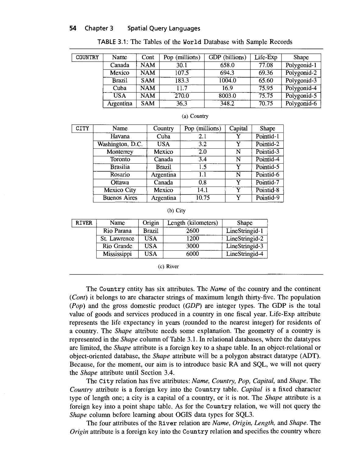
- 3.1.1 World Database 53
3.2 RA 55
3.2.1 The Select and Project Operations 55
3.2.2 Set Operations 56
3.2.3 Join Operation 57
3.3 Basic SQL Primer 59
3.3.1 DDL 59
3.3.2 DML 60
3.3.3 Basic Form of an SQL Query 60
3.3.4 Example Queries in SQL 61
3.3.5 Summary of RA and SQL 64
3.4 Extending SQL for Spatial Data 64
3.4.1 The OGIS Standard for Extending SQL 65
3.4.2 Limitations of the Standard 66
3.5 Example Queries that Emphasize Spatial Aspects 67
3.6 Trends: Object-Relational SQL 71
3.6.1 A Glance at SQL3 72
3.6.2 Object-Relational Schema 73
3.6.3 Example Queries 75
3.7 Summary 75
Bibliographic Notes 76
3.8 Appendix: State Park Database 79
3.8.1 Example Queries in RA 80
4 Spatial Storage and Indexing 83
4.1 Storage: Disks and Files 84
4.1.1 Disk Geometry and Implications 85
4.1.2 Buffer Manager 86
4.1.3 Field, Record, and File 87
4.1.4 File Structures 88
4.1.5 Clustering 90
4.2 Spatial Indexing 96
4.2.1 Grid Files 97
4.2.2 R-Trees 99
4.2.3 Cost Models 103
4.3 Trends 104
4.3.1 TR*-Tree for Object Decomposition 104
4.3.2 Concurrency Control 105
4.3.3 Spatial Join Index 107
4.4 Summary Ill
Bibliographic Notes Ill
5 Query Processing and Optimization 114
5.1 Evaluation of Spatial Operations 115
5.1.1 Overview 115

Contents vii
5.1.2 Spatial Operations 115
5.1.3 Two-Step Query Processing of Object Operations 116
5.1.4 Techniques for Spatial Selection 117
5.1.5 General Spatial Selection 118
5.1.6 Algorithms for Spatial-Join Operations 119
5.1.7 Strategies for Spatial Aggregate Operation:
Nearest Neighbor 122
5.2 Query Optimization 122
5.2.1 Logical Transformation 124
5.2.2 Cost-Based Optimization: Dynamic Programming 127
5.3 Analysis of Spatial Index Structures 129
5.3.1 Enumeration of Alternate Plans 131
5.3.2 Decomposition and Merge in Hybrid Architecture 132
5.4 Distributed Spatial Database Systems 132
5.4.1 Distributed DBMS Architecture 134
5.4.2 The Semijoin Operation 135
5.4.3 Web-Based Spatial Database Systems 136
5.5 Parallel Spatial Database Systems 138
5.5.1 Hardware Architectures 139
5.5.2 Parallel Query Evaluation 140
5.5.3 Application: Real-Time Terrain Visualization 142
5.6 Summary 145
Bibliographic Notes 146
6 Spatial Networks 149
6.1 Example Network Databases 149
6.2 Conceptual, Logical, and Physical Data Models 151
6.2.1 A Logical Data Model 151
6.2.2 Physical Data Models 154
6.3 Query Language for Graphs 157
6.3.1 Shortcomings of RA 158
6.3.2 SQL CONNECT Clause 159
6.3.3 Example Queries on the BART System 161
6.3.4 Trends: SQL3 Recursion 163
6.3.5 Trends: SQL3 ADTs for Networks 164
6.4 Graph Algorithms 165
6.4.1 Path-Query Processing 166
6.4.2 Graph Traversal Algorithms 166
6.4.3 Best-First Algorithm for Single Pair (v, d) Shortest Path .... 169
6.4.4 Trends: Hierarchical Strategies 170
6.5 Trends: Access Methods for Spatial Networks 173
6.5.1 A Measure of I/O Cost for Network Operations 174
6.5.2 A Graph-Partitioning Approach to Reduce Disk I/O 176
6.5.3 CCAM: A Connectivity Clustered Access Method
for Spatial Network 177
6.5.4 Summary 179
Bibliographic Notes 179

Contents
Introduction to Spatial Data Mining 182
7.1 Pattern Discovery 183
7.1.1 The Data-Mining Process 183
7.1.2 Statistics and Data Mining 185
7.1.3 Data Mining as a Search Problem 185
7.1.4 Unique Features of Spatial Data Mining 185
7.1.5 Famous Historical Examples of Spatial Data Exploration .... 186
7.2 Motivating Spatial Data Mining 187
7.2.1 An Illustrative Application Domain 187
7.2.2 Measures of Spatial Form and Auto-correlation 189
7.2.3 Spatial Statistical Models 191
7.2.4 The Data-Mining Trinity 193
7.3 Classification Techniques 194
7.3.1 Linear Regression 195
7.3.2 Spatial Regression 195
7.3.3 Model Evaluation 196
7.3.4 Predicting Location Using Map Similarity (PLUMS) 198
7.3.5 Markov Random Fields 198
7.4 Association Rule Discovery Techniques 202
7.4.1 Apriori: An Algorithm for Calculating Frequent Itemsets .... 202
7.4.2 Spatial Association Rules 204
7.4.3 Colocation Rules 204
7.5 Clustering 206
7.5.1 ^T-medoid: An Algorithm for Clustering 209
7.5.2 Clustering, Mixture Analysis, and the EM Algorithm 210
7.5.3 Strategies for Clustering Large Spatial Databases 213
7.6 Spatial Outlier Detection 215
7.7 Summary 221
7.8 Appendix: Bayesian Calculus 221
7.8.1 Conditional Probability 221
7.8.2 Maximum Likelihood 222
Bibliographic Notes 222
Trends in Spatial Databases 227
8.1 Database Support for Field Entities 227
8.1.1 Raster and Image Operations 228
8.1.2 Storage and Indexing 231
8.2 Content-Based Retrieval 233
8.2.1 Topological Similarity 233
8.2.2 Directional Similarity 234
8.2.3 Distance Similarity 235
8.2.4 Attribute Relational Graphs 235
8.2.5 Retrieval Step 237
8.3 Introduction to Spatial Data Warehouses 237
8.3.1 Aggregate Operations 238
8.3.2 An Example of Geometric Aggregation 240

Contents ix
8.3.3 Aggregation Hierarchy 242
8.3.4 What Is an Aggregation Hierarchy Used For? 245
8.4 Summary 246
Bibliographic Notes 246
Bibliography 250
Index 258

List of Figures
1.1 The evolution of the abbreviation GIS over the last two decades. In the
1980s GIS was Geographic Information System; in the 1990s, Geographic
Information Science was the preferred phrase, and now the trend is toward
Geographic Information Services 5
1.2 Landsat image of Ramsey county, Minnesota, with spatial layers of
information superimposed 6
1.3 Census blocks with boundary ID: 1050 7
1.4 Four tables required in a relational database with overlapping attributes
to accommodate the polyline datatype 8
1.5 Evolution of databases. [Khoshafian and Baker, 1998] 9
1.6 Three-layer architecture 10
1.7 Two relations to illustrate the difference between join
and spatial join 14
1.8 The filter-refine strategy for reducing computation time 15
1.9 Determining pairs of intersecting rectangles: (a) two sets of rectangles:
R and S\ (b) a rectangle T with its lower-left and upper-right corners
marked; and (c) the sorted set of rectangles with their joins. Note the
filtering nature of the plane sweep algorithm. In the example, twelve
possible rectangle pairs could be joined. The filtering step reduced the number
of possibilities to five. An exact geometry test can be used to check which
of the five pairs of objects satisfy the query predicate [Beckmann et al.,
1990] 16
1.10 (a) Programmer's viewpoint; (b) DBMS designer's viewpoint 17
1.11 Different ways of ordering multidimensional data: (a) row order; (b) Z-
order. If a line is drawn following the numbers in ascending order, the
Z pattern will become obvious 18
1.12 (a) Binary tree; (b) B-tree 18
1.13 R-tree extends B-tree for spatial objects 19
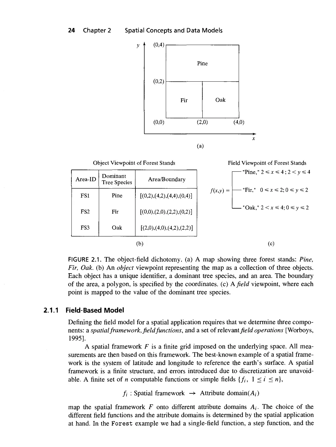
2.1 The object-field dichotomy, (a) A map showing three forest stands: Pine,
Fir, Oak. (b) An object viewpoint representing the map as a collection
of three objects. Each object has a unique identifier, a dominant tree
species, and an area. The boundary of the area, a polygon is specified by
the coordinates, (c) Afield viewpoint, where each point is mapped to the
value of the dominant tree species 24
2.2 An OGIS proposal for building blocks of spatial geometry in UML
notation [OGIS, 1999] 27
2.3 The nine-intersection model [Egenhofer et al., 1989] 30
2.4 An ER diagram for the State-Park example 37
2.5 Relational schema for the State-Park example 39
2.6 Schema for point, line, polygon, and elevation 40
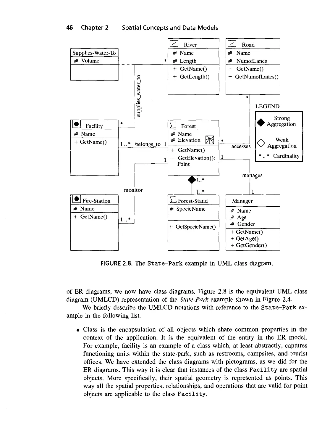
2.7 ER diagram for the State-Park example, with pictograms 45
2.8 The State-Park example in UML 46
xi

xii List of Figures
3.1 The ER diagram of the World database 53
3.2 The buffer of a river and points within and outside 69
3.3 Sample objects [Clementini and Felice, 1995] 78
3.4 The ER diagram of the StatePark database 80
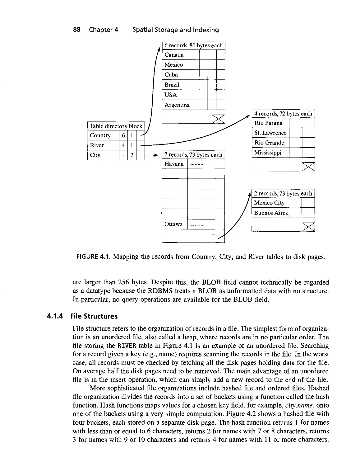
4.1 Mapping the records from Country, City, and River tables
to disk pages 88
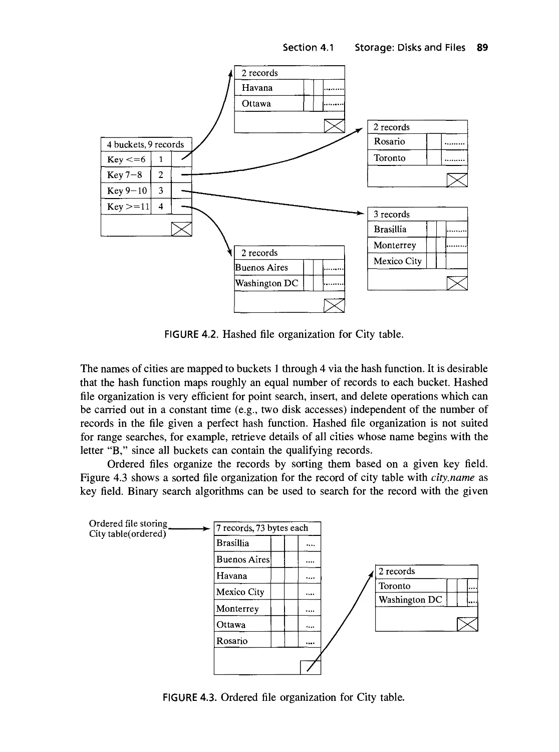
4.2 Hashed file organization for City table 89
4.3 Ordered file organization for City table 89
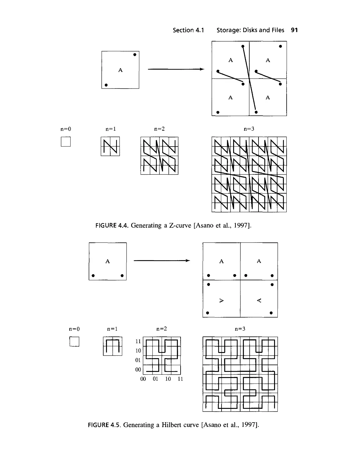
4.4 Generating a Z-curve [Asano et al., 1997] 91
4.5 Generating a Hilbert curve [Asano et al., 1997] 91
4.6 Example to calculate the z-value 92
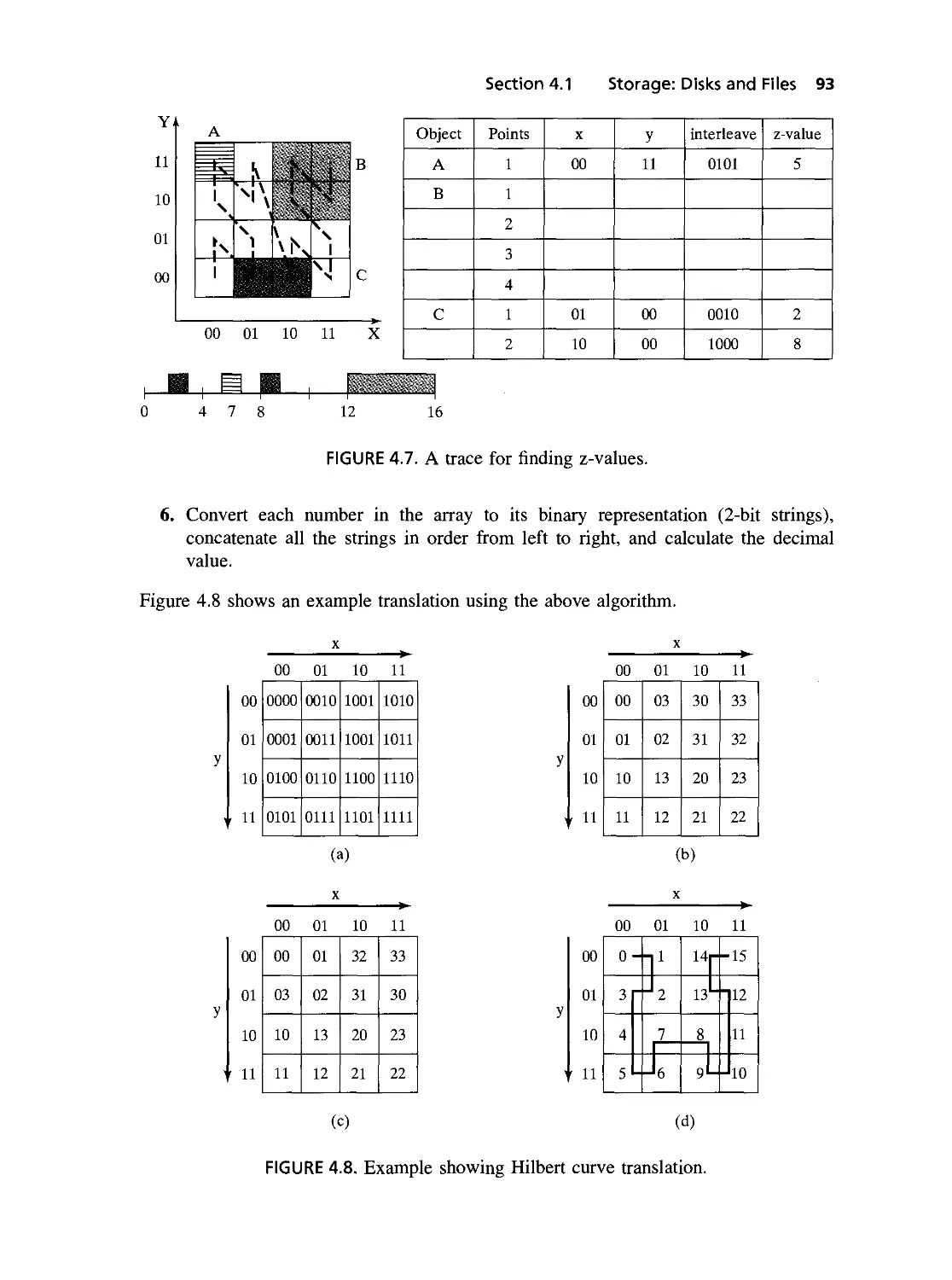
4.7 A trace for finding z-values 93
4.8 Example showing Hilbert curve translation 93
4.9 Illustration of clusters: (a) two clusters for the Z-curve; (b) one cluster
for the Hilbert curve 94
4.10 Secondary index on the City table 96
4.11 Primary index on the City table 97
4.12 A fixed-grid structure for points (A, B, C, D) 98
4.13 A two-dimensional grid directory 99
4.14 Grid file with linear scales 100
4.15 A collection of spatial objects 100
4.16 R-tree hierarchy 101
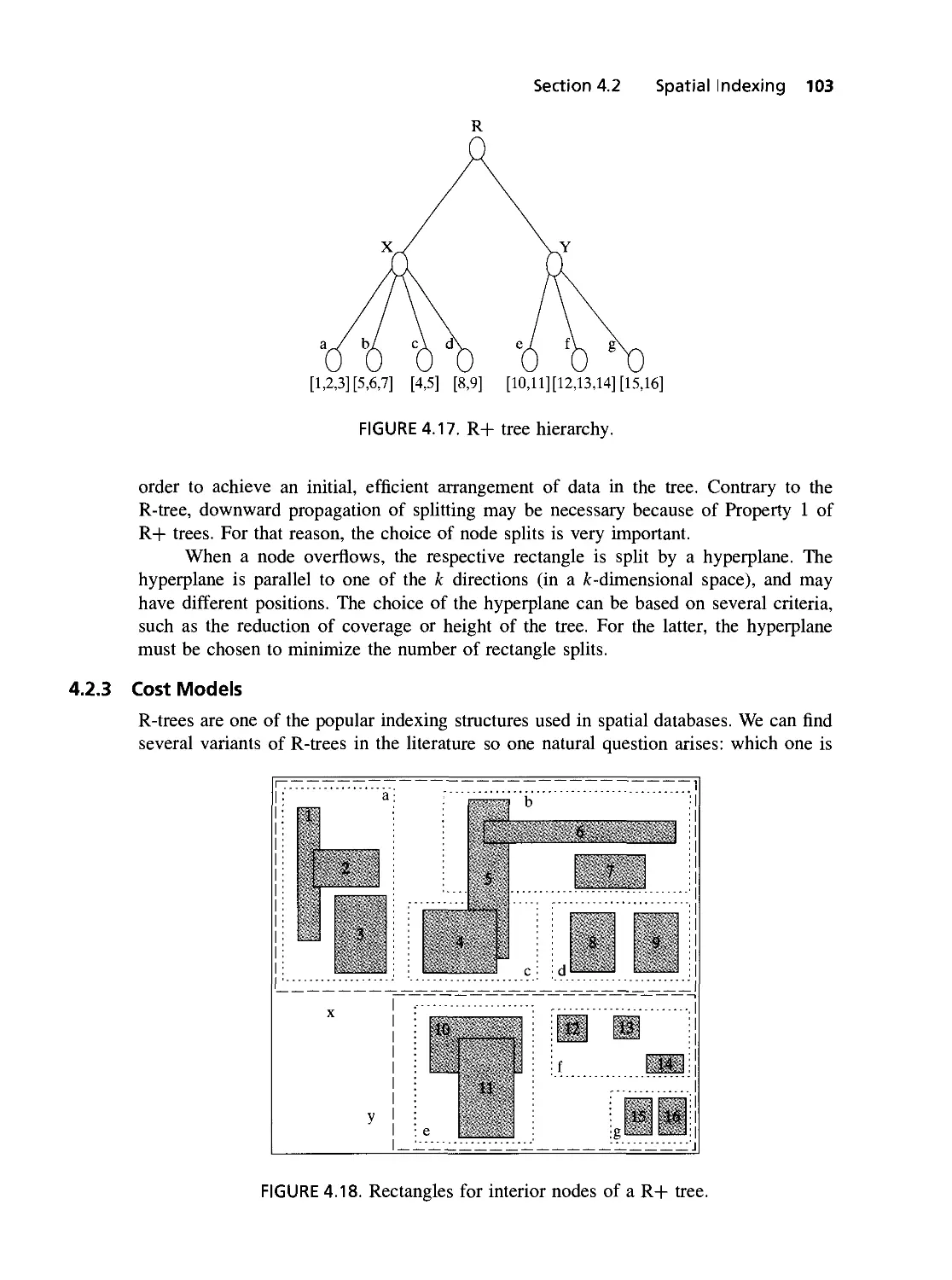
4.17 R+ tree hierarchy 103
4.18 Rectangles for interior nodes of a R+tree 103
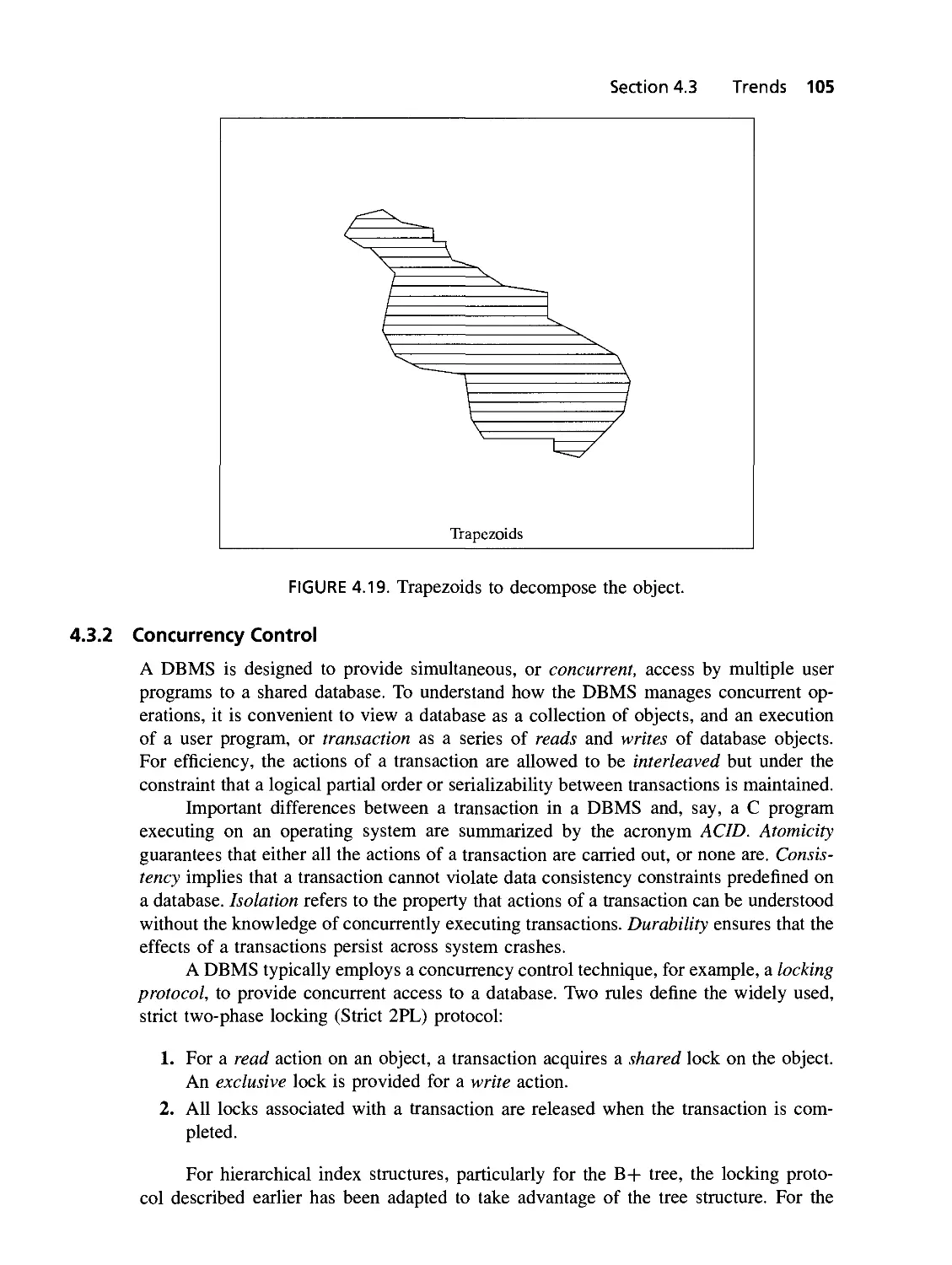
4.19 Trapezoids to decompose the object 105
4.20 A subsection of an R-link tree [Kornacker and Banks, 1995] 107
4.21 Constructing a join-index from two relations 108
4.22 Comparison of tuple-level adjacency matrices for equi-join
and spatial join 109
4.23 Construction of a PCG from a join-index 110
4.24 Exercise 1 112
5.1 Multistep processing [Brinkhoff et al., 1994] 117
5.2 Schema for a query optimizer 123
5.3 Query tree 124
5.4 Pushing down: select operation 125
5.5 Pushing down not always helpful 126
5.6 An execution strategy: query-evaluation plan 132
5.7 An execution strategy: query tree 133
5.8 Two methods of decomposition 134
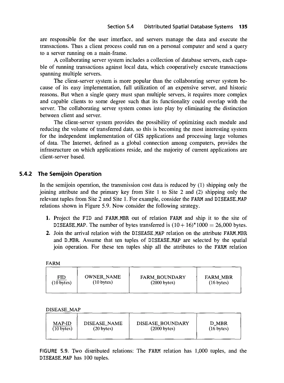
5.9 Two distributed relations: The FARM relation has 1,000 tuples, and the
DISEASE_MAP has 100 tuples 135
5.10 Web GIS architecture 136
5.11 Parallel architecture options 140
5.12 Example of allocations by different methods 142
5.13 Components of the terrain-visualization system 143
5.14 A sample polygonal map and a range query 143
5.15 Different modules of the parallel formulations 144

List of Figures
XIII
5.16 Alternatives for polygon/bounding-box division among processors. . . . 145
6.1 Two examples of spatial networks 150
6.2 Three different representations of a graph 154
6.3 A graph model for River Network example 157
6.4 A relation R and its transitive closure X 158
6.5 SQL's CONNECT clause operation 160
6.6 The result of BFS and DFS on a graph with source node 1 166
6.7 Routing example 172
6.8 Routing example 172
6.9 Graph with its denormalized table representation 174
6.10 Major roads in the city of Minneapolis 176
6.11 Cut-edges in CCAM paging of Minneapolis major roads 177
6.12 Clustering and storing a sample network (key represents
spatial order) 178
7.1 Data-mining process. The data-mining process involves a close interaction
between a domain expert and a data-mining analyst. The output of the
process is a set of hypothesis (patterns), which can then be rigorously
verified by statistical tools and visualized using a GIS. Finally the analyst
can interpret the patterns and make
and recommend appropriate action 183
7.2 Search results of data-mining algorithm, (a) One potential pattern out
of a total of 216. (b) If we constrain the patterns to be such that each
4x4 block can only be assigned one class, then the potential number
of patterns is reduced to 24. Based on other information, a data-mining
algorithm can quickly discover the "optimal" pattern 185
7.3 Darr wetland, 1995. (a) Learning dataset: The geometry of the marshland
and the locations of the nests; (b) spatial distribution of vegetation
durability over the marshland; (c) spatial distribution of water depth; and (d)
spatial distribution of distance to open water 187
7.4 Spatial distribution satisfying random distribution assumptions of
classical regression 188
7.5 (a) A spatial lattice; (b) its contiguity matrix; (c) its row-normalized
contiguity matrix 189
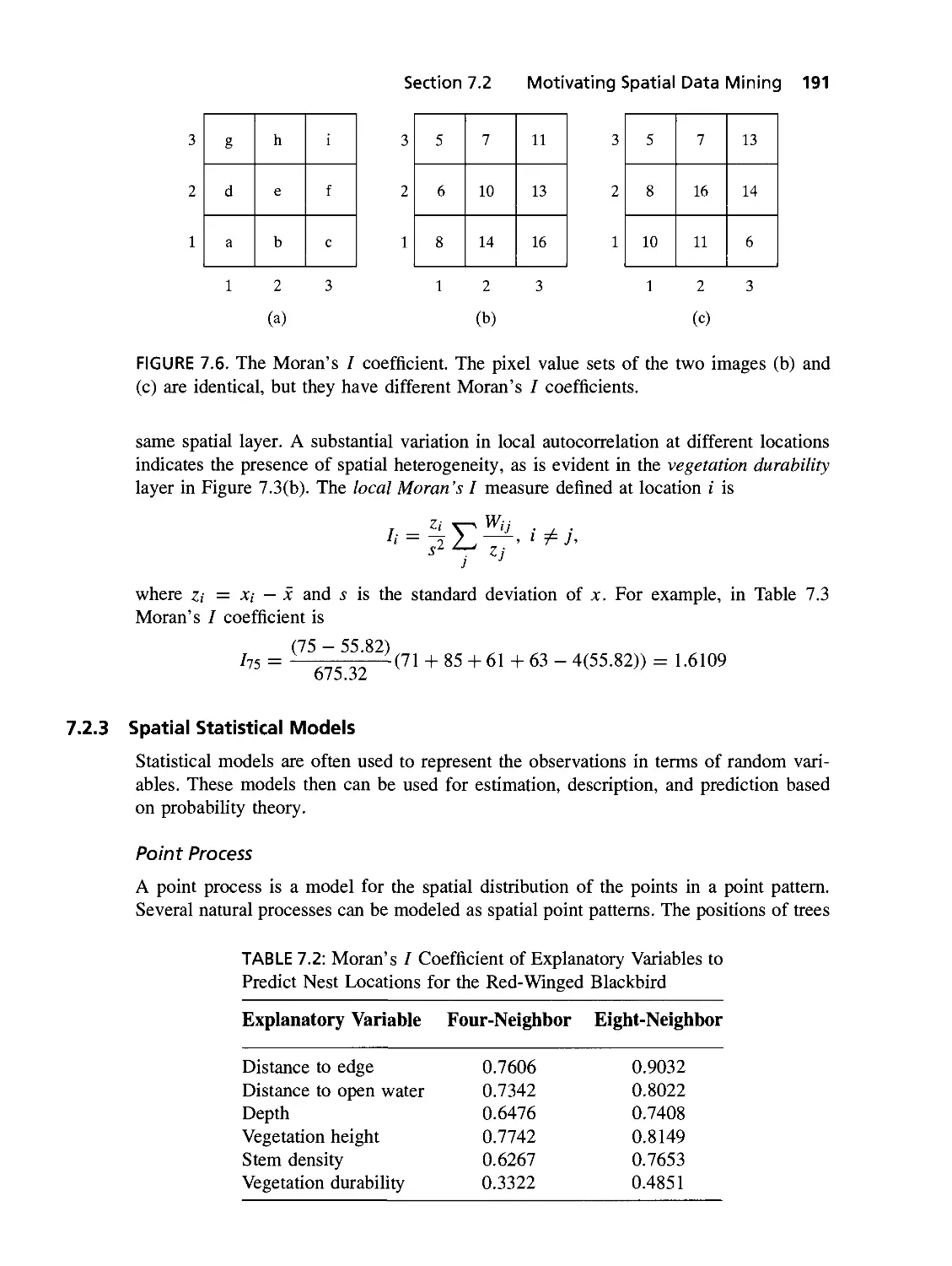
7.6 The Moran's / coefficient. The pixel value sets of the two images are
identical, but they have different Moran's / coefficients 190
7.7 The four possible outcomes for a two-class prediction 195
7.8 ROC curves (a) Comparison of the ROC curves for classical and SAR
models on the 1995 Darr wetland data, (b) Comparison of the two models
on the 1995 Stubble wetland data 196
7.9 Problems of ROC curves with spatial data, (a) The actual locations of
nest's; (b) pixels with actual nests; (c) location predicted by a model;
(d) location predicted by another mode. Prediction (d) is spatially more
accurate than (c). Classical measures of classification accuracy will not
capture this distinction 196
7.10 Spatial data sets with salt and pepper spatial patterns 199
7.11 Example database, frequent itemsets, and high-confidence rules 202
7.12 Sample colocation patterns 204

xiv List of Figures
7.13 Two interpretations of spatial clustering. If the goal is to identify locations
that dominate the surroundings (in terms of influence), then the clusters
are SI and S2. If the goal is to identify areas of homogeneous values,
the clusters are Al and A2 206
7.14 (a) A gray-scale 4x4 image, (b) The labels of the image generated using
the EM algorithm, (c) The labels generated for the same image using the
neighborhood EM algorithm. Notice the spatial smoothing attained by
modifying the objective function 210
7.15 Using the neighborhood EM algorithm, (a) As expected clustering
without any spatial information leads to poor results; (b) including spatial
information (fi = 1.0) leads to dramatic improvement of results; and
(c) overemphasizing spatial information (fi = 2.0) again leads to poor
results 213
7.16 A Data Set for Outlier Detection 215
7.17 Variogram Cloud and Moran Scatterplot to Detect Spatial Outliers. . . . 216
7.18 Scatterplot and Spatial Statistic Zs(x) to Detect Spatial Outliers 217
7.19 A network of traffic sensor stations 218
7.20 Spatial and temporal neighborhoods 218
7.21 Spatial outliers in traffic volume data 219
8.1 A continuous function and its raster representation 226
8.2 Example of a local operation: Thresholding 227
8.3 Neighborhoods of a cell and an example of a focal
operation: FocalSum 228
8.4 Example of a zonal operation: ZonalSum 228
8.5 Example of a global operation 229
8.6 The trim operation: dimension preserving 229
8.7 The slice operation: dimension reduction 230
8.8 Different strategies for storing arrays 230
8.9 The topological neighborhood graph [Ang et al., 1998]. The distance
between two relations is the shortest path on this graph 232
8.10 The directional neighborhood graph [Ang et al., 1998]. The distance
between two relations is the shortest solid line path on this graph. . . . 233
8.11 Visual perspective: distance as the least discriminating
spatial predicate 233
8.12 An image and its ARG [Petrakis and Faloutsos, 1997]. The ARG is
mapped onto an N-dimensional feature point 234
8.13 The general methodology of content-based retrieval 234
8.14 Computation of distributive aggregate function 236
8.15 Computation of algebraic aggregate function 237
8.16 An example of GIS aggregate function, geometric-union 239
8.17 The 0-D, 1-D, 2-D, and 3-D data cubes 240
8.18 An example of a data cube 241
8.19 An example of using the group-by operator 242

List of Tables
1.1 List of Common GIS Analysis Operations [Albrecht, 1998] 3
1.2 Different Types of Spaces with Example Operations 12
2.1 Examples of Topological and Nontopological Operations 29
2.2 Representative Example of Dynamic Spatial Operations
[Worboys, 1995] 31
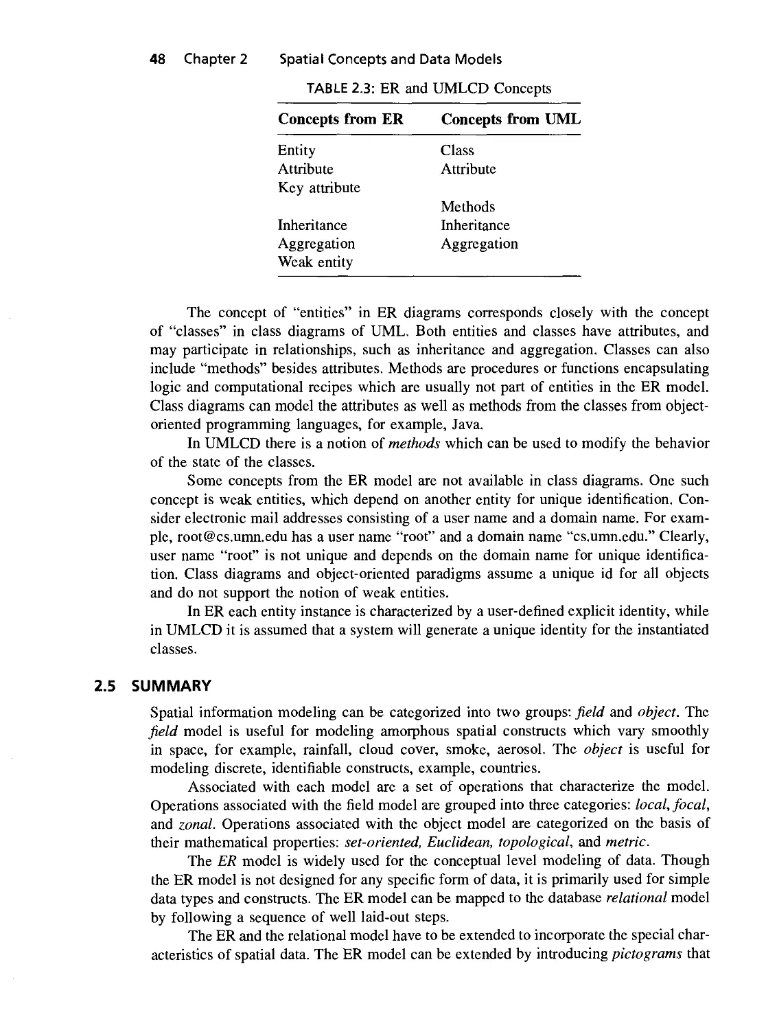
2.3 ER and UML Concepts 48
3.1 The Tables of the World Database 54
3.2 Results of Two Basic Operations in RA Select and Project 56
3.3 The Cross-Product of Relations R and S 57
3.4 The Results of Set Operations 57
3.5 Steps of the Conditional Join Operation 58
3.6 The Country and River Schema in SQL 60
3.7 Tables from the Select, Project, and Select and Project Operations ... 61
3.8 Results of Example Queries 62
3.9 A Sample of Operations Listed in the OGIS Standard for SQL
[OGIS, 1999] 66
3.10 Basic Datatypes 67
3.11 Results of Query 7 70
3.12 The Sequence of Creation of the Country Table 74
3.13 Tables for the StatePark Database 81
4.1 The Characteristics of a Traditional DBMS, a Programming Application,
and an SDBMS on the Basis of Relative CPU and I/O Costs 85
4.2 Physical and Performance Parameters of the Western Digital AC36400
Disk Drive 86
6.1 The Stop and DirectedRoute Tables of BART 155
6.2 The RouteStop Table of BART 156
6.3 The River and Fallslnto Relations of River Network 157
7.1 Habitat Variables Used for Predicting the Locations of the Nests of the
Red-Winged Blackbird. Note: There are six independent variables and
one dependent variable. The type of the dependent
variable is binary 186
7.2 Moran's / Coefficient of Explanatory Variables to Predict Nest Locations
for the Red-Winged Blackbird 190
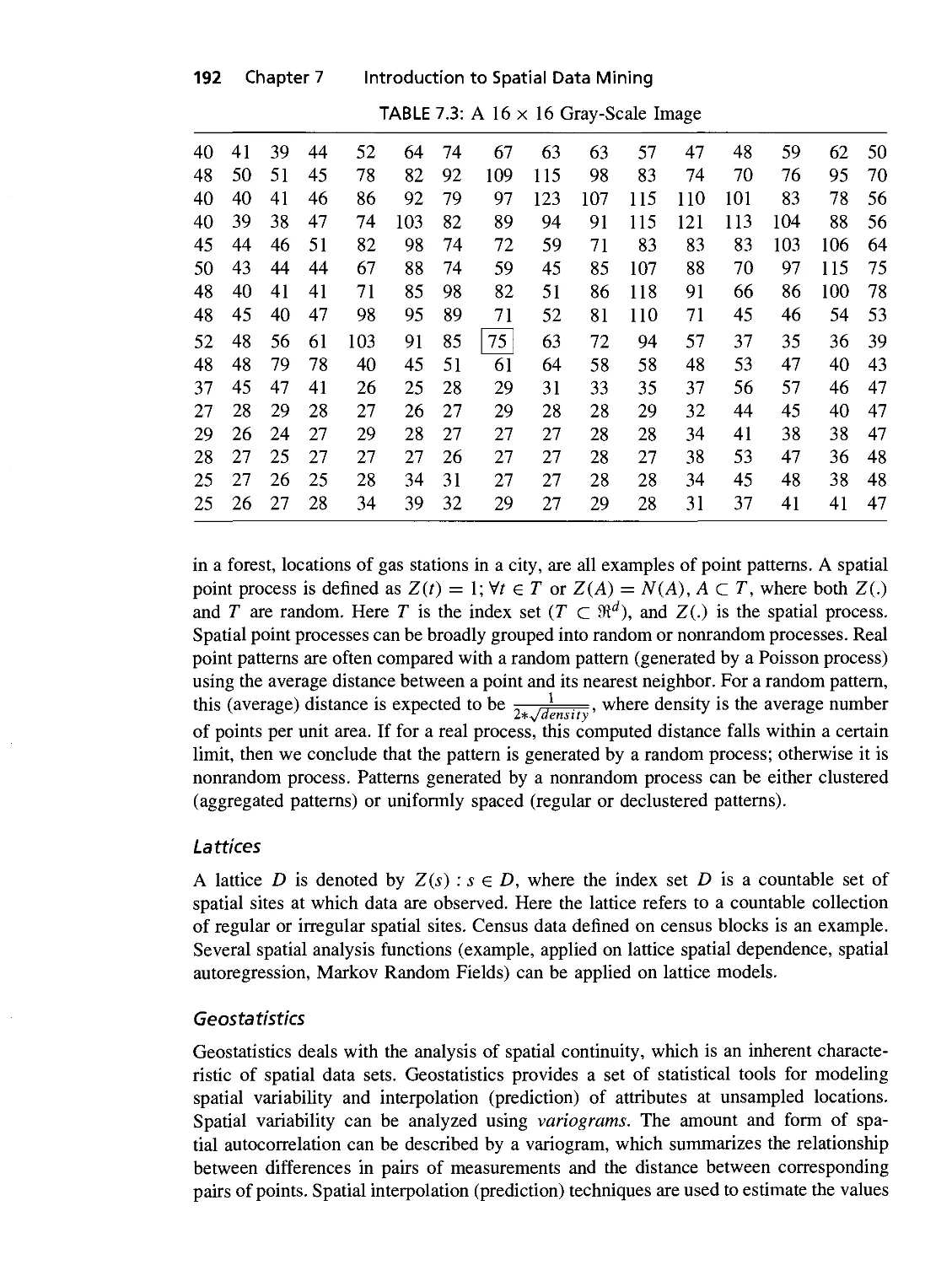
7.3 A 16 x 16 Gray-Scale Image 191
7.4 Support and Confidence of Three Rules 201
7.5 Examples of Spatial Association Rules Discovered in the 1995 Darr
Wetland Data 203
7.6 Four Options for Local Search in Clustering 209
7.7 Database of Facilities 222
8.1 Aggregation Operations 236
xv

xvi List of Tables
8.2 SQL Queries for Map Reclassification 238
8.3 Table of GROUP-BY Queries 243
8.4 Slice on the Value "America" of the Region Dimension 243
8.5 Dice on the Value "1994" of the Year Dimension and the Value "America"
of the Region Dimension 244

Preface
Over the years it has become evident in many areas of computer applications that the
functionality of database management systems has to be enlarged to include spatially
referenced data. The study of spatial database management systems (SDBMS) is a step
in the direction of providing models and algorithms for the efficient handling of data
related to space.
Spatial databases have now been an active area of research for over two decades.
Their results, example, spatial multidimensional indexing, are being used in many
different areas. The principle impetus for research in SDBMs comes from the needs of existing
applications such as geographical information systems (GIS) and computer-aided design
(CAD), as well as potential applications such as multimedia information systems, data
warehousing, and NASA's earth observation system. These spatial applications have over
one million existing users.
Major players in the commercial database industry have products specifically
designed to handle spatial data. These products include the spatial data engine (SDE), by
Environment Systems Research Institute (ESRI); as well as spatial datablades for object-
relational database servers from many vendors including Intergraph, Autodesk, Oracle,
IBM and Informix. Research prototypes include Postgres, Geo2, and Paradise. The
functionality provided by these systems includes a set of spatial data types such as the point,
line, and polygon, and a set of spatial operations, including intersection, enclosure, and
distance. An industrywide standard set of spatial data types and operations has been
developed by the Open Geographic Information Systems (OGIS) consortium. The spatial
types and operations can be made a part of an object-relational query language such as
SQL3. The performance enhancement provided by these systems includes a
multidimensional spatial index and algorithms for spatial access methods, spatial range queries, and
spatial joins.
The integration of spatial data into traditional databases amounts to resolving many
nontrivial issues at various levels. They range from deep ontological questions about the
modeling of space, for example, whether it should be field based or object based, thus
paralleling the wave-particle duality in physics to more mundane but important issues about
file management. These diverse topics make research in SDBMS truly interdisciplinary.
Let us use the example of a country dataset to highlight the special needs of
spatial databases. A country has at least one nonspatial datum, its name, and one spatial
datum, its boundary. There is no ambiguity about storing or representing its name, but
unfortunately it is not true for its boundary. Assuming that the boundary is represented
as a collection of straight lines, we need to include a spatial data type line and the
companion types point and region in the database system to facilitate spatial queries on
the object country. These new data types need to be manipulated and composed according
to some fixed rules leading to the creation of a spatial algebra. Because spatial data is
inherently visual and usually voluminous, database systems have to be augmented to
provide visual query processing and special spatial indexing . Other important database
issues such as concurrency control, bulk loading, storage, and security have to be revisited
and fine-tuned to build an effective spatial database management system.
XVII

xviii Preface
This book evolved from the class notes of a graduate course on Scientific Databases
(Csci 8705) in University of Minnesota. Researchers and students both within and
outside the Computer Science Department found the course very useful and applicable
to their work. Despite the good response and high level of interest in the topic, no
textbook available in the market was able to meet the interdisciplinary needs of the
audience. A recent book by [Scholl et al., 2001] focuses on traditional topics related
to query languages and access methods while leaving out current topics such as spatial
networks (e.g., road maps) and data mining for spatial patterns. A monograph by [Adam
and Gangopadhyay, 1997] catalogs research papers on database issues in GIS, with
little reference to the industrial state-of-the-art. Another [Worboys, 1995] also focuses
on GIS and has only two chapters devoted to database issues. Many of these books
neither use industry standards, e.g., OGIS, nor provide adequate instructional support,
example, questions and problems at the end of each chapter to allow students to assess
their understanding of the main concepts. Not surprisingly, our colleagues in academia
working in databases, parallel computing, multimedia information, civil and mechanical
engineering, and forestry have expressed a strong desire for a comprehensive text on
spatial databases. Industry professionals involved in software development for GIS and
CAD/CAM have also made several requests for information on spatial databases in a
collected form.
As a first step toward developing this book, we completed a survey paper, "Spatial
Databases: Accomplishments and Research Needs," for IEEE Transactions on Knowledge
and Data Engineering (Jan. 1999). We noticed that the research literature in computer
science was skewed with numerous publications on some topics (e.g., spatial indexes,
spatial join algorithms) and relatively scarce publications on many other important topics
(e.g., conceptual modeling of spatial data). We looked to GIS industry as well as GIS
researchers outside computer science for ideas in these areas for the relevant chapters in
the book.
Being on sabbatical for the academic year 1997-1998 facilitated initial work on the
book. We completed a draft of many chapters by expanding on the course notes of CSci
8705. The first draft of the book was used in database courses at the University of
Minnesota. Subsequently the book was revised using feedback from reviewers, colleagues,
and students.
We believe the following features are unique aspects of this book:
• The aim of this book is to provide a comprehensive overview of spatial databases
management systems. It covers current topics, example, spatial networks and spatial
data mining in addition to traditional topics, example, query languages, indexing,
query processing.
• A set of questions and problems is provided in each chapter to allow readers to test
understanding of core concepts, to apply core concepts in new application domains,
and to think beyond the material presented in the chapter. Additional instructional
aids (e.g., laboratories, lecture notes) are planned on the book Web site.
• A concerted effort has been made to "look beyond GIS." Techniques from SDBMS
are finding applications in many diverse areas, including multimedia
information, CAD/CAM, astronomy, meteorology, molecular biology, and computational
mechanics.

Preface xix
• In each chapter we have tried to bring out the object-relational database
framework, which is a clear trend in commercial database applications. This framework
allows spatial databases to reuse relational database facilities when possible, while
extending relational database facilities as needed.
• We will use spatial data types and operations specified by standards (e.g., OGIS)
to illustrate common spatial database queries. These standards can be incorporated
into an object-relational query language such as SQL-3.
• Self-contained treatment without assuming pre-requisite knowledge of GIS or
Databases.
• Complete coverage of spatial networks including modeling, querying and storage
methods.
• Detailed discussion of issues related to Spatial Data Mining.
• Balance between cutting-edge research and commercial trends.
• Easy to understand examples from common knowledge application domains.
CHAPTER ORGANIZATION
The book is divided into eight chapters, each one an important subarea within spatial
databases. We introduce the field of spatial databases in Chapter 1. In Chapter 2, we focus
on spatial data models and introduce the field versus object dichotomy and its implications
for database design. Chapter 3 discusses the necessary enhancements required to make
traditional query languages compatible with spatial databases. We provide an extensive
discussion of various proposals to extend SQL with spatial capabilities. Spatial databases
deal with extraordinarily large amounts of data, and it is essential for DBMS to provide
sophisticated storage, compression, and indexing methods to enhance the performance of
query processing. Spatial data storage and indexing schemes are covered in Chapter 4.
From query languages and indexing, we move on to query processing and optimization
in Chapter 5. Here we discover that many standard techniques from traditional databases
have to be abandoned or drastically modified in order to be applicable in a spatial context.
We also introduce the filter-refine paradigm for spatial query processing. In Chapter 6,
we show how spatial database technology is being applied to spatial networks. In this
chapter we also cover network data models and query languages. Chapter 7 covers the
emerging field of spatial data mining. In this chapter we expose the readers to the concept
of spatial dependency that is prevalent in spatial data sets, and show how this can be
modeled and incorporated into data mining process. Finally in Chapter 8, we discuss
emerging trends in spatial databases.
ACKNOWLEDGMENTS
We have received help from many people and we are extremely grateful to them. This
book would not have started without encouragement from Professor Vipin Kumar,
Computer Science Department, University of Minnesota; and Dr. Jack Dangermond, President,
Environmental Systems Research Institute (ESRI). This book benefitted a great deal from
access to ESRI researchers and products. We are also grateful to Dr. Siva Ravada (Oracle
Corporation) and Dr. Robert Uleman (Illustra Inc.) for help with understanding of their

xx Preface
spatial datablades. We are thankful to Alan Apt and his wonderful staff at Prentice Hall
for helping with the process of book-writing with constant encouragement. The
presentation improved a great deal from the comments from the anonymous reviewers and we
are grateful to them.
Our research related to spatial databases has been supported by many organizations
including the United Nations Development Programme, the National Science Foundation,
the National Aeronautics and Space Agency, the Army Research Laboratories, the U.S.
Department of Agriculture, the Federal Highway Administration, the US Department
of Transportation, the Minnesota Department of Transportation, the Center for Urban
and Regional Affairs, and the Computing Devices International. Many of the research
project resulted in surveys of research literature, as well as in development of innovative
techniques for problems related to spatial databases.
Special thanks to the members of spatial database research group in the Computer
Science Department at the University of Minnesota. They contributed in many different
ways including literature surveys, development of examples and figures, and insights
into various methods, as well in developing proper problem formulations and innovative
solution methods. We are extremely grateful to Vatsavai Ranga Raju for careful review
and multiple improvements to the earlier drafts. We also thank the students in different
offerings of Csci 8701, and Csci 8705 for working with the earlier drafts of the books
and providing helpful suggestions towards revising the material.
We benefitted from discussions with many other people over the years. They include
Marvin Bauer, Yvan Bedard, Paul Bolstad, Nick Bourbakis, Thomas Burk, John Carlis,
Jai Chakrapani, Vladimir Cherkassky, Douglas Chub, William Craig, Max Donath, Phil
Emmerman, Max Egenhofer, Michael Goodchild, Ralf Hartmut Gueting, Oliver Gunther,
John Gurney, Jia-Wei Han, Ravi Janardan, George Karypis, Hans-Peter Kriegel, Robert
McMaster, Robert Pierre, Shamkant Navathe, Raymond Ng, Hanan Samet, Paul Schrater,
Jaideep Srivastava, Benjamin Wah, Kyu-Young Whang, and Michael Worboys.

Foreword
Ever since Cro-Magnon hunters drew pictures of track lines and tallies thought to depict
migration routes on the walls of caves near Lascaux, France, 35,000 years ago, people
have been interested in graphics linked to geographic information. Today, such geographic
information systems (GISs) are used in applications ranging from tracking the migration
routes of caribou and polar bears, identifying the effects of oil development on animal life,
aiding farmers to minimize the use of pesticide in their farms, helping corporate supply
managers to predict the best places to build distribution warehouses, to relating information
about rainfall and aerial photographs to wetlands drying up at certain times of the year.
A GIS, in the strictest sense, is a computer system for assembling, storing,
manipulating, and displaying data with respect to their locations. However, modern GISs
often assimilate data from multiple disparate sources in many different forms in order to
answer queries and help analyze information. In a broad sense, a GIS not only converts
and stores geographical information in digital form for analysis, but must also collects,
transforms, aggregates, indexes, links, and mines related spatial databases. A modern
GIS makes it possible to integrate information that is difficult to associate through any
other means and combines mapped variables to build and analyze new variables.
With this broad perspective in mind, Shekhar and Chawla have done a marvelous
job in presenting the fundamentals and trends in geographical information processing.
The core of the book is a tour de force sequence of concepts and methods, progressively
explaining models, languages and algorithms until we distinguish branches from trees
and trees from forests. The authors not only explain the concepts but illustrate them well
by numerous examples. They have emphasized the many nontrivial issues in integrating
spatial data into traditional databases, ranging from deep ontological questions about
the modeling of space to the important issues about file management. Each chapter
is further supplemented by many thought-provoking exercises that aid readers in better
understanding of the concepts and algorithms presented. The book ends with an excellent
exposition of spatial data mining and future trends in spatial databases that helps readers
appreciate emerging research issues.
This book is suitable as a textbook for an interdisciplinary course on geographic
information systems, as well as a handy reference for people working in the area.
Readers should find it easy to understand and apply the concepts and algorithms learned,
even without any formal training in databases. Many disciplines will benefit from
techniques learned in this book, leading to wider applications of the technology throughout
government, business, and industry.
As the reader of the first books in this area, and I am confident that you will benefit
by what you learn in this exciting and rewarding area.
Prof. Benjamin Wan
University of Illinois at Urbana-Champaign
Department of Electrical and Computer Engineering
1101 W. Springfield Avenue
Urbana, IL 61801
President, IEEE Computer Society (2001)
March 2002
XXI

Foreword
Spatial information—that is, information about objects located in a spatial frame such
as the Earth's surface—has long been recognized as presenting special problems for
computing. As early as 1972 the term spatial data handling was being used to refer to
the activities of a small but dynamic community of researchers who were committed
to exploiting electronic data processing in order to increase productivity in such areas
as map compilation and editing; map measurement; and spatial data analysis. Spatial
information is rich in high-level structures, and although each of the classical models
of database management that began to emerge in the 1960s had something to offer to
this application area, neither the relational model nor object-oriented modeling provide
a perfect fit. The relational model handles topological relationships well, but lacks the
means to represent complex hierarchical relationships that span spatial scales; while
object-oriented models handle both topological and hierarchical relationships, but have
difficulty dealing with phenomena that are essentially continuous in space.
Books that elucidate the complex story of spatial databases are few and far between,
and thus this book is especially welcome. It covers the entire field, from representation
through query to analysis, in a style that is clear, logical, and rigorous. Especially welcome
is the chapter on data mining, which addresses both traditional spatial data analysis and
also new techniques that have been developed in the past few years to take advantage
of today's high-speed computing in processes of automated search for anomalies and
patterns in very large spatial databases. It is intended for computer science students, as
reflected in the sequence of topics and the style of presentation, but will also be useful
for students from other disciplines looking for a more rigorous and fundamental approach
than is provided by most textbooks on geographic information systems (GIS).
The importance of spatial databases is growing rapidly, partly as a result of the
recognition that their applications extend well beyond the traditional domain of GIS.
Location and time are powerful ways of identifying and characterizing information,
because many data sets have footprints in space and time. This is obviously true of
maps and Earth images, but is also true of many reports, books, photographs, and other
types of information. Thus location is a powerful basis for search, and for finding
relevant information in distributed resources such as the World Wide Web. There is growing
recognition that space (and time) provides important ways of integrating information that
go far beyond the traditional domains of spatial databases and GIS. The last chapter
of the book discusses some of these, and gives a sense of why many believe that the
importance of spatial databases is likely to continue to grow rapidly over the coming
years.
Michael F. Goodchild
National Center for Geographic Information and Analysis,
and Department of Geography,
University of California, Santa Barbara, CA 93106-4060, USA
xxiii

CHAPTER 1
Introduction to Spatial
Databases
1.1 OVERVIEW
1.2 WHO CAN BENEFIT FROM SPATIAL DATA MANAGEMENT?
1.3 GISANDSDBMS
1.4 THREE CLASSES OF USERS FOR SPATIAL DATABASES
1.5 AN EXAMPLE OF AN SDBMS APPLICATION
1.6 A STROLL THROUGH SPATIAL DATABASES
1.7 SUMMARY
1.1 OVERVIEW
We are in the midst of an information revolution. The raw material (data) which is
powering this controlled upheaval is not found below the earth's surface where it has
taken million of years to form but is being gathered constantly via sensors and other
data-gathering devices. For example, NASA's Earth Observing System (EOS) generates
one terabyte of data every day.
Satellite images are one prominent example of spatial data. To extract information
from a satellite image, the data has to be processed with respect to a spatial frame of
reference, possibly the earth's surface. But satellites are not the only source of spatial
data, and the earth's surface is not the only frame of reference. A silicon chip can be,
and often is, a frame of reference. In medical imaging the human body acts as a spatial
frame of reference. In fact, even a supermarket transaction is an example of spatial data
if, for example, a zip code is included. Queries, or commands, posed on spatial data are
called spatial queries. For example, the query "What are the names of all bookstores with
more than ten thousand titles?" is an example of a nonspatial query. On the other hand,
the query, "What are the names of all bookstores within ten miles of the Minneapolis
downtown?" is an example of a spatial query. This book is an exposition of efficient
techniques for the storage, management, and retrieval of spatial data.
Today, data is housed in and managed via a database management system (DBMS).
Databases and the software that manages them are the silent success story of the
information age. They have slowly permeated all aspects of daily living, and modern society
would come to a halt without them. Despite their spectacular success, the prevalent view
is that a majority of the DBMSs in existence today are either incapable of managing
spatial data or are not user-friendly when doing so. Now, why is that? The traditional
1

2 Chapter 1 Introduction to Spatial Databases
role of a DBMS has been that of a simple but effective warehouse of business and
accounting data. Information about employees, suppliers, customers, and products can be
safely stored and efficiently retrieved through a DBMS. The set of likely queries is
limited, and the database is organized to efficiently answer these queries. From the business
world, the DBMS made a painless migration into government agencies and academic
administrations.
Data residing in these mammoth databases is simple, consisting of numbers, names,
addresses, product descriptions, and so on. These DBMSs are very efficient for the tasks
they were designed for. For example, a query such as "List the top ten customers, in
terms of sales, in the year 1998" will be very efficiently answered by a DBMS even if it
has to scan through a very large customer database. Such commands are conventionally
called "queries" although they are not questions. The database will not scan through all
the customers; it will use an index, as you would do with this book, to narrow down the
search. On the other hand, a relatively simple query such as "List all the customers who
reside within fifty miles of the company headquarters" will confound the database. To
process this query, the database will have to transform the company headquarters and
customer addresses into a suitable reference system, possibly latitude and longitude, in
which distances can be computed and compared. Then the database will have to scan
through the entire customer list, compute the distance between the company and the
customer, and if this distance is less than fifty miles, save the customer's name. It will
not be able to use an index to narrow down the search, because traditional indices are
incapable of ordering multidimensional coordinate data. A simple and legitimate business
query thus can send a DBMS into a hopeless tailspin. Therefore the need for databases
tailored for handling spatial data and spatial queries is immediate.
1.2 WHO CAN BENEFIT FROM SPATIAL DATA MANAGEMENT?
Professionals from all walks of life have to deal with the management and analysis of
spatial data. Below we give a small but diverse list of professionals and one example of
a spatial query relevant to the work of each.
Mobile phone user: Where is the nearest gas station? Is there a pet-food vendor on my
way home?
Army field commander: Has there been any significant enemy troop movement since
last night?
Insurance risk manager: Which houses on the Mississippi River are most likely to be
affected by the next great flood?
Medical doctor: Based on this patient's Magnetic Resonance Imaging (MRI), have we
treated somebody with a similar condition?
Molecular biologist: Is the topology of the amino acid biosynthesis gene in the genome
found in any other sequence feature map in the database?
Astronomer: Find all blue galaxies within two arcmin of quasars.
Climatologist: How can I test and verify my new global warming model?

Section 1.3 GISandSDBMS 3
Pharmaceutical Researcher: Which molecules can dock with a given molecule based
on geometric shapes?
Sports: Which seats in a baseball stadium provide best view of pitcher and hitter? Where
should TV camera be mounted?
Corporate supply manager: Given trends about our future customer profile, which are
the best places to build distribution warehouses and retail stores?
Transport specialist: How should the road network be expanded to minimize traffic
congestion?
Urban sprawl specialist: Is new urban land development leading to the loss of rich
agricultural land.
Ski resort owner: Which mountains on our property are ideal for a beginner's ski run?
Farmer: How can I minimize the use of pesticide on my farm?
Golf entrepreneur: Where do I build a new golf course which will maximize profit
given the constraints of weather, Environmental Protection Agency pesticide
regulations, the Endangered Species Act, property prices, and the neighborhood
demographic profile.
Emergency service: Where is the person calling for help located? What is the best route
to reach her?
1.3 GISANDSDBMS
The Geographic Information System (GIS) is the principal technology motivating
interest in Spatial Database Management Systems (SDBMSs). GIS provides a convenient
mechanism for the analysis and visualization of geographic data. Geographic data is
spatial data whose underlying frame of reference is the earth's surface. The GIS provides
a rich set of analysis functions which allow a user to affect powerful transformations
on geographic data. The rich array of techniques that geographers have packed into the
GIS are the reasons behind its phenomenonal growth and multidisciplinary applications.
Table 1.1 lists a small sample of common GIS operations.
A GIS provides a rich set of operations over few objects and layers, whereas an
SDBMS provides simpler operations on a set of objects and sets of layers. For example,
TABLE 1.1: List of Common GIS Analysis Operations [Albrecht, 1998]
Search Thematic search, search by region, (re-)classification
Location analysis Buffer, corridor, overlay
Terrain analysis Slope/aspect, catchment, drainage network
Flow analysis Connectivity, shortest path
Distribution Change detection, proximity, nearest neighbor
Spatial analysis/Statistics Pattern, centrality, autocorrelation,
indices of similarity, topology: hole description
Measurements Distance, perimeter, shape, adjacency, direction

4 Chapter 1 Introduction to Spatial Databases
a GIS can list neighboring countries of a given country (e.g., France) given the political
boundaries of all countries. However it will be fairly tedious to answer set queries such
as, list the countries with the highest number of neighboring countries or list countries
which are completely surrounded by another country. Set-based queries can be answered
in an SDBMS, as we show in Chapter 3.
SDBMSs are also designed to handle very large amounts of spatial data stored on
secondary devices (e.g., magnetic disks, CD-ROM, jukeboxes, etc.), using specialized
indices and query-processing techniques. Finally, SDBMSs inherit the traditional DBMS
functionality of providing a concurrency-control mechanism to allow multiple users to
simultaneously access shared spatial data, while preserving the consistency of that data.
A GIS can be built as the front-end of an SDBMS. Before a GIS can carry out any
analysis of spatial data, it accesses that data from an SDBMS. Thus an efficient SDBMS
can greatly increase the efficiency and productivity of a GIS.
1.4 THREE CLASSES OF USERS FOR SPATIAL DATABASES
The use and management of spatial data to enhance productivity has now been
embraced by scientists, administrators, and business professionals alike. Equally important,
the concept that spatial or geographic or geospatial data has to be treated differently,
compared with other forms of data, has slowly permeated the thinking and planning of
all major database vendors. As a result, specialized spatial products have appeared in the
marketplace to enhance the spatial capabilities of generic DBMSs. For example, spatial
attachments, with esoteric names such as cartridge, datablade, or more benign names
such as spatial option have been introduced by Oracle, Informix, and IBM, respectively.
From a major database vendor perspective, there is a demand for specialized
products for the management of spatial data, but this is obviously not the only form of data
that businesses use. In fact, it is not the only form of specialized data. For example,
besides spatial attachments, database vendors have released attachments for temporal,
visual, and other multimedia forms of data.
On the other hand, GIS vendors have targeted users who are exclusively focused
on the analysis of spatial data. This market by definition is relatively narrow and consists
of specialists in the scientific community and/or government departments. Users of GIS
typically work in an isolated environment vis-a-vis other information technology users
and access specialized databases specifically designed for them. In order to manage the
ever-increasing volume of spatial (and nonspatial) data and link to commercial databases,
GIS vendors have introduced middleware products, such as ESRFs Spatial Data Engine.
The focus in the GIS community has evolved in the last decade, as shown in Figure 1.1.
GIS, which began as a software system for representing geographic information in a
layered fashion, attained the status of Geographic Information (GI) science by focusing
on the algebra of map and spatial operations. With the prominence of the personal
computing, the focus has again shifted to providing geographic or spatial services over
the personal computers. The prime examples are the spatially sensitive search engines and
map facilities in MS Office 2000 to augment the classical spreadsheet and database tools.
With the advent of the Internet, there is another group of users who want to use
spatial data but only at a very high and user friendly level. For example, one of the more
popular sites on the Internet provides direction maps to visitors. Another site provides
a spatially sensitive search engine. Queries such as "Find all Mexican restaurants in
downtown Minneapolis" can be answered by such search engines. Another promising

Section 1.5 An Example of an SDBMS Application 5
GISystems
GIServices
GIScience
1980s
1990s
2000s
Time
FIGURE 1.1. The evolution of the abbreviation GIS over the last two decades. In the
1980s GIS was Geographic Information System; in the 1990s, Geographic Information
Science was the preferred phrase, and now the trend is toward Geographic Information
Services.
use of spatial technologies is related to the location determination of mobile phones.
The U.S. federal government has mandated that by October 2001, the location of all cell
phones must be traceable to an accuracy of 125 meters, 67 percent of the time. Thus,
although it is often remarked that the Internet revolution has "killed" the concept of
geography, paradoxically, the demand for spatial technologies is continuously growing.
The recent increase in the use of personal digital assistants (PDAs), mobile phones,
and two-way pagers has opened up several opportunities for new applications. Example
applications are mobile workforces and location-based services. As the name suggests, the
mobile workforce works from remote locations—at clients' locations, branch offices, and
remote field locations. These workforces typically download a segment of data needed for
a particular task, work with that segment at a remote location, and update (synchronize)
their modifications with the master database at the end of the day. An important aspect of
this scenario is that the client hoards data and works locally on the data in a disconnected
fashion. An important trend in recent years is the availability of location-based services,
that is, the services that actually change depending on the geographic location of the
individual user. With the availability of global positioning systems (GPS), it is easy to
precisely determine the location of any client/user and offer appropriate solutions based
on the geographic location of the user. Example applications of location-based services
are to locate a customer, find the nearest pizza place with a gas station on the way,
display a road map for a new city with tourist locations highlighted, or location sensitive
transactions and alerts. The impact and importance of the location-based services led the
Open GIS Consortium (OGC) to initiate Open Location Services (OpenLS) with a vision
to integrate geospatial data and geoprocessing resources into the location services and
telecommunication infrastructure.
1.5 AN EXAMPLE OF AN SDBMS APPLICATION
Earlier we gave an example of a simple spatial query to illustrate the shortcomings
of traditional databases. We now give a more detailed example. Figure 1.2 shows a
Landsat Thematic Mapper (TM) image of Ramsey County, Minnesota. Overlaid on
the image are the boundaries (thick black lines) of census blocks and the locations

6 Chapter 1 Introduction to Spatial Databases
W-: <*.«_..
4?i%i»
'■»■'%■( ,7.' *' <i' ,;-> '■ :>
■ '■■"" ■(,> ' te
I"s ' r,,i ■% '■."■i"fl * f^f*'
* - - * U :w t, ** ■
,. .. .-*V'! *? ■' >* ■
■"■1". .,;j)..w' ' |n ."d^ft
-A '*>t>*:
9 . 4 ■$ ■ ■-■*«« ' "
FIGURE 1.2. Landsat image of Ramsey County, Minnesota, with spatial layers of
information superimposed.
of wetlands (thin black lines). From the image we can easily identify several lakes
(dark patches in north) and the Mississippi river (south). This county covers about 156
square miles and covers most of the urban and suburban regions of St. Paul. This figure
was created in ArcView, a popular GIS software program. A typical spatial database
consists of several images and vector layers like land parcels, transportation,
ecological regions, soils, etc. Here we have four layers: the basic image, a layer of census
blocks, another for wetlands, and finally the layer of county boundaries (white dashed
lines).

Section 1.5 An Example of an SDBMS Application 7
One natural way of storing information about the census blocks, for example,
their name, geographic area, population, and boundaries, is to create the following table
in the database:
create table census-blocks (
name
area
population
boundary
string ,
float,
number,
polyline );
In a (relational) database, all objects, entities, and concepts that have a distinct
identity are represented as relations or tables. A relation is defined by a name and a list
of distinguishing attributes that characterize the relation. All instances of the entity are
stored as tuples in the table. In the preceding code fragment, we have created a table
(relation) named censusMock, which has four attributes: name, area, population, and
boundary. At table creation time, the types of attributes have to be specified, and they
are string, float, number, and polyline. Polyline is a datatype to represent a sequence of
straight lines.
Figure 1.3 shows a hypothetical census block and how information about it can
be stored in a table. Unfortunately, such a table is not natural for a traditional relational
database because polyline is not a built-in datatype. One way to circumvent this problem
is to create a collection of tables with overlapping attributes, as shown in Figure 1.4.
Another way is to use a stored procedure. For a novice user, these implementations are
quite complex. The key point is that the census block data cannot be naturally mapped
onto a relational database. We need more constructs to handle spatial information in
order to reduce the semantic gap between the user's view of spatial data and the database
implementation. Such facilities are offered by the object-oriented software paradigm.
The object-oriented software paradigm is based on the principles of user-defined
datatypes, along with inheritance and polymorphism. The popularity of such languages
as C++, Java, and Visual Basic is an indicator that object-oriented concepts are firmly
Census blocks
Name
1050
Area
1
Population
1839
Boundary
Polyline((0,0),(0,l),(l,l),(l,0))
(0,0) B (1,0) x-axis
FIGURE 1.3. Census blocks with boundary ID: 1050.

8 Chapter 1 Introduction to Spatial Databases
Census_blocks Polygon
Name
340
Area
1
Population
1839
boundary-ID
1050
boundary-ID
1050
1050
1050
1050
edge-name
A
B
C
D
Edge
edge-name
A
A
B
B
C
C
D
D
endpoint
1
2
2
3
3
4
4
1
endpoint
1
2
3
4
x-coor
0
0
1
1
y-coor
1
0
0
1
FIGURE 1.4. Four tables required in a relational database with overlapping attributes to
accommodate the polyline datatype.
established in the software industry. It would seem that our land parcel problem is a
natural application of object-oriented design: Declare a class polyline and another class
land_parcel with attribute address, which is a string type, and another attribute boundary
which is of the type polyline. We do not even need an attribute area because we can
define a method area in the polyline class which will compute the area of any land parcel
on demand. So will that solve the problem? Are object-oriented databases (OODBMS)
the answer? Well, not quite.
The debate between relational versus object-oriented within the database
community parallels the debate between vector versus raster in GISs. The introduction of abstract
data types (ADTs) clearly adds flexibility to a DBMS, but there are two constraints
peculiar to databases that need to be resolved before ADTs can be fully integrated
into DBMSs.
• Market adoption of OODBMS products has been limited, despite the availability
of such products for several years. This reduces the financial resources and
engineering efforts to performance-tune OODBMS products. As a result, many GIS
users will use systems other than OODBMS to manage their spatial data in the
near future.
• SQL is the lingua franca of the database world, and it is tightly coupled with the
relational database model. SQL is a declarative language, that is, the user only

Section 1.5 An Example of an SDBMS Application 9
specifies the desired result rather than the means of production. For example, in
SQL the query "Find all land parcels adjacent to MY-HOUSE." should be able to
be specified as follows:
SELECT M.address
FROM land_parcel L, M
WHERE Adjacent(L,M) AND
L.address = 'MYHOUSE'
It is the responsibility of the DBMS to implement the operations specified in the
query. In particular, the function Adjacent(L, M) should be callable from within SQL.
The popular standard, SQL-92, supports user-defined functions and SQL-3/SQL 1999;
the next revision supports ADTs and a host of data structures such as lists, sets, arrays,
and bags. Relational databases that incorporate ADTs and other principles of object-
oriented design are called object relational database management systems (OR-DBMS).
The historical evolution of database technology is shown in Figure 1.5.
The current generation of OR-DBMSs offers a modular approach to ADTs. An
ADT can be built into or deleted from the system without affecting the rest of the system.
Although this "plug-in" approach opens up the DBMS for enhanced functionality, there
is very little built-in support for the optimization of operations. Our focus is to specialize
File Systems
Network DBMS
Hierarchical DBMS
Relational DBMS
Object-Oriented
Systems (OODBMS)
Object -Relational
ORDBMS
FIGURE 1.5. Evolution of databases. [Khoshafian and Baker, 1998]

10 Chapter 1 Introduction to Spatial Databases
an OR-DBMS to meet the requirements of spatial data. By doing so, we can extrapolate
spatial domain knowledge to improve the overall efficiency of the system. We are now
ready to give a definition of SDBMS for setting the scope of the book.
1. An SDBMS is a software module that can work with an underlying database
management system, for example, OR-DBMS, OODBMS.
2. SDBMSs support multiple spatial data models, commensurate spatial abstract data
types (ADTs), and a query language from which these ADTs are callable.
3. SDBMSs support spatial indexing, efficient algorithms for spatial operations, and
domain-specific rules for query optimization.
Figure 1.6 shows a representation of an architecture to build an SDBMS on top
of an OR-DBMS. This is a three-layer architecture. The top layer (from left to right) is
the spatial application, such as GIS, MMIS (multimedia information system), or CAD
(computer-aided design). This application layer does not interact directly with the OR-
DBMS but goes through a middle layer which we have labeled spatial database (SDB).
The middle layer is where most of the available spatial domain knowledge is
encapsulated, and this layer is "plugged" into the OR-DBMS. No wonder commercial OR-DBMS
Spatial Application
GIS
Spatial Database
Interface to Spatial Application
Abstract Data
Types
Interpretation,
Discretization,
Scale/Resolution
Consistency
H 0 E
Point Line Polygon
Data Volume
\(<
Space Taxonomy
Spatial Data Types
and Operations
Spatial Query
Languages
Algorithms for Spatial
Operations with Cost
Models
Spatial Index
Access Methods
(with Concurrency
Control)
Interface to DBMS
Index Structures
*&>
k$
§^
Spatial Join
m
Cost Functions
Selectivity Evaluation
Bulk Loading
Concurrency Control
Recovery/Backup
m
•a
Views
Derived Data
e
e
Object -
Relational
Database
Servers
FIGURE 1.6. Three-layer architecture.

Section 1.6 A Stroll through Spatial Databases 11
products have names such as Spatial Data Blade (Illustra), Spatial Data Cartridge
(Oracle), and Spatial Data Engine (ESRI).
We close this section by recalling the core features that are essential for any DBMS
to support but are implicit to a casual user:
1. Persistence: The ability to handle both transient and persistent data. Although
transient data is lost after a program terminates, persistent data not only transcends
program invocations, but also survives system and media crashes. Further, the DBMS
ensures that a smooth recovery takes place after a crash. In database management
systems, the state of the persistent object undergoes frequent changes, and it is
sometimes desirable to have access to the previous data states.
2. Transactions: Transactions map a database from one consistent state to another.
This mapping is atomic (i.e., it is executed completely or aborted). Typically, many
transactions are executed concurrently, and the DBMS imposes a serializable order
of execution. Consistency in a database is accomplished through the use of integrity
constraints. All database states must satisfy these constraints to be deemed
consistent. Furthermore, to maintain the security of the database, the scope of the
transactions is dependent on the user's access privileges.
A STROLL THROUGH SPATIAL DATABASES
We closed the previous section by introducing a three-layer architecture to build a
SDBMS on top of an OR-DBMS. We noted that most of the spatial domain
knowledge is encapsulated in the middle layer. In this section, we briefly describe some of the
core functionalities of the middle layer. This section can also be considered as a detailed
overview of the rest of the book, or a "quick tutorial" on SDBMSs.
Space Taxonomy and Data Models
Space is indeed the final frontier, not only in terms of travel but also in its inability to
be captured by a concise description. Consider the following refrain echoed by hapless
drivers all over: "I don't remember how far Jack's house is. Once I am nearby, I might
recall on which side of the street it lies, but I am certain that it is adjacent to a park."
This sentence gives a glimpse of how our brain (mind) structures geographic space.
We are terrible in estimating distances, maybe only slightly better in retaining direction
and orientation, but (we are) fairly good when it comes to remembering topological
relationships such as adjacent, connected, and inside.
Topology, a branch of mathematics, is exclusively devoted to the study of
relationships which do not change due to elastic deformation of underlying space. For example,
if there are two rectangles, one inside the other, or both adjacent to each other, drawn on
a rubber sheet, and if it is stretched, twisted, or shrunk, the named relationships between
the two rectangles will not change! Another clue about how our mind organizes space
is to examine the language we speak: The shape of an object is a major determinant
in an object's description. Is that the reason why we have trouble accepting a whale
as a mammal and a sea horse as a fish? Objects are described by nouns, and we have
as many nouns as different shapes. On the other hand, the spatial relationship between
objects are described by prepositions and encode very weak descriptions of their shape.
In the "Coffman Union is to the southeast of Vincent Hall," the shapes of the buildings

12 Chapter 1 Introduction to Spatial Databases
TABLE 1.2: Different Types of Spaces with Example Operations
Topological Adjacent
Network Shortest-path
Directional North-of
Euclidean Distance
play almost no role in the relationship "southeast." We could often replace the buildings
with coarse rectangles without affecting the relationship.
Space taxonomy refers to the multitude of descriptions that are available to
organize space: topological, network, directional, and Euclidean. Depending on why we are
interested in modeling space in the first place, we can choose an appropriate spatial
description. Table 1.2 shows one example of a spatial operation associated with a different
model of space. It is important to realize that no single description (model) of space can
answer all queries.
A data model is a rule or set of rules to identify and represent objects referenced by
space. Minnesota is the "land of ten thousand lakes." How can these lakes be represented?
An intuitive, direct way is to represent each lake as a two-dimensional region. Similarly
a stream, depending on the scale, can be represented as a one-dimensional curved line,
and a well-site by a zero-dimensional point. This is the object model. The object model
is ideal for representing such non-amorphous spatial entities as lakes, road networks, and
cities. The object model is conceptual; it is mapped onto the computer using the vector
data structure. A vector data structure maps regions into polygons, lines into polylines,
and points to points.
The field model is often used to represent continuous or amorphous concepts for
example, the temperature or the clouds field. A field is a function that maps the underlying
reference frame into an attribute domain. For temperature, popular attribute domains
are Celsius and Fahrenheit. The raster data structure implements the field model on a
computer. A raster data structure is a uniform grid imposed on the underlying space.
Because field values are spatially autocorrelated (they are continuous), the value of each
cell is typically the average of all the field points that lie within the cell. Other popular
data structures for fields are TIN (triangulated irregular network), contour lines, and point
grids. (More on this in Chapters 2 and 8.)
1.6.2 Query Language
From our discussion so far, it is obvious that the current functionality of relational query
language (e.g., SQL2) has to be extended if it is to be a natural spatial query language.
In particular, the ability to specify spatial ADT attributes and methods from within SQL
is crucial. The industrywide endeavor to formulate a standard to extend SQL goes by
the name SQL-3, the popular standard being SQL-2. SQL-3, provides support for ADTs
and other data structures. It specifies the syntax and the semantics, giving freedom to
vendors to customize their implementation.
For a spatial extension of SQL, a standard has already been agreed upon. The OGIS
(Open GIS) consortium, led by major GIS and database vendors, has proposed a
specification for incorporating 2D geospatial ADTs in SQL. The ADTs proposed are based on

Section 1.6 A^Stroll through Spatial Databases 13
the object model and include operations for specifying topological and spatial analysis
operations. In Chapter 2, we give a detailed description of the OGIS standard, along with
an example to illustrate how spatial queries can be performed from within SQL.
1.6.3 Query Processing
As mentioned before, a database user interacts with the database using a declarative query
language such as SQL. The user only specifies the result desired and not the algorithm to
retrieve the result. The DBMS must automatically implement a plan to efficiently execute
the query. Query processing refers to the sequence of steps that the DBMS will initiate
to process the query.
Queries can be broadly divided into two categories: single-scan queries and multi-
scan queries. In a single-scan query, a record (tuple) in the table (relation) being queried
has to be accessed at most once. Thus the worst-case scenario, in terms of time, is that
each record in the table will be accessed and processed to verify whether it meets the
query criterion. The first spatial query we introduced in this chapter—"List the names of
all bookstores which are within ten miles of the Minneapolis downtown"—is an example
of a single-scan query. The result of this query will be all bookstores that intersect a
circle of radius ten miles centered on the courthouse. This query is also an example of a
spatial-range query, where the range refers to the query region. Here the query region is
the circle of radius ten miles. If the query region is a rectangle, the spatial range query
is often referred to as a window query.
A join query is a prototype example of a multiscan query. To answer a join query,
the DBMS has to retrieve and combine two tables in the databases. If more than two
tables are required to process the query, then the tables may be processed in pairs. The
two tables are combined, or "joined," on a common attribute. Because a record in one
table can be associated with more than one record in the second table, records may have
to be accessed more than once to complete the join. In the context of SDBs, when the
joining attributes are spatial in nature, the query is referred to as a spatial-join query.
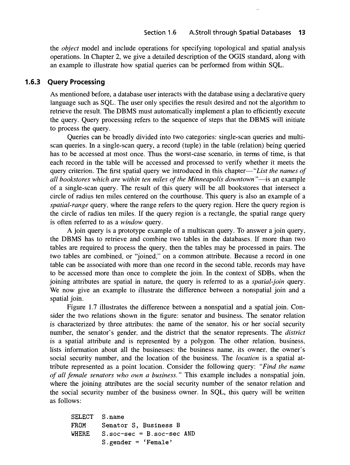
We now give an example to illustrate the difference between a nonspatial join and a
spatial join.
Figure 1.7 illustrates the difference between a nonspatial and a spatial join.
Consider the two relations shown in the figure: senator and business. The senator relation
is characterized by three attributes: the name of the senator, his or her social security
number, the senator's gender, and the district that the senator represents. The district
is a spatial attribute and is represented by a polygon. The other relation, business,
lists information about all the businesses: the business name, its owner, the owner's
social security number, and the location of the business. The location is a spatial
attribute represented as a point location. Consider the following query: "Find the name
of all female senators who own a business." This example includes a nonspatial join,
where the joining attributes are the social security number of the senator relation and
the social security number of the business owner. In SQL, this query will be written
as follows:
SELECT S.name
FROM Senator S, Business B
WHERE S.soc-sec = B.soc-sec AND
S.gender = 'Female'

14 Chapter 1 Introduction to Spatial Databases
SENATOR
NAME
SOC-SEC
GENDER
DISTRICT (POLYGON)
Join \ Spatial Join
BUSINESS
B-NAME
OWNER
SOC-SEC
LOCATION (POINT)
FIGURE 1.7. Two relations to illustrate the difference between join and spatial join.
Now consider the query, "Find all senators who serve a district of area greater than 300
square miles and who own a business within the district." This query includes a spatial-
join operation on the attributes location and district. Thus, while in a nonspatial join the
joining attributes must be of the same type, in a spatial join the attributes can be of
different types: point and polygon, in this case. This is how the query will be expressed in SQL:
SELECT S.name
FROM Senator S, Business B
WHERE S.district.AreaO > 300 AND
Within(B.location, S.district)
An SDBMS processes range queries using the filter-refine paradigm. This is a two-
step process. In the first step, the objects to be queried are represented by their minimum
bounding rectangles (MBRs). The rationale is that it is easier (computationally cheaper)
to compute the intersection between a query region and a rectangle rather than between
the query region and an arbitrary, irregularly shaped, spatial object. If the query region
is a rectangle, then at most four computations are needed to determine whether the two
rectangles intersect. This is called the filter-step, because many candidates are eliminated
by this step. The result of the filter-step contains the candidates that satisfy the original
query. The second step is to process the result of the filter-step using exact geometries.
This is a computationally expensive process, but the input set for this step, thanks to the
filter-step, has low cardinality. Figure 1.8 shows an example of the filter-refine strategy.
We now describe, with the help of an example, an algorithm to process the filter-
step of a spatial-join query. This algorithm is based on the plane sweep technique, which
is extensively used in computational geometry to compute the intersections of geometric
objects.
The filter step of many spatial-join queries can be reduced to the problem of
determining all pairs of intersecting rectangles. Consider two sets of rectangles
(Figure 1.9[b]) R = {Ri,R2, R3, R4} and S = [Su S2, S3}, which represent the MBRs of
the spatial attributes of two tables involved in a join. Each rectangle T can be identified
by its lower-left corner, (T.xl, T.yl) and its upper-right corner (T.xu, T.yu), as shown
in Figure 1.9(a). We sort all the rectangles in R and S according to the x values of their

Section 1.6 A Stroll through Spatial Databases 15
MBR
Query
Region
FIGURE 1.8. The filter-refine strategy for reducing computation time.
lower-left corners (i.e., on T.xl). The sorted rectangles are shown in Figure 1.9(c). We
collect all of the (sorted) rectangles in R and S in the set R U S and proceed as follows:
1. Move a sweep line, for example, a line perpendicular to the x-axis, from left to
right, and stop at the first entry in R U S. This is the rectangle T with the smallest
T.xl value. In our example (see Figure 1.9[a]) this is the rectangle R4.
2. Search through the sorted rectangles of S until arriving at the first rectangle S?
such that S?.xl > T.xu. Clearly, the relation [T.xl, T.xu] D [5J.xZ, 5J.xu] holds
(nonempty) for all 1 < j < /. In our example S? is S1. Note that the superscript
is in the order of array index in Figure 1.9(c), i.e., Sl = S2, S2 = Si, S3 = S3.
Thus S2 is a candidate rectangle that may overlap R4. This will be confirmed in
the next step.
3. If the relation [T.yl, T.yu] D [Sj .yl, Sj .yu] holds for any 1 < j < /, then the
rectangle 5J intersects T. Thus this step confirms that R4 and S2 indeed overlap,
and < R4, S2 > are part of the join result. Record all this information, and remove
the rectangle T from the set R U S. R4 is removed from the set R U S because it
cannot participate in any more pairs in the resulting set.
4. Move the sweep line across the set R U S until it reaches the next rectangle entry.
This is rectangle 52 in our example. Now proceed as in steps 2 and 3.
5. Stop when the R U S = 0.
The filter step of the spatial-join algorithm results in <R4,S2>, <Ri,S2>,
<Ri, S^>, <R2, S^>, </?3, S^> as candidate pairs for the refinement step, based on
the exact geometries of the objects. The refinement step may eliminate a few pairs from
the final result if exact geometry computation shows that there is no overlap. The main
purpose of the filter step is to reduce the computation cost of exact geometry
computation by eliminating as many pairs as possible. Chapters 5 and 7 present more details of
disk-based algorithms for processing spatial queries.

16 Chapter 1 Introduction to Spatial Databases
1 sweep line
s2
R4
Ri
*i
$2
R2
*3
x-axis
(a)
1 .
I
(T.xl,
(T
T
T.yl)
jtw, T.yu)
x-axis
(b)
R4
s2
Si
Ri
s3
R2
R3
(c)
FIGURE 1.9. Determining pairs of intersecting rectangles: (a) two sets of rectangles: R
and S; (b) a rectangle T with its lower-left and upper-right corners marked; and (c) the
sorted set of rectangles with their joins. Note the filtering nature of the plane sweep
algorithm. In the example, twelve possible rectangle pairs could be joined. The filtering
step reduced the number of possibilities to five. An exact geometry test can be used to
check which of the five pairs of objects satisfy the query predicate [Beckmann et al.,
1990].
1.6.4 File Organization and Indices
DBMSs have been designed to handle very large amounts of data. This translates into
a fundamental difference in how algorithms are designed in a GIS data analysis versus
a database environment. In the former, the main focus is to minimize the computation
time of an algorithm, assuming that the entire data set resides in main memory. In
the latter, emphasis is placed on minimizing the sum of the computation and the I/O
(input/output) time. The I/O time is the time required to transfer data from a disk (hard
drive) to the main memory. This is because, despite falling prices, the main memory is not
large enough to accommodate all the data for many large applications. This difference
is conceptualized in the way one perceives the fundamental design of the computer.
For many programmers, the computer essentially consists of two components: the CPU
(central processing unit) and an infinite amount of main memory (Figure 1.10[a]). On the
other hand, for many DBMS designers, the computer has three parts: the CPU, finite main
memory, and infinite disk space (Figure 1.10[b]). Although a CPU can directly access
data in the main memory, to access data on the disk, it first has to be transferred into
the main memory. The difference in time between accessing data from random access
memory (RAM) and disk is unbelievably large: a factor of a hundred thousand (year
2000). This ratio is getting worse every year because the CPU and memory are getting
faster at a higher rate than disks and secondary storage devices.

Section 1.6 A Stroll through Spatial Databases 17
CPU
CPU
MAIN
MEMORY
MAIN
MEMORY
DISK
DISK
(a) (b)
FIGURE 1.10. (a) Programmer's viewpoint; (b) DBMS designer's viewpoint.
At this moment (details in Chapter 4), it is worthwhile to view the secondary
storage device (hard drive) as a book. The smallest unit of transfer between the disk and
main memory is a page, and the records of tables are like structured lines of text on the
page. A query issued by a user essentially causes a search about a few selected lines
embedded in pages throughout the book. Some pages can reside in the main memory,
and pages can be fetched only one at a time. To accelerate the search, the database uses
an index. Thus in order to search for a line on a page, the DBMS can fetch all of the
pages spanned by a table and scan them line by line until the desired record is found.
The other option is to search in the index for a desired key word and then go directly
to the page specified in the index. The index entries in a book are sorted in alphabetical
order. Similarly, if the index is built on numbers, like the social security number, then
they can be numerically ordered.
Spatial data can be sorted and ordered, but that comes at the loss of spatial
proximity. What do we mean here? Consider Figure 1.11(a). Here we have a grid that is
row-ordered. Now consider the neighbors of 4. On the grid the neighbors of 4 are 3, 7,
and 8, but if stored in the way it is sorted, its neighbors will be 3 and 5. Thus,
sorting has destroyed the original neighborhood relationship. Much research has been done
to find better ways of ordering multidimensional data. Figure 1.11(b) shows another
method. It is worth pointing out that no total ordering can preserve spatial proximity
completely.
The B-tree (for balanced) index structure is arguably the most popular index
employed by a relational DBMS. It is sometimes stated that the B-tree index structure is a
major reason for the almost universal acceptance of relational database technology. The
B-tree implementation crucially depends on the existence of an order in the indexing
field. Figure 1.12 shows the crucial difference between a binary tree and a B-tree. Each
node of a B-tree corresponds to a page of the disk. The number of entries in each node

18 Chapter 1 Introduction to Spatial Databases
1
5
9
13
2
6
10
14
3
7
11
15
4
8
12
16
7
5
2
1
8
6
4
3
14
13
10
9
16
15
12
11
(a) (b)
FIGURE 1.11. Different ways of ordering multidimensional data: (a) row order; (b) Z-
order. If a line is drawn following the numbers in ascending order, the Z pattern will
become obvious.
depends on the characteristics of the indexing field and the size of the disk page. If a
disk page holds m keys, then the height of a B-tree is only 0(logm(n)), where n is the
number of total records. For trillon (1012) records, one only requires a B-tree of height 6
for m = 100. Thus a record for a given key value can be retrieved in about half a dozen
disk accesses even from such a large collection of records.
Because a natural order does not exist in multidimensional space, the B-tree cannot
be used directly to create an index of spatial objects. The combination of spatial-order
and B-tree is a common way to get around the lack of a natural order on spatial objects.
Many commercial systems have adopted such an approach.
The R-tree data structure was one of the first index specifically designed to handle
multidimensional extended objects. It essentially modifies the ideas of the B-tree to
accommodate extended spatial objects. Figure 1.13 shows an example of how the R-tree
organizes extended objects. More details follow in Chapter 4.
1.6.5 Query Optimization
One of the major strengths of relational database technology is how it efficiently executes
a query by generating a sophisticated query evaluation plan. To explain this we revisit
the query "Find the names of all female senators who own a business." This query is
actually a composition of two subqueries: a selection query and a join query. "Name all
(a) (b)
FIGURE 1.12. (a) Binary tree; (b) B-tree.

Section 1.6 A Stroll through Spatial Databases 19
A
B
S
d
h
f
C
i
J
FIGURE 1.13. R-tree extends B-tree for spatial objects.
female senators" is a selection query because we select all of the female senators from
a list of all senators. The query "Find all senators who own a business " is a join query
because we combine two tables to process the query. The question is, in which order
should these subqueries be processed: select before join or join before select? Remember
a join is a multiscan query, and select is a single-scan query, so it is more important
for a join operation to work on a smaller size table than the select operation. Now it is
obvious that select should be done before join.
Consider the spatial query we have discussed before: "Find all senators who serve
a district of area greater than 300 square miles and who own a business within the
district." This query too is a composition of two subqueries: a range query and a spatial-
join query. The range subquery is "Name all senators who serve a district of area greater
than 300 square miles." The spatial-join query is "Find all senators who own a business
located in the district they serve." Again, a range query is a single-scan and a join is
a multiscan query, but there is one important difference. The single-scan query has to
employ a potentially expensive function, S.district.Area(), to compute the area of each
district. Of course, the join function also involves a computationally expensive function,
Within(B.location,S.district), but the point is that it is very difficult to assess how to order
the processing of in spatial subqueries. This important step is taken up in Chapters 5 and 7.
1.6.6 Data Mining
Data mining, the systematic search for potentially useful information embedded in digital
data, is now a hot topic of research inside and outside academia. Major corporations
and government agencies have realized that the large amount of data that they have
accumulated over the years, and are still gathering, can be systematically explored to
provide a new perspective on their operations. Thus, data that was earlier considered a
burden in terms of storage and management has suddenly become a source of wealth and
profits. The story, now almost of mythic proportions, of how it was discovered by using
data-mining tools that people who buy diapers in the afternoon are likely to buy beer
too has fueled a massive effort to design and invent efficient tools for mining data. Until
now most of the effort in data mining has focused on algorithm design and analysis. A
database specialist can leverage his or her expertise on two fronts:

20 Chapter 1 Introduction to Spatial Databases
1. By designing algorithms that assume that the data sets are large or by designing
general scaling tools that can be coupled with data-mining algorithms
2. By extending SQL with "mining" functionality, so that mining tools are callable
from within SQL
Estimates showing that up to 80 percent of the data in digital form is actually
spatial data have spawned efforts to invent mining techniques that take the special nature
of spatial data into consideration. For example, random sampling is a common technique
applied in data mining to cut down on the size of the data set being analyzed without
significant loss of information. Traditional methods of sampling are not effective in the
case of spatial data because of spatial autocorrelation. Thus techniques from spatial
statistics should be incorporated into mining algorithms to deal with spatial data.
In GIS, data mining is not new. Map generalization and classification of remote
sensing images are relatively mature fields and are clearly related to data mining. Famous
historical examples of spatial data mining include identification of the contaminated water
source responsible for the 1854 cholera epidemic in London [Griffith, 1999], as well as
identification of fluoride in drinking water for good dental health. In Chapter 7 we make
an effort to bridge this gap.
1.7 SUMMARY
Spatial data management is of use in many disciplines, including geography, remote
sensing, urban planning, and natural resource management. Spatial database management
plays an important role in the solution of grand challenge scientific problems such as
global climate change and genomics.
There are three classes of users who can benefit from spatial database management
systems. Business users are interested in using spatial data to augment other forms of
information while deciding about marketing campaigns, distribution centers, and retail
locations. For a business user, spatial data is an important source of secondary information.
For scientific users who specialize in the study of the environment, natural
resources, and geography, spatial data is of paramount importance. Users in this group
have been using GIS products for the analysis of spatial data, but with the size of data
sets growing rapidly, there is a need for specialized data management techniques that
address the distinguishing properties of spatial data.
Finally there is a third class of users who want to use spatial data to personalize
their experience and interaction especially on the worldwide Web. For example, queries
on a search engine can produce results that are spatially localized and more meaningful.
BIBLIOGRAPHIC NOTES
1.1 For a history of database technology and a general introduction to DBMS, see
[Ramakrishnan, 1998; Elmasri and Navathe, 2000; Silberschatz et al., 1997]. For an overview
of the shortcomings of RDBMS in handling spatial data and a general introduction to object-
relational DBMS, see [Stonebraker and Moore, 1997].
1.2 For an overview of SDBs, see [Scholletal., 2001; Shekharet al., 1999a] and the special issue
of very large databases (VLDB) journal and the overview in [Guting, 1994a] in particular.
1.3 For integrating a SDB into off-the-shelf databases systems for CAD applications, see [Kriegel
et al., 2001]. For an example of SDBMS, see [de La Beaujardiere et al., 2000].

Section 1.7 Summary 21
1.3.2 Spatial data models are covered in [Egenhofer, 1991b; Worboys, 1995] and [Laurini and
Thompson, 1992; Price et al„ 2000].
1.3.3 Extension of SQL for SDBs is discussed in [Egenhofer, 1994]. The OGIS specification for
extending SQL for geospatial applications is described in [OpenGIS, 1998],
1.3.4 Representation of spatial data is covered extensively in [Laurini and Thompson, 1992;
Worboys, 1995]. The filter-refine paradigm is discussed in [Chrisman, 1997].
1.3.5 The standard reference in spatial indexing is [Samet, 1990]. An up-to-date overview is
in [Gaede and Gunther, 1998].
1.3.8 Issues related to the architectural design of SDBs are discussed in [Adam and Gangopadhyay,
1997; Worboys, 1995].
EXERCISES
Discussion
1. Discuss the differences between spatial and nonspatial data.
2. Geographic applications are a common source of spatial data. List at least four other
important sources of spatial data.
3. What are the advantages of storing spatial data in a DBMS as opposed to a file system?
4. How can object-relational databases be used to implement an SDBMS?
5. List the differences and similarities between spatial, CAD, and image databases?
6. The interplay between the vector and raster data models has often been compared with
the wave-particle duality in physics. Discuss.
7. Cognitive maps are described as "internal representations of the world and its
spatial properties stored in memory." Do humans represent spatial objects as discrete
entities in their minds? Is there a built-in bias against raster and in favor of vector
representation?
8. Sorting is a popular method to access "traditional data" rapidly. Why is it difficult to
sort spatial data?
9. Predicting global climate change has been identified as a premier challenge for the
scientific community. How can SDBMS contribute in this endeavor?
10. E-commerce retailers reach customers all over the world via the Internet from a single
facility. Some of them claim that geography and location are irrelevant in the Internet
age. Do you agree? Justify your answer.
11. Define location-based and location independent services. Provide examples.
12. XML is emerging as a popular data interchange model on internet applications.
Discusses the research impact of XML on spatial databases.
13. Compare and contrast;
(i) GIS vs. SDBMS
(ii) OODBMS vs. ORDBMS
(iii) GI Systems vs. GI Services
(iv) Data model vs. Query language
(v) Query processing vs. File organization and indices
(vi) Main memory vs. Disk
(vii) Querying vs. Data mining
14. Define spatial databases. List a few applications of spatial databases beyond those
listed in this chapter.

CHAPTER 2
Spatial Concepts
and Data Models
2.1 MODELS OF SPATIAL INFORMATION f
2.2 THREE-STEP DATABASE DESIGN i
2.3 TRENDS: EXTENDING THE ER MODEL WITH SPATIAL CONCEPTS
2.4 TRENDS: OBJECT-ORIENTED DATA MODELING WITH UML
2.5 SUMMARY
This chapter presents techniques related to the modeling of spatial database applications.
GIS is arguably the most popular spatial database application, and our discussion reflects
this fact. Besides GIS, other applications with a definite spatial or geometric component,
such as CAD and astronomy, can also benefit from the techniques described in this
chapter.
Traditional database concerns have typically been dominated by business and
administrative applications. There the focus had been to efficiently (and securely) process
large numbers of relatively simple transactions. Falling prices of data-capturing devices
such as the Global Positioning System (GPS), the easy availability of satellite and
cartographic data over the Internet, and the increasing power of desktop computing have
redefined the functionality of a database. A DBMS is no longer considered a distinct,
isolated repository of data but an active component of a multisystem computing
environment. In fact, the trend is to shift computationally intensive tasks directly to the DBMS.
A GIS is a premier example of this trend.
An SDBMS integrates the special needs of modeling spatial data into the system.
This is a nontrivial task because
• Spatial data is relatively more complex compared with traditional business data,
and the old database constructs are not adequate for handling it.
• Database design and implementation are typically handled by computer scientists,
while the handling of spatial data falls in the domain of geographers,
environmentalists, and other physical scientists. Traditionally, these disciplines have evolved
along different trajectories.
The remainder of the chapter is organized as follows. In Section 2.1 we describe the
different models for processing spatial information. In Section 2.2 we provide general
database design and modeling principles. Section 2.3 is devoted to the extensions of
the entity-relationship (ER) model for SDBs, and Section 2.4 is devoted to the Unified
22

Section 2.1 Models of Spatial Information 23
Modeling Language (UML), a conceptual model primarily designed for object-oriented
databases. We close with a summary of the chapter.
2.1 MODELS OF SPATIAL INFORMATION
We introduce an example, State-Park SDB which will be used to illustrate the different
concepts in spatial data modeling. A State-Park SDB consists of forests which are a
collections of forest-stands that correspond to different species of trees. A State-
Park is accessed by roads and has a manager. There are fire-Stations within a
state-park which are exclusively responsible for monitoring and managing fires in the
State-Park. The State-Park is also dotted with facilities such as camping groups and
offices. Finally, there are rivers which pass through the state park and also supply water
to the different facilities.
Models of spatial information are usually grouped into two broad categories: field
and object. We illustrate this dichotomy with the help of an example shown in Figure 2.1.
Consider an idealized forest partitioned into homogeneous areas, each with one
(dominant) tree species. In this example there are three species, namely, Fir, Oak, and
Pine.
There are two complementary ways of modeling the forest. In the functional
viewpoint, the forest is modeled as a function where the domain is the underlying geographic
space of the forest and the range is a set consisting of three elements—the names of the
tree species. The function, say /, maps each point of the space occupied by the forest
into exactly one element of the range. The function / is a step-function—constant where
trees are alike and changing to a different value where the tree species changes. In GIS
the functional model is called the Field model. In Figure 2.1(c), the field representation
of the forest is shown using a piece-wise function. A different field representation can
be defined on a grid with each cell specifying the name of the dominant tree species.
This second representation may be preferred if the boundaries of forest-stand are highly
irregular. Other field representation include iso-lines showing contours with fixed values
of a physical variable, for example, temperature, pressure.
Now consider the places where the function / changes values. In an idealized
setting where the demarcation between the tree species is clearly defined, we should
get the boundaries of polygons. Each polygon can be assigned a unique identifier and a
nonspatial attribute—the name of the tree species. Thus the forest can be modeled as a
collection of polygons (i.e., forest-stands) each corresponding to a tree species. This is
the Object viewpoint and is shown in Figure 2.1(b).
The decision to model a spatial application using a field or an object paradigm
is based on the requirements of the application and tradition. Amorphous phenomena,
for example, fire, flood, hazardous spills, are naturally modeled as fields the boundaries
are fluid. Other spatial phenomena can also be modeled using fields. Field models are
often used to model continuous spatial trends such as elevation, temperature, and soil
variation. In fact, in the area of remote-sensing, where the earth's surface is mapped
from satellite- and aircraft-based sensors, the field model is dominant. Object models are
more common in modeling transportation networks (e.g., roads), land parcels for
property tax, and legal ownership-related applications. It has been postulated that the object
model may have originated from societal needs to demarcate ownerships viewing land
as property [Couclelis, 1992].

24 Chapter 2 Spatial Concepts and Data Models
y f (0,4)
(0,2)
(0,0)
(a)
Object Viewpoint of Forest Stands
Area-ID
FSl
FS2
FS3
Dominant
Tree Species
Pine
Fir
Oak
Area/Boundary
[(0,2),(4,2),(4,4),(0,4)]
[(0,0),(2,0),(2,2),(0,2)]
[(2,0),(4,0),(4,2),(2,2)]
Field Viewpoint of Forest Stands
- "Pine," 2ssxs£4;2<yss4
f(x,y) -
"Fir," 0=sxs£2;0«;ys£2
I "Oak," 2<xss4;0syss2
(b)
(c)
FIGURE 2.1. The object-field dichotomy, (a) A map showing three forest stands: Pine,
Fir, Oak. (b) An object viewpoint representing the map as a collection of three objects.
Each object has a unique identifier, a dominant tree species, and an area. The boundary
of the area, a polygon, is specified by the coordinates, (c) Afield viewpoint, where each
point is mapped to the value of the dominant tree species.
2.1.1 Field-Based Model
Defining the field model for a spatial application requires that we determine three
components: a spatial framework, field functions, and a set of relevant field operations [Worboys,
1995].
A spatial framework F is a finite grid imposed on the underlying space. All
measurements are then based on this framework. The best-known example of a spatial
framework is the system of latitude and longitude to reference the earth's surface. A spatial
framework is a finite structure, and errors introduced due to discretization are
unavoidable. A finite set of n computable functions or simple fields {/,, 1 < i < n),
f : Spatial framework -> Attribute domain(A,)
map the spatial framework F onto different attribute domains A,-. The choice of the
different field functions and the attribute domains is determined by the spatial application
at hand. In the Forest example we had a single-field function, a step function, and the

Section 2.1 Models of Spatial Information 25
attribute domain was the set {fir, oak, pine}. For the special case when the functions
are single-valued and the underlying space is the Euclidean plane, fields are naturally
viewed as either surfaces or isolines, which are the locus of points that have the same
attribute value. The third important component of field-based modeling is specification
of the operations on the field functions.
Relationships and interactions between the different fields are specified by field
operations. Field operations map a subset of fields onto other fields. Examples of field
operations are union, +, and composition, o:
f+g:x-+f(x)+g(x)
f °g -x -*• f(g(x))
Field operations can be classified into three categories [Worboys, 1995]: local, focal, and
zonal.
Local Operations
For a local operation, the value of the new field at a given location in the spatial
framework depends only on the value of the input field at that location. For example, consider
an idealized State-Park which is completely partitioned into trees, lakes, and meadows.
Define a function / and g as:
/(*) =
1 if x = "tree"
0 otherwise
and
1 if x = "lake''
0 otherwise
g(x) =
Then f + g, that is, the union of / and g is defined as
if x = "tr
otherwise
This is an example of a local operation.
, , , w , f 1 if* = "tree" or "lake"
(f + g)(x) = | Q
Focal Operations
For a focal operation, the value of the resulting field at a given location depends on the
values that the input field assumes in a small neighborhood of the location. The limit
operation in calculus is an example of a focal operation. Let E(x, y) be the elevation field
of the State-Park. That is, E at (x, y) gives the value of the elevation at the location
(x, y) in the spatial framework F. Then the operation that calculates the gradient of the
elevation field, WE(x, y), is a focal operation, because the value of the gradient at (x, y)
depends on the value of the elevation field in a "small" neighborhood of (x, y). Here we
are assuming that the field varies smoothly and does not experience sharp jumps, as the
step function did in the Forest example.

26 Chapter 2 Spatial Concepts and Data Models
Zonal Operations
Zonal operations are naturally associated with aggregate operators or the integration
function, f dx dy in calculus. In the forest example, the step function, which maps the
forest onto the set of attributes {Oak, Fir, Pine}, also partitions the underlying space into
three polygons, or zones. An operation that calculates the average height of the trees for
each species is a zonal operation.
Object-Based Models
In object-based modeling, the focus is to abstract spatial information into distinct,
identifiable, and relevant things, or entities, called objects. For example, we can characterize
a park by the forest-stands, rivers, lakes, and roads that are contained in it. All these
entities are clearly distinct and identifiable. Whether they are relevant or not depends on
the application we are trying to model. Each object has a set of attributes that characterize
it. The key difference between spatial objects and the objects/entities that are ubiquitous
in traditional database modeling is that the attributes of spatial objects diverge into two
distinct categories: spatial and nonspatial. It is through its spatial attributes that an object
interacts with the underlying embedding space. In the Forest example, the forest-stand
representing Fir is a spatial object, with the polygon that represents its spatial extent
being its spatial attribute and the name Fir its nonspatial, alphanumeric attribute. A spatial
object can have more than one spatial attribute representing, for instance, many levels of
generalizations. A road on a map could be represented as a line or a polygon, depending
on the scale of the map.
Spatial Data Types
A key issue in object-based models of spatial information is the choice of a basic set
of spatial data types required to model common shapes on maps. Many proposals have
been made over the years. A consensus is slowly emerging in terms of the OGIS
standard [OGIS, 1999]. Figure 2.2 shows the fundamental building blocks of two-dimensional
spatial geometry and their interrelationships in UML notation. We give a brief description
of the UML notation in Section 2.4.
The most general shape is represented by "geometry" described via a "spatial
representation system," which is a coordinate system like latitude/longitude or some other
consensus framework. The "geometry" is subdivided into four categories, namely, point,
curve, surface, and geometry collection. Point describes the shape of a zero-dimensional
object, for example, city-centers in a map of the world. Curve describes the shapes of
one-dimensional objects, for example, rivers in the map of a world. The curve objects
are often approximated by a linestring, which is represented by two or more points. The
simplest linestring is a straight line joining two or more points. The category surface
describes the shape of two-dimensional objects, for example, countries on a map of the
world. A surface is often modeled by a polygon. Geometry collection represents
complex shapes, such as, collection of oil wells, a group of islands and so on. Geometry
collection in turn is of three types, namely, multipoint, multicurve, and multisurface. The
geometry collection spatial data types provide a "closure" property to OGIS spatial data
types under geometric operations such as "geometric-union," "geometric-difference," or

Section 2.1 Models of Spatial Information 27
Geometry
Point
1..*
I
Spatial Reference System
Curve
Surface
2..*
r t
Geometry Collection
■Or
i..*
Line String
£
Line
Polygon
LinearRing
1..*
£
Multisurface
2..*
Multicurve
Multipoint
J. i
Multipolygon
Multilinestring
!_J
FIGURE 2.2. An OGIS proposal for building blocks of spatial geometry in UML
notation [OGIS, 1999].
"geometric-intersection." For example, if one takes a geometric-difference of boundaries
of Canada and Quebec, the result is a "multisurface" even if Canada and Quebec were
of "surface" spatial data type. This property is useful to support multistep querying and
data processing.
Operations on Spatial Objects
How do spatial objects interact with each other? In field-based modeling, the field
function principally determines the type of operations allowed. After all, it would not be
possible to apply a gradient operation on a nonsmooth field! In object-based
modeling, the underlying embedding space determines the relationships that can exist
between objects. We now describe a typology of the embedding space and associated
relationships.
Set-Oriented
The simplest and most general of all embedding spaces is called set-oriented. Common
relationships allowable in this setting are the usual set-based relationships of union,
intersection, containment, and membership. Hierarchical relationships such as a forest-
stand contained in a forest, a forest contained in a state park, and a state park contained
within a state are adequately modeled by set theory.

28 Chapter 2 Spatial Concepts and Data Models
Topological
To get an intuitive feeling of what a topological space is, imagine two polygons that touch
(meet) each other and are drawn on a rubber sheet. Now if we deform the rubber sheet by
stretching or bending but not cutting or folding it, the adjacency of the polygons remains
intact. Meet is an example of a topological property, and the study of transformations
(deformations) that preserve topological properties is called topology. Consider the map
of the world with political boundaries of countries. The neighboring countries meet each
other, whether the map is drawn on a sphere or on a flat space. The area of a polygon
is clearly not a topological property. In fact, the relative areas of different countries
are often not preserved in many maps. Areas of countries near the equator are reduced
relative to the areas of countries near the poles in many planar maps. In Table 2.1 we
list some common topological and nontopological properties [Worboys, 1995].
From a spatial/geographic database point of view, topological relationships such
as meet, within, and overlap are most likely to be queried by a user of a spatial
database management system. Is a given land parcel adjacent to a hazardous waste
site? Does the river floodplain overlap a proposed highway network? All these are
examples of topological relationships. Two common types of topological queries in spatial
databases are:
• Find all objects that have a topological relation R to a given object.
• What is the topological relation between objects A and Bl
The binary topological relationship between two objects, A and B, in a plane Ift2
is based upon the intersection of A's interior (A°), boundary (3A), and exterior (A~)
with B's interior (B°), boundary (95) and exterior (B~) [Egenhofer, 1994]. The nine-
intersection matrix between the six object parts defines a topological relationship and
can be concisely represented using the following matrix:
/ A°nB° A°n3B A°C\B- \
r9(A, B)=l 3AnB° dAndB 3AHB-
\A-r\B° A~n3B A~nB-J
By considering the values empty (0) and nonempty (1), one can distinguish between
29 = 512 binary topological relationships. For a two-dimensional region embedded in
9ft2, eight relations can be realized, and they provide mutually exclusive complete
coverage. These relations are disjoint, meet, overlap, equal, contains, inside, covers, and
covered by.
Figure 2.3 shows how topological relations can be represented using the nine-
intersection matrix. For example, the disjoint relationship is described in the
nine-intersection model by the boolean matrix shown in the top-left corner of Figure 2.3. The
zero entries indicate that interior (A) has no points in common with either interior (B)
or boundary (B). Similarly interior (B) has no point in common with boundary (A).
Similarly, boundary (A) and boundary (B) have no points in common.
The topological relationships on other pairs of spatial data types, for example (point,
surface), (point, curve) can be defined in a similar manner. A point can be inside, outside,
or on the boundary of a surface as listed in Table 2.1. A curve may cross the interior of
a surface or may meet or be disjoint from a surface. A point may be an endpoint of a

Section 2.1 Models of Spatial Information 29
TABLE 2.1: Examples of Topological and Nontopological Operations
Topological
endpoint(point, arc)
simple-nonself-intersection (arc)
on-boundary (point, region)
inside (point, region)
outside (point, region)
open (region)
close (region)
connected (region)
inside (point, loop)
crosses (arc, region)
touches (region, region)
touches (arc, region)
overlap (region, region)
Nontopological
Euclidean-distance (point, point)
direction (point, point)
length (arc)
perimeter (area)
area (region)
A point at the end of an arc.
A nonself-intersecting arc does not cross itself.
Vancouver is on the boundary of Canada
and the United States.
Minneapolis is inside of Minnesota state.
Madison is outside of Minnesota state.
Interior of Canada is an open region
(excludes all its boundaries).
Carleton County is a closed region
(includes all its boundaries).
Switzerland is a connected region, whereas
Japan is not (given any two points in the area,
it is possible to follow a path from one point
to the other such that the path is
entirely within the area).
A point is within the loop.
A road (arc) passes through a forest (region).
Minnesota (region) is a neighboring state of
Wisconsin (region).
Interstate freeway 90 (arc) passes by
Lake Michigan (region).
Land cover (region) overlaps with land use
(region).
Distance between two points.
Madison city is east of Minneapolis city.
Length of a unit vector is one unit.
Perimeter of a unit square is 4 units.
Area of unit square is one square unit.
curve, interior point of a curve, or off the curve as listed in Table 2.1. The
relationships between curve are more complex and still an area of research [Clementini et al.,
1993].
Directional
Directional relationships can be of three types, namely, absolute, object-relative, or viewer
based. Absolute direction relationships are defined in the context to a global reference
system, for example, north, south, east, west, northeast, and so on. Object-relative
directions are defined, using the orientation of a give object. Example relationships include
left, right, front, behind, above, below, and so on. Viewer relative directions are defined
with respect to a specially designated reference object called the viewer.

30 Chapter 2 Spatial Concepts and Data Models
FIGURE 2.3. The nine-intersection model [Egenhofer et al., 1989].
Metric Space
Mathematically speaking, a set X is called a metric space if for any pair of points x
and y of X, there is an associated real number d(x, y), called the distance (also called a
metric) from x to y, with the following properties:
1. d(x, y) > 0 and d(x, x) = 0
2. d(x,y)=d(y,x)
3. d{x,y) <d(x,z)+d(z,y)
for all x, y, z in X. Any function that satisfies these properties is called a metric on X.
In metric spaces the notion of distance is well defined. A distance function can
be used to induce a topology on the space, and therefore every metric space is also a
topological space. In network or graph settings, metric spaces play a crucial role. Optimal
distance and shortest travel-time queries are ideally handled in a metric space setting.
Euclidean
Let R be the field of real numbers. A vector space V over R is a nonempty set V of
objects v called vectors, together with two operations:

Section 2.1 Models of Spatial Information 31
1. Addition: « + «eVforall«i;eV
2. Product: au e V for all a e R, v e V.
Besides the existence of a special vector 0, there are other axioms that the two
operations addition and product need to satisfy. For a complete discussion of vector
space see fBlyth and Robertson, 1999].
If there exists a (minimal) finite set of vectors {e\, e2,..., en] such that any v e V
can be expressed as a linear combination of the e'^s, that is, there exists a\,.. .a„ e R
such that:
v = aiei + ... + anen
then the vector space is finite dimensional. In a three-dimensional space, the e'.s
correspond to the familiar x,y,z coordinate axis. If we add the notion of inner product (angle)
to vector space, we get a Euclidean space. In a Euclidean space setting, all spatial
relationships, including set, topological, metric, and directional (north/south), can be defined.
2.1.5 Dynamic Spatial Operations
Most of the operations that we have discussed so far have been static, in the sense that the
operands are not affected by the application of the operation. For example, calculating the
length of a curve has no effect on the curve itself. Dynamic operations alter the objects
upon which the operations act. The three fundamental dynamic operations are create,
destroy, and update. All dynamic operations are variations upon one of these themes [Wor-
boys, 1995], In Table 2.2 some example of the create and update operations are listed.
An example of the merge operation is the "map-reclassification" operation
supported by many GIS software products. Consider reclassification of the map of countries
on the basis of the majority religion practiced in the countries, for example, none, Islam,
Christianity, Buddhism, and Hinduism. The boundaries between neighboring countries
with the same majority religion are removed via the merge operation in order to
reclassify the maps. Similar examples of other dynamic spatial operations can be found in
cartographic projections and map editing features in a GIS.
Additional classes of operations on spatial object exists. For example, operations
can be defined on the shape of an extended object to ask queries, such as, which objects
are squarish in shape? Which pair of objects fit like pieces of a jig-saw puzzle. The last
TABLE 2.2: Representative Example of Dynamic Spatial Operations [Worboys, 1995].
reproduce (X)
generate (X)
split (X)
merge (X,Y,Z)
translate
rotate
scale
reflect
shear
Produces an exact replica of X.
Generates an object that depends on but
does not replicate X.
Creates objects whose aggregation is X.
X, Y, and Z are merged to create a single object.
Shifts the position of the object in the plane.
Changes the orientation without changing the shape.
The object size is changed, but the shape remains
the same.
The mirror reflection of an object in a straight line.
Deforms the object in a predefined fashion.

32 Chapter 2 Spatial Concepts and Data Models
example is useful in designing new drugs (pharmaceutical) by finding molecules which
can dock in certain areas of other molecules. Another family of spatial operations is
based on visibility relationships to address queries like list the locations on a golf course
to get best view of hole 9. We hope to see consensus mathematical frameworks for such
families of operations in the near future.
Mapping Spatial Objects into Java
Having defined the spatial hierarchy (see Figure 2.2 and the corresponding array of spatial
relationships), we can easily program these notions into an object-oriented programming
language such as Java.
We give an example of how a specific query can be written in Java. The query is,
"Find all tourist offices within 10 miles of the Maple Campground."
The java class Facility and FacilitySet are used to model the locations of
tourist offices as well as the campgrounds. A separate class Query is used to model
the distance computation and the query itself. The Facility class has three attributes,
namely, name, type, and location. The type attribute is used to distinguish between tourist
offices and campgrounds. The location of facilities is point spatial datatype. This program
assumes that the spatial datatype point is available as part of a spatial library (e.g., SDE
from ESRI). The library also provides a distance function on the point spatial datatypes.
There are three methods in FacilityClass. The method facility is a constructor used to
initialize new objects. Method getName is used to extract the name attribute and method;
withinDistance is used to test if another facility is within a given distance.
Class FacilitySet is used to model a collection of facilities. For example, it can
model a set of tourist offices. It has two attributes, maxSize and FacilityTable. maxSize
designates the maximum size of the collection of facilities. The facilityTable is used to
store information about each facility. There is only one method in FacilitySet. This
method is used to read the information about various facilities from a file to initialize
the attributes of an instance of FacilitySet.
The class Query implements a query to extract all the tourist offices within 10
miles of the Maple campground. This class has one method, named main, which loops
through the list of tourist offices checking the distance to the Maple campground.
The key point of this discussion of the Java program is to show that the spatial
datatypes and operations can be used from a host language different from SQL, which is
used in the rest of the book. The second point is to compare the amount of programming
effort required by spatial querying. SQL will greatly reduce the amount of code needed
to specify simple spatial queries. It will also reduce the burden of performance tuning
and data-structure selection. We encourage readers to compare SQL with Java in the
coming chapters to revisit these points.
import java.lang.*;
import java.io.*;
import java.util.*;
/* assume class Point is given, which contains two attributes: x and y with
double type, and also some member functions, including distance (Point) */
/* Assume the original data is stored in file "facilityFile*'.

Section 2.1 Models of Spatial Information 33
Each line in the file represents a facility; use 00 as its delimiter, e.g.
Maple 00 campground 00 2.0 00 3.0
Office 00 Tourist-Office 00 6.0 00 8.9
public class Facility {
protected String name;
protected String type;
protected Point location;
public Facility (String name, String type, Point location) {
this.name = name;
this.type = type;
this.location = location;
>
public String getNameO {
return name;
>
public boolean withinDistance(Facility f, double d) {
if (this.location.distance(f.location) < d)
return true;
else
return false;
public class FacilitySet {
const maxSize = 50;
protected Facility[maxSize] facilityTable;
/* read from file filename and initialize the facility table */
public FacilitySet(String filename) {
BufferedReader in = new BufferedReader (new FileReader(filename));
String inline;
StringTokenizer strLine;
int i=0 ;
String token;
while ((inline = in.readLineO) != null) {
strLine = new StringTokenizer(inline, "00");
/* read name */
token = strLine.nextTokenO ;
FacilityTable[i].name = token;
/* read type */
token = strLine.nextToken();
FacilityTable[i].type = token;
/* read x coordinate */

34 Chapter 2 Spatial Concepts and Data Models
token = strLine.nextToken();
FacilityTable[i] .location.x = Double. valueOf (token) .doubleValueO ;
/* read x coordinate */
String type token = strLine.nextToken0;
FacilityTable [i++] .location.y = Double. valueOf (token) .doubleValueO ;
>
>
>
public class FacilityDemo {
public static void main (String [] args) {
Facility f = new FacilityC'Maple", "Campground", Point(2.0,4.0));
Facility[] fTable = new FacilitySetC'facilityFile");
String [] resultTable = new string [fTable. length] ;
int j=0;
for (int i=0; i < fTable.length; i++) {
if (f.withinDistance(fTable[i] , 2.0)
and fTable[i].type = "Tourist-Office")
resultTable[j++] = fTable[i] .name;
>
>
>
2.2 THREE-STEP DATABASE DESIGN
So far in this chapter we have described two models of spatial information: the object
model and the field model. Our view of these models was from the perspective of data
modeling involving concepts intrinsic to the spatial domain. We now introduce classical
data modeling from the perspective of database design. Our ultimate goal is to "blend"
the two families of concepts.
Database applications are modeled using a three-step [Elmasri and Navathe, 2000]
design process. In the first step, all the available information related to the application is
organized, using a high-level conceptual data model. At the conceptual level, the focus
is on the datatypes of the application, their relationships and constraints. The actual
implementation details are left out at this step of the design process. Plain text combined
with simple but consistent graphic notation is often used to express the conceptual data
model. The Entity Relationship (ER) model is one of the most prevalent of all conceptual
design tools.
The second step, also called the logical modeling phase, is related to the actual
implementation of the conceptual data model in a commercial DBMS. Data in a commercial
database is organized using an implementation model. Examples of implementation models
are hierarchical, network, and relational. The relational model is one of the most widely
implemented models in current commercial databases. In the relational model, the datatypes,
relationships, and constraints are all modeled as Relations. Tightly coupled with the
relational model is the formal query language relational algebra (RA). The RA consists of

Section 2.2 Three-Step Database Design 35
simple operations that allow quering of the data organized as relations. RA is described in
detail in Chapter 3.
The relational model does not fit the need of spatial data, as explained by [Herring,
1991]:
Relational algebra characterizes the querying capabilities of relational databases. A
relational database can answer any query expressible in relational algebra, which is universally
accepted model of traditional applications of relational databases.
In contrast, there is no universally accepted mathematical model of geographic information,
making it difficult to design spatial query languages and spatial databases. In addition, there
is a considerable semantic gap between GIS and relational databases, leading to complexities
and inconveniences.
Chapter 7 provides a specific example to show that RA is not capable of expressing
the transitive closure, an important graph operation, without additional assumptions. The
transitive closure operation is closely linked to the reclassification operation [Delis et al.,
1994], discussed in Section 2.1.5.
The third and final step, modeling of the physical design, deals with the nuts and
bolts of the actual computer implementation of the database applications. Issues related
to the storage, indexing, and memory management are handled at this level and will be
the subject of discussion in subsequent chapters. We now introduce the ER model.
The ER Model
The first step in database design is to come up with the conceptual model of the "mini-
world." The purpose of the conceptual model is to represent the miniworld in a manner
devoid of computer metaphors. The motivation is to separate out the concepts of the
application from the implementation detail. There are many design tools available for
conceptual data modeling, but the ER model is one of the most popular. The ER model
integrates seamlessly with the relational data model, which in turn is one of the most
prevalent logical models, the second step in the three-step design paradigm. Besides the
ER model and propelled by the success of the object-oriented design methodology, the
UML is another popular conceptual modeling tool. We discuss the UML in some detail
in the next section, but here we model the State-Park example using the ER model.
Entities and Attributes
In the ER model, the miniworld is partitioned into entities which are characterized by
attributes and interrelated via relationships. Entities are things or objects that have an
independent physical or conceptual existence. In the State-Park example, FOREST, RIVER,
FOREST-STAND, ROAD, and FIRE-STATION are all examples of entities.
Entities are characterized by attributes. For example, name is an attribute of the
entity FOREST. An attribute (or a set of attributes) that uniquely identifies instances of
an entity is called the key. In our example the name attribute of the entity ROAD is a key,
assuming it is not possible that two different roads have the same name. All instances
of ROAD in our example database have unique names. Though not a conceptual design
issue, a mechanism must exist in the DBMS to enforce this constraint.
Attributes can be single valued or multivalued. Species is a single-valued attribute of
FOREST-STAND. We now explain the existence of a multivalued attribute in the context

36 Chapter 2 Spatial Concepts and Data Models
of our example. The FACILITY entity has an attribute Pointid, which is a unique
identification for the spatial location of instances of the entity. We are assuming that the
map scale predicates instances of FACILITY to be represented as points. It is possible that
a given facility spans two distinct point locations, in which case the Pointid attribute
is multivalued. A similar argument holds for other entities.
Suppose we want to store information about the elevation of a FOREST. Because
elevation can change values within the FOREST entity, we model it as a multivalued
attribute, since field data type is not available.
Relationships
Besides entities and attributes, the third construct in the ER model is the relationship.
Entities interact or connect with each other through relationships. We have already noted
spatial relationships in the previous section; here we focus on the general concept of
relationships. Though many entities can participate in a given relationship, we will deal
only with binary relationships, that is, those between two entities. There are three kinds
of relationships based on cardinality constraints: one-one, many-one, and many-many.
One-One (1:1)
In a one-one relationship, each instance of one entity can relate to only one instance of
the other participating entity. For example, the relationship manages between the entities
MANAGER and FOREST is a one-one relationship; a FOREST can only have one MANAGER,
and a MANAGER can manage only one FOREST.
Many-One (MA)
A many-one relationship can potentially connect many instances of one entity with one
instance of the other entity participating in the relationship. The belongs-to is a many-one
relationship between the entities FACILITY and FOREST, assuming each facility belongs
to only one forest but many facilities can belong to a forest.
Many-Many (M:N)
Sometimes many instances of one entity can be related to many instances of the other
participating entity. The relationship supplies-water-to which connects the entities
RIVER and FACILITY is such a relationship. Sometimes relationships can have attributes
too. supplies-water-to has an attribute Volume which keeps track of the quantity of
water supplied by a river to a facility.
ER Diagram
Associated with the ER model is the ER diagram, which gives a graphic representation
to the conceptual model. In the ER diagram, entities are represented as boxes, attributes
as ovals connected to the boxes with straight lines, and relationships as diamond boxes.
The cardinality of the relationship, whether it is 1:1, M:\, or M:N, is shown around
the diamonds. The key attribute is underlined, and multivalued attributes are represented
as double-ovals. The ER diagram of the State-Parkexample is shown in Figure 2.4.
There are seven entities, namely, FOREST-STAND, RIVER, ROAD, FACILITY, FOREST,
FIRE-STATION, and MANAGER. The attributes of entity FOREST include name, elevation,
and polygonid. Name is a unique id, that is, each forest has a unique name. The diagram

Section 2.2 Three-Step Database Design 37
FIGURE 2.4. An ER diagram for the State-Park example.
also shows eight relationships. Entity FOREST participates in six relationships. Entity
FIRE-STATION participates in only one relationship, namely, monitors. The cardinality
constraints show that each fire station monitors one forest, but many fire stations can
monitor a forest. Some of the relationships are spatial in nature. These include crosses,
within, part-of. Many other spatial relationships are implicit in this diagram. For example,
a river crosses a road is shown explicitly, but a river crosses a forest is implicit.
2.2.2 The Relational Model
The relational model to represent data was introduced by Codd in 1970. Since then, it
has become one of the most popular logical data models. The popularity and power of
this model is a consequence of the simplicity of its structure. We explain the terminology
of the relational model in the context of the State-Park example. Suppose we wanted
to organize available data of all the forests in state parks. Then we could organize the
information in the form of a table, namely the table Forest, and list the array of the
available information in columns. For the Forest table, the associated data consists of
three things: the Name of the Forest, its Elevation, and spatial Geometry.
The table is called a relation, and the columns, attributes. Each different instance
of Forest will be identified with a row in the table. A row is called a tuple, and the
order in which the rows and columns appear in the table is unimportant. Thus a relation
is an unordered collection of tuples. Together the table and column names constitute
the relation schema, and a collection of rows or tuples is called a relational instance.
The number of columns is called the degree of the relation. The Forest is a relation
of degree three. Similarly, data about, for example, the different forest stands and rivers
can be organized in separate tables.

38 Chapter 2 Spatial Concepts and Data Models
What are the allowable values of the attributes? In traditional database applications
the datatypes of the attributes, called domains, are limited, consisting of integers, floats,
character strings, dates, and a few other domains. Furthermore, there is no provision
for user-defined data types. In the Forest table, the attribute name fits nicely into this
limited set but elevation and geometry do not. This is one of the reasons that traditional
relational database technology is hard pressed to meet the requirements for SDBs. Despite
that, we will show how spatial information can be mapped into a relational data model.
In the object-relational data model, it would be justified to assume that we have added
new basic domains or datatypes as specified in the OGIS standard. This is exactly what
we will do in the next section.
Certain constraints on the relational schema must be maintained to ensure the
logical consistency of the data. They are the key, entity integrity, and referential integrity
constraints. The key constraint specifies that every relation must have a primary key. A
key is a subset of the attributes of the relation whose values are unique across the tuples
in a relation. There may be many keys in a relation, and the one that is used to identify
the tuples in a relation is called the primary key. The entity integrity constraint states that
no primary key can be null. This constraint is obvious; it would be impossible to uniquely
identify tuples with a null value for its primary key. Logically consistent relationships
between the different relations are maintained through the enforcement of referential
integrity constraints. To explain the mechanism of referential integrity, we first describe the
notion of a foreign key. A foreign key is a set of attributes in a relation which is
duplicated in another relation. The referential integrity constraint stipulates that the value of the
attributes of a foreign key either must appear as a value in the primary key of another
relation or must be null. Thus a relation refers to another relation if it contains foreign keys.
Mapping the ER Model to the Relational Model
Many software packages, also called CASE tools, can translate an ER model to a
relational schema. Example software packages include ERwin, Oracle Designer 2000,
Rational Rose, and so on. This translation facility allows database designers to work
with conceptual data models, focusing on the needs of application domain. If it were not
for the spatial attributes, the ER model could be mapped seamlessly and intuitively into
the relational model. There are six basic steps:
1. Map each entity into a separate relation. The attributes of the entity are mapped
into the attributes of the relation. Similarly, the key of the entity is the primary
key of the relation. The relational schema for ER diagram of Figure 2.4 is shown
in Figure 2.5.
2. For relationships whose cardinality is 1:1, we place the key attribute of any one
of the entities as a foreign key in the other relation. For example, the relation
Manager has a foreign key attribute corresponding to the primary key, the name,
of the Forest.
3. If the cardinality of the relationship is MA, then place the primary key of 1 - side
relation as a foreign key in the relation of M — side. For example, the relation
Fire-Station has a foreign key which is the primary key of the relation Forest.
4. Relationships with the cardinality M:N have to be handled in a distinct manner.
Each M:N relationship is mapped onto a new relation. The name of the relation is

Section 2.2 Three-Step Database Design 39
Forest-Stand
Fstand-Geom
Stand-id Species Forest-name
(Integer) (varchar) (varchar)
River
Name Length
(varchar) (Real)
Road
Name NumofLanes
(varchar) (Integer)
Facility
Name Forest-name Forest-name-2
(varchar) (varchar) (varchar)
Forest
Name
(varchar)
Fire-Station
Name ForName
(varchar) (varchar)
Supplies_Water_To
FacName RivName Volume
(varchar) (varchar) (Real)
Manager
Name Age Gender ForName
(varchar) (Integer) (varchar) (varchar)
Stand-id
(Integer)
Polvgonid
(Integer)
River-Geom
Name
(Integer)
Lineid
(Integer)
Road-Geom
Rname
(varchar)
Lineid
(Integer)
Facility-Geom
Name
(varchar)
Pointid
(Integer)
Forest-Geom
Name
(varchar)
Polvgonid
(Integer)
Fstation-Geom
Name
(varchar)
Pointid
(Integer)
Road-Access-Forest
RoadName
(varchar)
ForName
(varchar)
FIGURE 2.5. Relational schema for the State-Park example.

40 Chapter 2 Spatial Concepts and Data Models
the name of the relationship, and the primary key of the relation consists of the pair
of primary keys of the participating entities. If the relationship has any attributes
then it becomes an attribute of the new relation. Supplies_Water_To is an
example of an M:N relationship between the entities Facility and River. The river
name and the facility name constitute the primary key, and the attribute volume
becomes an attribute in the new table. Note that the M:N spatial relationship Road
Crosses River results in a new table Road-Crosses-River.
5. For a multivalued attribute, a new relation is created that has two columns: one
corresponding to the multivalued attribute and the other corresponding to the key of
the entity that owns the multivalued attribute. Together the multivalued attribute and
the key of the entity constitute the primary key of the new relation. For example, the
Forest-Stand entity has a multivalued attribute polygonid which is an
identification number (integer) for the geometric location of the city. Pointid is a multivalued
attribute because a forest-stand may span two disjoint locations (e.g., a road may
cut through a forest stand). We therefore have the relation Fstand-Geom. Similarly,
we have relations Forest-Geom, River-Geom, Road-Geom, Facility-Geom, and
Fstation-Geom.
6. The elevation attribute needs to be handled in a distinct manner. First, as we have
pointed out, elevation is a multivalued attribute. Therefore we clearly need a new
relation namely, Elevation. The attributes of this new relation are Forest-Name,
Elevation, and Pointid as shown in Figure 2.6. The elevation attribute captures the
height of the forest at the pointid location. In this table all three attributes constitute
the primary key.
Spatial Tables
The spatial attributes and the space-varying attributes in the ER diagram have to be
handled in a special way in the relational model. New domains, for example, spatial
objects, are represented as new relations. The primary key for these relations is used as
the foreign key in relations representing entities containing attributes typed using these
domains. As described earlier, pointid, lineid, and polygonid are new domains and can
be modeled as separate relations. Corresponding to each one of these attributes, there is
a relation: Point, Line, and Polygon (see Figure 2.6).
Polygon
Polvgonid
(Integer)
Seq-no
(Integer)
Pointid
(Integer)
Line
Lineid
(Integer)
Seq-no
(Integer)
Pointid
(Integer)
Point
Pointid
(Integer)
Latitude
(Real)
Longitude
(Real)
Elevation
Forest-name
(varchar)
Pointid (F.K.)
(Integer)
Elevation
(Real)
FIGURE 2.6. Schema for point, line, polygon, and elevation.

Section 2.3 Trends: Extending the ER Model with Spatial Concepts 41
1. The Point table has three attributes: pointid, latitude, and longitude. Though there
are many other reference systems, the latitude-longitude system is the most familiar,
and all other reference systems can be derived from it.
2. A finite straight line can be defined in terms of two points. Therefore the pointid
attribute in the Line table is a foreign key to the point table. The seq-no refers to
the sequence number of the points that constitute a line identified by lineid.
3. The Polygon table is like the Line table with the constraint that the first and last
sequence numbers refer to the same pointid.
TRENDS: EXTENDING THE ER MODEL WITH SPATIAL CONCEPTS
This translation of spatial attributes in an ER diagram to spatial table does not take full
advantage of the spatial data types described in Section 2.1.3. It simply treats spatial
attributes as any other nonspatial attributes. We now describe the emerging trend toward
extending ER diagrams with pictograms to provide special treatment to spatial data types.
This reduces clutter in ER diagrams, as well as in the resulting relational schema, while
improving the quality of spatial modeling. The spatial relationships, for example, Road-
Crosses-River can be omitted from the ER diagram and made implicit. The relations
representing multivalued spatial attributes and M:N spatial relationships may not be
needed in a relational schema.
As the earlier discussion shows, the ER model is unable, at least intuitively, to
capture special semantics inherent in spatial modeling. Specifically, the shortcomings of
the ER model are:
1. The ER model was originally designed with an implicit assumption of an object-
based model. Therefore a field model cannot be naturally mapped using the ER
model.
2. While in a traditional ER model, relations between entities are derived from the
application under consideration, in spatial modeling there are always inherent
relationships between spatial objects. For example, all the topological relationships
discussed earlier are valid instances of relationships between two spatial
entities. How should they be incorporated into the ER model without cluttering the
diagram?
3. The type of entity used to model a spatial object depends on the scale of the "map."
A city can be mapped as a point or a polygon depending on the resolution of the
map. How should multiple representations of the same object be represented in a
conceptual model?
Extending the ER Model with Pictograms
Many extensions have been proposed to the ER model to make the conceptual modeling
of spatial applications easier and more intuitive. The idea is to add constructs that capture
and convey the semantics of spatial reasoning and at the same time keep the graphical
representation simple. Using pictograms to annotate and extend ER diagrams has been
recently proposed.
Spatial relationships, including topological, directional, and metric relationships,
are implicit between any two entities that have a spatial component. For example, it is
natural to consider the topological relationship-crow between a Forest and River entity.

42 Chapter 2 Spatial Concepts and Data Models
Including the cross relationship in an ER diagram does not convey added information
about the structure of the application being modeled.
We will show how pictograms can be used to convey the spatial datatypes, the
scale, and the implicit relationships of spatial entities. We will present the pictogram
enhancement in the Bachus-Naur form (BNF) grammar notation, though it is not necessary
to be familiar with the BNF notation to understand what follows. Information about the
grammar notation can be found in any standard computer science text on compilers as
well as many books on English grammar.
Entity Pictograms
Pictogram
A pictogram is a miniature representation of the object inserted inside of a box. These
iconic representations are used to extend ER diagrams and are inserted at appropriate
places inside the entity boxes. A pictogram can be a basic shape or a user-defined shape.
(Pictogram > *- | (Shape ) |
—-m
—m
Grammar (for Pictogram)
Shape
Shape is the basic graphical element in the pictogram, which represents the elements in
the spatial data model. A model element can be a basic shape, a multishape, a derived
shape, or an alternate shape. Many of the objects have simple basic shapes.
( Shape > *- ( Basic Shape >
*~ (Multi-Shape)
*• (Derived Shape >
*- (Alternate Shape >
Grammar (for Shape)
Basic Shape
In a vector model, the basic elements are the point, line, and polygon. In a typical
application, a majority of the spatial entities are represented as basic shapes. In the forest
example, we had represented a facility as a point (0-D), a river or road network as lines
(1-D), and forest areas as polygons (2-D).
( Basic Shape > »~ 0
— / 001
*- 2 Point Line Polygon
Grammar (for Basic Shape) Pictograms for Basic Shapes

Section 2.3 Trends: Extending the ER Model with Spatial Concepts 43
Multishape
To deal with objects that cannot be represented by one of the basic shapes, we have
defined a set of aggregate shapes. Cardinality is used to quantify multiple shapes. For
example, a river network will be represented as a concatenation of a line pictogram and
its cardinality n. Similarly, some features cannot be depicted at a given scale, for which
we use the cardinality of 0.
( Cardinality > *-
Grammar (for Cardinality)
0,1
1
l,n
0,n
n
2 ■
% O.n
Pictograms Multishapes
(using cardinality)
Derived Shape
If the shape of an object is derived from the shape of other objects, then we represent
the pictograms in italicized form. For example, we can derive the shape of the US from
the shapes of its state boundaries.
(Derived Shape >
(Basic Shape >
ZV ZZ7 ZW
Grammar (for Derived Shape)
Pictograms for Derived Shapes
Alternate Shape
Alternate shapes can be used for the same object based on certain conditions, for example,
depending on the scale, a river can be represented as a polygon or a line.
(Alternate Shape >
(Basic Shape > (Derived Shape >
( Basic Shape > (Basic Shape >
Grammar (for Alternate Shape)
Any Possible Shape
For a combination of shapes, we use a wild card * symbol, meaning that every geometric
shape is possible. For example, an irrigation network consists of stations (point), canals
(lines), and reservoirs (polygons).

44 Chapter 2 Spatial Concepts and Data Models
• 2
•/2,
Pictograms for Alternate Shapes
User-Defined Shape
Apart from the basic shapes of point, line, and polygon, users can define their own shapes.
For example, in order to convey more information, a user might prefer to represent an
irrigation network by using a pictogram other than the exclamation point.
Any Possible Shape
m
User Defined Shape
Relationship Pictograms
The relationship pictograms are used to model the relationships between the entities. For
example, part-of is used to model the relationship between a route and a network, or it
can be used to model the partitions of a forest into forest stands.
Part_of(Network) Part_of(Partition)
Pictograms for Relationships
The pictogram-enhanced ER diagram is shown Figure 2.7. The Facility and
Fire-Station entities are encoded with point pictograms, River and Road by line
pictograms, and Forest and Forest-Stand by polygon pictograms. The partjof
relationship between Forest and Forest-Stand is also shown. From the figure, it is clear
that the pictograms enhance the spatial semantics conveyed by the ER diagram.
The partjof (partition) pictogram implies three spatial integrity constraints:
1. forest.stands are spatially "disjoint," i.e., any point in space is part of at most one
forest_stand.
2. A forest_stand is spatially "inside" the forest it is parLof.
3. The geometric union of all forest_stands spatially "covers" the forest they belong to.
These spatial integrity constraints describe a spatial set-partition semantics.
It is useful to compare Figure 2.4 and Figure 2.7 to bring out the advantages
of the pictogram enhanced ER model. Note that Figure 2.7 is less cluttered as it has
fewer explicit relationships and attributes. Spatial relationships and attributes are
implicit. Second, Figure 2.7 has more information about spatial relationships. For
example, "river crosses forest" and "fire-station inside forest" are implied even though
Figure 2.7 did not include those explicitly. The spatial integrity constraint implied by
the partjof (partition) pictogram is also new. Last, the relational schema for Figure 2.7

Section 2.4 Trends: Object-Oriented Data Modeling with UML 45
FIGURE 2.7. ER diagram for the State-Park example, with pictograms.
can be simpler than the relational schema for Figure 2.4. The relations for M:N spatial
relationships as well as spatial data types were can be omitted.
2.4 TRENDS: OBJECT-ORIENTED DATA MODELING WITH UML
The popularity of object-oriented languages such as C++ and Java has encouraged
the growth of OODBMS. The motivation behind the growing interest in OODBMS
is that the direct mapping of the conceptual database schema into an object-oriented
language leads to a reduction of impedance mismatch. Impedance mismatch is the
degree of difficulty encountered when a model on one level is converted into a model
on another level (for example, when the ER model is mapped onto the relational data
model).
UML [Booch et al., 1999] is one of the emerging standards for conceptual level
modeling for object-oriented software design. It is a comprehensive language to model
the structural schema and dynamic behavior at conceptual level. As far as database design
is concerned, we are only interested in modeling the static structure of the system. Instead

46 Chapter 2 Spatial Concepts and Data Models
Supplies-Water-To
# Volume
* Facility
# Name
+ GetName()
• Fire-Station
# Name
+ GetName()
*
*
supplies_water_to
1.. * belongs to 1
mor
1..*
1
itor
E River
# Name
# Length
+ GetName()
+ GetLength()
Forest
# Name /
# Elevation ^
+ GetName()
+ GetElevation():
Point
Ai..«
I i..*
Forest-Stand
# SpecieName
+ GetSpecieNameQ
G3 Road
# Name
# NumofLanes
+ GetName()
+ GetNumofLanes()
*
*
1
LEGEND
A Strong
^T Aggregation
y\. Weak
n/ Aggregation
*.. * Cardinality
1
Manager
# Name
# Age
# Gender
+ GetName()
+ GetAge()
+ GetGender()
FIGURE 2.8. The State-Park example in UML class diagram.
of ER diagrams, we now have class diagrams. Figure 2.8 is the equivalent UML class
diagram (UMLCD) representation of the State-Park example shown in Figure 2.4.
We briefly describe the UMLCD notations with reference to the State-Park
example in the following list.
• Class is the encapsulation of all objects which share common properties in the
context of the application. It is the equivalent of the entity in the ER model.
For example, facility is an example of a class which, at least abstractly, captures
functioning units within the state-park, such as restrooms, campsites, and tourist
offices. We have extended the class diagrams with pictograms, as we did for the
ER diagrams. This way it is clear that instances of the class Facility are spatial
objects. More specifically, their spatial geometry is represented as points. This
way all the spatial properties, relationships, and operations that are valid for point
objects are applicable to the class Facility.

Section 2.4 Trends: Object-Oriented Data Modeling with UML 47
• Attributes characterize the objects of the class. Unlike ER notation, UMLCD has
no notion of a key attribute. This is because in object oriented (00) systems all
objects have a system-generated unique identification. Attributes also have a scope
or visibility associated with them. The scope regulates access to the attribute from
within or outside of the class. This is essential for controlling the degree of
modularity of the database design. There are three levels of scope, and each has a special
symbol:
1. + Public: This allows the attribute to be accessed and manipulated from
any class.
2. — Private: Only the class that owns the attribute is allowed to access the
attribute.
3. # Protected: Classes that are derived ("subtyped") from a parent class have
access to the attribute. We have chosen to make all the attributes in the
St ate-Park example protected.
• Methods are functions and are part of the class definition. They are responsible for
modifying the behavior, or state of the class. The state of the class is embodied
in the current values of the attributes. In object-oriented design, attributes should
only be accessed through methods. In the Facility class, the name attribute of
the class is accessed through the method GetName().
• Relationships relate one class to another or to itself. This is similar to the concept of
relationship in the ER model. For database modeling, UMLCD has three important
categories of relationships: aggregation, generalization, and association.
1. Aggregation is a specific construct in UMLCD to capture the part-whole
relationship. For example, the class Forest-Stand is engaged in a part-whole
relationship with the class Forest. Sometimes a class can be part of more
than one other classes. To distinguish the two cases, the former is called
strong aggregation and the latter weak.
2. Generalization is best described in the context of the spatial hierarchy shown
in Figure 2.2. For example, the class Geometry is a generalization of its
subclasses Point, Line, and Polygon.
3. Associations show how objects of different classes are related. Like
relationships in the ER model, associations can be binary if they connect two classes
or ternary if they connect three classes. The relation supplies-water Jo is an
example of an association between the classes Facility and River. Notice
that there is a class SuppliesWaterTo connected to the supplies .water Jo
association via a dotted line. This is because the association itself has an
attribute Volume.
2.4.1 Comparison between ER and UML
The main constructs in ER and UMLCD are summarized in Table 2.3. The
preceding discussion has shown that there are many similarities between these two modeling
paradigms. However, there are a few differences between ER and UMLCD.

48 Chapter 2 Spatial Concepts and Data Models
TABLE 2.3: ER and UMLCD Concepts
Concepts from ER Concepts from UML
Entity Class
Attribute Attribute
Key attribute
Methods
Inheritance Inheritance
Aggregation Aggregation
Weak entity
The concept of "entities" in ER diagrams corresponds closely with the concept
of "classes" in class diagrams of UML. Both entities and classes have attributes, and
may participate in relationships, such as inheritance and aggregation. Classes can also
include "methods" besides attributes. Methods are procedures or functions encapsulating
logic and computational recipes which are usually not part of entities in the ER model.
Class diagrams can model the attributes as well as methods from the classes from object-
oriented programming languages, for example, Java.
In UMLCD there is a notion of methods which can be used to modify the behavior
of the state of the classes.
Some concepts from the ER model are not available in class diagrams. One such
concept is weak entities, which depend on another entity for unique identification.
Consider electronic mail addresses consisting of a user name and a domain name. For
example, root@cs.umn.edu has a user name "root" and a domain name "cs.umn.edu." Clearly,
user name "root" is not unique and depends on the domain name for unique
identification. Class diagrams and object-oriented paradigms assume a unique id for all objects
and do not support the notion of weak entities.
In ER each entity instance is characterized by a user-defined explicit identity, while
in UMLCD it is assumed that a system will generate a unique identity for the instantiated
classes.
2.5 SUMMARY
Spatial information modeling can be categorized into two groups: field and object. The
field model is useful for modeling amorphous spatial constructs which vary smoothly
in space, for example, rainfall, cloud cover, smoke, aerosol. The object is useful for
modeling discrete, identifiable constructs, example, countries.
Associated with each model are a set of operations that characterize the model.
Operations associated with the field model are grouped into three categories: local, focal,
and zonal. Operations associated with the object model are categorized on the basis of
their mathematical properties: set-oriented, Euclidean, topological, and metric.
The ER model is widely used for the conceptual level modeling of data. Though
the ER model is not designed for any specific form of data, it is primarily used for simple
data types and constructs. The ER model can be mapped to the database relational model
by following a sequence of well laid-out steps.
The ER and the relational model have to be extended to incorporate the special
characteristics of spatial data. The ER model can be extended by introducing pictograms that

Section 2.5 Summary 49
symbolize different spatial data types and relationships. Similarly, the relational model
can be extended by incorporating new data types and their associated operations. For
example, three well-known data types used in spatial applications are point, line, and
polygon. UML, which is one of popular conceptual modeling language for OODBMS,
can also be extended with pictograms for spatial data modeling.
BIBLIOGRAPHIC NOTES
2.1 The object-field dichotomy is a recurring subject of debate in GIS and spatial modeling.
While database models have a bias toward the object viewpoint, most data collection is
geared towards field-type analysis. For a historical and psychological background to the
object-field debate, see [Couclelis, 1992],
2.1.1 Our discussion of field-based modeling follows [Worboys, 1995],
2.1.2 Topological aspects of the object-based spatial data model have been pioneered in [Egen-
hofer, 1991a] and rigorously extended in [Clementini et al., 1993],
2.1.4 For further discussion on an object model of direction, see [Shekhar et al., 1999a],
2.2 Database design and related issues are covered in any introductory text on databases. See,
for example [Elmasri and Navathe, 2000; Ramakrishnan, 1998].
2.3.1 Our discussion of extending ER models with pictograms follows [Shekhar et al., 1999c],
This paper presents a logical data model for spatial databases by extending the ER model
with spatial pictograms (PEER) and provides a mapping to translate PEER into logical data
model.
2.4 Extensions of ER modeling for spatial data have been explored in [Hadzilacos and Tryfona,
1997; Shekhar et al., 1997], A consensus is still lacking. For further discussion on modeling
geospatial application databases using UML-based repositories, see [Brodeur et al., 2000],
EXERCISES
1. Discuss "Scientific rigor and rationality favor the field model, but the human mind
prefers the object model."
2. Weather forecasting is an example where the variables of interest—pressure,
temperature, and wind—are modeled as fields. But the public prefers to receive information
in terms of discrete, entities. For example, "The front will stall," or "This high will
weaken" [Goodchild, 1986] Can you cite another example where this field-object
dichotomy is apparent?
3. A lake is sometimes modeled as an object. Can you give an example in which it might
be useful to model a lake as a field? Are lake boundaries are well defined?
4. Match the columns:
Nominal Temp, in Celsius
Ordinal Temp, in Kelvin
Interval Social security #
Ratio Color spectrum
5. Design an ER diagram to represent the geographic and political features of the World.
The World consists of three entities; country, city, and river. On the basis of these
three entities answer the following questions:

50 Chapter 2 Spatial Concepts and Data Models
• If two countries have diplomatic ties between them, they are related by the
relation diplomatic Jies. Draw this relationship on an ER diagram and label its
cardinality.
• Water is often described as the hot issue for the twenty-first century. If two
countries share a river, that does not necessarily mean they both have rights to
access its water. Represent the relation riverjownedJOy between the Country
and River entity.
• In many instances the capital city of a country is not its official business center.
For example, New York is the business capital of the US, Shanghai of China,
and Sydney of Australia. Represent the relationship business .capital between the
City and Country entities.
6. Consider the problem of representing the OGIS hierarchy in an 00 language such as
Java. How would you model inheritance? For example, Multipoint inherits
properties from both the Point and GeometryCollection classes. How will you model
associations and cardinality constraints? Where will you use abstract classes?
7. Study UML [Booch et al., 1999] for data modeling. Which UML diagrams are relevant
for data modeling? Do they offer any advantage over ER? How will you represent the
following concepts in UML: primary key, foreign key, entities, relationships,
cardinality constraints, participation constraints, and pictograms?
8. Model the State-Park example using UML.
9. Classify the following operations into local, focal, zonal: (a) slope, (b) snow-covered
park, (c) site selection for a new facility, (d) average population, and (e) total
population.
10. Many spatial data types in OGIS refer to a planar world. These include line string and
polygons. These may include large approximation errors while modeling the shapes
of long river or large counties on the spherical surface of earth. Propose a few
spherical spatial data types to better approximate large objects on a sphere. Which spatial
relationships (e.g., topological, metric) are affected by planar approximations?
11. Revisit the Java program implementing the query about tourist-offices within ten miles
of camp ground "Maple." The main() method in class FacilityDemo will slow down
linearly as the number of tourist-offices increases. Device a variation of plane-sweep
algorithm from Chapter 1 to speed up the search algorithm.
12. Develop translation rules to convert pictograms in a conceptual data model (e.g.,
ERD) to OGIS spatial data types embedded in a logical data model (e.g., Java, SQL)
or physical data model.
13. Consider a few 3x3 boolean matrices other than the eight shown in Figure 2.3.
Why are those matrices not interesting in defining topological relationships among
2-d surfaces embedded in R21 Provide an example topological relationship between
surfaces in 3-d, which is not modeled by eight operators in Figure 2.3.
14. Spatial data is sometimes considered a special case of multidimensional data, that
is, data embedded in multidimensional space (e.g., temperature, pressure, volume,
time). Compare and contrast spatial data embedded in Euclidean space (e.g., latitude,
longitude) with other multidimensional data.
15. Compare the primitive spatial data types in OGIS type hierarchy (2.2) and pictograms
defined in section 2.1.6. Provide pictograms for the following OGIS data types: point,
line string, polygon, multipoint, multiline string, multipolygon.
16. Both OGIS and pictograms include a set of six spatial data types: point, line string,
polygon, multipoint, multiline string, multipolygon.

Section 2.5 Summary 51
(a) Sketch an argument to show this set of six data types is closed under basic
geometric operations such as geometric-union, geometric-intersection, geometric-
difference, and so forth. A set S of data types is closed under operation O if the
resultant data type from applying O on elements in S is also in S.
(b) Why is closure an interesting property for query languages?
17. Consider the basic set S of six spatial data types. Select the most "natural" data type for
representing the shape of the following entities on a map of the world/nation. Identify
your assumptions: countries, rivers, lakes, highways, cities. How will the choices of
spatial data types change as the scale of the map changes? How would you represent
scale dependence in pictograms?
18. Study the ER diagrams in Figure 2.4. What does it specify about the following
questions:
(i) How many forests can a manager manage?
(ii) How many forest-stands can a manager manage?
(iii) How many fire-stations can monitor a forest?
(iv) How many facilities can belong to a forest?
(v) What are the spatial relationships between rivers and forests?
(vi) What are the spatial relationships among forest-stands in a forest?
19. Study the ER diagrams with pictograms in Figure 2.7. Which questions listed in
Exercise 18 will have different answers? Create a relational schema for Figure 2.7.
20. Study the relational schema in Figure 2.5 and identify any missing tables for M:N
relationships. Also identify any missing foreign keys for 1:1 and 1:N relationships
in Figure 2.4. Should the spatial tables in Figure 2.6 include additional tables for
collections of points, line-strings or polygons?
21. Revise the ER diagram with pictograms in Figure 2.7 to allow the following
requirements:
(i) Roads may have a spatial representation of line-strings (e.g., center-line) or
polygons (e.g., land parcel occupied).
(ii) Facilities may have a spatial representation of point collection or polygon
collection?
(iii) Roads are parts of a road network,
(iv) Manager have a mailing address and a map location.
22. Study some of the public-domain digital spatial data sets (e.g., census, TIGER files).
Develop conceptual data models (e.g., ER model and diagrams) for these data sets.
23. Suppose one wants to revise the data model for State-Park example to allow a Fire-
Station to monitor multiple forests. List revisions to ER diagrams (Figure 2.4 and
Figure 2.7) and relational schema (Figure 2.5).
24. Left and right sides of an object are inverted in mirror image, however top and bottom
are not. Explain using absolute and relative diagrams.

CHAPTER 3
Spatial Query Languages
3.1 STANDARD DATABASE QUERY LANGUAGES
3.2 RA
3.3 BASIC SQL PRIMER
3.4 EXTENDING SQL FOR SPATIAL DATA
3.5 EXAMPLE QUERIES THAT EMPHASIZE SPATIAL ASPECTS
3.6 TRENDS: OBJECT-RELATIONAL SQL
3.7 SUMMARY
3.8 APPENDIX: STATE PARK DATABASE
A query language, the principal means of interaction with the database, is a core
requirement of a DBMS. A popular commercial query language for relational database
management systems (RDBMS) is SQL. It is partly based on the formal query language,
relational algebra (RA) and it is easy to use, intuitive, and versatile. Because SDBMSs
are an example of an extensible DBMS and deal with both spatial and nonspatial data,
it is natural to seek for an extension of SQL to incorporate spatial data.
As shown in the previous chapter, the relational model has limitations in effectively
handling spatial data. Spatial data is "complex," involving a melange of polygons, lines,
and points, and the relational model is geared for dealing with simple data types such as
integers, strings, dates, and so forth.
Constructs from object-oriented programming, such as user-defined types and data
and functional inheritance, have found immediate applications in the modeling of complex
data. The widespread use of the relational model and SQL for applications involving
simple datatypes combined with the functionality of the object-oriented model has led to
the birth of a new "hybrid" paradigm for database management systems, the OR-DBMS.
A corollary to this newfound interest in OR-DBMS is the desire to extend SQL
with object functionality. This effort has materialized into a new OR-DBMS standard for
SQL:SQL3. Because we are dealing with spatial data, we examine the spatial extensions
and libraries for SQL3.
A unique feature of spatial data is that the "natural" medium of interaction with
the user is visual rather than textual. Hence any spatial query language should support
a sophisticated graphical-visual component. Having said that, we focus here on the non-
graphical spatial extensions of SQL. In Section 3.1, we introduce the World database,
which will form the basis of all query examples in the chapter. Sections 3.2 and 3.3
provide a brief overview of RA and SQL, respectively. Section 3.4 is devoted to a discussion
on the spatial requirements for extending SQL. We also introduce the OGIS standard for
52

Section 3.1 Standard Database Query Languages 53
extending SQL for geospatial data. In Section 3.5, we show how common spatial queries
can be posed in OGIS extended SQL. In Section 3.6, we introduce SQL3 and Oracle8's
implementation of a subset of SQL3.
STANDARD DATABASE QUERY LANGUAGES
Users interact with the data embedded in a DBMS using a query language. Unlike
traditional programming languages, database query languages are relatively easy to learn
and use. In this section we describe two such query languages. The first, RA, is the
more formal of the two and typically not implemented in commercial databases. The
importance of RA lies in the fact that it forms the core of SQL, the most popular and
widely implemented database query language.
World Database
We introduce RA and SQL with the help of an example database. We introduce a new
example database here to provide some diversity in examples and exercises. The World
database consists of three entities: Country, City, and River. The pictogram-enhanced
ER diagram of the database and the example tables are shown in Figure 3.1 and Table 3.1,
respectively. The schema of the database is shown below. Note that an underlined
attribute is a primary key. For example, Name is a primary key in Country table, City
table, and River table.
Country(Name: varchar(35), Cont: varchar(35), Pop: integer,
GDP:Integer, Life-Exp: integer, S/ia/>e:char(13))
City(Name: varchar(35), Country: varchar(35), Pop: integer,
Capital: char (1), Shape: char (9))
River (Name: varchar(35), Origin: varchar(35), Length: integer,
Shape :cha.x (13))
GDP
LENGTH
FIGURE 3.1. The ER diagram of the World database.

54 Chapter 3 Spatial Query Languages
TABLE 3.1: The Tables of the World Database with Sample Records
COUNTRY
Name
Canada
Mexico
Brazil
Cuba
USA
Argentina
Cont
NAM
NAM
SAM
NAM
NAM
SAM
Pop (millions)
30.1
107.5
183.3
11.7
270.0
36.3
GDP (billions)
658.0
694.3
1004.0
16.9
8003.0
348.2
Life-Exp
77.08
69.36
65.60
75.95
75.75
70.75
Shape
Polygonid-1
Polygonid-2
Polygonid-3
Polygonid-4
Polygonid-5
Polygonid-6
(a) Country
CITY
Name
Havana
Washington, D.C.
Monterrey
Toronto
Brasilia
Rosario
Ottawa
Mexico City
Buenos Aires
Country
Cuba
USA
Mexico
Canada
Brazil
Argentina
Canada
Mexico
Argentina
Pop (millions)
2.1
3.2
2.0
3.4
1.5
1.1
0.8
14.1
10.75
Capital
Y
Y
N
N
Y
N
Y
Y
Y
Shape
Pointid-1
Pointid-2
Pointid-3
Pointid-4
Pointid-5
Pointid-6
Pointid-7
Pointid-8
Pointid-9
(b) City
RIVER
Name
Rio Parana
St. Lawrence
Rio Grande
Mississippi
Origin
Brazil
USA
USA
USA
Length (kilometers)
2600
1200
3000
6000
Shape
LineStringid-1
LineStringid-2
LineStringid-3
LineStringid-4
(c) River
The Country entity has six attributes. The Name of the country and the continent
(Cont) it belongs to are character strings of maximum length thirty-five. The population
(Pop) and the gross domestic product (GDP) are integer types. The GDP is the total
value of goods and services produced in a country in one fiscal year. Life-Exp attribute
represents the life expectancy in years (rounded to the nearest integer) for residents of
a country. The Shape attribute needs some explanation. The geometry of a country is
represented in the Shape column of Table 3.1. In relational databases, where the datatypes
are limited, the Shape attribute is a foreign key to a shape table. In an object-relational or
object-oriented database, the Shape attribute will be a polygon abstract datatype (ADT).
Because, for the moment, our aim is to introduce basic RA and SQL, we will not query
the Shape attribute until Section 3.4.
The City relation has five attributes: Name, Country, Pop, Capital, and Shape. The
Country attribute is a foreign key into the Country table. Capital is a fixed character
type of length one; a city is a capital of a country, or it is not. The Shape attribute is a
foreign key into a point shape table. As for the Country relation, we will not query the
Shape column before learning about OGIS data types for SQL3.
The four attributes of the River relation are Name, Origin, Length, and Shape. The
Origin attribute is a foreign key into the Country relation and specifies the country where

Section 3.2 RA 55
the river originates. The Shape attribute is a foreign key into a line string shape table.
To determine the country of origin of a river, the geometric information specified in the
Shape attribute is not sufficient. The overloading of name across tables can be resolved
by a qualifying attribute with tables using a dot notation table.attribute. County.Name,
city .Name, and river.Name uniquely identify the Name attribute inside different tables.
We also need information about the direction of the river flow. In Chapter 7 we discuss
querying spatial networks where directional information is important.
3.2 RA
RA is a formal query language associated with the relational model. An algebra is a
mathematical structure consisting of two distinct sets of elements, (fta,ft0)- &a is the set
of operands and Q0 is the set of operations. An algebra must satisfy many axioms, but
the most crucial is that the result of an operation on an operand must remain in £la. A
simple example of an algebra is the set of integers. The operands are the integers, and
the operations are addition and multiplication. In Chapter 8 we discuss other kinds of
algebra associated with raster and image objects.
In RA there is only one type of operand and six basic operations. The operand is a
relation (table), and the six operations are select, project, union, cross-product, difference,
and intersection. We now introduce some of the basic operations in detail.
3.2.1 The Select and Project Operations
To manipulate data in a single relation, RA provides two operations: select and project.
The select operation retrieves a subset of rows of the relational table, and the project
operation extracts a subset of the columns. For example, to list all the countries in the
Country table which are in North-America (NAM), we use the following relational
algebra expression:
<7cont=NAM(CoMnfry)-
The result of this operation is shown in Table 3.2(a). The rows retrieved by the
select operation a are specified by the comparison selection operator, which in this
example is cont= 'North-America'. The schema of the input relation is not altered by the
select operator. The formal syntax of the select operation is
<7<selection operator > (Relation).
Subsets of columns for all rows in a relation are extracted by applying the project
operation, it. For example, to retrieve the names of all countries listed in the Country
table, we use the following expression:
7rName(c'OM"fO')-
The formal syntax of the project operation is
7r< list of attributes >(Relation)
We can combine the select and the project operations. The following expression
yields the names of countries in North America. See Table 3.2(c) for the result.
^Name (^Cont=N AM (Country))

56 Chapter 3 Spatial Query Languages
TABLE 3.2: Results of Two Basic Operations in RA Select and Project
Name
Canada
Mexico
Cuba
USA
Cont
NAM
NAM
NAM
NAM
Pop (millions)
30.1
107.5
11.7
270.0
GDP (billions)
658.0
694.3
16.9
8003.0
Life-Exp
77.08
69.36
75.95
75.75
Shape
Polygonid-1
Polygonid-2
Polygonid-4
Polygonid-5
Name
Canada
Mexico
Brazil
Cuba
USA
Argentina
(b) Project
Name
Canada
Mexico
Cuba
USA
Select
and
project
(a) Select
Set Operations
At its most fundamental level a relation is a set. Thus all set operations are valid operations
in the relational algebra. Set operations are applied to relations that are union-compatible.
Two relations are union-compatible if they have the same number of columns, share the
same domain, and if the columns appear in the same order from left to right.
• Union: If R and S are relations, then Rl) S returns all tuples which are either in
R or S. For example, we can use the union operation to list the countries which
are either in North America or have a river originating in them:
1. R = 7rName(cTCont=NAM(Country))
2. S = Trorigin (River)
3. RUS.
The resulting relation is shown in Table 3.4(a). Notice that the attributes R.Name
and S.Origin have the same domain, as R.Origin refers to County .Name. This is
sufficient for R and S to be union-compatible.
• Difference: R — S returns all tuples in R that are not in S. The difference operation
can be used, for example, to list all countries in North America that have no river
(listed in the River table) originating in them. The resulting relation is shown in
Table 3.4(b).
1. R = 7rName((7Cont=NAM(Country))
2. 5 = 7r0rigin(River)
3. R-S.

Section 3.2 RA 57
TABLE 3.3: The Cross-Product of Relations R and S
R
R.A
Ai
A2
R.B
Bx
B2
S
S.C
Ci
c2
S.D
£>i
D2
(a) Relation «
(b) Relation S
R x S
R.A
Ai
Ai
A2
A2
R.B
Si
Si
Z?2
B2
S.C
Ci
c2
Ci
c2
S.D
Oi
D2
J>1
D2
(c) R x S
• Intersection: For two union-compatible relations R and S, the intersection
operation RC\S returns all tuples which occur both in R and S. Note that this operation,
though convenient, is redundant: it can be derived from the difference operation,
R C\ S = R — (R — S). To list countries that are in South America and also have
an originating river, we use the intersection operation. The result is shown in
Table 3.4(c).
1. R = 7rName((7cont=S AM (Country))
2. R = Trorigin (River)
3. R(1S.
• Cross-Product: This operation applies to any pair of relations, not just those that
are union-compatible. R x S returns a relation whose schema contains all the
attributes of R followed by those of S. For simplicity, an abstract example is
shown in Table 3.3. Notice the use of the cascading dot notation to distinguish the
attributes of the two relations.
3.2.3 Join Operation
The select and project operations are useful for extracting information from a single
relation. The join operation is used to query across different relational tables. A join
operation can be thought of as a cross-product followed by the select operation. The
general join operation is called the conditional join. An important and special case of
the conditional join is called the natural join.
TABLE 3.4: The Results of Set Operations
NAME
Canada
Mexico
Brazil
Cuba
USA
(a)
Union
NAME
Canada
Mexico
Cuba
NAME
Brazil
w
K°)
Difference

58 Chapter 3 Spatial Query Languages
Conditional Joins
The general conditional join, mc, between two relations R and S is expressed as follows:
R mc S = vc(R x S).
The c condition usually refers to the attributes of both R and S. For example, we
can use the join operation to query for the names of the countries whose population is
greater than Mexico's (see Table 3.5):
1. R = 7rName> p0p (Country)
2. S = R. (S is duplicate copy of R)
3. Form the cross-product R x S. The schema of the R x S relation is
R x S R.Name R.Pop S.Name S.Pop
4. Apply condition, that is, the population of a country in relation S is greater than
the population of Mexico.
U = R m S = cx(R.Name = 'Mexico') a (R.Pop > S.Pop)(# x s)
Natural Join
An important special case of the conditional join is the natural join. In a natural join, only
the equality selection condition is applied to the common attributes of the two relations
and only one column in result represents common equi-join attribute. For example, a
natural join can be used to find the populations of countries where rivers originate. The
steps follow:
TABLE 3.5: Steps of the Conditional Join Operation
R x S
R.Name
Mexico
Mexico
Mexico
Mexico
Mexico
Mexico
R.Pop
107.5
107.5
107.5
107.5
107.5
107.5
S.Name
Canada
Mexico
Brazil
Cuba
USA
Argentina
S.Pop
30.1
107.5
183.3
11.7
270.0
36.3
(a) A portion ofJ!x S
R.Name
Mexico
Mexico
Mexico
R.Pop
107.5
107.5
107.5
S.Name
Canada
Cuba
Argentina
S.Pop
30.1
11.7
36.3
(b) The select operation on R x S

Section 3.3 Basic SQL Primer 59
1. Rename the Country relation C and the River relation R.
2. Form the cross-product C x R.
3. Join the two relations on the attributes C.Name and R. Origin. The domains of these
two attributes are identical,
c MC.Name = R.Origin R-
4. In a natural join, the selection condition is unambiguous; therefore, it does not have
to be explicitly subscripted in the join formula.
5. The final result is obtained by projecting onto the Name and Pop attributes:
^Name, Pop(c M R)-
3.3 BASIC SQL PRIMER
SQL is a commercial query language first developed at IBM. Since then, it has
become the standard query language for RDBMS. SQL is a declarative language,
that is, the user only has to specify the answer rather than a procedure to retrieve
the answer.
The SQL language has at least two separate components: the data definition
language (DDL) and the data modification language (DML). The DDL is used to create,
delete, and modify the definition of the tables in the database. In the DML, queries are
posed and rows inserted and deleted from tables specified in the DDL. SQL also have
other statements for data control language. We now provide a brief introduction to SQL.
Our aim is to provide enough understanding of the language so that readers can
appreciate the spatial extensions that we discuss in Section 3.4. A more detailed and complete
exposition of SQL can be found in any standard text on databases [Elmasri and Navathe,
2000; Ullman and Widom, 1999].
3.3.1 DDL
The creation of the relational schema and the addition and deletion of the tables are
specified in the DDL component of SQL. For example, the City schema introduced in
Section 3.2 is defined below in SQL. The Country and River tables are defined in
Table 3.6.
CREATE TABLE CITY {
Name VARCHAR(35),
Country VARCHAR(35),
Pop INT,
Capital CHAR(l),
Shape CHAR(13),
PRIMARY KEY Name }
The CREATE TABLE statement is used to define the relations in a relational
schema. The name of the table is CITY. The table has four columns, and the name of
each column and its corresponding datatype must be specified. The Name and Country
attributes must be ASCII character strings of less than thirty-five characters. Population

60 Chapter 3 Spatial Query Languages
TABLE 3.6: The Country and River Schema in SQL
CREATE TABLE Country {
Name VARCHAR(35),
Cont VARCHARC35),
Pop INT,
GDP INT,
Shape CHAR(15),
PRIMARY KEY (Name)
CREATE TABLE River {
Name VARCHAR(35),
Origin VARCHAR(35),
Length INT,
Shape CHAR(15),
PRIMARY KEY (Name)
(a) Country schema
(b) River schema
is of the type integer, and Capital is an attribute which is a single character Y or N. In
SQL92 the possible datatypes are fixed and cannot be user defined. We do not list the
complete set of datatypes, which can be found in any text on standard databases. Finally,
the Name attribute is the primary key of the relation. Thus each row in the table must
have a unique value for the Name attribute. Tables no longer in use can be removed from
the database using the DROP TABLE command. Another important command in DDL is
ALTER TABLE for modifying the schema of the relation.
DML
After the table has been created as specified in DDL, it is ready to accept data. This task,
which is often called "populating the table," is done in the DML component of SQL.
For example, the following statement adds one row to the table River:
INSERT INTO River(Name, Origin, Length)
VALUES('Mississippi','USA', 6000)
If all the attributes of the relation are not specified, then default values are automatically
substituted. The most often used default value is NULL. An attempt to add another row in
the River table with Name = 'Mississippi' will be rejected by the DBMS because
of the primary key constraint specified in the DDL.
The basic form to remove rows from the table is as follows:
DELETE FROM TABLE WHERE < CONDITIONS >
For example, the following statement removes the row from the table River that we
inserted above.
DELETE FROM River
WHERE Name = 'Mississippi'
Basic Form of an SQL Query
Once the database schema has been defined in the DDL component and the tables
populated, queries can be expressed in SQL to extract relevant subsets of data from the
database. The basic syntax of an SQL query is extremely simple:

Section 3.3 Basic SQL Primer 61
SELECT column-names
FROM relations
WHERE tuple-constraint
This form is equivalent to the RA expression consisting of n, a, and m. SQL
SELECT statement has more clauses related to aggregation (e.g., GROUP BY, HAVING),
ordering results (e.g., ORDER BY), and so forth. In addition, SQL allows the formulation
of nested queries. We illustrate these with a set of examples.
Example Queries in SQL
We now give examples of how to pose different types of queries in SQL. Our purpose is
to give a flavor of the versatility and power of SELECT statement. All the tables queried
are from the WORLD example introduced in Section 3.1.1. The results of the different
queries can be found in Tables 3.7 and 3.8.
1. Query: List all the cities and the country they belong to in the CITY table.
SELECT Ci.Name, Ci.Country
FROM CITY Ci
Comments: The SQL expression is equivalent to the project operation in RA.
The WHERE clause is missing in the SQL expression because there is no
TABLE 3.7: Tables from the Select, Project, and Select
and Project Operations
Name
Havana
Washington, D.C.
Brasilia
Ottawa
Mexico City
Buenos Aires
Country
Cuba
USA
Brazil
Canada
Mexico
Argentina
Pop(millions)
2.1
3.2
1.5
0.8
14.1
10.75
Capital
Y
Y
Y
Y
Y
Y
Shape
Point
Point
Point
Point
Point
Point
(a) Query 2 Select
Name
Havana
Washington, D.C.
Monterrey
Toronto
Brasilia
Rosario
Ottawa
Mexico City
Buenos Aires
Country
Cuba
USA
Mexico
Canada
Brazil
Argentina
Canada
Mexico
Argentina
Name
Mexico
Brazil
Life-exp
69.36
65.60
(c) Query 3: Select and
project
(b) Query 1 Project

62 Chapter 3 Spatial Query Languages
TABLE 3.8: Results of Example Queries
Ci.Name
Brasilia
Washington, D.C.
Co.Pop
183.3
270.0
Ci.Name
Washington, D.C.
Ci.Pop
3.2
(a) Query 4
(b) Query 5
Average-Pop
2.2
Cont
NAM
SAM
Continent-Pop
2343.05
676.1
(c) Query 6
(d) Query 7
Origin
USA
Min-length
1200
(e) Query 8
Co.Name
Mexico
Brazil
USA
(0 Query 9
equivalent of the select operation in RA required in this query. Also notice
the optional cascading dot notation. The CITY table is renamed Ci, and its
attributes are referenced as Ci.Name and Ci.Country.
2. Query: List the names of the capital cities in the CITY table.
SELECT *
FROM CITY
WHERE CAPITAL='Y'
Comments: This SQL expression is equivalent to the select operation in RA. It is
unfortunate that in SQL the select operation of RA is specified in the WHERE
and not the SELECT clause! The * in SELECT means that all the attributes in
the CITY table must be listed.
3. Query: List the attributes of countries in the Country relation where the life-
expectancy is less than seventy years.
SELECT Co.Name, Co.Life-Exp
FROM Country Co
WHERE Co.Life-Exp < 70
Comments: This expression is equivalent to n o a in RA. The projected attributes,
Co.Name and Co.Life-Exp in this example are specified in the SELECT
clause. The selection condition is specified in the WHERE clause.
4. Query: List the capital cities and populations of countries whose GDP exceeds
one trillion dollars.

Section 3.3 Basic SQL Primer 63
SELECT Ci.Name, Co.Pop
FROM City Ci, Country Co
WHERE Ci.Country = Co.Name AND
Co.GDP > 1000.0 AND
Ci.Capital= 'Y'
Comments: This is an implicit way of expressing the join operation. SQL2 and
SQL3 also support an explicit JOIN operation. In this case the two tables
City and Country are matched on their common attributes Ci. country and
Co.name. Furthermore, two selection conditions are specified separately on
the City and Country table. Notice how the cascading dot notation alleviated
the potential confusion that might have arisen as a result of the attribute names
in the two relations.
5. Query: What is the name and population of the capital city in the country where
the St. Lawrence River originates?
SELECT Ci.Name, Ci.Pop
FROM City Ci, Country Co, River R
WHERE R.Origin = Co.Name AND
Co.Name = Ci.Country AND
R.Name = 'St. Lawrence' AND
Ci.Capital= 'Y'
Comments: This query involves a join among three tables. The River and Country
tables are joined on the attributes Origin and Name. The Country and the
City tables are joined on the attributes Name and Country. There are two
selection conditions on the River and the City tables respectively.
6. Query: What is the average population of the noncapital cities listed in the City
table?
SELECT AVG(Ci.Pop)
FROM City Ci
WHERE Ci.Capital= 'N'
Comments: The AVG (Average) is an example of an aggregate operation. These
operations are not available in RA. Besides AVG, other aggregate operations
are COUNT, MAX, MIN, and SUM. The aggregate operations expand the
functionality of SQL because they allow computations to be performed on the
retrieved data.
7. Query: For each continent, find the average GDP.
SELECT Co.Cont, Avg(Co.GDP) AS Continent-GDP
FROM Country Co
GROUP BY Co.Cont
Comments: This query expression represents a major departure from the basic
SQL query format. This is because of the presence of the GROUP BY clause.

64 Chapter 3 Spatial Query Languages
The GROUP BY clause partitions the table on the basis of the attribute listed
in the clause. In this example there are two possible values of Co.cont: NAM
and SAM. Therefore the Country table is partitioned into two groups. For
each group, the average GDP is calculated. The average value is then stored
under the attribute Continent-GDP as specified in the SELECT clause.
8. Query: For each country in which at least two rivers originate, find the length of
the smallest river.
SELECT R.Origin, MIN(R.length) AS Min-length
FROM River R
GROUP BY R.Origin
HAVING COUNT(*) > 1
Comments: This is similar to the previous query. The difference is that the HAVING
clause allows selection conditions to be enforced on the different groups
formed in the GROUP BY clause. Thus only those groups are considered which
have more than one member.
9. Query: List the countries whose GDP is greater than that of Canada.
SELECT
FROM
WHERE
Co.Name
Country Co
Co.GDP
> ANY
( SELECT
FROM
WHERE
Col.GDP
Country Col
Col.Name = 'Canada'
)
Comments: This is an example of a nested query. These are queries which have
other queries embedded in them. A nested query becomes mandatory when
an intermediate table, which does not exist, is required before a query can be
evaluated. The embedded query typically appears in the WHERE clause, though
it can appear, albeit rarely, in the FROM and the SELECT clauses. The ANY is
a set comparison operator. Consult a standard database text for a complete
overview of nested queries.
Summary of RA and SQL
RA is a formal database query language. Although it is typically not implemented in
any commercial DBMS, it forms an important core of SQL. SQL is the most widely
implemented database language. SQL has two components: the DDL and DML. The
schema of the database tables are specified and populated in the DDL. The actual queries
are posed in DML. We have given a brief overview of SQL. More information can be
found in any standard text on databases.
EXTENDING SQL FOR SPATIAL DATA
Although they are powerful query-processing languages, RA and SQL have their
shortcomings. The main one is that these languages traditionally provided only simple
datatypes, for example, integers, dates, and strings. SDB applications must handle
complex datatypes such as points, lines, and polygons. Database vendors have responded in

Section 3.4 Extending SQL for Spatial Data 65
two ways: They have either used blobs to store spatial information, or they have created
a hybrid system in which spatial attributes are stored in operating-system files via a GIS.
SQL cannot process data stored as blobs, and it is the responsibility of the application
techniques to handle data in blob form [Stonebraker and Moore, 1997]. This solution is
neither efficient nor aesthetic because the data depends on the host-language application
code. In a hybrid system, spatial attributes are stored in a separate operating-system file
and thus are unable to take advantage of traditional database services such as query
language, concurrency control, and indexing support.
Object-oriented systems have had a major influence on expanding the capabilities of
DBMS to support spatial (complex) objects. The program to extend a relational database
with object-oriented features falls under the general framework of OR-DBMS. The key
feature of OR-DBMS is that it supports a version of SQL, SQL3/SQL99, which supports
the notion of user-defined types (as in Java or C++). Our goal is to study SQL3/SQL99
enough so that we can use it as a tool to manipulate and retrieve spatial data.
The principle demand of spatial SQL is to provide a higher abstraction of spatial
data by incorporating concepts closer to our perception of space [Egenhofer, 1994]. This
is accomplished by incorporating the object-oriented concept of user-defined ADTs. An
ADT is a user-defined type and its associated functions. For example, if we have land
parcels stored as polygons in a database, then a useful ADT may be a combination of
the type polygon and some associated function (method), say, adjacent. The adjacent
function may be applied to land parcels to determine if they share a common
boundary. The term abstract is used because the end user need not know the implementation
details of the associated functions. All end users need to know is the interface, that is,
the available functions and the data types for the input parameters and output results.
3.4.1 The OGIS Standard for Extending SQL
The OGIS consortium was formed by major software vendors to formulate an industry
wide standard related to GIS interoperability. The OGIS spatial data model can be
embedded in a variety of programming languages, for example, C, Java, SQL, and so on.
We focus on SQL embedding in this section.
The OGIS is based on a geometry data model shown in Figure 2.2. Recall that
the data model consists of a base-class, GEOMETRY, which is noninstantiable (i.e., objects
cannot be defined as instances of GEOMETRY), but specifies a spatial reference system
applicable to all its subclasses. The four major subclasses derived from the GEOMETRY
superclass are Point, Curve Surface and GeometryCollection. Associated with
each class is a set of operations that acts on instances of the classes. A subset of important
operations and their definitions are listed in Table 3.9.
The operations specified in the OGIS standard fall into three categories:
1. Basic operations apply to all geometry datatypes. For example, SpatialRef erence
returns the underlying coordinate system where the geometry of the object was
defined. Examples of common reference systems include the well-known latitude and
longitude system and the often-used Universal Traversal Mercator (UTM).
2. Operations test for topological relationships between spatial objects. For example,
overlap tests whether the interior (see Chapter 2) of two objects has a nonempty
set intersection.

66 Chapter 3 Spatial Query Languages
TABLE 3.9: A Sample of Operations Listed in the OGIS Standard for SQL [OGIS, 1999]
Returns the underlying coordinate system of the
geometry
Returns the minimum orthogonal bounding rectangle
of the geometry
Returns the geometry in a different representation
Returns true if the geometry is a null set
Returns true if the geometry is simple (no
self-intersection)
Returns the boundary of the geometry
Returns true if the interior and boundary of the two
geometries are spatially equal
Returns true if the boundaries and interior do not
intersect
Returns true if the geometries are not disjoint
Returns true if the boundaries of two surfaces
intersect but the interiors do not
Returns true if the interior of a surface intersects with
a curve
Returns true if the interior of the given geometry
does not intersect with the exterior of
another geometry
Tests if the given geometry contains another given
geometry
Returns true if the interiors of two geometries have
nonempty intersection
Returns the shortest distance between two geometries
Returns a geometry that consists of all points whose
distance from the given geometry is less than or
equal to the specified distance
Returns the smallest convex geometric set
enclosing the geometry
Returns the geometric intersection of two geometries
Returns the geometric union of two geometries
Returns the portion of a geometry that does not
intersect with another given geometry
SymmDiff Returns the portions of two geometries that do
not intersect with each other
Basic Functions
Topological/
Set
Operators
Spatial
Analysis
SpatialReferenceO
Envelope()
Export()
IsEmptyO
IsSimpleO
Boundary()
Equal
Disjoint
Intersect
Touch
Cross
Within
Contains
Overlap
Distance
Buffer
ConvexHull
Intersection
Union
Difference
3. General operations are for spatial analysis. For example, distance returns the
shortest distance between two spatial objects.
Limitations of the Standard
The OGIS specification is limited to the object model of space. As shown in the previous
chapter, spatial information is sometimes most naturally mapped onto a field-based model.
OGIS is developing consensus models for field datatypes and operations. In Chapter 8 we

Section 3.5 Example Queries that Emphasize Spatial Aspects 67
introduce some relevant operations for the field-based model which may be incorporated
into a future OGIS standard.
Even within the object model, the OGIS operations are limited for simple
SELECT-PROJECT-JOIN queries. Support for spatial aggregate queries with the GROUP
BY and HAVING clauses does pose problems (see Exercise 4). Finally, the focus in
the OGIS standard is exclusively on basic topological and metric spatial relationships.
Support for a whole class of metric operations, namely, those based on the direction
predicate (e.g., north, south, left, front), is missing. It also does not support dynamic,
shape-based, and visibility-based operations discussed in Section 2.1.5.
3.5 EXAMPLE QUERIES THAT EMPHASIZE SPATIAL ASPECTS
Using the OGIS datatypes and operations, we formulate SQL queries in the World
database which highlight the spatial relationships between the three entities: Country,
City, and River. We first redefine the relational schema, assuming that the OGIS
datatypes and operations are available in SQL. Revised schema is shown in Table 3.10.
1. Query: Find the names of all countries which are neighbors of the United States
(USA) in the Country table.
SELECT CI.Name AS "Neighbors of USA"
FROM Country CI, Country C2
WHERE Touch(CI.Shape, C2.Shape) = 1 AND
C2.Name = 'USA'
Comments: The Touch predicate checks if any two geometric objects are
adjacent to each other without overlapping. It is a useful operation to determine
neighboring geometric objects. The Touch operation is one of the eight
topological predicates specified in the OGIS standard. One of the nice properties
TABLE 3.10: Basic Tables
CREATE TABLE Country(
Name varchar(30),
Cont varchar(30),
Pop Integer,
GDP Number,
Shape Polygon);
(a)
CREATE TABLE River(
Name varchar(30),
Origin varchar(30),
Length Number,
Shape LineString);
(b)
CREATE TABLE
Name
City (
varchar(30),
Country varchar(30),
Pop integer,
Shape Point );
(c)

68 Chapter 3 Spatial Query Languages
of topological operations is that they are invariant under many geometric
transformations. In particular the choice of the coordinate system for the
World database will not affect the results of topological operations.
Topological operations apply to many different combinations of geometric
types. Therefore, in an ideal situation these operations should be defined in
an "overloaded" fashion. Unfortunately, many object-relational DBMSs do
not support object-oriented notions of class inheritance and operation
overloading. Thus, for all practical purposes these operations may be defined
individually for each combination of applicable geometric types.
2. Query: For all the rivers listed in the River table, find the countries through
which they pass.
SELECT R.Name C.Name
FROM River R, Country C
WHERE Cross(R.Shape, C.Shape) = 1
Comments: The Cross is also a topological predicate. It is most often used to
check for the intersection between a LineString and Polygon objects, as
in this example, or a pair of LineString objects.
3. Query: Which city listed in the City table is closest to each river listed in the
River table?
SELECT CI.Name, Rl.Name
FROM City CI, River Rl
WHERE Distance (CI.Shape, Rl.Shape) <
ALL (SELECT Distance(C2.Shape, Rl.Shape)
FROM City C2
WHERE CI.Name <> C2.Name
)
Comments: The Distance is a real-valued binary operation. It is being used
once in the WHERE clause and again in the SELECT clause of the subquery.
The Distance function is defined for any combination of geometric objects.
4. Query: The St. Lawrence River can supply water to cities that are within 300 km.
List the cities that can use water from the St. Lawrence.
SELECT Ci.Name
FROM City Ci, River R
WHERE Overlap(Ci.Shape, Buffer(R.Shape,300)) = 1 AND
R.Name = 'St. Lawrence'
Comments: The Buffer of a geometric object is a geometric region centered at
the object whose size is determined by a parameter in the Buffer operation.
In the example the query dictates the size of the buffer region. The buffer
operation is used in many GIS applications, including floodplain management
and urban and rural zoning laws. A graphical depiction of the buffer operation

Section 3.5 Example Queries that Emphasize Spatial Aspects 69
FIGURE 3.2. The buffer of a river and points within and outside.
is shown in Figure 3.2. In the figure, Cities A and B are likely to be affected
if there is a flood on the river, whereas City C will remain unaffected.
5. Query: List the name, population, and area of each country listed in the Country
table.
SELECT C.Name, C.Pop, Area(C.Shape) AS "Area"
FROM Country C
Comments: This query illustrates the use of the Area function. This function is
only applicable for Polygon and MultiPolygon geometry types. Calculating
the Area clearly depends upon the underlying coordinate system of the World
database. For example, if the shape of the Country tuples is given in terms
of latitude and longitude, then an intermediate coordinate transformation must
be be performed before the Area can be calculated. The same care must be
taken for Distance and the Length function.
6. Query: List the length of the rivers in each of the countries they pass through.
SELECT R.Name, C.Name, Length(Intersection(R.Shape, C.Shape))
AS "Length"
FROM River R, Country C
WHERE Cross(R.Shape, C.Shape) = 1
Comments: The return value of the Intersection binary operation is a
geometry type. The Intersection operation is different from the Intersects
function, which is a topological predicate to determine if two geometries
intersect. The Intersection of a LineString and Polygon can either be a
Point or LineString type. If a river does pass through a country, then the
result will be a LineString. In that case, the Length function will return
non-zero length of the river in each country it passes through.
7. Query: List the GDP and the distance of a country's capital city to the equator
for all countries.

70 Chapter 3 Spatial Query Languages
TABLE 3.11: Results of Query 7
Co. Name
Havana
Washington, D.C.
Brasilia
Ottawa
Mexico City
Buenos Aires
Co. GDP
16.9
8003
1004
658
694.3
348.2
Dist-to-Eq (in Km).
2562
4324
1756
5005
2161
3854
SELECT Co.GDP, Distance(Point(0,Ci.Shape.y),Ci.Shape)
AS "Distance"
FROM Country Co, City Ci
WHERE Co.Name = Ci.Country AND
Ci.Capital = 'Y'
Comments: Searching for implicit relationships between datasets stored in a
database is outside the scope of standard database functionality. Current DBMSs
are geared toward on-line transaction processing (OLTP), while this query, as
posed, is in the realm of on-line analytical processing (OLAP). OLAP itself
falls under the label of data mining, and we explore this topic in Chapter 8.
At the moment the best we can do is list each capital and its distance to the
equator.
Point (0, Ci. Shape. y) is a point on the equator which has the same
longitude as that of the current capital instantiated in Ci .Name. Results are shown
in Table 3.11
8. Query: List all countries, ordered by number of neighboring countries.
SELECT Co.Name, Count(Col.Name)
FROM Country Co, Country Col
WHERE Touch(Co.Shape, Col.Shape)
GROUP BY Co.Name
ORDER BY Count(Col.Name)
Comments: In this query all the countries with at least one neighbor are sorted
on the basis of number of neighbors.
9. Query: List the countries with only one neighboring country. A country is a
neighbor of another country if their land masses share a boundary. According
to this definition, island countries, like Iceland, have no neighbors.
SELECT Co.Name
FROM Country Co, Country Col
WHERE Touch(Co.Shape, Col.Shape))
GROUP BY Co.Name
HAVING Count(Col.Name) = 1

Section 3.6 Trends: Object-Relational SQL 71
SELECT
FROM
WHERE
Co.Name
Country Co
Co.Name IN
(SELECT Co.Name
FROM Country Co, Country Col
WHERE Touch(Co.Shape, Col.Shape)
GROUP BY Co.Name
HAVING Count(*) = 1)
Comments: Here we have a nested query in the FROM clause. The result of the
query within the FROM clause is a table consisting of pairs of countries which
are neighbors. The GROUP BY clause partitions the new table on the basis of
the names of the countries. Finally the HAVING clause forces the selection to
be paired to those countries that have only one neighbor. The HAVING clause
plays a role similar to the WHERE clause with the exception that it must include
such aggregate functions as count, sum, max, and min.
10. Query: Which country has the maximum number of neighbors?
CREATE VIEW Neighbor AS
SELECT Co.Name, Count(Col.Name) AS nununeighbors
FROM Country Co, Country Col
WHERE Touch(Co.Shape, Col.Shape)
GROUP BY Co.Name
SELECT Co.Name, numjieighbors
FROM Neighbor
WHERE numjneighbor = (SELECT Max(numjneighbors)
FROM Neighbor)
Comments: This query demonstrates the use of views in simplifying complex
queries. First query (view) computes the number of neighbors for each
country. This view creates a virtual table which can be used as a normal table
in subsequent queries. The second query selects the country with the largest
number of neighbors from the Neighbor view.
3.6 TRENDS: OBJECT-RELATIONAL SQL
The OGIS standard specifies the datatypes and their associated operations which are
considered essential for spatial applications such as GIS. For example, for the Point
datatype an important operation is Distance, which computes the distance between two
points. The length operation is not a semantically correct operation on a Point datatype.
This is similar to the argument that the concatenation operation makes more sense for
Character datatype than for, say, the Integer type.
In relational databases the set of datatypes is fixed. In object-relational and object-
oriented databases, this limitation has been relaxed, and there is built in support for
user-defined datatypes. Even though this feature is clearly an advantage, especially
when dealing with nontraditional database applications such as GIS, the burden of

72 Chapter 3 Spatial Query Languages
constructing syntactically and semantically correct datatypes is now on the database
application developer. To share some of the burden, commercial database vendors have
introduced application-specific "packages" which provide a seamless interface to the
database user. For example, Oracle markets a GIS specific package called the Spatial
Data Cartridge.
SQL3/SQL99, the proposed SQL standard for OR-DBMS allows user-defined
datatypes within the overall framework of a relational database. Two features of the
SQL3 standard that may be beneficial for defining user-defined spatial datatypes are
described below.
A Glance at SQL3
The SQL3/SQL99 proposes two major extensions to SQL2/SQL92, the current accepted
SQL draft.
1. ADT: An ADT can be defined using a CREATE TYPE statement. Like classes in
object-oriented technology, an ADT consists of attributes and member functions to
access the values of the attributes. Member functions can potentially modify the
value of the attributes in the datatype and thus can also change the database state.
An ADT can appear as a column type in a relational schema. To access the value
that the ADT encapsulates, a member function specified in the CREATE TYPE must
be used. For example, the following script creates a type Point with the definition
of one member function Distance:
CREATE TYPE Point (
x NUMBER,
y NUMBER,
FUNCTION Distance(:u Point,:v Point)
RETURNS NUMBER
);
The colons before u and v signify that these are local variables.
2. Row Type: A row type is a type for a relation. A row type specifies the schema
of a relation. For example the following statement creates a row type Point.
CREATE ROW TYPE Point (
x NUMBER,
y NUMBER );
We can now create a table that instantiates the row type. For example:
CREATE TABLE Pointtable of TYPE Point;
In this text we emphasize the use of ADT instead of row type. This is because the ADT
as a column type naturally harmonizes the definition of an OR-DBMS as an extended
relational database.

Section 3.6 Trends: Object-Relational SQL 73
Object-Relational Schema
Oracle8 is an OR-DBMS introduced by the Oracle Corporation. Similar products are
available from other database companies, for example, IBM. OR-DBMS implements a
part of the SQL3 Standard. The ADT is called the "object type" in this system.
Below we describe how the three basic spatial datatypes: Point, LineString,
and Polygon are constructed in Oracle8.
CREATE TYPE Point AS OBJECT (
x NUMBER,
y NUMBER,
MEMBER FUNCTION Distance(P2 IN Point) RETURN NUMBER,
PRAGMA RESTRICTJIEFERENCES(Distance, WNDS));
The Point type has two attributes, x and y, and one member function, Distance.
PRAGMA alludes to the fact that the Distance function will not modify the state of the
database: WNDS (Write No Database State). Of course in the OGIS standard many other
operations related to the Point type are specified, but for simplicity we have shown only
one. After its creation the Point type can be used in a relation as an attribute type. For
example, the schema of the relation City can be defined as follows:
CREATE
TABLE
Name
Country
Pop
Capital
Shape
City (
varchar(30),
varchar(35),
int,
char(l),
Point );
Once the relation schema has been defined, the table can be populated in the usual
way. For example, the following statement adds information related to Brasilia, the
capital of Brazil, into the database
INSERT INTO CITY(TBrasilia', 'Brazil', 1.5, 'Y\
Point(-55.4,-23.2));
The construction of the LineString datatype is slightly more involved than that
of the Point type. We begin by creating an intermediate type, LineType:
CREATE TYPE LineType AS VARRAY(500) OF Point;
Thus LineType is a variable array of Point datatype with a maximum length of 500.
Type specific member functions cannot be defined if the type is defined as a Varray.
Therefore we create another type LineString
CREATE TYPE LineString AS OBJECT (
Num_of.Points INT,
Geometry LineType,
MEMBER FUNCTION Length(SELF IN) RETURN NUMBER,
PRAGMA RESTRICT-REFERENCES(Length, WNDS));

74 Chapter 3 Spatial Query Languages
The attribute Num_of -Points stores the size (in terms of points) of each instance
of the LineString type. We are now ready to define the schema of the River table
CREATE TABLE River(
Name varchar(30),
Origin varchar(30),
Length number,
Shape LineString );
While inserting data into the River table, we have to keep track of the different
datatypes involved.
INSERT INTO RIVER('Mississippi', 'USA', 6000,
LineString(3, LineType(Point(1,1),Point(l,2),
Point(2,3)))
The Polygon type is similar to LineString. The sequence of type and table
creation and data insertion is given in Table 3.12.
TABLE 3.12: The Sequence of Creation of the Country Table
CREATE TYPE PolyType AS VARRAY(500) OF Point
(a)
CREATE TYPE Polygon AS OBJECT (
Num_of-Points INT,
Geometry PolyType ,
MEMBER FUNCTION Area(SELF IN) RETURN NUMBER,
PRAGMA RESTRICT-REFERENCES(Length, WNDS));
(b)
CREATE TABLE
Name
Cont
Pop
GDP
Life-Exp
Shape
Country(
varchar(30),
varchar(30),
int,
number,
number,
LineString );
(c)
INSERT INTO Country('Mexico', 'NAM', 107.5, 694.3, 69.36,
Polygon(23, Polytype(Point(1,1), ..., Point(1,1)))
(d)

Section 3.7 Summary 75
Example Queries
1. Query: List all the pairs of cities in the City table and the distances between
them.
SELECT CI. Name, CI .Distance (C2. Shape) AS "Distance"
FROM City CI, City C2
WHERE CI.Name <> C2.Name
Comments: Notice the object-oriented notation for the Distance function in
the SELECT clause. Contrast it with the test notation used in Section 3.5:
Distance (CI. Shape, C2. Shape). The predicate in the WHERE clause
ensures that the Distance function is not applied between two copies of the
same city.
2. Query: Validate the length of the rivers given in the River table, using the
geometric information encoded in the Shape attribute.
SELECT R.Name, R.Length, R.Length() AS "Derived Length"
FROM River R
Comments: This query is being used for data validation. The length of the rivers
is already available in the Length attribute of the River table. Using the
Length() function we can check the integrity of the data in the table.
3. Query: List the names, populations, and areas of all countries adjacent to the
USA.
SELECT C2.Name, C2.Pop, C2.Area() AS "Area"
FROM Country CI, Country C2
WHERE CI.Name = 'USA' AND
CI.Touch(C2.Shape) = 1
Comments: The AreaO function is a natural function for the Polygon ADT to
support. Along with AreaO, the query also invokes the Touch topological
predicate.
SUMMARY
In this chapter we discussed database query languages, covering the following topics.
RA is the formal query language associated with the relational model. It is rarely,
if ever, implemented in a commercial system but forms the core of SQL.
SQL is the most widely implemented query language. It is a declarative language,
in that the user only has to specify the result of the query rather than means of a arriving
at the result. SQL extends RA with many other important functions, including aggregate
functions to analytically process queried data.
The OGIS standard recommends a set of spatial datatypes and functions that are
considered crucial for spatial data querying.
SQL3/SQL 1999 is the standardization platform for the object-relational extension
of SQL. It is not specific to GIS or spatial databases but covers general object-relational
databases. The most natural scenario is that the OGIS standard recommendations will be
implemented in a subset of SQL3.

76 Chapter 3 Spatial Query Languages
BIBLIOGRAPHIC NOTES
3.1, 3.2, 3.3 A complete exposition of relational algebra and SQL can be found in any introductory
text in databases, including [Elmasri and Navathe, 2000; Ramakrishnan, 1998; Ullman
and Widom, 1999].
3.4, 3.5 Extensions of SQL for spatial applications are explored in [Egenhofer, 1994]. The
OGIS document [OpenGIS, 1998] is an attempt to harmonize the different spatial
extensions of SQL. For an example of query languages in supporting spatial data
analysis, see [Lin and Huang, 2001].
3.6 SQL 1999/SQL3 is the adopted standard for the object-relational extension of SQL.
Subsets of the standard have already been implemented in commercial products,
including Oracle's Oracle8 and IBM's DB2.
EXERCISES
For all queries in Exercises 1 and 2 refer to Table 3.1.
1. Express the following queries in relational algebra.
(a) Find all countries whose GDP is greater than $500 billion but less than $1 trillion.
(b) List the life expectancy in countries that have rivers originating in them.
(c) Find all cities that are either in South America or whose population is less than
two million.
(d) List all cities which are not in South America.
2. Express in SQL the queries listed in Exercise 1.
3. Express the following queries in SQL.
(a) Count the number of countries whose population is less than 100 million.
(b) Find the country in North America with the smallest GDP. Do not use the MIN
function. Hint: nested query.
(c) List all countries that are in North America or whose capital cities have a
population of less than 5 million.
(d) Find the country with the second highest GDP.
4. The Reclassify (see Section 2.1.5) is an aggregate function that combines spatial
geometries on the basis of nonspatial attributes. It creates new objects from the existing
ones, generally by removing the internal boundaries of the adjacent polygons whose
chosen attribute is same. Can we express the Reclassify operation using OGIS
operations and SQL92 with spatial datatypes? Explain.
5. Discuss the geometry data model of Figure 2.2. Given that on a "world" scale, cities
are represented as point datatypes, what datatype should be used to represent the
countries of the world. Note: Singapore, the Vatican, and Monaco are countries. What
are the implementation implications for the spatial functions recommended by the
OGIS standard.
6. [Egenhofer, 1994] proposes a list of requirements for extending SQL for spatial
applications. The requirements are shown below. Which of these the recommendations have
been accepted in the OGIS SQL standard? Discuss possible reasons for postponing
the others.
7. The OGIS standard includes a set of topological spatial predicates. How should the
standard be extended to include directional predicates such as East, North,
North-East, and so forth. Note that the directional predicates may be fuzzy: "Where
does North-East end and East begin?"
8. This exercise surveys the dimension-extended nine-intersection model: DE-9IM. The
DE-9IM extends Egenhofer's nine-intersection model introduced in Chapter 2. The

Section 3.7 Summary 77
Spatial ADT
Graphical presentation
Result combination
Context
Content examination
Selection by pointing
Display manipulations
Legend
Labels
Selection of map scale
Area of interest
An abstract data type spatial hierarchy with
associated operations
Natural medium of interaction with
spatial data
Combining the results of a sequence
of queries
Place result in context by including information not
explicitly requested
Provide mechanisms to guide the evolution of
map drawing
Pose and constraints by pointing to maps
Varying graphical presentation of spatial objects and
their parts
Descriptive legend
Labels for understanding of drawings
Produced map should allow user to continue applying
their skills on interpreting actual size of objects drawn
and the selection of a specific scale of rendering
Tools to restrict the area of interest to a particular
geography
template matrix of DE-9IM is shown below.
r9(A,B) =
dim(A° n B°)
dim(dA n B°)
dim(A- n B°)
dim(A°dB°)
dim(dAndB)
dim(A~ HdB)
dim(A° nB~)
dim(dA n B~)
dim(A~ (~1 B~)
The key difference between 9IM and DE-9IM is that instead of testing whether each
entry in the matrix is empty or nonempty; in the DE-9IM only the dimension of the
geometric object is required. The dimension of planar two-dimensional objects can
take four values: —1 for empty-set, 0 for points, 1 for lines, and 2 for nonzero area
objects. In many instances the value of the matrix entry does not matter. The following
is the list of values that the matrix entries can span.
T: X and Y must intersect. dim(X (~l Y) = 0, 1, 2. X and Y are either the interior,
exterior, or boundary of A and B respectively.
F: dim(X DY) = — 1. X and Y must not intersect.
*: It does not matter if the intersection exists. dim(X n Y) = {—1, 0,1, 2}
0: dim(X l~l Y) = 0
1: dim(XnY) = 1
2: dim(XnY) = 2
Below is the signature matrix of two equal objects.

78 Chapter 3 Spatial Query Languages
(a) What is the signature matrix (matrices) of the touch and cross topological
operations? Note that the signature matrix depends on the combination of the
datatypes. The signature matrix of a point/point combination is different from
that of a multipolygon/multipolygon combination.
(b) What operation (and combination of datatypes) does the following signature
matrix represent?
i! * n
I * * F I
\ T * * J
(c) Consider the sample figures shown Figure 3.3. What are signature matrices in
9IM and DE-9IM. Is DE-9IM superior to 9IM? Discuss.
9. Express the following queries in SQL, using the OGIS extended datatype and functions.
(a) List all cities in the City table which are within five thousand miles of
Washington, D.C.
(b) What is the length of Rio Paranas in Argentina and Brazil?
(c) Do Argentina and Brazil share a border?
(d) List the countries that lie completely south of the equator.
10. Given the schema:
RIVER(NAME:char, FLOOD-PLAIN:polygon, GEOMETRY:linstring)
ROAD(ID:char, NAMExhar, TYPExhar, GEOMETRY:linstring)
FOREST(NAME:char, GEOMETRY.polygon)
LAND-PARCELS(ID:integer, GEOMETRY:polygon, countyxhar)
Transform the following queries into SQL using the OGIS specified datatypes and
operations.
(a) Name all the rivers that cross Itasca State Forest.
(b) Name all the tar roads that intersect Francis Forest.
(c) All roads with stretches within the floodplain of the river Montana are susceptible
to flooding. Identify all these roads.
(d) No urban development is allowed within two miles of the Red River and five
miles of the Big Tree State Park. Identify the landparcels and the county they are
in that cannot be developed.
(e) A river defines part of boundary of a country.
FIGURE 3.3. Sample objects [Clementini and Felice, 1995]

Section 3.8 Appendix: State Park Database 79
11. Study the compiler tools such as YACC (Yet Another Compiler Compiler). Develop a
syntax scheme to generate SQL3 data definition statements from an Entity Relationship
Diagram (ERD) annotated with pictograms.
12. How would one model the following spatial relationships using 9-intersection model
or OGIS topological operations?
(a) A river (LineString) originates in a country (Polygon)
(b) A country (e.g., Vatican city) is completely surrounded by another (e.g., Italy)
country
(c) A river (e.g., Missouri) falls into another (e.g., Mississippi) river
(d) Forest stands partition a forest
13. Review the example RA queries provided for state park database in Appendix. Write
SQL expressions for each RA query.
14. Redraw the ER diagram provided in Figure 3.4 using pictograms. How will one
represent Fishing-Opener and Distance attributes in the new ER diagram. Generate tables
by translating the resulting ER diagram using SQL3/OGIS constructs.
15. Consider the table-designs in Figure 1.3 and 1.4. Describe SQL queries to compute
spatial properties (e.g. area, perimeter) of census blocks using each representation.
Which representation lead to simple queries?
16. Revisit the Java program in Section 2.1.6. Design Java programs to carry out the
spatial queries listed in Section 3.6.3. Compare and contrast querying spatial dataset
using Java with querying using SQL3/OGIS.
17. Define user defined data types for geometry aggregation data types in OGIS using
SQL3.
18. Revisit relational schema for state park example in Section 2.2.3. Outline SQL DML
statements to create relevant tables using OGIS spatial data type.
19. Consider shape-based queries, for example, list countries shaped like ladies boot or list
squarish census blocks. Propose extensions to SQL3/OGIS to support such queries.
20. Consider visibility-based queries, for example, list objects visible (not occluded) from
a vista-point and viewer orientation. Propose a set of data types and operations for
extending SQL3/OGIS to support such queries.
3.8 APPENDIX: STATE PARK DATABASE
The State Park database consists of two entities: Park and Lake. The attributes of
these two entities and their relationships are shown in Figure 3.4. The ER diagram is
mapped into the relational schema shown below. The entities and their relationships are
materialized in Table 3.13.
StatePark(Sid: integer, Sname: string, Area: float, Distance: float)
Lake(Lid: integer, Lname: string, Depth: float, Main-Catch: string)
ParkLake(Lid: integer, Sid: integer, Fishing-Opener: date)
The above schema represents three entities: StatePark, Lake, and ParkLake.
StatePark represents all the state parks in Minnesota, and its attributes are a unique
national identity number, Sid; the name of the park, Sname; its area in sq. km., Area;
and the distance of the park from Minneapolis, Distance. The Lake entity also has a
unique id, Lid, a name, Lname; the average depth of the lake, Depth; and the primary
fish in the lake, Main-catch. The ParkLake entity is used to integrate queries across
the two entities StatePark and Lake. ParkLake identifies the lakes that are in the state
parks. Its attributes are Lid, Sid, and the date the fishing season commences on the

80 Chapter 3 Spatial Query Languages
FIGURE 3.4. The ER diagram of the StatePark database.
given lake, Fishing-Opener. Here we are assuming that different lakes have different
Fishing-Openers.
3.8.1 Example Queries in RA
We now give examples that show how the relational operators defined earlier can be
used to retrieve and manipulate the data in a database. Our format is as follows: We first
list the query in plain English; then we give the equivalent expression in RA, and finally
we make comments about the algebraic expression, including an alternate form of the
algebraic expression.
TABLE 3.13: Tables for the StatePark Database
| Park
Sid
SI
S2
S3
Sname
Itasca
Woodbury
Brighton
Area
150.0
255.0
175.0
Distance
52
75
300
(a) Park
| Lake
Lid
100
200
300
400
Lname
Lino
Chaska
Sussex
Todd
Depth
20.0
30.0
45.0
28.0
Main-Catch
Walleye
Trout
Walleye
Bass
| ParkLake
Lid
100
200
300
Sid
SI
SI
S3
Fishing-Opener
05/15
05/15
06/01
(b) Lake
(c) ParkLake

Section 3.8 Appendix: State Park Database 81
Query: Find the name of the StatePark which contains the Lake with Lid
number 100.
^Spname (StatePark N ^Lid^ loo( ParkLake))
Comments: We begin by selecting the set of tuples in ParkLake with Lid 100.
The resultant set is naturally joined with the relation StatePark on the key
Sid. The result is projected onto the StatePark name, Spname. This query
can be broken into parts using the renaming operator p. The renaming operator
is used to name the intermediate relations that arise during the evaluation of
a complex query. It can also be used to rename the attributes of a relation.
For example,
p(Newname(l -> Att 1), Oldname)
renames the relation Oldname to the Newname. Also the first attribute,
counting from left to right, of the Newname is called Attl.
With this naming convention, we can break up this query into parts as follows:
p(Templ, cfLj^iooiParkLake))
p(Tempi, Tempi n StatePark)
7TSpname(Temp2)
An alternate formulation of the query is
JTsPname(cLid=ioo(ParkLake n StatePark)
From the point of view of implementation, this query is more expensive than
the previous one because it is performing a join on a larger set, and join is
the most expensive of all the five operators in relational algebra.
1. Query: Find the names of the StateParks with Lakes where the MainCatch is
Trout.
^Spname(StatePark n ( ParkLake n orMam„Catch = Trouf (Lake)))
Comments: Here we are applying two join operators in succession. But first we
reduce the set size by first selecting all Lakes with Main-Catch of Trout.
Then we join the resultant on the Lid key with ParkLake. This is followed
by another join with StatePark on Sid. Finally we project the answer on
the StatePark name.
2. Query: Find the Main-Catch of the lakes that are in Itasca State Park
^Main-Catch(Lake N ( ParkLake m orSpname= <Itasca> (StatePark )))
Comments: This query is very similar to the one above.
Query: Find the names of StateParks with at least one lake.
^Spname(StatePark n ParkLake)
Comment: The join on Sid creates an intermediate relation in which tuples from
the StatePark relation are attached to the tuples from ParkLake. The result
is then projected onto Spname.

82 Chapter 3 Spatial Query Languages
3. Query: List the names of StateParks with lakes whose main catch is either bass
or walleye.
p(TempLake, CTMain-Catch = Bass' (Lake) U CTMain_Catch = 'Walleye' (Lake)
^spname(TempLake n ParkLake n State Park)
Comments: Here we use the union operator for the first time. We first select lakes
with Main-Catch of bass or walleye. We then join on Lid with ParkLake
and join again on Sid with StatePark. We get the result by projecting on
Spname.
4. Query: Find the names of StateParks that have both bass and walleye as the
Main-Cat ch in their lakes.
p(TempBass,nSpname(oMain-Catch='Bass' * ParkLake n StatePark))
p(TempWall,7Tspname(0Main-Catch='Walleye' * ParkLake n StatePark))
TempBass n TempWall
Comment: This query formulation is barely right!
5. Query: Find the names of the StateParks that have at least two lakes.
cp(Temp,7Tsid,Spname,Lid(StatePark n ParkLake))
p(Temppair, Temp x Temp)
XSpnameV(Sidl=Sid2)/\(Lidl^Lid2)Temppair.
6. Query: Find the identification number, Sid, of the StateParks that are at least
fifty miles away from Minneapolis with lakes where the Main-Cat ch is not
trout.
Jisid(0distance>5oStatePark) -
Xsid((<?main-catch=>Trout'Lake n ParkLake n StatePark

CHAPTER 4
Spatial Storage and Indexing
4.1 STORAGE: DISKS AND FILES
4.2 SPATIAL INDEXING
4.3 TRENDS
4.4 SUMMARY
In this chapter we describe efficient ways of retrieving data from a spatial database. This
is often done through the use of indexes. Like the index in the back of a book, a database
index can be used to quickly access data requested by a particular query without stepping
through the entire database. We describe indexes which are particularly suited for spatial
databases. So far our discussion about SDBs has been largely confined to high-level
issues related to the modeling and querying of spatial data. In this chapter we explore
the physical database design and, in a manner of speaking, "go under the hood."
Physical database design is critical to ensure reasonable performance for various
queries written in an elegant but high-level logical language like SQL, which provides no
hints about implementation algorithms and data structures. Naive physical database design
may make the response time for answering even the simplest SQL queries unacceptable to
end users. Historically, physical database design techniques such as the B+ tree indexes
are credited for the large-scale adoption of relational database technology by providing
reasonable response time for SQL queries of many kinds. For example, searching a record
matching a given key in a collection of 10 billion records can be carried out by using ten-
disk accesses in a fraction of a second, even when the entire dataset is on a magnetic disk.
Developments in query processing techniques (discussed in Chapter 5) have continued to
improve performance at a rate higher than the improvements in hardware performance.
DBMSs systems are designed to handle large volumes of data. In order to
understand how data is stored, we need to explore briefly the design and geometry of typical
secondary storage devices. Familiarity with the characteristics of secondary storage will
help us design strategies for storing data so that it can be retrieved in an efficient manner.
The fundamental insight at the physical design level is that datasets are often too large to
fit in the primary memory of the computer and secondary storage access time is several
orders of magnitude slower than main memory. This is a performance bottleneck because
data has to be shipped back and forth between primary memory and secondary storage.
Thus the goal of good physical database design is to keep this amount of data transfer
to an absolute minimum.
The purpose of a spatial storage structure is to facilitate spatial selection and join
queries. That is, in response to a query the spatial access method will only search through
a relevant subset of objects embedded in the space to retrieve the query answer set.
A fundamental idea for spatial indexing and, in fact, for all spatial query processing,
is the use of approximations. This allows index structures to manage an object in terms of
83

84 Chapter 4 Spatial Storage and Indexing
one or more spatial keys, which are much simpler geometric objects than the object itself.
The prime example is the bounding box (the smallest axis-parallel rectangle enclosing
the object). For grid approximations, space is divided into cells by a regular grid, and the
object is represented by the set of cells that it intersects. The use of approximations leads
to a filter and refine strategy for query processing: First based on the approximations, a
filtering step is executed; it returns a set of candidates that is a superset of the objects
fulfilling a predicate. Second, for each candidate (or a pair of candidates in case of
a spatial join) in a refinement step the exact geometry is checked. Due to the use of
bounding boxes, most spatial data structures are designed to store either a set of points
(for point values) or a set of rectangles (for line or region values).
The operations offered by such structures are insert, delete, and member (find a
stored point or a rectangle) to manage the set as such. Apart from that, one or more query
operations are supported. For stored rectangles and points, some important operations are:
• Point query: Find all rectangles containing a given point.
• Range query: Find all points within a query rectangle.
• Nearest neighbor: Find the point closest to a query point.
• Distance scan: Enumerate points in increasing distance from a query point.
• Intersection query: Find all the rectangles intersecting a query rectangle.
• Containment query: Find all the rectangles completely within a query rectangle.
• Spatial join query: Find all pairs of rectangles that overlap each other.
In Section 4.1 we give a detailed description of physical storage requirements of
spatial data, including the geometry of storage devices, buffer management strategies,
file structure concepts, clustering, and space-filling curves. In Section 4.2 we describe
indexing strategies for spatial data. In Section 4.3 we focus on related issues about
concurrency control and spatial-join indexes.
4.1 STORAGE: DISKS AND FILES
The requirements of a traditional database transaction and a programming language
application are in some sense orthogonal. For example, a C program that computes the
inverse of a matrix is a CPU-intensive operation, involving complex formulas and
calculations. In the beginning of the program, the actual matrix data is pulled into the primary
memory. The dataset that the function operates on will be small enough to fit, all at
once, in the primary memory. The CPU's access to the primary memory is quite fast
(order of nanoseconds), and thus the efficiency of a program is directly related to the
CPU speed. Traditional database applications involve large amounts of data, and, despite
falling memory prices, it is still prohibitive to store all the data in the primary memory.
The DBMS has to arrange for portions of data to be shipped back and forth from the main
to a secondary storage device, typically a disk drive. This is a severe bottleneck, because
the access to secondary storage is relatively slow (order of milliseconds). Once the data
is in main memory, the functions that operate on the data are simple, involving operators
such as (<, =, >, MIN, MAX, AVG). Thus, for a traditional database application, the

Section 4.1 Storage: Disks and Files 85
TABLE 4.1: The Characteristics of a Traditional DBMS,
a Programming Application, and an SDBMS on the
Basis of Relative CPU and I/O Costs
CPU Cost I/O Cost
DBMS Low High
C Program High Low
SDBMS High High
cost of transferring data from secondary to primary memory, the I/O cost, is the right
measure of efficiency.
For spatial databases, the situation is more complex. First, the computational
complexity of functions involved in a spatial application is comparable to those in a
programming language application. Second, the storage requirements of a spatial database
are generally more severe than those of a traditional database. For example, one low-
resolution satellite image of the United States can consume as much as 30Mb of disk
space! As shown in Table 4.1 the difference between a traditional DBMS application, a
programming application, and an SDBMS application can be characterized on the basis
of the relative CPU and I/O costs.
In fact, a spatial database is typically too large to even fit on an average-sized
secondary storage device, and data spills over to tertiary storage, for example, a tape
drive. Tapes are sequential devices; to access the last byte of data on the disk, the whole
tape has to be wound, and they are usually off-line. The cost of off-loading data from
a tape is not included while measuring the performance of a DBMS. Secondary storage
(and of course the primary memory), on the other hand, is an example of random access
devices, very much like a CD-ROM.
4.1.1 Disk Geometry and Implications
To understand the geometry of the disk drive, the CD-ROM player analogy is a good
one to keep in mind. Metallic disks or platters are arranged and rotate on a spindle.
Magnetic tracks, where potential data resides, are marked on the platter in concentric
circles spreading out toward the edge of the platter. Because there are multiple platters,
all the tracks with the same diameter constitute a cylinder.
Each track is partitioned into sectors, and the size of a sector may be fixed by
the manufacturer of the drive. A disk block is an integer multiple of the sector, and this
multiple can be set at the time the disk is initialized. The disk block or simply the page is
the smallest unit of transfer between the disk and the main memory. Because the blocks
are laid out on tracks, a disk is a logical one-dimensional device. Data is transferred
from the disk to the primary memory using an array of disk heads, one per platter. When
instructed by the DBMS to fetch a block on the disk, the heads mechanically move, in
unison, and park themselves just above the track on which the block resides. All the
heads are in identical positions with respect to the tracks of their platters. Also, the heads
never touch the actual platters—that would be a disk crash! resulting in loss of data.
Once the head has moved to the correct track, the targeted block rotates under the head,
and the magnetized information on the block is copied through the disk head into the
main memory. Thus the whole process can be divided into three parts, each with their

86 Chapter 4 Spatial Storage and Indexing
TABLE 4.2: Physical and Performance Parameters
of the Western Digital AC36400 Disk Drive
Formatted Capacity
Cylinders
Sector/Track
Bytes per sector
Platters
Seek time
Latency time
6448 MB
13,328
63
512
3 double-sided
9.5 ms
5.5 ms
characteristic (averaged) time. The first, seek time {ts), is a measure of how long the
disk heads take to arrive at a particular track. The second, latency (?/), is the time it takes
for the block to rotate under the head. Finally, there is the transfer time (t,) to actually
read or write data in the block once the head is correctly positioned. Thus the total access
time (ta) is given by
ta = ts + ti + tt
and typically the following inequality holds true:
ts > tl > t;.
Though the transfer time, tt, is fixed at the time of disk initialization, a strategic
placement of data on the disk can considerably lower ts and ti, the seek and latency time,
respectively. Table 4.2 shows the typical physical and performance specifications of a
Western Digital Caviar AC36400 disk drive.
Buffer Manager
The buffer manager is a software module within the DBMS with the sole task of managing
the transfer of data between main and secondary memory. Because the quantity of data
that a typical database transaction interacts with is much larger than the capacity of the
main memory, the buffer manager has to implement a protocol for the efficient processing
of the transaction. In particular, it must ensure that the transaction is not suspended
because a piece of data is not available in the main memory. The protocols that the
manager implements are called replacement policies because they deal with replacing
pages in the main memory with those from the secondary memory. Conventional virtual
memory page replacement algorithms like least recently used (LRU) may not be sufficient
for buffer management in relational databases.
Buffer management in a relational database management system is primarily based
on relational query behavior. A set of pages which is accessed frequently is called a
hot set. This behavior is typical for loops (e.g., nested loops). In this scheme, a query
is given a local buffer pool of a size equal to its hot set size, and new queries are
allowed into the system only if its hot set fits in memory. Even though hot set provides
an accurate model of page access (reference) patterns for relational databases, it is based
on LRU replacement scheme. DBMIN algorithm [Chou and DeWitt, 1985] is based on
the query locality set model (QLSM). The page reference model of QLSM does not
depend on any particular page replacement scheme (e.g., LRU as in the case of the

Section 4.1 Storage: Disks and Files 87
hot set model). QLSM characterizes the reference patterns of a database operation into
sequential, random, and hierarchical references. Buffers are allocated and managed on a
per file instance (table) basis. The set of buffered pages associated with a file instance
is referred to as its locality set. Locality set sizes are estimated from a query plan and
database statistics. Bookkeeping is done by maintaining a global page table and global
free list. If the requested page is found in the locality set and global page table, the
page is directly returned, and usage statistics for that page are updated. If the page is not
found, then the page is read into the (one of the free pages) locality set. If a free page
is not available (i.e., size of the locality set is bigger than the maximum threshold), then
one of the existing pages is replaced according to a locality set specific page replacement
policy. A detailed simulation study shows that DBMIN provides 7 to 13 percent more
throughput than the hot set algorithm.
Field, Record, and File
The concept of a page is a useful abstraction for understanding the movement of data
between different memory devices. At a higher level of interaction, though, it is more
efficient to perceive data as organized in a hierarchy of file, record, and field. A file
is a collection of records spanning (possibly) multiple pages. A page is a collection of
slots, where each slot contains a record, and each record is a collection of fields of
the same or different types.
The size of a record in the COUNTRY table is size(name) + size(cont) + size(pop) +
size(GDP) + size(life-exp) + size(shape) < 30 + 30 + 4 + 4 + 4 + 8 = 80 bytes. This is
assuming that four bytes of storage is assigned to an integer data type and eight bytes
of storage for a pointer to the actual storage location for a shape spatial datatype. This
calculation assumes that varchar (N) datatype will be given N bytes for simplicity even
though in reality it may use less space. There are six records in the COUNTRY table, which
translates into a storage requirement of 480 bytes. This can be fitted into a single sector
of a disk as shown in Figure 4.1. Similarly, the size of the records for the CITY table
is seventy three bytes, and the storage needed for the nine records is 657 bytes, which
can fit into two sectors of the disk assuming 512 bytes sectors. Each sector also contains
format information to identify free space, the beginning of each record and possible
fields, the address of the next sector, and so forth. Special sectors may be used as a
directory to find the first sectors of various tables. Figure 4.1 simplifies many details of
actual storage but has the basic information to show how tables are stored physically on
secondary storage.
Within these broad parameters, there are many ways of specifically organizing
fields, records, and files to suit a particular application. For example, the fields of a
record can be of fixed or variable length; the records within a file can be ordered or
unordered; and the file can be organized as a linked list or directory of pages. The pros
and cons of each type of organization have been thoroughly examined and can be found
in any introductory book on databases [Ramakrishnan, 1998].
The binary large object (BLOB) field type has played an important role in the
development of spatial databases. Traditional databases cannot explicitly handle complex
datatypes like point, line, and polygon, but they do provide support for converting a
complex object into a binary representation and storing it in the BLOB field. This way
an RDBMS can manage and provide transactional support for complex datatypes. For
example, the Oracle RDBMS provides a LONG RAW field for storing byte strings which

88 Chapter 4 Spatial Storage and Indexing
6 records, 80 bytes each
Canada
Mexico
Cuba
Brazil
USA
Argentina
X
4 records, 72 bytes each
Rio Parana
St. Lawrence
Rio Grande
Mississippi
X
Table directory block
Country
River
City
6
4
-
1
1
2
7 records, 73 bytes each
Havana
Ottawa
2 records, 73 bytes each
Mexico City
Buenos Aires
X
FIGURE 4.1. Mapping the records from Country, City, and River tables to disk pages.
are larger than 256 bytes. Despite this, the BLOB field cannot technically be regarded
as a datatype because the RDBMS treats a BLOB as unformatted data with no structure.
In particular, no query operations are available for the BLOB field.
File Structures
File structure refers to the organization of records in a file. The simplest form of
organization is an unordered file, also called a heap, where records are in no particular order. The
file storing the RIVER table in Figure 4.1 is an example of an unordered file. Searching
for a record given a key (e.g., name) requires scanning the records in the file. In the worst
case, all records must be checked by fetching all the disk pages holding data for the file.
On average half the disk pages need to be retrieved. The main advantage of an unordered
file is in the insert operation, which can simply add a new record to the end of the file.
More sophisticated file organizations include hashed file and ordered files. Hashed
file organization divides the records into a set of buckets using a function called the hash
function. Hash functions maps values for a chosen key field, for example, city.name, onto
one of the buckets using a very simple computation. Figure 4.2 shows a hashed file with
four buckets, each stored on a separate disk page. The hash function returns 1 for names
with less than or equal to 6 characters, returns 2 for names with 7 or 8 characters, returns
3 for names with 9 or 10 characters and returns 4 for names with 11 or more characters.

Section 4.1
Storage: Disks and Files 89
4 buckets, 9 records
Key <=6 1
Key 7-8
Key 9-10
Key>=ll 4
2 records
Havana
Ottawa
X
2 records
Buenos Aires
Washington DC
X
2 records
Rosario
Toronto
X
3 records
Brasillia
Monterrey
Mexico City
X
FIGURE 4.2. Hashed file organization for City table.
The names of cities are mapped to buckets 1 through 4 via the hash function. It is desirable
that the hash function maps roughly an equal number of records to each bucket. Hashed
file organization is very efficient for point search, insert, and delete operations which can
be carried out in a constant time (e.g., two disk accesses) independent of the number of
records in the file given a perfect hash function. Hashed file organization is not suited
for range searches, for example, retrieve details of all cities whose name begins with the
letter "B," since all buckets can contain the qualifying records.
Ordered files organize the records by sorting them based on a given key field.
Figure 4.3 shows a sorted file organization for the record of city table with city.name as
key field. Binary search algorithms can be used to search for the record with the given
Ordered file storing _
City table(ordered)
7 records, 73 bytes each
Brasillia
Buenos Aires
Havana
Mexico City
Monterrey
Ottawa
Rosario
2 records
Toronto
Washington DC
X
FIGURE 4.3. Ordered file organization for City table.

90 Chapter 4 Spatial Storage and Indexing
value of key attribute. Range queries can also be processed with a binary search for first
qualifying records and scanning the following records. The cost of a binary search grows
logarithmically with the number of records in the file. A file with 1 million records can
be searched for the record containing a unique city name in about Iog2(l06) = 20 disk
accesses. The actual cost may be lower as each disk page contains multiple records.
We note that ordered file organization cannot be applied directly to a spatial field, for
example, location of a city, unless a total order is defined on points in a multidimensional
space. Ordered file organization can also be generalized to spatial clustering based file
organizations for spatial data sets.
Clustering
In its most abstract form, the goal of clustering is to reduce seek (ts) and latency (?/) time
in answering common large queries. For spatial databases, this implies that objects that are
adjacent in space and are commonly requested jointly by queries should be stored
physically together in secondary memory. There are three types of clustering [Brinkhoff and
Kriegel, 1994] that an SDBMS may support in order to provide efficient query processing:
1. Internal clustering: In order to speed up an access to a single object, the
complete representation of one object is stored in one disk page, assuming its size is
smaller than the free space on the page. Otherwise, the object is stored on multiple,
physically consecutive pages. In this case, the number of pages occupied by the
object is at most one higher than the minimum number of pages necessary to store
the object.
2. Local clustering: In order to speed up access to several objects, a set of spatial
objects (or their approximations) is grouped onto one page. This grouping may be
performed according to the location of the objects (or approximations) in data space.
3. Global clustering: In contrast to local clustering, a set of spatially adjacent objects
is stored not on one but on several physically consecutive pages which can be
accessed by a single read request.
The design of spatial clustering techniques is more difficult compared with
traditional clustering because there is no natural order in multidimensional space where
spatial data resides. This is complicated by the fact that the storage disk is a logical
one-dimensional device. Thus, what is needed is a mapping from a higher dimensional
space to a one-dimensional space which is distance-preserving, so that elements close
in space are mapped onto nearby points on the line, and one-to-one: no two points in the
space are mapped onto the same point on the line. Several mappings, none of them ideal,
have been proposed to accomplish this. The most prominent ones include the Z-order,
Gray code, and Hilbert curve. For simplicity, we postpone the discussion of more
sophisticated spatial clustering methods such as min-cut graph-partitioning (Section 6.5.2)
and geometric methods (Section 4.2.2), which are computationally more expensive but
may provide better clustering during bulk-loading.
We now show how Z-curve and the Hilbert curve can be uniformly generated by
using replacement rules [Asano et al., 1997]. The construction is shown in Figures 4.4
and 4.5. We begin by representing the area of an N x N grid as a single cell. We iterate,
and in the ith iteration, i = 0,..., n - 1 (for N = 2"), we partition the area of the N x N
grid into 2' ■ 2' blocks, each of size 2n_1 x 2"_1.

Section 4.1 Storage: Disks and Files 91
\
A \ A
A \ A
n=0
D
n=l
n=2
n=3
N
FIGURE 4.4. Generating a Z-curve [Asano et al., 1997].
A A
• • • •
> <C
n=0
□
n=
= 1
11
10
01
00
n=
=2
00 01 10 11
_..
n=
=3
FIGURE 4.5. Generating a Hilbert curve [Asano et al., 1997].

92 Chapter 4 Spatial Storage and Indexing
Thus, in each iteration, all cells are replaced by four blocks of size 2n~'~l x 2"_,_1.
Furthermore, the rotation of blocks is allowed. Two dots denote the entry and exit points
of the curve into a cell. In a cell that is not refined further, both dots coincide at the
center of the cell; in each refinement, the dots lie at the corresponding corner cells of the
refined partition. Finally, lines between dots on the right side of the productions represent
subsequent blocks in the numbering.
Algorithm for the Z-Curve and Hilbert Curve
The path of the space-filling curve imposes a linear order in space that can be obtained
by following the curve from one end to the other. See Figure 4.4.
We now give an algorithm for generating the values of the Z-curve and Hilbert
curve [Faloutsos and Roseman, 1989].
Z-Curve
1. Read the binary representation of the x and y coordinates.
2. Interleave the bits of the binary numbers into one string. See Figure 4.6 for an
example.
3. Calculate the decimal value of the resulting binary string.
Figure 4.7 shows additional examples to find the z-values, given x, y coordinates.
Hilbert Curve
1. Read in the n-bit binary representation of the x and y coordinates.
2. Interleave bits of the two binary numbers into one string.
3. Divide the string from left to right into 2-bit strings, st, for i = 1,..., n.
4. Give a decimal value, dt, for each 2-bit string, as follows: "00" equals 0, "01"
equals 1; "10" equals 3; "11" equals 2.
5. For each number j in the array, if
j = 0 then switch every following occurrence of 1 in the
array to 3 and every following occurrence of 3
in the array to 1;
y=3 then switch every following occurrence of 0 in the
array to 2 and every following occurrence of 2
in the array to 0;
,-L
1 0 0 (2,4)
I
I
I
1 ! I i [
X X X ir X X
0 0
0 0
(24)
FIGURE 4.6. Example to calculate the z-value.

Section 4.1 Storage: Disks and Files 93
Y
11
10
01
00
,
A
1
s
uh
K
s
1
K i
»
\
\k
\ 1
s
s
1
! Mn|si
B
(J
00 01 10 11
Object
A
B
C
Points
1
1
2
3
4
1
2
X
00
01
10
y
n
00
00
interleave
0101
0010
1000
z-value
5
2
8
4 7
12 16
FIGURE 4.7. A trace for finding z-values.
6. Convert each number in the array to its binary representation (2-bit strings),
concatenate all the strings in order from left to right, and calculate the decimal
value.
Figure 4.8 shows an example translation using the above algorithm.
00
01
10
11
00
0000
0001
0100
0101
01
0010
0011
0110
0111
10
1001
1001
1100
1101
11
1010
1011
1110
mi
00
01
10
11
00
00
01
10
11
01
03
02
13
12
10
30
31
20
21
11
33
32
23
22
(a)
(b)
00
01
10
' 11
00
00
03
10
11
01
01
02
13
12
10
32
31
20
21
11
33
30
23
22
00 01 10 11
00
01
10
t 11
0-
3|-
4
5L
-il
J2
7
-"6
14r
13L
8
1
I
-15
"12
11
-10
(c)
(d)
FIGURE 4.8. Example showing Hilbert curve translation.

94 Chapter 4 Spatial Storage and Indexing
A Measure of Disk Accesses
To analyze the clustering properties of the Z-curve and the Hilbert curve, we assume
a multidimensional space with finite granularity (number of cells), where each point
corresponds to a grid cell. The curves assign a single integer value to each cell. Ideally,
it is desirable to have mappings that result in fewer disk accesses. The number of disk
accesses, however, depends on several factors, such as the capacity of the disk pages, the
splitting algorithm, the insertion order, and so on. Here we shall use instead the average
number of clusters, or continuous runs, or buckets of grid points within a subspace
represented by a given query as the measure of clustering performance of the
spacefilling curves [Moon et al., 1996]. If each grid point is mapped to one disk block, this
measure exactly corresponds to the number of nonconsecutive disk accesses that involved
additional seek time. For instance, say that the 10 buckets accessed to answer a query
are 2, 4-8, 10-14, 16. In this case there are four clusters; on the other hand, if the buckets
to be accessed are numbered 9-13, 15-19, this corresponds to only two clusters. From a
clustering point of view, the second arrangement is 50 percent better than the first one.
See Figure 4.9 for an illustration.
Note that the Hilbert curve method is slightly better than the Z-curve because it
does not have any diagonal lines. However the Hilbert algorithm and the computation of
precise entry and exit points are more complex than the Z-curve.
Handling Regions
We can map ranges in N-dimensional space to points in twice as many (2N) dimensions
using the Z-curve for the minimum orthogonal bounding rectangle of extended objects. A
region typically breaks into one or more pieces (blocks), each of which can be described
by a z-value. A block is a square region that is the result of one or more quadtree
subdivisions of the original image. A quadtree subdivision recursively divides space into
four equal parts. Pixels are clearly lxl blocks. For example, the region labeled C in
Figure 4.7 breaks into two pixels, C\ and C2, with z-values
ZC] = 0010 = (2)io
zc2 = 1000 = (8) io
,,
sy
''
5
X
JS
"«S
^
-
r\ ^
^
"\
^
^
^
^
^
00
01
10
11
00 01 10 11
(a)
r*—
s
L>
$x
-1
■4— „
"I
J
r
i
00
01
10
11
00 01 10 11
(b)
FIGURE 4.9. Illustration of clusters: (a) two clusters for the Z-curve; (b) one cluster for
the Hilbert curve.

Section 4.1 Storage: Disks and Files 95
The region labeled B in Figure 4.7 consists of four pixels, which have the common
prefix 11 in their z-values; in this case, the z-value of B is exactly this common prefix,
zB = n
or, using "*" as the "don't care" character,
zg = 11 * *
A large region may be decomposed into many pieces; for efficiency, we typically
approximate such a region with a coarser-resolution region.
In conclusion, each object (and range query) can be uniquely represented by the
z-values of its blocks (or by the minimum and maximum z-values of its blocks). Each
such z-value can be treated as a primary key of a record of the form (z-value, object-id,
other attributes, ...), and it can be inserted in a primary-key file structure, such as a
B+ tree. Additional objects in the same address space can be handled in the same way;
their z-values will be inserted into the same B+ tree. These blocks are used for efficient
processing of range queries.
Algorithms for Access Methods
The Z-ordering method can handle all the queries that we have listed earlier:
• Point queries: Binary search on a given Z value in a sorted file, or use a B-tree
search on Z-value-based B-tree index.
• Range queries: The query shape is translated into a set of z-values as if it were
a data region. Typically, we opt for an approximate representation of it, trying to
balance the number of z-values and the amount of extra area in the approximation.
Then we search with the z-values of the data regions for matching z-values. The
matching is done efficiently because of the following observation: Let z\ and zi
be two z-values, and let z\ be the shorter one, without loss of generality; then, for
the corresponding regions (i.e., blocks) r\ and rj, there are only two possibilities:
(1) either r\ completely contains n, if z\ is the prefix of zi (e.g., z\ = 1***,
Z2 = 11** or z\ = *1**, Z2 = 11**), or (2) the two regions are disjoint (e.g.,
Zl =*0**, Z2 = 11**).
• Nearest-neighbor queries: The distance in Z-order space does not correspond well
to the distance in the original X-Y coordinate space. To handle the nearest neighbor
query using Z-order B-tree, first, we compute the z-value of the query point p,
and search the data point pj with the closest z-value from the B-tree. Then we
compute the distance r between p, and pj and issue a range query centered at
Pi with radius r. We check all the retrieved points and return the one with the
shortest distance to the query point.
• Spatial joins: The algorithm for spatial joins is a generalization of the algorithm
for the range query. Let S be a set of spatial objects (e.g., lakes) and R be another
set (e.g., railway-line segments). The spatial join "Find all the railways that cross
lakes" is handled as follows. The elements of set S are translated into z-values
and sorted; the elements of set R are also translated into a sorted list of z-values;
the two lists of z-values are then merged. The "don't care" character * has to be
treated carefully to determine overlap.

96 Chapter 4 Spatial Storage and Indexing
There are some disadvantages with using a Z-order B-tree. One problem is with
respect to join operations: index partitions cannot be directly joined if the grid structures are
not compatible, and we have to recompute the indexes in order to facilitate the spatial join.
Another disadvantage of a Z-order as the space filling curve is the long diagonal jumps
where the consecutive z-values connecting these jumps are far apart in X-Y coordinate
space. The spatial clustering of Z-ordering can be improved by using the Hilbert curve.
4.2 SPATIAL INDEXING
Index files are auxiliary files used to speed up the searching of a data file. The records in
an index file have only two fields, namely, the key-value and the address of a page in the
data file. Records in an index file are often ordered (possibly using a space filling curve)
and may be further organized using specialized search data-structures such as B tree,
R-tree, Grid file, and so on. Figure 4.10 shows a secondary index file of city table on the
key field name. Because the records in index files are only thirty eight bytes, assuming
eight byte addresses for disk pages, all nine index records fit in a single disk page. The
index records are sorted and contain addresses of disk pages in the data file containing
appropriate records. The data file itself may be unordered with respect to the key field.
If the records in the data file were ordered by the key field, then the index need only
keep the first key field value for each disk page of the data file as shown in Figure 4.11.
This kind of index is called the primary index.
Because the records in the index file are ordered, binary search can be used for
searching index files even if the data file is not ordered. In addition, the index file tends
to be smaller (in terms of number of disk pages) and thus is faster to search. Once an
9 records, 38 bytes each
Brasillia
Buenos Aires
Havana
Mexico City
Monterrey
Ottawa
Rosario
Toronto
Washington DC
i
/
Secondary index on
city name
7 records, 73 bytes
Havana
Washington DC
Monterrey
Toronto
Brasillia
Rosario
Ottawa
2 records, 73 bytes
Buenos Aires
Mexico City
Unordered file for city table
FIGURE 4.10. Secondary index on the City table.

Section 4.2 Spatial Indexing 97
7 records, 73 bytes
Brasillia
Buenos Aires
Havana
Mexico City
Monterrey
Ottawa
Rosario
2 records, 38 bytes each
Brasillia
Toronto
Primary index on city name
2 records, 73 bytes
Toronto
Washington DC
Ordered file for city table
FIGURE 4.11. Primary index on the City table.
appropriate index record is found, the data record is extracted by fetching the data file
disk page pointed to by the index record.
A spatial index structure organizes objects with a set of buckets (which normally
correspond to pages of secondary memory). Each bucket has an associated bucket region,
a part of space containing all objects stored in the bucket. Bucket regions are usually
rectangles. For point data structures, these regions are normally disjoint, and they partition
the space so that each point belongs to precisely one bucket. For some rectangle data
structures, bucket regions may overlap.
There are essentially two ways of providing a spatial index:
1. Dedicated external spatial data structures are added to the system, offering for
spatial attributes what a B-tree does for linear attributes.
2. Spatial objects are mapped into a 1-D space using a space filling curve (e.g., Z-
order, Hilbert-curve) so that they can be stored within a standard 1-D index such
as the B-tree.
Apart from spatial selection, spatial indexing also supports other operations such as
spatial join, finding the object closest to a query value, and so on.
4.2.1 Grid Files
One of the simplest methods to access multidimensional points is the fixed grid access
structure (e.g., latitude-longitude grid). As illustrated in Figure 4.12, the fixed-grid method

98 Chapter 4 Spatial Storage and Indexing
Am
•b
•c
.»
50 100 150 200
FIGURE 4.12. A fixed-grid structure for points (A, B, C, D).
divides the embedding n-dimensional hyperspace into equal-size buckets. The data
structure that implements the fixed grid is an n-dimensional array. The points that lie in a
cell can be stored in a dynamic structure (such as a linked list) to handle overflows. This
structure is useful for static uniformly distributed data (e.g., satellite imagery). However,
the fixed-grid structure is rigid, and its directory can be sparse and large.
To achieve more flexibility and better performance, [Nievergelt et al, 1984]
introduced the grid file. The grid file has relatively good I/O performance for exact-match
and partial-match retrieval. The grid file multiattribute indexing technique splits the
embedding n-dimensional space. However, in terms of locality, it uses a grid method, that
is, it partitions all regions in the splitting direction. With grid files, the goal is to achieve
the two disk-access principle: one access to get the directory entry and the other to get
the actual buckets to retrieve the record. More specifically, there are two parts to the
grid file. One part consists of an n-dimensional grid directory, where each entry in the
directory points to a data bucket. Figure 4.13 shows an n-dimensional grid directory
where n = 2. The second structure consists of one-dimensional arrays that are linear
scales. These arrays are used to identify the index of the grid directory that references
the block or bucket containing the objects (records).
To illustrate searching with grid files, consider the structure in Figure 4.14. Here
the buckets are A, B, C, D, E, F, G, H, I, J, K, L, M. Note that grid directory entries
(1,1) and (1,2) "share" the same bucket. This means points or records belonging to these
regions are stored in the same bucket. The same is true for entries (2, 3) and (3, 3), as
well as entries (1,4) and (2,4). Now suppose we are given a point such as (60, 80), and
we want to locate the bucket that stores the record/object with X = 60 and Y = 80. The
linear scale corresponding to the x-axis yields the index 3(X = 60), and the linear scale
corresponding to the y-axis has index 4(7 = 80). The (3, 4) entry of the grid directory
is bucket C. Therefore, the object with X = 60 and Y = 80 is located in bucket C.
In terms of dimensionality and locality, the partitioning is done with only one
hyperplane (or along one of the dimensions), but the split extends to all the regions in
the splitting direction. The search time for the grid file is good. For exact-match queries,
it takes one disk access to the directory and one access to the data. However, the nature
of the grid file makes the directory quite sparse, leading to wastage of main memory
buffers as well secondary storage. In other words, hypercubes may have very few or no
records, and adjacent directory entries may point to the same data block. The implication
of this statement is that for partial-match and range queries, many directory entries, but
only a few data blocks, may have to be scanned.

Section 4.2 Spatial Indexing 99
i—r
FIGURE 4.13. A two-dimensional grid directory and data pages.
4.2.2 R-Trees
One of the first access methods created to support extended objects was Guttman's R-
tree [Guttman, 1984]. The R-tree is a height-balanced tree which is the natural extension
of the B-tree for fc-dimensions. Objects are represented in the R-tree by their minimum
bounding rectangle (MBR). R-trees are characterized by the following properties:
1. Every leaf node contains between m and M index records, unless it is the root
(where m < Af/2).
2. For each index record (I, tuple-identifier) in a leaf node, / is the minimum bounding
rectangle that spatially contains the fc-dimensional data object represented by the
indicated tuple.
3. Every nonleaf node has between m and M children, unless it is a root.

100 Chapter 4 Spatial Storage and Indexing
100
75
50
25
A
A
H
K
B
E
I
K
C
F
I
L
D
G
J
M
100
--75
50
25
25 50 75 100
1 I 2 I 3 I 4
25 50 75
Linear scales
0 100
FIGURE 4.14. Grid file with linear scales.
4. For each entry (I, child-pointer) in a nonleaf node, / is the minimum bounding
rectangle that spatially contains the rectangles in the child node.
5. The root node has at least two children, unless it is a leaf.
6. All leaves appear on the same level.
7. All MBRs have sides parallel to the axis of a global coordinate system as shown
in Figure 4.15.
■:\i:Z.
e
m
..;::'.-::":i"-v:;:^.
Hi
i
FIGURE 4.15. A collection of spatial objects.

Section 4.2 Spatial Indexing 101
Each node in the tree corresponds to a disk page. A leaf node consists of a number
of entries with format (I, tuple-id), where / is an MBR, and tuple-id is the unique identifier
for the tuple in the database holding the object corresponding to that MBR. / is represented
as / = (/o,..., 4-1), where /, is a closed, bounded interval [a, b] along direction i.
Nonfinite intervals can also be considered, by having a, b, or both equal to infinity.
Nonleaf nodes are composed of a number of entries of the format (I, child-pointer)
where / is the MBR for all rectangles in the lower node entries pointed to by child-pointer.
Each node in the tree can have a maximum of M entries and a minimum (where m <
M/2) entry, unless it is the root. The root node has at least two children, unless it is a leaf.
In Figure 4.15, a set of spatial objects (MBRs) in a two-dimensional space is shown.
Figure 4.16 shows an R-tree for the set of MBRs of Figure 4.15. Each node of the tree
has a maximum of three entries. The objects are shown on the leaf nodes of the tree in
dark shading.
Point and range queries can be processed in a top-down recursive manner on R-tree.
The query point (or region) is tested first against each entry (I, child-pointer) in the root.
If the query point is inside (or query region overlaps with) I, then the search algorithm
is applied recursively on entries in the R-tree node pointed to by the child-pointer. This
process stops after reaching the leaves of R-tree. The selected entries in leaves are used
to retrieve the records associated with the selected spatial keys.
Example: Consider the search for objects overlapping with rectangle 5 in
Figure 4.16. Entry x in root overlaps with the rectangle 5 and the search will be continued
along that branch of R-tree. The entries b and c in x are overlapping with rectangle 5,
thus are searched next. Finally the rectangles 4, 5 and 6 are identified as leaf entries that
overlap the query rectangle 5.
Because the R-tree is a balanced tree, an insertion may propagate node splits toward
the root in case the leaf node for the inserted object is already filled. The page-split
algorithm is rather complex; however, R-tree has been implemented in many commercial
relational database systems that support conventional access methods and disk pages of
reasonable size (1024 bytes).
The maximum number of levels in an R-tree is Ll°gm A^J — 1, where N is the total
number of entries of the tree. In the worst case, there will be a node-space utilization of
m/M, except for the root. If m is greater than 3 or 4, the tree will spread horizontally,
so that almost all space is used for leaf nodes containing index records. Typically the
value of m is large, and the depth of the R-tree is relatively small. For example, an R-tree
indexing 100 million rectangles may have a depth of 5 given m = 100. The R-tree is
[1,2,3] [6,7] [4,5] [8,9] [10,11] [12,13,14] [15,16]
FIGURE 4.16. R-tree hierarchy.

102 Chapter 4 Spatial Storage and Indexing
a dynamic structure and also allows the storage of heterogeneous objects: for instance,
points, lines, and nonzero-area objects, as shown in Figure 4.15.
Search performance depends on two parameters: coverage and overlap. Coverage
of a level of the tree is the total area covered by all MBRs of all nodes at that level.
This way, coverage is an indirect measure of dead space area, or empty space covered
by the tree. Overlap of a level of the tree is the total area of space covered by more than
one rectangle associated with nodes at that level. Overlap may make it necessary to visit
more than one node of the tree to find an object. This problem associated with the R-tree
means that a worst case performance of search operations cannot be estimated, even if
an attempt is made to minimize overlap.
From the previous discussion, we can see that in order to have an efficient R-tree,
both coverage and overlap should be minimized, and the overlap minimization is even
more critical than coverage. This problem has led to the development of other variations
and alternative structures based on the R-tree. The packed R-tree, the /?*-tree, and the
R+ tree are such examples.
The packed R-tree approach assumes that data is relatively static and that data
objects are known before tree construction. The first time the database is created, it
is efficiently organized in order to minimize overlap and coverage. Further insertions
and deletions are treated just as in Guttman's original R-tree structure. The /?*-tree is
a variation that relies on a combined optimization of area, margin, and overlap of each
minimum bounding rectangle in intermediate nodes of the tree.
In R+ trees, the MBRs of spatial objects may be split by rectangles in nonleaf
nodes of the tree. The properties of an R+ tree follows:
1. For each entry (I, child-pointer) in an intermediate node, the subtree rooted at the
node pointed to by child-pointer contains a rectangle R if and only if R is covered
by /. The only exception is when / is a rectangle at a leaf node. In that case R must
just overlap with /.
2. For any two entries (I\, child-pointer\) and (I2, child-pointer^) of an intermediate
node, the overlap between l\ and I2 is zero.
3. The root has at least two children, unless it is a leaf.
4. All leaves are at the same level.
All rectangles in an intermediate node are disjoint, thus yielding zero overlap among
intermediate node entries. If an object MBR is split by two or more rectangles in higher
level nodes of the R+ tree, each of the entries associated with those rectangles in nonleaf
nodes will have a descendant leaf node that points to that object. This way, the height of
the tree may increase (although only slightly), but search operations will be performed
more efficiently.
Figure 4.17 shows an R+ tree for the set of spatial objects shown previously in
Figure 4.15. The new MBRs are shown in Figure 4.18. A maximum of three entries per
node is assumed. Pointers to two objects are duplicated as each of the corresponding
object overlap two leaf nodes rectangles. Please note that the bounding rectangles should
touch each other when they enclose a common object, for example, object 5 is common
for MBRs b and c. However they are shown as disjoint in Figure 4.18 for clarity.
R+ trees are better than packed R-trees for highly dynamic data because they
ensure continued efficiency. A packing algorithm can also be applied to R+ trees, in

Section 4.2 Spatial Indexing 103
[1,2,3] [5,6,7] [4,5] [8,9] [10,11] [12,13,14] [15,16]
FIGURE 4.17. R+ tree hierarchy.
order to achieve an initial, efficient arrangement of data in the tree. Contrary to the
R-tree, downward propagation of splitting may be necessary because of Property 1 of
R+ trees. For that reason, the choice of node splits is very important.
When a node overflows, the respective rectangle is split by a hyperplane. The
hyperplane is parallel to one of the k directions (in a ^-dimensional space), and may
have different positions. The choice of the hyperplane can be based on several criteria,
such as the reduction of coverage or height of the tree. For the latter, the hyperplane
must be chosen to minimize the number of rectangle splits.
4.2.3 Cost Models
R-trees are one of the popular indexing structures used in spatial databases. We can find
several variants of R-trees in the literature so one natural question arises: which one is
E£i
! 9
■;llv
■
f
m
14 |
!.■-
FIGURE 4.18. Rectangles for interior nodes of a R+ tree.

104 Chapter 4 Spatial Storage and Indexing
better or more efficient? In order to compare these variants, first we need accurate cost
models. Selection query performance over R-trees and R+ trees can be found in [Faloutsos
and Sellis, 1987]. This model assumes that the data is uniformly distributed, and all nodes
of the tree are fully populated (packed trees). Analytical cost models for predicting query
performance as a function of the average node size and query window size can be found in
[Kamel and Faloutsos, 1993; Pagel et al., 1993b]. These models capture the quantitative
relationship between area, perimeter and the number of objects, as a function of performance
of a R-tree. Most of these models estimate the performance as a function of the number of
nodes accessed alone, ignoring the buffer usage. Buffer based cost prediction models were
simultaneously and independently introduced in [Leutenegger and Lopez, 2000; Theodor-
idis et al., 2000a]. [Leutenegger and Lopez, 2000] extends the model described in [Kamel
and Faloutsos, 1993; Pagel et al., 1993b], taking into account the existence of a buffer.
They provide cost models for both uniform access and data driven access. Experimental
evaluation shows that small amounts of buffer can superlinearly improve the performance
of point queries over well-structured R-trees and provide linear improvements for poorly
structured R-trees. [Theodoridis et al., 2000a] provides cost models for selection and join
queries as a function of data properties based on path buffer for join queries.
Experimental evaluation shows that performance gain for join queries is about 10-30 percent for
one-dimensional data and about 50 percent for two-dimensional data.
4.3 TRENDS
4.3.1 TR*-Tree for Object Decomposition
Object approximations are used to reduce the number of exact geometry tests of polygons.
Object decompositions are used to speed-up such tests. Consider a point-in-polygon test.
This test is rather time-consuming for polygons with thousands of vertices. On the other
hand, only a small local part of the object is actually relevant for deciding whether an
object contains a point. This leads to the idea of object decompositions, where the objects
are divided into a number of simple and local components (e.g., triangles, trapezoids,
convex polygons, etc.) which satisfy some quantitative constraint.
Using object decompositions, geometric tests are applied only to the object
components, which is much more efficient than testing the whole polygon. To decide which
components are relevant for a particular test, the components of one object are organized
in specific spatial structures.
A decomposition strategy can be organized as follows:
1. In a preprocessing step, polygonal objects can be decomposed into a minimum set
of disjoint trapezoids, using a plane-sweep algorithm (see Figure 4.19).
2. Because a complete spatial order cannot be defined on the set of trapezoids that
are generated by this decomposition process, a binary search on these trapezoids
is not possible. Therefore, the R-tree can be used for the spatial search.
3. In order to speed up the geometric test, [Schneider and Kriegel, 1991] have
developed the TR*-tree, a variant of the R-tree, designed to minimize the main memory
operations and to store the trapezoids of the decomposed objects. The main
characteristic of the structure of the TR*-tree is its small maximum number of entries
per node. The TR*-tree representation of an accessed object is completely loaded
into main memory for spatial query processing.

Section 4.3 Trends 105
FIGURE 4.19. Trapezoids to decompose the object.
4.3.2 Concurrency Control
A DBMS is designed to provide simultaneous, or concurrent, access by multiple user
programs to a shared database. To understand how the DBMS manages concurrent
operations, it is convenient to view a database as a collection of objects, and an execution
of a user program, or transaction as a series of reads and writes of database objects.
For efficiency, the actions of a transaction are allowed to be interleaved but under the
constraint that a logical partial order or serializability between transactions is maintained.
Important differences between a transaction in a DBMS and, say, a C program
executing on an operating system are summarized by the acronym ACID. Atomicity
guarantees that either all the actions of a transaction are carried out, or none are.
Consistency implies that a transaction cannot violate data consistency constraints predefined on
a database. Isolation refers to the property that actions of a transaction can be understood
without the knowledge of concurrently executing transactions. Durability ensures that the
effects of a transactions persist across system crashes.
A DBMS typically employs a concurrency control technique, for example, a locking
protocol, to provide concurrent access to a database. Two rules define the widely used,
strict two-phase locking (Strict 2PL) protocol:
1. For a read action on an object, a transaction acquires a shared lock on the object.
An exclusive lock is provided for a write action.
2. All locks associated with a transaction are released when the transaction is
completed.
For hierarchical index structures, particularly for the B+ tree, the locking
protocol described earlier has been adapted to take advantage of the tree structure. For the

106 Chapter 4 Spatial Storage and Indexing
search and insert operations, the following observations have provided the insight for
modification:
• The function of the nonleaf nodes is to direct the search toward the leaf nodes
where the actual data is stored. Thus, a search operation does not need any locks
if nodes in the B-tree index are threaded at every level.
• The insert operation needs an exclusive lock only on one node at any time if index
nodes are threaded at each level.
For R-trees, the search and the update operations are different from those of B-
trees because (1) keys in an R-tree are multidimensional MBRs that have no linear order
defined on them, and (2) the keys can overlap. For search operations, this implies that
the query rectangle has to descend all subtrees that intersect or fully contain the range
specification. Furthermore, there is no guarantee that the child node contains any keys of
interest, even if its bounding rectangle intersects the search range. For update operations,
in R-trees, upward propagation can occur not only when a node is split but also when a
bounding rectangle is modified.
A strategy to increase degree of concurrency in B-trees by guaranteeing that only
one node needs to be locked at a given time has been proposed by [Lehman and Yao,
1981]. This strategy has been subsequently adapted for R-trees by [Kornacker and Banks,
1995]. Other concurrency control techniques for R-tree are proposed by [Chakrabarti and
Mehrotra, 1999].
The B-link tree adds a right-link pointer from a node to its right sibling on the same
level to order the nodes by their keys. Even if a node is split, a B-tree search process can
still traverse through it. A search process can identify a node that has been split, as splits
may lead to the highest key on the node being smaller than the query key. The search
process can follow the right-link pointer to look at new pages added by the split. The
traversal of the right-link ends when the search process reaches a node whose highest
key is larger than the query key. Similarly, an insertion process can avoid lock coupling
during the initial search to reach the correct leaf. If the page is split, the insertion process
can release the lock on the node after inserting a right sibling into the linked list at that
level. It may need to follow the right-link due to concurrent splits.
The B-link strategy depends on the linear order among the keys to determine when
a child node was split and also how far right the search process had to traverse. The
keys in an R-tree are MBRs which do not exhibit a natural linear order.
The R-link tree assigns a unique logical sequence number (LSN) to each node.
LSNs monotonically increase with time. The search and insertion operations use the
LSNs to identify split nodes and to end traversal of the right-link chain. Entries in each
node of an R-link tree consist of a key MBR, a pointer to the child node, and the expected
LSN number for the child node. When a node is split, the old LSN is assigned to the new
(right sibling) node, and a new LSN is generated for the old node! A process descending
down the tree can detect the split by comparing the node's LSN with that of the expected
LSN of the node in the parent. In case of a split, the search follows the right-link pointer
until it reaches at a node with a matching LSN.
An R-link tree is a balanced tree. Its index nodes contain a set of entries and a
right-link r. The nodes at each level of the tree form a single-linked list via the right-links.

Section 4.3 Trends 107
parent-1
parent-2
child's key rectangle
LSN(child-#)
child pointer
child-3
©
—*■
child-4
©
—»-
X child-5
©
FIGURE 4.20. A subsection of an R-link tree [Kornacker and Banks, 1995].
Entries on internal nodes contain a key rectangle k, a pointer p, and an expected LSN /.
There are two cases for an expected LSN:
1. Normal case: child-level I structure is consistent with parent level I + 1. In the
normal case, the pointer p points to a child node N. The right-link of child N
points to NULL or to another node R, which is also pointed to by some entry in
parent level / + 1. In Figure 4.20, entry x points to node child-1; both x's LSN
and child-l's LSN are matching, and child-l's right-link points to child-2, which
is also pointed to by entry w in parent-2.
2. Other Case: Child level I structure is newer than parent-level I + 1. In this case,
pointer p points to a child node N, where LSN(A0 > /. Child level / has a node
N' whose LSN is /. Child node N' can be reached via the right-link of N in
the linked-list at level /. Consider the entry w in parent-2 from Figure 4.20. The
LSN(w) is smaller than the LSN(child-2) and is equal to the LSN(child-3). Child-3
can be reached from child-2 via the right-link. Child-3 does not yet have an entry in
the parent level. This case is due to a split of node child-2, which will be reflected
at the parent level to complete the split.
4.3.3 Spatial Join Index
A spatial join index is a data structure that optimizes the spatial join query processing.
Join indexes improve the performance of recurring join queries over tables that have low
update rates. Join indexes are interesting for new applications such as data warehousing
due to the large volume of data and restricted updates.
The join-index is typically represented as a bipartite graph between the pages of
encumbent relations or their surrogates. When the number of buffer pages is fixed, the
join-computation problem is transformed into determining a page-access sequence such
that the join can be computed with the minimum number of redundant page accesses.
This problem is NP-hard, so it is unlikely that a polynomial time solution exists for this
problem. Solutions in the literature use a clustering method that groups pages in one or
both tables involved in the join to reduce total page accesses. Simpler heuristics either
group the pages of a single table via sorting or use incremental clustering methods.

108 Chapter 4 Spatial Storage and Indexing
Join Index: Basic Concepts
Consider a database with two relations, facility and forest stand. Facility has a point
attribute representing its location, and Forest Stand has a rectangle attribute that
represents its extent by a bounding box. The polygon representing its extent may be stored
separately. A point is represented by the x and y coordinates on the map. A rectangle is
represented by points that represent the bottom left and top right corners.
In Figure 4.21(a), points al,a2,a3, bl, bl represent facility locations, and
polygons Al, A2, Bl, B2, Cl,C2 are the bounding boxes that represent the limits of the
forest stands. The circle around each location shows the area within distance D from
a facility. The rectangle around each forest boundary represents the minimal
orthogonal bounding rectangle (MOBR) for each forest stand. Figure 4.21(b) shows two
relations, R and S, for this data set. Relation R represents facilities via the attributes
of a unique identifier, R.ID, the location (x,y coordinates), and other nonspatial
attributes. Relation S represents the forest stands via a unique identifier, S.ID, the MOBR,
and nonspatial attributes. MOBR {Xn, Yll,Xur, Yur) is represented via the
coordinates of the lower-left corner point (Xn, Yll) and the upper right corner point
(Xur, Yur). Now, consider the following query: Q: "Find all forest stands which are
within a distance D from each facility." This query will require a join on the
facility and forest stand relations, based on their spatial attributes. A spatial join is more
complex than an equi-join and is a special case of a ©-join, where © is a spatial
predicate, for example, touch, overlap, and cross. The query Q is an example of a
spatial join.
A spatial join algorithm may be used to find the pairs (facility, forest stand) that
satisfy query Q. Alternatively, a join-index may be used to materialize a subset of the
result to speed up processing for the future occurrence of Q, if there are few updates to the
spatial data. Figure 4.21(b) shows a join-index with two columns. Each tuple in the join-
index represents a tuple in the table JOIN(R, S, distance(R.Location, S.MOBR) < D).
In general, the tuples in a join-index may also contain pointers to the pages of R and
S, where the relevant tuples of R and S reside. We omit the pointer information in this
chapter to simplify the diagrams.
radius of circle
(a) Spatial attribute
of R and S
R Relation
(Facility Location)
Location Non-Spatial
(X,Y) Data
(7.9,16.7)
(3.4,11.4)
(19.5,13.1)
(18.7,6.4)
(9.5,7.1)
S Relation
(Forest-Stand Boundary)
ID
Al
A2
Bl
B2
CI
C2
MOBR Non-Spatial
xi.i yi.ixuryur) Data
(3,12.2,6.6,16) (...)
(13.4,7.7,19.5,10) (...)
(7.6,12.7.15.5.2) (...)
(15.5,15,20.4,19) (...)
(5.1.8.9,9.1,10.9) (...)
(7.5,2,9.7,15.1) (...)
(b) R and S relation table
and join-index
Join-I
RID
al
al
a2
a3
bl
b2
b2
ndex
SID
Al
Bl
CI
B2
A2
CI
C2
FIGURE 4.21. Constructing a join-index from two relations.

Section 4.3 Trends 109
A join-index describes a relationship between the objects of two relations. Assume
that each tuple of a relation has a surrogate (a system-defined identifier for tuples, pages,
etc.) that uniquely identifies that tuple. A join-index is a sequence of pairs of surrogates in
which each pair of surrogates identifies the result-tuple of a join. The tuples participating
in the join result are given by their surrogates. Formally, let R and S be two relations.
Then consider the join of R and S on attributes A of R and B of S. The join-index is thus
an abstraction of the join of the relations. If F defines the join predicate, then the join-
index is given by the set JI = [(rj,Sj)\F(ri.A,Sj.B) is true for r,- e R and Sj e S},
where r, and sj are surrogates of the ith tuple in R and the jth tuple in S, respectively.
For example, consider the facility and forest stand relational tables shown in Figure 4.21.
The facility relation is joined with the forest stand relation on the spatial attributes of
each relation. The join-index for this join contains the tuple IDs which match the spatial
join predicate.
A join-index can be described by a bipartite graph G = (V\,V2, E), where V\
contains the tuple IDs of relation R, and V2 contains the tuple IDs of relation S. Edge set
E contains an edge (vr, vs) for vr e R and vs e S, if there is a tuple corresponding to
(vr, vs) in the join-index. The bipartite graph models all of the related tuples as connected
vertices in the graph. In a graph, the edges connected to a node are called the incident
edges of that node, and the number of edges incident on a node is called the degree of
that node.
We use Figure 4.22 to illustrate one of the major differences between tuple-level
adjacency matrices of linear-key equi-join and spatial join. Figure 4.22(a) shows the
adjacency matrix for an equi-join. The horizontal-coordinate shows distinct values of
tuple-ids from one relation; the vertical-coordinate shows distinct values of tuple-ids
from the other relation. Shaded areas are collections of dots representing tuple-pairs
satisfying the equi-join predicate from the set of all tuple-pairs in the cross-product of
two relations. White space designates the tuple-pairs which do not satisfy the equi-join
predicate. Figure 4.22(b) presents the same information as Figure 4.22(a), where
tuples in each relation are sorted by the join attribute. Note that the shaded areas come
close to the diagonal for linearly ordered join attributes. Join-processing algorithms (e.g.,
sort-merge) can take advantage of this property. Figure 4.22(c) shows the adjacency
matrix for a ©-join, e.g., a spatial join. Note that the join attribute (e.g., spatial
location) may not be linear in general and may not have a natural sort order. However,
one may reorder the rows and columns of the adjacency matrix to bring in as many
Tuple-id-1
(a) Equi-join
FIGURE 4.22. Comparison of tuple-level adjacency matrices for equi-join and spatial join.
Sort x:
by £
^>1
join- x?
attribute "^
1
J
*f
^
•\„
ibject-i
Spatial (
■ ■ 1
m H
| ■ ■
^1 H
Sorted by join-attribute
(b) Equi-join
Spatial object-id 1
(c) Spatial join
Spatial object-id 1
(Re-order)
(d) Spatial join

110 Chapter 4 Spatial Storage and Indexing
dots (object-id pairs satisfying the spatial-join predicate) near the diagonal as possible.
The result of such efforts often yields an adjacency matrix similar to the one shown
in Figure 4.22(d), where a substantial number of shaded areas remain away from the
diagonal. Join-processing algorithms for spatial-join need to account for the off-diagonal
shaded areas.
Page-Connectivity Graph (PGC), Page-Access Sequence
When the join relationship between two relations is described at the page level, we get a
PCG. A PCG [Merrett et al., 1981] BG = (Vi, V2, E) is a bipartite graph in which vertex
set Vi represents the pages from the first relation, and vertex set V2 represents the pages
from the second relation. The set of edges is constructed as follows: an edge is added
between page (node) v\ in Vi and page (node) vJ2 in V2, if and only if there is at least
one pair of objects (r,-, sj) in the join-index such that r, e v\ and sj e vJ2. Figure 4.23
shows a page-connectivity graph for the join-index from Figure 4.21(b). Nodes (a, b)
represent the pages of relation R, and nodes (A, B, C) represent the pages of relation S.
A min-cut node partition [Hagen and Kahng, 1991; Kernighan and Lin, 1970] of graph
Bg = (V\,V2,E) partitions the nodes in V into disjoint subsets while minimizing the
number of edges whose incident nodes are in two different partitions. The cut-set of a
min-cut partition is the set of edges whose incident nodes are in two different partitions.
Fast and efficient heuristic algorithms [Karypis et al., 1998; Karypis and Kumar, 1998]
for this problem have become available in recent years. They can be used to cluster pages
in a PCG.
A join-index helps speed up join processing, because it keeps track of all the pairs
of tuples that satisfy the join predicate. Given a join-index J I, one can use the derived
PCG to schedule an efficient page-access sequence to fetch the data pages. The CPU
cost is fixed because there is a fixed cost associated with joining each pair of tuples, and
the number of tuples to be joined is fixed. I/O cost, on the other hand, depends on the
sequence of pages accessed. When there is limited buffer space in the memory, some of
the pages may have to be read multiple times from the disk. The page-access sequence
(and in turn the join-index clustering and the clustering of the base relation) determines
the I/O cost.
Example: We illustrate the dependency between the I/O cost of a join and the
order in which the data pages are accessed with the help of an example using the
page-connectivity graph shown in Figure 4.23. Assume that the buffer space is
limited to allow at most two pages of the relations in memory, after caching the whole
Page of relation R
al a2 a3 bl b2
/^^
Al A2
Bl B2
CI C2
Page of relation S
Join-Index
r>
PCG
1 1
1 0
1 1
a b
Adjacency Matrix
\
FIGURE 4.23. Construction of a PCG from a join-index.

Section 4.4 Summary 111
page-connectivity graph in memory. Consider the two-page access sequences: (i) (a, A,
b, B, a, C, b) and (ii) (a, A, b, C, a, B). Each sequence allows the computation of join
results using a limited buffer of two pages. However, in the first case, there are a total
of seven page accesses, and in the second case there are a total of six page accesses.
Note that the lower bound on the number of page accesses is five, as there are five
distinct pages in the PCG. However, with two buffer spaces, there is no page-access
sequence that will result in five-page accesses. This is because the cycle (a, A, b, C, a)
requires that at least three pages be in memory to avoid redundant page accesses. With
three buffer spaces, (a, B, A, C, b) is a page-access sequence that results in five-page
accesses.
4.4 SUMMARY
Classical storage and access methods face many challenges in managing spatial datasets.
Classical methods were designed for keys with total ordering, which is not naturally
defined on spatial keys embedded in a multidimensional space. Many spatial objects
(e.g., polygons) are extended objects that are often not supported by classical methods.
Finally, spatial selection predicates (e.g., overlap, crosses, nearest neighbor) are much
richer than those supported by classical methods.
A space filling curve (e.g., Z-curve, Hilbert) imposes a total order on points in a
multidimensional space. Using this total order, spatial point objects are to be indexed
using a classical index structure such as a B+ tree. Spatial queries can be transformed
to range queries on an underlying B+ tree using the space filling curve.
A grid file is a spatial index structure for spatial points. Each dimension is
partitioned independently. The partition points are stored in dimension vectors, which imposes
a grid structure on the space. A grid directory stores pointers to physical pages storing
relevant records.
R-trees are balanced search trees with rectangular search keys. Leaves contain
the identifiers and minimum bounding rectangles of spatial objects. Intermediate nodes
contain addresses and minimum bounding rectangle for data in children nodes. The R+
tree and R* tree provide performance optimization on the R-tree.
An R-link tree provides an efficient locking protocol for concurrent access to an
R-tree index structure. A join-index can be used to speed up spatial joins. TR* trees are
used to index edges and nodes within an extended spatial object (e.g., polygons).
BIBLIOGRAPHIC NOTES
4.1.5 For further discussion on the clustering property of the Hilbert Space-Filling Curve,
see [Leutenegger and Lopez, 2000]. For spatial clustering, see [Brinkhoff and Kriegel, 1994;
Faloutsos and Roseman, 1989].
4.2 A detailed study of spatial indexing is available in [Samet, 1990]. An overview is provided
in [Gaede and Gunther, 1998]. [den Bercken et al., 1997] discuss the bulk loading operation,
which creates an initial multidimensional index structure for a presumably very large data
set. For the implementation of an index type to support medium-dimensionality data in a
commercial product, see [Kanth et al., 1999].
4.2.2 The Z-order and the R-tree indexing methods have diffused into commercial products. The
R-tree was introduced in [Guttman, 1984]. The Z-order was rediscovered in the database
community by [Orenstein and Manola, 1988].

112 Chapter4 Spatial Storage and Indexing
4.2.3 Analytical cost models for R-trees can be found in [Faloutsos and Sellis, 1987; Kamel and
Faloutsos, 1993; Pagel et al., 1993b]. Effects of buffering on the performance of R-trees
were introduced in [Leutenegger and Lopez, 2000; Theodoridis et al., 2000a].
4.3.2 Concurrency control in the context of spatial databases is still an open area. Our
discussion follows [Kornacker and Banks, 1995]. [Chakrabarti and Mehrotra, 1999] discuss the
concurrency control problem in multidimensional access methods.
4.3.3 The join-index has wide applicability in the rapidly emerging area of data warehousing. Our
discussion is derived from the work of [Shekhar et al., 1999b].
EXERCISES
1. For the set of leaf and intermediate nodes in Figure 4.24, draw the corresponding
R-tree structure, and list the nodes searched by the dashed query rectangle. First
level nodes are 1 and 2. Second level nodes are A, B, C, D and E. Leaves include
a, b, ..., k.
2. Find the z-value and Hilbert curve for the pixels (01,10) and (11,11) in Figure 4.9-
3. Large spatial objects (e.g., large polygons or LineStrings) pose a challenge for
many spatial indices. One needs to either duplicate pointers to these objects across
multiple nodes of an index or decompose the large objects into smaller fragments
across many index-nodes. The former leads to a search down multiple paths in the
index and duplicate elimination postprocessing, whereas the latter leads to additional
postprocessing to merge fragments to reconstruct the object.
(a) How do R-trees and grid files deal with large objects?
(b) A recent approach groups extended spatial objects by their sizes, and indexes each
group independently. What are the strengths and weaknesses of this scheme?
4. Compare and contrast the following terms:
(a) Clustering versus indexing
(b) R-trees versus Grid File
(c) Hilbert curve versus Z-order
(d) Primary index versus secondary index
5. Which of the following properties are true for R-trees, grid files, and B-trees with
Z-order?
(a) Balance (i.e., distance(root/directory, data-page pointer) is the same for all data-
page pointers).
(b) Fixed depth (i.e., distance(root/directory, data-page pointer) is a constant that is
predefined).
1
- r
d \B
! /
e
8
C
h\
2
\ d \ i
1 i i
1
1
E j /
FIGURE 4.24. Exercise 1.

Section 4.4 Summary 113
(c) Nonoverlapping: different nodes at a given level in an index are mutually disjoint.
(d) 50 percent utilization per node: no node in an index is half empty.
6. (a) Draw a final grid file structure generated by inserting the following sequence of
points. Assume each disk page can hold at most three records.
(0, 0), (0, 1), (1, 1), (1,0), (0, 2), (1, 2), (2, 2), (2, 1), (2, 0)
Clearly show the dimension vector, directory grids, and data page,
(b) Repeat Exercise 6 with the R-tree. Assume an interval index node can hold at
most three pointers to other index nodes. A leaf index node can hold pointers to
three data records.
7. Draw a final grid file structures generated by inserting records with the following
sequence of point-keys: (0,0) (1,1) (2,2) (3,3) (4,4) (5,5) (5,1) (5,2) (5,3) (5,4) (5,0).
Assume each disk page can hold at most two records. Clearly show the dimension
vectors, directory grids, and data pages. Multiple solutions are possible. You are expected
to show a valid solution.
8. Repeat the above question with B-tree with Z-order. Assume an index node can hold
at most three pointers to other index nodes. A leaf index node can hold pointers to at
most two data records.
9. Repeat the above question with R-tree. Assume an index node can hold at most three
pointers to other index nodes. A leaf index node can hold pointers to at most two data
records.
10. Consider a set of rectangles whose left-bottom corners are located at the set of points
given in the previous question. Assume that each rectangle has a length of three units
and width of two units. Draw two possible R-trees. Assume an index node can hold
at most three pointers to other index nodes. A leaf index node can hold pointers to at
most two data records.
11. Compute the Hilbert function for a 4 x 4 grid shown in Figure 4.9 with the origin
changed to bottom-left corner.
12. What is a R-link tree? What is it used for in spatial databases.
13. Draw an R-link tree for the data set shown in Figure 4.15.
14. What is a join-index? List a few applications where join-index may be useful.
15. What is TR* tree? Compare and contrast it with R-trees.
16. Review the grid file in Figure 4.14. Which directory entries are accessed for
(a) a point query for (30,30),
(b) a range query for x [10,30] and y [10,30].
(c) a query to retrieve nearest neighbor of point (30,30).
17. Review the R-tree in Figure 4.16. Which nodes are accessed for
(a) a point query for a point inside rectangle 5.
(b) a range query for minimal orthogonal rectangle including rectangles 3 and 12.
18. Review the R+ tree in Figure 4.17. Which nodes are accessed for the queries listed
in Exercise 4.17?
19. Compute the Z-order for the pixels contained in object B in Figure 4.7. Compare the
computational cost of range searches for objects B and C in Figure 4.7 using Z-ordered
storage.
20. Compute Hilbert values for pixels in object A, B, and C in Figure 4.7. Compare the
computational cost of range searches for objects B and C using Hilbert curve ordered
storage.

CHAPTER 5
Query Processing
and Optimization
5.1 EVALUATION OF SPATIAL OPERATIONS
5.2 QUERY OPTIMIZATION
5.3 ANALYSIS OF SPATIAL INDEX STRUCTURES
5.4 DISTRIBUTED SPATIAL DATABASE SYSTEMS
5.5 PARALLEL SPATIAL DATABASE SYSTEMS
5.6 SUMMARY
Queries to a database are expressed in a high-level, declarative language such as SQL.
It is the responsibility of the database software to map the query into a sequence of
operations supported by spatial indexes and storage structures. The main goal is to
process a query accurately and in the minimum amount of time possible. In this chapter,
we focus on techniques that are used to process and optimize queries in the context
of spatial databases. In relational databases, most queries are composed from a fixed
set of basic operations. These basic relational operations form the building blocks for
the composition of all complex queries. Query processing and optimization are thus
divided into two steps: (1) design and fine-tune algorithms for each of the basic
relational operators, and (2) map high-level queries into a composition of these basic
relational operators and optimize, using information from the first step. The same paradigm
can be applied in the spatial database context, with a few important differences. First,
the application domain of spatial databases is diverse, and there is no consensus set
of building blocks (i.e. spatial operations) which can cover all cases. What we have
agreed upon are classes of spatial operations. Second, algorithms for spatial
operations are both CPU and I/O intensive. This makes the design process more complex
than in traditional databases, where common assumptions are that the I/O cost will
dominate CPU cost and that a good algorithm is one which minimizes the number of
disk accesses.
The chapter is organized as follows. In Section 5.1 we describe design and fine-
tuning algorithms for important spatial operators. In Section 5.2 we consider the general
problem of query optimization and show how queries composed of both spatial and non-
spatial predicates can be optimized. In Section 5.3 we look into some of the quantitative
analysis techniques for spatial index structures. In Sections 5.4 and 5.5, we look into
distributed and parallel spatial database systems, respectively.
114

Section 5.1 Evaluation of Spatial Operations 115
EVALUATION OF SPATIAL OPERATIONS
Overview
From a query-processing perspective, at least three major issues characterize the
differences between spatial and relational databases [Brinkhoff et al., 1993]:
1. Unlike relational databases, spatial databases have no fixed set of operators that
serve as building blocks for query evaluation.
2. Spatial databases deal with extremely large volumes of complex objects. These objects
have spatial extensions and cannot be naturally sorted in a one-dimensional array.
3. Computationally expensive algorithms are required to test for spatial predicates,
and the assumption that I/O costs dominate processing costs in the CPU is no
longer valid.
Spatial Operations
Spatial operations can be classified into four groups [Gaede and Gunther, 1998]:
1. Update operations: Standard database operations such as modify, create, and so on.
2. Selection operations: These can be of two kinds/types:
(a) Point query (PQ): Given a query point P, find all spatial objects O that
contain it:
PQ(p) = {O\peO.G^0]
where O.G is the geometry of object O.
For example, consider the following query: "Find all river flood-plains which
contain the SHRINE." SHRINE is a constant of the point type.
(b) Range or regional query (RQ): Given a query polygon P, find all spatial
objects O which intersect P. When the query polygon is a rectangle, this
query is called a window query. These queries are sometimes also referred
to as range queries.
RQ(P) = {O\0.G 0 P.G j= 0}
An example query could be, "Retrieve all forest-stands which overlap the
flood-plain of Nile."
3. Spatial join: Like the join operator in relational databases, the spatial join is one
of the more important operators. When two tables R and S are joined on a spatial
predicate 9, the join is called a spatial join. A variant of the spatial join and an
important operator in GIS is the map overlay. This operation combines two sets of
spatial objects to form a new set. The "boundaries" of a set of these new objects
are determined by the nonspatial attributes assigned by the overlay operation. For
example, if the operation assigns the same value of a nonspatial attribute to two
neighboring objects, then the objects are "merged."
R m0 S = {(o, o\o e R,o e S, 0(o.G, o .G)}

116 Chapter 5 Query Processing and Optimization
Some examples of the predicate 9 follow:
• intersect
• contains
• is_enclosed_by
• distance
• northwest
• adjacent
• meets
• overlap
An example of a spatial join is, "Find all forest-stands and river flood-plains which
overlap." In SQL, this query will be represented as follows:
SELECT FS.name, FP.name
FROM Forest_Stand FS, Floodi_Plain FP
WHERE overlap(FS.G, FP.G)
4. Spatial aggregate: An example of a spatial aggregate is, "Find the river closest to a
campground." Spatial aggregates are usually variants of the nearest neighbor search
problem: Given an object O , find all objects o having a minimum distance from o'.
NNQ(o') = {o\Vo" : dist(o .G, o.G) < dist(o'.G, o".G)}
5.1.3 Two-Step Query Processing of Object Operations
Spatial query processing involves complex data types, for example, a lake boundary might
need a thousand vertices for exact representation. Spatial operations typically follow a
two-step algorithm as shown in Figure 5.1 to efficiently process these large objects:
1. Filter step: In this step, the spatial objects are represented by simpler
approximations such as the MBR. For example, consider the following point query: "Find
all rivers whose flood-plains overlap the SHRINE." In SQL this will be
SELECT River.Name
FROM River
WHERE overlap(River.Flood-plain, :SHRINE)
We denote user defined parameters by prepending them with a :, for example,
: SHRINE. Now if we approximate the floodplains of all rivers with MBRs, then
determining whether the point is in an MBR is less expensive than to check if a point
is in an irregular polygon, that is, the exact shape of the floodplain. The answer from
this approximate test is a superset of the real answer set. This superset is sometimes
called the candidate set. Even the spatial predicate may be replaced by an
approximation to simplify a query optimizer. For example, touch (River. Flood-plain,
:SHRINE) may be replaced by overlap(MBR(River.Flood-plain, :SHRINE),
MBR(:SHRINE)) in the filter step. Many spatial operators, for example, inside,

Filter step
Section 5.1 Evaluation of Spatial Operations 117
Refinement step
Load object geometry
Test on exact
geometry
False hits
Hits
Query result
FIGURE 5.1. Multistep processing [Brinkhoff et al., 1994].
north-of, buffer can be approximated using the overlap relationship among
corresponding MBRs. Such a transformation guarantees that the no tuple from the
final answer using exact geometry is eliminated in the filter step.
2. Refinement step: Here, the exact geometry of each element from the candidate
set and the exact spatial predicate are examined. This usually requires the use of a
CPU-intensive algorithm. This step may sometimes be processed outside the spatial
database in an application program such as GIS, using the candidate set produced
by the spatial database in the filter step.
5.1.4 Techniques for Spatial Selection
We now describe the algorithms used for spatial selection. As shown earlier, there are
two broad categories of spatial selection: point and range. Consider this selection query:
SELECT F.Name
FROM Forest-Stand F
WHERE intersects(F.Geometry, :WINDOW)
In this query, we want to identify the names of all forest stands that intersect a
given window. This is an example of a range (regional) query.
Here is an example of a point query:
SELECT F.Name
FROM Forest-Stand F
WHERE within(.POINT, F.Geometry)
This query searches for the forest stand in which : POINT resides. What are the alternative
ways of processing these queries? The answer depends on how the file containing the
relation(s) being queried is organized. Three alternatives are described below.

118 Chapter 5 Query Processing and Optimization
Unsorted Data and No Index
In this situation, the only option is to use brute force to scan the whole file and test
each record for the predicate. Depending on the size of the relation it might be useful to
have a two-step (filter and refine) process to evaluate the predicate intersects. If the forest
stand is approximated by its MBR, then the approximation step for the range query would
correspond to checking for a rectangle-rectangle intersection. This process is inexpensive
compared with the cost of processing the entire object without filtering. The cost of the
scan is 0(n), where n is the number of pages contained in the relation Forest-Stand.
For the point query, the filter step will involve a point-in-rectangle operation. If there is
at most one forest stand containing the : POINT, on the average, only half the number of
pages will need to be accessed.
Spatial Indexing
We can use spatial indexing methods to access geometric data. A popular choice is the
R-tree family of methods to index the MBRs of the spatial attributes of a relation. Thus, for
a small overhead, scanning the whole file can be avoided (see Section 4.2.2). Point search
can often be processed in 0(log n) time using a search tree. The cost of a query that uses
an index tree depends on many factors, including the distribution of the data rectangles, the
size of the query window, the height of the tree, and the packing algorithm used to construct
the nodes of the index tree. One drawback with R-tree is that the MBRs of branches are
allowed to overlap, which can lead to searches along different branches of the index tree.
The R+ tree, a variant of the R-tree, avoids overlapping of the internal nodes. The main
problem with the R+ tree is the possibility that the data rectangles will be replicated across
internal nodes. This might lead to an increase in both search time and node overflow.
Hashing with Space-Filling Curves
Though there is no natural order in multidimensional spaces, there exist one-to-one
continuous mappings that map points of multidimensional space into one-dimensional
space. This way we can indirectly impose order on higher-dimensional spaces. Common
examples of space-filling curves are row-order Peano and Hilbert curves, but none of these
has the property that all records that are "locationally close" in the multidimensional space
are close in the range space of the mapping. Once the data has been "ordered" by a
spacefilling curve, a B-tree [Orenstein, 1986] index can be imposed on the ordered entries to
enhance the search (see Section 4.1). This scenario is the most natural in the case of point
data, and the cost of a point query will be 0(logBin)), where B is the blocking factor.
For a range query, the cost is on the order of 0(logs(n)) + — —.— „ . . Though
clustering-efficiency
the Z-order is not as efficient as other spatial access methods such as R-tree, it is one of
the few spatial data structures that has found its way into commercial database systems.
5.1.5 General Spatial Selection
In the most general case, a selection condition can be a combination of several
"primitive" selection conditions. In traditional databases, general conditions are first expressed
in conjunctive normal form (CNF), and then a combination of hashing and index trees is
used to accelerate query processing. For general spatial selections, the order in which the

Section 5.1 Evaluation of Spatial Operations 119
individual conditions in CNF is processed is important because different spatial
conditions can have very different processing costs. This is not the case in traditional databases,
where the standard assumption is that, on average, the cost of processing all nonspatial
condition is the same. Hellerstein [Hellerstein and Stonebraker, 1993] has proposed a
new measure, rank, that takes into account both the selectivity and cost of the spatial
functions to order the predicates:
differential cost'
where
. . cardinality(output(p))
selectivity),/?) =
cardinahty(input(p))
and the differential cost is the per-tuple cost of a predicate. Though the notion of
differential cost might seem unnatural for predicates, because they take relations as inputs, it is
more natural for user-defined methods. Furthermore, the key property of the differential
cost is that it remains constant throughout the life of the function and can be, along with
selectivity, stored in the system catalog. The main result is that predicates should be
applied in ascending order of rank.
5.1.6 Algorithms for Spatial-Join Operations
The join operation is the principal method of combining two relations. Conceptually a join
is defined as a cross-product followed by a selection condition. In practice, this viewpoint
can be very expensive because it involves computing the cross-product before applying
the selection criterion. This is especially true for spatial databases. Many ingenious
algorithms have been proposed to preempt the need to perform the cross-product. We
only concentrate on the filter step of the two-step filter-refine paradigm. In this way,
the spatial overlap operation will be reduced to a rectangle-rectangle intersection, the
cost of which is relatively modest compared with the I/O cost of retrieving pages from
secondary memory for processing. Consider the following join query in SQL:
SELECT *
FROM Forest-Stand F, River R
WHERE overlap(F.Geometry, R.Flood-plain)
Assume that the Forest-Stand relation, F, occupies M pages with pf tuples in
each page, and that the River relation, R, occupies N pages with pr tuples in each
page. Furthermore, assume that the average time taken to perform the overlap function
is T for a pair of objects.
Nested Loop
In this algorithm, all possible pairs of the tuples of F and R are enumerated and tested
against each other with the overlap function.
forall tuple / e F
forall tuple r e R

120 Chapter 5 Query Processing and Optimization
if overlap(F.Geom, R.Flood-Plain)
then add < f, r > to result
Here we scan the outer relation F, and for each tuple in F, we scan the entire relation R.
Thus the I/O cost is M + M = N, assuming 3 memory buffers and ignoring the cost of
writing the results. This cost can be prohibitive, and thus the nested loop algorithm, as
outlined earlier, is rarely used. One modification is to make efficient use of the available
buffer pages: If B buffer pages are available, then first transfer B — 2 pages of the outer
relation F, followed by a scan of the inner relation into one of the two remaining buffers.
We use the last buffer page to write tuples < /, r >, where / belongs to {F\,..., Fb-i]
and r e R-page. The cost of the I/O after using the buffer goes down dramatically:
M + N *[■&■].
Nested Loop with Index
If an index is available on one of the relations, then we can take advantage of that by
using the indexed relation in the inner loop. Then we do not have to scan the inner
relation completely in each iteration. Instead a range query can be performed, using the
index on the inner relation to retrieve the candidate tuple which many match the main
memory resident tuples of the outer relation.
Tree Matching [Brinkhoff et ai, 1993]
If spatial indices (e.g., R-trees) are available on both relations, the tree-matching strategy
becomes applicable. Let us review the R-tree index, and use it to illustrate this strategy.
The nodes of the tree contain entries in the form (ref, rect), where ref is the pointer to
the child node. The entry rect is the MBR of the entries of a child node or the MBR of
the spatial object, depending on whether the node is nonleaf or leaf, respectively. The
pages in secondary memory that correspond to the nonleaf nodes are called directory
pages, and the pages corresponding to the actual data are called data pages.
Now consider two sets of rectangles, i?i and R2, which represent two spatial
relations whose spatial objects have been indexed using an R-tree. We want to use the
R-tree structure to design an algorithm for the spatial-join operation. The spatial predicate
is the intersection of the two rectangles: (n, rj) belong to the join relation if
rect(r\) n rect (ri) -£ 0.
If //j, and Ir2 are the numbers of pages occupied by the nodes of the index tree for
relations R and S, then a lower bound on the I/O cost is //?, + Ir2.
The algorithm is based on the observation that the rectangles of the nonleaf nodes
contain the MBRs of all the rectangles appearing in the child nodes. Thus, if two directory
entries, Er\ and Er2, are disjoint, then so must be all the data rectangles in the
subsequent subtrees. If the directory entries do intersect, then data rectangles may intersect
somewhere down the subtree.
The basic algorithm follows:
SJ(R1, R2:R_N0DE);
01 BEGIN
02 FOR (all Er2 in R2) DO

Section 5.1 Evaluation of Spatial Operations 121
03 FOR (all Erl in Rl) DO
04 IF (overlap(Erl.rect, Er2.rect)) THEN
05 IF (Rl and R2 are leaf pages) THEN
06 output(Erl.oid, Er2.oid)
07 ELSE IF (Rl is a leaf page) THEN
08 ReadPage(Er2.ptr);
09 SJ(Erl.ptr, Er2.ptr)
10 ELSE IF (R2 is a leaf page) THEN
11 ReadPage(Erl.ptr);
12 SJ(Erl.ptr, Er2.ptr)
13 ELSE
14 ReadPage(Erl.ptr), ReadPage(Er2.ptr);
15 SJ(Erl.ptr,Er2.ptr)
16 END-IF
17 END-IF
18 END-F0R
19 END-F0R;
20 END.
The cost of the join algorithm can be determined from the cost of the spatial range
queries, if we take one relation as the source of the data rectangles and the other relation
as the source of the query windows. This idea has been used [Aref and Samet, 1994] to
derive analytical formulas for spatial-join queries. An overview of the cost analysis for
range and join queries appears in the next section.
Partition-Based Spatial Merge Join
[Patel and Dewitt, 1996] have proposed a new method called the partition-based spatial-
merge join. We describe the filter step of the algorithm:
• Filter Step: Given two relations F and R, the step can be described as follows:
1. For each tuple in F and R, form the key-pointer tuple consisting of the
unique OID of the tuple and the MBR of the spatial attribute. Call the new
relations Fkp and Rkp.
2. If both relations Fkp and Rkp fit in main memory, then the join relation can
be processed using a plane-sweep algorithm.
3. If the relations are too large to fit in main memory, we partition both the
relations into P parts. FXP,..., Fpp and Rxp,..., Rpp.
• Partition: The partition must satisfy two constraints:
1. For each Fi p, the overlapping element in Rkp lies in Rtp.
2. Both F-t p and Rt p lie in main memory.
Other strategies (e.g., external plane-sweep or join-index based) for spatial join are
available. In fact, design and comparison of strategies for spatial join continue to be an

122 Chapter 5 Query Processing and Optimization
active area of research. We have presented a few representative strategies and refer the
interested reader to the technical literature for more details.
5.1.7 Strategies for Spatial Aggregate Operation: Nearest Neighbor
Nearest neighbor queries are common in many applications. For example, a book-order
placed on an e-commerce Web site may be assigned to the nearest distribution center. A
two-pass algorithm for this problem was discussed at the end of Section 4.1. The first pass
retrieves the data page D containing query object QO to determine d, minimum distance
between any object in D to QO. The second pass is a range query to retrieve objects
within distance d of QO for determination of the nearest neighbor. This approach reuses
algorithms for spatial selection, e.g., point query and range query. Processing the nearest
neighbor query using a single pass requires different algorithms than those for spatial
selection. We present a representative branch and bound algorithm originally proposed
in [Roussopoulos et al., 1995]. This approach uses a couple of distance measures, search
pruning criteria, and a search algorithm.
Distance measures include min-distance (Point P, Rectangle R) and min-max-
distance (P, R). Min-distance (P, R) is zero if P is inside R or on boundary of R. If
P is outside R, then min-distance (P, R) is the Euclidean distance between P and any
edge of R. It represents the lower bound on the distance of any object inside R from P.
Min-max-distance (P, R) is the distance of P from the farthest point on any face of the R
containing vertex V, where V is the nearest vertex of R from point P. The construction
of an R-tree guarantees that there is an object O inside rectangle R in the R-tree such that
distance (O, P) < Min-max-distance (P, R). Min-distance (P, R) provides an optimistic
ordering of subtrees in nearest neighbor search, while min-max-distance (P, R) provides
a somewhat pessimistic ordering.
Search pruning strategies can be based on these measures, as well. For example,
an MBR M can be eliminated if there is another MBR M' such that with min-distance
(P, M) > min-max-distance (P, M'). An MBR M can also be eliminated if there is an
object O such that distance (P, O) < min-distance (P, M). Finally an object O can be
eliminated if there is an MBR M such that distance (P, O) > min-max-distance (P, M).
The search algorithm for nearest neighbor starts with the root node of the R-tree
and traverses the tree. For example, a breadth first traversal of the R-tree will visit
MBRs of the children of the interior nodes of current node for pruning using the above
rules. The remaining children will be expanded in the next iteration. The final iteration
will have a set of leaf nodes (database object level) from the MBRs that survive level-
wise pruning. The algorithm will need to compute the distance of each leaf from query
point P to determine the nearest neighbor. Alternatively a depth-first traversal or other
traversal of the R-tree may be used. This algorithm can be extended to find K-nearest
neighbors by slight modification of the pruning rules to retain the K best candidates.
Lastly, pruning criteria is applicable to their rectangle based indexing methods such as
Grid Files, Quad-tree, and so forth.
5.2 QUERY OPTIMIZATION
As noted in Chapter 3, queries are usually expressed in a high-level declarative language
such as SQL. This means that only the answer set is specified and that the strategy to
retrieve the result is left to the database. The metric for the strategy, or the evaluation
plan, is the time required to execute the query. In traditional databases, the metric is

Section 5.2 Query Optimization 123
largely a function of the I/O cost because the datatypes available and the functions that
operate on these datatypes are relatively simple to compute. The situation is different for
spatial databases, which involve complex data types and CPU-intensive functions. Thus
the task of selecting an optimal strategy is more involved for spatial databases than for
traditional databases.
The query optimizer, a module in the database software, generates different
evaluation plans and determines the appropriate execution strategy. The query optimizer draws
information from the systems catalog and combines it with certain heuristics and
techniques from dynamic programming to arrive at a suitable strategy (see Figure 5.2). The
query optimizer rarely, if ever, executes the very best plan. This is due to the
computational complexity of the overhead for optimization [Selinger et al., 1979]. The idea is to
avoid the worst plans and to select a good one. The procedures undertaken by the query
optimizer can be divided into two distinct parts: logical transformation and dynamic
programming [Adam and Gangopadhyay, 1997].
PARSER
QUERY
SQL GRAMMER
ABSTRACT DATA TYPES
OPTIMIZER
LOGICAL
vJRANSFORMATION/*-
( DECOMPOSITION V*-
DYNAMIC
PROGRAMMING^
HEURISTIC RULES
NONSPATIAL SPATIAL
HYBRID
ARCHITECTURE
SPECIFICATION
SYSTEM CATALOG
Selectivity Index CPU Bfr
COST FUNCTION
SPATIAL NONSPATIAL
EVALUATION
k MERGE ;
FIGURE 5.2. Schema for a query optimizer.

124 Chapter 5 Query Processing and Optimization
5.2.1 Logical Transformation
Parsing
Before the query optimizer can operate on the query, the high-level declarative
statement must be scanned through a parser. The parser checks the syntax and transforms
the statement into a query tree. In traditional databases, the datatypes and functions
are fixed, and the parser is relatively simple. Spatial databases are extensible database
systems and have provisions for user-defined types and methods. Therefore, compared
with traditional databases, the parser for spatial databases has to be considerably more
sophisticated to identify and manage user-defined datatypes and map them into
syntactically correct query trees. In the query tree, the leaf nodes correspond to the
relations involved and the internal nodes to the basic operations that constitute the query.
Recall that the basic operations include SELECT, PROJECT, JOIN and other set
operations. Query processing starts at the leaf nodes and proceeds up the tree until the
operation at the root node has been performed. Consider the following query from
Chapter 3:
"Find all lakes which have an area greater than 20 sq. km. and are within 50 km. from
the campground."
SELECT L.Name
FROM Lake L, Facilities Fa
WHERE Area(L.Geometry) > 20 AND
Fa.Name = 'campground' AND
Distance(Fa.Geometry, L.Geometry) < 50
Here we are assuming that the area is not precomputed and that it is not stored in the
relation. The area is a spatial function whose value is computed every time it is invoked.
The query tree generated by the above query is shown in Figure 5.3.
^L-Name
Area(L.Geometry) > 20
°" Fa.Name - 'Campground*
Distance(Fa.Geometry. L.Geometry) < 50
Lake L Facilities Fa
FIGURE 5.3. Query tree.

Section 5.2 Query Optimization 125
L.Name
(JArea(L.Geometry) > 20
Distance(Fa.Geometry, L.Geometry) < 50
Fa.Name = 'Campground*
Facilities Fa
FIGURE 5.4. Pushing down: select operation.
Logical Transformation
If the query tree of Figure 5.3 is used as a basis for generating an execution plan, then
the strategy may be poor. The join operation is expensive, and its cost is bounded by the
product of the size of the relations involved. We want to reduce the size of the relations
involved in the join operation. One option (Figure 5.4) is to push down the nonspatial
select operation
Fa.Name = 'Campground'.
In the logical transformation step, the query tree generated by the parser is mapped
onto equivalent query trees. This equivalence is the result of a formal set of rules inherited
from relational algebra. After the equivalent trees are enumerated, we can apply certain
heuristics to filter out obvious noncandidates for the final execution strategy. We just
illustrated an example of one heuristic when we pushed down the nonspatial select
operation toward the leaves of the tree. The logical transformation is analogous to the
filter step in query processing. It is a fast way of eliminating query trees that are usually
not optimal. Though certain clear-cut heuristics apply for traditional databases, the rules
for spatial databases can be ambiguous. For example, consider what would happen if we
pushed the other spatial select operation down the tree (see Figure 5.5):
Area(L.Geometry) > 20
It would appear that a spatial join should be executed after the spatial predicate. But
now there are two user-defined functions, Area and Distance, whose execution costs
must be ranked relative to each other. If the Area function is orders of magnitude more
CPU-intensive than the Distance function, then it might not be advisable to perform
the spatial selection before the join. Thus the main heuristic rule for relational databases
follows: "Apply select and project before the join and binary operations" are no longer
unconditional. All we can say is that the nonspatial select and project operators should be

126 Chapter 5 Query Processing and Optimization
"■L.Name
Distance(Fa.Geometry,L.Geometry) < 50
^AreaCL.Geometry) > 20 (JFa.Name = 'Campground'
Lake L Facilities Fa
FIGURE 5.5. Pushing down selections is not always helpful.
pushed down toward the leaves of the query tree. Are there any other heuristics that might
apply to expensive spatial functions? [Hellerstein and Stonebraker, 1993] has introduced
the notion of the rank of predicate p to grade different predicates:
selectivity — 1
Rank = — ^ ,
differential cost
where
. . cardinality(output(p))
selectivity(p) — —:
cardinahty(input(p))
The differential cost is the per-tuple cost of a predicate. Though the notion of differential
cost might seem unnatural for predicates, because they take relations as inputs, it is more
natural for user-defined methods. Furthermore, the key property of the differential cost
is that it remains constant throughout the life of the function and can be, along with
selectivity, stored in the system catalog. The main result is that predicates should be
applied in ascending order of rank.
The space of alternative plans is generated by certain well-defined rules within
relational algebra. These rules are defined from the algebraic notions of commutativity,
associativity, and distributivity. We now describe the rules for each of the operations
select, project, and join [Ramakrishnan, 1998]. Equivalence rules for a combination of
these operators are listed later.
Selections
There are two important equivalences for the Selection operator:
1. <Tciac2a...c„(R) = aCx{aC2{...{(rCn{R))...))
This rule allows us to combine several selections into one selection. For spatial
query processing, where selection conditions could be a combination of spatial
and nonspatial predicates, it would be worthwhile to push all of the nonspatial
conditions toward the right (i.e., to perform all of the nonspatial selections before
the spatial selections).

Section 5.2 Query Optimization 127
2. ctc, {aC2 (/?)) ee aci (ctC| (/?))
Here the rule specifies that selection conditions can be tested in any order. Again, it
is best to test for nonspatial conditions before spatial conditions, due to relative cost.
Projections
• If a,;'s are a set of attributes such that a, C a,+i for i = 1... n — 1, then
7Tai (R) = ;rai (^fl2 (... (;ra„ (/?))...))
Cross-Products and Joins
• The join operation is commutative.
R jx 5 = S JX fl
• The join operation is also associative.
fl t* (5 ki T) = (R m S) ta T
• The above equivalences imply that
(R tx T) tx S = (T tx R) tx S
Selection, Projection, and Join
For two or more operators, some of the equivalence rules follow:
• If the selection condition involves attributes retained by the projection operator,
then
na{oc{R)) = oc{na{R))
• If a selection condition c involves an attribute that only appears in R and not in
S, then
ac{R m S) = ac{R) m R
• Projection can be computed with join:
na{R ta S) = nai{R) n 7ra2(5),
where a\ is a subset of a, which appears in R, and 02 is a subset of a, which
appears in S.
Cost-Based Optimization: Dynamic Programming
Dynamic programming is a technique to determine the optimal execution strategy from
a set of execution plans. The optimal solution is derived on the basis of a cost
function. Each plan is evaluated by its cost function, and whichever plan minimizes it is
the optimal plan. In the dynamic programming step, we focus on each node of the
query tree and enumerate the different execution strategies available to process the node.
The different processing strategies for each node when combined for the whole query

128 Chapter 5 Query Processing and Optimization
tree constitute the plan space. The cardinality of the plan space is usually large, and
the performance within it can vary by orders of magnitude. In addition, the
underlying assumptions regarding the various parameters needed by the cost function are
often simplistic and sometimes even erroneous. Furthermore, the optimization time, the
time required to select the execution plan, must be kept at a minimum. All this
suggests, as we stated earlier, that our aim is to select a good plan but not necessarily
the best.
At the heart of dynamic programming lies the use of the cost function to evaluate
each execution strategy. The factors that a good cost function must take into account
follow [Elmasri and Navathe, 2000]:
1. Access cost: The cost of searching for and transferring data from secondary storage
2. Storage cost: The cost of storing intermediate temporary relations that are produced
by an execution strategy of the query
3. Computation cost: The CPU cost of performing in-memory operations
4. Communication cost: The cost of transferring information back and forth between
the client and the server
Traditionally, it has been assumed that I/O costs dominate all other costs in query
processing. This not true in spatial situations, and both access and computation cost
must be considered. Furthermore, with the advent of the worldwide Web and Web
programming languages such as Java, spatial databases might be distributed over many
sites. In this case, communication costs must also be taken into account in the cost
function.
Systems Catalog
The information required by the cost function to design an optimal execution strategy
is maintained in the systems catalog. This information includes the size of each file,
the number of records in a file, and the number of blocks over which the records are
spread. There should also be information about the indexes and indexing attributes.
Selectivity and the differential cost of predicates must also be included. In some instances
it is useful to materialize expensive, user-defined functions and to index their values for
fast retrieval. For instance, in the above example the Area (Geometry) function can be
precomputed and the values indexed. This definitely speeds up query evaluation, and the
system catalog could store information for these "eager" functions.
Cost Functions
The cost functions used in relational databases [Stonebraker and Moore, 1997] are a
variation of
cost = Exp(records-examined) + JC*Exp(pages-read),
where Exp (records-examined) is the expected number of records read and thus is a
measure of CPU time and Exp (pages-read) is the expected number of pages read from
storage and is a measure of I/O time. The K multiplier is a measure of how important
CPU resources are relative to I/O resources.

Section 5.3 Analysis of Spatial Index Structures 129
5.3 ANALYSIS OF SPATIAL INDEX STRUCTURES
This section provides a quantitative analysis of spatial index structures, which are an
integral part of SDBMS. The main characterization is to calculate the expected number
of disk accesses that are required to perform a spatial query. Though our main focus is
on the range query, we also derive estimates for the spatial-join (overlap) operation.
Spatial index structures map spatial objects onto pages of secondary memory called
buckets. The mapping is based on proximity, that is, an attempt is made to map objects
that are "locationally close" to the same page. Of course this is not always possible,
because the size of the bucket is fixed (e.g., 8KB). Objects are either point type or have a
spatial extent. It is conventional to represent a nonpoint object by its MBR. The physical
space corresponding to a bucket is called the bucket region. Bucket regions of point data
typically partition the data space, whereas those of nonpoint data may overlap and not
cover the entire space.
We begin by assuming that the space dimension is d = 2 and that address space
has been normalized to a unit square. Let B = {B\,..., Bm} be the set of buckets and
let R(B) = {R(Bi),..., R(Bm)} be the corresponding set of disjoint bucket regions.
Furthermore for a given query object Q, let the following hold:
• PiiQ) is the probability that Q intersects /?(£,•)■
• P(Q, j) is the probability that Q intersects exactly j bucket regions.
Then the expected number, E(Q), of buckets that Q will intersect is
in
E(Q)=J2j-P(QJ)
j=0
It is not difficult to show [Pagel et al., 1993a] that
m m
E(Q) = ^2j-P(QJ) = J^Pi(Q)
j=0 i=l
Point Query
If the point query Q is equally likely to appear at any point in the address space of
unit area, then PiiQ) is equal to the area of R(Bi). If R(B{) is a rectangle with sides
("i,i>"i,2)> then
m
E(Q) = XX1 *«u
; = 1
Range Query
Here we begin by considering the case in single dimension, i.e., d = 1. That is, we
assume, for the moment, that the query object Q is the interval (qi,qr) and that the
bucket region R(B() is the interval (dij, di,r). Then we have the following:
Lemma 1. Given that (qr — qi) + (d^r — dij) < 1, then
PiiQ) = (qr - qi) + (di,r ~ du)

130 Chapter 5 Query Processing and Optimization
Proof.
Pi(Q) = Probto e (du, d,-,r)} + Prob{(^ 3 (du, du)) a (qr e (du, d,-,r))}
= (d;,r - dtj) + Prob{qi e (dij - (qr - qi), dij))}
= (di,r - dij) + dij - (dij - (qr - qi))
= (qr - qi) + (di,r - dij)
Thus the expected number of disk accesses for a one-dimensional range
query is
m
E(Q) = X^r - du) +m*(qr- qi)
i=l
From here it is easy to extrapolate to the general case. For a range Q{q\ x qi) on
the bucket regions n^\ x n,2, the number of disk accesses is
m 2
i=i j=i
The above formula, valid for all spatial data structures, highlights the need
to minimize the perimeter of the MBRs along with their area and can be a useful
tool for cost estimation and query optimization. The only missing ingredient is
information about the size of the MBRs, the n't s in the above formula. We now
show how this information can be extracted for the R-tree family of index structures,
given a few parameters about the data set [Theodoridis and Sellis, 1996]. □
Definition. The density D of a set of m bucket regions with average size n —
{n\, n-£) is the average number of bucket regions that contain a given point of the
unit square. D — D(m, n) = m ■ n\ * ti2
[Theodoridis and Sellis, 1996] have shown that for a range query Q =
(<?l x qi),
1.
h-l ( 2
E(Q) = Y^\mj-Y[(nj,k+qk)\,
j=\ I k=\
where h is the height of the tree (the root at level j = h and the leaf at
level j = 1), my is the expected number of nodes at level j, and nj^ is the
average node extent in dimension k.
2. The height of the R-tree is
r m
where ac is the average node capacity (typically 70 percent), and mc is the
maximum number of entries in an R-node.

Section 5.3 Analysis of Spatial Index Structures 131
3. The number of nodes at level j is
m
m; —
(ac ■ mc)J
4. The average node extent at level j is
nj,k =
5. and Dj is the density at level j:
Dj=\\ +
Dj
0.5
Efjix - 1
(ac ■ mc)0-5
, where Dq = D
Cost Analysis of Spatial Join
Below a cost function is provided [Theodoridis et al., 1998] for the tree-matching join
algorithm introduced in the last section.
Given two spatial data sets of cardinality m«, and m«2 with entries stored in R-tree
indexes R\ and R2, respectively, our aim is to calculate the expected number of node
accesses (NA) needed to perform a join query. In join algorithms, buffer management
plays a crucial rule, so there is a difference between node accesses and disk accesses,
with the inequality DA < NA always being valid. Without getting into the details, the
formula for the tree-matching join query is
h-\
NAjotal(RuR2) = J] {NA(RU j) + NA(R2, j)},
1=1
where NA(R{, j), i = 1, 2, is the number of node accesses for Ri at level j. This can
be calculated from the formulas shown above for R-trees.
5.3.1 Enumeration of Alternate Plans
After the query has been formulated, the optimizer enumerates a set of plans and executes
the plan with the lowest estimated cost. The algebra of relational equivalence combined
with the implementation techniques available for each spatial and nonspatial operator
are used to enumerate the different plans. A query plan consists of a query tree with
additional annotations at each node that specify the access method to be used for the
nodal operator. For example, consider the following query:
"Find the name of the forest-stands which intersect a given : WINDOW and which overlap
flood-plains of rivers":
SELECT F.Name
FROM Forest-Stand F, River R
WHERE Intersect(F.Geometry, :WINDOW) AND
Overlap(F.Geometry, R.Flood-Plain)

132 Chapter 5 Query Processing and Optimization
^F.Name (on-lhe-fly)
'lntersect(F.Geometry,:WINDOW) (R-tree index)
Overlap(F.Geometry, R.Flood-Plan) (Tree-matching join)
Forest-Stand F River R
FIGURE 5.6. An execution strategy: query-evaluation plan.
A query-evaluation plan for the above query is shown in Figure 5.6. It specifies
that the spatial-join operation is implemented using the tree-matching method followed
by a range-query operation using the R-tree index method. The projection operation is
applied on-the-fly, that is, without the result on the previous intermediate result being
materialized. We have other choices available for the query-evaluation plan. For example,
instead of the tree-matching algorithm, a block-nested loop could be used for the join
operation. We could also have chosen a different, but algebraically equivalent, query tree
as the basis of a query-evaluation plan. In fact, the choice of R-tree index for selection
predicate is more meaningful when the selection is evaluated before the join.
Decomposition and Merge in Hybrid Architecture
A query in spatial database management systems based on a hybrid architecture is
decomposed into a spatial and a nonspatial part. The subqueries are optimized in separate
modules dedicated to spatial and nonspatial optimization and finally merged to provide
the desired result. The decomposition is based on three criteria: a subquery is created
for each spatial predicate, for each nonspatial predicate connected by conjunction to a
spatial predicate, and finally for all nonspatial predicates.
Consider the query tree shown in Figure 5.7. There are many ways of decomposing
this query tree into spatial and nonspatial parts. In Figure 5.8, we show two methods of
decomposition. Each of these decompositions may give a very different performance, and
another layer of software to determine an optimal decomposition has to be incorporated
into the query optimizer. Following decomposition, issues regarding the scheduling of
the subqueries must be addressed. For example, subqueries can be processed in sequence
or in parallel, depending upon how they are coupled.
DISTRIBUTED SPATIAL DATABASE SYSTEMS
We now briefly describe a relatively new class of database management systems called
distributed database management systems (DDMS). Proliferation of computer networks
and increased interconnectivity is one reason for the rapid growth in DDMS. A DDMS
XI

Section 5.4 Distributed Spatial Database Systems 133
^L.Name
^AreaCL.Geometry) > 20
Distance(Fa.Geometry, L.Geometry) < 50
°"Fa.Name - 'Campground'
Facilities Fa
FIGURE 5.7. An execution strategy: query tree.
is a collection of physically distributed databases managed by database management
software. SDBs are natural candidates for a DDMS architecture because spatial data is
collected by diverse organizations, and it may be difficult to replicate the database at a
centralized site.
For example, suppose an insurance company is trying to assess damage from crop
diseases for farmers in a county where all farms have been affected by various crop
diseases. Further suppose the reimbursement depends on the type of disease that has
occurred. The insurance company has access to the farm database, which is maintained
by the country registrar's office, and also has access to digital maps of disease spread,
which are created and maintained by the Department of Agriculture. Instead of obtaining
copies of data from two different government agencies, their databases could be part
of a distributed database. Then the following queries could be posed in a transparent
manner.
SELECT F.id, D.Name
FROM Farms F, Disease_Map D
WHERE Intersects(F.Boundary, D.Boundary)
Now how will this query be processed? The query requires that either (1) the
Farms relation be shipped to the site of the Disease_Map relation, (2) the Disease_Map
relation be transferred to the site of the Farm relation, or (3) the Farm and Disease_Map
relations be transferred to the insurance companies database. Though the CPU and the
I/O costs will not be affected by the choice of the option invoked, the transmission cost
of the data can vary significantly, depending on which of the three strategies is exercised.
In distributed databases there is a special join operation called the semijoin which can
in some instances dramatically reduce the transmission cost of data transfer. Before we
give an example of a semijoin operation, we briefly digress to describe the two types of
distributed architectures.

134 Chapter 5 Query Processing and Optimization
Nonspatial
Spatial
Lake L.
^UName
°" Fa.Name - 'Campground'
t^o
istance(Fa.Geometry, L.Geometry) < 50
°Area(L.Geometry) > 20
Facilities Fa
Nonspatial
7L.Name
Spatial
Nonspatial
Lake L
FIGURE 5.8. Two methods of decomposition.
5.4.1 Distributed DBMS Architecture
Depending on how we want to separate functionality across different DBMS-related
processes, we can use two types of architecture: a client-server system or a collaborating
server system.
In a client-server system, there are one or more client processes and one or more
server processes, and a client process can send a query to any server process. Clients

Section 5.4 Distributed Spatial Database Systems 135
are responsible for the user interface, and servers manage the data and execute the
transactions. Thus a client process could run on a personal computer and send a query
to a server running on a main-frame.
A collaborating server system includes a collection of database servers, each
capable of running transactions against local data, which cooperatively execute transactions
spanning multiple servers.
The client-server system is more popular than the collaborating server system
because of its easy implementation, full utilization of an expensive server, and historic
reasons. But when a single query must span multiple servers, it requires more complex
and capable clients to some degree such that its functionality could overlap with the
server. The collaborating server system comes into play by eliminating the distinction
between client and server.
The client-server system provides the possibility of optimizing each module and
reducing the volume of transferred data, so this is becoming the most interesting system
for the independent implementation of GIS applications and processing large volumes
of data. The Internet, defined as a global connection among computers, provides the
infrastructure on which applications reside, and the majority of current applications are
client-server based.
The Semijoin Operation
In the semijoin operation, the transmission cost data is reduced by (1) shipping only the
joining attribute and the primary key from Site 1 to Site 2 and (2) shipping only the
relevant tuples from Site 2 and Site 1. For example, consider the FARM and DISEASE_MAP
relations shown in Figure 5.9. Now consider the following strategy.
1. Project the FID and FARM_MBR out of relation FARM and ship it to the site of
DISEASE_MAP. The number of bytes transferred is (10+ 16)* 1000 = 26,000 bytes.
2. Join the arrival relation with the DISEASEJ1AP relation on the attribute FARM_MBR
and D_MBR. Assume that ten tuples of DISEASE_MAP are selected by the spatial
join operation. For these ten tuples ship all the attributes to the FARM relation
FARM
FID
(10 bytes)
OWNER_NAME
(10 bytes)
FARM_BOUNDARY
(2000 bytes)
FARM_MBR
(16 bytes)
DISEASE_MAP
MAP-ID
(10 bytes)
DISEASE_NAME
(20 bytes)
DISEASE_BOUNDARY
(2000 bytes)
D_MBR
(16 bytes)
FIGURE 5.9. Two distributed relations: The FARM relation has 1,000 tuples, and the
DISEASE_MAP has 100 tuples.

136 Chapter 5 Query Processing and Optimization
site. The number of bytes transferred is (10 + 20 + 2000 + 16)* 10 = 20,460
bytes.
On the FARM relation site, join the DISEASE_MAP tuples with the FARM relation.
Now our assumption is that all the farms are affected by some disease. Now ship
the FID, OWNERJJAME, and DISEASEJJAME to the insurance company site. In this
instance a total of (10 + 10 + 20)* 1000 = 40,000 bytes are transferred. Readers
can verify that the number of bytes transformed by semi-join are fewer than the
size of each relations using Exercise 5.18.
Web-Based Spatial Database Systems
Until recently spatial data products including thematic (forest, urban, wetlands, snow
cover, etc.) maps, remote sensing images have been confined to a few research labs and
government departments. Limited public access to these data products is provided through
paper maps. Ever-increasing demand and easy availability of the Internet have prompted
the development of Web-based Geographic Information Systems (WGIS) for easy
sharing of spatial data products over the Internet. Initial developments are focused around
developing Common Gateway Interface (CGI) wrappers around stand-alone GIS
software. Recent advancements in Web technologies and programming environments (e.g.,
Java applets, ActiveX controls) have prompted the developement of more sophisticated
WGISs and applications. Figure 5.10 shows a WGIS architecture (called MapServer)
developed at the University of Minnesota. This system was designed and implemented
using a standard 3-tier architecture. Core system components are briefly explained below.
CClients (Std. Browseisi
Static Images (GIKi
GMLView(GML)
m in 0
/ Internet
Web Clients
FIGURE 5.10. Web GIS architecture.

Section 5.4 Distributed Spatial Database Systems 137
Tier 1: The Client
In general, the client is any standard Web browser. The front-end system consists of
several Hyper Text Markup Language (HTML) documents which provide a description
of the graphical environment for user interaction with the server. These documents consist
of standard HTML tags and JavaScript elements. The browser constructs the Universal
Resource Locator (URL) from user input, opens an Hyper Text Transfer Protocol (HTTP)
connection with the server, and renders the results retrieved from the server.
Tier 2: The Application Server
The application server is the core component of WGIS. It consists of several layers.
Layer 1: The CGI Module
The Common Gateway Interface (CGI) module is the component of the application
server that responds to HTTP requests submitted by the clients and decodes the URL
into tokens (i.e., CGI variables). The parsed tokens are analyzed to identify whether
the client request is for visualization of a set of spatial layers (vector, raster), or query
(spatial, nonspatial), or geospatial analysis (filtering, spectral profile analysis, etc.). Based
on the task to perform, the request is transferred to the appropriate subsystem. The results
retrieved from the subsystem are provided to the client in a form understood by the Web
browser.
Layer 2: The GeoSpatial Analysis System
Core geographic analysis functionality is implemented in this layer. It parses the input
from the CGI module and sends the request for input data to the communication layer.
WGIS is a distributed system, which means that the spatial data may not necessarily
reside on the same server as the application server. Furthermore, the data may not even
reside on any single server, but instead may be distributed across several servers.
Layer 3: The Communication System
The communication system is responsible for talking to the geospatial database servers
available in the communication group. It identifies and accesses the required datasets
through the geospatial database system and returns the results to the geospatial analysis
system.
Tier 3: The GeoSpatial Database Access System (GSDAS)
GSDAS is based on an open architecture that is not tied down to a particular RDBMS or
file format. This layer consists of custom-developed interfaces such as the generic binary
band interleaved by the pixel (BIP) access module, public domain libraries to access
standard image formats such as GeoTIFF, and vendor-provided libraries for accessing
proprietary formats (e.g., the shapelib library for Arc/Info shape files and the "eimg"
library for ERDAS IMAGINE files). For nonspatial information, also known as attribute
data, the present library consists of native access to the MySQL and ORACLE RDBMS.
The GSDAS recognizes known formats and invokes appropriate modules to seamlessly
access these varying data sources in a single application.

138 Chapter 5 Query Processing and Optimization
Web applications are developed using a simple configuration file. This configuration
file defines the relationship between CGI variables and the spatial data layers, and is used
to control virtually all aspects of an application such as what layers are to be drawn,
how they are rendered, and how they are queried. This generic architecture allows easy
extendability and sophisticated Web application development environment. This system
is natively extended to support recent standards such as the Web map server (WMS) and
geographic markup language (GML).
The WMS specification standardizes the way in which maps are requested by
clients and the way servers describe their data holdings. Any standard browser (or client
system) can ask a WMS compliant server for one or more of the following services:
map images (GetMap), service-level metadata (GetCapabilities), and optionally
information about particular features (GetFeaturelnfo). These requests are submitted to the
server in the form of URLs. URLs are formed using a set of standard parameters (see
[OGIS, 2000], e.g., width, height, bbox, srs, etc.), based on the user interaction with
client system. The WMS complaint system (e.g., WGIS described earlier) will
generate the appropriate data set and return it to the client for visualization/processing.
In general the data sets are converted into standard image formats such GIF, TIFF,
and JPEG. The GIF, TIFF, and JPEG are industry standard image file formats, whose
description can be found in [Murray and van Ryper, 1999]. This static representation
poses several limitations on client side processing and querying. Recently OGC proposed
GML standard to alleviate these problems and promote interoperability among diverse
WGISs.
GML is an extensible Markup Language (XML) encoding for the transport and
storage of geographic information, which includes both the geometry and properties of
geographic features. The initial release of GML conforms to OGC's "Simple Features"
specification. GML provides support for the geometry elements corresponding to the
Point, Linestring, LinearRing, Polygon, Multipoint, MultiLineString, MultiPolygon, and
GeometryCollection. It also provides the coordinate element for encoding coordinates and
the box element for defining spatial extents. The major advantage of GML representation
is that we can build truly interoperable distributed GISs.
5.5 PARALLEL SPATIAL DATABASE SYSTEMS
Parallelism is an important trend in DBMSs. With the rapid growth of data and the
increasing use of Web browsers to access databases, a fast response time to a query
is now paramount. The earlier argument about the exorbitant price and fragility of
parallel systems is no longer relevant. The prices of conventional memories,
processors, and disks are falling rapidly, and now dedicated personal computers (PCs) are
being hooked together to simulate parallel environments. Implementing parallelism is
not the same as concurrency, because in concurrency a parallel environment is
simulated on a sequential machine in order to allow multiple users to access the system
simultaneously.
There are two important measures to evaluate parallel systems: linear speed-up and
linear scale-up. Linear speed-up implies that by doubling the hardware (from x to 2x
processors, disks, etc.), the time to complete the tasks will be halved. Linear scale-up
means that by doubling the hardware size, a job of size 2x can be completed in the same
time required for a job of size x on a smaller system. Though the initial impression may

Section 5.5 Parallel Spatial Database Systems 139
be that linear speed-up and scale-up are obvious implications of moving from sequential
to parallel systems, there are certain factors that degrade performance. Some of them
follow:
• Startup: If a parallel operation is subdivided into thousands of small tasks, then
the time to start each processor may dominate the total processing time.
• Interference: A slowdown can result when different processors are trying to
access shared resources.
• Skew: When workload on the processor is unequally distributed, the efficiency
of a parallel system can be effectively degraded because the processing time is
related to the time of the slowest job. Later on we discuss strategies to balance the
workload, and thus reduce the skew for a certain class of parallel architectures.
As in the sequential case, the requirements of parallel spatial database systems are
different from those of traditional relational systems. The fundamental difference is that
spatial operations are both CPU and I/O intensive. Furthermore, SDBs are accessed using
a high-level, spatially enabled declarative language, such as OGC SQL, which has more
basic operations than traditional SQL. Before we describe how spatial range-query and
join-query operations can be implemented in parallel, we briefly digress to outline the
different architectural options available for parallel database systems.
5.5.1 Hardware Architectures
In a parallel database system, there are three major types of resources: processors, main
memory modules, and secondary storage (usually disks). The different architectures for
parallel DBMSs are categorized by the way these resources interact. The three main
architectures are shared-memory (SM), shared-disk (SD), and shared-nothing (SN), and
they are shown in Figure 5.11.
The SN architecture is shown in Figure 5.11(a). Here each processor is associated
with a memory and some disk units that are exclusively accessed by that processor.
Together each set is called a node, and a network connecting these nodes is responsible
for the exchange of information among them. Because it minimizes resource sharing,
this architecture tends to minimize the interferences among different processors, which
is the basic problem with SM and SD. As a result, its scalability is much better than
for the other two architectures. Its capability of linear speed-up and scale-up has been
demonstrated. But how to balance the workload among different nodes becomes a difficult
task, especially with highly skewed data. Data availability could be a serious problem,
because the data on the corresponding disk is unavailable when a processor fails. More
intensive reorganization of the DBMS code is also required for this architecture.
The SN architecture is popular, and many commercial and prototype parallel
database systems are based on this architecture. However, in SDBs, communication cost
and dynamic load balancing in the design and implementation of the parallel algorithm
are very important issues with large or more complex objects, or with often-skewed data
distribution. Currently, the major concern is minimizing I/O cost, so much research done
in this field has been based on the SD architecture, even on the simpler, single-processor,
multidisk system, in order to reduce the communication cost. For example, the Paradise

140 Chapter 5 Query Processing and Optimization
Interconnection Network
P P P
P P P
M
M
Interconnection Network
M M M
M
Global Shared Memory
P P P
Interconnection Network
D
D
D
D D
D
D D
D
SHARED-NOTHING
(a)
SHARED-MEMORY
(b)
SHARED-DISK
(c)
FIGURE 5.11. Parallel architecture options.
object-relational database system, which is a parallel, geospatial DBMS, uses the shared-
disk architecture. Parallelizing range queries requires run-time work transfers to achieve
a good load balance when spatial data objects have varying sizes and complex shapes.
A disadvantage of SN architecture is replication of data across processors for dynamic
load balancing during run-time. This replication reduces the total memory available for
storing spatial data. An SM architecture facilitates these run-time work transfers, as all
the data is equally accessible to all the processors.
In SM architecture, multiple CPUs are attached to an interaction network and can
access a common, systemwide memory, as well as all disks in the system. Using SM
reduces communication overheads and easily achieves synchronization of processors.
The equal access to any portion of data for every processor makes this architecture very
suitable for load balancing. However, frequent access to the SM and disks by different
processors causes the network to form a bottleneck as the number of processors increases.
This, together with the fact that database applications are usually data intensive, results
in the poor scalability of this architecture.
In SD architecture, each processor has a private memory that can be directly
accessed only by that processor, but all processors can directly access all the disks in
the system. Reducing resource sharing reduces the major problem associated with the
SM architecture: contention for network bandwidth. This architecture thus becomes more
scalable; at the same time, it loses some of the advantages of the SM architecture memory.
Data-load balancing is relatively easy, for the same reason as in the SM architecture.
Parallel Query Evaluation
Parallel query evaluation may be processed at different levels for database applications.
At the system level, concurrent queries can be processed by different processors in
parallel to increase the throughput of the system, which is called interquery parallelism.

Section 5.5 Parallel Spatial Database Systems 141
At the next level, different operations in the same query may be processed by
different processors in parallel. This procedure is called interoperation parallelism. At
the next lower level, the same operation may be processed by different processors in
parallel, and this is called intraoperation parallelism. Here we only discuss intraopera-
tion parallelism.
Intraoperation parallelism can be achieved either by function partitioning or by data
partitioning. Function partitioning uses specialized data structures (e.g., distributed data
structures) and algorithms that may be different from their sequential counterparts. Data-
partitioning techniques divide the data among different processors and independently
execute the sequential algorithm on each processor. Data partitioning in turn is achieved
by "declustering" the data.
Spatial Declustering
The basic problem of declustering can be stated as follows: Given a set of atomic data
items, N disks, and a set of queries, divide the set of data items among the TV disks,
respecting the disk capacity constraints, to minimize the response time for the given
set of queries. Ideally the response time should be the sequential response time divided
by number of processors. Some declustering problems, for example, for the family of
all range queries, are known to have no solutions to ideal response time except for a
few special cases. Furthermore, declustering problems of many kind are NP-hard, and
heuristic solutions are commonly used. Different declustering techniques may be effective
for different query types and different query sets. For spatial data, the type of data—point,
line, or polygon—being accessed can also affect the choice of the declustering method.
Typically the MBR is used as a proxy for extended spatial objects.
Several heuristic methods are available for solving the declustering problem.
Depending on when we choose to divide and allocate the data, the declustering methods
can be classified into two types: static load balancing, which partitions and allocates
the data prior to the computation process; and dynamic load balancing, which works at
run time. If the data load balance is bad after static declustering, dynamic load
balancing can improve it by transferring spatial objects between processors. Often both static
declustering and dynamic load balancing are needed to achieve good speed-ups, due to
the highly nonuniform data distribution, as well as the great variation in the size and
extent of spatial data. Data replication (duplicating copies of data across multiple disks)
is also often needed for dynamic load balancing, as the cost of local processing is usually
less than the cost of data transfer for extended objects. We now review a common static
declustering method using space-partitioning functions.
Static Declustering via Space Partitioning
Static load balancing is usually implemented via a space-partitioning function
which methodically distributes data across different disks. For example, assume that
two-dimensional point data is distributed in the upper right quadrant of the coordinate
system. Furthermore, a grid imposed on the quadrant divides the two-dimensional space
into cells. We can identify cells with a pair of numbers (x, y). We number the first
coordinates in the cell identifier (x, y) from left to right, beginning with 0. We number
the second coordinates in cell identifier (x, y) from bottom to top. For example, (0, 0)
identifies the leftmost cell on the lowest row.

142 Chapter 5 Query Processing and Optimization
34567012 70123456 42 43 46 47 58 59 62 63 23672367 63 62 49 4847 44 43 42 7 6 10 7 4 3 2
6 7 0 12 3 4 5 6 7 0 12 3 4 5 40 41 44 45 56 57 60 61 0 14 5 0 14 5 60 61 50 51 46 45 40 41 4 5 2 3 6 5 0 1
12 3 4 5 6 7 0 5 6 7 0 12 3 4 34 35 38 39 50 51 54 55 2 3 6 7 2 3 6 7 59 56 55 52 33 34 39 38 3 0 7 4 12 6 5
45670123 45670123 32 33 36 37 4849 52 53 -*-0 1 4 5 0 1 4 5 58 57 54 53 32 35 36 37 2 16503 12
70123456 34567012 1011 141526273031 23672367 569 10 31 282726 -*-5 6 12 7 4 3 2
23456701 23456701 89 12 13 24 25 28 29 0145014 5 47811 30 29 24 25 47036501
56701234 12345670 2 3 67 18 19 22 23 23672367 32 13 1217 18 23 22 32541276
01234567 012 3 4567 01 45 16 17 20 21 01450145 01 1415 1619 20 21 01670 3 45
Linear Method CMD Method
disk-id = disk-id = Z-Curve Method -> disk-id = Z(x, y) mod 8 Hilbert Method -> disk-id = H(x, y) mod 8
(x + 5y) mod 8 (x + y) mod 8
FIGURE 5.12. Example of allocations by different methods.
A space-partitioning function assigns a disk-id to each cell. The disk-ids for a set
of N disks can be chosen from the range of integers 0 to TV — 1. For a two-dimensional
space, the function / can be defined as
f:Z+xZ+^[0,\,...,N-\],
where Z+ is the space of positive integers, and there are TV disks, starting from 0.
Figure 5.12 shows four examples of an 8 x 8 positive quadrant that can be mapped
onto eight disks numbered from 0 to 7. The Z-curve and Hilbert curve are described in
Chapter 4. We now describe a practical application of a parallel SDBMS.
Application: Real-Time Terrain Visualization
A real-time terrain-visualization system (e.g., a distributed, interactive simulation system)
is a virtual environment that lets users navigate and interact with a three-dimensional,
computer-generated, geographic environment in real time, like other virtual environments,
visualization systems, and distributed interactive simulation systems. This type of system
has three major components: interaction, 3-D graphics, and an SDBMS. Figure 5.13
shows the different components of a terrain-visualization system for a typical flight
simulator. The SDBMS component of the system contains a secondary storage unit for
storing the entire geographic database, and a main memory for storing the data related to
the current location of the simulator. The graphics engine receives the spatial data from
the SDBMS component and transforms this data into 3-D objects, which are then sent
to the display unit.
As the user moves over the terrain, the part of the map that is visible changes over
time, and the graphics engine has to be fed with the visible subset of spatial objects
for a given location and user's viewpoint. The graphics engine transforms the user's
viewpoint into a range query and sends it to the SDBMS unit. The SDBMS unit retrieves
the geographic description of an 8 km x 8 km (km = kilometer) area around the current
location of the user and sends it back to the graphic engine. For example, Figure 5.14
shows a polygonal map and a range query. The polygons in the map are shown with dotted
lines. The range query is represented by the rectangle, and the result of the range query is
shown in solid lines. The SDBMS unit retrieves the spatial data from the main memory
and computes its geometric intersection with the current viewport of the user, and sends
the results back to the graphics engine. The frequency of this operation depends on
the speed at which the user is moving over the terrain. For example, in the terrain
visualization of a flight simulator, a new range query may be generated twice a second,

Section 5.5 Parallel Spatial Database Systems 143
2/sec, 8km x :8km
Range query
Secondary storage
_ range
~~ query
Set of
Polygons
SDBMS
Secondary
storage
terrain
database
FIGURE 5.13. Components of the terrain-visualization system.
which leaves less than half a second for intersection computation. A typical map used
in this application contains tens of thousands of polygons (i.e., millions of edges), and
the range-query size can be 20 to 30 percent of the total map. This requires millions
of intersection-point computations in less than half a second. In order to meet such
::+-:r:^!;^m
v.--"-,.T-:'..-.n-;, >.••
/-.■■• •.-. .'...■>• .'.-■ .''■'•. •.■It- :: -•■•
FIGURE 5.14. A sample polygonal map and a range query.

144 Chapter 5 Query Processing and Optimization
Static
Partition
Get
next
Bbox
Approx. filtering
computation
Approx. filtering
computation
—»-
—>■
Intersection
computation
Intersection
computation
—*•
—p-
Polygonization
of the result
Polygonization
of the result
FIGURE 5.15. Different modules of the parallel formulations.
response-time constraints, SDBMS often caches a subset of spatial data in main memory.
The main-memory database may in turn query the secondary-storage database to get a
subset of data to be cached. The frequency of this operation should be very low for the
caching to be effective.
The existing sequential solutions for the range-query problem cannot always be
directly used as a solution to the spatial range-query problem, due to the high performance
requirements of many applications. For example, the limit on response time (i.e., half a
second, as shown in Figure 5.13) for solving the range-query problem necessitates the
use of parallel processing to deliver the required performance.
Data-partitioning with declustering and load balancing for parallelizing a sequential
algorithm to the GIS range-query problem can be used to meet the high-performance
needs of the range query. Figure 5.15 describes the steps in this scheme, The bounding
box is initially broadcast to all processors. Each processor then executes the sequential
GIS range-query algorithm on the local set of polygons. Dynamic Load Balancing (DLB)
techniques can be used to transfer some spatial object to idle processors if static partition
fails to equally distribute the load among processors.
Several techniques, such as preprocessing the spatial data, can be used to reduce the
sequential cost of the range-query problem. The cost of range-query processing can also
be reduced by noting that consecutive range queries may spatially overlap with previous
range queries, In this case, the new range query can be considered as an increment of
the previous one. Hence, incremental range-query methods can be used to solve this
problem. But this incremental range query can be expressed as a combination of one or
more smaller range queries.
A range-query problem can also be solved using pre-computation of the results.
For this, a fine grid is laid on top of the data, and the intersections of all the spatial
objects and the grid cells are computed and stored in the main memory. Because every
range query will be some combination of the grid cells, the intersection results for each
of the grid cells which make up the range query can be retrieved and sent to the graphics
engine. On the other hand, in the case of data-partitioning approaches, large objects
may be decomposed into smaller objects to improve the load balance among different
processors, thus increasing the efficiency of the solution.
But these two approaches result in increased total work for the graphics engine, as
it has to process more objects in the same amount of time. The cost of rendering at the
graphics engine also increases with the increased number of polygons. In addition, the
decomposition of objects requires more memory to store the objects. On the other hand,

Section 5.6 Summary 145
Options for Dividing the Polygon Data
o
m
00
c
■3
c
3
O
m
so
c
'■3
'>
Subsets Subsets of Subsets
No Division of polygons small polygons of edges
No
Division
Divide
into
small boxes
Divide
into
edges
I
III
IV
II
III
IV
III
III
IV
IV
IV
IV
FIGURE 5.16. Alternatives for polygon/bounding-box division among processors.
if the smaller pieces are to be merged again into a single object after the range query
operation, the merging will result in increased total work for the SDBMS component, as
merging of the smaller objects increases the total work.
For example, Figure 5.16 shows different combinations for partitioning polygonal
data into smaller sets. These combinations can be grouped into four types: Type I has no
division of data. Type II divides the set of polygons into subsets of polygons; however,
each polygon is treated as an atomic unit, and subdivision at the polygon level is not
allowed. In contrast, Type III divides the areas of individual polygons/bounding boxes
among different processors. Type IV schemes divide both the areas and the edges of the
individual polygons and the bounding box. The potential advantage of Type III and IV
schemes over a Type II scheme is the possibility of better load balance and less processor
idling, resulting in reduced parallel computation time. However, note that Type III and IV
schemes result either in increased total work or in increased work for the polygonization of
the result.
5.6 SUMMARY
Queries in a DBMS are expressed in declarative form. The DBMS software typically has
several components that are responsible for executing the queries in an efficient manner.
Spatial query operations can be classified into four groups: point, range, spatial
join, and spatial aggregate. The spatial component of a complex SQL is typically built
using elements in these four groups.
The distinguishing feature of query processing for spatial database management is
that spatial queries are both CPU and I/O intensive. For spatial query processing, the
filter-refine paradigm is used to minimize both the CPU and I/O cost.
For a given query there are several typical strategies to execute the query. The
query optimizer is a component in the DBMS that generates several plans for query
execution and then selects an optimal or an almost optimal plan. There are two well-known
techniques for query optimization: logical transformation and cost-based optimization.
Parallelism and distributivity are an important trend in DBMSs to address the rapid
growth of data and widespread usage of the worldwide Web. Widespread demand and use

146 Chapter 5 Query Processing and Optimization
of the Internet for spatial data distribution and processing have prompted OGIS to define
standards such as WMS and GML. Compliance of WGISs to these standards facilitates
interoperability and promotes collaborative systems. Parallel spatial query processing
has evoked considerable interest in cutting-edge technologies such as real-time terrain
visualization.
BIBLIOGRAPHIC NOTES
5.1 For the two-step filter-refine paradigm and the algebra of spatial operators, see [Brinkhoff
and Kriegel, 1994; Guting, 1994a].
5.1.6 Many algorithms for the important spatial-join operation have appeared in the literature. For
instance, see [Brinkhoff et al., 1993; Patel and DeWitt, 1996], and [Lo and Ravishankar,
1996; Mamoulis and Papadias, 1999; Patel and DeWitt, 2000; Song et al., 1999]. For the
case where neither of the inputs are indexed [Arge et al., 1998], consider the filter step
of the spatial-join problem. [Faloutsos et al., 2000] discuss a law governing the spatial join
selectivity across two sets of points. For spatial distance join processing, see [Shin et al.,
2000].
5.1.7 For further discussion on Nearest Neighbor Search, see [Seidl and Kriegel, 1998] and
[Goldstein and Ramakrishnan, 2000]. For "K Closest Pairs Query," which combines join and
nearest neighbor queries and discovers the K pairs of smallest distance objects from two
data sets, see [Corral et al., 2000], [Korn and Mufhukrishnan, 2000] discusses the concept
of reverse nearest neighbors, which are the points that have the query point as their nearest
neighbor.
5.2 Query optimization is another open area in the context of SDBs. Some important progress is
noted in [Hellerstein and Stonebraker, 1993], and [Chaudhuri and Shim, 1996]. [Theodor-
idis et al., 2000b] discuss the analytical models that estimate the cost of selection and
join queries using R-tree based structure. For selectivity estimation in spatial databases,
see [Acharya et al., 1999], [Leutenegger and Lopez, 2000] discuss the effect of buffering
on the performance of R-trees.
5.3 For a more detailed analysis of spatial index structures, consult [Faloutsos and Kamel, 1994;
Pagel et al., 1993a; Theodoridis et al., 1998].
5.4.3 More details on WGIS can be found in [Vatsavai et al., 2000]. This paper presents a novel
load balancing client/server architecture, which gives better performance than the typical
server-centric or client-centric systems.
5.5 More details on parallel GIS can be found in [Shekhar et al., 1998].
EXERCISES
1. For the given data space consisting of nine octahedrons (see Figure), calculate the cost
of processing a range query;
(a) Directly
(b) Using the filter-refine strategy
Assume there is no index on the space and the cost of processing each polygon is
equal to the number of edges. For the filter step, assume each polygon is represented
by its MBR.
2. How will the result change if the octahedrons are replaced by hexagons?
3. What is special about query optimization in SDBs relative to traditional relational
databases?

Section 5.6 Summary 147
O !
O i
ol
-G-—G—i O
O O JO
"D""0""J O
4. Consider the following strategies for spatial-join tree matching, nested loop with index,
choose applicable strategies for a spatial join under the following scenarios:
(a) Overlap join: neither data-set has available R-tree indices
(b) Overlap join: one data-set has available R-tree indices
(c) Overlap join: both data-sets have available R-tree indices
5. Which join strategies can be used for spatial join, with join predicates other than
overlap?
6. Tree transformation: draw query trees for the following queries:
(a) Which city in city table is closest to a river in the river table (Section 3.5)? Put
SQL equivalent.
(b) List countries where GDP is greater than that of Canada
(c) List countries that have at least as many (lakes/neighbors?) as France.
7. Apply the tree transform rules to generate a few equivalent query trees for each query
tree generated above.
8. Consider a composite query with a spatial join and two spatial selections. However,
this strategy does not allow the spatial join. Take advantage of the original indexes
on lakes and facilities. In addition, does writing and reading of file 1 and file 2 add
into costs? Devise an alternate strategy to simultaneously process join and the two
selections underneath.
9. We focused on strategies for point-selection, range-query selection, and spatial join for
overlap predicates in this chapter. Are these adequate to support processing of spatial
queries in SQL3/OGIS? (See Chapter 3.)
10. How can we process various topological predicates (e.g., inside, outside, touch, cross)
in terms of the overlap predicate as a filter, followed by an exact geometric operation?
11. Design an efficient single-pass algorithm for nearest neighbor query using one of the
following storage methods: Grid file, B+ tree with Z-order.
12. Study evolution of XML in the context of internet and web commerce. Redraw the
Figure 1.5 to incorporate recent trends in XML data management.
13. Compare the computational cost of the two-pass and one-pass algorithms for nearest
neighbor queries. When is one-pass algorithm preferred?
14. Compare and contrast the concepts in the following pairs:
(i) parallel vs. distributed databases
(ii) declustering vs. dynamic load balancing
(iii) shared nothing vs. shared disk architectures
(iv) client server vs. collaborative systems
15. What is GML? Why is it interesting to spatial databases and GIS?
16. Extend the one-pass algorithm for nearest neighbor query to answer K-nearest neighbor
query.

148 Chapter 5 Query Processing and Optimization
17. Consider the spatial join query between Farms and Disease-map presented in
Section 5.4 using table definition of Figure 5.9. Compute the communication cost (number
of bytes transferred) of 3 strategies listed below:
(i) Semi-join
(ii) Transfer Farm relation to other site
(iii) Transfer Disease-map to other site
Is semi-join strategy always cheaper than the other two strategies?
18. Study the static declustering techniques based on space partitioning functions in
Figure 5.12. Evaluate the I/O speed-up achieved by each method for the following
queries assuming each cell (x, y) resides in an independent disk block:
(i) row query, e.g., cells in lowest row
(ii) Column query, e.g., cells in leftmost column
(iii) range query, e.g., cells in bottom 4 rows of 2 leftmost columns.

CHAPTER 6
Spatial Networks
6.1 EXAMPLE NETWORK DATABASES
6.2 CONCEPTUAL, LOGICAL, AND PHYSICAL DATA MODELS
6.3 QUERY LANGUAGE FOR GRAPHS
6.4 GRAPH ALGORITHMS
6.5 ACCESS METHODS FOR SPATIAL NETWORKS
Spatial network databases (SNDB) are an important component of SDBs. SNDBs form
the kernel of many important applications, including transportation planning, air traffic
control, water, electric and gas utilities, telephone networks, urban management, river
transportation and irrigation canal management. Until now we have focused on spatial
objects and their interrelationships, which are based on the notion of proximity. Clearly
spatial proximity influences the behavior of nearby objects, but in SNDB a fundamental
role is played by relationships based on connectivity.
This shift in viewpoint from proximity to connectivity necessitates that SNDB be
treated separately. In this chapter we focus on how the different database techniques that
we have introduced—data modeling, query language, and indexing—have to be modified
to address the special needs of spatial network applications.
In Section 1 we introduce two network applications to guide and motivate the
different concepts that are introduced in this chapter. Section 2 provides a basic
introduction of graph concepts and graph operations. In Section 3 we see why standard query
languages fall short of adequately answering common graph queries. We also introduce
two extensions to augment these shortcomings. Section 4 is a brief survey of graph
algorithms with an emphasis on minimizing the I/O cost. Finally, in Section 5 we focus
on ways of optimizing standard graph operations.
6.1 EXAMPLE NETWORK DATABASES
We introduce two examples to motivate and guide us through the material presented in
this chapter. The two examples, a train network and a pair of river drainage systems,
are examples of well-known spatial networks. Starting with some typical queries
associated with the two networks, we address all relevant database management issues: data
modeling, query language, and indexing.
Train Network
The Bay Area Rapid Transit (BART) train system serves San Francisco and its neighboring
area in northern California. The five lines and ten routes (one for each direction) crisscross
149

150 Chapter 6 Spatial Networks
GoS
RS
YW
BW
BE/GrE
5
RN/YE
| Stop
stop-id
1
2
3
4
5
6
7
8
9
10
name
Richmond
Downtown Berkeley
Oakland City Center
Embarcadero
Daly City
San Leandro
Fremont
Pittsburg
Walnut Creek
Dublin
10
Q^
©
(a) BART
(b) River Network
FIGURE 6.1. Two examples of spatial networks.

Section 6.2 Conceptual, Logical, and Physical Data Models 151
through many urban and suburban townships. All the lines converge in downtown San
Francisco and then spread out in opposite directions. A map (simplified) of the BART
system is shown in Figure 6.1(a). We list some typical queries associated with the transit
system.
1. Find the number of stops on the Yellow West (YW) route.
2. List all stops which can be reached from Downtown Berkeley, without changing
trains.
3. List the route numbers that connect Downtown Berkeley and Daly City.
4. Find the last stop on the Blue West (BW) route.
River Network
The second example concerns two of the major river systems in the United States.
The Mississippi and the Colorado river systems consist of the Mississippi and the
Colorado rivers and many of their important tributaries. A map of the two systems is
shown in Figure 6.1(b). Again, we list a few relevant queries on the river networks.
1. List the names of all direct and indirect tributaries of the Mississippi river within
the state of Minnesota.
2. List the direct tributaries of the Colorado.
3. Which rivers could be affected if there is a spill in river PI?
6.2 CONCEPTUAL, LOGICAL, AND PHYSICAL DATA MODELS
We will first step through the database design process that was introduced in Chapter 2.
The spatial network application is first modeled at the conceptual level and then
subsequently mapped into a logical model.
We focus on the ubiquitous graph abstract datatype to model spatial network
applications. The most important notion for spatial networks, namely, the connectivity
between objects, can be neatly expressed in a graph-theoretic framework. The graph
abstract data types can be embedded into logical modes, for example, object-relational,
SQL3, and so on. Graph pictograms can be used in conceptual data models, for example,
ER model, UML, to simplify diagrams via making graph-based relationships implicit.
We leave choice of pictograms to the reader as Exercise 9.
6.2.1 A Logical Data Model
Basic Graph Concepts
A graph, G = (V, E) consists of a finite set of vertices V and a set of edges E, between
the vertices in V. Thus the edge set £ is a binary relationship on V. The graph is directed
if the pair of vertices that constitute the edge set are ordered; otherwise the graph is
undirected. Vertices and edges are sometimes called nodes and links respectively. The
first element of an ordered pair of vertices is sometimes referred to as the predecessor
or source, and the second element is referred to as the successor or destination or sink.
In the BART example, the nodes are the stations in the train system, and links
represent direct connections between the stations. The nodes do not have to be points. In
the River Network example, the nodes of a possible graph are rivers (and not their

152 Chapter 6 Spatial Networks
endpoints), and if one river falls into another, this relationship is represented by a link.
Different graph representations of the River Network may be suitable for other
applications. The BART system can be modeled as a directed or an undirected graph, depending
on the application, but the River Network is most naturally represented as a directed
graph.
Sometimes labels and weights are attached to the nodes and links of a graph to
encode additional information. For example, a name, geographic coordinates, or both can
be attached to the nodes of the train system, and distances between the station can be
captured as weights on the edges.
Two edges are adjacent if they share a common node. A sequence of adjacent edges
constitutes apath. For example, the sequence (vo, vi), (v\, V2), ■ ■ ■, (v„-2, vn-\), (vn-\,
vn) represents a path because each edge has a common node with the previous or
successor edge. If the endpoints vq and vn are equal, then the path is called a cycle. There are no
cycles in the river network, but a round trip journey on the train system constitutes a cycle.
Basic Graph Operations
Applications that are modeled as graphs have many common operations. We list some
of these operations in a high-level object-oriented notation extending the graph model
presented in [Bailey, 1998]. We assume that the reader is familiar with rudimentary,
object-oriented terminology and Java syntax. More detailed description of Java interfaces
for important graph classes can be found in [Bailey, 1998]. We want to emphasize
that each of these operations can be implemented in different ways, depending on the
application and the storage structure of the graph.
There are three fundamental classes (or entities) in graphs: Graph, Vertex, and
Edge. For each class we list a series of common operations, or methods, that are associated
with the class.
public class Graph
{
public void add(Object label);
// label represents the vertex to be added
public void addEdge(Object vl, Object v2, Object label);
// an edge is inserted between the two vertices vl and v2
public Object delete(Object label);
// removes a vertex
public Object deleteEdge(Object vl, Object v2);
// the edge spanned by vertices vl and v2 is removed
public Object get(Object label);
// the label of the vertex is returned
public Edge getEdge(Object vl, Object v2);
// the edge spanned by vertices vl and v2 is returned
public Object get-a-Successor(Object label);
// an adjacent node of the vertex is returned

Section 6.2 Conceptual, Logical, and Physical Data Models 153
public Iterator getSuccessors(Object label);
// all the adjacent neighbors are returned
public Iterator getPredecessors(Object label):
// all the parents are returned
public boolean isDirectedO;
// returns true if the graph is directed
Vertex and Edge are the other two important classes. Most graph algorithms keep
track of the Vertices and Edges they have visited by marking them. It is thus useful
to provide direct support for these operations. The Vertex is visible from the graph
interface, the class is declared public.
public class Vertex
{
public Vertex(Object label)
// the constructor for the class. A node with the appropriate
label is created.
public Object label0
// returns a label associated with the vertex
public boolean visit()
// marks the vertex as being visited.
public boolean isVisitedO
// returns true if and only if the vertex has been visited.
}
Similar to the Vertex class, the Edge class is declared public because it is visible
from the graph interface due to the getEdge method used in the graph class. We only
list a few of the basic Edge methods. The readers are invited to provide more methods
that they deem important.
public class Edge
{
public Edge(Object vl, Object v2, Object label, boolean directed)
// the constructor for the class. The edge is ''directed''
// if set true.
public Object start()
// returns the first node of the edge
public Object end()
// returns the second node of the edge

154 Chapter 6 Spatial Networks
Some systems include additional data types, e.g., route or path [Guting, 1994b;
Shekhar and Liu, 1997]. Informally, a path is a sequence starting with a node and ending
at another node. It contains other nodes and edges in traversal order. Routes in Bart
example represent paths. The rewrite operation on a path takes a set of transforms on
subsets of the nodes and edges to produce another path. For example, rewrite (edge —>,
path P) will drop all edges from P. The path evaluation operation aggregates a property
(e.g., edge length) of nodes and edges in the path to return a scalar (e.g., number).
Physical Data Models
The classes Graph, Node, and Edge are not exhaustive, but are common primitives that
are needed by many graph algorithms such as connectivity, shortest path, and so on.
Consensus sets of the abstract datatype to model spatial networks are in discussion, and we
hope to see standards soon. The Adjacency-matrix and the Adjacency-list are two
well-known main-memory data structures for implementing graphs. In the Adj acency-
matrix the rows and the columns of a graph represent the vertices of the graph. A
matrix entry can be either 1 or 0, depending on whether there is an edge between the
two vertices, as shown in Figure 6.2(b). If the graph is undirected, then the resulting
matrix is symmetric. The Adjacency-matrix structure is efficient for answering edge
queries: Is edge (u, v) in G?
The Adjacency-list structure is efficient for queries that involve enumerating the
vertices of a graph, e.g. find all neighbors of t;. The Adjacency-list data structure is an
array of pointers. Each element of the array corresponds to a vertex of the graph, and the
pointer points to a list of immediate successors of the vertex as shown in Figure 6.2(c).
(0.0)
Node (R)
(a)
id
1
2
3
4
5
X
4.0
6.0
5.0
3.0
1.0
y
5.0
3.0
1.0
2.0
3.0
Edge (S)
1
» 2
3 3
w 4
5
1
0
0
0
0
1
Destination
2 3 4
1
0
0
0
0
0
1
0
0
0
1
1
0
0
0
5
0
0
0
1
0
1
2
3
4
5
—
2
3
N
5
1
4
4
(b) Adjacency-matrix
(c) Adjacency-List
source
1
1
2
2
4
5
dest
2
4
3
4
5
1
distance
w
vlO
v5~
v'10
v'3"
v/IS
id
1
2
3
4
5
X
4.0
6.0
5.0
3.0
1.0
y
5.0
3.0
1.0
2.0
3.0
Successors
(2,4)
(3,4)
0
(5)
(1)
Predecessors
(5)
(1)
(2)
(1,2)
(4)
(d) Node and Edge Relations
(e) Denormalized Node Table
FIGURE 6.2. Three different representations of a graph.

Section 6.2 Conceptual, Logical, and Physical Data Models 155
As we have remarked before, main-memory data structures are not suitable for
database applications because the database is usually too big to fit in main memory at
one time. Thus graph algorithms have to guarantee efficient I/O processing before they
can be deployed in a DBMS.
Directed graphs can be implemented in a relational model using a pair of relations
R and 5* for the nodes and edges of the graph. The Node relation R and the Edge
relation 5* are shown in Figure 6.2(d). Notice that the edges in the relation S may be
physically clustered according to the value of the first attribute. We have also included
the coordinate points of the nodes in the R relation and the distance between the nodes
(weights) in the 5* relation.
A denormalized representation is shown in Figure 6.2(e) is often used to speed-up
the shortest path computation. This representation of node table contains coordinates,
list of successors, and list of predecessors. Other tabular representations for graphs are
possible. For example, one may use a node table, and a route table to capture the
relationships between nodes and routes arising in the application domain of public
transportation.
We now revisit the example spatial networks: BART and River Network.
Information related to BART is collected in three relations. The first relation, Stop, has two
attributes, stopid and name. These two attributes correspond to the identification
number and name of the stop. The two attributes of the second relation, DirectedRoute, are
number and name of the routes. The tables related to these two relations are shown in
Table 6.1. The RouteStop relation of the BART system is shown in Table 6.2. The three
attributes of the relation correspond to the routenumber; the stop identification number,
stopid; and the position of the stop in the route, route.
The River Network has two relations: River and Fallslnto, shown in Table 6.3.
The two attributes of the River, riverid and name, correspond to the identification number
and the name of the river, respectively. The Fallslnto relation also has two attributes:
source and dest, which are foreign keys to the River relation. The source attribute
corresponds to a river that will flow into the river referenced in the dest attribute.
In the BART example, all the paths corresponding to the routes of the different trains
have been materialized in the RouteStop relation. In the River Network relation, only
the vertices and edges of the network graph are enumerated.
TABLE 6.1: The Stop and DirectedRoute Tables of BART
( Stop
stopid
1
2
3
4
5
6
7
8
9
10
name
Richmond
Downtown Berkeley
Oakland City Center
Embarcadero
Daly City
San Leandro
Fremont
Pittsburg
Walnut Creek
Dublin
| DirectedRoute
number
1
2
3
4
5
6
7
8
9
10
name
Red South
Red North
Gold South
Gold North
Yellow West
Yellow East
Blue West
Blue East
Green West
Green East

156 Chapter 6 Spatial Networks
TABLE 6.2: The RouteStop Table of BART
RouteStop
routenumber
2
2
2
2
2
3
3
3
3
3
4
4
4
4
4
5
5
5
5
5
6
6
6
6
6
7
7
7
7
7
8
8
8
8
8
9
9
9
9
10
10
10
10
stopid
1
2
3
4
5
5
4
3
2
1
1
2
3
6
7
7
6
3
2
1
8
9
3
4
5
5
4
3
9
8
10
6
3
4
5
5
4
3
6
10
7
6
4
5
5
6
10
7
rank
1
2
3
4
5
1
2
3
4
5
1
2
3
4
5
1
2
3
4
5
1
2
3
4
5
1
2
3
4
5
1
2
3
4
5
1
2
3
4
5
1
2
3
4
1
2
3
4

Section 6.3 Query Language for Graphs 157
TABLE 6.3: The River and Fallslnto Relations of River Network
River
riverid
1
2
3
4
5
6
7
8
9
10
11
12
13
14
15
16
17
18
name
Mississippi
Ohio
Missouri
Red
Arkansas
Platte
Yellowstone
PI
P2
Yl
Y2
Colorado
Green
Gila
Gl
G2
Gil
GI2
Fallslnto
source
2
3
4
5
6
7
8
9
10
11
13
14
15
16
17
18
dest
1
1
1
1
3
3
6
6
7
7
12
12
13
13
14
14
6.3 QUERY LANGUAGE FOR GRAPHS
In Chapter 3 we discovered that the functionality of common query languages, such as
RA and SQL92, had to be extended in order to query spatial data. In this section we
will see that many important graph operations cannot be expressed in RA and SQL92.
One of the important operations in graphs is to determine all the nodes in a graph from
which a given node is accessible. Query languages based on relational algebra are unable
to express certain important graph queries without making certain assumptions about the
graphs.
FIGURE 6.3. A graph model for River Network example.

158 Chapter 6 Spatial Networks
6.3.1 Shortcomings of RA
An important graph operation is to determine the transitive closure of a graph. The
transitive closure G* of a graph G(V, E) is a graph that has the same vertex set V
as G but whose edge set consists of all paths in G. Consider the example shown
in Figure 6.4. The transitive closure of G (Figure 6.4[a]) is shown in Figure 6.4(c).
The graph G* has four new edges, each corresponding to a path in G. For example,
G* has the edge (1,3) because the node 3 is reachable from node 1 in the original
graph G.
The relations corresponding to graphs G and G* are shown in Figure 6.4(c)
and 6.4(d), respectively. Using RA operations, it is not possible to derive the relation
G* from G unless additional information about the structure of the graph is available.
In particular, the length of the longest path must be known to derive the transitive
closure. The following sequence of RA operations derives the transitive closure G*
from G.
1
2
3
4
5
6
Rename
Tx
T2
73
Ta
G*
=
=
=
=
=
Gi =GandG2 = G.
^G\.source,G2.dest(Gl ^G\.dest=G2.source Gl)
GUTi.
G XG.dest=T2.source ?2-
11T-?, .source, T-\ .dest * 3 ■
T2 U T4.
R
SOURCE
DEST
(b) Relation form
SOURCE
1
1
2
3
5
1
2
5
1
DEST
2
5
3
4
3
3
4
4
4
(c) Transitive closure (G) = Graph G*
(d) Transitive closure in relational form
FIGURE 6.4. A relation R and its transitive closure X.

Section 6.3 Query Language for Graphs 159
The sequence of steps to derive the transitive closure required two join operations.
This is because the longest path in the graph G passes through two intermediate nodes. If
this information was not available, then no RA operation could decide when the transitive
closure is achieved. Notice that
G* = G*U(G* x G)
More formally, for a given relation R, the transitive closure X is the least fixed-
point solution of the recursive equation
X = X U (R x X)
In the SQL3, a recursion operation RECURSIVE has been proposed to handle the
transitive closure operation. Before we introduce the RECURSIVE operation, we discuss
a similar operation, CONNECT, which is already available in many implementations of
SQL92.
SQL CONNECT Clause
The CONNECT clause can be used to traverse a directed acyclic graph (DAG). Graph
traversal is controlled by 'START WITH' and 'CONNECT BY' clauses. The root node
is specified by the 'START WITH' clause. The relationship between parent rows and child
rows is denned with the 'CONNECT BY' clause. The search direction is governed by
the use of a 'PRIOR' operator. The River-Network is an example of a DAG where the
direction of each edge is determined by the flow of the river. With the help of examples,
we show how important queries related to the River-Network can be expressed in SQL
using the CONNECT BY clause.
1. List the riverid of all direct and indirect tributaries of the river with riverid
equal to 1 (Mississippi).
SELECT source
FROM Fallslnto
CONNECT BY PRIOR source = dest
START WITH dest = 1
Comments: The intermediate results and final output of this query are shown in
Figure 6.5. The query begins with the START WITH clause. It selects all rows
in the Fallslnto table whose dest is equal to 1. The result is shown in
Figure 6.5(b). In the next step, using the source = dest hierarchy in the
CONNECT clause, all the rivers that are part of the hierarchy (i.e., flow into the
selected rivers) are added to the output. This process is repeated recursively
until all the nodes of the hierarchy have been visited. The CONNECT clause
traverses the DAG using breadth-first search (BFS). We discuss BFS in greater
detail in Section 6.4.
Note: The PRIOR keyword determines the search direction. In this example all
the child nodes of the node rooted at 1 will be returned. On the other hand
if we modify the above query with 'CONNECT BY source = PRIOR dest',
then all the parent nodes of the node rooted at 1 will be returned.

160 Chapter 6 Spatial Networks
PI
P2
Yl
Y2
Ohio
_T~} Platte ^
\J4issouri
/ Red /
jf J Yellowstone
\_Mississippi
Arkansas
(a) Missisippi network (Yl = Bighorn river,
Y2 = Powder river, PI = Sweet water river,
P2 = Big Thompson river).
SOURCE
Ohio
Missouri
Red
Arkansas
(1) First level
SOURCE
Ohio
Missouri
Platte
Yellowstone
Red
Arkansas
SOURCE
Ohio
Missouri
Platte
PI
P2
Yellowstone
Yl
Y2
Red
Arkansas
(3) Final result
(2) Second level
(b) The sequence of the CONNECT clause
FIGURE 6.5. SQL's CONNECT clause operation.
2. List the names of all direct and indirect tributaries of the Mississippi.
SELECT
FROM
WHERE
(
SELECT
FROM
CONNECT
START
(
SELECT
FROM
WHERE
)
)
name
River
riverid IN
source
Fallslnto
BY PRIOR source
WITH dest IN
dest
riverid
River
name = 'Mississippi'
Comments: This is a double-nested query. The added complexity is a
consequence of the fact that the CONNECT clause is processed before the WHERE
clause.
3. List all the direct tributaries of the Colorado River.
SELECT
FROM
WHERE
(
SELECT
FROM
name
River
riverid IN
source
Fallslnto

Section 6.3 Query Language for Graphs 161
Level < 1
BY PRIOR source = dest
WITH dest IN
riverid
River
name = 'Colorado'
WHERE
CONNECT
START
(
SELECT
FROM
WHERE
)
)
Comments: In the previous query we noted that the WHERE clause is processed
after the CONNECT clause. We can use this to select the levels of the DAG.
This can be done by using Level in the WHERE clause. Because this query
only requires the direct tributaries of the Mississippi, we set the Level < 1.
4. How many rivers may be affected if there is a hazardous spill in river PI.
SELECT
FROM
CONNECT
START
(
SELECT
FROM
WHERE
)
Comments:
COUNT(source)
FallsInto
BY source =
WITH source
PRIOR dest
IN
riverid
River
name = 'PI1
We can go "up" a hierarchy by switching the location of PRIOR
within the CONNECT clause.
Example Queries on the BART System
We now give examples of querying the BART system based upon the relations shown in
Tables 6.1 and 6.2. In Table 6.2 we have explicitly shown all the routes, their stops, and
the rank of the stops within the route.
1. How many stops are there on the Yellow West (YW) route.
SELECT COUNT(R.st opid)
FROM RouteStop R, DirectedRoute D
WHERE R.routenumber = D.rnumber AND
D.name = 'Yellow West'
Comments: Because the RouteStop table contains information about the route
numbers and not their names, we have to join the RouteStop relation with
the DirectedRoute relation to answer this query.
2. List the stops on Red North in alphabetical order.
SELECT S.name
FROM Stop S, RouteStop R, DirectedRoute D

162 Chapter 6 Spatial Networks
WHERE D.number
R.stopid
D.name =
ORDER BY name
= R.routenumber AND
= S.stopid AND
'Red North'
Comments: Information about the names of the stops and routes is given in the
Stop and DirectedRoute tables, respectively. Information about stops and
routes that visit them is given in RouteStop table. Thus two joins are
required: between RouteStop and DirectedRoute and between RouteStop
and Stop. The alphabetical order of the stops is furnished by the ORDER BY
clause.
Answer The output of this query is the following table:
Daly City
Downtown Berkeley
Embarcadero
Oakland City Center
Richmond
3. List the second stop on Red South.
SELECT S.name
FROM Stop S, RouteStop R, DirectedRoute D
WHERE D.number = R.routenumber AND
R.stopid = S.stopid AND
R.rank= 2 AND
D.name = 'Red South'
Comments: This is similar to the above query, except that the WHERE clause
includes an additional constraint: R.rank=2.
4. List the last stop on Blue West.
SELECT
FROM
WHERE
(
SELECT
FROM
WHERE
S.name
Stop S, RouteStop R, DirectedRoute D
S.stopid = R.stopid AND
R.routenumber = D.rnumber AND
D.name = 'Blue West' AND
R.rank =
Max(Rl.rank)
RouteStop Rl, DirectedRoute Dl
Dl.rnumber = Rl.routenumber AND
Dl.name = 'Blue West'
)
Comments: This is a nested query.

Section 6.3 Query Language for Graphs 163
5. List the route numbers which connect Downtown Berkeley and Daly City.
SELECT Rl.routenumber
FROM RouteStop Rl, RouteStop R2, Stop SI, Stop S2
WHERE Rl.routenumber = R2.routenumber AND
Rl.stopid = Sl.stopid AND
R2.stopid = S2.stopid AND
SI.name = 'Downtown Berkeley' AND
S2.name = 'Daly City'
Comments: First we join the relation RouteStop with itself. This is called a self-
join. Then we join the Stop relations on both sides of the self-joined relation.
The final step is to project the routenumber attribute of those rows in which
both Downtown Berkeley and Daly City appear.
6. List all stops that can be reached from Downtown Berkeley without transferring to
a different line.
SELECT Distinct(S2.name)
FROM RouteStop Rl, RouteStop R2, Stop SI, Stop S2
WHERE Rl.routenumber = R2.routenumber AND
Rl.stopid = Sl.stopid AND
R2.stopid = S2.stopid AND
SI.name = 'Downtown Berkeley' AND
Rl.stopid <> R2.stopid
Comments: The SQL expression for this query is similar to the previous one. The
RouteStop tables are self-joined on the attribute routenumber. The Stop
tables are joined on both ends to the self-joined route table.
Answer The output from this query is:
Daly City
Embarcadero
Fremont
Oakland City Center
Richmond
San Leandaro
Trends: SQL3 Recursion
The SQL3 provides constructs for computing the transitive closure of a relation. For
example, the transitive closure X of the relation R, which is shown in Figure 6.4, can
be derived as follows:
1) WITH RECURSIVE X(source, dest) AS
2) (SELECT source, dest FROM R)
3) UNION
4) ( SELECT R.source, X.dest

164 Chapter 6 Spatial Networks
5) FROM R, X
6) WHERE R.dest = X.source);
7) SELECT * FROM X
Comments: Recursive relations or relations whose value will be computed in a recursive
fashion are denned using the keyword phrase WITH RECURSIVE followed by the
schema of the recursive relation. Formally,
WITH RECURSIVE (Relation-Schema) ( Query involving recursive relation )
On Line (1) the recursive relation X is denned. Line (2) essentially initializes X with
the relation R because the relation X contains the relation R. Lines (4) to (6) are where
the recursion actually takes place. Essentially the following transitive rule is being
materialized in Lines (4) to (6):
X(a, b) and X(b, c) -> X(a, c)
Line (7) lists all the tuples of relation X.
Trends: SQL3 ADTs for Networks
We now discuss how to construct the basic ADT's encountered in spatial networks. Using
the object-relational features of Oracle8, one may create ADTs corresponding to Vertex,
Edge, and Graph.
To begin with one may create a new type vertexType. The vertexType has three
attributes: vid, x, and y. Vid is a unique identification for the vertex; x and y correspond
to the spatial location of the vertex.
The edgeset £ of a graph G(V, E) is a binary relation on the vertex set V. Therefore
the two attributes of edgeType, namely, source and dest, may be declared as references
to vertexType. This is essential if we want to keep the relations normalized. The weight
attribute in edgeType corresponds to the weight of an edge.
We can create tables corresponding to vertexType and edgeType. After the two
tables have been created, we can populate them by using the INSERT clause in SQL. For
example, the following statements will insert two tuples into the Vertex table.
INSERT INTO Vertex VALUES(1,3.0,4.0)
INSERT INTO Vertex VALUES(2,0.0,1.0)
Inserting data into the Edge table is slightly more involved because the source and
dest attributes are references to vertexType. The following SQL statement will insert
an edge whose weight is 10 and whose source and dest ids are 1 and 2, respectively.
INSERT INTO Edge
SELECT 10, ref(v), ref(w)
FROM Vertex v, Vertex w
Having populated two tables corresponding to the vertices and edges of a graph, we
can combine them to create a graph ADT. Given a graph G = (V, E), the two attributes
vset and eset correspond to V and E, respectively. In graphType we also have a member

Section 6.4 Graph Algorithms 165
function getsuccessor. This function admits an instance of vertexType as parameter,
called node, and returns the adjacency list of node. The return type of this function is
a set of vertices. We invite the reader to create a new ADT vsubset and complete the
definition of the member function. The PRAGMA clause is necessary if the getSuccessor
function will be used in queries. It specifies that the function will not change the state
of the database. As with Vertex and Edge, a table corresponding to graphType can be
created using the CREATE TABLE clause in SQL.
We now can insert data into the Graph table as follows:
INSERT INTO Graph
SELECT ref(v), ref(e)
FROM Vertex v, Edge e
Querying the Graph table is quite natural if we use the dot notation and keep track
of the references. For example, the query "Find the weight of the edge whose source id
is 1 and dest id is 2," can be expressed as
SELECT distinct(g.eset.weight)
FROM Graph g
WHERE g.eset.source.vid = 1 AND
g.eset.dest.vid = 2
6.4 GRAPH ALGORITHMS
In Section 6.3 we explored ways of extending SQL to query graphs. In particular we
described the SQL CONNECT operation and the SQL3 RECURSIVE operation. In this
section we elaborate on a variety of algorithms that are deployed to implement these
operations.
Frequent queries on spatial networks can be divided into three categories, single
scan queries, join queries and network analysis queries. Single scan queries include point
and range queries, for example, get, getEdge, get-a-successor, getSuccessors, and path
evaluation operations. Join queries on graph represent map overlay of multiple spatial
networks, for example, identify non-intersecting pairs of highways and city-roads which
are within 50 meters of each other. Network analysis queries represent a set of graph
queries based on transitive closure. These queries include shortest path, determination
of connectivity, shortest tours, location and allocation etc. For example, ESRI's network
engine supports network analysis operations like allocate (which assigns parts of network
to resources based on impedance and demand), tour (orders a series of stops and creates
a minimized path that visits each stop once), directions (generates a list of directions
that describe a route). Many single scan and join queries can be processed using the
techniques discussed in chapter 5, but network analysis queries can not be. We focus
on algorithms for processing network analysis queries in this section. In particular, we
focus on algorithms for shortest path and graph traversal problems since these are used in
processing of many network analysis queries as well some single scan and join queries.
We first provide the basic algorithms suitable for main memory resident spatial networks
and then describe hierarchical algorithms suitable for large spatial networks which may
not fit inside main memory.

166 Chapter 6 Spatial Networks
6.4.1 Path-Query Processing
Path-query processing is an important ingredient in spatial network applications. Support
for navigation, route planning, and traffic management essentially reduces to providing
path options based on some application-dependent criterion. For example, a well-known
graph operation is determining the "shortest" path between two points A and Bona
road network where the "shortest" criterion could be based on distance, travel time, or
some other user-specified constraint.
Path computations can be classified into three classes: single pair, single source,
and all pairs.
• Single Pair Given a graph G = (V, E) and vertices u and v in N, find an optimal
path between u and v. A special case is the well-known shortest-path problem.
• Single Source Given a source node u, find optimal paths from u to all reachable nodes
in G. This is also known as the partial transitive closure problem.
• All Pairs Find the optimal path in G between all pairs of nodes u and v in N. This
is related to the transitive closure problem.
Underlying the computation of all path queries are graph traversal algorithms which
search for paths by traversing from one node to another along the edges of a graph. As we
have seen before, searching for paths is a recursive operation, and therefore the adjacency
lists of nodes have to be repeatedly transferred from secondary storage to the main
memory buffer. Specific steps must be taken to design graph algorithms that minimize
the I/O cost in order to make query processing of graph operations efficient and effective.
6.4.2 Graph Traversal Algorithms
Graph traversal algorithms form the backbone of all path computation algorithms.
Examples of well-known graph traversal algorithms are the breadth-first, depth-first, and
Dijkstra 's. We now briefly describe each of these algorithms; more details can be found
in [Jiang, 1991].
Breadth-First Search (BFS)
Given a graph G and a source node v in G, the BFS algorithm visits all nodes that are
reachable from v. The algorithm first visits all the immediate neighbors of the source
node v. The immediate neighbors of a node are exactly the elements in the adjacency list
of the node. It then recursively visits the adjacency lists of the immediate neighbors and
so on. If the tuples of the edge relation are physically clustered according to the value
of their source nodes, then the majority of the members in the adjacency list are likely
to be found on the same disk page. This can greatly alleviate the I/O cost and improve
the overall efficiency of the algorithm. The pseudocode of the BFS algorithm is shown
below. An example run for a sample graph is shown in Figure 6.6 starting with node 1.
It visits nodes (2,4) in first iteration and nodes (3,5) in next iteration.
procedure BFS(G, v)
{ var u, w: integer;
visited := {v };

Section 6.4 Graph Algorithms 167
BFS
1
2
4
3
5
DFS
1
2
3
4
5
FIGURE 6.6. The result of BFS and DFS on a graph with source node 1.
if nonsink[v] then queue := v ;
foreach w in queue do
foreach u in adj —listw do
if u 3 visited then
{ visited := visited U { u };
if nonsink[u] then
queue := queue • u;
}
v denotes the source node from where the graph traversal begins. The nonsink array is to
make sure that the algorithm does not loop through nodes which have no immediate
neighbors, that is, nodes that are sinks. The "•" symbol stands for the insert-in-queue operation.
Depth-First Search
In contrast with BFS, the depth-first search (DFS) algorithm visits an immediate neighbor
of a source node and its successive neighbors recursively before visiting other immediate
neighbors. Thus DFS first exhausts the "depths" of each link before returning to the top
level to exhaust other "depths." The pseudocode of DFS is shown below.
procedure DFS(G, v)
visited := {v };
if nonsink[v] then VISIT(v) ;
procedure Visit(w)
{ var u, : integer;
foreach u in adj — listu
do

168 Chapter 6 Spatial Networks
if u 3 visited then
{ visited := visited U { u };
if nonsink[u] then VFSIT(u)
)
]
An example run for a sample graph is shown in Figure 6.6 starting with node 1. It may
visit node 2, 3, 4, and 5 in that order. Alternative orders of visit in DFS are (1,4,5,2,3),
and (1,2,4,5,3).
Dijkstra's Algorithm
Dijkstra's algorithm can be used to solve the single-source (partial transitive closure)
problem. The pseudocode is shown below.
procedure Dijkstra(G(V, E), v);
{
var: integer;
foreach u in V do {C(v, u) = inf; C(v, v) = 0; path(v, u) := null]
frontierSet := [v ]; exploredSet := emptySet;
while not_empty(frontierSet) do
{ select w from frontierSet with minimum C(v, w);
frontierSet := frontierSet- [w]; exploredSet := exploredSet + [w];
if (u = d) then terminate
else { fetch( w.adjacencyList);
foreach < u, C(w, u) > in w.adjacencyList
if C(v, u) > C(v, w) + C(w, u) then
{
C(v, u) := C(v, w) + C(w, «);
path(v, u) := path(v, w) + (w, u) ;
if u 3 frontierSet U exploredSet then
frontierSet := frontierSet + [«];
1
1
1
1
The input v in the procedure is the source node. The Dijkstra's algorithm will
compute the shortest path from the source node to all other reachable nodes. We enumerate
the steps of the algorithm.
1. The cost C(v, v) is set equal to zero. All other costs are set to infinity: C(v, u) =
inf. The path(u, v) is set to null.
2. The frontierSet is set equal to the source node i;. The exploredSet is initialized
to the empty set.
3. As long as the frontierSet is not empty, the following computations are
carried out.
4. A node w is selected from the frontierSet, which has the shortest path from the
source node i;. In the first iteration the source node is selected because the cost
C(v, v) is zero while all other costs are infinity.

Section 6.4 Graph Algorithms 169
5. The selected node w is removed from the frontierSet and added to the
exploredSet.
6. The adjacency list of w is retrieved from secondary storage if it is not already in
the main memory buffer.
7. For each element < u, C(w,u) > in the adjacency list satisfying the condition:
C(v, u) > C(v, w) + C(w, u) (i.e., there exists a shorter path from v to u via w),
the updates are performed.
8. The cost of the path from the source node v to u is updated to C(v,u) = C(v,w) +
C(w, u) and the path{v, u) = path(v, w) + path{w, u).
9. u is added to the frontierSet if it is not in the frontierSet or the exploredSet.
Consider the graph in Figure 6.2(a) with edge costs representing the distance shown
in Edge(s) table in Figure 6.2(d). Consider the problem of determining shortest path from
node 1 to node 5. Dijktra's algorithm will examine edges (1,2) and (1,4) in iteration 1
to set c(l,2) = distanced,2) and c(l,4) = distance(l,4).
It selects node 2 for next iteration since distance(l,2) < distance(l,4). It examines
edges (2,3) and (2,4) in iteration 2 to revise c(l,3) = distance(l,2) + distance(l,3). c(l,4)
is not revised since cost of path (1,2), (2,4) is higher than c(l,4). It picks node 4 for
exploration in iteration 3 since c(l,4) < c(l,3). Iteration 3 updates c(l,5) to be distance
(1,4) + distance(4,5) = length of path (1,4), (4,5).
Best-First Algorithm for Single Pair (v, d) Shortest Path
The Best-first search has been a framework for heuristics which speed up algorithms
by using semantic information about a domain. A* is a special case of best-first search
algorithms. It uses an estimator function f(v,d) to underestimate the cost of the shortest
path between node v and d. Best-first search without estimator functions is not very
different from Dijkstra's algorithm. The pseudocode is shown below.
procedure Dijkstra(G(V, E),v,d, /);
{
van integer;
foreach u in V do {C(v, u) = inf; C(v, v) = 0; path(v, u) := null}
frontierSet := [v]; exploredSet := emptySet;
while not_empty(frontierSet) do
{ select w from frontierSet with minimum (C(v, w)+ f(w, d));
frontierSet := frontierSet- [w]; exploredSet := exploredSet + [«;];
if (u = d) then terminate
else { fetch( w.adjacencyList);
foreach < u, C(w, u) > in w.adjacencyList
if C(v, u) > C(v, w) + C(w, u) then
{
C(v, u) := C(v, w) + C(w, u);
path(v, u) := path(v, w) + (w, u) ;
if u 3 frontierSet U exploredSet then
frontierSet := frontierSet + [«];
1
1
1
1

170 Chapter 6 Spatial Networks
The procedure terminates after the iteration which selects destination node d as
the best node in the frontierSet. The procedure can terminate quickly if the shortest path
from s to d has fewer edges, if f(v, d) is an underestimate of actual cost of shortest path
from v to d. It does not have to examine all nodes to discover the shortest path in many
cases. Furthermore, the estimator can provide extra information to focus the search on
the shortest path to the destination, reducing the number of nodes to be examined.
Consider the problem of determining shortest path from node 1 to node 5 in Figure 6.2(a).
Best first A* picks node 4 to be explored further in iteration 1 instead of node 2 using
euclidean distance as an estimator function. It finds a path to node 5 in next iteration.
Trends: Hierarchical Strategies
Hierarchical algorithms decompose a large spatial graph into a boundary graph and a
collection of fragment graphs, each of which is much smaller than the original graph.
Hierarchical graphs are particularly useful in reducing I/O costs and main-memory buffer
requirements for processing queries on graphs that are too large to fit inside the main-
memory buffers.
The basic idea of a hierarchical algorithm for computing a shortest path is to
decompose the original graph into a set of smaller fragment graphs and a summary
graph called a boundary graph. Proper construction of the boundary graph allows an
optimality preserving decomposition of the shortest path query on the original graph into
a set of shortest path queries on the smaller graphs.
The hierarchical graph has a two-level representation of the original graph. The
lower level is composed of a set of fragments of the original graph. The higher-level
graph is comprised of the boundary nodes (BN) and is called the boundary graph (BG).
Boundary nodes are denned as the set of nodes that have a neighbor in more than
one fragment, i.e. N-t e BN ^=> 3£,-,_,-, Ei,k\FRAG{k) ^ FRAG(j)- Edges in the
boundary graph are called boundary edges, and the boundary nodes of a fragment form
a clique in boundary graph, that is, are completely connected. The cost associated with
the boundary edge is the shortest-path cost through the fragment between the boundary
nodes. A boundary edge is associated with a fragment identifier. A boundary path is the
shortest path through the boundary graph.
Theorem 1. BG.SP(s,d)rewrite[Edge ->] = G.SP(s,d)rewritel
[BoundaryNode^-BoundaryNode, InteriorNode^-, Edge —>] if s,d e BG
Proof. Consider an optimal path G.SP(s,d) from s to d in G. From this path, rewrite
operation drops all the edges and interior (i.e., non-boundary) nodes. The resulting
path pg is a path consisting only of boundary nodes. Now, consider any pair of
adjacent boundary nodes, both the boundary nodes share a common fragment and its
interior nodes; also the path between them is optimal in that fragment because the
path G.SP (s,d) from s to d is optimal in G. Hence, there will exist a boundary edge in
the boundary graph between these boundary nodes corresponding to the shortest path
in that fragment; thus pg exists in the boundary graph. Also, because all the edges
'Rewrite [Guting, 1994b] in this case drops all the interior nodes and edges in the path and keeps just the
boundary nodes.

Section 6.4 Graph Algorithms 171
in the boundary graph correspond to a shortest path in their individual fragments,
there does not exist any path shorter than pg in the boundary graph between s and d;
therefore pg is the shortest directed path BG.SP (s,d) from s to d in BG. This can be
proved by induction on the number of boundary edges in the shortest path through
the boundary graph. □
Theorem 2. pg = (G.SP(s,d)rewrite[BoundaryNode^> BoundaryNode,
InteriorNode^-, Edge —>]) € Pset. where Pset = {pijrewrite[Edge —>] | pij =
BG.SP(bi,bj),bi e BoundaryNodes{Fragment(s)) bj € BoundaryNodes
(Fragment (d))}
Proof. Consider an optimal path from s to d in G. The subpath between the first
boundary node bt and the last boundary node bj in the path is optimal in G; hence
from Theorem 1, we have pg e Pset. □
Hierarchical Routing Algorithm
The following algorithm gives a template for finding a path in a hierarchical graph.
//BG = boundary graph
//CASE 1: Both Source s and Destination d are boundary nodes
boundaryPath = BG.GetPath(s,d);
path = ExpandBoundaryPath(boundaryPath);
//CASE 2: Source s is a local node and destination d is a boundary node
c = INFINITY;
for each bN in BoundaryNodes(Fragment(s)) do
if ((cpc = Fragment(s).SPC(s, bN) + BG.(bN.d)) < c) {
c = cpc;
minB = i;
}
path = Fragment(s).SP(s, minB) + ExpandBoundaryPath(BG.SP(minB, d);
//CASE 3: Destination is a local node and source is a boundary node
//Similar to CASE 2, but with source and destination reversed
//CASE 4: Both source and destination are local nodes
c = INFINITY;
for each sBN in BoundaryNodes(Fragment(s)) do
for each dBN in BoundaryNodes(Fragment(d)) do
if ((cpc=Fragment(s).SPC(s,sBN) + BG.SPC(sBN,dBN)
+ Fragment(d).SPC(dBN,d))< c) {
c = cpc;
minSB = sBN;
minDB = dBN;
}
if (Fragment(s) == Fragment(d) && c > Fragment(s).SPC(s,d))
path = Fragment(s).SP(s,d);
else
path = Fragment(s).SP(s, minSB) + ExpandBoundaryPath(BG.SP(minSB, minDB))
+ Fragment(d).SP(minDB, d);

172 Chapter 6 Spatial Networks
The following queries are sent to the database to compute the optimal path:
• SP (s, d): This query returns the shortest path between node s and d in given graph,
for example, G, BG or a fragment.
• SPC(s,d): Query to find the cost of the shortest path from a source s to a
destination d in a given graph.
• BoundaryNodes (f): Query that returns the set of boundary nodes for fragment f.
• Fragment (n): This query returns the fragment identifier for interior node n.
• ExpandBoundaryPath(boundaryPath): Query that expands the path through the
boundary graph and returns the corresponding path in G by using the
ExpandBoundaryEdge (boundaryEdge) query for each edge in the boundary path.
• ExpandBoundaryEdge (boundaryEdge): This query expands a boundary edge
and returns a corresponding path in G by computing the shortest path between the
endpoints of the edge in the fragment.
The hierarchical algorithm is composed of three steps: finding the relevant
boundary-node pair in the boundary graph, computing the boundary path, and
expanding the boundary path. The first step in determining the shortest path is to compute the
boundary node through which the shortest path leaves the source's fragment and enters
the destination's fragment. If both the source and destination are boundary nodes, then
it is trivial. If the source is an internal node and the destination is a boundary node, the
boundary node through which the shortest path leaves the source's fragment is found by
querying the fragment graph for the cost of the path from the source to all boundary
nodes of that fragment, and by querying the boundary graph for the cost of the shortest
path from all boundary nodes of the source's fragment to the destination. The source-
boundary-destination triple with the lowest aggregate cost determines the appropriate
boundary node. The case where the source is a boundary node and the destination is an
internal node is similar, but the roles of the source and destination are reversed. When
both the source and destination are internal nodes, the appropriate boundary node pair is
found by querying the fragment graphs to determine the cost of the shortest path from the
internal nodes to all boundary nodes of the fragment, as shown in Figure 6.7(a). Next, the
boundary graph is queried to compute the shortest path cost between all selected pairs
of boundary nodes, as illustrated in Figure 6.7(b). The path with the lowest aggregate
cost determines the boundary-node pair. Once the appropriate boundary-node pair has
been determined, the boundary graph is queried to determine the shortest path between
those boundary nodes, as Figure 6.8(a) shows. The final step is to expand the boundary
path by querying the fragments for the shortest path through them. Adjacent nodes in
the boundary path form source/destination pairs on which the shortest-path query can be
run on in a fragment as shown in Figure 6.8(b).
Lemma 1. The hierarchical routing algorithm finds an optimal path from s to d
[Jing et al., 1998].
Proof. The shortest path (s,d) is either interior to a fragment or has at least one
boundary node. The former case is covered by calling frag[i].GetPath(s,d). It is
important to note that even if the source and destination are in the same fragment,

Section 6.5 Trends: Access Methods for Spatial Networks 173
Fragment Boundary
Fragment Edge
Boundary Node
Source/Destination
Cross Fragment Cost
Cost to Boundary
Fragment Boundary
Fragment Edge
O Boundary Node
t Source/Destination
Boundary Edge
»^ Source/Destination
Boundary Node
(a) Step 1: Finding the cost from
source/destination to their
boundary nodes
(b) Cross fragment costs are used to
determine which boundary nodes
must be on the path
FIGURE 6.7. Routing example.
the shortest path between those two points may leave the fragment. In the latter
case, the shortest path (s,d) can be broken into three components: The path is from s
to the first boundary node b\, then the path from b\ to the last boundary node b\, and
finally the path from bi to d. From Theorem 2, the path from b\ to b\ is in ±set •
□
6.5 TRENDS: ACCESS METHODS FOR SPATIAL NETWORKS
SQL92 supports recursive queries using the CONNECT clause on a network which can
be modeled as a Directed Acyclic Graph. A RECURSIVE clause is included in the SQL3
■ Fragment Boundary
■ Fragment Edge
Boundary Node
Source/Destination
- Boundary Edge
Boundary Node on
Boundary Path
- Boundary Path
Fragment Boundary
Fragment Edge
Boundary Node
Source/Destination
Actual Path
(Through
Fragments)
(a) Step 3: Finding the path through
the boundary graph
(b) Step 4: Finding the shortest path using
boundary path information
FIGURE 6.8. Routing example.

174 Chapter 6 Spatial Networks
to support transitive closure operations. The query optimizer will optimize the transitive
closure operation in queries by selecting a suitable algorithm. The optimizer will consider
different sets of algorithms for different kinds of path computations. The ability to match
a path computation algorithm with the application query is of great importance in object-
relational and object-oriented databases.
In Section 6.2 we denned an interface for the Graph class which included many
important graph operations. An efficient implementation of these operations, or access
methods, is a prerequisite for the fast evaluation of any graph algorithm.
Both path computation queries and general management of network databases
require that the following operations be efficiently supported:
1. Create: <list of node records> —> Network
2. get: <node-id, Network> —> node properties
3. add: <node-id, node-properties, Network> —> Network
addEdge: <edge, edge-properties, Network> —> Network
4. delete: <node-id, Network> —> Network
deleteEdge: <edge, edge-properties, Network> —> Network
5. get-Successors: <node-id, Network> —> list of <node-id,
node-properties> of successors
6. get-a-Successor: <node-id, successor-id, Network> —>
node-properties of the successor
The first four operations are common to many data structures and not just graphs.
The Get-Successors and get-a-successor operations are unique to graph
applications because such applications access data by connectivity and traversal order. The
proximity relation plays a secondary role in network operations.
Get-a-Successor retrieves a specified successor of a given node, and
get-Successors retrieves the records for all successor nodes of a given node.
Get-a-Successor is used in route evaluation queries, whereas get-Successors() is
used in graph search algorithms such as Dijkstra's. Though get-Successors and
get-a-Successor can be implemented as a sequence of Find on relevant successors,
more efficient implementations are possible by denning that operation as distinct. The
get-Successors and get-a-Successor operations represent the dominant I/O cost of
many path queries on networks, including route evaluation and path computations.
Common tabular representation for a graph data-structure for efficient
implementation of a graph algorithm is the denormalized node table (Figure 6.9). We will base the
rest of the discussion in this section on this representation.
6.5.1 A Measure of I/O Cost for Network Operations
In Chapter 5 we showed how the expected cost of point and range queries can be
calculated. We derived a data-structure-independent measure for computing the I/O cost.
Such a measure can be used to compare and contrast different indexes and clustering
methods such as the R-tree and Z-order.
The measure for computing the I/O for point and range queries is clearly not
adequate in the context of spatial networks. This is, again, due to the fact that relationships
on networks are largely governed by the connectivity rather than the proximity relations.

Section 6.5 Trends: Access Methods for Spatial Networks 175
Node
nid
1
2
3
4
5
6
X
—
—
—
—
—
y
—
—
—
—
—
Successors
(2,5,6)
(3,5)
(4)
(5)
(6)
0
Predessors
0
(1)
(3)
(3)
(2,1)
(1,5)
FIGURE 6.9. Graph with its denormalized table representation.
For example, in the River Network example, the Yellowstone is closer to the Colorado
but flows into and thus is connected to the Missouri.
One simple and intuitive measure to compute the I/O for network operations is related
to the number of unsplit edges. An edge is unsplit if its two endpoints reside on the same
disk page. Similarly an edge is split if its two endpoints reside on different disk pages.
Consider the graph and its node and edge relation shown in Figure 6.9. The
attributes of the node relation are the node-id and x and y coordinates (not shown). The
attributes of the edge relation are source, destination, and weight. The weight attribute
could potentially encode spatial, temporal, and statistical information about the edge,
like the distance, travel time, and the frequency of edge usage. For example, a route
evaluation algorithm in traffic management is more likely to access a major highway
rather than an adjoining service road.
Assume that the node relation is physically clustered (as shown in Figure 6.9)
according to the value of the node-id and the disk page size is two tuples for the node
relation. In other words, node 1 and 2 share a page. There are two other pages, one with
nodes (3,4) and other with nodes (5,6). Then the operation get-Successors(l), which
retrieves the adjacency-list of node 1, will have to traverse 1 unsplit edge, (1,2), and two
split edges (1,5) and (1,6). If we can cluster the nodes which minimize the number of
unsplit edges, then that will reduce the I/O cost of network operations.

176 Chapter 6 Spatial Networks
Formally, we define the Connectivity Residue Ratio (CRR) as
Total number of unsplit edges
Total number of edges
It can be shown that maximizing the CRR will minimize the average I/O cost
of network operations like get-a-Successors(), and it usually reduces the cost of
get-successors() as well. As an example, consider the CRR for above discussed
paging scheme. For pages ((1,2), (3,4), (5,6)) of the graph shown in Figure 6.9, the CRR
is 3/8 = 0.375. If each page accomodate 3 nodes then higher CRR can be achieved. For
example, CRR ((1,2,3), (4,5,6)) is 4/8 = 0.5 and CRR ((1,5,6), (2,3,4)) is 5/8 = 0.625.
A Graph-Partitioning Approach to Reduce Disk I/O
Graph partitioning was introduced in Chapter 4 in the context of computing the spatial-
join of two relations in the presence of a join-index. The graph-partitioning problem
is to partition the nodes of a graph with costs (weights) on its edges into subsets of given
sizes, so as to minimize the sum of costs on all the cut edges. A cut edge is an edge that
straddles two nodes in different partitions. In our case, the size of the subsets is bounded
by the disk page size.
Thus, one approach to maximize the CRR is to partition the weighted graph using
a graph-partitioning algorithm. Many public domain packages are now available which
can rapidly partition graphs of extremely large sizes: up to a million nodes. Figure 6.10
FIGURE 6.10. Major roads in the city of Minneapolis.

Section 6.5 Trends: Access Methods for Spatial Networks 177
FIGURE 6.11. Cut-edges in CCAM paging of Minneapolis major roads.
shows the map of the major highways and streets in the city of Minneapolis, Minnesota,
in the United States. Figure 6.11 shows the cut edge (dashed) and the unsplit edges
(solid line) inside individual data pages of CCAM representation for the road map of
Minneapolis. CCAM is described in next subsection. It uses min-cut graph partitioning.
6.5.3 CCAM: A Connectivity Clustered Access Method for Spatial Network
CCAM clusters the nodes of the network via graph partition. In addition, an auxiliary
secondary index is used to support the Find(), get-a-Successor(), and get-Successors()
operations. The choice of a secondary index can be tailored to the application. Some
use the B+ tree with Z-order. Other access methods, such as the R-tree and Grid File,
can alternatively be created as secondary indexes in CCAM to suit the application. In
this section, we describe the file-structure and procedures used to implement the various
operations on networks.
Connectivity-Clustered Data File
For each node, a record stores the node data, coordinates, successor list, and predecessor
list. A successor list (predecessor list) contains a set of outgoing (incoming) edges, each
represented by the node-id of its end (start) node and the associated edge cost. The
successor list is also called the adjacency list, and is used in network computations. The
predecessor list is used in updating the successor list during the Insert() and DeleteQ operations.

178 Chapter 6 Spatial Networks
We will refer to the neighbor list of a node x as the set of nodes whose node-id appears
in the successor list or predecessor list of x. We note that the records do not have fixed
formats because the size of the successor list and predecessor list varies across nodes.
CCAM assigns nodes to the data page by a graph partitioning approach, which tries
to maximize the CRR. Each data page is kept at least half full whenever possible. Records
of the data file are not physically ordered by node-id values. A primary index cannot be
created without renaming the nodes to encode disk-page information in the node-id, and
it requires additional overhead during update operations. Therefore, a secondary index
can be created on top of the data file with an index entry for each record in the data file.
If networks are embedded in geographic space, (x, y) coordinates for each node
are also stored in the record. Then a spatial indexing scheme on the (x, y) coordinates
can be used as the secondary index. This secondary index can support point and range
queries on spatial databases.
Example: In Figure 6.12, a sample network and its CCAM is shown. The left half of
Figure 6.12 shows a spatial network. Nodes are annotated with the node-id (an integer)
and geographical coordinates (a pair of integers). To simplify the example, the node-id
is an integer representing the Z-order of the (x, y) coordinates. For example, the node
with the coordinates (1, 1) gets a node-id of 3. The solid lines that connect the nodes
represent edges. The dashed lines show the cuts and partitioning of the spatial network
into data pages. There exists a cut on edge e(u, v) if node u and node v fall into different
partitions. The partitions are (0, 1, 4, 5), (2, 3, 8, 9), (6, 7, 12, 13), and (10, 11, 14,
15). The right half of Figure 6.12 shows the data pages and the secondary index. We
note that the nodes are clustered into data pages by CCAM, using a graph-partitioning
O Node (x, y)
Sample Network Edge
Key_8
Key_9~
Key_l_0
Key_l_l"
Key_l_2"
Key_l_3"
Key_l_4"
Key_l_5"
NodeO
Nodel
Node 4
Node 5
Node 2
Node 3
Node 8
Node 9
Node 6
Node 7
Node 12
Node 13
Node 10
Node 11
Node 14
Node 15
B+tree (secondary index)
Data Page
FIGURE 6.12. Clustering and storing a sample network (key represents spatial order).

Section 6.5 Trends: Access Methods for Spatial Networks 179
approach. Nodes in the same partition set are stored on the same data page. They are
not physically ordered by their node-id values. A secondary index ordered by node-id is
used to facilitate the Find() operation. The secondary index in this example is a B+ tree
on the Z-order of (x,y) coordinates of each node.
6.5.4 Summary
Spatial networks, for example, road maps, represent one of the fastest growing
applications of SDBs. Spatial network data is often modeled as graphs, where nodes are
points embedded in space. Spatial networks are accessed via get-a-Successor(), and get-
successors() operations for path evaluation and shortest path computation. Efficient
implementation of these operations are often based on connectivity among nodes rather
than Euclidean distances.
Relational databases may represent graphs via a node table and an edge table.
Simple operations, for example, get-Successor() can be performed. However, RA-based
query languages (e.g., SQL2) are not capable of many graph operations (e.g., shortest
path) which require a transitive closure operation. Database query languages have recently
added the transitive closure operation. Specialized GIS products (e.g., ESRI Network
Engine) also supported spatial network data and computations.
Many database components (e.g., query processing strategies, storage and access
methods) are impacted from the addition of a graph operation in a query language. The
transitive closure can be processed using a BFS or a DFS strategy. Dijktra's algorithm is
a popular choice for computing partial transitive closures. Shortest path computation has
specialized strategies (A*, hierarchical) as well. Storage and access methods maximizing
CRR, a data-structure independent measure, tend to be most I/O efficient for graph
operations (e.g., get-a-Successor()). Special clustering methods, CCAM, cluster node
records using min-cut graph-partitioning algorithms to maximize CRR.
BIBLIOGRAPHIC NOTES
6.1 See [Guting, 1994b] for an extensive discussion on graph data models. The network model
implemented in the NETWORK extension of Arc/Info is widely disseminated [ESRI, 1991].
A detailed description of Java interfaces for important graph classes is given in [Bailey, 1998].
6.2 For further discussion on extending query languages for networks see [Mannino and Shapiro,
1990] and [Biskup et al., 1990]. Consult [van der Lans, 1992] for a detailed discussion on
the CONNECT clause. [Ullman and Widom, 1999], present a comprehensive description on the
RECURSIVE clause in SQL3.
6.3 See [Jing et al., 1998], and [Jiang, 1991] for graph algorithms that focus on I/O cost.
6.4 The CCAM access method, specifically designed for spatial network databases, is described
in [Shekhar and Liu, 1997].
EXERCISES
1. A unique aspect of spatial graphs is the Euclidean space in which they are embedded,
which provides directional and metric properties. Thus nodes and edges have
relationships such as left-of, right-of, north-of, and so on. An example is the restriction "no
left turn" on an intersection in the downtown area.
Consider the problem of modeling road maps using the conventional graph model
consisting of nodes and edges. A possible model may designate the road intersections

180 Chapter 6 Spatial Networks
to be the nodes, with road segments joining the intersections to the edges.
Unfortunately, the turn restrictions (e.g., No Left Turn) are hard to model in this context. A
routing algorithm (e.g., A*, Dijkstra) will consider all neighbors of a node and would
not be able to observe the turn restriction. One way to solve this problem is to add
attributes to nodes and edges and modify routing algorithms to pay attention to those
attributes. Another way to solve the problem is to redefine the nodes and edges so
that the turn restrictions modeled within the graph semantics and routing algorithms
are not modified.
Propose alternative definitions of nodes and edges so that the routing algorithm need
not be changed.
2. Study internet sites (e.g. mapquest.com) providing geographic services (e.g. routing).
List spatial data types and operations needed to implement these geographic
information services.
3. Express the following queries in SQL based on the table in Figure 6.1 and 6.2.
(a) Find the last stop on the Red North route.
(b) Which routes connect Richmond with San Leandro?
(c) Find the number of stops between Downtown Berkeley and Dublin.
4. What is special about spatial networks relative to spatial databases with
polygonal/linear objects?
5. We learned about graph operators (e.g., transitive closure, in the context of spatial
networks). Is this operator relevant to spatial databases with point, linear or polygonal
objects? Consider the GIS operation of reclassify, for example, given an elevation
map, produce a map of mountainous regions (elevation > 600m). Note that adjacent
polygons within mountains should be merged to remove common boundaries.
6. Given a polygonal map of the political boundaries of the countries of the world, do
the following:
(a) Classify the following queries into classes of transitive closure, shortest path, or
other.
(1) Find the minimum number of countries to be traveled through in going from
Greece to China.
(2) Find all countries with a land-based route to the United States.
(b) Write SQL3/recursive queries for the above queries.
7. Most of the discussion in this chapter focused on graph operations (e.g., transitive
closure, shortest path) on spatial networks. Are OGIS topological and metric
operations relevant to spatial networks? List a few point and OGIS topological and metric
operations.
8. Propose a suitable graph representation of the River Network to precisely answer the
following query: Which rivers can be polluted if there is a spill in a specific tributary.
9. Extend the set of pictograms discussed in Chapter 2 for conceptual modeling of spatial
networks.
10. Produce denormalize node table similar to Figure 6.2(e) for the River Network
example.
11. Extend the logical data model for spatial network by adding a sub-class "Path" for
the class "Graph." List a few useful operations and application domains. List a few
other interesting sub-class of "Graph."
12. Turn-restrictions are often attached to road networks, for example, left-turn from a
residential road onto an intersecting highway is often not allowed. Propose a graph
model for road networks to model turn restrications. Identify nodes and edges in the
graph. How will one compute the shortest path honoring turn restrictions?
13. Compare and contrast the CCAM with the R-trees. For each basic graph operation,
identify the efficient storage method between the two. Briefly explain your answer.

Section 6.5 Trends: Access Methods for Spatial Networks 181
14. Compare and contrast the Dijktra's algorithm with the Best-first algorithm for
computing the shortest path.
15. What is a hierarchical algorithm for shortest path problem? When should it be used?
16. Compare and contrast adjacency-list and adjacency-matrix representation for graphs.
Create adjacency-list and adjacency-matrix representation for following graphs:
(i) Graph G in Fig 6.4
(ii) Graph G* in Fig 6.4
(Hi) River network in Figure 6.3
17. What is the transitive closure of a graph? Construct transitive closure of the graph in
Figure 6.2(a).
18. What is CRR? Compute CRR for the CCAM paging scheme for the graph in
Figure 6.12. Also compute CRR for the following geometric paging scheme: page 1
contains (0,1,2,3), page 2 contains (4,5,6,7), page 3 contains (8,9,10,11) and page 4
(12,13,14,15).
19. Revisit map-reclassify operation discussed in Section 2.1.5. Discuss if SQL3 Recursion
and OGIS operations may be used to implement it.
20. Compare breadth first search, Dijktra's algorithm and best first search. When does
Dijktra' s algorithm reduce to breadth first search? When does best first search reduce
to breadth first search?
21. Consider a spatial network representing road maps with road-intersections as nodes
and road-segments between adjacent intersections as edges. Coordinates of center
points of road-segments are provided. In addition, stores and customer tables provide
names, addresses and location of retail-stores and customers. Explain how shortest
path algorithm may be used for the following network analysis problems:
(i) For a given customer, find the nearest store using driving distance along road
network,
(ii) For a given store S and a set of customers, find cheapest path to visit all
customers starting from S and returning to S.
(iii) For each store determine the set of customers it should serve minimizing the
total cost of serving all customers by using nearest stores,
(iv) Determine appropriate location for a new store to serve customers farthest from
current stores.

CHAPTER 7
Introduction to Spatial
Data Mining
7.1 PATTERN DISCOVERY
7.2 MOTIVATING SPATIAL DATA MINING
7.3 CLASSIFICATION TECHNIQUES
7.4 ASSOCIATION RULE DISCOVERY TECHNIQUES
7.5 CLUSTERING
7.6 SPATIAL OUTLIER DETECTION
7.7 SUMMARY
7.8 APPENDIX: BAYESIAN CALCULUS
In this chapter we present an overview of some important concepts related to the relatively
new and rapidly developing field of data mining. Our focus, of course, is on the mining
of spatial data, but the set of techniques that we discuss applies to many different types
of data sets, including temporal, multimedia, and text databases.
Data mining is the process of discovering interesting and potentially useful patterns
of information embedded in large databases. The mining metaphor is meant to convey
an impression that patterns are nuggets of precious information hidden within large
databases waiting to be discovered. Data mining has been quickly embraced by the
commercial world as a way of harnessing information from the large amounts of data
that corporations have collected and meticulously stored over the years.
If data mining is about extracting patterns from large databases, then the largest
databases have a strong spatial component. For example, the Earth Observation Satellites,
which are systematically mapping the entire surface of the earth, collect about one
terabyte of data every day. Other large spatial databases include the U.S. census, and
the weather and climate databases. The requirements of mining spatial databases are
different from those of mining classical relational databases. In particular, the notion of
spatial autocorrelation that similar objects tend to cluster in geographic space is unique
to spatial data mining.
The complete data-mining process is a combination of many subprocesses that are
worthy of study in their own right. Some important subprocesses are data extraction
and data cleaning, feature selection, algorithm design and tuning, and the analysis of
the output when the algorithm is applied to the data. For spatial data, the issue of
scale, that is, the level of aggregation at which the data is being analyzed, is also very
important. It is well known in spatial analysis that identical experiments at different
levels of scale can sometimes lead to contradictory results. Our focus in this chapter is
182

Section 7.1 Pattern Discovery 183
limited to the design of data-mining algorithms. In particular we describe how classical
data-mining algorithms can be extended to model the spatial autocorrelation property.
Here it is important to understand the distinction between spatial data mining and spatial
data analysis. As the name implies, spatial data analysis covers a broad spectrum of
techniques that deals with both the spatial and nonspatial characteristics of the spatial
objects. On the other hand, spatial data mining techniques are often derived from spatial
statistics, spatial analysis, machine learning, and databases, and are customized to analyze
massive data sets. This chapter provides an introduction to the upcoming field of spatial
data mining often building on the well-known techniques in spatial analysis and spatial
statistics. More rigorous treatment of spatial analysis and spatial statistics can be found
in [Bailey and Gatrell, 1995]; [Cressie, 1993]; [Fischer and Getis, 1997]; [Goodchild,
1986]; [Fotheringham and Rogerson, 1994].
In Section 7.1 we introduce the data-mining process and enumerate some well-
known techniques that are associated with data mining. In Section 7.2 we introduce
the important concept of spatial autocorrelation and show how it can be calculated and
integrated into classical data-mining techniques. In Section 7.3 we discuss
classification techniques and introduce the PLUMS model. Section 7.4 deals with association
rule discovery techniques, and Section 7.5 deals with various clustering techniques. In
Sections 7.6 we discuss spatial outlier detection techniques.
PATTERN DISCOVERY
Data mining is the process of discovering potentially interesting and useful patterns of
information embedded in large databases. A pattern can be a summary statistic, like
the mean, median, or standard deviation of a dataset, or a simple rule such as "Beach
property is, on average, 40 percent more expensive than inland property."
A well-publicized pattern, which has now become part of data mining lore, was
discovered in the transaction database of a national retailer: "People who buy diapers
in the afternoon also tend to buy beer." This was an unexpected and interesting finding
which the company put to profitable use by rearranging the store. Thus data mining
encompasses a set of techniques to generate hypotheses, followed by their validation
and verification via standard statistical tools. For example, if the store has a modest
1000 items, then finding which two items are correlated, or "go together," will require
half a million correlation tests. This can be very expensive computationally given large
set of transactions. Association rule algorithms can filter out a large fraction of these
correlation tests using much less computation. The promise of data mining is the ability
to rapidly and automatically search for local and potentially high-utility patterns using
computer algorithms.
The Data-Mining Process
The entire data-mining process is shown in Figure 7.1. In a typical scenario, a domain
expert (DE) consults a data-mining analyst (DMA) to solve a specific problem. For
example, a manager in a city law enforcement department may want to explain the
unusually high crime rate that the city is witnessing that year. The DE has access to
a database that may provide clues to the specific problem that she wants the DMA to
solve. An iterative process leads the DE and the DMA to agree upon a problem statement
whose solution may provide a satisfactory answer to the original problem.

184 Chapter 7 Introduction to Spatial Data Mining
Domain Expert
a.
<3
c
c
o
<
Verification
Refinement
Visualization
Problem Statement
Data Mining
Analyst
Association Rules
Clustering
Classification
Output
(Hypothesis)
Data Mining
Algorithm
OGIS SQL
xar
Database
FIGURE 7.1. Data-mining process. The data-mining process involves a close interaction
between a domain expert and a data-mining analyst. The output of the process is a
set of hypotheses (patterns), which can then be rigorously verified by statistical tools
and visualized using a GIS. Finally the analyst can interpret the patterns and make and
recommend appropriate action.
Now the DMA must decide which technique or combination of techniques is
required to address the problem. For example, the DMA may decide that the problem is
best addressed in the framework of classification, in which case the goal may be to build
a model that predicts the crime rate as a function of other socioeconomic variables. Once
an appropriate technique is selected, a suitable data-mining algorithm is chosen to
implement the technique. For classification, the DMA may decide to use linear regression
instead of decision trees because the class attribute is continuous valued.
In an ideal case the data-mining algorithm should be designed to directly access the
database using SQL (OGIS SQL for spatial databases) but typically a time-consuming
exercise is involved in transforming the database into an algorithm-compatible format.
The selection of a technique and the choice of an appropriate algorithm is also a non-
deterministic, iterative process. For example, most algorithms require the adjustment of
user-defined parameters, and in most cases there is no way to judge beforehand what are
the right parameters to set for a specific database.
The output of a data-mining algorithm is typically a hypothesis that can be in
the form of model parameters (as in regression), rules, or labels. Thus the output is

Section 7.1 Pattern Discovery 185
a potential pattern. The next step is verification, refinement, and visualization of the
pattern. For spatial data this part of the process is typically done with the help of GIS
software. The final part of the data-mining process is the interpretation of the pattern, and,
where possible, a recommendation for appropriate action. For example, the conclusion
might be that the high crime rate is directly attributable to a downturn in the city's
economic condition, in which case the law enforcement manager can direct the result
to the appropriate authorities in the city government. Or the data-mining results might
indicate that the high crime rate is a result of exceptionally high crime activity in a
few neighborhoods ("hot spots"). In this case the law enforcement agencies can saturate
those neighborhoods with police patrols.
7.1.2 Statistics and Data Mining
The entire data-mining process described looks suspiciously like statistics! So where is
the difference? One way to view data mining is as & filter (exploratory data analysis) step
before the application of rigorous statistical tools. The role of the filter step is to literally
plow through reams of data and generate some potentially interesting hypotheses which
can then be verified using statistics. This is similar to the use of R-trees to retrieve MBRs
to answer range queries. The R-tree and MBRs provided a fast filter to search the space
for potential candidates which satisfy a range query. The difference is that though R-trees
guarantee completeness, i.e., there will be no false dismissals. Such a concept exists for a
few (e.g., association rules) but not all (e.g., clustering) data mining techniques. A detailed
discussion of differences between data mining and statistics is given in [Hand, 1999].
7.1.3 Data Mining as a Search Problem
Data mining is the search for interesting and useful patterns in large databases. A data-
mining algorithm searches a potentially large space of patterns to come up with candidate
patterns which can be characterized as interesting or useful or both. For example, consider
a 4 x 4 image where we want to classify each pixel into one of two classes, black or
white in Figure 7.2. Then there are a total of 216 potential combinations. Now if we
assert that each 2x2 block can only be assigned to one class, black or white, then the
number of combinations reduces to 24. This restriction, though severe, is not completely
unjustified. As it happens, most neighboring pixels of an image tend to belong to the
same class, especially in a high-resolution image, due to spatial auto-correlation as well
as large sizes of many features.
7.1.4 Unique Features of Spatial Data Mining
The difference between classical and spatial data mining parallels the difference between
classical and spatial statistics. One of the fundamental assumptions that guide statistical
analysis is that the data samples are independently generated, as with successive tosses
of a coin, or the rolling of a die. When it comes to the analysis of spatial data, the
assumption about the independence of samples is generally false. In fact, spatial data tends
to be highly self-correlated. For example, people with similar characteristics, occupations,
and backgrounds tend to cluster together in the same neighborhoods. The economies of
a region tend to be similar. Changes in natural resources, wildlife, and temperature
vary gradually over space. In fact, this property of like things to cluster in space is so
fundamental that geographers have elevated it to the status of the first law of geography:

186 Chapter 7 Introduction to Spatial Data Mining
(a) (b)
FIGURE 7.2. Search results of a data-mining algorithm, (a) One potential pattern out of
a total of 216. (b) If we constrain the patterns to be such that each 4x4 block can only
be assigned one class, then the potential number of patterns is reduced to 24. Based on
other information, a data-mining algorithm can quickly discover the "optimal" pattern.
Everything is related to everything else, but nearby things are more related than distant
things [Tobler, 1979]. In spatial statistics, an area within statistics devoted to the analysis
of spatial data, this is called spatial autocorrelation.
7.1.5 Famous Historical Examples of Spatial Data Exploration
Spatial data mining is a process of automating the search for potentially useful patterns.
Some well-known examples of what we now call spatial data mining occurred well before
the invention of computers. [Griffith, 1999] provides some examples:
1. In 1855 when the Asiatic cholera was sweeping through London, an epidemiologist
marked all locations on a map where the disease had struck and discovered that the
locations formed a cluster whose centroid turned out to be a water pump. When the
government authorities turned off the water pump, the cholera began to subside.
Later scientists confirmed the water-borne nature of the disease.
2. The theory of Gondwanaland that all the continents formed one land mass was
postulated after R. Lenz discovered (using maps) that all the continents could be
fitted together into one-piece (like one giant jigsaw puzzle). Later fossil studies
provided additional evidence supporting the hypothesis.
3. In 1909 a group of dentists discovered that the residents of Colorado Springs had
unusually healthy teeth, and they attributed it to high level of natural fluoride in
the local drinking water supply. Researchers later confirmed the positive role of
fluoride in controlling tooth decay. Now all municipalities in the United States
ensure that all drinking water is fortified with fluoride.
The goal of spatial data mining is to automate the discoveries of such correlations,
which can then be examined by specialists for further validation and verification.

Section 7.2 Motivating Spatial Data Mining 187
7.2 MOTIVATING SPATIAL DATA MINING
7.2.1 An Illustrative Application Domain
We now introduce an example that will be used throughout this chapter to illustrate the
different concepts in spatial data mining. We are given data about two wetlands on the
shores of Lake Erie in Ohio, United States, in order to predict the spatial distribution of
a marsh-breeding bird, the red-winged blackbird (Agelaius phoeniceus). The names of
the wetlands are Darr and Stubble, and the data was collected from April to June in two
successive years, 1995 and 1996.
A uniform grid was imposed on the two wetlands, and different types of
measurements were recorded at each cell or pixel. The size of each pixel was 5x5 meters. The
values of seven attributes were recorded at each cell, and they are shown in Table 7.1.
Of course domain knowledge is crucial in deciding which attributes are important and
which are not. For example, Vegetation Durability was chosen over Vegetation
Species because specialized knowledge about the nesting habits of the red-winged
blackbird suggested that the choice of nest location is more dependent on the plant structure
and its resistance to wind and wave action than on the plant species.
Our aim is to build a model for predicting the location of bird nests in the wetlands.
Typically the model is built using a portion of the data, called the learning or training
data and then tested on the remainder of the data, called the testing data. For example,
later on we show how to build a model using the 1995 data on the Darr wetland and then
test it on either the 1996 Darr or 1995 Stubble wetland data. In the learning data, all the
attributes are used to build the model, and in the training data one value is hidden (in
our case the location of the nests). Using knowledge gained from the 1995 Darr data and
the value of the independent attributes in the test data, we want to predict the location
of the nests in Darr 1996 or in Stubble 1995.
In this chapter we focus on three independent attributes, namely, vegetation
durability, distance to open water, and water depth. The significance of these three variables was
established using classical statistical analysis. The spatial distribution of these variables
TABLE 7.1: Habitat Variables Used for Predicting the Locations of the Nests of the
Red-Winged Blackbird. Note: There are six independent variables and one dependent
variable. The type of the dependent variable is binary
Attribute
Vegetation
Durability(VD)
Stem Density (SD)
Stem Height (SH)
Distance to
Open Water(DOP)
Distance to
Edge (DTE)
Water Depth (WD)
Red-winged
Blackbird
Type
Ordinal
Numeric
Numeric
Numeric
Numeric
Numeric
Binary
Role
Independent
Independent
Independent
Independent
Independent
Independent
Dependent
Description
Ordinate scale from 10 to 100
In number of stems/w2
In centimeters above water
In meters
In meters
In centimeters
Record the presence/absence of
the nest in the cell

188 Chapter 7 Introduction to Spatial Data Mining
and the actual nest locations for the Darr wetland in 1995 are shown in Figure 7.3. Gray
scale is used to depict values of each attributes in Figure 7.3(b),(c) and (d) with darker
shade representing higher values. The number of pixels with non-zero (nz) values in
each map are shown below the map. For example, there are 85 nest locations and 5372
habitatable locations (pixels). These maps illustrate two important properties which are
inherent in spatial data.
1. The values of attributes which are referenced by spatial location tend to vary
gradually over space. Though this may seem obvious, classical data-mining techniques,
either explicitly or implicitly, assume that the data is independently generated. For
example, the maps in Figure 7.4 show the spatial distribution of attributes if they
were independently generated. This property of "smoothness" across space is called
spatial autocorrelation.
2. The spatial distribution of attributes sometimes shows distinct local trends which
contradict the global trends. This is most vivid in Figure 7.3(b), where the spatial
distribution of vegetation durability is jagged in the western section of the wetland
compared to the overall impression of uniformity across the wetland. Thus spatial
data is not only not independent, it is also not identically distributed.
Nest sites for 1995 Darr location Vegetation distribution across the wetland
0 20 40 60 80 100 120 140 160 0 20 40 60 80 100 120 140 160
nz = 85 nz = 5372
(a) Nest locations (b) Vegetation durability
Water depth variation across wetland Distance to open water
0 20 40 60 80 100 120 140 160 0 20 40 60 80 100 120 140 160
nz = 5372 nz = 5372
(c) Water depth (d) Distance to open water
FIGURE 7.3. Darr wetland, 1995. (a) Learning dataset: The geometry of the marshland
and the locations of the nests; (b) spatial distribution of vegetation durability over the
marshland; (c) spatial distribution of water depth; and (d) spatial distribution of distance
to open water.

Section 7.2 Motivating Spatial Data Mining 189
White Noise-No spatial autocorrelation
0 20 40 60 80 100 120 140 160 0 20 40 60 80 100 120 140 160
nz = 5372 nz = 195
(a) Pixel property with independent identical distribution (b) Random nest locations
FIGURE 7.4. Spatial distribution satisfying random distribution assumptions of classical
regression.
We now show how to quantify the notion of spatial autocorrelation and spatial
heterogeneity.
Measures of Spatial Form and Auto-correlation
As discussed in previous chapters, space can be viewed as continuous or discrete. Spatial
continuity is common in most earth science data sets. Often it is difficult to represent
data in continuous form, as an infinite number of samples exist in continuous space.
On the other hand, only finite number of samples are enumerated in discrete space. In
continuous space places are identified by coordinates, and in discrete space places are
identified as objects. Spatial statistics are used for exploring geographic information.
The term geostatistics is normally associated with continuous space and the term spatial
statistics is associated with discrete space.
Centrality, dispersion and shape are used to characterize spatial form for a collection
of points.
Mean center is the average location, computed as the mean of X and mean of Y
coordinates. The mean center is also known as the center of gravity of a spatial
distribution. Often the weighted mean center is the appropriate measure for several spatial
applications, example, center of population. The weighted mean center is computed as
the ratio between the sum of the coordinates of each point multiplied by its weight (e.g.,
number of people in block) and the sum of the weights. The measure center is used in
several forms. It can be used to simplify complex objects (e.g., to avoid storage
requirements and complexity of digitation of boundaries, a geographic object can be represented
by its center), or for identifying the most effective location for a planned activity (e.g., a
distribution center should be located at a central point so that travel to it is minimized).
Dispersion is a measure of the spread of a distribution around its center. Often used
measures of dispersion and variability are range, standard deviation, variance, and
coefficient of variance. Dispersion measures for geographic distributions are often calculated
as the summation over the ratio of the weight of geographic objects and the proximity
between them. Shape is multidimensional, and there is no single measure to capture all
of the dimensions of the shape. Many of shape measures are based on comparison of the
shape's perimeter with that of a circle of the same area.
Random distributed nest sites

190 Chapter 7 Introduction to Spatial Data Mining
It is a very common observation in many geospatial applications that the events at
a location are influenced by the events at neighboring locations. Spatial dependence can
be defined as "the propensity of a variable to exhibit similar (of different) values as a
function of the distance between the spatial locations at which it is measured." Spatial
autocorrelation is used to measure spatial dependence.
Spatial autocorrelation is a property that is often exhibited by variables which are
sampled over space. For example, the temperature values of two locations near to each
other will be similar. Similarly, soil fertility varies gradually over space and so do rainfall
and pressure. In statistics there are measures to quantify this interdependence. One such
measure is called Moran's /.
Moran's I: A Global Measure of Spatial Autocorrelation
Given a variable x = {xl,..., x„] which is sampled over n locations, Moran's /
coefficient is defined as
zWzf_
zz'
where z = {x\ — x,..., x„ — x], x is the mean of x, W is the n x n row-normalized
contiguity matrix, and z' is the transpose of z. For example, a spatial lattice, its contiguity
matrix, and its row-normalized contiguity matrix are shown in Figure 7.5. The row
labelled C in Figure 7.5(b) and Figure 7.5(c) has two non-zero entries for columns B
and D to represent that B and D are neighbors of C in Figure 7.5(a).
The key point to note here is that Moran's / coefficient depends not only on the
different values of the variable x but also on their arrangement. For example, Moran's /
coefficients of the two 3x3 images shown in Figure 7.6 are different even though the
sets of values of the pixels are identical. Readers are encouraged to compute the values
for Moran's / to confirm this. Moran's / coefficients for the four-neighbor relation and
the eight-neighbor relation are shown in Table 7.2.
Local Indicators of Spatial Autocorrelation
With the wide availability of high-resolution image data and the increasing use of GPS
devices to mark the locations of samples in fieldwork, the fact that spatial autocorrelation
exists is often moot. As a consequence, spatial statisticians often use local measures of
spatial autocorrelation to track how spatial dependence varies in different areas within the
A B C D
0 10 0
0.3 0 0.3 0.3
0 0.5 0 0.5
0 0.5 0.5 0
(a) Map (b) Boolean W (c) Row-normalized W
FIGURE 7.5. (a) A spatial lattice; (b) its contiguity matrix; (c) its row-normalized
contiguity matrix.
J\
c
B
D
A B C D
A
B
C
D
0
1
0
0
1
0
1
1
0
1
0
1
0
1
1
0
A
B
C
D

Section 7.2 Motivating Spatial Data Mining 191
g
d
a
h
e
b
i
f
c
3
2
1
5
6
8
7
10
14
11
13
16
3
2
1
5
8
10
7
16
11
13
14
6
2
(a)
2
(b)
2
(c)
FIGURE 7.6. The Moran's / coefficient. The pixel value sets of the two images (b) and
(c) are identical, but they have different Moran's / coefficients.
same spatial layer. A substantial variation in local autocorrelation at different locations
indicates the presence of spatial heterogeneity, as is evident in the vegetation durability
layer in Figure 7.3(b). The local Moran's I measure defined at location i is
Wa
i <■> V~* rr'J ■ j ■
where Zi = xi — x and s is the standard deviation of x. For example, in Table 7.3
Moran's / coefficient is
(75 - 55.82)
7?5 = ^^ (71 + 85 + 61 + 63 - 4(55.82)) = 1.6109
675.32
Spatial Statistical Models
Statistical models are often used to represent the observations in terms of random
variables. These models then can be used for estimation, description, and prediction based
on probability theory.
Point Process
A point process is a model for the spatial distribution of the points in a point pattern.
Several natural processes can be modeled as spatial point patterns. The positions of trees
TABLE 7.2: Moran's / Coefficient of Explanatory Variables to
Predict Nest Locations for the Red-Winged Blackbird
Explanatory Variable
Distance to edge
Distance to open water
Depth
Vegetation height
Stem density
Vegetation durability
Four-Neighbor
0.7606
0.7342
0.6476
0.7742
0.6267
0.3322
Eight-Neighbor
0.9032
0.8022
0.7408
0.8149
0.7653
0.4851

192 Chapter 7 Introduction to Spatial Data Mining
TABLE 7.3: A 16 x 16 Gray-Scale Image
40
48
40
40
45
50
48
48
52
48
37
27
29
28
25
25
41
50
40
39
44
43
40
45
48
48
45
28
26
27
27
26
39
51
41
38
46
44
41
40
56
79
47
29
24
25
26
27
44
45
46
47
51
44
41
47
61
78
41
28
27
27
25
28
52
78
86
74
82
67
71
98
103
40
26
27
29
27
28
34
64
82
92
103
98
88
85
95
91
45
25
26
28
27
34
39
74
92
79
82
74
74
98
89
85
51
28
27
27
26
31
32
67
109
97
89
72
59
82
71
75
61
29
29
27
27
27
29
63
115
123
94
59
45
51
52
63
64
31
28
27
27
27
27
63
98
107
91
71
85
86
81
72
58
33
28
28
28
28
29
57
83
115
115
83
107
118
110
94
58
35
29
28
27
28
28
47
74
110
121
83
88
91
71
57
48
37
32
34
38
34
31
48
70
101
113
83
70
66
45
37
53
56
44
41
53
45
37
59
76
83
104
103
97
86
46
35
47
57
45
38
47
48
41
62
95
78
88
106
115
100
54
36
40
46
40
38
36
38
41
50
70
56
56
64
75
78
53
39
43
47
47
47
48
48
47
in a forest, locations of gas stations in a city, are all examples of point patterns. A spatial
point process is defined as Z(t) = 1; Vf e T or Z(A) = N(A), A c T, where both Z(.)
and T are random. Here T is the index set (T c 5ftrf), and Z(.) is the spatial process.
Spatial point processes can be broadly grouped into random or nonrandom processes. Real
point patterns are often compared with a random pattern (generated by a Poisson process)
using the average distance between a point and its nearest neighbor. For a random pattern,
this (average) distance is expected to be , l . -., where density is the average number
of points per unit area. If for a real process, this computed distance falls within a certain
limit, then we conclude that the pattern is generated by a random process; otherwise it is
nonrandom process. Patterns generated by a nonrandom process can be either clustered
(aggregated patterns) or uniformly spaced (regular or declustered patterns).
Lattices
A lattice D is denoted by Z(s) : s e D, where the index set D is a countable set of
spatial sites at which data are observed. Here the lattice refers to a countable collection
of regular or irregular spatial sites. Census data defined on census blocks is an example.
Several spatial analysis functions (example, applied on lattice spatial dependence, spatial
autoregression, Markov Random Fields) can be applied on lattice models.
Geostatistics
Geostatistics deals with the analysis of spatial continuity, which is an inherent
characteristic of spatial data sets. Geostatistics provides a set of statistical tools for modeling
spatial variability and interpolation (prediction) of attributes at unsampled locations.
Spatial variability can be analyzed using variograms. The amount and form of
spatial autocorrelation can be described by a variogram, which summarizes the relationship
between differences in pairs of measurements and the distance between corresponding
pairs of points. Spatial interpolation (prediction) techniques are used to estimate the values

Section 7.2 Motivating Spatial Data Mining 193
at unsampled locations using the known values at sampled locations assuming the lack of
geo-stationarity in the domain, which rules out global models. Kriging is a well-known
estimation procedure used in geostatistics. Kriging uses known values (at sampled
locations) and a semivariogram (estimated from the data) to determine unknown values.
Kriging offers better estimates over conventional interpolation methods (such as weighted
average, nearest neighbor) for spatial data sets, because it takes into account the spatial
autocorrelation.
The Data-Mining Trinity
Data mining is a truly multidisciplinary area, and there are many novel ways of extracting
patterns from data. Still, if one were to label data-mining techniques, then the three most
noncontroversial labels would be classification, clustering, and association rules. Before
we describe each of these classes in detail, we present some representative examples
where these techniques can be applied.
Location Prediction and Thematic Classification
The goal of classification is to estimate the value of an attribute of a relation based on the
value of the relation's other attributes. Many problems can be expressed as classification
problems. For example, determining the locations of nests in a wetland based upon the
value of other attributes (vegetation durability, water depth) is a classification problem
sometimes also called the location prediction problem. Similarly, predicting where to
expect hot spots in crime activity can be cast as a location prediction problem. Retailers
essentially solve a location prediction problem when they decide upon a location for
a new store. The well-known expression in real-estate, "Location is everything," is a
popular manifestation of this problem.
In thematic classification, the goal is to categorize the pixels of satellite images into
classes (e.g., water, urban, rural, forest,...) based upon the values of the "spectral
signatures" recorded by receivers on board the satellite. The problem of thematic classification
has deep spatial connections because in most instances pixels, which are neighbors on
the image, belong to the same class. Thus satellite images naturally exhibit high spatial
autocorrelation, if pixel sizes are smaller than the size of spatial features.
Determining the Interaction among Attributes
Rapid pattern detection within a large volume of data that is being continuously
generated and stored in databases is one of the motivations behind data mining. One of
the simplest and probably most well-known data-mining techniques is the discovery of
relationships within attributes of a relation. For example, in the context of supermarket
data analysis, a pattern of the form X —> Y means that people who buy the product X
also have a high likelihood of buying product Y. In the context of spatial databases, we
have rules of the form of is-dose (house, beach) —> is .expensive (house), that is, houses
which are close to the beach are likely to be expensive. In the context of the bird habitat,
examples of the rules obtained were low vegtation durability —> high stem density. In
Section 7.4.1, we discuss Apriori, arguably the most well-known algorithm for
discovering association rules.
Due to computational efficiency reasons, associations and association rules are often
used to select candidate subsets of features for more rigorous statistical correlation analysis.

194 Chapter 7 Introduction to Spatial Data Mining
Identification of Hot Spots: Clusters and Outliers
As noted in Section 7.1.1, law enforcement agencies use hot spot analysis to determine
areas within their jurisdiction that have unusually high levels of crime. They do this
by recording the location of each crime and then using outlier detection and clustering
techniques to determine areas of high crime density. Outlier detection and clustering can
also be used to determine hot spots of nest location and disease clusters for cancer.
Another practical example of using spatial point clustering is to determine the
location of service stations. For example, suppose a car company has information about
the geographic location of all its customers and would like to open new service centers to
cater exclusively to their customers. Clustering methods can be employed to determine
the "optimal" location of service centers.
Clustering is an example of unsupervised learning, as no knowledge of the labels or
the numbers of labels is known a priori. As a result, clustering algorithms have to work
"harder" to determine the likely clusters. We discuss two methods of clustering later. The
K-medoid is a deterministic clustering algorithm where each record is placed exclusively
in one cluster. Probabilistic clustering on the other hand specifies the probability of each
record belonging to any cluster.
The traditional goal of outlier detection is to discover a "small" subset of data
points that are often viewed as noise, error, deviations, or exceptions. Outlier have been
informally defined as observations that appear to be inconsistent with the remainder
of the data set. The identification of outliers can lead to the discovery of unexpected
knowledge and has a number of practical applications in areas such as credit card fraud,
the performance analysis of athletes, voting irregularities, bankruptcy, weather prediction,
and hot spot detection.
In their simplest form, hot spots are regions in the study space that stand out
compared with the overall behavior prevalent in the space. Thus, hot spots can be identified by
visually inspecting the distribution of the data on the map or by thresholding. For
example, all regions where the attribute value (for example, crime rate) is at least two standard
deviations away from the mean can be labeled as hot spots. From a spatial autocorrelation
perspective, hot spots are locations where high local spatial autocorrelation exists.
In the following three sections, we cover three major approaches in data mining,
namely, classification, association rules, as well as clustering and outlier detection.
7.3 CLASSIFICATION TECHNIQUES
Simply stated, the classification is to find a function
f:D^L.
Here D, the domain of /, is the space of attribute data, and L is the set of labels.
For example, in our illustrative bird-habitat domain, D is the three-dimensional space
consisting of vegetation durability, water-depth, and distance to open water. The set L
consists of two labels: nest and no-nest. The goal of the classification problem is to
determine the appropriate /, from a given finite subset Train c D x L. The success of
classification is determined by the accuracy of / when applied to a data set test which is
disjoint from the train data. The classification problem is known as predictive modeling
because / is used to predict the labels L when only data from the set D is given.

Section 7.3 Classification Techniques 195
There are many techniques available to solve the classification problem. For
example, in maximum-likelihood classification the goal is to completely specify the joint-
probability distribution P(D, L). This is usually accomplished by an application of the
Bayes theorem and is the method of choice in remote-sensing classification. In the
business community, decision-tree classifiers are the method of choice because they are simple
to use. The decision-tree classifiers divide the attribute space (D in our case) into regions
and assign a label to each region. Neural networks generalize the decision-tree classifiers
by computing regions that have nonlinear boundaries. Another common method is to use
regression analysis to model the interaction between D and L, using an equation. For
example, the linear equation y = mx + c is used for modeling class boundary in linear
regression analysis.
In this chapter our focus is on extending classical data-mining techniques to
incorporate spatial autocorrelation, which is the key distinguishing property of spatial data.
Using linear regression as a proptype, we will show how classification methods can be
extended to model spatial autocorrelation. We have chosen linear regression analysis to
expound spatial classification because this method is most widely known, and spatial
regression is probably the most well-studied method for spatial classification in the
spatial statistics community. Other classification techniques (e.g. neural networks, decision
trees, rules) can be extended as well.
7.3.1 Linear Regression
When the class variable is real-valued, it is more appropriate to calculate the conditional
expectation rather than the conditional probability. Then the goal of classification is to
compute
E[C\Au...,An]
Writing in a more familiar notation, with C replaced by Y and the A'ts by X[s, and
assuming that all the attributes are identically and independently generated standard
normal random variables, the linear regression equation is
E[Y\X = x] = f(a+px),
where X = (Xi,..., X„). This expression is equivalent to the more familiar expression
Y = Xfi + €. Once again, the training data can be used to calculate the parameter vector
fi, which in turn can be used to calculate the value of the class attribute in the test
data set. Function / maps a + fix to a number between 0 and 1 to return probability.
Commonly a logistic function (e.g., logit, probit) is used for /.
7.3.2 Spatial Regression
As we have shown before, when variables are spatially referenced, they tend to exhibit
spatial autocorrelation. Thus the above assumption of identical independent distribution
(i.i.d.) of random variables is not appropriate in the context of spatial data. Spatial
statisticians have proposed many methods to extend regression techniques that account for
spatial autocorrelation. The simplest and most intuitive is to modify the regression
equation with the help of the contiguity matrix W. Thus the spatial autoregressive regression
(SAR) equation is
Y = pWY + Xp + €

196 Chapter 7 Introduction to Spatial Data Mining
The solution procedure for the SAR equation is decidedly more complex than that
for the classical regression equation because of the presence of the pWY term on the
right side of the equation. Also notice that the W matrix is quadratic in size relative to
the size of the data samples. Fortunately very few entries of W are nonzero, and sparse
matrix techniques are used, which exploit this fact, to speed up the solution process.
Model Evaluation
We have discussed two general models to solve the classification problem, namely, linear
regression and SAR. We now show the standard ways to evaluate the performance of
models and explain why the standard ways of evaluation are not adequate in the context
of spatial data mining.
In the case of a two-class classification problem, like nest or no-nest, there are
four possible outcomes that can occur. For example, a nest can be correctly predicted, in
which case it is called a true-positive (TP). A model can predict a nest where actually
there was a no-nest, in which case it is a false-positive (FP). Similarly a no-nest can
be correctly classified, a true-negative (TN), and a no-nest can be predicted where
there was actually a nest, which is a false-negative (FN). All the four combinations
are shown in Figure 7.7.
In classification the goal is to predict the conditional probability of one attribute
on the basis of the values of the other attributes. Thus the outcome of classification
techniques are probabilities. The way the probabilities are converted to actual class labels
is to choose a cut-off probability b, and label all records whose predicted probability is
greater than b by one class label, say nest and label the remaining records as no-nest.
By varying b we can get a good estimate of how two different classifiers are behaving
vis-a-vis each other. Thus for a given cut-off b, the True-Positive Rate (TPR(b)) and the
False-Positive Rate (FPR(b)) are defined as
TP(b)
TPR(b) = TP(b) + FN(b)
FPRib) = FPib)
FP(b) + TN(b)
Now if we plot TPR versus FPR for the two classifiers under consideration, then
the classifier whose curve is further above the diagonal TPR = FPR is the better model
ACTUAL CLASS
nest no-nest
TRUE POSITIVE (TP)
FALSE NEGATIVE (FN)
FALSE POSITIVE (FP)
TRUE NEGATIVE (TN)
FIGURE 7.7. The four possible outcomes for a two-class prediction.

Section 7.3 Classification Techniques 197
ROC Curve for learning data (Darr marshland 1995)
^T=r
— — Classical Regression
Spatial Regression
J I I I I L
ROC Curve for testing data (Stubble marshland 1995)
1
0.9
0.8
u 0.7
CO
*0.6
>
1 0.5
o
p-
u 0.4
=i
£ 0.3
0.2
0.1 0.2 0.3 0.4 0.5 0.6 0.7 0.8 0.9 1
False Positive Rate
(a) Training Data
0.1
0
1 1 1 I 1 J—J—i^TJ-
/ /
- / s
/ s
/ /
/ '
/ /
/ '
/ /
- / 1
/ /
- 1 t
J s
1 /
J /
7 /
L/
/
f 1 1
— — Classical Regression
Spatial Regression
1 1 1 1 1 1 1
;?-
0 0.1 0.2 0.3 0.4 0.5 0.6 0.7 0.8 0.9
False Positive Rate
(b) Test Data
FIGURE 7.8. ROC curves (a). Comparison of the ROC curves for classical and SAR
models on the 1995 Darr wetland data, (b) Comparison of the two models on the 1995
Stubble wetland data.
for that specific data set. These curves are called receiver operating characteristics (ROC)
curves. We have compared the classical regression and SAR model on the Darr 1995
training set and the Stubble 1995 test set. The results in Figure 7.8 clearly show that
including the spatial autocorrelation term pWY leads to substantial improvement in the
learning and predictive power of the regression model.
The model evaluation technique described above is not perfect in the context of
spatial data. Consider the example shown in Figure 7.9. Here the goal is to predict the
locations marked A. The ROC curves will fail to distinguish between the model that
predicts the locations shown in Figure 7.9(c) and another model that predicts locations
shown in Figure 7.9(d), even though the predictions in Figure 7.9(d) are closer to the
actual locations than those predicted by Figure 7.9(c). One may use this observation
to design a new framework to solve the two-class spatial classification problem in the
context of the location prediction problem, which is described next.
»—
_A
A "a
(a)
(b)
__P
:p__p _a
A A
(c)
j^
__P^_P
A A
(d)
Legend
® = nest location
A = actual nest in pixel
P = predicted nest in pixel
FIGURE 7.9. Problems of ROC curves with spatial data, (a) The actual locations of nests;
(b) pixels with actual nests; (c) location predicted by a model; (d) location predicted by
another mode. Prediction (d) is spatially more accurate than (c). Classical measures of
classification accuracy will not capture this distinction.

198 Chapter 7 Introduction to Spatial Data Mining
Predicting Location Using Map Similarity (PLUMS)
The location prediction problem is a generalization of the nest-location prediction
problem. It captures the essential properties of similar problems from other domains, including
crime prevention and environmental management. The problem is formally defined as
follows:
Given:
1. A spatial framework S consisting of sites {si,..., sn] for an underlying geographic
space G.
2. A collection of explanatory functions fxk : S ^- Rk,k — I,... K, where 7?* is the
range of possible values for the explanatory functions.
3. A dependent class variable fc : S -*■ C = c\,... cm
4. An value for parameter a, relative importance of spatial accuracy.
Find: Classification model: fc : Rl x ... Rk -* C.
Objective: Maximize similarity (mapSies(fc(fxi ,■■■, fxk)), map(fc))
= (I — a) classification_accuracy(/c\ fc) + (<* )spatial_accuracy((/c, fc)
Constraints:
1. Geographic space S is a multidimensional Euclidean space.1
2. The values of the explanatory functions, fx,,..., fxk, and the dependent class
variable, fc, may not be independent with respect to the corresponding values of
nearby spatial sites (that is, spatial autocorrelation exists).
3. The domain 7?* of the explanatory functions is the one-dimensional domain of real
numbers.
4. The domain of the dependent variable, C = {0, 1}.
This above formulation highlights two important aspects of location prediction. It
explicitly indicates that (i) the data samples may exhibit spatial autocorrelation and (ii)
an objective function (i.e., a map similarity measure) is a combination of classification
accuracy and spatial accuracy. The similarity between the dependent variable fc and
the predicted variable fc is a combination of the "traditional classification" accuracy
and representation-dependent "spatial classification" accuracy. The regularization term a
controls the degree of importance of spatial accuracy and is typically domain dependent.
As a ->■ 0, the map similarity measure approaches the traditional classification accuracy
measure. Intuitively, a captures the spatial autocorrelation present in spatial data.
Markov Random Fields
Markov random field (MRF) based Bayesian classifiers estimate classification model fc
using MRF and Bayes' rule. A set of random variables whose interdependency
relationship is represented by an undirected graph (i.e., a symmetric neighborhood matrix) is
1 The entire surface of the earth cannot be modeled as a Euclidean space, but locally the approximation
holds true.

Section 7.3 Classification Techniques 199
called a Markov Random Field (MRF). The Markov property specifies that a variable
depends only on its neighbors and is independent of all other variables. The location
prediction problem can be modeled in this framework by assuming that the class label,
/,• = fc(si), of different locations, Sj, constitute an MRF. In other words, random variable
/,■ is independent of lj if W(sj,sj) = 0.
The Bayesian rule can be used to predict /, from feature value vector X and
neighborhood class label vector L, as follows:
Pr(li\X, Lt) = j^ (7.1)
Li = L\1(sj) denotes the collection of class labels in the neighborhood of site s; excluding
the class label at .57.
A solution procedure can estimate Pr(/,-|L,-) from the training data, where L,
denotes a set of labels in the neighborhood of Sj excluding the label at Sj, by examining
the ratios of the frequencies of class labels to the total number of locations in the spatial
framework. Pr(X\U, Li) can be estimated using kernel functions from the observed
values in the training data set. For reliable estimates, even larger training data sets are needed
relative to those needed for the Bayesian classifiers without spatial context, because we
are estimating a more complex distribution. An assumption on Pr{X\U, L,) may be
useful if the training data set available is not large enough. A common assumption is the
uniformity of influence from all neighbors of a location. For computational efficiency it
can be assumed that only local explanatory data X(s{) and neighborhood label L, are
relevant in predicting class label /, = fc(si)- It is common to assume that all
interaction between neighbors is captured via the interaction in the class label variable. Many
domains also use specific parametric probability distribution forms, leading to simpler
solution procedures. In addition, it is frequently easier to work with a Gibbs distribution
specialized by the locally defined MRF, through the Hammersley-Clifford theorem.
Both SAR and MRF Bayesian classifiers model spatial context and have been used
by different communities for classification problems related to spatial datasets. Now we
compare these two approaches to modeling spatial context, using a probabilistic framework.
Comparison of SAR and MRF Using a Probabilistic Framework
We use a simple probabilistic framework to compare SAR and MRF in this section.
We will assume that classes /, e (c\,C2, ■■■, cm) are discrete and that the class label
estimate fci^i) for location s,- is a random variable. We also assume that feature values
(X) are constant as there is no specified generative model. Model parameters for SAR
are assumed to be constant, (i.e., ft is a constant vector and p is a constant number).
Finally, we assume that the spatial framework is a regular grid.
We first note that the basic SAR model can be rewritten as follows:
y = Xp + pWy + €
(I -pW)y = Xp+t
y = (I - pW)~xXp + (I - pW)-le = (QX)0 + Qe (7.2)
where Q = (I — pW)~l and ft, p are constants (because we are modeling a particular
problem). The effect of transforming feature vector X to QX can be viewed as a spatial

200 Chapter 7 Introduction to Spatial Data Mining
smoothing operation. The SAR model is similar to the linear logistic model in terms
of the transformed feature space. In other words, the SAR model assumes the linear
separability of classes in transformed feature space.
Figure 7.10 shows two data sets with a salt and pepper spatial distribution of the
feature values. There are two classes, c\ and C2, defined on this feature. Feature values
close to two map to class C2, and feature values close to one or three will map to c\. These
classes are not linearly separable in the original feature space. Local spatial smoothing
can eliminate the salt and pepper spatial pattern in the feature values to transform the
distribution of the feature values. In the top part of Figure 7.10, there are few values
of three and smoothing revises them close to one since most neighbors have values of
one. SAR can perform well with this data set because classes are linearly separable in
the transformed space. However, the bottom part of Figure 7.10 shows a different spatial
data set, where local smoothing does not make the classes linearly separable. Linear
classifiers cannot separate these classes even in the transformed feature space assuming
Q = (I — pW)~l does not make the classes linearly separable.
Although MRF and SAR classification have different formulations, they share
a common goal, estimating the posterior probability distribution: p(lj\X) where /,
M
M
M
M
M
2
2
2
M
M
2
2
2
M
M
2
M
M
M
JJ
M
M
M
M
3
1
1
••
1
1
3
1
M
M
••
1
M
1
M
M
M
M
3
1
1
m
1
1
3
1
M
M
1
M
M
M
M
M
m
2
2
2
M
M
2
2
2
M
••
2
m
m
M
Input Data
Linearly separable in transformed (smoothed) space.
M
M
M
M
—
2
2
2
M
M
2
2
2
M
M
2
m
m
M
Jj
—
—
—
M
1
3
3
M
3
3
1
1
••
••
3
3
••
1
••
••
••
M
1
1
1
••
1
3
1
1
••
1
1
••
M
••
••
••
M
2
2
2
M
M
2
2
2
M
M
2
••
M
••
Input Data
Transform
Nonlinearly separable in transformed (smoothed) space.
FIGURE 7.10. Spatial data sets with salt and pepper spatial patterns.

Section 7.3 Classification Techniques 201
abbreviates /($,•)■ However, the posterior for the two models is computed differently
with different assumptions. For MRF the posterior is computed using Bayes's rule. On
the other hand, in logistic regression, the posterior distribution is directly fit to the data.
For logistic regression, the probability of the class-label map C = {/($,-Vi} is given by:
N
Pr(C\X) = Y\p(li\X) (7.3)
i=i
One important difference between logistic regression and MRF is that logistic
regression assumes no dependence on neighboring classes. Given the logistic model, the
probability that the binary label takes its first value c\ at a location si is:
Pr(/'IX) = TT / n r/n' (7"4)
1 +exp(-Q,-X0)
where the dependence on the neighboring labels exerts itself through the W matrix, and
subscript i (in Q{) denotes the ith row of the matrix Q. Here we have used the fact that
y can be rewritten as in equation 7.2.
To find the local relationship between the MRF formulation and the logistic
regression formulation (for the two class case c\ = 1 and C2 = 0), at point S( for C — {0, 1}
Pr((li = l)\X,Li)
Pr(X\li = l,Li)Pr(li = l,Li)
Pr(X\U = 1, Lt)Pr(li = 1, Li) + Pr(X\h = 0, Li)Pr{U = 0, L{)
1
l+exp(-QiXP)'
which implies
(7.5)
O XB = ln(Pr(Xlh = l' Li)Pr(h = l' Li)\ (7 6)
Ul P \Pr(X\li = 0, Li)Pr(li = 0, Lf))
This last equation shows that the spatial dependence is introduced by the W term
through Qi. More importantly, it also shows that in fitting ft we are trying to
simultaneously fit the relative importance of the features and the relative frequency ( fr(/=oV'))
of the labels. In contrast, in the MRF formulation, we explicitly model the relative
frequencies in the class prior term. Finally, the relationship shows that we are making
distributional assumptions about the class conditional distributions in logistic regression.
Logistic regression and logistic SAR models belong to a more general exponential family.
The exponential family is given by
Pr(u\v) = eM0v)+B(u,7T)+eJu (7//)
where u, v are location and label respectively. This exponential family includes many
of the common distributions such as Gaussian, Binomial, Bernoulli, and Poisson as
special cases. The parameters 6V and tt control the form of the distribution. Equation 7.6
implies that the class conditional distributions are from the exponential family. Moreover,
the distributions Pr(X\lj = 1, L,) and Pr(X\U = 0, L,) are matched in all moments
higher than the mean (e.g., covariance, skew, kurtosis, etc.), such that in the difference

202 Chapter 7 Introduction to Spatial Data Mining
ln(Pr(X\li = 1, L{)) -ln(Pr(X\li = 0, Li)), the higher order terms cancel out, leaving
the linear term (8^u) in equation 7.7 on the left-hand side of equation 7.6.
7.4 ASSOCIATION RULE DISCOVERY TECHNIQUES
Association rules are patterns of the form X -*■ Y. One of the more famous patterns in
data mining, Diapers -> Beer, is an example of an association rule. Association rules, as
they are currently expressed, are a weaker form of correlation, as they do not discover
neg
negative associations. For example, the rule Tofu ->■ Beef (people who buy tofu are not
likely to buy beef) may hold true but is not considered an association rule. In probabilistic
terms an association rule X -> Y is an expression of conditional probability, P(Y\X).
An association rule is characterized by two parameters: support and confidence.
Formally let / = {i\,i2, ■ ■■, ik) be a set of items, and T = {t\,t2,..., tn) be a set of
transactions, where each ?,- is a subset of /. Let C be a subset of /. Then the support of C
with respect to T is the number of transactions that contain C: a(C) = {t\t e T,C C t.
Note that cr(C) denotes the cardinality of set C in this context instead of the relational
algebra operator. Then /, -*■ 12 if and only if the following two conditions hold:
Support: i\ and ii occur in at least s percent of the transactions: a<-'}~'2\
Confidence: Of all the transactions in which i\ occurs, at least c percent of them contain
For example, consider a set / = {A, B, C, D, E, F] of letters and a transaction
set T = {ABC, ABD, BDE, CEF) of words where the intraword ordering is irrelevant
(i.e., ABC = BCA = CAB). Table 7.4 shows the support and confidence of three
rules: A =>■ B, B =>■ C, F =>■ E. For another example, see Figure 7.11, which shows a
snapshot of sales at an electronics store. Also shown are examples of item sets which
enjoy high support and association rules with high confidence. We now describe Apriori,
an algorithm to rapidly discover association rules in large databases.
7.4.1 Apriori: An Algorithm for Calculating Frequent Itemsets
The Apriori algorithm is probably the most well-known algorithm for discovering
frequent item sets. Frequent item sets are sets that satisfy the support threshold as defined
earlier. The algorithm exploits a simple but fundamental monotonicity property of the
support measure: If an itemset has high support, then so do all its subsets. An outline of
the Apriori algorithm is shown below.
FrequentltemSet := 0 ;
k := 1;
TABLE 7.4: Support and Confidence
of Three Rules
Rule Support Confidence
A =>■ B 0.50 1.0
B =>■ C 0.25 0.33
F =>■ E 0.25 1.0

Section 7.4 Association Rule Discovery Techniques 203
FREQUENT ITEMSETS
ITEMS
Car CD Player
Car Alarm
TV
VCR
Computer
D
A
T
V
C
SUPPORT
100% (6)
83%(5)
67%(4)
50%(3)
ITEMSETS
A
C,AC
C,T,V,DA,DC,
AT,AV,DAC
DV,TC,VC,DAV,
DVQATQAVC,
DAVC
TRANSACTIONS
1
2
3
4
5
6
DAVC
ATC
DAVC
DATC
DATVC
ATV
ASSOCIATION RULES WITH CONFIDENCE = 100%
D —»-A(4/4)
D »- C (4/4)
D —»-AC(4/4)
T »-C(4/4)
V »-A(4/4)
C —»-A(5/5)
D —»-A(4/4)
D —»-A(3/3)
D —»-A(3/3)
D —»-A(4/4)
D —»-A(3/3)
D —»-A(3/3)
VC —»-A(3/3)
DV —»-A(3/3)
VC —»-A(3/3)
DAV—*- A (3/3)
DVC—*~ A (3/3)
AVC—*- A (3/3)
ASSOCIATION RULES WITH CONFIDENCE > =
D%
C —»-D(4/5)
A —»- C (5/6)
C —»- DA (4/5)
FIGURE 7.11. Example transaction database, frequent itemsets, and high-confidence rules.
While CandidateSetk ■£ 0 do
Create counter for each itemset in CandidateSetk
forall transactions in database do
Increment counter of itemset in CandidateSetk
which occurs in the transaction;
Lev elk '■= All elements in CandidateSetk which
exceed the support threshold
FrequentltemSet : = FrequentltemSet ULevelk;
CandidateSetk+\ : = All k+1-itemsets whose k-item subsets
are in Lev eh-
k:=k+l;
end
Apriori first discovers all the 1-itemsets (singletons) that ait frequent (i.e., that
exceed the support threshold). The second step is to combine all frequent itemsets to form
2-itemsets: CandidateSet2- The algorithm then evaluates this set to search for frequent
2-itemsets. This process goes on: frequent 2-itemsets are combined to form 3-itemsets,
until the set CandidateSetk is empty.
After all the frequent itemsets have been calculated, the next step is to search for
rules that satisfy the minimum confidence requirement. This is done as follows. Given a

204 Chapter 7 Introduction to Spatial Data Mining
frequent itemset {ABC}, all possible rules are checked to see if they satisfy the confidence
parameter c. For example, for each of the following rules,
{AB} -* {C}
{BC) -* {A)
{CA) -* {B)
the confidence measure is to be checked. Those that cross the threshold c are legitimate
association rules. Confidence of these rules can be computed from the support of frequent
itemsets.
There are two approaches toward generating spatial association rules. In the first
approach, the focus is on spatial predicates rather than items. The second approach
generalizes the notion of a transaction to include neighborhoods and the notion of association
rules to colocation rules.
7.4.2 Spatial Association Rules
Spatial association rules are defined in terms of spatial predicates rather than items. A
spatial association rule is a rule of the form
Pi A P2 A . . . A P„ -* QX A . . . A Qm,
where at least one of the P{s or Q'-s is a spatial predicate. For example, the rule
is-a(x, country) A touches(x, Mediterranean) -V isa(x, wine — exporter)
(i.e., a country that is adjacent to the Mediterranean Sea is a wine exporter) is an
association rule with support s and confidence c. Table 7.5 shows examples of
association rules that were discovered in the Darr 1995 wetland data. Association rules
were designed for categorical attributes, and therefore their application to datasets which
are numeric is limited. This is because the transformation from numeric to
categorical data involves a process of discretization which in most instances is somewhat
arbitrary. For example, in the Darr wetland example, what is a high Stem-Height?
7.4.3 Colocation Rules
Colocation rules attempt to generalize association rules to point collection data sets that
are indexed by space. There are several crucial differences between spatial and nonspatial
associations including:
TABLE 7.5: Examples of Spatial Association Rules Discovered in the 1995 Dan-
Wetland Data
Spatial Association Rule Sup. Conf.
StemJieight(x, high) A DistanceJo_edge(x, far)
->■ Vegetation.Durability{x, moderate) 0.1 0.94
Vegetation^Durability(x, moderate) A Distance Jojwater(x, close)
-* Stem .Height (x, high) 0.05 0.95
DistanceJowater(x, far) A Water_Depth(x, shallow)
-* Stem .Height (x, high) 0.05 0.94

Section 7.4 Association Rule Discovery Techniques 205
1. The notion of a transaction is absent in spatial situations, since data is embedded
in continuous space. Partitioning space into transactions can lead to overestimate
or underestimate of interest measures, for example, support or confidence.
2. Size of itemset in spatial databases in small, that is, there are many fewer items in the
itemset in a spatial situation than in a nonspatial situation. For example, in a retail
setting it is common to deal with distinct items that run into the tens of thousands.
This is not the case for spatial data sets where the equivalent of spatial items are
almost never more than few dozens. This implies that the cost of candidate generation
is no more a dominant factor as in Apriori algorithm. Enumeration of neighborhood
(e.g., instance of frequent itemsets) dominate the total computational cost.
3. In most instances, spatial items are discretized version of continuous variables. For
example, in the United States high per-capita income regions may be defined as
regions where the mean yearly income is greater than fifty thousand dollars.
In this approach of spatial association rules discovery, the notion of a transaction is
replaced by neighborhood. We illustrate this approach with the help of an example. The
colocation pattern discovery process finds frequently colocated subsets of spatial event
types given a map of their locations (see Figure 7.12). For example, analysis of habitats
#
70
60
50
>- 40
30
20
10
Co-location Patterns—Sample Data
f&>t
\Wm&
1\
■"h
;1\
,-w**
10
20
30
40
X
50
Answers:
<m
and ^
FIGURE 7.12. Sample colocation patterns.

206 Chapter 7 Introduction to Spatial Data Mining
of animals and plants may identify the colocation of predator-prey species, symbiotic
species, and fire events with ignition sources. Readers may find it interesting to analyze
the map in Figure 7.12 to find colocation patterns. There are two colocation patterns of
size two in this map as noted at the bottom of the figure.
7.5 CLUSTERING
Clustering is a process for discovering "groups," or clusters, in a large database. Unlike
classification, clustering involves no a priori information either on the number of groups
or what the group labels are. Thus there is no concept of training or test data data in
clustering. This is the reason that clustering is also referred as unsupervised learning.
The clusters are formed on the basis of a "similarity" criterion which is used to
determine the relationship between each pair of tuples in the database. Tuples that are
similar are usually grouped together, and then the group is labeled. For example, the pixels
of satellite images are often clustered on the basis of the spectral signature. This way a
remotely sensed image can be quickly segmented with minimal human intervention. Of
course, a domain expert does have to examine, verify, and possibly refine the clusters.
A famous example of population segmentation occurred in the 1996 U.S. presidential
election when political pundits identified "Soccer Moms" as the swing electorate who
were then assiduously courted by major political parties. Clustering is another technique
to determine the "hot spots" in crime analysis and disease tracking.
Clustering is a very well-known technique in statistics, and the data-mining's role
is to scale a clustering algorithm to deal with the large data sets that are now becoming
the norm rather than the exception. The size of the database is a function of the number
of records in the table and also the number of attributes (the dimensionality) of each
record. Besides the volume, the type of data, whether it is numeric, binary, categorical,
or ordinal, is an important determinant in the choice of the algorithm employed.
It is convenient to frame the clustering problem in a multidimensional attribute
space. Given n data objects described in terms of m variables, each object can be
represented as a point in an m-dimensional space. Clustering then reduces to determining
high-density groups of points from a set of nonuniformly distributed points. The search for
potential groups within the multidimensional space is then driven by a suitably chosen
similarity criterion.
For example, the counties in the United States census data be clustered on the
basis of, say, four attributes: rate-of-unemployment, population, per-capita-income, and
life-expectancy. Counties that have similar values for these attributes will be grouped or
clustered together.
When dealing with attribute data that is referenced in physical (e.g., geographic)
space the clustering problem can have two interpretations. Consider the plot shown in
Figure 7.13, which shows the variation of an attribute value (example, population density)
as a function of location shown on the x-axis. Now what are the clusters, and how do we
interpret them? For example, if our goal is to identify hot spots, for example, central cities
and their zones of influence from a set of cities that dominate other cities as measured
by the variance of an attribute value across the landscape, then we are looking for spatial
clusters marked SI and S2 in Figure 7.13. On the other hand, if our goal is to identify
pockets in the landscape where an attribute (or attributes) are homogeneously expressed,
then we are looking for clusters marked Al and A2. Though the second interpretation is

Section 7.5 Clustering 207
0.05
0.045
0.04
0.035 h
| 0.03
>
| 0.025
jo
*C
< 0.02
0.015
0.01
0.005
°0
-
-
■<- -
—
--A2-
-<—
- - *- ,
i
i i
--•si ■*-
A---A1---*- \
I I
1
\ -<--
-A2-
1
1 1
--S2 ■*-
L--A1--*
I I
V*~~
1
-
-A2--
^
10
20
30
40 50 60
Spatial Location
70
90
100
FIGURE 7.13. Two interpretations of spatial clustering. If the goal is to identify locations
that dominate the surroundings (in terms of influence), then the clusters are SI and S2.
If the goal is to identify areas of homogeneous values, the clusters are Al and A2.
essentially nonspatial, the spatial aspects exist because of the spatial autocorrelation that
may exist in the attribute data. The clusters identified should be spatially homogeneous
and not "speckled." These two interpretations of the clustering problem are formally
defined as below:
Definition 1. Given: A set S = {si,..., sn] of spatial objects (e.g., points) and
a real-valued, nonspatial attributes / evaluated on S, (e.g., / : S —> R).
Find: Two disjoint subsets of S, C, and NC = S -C, where C = {s\, ...,sk], NC =
{nc\,..., nc;}, and k < n.
Objective: minCcs £y=i \f(ncj) - £*
f(a)
^1=1 (dist(ncj,Cj) *
Where: dist(a, b) is the Euclidean or some other distance measure.
Constraints:
1. The data set conforms to the theory of central places, which postulates that
the influence of a central city decays as the square of the distance.
2. There is at most one nonspatial attribute.

208 Chapter 7 Introduction to Spatial Data Mining
Definition 2. Given: (1) A set S = {s\,..., sn] of spatial objects (e.g., points)
and a set of real-valued, nonspatial attributes /, i = 1,..., / defined on S, (i.e.,
for each i, /* : S —> R); and (2) neighborhood structure E on S.
Find: Find K subsets Ck c S ,k = I,..., K such that
Objective: minxes T,ck,sieck,SjeCk dist(F(st), F(sj)) + Y,tj nbddist(Cj, Cj)
Where: (1) F is the cross-product of the ffs, i = 1,..., n; (2) dist(a, b) is the Euclidean
or some other distance measure; and (3) nbddist(C, D) is the number of points in
C and D which belong to E, i.e., pairs of neighbor mapped to different clusters.
Constraints: |Q| > 1 for all k = 1,..., K.
Categories of Clustering Algorithms
Cluster analysis is one of most often performed data analysis technique in many fields.
This has resulted in a multitude of clustering algorithms, so it is useful to categorize them
into groups. Based on the technique adopted to define clusters, the clustering algorithms
can be categorized into four broad categories:
1. Hierarchical clustering methods start with all patterns as a single cluster, and
successively perform splitting or merging until a stopping criterion is met. This results
in a tree of clusters, called dendograms. The dendogram can be cut at different
levels to yield desired clusters. Hierarchical algorithms can further be divided into
agglomerative and divisive methods. Some of the hierarchical clustering algorithms
are: balanced iterative reducing and clustering using hierarchies (BIRCH),
clustering using representatives (CURE), and robust clustering using links (ROCK).
2. Partitional clustering algorithms start with each pattern as a single cluster and
iteratively reallocates data points to each cluster until a stopping criterion is met.
These methods tend to find clusters of spherical shape. K-means and K-medoids
are commonly used partitional algorithms. Squared error is the most frequently
used criterion function in partitional clustering. Some of the recent algorithms in
this category are partitioning around medoids (PAM), clustering large applications
(CLARA), clustering large applications based on randomized search (CLARANS),
and expectation-maximization (EM).
3. Density-based clustering algorithms try to find clusters based on density of data
points in a region. These algorithms treat clusters as dense regions of objects
in the data space. Some of the density-based clustering algorithms are: density-
based spatial clustering of applications with noise (DBSCAN), and density-based
clustering (DENCLUE).
4. Grid-based clustering algorithms first quantize the clustering space into a finite
number of cells and then perform the required operations on the quantized space.
Cells that contain more than certain number of points are treated as dense. The
dense cells are connected to form the clusters. Grid-based clustering algorithms are
primarily developed for analyzing large spatial data sets. Some of the grid-based
clustering algorithms are statistical information grid-based method (STING),
STING+, WaveCluster, BANG-clustering, and clustering in quest (CLIQUE).

Section 7.5 Clustering 209
Sometimes the distinction among these categories is diminishing, and some
algorithms can even be classified into more than one group. For example, CLIQUE can be
considered as both a density-based and grid-based clustering method.
We now describe two well-known approaches to clustering, the K-medoid
algorithm and mixture analysis using the EM algorithm. We also briefly discuss how the EM
algorithm can be modified to account for the special nature of spatial data.
7.5.1 K-medoid: An Algorithm for Clustering
We restrict our attention to points in the two-dimensional space R2, though the technique
can be readily generalized to a higher dimensional space. Given a set P of n data points,
P = {pi, p2, ■ ■-, Pn\ in R2, the goal of K-medoid clustering is to partition the data
points into k clusters such that the following objective function is minimized:
k
J(M) = J(mi,...,mk) = J2 J2 d(P'm^
i'=l peC,
In J(C), mi is the representative point of a cluster C,. If m, is restricted to be a
member of P, then it is called a medoid. On the other hand, if m, is the average of the
cluster points and not necessarily a member of P, then it is called the mean. Thus the
K-mean and the K-medoid approaches are intimately related. Even though the K-mean
algorithm is more well known, we focus on the K-medoid approach because the medoid,
unlike the median, is less sensitive to outliers.
The K-medoids characterize the K clusters, and each point in P belongs to its
nearest medoid. Because we have restricted the ambient space to be R2, the distance
function d is the usual Euclidean distance.
d{p, mi) = ((p(x) - mi(x))2 + (p(y) - mi(y))2)l2
Thus the K-medoid approach transforms the clustering problem into a search
problem. The search space X is the set of all k-subsets M of P (i.e., \M\ = k), and the
objective function is J(M). X can be modeled as a graph, where the nodes of the graph
are the elements of X. Two nodes M\ and Mi are adjacent if \M\ n Mi\ =k—\ (i.e.,+
they differ by one and only one data point).
The K-medoid algorithm consists of the following steps:
1. Choose an arbitrary node M0 in X.
2. Iteratively move from current node Mt to an adjacent node Mt+\ such that
J(Mt+\) < J(Mt). The move from current node to adjacent node consists of
replacing a current medoid m with a data point p e P. Thus Mt+\ = Mt U{p} — {m}.
3. Stop when J{Mt+\) > J{Mt) for all adjacent nodes.
Step 2 is the heart of the algorithm. There are many options available to move
from a node to its adjacent node. Table 7.6 lists some of the options. The table includes
the name of each option as it is referred to in the literature, the strategy for moving, and
whether the option will guarantee a local optima. All the options are examples of local
search because only the adjacent nodes are explored.

210 Chapter 7 Introduction to Spatial Data Mining
TABLE 7.6: Four Options for Local Search in Clustering
Strategy to move from Mt Guarantee
Local Search to Mt+i = Mt U [p] — [m] local optima
Global hill climbing (HC) Move to the best neighbor Yes
Randomized HC Move to best of No
sampled neighbors
Local HC Move to a new neighbor Yes
as soon as it is found
Distance-restricted Move to best neighbor No
HC within a specified distance
Clustering, Mixture Analysis, and the EM Algorithm
One drawback of the K-medoid (or K-mean) approach is that it produces "hard" clusters,
that is, each point is uniquely assigned to one and only one cluster. This can be a serious
limitation because it is not known a priori what the actual clusters are. In the statistics
literature, the clustering problem is often recast in terms of mixture models. In a mixture
model, the data is assumed to be generated by a sequence of probability distributions
where each distribution generates one cluster. The goal then is to identify the parameters
of each probability distribution and their weights in the overall mixture distribution.
In a mixture model, each instance of the database belongs to all the clusters but with
a different grade of membership, which is quantified by the weights of the individual
distributions in the mixture model. Thus the mixture model framework is more flexible
than the K-medoid approach. Typically each probability distribution is represented as a
normal distribution, and the challenge is to determine the mean, variance, and weight of
each distribution. The assumption of normality is not as restrictive as it might appear
because a statistics theorem guarantees that any probability distribution can be expressed
as a finite sum of normal distributions.
A Finite Mixture Example
Consider the gray-scale 4x4 image shown in Figure 7.14. Assume we want to
partition the set of pixels into two clusters, A and B, where each cluster is modeled
as a Gaussian distribution. The finite mixture problem is to calculate the parameters
I^A, H-B, Oa, 0B, PA, PB-
For the moment, assume the cluster membership of each pixel is given as shown
in Figure 7.14(b). Then all the parameters can be easily calculated. For example,
12+10 + 2+18+11 + 5 + 7 + 9+13 n
=9.7
9
(12 - mf + (io - m)2 +... + (13 - mQ2 = ?
8
9
16
Similarly fis = 17.6, ob = 4.1, and pa = fg- Computing the probability of a
given pixel value belonging to cluster is then a simple exercise using Bayes's Theorem.
V-a =
oA =
Pa =

Section 7.5 Clustering 211
12
17
11
7
15
10
5
9
25
2
17
12
20
18
17
13
1
2
1
1
2
1
1
1
2
1
2
2
2
1
2
1
1
1
1
1
1
1
1
1
2
1
1
1
2
2
1
1
(a)
(b)
(c)
FIGURE 7.14. (a) A gray-scale 4x4 image, (b) The labels of the image generated using
the EM algorithm, (c) The labels generated for the same image using the neighborhood
EM algorithm. Notice the spatial smoothing attained by modifying the objective function.
For example, given a pixel value x, the probability that it belongs to cluster A is
P(A\x) =
where
P(x\A)PA
) —
N(x,
P(x)
P(x\A)PA
P(x\A)pA + P(x
\B)pB
N(x,/j,A,aA)pA
N{x,y,A,oA)pA
1
V-A,0A)= ^_ ^
+ N(x,ij,b,
-U-iiA
— exp 2rr2
0b)pb
)2
Now in our case the cluster labels are not known and neither are the distribution
parameters. All we know is that there are two clusters and that each cluster is modeled as
a Gaussian distribution. At first this problem may appear to be unsolvable because there
are too many unknowns: cluster labels for each pixel and the distribution parameters
of the cluster. Problems of this type can be solved using the EM algorithm. The EM
algorithm, like the K-medoid algorithm, is an iterative algorithm which begins with the
guess estimate of the distribution parameters. It then computes the "expected values"
of the data given the initial parameters. The new, expected data values are then used
to calculate the maximum likelihood estimate for the distribution parameters (see the
appendix for a brief discussion of maximum likelihood estimation). This procedure is
iterated until some convergence criterion is met. The EM algorithm guarantees that the
maximum likelihood estimate will improve after each iteration, though the convergence
can be slow. The steps of the EM algorithm follow:
1. Guess the initial model parameters: uA
YPA and p°A and u°B, E£ and p%.
2. At each iteration j,
clusters A and B.
calculate the probability that the data object x belongs to
pj,PJ(x\A) pJRPJ(x\B)
P(A\x) = FA . P(B\x) =FB
PJ(x)
PJ(x)

212 Chapter 7 Introduction to Spatial Data Mining
3. Update the mixture parameters on the basis of the new estimate:
X X
j+1 _ E,xP(A|x) j+1 _ ExxP(B\x)
^ ExP(A\x) ^B ~ ExP(B\x)
aj+x = ExP(Mx)(x-ixJA+i)2 j+l = ZxP(B\x)(x-(ijB+l)2
°A £,P(A|x) °B ExP(B\x)
4. Compute the log estimate Ej = J2X l°8(?*(*))• If f°r some fixed stopping
criterion €, \Ej — Ej+i\ < €, then stop; else set j = j + 1.
The Neighborhood EM Algorithm
A careful reader may have noticed that the EM algorithm completely ignores the spatial
distribution of the pixel; it only works with the pixel values. Thus if we rearrange the
pixel values shown in Figure 7.14(a), the EM algorithm will still come up with the same
cluster labeling and the same values of the distribution parameters.2 Such a solution,
as we know, does not take into account the spatial autocorrelation property inherent in
spatial data. As we have mentioned before, the search space for spatially referenced data
is a combination of a conceptual attribute space and the physical (geographic) space. The
spatial autocorrelation property then implies that the clusters should vary gradually in
the physical space.
In order to make the EM algorithm spatially sensitive, we first follow the recipe
proposed by [Ambroise et al., 1997].
Step 1: The EM algorithm for mixture models is equivalent to the optimization of the
following objective function:
In In
D(c,[ik,ok,pk) = 'S^'S}2lCik\og{pkN {xt, iik, ok)) -'Y^^2,Ciklog{cik),
k=\ i=\ k=\ i=l
where c = Cjk, i = 1,..., n and k = 1,... K define a fuzzy classification
representing the grade of membership of data point x; into cluster k. The c,^'s satisfy
the constraints (0 < Cjk < 1, J^=1 Cjk = 1, YH=\ cik > 0)- Again we have two
clusters k = 1, 2, and there are n data points.
Step 2: In order to account for spatial autocorrelation, we introduce a new term,
2 n n
2-
G(c) = ?J2I2I2cii<cji<wu>
k=li=l7=1
where W = (wjj) is the contiguity matrix as denned before.
Actually because of the randomness of the initial parameters, each run of the EM algorithm can potentially
result in a different solution.

Section 7.5 Clustering 213
The new "spatially weighted" objective function is
U(c, n, a) = D(c, ix, a) + 0G(c),
where /3 > 0 is a parameter to control the spatial homogeneity of the dataset.
Step 3: Except for the new parameter c, which is an n x 2 matrix, all the parameters
are calculated exactly as before. The formula for c'iks is
w+i _ PkN(xj,nk, <rt)exp{l Tfpl Jjk+1v>ij)
Ctk ~ ELxrfNixi^T^nexpWZU^1^
At each iteration m , the c'ik can be solved using a fixed point iterative scheme.
We have carried out experiments using the neighborhood EM (NEM) algorithm
on the bird data set. We assume two clusters corresponding to the presence/absence of
nests. When fi = 0, the NEM reduces to the classical EM algorithm. We varied the fi
parameters, and the results are shown in Figure 7.15. The results lead us to conclude that
including spatial information in the clustering algorithm leads to a dramatic improvement
of results (Figure 7.15[b] compared with Figure 7.15[a]), but overemphasizing spatial
information leads to "oversmoothing" and degradation in accuracy.
Strategies for Clustering Large Spatial Databases
We now show how the K-medoid algorithm can be scaled by taking advantage of spatial
index structures that were introduced in Chapter 4.
Assume we have a spatial database of n points which is too large for all the
points to reside in the main memory at the same time. We make the following additional
assumptions:
1. A spatial index structure such as the /?-tree or Z-order is available in the SDBMS.
2. c is the average number of points stored in a disk page.
3. k is the number of clusters.
4. The cost of the K-medoid algorithm is dominated by Step 2, the computation of
J(Mt+l) - J(Mt).
Sampling via the R-Tree
The leaves of the /?-tree correspond to collections of points associated with an MBR.
We can choose a representative sample of the n points by selecting one sample point
(e.g., mean or medoid) from each leaf node. A natural choice of the sample point is a
data point closest to the centroid of the MBR. Thus instead of n points the algorithm
only has to cluster, on the average, n/c points.
Choose Only Relevant Clusters
One way to compute J(Mt+\) — J(Mt), is to loop over all the nonmedoid points and
calculate the distance afresh. The cost associated with such a strategy can be prohibitive,
given the large size of the database. Fortunately only the nonmedoid points associated
with the old medoid m and new medoid p in Mt+\ = M, U {p} — {m} contribute to
J(Mt+\) — J(Mt). Thus only the cluster points of m and p have to be fetched into the

Darr95 clustering with EM, beta = 0.0->Spatial blind
Darr95 clustering with EM, beta
1
-*
— °.i.-. °
« , *"•
— «o
~. &
"900= *
= 1.0
1 ' ' .Jw^w*'
" 0 "0 0
00 0 I *§#„
1 1 ,=0,4
x actual
0 predicted
1 I
#
-
_
60 80 100 120 140 160
nz = 1917
(a) Spatially blind (0 = 0.0)
20 40 60 80 100
nz = 180
(b) Spatial (0=1.0)
120 140 160
Darr95 clustering with EM, beta = 2.0
actual
1 predicted
60 80 100 120 140 160
nz = 2835
(c) Spatial (0 = 2.0)
FIGURE 7.15. Using the neighborhood EM algorithm, (a) As expected clustering without any spatial information leads to poor results;
(b) including spatial information (/B — 1.0) leads to dramatic improvement of results; and (c) overemphasizing spatial information (/6 = 2.0)
again leads to poor results.

Section 7.6 Spatial Outlier Detection 215
main memory. The success of this approach is predicated upon the efficient retrieval of
points corresponding to a cluster.
One way to efficiently retrieve the cluster points of a medoid is to observe that the
Voronoi polygons associated with the medoids contain their cluster points. Thus a range
query where the query region is the Voronoi polygon will retrieve all the cluster points
of a medoid m. Such a query can be efficiently processed using either the /?*-tree or the
Z-order index.
7.6 SPATIAL OUTLIER DETECTION
Global outliers have been informally defined as observations in a data set which appear
to be inconsistent with the remainder of that set of data [Barnett and Lewis, 1994], or
which deviate so much from other observations so as to arouse suspicions that they were
generated by a different mechanism [Hawkins, 1980]. The identification of global outliers
can lead to the discovery of unexpected knowledge and has a number of practical
applications in areas such as credit card fraud, athlete performance analysis, voting irregularity,
and severe weather prediction. This section focuses on spatial outliers, i.e., observations
which appear to be inconsistent with their neighborhoods. Detecting spatial outliers is
useful in many applications of geographic information systems and spatial databases.
These application domains include transportation, ecology, public safety, public health,
climatology, and location based services.
We model a spatial data set to be a collection of spatially referenced objects, such as
houses, roads, and traffic sensors. Spatial objects have two distinct categories of
dimensions along which attributes may be measured. Categories of dimensions of interest are
spatial and non-spatial. Spatial attributes of a spatially referenced object includes location,
shape, and other geometric or topological properties. Non-spatial attributes of a spatially
referenced object include traffic-sensor-identifiers, manufacturer, owner, age, and
measurement readings. A spatial neighborhood of a spatially referenced object is a subset of
the spatial data based on a spatial dimension, e.g., location. Spatial neighborhoods may
be defined based on spatial attributes, e.g., location, using spatial relationships such as
distance or adjacency. Comparisons between spatially referenced objects are based on
non-spatial attributes.
A spatial outlier is a spatially referenced object whose non-spatial attribute values
are significantly different from those of other spatially referenced objects in its spatial
neighborhood. Informally, a spatial outlier is a local instability (in values of non-spatial
attributes) or a spatially referenced object whose non-spatial attributes are extreme relative
to its neighbors, even though they may not be significantly different from those of
the entire population. For example, a new house in an old neighborhood of a growing
metropolitan area is a spatial outlier based on the non-spatial attribute house age.
We use an example to illustrate the differences between global and spatial outlier
detection methods. In Figure 7.16(a), the X-axis is the location of data points in one
dimensional space; the Y-axis is the attribute value for each data point. Global outlier
detection methods ignore the spatial location of each data point, and fit the distribution
model to the values of the non-spatial attribute. The outlier detected using a this approach
is the data point G, which has an extremely high attribute value 7.9, exceeding the
threshold of /x + 2a = 4.49 + 2 * 1.61 = 7.71, as shown in Figure 7.16(b). This test
assumes a normal distribution for attribute values.

216 Chapter 7 Introduction to Spatial Data Mining
Original Data Points
Histogram of Attribute Values
/u. + 2(x
10 12 14 16 18 20
Location
(a) An Example Data Set
2 4 6
Attribute Values
(b) Histogram
10
FIGURE 7.16. A Data Set for Outlier Detection.
Tests to detect spatial outliers seperate the spatial attributes from the non-spatial
attributes. Spatial attributes are used to characterize location, neighborhood, and distance.
Non-spatial attribute dimensions are used to compare a spatially referenced object to
its neighbors. Spatial statistics literature provides two kinds of tests, namely graphical
tests and quantitative tests. Graphical tests are based on visualization of spatial data
which highlight spatial outliers. Example methods include variogram clouds and Moran
scatterplots. Quantitative methods provide a precise test to distinguish spatial outliers
from the remainder of data. Scatterplots [Luc, 1994] are a representative technique from
the quantitative family.
A variogram-cloud displays data points related by neighborhood relationships. For
each pair of locations, the square-root of the absolute difference between attribute
values at the locations versus the Euclidean distance between the locations are plotted. In
data sets exhibiting strong spatial dependence, the variance in the attribute differences
will increase with increasing distance between locations. Locations that are near to one
another, but with large attribute differences, might indicate a spatial outlier, even though
the values at both locations may appear to be reasonable when examining the data set
non-spatially. Figure 7.17(a) shows a variogram cloud for the example data set shown
in Figure 7.16(a). This plot shows that two pairs (P, S) and (Q, S) in the left hand side
lie above the main group of pairs, and are possibly related to spatial outliers. The point
S may be identified as a spatial outlier since it occurs in both pairs (Q, S) and (P, S).
However, graphical tests of spatial outlier detection are limited by the lack of precise
criteria to distinguish spatial outliers. In addition, a variogram cloud requires non-trivial
post-processing of highlighted pairs to separate spatial outliers from their neighbors,
particularly when multiple outliers are present or density varies greatly.
A Moran scatterplot [Luc, 1995] is a plot of normalized attribute value (Z[/(Q] =
((/(0 — M/)/°7)) against the neighborhood average of normalized attribute values (W ■ Z),
where W is the row-normalized (i.e., Yl/ Wy = 1) neighborhood matrix, (i.e., Wjj > 0
iff neighbor^', j)). The upper left and lower right quadrants of Figure 7.17(b) indicate a
spatial association of dissimilar values: low values surrounded by high value neighbors

Section 7.6 Spatial Outlier Detection 217
Variogram Cloud
3
•c
2.5
< 2-
b
3
"3
^0.5
o
o
o
OS 0
I
• -«—
• -«—
t
• •
• •••
• •
• •
• •
•
.1
1 1 1
- (Q.S)
(P.S)
•
1 1 1
1 1
1 1
3
0 0.5 1 1.5 2 2.5
Pairwise Distance
(a) Variogram cloud
_3
>
<
o
u
I
N
o
-C
.2P
'S
Z
13
Moran Scatter Plot
3 5 53
op —3
-1.5 -1 -0.5 0 0.5 1 1.5 2
Z-Score of Attribute Values
(b) Moran scatterplot
FIGURE 7.17. Variogram Cloud and Moran Scatterplot to Detect Spatial Outliers.
(e.g., points P and Q), and high values surrounded by low values (e.g., point S). Thus we
can identify points(nodes) that are surrounded by unusually high or low value neighbors.
These points can be treated as spatial outliers.
Definition. Moran outuer is a point located in the upper left and lower right
quadrants of a Moran scatterplot. This point can be identified by (Z[f(i)]) x
(Ej(.WijZ[f(j)]))<0.
A scatterplot [Luc, 1994] shows attribute values on the X-axis and the average
of the attribute values in the neighborhood on the Y-axis. A least square regression
line is used to identify spatial outliers. A scatter sloping upward to the right indicates
a positive spatial autocorrelation (adjacent values tend to be similar); a scatter sloping
upward to the left indicates a negative spatial autocorrelation. The residual is defined as
the vertical distance (7-axis) between a point P with location (Xp, Yp) to the regression
line Y = mX + b, that is, residual e = Yp — (mXp + b). Cases with standardized
residuals, estandard
— e-V-t
, greater than 3.0 or less than —3.0 are flagged as possible
spatial outliers, where /^6 and af are the mean and standard deviation of the distribution of
the error term e. In Figure 7.18(a), a scatter plot shows the attribute values plotted against
the average of the attribute values in neighboring areas for the data set in Figure 7.16(a).
The point S turns out to be the farthest from the regression line and may be identified
as a spatial outlier.
Definition. Scatterplotoutiier is a point with significant standardized residual error
from the least square regression line in a scatter plot. Assuming errors are normally
distributed, then €standard = I ^r^ I > 0 is a common test. Nodes with standardized
residuals €standard
from regression line Y = mX + b and greater than 6 or
less than —9 are flagged as possible spatial outliers. The ixf and af are the mean
and standard deviation of the distribution of the error term e.

218 Chapter 7 Introduction to Spatial Data Mining
A location may also be compared to its neighborhood using the function S{x) =
[/(x) — Ey€N(x)(f(y))], where /(x) is the attribute value for a location x, N(x) is the
set of neighbors of x, and Ey€N(x)(f(y)) is the average attribute value for the neighbors
of x. The statistic function 5(x) denotes the difference of the attribute value of a sensor
located at x and the average attribute value of x's neighbors.
Spatial Statistic 5(x) is normally distributed if the attribute value /(x) is normally
distributed. A popular test for detecting spatial outliers for normally distributed /(x)
can be described as follows: Spatial statistic ZS(X) = I S^~'J-S | > 0. For each location
x with an attribute value /(x), the S(x) is the difference between the attribute value at
location x and the average attribute value of x's neighbors, (j,s is the mean value of S(x),
and as is the value of the standard deviation of S(x) over all stations. The choice of 6
depends on a specified confidence level. For example, a confidence level of 95 percent
will lead to 6 « 2.
Figure 7.18(b) shows the visualization of spatial statistic Zs(x) method using data
set in Figure 7.16(a). The X-axis is the location of data points in one dimensional space;
the Y-axis is the value of spatial statistic Zs(x) for each data point. We can easily observe
that the point S has the Zs(x) value exceeding 3, and will be detected as spatial outlier.
Note the two neighboring points P and Q of S have Zs(x) values close to -2 due to the
presence of spatial outlier in their neighborhoods.
We now give an application domain case study of spatial outliers. The map shown
in Figure 7.19 shows a network of sensor stations embedded in Interstate highways
surrounding the Minneapolis-St. Paul (Twin Cities) metropolitan area in Minnesota, US.
Each of the 900 stations (represented as polygons) measures the traffic volume and
occupancy on a particular stretch of the highway at regular intervals. The natural notion
of a neighborhood is defined in terms of graph connectivity rather than Euclidean distance.
Our objective is to determine stations that are "outliers" based on the values of the traffic
measurements (e.g., volume) from each station.
Scatter Plot
2 3 4 5 6
Attribute Values
(a) Scatterplot
N
Spatial Statistic Zs(x) Test
s—»•
•
•
•
- *. *U % • • *. •
p—^.
1 1 1 1 1 W 1 1 1
• 0*
1 1
0 2 4 6 8 10 12 14 16 18 20
Location
(b) Spatial statistic Zj(r)
FIGURE 7.18. Scatterplot and Spatial Statistic Zs(x) to Detect Spatial Outliers.

Section 7.6 Spatial Outlier Detection 219
I-35W
I-35E
1-394
1-694
FIGURE 7.19. A network of traffic sensor stations.
The three neighborhood definitions we consider are shown in Figure 7.20. We
consider spatio-temporal neighborhoods because time along with space are crucial for
the discovery of spatial outliers. In Figure 7.20, {s\, t\) and {53, ^3} are spatial neighbors
of {52, ^2} if si, and sj are connected to S2 in a spatial graph. Two data points {S2, ^3}
are temporal neighbors of {S2, t^S if t\, t2 and tz are consecutive time slots. In addition,
we define a neighborhood based on both space and time series as a spatial-temporal
Time
Temporal
Neighborhood
Spatial-Temporal
Neighborhood
m
1
•
m
Legend
Spatial
Neighbors
Temporal
Neighbors
Additional Neighbors
in Spatial-Temporal
Neighborhood
Window of
Spatial-Temporal
Neighborhood
sl s2 s3
Space
FIGURE 7.20. Spatial and temporal neighborhoods.

220 Chapter 7 Introduction to Spatial Data Mining
neighborhood. In Figure 7.20, (s\,t\),(s\,t2),(s\,S3),(s2,t\) are the spatial-temporal
neighbors of (s2, ti) if s\ and sj are connected to S2 in a spatial graph, and t\,t2 and t$
are consecutive time slots.
The choice of the test statistic to probe the existence of outliers is the next task to
consider. In this application we used S(x) = [/(x) — Ey€N(x)(f(y))], where /(x) is the
attribute value (e.g., volume) for neighbors of x. If /(x) has a normal distribution, then
it can be shown the 5(x) has a normal distribution too (see Exercises). A data point x
is considered an outlier if the z-score
S(x) -Us
The choice of 9 depends on the specified confidence interval. For example, a confidence
interval of 95 percent will lead to 9 = 2.
The third and final task for detecting outliers is the design and application of an
"efficient" algorithm to calculate the test statistic and apply the outlier detection test. This
is a nontrivial task because the size of typical data sets are too large to fit in the primary
memory. For example, in the traffic data there are approximately 4000 sensors, and
they emit a reading every five minutes. Thus for a six-month time frame, and assuming
each reading generates 100 bytes of data, the size of the data set is approximately
100 x 12 x 24 x 180 x 1000 = 5 gigabytes. Thus it becomes imperative that I/O efficient
algorithms be used to discover outliers.
The effectiveness of the Zs(x) method on the Twin-Cities traffic data set is
illustrated in the following example. Figure 7.21 shows one example of traffic flow outliers.
Figures 7.21(a) and (b) are the traffic volume maps for I-35W north bound and south
bound, respectively, on 1/21/1997. The X-axis shows 5-minute time slots for the whole
day and the Y-axis is the label of the stations installed on the highway, starting from 1
on the north end to 61 on the south end. The abnormal white line at 2:45PM and the
white rectangle from 8:20AM to 10:00AM on the X-axis and between stations 29 to 34
on the Y-axis can be easily observed from both (a) and (b). The white line at 2:45PM is
Average Traffic Volume (Time vs. Station)
1
T3
a
3
o
«
o
Z
£ MJ-
Average Traffic Volume (Time vs. Station)
FT
4 6 8 1012141618 2022 24
Time
(a) I-35W North Bound
2 4 6 8 1012141618 2022 24
Time
(b) I-35W South Bound
180
160
140
120
100
80
60
40
20
0
FIGURE 7.21. Spatial outliers in traffic volume data

Section 7.8 Appendix: Bayesian Calculus 221
an instance of temporal outliers, where the white rectangle is a spatial-temporal outlier.
Both represent missing data. Moreover, station 9 in Figure 7.21(a) exhibits inconsistent
traffic flow compared with its neighboring stations, and was detected as a spatial outlier.
Station 9 may be a malfunctioning sensor.
SUMMARY
Data mining is a rapidly developing area that lies at the intersection of database
management, statistics, and artificial intelligence. Data mining provides semiautomatic techniques
for discovering unexpected patterns in very large quantities of data.
Spatial data mining is a niche area within data mining for the rapid analysis of
spatial data. Spatial data mining can potentially influence major scientific challenges,
including the study of global climate change and genomics.
The distinguishing characteristic of spatial data mining can be neatly summarized
by the first law of geography: All things are related, but nearby things are more related
than distant things. The implication of this statement is that the standard assumption
of independence and identically distributed (iid) random variables, which characterize
classical data mining, is not applicable for the mining of spatial data. Spatial statisticians
have coined the word spatial-autocorrelation to capture this property of spatial data.
The important techniques in data mining are association rules, clustering,
classification, and regression. Each of these techniques has to be modified before it can be used
to mine spatial data. In general there are two strategies available to modify data mining
techniques to make them more sensitive for spatial data: The underlying statistical model,
which is based on the iid assumption, can be corrected, or the objective function, which
drives the search, can be modified to include a spatial term. The spatial autoregressive
regression technique is an example of the first approach, and the NEM algorithm is an
example of the latter.
APPENDIX: BAYESIAN CALCULUS
Probability theory provides a mathematical framework to deal with uncertainty. It is also
a cornerstone of data mining, because in data mining we are trying to generalize our
findings on the basis of a finite, albeit large, database.
Given a set of events CI, the probability P is a function from CI into [0, 1], which
satisfies the following two axioms:
l. P(ci) = i.
2. If A and B are mutually exclusive events (like the rolling of two dice), then
P(AB) = P(A)P(B)
Conditional Probability
The notion of conditional probability is central to data mining. A conditional probability,
P(A\B) = a, means that, given the event B has occurred, the probability of event A is
a. Thus if event B has occurred and everything else is irrelevant to A, then P(A) = a.
The basic rule for probability calculus is the following:
P(AB) = P(A\B)P(B) = P(B\A)P(A).

222 Chapter 7 Introduction to Spatial Data Mining
In words this statement says that the joint-probability P(AB) is the product of the
conditional P{A\B) and the marginal P(B). A simple manipulation of this rule results
in Bayes's Theorem.
/wo = f(*|A)m)
P(B)
In the context of Bayes's rule, P(A\B) is called the posterior probability, and the P(B)
is called the prior. Bayes's rule allows the inversion of probabilities, which is the
cornerstone of classification. For example, this allows probabilities to be calculated on the
test data based on the probabilities calculated on the training data.
7.8.2 Maximum Likelihood
Suppose we know that a random variable A is governed by a normal distribution N(6),
where 6 = (n,o) are the mean and standard deviation of the distribution. The goal of
probability theory is to study the chances of A in a sample space, given that 6 is fixed. In
statistics, we invert the problem (using Bayes's Theorem) and study the chances of the
parameter 6, given that A has happened (fixed). The normal distribution (or any other
distribution) N(A, 6) as a function of 6 (not x) is the likelihood function of 6. We then
want to choose 6 that has the maximum likelihood of generating the data A. This point
of view connects a statistical problem with differential calculus.
BIBLIOGRAPHIC NOTES
7.1 Data mining is a rapidly developing area that lies at the intersection of database management,
artificial intelligence, and statistics. Spatial data mining is an important but evolving area
within data mining. [Han et al., 1997] designed a system prototype of spatial data mining.
7.2 The data for the Darr and Stubble wetlands was collected by [Ozesmi and Ozesmi, 1999].
Classical data-mining techniques, such as logistic regression and neural networks, were
applied to predict the location of bird nests.
Spatial statisticians have grappled with spatial data for a long time. They have identified
and coined terms such as spatial autocorrelation and spatial heterogeneity to identify the
unique properties of spatial data. A good deal of spatial statistical methods can be found
in [Cressie, 1993].
7.3 For an overview of classical data-mining techniques consult [Han and Kamber, 2000]. Spatial
regression has been extensively discussed in [Anselin, 1988; LeSage, 1997]. LeSage has also
provided an excellent MATLAB toolbox on the Web for different spatial regression models.
7.4 The Apriori algorithm was introduced by [Agrawal and Srikant, 1994]. [Koperski and Han,
1995] carried out the first known extensions for spatial data.
7.4.3 For a more detailed discussion of spatial colocation patterns, consult [Shekhar and Huang,
2001].
7.4.5 More description of classical methods (Regression, Bayesian) and their spatial extensions
(SAR, MRF) can be found in [Shekhar et al., 2002]. This paper provides comparisons
between these models using a probabilistic and an experimental framework.
7.5 Our discussion of the K-medoid algorithm is from [Estivill-Castro and Murray, 1998]. The
EM algorithm is due to [Dempster et al., 1977], and the extensions for spatial data are
due to [Ambroise et al., 1997]. [Ordonez and Cereghini, 2000] present an efficient SQL

Section 7.8 Appendix: Bayesian Calculus 223
implementation of the EM algorithm to perform clustering in very large databases. For spatial
clustering based on wavelet transforms, consult [Sheikholeslami et al., 1998]. [Wang et al.,
1997] discuss a hierarchical statistical information grid based approach for clustering and
region oriented queries.
EXERCISES
1. Consider the following database (see Table 7.7) about entertainment facilities in
different cities.
TABLE 7.7: Database
of Facilities
(a)
(b)
(c)
(d)
(e)
CitylD
1
2
3
4
5
6
7
8
Facilities
a,b,e
b,c,d
c,e
d,c
d,e
a,c,e
a,b,c,e
a,b,c,d,e
Compute the support for item sets {a, b), {c}, and {a, b, c).
Compute the confidence for the association rules {a, b) -*■ {c}.
Compute the confidence for the association rules [c) —>■ {a, b).
Why is the confidence not symmetric but support is?
Extract spatial association rules with a support more than 30 and a confidence
more than 70 percent from the following table. X represents lakes in the database
(the total number of lakes is 100). For each rule, write the support and the
confidence.
spatial predicate
count
near(X.forest) 45
inside(X,state_park) 90
adjacent(X.federal-land) 50
near(X,forest) and inside(X,state_park) 30
near(X.forest) and adjacent(X.federalJand) 20
near(X.forest) and inside(X,state.park) and adjacent(X,federalJand) 10
Rule
support confidence
lake(X) => near(forest)
lake(X) and inside(X, state.park)
lake(X) and inside(X, state.park)
lake(X) and inside(X, state.park)
and adjacent(X.federaUand) => near(forest)
near(X, forest Jand)
adjacent(X,federalJand)

224 Chapter 7 Introduction to Spatial Data Mining
(f) In the computation of J{Mt+\) — J(Mt) in the K-medoid algorithm, why do only
the nonmedoid points of the m0(medoid-old) and m„ (medoid-new) in Mt+\ =
Mt U [mn) — [m0) have to be fetched in the main memory?
Hint: All the nonmedoid points satisfy one of the four following cases:
(i) p 3 Cmo A 3m € Mt such that d(p, m) < d(p,mn) => p e C{m)in
Mt+\.
(ii) p B Cmo A Vm e Mt,d(p,m) < d(p,mn) =>■ p e C{mn)inMt+\.
(Hi) p 3 Cmo A 3m\ € Mt such that d(p, mi) < d(p,mn) => p e C(m\)in
Mt+\.
(iv) /? 3 Cmo A 3mi € M, such that rf(p, mi) > d(p,mn) => /? e C(mn)in
Mt+\.
(g) Assume all the clusters have the same size. What is the performance gain due to
the above approach?
2. Consider a data set with N features and T transactions. How many distinct associations
can be enumerated, and how may distinct association rules can be found?
3. Which data mining technique would you use for following scenarios:
(a) An astronomer wants to determine if an unknown object in the sky is a special
kind of galaxy (i.e., bent-double galaxy).
(b) A meteorologist wants to predict the weather (temperature and precipitation) for
the Thanksgiving weekend.
(c) A urban planner who is designing a shopping mall wants to determine which
categories of stores tend to be visited together.
(d) A political analyst wants to group cities according to their voting history in the
last twenty years.
(e) In order to plan police patrols, the public safety department wants to identify hot
spots on a city map.
(f) Epidemiologists want to predict the spread and movement of the Blue Nile virus.
(g) Doctors want to determine if spatial location has an affect on the cancer rate,
(h) Natural resource planners want to assess the total area of pine forest stands using
remotely sensed images,
(i) A judge wants to redistrict the congressional districts based on new census data.
4. Compare and contrast:
(a) association rules versus statistical correlation.
(b) autocorrelation versus cross-correlation.
(c) classification versus location prediction.
(d) hotspots versus clusters.
(e) clustering versus classification
(f) association versus clustering
5. Consider the following set of nine points: (0,0), (0, 1), (1, 1), (1,0), (2, 3)(5,5),
(5, 6), (6,6), (6,5).
(a) Assume all the points belong to a single cluster. Calculate the mean and the
medoid of the cluster.
(b) Compare the mean and the medoid as the most representative point of the cluster.
Use the average distance from the representative point to all points in the cluster
as a comparison metric.
(c) Consider the scenario when the first four points are in one cluster and
the last four are in the second cluster. Compute means as representative
points for these clusters. Which cluster should the remaining point ((2, 3)) be
assigned to?

Section 7.8 Appendix: Bayesian Calculus 225
6. What is special about spatial data mining relative to mining relational data? Is it
adequate to materialize spatial features to be used as input to classical data mining
algorithms/models ?
7. What is special about spatial statistics relative to statistics?
8. Which of the following spatial features show positive spatial auto correlation? Why?
(Is there a physical/scientific reason?)
Elevation slope, water content, temperature, soil type, population density, annual
precipitation (rain, snow).
9. Classify the following spatial point functions into classes of positive spatial
autocorrelation, no spatial autocorrelation, and negative spatial autocorrelation:
(a) f(x,y) = \
(b)
f(r v\-\ l' lf lX+>'l is eVeI1'
JKx,y, - I 0> otherwise
(c) f(x, y) = (x- xo)2 + (y- yo)2
(d) f(x, y) is a random number from [0, 1]
10. Discuss the following assertion from an expert on marketing data analysis about mining
numeric data sets: "The only data mining techniques one needs is linear regression, if
features are selected carefully." Hint: Feature selection can simplify models.
11. Compute Moran's I for the gray-scale image shown in Figure 7.14(a), and matrices
in Figure 7.6(b) and 7.6(c).
12. Compare and contrast the concepts in the following pairs:
(i) Spatial outliers vs. global outliers
(ii) SAR vs. MRF Bayesian classifiers
(iii) Colocations vs. spatial association rules
(iv) Classification accuracy vs. spatial accuracy
13. Spatial data can be mined either via custom methods (e.g., colocations, spatial outliers
detection, SAR) or via classical methods (e.g., association rules, global outliers,
regression) after selecting relevent spatial features. Compare and contrast these approaches.
Where would you use each approach?
14. Spatial outlier detection computation may be modeled as a spatial self-join query.
Write SQL3/OGIS expression to identify spatial outliers using Zs(x) method. Assume
that the following tables were given:
(a) neighbor(location, location)
(b) observation(sensor-id, location, value)
15. Identify 2 clusters identified by K-medoid algorithm for following set of points:
(i) (0,0), (1,1), (1,0), (0,1), (6,6), (7,6), (6,7), (7,7)
(ii) (0,0), (1,1), (1,0), (0,1)
16. Clustering records retrieved together by frequent queries into common disk pages is
an important storage issue for spatial databases. Can the clustering methods discussed
in this chapter help spatial storage methods in that problem?
17. Define scale-dependent and scale-independent spatial patterns. Provide examples.
18. Study the notion of spatial accuracy discussed in Sections 7.3.3 and 7.3.4. Propose
measures of spatial accuracy given a map of predicted nest locations and actual nest
locations. How can a classification algorithm use proposed measures?
19. Consider spatial patterns based on shapes of spatial objects, for example,
country boundaries. Example patterns include identification of most common or unusual
shapes. Discuss how one may formalize the notion of shape and discover such patterns.

226 Chapter 7 Introduction to Spatial Data Mining
20. Consider sample data and co-location patterns in Figure 7.12. Discuss computational
approaches to find the co-location patterns from sample data. How would one define
conditional probability of a co-location rule? How would one define support for a
co-location? (Hint: spatial join on neighbor relation)
21. Consider the problem of detecting multiple spatial outliers. Discuss how one should
extend the techniques discussed in Section 7.6. Note that a true spatial outlier can
make its neighbor be flagged as spatial outliers by some of the tests discussed in
Section 7.6.

CHAPTER 8
Trends in Spatial Databases
8.1 DATABASE SUPPORT FOR FIELD ENTITIES
8.2 CONTENT-BASED RETRIEVAL
8.3 INTRODUCTION TO SPATIAL DATA WAREHOUSES
8.4 SUMMARY
In this chapter, we discuss some of the emerging database issues related to spatial
information systems. In particular we focus on the raster database management, content-based
retrieval, and spatial data warehouses.
Remote sensing images from satellites and scanning of topographic and thematic
maps have resulted in large amounts of raster data. We need efficient SDBMS support
for entities that are modeled as fields. Data warehouses process large volumes of data
obtained from operational and legacy systems. Data warehouses clean and transform
the data so that changes and trends can be inferred from it. This data analysis is used
in decision-support systems, which have become critical to many organizations. The
volume of data in these data warehouses is very large, due to its historical nature. This
data is often modeled and processed as multidimensional data. Even though the volume
processed in such queries is high, the query-response time has to be low to support
interactive and iterative data analysis to facilitate the data mining and discovery process.
In Section 1 we introduce important raster image operations. We also look into
storage and indexing schemes for raster data. Section 2 deals with content-based retrieval
(CBR). Section 3 provides an introduction to data warehousing terminology and concepts
as applicable to spatial data.
8.1 DATABASE SUPPORT FOR FIELD ENTITIES
SDB management systems must provide support for spatial entities, which are modeled as
fields. Examples of such entities include temperature, elevation, rainfall, and pressure. The
underlying commonality between these entities is that they are continuous: if two points
in their domains are close to each other, then so are the values of the field at those points.
Theoretically, a field model can be transformed into an object model by inverting
the field function. For example, if / is the temperature field, then all areas that are
experiencing temperatures of greater than 40° C can be characterized as
f~(x) = {x e Domain]f(x) > 40}.
From a computational point of view, calculating the inverse of (nonlinear) functions is
extremely difficult. It is more practical to deal with field entities directly.
227

228 Chapter 8 Trends in Spatial Databases
FIGURE 8.1. A continuous function and its raster representation.
But how can a field function be represented in a database? An important
consequence of the continuity of fields is that a relatively small sample of averaged field
values can be used to represent the whole function. For example, consider the function
shown in Figure 8.1. Each cell in the grid is assigned a color (or gray value) based on
the average value of a finite sample of points in that cell. The continuity of the field
function ensures that the distribution of averaged values is a good representation of the
original function. Thus a field function can be represented by a matrix of representative
values. In GIS this matrix is called a raster, and each cell of the raster is called a pixel,
which is short for picture element.
Another reason why database support for raster data is indispensable is that data
collected from satellites, aerial-photography, and digital elevation maps (DEMs) is already
in raster form.
8.1.1 Raster and Image Operations
Map algebra, first introduced by Tomlin [Tomlin, 1990], is a systematic framework
for organizing the vast array of operations used in raster analysis. Map algebra was
initially developed for the cartographic community but has now evolved as the preeminent
language for dealing with raster data. Many GIS commercial software products support
some form of map algebra. It is important to keep in mind that map algebra is a framework
for raster analysis rather than raster querying. Similar to map algebra, but more formal,
is the set of image-processing operations known as image algebra. Lately there has been

Section 8.1 Database Support for Field Entities 229
an attempt to formalize and extend the functionality of map algebra with techniques
borrowed from image algebra. The result is called Geo-Algebra\
An algebra is a mathematical structure consisting of two distinct sets of elements;
(Qa, Q0). Qa is the set of operands, and £}0 is the set of operations. There are many
axioms that an algebra must satisfy, but the most crucial is closure, that is, the result of
an operation on an operand must remain in £ia. A simple example of an algebra is the
set of natural numbers with operations addition and multiplication.
In map algebra the operand is the raster matrix, and the operations can be divided
into four classes: local, focal, zonal, and global. We describe each of these classes with
the help of examples.
Local Operations
A local operation maps a raster into another raster such that the value of a cell in the
new raster depends only on the value of that cell in the original raster. An example of
a local operation is shown in Figure 8.2.
The value of each cell of a raster is set to 0 or 1 depending on whether the value of
that cell in the original raster is below or above some user-defined value. In the figure, all
cells whose value is less than 3 are set to 0, and all those whose value is 3 or more are set
to 1. This operation is known as thresholding. For example, in a DEM, the thresholding
operation is used to identify cells that are above a certain height.
Focal Operations
In a focal operation, the value of a cell in the new raster is dependent on the values of the
cell and its neighboring cells in the original raster. There are three common definitions of
what constitutes the neighborhood of a cell. These are shown in Figure 8.3(a). Borrowing
an analogy from chess, these neighborhoods are called Rook, Bishop, and Queen. In
Figure 8.3(b) the value of a cell in the new raster is the sum of the values of the cells in
the original raster belonging to the Queen neighborhood. Example of focal operations
include slope, gradient, continuity etc., for fields. Figure 8.3(b) shows a focal operation,
namely focal sum using Queen neighborhood.
Zonal Operations
In a zonal operation, the value of a cell in the new raster is a function of the value of
that cell in the original layer and the values of other cells which appear in the same
zone specified in another raster. For example, in Figure 8.4, the value of the top left cell
(12) in the new raster is the sum of all cells in the original raster which are in the same
1
2
2
1
2
4
2
1
3
1
2
4
3
3
5
4
0
0
0
0
0
1
0
0
1
0
0
1
1
1
1
1
FIGURE 8.2. Example of a local operation: Thresholding.

230 Chapter 8 Trends in Spatial Databases
-*—
1"
-*-
(a) Rook, Bishop and Queen neighborhoods
1
2
2
1
2
4
2
1
3
1
2
4
3
3
5
4
9
13
13
6
13
19
19
12
16
27
26
18
10
17
19
15
(b) Example of a focal operation: FocalSum
FIGURE 8.3. Neighborhoods of a cell and an example of a focal operation: FocalSum.
zone A, as specified in the zonal map. This information can alternatively be represented
as a table with one row for each zone showing the sum of all cells for each zone. As the
example shows, the zones do not have to be contiguous, and they do not have to cover
all the cells of the input map.
Global Operations
In a global operation, the value of a cell in the new raster is a function of the location
or values of all cells in the original or another raster. Figure 8.5 shows an example of a
global operation. In the original raster, the locations of sources SI and S2 are given. Each
cell in the new raster records the distance of that cell from the nearest source. Two
adjacent cells in the horizontal and vertical directions are separated by unit distance and two
adjacent cells in diagonal locations are separated by distance equal to the square root of 2.
Image Operations
Besides the four classes of operations that we have described, there are two other
operations which are of particular interest in image processing. These are the trim and slice
operations. A trim operation extracts an axis-aligned subset of the original raster. An
example is shown in Figure 8.6. The slice operation is of particular interest in the area
12
10
10
12
14
10
10
14
14
10
14
14
12
12
A
C
C
A
B
C
C
B
B
C
B
B
A
A
1
2
2
1
2
4
2
1
3
1
2
4
3
3
5
4
Input map Zonal map Output map
?*-
V
\U
7t
FIGURE 8.4. Example of a zonal operation: ZonalSum.

Section 8.1 Database Support for Field Entities 231
SI
SI
S2
0.0
1.0
1.4
2.4
1.0
0.0
1.0
2.0
1.4
1.0
1.0
1.4
2.0
1.0
0.0
1.0
Location of sources Output map
FIGURE 8.5. Example of a global operation.
of medical imaging. A slice operation projects a higher-dimensional raster image into
one or a sequence of lower-dimensional raster images. The example shown in Figure 8.7
projects a three-dimensional raster into a sequence of three two-dimensional raster images
projected onto the underline z-axis.
8.1.2 Storage and Indexing
For querying and other database support, it is important that raster images be stored
within the database and not as files in the file system. Because the raster images occupy
a much greater fraction of the disk block space than other attributes, it is important to
have a separate storage strategy for them. For instance, if they are stored just as the other
attributes, then there is a danger of dramatically increasing the seek time of the tuples in
the relations because the blocking factor (number of record per disk block) will be small.
One strategy is to just store important information about the array with the other
attributes in a table and store the actual raw image in a separate table. In order to keep
track of the raw image a foreign key reference to the table containing the raw image is
included in the first relation.
For very large arrays, one efficient strategy is to decompose the arrays into tiles
and store the tiles individually as separate tuples in a relation. This is particularly useful
when a query requests only a subset of the original array, as in the trim operation.
For example, consider the raster image shown in Figure 8.8(a). If a query region
A wants to access a portion of the array, then the way in which the raster is partitioned
into disk pages can lead to dramatically different results. Assume that the raster is an
array of size 16,000 x 16,000, each pixel requires one byte of storage, the size of the
disk page is 16Kb = 16,000 bytes, and the size of query region A is 700 x 800.
1
2
2
1
2
4
2
1
3
1
2
4
3
3
5
4
Input map
1
2
2
2
4
2
3
1
2
FIGURE 8.6. The trim operation: dimension preserving.

232 Chapter 8 Trends in Spatial Databases
(<
f> >
,*1
l;
u
t,y
z2)
Slice
(
x,)
,z'-
1)
FIGURE 8.7. The slice operation: dimension reduction.
Linear Allocation
In this default strategy, each row of the array is assigned to one disk page, that is, the
array is partitioned into subarrays of size 1 x 16,000. To retrieve the elements that overlap
query region A requires 700 disk accesses. Because query region A corresponds to thirty
disk pages, this is prohibitively excessive.
Tiling
In this strategy the array is partitioned into subarrays of size 160 x 100. Thus,
assuming the query region is aligned with the tiles, the number of disk pages accessed is
5 x 8 = 40. Thus this tiling strategy dramatically reduces the number of page accesses
for this particular query. Obviously different query sizes will require a different optimal
tiling strategy. The tiling strategy and parameters can be fine-tuned by keeping track of
the query statistics. Furthermore an R-tree index can be built on the tiles for faster access
to the tiles matched by the query region.
Another strategy is based on data compression. A collection of images on a common
geographic area can be approximated by a smaller collection of orthogonal images.
Individual images can be compressed using techniques such as run-length encoding,
vector quantization, subband coding. Compression reduces the disk space needed to
store a collection of images.
Query region A
16,000
16,000
(a)
1 block
Linear allocation
(b)
Tiles of size 160*100
(c)
FIGURE 8.8. Different strategies for storing arrays.

Section 8.2 Content-Based Retrieval 233
CONTENT-BASED RETRIEVAL
From a database perspective, the operations of map algebra are of secondary interest
because they deal with data analysis as opposed to data querying. The key database
challenge is to efficiently retrieve images from a database that satisfies predicates specified
in the user query. Search predicate can be based on meta-data or content. Meta-data is
a description of an image using simpler datatypes (e.g., numeric, text). For example,
coordinates (latitude, longitude), place names, date, sensor type, are often attached to
each raster data-item. Images can be retrieved using predicates based on meta-data.
Such queries can be processed by the techniques discussed in Chapter 5. In contrast,
content of an image refers to full semantics of image beyond what is documented in
meta-data. Examples include color, texture, and spatial configuration of objects in the
images. Consider a search predicate to identify all raster images similar to a given
(example) image with a highway passing through urban areas and touching a lake. This
kind of querying is often called content-based retrieval because the result of the query
is dependent on the implicit content and relations embedded in the image. Examples of
potentially important content-based queries follow:
1. Find all images which have an ocean in the background and a beach in the
foreground.
2. Locate a photograph of a river in Minnesota with trees nearby.
3. Find all images of state parks which have a lake within them, are within a radius
of one hundred miles from Chicago, and are southwest of Chicago.
4. Retrieve countries shaped like ladies boots or tear drops.
5. Retrieve pairs of molecules or continents whose shapes fit like pieces of a jig-saw
puzzle.
The third query is significant for spatial databases because it involves all three
classes of spatial predicates, namely, topological (lake within forest), directional
(southwest of Chicago), and metric (within one hundred miles of Chicago). The last two
queries are based on shapes which has not been modelled by OGIS data model yet. The
ability to query image databases on the basis of spatial constraints is clearly a nontrivial
task and is a topic of intense current research.
The general methodology in content-based retrieval consists of five steps and is
shown in Figure 8.13. We briefly discuss the basic concepts used in this methodology.
Topological Similarity
We have discussed topological relations in detail in Chapters 2 and 3. There we noted that
topological relations can be expressed using Egenhofer's nine-intersection model. This
model is the basis of the OGIS extension of SQL that was presented in Chapter 3. For
polygonal objects, we can intuitively define a concept of neighborhood for topological
relations.
Two topological relations 7i and T^ are neighbors if T\ (T^) can be continuously
transformed in T^iTi) without going through an intermediate topological relation. Thus
Disjoint and Touch are neighbors but Disjoint and Overlap are not: Disjoint is
first transformed into touch and then into overlap. The neighborhood graph of the

234 Chapter 8 Trends in Spatial Databases
FIGURE 8.9. The topological neighborhood graph [Ang et al., 1998]. The distance between
two relations is the shortest path on this graph.
topological relations is shown in Figure 8.9. Formally, the distance Dtop(T\, T2) between
two relations 7\ and T2 is defined as
Dt0p (T\, T2) equals the numbers of edges in the shortest path on the neighborhood
graph between T\ and T^.
8.2.2 Directional Similarity
A notion similar to topological relations can be defined for directional relations. The
eight well-known directions follow:
{North (N), Northwest (NW), West (W), Southwest (SW), South (S), Southeast (SE),
East (E), Northeast (NE)}
The only difference is that for extended objects such as line and polygon the
directional relations are not well defined. For example, where does northwest end and
north begin? For content-based retrieval, a sort of fuzzy notion of directional relationships
is usually the preferred approach.
One approach is to use the neighborhood graph shown in Figure 8.10. The solid
lines are used to compute the distance between the two nodes, and the dotted lines
indicate that the distance between those two nodes is zero. Thus the distance Ddir (D\, D2)
between two directional relations D\ and D2 is
Ddir(DuD2)
shortest path on graph if D\ and D2 are connected by a solid line path
0 if Di and D2 are connected by a dotted line

Section 8.2 Content-Based Retrieval 235
FIGURE 8.10. The directional neighborhood graph [Ang et al., 1998]. The distance
between two relations is the shortest solid line path on this graph.
8.2.3 Distance Similarity
In some sense similarity based on distance is the least important of the three classes of
spatial relationships: topological, directional, and metric. This is particularly
true if the topological and directional relations remain unchanged. For example, consider
the two images shown in Figure 8.11. Image P is, at least visually, more similar to Q
than to R, even though, in terms of pure distance, P and R are closer.
For distance similarity, we will take the standard Euclidean square distance between
the centroids of the objects.
8.2.4 Attribute Relational Graphs
Attribute relational graphs (ARGs) are completely connected graphs which capture
information about objects and their relationships. For example, an image and its ARG are
shown in Figure 8.12. The nodes of the ARG are annotated with object labels, and the
edges between two nodes are labeled with information about the relationships between
the two nodes. For example, the edge between the two nodes 0\ and O2 is labeled (D,
61, 5.2). This means that between 0\ and O2 the topological relationship is disjoint, the
angle between them is 61° (measured in increasing subscript order), and the distance is
5.2 units.
Image P Image Q Image R
|Al
B
0
s
B
0
s
B
0
(a) (b) (c)
FIGURE 8.11. Visual perspective: distance as the least discriminating spatial predicate.

236 Chapter 8 Trends in Spatial Databases
N
o2
A
o3
X
X
Oi
(D, 61, 5.2)
ARG
(D, 75, 5.7)
°2 (Co, 124,1.8) °3
(b)
(a)
Feature Point
(O,, D, D, SW, SW, 52,57, Oz , Co, SE, 1.8, 03)
FIGURE 8.12. An image and its ARG [Petrakis and Faloutsos, 1997]. The ARG is mapped
onto an Af-dimensional feature point.
After the ARG has been created for each image, it is mapped into a
multidimensional point in a feature space. The points in this feature space are organized in some
prespecifed order: the first object followed by all the relationships between this and all
other objects, followed by the second object and all its relationships with subsequent
objects. At this stage the directional angles are also transformed into directional predicates.
For example the angle of 61° between 0\ and O2 is mapped into southwest.
Query image
ARG
ARG
Point in
N-dimensional
feature space
Collection of points
in
N-dimensional
feature space
Database of images
FIGURE 8.13. The general methodology of content-based retrieval.

Section 8.3 Introduction to Spatial Data Warehouses 237
Retrieval Step
1. Map all the images in the image database into points in a multidimensional feature
space. This mapping is done by first constructing an ARG for each image in the
database.
2. Define a distance metric corresponding to each criterion of similarity between
images. Possible examples of similarity criteria are the shape of the objects in
the image, brightness, color, texture, and spatial relationships. If a search is to be
conducted based on multiple similarity criteria, then the resulting distance metric
is an aggregation (e.g., sum) of the individual components. This task is usually
performed by a domain expert.
3. Build a storage method (e.g., an R-tree) to cluster and index the multidimensional
feature points.
4. Map the query image into a point or a region in the feature space and select points
which are near the query point, or within the query region. This step may use
nearest neighbor finding algorithms, or range query processing algorithms.
5. Return the images corresponding to the selected points as the result.
INTRODUCTION TO SPATIAL DATA WAREHOUSES
A data warehouse (DW) is a collection of decision support technologies aimed at enabling
knowledge workers (executives, managers, analysts) to make better and faster decisions.
DWs contain large amounts of information collected from a variety of independent
sources and often maintained separately from the operational databases. Traditionally,
operational databases are optimized for OLTP, where consistency and recoverability are
critical. Transactions are typically small and access a small number of records based on
the primary key. Operational databases maintain current state information. In contrast,
DWs maintain historical information and are designed for OLAP, where queries
aggregate large volumes of data in order to detect trends and anomalies. Dimensions, measures,
and aggregation hierarchies are the core concepts in data warehouses. Dimensions are
used to define the context of the measures, and can be viewed as independent variables
(or keys) which determine the values of measures (dependent variables). There are two
kinds of aggregation hierarchies, namely, a dimension power-set hierarchy and a per-
dimension concept hierarchy. To facilitate complex analysis, the data in the warehouse is
often modeled as a multidimensional data cube. For example, in a census data warehouse,
the age group, income type, race category, and time (year) are some of the dimensions
of interest. A data cube is an aggregate operator which generalizes the group-by SQL
queries in an Af-dimensional space.
Spatial DWs contain geographic data (e.g., satellite images, aerial photography), in
addition to nonspatial data. Examples of spatial DWs include the U.S. census dataset, EOS
archives of satellite imagery, Sequoia 2000, and highway traffic measurement archives.
A major difference between conventional and spatial DWs lies in the visualization of the
results. Conventional DW OLAP results are often shown as summary tables or
spreadsheets of text and numbers, whereas spatial DW results may be a mosaic of maps. Another
difference is related to choice and standardization (or lack of it) for the aggregate
operators on geometry data types (e.g., point, line, polygon). Neither existing databases
nor the emerging standard for geographic data, OGIS, has addressed this issue. In the

238 Chapter 8
Trends in Spatial Databases
TABLE 8.1: Aggregation Operations
Aggregation Function
Data Type
Distributive Function Algebraic Function
Holistic Function
Set of numbers Count,Min,Max,Sum Average, Standard Devi- Median, MostFrequent,
ation, MaxN, MinN Rank
Set of points, Convex Hull, Geomet- Centroid, Center of Nearest neighbor index,
lines, polygons ric Union, Geometric mass, Center of gravity Equi-partition
Intersection
remainder of the section, we overview important DW operations and their counterparts
in the spatial context.
8.3.1 Aggregate Operations
A data cube consists of a lattice of cuboids, each of which represents a certain level of
hierarchy. Aggregate functions compute statistics for a given set of values within each
cuboid. Examples of aggregate functions include sum, average, and centroid. Aggregate
functions can be grouped into three categories, namely, distributive, algebraic, and holistic
as suggested by [Gray et al., 1997]. We define these functions in this section and provide
some examples from the GIS domain. Table 8.1 shows all of these aggregation functions
for different data types.
Distributive
An aggregate function F is called distributive if there exists a function G such that the
value of F for an Af-dimensional cuboid can be computed by applying a G function to
the value of F in an (N + l)-dimensional cuboid. For example, when N = 1, F(My) =
G(F(Cj)) = G(F(Ri)), where My represents the elements of a two-dimensional matrix,
Cj denotes each column of the matrix, and /?,- denotes each row of the matrix. Consider
the aggregate functions Min and Count as shown in Figure 8.14. In the first example,
F = Min, then G = Min, because Min(Mij) = Min(Min(Cj)) = Min(Min(Ri)). In
the second example, F = Count, G = Sum, because Count(Mij) = Sum (Count (Cj)) =
Sum (Count (Ri)). Other distributive aggregate functions include Max and Sum. Note that
"null"-valued elements are ignored in computing aggregate functions.
Distributive aggregate function: Min
2-D Cuboid
M[i,j]
R[l]
R[2]
R[3]
R[4]
:[1] c[2] c[3] Min(R[i])
Min(C[j])
1
4
8
7
2
null
8
5
3
6
2
null
1
2
2
1-D Cuboid
|T] 0-D Cuboid
Min(M[i,j]
1-D Cuboid
Min(Min of 1-D cuboid)
Distributive aggregate function: Count
2-D Cuboid
M[ij] c[l] c[2] c[3] Count(R[i])
R[l]
R[2]
R[3]
R[4]
Count(C[j])
1
4
8
7
2
null
8
5
3
6
2
null
4
3
3
1-D Cuboid
Sui
3
2
3
2
1-D Cuboid
n((
10
Coi
Zou
0-D Cuboid
int(M[i,j] =
ntof 1-D cuboid)
FIGURE 8.14. Computation of distributive aggregate function.

Section 8.3 Introduction to Spatial Data Warehouses 239
Distributive GIS aggregate operations include convex hull, geometric union, and
geometric intersection. The convex hull of a set Q of points is the smallest convex
polygon P for which each point in Q is either on the boundary of P or in its interior.
Intuitively, the convex hull is the shape formed by a tight rubber band that surrounds
all the nails. The geometric intersection is a binary operation that takes two sets of
geometric areas and returns the set of regions that are covered by both of the original
areas. The geometric union is a binary operation that takes two sets of geometric areas
and returns the set of regions that are covered by at least one of the original areas. For
all these aggregations, the operator aggregates the computed regions of the subset, and
then computes the final result.
Algebraic
An aggregate function F is algebraic if F of an Af-dimensional cuboid can be computed
using a fixed number of aggregates of the (N+ l)-dimensional cuboid. Average, variance,
standard deviation, maxN, and minN are all algebraic. In Figure 8.15, for example, the
computations of average and variance for the matrix M are shown. The average of
elements in the two-dimensional matrix M can be computed from sum and count values
of the 1-D sub-cubes (e.g., rows or columns). The Variance can be derived from Count,
Sum (i.e., Yli %i)> and Sum of Sq (i.e., £,- Xf) of rows or columns. Similar techniques
apply to other algebraic functions.
An algebraic aggregate operation in GIS is center. The center of n geometric points
V
(Vy\ V'y) is defined as Center = ± £ y,, C* =
i v-7t. ^ _ ZX± r - ^Vy
. Both the center
and the count are required to compute the result for the next layer. The center of mass
and the center of gravity are other examples of algebraic aggregate functions.
Holistic
An aggregate function F is called holistic if the value of F for an Af-dimensional cuboid
cannot be computed from a constant number of aggregates of the (N + l)-dimensional
cuboid. Examples of holistic functions include Median, MostFrequent, and Rank.
Algebraic aggregate function: Average
2-D Cuboid Avg Sum Count
M[i,j] c[l]c[2]c[3] (R[iJ) (R[iJ) (R[iJ)
R[l]
R[2]
R[3]
R[4]
1
4
8
7
2
null
8
5
3
6
2
null
2
5
6
6
6
10
18
12
3
2
3
2
1-D
Cuboid
Avg(CLiJ) | 5 | 5 13.6
Sum(C[i]) | 20 | 15 | 11 | p(M) =
Count(CLi]) | 4 | 3 | 3 |
Te\ 0-D Cuboid
^^ Sum(R[i])
1-D Cuboid
y Count(R[i])
^^ Sum(C[j])
> Count(CLi])
Algebraic aggregate function: Variance
2-D Cuboid Var Count Sum Sum of Sq
M[i,j] c[l]c[2]c[3] (R[iJ) (R[iJ) (R[i]) (R[iJ)
R[l]
R[2]
R[3]
R[4]
1
4
8
7
2
null
8
5
3
6
2
null
0.6
1
8
1
3
2
3
2
6
10
18
12
14
52
132
74
Var(C[j]) | 25 | 6 12.8 | \0m\ 0-D Cuboid F(M)=
Count(CLi)) | 4 | 3 | 3 | — - V(Sum of Sq(R[i]))-
Sum(CLJ]) | 20 | 15 | 11 | 2)count(R[i]) -.
1
SumofSq(CLi]) |130| 93 | 49 |
(^Count(R[i])):
(Vsum (R[i])))2
FIGURE 8.15. Computation of algebraic aggregate function.

240 Chapter 8 Trends in Spatial Databases
Holistic GIS aggregate operations include equipartition and nearest-neighbor index.
Equipartition of a set of points yields a line L such that there are the same number of
point objects on each side of L. Nearest-neighbor index measures the degree of clustering
of objects in a spatial field. If a spatial field has the property that like values tend to
cluster together, then the field exhibits a high nearest-neighbor index. When new data is
added, many of the tuples in the nearest-neighbor relationship may change. Therefore, the
nearest-neighbor index is holistic. The line of equipartition could be changed with any
new added points. To compute the equipartition or nearest neighbor-index in all levels
of dimensions, we need the base data.
The computation of aggregate functions has graduated difficulty. The distributive
function can be computed from the next lower level of dimension values. The algebraic
function can be computed from a set of aggregates of the next lower level of data.
Distributive and algebraic aggregates for a very large disk-resident dataset can be computed
using a small number of main memory buffers. The holistic function needs the base data
to compute the result in all levels of dimension.
8.3.2 An Example of Geometric Aggregation
Figure 8.16 shows the results from the aggregation operation of geometric union. The
base table, Election-Base, has the following attributes: State Name, Governor Political
Party (GPP), majority Legislator Political Party (LPP), Boundary, and Delegates. The
Boundary is a foreign key pointing to another table which describes the geometric
polygon representing the state boundary polygon. From the base table and its corresponding
map, we issue the queries GQ1, GQ2, GQ3, GQ4, and GQ5 as listed in Table 8.2. If the
neighboring polygons have the same value in the attributes of the GROUP-BY clause, the
Geometric-Union-by-Continuous-Polygon operator merges them into one large polygon.
These queries have the same effect as the GIS reclassify map operation. For example, the
query GQ1 generates the same result as Base-Map reclassified by attributes GPP and LPP.
The map interpretation of these queries is shown in the left portion of Figure 8.16. The
boundaries of regions Ql, Q2,..., Q% are derived from the geometric union of smaller
regions PI, P2,..., P12 in the Base-Map. For example, Q2 represents the geometric
union of P2 and P3 as they have same value for the grouping attribute set <LPP,GPP>.
Similarly, regions A\, A2, A3 in Map-L2-A and regions SI, B2, B3 in Map-L2-B are
derived from the geometric-union of smaller regions in Map-Ll (or Base-Map). For
example, region Al in Map-L2-A is the geometric union of region Q\ and QA from Map-Ll.
TABLE 8.2: SQL Queries for Map Reclassification
GQ1 SELECT GPP, LPP, Geometric-Union-by-Continuous-Polygon (Boundary)
FROM Election-Base GROUP BY GPP, LPP
GQ2 SELECT GPP, Geometric-Union-by-Continuous-Polygon (Boundary)
FROM Election-Ll GROUP BY GPP
GQ3 SELECT LPP, Geometric-Union-by-Continuous-Polygon (Boundary)
FROM Election-Ll GROUP BY LPP
GQ4 SELECT GPP, Geometric-Union-by-Continuous-Polygon (Boundary)
FROM Election-Base GROUP BY GPP
GQ5 SELECT LPP, Geometric-Union-by-Continuous-Polygon (Boundary)
FROM Election-Base GROUP BY LPP

B
-£!
P.V
'P6
P9A
ase-
vlap
/nH
P7
P10
-L/P4
/P8~
y-*i2
/Pll\
Map-Ll
--Si/
64/--
/ Q5
Q7
Q2
/Q3
Q6
Q8
Map-L2-A Map-L2-B
Map-L3
Map Interpretation
Ejection-Base
State
Name
SI
S2
S3
S4
S5
S6
S7
S8
S9
SIO
Sll
S12
Governor
Political
Party
(GPP)
D
R
R
D
D
R
R
D
R
R
D
D
Legislator
Political
Party
(LPP)
D
D
D
D
R
R
R
R
D
D
D
D
Boundary
PI
P2
P3
P4
P5
P6
P7
P8
P9
P10
Pll
P12
Delegates
5
3
4
4
8
3
3
10
1
2
3
4
GQ1
GQ4
Region
Name
Ll-Rl
L1-R2
L1-R3
L1-R4
L1-R5
L1-R6
L1-R7
L1-R8
Governor
Political
Party
(GPP)
D
R
D
D
R
D
R
D
Legislator
Political
Party
(LPP)
D
D
D
R
R
R
D
D
Boundary
Ql
Q2
Q3
Q4
Q5
Q6
Q7
Q8
ens
Delegates
5
7
4
8
6
10
3
7
GQ2
GQ3
Election-L2-A
Region
Name
L2A-R1
L2A-R2
L2A-R3
Governor
Political
Party
(GPP)
D
R
D
Boundary
Al
A2
A3
Delegates
13
16
21
State
SI
S2
S3
S4
S5
S6
S7
S8
S9
SIO
Sll
S12
Region in
Map-Base
PI
P2
P3
P4
P5
P6
P7
P8
P9
P10
Pll
P12
Region in
Map-Ll
Ql
Q2
Q2
Q3
Q4
Q5
Q5
Q6
Q7
Q7
Q8
Q8
Region in
Map-L2-A
Al
A2
A2
A3
Al
A2
A2
A3
A2
A2
A3
A3
Region in
Map-L2-B
Bl
Bl
Bl
Bl
B2
B2
B2
B2
B3
B3
B3
B3
Region in
Map-L3
All
All
All
All
All
All
All
All
All
All
All
All
Election-L2-B
Region
Name
L2B-R1
L2B-R2
L2B-R3
Governor
Political
Party
(GPP)
D
R
D
Boundary
Bl
B2
B3
Delegates
16
24
10
Computation by Group-By Queries
FIGURE 8.16. An example of GIS aggregate function, geometric-union.

242 Chapter 8 Trends in Spatial Databases
8.3.3 Aggregation Hierarchy
The CUBE operator generalizes the histogram, cross-tabulation, roll-up, drill-down, and
subtotal constructs. It is the Af-dimensional generalization of simple aggregate functions.
Figure 8.17 shows the concept for aggregations up to three dimensions. The dimensions
are Year, Company, and Region. The measure is sales. The 0-D data cube is a point
that shows the total summary. There are three 1-D data cubes: Group-by Region, Group-
by Company, and Group-by Year. The three 2-D data cubes are cross tabs, which are a
combination of these three dimensions. The 3-D data cube is a cube with three intersecting
2-D cross tabs. Figure 8.18 shows the tabular forms of the total elements in a 3-D data
cube after a cube operation. Creating a data cube requires generating a power set of the
aggregation columns.
A tabular view of the individual subspace data-cubes of Figure 8.17 is shown in
Figure 8.19. The union of all the tables in Figure 8.19 yields the resulting table from the
Aggregate
□
Sum
0-D data cube
Group by
(with total)
By company
NWA
Delta
Sum I I
Group by
(with total)
By region
America
Europe
Asia
Sum
Group by
(with total)
By year
1994
1995
1996
Sum
1-D data cube
1994
1995
1996
By company
Cross tab
Chevy Ford By year
I
L_J
Sum
America
Europe
Asia
By company
Cross tab
Chevy Ford By region
I
L_J
Sum
America
Europe
Asia
By year
Cross tab
1994 1995 1996
i i
By region
L_J
Sum
2-D data cube
NWA
By company & year
Delta^^. 1994
By year
By company
By region & year
By region & company
Sum By region
Simplified
3-D data cube
FIGURE 8.17. The 0-D, 1-D, 2-D, and 3-D data cubes.

Section 8.3 Introduction to Spatial Data Warehouses 243
Cube-query
SELECT Company, Year, Region,
Sum(Sales) AS Sales
FROM SALES
GROUP BY CUBE Company, Year, Region
SALES
Company
NWA
NWA
NWA
NWA
NWA
NWA
NWA
NWA
NWA
Delta
Delta
Delta
Delta
Delta
Delta
Delta
Delta
Delta
Year
1994
1994
1994
1995
1995
1995
1996
1996
1996
1994
1994
1994
1995
1995
1995
1996
1996
1996
Region
America
Europe
Asia
America
Europe
Asia
America
Europe
Asia
America
Europe
Asia
America
Europe
Asia
America
Europe
Asia
Sales
20
15
5
12
6
18
7
20
17
15
3
12
9
14
20
15
8
16
Base table
CUBE
Data Cube
Company
ALL
NWA
Delta
ALL
ALL
ALL
ALL
ALL
ALL
NWA
NWA
NWA
Delta
Delta
Delta
NWA
NWA
NWA
Delta
Delta
Delta
ALL
ALL
ALL
ALL
ALL
ALL
ALL
ALL
ALL
Year
ALL
ALL
ALL
1994
1995
1996
ALL
ALL
ALL
1994
1995
1996
1994
1995
1996
ALL
ALL
ALL
ALL
ALL
ALL
1994
1994
1994
1995
1995
1995
1996
1996
1996
Region
ALL
ALL
ALL
ALL
ALL
ALL
America
Europe
Asia
ALL
ALL
ALL
ALL
ALL
ALL
America
Europe
Asia
America
Europe
Asia
America
Europe
Asia
America
Europe
Asia
America
Europe
Asia
Sales
232
120
112
70
79
83
78
66
88
40
36
44
30
43
39
39
41
40
39
25
48
35
18
17
21
20
38
22
28
33
Resulting table from cube operator
(aka data cube)
FIGURE 8.18. An example of a data cube.
data cube operator. The 0-dimensional subspace cube labeled "Aggregate" in Figure 8.17
is represented by Table "SALES-L2" in Figure 8.19. The one-dimensional subspace
cube labeled "By Company" in Figure 8.17 is represented by Table "SALES-Ll-C" in
Figure 8.19. The two-dimensional cube labeled "By Company & Year" is represented by
Table "SALES-LO-C" in Figure 8.19. Readers can establish the correspondence between
the remaining subspace cubes and tables.

6
SALES-Base
Company
NWA
NWA
NWA
NWA
NWA
NWA
NWA
NWA
NWA
Delta
Delta
Delta
Delta
Delta
Delta
Delta
Delta
Delta
Year
1994
1994
1994
1995
1995
1995
1996
1996
1996
1994
1994
1994
1995
1995
1995
1996
1996
1996
Region
America
Europe
Asia
America
Europe
Asia
America
Europe
Asia
America
Europe
Asia
America
Europe
Asia
America
Europe
Asia
Sales
20
15
5
12
6
18
7
20
17
15
3
12
9
14
20
15
8
16
Q5
Q4
SALES-L1-A
Company
ALL
ALL
ALL
Year
ALL
ALL
ALL
Region
America
Europe
Asia
Q2
Sales
78
66
88
^
SALES-LO-A
Company
ALL
ALL
ALL
ALL
ALL
ALL
ALL
ALL
ALL
Year
1994
1994
1994
1995
1995
1995
1996
1996
1996
Region
America
Europe
Asia
America
Europe
Asia
America
Europe
Asia
Sales
35
18
17
7.1
20
38
72
78
33
SALES-L2
Company Year Region
ALL | ALL | ALL
Sales
232
SALES-L1-B
Company
ALL
ALL
ALL
Year
1994
1995
1996
Region
ALL
ALL
ALL
Sales
70
79
83
SALES-L1-C
Company
NWA
Delta
Year
ALL
ALL
Region
ALL
ALL
Sales
120
112
SALES-L0-B
Company
NWA
NWA
NWA
Delta
Delta
Delta
Year
ALL
ALL
ALL
ALL
ALL
ALL
Region
America
Europe
Asia
America
Europe
Asia
Sales
39
41
40
39
25
SALES-L0-C
Company
NWA
NWA
NWA
Delta
Delta
Delta
Year
1994
1995
1996
1994
1995
1996
Region
ALL
ALL
ALL
ALL
ALL
ALL
Sales
40
36
44
30
43
39
FIGURE 8.19. An example of using the group-by operator.

Section 8.3 Introduction to Spatial Data Warehouses 245
TABLE 8.3: Table of GROUP-BY Queries
Ql SELECT 'ALL', Year, Region, SUM(Sales) FROM SALES-Base group-by Year,Region
Q2 SELECT 'ALL', 'ALL', Region SUM(Sales) FROM SALES-LO-A group-by Region
Q3 SELECT 'ALL', 'ALL', 'ALL' SUM(Sales) FROM SALES-L1-A
Q4 SELECT 'ALL', 'ALL', Region, SUM(Sales) FROM SALES-Base group-by Region
Q5 SELECT 'ALL', 'ALL', 'ALL', SUM(Sales) FROM SALES-Base
The cube operator can be modeled by a family of SQL queries using GROUP-BY
operators and aggregation functions. Each arrow in Figure 8.19 is represented by an
SQL query. Table 8.3 provides the corresponding queries for the five arrows labeled
Ql, Q2,..., Q5 in Figure 8.19. For example, query Ql in Table 8.3 aggregates "Sales"
by "Year" and "Region," and generates Table "SALES-LO-A" in Figure 8.19.
The GROUP-BY clause with CUBE operator specifies the grouping attributes which
should also appear in the SELECT clause, so that the value resulting from applying each
function to a group of tuples appears along with the value of the grouping attribute(s).
Figure 8.18 shows a SQL query with CUBE operator in the top left corner. SQL also
provides a ROLLUP operator for use in GROUP BY clause.
8.3.4 What Is an Aggregation Hierarchy Used For?
To support OLAP, the data cube provides the following operators : roll-up, drill-down,
slice and dice, and pivot. We now define these operators.
• Roll-up: Increasing the level of abstraction. This operator generalizes one or more
dimensions and aggregates the corresponding measures. For example, Table SALES-
LO-A in Figure 8.19 is the roll-up of Table SALES-Base on the Company dimension.
Many commercial implementations of SQL support ROLLUP operator as an
extension of GROUP BY clause. For example, ROLLUP(Year, Region) on SALES-Base
table will return a union of S ALES-LO-C (aggregate away Region) and SALES-LI -C
(aggregate away both Year and Region) with the SALES-Base table.
• Drill-down: Decreasing the level of abstraction or increasing detail. It specializes
in one or a few dimensions and presents low-level aggregations. For example,
Table SALES-LO-A in Figure 8.19 is the drill-down of Table SALES-L1-A on the
Year dimension.
• Slice and dice: Selection and projection. Slicing into one dimension is very much
like drilling one level down into that dimension, but the number of entries displayed
is limited to that specified in the slice command. A dice operation is like a slice
on more than one dimension. On a two-dimensional display, for example, dicing
means slicing on both the row and column dimensions.
Table 8.4 shows the result of slicing into the value of "America" on the Year
dimension from the Table SALES-L2 in Figure 8.19.
TABLE 8.4: Slice on the Value "America" of
the Region Dimension
Company Year Region Sales
ALL ALL America 78

246 Chapter 8 Trends in Spatial Databases
TABLE 8.5: Dice on the Value "1994" of the
Year Dimension and the Value "America" of
the Region Dimension
Company Year Region Sales
ALL 1994 America 35
Table 8.5 shows the result of dicing into the value of " 1994" on the Year dimension and
the value of "America" on the Region dimension from Table SALES-L2 in Figure 8.19.
• Pivoting: Reorienting the multidimensional view of data. It presents the measures
in different cross-tabular layouts. This function is often available in spreadsheet
software, for example, MS Excel.
8.4 SUMMARY
Recent advances in remote sensing technology are yielding an increasingly large amount
of spatial data in raster form. Raster databases are becoming extremely important as
much of the remote sensing data may never be converted to vector format. Raster data
can be modeled as fields. Map algebra provides a set of operators for manipulating raster
datasets. Tiling is a popular storage method for raster datasets.
Raster data-items can be queried by metadata or content. Queries specified by
metadata (e.g., recording date, sensor type, spatial location) can be processed using the
techniques discussed in earlier chapters. CBR requires new techniques for specifying and
processing the queries. CBR queries often look for most similar raster data items instead
of finding the raster data items that satisfy all query predicates. Spatial similarity among
raster data items can be specified in terms of an ARG, which models spatial objects
in respective raster data items along with their spatial relationships (e.g., topological,
directional, distance). CBR queries can be processed by finding ARGs most similar to
query ARGs. Efficient processing of CBR queries is still an active area of research.
A spatial DW is a special kind of database designed to efficiently support
statistical aggregate summary queries. Aggregate operations can be classified into three
groups, namely, distributive, algebraic, and holistic. Distributive and algebraic aggregate
functions can be computed using a small number of memory buffers using a single scan of
data sets, even when the data sets are too large to fit in the main memory. DW often deals
with a single fact table and a set of dimension tables where fact table is related to all
dimension tables. Summaries of interest can be specified in terms of subsets of dimensions.
Given N dimensions, there are power(2, N) interesting summary tables, each of which
may be computed using SQL queries with group by clauses. The CUBE operator is a
generalization of SQL group by clause to specify computation of all the power(2, N)
summary table via a single statement. The summary tables generated by the CUBE operators
can be explored using operations such as pivot, roll-up, drill-down, and slice and dice.
BIBLIOGRAPHIC NOTES
8.1 The vector-raster dichotomy is discussed in detail in [Couclelis, 1992]. Map algebra for
cartographic modeling was introduced in [Tomlin, 1990], image algebra for image
processing in Ritter [Ritter et al., 1990], and geo-algebra for dynamic spatial modeling in
[Takeyama and Couclelis, 1997]. For a database perspective, see [Baumann, 1994].

Section 8.4 Summary 247
8.2 Lately there has been a lot of focus on content-based retrieval. [Yoshitaka and Ichikawa, 1999]
provides a recent survey on CBR for multimedia databases. For a spatial perspective, see [Pa-
padias et al., 1999] and [Ang et al., 1998]. For indexing of attributed relational graphs, see [Pe-
trakis and Faloutsos, 1997]. A Spatial-Query-by-Sketch based system for GIS is given in [Egen-
hofer, 1997]. Texture based aerial images retrieval can be found in [Ma and Manjunath, 1998].
8.3 The concept of data cube and aggregate operations over it can be found in [Gray et al.,
1997]. See [Sarawagi and Stonebraker, 1994] for a detailed discussion on the storage of
multidimensional arrays in secondary and tertiary storage media. See [Keim, 1999] for
a similarity search of 3D spatial databases. For an example of spatial data warehouse,
see [Barclay et al., 2000; Shekhar et al., 2001b].
EXERCISES
1. Let R be the raster layer shown in Figure 8.2(a). Compute a new layer Rip by applying
the FocalMean operation. The FocalMean operation is defined as
Rip(x) =
1
\nbd{x)\
E *(?>■
yenbd(x)
Here x and y are pixels and nbd(x) is the set of neighboring pixels of x. Use the Queen
neighborhood template for nbd(x). The new raster layer Rip is a "blurred" image of
the original layer R. This is the reason the FocalMean operation is sometimes called
a low-pass filter.
Calculate a new layer RhP as
Rhp = R — Rip
The Rhp recovers the sharp edges (if any) in the original layer R. This is called a
high-pass filter. This is an example of a binary local operation.
The raster maps shown above represent the nitrogen content and the soil type at
each pixel. Calculate the average nitrogen content of each soil type and classify the
operation as either local, focal, zonal, or global.
Nitrogen content
1
2
2
1
2
4
2
1
3
1
2
4
3
3
5
4
A
C
C
A
B
C
C
B
B
C
B
B
A
A
Soil map
H
H
H
H
H
H
H
B
B
H
H
H
H
H
H
H
Locations of Banks and Households
4. The raster layer R shows the location of households (H) and Banks (B). Assume each
household does business with both the banks. A survey of the last thirty visits by

248 Chapter 8 Trends in Spatial Databases
members of the household was conducted which showed that a household interacted
with the nearest bank 60 percent of the time. What was the average distance that
members of the household traveled to banks in the last thirty days? Assume a distance
of one to horizontal and vertical neighbors, and 1.4 to diagonal neighbors.
5. From a database perspective, which sequence of operations is more efficient: trimoslice
or slice o trim! Assume right to left order of evaluation for operators.
6. For the binary raster image shown below, calculate the storage space required for
the following three data structures. Assume one byte is required for each number or
pointer.
• matrix representation.
• run-length encoding.
• quadtree.
Binary image
7. The vector versus raster dichotomy can be compared with the "what" and "where" in
natural language. Discuss.
8. Is topology implicit or explicit in raster DBMS ?
9. Compute the storage-space needed to store a raster representation of a 20km x 20km
rectangular area at a resolution of
(a) 10m x 10m pixels.
(b) lm x lm pixels.
(c) 1cm x 1cm pixels.
10. Study the raster data model proposed by OGIS. Compare it with the map algebra
model discussed in this chapter.
11. Define the "closure" property of algebra. Evaluate OGIS model for vector spatial data
for closure.
12. What is special about data warehousing for geospatial applications (e.g., census)?
13. Compare and contrast:
(a) measures versus dimensions
(b) data mining versus data warehousing.
(c) Rollup versus Drill down
(d) SQL2 GROUP BY aggregate queries versus GROUP BY aggregate queries with
CUBE operator.
(e) CUBE versus ROLLUP.
14. Classify following aggregate spatial functions into distributive, algebraic, and holistic
functions: mean, medoid, autocorrelation (Moran's I), minimum bounding orthogonal

Section 8.4 Summary 249
rectangle and minimum bounding circle, minimum bounding convex polygon, spatial
outlier detection tests in Section 7.4.
15. Map algebra is typically defined on raster maps of scalar features, that is, each cell
in the raster has a scalar value. Generalize map algebra to raster maps with vector
features for application in wind-velocity maps and elevation gradient maps for flood
analysis.
16. Some researchers in content based retrieval consider ARGs to be similar to the Entity
Relationship Models. Do you agree? Explain with a simple example.
17. Can ARG model raster images with amorphous phenomenon, e.g. clouds, smoke
aerosol? Explain.
18. Any arbitrary pair of spatial objects would always have some spatial relationship, e.g.
distance. This can lead to clique like ARGs with large number of edges to model
all spatial relationships. Suggest ways to sparsify ARGs for efficient content based
retrievals.
19. Consider the content based query to retrieve countries with a given shape (e.g. tear
drop, ladies boot, duck) of boundaries. Discuss how one may model shapes of spatial
objects and similarity between shapes.
20. Consider Figure 8.19. Write SQL aggregate queries for the unlabeled edges between
the tables.
21. Explore a spreadsheet software, for example, MS excel, to find pivot operation. Create
an example data-set and illustrate the effect of pivot operation.
22. Study the census data-set and model it as a data warehouse. List the dimensions,
measures, aggregation operations, and hierarchies.
23. Consider a table FACT (routenumber, stopid, rank, fare-collected, number-boarded,
number-disboared) extending the RouteStop given in Table 6.2. Use DW operations
and SQL to process following reports:
(i) Total fare-collected by stops
(ii) Total fare collected by routes
(Hi) Average activity (boarding + disboarding) by stops
(iv) Busiest stops in each route

Bibliography
Acharya, S., Poosala, V., and Ramaswamy, S. (1999). Selectivity estimation in spatial databases. In
SIGMOD 1999, Proceedings ACM SIGMOD International Conference on Management of Data,
June 1-3, 1999, Philadephia, Pennsylvania, USA, pages 13-24. ACM Press.
Adam, N. and Gangopadhyay, A. (1997). Database issues in Geographical Information Systems.
Kluwer Academics.
Agrawal, R. and Srikant, R. (1994). Fast algorithms for mining association rules. In Bocca, J. B.,
Jarke, M., and Zaniolo, C, editors, Proc. 20th Int. Conf. Very Large Data Bases, VLDB, pages
487^99. Morgan Kaufmann.
Albrecht, J. (1998). Universal analytical gis operations - a task-oriented systematization of data-
structure-independent gis functionality. In Geographic information research: transatlantic
perspectives, M. Craglia and H. Onsrud (Eds.), pages 557-591. Tylor & Francis.
Ambroise, C, Dang, V., and Govaert, G. (1997). Clustering of spatial data by the EM algorithm.
Quantitative Geology and Geostatistics, 9:493-504.
Ang, C, Ling, T., and Zhou, X. (1998). Qualitative spatial relationships represenation and its
retrieval. In Database and Expert Systems Applications(DEXA), volume 1460, pages 65-11.
Springer-Verlag.
Anselin, L. (1988). Spatial econometrics: Methods and models. Kluwer.
Aref, W. and Samet, H. (1994). A cost model for query optimization using R-trees. In The
Proceedings of the Second ACM Workshop on Advances in Geographic Information Systems,
ACM Press.
Arge, L., Procopiuc, O., Ramaswamy, S., Suel, T., and Vitter, J. S. (1998). Scalable sweeping-based
spatial join. In VLDB '98, Proceedings of 24rd International Conference on Very Large Data
Bases, August 24-27,1998, New York City, New York, USA, pages 570-581. Morgan Kaufmann.
Asano, T., Ranjan, D., Roos, T., Wiezl, E., and Widmayer, P. (1997). Space filling curves and
their use in the design of geometric data structures. Theoretical Computer Science, 181(1):3-15.
Bailey, D. (1998). Java structures. WCB McGraw-Hill.
Bailey, T. C. and Gatrell, A. (1995). Interactive spatial data analysis. Longman Scientific &
Technical.
Barclay, T., Slutz, D. R., and Gray, J. (2000). Terraserver: A spatial data warehouse. SIGMOD
Record, 29(2):307-318.
Barnett, V. and Lewis, T. (1994). Outliers in Statistical Data. John Wiley, New York, 3rd edition.
Baumann, P. (1994). Management of multidimensional discrete data. The VLDB Journal, 3(4):401-
444.
Beckmann, N., Kriegel, H., Schneider, R., and Seeger, B. (1990). The R*-tree: An efficient and
robust access method for points and rectangles. In Proceedings of the 1990 ACM SIGMOD
International Conference on Management of Data. ACM Press.
Biskup, J., Rasch, U., and Stiefeling, H. (1990). An extension of sql for querying graph relations.
Computer Languages, 15(2):65-82.
Blyth, T. and Robertson, E. (1999). Basic Linear Algebra. Springer-Verlag.
250

Bibliography 251
Booch, G., Rumbaugh, J., and Jacobson, I. (1999). The unified modeling language user guide.
Addison Wesley.
Brinkhoff, T., Kriegel, H., Schneider, R., and Seeger, B. (1994). Multi-step processing of spatial
joins. In Proceedings of ACM SIGMOD Int. Conf. on Management of Data, pages 197-208.
ACM Press.
Brinkhoff, T., Kriegel, H., and Seeger, B. (1993). Efficient processing of spatial joins using r-
trees. In Proceedings of ACM SIGMOD Int. Conf. on Management of Data, pages 237-246.
ACM Press.
Brinkhoff, T. and Kriegel, H.-P. (1994). The impact global clustering on spatial database systems.
In Proceedings of the 20th International Conference on Very Large Data Bases, (VLDB '94).
Morgan Kaufmann.
Brodeur, J., Bedard, Y., and Proulx, M.-J. (2000). Modelling geospatial application databases using
uml-based repositories aligned with international standards in geomatics. In ACM-GIS 2000,
Proceedings of the Eighth ACM Symposium on Advances in Geographic Information Systems,
November 10-11, 2000, Washington, DC, USA, pages 39^6. ACM.
Chakrabarti, K. and Mehrotra, S. (1999). Efficient concurrency control in multidimensional access
methods. In SIGMOD 1999, Proceedings ACM SIGMOD International Conference on
Management of Data, June 1-3, 1999, Philadephia, Pennsylvania, USA, pages 25-36. ACM Press.
Chaudhuri, S. and Shim, K. (1996). Optimization of queries with user-defined predicates. In
VLDB '96, Proceedings of 22nd International Conference on Very Large Data Bases, pages
87-98. Morgan Kaufmann.
Chou, H.-T. and DeWitt, D. J. (1985). An evaluation of buffer management strategies for relational
database systems. In VLDB '85, Proceedings of 11th International Conference on Very Large
Data Bases, pages 127-141. Morgan Kaufmann.
Chrisman, N. (1997). Exploring geographic information systems. John Wiley and Sons.
Clementini, E. and Felice, P. D. (1995). A comparison of methods for representing topological
relationships. Information Sciences, 3.
Clementini, E., Felice, P. D., and van Oosterom, P. (1993). A small set of formal topological
relationships suitable for end-user interaction. In Lecture Notes in Computer Science, Vol. 692,
pages 277-295. SSD '93, Springer-Verlag.
Corral, A., Manolopoulos, Y., Theodoridis, Y., and Vassilakopoulos, M. (2000). Closest pair queries
in spatial databases. In Proceedings of the 2000 ACM SIGMOD International Conference on
Management of Data, May 16-18, 2000, Dallas, Texas, USA, pages 189-200. ACM.
Couclelis, H. (1992). People manipulate objects (but cultivate fields): beyond on the raster-vector
debate in gis. In Theories and Methods of Spatio-temporal Reasoning in Geographic Space,
pages 65-77.
Cressie, N. A. (1993). Statistics for spatial data. Wiley Series in Probability and Statistics.
de La Beaujardiere, J., Mitchell, H., Raskin, R. G., and Rao, A. (2000). The nasa digital earth
testbed. In ACM-GIS 2000, Proceedings of the Eighth ACM Symposium on Advances in
Geographic Information Systems, November 10-11, 2000, Washington, D.C., USA, pages 47-53.
ACM.
Delis, V., Hadzilacos, T., and Tryfona, N. (1994). An introduction to layer algebra. In Proceedings
of Advances in GIS Research. Taylor and Francis.
Dempster, A., Laird, N., and Rubin, D. (1977). Maximum likelihood from incomplete data using
the EM algorithm. Journal of the Royal Statistical Society, 39(B).

252 Bibliography
den Bercken, J. V., Seeger, B., and Widmayer, P. (1997). A generic approach to bulk loading
multidimensional index structures. In VLDB '97, Proceedings of 23rd International
Conference on Very Large Data Bases, August 25-29, 1997, Athens, Greece, pages 406—415. Morgan
Kaufmann.
Egenhofer, M. (1991a). Extending SQL for geographical display. Cartography and Geographic
Information Systems, 18(4):230-245.
Egenhofer, M. (1991b). Reasoning about binary topological relations. In SSD '91, Advances in
Spatial Databases, Second International Symposium, pages 143-160. Springer-Verlag.
Egenhofer, M. (1994). Spatial SQL: A Query and Presentation Language. IEEE TKDE, 6(l):86-95.
Egenhofer, M. (1997). Query Processing in Spatial-Query-by-Sketch. Journal of Visual Languages
and Computing, 8(4):403^24.
Egenhofer, M., Frank, A. U., and Jackson, J. P. (1989). A topological data model for spatial
databases. In SSD '89, Design and Implementation of Large Spatial Databases, First Symposium,
pages 47-66. Springer-Verlag.
Elmasri, R. and Navathe, S. (2000). Fundamentals of database systems. Addison Wesley &
Benjamin Cummings.
ESRI (1991). Network analysis: Modeling network systems. Environmental Systems Research
Institute, Inc.
Estivill-Castro, V. and Murray, A. (1998). Discovering associations in spatial data—an efficient
medoid based approach. In Research and Development in Knowledge Discovery and Data Mining
(PAKDD-98), volume 1394, pages 110-121. Springer.
Faloutsos, C. and Kamel, I. (1994). Beyond uniformity and independence: Analysis of r-tree
using the concept of fractal dimension. In Proceeding 13th ACM-SIGACT-SIGMOD-SIGART
Symposium on Principles of Database Systems, pages 4—13. ACM Press.
Faloutsos, C. and Roseman, S. (1989). Fractals for secondary key retrieveal. In Proceedings of
the ACM conference on Principles of Database Systems, pages 247-252.
Faloutsos, C, Seeger, B., Traina, A. J. M., and Jr., C. T. (2000). Spatial join selectivity using power
laws. In Proceedings of the 2000 ACM SIGMOD International Conference on Management of
Data, May 16-18, 2000, Dallas, Texas, USA, pages 177-188. ACM.
Faloutsos, C. and Sellis, T. (1987). Analysis of object oriented spatial access methods. In
Proceedings of the 1987 ACM SIGMOD International Conference on Management of Data, pages
426-439. ACM Press.
Fischer, M. and Getis, A. (1997). Recent developments in spatial analysis. Springer Verlag.
Fotheringham, A. S. and Rogerson, P. A. (1994). Spatial Analysis and GIS. Taylor and Francis.
Gaede, V. and Gunther, O. (1998). Multidimensional access methods. ACM Computing Surveys,
30(2): 170-231.
Goldstein, J. and Ramakrishnan, R. (2000). Contrast plots and p-sphere trees: Space vs. time in
nearest neighbour searches. In VLDB 2000, Proceedings of 26th International Conference on Very
Large Data Bases, September 10-14, 2000, Cairo, Egypt, pages 429^40. Morgan Kaufmann.
Goodchild, M. F. (1986). Spatial Autocorrelation. CATMOG 47, GeoBooks.
Gray, J., Chaudhuri, S., Bosworth, A., Layman, A., Reichart, D., Venkatrao, M., Pellow, F., and
Pirahesh, H. (1997). Data Cube: A Relational Aggregation Operator Generalizing Group-By,
Cross-Tab, and Sub-Totals. Data Mining and Knowledge Discovery, l(l):29-53.
Griffith, D. (1999). Statistical and mathematical sources of regional science theory: Map pattern
analysis as an example. Papers in Regional Science, 78(1):21—45.

Bibliography 253
Guting, R. (1994a). An Introduction to Spatial Database Systems. The VLDB Journal, 3(4):357-
399.
Guting, R. (1994b). Graph DB: Modeling and querying graphs in databases. In VLDB '94,
Proccdings of 20th International Conference on Very Large Data Bases. Morgan Kaufmann.
Guttman, A. (1984). R-tree: A dynamic index structure for spatial searching. In SIGMOD '84,
Proceedings of the ACM SIGMOD Conference. ACM Press, ACM Press.
Hadzilacos, T. and Tryfona, N. (1997). An extended entity-relationship model for geographic
applications. SIGMOD Record, 26(3).
Hagen, L. and Kahng, A. (1991). Fast spectral methods for ratio cut partitioning and clustering.
In Proceedings of IEEE International Conference on Computer Aided Design, pages 10-13.
Han, J. and Kamber, M. (2000). Data Mining: Concepts and Techniques. Morgan Kaufmann.
Han, J., Koperski, K., and Stefanovic, N. (1997). Geominer: A system prototype for spatial data
mining. In SIGMOD 1997, Proceedings ACM SIGMOD International Conference on
Management of Data, May 13-15, 1997, Tucson, Arizona, USA, pages 553-556. ACM Press.
Hand, D. J. (1999). Statistics and Data Mining: Intersecting Disciplines. SIGKDD Explorations,
1(1):16-19.
Hawkins, D. (1980). Identification of Outliers. Chapman and Hall.
Hellerstein, J. and Stonebraker, M. (1993). Predicate migration: Optimizing queries with expensive
predicates. In SIGMOD '93, Proceedings of the ACM SIGMOD International Conference on
Management of Data, pages 267-276. ACM Press.
Herring, J. (1991). The mathematical modeling of spatial and non-spatial information in geographic
information systems. In Mark, D. and Frank, U., editors, Cognitive and Linguisitic Aspects of
Geographic Space, pages 313-350.
Jiang, B. (1991). Traversing graphs in a paging environment, bfs or dfs? Information Processing
Letters, 37(3): 143-147.
Jing, N., Huang, Y., and Rundensteiner, E. (1998). Hierarchical encoded path views for path query
processing: An optimal model and its performance evaluation. IEEE Transactions on Knowledge
and Data Engineering, 10(3):409^32.
Kamel, I. and Faloutsos, C. (1993). On packing r-trees. In CIKM'93, Proceedings of the Second
International Conference on Information and Knowledge Management, pages 490^99. ACM
Press.
Kanth, K. V. R., Ravada, S., Sharma, J., and Banerjee, J. (1999). Indexing medium-dimensionality
data in oracle. In SIGMOD 1999, Proceedings ACM SIGMOD International Conference on
Management of Data, June 1-3, 1999, Philadephia, Pennsylvania, USA, pages 521-522. ACM
Press.
Karypis, G., Aggarwal, R., Kumar, V., and Shekhar, S. (1998). hmetis home page. http://www-
users.cs.umn.edu/ ~karypis/metis/hmetis/main.html.
Karypis, G. and Kumar, V. (1998). Metis home page, http://www-users.cs.umn.edu/~karypis/
metis/metis/main.html.
Keim, D. A. (1999). Efficient geometry-based similarity search of 3d spatial databases. In SIGMOD
1999, Proceedings ACM SIGMOD International Conference on Management of Data, June 1-3,
1999, Philadephia, Pennsylvania, USA, pages 419^30. ACM Press.
Kernighan, B. W. and Lin, S. (1970). An efficient heuristic procedure for partitioning graphs. Bell
System Technical Journal, 49(2):291-307.

254 Bibliography
Khoshafian, S. and Baker, A. (1998). MultiMedia and Imaging Databases, Morgan Kaufmann.
Koperski, K. and Han, J. (1995). Discovery of spatial association rules in geographic information
systems. In Advances in Spatial Databases, 4th International Symposium(SSD '95), pages 47-66.
Springer-Verlag.
Korn, F. and Muthukrishnan, S. (2000). Influence sets based on reverse nearest neighbor queries.
In Proceedings of the 2000 ACM SIGMOD International Conference on Management of Data,
May 16-18, 2000, Dallas, Texas, USA, pages 201-212. ACM.
Kornacker, M. and Banks, D. (1995). High-concurrency locking in R-trees. In VLDB '95,
Proceedings of 21th International Conference on Very Large Data Bases. Morgan Kaufmann.
Kriegel, H.-P., Muller, A., Potke, M., and Seidl, T. (2001). Spatial data management for computer
aided design. In ACM SIGMOD International Conference on Management of Data, page 614.
ACM Press.
Laurini, R. and Thompson, D. (1992). Fundamentals of spatial information systems. Academic
Press.
Lehman, P. and Yao, S. (1981). Efficient locking for concurrent operations on b-trees. ACM TODS,
6(4).
LeSage, J. (1997). Regression analysis of spatial data. Journal of Regional Analysis and Policy
(Publisher: Mid-Continent Regional Science Association and UNL College of Business
Administration), 27(2):83-94.
Leutenegger, S. T. and Lopez, M. A. (2000). The effect of buffering on the performance of r-trees.
IEEE Transactions on Knowledge and Data Engineering, 12(1):33—44.
Lin, H. and Huang, B. (2001). Sql/sda: A query language for supporting spatial data analysis
and its web-based implementation. IEEE Transactions on Knowledge and Data Engineering,
13(4):671-682.
Lo, M. and Ravishankar, C. (1996). Spatial hash joins. In ACM SIGMOD International Conference
on Management of Data, pages 247-258. ACM Press.
Luc, A. (1994). Exploratory Spatial Data Analysis and Geographic Information Systems. In Painho,
M., editor, New Tools for Spatial Analysis, pages 45-54.
Luc, A. (1995). Local Indicators of Spatial Association: LISA. Geographical Analysis, 27(2):93-
115.
Ma, W. and Manjunath, B. (1998). A texture thesaurus for browsing large aerial photographs.
Journal of the American Society for Information Science, 49(7):633^8.
Mamoulis, N. and Papadias, D. (1999). Integration of spatial join algorithms for processing multiple
inputs. In SIGMOD 1999, Proceedings ACM SIGMOD International Conference on Management
of Data, June 1-3, 1999, Philadephia, Pennsylvania, USA, pages 1-12. ACM Press.
Mannino, M. and Shapiro, L. (1990). Extensions to query languages for graph traversal problem.
IEEE TKDE, 2(3):353-363.
Merrett, T., Kimbayasi, Y., and Yasuura, H. (1981). Scheduling of page-fetches in join
operations. In Proceedings of the 7th International Conference on Very Large Data Bases. Morgan
Kaufmann.
Moon, B., Jagadish, H., Faloutsos, C, and Saltz, J. H. (1996). Analysis of the clustering properties
of hilbert space-filling curve. Technical Report UMIACS-TR-96-20, CS dept., University of
Maryland.
Murray, J. D. and van Ryper, W. (1999). Encyclopedia of Graphics File Formats. O'REILLY.

Bibliography 255
Nievergelt, J., Hinterberger, H., and Sevcik, K. (1984). The grid file: An adaptable, symmetric
multikey file structure. ACM Transactions on Database Systems, 9(1):38-71.
OGIS (1999). Open GIS consortium: Open GIS simple features specification for SQL (Revision
1.1). In URL: http://www.opengis.org/techno/specs.htm,
OGIS (2000). Web map server interfaces implementation specification. In URL: http:// www.
opengis.org/techno/specs/00-028.pdf.
OpenGIS (1998). Open GIS simple features specification for SQL. Open GIS Consortium, Inc.,
http ://w w w .opengi s. org.
Ordonez, C. and Cereghini, P. (2000). Sqlem: Fast clustering in sql using the em algorithm.
SIGMOD Record, 29(2):559-570.
Orenstein, J. (1986). Spatial query processing in an object-oriented database. In Proceedings of
the 1986 ACM SIGMOD International Conference on Management of Data. ACM Press.
Orenstein, J. and Manola, F. (1988). PROBE spatial data modeling and query processing in an
image database application. IEEE Trans on Software Engineering, 14(5):611-629.
Ozesmi, S. and Ozesmi, U. (1999). An artificial neural network approach to spatial habitat modeling
with interspecific interation. Ecological Modeling, 116:15-31.
Pagel, B.-U., Six, H.-W., and Toben, H. (1993a). The transformation technique for spatial objects
revisited. In SSD, Lecture Notes in Computer Science, Vol. 2121, pages 73-88. Springer-Verlag.
Pagel, B.-U., Six, H.-W., Toben, H., and Widmayer, P. (1993b). Towards an analysis of range
query performance in spatial data structures. In Proceedings of the Twelfth ACM SIGACT-
SIGMODSIGART Symposium on Principles of Database Systems, pages 214—221. ACM Press.
Papadias, D., Karacapilidis, N., and Arkoumanis, D. (1999). Processing fuzzy spatial queries: A
configuration similarity. International Journal of GIS, 13(2):93—128.
Patel, J. and Dewitt, D. (1996). Partition based spatial-merge join. Proceedings of ACM SIGMOD,
pages 259-270.
Patel, J. M. and DeWitt, D. J. (1996). Partition Based Spatial-Merge Join. In Proceedings of the
1996 ACM SIGMOD International Conference on Management of Data. ACM Press.
Patel, J. M. and DeWitt, D. J. (2000). Clone join and shadow join: two parallel spatial join
algorithms. In ACM-G1S 2000, Proceedings of the Eighth ACM Symposium on Advances in
Geographic Information Systems, November 10-11, 2000, Washington, D.C., USA, pages 54—61.
ACM.
Petrakis, E. and Faloutsos, C. (1997). Similarity searching in medical image databases. IEEE
TKDE, 9(3):433^47.
Price, R., Tryfona, N., and Jensen, C. S. (2000). Modeling part-whole relationships for spatial
data. In ACM-GIS 2000, Proceedings of the Eighth ACM Symposium on Advances in Geographic
Information Systems, November 10-11, 2000, Washington, D.C., USA, pages 1-8. ACM.
Ramakrishnan, R. (1998). Database management system. McGraw Hill.
Ritter, G., Wilson, J., and Davidson, J. (1990). Image algebra: An overview. Computer Vision,
Graphics and Image Processing, 49:297-331.
Roussopoulos, N., Kelley, S., and Vincent, F. (1995). Nearest neighbor queries. In Proceedings
of the 1995 ACM SIGMOD International Conference on Management of Data. ACM Press.
Samet, H. (1990). The design and analysis of spatial data structures. Addison-Wesley.
Sarawagi, S. and Stonebraker, M. (1994). Efficient organization of large multidimensional arrays. In
Tenth International Conference on Data Engineering, pages 328-336. IEEE Computer Society.

256 Bibliography
Schneider, R. and Kriegel, H.-P. (1991). The tr*-tree: A new representation of polygonal objects
supporting spatial queries and operations. In Lecture Notes in Computer Science, Vol. 553, pages
249-264. SSD '93.
Scholl, M. O., Voisard, A., and Rigaux, P. (2001). Spatial database management systems. Morgan
Kaufmann Publishers.
Seidl, T. and Kriegel, H.-P. (1998). Optimal multi-step k-nearest neighbor search. In SIGMOD
1998, Proceedings ACM SIGMOD International Conference on Management of Data, June 2-4,
1998, Seattle, Washington, USA, pages 154-165. ACM Press.
Selinger, P. G., Astrahan, M. M„ Chamberlin, D. D., Lorie, R. A., and Price, T. G. (1979). Access
path selection in a relational database management system. In Proceedings of the ACM SIGMOD
International Conference on Management of Data, pages 23-34. ACM Press.
Sheikholeslami, G., Chatterjee, S., and Zhang, A. (1998). Wavecluster: A multi-resolution clustering
approach for very large spatial databases. In VLDB '98, Proceedings of 24rd International
Conference on Very Large Data Bases, August 24-27, 1998, New York City, New York, USA,
pages 428^39. Morgan Kaufmann.
Shekhar, S., Chawla, S., Ravada, S., Fetterer, A., Liu, X., and Lu, C. (1999a). Spatial databases—
accomplishments and research needs. IEEE TKDE, ll(l):45-55.
Shekhar, S., Coyle, M., Liu, D.-R., Goyal, B., and Sarkar, S. (1997). Data models in geographic
information systems. Communication of the ACM, 40(4).
Shekhar, S. and Huang, Y. (2001). Discovering spatial co-location patterns: A summary of results.
In Proceedings of the 7th International Symposium on Spatial and Temporal Databases, SSTD
2001, Redondo Beach, CA, USA, July 12-15, 2001, volume 2121 of Lecture Notes in Computer
Science, pages 236-256. Springer.
Shekhar, S. and Liu, D.-R. (1997). A connectivity-clustered access method for networks and
network computation. IEEE TKDE, 9(1): 102-117.
Shekhar, S., Lu, C, Chawla, S., and Ravada, S. (1999b). Efficient join index based join processing;
a clustering approach. TR99-030 (Also to appear in IEEE TKDE).
Shekhar, S., Schrater, P. R., Vatsavai, R. R., Wu, W., and Chawla, S. (2002). Spatial contextual
classification and prediction models for mining geospatial data. IEEE Transactions on
Multimedia, 4(2): 1-15.
Shekhar, S., Vatsavai, R. R., Chawla, S., and Burk, T. E. (1999c). Spatial pictogram enhanced
conceptual data models and their translation to logical data models. Integrated Spatial Databases:
Digital Images and GIS. Lecture Notes in Computer Science, 1737:77-104.
Shin, H., Moon, B., and Lee, S. (2000). Adaptive multi-stage distance join processing. SIGMOD
Record, 29(2):343-354.
Silberschatz, A., Korth, H., and Sudarshan, S. (1997). Database system concepts, 3rd Ed. McGraw-
Hill.
Song, J.-W., Whang, K.-Y., Lee, Y.-K., Lee, M.-J., and Kim, S.-W. (1999). Transformation-based
spatial join. In Proceedings of the 1999 ACM C1KM International Conference on Information
and Knowledge Management, Kansas City, Missouri, USA, November 2-6, 1999, pages 15-26.
ACM.
Stonebraker, M. and Moore, D. (1997). Object relational DBMSs: The next great wave. Morgan
Kaufmann.
Takeyama, M. and Couclelis, H. (1997). Map dynamics: integrating cellular automata and gis
through geo-algebra. International Journal of GIS, 11(1):73-91.

Bibliography 257
Theodoridis, Y. and Sellis, T. (1996). A model for the prediction of r-tree performance. In
Proceedings of the Fifteenth ACM SIGACT-SIGMOD-SIGART Symposium on Principles of Database
Systems, pages 161-171. ACM Press.
Theodoridis, Y., Stefanakis, E., and Sellis, T. (1998). Cost models for join queries in spatial
databases. In Proceedings of the Fourteenth International Conference on Data Engineering,
pages 476-483. IEEE Press.
Theodoridis, Y., Stefanakis, E., and Sellis, T. (2000a). Efficient cost models for spatial queries
using r-trees. IEEE TKDE, 12(1).
Theodoridis, Y., Stefanakis, E., and Sellis, T. K. (2000b). Efficient cost models for spatial queries
using r-trees. IEEE Transactions on Knowledge and Data Engineering, 12(1):19—32.
Tobler, W. (1979). Cellular geography. In Philosophy in Geography, Eds., S. Gale and G. Olsson.
D. Reidel Publishing Company: Dordrecht, Holland.
Tomlin, C. (1990). Geographic information systems and cartographic modeling. Prentice-Hall.
Ullman, J. and Widom, J. (1999). A first course in database systems. Prentice-Hall.
van der Lans, R. F. (1992). The SQL guide to Oracle. Addison-Wesley.
Vatsavai, R. R., Burk, T. E., Wilson, B. T., and Shekhar, S. (2000). A web-based browsing and
spatial analysis system for regional natural resource analysis and mapping. In Proceedings of
the Eighth ACM Symposium on Advances in Geographic Information Systems ACMGIS, pages
95-101.
Wang, W., Yang, J., and Muntz, R. R. (1997). Sting: A statistical information grid approach to
spatial data mining. In VLDB '97, Proceedings of 23rd International Conference on Very Large
Data Bases, August 25-29, 1997, Athens, Greece, pages 186-195. Morgan Kaufmann.
Worboys, M. (1995). GIS: A computing perspective. Taylor and Francis.
Yoshitaka, A. and Ichikawa, T. (1999). A Survey on Content-Based Retrieval for Multimedia
Databases. IEEE TKDE, ll(l):81-93.

Index
A
Abstract Data Types, 8
access, 11
ADTs, 8
Algebra
Definition, 229
Operand, 229
Operation, 229
Apriori-Association Rule Algorithm, 202
Association Rules, see Also Data Mining,
202
Apriori Algorithm, 202
confidence, 202
Spatial extension, 204
support, 202
B
Bayesian Statistics, see Classification, 221
Binary Large Object (BLOB), 87
Blobs, 65
Bounding box, 84
bucket, 97
Buffer, 86
C
CBR
Attributed Relational Graphs, 235
Directional Similarity, 234
Distance Similarity, 235
retrieval vs. analysis, 233
Spatial Relations, 233
Topological Similarity, 233
Clustering
Definition, 206
Clustering Algorithm
For Large Databases, 213
K-medoid, 209
Using R trees, 213
Concurrency, 65
Content Based Retrieval (CBR),
233
D
Data Mining, 19
Data Mining Techniques
Association Rules, 202
Classification, 195
Clustering, 206
database design, xix
Database Management System, 1
DBMS, 1
Fields, 227
DBMS Architecture
Parallel, 138
Declustering, 141
Dynamic Load Balancing,
141
Query Evaluation, 140
Shared-Disk, 140
Shared-Nothing, 139
Static Load Balancing, 141
Declustering, 141
directional, 12
Disk Characteristics
latency, 86
seek time, 86
transfer time, 86
Disk Geometry
Block, 86
cylinder, 85
Page, 86
platter, 85
sectors, 86
tracks, 85
Distributed System, 132
Client-Server, 134
Collaborating Server, 135
258

Dynamic Operations
Create, 31
Destroy, 31
Update, 31
Earth Observing System, 1
ER Diagram
Attributes-Ovals, 36
cardinality, 36
Entities-Box, 36
multi-valued, 36
Relationships-Diamonds,
36
ER with Pictograms
entity, 42
Relationships, 44
Shape, 42
Algernate-Shape, 43
Any-Shape, 43
Basic, 42
Derived-Shape, 43
Multi-Shape, 42
User-Defined-Shape, 44
Euclidean, 12
Field, 12
Field Operations
Focal, 25
Local, 25
Zonal, 26
filter-refine paradigm, 14
G
Geo-Algebra, 228
Geographic Information System, 3
GIS, 3
Graph Access Methods, 174
CRR-I/O measure, 174
Get-A-successor, 174
Get-successors, 174
partitioning, 176
Graph Definitions
adjacent, 152
cycle, 152
directed graphs, 151
nodes, 151
paths, 152
vertices, 151
Graph Implementation
Adjacency List, 154
Adjacency Matrix, 154
Relational Model, 154
Graph Operations
Classes
Edge, 153
Vertex, 152
Elementary, 152
Graph Query Language, 157
Connect clause, 159
Recursion clause, 163
Relational Algebra, 158
SQL3, 163
SQL3 ADTs, 164
Transitive Closure, 158
Graph Query Processing, see Path
Computations, 166
Graph Traversal Algorithms
Breadth-First Search, 166
Depth-First Search, 167
Dijkstra Algorithm, 168
Grid File
Bucket, 98
Directory, 98
Two-Disk Principle, 98
Grid Files
Hyperplane, 98
Linear scales, 98
H
Hilbert Curve
Algorithm, 92
Hilbert curve, 90
Image Algebra, 228
slice, 230
trim, 230
inheritance, 7
integrity, 11
K
K-mediod-Clustering Algorithm, 209

260 Index
Locking Protocol, 105
Locks
R-tree vs. B-tree, 106
LRU, 86
M
Map Algebra, 228
Focal Operation, 229
Global Operation, 230
Local Operation, 229
Zonal Operation, 229
Memory
primary, 84
secondary, 84
Tertiary, 85
metric space, 30
Model
conceptual, 34
logical, 34
Relational, 34
Models of Spatial Information
Field-based, 24
multi-dimensional, 2
multi-scan query, 13
N
network, 12
nine-intersection model, 28
O
Object, 12
Object-based, 26
object-oriented, 7
Parallel Architecture, 138
Path Computation Algorithm, see Graph
Traversal Algorithms, 166
Path Computations
All Pair, 166
Single Pair, 166
Single Source, 166
Physical Clustering
Global, 90
internal, 90
Local, 90
polygons, 64
polymorphism, 7
Probability
Conditional, 221
Likelihood, 222
queries, 77
Query Decomposition
hybrid, 132
merge, 132
subqueries, 132
Query Optimization
cost based, 127
access cost, 128
communication cost, 128
computation cost, 128
storage cost, 128
CPU-cost, 123
Dynamic Programming, 127
I/O cost, 122
Logical Transformation, 124
push down, 125
rank, 126
System Catalog, 128
Query Processing
Filter, 116
Refine, 117
R
R-link trees, 106
R-tree
Balanced Tree, 101
Construction, 99
Leaf Node, 101
NonLeaf Node, 101
Performance
coverage, 102
overlap, 102
variations
R+-tree, 102
i?*-tree, 102
Packed R-tree, 102
Raster
aerial-photography, 228
Digital Elevation Maps, 228
satellites, 228
Storage and Indexing, 231
raster, 228
Raster Data Access
Linear Allocation, 232
Tiling, 232

Index 261
Raster DBMS
Field Entities, 227
Raster Language, see Map Algebra, 228
RDBMS
SQL, 59
Relational Algebra
Formal Query Language, 55
Join
Conditional, 58
Natural, 58
Project, 55
Select, 55
Set Operations
Cross-Product, 57
Difference, 56
Intersection, 57
Union, 56
Relational Model
attributes, 37
domain, 37
relation, 37
relational instance, 37
schema, 37
Relational Model constraints
Foreign Key, 38
Primary Key, 38
Referential Integrity, 38
Relationships
many-many, 36
many-one, 36
one-one, 36
SDBMS, 3
security, 11
spatial database, xviii
Spatial Database Management Systems, 3
spatial index analysis
cost function
buckets, 129
Density of Buckets, 130
Point Query, 129
Range Query, 129
Spatial Join, 131
Spatial Join Algorithms
Nested Loop, 119
Nested Loop with Index, 120
Partition based Merge, 121
Tree Matching, 120
spatial join query, 13
Spatial Network
conceptual model, 151
Graphs, 151
Spatial Network Databases
Access Methods, 174
applications, 149
connectivity vs. proximity, 149
Query Language, 157
Spatial Network Databases(SNDB), 149
Spatial Network Example
River network, 151
Spatial Network Examples
Train Network, 149
Spatial Operations
Join
contains, 116
direction, 116
distance, 116
enclosed, 116
intersect, 116
topological, 116
Nearest-Neighbor, 116
Selection
Point, 115
Regional, 115
Update, 115
spatial queries, 1
spatial range, 13
Spatial Selection Algorithms
brute force, 118
Hashing, 118
indexing, 118
Spatial Statistics
Autocorrelation, 190
SQL, 64
Commands
Alter Table, 60
Create Table, 59
Delete, 60
Drop Table, 60
Group-By, 63
Insert, 60
Project, 60
Select, 60
Where, 60
Data Definition Language, 59
Data Manipulation Language, 60
Data Modification Language, 59
declarative query language, 59
Extensions
Oracle8, 75

262 Index
SQL (Continued)
SQL3, 72
Null Value, 60
OGIS
Limitations, 66
Methods(Functions), 66
Oracle8
PRAGMA, 75
see Chapter 7, 75
Varray, 75
Superset of Relational Algebra, 61
SQL Extensions
Abstract Data Types (ADTs), 65
Blobs, 65
OGIS standard, 65
User-Defined Types, 65
SQL-3/SQL 1999, 9
SQL-92, 9
state, 11
states, 11
U
UML
Attributes
Private, 47
Protected, 47
Public, 47
Class, 47
Difference with ER, 47
Methods, 47
Relationships
Aggregation, 47
Associations, 47
Generalization, 47
Unified Modeling Language (UML),
46
vector space, 30
topological, 12
Topological Relations
contains, 28
coveredBy, 28
covers, 28
disjoint, 28
equal, 28
inside, 28
meet, 28
overlap, 28
transactions, 11
Transitive closure and Reclassification, 35
W
window query, 13
Z-Curve, 90
Algorithm, 92
Handling Regions, 94
Query Processing
Join, 95
Nearest Neighbor, 95
Point, 95
Range, 95

Databases
TOUR
Shashi Shekhar - Sanjay Chawla
"It is more up-to-date and provides a single reference for the topic, which otherwise gets dispersed in other
books and papers. It provides a more detailed coverage of the basic issues in Spatial Database systems."
—Alia I. Abelmoty, University of Glamorgan, Wales, UK
"It covers the entire field, from representation through query to analysis, in a style that is clear, logical, and
rigorous. Especially welcome is the chapter on data mining."
—Michael F. Goodchild, NCGIA and Dept. of Geography, University of California, Santa Barbara
"This volume, by surveying GIS and Database topics, allows it to be a stand-alone reference. There is
really nothing else on the market, and it is a valuable and important area. It follows a good progression
of topics and builds on previous chapters. Good coverage on indexing: good examples for querying."
—Fred Petry, Tulane University
"This book was extremely valuable in understanding the state of the art in spatial databases due to
emphasis on industry standard OGIS instead of on individual products."
—Siva Ravada, Manager, Spatial Data Products Division, Oracle Corporation
This inter-disciplinary comprehensive text shows how to manage spatial data in GIS, CAD, and multimedia
systems and their application domains. This book helps readers master various stages of traditional spatial
database design and implementation, introducing conceptual models (e.g. pictogram-enhanced ERD),
explaining query languages (e.g. OGIS, SQL3), and finally describing efficient implementations using
query optimization algorithms as well as spatial storage and indexing methods (e.g. R-trees). For students
or professionals, this book balances cutting-edge research and practice to provide many firsts.
OUTSTANDING FEATURES
• Comprehensive yet concise overview of Spatial Databases for students and practitioners.
• Self-contained treatment without assuming pre-requisite knowledge of GIS or Databases.
• Extensive use of industry standards, such as OGIS spatial data types and operations.
• Complete coverage of spatial networks including modeling, querying and storage methods.
• Detailed discussion of issues related to Spatial Data Mining.
• Balance between cutting-edge research and commercial trends.
• Variety of exercises at the end of each chapter.
• Easy-to-understand examples from common knowledge application-domains.
Shashi Shekhar, an authority on spatial databases, is a professor and the head of the Spatial Database
Research Group in the Department of Computer Science at the University of Minnesota. Shashi has
published numerous articles and has advised many organizations on spatial database issues. He holds a
Ph.D. degree in Computer Science from the University of California. Berkeley. Sanjay Chawla is a Senior
Technical Instructor with Vignette Corporation in Waltham, Massachusetts. He holds a Ph.D. degree from
the University of Tennessee.
ISBN n-13-ni74fi0-7
Pearson Prentice Hall
Education Upper Saddle River, NJ 07458
' "-" www.prenhall.coni
Spatial
7Rni^nM7/. Rn?
90000