/


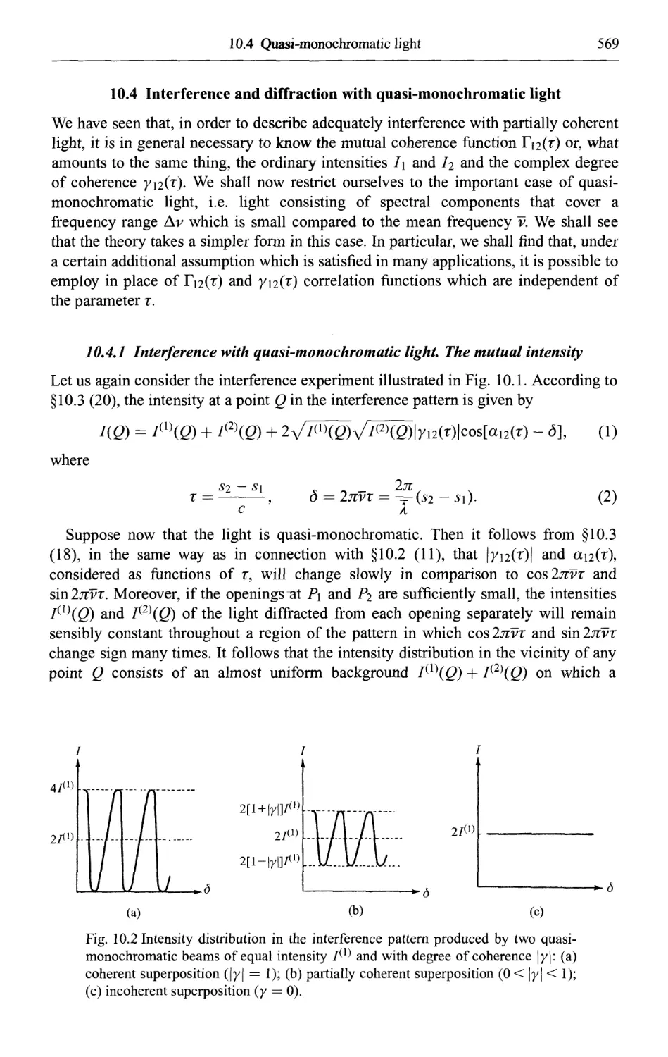


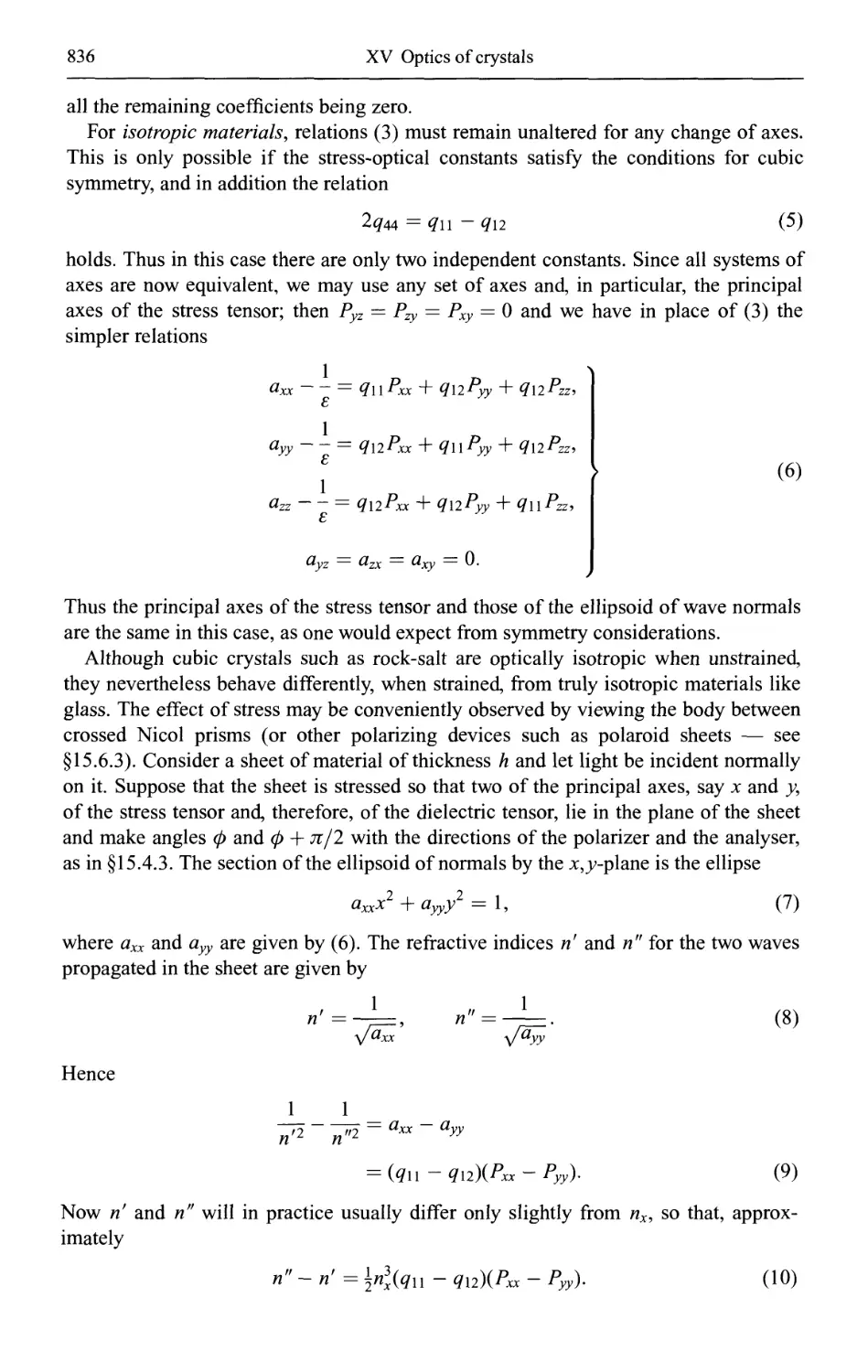


Text
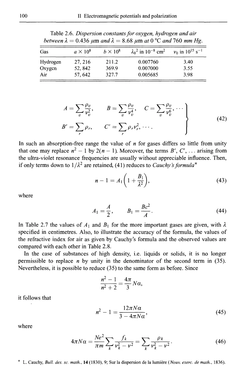
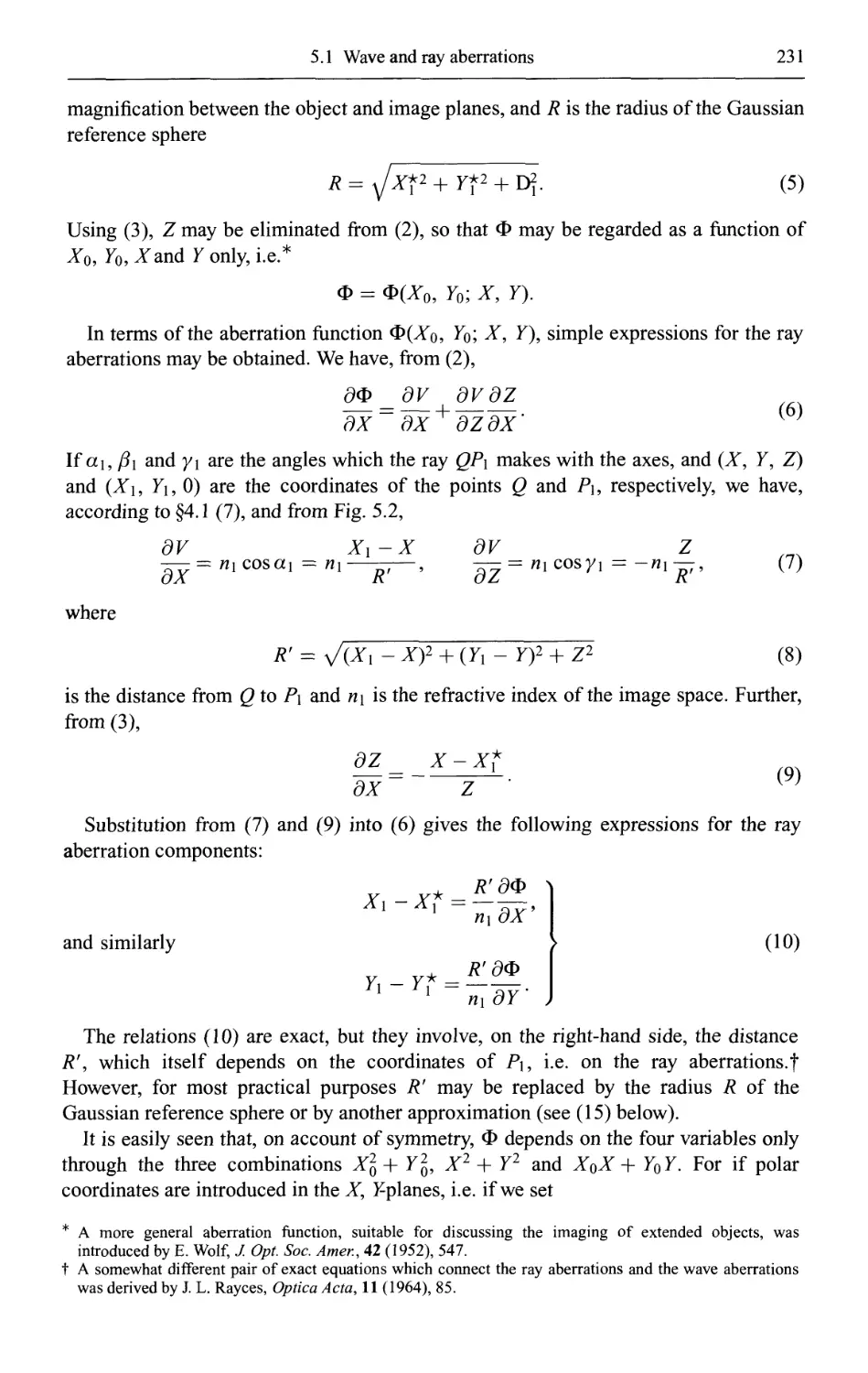
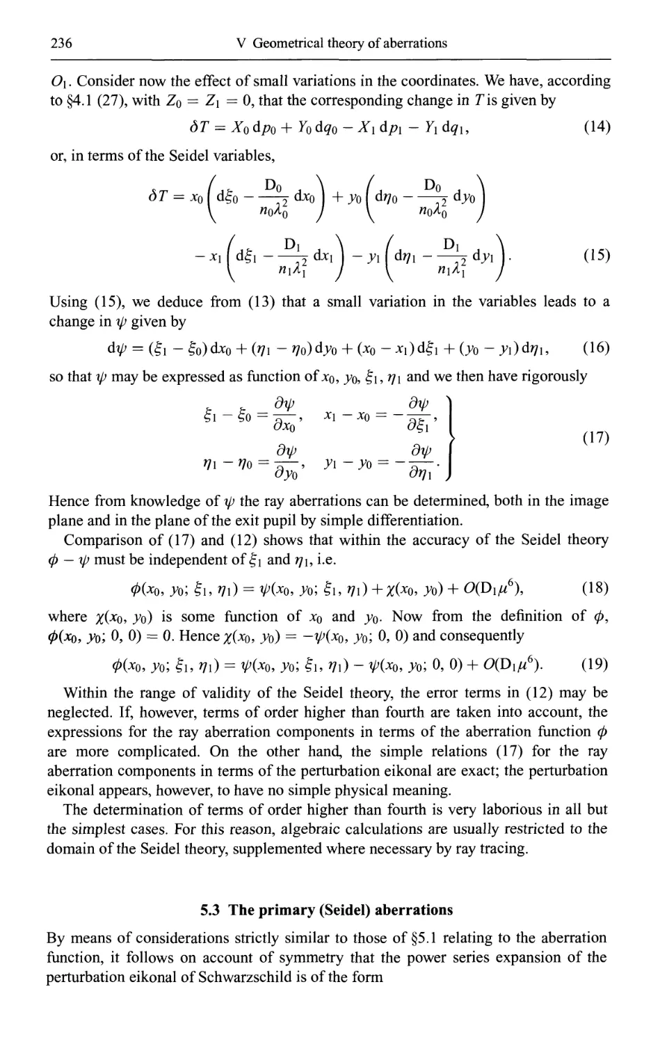
Principles of optics
Principles of Optics is one of the classic science books of the
twentieth century, and probably the most influential book in optics
published in the past 40 years. The new edition is the first ever
thoroughly revised and expanded edition of this standard text.
Among the new material, much of which is not available in any other
optics text, is a section on the CAT scan (computerized axial
tomography), which has revolutionized medical diagnostics. The book also
includes a new chapter on scattering from inhomogeneous media which
provides a comprehensive treatment of the theory of scattering of scalar
as well as of electromagnetic waves, including the Born series and the
Rytov series. The chapter also presents an account of the principles of
diffraction tomography - a refinement of the CAT scan - to which Emil
Wolf, one of the authors, has made a basic contribution by formulating
in 1969 what is generally regarded to be the basic theorem in this field.
The chapter also includes an account of scattering from periodic
potentials and its connection to the classic subject of determining the
structure of crystals from X-ray diffraction experiments, including
accounts of von Laue equations, Bragg's law, the Ewald sphere of
reflection and the Ewald limiting sphere, both generalized to continuous
media. These topics, although originally introduced in connection with
the theory of X-ray diffraction by crystals, have since become of
considerable relevance to optics, for example in connection with deep
holograms.
Other new topics covered in this new edition include interference with
broad-band light, which introduces the reader to an important
phenomenon discovered relatively recently by Emil Wolf, namely the generation
of shifts of spectral lines and other modifications of spectra of radiated
fields due to the state of coherence of a source. There is also a section
on the so-called Rayleigh-Sommerfeld diffraction theory which, in
recent times, has been finding increasing popularity among optical
scientists. There are also several new appendices, including one on
energy conservation in scalar wavefields, which is seldom discussed in
books on optics.
The new edition of this standard reference will continue to be
invaluable to advanced undergraduates, graduate students and
researchers working in most areas of optics.
To the Memory of
Sir Ernest Oppenheimer
Principles of optics
Electromagnetic theory of propagation,
interference and diffraction of light
MAX BORN
MA, DrPhil, FRS
Nobel Laureate
Formerly Professor at the Universities of Göttingen and Edinburgh
and
EMILWOLF
PhD, DSc
Wilson Professor of Optical Physics, University of Rochester, NY
with contributions by
A.B.BHATIA, P.C.CLEMMOW, D.GABOR, A.R.STOKES,
A.M.TAYLOR, P.A.WAYMAN AND W.L.WILCOCK
SEVENTH (EXPANDED) EDITION
Cambridge
UNIVERSITY PRESS
PUBLISHED BY THE PRESS SYNDICATE OF THE UNIVERSITY OF CAMBRIDGE
The Pitt Building, Trumpington Street, Cambridge, United Kingdom
CAMBRIDGE UNIVERSITY PRESS
The Edinburgh Building, Cambridge CB2 2RU, UK
40 West 20th Street, New York, NY 10011-4211, USA
477 Williamstown Road, Port Melbourne, VIC 3207, Australia
Ruiz de Alarcon 13, 28014 Madrid, Spain
Dock House, The Waterfront, Cape Town 8001, South Africa
http ://www. Cambridge. org
Seventh (expanded) edition © Margaret Farley-Born and Emil Wolf 1999
This book is in copyright. Subject to statutory exception
and to the provisions of relevant collective licensing agreements,
no reproduction of any part may take place without
the written permission of Cambridge University Press.
First published 1959 by Pergamon Press Ltd, London
Sixth edition 1980
Reprinted (with corrections) 1983, 1984, 1986, 1987, 1989, 1991, 1993
Reissued by Cambridge University Press 1997
Seventh (expanded) edition 1999
Reprinted with corrections, 2002
Reprinted 2003, 2005
Printed in the United Kingdom at the University Press, Cambridge
A catalogue record for this book is available from the British Library
Library of Congress Cataloguing in Publication data
Born, Max
Principles of Optics-7th ed.
1. Optics
I. Title II. Wolf Emil
535 QC351 80-41470
ISBN 0 521 642221 hardback
KT
Preface to corrected reprint of the seventh edition
As mentioned in the Preface to the seventh edition of this work, a change to a new
publisher has made it possible to reset the whole text. Not surprisingly such a large
amount of typesetting introduced some typographical errors. Those found by now have
been corrected, as has been other inaccuracies which the reviewers and readers of the
book brought to my attention. A small number of additional references have also been
included. For the sake of completeness the Prefaces to the third, fourth and fifth
editions have also been added.
I am particularly indebted to Dr E. Hecht who in a thorough review of the seventh
edition noted several errors and inaccuracies that have now been corrected. I am also
obliged to Dr S. H. Wiersma and Mr Damon Diehl who read much of the text very
carefully and supplied me with long lists of misprints and other errors. I must also
thank my friends and colleagues Professor Taco Visser, Dr Daniel F. V James, Dr Peter
Milonni, Professor Richard M. Sillitto, Mrs Winifred Sillitto and Dr Andrei Shchegrov
for drawing my attention to a number of errors. Finally I wish to express my
indebtedness to my colleague and former student Dr Greg Gbur for much help with
the preparation of the corrected version.
Rochester, New York EW
August 2001
v
Preface to the first edition
The idea of writing this book was a result of frequent enquiries about the possibility of
publishing in the English language a book on optics written by one of us* more than
twenty-five years ago. A preliminary survey of the literature showed that numerous
researches on almost every aspect of optics have been carried out in the intervening
years, so that the book no longer gives a comprehensive and balanced picture of the
field. In consequence it was felt that a translation was hardly appropriate; instead a
substantially new book was prepared, which we are now placing before the reader. In
planning this book it soon became apparent that even if only the most important
developments which took place since the publication of Optik were incorporated, the
book would become impracticably large. It was, therefore, deemed necessary to restrict
its scope to a narrower field. Optik itself did not treat the whole of optics. The optics of
moving media, optics of X-rays and y-rays, the theory of spectra and the full
connection between optics and atomic physics were not discussed; nor did the old
book consider the effects of light on our visual sense organ - the eye. These subjects
can be treated more appropriately in connection with other fields such as relativity,
quantum mechanics, atomic and nuclear physics, and physiology. In this book not only
are these subjects excluded, but also the classical molecular optics which was the
subject matter of almost half of the German book. Thus our discussion is restricted to
those optical phenomena which may be treated in terms of Maxwell's phenomenologi-
cal theory. This includes all situations in which the atomistic structure of matter plays
no decisive part. The connection with atomic physics, quantum mechanics, and
physiology is indicated only by short references wherever necessary. The fact that,
even after this limitation, the book is much larger than Optik, gives some indication
about the extent of the researches that have been carried out in classical optics in
recent times.
We have aimed at giving, within the framework just outlined, a reasonably complete
picture of our present knowledge. We have attempted to present the theory in such a
way that practically all the results can be traced back to the basic equations of
Maxwell's electromagnetic theory, from which our whole consideration starts.
In Chapter I the main properties of the electromagnetic field are discussed and the
effect of matter on the propagation of the electromagnetic disturbance is described
formally, in terms of the usual material constants. A more physical approach to the
* Max Born, Optik (Berlin, Springer, 1933).
vi
Preface to the first edition
VI1
question of influence of matter is developed in Chapter II: it is shown that in the
presence of an external incident field, each volume element of a material medium may
be assumed to give rise to a secondary (scattered) wavelet and that the combination of
these wavelets leads to the observable, macroscopic field. This approach is of
considerable physical significance and its power is illustrated in a later chapter (Chapter Xll)
in connection with the diffraction of light by ultrasonic waves, first treated in this way
by A. B. Bhatia and W. J. Noble; Chapter XII was contributed by Prof. Bhatia himself.
A considerable part of Chapter III is devoted to showing how geometrical optics
follows from Maxwell's wave theory as a limiting case of short wavelengths. In
addition to discussing the main properties of rays and wave-fronts, the vectorial
aspects of the problem (propagation of the directions of the field vectors) are also
considered. A detailed discussion of the foundations of geometrical optics seemed to
us desirable in view of the important developments made in recent years in the related
field of microwave optics (optics of short radio waves). These developments were often
stimulated by the close analogy between the two fields and have provided new
experimental techniques for testing the predictions of the theory. We found it
convenient to separate the mathematical apparatus of geometrical optics - the calculus
of variations - from the main text; an appendix on this subject (Appendix I) is based
in the main part on unpublished lectures given by D. Hubert at Göttingen University in
the early years of this century. The following appendix (Appendix II), contributed by
Prof. D. Gabor, shows the close formal analogy that exists between geometrical optics,
classical mechanics, and electron optics, when these subjects are presented in the
language of the calculus of variations.
We make no apology for basing our treatment of geometrical theory of imaging
(Chapter IV) on Hamilton's classical methods of characteristic functions. Though these
methods have found little favour in connection with the design of optical instruments,
they represent nevertheless an essential tool for presenting in a unified manner the
many diverse aspects of the subject. It is, of course, possible to derive some of the
results more simply from ad hoc assumptions; but, however valuable such an approach
may be for the solution of individual problems, it cannot have more than illustrative
value in a book concerned with a systematic development of a theory from a few
simple postulates.
The defect of optical images (the influence of aberrations) may be studied either by
geometrical optics (appropriate when the aberrations are large), or by diffraction
theory (when they are sufficiently small). Since one usually proceeds from quite
different starting points in the two methods of treatment, a comparison of results has in
the past not always been easy. We have attempted to develop a more unified treatment,
based on the concept of the deformation of wave-fronts. In the geometrical analysis of
aberrations (Chapter V) we have found it possible and advantageous to follow, after a
slight modification of his eikonal, the old method of K. Schwarzschild. The chapter on
diffraction theory of aberrations (Chapter IX) gives an account of the Nijboer-Zernike
theory and also includes an introductory section on the imaging of extended objects, in
coherent and in incoherent illumination, based on the techniques of Fourier
transforms.
Chapter VI, contributed by Dr P. A. Wayman, gives a brief description of the main
image-forming optical systems. Its purpose is to provide a framework for those parts
of the book which deal with the theory of image formation.
Vlll
Preface to the first edition
Chapter VII is concerned with the elements of the theory of interference and with
interferometers. Some of the theoretical sections have their nucleus in the
corresponding sections of Optik, but the chapter has been completely re-written by Dr W. L.
Wilcock, who has also considerably broadened its scope.
Chapter VIII is mainly concerned with the Fresnel-Kirchhoff diffraction theory and
with some of its applications. In addition to the usual topics, the chapter includes a
detailed discussion of the central problem of optical image formation - the analysis of
the three-dimensional light distribution near the geometrical focus. An acount is also
given of a less familiar alternative approach to diffraction, based on the notion of the
boundary diffraction wave of T. Young.
The chapters so far referred to are mainly concerned with perfectly monochromatic
(and therefore completely coherent) light, produced by point sources. Chapter X deals
with the more realistic case of light produced by sources of finite extension and
covering a finite frequency range. This is the subject of partial coherence, where
considerable progress has been made in recent years. In fact, a systematic theory of
interference and diffraction with partially coherent light has now been developed. This
chapter also includes an account of the closely related subject of partial polarization,
from the standpoint of coherence theory.
Chapter XI deals with rigorous diffraction theory, a field that has witnessed a
tremendous development over the period of the last twenty years,* stimulated largely
by advances in the ultra-shortwave radio techniques. This chapter was contributed by
Dr P. C. Clemmow who also prepared Appendix III, which deals with the mathematical
methods of steepest descent and stationary phase.
The last two chapters, 'Optics of metals' (Chapter XIII) and 'Optics of crystals'
(Chapter XIV) are based largely on the corresponding chapters of Optik, but were
revised and extended with the help of Prof. A. M. Taylor and Dr A. R. Stokes
respectively. These two subjects are perhaps discussed in less detail than might seem
appropriate. However, the optics of metals can only be treated adequately with the help
of quantum mechanics of electrons, which is outside the scope of this book. In crystal
optics the centre of interest has gradually shifted from visible radiation to X-rays, and
the progress made in recent years has been of a technical rather than theoretical nature.
Though we have aimed at producing a book which in its methods of presentation
and general approach would be similar to Optik, it will be evident that the present
book is neither a translation of Optik, nor entirely a compilation of known data. As
regards our own share in its production, the elder coauthor (M. B.) has contributed that
material from Optik which has been used as a basis for some of the chapters in the
present treatise, and has taken an active part in the general planning of the book and in
numerous discussions concerning disputable points, presentation, etc. Most of the
compiling, writing and checking of the text was done by the younger coauthor (E. W.).
Naturally we have tried to use systematic notation throughout the book. But in a
book that covers such a wide field, the number of letters in available alphabets is far
too limited. We have, therefore, not always been able to use the most elegant notation
but we hope that we have succeeded, at least, in avoiding the use in any one section of
the same symbol for different quantities.
* The important review article by C. J. Bouwkamp, Rep. Progr. Phys. (London, Physical Society), 17 A954),
35, records more than 500 papers published in the period 1940-1954.
Preface to the first edition
IX
In general we use vector notation as customary in Great Britain. After much
reflection we rejected the use of the nabla operator alone and employed also the
customary 'div', 'grad' and 'curl'. Also, we did not adopt the modern electrotechnical
units, as their main advantage lies in connection with purely electromagnetic
measurements, and these play a negligible part in our discussions; moreover, we hope, that if
ever a second volume {Molecular and Atomic Optics) and perhaps a third volume
{Quantum Optics) is written, the C.G.S. system, as used in theoretical physics, will
have returned to favour. Although, in this system of units, the magnetic permeability pi
of most substances differs inappreciably from unity at optical frequencies, we have
retained it in some of the equations. This has the advantage of greater symmetry and
makes it possible to derive 'dual' results by making use of the symmetry properties of
Maxwell's equations. For time periodic fields wc have used, in complex representation,
the factor exp(—icot) throughout.
We have not attempted the task of referring to all the relevant publications. The
references that are given, and which, we hope, include the most important papers, are
to help the reader to gain some orientation in the literature; an omission of any
particular reference should not be interpreted as due to our lack of regard for its merit.
In conclusion it is a pleasure to thank many friends and colleagues for advice and
help. In the first place we wish to record our gratitude to Professor D. Gabor for useful
advice and assistance in the early stages of this project, as well as for providing a draft
concerning his ingenious method of reconstructed wave-fronts (§8.10). We are also
greatly indebted to Dr F. Abeles, who prepared a draft, which is the backbone of §1.6,
on the propagation of electromagnetic waves through stratified media, a field to which
he himself has made a substantial contribution. We have also benefited by advice on
this subject from Dr B. H. Billings.
We are much indebted to Dr H. H. Hopkins, Dr R. A. Silverman, Dr W. T. Welford
and Dr G. Wyllie for critical comments and valuable advice, and to them and also to
Dr G. Black, Dr H. J. J. Braddick, Dr N. Chako, Dr F. D. Kahn, Mr A. Nisbet, Dr M.
Ross and Mr R. M. Sillitto for scrutinizing various sections of the manuscript. We are
obliged to Polaroid Corporation for information concerning dichroic materials. Dr F.
D. Kahn helped with proof-reading and Dr P. Roman and Mrs M. Podolanski with the
preparation of the author index.
The main part of the writing was done at the Universities of Edinburgh and
Manchester. The last stages were completed whilst one of the authors (E. W.) was a
guest at the Institute of Mathematical Sciences, New York University. We are grateful
to Professor M. Kline, Head of its Division of Electromagnetic Research, for his
helpful interest and for placing at our disposal some of the technical facilities of the
Institute.
We gratefully acknowledge the loan of original photographs by Professor M.
Francon and Dr M. Cagnet (Figs 7.4, 7.26, 7.28, 7.60, 15.24, 15.26), Professor H.
Lipson and his coworkers at the Manchester College of Science and Technology (Figs.
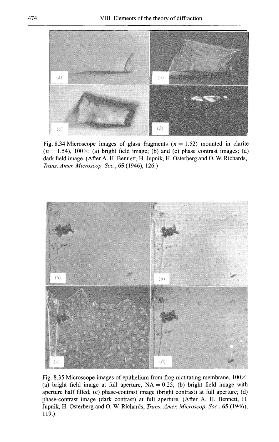
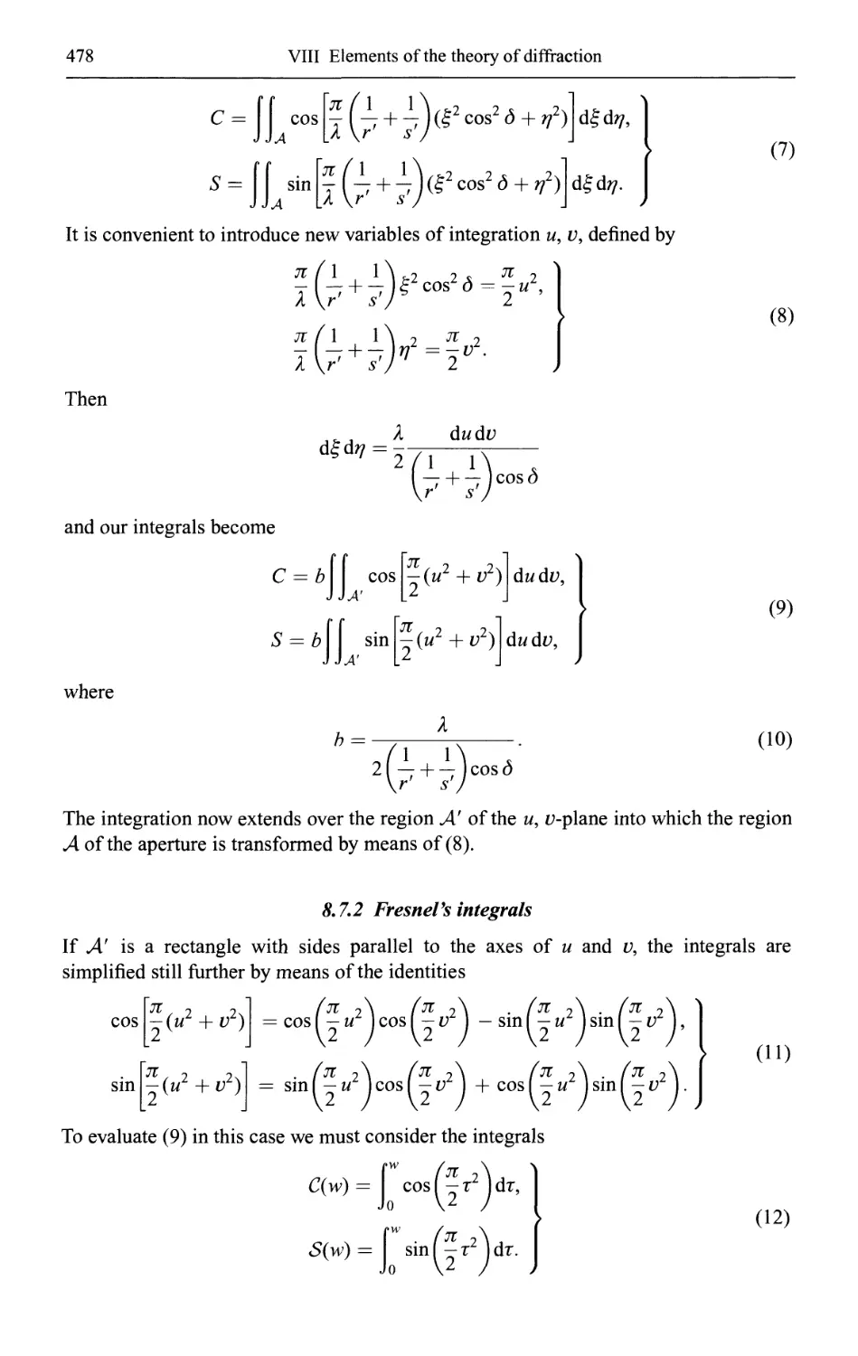
8.10, 8.12, 8A5), Dr O. W. Richards (Figs. 8.34, 8.35), and Professor F. Zernike and Dr
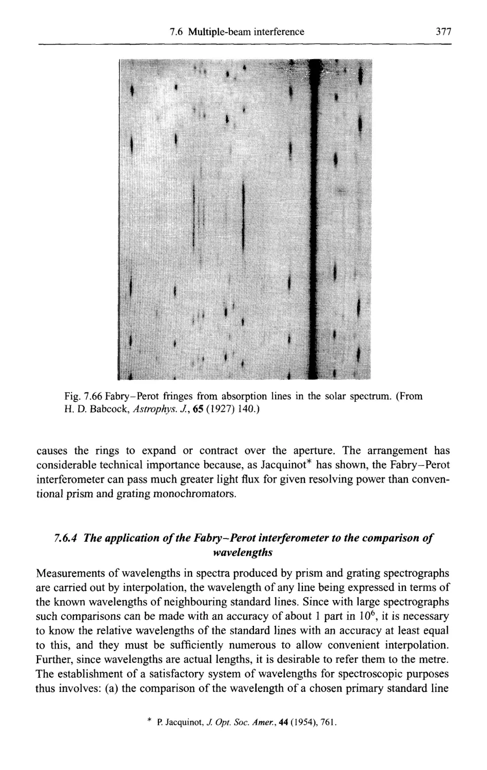
K. Nienhus (Figs. 9.4, 9.5, 9.8, 9.10, 9.11). Fig. 7.66 is reproduced by courtesy of the
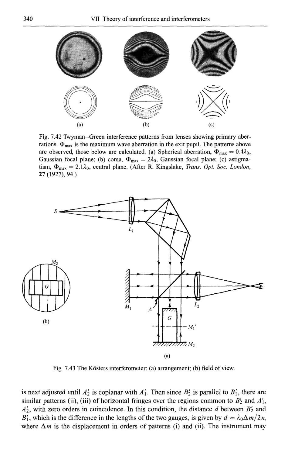
Director of the Mount Wilson and Palomar Observatories. The blocks of Fig. 7.42
were kindly loaned by Messrs Hilger and Watts, Ltd, and those of Figs. 7.64 and 7.65
by Dr K. W. Meissner.
Financial assistance was provided by Messrs Industrial Distributors Ltd, London,
X
Preface to the second edition
and we wish to acknowledge the generosity of the late Sir Ernest Oppenheimer, its
former head.
Finally, it is a pleasure to thank our publishers and in particular Mr E. J. Buckley,
Mr D. M. Lowe and also Dr P. Rosbaud, who as a former Director of Pergamon Press
was closely associated with this project in its early stages, for the great care they have
taken in the production of the book. It is a pleasure to pay tribute also to the printers,
Pitman Press of Bath, for the excellence of their printing.
Bad Pyrmont and Manchester Max Born
January 1959 Emil Wolf
Preface to the second edition
Advantage has been taken in the preparation of a new edition of this work to make a
number of corrections of errors and misprints, to make a few minor additions and to
include some new references.
Since the appearance of the first edition almost exactly three years ago, the first
optical masers (lasers) have been developed. By means of these devices very intense
and highly coherent light beams may be produced. Whilst it is evident that optical
masers will prove of considerable value not only for optics but also for other sciences
and for technology, no account of them is given in this new edition. For the basic
principles of maser action have roots outside the domain of classical electromagnetic
theory on which considerations of this book are based. We have, however, included a
few references to recent researches in which light generated by optical masers was
utilized or which have been stimulated by the potentialities of these new optical
devices.
We wish to acknowledge our gratitude to a number of readers who drew our
attention to errors and misprints. We are also obliged to Dr B. Karczewski and Mr C.
L. Mehta for assistance with the revisions.
Bad Pyrmont and Rochester
November 1962
M.B.
E.W.
Preface to the third edition
A number of errors and misprints which were present in the earlier editions of this
work have been corrected and references to some recent publications have been added.
A new figure (8.54) which relates to an interesting recent development in the
wavefront reconstruction technique was also included. We are indebted to E. N. Leith
and J. Upatnieks for a loan of the original photographs.
Bad Pyrmont and Rochester M. B.
July 1965 E.W.
Preface to the fourth edition
Owing to the appreciable size of this work, it was found impractical to incorporate in
this new edition additional material relating to the most recent developments in optics.
We have, however, made further corrections and improvements in the text and have
added references to some recent publications.
We are indebted to Dr E. W. Marchand and Mr. T. Kusakawa for supplying us with
lists of misprints and errors found in the previous editions. We are also obliged to Dr
G. Bedard for assistance with the revisions.
Bad Pyrmont and Rochester M. B.
August 1968 E. W.
XI
Preface to the fifth edition
Some further errors and misprints that were found in the earlier editions of this work
have been corrected, the text in several sections has been improved and a number of
references to recent publications have been added. More extensive changes have been
made in §§13.1-13.3, dealing with the optical properties of metals. It is well known
that a purely classical theory is inadequate to describe the interaction of an
electromagnetic field with a metal in the optical range of the spectrum. Nevertheless, it is
possible to indicate some of the main features of this process by means of a classical
model, provided that the frequency dependence of the conductivity is properly taken
into account and the role that the free, as well as the bound, electrons play in the
response of the metal to an external electromagnetic field is understood, at least in
qualitative terms. The changes in §§13.1-13.3 concern mainly these aspects of the
theory and the revised sections are believed to be free of misleading statements and
inaccuracies that were present in this connection in the earlier editions of this work
and which can also be commonly found in many other optical texts.
I am grateful to some of our readers for informing me about misprints and errors. I
wish to specifically acknowledge my indebtedness to Prof. A. D. Buckinham, Dr D.
Canals Frau and, once again, Dr E. W. Marchand, who supplied me with detailed lists
of corrections and to Dr E. Lalor and Dr G. C. Sherman for having drawn my attention
to the need for making more substantial changes in Chapter XIII. I am also much
obliged to Mr J. T. Foley for assistance with the revisions.
Rochester
January 1974 E. W.
Preface to the sixth edition
This edition differs from its immediate predecessor chiefly in that it contains
corrections of a small number of errors and misprints.
Rochester E.W.
September 1985
Xll
Preface to the seventh edition
Forty years ago this month Max Born and I dispatched to the publishers the Preface to
the first edition of Principles of Optics. Since that time the book has been published in
six editions and has been reprinted seventeen times (not counting unauthorized
editions and several translations), usually with only a small number of corrections. A
recent change to a new publisher, who expressed willingness to reset the whole text,
has given me the opportunity to make more substantial changes.
The first edition was published a year before the invention of the laser, an event
which triggered an explosion of activities in optics and soon led to the creation of
entirely new fields, such as non-linear optics, fiber optics and opto-electronics.
Numerous applications followed, in medicine, in optical data storage, in information
transfer and in many other areas. On a more fundamental level, quantum optics
emerged as a vibrant and rapidly expanding field, which has provided new ways of
testing some basic assumptions of quantum physics relating, for example, to
localization and indistinguishability The progress made in these fields has been rapid and
broad and some of the newer areas have themselves become the subjects of books.
It is clear that a fully updated new edition of Principles of Optics would require that
it be expanded into several volumes. Consequently, in order to preserve a single-
volume, only a few new topics have been added; they were selected to some extent so
as not to necessitate major revisions of the original text. Specifically, the following
new material has been added:
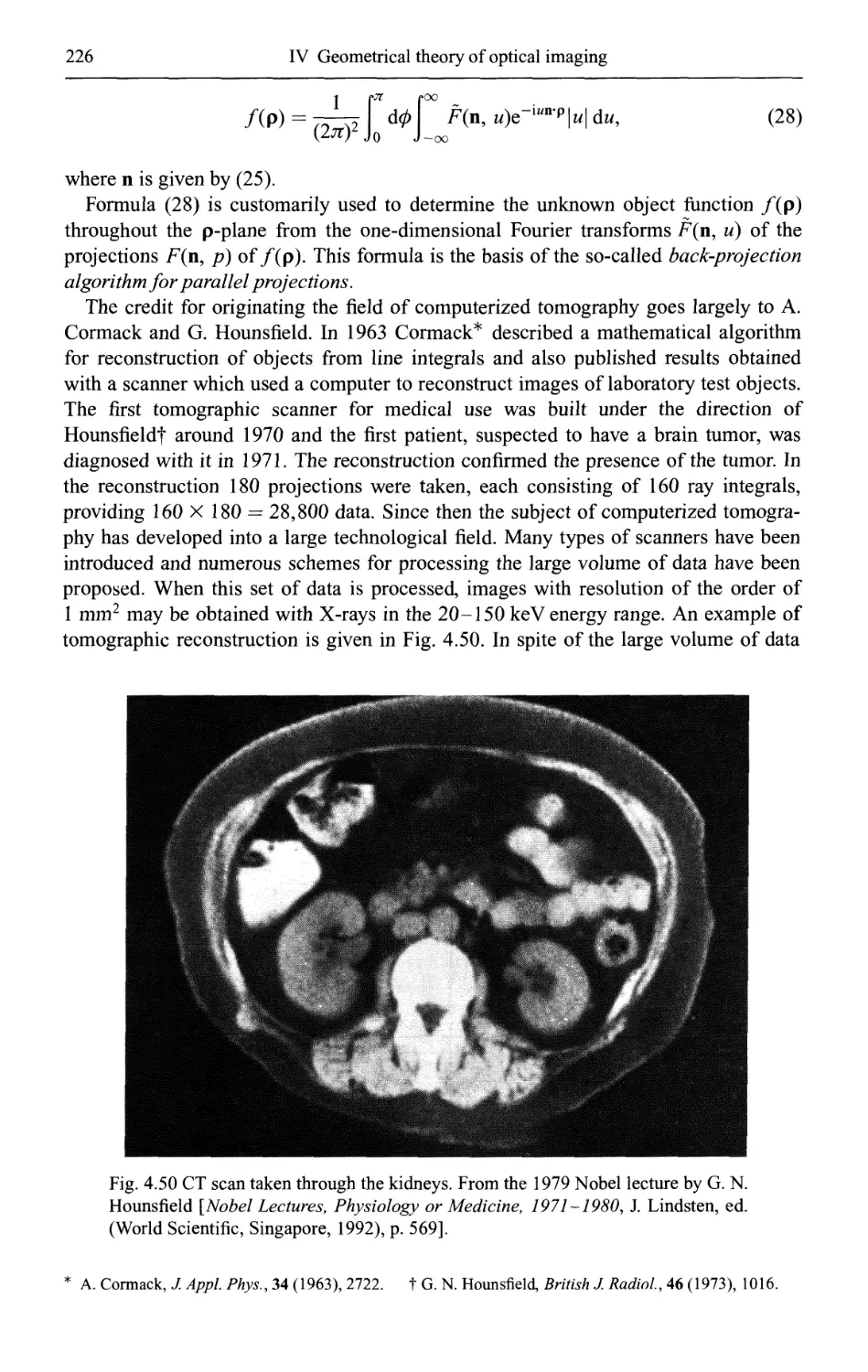
A) Section 4.11, which presents the principles of computerized axial tomography,
generally referred to as CAT. This subject originated in the early 1960s and has
revolutionized diagnostic medicine. The section also includes an account of the Radon
transform, introduced as early as 1917, which underlies the theory of computerized
axial tomography, although this was not known to its inventors. The fact that three
Nobel Prizes have been awarded for this invention and its applications attests to its
importance. More recently the theory underlying the CAT scan is finding much broader
usage, for example in connection with the reconstruction of quantum states.
B) Section 8.11 gives an account of the so-called Rayleigh-Kirchhoff diffraction
theory. This theory has become rather popular after it was introduced in the book
Optics by A. Sommerfeld, published in 1954. It is preferred by some optical scientists
to the much older classic Kirchhoff diffraction theory. However, which of these
theories better describes various diffraction effects is still an open question.
C) Section 10.5 discusses some effects discovered relatively recently arising on
Xlll
XIV
Preface to the seventh edition
superposition of broad-band light beams of any state of coherence. The analysis of
such effects has demonstrated that even though under such circumstances interference
fringes may not be seen in the region of superposition, the light distribution in that
region may nevertheless contain important physical information which is revealed
when the light is spectrally analyzed. One may then find that the spectrum of the light
is different at different points of observation and from such spectral changes one may
determine coherence properties of the light. This effect is an example of a coherence
phenomenon in the space-frequency domain, which must be distinguished from the
more familiar coherence effects in the space-time domain. The quantitative measure of
space-frequency coherence phenomena is the so-called spectral degree of coherence,
which is introduced in this new edition in the somewhat revised Section 10.5. The
experiment which is analyzed in that section also provides an elementary introduction
to the phenomenon of correlation-induced spectral changes, discovered just over 10
years ago and studied extensively since that time.
D) A new Chapter 13 presents the theory of scattering of light by inhomogeneous
media. In the context of optics this subject was largely developed in relatively recent
times although essentially the same theory was well established many years ago in
connection with quantum mechanical potential scattering. The chapter presents the
basic integral equation of light scattering on linear isotropic bodies, discusses the
solution of the equation in series form and includes a detailed account of the first Born
and the first Rytov approximations. The chapter includes a brief description of the
classic theory of scattering by a medium with periodic structure, which is the basis of
the theory of X-ray diffraction by crystals. The chapter also covers the von Laue
equations, Bragg's law, the Ewald sphere of reflection and the Ewald limiting sphere.
In recent years these subjects have become important in the broad area of inverse light
scattering and they have found new applications, for example in connection with
holographic gratings. The chapter also contains a detailed account of the optical cross-
section theorem (usually known as the optical theorem), which, in spite of its name, is
seldom discussed in the optical literature.
Another topic treated in Chapter 13 is diffraction tomography. In computerized axial
tomography discussed in the new Section 4.11, the finite wavelength of the radiation is
ignored. This is usually justified when the technique is used with X-rays, but the
approximation is often inadequate in applications where light waves or sound waves
are used. Diffraction tomography takes the finite wavelength of the radiation into
account and, therefore, provides better resolution.
In addition to the new material already mentioned, this new edition also contains
several new appendices (VIII, XI and XII), many new references, some of which
replace older ones, and a few relatively small changes have been made in the text,
usually with the aim of improving clarity and updating information.
It is a pleasure to thank several colleagues, friends and students for their help. I am
obliged to Professor Harrison H. Barrett for helpful suggestions which led to
improvements of Sections 4.11 and 13.2 on computerized axial tomography and on diffraction
tomography. I am indebted to my long-time friend and colleague Professor Leonard
Mandel for useful comments on some parts of the manuscript. Dr Doo Cho and Dr V
N. Mahajan were kind enough to draw my attention to some inaccuracies which they
found in earlier editions and which have now been taken care of. My collaborators Dr
Preface to the seventh edition
xv
Yajun Li, Dr Taco D. Visser and my former students Dr Avshalom Gamliel, Dr David
G. Fischer and Dr Kisik Kim have read some of the new sections and have made
helpful comments leading to improvements. My former student Dr Weijian Wang
kindly prepared most of the new figures. I am particularly grateful to two of my present
graduate students, P. Scott Carney and Greg J. Gbur, who provided invaluable help by
checking calculations and references, weeding out inaccuracies, suggesting
improvements in the presentation and helping with proof-reading.
I wish to express my appreciation to Mrs Patricia Sulouff, Head Librarian of the
Physics-Optics-Astronomy library at the University of Rochester for helping to trace
some of the more obscure references and for locating papers and books that were not
easily accessible. I am also obliged to Mrs Ellen Calkins for typing and re-typing
several drafts of the manuscript of the new sections and for preparing the author index.
Most of the revisions were prepared whilst I was on a visiting appointment at the
Center for Research and Education in Optics and Research (CREOL) at the University
of Central Florida during the 1998 Spring Semester. I wish to thank Professors M. J.
Soileau, M. G. Moharam and G. I. Stegeman of the CREOL faculty for providing a
congenial environment and facilities for this work.
The family life of most authors suffers during the time when one of the marriage
partners is engaged in book writing. Mine was no exception, but I am glad to say that
my wife, Marlies, survived this period cheerfully and without complaints. She has
helped with checking the manuscript and the proofs, for which I am grateful.
I acknowledge with thanks the fine cooperation that I received from the staff of
Cambridge University Press. I am particularly appreciative of the considerable help
provided by Dr Simon Capelin, the publishing director for Physical Sciences. I am also
obliged to Mrs Maureen Storey for thorough copy-editing of the whole book and to
Ms Miranda Fyfe and particularly to Mrs Jayne Aldhouse for their cooperation in
meeting the rather stringent production deadlines.
I am sometimes asked about my collaboration with Max Born, which resulted in the
publication of Principles of Optics. Interested readers can find it discussed in my
article 'Recollections of Max Born,' published in Optics News 9, 10-16
(November/December, 1983).*
Rochester, New York Emil Wolf
January 1999
The article has been reprinted in Technology of Our Times, ed. F. Sue (SPIE Optical Engineering Press,
Bellington, WA, 1990), 15-26 and also in Astrophysics and Space Science 227, ed. A. L. Peratt (Kluwer
Academic Publishers, Dordrecht, The Netherlands, 1995), 277-97 and in Selected Works of Emil Wolf with
Commentary (World Scientific, Singapore, 2001), 552-558.
Contents
Historical introduction xxv
I Basic properties of the electromagnetic field 1
1.1 The electromagnetic field 1
1.1.1 Maxwell's equations 1
1.1.2 Material equations 2
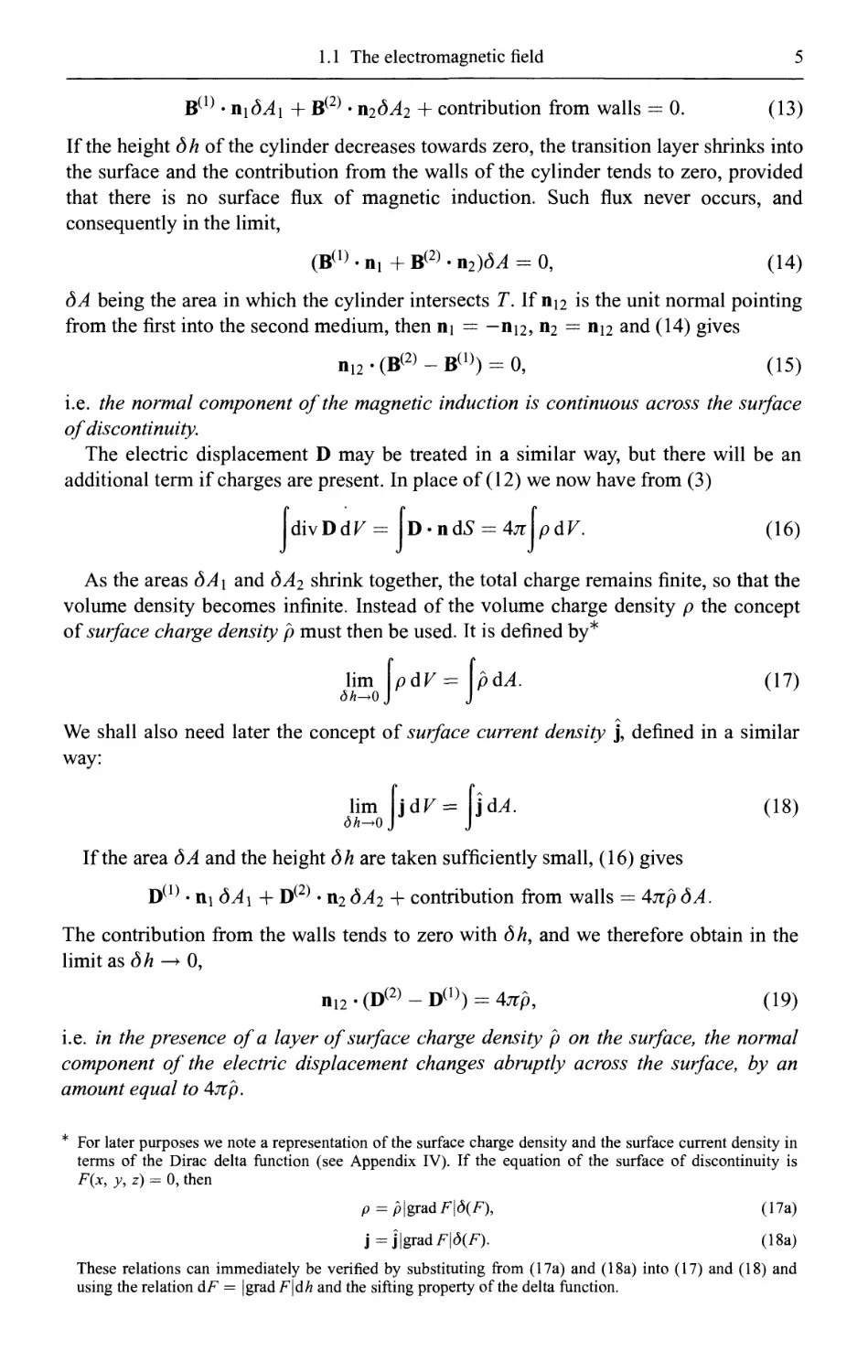
1.1.3 Boundary conditions at a surface of discontinuity 4
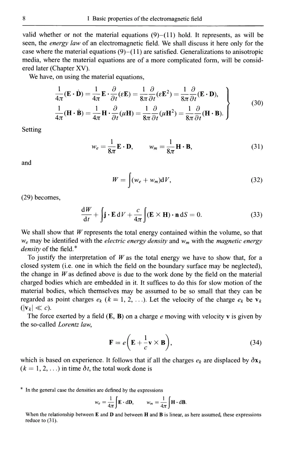
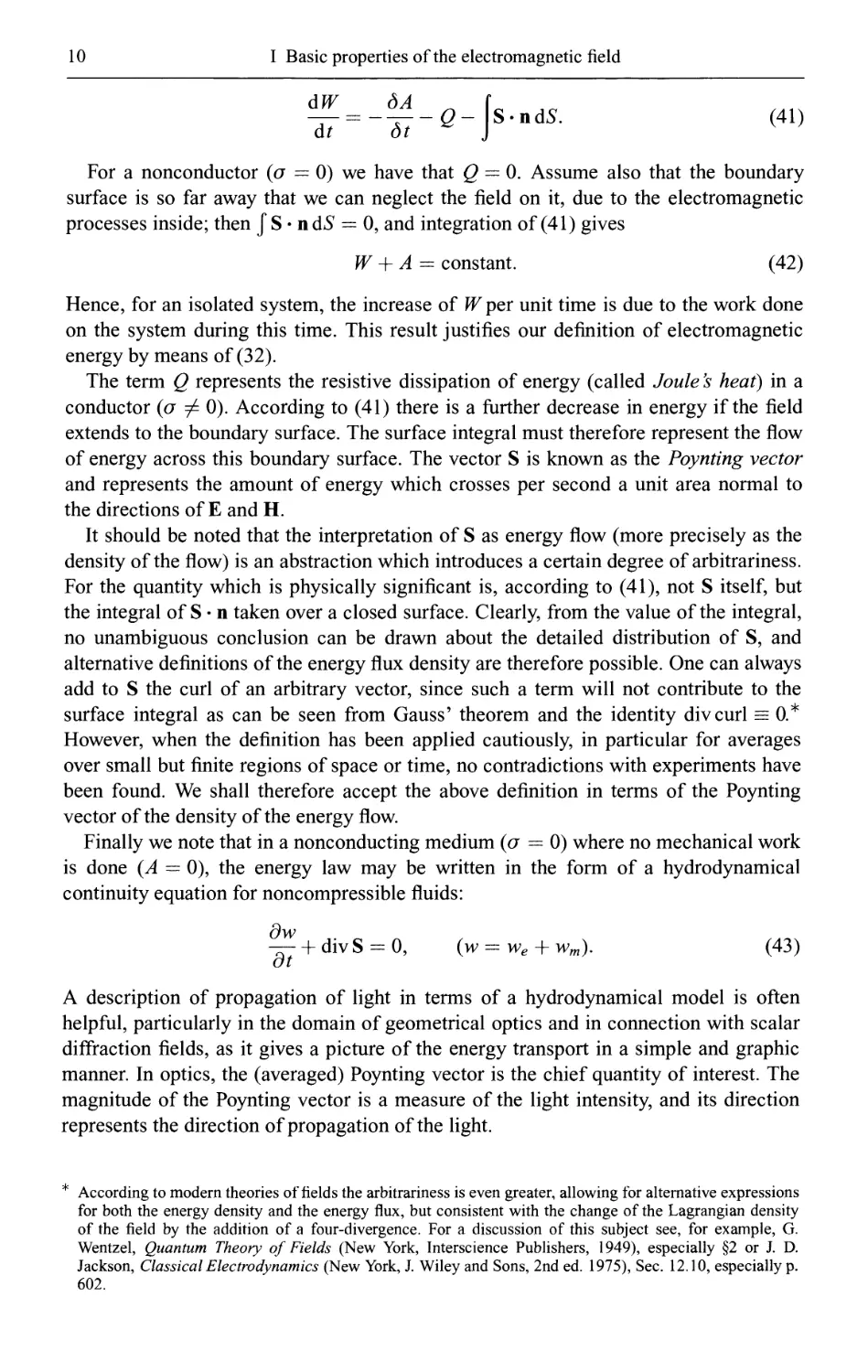
1.1.4 The energy law of the electromagnetic field 7
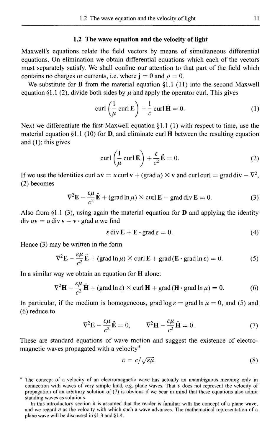
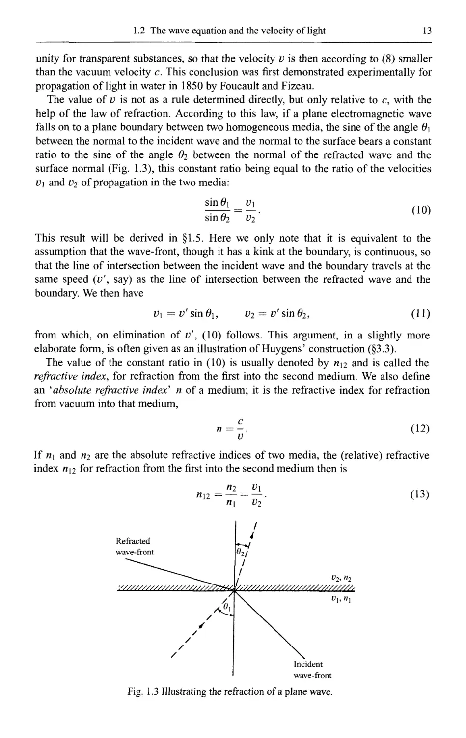
1.2 The wave equation and the velocity of light 11
1.3 Scalar waves 14
1.3.1 Plane waves 15
1.3.2 Spherical waves 16
1.3.3 Harmonic waves. The phase velocity 16
1.3.4 Wave packets. The group velocity 19
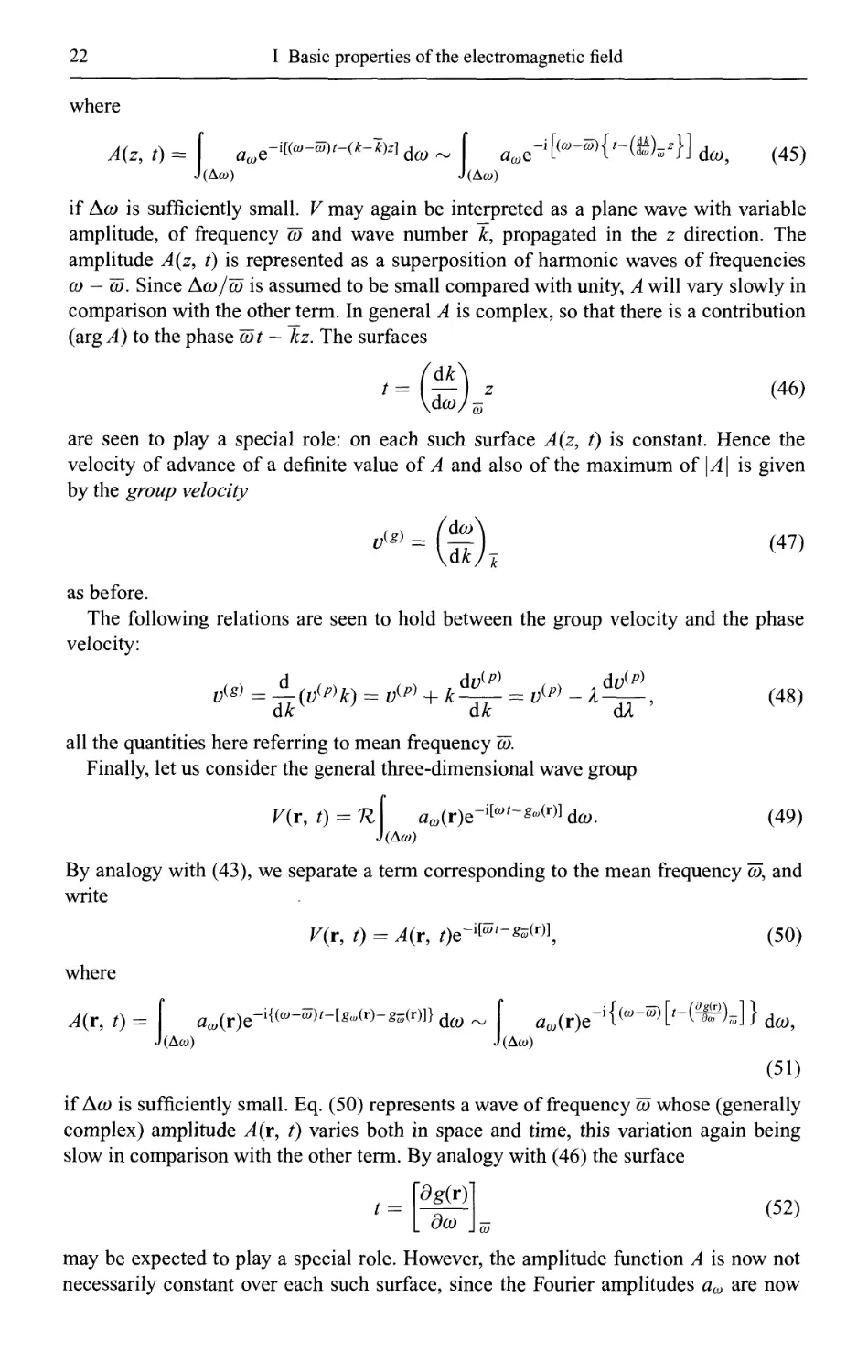
1.4 Vector waves 24
1.4.1 The general electromagnetic plane wave 24
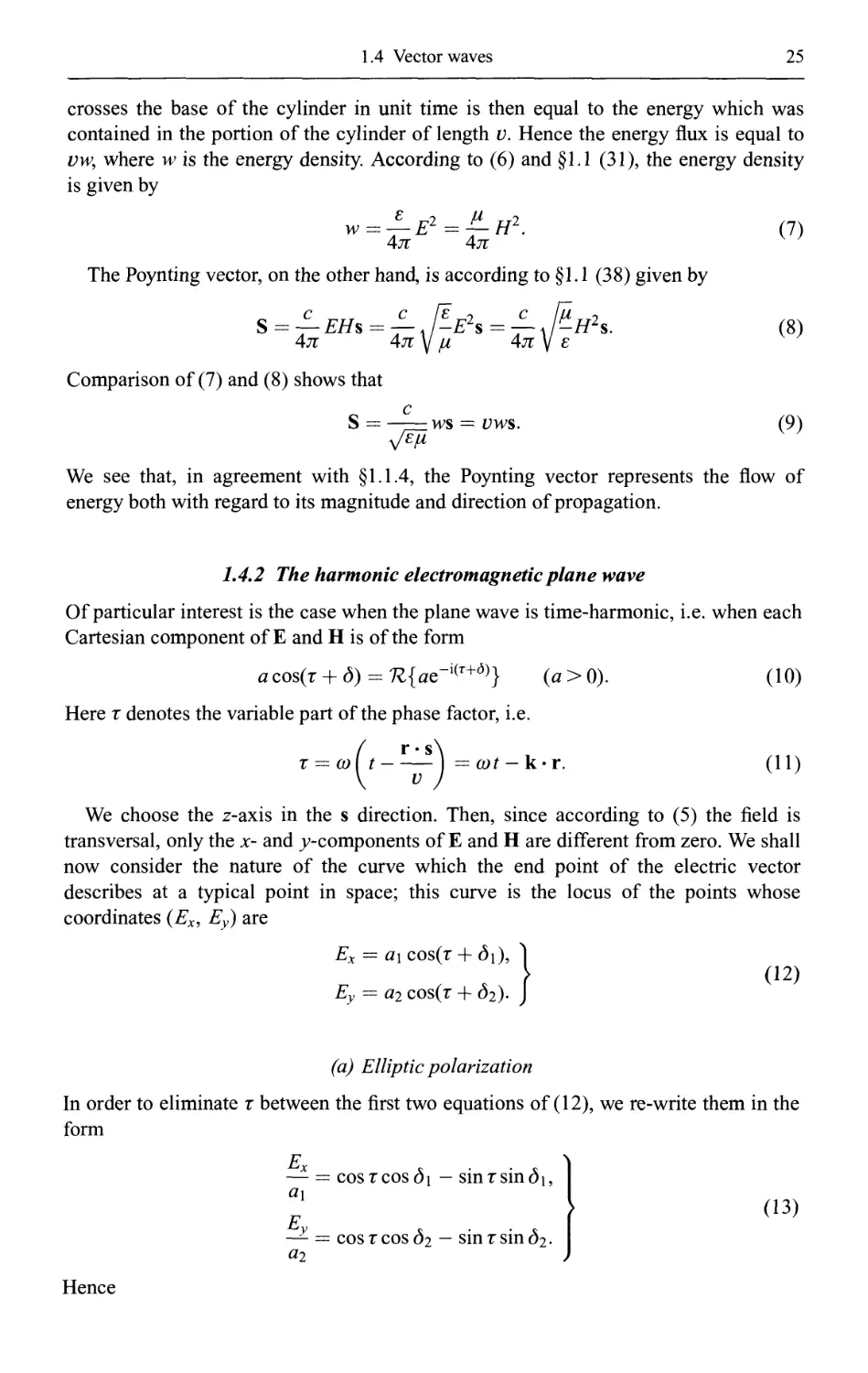
1.4.2 The harmonic electromagnetic plane wave 25
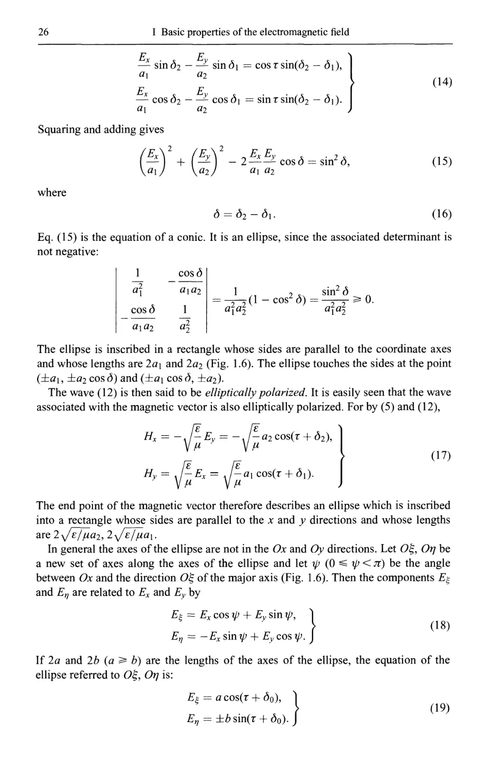
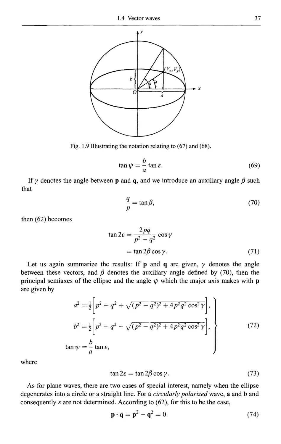
(a) Elliptic polarization 25
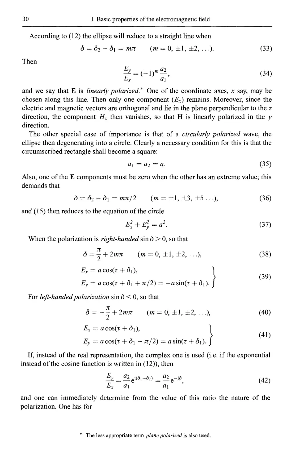
(b) Linear and circular polarization 29
(c) Characterization of the state of polarization by Stokes parameters 31
1.4.3 Harmonic vector waves of arbitrary form 33
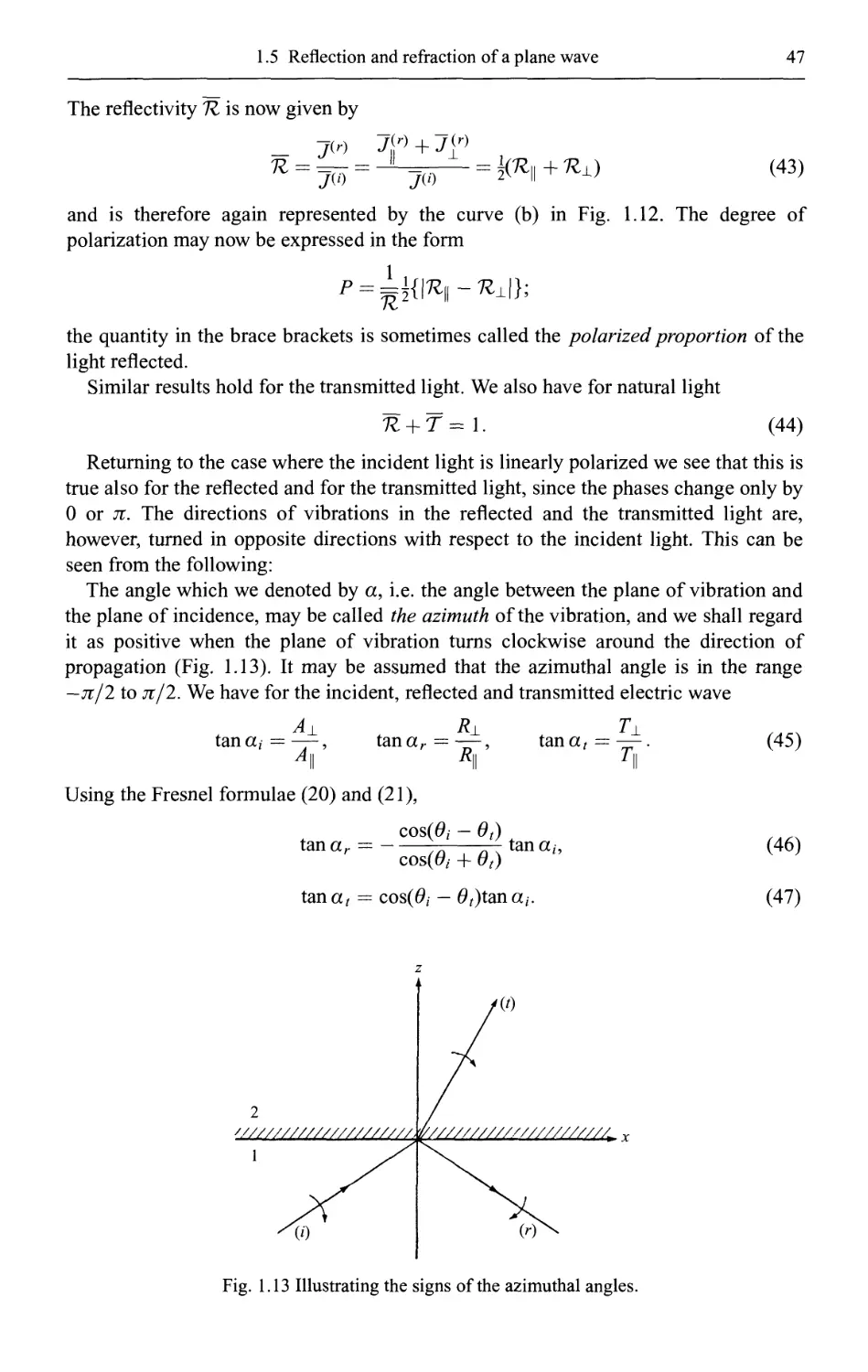
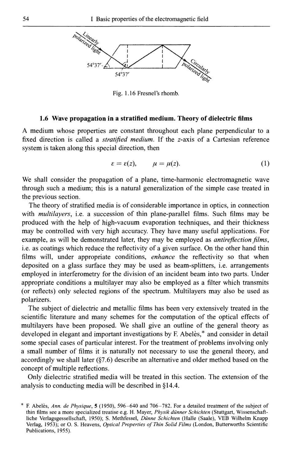
1.5 Reflection and refraction of a plane wave 3 8
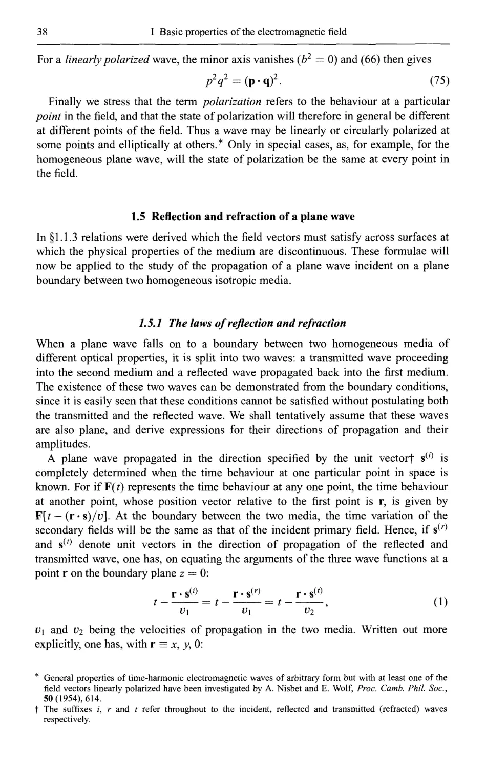
1.5.1 The laws of reflection and refraction 3 8
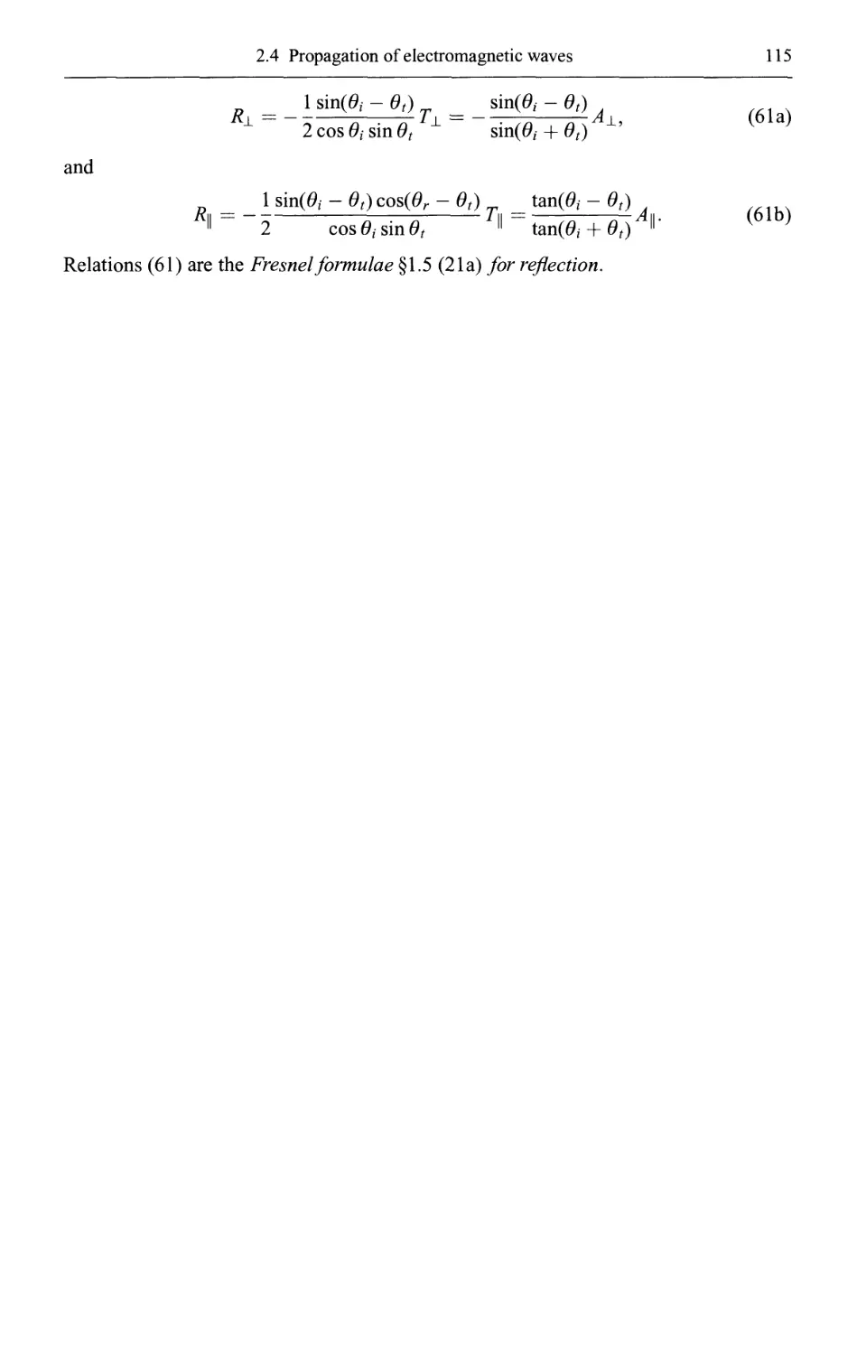
1.5.2 Fresnel formulae 40
1.5.3 The reflectivity and transmissivity; polarization on reflection and refraction 43
1.5.4 Total reflection 49
1.6 Wave propagation in a stratified medium. Theory of dielectric films 54
1.6.1 The basic differential equations 55
1.6.2 The characteristic matrix of a stratified medium 58
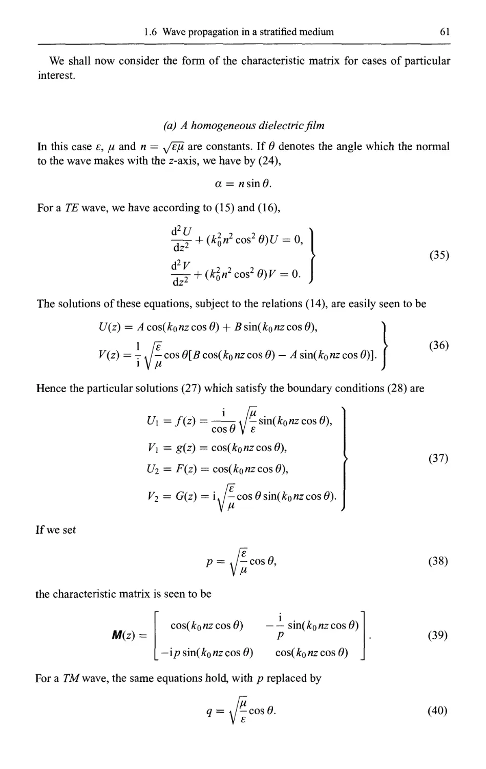
(a) A homogeneous dielectric film 61
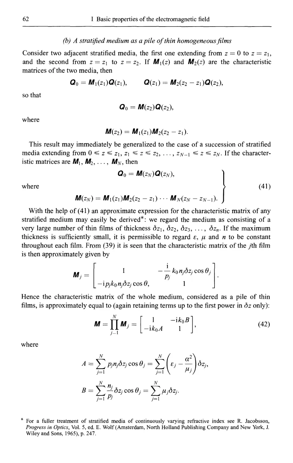
(b) A stratified medium as a pile of thin homogeneous films 62
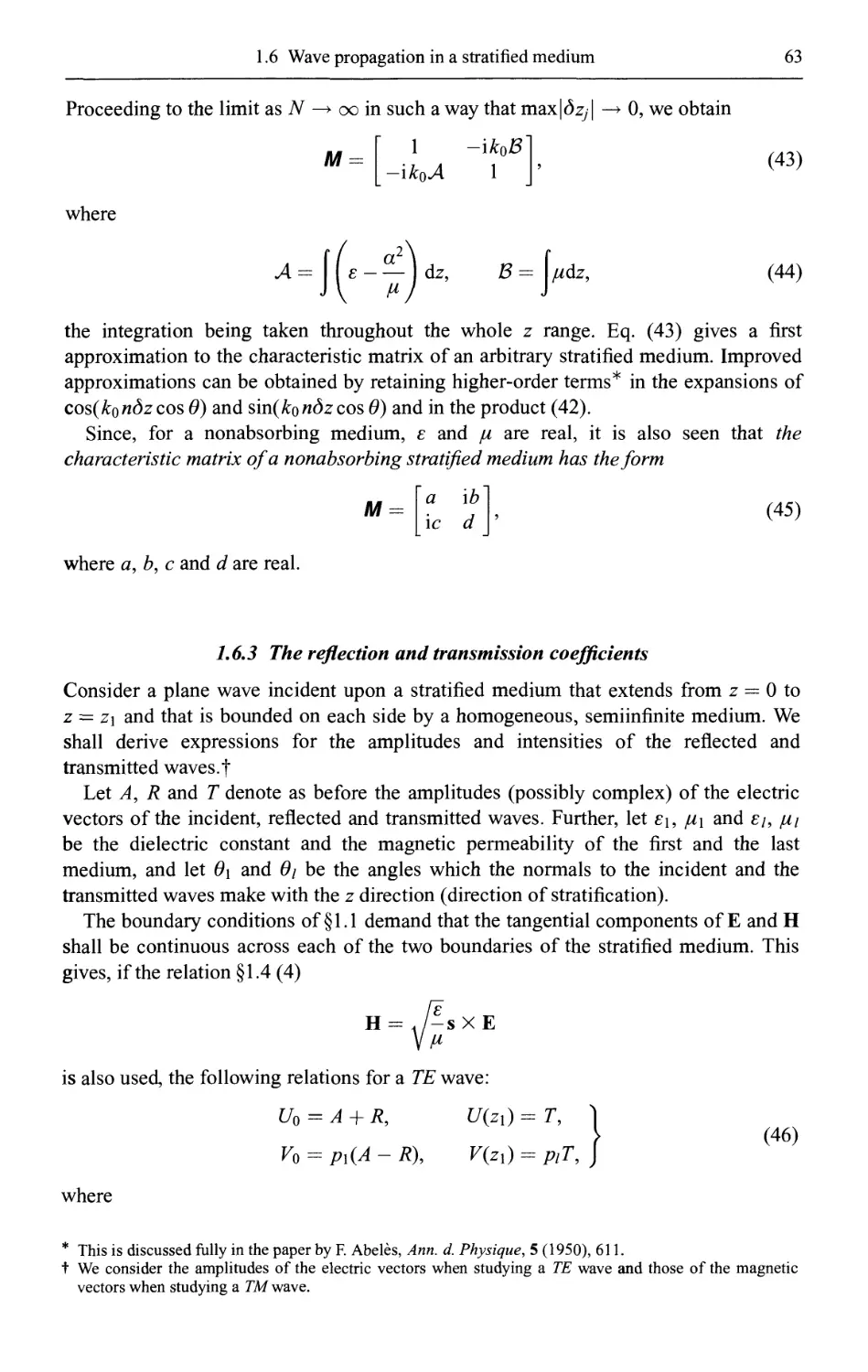
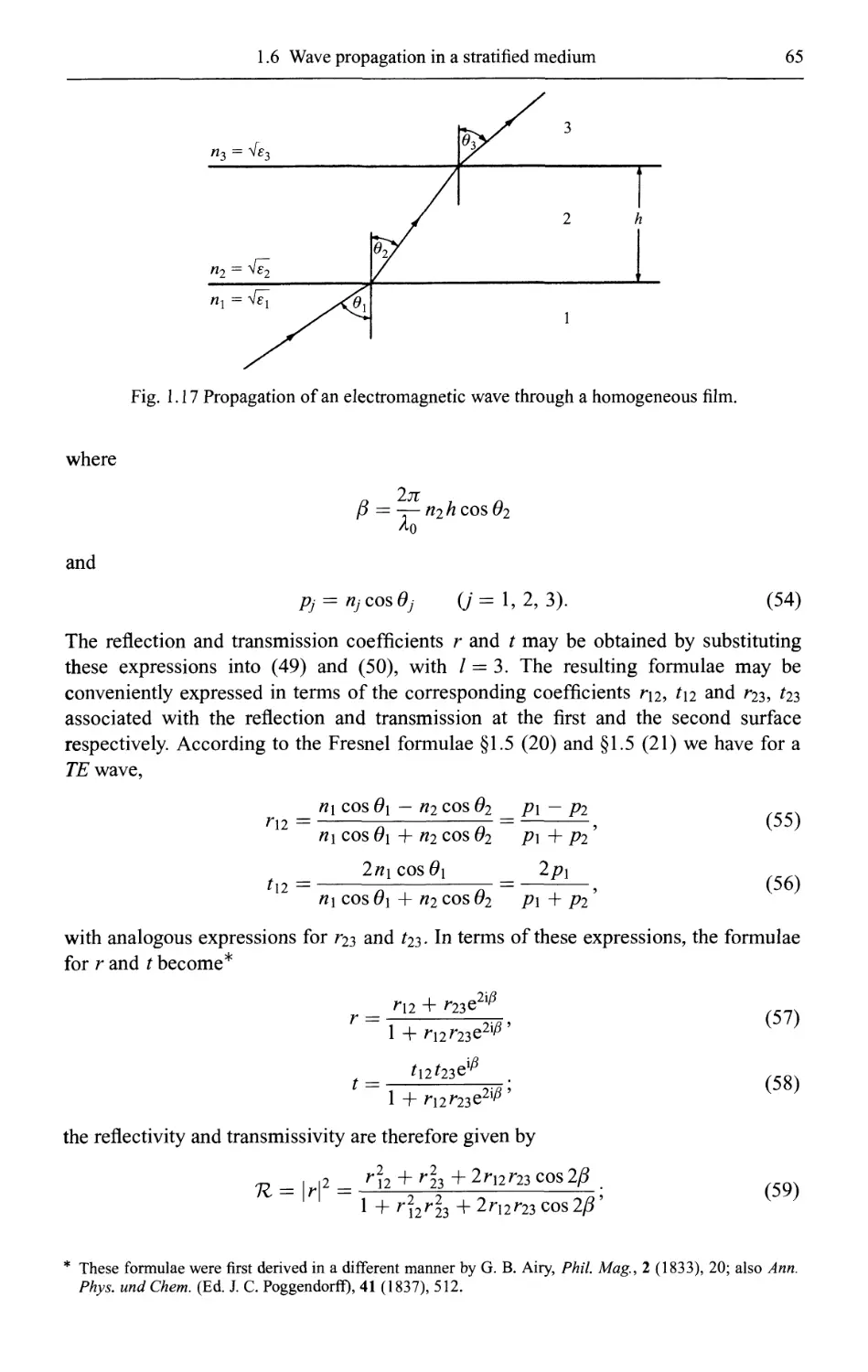
1.6.3 The reflection and transmission coefficients 63
1.6.4 A homogeneous dielectric film 64
1.6.5 Periodically stratified media 70
II Electromagnetic potentials and polarization 75
2.1 The electrodynamic potentials in the vacuum 76
xvi
Contents
xvii
2.1.1 The vector and scalar potentials 76
2.1.2 Retarded potentials 78
2.2 Polarization and magnetization 80
2.2.1 The potentials in terms of polarization and magnetization 80
2.2.2 Hertz vectors 84
2.2.3 The field of a linear electric dipole 85
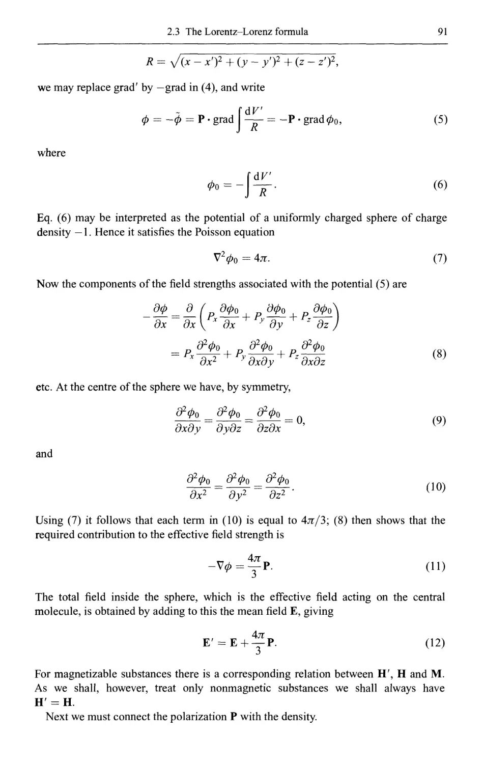
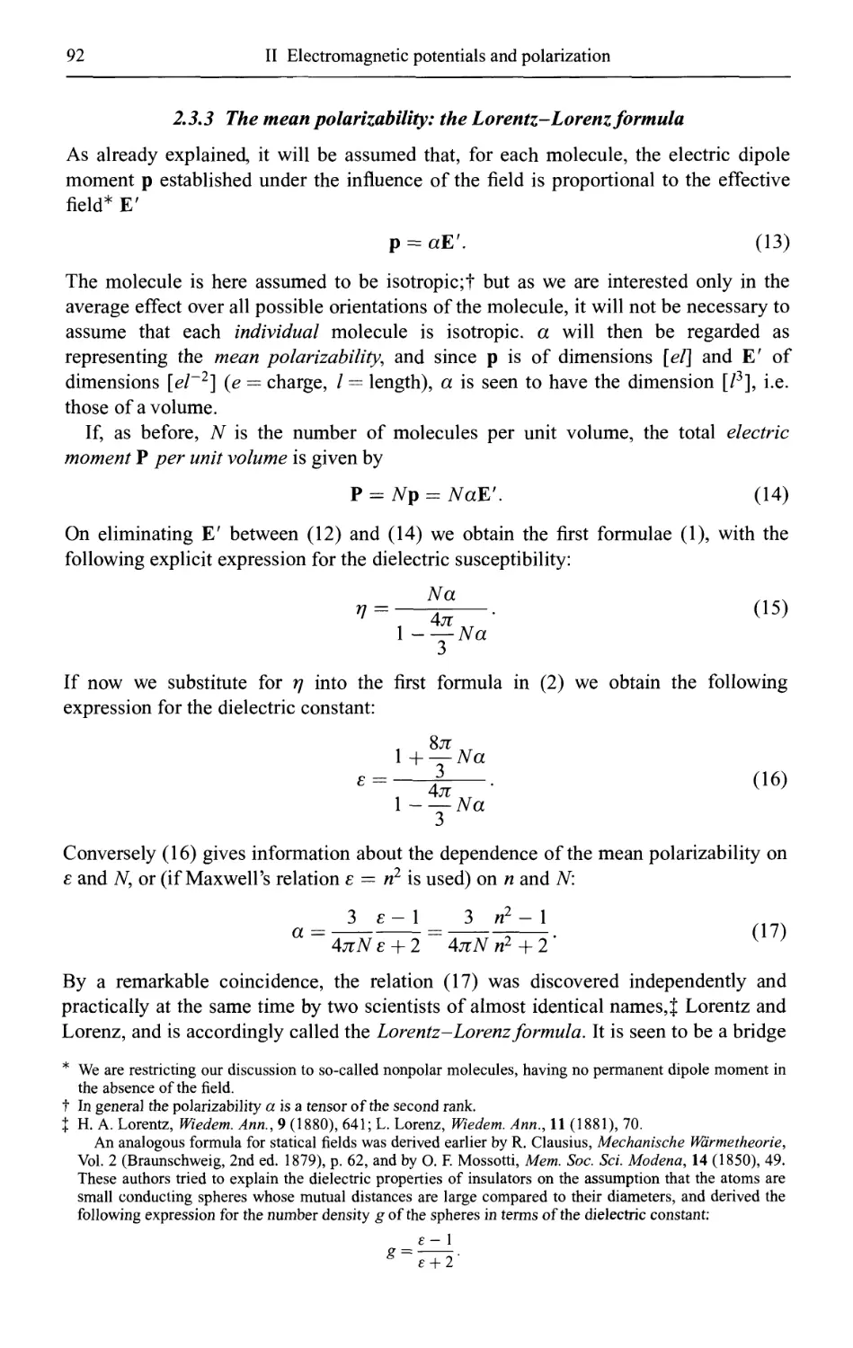
2.3 The Lorentz-Lorenz formula and elementary dispersion theory 89
2.3.1 The dielectric and magnetic susceptibilities 89
2.3.2 The effective field 90
2.3.3 The mean polarizability: the Lorentz-Lorenz formula 92
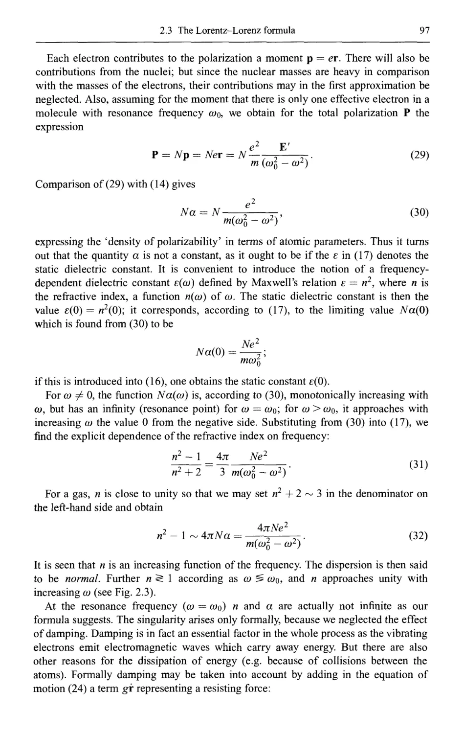
2.3.4 Elementary theory of dispersion 95
2.4 Propagation of electromagnetic waves treated by integral equations 103
2.4.1 The basic integral equation 104
2.4.2 The Ewald-Oseen extinction theorem and a rigorous derivation of the
Lorentz-Lorenz formula 105
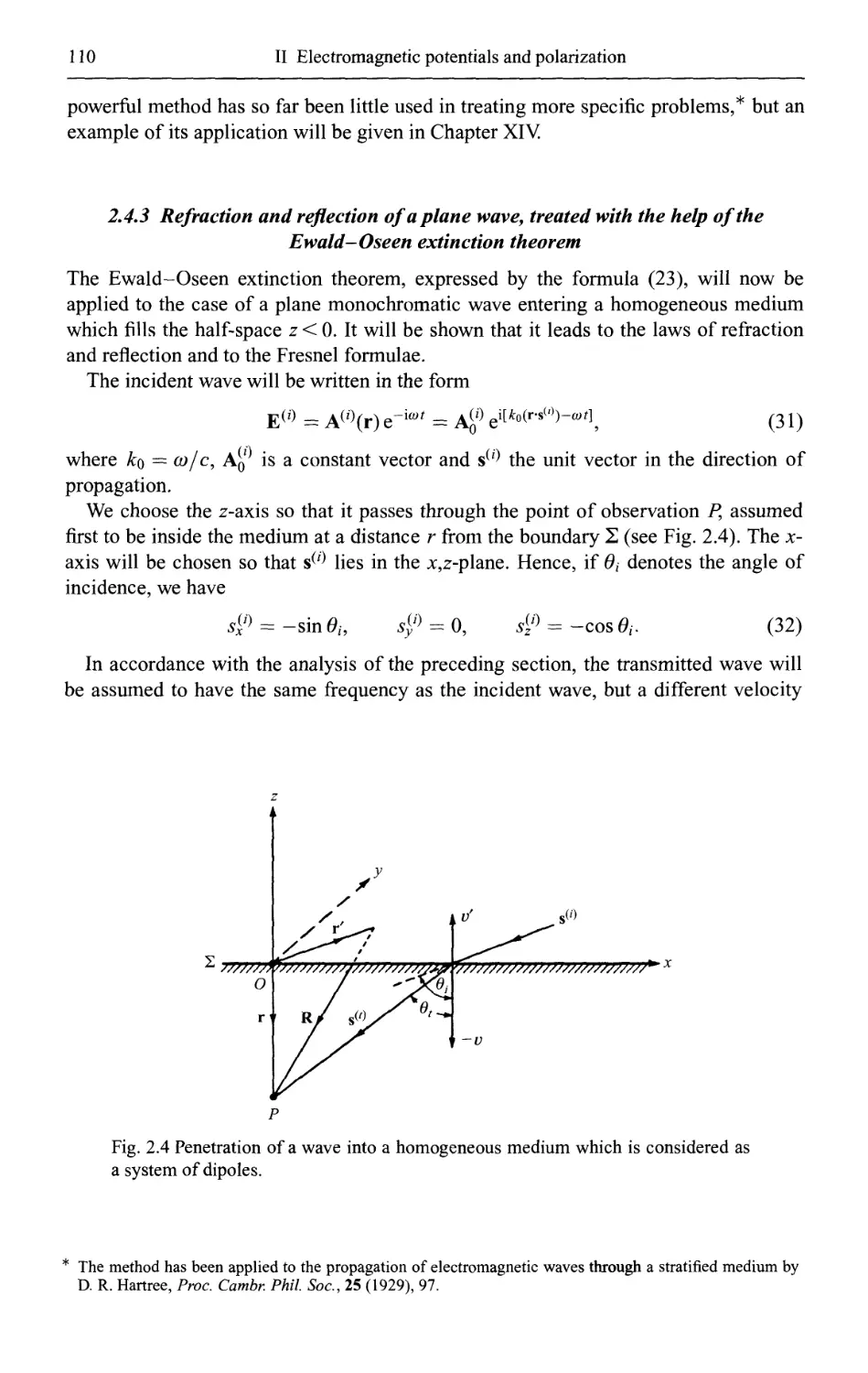
2.4.3 Refraction and reflection of a plane wave, treated with the help of the
Ewald-Oseen extinction theorem 110
III Foundations of geometrical optics 116
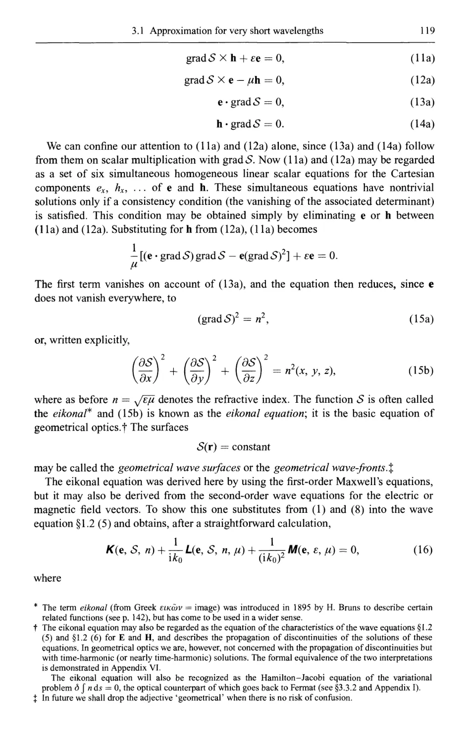
3.1 Approximation for very short wavelengths 116
3.1.1 Derivation of the eikonal equation 117
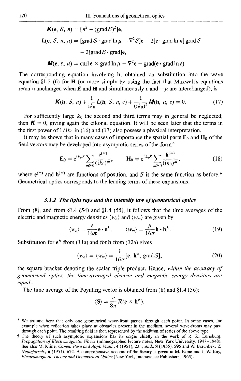
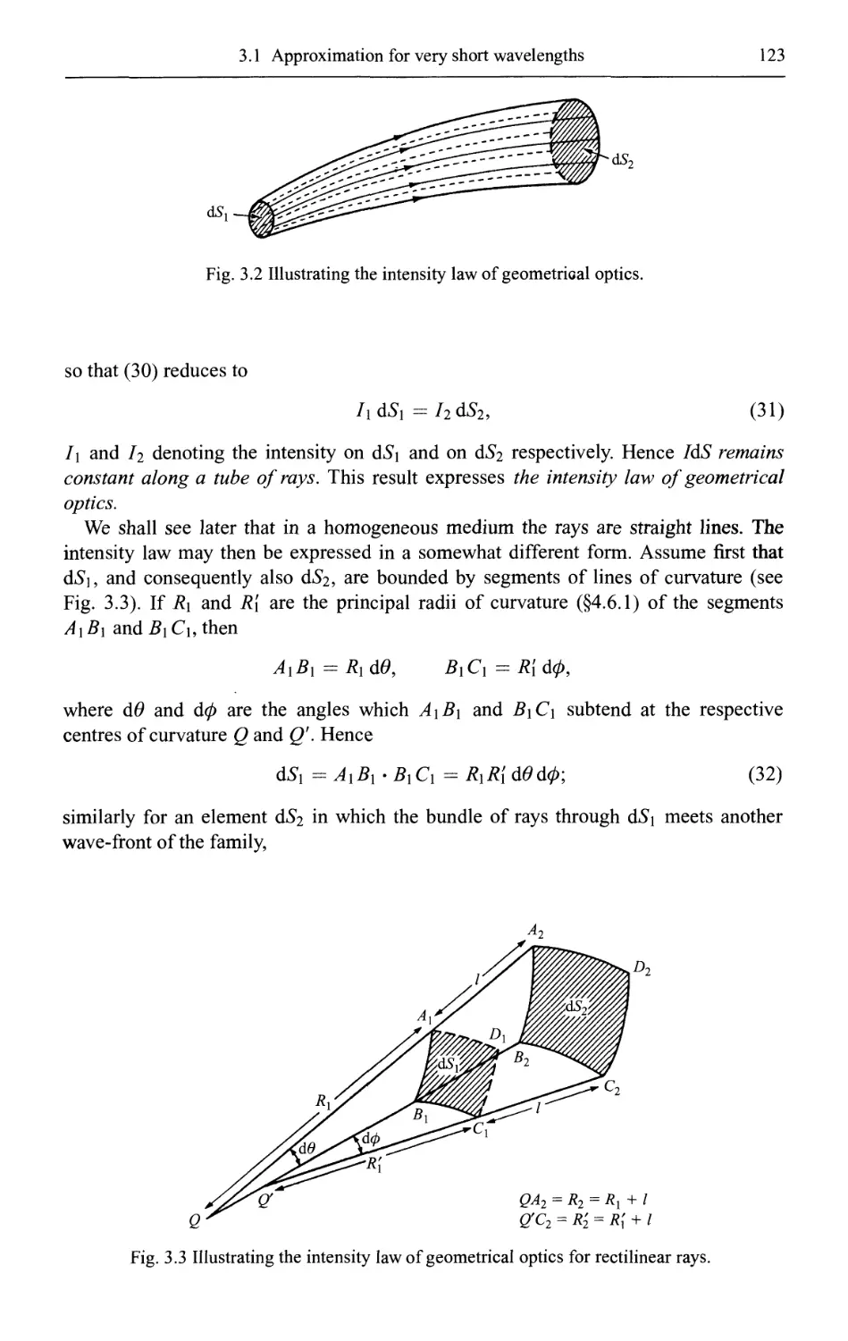
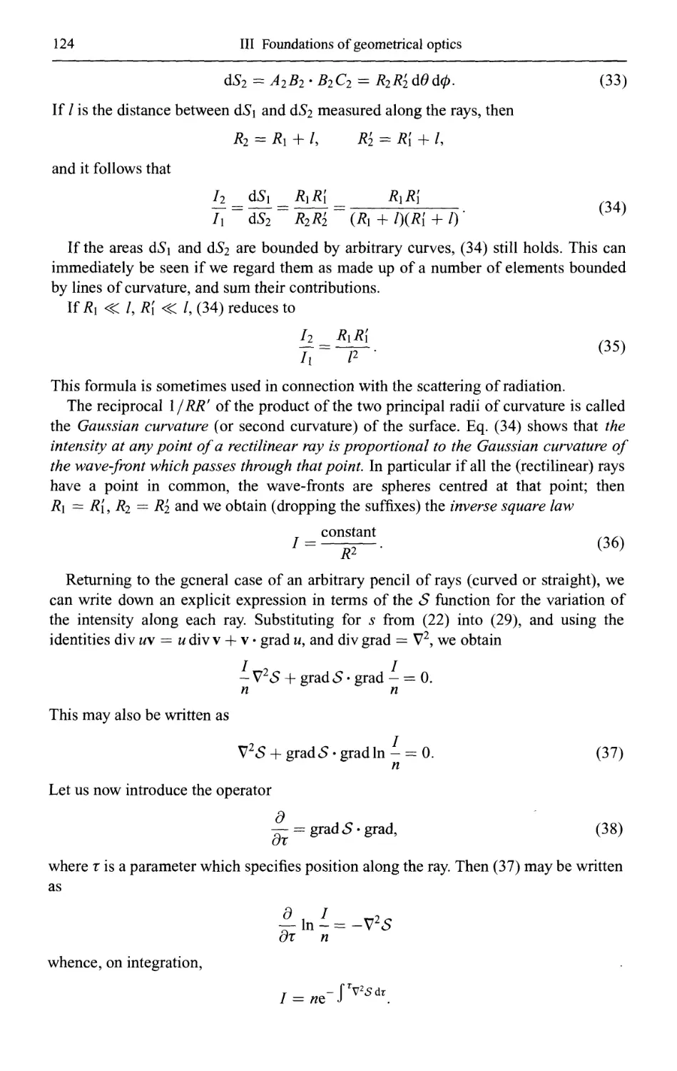
3.1.2 The light rays and the intensity law of geometrical optics 120
3.1.3 Propagation of the amplitude vectors 125
3.1.4 Generalizations and the limits of validity of geometrical optics 127
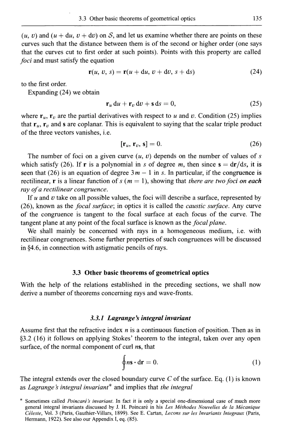
3.2 General properties of rays 129
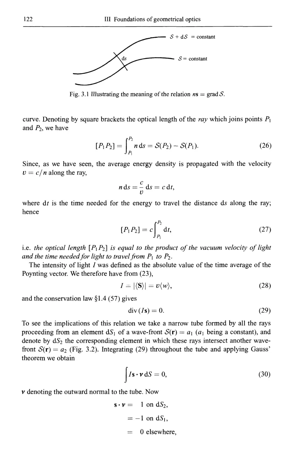
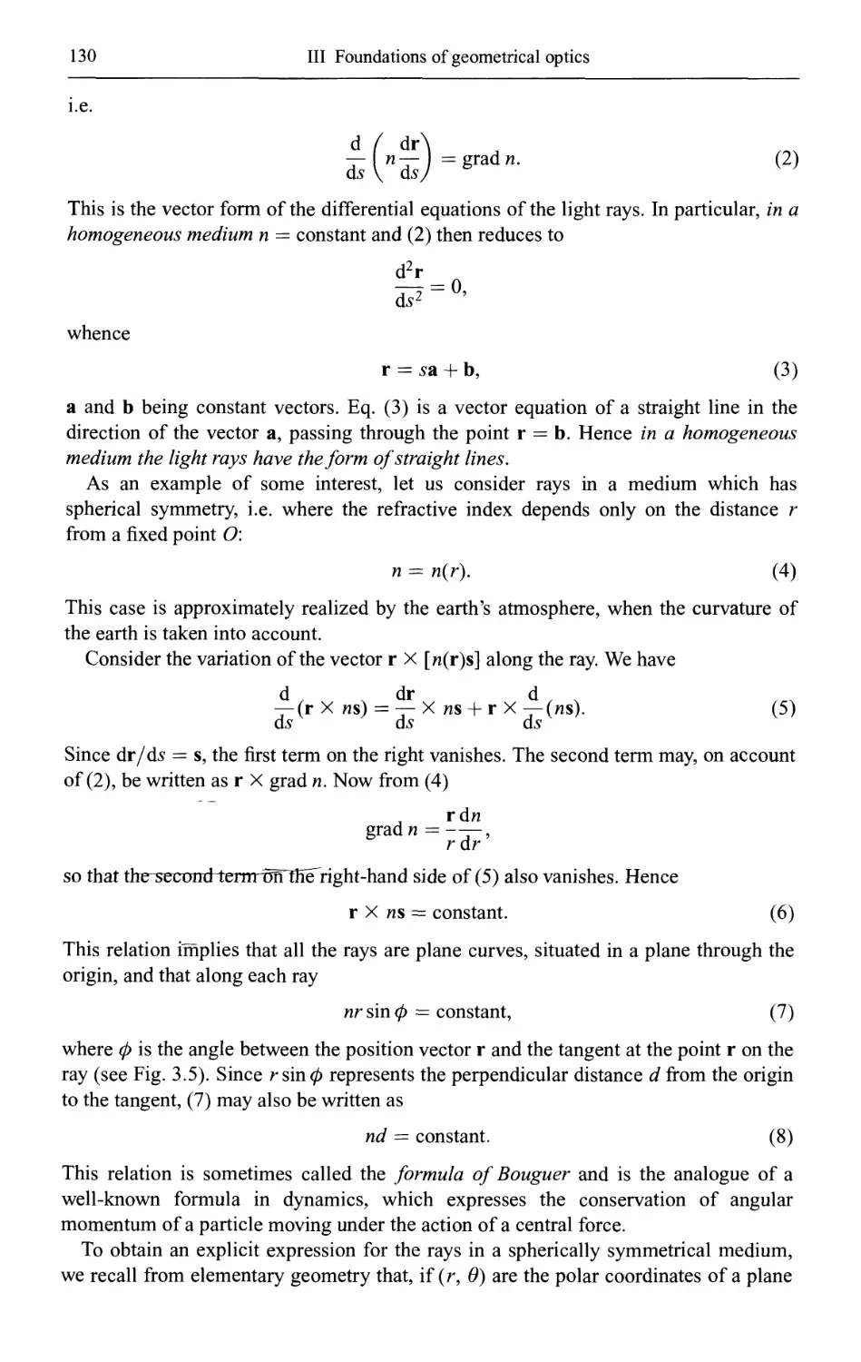
3.2.1 The differential equation of light rays 129
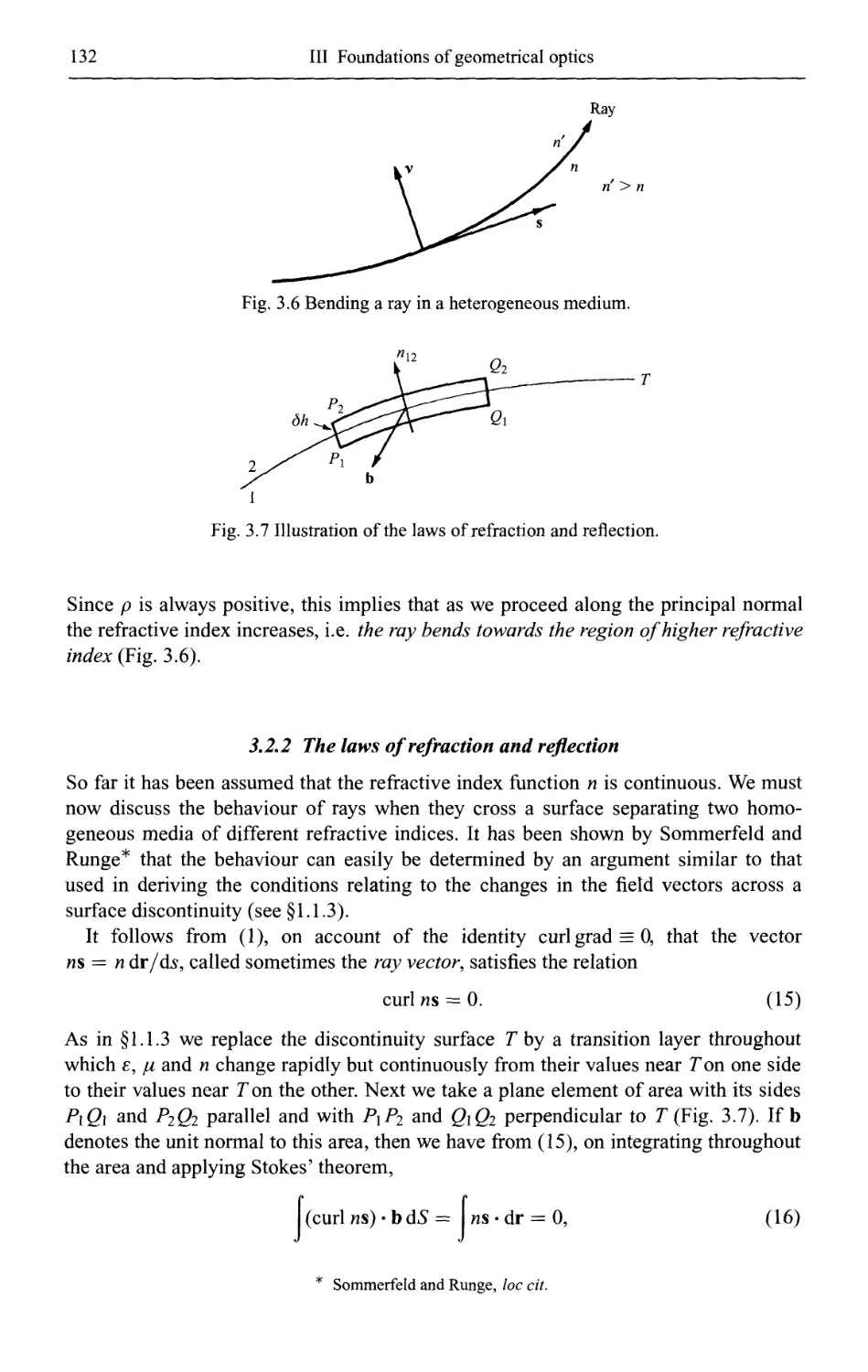
3.2.2 The laws of refraction and reflection 132
3.2.3 Ray congruences and their focal properties 134
3.3 Other basic theorems of geometrical optics 135
3.3.1 Lagrange 's integral invariant 13 5
3.3.2 The principle of Fermat 136
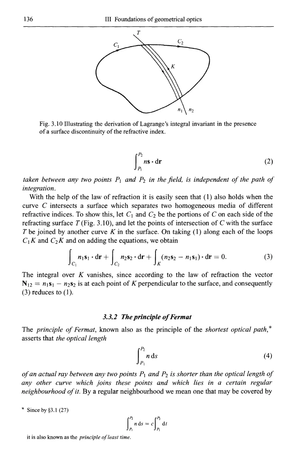
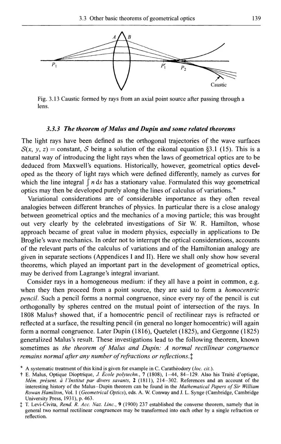
3.3.3 The theorem of Malus and Dupin and some related theorems 139
IV Geometrical theory of optical imaging 142
4.1 The characteristic functions of Hamilton 142
4.1.1 The point characteristic 142
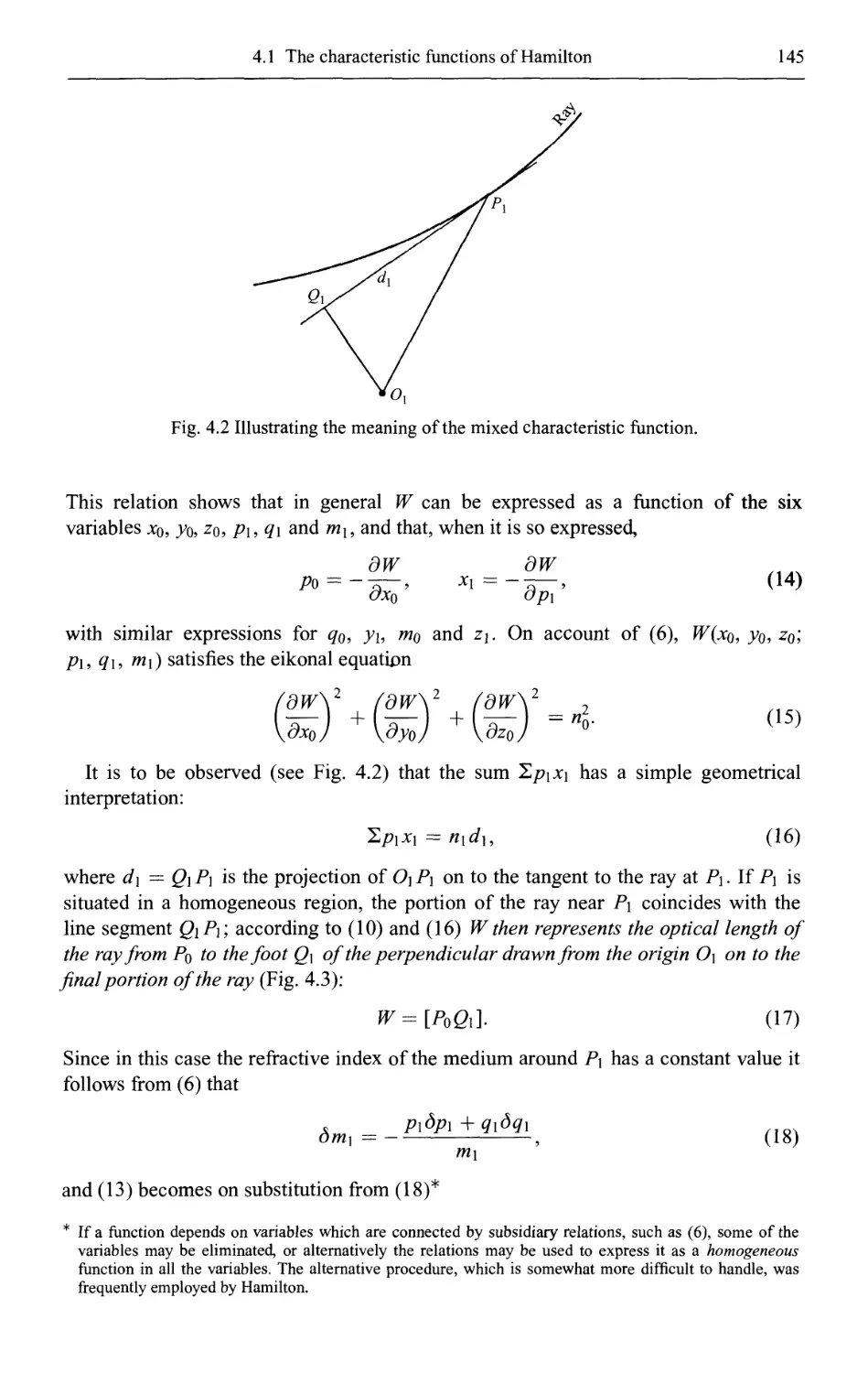
4.1.2 The mixed characteristic 144
4.1.3 The angle characteristic 146
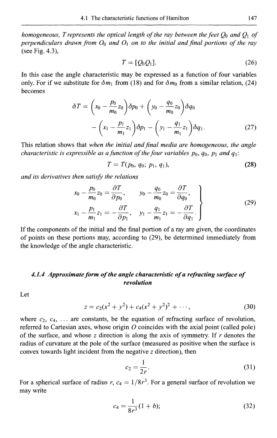
4.1.4 Approximate form of the angle characteristic of a refracting surface of
revolution 147
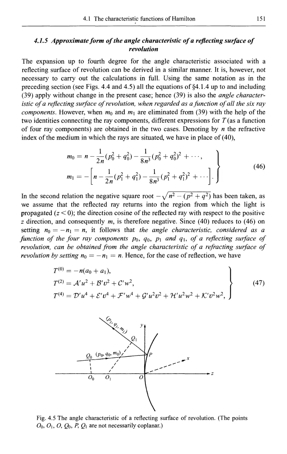
4.1.5 Approximate form of the angle characteristic of a reflecting surface of
revolution 151
4.2 Perfect imaging 152
4.2.1 General theorems 153
4.2.2 Maxwell's'fish-eye' 157
4.2.3 Stigmatic imaging of surfaces 159
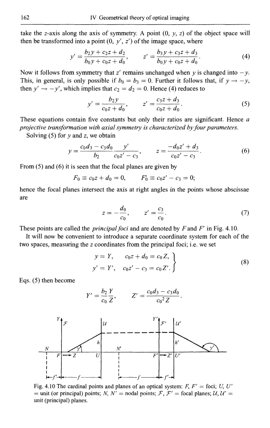
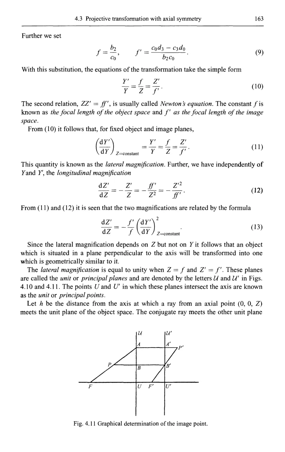
4.3 Projective transformation (collineation) with axial symmetry 160
4.3.1 General formulae 161
4.3.2 The telescopic case 164
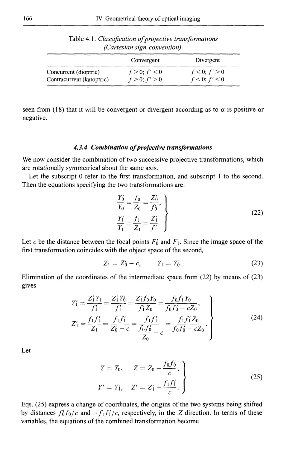
4.3.3 Classification of projective transformations 165
4.3.4 Combination of projective transformations 166
4.4 Gaussian optics 167
4.4.1 Refracting surface of revolution 167
XVlll
Contents
4.4.2 Reflecting surface of revolution 170
4.4.3 The thick lens 171
4.4.4 The thin lens 174
4.4.5 The general centred system 175
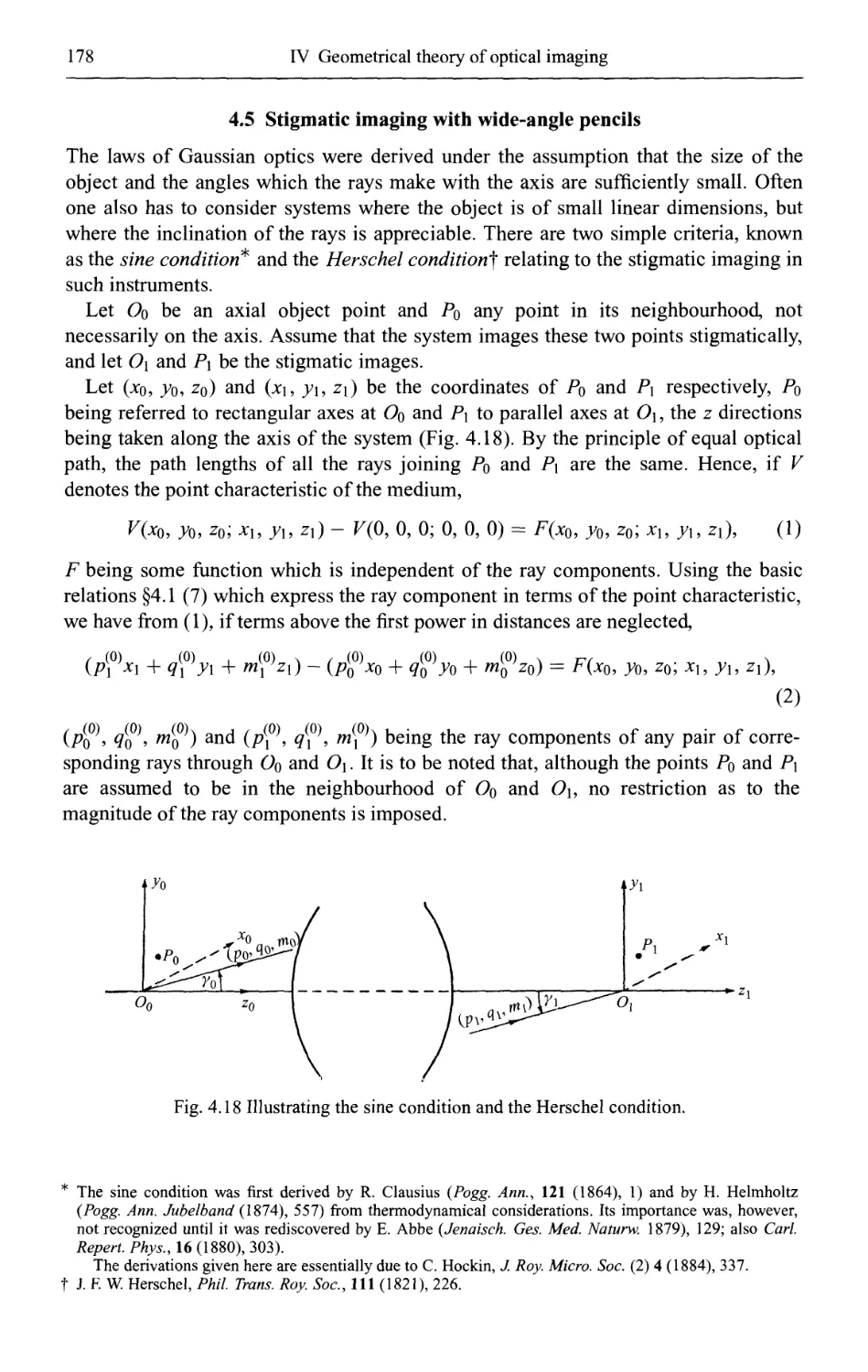
4.5 Stigmatic imaging with wide-angle pencils 178
4.5.1 The sine condition 179
4.5.2 The Herschel condition 180
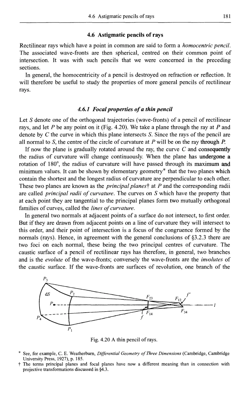
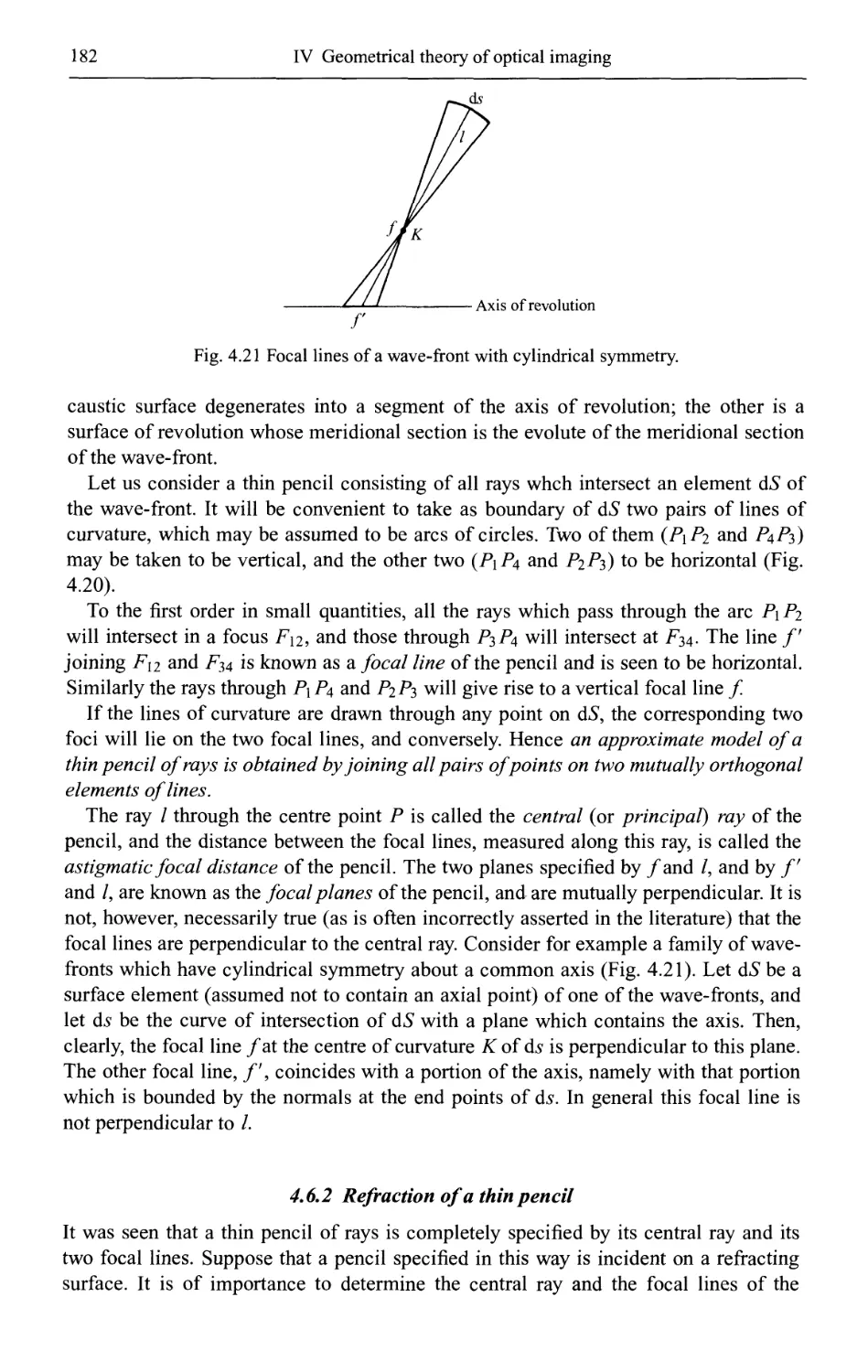
4.6 Astigmatic pencils of rays 181
4.6.1 Focal properties of a thin pencil 181
4.6.2 Refraction of a thin pencil 182
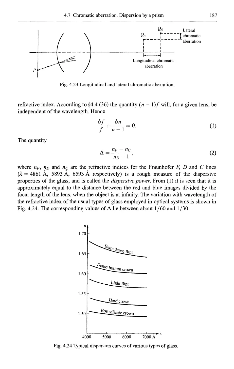
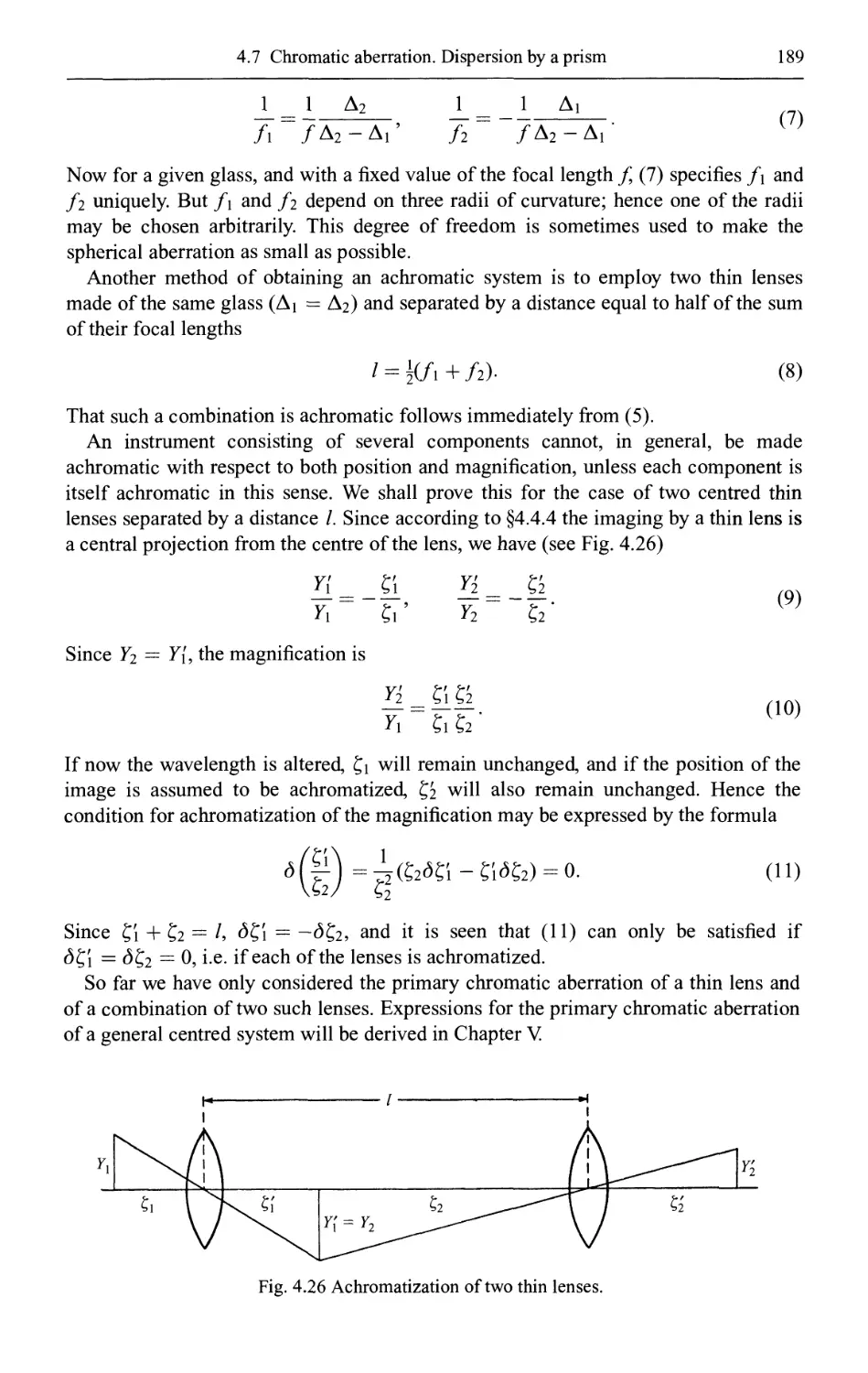
4.7 Chromatic aberration. Dispersion by a prism 186
4.7.1 Chromatic aberration 186
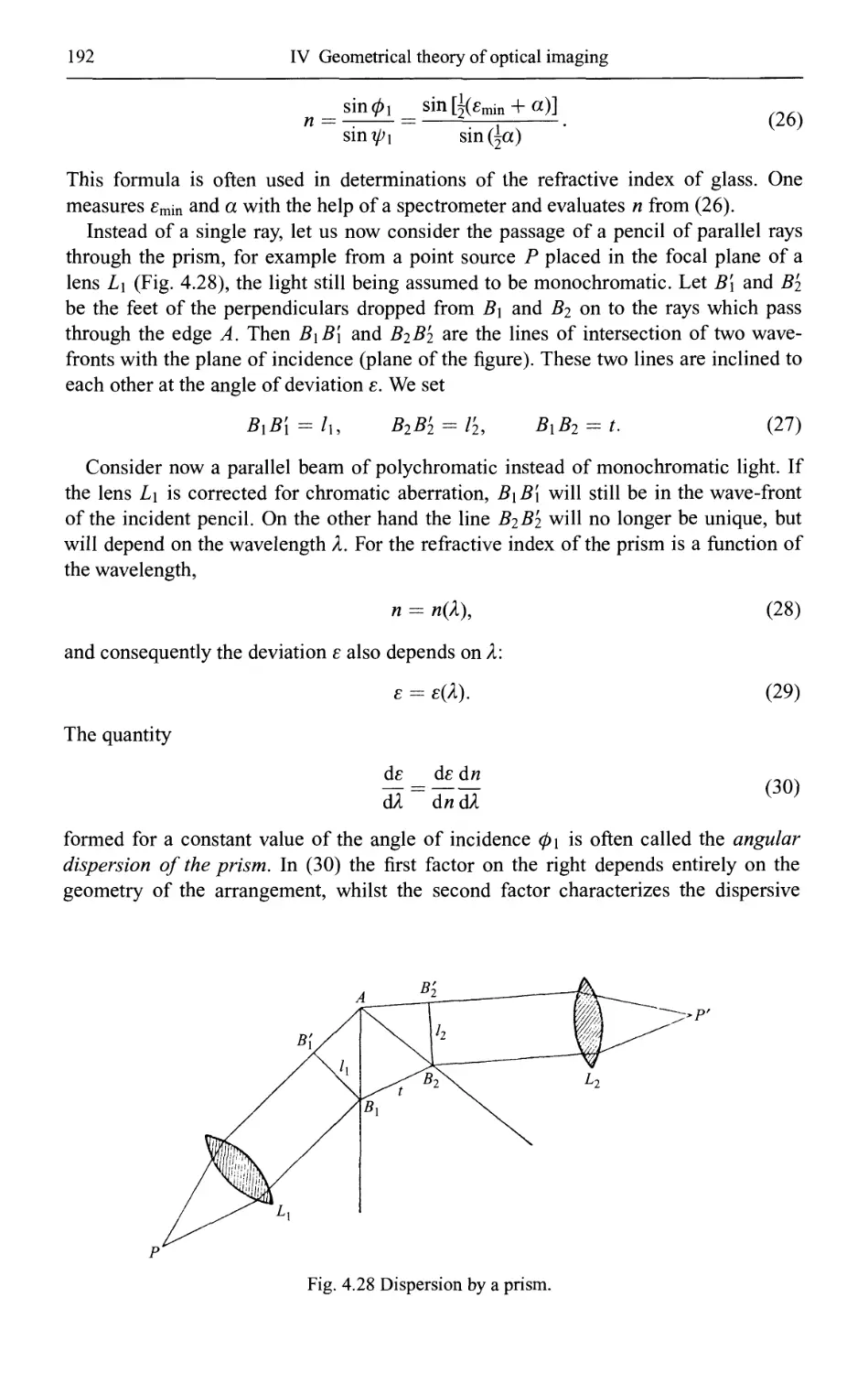
4.7.2 Dispersion by a prism 190
4.8 Radiometry and apertures 193
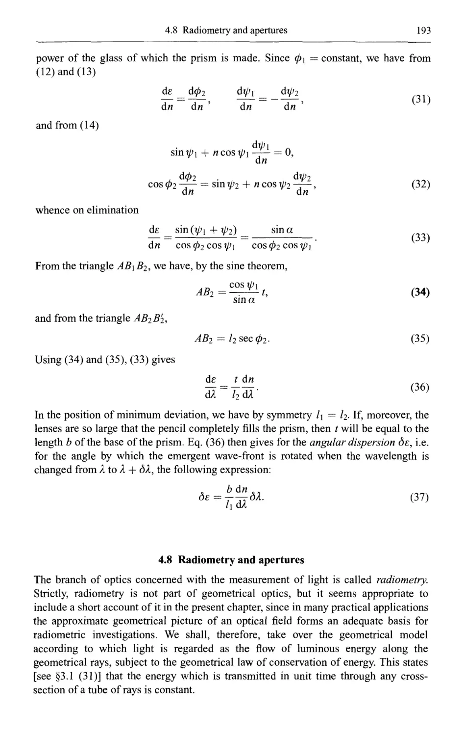
4.8.1 Basic concepts of radiometry 194
4.8.2 Stops and pupils 199
4.8.3 Brightness and illumination of images 201
4.9 Ray tracing 204
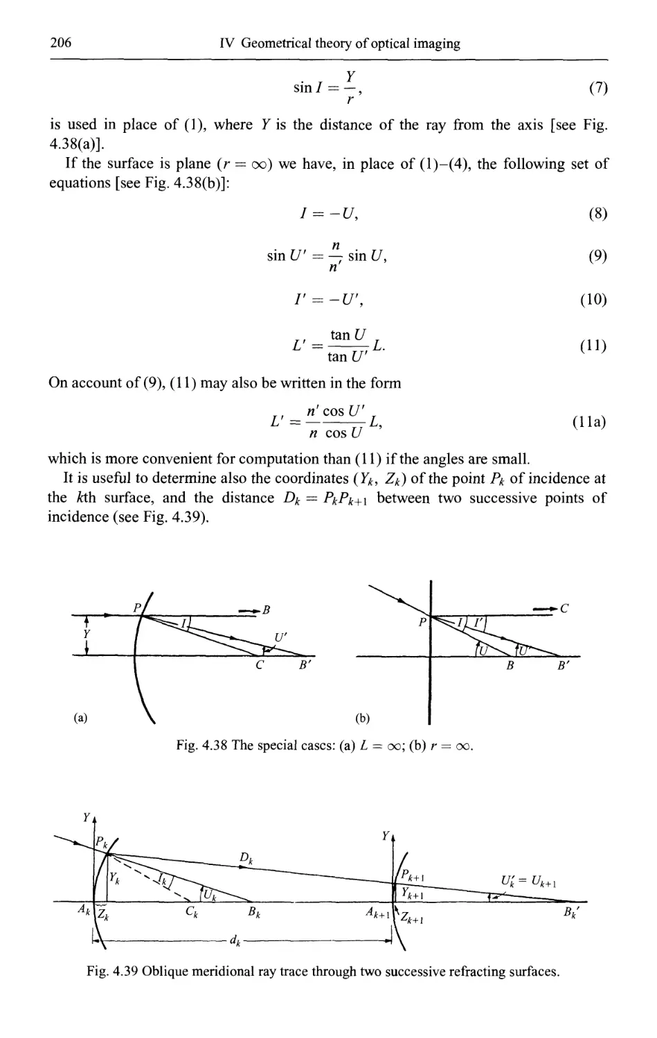
4.9.1 Oblique meridional rays 204
4.9.2 Paraxial rays 207
4.9.3 Skew rays 208
4.10 Design of aspheric surfaces 211
4.10.1 Attainment of axial stigmatism 211
4.10.2 Attainment of aplanatism 214
4.11 Image-reconstruction from projections (computerized tomography) 217
4.11.1 Introduction 217
4.11.2 Beam propagation in an absorbing medium 218
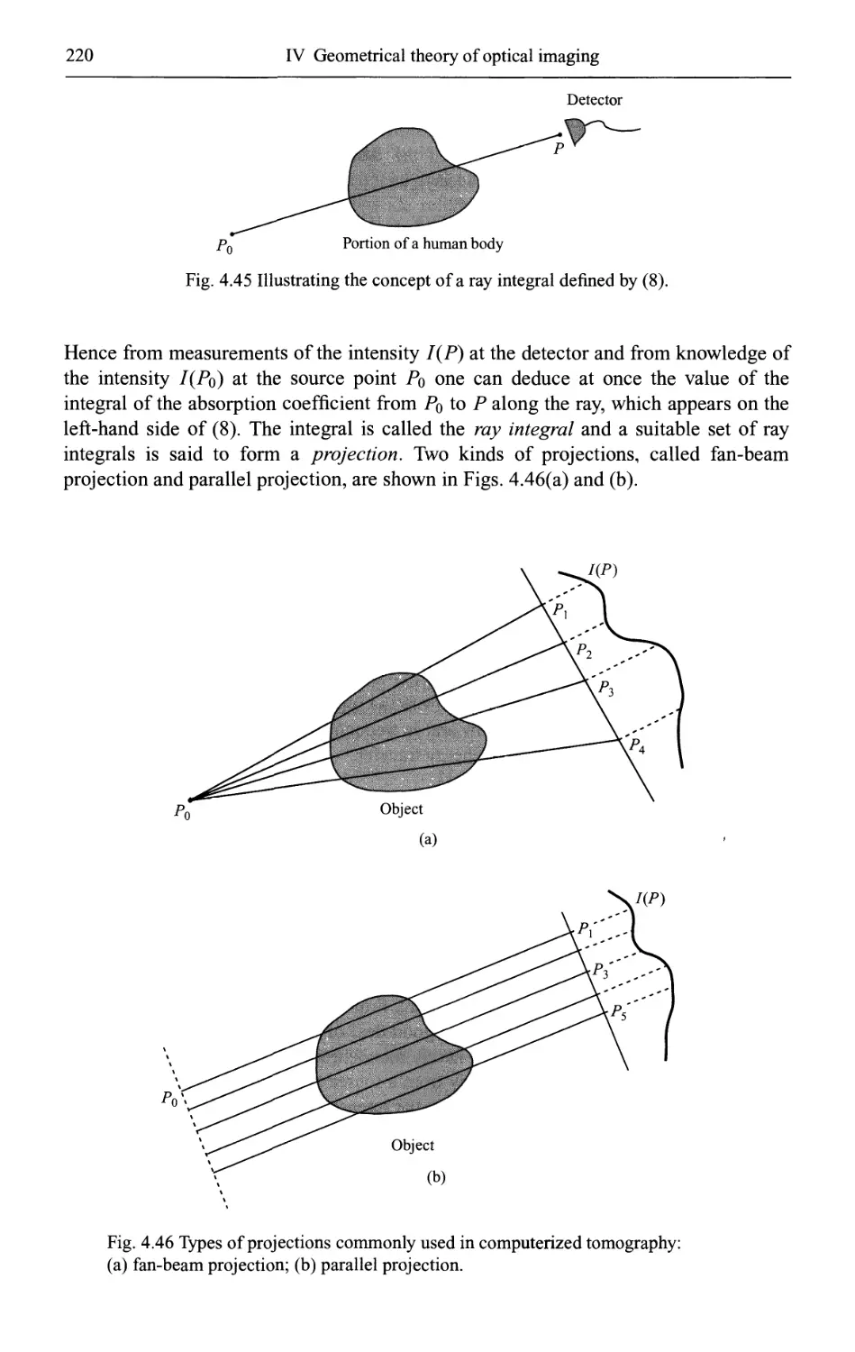
4.11.3 Ray integrals and projections 219
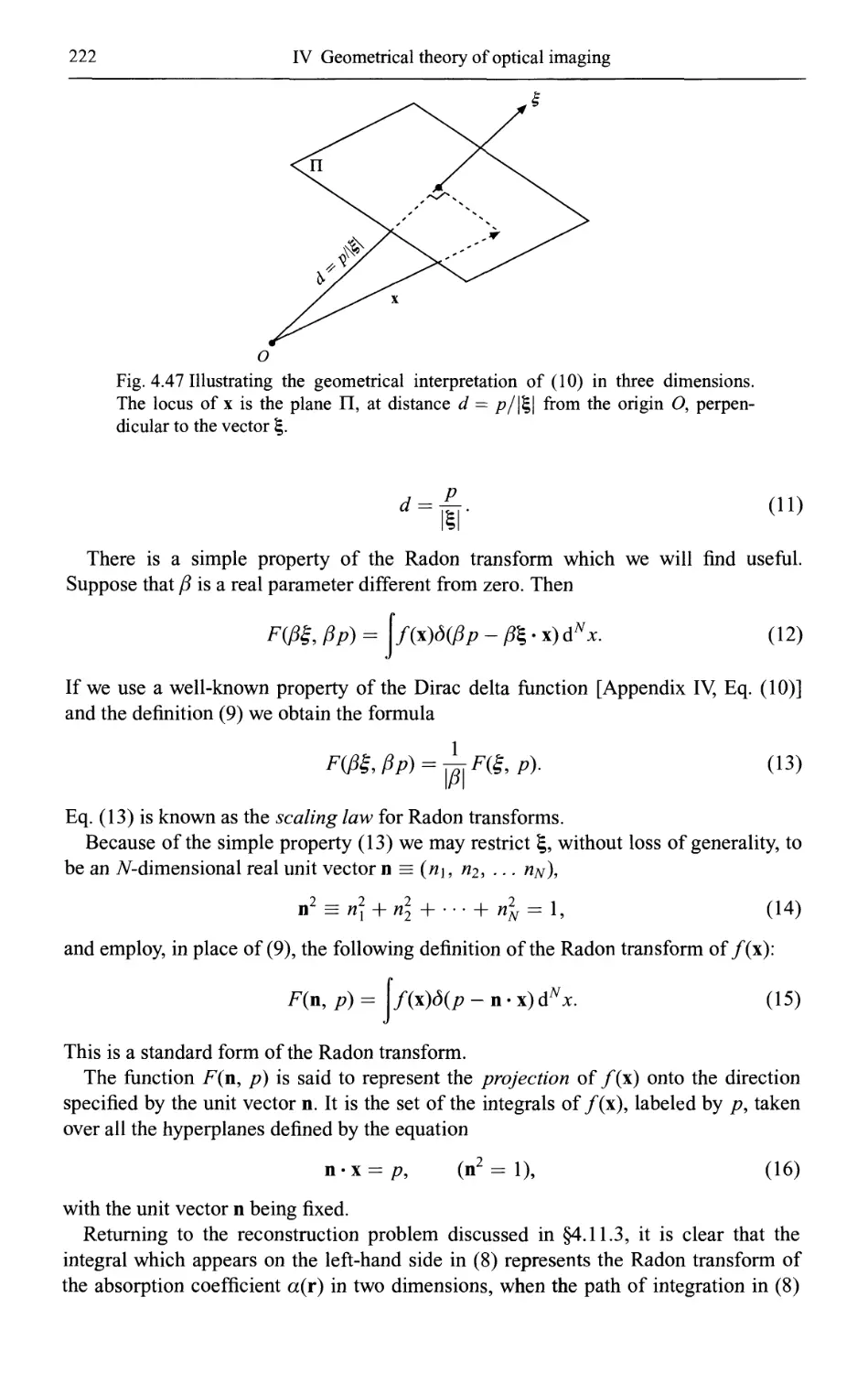
4.11.4 The Af-dimensional Radon transform 221
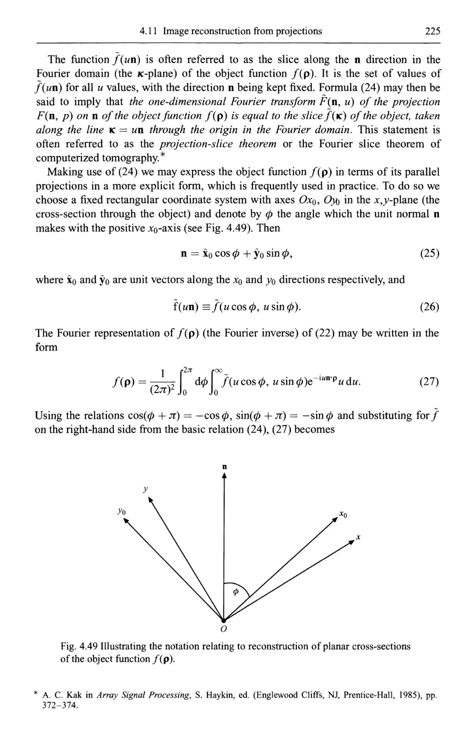
4.11.5 Reconstruction of cross-sections and the projection-slice theorem of
computerized tomography 223
V Geometrical theory of aberrations 228
5.1 Wave and ray aberrations; the aberration function 229
5.2 The perturbation eikonal of Schwarzschild 233
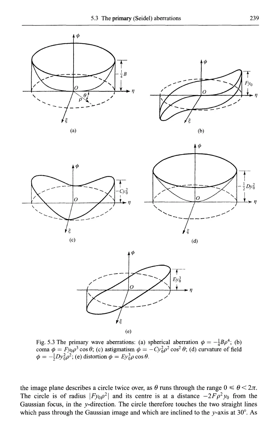
5.3 The primary (Seidel) aberrations 236
(a) Spherical aberration (B ^ 0) 238
(b) Coma (F ^0) 238
(c) Astigmatism (C ^ 0) and curvature of field (D ^ 0) 240
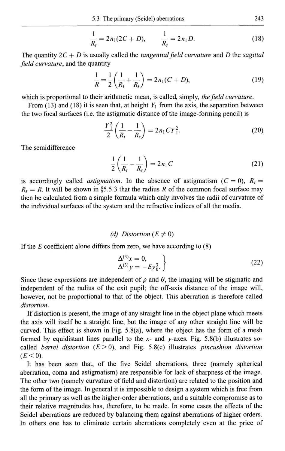
(d) Distortion (E ^ 0) 243
5.4 Addition theorem for the primary aberrations 244
5.5 The primary aberration coefficients of a general centred lens system 246
5.5.1 The Seidel formulae in terms of two paraxial rays 246
5.5.2 The Seidel formulae in terms of one paraxial ray 251
5.5.3 Petzval's theorem 253
5.6 Example: The primary aberrations of a thin lens 254
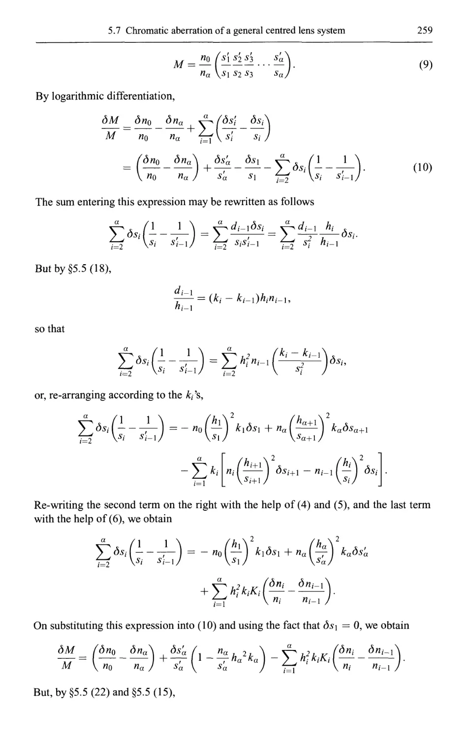
5.7 The chromatic aberration of a general centred lens system 257
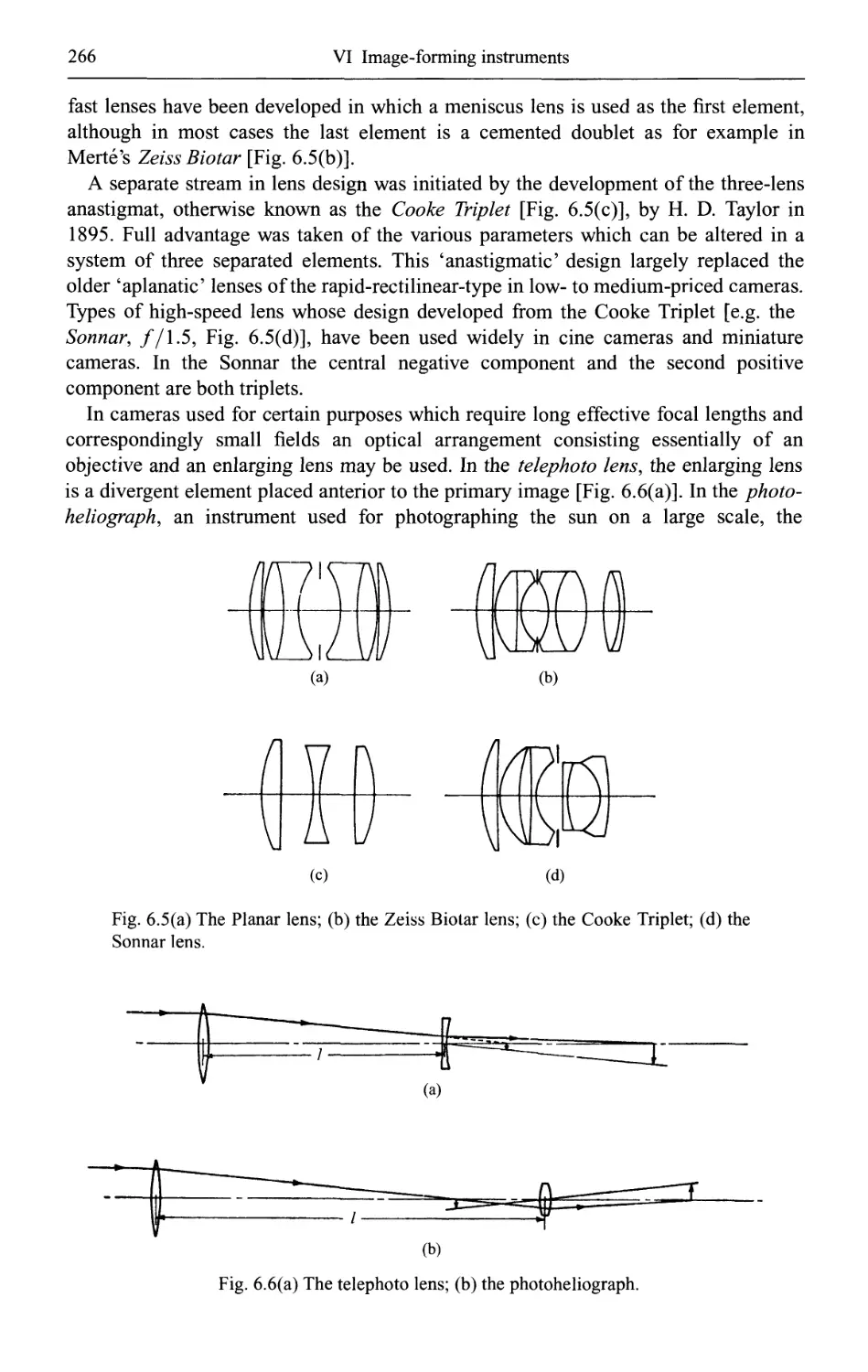
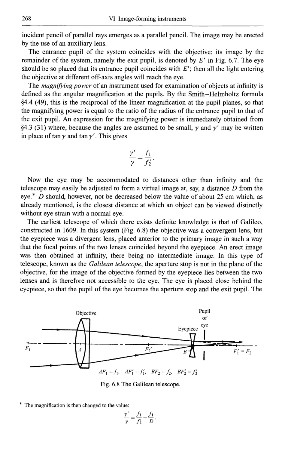
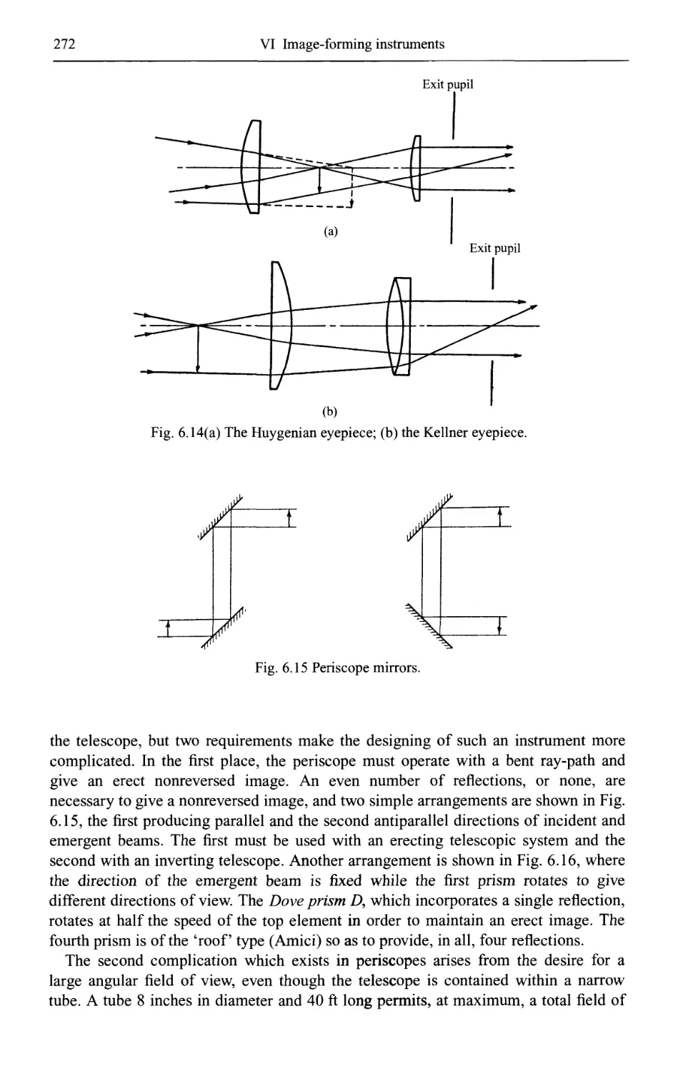
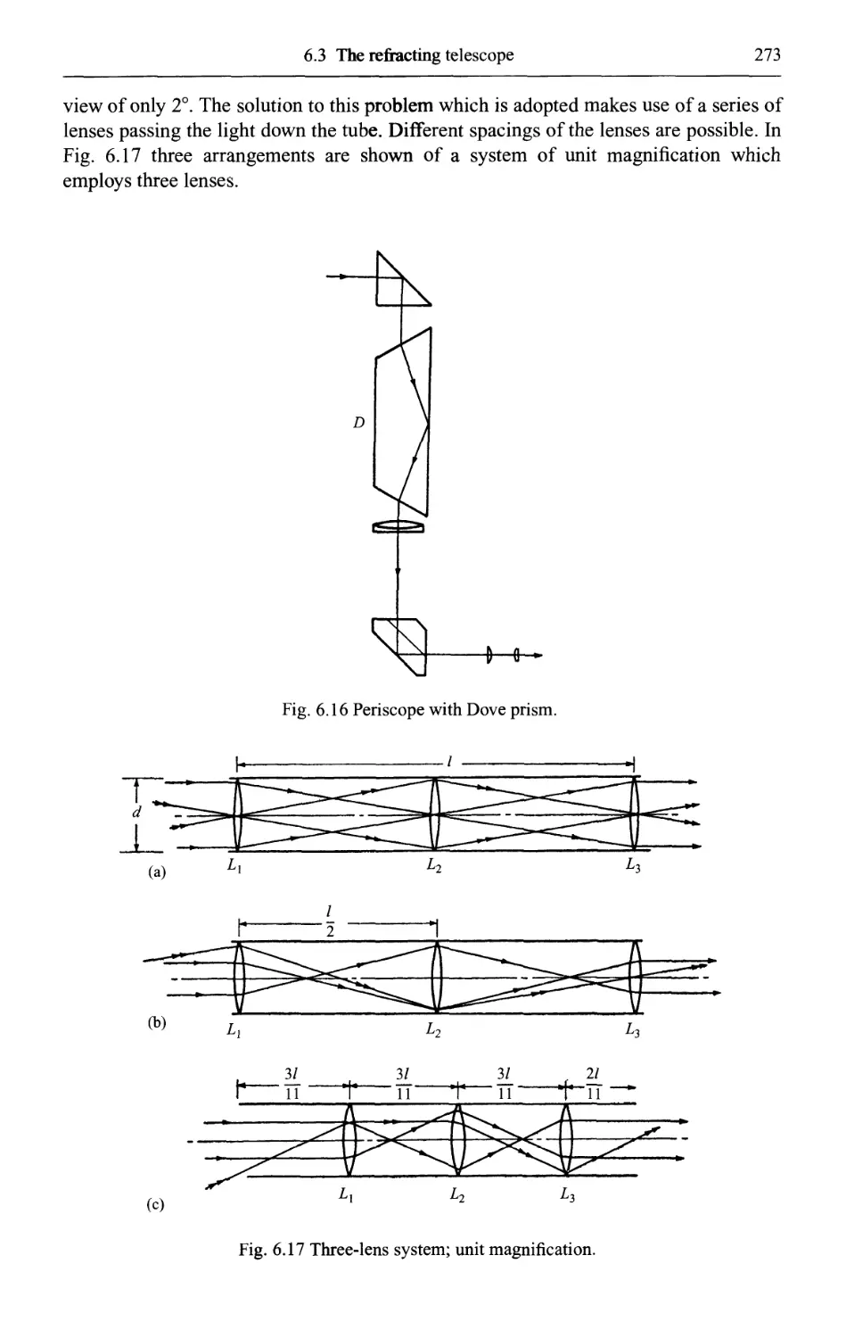
VI Image-forming instruments 261
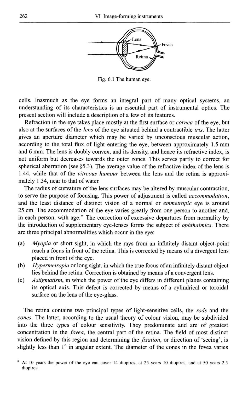
6.1 The eye 261
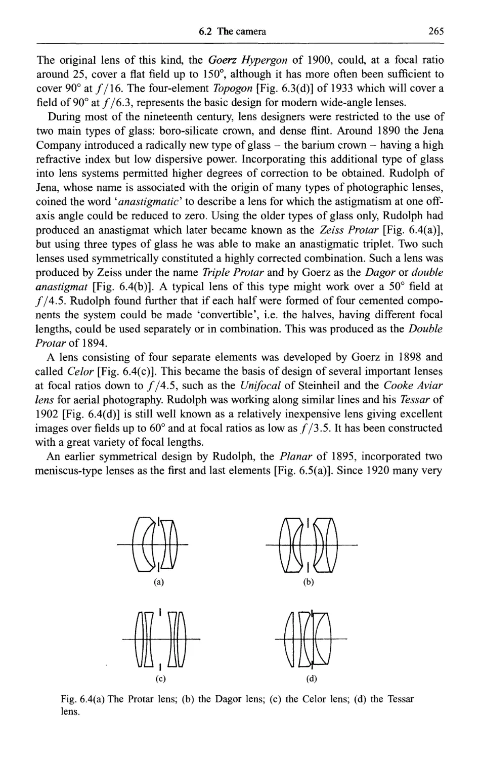
6.2 The camera 263
6.3 The refracting telescope 267
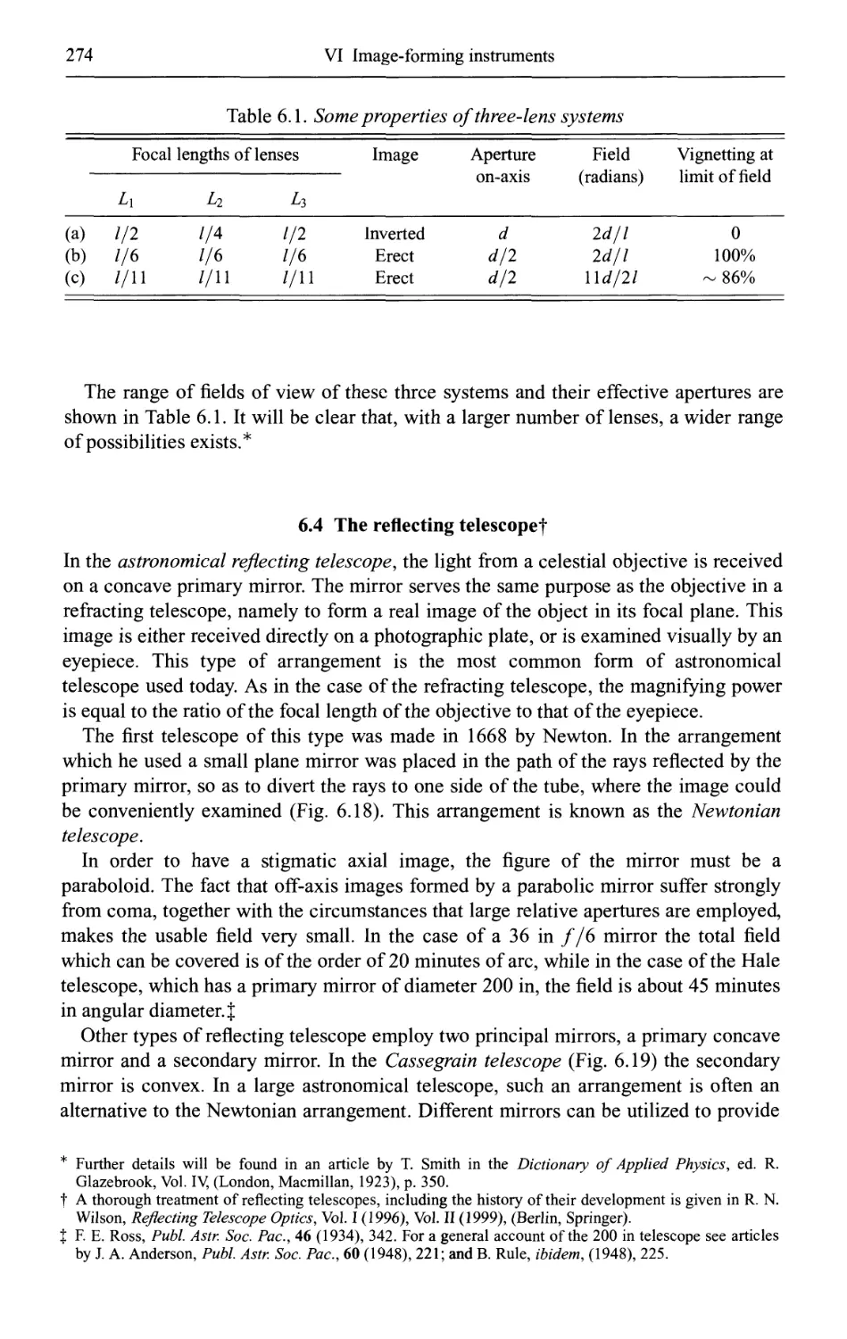
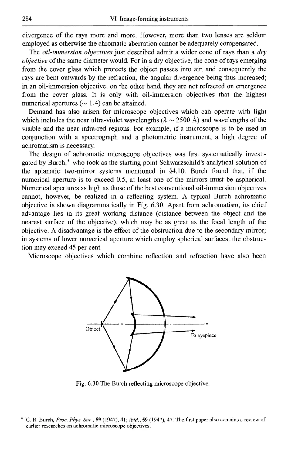
6.4 The reflecting telescope 274
Contents
xix
6.5 Instruments of illumination 279
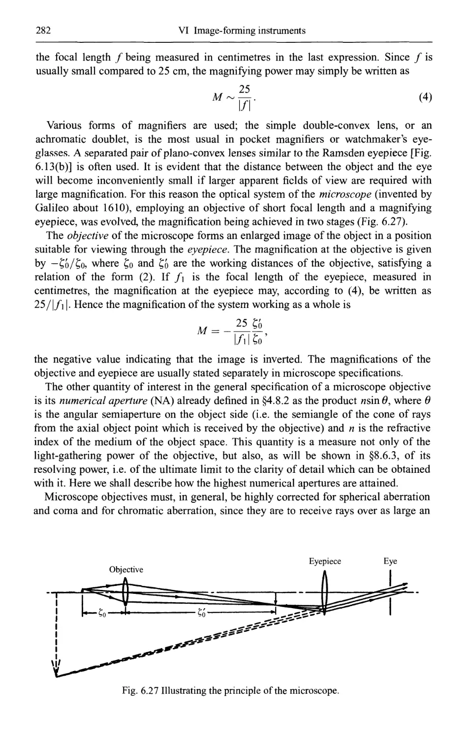
6.6 The microscope 281
VII Elements of the theory of interference and interferometers 286
7.1 Introduction 286
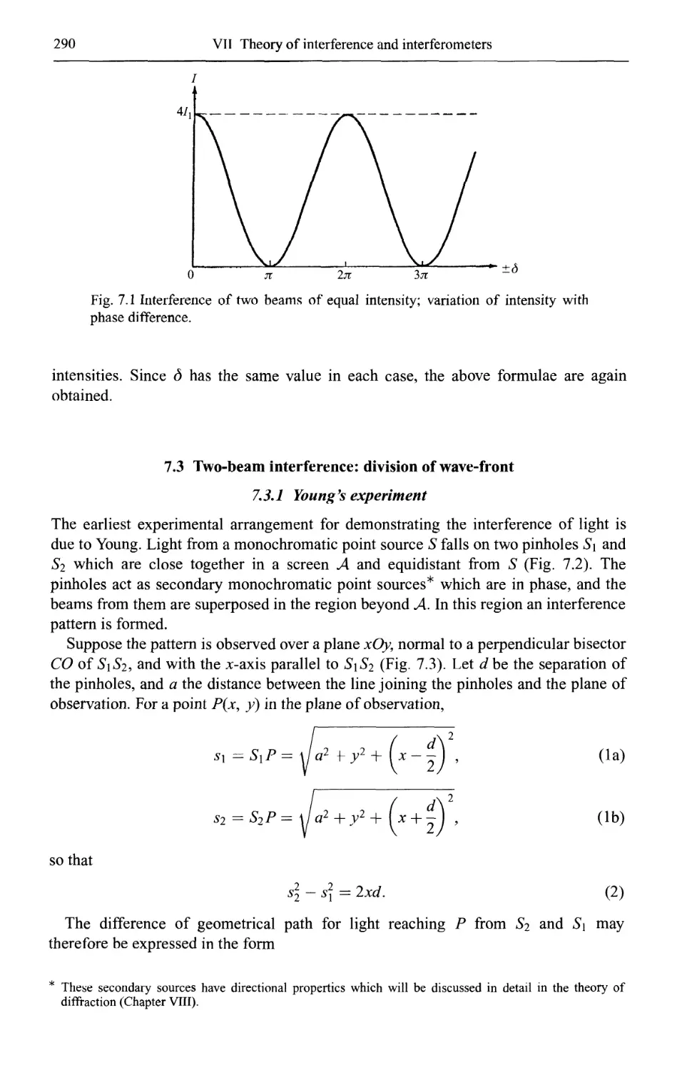
7.2 Interference of two monochromatic waves 287
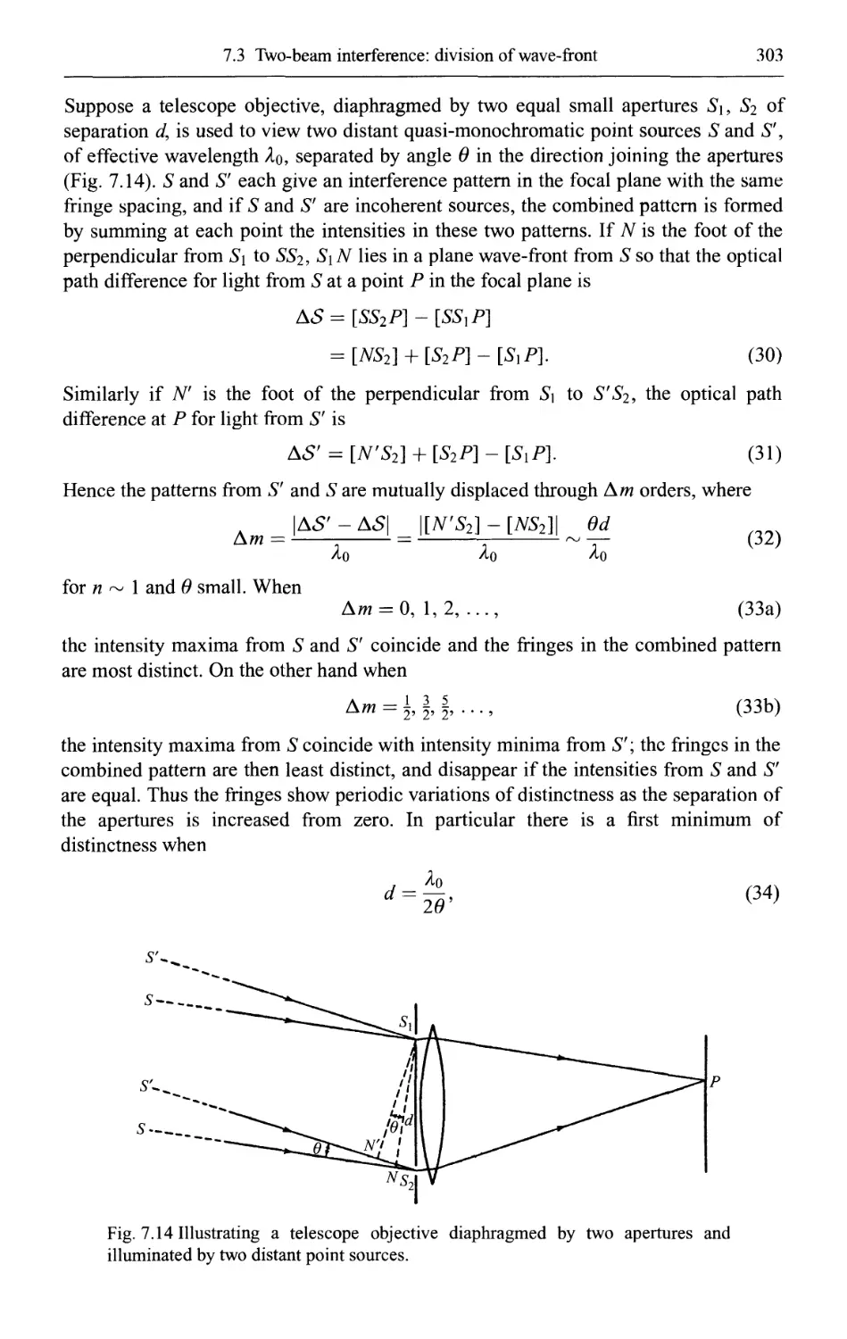
7.3 Two-beam interference: division of wave-front 290
7.3.1 Young's experiment 290
7.3.2 Fresnel's mirrors and similar arrangements 292
7.3.3 Fringes with quasi-monochromatic and white light 295
7.3.4 Use of slit sources; visibility of fringes 296
7.3.5 Application to the measurement of optical path difference: the Rayleigh
interferometer 299
7.3.6 Application to the measurement of angular dimensions of sources:
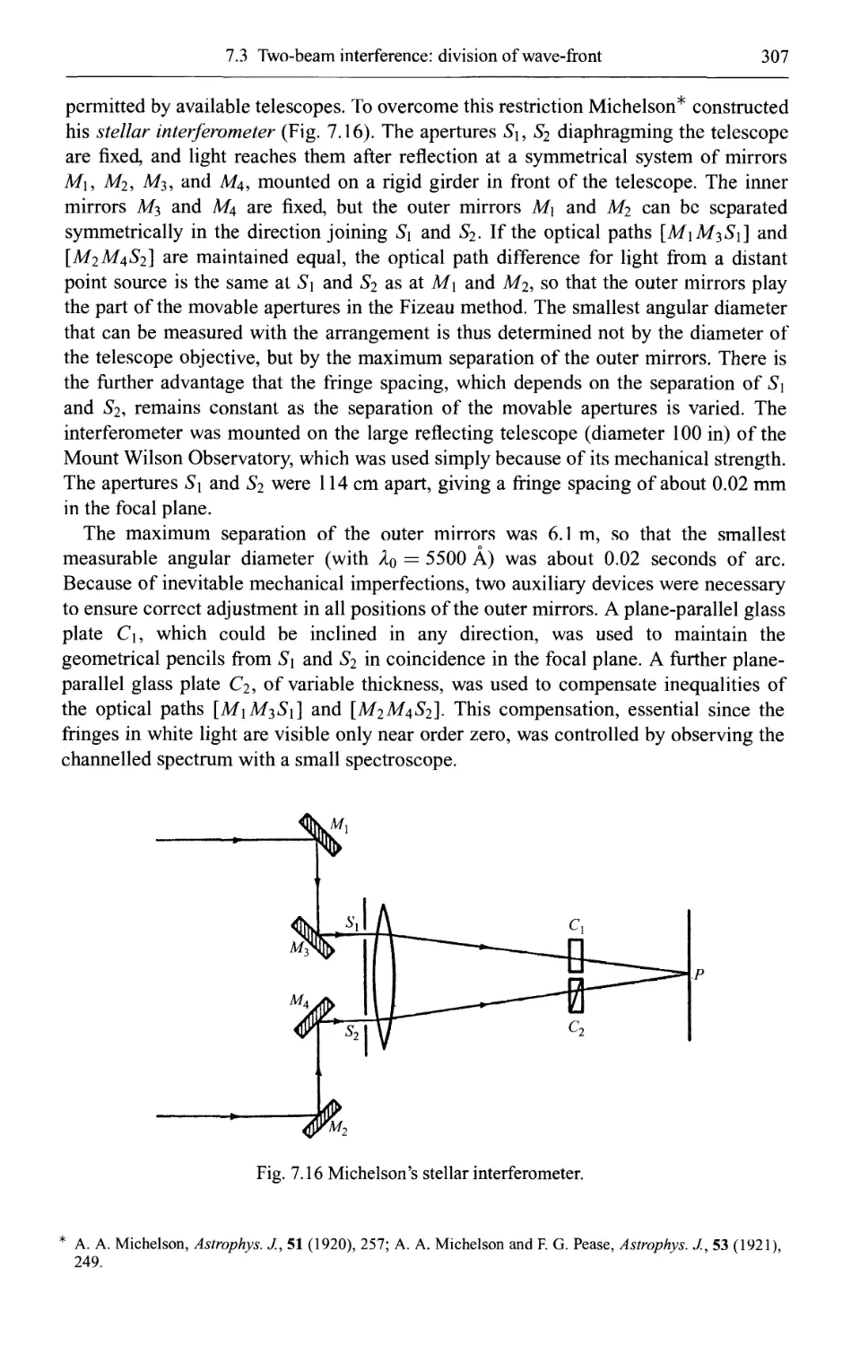
the Michelson stellar interferometer 302
7.4 Standing waves 308
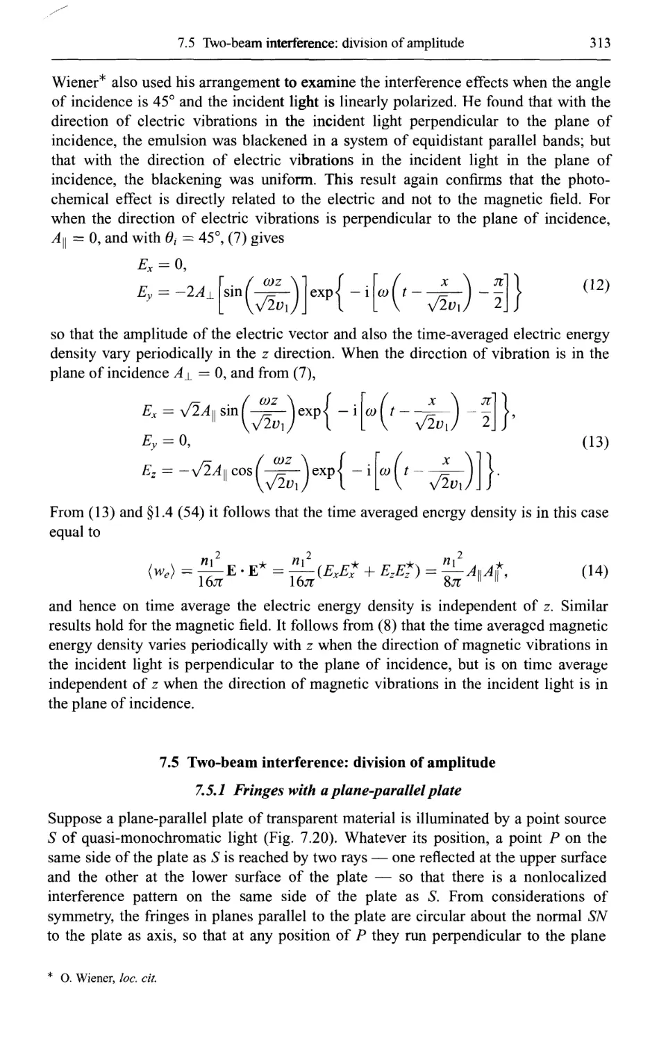
7.5 Two-beam interference: division of amplitude 313
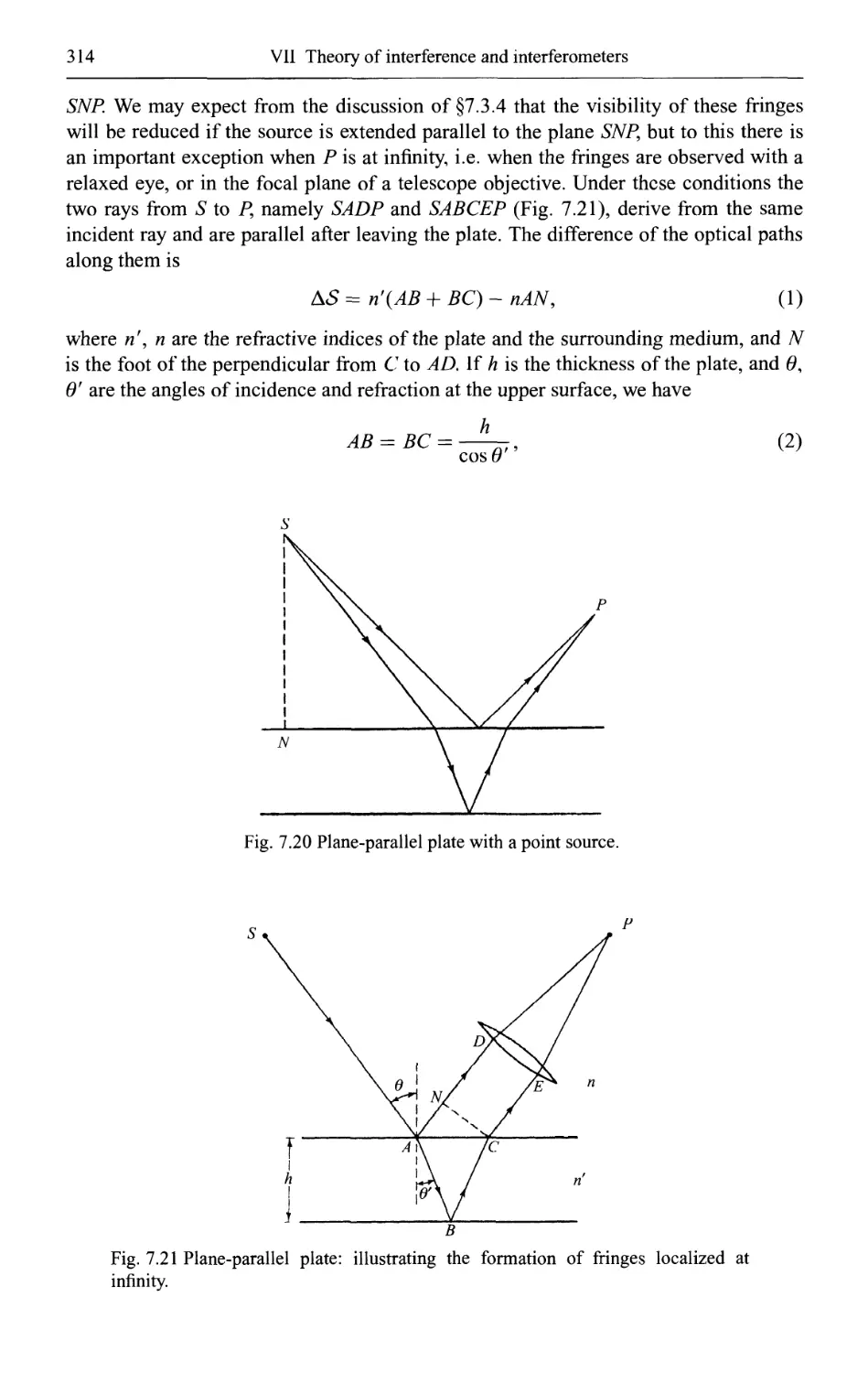
7.5.1 Fringes with a plane-parallel plate 313
7.5.2 Fringes with thin films; the Fizeau interferometer 318
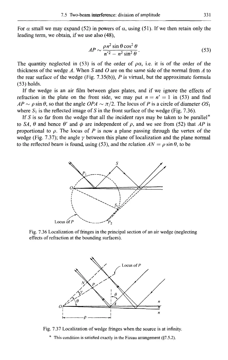
7.5.3 Localization of fringes 325
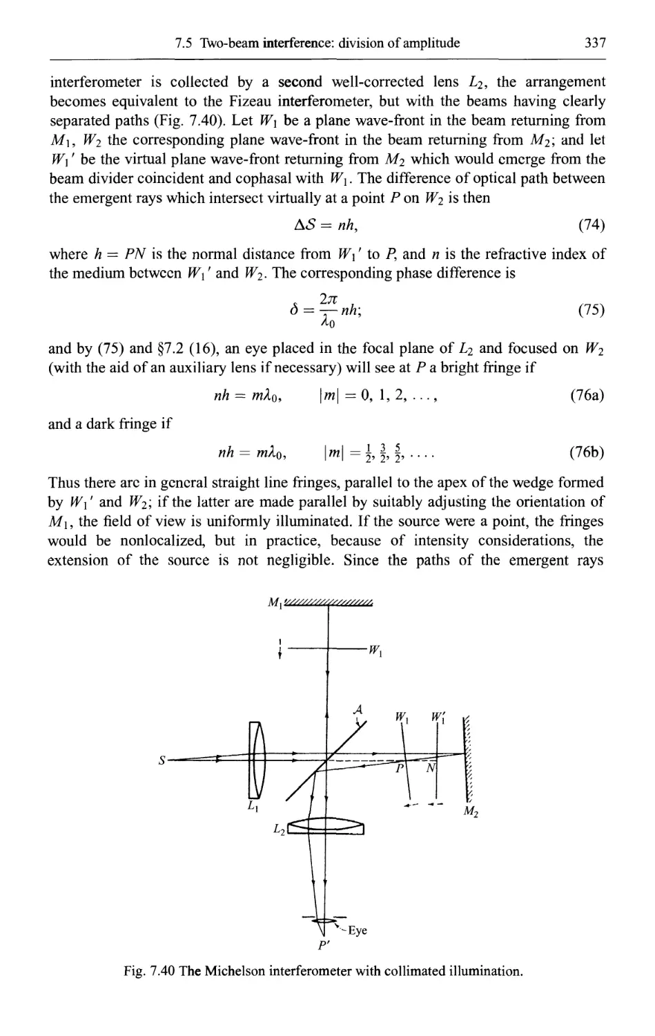
7.5.4 The Michelson interferometer 334
7.5.5 The Twyman-Green and related interferometers 336
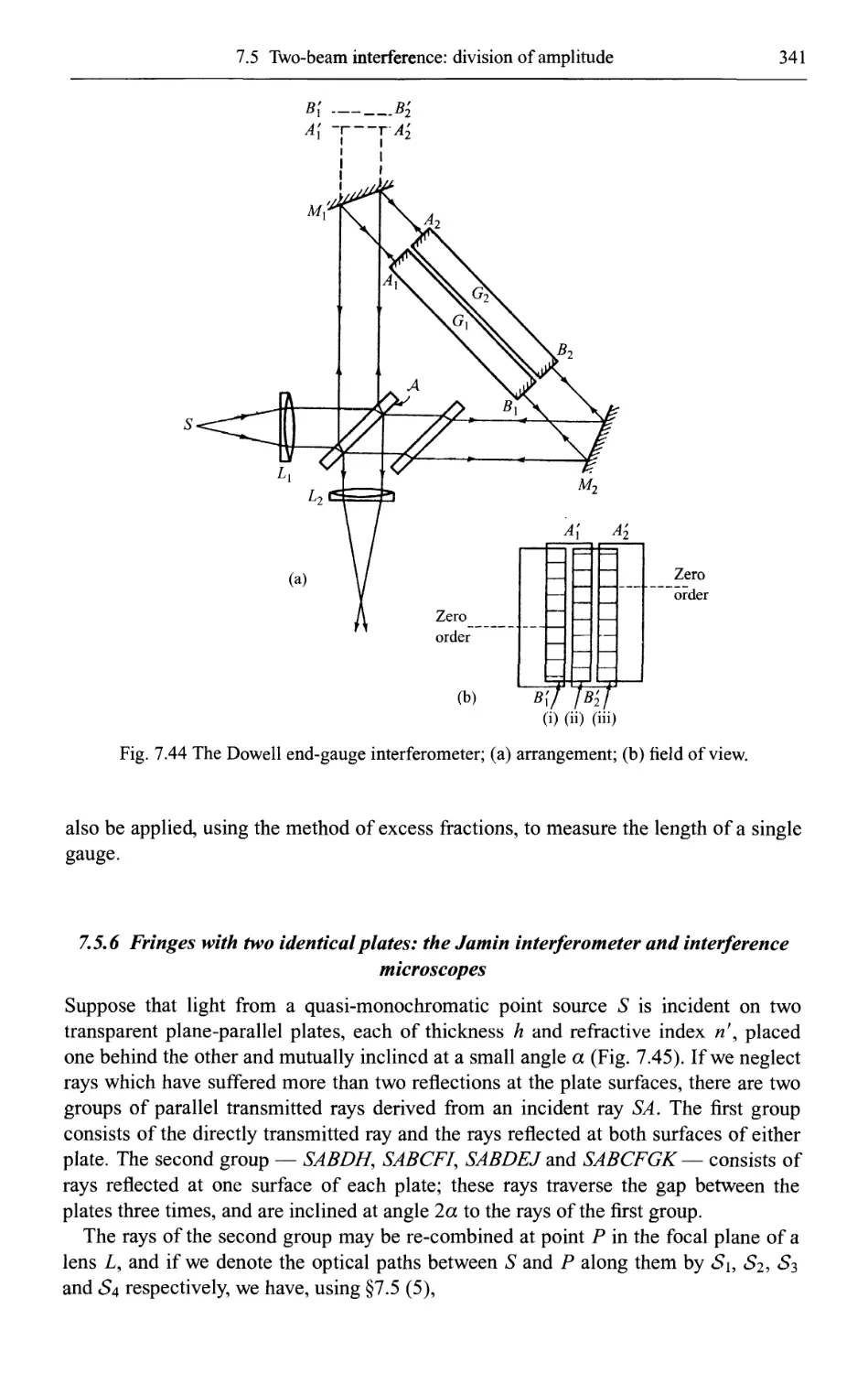
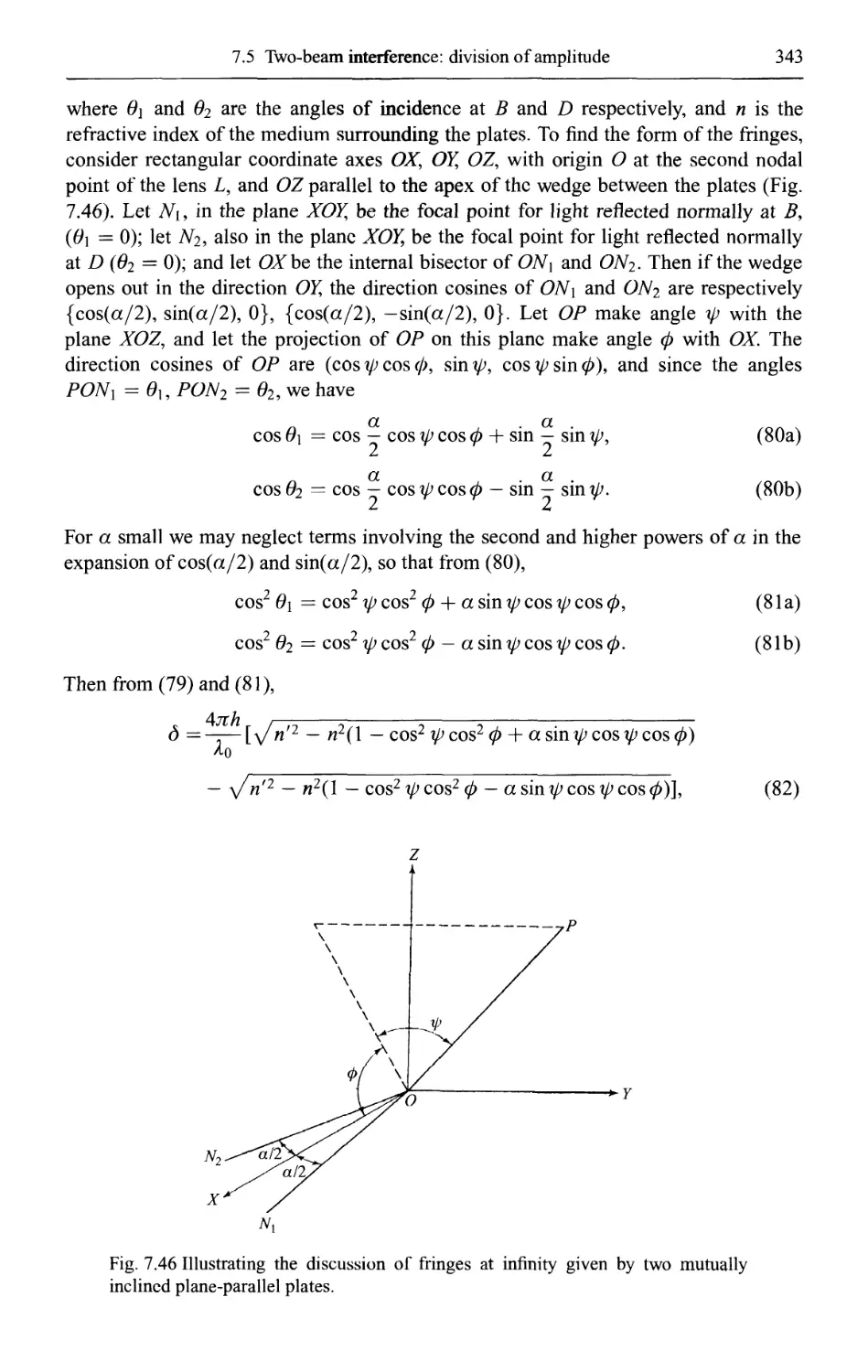
7.5.6 Fringes with two identical plates: the Jamin interferometer and
interference microscopes 341
7.5.7 The Mach-Zehnder interferometer; the Bates wave-front shearing
interferometer 348
7.5.8 The coherence length; the application of two-beam interference to the
study of the fine structure of spectral lines 352
7.6 Multiple-beam interference 359
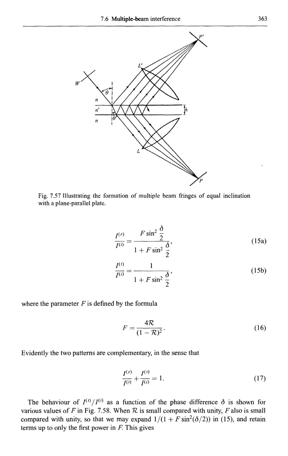
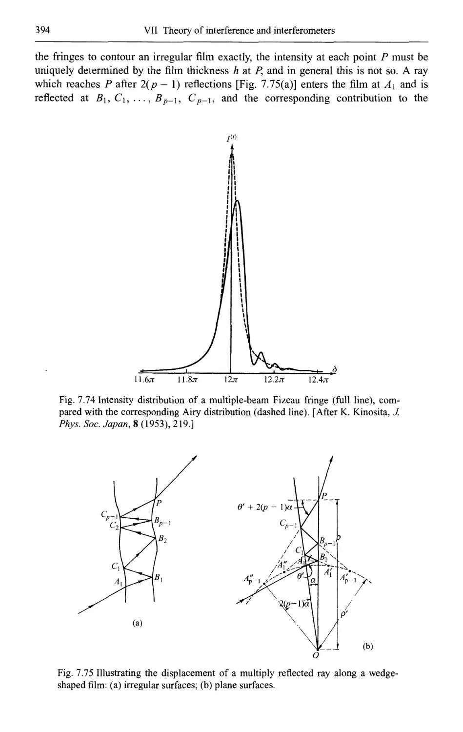
7.6.1 Multiple-beam fringes with a plane-parallel plate 360
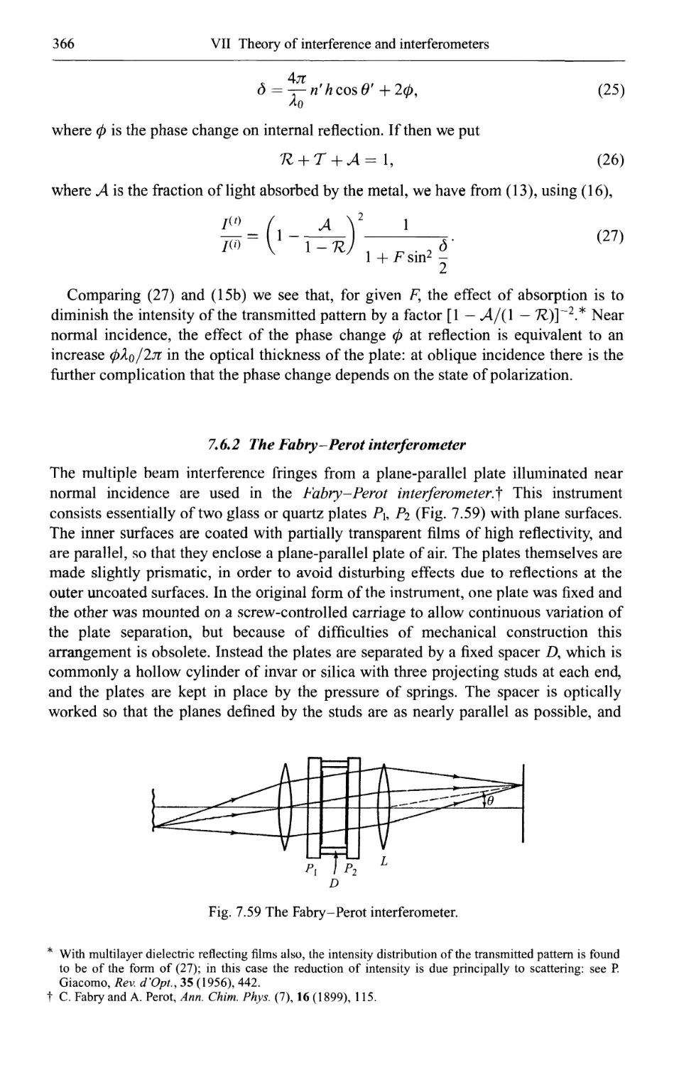
7.6.2 The Fabry-Perot interferometer 366
7.6.3 The application of the Fabry-Perot interferometer to the study of the
fine structure of spectral lines 370
7.6.4 The application of the Fabry-Perot interferometer to the comparison of
wavelengths 377
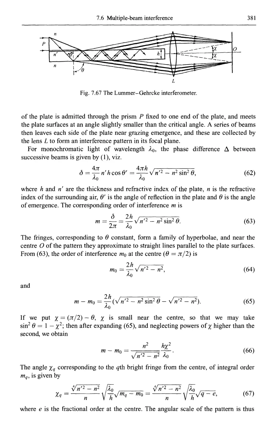
7.6.5 The Lummer-Gehrcke interferometer 380
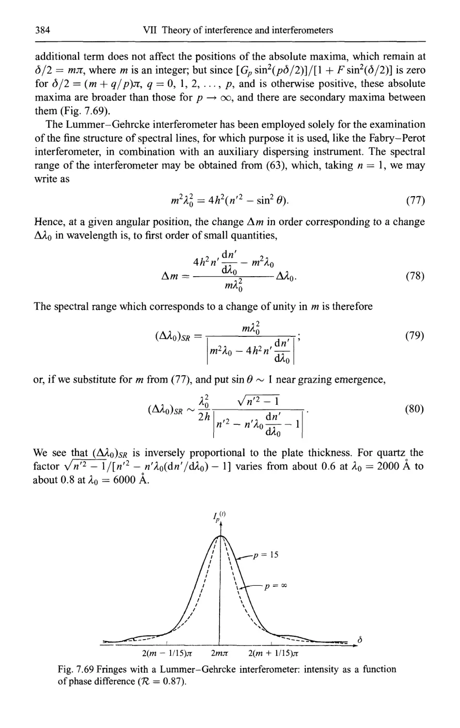
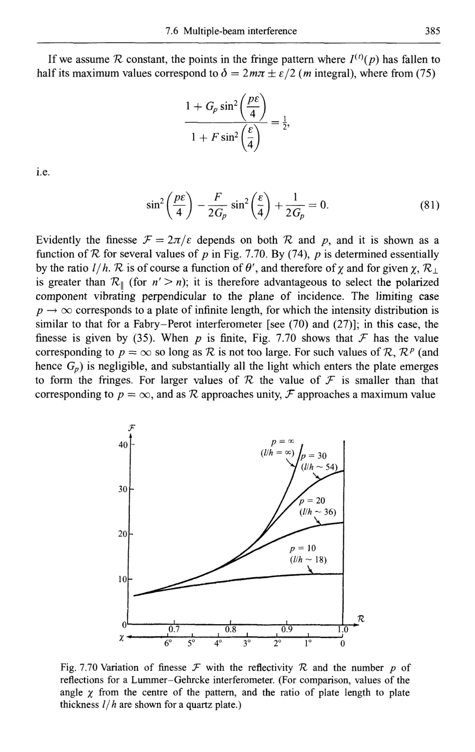
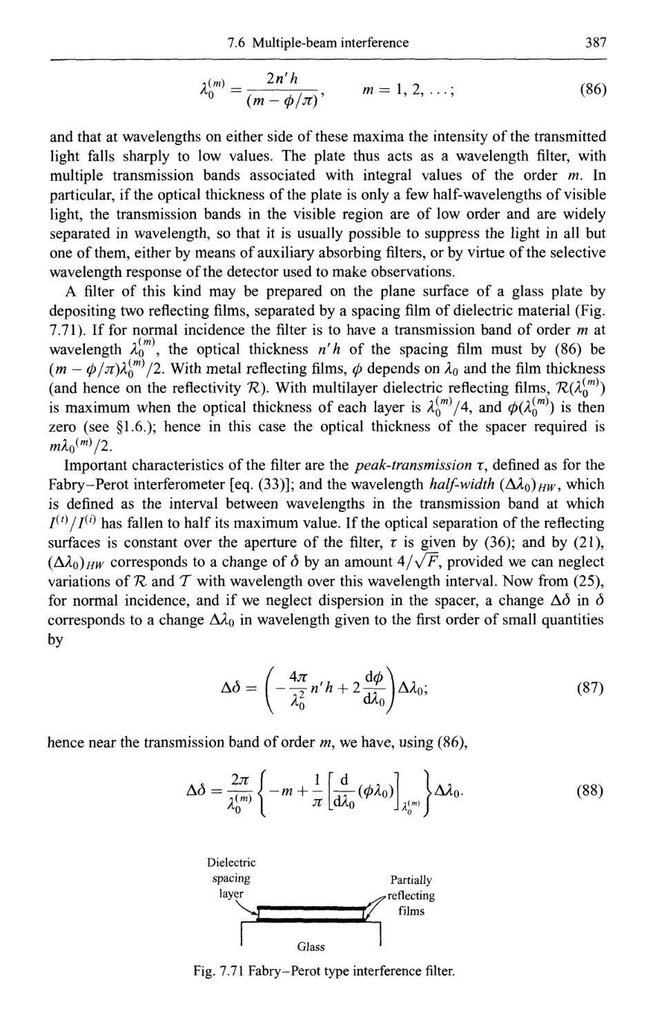
7.6.6 Interference filters 386
7.6.7 Multiple-beam fringes with thin films 391
7.6.8 Multiple-beam fringes with two plane-parallel plates 401
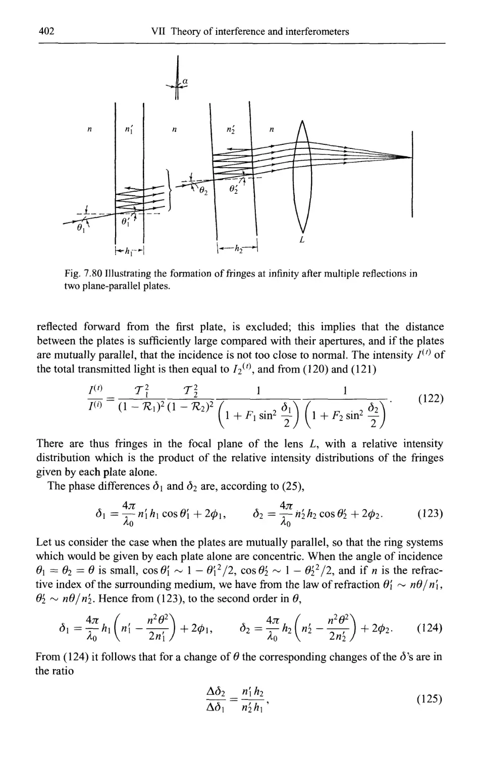
(a) Fringes with monochromatic and quasi-monochromatic light 401
(b) Fringes of superposition 405
7.7 The comparison of wavelengths with the standard metre 409
VIII Elements of the theory of diffraction 412
8.1 Introduction 412
8.2 The Huygens-Fresnel principle 413
8.3 Kirchhofes diffraction theory 417
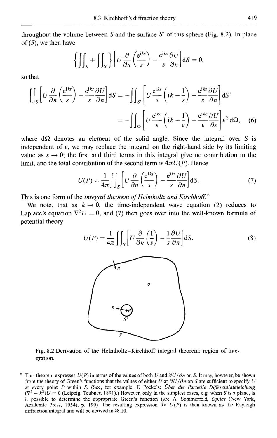
8.3.1 The integral theorem of Kirchhoff 417
8.3.2 Kirchhoff's diffraction theory 421
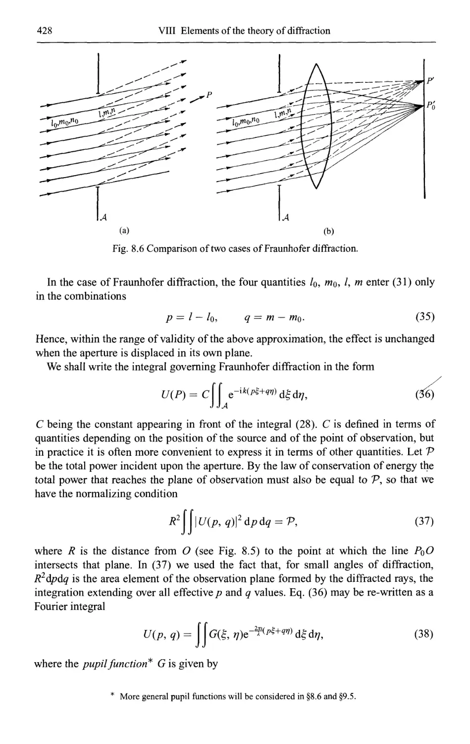
8.3.3 Fraunhofer and Fresnel diffraction 425
8.4 Transition to a scalar theory 430
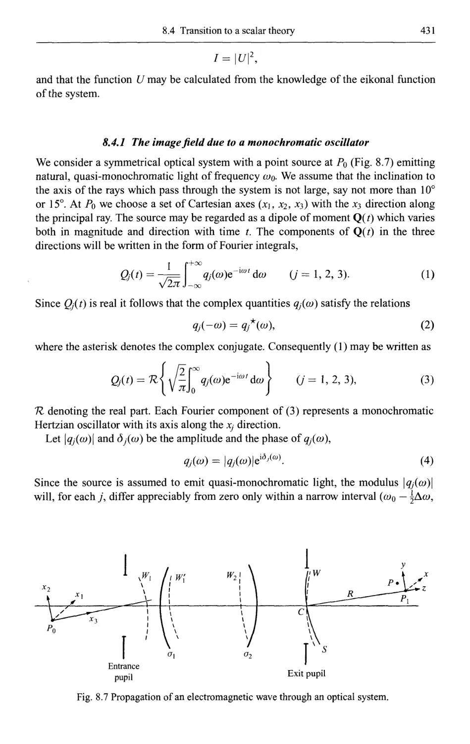
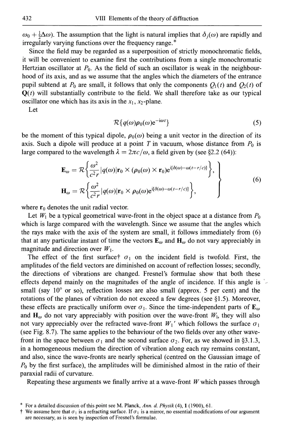
8.4.1 The image field due to a monochromatic oscillator 431
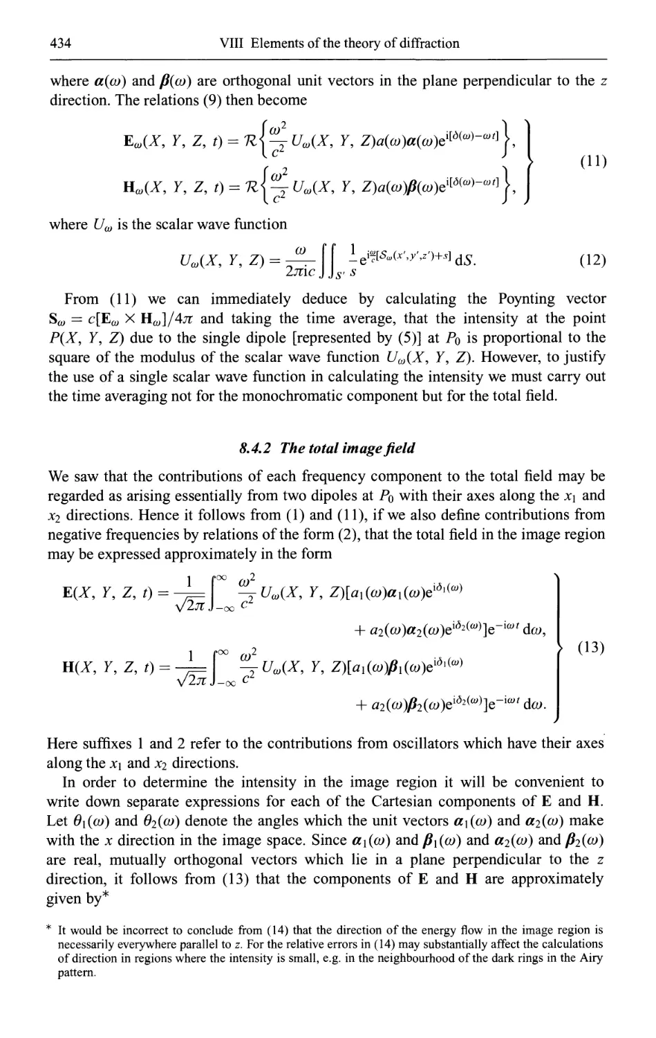
8.4.2 The total image field 434
XX
Contents
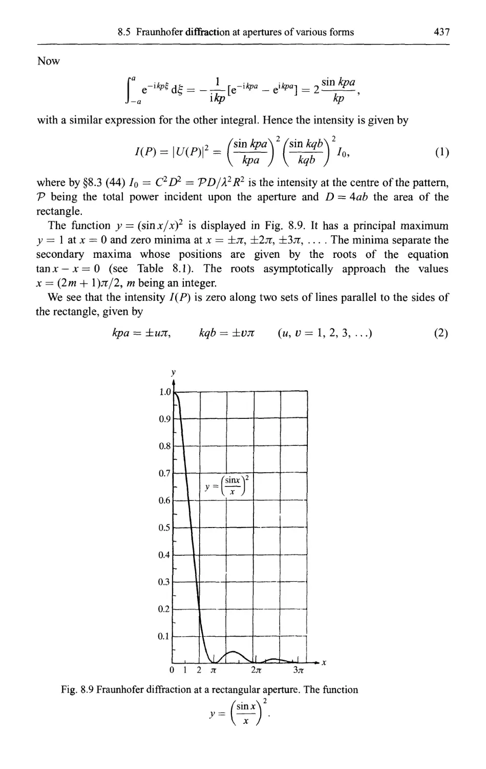
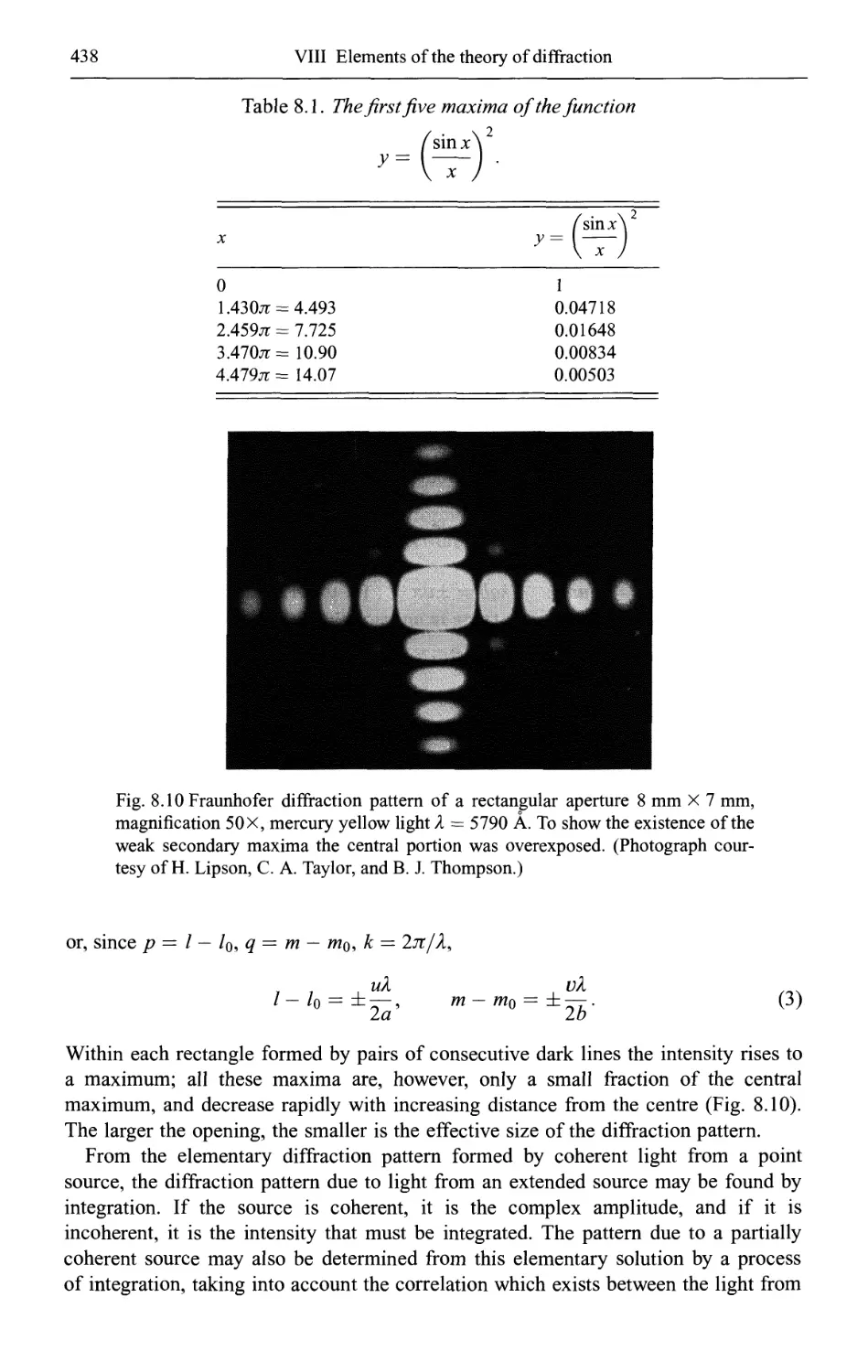
8.5 Fraunhofer diffraction at apertures of various forms 436
8.5.1 The rectangular aperture and the slit 436
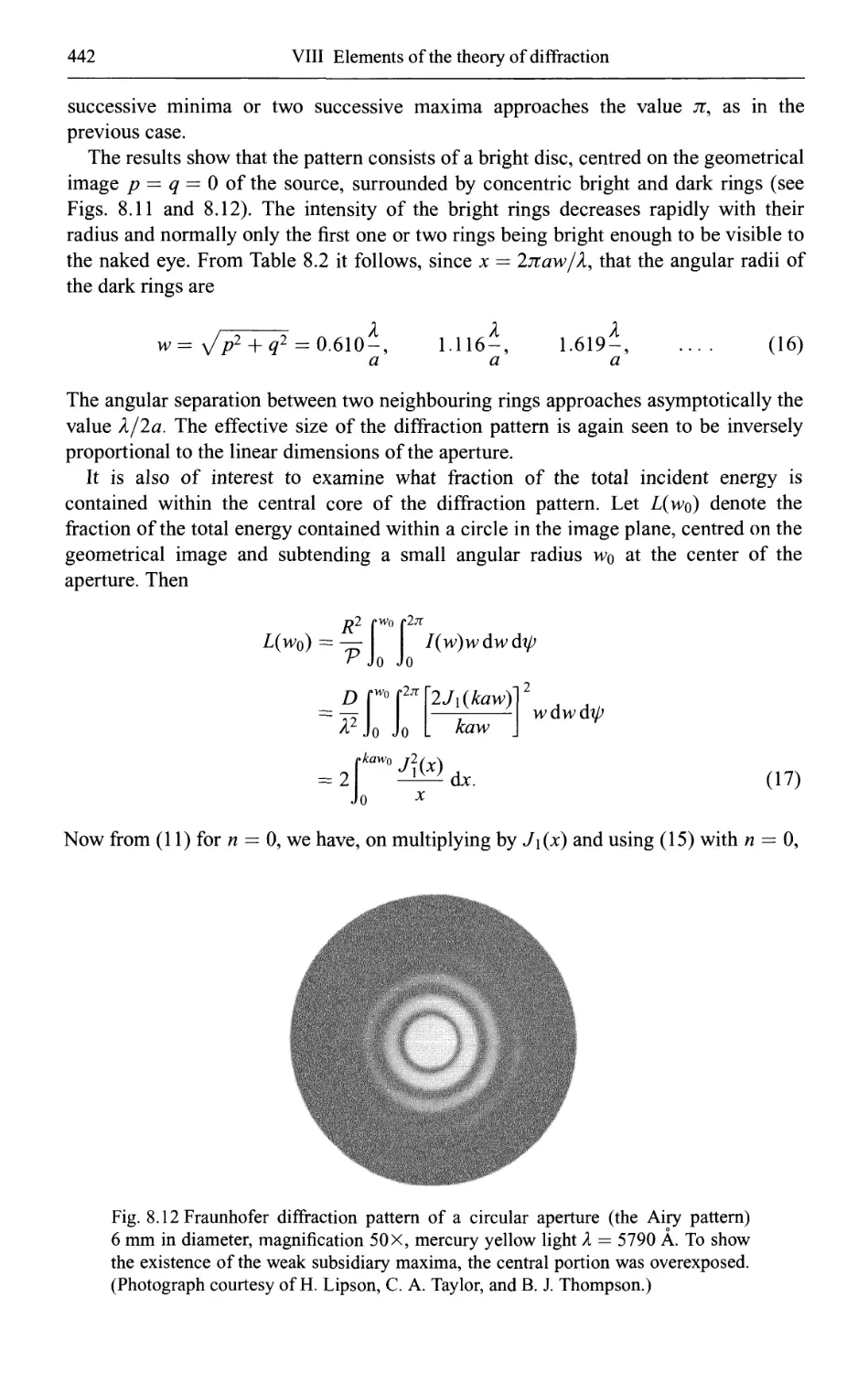
8.5.2 The circular aperture 439
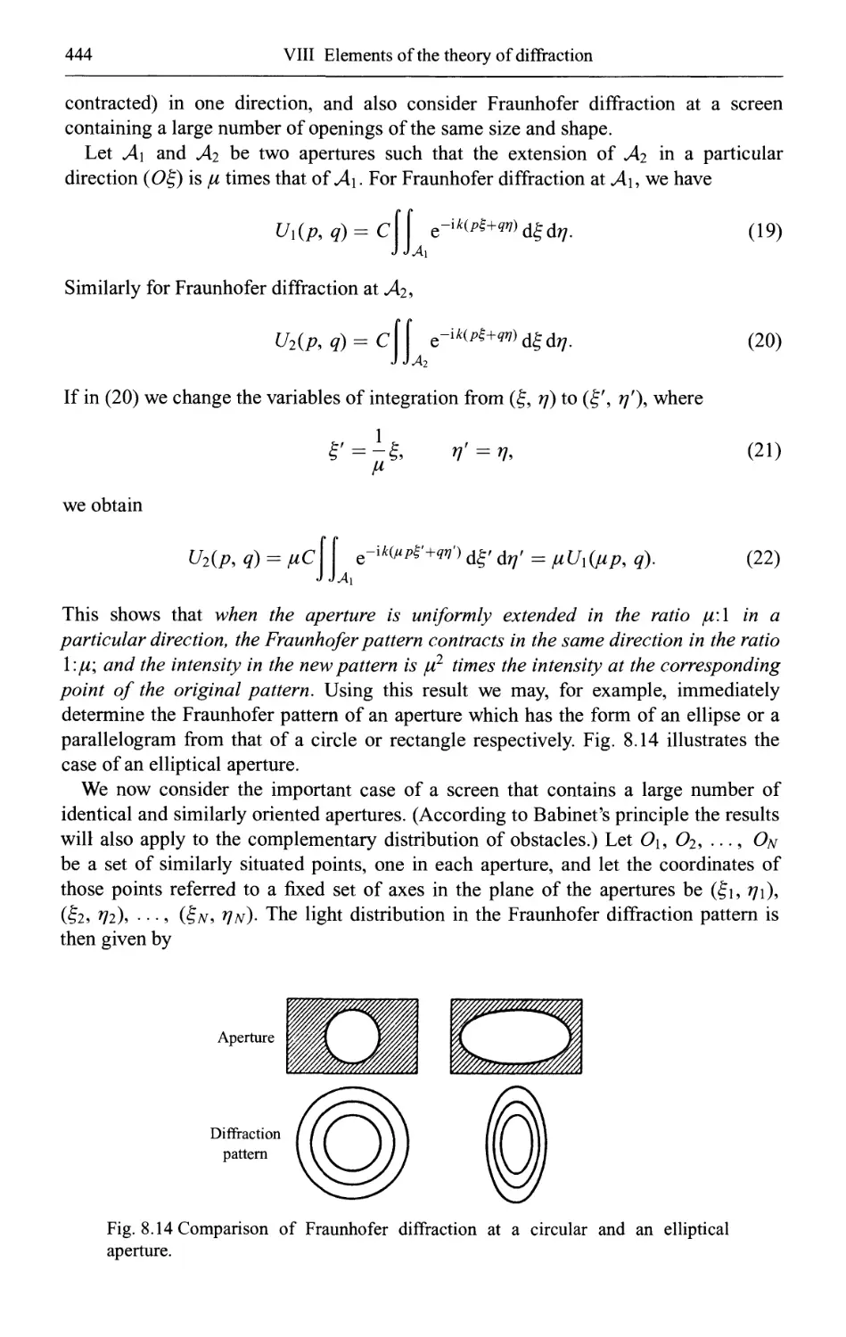
8.5.3 Other forms of aperture 443
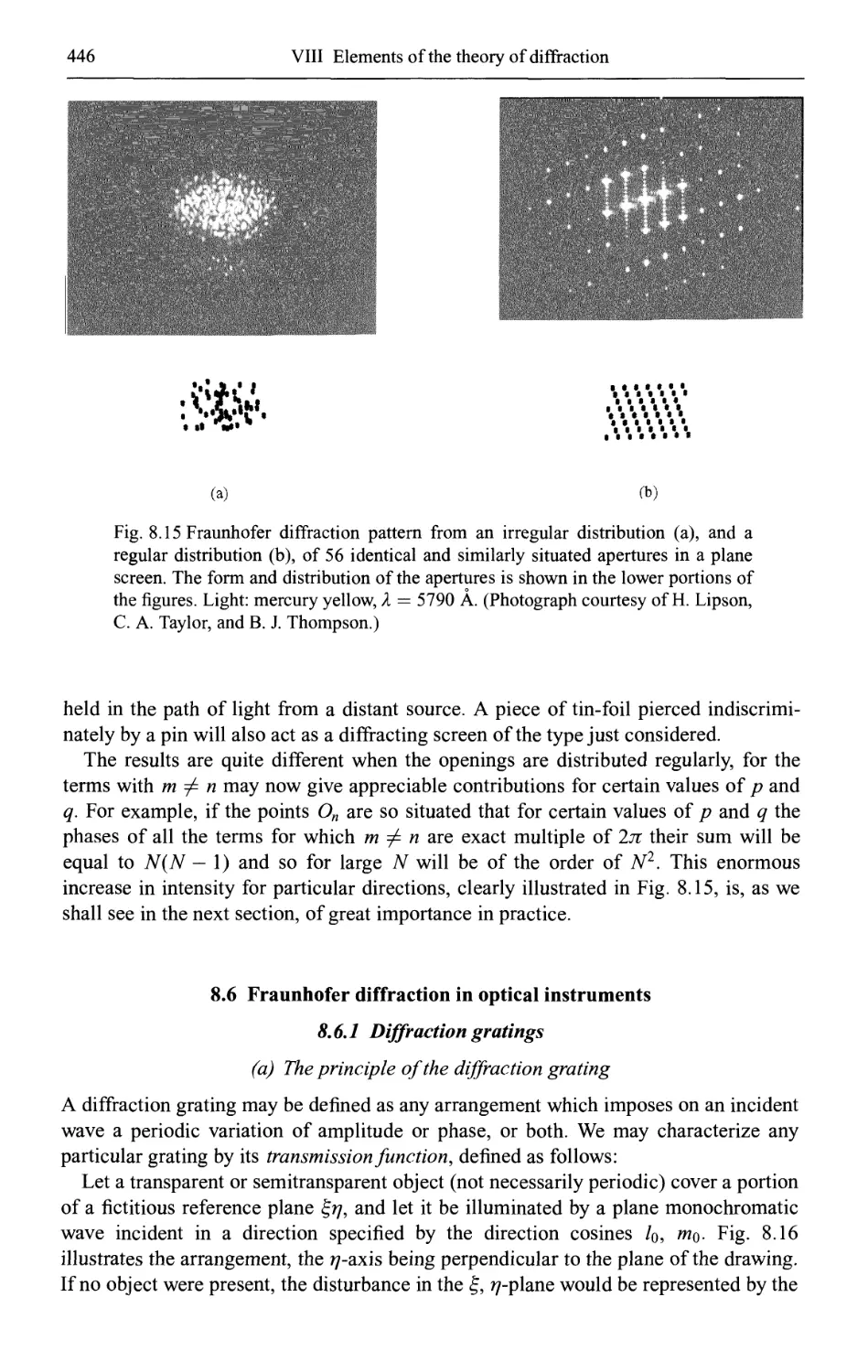
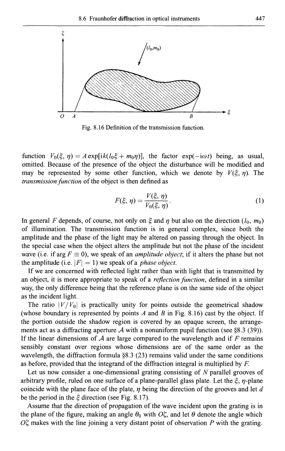
8.6 Fraunhofer diffraction in optical instruments 446
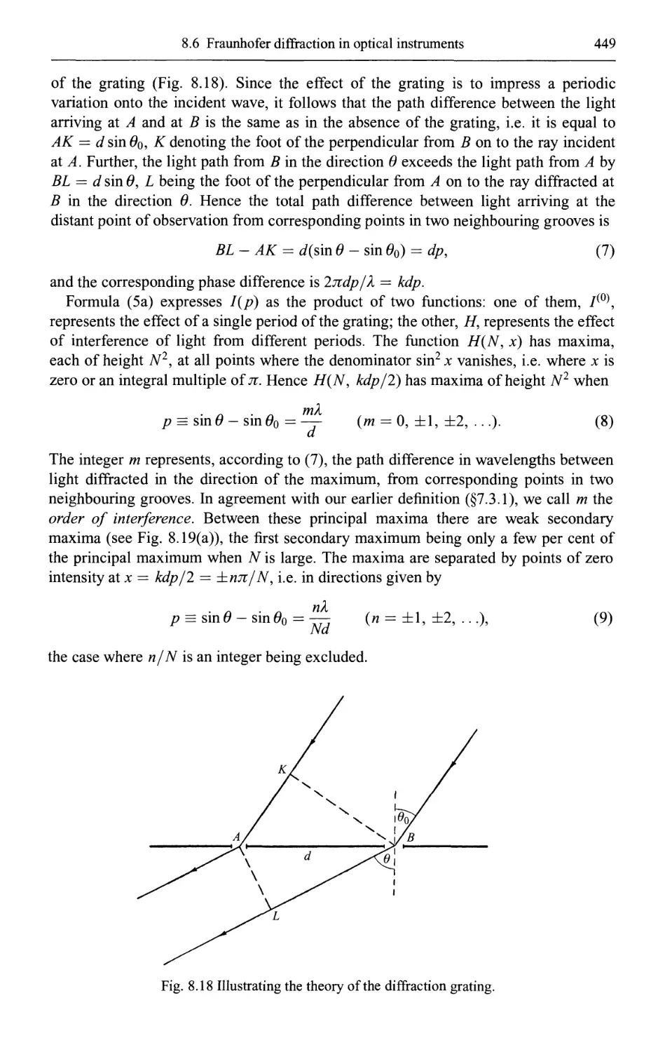
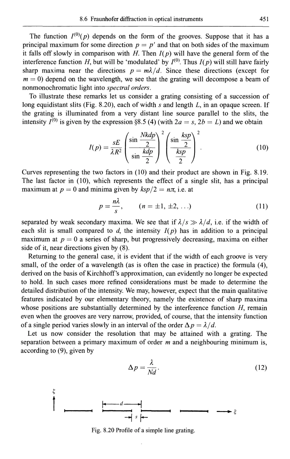
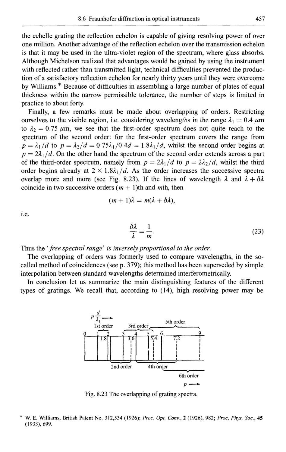
8.6.1 Diffraction gratings 446
(a) The principle of the diffraction grating 446
(b) Types of grating 453
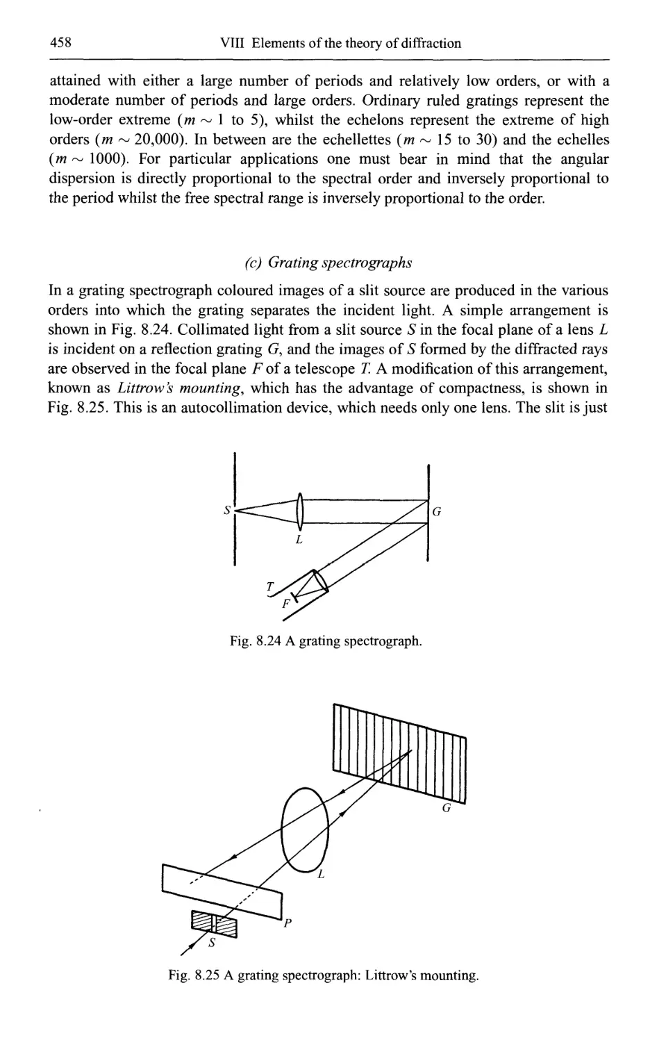
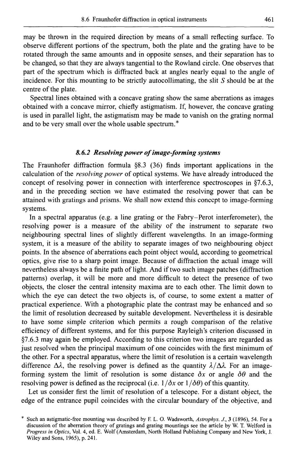
(c) Grating spectrographs 458
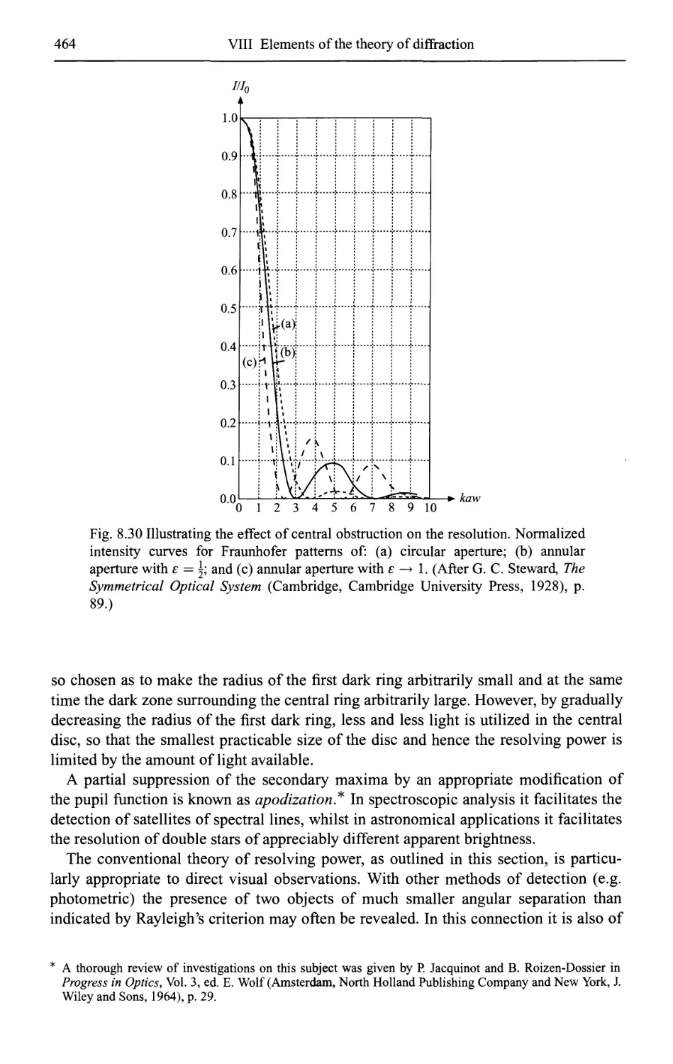
8.6.2 Resolving power of image-forming systems 461
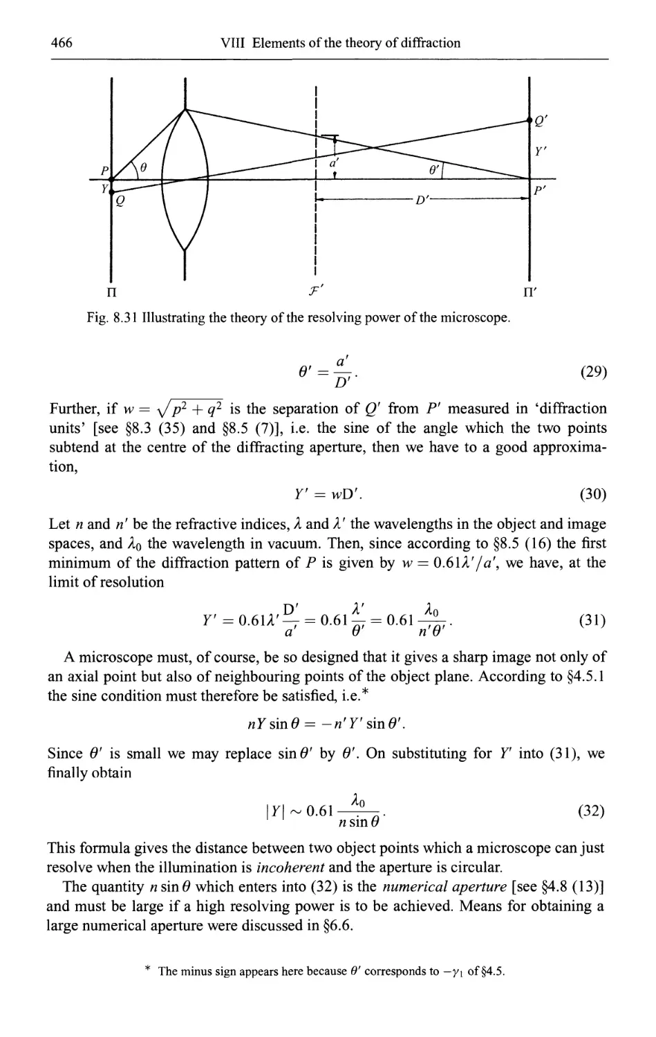
8.6.3 Image formation in the microscope 465
(a) Incoherent illumination 465
(b) Coherent illumination - Abbe's theory 467
(c) Coherent illumination - Zernike's phase contrast method of
observation 472
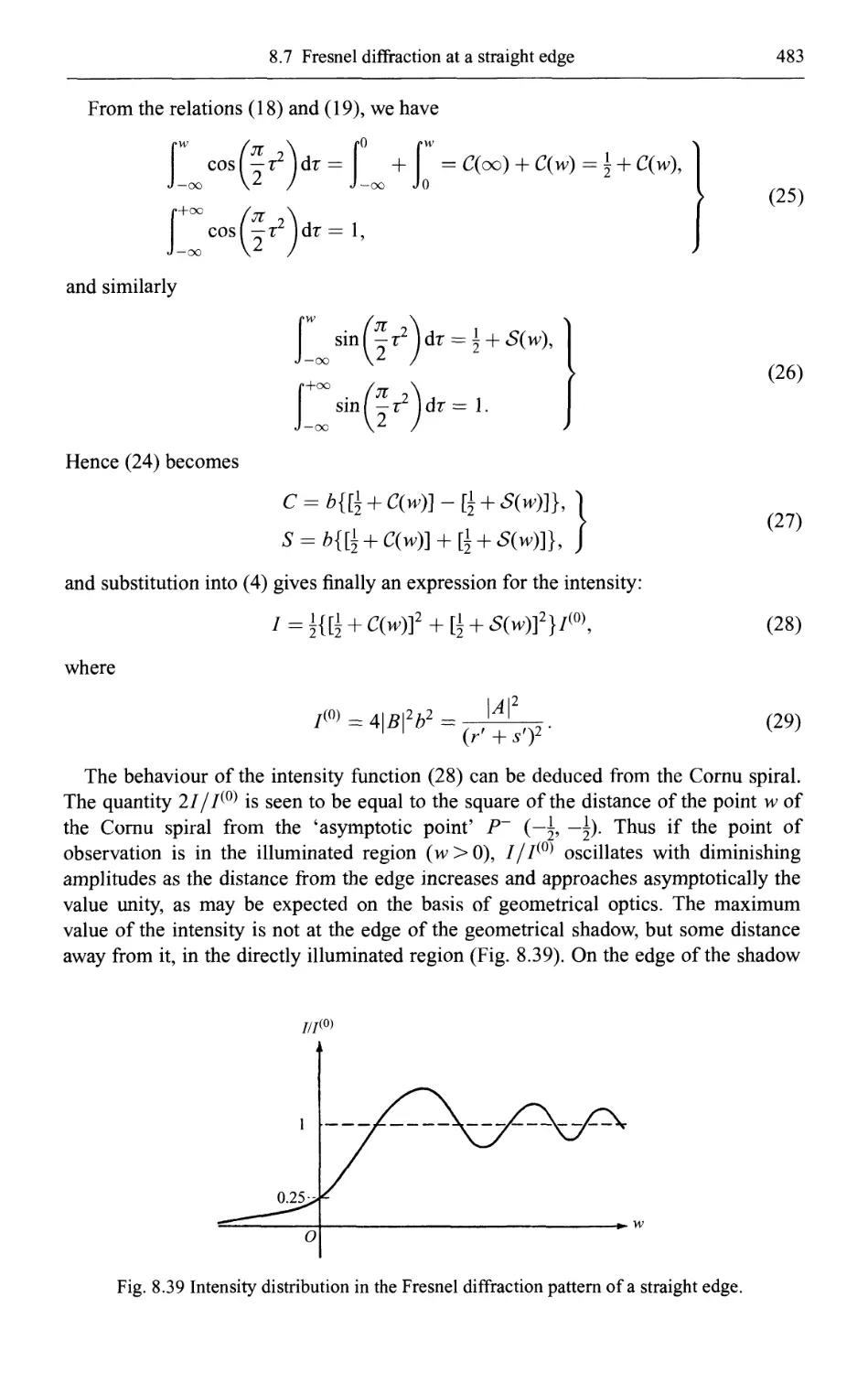
8.7 Fresnel diffraction at a straight edge 476
8.7.1 The diffraction integral 476
8.7.2 Fresnel's integrals 478
8.7.3 Fresnel diffraction at a straight edge 481
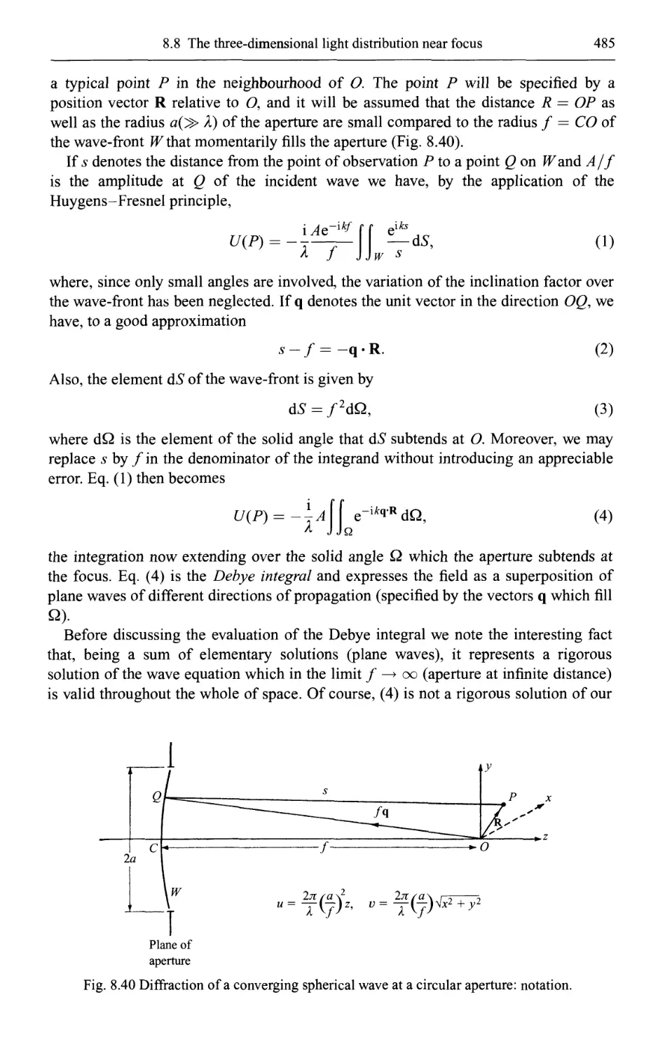
8.8 The three-dimensional light distribution near focus 484
8.8.1 Evaluation of the diffraction integral in terms of Lommel functions 484
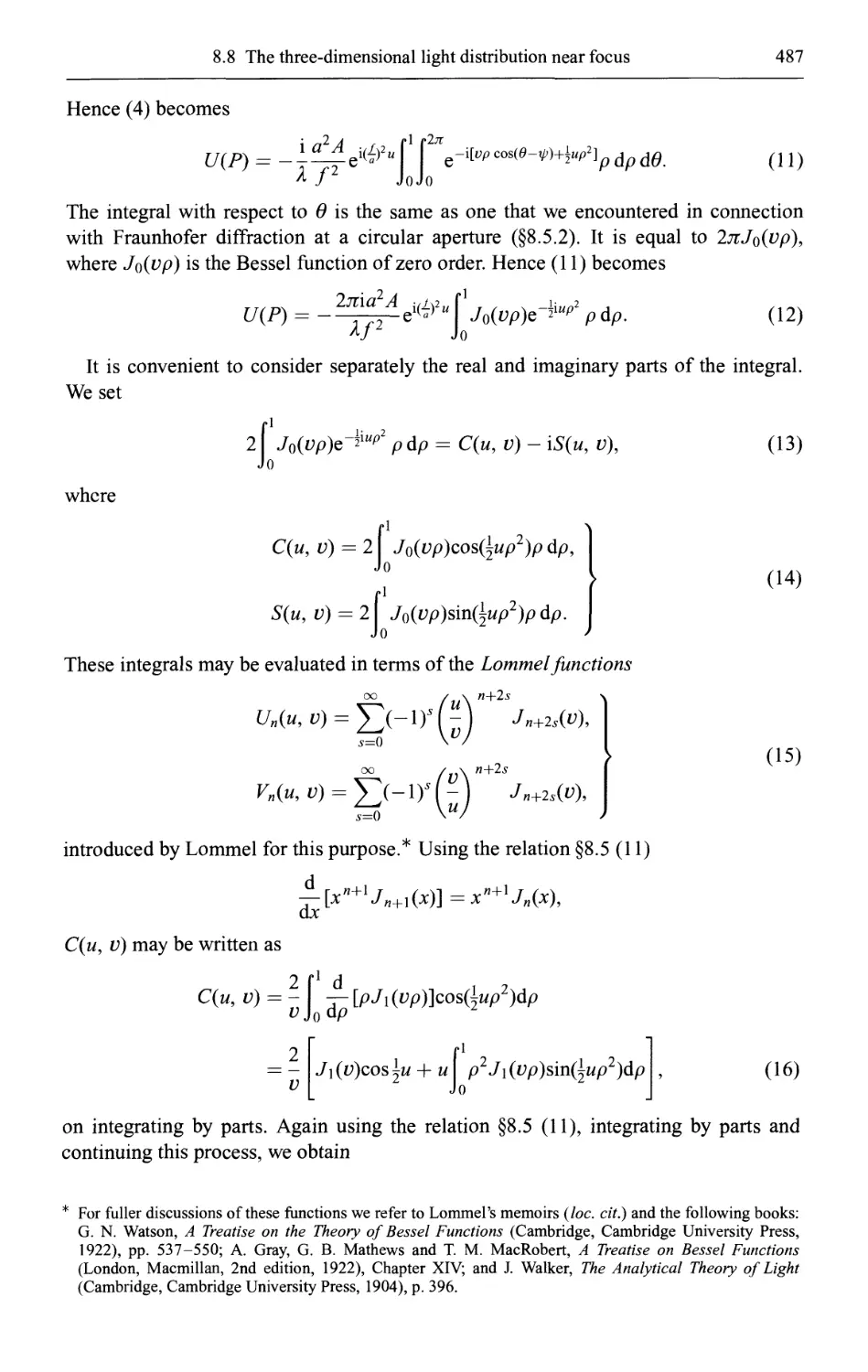
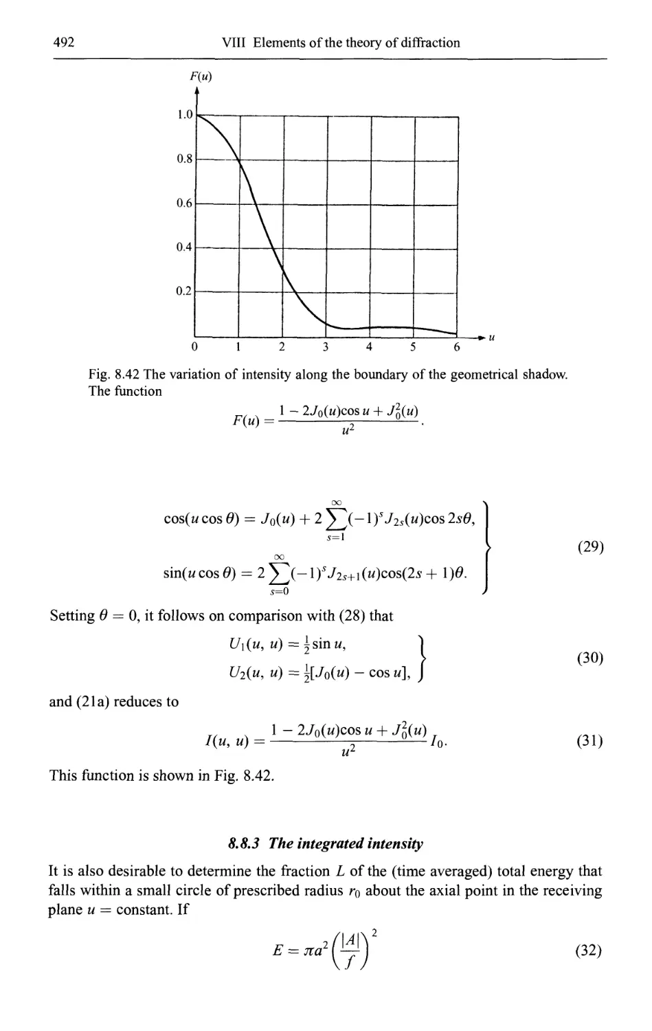
8.8.2 The distribution of intensity 489
(a) Intensity in the geometrical focal plane 490
(b) Intensity along the axis 491
(c) Intensity along the boundary of the geometrical shadow 491
8.8.3 The integrated intensity 492
8.8.4 The phase behaviour 494
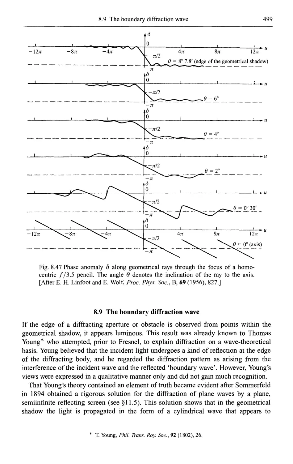
8.9 The boundary diffraction wave 499
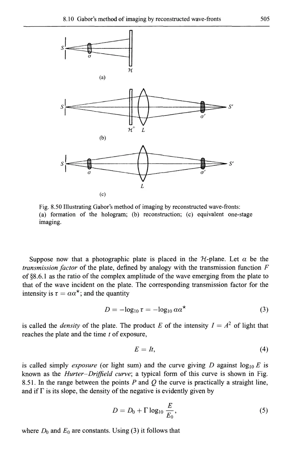
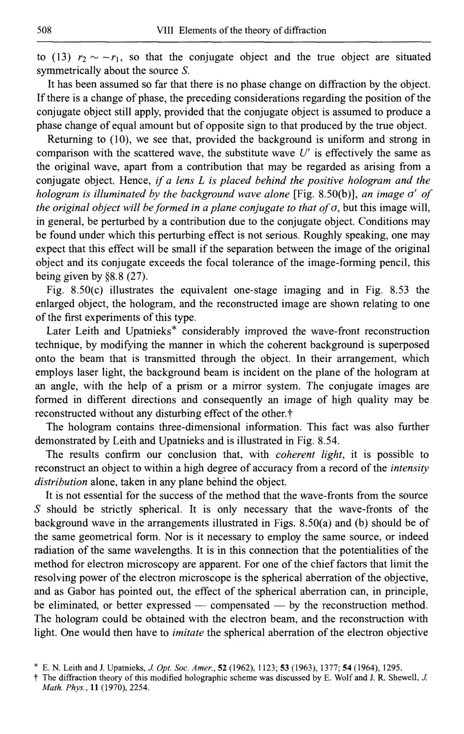
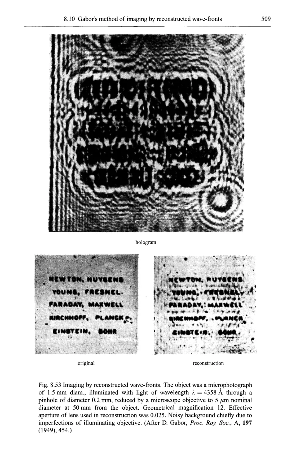
8.10 Gabor's method of imaging by reconstructed wave-fronts (holography) 504
8.10.1 Producing the positive hologram 504
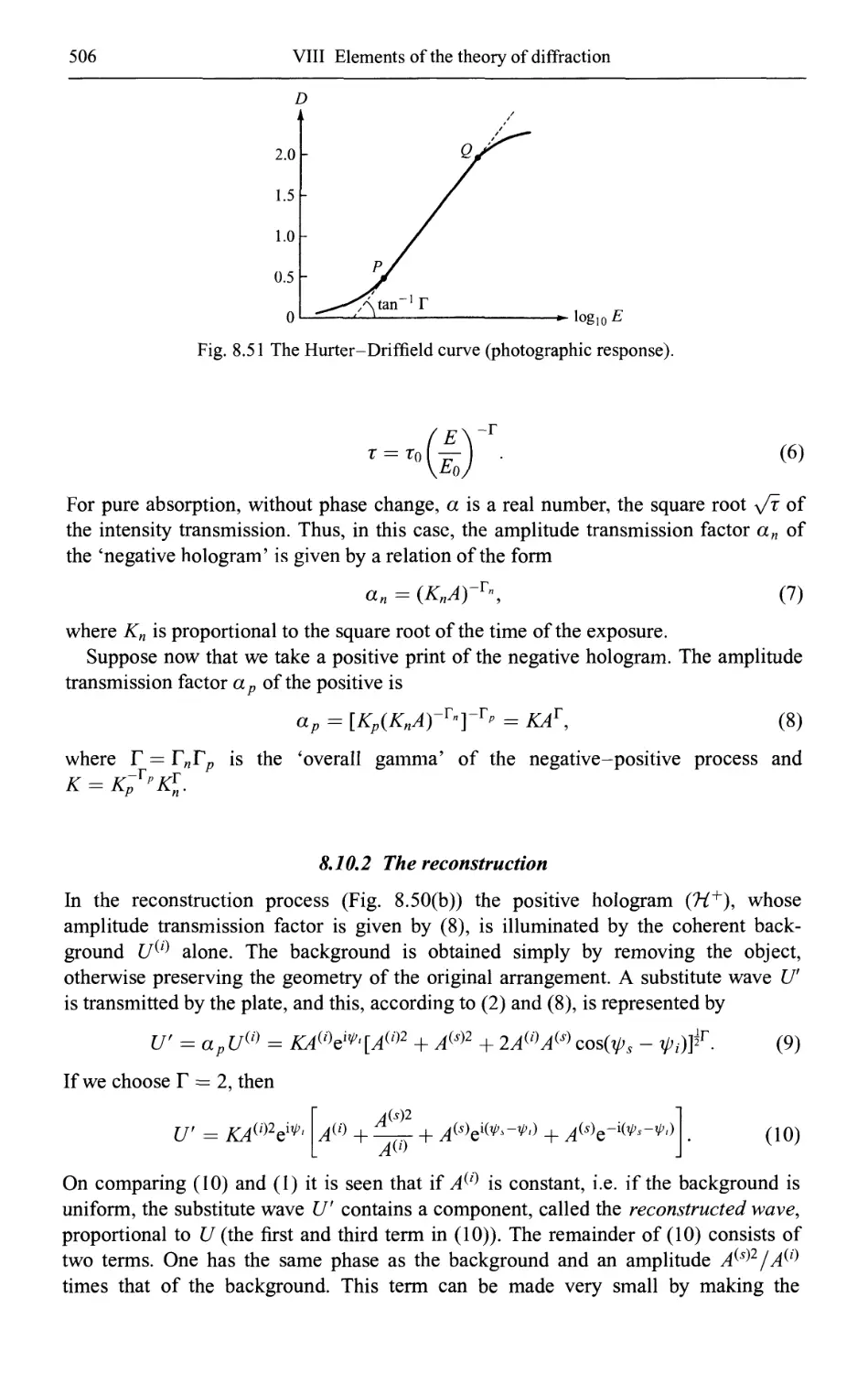
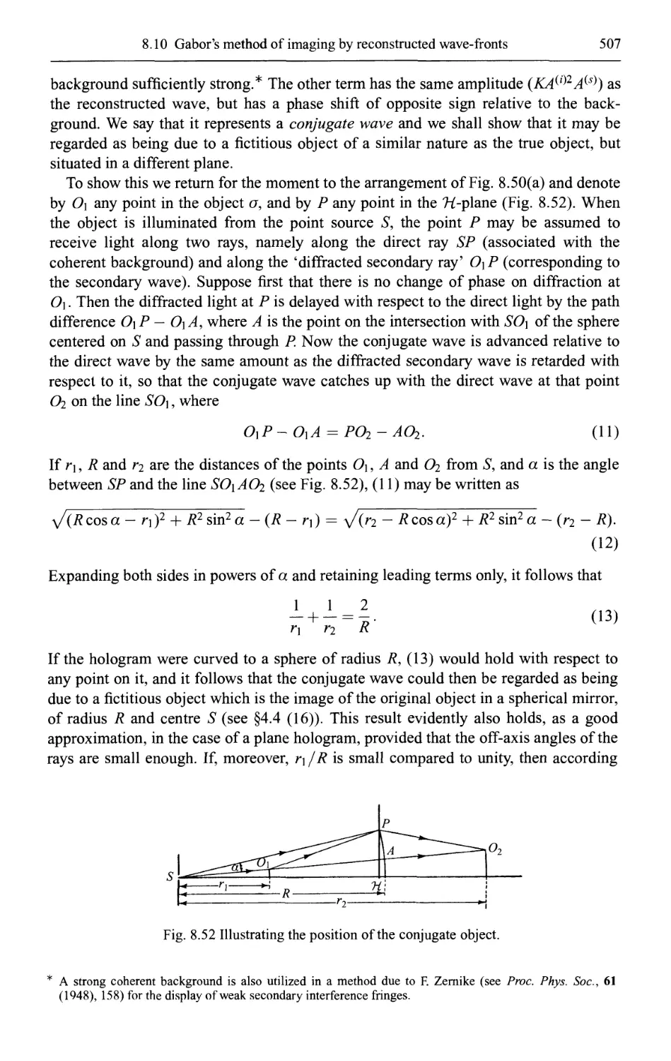
8.10.2 The reconstruction 506
8.11 The Rayleigh-Sommerfeld diffraction integrals 512
8.11.1 The Rayleigh diffraction integrals 512
8.11.2 The Rayleigh-Sommerfeld diffraction integrals 514
IX The diffraction theory of aberrations 517
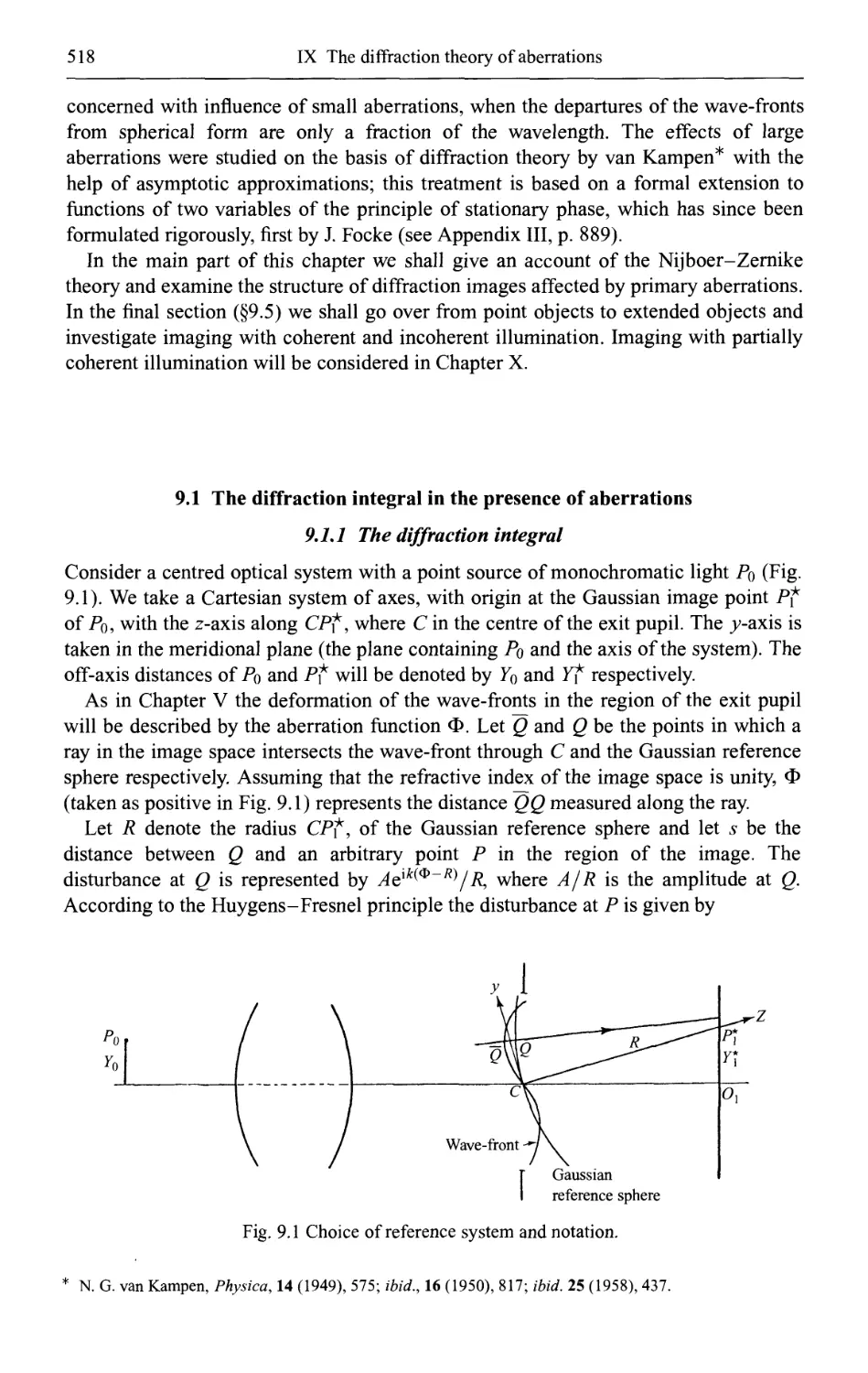
9.1 The diffraction integral in the presence of aberrations 518
9.1.1 The diffraction integral 518
9.1.2. The displacement theorem. Change of reference sphere 520
9.1.3. A relation between the intensity and the average deformation of
wave-fronts 522
9.2 Expansion of the aberration function 523
9.2.1 The circle polynomials of Zernike 523
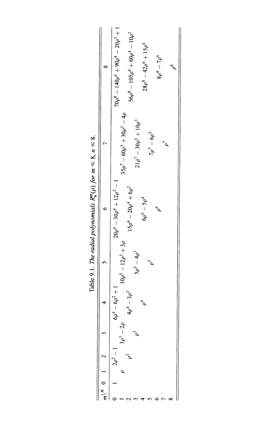
9.2.2 Expansion of the aberration function 525
9.3 Tolerance conditions for primary aberrations 527
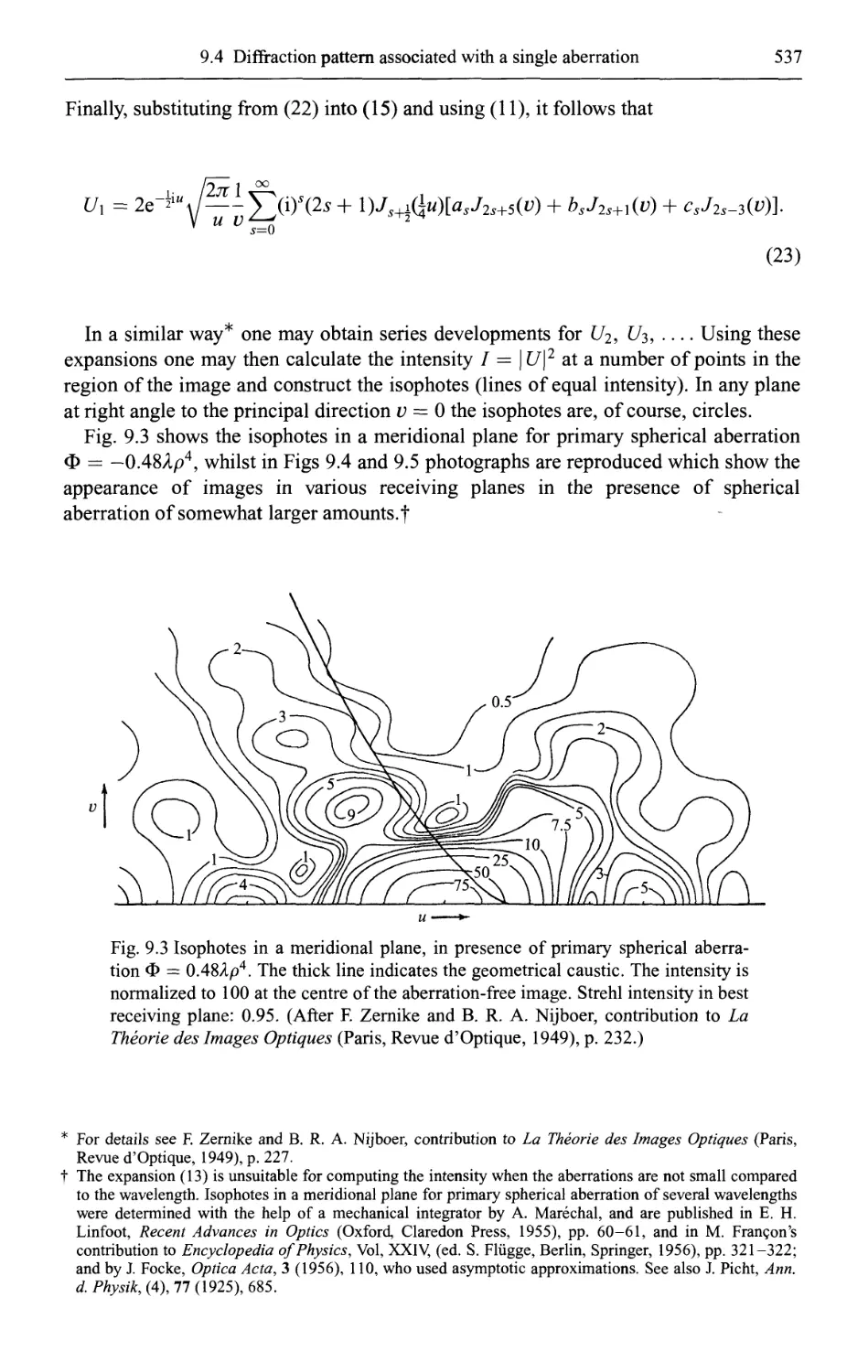
9.4 The diffraction pattern associated with a single aberration 532
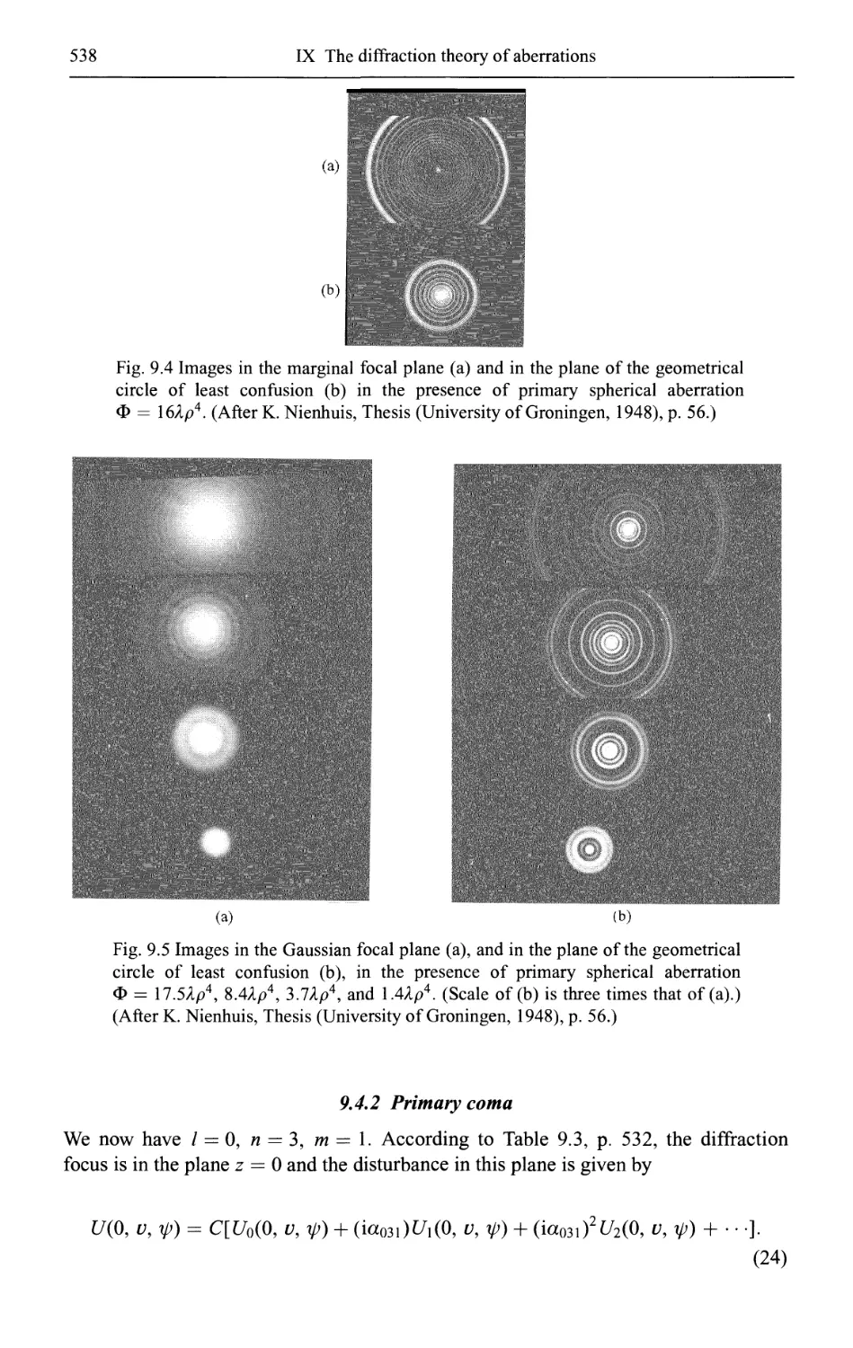
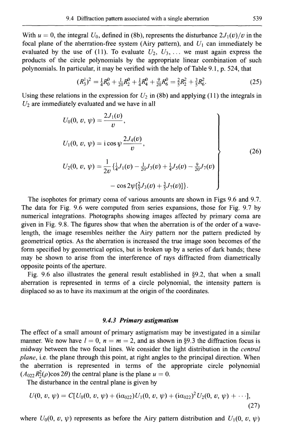
9.4.1 Primary spherical aberration 536
9.4.2 Primary coma 538
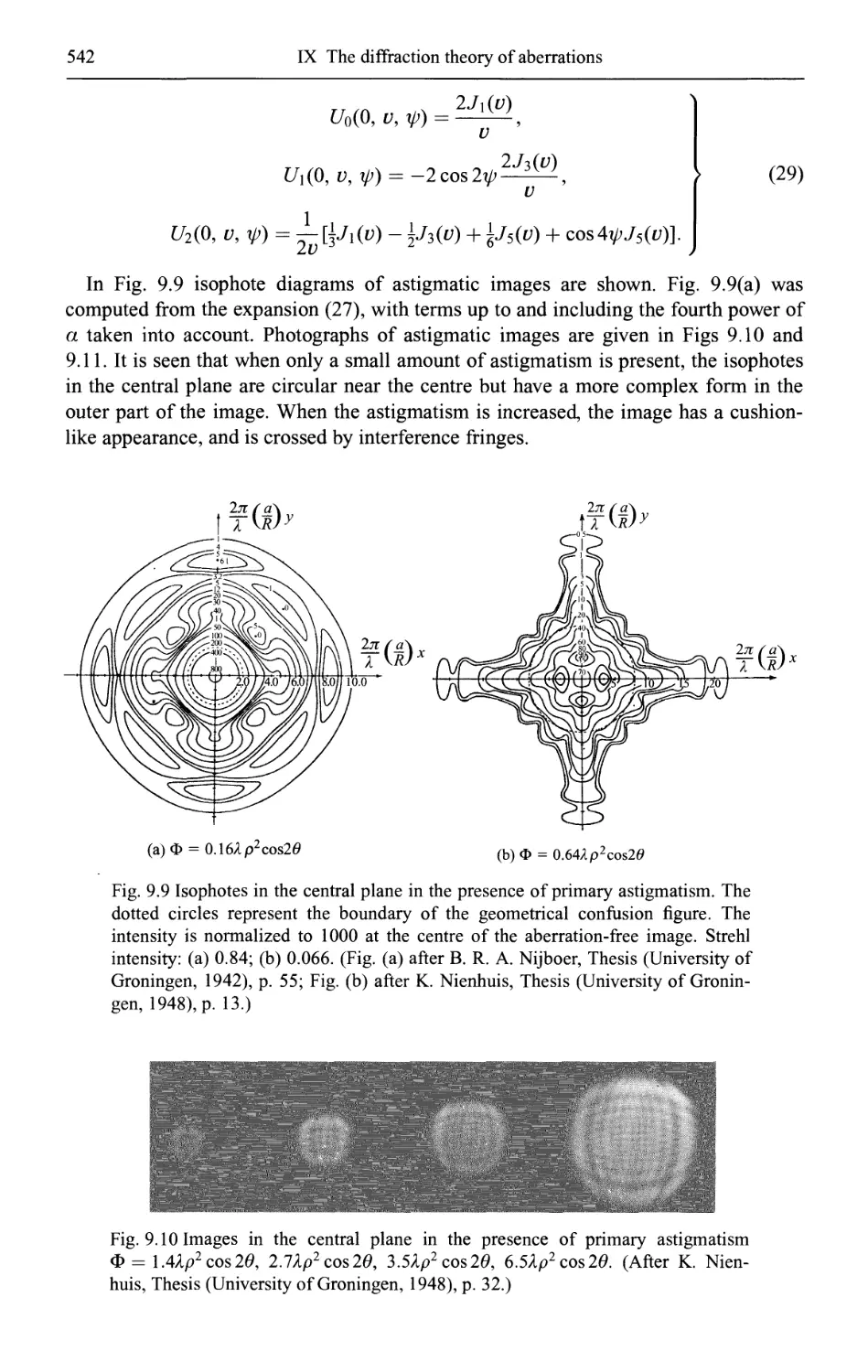
9.4.3 Primary astigmatism 539
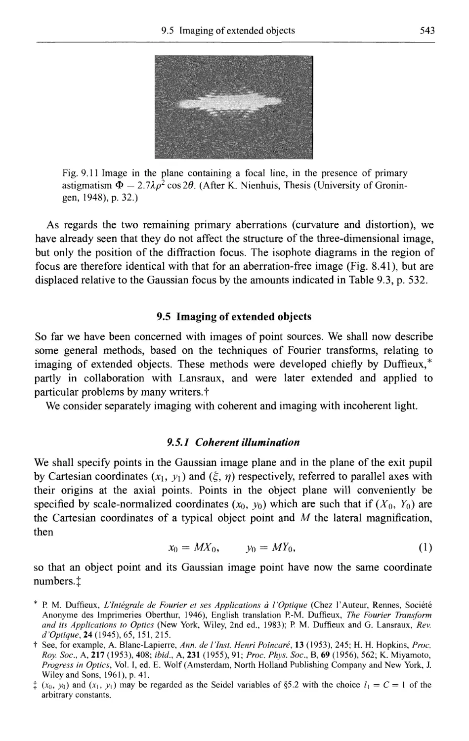
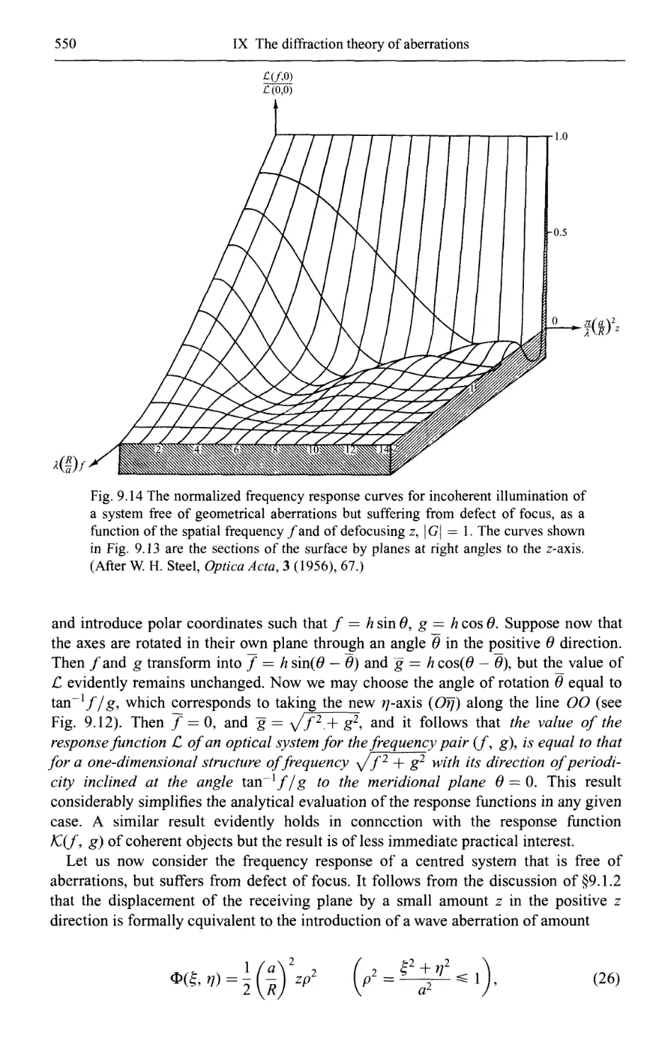
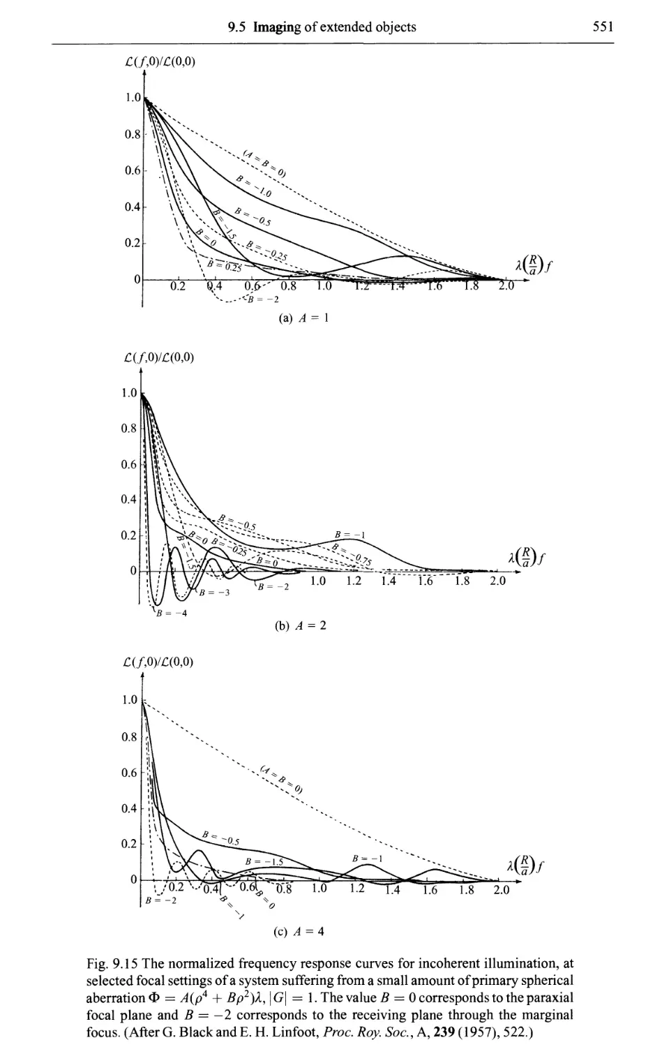
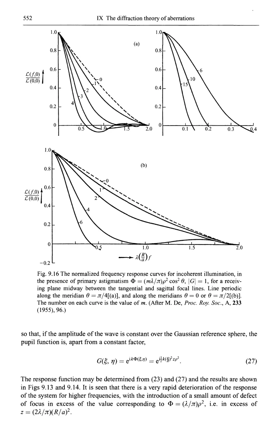
9.5 Imaging of extended objects 543
9.5.1 Coherent illumination 543
9.5.2 Incoherent illumination 547
Contents
xxi
X Interference and diffraction with partially coherent light 554
10.1 Introduction 554
10.2 A complex representation of real polychromatic fields 557
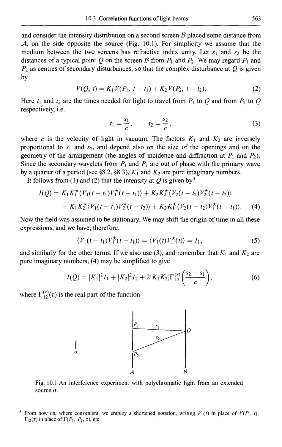
10.3 The correlation functions of light beams 562
10.3.1 Interference of two partially coherent beams. The mutual coherence
function and the complex degree of coherence 562
10.3.2 Spectral representation of mutual coherence 566
10.4 Interference and diffraction with quasi-monochromatic light 569
10.4.1 Interference with quasi-monochromatic light. The mutual intensity 569
10.4.2 Calculation of mutual intensity and degree of coherence for light from
an extended incoherent quasi-monochromatic source 572
(a) The van Cittert-Zernike theorem 572
(b) Hopkins' formula 577
10.4.3 An example 578
10.4.4 Propagation of mutual intensity 580
10.5 Interference with broad-band light and the spectral degree of coherence.
Correlation-induced spectral changes 585
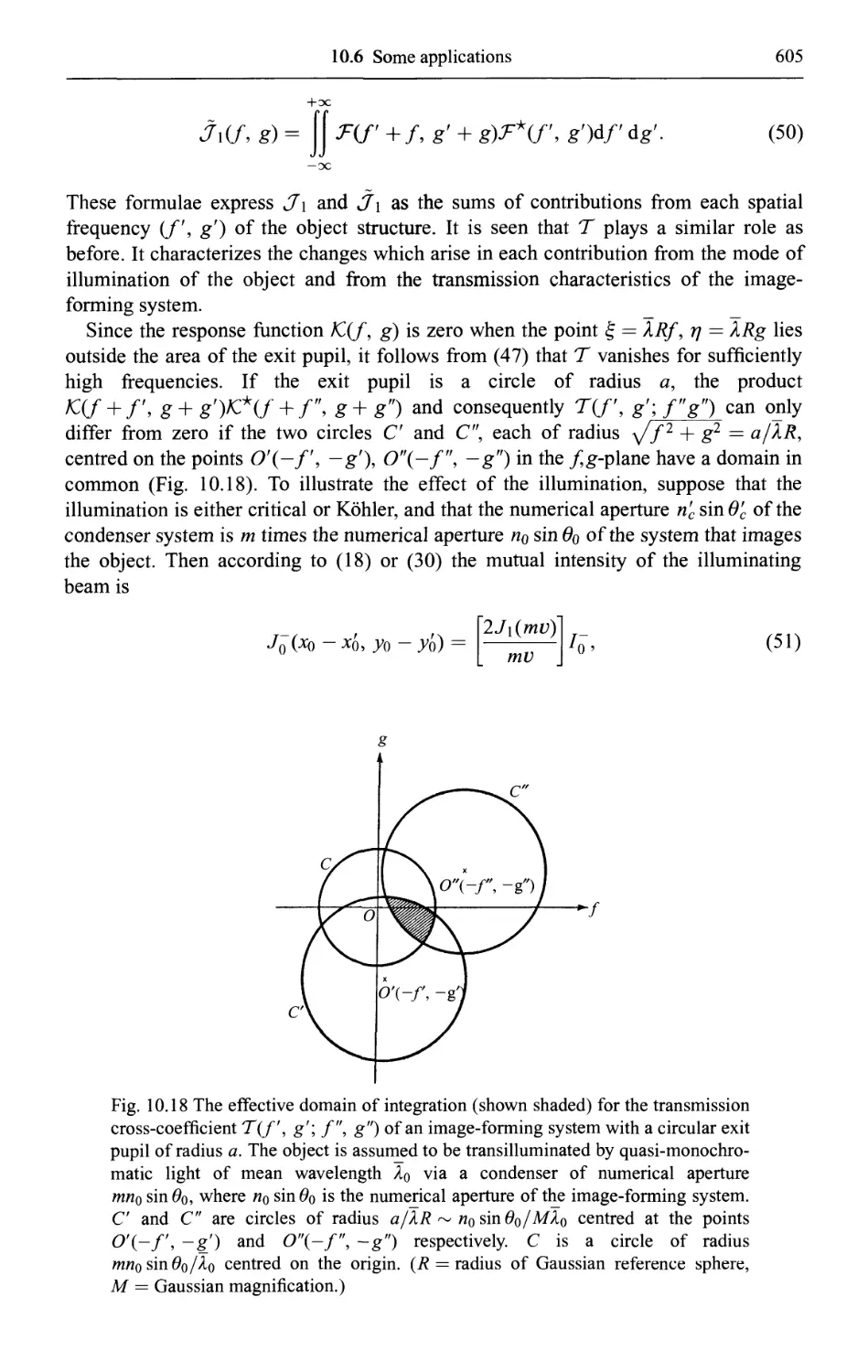
10.6 Some applications 590
10.6.1 The degree of coherence in the image of an extended incoherent
quasi-monochromatic source 590
10.6.2 The influence of the condenser on resolution in a microscope 595
(a) Critical illumination 595
(b) Köhler's illumination 598
10.6.3 Imaging with partially coherent quasi-monochromatic illumination 599
(a) Transmission of mutual intensity through an optical system 599
(b) Images of transilluminated objects 602
10.7 Some theorems relating to mutual coherence 606
10.7.1 Calculation of mutual coherence for light from an incoherent source 606
10.7.2 Propagation of mutual coherence 609
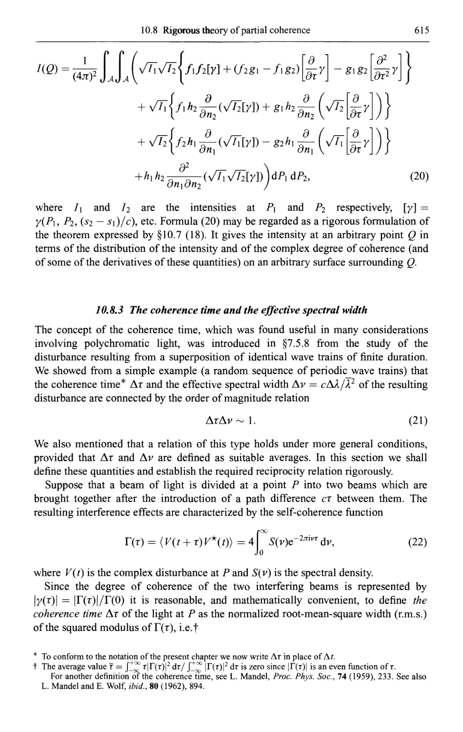
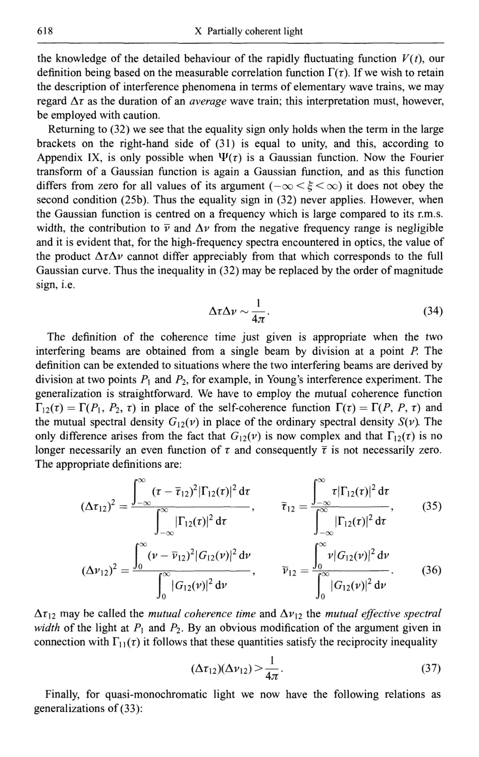
10.8 Rigorous theory of partial coherence 610
10.8.1 Wave equations for mutual coherence 610
10.8.2 Rigorous formulation of the propagation law for mutual coherence 612
10.8.3 The coherence time and the effective spectral width 615
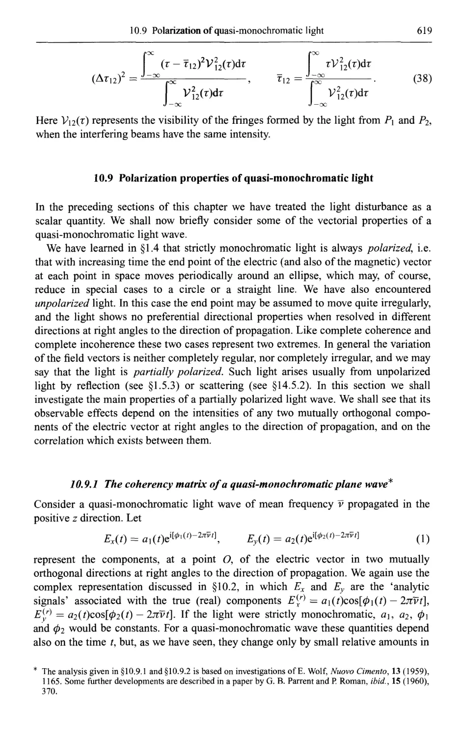
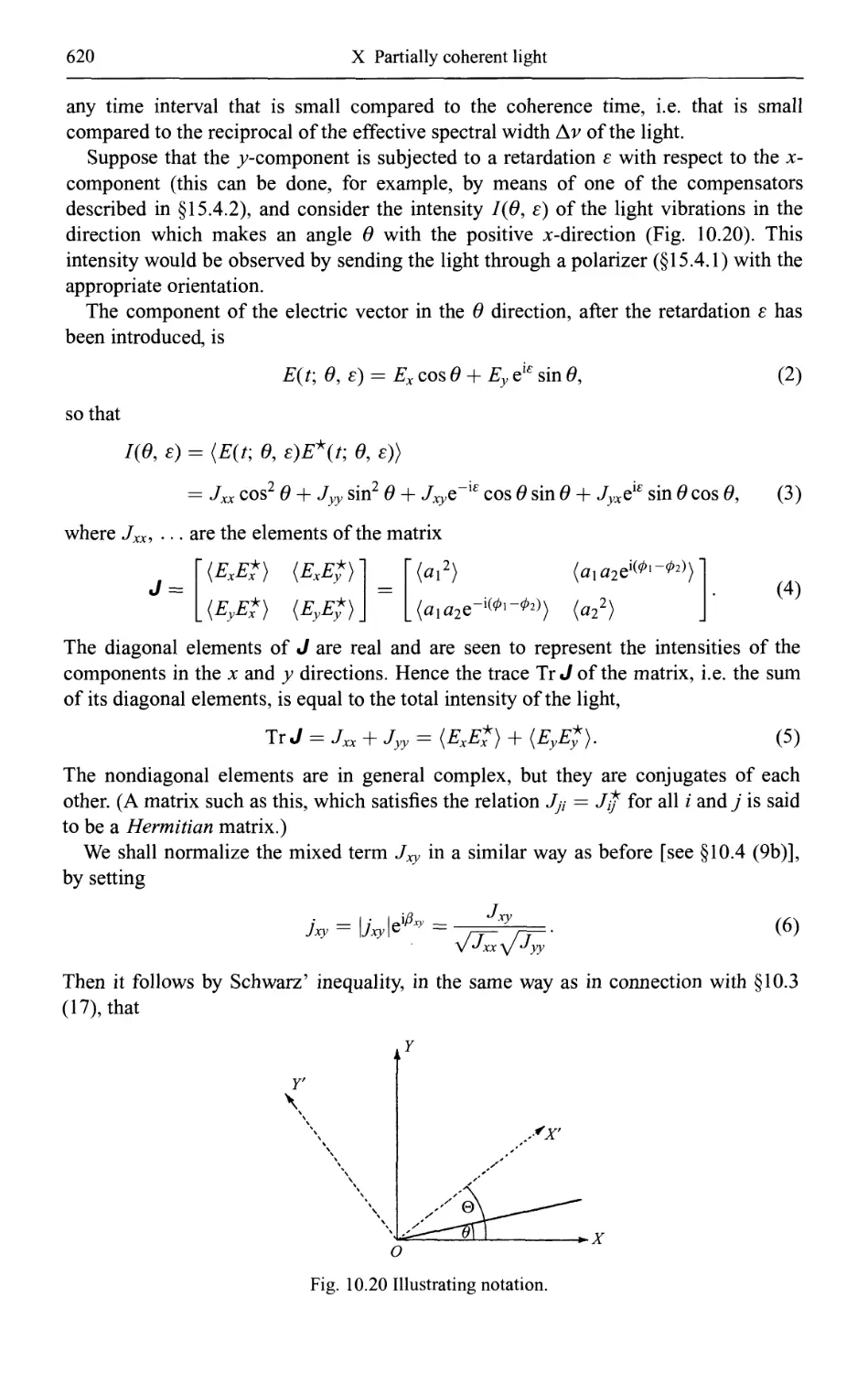
10.9 Polarization properties of quasi-monochromatic light 619
10.9.1 The coherency matrix of a quasi-monochromatic plane wave 619
(a) Completely unpolarized light (natural light) 624
(b) Complete polarized light 624
10.9.2 Some equivalent representations. The degree of polarization of a light
wave 626
10.9.3 The Stokes parameters of a quasi-monochromatic plane wave 630
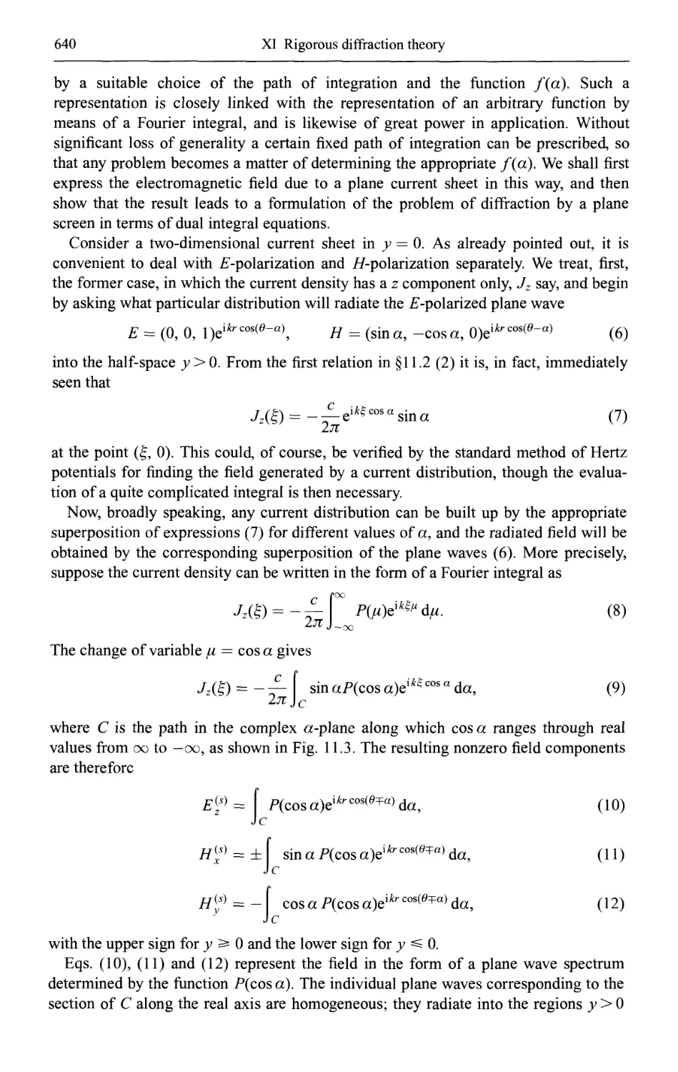
XI Rigorous diffraction theory 633
11.1 Introduction 63 3
11.2 Boundary conditions and surface currents 635
11.3 Diffraction by a plane screen: electromagnetic form of Babinet's principle 636
11.4 Two-dimensional diffraction by a plane screen 638
11.4.1 The scalar nature of two-dimensional electromagnetic fields 638
11.4.2 An angular spectrum of plane waves 639
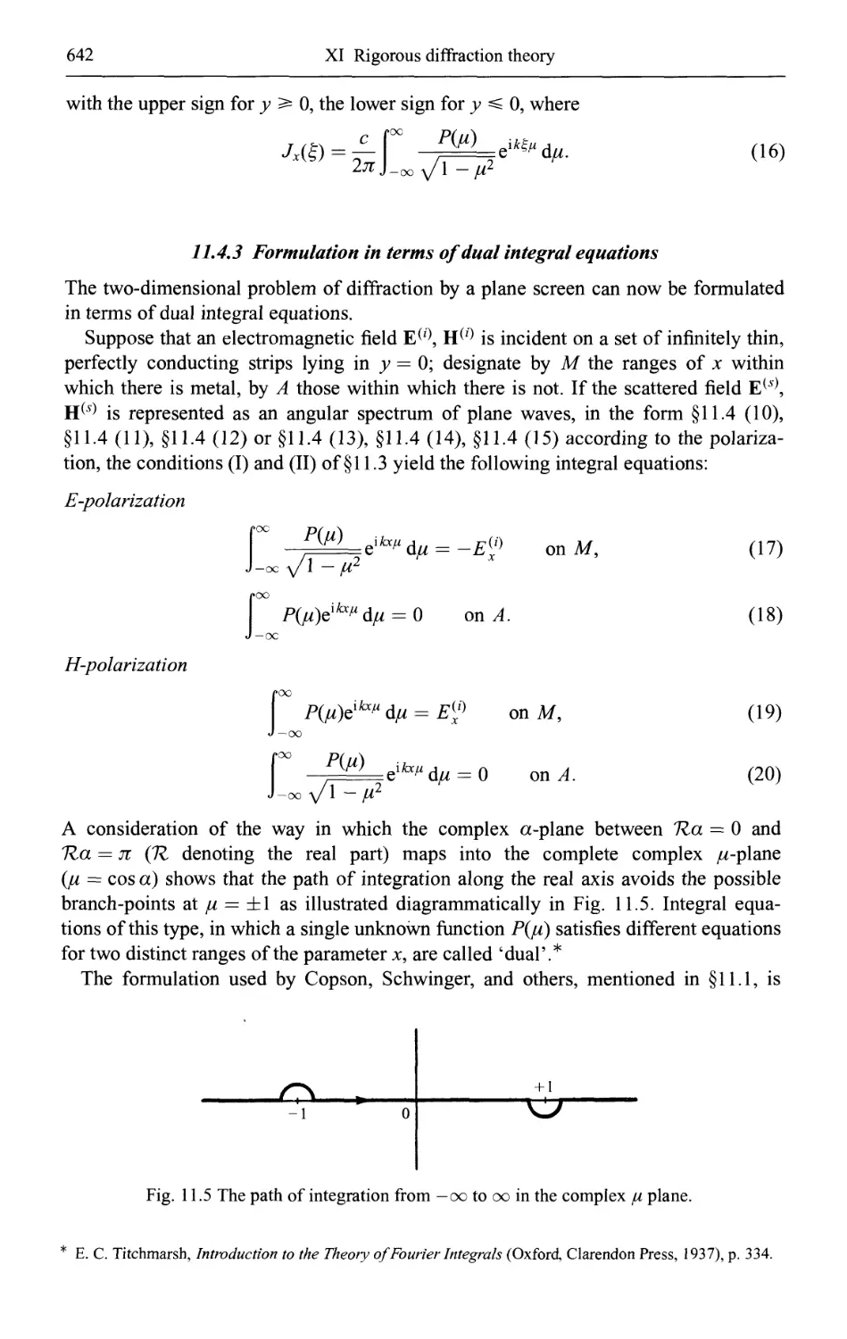
11.4.3 Formulation in terms of dual integral equations 642
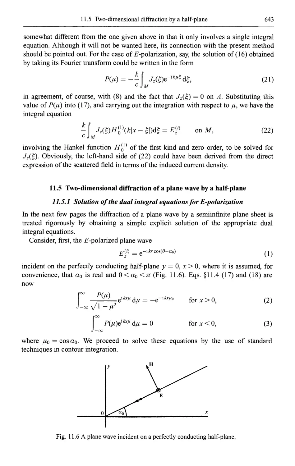
11.5 Two-dimensional diffraction of a plane wave by a half-plane 643
11.5.1 Solution of the dual integral equations for ^-polarization 643
11.5.2 Expression of the solution in terms of Fresnel integrals 645
11.5.3 The nature of the solution 648
XX11
Contents
11.5.4 The solution for //-polarization 652
11.5.5 Some numerical calculations 653
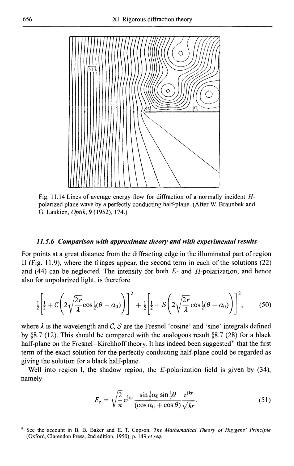
11.5.6 Comparison with approximate theory and with experimental results 656
11.6 Three-dimensional diffraction of a plane wave by a half-plane 657
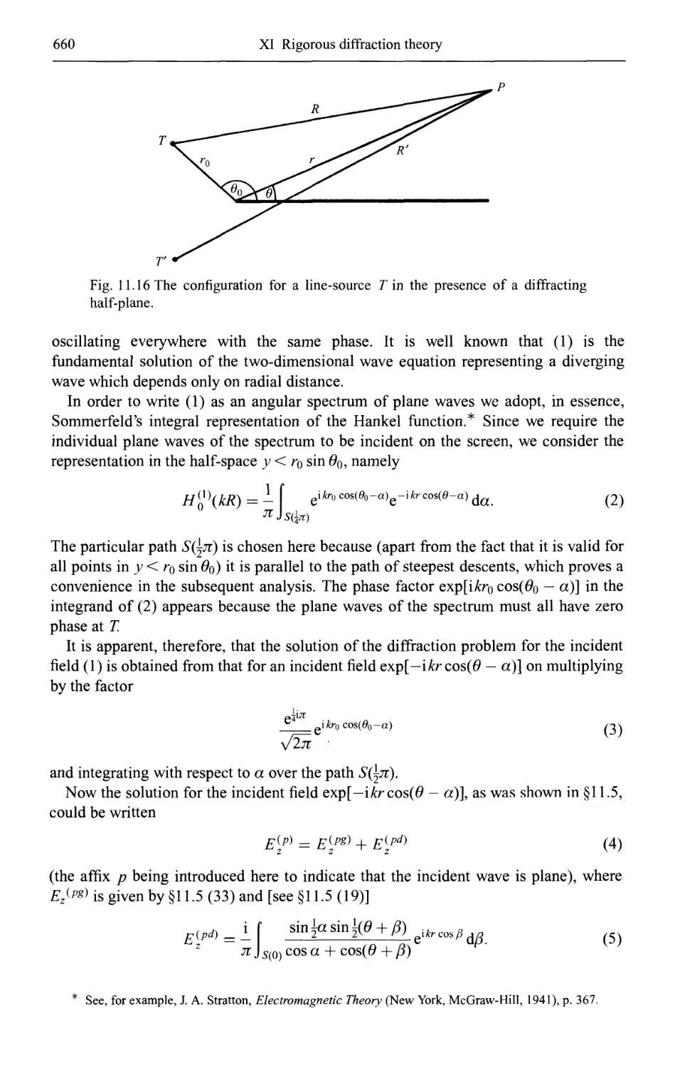
11.7 Diffraction of a field due to a localized source by a half-plane 659
11.7.1 A line-current parallel to the diffracting edge 659
11.7.2 Adipole 664
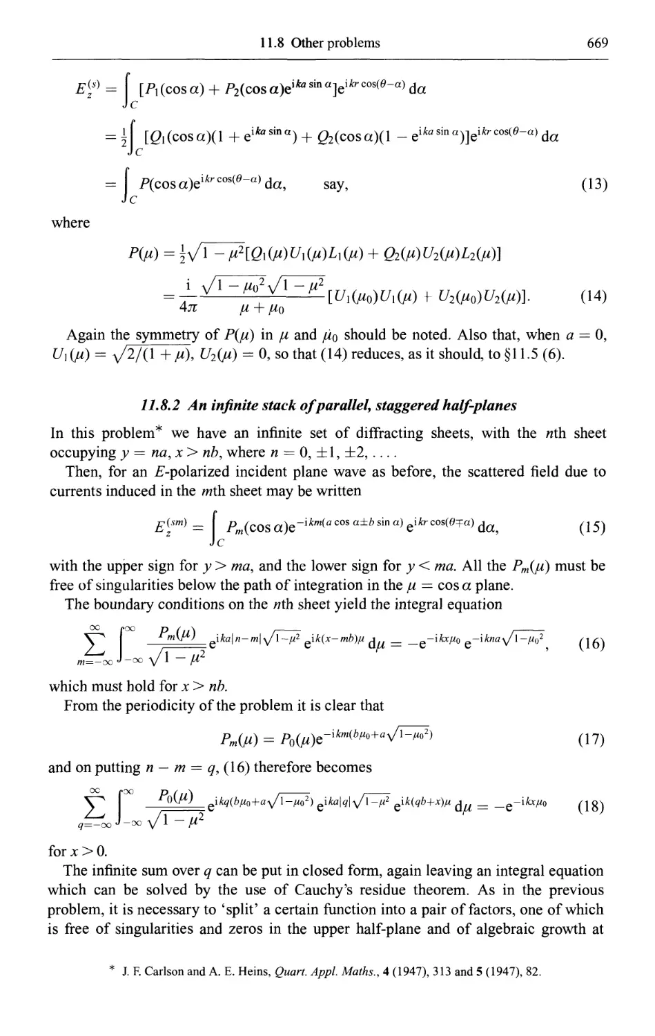
11.8 Other problems 667
11.8.1 Two parallel half-planes 667
11.8.2 An infinite stack of parallel, staggered half-planes 669
11.8.3 A strip 670
11.8.4 Further problems 671
11.9 Uniqueness of solution 672
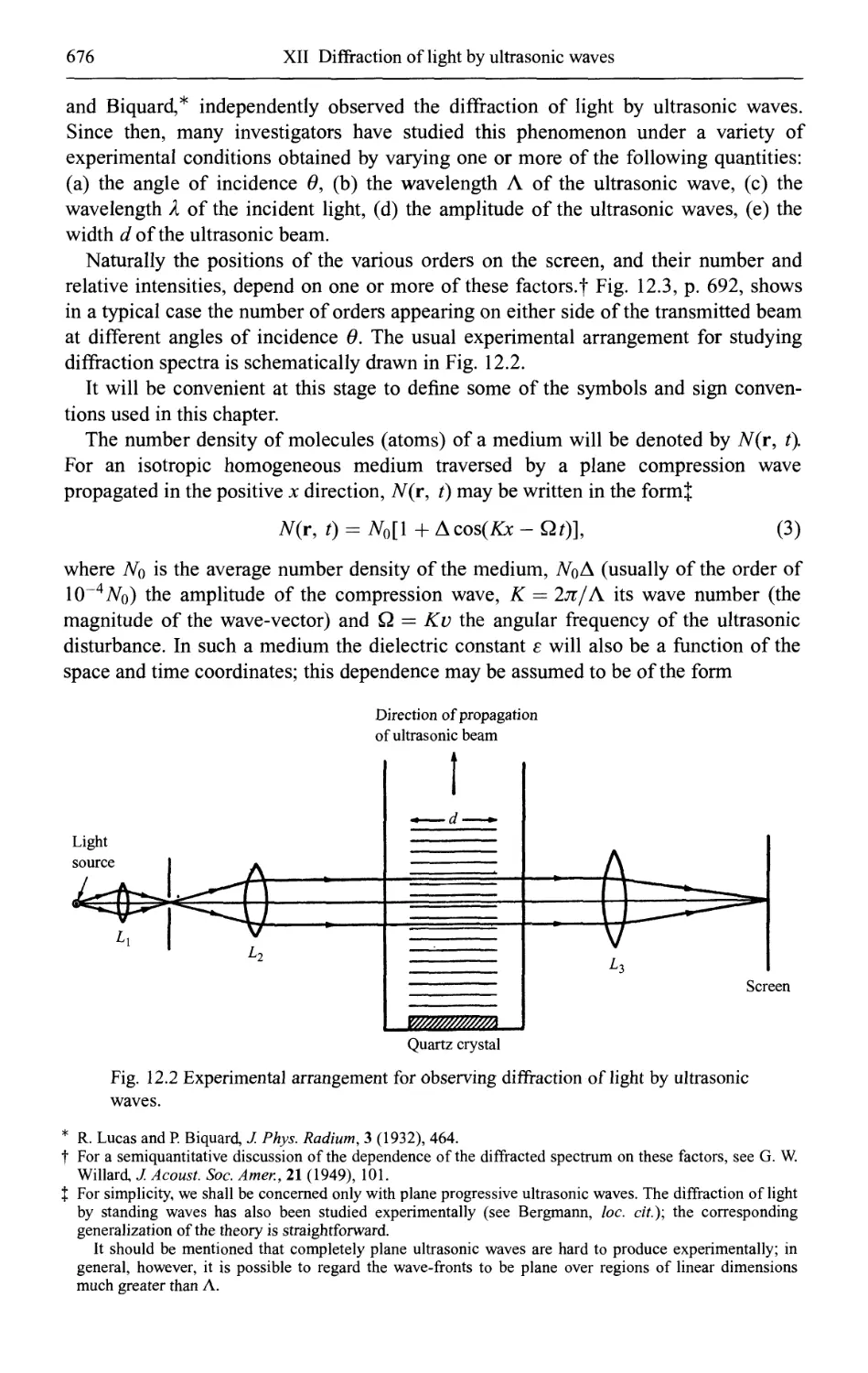
XII Diffraction of light by ultrasonic waves 674
12.1 Qualitative description of the phenomenon and summary of theories based on
Maxwell's differential equations 674
12.1.1 Qualitative description of the phenomenon 674
12.1.2 Summary of theories based on Maxwell's equations 677
12.2 Diffraction of light by ultrasonic waves as treated by the integral equation
method 680
12.2.1 Integral equation for E-polarization 682
12.2.2 The trial solution of the integral equation 682
12.2.3 Expressions for the amplitudes of the light waves in the diffracted and
reflected spectra 686
12.2.4 Solution of the equations by a method of successive approximations 686
12.2.5 Expressions for the intensities of the first and second order lines for
some special cases 689
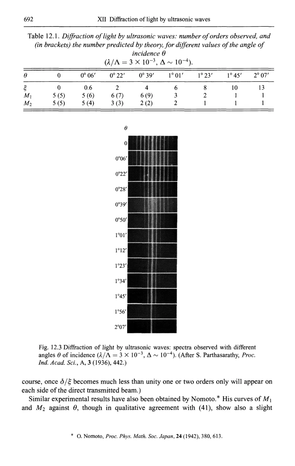
12.2.6 Some qualitative results 691
12.2.7 The Raman-Nath approximation 693
XIII Scattering from inhomogeneous media 695
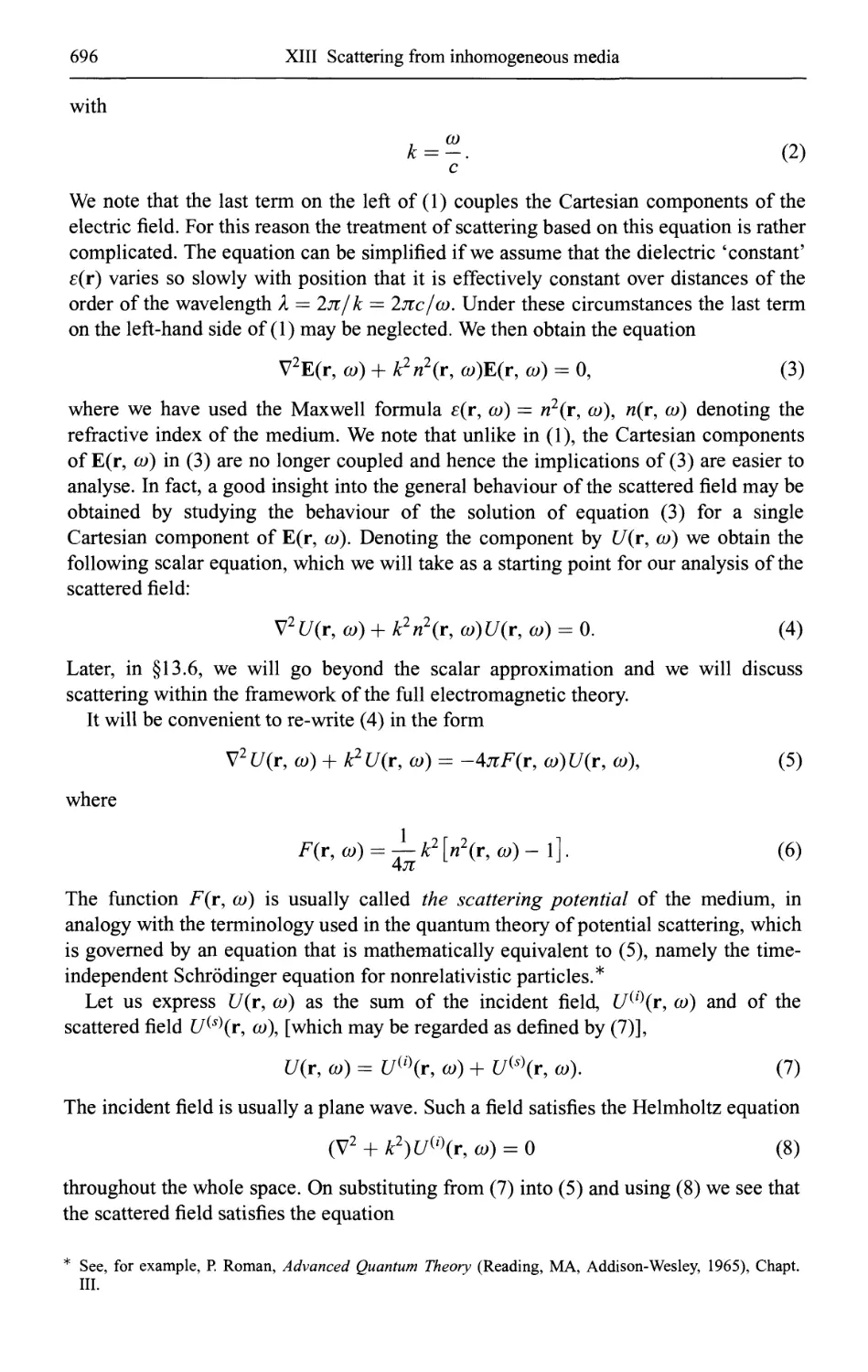
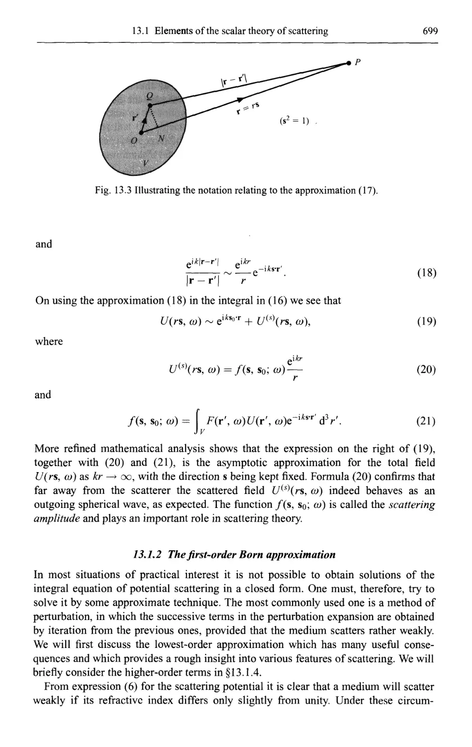
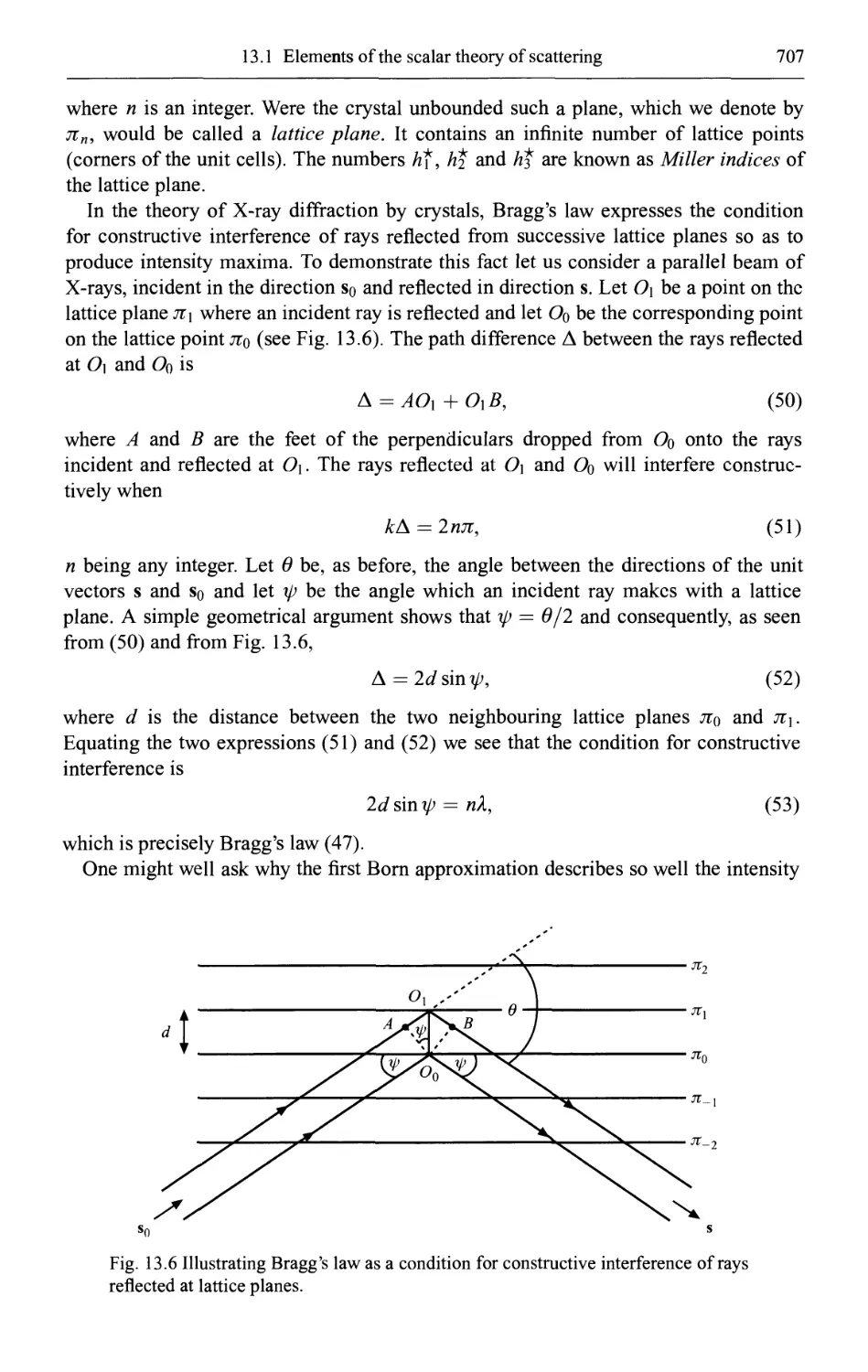
13.1 Elements of the scalar theory of scattering 695
13.1.1 Derivation of the basic integral equation 695
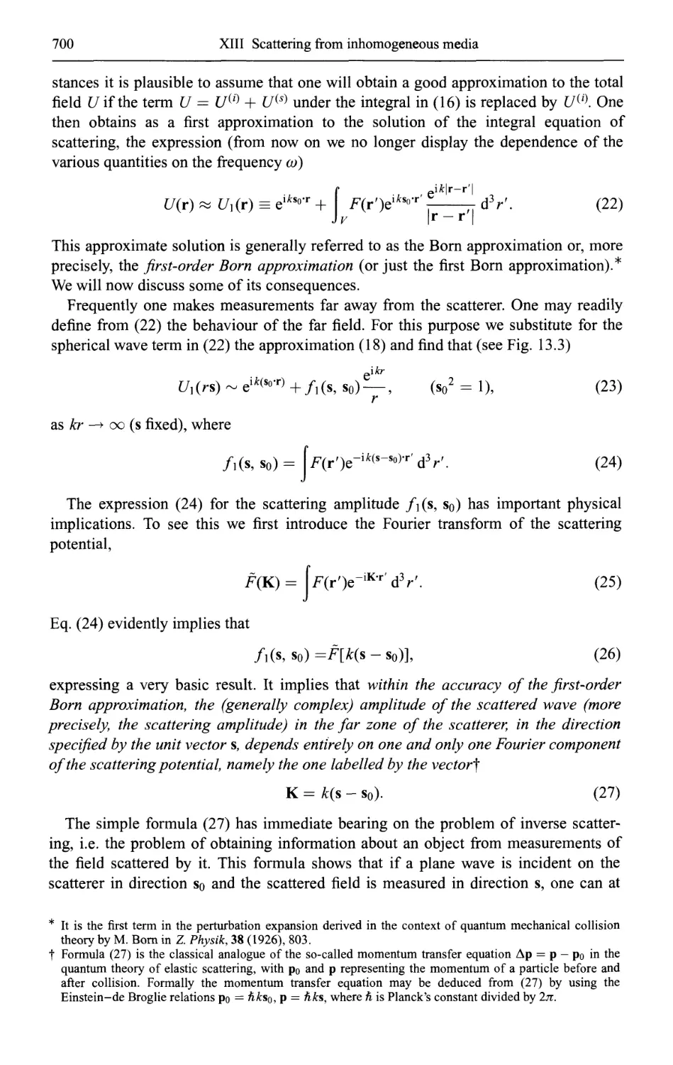
13.1.2 The first-order Born approximation 699
13.1.3 Scattering from periodic potentials 703
13.1.4 Multiple scattering 708
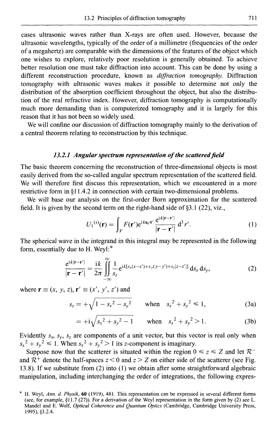
13.2 Principles of diffraction tomography for reconstruction of the scattering
potential 710
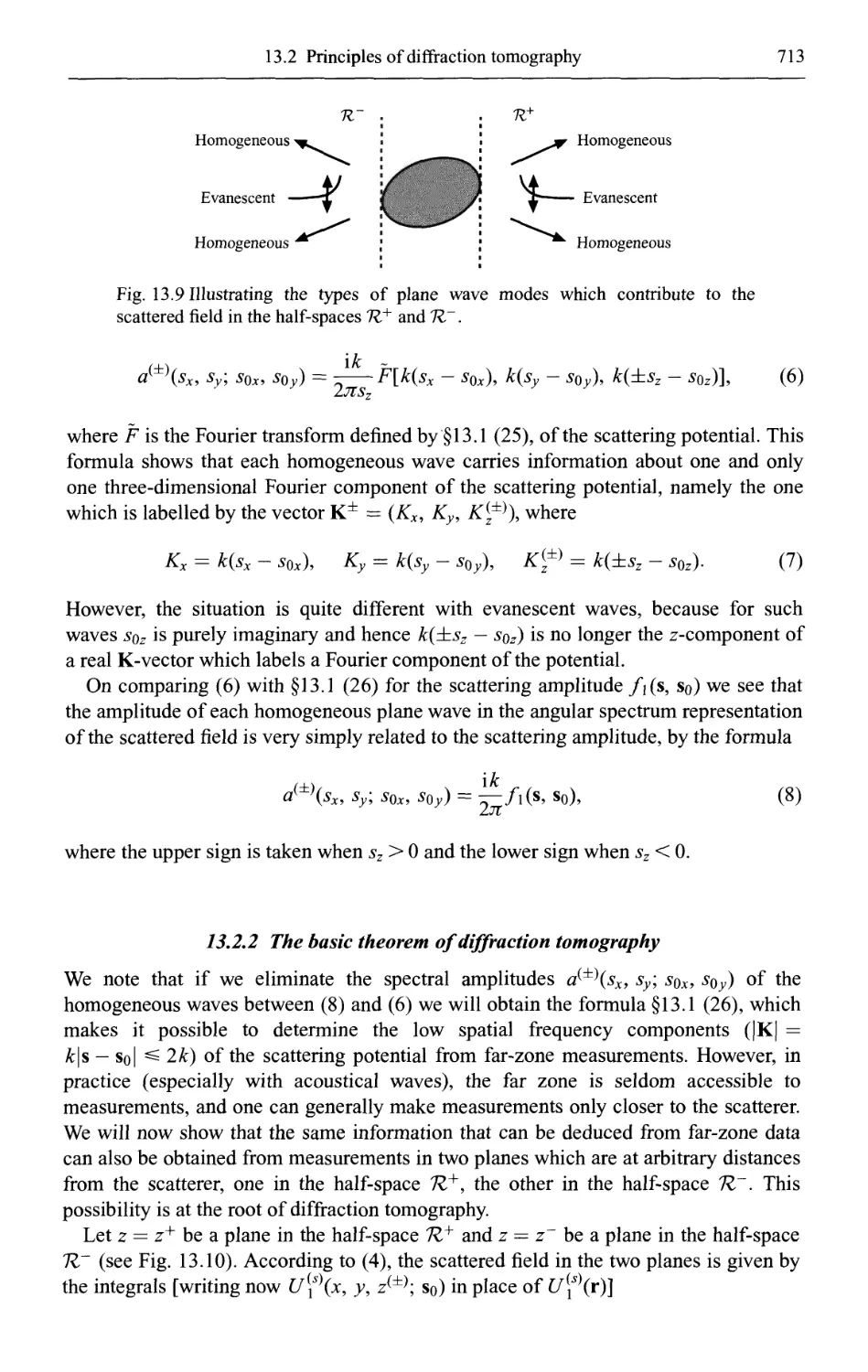
13.2.1 Angular spectrum representation of the scattered field 711
13.2.2 The basic theorem of diffraction tomography 713
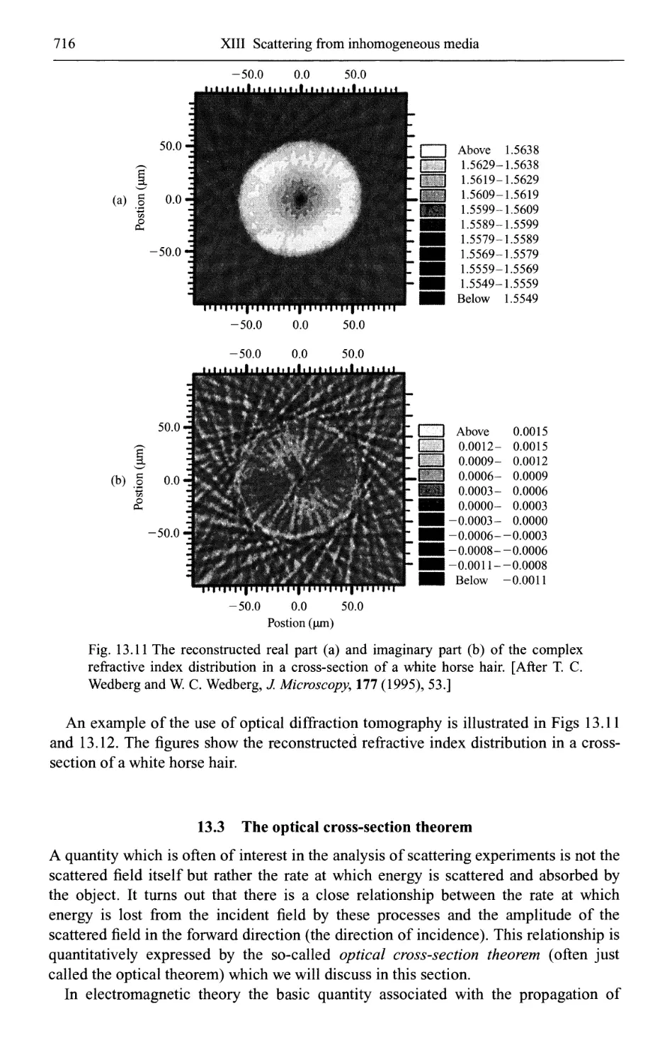
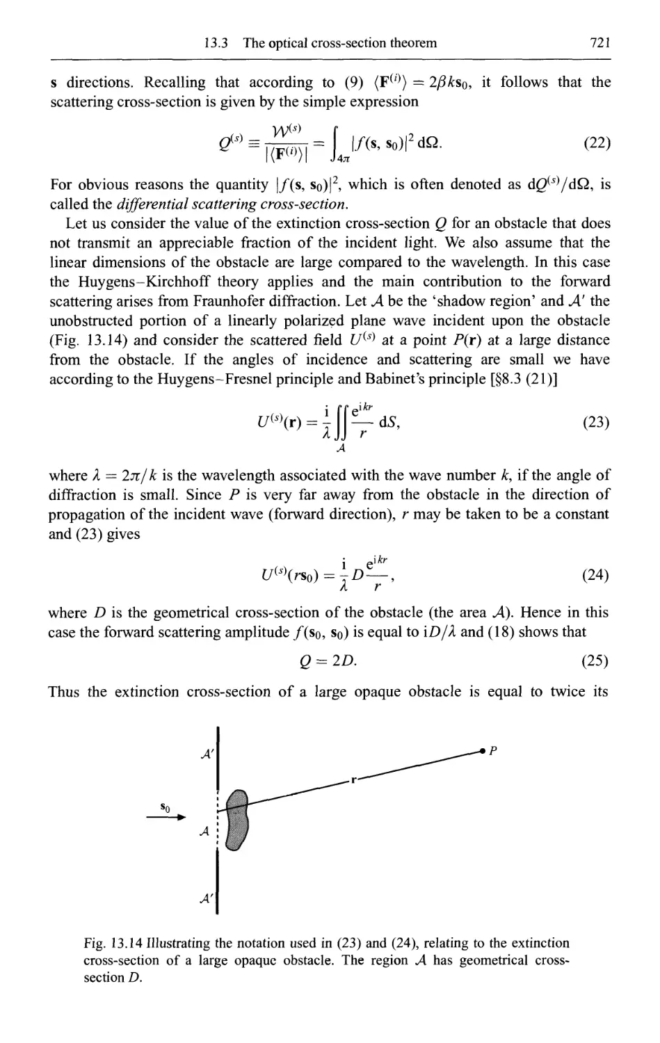
13.3 The optical cross-section theorem 716
13.4 A reciprocity relation 724
13.5 The Rytov series 726
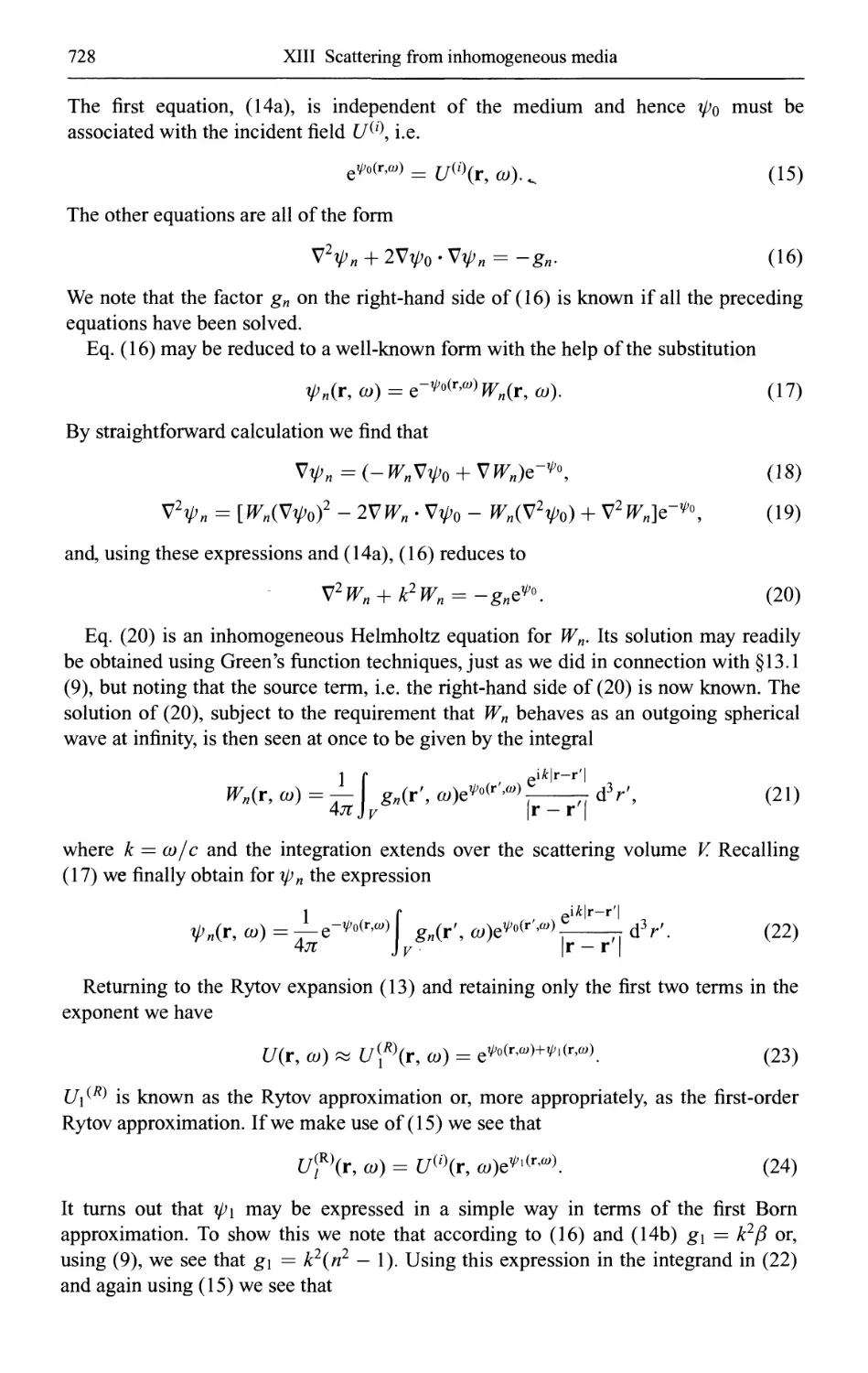
13.6 Scattering of electromagnetic waves 729
13.6.1 The integro-differential equations of electromagnetic scattering
theory 729
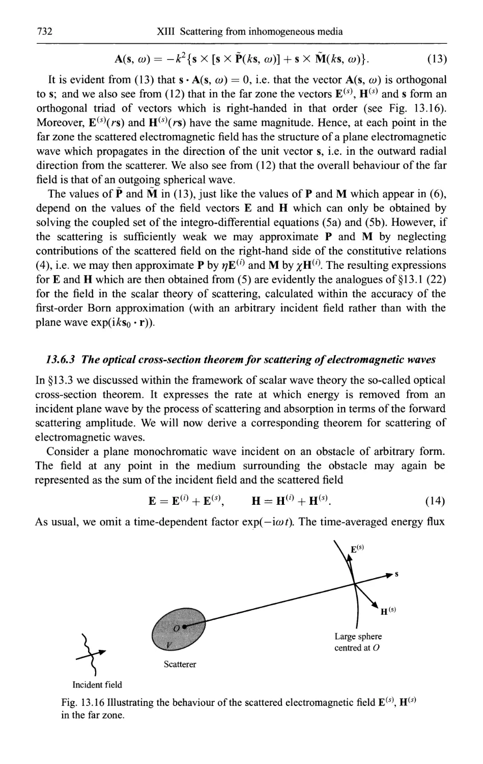
13.6.2 The far field 730
13.6.3 The optical cross-section theorem for scattering of electromagnetic 732
waves
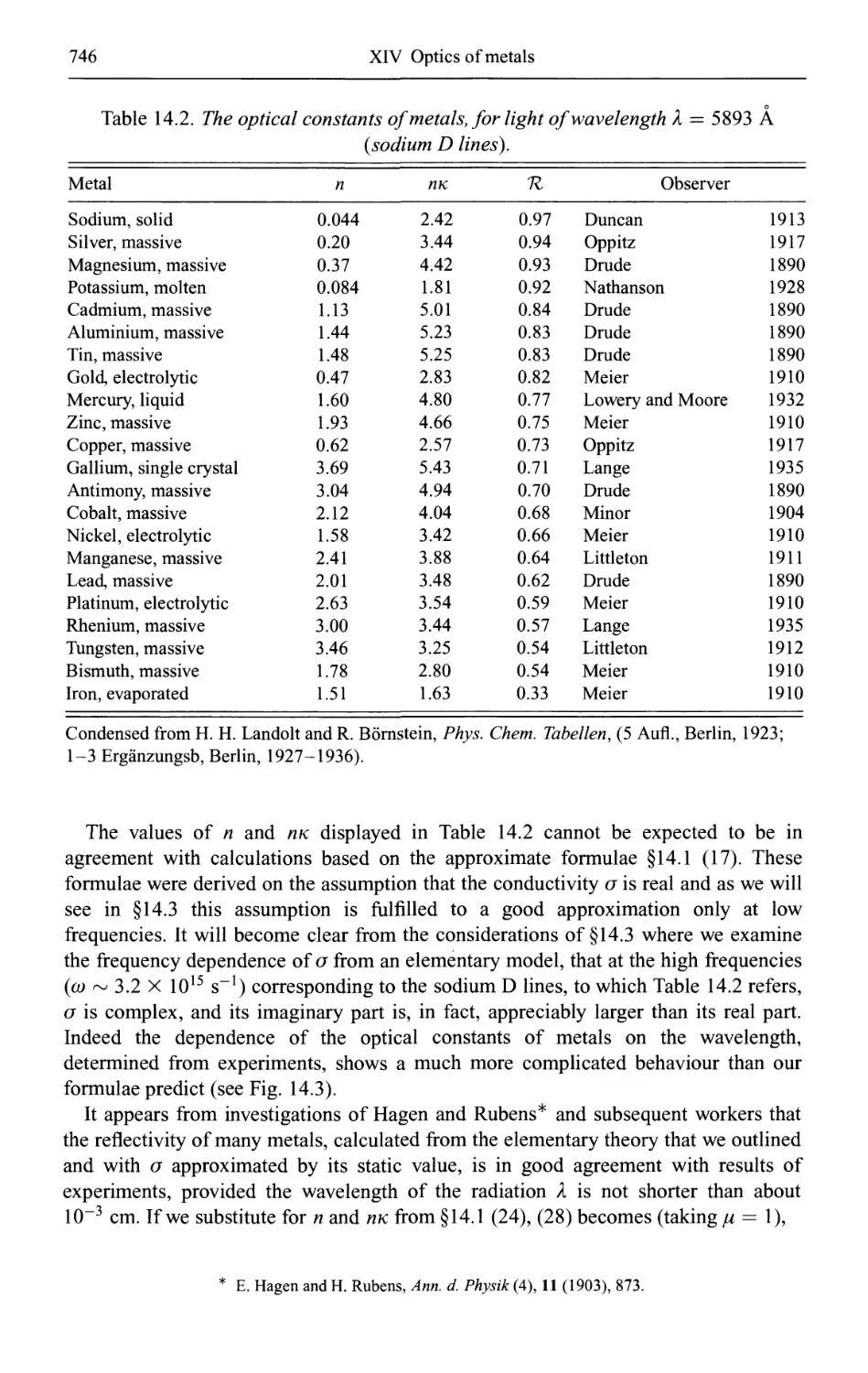
XIV Optics of metals
14.1 Wave propagation in a conductor
735
735
Contents
XXlll
14.2 Refraction and reflection at a metal surface 739
14.3 Elementary electron theory of the optical constants of metals 749
14.4 Wave propagation in a stratified conducting medium. Theory of metallic
films 752
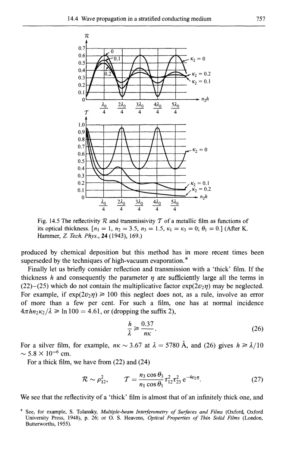
14.4.1 An absorbing film on a transparent substrate 752
14.4.2 A transparent film on an absorbing substrate 758
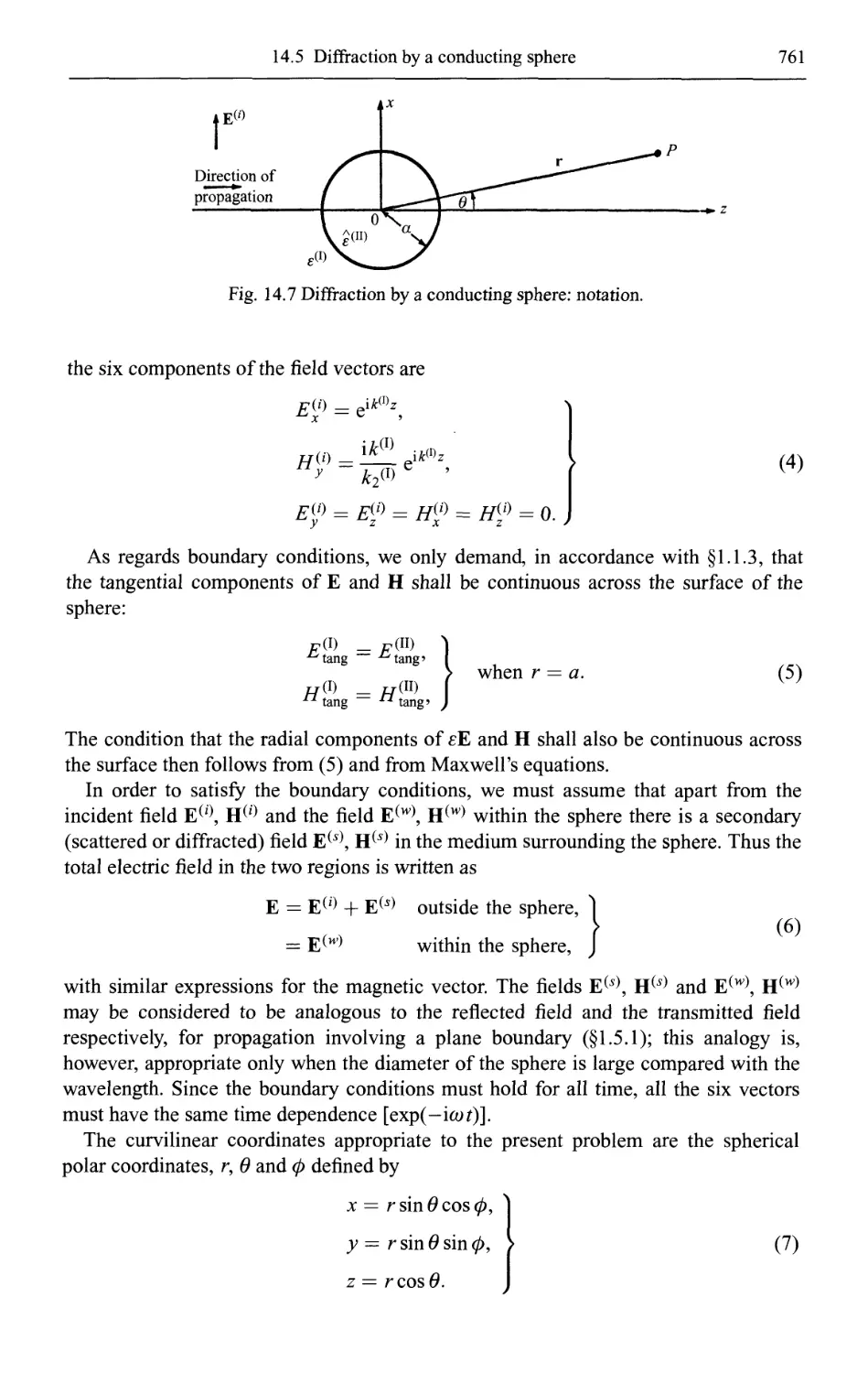
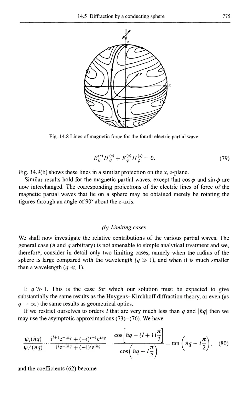
14.5 Diffraction by a conducting sphere; theory of Mie 759
14.5.1 Mathematical solution of the problem 760
(a) Representation of the field in terms of Debye's potentials 760
(b) Series expansions for the field components 765
(c) Summary of formulae relating to the associated Legendre
functions and to the cylindrical functions 772
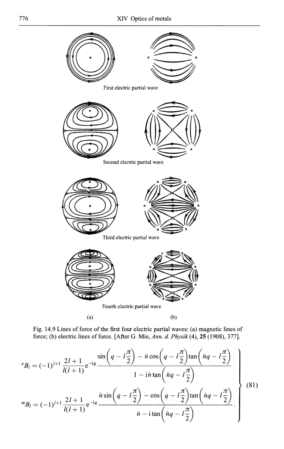
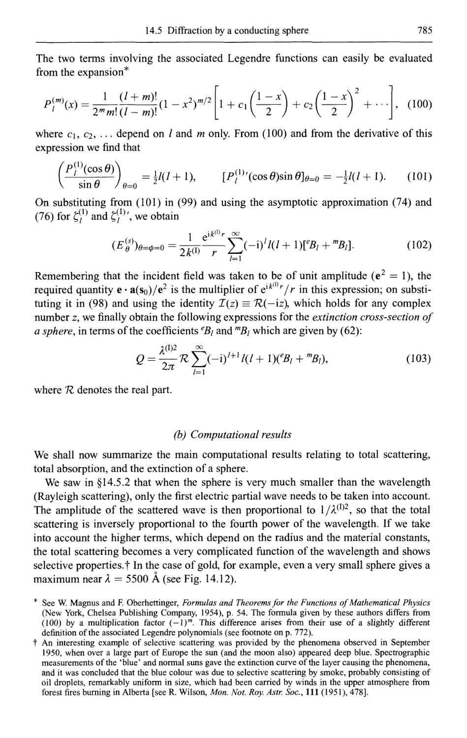
14.5.2 Some consequences of Mie's formulae 774
(a) The partial waves 774
(b) Limiting cases 775
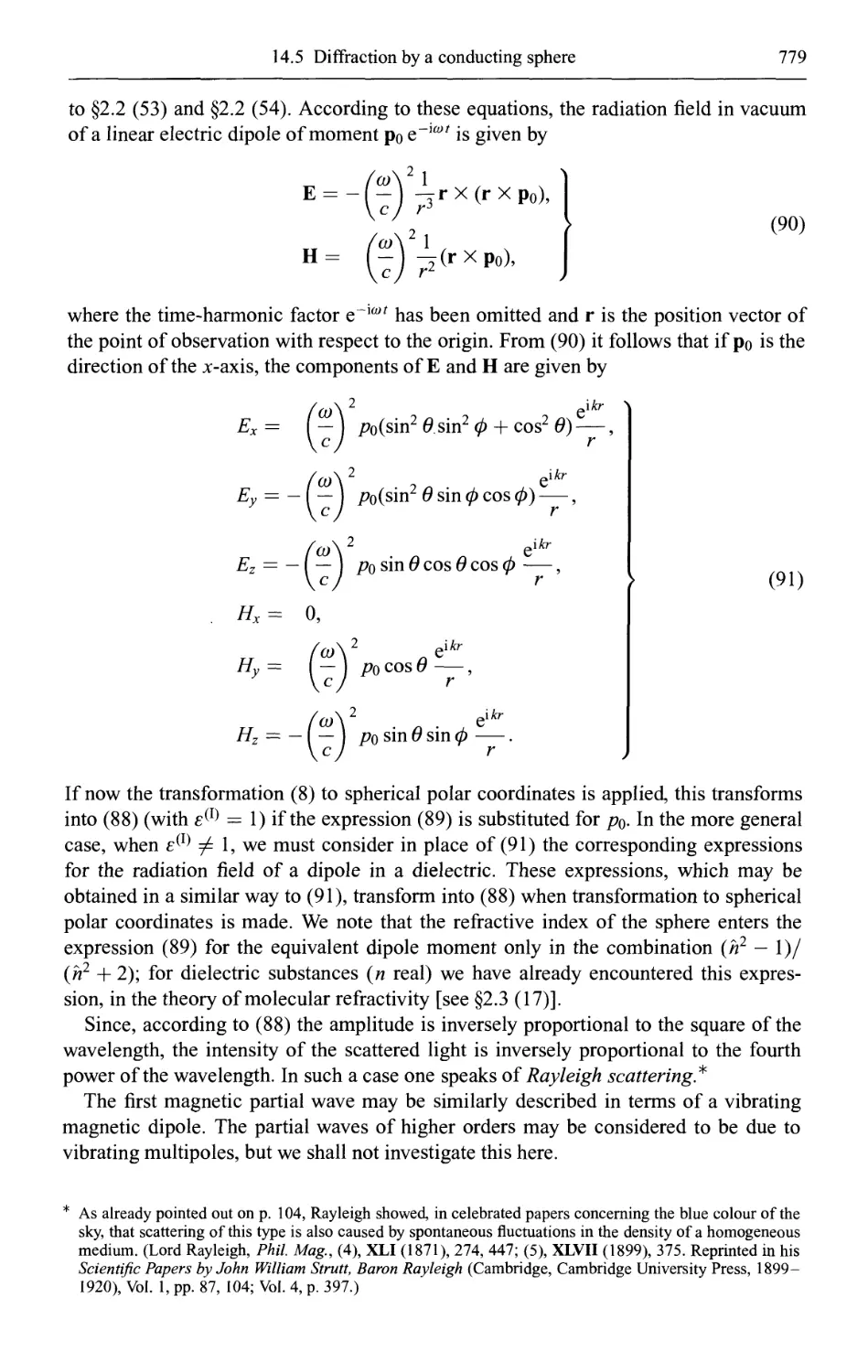
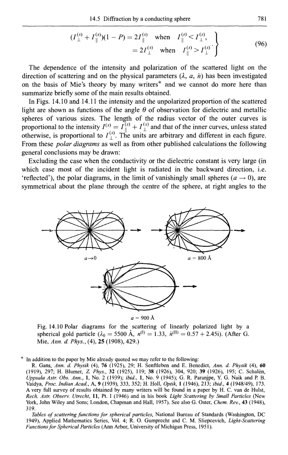
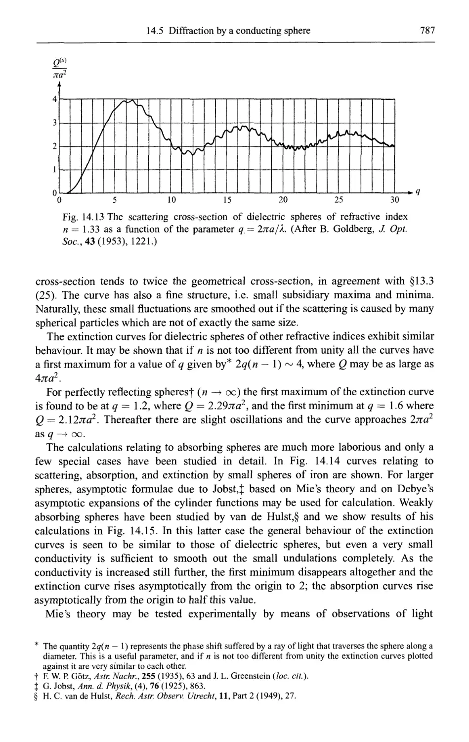
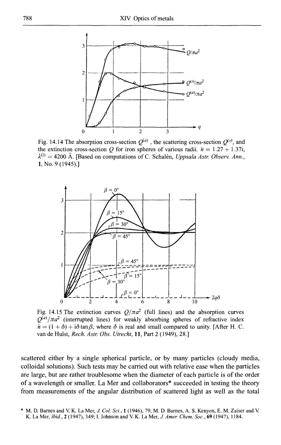
(c) Intensity and polarization of the scattered light 780
14.5.3 Total scattering and extinction 784
(a) Some general considerations 784
(b) Computational results 785
XV Optics of crystals 790
15.1 The dielectric tensor of an anisotropic medium 790
15.2 The structure of a monochromatic plane wave in an anisotropic medium 792
15.2.1 The phase velocity and the ray velocity 792
15.2.2 Fresnel's formulae for the propagation of light in crystals 795
15.2.3 Geometrical constructions for determining the velocities of
propagation and the directions of vibration 799
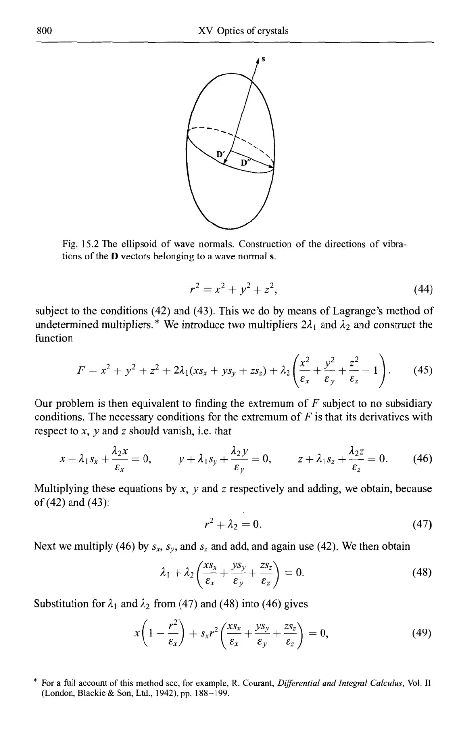
(a) The ellipsoid of wave normals 799
(b) The ray ellipsoid 802
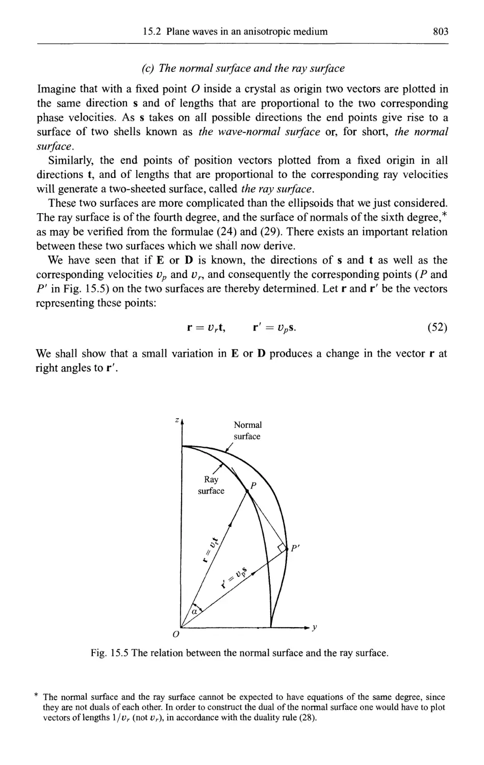
(c) The normal surface and the ray surface 803
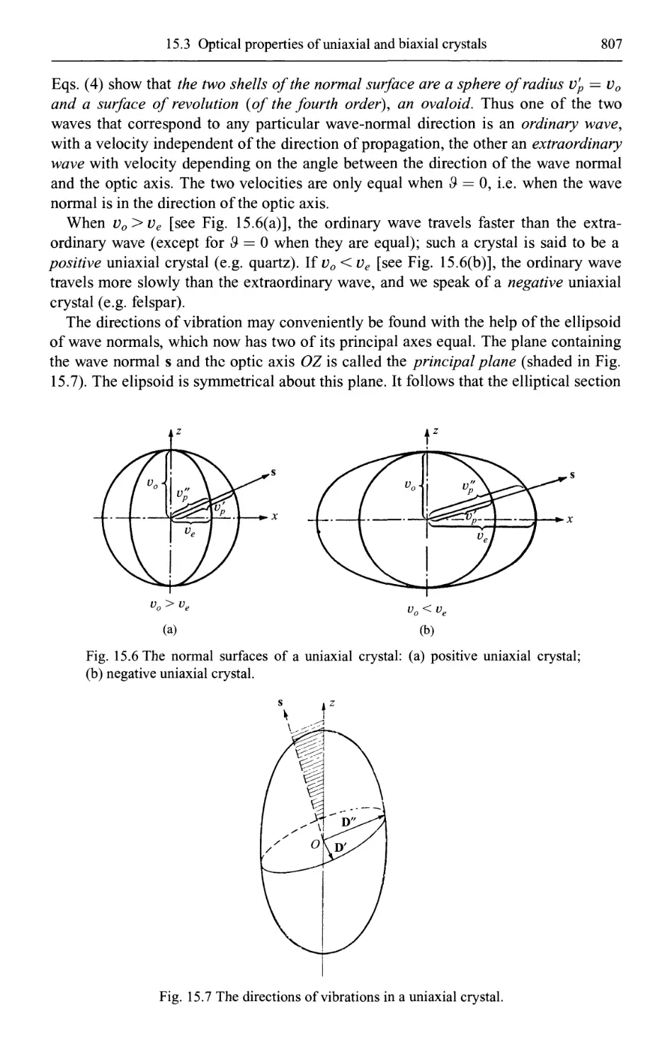
15.3 Optical properties of uniaxial and biaxial crystals 805
15.3.1 The optical classification of crystals 805
15.3.2 Light propagation in uniaxial crystals 806
15.3.3 Light propagation in biaxial crystals 808
15.3.4 Refraction in crystals 811
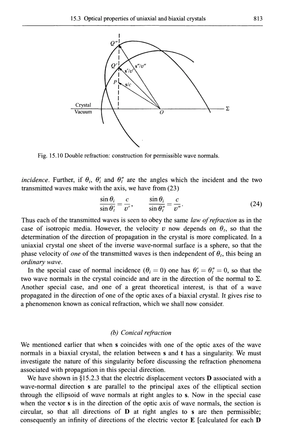
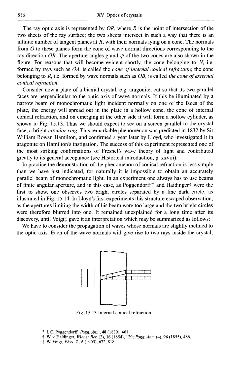
(a) Double refraction 811
(b) Conical refraction 813
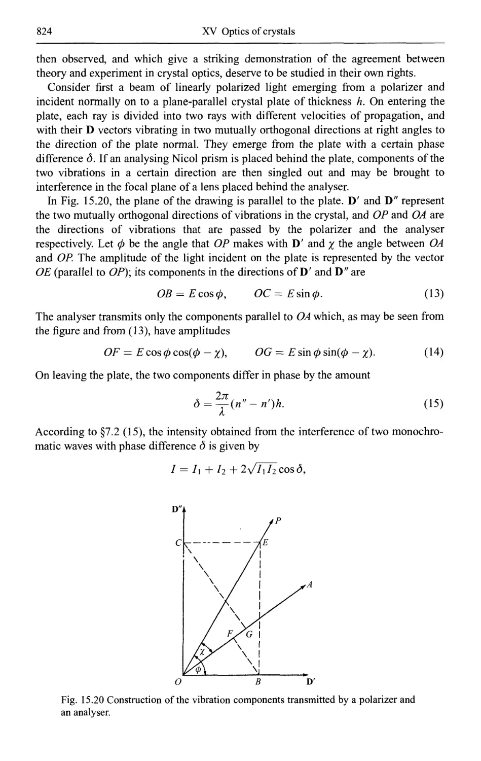
15.4 Measurements in crystal optics 818
15.4.1 The Nicol prism 818
15.4.2 Compensators 820
(a) The quarter-wave plate 820
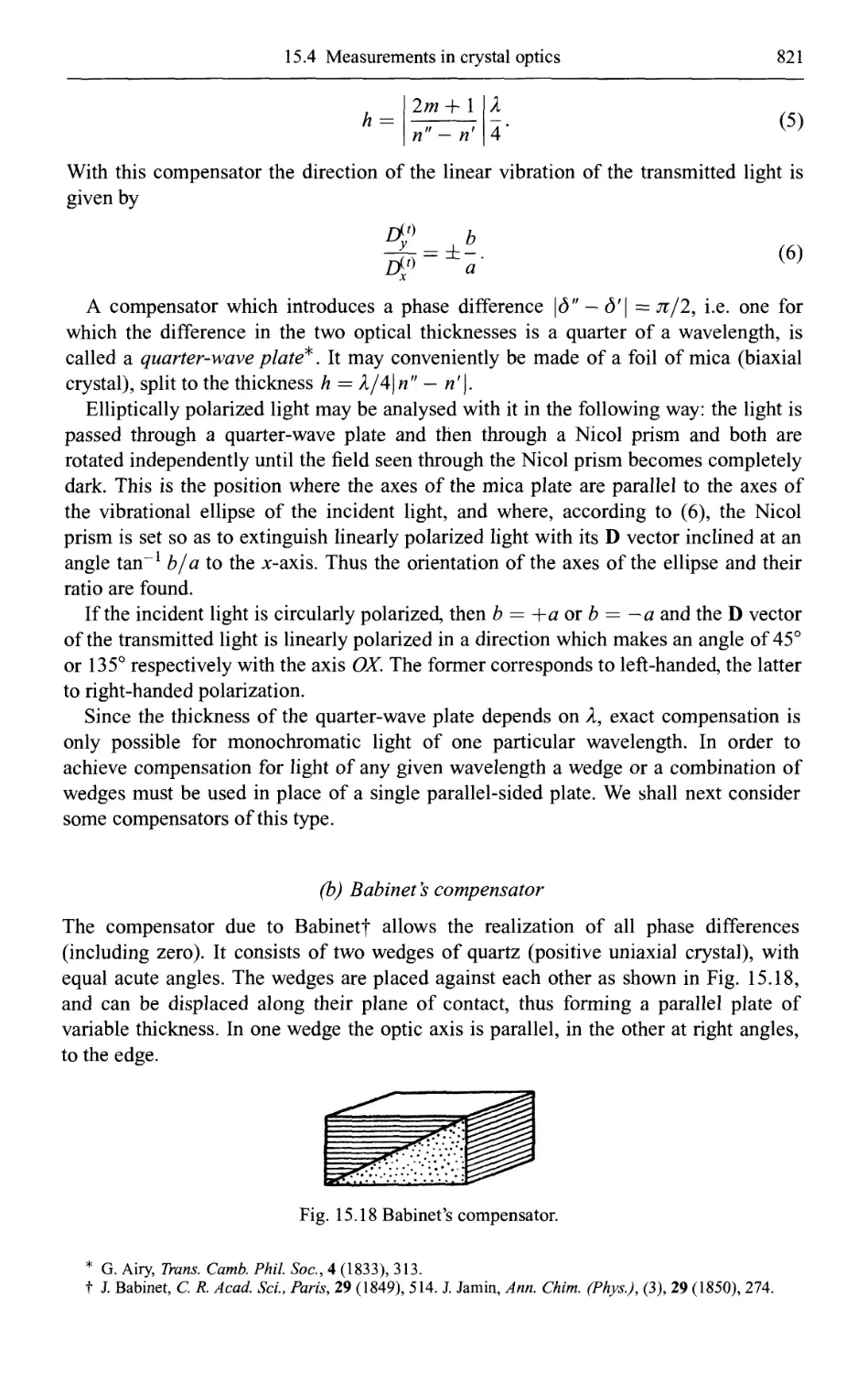
(b) Babinet's compensator 821
(c) Soleil's compensator 823
(d) Berek's compensator 823
15.4.3 Interference with crystal plates 823
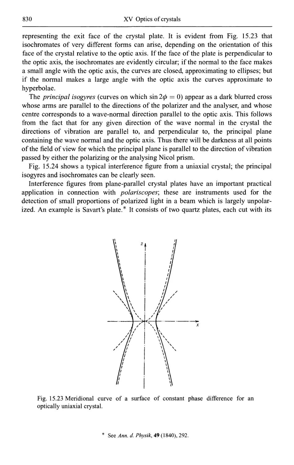
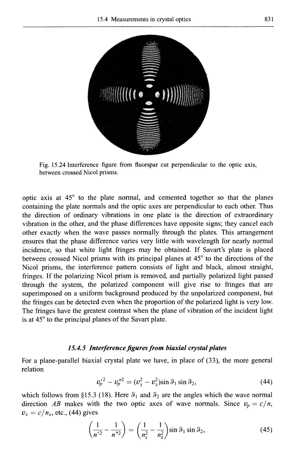
15.4.4 Interference figures from uniaxial crystal plates 829
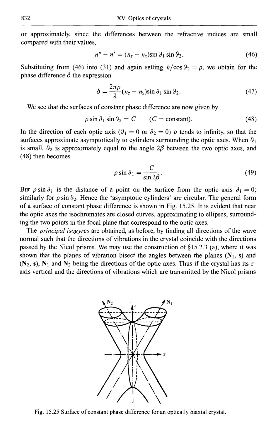
15.4.5 Interference figures from biaxial crystal plates 831
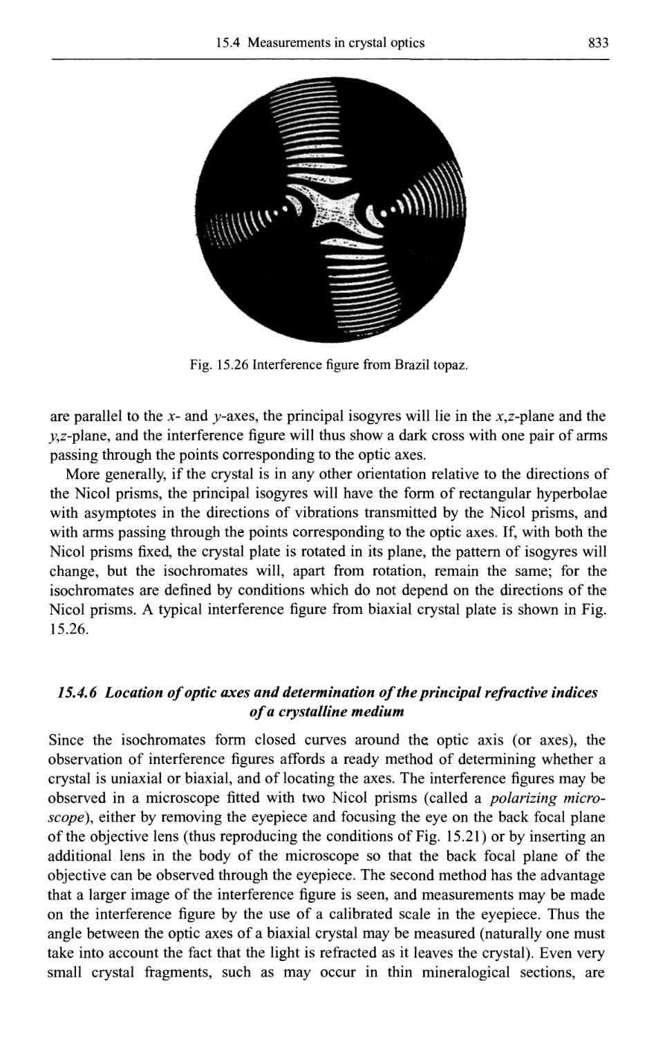
15.4.6 Location of optic axes and determination of the principal refractive
indices of a crystalline medium 833
15.5 Stress birefringence and form birefringence 834
15.5.1 Stress birefringence 834
15.5.2 Form birefringence 837
XXIV
Contents
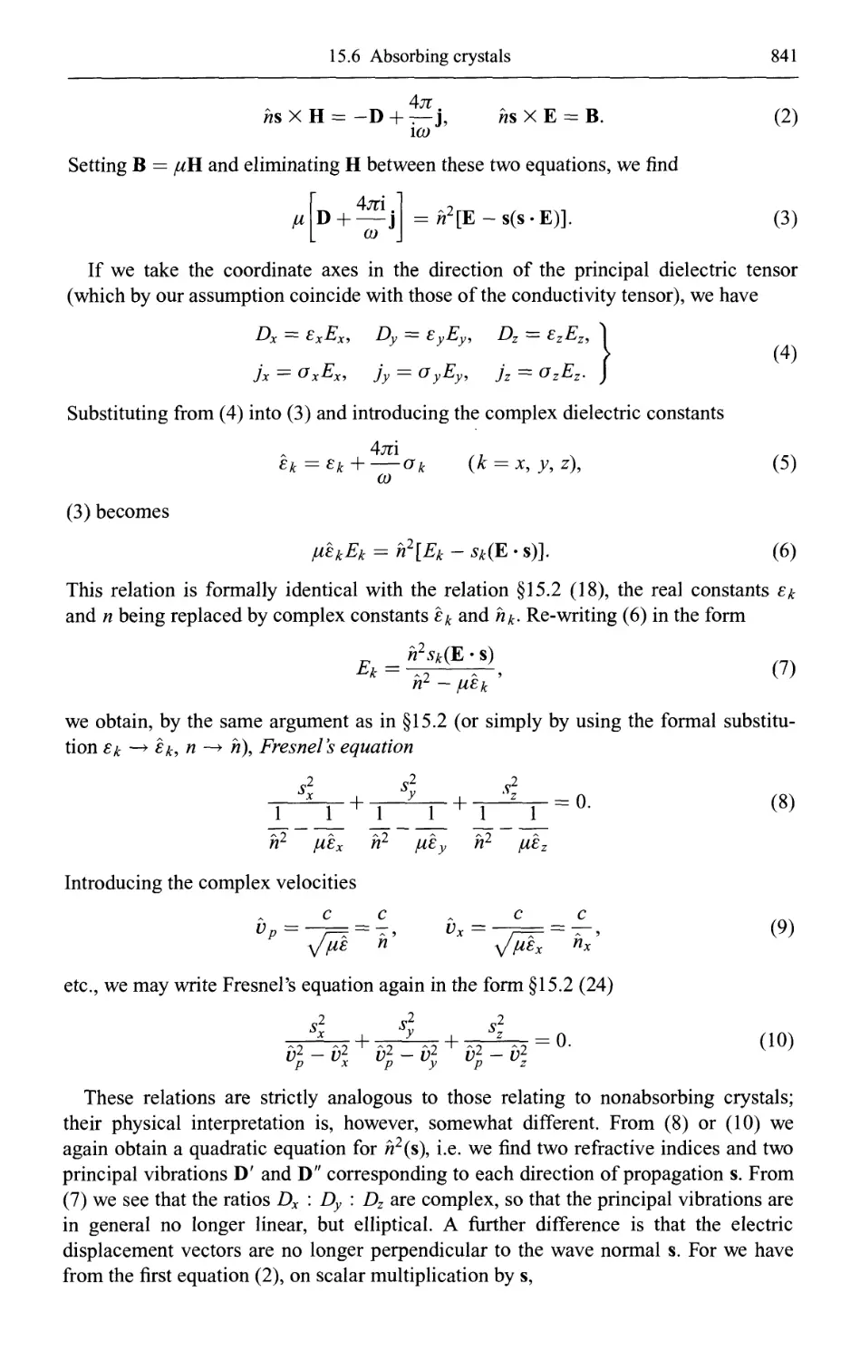
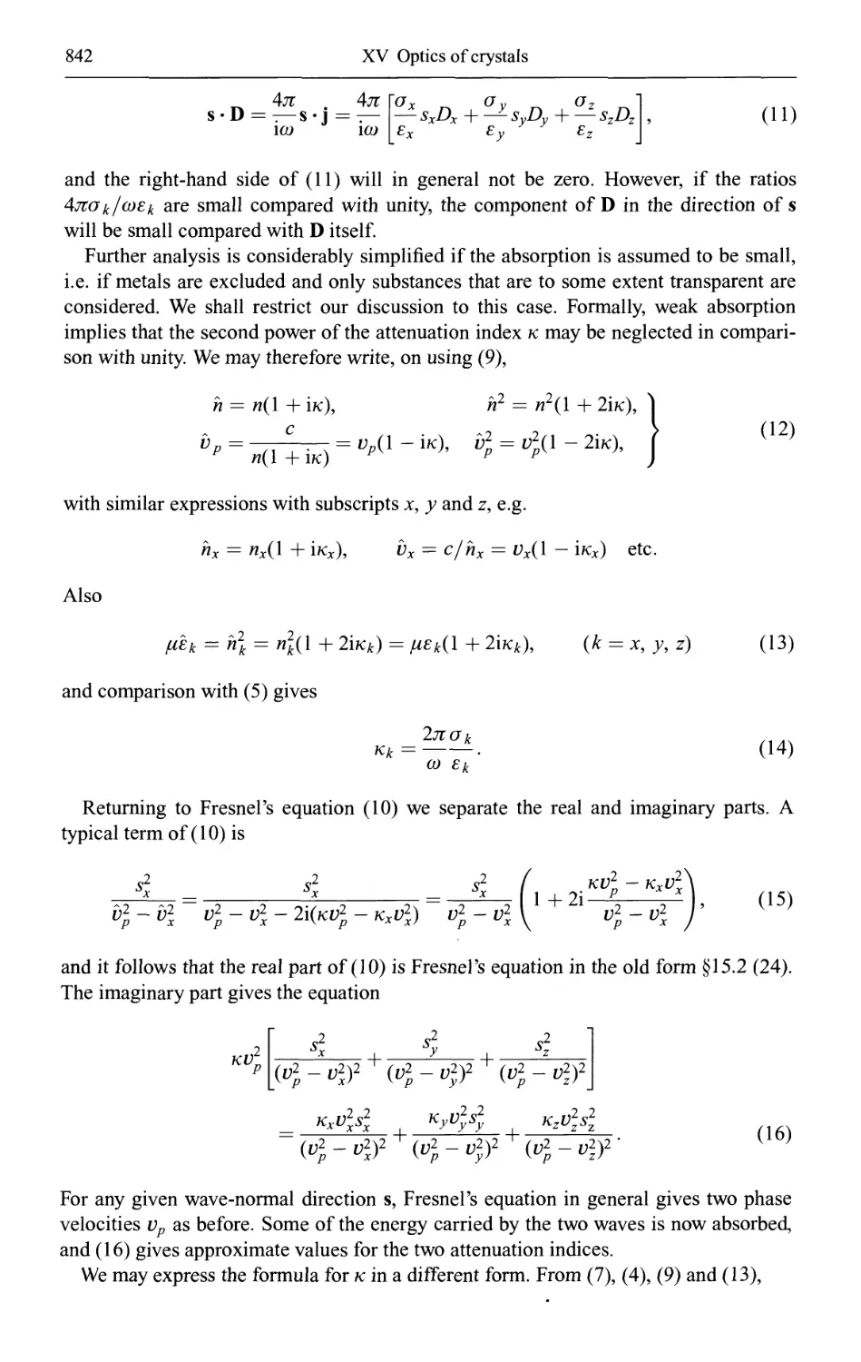
15.6 Absorbing crystals 840
15.6.1 Light propagation in an absorbing anisotropic medium 840
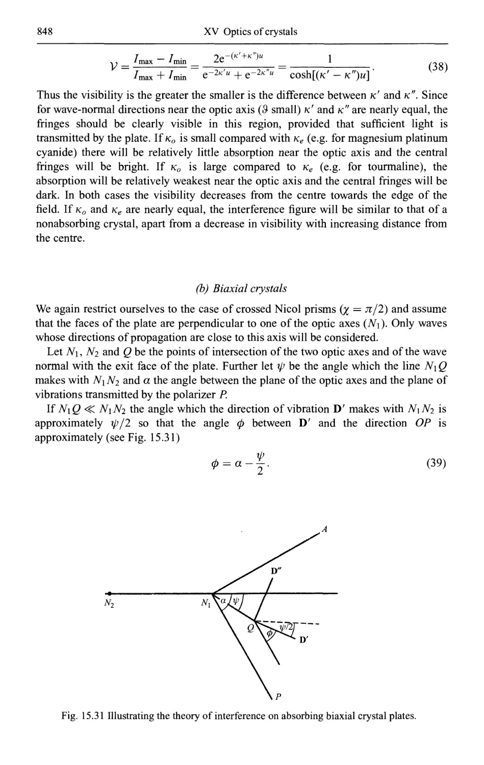
15.6.2 Interference figures from absorbing crystal plates 846
(a) Uniaxial crystals 847
(b) Biaxial crystals 848
15.6.3 Dichroic polarizers 849
Appendices 853
I The Calculus of variations 853
1 Euler's equations as necessary conditions for an extremum 853
2 Hubert's independence integral and the Hamilton-Jacobi equation 855
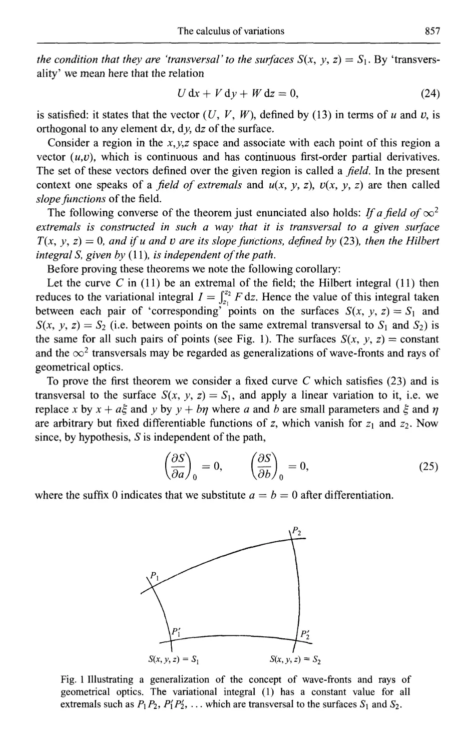
3 The field of extremals 856
4 Determination of all extremals from the solution of the Hamilton-Jacobi equation 858
5 Hamilton's canonical equations 860
6 The special case when the independent variable does not appear explicitly in the integrand 861
7 Discontinuities 862
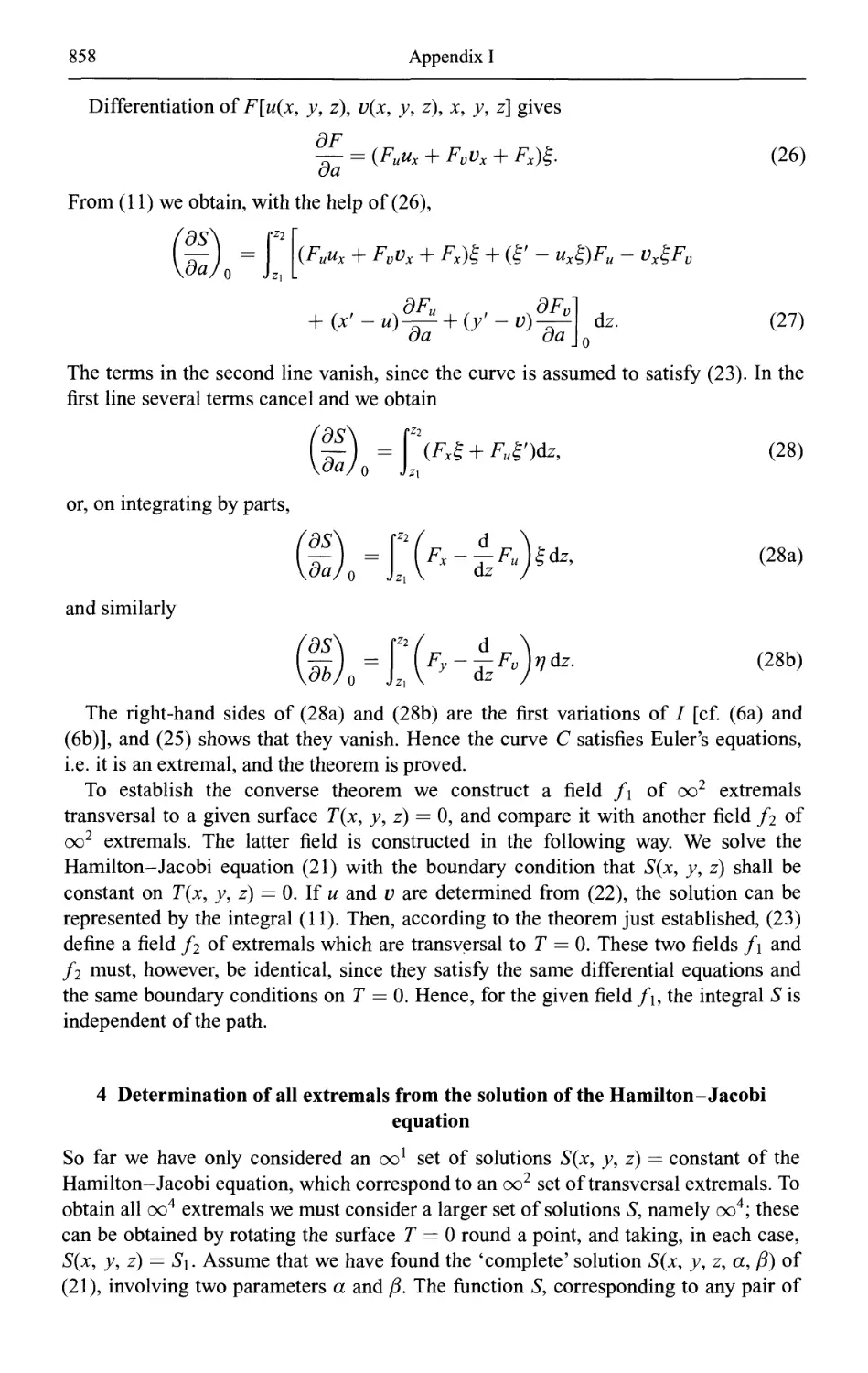
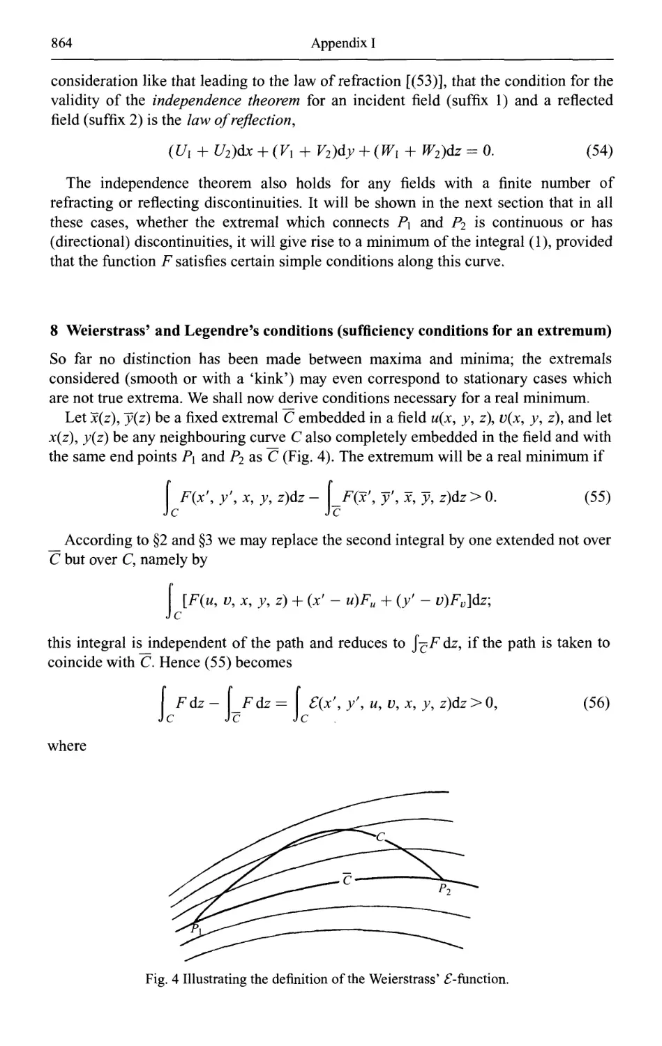
8 Weierstrass' and Legendre's conditions (sufficiency conditions for an extremum) 864
9 Minimum of the variational integral when one end point is constrained to a surface 866
10 Jacobi's criterion for a minimum 867
11 Example I: Optics 868
12 Example TT: Mechanics of material points 870
II Light optics, electron optics and wave mechanics 873
1 The Hamiltonian analogy in elementary form 873
2 The Hamiltonian analogy in variational form 876
3 Wave mechanics of free electrons 879
4 The application of optical principles to electron optics 881
III Asymptotic approximations to integrals 883
1 The method of steepest descent 883
2 The method of stationary phase 888
3 Double integrals 890
IV The Dirac delta function 892
V A mathematical lemma used in the rigorous derivation of the Lorentz-Lorenz formula
(§2.4.2) 898
VI Propagation of discontinuities in an electromagnetic field (§3.1.1) 901
1 Relations connecting discontinuous changes in field vectors 901
2 The field on a moving discontinuity surface 903
VII The circle polynomials of Zernike (§9.2.1) 905
1 Some general considerations 905
2 Explicit expressions for the radial polynomials Rtm{p) 907
Vin Proof of the inequality \fin(y)\ ^ 1 for the spectral degree of coherence (§10.5) 911
IX Proof of a reciprocity inequality (§10.8.3) 912
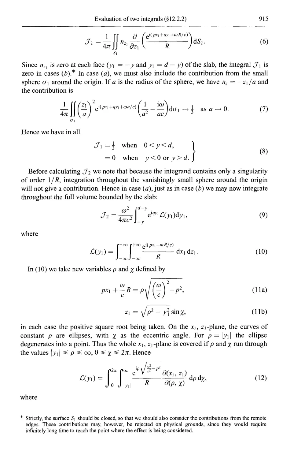
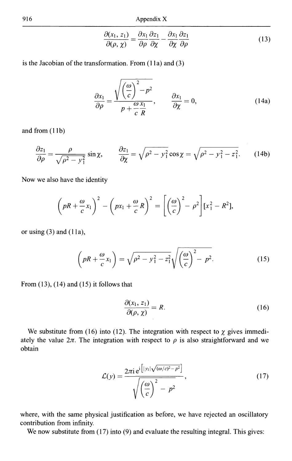
X Evaluation of two integrals (§12.2.2) 914
XI Energy conservation in scalar wavefields (§13.3) 918
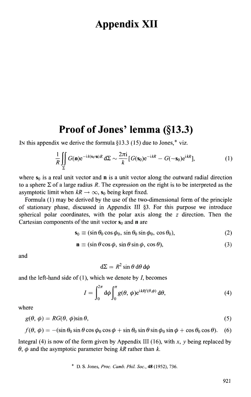
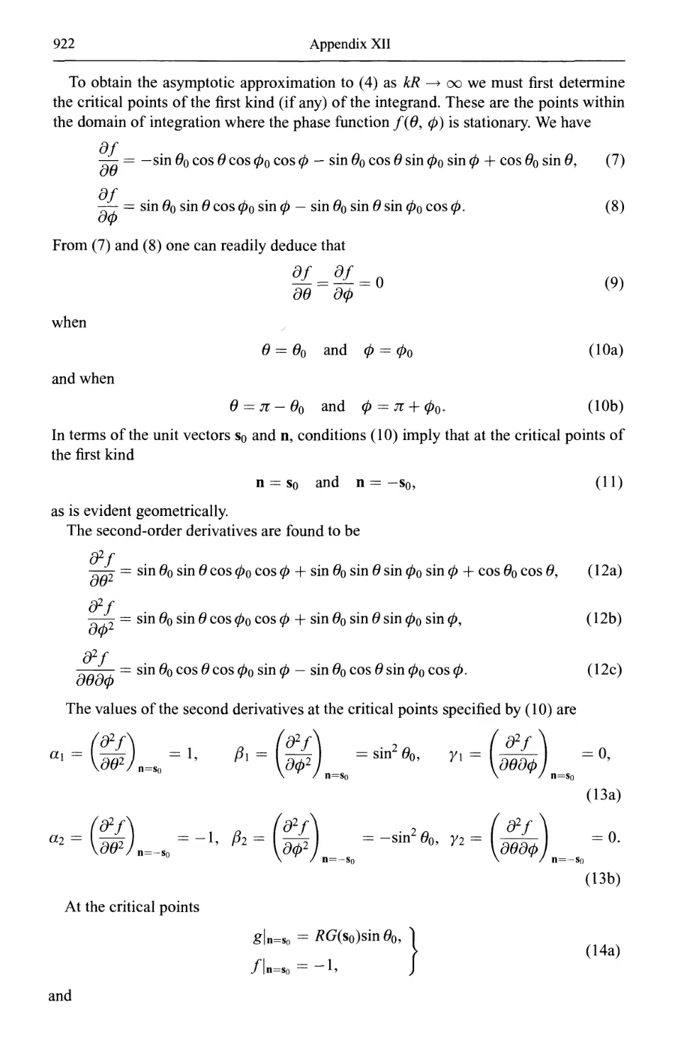
XII Proof of Jones' lemma (§13.3) 921
Author index
Subject index
925
936
Historical introduction
The physical principles underlying the optical phenomena with which we are
concerned in this treatise were substantially formulated before 1900. Since that year,
optics, like the rest of physics, has undergone a thorough revolution by the discovery
of the quantum of energy. While this discovery has profoundly affected our views
about the nature of light, it has not made the earlier theories and techniques
superfluous; rather, it has brought out their limitations and defined their range of validity.
The extension of the older principles and methods and their applications to very many
diverse situations has continued, and is continuing with undiminished intensity.
In attempting to present in an orderly way the knowledge acquired over a period of
several centuries in such a vast field it is impossible to follow the historical
development, with its numerous false starts and detours. It is therefore deemed necessary to
record separately, in this preliminary section, the main landmarks in the evolution of
ideas concerning the nature of light.*
The philosophers of antiquity speculated about the nature of light, being familiar
with burning glasses, with the rectilinear propagation of light, and with refraction and
reflection. The first systematic writings on optics of which we have any definite
knowledge are due to the Greek philosophers and mathematicians [Empedocles (c.
490-430 BC), Euclid (c. 300 BC)].
Amongst the founders of the new philosophy, Rene Descartes A596-1650) may be
singled out for mention as having formulated views on the nature of light on the basis
of his metaphysical ideas.f Descartes considered light to be essentially a pressure
transmitted through a perfectly elastic medium (the aether) which fills all space, and
he attributed the diversity of colours to rotary motions with different velocities of the
particles in this medium. But it was only after Galileo Galilei A564-1642) had, by his
* For a more extensive account of the history of optics, reference may be made to: J. Priestley History and
Present State of Discoveries relating to Vision, Light and Colours B Vols., London, 1772); Thomas Young,
A Course of Lectures on Natural Philosophy and the Mechanical Arts Vol. 1 (London, 1845), pp. 374-
385; E. Wilde, Geschichte der Optik vom Ursprung dieser Wissenschaft bis auf die gegenwärtige Zeit, 2
Vols, (Berlin, 1838, 1843); Ernst Mach, The Principles of Physical Optics, A historical and philosophical
treatment (First German edition 1913. English translation 1926, reprinted by Dover Publications, New
York, 1953); E. Hoppe, Geschichte der Optik (Leipzig, Weber, 1926); V Ronchi, Storia della Luce
(Bologna: Zanichelli, 2nd. Ed., 1952). A comprehensive historical account up to recent times is E. T.
Whittaker's A History of the Theories of Aether and Electricity, Vol. I (The Classical Theories), revised
and enlarged edition 1952; Vol. II (The Modern Theories 1900-1926), 1953, published by T. Nelson and
Sons, London and Edinburgh. The first volume was used as the chief source for this introductory section.
f R. Descartes, Dioptrique, Meteores (published (anonymously) in Ley den in 1637 with prefactory essay
'Discours de la methode'). Principia Philosophiae (Amsterdam, 1644).
XXV
XXVI
Historical introduction
development of mechanics, demonstrated the power of the experimental method that
optics was put on a firm foundation. The law of reflection was known to the Greeks;
the law of refraction was discovered experimentally in 1621 by Willebrord Snell*
(Snellius, c. 1580-1626). In 1657 Pierre de Fermat A601-1665) enunciated the
celebrated Principle of Least Timef in the form 'Nature always acts by the shortest
course'. According to this principle, light always follows that path which brings it to
its destination in the shortest time, and from this, in turn, and from the assumption of
varying 'resistance' in different media, the law of refraction follows. This principle is
of great philosophical significance, and because it seems to imply a teleological
manner of explanation, foreign to natural science, it has raised a great deal of
controversy.
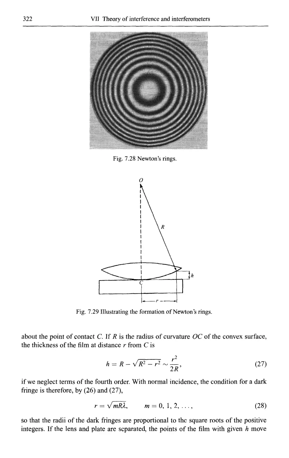
The first phenomenon of interference, the colours exhibited by thin films now
known as 'Newton's rings', was discovered independently by Robert BoyleJ A627-
1691) and Robert Hooke§ A635-1703). Hooke also observed the presence of light in
the geometrical shadow, the 'diffraction' of light but this phenomenon had been noted
previously by Francesco Maria Grimaldi|| A618-1663). Hooke was the first to
advocate the view that light consists of rapid vibrations propagated instantaneously, or
with a very great speed, over any distance, and believed that in an homogeneous
medium every vibration will generate a sphere which will grow steadily.]f By means of
these ideas Hooke attempted an explanation of the phenomenon of refraction, and an
interpretation of colours. But the basic quality of colour was revealed only when Isaac
Newton A642-1727) discovered** in 1666 that white light could be split up into
component colours by means of a prism, and found that each pure colour is
characterized by a specific refrangibility. The difficulties which the wave theory
encountered in connection with the rectilinear propagation of light and of polarization
(discovered by Huygenstf) seemed to Newton so decisive that he devoted himself to
the development of an emission (or corpuscular) theory, according to which light is
propagated from a luminous body in the form of minute particles.
At the time of the publication of Newton's theory of colour it was not known
whether light was propagated instantaneously or not. The discovery of the finite speed
of light was made in 1675 by Olaf Römer A644-1710) from the observations of the
eclipses of Jupiter's satellites. J J
The wave theory of light which, as we saw, had Hooke amongst its first champions
was greatly improved and extended by Christian Huygensft A629-1695). He
enunciated the principle, subsequently named after him, according to which every point of
the 'aether' upon which the luminous disturbance falls may be regarded as the centre
of a new disturbance propagated in the form of spherical waves; these secondary waves
* Snell died in 1626 without making his discoveries public. The law was first published by Descartes in his
Dioptrique without an acknowledgement to Snell, though it is generally believed that Descartes had seen
Snell's manuscript on this subject.
t In a letter to Cureau de la Chambre. It is published in Oeuvres de Fermat, Vol. 2 (Paris, 1891) p. 354.
X The Philosophical Works o/Robert Boyle (abridged by P. Shaw), Vol. II (Second ed. London, 1738), p. 70.
§ R. Hooke, Micrographia A665), 47.
|| KM. Grimaldi, Physico-Mathesis de lumine, coloribus, et iride (Bologna, 1665).
If The early wave theories of Hooke and Huygens operate with single 'pulses' rather than with wave trains of
definite wavelengths.
**I. Newton, Phil Trans. No. 80 (Feb. 1672), 3075.
ttChr. Huygens, Traite de la lumiere (completed in 1678, published in Leyden in 1690).
JJOlaf Römer, Mem. de l'Acad. Sei. Paris, 10 A666-1699), 575; J. de Sav. A676), 223.
Historical introduction
xxvii
combine in such a manner that their envelope determines the wave-front at any later
time. With the aid of this principle he succeeded in deriving the laws of reflection and
refraction. He was also able to interpret the double refraction of calc-spar [discovered
in 1669 by Erasmus Bartholinus A625-1698)] by assuming that in the crystal there is,
in addition to a primary spherical wave, a secondary ellipsoidal wave. It was in the
course of this investigation that Huygens made the fundamental discovery of
polarization: each of the two rays arising from refraction by calc-spar may be extinguished by
passing it through a second crystal of the same material if the latter crystal be rotated
about the direction of the ray. It was, however, left to Newton to interpret these
phenomena; he assumed that rays have 'sides'; and indeed this 'transversality' seemed
to him an insuperable objection to the acceptance of the wave theory, since at that time
scientists were familiar only with longitudinal waves (from the propagation of sound).
The rejection of the wave theory on the authority of Newton lead to its abeyance for
nearly a century, but it still found an occasional supporter, such as the great
mathematician Leonhard Euler A707-1783).*
It was not until the beginning of the nineteenth century that the decisive discoveries
were made which led to general acceptance of the wave theory. The first step towards
this was the enunciation in 1801 by Thomas Young A773-1829) of the principle of
interference and the explanation of the colours of thin films.f However, as Young's
views were expressed largely in a qualitative manner, they did not gain general
recognition.
About this time, polarization of light by reflection was discovered by Etienne Louis
MalusJ A775-1812). Apparently, one evening in 1808, he observed the reflection of
the sun from a window pane through a calc-spar crystal, and found that the two images
obtained by double refraction varied in relative intensities as the crystal was rotated
about the line of sight. However, Malus did not attempt an interpretation of this
phenomenon, being of the opinion that current theories were incapable of providing an
explanation.
In the meantime the emission theory had been developed further by Pierre Simon de
Laplace A749-1827) and Jean-Baptiste Biot A774-1862). Its supporters proposed
the subject of diffraction for the prize question set by the Paris Academy for 1818, in
the expectation that a treatment of this subject would lead to the crowning triumph of
the emission theory. But their hopes were disappointed, for, in spite of strong
opposition, the prize was awarded to Augustin Jean Fresnel A788-1827), whose
treatment§ was based on the wave theory, and was the first of a succession of
investigations which, in the course of a few years, were to discredit the corpuscular
theory completely. The substance of his memoir consisted of a synthesis of Huygens'
Envelope Construction with Young's Principle of Interference. This, as Fresnel showed,
was sufficient to explain not only the 'rectilinear propagation' of light but also the
minute deviations from it - diffraction phenomena. Fresnel calculated the diffraction
caused by straight edges, small apertures and screens; particularly impressive was the
* L. Euleri Opuscula varii argumenti (Berlin, 1746), p. 169.
t Th. Young, Phil. Trans. Roy. Soc, London xcii, 12 A802) 387. Miscellaneous works of the late Thomas
Young, Vol. I (London, J. Murray, 1885) pp. 140, 170.
% E. L. Malus, Nouveau Bull d. Sei., par la Soc. Philomatique, Vol. 1 A809), 266. Mem. de la Soc.
d'Arcueil,Vo\. 2 (IS09).
§ A. Fresnel, Ann. Chim. etPhys., B), 1 A816) 239; Oeuvres, Vol. 1, 89, 129.
XXV111
Historical introduction
experimental confirmation by Arago of a prediction, deduced by Poisson from
Fresnel's theory, that in the centre of the shadow of a small circular disc there should
appear a bright spot.
In the same year A818), Fresnel also investigated the important problem of the
influence of the earth's motion on the propagation of light, the question being whether
there was any difference between the light from stellar and terrestrial sources.
Dominique Frangois Arago A786-1853) found from experiment that (apart from
aberration) there was no difference. On the basis of these findings Fresnel developed
his theory of the partial convection of the luminiferous aether by matter, a theory
confirmed in 1851 by direct experiment carried out by Armand Hypolite Louis Fizeau
A819-1896). Together with Arago, Fresnel investigated the interference of polarized
rays of light and found (in 1816) that two rays polarized at right angles to each other
never interfere. This fact could not be reconciled with the assumption of longitudinal
waves, which had hitherto been taken for granted. Young, who had heard of this
discovery from Arago, found in 1817 the key to the solution when he assumed that the
vibrations were transverse.
Fresnel at once grasped the full significance of this hypothesis, which he sought to
put on a more secure dynamical basis* and from which he drew numerous
conclusions. For, since only longitudinal oscillations in a fluid are possible, the aether must
behave like a solid body; but at that time a theory of elastic waves in solids had not yet
been formulated. Instead of developing such a theory and deducing the optical
consequences from it, Fresnel proceeded by inference, and sought to deduce the
properties of the luminiferous aether from the observations. The peculiar laws of light
propagation in crystals were Fresnel's starting point; the elucidation of these laws and
their reduction to a few simple assumptions about the nature of elementary waves
represents one of the greatest achievements of natural science. In 1832, William
Rowan Hamiltonf A805-1865), who himself made important contributions to the
development of optics, drew attention to an important deduction from Fresnel's
construction, by predicting the so-called conical refraction, whose existence was
confirmed experimentally shortly afterwards by Humphrey Lloyd J A800-1881).
It was also Fresnel who (in 1821) gave the first indication of the cause of dispersion
by taking into account the molecular structure of matter§, a suggestion elaborated later
by Cauchy.
Dynamical models of the mechanism of aether vibrations led Fresnel to deduce the
laws which now bear his name, governing the intensity and polarization of light rays
produced by reflection and refraction. ||
Fresnel's work had put the wave theory on such a secure foundation that it seemed
almost superfluous when in 1850 Foucault^f and Fizeau and Breguet** undertook a
crucial experiment first suggested by Arago. The corpuscular theory explains refraction
* A. Fresnel, Oeuvres Completes d'Augustin Fresnel, Vol. 2 (Paris, Imprimiere Imperiale, 1866-1870), pp.
261,479).
t W. R. Hamilton, Trans. Roy. Irish Acad., 17 A833), 1. Also Hamilton's Mathematical Papers, eds. J. L.
Synge and W. Conway, Vol. 1 (Cambridge, Cambridge University Press, 1931) p. 285.
% H. Lloyd, Trans. Roy. Irish Acad, 17 A833), 145.
§ A. Fresnel, ibid, p. 438.
|| A. Fresnel, Mem. de I'Acad., 11 A832), 393; Oeuvres, 1, 767.
<|| L. Foucault, Compt. Rend. Acad. Sei. Paris, 30 A850), 551.
**H. Fizeau and L. Breguet, Compt. Rend. Acad. Sei. Paris, 30 A850), 562, 771.
Historical introduction
xxix
in terms of the attraction of the light-corpuscles at the boundary towards the optically
denser medium, and this implies a greater velocity in the denser medium; on the other
hand the wave theory demands, according to Huygens' construction, that a smaller
velocity obtains in the optically denser medium. The direct measurement of the velocity
of light in air and water decided unambiguously in favour of the wave theory.
The decades that followed witnessed the development of the elastic aether theory.
The first step was the formulation of a theory of the elasticity of solid bodies. Claude
Louis Marie Henri Navier A785-1836) developed such a theory*, discerning that
matter consists of countless particles (mass points, atoms) exerting on each other
forces along the lines joining them. The now customary derivation of the equations of
elasticity by means of the continuum concept is due to Augustine Louis Cauchyf
A789-1857). Of other scientists who participated in the development of optical
theory, mention must be made of Simeon Denis PoissonJ A781-1840), George
Green§ A793-1841), James MacCullagh|| A809-1847) and Franz Neumann^ A798-
1895). Today it is no longer relevant to enter into the details of these theories or into
the difficulties which they encountered; for the difficulties were all caused by the
requirement that optical processes should be explicable in mechanical terms, a
condition which has long since been abandoned. The following indication will suffice.
Consider two contiguous elastic media, and assume that in the first a transverse wave
is propagated towards their common boundary. In the second medium the wave will be
resolved, in accordance with the laws of mechanics, into longitudinal and transverse
waves. But, according to Arago's and Fresnel's experiments, elastic longitudinal waves
must be ruled out and must therefore be eliminated somehow. This, however, is not
possible without violating the laws of mechanics expressed by the boundary conditions
for strains and stresses. The various theories put forward by the authors mentioned
above differ in regard to the assumed boundary conditions, which always conflicted in
some way with the laws of mechanics.
An obvious objection to regarding the aether as an elastic solid is expressed in the
following query: How is one to imagine planets travelling through such a medium at
enormous speeds without any appreciable resistance? George Gabriel Stokes A819—
1903) thought that this objection could be met on the grounds that the planetary speeds
are very small compared to the speeds of the aetherial particles in the vibrations
constituting light; for it is known that bodies like pitch or sealing wax are capable of
rapid vibrations but yield completely to stresses applied over a long period. Such
controversies seem superfluous today since we no longer consider it necessary to have
mechanical pictures of all natural phenomena.
A first step away from the concept of an elastic aether was taken by MacCullagh,**
who postulated a medium with properties not possessed by ordinary bodies. The latter
store up energy when the volume elements change shape, but not during rotation. In
MacCullagh's aether the inverse conditions prevail. The laws of propagation of waves
* C. L. M. H. Navier, Mem. de I'Acad., 7, (submitted in 1821, published in 1827), 375.
t A. L. Cauchy, Exercise de Mathematiques, 3 A828), 160.
J S. D. Poisson, Mem. del'Acad., 8 A828), 623.
§ G. Green, Trans. Camb. Phil. Soc. A838); Math. Papers, 245.
|| J. MacCullagh, Phil. Mag. C), 10 A837), 42, 382; Proc. Roy. Irish Acad., 18 A837).
1 F. Neumann, Abh. Berl. Akad, Math. Kl. A835), 1.
**J. MacCullagh, Trans. Roy. Irish Acad., 21, Coll. Works, Dublin A880), 145.
XXX
Historical introduction
in such a medium show a close similarity to Maxwell's equations of electromagnetic
waves which are the basis of modern optics.
In spite of the many difficulties, the theory of an elastic aether persisted for a long
time and most of the great physicists of the nineteenth century contributed to it. In
addition to those already named, mention must be made of William Thomson* (Lord
Kelvin, 1824-1908), Carl Neumannf A832-1925), John William StruttJ (Lord
Rayleigh, 1842-1919), and Gustav Kirchhof^ A824-1887). During this period many
optical problems were solved, but the foundations of optics remained in an
unsatisfactory state.
In the meantime researches in electricity and magnetism had developed almost
independently of optics, culminating in the discoveries of Michael Faraday|| A791 —
1867). James Clerk Maxwell]} A831-1879) succeeded in summing up all previous
experiences in this field in a system of equations, the most important consequence of
which was to establish the possibility of electromagnetic waves, propagated with a
velocity which could be calculated from the results of purely electrical measurements.
Actually, some years earlier Rudolph Kohlrausch A809-1858) and Wilhelm Weber**
A804-1891) had carried out such measurements and the velocity turned out to be that
of light. This led Maxwell to conjecture that light waves are electromagnetic waves; a
conjecture verified by direct experiment in 1888 by Heinrich Hertzft A857-1894). In
spite of this, Maxwell's electromagnetic theory had a long struggle to gain general
acceptance. It seems to be a characteristic of the human mind that familiar concepts
are abandoned only with the greatest reluctance, especially when a concrete picture of
the phenomena has to be sacrificed. Maxwell himself, and his followers, tried for a
long time to describe the electromagnetic field with the aid of mechanical models. It
was only gradually, as Maxwell's concepts became more familiar, that the search for
an 'explanation' of his equations in terms of mechanical models was abandoned; today
there is no conceptual difficulty in regarding Maxwell's field as something which
cannot be reduced to anything simpler.
But even the electromagnetic theory of light has attained the limits of its
serviceability. It is capable of explaining, in their main features, all phenomena connected
with the propagation of light. However, it fails to elucidate the processes of emission
and absorption, in which the finer features of the interaction between matter and the
optical field are manifested.
The laws underlying these processes are the proper object of modern optics, indeed
of modern physics. Their story begins with the discovery of certain regularities in
spectra. The first step was Josef Fraunhofer's A787-1826) discovery} $ A814-1817)
* W. Thomson, Phil. Mag., E), 26 A888), 414. Baltimore Lectures (London, 1904).
f C. Neumann, Math. Ann., 1 A869), 325, 2 A870), 182.
J J. W. Strutt, (Lord Rayleigh), Phil. Mag., D) 41 A871), 519; 42 A871), 81.
§ G. Kirchhoff, Berl Abh. Physik, Abteiig. 2 A876), 57; Ges. Abh. 352; Berl Ber. A882), 641; Pogg. Ann.
Physik, u. Chem. B), 18 A883), 663; Ges. Abh., Nachtrag. 22.
|| M. Faraday, Experimental Researches in Electricity (London, 1839).
f J. C. Maxwell, A Treatise on Electricity and Magnetism, 2 Vols. (Oxford, 1873).
**R. Kohlrausch and W. Weber, Pogg. Ann. Physik u. Chem. B), 99 A856), 10.
f|H. Hertz, Sitzb. Berl. Akad. Wiss., Feb. 2, 1888; Wiedem. Ann. 34 A888), 551; English translation in his
Electric Waves (London, Macmillan, 1893), p. 107.
%%]. Fraunhofer, Gilberts Ann., 56 A817), 264. W. H. Wollaston A766-1828) observed these lines in 1802
{Phil. Trans. Roy. Soc, London A802), 365) but had not appreciated his discovery and interpreted them
incorrectly.
Historical introduction
xxxi
of the dark lines in the solar spectrum, since named after him; and their interpretation
as absorption lines given in 1861 on the basis of experiments by Roger Wilhelm
Bunsen A811-1899) and Gustav Kirchhoff* A824-1887). The light of the
continuous spectrum of the body of the sun, passing the cooler gases of the sun's atmosphere,
loses by absorption just those wavelengths which are emitted by the gases. This
discovery was the beginning of spectrum analysis, which is based on the recognition
that every gaseous chemical element possesses a characteristic line spectrum. The
investigation of these spectra has been a major object of physical research up to and
including the present; and since light is its subject, and optical methods are employed,
it is often considered as a part of optics. The problem of how light is produced or
destroyed in atoms is, however, not exclusively of an optical nature, as it involves
equally the mechanics of the atom itself; and the laws of spectral lines reveal not so
much the nature of light as the structure of the emitting particles. Thus, from being a
part of optics, spectroscopy has gradually evolved into a separate discipline which
provides the empirical foundations for atomic and molecular physics. This field is,
however, beyond the scope of this book.
Concerning methods, it has become apparent that classical mechanics is inadequate
for a proper description of events occurring within the atom and must be replaced by
the quantum theory, originated in 1900 by Max Planck| A858-1947). Its application
to the atomic structure, led in 1913, to the explanation by Niels BohrJ A885-1962) of
the simple laws of line spectra of gases. From these beginnings and from the ever
increasing experimental material, modern quantum mechanics developed (Heisenberg,
Born, Jordan, de Broglie, Schrödinger, Dirac).§ By its means considerable insight has
been obtained into the structure of atoms and molecules.
However, our concept of the nature of light has also been greatly influenced by
quantum theory. Even in its first form due to Planck there appears a proposition which
is directly opposed to classical ideas, namely that an oscillating electric system does
not impart its energy to the electromagnetic field in a continuous manner but in finite
amounts, or 'quanta' e — hv, proportional to the frequency v of the light, where
h — 6.55 X 10~27 erg/s is Planck's constant. We may say that the occurrence of the
constant h is the feature which distinguishes modern physics from the old.
It was only gradually that the paradoxical, almost irrational, character of Planck's
equation e = hv was fully realized by physicists. This was brought about mainly by
the work of Einstein and Bohr. On the basis of Planck's theory, Einstein A879-1955)
revived in 1905 the corpuscular theory of light in a new form|| by assuming that
Planck's energy quanta exist as real light-particles, called 'light quanta' or 'photons'.
He thereby succeeded in explaining some phenomena which had been discovered more
recently in connection with the transformation of light into corpuscular energy,
* R. Bunsen and G. Kirchhoff, Untersuchungen über das Sonnenspektrum und die Spektren der Chemischen
Elemente., Abh. kgl Akad. Wiss. (Berlin, 1861) p. 1863.
t M. Planck, Verh. d. deutschphys. Ges., 2 A900) 202, 237. Ann. d. Physik D), 4 A901), 553.
% N. Bohr, Phil. Mag. F), 26 A913), 1, 476, 857.
§ W. Heisenberg, Z. Phys., 33 A925), 879; M. Born and P. Jordan, ibid., 34 A925), 858; M. Born, W.
Heisenberg, and P. Jordan, ibid., 35 A926), 557; L. de Broglie, These (Paris, 1924); Ann. de Physique
A0), 3 A925), 22; E. Schrödinger, Ann. d Physik D), 79 A926), 361, 489 and 734; 80 A926), 437; 81
A926), 109. English translation: Collected Papers on Wave Mechanics by E. Schrödinger (London and
Glasgow, Blackie, 1928); P. A. M. Dirac, Proc. Roy. Soc. A, 109 A925), 642; ibid., 110 A926), 561.
|| A. Einstein, Ann. d. PhysikD), 17 A905), 132; 20 A906), 199.
XXX11
Historical introduction
phenomena which were inexplicable by the wave theory. Chief among these are the so-
called photoelectric effect and the fundamentals of photochemistry. In phenomena of
this type light does not impart to a detached particle an energy proportional to its
intensity, as demanded by the wave theory, but behaves rather like a hail of small shots.
The energy imparted to the secondary particles is independent of the intensity, and
depends only on the frequency of the light (according to the law e = hv). The number
of observations confirming this property of light increased year by year and the
situation arose that the simultaneous validity of both wave and corpuscular theories
had to be recognized, the former being exemplified by the phenomena of interference,
the latter by the photoelectric effect. It is only in more recent years that the
development of quantum mechanics has led to a partial elucidation of this paradoxical state of
affairs, but this has entailed giving up a fundamental principle of the older physics,
namely the principle of deterministic causality.
The detailed theory of the interaction between field and matter required the
extension of the methods of quantum mechanics (field quantization). For the
electromagnetic radiation field this was first carried out by Dirac* and these investigations
form the basis of quantum optics. However, it was mainly the development of radically
new light sources, the lasers, in the 1960s that led to the emergence of quantum optics
as a new discipline. The invention of the laser provided new sources of very intense,
coherent and highly directional light beams. Such sources are analogous to devices
known as masers, developed a few years earlier, for generating and amplifying
microwave radiation by conversion of atomic and molecular energy by the process of
stimulated emission. Pioneering contributions which led to the invention of these
devices were made notably by Basov, Prokhorov, Townes, Schawlow and Maiman.f
Apart from providing an important tool for research in quantum optics, the invention
of the laser led to numerous applications and originated several new fields such as
quantum-electronics, nonlinear optics, fiber optics and others.
Another branch of optics, not touched upon in this work, is the optics of moving
bodies. Like the quantum theory it has grown into a vast independent field of study.
The first observed phenomenon in this field, recorded in 1728 by James BradleyJ
A692-1762), was the aberration of 'fixed stars', i.e. the observation of slightly
different angular positions of the stars according to the motion of the earth relative to
the direction of the light ray. Bradley correctly interpreted this phenomenon as being
due to the finite velocity of light and thus was able to determine the velocity. We have
already mentioned other phenomena belonging to optics of moving media: Fresnel was
the first to enquire into the convection of light by moving bodies and to show that it
behaved as if the luminiferous aether participated in the movement only with a fraction
of the speed of the moving bodies; Fizeau then demonstrated this partial convection
experimentally with the aid of flowing water. The effect of the motion of the light
source or of the observer was investigated by Christian Doppler§ A803-1853) who
formulated the well-known principle named after him. So long as the elastic theory of
light held the field and the precision of measurements was sufficiently limited,
* P. A. M Dirac, Proc. Roy. Soc, A114 A927), 243, 710.
t N. G. Basov and A. M. Prokhorov, Zh. Eksp. Teor. Fiz., 27 A954), 431; A. L. Schawlow and C. H. Townes,
Phys. Rev., 112 A958), 1940; T. H. Maiman, Nature, 187 A960), 493.
% J. Bradley, Phil. Trans., 35 A728), 637.
§ Chr. Doppier, Abh. Köngl. böhm. Geselsch, 2 A842), 466; Pogg. Ann., 68 A847), I.
Historical introduction
XXXlll
Fresnel's ideas on partial convection sufficed for a satisfactory explanation of all the
phenomena. But the electromagnetic theory of light encountered difficulties of a
fundamental nature. Hertz was the first to attempt to generalize Maxwell's laws to
moving bodies. His formulae were, however, in conflict with some electromagnetic
and optical experiments. Of great importance was the theory of Hendrik Antoon
Lorentz A853-1928) who assumed an 'aether in a state of absolute rest' to be the
carrier of the electromagnetic field and deduced the properties of material bodies from
the interaction of elementary electric particles - the electrons. He was able to show
that Fresnel's coefficient of convection could be obtained correctly from his theory and
that in general all phenomena known at the time A895) lent themselves to explanation
by this hypothesis.* But the enormous increase of precision in the determination of
optical paths by means of the interferometer of Albert Abraham Michelson A852—
1931) led to a new anomaly: it proved impossible to demonstrate the existence of an
'aether drift' required by the theory of the 'stationary aether'.t The anomaly was
resolved by Albert Einstein J in 1905 in his special theory of relativity. The theory is
founded on a critique of the concepts of time and space and leads to the abandonment
of Euclidian geometry and the intuitive conception of simultaneity. Its further
development into the so-called general theory of relativity§ led to a completely new conception
of gravitational phenomena by a 'geometrization' of the space-time manifold. The
application of this theory involves the use of special mathematical and physical
methods which, although relevant to optics in many cases, may easily be considered
separately from it. The number of optical phenomena in which the motion of bodies
(e.g. light sources) plays a significant part is rather small.
* H. A. Lorentz, Versuch einer Theorie der electrischen und optischen Erscheinungen in bewegten Körpern
(Leiden, E. J. Brill 1895; reprinted by Teubner, Leipzig, 1906).
t A. A. Michelson, Amer. Jour Sei. C), 22 A881), 20; A. A. Michelson and E. W. Morley, Amer. Jour Sei.
C), 34 A887), 333; Phil. Mag., 24 A887), 449.
t A. Einstein, Ann. d. Physik D), 17 A905), 891.
§ A. Einstein, Berl. Sitz. A915), 778, 799, 831, 844. Ann. d. Physik D) 49 A916), 769.
I
Basic properties of the electromagnetic field
1.1 The electromagnetic field
LL1 Maxwell's equations
The state of excitation which is established in space by the presence of electric charges
is said to constitute an electromagnetic field. It is represented by two vectors, E and B,
called the electric vector and the magnetic induction respectively.*
To describe the effect of the field on material objects, it is necessary to introduce a
second set of vectors, viz. the electric current density j, the electric displacement D,
and the magnetic vector H.
The space and time derivatives of the five vectors are related by Maxwells
equations, which hold at every point in whose neighbourhood the physical properties
of the medium are continuous:!
1 • 4jt
curlH--D = — j, A)
c c
curlE + -B = 0, B)
c
the dot denoting differentiation with respect to time.
* In elementary considerations E and H are, for historical reasons, usually regarded as the basic field vectors,
and D and B as describing the influence of matter. In general theory, however, the present interpretation is
compulsory for reasons connected with the electrodynamics of moving media.
The four Maxwell equations A)-D) can be divided into two sets of equations, one consisting of two
homogeneous equations (right-hand side zero), containing E and B, the other of two nonhomogeneous
equations (right-hand side different from zero), containing D and H. If a coordinate transformation of
space and time (relativistic Lorentz transformation) is carried out, the equations of each group transform
together, the equations remaining unaltered in form if j/c and p are transformed as a four-vector, and each
of the pairs E, B and D, H as a six-vector (antisymmetric tensor of the second order). Since the
nonhomogeneous set contains charges and currents (which represent the influence of matter), one has to
attribute the corresponding pair (D, H) to the influence of matter. It is, however, customary to refer to H
and not to B as the magnetic field vector; wc shall conform to this terminology when there is no risk of
confusion.
f The so-called Gaussian system of units is used here, i.e. the electrical quantities (E, D, j and p) are
measured in electrostatic units, and the magnetic quantities (H and B) in electromagnetic units. The
constant c in A) and B) relates the unit of charge in the two systems; it is the velocity of light in the
vacuum and is approximately equal to 3 X 1010 cm/s. (A more accurate value is given in §1.2.)
1
2
T Basic properties of the electromagnetic field
They are supplemented by two scalar relations:
divD = 4jrp, C)
divB = 0. D)
Eq. C) may be regarded as a defining equation for the electric charge density p and D)
may be said to imply that no free magnetic poles exist.
From A) it follows (since divcurl = 0) that
divj = — — divD,
or, using C),
! + divj = 0. E)
By analogy with a similar relation encountered in hydrodynamics, E) is called the
equation of continuity. It expresses the fact that the charge is conserved in the
neighbourhood of any point. For if one integrates E) over any region of space, one
obtains, with the help of Gauss' theorem,
^Jpd^ + Jj.ndS = 0, F)
the second integral being taken over the surface bounding the region and the first
throughout the volume, n denoting the unit outward normal. This equation implies that
the total charge
e = \pdV G)
contained within the domain can only increase on account of the flow of electric
current
J
J-ndS. (8)
If all the field quantities are independent of time, and if, moreover, there are no
currents (j = 0), the field is said to be static. If all the field quantities are time
independent, but currents are present (j ^ 0), one speaks of a stationary field. In
optical fields the field vectors are very rapidly varying functions of time, but the
sources of the field are usually such that, when averages over any macroscopic time
interval are considered rather than the instantaneous values, the properties of the field
are found to be independent of the instant of time at which the average is taken. The
word stationary is often used in a wider sense to describe a field of this type. An
example is a field constituted by the steady flux of radiation (say from a distant star)
through an optical system.
1.1.2 Material equations
The Maxwell equations A)-D) connect the five basic quantities E, H, B, D and j. To
allow a unique determination of the field vectors from a given distribution of currents
1.1 The electromagnetic field
3
and charges, these equations must be supplemented by relations which describe the
behaviour of substances under the influence of the field. These relations are known as
material equations* (or constitutive relations). In general they are rather complicated;
but if the field is time-harmonic (see §1.4.3), and if the bodies are at rest, or in very
slow motion relative to each other, and if the material is isotropic (i.e. when its
physical properties at each point are independent of direction), they take usually the
relatively simple formt
j = "E, (9)
D = £E, A0)
B = //H. A1)
Here a is called the specific conductivity, e is known as the dielectric constant (or
permittivity) and pi is called the magnetic permeability.
Eq. (9) is the differential form of Ohm's law. Substances for which a / 0 (or more
precisely is not negligibly small; the precise meaning of this cannot, however, be
discussed here) are called conductors. Metals are very good conductors, but there are
other classes of good conducting materials such as ionic solutions in liquids and also
in solids. In metals the conductivity decreases with increasing temperature. However,
in other classes of materials, known as semiconductors (e.g. germanium), conductivity
increases with temperature over a wide range.
Substances for which a is negligibly small are called insulators or dielectrics. Their
electric and magnetic properties are then completely determined by e and ju. For most
substances the magnetic permeability pi is practically unity. If this is not the case, i.e.
if pi differs appreciably from unity, we say that the substance is magnetic. In particular,
if pi > 1, the substance is said to be paramagnetic (e.g. platinum, oxygen, nitrogen
dioxide), while if pi < 1 it is said to be diamagnetic (e.g. bismuth, copper, hydrogen,
water).
If the fields are exceptionally strong, such as are obtained, for example, by focusing
light that is generated by a laser, the right-hand sides of the material equations may
have to be supplemented by terms involving components of the field vectors in powers
higher than the first. J
In many cases the quantities a, e and /u will be independent of the field strengths; in
other cases, however, the behaviour of the material cannot be described in such a
simple way. Thus, for example, in a gas of free ions the current, which is determined
* There is an alternative way of describing the behaviour of matter. Instead of the quantities e = D/E,
pi — B/ H one considers the differences D - E and B — H; these have a simpler physical significance and
will be discussed in Chapter II.
t The more general relations, applicable also to moving bodies, are studied in the theory of relativity. We
shall only need the following result from the more general theory: that in the case of moving charges there
is, in addition to the conduction current oE, a convection current pv, where v is the velocity of the moving
charges and p the charge density (cf. p. 9).
J Nonlinear relationship between the displacement vector D and the electric field E was first demonstrated
in this way by P. A. Franken, A. E. Hill, C. W. Peters and G. Weinrich, Phys. Rev. Lett., 7 A961), 118.
For systematic treatments of nonlinear effects see N. Bloembergen, Nonlinear Optics (New York, W. A.
Benjamin, Inc., 1965), P. N. Butcher and D. Cotter, The Elements of Nonlinear Optics (Cambridge,
Cambridge University Press, 1990) or R. W. Boyd, Nonlinear Optics (Boston, Academic Press, 1992).
4
I Basic properties of the electromagnetic field
by the mean speed of the ions, depends, at any moment, not on the instantaneous value
of E, but on all its previous values. Again, in so-called ferromagnetic substances
(substances which are very highly magnetic, e.g. iron, cobalt and nickel) the value of
the magnetic induction B is determined by the past history of the field H rather than by
its instantaneous value. The substance is then said to exhibit hysteresis. A similar
history-dependence will be found for the electric displacement in certain dielectric
materials. Fortunately hysteretic effects are rarely significant for the high-frequency
field encountered in optics.
In the main part of this book we shall study the propagation in substances which
light can penetrate without appreciable weakening (e.g. air, glass). Such substances are
said to be transparent and must be electrical nonconductors (a — 0), since conduction
implies the evolution of Joule heat (see §1.1.4) and therefore loss of electromagnetic
energy. Optical properties of conducting media will be discussed in Chapter XIV.
1.13 Boundary conditions at a surface of discontinuity
Maxwell's equations were only stated for regions of space throughout which the
physical properties of the medium (characterized by £ and pt) are continuous. In optics
one often deals with situations in which the properties change abruptly across one or
more surfaces. The vectors E, H, B and D may then be expected also to become
discontinuous, while p and j will degenerate into corresponding surface quantities. We
shall derive relations describing the transition across such a discontinuity surface.
Let us replace the sharp discontinuity surface T by a thin transition layer within
which e and /u vary rapidly but continuously from their values near T on one side to
their value near Ton the other. Within this layer we construct a small near-cylinder,
bounded by a stockade of normals to T; roofed and floored by small areas 6A\ and
ÖÄ2 on each side of T, at constant distance from it, measured along their common
normal (Fig. 1.1). Since B and its derivatives may be assumed to be continuous
throughout this cylinder, we may apply Gauss' theorem to the integral of divB taken
throughout the volume of the cylinder and obtain, from D),
divBdF
B-ndS = 0;
A2)
the second integral is taken over the surface of the cylinder, and n is the unit outward
normal.
Since the areas dA\ and dAi are assumed to be small, B may be considered to have
constants values BA) and BB) on dA\ and dA2, and A2) may then be replaced by
Fig. 1.1 Derivation of boundary conditions for the normal components of B and D.
1.1 The electromagnetic field
5
BA) • nidAi + BB) • n2dA2 + contribution from walls = 0. A3)
If the height dh of the cylinder decreases towards zero, the transition layer shrinks into
the surface and the contribution from the walls of the cylinder tends to zero, provided
that there is no surface flux of magnetic induction. Such flux never occurs, and
consequently in the limit,
(BA) - m + BB) • n2)dA = 0, A4)
6A being the area in which the cylinder intersects T. If j\\2 is the unit normal pointing
from the first into the second medium, then ni = —1112, n2 =1112 and A4) gives
n12 • (BB) - BA)) - 0, A5)
i.e. the normal component of the magnetic induction is continuous across the surface
of discontinuity.
The electric displacement D may be treated in a similar way, but there will be an
additional term if charges are present. In place of A2) we now have from C)
[divDdF = [D-ndS = 47r|pdF.
A6)
As the areas dA\ and ÖA2 shrink together, the total charge remains finite, so that the
volume density becomes infinite. Instead of the volume charge density p the concept
of surface charge density p must then be used. It is defined by*
lim \pdV= \pdA. A7)
We shall also need later the concept of surface current density j, defined in a similar
way:
lim
dÄ->0
)dV =
}dA. A8)
If the area dA and the height dh are taken sufficiently small, A6) gives
DA) • ni dA\ + DB) • n2 dA2 + contribution from walls = 4jcp dA.
The contribution from the walls tends to zero with dh, and we therefore obtain in the
limit as dh —► 0,
1112 • (DB) - DA)) = 4;rp, A9)
i.e. in the presence of a layer of surface charge density p on the surface, the normal
component of the electric displacement changes abruptly across the surface, by an
amount equal to 4jrp.
* For later purposes we note a representation of the surface charge density and the surface current density in
terms of the Dirac delta function (see Appendix IV). If the equation of the surface of discontinuity is
F(x, y, z) = 0, then
p=p|gradF|E(F), A7a)
j=i|gradF|<KF). A8a)
These relations can immediately be verified by substituting from A7a) and A8a) into A7) and A8) and
using the relation dF = |gradF|d/z and the sifting property of the delta function.
6
I Basic properties of the electromagnetic field
Next, we examine the behaviour of the tangential components. Let us replace the
sharp discontinuity surface by a continuous transition layer. We also replace the
cylinder of Fig. 1.1 by a 'rectangular' area with sides parallel and perpendicular to T
(Fig. 1.2).
Let b be the unit vector perpendicular to the plane of the rectangle. Then it follows
from B) and from Stokes' theorem that
[curlE-bdS = [E-dr = -- [ß.bdS, B0)
the first and third integrals being taken throughout the area of the rectangle, and the
second along its boundary. If the lengths P\Q\ (= ds\), and P2Q1 (— ^2) are small, E
may be replaced by constant values EA) and EB) along each of these segments.
Similarly B may be replaced by a constant value. Eq. B0) then gives
EA) • ti dsx + EB) • t2 ds2 + contribution from ends = - -B • b dsöh, B1)
c
where ds is the line element in which the rectangle intersects the surface. If now the
height of the rectangle is gradually decreased, the contribution from the ends P\ P2 and
Q\ Ö2 will tend to zero, provided that E does not in the limit acquire sufficiently sharp
singularities; this possibility will be excluded. Assuming also that B remains finite, we
obtain in the limit as d h —> 0,
(EA) - ti + EB) - t2)ds = 0. B2)
If t is the unit tangent along the surface, then (see Fig. 1.2) ti = —t = —b X n12,
t2 = t = b X ni2, and B2) gives
b - [H12 X (EB) - EA))] = 0.
Since the orientation of the rectangle and consequently that of the unit vector b is
arbitrary, it follows that
n12 X (EB) - EA)) - 0, B3)
i.e. the tangential component of the electric vector is continuous across the surface.
Finally consider the behaviour of the tangential component of the magnetic vector.
The analysis is similar, but there is an additional term if currents are present. In place
of B1) wc now have
Fig. 1.2 Derivation of boundary conditions for the tangential components of E and H.
1.1 The electromagnetic field
7
1 • 4jv~
HA) • ti dsi + HB) • t2 ds2 + contribution from ends = -D • b as dh H j • b ds.
c c
B4)
On proceeding to the limit dh —> 0 as before, we obtain
n12X (HO-H^-j. B5)
c
From B5) is follows that in the presence of a surface current of density j, the
tangential component (considered as a vector quantity) of the magnetic vector changes
abruptly, its discontinuity being Dji/c)] X n\2.
Apart from discontinuities due to the abrupt changes in the physical properties of
the medium, the field vectors may also be discontinuous because of the presence of a
source which begins to radiate at a particular instant of time t = to. The disturbance
then spreads into the surrounding space, and at any later instant t\ > to will have filled
a well-defined region. Across the (moving) boundary of this region, the field vectors
will change abruptly from finite values on the boundary to the value zero outside it.
The various cases of discontinuity may be covered by rewriting Maxwell's equations
in an integral form.* The general discontinuity conditions may also be written in the
form of simple difference equations; a derivation of these equations is given in
Appendix VI.
1.1.4 The energy law of the electromagnetic field
Electromagnetic theory interprets the light intensity as the energy flux of the field. It is
therefore necessary to recall the energy law of Maxwell's theory.
From A) and B) it follows that
Ait 1 • 1
E - curlH - H - curlE = —j • E + -E • D + -H • B. B6)
c c c
Also, by a well-known vector identity, the term on the left may be expressed as the
divergence of the vector product of H and E:
E - curl H - H • curl E = -div (E X H). B7)
From B6) and B7) we have that
1 Ait
(E • D + H - B) + — j - E + div(E X H) = 0. B8)
c c
When we multiply this equation by c/4jt, integrate throughout an arbitrary volume and
apply Gauss's theorem, this gives
i^E-D + H.
B)dF +
j.Ed^
(EXH)-ndS = 0, B9)
where the last integral is taken over the boundary of the volume, n being the unit
outward normal.
The relation B9) is a direct consequence of Maxwell's equations and is therefore
* See, for example, A. Sommerfeld, Electrodynamics (New York, Academic Press, 1952), p. 11; or J. A.
Stratton, Electromagnetic Theory (New York, McGraw-Hill, 1941), p. 6.
I Basic properties of the electromagnetic field
valid whether or not the material equations (9)-A1) hold. It represents, as will be
seen, the energy law of an electromagnetic field. We shall discuss it here only for the
case where the material equations (9)-A1) are satisfied. Generalizations to anisotropic
media, where the material equations are of a more complicated form, will be
considered later (Chapter XV).
We have, on using the material equations,
— (E • D) = — E • — (eE) = —-(eE2) = —-(E • D),
4jty ' An dty ' totdr ' %ndv '
l^=h*it^=ll^=li^-
C0)
Setting
and
we = —E-D, wm = —H-B, C1)
W=\{we + wm)dV, C2)
B9) becomes,
äW f
J-Edr + £
(EXH).ndS = 0. C3)
We shall show that W represents the total energy contained within the volume, so that
we may be identified with the electric energy density and wm with the magnetic energy
density of the field.*
To justify the interpretation of W as the total energy we have to show that, for a
closed system (i.e. one in which the field on the boundary surface may be neglected),
the change in ^as defined above is due to the work done by the field on the material
charged bodies which are embedded in it. It suffices to do this for slow motion of the
material bodies, which themselves may be assumed to be so small that they can be
regarded as point charges e* (k = 1, 2, ...). Let the velocity of the charge e* be v^
(|v*| < c).
The force exerted by a field (E, B) on a charge e moving with velocity v is given by
the so-called Lorentz law,
F = Je + -vXBJ, C4)
which is based on experience. It follows that if all the charges e^ are displaced by dx^
(k = 1, 2, ...) in time öt, the total work done is
* In the general case the densities are defined by the expressions
We = — [E - dD, wm = — IH . dB.
4jtJ 4jtJ
When the relationship between E and D and between H and B is linear, as here assumed, these expressions
reduce to C1).
1.1 The electromagnetic field
9
ÖA = ^2 F* • dxk = Y^ ek (E* + - v* X B) • dxk
k k ^ c '
= ^2 ek&k -dxk = ^2 ekEk • Vit dt,
k k
since dxk = Vkdt. If the number of charged particles is large, we can consider the
distribution to be continuous. We introduce the charge density p (i.e. total charge per
unit volume) and the last equation becomes
öA = öt
pv-EdF, C5)
the integration being carried throughout an arbitrary volume. Now the velocity v does
not appear explicitly in Maxwell's equations, but it may be introduced by using an
experimental result found by Röntgen*, according to which a convection current (i.e. a
set of moving charges) has the same electromagnetic effect as a conduction current in
a wire. Hence the current density j appearing in Maxwell's equations can be split into
two parts
j=jc+j</, C6)
where
jc = tfE
is the conduction current density, and
\v = PV
represents the convection current density. C5) may therefore be written as
öA = öt\jü-EdV. C7)
Let us now define a vector S and a scalar Q by the relations
S = ^(EXH), C8)
|jc.EdF = |a
E2dF. C9)
Then by C5) and C6)
|j.EdK = ß + |j0-EdK
= Q + % D0)
where the second function is not, of course, a total derivative of a space-time function.
Eq. C3) now takes the form
* W. C. Röntgen, Ann. d. Physik, 35 A888), 264; 40 A890), 93.
10
I Basic properties of the electromagnetic field
S=-£-«-H-
For a nonconductor (a = 0) we have that 0 = 0. Assume also that the boundary
surface is so far away that we can neglect the field on it, due to the electromagnetic
processes inside; then JS • ndS = 0, and integration of D1) gives
W + A — constant. D2)
Hence, for an isolated system, the increase of ^per unit time is due to the work done
on the system during this time. This result justifies our definition of electromagnetic
energy by means of C2).
The term Q represents the resistive dissipation of energy (called Joule s heat) in a
conductor (a ^ 0). According to D1) there is a further decrease in energy if the field
extends to the boundary surface. The surface integral must therefore represent the flow
of energy across this boundary surface. The vector S is known as the Poynting vector
and represents the amount of energy which crosses per second a unit area normal to
the directions of E and H.
It should be noted that the interpretation of S as energy flow (more precisely as the
density of the flow) is an abstraction which introduces a certain degree of arbitrariness.
For the quantity which is physically significant is, according to D1), not S itself, but
the integral of S • n taken over a closed surface. Clearly, from the value of the integral,
no unambiguous conclusion can be drawn about the detailed distribution of S, and
alternative definitions of the energy flux density are therefore possible. One can always
add to S the curl of an arbitrary vector, since such a term will not contribute to the
surface integral as can be seen from Gauss' theorem and the identity divcurl = 0.*
However, when the definition has been applied cautiously, in particular for averages
over small but finite regions of space or time, no contradictions with experiments have
been found. We shall therefore accept the above definition in terms of the Poynting
vector of the density of the energy flow.
Finally we note that in a nonconducting medium (a = 0) where no mechanical work
is done (A = 0), the energy law may be written in the form of a hydrodynamical
continuity equation for noncompressible fluids:
dw
—- + div S = 0, (w = we + ww). D3)
at
A description of propagation of light in terms of a hydrodynamical model is often
helpful, particularly in the domain of geometrical optics and in connection with scalar
diffraction fields, as it gives a picture of the energy transport in a simple and graphic
manner. In optics, the (averaged) Poynting vector is the chief quantity of interest. The
magnitude of the Poynting vector is a measure of the light intensity, and its direction
represents the direction of propagation of the light.
* According to modern theories of fields the arbitrariness is even greater, allowing for alternative expressions
for both the energy density and the energy flux, but consistent with the change of the Lagrangian density
of the field by the addition of a four-divergence. For a discussion of this subject see, for example, G.
Wentzel, Quantum Theory of Fields (New York, Interscience Publishers, 1949), especially §2 or J. D.
Jackson, Classical Electrodynamics (New York, J. Wiley and Sons, 2nd ed. 1975), Sec. 12.10, especially p.
602.
1.2 The wave equation and the velocity of light
11
1.2 The wave equation and the velocity of light
Maxwell's equations relate the field vectors by means of simultaneous differential
equations. On elimination we obtain differential equations which each of the vectors
must separately satisfy. We shall confine our attention to that part of the field which
contains no charges or currents, i.e. where j = 0 and p — 0.
We substitute for B from the material equation §1.1 A1) into the second Maxwell
equation §1.1 B), divide both sides by ju and apply the operator curl. This gives
curl (- curl E j + - curl H = 0. A)
Next we differentiate the first Maxwell equation §1.1 A) with respect to time, use the
material equation §1.1 A0) for D, and eliminate curlH between the resulting equation
and A); this gives
curl (- curl E J + -^ E = 0. B)
If we use the identities curl u\ — u curl v + (grad u) X v and curl curl = grad div — V2,
B) becomes
V2E - % E + (grad In ju) X curl E - grad div E = 0. C)
Also from §1.1 C), using again the material equation for D and applying the identity
div u\ = u div v + v • grad u we find
£divE + E- grade = 0. D)
Hence C) may be written in the form
V2E - % E + (grad In u) X curl E + grad (E • grad In e) = 0. E)
In a similar way we obtain an equation for H alone:
V2H - % H + (grad In e) X curl H + grad (H • grad In a) = 0. F)
In particular, if the medium is homogeneous, grad log e = grad In // = 0, and E) and
F) reduce to
V2E-^E = 0, V2H-^H = 0. G)
c1 cl
These are standard equations of wave motion and suggest the existence of
electromagnetic waves propagated with a velocity*
v = c/y/e/i. (8)
* The concept of a velocity of an electromagnetic wave has actually an unambiguous meaning only in
connection with waves of very simple kind, e.g. plane waves. That v does not represent the velocity of
propagation of an arbitrary solution of G) is obvious if we bear in mind that these equations also admit
standing waves as solutions.
In this introductory section it is assumed that the reader is familiar with the concept of a plane wave,
and we regard v as the velocity with which such a wave advances. The mathematical representation of a
plane wave will be discussed in §1.3 and §1.4.
12
I Basic properties of the electromagnetic field
The constant c was first determined by R. Kohlrausch and W. Weber in 1856 from
the ratio of the values of the capacity of a condenser measured in electrostatic and
electromagnetic units, and it was found to be identical with the velocity of light in free
space. Using this result, Maxwell developed his electromagnetic theory of light,
predicting the existence of electromagnetic waves; the correctness of this prediction
was confirmed by the celebrated experiments of H. Hertz (see Historical introduction).
As in all wave theories of light, the elementary process which produces the optical
impression is regarded as being a harmonic wave in space-time (studied in its simplest
form in §1.3 and §1.4). If its frequency is in the range from 4 X 10¹⁴ s_1 to
7.5 X 10¹⁴ s-1 (approximately) it gives rise to the psychological impression of a
definite colour. (The opposite, however, is not true: coloured light of a certain
subjective quality may be a composition of harmonic waves of very different
frequency distributions.) The actual connection between colour and frequency is very
involved and will not be studied in this book.*
The first determination of the velocity of light| was made by Römer in 1675 from
observations of the eclipses of the first satellite of Jupiter and later in a different way
(from aberration of fixed stars) by Bradley A728).
The first measurements of the velocity of light from terrestrial sources were carried
out by Fizeau in 1849. It is necessary to employ a modulator, which marks off a
portion of the beam J and for this purpose Fizeau used a rotation wheel. Later methods
employed rotating mirrors or electronic shutters. The rotating mirror method was
suggested by Wheatstone in 1834 and was used by Foucault in 1860. It was later
systematically developed over a period of many years by Michelson. The average
value based on about 200 measurements by Michelson gave c as 299,796 km/s. An
optical shutter method employing a Kerr cell was developed by Karolus and Mittel-
staedt A928), Anderson A937) and Hüttel A940). The values of c obtained from these
measurements are in excellent agreement with those based on indirect methods, such
as determinations from the ratio of an electric charge measured in electrostatic and
electromagnetic units; for example Rosa and Dorsey A907) in this way found c as
299,784 km/s. Measurements of the velocity of electromagnetic waves on wires
carried out by Mercier A923) gave the value of c equal to 299,782 km/s. The value
adopted by the Fifteenth General Conference of Weights and Measures§ is
c = 299,792.458 km/s. (9)
The close agreement between the values of c obtained from measurements of very
different kinds (and in some cases using radiation whose frequencies differ by a factor
of hundreds of thousands from those used in the optical measurements) gives a striking
confirmation of Maxwell's theory.
The dielectric constant e is usually greater than unity, and ju is practically equal to
* The sensitivity of the human eye to different colours is, however, briefly discussed in §4.8.1.
f For a description of the methods used for determination of the velocity of light, see for example, E.
Bergstrand, Encyclopedia of Physics, ed. S. Flügge, Vol. 24 (Berlin, Springer, 1956), p. 1.
Detailed analysis of the results obtained by different methods is also given by R. T. Birge in Rep. Progr.
Phys. (London, The Physical Society), 8 A941), 90.
J Such determinations give essentially the group velocity (see §1.3.4). The difference between the group
velocity and the phase velocity in air at standard temperature and pressure is about 1 part in 50,000.
§ Conference Generale des Poids et Mesures, XV, Paris, 1975, Comptes Rendus des Seances (Paris, Bureau
International des Poids et Mesures, 1976).
1.2 The wave equation and the velocity of light
13
unity for transparent substances, so that the velocity v is then according to (8) smaller
than the vacuum velocity c. This conclusion was first demonstrated experimentally for
propagation of light in water in 1850 by Foucault and Fizeau.
The value of v is not as a rule determined directly, but only relative to c, with the
help of the law of refraction. According to this law, if a plane electromagnetic wave
falls on to a plane boundary between two homogeneous media, the sine of the angle 0\
between the normal to the incident wave and the normal to the surface bears a constant
ratio to the sine of the angle 02 between the normal of the refracted wave and the
surface normal (Fig. 1.3), this constant ratio being equal to the ratio of the velocities
V\ and Ü2 of propagation in the two media:
sin öi
sin 62
v2
A0)
This result will be derived in §1.5. Here we only note that it is equivalent to the
assumption that the wave-front, though it has a kink at the boundary, is continuous, so
that the line of intersection between the incident wave and the boundary travels at the
same speed (*/, say) as the line of intersection between the refracted wave and the
boundary. We then have
U\ = v' sin 0\, U2 = v' sin 02,
A1)
from which, on elimination of v', A0) follows. This argument, in a slightly more
elaborate form, is often given as an illustration of Huygens' construction (§3.3).
The value of the constant ratio in A0) is usually denoted by «12 and is called the
refractive index, for refraction from the first into the second medium. We also define
an 'absolute refractive index' n of a medium; it is the refractive index for refraction
from vacuum into that medium,
A2)
If n\ and «2 are the absolute refractive indices of two media, the (relative) refractive
index «12 for refraction from the first into the second medium then is
nn
v2
A3)
Refracted
wave-front
Incident
wave-front
Fig. 1.3 Illustrating the refraction of a plane wave.
14
I Basic properties of the electromagnetic field
Table 1.1. Refractive indices and static dielectric constants of
certain gases
Air
Hydrogen H2
Carbon dioxide C02
Carbon monoxide CO
n (yellow light)
1.000294
1.000138
1.000449
1.000340
Ve
1.000295
1.000132
1.000473
1.000345
Table 1.2. Refractive indices and static dielectric constants of
certain liquids
Methyl alcohol CH3OH
Ethyl alcohol C2H5OH
Water H20
n (yellow light)
1.34
1.36
1.33
v^
5.7
5.0
9.0
Comparison of A2) and (8) gives Maxwell's formula:
n = v^- A4)
Since for all substances with which we shall be concerned, ju is effectively unity
(nonmagnetic substances), the refractive index should then be equal to the square root
of the dielectric constant, which has been assumed to be a constant of the material. On
the other hand, well-known experiments on prismatic colours, first carried out by
Newton, show that the index of refraction depends on the colour, i.e. on the frequency
of the light. If we are to retain Maxwell's formula, it must be supposed that e is not a
constant characteristic of the material, but is a function of the frequency of the field.
The dependence of e on frequency can only be treated by taking into account the
atomic structure of matter, and will be briefly discussed in §2.3.
Maxwell's formula (with e equal to the static dielectric constant) gives a good
approximation for such substances as gases with a simple chemical structure which do not
disperse light substantially, i.e. for those whose optical properties do not strongly depend
on the colour of the light. Results of some early measurements for such gases, carried out
by L. Boltzmann,* are given in Table 1.1. Eq. A4) also gives a good approximation for
liquid hydrocarbons; for example benzene €0¾ has n ~ 1.482 for yellow light whilst
y/e = 1.489. On the other hand, there is a strong deviation from the formula for many
solid bodies (e.g. glasses), and for some liquids, as illustrated in Table 1.2.
1.3 Scalar waves
In a homogeneous medium in regions free of currents and charges, each rectangular
component V(r, t) of the field vectors satisfies, according to §1.2 G), the homogeneous
wave equation
* L. Boltzmann, Wien. Ber., 69 A874), 795; Pogg. Ann., 155 A875), 403; Wiss. Abh. Physik-techn.
Reichsanst., 1, Nr. 26, 537.
1.3 Scalar waves
15
V2V-
1 ctV
= 0.
v2 dt2
We shall now briefly examine the simplest solution of this equation.
A)
1.3.1 Plane waves
Let r(jc, y, z) be a position vector of a point P in space and s(sx, sy, s2) a unit vector in
a fixed direction. Any solution of A) of the form
V = V(r - s, t) B)
is said to represent a plane wave, since at each instant of time V is constant over each
of the planes
r • s = constant
which are perpendicular to the unit vector s.
It will be convenient to choose a new set of Cartesian axes 0£, Or], Ot, with Ot, in
the direction of s. Then (see Fig. 1.4)
r-s = £, C)
and one has
d d
d d
= sv
dx ~xd^ dy yd^
From these relations one easily finds that
dt2'
&V 1 &V
dz~Szdt;-
so that A) becomes
If we set
d? v2 dt2 °'
£ - vt = p, t, + vt = q,
D)
E)
F)
Fig. 1.4 Propagation of a plane wave.
16
I Basic properties of the electromagnetic field
E) takes the form
0. G)
dpdq
The general solution of this equation is
V=Vl(p)+V2(q)
= Fi(r - s - vt) + V2(r • s + vt), (8)
where V\ and V2 are arbitrary functions.
We see that the argument of V\ is unchanged when (£, t) is replaced by (£ + i>r,
£ + r), where r is arbitrary. Hence V\ represents a disturbance which is propagated
with velocity v in the positive £ direction. Similarly V2(& + vt) represents a
disturbance which is propagated with velocity v in the negative £ direction.
1.3.2 Spherical waves
Next we consider solutions representing spherical waves, i.e. solutions of the form
V = V(r, t), (9)
where r — \r\ — y/'x2 + y2 + z2.
Using the relations d/dx = (dr/dx)(d/dr) = (x/r)(d/dr), etc., one finds after a
straightforward calculation that
V2V = ^(rV), A0)
so that the wave equation A) now becomes
Ö2 1 d2
e?W-*W™ = 0- A1)
Now this equation is identical with E), if £ is replaced in the latter by r and Kby rV.
Hence the solution of A1) can immediately be written down from (8):
v= Vi{r-vt) | V2(r + ut)
r r
V\ and V2 being again arbitrary functions. The first term on the right-hand side of A2)
represents a spherical wave diverging from the origin, the second a spherical wave
converging towards the origin, the velocity of propagation being v in both cases.
1.3.3 Harmonic waves. The phase velocity
At a point r0 in space the wave disturbance is a function of time only:
V(r0, t) = F(t). A3)
As will be evident from our earlier remarks about colour, the case when F is periodic
is of particular interest. Accordingly we consider the case when Fhas the form
F(t) = acos(o)t + ö). A4)
1.3 Scalar waves
17
Here a (> 0) is called the amplitude, and the argument o)t + ö of the cosine term is
called the phase. The quantity
is called the frequency and represents the number of vibrations per second, co is called
the angular frequency and gives the number of vibrations in 2jz seconds. Since F
remains unchanged when t is replaced by t + T9 T is the period of the vibrations.
Wave functions (i.e. solutions of the wave equation) of the form A4) are said to be
harmonic with respect to time.
Let us first consider a wave function which represents a harmonic plane wave
propagated in the direction specified by a unit vector s. According to §1.3.1 it is
obtained on replacing t by t — r • s/v in A4):
V(r, t) = a cos
Q)[ f-— ) +<5
A6)
Eq. A6) remains unchanged when r • s is replaced by r • s -f- X, where
A = ü — = uT. A7)
(O
The length X is called the wavelength. It is also useful to define a reduced wavelength
Xq as
X0 = cT = nX; A8)
this is the wavelength which corresponds to a harmonic wave of the same frequency
propagated in vacuo. In spectroscopy one uses also the concept of a wave number* k,
which is defined as the number of wavelengths in vacuo, per unit of length (cm):
1 v
K = y = -. A9)
/io c
It is also convenient to define vectors ko and k in the direction s of propagation,
whose lengths are respectively
2jt a)
k0 = 2jZK = — = -, B0)
M c
and
2jz no) a) ^^
k=nk0= — = — = —. B1)
lev
The vector k = ks is called the wave vector or the propagation vector in the medium,
k0 = &0s being the corresponding vector in the vacuum.
Instead of the constant d one also uses the concept of path length I, which is the
distance through which a wave-front recedes when the phase increases by d:
l=»d=*d = JlLd. B2)
co 2jz 2jw
We shall refer to k as the 'spectroscopic wave number' and reserve the term 'wave number' for k0 or k,
defined by B0) and B1), as customary in optics.
18
I Basic properties of the electromagnetic field
Let us now consider time-harmonic waves of more complicated form. A general
time-harmonic, real, scalar wave of frequency a) may be defined as a real solution of
the wave equation, of the form
V(r9t) = a(r)cos[cot~g(r)]9 B3)
a (> 0) and g being real scalar functions of positions. The surfaces
g(r) = constant B4)
are called cophasal surfaces or wave surfaces. In contrast with the previous case, the
surfaces of constant amplitude of the wave B3) do not, in general, coincide with the
surfaces of constant phase. Such a wave is said to be inhomogeneous.
Calculations with harmonic waves are simplified by the use of exponential instead
of trigonometric functions. Eq. B3) may be written as
V(r9 t) = K{U{r)e-ia"}9 B5)
where
£/(r) = a(r)elg(r\ B6)
and 1Z denotes the real part. On substitution from B6) into the wave equation (l), one
finds that U must satisfy the equation
V2U+n2k02U = 0. B7)
U is called the complex amplitude* of the wave. In particular, for a plane wave one has
g(r) = a)f — J -<5 = ifc(r-s)-<5 = k-r-<5. B8)
If the operations on Fare linear, one may drop the symbol TZ in B5) and operate
directly with the complex function, the real part of the final expression being then
understood to represent the physical quantity in question. However, when dealing with
expressions which involve nonlinear operations such as squaring, etc. (e.g. in
calculations of the electric or magnetic energy densities), one must in general take the real
parts first and operate with these alone.f
Unlike a plane harmonic wave, the more general wave B5) is not periodic with
respect to space. The phase cot - g(r) is, however, seen to be the same for (r, t) and
(r + dr, t + dt)9 provided that
codt- (grad g) • dr = 0. B9)
If we denote by q the unit vector in the direction of dr, and write dr = q ds9 then B9)
gives
at q-gradg
This expression will be numerically smallest when q is the normal to the cophasal
surface, i.e. when q = grad g/\gmd g\, the value then being
* In the case of a plane wave, one often separates the constant factor e_1<5 and implies by complex amplitude
only the variable part aexhr.
f This is not necessary when only a time average of a quadratic expression is required [see §1.4, E4)-E6)].
1.3 Scalar waves
19
|gradg|
v^p\r) is called the phase velocity and is the speed with which each of the cophasal
surfaces advances. For a plane electromagnetic wave one has from B8) that
grad g — k, and therefore
^) = ^ = c
because of B1). For waves of more complicated form, the phase velocity £>(/7) will in
general differ from c/y/efi and will vary from point to point even in a homogeneous
medium. However, it will be seen later (§3.1.2) that, when the frequency is sufficiently
large, the phase velocity is approximately equal to c/y/e/I, even for waves whose
cophasal surfaces are not plane.
It must be noted that the expression for ds/dt given by C0) is not the resolute of the
phase velocity in the q direction, i.e. the phase velocity does not behave as a vector.
On the other hand its reciprocal, i.e. the quantity
ds co
is seen to be the component of the vector (grad g)/(o in the q direction. The vector
(grad g)/(o is sometimes called phase slowness.
The phase velocity may in certain cases be greater than c. For plane waves this will
be so when n = y/eji is smaller than unity, as in the case of dispersing media in
regions of the so-called anomalous dispersion* (see §2.3.4). Now according to the
theory of relativity, signals can never travel faster than c. This implies that the phase
velocity cannot correspond to a velocity with which a signal is propagated. It is, in
fact, easy to see that the phase velocity cannot be determined experimentally and must
therefore be considered to be void of any direct physical significance. For in order to
measure this velocity, it would be necessary to affix a mark to the infinitely extended
smooth wave and to measure the velocity of the mark. This would, however, mean the
replacement of the infinite harmonic wave train by another function of space and time.
13A Wave packets. The group velocity
The monochromatic waves considered in the preceding section are idealizations never
strictly realized in practice. It follows from Fourier's theorem that any wave V(r, t)
(provided it satisfies certain very general conditions) may be regarded as a
superposition of monochromatic waves of different frequencies:
poo
■= a{
Jo
V(r, t) = aa(r) cos[cot - g^r)] dco. C3)
The problem of propagation of electromagnetic signals in dispersive media has been investigated in classic
papers by A. Sommerfeld, Ann. d. Physik, 44 A914), 177 and by L. Brillouin, ibid., 44 A914), 203.
English translations of these papers are included in L. Brillouin, Wave Propagation and Group Velocity
(New York, Academic Press, 1960), pp. 17, 43. A systematic treatment of propagation of transient
electromagnetic fields through dielectric media which exhibit both dispersion and absorption is given in K.
E. Oughstun and G. C. Sherman, Electromagnetic Pulse Propagation in Causal Dielectrics (Berlin and
New York, Springer, 1994).
20
I Basic properties of the electromagnetic field
It will again be convenient to use a complex representation, in which V is regarded as
the real part of an associated complex wave:*
y(r, t) = TZ
a^Q-'^-z^Ao). C3a)
o
A wave may be said to be 'almost monochromatic,' if the Fourier amplitudes a^ differ
appreciably from zero only within a narrow range
Co - \Aco 5¾ co ^(ö + \Aco (Aco/iD <C 1)
around a mean frequency To. In such a case one usually speaks of a wave group or a
wave packet.^
To illustrate some of the main properties of a wave group, consider first a wave
formed by the superposition of two plane monochromatic waves of the same
amplitudes and slightly different frequencies and wave numbers, propagated in the
direction of the z-axis:
V(z, t) = aQ-'l{a>t~kz) + ae~>[("+^)t~(Mk>l^ C4)
The symbol 'R, is omitted here in accordance with the convention explained earlier. Eq.
C4) may be written in the form
Viz t) — areiKtö(D+zdk) _^_ e-±i(tö(o-zökhe-i(aJt-lz)
= 2a cos&töo) - zök)]Q~KWt~Jz\ C5)
where
äj = co + \dto, ~k=k + \dk C6)
are the mean frequency and the mean wave number respectively. Eq. C5) may be
interpreted as representing a plane wave of frequency To and wavelength In/k
propagated in the z direction. The amplitude of this wave is, however, not constant, but
varies with time and position, between the values la and 0 (Fig. 1.5), giving rise to the
well-known phenomenon of beats. The successive maxima of the amplitude function
are at intervals
dt = —- (with z fixed) or dz = — (with t fixed) C7)
oca ok
from each other, whilst the maxima of the phase function are at intervals
2jt 2jt
dt = — (with z fixed) or dz = = (with t fixed). C8)
co k
Hence, since öco/cö and dk/k are assumed to be small compared with unity, the
amplitude will vary slowly in comparison with the other term.
From C5) it follows that the planes of constant amplitude and, in particular, the
maxima of the amplitude are propagated with the velocity
* For a fuller discussion of the complex representation of real polychromatic waves see §10.2.
t Strictly speaking, in order that V should exhibit properties commonly attributed to a wave group, one
should also assume that over the effective frequency range the phase function gw can be approximated by
a linear function of co.
1.3 Scalar waves
21
±1
a
»
71 ( 7l\
-(or z)
(orz)
Fig. 1.5 A simple wave group: (a) the wave a cos(cot — kz)\ (b) the wave
2aQos[\{tda> — zdk)]; (c) the wave group 2acos[j(tda> — zök)]cos(cot ~ kz). The
ordinate represents one of the two independent variables (t or z) whilst the other is
kept constant.
n(s)
da)
"dk9
whilst the planes of constant phase are propagated with the velocity
k
C9)
D0)
v^ is called the group velocity of the wave. Since V obeys the wave equation, the
frequency a) and the wave number k are related; in a medium of refractive index n,
one has (see B1))
m
D1)
k = n(a)) —,
c
where n is the refractive index function. Eq. D1) expresses the dispersion of the wave.
In a nondispersive medium, n is independent of cd\ the phase velocity v^ and the
group velocity v^ are then both equal to c/n. In a dispersive medium, however, the
two velocities will, in general, be different.
Since öco is assumed to be small, dco/dk may be replaced by the derivative da)/dk,
so that the expression for the group velocity may be written as
v(g) =
~dk'
D2)
This relation is, in fact, valid under more general conditions, as we shall now show.
Consider a one-dimensional wave group
V(z:
,0=( '
J (Aw)
fl^e-^'-^dö»,
D3)
where Aco denotes the small interval around a mean frequency w (Aco/w <C 1) for
which üoj differs appreciably from zero. Let k = n(ajOö/c be the corresponding wave
number. Then D3) may be expressed in the form
V(z, t) = A(z, 0e
-\(öJt— kz)
D4)
22
I Basic properties of the electromagnetic field
where
A(z9 t) =
-iKMK*-*):]^
(Ao>)
ame
•>[(»-*>{'-&)*>}] da>, D5)
(Ao>)
if A&> is sufficiently small. F may again be interpreted as a plane wave with variable
amplitude, of frequency to and wave number k, propagated in the z direction. The
amplitude A(z, t) is represented as a superposition of harmonic waves of frequencies
cd -co. Since Aco/to is assumed to be small compared with unity, A will vary slowly in
comparison with the other term. In general A is complex, so that there is a contribution
(arg A) to the phase tot — kz. The surfaces
\dcoJm
D6)
are seen to play a special role: on each such surface A(z, t) is constant. Hence the
velocity of advance of a definite value of A and also of the maximum of \A\ is given
by the group velocity
fdto^
\dkj-k
D7)
as before.
The following relations are seen to hold between the group velocity and the phase
velocity:
ak ak oA
all the quantities here referring to mean frequency to.
Finally, let us consider the general three-dimensional wave group
K(r, t) = U \ ao,(r)e-i[a,'-s»(r)] dco.
J (Am)
D8)
D9)
By analogy with D3), we separate a term corresponding to the mean frequency (o, and
write
V(r, t) = A(r, t)e~{[0Jt-g-(r)\
E0)
where
J(Aco) J(Aco)
E1)
if Aco is sufficiently small. Eq. E0) represents a wave of frequency to whose (generally
complex) amplitude A(r, t) varies both in space and time, this variation again being
slow in comparison with the other term. By analogy with D6) the surface
t =
dg(r)
dto
E2)
may be expected to play a special role. However, the amplitude function A is now not
necessarily constant over each such surface, since the Fourier amplitudes a^ are now
1.3 Scalar waves
23
functions not only of the frequency but also of the position. The significance of E2) is
seen by considering the absolute amplitude M — \A\. We have
M2(r, i) = A(r9 t)A*(r9 t) =
(Aco) J
(Aco)
Mr)aß>'(r)e'
-i{<«-*o[*-(md}
d(odcof.
E3)
Obviously the imaginary part of the double integral vanishes since M2 is real.
(Formally this may be verified by interchanging the independent variables cu and co'
and noting that the imaginary part of the integrand then changes sign.) Hence
M2(r, t) =
-J 1
J (Aco) J (
Mr)<3a/(r)cos< (ö>-tt/)
(Aft>)J(Aft>)
t~
dg(r)
dco Jtt,
da)d(of. E4)
Fixing our attention on any particular point r = ro and remembering that a^ is either
positive or zero, we see that M2(yq, t) attains its maximum when the argument of the
cosine term is zero, i.e. when t — (dg(ro)/d(o)^. Thus E2) represents the surfaces on
which the absolute amplitude attains its maximum at time t in the sense just explained.
It is therefore appropriate to define the group velocity of the general three-dimensional
wave group as the velocity with which these surfaces advance. Considering a small
displacement dr — qds, where q is a unit vector in the direction normal to the surface,
we have from E2) that the corresponding change dt is given by
dt = ös
grad
dg(r)
dco
so that the group velocity of the general three-dimensional group is given by
,,<g) ^ !
grad
dtO J TT,
E5)
E6)
This expression should be compared with C1)
niP)
1
grades
E7)
for the phase velocity of a general harmonic wave. In the special case of a group of
plane waves propagated in the z direction, gw = kz, and E6) reduces to D7).
It is evident from the preceding discussion that the effective frequency range Aoj is
an important parameter relating to a wave group; it is this quantity which substantially
determines the rate of variation of the amplitude and the phase. If the medium is not
strongly dispersive, a wave group will travel a considerable distance without
appreciable variation. In such circumstances, the group velocity, which may be considered as
the velocity of the propagation of the group as a whole, will also represent the velocity
at which the energy is propagated.* This, however, is not true in general. In particular,
in regions of anomalous dispersion (see §2.3.4) the group velocity may exceed the
*See, for example, F. Borgnis, Z. Phys., 117 A941), 642; L. J. F. Broer, Appl. Sei. Res., A2 A951), 329.
24
I Basic properties of the electromagnetic field
speed of light in vacuum or become negative,* but there is no conflict with the special
theory of relativity. ^
1.4 Vector waves
1.4.1 The general electromagnetic plane wave
The simplest electromagnetic field is that of a plane wave; then each Cartesian
component of the field vectors and consequently E and H are, according to §1.3.1,
functions of the variable u = r • s — vt only:
E = E(r • s - vt), H = H(r • s - vt), A)
s denoting as before a unit vector in the direction of propagation.
Denoting by a dot differentiation with respect to t, and by a prime differentiation
with respect to the variable u, we have
E = -vE',
BE BE
(curl E)x = -^ - -jg = E'zsy - E'ysz = (s X E%.
B)
Substituting these expressions into Maxwell's equations §1.1 A), §1.1 B) with j = 0,
and using the material equations §1.1 A0), §1.1 A1) we obtain
sXH'+— E'
c
o,
sXE'
flV
H' = 0.
C)
If we set the additive constants of integration equal to zero (i.e. neglect a field constant
in space) and set, as before, v/c = l/y/eß, C) gives, on integration,
E = -A/^sXH,
H= J-sXE.
D)
Scalar multiplication with s gives
E . s = H • s = 0. E)
This relation expresses the 'transversality' of the field, i.e. it shows that the electric
and magnetic field vectors lie in planes normal to the direction of propagation. From
D) and E) it is seen that E, H and s form a right-handed orthogonal triad of vectors.
We also have from D) that
y/jiH = VeE, F)
where E = |E|, H = |H|.
Let us now consider the amount of energy which crosses, in unit time, an element of
area perpendicular to the direction of propagation. Imagine a cylinder whose axis is
parallel to s and whose cross-sectional area is unity. The amount of energy which
* L. J. Wang, A. Kuzmich and A. Dogariu, Nature, 406 B000), 277.
t R. Y. Chiao and A. M. Steinberg in Progress in Optics, Vol. XXXVII, ed. E. Wolf (Amsterdam, Elsevier,
1997), p. 345 et seq.
1.4 Vector waves
25
crosses the base of the cylinder in unit time is then equal to the energy which was
contained in the portion of the cylinder of length v. Hence the energy flux is equal to
vw, where w is the energy density. According to F) and §1.1 C1), the energy density
is given by
The Poynting vector, on the other hand, is according to §1.1 C8) given by
S = ^-EH* = ^-.ß-E2s = ^-J^Hh. (8)
4jz An Y fi An V £
Comparison of G) and (8) shows that
c
S = —— WS = ÜWS. (9)
£jU
We see that, in agreement with §1.1.4, the Poynting vector represents the flow of
energy both with regard to its magnitude and direction of propagation.
1.4.2 The harmonic electromagnetic plane wave
Of particular interest is the case when the plane wave is time-harmonic, i.e. when each
Cartesian component of E and H is of the form
acos(r + E) = n{ae-{{T+d)} (a > 0). A0)
Here r denotes the variable part of the phase factor, i.e.
r = Q)(t ) = cot-k-r. A1)
We choose the z-axis in the s direction. Then, since according to E) the field is
transversal, only the x- and ^-components of E and H are different from zero. We shall
now consider the nature of the curve which the end point of the electric vector
describes at a typical point in space; this curve is the locus of the points whose
coordinates (Ex, Ey) are
Ex = a\ cos(r + di), 1
\ A2)
Ey = Ü2 cos(r + öi)- J
(a) Elliptic polarization
In order to eliminate r between the first two equations of A2), we re-write them in the
form
— = cos x cos öi — sin r sin öi,
öi
E
— = cost cos Ö2 — sinrsinÖ2-
a2
A3)
Hence
26
I Basic properties of the electromagnetic field
Squaring and adding gives
— sin o2 sin Oi
ax a2
x jt y jt
COSO2 COSOi
— I +
a2
EyY
a2J
cosrsin(C2 — d\),
- sinrsin(ö2 — d\).
A4)
' a\ a2
cosö = sin2 C,
where
ö = d2 — d\.
A5)
A6)
Eq. A5) is the equation of a conic. It is an ellipse, since the associated determinant is
not negative:
1
cos d
a\a2
COS Ö
a\a2
2 2
a\a\
A -cos2d)
sin2 d
2 2~
a\a\
The ellipse is inscribed in a rectangle whose sides are parallel to the coordinate axes
and whose lengths are 2a\ and 2a2 (Fig. 1.6). The ellipse touches the sides at the point
(±a\, ±a2 cosE) and (±a\ cos^5, ±a2).
The wave A2) is then said to be elliptically polarized. It is easily seen that the wave
associated with the magnetic vector is also elliptically polarized. For by E) and A2),
Hx = -
Ey = -J-a2 cos(r + d2),
Hy- \I-Ex =
n
a\ cos(r + <3i).
A7)
The end point of the magnetic vector therefore describes an ellipse which is inscribed
into a rectangle whose sides are parallel to the x and y directions and whose lengths
are 2^e/pia2, 2^/e/ pia\.
In general the axes of the ellipse are not in the Ox and Oy directions. Let 0£, Orj be
a new set of axes along the axes of the ellipse and let xp @ ^ xp < jz) be the angle
between Ox and the direction 0£ of the major axis (Fig. 1.6). Then the components E%
and Ev are related to Ex and Ey by
2¾ = Ex cos xp + Ey sin ip,
En~—Ex sin xp + Ey cos xp.
A8)
If 2a and 2b (a ^ b) are the lengths of the axes of the ellipse, the equation of the
ellipse referred to (9£, Orj is:
E% = a cos(r + do),
E„ = ±Z?sin(r+ öo).
A9)
1.4 Vector waves
27
4
ea2
1
\t~ ^,
^ 2«! *l
Fig. 1.6 Elliptically polarized wave. The vibrational ellipse for the electric vector.
The two signs distinguish the two possible senses in which the end point of the electric
vector may describe the ellipse.
To determine a and b we compare A8) and A9) and use A3):
^(cosTcosdo — sin r sin do) = #i (cost cos di — sinrsinöi)cosi/^
+ 02(cos t cos 02 — sin r sin d2)sin jp;
±b(sin x cos d0 + cost sin do) — — a i (cost cos d\ — sin r sind i)sin?/J
+ ^2 (cos r cos 02 ~ sin r sin Ö2)cos ip.
Next we equate the coefficients of cos r and sin r:
a cos do = a\ cos d\ cos ip + ai cos di sin ^, B0a)
a sin E0 = a\ sin di cos ip + <22 sin (¾ sin t/>, B0b)
±bcosd0 — a\ sinöi sini/j — a2 sin (¾ cos ip, B1a)
±Z?sinE0 = —^i cosöi sinip + ß2cosd2cos?/>. B1b)
On squaring and adding B0a) and B0b) and using A6) we obtain
a1 = a\ cos2 ip -f a\ sin2 ip + 2a\ a2 cos ip sin ip cos E,
and similarly from B1a) and B1b)
b2 = a\ sin2ip + a\ cos2 ip — 2a\ #2 cos ip sin ^ cos d.
Hence
a2 + Z>2
Next we multiply B0a) by B1a), B0b) by B1b) and add. This gives
^fab ~ a\ü2 sind.
Further on dividing B1a) by B0a) and B1b) by B0b) we obtain
2 2
ax + a2.
B2)
B3)
B4)
±-
b _ ai sindi sin^ — a2sinÖ2COS V — «i cosdi sinxp + aicosdicosip
a a\ cosöi cosV + 02 cos $2 sin V ai sindi cosV + a2sin<52 sint/;
28
I Basic properties of the electromagnetic field
and these relations give the following equation for \p\
(a\ — <z2)sin 2ip = 2a\ ct2 cos ö cos 2\p.
It will be convenient to introduce an auxiliary angle a @ ^ a ^ Jt/2), such that
— = tana. B5)
ax
The preceding equation then becomes
2^ifl2 e 2 tan a .
tan 2\p ~ -^ y cos o — — cos o,
a\ - al2 1 - tan2 a
i.e.
tan 2ip = (tan 2a)cos d. B6)
Now from B3) and B4) we also have
2ab 2a\ü2
b2 a] + a
sin d — (sin 2a)sin d. B7)
Let x (-^/4 ^ % ^ Jr/4) be another auxiliary angle, such that
T- = tanx- B8)
The numerical value of tan x represents the ratio of the axes of the ellipse and the sign
of x distinguishes the two senses in which the ellipse may be described. Eq. B7) may
be written in the form
sin 2x = (sin 2a)sin ö. B9)
It will be useful to summarize the results. If a\, ai and the phase difference d are
given, referred to an arbitrary set of axes, and if a @ =¾ a =¾ jt/2) denotes an angle
such that
tana = —, C0)
a\
then the principal semiaxes a and b of the ellipse and the angle ip @ ^ ip < 7t) which
the major axis makes with Ox are specified by the formulae
a1 + b2 = ($ + (%, C1a)
tan 2\p — (tan 2a)cos E, C lb)
sin 2% = (sin2a)sinö, C1c)
where x (-^/4 < x ^ Jt/4) is an auxiliary angle which specifies the shape and
orientation of the vibrational ellipse:
tanx = Tb/a. C2)
Conversely, if the lengths a and b of the axes and the orientation of the ellipse are
known (i.e. a, b and rp given) these formulae enable the determination of the
amplitudes a\, ai and the phase difference d. In Chapter Xy instruments will be
described by means of which these quantities may be directly determined.
1.4 Vector waves
29
Before discussing some important special cases, we must say a few words about the
terminology. We distinguish two cases of polarization, according to the sense in which
the end point of the electric vector describes the ellipse. It seems natural to call the
polarization right-handed or left-handed according to whether the rotation of E and the
direction of propagation form a right-handed or left-handed screw. But the traditional
terminology is just the opposite — being based on the apparent behaviour of E when
'viewed' face on by the observer. We shall conform throughout this book to this
customary usage. Thus we say that the polarization is right-handed when to an
observer looking in the direction from which the light is coming, the end point of the
electric vector would appear to describe the ellipse in the clockwise sense. If we
consider the values of A2) for two time instants separated by a quarter of a period, we
see that in this case sin E > 0, or by B9), 0 <% =¾ tz/4. For left-handed polarization
the opposite is the case, i.e. to an observer looking in the direction from which the
light is propagated, the electric vector would appear to describe the ellipse
anticlockwise; in this case sin d < 0, so that — 7t/4 =¾ % < 0.
For reasons connected with the historical development of optics, the direction of the
magnetic vector is often called the direction of polarization and the plane containing
the magnetic vector and the direction of propagation is known as the plane of
polarization. This terminology is, however, not used by all writers; some define these
quantities with respect to the electric rather than the magnetic vector. This lack of
uniformity arises partly from the fact that there is no single physical entity which
could be described without ambiguity as 'the light vector'. When particular attention
is paid to the physical effect of the field vectors, there would actually be some grounds
for regarding E as the light vector, for every action is a consequence of the motion of
elementary charged particles (electrons, nuclei) set into motion by the electromagnetic
field. The mechanical force F of the field on the particle is then given by Lorentz' law,
§1.1 C4).
F = e(E + -vXH],
e being the charge and v the velocity of the particle. Hence the electric vector is seen
to act even when the particle is at rest. On the other hand, the magnetic vector plays a
part only when the particle is in motion; however, since v/c is usually very small
compared to unity this effect may often be neglected. Nevertheless the 'direction of
polarization' and the 'plane of polarization' are usually associated with the magnetic
vector. The reason for this nomenclature will become apparent in the next section
when polarization on reflection is discussed.
To avoid confusion we shall, in accordance with more recent practice, not use the
terms 'direction of polarization' and 'plane of polarization'; instead we shall speak of
direction of vibration and plane of vibration to denote the direction of a field vector
and the plane containing the field vector and the direction of propagation, the vector in
question being specified in each case.
(b) Linear and circular polarization
Two special cases are of particular importance, namely when the polarization ellipse
degenerates into a straight line or a circle.
30
I Basic properties of the electromagnetic field
According to A2) the ellipse will reduce to a straight line when
d = d2-di = m7t 0 = 0, ±1, ±2, ...). C3)
Then
f = (-l)m^, C4)
Ex a\
and we say that E is linearly polarized* One of the coordinate axes, x say, may be
chosen along this line. Then only one component (Ex) remains. Moreover, since the
electric and magnetic vectors are orthogonal and lie in the plane perpendicular to the z
direction, the component Hx then vanishes, so that H is linearly polarized in the y
direction.
The other special case of importance is that of a circularly polarized wave, the
ellipse then degenerating into a circle. Clearly a necessary condition for this is that the
circumscribed rectangle shall become a square:
a\= Ü2 — a. C5)
Also, one of the E components must be zero when the other has an extreme value; this
demands that
d = E2 - Ei = mjt/2 (m = ±1, ±3, ±5 ...), C6)
and A5) then reduces to the equation of the circle
E2x + E2y = a2. C7)
When the polarization is right-handed sin d > 0, so that
d = ^ + 2mJt (/n = 0, ±1, ±2, ...), C8)
Ex = tfcos(r + d\\ |
Ey = acos(r + d\ + n/2) = —a sin(r + d\). J
For left-handed polarization sind < 0, so that
0 = -- + 2m7t (m = 0, ±1, ±2, ...), D0)
C9)
Ex = acos(r + d\),
Ey = acos(r + ö\ — jt/2) = asin(r + d\).
D1)
If, instead of the real representation, the complex one is used (i.e. if the exponential
instead of the cosine function is written in A2)), then
^ = ^ei(*-fc)=fV^ D2)
Ex a] a\
and one can immediately determine from the value of this ratio the nature of the
polarization. One has for
* The less appropriate term plane polarized is also used.
1.4 Vector waves
31
jf\
Y --' A
E = 0
0<E<-
<E < it
PxJ
2
2
Ki"N
LU
2
ra
d = Jt
c 3jt 3jt 3jt
jt<E<— E-- — < E < 2jr
2 2 2
Fig. 1.7 Elliptical polarization with various values of the phase difference d.
(i) Linearly polarized electric wave (d = mjr, m — 0, ±1, ±2, ...):
Ey/Ex = (-\r^.
ax
(ii) Right-handed circularly polarized electric wave* (a\ = 02, d = jr/2):
^/£x = e--/2 = -i.
(iii) Left-handed circularly polarized electric wave (a\ = «2, <5 = —Ji/2):
Ey/E:
Jjt/2
More generally it may be shown that for right-handed elliptical polarization, the
ratio Ey/Ex has a negative imaginary part, whereas for left-handed elliptical
polarization the imaginary part is positive.
Fig. 1.7 illustrates how the polarization ellipse changes with varying d.
(c) Characterization of the state of polarization by Stokes parameters
To characterize the polarization ellipse three independent quantities are necessary, e.g.
the amplitudes a\ and 02 and the phase difference d, or the major and minor axes a, b
and the angle % which specifies the orientation of the ellipse. For practical puposes it is
convenient to characterize the state of polarization by certain parameters which are all
of the same physical dimensions, and which were introduced by G. G. Stokes in 1852,
in his investigations relating to partially polarized light. We shall define them later
(§10.9.3) in their full generality. We will also show there that for any given wave these
parameters may be determined from simple experiments.
The Stokes parameters of a plane monochromatic wave are the four quantities
so
•*2'
2 2
s\ — a\ — a2,
S2 = 2a\a2 cos E,
J3 = 2aiü2 sind. J
Only three of them are independent since they are related by the identity
D3)
* NB. This is right-handed according to the traditional, not the natural nomenclature.
32
I Basic properties of the electromagnetic field
4 = ^+4+4. D4)
The parameter s0 is evidently proportional to the intensity of the wave. The
parameters su si, and S3 are related in a simple way to the angle ip @ ^ \p < it) which
specifies the orientation of the ellipse and the angle % (—jt/4 ^ % ^ nl^) wmcn
characterizes the ellipticity and the sense in which the ellipse is being described. In
fact the following relations hold:
s\ = s0 cos 2% cos 2i/j, D5a)
si = so cos 2% sin 2ip, D5b)
s3=s0sin2x- D5c)
The relation D5c) follows from B5) and B9). To derive the other two relations we
note that according to the equation preceding B6),
s2 = s\ tan 2ip. D6)
The relation D5a) follows on substitution from D6) and from D5c) into D4). Finally,
D5b) is obtained on substitution from D5a) into D6).
The relations D5) indicate a simple geometrical representation of all the different
states of polarization: s\, s2 and S3 may be regarded as the Cartesian coordinates of a
point P on a sphere 2 of radius s0, such that 2% and 2\p are the spherical angular
coordinates of this point (see Fig. 1.8). Thus to every possible state of polarization of a
plane monochromatic wave of a given intensity (s§ = constant), there corresponds one
point on 2 and vice versa. Since % is positive or negative according as the polarization
is right-handed or left-handed, it follows from D5c) that right-handed polarization is
represented by points on 2 which lie above the equatorial plane (x, j-plane), and left-
Fig. 1.8 Poincare's representation of the state of polarization of a monochromatic
wave. (The Poincare sphere.)
1.4 Vector waves
33
handed polarization by points on 2 which lie below this plane. Further, for linearly
polarized light the phase difference d is zero or an integral multiple of it\ according to
D3) the Stokes parameter S3 is then zero, so that linear polarization is represented by
points in the equatorial plane. For circular polarization a\ = a2 and ö = jt/2 or — jt/2
according as the polarization is right- or left-handed; hence right-handed circular
polarization is represented by the north pole (s\ = s2 — 0, S3 = s0) and left-handed
circular polarization by the south pole (s\ = s2 = 0, S3 — —s§). This geometrical
representation of different states of polarization by points on a sphere is due to
Poincare,* and is very useful in crystal optics for determining the effect of crystalline
media on the state of polarization of light traversing it.f The sphere 2 is called the
Poincare sphere.
1.4.3 Harmonic vector waves of arbitrary form
The main results of the preceding sections can easily be extended to time-harmonic
waves of more complicated form.
A general time-harmonic real vector wave V(r, i) is a solution of the vector wave
equation, whose Cartesian components Vx, Vy, Vz are represented by expressions of
the form §1.3 B3):
Vx(r, t) = a{(r)cos[cot - gl(r)]9 }
Vy(r, i) = a2(r) cos[cot - g2(r)], \ D7)
Vz(r, t) = a3(r)cos[cot - g3(r)], J
where as and gs (s = 1, 2, 3) are real functions of position. For the plane harmonic
wave considered in the preceding section the 0's were constant, and gs(r) = k • r — ds.
It will be convenient to write D7) in the form
Vx(r, t) = px(r)coscot + qx(r)smcot etc., D8)
where
Px(r) = tfi(r)cosgi(r), )
> D9)
^(r) = ai(r)singi(r). J
If a new set of axes is chosen, then each component of V with respect to the new set
will again be of the form D7), since each new component is a linear combination of
the old ones and can therefore involve only the sum of terms in cos cot and sin cot.
We may regard (px, py, pz) and (qx, qy, qz) as components of two real vectors p and
q. Then
V(r, i) — p(r)coscot + q(r)sina^. E0)
By Fourier analysis, an arbitrary vector wave may be expressed as superposition of
waves of this type.
* H. Poincare, Theorie Mathematique de la Lumiere, Vol. 2 (Paris, Georges Carre, 1892) Chap. 12.
t Examples illustrating the method and references to the relevant literature are given in H. G. Jerrard, J. Opt.
Soc. Amer., 44 A954), 634. See also the paper by M. J. Walker, referred to in §10.9.3 and S. Pancharatnam,
Proc. Ind. Acad Sei., A, 44 A956), 247.
34
I Basic properties of the electromagnetic field
As in the case of scalar waves, it is often convenient to use a complex representation.
We write E0) in the form
V(r, t) = TZ{V(r)Q-{0Jt}, E1)
where U is the complex vector
U(r) = p(r) + iq(r), E2)
1Z denoting the real part. When the operations on V are linear one can, as in the
corresponding scalar case, operate directly on the complex quantity, omitting the
symbol 1Z altogether. The real part of the final expression is then understood to
represent the physical quantity in question.
Operations with complex vectors follow the usual rules of vector algebra and of
algebra of complex numbers. For example, the conjugate of U is the vector
U* = p - iq.
Similarly
U2 - U - U = p2 - q2 + 2ip • q,
U.U* = (p + iq).(p-iq) = p2+q2,
etc.
To illustrate calculations with complex vectors we shall derive formulae needed
later for the energy densities and the Poynting vector in a time-harmonic
electromagnetic field. The electric and magnetic vectors then are of the form
E(r, t) = lZ{E0(r)Q-ia)t} = i[E0(r)e-^ + EftiOe1»'], ]
} E3)
H(r, t) = K{K0(r)e-icot} = £[H0(r)e-ia" + Hf(r)eiw'], J
Eo and H0 being complex vector functions of position. Since the optical frequencies
are very large (co is of order 1015 s"-1), one cannot observe the instantaneous values of
any of the rapidly oscillating quantities, but only their time average taken over a time
interval (say —T'^t^T') which is large compared to the fundamental period
T — Ijz/co. In particular, the time-averaged electric energy density is
{We) = iMV &£2 dt = Ä^fr^614" + 2E° '^ + Et2e2mt]dt-
Now
-r
V i \ T
4\(oT,L J_r An T'
Since T' is assumed to be large compared to T, T/Tf will be small compared to unity,
so that the integral involving e~2mu may be neglected. Similarly the integral involving
Q2ia)t may aiso ke negiected, and we finally obtain
K>=t|-Eo-E?. E4)
In a similar way the time average of the magnetic energy density is seen to be
1.4 Vector waves
35
K>=^-H0-Hf. E5)
The average of the Poynting vector is given by
-f
<s> = 2rJ_r^(EXH)d'
= ^^7 f itEo X Hoe""' + E0 X Hj + Ej X Ho + Ej X Hje2i«"]d/
4ji2T J_r
~-^(E0XHj + Ef XHo)
= ^ft(EoXH£). E6)
OTT
The law of conservation of energy also takes a simple form. For a nonconducting
medium (a = 0) where no mechanical work is done, we find, on taking the time
average of §1.1 D3) that
div (S) = 0. E7)
If we integrate E7) throughout an arbitrary volume which contains no radiator or
absorber of energy, and apply Gauss' theorem, it follows that
f(S).ndS = 0, E8)
n being the outward normal to the surface; the integration is taken over the boundary.
Thus the averaged total flux of energy through any closed surface is zero.
We now return to the general time-harmonic vector wave E0), and consider the
behaviour of Vat a point r = r0 in space. In general, as time varies, the end point of V
describes an ellipse, so that, like the plane wave, the wave E0) is in general also
elliptically polarized. To see this we note first that, with varying time, the end point
describes a curve in the plane specified by p(r0) and q(ro). Since V is periodic, the
curve must be closed. Now we may set
(p + iq) = (a + ib)ei£, E9)
where £ is any scalar. In terms of p, q and £,
a = p cos £ -f q sin £, 1
F0)
b = -p sin 8 + q cos 8. J
Let us choose 8 so that the vectors a and b are perpendicular to each other and let
|a| 2* |b|. For a and b to be orthogonal, £ must satisfy the equation
(pcos£ + qshi£) •(—psin£ + qcos£) = 0, F1)
i.e.
tan2£= ^P'q,. F2)
p2-q2
We now consider as parameters specifying the wave the five independent compo-
36
I Basic properties of the electromagnetic field
nents of the orthogonal vectors a and b and the corresponding phase factor e, instead
of the six rectangular components of p and q. Then from E1), E2) and E9),
V = n{(a + ib)Q-i{0Jt-e)}
= Sicos(a)t — 8) + b sin(a^ — e). F3)
If we take Cartesian axes with origin at ro and with the x and y directions along a and
b, then
Vx = a cos(a>£ - £), Vy = b sin(a)t - e), Vz — 0. F4)
This represents an ellipse (the polarization ellipse)
V2
X
a2
with semiaxes of lengths a and b along the x and y coordinate axes. By elementary
geometry it may be shown that p and q are a pair of conjugate semi diameters of the ellipse.
As in the case of plane waves, the ellipse may be described in two possible senses,
corresponding to left- and right-handed polarization; these are distinguished by the
sign of the scalar triple product [a, b, Ve] = [p, q, Ve].
The lengths of the semiaxes of the polarization ellipse are easily obtained from F0)
and F2). From F0)
a — p cos e + q sin e + 2p • q sin e cos e
V2
^= 1
F5)
— j(.£>2 + q2) + %(p2 - q2)cos 2e + p • q sin 2e.
From F2)
sin 2e =
Hence
2p-q
y/tf-q^+Mp-qfi'
cos2s =
y/(p2-q2J+4(p-qf'
Similarly one finds
a2=\
b2=i
p2 + q2 + v/(p2-<?2J+4(p.qJ
p2 + q2~ V(P2~q2J+4(p-qJ
F6)
To find an expression for the angle between a and p we express the equation of the
ellipse in parametric form:
Vx — a cos 0, Vy = b sin 0, F7)
where 0 is the eccentric angle (see Fig. 1.9). From elementary geometry we learn that
this angle is related to the polar angle 6 of the point (Vx, Vy) by
tanö = - tan0.
a
F8)
Comparison of F4) and F7) shows that in the present case $ ~ cot — e. Now
according to E0), V = p when t — 0, so that the eccentric angle of p is — e. Hence the
angle ip between p and a is given by
1.4 Vector waves
37
ix b i
L o
\y
a
{J^A
Fig. 1.9 Illustrating the notation relating to F7) and F8).
tan^ = - tans.
a
F9)
If y denotes the angle between p and q, and we introduce an auxiliary angle ß such
that
then F2) becomes
^ = tan/8,
P
2pq
tan 2s — — cos y
p2-q2
G0)
= tan 2ß cosy.
G1)
Let us again summarize the results: If p and q are given, y denotes the angle
between these vectors, and ß denotes the auxiliary angle defined by G0), then the
principal semiaxes of the ellipse and the angle \p which the major axis makes with p
are given by
p2 + q2 + yj(p2 - q2J + 4/?V cos2 y
9=\
p2 + q2 - \/(p2 - q2J + 4p2q2 cos2 y
tan xp = - tan £,
a
G2)
where
tan 2s = tan 2ß cos y.
G3)
As for plane waves, there are two cases of special interest, namely when the ellipse
degenerates into a circle or a straight line. For a circularly polarized wave, a and b and
consequently s are not determined. According to F2), for this to be the case,
P-q = P2-q2 = o.
G4)
38
I Basic properties of the electromagnetic field
For a linearly polarizedwave, the minor axis vanishes (b2 = 0) and F6) then gives
A2=(p-qJ- G5)
Finally we stress that the term polarization refers to the behaviour at a particular
point in the field, and that the state of polarization will therefore in general be different
at different points of the field. Thus a wave may be linearly or circularly polarized at
some points and elliptically at others.* Only in special cases, as, for example, for the
homogeneous plane wave, will the state of polarization be the same at every point in
the field.
1.5 Reflection and refraction of a plane wave
In §1.1.3 relations were derived which the field vectors must satisfy across surfaces at
which the physical properties of the medium are discontinuous. These formulae will
now be applied to the study of the propagation of a plane wave incident on a plane
boundary between two homogeneous isotropic media.
7.5.7 The laws of reflection and refraction
When a plane wave falls on to a boundary between two homogeneous media of
different optical properties, it is split into two waves: a transmitted wave proceeding
into the second medium and a reflected wave propagated back into the first medium.
The existence of these two waves can be demonstrated from the boundary conditions,
since it is easily seen that these conditions cannot be satisfied without postulating both
the transmitted and the reflected wave. We shall tentatively assume that these waves
are also plane, and derive expressions for their directions of propagation and their
amplitudes.
A plane wave propagated in the direction specified by the unit vectorf sw is
completely determined when the time behaviour at one particular point in space is
known. For if ¥(t) represents the time behaviour at any one point, the time behaviour
at another point, whose position vector relative to the first point is r, is given by
¥[t - (r • s)/u]. At the boundary between the two media, the time variation of the
secondary fields will be the same as that of the incident primary field. Hence, if s(r)
and s^ denote unit vectors in the direction of propagation of the reflected and
transmitted wave, one has, on equating the arguments of the three wave functions at a
point r on the boundary plane z — 0:
r • s^ r • s(r) r • s<'}
V\ and Ü2 being the velocities of propagation in the two media. Written out more
explicitly, one has, with r = x, y, 0:
* General properties of time-harmonic electromagnetic waves of arbitrary form but with at least one of the
field vectors linearly polarized have been investigated by A. Nisbet and E. Wolf, Proc. Camb. Phil Soc,
50A954),614.
t The suffixes i, r and t refer throughout to the incident, reflected and transmitted (refracted) waves
respectively.
1.5 Reflection and refraction of a plane wave
39
r@ .
c@
xsil) + ysy> _ xskr) + ^-
(r)
M
xs
@
-^4°
V] V\ Ü2
Since B) must hold for all values x and y on the boundary,
M
s(r)
e@
,@
c(r)
e@
1>1
1>1
v2
Vi Vi
v2
B)
C)
The plane specified by s(z) and the normal to the boundary is called the plane of
incidence. Eqs. C) show that both s(^ and s(r) lie in this plane.
Taking the plane of incidence as the x, z-plane and denoting by 0,, Qr and 0t the
angle which s(z), s^ and s^ make with Oz, one has (see Fig. 1.10)
sjp = sin 0,, 4° = 0, 4° = cos 0,-, ]
4r) = sin0r, 4r) = 0, 4r) = cos0r,
sin 0,, 4° = 0, 4° = cos 0,. J
M)
D)
For waves propagated from the first into the second medium, the z components of the s
vectors are positive; for those propagated in the opposite sense, they are negative:
4° = cos 0, ^ 0, s(zr) = cos 8r *£ 0,
The first set in C) gives, on substituting from D)
sin 0/ sin 0r sin 0t
V\ V\ V2
Hence, sin 6r = sin 0,, and we find, also using E), that cos 0r
0r = jz — 0t.
4° = cos dt ** 0.
-cos 0,, so that
E)
F)
G)
This relation, together with the statement that the reflected wave normal s(r) is in the
plane of incidence, constitute the law of reflection.
Also from F), using Maxwell's relation §1.2 A4) connecting the refractive index
and the dielectric constant,
Fig. 1.10 Refraction and reflection of a plane wave. Plane of incidence.
40
I Basic properties of the electromagnetic field
-r-z- = — = \ = — = wi2- (8)
smOt V2 V £i^i wi
The relation sin 0//sin 0t — ri2/n\, together with the statement that the refracted wave
normal s^ is in the plane of incidence, constitute the law of refraction (or Snell's law).
When ti2 > n\, then «12 > 1, and one says that the second medium is optically
denser than the first medium. In this case, by (8),
sin 6t ~ — sin Qx < sin 0,, (9)
«12
so that there is a real angle 0t of refraction for every angle of incidence. If, however,
the second medium is optically less dense than the first medium (i.e. if nu < 1), one
obtains a real value for 0t only for those incident angles 0/ for which sin 0, =¾ «12. For
larger values of the angle of incidence, so-called total reflection takes place. It will be
considered separately in §1.5.4.
1.5.2 Fresnelformulae
Next we consider the amplitudes of the reflected and the transmitted waves. We shall
assume that the two (homogeneous and isotropic) media are both of zero conductivity
and consequently perfectly transparent; their magnetic permeabilities will then in fact
differ from unity by negligible amounts, and accordingly we take pi\ — {12 = 1.
Let A be the amplitude of the electric vector of the incident field. We take A to be
complex, with its phase equal to the constant part of the argument of the wave
function; the variable part is
( r-s@\ ( *sin0i + zcos0A /1A.
We resolve each vector into components parallel (denoted by subscript ||) and
perpendicular (subscript _L) to the plane of incidence. The choice of the positive
directions for the parallel components is indicated in Fig. 1.10. The perpendicular
components must be visualized at right angles to the plane of the figure.
The components of the electric vector of the incident field then are
£@ = -A{{ cos 0/e-iT', E® = A±e-iTt, E® = A{[ sin fte""'. A1)
The components of the magnetic vector are immediately obtained by using §1.4 D)
(with ju = 1):
H = V^s X E. A2)
This gives
H® = -^xcosö/v^ie""', HP = -A\\y/eiCiTi9 H® = 4sinÖ^ie"iT'. A3)
Similarly if T and R are the complex amplitudes of the transmitted and reflected
waves, the corresponding components of the electric and magnetic vectors are:
1.5 Reflection and refraction of a plane wave
41
Transmitted field
Ejp = -T\\ cos(9,e-ir% E^ = T±e~iTt, E^ = T\\ sin0,e-iT<,
H^ = -T± cos0,v^2e-ir<, H^ = -T^e'"', #i° = T± sin 0^2^
with
r-s^\ ( x sin 0, + z cos 6t
rt = col t ) = co( t —
v2
v2
A4)
A5)
Reflected field
E<tr) = -R\\ cos dre'iTr9
H<tr) = -R± COS Ory/CxQ-
with
£$r> = R±Q-iT\ 4r) = Ä|| sin 0re"ir%
#W = -Än^e-^, /#> = R± sin0r>/fiie-^,
rr = &H ^
rs
.«W
i>i
<y f-
xsin0r + zcos0r
A6)
A7)
The boundary conditions §1.1 B3), §1.1 B5) demand that across the boundary the
tangential components of E and H should be continuous. Hence we must have
/7@ _i_ fir) — /7@ /7@ i f{r) _ f{t)
HP + H^ = Hjt'\ H^ + Hy> = H$0,
A8)
the conditions §1.1 A5) and §1.1 A9), being then automatically fulfilled for the normal
components of B and D. On substituting into A8) for all the components, and using
the fact that cos Br — cos(jt — 0,-) — —cos 0,, we obtain the four relations
cos0,-(^41| - R\) = cos 0,7^,
Ax. + R± = T±,
y/e\ cosOj(A± — R±) = s/E2CosdtT±_,
^(^11 + ^) = ^^11.
A9)
We note that the equations A9) fall into two groups, one of which contains only the
components parallel to the plane of incidence, whilst the other contains only those
which are perpendicular to the plane of incidence. These two kinds of waves are,
therefore, independent of one another.
We can solve A9) for the components of the reflected and transmitted waves in
terms of those of the incident wave, giving (using again the Maxwell relation n = y/e)
42
I Basic properties of the electromagnetic field
r, =
ah
2n\ cos0z
n2 cos 0[ + ^i cos0/
2«i cos0,
«i cos 0/ + «2 cos 0,'
ri2COs6i — n\ cosdt
ri2 cos Of + «i cos0/
B0)
«i cos0,- — no cosdt
R± = -^-2 i A±.
n\ cos Of + ri2 cos 8t
B1)
Eqs. B0) and B1) are called Fresnel formulae, having first been derived in a slightly
less general form by Fresnel in 1823, on the basis of his elastic theory of light. They
are usually written in the following alternative form, which may be obtained from B0)
and B1) by using the law of refraction (8):
7ii =
2 sin 6t cos 0,
sin@, + 0,)cos@,- - 6,)
2 sin 0, cos 0,
1 = sin@, + 0,) x'
tan@, - 0Q A
*■ = tan@, + 0,) ■*
sin@, - 0,) ,
^- sin@,+0()^-
B0a)
B1a)
Since 0, and 0, are real (the case of total reflection being excluded for the present),
the trigonometrical factors on the right-hand sides of B0a) and B1a) will also be real.
Consequently the phase of each component of the reflected or transmitted wave is
either equal to the phase of the corresponding component of the incident wave or
differs from it by jr. Since T\\ and T± have the same signs as A\\ and A±, the phase of
the transmitted wave is actually equal to that of the incident wave. In the case of the
reflected wave, the phase will, however, depend on the relative magnitudes of 0, and
0t. For, if the second medium is optically denser than the first (£2 > £\), then 0t < 0Z;
according to B1), the signs of R± and A± are different and the phases therefore differ*
by it. Under the same circumstances tan@z - 6t) is positive, but the denominator
tan@z + 0t) becomes negative for 0/ + 6t>Jt/2, and the phase of R\\ and A\\ then
differ by jr. Similar considerations apply when the second medium is optically less
dense than the first.
For normal incidence, 0/ = 0 and consequently 0t = 0, and B0) and B1) reduce to
From A1) and A6) it follows that in the plane z --
4° AL'
E^_
EP :
This result implies that in the plane z = 0, the phases of E^r) and Efi differ by it, whereas the phases of
Ejcr) and E^> are equal to each other. This difference in the behaviour of the phases of the y- and x-
components is rather formal, arising from the way in which the angle of reflection 6r was defined (see Fig.
1.10).
1.5 Reflection and refraction of a plane wave
43
where n = ni/ni.
T\\= TA\\
11 n + 1 "
7± =
n+ 1
n- 1
n + 1
Ah
Rx = —rA±,
n + 1
B2)
B3)
1.5.3 The reflectivity and transmissivity; polarization on reflection and refraction
We shall now examine how the energy of the incident field is divided between the two
secondary fields.
According to §1.4 (8), the light intensity is given (again assuming ft = 1) by
4n An
B4)
The amount of energy in the primary wave which is incident on a unit area of the
boundary per second is therefore
J® = 5^008 0/= ^-\A |2 cos 0,-,
An
B5)
and the energies of the reflected and transmitted wave leaving a unit area of the
boundary per second are given by similar expressions:
The ratios
JM = SWcos0,=^-|/?|2cos6>„
An
J<l) = S^cosdt=^\T\2cos6t.
JV~\A\2 JW~ niCosOi\A\2
B6)
B7)
are called the reflectivity and transmissivity respectively.* It can easily be verified that,
in agreement with the law of conservation of energy,
U + T=\. B8)
The reflectivity and transmissivity depend on the polarization of the incident wave.
They may be expressed in terms of the reflectivity and transmissivity associated with
polarizations in the parallel and perpendicular directions, respectively.
Let a/ be the angle which the E vector of the incident wave makes with the plane of
incidence. Then
* If // 7^ 1, the factor n2/n\ in the expression for T must be replaced by \Ze2/jU2/\/s]//i], as is
immediately evident from §1.4 (8).
44
I Basic properties of the electromagnetic field
A\\ = A cos at, A± = Asinoii.
B9)
Let
and
Then
II An' »■ ■
J@=^|^|2COSÖ J@sin2a
-1 An
T=Sw2co8e"
4tt
n = To = —7(ö— = Ifcos2 «'•+ 7[ösin2 a"
= 7^11 cos2 a,- + 7£x sin2 ai>
where
ftu =
ftx =
^1^^@,-0,)
Jf) M||2 tan2@, + 0,)'
•f|r)_ \R±\2 _sin2@,-0,)
4')_Mx|2_sin2(Ö, + ö,)'J
In a similar way, we obtain
with
r„ =
X = -^ = T|| cosz a, + Tj. sinz a*,
•mi «2 cos 0, | T\\ |2 sin 20, sin 20,
T,
Jf n\ cos0, M|||2 sin2@, + 0,)cos2@,- - 0,)'
J^__n2 cos 0,| rj,|2 _ sin 20, sin 20,
/{') «J cos 0,- Mx|2 sin2@,- + 0,) '
Again we may verify that
ftn+T|| = l, K± + T± = l.
C0)
C1)
C2)
C3)
C4)
C5)
C6)
For normal incidence the distinction between the parallel and perpendicular
components disappears, and one has from B2), B3) and B7)
2
n =
r =
n- 1
n + 1
An
(n~Tlj
C7)
2 *
It is seen from C7) that
1.5 Reflection and refraction of a plane wave
45
lim 1Z = 0,
limT = 1.
n-»l
C8)
Similar results also hold for the limiting values of 7£||, T||, and 7l±, T±, as can easily
be seen from C3) and C5), making use of the fact that, according to the law of
refraction, 0t —> 0/ as n —> 1. Hence the smaller the difference in the optical densities
of the two media, the less energy is carried away by the reflected wave.
The denominators in C3) and C5) are finite, except when 0; + 6t = n/2. Then
tan@z + 6t) = oo and consequently Tt\\ = 0. In this case (see Fig. 1.11) the reflected
and transmitted rays are perpendicular to each other, and it follows from the law of
refraction (since now sin 0t = sin[(jr/2) — 0,] = cos 0,) that
tan0, = n.
C9)
The angle 0/ given by C9) is called the polarizing or Brewster angle; its significance
was noted first in 1815 by David Brewster A781-1868): If light is incident under this
angle, the electric vector of the reflected light has no component in the plane of
incidence. One usually says that the light is then polarized 'in the plane of incidence'.
According to this traditional terminology the plane of polarization is therefore the
plane which contains the magnetic vector and the direction of propagation. For reasons
already explained in §1.4.2 it is, however, better not to use this term. The above result
is often called Brewster's law.
In Fig. 1.12 the reflectivity for glass of refractive index 1.52 is plotted against the
angle of incidence 0,. The numbers along the upper horizontal refer to the angle of
refraction 0,. The zero value of the curve (a) (for %\\) corresponds to the polarizing
angle tan 1.52 = 56°40'.
The refractive indices with respect to air are usually of the order of 1.5 at optical
wavelengths, but at radio wavelengths they are much larger, there being a
corresponding increase in the polarizing angle. For example, at optical wavelengths the refractive
index of water is about 1.3 and the polarizing angle 53°. For radio wavelengths its
value is about 9, the polarizing angle then being in the neighbourhood of 84°.
According to C2), the curve (b) in Fig. 1.12 is seen to correspond to a = 45°. The
same curve, as will now be shown, represents also the reflectivity 1Z for natural light,
2
1 ^<^
^""@
/@
~Bi,
£6r 7tl2
^/vy/V////////////////, T
w\^
Fig. 1.11 Illustrating the polarizing (Brewster's) angle.
46
I Basic properties of the electromagnetic field
13°0'
25°r 34°44' 40°23'
0,-= 6°34' 19°12' 30°16' 38°11'
(a)
56°4
/ L
°/
f(bb
.^
y
/
7
/y
7
il
J
1
J
/1
f
/
41°8'
1.0
0.9
0.8
0.7
0.6
0.5
0.4
0.3
0.2
0.1
0,- = 0° 10° 20° 30° 40° 50° 60° 70° 80° 90°
Fig. 1.12 Intensity of reflected light as a function of the angle of incidence: (a) 1Z±;
(b) i(ft| + H±); (c) U\\. [After O. D. Chwolson, Lehrb. d. Physik (Braunschweig,
Vieweg), Bd. 2. 2 Aufl. A922), p. 716.]
i.e. for light obtained from a body which is made to glow, by raising its temperature.
The directions of vibration of natural light vary rapidly in a random, irregular manner.
The corresponding reflectivity 1Z may be obtained by averaging over all directions.
Since the averages of sin2 a and cos2 a are ^, we obtain for the average values of J®
and jW the relations
7@ _7@ __i/@
D0)
For the reflected light, however, the two components will in general differ from each
other. For, using D0), one has
7<r>
J(r) -iX /@ -17^.,/@
~l(r)
-J{r) -ll^rtO -177,/@
D1)
The reflected light is then said to be partially polarized and its degree of polarization P
may be defined to be*
I Tlw - K±
P =
K\\ + K±
D2)
* A more general definition of the degree of polarization is given in §10.9.2, where its physical significance
is also discussed.
1.5 Reflection and refraction of a plane wave
47
The reflectivity TZ is now given by
J(r) 7<r>+7<r>
D3)
and is therefore again represented by the curve (b) in Fig. 1.12. The degree of
polarization may now be expressed in the form
^ = ^{1^11-^1};
the quantity in the brace brackets is sometimes called the polarized proportion of the
light reflected.
Similar results hold for the transmitted light. We also have for natural light
1l + T= 1.
D4)
Returning to the case where the incident light is linearly polarized we see that this is
true also for the reflected and for the transmitted light, since the phases change only by
0 or 7t. The directions of vibrations in the reflected and the transmitted light are,
however, turned in opposite directions with respect to the incident light. This can be
seen from the following:
The angle which we denoted by a, i.e. the angle between the plane of vibration and
the plane of incidence, may be called the azimuth of the vibration, and we shall regard
it as positive when the plane of vibration turns clockwise around the direction of
propagation (Fig. LI3). It may be assumed that the azimuthal angle is in the range
—jt/2 to jt/2. We have for the incident, reflected and transmitted electric wave
tan a *
tanar =
R±
R\\
tana.
Using the Fresnel formulae B0) and B1),
008@,- - 6t)
tan ar = tan a,-,
cos@/ -h 6t)
tana, = cos(#, - 0,)tana,-.
D5)
D6)
D7)
Fig. 1.13 Illustrating the signs of the azimuthal angles.
48
I Basic properties of the electromagnetic field
Since 0 ^ 6l ^ Jt/2, 0<0t< Jt/2,
|tanar| > |tana/|,
|tana,| ^ |tana/|.
D8)
D9)
In D8) the equality sign holds only for normal or tangential incidence @/ = 6t = 0 or
6i = Jt/2); in D9) it holds only for normal incidence. The two inequalities imply that
on reflection the plane of vibration is turned away from the plane of incidence,
whereas on refraction it is turned towards it. In Fig. 1.14 the behaviour of ar and at is
illustrated for n = 1.52 and at = 45°. We see that, when 6t is equal to the polarizing
angle 56°40', ar = 90°. In fact, according to D6), tanar = oo (i.e. ar = Jt/2), for
0( + 9t = Jt/2, whatever the value of a, may be.
It follows from Brewster's law that polarized light may be produced simply by
allowing reflection to take place at the polarizing angle. One of the oldest instruments
based on this principle is the so-called Nörrenberg's Reflecting Polariscope (after
Nörrenberg, 1787-1862). It consists essentially of two glass plates (Fig. 1.15) which
140°
130°
120°
110°
100°
90°
80°
70°
60°
50°
40°
30°
20°
10°
0°10o20o30o40o50o60o70o80o90°
Fig. 1.14 Azimuthal angles as functions of the angle of incidence. [After O. D.
Chwolson, Lehrb. d. Physik (Braunschweig, Vieweg), Bd. 2. 2 Aufl. A922), p.
716.]
I—
-
r^
--
—
I-
—
f—
1 —
1 I
—
%
sA
56Ü401
i i 1
Fig. 1.15 Principle of the Nörrenberg Reflecting Polariscope: P = polarizing glass
plate; S = reflecting mirror; A = analyser; i — incident beam; p = polarized beam;
r = beam reflected at A.
1.5 Reflection and refraction of a plane wave
49
the rays meet at the polarizing angle. The first plate plays the role of a polarizer, i.e. of
an instrument producing linearly polarized light from unpolarized light; the second
plays the role of an analyzer, i.e. an arrangement which detects linearly polarized light.
This instrument has, however, several disadvantages, chiefly that the fraction of the
light reflected at the polarizing angle is comparatively small, and the path of the ray
through the instrument is rather complicated. It is preferable to employ instruments
which polarize the incident light without changing its direction of propagation. This
can be done, for example, by using a pile of thin plane-parallel plates. If a beam of
unpolarized light is incident on the pile, it is partially polarized on each refraction, and
one can achieve a reasonably high degree of polarization even with a small number of
plates. After passing through both boundaries of a plate the intensities of the two
components will be in the ratio
^) =cos4@/-0*)<l, E0)
a result obtained by applying C5) twice in succession. This shows that, on emerging
from the plate, the parallel component is stronger than the perpendicular component,
the degree of polarization being greater, the greater 0t is. If 6t is equal to the polarizing
angle, dt + dt — 7t/2, tan 0r = n, and we then have
For n = 1.5 this expression has the value 0.73. Hence, if the light passes through five
plates, for example, we obtain the ratio 0.735 ~ 0.2.
In the past, polarized light was as a rule produced by double refraction in crystals of
calcite or quartz, as described in §15.4.1. Today the most convenient method is by the
use of so-called polaroid films. Their action is based on a property known as
dichroism. By this we mean the property shown by certain materials of having different
absorption coefficients for light polarized in different directions. Polyvinyl alcohol
films impregnated by iodine, for example, can be made which transmit nearly 80 per
cent of light polarized in one plane, and less than 1 per cent of light polarized at right
angles to this plane. The theory of this effect will be briefly discussed in §15.6.3.
1.5.4 Total reflection
So far we have excluded the case when the law of refraction
sin0f = ^i E2)
«12
does not give a real value for the angle of refraction 6t. We shall now examine this
case. It occurs when light is propagated from an optically denser medium into one
which is optically less dense, i.e. when
»12 = —= a/ <1,
nx ]/SijUx
50
I Basic properties of the electromagnetic field
provided that the angle of incidence df exceeds the critical value 6t given by
sinö/ = «12. E3)
When dt = &i, sin dt — 1, i.e. dt = 90°, so that the light emerges in a direction tangent
to the boundary. If 0, exceeds the limiting value 0/, no light enters the second medium.
All the incident light is then reflected back into the first medium and we speak of total
reflection.
Nevertheless the electromagnetic field in the second medium does not disappear,
only there is no longer a flow of energy across the boundary. For, if (omitting the
subscript 12 on nu) we set
sin 0,= , cos0, = ±ia/— 1, E4)
n
in the phase factor A5) of the transmitted wave, we have
'('-^)e^V~_l
E5)
Eq. E5) represents an inhomogeneous wave which is propagated along the boundary
in the plane of incidence (i.e. in the x direction), and which varies exponentially with
the distance z from the boundary. Naturally only the negative sign in front of the
square root in E5) corresponds to the physical situation, since otherwise the amplitude
would tend to infinity with increasing distance. The amplitude is seen to decrease very
rapidly with the depth z of penetration, the effective depth of penetration being of the
order of 1J/00 = X2/2jz, i.e. of the order of a wavelength. The wave is not transversal
since, as will be shown below, the component of the electric vector in the direction of
propagation does not vanish.
Experimental verification of the disturbance in the second (less dense) medium is
somewhat troublesome, since any arrangement used for its detection will perturb the
boundary conditions. A rough confirmation may be obtained by bringing up a second
refracting medium within about a quarter of a wavelength of the interface at which
total reflection is taking place, and observing the entry of the radiation into the second
medium.*
To apply the Fresnel formulae B1a) to the case of total reflection, we rewrite them
in the form
sin 6t cos 6i — sin dt cos 0t
" sin dt cos 0i + sin 0t cos 0t "'
sin 6i cos dt — sin dt cos 0Z
^-L ~ :—n n—i :—n 2T^-L'
sin Vi cos Vt + sin vt cos 0Z
E6)
and substitute into these expressions from E4), remembering that the upper sign is to
be taken in front of the square root. We then obtain
* An elegant way of doing this was described by W. Culshaw and D. S. Jones, Proc. Phys. Soc, B, 66
A953), 859, using electrically generated waves of wavelength 1.25 cm.
1.5 Reflection and refraction of a plane wave
51
n2 cos di — i y/sin2 0t — n2
An = . /.
n2 cos Oi + i v sin2 0/ — «2
cos di - i\/sin2 #z - n2 Ä
R± = =A±.
cos #z + i a/sin2 #z - rc2
E7)
Hence
l*lll = Mlll,
|ä_l| = |^4_l|,
E8)
i.e. for each component, the intensity of the light which is totally reflected is equal to
the intensity of the incident light.
Although there is a field in the second medium, it is easy to see that no energy flows
across the boundary. More precisely it will be shown that, although the component of
the Poynting vector in the direction normal to the boundary is in general finite, its time
average vanishes; this implies that the energy flows to and fro, but that there is no
lasting flow into the second medium.
We write down the x- and ^-components of the transmitted field, for z ~ 0, and
make use of E4). (Real expressions must now be used for E and H since the energy
flow is a quadratic function of the components.) Denoting the conjugate of a complex
quantity by an asterisk, we have from A4),
E<p = 4G|| cos0,e-ir? + Tf cos*0,e+ir?)
l /sin20z
nL
1 r„e-1T< - Tte
*^+ir°
EM
l2(T^~
tU+"°),
HP = ~\(TL cos et^2t~a° + Tt cos* 0;V^e+iT")
~2^E2
sin2 dt
- 1 7j.e"
Th+">),
H"
yfeiTp-* + Tfe+k°),
where
r: = ft> t-
xsinö
nv2
sP =^{ePh<P - e^hP)
If we now form the time average of
c
4ttv
over an interval —t'^t^t', where t' is large compared with the period T = Ijt/co,
then both terms disappear for z = 0; for one contains the factor
_1_
It'
?J>*
-2ir°
r*2e+2ir?
2ia»;c sin 0,
)dt = [ Th~^~
1\\ e
>©■
(O denoting the order symbol) which is negligibly small when t' > T; the other
contains a similar factor with T± in place of T\\.
52
I Basic properties of the electromagnetic field
On the other hand, if the other two components of S(^ for z = 0 are calculated,
namely S^ and Sf>*\ their time averaged values are in general found to be finite.
Energy therefore does not penetrate into the second medium, but flows along the
boundary in the plane of incidence.
The preceding analysis applies to a stationary state, and is based on the assumption
that the boundary surface and the wave-fronts are of infinite extent. It does not explain
how the energy initially entered the second medium. In an actual experiment, the
incident wave will be bounded both in space and time*; at the beginning of the process
a small amount of energy will penetrate into the second medium and will give rise to a
field there.
Finally, we determine the changes in the phases of the components of the reflected
and the incident wave. On account of E8) we may set
^L = ew«, ~ = ^. E9)
A\\ A±
Now according to E7), R\\/A\\ and R±/A± are each of the form z(z*)~x. Hence if a is
the argument of z (i.e. z = aeia, with a, a both real), then
Qid = z(zk)'x = e2ia, i.e. tan - = tana,
and therefore
tan*«- ^^
2 n2 cos Oi
d± Jsm2 Oi —
tan — = --
2 cos Bi
F0)
The two components are seen to undergo phase jumps of different amounts. Linearly
polarized light will in consequence become elliptically polarized on total reflection.
One can also immediately write down an expression for the relative phase difference
d = dj_- df
d± <5|. A ,\V sin2 Bj
tan -F - tan -11 -r - 1 '
s tan —— tan —- \ ? x / a
o 2 2 \" / cos0/
tan - = ■ L z - x 7 '
2 1 d± oil , sin2 Bi-n2
l -h tan — tan -^ l + — j—
2 2 nl cosz 0{
i.e.
ö cos Bi\/sm2 Bi - n2 „^
tan- = r-r-z . F1)
2 sin2^
This expression vanishes for grazing incidence (Bi — Jt/2), and for incidence at the
critical angle Bt (sin B( = n). Between these two values there lies the maximum value
of the relative phase difference; it is determined from the equation
* The total reflection of a beam of light of finite cross-section has become of considerable interest in recent
years in connection with the so-called Goos-Hänchen effect. For a review of some of the pertinent
literature, see H. K. V Lotsch, Optik, 32 A970), 116, 189, 299, 553.
1.5 Reflection and refraction of a plane wave
53
do/ sin3 0,Vsin2 0, - «2
This is satisfied when
si*2 0, = ^. F2)
On substituting from F2) into F1), we obtain for the maximum dm of the relative
phase difference d, the expression
tanT = ^r. F3)
From F1) it is seen that, with n given, there are two values of the angle 0, of
incidence for every value of <5.
The phase change which takes place on total reflection may be used (as shown
already by Fresnel) to produce circularly polarized light from light which is linearly
polarized. The amplitude components of the incident light are made equal
(|>4||| = |^4j_ |) by taking the incident wave to be polarized in a direction which makes
an angle of 45° with the normal to the plane of incidence (i.e. at = 45°). Then, by
E8), |i?||| = \R±\. Further, n and 0Z are chosen in such a way that the relative phase
difference d is equal to 90°. To attain this value of d by a single reflection, it would be
necessary, according to F3), that
it „ 1 - n2
tan-=l< — ,
4 In
i.e.
» = Hi2<v/2- 1 =0.414.
This means that the refractive index «21 = 1/" of the denser with respect to the less
dense medium would have to be at least 2.41. This value is rather large, although there
are nonabsorbing substances whose refractive index comes close to, and even exceeds,
this value. Fresnel made use of two total reflections on glass. When «2i = 1.51, one
obtains, according to F2) and F3), a maximum relative phase difference 6m— 45° 56'
when the angle of incidence 0, equals 51° 20'. It is therefore just possible to attain the
value ö — 45°, namely, with either of the following angles of incidence:
0/= 48° 37', 0,- = 54° 37'.
A phase difference of 90° may therefore be obtained by means of two successive total
reflections at either of these angles. For this purpose a glass block is used, of the form
shown in Fig. 1.16, known as Fresnel s rhomb.
Fresnel's rhomb may, of course, be also used to produce elliptically polarized light;
the azimuth of the incident (linearly polarized) light must then be taken different from
45°. One may also invert the procedure and produce, by means of Fresnel's rhomb,
linearly polarized light from elliptically polarized light.
Measurement of the critical angle 0/ gives a convenient and accurate way of
determining the index of refraction n = sin 0,-. Instruments used for this purpose are
called refractometers.
54
I Basic properties of the electromagnetic field
Fig. 1.16 Fresnel's rhomb.
1.6 Wave propagation in a stratified medium. Theory of dielectric films
A medium whose properties are constant throughout each plane perpendicular to a
fixed direction is called a stratified medium. If the z-axis of a Cartesian reference
system is taken along this special direction, then
a = e(z\ ju = ju(z). A)
We shall consider the propagation of a plane, time-harmonic electromagnetic wave
through such a medium; this is a natural generalization of the simple case treated in
the previous section.
The theory of stratified media is of considerable importance in optics, in connection
with multilayers, i.e. a succession of thin plane-parallel films. Such films may be
produced with the help of high-vacuum evaporation techniques, and their thickness
may be controlled with very high accuracy. They have many useful applications. For
example, as will be demonstrated later, they may be employed as antireflection films,
i.e. as coatings which reduce the reflectivity of a given surface. On the other hand thin
films will, under appropriate conditions, enhance the reflectivity so that when
deposited on a glass surface they may be used as beam-splitters, i.e. arrangements
employed in interferometry for the division of an incident beam into two parts. Under
appropriate conditions a multilayer may also be employed as a filter which transmits
(or reflects) only selected regions of the spectrum. Multilayers may also be used as
polarizers.
The subject of dielectric and metallic films has been very extensively treated in the
scientific literature and many schemes for the computation of the optical effects of
multilayers have been proposed. We shall give an outline of the general theory as
developed in elegant and important investigations by F. Abeles,* and consider in detail
some special cases of particular interest. For the treatment of problems involving only
a small number of films it is naturally not necessary to use the general theory, and
accordingly we shall later (§7.6) describe an alternative and older method based on the
concept of multiple reflections.
Only dielectric stratified media will be treated in this section. The extension of the
analysis to conducting media will be described in §14.4.
* F. Abeles, Ann. de Physique, 5 A950), 596-640 and 706-782. For a detailed treatment of the subject of
thin films see a more specialized treatise e.g. H. Mayer, Physik dünner Schichten (Stuttgart,
Wissenschaftliche Verlagsgessellschaft, 1950); S. Methfessel, Dünne Schichten (Halle (Saale), VEB Wilhelm Knapp
Verlag, 1953); or O. S. Heavens, Optical Properties of Thin Solid Films (London, Butterworths Scientific
Publications, 1955).
1.6 Wave propagation in a stratified medium
55
1.6.1 The basic differential equations
Consider a plane, time-harmonic electromagnetic wave propagated through a stratified
medium. In the special case when the wave is linearly polarized with its electric vector
perpendicular to the plane of incidence we shall speak of a transverse electric wave
(denoted by TE); when it is linearly polarized with its magnetic vector perpendicular
to the plane of incidence we shall speak of a transverse magnetic wave (denoted by
TM)* Any arbitrarily polarized plane wave may be resolved into two waves, one of
which is a TE wave and the other a TM wave. Since according to §1.5 the boundary
conditions at a discontinuity surface for the perpendicular and parallel components are
independent of each other, these two waves will also be mutually independent.
Moreover, Maxwell's equations remain unchanged when E and H and simultaneously
e and —jjl are interchanged. Thus any theorem relating to TM waves may immediately
be deduced from the corresponding result for TE waves by making this change. It will,
therefore, be sufficient to study in detail the TE waves only.
We take the plane of incidence to be the y, z-plane,| z being the direction of
stratification. For a TE wave, Ey ~ Ez — 0 and Maxwell's equations reduce to the
following six scalar equations (time dependence exp(—icot) being assumed):
dHz dHv isco „ „ ,, , ioju TT /rs x
^-^ + Ex = 0, la) -Hhx = 09 2a)
ay oz c c
dHx dHz ^ „,x dEx ioju y ^ ^ x
-&—ftT=°. (lb) -d-^rH> = °> Bb)
^-^ = 0, Ac) f^//z = 0. Bc)
ox ay oy c
These equations show that Hy, Hz and Ex are functions of y and z only. Eliminating
Hv and Hz between (la), Bb) and Bc) (or by taking the x-component of the wave
equation §1.2 E) for E) it follows that
d2Ex d2Ex 2 2 dQn/4)dEx
- + -+^0^ = -^--, C)
where
2 j 0) 2JI
n =£/*, fc0= — = — . D)
c Ao
To solve C) we take, as a trial solution, a product of two functions, one involving y
only and the other involving z only:
EX(J, z) = Y(y)U(z). E)
Eq. C) then becomes
* The terms '^-polarized' and '//-polarized' are also used (see §11.4.1). It should be mentioned that the
terms 'transverse electric wave' and 'transverse magnetic wave' have different meanings in the theory of
wave guides.
t Not the x, z-plane as in the previous section.
56
I Basic properties of the electromagnetic field
ld2Y_ I d2U 22 djlnfi) 1 dU
Ydyi-~Vdli nkü+~dTÜdz- F)
Now the term on the left is a function of y only whilst the terms on the right depend
only on z. Hence F) can only hold if each side is equal to a constant (—K2 say):
ld2y- k2 m
Yd?' ' ()
^u_ä^du K2u
azl dz dz
(8)
It will be convenient to set
K2 = k2a2. (9)
Then G) gives
Y = [constant] ehay,
and consequently Ex is of the form
Ex = U(z)GKkoay-at\ A0)
where U(z) is a (possibly complex) function of z. From Bb) and Bc) we see that Hy
and Hz are given by expressions of the same form:
Hy= Vizy^y-0"), A1)
Hz = w(z)Qi(koay-wt\ A2)
On account of (la), Bb) and Bc), the amplitude functions U, Fand JFare related by
the following equations:
V' = ik0(aW + eU), A3a)
U' = ik0ftV9 A3b)
aU + juW = 0, A3c)
the prime denoting differentiation with respect to z. Substituting for JFfrom A3c) into
A3a) we have, together with A3b), a pair of simultaneous first-order differential
equations* for £/and V:
Uf = ik0juV,
V --
A4)
Eqs. A4) are of the same form as the equations of an electric transmission line, i.e.
dV dl
_=_z/, _=_^,
where Fis the voltage across the line, I is the current in the line, Z is the series impedance, and 7 the shunt
admittance. The theory of stratified media may therefore be developed in a strict analogy with the theory
of electric transmission lines, as has been done by several authors, for example, R. B. Muchmore, J. Opt.
Soc. Amer., 38 A948), 20; K. Schuster, Ann. d. Physik F), 4 A949), 352; R. Kronig, R. S. Blaisse and J. J.
v. d. Sande, J. Appl Sei. Res., B, 1 A947), 63.
1.6 Wave propagation in a stratified medium
57
Elimination between these equations finally gives the following second-order linear
differential equations for U and V:
d2u ^)äu + kl{n2_a2)u^o>
dV 9 9 9
--+k2(n2-a2)V = 0.
dz
A5)
A6)
According to the substitution rule which is a consequence of the symmetry of
Maxwell's equations, it immediately follows that for the TMwave (Hy = Hz = 0), the
nonvanishing components of the field vectors are of the form:
hx = u(z)e(koay-wt\
Ey = -r(z)ei(*oa^°,
Ez = -w{z)j{k«ay-wt),
Uf = ik0£V,
V'
where
i£0l ju )U,
and Wis related to Uby means of the equation
aU + eW = 0.
£/and Know satisfy the following second-order linear differential equations:
d2U d(ln£)d£/ r2/ 2 . „
y ' + k20(n2 - a2)U = 0,
d2V
dz2
dz2
d
,„(
dz
{"-
dz
dz
3]
1 /v0
dF
dz
+ k2(n2-a2)V
0.
A7)
A8)
A9)
B0)
B1)
B2)
B3)
U9 V and W are in general complex functions of z. The surfaces of constant
amplitude of Ex are given by
\U(z)\ = constant,
whilst the surfaces of constant phase have the equation
0(z) + koay = constant,
where 0(z) is the phase of U. The two sets of surfaces do not in general coincide so
that Ex (and similarly Hy and Hz) is an inhomogeneous wave. For a small
displacement (dj>, dz) along a cophasal surface, (pf(z)dz + k^ady = 0; hence if 6 denotes the
angle which the normal to the co-phasal surface makes with OZ, then
dz k0a
tan 8 = — —- = ■
dy 0'(z)
In the special case when the wave is a homogeneous plane wave,
58
I Basic properties of the electromagnetic field
0(z) = konzcosd, a = nsind. B4)
Hence the relation
a = constant
imposed by (9) may be regarded as a generalization of Snell s law of refraction to
stratified media.
1.6.2 The characteristic matrix of a stratified medium
The solutions, subject to appropriate boundary conditions, of the differential equations
which we have just derived, and various theorems relating to stratified media, can most
conveniently be expressed in terms of matrices. We shall therefore give a brief account
of the main definitions relating to matrices before discussing the consequences of our
equations.
I. By a matrix one understands a system of real or complex numbers, arranged in a
rectangular or a square array:
1^11 012 •*• a\n\
021 022 * * • 02«
|_0ml 0w2 ' 0/w? J
ay denoting the element in the /th row and the y'th column. The matrix is denoted
symbolically by A or [ay], and is said to be an m by n matrix (or m X n matrix), since
it contains m rows and n columns. In the special case when m = n, A is said to be a
square matrix of order m. If A is a square matrix, the determinant whose elements are
the same, and are in the same positions as the elements of 4, is said to be the
determinant of the matrix A; it is denoted by \A\ or \ay\. If \A\ — 1, A is said to be
unimodular.
By definition two matrices are equal only if they have the same number of rows (m)
and the same number of columns (n), and if their corresponding elements are equal. If
A = [ay] and B — [by] are two matrices with the same number of rows and the same
number of columns, then their sum A + B is defined as the matrix C whose elements
are cy = ay + by. Similarly their difference A- B is defined as the matrix D with
elements dy = ay — by.
A matrix having every element zero is called a null matrix. The square matrix with
elements ay = 0 when i ^ j and aü = 1 for every value of i is called unit matrix and
will be denoted by /.
The product of a matrix A and a number X (real or complex) is defined as the matrix
B with elements by = kay.
The product AB of two matrices is defined only when the number of columns in A
is equal to the number of rows in B. If A is an m X p matrix and B is a p X n matrix
the product is then by definition the m X n matrix with elements
1.6 Wave propagation in a stratified medium
59
/] aikbkj-
k=\
ll
1 oj
[1
L°
0"
-1
1
-1"
0
0
Ol
-lj
ro r
[l 0
o r
-1 0
The process of multiplication of two matrices is thus analogous to the row-by-column
rule for multiplication of determinants of equal orders. In general AB ^ BA. For
example
whilst
In the special case when AB = BA, the matrices A and B are said to commute.
The above definitions and properties of matrices are the only ones necessary for our
purposes, and we can, therefore, now return to our discussion of propagation of
electromagnetic waves through a stratified medium.
II. Since the functions U{z) and V{z) of §1.6.1 each satisfy a second-order linear
differential equation [A5) and A6)], it follows that £/and Fmay each be expressed as
a linear combination of two particular solutions, say Uh U2 and V\, V2. These
particular solutions cannot be arbitrary; they must be coupled by the first-order
differential equations A4):
U\ =ik0juVu
From these relations it follows that
Vi U'2 - U\ V2 = 0,
so that
172 = ikoftV29
n = ik0
Ux Vf2 - V\ U2 - 0,
B5)
d
-r{U\V2-
dz
This relation implies that the determinant
D =
U2Vi) = 0.
Ux
U2
Vi
v2
B6)
associated with any two arbitrary solutions of A4) is a constant, i.e. that D is an
invariant of our system of equations.*
* This also follows from a well-known property of a Wronskian of second-order linear differential equations.
Moreover, it may also be shown that, if U\ is known, Ui may be obtained by integration from the relation
U2 = ikDUi
dz.
See F. Abeles, Ann. de Physique, 5 A950), 603.
60
I Basic properties of the electromagnetic field
For our purposes the most convenient choice of the particular solutions is
t/i=/(z), U2 = F(z\
Vi = g{z\ V2 = G{z\
such that
/@) = G@) = 0 and F@) = g@) = 1.
Then the solutions with
£/@) = t/0, V@) = V0,
may be expressed in the form
B7)
B8)
B9)
V=GU0 + gV0
::}
or, in matrix notation,
Q = NQo,
where
Q =
U(z)
V(z)
Qo =
Vo
N
F(z) f(z)
G{z) g(z)
C0)
C1)
On account of the relation D = constant, the determinant of the square matrix N is a
constant. The value of this constant may immediately be found by taking z — 0, giving
\N\ = Fg-fG = \.
It is usually more convenient to express Uq and Vo as functions of U(z) and V(z).
Solving for Uo and V0, we obtain
Qo = MQ C2)
where
M
g(z)
-G(z)
-m
F(z)
This matrix is also unimodular,
|W| = 1.
C3)
C4)
The significance of M is clear: it relates the x- and j-components of the electric (or
magnetic) vectors in the plane z = 0 to the components in an arbitrary plane
z = constant. Now we saw that knowledge of U and V is sufficient for the complete
specification of the field. Hence for the purposes of determining the propagation of a
plane monochromatic wave through a stratified medium, the medium only need be
specified by an appropriate two by two unimodular matrix M. For this reason we shall
call M the characteristic matrix of the stratified medium. The constancy of the
determinant \M\ may be shown to imply the conservation of energy.*
To show this, one evaluates the reflectivity and transmissivity E1) in terms of the matrix elements. If
further one uses the fact that for a nonabsorbing medium the characteristic matrix is of the form indicated
by D5), it follows that the conservation law K + T = 1 will be satisfied provided that \M\ = 1.
1.6 Wave propagation in a stratified medium
61
We shall now consider the form of the characteristic matrix for cases of particular
interest.
(a) A homogeneous dielectric film
In this case £, /u and n = y/FJi are constants. If 6 denotes the angle which the normal
to the wave makes with the z-axis, we have by B4),
a = n sin 6.
For a TE wave, we have according to A5) and A6),
d2U
—T + (kz0nzcoszG)U = 0,
dzz
d2V ,, i
— + (k20n2 cos2 0)V = 0.
The solutions of these equations, subject to the relations A4), are easily seen to be
U(z) = A cos(konz cos 0) + B sin(Ä:oflzcos 0),
1 fe
V(z) = -. -cos6[Bcos(k0nzcosd) - A sin(£Oflzcos0)].
l y fi
Hence the particular solutions B7) which satisfy the boundary conditions B8) are
1 U
U\ = f{z) = -\ —sin(konzcos 0),
cos 6 V £
V\ = g(z) = cos(konzcosÖ),
Ü2 = F(z) = COS(&oflZCOS0),
C5)
C6)
Vi = G(z) = i, - cos 6 sin(konz cos 8).
C7)
If we set
p = a /—cos 0,
Vi"
the characteristic matrix is seen to be
M(z) =
cos(k0 nz cos 6) sin(&oflzcos 6)
P
—ip sin(£0 nz cos 6) cos(&o nz cos 6)
For a TM wave, the same equations hold, with p replaced by
q = ^/-cos#.
C8)
C9)
D0)
62
I Basic properties of the electromagnetic field
(b) A stratified medium as a pile of thin homogeneous films
Consider two adjacent stratified media, the first one extending from z — 0 to z = zu
and the second from z — zx to z — z2. If M\(z) and M2(z) are the characteristic
matrices of the two media, then
Q0 = Mx(zx)Q(zx\ Q(zi) = M2(z2 - ziH(z2),
so that
Qo = M(z2)Q(z2\
where
M(z2) = Ml(zl)M2(z2-zly
This result may immediately be generalized to the case of a succession of stratified
media extending from 0 =¾ z ^ z\9 z\ ^ z =^ z2, ..., zN_x =¾ z ^ z#. If the
characteristic matrices are Mu M2, ..., MN, then
Qo = M(ztf)Qtav), 1
where > D1)
Af(z^) = Afi(zi)Af2(z2 - zi) - • • Af#(*jv - z#_i). J
With the help of D1) an approximate expression for the characteristic matrix of any
stratified medium may easily be derived*: we regard the medium as consisting of a
very large number of thin films of thickness dz\, dz2, dzi, ..., dzn. If the maximum
thickness is sufficiently small, it is permissible to regard £, pi and n to be constant
throughout each film. From C9) it is seen that the characteristic matrix of the yth film
is then approximately given by
M}
1 ko mdzj cos 0;
Pj
—ipjko njdzj cos 0, 1
Hence the characteristic matrix of the whole medium, considered as a pile of thin
films, is approximately equal to (again retaining terms up to the first power in dz only):
m=n mj
i
-ikoA
-ik0B
1
D2)
where
N
A = Y^ Pjnfizj cos 6j
y=i
El
7=1
özh
B- E?^
~tpj
COSdj
7=1
For a fuller treatment of stratified media of continuously varying refractive index see R. Jacobsson,
Progress in Optics, Vol. 5, ed. E. Wolf (Amsterdam, North Holland Publishing Company and New York, J.
Wiley and Sons, 1965), p. 247.
1.6 Wave propagation in a stratified medium
63
Proceeding to the limit as N —» oo in such a way that max|öz7-| —► 0, we obtain
M =
where
1 -ik0B
-ik0A 1
D3)
^=f(e- — Jdz, B=Ldz, D4)
the integration being taken throughout the whole z range. Eq. D3) gives a first
approximation to the characteristic matrix of an arbitrary stratified medium. Improved
approximations can be obtained by retaining higher-order terms* in the expansions of
cos(kondzcos 6) and sin(kondzcos 6) and in the product D2).
Since, for a nonabsorbing medium, e and pi are real, it is also seen that the
characteristic matrix of a nonabsorbing stratified medium has the form
M
where a9 b9 c and d are real.
a \b
\c d
D5)
1.6.3 The reflection and transmission coefficients
Consider a plane wave incident upon a stratified medium that extends from z = 0 to
z = z\ and that is bounded on each side by a homogeneous, semiinfinite medium. We
shall derive expressions for the amplitudes and intensities of the reflected and
transmitted waves.|
Let A, R and T denote as before the amplitudes (possibly complex) of the electric
vectors of the incident, reflected and transmitted waves. Further, let s\9 pt\ and £/, /ui
be the dielectric constant and the magnetic permeability of the first and the last
medium, and let d\ and 0/ be the angles which the normals to the incident and the
transmitted waves make with the z direction (direction of stratification).
The boundary conditions of §1.1 demand that the tangential components of E and H
shall be continuous across each of the two boundaries of the stratified medium. This
gives, if the relation §1.4 D)
H=J-sXE
is also used, the following relations for a TE wave:
Uo = A + R, U(zi)=T,
D6)
Vo = Pl(A-R)9 V{zx) = PlT\
where
* This is discussed fully in the paper by F. Abeles, Ann. d. Physique, 5 A950), 611.
t We consider the amplitudes of the electric vectors when studying a TE wave and those of the magnetic
vectors when studying a TM wave.
64
I Basic properties of the electromagnetic field
P\ — w —cos 0i, pi = a —cos0/. D7)
\ jUi ]j fli
The four quantities {/n, Vq9 U and V given by D6) are connected by the basic relation
C2); hence
A + R = (m'n + m[2pi)T9 )
} D8)
Pi(A-R) = (m!n + mi2Pi)T9 J
m\j being the elements of the characteristic matrix of the medium, evaluated for z — z\.
From D8) we obtain the reflection and transmission coefficients of the film:
_ R = (m[i + m'npi)p\ - (mf2i + m^Pi) _
A (mil + rn'i2pi)pi + (/nil + m^PiY
A (m\i + rn[2pi)pi + (^21 + ^22/¾)'
In terms of r and t9 the reflectivity and transmissivity are
ft=|r|2, T = ^|f|2. E1)
Pi
The phase dr of r may be called the phase change on reflection and the phase dt of t
the phase change on transmission. The phase change dr is referred to the first surface
of discontinuity, whilst the phase change di is referred to the plane boundary between
the stratified medium and the last semiinfinite medium.
The corresponding formulae for a TM wave are immediately obtained from D9)-
E1) on replacing the quantities pi and pi by
Qi = \ —cos 0i, a 1 = x —cos0/. E2)
V £1 V ei
r and t are then the ratios of the amplitudes of the magnetic and not the electric
vectors.
1.6.4 A homogeneous dielectric film*
The properties of an homogeneous dielectric film situated between two homogeneous
media are of particular interest in optics, and we shall, therefore, study this case more
fully. We assume all the media to be nonmagnetic (ju — 1).
The characteristic matrix of a homogeneous dielectric film is given by C9).
Denoting by subscripts 1, 2 and 3 quantities which refer to the three media (see Fig. 1.17),
and by h the thickness of the film, we have
fw'n = #222 = cos /?, m'i2 = sin ß9 mix = —ip2 sin/J, E3)
Pi
* An alternative derivation of the main formulae relating to the properties of a single dielectric film will be
found in §7.6.1. The formulae may, of course, also be derived directly by applying the boundary conditions
of §1.1.3 at each boundary of the film [see M. Born, Optik (Berlin, Springer, 1933, reprinted 1965), p. 125;
or H. Mayer, Physik dünner Schichten (Stuttgart, Wissenschaftliche Verlagsgesellschaft 1950), p. 145.]
1.6 Wave propagation in a stratified medium
65
Fig. 1.17 Propagation of an electromagnetic wave through a homogeneous film.
where
and
ß = -7-n2hcos62
/to
Pj = rij cos 6j (j = 1, 2, 3).
E4)
The reflection and transmission coefficients r and t may be obtained by substituting
these expressions into D9) and E0), with 1 = 3. The resulting formulae may be
conveniently expressed in terms of the corresponding coefficients r\2, tn and r23, ^23
associated with the reflection and transmission at the first and the second surface
respectively. According to the Fresnel formulae §1.5 B0) and §1.5 B1) we have for a
TE wave,
r\i =
*12 =
n\ cos 6\ — Hi cos 62 p\ — pi
n\ cos 6\ + ri2 cos 62 P\ + Pi
2«i cos 6\ _ 2p\
n\ cos #i + n2 cos 02 /?i + Pi'
E5)
E6)
with analogous expressions for r23 and t23. In terms of these expressions, the formulae
for /• and t become*
t =
r\i + r2ie2iß
1 +r12r23e2^'
tl2t23eiß
l + rnr23e2iß'
the reflectivity and transmissivity are therefore given by
_. 2 _ r\2 + r\\ + 2ri2r23 cos 2/3 _
1 + r?2r23 + 2ri2r23 COS 2/? '
E7)
E8)
E9)
* These formulae were first derived in a different manner by G. B. Airy, Phil. Mag., 2 A833), 20; also Ann.
Phys. und Chem. (Ed. J. C. PoggendorfT), 41 A837), 512.
66
I Basic properties of the electromagnetic field
and
r = El \t\2 = niQOs6i ^23 F0)
px n\ cosöi 1 + r\2r\3 +2ri2r23COs2^'
A straightforward calculation gives, as expected,
ft + T= 1.
The phase changes can also easily be calculated from E7) and E8), and are found
to be given by
* , x ^23A - r?9)sin2/? ^^
tan<5r - tan(arg r) = 223V n \ —, F1)
7-12A + >23) + r23(l + rf2)cos2/3
tand, = tan(arg i) = tanß. F2)
1 + ri2r23
Let us now briefly consider the implications of these formulae. We first note that
E9) and F0) remain unchanged when ß is replaced by ß -f ji, i.e. when h is replaced
by h 4- Ah, where
Ah = _J° F3)
2n2 cos #2
Hence the reflectivity and transmissivity of dielectric films which differ in thickness by
an integral multiple ofX^jlni cos 6½ are the same.
Next we determine the optical thickness for which the reflection coefficient has a
maximum or a minimum. If we set
H=n2h, F4)
we find from E9) that
i.e. when
Jr =0 when sin2/3 = 0,
an
// = -^i-, (m = 0, 1,2,...)•
4cos#2'
We must distinguish two cases:
A) When m is odd, i.e. when //has any of the values
/lo 3/lo 5/lo
H =
4 cos 62 4 cos Q2 4 cos 02
then cos2ß ~ -\ and E9) reduces to
1 - 7*127*237
In particular for normal incidence, one has from E5)
n\ - n2 n2- n3
r\2 = ; , 7*23 = ; , F6)
TZl + «2 «2 + «3
1.6 Wave propagation in a stratified medium
67
and F5) becomes
n=fn_1n1-4\2
B) When m is even, i.e. when the optical thickness has any of the values
_ Ao 2Ap 3Ao
2 cos #2 ' 2 cos #2 ' 2 cos #2 '
then cos 2/3 = 1 and E9) reduces to
n=(Sn±K\\ F8)
,1 + rnr23
In particular, for normal incidence, this becomes
n=(^^)\ F9)
and is seen to be independent of n2. Now the only difference in the case of oblique
incidence is the replacement of nj by nj cos 6j (/ = 1, 2, 3, ...) in all the formulae;
hence a plate whose optical thickness is mAo/2cosÖ2 (jn= 1, 2, 3, ...) has no
influence on the intensity of the reflected (or transmitted) radiation.
Next we must determine the nature of these extreme values. After a straightforward
calculation we find that when H = mA0/4 cos 62(m— 1,2,...)
according as
dH2
(-iyVl2r23(l + r\2r\3 - r\2 - r2n) § 0,
G0)
so that with the upper sign there is a minimum and with the lower sign a maximum. In
particular, for normal incidence, r\2 and r23 are given by F6) and we have
maximum, if (— l)m(n\ — «2X^2 — «3) > 0, 1
\ G1)
minimum, if (— l)m(n\ — «2X^2 — «3)<0. J
Usually the first medium is air (n\ ~ l) and we see that with a film whose optical
thickness has any of the values Ao/4, 3Ao/4, 5Ao/4, ... the reflectivity is then a
maximum or a minimum according to whether the refractive index of the film is greater
or smaller than the refractive index of the last medium; for a film whose optical
thickness has any of the values Ao/2, 2Ao/2, 3Ao/2,... the opposite is the case.
These results, which are illustrated in Fig. 1.18, are found to be in good agreement
with experiment.*
It is evident from the preceding analysis that a plate whose optical thickness is a
quarter of the wavelength and whose refractive index is low enough may be used as an
antireflection film, i.e. a film by means of which the reflectivity of a surface is reduced.
* See, for example, K. Hammer, Z tech. Phys., 24 A943), 169.
I Basic properties of the electromagnetic field
n2 = 3.0
Fig. 1.18 The reflectivity of a dielectric film of refractive index «2 as a function of
its optical thickness. @\ = 0, ri\ = 1, «3 = 1.5). [After R. Messner, Zeiss Nachr., 4
(H9) A943), 253.]
(The surface is then said to be 'bloomed'.) The two substances most commonly used
for this purpose are cryolite (n ~ 1.35) and magnesium fluoride (MgF2, n ~ 1.38)*.
According to F7), the reflectivity at normal incidence would be strictly zero if
n2 = y/n\n$.
G2)
With n\ — 1, «3 = 1.5 this demands «2 ~ 122, a condition which cannot be satisfied
in practice. A fuller analysis of E9) shows, however, that with oblique incidence it is
possible to have zero reflectivity for a TM wave (electric vector parallel to the plane of
incidence) but not for a TE wave (electric vector perpendicular to the plane of
incidence), i.e. under favourable conditions one can have simultaneously 1Z\\ — 0,
7Zj_ ^ 0. Hence a thin film of a suitable dielectric material may also be used as a
polarizer, working by reflection. Such a polarizer may be regarded as a generalization
of the simple arrangement discussed earlier in connection with Brewster's angle. To
obtain a large value for 1Z± (with 1Z^ =■ 0), the refractive index «2 of the film must be
as large as possible.! For example, with n\ = 1, «2 = 2.5, n^ = 1.53 one obtains
fty = 0,1Z± = 0.79 when dx = 74°30'.
If a glass surface is coated with a material of sufficiently high refractive index, the
reflectivity of the surface will, according to the preceding analysis, be greatly enhanced
* The design and performance of multilayer antirerlection films are discussed by A. Müsset and A. Thelen in
Progress in Optics, Vol. 8, ed. E. Wolf (Amsterdam, North-Holland Publishing Company and New York,
American Elsevier Publishing Company, 1970), p. 201.
f Cf. H. Schröder, Optik 3 A948), 499.
1.6 Wave propagation in a stratified medium
69
(see Figs. 1.18 and 1.19). The surface will then act as a good beam-splitter. Coatings
of titanium dioxide (ÜO2, n ~ 2.45) or zinc sulphide (ZnS, n ~ 2.3) are very suitable
for this purpose, giving a maximum reflectivity of about 0.3. There are other
substances which have high refractive indices, but they absorb some of the incident
light. For example, with a coating of stibnite (Sb2S3, n ~ 2.8) one can attain the values
1Z = T = 0.46, but 8 per cent of the incident light is then absorbed by the film.
It is also of interest to examine the case when total reflection takes place on the first
boundary. In this case
n\ sin 9\ > ri2, n\ sin 6\ < «3,
and [see §1.5 E4)],
«2 cos #2 = i\] n\ sin2#i — n\.
The coefficients for reflection at the two boundaries now are (see §1.5 B1))
_ n\ cosöi — iy/n\ sin2 6\ — n\
G3)
r\i
r23 =
n\ cos 6\ + iyjn\sm2 6\
If we set
where, according to G3),
i\/«i sin2 6\ — «2 — ^3 cos #3
i^/«2sin2 0\ — n\ + «3 cos Ö3
£0^2^ cos #2 = ib9
G4)
G5)
b = — hJn\ sin2 0\ — n\,
/to v
we obtain for the reflection coefficients the following expression, in place of E7):
G6)
Fig. 1.19 The reflectivity at normal incidence of a quarter-wave film («2^ = >^o/4)
as a function of the refractive index «2 of the film. (After K. Hammer, Z tech.
Phys., 24, A943), 169.)
70
I Basic properties of the electromagnetic field
rn + r23e 2b
Since \r\2\ = \r23\ — 1, r\2 and r23 are of the form
m = J*12, r23 = eife, G8)
where the (p's are real; hence the reflectivity now is
|2 _ e2b + e~2& + 2 cos@,2 - <px)
e2b + e~2b + 2 COS@12 + 023)
n=\r\=^nr-—iir-^—7T^—t^t- G9)
In contrast with the previous case, 1Z is now no longer a periodic function of the
thickness of the film. Eq. G6) shows that if the dependence of the refractive index on
the wavelength is neglected, b is inversely proportional to wavelength. Since for
sufficiently large values of b, 1Z will be practically unity, the shorter wavelengths will
not be transmitted; the film then acts as a low-pass filter, i.e. one which transmits the
long wavelengths only.
We have seen that by the use of dielectric films of suitable material, many useful
effects can be obtained. It will be apparent that, with a number of such films arranged
in succession, the desired features may be still further enhanced. The characteristic
matrix of such a multilayer may be obtained with the help of the theorem expressed by
D1).* We shall discuss in detail only the case when the multilayer is periodic.
1.6.5 Periodically stratified media
A stratified periodic medium with period h is characterized by a dielectric constant e
and a magnetic permeability /u which are functions of z only and are such that
e(z + jh) = e(z), ju(z + jh) = //(z),
j being an integer in some fixed range 1 =¾ j ^ N.
Let M(h) be the characteristic matrix corresponding to one period and write|
M(h) =
mu m\2
Wl2\ M22
(80)
According to D1) we then have, on account of the periodicity,
M(Nh) = M(h) • M(h). • • M(h) = [M(h)]N. (81)
V v '
N times
To evaluate the elements of the matrix M(Nh) we use a result from the theory of
matrices, according to which the Mh power of a unimodular matrix M(h) is J
* Formulae relating to multilayers have been given by many writers, e.g. R. L. Mooney, J. Opt. Soc. Amen,
36 A946), 256; W. Weinstein, ibid, 37 A947), 576.
t We now omit the prime on the matrix elements.
t The correctness of this result may be verified by induction, using the recurrence relation
Uj(x) = 2xUj-i(x) - Uj-2(x),
which follows as an identity from the definition of the Chebyshev polynomials.
A direct proof based on the theory of matrices was given by F. Abeles, Ann. de Physique, 5 A950), 777.
1.6 Wave propagation in a stratified medium
71
[M(h)]N =
where
mnUN-\{d) - UN-2{a) m\2UN-
m2\UN-\(a) m22UN-
a = \{mn + m22),
i (a)
i (a)
UN-2{a)
and Un are the Chebyshev polynomials of the second kind*:
sin[GV + l)cos_1 x]
UN{x)
a/T^?
(82)
(83)
(84)
A multilayer usually consists of a succession of homogeneous layers of alternately
low and high refractive indices «2 and n?> and of thickness hi and hi, placed between
two homogeneous media of refractive indices n\ and «/. (See Fig. 1.20.) We again
assume the media to be nonmagnetic (//=1) and set
,
*3.
h2:
h
h:
h\
h\
h\
,
/<$
£
y
^
A
K
#2
"/
«2
«3
n2
n3
n2
«1
Fig. 1.20 A periodic multilayer.
* These polynomials satisfy the following orthogonality and normalizing conditions:
r+i
Un(x)Um(x)v1 — x2 dx = 0 when n ^ m
= — when n = m.
2
The explicit expressions of the first six polynomials are:
U0(x)= 1, ZY3(*) = 8x3 - 4x,
U{(x) = 2x, UA(x) = \6x4 - \2x2 + 1,
U2(x) = 4x2 - 1, ^5(x) = 32x5 - 32x3 + 6x.
Tables of Chebyshev polynomials have been published by the National Bureau of Standards Washington
(Applied Mathematics Series 9 A952)), where the main properties of the polynomials are also
summarized. See also Higher Transcendental Functions [Bateman Manuscript Project (New York, McGraw-
Hill, Vol. 2 1953), p. 183].
72
I Basic properties of the electromagnetic field
ßi = -T-n2h2 cos 02, /¾ = ^-n3h3cos03,
Aq Ao
p2 = fl2 COS 02,
The characteristic matrix M2(h) of one r
cos ß2
|_— ip2sinß2 cos /¾
*f2(A) =
/?3 = «3 COS 03,
h = h2-\-h3. /
period then is, according to C9) and D1),
cos ß3 sin /¾
L-i/?3sin^3 cos /¾
; )82 cos )83 sin ß2 sin /¾ cos ß2 sin /¾ sin ß2 cos /83
Pi P3 P2
(85)
sin ß2
Pi
cos )82 cos ß3 sin ß2 sin ß3 cos p2 sin ß3 sin ß2 <
Pi P3 Pi
Pi
—ip2 sin ß2 cos )83 — ip3 cos/?2 sin )83 cos/32 cos ß3 sin/?2 sin ß3
L P3
(86)
rding to (81), the characteristic matrix M2N(Nh) of the multilayer (with 27V
is given by the following formula due to Abeles:
Hence according to (81), the characteristic mr<
films in all) is given by the following formula
M2N(Nh) =
M\\ M\2
M2\ M22
(87)
where
M\\ = [ cos/?2 cosß3 sin/?2 sin/¾ )UN-\(a) — UN-2(a),
V pi J
M\2 = -if — cos/?2sin/?3 H sin)82cos)83 )Un-\{ci\
\P3 Pi J
M2\ = ~i(p2 sin/?2 cosß3 + p3 cos/?2 sinß3)UN-\(a),
A^22 = I cos/?2 cos/?3 sin/32 sin/33 )^-1@) - UN-2(a),
\ P3 J
(88)
and
a = cos)82 cos)83 - \(— + — ^ sin/32 sin )¾. (89)
The reflection and transmission coefficients of the multilayer are immediately obtained
by substituting these expressions into D9) and E0).
Of particular interest is the case when the two basic layers are of the same optical
thickness (usually a0/4), i.e. when
n2h2 = n3h3,
and the incidence is normal @\ = 0). Then
lit
ßi=ß3=^n2h2=^n3h3, (91)
A0 Ao
denote this common value by ß, the argument of the Chebyshev polynomials
)
(90)
(91)
and if we
reduces to
1.6 Wave propagation in a stratified medium
73
cos2ß
, «3\ . 2d
—I— siir p.
«3 «2/
(92)
It is seen that a cannot exceed unity, but that for some values of ß it may become
smaller than — 1. Then cos-1 a will be imaginary and consequently, since for any %
qX Q X
sinix = isinh# = i - ,
Um will have exponential behaviour. It follows that the reflectivity of such a multilayer
will increase rapidly with the number of the periods.
With quarter-wave films (n2h2 = A3 = ^o/4) at normal incidence (again
assuming nonmagnetic media),
ß = jr/2, p2 = n2, P3 = n3,
and (86) reduces to
M2(h)
-* 0
n2
0 -*
«3
(93)
(94)
The characteristic matrix (87) of the multilayer whose basic period is such a double
layer is, as can be directly verified by multiplying (94) TV times by itself,
M2N(Nh)
Hi
n2
0
_n2\1
(95)
According to D9) and E1) the reflectivity is
A
n
2N
IN
1
V
njAw
»1) J
(96)
This shows that for a fixed number N of the double layers,* 1Z2N increases when the
ratio n2/n3 is increased, and that if this ratio is fixed 7¾^ increases with N.
Sometimes, for example, for plate coatings of the Fabry-Perot interferometer (see
§7.6) the layers are arranged in succession characterized by the sequence n2, «3, n2,
«3, ..., n2, ni, n2 of refractive indices. The characteristic matrix of this multilayer is
M
2N+\
= M
2N
M,
(97)
where M2m is given by (87) and M is the characteristic matrix of the last film in the
sequence. In particular with quarter-wave films at normal incidence, M2N reduces to
(95), ß2 = jr/2, and (97) then becomes
* A thorough discussion of the properties of a system of double layers will be found in a paper by C. Dufour
and A. Herpin, Rev. Opt., 32 A953), 321.
74
I Basic properties of the electromagnetic field
M
2N+1 =
-\n2\ -
Hi
n3
n2 \ n2
0
(98)
Substitution into D9) and E1) gives the required reflectivity:
UlN+l
2N\ 2
/,
V +WWw /
«2\/«2\/«2\2iV\
n\) \ni) \n-j)
\ / \ s \ 2N
\ /\ /\
(99)
The reflectivity is seen to increase rapidly with the ratio n2/n3 and with N (see Table
1.3).
Table 1.3. Reflectivity 1Z2n+\ of multilayers
formed by a periodic succession of quarter-wave
films of zinc sulphide and cryolite at normal
incidence (n\ = 1, n2 = 2.3, «3 = 1.35,
n\ ■= 1.52, n2h2 = «3^3 = Ao/4,
A0 = 5460 A, Oi = 0).
N
1^2 N+\
0.306
0.672
0.872 @.865)
0.954 @.945)
0.984 @.97)
The values in brackets are experimental results
obtained by P. Giacomo, Compt. Rend. Acad. Sei., Paris,
235A952),1627.
II
Electromagnetic potentials and polarization
In the preceding chapter the effect of matter on an electromagnetic field was expressed
in terms of a number of macroscopic constants. These have only a limited range of
validity and are in fact inadequate to describe certain processes, such as the emission,
absorption and dispersion of light. A full account of these phenomena would involve an
extensive study of the atomistic theory and lies therefore outside the scope of this book.
It is possible, however, to describe the interaction of field and matter by means of a
simple model which is entirely adequate for most branches of optics. For this purpose
each of the vectors D and B is expressed as the sum of two terms.* Of these one is
taken to be the vacuum field and the other is regarded as arising from the influence of
matter. Thus one is led to the introduction of two new vectors for describing the effects
of matter: the electric polarization (P) and the magnetic polarization or magnetization
(M). Instead of the material equations A0) and A1) in §1.1 connecting D and B with E
and H, we now have equations connecting P and M with E and H. These new
equations have a more direct physical meaning and lead to the following conception of
the propagation of an electromagnetic field in matter:
An electromagnetic field produces at a given volume element certain amounts of
polarization P and M which, in the first approximation, are proportional to the field,
the constant of proportionality being a measure of the reaction of the field. Each
volume element then becomes a source of a new secondary or scattered wavelet,
whose strength is related in a simple way to P and M. All the secondary wavelets
combine with each other and with the incident field and form the total field, this being
the one from which the whole consideration proceeds. By expressing this identity
formally, we obtain two integral equations,! which may be shown to be equivalent to
Maxwell's differential equations, but which describe the propagation of the
electromagnetic field in a manner more clearly related to the atomic constitution of matter.
The two main results which will be obtained from the theory are: A) The Lorentz-
Lorenz formula, which relates the macroscopic-optical properties of the medium to the
number and the properties of the scattering particles, and B) the so-called extinction
* According to the remarks on p. 1, it would be more appropriate to write H in place of B. This departure
from the general theory is made here for the sake of the trivial convenience of having the positive signs on
the right-hand side of §2.2 B), as is customary.
f In the case of nonmagnetic substances there is only one integral equation. The second integral equation
reduces to a relatively simple expression for the magnetic field, and may be evaluated when the solution of
the first equation has been determined.
The 'material' integral equations discussed here must be distinguished from the 'geometrical' integral
equations used in the treatment of certain diffraction problems (Chapter XI).
75
76
II Electromagnetic potentials and polarization
theorem of Ewald and Oseen, which shows how an external electromagnetic
disturbance travelling with the velocity of the light in vacuum is exactly cancelled out and
replaced in the substance by the secondary disturbance travelling with an appropriately
smaller velocity.
The theory provides an alternative mathematical approach to the treatment of some
problems of electromagnetic theory. This will be illustrated by the derivation of the
laws of refraction and reflection and the Fresnel formulae, and will be further
illustrated by the treatment of a more complex problem in Chapter XII.
In the derivation of these results some new mathematical apparatus will be required.
Accordingly, we shall first discuss the representation of an electromagnetic field in
terms of so-called retarded potentials, these being generalizations of the well-known
static potentials. The expression of the potentials in terms of the polarization vectors
leads to another set of auxiliary quantities, known as Hertz vectors. In §2.1 and §2.2 we
discuss these mathematical preliminaries and in §2.3 we briefly explain the underlying
physical concepts. The integral equations and the two basic theorems already referred
to will be derived in §2.4.
2.1 The electrodynamic potentials in the vacuum
2.1.1 The vector and scalar potentials
Let us consider an electromagnetic field in vacuum due to a given distribution of
charges p(r, i) and currents j(r, t). It obeys Maxwell's equations §1.1 A)-D) which
may be written (since in vacuum D = E and B = H) in the form:
CUrlB-iE = — j, A)
c c
curlE+-B = 0, B)
c
divE = 4jrp, C)
divB = 0. D)
Since the divergence of the curl of any vector is zero, D) will be satisfied if we set
B = curlA, E)
A being an arbitrary vector function of position and time. If we substitute from E) into
Maxwell's second equation, we have
curl(EH--A) =0. F)
Eq. F) will hold if
E = --A-grad0, G)
c
</> being an arbitrary scalar function. A and </> must now be determined in such a way
as to satisfy the remaining Maxwell equations.
Substituting from E) and G) into A) and C), and using the identities curl curl =
grad div — V2 and div grad = V2, we obtain
2.1 The electrodynamic potentials in the vacuum
77
and
1 ( 1 \ 4jz
V2A--rÄ-grad divA + -0 = j, (8)
cz V c J c
V20--^0 + -ö-(divA + -0j = -Ajip. (9)
If we prescribe between A and (p the relation
divA+ -0 = 0, A0)
c
then (8) and (9) reduce to the inhomogeneous wave equations
V'A-^-^j, (,1)
and
7 1 ..
V20--T0 = -4^p. A2)
cz
The two functions A and 0, from which B and E may be determined by means of the
relations E) and G), are known as the magnetic vector potential and the electric
scalar potential respectively. The relation A0), which couples the two potentials, is
called the Lorentz condition. We note that it is consistent with the continuity equation
§1.1 E)
p + divj = 0. A3)
It is to be observed that A1), A2) and A0) do not define the two potentials uniquely.
For if we add to A the vector grad#, where % is arbitrary, B will remain unchanged,
and if, in addition, (p is replaced by (p — %jc, E also will remain unchanged. In other
words B and E are invariant under the transformation
A' =A + gradx, A4a)
0' = 0--*- A4b)
c
Now from A0) and A4),
divA' + ^'-(V2x-3*j=0. A5)
-r<P'-(v2x--
c \ c
Hence A' and 0' will satisfy the Lorentz relation, if one imposes on % the condition
V2X-^ = 0. A6)
Eqs. A4), subject to the condition A6), express the so-called gauge transformation.
The gauge transformation may be used to simplify the expressions for the field vectors.
For example in a region where the charge density p is zero, (p satisfies the
homogeneous wave equation
V20 --^0 = 0 A7)
78
II Electromagnetic potentials and polarization
and x may then be so chosen, that the scalar potential vanishes. According to A4b)
and A6) it is only necessary to take
X = c
0df. A8)
The field can then be derived from the vector potential alone* by means of the
relations (dropping the prime on A)
B = curlA, E = --A, A9)
c
whilst the Lorentz condition reduces to
divA = 0. B0)
2.1.2 Retarded potentials
We now consider the solution [subject to the relation A0)] of the inhomogeneous wave
equations A1) and A2) for the vector and scalar potentials, and show first that these
equations are satisfied by the following functions:
«,,0. J"*';"",»". B2,
Here
Ä = |r - r'| = yj(x - x'f +(y - y'f + (z ~ z'f B3)
is the distance from the point r(x, y, z) to the volume element dV at r'{x\ y\ z'), the
integration being carried throughout the whole space.
To verify that B2) satisfies the inhomogeneous wave equation for the scalar
potential, we imagine that the point r is surrounded by a sphere of radius a, centred on
that point, and divide B2) into two parts:
0 = 0i + 02, B4)
where 0i represents the contribution to the integral from the interior of the sphere and
02 the contribution from the rest of space. Since R ^ 0 for every point r'(x\ y\ z')
outside the sphere it will be permissible to differentiate 02 under the integral sign. We
can then verify by a straightforward calculation that 02 satisfies the homogeneous
wave equation
V202 -^02=0, B5)
cz
consisting, simply as it does, of a set of superposed spherical waves [see §1.3 A2)]. In
* Eq. A9) expresses the field in a charge-free region in vacuum in terms of three scalar wave functions
(Cartesian components of A). On account of B0) they are, however, not independent. It may be shown that
in such a region the field can in fact be derived from two real scalar wave functions alone (see, for
example, S. A. SchelkunofY, Electromagnetic Waves (New York, Van Nostrand, 1943) p. 382; H. S. Green
and E. Wolf, Proc. Phys. Soc, A, 66 A953), 1129; A. Nisbet, Proc. Roy Soc, A, 231 A955), 251).
2.1 The electrodynamic potentials in the vacuum
79
the case of (pi we must, however, proceed differently, since the integrand has a
singularity at the centre R = 0.
We note that by making the radius of the sphere sufficiently small, we can secure
(assuming p to be a continuous function of r and t) that for all points r' inside the
sphere p(r', t — R/c) differs from p(r, t) by an amount smaller than any prescribed
value. Hence, as the radius a tends to zero, V20i will approach more and more closely
the value of the electrostatic potential of a homogeneously charged sphere, with charge
density p; i.e. for a sufficiently small a,
V20j = -4np(r, t). B6)
Also, as a —> 0, (j>i —> 0. For if a is sufficiently small we may write
dV
0i = P(r, 0
pa
= Ajtp\
= 2jta2p, B7)
>a
Rdr
o
and this tends to zero with a. Hence it follows from B4)-B6) that as a —► 0,
1-: w, J
c
V20 — # = V2@! + 02) -^@i+ 02) -+ ~4jrp(r, /), B8)
so that B2) satisfies the inhomogeneous wave equation for the scalar potential. In a
strictly analogous manner we can show that each Cartesian component of B1) is a
solution of the corresponding scalar wave equation, whose inhomogeneous term
contains, in place of p, the appropriate component of j/c. Hence B1) satisfies the
inhomogeneous wave equation for the vector potential. Moreover, on account of the
continuity relation A3), these solutions also satisfy the Lorentz relation A0).
The expressions B1) and B2) have a simple physical interpretation. They show that
one may regard A and 0 as arising from contributions from each volume element of
space, a typical element dVf contributing the amounts
lj(r',t-R/c) p(r', t - R/c)
r and
c R R
to A and 0 respectively. Now R/c is precisely the time needed for light to travel from
the point r' to r, so that each contribution has to leave the element at such preceding
time as to reach the point of observation at the required time t. For this reason B1) and
B2) are called retarded potentials*
Eqs. B1) and B2) represent a special solution of the wave equations A1) and A2),
namely that which arises from the given charges and currents. The general solution is
* It is also possible to construct solutions in the form of advanced potentials (with t + R/c in place of
t — R/c). These represent the effect of incoming spherical waves, whereas the retarded potentials represent
the effect of outgoing spherical waves.
At the cost of some formal asymmetry, we may restrict our attention to solutions in terms of retarded
potentials only. When the interaction of radiation and matter is considered thermodynamically, then there
is an asymmetry in the physical situation which reinforces this choice (see M. Born, Natural Philosophy of
Cause and Chance (Oxford, Clarendon Press, 1949; New York, Dover Publications, 1964), especially
p. 26).
80
II Electromagnetic potentials and polarization
obtained by adding to this the general solutions (again subject to the Lorentz
condition) of the homogeneous wave equations
V2A--^A = 0, B9)
V20 -4-0 = 0. C0)
c1
2.2 Polarization and magnetization
2.2.1 The potentials in terms of polarization and magnetization
In Chapter I the field was studied with the help of the material relations D = eE,
B = juH; these imply that the fields E and H are regarded as producing at each point
of the substance certain displacements D and B which are proportional to them.
Instead of these 'multiplicative relations' we shall now describe the interaction of
matter and field by means of 'additive relations',
D = E + 4;rP, A)
B - H + 4ttM. B)
Here P is called the electric polarization and M the magnetic polarization or
magnetization. The physical meaning of these quantities will become clear later; here
we only observe that P and M both vanish in vacuum so that these quantities represent
the influence of matter on the field in a simple intuitive way.
Assume the material to be nonconducting (a = 0) and consider the field in a region
where the current and charge densities are zero (p — j = 0). Eliminating D and H
from Maxwell's equations §1.1 A)-D) by means of A) and B), we obtain
C)
D)
E)
divB = 0, F)
where the free current density j and the free charge density p are defined by the
relations
j =P + ccurlM, G)
p = -divP. (8)
Eqs. C)-F) are formally identical with the equations for the field in vacuum
considered in the previous section. Hence, as in the vacuum case, we may introduce a vector
potential A and a scalar potential 0 such that
B = curlA, (9)
E = —A-grad0. A0)
c
curlB--E =
c
curl E+ -6 =
c
divE =
Ak■-
= o,
= 4jip,
2.2 Polarization and magnetization
81
Moreover, if we impose, as before, the Lorentz condition
divA+ -0 = 0,
c
(id
we have, by analogy with §2.1 A1) and §2.1 A2), the following equations for A and (p:
v2a-4ä
vV--j0
Now condition A1) is consistent with A2) and A3) provided that
| + divj = 0;
A2)
A3)
A4)
this relation is, in fact, satisfied identically, as can be immediately seen from G) and
(8), on using the vector identity div curl = 0.
In terms of the polarization and magnetization, the solutions of A2) and A3) may,
according to §2.1 B1) and §2.1 B2), and by G) and (8), be expressed in the form
0 = -Ji[<uv'p]dr,
A =
f]
1 R
\ 1 •"
curl'M + -P
c
dV.
A5)
A6)
Here the differential operators div' and curl' are taken with respect to the coordinates
(jc', j', z') of the variable point of integration r' at which the volume element dV is
situated, and the square brackets denote retarded values, i.e. they imply that the
argument t is replaced by t — R/c inside each bracket.
By a straightforward calculation the following identities can be verified:
div'[P] = [div'P]+-^R-[P],
cR
curl' [M] = [curl'M]+^RX [M],
where
R = r-r'.
Hence A5) and A6) may be written as
¢ =
A =
Idiv<[P]_JLR.rp^dr,
~ curl' [M]~RX[M]+i [P] [> dK'.
A7a)
A7b)
A8)
A9)
B0)
From the first term in each of these integrals we can separate an integral over the
boundary surface. To do this we use the vector identities
82
II Electromagnetic potentials and polarization
div Qpj = i divP + P - grad i, B1a)
curl( -M ) =- curlM - M X grad -. B1b)
\R J R R
Integrating these relations throughout an arbitrary finite domain, we obtain, on using
the Gauss theorem,
J^(n.P)d5-j|^divP + P.grad^}dF, B2a)
[^(nXM)d^ N^curlM-MXgradMdF, B2b)
the integrals on the left extending over the surface bounding the domain, n being the
unit outward normal to the surface.
Assume now that the substance (i.e. the region of space where P and M differ from
zero) remains within a finite closed surface. If then the integrals A9) and B0) are
extended over the volume inside this surface, the surface integrals in B2) vanish and
A9) and B0) may be expressed in the form
0 = j{[P]-grad'4 + iR'[P])dr' B3)
R cR2
A =
[M] X grad' I - -Lr X [M] + ^ [P] ^ dF'. B4)
From B3) and B4) the physical significance of P and M can be appreciated. For this
purpose consider the case when P and M are zero everywhere except within a
vanishingly small volume element at ro(x0, yo, zo). We may express this assumption
formally with the help of Dirac's d function (see Appendix IV):
P(r', 0 = p@<3(r'-r0), B5)
M(r', 0 = m@<5(r' - r0). B6)
B3) and B4) then become
0 = [p].grado- + ^R-[p], B7)
A = [m] X grado 1 - -Lr x [m] + ^ [p], B8)
where now
R = r-r0, Ä=|r»r0|, B9)
and grado implies that the operator is taken with respect to the coordinates jco, yo, ^o of
the point r0.
Eqs. B7) and B8) have a simple interpretation. Consider the electrostatic potential
of two fixed electric charges — e and +e situated at points whose position vectors with
respect to a fixed point öo(ro) are ~a and ^a respectively. The Coulomb potential
0(R) due to the charges is (see Fig. 2.1):
2.2 Polarization and magnetization
83
Fig. 2.1 Notation used in calculating the potentials of an electric dipole.
e e
If a is sufficiently small, we may expand 1/7¾ in powers of the components of a and
obtain
i = i+a-gradi+---' C1)
where the operator grad is taken with respect to the coordinates of the point at which
the charge — e is situated. If we neglect the higher-order terms in C1), C0) becomes
$ = en- grad — = e—y-. C2)
Suppose now that a is gradually decreased whilst e is increased without limits in such
a way that ea approaches a finite value p:
lim ea = p. C3)
a—>0
Then R\ approaches R and C2) becomes in the limit
0 = p-grado-. C4)
This expression is identical with B7) in the special case when p is independent of
time.
If the charges depend on time but at each instant of time differ only in sign, we have,
in place of C0),
e(;-*2A0 e(t-Ry/c)
9 R2 R{ { }
and obtain by the same limiting process
0 = [p]' grado - + -^R • [p],
which is B7). Thus B3) may be interpreted as the scalar potential of a distribution of
electric dipoles of moment P per unit volume. The last term in B8) may be shown to
be the magnetic potential arising from these dipoles.
In a similar way B8) may be shown to be the vector potential of a magnetic dipole
of moment m@, such a dipole being equivalent, of course, to an infinitesimal closed
84
II Electromagnetic potentials and polarization
circuit of area A normal to m, carrying the current* cm/A. Hence the first two terms
in B4) may be interpreted as the vector potential of a distribution of magnetic dipoles
of moment M per unit volume.
2.2.2 Hertz vectors
Instead of using the potentials A and <p one can represent the field in terms of another
pair of potential functions IIe and IIm which depend on P and M in a much simpler
way. They are known as the Hertz vectors or polarization potentials^ and may be
introduced by means of the relations
A = -11«, +curl 11*, C6)
c
0 = -divIIe. C7)
ne and nm are seen to bear the same mathematical relationship to A and 0 as the
polarizations P and M bear to j/c and p.
The Lorentz condition is now automatically satisfied and A2) and A3) for A and (/)
will also be satisfied if We and II m are solutions of the inhomogeneous wave equations
V2ne-\iie = -4jiV, C8)
c1
1
V2nw-^IIm = -47rM. C9)
According to §2.1, particular solutions of these equations may be expressed in the form
of retarded potentials
n« = [2^ iv, D0)
n. = JM<r. D,)
The field vectors may be expressed directly in terms of lle and IIm by simple
differentiation. We have from (9) and C6),
B = curl f - tle + curl II m J, D2)
and from A0), C6) and C7),
* For a discussion of Ampere's infinitesimal currents see any standard textbook on electricity, or Max Born,
Optik (Berlin, Springer, 1933, reprinted 1965), pp. 305-306.
f lle and nm have similar transformation properties as E and B (or D and H), i.e. they form a six vector
(antisymmetric tensor of the second rank). They are generalizations of a certain potential function
introduced for the electromagnetic field of an oscillating dipole by H. Hertz, Ann. d. Physik., 36 A889), 1.
The vector character of the Hertz potential was noted by A. Righi, Nuovo Cimento, 2 A901), 104, who
introduced the corresponding magnetic potential. A general theory of the Hertz vectors and the associated
gauge transformation is due to F. Kottler, Ann. d. Physik D), 71 A923), 462 and in Progress in Optics,
Vol. 6, ed. E. Wolf (Amsterdam, North-Holland Publishing Company, 1967), p. 331 (Appendix B). See
also A. Nisbet, Proc. Roy. Soc, A 231 A955), 250, and W. H. McCrea, ibid., 240 A957), 447.
2.2 Polarization and magnetization
85
E = --— f-ne + curinmj +graddivne
= curl(-^nw + curinj + (v2ne-^ile\ D3)
where the identity graddiv = curl curl + V2 has been used. According to C8) the term
in the second bracket is equal to —4jtP; hence, using A),
D - curl ( - ~tlm + curl IIe j. D4)
Finally, from B), D2) and C9)
h = curl (-rie +curl nw) + (v2nm-^-n
9 «wi
\C J \ C
= -^f--nOT + curinJ +graddivllm. D5)
It was shown in §2.1 that the potentials A and 0 associated with a given field are not
unique; any other pair (A', 0') which can be derived from a possible (A, ¢) by means
of a gauge transformation §2.1 A4) will represent the same field. The Hertz vectors
too are not unique. They may be subjected to the following transformation, which
leaves the field vectors invariant:
Ii; = Tle + curl F - grad G, "|
1 . > D6)
nm = nm--F, J
where the vector function F and the scalar function G are any solutions of the
homogeneous wave equations
V2F-^rF = 0,
v2g-\g = o.
c2
D7)
The invariance under this transformation is readily verified by substituting from D6)
into C6) and C7). A and (p are then transformed into A' and 0' according to §2.1 A4),
with
X = --G.
Moreover, substituting from D6) and C8) and C9) shows that 11^ and Wm also satisfy
the inhomogeneous wave equations for the Hertz vectors.
2.2.3 The field of a linear electric dipole
For the purpose of later applications it will be useful to write down the full explicit
solutions of the field equations for a field in vacuum produced by a linear electric
86
II Electromagnetic potentials and polarization
dipole, situated at a point r0 and vibrating in a fixed direction specified by a unit vector
n. Such a dipole is characterized by an electric polarization
P(r, t) = p(t)ö(r - r0)n, D8)
where p is a function of time and ö the Dirac delta function. A general dipole whose
orientation n is also a function of time is equivalent to three linear dipoles, with their
moment vectors oriented along three mutually perpendicular directions.
According to D0) the electric Hertz vector associated with D8) is
n« = *^2n, D9,
where R is the distance of the point r from the point ro.
Since II m = 0 and IIe satisfies (except at the origin) the homogeneous wave
equation for vacuum, D2)-D5) become
E = D = curl curl IIe, E0)
B = H = -curin^. E1)
c
Using the identity curl curl = graddiv - V2 and the relation V2II^ = (\/c2)Tie, Eq.
E0) may be re-written in the form
E = D = graddivne - — tle. E2)
cz
From D9) we obtain, after a simple calculation,
cur,n«={^ + I|}(„XR),
where, as before, the square brackets denote retarded values. Substituting into E2) and
E1) we obtain the required formulae for the field vectors:
XW+^¥+?^)(n'R)R - {w+d?+^r E3)
B = H= I
i + j§ ><«**>- («)
We shall also later need expressions for E and H in terms of spherical polar
coordinates. Taking the n direction as the z-axis (see Fig. 2.2), and denoting by ir, iß and
iyj the unit vectors in the direction of increasing R, 6 and ip we have
R = Rix, n = (cos 0)iR - (sin #)i#,
(n • R) - R cos (9, (n X R) = (R sin 0)^, E5)
and E3) and E4) give
2.2 Polarization and magnetization
87
Fig. 2.2 Calculation of a linear electric dipole with momentum vector along the
E = ER\R + Eoio, H = HyUf» E6)
where
Thus the electric vector lies in the meridional plane through the axis of the dipole, and
the magnetic vector is perpendicular to this plane.
Of particular interest is the field in regions which are so far away from the dipole
that all terms but those in \/R may be neglected in the above expressions. This wave-
(or radiation-)zone is characterized by
R> c
R> c
In this region
Eq ~ Hu
~TB sin d>
clR
E8)
E9)
and the other components are negligible. Hence, in the wave zone, E and H are of
equal magnitude and perpendicular to each other and to the radius vector R, which
now coincides with the direction of the Poynting vector. In this zone the structure of
the field of a linear electric dipole is therefore similar to that of a plane wave. However,
on each 'wave surface' (sphere centred on 1¾) the field vectors now vary from point to
point, diminishing in magnitude from the equator to the poles, being zero on the axis
II Electromagnetic potentials and polarization
of the oscillator. The dipole therefore does not radiate energy in the direction of its
axis.
Let us now calculate the amount of energy radiated per second across each of the
spherical wave surfaces. It is given by the integral of the magnitude S of the Poynting
vector taken over this surface. In the wave zone,
s=^Ex^=^E^=S^sm26' Fo)
Hence the total amount of energy which is radiated across the spherical surface per
second is (da denoting element of the surface)
Söa= W2
Atic^R2
2[pf
sin2 6 -ItiR1 sin dad
o
F1)
3c3 '
Consider the special case when p(i) is periodic with angular frequency a>:
p(t) = p0e-i<ot, F2)
where po is a complex constant, and the real part of F2) is understood to represent p.
The two conditions E8) now reduce to the single condition
R > Xßn (A = 27tc/co) F3)
and E9) gives, for the nonvanishing components of the field in the wave zone,
/0)\2 G-i(o(t-R/c)
Ee = ify~-(--J PosmO , F4)
it being understood that the real part of the expression on the right-hand side of F4) is
taken. The amount of energy crossing per second a unit area of the spherical surface in
the wave zone is
/ \ 4i |2
s = C f@\ \po±_ s[n2Gcos2^t _ Ri^ _ a^ F5)
a being the phase of po.
On taking the time average over an interval of time which is large compared with
the period T = 2jz/cd, F5) reduces to
The (time averaged) energy crossing the whole surface per second is therefore
(S)do=- r—. F7)
2.3 The Lorentz-Lorenz formula
89
2.3 The Lorentz-Lorenz formula and elementary dispersion theory*
2.3.1 The dielectric and magnetic susceptibilities
The interpretation of the potentials in terms of polarization and magnetization is of
fundamental importance in the atomic theory of matter. From the standpoint of such a
theory the additive relations §2.2 A) and B) connecting E and D and P and H with B
and M have a more direct physical meaning than the multiplicative relations [the
material equations §1.1 A0) and §1.1 A1)].
In the atomic theory one regards matter as composed of interacting particles (atoms
and molecules) embedded in the vacuum. These entities produce a field which has
large local variations in the interior of the matter. This internal field is modified by any
field which is applied externally; the properties of the matter are then derived by
averaging over the total field within it. As long as the region over which the average is
taken is large compared with the linear dimensions of the particles, the
electromagnetic properties of each can be simply described by an electric and a magnetic dipole;
the secondary field is then the field due to these dipoles (with retardation). This is, in
fact, exactly what we have just described by regarding matter as a continuous
distribution interacting with the field: it corresponds to the first approximation (for
slow variation in space) of the atomic theory. In this approximation for sufficiently
weak fieldsf one can assume P and M to be proportional to E and H respectively:
P-7/E, M=XH A)
The factor rj is called the dielectric susceptibility and % the magnetic susceptibility, the
latter being a concept current in practical magnetism. From A) and from §2.2 A) and
§2.2 B) it follows, on comparison with the material equations §1.1 A0) and §1.1 A1),
that the dielectric constant e and the magnetic permeability /u are related to the
dielectric and magnetic susceptibilities by the formulae
s = 1 + 4jzrj, //=1+ 4jz%. B)
By means of B) the complete formal equivalence of the 'multiplicative' and 'additive'
treatments is secured. But such formal comparison of the constants makes no use of
any of the consequences of the atomistic structure. While a detailed discussion
involving the results of the atomistic theory is outside the scope of this book, it will be
useful to introduce some of the relevant concepts and formulae. With their help we
shall obtain a clearer understanding of the physical content of the integral equations
which will be introduced in §2.4 in place of the usual differential equations of
Maxwell's theory.
The simplest assumption which leads one step into the atomistic theory is to regard
* In this section we depart from our deductive treatment in order to obtain a clearer understanding of the
phenomena before formulating the integral equations which will be introduced in §2.4 in place of
Maxwell's differential equations. The considerations of this section are more illustrative than rigorous,
since a rigorous treatment would involve most of the atomistic theory of matter and take us far beyond the
reasonable bounds of this book.
t A field which is considered strong on the atomic level is one in which the electrostatic energy of an
electron changes by an appreciable fraction of the ionization potential of the atom in a distance equal to
the atomic diameter, i.e. a field of millions of volts per centimetre. Electrical breakdowns in real materials
actually occur at much smaller fields.
90
II Electromagnetic potentials and polarization
matter as being made up of certain physical entities — the molecules — which are
polarizable, so that under the influence of an external field they show electric and
magnetic moments. In the first approximation it may be assumed that the components
of these moments are linear functions of the components of the field; in general the
direction of the moment vector does not coincide with the direction of the field. This
assumption has many consequences, which can only be briefly studied here. We shall
confine our attention to isotropic nonmagnetic substances, and examine first the
dependence of the electric constants on the density in a substance composed of similar
molecules. We shall also study the dependence of the refractive index on frequency.
Only somewhat oversimplified arguments can be put forward here, but a rigorous,
though a more formal, derivation of the main result (the Lorentz-Lorenz formula) will
be given in §2.4.
2.3.2 The effective field
To begin with we must distinguish between the effective field E', H' acting on a
molecule and the mean or observed field E, H obtained by averaging over a region
which contains a great number of molecules. The difference between the two fields is
due to the gaps between the molecules and depends on the number of molecules per
unit volume (their number density TV).
To estimate the difference E' — E, consider a particular molecule and imagine it to
be surrounded by a small sphere whose radius is nevertheless large compared with its
linear dimensions. We shall consider separately the effects on the central molecule
produced by the matter outside and inside this sphere.
In determining the effect of the matter outside the sphere we may clearly neglect the
molecular structure and treat the substance as continuous. We may then assume that,
outside the sphere, the polarization P produced by the mean electric field is constant.
Concerning the effect of the molecules inside the sphere we shall assume, as may be
shown for a number of important special cases, including that of random distribution,
that they do not produce any resulting field at the central molecule. Hence we may
regard the molecule as being situated in a spherical region, inside which there is
vacuum and outside which there is a homogeneously polarized medium. We must then
determine the potential 0 of this configuration, i.e. of the free charges on the spherical
discontinuity surface at which P changes from the interior value zero to a constant
exterior value.
For this purpose consider the potential 0 of the 'complementary' configuration,
namely of a homogeneously polarized sphere surrounded by vacuum. The
superposition of these two configurations is a homogeneously polarized substance with no
boundary. Hence the potential due to the boundary is zero and we have
0 + 0 = 0. C)
Now the potential 0 can be immediately obtained from §2.2 B3) by taking P to be
constant. This gives
0 = -0 = -P. I grad'4 dK'. D)
Since
2.3 The Lorentz-Lorenz formula
91
we may replace grad' by —grad in D), and write
0 = -0 = P . grad _ = -p . grad 0o, E)
where
dVf
00 =
<6)
Eq. F) may be interpreted as the potential of a uniformly charged sphere of charge
density —1. Hence it satisfies the Poisson equation
V20o = 4*r. G)
Now the components of the field strengths associated with the potential E) are
_ 00 = d_ t 000 + p dcfo + p 900
dx dx\x dx y dy dz
dx2 y dxdy z dxdz
etc. At the centre of the sphere we have, by symmetry,
d20o d20o d20o
dxdy dydz dzdx
and
d20o = g20o = d20o
dx2 dy2 dz2 '
= 0, (9)
A0)
Using G) it follows that each term in A0) is equal to 4;r/3; (8) then shows that the
required contribution to the effective field strength is
-V0=yP. A1)
The total field inside the sphere, which is the effective field acting on the central
molecule, is obtained by adding to this the mean field E, giving
E' = E+ — P A2)
For magnetizable substances there is a corresponding relation between H', H and M.
As we shall, however, treat only nonmagnetic substances we shall always have
H ' = H.
Next we must connect the polarization P with the density.
92
II Electromagnetic potentials and polarization
233 The mean polarizability: the Lorentz-Lorenz formula
As already explained, it will be assumed that, for each molecule, the electric dipole
moment p established under the influence of the field is proportional to the effective
field* E'
p = aE'. A3)
The molecule is here assumed to be isotropic;t but as we are interested only in the
average effect over all possible orientations of the molecule, it will not be necessary to
assume that each individual molecule is isotropic, a will then be regarded as
representing the mean polarizability, and since p is of dimensions [el] and E' of
dimensions [el~2] (e = charge, / = length), a is seen to have the dimension [/3], i.e.
those of a volume.
If, as before, N is the number of molecules per unit volume, the total electric
moment P per unit volume is given by
p = Np = NaE'. A4)
On eliminating E' between A2) and A4) we obtain the first formulae A), with the
following explicit expression for the dielectric susceptibility:
1 ——Na
3
If now we substitute for rj into the first formula in B) we obtain the following
expression for the dielectric constant:
« = It • A6>
3
Conversely A6) gives information about the dependence of the mean polarizability on
£ and N, or (if Maxwell's relation e = n2 is used) on n and N:
3 g-l= 3 n2-l
a AjzNe + I 4jrNn2+2' { }
By a remarkable coincidence, the relation A7) was discovered independently and
practically at the same time by two scientists of almost identical names, J Lorentz and
Lorenz, and is accordingly called the Lorentz-Lorenz formula. It is seen to be a bridge
* We are restricting our discussion to so-called nonpolar molecules, having no permanent dipole moment in
the absence of the field.
f In general the polarizability a is a tensor of the second rank.
% H. A. Lorentz, Wiedem. Ann., 9 A880), 641; L. Lorenz, Wiedem. Ann., 11 A881), 70.
An analogous formula for statical fields was derived earlier by R. Clausius, Mechanische Wärmetheorie,
Vol. 2 (Braunschweig, 2nd ed. 1879), p. 62, and by O. F. Mossotti, Mem. Soc. Sei. Modena, 14 A850), 49.
These authors tried to explain the dielectric properties of insulators on the assumption that the atoms are
small conducting spheres whose mutual distances are large compared to their diameters, and derived the
following expression for the number density g of the spheres in terms of the dielectric constant:
2.3 The Lorentz-Lorenz formula
93
1.0002929
1.01241
1.02842
1.04027
1.05213
4.606
4.661
4.713
4.743
4.772
Table 2.1. The molar refractivity A of air at different
pressures and at about 14.5 °C,for sodium D light.
Pressure in atm n A
1.00
42.13
96.16
136.21
176.27
which connects Maxwell's phenomenological theory with the atomistic theory of
matter.
Instead of the mean polarizability a one often uses another quantity A, called molar
refractivity. (In the case of monatomic substances it is also called atomic refractivity.)
This is essentially the total polarizability of a mole of the substance,* being defined as
Ajr
A=—Nma. A8)
Here Nm — 6.02 X 10²³ is the Avogadro number,! namely the number of molecules in
a mole. If FT is the molecular weight, p the density, p the pressure and 77 the absolute
temperature, then the molar volume is
£-*-£, (.9)
N p p
where Boyle's law was used. Hence the molar refractivity may be written in the
alternative forms
A Wn2 - 1 RT n2 - 1
A = 7—~ = 5—~ • B°)
p n2 + 2 p n2 + 2 y
Eq. B0) shows that A has the dimensions and the order of magnitude of a molar
volume.
For a gas, n2 is nearly unity, so that
n2~l A W n2 - 1 RT n2 - 1
4jtN p 3 p 3
The formula B0) gives the explicit dependence of the refractive index, for light of
any one particular colour, on the density, and it should hold when the density is
changed provided that isotropy is preserved. In the case of gases we actually find that
n2 — 1 and p are very nearly proportional to each other as demanded by the second
formula in B1). But even at high pressure, when n will differ appreciably from unity,
the molar refractivity remains substantially constant, as illustrated in Table 2.1. The
* A mole or a gram-molecule is that amount of the substance whose weight, in grams, is equal to the
molecular weight of the substance.
t This is the name internationally accepted; however, in the German literature the term Loschmidt's number
is used, after the physicist who first gave a numerical estimate for it from experimental data.
94
II Electromagnetic potentials and polarization
Table 2.2. Molar refractivity A of different compounds for sodium D light; in the
columns giving n and A the first entry refers to liquid state, the second to vapour The
densities of the vapours are not stated but were calculated assuming perfect gas law
from the known density of hydrogen.
Substance
Oxygen
Hydrochloric acid
Water
Carbon disulphide
Acetone
Formula
o2
HCl
H20
CS2
C3H60
W
32
36.5
18
76
58
n
1.221
1.000271
1.245
1.000447
1.334
1.000249
1.628
1.00147
1.3589
1.00108
P
1.124
0.95
1.00
1.264
0.791
A
4.00
4.05
5.95
6.68
3.71
3.72
21.33
21.99
16.14
16.16
Table 2.3. Molar refractivity for sodium D light of mixtures of water and sulphuric
acid at 15 °C.
Weight per
cent
0
19.98
39.76
59.98
80.10
100
iVi'
Nx +N2
0
0.044
0.109
0.216
0.425
1
W
18.00
21.52
26.72
35.28
52.00
98
n
1.3336
1.3578
1.3817
1.4065
1.4308
1.4277
P
0.9991
1.1381
1.2936
1.4803
1.6955
1.8417
A (interpolated
from B2))
3.72
4.19
4.80
5.86
7.95
13.68
A (calculated
from B0))
3.72
4.15
4.81
5.86
7.93
13.68
molar refractivity is also found to remain practically constant when the gas is
condensed into a liquid (Table 2.2).
From B0) it can be shown that, to a good approximation, the molar refractivity of a
mixture of two substances is equal to the sum of the contributions due to each
substance. Thus, if two liquids of refractivities A\ and A2 are mixed, and if a unit
volume of the first liquid contains N) molecules and of the second N2 molecules, then
the molar refractivity of the mixture will be
A =
NXAX +N2A2
N} + N2
B2)
This result is also found to be in reasonably good agreement with experiment (see
Table 2.3).
Finally, we consider the dependence of the molar refractivity A of a compound on
the atomic refractivities of its constituent atoms. If the molecule consists of M\ atoms
of refractivity A\ and of Mi atoms of refractivity A2, etc., then obviously
2.3 The Lorentz-Lorenz formula
95
Table 2.4. Atomic refractivities of various
elements for sodium D light.
Element Formula Atomic A
weight
Hydrogen H 1 1.02
Carbon C 12 2.11
Oxygen O 16 2.01
Sulphur S 32 8.23
Chlorine CI 35.5 5.72
Table 2.5. The molar refractivities of various compounds for
sodium D light.
Substance
Hydrochloric acid
Water
Carbon disulphide
Acetone
Formula
HCl
H20
CS2
C3H60
A (calculated
from B0))
6.68
3.72
21.97
16.14
A (calculated
from B3))
6.74
4.05
18.57
14.46
A=JsTxAx+M2A2. B3)
This formula also agrees fairly well with experiment, as is seen from Table 2.5. The
refractivities of the constituent atoms are given in Table 2.4.
The good agreement obtained in this case is really better than one could reasonably
expect, on the basis of our simple considerations. Refinements are in fact necessary in
some cases; for example in the case of nitrogen one has to attribute different atomic
polarizabilities to the nitrogen atom according to the compounds which it enters. With
the necessary modifications, the polarizability a is quite a well-defined atomic
parameter which may be used also in the study of other phenomena, such as the van
der Waals cohesion forces, adsorption phenomena on surfaces, etc. These can only be
satisfactorily treated, however, with the help of quantum mechanics.
2.3.4 Elementary theory of dispersion
In §1.2 it was pointed out that the phase velocity and consequently the refractive index
cannot be constants of the medium as suggested by our earlier formal considerations,
but that these quantities must in fact depend on frequency. The variation of the
refractive index with frequency constitutes the phenomenon of dispersion. For an
adequate treatment of dispersion, it would be necessary to go deeply into the atomic
theory of matter, but it is possible to give a simplified model of a dispersing medium
(essentially due to H. A. Lorentz) by making use of one or two basic results concerning
the structure of molecules.
A molecule consists of a number of heavy particles (the atomic nuclei of the atoms
96
II Electromagnetic potentials and polarization
forming the molecule) around which light particles (electrons) revolve. The electrons
carry negative and the nuclei positive charges. In neutral molecules the charges of the
electrons just compensate those of the nuclei. However, the centres of the positive
(nuclear) charges and that of the negative (electronic) charges may not coincide; this
system has then an electric dipole and is called polar. For the sake of simplicity we
shall here exclude polar molecules, although these play a great part in many physical
and chemical phenomena.
If a nonpolar molecule is subjected to an electric field, the electrons and nuclei are
displaced and a dipole moment is generated. The vectorial sum of all the dipole
moments of the molecules in the unit of volume is essentially the polarization vector P
introduced formally in the preceding section.
In order to determine the dependence of the polarization and of the refractive index
on the frequency of the field we must first find the displacement r of each charged
particle from its equilibrium position. We may assume that each electron is acted on
by the Lorentz force F [see §1.1 C4)]:
F = eJE'+-XB'))
where e is the charge of the electron and v its velocity. It will be assumed that the
velocity of the electron is small in comparison with the velocity c of light in vacuum,
so that the contribution of the magnetic field may be neglected in the expression for
the Lorentz force. The rigorous determination of the effective displacement of the
nuclei and electrons under the action of the electric force is a complicated problem of
quantum mechanics. It is, however, plausible, and actually confirmed by the rigorous
theory, that the electron behaves, to a good approximation, as if it were bound to an
equilibrium position by a quasi-elastic restoring force
Q = -qr.
Hence if m denotes the mass of the electron, its equation of motion is
mr + qr = eE'. B4)
Let co be the angular frequency of the incident field,
E'-E^e-1^, B5)
and take as trial solution of B4) the expression
r-r0e^. B6)
B4) then gives the required stationary solution
r= , f 2,, B7)
m(a>oz — coz)
where
coo = \ß- B8)
V m
is called the resonance (or absorption) frequency. According to B7) the electron
oscillates wjth the frequency of the incident field.
2.3 The Lorentz-Lorenz formula
97
Each electron contributes to the polarization a moment p = er. There will also be
contributions from the nuclei; but since the nuclear masses are heavy in comparison
with the masses of the electrons, their contributions may in the first approximation be
neglected. Also, assuming for the moment that there is only one effective electron in a
molecule with resonance frequency a>o, we obtain for the total polarization P the
expression
e2 E'
p = ATp = Ner = N-—, r-. B9)
m (a>£ - (xJ)
Comparison of B9) with A4) gives
e2
Na = N-—2 -, C0)
m(a>Q - (jo1)
expressing the 'density of polarizability' in terms of atomic parameters. Thus it turns
out that the quantity a is not a constant, as it ought to be if the £ in A7) denotes the
static dielectric constant. It is convenient to introduce the notion of a frequency-
dependent dielectric constant e(co) defined by Maxwell's relation e = n2, where n is
the refractive index, a function n(a>) of co. The static dielectric constant is then the
value £@) = n2@); it corresponds, according to A7), to the limiting value Na@)
which is found from C0) to be
Ne2
Na@) = -
if this is introduced into A6), one obtains the static constant 6:@).
For a) 7^ 0, the function Na(co) is, according to C0), monotonically increasing with
(o, but has an infinity (resonance point) for a> = (x)q\ for co > coq, it approaches with
increasing co the value 0 from the negative side. Substituting from C0) into A7), we
find the explicit dependence of the refractive index on frequency:
n2 - 1 4jz Ne2
n2 + 2 3 m{(x)l ~ co2)
C1)
For a gas, n is close to unity so that we may set n2 + 2 ~ 3 in the denominator on
the left-hand side and obtain
n2 - 1 ~ AjcNa = ^f^* C2)
m(cüQ — coz)
It is seen that n is an increasing function of the frequency. The dispersion is then said
to be normal. Further n ^ 1 according as co § a>o, and n approaches unity with
increasing co (see Fig. 2.3).
At the resonance frequency (a> = a>o) n and a are actually not infinite as our
formula suggests. The singularity arises only formally, because we neglected the effect
of damping. Damping is in fact an essential factor in the whole process as the vibrating
electrons emit electromagnetic waves which carry away energy. But there are also
other reasons for the dissipation of energy (e.g. because of collisions between the
atoms). Formally damping may be taken into account by adding in the equation of
motion B4) a term gic representing a resisting force:
98
II Electromagnetic potentials and polarization
Fig. 2.3 Dispersion curves: full curve - effect of damping neglected; dashed curve
- effect of damping taken into account. (The ordinates represent the real parts of
n2 and of 4jiNa.)
mi + gr + qx = eE''.
C3)
Instead of B7) we now have
eE'
m(a)\ — aJ) — icog
C4)
The polarization, and hence also Na, becomes a complex quantity. It can be shown
(cf. the similar situation in the theory of metals where a complex refractive index is
used — Chapter XIV) that the modulus of this complex function is — apart from a
small factor, due to absorption — the actual 'density of polarizability' and this is
shown by the dashed curve in Fig. 2.3. The curve has a sharp maximum at a value of co
which is slightly smaller than a>0> and a sharp minimum at a value slightly greater than
coq. Between the maximum and minimum the function decreases with increasing
frequency and we speak of a region of anomalous dispersion. The rays of shorter
wavelength are then refracted less than those of longer wavelength, and this results in
the reversal of the usual sequence of prismatic colours. For our purposes the region of
anomalous dispersion is of little importance, since the absorption frequencies of free
atoms lie almost exclusively in the ultra-violet region of the spectrum. The refractive
index for visible light is then always greater than unity.
So far we have assumed that the system has only one resonance frequency. In
general there will be many such frequencies, even in systems with the same kind of
molecules; C1) and C2) must then be replaced by more general expressions.
Neglecting for the moment again the motion of the nuclei, one has, in place of C1),
4ji
3 n2 +2
3 mZ^2_
(J0L
C5)
where Nfk is the number of electrons corresponding to the resonance frequency a)k>
For gases (n ~ 1) we may rewrite C5) in the form
2.3 The Lorentz-Lorenz formula
99
*r - 1 = AjzNa
\^_P±_
^1,2
-E
Pi
^24
c2^-Ai
C6)
where
Using the identity
C6) becomes
Pk
Vk
= N—fk9
Jim
2jz Xk
X2
n2 -l=a
(X) C
In X ,
1+A'-Ai'
C7)
C8)
with
ES=^E^'
■v2,
k k
h C2pk l n 24
°k =—4~ = -? Pk*-k-
vi c2'
C9)
For the representation of the refractive index over the whole visible range it is
usually sufficient to take account of only one or two resonance frequencies in the
ultraviolet region. Koch,* for example, found that for the range from X ~ 0.436 jum to
X = 8.68 //m, the following formula holds for hydrogen, oxygen and air:
n2 -1 =0 + - ö, D0)
X2-X\
where the constants, a, b and Xo are shown in Table 2.6.
In a spectral range which contains no resonance frequencies, C8) may with a good
accuracy be replaced by a simpler formula. For all substances which appear transparent
to the eye, the visible domain of the spectrum is such a range. Denoting by vv the
absorption frequencies which are on the short wavelength side (violet), and by vr those
on the long wavelength side (red), the dispersion formula C6) becomes, on expanding
into power series with respect to v and X respectively:
B' C
n2-\=A + Bv2 + Cv4 +
A Be2 Cc4
= ^+-^ + ^+-
B'X2 CX4
D1)
where
* J. Koch, Nov. Act. Soc. Ups. D), 2 A909), 61.
100
II Electromagnetic potentials and polarization
Table 2.6
between X -
Gas
Hydrogen
Oxygen
Air
. Dispersion constants for
-- 0.436 ptm and X = 8.68
aX 108
27,216
52, 842
57, 642
b X 108 X
211.2
369.9
327.7
• oxygen, hydrogen and air
pern at 0 °C and 760 mm Hg.
o2 in 10~8 cm2
0.007760
0.007000
0.005685
v0 in 1015 s_1
3.40
3.55
3.98
A Z^ v2 ' ^ ~ Z^ v4 ' C _ Z^ v6 '
t; Kf v v v v
D2)
In such an absorption-free range the value of n for gases differs so little from unity
that one may replace n2 - 1 by 2(n — 1). Moreover, the terms B', C, ... arising from
the ultra-violet resonance frequencies are usually without appreciable influence. Then,
if only terms down to l/X2 are retained, D1) reduces to Cauchys formula*
»-l=^i(l+^), D3)
where
Al=± B,=^. D4)
2 A
In Table 2.7 the values of A\ and B\ for the more important gases are given, with X
specified in centimetres. Also, to illustrate the accuracy of the formula, the values of
the refractive index for air as given by Cauchy's formula and the observed values are
compared with each other in Table 2.8.
In the case of substances of high density, i.e. liquids or solids, it is no longer
permissible to replace n by unity in the denominator of the second term in C5).
Nevertheless, it is possible to reduce C5) to the same form as before. Since
n2-\ 4jz „
it follows that
2 12jrNa
"-1=3-T4^' D5)
where
itm ^7^ v\ — vz t-r* v\ — v1
* L. Cauchy, Bull des. sc. math., 14 A830), 9; Sur la dispersion de la lumiere (Nouv. exerc. de math., 1836).
2.3 The Lorentz-Lorenz formula
101
Table 2.7. The constants A\ and B\ ofCau-
chy s dispersion formula for various gases.
Gas
Argon
Nitrogen
Helium
Hydrogen
Oxygen
Air
Ethane
Methane
Ax X 105
27.92
29.19
3.48
13.6
26.63
28.79
73.65
42.6
Bx X 1011 cm
5.6
7.7
2.3
7.7
5.07
5.67
9.08
14.41
Table 2.8. Observed values of the refractive index for air
and the values given by Cauchys dispersion formula D3).
X X 105 cm
7.594
6.563
5.896
5.378
5.184
4.861
4.677
4.308
3.969
3.728
3.441
3.180
3.021
2.948
(/i- i)x io4
observed
2.905
2.916
2.926
2.935
2.940
2.948
2.951
2.966
2.983
2.995
3.016
3.040
3.056
3.065
(/i-1)X 104
calculated
2.907
2.917
2.926
2.935
2.940
2.948
2.954
2.967
2.983
2.996
3.017
3.041
3.058
3.067
Difference
0.002
0.001
0.000
0.000
0.000
0.000
0.003
0.001
0.000
0.001
0.001
0.001
0.002
0.002
It will, as a rule, be sufficient to take into account only a finite number of the
absorption frequencies, and it follows that n2 — 1, given by D5), represents a rational
function in v2, and may therefore be decomposed into partial fractions. For this
purpose one must find the zero values of the denominator, i.e. the roots of the equation
3 - 4jzNa = 3 - V ,p* = 0. D7)
If the roots are denoted by v^ then D5) may be reduced to the form
102
II Electromagnetic potentials and polarization
which is identical in form with the formula C6) for gases.
For example if there is only a single absorption frequency, V\, this frequency will be
the root of the equation
3--2^-2 = 0, D9)
whence
—2 2 1
Pi =Pl-
Eq. D8), which may also be written in the form C8), is known as Sellmeir's
dispersion formula.
So far the effect of the motion of the nuclei has been neglected. It is, in fact, only of
importance at very long wavelengths (infra-red). The reason for this can easily be
understood. The electric moment and the mean polarizability may be approximately
divided into two parts, one associated with the electrons and the other with the nuclei,
P = Pe + P«> E1)
where
pe = aeE\ pn = anE'. E2)
The electrons will follow the field almost instantly, up to rather high frequencies,
including in many cases those of the whole visible spectrum. The nuclear masses, on
the other hand, are so heavy that they cannot follow the field in the high-frequency
region, i.e. an ~ 0 for visible light. This can also be seen from the dispersion formula
D1) where w2 — 1 is represented by two sets of terms, one due to the high-frequency
(violet) vibration vv, the other due to the low-frequency (red) vibrations vr. It is
reasonable to assume, and it follows rigorously from quantum mechanics, that the
quasi-elastic forces binding the nuclei and electrons are all of the same order of
magnitude; hence the order of magnitude of the frequencies will be related by
mv] ~ Mv\, E3)
where m is the electronic and M the nuclear mass, and ve and vn are the frequencies of
vibrations of the electrons and nuclei respectively. In order to extend the formulae D1)
and D2) to take into account also the motion of the nuclei, we may simply assume that
the violet vibrations are due to the electrons, and the red vibrations due to the nuclei.
Then we have also to distinguish two types of factors pk as given by C7), those due to
the electronic and those due to the nuclear vibrations, and we have the order of
magnitude relation
mpe ~ Mpn. E4)
The coefficients D2) of the dispersion formulae are therefore of the following orders
of magnitude:
E0)
2.4 Propagation of electromagnetic waves
103
hi r^i (, r^j
and we have
«2-i
,2'
M M
v1 , v4 m I , v} , ,vt
E5)
1+a—+ 6— +...- lfl'-l+i'_l
E6)
where a, b, ..., a', 6', ... are numerical constants of the order of unity. The terms in
the first line correspond to the electronic part ae of the polarizability, in the second
line to its nuclear part an; since m/M is small (~ 1/1840) we see that the latter terms
will be negligible, provided that the frequency v is not a very small fraction of the
violet resonance frequencies ve.
Hence for an optical frequency (i.e. one corresponding to visible light), the
polarization is given essentially by ae alone (as assumed in our preceding
calculations), while for a static field it is given by ae + an.
The considerations of the present section were entirely based on classical
mechanics. When similar calculations are carried on the basis of quantum mechanics, the
interaction of the field and matter may still be described in terms of virtual oscillators,
but the number of the oscillators, even when only a single electron is present, is found
to be infinite. Eq. C5) still applies, but the strength factors fk no longer specify the
number of electrons of a particular type, but rather the number of virtual oscillators
belonging to one electron or to a set of electrons. In most cases only a finite number of
the fk factors have an appreciable value, the others may be neglected. In fact the whole
formal theory is hardly affected by the introduction of quantum mechanics, but with
its help one can calculate the fk factors for a given electronic system.
2.4 Propagation of electromagnetic waves treated by integral equations*
At the beginning of this chapter a method was outlined for the treatment of
propagation of electromagnetic waves in terms of integral equations, and in the sections which
followed, auxiliary quantities needed for this purpose were introduced. We shall now
formulate these integral equations and discuss some of their consequences. This may
be done entirely within the framework of the macroscopic theory as dealt with
throughout this book. Within this framework the integral equations are equivalent to
Maxwell's equations and represent the mathematical description of the electromagnetic
phenomena in terms of mutual interactions over finite distances (which of course need
* The theory here described was developed chiefly by W. Esmarch, Ann. d. Physik, 42 A913), 1257; C. W.
Oseen, ibid., 48 A915), 1; and W. Boethe, Beiträge zur Theorie der Brechung und Reflexion (Dissertation,
Berlin,! 914), and Ann. d. Physik, 64 A921), 693. A full account of the theory was given by R. Lundblad,
Univ. Ärsskrift, Upsala A920). See also C. G. Darwin, Trans. Camb. Phil. Soc, 23 A924), 137, and H.
Hoek, Algemeene theorie der optische activiteit van isotrope media (Thesis, Leiden, 1939). A
comprehensive review of this work and of more recent developments was given by J. van Kranendonk and J. E. Sipe
in Progress in Optics Vol. 15, ed. E. Wolf (Amsterdam, North Holland Publishing Company, 1977), p. 245.
Some generalizations of this theory which take into account nonlinear behaviour of the medium (arising
when the fields are exceptionally strong) were discussed by N. Bloembergen and P. S. Pershan, Phys. Rev,
128A962),619.
104
II Electromagnetic potentials and polarization
time for transfer). A definite advantage of this treatment, which in some cases is more
powerful than the more customary treatment based on differential equations, is that it
connects macroscopic phenomena with the molecular ones, discussed in the previous
section.
As already explained, a substance may be considered to consist of molecules which
react to the incident waves like dipoles. All the emitted dipole waves then give rise to
the effective force acting on any other dipole and also determine the average
measurable field. It will be assumed that the dipoles are evenly distributed throughout
the medium, and the average value P of their electric moment per unit volume will be
considered as the basic quantity. Actually the molecules are never quite evenly
distributed throughout a medium (i.e. there are density fluctuations) and consequently
the electric moment of the individual particles exhibits fluctuations about the average
value. The resulting phenomena may be accounted for in the present theory by
carrying the calculations one step further, i.e. one calculates not only the averages but
also their mean square deviations. Such calculations are of importance in some
problems, e.g. for the explanation of the blue colour of the sky, as first given by
Rayleigh.* But this extension of the theory cannot be given here.f
2.4.1 The basic integral equation
We consider the propagation of an electromagnetic wave in an homogeneous, isotropic
nonmagnetic medium. The electric and magnetic fields Ej and Hj which act on the yth
dipole in the interior of the medium can be divided into the incident fields E(l), Hw
(propagated with the vacuum velocity c) and the contribution arising from all the
dipoles:
n ^' > A)
the summation extending over all the dipoles except the yth one. At the point r7 where
they'th dipole is situated, the field of the /th dipole is obtained from §2.2 D9)-E1):
, p/(f - Rji/c)
Eß = curl curl — 3lL^-,
Rß
H 'curl ^-½
B)
Rß )
pi(t) denoting the moment of the /th dipole, Rß = |ry — r/|, and the operation curl is
taken with respect to the coordinates xy, y>j, z, of the yth dipole.
As already explained, the distribution may to a good approximation be treated as
* We shall refer to Rayleigh's theory again in a later section (§14.5) which deals with the scattering of
spherical particles situated in vacuum. If the particles are small, the dependence of the intensity of the
scattered radiation on the wavelength is the same as in the present case of spontaneous fluctuations of
density in a homogeneous medium (namely inversely proportional to the fourth power of the wavelength).
The fluctuation theory, however, gives in addition to this result the dependence of the scattered intensity on
the density fluctuation.
f It is discussed, for example, in M. Born, Optik (Berlin, Springer, 1933, reprinted 1965), §81.
2.4 Propagation of electromagnetic waves
105
continuous, i.e. the moment of the dipoles may be considered to be a continuous
function of position (and of time): p = p(r, t). Likewise the number density TV will be
assumed to be a continuous function N(r) of position. The total electric dipole P per
unit volume is then given by §2.3 A4):
F = Np = NaE'. C)
For reasons explained in §2.3, the contribution of the magnetic force has been
neglected in C). Since the material is also assumed to be nonmagnetic (i.e. M = 0),
the effective field H' will not enter into the conditions for the dynamical equilibrium
to be established.
If we substitute from B) into A) and go over to a continuous distribution, using C),
we obtain*
E'(r, t) = E@ + | curl curl Na E (r > ' ~ Rlc^ dv^ D)
H'(r, t) = H^+McurlAraEV?^~^/c) dV, E)
where
R= |r-r'|.
If the point of observation r is outside the medium, the integral is taken throughout the
whole medium. If it is inside the medium, a small domain occupied by the atom must
be first excluded; we consider it to be a small sphere a of radius a. Eventually we will
proceed to the limit a —> 0 in the usual way.
Eq. D) is an integro-differential equation for E'. When it is solved, H' may be
obtained from E). The two equations are essentially equivalent to Maxwell's equations
for isotropic nonmagnetic substances. Generalization to magnetic substances may be
obtained with the help of the second Hertz vector.
2.4.2 The Ewald- Oseen extinction theorem and a rigorous derivation of the
Lorentz-Lorenz formula
Eq. D) connects the effective electric field with the incident electric field in a rather
complicated manner and only in special cases can this equation be solved explicitly.
Nevertheless it is possible to derive from it some basic results, such as the Lorentz-
Lorenz formula, the laws of refraction and reflection, and the Fresnel formulae. Before
showing this we shall establish an important general consequence of the solution.
Let Z denote the boundary of the medium. For points of observation inside the
medium the basic equation D) may be written in the form
P = Na(E{i) + E(d)), F)
* One must sum the fields and not the potentials, i.e. in D) the operator curl curl must be under the
integration sign and not outside it; the field acting on the molecule as expressed by C) is obtained by
summing all the individual fields. The singularities of the fields at the sources lead to a difference between
the sum of the fields and the field associated with the total potential (sum of potentials associated with the
individual fields). See A5) below.
106
II Electromagnetic potentials and polarization
where E(^ denotes the contribution from the dipoles:
E<* = f curl curl ?(r^ ~ R/c) dV. G)
Jo R
Here we have indicated explicitly the boundary of the volume over which the
integration is carried out.
The incident field Ew will be assumed to be monochromatic, with angular
frequency oj,
E«=A(/)(r)e~ia,/, (8)
and we take, as a trial solution for P, a wave which is also monochromatic and of the
same frequency, but which has a different velocity of propagation (say c/n),
F = (n2-l)^0Q(r)Q-{ü)\ (9)
where, as before, ko = co/c and
V2Q + /i2*jJQ = 0. A0)
In (9) the constant factor (n2 — 1)ätq has been introduced to simplify later formulae.
The constant n must be regarded as an unknown quantity, its determination being one
of the chief aims of the present analysis.
We also assume that Q has no sources in the medium, i.e. that inside the medium
divQ = 0. A1)
The possibility of solving the basic integro-differential equation F) in the form
represented by our trial solution may appear somewhat strange at first sight, since E(i)
represents a wave propagated with the vacuum velocity c, whereas P is assumed to be
propagated with the velocity c/n. It will, however, be shown that the dipole field E^
may be expressed as the sum of two terms, one of which obeys the wave equation in the
vacuum and cancels out exactly the incident wave, whereas the other satisfies the wave
equation for propagation with velocity c/n. The incident wave may therefore be
regarded as extinguished at any point within the medium by interference with the dipole
field and replaced by another wave with a different velocity (and generally also with a
different direction) of propagation. This result is known as the extinction theorem and
was established first for crystalline media by Ewald* and for isotropic media by
Oseen.f In more recent times it has been shown that an analogous extinction theory can
also be formulated within the frameworks of Maxwell's electromagnetic theory, J the
scalar wave theory § and non-relativistic quantum mechanics. ||
* P. P. Ewald (Dissertation, München, 1912); Ann. d. Physik, 49 A916), 1.
f C. W. Oseen, Ann. d. Physik, 48 A915), 1.
t J. J. Sein, Opt. Comm., 2 A970), 170; J. de Goede and P. Mazur, Physica, 58 A972), 568; D. N. Pattanayak
and E. Wolf, Opt. Comm., 6 A972), 217; E. Wolf in Coherence and Quantum Optics, eds. L. Mandel and
E. Wolf (New York, Plenum Press, 1973), p. 339. See also H. Fearn, D. F. V James and P. Milonni, Am. J.
Phys., 64 A996), 986.
The extinction theorem has also been formulated within the framework of nonrelativistic quantum
mechanics by D. N. Pattanayak and E. Wolf, Phys. Rev. D, 13 A976), 913; ibid., 13 A976), 2287.
§ T. D. Visser, P. S. Carney and E. Wolf, Phys. Letts. A 249 A998), 243; see also T. D. Visser and E. Wolf,
Phys. Rev. E 59 A999) 2355, Sec. IV
|| D. N. Pattanayak and E. Wolf, Phys. Rev. D13 A976), 913; ibid. 13 A976), 2287. See also E. Wolf, loc. cit.
2.4 Propagation of electromagnetic waves
107
To establish the extinction theorem we rewrite F) in its time-free form
1
Q = Na
(n2 - 1I4
A@+AW)
A2)
where
E^> = (n2 - 1)^A^ e~ilut,
A(rf)= f curl curl Q(r')G(R)dV,
Jo
A3)
and
G =
Jk0R
R
A4)
It is shown in Appendix V that, when the radius of the sphere o is sufficiently small,
r2 rZ o_.
curl curl Q(r')G(R) dV = curl curl Q(r')G(R) dV - —Q(r). A5)
Jo Jo ^
Now the function G represents a spherical wave in the vacuum and therefore satisfies
the Helmholtz equation
V2G+k20G = 0, A6)
except when R = 0. Hence it follows from A0) and A6) that the term under the
integral sign on the right of A5) may be expressed in the form
QG
1
(QV2G-GV2Q),
(n2 - l)k2
giving on integration with the help of Green's theorem
[ Q(r')G(R)dV =
JO
1
A7)
(«2 - l)k2
^-°°°
SKlt
v dR 8R
A8)
where d/dv' denotes differentiation along the outward normal to the boundary H. A
straightforward calculation gives (see §8.3.1) for the limit of the surface integral over o
as a —» 0 the value —4jrQ(r), so that
Q(r')G(R)dV
1
(n*-\)kl
j^-^1^4^
' dv' dv'
A9)
From A3), A5) and A9) we obtain, in the limit,
108
II Electromagnetic potentials and polarization
i(d)
= [ curl curl Q(r')G(£)dK'
Jo
(n2 - \)k\
An curl curl Q + curl curl
G
dQ
dv'
dS'
$Jl
Q(r)
B0)
Next we use the identity
curl curl Q = grad div Q - V2Q.
The first term on the right vanishes on account of A1), and the second is by A0) equal
to «2&oQ. Hence, on substituting into B0), we finally obtain the following expression
for the dipole field:
LW
_ 4n (n2 + 2\
Q +
{rfi - l)k20
curl curl
09G_ dQ
X\dv' dv'
dS'.
B1)
According to A0) the first term on the right represents a wave propagated with the
velocity c/n, whereas the second is seen to represent a wave which, like G, is
propagated with the vacuum velocity c. Hence, as anticipated, the basic equation A2)
splits into two groups of terms, each of which represents a wave propagated with a
different velocity of propagation. This is only possible if each group vanishes
separately, so that
.2
4jz t nz - 1
—-Na = -^—-
3 n2 + 2
and
AO) + curlcurlj2(Q0-G0)dy=O.
B2)
B3)
The relation B3) expresses the extinction of the incident wave
Ew = A(/) e_iö"
at any point inside the medium, by interference with part of the dipole field. The
incident wave is replaced by another wave, namely by
1
Na
^-(n2 - l)k2Qe~ia" = y (n2 + 2)*2Qe—', B4)
which is propagated with velocity c/n inside the medium, n is given by B2) in terms
of the number density N and the polarizability a\ this relation will be recognized as
the Lorentz-Lorenzformula, tentatively introduced in §2.3.3.
We must now connect the effective field Er with the ordinary field E of Maxwell's
theory. To do this, we write down the two definitions of the electric displacement D:
D = eE = n2E B5a)
and
D = E + 4/rP.
B5b)
2.4 Propagation of electromagnetic waves
109
Elimination of D between these two equations gives
1
B6)
Now from C) and B2),
E' = P
Na
4jtn2 + 2
Tn2-l
P,
so that, using B6), we obtain
E'
E + yP,
B7)
in agreement with §2.3 A2). Finally from B6) and (9) it is seen that, in terms of Q, the
field E inside the medium (n =^ 1) is given by
E = 4jtklQQ
B8)
To determine the electric field outside the medium we must return to D). The
integrals occurring in these equations now extend over the whole medium, so that the
operator curl curl may be taken outside the respective integrals. Further, since outside
the medium D = E, we have P = 0 there, and consequently, by B7), we have,
formally, E' = E. In place of F) we now obtain
E = E<'"> + E<r\
where
E<r) = curl curl
\r(r',t-R/c)
R
dV.
B9)
For the time harmonic case here considered, we have, on substituting from (9), using
A7) and Green's theorem,
E(r) = A(r) Q-i0Jt
where
A^ = curl curl
L(<
dG_
dv'
dS',
C0)
and Q is the same function on the surface 2! as before.
So far we have considered the electric field only. To determine the magnetic field we
have only to substitute for E' into E) and evaluate the integral. This can be done by a
similar calculation as above, but the evaluation is somewhat simpler now, since the
operator curl in E) may be taken outside the integral sign, as is evident from
discussion of Appendix V On comparing the resulting expressions for H with those
for E we find that the solutions are consistent with Maxwell's equations. Since these
calculations are straightforward and do not bring out any important new features, they
will not be given here.
It is of very great interest that an approach based on the physical remark that the
field in matter is more naturally characterized by the polarization than by the
displacement vector should lead so elegantly, via the integro-differential equation D),
to a strict derivation of the Lorentz-Lorenz formula and the extinction theorem. This
110
II Electromagnetic potentials and polarization
powerful method has so far been little used in treating more specific problems,* but an
example of its application will be given in Chapter XIV.
2.4.3 Refraction and reflection of a plane wave, treated with the help of the
Ewald-Oseen extinction theorem
The Ewald-Oseen extinction theorem, expressed by the formula B3), will now be
applied to the case of a plane monochromatic wave entering a homogeneous medium
which fills the half-space z < 0. It will be shown that it leads to the laws of refraction
and reflection and to the Fresnel formulae.
The incident wave will be written in the form
E@ = A@(r) e-i"' = A@ ei[Mr-sw)-^]? C1)
where ko ~ (o/c, Aq is a constant vector and s(/) the unit vector in the direction of
propagation.
We choose the z-axis so that it passes through the point of observation P, assumed
first to be inside the medium at a distance r from the boundary Z (see Fig. 2.4). The x-
axis will be chosen so that sw lies in the x,z-plane. Hence, if 0,- denotes the angle of
incidence, we have
sjt° = -sin 6h sj,° - 0, 4° = -cos 0,-.
C2)
In accordance with the analysis of the preceding section, the transmitted wave will
be assumed to have the same frequency as the incident wave, but a different velocity
Fig. 2.4 Penetration of a wave into a homogeneous medium which is considered as
a system of dipoles.
* The method has been applied to the propagation of electromagnetic waves through a stratified medium by
D. R. Hartree, Proc. Cambr. Phil Soc, 25 A929), 97.
2.4 Propagation of electromagnetic waves
111
c/n, n being given in terms of the polarizability and the density by the Lorentz-
Lorenz formula. As our trial solution for the transmitted wave we take a plane wave
propagated in the direction of a unit vector $^ which is assumed to lie in the x,z-
plane:
,@
-sin 0,, 4° = °> 4° = -cos 0,.
B8) then becomes
E = 4jtJdQQ-[@t = 4jrfcto0ei[*oW(r'@)-"'],
C3)
C4)
Qo being a constant vector which, on account of A1), is orthogonal to s^\
The solution of the integro-differential equation can easily be obtained if we only
consider points of observation P whose distance from the boundary z = 0 is large
compared to the wavelength, i.e. if
Ijtr
— =k0r^> 1.
C5)
This condition is merely imposed to simplify the calculations and does not correspond
to a limitation on the physical validity of the integro-differential equation.*
The derivatives occurring in the integral over 2 are now
öQ(r') d
;Qoe:
int0(r'-s<'>)
dv' dv
dG(R) d eik«R
inko
dr'
dv7
«(')
Qoe
i»*o(r'-s(,))
dv'
dv' R =lk°dVG(l+^R ■
C6a)
C6b)
The last term in C6b) may be neglected because of C5), and the integral occurring in
B3) becomes
J =
2,Q0-G0)d5' = ^Qo
XV
dR
8v' n\dv''S
dr'
.@
R
dS'.
C7)
The components of the vectors r, r' and R are (see Fig. 2.4),
r: 0,
r': x',
R: -x',
so that
R = ^x'2 + y'2 + r2,
dR r
Eq. C7) becomes on substitution
0, -r,
y\ o,
r'-s(') =-x'sinO,, ]
|1S<'> = 5<'> = -COS0,. |
dv )
C8)
* The exact solution of the integro-differential equation for the problem of refraction and reflection was
given by E. Lalor and E. Wolf, J. Opt. Soc. Amen, 62 A972), 1165.
112
II Electromagnetic potentials and polarization
r
+00 1 /
-5 ( - + n cos 6,} ek^R-m'sin e<' dx' dy'.
C9)
It will be convenient to introduce an angle 0 and an associated unit vector s, defined
by
nsm8t = sin0,
sx = —sin0, sy = 0, s2 = —cos0.
D0)
D1)
Since &or was assumed to be large compared with unity, the exponent in C9) will also
be large compared with unity and the exponential term will oscillate rapidly and
change sign many times as the point (x\ y') explores the domain of integration. Under
these conditions, a good approximation to the value of J is obtained by the application
of the following formula, which is a consequence of the principle of stationary phase
[see Appendix III, B0)]:
f f g(x', y') e'*''^ dx' d/ ~ ^ £ I °J Six'j, y'j) e
JJD k0 V. /l«,/?.--v2|
' „'lJt«/(«).
D2)
ajßj-fjl
Here (x/', yf) are the points in the domain D of integration at which f is stationary
and
dx'2
tj-yj
ßj =
Yj =
xj>yj
D3a)
and
( +1 when djßj > y), aj > 0,
Oj = < -1 when ajßj > yj, ay < 0,
[ — i when ajßj < y2-.
In the present case, we have, if we also use D0) and D1),
1 (r sin0
D3b)
8 R\R +sind,
cos 6,\, f = R — x' sin <p,
D4)
and consequently
df
dx' ^/X'2 + yi + r2
For f to be stationary,
dx' dy'
sin ^, — =
dy' v'x'2 + y'2 + r2
0.
Hence (noting that the positive square root is to be taken in evaluating the partial
derivatives), f is seen to be stationary only when
x — x\,
y =y\,
where
2.4 Propagation of electromagnetic waves
113
xi = rtan0, y[=0. D5)
The expressions in D3) and D4) take the following values at this point:
d2f\ cos3 <p (d2f \ cos <p
\ / x\,yi
ox = 1, D6b)
*1=(^=^' D6c)
/(*{, M) = rcos0 = r-s, D6d)
r sm 0t
Formula D2) now gives ____—-----———
P f+0° I fc + „ cos A^«- - »<> dx' d/ = ^ + ^ e>^),
J-00J-00 R\R / h cos0sin<9,
so that C9) becomes
J =
f (Q*z_ 0«) <? . _to!i=<i±^Qoe..«. D7)
|2V #v öv / cos0sin<9,
We now substitute this expression into the integro-differential equation B3), which
expresses the extinction of the incident wave. We have
curlQ0e^o(rs) = i*0(s X Q0)e^o(r,s),
curl curl Q0e^o(r's) = -k02s X (s X Qo)e^o(r's).
Hence B3) reduces to
AWei*„(r-s<0) = -2^Sin(^ + ys X (s X Q«,)^™. D8)
cos 0 sin &t
Now this must be an identity for all points r on the boundary. Hence
s = s(/), D9)
and
cos (j) sin 6,
E0)
Eq. D9) expresses the law of refraction §1.5 (8). For it implies that
0 = 0,, E1)
or, by D0),
nsinOt = sin 8t. E2)
Moreover, D1) and C2) show that the vector s^ lies in the plane specified by s^ and
the normal to ü.
114
II Electromagnetic potentials and polarization
Eq. E0) connects the amplitudes of the incident wave C1) and the transmitted wave
C4). Denoting the (vector) amplitude of the transmitted wave by T0,
To = 4jr*gQo, E3)
and expanding the vector triple product, E0) becomes
u 2 cos 6i sin 0t
Let A±, A\\ and 7j_, T\\ be the components of Aq and of T0 in directions perpendicular
and parallel to the plane of incidence. Then, remembering that Aq is orthogonal to s(z)
and To is orthogonal to s^\ and that sw and s^ are inclined to each other at an angle
Fi - (9,), it follows from E4) that
1 sin@, + 0,) „,
2 cos &i sin ut
lsin@/ + 0,)cosffl-0,)
11 2 cos 0; sin 0, " V 7
These relations will be recognized as the Fresnel formulae §1.5 B0a) for refraction.
Finally we consider the case when the point of observation is outside the medium
(z > 0). The calculations are strictly analogous, only z' = — r must now be replaced by
z' = r in the appropriate formulae. This is equivalent to replacing sz by — sz in D6d),
i.e. to replacing 0 = 0y by 0 — 9r, where
0r = it - 0,-. E6)
In place of the unit vector s = s(z) we now introduce the unit vector s(r) with
components
4r) = -sin 8r = -sin 0,, s{yr) = 0, s[r) = -cos 6r = cos 0,-, E7)
and obtain instead of D7),
J'= I(Q^ - G^]dS' = -2*^^Qoe'Mr's'r,)- E8)
dv' dv'J cos 0, sin 0,
Eq. C0) now gives for the time-independent part of the reflected wave
A(r) eiMr*'>) = 2jiklSin(^' T el! [s(r) X (SM X Q0)] eik°^\ E9)
cos 0, sin 0,
Eq. E9) represents a plane wave propagated in the direction specified by the unit
vector s(r), this direction being related to the direction s(/) of the incident wave by E6);
relation E6) expresses the law of reflection, in agreement with §1.5 G).
In terms of the amplitude of the transmitted wave, the amplitude Aq of the reflected
wave is
(r) = lsin@,-0Q _ c(rWr)
0 2 cos 0, sin 0/
Ao = ~~ v ' . L [To - s(r)(s(r) • To)]. F0)
Denoting by R± and Ä|| the components of Aq in directions perpendicular and parallel
to the plane of incidence, and using E5)9 we obtain
2.4 Propagation of electromagnetic waves
115
and
1 sinffl - 6,) r sin@, - 6,) A ... .
R± ~ ~2cosdiSm9,T± - -Sm(di + et)ÄL' FU)
lsinffl- 6,) cosFr -6,)„ tan^-ÖO
*" = _2 cos0,801^ ^=^@, + 0,) ■" ( }
Relations F1) are the Fresnel formulae §1.5 B1a) for reflection.
Ill
Foundations of geometrical optics
3.1 Approximation for very short wavelengths
Tue electromagnetic field associated with the propagation of visible light is
characterized by very rapid oscillations (frequencies of the order of 1014 s) or, what amounts
to the same thing, by the smallness of the wavelength (of order 10-5 cm). It may
therefore be expected that a good first approximation to the propagation laws in such
cases may be obtained by a complete neglect of the finiteness of the wavelength. It is
found that for many optical problems such a procedure is entirely adequate; in fact,
phenomena which can be attributed to departures from this approximate theory (so-
called diffraction phenomena, studied in Chapter VIII) can only be demonstrated by
means of carefully conducted experiments.
The branch of optics which is characterized by the neglect of the wavelength, i.e.
that corresponding to the limiting case Ao —> 0, is known as geometrical optics* since
in this approximation the optical laws may be formulated in the language of geometry.
The energy may then be regarded as being transported along certain curves (light
rays). A physical model of a pencil of rays may be obtained by allowing the light from
a source of negligible extension to pass through a very small opening in an opaque
screen. The light which reaches the space behind the screen will fill a region the
boundary of which (the edge of the pencil) will, at first sight, appear to be sharp. A
more careful examination will reveal, however, that the light intensity near the
boundary varies rapidly but continuously from darkness in the shadow to lightness in
the illuminated region, and that the variation is not monotonic but is of an oscillatory
character, manifested by the appearance of bright and dark bands, called diffraction
fringes. The region in which this rapid variation takes place is only of the order of
magnitude of the wavelength. Hence, as long as this magnitude is neglected in
comparison with the dimensions of the opening, we may speak of a sharply bounded
pencil of rays.| On reducing the size of the opening down to the dimensions of the
* The historical development of geometrical optics is described by M. Herzberger, Strahlenoptik (Berlin,
Springer, 1931), p. 179; Z Instrumentenkunde, 52 A932), 429-435, 485-493, 534-542, C. Caratheodory,
Geometrische Optik (Berlin, Springer, 1937) and E. Mach, The Principles of Physical Optics, A Historical
and Philosophical Treatment (First German edition 1913, English translation: London, Methuen, 1926;
reprinted by Dover Publications, New York, 1953).
f That the boundary becomes sharp in the limit as Xq —> 0 was first shown by G. Kirchhoff, Vorlesungen ü.
Math. Phys., Vol. 2 (Mathematische Optik) (Leipzig, Tuebner, 1891), p. 33. See also B. B. Baker and E. T.
Copson, The Mathematical Theory of Huygens' Principle (Oxford, Clarendon Press, 2nd edition, 1950),
p. 79, and A. Sommerfeld, Optics (New York, Academic Press, 1954), §35.
116
3.1 Approximation for very short wavelengths
117
wavelength phenomena appear which need more refined study. If, however, one
considers only the limiting case of negligible wavelengths, no restriction on the size of
the opening is imposed, and we may say that an opening of vanishingly small
dimensions defines an infinitely thin pencil — the light ray. It will be shown that the
variation in the cross-section of a pencil of rays is a measure of the variation of the
intensity of the light. Moreover, it will be seen that it is possible to associate a state of
polarization with each ray, and to study its variation along the ray.
Further it will be seen that for small wavelengths the field has the same general
character as that of a plane wave, and, moreover, that within the approximation of
geometrical optics the laws of refraction and reflection established for plane waves
incident upon a plane boundary remain valid under more general conditions. Hence if
a light ray falls on a sharp boundary (e.g. the surface of a lens) it is split into a reflected
ray and a transmitted ray, and the changes in the state of polarization as well as the
reflectivity and transmissivity may be calculated from the corresponding formulae for
plane waves.
The preceding remarks imply that, when the wavelength is small enough, the sum
total of optical phenomena may be deduced from geometrical considerations, by
determining the paths of the light rays and calculating the associated intensity and
polarization. We shall now formulate the appropriate laws by considering the
implications of Maxwell's equations when Ao —> 0.*
3.1.1 Derivation of the eikonal equation
We consider a general time-harmonic field
E(r, 0 = E0(r)e-^, 1
H(r, 0 = H0(r)e-iw?, J
in a nonconducting isotropic medium. E0 and Ho denote complex vector functions of
positions, and, as explained in §1.4.3, the real parts of the expressions on the right-
hand side of A) are understood to represent the fields.
The complex vectors Eo and H0 will satisfy Maxwell's equations in their time-free
form, obtained on substituting A) into §1.1 A)-D). In regions free of currents and
charges (j = p = 0), these equations are
curlHo + i£0£:Eo =0, B)
curlEo - ikopiHo = 0, C)
div£E0 = 0, D)
div//H0 = 0. E)
* It was first shown by A. Sommerfeld and J. Runge, Ann. d. Physik, 35 A911), 289, using a suggestion of P.
Debye, that the basic equation of geometrical optics [the eikonal equation A5b)] may be derived from the
(scalar) wave equation in the limiting case Ao —> 0. Generalizations which take into account the vectorial
character of the electromagnetic field are due to W. S. Ignatowsky, Trans. State Opt. Institute {Petrograd),
1 A919), No 3, 30; V A. Fock, ibid., 3 A924), 3; S. M. Rytov, Com.pt. Rend. (Doklady) Acad Sei. URSS,
18 A938), 263; N. Arley, Del KgL Danske Videns Seist, 22 A945), No. 8; F. G. Friedlander, Proc.
Cambr. Phil. Soc., 43 A947), 284; K. Suchy, Ann. d. Physik., 11 A952), 113, ibid., 12 A953), 423, and
ibid., 13 A953), 178; R. S. Ingarden and A. Krzywicki, Acta Phys. Polonica, 14 A955), 255.
118
III Foundations of geometrical optics
Here the material relations D = eE, B = //H have been used and, as before,
ko = cd/c = 2jt/Ao, A0 being the vacuum wavelength.
We have seen that a homogeneous plane wave in a medium of refractive index
n — y/ejü, propagated in the direction specified by the unit vector s, is represented by
E0 = ee^ow(s'r), H0 = hjk°n(s'r\ F)
where e and h are constant, generally complex vectors. For a (monochromatic) electric
dipole field in the vacuum we found (see §2.2) that
E0 = eeUor, Ho = he1*0', G)
r being the distance from the dipole. Here e and h are no longer constant vectors, but
at distances sufficiently far away from the dipole (r ^> Ao) these vectors are, with
suitable normalization of the dipole moment, independent of ko.
These examples suggest that in regions which are many wavelengths away from the
sources we may represent more general types of fields in the form
E0 = e(r)e^o5(r), H0 = h(r)e^o5(r), (8)
where <S(r), 'the optical path', is a real scalar function of position, and e(r) and h(r)
are vector functions of position, which may in general be complex.* With (8) as a trial
solution, Maxwell's equations lead to a set of relations between e, h and S. It will be
shown that for large ko (small Ao) these relations demand that S should satisfy a
certain differential equation, which is independent of the amplitude vectors e and h.
From (8), using well-known vector identities,
curl H0 = (curl h + ik0 grad S X h)eik°s, (9)
div//H0 = (ju divh + h • grad/* + ik0/ih • gradS)eik°s, A0)
with similar expressions for curl Eo and div £E0. Hence B)-E) become
gradS X h + ee = - — curlh, A1)
l&o
grad<S X e - /uh = - — curl e, A2)
e • grad<S = — —(e • grading 4- dive), A3)
1*0
h • grade? = -rr-(h • gradln// + divh). A4)
1*0
We are interested in the solution for very large values of ko. Hence as long as the
multiplicative factors of l/i&o on the right-hand side are not exceptionally large they
may be neglected, and the equations then reduce to
* Complex e and h are necessary, if all possible states of polarization are to be included. According to §1.4
G5) real e and h correspond to fields which are linearly polarized.
3.1 Approximation for very short wavelengths
119
grad<SXh + £e = 0, A1a)
grad<SX e-//h = 0, A2a)
e-grad<S = 0, A3a)
h-grad<S = 0. A4a)
We can confine our attention to A1a) and A2a) alone, since A3a) and A4a) follow
from them on scalar multiplication with grad<S. Now A1a) and A2a) may be regarded
as a set of six simultaneous homogeneous linear scalar equations for the Cartesian
components eX9 hx, ... of e and h. These simultaneous equations have nontrivial
solutions only if a consistency condition (the vanishing of the associated determinant)
is satisfied. This condition may be obtained simply by eliminating e or h between
A1a) and A2a). Substituting for h from A2a), A1a) becomes
1 9
- [(e • grad<S) grad<S - e(grad<S) ] + ee = 0.
pi
The first term vanishes on account of A3a), and the equation then reduces, since e
does not vanish everywhere, to
(gradSJ = n2, A5a)
or, written explicitly,
dsy fds\2 (dsv 2/ . /lcl^
+ IT + IT =n2(x,y9z), A5b)
dx/ \dyj \dzj
where as before n — y/ejl denotes the refractive index. The function S is often called
the eikonal* and A5b) is known as the eikonal equation; it is the basic equation of
geometrical optics.f The surfaces
<S(r) = constant
may be called the geometrical wave surfaces or the geometrical wave-fronts.%
The eikonal equation was derived here by using the first-order Maxwell's equations,
but it may also be derived from the second-order wave equations for the electric or
magnetic field vectors. To show this one substitutes from A) and (8) into the wave
equation §1.2 E) and obtains, after a straightforward calculation,
#C(e, 5,/i) + — L(e, S, /i, /*) + —-, M(e, e, p) = 0, A6)
i*o (i*or
where
* The term eikonal (from Greek eikwv = image) was introduced in 1895 by H. Brans to describe certain
related functions (see p. 142), but has come to be used in a wider sense.
f The eikonal equation may also be regarded as the equation of the characteristics of the wave equations §1.2
E) and §1.2 F) for E and H, and describes the propagation of discontinuities of the solutions of these
equations. In geometrical optics we are, however, not concerned with the propagation of discontinuities but
with time-harmonic (or nearly time-harmonic) solutions. The formal equivalence of the two interpretations
is demonstrated in Appendix VI.
The eikonal equation will also be recognized as the Hamilton-Jacobi equation of the variational
problem 6 j n ds = 0, the optical counterpart of which goes back to Fermat (see §3.3.2 and Appendix I).
J In future we shall drop the adjective 'geometrical' when there is no risk of confusion.
120
III Foundations of geometrical optics
K(e,S, «)-[«2-(grad5J]e,
L(e, S, n, ju) = [grad<S • grading — V2<S]e — 2[e • gradln n] grad<S
- 2[grad<S»grad]e,
M(e, £, fX) = curl e X grading — V2e — grad(e • grading).
The corresponding equation involving h, obtained on substitution into the wave
equation §1.2 F) for H (or more simply by using the fact that Maxwell's equations
remain unchanged when E and H and simultaneously e and —/u are interchanged), is
K(h,S, „) + 7i.L(h,5, n9e) + -^M(h9/i9e) = 0. A7)
For sufficiently large ko the second and third terms may in general be neglected;
then K = 0, giving again the eikonal equation. It will be seen later that the terms in
the first power of l/i&o in A6) and A7) also possess a physical interpretation.
It may be shown that in many cases of importance the spatial parts Eo and H0 of the
field vectors may be developed into asymptotic series of the form*
where e(m) and h(m) are functions of position, and S is the same function as before.f
Geometrical optics corresponds to the leading terms of these expansions.
3.1.2 The light rays and the intensity law of geometrical optics
From (8), and from §1.4 E4) and §1.4 E5), it follows that the time averages of the
electric and magnetic energy densities (we) and (wm) are given by
Substitution for e* from A1a) and for h from A2a) gives
{we) = W = t^- [e, h*, gradS], B0)
the square bracket denoting the scalar triple product. Hence, within the accuracy of
geometrical optics, the time-averaged electric and magnetic energy densities are
equal.
The time average of the Poynting vector is obtained from (8) and §1.4 E6):
<S}=^(eXh*).
* We assume here that only one geometrical wave-front passes through each point. In some cases, for
example when reflection takes place at obstacles present in the medium, several wave-fronts may pass
through each point. The resulting field is then represented by the addition of series of the above type.
f The theory of such asymptotic expansions has its origin chiefly in the work of R. K. Lüneburg,
Propagation of Electromagnetic Waves (mimeographed lecture notes, New York University, 1947-1948).
See also M. Kline, Comm. Pure and Appl Math., 4 A951), 225; ibid., 8 A955), 595 and W. Braunbek, Z
Naturforsch., 6 A951), 672. A comprehensive account of the theory is given in M Kline and I. W. Kay,
Electromagnetic Theory and Geometrical Optics (New York, Interscience Publishers, 1965).
3.1 Approximation for very short wavelengths
121
Using A2a), we obtain
öJt/Ä
The last term vanishes on account of A3a) so that we have, if use is made of the
expression for (we) and of Maxwell's relation e/u = n2,
(S)=^(w,)grad5. B1)
Since (we) = (wm), the term 2(we) represents the time average (w) of the total energy
density (i.e. (w) = (we) + (ww)). Also, on account of the eikonal equation, (grad<S)/rc
is a unit vector (s say),
_ grad<S _ grad<S
n "|grad5|' { }
and B1) shows that s is in the direction of the average Poynting vector. If, as before,
we set c/n = v, B1) becomes
(S) = v{w)s. B3)
Hence the average Poynting vector is in the direction of the normal to the geometrical
wave-front, and its magnitude is equal to the product of the average energy density
and the velocity v = c/n. This result is analogous to the relation §1.4 (9) for plane
waves, and shows that within the accuracy of geometrical optics the average energy
density is propagated with the velocity v = c/n.
The geometrical light rays may now be defined as the orthogonal trajectories to the
geometrical wave-fronts S = constant. We shall regard them as oriented curves whose
direction coincides everywhere with the direction of the average Poynting vector.* If
r(s) denotes the position vector of a point P on a ray, considered as a function of the
length of arc s of the ray, then dx/ds ~ s, and the equation of the ray may be written as
/i^ = grad«S. B4)
ds
From A3a) and A4a) it is seen that the electric and magnetic vectors are at every
point orthogonal to the ray.
The meaning of B4) may be made clearer from the following remarks. Consider
two neighbouring wave-fronts S — constant and S + d<S = constant (Fig. 3.1). Then
— = —.grad<S= n. B5)
as as
Hence the distance d^ between points on the opposite ends of a normal cutting the two
wave-fronts is inversely proportional to the refractive index, i.e. directly proportional
to v.
The integral Jc n ds taken along a curve C is known as the optical length of the
* This definition of light rays is appropriate for isotropic media only. We shall see later (Chapter XV) that in
an anisotropic medium the direction of the wave-front normal does not, in general, coincide with the
direction of the Poynting vector.
122
III Foundations of geometrical optics
S + d<S = constant
S = constant
Fig. 3.1 Illustrating the meaning of the relation ns = grad<5.
curve. Denoting by square brackets the optical length of the ray which joins points P\
and P2, we have
[P1P2] = f 'rids = S(P2) ~ 5(A). B6)
Since, as we have seen, the average energy density is propagated with the velocity
v — c/n along the ray,
c
nds = - ds = cdt,
v
where d/is the time needed for the energy to travel the distance ds along the ray;
hence
[PiP2] = c{2dt, B7)
i.e. the optical length [P1P2] is equal to the product of the vacuum velocity of light
and the time needed for light to travel from P\ to P2.
The intensity of light I was defined as the absolute value of the time average of the
Poynting vector. We therefore have from B3),
/=|(S>| = i;(W>, B8)
and the conservation law §1.4 E7) gives
div(/s) = 0. B9)
To see the implications of this relation we take a narrow tube formed by all the rays
proceeding from an element dSi of a wave-front <S(r) = a\ (a\ being a constant), and
denote by dS2 the corresponding element in which these rays intersect another wave-
front <S(r) = a2 (Fig. 3.2). Integrating B9) throughout the tube and applying Gauss'
theorem we obtain
f/s-vdS = 0, C0)
v denoting the outward normal to the tube. Now
S- v = 1 on dS2,
= -1 ondSi,
= 0 elsewhere,
3.1 Approximation for very short wavelengths
123
Fig. 3.2 Illustrating the intensity law of geometrical optics.
so that C0) reduces to
hdSi = I2dS2, C1)
I\ and I2 denoting the intensity on dS\ and on dS2 respectively. Hence IdS remains
constant along a tube of rays. This result expresses the intensity law of geometrical
optics.
We shall see later that in a homogeneous medium the rays are straight lines. The
intensity law may then be expressed in a somewhat different form. Assume first that
dSi, and consequently also dS2, are bounded by segments of lines of curvature (see
Fig. 3.3). If R\ and R{ are the principal radii of curvature (§4.6.1) of the segments
A\B\ and 5iCi, then
AiBi = Ri dö, BiCi =Ä{d0,
where dö and d0 are the angles which A\B\ and B\C\ subtend at the respective
centres of curvature Q and Q'. Hence
dSi=AiBx* BXCX = RXR[ d(9d0; C2)
similarly for an element AS2 in which the bundle of rays through dSi meets another
wave-front of the family,
124
III Foundations of geometrical optics
dS2 = A2B2 -B2C2 = R2R^d6d(f). C3)
If / is the distance between dS\ and dS2 measured along the rays, then
R2 = R\ + h Ri = R[ + /,
and it follows that
I2 = dS1=R1R[= R}R[
/i dS2 R2R{ (Rx + l)(R[ + /)' ( }
If the areas dS\ and dS2 are bounded by arbitrary curves, C4) still holds. This can
immediately be seen if we regard them as made up of a number of elements bounded
by lines of curvature, and sum their contributions.
If Ri < /, R{ < /, C4) reduces to
This formula is sometimes used in connection with the scattering of radiation.
The reciprocal 1 /RR' of the product of the two principal radii of curvature is called
the Gaussian curvature (or second curvature) of the surface. Eq. C4) shows that the
intensity at any point of a rectilinear ray is proportional to the Gaussian curvature of
the wave-front which passes through that point. In particular if all the (rectilinear) rays
have a point in common, the wave-fronts are spheres centred at that point; then
R\ = R{, R2 — R2 and we obtain (dropping the suffixes) the inverse square law
constant
7 = -#- C6)
Returning to the general case of an arbitrary pencil of rays (curved or straight), we
can write down an explicit expression in terms of the S function for the variation of
the intensity along each ray. Substituting for s from B2) into B9), and using the
identities div us — u div v + v • grad u9 and div grad = V2, we obtain
- V25 + grad S • grad - = 0.
n n
This may also be written as
V25 + grad S • grad In - = 0. C7)
n
Let us now introduce the operator
— = gradS- grad, C8)
where r is a parameter which specifies position along the ray. Then C7) may be written
as
or n
whence, on integration,
I = «e J
3.1 Approximation for very short wavelengths
125
But by C8), A5) and B5),
(gradSJ n2 n
so that we finally obtain the following expressions for the ratio of the intensities at any
two points of a ray:
— = — e J5i " = — e J*i , D0)
I\ n\ n\
the integrals being taken along the ray.*
3.1.3 Propagation of the amplitude vectors
We have seen that, when the wavelength is sufficiently small, the transport of energy
may be represented by means of a simple hydrodynamical model which may be
completely described in terms of the real scalar function S, this function being a
solution of the eikonal equation A5). According to traditional terminology, one
understands by geometrical optics this approximate picture of energy propagation,
using the concept of rays and wave-fronts. In other words polarization properties are
excluded. The reason for this restriction is undoubtedly due to the fact that the simple
laws of geometrical optics concerning rays and wave-fronts were known from
experiments long before the electromagnetic theory of light was established. It is, however,
possible, and from our point of view quite natural, to extend the meaning of
geometrical optics to embrace also certain geometrical laws relating to the propagation
of the 'amplitude vectors' e and h. These laws may be easily deduced from the wave
equations A6)-A7).
Since S satisfies the eikonal equation, it follows that K = 0, and we see that when
ko is sufficiently large (Xo small enough), only the L-terms need to be retained in A6)
and A7). Hence, in the present approximation, the amplitude vectors and the eikonal
are connected by the relations L = 0. If we use again the operator d/dr introduced by
C8), the equations L = 0 become
^ + ^(v25-^)e + (e.gradln«)grad5 = 0, D1)
t+\ \s ~ ~ir)h+(h"gradln w) grad5 = °" D2)
These are the required transport equations for the variation of e and h along each ray.
The implications of these equations can best be understood by examining separately
the variation of the magnitude and of the direction of these vectors.
It has been shown by M. Kline, Comm. Pure and Appl. Maths., 14 A961), 473 that the intensity ratio D0)
may be expressed in terms of an integral which involves the principal radii of curvature of the associated
wavefronts. Kline's formula is a natural generalization, to inhomogeneous media, of the formula C4). See
also M. Kline and I. W. Kay, ibid, 184.
126
III Foundations of geometrical optics
We multiply D1) scalarly by e* and add to the resulting equation the corresponding
equation obtained by taking the complex conjugate. This gives
|(...v(v*-^I.V-a
D3)
On account of the identity div ux = u div v + v • grad w, the second and third term may
be combined as follows:
V2<S-
d In /u
dr'
V2S — grad<S• grading = //div ( — grad<S
D4)
Integrating D3) along a ray, the following expression for the ratio of e • e* at any two
points of the ray is obtained:*
(e • e*J - f2 fi div (i grad S) dr - f Jl div (I grad S) ds
(e-e*)i
Similarly
(h - h*J _ - £* ^ß div (I grad5)d5
Next consider the variation of the complex unit vectors
e h
u =
Ve~^(
Vh - h*'
along each ray. Substitution into D1) gives
du ]_
<91n(e-e*)
+ v2<s-
din//
u 4- (u • grad In n) grad S = 0.
dr dr
The second, third and fourth terms vanish on account of D3), and it follows that
and similarly
du du
— = a — = -(u • grad In n) grad S,
ox as
dv dv
■ = n— = — (v • grad In n) grad 5.
dr
d*
D5)
D6)
D7)
D8)
D9)
* This relation may also be written in the alternative form
e-e"
which follows when D3) is re-written in the form
-J7^ds
dx
In
= -V2<S,
D5a)
and the integral is taken along a ray. Eq. D5a) is in fact only another way of expressing the relation D0)
for the variation of intensity, and follows from it when the relation
/ = — (We )=^- (e-e*
and the Maxwell formula £ju = n2 are used.
3.1 Approximation for very short wavelengths
127
This is the required law for the variation of u and v along each ray.* In particular, for
a homogeneous medium (n = constant) D8) and D9) reduce to du/ds = d\/ds = 0 so
that u and v then remain constant along each ray.
Finally we note that for a time-harmonic homogeneous plane wave in a
homogeneous medium, S = ns • r and e, h, e and ju are all constants, and consequently
K = L = M = 0 in A6). Such a wave (whatever its frequency) therefore obeys
rigorously the laws of geometrical optics.
3.1.4 Generalizations and the limits of validity of geometrical optics
The considerations of the preceding sections apply to a strictly monochromatic field.
Such a field, which may be regarded as a typical Fourier component of an arbitrary
field, is produced by a harmonic oscillator, or by a set of such oscillators of the same
frequency.
In optics one usually deals with a source which emits light within a narrow, but
nevertheless finite, frequency range. The source may then be regarded as arising from
a large number of harmonic oscillators whose frequencies fall within this range. To
obtain the intensity at a typical field point P one has to sum the individual fields
produced by each oscillator (element of the source):
E —^E„, H = y Hft.
n n
The intensity is then given by (using real representation)
E0)
/(P)=KS>|=^|(EXH>|=^
]T(E„ x H„
c
Ait
^(E„XH„) + ^(EnXHm)
n n^m
E1)
In many optical problems it is usually permissible to assume that the second sum in
E1) vanishes (the fields are then said to be incoherent), so that
1(F) =
An
£(E„ X H„> = £(S„>
E2)
The relations D8) and D9) have an interesting interpretation in terms of non-Euclidean geometry. If we
consider the associated non-Euclidean space whose line element is given by
ds' = nds = nydoc2 4- dy2 + dz2,
then the geometrical light rays correspond to geodesies in this space, and D8) and D9) may be shown to
imply that each of the two vectors u and v is transferred parallel to itself (in the sense of Levi-Civita
parallelism) along each ray. See E. Bortolotti, Rend. R. Ace. Naz. Line., 6a, 4 A926), 552; S. M. Rytov,
Compt. Rend. (Doklady) Acad. Sei. URSS, 18 A938), 263; R. K. Lüneburg, Mathematical Theory of
Optics (Berkeley and Los Angeles, University of California Press, 1964), pp. 51-55; M. Kline and I. W.
Kay, Electromagnetic Theory and Geometrical Optics (New York, Interscience Publishers, 1965), pp.
180-183.
More recently the Levi-Civita parallelism has been found to play an important role in connection with
the so-called geometrical phase or Berry phase, encountered in the transport of some quantum states in
parameter space. [See, for example, A Shapere and F. Wilczek (eds.) Geometric Phases in Physics,
(Singapore, World Scientific, 1989). For a historical account of the subject, see M. Berry, Physics Today,
Dec. A990), 34 and I. Bialynicki-Birula, ibid, July A991), 83.]
128
III Foundations of geometrical optics
S„ denoting the Poynting vector due to the nth element of the source. The more
general situation when the second term on the right of E1) has a nonzero value has to
be analysed by the use of optical coherence theory (Chapter X).
Let öS be a small portion of a wave-front associated with one particular element of
the source. Every element of the source sends through öS a tube of rays, and the
central rays of these tubes fill a cone of solid angle dQ (Fig. 3.4). If the semivertical
angle of this cone is small enough, we may neglect the variation of S„ with direction,
and E2) may then be replaced by
/(P) = 52l(Sn)| = ^/„. E3)
n n
Now the number of elements (oscillators) may be regarded as being so large that no
appreciable error is introduced by treating the distribution as continuous. The
contribution due to each element is then infinitesimal, but the total effect is finite. The
sum (integral) is then proportional to dQ:
1(F) = BdQ,
and the total (time-averaged) energy flux OF which crosses the element öS per unit
time is given by
dF = BdQdS. E4)
This formula is of importance in radiometry, and we will return to it in §4.8.1.
We must now briefly consider the limits of validity of geometrical optics. The
eikonal equation was derived on the assumption that the terms on the right-hand sides
of A1) and A2) may be neglected. If the dimensionless quantities £, ju and |grad<S| are
assumed to be of order unity, we see that this neglect will be justified provided that the
magnitudes of the changes in e and h are small compared with the magnitudes of e and
h over domains whose linear dimensions are of the order of a wavelength. This
condition is violated, for example, at boundaries of shadows, for across such
boundaries the intensity (and therefore also e and h) changes rapidly. In the
neighbourhood of points where the intensity distribution has a very sharp maximum (e.g. at a
focus, see §8.8), geometrical optics likewise cannot be expected to describe correctly
the behaviour of the field.
The transport equations D1) and D2) for the complex amplitude vectors e and h
were obtained on the assumption that S satisfies the eikonal equation, and that the
terms Xo\M(e, e, /u)\ and Ao\M(h9 ju, e)\ are small compared with |L(e, S, n, ju)\ and
|L(h, S, n, s)\9 respectively. This imposes certain additional restrictions on, not only
Cone of solid
angle dQ formed
by central rays
Source
Fig. 3.4 Illustrating the intensity law of geometrical optics with an extended
incoherent source.
3.2 General properties of rays
129
the first, but also on the second derivatives of e and h. These conditions are rather
complicated and will not be studied here.
It is, of course, possible to obtain improved approximations by retaining some of the
higher-order terms in the expansions A8) for the field vectors.* In problems of
instrumental optics, the practical advantage of such a procedure is, however, doubtful,
since the closer the special regions are approached the more terms have to be included,
and the expansions usually break down completely at points of particular interest (e.g.
at a focus or at a caustic surface). A more powerful approach to the study of the
intensity distribution in such regions is offered by methods which will be discussed in
the chapters on diffraction.
Finally we stress that the simplicity of the geometrical optics model arises
essentially from the fact that, in general, the field behaves locally as a plane wave. At
optical wavelengths, the regions for which this simple geometrical model is inadequate
are an exception rather than a rule; in fact for most optical problems geometrical
optics furnishes at least a good starting point for more refined investigations.
3.2 General properties of rays
3.2.1 The differential equation of light rays
The light rays have been defined as the orthogonal trajectories to the geometrical
wave-fronts S(x, y, z) — constant and we have seen that, if r is a position vector of a
typical point on a ray and s the length of the ray measured from a fixed point on it,
then
«—= grad<S. A)
This equation specifies the rays by means of the function S, but one can easily derive
from it a differential equation which specifies the rays directly in terms of the
refractive index function n(r).
Differentiating A) with respect to s we obtain
^(WS=^(grad5)
dr
=—-grad (grad <S)
as
= - grad S • grad (grad S) (by A))
n
1 9
= — grad [(grad S)z]
Ln
= -!- grad«2 [by §3.1A5)],
Ln
* A theory which takes into account some of the higher-order terms was developed by J. B. Keller and is
known as the geometrical theory of diffraction. Its central concept is that of a diffracted ray which obeys a
generalized Fermat principle. For a review of the theory see J. B. Keller in J. Opt Soc. Amer, 52 A962),
116. A collection of some papers on this subject is given in R. C. Hansen (ed.), Geometrical Theory of
Diffraction (New York, J. Wiley, 1981). Some of its uses are described in G. L. James, Geometrical Theory
of Diffraction for Electromagnetic Waves (London and New York, The Institute of Electrical Engineers,
1976; revised edition 1980).
130
III Foundations of geometrical optics
i.e.
^(MS=gradM- B)
This is the vector form of the differential equations of the light rays. In particular, in a
homogeneous medium n = constant and B) then reduces to
whence
r = sü + b, C)
a and b being constant vectors. Eq. C) is a vector equation of a straight line in the
direction of the vector a, passing through the point r = b. Hence in a homogeneous
medium the light rays have the form of straight lines.
As an example of some interest, let us consider rays in a medium which has
spherical symmetry, i.e. where the refractive index depends only on the distance r
from a fixed point O:
n ~ n{r). D)
This case is approximately realized by the earth's atmosphere, when the curvature of
the earth is taken into account.
Consider the variation of the vector r X [/z(r)s] along the ray. We have
d . x dr d , x
— (r X /is) = — X /is + r X — (ws). E)
As As As
Since dr/As = s, the first term on the right vanishes. The second term may, on account
of B), be written as r X grad n. Now from D)
rd/z
grad n =-—,
r dr
so that the second temr^nTH^nght-hand side of E) also vanishes. Hence
r X /is = constant. F)
This relation implies that all the rays are plane curves, situated in a plane through the
origin, and that along each ray
nr sin (ft ~ constant, G)
where (ft is the angle between the position vector r and the tangent at the point r on the
ray (see Fig. 3.5). Since rsincft represents the perpendicular distance d from the origin
to the tangent, G) may also be written as
nd = constant. (8)
This relation is sometimes called the formula of Bouguer and is the analogue of a
well-known formula in dynamics, which expresses the conservation of angular
momentum of a particle moving under the action of a central force.
To obtain an explicit expression for the rays in a spherically symmetrical medium,
we recall from elementary geometry that, if (r, 6) are the polar coordinates of a plane
3.2 General properties of rays
131
Fig. 3.5 Illustrating Bouguer's formula, nd — constant, for rays in a medium with
spherical symmetry.
curve, then the angle 0 between the radius vector to a point P on the curve and the
tangent at P is given by*
r(9)
sm0= K-1=2. (9)
From G) and (9)
^ = -V«2r2-c2, A0)
ad c
c being a constant. The equation of rays in a medium with spherical symmetry may
therefore be written in the form
r dr
J rynlrl —
J rynlrl — cl
Let us now return to the general case and consider the curvature vector of a ray, i.e.
the vector
ds 1
K = - = -v, A2)
ds p
whose magnitude 1/p is the reciprocal of the radius of curvature; v is the unit principal
normal at a typical point of the ray.
From B) and A2) it follows that
An
nK = grad/z — —s. A3)
ds
This relation shows that the gradient of the refractive index lies in the osculating plane
of the ray.
If we multiply A3) scalarly by K and use A2) we find that
|K|=- = vgradln/i. A4)
9
* See, for example, R. Courant, Differential and Integral Calculus, Vol. I (Glasgow, Blackie, 2nd edition,
1942), p. 265.
132
III Foundations of geometrical optics
n' > n
Fig. 3.6 Bending a ray in a heterogeneous medium.
Fig. 3.7 Illustration of the laws of refraction and reflection.
Since p is always positive, this implies that as we proceed along the principal normal
the refractive index increases, i.e. the ray bends towards the region of higher refractive
index (Fig. 3.6).
3.2.2 The laws of refraction and reflection
So far it has been assumed that the refractive index function n is continuous. We must
now discuss the behaviour of rays when they cross a surface separating two
homogeneous media of different refractive indices. It has been shown by Sommerfeld and
Runge* that the behaviour can easily be determined by an argument similar to that
used in deriving the conditions relating to the changes in the field vectors across a
surface discontinuity (see §1.1.3).
It follows from A), on account of the identity curlgrad = 0, that the vector
ns = n dr/ds, called sometimes the ray vector, satisfies the relation
curl ns = 0.
A5)
As in §1.1.3 we replace the discontinuity surface T by a transition layer throughout
which e, fi and n change rapidly but continuously from their values near Ton one side
to their values near Ton the other. Next we take a plane element of area with its sides
PiQi and P2Q2 parallel and with P1P2 and Q1Q2 perpendicular to T (Fig. 3.7). If b
denotes the unit normal to this area, then we have from A5), on integrating throughout
the area and applying Stokes' theorem,
(curl/is)-bd5' =
ns • dr — 0,
A6)
* Sommerfeld and Runge, loc cit.
3.2 General properties of rays
133
the second integral being taken along the boundary curve P\ Q\ Q2P2. Proceeding to
the limit as the height öh —► 0, in a strictly similar manner as in the derivation of §1.1
B3), we obtain
ni2X(/!2s2-/!iSi) = 0, A7)
where n\2 is the unit normal to the boundary surface pointing from the first into the
second medium. Eq. A7) implies that the tangential component of the ray vector ns is
continuous across the surface or, what amounts to the same thing, the vector
Ni2 = «2S2 — W1S1 is normal to the surface.
Let 6\ and #2 be the angles which the incident ray and the refracted ray make with
the normal n\2 to the surface (see Fig. 3.8(a)). Then it follows from A7) that
«2A*12 X s2) = wi(n12 X si), A8)
so that
«2 sin #2 = «1 sin 01. A9)
Eq. A8) implies that the refracted ray lies in the same plane as the incident ray and
the normal to the surface {the plane of incidence) and A9) shows that the ratio of the
sine of the angle of refraction to the sine of the angle of incidence is equal to the ratio
n\/n2 of the refractive indices. These two results express the law of refraction (Snell's
law). This law has already been derived in §1.5 for the special case of plane waves. But
whilst the earlier discussion concerned a plane wave of arbitrary wavelength falling
upon a plane refracting surface, the present analysis applies to waves and refracting
surfaces of more general form, provided that the wavelength is sufficiently small
(Ao —> 0). This condition means, in practice, that the radii of curvature of the incident
wave and of the boundary surface must be large compared to the wavelength of the
incident light.
As in the case treated in §1.5 we must expect that there will be another wave, the
reflected wave, propagated back into the first medium. Setting n2 = n\ in A8) and
A9) [see Fig. 3.8(b)] it follows that the reflected ray lies in the plane of incidence and
that sin 02 = sin 6\; hence
02=Jt-0i. B0)
The last two results express the law of reflection.
(a) I (b) I
Fig. 3.8 Illustrating the laws of (a) refraction and (b) reflection.
134
III Foundations of geometrical optics
3.2.3 Ray congruences and their focal properties
The relation A5), namely
curl HS = 0, B1)
characterizes all the ray systems which can be realized in an isotropic medium and
distinguishes them from more general families of curves. In a homogeneous isotropic
medium n is constant, and B1) then reduces to
curls = 0. B2)
Rays in a heterogeneous isotropic medium can also be characterized by a relation
independent of n. It may be obtained by applying to B1) the identity curl«s =
n curl s + (grad n) X s and taking the scalar product with s. It then follows that a
system of rays in any isotropic medium must satisfy the relation
s • curl s = 0. B3)
A system of curves which fills a portion of space in such a way that in general a
single curve passes through each point of the region is called a congruence. If there
exists a family of surfaces which cut each of the curves orthogonally the congruence is
said to be normal; if there is no such family, it is said to be skew. For ordinary
geometrical optics (light propagation) only normal congruences are of interest, but in
electron optics (see Appendix II) skew congruences also play an important part.
If each curve of the congruence is a straight line the congruence is said to be
rectilinear; B3) and B2) are the necessary and sufficient conditions that the curves
should represent a normal and a normal rectilinear congruence, respectively.*
Let us choose a set of curvilinear coordinate lines u, v on one of the orthogonal
surfaces S(x, y, z) — constant. To every point Q(u, v) of this surface there will then
correspond one curve of the congruence, namely that curve which meets S in Q. Let r
denote the position vector of a point P on the curve, r may then be regarded as a
function of the coordinates (w, v) and of the length of arc s between Q and P9 measured
along the curve (Fig. 3.9).
Consider two neighbouring curves of the congruence passing through the points
Curve of the
normal congruence
(ray)
Surface S = constant
Fig. 3.9 Notation relating to normal congruence.
* For a more detailed discussion of congruences of curves see, for example, C. E. Weatherburn, Differential
Geometry of Three Dimensions (Cambridge, Cambridge University Press), Vol. I A927), Chapter X; Vol.
II A930), Chapter XIII.
u = constant
v = constant
3.3 Other basic theorems of geometrical optics
135
(u, v) and (u + du, v + dv) on S, and let us examine whether there are points on these
curves such that the distance between them is of the second or higher order (one says
that the curves cut to first order at such points). Points with this property are called
foci and must satisfy the equation
r(w, v9 s) = y{u + dw, v + dv, s + ds) B4)
to the first order.
Expanding B4) we obtain
ru du + rv dv + s ds = 0, B5)
where ru, rv are the partial derivatives with respect to u and v. Condition B5) implies
that rw, r^ and s are coplanar. This is equivalent to saying that the scalar triple product
of the three vectors vanishes, i.e.
[rU9 rü9 s] = 0. B6)
The number of foci on a given curve (u, v) depends on the number of values of s
which satisfy B6). If r is a polynomial in s of degree m, then since s = dr/ds, it is
seen that B6) is an equation of degree 3 m — 1 in s. In particular, if the congruence is
rectilinear, r is a linear function of s (m = 1), showing that there are two foci on each
ray of a rectilinear congruence.
If u and v take on all possible values, the foci will describe a surface, represented by
B6), known as the focal surface; in optics it is called the caustic surface. Any curve
of the congruence is tangent to the focal surface at each focus of the curve. The
tangent plane at any point of the focal surface is known as the focal plane.
We shall mainly be concerned with rays in a homogeneous medium, i.e. with
rectilinear congruences. Some further properties of such congruences will be discussed
in §4.6, in connection with astigmatic pencils of rays.
3.3 Other basic theorems of geometrical optics
With the help of the relations established in the preceding sections, we shall now
derive a number of theorems concerning rays and wave-fronts.
3.3.1 Lagrange's integral invariant
Assume first that the refractive index n is a continuous function of position. Then as in
§3.2 A6) it follows on applying Stokes' theorem to the integral, taken over any open
surface, of the normal component of curl ns, that
clO2S-dr = 0. A)
The integral extends over the closed boundary curve C of the surface. Eq. A) is known
as Lagrange 's integral invariant* and implies that the integral
* Sometimes called Poincare's invariant. In fact it is only a special one-dimensional case of much more
general integral invariants discussed by J. H. Poincare in his Les Methodes Nouvelles de la Mecanique
Celeste, Vol. 3 (Paris, Gauthier-Villars, 1899). See E. Cartan, Lecons sur les Invariants Integraux (Paris,
Hermann, 1922). See also our Appendix I, eq. (85).
136
III Foundations of geometrical optics
Fig. 3.10 Illustrating the derivation of Lagrange's integral invariant in the presence
of a surface discontinuity of the refractive index.
ns-dr B)
taken between any two points P\ and /¾ in the field, is independent of the path of
integration.
With the help of the law of refraction it is easily seen that A) also holds when the
curve C intersects a surface which separates two homogeneous media of different
refractive indices. To show this, let C\ and Ci be the portions of C on each side of the
refracting surface 77 (Fig. 3.10), and let the points of intersection of C with the surface
71 be joined by another curve K in the surface. On taking A) along each of the loops
C\ K and C2K and on adding the equations, we obtain
fliSi'dr-f n2$2' dr-f I («2S2 — n\S\) • dr = 0. C)
Jci Jc2 jk
The integral over K vanishes, since according to the law of refraction the vector
N12 = «iSi — «2S2 is at each point of ^perpendicular to the surface, and consequently
C) reduces to A).
3.3.2 The principle of Fermat
The principle of Fermat, known also as the principle of the shortest optical path*
asserts that the optical length
cPi
nds D)
JPi
of an actual ray between any two points P\ and Pi is shorter than the optical length of
any other curve which joins these points and which lies in a certain regular
neighbourhood of it. By a regular neighbourhood we mean one that may be covered by
* Since by §3.1B7)
nds = c\ dt
JPi jp}
it is also known as the principle of least time.
3.3 Other basic theorems of geometrical optics
137
rays in such a way that one (and only one) ray passes through each point of it. Such a
covering is exhibited, for example, by rays from a point source Pi in that domain
around P{ where the rays on account of refraction or reflection or on account of their
curvature do not intersect each other.
Before proving this theorem it may be mentioned that it is possible to formulate
Fermat's principle in a form which is weaker but which has a wider range of validity.
According to this formulation the actual ray is distinguished from other curves (no
longer restricted to lie in a regular neighbourhood) by a stationary value of the
integral.*
To prove Fermat's principle, we take a pencil of rays and compare a segment P1P2
of a ray C with an arbitrary curve C joining P\ and 7¾ (Fig- 3.11). Let two
neighbouring orthogonal trajectories (wave-fronts) of the pencil intersect C in Q\ and
Q2 and C in Q\ and Q2. Further let 0 be the point of intersection of the trajectory
Q2Q2 with the ray C which passes through Q\.
Applying Lagrange's integral relation to the small triangle Q\ Q2Q2, we have
(ns • dr)ölÖ2 + (ns • dr)^ - (nds)Q]Qz = 0.
Now from the definition of the scalar product
(ns-dr)QlQz ^(nds)QlQ2.
Further, s is orthogonal to dr on the wave-front, so that
E)
Fig. 3.11 Illustrating Fermat's principle.
To find the curves for which the integral has a stationary value we must apply in general the methods of
the variational calculus, described in Appendix I. It is shown there that such curves satisfy the Euler
differential equations Appendix I G). In the present case these are nothing but the equations §3.2 B) of the
rays as shown in §11 of Appendix I.
It has been stressed by C. Caratheodory [Geometrische Optik (Berlin, Springer, 1937)] that the
stationary value is never a true maximum. In the weaker formulation of Fermat's principle it is therefore
appropriate to speak of a stationary value rather than of an extremal value. The minimal formulation on
the other hand corresponds to a 'strong minimum' in the sense of Jacobi (Appendix I, §10).
138
III Foundations of geometrical optics
Also from §3.1 B5), since Q\, Q2 and Q\9 Q2 are corresponding points on the two
wave-fronts,
On substituting from the last three relations into E) we find that
("<%& ^(ndshiQ2> F)
whence, on integration,
Irtds^ nds. G)
ic ic
Moreover, the equality sign could only hold if the directions of s and dr were
coincident at every point of C, i.e. if the comparison curve was an actual ray. This case
is excluded by our assumption that not more than one ray passes through any point of
the neighbourhood. Hence the optical length of the ray is smaller than the optical
length of the comparison curve, which is Fermat's principle.
It can easily be seen that, when the regularity condition is not fulfilled, the optical
length of the ray may no longer be a minimum. Consider for example a field of rays
from a point source P\ in a homogeneous medium, reflected by a plane mirror (Fig.
3.12). Two rays then pass through each point P2; the optical length of the direct ray
P\P2 is an absolute minimum but the reflected ray P\MP2 gives a minimum only
relative to curves in a certain restricted neighbourhood of it. In general when rays from
a point source Pi are refracted or reflected at boundaries between homogeneous media,
the regular neighbourhood will terminate on the envelope (caustic) formed by the rays.
The point P[ at which a ray from a point source at P\ touches the envelope is called
the conjugate of P\ on the particular ray. For the optical length of a ray Pi P2 to be a
minimum, P2 must lie between Pi and P{, i.e. Pi and P2 must lie on the same side of
the caustic. For example, in the case of an uncorrected lens (Fig. 3.13) the central ray
from Pi has a minimal optical length only up to the tip (P{) of the caustic (the
Gaussian image of Pi). For any point P2 which lies behind the envelope the optical
length of the direct path P\P[P2 exceeds that of the broken path P\ABP2.
Fig. 3.12 Field of rays obtained by a reflection of light from a point source on a
plane mirror.
3.3 Other basic theorems of geometrical optics
139
Fig. 3.13 Caustic formed by rays from an axial point source after passing through a
lens.
3.3.3 The theorem of Malus and Dupin and some related theorems
The light rays have been defined as the orthogonal trajectories of the wave surfaces
<S(x, y9 z) — constant, S being a solution of the eikonal equation §3.1 A5). This is a
natural way of introducing the light rays when the laws of geometrical optics are to be
deduced from Maxwell's equations. Historically, however, geometrical optics
developed as the theory of light rays which were defined differently, namely as curves for
which the line integral J n As has a stationary value. Formulated this way geometrical
optics may then be developed purely along the lines of calculus of variations.*
Variational considerations are of considerable importance as they often reveal
analogies between different branches of physics. In particular there is a close analogy
between geometrical optics and the mechanics of a moving particle; this was brought
out very clearly by the celebrated investigations of Sir W. R. Hamilton, whose
approach became of great value in modern physics, especially in applications to De
Broglie's wave mechanics. In order not to interrupt the optical considerations, accounts
of the relevant parts of the calculus of variations and of the Hamiltonian analogy are
given in separate sections (Appendices I and II). Here we shall only show how several
theorems, which played an important part in the development of geometrical optics,
may be derived from Lagrange's integral invariant.
Consider rays in a homogeneous medium: if they all have a point in common, e.g.
when they then proceed from a point source, they are said to form a homocentric
pencil. Such a pencil forms a normal congruence, since every ray of the pencil is cut
orthogonally by spheres centred on the mutual point of intersection of the rays. In
1808 Malust showed that, if a homocentric pencil of rectilinear rays is refracted or
reflected at a surface, the resulting pencil (in general no longer homocentric) will again
form a normal congruence. Later Dupin A816), Quetelet A825), and Gergonne A825)
generalized Malus's result. These investigations lead to the following theorem, known
sometimes as the theorem of Malus and Dupin: A normal rectilinear congruence
remains normal after any number of refractions or reflections.%
* A systematic treatment of this kind is given for example in C. Caratheodory (loc. cit.).
t E. Malus, Optique Dioptrique, J. Ecole polytechn., 7 A808), 1-44, 84-129. Also his Traite d'optique,
Mem. present, ä l'Institut par divers savants, 2 A811), 214-302. References and an account of the
interesting history of the Malus-Dupin theorem can be found in the Mathematical Papers of Sir William
Rowan Hamilton, Vol. 1 (Geometrical Optics), eds. A. W. Conway and J. L. Synge (Cambridge, Cambridge
University Press, 1931), p. 463.
J T. Levi-Civita, Rend. R. Ace. Naz. Line, 9 A900) 237 established the converse theorem, namely that in
general two normal rectilinear congruences may be transformed into each other by a single refraction or
reflection.
140
III Foundations of geometrical optics
It will be sufficient to establish the theorem for a single refraction. Consider a
normal rectilinear congruence of rays in a homogeneous medium of refractive index
n\ and assume that the rays undergo a refraction at a surface Twhich separates this
medium from another homogeneous medium of refractive index n2 (Fig- 3.14).
Let S\ be one of the orthogonal trajectories (wave-fronts) in the first region, and let
A\ and P be the points of intersections of a typical ray in the first medium with S\ and
with T respectively, and let A2 be any point on the refracted ray. If the point A\ is
displaced to another point B\ on the wave-front, the point P will be displaced to
another point Q on the refracting surface. Now take a point B2, on the ray which is
refracted at Q, such that the optical path from B\ to B2 is equal to the optical path
from A\ to A2:
[A1PA2] = [BlQB2]. (8)
As B\ takes on all possible positions on Si the point B2 describes a surface S2. It will
now be shown that the refracted ray QB2 is perpendicular to this surface.
Applying Lagrange's integral invariant to the closed path A\PA2B2QB\A\, it
follows that
n ds + m • dr + n &s + ns • dr — 0. (9)
JA1PA2 JA2B2 JB2QBx JBxAx
Now by (8),
nds+\ nds = 0. A0)
JA1PA2 JBiQB\
Moreover, since on S\ the unit vector s is everywhere orthogonal to S\,
f «s-dr = 0, A1)
JB1A1
so that (9) reduces to
f «s-dr^O. A2)
ja2b2
This relation must hold for every curve on S2. This is only possible if s • dr = 0 for
every linear element dr of S2, i.e. if the refracted rays are orthogonal to the surface; in
Fig. 3.14 Illustrating the theorem of Malus and Dupin.
3.3 Other basic theorems of geometrical optics
141
other words if the refracted rays form a normal congruence. The proof for reflection is
strictly analogous.
Since [A\PÄ2] = [B\QB2] it follows that the optical path length between any two
orthogonal surfaces (wave-fronts) is the same for all rays. This result clearly remains
valid when several successive refractions or reflections take place and, as is
immediately obvious from §3.1 B6) it also applies to rays in a medium with a continuously
varying refractive index. This theorem is known as the principle of equal optical path;
it implies that the orthogonal trajectories (geometrical wave-fronts) of a normal
congruence of rays, or of a set of normal congruences generated by successive
refractions or reflections, are 'optically parallel' to each other (see Appendix I).
A related theorem, first put forward by Huygens* asserts that each element of a
wave front may be regarded as the centre of a secondary disturbance which gives rise
to spherical wavelets', and, moreover, that the position of the wave-front at any later
time is the envelope of all such wavelets. This result, sometimes called Huygens'
construction, is essentially a rule for the construction of a set of surfaces which are
'optically parallel' to each other. If the medium is homogeneous, one can use in the
construction wavelets of finite radius, in other cases one has to proceed in infinitesimal
steps.
Huygens' theorem was later extended by Fresnel and led to the formulation of the
so-called Huygens-Fresnel principle, which is of great importance in the theory of
diffraction (see §8.2), and which may be regarded as the basic postulate of the wave
theory of light.
* Chr. Huygens, Traite de la Lumiere (Leyden, 1690); English translation {Treatise on Light) by S. P.
Thompson (London, Macmillan & Co., 1912).
IV
Geometrical theory of optical imaging
4.1 The characteristic functions of Hamilton
In §3.1 it was shown that, within the approximations of geometrical optics, the field
may be characterized by a single scalar function 5(r). Since <S(r) satisfies the eikonal
equation §3.1 A5), this function is fully specified by the refractive index function n(r)
alone, together with the appropriate boundary conditions.
Instead of the function <S(r), closely related functions known as characteristic
functions of the medium are often used. They were introduced into optics by W. R.
Hamilton, in a series of classical papers.* Although on account of algebraic
complexity it is impossible to determine the characteristic functions explicitly for all but the
simplest media, Hamilton's methods nevertheless form a very powerful tool for
systematic analytical investigations of the general properties of optical systems.
In discussing the properties of these functions and their applications, an isotropic
but generally heterogeneous medium will be assumed.
4.1.1 The point characteristic
Let (jco, yo, zo) and (x\, y\, z\) be respectively the coordinates of two points Po and P\
each referred to a different set of mutually parallel, rectangular axest (Fig. 4.1). If the
two points are imagined to be joined by all possible curves, there will, in general, be
some amongst them, the optical rays, which satisfy Fermat's principle. Assume for the
present that not more than one ray joins any two arbitrary points. The characteristic
function V, or the point characteristic, is then defined as the optical length [PoP\] of
the ray between the two points, considered as a function of their coordinates,
* Sir W R. Hamilton, Trans. Roy. Irish Acad., 15 A828), 69; ibid., 16 A830), 1; ibid., 16 A831), 93; ibid.,
17 A837), 1. Reprinted in The Mathematical Papers of Sir W. R. Hamilton, Vol. I (Geometrical Optics),
eds. A. W. Conway and J. L. Synge (Cambridge, Cambridge University Press, 1931).
Many years later Brims independently considered similar functions which he called eikonals (H. Brims,
Abh. Kgl. Sachs. Ges. Wiss., math-phys. Kl, 21 A895), 323). As already mentioned on p. 119, this term
has come to be used in a wider sense. The characteristic functions of Hamilton are themselves often
referred to as eikonals.
A useful introduction to Hamilton's methods is a monograph by J. L. Synge, Geometrical Optics
(Cambridge, Cambridge University Press, 1937). The relationship between the work of Hamilton and
Bruns was discussed by F. Klein in Z Math. Phys., 46 A901), 376, and Ges. Math. Abh., 2 A922), 603, C.
Caratheodory, Geometrische Optik (Berlin, Springer, 1937), p. 4, and in a polemic between M. Herzberger
and J. L. Synge, J. Opt. Soc. Amer, 27 A937), 75, 133, 138.
f The use of two reference systems has some advantages, since Pq and P\ are often situated in different
regions, namely, the object- and image-spaces of an optical system.
142
4.1 The characteristic functions of Hamilton
143
4^;i
»l +xi
Fig. 4.1 Illustrating the definition of the point characteristic function.
V(xq, y0, z0; xu yu zx) =
nds.
Po
It is important to note that this function is defined by the medium.
From A) and §3.1 B6) it follows that
V(xq9 y0, z0; xu yu z\) = S(xu y\, z\) ~ 5(x0, y0, z0)9
A)
B)
where the function S is now associated with any pencil of rays to which the natural ray
through P0 and Pi belongs (for example, a pencil produced by a point source at P0)-*
Then by §3.1 B4), the unit vectors So and Si at P0 and P\, in the direction of the ray,
are given by
grad0 V= -n0s0,
grad1 V = «iSi,
C)
the superscripts 0 and 1 implying that the operator grad is taken with respect to the
coordinates (xo, yo> zo) and (x\, y\, z\) respectively.
The vector
g
ns
D)
is sometimes called the ray vector. If a, ß and y are the angles which the ray vector
makes with the coordinate axes, its projections!
p— neos a, q=ncosß, m = ncosy,
onto the axes are called the ray components. On account of the identity
E)
they satisfy the relation
cos2 a + cos2 ß + cos2y = 1,
p2 + q2 + m2
F)
* In the language of the calculus of variations, S represents the solution which involves a two-parameter
family (oo2) of extremals, of the Hamilton-Jacobi equation, associated with Fermat's variational problem.
The point characteristic function V represents the general solution, which involves all (oo4) extremals (see
Appendix I).
t This 'asymmetrical' notation is purposely chosen here to remind us that on account of the identity F),
only two of the ray components are independent.
144
IV Geometrical theory of optical imaging
From C) it follows that the ray components at P0 and P\ are given by
_ÖF px=®L G)
with similar expressions for q0, q\, and mo, nt\. These relations show that, from the
knowledge of the point characteristic, the components of the ray which joins any two
points in the medium can immediately be determined. Further it follows from F) and
G) that the point characteristic satisfies the eikonal equation in both sets of variables:
dV\2 fdV\2 fdV "
9V + Wo) + \jR = "»• (8)
2 X^V (OL
Instead of the point characteristic it is often convenient to use certain related functions
(also introduced by Hamilton), known as the mixed characteristic and the angle
characteristic. They may be derived from the point characteristic by means of
Legendre transformations,* and are particularly useful when either /¾ or Pi or both
these points are at infinity.
4.1.2 The mixed characteristic
The mixed characteristic function Wis defined by the equation!
W=V-Zplxl9 A0)
where 2 denotes summation over the three similar terms with suffix one. Eq. A0)
expresses W as a function of nine variables, but in general only six (and in a
homogeneous medium only five) are independent. To show this, consider the effect of
small displacements of the points P0 and Pi. The corresponding change in W is then
given by
dW = dV-?>pidx\ -ZxiEpi. A1)
Now by G),
From A1) and A2),
ÖV ~ Hp\dx\ — UpodxQ. A2)
6W = —^Ipodxo — XxiC/?i. A3)
* A Legendre transformation transforms in general a function f(x, y) into a function g(x, z), where
z = df/dy, in such a way that the derivative of g with respect to the new variable z is equal to the old
variable y.
t To bring out more clearly its physical meaning, we follow Synge, loc. cit, in defining the mixed
characteristic with opposite sign to that used by Hamilton.
One can also define a mixed characteristic
W'= V + Xpoxo,
the summation being taken over similar terms with suffix zero. The properties of Wand W are, of course,
strictly analogous.
4.1 The characteristic functions of Hamilton
145
Fig. 4.2 Illustrating the meaning of the mixed characteristic function.
This relation shows that in general W can be expressed as a function of the six
variables xo, yo, zo, p\, q\ and mu and that, when it is so expressed,
dw dw
Po = --£—> xi = --^-' A4)
dx0 dpi
with similar expressions for q0, yh mo and z\. On account of F), W(xq, y0, z0;
P\, <7i> wi) satisfies the eikonal equatipn
?K)\(m2+(m2=< A5)
dxoj \dyoJ \dz0J
It is to be observed (see Fig. 4.2) that the sum 2/?iXi has a simple geometrical
interpretation:
2p\x\ = n\d\9 A6)
where d\ — Q\P\ is the projection of 0\P\ on to the tangent to the ray at P\. If P\ is
situated in a homogeneous region, the portion of the ray near Pi coincides with the
line segment Q\P\\ according to A0) and A6) W then represents the optical length of
the ray from Pq to the foot Q\ of the perpendicular drawn from the origin 0\ on to the
final portion of the ray (Fig. 4.3):
^ = ^001]. A7)
Since in this case the refractive index of the medium around P\ has a constant value it
follows from F) that
P\dpi+qidqi
o/wi = , A8)
m\
*
and A3) becomes on substitution from A8)
* If a function depends on variables which are connected by subsidiary relations, such as F), some of the
variables may be eliminated, or alternatively the relations may be used to express it as a homogeneous
function in all the variables. The alternative procedure, which is somewhat more difficult to handle, was
frequently employed by Hamilton.
146
IV Geometrical theory of optical imaging
Fig. 4.3 Interpretation of Hamilton's characteristic functions when the initial and
final media are homogeneous:
V(xq, y0, z0; *i, j>i, zi) = [PoP\]9
JV(x0, yo, z0; pu q\) = [PoßiL
T(po, qo; Pu q\) = [ßoßiL
ÖW= -Zpoöxo - (xi-^-Zl\dPl - (y{-^zl)dql. A9)
Hence when the final medium is homogeneous, the mixed characteristic is expressible
as a function of five variables:
W = W(x0, 70, zol Pu q\),
and its derivatives then satisfy the relations
dW dW dW
^0 = -^—, ^0 = -^—, rn0 = --—, B1)
öxo dy0 ozq
P\ dW qx dW
xi z\ =--—, yx Zl=-—-. B2)
m\ op\ m\ oq\
Eqs. B1) and B2) show that if a point on the ray in the initial medium and the
components of the ray in the final medium are given, the ray components in the initial
medium and points on the ray in the final medium may immediately be determined
from the knowledge of the mixed characteristic.
4.1.3 The angle characteristic
The angle characteristic Tmay be defined by means of the relation
T = V + 2po*o - 2/71*1 • B3)
If Po and Pi are slightly displaced, the corresponding change in Tis given by
dT = 2x0E/?o - Z*idp\, B4)
where A2) was used. Hence Tis expressible as a function of the six ray components,
and when expressed in this way,
dT dT
xo = t;— > xi — — ——, yiJ)
dpo dpi
with similar relations for the other coordinates.
It is seen from B3) that if the regions in which Pq and P\ are situated are both
4.1 The characteristic functions of Hamilton
147
homogeneous, T represents the optical length of the ray between the feet Qo and Q\ of
perpendiculars drawn from Oq and 0\ on to the initial and final portions of the ray
(see Fig. 4.3),
r = [&&].
B6)
In this case the angle characteristic may be expressed as a function of four variables
only. For if we substitute for dm\ from A8) and for dmo from a similar relation, B4)
becomes
ÖT
*o -z0)dpo+ lyo zq )dq0
m0 J V m0
- U -^*iW - (^-~z')d^- B7>
This relation shows that when the initial and final media are homogeneous, the angle
characteristic is expressible as a function of the four variables po, qo, P\ cind q\:
T= T(po, q0; pu qi),
and its derivatives then satisfy the relations
xo -
x\ -
Po dT
z° ~ "a—'
m0 dpo
Pi dT
Zl = ~^~'
m\ op\
yo-
y\ -
qo dT
zo = ~E—'
m0 aqo
qx dT
m} dq\
B8)
B9)
If the components of the initial and the final portion of a ray are given, the coordinates
of points on these portions may, according to B9), be determined immediately from
the knowledge of the angle characteristic.
4.1,4 Approximate form of the angle characteristic of a refracting surface of
revolution
Let
z = c2(xz + yl) + c4(xz + ylf +
C0)
where c?2, C4, ... are constants, be the equation of refracting surface of revolution,
referred to Cartesian axes, whose origin O coincides with the axial point (called pole)
of the surface, and whose z direction is along the axis of symmetry If r denotes the
radius of curvature at the pole of the surface (measured as positive when the surface is
convex towards light incident from the negative z direction), then
C2=~. C1)
2r
For a spherical surface of radius r, c^ = l/8r3. For a general surface of revolution we
may write
1
C4 = 8^A + Z?);
C2)
148
IV Geometrical theory of optical imaging
the constant b (sometimes called the deformation coefficient) is a rough measure of the
departure of the surface from spherical form. In terms of r and b,
(x2 + y2J
x2-\-y2
2r
+ -
8r*
-A + 6) + --
C3)
It will be assumed that the regions on either side of the surface are homogeneous
and of refractive indices hq and n\ respectively. The angle characteristic will be
referred to systems of axes parallel to those at O and with origins at axial points
6>o@, 0, a0) and 6>i@, 0, a{) (a0 < 0, ax > 0, r > 0 in Fig. 4.4).
If P is the point of intersection of the incident ray with the refracting surface, and if
Qo and Q\ are the feet of the perpendiculars drawn from (¾ and 0\ onto the incident
and the refracted ray, the angle characteristic Tis then, according to B6),
T = [QoP] + [PQi]
= {xpo + yqo + (z- ao)m0} - {xp\ + yq\ +{z- a\)m\}9 C4)
where (x, y, z) are the coordinates of P with respect to the axes at O, and (po, qo, mo),
(/?!, q\, m\) are the components of the ray incident and refracted at P.
The coordinates (x, y, z) may be eliminated from C4) with the help of the law of
refraction. According to §3.2.2, the law of refraction is equivalent to the assertion that
the vector N(/?o — p\, qo — q\, m0 — mi)is normal to the surface at P Hence if C3) is
written in the form
2\2
F(x, y,z) = z-
+ yz (x2 + y1)
then
2—-
dx
2r
-X
-X
X
Sr3
■A + 6) =0,
r
Po - Pu
= qo-4u
= mo — m\.
C5)
C6)
Fig. 4.4 The angle characteristic of a refracting surface of revolution. (The points
Oq, O, Oi, Q\, P, Qq are not necessarily coplanar.)
4.1 The characteristic functions of Hamilton
149
These equations imply that
Po- P\ , A
-r— h Ax,
y = -r-
qo-q\
+ Aj,
C7)
mo — m\
where Ax and Ay are quantities of the third order in /?, q, x/r, y/r. To express z in
terms of the ray components, we substitute from C7) into C5), and obtain
2(m\ - moJ
1 r(\ + b)
[(po-PiJ + (qo~qiJ]+-
1
+
m\ — mo
\2 , /„ „ \2i2
- [Ax(p0 - P\) + &y(qo - q\)]
8A?!! -mof
[(po~piy + (qo-qiyr +
C8)
To find the expansion of T up to and including the fourth-order terms it is not
necessary to evaluate Ax and Ay; for when we substitute from C7) and C8) into C4),
the contributions involving Ax and Ay are seen to be of order higher than the fourth
and may therefore be neglected. Eq. C4) then becomes
T(po, qo, m0; Pu qu m\) = ~ mo<*o + ^i*i + ^ z[(Po ~ P\f + (qo ~ qiJ]
2(m\ — mo)
1 rjl+b)
8 (mi — moJ
2i2
■[(Po-P\Y + (qo-qiY]
C9)
Eq. C9) is the expansion of the angle characteristic up to the fourth order, the angle
characteristic being considered as a function of all the six ray components. Two of the
components may be eliminated by using the identity F). We have from F)
mo = "o -^0¾ + To) - ^tOo + To) + ''
m\ — n\
1
2wo'
1
2n\
1
„2x2
Sri
r.2\2
■(pi + qi)-^i(pi + qir +
D0)
so that
1
m\ —mo n\ — «o
1 -■
1
2«o(«i - "o)
(A + <ti)
1
2«i(«i - n0)
(Pi + q\) +
D1)
Eq. C9) becomes, on substitution from D1):
T(Po, qol Pu qi) = nxax - n0a0
+
ao
;[(Po - P\Y + (qo - qiY] + =—(/$ + To)
a\
2(«i — no) 2no 2n\
(pi + qi)
4(«i - n0J
A + b)r
[(Po-piJ+(qo-qif]
Po + il pi + q
«o
"l
2i2
,3[(Po - PiJ + (qo - q\Y]
- »or
8(»i - «oK
ao
a\
+SU + Ä2-5^+^ +
D2)
150
IV Geometrical theory of optical imaging
The four variables po, q0, p\ and q\ are seen to enter this expression only in the three
combinations*
p2 + q2 = u2, p\ + q\ = v2, and p0p\ + qoq\ = w2.
With this substitution D2) becomes, on separating into orders,
where
and
r@) = n\a\ - n0a0,
T& = Au2 + Bv2 + Cw2,
TW = Vu4 + £v4 + TwA + gu2v2 + ^2^2 + JCvW,
A =
B =
C =
V =
£ = -
T =
0=-
H =
K = -
1
2
1
2
)
-
L
I" r a
\n\ — no n
r a\
n\ - n0 n\
r
ii - wo'
r
4(/ii - n0)
r
\(nx - no)
OJ
X
1
2 1
2 h
l+b 1"
2(n, - n0) "o.
1+6 1]
2(«1 - M0) «lj
| 00
] 8Ǥ'
fli |
8"i'
-A + b)r 1
2(/ii - n0K' |
L
r
\(nx - n0)
r
2(nx - noJ
r
2(,
n{ - n0J
2 "
l + b 1 1"
«i - n0 n0 n\
"i + 6 r
+ —
_wi - «o m_
'i + b r
n\ — no n\_
9 1
5 1
)
D3)
D4)
D5)
It can be shown more generally that the angle characteristic of any medium which is rotationally
symmetrical about the z-axis depends on the four variables only through the three combinations D3). To
see this, we use a result proved in §5.1, according to which any function F(xo, yo', x\, y\) which is invariant
with respect to rotation of axes about the origin in the x, ^-plane depends only on the three scalar products
ro = xo + ^o» r? = xi + y\> ro • ri = *o*i + yoyi,
of the two vectors r0(xo, yo), rifo, y\). Identifying r0 and ri with the projections of the propagation
vectors go(/?o, qo, mo) and gi(/?i, q\, m\) on to the x, ^-planes, the result follows.
4.1 The characteristic functions of Hamilton
151
4.1.5 Approximate form of the angle characteristic of a reflecting surface of
revolution
The expansion up to fourth degree for the angle characteristic associated with a
reflecting surface of revolution can be derived in a similar manner. It is, however, not
necessary to carry out the calculations in full. Using the same notation as in the
preceding section (see Figs. 4.4 and 4.5) all the equations of §4.1.4 up to and including
C9) apply without change in the present case; hence C9) is also the angle
characteristic of a reflecting surface of revolution, when regarded as a function of all the six ray
components. However, when mo and m\ are eliminated from C9) with the help of the
two identities connecting the ray components, different expressions for T(as a function
of four ray components) are obtained in the two cases. Denoting by n the refractive
index of the medium in which the rays are situated, we have in place of D0),
«o = 1.-^ + ^0)-8^(/-8-
m\ = —
1
2~n
1
<& +
„2x2
«-^:(/^ + ¢1)-g^3 (/^+ cr +
D6)
In the second relation the negative square root — y/n2 — (p2 + q2) has been taken, as
we assume that the reflected ray returns into the region from which the light is
propagated (z < 0); the direction cosine of the reflected ray with respect to the positive
z direction, and consequently m, is therefore negative. Since D0) reduces to D6) on
setting n0 = —n\ = n, it follows that the angle characteristic, considered as a
function of the four ray components po, qo, P\ and q\, of a reflecting surface of
revolution, can be obtained from the angle characteristic of a refracting surface of
revolution by setting no = — n\ = n. Hence, for the case of reflection, we have
T^ = -n(ao + ax\
TW = A'u2 + B'v2 + C'w2,
r<4> = Vu4 + s'v4 + rw4 + gfu2v2 + Wu2w2 + icv2w2,
D7)
nA
\ö!
/ >v
öoj^^o)/ J
~~T /
o0 ox o\
lP
Fig. 4.5 The angle characteristic of a reflecting surface of revolution. (The points
Oq, Oi, O, go, P, Q\ are not necessarily coplanar.)
152
IV Geometrical theory of optical imaging
where
A'=—[-$r + a0],
In L
C
2n'
V = --
£' = ■
16n3
16rc3
4
\+b
+ 1
+ 1
16«3 '
G'
Hf
K'
I6n3
8/23
Sn3
1+6
2
2
1 + 6
+ 1
+
+
8«3'
D8)
4.2 Perfect imaging
Consider the propagation of light from a point source situated at a point Pq in a
medium specified by a refractive index function n(x, y, z). An infinite number of rays
will then proceed from Pq, but in general only a finite number will pass through any
other point of the medium. In special cases, however, a point P\ may be found through
which an infinity of rays pass. Such a point P\ is said to be a stigmatic (or a sharp)
image of P0-
In an ideal optical instrument every point Po of a three-dimensional region, called
the object space, will give rise to a stigmatic image P\. The totality of the image points
defines the image space. The corresponding points in the two spaces are said to be
conjugate points. In general not all the rays which proceed from P0 will reach the
image space; some, for example, will be excluded by the diaphragms of the
instrument. Those rays which reach the image space will be said to lie in the field of
the instrument. When /¾ describes a curve Co in the object space, Pi will describe a
conjugate curve C\. The two curves will not necessarily be geometrically similar to
each other. If every curve C0 of the object space is geometrically similar to its image,
we may say that the imaging between the two spaces is perfect. In a similar way we
may define perfect imaging between two surfaces.
Optical instruments which are perfect in the sense just defined are of considerable
interest, and accordingly we shall formulate some general theorems relating to
perfect, or at least sharp, imaging of three-dimensional domains. Some results
4.2 Perfect imaging
153
relating to sharp imaging of two-dimensional domains (surfaces) will be briefly
discussed in §4.2.3.
4.2.1 General theorems
An optical system J which images stigmatically a three-dimensional domain is often
called an absolute instrument. It will be shown that in an absolute instrument the
optical length of any curve in the object space is equal to the optical length of its
image. This theorem was first put forward by Maxwell* in 1858 for the special case
when both the object and the image space are homogeneous. More rigorous proofs
were later given by H. Bruns A895), F. Klein A901) and H. Liebmann A916).t
The theorem was later shown by CaratheodoryJ not to be restricted to homogeneous
media, but to be valid also when the media are heterogeneous and anisotropic. In
proving this theorem the method of Caratheodory will be used, but our discussion will
be restricted to absolute instruments with isotropic (but generally heterogeneous)
object and image spaces.§
Let AoBo and A\B\ be ray-segments in the object and image spaces (Fig. 4.6) of a
ray which lies in the field of an absolute instrument J. Any other ray with a line-
element which neither in position nor in direction departs appreciably from an element
of AqBqA\B\ will also lie in the field of the instrument.
If each element of a curve (which is assumed to have a continuously turning
tangent) coincides with an element of some ray which lies completely in the field of
Fig. 4.6 An absolute optical instrument.
* I C. Maxwell, Quart. J. Pure Appl Maths., 2 A858), p. 233. Also his Scientific Papers, Vol. 1 (Cambridge,
Cambridge University Press, 1890), p. 271.
t H. Bruns, "Das Eikonal", Abh. Kgl. sächs. Ges. Wiss., math-phys. Kl, 21 A895), 370; F. Klein, Z. Math.
Phys., 46 A901), 376; Ges. Math. Abh., 2 A922), 607. (See also E. T. Whittaker, The Theory of Optical
Instruments (Cambridge, Cambridge University Press, 1907), p. 47. H. Liebmann, Sitzgsber. bayer. Akad.
Wiss., Math-naturw. Abt. A916), 183. An account of these researches will also be found in an article by H.
Boegehold in S. Czapski and O. Eppenstein, Grundzüge der Optischen Instrumente nach Abbe (Leipzig,
Barth, 3rd edition, 1924), p. 213.)
% C. Caratheodory, Sitzgsber. bayer. Akad. Wiss. Math-naturw. Abt., 56 A926), 1.
§ In microwave optics the use of heterogeneous substances is common [see, for example, J. Brown,
Microwave Lenses (London, Methuen, 1953)]. In light optics interest in them has developed more recently
(see E. W. Marchand, Progress in Optics, Vol. 11, ed. E. Wolf (Amsterdam, North Holland Publishing
Company and New York, American Elsevier Publishing Company, 1973), p. 305 and E. W. Marchand,
Gradient Index Optics (New York, Academic Press, 1978).)
154
IV Geometrical theory of optical imaging
J, the curve will be said to lie tangentially in the field of J. If a 'polygon' with a
sufficient number of sides is inscribed into such a curve, each side of the polygon
will coincide with an element of a ray which lies completely in the field of the
instrument.
According to the principle of equal optical path (see §3.3.3), all the rays which join
Aq to its image A\ have the same optical length. We shall denote this optical path
length by V(Ao) and will show that it is in fact independent of Ao.
Let Bo and B\ be another pair of conjugate points. Then (see Fig. 4.6)
[AXB{\ = [A0B0] + V(B0) - V(A0). A)
Let Co be a curve which joins A0 and 2¾ and which lies tangentially in the field of the
instrument, and let C\ be its image. We inscribe into Q a polygon AoPoQoBo and
denote the image points of /¾ and Q0 by P\ and Q\. Then, on applying A) to the side
A\P\, we have
[AlP[] = [A0Po]+V(Po)-V(Aol
and similarly for the other sides:
[PiQ\] = [PoQo]+V(Q0)-V{P0),
and
[QiBi] = [QoBo]+V(Bo)-V(Qo).
Hence
[A{PX] + [P{Q{] + [Q{BX] = [A0P0] + [PoQo] + [Q>B0] + V(B0) - V(A0).
Obviously this result can be extended to a polygon of any number of sides N.
Proceeding to the limit, as Af —> oo in such a way that the greatest side tends to zero,
we obtain the relation
U = U + V(B0) - V(A0% B)
where
L0 = n0 ds0, L\ = n\ ds*i C)
Jco JCx
are the optical lengths of the curves C0 and C\. Next, it will be shown that
V{Bo) = V(A0).
The points on the two curves are in a one-one correspondence, which may be
expressed by relations of the form
*i = /(*o, yo, zo), y\ = g(xo, yo, z0% z\ = h(x0, Jo, zo)- D)
An element d^i of C\ is a function of the corresponding element dso,
W(£J+(£J+(S)v
Hence
4.2 Perfect imaging
155
where
^'^'^'^'^r*0' F)
FfXl 7l Zl ** ^i *Zl) = ni(jCl 7l Zl) /f^V + fe) + (*EL)
\u u u ds*0' ds0' dsoj l U U V \dsoJ \dsoJ \ds0J
is a homogeneous function of the first degree in the derivatives dx\/dso, dy\/dso and
dz\/ds0; moreover, F remains unchanged when dxi/dso, •••, is replaced by
-dxi /dso, Now from D),
dxi_ = ^/dxo df_dyo <V^o (J)
dso dxo dso dyo dso dzo dso '
with similar expressions for dy\/dso and dz\/dso. Hence using G) and D), F can be
expressed in the form
( dxx dy{ dzA ( dx0 dy0 dz0\
V ds0 ds0 dsoj V ds0 ds0 ds0J
O being also a homogeneous function of the first degree in dxo/dso, • • •; moreover, <£
remains unchanged when dxo/d^o, ..., is replaced by — dx0/dso, ...,
^( dx0 dy0 dz0\ ( dx0 dj0 dz0\
<£ x0, ^0,^0, -7—, -7—, -7- = $ *ö, ^0^0, 7—,7—,^- . (9)
\ ds*0 ds0 d5*0y V dso ds0 ds0J
From B), F) and (8) it follows that
f (no-&)dso=V(Ao)-V(B0)9 A0)
JCo
showing that the value of the curvilinear integral in A0) depends only on the end
points Ao, Bo and not on the choice of Co. The curve Co is, however, not quite
arbitrary, for it must lie tangentially in the field of the instrument. Nevertheless, it may
be concluded that the expression (no — ¢) dso must be a complete differential of some
function *¥,
_ ö^Fdxo d*¥_dy± dWdzp
dxo dso dyo dso dzo dso
If now the derivatives dx0/dso, .., are replaced by —dxo/dso, the right-hand side will
change sign, but the left-hand side will, on account of (9), remain unchanged. This is
only possible if each side vanishes (*P = constant); hence
® = n0. A1)
Eq. A0) shows that V(Ao) = V(B0) and consequently B) reduces to the relation
L\ — Lq. Hence for any curve, whether or not it lies tangentially in the field, provided
only it has an image,
nodso
Co
n\ds\. A2)
c,
156
IV Geometrical theory of optical imaging
This is Maxwells theorem for an absolute instrument*
From Maxwell's theorem a number of interesting conclusions can immediately be
drawn. Consider a small triangle whose sides are of lengths ds^\ ds{^\ ds^ and let
ds[ \ ds[ , ds[) be the sides of its image formed by an absolute instrument. Further let
no and n\ be the refractive indices of the regions where the triangles are situated. By
Maxwell's theorem,
n0 ds^ = m ds{*\ n0 dsf} = nx dsf\ n0 ds^ = nx dsf\ A3)
Hence the two triangles are similar to each other and corresponding sides are in the
inverse ratio of the refractive indices. The angle between any two curves will therefore
be preserved in the imaging, i.e. the imaging must be a conformal transformation.
Now there is a general theorem due to Liouville| according to which a conformal
transformation of a three-dimensional domain on to a three-dimensional domain can
only be a projective transformation (collineation), an inversion^ or the combination of
Fig. 4.7 Illustrating Lenz' proof of Maxwell's theorem for an absolute instrument.
* The following less general, but very simple and elegant proof of Maxwell's theorem was given by W. Lenz
(contribution in Probleme der Modernen Physik, ed. P. Debye (Leipzig, Hirzel, 1928), p. 198.
Assume that all the rays from each object point reach the image and let (A0, A\) and (Bq, B\) be two
conjugate pairs. By hypothesis, the ray AqBq must pass through A\ and B\. Likewise BqAq must pass
through these points. Hence each ray must be a closed curve and by the principle of equal optical path it
follows that (see Fig. 4.7)
L-^O/i i Jclockwise == L-^O-^ 1J anticlockwise
and
l£>Qn\ Jclockwise = L--"l J anticlockwise-
Let
[A0Bo] = L0, [AxBi] = Lu [B0Al] = d, [BlA0] = d'.
The two equations then become
Lo + d = d' + Lu
d + Lx = L0 + d'
and on subtraction we obtain
Lq ~ L\.
This proves Maxwell's theorem for the special case when the curve is a portion of a ray. Generalization to
an arbitrary curve may be obtained as in our main proof, by regarding the curve as a limiting form of a
polygon formed by a large number of ray segments.
t See, for example, W. Blaschke, Vorlesungen über Differential-Geometrie I (Berlin, Springer, 2nd edition
1924), p. 68; Dth edition 1945), p. 101.
% An inversion transforms each point PQ into a point P{ on the line joining P0 with a fixed origin O, and the
product OP0 • OP\ is constant.
4.2 Perfect imaging
157
these two transformations. We have thus established the following theorem due to
Caratheodory: The imaging by an absolute instrument is a projective transformation,
an inversion, or a combination of the two.
Let us now briefly consider the case when the imaging between the two spaces is not
only stigmatic but is perfect, i.e. it is such that any figure is transformed into one which
is geometrically similar to it. Clearly the imaging must be a projective transformation,
since it transforms lines into lines.* It then follows from A3) that the magnification
dsi/dso between any two conjugate linear elements is equal to the ratio n$/n\ of the
refractive indices. In particular, if w0 = n\ ~ constant, then ds\/dso — 1, so that a
perfect imaging between two homogeneous spaces of equal refractive indices is always
trivial in the sense that it produces an image which is congruent with the object. A
plane mirror (or a combination of plane mirrors) is the only known instrument which
produces such imaging.
These general considerations imply that, in order to obtain nontrivial imaging
between homogeneous spaces of equal refractive indices, the requirement of exact
stigmatism or of strict similarity between the object and the image must be dropped.
4.2.2 Maxwell's 'fish-eye'
A simple and interesting example of an absolute instrument is presented by the
medium which is characterized by the refractive index function
n{r) = n0, A4)
1 + (r/aI
where r denotes the distance from a fixed point O, and no and a are constants. It is
known as the 'fish-eye' and was first investigated by Maxwell.f
It was shown in §3.2 that in a medium with spherical symmetry the rays are plane
curves which lie in planes through the origin, and that the equation of the rays may be
written in the form [see §3.2 A1)]
dr
8
r^/n2(r)r2 — c2
c being a constant. On substituting from A4) and setting
r c
P = -, K = —, A5)
a ano
Cf. F. Klein, Elementary Mathematics from an Advanced Standpoint, Vol. II (translated from third German
edition, London, Macmillan, 1939, p. 89; reprinted by Dover Publications, New York).
J. C. Maxwell, Cambridge and Dublin Math. I, 8 A854), 188; also Scientific Papers, Vol I (Cambridge,
Cambridge University Press), p. 76.
Interesting generalizations of Maxwell's fish-eye were found by W. Lenz, contribution in Probleme der
Modernen Physik, ed. P. Debye (Leipzig, Hirzel, 1928), p. 198 and R. Stettier, Optik, 12 A955), 529. The
latter paper also includes a generalization of the so-called Lüneburg lens which, because of its wide angle
scanning capabilities, has useful applications in microwave antenna design. This lens, first considered by
R. K. Lüneburg in his Mathematical Theory of Optics (University of California Press, Berkeley and Los
Angeles, 1964) §29, is an inhomogeneous sphere with the refractive index function n(r) = V2 — r2
@ =¾ r =¾ 1), which brings to a sharp focus every incident pencil of parallel rays. See also R. F. Rinehart, J.
Appl. Phys., 19 A948), 860; A. Fletcher, T Murphy and A. Young, Proc. Roy Soc., A 223 A954), 216;
and G. Toraldo di Francia, Optica Acta, 1 A954-1955), 157.
158
IV Geometrical theory of optical imaging
we obtain
e =
' W+p2)dp
pvV2-*2(i + p2J'
A6)
It may be verified that
W+p2)
so that A6) becomes
sin@ — a) ■
d_
dp
K
arc sin
Vl - 4K2 P
2 2
rL — aL
\/a2n02
Ac1
ar
A7)
where a is a constant of integration.
Eq. A7) is the polar equation of the rays. The one-parameter family of rays through
a fixed point Po(r0, 0O) is therefore given by
2 2
rl — cr
2 2
ro — a
r sin@ — a) r0 sin@o — «)
A8)
It is seen that whatever the value of a, this equation is satisfied by r = r\9 6 = 0\,
where
n =—, öi = 7t + do,
ro
A9)
showing that all the rays from an arbitrary point /¾ meet in a point P\ on the line
joining /¾ to O; /¾ and P\ are on opposite sides ofO and OPo • OP\ — a1. Hence the
fish-eye is an absolute instrument in which the imaging is an inversion.
We note that A7) is satisfied by r = a, 6 = a and r — a, 6 = 7t + a; each ray
therefore intersects the fixed circle r = am diametrically opposite points (see Fig. 4.8).
Circle r = a
Fig. 4.8 Rays in Maxwell's 'fish-eye'.
4.2 Perfect imaging
159
To obtain the equation of the rays in Cartesian coordinates, we put x = r cos 0,
y = r sin 6 in A7), and find
c
2 i „2 2\
vcosa — xsina = — — (x + y — a ),
ay/a2 no2 — 4c2
or
(x + b sin aJ + (y- b cos aJ = a2 + b2 B0)
where
b = — x/a2n02 -4c2.
2c
Eq. B0) shows that each ray is a circle.
4.2.3 Stigmatic imaging of surfaces
So far we have been concerned only with perfect or sharp imaging of three-
dimensional domains. We saw that when the object space and image space are
homogeneous and of equal refractive indices, perfect imaging can only be of a trivial
kind, producing a mirror image of the object. It is natural to inquire whether nontrivial
imaging may be obtained, when it is required that only certain surfaces should be
imaged perfectly (or at least sharply) by the instrument. This question has been
investigated by a number of authors,* who found that when the object space and
image space are homogeneous, not more than two surfaces may in general^ be sharply
imaged by a rotationally symmetrical system. For the proof of this theorem the papers
by Boegehold and Herzberger and by Smith should be consulted. Here we shall only
consider in detail a simple case of sharp imaging of a spherical surface which is of
particular interest in practice.
Consider the refraction at a solid homogeneous sphere S embedded in a
homogeneous medium. Let O be the centre of the sphere, r its radius, and n and n' the
refractive indices of the sphere and of the surrounding medium respectively. Further,
let AQ be a ray incident upon the sphere. The refracted ray QB can easily be found by
means of the following construction:
Let So and S\ be two spheres whose centres are at O and whose radii are
r0=—r, n =—r. B1)
n n
If Pq is the point of intersection of AQ with So, and Pi is the point at which OPo meets
Si, then QP\ is the refracted ray. For one has, by construction (see Fig. 4.9)
°Q = °K=?L. B2)
OPo OQ n y '
* H. Boegehold and M. Herzberger, Compositio Mathematica, 1 A935), 448; M. Herzberger, Ann. New York
Acad. Sei., 48 A946), Art. 1, 1; T. Smith, Proc. Phys. Soc.9 60 A948), 293. See also C. G. Wynne, Proc.
Phys.Soc, 65B A952), 436.
t 'In general' implies here that certain degenerate cases in which the whole object space is imaged sharply
(e.g. by reflection on a plane mirror) are excluded.
160
IV Geometrical theory of optical imaging
n <n n > n
Fig. 4.9 Refraction at a spherical surface. Aplanatic points.
Moreover,
QOP0 = QOP{.
B3)
B4)
Hence the triangles OQP0 and OP\ Q are similar, and consequently
sin 0o OPq n
sin 0i OQ «''
where 0o = AOQPo and 0i = /LOQP\ are the angles of incidence and refraction
respectively. 0O and 0i satisfy the law of refraction, and consequently QP\ is the
refracted ray.
The construction implies that all rays which diverge from a point /¾ on So will form
a (virtual) stigmatic image at the point Pi in which the diameter 0PO intersects Si.
Hence the sphere S\ is a stigmatic image of So, and vice versa.
It will be useful to express B4) in a somewhat different form. If we denote by #o
and 9\ the angles which the two conjugate rays make with the line PoPi, i.e.
0o = Z.OP0Q, 0\ = LOP\Q, then, since the two triangles are similar, it follows that
#o — 0i and 0\ = 0o; hence
sin d\
. ' = — = constant,
sin 6>o n
B5)
Eq. B5) is a special case of the so-called sine condition whose significance will be
explained in §4.5. In accordance with the terminology of §4.5, /¾ and Pi are called
aplanatic points of the spherical surface S.
The existence of the aplanatic points for refraction at a spherical surface is made use
of, as will be shown in §6.6, in the construction of certain microscope objectives.
4.3 Projective transformation (collineation) with axial symmetry
It has been shown in the previous section that perfect imaging between three-
dimensional domains must necessarily be a projective transformation, since it
transforms lines into lines. But even when the requirements for perfect imaging are not
strictly fulfilled, the properties of projective transformations are of great importance.
For, as will be seen later, the relationship between the object and the image in any
4.3 Projective transformation with axial symmetry
161
optical system is, at least to a first approximation, a transformation of this kind. It will
therefore be convenient to study the general properties of a projective transformation
before deriving the laws of image formation in actual instruments. Though this
preliminary discussion is essentially of a geometrical nature, it will be convenient to
retain, where possible, the terminology of optics.
43 A General formulae
Let (x, y9 z) be the coordinates of a point P of the object space and (V, yf, z') the
coordinates of a point P' in the image space, both referred at present to the same set of
Cartesian rectangular axes, chosen arbitrarily. A projective relationship between the
two spaces is mathematically expressed by relations of the form
x = T9 y =ir> z =v> A)
ro ro ro
where
F{ = atx + bty + Ciz + dt (i = 0,1,2,3). B)
Pairs of points related by A) will be said to form a conjugate pair.
Solving A) for x, y, z, we obtain relations of the same form
F[ Fi Fi
ro ^o ^o
where
Fi = ab'+ bly'+ c'tz'+ di
From A) it follows that the image of any point situated in the plane F0 = 0 will lie
at infinity. Similarly from C) it is seen that all object points whose images lie in the
plane Fq = 0 are at infinity. The plane F0 = 0 is called the focal plane of the object
space and the plane Fq = 0 is known as the focal plane of the image space* Rays
which are parallel in the object space will be transformed into rays which intersect in a
point on the focal plane Fo = 0. Similarly rays from a point in the focal plane F0 = 0
will transform into a pencil of parallel rays. In special cases both the focal planes may
lie at infinity. The transformation is then said to be affine or telescopic. Then to finite
values (x, y, z) there correspond finite values of (V, y\ z7), so that in a telescopic
transformation one always has Fo ^ 0 and Fo ^ 0. This clearly is only possible when
ao — b0 = Co = 0 and ab = b'o — Co — 0.
Of special importance for optics is the case of axial symmetry, since the majority of
optical systems consist of surfaces of revolution with a common axis (called usually
centred systems). It then follows from symmetry that the image of each point /¾ lies in
the plane which contains P0 and the axis; in considering the properties of the
associated projective transformation we may therefore restrict our discussion to points
situated in such a meridional plane. Let the meridional plane be the y, z-plane and
* The terms 'focal plane' and 'focal points' have here a somewhat different meaning than in connection with
normal congruences (§3.2.3) and astigmatic pencils (§4.6).
162
IV Geometrical theory of optical imaging
take the z-axis along the axis of symmetry. A point @, y, z) of the object space will
then be transformed into a point @, y', z') of the image space, where
y =
biy + c2z + d2
b0y + c0z + do''
z =
b3y+c3z + d3
b0y + c0z + d0 '
D)
Now it follows from symmetry that z' remains unchanged when y is changed into —y.
This, in general, is only possible if b0 — b3 = 0. Further it follows that, if y —> —y,
then y —► — y', which implies that c2 — d2 — 0. Hence D) reduces to
y
biy
c0z + doJ
c3z + d3
cqz + do
E)
These equations contain five constants but only their ratios are significant. Hence a
projective transformation with axial symmetry is characterized by four parameters.
Solving E) for y and z, we obtain
y-
c0d3 - c3do
y
z = •
—doz' -\- d3
F)
b2 coz' - c3' coz' - c3
From E) and F) it is seen that the focal planes are given by
Fo = coz + do = 0, Fo = coz' - c3 = 0;
hence the focal planes intersect the axis at right angles in the points whose abscissae
are
— _f^ ' -°1
co' c0
G)
These points are called the principal foci and are denoted by Fand F' in Fig. 4.10.
It will now be convenient to introduce a separate coordinate system for each of the
two spaces, measuring the z coordinates from the principal foci; i.e. we set
Eqs. E) then become
y=Y,
y' = Y',
c0 Z'
c0z + d0 = c0Z, 1
c0z' - c3 = c0Z'. J
7, C(,d^ - c3 J0
- co2Z
(8)
Y
N
1 F
K-r-*
F
^y\
—-Z
. /_
h
u
»i
u
AT
r*
~f-
r,
F'
i
r
-—Z'
-r-
w
K ^\
U'
^^Zj\
r—j -^ j n r j -^. j -^
Fig. 4.10 The cardinal points and planes of an optical system: F, F' — foci; U, U'
= unit (or principal) points; N, N' = nodal points; F, F' = focal planes; U, W =
unit (principal) planes.
4.3 Projective transformation with axial symmetry
163
Further we set
CO
/' =
Cpd3 — C3CJQ
b2c0
With this substitution, the equations of the transformation take the simple form
Y Z f
(9)
A0)
The second relation, ZZ' = ff\ is usually called Newtons equation. The constant /is
known as the focal length of the object space and /' as the focal length of the image
space.
From A0) it follows that, for fixed object and image planes,
(ii)
rdY'\ _Y'_f_z'
AY J Z=constant Y % f
This quantity is known as the lateral magnification. Further, we have independently of
Fand Y, the longitudinal magnification
ff
From A1) and A2) it is seen that the two magnifications are related by the formula
2
dZ'
~dZ
Z'
iL
z2
A2)
dZ'
~&Z
f\dY)Z-_
A3)
constant
Since the lateral magnification depends on Z but not on Y it follows that an object
which is situated in a plane perpendicular to the axis will be transformed into one
which is geometrically similar to it.
The lateral magnification is equal to unity when Z — f and Z' — f. These planes
are called the unit or principal planes and are denoted by the letters U and W in Figs.
4.10 and 4.11. The points U and U' in which these planes intersect the axis are known
as the unit or principal points.
Let h be the distance from the axis at which a ray from an axial point @, 0, Z)
meets the unit plane of the object space. The conjugate ray meets the other unit plane
p /f . ,.
F
U
A
B /
U F'
/i
B'
U'
Fig. 4.11 Graphical determination of the image point.
164
IV Geometrical theory of optical imaging
at the same distance (h) from the axis; and the angles y and y' which the two rays
make with the axis are given by (see Fig. 4.10)
h , h
tany = — -, tany '=■
f-r ' r-z'
The ratio
tan/ f-Z Z f
A4)
tany f'-Z' f Z'
is known as the angular magnification or convergence ratio. It is independent of h and
h' and is equal to unity when Z = — /' and Z' = — f. The two axial points TV and TV'
specified by these expressions are known as nodal points. They are the two conjugate
points which are characterized by the property that conjugate rays passing through
them are parallel to each other. The distance between the nodal points is equal to the
distance between the unit points. When f = — /' the nodal points and the unit points
coincide. The foci, the unit points and the nodal points are called cardinal points of
the transformation.
It is sometimes convenient to measure distances from the unit planes rather than
from the focal planes. This means that in place of Z and Z' we use the variables
£=Z-/, ? = Z'-f. A5)
Newton's equation ZZ' — ff then becomes
f f
^ + ^7=-1- A6)
Using the properties of the focal points and the principal planes, we can find the
point P' conjugate to a given point P by a simple geometrical construction. Two lines
are drawn through P, one parallel to the axis and the other through the focus F (Fig.
4.11). Let A and B be the points in which these lines intersect the unit plane U. From
the property of the unit planes it then follows that the points A' and B\ which are
conjugate to A and B, are the points of intersection with W of the two lines through A
and B drawn parallel to the axis. Moreover, since PA passes through the focus F, PA'
must be parallel to the axis, and since PB is parallel to the axis, P'B' must pass
through the other focus F'. Hence the image point P' is the point of intersection of
AA'mihB'F'.
4.3.2 The telescopic case
We shall now consider the special case of telescopic (affine) collineation. As already
explained it is characterized by having both focal planes at infinity. The coefficient c$
in E) and F) then vanishes, and E) reduces to
/=^, *'=^. A7)
«0 «0
We shall again choose separate coordinate systems for the object space and for the
image space. As origins we take any conjugate axial pair of points. Referred to the
new set of axes, the equations of the transformation take the simple form
4.3 Projective transformation with axial symmetry
165
Y' = aY, Z'=ßZ, A8)
where a = bi/do and/? = c^/do.
The lateral as well as the longitudinal magnification is now constant. The angular
magnification is also constant; to show this, consider two conjugate rays and take the
origins of the two coordinate systems at the points in which these rays intersect the
axis. The equations of the two rays then are
7=Ztany, 7' = Z'tany'. A9)
Hence
tan/=rz = a = i2 (m
tany Z'Y ß c3' l }
Although in a telescopic transformation both /and f are infinite, the ratio f'/f
must be regarded as finite. For by (9), as Co —> 0,
/' c3d0 ß
f W
B1)
433 Classification of projective transformations
Projective transformations may be classified according to the signs of the focal
lengths.
When the focal lengths are of opposite signs, ff <0, and according to A2)
dZ'/dZ>0. This implies that if the object is displaced in a direction parallel to the
axis, the image will be displaced in the same direction. It will be seen later that such
imaging occurs whenever the image is produced either by refraction alone, or by an
even number of reflections, or by a combination of the two. Such imaging is called
concurrent or dioptric.
When the focal lengths have equal signs, ff'>0, dZ'/dZ<0, so that to a
displacement of the object in a direction parallel to the axis, there corresponds a
displacement of the image in the opposite direction. This type of imaging is produced
by means of an odd number of reflections, or by a combination of an odd number of
reflections with any number of refractions. Imaging of this type is called contracurrent
or katoptric.
In each group two types of transformations are distinguished, according to the sign
of the focal length f. It is seen from A1) that for Z>0 the lateral magnification is
positive or negative according as f > 0 or f < 0. Hence an object situated in the right-
hand half of the object space will have an image which is similarly oriented or
inverted, according as /is positive or negative. In the former case the transformation is
said to be convergent; in the latter, it is said to be divergent. This terminology is
derived from the fact that an incident bundle of parallel rays, after passing the unit
plane of the image space, is rendered convergent in the former case and divergent in
the latter. The four cases are summarized in Table 4.1.
In the special case when the transformation is telescopic, the four types are
distinguished by the signs of a and ß. It follows from B1) that the transformation will
be concurrent when ß is positive and contracurrent when it is negative. Further it is
166
IV Geometrical theory of optical imaging
Table 4.1. Classification of projective transformations
(Cartesian sign-convention).
Convergent
Divergent
Concurrent (dioptric)
Contracurrent (katoptric)
/>0;/'<0
/>0;/'>0
/<0;/'>0
/<0;/'<0
seen from A8) that it will be convergent or divergent according as to a is positive or
negative.
4.3.4 Combination of projective transformations
We now consider the combination of two successive projective transformations, which
are rotationally symmetrical about the same axis.
Let the subscript 0 refer to the first transformation, and subscript 1 to the second.
Then the equations specifying the two transformations are:
B2)
Let c be the distance between the focal points Fo and F\. Since the image space of the
first transformation coincides with the object space of the second,
^0 Zq
Y[ /,
Yx Zx
Z0
/6'
Zi
/{'
Zi = Z6 - c,
Yx = Y&.
B3)
Elimination of the coordinates of the intermediate space from B2) by means of B3)
gives
Y{ =
Z[ =
Z\Y\ Z'iYq Zj/oFo fofiYo
n
An
fi
/i/{
/i Zo /o/o - cZo'
/i/i /i/i ^o
Z6 - c /o/o
/o/o - cZo'
B4)
Let
r = Fo, Z
Y' = Y[, Z' = Z\ +
Mo)
C
/i/f
B5)
Eqs. B5) express a change of coordinates, the origins of the two systems being shifted
by distances fofo/c and —f\f[/c, respectively, in the Z direction. In terms of these
variables, the equations of the combined transformation become
4.4 Gaussian optics
167
r f z'
T-z = 7' B6)
where
/ = _M, r = M. B7)
c c
The distances between the origins of the new and the old systems of coordinates, i.e.
the distances d = FqF and d' = F[F' of the foci of the equivalent transformation
from the foci of the individual transformations, are seen from B5) to be
<5=M> «5' = _M. B8)
c c
If c — 0, then f = f — oo so that the equivalent collineation is telescopic. Eqs.
B4) then reduce to
Jo
ry, /l/l 7 .
jo/o
B9)
the constants a and ß in A8) of the equivalent transformation are therefore
« = £. £ = 7^- C0)
/0 /0/0
The angular magnification is now
tan/ = Q = /o
tan7 ~ß~fi''
If one or both of the transformations are telescopic, the above considerations must
be somewhat modified.
C1)
4.4 Gaussian optics
We shall now study the elementary properties of lenses, mirrors and their
combinations. In this elementary theory only those points and rays will be considered which lie
in the immediate neighbourhood of the axis; terms involving squares and higher
powers of off-axis distances, or of the angles which the rays make with the axis, will
be neglected. The resulting theory is known as Gaussian optics.*
4.4.1 Refracting surface of revolution
Consider a pencil of rays incident on a refracting surface of revolution which separates
two homogeneous media of refractive indices no and n\. To begin with, points and rays
in both media will be referred to the same Cartesian reference system, whose origin
* As before, the usual sign convention of analytical geometry (Cartesian sign convention) is used. The
various sign conventions employed in practice are very fully discussed in a Report on the Teaching of
Geometrical Optics published by the Physical Society (London) in 1934.
168
IV Geometrical theory of optical imaging
will be taken at the pole O of the surface, with the z direction along the axis of
symmetry.
Let Pq(xo, y0, zo) and P\(x\, y\, z\) be points on the incident and on the refracted
ray, respectively. Neglecting terms of degree higher than first, it follows from §4.1
B9), §4.1 D0) and §4.1 D4) that the coordinates of these points and the components of
the two rays are connected by the relations
*> dTB) OA +.C
xo - —zo = ~KZ~ = 2Apo + Cpu
n0 dpo
P^ 0TV
x\ z\ = - —— = -2Bpi - Cp0
n\ dpi
yo zo = —— = 2Aq0 + Cqu
no oqo
>
(la)
¢1
nx
where, according to §4.1 D5),
dTV>
dqx
A = B:
1
= -2Bqx - Cq0,
C =
(lb)
B)
2 n\ — hq n\ ~ no
r being the paraxial radius of curvature of the surface.
Let us examine under what conditions all the rays from Pq (which may be assumed
to lie in the plane x = 0) will, after refraction, pass through P\. The coordinates of P\
will then depend only on the coordinates of P0 and not on the components of the rays,
so that when q\ is eliminated from (lb), qo must also disappear.
Now from the first equation (lb)
1
yo - qo[ 2A-\ z0
n0
and substituting this into the second equation, we obtain
J1 = _|2E-±z,)iÄ +
C \ nx
2A + —zo) -C
no
go-
Hence P\ will be a stigmatic image of /¾ if
2A + — zo
no
or, on substituting from B), if
r zq
n\ - no no
Eq. F) may be written in the form
2ß Z!
EL
nx
nx - no
(n\ - n0J
'I 1
no I
,r zo
r z\
C)
D)
E)
F)
G)
It is seen that, within the present degree of approximation, every point gives rise to a
4.4 Gaussian optics
169
stigmatic image; and the distances of the conjugate planes from the pole O of the
surface are related by G). Moreover, D), subject to E), implies that the imaging is a
projective transformation.
The expressions on either side of G) are known as Abbes (refraction) invariant and
play an important part in the theory of optical imaging. Eq. G) may also be written in
the form
n\ n0 _ n\ - n0
— . («J
The quantity (n\ — n$)/r is known as the power of the refracting surface and will be
denoted by V,
V = ^. (9)
According to D) and E) the lateral magnification y\/yo is equal to unity when
z\/n\ =2B + C. But by B), IB + C = 0. Hence the unit points U0 and U\ are given
by zo = z\ = 0, i.e. the unit points coincide with the pole of the surface. Further, from
(8),
n0r
zq —► as z\ —► oo
n\ - n0
and
n\r
n\ - «o
as z0 —► —oo,
so that the abscissae of the foci Fo and Fi are — nor/(n\ — n0) and n\r/{n\ — no),
respectively. The focal lengths fo = Fo Uo, f\ — F\ U\ are therefore given by
nor
fo
n\ - n0
and
A0)
J\ —
n\ - no
or, in terms of the power V of the surface,*
h h
Since fo and f\ have different signs, the imaging is concurrent (see §4.3.3). If the
surface is convex towards the incident light (r > 0) and if n0 < n\ then /0 > 0, f\ < 0,
and the imaging is convergent. If r > 0 and «0 > «i it is divergent (Fig. 4.12). When
the surface is concave towards the incident light the situation is reversed.
Using the expressions A0) for the focal lengths, (8) becomes
* It will be seen later that the relation »o//o = —n\lf\ is not restricted to a single refracting surface, but
holds in general for any centred system, the quantities with suffix zero referring to the object space, those
with the suffix 1 to the image space. Eq. A1) may therefore be regarded as defining the power of a general
centred system. The practical unit of power is a dioptre, it is the reciprocal of the focal length, when the
focal length is expressed in metres. The power is positive when the system is convergent (/0 > 0) and
negative when it is divergent (fo < 0).
170
IV Geometrical theory of optical imaging
U0,UX
rix >«n
UvUx
n] <nn
-*- Z
Fig. 4.12 Position of the cardinal points for refraction at a surface of revolution.
£ + £=-1;
Z0 Z\
A2)
2«0'
2n\
A3)
and the coefficients B) may be written in the form
/i
no nx
Let us introduce separate coordinate systems in the two spaces, with the origins at
the foci, and with the axes parallel to those at O:
Xo = xo, X\ = x\,
^0 = 70, Y\=yu
Zq = z0 4- /o, Zi = zi + /i.
Eqs. A2) and D), subject to E), then reduce to the standard form §4.3 A0):
^o Zo /i
A4)
4.4.2 Reflecting surface of revolution
It is seen that with a notation strictly analogous to that used in the previous section,
equations of the form (la) and (lb) also hold when reflection takes place on a surface
of revolution, the coefficients A, B and C now being replaced by the corresponding
coefficients A'9 B' and C of §4.1.5. It has been shown in §4.1.5 that A\ B' and C can
be obtained from A, B and C on setting n0 = —n\ = n, n denoting the refractive index
of the medium in which the rays are situated. Hence the appropriate formulae for
reflection may be immediately written down by making this substitution in the
preceding formulae. In particular, G) gives
4.4 Gaussian optics
171
u0,
\
1 \ --.
ok Fo.Fi C
Un, Uy
r>0 r<0
Fig. 4.13 Position of the cardinal points for reflection on a mirror of revolution.
1 1
=
z0 r
1 1
+ -,
z\ r
A5)
the expression on either side of A5) being Abbe's {reflection) invariant. Eq. A5) may
also be written as
1 1 __2
zo z\ r'
The focal lengths /o and f\ are now given by
/0=/1 = -
2'
and the power V is
2«
r
A6)
A7)
A8)
Since fof\ > 0, the imaging is contracurrent (katoptric). When the surface is convex
towards the incident light (r > 0) /0 < 0, and the imaging is then divergent; when it is
concave towards the incident light (r <0) fo> 0, and the imaging is convergent (Fig.
4.13).
4.4.3 The thick lens
Next we derive the Gaussian formulae relating to imaging by two surfaces which are
rotationally symmetrical about the same axis.
Let no, n\ and «2 be the refractive indices of the three regions, taken in the order in
which light passes through them, and let r\ and r2 be the radii of curvature of the
surfaces at their axial points, measured positive when the surface is convex towards the
incident light.
By A0), the focal lengths of the first surface are given by
npr 1 nxrx
jo = , Jo — , A^)
n\ - no
n\ - no
and of the second surface by
172
IV Geometrical theory of optical imaging
/i="
n\r2
/{ = -
n2r2
n2 — «1 n2 — «i
According to §4.3 B7) the focal lengths of the combination are
/ =
/o/i
/' =
/6/7
B0)
B1)
where c is the distance between the foci Fo' and Fi. Let t be the axial thickness of the
lens, i.e. the distance between the poles of the two surfaces; then (see Fig. 4.14)
On substituting into B2) for /o' and for f\ we obtain
D
c —
(»i - n0)(n2 - n\Y
where
D = (m- n0)(n2 - m)t - »i[(»2 - »On + (»i - »o)^].
B2)
B3)
B4)
The required expressions for the focal lengths of the combination are now obtained on
substituting for/o, f\, fo, /i and c into B1). This gives
/:
-«o^i
r\r2
f = nxn2
rxr2
D ' J D
Since j^r is negative, the imaging is concurrent. The power V of the lens is
n2 1 D
f f
nx rxr2
= Vl+V2-—ViV2,
n\
where V\ and V2 are the powers of the two surfaces.
By §4.3 B8), the distances b = F0F and d' = F[F' are seen to be
B5)
B6)
Fig. 4.14 The cardinal points of a combined system (thick lens).
4.4 Gaussian optics
173
ö = -non
ri2 — n\ r\
n\ — no D"
d' — n\ri2
n\ - ftp r\
ri2 — n\ D
B7)
The distances d and d' of the principal planes U and W from the poles of the surfaces
are (see Fig. 4.14)
d = d+f-fo = -n0(n2 - «0
Hi
D'
d' = d'+/'-/,' = »2(«l-«o)^.
B8)
Of particular importance is the case where the media on both sides of the lens are of
the same refractive index, i.e. when /z2 = n0. If we set ni/no = n\/ri2 = n, the
formulae then reduce to
/ = -/' = -
nr\r2
where
2 2
A ri A' r2
A A
n t rot
d = (n -1)-1-, rf'=(« -1)-1-,
A = (« - l)[n(r, - r2) - (ii - 1)/].
B9)
C0)
Referred to axes at the foci F and F', the abscissae of the unit points are Z = / and
Z' = /', and the nodal points are given by Z = —/', Z = —/. Since f = —/' the unit
points and the nodal points now coincide. Formula §4.3 A6) which relates the
distances £ and £' of conjugate planes from the unit planes becomes
1 _ j_
1_
7'
The lens is convergent (f > 0) or divergent (/ < 0) according as
nr2
/■■
0,
C1)
C2)
i.e. according as
1 1
r2 rx
n-\ t
C3)
« r\V2
When f = oo,we have the intermediate case of telescopic imaging. Then A = 0, i.e.
w-1
n -n
-t.
C4)
The three cases may be illustrated by considering a double convex lens, r\ > 0,
7*2 < 0 (Fig. 4.15). If, for simplicity, we assume that both radii are numerically equal,
i.e. r\ ~ — V2 = r, the imaging will be convergent or divergent according as
t ^ 2nr/{n — 1) and telescopic when t = 2nr/(n — 1).
174
IV Geometrical theory of optical imaging
UW
UW
(c)
Convergent
Divergent
Fig. 4.15 Common types of lens: (a) double-convex; (b) plano-convex; (c)
convergent meniscus; (d) double-concave; (e) plano-concave; (f) divergent meniscus. U
and W are the unit planes, light being assumed to be incident from the left
4.4.4 The thin lens
The preceding formulae take a particularly simple form when the lens is so thin that
the axial thickness t may be neglected. Then, according to B8), d = d' — 0, so that
the unit planes pass through the axial point of the (infinitely thin) lens. Consequently,
the rays which go through the centre of the lens will not suffer any deviation; this
implies that imaging by a thin lens is a central projection from the centre of the lens.
From B6) it follows, on setting t = 0, that
n\ — no n2 — n\
p = pl+p2=.
r\
ri
C5)
i.e. the power of a thin lens is equal to the sum of the powers of the surfaces forming
it.
If the media on the two sides of the lens are of equal refractive indices (no = n{),
we have from B5)
■ " („-„(I.!
f f \n r2
C6)
where as before, n = n\/no = n]/n2. Assuming that n > 1, as is usually the case, /is
seen to be positive or negative according as the curvature \jr\ of the first surface is
greater or smaller than the curvature I/V2 of the second surface (an appropriate sign
being associated with the curvature). This implies that thin lenses whose thicknesses
decrease from centre to the edge are convergent, and those whose thicknesses increase
to the edge are divergent.
For later purposes we shall write down an expression for the focal lengths /and /'
of a system consisting of two centred thin lenses, situated in air. According to §4.3 B7)
we have, since /0 = -/6, A = -fu
1
f
1
77
/0/1'
C7)
c being the distance between the foci Fb and F\ (see Fig. 4.16). If / is the distance
between the two lenses, then
4.4 Gaussian optics
175
Fig. 4.16 System formed by two centred thin lenses.
/ = /o + c+/]. C8)
Hence
1 1 1 1 /
f~~7~7o+Ä~7ÖÄ' {)
When the lenses are in contact (/ = 0), C9) may also be written in the form
V = V\ + 7*2, so that the power of the combination is then simply equal to sum of the
powers of the two lenses.
4.4.5 The general centred system
Within the approximations of Gaussian theory, a refraction or a reflection at a surface
of revolution was seen to give rise to a projective relationship between the object and
the image spaces.* Since according to §4.3 successive applications of projective
transformations are equivalent to a single projective transformation, it follows that
imaging by a centred system is, to the present degree of approximation, also a
transformation of this type. The cardinal points of the equivalent transformation may
be found by the application of the formulae of §4.4.1, §4.4.2 and §4.3.4. We shall
mainly confine our discussion to the derivation of an important invariant relation valid
(within the present degree of accuracy) for any centred system.
Let S\, S2, ... Sm be the successive surfaces of the system, /o, /i, • • • fm~\ the
corresponding focal lengths, and «0> n\ • • • nm the refractive indices of the successive
spaces (Fig. 4.17). Further, let Pq, P* be two points in the object space, situated in a
meridional plane, and let Pi, P*, Pi, P*, ..., be their images in the successive
surfaces. Referred to axes at the foci of the first surface, the coordinates of Po, P$ and
Pi, Pi* are related by A4), viz.
h = f1=zi^ D0)
^o Zq /i
ZL = Ä = ^L D1)
* As in the case of a single surface, the object and the image spaces are regarded as superposed onto each
other and extending indefinitely in all directions. The part of the object space which lies in front of the first
surface (counted in the order in which the light traverses the system) is said to form the real portion of the
object space and the portion of the image space which follows the last surface is called the real portion of
the image space. The remaining portions of the two spaces are said to be virtual. In a similar manner we
may define the real and virtual parts of any of the intermediate spaces of the system.
176
IV Geometrical theory of optical imaging
Sx S2
Fig. 4.17 Illustrating the Smith-Helmholtz formula.
Hence
and
Let
Then from D2) and D3),
zt-
/i
zt-
/o
Zl
_Zo
Yt
Yt
Yt
zt-
zt-
Yx
Y0
Yo
z0 =
Zi =
YoYt-hYt
YoYt
_YxYt-YoYt
YxYt
AZ0, 1
AZl J
foY0Y$ f\YxY\
NowbyA0),/0//i
AZo AZi
-no/n\,so that this equation may be written as
n0Y0Y$ nxYxYl
AZ0 AZi
Similarly, for refraction at the second surface,
niYiYf n2Y2Yt
AZ{ AZ2
and generally
n^Yi-xYti nJiYf
A *£ i *£ /w).
D2)
D3)
D4)
D5)
D6)
D7)
D8)
AZ/_i AZ,
Hence riiYjYf jAZt is an invariant in the successive transformations. This result plays
an important part in the geometrical theory of image formation. If we set
Yf jAZ{ = tany, (see Fig. 4.17), D8) becomes
nt-17i_ i tan y,-_ x = nt Yt tan yt.
Since to the present degree of accuracy, tany and tany' may be replaced by y and y',
respectively, we obtain the Smith-Helmholtz formula*
* This formula is also associated with the names of Lagrange and Clausius. It was actually known in more
restricted forms to earlier writers, e.g. Huygens and Cotes. (See Lord Rayleigh, Phil. Mag., E) 21 A886),
466.)
4.4 Gaussian optics
177
«z-iIVi )/,--1 = rnYiYi. D9)
The quantity «/7/)// is known as the Smith-Helmholtz invariant.
From D8) and D9) a number of important conclusions may be drawn. As one is
usually interested only in relations between quantities pertaining to the first and the
last medium (object and image space), we shall drop the suffixes and denote quantities
which refer to these two spaces by unprimed and primed symbols respectively.
Let G, Z) and G 4- E7, Z 4- dZ) be two neighbouring points in the object space
and G\ Z') and G' 4- 6Y'9 Z' 4- dZr) the conjugate points. The Smith-Helmholtz
formula gives, by successive application, the following relation:
nY(Y + dY) _ n'Y'(Y' + dY')
ÖZ " ÖZ' ' { }
In the limit as d 7 —> 0 and dZ —> 0, this reduces to
dZWT-
dZ n Y2 K }
According to §4.3 A1), we may write Yf/7 = (d7'/d7)z=constant, and E1) becomes
dZ' n'(dY'\2
dZ, n \ai / z=constant
known as Maxwells elongation formula. It implies that the longitudinal magnification
is equal to the square of the lateral magnification multiplied by the ratio n' / n of the
refractive indices. Now in §4.3 we derived an analogous formula (A3)) connecting the
magnifications and the ratio of the focal lengths. On comparing these two formulae it
is seen that
£=-^, E3)
f n
i.e. the ratio of the focal lengths of the instrument is equal to the ratio n'/n of the
refractive indices, taken with a negative sign.
From the Smith-Helmholtz formula is also follows that
^YL^IL E4)
d7 y n" K }
showing that the product of the lateral and the angular magnification is independent
of the choice of the conjugate planes.
It has been assumed so far that the system consists of refracting surfaces only. If one
of the surfaces (say the /th one) is a mirror, we obtain in place of D8),
Yi^Ytx YiY?
AZi-i AZ/
the negative sign arising from the fact that for reflection fi-i/f = 1, whereas for
refraction//_i/// = — «/_i/«/. In consequence n' must be replaced by —ri in the final
formulae. More generally nf must be replaced by — nf when the system contains an
odd number of mirrors; when it contains an even number of mirrors, the final formulae
remain unchanged.
178
IV Geometrical theory of optical imaging
4.5 Stigmatic imaging with wide-angle pencils
The laws of Gaussian optics were derived under the assumption that the size of the
object and the angles which the rays make with the axis are sufficiently small. Often
one also has to consider systems where the object is of small linear dimensions, but
where the inclination of the rays is appreciable. There are two simple criteria, known
as the sine condition* and the Herschel condition^ relating to the stigmatic imaging in
such instruments.
Let Oo be an axial object point and P0 any point in its neighbourhood, not
necessarily on the axis. Assume that the system images these two points stigmatic ally,
and let 0\ and Pi be the stigmatic images.
Let (xo, >>o, zq) and (jci, y\, z\) be the coordinates of /¾ and Pi respectively, Po
being referred to rectangular axes at (¾ and Pi to parallel axes at 0\, the z directions
being taken along the axis of the system (Fig. 4.18). By the principle of equal optical
path, the path lengths of all the rays joining P0 and Pi are the same. Hence, if V
denotes the point characteristic of the medium,
V(xo, yo, z0; xu yu z\) - V@9 0, 0; 0, 0, 0) = F(x0, y0, z0; xu yu z\), A)
F being some function which is independent of the ray components. Using the basic
relations §4.1 G) which express the ray component in terms of the point characteristic,
we have from A), if terms above the first power in distances are neglected,
/n@)Y
(Pi *i
@) , @) \
q\ }y\ + m\ }zx)
/ @)
Ä
m@0)z0) = F(xo, yo, z0; xu yu z\\
B)
(Pf\
qf\ 4») and (Pf\
a@)
j°>
m\;) being the ray components of any pair of
corresponding rays through (¾ and 0\. It is to be noted that, although the points Po and Pi
are assumed to be in the neighbourhood of O0 and 0\, no restriction as to the
magnitude of the ray components is imposed.
yo
rXoa(VmoV
Fig. 4.18 Illustrating the sine condition and the Herschel condition.
* The sine condition was first derived by R. Clausius (Pogg. Ann., 121 A864), 1) and by H. Helmholtz
(P°gg- Ann. Jubelband A874), 557) from thermodynamical considerations. Its importance was, however,
not recognized until it was rediscovered by E. Abbe (Jenaisch. Ges. Med. Natunv. 1879), 129; also Carl.
Repert. Phys., 16 A880), 303).
The derivations given here are essentially due to C. Hockin, J Roy. Micro. Soc. B) 4 A884), 337.
f J. F. W. Herschel, Phil. Trans. Roy. Soc, 111 A821), 226.
4.5 Stigmatic imaging with wide-angle pencils
179
Two cases are of particular interest, namely (i) when P0 and Pi lie in the planes
zo = 0 and z\ = 0, respectively, and (ii) when /¾ and Pi are on the axis of symmetry.
The two cases will be considered separately.
4.5.1 The sine condition
Without loss of generality we may again consider only points in a meridional plane
(x0 = jci = 0). If P0 lies in the plane z0 = 0 and Pi in the plane z\ = 0, B) becomes
q?yi - Ä = F@, yo, 0; 0, yu 0). C)
This relation holds for each pair of conjugate rays. In particular it must, therefore, hold
for the axial pair pf = qf = 0, pf = qf = 0. Hence
F@, ^, 0; 0,^i, 0) = 0. D)
,,@),, _ „@)v /ex
0i y\ — % y^ \?)
Relation C) becomes
or, more explicitly,
n\y\ sinyi = nQy0 siny0, F)
y0 and y\ being the angles which the corresponding rays through (¾ and 0\ make with
the z-axis, and n0 and n\ being the refractive indices of the object and image spaces.
Eq. F) is known as the sine condition, and is the required condition under which a
small region of the object plane in the neighbourhood of the axis is imaged sharply by
a pencil of any angular divergence. If the angular divergence is sufficiently small,
sinyo and sin/i may be replaced by y0 and yu respectively, and the sine condition
reduces to the Smith-Helmholtz formula, §4.4 D9).
If the object lies at infinity, the sine condition takes a different form. Assume first
that the axial object point is at a great distance from the first surface. If Z0 is the
abscissa of this point referred now to axes at the first focus, and Ao is the height above
the axis at which a ray from the axial point meets the first surface, then
sinyo ~ — Ao/Z0; more precisely Zo sin yo/ho —> — 1 as Zo —► —oc whilst ho is kept
fixed. Hence, if Z0 is large enough, F) may be written as
— Ao = Zosmyi. G)
n\ yo
But by §4.3 A0), yx ZQ/y0 = /0, and by §4.4 E3) n0/n{ = -/0//1, so that in the limit
F) reduces to (see Fig. 4.19)
An
^-^ Y\
Fig. 4.19 The sine condition when the object is at infinity.
180
IV Geometrical theory of optical imaging
*° ■ = /,. (8)
sin/i
This implies that each ray which is incident in the direction parallel to the axis
intersects its conjugate ray on a sphere of radius f\, which is centred at the focus F\.
Axial points which are stigmatic images of each other, and which, in addition, have
the property that conjugate rays which pass through them satisfy the sine condition,
are said to form an aplanatic pair. We have already encountered such point pairs when
studying the refraction at a spherical surface (§4.2.3).
In the terminology of the theory of aberrations (see Chapter V), axial stigmatism
implies the absence of all those terms in the expansion of the characteristic function
which do not depend on the off-axis distance of the object, i.e. it implies the absence
of spherical aberration of all orders. If, in addition, the sine condition is satisfied, then
all terms in the characteristic function which depend on the first power of the off-axis
distance must also vanish; these terms represent aberrations known as circular coma.
Since the sine condition gives information about the quality of the off-axis image in
terms of the properties of axial pencils it is of great importance for optical design.
4.5.2 The Herschel condition
Next consider the case when /¾ and P\ lie on the axis of the system (xq — yo — 0,
*i = y\ ~ 0). The condition B) for sharp imaging reduces to
mfzx - mfzo = F@, 0, z0; 0, 0, zx\ (9)
or, in terms of yo and y\,
n\zx cos yx - n0z0 cosy0 = F@, 0, z0; 0, 0, zx). A0)
In particular for the axial ray this gives
F@, 0, z0; 0, 0, z\) = n\zi - n0z0- A1)
Hence A0) may be written as
nxzx sin2(yi/2) = n0z0 sin2(y0/2). A2)
This is one form of the Herschel condition. Since the distances from the origin are
assumed to be small, we have, by §4.4 E2),
Z^ = ^(yA\ A3)
^0 n0 \y0J
so that the Herschel condition may also be written in the form
nxyi sin(j/i/2) -= n0y0 sm(y0/2). A4)
When the Herschel condition is satisfied, an element of the axis in the immediate
neighbourhood of (¾ will be imaged sharply by a pencil of rays, irrespective of the
angular divergence of the pencil.
It is to be noted that the sine condition and the Herschel condition cannot hold
simultaneously unless y\ — 7o- Then y\/yo = z\/zq = «o/wi> i-e. the longitudinal and
lateral magnifications must then be equal to the ratio of the refractive indices of the
object and image space.
4.6 Astigmatic pencils of rays
181
4.6 Astigmatic pencils of rays
Rectilinear rays which have a point in common are said to form a homocentric pencil.
The associated wave-fronts are then spherical, centred on their common point of
intersection. It was with such pencils that we were concerned in the preceding
sections.
In general, the homocentricity of a pencil is destroyed on refraction or reflection. It
will therefore be useful to study the properties of more general pencils of rectilinear
rays.
4.6.1 Focal properties of a thin pencil
Let S denote one of the orthogonal trajectories (wave-fronts) of a pencil of rectilinear
rays, and let P be any point on it (Fig. 4.20). We take a plane through the ray at P and
denote by C the curve in which this plane intersects S. Since the rays of the pencil are
all normal to S, the centre of the circle of curvature at P will be on the ray through P.
If now the plane is gradually rotated around the ray, the curve C and consequently
the radius of curvature will change continuously. When the plane has undergone a
rotation of 180°, the radius of curvature will have passed through its maximum and
minimum values. It can be shown by elementary geometry* that the two planes which
contain the shortest and the longest radius of curvature are perpendicular to each other.
These two planes are known as the principal planes^ at P and the corresponding radii
are called principal radii of curvature. The curves on S which have the property that
at each point they are tangential to the principal planes form two mutually orthogonal
families of curves, called the lines of curvature.
In general two normals at adjacent points of a surface do not intersect, to first order.
But if they are drawn from adjacent points on a line of curvature they will intersect to
this order, and their point of intersection is a focus of the congruence formed by the
normals (rays). Hence, in agreement with the general conclusions of §3.2.3 there are
two foci on each normal, these being the two principal centres of curvature. The
caustic surface of a pencil of rectilinear rays has therefore, in general, two branches
and is the evolute of the wave-fronts; conversely the wave-fronts are the involutes of
the caustic surface. If the wave-fronts are surfaces of revolution, one branch of the
Pi
Fig. 4.20 A thin pencil of rays.
* See, for example, C. E. Weatherburn, Differential Geometry of Three Dimensions (Cambridge, Cambridge
University Press, 1927), p. 185.
f The terms principal planes and focal planes have now a different meaning than in connection with
projective transformations discussed in §4.3.
182
IV Geometrical theory of optical imaging
f/K
f < * Axis of revolution
r
Fig. 4.21 Focal lines of a wave-front with cylindrical symmetry.
caustic surface degenerates into a segment of the axis of revolution; the other is a
surface of revolution whose meridional section is the evolute of the meridional section
of the wave-front.
Let us consider a thin pencil consisting of all rays whch intersect an element dS of
the wave-front. It will be convenient to take as boundary of dS two pairs of lines of
curvature, which may be assumed to be arcs of circles. Two of them (P\Pi and P4P3)
may be taken to be vertical, and the other two (P1P4 and P2P3) to be horizontal (Fig.
4.20).
To the first order in small quantities, all the rays which pass through the arc Pi /¾
will intersect in a focus F\2, and those through P3P4 will intersect at F34. The line /'
joining Fu and F34 is known as a focal line of the pencil and is seen to be horizontal.
Similarly the rays through Pi P4 and P2P3 will give rise to a vertical focal line f
If the lines of curvature are drawn through any point on dS, the corresponding two
foci will lie on the two focal lines, and conversely. Hence an approximate model of a
thin pencil of rays is obtained by joining all pairs of points on two mutually orthogonal
elements of lines.
The ray I through the centre point P is called the central (or principal) ray of the
pencil, and the distance between the focal lines, measured along this ray, is called the
astigmatic focal distance of the pencil. The two planes specified by /and /, and by /'
and /, are known as the focal planes of the pencil, and are mutually perpendicular. It is
not, however, necessarily true (as is often incorrectly asserted in the literature) that the
focal lines are perpendicular to the central ray. Consider for example a family of wave-
fronts which have cylindrical symmetry about a common axis (Fig. 4.21). Let dS be a
surface element (assumed not to contain an axial point) of one of the wave-fronts, and
let ds be the curve of intersection of dS with a plane which contains the axis. Then,
clearly, the focal line /at the centre of curvature Koids is perpendicular to this plane.
The other focal line, /', coincides with a portion of the axis, namely with that portion
which is bounded by the normals at the end points of ds. In general this focal line is
not perpendicular to /.
4.6.2 Refraction of a thin pencil
It was seen that a thin pencil of rays is completely specified by its central ray and its
two focal lines. Suppose that a pencil specified in this way is incident on a refracting
surface. It is of importance to determine the central ray and the focal lines of the
4.6 Astigmatic pencils of rays
183
refracted pencil. We shall consider the case of particular importance in practice,
namely, when one of the principal planes of the incident pencil coincides with a
principal plane of curvature of the surface at the point O at which the central ray meets
it (Fig. 4.22).
Take Cartesian axes at O, with Oz along the normal to the surface T and with Ox
and Oy in the direction of the principal lines of curvature of T.
Further, let 90 and 6\ be the angles which the central rays /o and h of the two
pencils make with Oz. Let F0 and Fo be the foci of the incident pencil, situated at
z = £o and z = £o respectively. The focal line at F0 will be assumed to be
perpendicular to the plane of incidence; Fo is then said to be a primary focus, and the
corresponding focal line /o the primary focal line. The focus Fd is called the
secondary focus\ the corresponding focal line /o (which lies in the plane of incidence)
is known as the secondary focal line. In the case of a centred system, the primary and
the secondary foci of a pencil whose central ray lies in the meridional plane are known
as the tangential focus and the sagittal focus respectively.
To find the focal lines of the refracted pencil it is necessary to write down first an
expression for the angle characteristic of the refracting surface. If the radii of curvature
of the surface in the principal directions Ox and Oy are rx and ry respectively, the
equation of the surface is
x2 y2
2 = -^- + 4-
(i)
Now according to §4.1 C4), the angle characteristic referred to a set of axes at O is
(taking a0 = a\ — 0)
T = (Po- P\)x + (go - q\)y + (wo - m\)z.
B)
From the law of refraction it follows, in a way similar to that described in §4.1 (which
corresponds to the case rx = ry), when terms of the lowest degree only are retained,
that
x =
y = -ry
Po - Pi
mo — m\
go-gi
mo — m\
C)
Fig. 4.22 Refraction of a thin astigmatic pencil.
184
IV Geometrical theory of optical imaging
Substitution into A) gives
with
1 2 2
ju = m\ ~ mo = n\ cos 0i — «o cos Öq.
D)
E)
Substitution from C) and D) then leads to the required expression for the angle
characteristic:
T(po, qol pu q\) = ^[rx(Po ~ P\f + ry(q0 - q\J] 4-
F)
On using this expression in §4.1 B9), the equations of the incident and refracted ray
are obtained:
Po 1 , .
*o ?o = - rx(po - p\),
*i z\ =-rx(po - P\X
m\ ju
G)
(8)
the corresponding equations involving the y coordinates being strictly analogous.
Consider now the changes in the various quantities as we pass from the central ray
to a neighbouring ray. From G) and (8)
bx\ dz\
.^
+ rx
m
K?)
-'(?)]
-(¾
(9)
A0)
m\ \m
Now the components of the central ray of the incident pencil are
Po = 0, q0 = n0 sin 80, m0 = n0 cos 0o,
so that
6 (^-
I/n0
m0z
;(m0dpo - pQdm0)
A1)
and
= — sec 90dp0,
n0
A2)
m0
mo
1
(modqo - qoöm0)
= — sec3 6odqo.
no
Here use was made of the identity modmo 4- podpo + qodqo — 0.
Eqs. (9) and A0) become
A3)
4.6 Astigmatic pencils of rays
185
öxo = — sec 9odpo rx(dpx - dp0),
dxi = — sec 9idpi rx(dp\ - dp0).
n\ ju
A4)
A5)
In deriving A5) use was also made of the fact that p\ = 0; this result follows from
the law of refraction and the assumption that pQ = 0. In a similar way we find
dyQ - (tan<9o)dz0 = — (sec3 60)dqQ - ry
no
dyi — (tanöi)özi = —(sQC36\)öq\ — ry
n\
Consider now those rays of the pencil which pass through the focus F0. Then
zq = £o> dxo = dyo = özq = 0. Since all these rays also intersect the focal line fo\
dp0 — 0. With this substitution A4) and A6) give
dpi = 0, A4a)
and
m
m
-*(?)]
-E)]
A6)
A7)
— sec300öqo ry(dq{ - dqo) = 0.
no ju
A6a)
Eq. A4a) shows that the corresponding refracted rays lie in the y, z-plane. Now since
all the rays from F0 pass through the focus F\ (z\ = £i), A7) must hold with z\ = £i,
dx\ = dy\ = 6z\ = 0, whatever the value of dqo, so that
-sec 0\dqi ry(dqi - dq0) = 0.
fl\ JU
A7a)
Eqs. A6a) and A7a) can be satisfied simultaneously for an arbitrary value of dqo only
if
no cos3#o «l cos30) «o cos do — "l cos 8\
to
Si
A8)
This relation gives the position of the focus F\ of the refracted rays. From A4a) it is
seen that the focal line through F\ is perpendicular to the y, z-plane so that F\ is a
primary focus.
To find the position of the other focus, consider the rays which proceed from Fq.
Then z0 = £o> dxo = dy0 = dzo = 0. Since all these rays intersect the focal line /0,
dqo = dmo = 0. Eqs. A4) and A6) now give
and
W 1
— sec 00dp0 rx(dp\ - 6p0) = 0,
dqx = 0.
A4b)
A6b)
Eq. A6b) shows that the refracted rays now lie in the x, z-plane. All these rays will
pass through the other focus F{(z\ — £}), so that A5) must be satisfied with z\ — £},
dx\ = dy\ = dz\ = 0, whatever the value ofdpo. Hence,
186
IV Geometrical theory of optical imaging
w i
— sec 9\dp\ rx(dp\ — dpo) = 0. A5b)
n\ pi
Since A5b) and A4b) hold simultaneously for any arbitrary value of dp0, it follows
that
«o cos #o «l cos 0\ _ no cos 0O — «l cos 6\
Co Ci rx
This relation gives the position of the secondary focus F{.
It is often convenient to specify the position of the foci by means of their distances
from O rather than by means of their z coordinates. If OF0 = Oq\ OFQ — d^\
OF] = d\f\ OF\ = d[s) (in Fig. 4.22 4° < 0, d@s) < 0, d\t] > 0, d[s) > 0), then
^ = 4°cos6/o, ^=d[t}coseu 1
% = 45)cos0o, £i' = 4J)cos0,, J
and the two relations A8) and A9) become
«ocos20o n\ cos2 9\ nocosOo — n\cos6\
B0)
and
d{t)
"o
/,°
ni «ocosöo — "l cos öi
B1)
B2)
The corresponding relations for reflection may be obtained by setting n\ — — nö.
4.7 Chromatic aberration. Dispersion by a prism
In Chapter II it was shown that the refractive index is not a material constant but
depends on colour, i.e. on the wavelength of light. We shall now discuss some
elementary consequences of this result in relation to the performance of lenses and
prisms.
4.7.1 Chromatic aberration
If a ray of polychromatic light is incident upon a refracting surface, it is split into a set
of rays, each of which is associated with a different wavelength. In traversing an
optical system, light of different wavelengths will therefore, after the first refraction,
follow slightly different paths. In consequence, the image will not be sharp and the
system is said to suffer from chromatic aberration.
We shall again confine our attention to points and rays in the immediate
neighbourhood of the axis, i.e. it will be assumed that the imaging in each wavelength obeys the
laws of Gaussian optics. The chromatic aberration is then said to be of the first order,
or primary. If Qa and Qß are the images of a point P in two different wavelengths (Fig.
4.23), the projections of QaQß in the directions parallel and perpendicular to the axis
are known as longitudinal and lateral chromatic aberration respectively.
Consider the change of in the focal length of a thin lens, due to a change on in the
4.7 Chromatic aberration. Dispersion by a prism
187
Vß Lateral
I chromatic
*~ i aberration
r-
l
I
J_
Longitudinal chromatic
aberration
Fig. 4.23 Longitudinal and lateral chromatic aberration.
refractive index. According to §4.4 C6) the quantity (n
independent of the wavelength. Hence
f
on
M-l
0.
1)/ will, for a given lens, be
A)
The quantity
nF - nc
nD
1 '
B)
where rip, no and nc are the refractive indices for the Fraunhofer F, D and C lines
(A = 4861 A, 5893 A, 6593 A respectively) is a rough measure of the dispersive
properties of the glass, and is called the dispersive power. From A) it is seen that it is
approximately equal to the distance between the red and blue images divided by the
focal length of the lens, when the object is at infinity. The variation with wavelength of
the refractive index of the usual types of glass employed in optical systems is shown in
Fig. 4.24. The corresponding values of A lie between about 1/60 and 1/30.
n
1.70
1.65
1.60
1.55
1.50
J^ghlfiint
' '^^[ard crown
_—-J*££osiiicate crown
i. i ,.. i . . fc
4000 5000 6000 7000Ä
Fig. 4.24 Typical dispersion curves of various types of glass.
188
IV Geometrical theory of optical imaging
To obtain an image of good quality, the monochromatic as well as the chromatic
aberrations must be small. Usually a compromise has to be made, since in general it is
impossible to eliminate all the aberrations simultaneously. Often it is sufficient to
eliminate the chromatic aberration for two selected wavelengths only. The choice of
these wavelengths will naturally depend on the purpose for which the system is
designed; for example, since the ordinary photographic plate is more sensitive to the
blue region than is the human eye, photographic objectives are usually 'achromatized'
for colours nearer to the blue end of the spectrum than is the case in visual instruments.
Achromatization with respect to two wavelengths does, of course, not secure a
complete removal of the colour error. The remaining chromatic aberration is known as
the secondary spectrum.
Let us now examine under what conditions two thin lenses will form an achromatic
combination with respect to their focal lengths. According to §4.4 C9) the reciprocal
of the focal length of a combination of two thin lenses separated by a distance I is
given by
l_
7
i
"a
i
i
Mi
It is seen that of = 0 when
f\ A
i
hh
A h
^=0.
If the achromatization is made for the C and F lines, we have, using A) and B),
A,/2 + A2/,
1 =
A! +A2
C)
D)
E)
where Ai and A2 are the dispersive powers of the two lenses.
One method of reducing the chromatic aberration is to employ two thin lenses in
contact (Fig. 4.25), one made of crown glass, and the other of flint glass. In this case,
since I = 0, we have, according to E),
Ai A2
/1 /2
0,
F)
or, using C),
Crown glass
Flint glass
Fig. 4.25 An achromatic doublet.
4.7 Chromatic aberration. Dispersion by a prism
189
1 _]_
1
/A2
G)
Now for a given glass, and with a fixed value of the focal length /, G) specifies f\ and
/2 uniquely. But f\ and /2 depend on three radii of curvature; hence one of the radii
may be chosen arbitrarily. This degree of freedom is sometimes used to make the
spherical aberration as small as possible.
Another method of obtaining an achromatic system is to employ two thin lenses
made of the same glass (Ai = A2) and separated by a distance equal to half of the sum
of their focal lengths
i = kfi+fi).
(8)
That such a combination is achromatic follows immediately from E).
An instrument consisting of several components cannot, in general, be made
achromatic with respect to both position and magnification, unless each component is
itself achromatic in this sense. We shall prove this for the case of two centred thin
lenses separated by a distance /. Since according to §4.4.4 the imaging by a thin lens is
a central projection from the centre of the lens, we have (see Fig. 4.26)
(9)
Since Yi = Y{, the magnification is
Y[ £i Y{
Yx £, ' Y2
tion is
Yi £i £
Yx £1 £2 '
8
A0)
If now the wavelength is altered, t,x will remain unchanged, and if the position of the
image is assumed to be achromatized, £2 will also remain unchanged. Hence the
condition for achromatization of the magnification may be expressed by the formula
1
a(S2<5S',-Si<5£2) = 0.
A1)
Since £i -f £2 = U <5£i = -E^2, and it is seen that A1) can only be satisfied if
<5£i = Ö& — 0, i.e. if each of the lenses is achromatized.
So far we have only considered the primary chromatic aberration of a thin lens and
of a combination of two such lenses. Expressions for the primary chromatic aberration
of a general centred system will be derived in Chapter V
Fig. 4.26 Achromatization of two thin lenses.
190
IV Geometrical theory of optical imaging
4.7.2 Dispersion by a prism
We shall now briefly discuss the passage of light through a prism.
Let a be the angle between the two faces of the prism. It is assumed that the edge A
in which the two faces meet is perpendicular to the plane which contains the incident,
transmitted and emergent rays (Fig. 4.27). To begin with the light will be assumed to
be strictly monochromatic.
Let B\ and B2 be the points of intersection of the incident and the emergent ray with
the two faces, 0i and ip\ the angles of incidence and refraction at B\, and xp2 and 02
the inner and outer angles at B2 (i.e. the angles which the ray B\B2 and the emergent
ray make with the normal at B2). Further let C be the point of intersection of the
normals to the prism at B\ and B2, and D the point of intersection of the incident and
the emergent rays, when these are prolonged sufficiently far.
If £ is the angle of deviation, i.e. the angle which the emergent ray makes with the
incident ray, then
0i + 02 = £ + a,
A2)
A3)
Further, by the law of refraction,
sin0i = «sin^i,
sin 02 = nsinip2,
A4)
where n is the refractive index of the glass with respect to the surrounding air. The
deviation e will have an extremum when
de
0.
A5)
Using A2) this implies that
d0,
= -1.
A6)
Now we have from A3) and A4),
A
D ^
32/;
Fig. 4.27 Passage of a ray through a prism.
4.7 Chromatic aberration. Dispersion by a prism
191
and hence,
From A6)
Aip{
d0i
COS 01 =
d02
COS^2T-:
d0i
on elimination
d02
d0i
dV>2
d0i'
= ncosip
= ncosip:
dVi
d0i'
dip2
-XT"'
d0i
COS 01 COS ^2
COSt^l COS 02
and A8) it follows that, for an extremum,
COS 0i
COS ^i
whence, on squaring and using A4)
1 — sin2 01
COSt/^2
COS 02
i
1 — sin2 02
A7)
ft2 — sin2 0i n2 — sin2 02
A8)
A9)
B0)
This equation is satisfied by
then
0i =02;
B1)
To determine the nature of the extremum we must evaluate d2£/d0!2. From A2)
and A8),
d2£ d202 d02 d
d0i2 d0i2 d0i d0i
In -
d02
d0i
d02
d0i
A\p 2 Aip\ d02
-tan0i - tanip2 77- + tan\p\ —— + tan02 7—
d0i d0i d0i
When 0i = 02, \p\ = ip2, this becomes with the help of A6), A7) and A4),
' d2e
,d0i2,
= 2tan0! — IXampi
cos 0i
«cost/>i
2 tan 0i 1
tarripi
tan2 0i
B2)
B3)
Since n > 1, 0i > xpu also since O<0i <jt/2, tan0i >0. Hence (d2e/d0i2) >0, so
that the deviation is a minimum. According to B1) it takes place when the passage of
the rays through the prism is symmetrical. The minimal value of the deviation then is
£min = 201 - a. B4)
In terms of £min and a, the angle of incidence and the angle of refraction at the first
face of the prism are
01 =iOmin + a),
ipi = \a,
B5)
so that
192
IV Geometrical theory of optical imaging
n —
sin 0i _ sin [±(£min + a)]
sint/^i
sin (|a)
B6)
This formula is often used in determinations of the refractive index of glass. One
measures £min and a with the help of a spectrometer and evaluates n from B6).
Instead of a single ray, let us now consider the passage of a pencil of parallel rays
through the prism, for example from a point source P placed in the focal plane of a
lens L\ (Fig. 4.28), the light still being assumed to be monochromatic. Let B[ and B'2
be the feet of the perpendiculars dropped from B\ and B2 on to the rays which pass
through the edge A. Then B\B\ and B2B2 are the lines of intersection of two wave-
fronts with the plane of incidence (plane of the figure). These two lines are inclined to
each other at the angle of deviation e. We set
B\B\ — /1
B2B2 — I2,
B\B2
B7)
Consider now a parallel beam of polychromatic instead of monochromatic light. If
the lens L\ is corrected for chromatic aberration, B\B\ will still be in the wave-front
of the incident pencil. On the other hand the line £2#2 will no longer be unique, but
will depend on the wavelength X. For the refractive index of the prism is a function of
the wavelength,
n = n(X),
and consequently the deviation e also depends on X\
s = e(A).
The quantity
d£
dedn
dndX
B8)
B9)
C0)
formed for a constant value of the angle of incidence 0i is often called the angular
dispersion of the prism. In C0) the first factor on the right depends entirely on the
geometry of the arrangement, whilst the second factor characterizes the dispersive
Fig. 4.28 Dispersion by a prism.
4.8 Radiometry and apertures
193
power of the glass of which the prism is made. Since (p\ = constant, we have from
A2) and A3)
Ae _ d02 dVi Atp2
An An ' An An
C1)
and from A4)
Aip\
sint/^i + «cos ip\—— = 0,
An
, d02 . di/J2
cos ¢2 —A— — sin ip2 + n cos ip2 -;—, C2)
a« a«
whence on elimination
Ae sin(ipi +ip2) sin a
An COS 02 COS t/>] COS (jJ COS t/Jj
From the triangle AB\B2, we have, by the sine theorem,
C3)
COSt/^i
AB2=—^t, C4)
sin a
and from the triangle AB2B2,
Using C4) and C5), C3) gives
AB2 = l2 sec fc. C5)
Ae t An
AX l2AX
C6)
In the position of minimum deviation, we have by symmetry l\ = l2. If, moreover, the
lenses are so large that the pencil completely fills the prism, then t will be equal to the
length b of the base of the prism. Eq. C6) then gives for the angular dispersion de, i.e.
for the angle by which the emergent wave-front is rotated when the wavelength is
changed from X to A -f dX, the following expression:
4.8 Radiometry and apertures
The branch of optics concerned with the measurement of light is called radiometry.
Strictly, radiometry is not part of geometrical optics, but it seems appropriate to
include a short account of it in the present chapter, since in many practical applications
the approximate geometrical picture of an optical field forms an adequate basis for
radiometric investigations. We shall, therefore, take over the geometrical model
according to which light is regarded as the flow of luminous energy along the
geometrical rays, subject to the geometrical law of conservation of energy. This states
[see §3.1 C1)] that the energy which is transmitted in unit time through any cross-
section of a tube of rays is constant.
194
IV Geometrical theory of optical imaging
4.8.1 Basic concepts of radiotnetty*
In radiometry we are concerned essentially with the light energy emerging from a
portion of a surface S. This surface may be fictitious, or it may coincide with the actual
radiating surface of a source, or with an illuminated surface of a solid. If the latter is
opaque, it is the reflected light which is considered; if it is transparent or semitranspar-
ent (in which case the light is partly absorbed or scattered), it is the transmitted light
which is usually measured.
Let P(£, r/) be a typical point on S referred to any convenient set of curvilinear
coordinates on the surface. The (time averaged) amount of energy which emerges per
unit time from the element öS of the surface at P and which falls within an element
ÖQ of the solid angle around a direction specified by the polar angles (a, /3), may
sometimes be expressed in the form
dF = Bcos6dSdQ9 A)
which is a generalization of §3.1 E4)f. Here 6 is the angle which the direction (a, ß)
makes with the normal to the surface element (see Fig. 4.29), and B is a factor which
in general depends on (£, rj) and (a, /3),
B = 5(£ m a, ß). B)
The factor cos# is introduced in A) since it is the projection of öS on to a plane
normal to the direction (a, /?), rather than öS itself, which is the physically significant
quantity. B is called the brightness, also sometimes called the radiance or the specific
Fig. 4.29 Energy transfer from a surface element.
* Only the fundamental notions of radiometry will be discussed. For further information and for the
description of instruments used for measuring light see, for example, J. W. T. Walsh, Photometry (London,
Constable, 2nd edition, 1953) or W. E. Forsythe (ed.), Measurement of Radiant Energy (New York and
London, McGraw-Hill, 1937) or R. W. Boyd, Radiometry and the Detection of Optical Radiation (New
York, J. Wiley and Sons, 1983).
t As already mentioned in §3.1 in the transition from §3.1 E2) to §3.1 E4), the expression for the energy
flux dF does not hold, in general, even for fields of very short wavelengths. For a discussion of this point
and of the difficulties of providing a rigorous basis for radiometry see E. Wolf, J. Opt. Soc. Amer 68
A978), 6. Many papers concerned with the foundations of radiometry are reprinted in A. T. Friberg (ed.)
Selected Papers on Coherence and Radiometry (Bellingham, WA, SPIE Optical Engineering Press, 1993).
The foundations of radiometry under somewhat restricted conditions are discussed in Sec. 5.7 of L.
Mandel and E. Wolf, Optical Coherence and Quantum Optics (Cambridge, Cambridge University Press,
1995).
4.8 Radiometry and apertures
195
intensity, at the point (£, rj) in the direction (a, ß). It must be distinguished from the
visual sensation of brightness, from which it will in general differ, because the eye is
not equally sensitive to all colours;* this point will be discussed more fully later.
OF is usually decomposed in two different ways, to show the explicit dependence on
ÖQ and öS:
OF = ÖIÖQ = ÖEÖS. C)
Comparison of A) and C) gives
OF
öI = —- = Bcos6öS, D)
oil
OF
öE = — = BcosOöQ. E)
The integral
I(a,ß) = \BcosOdS F)
taken over a piece of surface is called the radiant intensity^ in the direction (a, /?),
and the integral
E(& rj)= \BcosOAQ G)
taken throughout a solid angle is called the radiometric illumination at the point
(I V).
The variation of B with direction will depend on the nature of the surface, especially
on whether it is rough or smooth, whether it is self-luminous, or whether it transmits
or reflects other light. Often it is permissible to assume that, to a good approximation,
B is independent of the direction. The radiation is then said to be isotropic. If the
radiation is isotropic and if the radiating surface is plane, F) reduces to
I(a,ß) = I0 cos 6, (8)
where
/o= IßdS.
The photometric intensity in any direction then varies as the cosine of the angle
between that direction and the normal to the surface. Eq. (8) is known as Lamberts
{cosine) law, and when satisfied one speaks of diffuse emission or diffuse reflection,
according to whether the surface is emitting or reflecting.
The measurement of the quantities F, B, I and E involves the determination of a
* One often uses the adjective 'photometric' when one wishes to stress that a particular quantity is evaluated
with regard to its visual, rather than its true physical effects.
t In Chapter I the light intensity was denned as the time average of the amount of energy which crosses per
second a unit area perpendicular to the direction of the flow. This quantity must not be confused with the
radiant intensity as defined by F). It is unfortunate that the same word is used to denote two different
quantities. Except in the present section we shall always understand by 'intensity' the quantity introduced
in Chapter I. If the surface element öS at P is orthogonal to the Poynting vector, the intensity (in the sense
of Chapter I) is equal to the illumination ÖE at P.
196
IV Geometrical theory of optical imaging
time interval, an area, a direction, a solid angle and an energy. The averages involved
are often small and consequently sensitive instruments have to be used. They are
essentially of two kinds. First, those which react to the heat developed in an absorbing
medium (e.g. bolometer, thermo-couple, etc.) and are mainly used in studying heat
radiation (infra-red); secondly, those which are based on the (surface) photoelectric
effect, i.e. on the phenomenon of emission of electrons from a metal, caused by the
incidence of light on the surface of the metal (in monochromatic light the number of
emitted electrons, i.e. the current produced, is proportional to the energy of the
incident light). Instruments of this kind are used, for instance, as exposure meters in
photography.
In technical radiometry, however, indirect methods are used. One defines and
constructs a standard source of light, and expresses its photometric data in absolute
energy units. Measurements are then made relative to this source, often using the eye
as a null indicator, namely as an indicator of equal brightness. The comparison is
based on a simple law which holds for the illumination due to a very small source* Q:
Let öS be a surface element at P and let QP = r. If 0 is the angle which QP makes
with the normal to öS (see Fig. 4.30), then the energy which the source sends through
öS per unit time is IdQ, where I is the radiant intensity of the source in the direction
QP, and dQ is the solid angle which öS subtends at Q. Now by elementary geometry,
cos 60S =- r2öQ. (9)
Hence, using C), we have
I cosO
^ = -2-- A0)
Eq. A0) is the basic equation of practical radiometry. It expresses the so-called cosine
law of illumination (E proportional to cosö) and the inverse square law (E inversely
proportional to r2), and enables a comparison of the intensities of sources with the
help of simple geometry. If a surface element öS is illuminated by two point sources
Q\ and Qi of intensities I\ and I2, and if the lines connecting öS with the sources
make angles 0\ and 6½ with the normal to öS (Fig. 4.31) then, when the illuminations
are equal, we have
Fig. 4.30 Illumination from a point source.
* The radiant intensity I of a point source is defined by a procedure often used in connection with limiting
concepts. Let us suppose that the area of the surface decreases towards zero, while at the same time B
increases towards infinity, in such a way that the integral F) remains finite. Then I is a function of a and ß
and of the position of the point source.
In calculating the radiometric illumination, the finite extension of the source is usually neglected when
its linear dimensions are less than about 1 /20 of its distance from the illuminated surface.
4.8 Radiometry and apertures
197
Fig. 4.31 Comparison of the intensities of two point sources.
A
1
0.9
0.8
0.7
0.6
0.5
0.4
0.3
0.2
0.1
X
-
-
-
-
I
- 1
1
/ \(b)
1 1 1
\(a)
N— 1^^, 1 ^
400
450
500
550
600
650
700
Fig. 4.32
light and
The relative visibility curve K\ of the average human eye: (a) for bright
(b) for feeble light.
,-2
/i:/2=
COS d\ COS 62
A1)
With the help of A1), the strength of a given source may be determined by a
comparison with a standard source.
The equality of the illumination produced by two sources can be detected either by
physical means, or directly, by the eye. Comparison by the eye is relatively easy when
the light from the two sources is monochromatic and of the same frequency, but in
general one has to compare sources which emit light of different spectral
compositions. This simple procedure can then no longer be used, since the eye is not equally
sensitive to light of all wavelengths. Filters, each of which transmits light in a narrow
range around a known wavelength of the spectrum, must be used instead; the
determination of equality of illumination for different colours is then reduced to the
determination of the relative energy values, taking into account the relative visibility
curve of the eye. This is the curve obtained by plotting the reciprocal Kx of that
amount of flux which produces the same sensation of brightness, against the
wavelength. The curve depends to some extent on the strength of the illumination. For
bright light it has a maximum near 550 nm. (See Fig. 4.32 and Table 4.2.) With
198
IV Geometrical theory of optical imaging
Table 4.2. The relative visibility factor Kx of an average human eye
(bright light)
X (in nm)
400
410
420
430
440
450
460
470
480
490
500
510
520
530
540
550
560
570
580
590
Kx
0.0004
0.0012
0.0040
0.0116
0.023
0.038
0.060
0.091
0.139
0.208
0.323
0.503
0.710
0.862
0.954
0.995
0.995
0.952
0.870
0.757
X (in nm)
600
610
620
630
640
650
660
670
680
690
700
710
720
730
740
750
760
KX
0.631
0.503
0.381
0.265
0.175
0.107
0.061
0.032
0.017
0.0082
0.0041
0.0021
0.00105
0.00052
0.00025
0.00012
0.00006
decreasing strength of illumination the curve retains its shape but the maximum shifts
towards the blue end of the spectrum, being at about 507 nm for very faint light. This
phenomenon is known as the Purkinje effect.
If the flux of energy is evaluated with respect to the visual sensation which it
produces, rather than with regard to its true physical magnitude, one speaks of the
luminous energy F':
\kxFxAX
F' = }— , A2)
KkAk
Fx AX being the amount of energy in the range (A, A + dX), Kx the relative visibility
and the integration being taken throughout the spectral range. The quantities B\ V
and E\ which bear the same relations to B, I and E as F' bears to F, are usually called
the luminance, the luminous intensity (or candle power) and the illumination
respectively. These concepts are extensively used in photometry.
There are practical units for each of the four quantities F\ B\ V and E'. Since it is
easier to maintain a standard of luminous intensity rather than of luminous flux, the
unit of luminous intensity is usually considered to be the basic photometric unit, and
those for F\ B' and E' are expressed in terms of it. The adopted standard of luminous
intensity was at one time the international candle, a standard preserved by a number
4.8 Radiometry and apertures
199
of carbon lamps kept at various national laboratories. In more recent times it has been
replaced by a new standard called the candela (cd); this is defined as one-sixtieth of
the luminous intensity per square centimetre of a black body radiator at the
temperature of solidification of platinum B042 K approx.). The value of the luminous intensity
of light of a different spectral composition must be evaluated by the procedure already
explained, taking into account the relative visibility curve.
The unit of luminous flux is called the lumen. It is the luminous flux emitted within
a unit solid angle by a uniform point source of luminous intensity 1 candela.
The unit of illumination depends on the unit of length employed. The metric unit of
illumination is the lux (lx), sometimes also called the metre-candle; it is the
illumination of a surface area of one square metre receiving a luminous flux of one lumen. The
old British unit is the lumen per square foot, formerly called the foot-candle (f.c).
The unit of luminance is the candela per square centimetre, termed the stilb (sb),
and the candela per square metre termed the nit. In the old British system, the units
used are the candela per square inch or candela per square foot.
Other units are also used, but for their definitions and their relation to the units here
discussed we must refer to books on radiometry and photometry.
4.8.2 Stops and pupils*
The amount of light which reaches the image space of an optical system depends not
only on the brightness of the object but also on the dimensions of the optical elements
(lenses, mirrors) and of the stops. A stop (or diaphragm) is an opening, usually
circular, in an opaque screen. The opaque parts of the screen prevent some of the
severely aberrated rays from reaching the image. For the purposes of the present
discussion it will be convenient to include the edges of the lenses and mirrors as well
as diaphragms in the term 'stop'.
Consider all the rays from the axial object point /¾. The stop which determines the
cross-section of the image-forming pencil is called the aperture stop. To determine its
position, the Gaussian image of each stop must be found in the part of the system
which precedes it; the image which subtends the smallest angle at /¾ is called the
entrance pupil. The physical stop which gives rise to the entrance pupil is the aperture
stop. (If it lies in front of the first surface it is identical with the entrance pupil.) The
angle 2¾ which the diameter of the entrance pupil subtends at P0 is called the angular
aperture on the object side, or simply angular aperture (Fig. 4.33).
The image of the aperture stop formed by the part of the system which follows it
(also the image of the entry pupil by the whole system) is known as the exit pupil; the
angle 26\ which its diameter subtends at the image P\ may be called the angular
aperture on the image side (sometimes also the projection angle).
In the pencil of rays which proceeds from each object point, there will be a ray
which passes through the centre of the entrance pupil. This special ray is known as the
principal ray (also the chief or the reference ray) of the pencil, and is of particular
importance in the theory of aberrations. In the absence of aberrations, the principal ray
* The theory of stops was formulated by E. Abbe, Jena Z. Naturwiss., 6 A871), 263, and was extended by
M. von Rohr, Zentr. Ztg. Opt. Meek, 41 A920), 145, 159, 171.
200 IV Geometrical theory of optical imaging
Fig. 4.33 Stops and pupils.
will also pass through the centre of the aperture stop and through the centre of the exit
pupil.
If the aperture stop is situated in the back focal plane of that part of the system
which precedes it, then the entrance pupil will be at infinity and all the principal rays
in the object space will be parallel to the axis. Such a system is said to be telecentric
on the object side. If the aperture stop is in the front focal plane of the part of the
system which follows it, then the exit pupil will be at infinity and the principal rays in
the image space will be parallel to the axis; the system is then said to be telecentric on
the image side. Telecentric arrangements are useful in measurements of the size of the
object
If other parameters are kept fixed, the angular aperture is a measure of the amount
of light which traverses the system. There are other quantities which are frequently
used to specify the 'light-gathering power' of an optical system, for example the
numerical aperture (NA) of a microscope objective. This is defined as the sine of the
angular semiaperture in the object space multiplied by the refractive index of the
object space,
NA=«sin0o. A3)
When a system is designed to work with objects at a great distance, as in the case of
telescopes or certain photographic lenses, a convenient measure of its light-gathering
power is the so-called 'F number' or ' nominal focal ratio'. It is the ratio of the focal
length /of the system to the diameter d of the entrance pupil:
F = f/d. A4)
Thus for a lens of 10 cm focal length which works with an aperture of 2 cm, F = 5. It
is called an //5 lens and is said to work at a 'speed' off/5.
Quantities such as the angular aperture, the numerical aperture, and the F number,
which may be taken as the measure of the light-gathering power of the instrument, are
often called relative apertures.
In addition to aperture stops, optical systems also possess field stops; they determine
what proportion of the surface of an extended object is imaged by the instrument. The
distinction between the two types of stops is illustrated in Fig. 4.34.
To determine the field stop, we again find first the image of each stop in the part of
4.8 Radiometry and apertures
201
Aperture Field
stop stop
Fig. 4.34 Illustrating the distinction between the aperture stop and a field stop.
Fig. 4.35 Vignetting.
the system which precedes it. That image which subtends the smallest angle B0o in
Fig. 4.33) at the centre of the entrance pupil is called the entrance window, and the
angle 20o is called the field angle or the angular field of view. The physical stop which
corresponds to the entrance window is then the required field stop.
The image of the entrance window by the instrument (that is also the image of the
field stop by the part of the system which follows it) is called the exit window. The
angle B01 in Fig. 4.33) which the diameter of the exit window subtends at the centre
of the exit pupil is sometimes called the image field angle.
It may happen that, although the aperture stop is smaller than the lenses, some of the
rays miss part of a lens entirely and parts of a lens may receive no light at all from
certain regions of the object. This effect is known as vignetting, and is illustrated in
Fig. 4.35. It is seldom encountered in systems like telescopes which have a relatively
small field of view, but is of importance in other instruments, such as photographic
objectives. Designers sometimes rely on vignetting to obliterate undesirable off-axis
aberrations.
4.8.3 Brightness and illumination of images
We shall now briefly consider the relations between the basic radiometric quantities
which characterize the radiation in the image and object space.
Assume that the object is a small plane element of area öSq, perpendicular to the
202
IV Geometrical theory of optical imaging
axis and radiating in accordance with Lambert's law. The brightness Bo is then
independent of direction. The amount of energy öFq which falls per unit time on to an
annular element of the entry pupil centred on the axis is
6F0 — Bo cos y0dSodQ0, A5)
where
öQo = 2jtsinyodyo, A6)
7o being the angle which a typical ray passing through the annulus makes with the
axis. Hence if <% denotes, as before, the angular semiaperture on the object side, the
total flux of energy which falls on to the entrance pupil per unit time is
Fo = IjtBqÖSo sin yo cos 70 dyo
Jo
= 7tBoöS0sm200. A7)
The energy flux Fx emerging from the exit pupil may be expressed in a similar
form:
Fi =^(¾ sin2 0!. A8)
F\ cannot exceed Fo and can only be equal to it if there are no losses due to reflection,
absorption or scattering within the system; hence
Bx sin2 exdSi *£ B0 sin2 60öSo. A9)
Now the ratio dS\ /dSo is equal to the square of the lateral magnification M:
§=M2. B0)
0S0
If further it is assumed that the system obeys the sine condition (§4.5, F)),
^# = M. B1)
n\ sin 6\
On substituting from B0) and B1) into A9) it follows that
Bx *£ (^-) B0. B2)
In particular, if the refractive indices of the object and image spaces are equal, then
according to B2), the brightness of the image cannot exceed that of the object, and
can only be equal to it if the losses of light within the system are negligible.
From A8) and B2) it follows, assuming the losses to be negligible, that
Fi = it f—\ B0dS{ sin2 0,, B3)
so that the radiometric illumination E\ = F\ /dS\ at the axial point P\ of the image is
Ex =^(-) #o sin2 Oi. B4)
4.8 Radiometry and apertures
203
If 6\ is small, the solid angle Ql9 which the exit pupil subtends at P\, is
approximately equal to it sin2 6\, so that B4) may then be written as
E{ = f^-\ 50Qi. B5)
This relation applies to the axial image, but the off-axis image may be treated in a
similar way. If 0i is the angle which the principal ray CQ\ makes with the axis (see
Fig. 4.36), then we have in place of B5),
£oQicos0i,
B6)
Qi being the solid angle which the exit pupil subtends at Q\. With the help of (9) it
follows that
ä7 = cosHcäJ=cos01'
so that
BqQ\ COS 01.
B7)
B8)
This formula shows that the illumination in the image decreases as the fourth power of
the cosine of the angle which the principal ray through the image point makes with the
axis, it being assumed that the object radiates according to Lambert's law, that there
are no losses of light within the system and that the angular semiaperture d\ is small.
In applying the preceding formulae, it should be remembered that they have been
derived with the help of the laws of geometrical optics. For a very small source or a
source which is not highly incoherent they may no longer give a good approximation.
For example, the image of a point source is not a point but a bright disc surrounded by
rings (the Airy pattern, see §8.5.2); the light is then distributed over the whole
diffraction pattern, and consequently the illumination at the geometrical focus is
smaller than that given by B4).
Image
plane
Fig. 4.36 Illumination at an off-axis image point.
204
IV Geometrical theory of optical imaging
4.9 Ray tracing*
In designing optical instruments it is necessary to determine the path of the light with
a greater accuracy than that given by Gaussian optics. This may be done by algebraic
analysis, taking into account the higher-order terms in the expansion of the
characteristic function, a procedure discussed in the next chapter. Alternatively one may
determine the path of the light rays accurately with the help of elementary geometry,
by successive application of the law of refraction (or reflection); this method, which
will now be briefly described, is known as ray tracing and is extensively employed in
practice.
4.9.1 Oblique meridional rays\
We consider first the tracing of an oblique meridional ray, i.e. a meridional ray from an
extra-axial object point. Let A be the pole of the first surface of the system. The
surface will be assumed to be a spherical refracting surface of radius r centred at a
point C, and separating media of refractive indices n and ri'. An incident ray OP (see
Fig. 4.37) in the meridional plane is specified by the angle U which it makes with the
axis, and by the distance L = AB between the pole of A and the point B at which it
meets the axis. Let I be the angle between the incident ray and the normal PC. The
corresponding quantities relating to the refracted ray are denoted by primed symbols.
The following sign convention is used: The quantities r, L and L are taken to be
positive when C, B and B' are to the right of A9 the light being assumed to be incident
Fig. 4.37 Notation used in an oblique meridional ray trace.
* For a fuller discussion of ray tracing, see, for example, A. E. Conrady, Applied Optics and Optical Design,
Part I (Oxford, Oxford University Press, 1929; reprinted by Dover Publications, Inc., New York, 1957); M.
von Rohr, The Geometrical Investigation of Formation of Images in Optical Systems, translated from
German by R. Kanthack (London, HM Stationery Office, 1920), and M. Herzberger, Modern Geometrical
Optics (New York, Interscience Publishers, 1958). A method for the tracing of rays with the help of
electronic computing machines was described by G. Black, Proc. Phys. Soc. B, 68 A954), 569. A method
for the tracing of rays through nonspherical surfaces was proposed by T. Smith, Proc. Phys. Soc, 57
A945), 286; see also W. Weinstein, Proc. Phys. Soc. B, 65 A952), 731.
t In §4.9.1, §4.9.2, and §4.10 the notation and the sign convention usually employed in a meridional ray trace
are used. The sign convention for angles differs from the Cartesian sign convention used throughout the
rest of the book; to revert to the Cartesian sign convention set U = -y, U' = -y'.
4.9 Ray tracing 205
from the left. The angles U and U' are considered to be positive if the axis can be
brought into coincidence with the rays PB and PB' by a clockwise rotation of less than
90° about B or B' respectively. The angles I and /' are taken to be positive if the
incident and the refracted rays may be made to coincide with the normal PC by a
clockwise rotation of less than 90° about the point P of incidence.
The quantities L and U which specify the incident ray may be assumed to be known.
It is then necessary to calculate V and U\ Assuming also for the moment that both L
and r are finite, we have, from the triangle PCB:
L- r .
sin/ = sint/. A)
By the law of refraction
Also from the figure
Finally, from the triangle PCB\
n
sin/' = —- sin/. B)
n
u' = u + i-r. C)
By successive application of the refraction equations A)-D), the quantities V and U\
which specify the refracted ray PB', are obtained.
The refracted ray PB' now becomes the incident ray for the second surface. Writing
L'\ in place of L' and U{ in place of U', and denoting by L2, U2 the corresponding
values, with L2 referred to the pole of the second surface, we have the transfer
equations
L2 = L[- d, E)
U2 = U{, F)
where d > 0 is the distance between the poles of the two surfaces.
Next the 'incident values' given by E) and F) are substituted into the refraction
equations A)-D). Solving for the primed quantities, the ray is then traced through the
second surface. In this way, by the repeated application of the refraction and the
transfer equations, the values V and U\ relating to the ray in the image space, are
obtained. The point of intersection of this ray with the image plane may then be
determined. In practice, one would naturally trace not a single ray, but a number of
suitably selected rays through the system; their intersection points with the image
plane then give a rough estimate of the performance of the system.
If one of the surfaces (say the Ath) is a mirror, the appropriate formulae to be used
may be formally deduced from the preceding ones by setting n'k = —nk. Then dk must
be considered to be negative. Moreover, all the remaining refractive indices and the
subsequent d values must also be considered to be negative, unless a second reflection
takes place, when they revert to positive signs.
Next consider the two special cases which were so far excluded. If the incident ray
is parallel to the axis (L = 00) the equation
206
IV Geometrical theory of optical imaging
sin I = —,
r
G)
is used in place of A), where Y is the distance of the ray from the axis [see Fig.
4.38(a)].
If the surface is plane (r = oo) we have, in place of A)-D), the following set of
equations [see Fig. 4.38(b)]:
I = -U,
n
sin U = — sin U,
n
I' = -17',
tan£/'
On account of (9), A1) may also be written in the form
__ w'cos U'
n cos U
(8)
(9)
A0)
A1)
A1a)
which is more convenient for computation than A1) if the angles are small.
It is useful to determine also the coordinates G^, Z#) of the point Pk of incidence at
the Äth surface, and the distance Dk = PkPk+i between two successive points of
incidence (see Fig. 4.39).
~r
Y
JL
p/
^/r_
—+B
Zz^**iJ'
(a)
C Bf
Fig. 4.38 The special cases: (a) L ~ oo; (b) r = oo.
\^
p
(b)
_^c
/^^7-^
S 5'
Fig. 4.39 Oblique meridional ray trace through two successive refracting surfaces.
4.9 Ray tracing
207
From the figure,
Yk = rksm(Uk + /,), A2)
Yh2
Zk = rk- rk cos(Uk + Ik) = — , A3)
[1 +COS(C4H-/ifc)]rA:
A = D + Zfc-H - Z*)sec £#. A4)
In terms of Yk, Zk and Uk,
Lk = Zk+-\j. A5)
tan Uk
This relation may be used as a check on the value computed from A la) or A1).
In the special case when Lk is infinite, Uk = 0, and A2)-A5) still hold. If rk is
infinite, Yk may be computed from the relation
Yk = Lk tan Uk9 A6)
Zk then being zero.
4.9.2 Paraxial rays
If the inclination of a ray to the axis is sufficiently small, the sines of the various angles
may be replaced, in the preceding formulae, by the angles themselves. The formulae
then reduce to the Gaussian approximation for the path of the light. Such 'paraxial
ray-tracing formulae' are used in practice for computing the Gaussian magnification
and the focal length of the system. A brief summary of these formulae will therefore
be given here.
It is customary to denote quantities which refer to the paraxial region by small
letters. The refraction equations A)-D) become
A7)
A8)
A9)
B0)
B1)
B2)
In a similar way the paraxial equations for the cases L — oc and r — oc are obtained
from G)-A la).
The paraxial equation for the incidence height, needed later, follows from A2):
yu = n(uk + ik). B3)
Although the relations A7)-B0) involve the angles which the incident ray and the
refracted ray make with the axis, /' is independent of these quantities. This result,
The transfer equations E)
and
l~r
i — w,
r
; n •
1 =—h
n
u' = u + i — i
„ V
V = — r+r.
u
F) take the form
/2 = /1- d,
U2 = U\.
208
IV Geometrical theory of optical imaging
established in a different manner in §4.4.1 follows when /, V and u( are eliminated
from the above relations. It is then found that u also disappears, and we obtain
nI---
1 1
~r~l
B4)
This will be recognized as Abbe's relation §4.4 G).
To determine the lateral Gaussian magnification M, it is only necessary to trace a
paraxial ray from the axial object point. Then according to §4.4 E4),
n\ u\
ni ui'
M
B5)
where the subscripts 1 and / refer to the first and last medium.
The focal length /' of the system may be obtained by tracing a paraxial ray at any
desired height y\ from an infinitely distant object. The equation of the conjugate ray in
the image space, referred to axes at the second focal point, is then yijzi = —u{, and it
follows from §4.3 A0) that
Zl
r =
B6)
4.9.3 Skew rays
So far only rays which lie in a meridional plane were considered. We shall now briefly
discuss the tracing of skew rays, i.e. rays which are not coplanar with the axis. The
tracing of such rays is much more laborious and is usually carried out only in the
design of systems with very high apertures.
A ray will now be specified by its direction cosines and by the coordinates of the
point at which it meets a particular surface of the system. We take Cartesian
rectangular axes at the pole A \ of the first surface, with the Z-axis along the axis of the
system. Let L\9 M\, N\, (L\ + M\ -f N\ — 1) be the direction cosines of a ray incident
at the point P\(XU Yu Zx) (see Fig. 4.40).
The first step is to calculate the cosine of the angle I\ of incidence. If r\ is the
radius of the first surface, and direction cosines of the normal at Pi are
7 - Xl
u — —,
Mi = --,
NX^
r\
Fig. 4.40 Tracing a skew ray.
4.9 Ray tracing
209
so that
cos I{ = L{L{ + M{Mi + A^iTVj
= A^i --(UXX + M{Yi + NiZx). B7)
The next step is to determine the direction cosines L\', M\', /Vi' of the refracted
ray. This is done in two stages: One calculates first the cosine of the angle of refraction,
using the law of refraction in the form
n' cos/{ = \/n'2 - n1 + n1 cos2 Ix. B8)
One then uses the fact that the refracted ray lies in the plane specified by the incident
ray and the surface normal. Denoting by Si, si and si the unit vectors along the
incident ray, the refracted ray, and the normal, i.e. the vectors with components
(Li, Mi, N\), (L\'9 M\\ N\) and (L\9 M\9 N\), the coplanarity condition gives
si =Asi +/isu B9)
where X and pi are certain scalar functions. To determine A and pi we first multiply B9)
scalarly by si, and use the fact that (see Fig. 4.40) si -si = cos(/i - I[)9 &\*s\ =
cos 11. This gives
cos(/i — I[) = X + ficosI\.
Next we multiply B9) scalarly by Si, and use the relations si • si = cos/i, si • s\ =
cos 11. We then obtain
cos/i = XcosI\ + ju.
From the last two relations it follows that
X ~ ——— = —-, u = -(« cos/ - ncosI\)9
smli n n
and B9) then gives the following three equations for the direction cosines of the
refracted ray:
riL[ = nL\ — oX\9
n'M[ = nMi-oYi9 } C0)
n'N{ = nNi -o(Zx - n),
where
a ~ —(w'cos/J — wcos/j). C1)
r\
This completes the ray trace through the first surface, by means of the refraction
equations B7), B8), C0) and C1).
The refracted ray now becomes the incident ray for the second surface. Taking
parallel axes at the pole A^ of the second surface, we have the transfer equations for
the direction cosines
L2=L[9 M2 = M'U N2=N{. C2)
210
IV Geometrical theory of optical imaging
Let d be the distance A\A2 between the poles of the two surfaces. Denoting by Xf9
7+, Z\ the coordinates of the point P\ referred to the axes at A2, we have the transfer
equations for the coordinates
X\ = Xu 7+ = Yu Z\ = ZX- d. C3)
Next the coordinates (X2, Y2j Z2) of the point P2 in which the refracted ray meets
the second surface must be determined. If D denotes the distance from Pi and P2, then
X2=Xf + L2D,
Y2 = 7+ + M2D, } C4)
Z2 = Z\ + N2D.
To determine D we use the fact that P2 lies on the second surface. If r2 is the radius of
this surface, then
X\ + Y\ + Z\- 2Z2r2 = 0. C5)
On substituting into this equation from C4) the following equation for D is obtained:
D* - 2Fr2D + GT2 = 0, C6)
where
F=N2- ~{L2X\ + M2Y\ + N2Z\\
G = -[(Xtf + (Ytf + (ZtJ] - 2Z+.
r2
C7)
Eq. C6) gives the following expression for D, if we also make use of the fact that
D = d for the axial ray:
D=r2 [F- JF2--G . C8)
The coordinates of P2 are determined on substituting for D into C4).
Finally, to complete the cycle, the cosine of the angle I2 of incidence at the second
surface must be calculated. It is given by a relation strictly analogous to B7):
cos I2 = N2~- (L2X2 + M2Y2 + N2 Z2), C9)
or, using C4) and C8)
cos I2 — F D
r*2
F2- — G. D0)
Hence the last stage consists of the evaluation of the formulae D0), C8) and C4).
Because of the labour involved in the tracing of a general skew ray, the calculations
are sometimes restricted to skew rays which lie in the immediate neighbourhood of a
selected principal ray. Such skew rays may be traced through the system with the help
4.10 Design of aspheric surfaces
211
of simplified schemes,* which are similar to those used for paraxial ray tracing and
are adequate for determining the position of the sagittal focal surface.
4.10 Design of aspheric surfaces
In the great majority of optical systems lenses and mirrors are employed, the surfaces
of which have plane, spherical or paraboloidal form. The restriction to surfaces of such
simple form is mainly due to the practical difficulties encountered in the production of
surfaces of more complicated shapes with the high degree of precision required in
optics. The restriction to surfaces of simple form naturally imposes limitations on the
ultimate performance which systems of conventional design can attain. For this reason,
in spite of the difficulties of manufacture, surfaces of more complicated form, called
aspheric surfaces, are employed in certain systems. As early as 1905, K. Schwarz-
schildf considered a class of telescope objectives consisting of two aspheric mirrors,
and showed that such systems can be made aplanatic.
In 1930, Bernhard Schmidt, an optician of Hamburg, constructed a telescope of a
new type, which consisted of a spherical mirror and a suitably designed aspheric lens
placed at its centre of curvature. The performance of this system (considered more
fully in §6.4) was found to be quite outstanding. By means of such a telescope it is
possible to photograph on one plate a very large region of the sky, many hundred times
larger than can be obtained with telescopes of conventional design. The Schmidt
camera has since become an important tool in astronomical research. Aspheric
systems which use the principle of the Schmidt camera are also employed in certain
projection-type television receivers,^ in X-ray fluorescent screen photography, and
certain fast low-dispersion spectrographs. Aspheric surfaces find also useful
application in microscopy (see §6.6).
By making one surface of any centred system aspherical, it is possible, in general, to
ensure exact axial stigmatism; by means of two aspheric surfaces any centred system
may in general be made aplanatic. In this section formulae will be derived for the
design of such aspheric surfaces.
4.10.1 Attainment of axial stigmatism§
Consider the rays from an axial object point P. In the image space of the system the
rays from different zones of the exit pupil will in general intersect the axis at different
points. Let S^ be the last surface of the system and O its axial point (Fig. 4.41). It
will be shown that it is possible to modify the profile of S^ in such a way as to
compensate exactly for the departure from the homocentricity of the image-forming
* See H. H. Hopkins, Proc. Phys. Soc, 58 A946), 663; also his Wave Theory of Aberrations (Oxford,
Clarendon Press, 1950), pp. 59, 65.
f K. Schwarzschild, Astr. Mitt. Königl. Sternwarte Göttingen A905). Reprinted from Abh. Königl. Ges. Wiss.
Göttingen, Math. Phys. Klasse, 4 A905-1906), No. 2.
Two telescopes of this type were later constructed, one with an aperture of 24 in at the University of
Indiana and another, with a 12-in aperture, at Brown University.
% See, for example, I. G. Mallofifand D. W. Epstein, Electronics 17 A944), 98.
§ The methods here described are due to E. Wolf and W. S. Preddy, Proc. Phys. Soc, 59 A947), 704; also E.
Wolf, Proc. Phys. Soc, 61 A948), 494. Similar formulae were also given by R. K. Lüneburg in his
Mathematical Theory of Optics (Berkeley and Los Angeles, University of California Press, 1964), §24.
212
IV Geometrical theory of optical imaging
Fig. 4.41 Design of an aspheric surface to attain axial stigmatism.
pencil; more precisely we shall show that it is possible in general to replace S^ by a
new surface S which will ensure that all the rays in the image space meet the axis at
any prescribed point Q.
On account of symmetry only meridional rays need be considered. Each ray in the
space which precedes the last surface will be specified by the following parameters:
the angle U which it makes with the axis and the distance H = OM at which it
intersects the l^axis (see Fig. 4.41). It will be convenient to label the rays: Let t be any
convenient parameter, for example the angle Uo which the corresponding ray in the
object space makes with the axis, or the height at which it meets the first surface. The
pencil may then be completely specified by the two functional relations
U=U(t)9 H=H(t). A)
It may be assumed that t — 0 for the axial ray. In general the relations A) will not be
known in an explicit form; a table of values of U and H for any prescribed set of t
values may, however, be obtained from a ray trace.
Let WbQ the orthogonal surface (wave-front) through O of the pencil (Fig. 4.41),
and let N be the point in which the ray through M meets it. Assuming that a correcting
surface S with the required property can be found, it follows that in the corrected
system the optical path length from N to Q must be equal to the optical path length
from O to Q. Hence, if T(Y, Z) is the point in which the ray meets S,
[NT\ + [TQ] = [OQ\. B)
If n is the refractive index of the space which precedes 5, and ri the refractive index
of the image space, we have*
[NT] = [MT] - [MN] = «Zsec U - [MN], "j
[TQ] = nf y/(L'-Z? + (H-ZUmU?9 I C)
[OQ] = n'L\ J
V denoting the distance from O to Q.
The optical path [MN] which occurs in the expression for [NT] may also be
* As in §4.9.1, the angle U is considered to be positive if the axis can be brought into coincidence with the
ray by a clockwise rotation of less than 90° about the axial point.
4.10 Design of aspheric surfaces
213
evaluated in terms of the given quantities. By applying Lagrange's invariant relation
§3.3 A) to the curve formed by the segment OM of the Kaxis, the segment MN of the
ray and the curve NO on the wave-front W, we have
ns-dr
JOM
+
ns • dr + ns • dr = 0,
MN JNO
D)
where s is the unit vector along the ray and dr an element of the path of integration.
Now from the figure,
«s«dr = — n\ sin£/d//= — n\ sinC/ —— dt,
JOM Jo Jo &
ns • dr = [MN],
ns • dr = 0,
1NO
and hence D) gives
E)
[MN]
"f
Jo
sin U—— dt.
dt
F)
Eq. F) expresses [MN] as an integral which may be evaluated numerically from a
table of Uand //values.*
Substitution from C) and F) into B) leads to the following equation for Z:
AZ2 + 2#Zcos U + £cos2 U = 0,
G)
with
A=n'2- n2,
ft J TT
B=n2\ sin t/— df - n'2(I' cos t/ + //sin t/) 4- nn'L',
Jo <»
C = n'2H2 - (n\ sin U^- dt) (n[ sin £/^ df + 2»'Z/
(8)
Hence
Also, from the figure,
Z = ^[-B±>/&=ÄC\.
Y = H~ Ztan U.
(9)
A0)
Since Z = U = // = 0 when £ = 0, and since we assume L' to be positive (see Fig.
4.41), the positive sign must be taken in front of the square root in (9). Finally,
combining (9) and A0), we obtain
* It is, of course, possible to evaluate [MN] directly from a ray trace by making use of the property that the
optical path from P to N is equal to the optical path from P to O. This gives
[MN] = [PO] - [PM].
214
IV Geometrical theory of optical imaging
2tir=*««-»t,, (II)
A
Eq. A1) is an exact parametric equation of the aspheric surface S in terms of the free
parameter t.
The special case when the focus Q is at infinity (Z/ = oo) is also of interest. To
derive the appropriate formula we note that both B and C contain V in the first power
only. Hence for sufficiently large V,
-B + VB2-AC = B
-1-M/1-0T
1 AC 1A2C2
IB 8 &
I AC /1
2-B+°{v
In the limit, as U —» oo, A1) therefore reduces to
Z + iY =
m-w
n — nf cos U
1 dH
sinU—dt + iH. A2)
o &
We have only considered the case when the aspheric surface is the last surface of the
system but the method may be extended to the design of an aspheric surface situated in
the interior of an optical system. The computation is, however, much more laborious in
such cases and will not be considered here.*
4.10.2 Attainment of aplanatism^
We have seen that by making one surface of a system aspherical, it is possible to attain
exact axial stigmatism. We shall now consider the design of two aspheric surfaces
which will ensure not only axial stigmatism but also the satisfaction of the sine
condition.
Let S and S' be the two aspheric surfaces, the profiles of which are to be determined.
It will be assumed that S and S' are neighbouring surfaces in the system. J They may,
however, be separated from the object or image points by any number of refracting or
reflecting surfaces. Again, we shall be concerned only with the final correction of the
system, and assume that all the design data, save the profiles of S and 5", are known.
We introduce two sets of Cartesian rectangular axes, with origins at the poles O and
O' of S and 5", and with the Z-axes along the axis of the system. The surface S will be
referred to the axes at 0, and S' to the axes at O'.
* For details see E. Wolf, Proc. Phys. Soc, 61 A948), 494. Other methods were described by M. Herzberger
and H. O. Hoadley, J. Opt. Soc. Amen, 36 A946), 334; and D. S. Volosov J. Opt. Soc. Amer., 37 A947),
342.
t The methods described in this section are due to G. D. Wassermann and E. Wolf, Proc. Phys. Soc. B, 62
A949),2.
J A generalization to systems where S and S' are not optical neighbours was described by E. M. Vaskas, J.
Opt. Soc. Amer., 47 A957), 669.
4.10 Design of aspheric surfaces
215
In the space which precedes S, the pencil of rays from the axial object point P will
again be specified by a relation of the form (see Fig. 4.42)
U=U(t\ H=H(t). A3)
The pencil of rays in the space which follows S' (in the corrected system) will be
specified by a similar relation:
U' = U\t'\ H' = H'(t'). A4)
Eq. A4) may be obtained in a tabulated form by tracing rays backwards from the
selected axial image point P\
If the object and image are at finite distances we choose as the parameters t and t'
the sines of the angles which the corresponding rays in the object and image spaces
make with the axis of the system:*
t — sinUo, t' = sinU\. A5)
If the object is at infinity, we choose as the t parameter the distance Ho of the
corresponding ray in the object space from the axis; if the image is at infinity we take
t' = H\, H\ being the distance from the axis of the corresponding ray in the image
space. In either of these cases, the sine condition demands that
t
— ~ constant. A6)
t'
Our problem may now be formulated as follows: Given A3) and A4), find two
surfaces S and S' which ensure that the pencil ((/, H) goes over into the pencil
(£/', H') by successive refractions at the two surfaces; and, moreover, the
corresponding rays in the two pencils must satisfy the relation A6).
Let n be the refractive index of the space which precedes S, nf the refractive index
of the space which follows S\ and n* that of the space between them. Further let s be
the unit vector along the ray incident at the point T(Z, Y) and s* the unit vector along
the refracted ray (see Fig. 4.42).
Fig. 4.42 Design of two aspheric surfaces to attain aplanatism.
* If instead of the sine condition we wished (in addition to axial stigmatism) to satisfy the Herschel
condition, we would choose
t = sin C/o/2, t' = sin U\ /2.
216
IV Geometrical theory of optical imaging
According to the law of refraction (§3.2.2) the vector N = ws — n*s* must be in the
direction of the surface normal at T. Hence if r is the unit tangent at T of the
meridional section of the surface,
(ns
w V) • x = 0.
A7)
Now the components of the vectors s, s* and r are:
s: 0, —sin U, cos U,
«*.
r:
0,
0,
-sin C/*,
7
cos U*,
Z
A8)
here G* is the angle which the refracted ray TT makes with the axis of the system,
and the dot denotes differentiation with respect to the parameter t. Eq. A7) becomes
n(ZcosU-Y sin U) = n*(Z cos U* - Y sin £/*).
A9)
Now if D is the distance from Tto T, Dy and Dz the projections of D on to the Fand
Z-axes, and d the axial distance from O to O',
cost/*
A
sin£/*
with
A-= F
r,
Also, from the figure,
Dz = d + Z' - Z,
7 = H- ZtsmU,
Y' = H'-Z'tonU'.
Dy
D'
D
Dy2+DZ2.
B0)
B1)
B2)
B3)
On substituting in A9) for cos U* and sin U* from B0), and for Y from B2), we find
that
dZ
d;
nD cos £/ — /7 A
wZ)sin £/ — w*A
+ tan C/
^-ZoV(tanC/)
B4)
Similarly
dZ'
n'DcosU' -n*Dz
n'DsinU' - n*Dv
+ tan U'
w-z'h^u'^- B5)
Eqs. B1)-B5), subject to the relation A6) and the boundary conditions Z = Z' = 0
when f = *' = 0, enable a complete computation of the two correcting surfaces to be
carried out. For, using B1), B2) and B3) we may eliminate Fand Y' from B4) and
B5); and, using A6), we then obtain two first-order simultaneous differential equations
for Zand Z' of the type
dZ dZ'
— = f(Z9Z'9t)9 —=g(Z,Z\t).
B6)
4.11 Image reconstruction from projections
217
These may be integrated by standard methods.* Since, however, it is necessary to
determine not only Z and Z' but also Fand Y' for a selected range of the parameter t,
it is preferable not to eliminate Fand Y' but rather to solve for the unknown quantities
step by step.
4.11 Image reconstruction from projections (computerized tomography)
4.11.1 Introduction
The theory of imaging which we have considered so far has been mainly concerned
with the formation of images of planar objects. If the object is three-dimensional and
semi-transparent, the image of each of its planar cross-sections does not provide
reliable information about the object; this is so because on propagating to the image
plane the light must first pass through the portion of the object in front of the cross-
section of interest [see Fig. 4.43(b)] and the information which it carries then becomes
distorted. Only if the interaction of the light with the portion of the object through
which it must pass is sufficiently weak (as is frequently but not always the case in
n
IT
Optical system
2-D object
(e.g. a transparency)
(a)
Image plane
rio n;
Optical system
3-D object
(e.g. human brain)
Image planes
(b)
Fig. 4.43 Imaging of (a) a two-dimensional and (b) a three-dimensional object.
For example, by Adams' method (see E. T. Whittaker and G. Robinson, The Calculus of Observations
(Glasgow, Blackie & Son, 4th edition, 1946), p. 363), or by the method of Runge and Kutta [see C. Runge
and H. König, Numerisches Rechnen, (Berlin, Springer, 1924)].
218
IV Geometrical theory of optical imaging
microscopy) can one ignore such distortions.
The problem of obtaining reliable information about the structure of
three-dimensional objects arises in many fields. It is of particular importance in diagnostic
medicine but such problems also frequently arise in many other fields.
Because direct imaging cannot provide reliable information about the structure of
three-dimensional objects, some indirect methods must be used. The oldest, and
undoubtedly the most successful one for some applications, is so-called computerized
(or computed) axial tomography, or just computerized tomography, often abbreviated
as CAT or CT. This technique was originally developed for use in medical diagnostics
with X-rays, but was later adapted for other applications, using in many cases other
kinds of radiation and even elementary particles.
In computerized tomography the underlying physical model for propagation of
radiation through the object is still that of geometrical optics but the reconstruction
process requires much more sophisticated mathematical methods than are used in the
usual theory of optical image formation. In this section we will describe this
reconstruction technique.
4.11.2 Beam propagation in an absorbing medium
Before considering the main problem of reconstruction of three-dimensional objects
by computerized tomography, we will derive an intensity law for beams which
propagate in a weakly absorbing medium whose real refractive index n is constant.
Were the medium non-absorbing, the variation of the space-dependent parts of a
(complex) monochromatic electromagnetic field of frequency co along each ray in the
beam would be given by the formula [see §3.1 F)]
E2=E1ei^on/, Kb^Hje1*0, A)
where ko — co/c is the free-space wave number and I is the distance between two
typical points Px and P2 on the ray (Fig. 4.44); E\ and E2 are the space-dependent
parts of the electric fields at the points P\ and P2, respectively. Hj and H2 are the
space-dependent parts of the magnetic fields at these points.
Suppose next that the medium is weakly absorbing. Formally, absorption may be
taken into account by replacing the real refractive index n by a complex one, which we
denote by h,
ä =/i(l+i/c), B)
where jc, just like n, is a real constant. The constant k is usually called the attenuation
Fig. 4.44 Illustrating the formula A).
4.11 Image reconstruction from projections
219
index of the medium. The theory of the complex refractive index h will be discussed
in§14.1.
As before we identify the intensity of the field with the absolute value of the
Poynting vector [see §3.1 B8) and §1.4 E6)], i.e.
/ = ^|72(EXH*)|, C)
where 71 denotes the real part. It follows from A), with n replaced by h — n(\ + Ik),
that
E2 X H2* = Ei X HjV2*0™7. D)
From D) and C) we see at once that the intensities at the points P\ and Pi are related
by the formula
h=he~al, E)
where the constant
a = 2k0nK F)
is called the absorption coefficient of the medium.
Suppose next that the absorption coefficient is not a constant but that it varies with
position. Then in place of E) one has the more general formula
h = h exp -
2a(r)d/V G)
Pi J
where the integral is taken along the ray from the initial point Pi to the final point P2.
Formula G) is often called Beers law and is frequently derived by quasi-geometrical
arguments of the theory of radiative energy transfer.*
4.11.3 Ray integrals and projections
Suppose that a narrow beam of X-rays traverses a portion of the human body. Because
the wavelengths of X-rays are generally very short on the scale of variation of the
physical properties of the human body, geometrical optics will adequately describe the
propagation, and Beer's law G) may be expected to apply.
One of the principal quantities which provides information about many organs in the
human body is the absorption coefficient a(r). From the knowledge of its distribution,
radiologists and physicians can deduce a good deal of information about the anatomy
of the organ. Suppose that a beam of nearly monochromatic X-rays is passed through
some organ or tissue of the human body from a source point 7¾ to a detector located at
a point P (see Fig. 4.45), which measures the intensity, denoted by I. It follows from
Beer's law G) that
P HP)
a(r)ds = -\n-}->- (8)
p0 /C^oJ
See, for example, L. Mandel and E. Wolf, Optical Coherence and Quantum Optics (Cambridge,
Cambridge University Press, 1995), Sec. 5.7.4.
220
IV Geometrical theory of optical imaging
Detector
p0 Portion of a human body
Fig. 4.45 Illustrating the concept of a ray integral defined by (8).
Hence from measurements of the intensity I(P) at the detector and from knowledge of
the intensity I(Po) at the source point /¾ one can deduce at once the value of the
integral of the absorption coefficient from P0 to P along the ray, which appears on the
left-hand side of (8). The integral is called the ray integral and a suitable set of ray
integrals is said to form a projection. Two kinds of projections, called fan-beam
projection and parallel projection, are shown in Figs. 4.46(a) and (b).
Fig. 4.46 Types of projections commonly used in computerized tomography:
(a) fan-beam projection; (b) parallel projection.
4.11 Image reconstruction from projections
221
The basic question of computerized tomography is the following: Can one deduce,
from a sufficient number of projections, the spatial distribution of the absorption
coefficient a(r) throughout an organ of the human body or throughout some other
object? The answer to this question is yes. The mathematical solution to this problem
was obtained many years ago by J. Radon*, but this was not known to the pioneers of
computerized tomography, which was developed about half a century later. We will
briefly mention the historical background and development of the subject at the end of
§4.11.5.
We will now describe the essence of Radon's work which is relevant to computerized
tomography.
4.11.4 The N-dimensional Radon transform
In medical diagnostic applications of computerized tomography utilizing X-rays, one
generally wishes to obtain information about planar sections of a portion of the human
body. In applications which use electron beams, on the other hand, one usually requires
information about three-dimensional objects. To cover the different cases it will be
convenient to describe the reconstruction procedure for a domain with an arbitrary
number of spatial dimensions. Later we will specialize the results to two dimensions.
Let x and \ be TV-dimensional vectors,
X = (Xi, X2, .-. Xtf),
§ = (§!,&,. ••§*),
and let
| • x = £ix\ + £2*2 H h £nXn
be the scalar product of the two vectors. Further let /(x) be an arbitrary function of x.
The Radon transform of f(x) is defined by the formula
F(i,p) = \f(x)ö(p-$.x)dNx, (9)
where 6 is the one-dimensional Dirac delta function, p is an arbitrary scalar and the
integration extends over the whole x-space.
The presence of the Dirac delta function in the integrand in (9) implies that the
function F(£, p) contains only those contributions from f(\) for which the end points
of the vector x are constrained to lie on the locus
§•* = />. A0)
In two dimensions this locus is a straight line, in three dimensions it is a plane. In
general the locus is an (N — l)-dimensional hyperplane in an TV-dimensional space.
The three-dimensional case is illustrated in Fig. 4.47. The plane to which the end
points of the vectors x are constrained is perpendicular to the vector § and the distance
of the plane from the origin, measured along the normal to the plane, is
* J. Radon, Ber. König. Säch. Akad. Wiss. (Leipzig), Math. Phys. Klasse 69 A917), 262. An English
translation of this paper is included in S. R. Deans, The Radon Transform and some of its Applications
(New York, J. Wiley, 1983), pp. 204-217.
222
IV Geometrical theory of optical imaging
O
Fig. 4.47 Illustrating the geometrical interpretation of A0) in three dimensions.
The locus of x is the plane II, at distance d = p/\%\ from the origin O,
perpendicular to the vector %.
There is a simple property of the Radon transform which we will find useful.
Suppose that ß is a real parameter different from zero. Then
F(ߧ, ßp) = ^f(x)ö(ßp -ßl-x) dNx. A2)
If we use a well-known property of the Dirac delta function [Appendix IV, Eq. A0)]
and the definition (9) we obtain the formula
F(ßS,ßp) = jjj-F(§9p). A3)
Eq. A3) is known as the scaling law for Radon transforms.
Because of the simple property A3) we may restrict §, without loss of generality, to
be an TV-dimensional real unit vector n = (/2j, /22, ... nN),
n2 = n\ + n\ + --. + 4 = 1, A4)
and employ, in place of (9), the following definition of the Radon transform of/(x):
F(n, p) = jf(xyd(p-n-K)dNx. A5)
This is a standard form of the Radon transform.
The function F(n, p) is said to represent the projection of f(x) onto the direction
specified by the unit vector n. It is the set of the integrals of/(x), labeled by p, taken
over all the hyperplanes defined by the equation
n.x-A (n2 = l), A6)
with the unit vector n being fixed.
Returning to the reconstruction problem discussed in §4.11.3, it is clear that the
integral which appears on the left-hand side in (8) represents the Radon transform of
the absorption coefficient a(r) in two dimensions, when the path of integration in (8)
4.11 Image reconstruction from projections
223
is taken along a line perpendicular to the unit vector n at distance p from the origin.
According to (8) the value of the ray integral may be obtained from measurements of
the intensity I(P) and from knowledge of the initial intensity I(Pq). Hence the
reconstruction problem of computerized tomography is to determine the function /(x),
often representing the absorption coefficient a(r), from knowledge of a set of Radon
transforms of/(x), i.e. from a set of projections (ray integrals) of/(x). We will now
show how this reconstruction can be carried out.
Let us first represent the Dirac delta function which appears in the integrand on the
right-hand side of A5) as a Fourier integral [see Appendix IV, Eq. B3)]
1 /»OO
d(p - n - x) - — e-iw(^-n'x) du. A7)
On substituting from A7) into A5) and interchanging the order of integrations we find
that
F<*»=h
f(un)e-lup du, A8)
where/(K) is the TV-dimensional Fourier transform of/(x), viz.,
/(K) =
/(x)elK'xdyvx. A9)
On taking the Fourier inverse of A8) we find that
f(un) =
F(n, p)Jup dp. B0)
This is an important formula. It shows that the N-dimensional Fourier transform /(K),
with the argument K — un, of the unknown function f(x) is just the one-dimensional
Fourier transform, taken with respect to the scalar parameter p, of the Radon
transform F(n, p) off(x). This result holds irrespective of the dimensionality N of the
x-space.
One may now carry out the reconstruction of the function f(x) from the knowledge
of the Radon transform F(n, p), which represents the projection of the function f(\)
onto the direction n. Hence from knowledge of all the projections of /(x), which is
equivalent to knowledge of the Radon transform for all values of its arguments, one
can calculate all the Fourier components/(K) by the use of B0). From knowledge of
/(K) one can then synthesize the unknown function /(x), using the inverse of A9).*
4.11.5 Reconstruction of cross-sections and the projection-slice theorem of
computerized tomography
As already mentioned, in diagnostic medicine one frequently wishes to determine the
variation of the absorption coefficient in a cross-sectional plane through the human
body. One can often obtain such information by the use of computerized tomography
with X-rays. The appropriate formulae to carry out the reconstruction can readily be
* For fuller discussions of the Radon transform and some of its uses see, for example, S. R. Deans, he. cit.
or H. H. Barrett, in Progress in Optics, Vol. XXI, E. Wolf, ed. (Amsterdam, Elsevier, 1984), p. 217.
224
IV Geometrical theory of optical imaging
obtained by specializing the results which we just derived to the situation where the
dimension of the domains of interest (planar cross-sections) is N = 2. We will now
briefly consider this important special case.
As already noted there are several types of arrangements (e.g. those shown in Fig.
4.46) which are commonly used. We will only consider parallel projections. The
transmitted intensity is then measured on lines perpendicular to the ray directions, as
shown in Fig. 4.48. It will be convenient to denote the two-dimensional vector which
specifies points in the object by p (corresponding to x in the general case) and denote
its Cartesian components by x and y (rather than by x\ and #2), as indicated in Fig.
4.48. We will refer to the function /(p) which is to be determined as the object
function. It may be the absorption coefficient (denoted by a in §4.11.2) or some other
quantity of interest.
The projection of the object function onto the n direction (n2 = 1) which is
perpendicular to the ray is given by the two-dimensional Radon transform
-1
F(n,p)= \f(p)d(p-n>p)d2p.
B1)
Let us introduce the two-dimensional Fourier transform/(k) of/(p), (k denoting a
two-dimensional vector which is the analogue of the TV-dimensional vector K in
Fourier space),
/(k)= /(p)eiK-PdV,
B2)
and the one-dimensional Fourier transform of the Radon transform F(n, p) with
respect to the p variable, viz.
F(n, u)
F(n, p)eiup dp.
B3)
Then Eq. B0), specialized to two dimensions, may be written in the compact form
/(«n)=F(n,ii). B4)
pn'
▲
\
Isll
, -''' /-
,--'' / Measurement
-tilH——-^ line
Object
—►
Fig. 4.48 Geometry and notation relating to the use of computerized tomography
for determining a two-dimensional object function f(p) from parallel projections.
4.11 Image reconstruction from projections
225
The function/(t/n) is often referred to as the slice along the n direction in the
Fourier domain (the ic-plane) of the object function /(p). It is the set of values of
f(un) for all u values, with the direction n being kept fixed. Formula B4) may then be
said to imply that the one-dimensional Fourier transform F(n, u) of the projection
F(n, p) on n of the object function /(p) is equal to the slice /(k) of the object, taken
along the line k = un through the origin in the Fourier domain. This statement is
often referred to as the projection-slice theorem or the Fourier slice theorem of
computerized tomography.*
Making use of B4) we may express the object function /(p) in terms of its parallel
projections in a more explicit form, which is frequently used in practice. To do so we
choose a fixed rectangular coordinate system with axes Ox0, Oyo in the x,jy-plane (the
cross-section through the object) and denote by 0 the angle which the unit normal n
makes with the positive jto-axis (see Fig. 4.49). Then
n = x0 cos 0 + yo sin 0, B5)
where x0 and yo are unit vectors along the xo and j^o directions respectively, and
f(wn) =/(wcos0, wsin0). B6)
The Fourier representation of/(p) (the Fourier inverse) of B2) may be written in the
form
-^- »oo
f(u cos 0, u sin 0)e"iMn*pt/ du. B7)
o
Using the relations cos@ + jc) — — cos0, sin@ + Jt) = —sin0 and substituting for/
on the right-hand side from the basic relation B4), B7) becomes
o
Fig. 4.49 Illustrating the notation relating to reconstruction of planar cross-sections
of the object function /(p).
* A. C. Kak in Array Signal Processing, S. Haykin, ed. (Englewood Cliffs, NJ, Prentice-Hall, 1985), pp.
372-374.
/(P)
Bjt)
1 f ,
226
IV Geometrical theory of optical imaging
Ap) =
Bnf
>7l /»O
o J-
F(n, M)e_iun'p|w|di/,
B8)
where n is given by B5).
Formula B8) is customarily used to determine the unknown object function /(p)
throughout the p-plane from the one-dimensional Fourier transforms F(n, u) of the
projections F(n, p) of/(p). This formula is the basis of the so-called back-projection
algorithm for parallel projections.
The credit for originating the field of computerized tomography goes largely to A.
Cormack and G. Hounsfield. In 1963 Cormack* described a mathematical algorithm
for reconstruction of objects from line integrals and also published results obtained
with a scanner which used a computer to reconstruct images of laboratory test objects.
The first tomographic scanner for medical use was built under the direction of
Hounsfieldf around 1970 and the first patient, suspected to have a brain tumor, was
diagnosed with it in 1971. The reconstruction confirmed the presence of the tumor. In
the reconstruction 180 projections were taken, each consisting of 160 ray integrals,
providing 160 X 180 = 28,800 data. Since then the subject of computerized
tomography has developed into a large technological field. Many types of scanners have been
introduced and numerous schemes for processing the large volume of data have been
proposed. When this set of data is processed, images with resolution of the order of
1 mm2 may be obtained with X-rays in the 20-150 keV energy range. An example of
tomographic reconstruction is given in Fig. 4.50. In spite of the large volume of data
Fig. 4.50 CT scan taken through the kidneys. From the 1979 Nobel lecture by G. N.
Hounsfield [Nobel Lectures, Physiology or Medicine, 1971-1980, J. Lindsten, ed.
(World Scientific, Singapore, 1992), p. 569].
* A. Cormack, J. Appl Phys., 34 A963), 2722. t G. N. Hounsfield, British J. Radiol., 46 A973), 1016.
4.11 Image reconstruction from projections
227
collected in such measurements, the total dosage of X-rays is typically lower than that
used in conventional radiology.
As we have already mentioned, computerized tomography is used today in many
different fields and also with different types of radiation and even with elementary
particles. It has been applied in investigations to determine the geological composition
under the Earth's surface required for oil exploration and for the detection of
hazardous regions in the excavation of mines. It is also used for nondestructive testing
of materials, in holographic interferometry for determining the three-dimensional
distribution of the refractive index generated by temperature variations in gases, etc.
Medical applications abound. Computerized tomography with acoustical waves is
used to detect cancerous tumors in women's breasts. In nuclear medicine radioactive
isotopes are introduced inside the patient's body and the distribution of radioactivity
inside various organs is then determined by tomographic methods. The reconstruction
provides maps of the distribution of molecules in the organ under examination*.
Computerized tomographic reconstructions in electron microscopy were responsible
for basic discoveries in molecular biology and in the determination of the structure of
viruses. In the pioneering researches by A. Klug and his collaborators! a resolution of
the order of 30 A was achieved.
The importance of computerized tomography may be judged from the fact that
several Nobel prizes have been awarded for its invention and for discoveries made with
it: In 1979 the Nobel prize in physiology and medicine was awarded jointly to A. M.
Cormack and G. N. Hounsfield and the 1982 Nobel prize in chemistry was awarded to
A. Klug.
Finally we mention that there was a precursor to medical tomography in quite a
different field. In 1956 BracewellJ obtained one-dimensional projections of the two-
dimensional radio sky from which he determined the brightness distribution across a
radio source.
* A historical account of the development of computerized tomography in the context of medical diagnostics
is given in S. Webb, From the Watching of Shadows (Bristol, Adam Hilger, 1990).
t D. J. de Rosier and A. Klug, Nature, 111 A968), 130; R. A. Crowther, D. J. de Rosier and A. Klug, Proc.
Roy. Soc. Lond, A 317 A970), 319; A. Klug and R. A. Crowther, Nature, 238 A972), 435.
J R. N. Bracewell, Austral. J. Phys., 9 A956), 198. See also R. N. Bracewell and A. C. Riddle, Astroph. J.,
150A967),427.
V
Geometrical theory of aberrations
In §4.9 it was mentioned that within the domain of geometrical optics the departure of
the path of light from the predictions of the Gaussian theory may be studied either with
the help of ray-tracing or by means of algebraic analysis. In the latter treatment, which
forms the subject matter of this chapter, terms which involve off-axis distances in
powers higher than the second in the expansion of the characteristic functions are
retained. These terms represent geometrical aberrations.
The discovery of photography in 1839 by Daguerre A789-1851) was chiefly
responsible for early attempts to extend the Gaussian theory. Practical optics, which
until then was mainly concerned with the construction of telescope objectives, was
confronted with the new task of producing objectives with large apertures and large
fields. J. Petzval, a Hungarian mathematician, attacked with considerable success the
related problem of supplementing the Gaussian formulae by terms involving higher
powers of the angles of inclination of rays with the axis. Unfortunately, Petzval's
extensive manuscript on the subject was destroyed by thieves; what is known about
this work comes chiefly from semipopular reports.* Petzval demonstrated the practical
value of his calculations by constructing in about 1840 his well-known portrait lens
[shown in Fig. 6.3(b)] which proved greatly superior to any then in existence. The
earliest systematic treatment of geometrical aberrations which was published in full is
due to Seidel, f who took into account all the terms of the third order in a general
centred system of spherical surfaces. Since then, his analysis has been extended and
simplified by many writers.
As the wave-fronts are the orthogonal trajectories of the pencils of rays it follows
that the lack of homocentricity of the image-forming pencil is accompanied by
departures of the associated wave-fronts from the spherical form. Knowledge of the
shape of the wave-fronts is of particular importance in more refined treatments of
aberrations, based on diffraction theory (see Chapter IX). For this reason, and also
because of the intimate connection between the nonhomocentricities of the ray pencils
and the asphericities of the associated wave-fronts, we shall consider these two defects
side by side. Our analysis will in part be based on important investigations of
SchwarzschildJ adapted somewhat to this purpose.
* J. Petzval, Bericht über die Ergebnisse einiger dioptrischer Untersuchungen (Pesth, 1843); also Bericht
über optische Untersuchungen, Ber. Kais. Akad. Wien, Math, naturwiss. Kl, 24 A857), 50, 92, 129.
t L. Seidel, Astr. Nachr., 43 A856), No. 1027, 289, No. 1028, 305, No. 1029, 321.
% K. Schwarzschild, Abh. Königl. Ges. Wis. Göttingen. Math-phys. Kl, 4 A905-1906), Nos. 1, 2, 3.
Footnote continued on page 229
228
5.1 Wave and ray aberrations
229
5.1 Wave and ray aberrations; the aberration function
Consider a rotationally symmetrical optical system. Let Pq, P{ and P\ be the points in
which a ray from an object point /¾ intersects the plane of the entrance pupil, the exit
pupil, and the Gaussian image plane respectively. If P* is the Gaussian image of Po,
the vector ö\ = P\P\ will be called the aberration of the ray, or simply the ray
aberration (see Fig. 5.1).
Let Wbe the wave-front through the centre 0[ of the exit pupil, associated with the
image-forming pencil which reaches the image space from Po- In the absence of
aberrations, ^coincides with a sphere S which is centred on the Gaussian image point
P* and which passes through 0{; S will be called the Gaussian reference sphere (see
Fig. 5.2).
Let Q and Q be the points of intersection of the ray P[P\ with the Gaussian
reference sphere and with the wave-front W respectively. The optical path length
O — [QQ] may be called the aberration of the wave element at Q, or simply the wave
aberration, and will be regarded as positive if Q and P\ are on the opposite sides of Q.
In ordinary instruments, the wave aberrations may be as much as forty or fifty
wavelengths, but in instruments used for more precise work (such as astronomical
telescopes or microscopes) they must be reduced to a much smaller value, only a
fraction of a wavelength.
One can easily derive expressions for the wave aberration in terms of Hamilton's
exit pupil \^*r
Gaussian image
plane
Fig. 5.1 The object plane, the image plane and the pupil planes.
Reprinted in Astr. Mitt. Königl. Sternwarte Göttingen A905). An extension of Schwarzschild's analysis to
systems without rotational symmetry was made by G. D. Rabinovich, Akad. Nauk. SSSR, Zh. Eksp. Teor. Fiz.,
16A946),161.
230
V Geometrical theory of aberrations
Plane of
exit pupil
Fig. 5.2 Wave aberration and ray aberration. (The ray QQP\ does not necessarily
lie in the meridional plane 0\ 0\ Pi*.)
point characteristic function of the system. If brackets [...] denote as before the optical
path length, we have
* - [QQ]
= [PoQ] - [Pool
= [PoQ] - [PoO[]. (l)
Here use was made of the fact that Q and 0[ are on the same wave-front, so that
[PoQ] = [PoOi].
Let us introduce two sets of mutually parallel Cartesian rectangular axes, with
origins at the axial points (¾ and 0\ of the object and image planes, and with the Z
directions along the axis of the system. Points in the object space will be referred to
the axes at O0, and points in the image space to the axes at 0\. The Z coordinates of
the pupil planes will be denoted by D0 and Di (Di is negative in Fig. 5.1).
In terms of the point characteristic V, the wave aberration is, according to A), given
by
O = V(X0, Y0, 0; X, F, Z) - V(X0, Y0, 0; 0, 0, DO, B)
(Xo, Yq) being the coordinates of P0 and (X, Y, Z) those of Q. Now the coordinates
(X, Y, Z) are not independent; they are connected by a relation which expresses the
fact that Q lies on the Gaussian reference sphere:
(X - X?J + G- Fi*J + Z2 = R2. C)
Here
Xt = MXo, Fi* = MFo, D)
are the coordinates of the Gaussian image point P*, M is the Gaussian lateral
5.1 Wave and ray aberrations
231
magnification between the object and image planes, and R is the radius of the Gaussian
reference sphere
R = Jxf* + Ff2 + Df. E)
Using C), Z may be eliminated from B), so that <& may be regarded as a function of
Xo, F0,^andF only, i.e.*
$ = &(Xo, Y0; X, Y).
In terms of the aberration function <KXo, Jo; -^\ ^)> simple expressions for the ray
aberrations may be obtained. We have, from B),
d®_dV_ dVdZ
'dX~OX + dZdX' ( }
If a\, ßi and y\ are the angles which the ray QP\ makes with the axes, and {X, Y, Z)
and (X\, Y\, 0) are the coordinates of the points Q and Pi, respectively, we have,
according to §4.1 G), and from Fig. 5.2,
dV Xx-X dV Z
— =«icosai = »i R, , —=nlcosyl = -rn—, G)
where
R' = ^(Xi-Xf + iY.-Yf + Z2 (8)
is the distance from Q to P\ and n\ is the refractive index of the image space. Further,
from C),
dX Z ' K '
Substitution from G) and (9) into F) gives the following expressions for the ray
aberration components:
X Y*-R'd<i>
and similarly
A0)
The relations A0) are exact, but they involve, on the right-hand side, the distance
R', which itself depends on the coordinates of P\, i.e. on the ray aberrations.!
However, for most practical purposes R' may be replaced by the radius R of the
Gaussian reference sphere or by another approximation (see A5) below).
It is easily seen that, on account of symmetry, 4> depends on the four variables only
through the three combinations X\ + Y\, X2 + Y2 and X0X + Y0Y. For if polar
coordinates are introduced in the X, ^planes, i.e. if we set
* A more general aberration function, suitable for discussing the imaging of extended objects, was
introduced by E. Wolf, J. Opt. Soc. Amer., 42 A952), 547.
t A somewhat different pair of exact equations which connect the ray aberrations and the wave aberrations
was derived by J. L. Rayces, Optica Acta, 11 A964), 85.
232
V Geometrical theory of aberrations
Xo = ro cos 0o, X — r cos 0,
Yo = f*o sin 6o, Y = r sin 0,
O becomes a function of ro, r, 0o and 0; or, what amounts to the same thing, a function
of ro, r, 0o — 0 and 0. Suppose now that the X- and Kaxes at 6¾ and 0\ are rotated
through the same angle and in the same sense about the axis of the system. This leaves
r0, r and 0o — 0 unchanged, whilst 0 increases by the angle of rotation. Since O is
invariant with respect to such rotations, it must be independent of the last variable, i.e.
it depends on ro, r and 0o — 0 only. Hence the aberration function O may be expressed
as a function of the three scalar products
ro2 = X\+Y\9 r2 = X2 + Y2 and r0 • r = X0X + Y0Y, A2)
of the two vectors r0(^o> Y)andr(X, Y).
From this result it follows that, if <E> is expanded into a power series with respect to
the four coordinates, the expansion will contain only terms of even degree. There will
be no terms of zero degree, since ¢@, 0; 0, 0) = 0. Moreover, there will be no terms
of the second degree, except possibly for a term proportional to (Xq -f Yq); for
according to A0) such terms would give rise to ray aberrations depending linearly on
the coordinates, and this contradicts the fact that Pi* is the Gaussian image of Pq.
Hence the expansion is of the form
<£> = c(X2 + Y2) + 0D) + <DF) + - • •, A3)
where c is a constant and &2k>> is a polynomial of degree 2k in the coordinates, and
contains these coordinates in powers of the three scalar invariants A2) only. A term of
a particular degree 2 k is said to represent a wave aberration of order 2L The
aberrations of the lowest order B k = 4) are usually called primary or Seidel
aberrations* and will be studied in detail in §5.3.
To show the order of magnitude of certain expressions and the degree of
approximation involved in some of our calculations, it is convenient to introduce a parameter /u.
This may be any quantity of the first order, e.g. the angular aperture of the system.
Then all the rays passing through the system may be assumed to make angles 0(ju)
with the optical axis, where the symbol O(ju) means 'not exceeding a moderate
multiple' of ju.
Consider the error involved on replacing R' in the basic relations A0) by quantities
independent of X\ and Y\. From C) and E),
Z2 = D2- (X2 + Y2) + 2(XXf + YYf) A4)
and (8) then gives
„, n I", , X\ + Y\ - 2X(X, - X?) - 27G! - Y*)] ^
R =-D,p+ ^ j
X*2 -\- Y*2
= -Di '2p ' + O0V). A5)
* Since the ray aberrations associated with wave aberrations of this order are of the third degree in the
coordinates, they are also sometimes called the third-order aberrations.
(ii)
5.2 The perturbation eikonal of Schwarzschild
233
The relations A0) for the ray aberration components then become
^_X,* = -l(D1+^±^)ff + W„'> (,6a,
Di <90 ,
= -iäx+(XD'li)- <16b)
= -iäY+°v^ A7b)
5.2 The perturbation eikonal of Schwarzschild
In his researches on geometrical aberrations, Schwarzschild employed a method
similar to that used in the calculations of orbital elements in celestial mechanics. In
such calculations variables are introduced which remain constant in the unperturbed
motion, and the small changes which these quantities undergo in the actual motion are
then determined with the help of a perturbation function. By analogy with this
procedure, Schwarzschild introduced, in the papers already referred to, certain
variables which, within the accuracy of Gaussian optics, have constant values along
each ray passing through the optical system. With the help of a certain perturbation
function which he introduced and called the Seidel eikonal, he then studied the
changes which these variables undergo when the fourth-order terms in the expansion
of the characteristic function are taken into account.* Schwarzschild called these
special variables the Seidel variables, as they are related to those employed previously
by Seidel.
Within the accuracy of the Seidel theory, the aberration function O defined in the
preceding section is very closely related to the perturbation eikonal of Schwarzschild;
and by following closely Schwarzschild's procedure one can derive the expressions for
the fourth-order coefficients in the expansion of the aberration function for any centred
system. This will be done in detail in §5.5. Here the Seidel variables will be defined
and the connection between our aberration function and the perturbation function of
Schwarzschild will be examined.
Let us introduce new units of length /0 in the object plane and l\ in the Gaussian
image plane, such that
hM m
is the lateral Gaussian magnification between the two planes. Points in the object plane
* Schwarzschild also considered the general types of fifth-order ray aberrations. Expressions for the
associated sixth-order coefficients in the expansion of the characteristic function (Schwarzschild's
perturbation eikonal) were first given by his pupil A. Kohlschütter in his dissertation (Göttingen, 1908).
Fifth-order aberrations were also investigated by M. Herzberger, J. Opt. Soc. Amer., 29 A939), 395, and
also his Modern Geometrical Optics (New York, Interscience Publishers, 1958), H. A. Buchdahl, Optical
Aberration Coefficients (Oxford, Oxford University Press, 1954) and by other workers. A review of higher
order aberration theory was published by J. Focke in Progress in Optics, Vol. 4, ed. E. Wolf (Amsterdam,
North Holland Publishing Company and New York, J. Wiley and Sons, 1965), p. 1.
234
V Geometrical theory of aberrations
will be specified by the coordinates *o, yo, and points in the image space by the
coordinates x\, y\, such that
Xo — ^~T~5 *1 — ^~T~>
° l > B)
*> = c-, „=€-,
where (Xo, Yo), (Xx, Y\) are the ordinary coordinates of Po and P\ (see Fig. 5.1), and
C is a constant to be specified later. Within the accuracy of Gaussian optics, x\ — xo
andji = y0.
The coordinates (Xb, Yo) of the points where the ray from (Xo, Yo) meets the
entrance pupil are connected with the ray components by the relations
X'o — Xp _ po Yp — 7q qo . .
D° Vno - Po - <lo' D° Vno - Po - 4o '
the expressions for the intersection points of the ray with the exit pupil being strictly
similar. Within the accuracy of Gaussian optics, the square roots in the denominators
may be replaced by no and n\, respectively, and the following linear relations between
the coordinates are then obtained:
Xb — Xo
Do
Yj-Yp
Do
Po
no'
qo
no9
X\-XX /7i
Di nx
Y[ - YX qx
Di nY
D)
Next we introduce new units of length Ao and k\ in the plane of the entrance and the
exit pupil such that
^-=M' E)
/to
is the lateral magnification between the two planes. In place of Xo, Yo, X[, Y[, the
following variables will be used:
F)
. _ Xb _ X0 , Do/7o fc _ X[ _ Xx ^ VxPx
SO — ~7- — -, T -: , §1 — -T— — -: h -:
Ao AO Ao«0 M M A\n\
_7(J 70 , Do^o Y[ 7i Dxqx
^0-^--^- + , V\ — -7- — -7- -r 1 •
Ao Ao Aoflo M Al A\ft\
Within the accuracy of Gaussian optics, £1 = £0, V\ = Vo-
In order to simplify later calculations, it will be convenient to choose C as*
* Another choice of C, which is often useful in the study of images on the basis of diffraction theory, is
C = knok sin6q = —bt\l\ sin0\.
Here k is the vacuum wave number of the light and 20o and 29\ are the angular apertures of the system,
i.e. the angles which the entrance pupil and the exit pupil subtend at the axial object and image points
respectively. With this choice of C,
xo = knoXo sin60, x\ = —kn\X\ sin#i,
y0 = kno Yq sin 0q, y\ = —kn\ Y\ sin d\.
5.2 The perturbation eikonal of Schwarzschild
235
C =
Do
D,
G)
The equality of the two terms on the right-hand side follows from the Smith-
Helmholtz formula [§4.4 D8)].
The quantities defined by B) and F) are the Seidel variables. The inverse relations
expressing the old variables in terms of the Seidel variables will also be needed. We
have, on solving B) and F):
^0 — —T~ x0>
yo,
Po
¢0
noAo
Do
Mo c. 1
-—£o-r*o,
JJO A0
«0^0 1
Uq Aq
X - Dl x
n\k\
Di
(8)
P\
q\
/iiAi
Mi & l
-dT^-^1'
«iA
i*i
Di
-Vi
I
■y\-
(9)
Next the aberration function will be expressed in terms of the Seidel variables. We
note first of all that the arguments Xand Y may be replaced by X\ and Y{ in <J> without
changing the error term in §5.1 A6b) and §5.1 A7b). Let us denote by <p the aberration
function, when regarded as a function of the Seidel variables,
Then
<D(X0, Y0; X'u Y[) = 0(*o, y0; &, 17,).
d<$> d<f> 0§i 1 d<p
dX[ d£i dX\ Ai 0£,'
and from B), A) and G) and §5.1 D)
Xx-Xt = ^\-(x\ -xo).
tl\A.\
With the help of Eqs. A1), the formulae A6b) and A7b) of §5.1 give
xi -xo = -^-+0(Dlfi5),
C$i
7i-j>0 = -|^+O(D,A5).
A0)
A1a)
(lib)
A2)
It was mentioned earlier that within the accuracy of the Seidel theory, 0 is closely
related to a perturbation function introduced by Schwarzschild and called by him the
Seidel eikonal. This perturbation function is defined by the expression
^ = T + ^%(x20 + y20)
D,
2mA?v '
(A + yi) + xo(^i - ^o) + yo(rji-Vo), A3)
2npA0
where T = T(po, qo; p\, q\) is the angle characteristic, referred to origins at (¾ and
236
V Geometrical theory of aberrations
0\. Consider now the effect of small variations in the coordinates. We have, according
to §4.1 B7), with Zo — Z\= 0, that the corresponding change in Tis given by
ÖT = Xo dpo + Y0 dq0 - Xx dpx - Yx dqu A4)
or, in terms of the Seidel variables,
E77 = x0 [ d£0 To ^o I + Jo [ d?7o % dW I
\ Mo J \ M0 J
- xi f d£i ^ dxA - yi\ drji ^ dji I. A5)
^ Mi J \ nxkx J
Using A5), we deduce from A3) that a small variation in the variables leads to a
change in \p given by
dtp = (£i - £o)dx0 + (rj\ - m)dyo + (*b - *i)d£i + (jo - Ji)d?7i, A6)
so that xp may be expressed as function of xo, Jo? £i» *7i and we then have rigorously
t z dtp dip
^-^=^ X1"X0 = -^' t
> A7)
Hence from knowledge of \p the ray aberrations can be determined, both in the image
plane and in the plane of the exit pupil by simple differentiation.
Comparison of A7) and A2) shows that within the accuracy of the Seidel theory
0 — \p must be independent of £i and rjx, i.e.
0(*o, jo; £i, v\) = V(*o, jo; £i, */i) + *(*<>, jo) + 0(Di^6), A8)
where x(xo, Jo) is some function of xo and jo. Now from the definition of 0,
0(xo, Jo; 0, 0) = 0. Hence x(xo, Jo) = -V(*b> Jo; 0, 0) and consequently
0(^o, jo; £1, vi) = V>(*o, jo; £1, v\) - Vte>> jo; o, 0) + 0(dxju6). A9)
Within the range of validity of the Seidel theory, the error terms in A2) may be
neglected. If, however, terms of order higher than fourth are taken into account, the
expressions for the ray aberration components in terms of the aberration function 0
are more complicated. On the other hand, the simple relations A7) for the ray
aberration components in terms of the perturbation eikonal are exact; the perturbation
eikonal appears, however, to have no simple physical meaning.
The determination of terms of order higher than fourth is very laborious in all but
the simplest cases. For this reason, algebraic calculations are usually restricted to the
domain of the Seidel theory, supplemented where necessary by ray tracing.
5.3 The primary (Seidel) aberrations
By means of considerations strictly similar to those of §5.1 relating to the aberration
function, it follows on account of symmetry that the power series expansion of the
perturbation eikonal of Schwarzschild is of the form
5.3 The primary (Seidel) aberrations
237
xp = ^(°) + t//4) + i//6) + yW + ..., A)
where t//2*) is a polynomial of degree 2 k in the four variables; and, moreover, that the
four variables enter only in the three combinations
r2 = x\ + .y o, P2 = £i + *7i, k2 = *o£i + JWi. B)
In A) the term of the second degree is absent, for the presence of such a term would,
according to §5.2 A7), contradict the fact that within the accuracy of Gaussian optics,
*i = xo, y\ = y0, li = %o, and rjY = rj0.
Since the variables enter only in the combinations B), it follows that t/^4) must be of
the form
^D) = -\ArA - \Bp4 - Ck4 - \D?p2 + E?k2 + FpW, C)
where A, B, ... are constants. The signs and the numerical factors in C) have been
chosen in agreement with the usual practice; they lead to convenient expressions for
the ray aberrations. The evaluation of the aberration constants for any centred system
will be discussed in §5.5.
Clearly the power series expansion of (p is of the same form as A), but it contains no
term of zero order (<^@) = 0), and the leading term 0D) differs from ^D) by the
absence of the term —\Ax4, as is immediately obvious from §5.2 A9). Hence the
general expression for the wave aberration of the lowest order (fourth) is
0D) = -\BpA - Ck4 - \D^p2 + Et2*:2 + Fp2K2, D)
B,C, ... being the same coefficients as in C).
Substitution from D) into §5.2 A2) gives the general expression for the ray
aberration components of the lowest (third) order:
Av)x = Xl-Xo = aih(xi-x*) }
= x0BCk2 -Et2- Fp2) + ^(Bp2 + Dr2 - 2Fk2),
) E)
1
= yoBCK2 -Er2- Fp2) + rji(Bp2 + Dr2 - 2Fk2). J
The coefficient A does not enter D) and E), so that there are altogether five types of
aberrations of the lowest order characterized by the five coefficients B, C, Z), E and F.
As already mentioned on p. 233 these aberrations are known as primary or Seidel
aberrations.
To discuss the effect of the Seidel aberrations it will be convenient to choose the
axes so that the y, z-plane passes through the object point; then xo = 0. If further polar
coordinates are introduced, so that
£i = p sin 0, rj\ = p cos 0, F)
D) becomes
0<4> = -\Bp4 - Cy2p2 cos2 6 - \DyJ-p2 + Ey^p cos 0 + Fy0p3 cos 0, G)
and E) takes the form
238
V Geometrical theory of aberrations
AC)x = Bp3 sin 0 - 2Fyop2 sin 0 cos 0 + Dy\p sin 0,
A<3>;y - £p3 cos 0 - Fy0p2(l + 2 cos2 0) + BC + D)y20p cos 0 - £y03-
In the special case when all the coefficients in G) have zero values, the wave-front
in the exit pupil coincides (within the present degree of accuracy) with the Gaussian
reference sphere (see Fig. 5.2). In general, the coefficients will have finite values. Each
term then represents a particular type of departure of the wave-front from the ideal
spherical form; the five different types are illustrated in Fig. 5.3.
The significance of the ray aberrations associated with a given object point may be
illustrated graphically by means of so-called aberration (or characteristic) curves.
These are the curves traced out in the image plane by the intersection points of all the
rays emerging from a fixed zone p = constant of the exit pupil. The area covered by
the aberration curves which correspond to all the possible values of p then represent
the imperfect image.
We shall consider in turn each of the Seidel aberrations.*
(a) Spherical aberration (B ^ 0)
When all the coefficients except B are zero, (8) reduces to
AC)x = £/?3sin0,
A&y = Bp3cos6.
The aberration curves are therefore concentric circles whose centres are at the
Gaussian image point and whose radii increase with the third power of the zonal radius
p, but are independent of the position (y0) of the object in the field of view. This defect
of the image is known as the spherical aberration.
The spherical aberration, being independent of yo, affects the off-axis as well as the
axial image. The rays from an axial object point which make an appreciable angle with
the axis will intersect the axis in points which lie in front of or behind the Gaussian
focus (Fig. 5.4). The point at which the rays from the edge of the aperture intersect the
axis is called the marginal focus. If a screen is placed in the image region at right
angles to the axis, there is a position for which the circular image spot appearing on
the screen is a minimum; this minimal 'image' is called the circle of least confusion.
(b) Coma (F ^0)
The aberration characterized by the coefficient F is known as coma. According to (8)
the ray aberration components are in this case
A<3)x = -2Fp2y0 sin 6 cos 0 = -Fy0p2 sin 20,
A&y = -Fp2y0(\ + 2 cos2 0) = -Fy0p2B + cos 20).
It is seen that, if y0 is fixed and the zonal radius p is kept constant, the point P\ in
* Aberration curves associated with aberrations of higher orders are discussed by G. C. Steward, Trans.
Camb. Phil. Soc, 23 A926), 235 and by N. Chako, Trans. Chalmers University of Technology
(Gothenburg), Nr. 191 A957).
(9)
A0)
5.3 The primary (Seidel) aberrations
239
(a)
(b)
(c)
(d)
*—*- rj
(e)
Fig. 5.3 The primary wave aberrations: (a) spherical aberration 0 = —^Bp4; (b)
coma 0 — Fyop3 cos 6; (c) astigmatism 0 = — Cy\p2 cos2 0; (d) curvature of field
0 = -\Dylp2\ (e) distortion 0 = Eylp cos 0.
the image plane describes a circle twice over, as 6 runs through the range 0 ^ 0 < lit.
The circle is of radius |Fj>0p2| and its centre is at a distance —2Fp2yo from the
Gaussian focus, in the ^-direction. The circle therefore touches the two straight lines
which pass through the Gaussian image and which are inclined to the y-axis at 30°. As
240
V Geometrical theory of aberrations
Plane of
exit pupil
Fig. 5.4 Spherical aberration.
Gaussian
image plane
p takes on all possible values, the circles cover a region bounded by segments of the
two straight lines and by an arc of the largest aberration circle (see Fig. 5.5). The
overall size of this pattern increases linearly with the off-axis distance of the object
point. Now in §4.5 it was shown that, if the Abbe sine condition is satisfied, an element
of the object plane in the immediate neighbourhood of the axis will be imaged sharply
by the system. In such a case the expansion of the aberration function cannot therefore
contain terms which depend linearly on yo. Hence if the sine condition is satisfied, the
primary coma, in particular, will be absent.
(c) Astigmatism (C ^ 0) and curvature of field (D ^ 0)
The effects of the aberrations which are characterized by the coefficients C and D can
best be studied together. We have from (8), if all the other coefficients have zero
values,
5.3 The primary (Seidel) aberrations
241
AC)x = Dpy20 sin 0,
A^y = BC + D)py2cos6.
To see the significance of these aberrations, assume to begin with that the image-
forming pencil is very narrow. According to §4.6, the rays of such a pencil intersect
two short lines, of which one (the tangential focal line) is at right angles to the
meridional plane, and the other (the sagittal focal line) lies in this plane. Consider now
light from all the points in a finite region of the object plane. The focal lines in the
image space give rise to two surfaces, the tangential and the sagittal focal surface. To
a first approximation these surfaces may be considered to be spheres. Let Rt and Rs be
their radii, regarded as positive if the corresponding centre of curvature lies on the side
of the image plane from which the light is propagated (Rt > 0, Rs < 0 in Fig. 5.6).
The radii of curvature may be expressed in terms of the coefficients C and D. To
show this it will be convenient to calculate the ray aberrations in the presence of
curvature, using first the ordinary rather than the Seidel coordinates. We have (see Fig.
5.7)
where u is the small distance between the sagittal focal line and the image plane. If v
denotes the distance of this focal line from the axis,
R2 = v2 + (Rt - u)\
i.e.
v2 =2Rtu-u2.
A1)
Fig. 5.6 The tangential and sagittal focal surfaces.
242
V Geometrical theory of aberrations
ACm
Fig. 5.7 Astigmatism and curvature of field.
If u is regarded as a small quantity of the first order, v may be replaced by Y\9 and u2
may be neglected in the last equation, so that
u ~
I?
2R,'
and A2) gives, if we also neglect u in comparison with Di,
Similarly
AC)Fi=HIl.
1 2RtD\
2R, D,
A3)
A4)
A5)
Next these relations will be expressed in terms of the Seidel variables. Substitution
from §5.2 F) and §5.2 (8) leads to
AC)v_^iAC)y _ mlx Y\ Y[ _ WlA, Df 2
A y~ D, A Yx~ D, 2^0,-20^^,2^^17715
i.e.
and similarly
A<3>7 :
A^>
2mR,'
2n\Rs
A6)
A7)
In A6) and A7) yi may be replaced by yo, and we finally obtain, on comparison with
A1) and on using F),
5.3 The primary (Seidel) aberrations
243
±- = 2mBC+D)9 ]r = 2nxD. A8)
The quantity 2C + D is usually called the tangential field curvature and D the sagittal
field curvature, and the quantity
1 1/1 1
* 2KR,'RS'=2MC + DX A9)
which is proportional to their arithmetic mean, is called, simply, the field curvature.
From A3) and A8) it is seen that, at height Y\ from the axis, the separation between
the two focal surfaces (i.e. the astigmatic distance of the image-forming pencil) is
11A.1
2 \R, R,
The semidifference
11 * =2nxCY]. B0)
Ki-£)=2B,c B1)
is accordingly called astigmatism. In the absence of astigmatism (C — 0), Rt =
Rs — R. It will be shown in §5.5.3 that the radius R of the common focal surface may
then be calculated from a simple formula which only involves the radii of curvature of
the individual surfaces of the system and the refractive indices of all the media.
(d) Distortion (E / 0)
If the E coefficient alone differs from zero, we have according to (8)
A<3>* = 0,
AC)y = _£y3 ( B2)
Since these expressions are independent of p and 0, the imaging will be stigmatic and
independent of the radius of the exit pupil; the off-axis distance of the image will,
however, not be proportional to that of the object. This aberration is therefore called
distortion.
If distortion is present, the image of any straight line in the object plane which meets
the axis will itself be a straight line, but the image of any other straight line will be
curved. This effect is shown in Fig. 5.8(a), where the object has the form of a mesh
formed by equidistant lines parallel to the x- and ^-axes. Fig. 5.8(b) illustrates so-
called barrel distortion (E>0), and Fig. 5.8(c) illustrates pincushion distortion
(£<0).
It has been seen that, of the five Seidel aberrations, three (namely spherical
aberration, coma and astigmatism) are responsible for lack of sharpness of the image.
The other two (namely curvature of field and distortion) are related to the position and
the form of the image. In general it is impossible to design a system which is free from
all the primary as well as the higher-order aberrations, and a suitable compromise as to
their relative magnitudes has, therefore, to be made. In some cases the effects of the
Seidel aberrations are reduced by balancing them against aberrations of higher orders.
In others one has to eliminate certain aberrations completely even at the price of
244
V Geometrical theory of aberrations
yo
(a)
Fig. 5.8 (a) Object, (b) Image in the presence of barrel distortion (E > 0). (c) Image
in the presence of pincushion distortion (E < 0).
introducing aberrations of other types. For example, because of the asymmetric
appearance of an image in the presence of coma, this aberration must always be
suppressed in telescopes, as it would make precise positional measurements
impracticable. On the other hand a certain amount of curvature of the field and of distortion is
then relatively harmless as these can be eliminated by calculation.
So far we have studied the aberration effects on the basis of geometrical optics only.
If, however, the aberrations are very small (wave aberrations of the order of a
wavelength or less), diffraction plays an important part. The geometrical theory must
then be supplemented by more refined considerations. This will be done in Chapter IX.
5.4 Addition theorem for the primary aberrations
Having considered the significance of the primary aberrations, we must turn our
attention to the more difficult task of calculating the primary aberration coefficients
for a general centred system. As was seen, this is equivalent to determining the fourth-
order terms in the power series expansion of the perturbation eikonal of Schwarzschild.
In order not to interrupt the main calculations, it will be convenient to consider first
the manner in which the perturbation eikonal of an optical system depends on the
perturbation eikonals associated with the imaging by each surface of the system.
Consider a centred system which consists of two surfaces of revolution, and let (¾
be the axial object point and 0\ and (¾ its Gaussian images by the first surface and by
both the surfaces, respectively. Further let
T\ = Ti(po, q0; pu q\) A)
be the angle characteristic for refraction at the first surface, and
T2 = T2(p\, q\\ pi> qi)
B)
the angle characteristic for refraction at the second surface, the former being referred
to axes at (¾ and 0\ and the latter to parallel axes at 0\ and (¾ the Z-axes are taken
along the axis of the system. Since the media are assumed to be homogeneous, the
5.4 Addition theorem for the primary aberrations
245
angle characteristic represents the optical path between the feet of the perpendiculars
dropped on to the initial and final portions of the ray from the two origins (see Fig.
4.3). Hence the angle characteristic T of the system referred to axes at (¾ and (¾ is
obtained from T\ and Ti by addition:
T=TX + T2. C)
In this expression, the variables p\, q\ referring to the ray in the intermediate space
must be eliminated with the help of formulae describing the imaging by each surface.
It will be convenient to carry out the elimination explicitly in the corresponding
relation for the perturbation eikonal.
According to §5.2 A3), the perturbation eikonals ip\ and ip2 are given by
V>i = ri +T-12 (*o + J'o) - T-72 (*i + y\) + xoGi - &) + yo(Vi - Vol
2/20/L0 2n\Ax
and
^2 = ^2+-^(^^^^)-^^(^2 + ^2) + ^(^-^1) + 71(^-/71M
2n\Ax 2n2A,2
and the perturbation eikonal xp of the combination is
V = T + ^rrrfo2 + y^ - ^2 (x2 + y\) + xo(h - &) + yo(V2 - my
Hence, using C),
V = Vi + V2 + (*b - *i)(& - £1) + (yo - y\)(rj2 - V\\
or, using §5.2 A7)
dxp\dxp2 dxp\dxlJ
^ = ^1+^2+^^ + ^2^. 4)
If in D) the power series expansions for \p\ and ^2 are substituted, it follows (since
according to §5.3 A) there are no terms of second order) that
^ = vi0) + ^0) + vi4) + vf+ •••, E)
the terms not shown being of sixth and higher orders. Now in rpf* and ip^ we may
obviously replace the arguments by their Gaussian values. Hence the variables relating
to the intermediate space may be eliminated by means of the following rule: In
V(i4)(*o, yol £1, V\) replace £1, rjY by §2, rj2 and in v44)(*i> yu £2, m) replace xi, yx by
xo, 70j and add the resulting expressions. This gives ^D) as a function of the four
variables xo, y&> and £2, V2 as required. This elimination will now be carried out more
explicitly.
According to §5.3 C), ip[' and ip[' are of the form
tpf> = -\An* - \B,p\ - C,< - \D^p\ + £,¾ + Ftpfä, )
with
t% = x20 + y\, p\ = %\+ri\9 k201= xoli + yoVi \
F)
246
V Geometrical theory of aberrations
V44) = -\MA - \B2p\ - C2k4u - \D2v\p2 + Ev2^ + F2pWl2, }
^xiL\ dt±jiy2 ^/^12 2
with
G)
r2l=x\+yi29 pl = £22 + nl, k2! = xi£2 + y{r]2.
Replacing £u Y]X by §2, V2 and xu yx by x0, y0, i.e. pi by p2, U by r0, k\2 and k^ by
^02 = Xo£> + JW2, (8)
we obtain on addition
^ = - \{AX + A2)xl - \{BX + B2)p\ - (d + C2L - I(A + D2)r^p2
+ (Ex + ^2)r^4 + (FY + F2)p^2. (9)
A similar result obviously holds for a centred system consisting of any number of
surfaces. We have thus proved the following theorem:
Each primary aberration coefficient of a centred system is the sum of the
corresponding aberration coefficients associated with the individual surfaces of the system.
It is at this point of our analysis that the advantage of the Seidel variables is
particularly evident; for this simple and important result depends basically upon the
use of the Seidel variables and has no analogy when ordinary variables are used.
5.5 The primary aberration coefficients of a general centred lens system
The theorem established in the preceding section reduces the problem of determining
the primary aberration coefficients of a general centred system to that of calculating
the corresponding coefficients for each of its surfaces. This calculation will now be
carried out.
5.5.1 The Seidel formulae in terms of two paraxial rays
It may be recalled that the Seidel aberration coefficients may (apart from simple
numerical factors) be identified with the coefficients of the fourth-order terms in the
power series expansion of the perturbation eikonal xp of Schwarzschild. According to
§5.2 A3), this function is obtained by adding to the angle characteristic T certain
quadratic terms, and by expressing the resulting expression in terms of the Seidel
variables. Since the relations between the Seidel variables and the ray components are
linear, the order of the terms does not change by transition from the one set of
variables to the other. Hence
VD)Oo, y0; £i, m) = tD\po, qo; pu q\)- 0)
The expansion of the angle characteristic up to the fourth order for a refracting
surface of revolution was derived in §4.1. The fourth-order contribution may, according
to §4.1 D2), be written in the form*
* As in §4.1, r denotes the radius of the surface. This symbol should not be confused with the symbol r
which denotes the rotational invariant yjx\ + y\ introduced in §5.3 B).
5.5 Primary aberration coefficients of centred lens
247
TD)(po, qo; P\,q\)= -
4(«i - noJ
[(Po- P\f + (qo~qif]
X
pl + ql pi + q]
n0 «i
[(Po-pxY + tio-qiYY
V+b)r r,_ _^2 , ,_ 22
8(«i - «oK
+ ^0 + ^-^ + ^-
B)
It will be convenient to choose the axial points z = ao, z = ai as the axial object point
and its Gaussian image, and to set (see Fig. 5.9)
s = ao, s'= a\, t = a0 + D0, f = ay + Di. C)
The associated Abbe invariants (§4.4 G)) will be denoted by K and L respectively:
"»iHj-n;-?^*
*[7—t)=niVr-7]=L-
D)
E)
Before substituting into A) the expressions for the ray components in terms of the
Seidel variables, it will be useful to re-write A) in a slightly different form. Because of
D) we have
8(»i - n0y
[(Po-piY + (qo-qOzY =
S(n\ — noL \s' s
Using this relation, B) may be written as
nT--)[(Po-PiY + (qo-qif}
111
«0
Object Plane of
plane entrance pupil
Plane of Gaussian
exit pupil image plane
Fig. 5.9 Notation used in the calculation of the primary aberration coefficients.
248
V Geometrical theory of aberrations
7D)
^(^^2 [(A) - Pi? + (<7o - qiJ]--(A + 9o)
Sn0sUni-n0y n0
1 f n±
\n\s' \(n\ -
no):
[(Po - PiJ + (<7o - qif] -—(P2 + ¢1)
«1
br
8(/11 - «0)
te-Ar+^-^ifr.
F)
In F), the arguments may be replaced by their Gaussian approximations; in
particular, the Seidel variables referring to points on the incident and the refracted ray
may be interchanged. In order to obtain \p^ as a function of xo, yo, £1 and rj\, we may
then use in place of §5.2 (9) the relations
Do Ao L>1 Ai
1
«0A0 1 W1A1
#o - -jz-vi - j-yo> qi = -^r-vi -T-yo-
DO Ao JJl Ai
G)
It will be useful to make one further modification. The Gaussian lateral magnification
between the object and the image plane (/1//0) and between the planes of the entrance
and the exit pupil (ai/a0) may be obtained from §4.4 A4) and §4.4 A0), or more
simply by noting that imaging by a spherical surface is a projection from the centre of
the sphere. Hence, if D) is also used,
I] _ r — s' _ riQSf
/0 r — s n\s ''
ai _r- t' _ n0t'
Ao r — t n\t
(8)
Introducing the abbreviations
j _ ApS _k\S' _ t _ t'
D0 Di ' A0«o Ai/ii'
where (8) and §5.2 G) were used, G) becomes
(9)
Po = wo(-£i
jx0\ p^n^^-fxo
'h H \ h H
qo = m\-rjx -—yo), qi = wi\j7*7i ~YyQ
If as before, r2, p2 and k2 denote the three rotational invariants
r2=x2 + y2, p2 = gx+rj\, k2 = x0£i + yoVu
A0)
A1)
the terms in the curly brackets of F) become
5.5 Primary aberration coefficients of centred lens
249
(A) - Pi? + (¢0 - qxf = (^-7-^) (/fV + h2p2 ~ 2HHk2)'
nor
, ,2" [(/¾ - P\f + (¢0 - q\f] -—(^0 + <7o)
(«1 - nor no
H2*2
L-(K-L)-
+ hlpzK - 2hHKzL,
rni - n0Y[(P° ~ Pl) + (*° " qx)] ~ ~(Pl + qx)
//¥
L-(K-LO
n\
a 7
+ AVa: - 2hHKlL.
Substituting from these relations into F) and recalling A), we finally obtain the
required expression for \p^\
¢,D) = ir4#4
b 2/ 1
1
HK-Lf
ynos nis
s s1
2L(K - L)
\not n\t'J
n0t2 n\t'2
.41.4
-p4h
^(«o - «0 + K2
1
1
«05 «15
+ V-KAH2h2
4
-TT(no - n\) + KL
-rV//3/*
2
1
-o2K2Hh3
:(n0 - n\) + KL
\nos n\s
1 1
/20^ n\s
(--—
\nos n\s'
K(K - L)
1
1
not n\t
-(no-nO + L'l j \-L{K-L)[ — -
1
1
not n\t'
A2)
This formula gives, on comparison with the general expression §5.3 C), the fourth-
order coefficients A, B, ..., F of the perturbation eikonal of a refracting surface of
revolution.
Generalization to a centred system consisting of any number of refracting surfaces
is now straightforward. Let us denote by the suffix i quantities referring to the /th
surface, and let nt be the refractive index of the medium which follows the /th surface.
Then, using the addition theorem of §5.4 it follows from A2) on comparison with §5.3
C) that
250
V Geometrical theory of aberrations
i
c = £>?*?
i
i
* = £>?*<
1
bi < \ , T
fliSi fli-\Si
1 1
«/5/ Hi-iSi
1 1
-r(n,-- nt-i) + KiL}
-KiiKi-m^-,— l
ntti fii-xU
bt t2 ( 1
1
n/5/ n/_i J,
*■ = £>*?
-1,(^-1,)(-^---*—
fliti ni-\ti
1
1
-4(w,-- w«-i) + KiL,
n \riiSi nt-\Si
A3)
These are the Seidel formulae for the primary aberration coefficients of a general
centred system of refracting surfaces.*
Eqs. A3) express the primary aberration coefficients in terms of data specifying the
passage of two paraxial rays through the system, namely a ray from the axial object
point and a ray from the centre of the entrance pupil. It will be useful to summarize the
relevant Gaussian formulae. Let dt be the distance between the poles of the /th and the
(/ + l)th surface. Since the Gaussian image formed by the first i surfaces of the system
is the object for the (i + l)th surface, we have the transfer formulae
s/+i — si ~ dii U+\ — U — d[.
A4)
Given the distances s\ and t\ of the object plane and the plane of the entrance pupil
from the pole of the first surface, the distances s[9 t\, s2, t2, s2, t2, ... and the
corresponding values K\,L\, K2, L2, ... may then be calculated successively from the
Abbe relations
Ki,
1 1\ (\ 1
»i-il I = «i
Vi si
A5)
and from A4). We also have to determine the quantities ht and Ht. If for simplicity the
arbitrary length A0 in the plane of the entrance pupil is taken equal to unity, and the
Seidel actually considered centred systems consisting of spherical surfaces only. The effects of aspheri-
cities (characterized by the constants 6,) were taken into account by later writers (see M. von Rohr,
Geometrical Investigation of Formation of Images in Optical Systems, translated from German by R.
Kanthack (London, HM Stationery Office, 1920), p. 344).
5.5 Primary aberration coefficients of centred lens
251
no
Hi+\ ti+\
Hi ~lf'
A,
hM
hi
51
t\ -si
■Si+1
~ S'i '
relations D/ = t\ — s\ = ti+\ - si+\ are used, it is seen from (9) that ht and Ht may be
calculated in succession from the relations*
A6)
From (9) and from the Abbe relations D) and E) we obtain the following relation,
which may be used as a check on the calculations and which will be needed later:
i TT ^jll S* l (\ H\
1 '""/1/-1(¾-St) " nM -s'd ~ U~Ki K )
5.5.2 The Seidel formulae in terms of one paraxial ray
It is often desirable to express the primary aberration coefficients in a form which
shows as clearly as possible the dependence of the coefficients on parameters which
specify the optical system, and for this purpose A3) are not the most convenient set of
formulae. To evaluate them, two rays must be traced through the system in accordance
with the laws of Gaussian optics, namely a ray from the axial object point and a ray
from the centre of the entrance pupil. It was, however, shown by Seidel that we may
eliminate the data relating to the second ray and thus express the primary aberration
coefficients by means of quantities which relate to the first ray only. Naturally one
quantity depending on the position of the entrance pupil remains in the formulae, since
alteration of the position of the stop will obviously influence the aberrations.
To eliminate the data referring to the ray from the centre of the entrance pupil, it is
necessary first of all to express the heights Ht in terms of A,. From A6), A4) and A7)
HihA— —
hi+i hf hihi+x \ t\ s\
1 Hihidi(~-\f
hihi+x \s\ t\
di
A8)
If quantities &, are defined by
it follows from A8) that
Hi = kthi, A9)
w+i
j=i njhjhj+\'
= ^ + hnf-. B0)
The relation hi+\/ht = Si+\/s'l implies that ht is proportional to the height from the axis, at which a
paraxial ray from the axial object point intersects the /th surface. The relation Hi+\/Hi ~ ti+\/'t\ gives a
similar interpretation to //,-, in terms of a paraxial ray from the centre of the entrance pupil.
252
V Geometrical theory of aberrations
where, according to A6),
Hi hjh-sQ
k\= — = . B1)
Ai n0s\
The other quantities in A3) which relate to the paraxial ray from the centre of the
entrance pupil may also easily be expressed in terms of quantities referring to the other
ray. From A7) and A9)
L/ = ^+-L. B2)
kihf
Further from A5) and B2)
1111/11
riiti rii-\ti rtiTi ni-\ri \nf n
li-\
Lt
i(M.l(A+!)-ü-^) U,+-L
1 1 1
riiS- m-iSi kihf \nf n2i_l/
Substitution from A9), B2) and B3) into A3) finally gives
D = iV"A?i?4(n, - n,.i)+ *?MT,<2 + hjkJCM—, - —
^ I Yi \nisi W/-.
B3)
HZ *1Z
2^f r] \tiiSi n,_is,-
1 + hijktKi ( 1 1
2 2
«7 -i
> B4)
This is the required form of the Seidel formulae. The position of the entrance pupil
enters here only through the factor k\ which is related to the distance t\ of the plane of
the entrance pupil from the pole of the first surface by B1). The quantities st, si Kt
and hi are again computed from the appropriate relations in A4)-A6), whilst the £/'s
are determined from B0).
5.5 Primary aberration coefficients of centred lens
253
5,5.3 Petzval 's theorem
From the expressions for the coefficients of astigmatism and curvature we can derive
an interesting relation due to Petzval. We have
c - D = ^EJK1 + A? *<*--J - 2h'k^ - A;W] (-—> - rV)
+Ki(\-A
-1
1_ J_
^2 ~~ ZT~
lv^ 1/1 1 \
2^ri\ni m-\)
where A5) was used.
According to §5.3, C and Z) determine the sagittal and the tangential field curvature.
If na denotes the refractive index of the last medium, it follows from §5.3 A8) and
§5.3 B1) that
c=i(ir£)' D=dbi" B6)
Hence B5) may be written as
> ' 2„EI(±__L). B7)
We thus obtain a relation between the curvatures of the two focal surfaces which
contains only the radii of the refracting surfaces of the system and the corresponding
refractive indices. If the system is free of spherical aberration, coma, and astigmatism,
then a sharp image is formed on a surface of radius Rs = Rt — R; and the radius of
this surface is according to B7) given by
R- "a?r;U „,._,}
B8)
This result is known as Petzval s theorem.
The condition
£ A (!__!_)=. B9,
is known as Petzval s condition. It is a necessary condition for flatness of the field. It
should, however, be remembered that this condition belongs to the domain of the
Seidel theory; it loses its significance outside this domain.
Whether or not aberrations are present, the spherical surface which touches the two
focal surfaces at their common axial point and whose radius R is given by B8) is
called the Petzval surface. According to B7) and B8) the radii of curvature of the
254
V Geometrical theory of aberrations
sagittal focal surface, the tangential focal surface, and the Petzval surface are related
by
3 _ 1 _ 2
Rs Rt R
C0)
5.6 Example: The primary aberrations of a thin lens
The Seidel formulae will now be used to find the primary aberration coefficients of a
thin lens of refractive index n, situated in air (vacuum). In this case
no = n2 = 1,
n\ — n.
(i)
Since the thickness d of the lens is assumed to be negligible, we have according to §5.5
A4)
J_ 1
and §5.5 A5) gives
r\ s\
±_i
Further from §5.5 A6), §5.5 B1) and §5.5 B0), using B)
hi = //2 = h, k\ = £2 = k,
K\,
^-41 = ¾.
ri s'2.
B)
C)
where
h = -
s\
h - s\
k =
t\(ti -si)
D)
It will be convenient to characterize the lens by a number of simple parameters. Let
V be the power of the lens (see §4.4 C5) and §4.4 C6))
and let
From C),
V ' („-,)(±-±
G=(/1-1)(- + -
\r\ r2
1 n 1
r\ sx s\
so that, because of B),
1_1
s'2 s\
This relation will be written in the form
( n1 n 1
(n- 1)- = r,
r2 s2 s2
E)
F)
G)
(8)
5.6 Example: The primary aberrations of a thin lens
255
1
V
2 '
1 +V-K-
(9)
/C plays a similar role for the lens as K does for a single surface. Accordingly, /C will
be referred to as the Abbe invariant of the lens.
The deformation coefficients b\ and b2 of the two surfaces of the lens will be seen
later to enter the formulae only through the quantity
/, = 0,-1)(^-¾
A0)
this quantity may be called the deformation coefficient of the lens.
We now express the various quantities which enter the Seidel formulae §5.5 B4) in
terms of the parameters V, a, ß and /C. The first three specify the lens and the last
specifies the position of the object. First, we obtain from C)
K}=JC
o + nV
2G2-1M
K2=K +
o — nV
2(»-l)'
A1)
Further
J_ 1
ns\ S\
_L_ _L
52 tlS2
n2-\
2nz 2
1
/C
a
A2)
n*- In1 2
Substitution into the Seidel formulae §5.5 B4) leads to the following expressions for
the primary aberration coefficients of a thin lens:
B = h4U,
F = h4kU + h2V,
C = hAk2U + 2h2W + \V,
D = h4k2U + 2h2kV + *^V,
In
3n+l
E = h4k3U + 3h2k2V + k
In
V,
A3)
where
U
\_ n2
2^ + 8(n-lJ
p3_
+
1
2«(n + 2)
2(« + 2)
n + 2
IC2V
2(n - 1)
o + 2(« + i)/c
2n
n+ 1
■ff +Bn+l)/C
A4)
L2(« - 1)
Only the case when the entrance pupil coincides with the lens (t\ = 0) will be
considered here. According to D) we then have
A = -1, k = 0,
256
V Geometrical theory of aberrations
and A3) become
A5)
B=U,
F=V,
2 4n
l-(C-D) = --}-V,
2 4n
£ = 0.
The quantities U and V defined by A4) are seen to represent the spherical aberration
and coma of a lens working with the stop in the plane of the lens. Such a lens is free
from distortion (E = 0) but astigmatism and field curvature are always present
(C ^ 0, D ^ 0).
Let us examine whether, for a given lens which is working with the stop in the plane
of the lens, there exists a pair of aplanatic points (B = F = 0). For coma to be absent
we must have, according to A5), V — 0, i.e.
n + 1
2(/f - 1)
a+Bn+l)K = 0.
Eq. (9) then gives the object distance s\:
s\ 2
n+ 1
2(n - l)Bn + 1)
-o.
A6)
A7)
With this choice of s\, the spherical aberration of the lens is fully determined. Hence
in general there is no aplanatic point pair for a given lens working with the stop at the
lens. However, if only V and a are given, one may eliminate the spherical aberration
by an appropriate choice of the deformation coefficient ß.
Conversely, if the object distance s\ and the focal length f — l/V are given one
may first choose the radii r\ and r2 in such a way that coma vanishes. According to
A7), E) and F) we have in this case,
_1_ _ 2k+1 1 n2
r\ n -\- 1 S\ n2 — 1
V,
1
2n + 1 1 n2
n + 1 s\
n
1
A8)
This gives, for example, for an object at infinity (s\ = oo) and with n = 1.5,
n 9V r"
ri
-5^=-5/.
A9)
Such a coma-free lens is shown in Fig. 5.10, where C\ and C2 are the centres of
curvature of the two surfaces of the lens.
Next, the spherical aberration may be eliminated by a suitable choice of ß. When
the object is at infinity, we have, according to (9), /C = —P/2, and hence from A6)
o — {In + \){n — \)V/(n + 1); the condition U = 0 for the absence of spherical
aberration then gives the following expression for ß:
5.7 Chromatic aberration of a general centred lens system
257
5/-
^=1
Fig. 5.10 Coma-free thin lens (object at infinity).
iß-*-
+-
i
8(«-lJ 8(» + 2) 2n(n + 2)
(n + 2)Bn+l)
2(«+l)
-(«+1)
whence
ß
(n2 - 1>
V3.
For n = 1.5 this gives
so that by A9) and A0)
ß
>&*,
129bi +b2 = -540.
B0)
B1)
B2)
This may be satisfied, for example, by taking b\ = bi — —0.74.
Instead of eliminating coma, one may first attempt to reduce the spherical aberration
as much as possible. It is then found that, if the focal length is positive, the spherical
aberration may be removed completely only if the object lies in a certain limited range;
for n = 1.5 this range extends from 0.36/to 0.44/behind the lens. For any other
position of the object a certain amount of spherical aberration will always be present.
In order to affect the curvature of field, the lens must be used with a stop placed in
an appropriate position, which may be determined from the general formulae A3). For
a lens with a positive focal length and with n = 1.5, the curvature may be eliminated
only if the object lies within a range extending from one focal length in front of the
lens to half of the focal length behind it.
For a system which consists of a number of lenses, the calculations become more
complicated. The removal of the chromatic aberration is then of primary importance.
The primary aberrations of an achromatic telescope objective which consists of two
cemented thin lenses may still be investigated with relative ease, and it is found that all
the primary aberrations except astigmatism and curvature of field may be eliminated;
it may therefore be used over a narrow field only (at most up to about 3° for an //10
system).
5.7 The chromatic aberration of a general centred lens system
Chromatic aberration has already been briefly discussed in §4.7. Here explicit
expressions will be derived for the chromatic change in the position of the image, and in the
magnification, using the general formalism of the preceding sections.* The system
We again follow substantially the analysis of K. Schwarzschild, Abh. Königl. Ges. Wiss. Göttingen, Math,-
phys. KL, 4 A905-1906), No. 3. Reprinted in Astr. Mitt. Königl. Sternwarte Göttingen A905).
258
V Geometrical theory of aberrations
will be assumed to be perfectly corrected for monochromatic light. This is a
permissible idealization if effects of the leading order only are being considered; for
changes in the monochromatic, aberrations associated with a small change in the
wavelength may be assumed to be small in comparison with the magnitudes of the
aberrations themselves; in general these changes will therefore be of the same order of
magnitude as the terms neglected in the Seidel theory.
According to §5.5 A5) and §5.5 A4),
5/+i = si - dt. B)
If d denotes the change in a quantity associated with a small change dX in the
wavelength, we have from A) and B),
ÖS- ÖS; fÖfli Ö7I/-A
rii-pr- /!,-_! — = \Kh C)
Si1 Si1 V »« «/-1 J
dsi+x = dsi D)
Multiplying C) by A/2 and using the relation
A/+i _ s,-+i
hi s-
we find that
E)
h-^Jdsl+l - „,_, (OlV&s, = -kJK,(** - ^±±). F)
^i+1/ \siJ \ni ni~\ J
Let a denote the number of surfaces in the system. Then by adding all the equations
of the form F) it follows that
Since the position of the object is independent of the wavelength, ds\ = 0, and we
obtain the following expression for the chromatic change ds'a in the position of the
image:
«--ftr/E^-Tr)- m
na \na/ i—\ \ ni ni-\ J
Next consider the chromatic change in the magnification M of the system. We have
k h h la-\
Now by §5.5 (8),
U _ rtj-x s\
//-1 nt Si'
so that
5.7 Chromatic aberration of a general centred lens system
259
M
n0 (SXS2S3 s'c
na \s\ s2 s3
(9)
By logarithmic differentiation,
ÖM dno dna y^fds'i dsi
M n0 na ^\Si st-
dn0 _ dna\ ds^ _^1_V^a (\_ L
no na J s'a sx j^ \si s\-\
The sum entering this expression may be rewritten as follows
i=2 \si Si-\J i=2 sisi-\ i=2 Si
S? A,-l
But by §5.5 A8),
dj-\
A/-1
= (kt- ki-i)hini-u
so that
1=2 ^1 Sl~lS i=2
ki ki—\ 1 x
H 5 lost,
or, re-arranging according to the kf%
£**
/=2
I 1
St S'i-i
n0\—) kids\ + nal-^-) kadsa+{
£*'
( -^- J 0^,-+1 - «1-1 ( — ) Ost
A0)
Re-writing the second term on the right with the help of D) and E), and the last term
with the help of F), we obtain
^dSi(lrir) = -"°0r) M5i+Wa(t) kaös'a
On substituting this expression into A0) and using the fact that ös\ — 0, we obtain
»a / ^a V 5« / 1=f V »/ »«-1 /
EM /E«o d«a^\ , ds'a
M \n0
But, by §5.5 B2) and §5.5 A5),
260
V Geometrical theory of aberrations
S'„
1 „, naKa\
6&
s'
1 -
s'a(La-Ka)\
ds'a
so that we finally obtain the following expression for the chromatic change ÖM in the
magnification
ÖM=/öno_önA+^ _^ ^J^ _öj^\ (U)
M \n0 na J s'a- ta j^ \nt nt-\ J
If the refractive indices of the object and the image space are equal, as is usually the
case, the first two terms on the right-hand side cancel out. If the system is
achromatized with respect to the position of the image, ds'a [given by G)] also
vanishes, and we then obtain the following two conditions for the achromatization of
the position of the image and of the magnification
P«&
dnt-
and
Y^h'kiKt
dnt
»i-i
= 0,
0.
A2)
A3)
For a thin lens in air, we obtain, on using the appropriate formulae from §5.6, the
following expressions for the two sums:
and
ZA?*,-
^h2.kiKi
dnt dni-\
*i
»i_i
»i-i
h2V
on
n-V
h2kV
on
r
A4)
A5)
where A, k, and the power V of the lens are given by §5.6 D) and §5.6 E). The
corresponding expressions for the chromatic change in the position of the image and
in the magnification are then obtained by substituting from A4) into G) and from A5)
into A1) respectively.
VI
Image-forming instruments
The three preceding chapters give an account of the geometrical theory of optical
imaging, using for the main part the predictions of Gaussian optics of the Seidel
theory. An outstanding instance of the invaluable service rendered by this branch of
optics lies in its ability to present the working principles of optical instruments in an
easily visualized form. Although the quality of optical systems cannot be estimated by
means of Gaussian theory alone, the purpose served by the separate optical elements
can be indicated in this way, so that a simple, though somewhat approximate, picture
of the action of the system can often be obtained without entering into the full
intricacy of the techniques of optical design.
The development of optical instruments in the past has proceeded just as fast as
technical difficulties have been overcome. It is hardly possible to give a step-by-step
account of the design of optical systems, for two reasons. Firstly, the limitations of a
given arrangement are not indicated by the predictions of the simple theory; in
particular cases this needs to be supplemented by a fuller analysis often involving
tedious calculations. Secondly, difficulties of a practical nature may prevent an
otherwise praiseworthy arrangement from being used. It is not intended in this account to
discuss the theoretical and practical limitations in individual cases; only the basic
principles underlying the arrangement of some of the more important optical
instruments will be given, in order to provide a framework for some of the later chapters
which deal with the more detailed theories of optical image formation.*
6.1 The eye
Perhaps the simplest of optical instruments is that consisting of a single convergent
lens forming a real image of an object upon a light-sensitive surface. Examples of such
an optical system are found in the photographic camera and in the eye (Fig. 6.1). The
back inner surface of the eye,f called the retina, consists of a layer of light-sensitive
* For fuller accounts of optical instruments see, for example, R. Glazebrook (ed.), Dictionary of Applied
Physics, Vol. IV (London, Macmillan, 1923); L. C. Martin, An Introduction to Applied Optics, Vol. II
(London, Pitman, 1950); G. A. Boutry, Optique Instrumentale (Paris, Masson, 1946). References to books
and articles dealing with particular types of instruments will be found in D. A. Jacobs, Fundamentals of
Optical Engineering (New York, McGraw-Hill, 1943).
t For a detailed account of physiological optics the reader is referred to the standard work of H. Helmholtz,
Handbuch der Physiologischen Optik (Hamburg and Leipzig); L. Voss, 3 Aufl., I A909), II A911), III
A910). English translation edited by J. P. C. Southall (published by the Optical Society of America, 1924);
and to J. P. C. Southall, An Introduction to Physiological Optics (Oxford, Oxford University Press, 1937).
261
262
VI Image-forming instruments
Lens \\
——^ S\-^ Fovea
Retina -*/^^
Fig. 6.1 The human eye.
cells. Inasmuch as the eye forms an integral part of many optical systems, an
understanding of its characteristics is an essential part of instrumental optics. The
present section will include a description of a few of its features.
Refraction in the eye takes place mostly at the first surface or cornea of the eye, but
also at the surfaces of the lens of the eye situated behind a contractible iris. The latter
gives an aperture diameter which may be varied by unconscious muscular action,
according to the total flux of light entering the eye, between approximately 1.5 mm
and 6 mm. The lens is doubly convex, and its density, and hence its refractive index, is
not uniform but decreases towards the outer zones. This serves partly to correct for
spherical aberration (see §5.3). The average value of the refractive index of the lens is
1.44, while that of the vitreous humour between the lens and the retina is
approximately 1.34, near to that of water.
The radius of curvature of the lens surfaces may be altered by muscular contraction,
to serve the purpose of focusing. This power of adjustment is called accommodation,
and the least distance of distinct vision of a normal or emmetropic eye is around
25 cm. The accommodation of the eye varies greatly from one person to another and,
in each person, with age.* The correction of excessive departures from normality by
the introduction of supplementary eye-lenses forms the subject of ophthalmics. There
are three principal abnormalities which occur in the eye:
(a) Myopia or short sight, in which the rays from an infinitely distant object-point
reach a focus in front of the retina. This is corrected by means of a divergent lens
placed in front of the eye.
(b) Hypermetropia or long sight, in which the true focus of an infinitely distant object
lies behind the retina. Correction is obtained by means of a convergent lens.
(c) Astigmatism, in which the power of the eye differs in different planes containing
its optical axis. This defect is corrected by means of a cylindrical or toroidal
surface on the lens of the eye-glass.
The retina contains two principal types of light-sensitive cells, the rods and the
cones. The latter, according to the usual theory of colour vision, may be subdivided
into the three types of colour sensitivity. They predominate and are of greatest
concentration in the fovea, the central part of the retina. The field of most distinct
vision defined by this region and determining the fixation, or direction of 'seeing', is
slightly less than 1° in angular extent. The diameter of the cones in the fovea varies
* At 10 years the power of the eye can cover 14 dioptres, at 25 years 10 dioptres, and at 50 years 2.5
dioptres.
6.2 The camera
263
between 0.0015 mm and 0.005 mm. The rods, which are not so highly selective in
colour range, predominate in the outer regions and are the most responsive to low-
intensity sources. This is the cause of the phenomenon of 'averted vision' in scanning,
for instance, the night sky.
There is an ultimate limit to the clarity of detail which one can attain with any given
optical system. In the last analysis this limit arises, as will be seen in §8.6.2, from the
wave nature of light. The practical limit down to which two object points separated by
a small distance may be distinguished by the eye, its visual acuity, is clearly a quantity
of the greatest interest to the optical designer, for upon it depend the tolerances, both
optical and mechanical, to which a visual instrument ought to be made. For a normal
eye, this limiting angular separation is about one minute of arc in angular measure,
corresponding to separation of about 0.0045 mm on the retina, if a focal length of
15 mm is assumed. When the aperture of the eye is increased beyond 5 mm, the effect
of chromatic aberration and spherical aberration will decrease the resolving power. In
designing a visual instrument one therefore usually assumes that a pencil not more
than 4-5 mm in diameter is to enter the eye. Visual instruments are seldom, if ever,
designed with a view to compensating the defects of the eye, because the amounts
present in the eye vary from person to person.
6.2 The camera
In the photographic camera (Fig. 6.2), a real inverted image of an object is formed by
a lens or combination of lenses upon the surface of a photographic film or plate. The
object may be stationary or in motion relative to the camera. In the latter case short
exposures are necessary, and the aperture must therefore be as large as possible, in
order to collect sufficient light. It follows from §4.8 B4) that the light reaching the
image per unit area (the illumination E) from an extended object is proportional to the
ratio d2/f2, d being the diameter of the entrance pupil and /the focal length, i.e. it is
inversely proportional to the square of the F number (nominal focal ratio). This may
usually be varied by means of a variable diaphragm.
In the absence of aberrations, the image of a distant object which subtends an angle
69 at the first nodal points is of linear dimensions fdO. Hence, in order to produce a
large image, the focal length must be large. Thus the two main characteristics of a
camera are the focal length of its optical system and the range of the focal ratios at
which it can operate. Another possible requirement of a camera is that it should cover
Photographic
plate
Fig. 6.2 The photographic camera.
264
VI Image-forming instruments
a large angular field. Cameras are often designed to cover a field between 10° and 90°,
using a focal length in the range from 1 in to 6 ft. Greater focal lengths F-60 ft) are
needed in astronomical photography, where fields of much smaller angular extent
(~ 1°) containing effective point sources must often be reproduced on a large scale.
The simplest of small cameras use a single convergent lens, usually of meniscus
form (concavo-convex) with a stop somewhat displaced from the lens, as shown in Fig.
6.2. No correction is made for chromatic effects and therefore such lenses were more
satisfactory when photographic emulsions were generally sensitive to only a small
region at the blue end of the spectrum D000-4800 A). Such lenses are often used in
cheaper types of camera at a focal ratio //11 over a 45° field.
The 'landscape lens\ as this meniscus form was once called, originated about 1812
and was followed, soon after the introduction of photography, by the achromatic
doublet of Chevalier [Fig. 6.3(a)]. The aim of the achromatic combination was to make
the focus of the photographically active light coincident with that of the visual light
(brightest around X = 5800 A); good images could not be obtained at focal ratios
lower than //16. The need for a much 'faster' lens (i.e. one with a lower focal ratio)
for portrait photography resulted in the widespread use of the Petzval portrait lens
invented in about 1840 [Fig. 6.3(b)] and comprising two separated doublets. This
arrangement gave a field surface with considerable curvature, but good definition was
obtainable over a field of a few degrees at focal ratios down to //4. A development of
the Petzval lens by Dallmeyer has been used extensively in cine projectors.
It has been known since about 1841 that a symmetrical lens would automatically be
free from distortion. This is strictly true only for the case of unit magnification, but is
substantially true for other working distances. This principle has been the basis of
design of several long lines of successful photographic lenses. The Rapid-Rectilinear
of Dallmeyer [Fig. 6.3(c)] dates from 1866. It was used in many cameras and
eventually at focal ratios down to //8 (as late as 1920), over fields of about 45°. Many
firms manufactured such lenses and they became known under the general term of
'aplanaf. The same principle of symmetry, leading to freedom from distortion, has
been continuously followed in the design of lenses intended to cover very wide fields.
(a) (b)
1-:1 #-
(c) (d)
Fig. 6.3(a) The Chevalier lens; (b) the Petzval lens; (c) the Rapid-Rectilinear lens;
(d) the Topogon lens.
6.2 The camera
265
The original lens of this kind, the Goerz Hypergon of 1900, could, at a focal ratio
around 25, cover a flat field up to 150°, although it has more often been sufficient to
cover 90° at //16. The four-element Topogon [Fig. 6.3(d)] of 1933 which will cover a
field of 90° at //6.3, represents the basic design for modern wide-angle lenses.
During most of the nineteenth century, lens designers were restricted to the use of
two main types of glass: boro-silicate crown, and dense flint. Around 1890 the Jena
Company introduced a radically new type of glass - the barium crown - having a high
refractive index but low dispersive power. Incorporating this additional type of glass
into lens systems permitted higher degrees of correction to be obtained. Rudolph of
Jena, whose name is associated with the origin of many types of photographic lenses,
coined the word 'anastigmatic' to describe a lens for which the astigmatism at one off-
axis angle could be reduced to zero. Using the older types of glass only, Rudolph had
produced an anastigmat which later became known as the Zeiss Protar [Fig. 6.4(a)],
but using three types of glass he was able to make an anastigmatic triplet. Two such
lenses used symmetrically constituted a highly corrected combination. Such a lens was
produced by Zeiss under the name Triple Protar and by Goerz as the Dagor or double
anastigmat [Fig. 6.4(b)]. A typical lens of this type might work over a 50° field at
//4.5. Rudolph found further that if each half were formed of four cemented
components the system could be made 'convertible', i.e. the halves, having different focal
lengths, could be used separately or in combination. This was produced as the Double
Protar of 1894.
A lens consisting of four separate elements was developed by Goerz in 1898 and
called Celor [Fig. 6.4(c)]. This became the basis of design of several important lenses
at focal ratios down to //4.5, such as the Unifocal of Steinheil and the Cooke Aviar
lens for aerial photography. Rudolph was working along similar lines and his Tessar of
1902 [Fig. 6.4(d)] is still well known as a relatively inexpensive lens giving excellent
images over fields up to 60° and at focal ratios as low as //3.5. It has been constructed
with a great variety of focal lengths.
An earlier symmetrical design by Rudolph, the Planar of 1895, incorporated two
meniscus-type lenses as the first and last elements [Fig. 6.5(a)]. Since 1920 many very
* m-
(a) (b)
n- #
(c) (d)
Fig. 6.4(a) The Protar lens; (b) the Dagor lens; (c) the Celor lens; (d) the Tessar
lens.
266
VI Image-forming instruments
fast lenses have been developed in which a meniscus lens is used as the first element,
although in most cases the last element is a cemented doublet as for example in
Merte's Zeiss Biotar [Fig. 6.5(b)].
A separate stream in lens design was initiated by the development of the three-lens
anastigmat, otherwise known as the Cooke Triplet [Fig. 6.5(c)], by H. D. Taylor in
1895. Full advantage was taken of the various parameters which can be altered in a
system of three separated elements. This 'anastigmatic' design largely replaced the
older 'aplanatic' lenses of the rapid-rectilinear-type in low- to medium-priced cameras.
Types of high-speed lens whose design developed from the Cooke Triplet [e.g. the
Sonnar, //1.5, Fig. 6.5(d)], have been used widely in cine cameras and miniature
cameras. In the Sonnar the central negative component and the second positive
component are both triplets.
In cameras used for certain purposes which require long effective focal lengths and
correspondingly small fields an optical arrangement consisting essentially of an
objective and an enlarging lens may be used. In the telephoto lens, the enlarging lens
is a divergent element placed anterior to the primary image [Fig. 6.6(a)]. In the photo-
heliograph, an instrument used for photographing the sun on a large scale, the
(c)
(d)
Fig. 6.5(a) The Planar lens; (b) the Zeiss Biotar lens; (c) the Cooke Triplet; (d) the
Sonnar lens.
Fig. 6.6(a) The telephoto lens; (b) the photoheliograph.
6.3 The refracting telescope
267
enlarging lens is usually a convergent system [Fig. 6.6(b)]. In these systems the
effective focal length /is approximately given by the expression §4.7 C):
I-jL l l
where f\ and /2 are respectively the focal lengths of the objective and the enlarging
lens, and / is their separation. The effective focal length may be greater than the
overall length from the objective to the focal plane by a factor up to 15.*
Finally it is to be noted that the F number of a photograpic objective is an
approximate measure of the 'speed of action' of the system only where the object is an
extended one. With a point-source object (as is effectively the case in astronomical
photography), the light reaching the image plane would, under ideal conditions, be
concentrated in a vanishingly small area, so that the square of the aperture diameter,
rather than F number, would characterize its light-gathering power. In reality the
situation is more complicated, as several factors contribute to a spreading of the light
over a finite (though often a very small) area. Chief amongst these are diffraction (see
Chapter VIII), the granularity of the photographic emulsion, and the unsteadiness of
the atmosphere.
6.3 The refracting telescope!
The telescope is an optical system by means of which an enlarged image of a distant
object may be viewed. The principle of the astronomical refracting telescope is shown
in Fig. 6.7. It consists of two convergent lenses the first of which, the objective, is
usually an achromatic doublet forming a real inverted image, /, which is examined
using the second lens, the eyepiece. In the normal state of adjustment the second focal
plane of the objective coincides with the first focal plane of the eyepiece, so that an
Objective
Fig. 6.7 The astronomical refracting telescope.
* Fuller discussions of photographic lenses will be found in W. Merte, R. Richter and M. Von Rohr, Das
Photographische Objectiv (Vienna, J. Springer, 1932). More recent designs are described in articles by W.
Taylor and H. W. Lee, Proc. Phys. Soc, 47 A935), 502; H. W. Lee, Rep. Progr. Phys. (London, Physical
Society), 7 A940), 130; R. Kingslake, Proceedings of the London Conference on Optical Instruments
(London, Chapman & Hall, 1951), p. 1 and C. G. Wynne, Rep. Progr. Phys. (London, Physical Society), 19
A956), 298. For a historical account, see R. Kingslake, A History of the Photographic Lens (Academic
Press, Boston, 1989).
t For a fuller discussion of such telescopes see, for example, A. Danjon and A. Couder, Lunettes et
Telescopes (Paris, Revue d'Optique, 1935).
268
VI Image-forming instruments
incident pencil of parallel rays emerges as a parallel pencil. The image may be erected
by the use of an auxiliary lens.
The entrance pupil of the system coincides with the objective; its image by the
remainder of the system, namely the exit pupil, is denoted by Ef in Fig. 6.7. The eye
should be so placed that its entrance pupil coincides with E'\ then all the light entering
the objective at different off-axis angles will reach the eye.
The magnifying power of an instrument used for examination of objects at infinity is
defined as the angular magnification at the pupils. By the Smith-Helmholtz formula
§4.4 D9), this is the reciprocal of the linear magnification at the pupil planes, so that
the magnifying power is equal to the ratio of the radius of the entrance pupil to that of
the exit pupil. An expression for the magnifying power is immediately obtained from
§4.3 C1) where, because the angles are assumed to be small, y and y' may be written
in place of tan y and tan y\ This gives
Y fi
Now the eye may be accommodated to distances other than infinity and the
telescope may easily be adjusted to form a virtual image at, say, a distance D from the
eye.* D should, however, not be decreased below the value of about 25 cm which, as
already mentioned, is the closest distance at which an object can be viewed distinctly
without eye strain with a normal eye.
The earliest telescope of which there exists definite knowledge is that of Galileo,
constructed in 1609. In this system (Fig. 6.8) the objective was a convergent lens, but
the eyepiece was a divergent lens, placed anterior to the primary image in such a way
that the focal points of the two lenses coincided beyond the eyepiece. An erect image
was then obtained at infinity, there being no intermediate image. In this type of
telescope, known as the Galilean telescope, the aperture stop is not in the plane of the
objective, for the image of the objective formed by the eyepiece lies between the two
lenses and is therefore not accessible to the eye. The eye is placed close behind the
eyepiece, so that the pupil of the eye becomes the aperture stop and the exit pupil. The
AFx=fl9 AF{=f'h BF2=f2, BFi=f2
Fig. 6.8 The Galilean telescope.
* The magnification is then changed to the value:
y fi d'
6.3 The refracting telescope
269
principal ray for points at the limit of the field will pass very near to the edge of the
objective, so that the objective serves as a field stop rather than as an aperture stop.
A disadvantage of the Galilean telescope is that it is limited to small fields and that
it does not possess a real image where cross-wires, or a graticule, may be placed. On
the other hand, its small overall length and the fact that it gives an erect image make
the system very suitable for use in opera glasses, usually with a magnification of two
to three times.
In the binocular, which uses an optical arrangement similar to that of an
astronomical telescope, an erect image is obtained by means of four reflections, as shown in
Fig. 6.9. These reflections take place at an incidence angle of 45° at the glass-air
surfaces of so-called Porro prisms; this angle being, of course, beyond the critical
angle. A reflection of this kind forms a convenient and efficient device often used in
small optical instruments. An alternative form of binocular uses the König erecting
prism. This incorporates the device of the 'roof where two adjacent reflecting
surfaces, at right angles to each other within a second of arc, are placed athwart the
optical beam, as shown in Fig. 6.10. The larger spacing in the more usual type of
binocular of the two objectives is of advantage, however, since it serves to enhance the
stereoscopic effect.*
Terrestrial telescopes are generally similar to the astronomical telescope; but an
erect image must be obtained, either with the help of erecting prisms, as in the
binocular, or with the use of additional lenses. A typical system is shown in Fig. 6.11.
The telescope objective is usually an achromatic combination of two lenses in which
the radii of curvature are such as to give, with spherical surfaces, little spherical
aberration. If a cemented doublet is to be used, a design in which the first (crown)
component is equi-convex and the second (flint) component is plano-concave is often
a suitable solution [Fig. 6.12(a)]. If freedom from coma is desired as well as freedom
from spherical aberration, as in a high-quality astronomical telescope, it is necessary
to utilize the extra flexibility in design of two noncemented components, and to choose
Fig. 6.9 The binocular telescope.
* For a fuller account of binoculars see M. von Rohr, Die Binokularen Instrumente (Berlin, J. Springer,
1920).
270
VI Image-forming instruments
Fig. 6.10 The König erecting prism.
VJ Exit
Objective pupil
Fig. 6.11 The terrestrial telescope.
the radii to give an aplanatic design. The design may then be approximately that shown
in Fig. 6.12(b). This includes a concavo-convex flint component. The steep concave
curve of the first surface of this component can be reduced if a coma-free design with
aspherical figuring on one surface to give axial stigmatism is adopted.
An objective with the crown lens in front is the usual form, originally known as the
Fraunhofer objective. The Steinheil, or 'flint-infront\ objective is less used because
of the greater susceptibility of the flint glass (less stable than crown glass) to
atmospheric degradation.
The photovisual objective, shown in Fig. 6.12(c), is the third type of objective
commonly used in refracting telescopes. The use of three different glasses permits a
considerable reduction of chromatic difference of focus over a given spectral range to
be obtained. This objective is almost equally good for 'photographic' and 'visual'
wavelengths, and at one time was popular for astronomical use at apertures up to about
12 in. The steep curves of the centre component, making centring difficult, and the
early use of unstable varieties of flint glass, have detracted, however, from the value of
these lenses.
The eyepiece of a visual telescope must, broadly, satisfy two requirements. Firstly, it
must have a focal length which will give the required degree of magnification.
Secondly, it must have sufficient aperture to collect the light from an extended object.
These requirements can be achieved by means of a single lens, as shown in Fig.
6.13(a), but more conveniently two smaller lenses can be used as in Fig. 6.13(b), which
shows the optical arrangement of the Ramsden eyepiece.
The eyepiece should form an image of the aperture stop at a position convenient for
placing the eye. The distance of this image behind the last surface of the eyepiece is
called the eye-relief.
6.3 The refracting telescope
271
(a) (b) (c)
Fig. 6.12(a) Cemented achromat; (b) aplanatic achromat; (c) photovisual objective.
Exit pupil
Field lens
Eye lens Exit pupil
(b)
Fig. 6.13(a) Single-lens eyepiece; (b) the Ramsden eyepiece.
The first component of a two-component eyepiece is called the field lens because it
is often very near to the primary image. It is separated from this image partly to
prevent any dust or imperfection on the lens being visible, and partly to render the
plane of the image accessible to cross-wires, or a graticule. The second component is
called the eye lens.
The most common eyepiece in use is the Ramsden eyepiece, and the other chief
type is the Huygenian eyepiece, shown in Fig. 6.14(a), which has the field lens anterior
to the primary image. The disadvantages of the Huygenian eyepiece are firstly the
rather short eye-relief obtainable, and secondly the fact that it cannot be used with
cross-wires external to itself. It cannot give such a high correction for spherical
aberration as the Ramsden eyepiece, but is free from lateral chromatic aberration and
off-axis coma.
The use of two lenses (see Fig. 6.14) instead of one aids the removal of harmful
chromatic aberrations, and correction in the Ramsden eyepiece can be greatly
improved by using a doublet as the eye lens. More complicated are the 'orthoscopic' and
'symmetrical' eyepieces, each using four components but generally similar to the
Ramsden eyepiece. A higher degree of correction for aberrations is obtained,
especially with regard to distortion, and longer eye-reliefs are available for a given power.
The principle of the periscope, i.e. an instrument used for viewing objects which
are situated so that direct viewing is precluded by an obstacle, is the same as that of
272
VI Image-forming instruments
Exit pupil
Fig. 6.14(a) The Huygenian eyepiece; (b) the Kellner eyepiece.
A
4L
*H
^
Fig. 6.15 Periscope mirrors.
the telescope, but two requirements make the designing of such an instrument more
complicated. In the first place, the periscope must operate with a bent ray-path and
give an erect nonreversed image. An even number of reflections, or none, are
necessary to give a nonreversed image, and two simple arrangements are shown in Fig.
6.15, the first producing parallel and the second antiparallel directions of incident and
emergent beams. The first must be used with an erecting telescopic system and the
second with an inverting telescope. Another arrangement is shown in Fig. 6.16, where
the direction of the Gmergent beam is fixed while the first prism rotates to give
different directions of view. The Dove prism D, which incorporates a single reflection,
rotates at half the speed of the top element in order to maintain an erect image. The
fourth prism is of the 'roof type (Amici) so as to provide, in all, four reflections.
The second complication which exists in periscopes arises from the desire for a
large angular field of view, even though the telescope is contained within a narrow
tube. A tube 8 inches in diameter and 40 ft long permits, at maximum, a total field of
6.3 The refracting telescope
273
view of only 2°. The solution to this problem which is adopted makes use of a series of
lenses passing the light down the tube. Different spacings of the lenses are possible. In
Fig. 6.17 three arrangements are shown of a system of unit magnification which
employs three lenses.
-Mh
Fig. 6.16 Periscope with Dove prism.
Fig. 6.17 Three-lens system; unit magnification.
274
VI Image-forming instruments
(a)
(b)
(c)
Focal
u
1/2
//6
//11
Table 6.1. Some properties of three-lens
lengths
L2
//4
//6
//11
of lenses Image
L3
//2 Inverted
//6 Erect
//11 Erect
Aperture
on-axis
d
d/2
d/2
systems
Field
(radians)
2d/I
2d/I
11^//2/
Vignetting at
limit of field
0
100%
~ 86%
The range of fields of view of these three systems and their effective apertures are
shown in Table 6.1. It will be clear that, with a larger number of lenses, a wider range
of possibilities exists.*
6.4 The reflecting telescope!
In the astronomical reflecting telescope, the light from a celestial objective is received
on a concave primary mirror. The mirror serves the same purpose as the objective in a
refracting telescope, namely to form a real image of the object in its focal plane. This
image is either received directly on a photographic plate, or is examined visually by an
eyepiece. This type of arrangement is the most common form of astronomical
telescope used today. As in the case of the refracting telescope, the magnifying power
is equal to the ratio of the focal length of the objective to that of the eyepiece.
The first telescope of this type was made in 1668 by Newton. In the arrangement
which he used a small plane mirror was placed in the path of the rays reflected by the
primary mirror, so as to divert the rays to one side of the tube, where the image could
be conveniently examined (Fig. 6.18). This arrangement is known as the Newtonian
telescope.
In order to have a stigmatic axial image, the figure of the mirror must be a
paraboloid. The fact that off-axis images formed by a parabolic mirror suffer strongly
from coma, together with the circumstances that large relative apertures are employed,
makes the usable field very small. In the case of a 36 in //6 mirror the total field
which can be covered is of the order of 20 minutes of arc, while in the case of the Hale
telescope, which has a primary mirror of diameter 200 in, the field is about 45 minutes
in angular diameter. J
Other types of reflecting telescope employ two principal mirrors, a primary concave
mirror and a secondary mirror. In the Cassegrain telescope (Fig. 6.19) the secondary
mirror is convex. In a large astronomical telescope, such an arrangement is often an
alternative to the Newtonian arrangement. Different mirrors can be utilized to provide
* Further details will be found in an article by T. Smith in the Dictionary of Applied Physics, ed. R.
Glazebrook, Vol. IV, (London, Macmillan, 1923), p. 350.
t A thorough treatment of reflecting telescopes, including the history of their development is given in R. N.
Wilson, Reflecting Telescope Optics, Vol. I A996), Vol. II A999), (Berlin, Springer).
% F. E. Ross, Publ. Astr. Soc. Pac, 46 A934), 342. For a general account of the 200 in telescope see articles
by J. A. Anderson, Publ. Astr. Soc. Pac, 60 A948), 221; and B. Rule, ibidem, A948), 225.
6.4 The reflecting telescope
275
Fig. 6.18 The Newtonian telescope.
Fig. 6.19 The Cassegrain telescope.
a variety of focal lengths. If the figure of the primary mirror is a paraboloid, the
secondary mirror must have a hyperbolic figure. Other figures for the two mirrors can
be chosen which give a stigmatic axial image and different amounts of off-axis coma.
In §4.10 we mentioned a two-mirror system proposed by Schwarzschild, which is
completely aplanatic; the figures of the two mirrors are, however, more complicated.
The Cassegrain system is often employed in terrestrial telescopes used for viewing
landscapes as it provides a compact and inexpensive instrument with a long focal
length, and a high degree of enlargement can be obtained without the need for a short
eye-relief.
The Gregorian telescope, less common than the Cassegrain, employs a concave
secondary mirror placed beyond the prime focus of the primary mirror.
In the largest reflecting telescopes, very great focal lengths, greater than that of the
largest refractor, may be obtained by the use of a secondary mirror. In the Coude
arrangement the beam is reflected by a third (plane) mirror down the polar axis (about
which the telescope rotates), so that it can be made to feed a fixed spectrograph.
One of the principal advantages of the reflecting telescope is its complete freedom
from chromatic aberration. This, as well as the fact that the curvature required in the
mirror surface is much less than that in a lens, enables reflectors to be built which have
a smaller focal ratio than refractors. As well as giving brighter images, this results in a
much more compact optical system. Moreover, a mirror can be built in larger sizes
than a lens, because optical inhomogeneities in a mirror block are of no significance.
The disadvantages of the reflecting telescope for astronomical use lie principally in
its sensitivity to thermal effects in the mirror surface and in the telescope tube, in its
inability to cover more than a small angular field of view, and in the mechanical
difficulties of making a sufficiently rigid mounting. It is this last aspect, in fact, which
produced the most difficult of the problems which confronted the builders of the Hale
telescope.
The successful use of the reflecting telescope with photographic plates has produced
276
VI Image-forming instruments
the desire for covering larger fields, and one of the methods available for increasing
the usable field consists in employing field lenses just in front of the photographic
plate. These lenses are designed to introduce off-axis coma such as to compensate that
of the main mirror. Fields of the order of 1^° may be obtained with a 36 in telescope.*
Much more successful in an attempt to photograph wide angular fields with large
reflecting systems has been the optical arrangement already referred to in §4.10,
invented by B. Schmidt around 1930.f While a parabolic mirror gives perfect imaging
for the axial rays and badly comatic images a short distance off-axis, a spherical mirror
with an aperture stop at its centre of curvature C would give uniform images over a
wide spherical field surface concentric with itself, each image suffering from a large
amount of spherical aberration. Schmidt introduced into the aperture stop a thin, nearly
plane-parallel plate, called the corrector plate, one face of which was plane, whilst the
other was figured (Figs. 6.20, 6.21). The purpose of this plate was to 'pre-correct' the
Spherical
Stop
Fig. 6.20 The Schmidt camera. (The figuring of the corrector plate is greatly
exaggerated.)
y
u
■*T(y) £
Fig. 6.21 Profiles of the Schmidt corrector plates,
exaggerated.)
(The figurings are greatly
* See F. E. Ross, Astrophys. J., 81 A935), 156.
t B. Schmidt, Central-Zeitung f. Optik u. Mechanik, 52 A931), Heft 2, and Mitt. Hamburg. Sternw.
Bergedorf, 7 A932), No. 36, 15. See also R. Schorr, Zeitschr. f Instrumkde, 56 A936), 336, Mitt.
Hamburg Sternw. Bergedorf, 7 A936), Nr. 42, 175 and Astr. Nachr., 258 A936), 45.
6.4 The reflecting telescope
277
plane wave-fronts entering the system in such a way as to compensate exactly the
spherical aberration introduced by the spherical mirror.
We can easily derive an expression for the aspheric profile of the corrector plate of
the Schmidt camera. For this purpose let us compare the expressions for a spherical
and a paraboloidal mirror. The equation of a spherical mirror of radius R — 2f is
given by (see Fig. 6.22)
(z^-2fJ+y2 = BfJ,
i.e.
4/+ 64/3 + •
whilst for a paraboloid with the same paraxial radius (R = 2/),
Jp) - f_
/'
Now a pencil of parallel rays incident in the direction of the axis would be rendered
stigmatic by the paraboloid; hence at the zone of radius y, the amount of pre-correction
which has to be introduced in the waves incident upon the spherical mirror is given by
1 Z J2/3
approximately, terms involving sixth and higher powers of y being neglected.* After
passage through the plate, the rays are still nearly parallel, so that it makes no
appreciable difference whether y is measured at the mirror or at the plate. Hence if n
is the refractive index of the plate, its thickness T(y) for a zone of radius y must
Fig. 6.22 Spherical mirror.
* This may be shown to be a permissible approximation if the focal ratio of the Schmidt camera is not lower
than about//3.
278
VI Image-forming instruments
exceed its axial thickness T@) by an amount given by
(*-l)|7O0-7X0)] = 2(z<*> - z<'>),
i.e.
T(y)-T@) = y A)
32(/7 - 1)/3
The profile of such a corrector plate is shown in Fig. 6.21(a).
The asphericities required are very small. Consider, for example, an //3.5 Schmidt
camera, with a corrector plate of aperture diameter 2yo = 40 cm. Then / = 140 cm.
With n = 1.5 the maximum asphericity [T(y) — r@)]max is, according to A), equal to
yo4/32(n - 1)/3 = 0.0036 cm.
A further improvement may be obtained by comparing the spherical mirror with a
somewhat different 'reference paraboloid'. If/' is the focal length of the paraboloid,
then z(/7) = y2 /4f, and one obtains in place of A) the following expression for the
plate profile:
v4 - Ay2
T^-T^ = ik^)P> B)
where
With a corrector plate given by B), rays incident parallel to the axis will converge,
after passing through the system, to a point at a distance /' from the axial point of the
mirror. This additional degree of freedom (choice of/') may be used to minimize the
chromatic aberration introduced by the plate. Since
dT -
— = 0 when yBy2 - A) = 0,
dy
it follows that a ray parallel to the axis and incident at height ~y — y/A/2 is not
deflected by the plate. The zone of radius J = y/A/2 is known as the neutral zone. In
order to minimize the chromatic aberration, the neutral zone must be fairly close to the
edge of the plate,* as shown in Fig. 6.21(b).
It is evident that the corrector plate does not impart to rays which pass obliquely
through the plate precisely the same deviations as to those passing normally. In
consequence, the system will not be free from off-axis aberrations. Judged by ordinary
standards, the images formed on the spherical receiving surface concentric with the
mirror are, however, of excellent quality;| this is so even in a Schmidt camera of low
* More precisely, the diameter of the colour confusion circle may be shown to be least when the neutral zone
is at about 0.87 of the full radius yo of the plate. This corresponds to a choice A = \yo2. For a discussion
of this point see B. Strömgren, Vierteljahrsschrift der Astr. Ges., 70 A935), 82 and E. H. Linfoot, Mon.
Not. Roy. Astr. Soc, 109 A949), 279. (Also his Recent Advances in Optics (Oxford, Clarendon Press,
1955), pp. 182,192.)
f This is partly due to the fact that field curvature may be shown to be the only primary aberration of the
system. (B. Strömgren, he. cit.) The fifth-order aberrations of the Schmidt camera were investigated by C.
Caratheodory, Elementare Theorie des Spiegelteleskops von B. Schmidt (Leipzig, Teubner, 1940), and E.
H. Linfoot, loc. cit.
6.5 Instruments of illumination
279
Focal
surface
Corrector
plate
(b)
Fig. 6.23(a) The Schmidt-Cassegrain camera; (b) the Baker Super-Schmidt
camera.
focal ratio, working over a field many times larger than is possible with systems of a
more conventional design.
More complex systems using the principle of the Schmidt camera have been
considered* and in some cases built. Most important amongst these are the Schmidt-
Cassegrain camera which employs two (spherical or aspheric) mirrors together with a
corrector plate [Fig. 6.23(a)] and the Baker Super-Schmidt camera, consisting of a
spherical mirror, two menisci, and a corrector plate [Fig. 6.23(b)]. The former
possesses the advantage that it operates with a flat field surface, which can be made
more accessible than in the Schmidt camera; also, the overall length of this system is
shorter than that of the Schmidt camera with the same focal length. The Baker Super-
Schmidt camera can operate with extremely low focal ratios.
6.5 Instruments of illumination
The function of collecting as much light as possible from an artificial source and of
deflecting it through the entrance pupil of an optical system, covering specified angles
of acceptance at that entrance pupil, is carried out by an instrument of illumination.
Light can only be obtained from a source of finite size and so the design of the
For a review of such systems see H. Slevogt, Zeitschr. f Instrumkde, 62 A942), 312; H. Kohler, Astr.
Nachr., 278 A949), 1; E. H. Linfoot, Mon. Not. Roy. Astr. Soc, 108 A948), 81. (Also his Recent Advances
in Optics (Oxford, Clarendon Press, 1955) Chapter IV) For a fuller description of the Baker Super-Schmidt
camera see F. L. Whipple, Sky and Telescope, 8 A949), 90.
280
VI Image-forming instruments
instrument depends upon the nature of the source as well as upon the specification of
the illumination required.
In Fig. 6.24 is shown the entrance pupil of diameter r of an optical system requiring
illumination over directions making angles with the axis up to a value 0. Let d be the
diameter of the source, supposed circular. For greatest efficiency the illuminating
system must work with magnification r/d, while its aperture must subtend an angle
20 from the entrance pupil. The working distance w must be greater than a certain
prescribed value. It is clear from a consideration of Fig. 6.24 that for lower values of d
the angle of collection, 2ip, will be greater, hence less light will be wasted. Also, large
angles of illumination (large 0) will often make possible smaller values of w/r, so
that larger sources can then be used with reasonable efficiency. Thus it is clear that in
any particular case there is a restriction on the largest source which will give
reasonable efficiency and that this restriction is less stringent when large angles of
illumination are required. In a photographic enlarger @ ~ 20°), large sources (frosted bulbs or
cold-cathode tubes) often provide reasonably efficient illumination. In a
cinematograph projector @ ~ 5°) requiring maximum brightness, an electric filament is
suitable. With a searchlight, where a strong beam over only 1° or 2° is required,
especially small bright sources are the only possible ones, unless the size of the
instrument is to be unduly great.
Instrument of illumination
Fig. 6.24 Notation relating to an instrument of illumination.
II
(a) (b)
Fig. 6.25 Condenser lenses.
6.6 The microscope
281
In many instruments, the illumination can be provided by means of a suitable source
and a condenser lens. This lens must be sufficiently free from aberrations to be able to
utilize the smallness of the source. Every condenser may be said to possess a 'focal
sphere', which represents the minimum source size with which it can efficiently be
used. A design which is usually sufficiently good to give satisfactory results is that of
the double plano-convex condenser [Fig. 6.25(a)], though sometimes a triple
condenser is used [Fig. 6.25(b)]. In other cases a single lens may be adequate.
The illumination required by microscopes involves more complex consideration and
will be briefly discussed later (§8.6.3 and §10.6.2).
6.6 The microscope
The apparent size of an object is determined by the size of its retinal image. If the eye
is unaided, this apparent size depends on the angle which the object subtends at the
eye. For a normal eye, the least distance of distinct vision is, as mentioned in §6.1,
about 25 cm. This is the most favourable distance at which to examine the detail of
any object. If a convergent lens is placed before the eye, the object may be brought
much closer; for the lens will form an enlarged virtual image at a distance greater than
the object distance (see Fig. 6.26), and it is the virtual image rather than the object
itself, which is then being viewed.
The magnifying power of a visual instrument used to examine nearby objects is
defined as the ratio of the angle subtended at the eye by the image of an object when
the object is so placed that the image is at a standard distance (usually 25 cm) from the
eye, to the angle subtended by the object when placed at the standard distance from
the eye and viewed directly. This is equivalent to defining the magnifying power M as
the ordinary linear magnification when the image is situated at the standard distance in
front of the exit pupil of the instrument. For a simple lens, we have (see Fig. 6.26)
where £' = 25 cm is the standard distance. By §4.4 C1),
1 1 1
so that
j ? Vy B)
M='+wr1+vv <3)
Fig. 6.26 The magnifier.
282
VI Image-forming instruments
the focal length f being measured in centimetres in the last expression. Since f is
usually small compared to 25 cm, the magnifying power may simply be written as
M~m <4)
Various forms of magnifiers are used; the simple double-convex lens, or an
achromatic doublet, is the most usual in pocket magnifiers or watchmaker's
eyeglasses. A separated pair of plano-convex lenses similar to the Ramsden eyepiece [Fig.
6.13(b)] is often used. It is evident that the distance between the object and the eye
will become inconveniently small if larger apparent fields of view are required with
large magnification. For this reason the optical system of the microscope (invented by
Galileo about 1610), employing an objective of short focal length and a magnifying
eyepiece, was evolved, the magnification being achieved in two stages (Fig. 6.27).
The objective of the microscope forms an enlarged image of the object in a position
suitable for viewing through the eyepiece. The magnification at the objective is given
by — £o/£o> where £o and £6 are the working distances of the objective, satisfying a
relation of the form B). If f\ is the focal length of the eyepiece, measured in
centimetres, the magnification at the eyepiece may, according to D), be written as
25/|/i |. Hence the magnification of the system working as a whole is
l/ilSo*
the negative value indicating that the image is inverted. The magnifications of the
objective and eyepiece are usually stated separately in microscope specifications.
The other quantity of interest in the general specification of a microscope objective
is its numerical aperture (NA) already defined in §4.8.2 as the product «sin 0, where 0
is the angular semiaperture on the object side (i.e. the semiangle of the cone of rays
from the axial object point which is received by the objective) and n is the refractive
index of the medium of the object space. This quantity is a measure not only of the
light-gathering power of the objective, but also, as will be shown in §8.6.3, of its
resolving power, i.e. of the ultimate limit to the clarity of detail which can be obtained
with it. Here we shall describe how the highest numerical apertures are attained.
Microscope objectives must, in general, be highly corrected for spherical aberration
and coma and for chromatic aberration, since they are to receive rays over as large an
Fig. 6.27 Illustrating the principle of the microscope.
6.6 The microscope
283
aperture as possible. In objectives of low magnification (~ 10X) it is possible to
employ two separated cemented achromats [Fig. 6.29(a)], the combination being
corrected for spherical aberration and coma. Such lens combinations are, however, not
suitable for objectives of high magnification (~ 50X or more). One then uses different
lens systems, which utilize the existence of aplanatic points of a spherical surface (see
§4.2.3) in the following way:
The object is placed at a point P close to the plano-convex lens [Fig. 6.28(a)] and
the space between the object and the lens is filled with oil, the refractive index n of
which is nearly equal to that of the lens. If C is the centre of curvature of the curved
portion of the lens, and r the radius of curvature, then a point at distance r\jn\ from C
will give rise to a virtual image P\ at distance n\ r\ from C, the imaging between the
two points being aplanatic. In this way a higher numerical aperture may be employed,
the angular divergence of the rays from P being reduced within the system, without
the introduction of monochromatic aberrations. Chromatic aberration is, however,
introduced and this must be compensated by the rest of the system.
The angular divergence of the rays may be reduced still further by the use of a
convergent meniscus* [Fig. 6.28(b)]. The front surface of the meniscus has its centre
of curvature at P\, and the radius of its rear surface is such that P is an aplanatic point
with respect to it. The rays refracted from this surface form a virtual image at the other
aplanatic point P2. Adding further menisci, it is possible to produce successive virtual
images P3, P4,. . . lying further and further away from P, thus reducing the angular
(a) (b)
Fig. 6.28 Reduction of the angular divergence of rays in microscopes.
^^^ I es=23 I I ^25
(a) (b) (c)
Fig. 6.29 Microscope objectives: (a) low power; (b) medium power; (c) high power.
* This method is due to G. B. Amici, Ann. de chim. etphys. C), 12 A844), 117.
284
VI Image-forming instruments
divergence of the rays more and more. However, more than two lenses are seldom
employed as otherwise the chromatic aberration cannot be adequately compensated.
The oil-immersion objectives just described admit a wider cone of rays than a dry
objective of the same diameter would. For in a dry objective, the cone of rays emerging
from the cover glass which protects the object passes into air, and consequently the
rays are bent outwards by the refraction, the angular divergence being thus increased;
in an oil-immersion objective, on the other hand, they are not refracted on emergence
from the cover glass. It is only with oil-immersion objectives that the highest
numerical apertures (~ 1.4) can be attained.
Demand has also arisen for microscope objectives which can operate with light
which includes the near ultra-violet wavelengths {X ~ 2500 A) and wavelengths of the
visible and the near infra-red regions. For example, if a microscope is to be used in
conjunction with a spectrograph and a photometric instrument, a high degree of
achromatism is necessary.
The design of achromatic microscope objectives was first systematically
investigated by Burch,* who took as the starting point Schwarzschild's analytical solution of
the aplanatic two-mirror systems mentioned in §4.10. Burch found that, if the
numerical aperture is to exceed 0.5, at least one of the mirrors must be aspherical.
Numerical apertures as high as those of the best conventional oil-immersion objectives
cannot, however, be realized in a reflecting system. A typical Burch achromatic
objective is shown diagrammatically in Fig. 6.30. Apart from achromatism, its chief
advantage lies in its great working distance (distance between the object and the
nearest surface of the objective), which may be as great as the focal length of the
objective. A disadvantage is the effect of the obstruction due to the secondary mirror;
in systems of lower numerical aperture which employ spherical surfaces, the
obstruction may exceed 45 per cent.
Microscope objectives which combine reflection and refraction have also been
Object _
To eyepiece
Fig. 6.30 The Burch reflecting microscope objective.
* C. R. Burch, Proc. Phys. Soc, 59 A947), 41; ibid., 59 A947), 47. The first paper also contains a review of
earlier researches on achromatic microscope objectives.
6.6 The microscope
285
considered. Thus Bouwers* has constructed a system in which the reflections take
place at concentric spherical silvered surfaces within glass, the silvering on the second
surface being so distributed that the effective obstruction is reduced to 20 per cent. A
two-mirror objective with low obstruction ratio was also described by Greyt It used
quartz and fluorite components of considerable power which, whilst maintaining
adequate colour correction throughout the ultra-violet and visible wavelengths,
effectively replace the figuring which would otherwise be necessary on the mirrors.
The objects examined under a microscope are not usually luminous and have
therefore to be illuminated. In most cases the object has the form of a thin slice of
transparent material. It is then illuminated from behind, or transilluminated. In systems
of low numerical aperture (NA up to 0.25), diffuse ambient light reflected at oblique
incidence from a concave mirror will suffice, but otherwise illumination from an
artificial source is necessary. To obtain sufficient concentration of light, an auxiliary
lens system, a condenser, is used. There are various methods of illumination, two of
which will be described in Chapter X.
The present section has included only the basic principles of a microscope. An
adequate discussion of the image formation in a microscope needs more refined
methods (see §8.6.3, §9.5 and §10.6).
* A. Bouwers, Achievements in Optics (Amsterdam, Elsevier, 1946).
t D. S. Grey, Proceedings of the London Conference on Optical Instruments (London, Chapman & Hall,
1951), p. 65.
VII
Elements of the theory of interference and
interferometers
7.1 Introduction
In Chapter III a geometrical model of the propagation of light was derived from the
basic equations of electromagnetic theory, and it was shown that, with certain
approximations, variations of intensity in a beam of light can be described in terms of
changes in the cross-sectional area of a tube of rays. When two or more light beams
are superposed, the distribution of intensity can no longer in general be described in
such a simple manner. Thus if light from a source is divided by suitable apparatus into
two beams which are then superposed, the intensity in the region of superposition is
found to vary from point to point between maxima which exceed the sum of the
intensities in the beams, and minima which may be zero. This phenomenon is called
interference. We shall see shortly that the superposition of beams of strictly
monochromatic light always gives rise to interference. However, light produced by a real
physical source is never strictly monochromatic but, as we learn from atomistic theory,
the amplitude and phase undergo irregular fluctuations much too rapid for the eye or
an ordinary physical detector to follow. If the two beams originate in the same source,
the fluctuations in the two beams are in general correlated, and the beams are said to
be completely or partially coherent depending on whether the correlation is complete
or partial. In beams from different sources, the fluctuations are completely
uncorrected, and the beams are said to be mutually incoherent. When such beams from
different sources are superposed, no interference is observed under ordinary
experimental conditions, the total intensity being everywhere the sum of the intensities of the
individual beams. We shall see later (Chapter X) that the 'degree of correlation' that
exists between the fluctuations in two light beams determines, and conversely is
revealed by, the 'depth of modulation' of the interference pattern to which the beams
give rise on superposition.
There are two general methods of obtaining beams from a single beam of light, and
these provide a basis for classifying the arrangements used to produce interference. In
one the beam is divided by passage through apertures placed side by side. This method,
which is called division of wave-front, is useful only with sufficiently small sources.
Alternatively the beam is divided at one or more partially reflecting surfaces, at each
of which part of the light is reflected and part transmitted. This method is called
division of amplitude', it can be used with extended sources, and so the effects may be
286
7.2 Interference of two monochromatic waves
287
of greater intensity than with division of wave-front. In either case, it is convenient to
consider separately the effects which result from the superposition of two beams (two-
beam interference), and those which result from the superposition of more than two
beams (multiple-beam interference).
Historically, interference phenomena have been the means of establishing the wave
nature of light (see Historical introduction) and today they have important practical
uses, for example in spectroscopy and metrology. In this chapter we shall be concerned
mainly with the idealized case of interference between beams from perfectly
monochromatic sources. The elementary monochromatic theory is adequate to describe the
action of the apparatus used in the great majority of interference experiments. Where
necessary, we shall, with the help of Fourier's theorem, take explicit account of the fact
that real sources are not monochromatic; but this fact is always implied by our
treatment of extended primary sources, which we consider to be made up of a large
number of mutually incoherent point sources. Throughout the chapter we assume,
whenever possible, that the individual beams obey the laws of geometrical optics,
neglecting diffraction effects which, as briefly explained in §3.1.4, arise in the
neighbourhood of focal points and shadow boundaries. These effects will be
considered in detail in Chapter VIII for the case of monochromatic light. The general case of
interference and diffraction with polychromatic partially coherent light will be
considered in Chapter X.
7.2 Interference of two monochromatic waves
The intensity I of light has been defined as the time average of the amount of energy
which crosses in unit time a unit area perpendicular to the direction of the energy flow.
For a plane wave, according to §1.4 (8), §1.4 (9),
and we have seen in Chapter III that these relations hold, at least as an approximation,
for waves of more general type. Since we shall be comparing intensities in the same
medium we may take the quantity (E2) as a measure of intensity. We shall be
concerned mainly with monochromatic fields, and represent the electric vector E in
the form
E(r, t) = n{A(r)Q~iü)t} = ±[A(r)Q-ia,t + A*(r)eift"]. B)
Here A is a complex vector with Cartesian rectangular components
Ax = öi(r)e^l(r), Ay = a2(r)eig2(r\ Az = fl3(r)eift(r), C)
where Uj and gj (j = 1, 2, 3) are real functions. For a homogeneous plane wave the
amplitudes aj are constant, whilst the phase functions gj are of the form
gj(r) = k • r — dj, where k is the propagation vector and the d/s are phase constants
which specify the state of polarization.
From B),
E2 - ±(A2e-2ky/ + A*2e2ky/ + 2A • A*), D)
288
VII Theory of interference and interferometers
whence, taking the time average over an interval large compared with the period
T = 2jt/co,
(E2) = IA - A* = \(\AX\2 + \Ay\2 + \AZ\2) = \(a\ + a\ + a2). E)
Suppose now that two monochromatic waves Ej and E2 are superposed at some
point P. The total electric field at P is
E = Ei+E2, F)
so that
E2=E2 + E2 + 2Ei-E2. G)
Hence the total intensity at P is
/ = /1 + /2+./12, (8)
where
/, - (Ei2), I2 = (E22> (9a)
are the intensities of the two waves, and
J12=2<E,.E2> (9b)
is the interference term. Let A and B be the complex amplitudes of the two waves,
where
4, = ^,..., 5x = 6ieiÄ1,.... A0)
The (real) phases gj and hj of the two waves will in general be different, since the
waves will have travelled to P by different paths; but if the experimental conditions are
such that the same phase difference d is introduced between the corresponding
components, we have
In
gi ~ hi = g2 - h2 = g3 - h3 = d = -T-AS, A1)
/to
where AS is the difference between the optical paths for the two waves from their
common source to P, and A0 is the wavelength in vacuum. In terms of A and B,
Ei - E2 = |(Ae "*"' + A*eiftU). (Be~iü)t + B*eift")
= |(A - Be~2{ü)t + A* • B*e2ifl" + A. B* + A* • B), A2)
so that
J[2 = 2(E, - E2) = i(A. B* + A* - B)
= CL\b\ COS(gi - hi) + tf262 COS(g2 ~ h2) + ^3¾ COS(g3 - A3)
= (a\b\ + a2b2 + a363)cosE. A3)
This expression shows the dependence of the interference term on the amplitude
components and on the phase difference of the two waves.
In the derivation of A3) we have made no use of electromagnetic theory, and in
particular, no use of the fact that the vibrations are transverse. Now in the Historical
introduction it was mentioned that Fresnel and Arago found that two light beams
7.2 Interference of two monochromatic waves
289
polarized at right angles to each other do not interfere, from which they concluded that
light vibrations must be transverse. This conclusion is easily verified from A3).
Suppose the two waves are propagated in the z-direction, and let the electric vector of
the first wave be in the x, z-plane and that of the second wave in the y, z-plane. Then
a2 = 0, bx= 0,
and from A3) the interference term is
J\2 — #3¾ COS Ö.
Since the observations of Fresnel and Arago showed that no interference takes place
under these circumstances, we must conclude that a^ — 63 = 0, i.e. that the electric
vectors of the two waves must be perpendicular to the z-direction. Hence light waves
must be transverse, in agreement with our earlier deduction from electromagnetic
theory.
Let us consider the distribution of intensity resulting from the superposition of two
waves which are propagated in the z-direction, and are linearly polarized with their E
vectors in the x-direction. Then
a2 = a3 = b2 = b3 = 0,
so that using E), (9a) and A3),
/1 - \a\, h = \b\, )
and > A4)
J12 = a\b\ cosE = 2y/l\h cosd. J
The total intensity is then given by (8) as
/ = /, +/2 + 2v/7^cos<5. A5)
Evidently there will be maxima of intensity
/max = /l+/2+2v^772
when } A6a)
|d| =0, 2jt, 4jt, ...
and minima of intensity
^min = ^1 + h — 2y/I\l2
when } A6b)
\d\ = ji,3tt, ...
In the special case when I\ — /2, A5) reduces to
/ = 2/i(l + cos Ö) = 4/i cos2 -, A7)
and the intensity varies between a maximum value /max = 4/i, and a minimum value
/min = 0 (Fig. 7.1).
The same formulae hold also for natural unpolarized light since, as will be seen later
(§10.9.2), a beam of natural light may be represented as a superposition of two
incoherent beams linearly polarized at right angles to each other (say in the x and y
directions). The interference between the x-components and ^-components may then
be considered separately, and the total intensity is obtained by addition of the separate
290
VII Theory of interference and interferometers
Fig. 7.1 Interference of two beams of equal intensity; variation of intensity with
phase difference.
intensities. Since d has the same value in each case, the above formulae are again
obtained.
7.3 Two-beam interference: division of wave-front
73A Young's experiment
The earliest experimental arrangement for demonstrating the interference of light is
due to Young. Light from a monochromatic point source 5 falls on two pinholes S\ and
52 which are close together in a screen A and equidistant from 5 (Fig. 7.2). The
pinholes act as secondary monochromatic point sources* which are in phase, and the
beams from them are superposed in the region beyond A. In this region an interference
pattern is formed.
Suppose the pattern is observed over a plane xOy, normal to a perpendicular bisector
CO of 5i52, and with the x-axis parallel to 5i52 (Fig. 7.3). Let d be the separation of
the pinholes, and a the distance between the line joining the pinholes and the plane of
observation. For a point P(x, y) in the plane of observation,
s\ ^SXP
fjH
S2
S2P:
so that
a1 + yl + \x +
2xd.
(la)
(lb)
B)
The difference of geometrical path for light reaching P from 52 and S\ may
therefore be expressed in the form
* These secondary sources have directional properties which will be discussed in detail in the theory of
diffraction (Chapter VIII).
7.3 Two-beam interference: division of wave-front
291
Fig. 7.2 Young's experiment.
Fig. 7.3 Illustrating interference with two point sources.
As = S2 — s\
2xd
S2 + S1
C)
In practice, because of the short wavelength of visible light, the pattern can be
observed conveniently only if d is much smaller than a. Then provided x and y are
also small compared with a,
S2 + s\ ~ 2a, D)
so that apart from terms of the second and higher orders in d/a, x/a, y/a,
As = —. E)
a
If n is the refractive index of the medium (assumed homogeneous) in which the
experiment is made, the difference of optical path from S2 and S\ to P is therefore
AS = nAs =
nxd
and the corresponding phase difference is
Ijx nxd
A0 a
F)
G)
292
VII Theory of interference and interferometers
Fig. 7.4 Young's interference fringes.
Since the angle S\ PSi is very small, we can consider the waves from S\ and S2 to be
propagated in the same direction at P9 so that the intensity can be calculated from §7.2
A5); according to G) and §7.2 A6) there are maxima of intensity when
maAo
nd
and minima of intensity when
maX§
nd
*i|=0, 1,2,...
\m\ =1 l *
\m\ — 2' 2' 2'
(8a)
(8b)
The interference pattern in the immediate vicinity of O thus consists of bright and dark
bands called interference fringes (Fig. 7.4), equidistant and running at right angles to
the line S\Si joining the two sources. The separation of adjacent bright fringes is
alo/nd. At any point of the interference pattern the number m defined by
_ Ö _AS
is called the order of interference at the point: thus the bright fringes correspond to
integral orders.
7.3.2 FresneVs mirrors and similar arrangements
Young's experiment is of historical importance as a crucial step in establishing the
wave theory of light. It also provides a method, though one of low precision, of
measuring the wavelength of monochromatic light with an extremely simple apparatus;
it is necessary to measure only d, a and the fringe spacing, which in air (/2 ~ 1) is
a^o/d. However, the light from the primary source S does not reach the region of
superposition by uninterrupted rectilinear paths of the kind to which geometrical
optics applies, and in order to show that this circumstance is not essential to the
production of interference effects a number of alternative ways of producing two
coherent sources were subsequently devised.
One example is the arrangement known as FresneVs mirrors (Fig. 7.5). Light from a
point source S is incident on two plane mirrors M\ and M2, mutually inclined at a
small angle, and reflection at the mirrors gives rise to two virtual images S\, S2 of S
which act as coherent sources. The plane SS\S2 is evidently normal to the line of
intersection of the mirrors, which it meets in A. If SA — b, then
7.3 Two-beam interference: division of wave-front
293
i,-------::
Fig. 7.5 Fresncl's mirrors.
Fig. 7.6 Lloyd's mirror.
Sii4 = S2A = b,
so that the perpendicular bisector of S\S2 also passes through A. The separation of S\
and S2 is
d = 2Z?sina,
A0)
where a is the angle between the mirrors.
An even simpler arrangement is Lloyd's mirror (Fig. 7.6). A point source Si is
placed some distance away from a plane mirror Mand close to the plane of the mirror
surface, so that light is reflected at nearly grazing incidence. The coherent sources are
the primary source S\ and its virtual image S2 in the mirror. The perpendicular bisector
of S\S2 then lies in the plane of the mirror surface.
We may mention two other similar devices. FresneVs bi-prism (Fig. 7.7) is formed
by two equal prisms of small refracting angle placed together base to base with their
refracting edges parallel. A pencil of light from a point source S is divided by
refraction into two overlapping pencils. These refracted pencils are not strictly
stigmatic, but because of the smallness of the refracting angle and of the angular
aperture of the pencils used we may neglect this aberration and suppose the prisms to
form two virtual images S\, S2 of S. Billet's split lens (Fig. 7.8) consists of a convex
lens cut diametrically into two, the halves being separated by a small distance at right
angles to the optic axis. Two real images S\, .¾ are then produced from a single point
source S.
294
VII Theory of interference and interferometers
Fig. 7.7 Fresnel's bi-prism.
Fig. 7.8 Billet's split lens.
With all these arrangements which use a primary point source, interference fringes
are visible in monochromatic light over any plane in the region common to the
diverging pencils from the sources S\ and S2 (shown hatched in Figs. 7.5-7.8). Such
fringes are said to be nonlocalized. Denoting as before the distances S]P and S2P by
51 and s2, the locus of points P for which the phase difference between waves from S2
and S\ is constant is the surface defined by
s2 — s\ = constant. A1)
Hence the maxima and minima of the resultant intensity form a family of hyperbo-
loids of revolution about S\S2 as axis, and having S\ and ,¾ as common foci. The
fringes in a plane normal to the perpendicular bisector CO of S] S2 are sections of
these hyperboloids, and are themselves hyperbolae; but near O they approximate, as
we have seen in §7.3.1, to equidistant straight lines running at right angles to £1¾. m
a plane normal to S]S2 the sections of the hyperboloids are concentric circles, but
such fringes cannot be observed with the arrangements described above. They can,
however, be seen in Meslin 's experiment, in which the halves of Billet's split lens are
separated along the optic axis instead of transversely (Fig. 7.9). The sources Si and
52 are then at different points of the optic axis, and the corresponding pencils overlap
in a region between them. Here fringes can be observed which in planes normal to
S\S2 are concentric circles centred on the optic axis; the portions seen are
semicircular since the region common to the pencils is limited by a plane passing
through the optic axis.
7.3 Two-beam interference: division of wave-front
295
Fig. 7.9 Meslin's experiment.
733 Fringes with quasi-monochromatic and white light
So far we have assumed that the primary point source is monochromatic. We now
remove this restriction and suppose that a point source S of polychromatic light is
used, for example with Fresnel's mirrors (Fig. 7.5). As we shall see later (§7.5.8), such
light can be represented by a combination of mutually incoherent monochromatic
components extending over a range of frequencies. Each component produces an
interference pattern as described above, and the total intensity is everywhere the sum
of the intensities in these monochromatic patterns. Suppose that the components cover
a wavelength range AA0 around a mean wavelength Arj. The central maxima of all the
monochromatic patterns, corresponding to equality of the paths from S\ and »%,
coincide in passing through 0, but elsewhere the patterns are mutually displaced
because their scale is proportional to wavelength; the maxima of order m are spread
over a distance Ax in the plane of observation where, by (8),
Ax=l—^-AX0. A2)
nd
Consider first the case when the wavelength range AAo is small compared to the
mean wavelength Xo, i.e.
AA0
-j1 «1- A3)
/to
We shall call light which satisfies this condition quasi-monochromatic light*
If over the field of observation
or by (9) if
we can neglect Ax
\m\
\AS
« —
, /to2
compared with the mean separation aho/nd
of adjacent
A4)
A5)
maxima,
* Since Xo = Ijic/coo, A3) may also be expressed in the form
where Acüq is the effective frequency range and öJ0 the mean frequency.
296
VII Theory of interference and interferometers
and take the component patterns to be in coincidence. There are then fringes in the
plane of observations which have the same appearance as those given by a strictly
monochromatic source of wavelength Ao.
If the light is quasi-monochromatic but A5) is not satisfied, the fringes are less
distinct than with monochromatic light, the total intensity depending on the
distribution of intensity amongst the monochromatic components.
If the light is not quasi-monochromatic, i.e. if A3) is not satisfied, what is observed
depends also on the spectral response of the radiation detector used. A case of practical
importance is when the light is white and the observation is visual, so that the effective
wavelength range extends from about 4000 A to about 7000 A and AAo/Ao is of the
order of j. There is then a central white fringe in the position of the monochromatic
fringe of order zero, with a few coloured maxima and minima on either side, and
farther away what appears to the eye to be uniform white illumination. This light at
some distance from the centre of the pattern is not normal white light. Thus at distance
x from the central fringe there are according to (8) maxima of intensity for
A0 = , |m| = l,2,3,..., A6a)
a m
and minima of intensity for
Ao = --, M =!,§,§.... A6b)
am z L L
Hence if the light enters a spectroscope with its slit parallel to the direction of
monochromatic fringes, so that x is constant for the light admitted, the spectrum is
crossed by light and dark bands parallel to the slit — an example of a so-called
channelled spectrum. The bands are equally spaced in spectroscopic wave number
1/Ao, the separation of adjacent bright bands being a/nd\x\.
As will appear later, the white light fringe pattern is useful in interferometry because
in particular cases it enables the monochromatic fringe corresponding to zero path
difference to be recognized. We have referred to the central fringe obtained with
Fresnel's mirrors as an intensity maximum, and this is the case also with Fresnel's bi-
prism, Billet's split lens, and in Young's experiment. With Lloyd's mirror, however, the
fringe which lies in the plane of the mirror surface is an intensity minimum, and with a
white light source it appears black. This is because the phase of the wave reflected
from the mirror is changed by n on reflection (see §1.5.2), irrespective of its
wavelength. In Mcslin's experiment also the centre of the pattern is an intensity
minimum, in this case because, as we shall see later (§8.8.4), the wave suffers a phase
change of Jt on its passage through focus.
73 A Use of slit sources; visibility of fringes
The foregoing discussion has been in terms of a primary point source, but since
practical sources have finite extension we must examine how such extension affects
the fringes. The description of a true physical source involves atomistic theory, which
is outside the scope of this book, but for our purposes it is adequate to idealize the
situation by regarding the source to be made up of a large number of point sources
7.3 Two-beam interference: division of wave-front
297
which are mutually incoherent. The intensity at any point in the wave-field is then the
sum of the intensities from the individual point sources.
With the arrangements we have described (Meslin's experiment excepted) the
fringes are perpendicular to the plane which contains the primary point source S and
the derived sources Si and 52, and it follows that if 5 is displaced perpendicular to this
plane the fringes are merely displaced parallel to their length. Hence a line source —
or in practice a sufficiently narrow slit source — in this direction may be used without
impairing the distinctness of the fringes, at least so far as their curvature is negligible.
Similarly the pinholes of Young's experiment may be replaced by narrow slits parallel
to the slit source. In this way the intensity of the patterns can be increased, though
there is an additional experimental difficulty in securing correct orientation of the
source.
To obtain even more light in the patterns it is necessary to increase the width of the
source slit, but then the fringes become less distinct. Consider, for example, the case
of Fresnel's mirrors. If the source 5 is displaced to 5' at right angles to SA and in the
plane 55i52 (Fig. 7.10), the secondary sources Si, S2 are displaced to S{, S2, and apart
from terms of second order their separation d — and therefore the fringe spacing — is
unchanged; but the central fringe is displaced from 0 to 0', since it lies on the
perpendicular bisector of 5E½ which passes through A. If SS' = £ (taken positive in
Fig. 7.10) then S}S{ = S2Si = £, so that
00'=^^. A7)
b
Hence if at P the optical path difference for light from the source S is AS, the optical
path difference for light from the source 5' is, by F),
nd
AS' = AS 00' = AS - D£, A8)
a
where
DJ_a-b)nd
ab
Fig. 7.10 Illustrating Fresnel's mirrors with slit source.
298
VII Theory of interference and interferometers
The corresponding phase difference is
lit
<3(£, AS) =—(AS-£>£).
/to
B0)
Suppose now that the source is a slit of width e centred on S. We assume that the
number of point sources which constitute the slit source is so large that we may treat it
as effectively continuous, and imagine it divided into elementary strips perpendicular
to the plane SS1S2. If hdt, is the intensity at P from an elementary strip when the light
reaches P from one mirror only, the intensity at P from the elementary strip through S'
is, by §7.2 A7),
i(£,AS)d£ = 2/i(l + cos ($)d£,
and the total intensity at P is given by
I(e, AS) = 2i! f
e/2
-e/2
A +cos<$)d£.
B1)
On substituting from B0) into B1) and evaluating the integral we obtain
I(e9 AS) = 2/1
1 +
/ . JtDe\
1 sin -:— *
TtDe
cos ( — AS
B2)
where /1 = /1 e.
Following Michelson we take as measure of the distinctness of the fringes at P their
visibility V defined by
V =
+ /„
B3)
where Imax and /mjn are the maximum and minimum intensities in the immediate
neighbourhood of P. Evidently V has a maximum value of unity when /min = 0, as is
the case for fringes from two equal monochromatic point sources, and declines to zero
when /max = /min and the fringes disappear. In the present case
(
^max — ^'\
1 +
TtDe
sin
(
so that
jeDe
v
^min — ^ 1
TtDe
TtDe
sin
Ao
TtDe
B4)
sin
Xo
TtDe
B5)
The visibility V given by B5) is shown as a function of the source width e in Fig. 7.11.
We see that the visibility is greater than about 0.9 when e does not exceed Ao/4D, or
from B0), when the range of phase difference at P corresponding to the elements of
the source does not exceed Tt/2. If we somewhat arbitrarily take this condition to
7.3 Two-beam interference: division of wave-front
299
Fig. 7.11 Variation of fringe visibility with width e of source slit. (FresneFs
mirrors.)
define the maximum slit width which gives rise to satisfactory fringes, we have from
A9) e «ft Aoab/4(a - b)nd, or, using A0),
8(<z — b)n sm a
where, as before, a is the angle between the mirrors. Evidently the tolerable value of e
increases as (a — b) decreases, i.e. as the plane of observation approaches the mirror
junction. For example, with typical values a =2 minutes of arc, a = 120 cm,
b = 100 cm, Ao = 5500 A, n = 1, we have e ^ 0.7 mm; the spacing of the bright
fringes is according to (8) and A0) given by the formula aAo/2bnsina; in the present
case it is equal to 0.57 mm.
Similar considerations apply to the source width with FresneFs bi-prism, Billet's
split lens and in Young's experiment. With Lloyd's mirror the situation is different
since displacement of the source S normal to the mirror plane results in displacement
of its image in the opposite direction. With a slit source of finite width the elementary
patterns therefore have minima which coincide in the plane of the mirror but are of
different spacing, so that the visibility of the fringes decreases with increasing distance
from the mirror plane.
7.3.5 Application to the measurement of optical path difference: the Rayleigh
interferometer
We will anticipate a result from the theory of diffraction by saying that the light from
the secondary sources S\ and £2 in Young's experiment has greatest intensity in the
direction of the geometrical rays from the primary source S. In Young's experiment
these rays diverge beyond ^ and *%, but if a lens is introduced in front of the apertures
(Fig. 7.12) they may be brought together at O, conjugate to S with respect to the lens.
300
VII Theory of interference and interferometers
Fig. 7.12 Illustrating the use of a lens with Young's arrangement.
In this way the intensity in the interference pattern near O is increased, and the fringes
can be observed with the apertures S\ and 5½ farther apart. The separation of adjacent
bright fringes is still aXo/nd, and by the principle of equal optical path, if the lens is
stigmatic for S the fringe of order zero is at O. If the lens is not stigmatic for S the
fringe of order zero will be displaced from O by an amount which depends on the
difference of optical path from S to O through the two apertures; for a difference of
optical path AS, the displacement will be Am times the separation of adjacent bright
fringes where
Am = ~. B7)
Evidently the arrangement may be used as a quantitative test of the performance of the
lens, as was done by Michelson.* If one aperture is fixed over the centre of the lens,
measurements of Aw for different radial positions of the other aperture give the
departure from sphericity of the wave-front from S after passage through the lens (the
wave aberration).
Similarly, if a plate of transparent material of thickness I and refractive index n' is
introduced into the path of the light from S2, the optical path [SS2O] is increased by
(ri — n)l and there will be a change Am in the order of interference at O given by
Am = (n'~n)l. B8)
From measurement of Am, I and Ao, the difference (n' — ri) between the refractive
index of the plate and that of the surrounding medium can be determined, and used in
this way the arrangement forms the basis of the Rayleigh interferometer^ which is
used for the precision determination of the refractive indices of gases. A modern form
of this instrument is shown in plan and side elevation in Fig. 7.13. Light from a slit
source S is collimated by the lens L\ before falling on slit apertures Si, *% which are
parallel to S; the geometrical rays from Si and S2 are then parallel in passing through
separate gas chambers T\ and T2 before being re-combined by the lens L2 in its focal
plane, where interference fringes are formed, parallel to the slits. J The presence of the
* A. A. Michelson, Astrophys. J, 47 A918), 283.
t Lord Rayleigh, Proc. Roy Soc., 59 A896), 198.
F. Haber and F. Löwe, Zeits.f. angew. Chem., 23 A910), 1393.
J The exact distribution of intensity in the focal plane of Li can be found by the theory of Fraunhofer
diffraction (§8.5).
7.3 Two-beam interference: division of wave-front
301
T2
Plan
H
m,
m
Side elevation
Fig. 7.13 The Rayleigh interferometer.
gas chambers requires S\ and *% to be widely separated, so that the fringes are closely
spaced and a high magnification is needed to observe them; further, the restriction on
the width of the source slit S is correspondingly severe, so that the amount of light in
the pattern is small. Since magnification is needed only in the direction at right angles
to the fringes it is best obtained by a cylindrical eyepiece in the form of a thin glass
rod parallel to the fringes. The pattern viewed in this way appears much brighter than
if a spherical eyepiece were used, but the use of a cylindrical eyepiece has a further
important advantage. It allows a second fixed system of fringes, with the same spacing
as the main system but formed by light from S\ and *% which passes beneath the gas
chambers, to be used as a fiducial mark. By means of the glass plate G this fiducial
system is displaced vertically so that its upper edge meets the lower edge of the main
system in a sharp dividing line which is the edge of G as viewed through L2. In this
way the detection of displacement of the main fringe system due to changes in the
optical path in T\ and T2 is made to depend on the vernier acuity of the eye, which is
high, and displacements as small as ^ order can be detected. Accidental displacements
of the optical system also become less important in so far as both fringe systems are
equally affected.
In the technical use of the instrument it is convenient to compensate the optical path
difference, rather than to count fringes. To achieve this the light emerging from the gas
chambers is passed through thin glass plates, of which one, C\9 is fixed while the other,
C2, can be rotated about a horizontal axis to give reproducible changes in the optical
path of the light from S2- The compensator is calibrated with monochromatic light to
give the mean rotation corresponding to one order displacement of the main system.
The fringe systems are then used as a null indicator of equality of the optical paths
[SS\O] and [SS2O]. In normal use the gas chambers are evacuated, and with white
light the central fringes of the main and fiducial systems are brought into approximate
coincidence by means of the compensator. An exact setting for coincidence of the zero
orders is then made with monochromatic light. Next the gas under investigation is
admitted to one chamber and again, first with white light and then with monochromatic
302
VII Theory of interference and interferometers
light, the compensator is adjusted to bring the zero orders into coincidence.* The
difference between the two settings of the compensator in terms of its calibration gives
the order displacement Am of the main system due to the introduction of the gas, and
its refractive index ri is obtained from B8):
(«'-l) = yAw, B9)
where / is the length of the gas chamber. With typical values / = 100 cm, Ao =
5500 A and settings correct to ^ order, the detectable change of (nf — 1) is about
10"8.f
Higher sensitivity can in principle be obtained by increasing /, but this is limited in
practice by difficulties of temperature control. For the same reason, versions of the
instrument intended for the measurement of differences of refractive index of liquids
employ only short chambers. Further, the path difference that can be compensated is
limited, so that if the difference of refractive index in the two chambers is large the
length of the chambers must be proportionately reduced.
7.3.6 Application to the measurement of angular dimensions of sources: the
Michelson stellar interferometer
We have already seen (§7.3.4) that in Young's experiment the distinctness of the fringes
is affected by extension of the source in the direction joining the apertures ^1,-¾. This
effect is the basis of methods of measuring the angular dimensions of small sources.
* The optical paths from S\ to £2 to the main pattern involve media of differing dispersion, so that, unlike in
the simple case considered in §7.3.3, the zero orders for light of different wavelengths do not in general
coincide, and with white light there is no perfectly white fringe. The fringe showing least colour is that for
which dm/dXo = 0 at some mean wavelength X — 1$ in the visible spectrum which depends on the
wavelength response of the eye, and this is called the achromatic fringe by analogy with the term
achromatic as applied to a lens. If the compensator introduces an optical path difference AS, the order of
interference at O is
m = [(n'-l)l + AS]^-,
so that
S=-("'-'-^)HiS-^M'
Hence the achromatic fringe is at O when
and with this setting of the compensator the zero order of the monochromatic pattern is not in general at O
since this requires
(ASfc, = -/(»' - 1^.
The effect may be large enough to make identification of the monochromatic fringe of zero order
uncertain, in which case a preliminary measurement must be made at low pressure or with short chambers.
We note further that the achromatic fringe is recognizable only if, at the point of the pattern where
(dm/dko)j = 0, the range of m for wavelengths in the visible spectrum is sufficiently small. For this
reason, in interferometers which are required to show fringes in white light, the interfering waves are
arranged to have as far as possible equal paths in media of identical dispersion.
f The value of («' — 1) for common gases is of the order of 10-4 (see Table 1.1, p. 14).
7.3 Two-beam interference: division of wave-front
303
Suppose a telescope objective, diaphragmed by two equal small apertures S\, S2 of
separation d, is used to view two distant quasi-monochromatic point sources S and S\
of effective wavelength Ao, separated by angle 6 in the direction joining the apertures
(Fig. 7.14). S and Sr each give an interference pattern in the focal plane with the same
fringe spacing, and if S and Sr are incoherent sources, the combined pattern is formed
by summing at each point the intensities in these two patterns. If N is the foot of the
perpendicular from S\ to SS2, S\N lies in a plane wave-front from S so that the optical
path difference for light from S at a point P in the focal plane is
AS = [SS2P]-[SSXP]
= [NS2] + [S2P\-[SlP\. C0)
Similarly if N' is the foot of the perpendicular from S\ to S'S2, the optical path
difference at P for light from S' is
AS' = [N'S2] + [S2P]-[S{Pl C1)
Hence the patterns from S' and S are mutually displaced through Am orders, where
|A<S'-A<S| \[N'S2]-[NS2]\ Od
Am
for n ~ 1 and 9 small. When
Ao
Am = 0, 1, 2,
Ao
C2)
C3a)
the intensity maxima from S and 5' coincide and the fringes in the combined pattern
are most distinct. On the other hand when
Am = i \, f, ..., C3b)
the intensity maxima from S coincide with intensity minima from S'; the fringes in the
combined pattern are then least distinct, and disappear if the intensities from S and S'
are equal. Thus the fringes show periodic variations of distinctness as the separation of
the apertures is increased from zero. In particular there is a first minimum of
distinctness when
d
20'
C4)
Fig. 7.14 Illustrating a telescope objective diaphragmed by two apertures and
illuminated by two distant point sources.
304
VII Theory of interference and interferometers
and if this condition is observed, 0 may be determined from d and Xq.
Let us consider now the more general case of a quasi-monochromatic primary
source extended about an origin 5. As before we may take such a source to be made up
of mutually incoherent point sources. We may imagine it divided into elementary strips
at right angles to the direction joining the apertures S\ and 52, and find the intensity at
a point P in the focal plane as the sum of the intensity contributions from these
elements. Suppose that A<S is the optical path difference at P for light from the
element through the origin 5, so that for given d the position of P is defined by AS.
The optical path difference for light from the element at angle a from 5 is, by C2),
AS + ad, and the corresponding phase difference is
ö(a, AS) = ^(AS + ad).
C5)
We again assume that the number of the point sources that make up the extended
source is so large that we may treat the extended source as effectively continuous. The
total intensity at P is then by §7.2 A5)
I(d, AS) =
i\da -f
/2da -f 2 \fi\h cosöda,
C6)
where i\(a, A<S)da and ii(a, AS)da are the intensities at P due to an elementary strip
when the light reaches P through one of the apertures only, and the integration is taken
over the range of values of a subtended by all the source elements.
We have already mentioned in §7.3.5 that, because of diffraction, the secondary
sources formed by the apertures S\ and 52 have directional properties, but if we can
neglect these* over the range of values of a involved in C6), we may write
i\(a, AS) = /2(a, AS) — i(a)f(AS),
C7)
where i(a) is proportional to the intensity of the corresponding strip of the source, and
f{AS) characterizes the directional properties of S\ (or S2)- From C6), using C7) and
C5) we then have
I(d, AS) = 2f(AS) li(a)(l + cos<5)da
= /(AS)|P + C(d)cos(yAS) - s(d)sin\TAS
C8)
where
P = 2 /(a)da,
C(d) = 2 /(a)cos (— ad j da,
S(d) = 2 /(a)sinI-p-ad)da.
C9)
* This approximation is justified if the apertures are sufficiently narrow, as will be clear from §8.5.
7.3 Two-beam interference: division of wave-front
305
If we further assume that the variation of f{AS) is slow compared with that of
cosBjtA<S/Ao) and sinBjrA<S/Ao),* the positions of the maxima and minima of I are
given by
dl _ In
d(KS)~ ~~T0
-0H
Csinl^AS ) +Scos[ -^AS
/to
i.e. by
tanUA5J=-c- D0)
From C8) and D0) the extreme values of I are therefore
/ext = f(AS)[P ± VC2 + S2] D1)
and hence the visibility of the fringes, defined by B3), is
VW> = ^±2. D2,
The functions V(d) for a number of different functions i{a) are shown in Fig. 7.15.
Fig. 7.15(a) corresponds to the case of two point sources, which we treated simply at
the beginning of this section. In Fig. 7.15(b) the source is of uniform intensity and
rectangular, with sides parallel to the line joining the apertures S\ and S2; evidently
V(d) in this case is the same as the visibility function of Fig. 7.11. In Fig. 7.15(c) the
source is a circular disc with radial symmetry; the left-hand curve corresponds to
uniform intensity, and the others to different degrees of darkening from centre to edge.
Conversely, if the positions of the fringes and their visibility are measured as
functions of the aperture separation J, the functions C and S can be determined from
D0) and D2), apart from the constant factor of proportionality P and the sign; the
latter may usually be fixed from considerations of physical plausibility. The intensity
distribution /(a) of the source can then be obtained from C9) by the Fourier inversion
theorem. Measurements of this kind, though in principle possible, are difficult.
However, if the source is known in advance to have one of the forms to which Fig.
7.15 refers, its angular dimensions can be determined simply by observing the smallest
value of d for which the visibility of the fringes is minimum. This condition occurs
when
d = %, D3)
where A = 0.5 for two point sources of angular separation 0, as we have seen in C4);
A = 1.22 for a uniform circular disc source of angular diameter &; and A > 1.22 for a
circular disc source darker at the edges than at the centre.
This method was suggested first by Fizeau| and later by MichelsonJ as a means of
determining the angular dimensions of astronomical objects which are too small or
distant to be measured with an undiaphragmed telescope (see §8.6.2). Such objects
emit white light, and because of intensity considerations the observations have to be
* This approximation is justified if the apertures are sufficiently narrow, as will be clear from §8.5.
t H. Fizeau, C. R. Acad. Sei. Paris, 66 A868), 934. { A. A. Michelson, Phil. Mag. E), 30 A890), 1.
306
VII Theory of interference and interferometers
(a)
(b)
(c)
Fig. 7.15 Variation of fringe visibility with aperture separation (arrangement of Fig.
7.14). (a) Two equal point sources with angular separation 0 in the direction of the
line joining the apertures, (b) Uniform rectangular source with sides parallel to the
line joining the apertures and of angular width 6. (c) Circular disc source of angular
diameter 6 = 2/%, with intensity distribution I(ß) oc (/?02 - ß2)p, where ß is the
angular radius from the centre.
made with white light fringes.* It is therefore necessary to assume for Xq in D3) an
effective wavelength which depends on the wavelength distribution of intensity of the
light and the colour response of the eye. With this limitation the method was
successfully used to measure the angular diameters of planetary satellitest and the
angular separation of double stars whose diameters are small compared with their
distance apartj, but attempts to apply it to single stars failed because of their small
angular diameters; the fringes remained distinct with the largest aperture separation
* The general problem of fringes produced by extended sources of finite wavelength range is elegantly
treated by the theory of partial coherence (Chapter X). In §10.4, p. 576, the action of Michelson's stellar
interferometer is briefly discussed from the standpoint of this theory.
t A. A. Michelson, Nature, Lond., 45 A891), 160. % J. A. Anderson, Astrophys. I, 51 A920), 263.
7.3 Two-beam interference: division of wave-front
307
permitted by available telescopes. To overcome this restriction Michelson* constructed
his stellar interferometer (Fig. 7.16). The apertures S\9 S2 diaphragming the telescope
are fixed, and light reaches them after reflection at a symmetrical system of mirrors
M\9 A/2, M3, and A/4, mounted on a rigid girder in front of the telescope. The inner
mirrors A/3 and Af4 are fixed, but the outer mirrors M\ and A/2 can be separated
symmetrically in the direction joining S\ and 1¾. If the optical paths [M\M^S\] and
[M2M4S2] are maintained equal, the optical path difference for light from a distant
point source is the same at S\ and S2 as at M\ and A/2, so that the outer mirrors play
the part of the movable apertures in the Fizeau method. The smallest angular diameter
that can be measured with the arrangement is thus determined not by the diameter of
the telescope objective, but by the maximum separation of the outer mirrors. There is
the further advantage that the fringe spacing, which depends on the separation of S\
and S2, remains constant as the separation of the movable apertures is varied. The
interferometer was mounted on the large reflecting telescope (diameter 100 in) of the
Mount Wilson Observatory, which was used simply because of its mechanical strength.
The apertures S\ and #2 were 114 cm apart, giving a fringe spacing of about 0.02 mm
in the focal plane.
The maximum separation of the outer mirrors was 6.1 m, so that the smallest
measurable angular diameter (with X0 = 5500 A) was about 0.02 seconds of arc.
Because of inevitable mechanical imperfections, two auxiliary devices were necessary
to ensure correct adjustment in all positions of the outer mirrors. A plane-parallel glass
plate C\, which could be inclined in any direction, was used to maintain the
geometrical pencils from S\ and S2 in coincidence in the focal plane. A further plane-
parallel glass plate C2, of variable thickness, was used to compensate inequalities of
the optical paths [M1A/3S1] and [M2M4S2]. This compensation, essential since the
fringes in white light are visible only near order zero, was controlled by observing the
channelled spectrum with a small spectroscope.
Fig. 7.16 Michelson's stellar interferometer.
* A. A. Michelson, Astrophys. J., 51 A920), 257; A. A. Michelson and F. G. Pease, Astrophys. J., 53 A921),
249.
308
VII Theory of interference and interferometers
The first star whose angular diameter was successfully measured was Betelgeuse (a
Orionis). The value found was 0.047 seconds of arc. With the distance of this star from
the sun, determined trigonometrically, its linear diameter is then found as
4.1 X 10⁸ km, which is about 300 times the diameter of the sun A.4 X 106 km) and
exceeds the diameter of the earth's orbit C X 108 km). Only a few other stars have
been measured, all of them, like Betelgeuse, giant stars with linear diameters many
times greater than the sun. In part the smallness of this number is due to the inherent
difficulties of the measurements, which are hampered by the disturbing effects of
atmospheric turbulence, though Michelson and Pease discovered these effects to be of
less consequence than in normal observations with telescopes of large aperture.
Variations of refractive index above the small apertures of the interferometer cause the
interference pattern to move as a whole, and providing this motion is slow the fringes
remain observable, whereas under the same conditions the star image formed by the
full aperture telescope would be much impaired. But apart from these observational
difficulties, a maximum separation of the outer mirrors of 6 m is insufficient to permit
measurements of the great majority of stars, which have diameters not very different
from that of the sun. At the distance of the nearest star the sun's disc would subtend an
angle of only 0.007 seconds of arc, and to observe the first disappearance of the fringes
a mirror separation of about 20 m would be necessary. In more recent times other
stellar interferometers, based on the principle introduced by Michelson, have been
built* and are finding useful applications, both in optical and in radio astronomy, f
Hanbury Brown and TwissJ have devised a radio interferometer, in which the
signals at the aerials are detected separately and the angular size of the source is
obtained from measurements of the correlation of the intensity fluctuations of the
signals as a function of aerial separation. They have also shown§ that an equivalent
arrangement may be used with visible light. The light from a star, collected by two
concave mirrors, is focused onto two photoelectric cells, and the correlation of
fluctuations in their photocurrents is measured as the mirror separation is varied. With
this arrangement (called an intensity interferometer) large mirror separations present
no difficulty, so that measurements of stars of much smaller diameter become possible.
The principle of the method is best understood from the standpoint of the theory of
partial coherence and is briefly discussed in §10.4, pp. 576-577.
7.4 Standing waves
With the arrangements we have considered so far, the two waves which interfere are
propagated in approximately the same direction at the point of observation. We now
consider the interference effects of two waves propagated in different directions, taking
as an example the interference of the incident and reflected waves when a plane
monochromatic wave falls on a highly reflecting plane surface.
Suppose the surface is the plane z = 0, with the positive direction of z pointing into
* A survey of such interferometers is given by J. T. Armstrong, D. J. Hutter, K. J. Johnston and D.
Mozurkewich, Physics Today, May A995), 42.
t See, for example, A. R. Thompson, J. M. Morgan and G. W. Swenson, Interferometry and Synthesis in
Radio Astronomy (New York, Wiley, 1986).
% R. Hanbury Brown and R. Q. Twiss, Phil. Mag. G), 45 A954), 663.
§ R. Hanbury Brown and R. Q. Twiss, Nature, 178 A956), 1046; Proc. Roy. Soc. A 248 A958), 199, 222.
7.4 Standing waves
309
the medium from which the wave is incident, and let n\ and ni be the refractive
indices of the two media (Fig. 7.17).
Let 6j be the angle of incidence, and let the Jtz-plane be the plane of incidence. If
E(i) is the electric vector of the incident wave, and if as in §1.5.2 we denote by A\\ and
A± the amplitudes of the components of E(/) parallel and perpendicular respectively to
the plane of incidence, the Cartesian components of E(/) are given by §1.5 A1), with z
replaced by —z, i.e.
E® = -A\\ cos 0ie-iT'9E<p
.y - A±e-iTl, E® - -A\\ sin 0;e~iT
(as usual the real parts being understood), where
x sin 0i — z cos 0,
Tj = CD\ t -
A)
B)
and V\ is the velocity of propagation in the first medium. The Cartesian components of
the electric vector E(r) of the reflected wave are given by similar expressions (§1.5
A6)) which, if the law of reflection §1.5 G) is used, are
Ejtr) = am cos0,e-iT', E^ = R±e-[T>, E{zr) = -R, sinfte"
a-ir,
where
xr = col t
x sin 0/ + z cos 0t
C)
D)
The amplitudes R\\, R± of the reflected wave are related to the amplitudes A\\9 A±of
the incident wave by the Fresnel formulae §1.5 B1), viz.
R\\
ri2 cos 0i — n\ cos0,
nicosOi + n\ cos 6t
n\ cosdi - nicosdt Ä
" n\ cosdi 4 ri2cos0t
E)
To simplify the discussion we suppose n2/n\ to be so large that the reflectivity may be
taken as unity; E) then gives, in the limit as ni/n\ —> oo,*
Fig. 7.17 Reflection of a plane wave at a plane surface.
We exclude grazing incidence (cosdl —► 0), for which the reflectivity approaches unity even when n2/n\
is not large; in this case E) gives R\\ = —A\\, R± = —A±. This corresponds to the case of Lloyd's mirror
(§7.3.2).
310
VII Theory of interference and interferometers
^11 = At,
R± = -Al-
F)
By substituting from F) into C), and adding the expressions for the incident and
reflected fields, we obtain the total field. Thus the x-component of the electric vector
of the total field is
Ex = 40 + £j'>
2,411 cos0, sin
OJZ COS 0,
Similarly,
and
Ey = ~2A±
sin
coz cos 0/
. r , x sin 0.\ jr-.
. r ,^ x sin d, N jr-,
£z = —2^|| sin0.
/a>z cos 0/
cos
.r ,, x sin 0,.,
Ga)
Gb)
Gc)
In a strictly analogous manner we obtain from §1.5 A3) and §1.5 A6) the following
expressions for the components of the magnetic vector of the total field:
Hx = —2A±n\ cos0|
fcoz cos 6j
cos
V v\
.r , x sin #,.-,
//y = —2A\\n\
cos
o>z cos 0/
i/z = 2ALn\ sin0.
sm
OJZ COS 0/
1>1
. r ., xsmflni
. r , x sin 0,. jr.
(8a)
(8b)
(8c)
where the Maxwell relation n\ = y/^7 has been used. Each of the expressions G) and
(8) represents a wave propagated in the x-direction with velocity *;i/sin0;. T^ie
amplitude of the wave is not constant, but varies periodically in the z direction, with
period 2jcV\ /cd cos 0, — X§/n\ cos 0/, where X§ is the wavelength in vacuum. \
The case of normal incidence @/ = 0) is of particular interest. If AX9 Ay are the I
amplitude components of the electric vector, we may write, from A), A^ — —AX9j
A± = Ay\ and G) and (8) give /
Ex = ~2AX
Ey — ~2Ay
sin —
sin
0)Z
V\
-i(wf-f)
e-i(^^-f)?
Hx = — 2Ayn\
(9)
/a)z\
cos —
w
Hy = 2Axn\
//, = 0.
fu>z\
cos —
. Wj
A0)
7.4 Standing waves
311
We see that at each instant of time the phase is constant throughout the first medium.
There is no finite velocity of propagation, and we speak of a standing wave. The
amplitudes of the electric and magnetic vectors arc periodic functions of z; the planes
of zero amplitude are called nodes, and the planes where the amplitude has extreme
values are called antinodes. From (9), the nodes of the electric field are given by
z = ■
mjzvi
0)
mXo
2n\
m = 0, 1, 2, ...,
and the antinodes by
mXo
2n\
— 2' 2' 2'
(lla)
(lib)
From A0), the nodes of the magnetic field coincide with the antinodes of the electric
field, and vice versa. In particular, the reflecting surface is a node of the electric field
and an antinode of the magnetic field.
The existence of standing light waves was first demonstrated experimentally by
Wiener.* His arrangement is illustrated in Fig. 7.18. A plane mirror M, silvered on the
front surface, was illuminated normally by a parallel beam of quasi-monochromatic
light. A film F of transparent photographic emulsion, coated on the plane surface of a
glass plate G and less than 1/20 wavelength thick, was placed in front of M and
inclined to it at a small angle. On development, the emulsion was found to be
blackened in equidistant parallel bands with transparent regions between. The maxima
of blackening corresponded to the intersection of F with the antinodal planes of either
the electric or the magnetic field. From further experiments, in which the emulsion
coated plate was pressed in contact with a convex spherical reflecting surface, Wiener
concluded that there was no blackening at the surface of the mirror, which we have
Fig. 7.18 Wiener's experiment on standing waves. (The inclination of the plate to
the mirror is greatly exaggerated.)
* O. Wiener, Ann. d. Physik, 40 A890), 203.
312
VII Theory of interference and interferometers
seen to be an antinode of the magnetic field.* The blackened regions therefore
correspond to antinodes of the electric field, i.e. the photochemical action is directly
related to the electric and not to the magnetic vector. This conclusion is, of course, to
be expected from electron theory. The photographic process is an ionization process,
in which an electron is removed from an atomic bond of silver halide, and the
electromagnetic force on a charged particle at rest is proportional to the electric vector
[see §1.1 C4)].
Similar experiments have been made using fluorescent films,f and photoemissive
films, J as detectors of standing waves in place of the photographic emulsion used by
Wiener. In both cases, and again as is to be expected from electron theory, the
maximum response was found at the antinodes of the electric field.
Standing light waves are the basis of a method of colour photography originated by
Lippmann.§ Plates coated with a transparent fine-grain photographic emulsion are
exposed in the camera, with the emulsion side away from the incident light and in
contact with a reflecting surface of mercury (Fig. 7.19). Suppose for simplicity that the
plate is exposed to normally incident quasi-monochromatic light of wavelength Xq.
Since the photochemical action is maximum at the antinodes of the electric field, given
by A lb), the silver in the developed plate forms a system of equidistant layers, parallel
to the surface of the emulsion and with optical separation A0/2. If the plate is now
illuminated normally with white light, these silver layers act as partially reflecting
surfaces, so that the reflected light consists of a series of beams with optical path
differences which are integral multiples of A0. We shall consider later (§7.6) the
interference of such a series of beams. The analysis shows that there is a maximum of
resultant intensity for wavelength Ao, which is quite sharp if the number of beams is
large. The Lippmann plate thus acts as a selective reflector for light of the wavelength
used to prepare it.
Transparent
photographic emulsion
Mercury
Glass
plate**
Direction of
incident light
Fig. 7.19 Lippmann's arrangement for colour photography.
* We here assume that F), which was derived for dielectric media, is valid for a silvered reflecting surface.
The theory of metallic reflection, which is discussed in Chapter XIV, shows that this is justified under the
conditions of Wiener's experiment.
f P. Drude and W. Nernst, Wiedem. Ann., 45 A892), 460.
% H. E. Ives and T. C. Fry, J. Opt. Soc. Amer., 23 A933), 73.
§ G. Lippmann, C. R. Acad. Sei. Paris, 112 A891), 274.
7.5 Two-beam interference: division of amplitude
313
Wiener* also used his arrangement to examine the interference effects when the angle
of incidence is 45° and the incident light is linearly polarized. He found that with the
direction of electric vibrations in the incident light perpendicular to the plane of
incidence, the emulsion was blackened in a system of equidistant parallel bands; but
that with the direction of electric vibrations in the incident light in the plane of
incidence, the blackening was uniform. This result again confirms that the
photochemical effect is directly related to the electric and not to the magnetic field. For
when the direction of electric vibrations is perpendicular to the plane of incidence,
A\\=Q, and with 0,- = 45°, G) gives
Ey — —2A±
' . / coz
sin ——
exp
0)[ t
V2v}
A2)
so that the amplitude of the electric vector and also the time-averaged electric energy
density vary periodically in the z direction. When the direction of vibration is in the
plane of incidence A± = 0, and from G),
Ex = y/2A\\
sin
ooz
V2v\
Ey = 0,
Ez = — y/2A\\ COS
exp
0)\ t
\flV\
^r{-\
A3)
col t-
\flvx
From A3) and §1.4 E4) it follows that the time averaged energy density is in this case
equal to
(we) = ^-E • E* = £-{ExE? + EZE?) = ^-A{lAl
I6jt \bn 8tt " "
A4)
and hence on time average the electric energy density is independent of z. Similar
results hold for the magnetic field. It follows from (8) that the time averaged magnetic
energy density varies periodically with z when the direction of magnetic vibrations in
the incident light is perpendicular to the plane of incidence, but is on time average
independent of z when the direction of magnetic vibrations in the incident light is in
the plane of incidence.
7.5 Two-beam interference: division of amplitude
7.5.1 Fringes with a plane-parallel plate
Suppose a plane-parallel plate of transparent material is illuminated by a point source
S of quasi-monochromatic light (Fig. 7.20). Whatever its position, a point P on the
same side of the plate as S is reached by two rays — one reflected at the upper surface
and the other at the lower surface of the plate — so that there is a nonlocalized
interference pattern on the same side of the plate as S. From considerations of
symmetry, the fringes in planes parallel to the plate are circular about the normal SN
to the plate as axis, so that at any position of P they run perpendicular to the plane
* O. Wiener, he. cit.
314
VII Theory of interference and interferometers
SNP. We may expect from the discussion of §7.3.4 that the visibility of these fringes
will be reduced if the source is extended parallel to the plane SNP, but to this there is
an important exception when P is at infinity, i.e. when the fringes are observed with a
relaxed eye, or in the focal plane of a telescope objective. Under these conditions the
two rays from S to P, namely SADP and SABCEP (Fig. 7.21), derive from the same
incident ray and are parallel after leaving the plate. The difference of the optical paths
along them is
AS = n\AB + BC) - nAN,
A)
where n\ n are the refractive indices of the plate and the surrounding medium, and N
is the foot of the perpendicular from C to AD. If h is the thickness of the plate, and 0,
6' are the angles of incidence and refraction at the upper surface, we have
AB = BC =
cos#"
B)
Fig. 7.20 Plane-parallel plate with a point source.
Fig. 7.21 Plane-parallel plate: illustrating the formation of fringes localized at
infinity.
7.5 Two-beam interference: division of amplitude
315
AN = AC sin 0 = 2htm0' sin 0, C)
n'smO' = nsinß. D)
Hence from A), B), C) and D),
AS = 2n'hcos0\ E)
and the corresponding phase difference is
Aji
ö = —n'hcosOf. F)
/o
We must also take into account the phase change of n which, according to the Fresnel
formulae §1.5 B1a), occurs on reflection at either the upper or lower surface. The total
phase difference at P is therefore
An
ö = — n'h cos 0' ± it Ga)
/to
Anh
= -rW/i'2-/i2sin20±jr. Gb)
Ao
Now 6 is determined only by the position of P in the focal plane of the telescope, so
that ö is independent of the position of S. It follows that the fringes are just as distinct
with an extended source as with a point source. Since this is true only for one
particular plane of observation, the fringes are said to be localized — in this case —
localized at infinity.
The intensity in the pattern varies according to the relation §7.2 A5); from G) and
§7.2 A6) there are bright fringes when
X
2«'/*cos0'±y = 7wA0, /77 = 0,1,2,..., (8a)
and dark fringes when
X
2n'hcos0' ±y= nd0, m = ± §, f, .... (8b)
A given fringe is thus characterized by a constant value of 0' (and therefore 0), and so
is formed by light incident on the plate at a particular angle. For this reason the fringes
are often called fringes of equal inclination. When the axis of the telescope objective
is normal to the plate, the fringes are concentric circles about the focal point for
normally reflected light @ = 0' — 0). The order of interference is highest at the centre
of the pattern, where it has the value mo given by
2n'h±^=m0Xo; (9)
mo is not necessarily an integer, and we may write
mo = mi + e, A0)
where m\ is the integral order of the innermost bright fringe, and e, which is less than
unity, is called the fractional order at the centre. For the /?th bright fringe from the
centre, of angular radius 0p, the order of interference is mp, where by (8a),
316
VIT Theory of interference and interferometers
2n'hcosOp ± — = mpX$
= [mi-(p-l)Ho; A1)
and from (9), A0) and A1),
2«'AA -cos0;) = (/>- l+e)A0. A2)
Now if Op is small, we have from the law of refraction n' ~ n0p/0p9 and
1 - cos6>; - 0'p2/2 ~ n202/2nf2; hence from A2),
ep-'-^V^TT-e. A3)
The angular scale of the pattern is thus proportional to y/TJh, and if e =- 0, so that
there is an intensity maximum at the centre, the radii of the bright fringes are
proportional to the square roots of the positive integers.
Similar fringes localized at infinity may be obtained with a parallel layer of air,
bounded by the inner plane surfaces of two transparent plates (Fig. 7.22). With this
arrangement the fringes can be observed as the thickness h is varied continuously by
separating the plates. As h increases, the fringes expand from the centre of the pattern,
and a new fringe appears there each time h increases by Ao/2 (taking n' = 1 for air).
To avoid disturbing effects of the reflections at the outer surfaces, the plates are made
slightly wedge-shaped. The difference of optical path from S to P for light reflected at
the outer surfaces then varies with the position of S, so that with an extended source
this light gives, on average, uniform intensity over the focal plane. The fringes formed
by light reflected from the inner parallel surfaces are superposed on this background.
Fig. 7.22 Illustrating the formation of fringes localized at infinity with a plane-
parallel layer of air.
7.5 Two-beam interference: division of amplitude
317
Unless the plate is very thin, the fringes correspond to high orders of interference
and so are not visible in white light. For example, if h = 1 cm and ri = 1.5, the order
of interference at the centre is about 75,000 for A0 = 4000 A and about 43,000 for
A0 = 7000 A; hence in the visible spectrum there are about 32,000 wavelengths giving
intensity maxima at the centre. It is clear from E) and §7.3 A5) that if the fringes are
to be distinct, the departure from strict monochromatism of the source becomes more
severely restricted as the optical thickness of the plate is increased. As we shall see
later (§7.5.8), there is an upper limit to the optical thickness of a plate that will yield
fringes with available sources.
So far we have assumed that the optical thickness of the plate is everywhere the
same. In practice this assumption may be justified by using a suitable diaphragm to
limit the illuminated area of the plate. From (8), a change of optical thickness A(n'h)
results in a displacement of the pattern through Am orders, where
2cos0' A/ ,fx
Am =:—. A(ji'A), A4)
AO
and at the centre, where 0' = 0,
2
Am = ~A(n'h). A5)
/to
Thus if the plate is moved relative to the diaphragm, variations of n'h may be
determined from changes of the order of interference at the centre. The method has
been used in optical workshops for testing plates which are required to be of uniform
optical thickness.*
We have considered so far only the light reflected from the plate, but evidently
similar considerations apply also to the transmitted light. In this case (Fig. 7.23) two
Fig. 7.23 Plane-parallel plate: illustrating the formation of fringes localized at
infinity in transmitted light.
* F. Twyman, Prism and Lens Making (London, Hilger and Watts Ltd., 2nd edition, 1952), p. 388.
318
VIT Theory of interference and interferometers
rays from S reach the focal plane of the telescope at P, one directly transmitted and the
other after two internal reflections. The difference of optical path along them is found,
in a way similar to the derivation of E), to be
AS = 2»'A cos 0', A6)
so that the corresponding phase difference is
Ajr
ö= — n'hcos6'. A7)
An
There is no additional phase difference from phase changes on reflection, since the
internal reflections take place at the two surfaces under identical conditions. With an
extended source there is again an interference pattern localized at infinity, and
comparison of A7) and Ga) shows that this pattern in transmitted light and the pattern
in reflected light are complementary, in the sense that the bright fringes of the one and
the dark fringes of the other are in the same angular positions relative to the plate
normal. However, if the reflectivity of the plate surfaces is low (as for example with
glass-air boundaries, for which the reflectivity at normal incidence is about 0.04), the
two beams which form the transmitted pattern arc of very different intensity; by §7.2
A6), the difference of intensity between maxima and minima is small, and the fringes
are of low visibility.
The foregoing discussion is only approximate because we have ignored the effect of
multiple internal reflections in the plate. In reality a series of beams reaches P from S,
and not just two as we have supposed. So long as the reflectivity of the plate surfaces is
low, the approximation is good because the beams after the first two carry negligible
energy. From the more exact discussion given later (§7.6) we shall see that the
positions of the maxima and minima are given correctly by (8); but if the reflectivity
of the plate surfaces is high, the multiple reflections greatly modify the distribution of
intensity in the fringes.
7.5.2 Fringes with thin films; the Fizeau interferometer
Suppose a transparent film with plane reflecting surfaces, not necessarily parallel, is
illuminated by a point source S of quasi-monochromatic light. Two rays* from S,
namely SAP and SBCDP (Fig. 7.24), reach any point P on the same side of the film as
S, so that there is a nonlocalized interference pattern in this region. The difference
between these two optical paths from S to P is
AS = n(SB + DP-SÄ- AP) + n'(BC + CD), A8)
where n\ n are respectively the refractive indices of the film and of the surrounding
medium. The exact value of A<S may be difficult to calculate, but if the film is
sufficiently thin, B, A and D are close together on the upper surface, so that
nSA ~ nSB+n'BNu A9a)
and
nAP ~ nDP + n''N2D, A9b)
* We again neglect multiple reflections; their effect is considered later (§7.6).
7.5 Two-beam interference: division of amplitude
319
Fig. 7.24 Thin film with point source.
where AN\, AN2 are respectively perpendicular to BC, CD. From A8) and A9),
AS~n'(NiC+CN2). B0)
Further, if the angle between the surfaces of the film is sufficiently small,
NYC + CN2 ~ N{C+ CNi, B1)
where N[, Ni are respectively the feet of perpendiculars from E to BC, CD; and E is
the intersection with the upper surface of the normal to the lower surface at C. Now
N[C=CNi = hcos6r, B2)
where h = CE is the thickness of the film at C, measured normal to the lower surface,
and 9' is the angle of reflection in the film. Hence for a thin film of small angle we
may write, from B0), B1) and B2),
AS = 2n'Acos0', B3)
and the corresponding phase difference at P is
4jt
E = T-n,Acosö/. B4)
/to
Tn general, for a given P, both h and 6' vary with the position of S, and a small
extension of the source makes the range of ö at P so large that the fringes disappear.
There is, however, a special case when P is in the film, as when observations are made
with a microscope focused on the film, or with the eye accommodated for it. Under
these circumstances h is practically the same for all pairs of rays from an extended
source reaching P\ conjugate to P (Fig. 7.25), and differences of d at P' are due
mainly to differences of cos 6'. If the range of values of cos 0' is sufficiently small, the
range of d at P' may be much less than 2jt, even with a source of appreciable
extension, and distinct fringes are then visible, apparently localized in the film. In
practice, the condition of a small range of cos 9' can be satisfied by observing near
normal incidence, and also by restricting the entrance pupil, though the pupil of the
unaided eye may itself be sufficiently small. Taking into account the phase change of
320
VII Theory of interference and interferometers
Fig. 7.25 Thin film: illustrating the formation of fringes localized in the film.
Jt on reflection at one of the surfaces of the film, there are, by B4) and §7.2 A6),
maxima of intensity at P' (and so apparently at P) when
2
2n'hcos6' ±-j = mA0, /w = 0, 1,2, ..., B5a)
and minima of intensity when
2
2n'hcos 6' ± y = mA0, m = ± \, \, ..., B5b)
where cos#' is a mean value of cos 6' for the points of the source which contribute
light to P'. The quantity n'h which appears in these relations is the optical thickness of
the film at P; as far as our approximations are justified, the state of interference at P is
unaffected by the film thickness elsewhere. It follows that B5) holds even if the
bounding surfaces of the thin film are not plane, so long as the angle between them
remains small. Then if cos 0' is effectively constant, the fringes are loci of points in
the film at which the optical thickness is constant, and for this reason they are often
called fringes of equal thickness (Fig. 7.26).
Such fringes may be observed in a thin air film between two reflecting surfaces of
two transparent plates. Near normal incidence, the condition B5) for a dark fringe then
becomes, with cos 0' — 1, and the wavelength A = X0/n in air,
mX
A = —-, m -0,1,2,.... B6)
The fringes are thus contours of the film at thickness intervals A/2. If the film is of
constant thickness the intensity over it is uniform; this effect is commonly used to test
the figure of an optical surface by observing the film between the surface and a
reference surface (proof plate) of equal and opposite curvature. When the air film is a
wedge formed between plane surfaces, the fringes are equidistant and parallel to the
apex of the wedge. The linear separation of adjacent bright fringes is A/2a, where a is
the wedge angle; for example with a — 1 minute of arc, A = 5500 A, the separation is
about 1.9 mm, showing that the wedge angle must be very small if the fringes are to be
reasonably spaced. Wedge fringes are used in testing end gauges which serve as
7.5 Two-beam interference: division of amplitude
321
standards of length in mechanical workshops. The gauge G\ (Fig. 7.27) is a steel block
with two opposite surfaces, which define its length, polished plane and parallel. One of
these surfaces, and one surface of a reference gauge (¾ of the same nominal length, is
wrung in contact with a plane steel surface, and the plane surface of a transparent plate
T is allowed to rest on the upper surfaces of the gauges. In general there are wedge-
shaped air films between the plate and the gauges, and fringes can be observed in them
with monochromatic light. The difference in the lengths of the gauges can be found
from their distance apart and the fringe spacing.*
The fringes called Newton 's rings (Fig. 7.28), which are of historical interest in
connection with Newton's views on the nature of light, are another example of fringes
of equal thickness. They are observed in the air film between the convex spherical
surface of a lens and a plane glass surface in contact (Fig. 7.29). The fringes are circles
Fig. 7.26 Fringes of equal thickness given by a thin sheet of glass.
Wedge-shaped
air films
Fig. 7.27 Interferometric comparison of end gauges.
The phase change on reflection at the metallic surface is not strictly jt, as assumed in B5), but this does
not affect the fringe spacing.
322
VII Theory of interference and interferometers
f.-,
~~-» -,„ ^,.- •":
.' ' *■ ■-'
• ■ '" .,.,. '"« -.
.•£* -K > *
Fig. 7.28 Newton's rings.
Fig. 7.29 Illustrating the formation of Newton's rings.
about the point of contact C. If R is the radius of curvature OC of the convex surface,
the thickness of the film at distance r from C is
h = R-VR2-r2
2R"
B7)
if we neglect terms of the fourth order. With normal incidence, the condition for a dark
fringe is therefore, by B6) and B7),
r = VmRX, /w = 0, 1, 2, ...,
B8)
so that the radii of the dark fringes are proportional to the square roots of the positive
integers. If the lens and plate are separated, the points of the film with given h move
7.5 Two-beam interference: division of amplitude
323
inwards and the fringes collapse towards the centre, where one disappears each time
the separation increases by A/2. It is interesting to note that, like Young's experiment,
the arrangement provides a means of determining the approximate wavelength of light
with very simple apparatus.
If the film thickness is only a few half-wavelengths, the orders of interference in the
monochromatic pattern are very low, and fringes are visible with a white light source.
The reflected colours exhibited by soap bubbles, and by oil films on water, are
examples of such fringes. With the arrangement for observing Newton's rings (Fig.
7.29), the phase difference at the centre is jz for all wavelengths when the lens and
plate are in contact, so that with white light there is a black central spot. Away from
this the patterns from the different monochromatic components of the source become
increasingly out of step; to visual observation' there are coloured rings immediately
surrounding the centre, in a characteristic sequence known as Newton's colours, and
farther out is what appears to the eye to be uniform white illumination (§7.3.3).
Similarly, with a wedge-shaped air film, there is in white light a black fringe defining
the apex of the wedge.
We have been concerned so far with light reflected from the film, but an interference
pattern localized in the film is visible also in transmitted light. As in the case of a
plane-parallel plate, the patterns with reflected and transmitted light are
complementary; the bright fringes of one appear at the same points of the film as the dark fringes
of the other. With surfaces of low reflectivity, the visibility of the fringes in the
transmitted pattern is low because of the disparity of intensities of the interfering
beams.
We have seen that if the fringes are to be distinct the range of values of cos 6[
corresponding to each point of the film must be restricted, and that the fringes follow
lines of equal optical thickness only if cosö' ~ 1. These conditions are satisfied
simultaneously over a large area of the film in the Fizeau interferometer* (Fig. 7.30).
Light from a quasi-monochromatic source S, after reflection at a small mirror, is
collimated by the lens L and falls on the film F at nearly normal incidence. The light
reflected from the surfaces of the film returns through L and converges to an aperture
S' in the focal plane of L. To an eye placed immediately behind S' and accommodated
for the film, fringes are visible over the whole area illuminated by L, following lines of
equal optical thickness. These fringes are often called Fizeau fringes. As we shall see
later (§7.5.3), Fizeau fringes may be obtained with films which are not thin providing
the source is sufficiently small, and the interferometer is used in optical workshops to
test the uniformity of optical thickness of plane-parallel transparent plates. It is also
used in the National Physical Laboratory (NPL) in Great Britain to measure the
lengths of end gauges.f The arrangement for this is shown in Fig. 7.31(a). One surface
of the gauge G is wrung in contact with the plane surface of a polished steel plate B so
that the upper surfaces of G and B are parallel, and a transparent plate T, whose lower
surface is plane, is mounted above them. In general there are wedge-shaped air films
between T and G, and between T and B, in each of which an interference pattern can
be observed. The fringes are parallel straight lines with the same spacing in each
pattern, and by adjusting the inclination of T the fringes are arranged to run at right
* H. Fizeau, Ann. Chim. Phys. C), 66 A862), 429. f F. H. Rolt, Engineering, 144 A937), 162.
324
VII Theory of interference and interferometers
Fig. 7.30 The Fizeau interferometer.
Fig. 7.31 NPL gauge-measuring interferometer: (a) arrangement; (b) field of view.
angles to one edge of the gauge; the appearance is then as in Fig. 7.31(b). If at a point
on the edge of the gauge the air films over G and B are of thickness h\ and h2,
respectively, and if the corresponding orders of interference are mu m2, the length d
of the gauge is given by B6) as
7.5 Two-beam interference: division of amplitude
325
A A
d = h2- h\ =(m2- mi)- = Am-, B9)
where Am is the order displacement of the two patterns. Thus we may write
d = (x + e)^9 C0)
where x is an unknown integer, and e < 1 is the fractional order displacement, which
can be measured by interpolation. The value of x is found by the method of excess
fractions, which was first used in interferometry by Benoit.* The fractional order
displacement of the patterns is measured with light of four known wavelengths, which
are conveniently isolated in turn from a suitable source by rotation of the constant
deviation prism D. There are then relations of the form
A A A A
d = (xi + ei)y = (x2 + e2) — = (x3 + e3)— = (x4 + e4) —, C1)
where x\,x2, x3 and X4 are unknown integers; and these relations define a set of tetrads
of possible values of x\, x2, X3, and x4. An approximate measurement of d with a
micrometer is sufficient to decide which of these tetrads is correct, and hence a precise
value of d is obtained. With proper precautions, measurements of gauges up to about
10 cm in length can be made; if the fractional order is correct to 0.1, the accuracy is
±2.5 X 1(T6 cm for A = 5000 A.
It is evident that there is a limiting case of the Fizeau arrangement when the source
S (Fig. 7.30) is reduced to a point, so that 0' has a unique value at each point of the
film. Under these circumstances, however, at least if the film surfaces are plane, the
fringes must be nonlocalized, i.e. the fringes over any plane common to the reflected
beams are just as distinct as those in the film. We are therefore led to examine more
closely the concept of fringe localization, and its relation to the extension of the
source.
7.5.3 Localization of fringes^
The arrangements for producing interference effects that we have considered so far
may be represented generally as devices by which light from a source is made to reach
points in a region of space by two different paths. Let P be a point in this region, and
suppose first that the light originates in a quasi-monochromatic point source S, of
wavelength A0. If SA\B\P, SA2B2P are the two rays from S to P (Fig. 7.32), the phase
difference at P is
do = y-{[^2^2^] - [SAxBxP]}. C2)
/to
The value of d0 depends on the position of P but it is uniquely determined for all P, so
that interference fringes, following the loci of points for which do is constant, are
formed over any plane in the region common to the two paths from S. We say that the
* J. R. Benoit, Journ. de Phys. C), 7 A898), 57.
t For a more extensive discussion of the localization of fringes see J. Mace de Lepinay and C. Fabry, Journ.
de Phys. B), 10A891), 5.
326
VII Theory of interference and interferometers
<3£>
Fig. 7.32 Illustrating interference of two beams from a point source.
fringes are nonlocalized; their visibility depends only on the relative intensities of the
two waves. Such fringes are always obtained with a point source.
Suppose now that the source is a quasi-monochromatic primary source extended
about S. As in §7.3.4 we assume that such a source is made up of incoherent point
sources, each of which gives rise to a nonlocalized interference pattern; the total
intensity is then, at each point, the sum of the intensities in these elementary patterns.
If the phase difference at P is not the same for all points of the extended source, the
elementary patterns are mutually displaced in the vicinity of P9 and the visibility of the
fringes at P is less than with a point source. In general, as we shall see later, the mutual
displacement — and hence the reduction of visibility — increases with the extension
of the source, but at a rate which depends on the position of P. Thus as the source is
extended about S, the visibility at some positions of P may remain at or near its value
with a point source, when elsewhere it has fallen effectively to zero. We then say that
the fringes are localized; such fringes are characteristic of an extended source.
The reduction of visibility associated with a given source extension is in general
difficult to calculate, since it depends on the relative intensities of the elementary
patterns as well as their mutual displacement. However, we can easily recognize two
extreme cases. A mutual displacement of the elementary patterns which is small
compared with one order will obviously have little effect on the fringes; and in the
special circumstances to which Fig. 7.11 refers we have seen that the loss of visibility
remains inappreciable, at least for visual observations, so long as
where Emax, dm[n are the maximum and minimum phase differences at P for points of
the extended source. This criterion is valid also for the source distributions of Figs.
7.15 (b), (c), and we may assume it to be generally satisfactory. On the other hand,
when
^max ^min > jr, C4)
the elementary patterns are mutually displaced through many orders, and the visibility
of the fringes will be very small.
Let us now examine how ö for a point S' of the extended source depends on the
position of S' relative to S. The points S and P are 'conjugate' in the sense that a point
source of wavelength A0 at P would give rise to two waves at S with phase difference
öo- If W\, W2 are the wave-fronts through S for these two waves (Fig. 7.33), W\, W2
7.5 Two-beam interference: division of amplitude
327
are normal to SAu SA2 respectively; their curvatures depend on the positions of S and
P9 and on the optical properties of the particular arrangement. Let the normals from S'
to W\9 Wi meet them in N\9 N2, respectively. The optical path from N\ to P is equal
to [SA\B\P], and similarly the optical path from N2 to P is equal to [SA2B2P]. The
phase difference at P corresponding to S' is therefore
Ö = ^{[S'N2] + [SA2B2P] - [S'NX] - [SAiBxP]}, C5)
or by C2),
d - d0 = -T— (s2 - si), C6)
Ao
where s\ = S'N\9 s2 = S'N2, and n is the refractive index of the medium surrounding
the source.
Let S be the origin of rectangular coordinate axes SX9 SY, SZ9 with SZ and SX
respectively internal and external bisectors of the angle A\SA2 (Fig. 7.34). If W\9 W2
have radii of curvature R\9 R2 in the planes S'SA\9 S'SA2 respectively, the corres-
Fig. 7.33 Illustrating interference of two beams from an extended source.
Fig. 7.34 Illustrating the discussion of fringe localization with a two-beam
interference arrangement.
328
VII Theory of interference and interferometers
ponding centres of curvature C\, C2 are at {R\ sin(/3/2), 0, R\ cos(/J/2)},
{—R2sm(ß/2), 0, R2cos(ß/2)} respectively, where ß denotes the angle A\SA2. If
(x, y9 z) are the coordinates of S\ then
CiS" = *!+/?!
7?i sin
/?
+y2 +
R\ cos
/3
= Rr
I 2 f . ß ß\ (x2+y2+z2)
C7)
When the source has linear dimensions small compared with R\ we may neglect
powers of x/R\, y/R\, z/R\ higher than the second, so that
. ß ß 1
s\ ~-xsin--zcos -H
2 2 2/?!
Similarly,
. ß ß 1
,2~*sin--zcos- + —
x2 + y2 + z2
x2 + y2+z2
- 0 ß
x sin - + z cos -
2 2
* sin - — z cos t
2 2
C8)
C9)
In most cases of practical interest ß is small and terms in the expansions of C8) and
C9) which involve ß2 and ßz/R may be neglected. From C6), C8) and C9) we then
obtain
ö-ö()
2jtn
ßx + "{Y2~Yx](x +y)
When the term of D0) independent of ß can be neglected,
2jtn
<5-«So
An
-ßx.
D0)
D1)
With this approximation, 6 = d0 when x = 0, so that the phase difference (and hence
reduction of the visibility) is negligible when the source is extended in the plane YSZ.
By C3) and D1), the reduction of visibility remains inappreciable if the source
extension normal to this plane does not exceed Xo/4nß. Now the orientations of SA\
and SA2, and hence of the coordinate axes we have chosen, depend in general on the
position of P. If for all P the planes YSZ have a common line intersection, a line source
(or in practice a slit source of width less than X^/Anß) along this intersection gives
fringes which have everywhere the same visibility as with a point source; the fringes
remain nonlocalized. This is so for the arrangements of §7.3.2 (except Meslin's
experiment). With Fresnel's mirrors, for example, whatever the position of P, the plane
YSZ contains the line through S parallel to the mirror junction, and a slit source
oriented along this line gives nonlocalized fringes, as we have seen in §7.3.4. It is easy
to verify that the expression §7.3. B6) for the slit width is equivalent to e ^¾ XojAnß.
More generally, however, the planes YSZ for all P have no common intersection. A
line source may lie in the plane YSZ for points P in a restricted region; but elsewhere
the source extends outside this plane to distances large compared with X^jlriß, and
according to C4) and D1) this means that the visibility is very small. Under these
7.5 Two-beam interference: division of amplitude
329
circumstances the fringes given by a slit source are localized, and the region of
localization depends on the orientation of the slit.
The value of ß depends on the position of P, and by D0), if we neglect the
dependence of R\ and /¾ on ß, d — d0 for given x decreases as ß decreases. It follows
that, as the source extension normal to the plane YSZ is increased, the fringes become
localized in regions corresponding to sufficiently small values of ß. In particular,
ß = 0 when SA\ and SA2 coincide; the region of localization includes those points P
— if they exist — which lie at the intersection of two rays derived from a single
incident ray from S. In the vicinity of these points, ß is negligible, and we have from
D0),
*-*-?(*-^+^ D2>
If W\, W2 are spherical, R\ and /¾ are independent of x and y, and the reduction of
visibility is independent of the direction in which the source is extended in the plane
YSZ. For a circular source in this plane, the reduction of visibility is, according to C3)
and D2), inappreciable providing the radius of the source does not exceed about
^/hRiRi/2n\Rl-R2\.
In the case of a plane parallel plate observed with a telescope (§7.5.1), ß = 0 when
P is in the focal plane of the telescope objective. R\ and /¾ are then both infinite for
all positions of S, so that by D2), d = do for all x and y. Thus the fringes in the focal
plane of the objective suffer no reduction of visibility whatever the position and
extension of the source. In practice, the aperture of the telescope always sets an upper
limit to the effective extension of the source. Hence if the fringes are observed outside
the focal plane of the objective, as when the telescope is imperfectly adjusted, the
reduction of visibility remains inappreciable so long as this effective extension of the
source does not exceed the value allowed by C3) and D0).
As a further example*, let us consider the fringes in reflected light from a
transparent wedge of refractive index n\ bounded by plane surfaces inclined at a small
angle a, and situated in a medium of refractive index n. Suppose S is a quasi-
monochromatic point source, and consider a ray in a principal section of the wedge
(section at right angles to the apex), which meets the front surface of the wedge in A
(Fig. 7.35). This incident ray gives rise to a reflected ray AP, and a refracted ray AB
which, after reflection at B on the rear surface and refraction at C on the front surface,
emerges along CP to meet the first ray in P When the source is extended about S, the
fringes near the plane SAP become localized in the vicinity of P.
Let p be the distance of A from the apex O of the wedge; let 0, 6' be respectively
the angles of incidence and refraction at A; and let 0 be the angle APC. When B and
O are on the same side of the normal from A to the rear surface of the wedge, P is real
(Fig. 7.35(a)); the angle of reflection at B is @f — a), the angle of emergence at C is
F — 0), and we have by elementary geometry,
* For fuller treatments of the fringes given by a plane wedge see J. Mace de Lepinay, Journ. de Phys. B), 9
A890), 121; W. Feussner and L. Janicki, Handbuch der Physikalischen Optik, Vol. I, ed. E. Gehrcke
(Leipzig, Barth, 1926), p. 396; G. F. C. Searle, Phil Mag. G), 37 A946), 361.
330
VII Theory of interference and interferometers
(a)
Nj/C:
1 py'\ IV?^--^^^
U P H
(b)
Fig. 7.35 Rays reflected and refracted at the surfaces of a plane wedge.
AB
psina
cos@' — a)'
BC _ cos0'
lB~ cos@' -2aY
AC _ sin 2@' -a)
~ÄB~ cos@' -2aY
AP _ cos(<9 - 0)
AC sin0
CP cos 0
AC sin0
We also have, by Snell's law, for refraction at A and C respectively:
ri sinö' = flsinö;
n' sin@' — 2a) = n sin@ — 0).
From D8) and D9), by subtraction and the use of the identity
. , - a + h . a — h
sin a — smb = 2 cos —-— sin
2 '
we have
. 0 h sin a cos@ — a)
sin — =
2
« cos ( 0 — —
and providing 0 is not too near jt/2, we may write, for a small,
2Az'acos0'
4>-
neos 9
From D3), D5) and D6),
AP =
2p sin a sin@' — a)cos@ — ¢)
cos@' - 2a)sin <p
D3)
D4)
D5)
D6)
D7)
D8)
D9)
E0)
E1)
E2)
7.5 Two-beam interference: division of amplitude
331
For a small we may expand E2) in powers of a, using E1). If we then retain only the
leading term, we obtain, if we use also D8),
AP<
pn2 sin 8 cos2 6
n'2 — n2 sin2 6 '
E3)
The quantity neglected in E3) is of the order of pa, i.e. it is of the order of the
thickness of the wedge A. When S and O are on the same side of the normal from A to
the rear surface of the wedge (Fig. 7.35(b)), P is virtual, but the approximate formula
E3) holds.
If the wedge is an air film between glass plates, and if we ignore the effects of
refraction in the plate on the front side, we may put n — n' — \ in E3) and find
AP ~ p sin #, so that the angle OP A ~ Jt/2. The locus of P is a circle of diameter OS\
where S\ is the reflected image of S in the front surface of the wedge (Fig. 7.36).
If S is so far from the wedge that all the incident rays may be taken to be parallel*
to &4, 6 and hence 6' and <p are independent of p, and we see from E2) that AP is
proportional to p. The locus of P is now a plane passing through the vertex of the
wedge (Fig. 7.37); the angle y between this plane of localization and the plane normal
to the reflected beam is found, using E3), and the relation AN = p sin #, to be
Locus of P
Fig. 7.36 Localization of fringes in the principal section of an air wedge (neglecting
effects of refraction at the bounding surfaces).
Fig, 7.37 Localization of wedge fringes when the source is at infinity.
* This condition is satisfied exactly in the Fizcau arrangement (§7.5.2).
332
VII Theory of interference and interferometers
AN-AP ( n'2~n2
tany=—— [— __Jtan0. E4)
ON \n l — nl sin2 6J
Evidently when 0 = 0, y ~ 0, so that for normally incident light the plane of
localization effectively coincides with the front surface of the wedge.
Let us now consider the difference of optical path AS at P From Fig. 7.35(a), when
P is real,
AS = n'(AB + BC) + n(CP - AP). E5)
By D3) and D4), for a small and 6' not too near jt/2,
_ 2p sin a cos a 2h ,^ ^
AB^BC = ~^—-f—— -, E6)
cos@'-2a) cos 0" v '
where
A = ptana E7)
is the thickness of the wedge at A, and in the approximation we have neglected terms
involving powers of a. Similarly, by D3), D5), D6) and D7),
-2p sin a sin I 6 - — ]sin@' - a) ^7 . n . ni
CP-AP = — ^ 2> >__2hsme*ne
0 ,a, ~ , COS(9'
cos — cos@ - 2a)
Hence by E5), E6), E8) and D8),
AS~2n'hcos&\ E9)
and the corresponding phase difference at P is
Ajt Airh. i
d^—n,hcos6,=-r- Vn'2 - n2 sin2 0. F0)
/to /to
In a similar way we find that this approximation holds also for the conditions of Fig.
7.35(b), when P is virtual. When the phase change jz which occurs on reflection at one
of the wedge surfaces is taken into account, there are, by F0) and §7.2 A6), maxima
of intensity at P when
In'hcosd' ± — = /wAo, m — 0, 1, 2, ..., F1a)
and minima of intensity when
2n'hcos0' ±'-^ = mho, m = \>\>\> F1b)
Evidently, for 6' constant, the fringes in the plane of localization are equidistant and
parallel to the apex of the wedge.
Finally, let us see how far the source may be extended about S without appreciably
reducing the visibility of the fringes at P For this we imagine a point source placed at
P, and determine the radii of curvature R\, /¾ of the wave-fronts W\, W2 for light
reaching S after reflection at the front and rear surfaces of the wedge (Fig. 7.38). W\ is
spherical; its centre of curvature is at P\ on AS, where Pi is the reflected image of P in
the front surface of the wedge. Thus
7.5 Two-beam interference: division of amplitude
333
Fig. 7.38 Centres of curvature of wave-fronts from a point source after reflection
and refraction at the surfaces of a plane wedge.
#, = SPi =SA + AP. F2)
W2 is in general not spherical. Consider first its radius of curvature in the principal
section of the wedge. After refraction at C, the centre of curvature P' is situated on
BC at a position given by §4.6 B1). With the notation of §4.6 we have no = «,
nx - n\ ry = oo, do = 0 - 0, 0, = 0' - 2a, d0{t) = CP, di& = CP', and §4.6 B1)
gives
CP' _n'cos2 F' -2a)
CP ~~ «cos2@-0)
After reflection at B, the centre of curvature is at P" on AB, where P" is the reflected
image of P' in the rear surface of the wedge; and after refraction at A, the centre of
curvature is at P2 on AS, where according to §4.6 B1) (with no = «', rt\ — n,ry — oo,
Oo = 0', 0i = 0, do{t) = ,4P", di<'> = A2P)9
nCOs2& F4)
F3)
AP" n'cos2d
2 A'
The radius of curvature R2 of the section of W2 in the principal section of the wedge is
therefore
R2 = SP2 = SA + AP2,
where according to F4), and the relation AP" = AB + BC + CP',
n cos2 0
^2
«'cos20
7(AB + BC+CP');
or, using F3),
ncos20/jn _ cos2 0 cos2 (8' -2a) „„
Ap2 = f^_,nf(AB + BC) + — V^ ^ CP.
n' cos2 0
Now for small a this reduces to
cos2 0' cos2@ - 0)
F5)
F6)
F7)
334
VII Theory of interference and interferometers
n cos2 6
ncos20 2h d 2/zsin(9sin0'
■ + AP , F8)
«'cos20'cos(9' cos<9'
where the relations E6) and E8) have been used. From F2), F5) and F8) we finally
find that
2h ( «cos2 0
G0)
R2-R1 57(- , -sinflsine'l. F9)
cosfl \« cos2 0 J
In a similar way we may derive the corresponding expression relating to the section of
W2 at right angles to the principal section of the wedge. In place of §4.6 B1) we must
now use §4.6 B2); this gives, instead of F3) and F4),
~CP~~n~' ~ÄF'~~~n
and leads to the following formula for the difference in the radii of curvature of the
sections of W\ and W2 at right angles to the principal section:
Ri-Ri~ -^7 {-, - sin 0 sin 0') . G1)
cost/ \n J
As we have noted earlier, C3) and D2) imply that the reduction of visibility at P is
inappreciable if the radial extension of the source about SA does not exceed
^JkoR\R2/2n\Ri - R2\. Now when 0 is not too close to ji/2 we see from F9) and G1)
that R2 ~ R\ is of the order of h; then if R\ is sufficiently large compared with A, as
with the Fizeau arrangement, we may take R2/R\ ~ 1. With this approximation the
tolerable angular radius of the source, as viewed from Pi, is
A0R1R2 I Ao
R{ V 2n\Rx - R2\ V 2n\Ri - RA
In particular, near normal incidence, F9) and G1) give R2 — R\ ~ 2hn/n', and G2)
becomes
1 Mo*' ,_
£~2^V/T G3)
With typical values for a thin air film, h = 0.01 cm, n' = n ~ 1, Ao = 5500 A, G3)
gives e ~ 2°. Evidently the tolerable source extension is proportional to y/\/h\ for
example, in the above case, but with h = 1 cm, s according to G3) is about 12 minutes
of arc. Thus, as we have mentioned in discussing the Fizeau interferometer, fringes of
high visibility may be obtained when the wedge is not thin, provided the source is
sufficiently small.
7.5.4 The Michelson interferometer
In the arrangements of §7.5.1 and §7.5.2 the two beams are superposed except in the
region between the bounding surfaces of the plate or film. For some purposes this is
inconvenient; it may be avoided by using an auxiliary semireflecting surface to
7.5 Two-beam interference: division of amplitude
335
produce the beams, which may then be clearly separated before re-combination. Such
an arrangement is the basis of the Michelson interferometer*
The simplest form of the instrument is shown in Fig. 7.39. Light from an extended
source S is divided at the semireflecting surface A of a plane parallel glass plate D
into two beams at right angles. These are reflected at plane mirrors M\, Mi, and return
to D9 where they are re-combined to enter the observing telescope T. Mi is fixed, while
M\ is mounted on a carriage and can be moved towards or away from D by means of a
micrometer screw. The beam reflected from M\ traverses the dispersive material of D
three times before reaching T, compared with a single passage for the beam reflected
from Mi. To remove this asymmetry, which would otherwise prevent the use of white
light fringes, a compensating plate C, of material and thickness identical to D and
parallel to it, is introduced between D and M2.
Suppose Mi is the image of Mi in the beam-divider. The optical path between S
and the point P along a ray SIiJI2P, transmitted at A and reflected at M2, is equal to
the optical path between S and P along the ray SI\ KI2P, reflected at A and reflected at
the virtual surface M2. The interference pattern observed with the telescope may
therefore be considered to arise from an air film bounded by the real reflecting surface
M\ and the virtual reflecting surface M2, provided we associate with the latter a phase
change 0 equal to the difference between the phase changes for external and internal
reflection at A. The value of <p depends on the nature of the semi-reflector A
When M\ and M2 are parallel, the fringes given by a quasi-monochromatic source
1
P
Fig. 7.39 The Michelson interferometer.
* A. A. Michelson, Amer. J. Sei. C), 22 A881), 120; Phil. Mag. E), 13 A882), 236.
336
VII Theory of interference and interferometers
are circular and localized at infinity. They differ from the fringes of equal inclination
considered in §7.5.1 only in that here there are no multiple reflections, so that the
intensity distribution is strictly in accordance with §7.2 A5). If Mi is moved so that it
approaches M2, the fringes contract towards the centre, but the angular scale of the
pattern increases until, when M\ coincides with M2, the illumination over the field of
view is uniform at a level which depends on ¢. The mirrors M\ and M2 are then said
to be in optical contact. When M\ and M2 are close together but mutually inclined to
form a wedge of small angle, there are fringes localized at or near the surface of this
wedge. If the separation of M\ and M2 is sufficiently small, these fringes are fringes
of equal thickness and so are equidistant straight lines parallel to the apex of the
wedge. As the separation increases, however, the range of incidence angle
corresponding to each point of the field of view, and the variation of mean incidence angle over
the field of view, cease to be negligible; the visibility of the fringes decreases, and they
become curved with convex side towards the wedge apex.
Whether M\ and M2 are parallel or inclined, a change Am • Xq of the optical path in
either arm of the instrument results in a displacement of the pattern through Am
orders. Displacements can be estimated visually to about l/20th order, but in certain
circumstances displacements as small as 1/1000 order can be detected* by a method
due to Kennedy.f
When the separation of M\ and M2 is only a few wavelengths, fringes are visible
with white light. They are used to recognize a reference fringe in the monochromatic
pattern. If |0| = jt, the central fringe of the white light pattern is black and defines the
intersection of M\ and M2, so that it is in the same position as the monochromatic
fringe with \m\ = ^; otherwise the achromatic fringe does not in general coincide with
a bright or dark fringe of the monochromatic pattern, but this presents no difficulty if
the transfer between white light and monochromatic patterns is made consistently.
Except in modified forms using collimated illumination (§7.5.5), the Michelson
interferometer is now obsolete, but it is famous because of its use by Michelson in
three important experiments: the Michelson-Morley ether-drift experiment; J the first
systematic study of the fine structure of spectral lines; and the first direct comparison
of the wavelength of spectral lines with the standard metre.§ In this book we are not
concerned with the first of these experiments, since we confine our attention to the
optics of stationary media; nor shall we describe the third, since more precise
measurements have subsequently been made by other methods (§7.7). Michelson's method of
analysing spectral lines has also been superseded by more direct methods, but because
of its considerable theoretical interest and because of its connection with the theory of
partial coherence we shall discuss it in detail later (§7.5.8).
7.5.5 The Twyman - Green and related interferometers
If a Michelson interferometer is illuminated by a point source S of
quasi-monochromatic light at the focus of a well-corrected lens L\, and the light emerging from the
* K. K. Illingworth, Phys. Rev. B), 30 A927), 692.
t R. J. Kennedy, Proc. Nat. Acad. Sei., 12 A926), 621.
J A. A. Michelson and E. W. Morley, Phil. Mag. E), 24 A887), 449.
§ A. A. Michelson and J. R. Benoit, Trav. et Mem. Int. Bur. Poids etMes., 11 A895), 1.
7.5 Two-beam interference: division of amplitude
337
interferometer is collected by a second well-corrected lens L2, the arrangement
becomes equivalent to the Fizeau interferometer, but with the beams having clearly
separated paths (Fig. 7.40). Let W\ be a plane wave-front in the beam returning from
M\, W2 the corresponding plane wave-front in the beam returning from M2\ and let
W\' be the virtual plane wave-front returning from M2 which would emerge from the
beam divider coincident and cophasal with W\. The difference of optical path between
the emergent rays which intersect virtually at a point P on W2 is then
AS = nh, G4)
where h = PN is the normal distance from W\' to P9 and n is the refractive index of
the medium between W\' and W2. The corresponding phase difference is
0 = —nh;
G5)
and by G5) and §7.2 A6), an eye placed in the focal plane of L2 and focused on W2
(with the aid of an auxiliary lens if necessary) will see at P a bright fringe if
nh = mXo, \m\ — 0, 1, 2, ..., G6a)
and a dark fringe if
nh — mho,
\m\
13 5
2' 2' 2'
G6b)
Thus there arc in general straight line fringes, parallel to the apex of the wedge formed
by W\ and W2\ if the latter are made parallel by suitably adjusting the orientation of
M\, the field of view is uniformly illuminated. If the source were a point, the fringes
would be nonlocalized, but in practice, because of intensity considerations, the
extension of the source is not negligible. Since the paths of the emergent rays
Fig. 7.40 The Michelson interferometer with collimated illumination.
338
VII Theory of interference and interferometers
correspond to reflection from a wedge formed by M2 and M\ is the virtual image of
M\ in the beam-divider, the fringes with an extended source are virtually localized in
the vicinity of this wedge, as in the case of Fizeau fringes (p. 323); and the tolerable
source extension is greatest when M\ and M2 coincide. On the other hand, because of
the departure from monochromatism of the source, the fringes are visible only if the
optical paths in the two arms are sufficiently near to equality. It is important to note
that the conditions of equality of optical paths, and coincidence of MJ and M2, are not
in general satisfied simultaneously if the arrangement is asymmetrical about A.
This modification of the Michelson interferometer was introduced by Twyman and
Green* for testing optical elements. The element is inserted in the arm M2 in such a way
that, if it were perfect, the returning wave-front W2 would be plane. Since by G6) the
bright fringes may be regarded as contours of W2 defined by planes parallel to W\' at
intervals of Ao (taking n - 1 for air), deformation of W2 resulting from the double
passage of light through the element may be measured. The sign of the deformation can
be determined from the direction of motion of the fringes when the distance of M\ from
the beam-divider is increased. The arrangement^ for testing a prism at minimum
deviation is shown in Fig. 7.41(a). The fringes are observed coincident with one of the
prism surfaces, and may be traced there by the observer as a guide to subsequent local
polishing. In this way internal variations in refractive index of the prism material can be
compensated. Fig. 7.41(b) shows the arrangement used for testing a camera lens.J M2 is
a spherical convex mirror with its centre of curvature at the focus of the lens C to be
tested. The latter can be rotated about a line perpendicular to its axis to allow tests at
different obliquities, and a mechanical linkage ensures that the centre of curvature of
M2 remains in the focal plane as the lens is rotated. There is some uncertainty in relating
defects shown by the fringes to points of the lens aperture because, when the lens is
imperfect, the outward and return paths of a ray through it do not coincide. This
uncertainty is diminished by having the radius of curvature of M2 as large as possible,
and further by using a suitable optical system to observe the virtual fringe pattern on the
surface of M2. Photographs of such fringe patterns, together with the corresponding
computed patterns, are shown in Fig. 7.42.
The Twyman-Green arrangement is applied to the measurement of the length of
end gauges in the Kösters interferometer^ [Fig. 7.43(a)]. The gauge G is wrung to the
mirror M2\ and the mirror M\ is positioned so that the equivalent virtual reflecting
surface M[ is about midway between M2 and the upper surface of G, and inclined to
them at a suitable small angle. With a quasi-monochromatic source, parallel
equidistant fringes are then visible over M2 and G, running at right angles to one edge of G
[Fig. 7.43(b)]. The length of G is found by the method of excess fractions, as with the
NPL gauge-measuring interferometer already described (§7.5.2). There is evidently a
close resemblance between these two instruments.^
* F. Twyman and A. Green, British Patent No. 103832 A916).
t F. Twyman, Phil Mag. F), 35 A918), 49.
% F. Twyman, Phil Mag. F), 42 A921), 777.
§ W. Kösters, Handbuch der Physikalischen Optik, Vol. I, ed. E. Gehrcke (Leipzig, Barth, 1927), p. 484.
\ With both arrangements there is an upper limit to the separation of reflecting surfaces for which fringes of
adequate visibility can be observed; this limit depends on the angular size of the source (§7.5.3), and its
departure from monochromatism (§7.5.8). Since the Kösters arrangement allows the auxiliary reflecting
surface M{ to be positioned midway between the ends of the gauge, it can be used with a given source to
measure gauges about twice as long as the maximum with the NPL instrument.
7.5 Two-beam interference: division of amplitude
339
M} 'AA'AAAA'A'A
Fig. 7.41 The Twyman-Green interferometer: arrangement for testing (a) a prism
and (b) a camera lens.
We may mention also a similar interferometer — the Dowell end-gauge inter-
ferometer* [Fig. 7.44(a)] — which enables the lengths of two end gauges to be
compared without need for wringing contacts. Suppose A[, A2 are the virtual images
in Mi of the end surfaces A\, A2 of the gauges G\9 G2; and B[, B2 are the virtual
images in M2 and the beam divider of the end surfaces B\, B2. It is arranged that the
plane virtual reflecting surfaces A[, A2, B[, B2 appear to overlap [Fig. 7.44(b)], and
the interference effects may be considered to arise from the wedge-shaped air films
between them. By suitably adjusting G\, a pattern (i) of horizontal fringes is obtained
with monochromatic light over the region common to A\ and BJ, and the zero order
fringe, which can be recognized in white light, is brought to the centre of the field. G2
* J. H. Dowell, British Patent No. 555672, A942).
340
VII Theory of interference and interferometers
^INk
•&F
(b)
(c)
Fig. 7.42 Twyman-Green interference patterns from lenses showing primary
aberrations. Omax is the maximum wave aberration in the exit pupil. The patterns above
are observed, those below are calculated, (a) Spherical aberration, Omax = 0.4A0,
Gaussian focal plane; (b) coma, Omax = 2Ao, Gaussian focal plane; (c)
astigmatism, Omax = 2.Uo, central plane. (After R. Kingslake, Trans. Opt. Soc. London,
27 A927), 94.)
///////////// M2
00
Fig. 7.43 The Kösters interferometer: (a) arrangement; (b) field of view.
is next adjusted until A'i'is coplanar with A[. Then since 2¾ is parallel to B[, there are
similar patterns (ii), (iii) of horizontal fringes over the regions common to B'2 and A},
A'2, with zero orders in coincidence. In this condition, the distance d between B2 and
B[, which is the difference in the lengths of the two gauges, is given by d = A0Am/2«,
where Am is the displacement in orders of patterns (i) and (ii). The instrument may
7.5 Two-beam interference: division of amplitude
341
B{ B'2
A[ -i r■ A'2
! i
(b) sqyiq
@ (Ü) (iü)
Fig. 7.44 The Dowell end-gauge interferometer; (a) arrangement; (b) field of view.
also be applied, using the method of excess fractions, to measure the length of a single
gauge.
7.5.6 Fringes with two identical plates: the Jamin interferometer and interference
microscopes
Suppose that light from a quasi-monochromatic point source S is incident on two
transparent plane-parallel plates, each of thickness h and refractive index nf, placed
one behind the other and mutually inclined at a small angle a (Fig. 7.45). If we neglect
rays which have suffered more than two reflections at the plate surfaces, there are two
groups of parallel transmitted rays derived from an incident ray SA. The first group
consists of the directly transmitted ray and the rays reflected at both surfaces of either
plate. The second group — SABDH, SABCFI, SABDEJ tmd SABCFGK— consists of
rays reflected at one surface of each plate; these rays traverse the gap between the
plates three times, and are inclined at angle 2a to the rays of the first group.
The rays of the second group may be re-combined at point P in the focal plane of a
lens L, and if we denote the optical paths between S and P along them by «Si, <S2> S3
and S4 respectively, we have, using §7.5 E),
342
VII Theory of interference and interferometers
Fig. 7.45 Two identical plane-parallel plates: illustrating the formation of fringes
localized at infinity.
Si — S\ = A<?2i — 2n'hcos6{,
S3-S2 = AS32 = 2n'h(cos 02 - cos 0{),
S4 — S3 = A4S43 = In'hcos 0|,
G7a)
G7b)
G7c)
where 0[ and 0½ are respectively the angles of refraction in the second plate at B and
the first plate at D. Since, for given P, the angles 0J and 02 depend only on the
orientation of the plates, the optical path differences AS are independent of the
position of S, and an interference pattern is formed in the focal plane of L with an
extended source. Provided the range of angles of incidence is not too large, this pattern
is not overlapped by light from rays of the first group. Further, since cos0{ ~ cos #2,
A«?2i and A&o are large compared with A<?32 when h is sufficiently large, so that we
may employ a source for which the condition §7.3 A5) for distinct fringes holds with
respect to A<!?32 but not with respect to Ac>2i and AS43. In these circumstances we may
consider the fringe pattern to be associated only with rays such as SABCFI and
SABDEJ; the remainder of the light produces an effectively uniform background which
merely reduces the visibility of the fringes.
From G7b), the phase difference at P corresponding to AS32 is
4jt
E = —h'A(cos0£-cos0{);
i.e. using the law of refraction,
4jth
(V*~2
12 02 - a/«'2 -n2 sin2 0j),
G8)
G9)
7.5 Two-beam interference: division of amplitude
343
where 0] and 02 are the angles of incidence at B and D respectively, and n is the
refractive index of the medium surrounding the plates. To find the form of the fringes,
consider rectangular coordinate axes OX, OY, OZ, with origin O at the second nodal
point of the lens L, and OZ parallel to the apex of the wedge between the plates (Fig.
7.46). Let N\, in the plane XOY, be the focal point for light reflected normally at B,
(ßx = 0); let N2, also in the plane XOY, be the focal point for light reflected normally
at D @2 = 0); and let OX be the internal bisector of ON\ and ON2. Then if the wedge
opens out in the direction OY, the direction cosines of ON\ and ON2 are respectively
(cos(a/2), sin(a/2), 0}, (cos(a/2), -sin(a/2), 0}. Let OP make angle ip with the
plane XOZ, and let the projection of OP on this plane make angle 0 with OX. The
direction cosines of OP are (cos \p cos 0, sin ^, cos \p sin 0), and since the angles
PONx = 0!, PON2 = ft, we have
a . a .
cos 0] = cos — cos ip cos 0 + sin — sin ip,
a . a .
cos 02 = cos — cos ip cos 0 — sin — sin ip.
(80a)
(80b)
For a small we may neglect terms involving the second and higher powers of a in the
expansion of cos(a/2) and sin(a/2), so that from (80),
cos2 0i = cos2 \j) cos2 0 + a sin \p cos ip cos 0,
cos2 02 = cos2 ip cos 0 — a sin ip cos t/> cos 0.
(81a)
(81b)
Then from G9) and (81),
4;r/j,
ö — —— [y' ri2 — n2(\ — cos2 ^ cos2 0 + a sin ^ cos ^ cos 0)
— y;n'2 — n2{\ — cos2 ip cos2 (p — a simp cos ^ cos 0)],
(82)
^7
Fig. 7.46 Illustrating the discussion of fringes at infinity given by two mutually
inclined plane-parallel plates.
344
VII Theory of interference and interferometers
and after expansion in powers of a, and again neglecting terms in powers of a higher
than the first, we obtain
_ 4jth n2asintpcosipcos$
o = —
>m) y/ri2 — n2{\ — cos2 ipcos2 0)
Thus according to (83) and §7.2 A6), there is a bright fringe at P when
sin \j) cos \p cos 0 mko
(83)
y/n'2 - n2(\ - cos2 yjcos2 0) 2n2ha'
and a dark fringe when
sin \p cos ip cos 0 wAo
yV2 - n2(\ - cos2 V cos2 0) 2rc2/*a'
/w|=0, 1,2, ..., (84a)
M = H§,.... (84b)
When P is close to the plane XOZ, so that i/j is small, the order of interference m is
low, and in this region fringes can be observed in white light. The central white fringe
(m — 0) lies in the plane .YÖZand is formed by light for which 6\ — O2.
In the special case of observation near normal incidence, \p and 0 are both small,
and neglecting terms of the second and higher powers in \p and 0, (84a) reduces to
V=^YJr> H =0,1,2,.... (85)
2nlha
The fringes in quasi-monochromatic light are thus equidistant straight lines, parallel to
the apex of the wedge between the plates. The angular separation of adjacent bright
fringes is proportional to the refractive index of the plates, and inversely proportional
to their thickness and the angle between them. Such fringes were first observed by
Brewster, and are called Brewster's fringes.
Similar fringes are used in the Jamin interferometer* which was at one time widely
used for measurements of the refractive index of gases, though it has now been
superseded by the Rayleigh interferometer (§7.3.5). The instrument consists essentially
of two equally thick plane-parallel glass plates of the same refractive index, opaquely
silvered on the surfaces M\, Mi, and arranged as shown in Fig. 7.47. A beam of light
from an extended source, incident on one plate at about 45°, gives rise to two beams,
one reflected from the front surface of the first plate and the rear surface of the second,
the other reflected from the rear surface of the first plate and the front surface of the
second; and the two are recombined to give an interference pattern in the focal plane
of the telescope T. The thickness of the plates is such that, when suitably diaphragmed,
the beams are clearly separated between the plates, and here are inserted gas chambers
Gi, G2 and a compensator C\, C2 similar to that described in §7.3.5. In use, the plates
are inclined so that they make a wedge of small angle with apex parallel to the plane
of Fig. 7.47, which we take to be horizontal. The plate surfaces are approximately
vertical, so that, with the notation of Fig. 7.46, the plane XOZ is approximately
horizontal; the region of observation then corresponds to \p small, and from (84a) the
bright fringes are given by
* J. Jamin, C R. Acad. Sei. Paris, 42 A856), 482.
7.5 Two-beam interference: division of amplitude
345
Fig. 7.47 The Jamin interferometer.
COS0
Xl>:
mkc)
vV2-«2sin20 2n2ha
\m\ = 0, 1,2,
(86)
Now 0 ~ 45° and over a small angular field the variation of the term in 0 is negligible.
The fringes therefore follow loci of constant ip, i.e. they are horizontal, and are
equidistant. They are of low order, and by suitable adjustment the zero-order fringe
m(ip — 0), recognizable in white light, can be brought to the centre of the field of view.*
The interferometer is used for measurements in a manner similar to that already
described for the Rayleigh interferometer, except that there is no second system of
fringes to serve as a fiducial mark, and settings are made on a cross-wire in the
telescope. In consequence the instrument is more sensitive to disturbances of the
optical system than the Rayleigh instrument, and the precision of measurement is
lower.
A variant of the Jamin interferometer, using plates which are slightly wedge-shaped
instead of plane parallel, was developed by Sirks,t and later by Pringsheim, J for the
measurement of the refractive index of small objects. The plates are set with the wedge
apexes antiparallel and the inner unsilvered surfaces approximately parallel (Fig.
7.48), and are illuminated with collimated light. Corresponding to an incident ray SA
in a principal section of the wedges, the two rays SABCG, SADEF which leave the
second plate intersect virtually at a point P behind the second plate; and with a quasi-
If the plates are inclined so that they form a wedge with apex vertical, the plane XOY is horizontal. The
region of observation then corresponds to </> small, and the intensity maxima are given by (84a) as
cos ip sin ip
y/n'2 - n2 sin2 \j> 2n2ha
|iw|=0, 1,2,
The fringes follow loci of constant ip, which now means that they are vertical, but with \p ~ 45° the order
of interference is not near zero. White light fringes cannot be obtained with this orientation of the plates.
t J. A. Sirks, Hd Ned. Nat. en Geneesk. Congr., Groningen A893), p. 92.
t E. Pringsheim, Verh. Phys. Ges. Berlin, 17 A898), 152.
346
VII Theory of interference and interferometers
Fig. 7.48 The Sirks-Pringsheim interferometer.
monochromatic source of not too large extension there are fringes apparently localized
in the vicinity of P, which can be observed with the microscope M. The fringes at P
run at right angles to the plane defined by the two emergent rays, i.e. parallel to the
wedge apexes. The object O to be examined is placed between the plates in the path of
the ray CG. The image P' of P in the front surface of the second plate also lies on CG,
at a position which depends on the inclination of the plates. According to
Pringsheim*, P' is approximately midway between the plates when the inner plate
surfaces are parallel, but a small rotation of either plate about an axis parallel to the
wedge apexes results in an appreciable displacement of P'. By means of such an
adjustment, P' can be made to lie in O, and the object and fringe system then appear
superposed in the field of the microscope. The change in the order of interference at
P' which results from the introduction of the object can be determined by means of a
compensator, and hence the refractive index of the object at P' may be found if its
thickness is known.
More recently, a similar combination of microscope and interferometer has been
developed by Dysonf (Fig. 7.49). The object to be examined, mounted on a glass slide,
is placed at O between two identical glass plates G\, G2 which are plane wedges of
small angle with their apexes antiparallel. The upper surface of the lower plate G\ is
coated with a partially transparent silver film, and its lower surface has a small
opaquely silvered central spot C somewhat larger than the field of view of the
microscope. The upper plate G2 is coated on each side with a partially transparent
silver film. Spaces between the object slide and the glass plates are filled with medium
of the same refractive index as the glass. The arrangement is illuminated by light from
the microscope condenser converging to an image of the source in the plane of O. Part
of this light — the object beam — passes through O and emerges from G2 after
* E. Pringsheim, he. cit. f J. Dyson, Proc. Roy. Soc., A, 204 A950), 170.
7.5 Two-beam interference: division of amplitude
347
Fig. 7.49 The Dyson interferometer.
reflection at the upper and lower surfaces. Another part — the reference beam — is
reflected at the upper surface of G\ and converges to C; from here it is reflected, and
after passing outside 0, which lies in the shadow of C, it is directly transmitted
through (¾. A glass block, with spherical upper surface R opaquely silvered except for
a small clear aperture A on the axis, is cemented to Gi and is so designed that, after
reflection at R and the upper surface of G2, the object and reference beams converge
to A. Near A the reference beam then forms a real image 0\ of the source, and the
object beam forms a real image 02 of the source with a real image n of the object
plane superposed. The latter is observed by means of a conventional microscope.*
Corresponding points of 0\ and cr2 are images of the same point of the source, and
so act as mutually coherent secondary sources. The arrangement is adjusted so that
such points coincide. In the absence of an object, the optical paths of the object and
reference beams to any point P of IT are then equal, and if we neglect small phase
differences due to differing conditions of reflection at silvered surfaces, the order of
interference is zero over all II — a condition that can be recognized in white light.
When an object is introduced at O, the optical path of the object beam to P is
increased by approximately («' — n)l, where n' and I are respectively the refractive
index and thickness of the object at the point Pf conjugate to P, and n is the refractive
index of the surrounding medium. Variations of n' and / over the object thus give rise
to variations of intensity over IT in quasi-monochromatic light, and to variations of
* For beams other than those mentioned, A is completely covered by the shadow of C, so that light from
these beams does not enter the microscope.
348
VII Theory of interference and interferometers
colour in white light. If the plate G2 is moved in a direction normal to the wedge
vertex and the optical axis, the optical path of the reference beam is altered, and by
this means the change of optical path of the object beam can be compensated. From
calibration of this movement of G2 with monochromatic light, (V — ri)l can be
determined, giving ri if n and I are known.*
7.5.7 The Mach-Zehnder interferometer; the Bates wave-front shearing
interferometer
In the Jamin interferometer (§7.5.6), the front surfaces of the two plates act as beam-
dividers and the rear surfaces as plane mirrors, but these elements cannot be adjusted
independently, and the separation of the two beams is limited by the thickness of the
plates. A much more versatile instrument, in which the beams may be widely
separated, is obtained when the beam-dividers and mirrors are separate elements. This
is the basis of the Mach-Zehnder interferometer^ which is used to measure variations
of refractive index, and hence of density, in compressible gas flows.
The arrangement is shown in Fig. 7.50. Light from a source S in the focal plane of a
well-corrected lens L\ is divided at the semireflecting surface A\ of a plane-parallel
glass plate D\ into two beams, which, after reflection at plane mirrors Mi, M2, are
recombined at the semireflecting surface A2 of a second identical plane-parallel plate
ZJ, and emerge to a well-corrected collecting lens L2. The four reflecting surfaces are
usually arranged to be approximately parallel, with their centres at the corners of a
parallelogram. Suppose the source is a point source of quasi-monochromatic light. Let
W\ be a plane wave-front in the beam between M\ and D2, W2 the corresponding
plane wave-front in the beam between M2 and ZJ, and W\ the virtual plane wave-front
between M2 and D2 which would emerge from D2 coincident and cophasal with W\.
At a point P on W2, the virtual phase difference between the emergent beams is then
E = ^/iA, (87)
/to
where h = PN is the normal distance from P to W{9 and n is the refractive index of
the medium between W2 and W{. At the point P' in the emergent beams, conjugate to
P9 there will by §7.2 A6) be a bright fringe if
nh — mAo, \m\ = 0, 1, 2, ..., (88a)
and a dark fringe if
nh = mA0, \m\ = ± f, f, .... (88b)
When W{ and W2 are parallel, the intensity is the same for all P, and under these
circumstances an extended source would give fringes at infinity (i.e. in the focal plane
* In practice, the adjustment for coincidence of 0\ and ¢72 is never perfect. Further, the introduction of a
refracting object, and the use of G\ as a compensator, each results in a mutual displacement of o\ and o2
parallel to the optical axis. A satisfactory account of the interference effects in the region of 0\ and ¢72
when corresponding points of these images do not coincide is beyond the scope of the elementary
treatment of this chapter; it may be treated elegantly by the theory of partial coherence (Chapter X).
t L. Zehnder, Zeitschr.f. Instrkde, 11 A891), 275. L. Mach, Zeitschr.f. Instrkde, 12 A892), 89.
7.5 Two-beam interference: division of amplitude
349
wx
Fig. 7.50 The Mach-Zehnder interferometer.
of L2) similar to those of the Jamin interferometer. In general, however, W{ and W2
arc mutually inclined, and the fringes are straight lines parallel to their intersection. Tt
is these wedge fringes that are normally used in the examination of gas flows, and
because of intensity considerations it is desirable to form them with the largest source
extension possible without loss of visibility. As we have seen in §7.5.3, the fringes then
become localized in the region where intersecting rays have the smallest angular
separation on leaving S. The position of this region of localization can be varied by
varying the combination of rotations of the elements used to produce the mutual
inclination of W\ and W2. For example, if the reflecting surfaces are initially parallel,
and if for simplicity we consider the case of rotations about axes perpendicular to the
plane of centres, the virtual region of localization is near M2 when M2 is rotated [Fig.
7.51(a)], but lies between M2 and D2 when both M2 and D2 are rotated [Fig. 7.51(b)].
This property distinguishes the wedge fringes of the Mach-Zehndcr interferometer
from those given by the Michelson interferometer with collimated light (§7.5.5), which
are virtually localized in the vicinity of the mirrors.
In the technical use of the instrument, the region C\ (Fig. 7.52) where the gas flow
is to be examined — commonly the working section of a wind tunnel or shock-wave
tube — and a compensating chamber C2, are in opposite arms of the interferometer,
which is adjusted to give fringes near zero order, of desired orientation and spacing,
and virtually localized near a chosen plane inside C\, normal to the direction of the
350
VII Theory of interference and interferometers
D
Region of ^
localization
(a)
Region of
localization"
(b)
Fig. 7.51 Illustrating fringe localization in the Mach-Zehnder interferometer.
W -
Fig. 7.52 The Bates wave-front shearing interferometer: (a) arrangement; (b) field
of view with sheared wave-fronts.
^X
incident light. This plane is imaged on a photographic plate by means of L2 and a
highly-corrected camera lens. Photographs of the fringe pattern arc obtained with and
without gas flow, and the order displacement Am of the two patterns at selected points
P' of the image plane is measured, white light fringes being used if necessary to
7.5 Two-beam interference: division of amplitude
351
identify corresponding orders. If n is the refractive index of the undisturbed gas in C\9
and n' the refractive index under flow conditions, we have
-£J<*
Am = — \(n' -n)ds9 (89)
/to J
where the integration is taken along the path of the ray passing through C\ and
reaching P\ Let Ox9 Oy9 Oz be rectangular coordinate axes in C\9 with origin O in the
chosen plane in C\ and OZ in the direction of the incident light; and let P9 coordinates
(x, y, 0), be the point conjugate to P' when there is no flow in C\. Then if refractive
deviations of rays caused by the flow are negligible, (89) may be written
Am(x9 j>) = T
/Iq
[n'(x, y, z) - n]dz, (90)
Jo
where s is the length of C\\ and when the flow satisfies certain symmetry conditions*
(90) may be solved for (nr - n) in terms of the measured Am, The density change Ap
due to the flow may then be determined since Ap is proportional to («' — n).
In a modified form due to Bates,! the Mach-Zehnder arrangement may also be used
to measure the asphericity of convergent wave-fronts without the need for a
substantially error-free reference wave-front, such as is required for the Twyman-Green
method (p. 338). The arrangement, which is particularly advantageous for testing the
performance of large aperture systems, is shown in Fig. 7.52(a). The convergent beam
to be tested, with principal axis OA which we take to be horizontal, is divided at D\
into two beams converging to images S\, S2 of a sufficiently small
quasi-monochromatic source. Initially the four reflecting surfaces are vertical and parallel, and
positioned so that S\ and S2 coincide on the semireflecting surface of D2.
Corresponding to an incident wave-front W9 the virtual emergent wave-fronts W\ and W2, with
principal axes OiSi and 6½¾ are then exactly superposed, and an eye placed behind
D2 will see the field of view uniformly illuminated. D\ and M\ are now rotated as a
whole about an axis parallel to OA9 so that 0\S\ and (¾¾ are given a small vertical
separation. This is substantially equivalent to tilting W2 relative to W\ about a
horizontal axis, and the field is crossed by equidistant horizontal fringes, which are
visible in white light.
Suppose now that D2 is rotated about a vertical axis through 5*i and S2; 0\S\ then
rotates about Si in a horizontal plane, i.e. W\ is sheared relative to W2. When W\ and
W2 are perfectly spherical, the fringe pattern observed in the region where they overlap
is unaffected by the shear, but otherwise the fringes are displaced by an amount which
depends on the asphericity of W. Thus if 02X is a coordinate axis in the shear
direction, with origin 029 the order displacement Am(x9 a) at the point P9 coordinate x9
is
Am(x; a) = ~ [S(x) - S(x - a)], (91)
* See, for example, R. Ladenburg and D. Bershader, Interferometry in High Speed Aerodynamics and Jet
Propulsion, Vol. IX, Physical Measurements in Gas Dynamics and Combustion (London, Oxford
University Press, 1955), Article A.3.
t W. J. Bates, Proc. Phys. Soc, 59 A947), 940.
352
VII Theory of interference and interferometers
where S is the optical path between W2 and a sphere with centre 52 and radius 02S2,
and a is the shear distance [Fig. 7.52(b)]. From (91), since S is zero at 02 (x — 0),
Am(a; a) = -7-S(a)\ (92a)
and similarly
AmBa; a) = — [SBa) — S(a)],
Ao
so that
Am(a; a) + AmBa; a) = -z-SBa). (92b)
In a similar way we may find expressions SCa), <SDa), ... etc., and we see that
S(x) can be determined at intervals of a from measurements of Am. Alternatively,
when a is not too large, we have from (91)
Am(X;a)~^, (93)
Ao cbc
showing that Am is proportional to the angular aberration dS/dx of the ray leaving P.
Evidently when there is no symmetry of revolution the whole wave-front may in
principle be examined by varying the shear direction.
When the wave-fronts are sheared, the emergent rays which intersect virtually at P
traverse the beam-dividers at different angles, and if the fringe displacement on
shearing is to depend only on the asphericity, this difference must be compensated. For
this purpose, two compensating plates, identical to the plates used for the beam-
dividers, are introduced into the interferometer arms. One of them, C\9 is fixed parallel
to Z>2 and rotates with it during shearing; the other, C2, is connected to D2 by a
mechanical linkage, which causes it to rotate at twice the rate of D2 in the opposite
sense. More recently Drew* has developed a simpler form of the interferometer in
which compensating plates are unnecessary.
7.5.8 The coherence length; the application of two-beam interference to the study of
the fine structure of spectral lines
When a gas, for example cadmium vapour, is excited under suitable conditions by an
electrical discharge, it emits light whose spectrum consists of sharp bright lines
separated by dark regions — a so-called emission line spectrum. If the light of one of
these lines is isolated and used to illuminate, for example, a Michelson interferometer
adjusted to give circular fringes, it is found that the fringes are distinct if the optical
paths of the two interfering beams are nearly equal; but that as the difference of optical
path is increased, the visibility of the fringes decreases (in general not monotonically),
and they eventually disappear.
* R, L. Drew, Proc. Phys. Soc. B, 64 A951), 1005.
Applications of shearing interferometry are discussed in an article by O. Bryngdahl in Progress in Optics,
Vol 4, ed. E. Wolf (Amsterdam, North Holland Publishing Company and New York, J. Wiley and Sons,
1965), p. 37.
7.5 Two-beam interference: division of amplitude
353
We can account for this disappearance of the fringes by supposing that the light of
the spectral line is not strictly monochromatic, but is made up of wave trains of finite
length, of which a large number pass at random time intervals during the time
required to make an observation. Let us assume for the moment that all these wave
trains are identical. Each one entering the interferometer is divided into two trains of
equal length; and when the difference of optical path in the arms of the interferometer
is greater than this length, one of these two wave trains has passed the point of
observation P before the other arrives. There is then no interference at P due to pairs
of wave trains derived from the same incident wave train; the wave trains superposed
at P at any instant are derived from different incident wave trains, and because these
arrive at random, and in rapid succession, their contributions to the interference term
average to zero over the relatively long time required to make an observation.
We can put this explanation into another form, which is mathematically more
convenient for describing the variation of fringe visibility with path difference, by
using the method of Fourier integral analysis. Let F(t) be the light disturbance at a
point at time t, due to a single wave train. We assume F to be zero for \t\ ^ to, and
express it as a Fourier integral
fOO
F(t) = f{y)Q-l3lwl dv, (94)
J—oo
where by the Fourier inversion theorem,
f(v) = F(t)e2niv' dt. (95)
J—oo
If N such wave trains pass the point during the time required to make an observation,
the total light disturbance involved in the observation may be written
F(f) = £>(*-**), (96)
where the tn's denote the times of arrival of the wave trains. The light intensity
averaged over the time interval 2 77 needed to make an observation is
^ "+00
I V(t)\2 dt (97)
— OO
if T is large compared to the half-duration /0 of each wave train. Now from (94) and
(96),
r+oc
V(t)= v(v)e-2mvt dv, (98)
J—oo
where
v(v)=f(v)J2e2™'"; (99)
«=i
IT
\v{0\2dt~ —
so that by Parseval's theorem,
354
VII Theory of interference and interferometers
f+00 r I oo r+oo /v N
\V(t)\2dt=\ \v(v)\2dv=\ \f(v)\2J2J2t2mr^'m)dv-
J—oo J—oo .'—oo „— i m—\
A00)
n=\ m—\
We have
N N
V^ V^ Q2mv(tn~tm) _ ^ + V^ e27Tiv(rn-^
-*m)
W=l am=1
riy^m
N + 2 Y2 cos2jrv(t„ - t„).
A01)
Now since the t„'s are distributed at random, there is an equal likelihood for each
cosine term to be positive or negative. Hence the average value of the double sum in
A00) in a large number of similar experiments is N, and it follows from (97) and A00)
that the mean intensity is given by
2~f\_
\f(v)\2 dv,
A02)
i.e. it is proportional to the integral of the intensities /(v) = |/(v)|2 (incoherent
superposition) of the monochromatic components of which a single wave train is made
up.* With the interferometer, each monochromatic component produces an
interference pattern as described in §7.5.4, and as the path difference is increased from zero,
these component patterns show increasing mutual displacement because of the
difference of wavelength. The visibility of the fringes therefore decreases, and they
disappear altogether when the optical path difference is sufficiently large.
These two ways of interpreting the absence of fringes at sufficiently large path
differences — in terms of either a random succession of finite wave trains, or a
superposition of monochromatic components distributed over a range of frequency —
are for most practical purposes equivalent; and from the discussion above we must
expect that the longer the wave trains, the narrower the frequency range over which the
Fourier components have appreciable intensity. We may illustrate this relationship by a
simple example. Suppose the wave trains are all of duration At, during which F(t) is
simply periodic with frequency vq, i.e.
F(t) = f0e-2jtiv°* when 11\ ** —,
= 0
when \t\> —,
ii 2
A03)
where /o is constant. Then from (95) and A03),
A rigorous formulation of the result is given by a theorem due to N. Campbell, well known in the analysis
of random noise, especially in connection with the shot effect (fluctuations in intensity of a stream of
electrons in vacuum tubes). See S. O. Rice, Bell Tech. 1, 23 A944), 282. (Reprinted in Selected Papers on
Noise and Stochastic Processes, ed. N. Wax (New York, Dover Publications, 1954), p. 133.)
7.5 Two-beam interference: division of amplitude
355
/(
r41
v) = fo\ e2jri(v-Vo)'d/
= /oA/
sin{^ - ^o)A/}
tt(v - v0)At
A04)
The function [sin{jr(v - v0)At}/jt(v - v0)At]2, which governs the intensity
distribution of the Fourier components of A03), is shown in Fig. 7.53. The frequency interval
i'o — Av/2 =¾ v =¾ Vq + Av/2 over which the intensity may be said to be appreciable is
somewhat arbitrary, but since the first zero (which occurs when the argument of the
sine term is equal to n) corresponds to v — vq = ±l/At, it is clear that
Av ~ —.
At
A05)
Thus the effective frequency range of the Fourier spectrum is of the order of the
reciprocal of the duration of a single wave train.
This example, in which the wave trains are all identical and of simple form, is only
an idealization of the light from real sources. According to atomic theory, the loss of
energy by atoms during emission results in damping of the wave trains. Further, the
atoms are in random thermal motion relative to the observer, so that observed spectra
are modified by the Doppler effect. Again, emitting atoms are disturbed by their
neighbours, with the result that the wave trains are irregularly modified. For these
reasons we cannot expect with real light to give simple meanings to the terms 'duration
of the wave trains' and 'frequency range of the Fourier spectrum'. However, for any
light disturbance V(t), and its Fourier inverse u(v\ it is possible to define quantities A*
and Av which may respectively be regarded as the average duration of the wave trains
of which V is composed, and the effective frequency range of the Fourier spectrum;
and it can be shown that these averages always satisfy the reciprocity relation
AtAv
1
4jt'
A06)
Fig. 7.53 The function
J sin[jr(r
\ Jt(v-
-vo)At]\2
v0)At J '
356
VII Theory of interference and interferometers
This inequality, which in a sense is analogous to the Heisenberg uncertainty relation in
quantum mechanics, is derived and discussed in §10.8.3. Here we remark only that in
most cases of practical interest the inequality in A06) may be replaced by the order of
magnitude sign.
The time At of A06) is known as the coherence time of the light; and if A0 is the
mean wavelength, the length A/ defined by
A/ =cAt~ -f- = ^f, A07)
Av AAo
is known as the coherence length. By comparison of A07) and §7.3 A5) we see that
our earlier restriction on the path difference between quasi-monochromatic beams
implies that the path difference must be small compared to the coherence length of the
light. When the difference of optical path is of the order of, or much greater than, the
coherence length, interference effects are no longer appreciable.
Jt is clear from the foregoing that observations of the variation of fringe visibility
with optical path difference in a suitable interference experiment must yield
information about the spectral intensity distribution of the light used. The first observations of
this kind were made by Fizeau.* Using his interferometer (§7.5.2) illuminated by the
yellow light of a sodium flame, he obtained Newton's rings and observed their
appearance as the separation of the lens and plate was increased. He found that while
the rings were distinct when the lens and plate were in contact, they were almost
invisible near the position of the 490th ring, but had regained almost their original
distinctness near the 980th ring; and he was able to follow such periodic variations of
visibility through 52 cycles each of about 980 rings. From these observations Fizeau
correctly inferred that the yellow sodium light has two components of approximately
equal intensity. The maxima of fringe visibility occur when the path difference is an
integral multiple of the wavelength of each component, so that their wavelengths are in
the approximate ratio 981/980. He was able to confirm this conclusion by direct
observation with a prism spectroscope.
Later, more elaborate observations were made by Michelson,| who measured the
visibility of circular fringes formed in his interferometer by comparing them with a set
of circular fringes of known variable visibility. In this way he was able to construct
visibility curves, showing fringe visibility as a function of path difference, for the light
of a large number of spectral lines.
Let us examine how the visibility curve is related to the spectral intensity
distribution. For simplicity we assume that the intensities of the two interfering beams are
equal. For optical path difference AS, the phase difference is
<5(*o, AS) = k0AS, A08)
where ko = 2jt/Ao is the wave number; so that by §7.2 A7), the intensity due to the
components in the elementary wave number range dko is
i(k0, AS)dk0 = 2ii(k0)[l + cos(k0AS)]dk0, A09)
where i\(ko) represents the spectral distribution of intensity of either beam. Since, as
* H. Fizeau, Ann. Chim. Phys. C), 66 A862), 429.
f A. A. Michelson, Phil Mag. E), 31 A891), 338; ibid., 34 A892), 280.
7.5 Two-beam interference: division of amplitude
357
already shown, the different spectral components add incoherently, the total intensity
in the interference pattern is
-I
I(AS) = 2 ii(k0)[l + cos(k0AS)]dk0.
A10)
For the light of a spectral line, i\(ko) will be negligible except in a small range of ko
about some mean wave number ko- If then we put
x = ko — ko, 1
j{x) = h(ko + x), J
we may write in place of A10)
/ = 2 [/(*){ 1 + cos[(I0 + x)AS]}dx.
(Ill)
A12)
From this point the analysis is similar to that of p. 304-305. Thus A12) may be written
[cf. §7.3 C8)]
where
/(AS) = P + C(AS)cos(k0AS) - S(A5)sin(ifcoA5),
j(x)dx,
C(AS) = 2 \j(x)cos(xAS)dx,
S(AS) = 2 |y(jc)sin(xA5)(k.
A13)
A14)
Since, for a spectral line, j(x) has nonzero values only for |jc| <C &0, the variation of C
and S is negligible compared with that of cos(&oA<S) and sin(&oAc>), and it follows that
the positions of the extrema of/are to a good approximation given by
d/
d(A<S)
= -£o[Csin(£0A<S) + Scos(k0AS)] = 0,
i.e. by
tan(£0Ac>)
From A13) and A15), the extreme values of/are therefore
iQXt = p±Vc2 + s2.
Hence the visibility curve is given by
V(AS) -
^max -'min
Vc2 + s2
^max ~r -"min
We note that A13) may also be written as
A15)
A16)
A17)
358
VII Theory of interference and interferometers
I = P
JC2 + S2 -
1 + -—^-— cos@ + k„AS)
A18)
where tan0 = S/C, so that the visibility curve is the envelope of the normalized
intensity curve I/P.
The calculated visibility curves for a number of assumed spectral distributions of
intensity are shown in Fig. 7.54. But in practice we have the converse problem of
determining the spectral distribution from the observed visibility curve. If j(x) is
symmetrical, £ = 0 and A17) reduces to
v-!3.
A19)
In this case the visibility curve determines C (apart from the constant factor of
proportionality P, and the sign, which may usually be fixed from considerations of
physical plausibility); and j(x) can be obtained from A14) by Fourier inversion. In
Jo\-~
0 !0
M
(a)
./=./0 when |x| <\£±k9
7 = 0 when \x\ > \ A£,
V=|sinftA*AS)|
liAJfcASl
(b)
J =Joe
V~ e~(l£)
ASV
(C)
(d)
-(ax+ßJ + yoe
^v2
-(<xx-ßJ
V~e~(~to) \cos(^AS)\,
V ~- le"(Sr) V5 + 4 cos(~ AS),
with
with
aA&
aAk
= 1.
Fig. 7.54 Visibility curves corresponding to various spectral distributions. (The
analytical expressions for V were derived on the assumption that the light is quasi-
monochromatic.) In figures (b), (c), (d) AÄ: = 2\/ln~2/a ~ 1.66/a.
7.6 Multiple-beam interference 359
V
1.0
0.5
0 5 10 15 20 cm
Fig. 7.55 Visibility curve for the red cadmium line. (After A. A. Michelson, Phil
Mag. E),4A892),291.)
general, however, the visibility curve determines only \JC2 + S2, and alone it is in
general insufficient to determine j(x) since this requires both C and S to be known
separately. It was pointed out by Rayleigh* that both C and S can be determined if
measurements are made not only of the visibility of the fringes but also of their
position, since the latter would by A15) give the ratio C/S; but such measurements
are very difficult to make.t
In spite of this limitation, Michelson was able to deduce structures for simple
spectral lines which have been broadly confirmed by later work. In particular, he found
the red line (A = 6438 A) of cadmium to be the most nearly monochromatic of all
those he examined: its visibility curve (Fig. 7.55) corresponded to a symmetrical
spectral distribution of Gaussian form with a width of only 0.013 A at half peak
intensity, and he was able to observe fringes with a path difference exceeding 500 000
wavelengths (~ 30 cm).
This method of analysing spectra by means of two-beam interference, which is of
historical importance as the first use of interference in spectroscopy, was superseded
by methods involving multiple-beam interference (§7.6). More recently, however,
interest in the use of the two-beam method has been revived partly because for
technical reasons it has advantages in the infra-red region of the spectrum. J
7.6 Multiple-beam interference
When a beam of light is incident on a transparent plate, there are multiple reflections
at the plate surfaces, with the result that a series of beams of diminishing amplitude
emerges on each side of the plate. In discussing the interference effects produced by
such plates (§7.5.1, §7.5.2, §7.5.6) we neglected the contribution to the resultant
intensity made by those beams which suffer more than two reflections — an
* Lord Rayleigh, Phil. Mag. E). 34 A892), 407; see also E. Wolf, Proc. Phys. Soc, 80 A962), 1269.
t A number of such measurements were reported by A. Perard, Rev. d'Optique, 7 A928), 1; Reunions
('Institut d'Optique (Paris: Revue d'Optique), 6 erne annee, A935), p. 10.
X See, for example P. Fellgctt, Journ. de Phys., 19 A958), 187, 237. See also the review article on Fourier
spectroscopy by G. A. Vanasse and H. Sakai in Progress in Optics, Vol. 6, ed. E. Wolf (Amsterdam, North
Holland Publishing Company and New York, J. Wiley and Sons, 1967), p. 259.
360
VII Theory of interference and interferometers
approximation which is justified when the reflectivity of the surfaces is low. We will
now take into account all the reflected beams: we shall see that if the reflectivity of the
surfaces is high, the intensity distribution in the fringe patterns is modified in a way
which has important practical uses.
7.6.1 Multiple-beam fringes with a plane-parallel plate
Consider a plane-parallel transparent plate of refractive index n\ surrounded by a
medium of refractive index n, and suppose that a plane wave of monochromatic light
is incident upon the plate at angle 0. Let the ray SBX (Fig. 7.56) represent the direction
of propagation of the incident wave. At the first surface this wave is divided into two
plane waves, one reflected in the direction B\ C\ and the other transmitted into the
plate in the direction B{ D{. The latter wave is incident on the second surface at angle
0' and is there divided into two plane waves, one transmitted in the direction D\E\,
the other reflected back into the plate in the direction A #2; and the process of division
of the wave remaining inside the plate continues as indicated in the figure.
Let A(l) be the amplitude of the electric vector of the incident wave, which we
assume to be linearly polarized, with the electric vector either parallel or perpendicular
to the plane of incidence. As in §1.5.2 we take A^ to be complex, with its phase equal
to the constant part of the phase of the wave function. For each member of either the
reflected or the transmitted set of waves, the variable part of the phase of the wave
function differs from that of the preceding member by an amount which corresponds
to a double traversal of the plate. According to §7.5 F) this phase difference is
4jt
d=T-»'Acos0', A)
where h is the thickness of the plate and ao is the wavelength in vacuum. For a wave
travelling from the surrounding medium into the plate, let r be the reflection coeffi-
Fig. 7.56 Reflection of a plane wave in a plane-parallel plate.
7.6 Multiple-beam interference
361
cient (ratio of reflected and incident amplitudes), and t the transmission coefficient
(ratio of transmitted and incident amplitudes); and let r\ t' be the corresponding
coefficients for a wave travelling from the plate to the surrounding medium. The
complex amplitudes of the waves reflected from the plate are then
rA(i\ tt'r'A^e6, tt'r,3A(i)Q2id9 ..., tfV^-3)^V(^1)d, ....
Similarly, the complex amplitudes of the waves transmitted through the plate are, apart
from an unimportant constant phase factor,
tt'A{i\ tt'rf2A{i)J\ tt'r'4A(i)e2id, ..., ^^^@^1^ ....
The quantities r, r', t, t' are given in terms of n, n\ 0, 6' by the Fresnel formulae of
§1.5.2. For our present purposes we do not need these explicit expressions, but only
relations between them. Thus for either polarized component, we see from relations
B0a) and §1.5 C5) that
tt' = T; B)
similarly using § 1.5 B1 a) we have
r = -r\ C)
whence by §1.5 C3),
r2 = r'2 = K, D)
where 1Z and T, respectively the reflectivity and transmissivity of the plate surfaces,
are related by
ft + T=l. E)
If the first p reflected waves are superposed, the amplitude A{r\p) of the electric
vector of the reflected light is given by the expression
A^r\p) = [r + tfVeia(l + r,2eö + • • • + rf2ip-2)Qi{p~2)d)]A{i)
1 _ r>2{p~\) i{p~\)d
A(i\ F)
If the plate is sufficiently long, the number of reflected waves is large; and in the limit
as p —> oo, we have from F), if C) is also used,
^ = ^,--¾¾^.. G>
From B), D) and E) we hence obtain
^ = (l-eW7e
1 - K&6 v '
so that the intensity 1^ = A^A^* of the reflected light is
= B-2cos^ _ 4WI /@
-,+^-2ftcos<5 -{l_nJ+An^d- ' °
where /(z) = A^A^* is the intensity of the incident light.
362
VII Theory of interference and interferometers
In a similar way we obtain the following expression for the amplitude A(t>} of the
transmitted light:
A«\p) = tt'{\ + r'2eiE + • • • + r'2{P-x)J{p-l)d)A{()
i _ rt2pJ[pd\
In the limit as p —> oo, A0) reduces to
Hence, using B) and D), we have
A(t) = —5r^@, A2)
and the corresponding intensity 1^ = A^A^* of the transmitted light is
/@ = 1+V2T\l> A /W = X /<0- <13>
l+^-27lcos<5 (i_^J+47esin^
Formulae (9) and A3), which are known as Airy s formulae, are in agreement with
results already derived from the general theory of propagation in stratified media
(§1.6); for if in §1.6 F0) we put ru = r, r23> = r\ t{2 = t, t23 = t\ 2ß = d, and use
the relations B) and C) above, (9) and A3) follow.*
Suppose now that plane waves of equal intensity are incident over a range of angles,
and the transmitted light is collected by a lens L (Fig. 7.57). At a point P in the focal
plane of L, the intensity is in the ratio I^l)/I^l) to the intensity at P when the plate is
removed; hence according to A3) there will, when the plate is present, be maxima of
intensity at P when the order of interference m, defined by
6 In'hcosG'
m= — = , A4)
ZJT /to
has integral values 1,2, ..., and minima when it has half-integral values \, |, f, —
Evidently there are fringes of equal inclination in the focal plane of Z, following loci
of constant 6' (and therefore 6). Similarly, if the light reflected from the plate is
collected by a lens Z/, there are fringes of equal inclination in the focal plane of L'\
and from (9) we find that the intensity maxima of this reflected pattern correspond to
half-integral vaues ^, |, |, ... of the order of interference m, and minima to integral
values 1, 2, Thus the fringes of both patterns are in the positions given by the
approximate treatment of §7.5.1, in which we took into account only the first two
beams from each side of the plate.
The intensity distributions of the reflected and transmitted patterns are given by (9)
and A3), which, using E), we may write as
* When this comparison is made it must be remembered that, unlike here, the symbols Ti and T denote in
§1.6 the reflectivity and transmissivity of the whole plate.
7.6 Multiple-beam interference
363
Fig. 7.57 Illustrating the formation of multiple beam fringes of equal inclination
with a plane-parallel plate.
f(r)
7@
Fsm2
1 + F sin2
d'
A5a)
/@
/@
1
1 + F sin2 -
2
A5b)
where the parameter F is defined by the formula
F =
All
A - ftJ'
A6)
Evidently the two patterns are complementary, in the sense that
/W /@
/@ + /@ ~ •
A7)
The behaviour of /@//@ as a function of the phase difference d is shown for
various values of F in Fig. 7.58. When TZ is small compared with unity, Falso is small
compared with unity, so that we may expand 1/A + Fsin2(d/2)) in A5), and retain
terms up to only the first power in F This gives
364
VII Theory of interference and interferometers
11 = 0.045
2mn
2(m + l)jt
Fig. 7,58 Multiple beam fringes of equal inclination in transmitted light: ratio
/@//@ of transmitted and incident intensities as a function of phase difference 6
(m is an integer).
j(r) OF
j^ ~ F sin2 - = y(l -cos C),
/@
r^j 1
/@
Fsin2 -= 1-^-A -cosE),
A8a)
A8b)
i.e. the intensity variations are of the form of §7.2 A5), characteristic of two interfering
beams. If 1Z is increased, the intensity of the minima of the transmitted pattern falls,
and the maxima become sharper until, when 1Z approaches unity so that F is large, the
intensity of the transmitted light is very small except in the immediate neighbourhood
of those maxima. The pattern in transmitted light then consists of narrow bright fringes
on an almost completely dark background. Similarly the pattern in reflected light
becomes one of narrow dark fringes on an otherwise nearly uniform bright
background. The sharpness of the fringes is conveniently measured by their half-intensity
width, or half-width, which, in the case of the pattern in transmitted light, is the width
between the points on either side of a maximum where the intensity has fallen to half
its maximum value. The ratio of the separation of adjacent fringes and the half-width
we shall call the finesse T of the fringes. For the fringe of integral order m, the points
where the intensity is half its maximum value are at
2mjt±
2'
whereby A5b)
1
1 -hFsin2
_ — I-
£ 2'
A9)
B0)
and when F is sufficiently large, e is so small that we may put sin(£/4) = e/A in B0)
and obtain the half-width as
e =
Vf'
B1)
7.6 Multiple-beam interference
365
Since the separation of adjacent fringes corresponds to a change lit of d, the finesse is
then
f-^-^- B2)
So far we have assumed the light to be strictly monochromatic. With quasi-
monochromatic light, the intensity distribution is the sum of intensity distributions of
the form of A5) due to each monochromatic component; and if these components
cover a wavelength range AAo about mean wavelength Ao, the maxima of order m
spread over a distance which corresponds to |A($| in the pattern of wavelength Ao,
where from A4), if we neglect dependence of rih on wavelength, |AE| — 27rmAA0/A0.
We can take these component patterns to be in coincidence, and the resultant intensity
distribution to be the same as that from a strictly monochromatic source of wavelength
A0, provided |A<5| is negligible compared with the half-width £ of a monochromatic
fringe. From B2) this condition is mT <C Ao/AA0, i.e.
^A5«^~, B3)
where
AS = -2-Ö = mX0 B4)
2tt
is the difference of optical path of successive interfering beams; B3) may be compared
with the analogous inequality §7.3 A5) relating to two-beam interference. The quantity
on the right of B3) will be recognized as the coherence length of the light [see §7.5
A07)].
From the foregoing it is evident that as the reflectivity of the surfaces — and hence
T — is increased, the intensity distributions become more favourable for the
measurement of fringe positions, and fringes due to different monochromatic components may
become clearly separated in the transmitted pattern. It is for these reasons that
multiple-beam interferometry is of practical importance. At normal incidence the
reflectivity of a surface between available dielectrics is low at optical wavelengths: for
example, for an interface between air (n ~ 1) and glass (nr ~ 1.5), §1.5 C7) gives
1Z ~ 0.04. Increased reflectivity can be obtained at oblique incidence, and as we have
seen in §1.5, 7^ —^ 1 when the direction of propagation in the optically denser medium
approaches the critical angle. Reflectivity approaching unity may also be obtained near
normal incidence by coating the dielectric surface with a multilayer system of suitable
dielectric films (as shown in §1.6) or with a partially transparent film of metal. The
theory of metal films on dielectric substrates is given in Chapter Xiy but here we may
anticipate it by saying that such films absorb light, that the phase changes on reflection
are no longer necessarily zero or 7t and that the reflectivities and phase changes on the
two sides of the film are different when the bounding dielectric media are of different
refractive index. In consequence the analysis above is not valid for a plate coated with
metal films. However, when the films on the two surfaces of the plate are identical,
A2) and A3) hold provided we interpret 1Z as the reflectivity for internal reflection,
and replace ö as defined by A) by
366
VII Theory of interference and interferometers
d = — n'hcosO' +2$, B5)
where (j) is the phase change on internal reflection. If then we put
K + T + A=l9 B6)
where A is the fraction of light absorbed by the metal, we have from A3), using A6),
£H>-r^)—TTTi- <27)
1 + F sin2 -
2
Comparing B7) and A5b) we see that, for given F, the effect of absorption is to
diminish the intensity of the transmitted pattern by a factor [1 — A/(I — 1Z)]~2* Near
normal incidence, the effect of the phase change 0 at reflection is equivalent to an
increase ^Xq/Iji in the optical thickness of the plate: at oblique incidence there is the
further complication that the phase change depends on the state of polarization.
7* 6*2 The Fabry -Perot interferometer
The multiple beam interference fringes from a plane-parallel plate illuminated near
normal incidence are used in the Fabry-Perot interferometer.^ This instrument
consists essentially of two glass or quartz plates Ph Pi (Fig. 7.59) with plane surfaces.
The inner surfaces are coated with partially transparent films of high reflectivity, and
are parallel, so that they enclose a plane-parallel plate of air. The plates themselves are
made slightly prismatic, in order to avoid disturbing effects due to reflections at the
outer uncoated surfaces. In the original form of the instrument, one plate was fixed and
the other was mounted on a screw-controlled carriage to allow continuous variation of
the plate separation, but because of difficulties of mechanical construction this
arrangement is obsolete. Instead the plates are separated by a fixed spacer D, which is
commonly a hollow cylinder of invar or silica with three projecting studs at each end,
and the plates are kept in place by the pressure of springs. The spacer is optically
worked so that the planes defined by the studs are as nearly parallel as possible, and
Fig. 7.59 The Fabry-Perot interferometer.
* With multilayer dielectric reflecting films also, the intensity distribution of the transmitted pattern is found
to be of the form of B7); in this case the reduction of intensity is due principally to scattering: see P.
Giacomo, Rev. d'Opt., 35 A956), 442.
t C. Fabry and A. Perot, Ann. Chim. Phys. G), 16 A899), 115.
7.6 Multiple-beam interference
367
fine adjustments can be made by varying the spring pressure. This form of the
interferometer, with fixed plate separation, is sometimes called a Fabry-Perot etalon.
As we have seen in §7.6.1, light from an extended quasi-monochromatic source S
which satisfies B3) forms narrow bright fringes of equal inclination in the focal plane
of the lens L. From B5) the order of interference is given by
_ d_ _ Irihcosd' <p_
7.71 Äq JX
where ri is the refractive index of the air between the plates, h is the separation of the
reflecting surfaces, 6' is the angle of reflection, and 0 is the phase change. The axis of
the lens is usually normal to the plates, and the bright fringes, corresponding to
integral values of m, are then circles with common centre at the focal point for
normally transmitted light (Fig. 7.60). At this point, m has its maximum value m0
given by
«o = -j—+ r. B9)
Aq 71
In general m0 is not an integer, and we may write
m0 = m\ + e9 C0)
where m\ is the integral order of the innermost bright fringe, and e, which is less than
unity, is the fractional order at the centre. From B8), B9) and C0), in an exactly
similar way to the derivation of §7.5 A3), we obtain the angular radius 6p of the jpth
bright fringe from the centre, when 0p is not too large, as
eP = \^^TT-e, C1)
Fig. 7.60 Fabry-Perot fringes.
368
VII Theory of interference and interferometers
where n is the refractive index of the air outside the plates. The diameter Dp of this
fringe is therefore given by
4n'A0f2
D/ = Bfdp)z = g- (p-l+ e), C2)
where /is the focal length of the lens L.
The characteristics of the Fabry-Perot interferometer which are of importance in
practice are the finesse JF, already defined as the ratio of fringe separation and half-
width; the peak transmission
/@
r={W)) ; C3)
max
and the contrast factor
'/(t)\ I //@
/@ I I V /@1 . ' ( )
*v / max/ V / mm
where 1^ is the intensity in the fringe pattern, and 1^ is the corresponding intensity
when the interferometer is removed. If we assume for the moment that the inner
surfaces of the plates are plane and parallel, and neglect the reflections at the outer
surfaces, /(')//(') is given by B7). Comparing B7) with A5b), we see that the finesse
is given by B2), and using A6) we have
*-■[=*■ <35)
From B7) the peak transmission is
i-n
and also from B2) and A6), the contrast factor is
*=U-t4j7J; C6)
l+ft\2 , 4.F2
c = 1+f=[t^z)=]+if- C7)
As we have mentioned in §7.6.1, the plate coatings may be either metal films, usually
of silver or aluminium, or dielectric films, formed of alternate layers each X$/4 in
optical thickness, of high and low refractive index media - for example, zinc sulphide
and cryolite.* Both kinds of film are prepared by thermal evaporation in vacuum. At a
given wavelength, 1Z in general increases with increasing film thickness, in the case of
metals, and with increasing number of layers, in the case of dielectrics (see Table 1.3,
§1.6). However, it is found with both types of coating that at the high values of 1Z
which are of practical interest, an increase of 72. is accompanied by an increase of
-4/A - 7£), i.e. from C5) and C6), r decreases with increasing T. Thus high values
of both peak transmission and finesse (or contrast factor) are incompatible
requirements, and in practice some compromise must be made between them. Fig. 7.61 shows
values of r and T derived from measurements on typical films. We see that, except in
* Combinations of metal films and dielectric films have also been used: see C. Dufour, Ann. de Physique
A2),6A951),5.
7.6 Multiple-beam interference
369
4300 Ä
Z/ 5500 Ä ,
©@^30Ä5500Ä
& <3f 300Ä
©4600 Ä
©^500
5500 Ä
Fig. 7.61 Peak-transmission r and finesse J?7 with various reflecting coatings,
assuming perfectly plane and parallel surfaces. — Fresh silver films, (from H.
Kuhn and B. A. Wilson, Proc. Phys. Soc. B, 63 A950), 745). --- Aluminium films
(from J. C. Burridge, H. Kuhn and A. Pery, Proc. Phys. Soc. B, 66 A953), 963). o
Zinc sulphide-cryolite films (from P. Giacomo, Rev. d'Opt, 35 A956), 317: J. Ring
and W. L. Wilcock, Nature, 111 A953), 648; ibid. 173 A954), 994). □ Lead
chloride-magnesium fluoride films (from S. Penselin and A. Steudel, Z Phys., 142
A955), 21). The number of layers and the optimum wavelengths for the dielectric
films are indicated.
the extreme red, the highest values of finesse for given peak transmission are obtained
with dielectric films. We must note, however, that the reflection coefficient of a
multilayer dielectric film is high only in a limited wavelength region about the
wavelength Ao for which the layers have optical thickness Ao/4, so that dielectric
coatings are unsuited to applications where a single interferometer is to be used with
light covering a wide range of wavelengths. At wavelengths in the visible spectrum,
silver gives sharper fringes for given peak transmission than aluminium, but below
about 4000 A the converse is true, and aluminium coatings have been used for work in
the ultra-violet as far as 2000 A.
The discussion above refers to an ideal interferometer in which the reflecting
surfaces are perfectly plane and parallel.* In practice the surfaces of interferometer
plates cannot be worked perfectly plane, and in consequence the plate separation h
always varies over the aperture. The effect of such variations has been considered by
Dufour and Piccaf and by Chabbal.J They have shown that the finesse and peak
transmission are always less than the values given by C5) and C6), and that as 1Z —> 1,
the finesse approaches a limit J^ which depends only on the defects of the plates, i.e.
with given plates there is an upper limit of fringe sharpness which cannot be exceeded
* A modified version of the Fabry-Perot interferometer in which the plane mirrors are replaced by spherical
ones of equal radii of curvature and with coincident foci was described by P. Connes, Rev. d'Opt, 35
A956), 37; Journ. de Phys., 19 A958), 262. Interferometers of this type are used as laser resonators (see,
for example, O. Svelto, Principles of Lasers (New York, Plenum Press, 4th edition 1998), Chapter 4).
f C. Dufour and R. Picea, Rev. d'Opt, 24 A945), 19.
% R. Chabbal, J. Rech. Cent. Nat Rech. Sei, Labs. Bellevue (Paris), No. 24 A953), 138.
370
VII Theory of interference and interferometers
Table 7.1. Fabry-Perot interferometer with fresh silver films, used at wavelength
5200 A. Finesse F and peak transmission x for (a) plane plates and (b) spherically
curved plates such that nh differs by 52 A between centre and edge.
(a) Plane plates (b) Spherical curved plates {Fd = 50)
F x F x
25 0.59 22 0.55
50 0.44 36 0.34
75 0.30 42 0.20
100 0.20 45 0.11
125 0.13 46 0.06
The values for (a) arc from Fig. 7.61. The values for (b) were obtained from theoretical curves
given by R. Chabbal, J. Rech. Cent. Nat. Rech. Sei., Labs. Bellevue (Paris), No. 24 A953), 138.
whatever the reflectivity of the coatings. The value of Fd depends on the form and
magnitude of the departure from plane parallelism. For the particular case where the
defect is a slight spherical curvature of the plates, such that n'h changes by Ao/q
between centre and edge of the interferometer aperture, Fd = q/2. As an example we
may take the case of an interferometer with q = 100 (i.e. Fd = 50), coated with fresh
silver films and used at X ~ 5200 Ä. The finesse and peak transmission, compared
with values taken from Fig. 7.61, are shown in Table 7.1. We see that when F ^ Fd,
increase of reflectivity results in a reduction of peak transmission with little
compensating increase of the finesse. The example also illustrates the high degree of flatness
of the plates that would be required to take full advantage of attainable reflectivities.
7.6.3 The application of the Fabry-Perot interferometer to the study of the fine
structure of spectral lines
When a Fabry-Perot interferometer is illuminated by quasi-monochromatic light
which does not satisfy condition B3), the form of the intensity distribution of the
transmitted light differs from that given by B7), and yields some information about
the spectral distribution of the light used. In particular, suppose the light has two
monochromatic components. If we imagine that their wavelength difference is
gradually increased, and provided they do not differ too greatly in intensity, their
presence will eventually be evident from the presence of two mutually displaced sets
of maxima in the interference pattern. The components are then said to be resolved by
the interferometer. In this way Fabry and Perot* were able to observe directly the fine
structure of spectral lines which Michelson could only infer (§7.5.8), and the Fabry-
Perot interferometer has since played a dominant role in this branch of spectroscopy.
In order to compare the powers of different instruments to resolve spectral structure,
it is convenient to consider the case when the two components are of equal intensity,
and to fix somewhat arbitrarily a displacement of maxima at which the components
* C. Fabry and A. Perot, Ann. Chim. Phys. G), 16 A899), 115.
7.6 Multiple-beam interference
371
may be said to be 'just resolved'. If Ao+^A^o are the wavelengths of the two
components, the quantity Ao/AAo is called the resolving power of the instrument. Such
a criterion of resolution was first introduced by Lord Rayleigh,* in connection with
prism and grating spectroscopes, where the intensity distribution for monochromatic
light is of the form 1(d) = [sin(E/2)/(E/2)]2/max. Rayleigh proposed that, in this case,
two components of equal intensity should be considered to be just resolved when the
principal intensity maximum of one coincides with the first intensity minimum of the
other (Fig. 7.62); in the combined distribution, the ratio of the intensity at the
midpoint to that at the maxima is then 8/jr2 = 0.811.
Let us adopt this saddle-to-peak intensity ratio as a criterion of resolution in the case
of the Fabry-Perot interferometer.| If the reflectivity of the plates is not so high that
their imperfections are important, the intensity distribution 1(d) due to a single
monochromatic component may be written, from B7), in the form
/(E)
h
1 +Fsm2
Ö'
C8)
and the total intensity h0t(d, e) resulting from the superposition of two such
components, whose relative displacement corresponds to a change of d by an amount e, is
/^(E,^) = /(E + ^) + /(E-^)
- + -
/o
/o
1 + F sin2
& + &
1 + Fsin2
(ö
w
C9)
The total intensity at the point midway between the intensity maxima of the two
components is ItotBrruz, e), where m is an integer; and if, when the components are
0.8 i/m
Fig. 7.62 Illustrating two monochromatic spectral components just resolved
according to the Rayleigh criterion.
* Lord Rayleigh, Phil. Mag. E), 8 A879), 261.
t No special physical significance is to be attached to the Rayleigh criterion, and from time to time other
criteria of resolution have been proposed. For purposes of comparison of different instruments the
particular choice of criterion is of little importance.
372
VII Theory of interference and interferometers
just resolved, we take the maxima of total intensity to coincide with the intensity
maxima of the components, the total intensity at the maxima is ItotBmjz ± ^e, e).
Hence, with the criterion we have chosen, the two lines are just resolved when e is
such that
2/0 £ = 0.81 f/o+ ^-el D0)
1 + Fsin2- ] 1 + Fsin2
If the finesse of the fringes is high, £ in D0) is small compared with jr/2 and we may
put sin £ = s; D0) then reduces to
F2e4 - 15.5FE2 - 30 = 0,
which gives
4.15 2.07JT
£ = 7? = — <41)
because of B2).
Now from B8), if we take n' to be independent of wavelength, and if h is so large
that we can neglect 0 compared with d, we have
.... Ann'h cos 0'. ^ AA0 ,.-.
|AÖ| = t-2 AAo = 2jrm-A D2)
At the limit of resolution, |A<5| is equal to the value s given by D1), so that the
resolving power of the interferometer is
-rf- = 0.97 mF. D3)
By analogy with the expression §8.6 A4) for the resolving power of a diffraction
grating, where one is concerned with a finite number of interfering beams of equal
intensity, the factor 0.97T is sometimes called the effective number of beams. Near
normal incidence, m ~ In'h/Xo and we may take the resolving power to be
Ap ITn'h
AAo Ao
Thus the resolving power of the interferometer is proportional to the finesse and to the
optical separation of the plates. As an example we may take T — 30 (TZ ~ 0.9), a
value which can easily be attained in the visible spectrum; with n'h — 4 mm, the
resolving power for Ao = 5000 A is then about 5 X 10⁵, which is of the order of the
resolving power attainable with the largest line gratings. For spectroscopic purposes, it
is also convenient to use the interval Ako of spectroscopic wave number (jco = 1 /Ao)
corresponding to the least resolvable wavelength difference AAo:
Ako =^~-* D5)
A02 2Tnn
The quantity Ako of D5) is sometimes called the resolving limit of the interferometer.
For the above example, the resolving limit is about 0.04 cm~l.
If the wavelength separation of two components is sufficiently large, the displace-
7.6 Multiple-beam interference
373
merit between the two patterns is greater than the distance between adjacent maxima
of either, and there is said to be 'overlapping' of orders. The wavelength difference
(AAo)sk corresponding to a displacement of one order (\Ad\ = lit) is called the
spectral range of the interferometer; near normal incidence, from D2),
(M0)SR = ^~^-. D6)
m 2n h
In terms of spectroscopic wave number, the spectral range is
(Ako)sr = ^0 27h- D7)
It is seen that the spectral range is inversely proportional to the plate separation, so
that an increase of resolving power obtained by increasing the plate separation is
accompanied by a proportionate reduction of the spectral range. Comparing D4) and
D6), we see also that the spectral range (AAo)sk is approximately T times the least
resolvable wavelength difference. With the values of T that can be reached in practice,
the spectral range is very small when the resolving power is high. For the typical case
considered above (T = 30, n'h = 4 mm, X0 = 5000 A), (AX0)sr ~ 0.3 A. In §7.6.8
we shall see that a greater spectral range can be obtained by using two Fabry-Perot
interferometers in series. Nevertheless, when complex spectra are to be examined, it is
necessary to separate the patterns of all but the closest lines by means of auxiliary
apparatus, as we shall describe later.
When two close components are resolved, the interval of spectroscopic wave number
between them is easily determined from measurements of the ring diameters and the plate
separation. From B9) and C0), for spectroscopic wave numbers kq, k'o, we may write
mi+ei= 2n'hK0+-, m[ + e[ = 2n'hKo+ — , D8)
71 Jt
where m\9 m{ are the integral orders of the first bright rings, e\, e\ are the fractional
orders at the centre, and we have assumed $ to be constant over the interval from kq to
Kb. Hence, by subtraction
(mi - mi) + (e[ - e\)
ko-ko= ^ • D9)
For each line, the fractional orders may be obtained from measurements of the
diameters of two bright rings. Thus from C2) the diameters Dp, Dq of the pth and #th
rings are related by
3
D\
e = (q-
P-
q-
1)^
*,-
-l+e
■l + e'
-(/--
^-
1)^
whence
e = (a-l)Dl-(p-l)Dl
E0)
If measurements are made on more than two rings, a mean value of e can be found by
the least squares method. The value of the integer (m\ — rri]\ which is the number of
orders of overlap between the two patterns, is decided from observations of the change
374
VII Theory of interference and interferometers
in the patterns when the plate separation is reduced. Usually the accuracy of the
measured order separation (m[ — m\) -f (e[ — e\) does not exceed 1 part in 103; since
plate separations less than about 1 mm are rarely used, h is then obtained accurately
enough by means of a micrometer, and ri for air can be taken as unity.
We have already mentioned that because of the small spectral range of the
interferometer, the patterns from all but very close lines must be separated. When the
observations are photographic, this separation is usually achieved by 'crossing' the
interferometer with a stigmatic prism or grating spectrograph. One arrangement is
shown in Fig. 7.63. The interferometer I is illuminated with light from the source S in
the focal plane of the lens L\, and the interference pattern is projected onto the plane
of the spectrograph slit by means of the well-corrected lens L2* The orientation of the
interferometer is adjusted so that the centre of the pattern coincides with the centre of
the slit. The slit then selects a diametrical section from the ring system of each line
present, and the action of the spectrograph is to separate these sections. When the
spectrum to be examined consists of emission lines, the slit may usually be relatively
wide. The appearance in the focal plane of the spectrograph is then as in Fig. 7.64, the
images of the slit formed in the light of each line being crossed by short arcs of the
bright fringes. A similar appearance is obtained with absorption lines, provided the
continuous background associated with each line extends over a wavelength range less
than the spectral range of the interferometer. The absorption lines appear as dark lines
across the broader bright fringes from the background (Fig. 7.65).
When the continuous background extends over a wide wavelength range, as for
example in the solar spectrum, the situation is more complicated.f To understand it,
let us suppose for the moment that the width of the spectrograph slit is negligibly
small, and that the resolving power of the spectrograph is then infinite. Let Ox, Oy be
rectangular coordinate axes in the focal plane of the spectrograph, with origin O on the
line defined by light passing through the centre of the slit, and Oy parallel to the slit.
Along a line x = constant, the wavelength Ao is constant, and the maxima of intensity
are in positions determined by B8), which we may write
Fig. 7.63 A Fabry-Perot interferometer crossed with a prism spectrograph.
* Other arrangements of interferometer and spectrograph have been used. The choice of a suitable
arrangement for a particular purpose depends on such considerations as compactness and expense, the
size, intensity and uniformity of the source, and the importance of 'ghost' patterns which arise from
unwanted reflections at surfaces in the system. (See S. Tolansky, High Resolution Spectroscopy (London,
Methuen, 1947), Chapter 9.)
t Tt was first discussed by C. Fabry and H. Buisson, Journ. de Phys. D), 9A910), 197.
7.6 Multiple-beam interference
375
^^^^^SSs
Fig. 7.64 Fabry-Perot fringes from lines in the emission spectrum of helium
(photographic negative). (After K. W. Meissner, J. Opt. Soc. Amen, 31 A941),
416.)
(a)
Fig. 7.65 Fabry-Perot fringes from two lines in the spectrum of neon (photographic
negative): (a) emission only; (b) central absorption of the line of wavelength
6402 A, indicated by arrows. (After K. W. Meissner, J. Opt. Soc. Amen, 32 A942),
191.)
376
VII Theory of interference and interferometers
m_r \Xo = 2n'hcosO' =2n'hi 1 -—J =2h(l -y), /n = 1, 2, ...,
E1)
where we have assumed 6f to be small, and put ri = n = 1 for air. The angle 6 is the
angle of emergence from the interferometer; for 6 small, it is related to the coordinate
y by y = Mf9, where /is the focal length of the lens Li used to project the fringes on
the slit and M is the magnification introduced by the spectrograph. Further, Ao is
related to the coordinate x, say F(x) = Ao, where the function F is characteristic of the
dispersion of the spectrograph. Using these relations to eliminate Ao and 0 from E1),
we obtain the loci of intensity maxima when the source emits a continuous spectrum:
m-t)Fix) = 2hy~2Wp)' »=1.2,.... E2)
Between these maxima the relative intensity distribution is characteristic of the
interferometer; the spectrum in the focal plane of the spectrograph is thus channelled
with narrow bright fringes separated by broader dark intervals. The channels are
symmetrical about the line y = 0, convex on the side towards longer wavelengths, and
for y = constant their wavelength separation is evidently equal to the spectral range of
the interferometer. In the special case when F(x) is a linear function of jc, the channels
are parabolic.
When absorption lines are present, the bright channels are interrupted by dark spots
where they intersect the absorption lines, i.e. these dark spots have exactly the same
positions as bright maxima would have if they were formed by emission lines of the
same wavelength as the absorption lines. If the slit is opened symmetrically, the dark
spots extend in the x direction; at the same time, the bright channels similarly broaden
in the x direction, until eventually they touch, and coalesce. In this condition, there is
what appears to be a continuous spectrum containing dark 'fringe' patterns from the
absorption lines (Fig. 7.66), which may be measured in the same way as bright patterns
from emission lines. In practice, because of diffraction, the resolving power of the
spectrograph is not infinite and in consequence the light of any given wavelength is
initially spread over a finite distance in the x direction. The effect of this is similar to
that of opening the slit, i.e. the bright channels are broadened in the x direction, and
they will overlap unless the spectrograph is able to resolve clearly wavelengths whose
separation is that of adjacent bright channels. We have seen that this separation is
equal to the spectral range of the interferometer, which decreases with increasing plate
separation. The finite resolving power of the auxiliary spectrograph thus sets an upper
limit to the plate separation that can be employed.
The Fabry-Perot interferometer may also be used for spectroscopy in conjunction
with photoelectric detectors.* The light of the spectral line to be examined, after
isolation by means of a preliminary monochromator, is fed to the interferometer, and
the interference pattern is projected onto an annular aperture concentric with the rings,
which allows the light in a small fraction of an order to reach the photocell. The
pattern is explored by varying the optical separation of the interferometer plates, which
* P. Jacquinot and C. Dufour, J. Rech. Cent. Nat. Rech. Sei., Labs. Bellevue (Paris), No. 6 A948), 91.
7.6 Multiple-beam interference
377
Fig. 7.66 Fabry-Perot fringes from absorption lines in the solar spectrum. (From
H. D. Babcock, Astrophys. J., 65 A927) 140.)
causes the rings to expand or contract over the aperture. The arrangement has
considerable technical importance because, as Jacquinot* has shown, the Fabry-Perot
interferometer can pass much greater light flux for given resolving power than
conventional prism and grating monochromators.
7.6.4 The application of the Fabry-Perot interferometer to the comparison of
wavelengths
Measurements of wavelengths in spectra produced by prism and grating spectrographs
are carried out by interpolation, the wavelength of any line being expressed in terms of
the known wavelengths of neighbouring standard lines. Since with large spectrographs
such comparisons can be made with an accuracy of about 1 part in 106, it is necessary
to know the relative wavelengths of the standard lines with an accuracy at least equal
to this, and they must be sufficiently numerous to allow convenient interpolation.
Further, since wavelengths are actual lengths, it is desirable to refer them to the metre.
The establishment of a satisfactory system of wavelengths for spectroscopic purposes
thus involves: (a) the comparison of the wavelength of a chosen primary standard line
* P. Jacquinot, J. Opt. Soc. Amer., 44 A954), 761.
378
VII Theory of interference and interferometers
with the material standard which represents the metre, and (b) the comparison of the
wavelength of the primary standard with the wavelengths of other lines which are to
serve as secondary standards throughout the spectrum. The primary standard, chosen
in 1907,* is the red line F438 A) of cadmium, excited under prescribed conditions.f
The measurement of the wavelength of this line in terms of the metre is a metrological
process requiring special methods, which we shall describe in §7.7. The value found is
6438.4696 X 10-10 metre, and is taken to be 6438.4696 A. This is the definition of the
angstrom; it does not differ from 10-10 metre by more than 1 part in 3 X 10⁶. With the
primary standard of wavelength so defined, the comparison of other wavelengths with
it is a purely optical process which has been one of the important applications of the
Fabry-Perot interferometer.
The interferometer is illuminated (preferably simultaneously) with light of the
primary standard and unknown lines, and the patterns are separated and photographed
by means of a suitable arrangement. Let Xs be the wavelength of the standard line in
the air of refractive index n' between the interferometer plates, and similarly let
Ai, A2, ... be the wavelengths of the unknown lines. Then from B9) and C0), if we
neglect the variation of 0A with wavelength, we have
(m[s + es)ls = (wn + e\)X\ = (mn + e2)fa =---= 2//, E3a)
2H = 2h+^9 E3b)
71
where m\s, mn, mn, ... are the integral orders of the first bright rings, and es, e\,
G2, ... are the fractional orders at the centre. For each line, the fractional orders may
be obtained from measurements of the ring diameters, as we have already described (p.
374). The integers m\S9 mn, m\2, ... are found by the method of excess fractions, to
which we referred briefly on p. 325. For this, the starting point is a measurement of the
separation h of the plates by means of a micrometer. The integer m[s nearest 2h/Xs is
then an approximate value of m\s, and we may write
mis = m[s+x, E4)
where x is an unknown integer. If the uncertainty of the measurement of his Ah, then
■■ 24S E5,
Ac
For example, with Ah ~ 0.01 mm and Xs = 6438 A, |x| =¾ 30. Next, with known
approximate values Al, A£, ... of Ai, A2, ..., the approximate orders of interference
for the unknown lines corresponding to order (m\sf + es) of Xs are calculated from
E3a) as
m'n +e\ = (m\s + es)^,
m\2 + e2 = {m\s + es)^.
A2
E6)
* Trans. Int. Union for Co-operation in Solar Research, Vol. II (Manchester, Manchester Univ. Press, 1908),
p. 17.
t Proc. Verb. Com. Int. PoidsetMes. B), 17 A935), 91.
7.6 Multiple-beam interference
379
If we put X\ — X[ + AA'i, we have, from E3a) and E4),
(mn + e\)(k\ + AX[) = (mis + es)Xs
= (m\s + x + e5)Xs, E7)
whence, using E6)
Ac — Al
mn + ei = /wii + x +
e'i + '"'
X\
(^11+^1)-77^. E8)
Al
The fractional part contributed by the expression in square brackets on the right-hand
side of E8) is now calculated for the possible values of x allowed by E5). For the
correct x, this calculated fraction must agree with the measured fraction e\ on the left-
hand side of E8) within the uncertainty (m\\ + e\)AX[/Xu which is small compared
with unity if the plate separation is sufficiently small; for example, with approximate
wavelengths obtained from grating measurements, AX\/X[ ~ 10-5, so that
(mn + e\)AX[/X\ ~ 0.1 for m\\ ~ 104, which corresponds to h ~ m\\X\/2 ~ 3 mm
for wavelengths in the visible spectrum. The comparison of calculated and measured
fractions then shows some values of x to be inadmissible, and similar calculations with
approximate wavelengths A£, A3, ... enable x to be determined unambiguously.
Usually three lines suffice, if their wavelengths are suitably spaced, with perhaps a
fourth to serve as a check.
With x known, m\s, mn, m\29 ... are given by E4) and E8), and from E3a) we
have
Xt=Hli±±X„ X2=^±^XS,.... E9)
mn + e\ mn + ^2
Since the integral orders are not in doubt, the uncertainties AAi, AA2, ... of these
wavelengths derive only from the uncertainties of the measured fractions es, e\,
e2, If the latter are within ±0.01, a precision which is not difficult to attain with
high reflectivity coatings, and with m\s, mn, m\2, ... of the order of 104 as in the
example above, AA1/A1, AA2/A2, ... are of the order of 10~6, i.e. the measurements
have increased the accuracy with which Ai, A2, ... are known by a factor of the order
of ten. The improved wavelengths may now be used in a repetition of the experiment
with larger plate separation, which in turn yields still more accurate wavelength values;
and the process may be continued as far as is justified by the sharpness of the lines to
be measured.
We have assumed above that, apart from the primary standard, only relatively
inaccurate values of wavelength are available.* Once a number of secondary standards
have been measured with an accuracy approaching that with which the primary
standard is defined, the determination of further wavelengths is simplified. The
For their earliest comparisons of wavelengths with that of the red cadmium line, Fabry and Perot (Ann.
Chim. Phys., 16 A899), 289) employed the sliding plate form of their interferometer. They made use of
accurate values of the wavelengths of the green E086 A) and blue D800 A) cadmium lines obtained by
two-beam interferometry (A. A. Michelson and J. R. Benoit, Trav. et. Mem. Bur. Int. Poids et Mes., 11
A895), 1), and determined integral orders by the so-called "method of coincidences'. In principle this is
the same as the method of excess fractions we have described, but it requires visual observation and is
laborious.
380
VII Theory of interference and interferometers
standard wavelengths are used with the method of excess fractions* to determine 2H,
which need only be small enough to allow mn, m\2, ... to be determined
unambiguously from the approximate wavelengths AJ, Ä2, Thus from E3a) and E7),
2H
m\\ +e\ =
M
(mn
.AAi
F0)
ei)AAi/A} ~ 0.3 say. If as before
and mn is obtained unambiguously if (mn
AÄ[/Ä[ ~ 10~5, this implies mn ~3X 10⁴, which corresponds to H ~ 10 mm for
wavelengths in the visible spectrum; and with the measured fraction e\ within ±0.01,
the uncertainty AA1/A1 of the wavelength Ä\ — 2H/(m\\ + e\) is about 3 X 10~7, i.e.
the single application of the interferometer increases the accuracy by a factor of about
thirty.
In practice, the assumption that 0A is independent of wavelength may not be
justified if the lines to be compared are widely separated in the spectrum. Systematic
errors from this cause can be eliminated if measurements are made with two values h\,
h\\ of h. For then, from B9) and C0), with the same notation as in E3), we may write
(mis + es)i
(m{s + es)u
05
Jt _
05
Jt _
\ÄS —
^5 =
(mn +ei)i
(mn +ei)ri
.^1
jr.
jt
2Ai,
2 An,
whence
(m\s + es)\\ - (mis + es)\
F1)
(mn +^1I1 -(/W11 +^1I
The wavelengths obtained after correction for phase change must be reduced to their
values under the standard conditions of dry air at 15 °C and 760 mm Hg pressure for
which the primary standard is defined. For this reduction it is necessary to know the
dispersion of air. If the wavelengths are to be further reduced to values in vacuum, the
refractive index of air must also be known. Values of the refractive index and
dispersion of air sufficiently accurate for this purpose have been obtained by multiple-
beam methods (§7.6.8).
7.6.5 The Lummer- Gehrcke interferometer
We have already mentioned in §7.6.1 that the reflection coefficient of a dielectric
interface approaches unity when the angle of incidence in the denser medium nears
the critical angle. This effect is used in the multiple-beam interferometer devised by
Lummer and Gehrcke,f which consists essentially of a long plane-parallel plate of
glass or crystalline quartz (Fig. 7.67). A beam of light from a source on the long axis
If the standard wavelengths are sufficiently close together, it is possible to calculate quickly an approximate
value of x, and so reduce the amount of computation (see, for example, C. V Jackson, Phil. Trans. Roy.
Soc. A., 236 A936), 1). G. R. Harrison {J. Opt. Soc. Amer., 36 A946), 644) has described a machine by
means of which wavelengths are determined directly from interferometer patterns, the necessary
computations being carried out automatically.
0. Lummer, Verh. Deutsch. Phys. Ges., 3 A901), 85.
0. Lummer and E. Gehrcke, Ann. d. Physik, D), 10 A903), 457.
7.6 Multiple-beam interference
381
Fig. 7.67 The Lummer-Gehrcke interferometer.
of the plate is admitted through the prism P fixed to one end of the plate, and meets
the plate surfaces at an angle slightly smaller than the critical angle. A series of beams
then leaves each side of the plate near grazing emergence, and these are collected by
the lens L to form an interference pattern in its focal plane.
For monochromatic light of wavelength Ao, the phase difference A between
successive beams is given by A), viz.
Aji AjzH I
d — -7-nfhcos6f = ——vn'2 - n2 sin2 0,
AO AO
F2)
where h and n' are the thickness and refractive index of the plate, n is the refractive
index of the surrounding air, 0' is the angle of reflection in the plate and 0 is the angle
of emergence. The corresponding order of interference m is
2h
m
2jz ao
fr sin
in20.
F3)
The fringes, corresponding to 6 constant, form a family of hyperbolae, and near the
centre O of the pattern they approximate to straight lines parallel to the plate surfaces.
From F3), the order of interference mo at the centre (9 = jt/2) is
2h
mo — — Vn'2 — n2,
AO
and
2h
m — mo~ -7~(Vnf2 ~ n2 sin2 6 — Vn'2 — n2).
AQ
F4)
F5)
If we put x — (^/2) — #, X is small near the centre, so that we may take
sin2 6 = 1 — %2\ then after expanding F5), and neglecting powers of % higher than the
second, we obtain
m~ mo
h%2
\Jri2 — n1 ao
F6)
The angle %q corresponding to the #th bright fringe from the centre, of integral order
mq, is given by
Xq
</n^
Mo .
<ft^
-Vi ~ e>
F7)
where e is the fractional order at the centre. The angular scale of the pattern is thus
382
VII Theory of interference and interferometers
proportional to yfkö/h, and if e = 0 the distances of the bright fringes from the axis
are proportional to the square roots of the positive integers.
The intensity distribution in the pattern differs from that considered in §7.6.1
because there is now no contribution from light externally reflected at the plate
surfaces. To simplify discussion of this point it is convenient to consider the
arrangement of Fig. 7.68, in which light is refracted into the plate through an aperture JK
bounded by the diaphragm AB, It is evident that, as far as the action of the plate is
concerned, the prism of Fig. 7.67 behaves as such an aperture, but with negligible
reflection coefficient.* Suppose P and P' are the focal points of L for light emerging
from the lower and upper surfaces of the plate at angle 0, and let A be the complex
amplitude of the light at P when the plate is removed. The complex amplitudes at P of
the beams of the lower set are (see §7.6.1), apart from an unimportant constant phase
factor,
tt'A,
tt'r'2Ae\
tt'r,2{P-x)AJ{p-
i)<5
and the amplitude at P resulting from the superposition of the first p beams is
therefore
A{t\p) = A + r,2Qid + • • • + rf2(p'l)Qi(p l)d)tt'A
1 _ ftPGipd
= — —^t- TA.
1 - Uq10
If we take the limit as the number of beams p —» oo, we obtain
T
A™ = A{t\oc) =
and the intensity I(t) = A{t)A{t)* at P is then
T2
/<*> = /(r)(oo) -
1-fte^
-1 =■
1
1 +112 -ITZcosd , ^ . 0 ö
1 + F sin2 -
/,
F8)
F9)
G0)
Fig. 7.68 Illustrating multiple reflections in a plane-parallel plate when the
externally reflected beam is suppressed.
A similar arrangement is realized in practice if light is admitted to a Fabry-Perot interferometer through a
clear aperture in one of the reflecting coatings; its properties have been discussed by C. Dufour in Rev.
^0/7/.,24A945),11.
7.6 Multiple-beam interference
383
where I — AA* is the intensity at P when the plate is removed. Similarly, the
amplitudes at P' of the beams of the upper set are
tt'r'A, tt'r'3eidA, ..., tt'{r'Jp-xe{p-X)öA,
so that the amplitude at P' resulting from the superposition of the first p beams is
A{r\p) = A + r'2eö + • • • + r'2{p-l)e{p-X)ö)tt'r'A
= V4Vv^^; G1)
and in the limit as p —► oo the intensity at P' is
v ' 1+ft2-2ftcos<5 v J
From G0) and G2) it is evident that the maxima of the patterns above and below the
plate are at the same angular positions relative to the plate normal.
Successive beams emerging from one side of the plate are evidently separated by a
distance 2/ztanö' along the plate, so that for a plate of length /, the number of beams
p is given by
^kcotd' = ^kv-r-T7i-v> <73>
In In V nzsmz 6
or, for 6 ~ ji/2, and with n = 1 for air,
/?~^VV2-1. G4)
As 0f approaches the critical angle, H —► 1 and 1ZP ceases to be negligible, and the
use of the limiting expressions G0), G2) with p —» oo is then not justified. In these
circumstances the intensity distribution in the upper pattern is obtained from F8) as
1 + TZ2 - LK COS 0
A - UPJ + 4-RP sin2 ^-
= ^_T2/
A - KJ + Ml sin2 -
1 + Gp sin2 4~
I-{\-npJI, G5)
1 +Fsin2-
where
4-RP
A -HPI'
GP = „ ^, G6)
and F is given by A6). Thus the intensity distribution is governed by the function
[1 + Gpsm2(pd/2)]/[l + Fsin2(d/2)], which differs from the distribution function
for p->oo by the addition of the term [Gpsin2(pd/2)]/[l + Fsin2(<5/2)]. This
384
VII Theory of interference and interferometers
additional term does not affect the positions of the absolute maxima, which remain at
6/2 — nur, where m is an integer; but since [Gp sin2 (pd/2)]/[I + F sin2F/2)] is zero
for 6/2 = (m + q/p)n, q = 0, 1, 2, ..., p, and is otherwise positive, these absolute
maxima are broader than those for p —► oo, and there are secondary maxima between
them (Fig. 7.69).
The Lummer-Gehrcke interferometer has been employed solely for the examination
of the fine structure of spectral lines, for which purpose it is used, like the Fabry-Perot
interferometer, in combination with an auxiliary dispersing instrument. The spectral
range of the interferometer may be obtained from F3), which, taking n = 1, we may
write as
-2i2
mzÄz=4hz(nfZ-sinz0).
G7)
Hence, at a given angular position, the change Am in order corresponding to a change
AAo m wavelength is, to first order of small quantities,
~ ,&ri r.
hj °
Am = ^2 A^o-
The spectral range which corresponds to a change of unity in m is therefore
(AA0)sr =
mkr.
m2Ao - 4h2nf
d^
(U0
G8)
G9)
or, if we substitute for m from G7), and put sin 9 ~ 1 near grazing emergence,
i2
(AA0)
V*~2
1
SR
2h
'2 n dn 1
(80)
We see that (A1q)sr is inversely proportional to the plate thickness. For quartz the
factor vV2 - \/[n'2 - rifa(&ri/dkv) - 1] varies from about 0.6 at A0 = 2000 A to
about 0.8 at Ao = 6000 A.
2(m - \I\5)jz 2mji 2(m + l/15)jr
Fig. 7.69 Fringes with a Lummer-Gehrcke interferometer: intensity as a function
of phase difference (U = 0.87).
7.6 Multiple-beam interference
385
If we assume 1Z constant, the points in the fringe pattern where I^\p) has fallen to
half its maximum values correspond to d = Imjt ± e/2 (m integral), where from G5)
1 + G>sin*(f
l+Fsin2!^-
I
2'
i.e.
sin
F . 2fe\ 1
0.
(81)
Evidently the finesse T — In je depends on both 71 and p, and it is shown as a
function of 71 for several values of p in Fig. 7.70. By G4), p is determined essentially
by the ratio I/ h. 71 is of course a function of 0', and therefore of % and for given x, 7£_l
is greater than 1l\\ (for ri > n)\ it is therefore advantageous to select the polarized
component vibrating perpendicular to the plane of incidence. The limiting case
p —> oo corresponds to a plate of infinite length, for which the intensity distribution is
similar to that for a Fabry-Perot interferometer [see G0) and B7)]; in this case, the
finesse is given by C5). When p is finite, Fig. 7.70 shows that T has the value
corresponding to p = oo so long as 1Z is not too large. For such values of 71, 7ip (and
hence Gp) is negligible, and substantially all the light which enters the plate emerges
to form the fringes. For larger values of 71 the value of T is smaller than that
corresponding to p ~ oo, and as 71 approaches unity, T approaches a maximum value
Fig. 7.70 Variation of finesse T with the reflectivity 1Z and the number p of
reflections for a Lummer-Gehrcke interferometer. (For comparison, values of the
angle % from the centre of the pattern, and the ratio of plate length to plate
thickness l/h are shown for a quartz plate.)
386
VII Theory of interference and interferometers
111
?i = —, (82)
£/
where the limiting value £/ can be obtained with the help of (81). Thus setting
K=l-T9 we have, for T small, 1-KP ~ pT, so that F/Gp =
A - KPJ/Kr-\\ - 7^J ~ p2/(l - T)P~X -+ p2 as T -► 0; and since \/Gp -+ 0 as
T-+0,(81) gives
sin2 ^-^^^=0. (83)
Hence for £/ small,
4/2 \4
/?£/
0.45jt, Ji =1.1 p. (84)
However, G5) shows that as 72, —► 1 the intensity I^\p) in the pattern tends to zero; an
increasing proportion of the light which enters the plate remains inside after the last
reflection and is lost at the far end of the plate. If, as is usual, any appreciable loss of
light is unacceptable, the interferometer must be used in the region where T has the
value corresponding to p = oo, and it can be seen from Fig. 7.70 that the highest value
of T is then approximately 2^/3 ~ 0.7p. In this region the form of the relative
intensity distribution is similar to that given by the Fabry-Perot interferometer, so that,
as we have seen on p. 373 we may take the smallest resolvable wavelength difference
to be approximately XjT times the spectral range (AAo)sk. Using G4) and (80) we
thus obtain the resolving power corresponding to T ~ 0.7/7 as
A0 0.7 pl0 I
AA0 (AAo)s* ' I
n,2~nfX0^-l
dn'
(85)
The resolving power given by (85) depends only on the length of the plate, and not at
all on its thickness, but we must remember that this resolving power is reached at a
value of 6 which approaches jr/2 as / increases. In practice, the length / of the plate is
limited by technical difficulties of manufacture.
When made of crystalline quartz the Lummer-Gehrcke interferometer is transparent
down to about 2000 A, and for long it was the best available interferometer for high-
resolution spectroscopy in the ultra-violet region. However, the development of
ultraviolet reflecting coatings suitable for use in the Fabry-Perot interferometer, and the
successful construction of reflecting echelon gratings, have removed this advantage,
and the Lummer-Gehrcke interferometer is now only rarely employed in research.
7.6.6 Interference filters
Suppose a parallel beam of white light is incident normally on a plane-parallel plate
having surfaces of high reflectivity. We see from B7) that there are maxima of the
intensity of the transmitted light when the phase difference d is an integral multiple of
2jz, or, by B5), when Aq = A^ where
7.6 Multiple-beam interference
387
2n'h
(m — (p/jt)'
4W) = ,_. ,,-, > «=1,2,...; (86)
and that at wavelengths on either side of these maxima the intensity of the transmitted
light falls sharply to low values. The plate thus acts as a wavelength filter, with
multiple transmission bands associated with integral values of the order m. In
particular, if the optical thickness of the plate is only a few half-wavelengths of visible
light, the transmission bands in the visible region are of low order and are widely
separated in wavelength, so that it is usually possible to suppress the light in all but
one of them, either by means of auxiliary absorbing filters, or by virtue of the selective
wavelength response of the detector used to make observations.
A filter of this kind may be prepared on the plane surface of a glass plate by
depositing two reflecting films, separated by a spacing film of dielectric material (Fig.
7.71). If for normal incidence the filter is to have a transmission band of order m at
wavelength X0m , the optical thickness n'h of the spacing film must by (86) be
(m — ^/jt)AqW)/2. With metal reflecting films, (j) depends on Xq and the film thickness
(and hence on the reflectivity 1Z). With multilayer dielectric reflecting films, 7^A^)
is maximum when the optical thickness of each layer is X^/4, and 0(/¾ ) is then
zero (see §1.6.); hence in this case the optical thickness of the spacer required is
mX^/2.
Important characteristics of the filter are the peak-transmission r, defined as for the
Fabry-Perot interferometer [eq. C3)]; and the wavelength half-width (AXo)hw, which
is defined as the interval between wavelengths in the transmission band at which
/@//@ has fallen to half its maximum value. If the optical separation of the reflecting
surfaces is constant over the aperture of the filter, r is given by C6); and by B1),
(AXo)hw corresponds to a change of d by an amount 4/\/F, provided we can neglect
variations of H and T with wavelength over this wavelength interval. Now from B5),
for normal incidence, and if we neglect dispersion in the spacer, a change Ad in d
corresponds to a change AAo in wavelength given to the first order of small quantities
by
M=(-^"'* + 2S)^ <87)
hence near the transmission band of order m, we have, using (86),
d
Ao — -r-r< -m + —
ÖJ.0
(88)
Dielectric
spacing Partially
layer ^.reflecting
^ >f
films
Glass
Fig. 7.71 Fabry-Perot type interference filter.
388
VII Theory of interference and interferometers
The wavelength half-width of the filter, which as we have just seen corresponds to a
change in d of4/y/F, is therefore
/Al \ f^O ^_ A0
{/\ao)hw —
Jty/F
1
m
it
ir@^o)
dAo
2(m)
A0
1
m
It
4~(M))
cUo
Ao
(89)
where the relation B2) has been used. When the reflecting films are of metal, d0/cUo
is so small that d@Ao)/(Uo ~ 0- The phase change effects when the reflecting films
involve dielectric multilayers have been discussed by Dufour,* who has shown that in
the visible spectrum, with zinc sulphide and cryolite as the dielectric materials,
(d/(Uo)@Ao)/jr lies between about —1.0 and — 1.5.t
We have seen that with available reflecting films r decreases with increasing J^*, so
that for filters of given order prepared with given materials, smaller half-widths are
associated with lower peak transmissions. In practice, as with the Fabry-Perot
interferometer, an upper limit to the useful reflectivity is set by variations of the optical
separation of the reflecting surfaces over the aperture. In this connection, however,
departures from planeness of the glass surface on which the filter is prepared are not
important, since the evaporated films follow the contours of the surface on which they
are deposited. With a suitable arrangement for preparing the filter, the variation of
optical separation of the reflecting surfaces can be made much smaller than is possible
for the two independently worked surfaces of the Fabry-Perot interferometer, and
correspondingly higher reflectivities may be employed. Typical performance data for
filters with metal and metal-dielectric reflecting films are shown in Table 7.2, and for
all dielectric filters in Table 7.3. It is seen that the highest peak transmissions for given
half-width are obtained with reflecting films which involve dielectric layers. We may
note that, because of the wavelength dependence of the reflecting properties of such
films, filters in which they are used have secondary transmission bands in addition to
those given by (86).
Since filters are usually required to transmit a specified wavelength, the optical
thickness of the spacer must be accurately controlled. From (86), a change A(n'h) in
n'h corresponds to a displacement AAq of the transmission band of order m given by
AA@m) = X{0m)A(nrh)/n'h. Thus with k@m) = 5000 A, for example,an error of 1 per
cent in the optical thickness of the spacer results in an error of 50 A in the position of
the pass-band, which is greater than the half-width of narrow band filters. Suitable
methods for monitoring the thickness of the spacer during deposition have been
described by Greenland and Billington4 Giacomo and Jacquinot§ and Lissberger and
Ring.]} We see also from B5) that the pass-band may be adjusted to shorter
wavelengths by tilting the filter so that the incidence is no longer normal, but the
performance deteriorates as the tilt increases. In particular, when the reflecting films
are of metal, the phase changes 0|| and $± for light polarized with its electric vector
* C. Dufour, Rev d'Opt., 31 A952), 1.
t In discussing the resolving power of the Fabry-Perot interferometer, we neglected wavelength dependence
of 0 [see D2) and (88)]. This is evidently justified when m is sufficiently large.
t K. M. Greenland and C. Billington, Journ. de Phys., 11 A950), 418.
§ P. Giacomo and P. Jacquinot, J. Phys., 13 A952), 59A.
1} P. H. Lissberger and J. Ring, Optica Acta. 2 A955), 42.
7.6 Multiple-beam interference
389
Table 7.2. Performance of interference filters with metal and metal-dielectric
reflecting films. M denotes a metal film (silver), L denotes a quarter-wave layer of low
refractive index dielectric (magnesium fluoride), and H denotes a quarter-wave layer
of high refractive index dielectric {zinc sulphide).
Type of filter
M-2L-M
M-4L-M
MLH-2L-HLM
MLHLH-2L-
-HLHLM
Wavelength A0(m)
of
maximum transmission
5310Ä
5350 A
5470 A
6050 A
Peak transmission
T
0.30
0.26
0.43
0.38
Half-width
(AAo )hw
130 A
70 A
48 A
20 A
From A. F. Turner, J. Phys., 11 A950), 457.
Table 7.3. Performance of zinc sulphide-cryolite interference filters. L denotes a
quarter-wave layer of cryolite, Hdenotes a quarter-wave layer of zinc sulphide.
Type of filter
HLH-2L-HLH
HLHLH-2L-HLHLH
HLHLHL-2H-LHLHLH
HLHLHLH-2L-HLHLHLH
HLHLHLHL-2H-LHLHLHLH
HLHLHLHLHL-2H-LHLHLHLHLH
Wavelength A0(
»Hf
maximum transmission
5185Ä
4750 A
6565 A
5200 A
6500 A
6600 A
Peak
transmission r
0.90
0.85
0.90
0.70
0.80
0.50
Half-width
(Alo) hw
380 A
110A
65 A
40 A
35 A
20 A
From P. H. Lissberger and J. Ring, Optica Acta, 2 A955^, 45.
parallel and perpendicular to the plane of incidence become unequal, and the pass-
bands for the two polarized components are at different wavelengths. The wavelength
displacement of the pass-band for given tilt depends on 0', the angle of reflection in
the spacer, and so is lower the higher the refractive index of the spacer. For this reason
it is advantageous to make the spacer of high refractive index material if the filter is to
be used in a convergent beam.
In another form of interference filter — the so-called frustrated total reflection filter,
first described by Leurgans and Turner* — each reflecting film is a thin layer of low
refractive index material between media of higher refractive index. We have seen in
§1.5.4 that if such a layer is sufficiently thin, and is illuminated at an angle greater than
the critical angle, the reflection is not total; some light passes through the layer, which
thus acts as a nonabsorbing reflector, and any desired reflectivity may be obtained by
adjusting the layer thickness. The construction of the filter is shown in Fig. 7.72. The
hypotenuse face of a prism of dense glass is coated with a layer of low refractive index,
followed by a spacing layer of high refractive index and a further layer of low
refractive index; and a second similar prism is attached to the first by means of a
* P. Leurgans and A. F. Turner, J. Opt. Soc. Amen, 37 A947), 983.
390
VII Theory of interference and interferometers
Table 7.4. Performance data of some frustrated total reflection filters, with reflecting
layers of magnesium fluoride on dense flint glass, and spacing layers of zinc sulphide.
Order of interference
Polarization
Wavelength of maximum
transmission A0(m)
Peak transmission t
Half-width AAo \hw
1
II
4600 A
>0.93
66 A
_L
5300 A
>0.93
120 A
II
4630 A
0.90
50 A
2
_L
5080 A
0.90
49 A
II
—
1
J.
5110Ä
0.12
30 A
From A. R. Turner, J. Phys., 11 A950), 458.
Low refractive index
dielectric layers
High refractive
index dielectric
spacing layer
Fig. 7.72 A frustrated total reflection interference filter.
cement of the same refractive index as the glass. The prism angle and the refractive
indices are chosen so that light incident normally on the prism base meets the low
index layers at an angle greater than the critical angle. The wavelengths of the
transmission bands depend on the optical thickness of the spacer, the angle of
reflection in it, and the phase change on reflection; the reflectivity (and hence the half-
width for given order) depends on the thickness of the low refractive index layers. The
phase change depends on the state of polarization, and so the transmission bands of
given order for the components vibrating parallel and perpendicular to the plane of
incidence are at different wavelengths. Performance data for typical filters prepared for
use in the visible spectrum are given in Table 7.4. Filters of this type have also been
made for use with centimetre waves.*
* B. H. Billings, J. Opt. Soc. Amen, 39 A949), 634.
7.6 Multiple-beam interference
391
7.6.7 Multiple-beam fringes with thin films
In §7.6.1 we have seen how the fringes of equal inclination from a plane parallel plate
become much narrower when the reflectivity of the surfaces is increased. Increased
reflectivity has a similar effect on the intensity distribution of the Fizeau fringes of
equal thickness (§7.5.2) given by a thin film, with the result that finer details of the
thickness contours of the film are revealed.
For simplicity we consider first the case of a film in the form of a wedge with plane
surfaces inclined at a small angle a, illuminated with a plane wave of monochromatic
light propagated at right angles to the wedge apex O (Fig. 7.73)*. Because of multiple
reflections at the surfaces, the transmitted light consists of a set of plane waves
propagated in different directions. If the wave transmitted through the first surface
approaches the second surface from the side of the normal nearer the wedge apex and
is incident at angle 0', the pth wave of the transmitted set emerges at angle 0P where,
from the laws of refraction and reflection,
n sin 0p = ri sin[0' + 2(p - l)a], (90)
n' being the refractive index of the film, and n that of the surrounding medium. The
virtual transmitted wave-fronts W\, W2, ..., Wp, ..., which contain the wedge apex
would be cophasal if there were no phase change at reflection. At a point P on the
second surface, at distance p from O, the difference of optical path of the pth wave
and the wave which is directly transmitted (p = 1) is therefore
ASP = n{PNp ~PN{) = np (sin 0^ - sin00, (91)
Fig. 7.73 Illustrating multiple reflections in a wedge.
* The analysis given here is essentially due to J. Brossel, Proc. Phys. Soc., 59 A947), 224.
392
VII Theory of interference and interferometers
where Np, N\ are the feet of the perpendiculars from P to Wp, W\ respectively. If 0 is
the phase change arising from a single reflection at either surface of the wedge, the
total phase difference dp between the /7th wave and the directly transmitted wave is, if
(90) and (91) are used,
dp=^ASp + 2(/7 -1H
Aq
lit
/i'p{sin[0' + 2(/? - \)a] - sin 0'} + 2(/7 - 1H
4jt
= — n'h cos 6
Aq
f sin(/7 — \)a
tana
{cos(/7 - \)a - tan 6' sin(/7 - \)a} + 2(/7 - 1H,
(92)
where
h — p tan a
is the thickness of the film at P. If the wave transmitted through the first surface meets
the second surface from the side of the normal away from the wedge apex, the wave-
front W\ is real. In this case 6P is given by (92), but with the sign of the term in tan 6'
changed.
With notation similar to that of §7.6.1, the amplitudes of the transmitted waves are
tt'A^Qlö\ tt'r'2A{i)eö\ ..., ttfr'2{p-X)A{i)Qlöp,
and the amplitude at P resulting from the superposition of the infinity of such waves is
(93)
A(t) = A(l)tt' J^ r'2(P-%id* = A(i)T^llp-
p=\ p=\
'e*'.
The corresponding intensity is
jC) = /(i)q-2
$>>"
•eM'
(94)
Let us examine the consequences of retaining only a finite number of terms in the
series in (93) and (94). \A(t)\ cannot be greater than \A^\T/(\ - K\ and if only the
first p terms are taken into account, the error |Av4^| in A^ cannot exceed
\A^\T1ZP/A — 1Z). The corresponding relative error \AI^\/I^ satisfies the relation
|A/C>|
LAW
AC)
«2
Ad)
AC)
TW
(95)
We shall see later that in the conditions of most practical interest, 1^ is given nearly
enough by the Airy formula A3), according to which the minimum intensity
corresponds to \A^\ = \A^\T/(\ +11). Thus if for this particular value of \A^\ we
wish \AI^\/I^ to be not greater than 0.01 say, which means that the relative error of
intensities in the neighbourhood of maxima of 1^ will be much less than 0.01, we find
from (95) that the number p of terms which have to be retained in the series is given
by the relation
7.6 Multiple-beam interference
393
KP~^T—5- (96)
2001 + n
With n = 0.93, for example, p ~ 120.
With only a finite number of terms in the summation of (94), and provided a is
sufficiently small, we may expand (92) in powers of a and retain terms only up to the
second power, whence
(Ait \ Ait
dp = (/7-l) — w'Acos0'+20 -(/?- \fa-^-rihsin6'
V/o J A0
(97)
(p - 1)B/72 - Ap + 3)a2 4jtk'A cos 0'
3 Ä^ "
In particular, for normal incidence Ff = 0),
dp = (p _ dfe^ + ^) _ 0> - 1XV - 4p + 3)«; w/, (98)
\ Ao / 3 Ao
When the term of (98) in a2 is small compared with jt, we may neglect it and take the
phase difference dp — dp-\ of successive waves to be constant and equal to
d = Ajtri'A/Ao + 20. Then 1^ is given by the Airy formula A3), so that there are
fringes in the plane of the wedge with an intensity distribution similar to that of the
fringes at infinity from a plane-parallel plate (Fig. 7.58). The positions of the intensity
maxima, which correspond to d = 2mjr, are given by
2/i'A = (m- -W m = 1, 2, ... . (99)
Thus the fringes are parallel to the wedge apex; they are spaced at intervals X^/ln'a.
If the reflectivity is high AZ ^ 0.9), so that p is large and we may replace the term
(p - 1)Bp2 - Ap + 3) by 2p\ the condition that the term of (98) in a2 should be
small compared with jt requires
1A
n'h«^-2. A00)
With values of a corresponding to a distance between adjacent fringes of the order of
1 cm or less, this condition represents a severe restriction of «'A, and the fringes have
the Airy intensity distribution only in the region of the wedge near the apex where the
optical thickness is a few wavelengths. For example, with a ~ 2.5 X 10~4 (which with
n' ~ \9 A0 = 5500 A corresponds to about 1 fringe per mm), p ~ 50 (R ~ 0.9), A00)
gives n'h <C 50A0. Further from the wedge apex, the term of (98) in a2 becomes
increasingly significant, and numerical calculations show (Fig. 7.74) that 1^ begins to
be affected in three ways: the intensities of the maxima become less, and their half-
widths greater, than the values given by the Airy formula; the maxima are displaced
from the positions given by (99), away from the wedge apex; and the fringes become
asymmetrical, with secondary maxima on the side away from the wedge apex.
According to (99) the fringes follow lines of equal optical thickness when the
surfaces of the film are plane. However, the important practical application of the
fringes is to the examination of films whose surfaces are not plane, and we must now
consider how closely the fringes follow thickness contours in such circumstances. For
394
VII Theory of interference and interferometers
the fringes to contour an irregular film exactly, the intensity at each point P must be
uniquely determined by the film thickness h at P, and in general this is not so. A ray
which reaches P after 2(p — 1) reflections [Fig. 7.75(a)] enters the film at A\ and is
reflected at £1, C\
Bp-\9 Cp-\, and the corresponding contribution to the
U.6jt
11.8JT
12jt
\2.2jz
\2Ajz
Fig. 7.74 Intensity distribution of a multiple-beam Fizeau fringe (full line),
compared with the corresponding Airy distribution (dashed line). [After K. Kinosita, J.
Phys. Soc. Japan, 8 A953), 219.]
Fig. 7.75 Illustrating the displacement of a multiply reflected ray along a wedge-
shaped film: (a) irregular surfaces; (b) plane surfaces.
7.6 Multiple-beam interference
395
resultant amplitude at P depends on the optical thickness of the film between A\ and
P. The fringes may thus be displaced from the true contours of optical thickness by an
amount which depends on the shape of the film in the vicinity of P. The effect is
evidently more important the higher the reflectivity, but for given reflectivity it is
smallest where the film thickness is smallest, and when the incidence is near normal.
We may estimate the extent of the region of the film which influences the intensity at
P if we assume that over it the surfaces arc plane [Fig. 7.75(b)]. Let A\, A'{, • •,
A'p-], Ap-\ be the images of A\ corresponding to successive reflections at the second
and first surfaces of the film. These images, which are in the principal section of the
wedge through A\, lie on a circle with centre O at the wedge apex and radius
OA\ — p'\ and the angle A\OAp-\ — 2(/7 — l)a. The image Ap-\ is associated with
the portion CP-\P of the ray so that CP-\P produced must pass through Ap_\. If we
take the ray at B\ to be in a principal section of the wedge, and to be incident at angle
6' from the side of the normal nearer O, the angle of incidence of the ray when it
reaches P is 6' + 2(/7 - \)a. In the triangle Ap-{PO we then have OAp-\ = p\ and
the angles
A;PO = Jt/2 - [0f + 2(/7 - l)a], PA'p'O = Jt/2 + @' - a);
so that putting OP — p, we have p'/cos[0' + 2(/7 — \)a] = p/cosFf — a). Hence
F p F tana\ cos@'- a) J V '
and for 8' — 0, and neglecting powers of a higher than the second, this reduces to
4/72 -8/7 + 3
Ap = -J- P ha. A02)
Thus if there are p significant beams we may expect the intensity at P to be influenced
by the film thickness over a distance of the order of 2p2ha about P. Even with high
reflectivities this distance is small when h is only a few wavelengths of visible light.
For example, when p ~ 50, h — 2.5 X 10⁻⁴ cm (about five wavelengths), and a —
2.5 X 10~4, it amounts to about 3 X 10⁻³ mm. Provided small irregularities of the
fringes are interpreted with caution, the fringes delineate optical thickness contours of
irregular films when the film thickness is sufficiently small.
We have assumed so far that the source is a point, but in practice, because of
intensity considerations, it is desirable to use an extended source of maximum possible
size. According to (97), if we can neglect terms in a and a2, the intensity maxima for
nonnormal incidence occur when
2n'hcosOf = im--\h, m = 1,2, ..., A03)
and since this relation rests on neglect of the wedge angle it is valid for all planes of
incidence. Hence if the source is extended radially, so that the angles of incidence
cover the range 0 =¾ 6' =¾ £', the maxima of given order spread over a distance
corresponding to Am orders, where from A03), for e' small,
2 n'hs'2
Am = — n'h\A(cos0f)\ =— . A04)
Ao /to
396
VII Theory of interference and interferometers
The importance of this fringe broadening due to the source extension depends on the
finesse T of the fringes formed by a single element of the source: an increase of e'
will result mainly in increased intensity of the maxima when n'he'2/^ <C \jT, but
mainly in increased fringe width when rihe'2/Ao > \jT. For a closer examination of
the effect we may take advantage of its formal similarity to the broadening of Fabry-
Perot fringes which results from spherical curvature of the interferometer plates (p.
370). Appropriate modification of the results of Dufour and Picea* shows that there is
little increase of intensity of the maxima once n'he'2 /Ao exceeds \jT, and a
reasonable criterion is that it should have half this value, the fringes then being about 10 per
cent broader than with a point source. Taking into account refraction at the first surface
of the film, we may therefore take the tolerable angular radius e of the source to be
n'e' 1 /A„/i' n_
£~ — ~»V2Sr A05)
which may be compared with the analogous relation §7.5 G3) relating to two-beam
interference. When h is only a few wavelengths, e is not very small; for example, with
h ~ 5A0, T = 30 (Tl ~ 0.9), n' ~ n ~ 1, A05) gives e ~ 3°. Thus the incident light
need not be strictly collimated, and the large sources permitted are advantageous for
observation of the fringes under high magnification.
When the light is quasi-monochromatic, with wavelength components covering a
wavelength range AAo about mean wavelength Ao, the maxima of given order spread
over a distance which corresponds to Am orders, where from (99), if we neglect
wavelength dependence of n' and 0, Am = 2«'/jAAo/Aq. The fringes are not
significantly broadened by a departure from strict monochromatism if this quantity is small
compared with 1/T, i.e. if
AAo« :^=. A06)
In nT
Again, when rih is only a few wavelengths, this is not a severe condition; for example,
with n'h ~ 5Ao, T — 30, A0 = 5500 A, A06) gives AA0 <C 18 A. In consequence the
source is not restricted to the type familiar in interferometry with large path
differences, but instead high-pressure arc discharges may be employed, which are very
bright and are further advantageous for observations with high magnification.
We have been concerned above with light transmitted through the film, but a
multiple-beam interference pattern may also be observed with reflected light. When
there is no absorption at the reflecting surfaces, this pattern is complementary to the
transmitted pattern in the sense that the sum of the intensities in the two is at each
point equal to the incident intensity. The effect of absorption, which is always
associated with practical reflecting coatings, has been considered by Holden. | He has
shown that, with silver coatings of high reflectivity and low absorption, the pattern in
reflected light is of dark fringes on a nearly uniform background; that these fringes are
narrower than the corresponding bright fringes in transmitted light; but that the
intensity at the minima of the reflected pattern is critically dependent on the absorption
* C. Dufour and R. Picea, Rev. d'Opt., 24 A945), 19.
t J. Holden, Proc. Phys. Soc. B, 62 A949), 405.
7.6 Multiple-beam interference
397
in the coating on the entrant surface of the film, and if this absorption is too high the
fringes are invisible.
Multiple-beam Fizeau fringes are used in optical workshops to test the figure of
high-grade optical flats such as are required for the Fabry-Perot interferometer, and
they have been employed extensively by Tolansky and his coworkers to study the
topography of crystal and metal surfaces which are nearly plane.* For this, the surface
to be examined and the surface of an optical flat — each with a reflecting coating of
silver — are held as close together as possible, and fringes in the air film between them
are observed with a microscope of sufficient angular aperture to collect all the
significant beams. If X ~ X^/n' is the wavelength in air, the fringes are contours of the
unknown surface defined by planes parallel to the optical flat at intervals of A/2. When
the mutual inclination of the surfaces is sufficient to give a number of fringes in the
field of view (see, for example, Fig. 7.76), the topography of the unknown surface can
be quantitatively evaluated by measuring the deviation of the fringes from straight
lines. In crossing a surface feature of height Ah, a fringe suffers a lateral displacement
corresponding to Aw orders, where
Ah = -Am; A07)
so that Ah can be determined if Am is known, and Am is, at least approximately, the
ratio of the fringe displacement and the distance between adjacent fringes. When the
reflectivity is high, surface features of very small height can be measured in this way.
A displacement equal to the fringe half-width, which is easily measurable, corresponds
to Ah = A/2JF, and with A = 5500 A, T = 40, this is only about 70 A.| Whether a
Fig. 7.76 Multiple-beam Fizeau fringes over a cleavage surface of mica
(transmitted light). The fringes are given by the green E461 A) and yellow E770 A,
5790 A) lines of mercury. (Photograph courtesy of W. L. Wilcock.)
* S. Tolansky, Multiple-beam Interferometryof Surfaces and Films (Oxford, Clarendon Press, 1948).
t Although the silver coating is about 500 A thick, it has been established that it does not alter the surface
topography to an extent which is detectable by the technique.
398
VII Theory of interference and interferometers
surface feature is an elevation or a depression can often be decided by observing the
direction of motion of the fringes when the separation of the surfaces is altered, but in
general it is necessary to use more than one wavelength. With fringes in transmitted
light the several wavelengths can be used simultaneously, and the yellow lines of
mercury A = 5770 A, 5790 A are convenient. The fringes then occur in close pairs
whose separation increases with increasing order of interference; the direction of the
local wedge angle is thus immediately visible, and if there is a discontinuity in the
fringes, as when they cross a crystal cleavage step, it is possible to decide which are
corresponding orders on opposite sides.
If the unknown surface is nearly plane, its inclination to the optical flat may be
reduced until the whole field of view is occupied by only one fringe (see, for example,
Fig. 7.77). Under these conditions extremely small variations of height can lead to
detectable variations of intensity. Let I, I + A/ be the intensities over adjacent areas
with a small difference of height A/z, which corresponds to a change AE in d. The
contrast, defined by |A/|/7, is maximum when d is adjusted to make \dl/dd\/l
maximum. Considering the pattern in transmitted light, we have from B7)
/«> 1
whence
7max 1-fFsin2-
-Fsind
A08)
1 H-Fsin2 -
2 *
A09)
Hence
Fig. 7.77 Multiple-beam Fizeau fringe over a crystal surface of diamond.
(Photograph courtesy of W. L. Wilcock.)
7.6 Multiple-beam interference
399
/(')
so that for maximum contrast,
d/<'> I Fsind
do \~ { AY
A10)
2| 1 + Fsin2 -)cos<3
F sin2 E = 0.
(Ill)
When the reflectivity is high, F is large and the values of 6 which satisfy A11) are
close to integral multiples of In, so that we may write d = 2mn ± e, where m is an
integer and £ is small compared with jt/2. We then obtain from A11), neglecting
powers of e higher than the second,
2 2
and A10) then gives
I dl(,) I Fe
A12)
1
7(ö
dd
2 1 +
Fe'
^F
2 '
A13)
Hence to first order the maximum contrast is given by
A/">
/@
/@
d/<'>
dö
|Ac5|
7F
|A<5|.
A14)
Since, from (99), A<3 and AA are related by |Aö| = 4jt|A/j|/A, and if the relation B2)
is used, the maximum contrast may be expressed in the form
!A/W| .. ....
A15)
/@
4f(.,,
'T|A/!|
With X = 5500 Ä, T = 40, A15) gives |A/("//<')|max ~ 0.1 when Ah is only ~ 3.5 A,
which is of the order of molecular dimensions.
We have considered so far the effects with quasi-monochromatic light. Suppose now
that the film is illuminated at normal incidence with white light, and that by means of
an achromatic lens L the transmitted light is used to form an image of the film in the
plane of the slit of a spectrograph (Fig. 7.78). For each wavelength component, the
phase relationship of the beams reaching a point P' of the slit is the same as at the
point P of the film conjugate to P'. Hence if the film is sufficiently thin to satisfy
condition A00), there are according to (99) maxima of intensity at P for those
wavelengths AJ, which satisfy the relation
Film
71
L Spectrograph
slit
Fig. 7.78 Arrangement for the observation of white light fringes from a thin film.
400
VII Theory of interference and interferometers
;0) _
2/i'A
m
m= 1, 2, ..
A16)
where /z'A is the optical thickness of the film at P; and the intensity at wavelengths
between these maxima is given by the Airy formula. Thus when the reflectivity is high,
the spectrum in the focal plane of the spectrograph is channelled with narrow bright
fringes separated by much broader dark intervals, the wavelength separation of
adjacent fringes being greater the thinner the film.
In the special case when n'h is constant, Aq is constant and the fringes are straight
lines parallel to the slit. These fringes are sometimes called Edser-Butler fringes. If 0
is independent of wavelength they are spaced at equal intervals Atco = \/2n'h of
spectroscopic wave-number tco — 1/Ao, and because of this property they are useful
for the calibration of spectrographs, particularly in the infra-red where standard
wavelengths are not numerous. More generally, Aq^ varies along a fringe in a way
which depends on the variation of optical thickness along the section of the film
conjugate to the slit. In particular, if the film is an air film formed between an unknown
surface and an optical flat, the fringes provide a powerful means of measuring the
profile of a chosen section of the unknown surface. Such fringes, first described by
Tolansky,* are sometimes called fringes of equal chromatic order (Fig. 7.79).
Suppose the thicknesses of the film at two points P\9 P2 are h\9 h2, and let the
maximum of order m at the conjugate points P\\ P2r on the slit be at wavelengths in
air X[m\ XBm) respectively. Then using A16) we obtain, since A(m) = X{0m)/n\
Ah = h2 - h\ —
where
a =
01 \ X{2m) -X[m) a {m)
^ 2 + 2^ >
01 -02
71
A17a)
A17b)
I I I Iff 1 i I»illll»|llililti»lili|l!
Fig. 7.79 Fringes of equal chromatic order given by a section of a diamond crystal
surface. The scale is of wavelength in hundreds of angstroms. (After S. Tolansky
and W. L. Wilcock, Proc. Roy. Soc, A, 191 A947), 192.)
* S. Tolansky, Phil. Mag. G), 36 A945), 225.
7.6 Multiple-beam interference
401
and 0i, 02 are the phase changes at reflection for wavelengths Aj , A^. The quantity
m — (pi/ji may be determined by measuring the wavelength separation of adjacent
fringes. Thus if, for the point P\' of the slit, the maximum of order m -h 1 is at
wavelength A[m+ we have also from A16)
m
-£>!--(»+'-£>r\
i.e.
where
d) A(m+1)
/n - — = A + b) ( , 1 ,^, A18a)
01 ~0i
A18b)
71
and 0i is the phase change at reflection for wavelength h[m+ . If the fringes are
discontinuous, the wavelength separation of adjacent fringes on each side of the
discontinuity must be measured in order to identify corresponding orders. From A17)
and A18),
lOn+l) ;(m) ;(m)
im i(w+i)
/it — /ii
2 • A19)
With reflecting coatings of silver, the quantities a and b, which arise from variation of
phase change with wavelength, are negligible when the wavelength interval involved is
not too large. Measurement of X\ , X[m+l^ and A^ then gives Ah; and since by A19)
Ah is proportional to A^ — A,\m\ the profile of the chosen section of the unknown
surface is obtained by plotting a single fringe on a scale proportional to wavelength.
7.6.8 Multiple-beam fringes with two plane-parallel plates
(a) Fringes with monochromatic and quasi-monochromatic light
Consider two plane-parallel plates, with surfaces of high reflectivity, placed one behind
the other and illuminated with plane waves of monochromatic light (Fig. 7.80). If we
use the notation of §7.6.1, and distinguish the two plates by subscripts 1 and 2, the
intensity of the light transmitted through the first plate is, according to B7) and B6),
., _ T\ 1
" ('-^l+F.sin^
2
'i = 7T~^ 7Tl(i\ A20)
where 1^ is the intensity of the incident light. Similarly, the intensity of the light
transmitted through the second plate, corresponding to incident intensity //, is
T2 1
72 -A-¾J ,, .2Ö2X ' A21)
1 + F2 sin2 —
2
We will suppose that light reflected back from the second plate, and subsequently
402
VII Theory of interference and interferometers
Fig. 7.80 Illustrating the formation of fringes at infinity after multiple reflections in
two plane-parallel plates.
reflected forward from the first plate, is excluded; this implies that the distance
between the plates is sufficiently large compared with their apertures, and if the plates
are mutually parallel, that the incidence is not too close to normal. The intensity /(/) of
the total transmitted light is then equal to /2(?), and from A20) and A21)
/@
/@
n
T2
1 2
1
1
{\~nxf{i-n2f
1 + Fi sin2 ~ 1 + F2 sin2
A22)
There are thus fringes in the focal plane of the lens L, with a relative intensity
distribution which is the product of the relative intensity distributions of the fringes
given by each plate alone.
The phase differences d\ and d2 are, according to B5),
4jt
ö\ = -r-n\h\ cosöi
/Lo
4jt
201, <52 = -7-/12*2 cos 0£ +202-
A23)
Let us consider the case when the plates are mutually parallel, so that the ring systems
which would be given by each plate alone are concentric. When the angle of incidence
0! = 02 = 0 is small, cos0I - 1 - 0i2/2, cos 02 ~ 1 - 022/2, and if n is the
refractive index of the surrounding medium, we have from the law of refraction 6[ ~ n0/n\,
02 ~ n6/n2. Hence from A23), to the second order in 0,
<$i = —hx[n[ -^-^)+201, d2= — h2(n'2-—- + 202. A24)
ÄQ
2n\
2n'2
From A24) it follows that for a change of 0 the corresponding changes of the C's are in
the ratio
AC2
AEi
n\h
\n2
n2hx
A25)
7.6 Multiple-beam interference
403
where 0 has been taken to be independent of 6. If the refractive indices and
thicknesses of the plates are such that in some direction 6 = 6q, the order of
interference is integral for each plate, i.e. if
6 = 6q, d\ = 2m\Jt, d2 = 2m2Jt (m\ and m2 integers), A26)
the terms of A22) in F\ and F2 both have their maximum value of unity, and there is
an absolute maximum of the intensity of the transmitted light, for 6 = 0O- If also
-TT = a> A27)
n2hi
where a is a positive integer, we see from A25) that the integral orders (m2 — a),
(m2 — 2a), ... of the second plate correspond to the same values of 6 as the integral
orders (m\ — 1), (m\ — 2), ... of the first plate, so that there are absolute maxima of
/@//@ in these directions also.*
The form of the intensity curve of the transmitted light is shown in Fig. 7.81.
Between successive principal maxima there are (a — I) secondary maxima,
corresponding to integral orders (m2 ~ 1), (m2 — 2), ..., (m2 — a + 1), ... of the second
plate; but if F\ is large, and a is not too large, the corresponding values of the term in
Fi are small compared with unity, so that these secondary maxima are much weaker
than the principal maxima.
Fringes of this kind from two Fabry-Perot interferometers have been used to
examine the fine structure of spectral lines. The spacers are worked so that h2/h\ is
approximately equal to the desired integer a, and fine adjustments are conveniently
made by enclosing one of the interferometers in an air-tight container and varying the
pressure — and hence the refractive index — of the air inside.f
When a is greater than unity, the combination has the advantage of greater spectral
range for given resolving power than can be obtained with a single interferometer. J
The change of wavelength required to displace the pattern by an amount equal to the
separation of adjacent principal maxima corresponds to a change of unity in the order
In practice only a finite number p of coincidences is required, and then «i ^2/^2^1 is sufficiently close to
an integer a if the mutual displacement of the maxima of the terms in F\, F2 at d\ = 2(m\ — p)jt,
d2 = 2(rri2 — pdOi is small compared with their half-widths. Using A25) and B1), these half-widths, in
terms of ^2, are 4«! h2jn2h\\f¥~\, 4j\fF2~. Hence the required condition is
\n[h2,
. , 2pjt — Ipaii
n2h]
which we may write, for (n\ h2J n'2 h\) ~ a,
\n\hi
n2hi
n\h2 4 4
--J^ + lh 026a)
P \Fi ^2
where T\, T2 are the values of finesse for the fringes given by each plate alone. So long as p is not
too large and the order of interference nt\ for the first plate is not too small, A26) and A26a) may in
practice be satisfied simultaneously. Thus with .7^=.^2 = 30 and a = 1, A26a) requires
\{n\h2/n2hi) - a\ < 1/15/?; whilst A26) can always be satisfied by a change of the order of A0/4 in
n'2h2, and the corresponding change of n\h2jn2h\ is about n']Xo/4n22h] ~ n\12n'22m\, since
m\ ~ 2n[h\/Xo.
f It is also possible, though less satisfactory, to make fine adjustments by tilting one interferometer relative
to the other.
J The arrangement was first described by W. V Houston, Phys. Rev. B), 29 A927), 478, and by E. Gehrcke
andE. Lau, Zeits.f. tech. Physik, 8 A927), 157.
404
VII Theory of interference and interferometers
/@//@
2 (ml - \)jt
2 (m2 - 4)ji 2 (m2 - 3)jt 2 (m2 - 2)jt
2 mxTi
2 m2Jt
Fig. 7.81 Multiple-beam fringes of equal inclination from two plane-parallel plates:
ratio of transmitted and incident intensities as a function of phase differences d]
and E2. (¾ = 0.64,1Z2 = 0.64, a = 4.)
of interference in the first plate, and a change of a in the order of interference in the
second plate. The spectral range without overlap of principal maxima is thus equal to
the spectral range of the thinner interferometer, and is a times the spectral range of the
thicker interferometer (see D6)). The half-width of the principal maxima corresponds
to d\ = 2m\Jt ± £\/2 or Ö2 = 2m2Jt ± s2/2 (m\9 mi integers), where from A22),
or by A25) and A27),
1 + Fi sin2 ^
™2 £2
1 + F2 sin2 -
4
1 + Fi sinz j-) [ 1 + F2 sin
= 2,
= 2.
A28)
For F2 sufficiently large, e2 is much less than ji/2 and we may take sin £2 = £2- Eq«
A28) then reduces to
h* 1 I-1-*
0, A29)
«+3
a1
tJ
Fi Fi
whence
£2 =■
4^2
F2+-
+
„, 6FXF2 Fx2
F22 +-^^ + ^-
A30)
When the thinner interferometer is removed, Fi = 0 and A30) reduces to
s2 = 4/y/F2, in agreement with B1). Otherwise e2 is less than 4/v/F2, so that the
half-width of the principal maxima is less than the half-width of the fringes from the
thicker interferometer. In practice a is made equal to 3 or more, and we see from A30)
7.6 Multiple-beam interference
405
that an increase of F-i results in a much greater reduction of £2 than the same increase
of Fi. We must also remember that the peak-transmission of the combination is equal
to the product 2:^2 of the peak transmissions of the two interferometers, as may be
seen from A22) and C3); and we have seen in §7.6.2 that, with available reflecting
coatings, increases of 7Z\ and 7¾ (and hence of F\ and F2) are accompanied by
decreases of xx and T2. For these reasons it is advantageous to make F\ no larger than
is necessary to suppress the secondary maxima to a satisfactory degree, and to make
F2 as large as intensity considerations permit. In these circumstances, F\/a2 is so
small compared with F2 that e2 ~ ^/yfFi and the resolving power of the combination
is nearly enough that of the thicker interferometer. The presence of secondary maxima
is inconvenient if the source to be examined has spectral components of widely
different intensities, since the principal maxima from a weak component may be
confused with the secondary maxima from a strong component. Such doubts may be
removed by making observations with different thickness combinations.
When a—\ there are no secondary maxima, and from A22) and C4) the contrast
factor of the combination is equal to the product C\Ci of the contrast factors of the two
interferometers. For given peak transmission it is possible to obtain a much higher
contrast factor than with a single interferometer, and the arrangement is of value for
observations of weak satellites of spectral lines.*
(b) Fringes of superposition
Fringes of great practical importance may be observed when two plane-parallel plates,
mutually inclined at angle a, are illuminated near normal incidence with light which is
so far from monochromatic that no fringes can be observed with either plate alone. To
understand this,f consider first the transmission of a monochromatic wave of wave
number ko = 2jt/Ao through one plate. Let A^l\ko) and A^\ko) be the complex
amplitude of the incident and of the transmitted wave respectively. Taking all the
reflections into account, we have, according to A0), when B) and D) are also used,
00
A(t\k0) = A{i)(ko)T^2npQipd, A31)
P=o
so that the intensity 1^ = A^A^* of the transmitted light is
PC OO
I{t\ko) = I{i\k0)T2 J2 Yl Kpnp'^p-p,)\ A32)
77=0 p'=0
where I® = A^A®* is the intensity of the incident light. If we set \p — p'\ = q,
A32) may be re-written in the form
* L. C. Bradley and H. Kuhn, Nature, London, 162 A948), 412.
C. Dufour, Ann. de Physique, Paris A2), 6 A951), 5.
f The analysis given here follows essentially that of J. R. Benoit, C. Fabry and A. Perot, Trav. et Mem. Bur.
Int. Poids etMes., 15 A913), 1.
406
VII Theory of interference and interferometers
/<')(jfc0) = I^(k0)T2 J2n2pJ 1 +Y^Kq(Jqd + Q~iqd) I
T2 / °° \
= /^0)^^2 1+2J]^cos¢C . A33)
With two plates in series, if we neglect the light reflected backwards and forwards
between them, the intensity of the monochromatic light transmitted by both plates
therefore is
T2T2 ( °° \
X
1+2^7¾ cos5¾ ), A34)
where the suffixes 1 and 2 refer to the first and the second plate respectively. The phase
differences d\ and 62 are given by the expressions
d\ = koAS\ +20! = k02n[h\ cos6{ -f 20i, 1 .
d2 = k0AS2 +202 = k02nf2h2cos8Z> + 202, J U
where the various symbols have the same meaning as before.
Now if the light is not monochromatic we may regard it as superposition of
monochromatic components of different frequencies. According to §7.5.8 the different
components add incoherently, so that the total intensity is given by the sum (integral)
of the intensities of the individual components. Thus from A34) we obtain the
following expression for the total intensity of the light transmitted by both plates:
J A-7^)A -n\) yo\ ^ l 7
X (l+2Jr7^cos^]dJfco, A36)
where P\ko) represents the spectral intensity distribution of the incident light. The
quantities 1Z and T are in general functions of Icq, but we will assume that their
variation with ko is negligible in the range over which fl\ko) is appreciable. The first
factors in A36) may then be taken outside the integral, and we may re-write the
resulting expression in the form
/(/) = (l-^'-^J^oHl + 2(a, +o2 + a+ + a^)}dk0, A37a)
where
7.6 Multiple-beam interference
407
0\ = y^7£[cosrEi,
r=X
oc
02 = y^ 7V2 cos sE2,
oo oc
a12+ = ^ Yl U^n2 C0S(rÖ1 + sd^
r=\ s=\
oc oo
°n~ = Y^Y ^i7^ cos(röi - jd2).
=1 5=1
A37b)
If the monochromatic components cover a wavelength range AAo about a mean
wavelength Xq, the corresponding range of ko is 2;rAAo/Ao2 and when A«Si and A52
are sufficiently large compared with the coherence length Xo2/AA, the ranges of d\ and
d2 are large compared with 2^.* In these circumstances oj, cr2 and o\2 will vary
rapidly over the domain of integration and each will change sign many times. In
consequence these terms will not contribute appreciably to I^\ and A37) reduces tof
7@
T2T2
1 X1 2
A - 1Z\){\ - K\)
f / oc oo
i(i\k0) (l+2 J2 J2 n\ nicos(rö
J \ r=l 5=1
1-5¾) d*0. A38)
In general the quantities rd\ — sd2 will also be at least of the order of d\ or d2, so that
the integrals of the cosine terms in A38) will also be negligible, and 1^ is then
effectively independent of d\ and d2. There is, however, an exception when
aUsi+lp)-b(AS2 +
202
ko
£,
A39)
where a and b are small integers without a common factor, and |e| is not large
compared with Ao2/AAq. In this case, for
we have
r = qa, s = qb (#=1,2,3,...),
rd\ — sdi ~ qkoe,
A40)
A41)
and the range of values of \rd\ — sd2| is \qeAko\, which is not large compared with
2jtq; for these values of r and s the integrals of the cosine terms in A38) are not
necessarily negligible, and we obtain
/<'>(£)
T2T2
1 X1 2
(l - n2){\ - n\)
i(i\k0)A+2 Y^{1laxllb2)qcos0JtO£ Jd/c0. A42)
?=1
The series under the integral sum of A42) is identical with the series entering the
expression A33) for the intensity of a monochromatic wave transmitted by a single
* As is evident on integrating A33) over all spectral components, this implies that with either plate alone the
transmitted intensity is effectively independent of d, i.e. there are no fringes.
f A rigorous justification of the transition from A37a) to A42) would require more refined considerations
than those given here.
408
VII Theory of interference and interferometers
plate, and in §7.6.1 it has been evaluated in a closed form A3). Hence the sum of the
series may immediately be written down by comparison,
1 + 2 £G^)* cos qkoe = ^^ j-. A43)
9=i (l - nxnlf + Anaxnb2 sin2 4-
FromA42)andA43),
r\T\[\ - {KaxKb2J]
/%)
#
Xh)
1+W(^
d*o, A44)
(l - iz\)(\ - n\){\ - n?R%?
where
47e?7£?
B = 1—1tt. A45)
(l - nTRty
By comparison with A5b) we see that the intensity distribution A44) is equivalent
to a superposition of monochromatic intensity distributions, each of the form shown in
Fig. 7.58. The intensity maxima of these distributions occur when k^e is an integral
multiple of 2jt, i.e. when
£ = raA0, \m\ = 0, 1, 2, ... . A46)
If we take n[, n2, 0i/&o and 02 Ao to be constant over the spectral range involved
in A44), the zero-order maxima (e = 0) of the monochromatic intensity distributions
coincide in a central fringe. By A39) and A35), the position of this fringe in the focal
plane of the lens L (Fig. 7.80) is defined by
n2h2cos02-\-c2 = a
n[hicos0[ +ci ~*' ^
where c\, c2 are the values of 0i/£o, (j>i/ko respectively. On either side of this fringe,
as \e\ increases, the component patterns are mutually displaced because the scale of
each is proportional to wavelength, and the fringes become less distinct. With white
light there is a central white fringe in the position given by A47), with coloured
maxima and minima on either side, and further away what appears to the eye to be
uniform illumination. These fringes are called fringes of superposition. They are the
multiple-beam form of Brewster's fringes (§7.5.6), and like them are straight lines,
parallel to the apex of the wedge formed between the plates, and with spacing inversely
proportional to the wedge angle a.
Fringes of superposition can be used, in a way suggested by Fabry and Buisson,* to
determine the difference of optical thickness of two Fabry-Perot etalons whose optical
thicknesses are very nearly in integral ratio a. For this purpose, one etalon is fixed and
the other is tilted until the central white fringe passes through O, the focal point of the
lens L for light transmitted normally through the fixed etalon (Fig. 7.80). If the first
etalon is fixed we then have 0\ = 0[ = 0, and 02 = a, where a is the angle between
the etalons. For a small we have, from the law of refraction, 02 ~ na/n2, where n is
* C. Fabry and H. Buisson, Journ. de Phys. E), 9 A919), 189.
7.7 The comparison of wavelengths with the standard metre
409
the refractive index of the air surrounding the etalons; cos 02 ~ 1 — #22/2 ~
1 - n2a2/2n'22; and from A47), putting b = 1, we have, to the second power of a,
(»2*2 + c2) - a(n[hi + ci) = ^r^a2. A48a)
ln2
Alternatively, if the second etalon is fixed the white fringe is at O when
n2ah\ o
a{n\hx + a) - {ri2h2 + c2) = -z-~a2. A48b)
2ri\
Even when the etalons are evacuated, as is sometimes the case, we may take
n[ = ri2 = n if the difference \a(n[h\ + c\) — (n2h2 + c2)\ is sufficiently small, and
measurement of a gives this difference in terms of the optical thickness of one of the
etalons. Measurements with values of a as high as 10 have been made in this way.
A similar arrangement, but with etalons of approximately equal thickness, has been
used to measure the refractive index and dispersion of air.* The etalons are first
evacuated, and one is tilted to give fringes of convenient spacing with nearly
monochromatic light of mean wavelength An. Air is then slowly admitted to the fixed etalon, of
thickness h, causing a change 2(n — \)h of e, where n is the refractive index of the air.
The corresponding number Am of fringes passing O is counted, and from A46),
As 2(/i - 1)A
Am = v ) ^ A49)
Ao Ao
giving (n — 1) if h and A0 are known.
7.7 The comparison of wavelengths with the standard metre
The standard of length used to be the distance between two lines engraved on a bar of
platinum-iridium alloy at a temperature of 0 °C. This bar, which is kept in France, is
called the International Prototype Metre, and, as we have already mentioned in §7.6.4,
the relation of optical wavelengths to actual lengths rests on a comparison of the
wavelength of the red line F438 A) of cadmium with this standard. The comparison
was first made in 1892 by Michelson and Benoitf using a form of the Michelson
interferometer, but in 1905 the measurement was repeated with increased accuracy by
Benoit, Fabry and Perot. J They used five Fabry-Perot etalons of lengths
approximately 6.25, 12.5, 25, 50 and 100 cm. The number of wavelengths of the cadmium red
line in the length of the shortest etalon was determined by the method of excess
fractions, which requires a knowledge of sufficiently accurate wavelength ratios
(§7.6.4) but not actual wavelengths. The length of each etalon was then compared with
that of the next longer by means of white light fringes. For this, the two etalons were
set parallel and illuminated by white light, and the transmitted light was passed
through a thin wedge of air formed between two half-silvered plane surfaces. Under
these circumstances, fringes similar to those described in §7.6.8(/)) are localized in the
wedge, the central fringe being along the line where the thickness of the wedge is
* H. Barrell and J. E. Sears, Phil. Trans. Roy. Soc.9 A, 238 A939), 1.
f A. A. Michelson and J. R. Benoit, Trav. et Mem. Bur. Int. Poids etMes., 11 A895), 1.
I J. R. Benoit, C. Fabry and A. Perot, Trav. et Mem. Bur. Int. Poids etMes., 15 A913), 1.
410
VII Theory of interference and interferometers
equal to the difference between the length of the longer etalon and twice the length of
the shorter etalon. This difference was obtained in wavelengths of the red cadmium
line from a previous calibration of the wedge thickness, and so after four inter-
comparisons the number of wavelengths in the length of the 100 cm etalon was
determined. Finally, the difference between the length of this etalon and a copy of the
prototype metre was measured. This part of the experiment involved making settings
with high-quality travelling microscopes on the terminal graduation lines on the metre
and on similar graduation lines engraved on the edges of the end plates of the etalon,
the distance between these latter lines and the reflecting surfaces of the etalon being
determined by a subsidiary experiment. The final result obtained for the wavelength of
the red cadmium line in dry air at 15 °C and 760 mmHg pressure was
6438.4696 X 10-10 m, with a probable error for the interferometric measurements of
about 1 part in 107.
Further re-determinations* of the relationship between the wavelength of the red
cadmium line and the metre were made in a number of standardizing laboratories with
methods the same as, or similar in principle to, that of Benoit, Fabry and Perot. The
experiment of Sears and Barrellf is of interest because they were able to make direct
measurements of the wavelength in vacuum. They used only three Fabry-Perot
etalons, the longest being slightly over a metre in length, and the others approximately
one-third and one-ninth of this. The spacers were invar cylinders with optically flat
chromium-plated ends to which the etalon plates were wrung, and the joint so formed
was airtight so that the etalons could be evacuated. The number of wavelengths in the
length of the shortest etalon was determined by the method of excess fractions, and the
inter-comparison of the etalons was made with the fringes of superposition described
in §7.6.8. The longest etalon was large enough to accommodate a steel end gauge,
nominally a metre long, and the distances in wavelengths between the polished ends of
the gauge and the reflecting surfaces of the etalon were determined from observations
of fringes at infinity with reflected light. In this way the length of the end gauge was
obtained in terms of the wavelength of the red cadmium line with an accuracy of about
2 parts in 108. Finally, the end gauge was compared with a copy of the metre by well-
established procedure for comparison of an end standard with a line standard. J
When the results of all determinations are reduced to the wavelength in standard air
(air at 15 °C and 760 mmHg pressure, containing no water vapour and 0.03 per cent of
carbon dioxide), the mean value is found to be 6438.4696 X 10~~10 m, which by chance
in the value used for the definition of the Angström. The greatest departure of any one
determination from the mean is 1 part in about 3 X 10⁶, or about 3 X 10~4 mm in a
metre. This is much less than the width of the graduation lines on the Prototype Metre
and on the copies of it which have been used in the experiments, and there is no doubt
that it represents the uncertainty in the comparisons made with travelling microscopes.
The interferometric measurements can be made with much higher precision, so that it
is natural to consider the replacement of the material standard by a definition of the
metre in terms of the wavelength of some spectral line.
* For references see H. Barrell, Proc. Roy. Soc, A, 186 A946), 164.
t J. E. Sears and H. Barrell, Phil. Trans. Roy. Soc, A, 231 A932), 75; 233 A934), 143.
X For details see J. E. Sears, Proc. Roy Soc, A, 186 A946), 152.
7.7 The comparison of wavelengths with the standard metre
411
The International Committee of Weights and Measures accepted a proposal to this
effect in 1954,* with the proviso that, in order to preserve as far as possible continuity
in the standard of length, the re-definition should be consistent with the value
6438.4696 X KT10 m for the wavelength of the red cadmium line. In 1958 the
Committee decidedf that the best available choice of spectral line is the line of
approximate wavelength 6056 A corresponding to the transition between levels 2p\o
and 5d5 of the krypton atom of mass number 86; and on the basis of measurements in
five different laboratories it proposed that the metre should be defined as exactly
1,650,763.73 wavelengths in vacuum of this radiation. This definition was approved
unanimously in 1960 by the 11th General Conference of Weights and Measures. J The
primary standards of wavelength and the primary standard of length were therefore
made identical, and the angstrom is exactly 10-10 m.
* Proc. Verb. Com. Int. Poids etMes., 24 A954) 2.
t Proc. Verb. Com. Int. Poids etMes. B), 26-B A958) M.30.
+ CR. 11me Conf. Gen. Poids et Mes. (Paris, Gauthier-Villars, 1960) pp. 51, 85.
VIII
Elements of the theory of diffraction
8.1 Introduction
In carrying out the transition from the general electromagnetic field to the optical field,
which is characterized by very high frequencies (short wavelengths), we found that in
certain regions the simple geometrical model of energy propagation was inadequate.
In particular, we saw that deviations from this model must be expected in the
immediate neighbourhood of the boundaries of shadows and in regions where a large
number of rays meet. These deviations are manifested by the appearance of dark and
bright bands, the diffraction fringes. Diffraction theory is mainly concerned with the
field in these special regions; such regions are of great practical interest as they include
the part of the image space in which the optical image is situated (region of focus).
The first reference to diffraction phenomena appears in the work of Leonardo da
Vinci A452-1519). Such phenomena were, however, first accurately described by
Grimaldi in a book, published in 1665, two years after his death. The corpuscular
theory, which, at the time, was widely believed to describe correctly the propagation of
light, could not explain diffraction. Huygens, the first proponent of the wave theory,
seems to have been unaware of Grimaldi's discoveries; otherwise he would have
undoubtedly quoted them in support of his views. The possibility of explaining
diffraction effects on the basis of a wave theory was not noticed until about 1818. In
that year there appeared the celebrated memoir of Fresnel (see Historical introduction)
in which he showed that diffraction can be explained by the application of Huygens'
construction (see §3.3.3) together with the principle of interference. FresnePs analysis
was later put on a sound mathematical basis by Kirchhoff A882), and the subject has
since then been extensively discussed by many writers.*
Diffraction problems are amongst the most difficult ones encountered in optics.
Solutions which, in some sense, can be regarded as rigorous are very rare in diffraction
theory. The first such solution was given as late as 1896 by A. Sommerfeld when, in an
important paper, he discussed the diffraction of a plane wave by a perfectly conducting
semi-infinite plane screen. Since then rigorous solutions of a small number of other
diffraction problems (mainly two-dimensional) have also been found (see Chapter XI),
but, because of mathematical difficulties, approximate methods must be used in most
cases of practical interest. Of these the theory of Huygens and Fresnel is by far the
* For a fuller historical account of the development of the subject see C. F. Meyer, The Diffraction of Light,
X-rays, and Material Particles (Chicago, The University Press, 1934).
412
8.2 The Huygens-Fresnel principle
413
most powerful and is adequate for the treatment of the majority of problems
encountered in instrumental optics. This theory and some of its applications form the
main subject matter of this chapter.
8.2 The Huygens-Fresnel principle
According to Huygens' construction (§3.3.3), every point of a wave-front may be
considered as a centre of a secondary disturbance which gives rise to spherical
wavelets, and the wave-front at any later instant may be regarded as the envelope of
these wavelets. Fresnel was able to account for diffraction by supplementing Huygens'
construction with the postulate that the secondary wavelets mutually interfere. This
combination of Huygens' construction with the principle of interference is called the
Huygens-Fresnel principle. Before applying it to the study of diffraction effects we
shall verify that (with certain simple additional assumptions) the principle correctly
describes the propagation of light in free space.
Let S (Fig. 8.1) be the instantaneous position of a spherical monochromatic wave-
front of radius ro which proceeds from a point source Pq, and let P be a point at which
the light disturbance is to be determined. The time periodic factor e~l0Jt being omitted,
the disturbance at a point Q on the wave-front may be represented by Aelkr° /r0, where
A is the amplitude at unit distance from the source. In accordance with the Huygens-
Fresnel principle we regard each element of the wave-front as the centre of a secondary
disturbance which is propagated in the form of spherical wavelets, and obtain for the
contribution dU(P) due to the element dS at Q the expression
dU(F) = K(x) dS,
r0 s
where s = QP and K(%) is an inclination factor which describes the variation with
Fig. 8.1 Fresnel's zone construction.
414
VIII Elements of the theory of diffraction
direction of the amplitude of the secondary waves, % being the angle (often called the
angle of diffraction) between the normal at Q and the direction QP Following Fresnel
we assume that K is maximum in the original direction of propagation, i.e. for x — 0,
and that it rapidly decreases with increasing #, being zero when QP is tangential to the
wave-front, i.e. when % = jt/2; and finally, that only that part S' of the primary wave
contributes to the effect at P, which is not obstructed by obstacles which may be
situated between Pq and P. Hence the total disturbance at P is given by
U(P) =
ÄQifcr° f f Qlks
ro
K(x)dS. A)
s s
To evaluate A) we shall use the so-called zone construction of Fresnel. With centre
at P, we construct spheres of radii
X 1 2X 1 3A 1 jX
where b — CP, C being the point of intersection of PoP with the wave-front S (see
Fig. 8.1). The spheres divide S into a number of zones Z\, Z2, Z3, ..., Zj,
We assume that both ro and b are large compared to the wavelength; then K may be
assumed to have the same value, Kj, for points on one and the same zone. From the
figure
s2 = rl + (r0 + bJ - 2r0(r0 + b)cos 6,
so that
and therefore
s ds = r0(r0 + *)sin 0 dO, B)
ro
dS = r2sin6dOd0 = —?—sdsd$9
r0 + b
cp being the azimuthal angle. Hence the contribution of the yth zone to U(P) is
AQikr0
Uf(P) = 2jr -Kf
J r0 + b J,
b+jXjl
Q[ksds
b+(J-W2
= -±ELKi— eW(l-e-ia/2).
k J r0 + b
Since kX — 2n, the last two factors reduce to
ejW2(l - e"iH/2) = ei7tJ(\ - e"i7r) = (-1/2,
so that
Aq\ k(r0+b)
Uj(P) = 2iX{-\y+xKj —-. C)
^0 + ^
We note that the contributions of the successive zones are alternately positive and
negative. The total effect at P is obtained by summing all the contributions:
Aeik(r0 + b) "
u^ = 2ü-^r^(-l)J+iKj- D)
8.2 The Huygens-Fresnel principle
415
The series
./=1
•• + (-i)w+X
E)
can now be approximately summed by a method due to Schuster.*
First we write E) in the form
2
2
K2
K3
2
+
K3
2
K4
2
+
F)
the last term being \Kn or \Kn-\ — Kn according to n being odd or even. Let us
assume for the moment that the law which specifies the directional variation is such
that Kj is greater than the arithmetic mean of its two neighbours Kj-\ and Kj+\. Then
each of the bracketed terms in F) is negative and it follows that
2< — + —-
2 2
and
2<f-
Kn-
when n is odd
— K„ when n is even.
G)
We can also write E) in the form
*=* ,-Mf-*,+fi-
K4
2
K5+^\-
(8)
the last term now being —~Kn-\ + Kn when n is odd and —\Kn when n is even. Hence
K2 Kn-
2 > Kx - -± -
■ + Kn (n odd)
and
2 2
(n even).
(9)
Now each Kj differs only slightly from its neighbouring values Kj-\ and Kj+\ so that
the right-hand sides of the corresponding relations in G) and (9) are practically equal,
and, therefore, approximately,
and
2
Kx
2
+ f
Kn
2
(n odd)
(n even).
A0)
It may easily be verified that A0) remains valid when each Kj is smaller than the
arithmetic mean of its two neighbours, each of the bracketed terms in F) and (8) then
being positive. Moreover, A0) may be expected to remain valid even when only some
of the bracketed terms are negative whilst the others are positive, for the series may
then be divided into two parts according to the signs of the bracketed terms and a
* A. Schuster, Phil Mag. E), 31 A891), p. 77.
416
VIII Elements of the theory of diffraction
similar argument may be applied to each part. We may, therefore, conclude that the
sum of the series is given by A0) unless the bracketed terms in F) and (8) change sign
so frequently that the error terms add up to an appreciable amount. If we exclude the
later case it follows from A0) and D) that
AQik(r0-\-b)
U(P) = \X{Kx±Kn) ——, A1)
ro + b
the upper or lower sign being taken according as n is odd or even. Using C), A1) may
be also written in the form
U(P) = \[Ul(P)+U„(P)]. A2)
For the last zone (Zn) that can be seen from P, QP is a tangent to the wave, i.e.
X = Jt/2, and for this value of %, as already mentioned, K was assumed to be zero.
Hence Kn — 0 and A1) reduces to
Aeik(r0+b)
U(P) = \XKX -— = \U,{P\ A3)
r0 + b
showing that the total disturbance at P is equal to half of the disturbance due to the
first zone.
Eq. A3) is in agreement with the expression for the effect of the spherical wave if
dKi = 1,
i.e. if
i e~i7r/2
*—!-—■ (,4)
The factor q~171^2 may be accounted for by assuming that the secondary waves oscillate
a quarter of a period out of phase with the primary wave; the other factor can be
explained by assuming that the amplitudes of the secondary vibrations are in the ratio
of 1 :A to those of the primary vibrations. We can therefore conclude that, with these
assumptions about the amplitude and phase of the secondary waves, the Huygens-
Fresnel principle leads to the correct expression for the propagation of a spherical
wave in free space. The additional assumptions must, however, be regarded as purely a
convenient way of interpreting the mathematical expressions and as being devoid of
any physical significance; the real justification of the factor A4) will become evident
later (§8.3).
Still following Fresnel, let us consider the effect at P when some of the zones are
obstructed by a plane screen with a circular opening, perpendicular to P$P and with its
centre on this line. The total disturbance at P must now be regarded as due to wavelets
from only those zones that are not obstructed by the screen. When the screen covers all
but half of the first zone, C) gives, on setting 7=1, and multiplying by \,
AJk(r0+b) ApiKro+b)
U{P) = iXKx^-- = ^-—-; A5)
r0 + b r0 + b
hence the disturbance at P is now the same as would be obtained if no screen were
present. When all the zones are covered except the first, C) gives
8.2 The Huygens-Fresnel principle
417
A^k(r0+b) Jeik(r0+b)
U(P) = 2\XKX —— = 2 ——, A6)
/¾ + b r0 + b
so that the intensity I(P) = | U(P)\2 is four times larger than if the screen were absent.
When the opening is increased still further the intensity will decrease, since the first
two terms in D) have different signs. Moreover, since K\ and K2 are nearly equal, it
follows that there will be almost complete darkness at P when the opening is
approximately equal to the first two zones. Thus, when the size of the opening is
varied, there is a periodic fluctuation in the intensity at P. Similar results are obtained
when the size of the opening and the source are fixed, but the position of the point P of
observation is varied along the axis; for then, as P gradually approaches the screen, an
increasingly larger number of zones is required to fill the opening completely.
The total number of zones has a simple form when the radius of the opening is much
smaller than the perpendicular distance from the screen to the observation point P. Let
us consider an opening of radius ö, centered on the point C, perpendicular to P0P (see
Fig. 8.1). The outermost (Mh say) Fresnel zone contained within the aperture will have
a radius roughly equal to the distance from the point P to the edge of the aperture, i.e.
6 + ^=vV+fl2. A7)
When a < b one has yb2 + a2 « b + (b/2)(a/bJ. On substituting from this
expression into A7) it follows that
N = w A8)
The number TV, which represents the number of Fresnel zones in the opening, is known
as the Fresnel number of the system. This parameter also plays an important role in the
theory of laser resonators.*
All these results were found to be in good agreement with experiment. One
prediction of Fresnel's theory made a strong impression on his contemporaries, and
was, in fact, one of the decisive factors which temporarily ended the long battle
between the corpuscular and the wave theory of light in favour of the latter. It concerns
the effect which arises when the first zone is obstructed by a small circular disc placed
at right angles to PqP. According to E) the complex amplitude at P is then given by
AQ\k(r\)+b)
u(P) = 2tt—-rl-Ki + *3 - a» + ■ • •], A9)
and, by a similar argument as before, the sum of the series in the brackets is —K2/2.
Since K2 is assumed to differ only slightly from K\ = 1/U, it follows that there is
light in the geometrical shadow of the disc, and, moreover, that the intensity there is
the same as if no disc were present, f
* See, for example, A. E. Siegman, Lasers (Mill Valley, University Science Books, 1986). pp. 769-70.
t That a bright spot should appear at the centre of the shadow of a small disc was deduced from Fresnel's
theory by S. D. Poisson in 1818. Poisson, who was a member of the committee of the French Academy
which reviewed Fresnel's prize memoir, appears to have considered this conclusion contrary to experiment
and so refuting Fresnel's theory. However, Arago, another member of the committee, performed the
experiment and found that the surprising prediction was correct. A similar observation had been made a
century earlier by Maraldi but had been forgotten.
418
VIII Elements of the theory of diffraction
8.3 Kirchhoff's diffraction theory
83.1 The integral theorem of Kirchhoff
The basic idea of the Huygens-Fresnel theory is that the light disturbance at a point P
arises from the superposition of secondary waves that proceed from a surface situated
between this point and the light source. This idea was put on a sounder mathematical
basis by Kirchhoff*, who showed that the Huygens-Fresnel principle may be regarded
as an approximate form of a certain integral theoremf which expresses the solution of
the homogeneous wave equation, at an arbitrary point in the field, in terms of the
values of the solution and its first derivatives at all points on an arbitrary closed surface
surrounding P.
We consider first a strictly monochromatic scalar wave
V(x9y9z9t)=U(x9y9z)e-{o>t. A)
In vacuum the space-dependent part then satisfies the time-independent wave equation
(V2 + k2)U = 0, B)
where k — co/c. Eq. B) is also known as the Helmholtz equation.
Let v be a volume bounded by a closed surface S, and let P be any point within it;
we assume that U possesses continuous first- and second-order partial derivatives
within and on this surface. If U' is any other function which satisfies the same
continuity requirements as U, we have by Green's theorem
where d/dn denotes differentiation along the inward% normal to S. In particular, if U'
also satisfies the time-independent wave equation, i.e. if
{V2 + k2)U' = 0, D)
then it follows at once from B) and D) that the integrand on the left of C) vanishes at
every point of u, and consequently
[((^-^W (J)
jis\ un on)
Suppose we take U'{x, y, z) = elks/s, where s denotes the distance from P to the
point (x, y, z). This function has a singularity for s = 0, and since U' was assumed to
be continuous and differentiable, P must be excluded from the domain of integration.
We shall therefore surround P by a small sphere of radius e and extend the integration
* G. Kirchhofe, Bed. Ber. A882), 641; Ann. d. Physik. B), 18 A883), 663; Ges. Abh. Nachtr., 22.
Kirchhoff's theory applies to the diffraction of scalar waves. As will be shown in §8.4 a scalar theory is
usually quite adequate for the treatment of the majority of problems of instrumental optics.
Vectorial generalizations of the Huygens-Fresnel principle have been proposed by many authors. The
first satisfactory generalization is due to F. Kottler, Ann. d. Physik, 71 A923), 457; 72 A923), 320. (See B.
B. Baker and E. T. Copson, The Mathematical Theory of Huygens' Principle (Oxford, Clarendon Press,
2nd edition, 1950), p. 114.)
f For monochromatic waves this theorem was derived earlier in acoustics by H. von Helmholtz, J.f. Math.,
57A859),7.
| Green's theorem is usually expressed in terms of the outward normal, but the inward normal is more
convenient in the present application.
8.3 KirchhofFs diffraction theory
419
throughout the volume between S and the surface Sf of this sphere (Fig. 8.2). In place
of E), we then have
^iks\ a\ks
UM
dn.
dS = 0,
so that
II
4
si dn
liks
^iks
dn.
--11
JJQ
^ dS"
p\ks
rV
cj-ke
iifc-
iifc-
■3
-9
Qxksdu\
s dn
Qik€dU
£ ÖS
— £zdQ, F)
where dQ denotes an element of the solid angle. Since the integral over S is
independent of £, we may replace the integral on the right-hand side by its limiting
value as £ —> 0; the first and third terms in this integral give no contribution in the
limit, and the total contribution of the second term is 4jtU(P). Hence
QiksdU]
U(P) =
1
4jt
U
d_
dn
jks
s dn
dS.
G)
This is one form of the integral theorem ofHelmholtz and Kirchhoff *
We note, that as k —» 0, the time-independent wave equation B) reduces to
Laplace's equation W2U = 0, and G) then goes over into the well-known formula of
potential theory
U(P)
1
4jr
fhr
JsL on
\dU
s dn
AS.
(8)
Fig. 8.2 Derivation of the Helmholtz-Kirchhoff integral theorem: region of
integration.
This theorem expresses U(P) in terms of the values of both t/and dU/dn on S. It may, however, be shown
from the theory of Green's functions that the values of either U or dU/dn on S are sufficient to specify U
at every point P within S. (See, for example, F. Pockels: Über die Partielle Differentialgleichung
(V2 + k2)U = 0 (Leipzig, Teubner, 1891).) However, only in the simplest cases, e.g. when S is a plane, is
it possible to determine the appropriate Green's function (see A. Sommerfeld, Optics (New York,
Academic Press, 1954), p. 199). The resulting expression for U(P) is then known as the Rayleigh
diffraction integral and will be derived in §8.10.
420
VIII Elements of the theory of diffraction
If P lies outside the surface S, but U is still assumed to be continuous and
differentiable up to the second order within S, and if as before we take U' = elks/s, C)
remains valid throughout the whole volume within S. According to E) the surface
integral then has the value zero.
There is a complementary form of the Helmholtz-Kirchhoff theorem for the case
when U is continuous and differentiable up to the second order outside and on a closed
surface S (sources inside). In this case, however, as in other problems of propagation
in an infinite medium, the boundary values on S are no longer sufficient to specify the
solution uniquely and additional assumptions must be made about the behaviour of the
solution as s —► oo. For a discussion of this case we must, however, refer elsewhere.*
So far we have considered strictly monochromatic waves. We now derive the general
form of Kirchhoff 's theorem which applies to waves that are not necessarily
monochromatic.
Let V(x, y, z, t) be a solution of the wave equation
1 &V
WZV = -
dt2
and assume that Kcan be represented in the form of a Fourier integral
1 f+OO
V(x, y, z, t) =
2;rJ-c
Then, by the Fourier inversion formula
Ua,(x, y, z) =
1
£/„(*, ;y,z)e-la"dfl>.
V(x,y,z,t)el0Jtdt.
(9)
A0)
A1)
Since V(x, y, z, t) is assumed to satisfy the wave equation (9), Uw(x, y, z) will satisfy
the time-independent wave equation B). If, moreover, V obeys the appropriate
regularity conditions within and on a closed surface S, we may apply the Kirchhof!
formula separately to each Fourier component Uw(x, y, z) = U^P):
When we change the order of integration and set k = co/c, A0) becomes,
V(P, t)
AS
AS
1
In J
1
Iti J
'{"■§-
, I on
-\(o(t—s/c)
Q-iatt-s/c) dU
dn
dco
-hoc
Ua
d_
dn
\oj ds 1
sc dn)
■io)(t—s/c)
Q~Mt-s/c)dUa
s dn
dco
or using A0),
V(P, t)
1 ds
csdn
~dV
1
'dV
ßn_
>AS.
A3)
* See for example B. B. Baker and E. T. Copson, loc. cit, p. 26.
8.3 Kirchhoff's diffraction theory
421
The square brackets denote 'retarded values', i.e. values of the functions taken at the
time t — s/c. The formula A3) is the general form of Kirchhoff's theorem.
It can also be seen by analogy with the previous case, that the value of the integral
in A3) is zero when P is outside S.
The last term in A3) represents the contribution of a distribution of sources of
strength — A/4Jt)(dV/dn) per unit area, whilst the first two terms may be shown to
represent a contribution of doublets of strength V/4jt per unit area, directed normally
to the surface. Naturally these sources and doublets are fictitious, there being no deep
physical significance behind such an interpretation.
8.3.2 Kirchhoff's diffraction theory
Whilst the integral theorem of Kirchhoff embodies the basic idea of the Huygens-Fresnel
principle/the laws governing the contributions from different elements of the surface are
^ndfe complicated than Fresnel assumed. Kirchhoff showed, however, that in many cases
the theorem may be reduced to an approximate but much simpler form, which is
essentially equivalent to the formulation of Fresnel, but which in addition gives an explicit
formula for the inclination factor that remained undetermined in Fresnel's theory.
Consider a monochromatic wave, from a point source Po, propagated through an
opening in a plane opaque screen, and let P as before be the point at which the light
disturbance is to be determined. We assume that the linear dimensions of the opening,
although large compared to the wavelength, are small compared to the distances of
both Po and P from the screen.
To find the disturbance at P we take Kirchhoff's integral over a surface S formed by
(see Fig. 8.3(a)): A) the opening A, B) a portion B of the nonilluminated side of the
screen, and C) a portion C of a large sphere of radius R, centred at P which, together
with A and B, forms a closed surface.
Kirchhoff's theorem, expressed by G), then gives
™-i[fWWü{"s(T)-G)$« <">
(a)
Fig. 8.3 Illustrating the derivation of the Fresnel-Kirchhoff diffraction formula.
422
VIII Elements of the theory of diffraction
where, as before, s is the distance of the element dS from P and d/dn denotes
differentiation along the inward normal to the surface of integration.
The difficulty is encountered that the values of U and dU/dn on A, B and C which
should be substituted into A4) are never known exactly. However, it is reasonable to
suppose that everywhere on A, except in the immediate neighbourhood of the rim of
the opening, U and dU/dn will not appreciably differ from the values obtained in the
absence of the screen, and that on B these quantities will be approximately zero.
Kirchhoff accordingly set
A rr ttO) 9U 9U(i) }
on A: £/=£/<'>, — = ——,
on on
dU
onB: U = 0 — = 0,
on
A5)
where
£/<*> =
Aq
,ikr
dU{i) _ Aeikr
dn r
ik-
cos(n, r)
A6)
are the values relating to the incident field (see Fig. 8.3(b)) and A is a constant. The
approximations A5) are called Kirchhofes boundary conditions and are the basis of
Kirchhoff s diffraction theory.
It remains to consider the contribution from the spherical portion C. Now it is
evident that by taking the radius R sufficiently large, the values of U and dU/dn on C
may be made arbitrarily small, which suggests that the contribution from C may be
neglected. However, by letting R increase indefinitely, the area of C also increases
beyond all limits, so that the condition U —* 0 and dU /dn —► 0 as R —» oo is not
sufficient to make the integral vanish. A more precise assumption about the behaviour
of the wave function at a large distance from the screen must therefore be made, a
point which we have already touched upon on p. 419 in connection with the
uniqueness of solutions in problems involving an infinite medium. For our purpos^s-if
is sufficient to make the physically obvious assumption that the radiation fielddöes not
exist at all times but that it is produced by a source that begins to raffelte at some
particular instant of time t — to,* (This, of course, implies, that we now depart from
strict monochromaticity, since a perfectly monochromatic field would exist for all
times.) Then at any time t > to, the field fills a region of space the outer boundary of
which is at distance not greater than c(t — to) from Po, c being the velocity of light.
Hence if the radius R is chosen so large that at the time when the disturbance at P is
considered no contributions from C could have reached P because at the appropriate
earlier time the field has not reached these distant regions, the integral over C will
vanish. Thus finally, on substituting into A4), and neglecting in the normal derivatives
the terms l/r and \/s in comparison to k, we obtain
u^-'i
Jk(r+s)
rs
[cos(n9 r) — cos(«, s)]dS,
A7)
which is known as the Fresnel-Kirchhoff diffraction formula.
* This assumption is not essential but shortens the discussion. For a more formal argument see M. Born,
Optik (Berlin, Springer, 1933, reprinted 1965), p. 149 or B. B. Baker and E. T. Copson, loc. cit., p. 25.
8.3 KirchhofTs diffraction theory
423
It is evident that in place of A any other open surface, the rim of which coincides
with the edge of the aperture, could have been chosen. In particular we may choose
instead of A a portion W of an incident wave front which approximately fills the
aperture, together with a portion C of a cone with vertex at /¾ and with generators
through the rim of the aperture (Fig. 8.4). If the radius of curvature of the wave is
sufficiently large, the contribution from C may obviously be neglected. Also, on W,
cos(n, /¾) = 1. If further we set % — it — (ro, s) we obtain, in place of A7),
U(P)
i AQikr°
2X r0
W
^iks
(l+cosx)dS,
A8)
where /¾ is the radius of the wave-front W. This result is in agreement with Fresnel's
formulation of Huygens' principle if, as the contribution from the element dPFof the
wave-front we take
Aei£r0 Q\ks
IX r0
A + cos#)d£.
A9)
Comparison of A8) with §8.2 A) gives for the inclination factor of Fresnel's theory the
expression*
K(x) = -^A + cos x)-
B0)
For the central zone % = 0, and B0) gives K\ = K@) = -i/X in agreement with §8.2.
A4). It is, however, not true, as Fresnel assumed, that K(jt/2) = 0.
Returning now to the Fresnel-Kirchhoff diffraction formula A7), we note that it is
symmetrical with respect to the source and the point of observation. This implies that
a point source at Pq will produce at P the same effect as a point source of equal
intensity placed at P will produce at Pq. This result is sometimes referred to as the
reciprocity theorem (or the reversion theorem) ofHelmholtz.
So far we have assumed that the light on its passage from the source to P does not
encounter any other surface than the diffracting screen; the incident waves are then
spherical. The analysis can be easily extended to cover more complicated cases, where
Fig. 8.4 Illustrating the diffraction formula A8).
Expression B0) for the inclination factor was first derived by G. G. Stokes, Trans. Camb. Phil. Soc, 9
A849), 1; reprinted in his Math. andPhys. Papers, Vol. 2 (Cambridge, Cambridge University Press, 1883),
p. 243.
424
VIII Elements of the theory of diffraction
the waves are no longer of such simple form. It is again found that, provided the radii of
curvature at each point of the wave-front are large compared to the wavelength, and
provided that the angles involved are sufficiently small, the results of Kirchhoff's theory
are substantially equivalent to predictions based on the Huygens-Fresnel principle.
From the preceding discussion we can also immediately draw a conclusion which
concerns the distribution of light diffracted by complementary screens, i.e. by screens
which are such that the openings in one correspond exactly to the opaque portions of
the others and vice versa. Let U\(P) and Ü2{P) denote respectively the values of the
complex displacement when the first or the second screen alone is placed between the
source and the point P of observation, and let U(P) be the value when no screen is
present. Then, since U\ and £/2 can be expressed as integrals over the openings, and
since the openings in the two screens just add up to fill the whole plane,
C/i + £/2 = £/. B1)
This result is known as Babinet's principle *
From Babinet's principle two conclusions follow at once: If U\ ~ 0, then £/2 = U;
hence at points at which the intensity is zero in the presence of one of the screens, the
intensity in the presence of the other is the same as if no screen was present. Further if
U = 0, then U\ = —£/2; this implies that, at points where U is zero, the phases of U\
and £/2 differ by it and the intensities I\ = \U\ |2, /2 = \Ui\2 are equal. If, for example,
a point source is imaged by an error-free lens, the light distribution U in the image
plane will be zero except in the immediate neighbourhood of the image O of the
source. If then complementary screens are placed between the object and the image
one has I\ = 12 except in the neighbourhood of O. /
The consequences of the basic approximation A5) of Kirchhoff 's theory h^ve been
subject to many critical discussions, which showed, for example, that/Kirchhoff's
solution does not reproduce the assumed values in the plane of the apeiwef. However,
more recently it was shown by Wolf and MarchandJ that Kirchhoff's theory may be
interpreted in a mathematically consistent way, as providing an exact solution to a
somewhat different boundary value problem than that specified by A5) and A6). It
turns out that Kirchhoff's theory is entirely adequate for the treatment of the majority
of problems encountered in instrumental optics. This is mainly due to the smallness of
the optical wavelengths in comparison with the dimensions of the diffracting
obstacles.§ In other problems, such as those relating to the behaviour of the field in the
* A. Babinet, Compt. Rend., 4 A837), 638. An analogous theorem of this type, which involves the
electromagnetic field vectors rather than the single scalar U and which may be considered as rigorous
formulation of Babinet's principle, is given in §11.3.
f H. Poincare, Theorie mathematique de la lumiere (Paris, George Carre, II A892)), pp. 187-8. See also B.
B. Baker and E. T. Copson, loc. cit., pp. 71-72 and G. Toraldo di Francia, Atti Fond. Giorgio Ronchi, XI
A956), §6.
I E. Wolf and E. W. Marchand, J. Opt. Soc. Amen, 56 A966), 1712. Also, it has been shown by F. Kottier,
Ann. d. Physik, 70 A923), 405 that Kirchhoff's theory may be regarded as providing a rigorous solution to
a certain saltus problem (a problem with prescribed discontinuities rather than prescribed boundary
values). This interpretation is of particular interest in connection with the problem of diffraction at a black
(completely absorbing) screen. (See also F. Kottler, Progress in Optics, Vol. 4, ed. E. Wolf (Amsterdam,
North Holland Publishing Company and New York, J. Wiley and Sons, 1964), p. 281 and B. B. Baker and
E. T. Copson, loc. cit., p. 98.)
An article by C. J. Bouwkamp, Rep. Progr. Phys. (London, Physical Society), 17 A954), 35, contains
references to numerous papers concerned with various modifications of Kirchhoff's theory.
§ See S. Silver, J. Opt. Soc. Amer, 52 A962), 131.
8.3 KirchhofTs diffraction theory
425
immediate neighbourhood of screens and obstacles, more refined methods have to be
used; they must then be considered as boundary-value problems of electromagnetic
theory, with the sources as appropriate singularities of the wave functions. Only in a
very limited number of cases have such solutions been found; some of them will be
discussed in Chapter XL
8.3.3 Fraunhofer and Fresnel diffraction
We now examine more closely the Fresnel-Kirchhoff diffraction integral A7),
pi£(r+s)
U(P)
2/JL
rs
[cos(w, r) — cos(n, s)]dS.
B2)
As the element dS explores the domain of integration, r + s will in general change
by very many wavelengths, so that the factor elk(r+s) will oscillate rapidly. On the other
hand, if the distances of the points /¾ and P from the screen are large compared to the
linear dimensions of the aperture, the factor [cos(n, r) — cos(n, s)] will not vary
appreciably over the aperture. Further, we assume that if O is any point in the aperture,
the angles which the lines PqO and OP make with P$P are not too large. We may then
replace this factor by 2 cos E, where d is the angle between the line PoP and the
normal to the screen. Finally the factor \/rs may be replaced by \/r's\ where r' and
s' are the distance of /¾ and P from the origin and B2) then reduces to
rTrn^ Aicosd
U(P)~---—
\\ eik(r+s)dS.
B3)
We take a Cartesian reference system with origin in the aperture and with the x~ and
7-axes in the plane of the aperture and choose the positive z direction to point into the
half-space that contains the point P of observation (Fig. 8.5).
If (jco, yo, zo) and (x, y, z) are the coordinates of/¾ and of P respectively, and (£, rj)
the coordinates of a point Q in the aperture, we have
r2 = (xo-tJ + (y0-tiJ+zo2, }
B4)
sl=(x-%J + {y-r)J+z2,
r'2 = 4 + yo + 4> ]
x2 + y2 + z2.
B5)
Fig. 8.5 Diffraction at an aperture in a plane screen.
426
VIII Elements of the theory of diffraction
Hence
r2 = r'2 -2(*b£ + yoV) + £2+*72,
s2 = s'2 - 2(*§ + yrj) + £2 + /72.
B6)
Since we assumed that the linear dimensions of the aperture are small compared to
both r and s' we may expand r and s as power series in £//*', 17//*', £/s' and /7/^'. We
then obtain
, xot + yov , %2 + n
r - V
(*>£ + yoV?
s ~ s
x£ + yv £2 + v2
2r' 2r'3
(x£ + yvJ
B7)
s' Is'
Substitution from B7) into B3) gives
icosdAek{r'+s^
Is'*
U{P) = ~-
X
r s
[[ e^^dSdjy,
B8)
where
f(n \ x°%+-^7 x^ + yv { ¥ + v2 ^£2 + v2
r 5' 2r' ' 2s'
(*og + 7o^yJ (*£ + yyJ
2r'3 2s'3
If we denote by (/0, mo) and (/, m) the first two direction cosines
x
1 _ x°
to — j,
r
yo
m0
1 =
-f
B9)
C0/
B9) may be written in the form
/(£ /7) = (/0 - /)£ + (wo - *7
+ ;
7 + 7)(^ + ^)-
(/o£+m0?7J (/£+m*7J
C1)
We have reduced the problem of determining the light disturbance at P to the
evaluation of the integral B8). Naturally the evaluation is simpler to carry out when
the quadratic and higher-order terms in £ and rj may be neglected in f In this case one
speaks of Fraunhofer diffraction', when the quadratic terms cannot be neglected, one
speaks of Fresnel diffraction. Fortunately the simpler case of Fraunhofer diffraction is
of much greater importance in optics.
Strictly speaking, the second and higher-order terms disappear only in the limiting
case r' —> 00, s' —» 00, i.e. when both the source and the point of observation are at
infinity (the factor A outside the integral must then be assumed to tend to infinity like
rV). It is, however, evident that the second-order terms do not appreciably contribute
to the integral if
8.3 Kirchhoff's diffraction theory
427
\k
1 , lYe2 , ^ (lo^mprjJ (/g + mrjf
r s
< 2jt. C2)
We can immediately recognize certain conditions under which C2) will be satisfied. If
we make use of inequalities of the form (/o£ + rriQrjJ ^ (/02 + m02)(£2 + rj2) and
remember that /o2, mo2, /2 and m2 cannot exceed unity, we find that C2) will be
satisfied if
k'|»(g2+72)max and |s'|> ^2+f^\ C3)
or if
1 + 1 = 0 and /2,m2, /2 ^ << ^^
- = 0 and /2, m2, /2, m2 « /&, ', ^ . C4)
Conditions C3) give an estimate of the distances r' and sf for which the Fraunhofer
representation may be used. Conditions C4) imply that Fraunhofer diffraction also
occurs when the point of observation is situated in a plane parallel to that of the
aperture, provided that both the point of observation and the source are sufficiently
close to the z-axis. Here two cases may be distinguished: When r' is negative, the
wave-fronts incident upon the aperture are concave to the direction of the propagation,
i.e. /¾ is a centre of convergence and not of divergence of the incident wave. This case
is of great practical importance, as it arises in the image space of a well-corrected
centred system that images a point source which is not far from the axis. A Fraunhofer
pattern is then formed in the Gaussian image plane and may be considered as arising
from the diffraction of the image-forming wave on the exit pupil. When r' is positive,
the wave-fronts are convex to the direction of propagation. The diffraction phenomena
are virtual, being apparently formed on a screen through the source Po- This case
arises, for example, when an aperture is held in front of the eye, or the object glass of a
telescope adjusted for distant vision of the light source.
To understand in more physical terms why Fraunhofer phenomena are observed in
the focal plane of a well-corrected lens, let us compare first the two situations
illustrated in Fig. 8.6. In Fig. 8.6(a) a pencil of rays from an infinitely distant point is
incident upon the aperture in the direction specified by the direction cosines /o, mo, «o-
The effect observed at a very distant point P in the direction /, m, n may be regarded
as arising from the superposition of plane waves originating at each point of the
aperture and propagated in this direction. These waves (which have no existence in the
domain of geometrical optics) may be called diffracted waves and the corresponding
wave-normals the diffracted rays.
If now a well-corrected lens is placed behind the screen [Fig. 8.6(b)] all the light
diffracted in the (/, m, n) direction will be brought to a focus P' in the focal plane of
the lens. Since the optical path from a wave-front of the diffracted pencil to P' is the
same for all the rays, one obtains substantially the same interference effects as in the
first case; it being assumed, of course, that the lens is so large that it introduces no
additional diffraction. More generally still, the restriction that the wave incident upon
the aperture is plane may also be removed, provided that the path lengths from the
source to P' are substantially the same for all the rays.
428
VIII Elements of the theory of diffraction
(a) (b)
Fig. 8.6 Comparison of two cases of Fraunhofer diffraction.
In the case of Fraunhofer diffraction, the four quantities /o, mo, /, m enter C1) only
in the combinations
p= l-lo,
m — mo.
C5)
Hence, within the range of validity of the above approximation, the effect is unchanged
when the aperture is displaced in its own plane.
We shall write the integral governing Fraunhofer diffraction in the form
£/(/*) = c[[ e-^+^dtd??,
C6)
C being the constant appearing in front of the integral B8). C is defined in terms of
quantities depending on the position of the source and of the point of observation, but
in practice it is often more convenient to express it in terms of other quantities. Let V
be the total power incident upon the aperture. By the law of conservation of energy the
total power that reaches the plane of observation must also be equal to V, so that we
have the normalizing condition
&^\U(p9q)\2dpdq = V,
C7)
where R is the distance from O (see Fig. 8.5) to the point at which the line P^O
intersects that plane. In C7) we used the fact that, for small angles of diffraction,
R2dpdq is the area element of the observation plane formed by the diffracted rays, the
integration extending over all effective/? and q values. Eq. C6) may be re-written as a
Fourier integral
U(p, q) = Jjc(£, irte-^+^dldi/,
where the pupil function* G is given by
C8)
* More general pupil functions will be considered in §8.6 and §9.5.
8.3 KirchhofFs diffraction theory
429
G(£, rj) = constant (C) at points in the opening
= 0 at points outside opening C9)
and the integral extends over the whole £, rj plane.
By Parseval's theorem for Fourier transforms*
JJ|G(£ v)\2d^dV = Q) jj|t/(/>, q)\2dpdq, D0)
or, substituting from C7) and C9) and denoting by D the area of the opening,
V
= \C\2D D11
and consequentlyt
1 FP
The basic integral for Fraunhofer diffraction then takes the form
u(p' q) = Ir Vl J] Q~lKp^qv) ^ ^- D3>
A
We note that the intensity 1$ = \U@, 0)|2 at the centre of the pattern p = q = 0 is
given by
4)=(^)-^1 II d^l =^=^02. D4)
(iJ?(ji^') -^-^-
In deriving D3) we have disregarded the fact that C6) was obtained subject to
certain restrictions on the range of p and q. The errors introduced by extending the
integration in D0) over all p and q values is, however, negligible, since U(p, q) is
very small except in the neighbourhood of p — q = 0.
Let us now return to the basic diffraction integral B8). As the point (£, rj) explores
the domain of integration, the function /(£, rj) will change by very many wavelengths,
so that both the real and imaginary parts of the integrand will change sign many times.
In consequence the contributions from the various elements will in general virtually
cancel each other out (destructive interference). The situation is, however, different for
an element which surrounds a point (called critical point or pole) where /(£, rj) is
stationary. Here the integrand varies much more slowly and may be expected to give a
significant contribution. Hence, when the wavelength is sufficiently small, the value of
the integral is determined substantially by the behaviour of /in the neighbourhood of
points where /is stationary. This is the principle of the method of stationary phase for
determining the asymptotic behaviour of a certain class of integrals, and is discussed
more fully in Appendix III. Here we only note the bearing of this result on the
classification of diffraction phenomena:
* See I. N. Sneddon, Fourier Transforms (New York, McGraw-Hill, 1951), pp. 25 and 44.
t We omit here a constant phase factor as it contributes nothing to the intensity I = \U\2.
430
VIII Elements of the theory of diffraction
On comparing B2) and B8) we see that r + s = rf + sr -f f, so that (see Fig. 8.5)
f = p0Q + Qp + constant. D5)
Obviously /considered as function of Q will be stationary when Q is collinear with P0
and P. Hence the main contribution to the disturbance at P comes from the immediate
neighbourhood of the point Q where the line joining the source to the point of
observation intersects the plane of the aperture. Now in the special case of Fraunhofer
diffraction, P0 and P are effectively at infinity, so that there is no preferential point Q.
In this case the behaviour of the diffraction integral must, therefore, be expected to be
somewhat exceptional.
In §8.5—§8.8 we shall study the most important cases of Fraunhofer and Fresnel
diffraction. But first we must justify the use of the single scalar wave function U in
calculations of the light intensity.
8.4 Transition to a scalar theory*
The only property of the U function that we used in the derivation of the Kirchhoff
integral theorem was that it satisfies the homogeneous scalar wave equation. It
therefore follows that this theorem and the conclusion of the preceding section apply
to each of the Cartesian components of the field vectors, the vector potential, the Hertz
vectors, etc., in regions where there are no currents and charges. To obtain a complete
description of the field, the theorem must be applied separately to each of the Cartesian
components. Fortunately it turns out that in the majority of problems encountered in
optics an approximate description in terms of a single complex scalar wave function is
adequate.
A complete description of an electromagnetic field requires the specification of the
magnitude of the field vectors as well as their direction (polarization), both as
functions of position and time. However, because of the very high frequencies of
optical fields (of the order of 1014/s), one cannot measure the instantaneous values of
any of these quantities, but only certain time averages over intervals that are large
compared to the optical periods. Moreover, one usually deals with natural light, so that
there is no preferential polarization direction of the observable (macroscopic) field.
The quantity which is then of primary interest is the intensity I defined in §1.1.4 as the
time average of the energy which crosses a unit area containing the electric and
magnetic vector in unit time
We shall show that the electromagnetic field which is associated with the passage of
natural light through an optical instrument of moderate aperture and of conventional
design is such that the intensity may approximately be represented in terms of a single
complex scalar wave function by means of the formula!
* We follow here substantially the analysis of O. Theimer, G. D. Wassermann and E. Wolf, Proc. Roy. Soc,
A, 212 A952), 426.
f More generally it was shown by E. Wolf, Proc. Phys. Soc, 74 A959), 269, that both the (time-averaged)
energy density and energy flow in an unpolarized quasi-monochromatic field may always be derived from
one complex time-harmonic scalar wave function.
8.4 Transition to a scalar theory
431
i=\u\\
and that the function £/may be calculated from the knowledge of the eikonal function
of the system.
8.4.1 The image field due to a monochromatic oscillator
We consider a symmetrical optical system with a point source at Pq (Fig. 8.7) emitting
natural, quasi-monochromatic light of frequency coq. We assume that the inclination to
the axis of the rays which pass through the system is not large, say not more than 10°
or 15°. At Po we choose a set of Cartesian axes (x\, X2, x3) with the x3 direction along
the principal ray. The source may be regarded as a dipole of moment Q(t) which varies
both in magnitude and direction with time t. The components of QG) in the three
directions will be written in the form of Fourier integrals,
Qj(t)
l
ri-c
J— o
qj(a))e~lu" da) (/=1,2,3).
A)
Since Qj(t) is real it follows that the complex quantities #/(<w) satisfy the relations
qA-oi) = «A«0. B)
where the asterisk denotes the complex conjugate. Consequently A) may be written as
Q(t) = n
qj(ü))e-ia" da)
(/=1,2,3),
C)
11 denoting the real part. Each Fourier component of C) represents a monochromatic
Hertzian oscillator with its axis along the x, direction.
Let \qj(co)\ and öj(a>) be the amplitude and the phase of qj(co),
qj(co) = |#(a>)|ew». D)
Since the source is assumed to emit quasi-monochromatic light, the modulus \qj(co)\
will, for each j\ differ appreciably from zero only within a narrow interval (a>o — |Ao>,
w,
Entrance
pupil
Fig. 8.7 Propagation of an electromagnetic wave through an optical system.
432
VIII Elements of the theory of diffraction
coo + 1}A(d). The assumption that the light is natural implies that dj(co) are rapidly and
irregularly varying functions over the frequency range.*
Since the field may be regarded as a superposition of strictly monochromatic fields,
it will be convenient to examine first the contributions from a single monochromatic
Hertzian oscillator at P0- As the field of such an oscillator is weak in the
neighbourhood of its axis, and as we assume that the angles which the diameters of the entrance
pupil subtend at P0 are small, it follows that only the components Q\(t) and 02@ of
Q(t) will substantially contribute to the field. We shall therefore take as our typical
oscillator one which has its axis in the x\, X2 -plane.
Let
n{q(co)p0(co)Q-^} E)
be the moment of this typical dipole, po(a)) being a unit vector in the direction of its
axis. Such a dipole will produce at a point T in vacuum, whose distance from P$ is
large compared to the wavelength X = 2jic/co, a field given by (see §2.2 F4)):
E» = n{^-\q(oi)\To X (p0(a>) X To)eW»)-<*-r/c)]\ j
2 F)
H«, = Tl\~r IrtöOlro X po^e^-^-^1}, J
where r0 denotes the unit radial vector.
Let W\ be a typical geometrical wave-front in the object space at a distance from P0
which is large compared with the wavelength. Since we assume that the angles which
the rays make with the axis of the system are small, it follows immediately from F)
that at any particular instant of time the vectors Ew and H^ do not vary appreciably in
magnitude and direction over W\.
The effect of the first surfacef 0\ on the incident field is twofold. First, the
amplitudes of the field vectors are diminished on account of reflection losses; secondly,
the directions of vibrations are changed. Fresnel's formulae show that both these
effects depend mainly on the magnitudes of the angle of incidence. If this angle is -
small (say 10° or so), reflection losses are also small (approx. 5 per cent) and the
rotations of the planes of vibration do not exceed a few degrees (see §1.5). Moreover,
these effects are practically uniform over o\. Since the time-independent parts of E^
and Hw do not vary appreciably with position over the wave-front W\, they will also
not vary appreciably over the refracted wave-front W\ which follows the surface 0\
(see Fig. 8.7). The same applies to the behaviour of the two fields over any other wave-
front in the space between d\ and the second surface 02. For, as we showed in §3.1.3,
in a homogeneous medium the direction of vibration along each ray remains constant,
and also, since the wave-fronts are nearly spherical (centred on the Gaussian image of
P0 by the first surface), the amplitudes will be diminished almost in the ratio of their
paraxial radii of curvature.
Repeating these arguments we finally arrive at a wave-front W which passes through
* For a detailed discussion of this point see M. Planck, Ann. d. Physik D), 1 A900), 61.
t We assume here that o\ is a refracting surface. If 0\ is a mirror, no essential modifications of our argument
are necessary, as is seen by inspection of Fresnel's formulae.
8.4 Transition to a scalar theory
433
the centre C of the exit pupil and find again that the time-independent parts of Ew and
Hw do not vary appreciably over this wave-front. This result makes it immediately
possible to write down an approximate mathematical representation for the field
vectors in the region of the image.
We take rectangular Cartesian axes (x, y, z) with origin at the Gaussian image Pi of
P0, with the z direction along CP\. The field at all points in the region of the aperture
except those in the immediate neighbourhood of the edge of the aperture can be
approximately expressed in the form (see Chapter III)
-a>[t-\SM,y,z)}}
E„(x, y, z, t) = K\ ^-e„(x, y, z)^d^~'
H„(x, y, z, t) = n{^K(x, y, zy««)-«^-^)]}^ J
G)
which may be regarded as generalization of F). Hence 5w(jc, y, z) is the optical length
from the object point to the point (x, y, z), and eö>(x, y, z) and hö>(x, y, z) are mutually
orthogonal real vectors.* In a homogeneous non-magnetic medium of refractive index
n, these vectors satisfy the relation [see §3.1 A9) and §3.1 B0)]
\K\ = »|ea,|. (8)
We take a reference sphere S, centred on Pi, which passes through the centre C of
the exit pupil, and denote by R its radius CP\. In practice the distance between S and
Wv/ili nowhere exceed a few dozen wavelengths. Consequently on Sjust as on Wthe
amplitude vectors ew and hw will be practically constant in magnitude and direction.
Let P(X, Y, Z) be a point in the region of the image where the intensity is to be
determined. If the angles which the diameters of the exit pupil subtend at P are small,
we may apply Kirchhofes formula with the same approximation as in the previous
section, and we find on integrating the expressions G) over that part S' of S which
approximately fills the exit pupil, if in addition we also neglect the variation of the
inclination factor over S', that
E„(X, 7, Z,t) = K
CO"
2mc3
3
ai[<5(ö>)—cot]
\-
JS'S
e«,(x', y', z')e'7[^(*>V)+*] dS,
HviX, Y, Z,t) = K
CO
2jiic3
J[d(co)-cot]
l\
-K(x', y, z-)e^s"(x''y''z')+s] as,
(9)
where s is the distance from a typical point (x', y\ z') on the reference sphere to P.
Since the vectors eö>(xr, y\ zf) and h^x', y\ zf) do not vary appreciably over the
surface of integration we may replace them by the values e<y@, 0, —R) and
h<ü@, 0, -R) which they take at the centre C of the exit pupil. Now these vectors are
orthogonal and satisfy (8), so that we may set, if in addition we take n = 1,
eo,@, 0, -R) =
MO, 0, -R)
= a(o))a(a)), 1
= a(oj)ß(ojl /
A0)
That e^ and h^ are real follows from the fact that the corresponding vectors in F) are real (linear
polarization) and that the state of polarization remains linear on each refraction (see §1.5.2). Moreover,
between any two consecutive surfaces, the state of polarization is constant along each ray, as shown in
§3.1.3.
434
VIII Elements of the theory of diffraction
where a(co) and ß(co) are orthogonal unit vectors in the plane perpendicular to the z
direction. The relations (9) then become
E(
IV
,{X9 7, Z, t) = ns — Ua(X, 7, Z)a(a>)a(üj)<
ti[d((o)-cot]
CO
Ho,(JT, 7, Z, 0 = ^1 -T u»(x> Y> Z)a(co)ß(co)^d(a))-^
where Um is the scalar wave function
}.J
(id
Um{X, Y, Z) = -^- f f leW'*»*] dS.
A2)
From A1) we can immediately deduce by calculating the Poynting vector
Sw = c[Ew X Hß>]/4jr and taking the time average, that the intensity at the point
P(X, 7, Z) due to the single dipole [represented by E)] at /¾ is proportional to the
square of the modulus of the scalar wave function U^iX, 7, Z). However, to justify
the use of a single scalar wave function in calculating the intensity we must carry out
the time averaging not for the monochromatic component but for the total field.
8.4.2 The total image field
We saw that the contributions of each frequency component to the total field may be
regarded as arising essentially from two dipoles at Po with their axes along the x\ and
x2 directions. Hence it follows from A) and A1), if we also define contributions from
negative frequencies by relations of the form B), that the total field in the image region
may be expressed approximately in the form
1 f°° aJ
E(X, Y9Z,t) = -=\ — Ua(X, 7, Z)[fll(tt>)ai(tt>)ei<5l(fl,>
+ a2(a))a2(co)Qid2^]Q-l(ot da>,
1
H(Z, 7, Z, 0 =
co*-
2jt,
Ua(X9 7, Z)[ai(a>)ft(<y)e:
i<5i(ö>)
A3)
+ a2(oj)ß2(aj)QiÖ2(ü,)]Q-1(üt da).
Here suffixes 1 and 2 refer to the contributions from oscillators which have their axes
along the x\ and x2 directions.
In order to determine the intensity in the image region it will be convenient to
write down separate expressions for each of the Cartesian components of E and H.
Let 9\(co) and 62(co) denote the angles which the unit vectors a\(co) and a2(co) make
with the x direction in the image space. Since a\(co) and ß\((o) and a2(co) and ß2(co)
are real, mutually orthogonal vectors which lie in a plane perpendicular to the z
direction, it follows from A3) that the components of E and H are approximately
given by*
* It would be incorrect to conclude from A4) that the direction of the energy flow in the image region is
necessarily everywhere parallel to z. For the relative errors in A4) may substantially affect the calculations
of direction in regions where the intensity is small, e.g. in the neighbourhood of the dark rings in the Airy
pattern.
8.4 Transition to a scalar theory
435
EX(X, 7, Z, t) = Hy(X, Y, Z, t)
Ey(X,Y,Z,t) = -Hx(X9Y,Z,t) =
E2(X9 7, Z, t) = HZ(X, Y, Z, t) = 0,
where
„2
lit
1
+oc
Um{X, Y,Z)f(co)s-,a"d(o,
Um(X, Y, Z)g(a))e-mt d<o,
) A4)
0)
f((o) = — [fll(ü>)cos0i(ü>)elö,w + a2(cD)cos62(a))Ql02{(u)l
Jd2(cüh
A5)
0/
,iCi(ö>)
g(<y) = — [Ä1(ß;)sinö,(ß;)eIölW + tf2(^)sinö2(^)e102^]
Jö2(oj)-i
It follows from A4) that the magnitude of the Poynting vector S = c[E X H]/4ji can
be expressed approximately in the form
c
\S\=^[E* + ® = -[Hl + HH
A6)
We must now determine the time average of this quantity.
For reasons of convergence we assume that the radiation field exists only between
the instants t = —T and t — T, where T ^> 2jt/aH; it is easy to pass to the limit
T -^ oo subsequently. It follows from A4), by the Fourier inversion theorem, that
UUX, Y, Z)f{(o) =
1
L
EX(X, Y,Z,t)JmAt,
with similar expressions involving Ey, Hx and Hy. Now we have by A4)
{El) = ~
E\dt = — \ Exdt^==\ UvXcoye-»" dco,
-T ' 2/ J-T V2jrJ-oo
A7)
A8)
or, inverting the order of integration,
1
<3> =
2T-
i r+oo
if
Uu,f((o) dco
ExQ~lu"dt
UufvUZfZdto by A7)
1 @0
= j\ \U„|21/(«>)|2do»,
since [/-^/(-o>) = U%f*(to). Similarly
\Ua\2\g((o)\2dü>.
(El) = T
A9)
B0)
Hence, the intensity I(X, 7, Z), defined as the time average of the magnitude of the
Poynting vector, is, according to A6), A9) and B0),
Jo
I(X, 7, Z)
4jiT
\UviX, Y, Z)\2[\f(co)\2 + \g(co)\2]dco.
B1)
436
VIII Elements of the theory of diffraction
Now if |Aö>| is sufficiently small |U^l will be practically independent of co over the
effective frequency range, so that \U(o\ may then be replaced by
outside the integral. The remaining term
U(o0\ and taken
AjzT
{\f(a>)\2 + \g(co)\2}dco,
B2)
which is independent of X, Y, and Z, must also be independent of T (implicitly
contained in /and g on account of A7)) if a stationary phenomenon is observed.
Hence B2) must be a constant (Co say) and the intensity may therefore be finally
written in the form
I(X9 Y, Z) = C0| £/«*(*, Y,Z)\
B3)
The constant Co depends in a complicated manner on the source and on the optical
instrument; however, one is usually only interested in the relative distribution of the
intensity and not in its absolute value. The intensity may then simply be measured by
the quantity |£/ö>0|2. Thus the complex scalar function A2) is adequate for calculating
the intensity distribution in the image formed with a source of natural light by an
optical system of moderate numerical aperture.
8.5 Fraunhofer diffraction at apertures of various forms
We shall now investigate the Fraunhofer diffraction pattern for apertures of various
forms.
8.5.1 The rectangular aperture and the slit
Consider first a rectangular aperture of sides 2a and 2b. With origin O at the centre of
the rectangle and with Of; and Orj axes parallel to the sides (Fig. 8.8), the Fraunhofer
diffraction integral §8.3 C6) becomes
U(P) = C [ [ e-Wrt+vi) d£dV = C f e w d£ [ Q~ikqr} drj.
J~aJ—b J—a J—b
2b \
O
-2a-
Fig. 8.8 Rectangular aperture.
8.5 Fraunhofer diffraction at apertures of various forms
437
Now
A)
J-a ity kp '
with a similar expression for the other integral. Hence the intensity is given by
where by §8.3 D4) I0 = C2lß = VD/X2R2 is the intensity at the centre of the pattern,
V being the total power incident upon the aperture and D = Aab the area of the
rectangle.
The function y — (sinx/xJ is displayed in Fig. 8.9. It has a principal maximum
y = 1 at x = 0 and zero minima at x ~ ±tz, ±2jz, ±3jz, .... The minima separate the
secondary maxima whose positions are given by the roots of the equation
tmx - x = 0 (see Table 8.1). The roots asymptotically approach the values
x = B m -h 1)tt/2, m being an integer.
We see that the intensity I(P) is zero along two sets of lines parallel to the sides of
the rectangle, given by
kpa = ±ujt, kqb = ±vjt (w, v = 1, 2, 3, ...)
B)
A
f\
y=[—)
y
2^J
1--1
-W.I
—-X
1.0
0.9
0.8
0.7
0.6
0.5
0.4
0.3
0.2
0.1 !
0 1 2 Ji 2jz 3ji
Fig. 8.9 Fraunhofer diffraction at a rectangular aperture. The function
y =
sinx\
438
VIII Elements of the theory of diffraction
Table 8.1. The first five maxima of the function
2
I sin x ^
y-
sinx
0
1.430^ = 4.493
2.459JT = 7.725
3.470jt= 10.90
4.479JT = 14.07
1
0.04718
0.01648
0.00834
0.00503
* jjjjl ^^B
• • t
Fig. 8.10 Fraunhofer diffraction pattern of a rectangular aperture 8 mm X 7 mm,
magnification 50 X, mercury yellow light A = 5790 A. To show the existence of the
weak secondary maxima the central portion was overexposed. (Photograph
courtesy of H. Lipson, C. A. Taylor, and B. J. Thompson.)
or, since p = I — Iq, q = m — mo, k = 2ji/1,
/-/o = ± —, m- m0 = ±—-
2a lb
C)
Within each rectangle formed by pairs of consecutive dark lines the intensity rises to
a maximum; all these maxima are, however, only a small fraction of the central
maximum, and decrease rapidly with increasing distance from the centre (Fig. 8.10).
The larger the opening, the smaller is the effective size of the diffraction pattern.
From the elementary diffraction pattern formed by coherent light from a point
source, the diffraction pattern due to light from an extended source may be found by
integration. If the source is coherent, it is the complex amplitude, and if it is
incoherent, it is the intensity that must be integrated. The pattern due to a partially
coherent source may also be determined from this elementary solution by a process
of integration, taking into account the correlation which exists between the light from
8.5 Fraunhofer diffraction at apertures of various forms
439
the different elements of the source (see Chapter X). A case of particular importance
is that of a very long incoherent line source (e.g. a luminous wire), the light from
which is diffracted by a narrow slit, parallel to the source. For simplicity of
calculations we assume that the luminous wire as well as the slit are effectively
infinitely long, and take the j^-axis in the direction of the source. Since q = m — mo
where mo specifies the position of a point source, it follows that the intensity /' due
to the line source is obtained by integrating A) with respect to q:
f+0° _ 1 SsmkpaV C+00/sinA2
J-oc kb\ kpa ) 0J^oo V t J
Now*
f+°° /sin A 2
d^ = jr,
nr
so that
where
/■ - i^i«.
r-Xi-2aV ™
Io-Tbh-J¥- E)
The pattern is again characterized by the function [sin(x)/x]2, and consists of a
succession of bright and dark fringes parallel to the line source and the slit. The
constant V is the intensity at the central position p — 0.
8.5.2 The circular aperture
In a similar way we may investigate Fraunhofer diffraction at a circular aperture. It is
now appropriate to use polar instead of rectangular coordinates. Let (p, 0) be the polar
coordinates of a typical point in the aperture:
p cos 0 = £, p sin 0 = Y]\ F)
and let (w, ip) be the coordinates of a point P in the diffraction pattern, referred to the
geometrical image of the source:
w cos ip — p, w sin \p = q. G)
From the definition of p and q it follows that w = y/'p1 + q2 is the sine of the angle
which the direction (p, q) makes with the central direction p = q = 0. The diffraction
integral §8.3 C6) now becomes, if a is the radius of the circular aperture,
n2jt
Q-ikpwcos{d-^pdpde. (8)
0
* See, for example, W Gröbner and N. Hofreiter, Integraltafel, Vol. II (Wien, Springer, 1950), p. 333.
440
VIII Elements of the theory of diffraction
Now we have the well-known integral representation of the Bessel functions* Jn(z):
-n (lit
— elxcosaelnada
2n Jo
MX).
Eq. (8) therefore reduces to
U(P) = 2jiC
Jo(kpw)pdp.
Also, there is the well-known recurrence relation!
-[xw+1yw+1(x>]
ax
rn+\
Jn{x),
giving, for n = 0, on integration
x'Jo(x')dx' = xJ\(x).
From A0) and A2) it follows that
U(F) = CD
2J\(kaw)
kaw
where D = jta2. Hence the intensity is given by
I(P) = \U(P)\
2 _
2J\(kaw)
kaw
(9)
A0)
A1)
A2)
A3)
A4)
where by §8.3 D4) I0 = C2^2 = VD/X2R2. This is a celebrated formula first derived
in a somewhat different form by Airy. J
The intensity distribution in the neighbourhood of the geometrical image is
characterized by the function y — BJ\(x)/xJ shown in Fig. 8.11. It has its principal
maximum y — 1 at x = 0, and with increasing x it oscillates with gradually
diminishing amplitude, in a similar way to the function [sin(x)/x]2 which we discussed in
§8.5.1. The intensity is zero (minimum) for values of x given by J\(x) = 0. The
minima are no longer strictly equidistant (see Table 8.2). The positions of the
secondary maxima are given by the values of x that satisfy the equation
* See, for example, E. Jahnke and F. Emde, Tables of Functions with Formulae and Curves (Leipzig,
Teubner, 1933; reprinted by Dover Publications, New York, 4th edition, 1945), p. 149; or G. N. Watson, A
Treatise on the Theory of Bessel Functions (Cambridge, Cambridge University Press, 1922), p. 20,
equation 5 (with an obvious substitution).
f See, for example, E. Jahnke and F. Emde, loc. cit., p. 145 or E. T. Whittaker and G. N. Watson, A Course
of Modern Analysis (Cambridge, Cambridge University Press, 4th edition, 1952), pp. 360-361.
% G. B. Airy, Trans. Camb. Phil. Soc, 5 A835), 283. Almost at the same time as Airy, Schwerd obtained an
approximate solution by replacing the circle by a regular polygon with 180 sides.
Vectorial treatments of diffraction of a convergent spherical wave at a circular aperture, which take into
account polarization properties of the field were published by W. S. Ignatowski, Trans. Opt. Inst.
Petrograd., 1 A919) No 4, 36; V A. Fock, ibid., 3 A924), 24; H. H. Hopkins, Proc. Phys. Soc. 55 A943),
116; R. Burtin, Optica Acta, 3 A956), 104; B. Richards and E. Wolf, Proc. Roy. Soc, A, 253 A959), 358;
A. Boivin and E. Wolf, Phys. Rev., 138 A965), B 1561; A. Boivin, J. Dow and E. Wolf, J. Opt. Soc. Amer,
57A967), 1171.
8.5 Fraunhofer diffraction at apertures of various forms
441
Table 8.2. The first few maxima and minima of the function
\2Ji(x)]2
y =
2Ji(x)
0
1.220^ = 3.833
1.635jt = 5.136
2.233tt = 7.016
2.679ji = 8.417
3.238;r= 10.174
3.699^=11.620
1
0
0.0175
0
0.0042
0
0.0016
Max
Min
Max
Min
Max
Min
Max
1.0
0.9
0.8
0.7
0.6
0.5
0.4
0.3
0.2
0.1
L
^
\
\
\
\
\
y =
\
\
\
"Z/,(x)f
L x J
0123456789
Fig. 8.11 Fraunhofer diffraction at a circular aperture. The function y ■
or using the formula* (analogous to A1))
2Ji(x)
-[x-"Jn(x)] = -x-"Jn+1(x),
ax
A5)
by the roots of the equations Ji{x) = 0. With increasing x the separation between two
* See for example E. Jahnke and F. Emde, he. cit., p. 145, or E. T. Whittaker and G. N. Watson, he. cit., p.
361.
442
VIII Elements of the theory of diffraction
successive minima or two successive maxima approaches the value 7t, as in the
previous case.
The results show that the pattern consists of a bright disc, centred on the geometrical
image p — q = 0 of the source, surrounded by concentric bright and dark rings (see
Figs. 8.11 and 8.12). The intensity of the bright rings decreases rapidly with their
radius and normally only the first one or two rings being bright enough to be visible to
the naked eye. From Table 8.2 it follows, since x = Inaw/X, that the angular radii of
the dark rings are
w= vV+ ?2 = 0.610-, 1.116-, 1.619-, .... A6)
a a a
The angular separation between two neighbouring rings approaches asymptotically the
value Xjla. The effective size of the diffraction pattern is again seen to be inversely
proportional to the linear dimensions of the aperture.
It is also of interest to examine what fraction of the total incident energy is
contained within the central core of the diffraction pattern. Let L(wo) denote the
fraction of the total energy contained within a circle in the image plane, centred on the
geometrical image and subtending a small angular radius wo at the center of the
aperture. Then
n2 ?wq o2tz
L(wq) = — I(w)wdwd\p
r Jo Jo
= ^Jo Jo
^^\2Jl{kawf2
kaw
kaw° j\{x)
wdwdip
dx. A7)
Now from A1) for n = 0, we have, on multiplying by J\(x) and using A5) with n — 0,
Fig. 8.12 Fraunhofer diffraction pattern of a circular aperture (the Airy pattern)
6 mm in diameter, magnification 50X, mercury yellow light A = 5790 A. To show
the existence of the weak subsidiary maxima, the central portion was overexposed.
(Photograph courtesy of H. Lipson, C. A. Taylor, and B. J. Thompson.)
8.5 Fraunhofer diffraction at apertures of various forms
443
0 2 4 6 8 10 12
Fig. 8.13 The function 1 — Jq(x) — J\(x) representing the fraction of the total
energy contained within circles of prescribed radii in the Fraunhofer diffraction
pattern of a circular aperture.
= J0(x)Ji(x) —Ji(x)
x ax
= -^^)+^I-
The expression A7) now becomes, remembering that Jo@) = 1, J\@) — 0,
L(w0) = 1 - Jl(kawo) - J\(kaw0\ A8)
a formula due to Rayleigh.* This function is shown in Fig. 8.13. For the dark rings
J\(kawo) — 0, so that the fraction of the total energy outside any dark ring is simply
Jl(kawo). For the first, second and third dark rings, Jl(kawo) is equal to 0.162, 0.090,
and 0.062 respectively. Thus more than 90 per cent of the light is contained within the
circle bounded by the second dark ring.
8.5.3 Other forms of aperture
Fraunhofer diffraction at apertures of other forms may be studied in a similar manner,
the calculations being particularly simple when curvilinear coordinates can be chosen
so that one of the coordinate lines coincides with the boundary of the aperture. We
cannot discuss other cases in detail here,| but we shall derive a useful theorem
concerning the modification of the pattern when the aperture is uniformly extended (or
* Lord Rayleigh, Phil. Mag. E), 11 A881), 214. Also Scientific papers by John William Strutt, Baron
Rayleigh, Vol. 1 (Cambridge, Cambridge University Press, 1899-1920), p. 513.
f Fraunhofer diffraction at an annular aperture is briefly considered in connection with resolving power in
§8.6.2.
Photographs of Fraunhofer diffraction patterns for apertures of various forms can be found in a paper by
J. Scheiner and S. Hirayama, Abh. d. Konigl. Akad. Wissensch., Berlin A894), Anhang I. Photographs of
Fresnel patterns were published by Y. V Kathavate, Proc. Ind. Acad. Sei., 21 A945), 177-210.
444
VIII Elements of the theory of diffraction
contracted) in one direction, and also consider Fraunhofer diffraction at a screen
containing a large number of openings of the same size and shape.
Let A\ and Ai be two apertures such that the extension of Ai in a particular
direction @%) is ju times that of A\. For Fraunhofer diffraction at A\, we have
Ul(p9q)=c\\ Q-lk{^+qr})d^drj.
Similarly for Fraunhofer diffraction at Ai,
U2(p, q) = c[[ e-^+^d^d*/.
If in B0) we change the variables of integration from (£, rj) to (£', rj'), where
1
£'=-£ V' = V,
[A
A9)
B0)
B1)
we obtain
U2(p, q) = /JiM e-WP?+«»') d£' drjf = pU^p, q). B2)
This shows that when the aperture is uniformly extended in the ratio ju:l in a
particular direction, the Fraunhofer pattern contracts in the same direction in the ratio
\:/jl\ and the intensity in the new pattern is fi2 times the intensity at the corresponding
point of the original pattern. Using this result we may, for example, immediately
determine the Fraunhofer pattern of an aperture which has the form of an ellipse or a
parallelogram from that of a circle or rectangle respectively. Fig. 8.14 illustrates the
case of an elliptical aperture.
We now consider the important case of a screen that contains a large number of
identical and similarly oriented apertures. (According to Babinet's principle the results
will also apply to the complementary distribution of obstacles.) Let 0\, 02, .. •, On
be a set of similarly situated points, one in each aperture, and let the coordinates of
those points referred to a fixed set of axes in the plane of the apertures be (£i, r]\),
(£2, Vi), • • • j (£n, Wn)- The light distribution in the Fraunhofer diffraction pattern is
then given by
Aperture
Diffraction
pattern
Fig. 8.14 Comparison of Fraunhofer diffraction at a circular and an elliptical
aperture.
8.5 Fraunhofer diffraction at apertures of various forms
445
U(p, q) = CJ2 f f e-^+^fo»**™ d£' &V'
= Cj^e-^^+^f f e-^^'+^dg'd^', B3)
„ J JA
where the integration extends over any one opening A of the set. The integral
expresses the effect of a single aperture, whilst the sum represents the superposition of
the coherent diffraction patterns. If I®\p, q) is the intensity distribution arising from
a single aperture, then, according to B3), the total intensity is given by
I(p, q) = /@)(a ^K^e-1*^"^^
I n
= /@)(a q) J2 J2e-1**«"-*»»*'--''-». B4)
n m
The simplest case, that of two openings, was considered earlier in §7.2, in
connection with the theory of interference. However, we neglected there the dependence of
/@) on p and q (i.e. the effect of diffraction at each opening) and only studied the
effect of superposition. It is easily seen that the earlier result (§7.2 A7)) is in
agreement with B4). For if JV = 2, B4) reduces to
= 4/@)cos2iö,
with
ö = k[p(b-&) + q(r,2-m)l
Let us now consider the effect of a large number of apertures. We shall see that quite
different results are obtained, depending on whether the apertures are distributed
regularly or irregularly over the screen.
When the apertures are distributed irregularly over the screen, terms with different
values of m and n in the double sum will fluctuate rapidly between +1 and -lasm
and n take on different values, and in consequence the sum of such terms will have
zero mean value. Each remaining term (m = n) has the value unity. Hence it follows
that except for local fluctuations* the total intensity is TV times the intensity of the light
diffracted by a single aperture:
I(p, q) - NI^(p, q). B5)
Diffraction effects of this type or, more often still, complementary effects (in the sense
of Babinet's principle) may be easily observed, for example when a glass plate, dusted
with lycopodium powder or covered with other particles of equal size and shape, is
Fluctuations of a somewhat different type arise when the apertures are not of the same form, but are
distributed regularly or according to some statistical law (M. v. Laue, Berl. Ber., A914), 1144). Similar
effects are observed in connection with diffraction of X-rays by liquids (J. A. Prins, Naturwiss., 19 A931),
435).
446
VIII Elements of the theory of diffraction
*i \ a » • ♦
••••••••••a
(a) (b)
Fig. 8.15 Fraunhofer diffraction pattern from an irregular distribution (a), and a
regular distribution (b), of 56 identical and similarly situated apertures in a plane
screen. The form and distribution of the apertures is shown in the lower portions of
the figures. Light: mercury yellow, X = 5790 A. (Photograph courtesy of H. Lipson,
C. A. Taylor, and B. J. Thompson.)
held in the path of light from a distant source. A piece of tin-foil pierced
indiscriminately by a pin will also act as a diffracting screen of the type just considered.
The results are quite different when the openings are distributed regularly, for the
terms with m ^ n may now give appreciable contributions for certain values of p and
q. For example, if the points On are so situated that for certain values of p and q the
phases of all the terms for which m ^ n are exact multiple of lit their sum will be
equal to N(N — 1) and so for large N will be of the order of TV2. This enormous
increase in intensity for particular directions, clearly illustrated in Fig. 8.15, is, as we
shall see in the next section, of great importance in practice.
8.6 Fraunhofer diffraction in optical instruments
8.6.1 Diffraction gratings
(a) The principle of the diffraction grating
A diffraction grating may be defined as any arrangement which imposes on an incident
wave a periodic variation of amplitude or phase, or both. We may characterize any
particular grating by its transmission function, defined as follows:
Let a transparent or semitransparent object (not necessarily periodic) cover a portion
of a fictitious reference plane ^rj, and let it be illuminated by a plane monochromatic
wave incident in a direction specified by the direction cosines /o, mo. Fig. 8.16
illustrates the arrangement, the ^-axis being perpendicular to the plane of the drawing.
If no object were present, the disturbance in the £, ?7-plane would be represented by the
8.6 Fraunhofer diffraction in optical instruments
447
O A B
Fig. 8.16 Definition of the transmission function.
function F0(£, rj) = A exp[i£(/o£ + moV)]> me factor exp(—ieot) being, as usual,
omitted. Because of the presence of the object the disturbance will be modified and
may be represented by some other function, which we denote by V(£, rj). The
transmission function of the object is then defined as
In general F depends, of course, not only on £ and rj but also on the direction (/o, mo)
of illumination. The transmission function is in general complex, since both the
amplitude and the phase of the light may be altered on passing through the object. In
the special case when the object alters the amplitude but not the phase of the incident
wave (i.e. if arg F = 0), we speak of an amplitude object; if it alters the phase but not
the amplitude (i.e. \F\ = 1) we speak of a phase object.
If we are concerned with reflected light rather than with light that is transmitted by
an object, it is more appropriate to speak of a reflection function, defined in a similar
way, the only difference being that the reference plane is on the same side of the object
as the incident light.
The ratio | V/ V0 | is practically unity for points outside the geometrical shadow
(whose boundary is represented by points A and B in Fig. 8.16) cast by the object. If
the portion outside the shadow region is covered by an opaque screen, the
arrangements act as a diffracting aperture A with a nonuniform pupil function (see §8.3 C9)).
If the linear dimensions of A are large compared to the wavelength and if F remains
sensibly constant over regions whose dimensions are of the same order as the
wavelength, the diffraction formula §8.3 B3) remains valid under the same conditions
as before, provided that the integrand of the diffraction integral is multiplied by F
Let us now consider a one-dimensional grating consisting of N parallel grooves of
arbitrary profile, ruled on one surface of a plane-parallel glass plate. Let the £, ?7-plane
coincide with the plane face of the plate, r/ being the direction of the grooves and let d
be the period in the £ direction (see Fig. 8.17).
Assume that the direction of propagation of the wave incident upon the grating is in
the plane of the figure, making an angle #o with <9£, and let 0 denote the angle which
Ot, makes with the line joining a very distant point of observation P with the grating.
448
VIII Elements of the theory of diffraction
o
Fig. 8.17 Illustrating the theory of the diffraction grating.
As before we set /o = sinöo, / = sinö, p = I — l0 = sin# — sinö0- The complex
amplitude at P is then immediately obtained from §8.5 B3), where the integrand must
be multiplied by the transmission function F of one periodic element. We may set
q = 0 and
£n = nd, rjn = 0 (/1 = 0,1,...,^-1). B)
We then obtain
N-\
u(p) = u@\p) Y^ Q~ikndp = u@)(p)
1
-\Nkdp
/i=0
1 _ Q—ikdp
where*
Hence
U{0\p) = c\ F(£)e-iAp*d§.
JA
C)
D)
I(p) =\U(p)\2
(I — Q~iNkdp\ /i _ Q\Nkdp\
A _ e-ik#>) ' A _ eifc//>)
l^@)(/>)l2
1 — cos Afo//?
/@)(^>,
1 — cos kdp
where fl°\p) = | £/@)(/?)|2. If we introduce the function
^sin Nx^
H(N, x)
sinx
E)
F)
Ea)
the formula E) for the intensity may be written as
i(p)=H^N,fy^(p).
Before discussing the implications of this basic formula we note that according to
C) the light distribution is the same as that due to a set of coherent secondary sources
each characterized by the same amplitude function \U^°\p)\ and with phases that
differ from each other by integral multiples of k dp. To see the significance of this
phase difference consider two corresponding points A and B in neighbouring grooves
* Since F depends on /o, the quantities t/@) and /@) now depend on both / and /o and not on the difference
/ — /o only. As we are only interested in effects for a fixed direction of incidence, we may regard /0 as a
constant and retain the previous notation.
8.6 Fraunhofer diffraction in optical instruments
449
of the grating (Fig. 8.18). Since the effect of the grating is to impress a periodic
variation onto the incident wave, it follows that the path difference between the light
arriving at A and at B is the same as in the absence of the grating, i.e. it is equal to
AK — d sin 0O, K denoting the foot of the perpendicular from B on to the ray incident
at A. Further, the light path from B in the direction 0 exceeds the light path from A by
BL = d sin 0, L being the foot of the perpendicular from A on to the ray diffracted at
B in the direction 0. Hence the total path difference between light arriving at the
distant point of observation from corresponding points in two neighbouring grooves is
BL-AK = d(sin 0 - sin 0O) = dp, G)
and the corresponding phase difference is litdp/X — kdp.
Formula Ea) expresses I(p) as the product of two functions: one of them, /@),
represents the effect of a single period of the grating; the other, //, represents the effect
of interference of light from different periods. The function H(N, x) has maxima,
each of height N2, at all points where the denominator sin2x vanishes, i.e. where x is
zero or an integral multiple of it. Hence H(N, kdp/2) has maxima of height N2 when
/? = sin (9 - sin <90 = -^- (m = 0, ±1, ±2, ...). (8)
d
The integer m represents, according to G), the path difference in wavelengths between
light diffracted in the direction of the maximum, from corresponding points in two
neighbouring grooves. In agreement with our earlier definition (§7.3.1), we call m the
order of interference. Between these principal maxima there are weak secondary
maxima (see Fig. 8.19(a)), the first secondary maximum being only a few per cent of
the principal maximum when N is large. The maxima are separated by points of zero
intensity at x — kdp/2 = ±njr/N, i.e. in directions given by
p = sin (9 - sin 0o =-^ {n = ±1, ±2, ...), (9)
the case where n/N is an integer being excluded.
Fig. 8.18 Illustrating the theory of the diffraction grating.
450
VIII Elements of the theory of diffraction
(a)
1
k i
LlfWlI
\ 1
l/Wll
1 /
i/Wil
1 J
1/Wll
\ j
uWu
1
1/WiAJ
\ i
| I
k^n/ L J
| |
\DmN
] 1
IwiL
\ i
LJ
» i
i/W\L
\
L »
O 2 22
(b)
^-nfVti ■ ft/*"^-^?\7rm*i
<^t^Aa..aW»w
22
s
Fig. 8.19 (a) The normalized interference function
1
#2
//(#, fo//?/2) =
sin(Nkdp/2)
[Nsm(kdp/2\
(b) The normalized intensity function of a slit
/@)(/>):
sin Asp/2
—- p
ksp/2 J
(c) The normalized intensity function of a grating consisting of N similar
equidistant parallel slits
1
;I(P)
sin(Nkdp/2)
N2 yv' [Nsm(kdp/2)\
sin ksp/2
L ksp/2
Only the range p 5* 0 is shown, all the curves being symmetrical about the
vertical axis p = 0.
8.6 Fraunhofer diffraction in optical instruments
451
The function I^°\p) depends on the form of the grooves. Suppose that it has a
principal maximum for some direction p — p' and that on both sides of the maximum
it falls off slowly in comparison with //. Then I(p) will have the general form of the
interference function //, but will be 'modulated' by /@). Thus I(p) will still have fairly
sharp maxima near the directions p = mX/d. Since these directions (except for
m — 0) depend on the wavelength, we see that the grating will decompose a beam of
nonmonochromatic light into spectral orders.
To illustrate these remarks let us consider a grating consisting of a succession of
long equidistant slits (Fig. 8.20), each of width s and length L, in an opaque screen. If
the grating is illuminated from a very distant line source parallel to the slits, the
intensity /@) is given by the expression §8.5 D) (with 2a = s, 2b — L) and we obtain
'(/>> = Tiö oH -£dH ■ do)
Curves representing the two factors in A0) and their product are shown in Fig. 8.19.
The last factor in A0), which represents the effect of a single slit, has a principal
maximum at p = 0 and minima given by ksp/2 = rut, i.e. at
P = —, (/i = ±1, ±2,...) A1)
s
separated by weak secondary maxima. We see that if X/s ^> X/d, i.e. if the width of
each slit is small compared to d, the intensity I(p) has in addition to a principal
maximum at p = 0 a series of sharp, but progressively decreasing, maxima on either
side of it, near directions given by (8).
Returning to the general case, it is evident that if the width of each groove is very
small, of the order of a wavelength (as is often the case in practice) the formula D),
derived on the basis of Kirchhoff's approximation, can evidently no longer be expected
to hold. In such cases more refined considerations must be made to determine the
detailed distribution of the intensity. We may, however, expect that the main qualitative
features indicated by our elementary theory, namely the existence of sharp maxima
whose positions are substantially determined by the interference function //, remain
even when the grooves are very narrow, provided, of course, that the intensity function
of a single period varies slowly in an interval of the order Ap = X/d.
Let us now consider the resolution that may be attained with a grating. The
separation between a primary maximum of order m and a neighbouring minimum is,
according to (9), given by
A»=w <12>
h—'—■i
H
Fig. 8.20 Profile of a simple line grating.
452
VIII Elements of the theory of diffraction
If the wavelength is changed by an amount AA, the mth-order maximum is, according
to (8), displaced by an amount
A> = ^AA. A3)
a
Assuming that the lines of wavelength A ± ^AX will just be resolved when the
maximum of the one wavelength coincides with the first minimum of the other (see p.
371) we have on the limit of resolution in the mth order, Ap — A'p, i.e.
~=HN. A4)
Thus, the resolving power is equal to the product of the order number m and the
number N of the grooves. For the mth order we have, according to (8), that
d{sm 0 — sin 0$) = mX, so that we may also express the resolving power in the form
X Nd\sin6 - sinö01 „ , ,
äx= 1 • A4a)
Because of G) this implies that the resolving power is equal to the number of
wavelengths in the path difference between rays that are diffracted in the direction 0
from the two extreme ends {separated by distance Nd) of the grating. It is to be noted
that since |sinö — sin0o| cannot exceed 2, the resolving power that can be attained
with a grating of overall width w can never exceed the value 2w/X.
Let us illustrate the formula A4) by determining the number of grooves that a
grating must have, in order to separate two lines which are a tenth of an angstrom unit
apart, near the centre of the visible region of the spectrum. In this case X ~ 5500 A,
AX = 10~* A, and if we observe in the second order (m — 2), we must have, according
to A4) iV^5.5X 10³/2 X 10 = 27,500, i.e. the grating must have at least 27,500
grooves.
For comparison let us consider the resolving power of a prism, in the position of
minimum deviation, with a line source that is parallel to the edge A of the prism (slit
of the spectrograph). A pencil of parallel rays will be incident upon the prism and will
be diffracted at a rectangle of width l\ = /2 (see Fig. 4.28). According to §8.5 B), the
first minimum of the intensity is at an angular distance (assumed to be small)
P = T A5)
from the geometrical image of the slit. The change in the angular dispersion
corresponding to a change of wavelength by amount AX is, according to §4.7 C6),
where t is the greatest thickness of the glass through which one of the extreme rays has
passed, and n is the refractive index of the material of the prism. Since at the limit of
resolution p ~ Ae the resolving power is given by
A I dw I ,, _
ÄxHdX A7)
Eq. A7) shows that, with a given glass, the resolving power of a prism depends only
8.6 Fraunhofer diffraction in optical instruments
453
on the greatest thickness of the glass traversed by the rays; in particular the resolving
power is independent of the angle of the prism. As an example, suppose that the length
of the base of the prism is equal to 5 cm and that it is made of heavy flint glass, for
which An/AX ~ 1000 cm at wavelength X = 5500 A. If the prism is completely
filled with light, then according to A7) it will resolve lines near the centre of the
visible region which are not less than AX apart, where AX ~ 5.5 X 10⁻⁵ cm/5 X
103 = 1.1 A. Thus a prism of this considerable size has a resolving power 10 times
smaller than the grating of 27,500 grooves discussed before.
We have so far considered one-dimensional gratings only, but the analysis may
easily be extended to two- and three-dimensional periodic arrangements of diffracting
bodies. Two-dimensional gratings (sometimes called cross gratings) find no practical
applications, though their effects can often be observed, for example when looking at a
bright source through a finely woven material (e.g. a handkerchief). The theory of
three-dimensional gratings (sometimes called space gratings) is, on the other hand, of
great importance, such gratings being formed by a regular arrangement of atoms in a
crystal. The lattice distances (distances between neighbouring atoms) are of the order
of an angstrom unit A0-8 cm), this being also the order of magnitude of the
wavelengths of X-rays. Hence, by sending a beam of X-rays through a crystal,
diffraction patterns are produced, and from their analysis information about the
structure of the crystal may be deduced. We will briefly discuss this subject in §13.1.3.
Another example of a grating-like structure is presented by ultra-sonic waves in
liquids. These are elastic waves produced by a piezo-electric oscillator, differing from
ordinary sound waves only in having a frequency well above the upper limit of
audibility. Such waves give rise to rarefactions and condensations in the liquid which
then act on the incident light like a grating. The theory of this phenomenon is
discussed in Chapter XII. For the rest of this section we shall restrict our attention to
one-dimensional gratings as used in spectroscopic work.
(b) Types of grating*
The principle of the diffraction grating was discovered by Rittenhouse in 1785,| but
this discovery attracted practically no attention. The principle was re-discovered by
Fraunhofer J in 1819. Fraunhofer 's first gratings were made by winding very fine wire
round two parallel screws. Because of the relative ease with which wire gratings may
be constructed these are occasionally used even today, particularly in the long-
wavelength (infra-red) range. Later Fraunhofer made gratings with the help of a
machine, by ruling through gold films deposited on a glass plate; also, using a diamond
as a ruling point, he ruled the grooves directly onto the surface of glass.
Great advances in the technique of production of gratings were made by Rowland§
who constructed several excellent ruling machines and also invented the so-called
* For a fuller account of methods of production of gratings and their development, see G. R. Harrison, J.
Opt. Soc. Amen, 39 A949), 413.
f D. Rittenhouse, Trans. Amer. Phil. Soc, 2 A786), 201. Sec also the article by T. D. Cope in Journ. Franklin
/^.,214A932),99.
% J. Fraunhofer, Denkschr. Akad. Wiss. München, 8 A821-1822), 1. Ann. d. Physik, 74 A823), 337.
Reprinted in his collected works (Munich, 1888), pp. 51, 117.
§ H. A. Rowland, Phil. Mag. E), 13 A882), 469. Nature, 26 A882), 211. Phil. Mag., 16 A883), 297.
454
VIII Elements of the theory of diffraction
concave grating (discussed on pp. 459-461). Rowland's machine was able to rule
gratings with grooves over 4 in long over a length of 6 in, and his first machine ruled
about 14,000 grooves per inch, giving a resolving power in excess of 150,000. Later
Michelson ruled gratings considerably wider than 6 in, with a resolving power
approaching 400,000.
Most of the early gratings were ruled on speculum metal and glass, but the more
recent practice is to rule the grooves on evaporated layers of aluminium. Since
aluminium is a soft metal it causes less wear on the ruling point (diamond) and it also
reflects better in the ultra-violet.
A perfect grating would have all the grooves strictly parallel and of identical form,
but in practice errors will naturally occur. Quite irregular errors lead to a blurring of
the spectrum and are not so serious as systematic errors, such as periodic errors of
spacing. These errors give rise to spurious lines in the spectrum, known as ghosts.
Often they can be distinguished from true lines only with difficulty.
High resolving power is not always the only important requirement in spectroscopic
applications. When little energy is available, as for example in the study of spectra of
faint stars or nebulae, or for work in the infra-red region of the spectrum, it is essential
that as much light as possible should be diffracted into one particular order. Moreover,
for precise wavelength measurements, a grating that gives high dispersion must be
used. According to (8), the angular dispersion (with a fixed angle of incidence) is
given by
so that to obtain high dispersion the spacing d should be small or the observations
must be made in high orders (m large). If, however, the grating is formed by a
succession of opaque and transparent (or reflecting) strips, only a small fraction of the
incident light is thrown into any one order. This drawback is overcome in modern
practice by ruling the grooves to controlled shape. With a grating which consists of
grooves of the form shown in Fig. 8.21, most of the light may be directed into one or
two orders on one side of the central image. Gratings of this type, with fairly coarse
grooves, are called echelette gratings, because they may be regarded as being
intermediate between the older types of grating and the so-called echelon gratings
which will be described later. Echelette gratings were first ruled by Wood* on copper
Fig. 8.21 Reflection grating with controlled groove form.
* R. W. Wood, Phil. Mag., 20 A910), 770; Ibid. 23 A912), 310; A. Trowbridge and R. W. Wood, ibid., 20
A910),886,898.
8.6 Fraunhofer diffraction in optical instruments
455
plates, using the natural edge of a selected carborundum crystal as a ruling point. Later
they were ruled with diamond edges ground to the desired shape. They had 2000-
3000 grooves per inch, and when used with visible light they sent the greater part of
the light into a group of spectra near the 15th or 30th order. Echelette gratings have
considerable value in infra-red spectroscopy
More recently methods have been developed for controlling the groove shape for
gratings with much smaller groove spacing.* These blazed gratings, as they are called,
have grooves of similar form as the echelettes, but form the most intense spectra in
much lower orders (usually the first or second).
It appears that the resolving power of gratings of the type described is limited by
practical considerations of manufacture to about 400,000. For some applications (e.g.
for the study of Zeeman effects and the hyperfine and isotope structure patterns), a
resolving power that exceeds this value is required. For the attainment of such a high
resolving power, Harrisonf proposed the so-called echelle grating, which has wide,
shallow grooves and is designed for use at an angle of incidence greater than 45°, the
direction of incidence being normal to the narrow side of the step. These gratings
operate with relatively high orders (m ~ 1000). A 10 in echelle with 100 grooves per
inch, designed for observation in the 1000th order, has a resolving power of
l,000,000t
Because a grating of good quality is very difficult to produce, replicas of original
rulings are often used.§ These are obtained by moulding from an original ruled master
grating.
Finally we must mention a 'grating' of an entirely different construction, the echelon
invented by Michelson.|| It consists of a series of strictly similar plane-parallel glass
plates arranged in the form of a flight of steps (hence the name), as shown in Fig. 8.22.
Each step retards the beam of light which passes through it by the same amount with
respect to its neighbour. Because the breadth of each step is large compared to the
wavelength, the effect of diffraction is confined to small angles, so that most of the
light is concentrated in one or two spectra near the direction 0 = 0, and these
correspond to very high orders, since the retardation introduced between successive
beams is very many wavelengths.
The resolving power of the echelon depends not only on the path difference between
the rays from the extreme ends of the grating but also (though to a much lesser extent)
on the dispersion of the glass. If n is the refractive index, t the thickness of each step,
and d its breadth (see Fig. 8.22), the path difference between rays diffracted from
neighbouring steps is evidently pd + (n — \)t, it being assumed that p is small. Hence
the positions of the principal maxima are given by
pd + (n- \)t = ml, (m = 0, 1, 2, ...). A9)
* R. W. Wood, Nature, 140 A937), 723; J. Opt. Soc. Amer., 34 A944), 509; H. Babcock, ibid., 34 A944), 1.
f G. R. Harrison, J. Opt. Soc. Amer., 39 A949), 522.
% For a review of the theory and production of high-resolution gratings, see G. W. Stroke, Progress in Optics,
Vol. 2, ed. E. Wolf (Amsterdam, North Holland Publishing Company and New York, J. Wiley and Sons,
1963), p. 1.
§ First replicas were made by T. Thorp, British Patent No. 11,460 A899); and later by R. J. Wallace,
Astrophys. J., 22 A905), 123; ibid., 23 A906), 96. Improved methods have been described by T. Merton,
Proc. Roy. Soc. A, 201 A950), 187.
|| A. A. Michelson, Astrophys. J., 8 A898), 37; Proc. Amer. Acad. Arts Sei., 35 A899), 109.
456
VIII Elements of the theory of diffraction
Fig. 8.22 Michelson's echelon.
If the wavelength is changed by an amount AX, the mth-order maximum is displaced
by
A> =
m— t
dn
dX
AA
d '
B0)
The separation Ap between a principal maximum of order m and a neighbouring
minimum is again given by A2), so that the condition Ap = A'p for the limit of
resolution gives
AX
= N
dn
B1)
Here we may substitute for m the value (n - \)t/X obtained from A9) by neglecting
the term pd, for the p values for which the intensity is appreciable are of the order of
X/d, i.e. pd is of the order of a wavelength, whilst (n - l)Ms of the order of many
thousand wavelengths. We thus obtain the following expression for the resolving
power of the echelon:
i-rN
n- 1
X
dn
dX
B2)
The ratio (dn/dX)/[(n - 1)/A] is small. For flint glass near the centre of the visible
region it has a value near -0.05 to -0.1. Hence, under these circumstances, the
resolving power of an echelon exceeds, by about 5-10 per cent, the resolving power of
a line grating with Ngrooves, when observation is made in the order m — {n— \)t/X.
One of Michelson's echelons consisted of twenty plates, each having a thickness
£ = 18 mm, and the breadth d of each step was about 1 mm. Taking n = 1.5, the
retardation between two successive beams measured in wavelengths of green light
2 = 5 X 10~5 cm was m ~ 0.5 X 1.8/5 X 10 ~ 20,000. Assuming (dn/dl)/
[(/i-1)/A] = -0.1, this gives a resolving power of about 20 B0,000 + 0.1 X
20,000) = 440,000.
More important is the reflection echelon. Here each step is made highly reflecting
by means of metallic coating, and the spectra formed by reflected light are observed.
With a reflection echelon the resolving power is 3-4 times larger than with a
transmission echelon of corresponding dimensions, since each step introduces a
retardation between successive beams of amount 2t instead of (n — \)t ~ t/2. Like
8.6 Fraunhofer diffraction in optical instruments
457
the echelle grating the reflection echelon is capable of giving resolving power of over
one million. Another advantage of the reflection echelon over the transmission echelon
is that it may be used in the ultra-violet region of the spectrum, where glass absorbs.
Although Michelson realized that advantages would be gained by using the instrument
with reflected rather than transmitted light, technical difficulties prevented the
production of a satisfactory reflection echelon for nearly thirty years until they were overcome
by Williams.* Because of difficulties in assembling a large number of plates of equal
thickness within the narrow permissible tolerance, the number of steps is limited in
practice to about forty.
Finally, a few remarks must be made about overlapping of orders. Restricting
ourselves to the visible region, i.e. considering wavelengths in the range k\ — 0.4 jum
to X2 = 0.75 /urn, we see that the first-order spectrum does not quite reach to the
spectrum of the second order: for the first-order spectrum covers the range from
p = X\/d to p — X2/d — 0.15Xi/0Ad = \.%X\/d, whilst the second order begins at
p — 2X\/d. On the other hand the spectrum of the second order extends across a part
of the third-order spectrum, namely from p = 2X\/d to p = 2X2/d, whilst the third
order begins already at 2 X l.8X\/d. As the order increases the successive spectra
overlap more and more (see Fig. 8.23). If the lines of wavelength X and X + dX
coincide in two successive orders (m + l)th and mth, then
(m + \)X = m(X + (JA),
i.e.
ÖX
X
l_
m
B3)
Thus the 'free spectral range' is inversely proportional to the order.
The overlapping of orders was formerly used to compare wavelengths, in the so-
called method of coincidences (see p. 379); this method has been superseded by simple
interpolation between standard wavelengths determined interferometrically.
In conclusion let us summarize the main distinguishing features of the different
types of gratings. We recall that, according to A4), high resolving power may be
d
1st order
3rd order .
5th order
5
TFT
1
1
1
1
t
3pr
i
1
1
1
1
7:2 j
1
1
i
1 1
i 1
1 L—
2nd order
4th order
6th order
Fig. 8.23 The overlapping of grating spectra.
W. E. Williams, British Patent No. 312,534 A926); Proc. Opt. Conv., 2 A926), 982; Proc. Phys. Soc, 45
A933),699.
458
VIII Elements of the theory of diffraction
attained with either a large number of periods and relatively low orders, or with a
moderate number of periods and large orders. Ordinary ruled gratings represent the
low-order extreme (m ~ 1 to 5), whilst the echelons represent the extreme of high
orders (m ~ 20,000). In between are the echellettes (m ~ 15 to 30) and the echelles
(m ~ 1000). For particular applications one must bear in mind that the angular
dispersion is directly proportional to the spectral order and inversely proportional to
the period whilst the free spectral range is inversely proportional to the order.
(c) Grating spectrographs
In a grating spectrograph coloured images of a slit source are produced in the various
orders into which the grating separates the incident light. A simple arrangement is
shown in Fig. 8.24. Collimated light from a slit source S in the focal plane of a lens L
is incident on a reflection grating G, and the images of S formed by the diffracted rays
are observed in the focal plane F of a telescope T. A modification of this arrangement,
known as Littrows mounting, which has the advantage of compactness, is shown in
Fig. 8.25. This is an autocollimation device, which needs only one lens. The slit is just
Fig. 8.24 A grating spectrograph.
Fig. 8.25 A grating spectrograph: Littrow's mounting.
8.6 Fraunhofer diffraction in optical instruments
459
below the plate P and the lens is near the grating, which can be turned through a
prescribed angle with respect to the direction of the incident beam.
In order to avoid losses of light which necessarily arise when the diffracted rays are
focused by means of lenses, Rowland introduced the concave grating. Here the
grooves are ruled on a concave highly reflecting metal surface, i.e. on a concave
mirror, in such a way that their projections on a chord of the mirror surface are
equidistant. A simple geometrical theorem indicates the possible positions of the slit
and the plane of observation relative to the grating:
Let Q be the midpoint of the surface of the grating and C its centre of curvature, and
describe a circle K with centre at the midpoint O of QC and with radius r —
OQ = OC (Fig. 8.26). We shall prove that light from any point S of the circle K will
be approximately reflected to a point P and diffracted to points P', P'\ ... on the
circle, each of these points being a focus for diffracted rays of a particular order. To
show this, construct the reflected ray QP corresponding to the incident ray SQ. If
a = Z-SQC is the angle of incidence, the angle /-CQP of reflection is also equal to a
and, moreover, the arc SC is equal to the arc CP Consider now another ray from S
incident upon the grating at a different point R. If the diameter of the circle is
sufficiently large (in practice it is usually several feet), then no appreciable error is
introduced by assuming R to lie on the circle K. Hence, since C is the centre of
curvature of the grating, the angle of incidence ASRC and consequently also the angle
of reflection are again equal to a. Moreover, since the arc CP is equal to the arc SC it
follows that the ray reflected at R again passes through P.
Similar considerations apply to the diffracted rays. Let ß be the angle which a ray
diffracted at Q makes with QP. The corresponding ray of the same order, diffracted at
R, will make the same angle (ß) with RP Hence the ray diffracted at Q makes the
same angle with SQ as the ray diffracted at R makes with SR, namely 2a + ß. The two
diffracted rays, therefore, meet in a point P' of the circle K. Thus, to obtain sharp
lines, the slit, the grating and the plane of observation (photographic plate) should be
situated on a circle, whose diameter is equal to the radius of curvature of the concave
grating.
There are several mountings based on this principle. Rowland himself used the
arrangement shown in Fig. 8.27. Here the grating G and the plate holder P are fixed to
opposite ends of a movable girder, whose length is equal to the radius of curvature of
Fig. 8.26 Focusing with a concave grating (Rowland's circle).
460 VIII Elements of the theory of diffraction
the grating. The two ends of the girder are free to move along fixed tracks which are at
right angles to each other. The slit S is mounted immediately above their intersection
in such a way that light falling normally on the slit proceeds along SG. The slit is thus
situated on a Rowland circle with diameter PG and the order of the spectrum
appearing on the plate depends on the position of the girder.
A different arrangement, shown in Fig. 8.28, avoids the use of mobile parts. Here a
circular steel rail to which the slit S and the grating G are permanently attached plays
the part of Rowland's circle. Round the rail a series of plate holders Po> P\, P-\, • • • is
set up, so that spectra of several orders can be photographed simultaneously. This
arrangement, called Paschen s mounting, also has the advantage of great stability.
Another arrangement due to Eagle has, like the Littrow mounting for a plane
grating, the advantage of compactness. Here the slit is immediately above or below the
centre of the plate holder (Fig. 8.29), or it may be mounted at the side and the light
S\ -1¾^
Fig. 8.27 Rowland's mounting for a concave grating.
Fig. 8.28 Paschen 's mounting for a concave grating.
Fig. 8.29 Eagle's mounting for a concave grating.
8.6 Fraunhofer diffraction in optical instruments
461
may be thrown in the required direction by means of a small reflecting surface. To
observe different portions of the spectrum, both the plate and the grating have to be
rotated through the same amounts and in opposite senses, and their separation has to
be changed, so that they are always tangential to the Rowland circle. One observes that
part of the spectrum which is diffracted back at angles nearly equal to the angle of
incidence. For this mounting to be strictly autocollimating, the slit S should be at the
centre of the plate.
Spectral lines obtained with a concave grating show the same aberrations as images
obtained with a concave mirror, chiefly astigmatism. If, however, the concave grating
is used in parallel light, the astigmatism may be made to vanish on the grating normal
and to be very small over the whole usable spectrum.*
8.6.2 Resolving power of image-forming systems
The Fraunhofer diffraction formula §8.3 C6) finds important applications in the
calculation of the resolving power of optical systems. We have already introduced the
concept of resolving power in connection with interference spectroscopes in §7.6.3,
and in the preceding section we have estimated the resolving power that can be
attained with gratings and prisms. We shall now extend this concept to image-forming
systems.
In a spectral apparatus (e.g. a line grating or the Fabry-Perot interferometer), the
resolving power is a measure of the ability of the instrument to separate two
neighbouring spectral lines of slightly different wavelengths. In an image-forming
system, it is a measure of the ability to separate images of two neighbouring object
points. In the absence of aberrations each point object would, according to geometrical
optics, give rise to a sharp point image. Because of diffraction the actual image will
nevertheless always be a finite path of light. And if two such image patches (diffraction
patterns) overlap, it will be more and more difficult to detect the presence of two
objects, the closer the central intensity maxima are to each other. The limit down to
which the eye can detect the two objects is, of course, to some extent a matter of
practical experience. With a photographic plate the contrast may be enhanced and so
the limit of resolution decreased by suitable development. Nevertheless it is desirable
to have some simple criterion which permits a rough comparison of the relative
efficiency of different systems, and for this purpose Rayleigh's criterion discussed in
§7.6.3 may again be employed. According to this criterion two images are regarded as
just resolved when the principal maximum of one coincides with the first minimum of
the other. For a spectral apparatus, where the limit of resolution is a certain wavelength
difference AA, the resolving power is defined as the quantity A/AA. For an image-
forming system the limit of resolution is some distance dx or angle 66 and the
resolving power is defined as the reciprocal (i.e. I/öx or l/dd) of this quantity.
Let us consider first the limit of resolution of a telescope. For a distant object, the
edge of the entrance pupil coincides with the circular boundary of the objective, and
* Such an astigmatic-free mounting was described by F. L. O. Wadsworth, Astrophys. J., 3 A896), 54. For a
discussion of the aberration theory of gratings and grating mountings see the article by W. T. Welford in
Progress in Optics, Vol. 4, ed. E. Wolf (Amsterdam, North Holland Publishing Company and New York, J.
Wiley and Sons, 1965), p. 241.
462
VIII Elements of the theory of diffraction
acts as the diffracting aperture. If a is the radius of the objective aperture then,
according to §8.5 A6), the position of the first minimum of intensity referred to the
central maximum is given by*
w = 0.61-. B4)
a
Now w = yjp2 -f- q2 represents the sine of the angle 0 which the direction (/?, q)
makes with the central direction p = q = 0. This angle is usually so small that its sine
may be replaced by the angle itself, and it then follows that (on the basis of Rayleigh's
criterion) the angular separation of two stars that can just be resolved is 0.61 X/a.
With a given objective, the angular size of the image as seen by the eye depends on
the magnification of the eyepiece. It is impossible, however, to bring out detail not
present in the primary image by increasing the power of the eyepiece, for each element
of the primary image is a small diffraction pattern, and the actual image, as seen by
the eyepiece, is only the ensemble of the magnified images of these patterns.
Consider the well-known large telescope at Mount Palomar which has a diameter
2a ~ 5 m. Neglecting for the moment the effect of the central obstruction in the
telescope, the theoretical limit of resolution for light near the centre of the visible
range (A ~ 5.6 X 10~5 cm) is seen to be
„ _ 5.6 X 10~5cm , A _ n
0 ~ 0.61 — —z ~ 1.4 X 10~7
^ 2.5 X 102 cm
or, in seconds of arc,
0-0.028".
In §6.1 we quoted the value of 1 minute of arc for the limit of resolution of the eye.
We can now give a more precise estimate. Since the diameter of the pupil of the eye
varies from about 1.5 mm to about 6 mm (depending on the intensity of the light), it
follows that the limit of resolution lies in the range (again taking X = 5.6 X 10⁻⁵ cm)
„ 5.6 X 10⁻⁵ ± ^ _ 5.6 X 10~5
0.61 r > 0 > 0.61 r-,
0.75 X 10⁻¹ ^ 3 X 10⁻¹ '
i.e.
4.55 X 1O~4>0>1.14X 10~4
or, in minutes and seconds,
1'34">0>O'24".
So far we have assumed the aperture to be circular. Of considerable interest is also
the case of an annular aperture, since in many telescopes, for example, the central
portion of the circular aperture is obstructed by the presence of a secondary mirror.
Suppose that the annular aperture is bounded by two concentric circles of radii a and
ea, where e is some positive number less than unity. The light distribution in the
Fraunhofer pattern is then represented by an integral of the form §8.5 (8), but with the
* According to §7.6.3 the saddle-to-peak intensity ratio at the limit of resolution for diffraction at a slit
aperture is 8/jt2 = 0.811. The corresponding value for the present case (circular aperture) is 0.735.
8.6 Fraunhofer diffraction in optical instruments
463
p integration extending only over the domain ea ^ p =¾ a. In place of §8.5 A3) we
then obtain
U(P) = Cna2
2J\(kaw)
kaw
Cjze2a2
2J\(ksaw)
keaw
B5)
2
/o, B6)
so that the intensity is given by
1 [^(fawA __ 2 BJ{(keaw)X\
^r> (i_£2J[^ kaw J y k8aw )\
where /q = \C\2Jt2a4(l — e2J is the intensity at the centre w = 0 of the pattern. The
positions of the minima (zeros) of intensity are now given by the roots of the equation
Jx (kaw) - eJ} (keaw) = 0 (w ^ 0), B7)
whilst the maxima are given by the roots of
J2{kaw) ~ s2J2(k£aw) = 0. B8)
In deriving B8), §8.5 A5) was used, as in the case of circular aperture. For the
unobstructed aperture (s — 0) the first root of B7) is, of course, the value given by
B7), namely w — 3.83/£a = 0.6U/a. As £ is increased, the first root of B7)
decreases,* and with £ — \, for example, it is slightly less than 3A5/ka = 0.50X/a. As
the principal maximum remains at w = 0 independently of £, we see that on
obstructing the central portion of the aperture the resolving power is increased. This
improvement is, however, accompanied by a decrease in the brightness of the image. Also the
secondary maxima become more pronounced so that the contrast is reduced. With
£ = j, the first secondary maximum (at w — 4,8/½) is 0.10 of the principal maximum,
as compared with the value 0.018 (at w — 5.14/ka) for a circular aperture (see Fig.
8.30).
The obstruction of the central part of the circular aperture corresponds to the
replacement of the pupil function [see §8.3 C9)] G(£, rj) = C or 0 according as
O^p^a or p>a by G(£, yj) = C or 0 according as £a =¾ p ^ a or p < £a, p > a.
Naturally it is possible to alter the pupil function in other ways. A general method for
modifying a pupil function consists in depositing on one or more surfaces of the
system a thin, partially transmitting film of suitable substance. The same effect may be
achieved by means of a specially constructed 'filter', for example, a hollow lens of
appropriate form filled with an absorbing liquid. The problem arises of determining
the form of the pupil function which, in some agreed sense, would give the best
possible image. This problem has been investigated by a number of workers.! Of
particular interest is a result due to Toraldo di Francia, J that the pupil function may be
* From B6) it follows by a simple calculation that as e —> 1, I//0 —> Jo2(kaw). Since the first zero of the
equation Jo(x) = 0 is at x = 2.40, it follows that with increasing € the radius of the first dark ring
approaches the value given by w = 2.40/ka = 0.38A/a.
f See, for example, R. Straubel, P. Zeeman Verh. (Den Haag, Martinus Nijhoff, 1935), p. 302; R. K.
Lüneburg, Mathematical Theory of Optics (Berkeley and Los Angeles, University of California Press,
1964), §50; H. Osterberg and J. E. Wilkins, J. Opt. Soc. Amer., 39 A949), 553; G. Lansraux, Rev.
d'Optique,32 A953),475.
A brief review of investigations in this field is given in an article by E. Wolf, Rep. Progr. Phys. (London,
Physical Society), 14 A951), 109.
% G. Toraldo di Francia, Suppl Nuovo Cimento, 9 A952), 426.
464
VIII Elements of the theory of diffraction
'0 123456789 10
kaw
Fig. 8.30 Illustrating the effect of central obstruction on the resolution. Normalized
intensity curves for Fraunhofer patterns of: (a) circular aperture; (b) annular
aperture with e = £; and (c) annular aperture with e —► 1. (After G. C. Steward, The
Symmetrical Optical System (Cambridge, Cambridge University Press, 1928), p.
89.)
so chosen as to make the radius of the first dark ring arbitrarily small and at the same
time the dark zone surrounding the central ring arbitrarily large. However, by gradually
decreasing the radius of the first dark ring, less and less light is utilized in the central
disc, so that the smallest practicable size of the disc and hence the resolving power is
limited by the amount of light available.
A partial suppression of the secondary maxima by an appropriate modification of
the pupil function is known as apodization* In spectroscopic analysis it facilitates the
detection of satellites of spectral lines, whilst in astronomical applications it facilitates
the resolution of double stars of appreciably different apparent brightness.
The conventional theory of resolving power, as outlined in this section, is
particularly appropriate to direct visual observations. With other methods of detection (e.g.
photometric) the presence of two objects of much smaller angular separation than
indicated by Rayleigh's criterion may often be revealed. In this connection it is also of
A thorough review of investigations on this subject was given by P. Jacquinot and B. Roizen-Dossier in
Progress in Optics, Vol. 3, ed. E. Wolf (Amsterdam, North Holland Publishing Company and New York, J.
Wiley and Sons, 1964), p. 29.
8.6 Fraunhofer diffraction in optical instruments
465
interest to compare the relative resolving efficiency of a telescope and a Michelson
stellar interferometer (§7.3.6). If the presence of two stars is judged by means of the
first vanishing of the fringes formed by the interferometer, and if d is the maximum
distance by which its outer mirrors may be separated, then according to §7.3 C4)
double stars down to angular separation <f> ~ \X/d may be detected with this
instrument. Comparison of this value with B4) shows that, to detect double stars of
this separation with a telescope used visually, the diameter 2a of its objective would
have to be about 2.4d.
8.6.3 Image formation in the microscope
In the elementary theory of resolving power which we have just outlined, light from
the two object points was assumed to be incoherent. This assumption is justified when
the two objects are self-luminous, e.g. with stars viewed by a telescope. The intensity
observed at any point in the image plane is then equal to the sum of the intensities due
to each of the object points.
In a microscope the situation is, as a rule, much more complicated. The object is
usually nonluminous and must, therefore, be illuminated with the help of an auxiliary
system. Owing to diffraction on the aperture of the illuminating system (condenser),
each element of the source gives rise to a diffraction pattern in the object plane of the
microscope. The diffraction patterns which have centres on points that are sufficiently
close to each other partly overlap, and in consequence the light vibrations at
neighbouring points of the object plane are in general partially correlated. Some of this
light is transmitted through the object with or without a change of phase, whilst the
rest is scattered, reflected or absorbed. In consequence, it is in general impossible to
obtain, by means of a single observation, or even by the use of one particular
arrangement, a faithful enlarged picture showing all the small-scale structural
variations of the object. Various methods of observation have, therefore, been developed,
each suitable for the study of certain types of objects, or designed to bring out
particular features.
We shall briefly outline the theory of image formation in a microscope, confining
our attention first of all to the two extreme cases of completely incoherent and
perfectly coherent illumination. Partially coherent illumination will be discussed in
§10.5.2.
(a) Incoherent illumination
We first consider a self-luminous object (e.g. an incandescent filament of an electric
bulb). Let P be the axial point of the object and Q a neighbouring point in the object
plane, at a distance Y from P, and let P' and Q' be the images of these points (Fig.
8.31). Further let 6 and 6' be the angles which the marginal rays of the axial pencils
make with the axis.
If a' is the radius of the region (assumed to be circular) in which the beam of light
converging on P' intersects the back focal plane T' and if D' is the distance between
the back focal plane and the image plane, then, since 6' is small,
466
VIII Elements of the theory of diffraction
n T IT
Fig. 8.31 Illustrating the theory of the resolving power of the microscope.
^ a
6 = W
B9)
Further, if w = y/p2 + q2 is the separation of Q' from P' measured in 'diffraction
units' [see §8.3 C5) and §8.5 G)], i.e. the sine of the angle which the two points
subtend at the centre of the diffracting aperture, then we have to a good
approximation,
7' = wDf.
C0)
Let n and n' be the refractive indices, A and X' the wavelengths in the object and image
spaces, and A0 the wavelength in vacuum. Then, since according to §8.5 A6) the first
minimum of the diffraction pattern of P is given by w — 0.6\k'/a\ we have, at the
limit of resolution
r = 0.61^ = 0.61 ^ = 0.61 A,
C1)
A microscope must, of course, be so designed that it gives a sharp image not only of
an axial point but also of neighbouring points of the object plane. According to §4.5.1
the sine condition must therefore be satisfied, i.e.*
nYsmß = -n'Yfsm0'.
Since 0' is small we may replace sin#' by 0'. On substituting for T into C1), we
finally obtain
\Y\ -0.61
Xq
n sin 6'
C2)
This formula gives the distance between two object points which a microscope can just
resolve when the illumination is incoherent and the aperture is circular.
The quantity n sinö which enters into C2) is the numerical aperture [see §4.8 A3)]
and must be large if a high resolving power is to be achieved. Means for obtaining a
large numerical aperture were discussed in §6.6.
* The minus sign appears here because 6' corresponds to — y\ of §4.5.
8.6 Fraunhofer diffraction in optical instruments
467
(b) Coherent illumination — Abbe s theory
We now consider the other extreme case, namely when the light emerging from the
object may be treated as strictly coherent. This situation is approximately realized
when a thin object of relatively simple structure is illuminated by light from a
sufficiently small source via a condenser of low aperture (see §10.5.2).
The first satisfactory theory of resolution with coherent illumination was formulated
and also illustrated with beautiful experiments, by E. Abbe.* According to Abbe, the
object acts as a diffraction grating, so that not only every element of the aperture of the
objective, but also every element of the object must be taken into account in
determining the complex disturbance at any particular point in the image plane.
Expressed mathematically, the transition from the object to the image involves two
integrations, one extending over the object plane, the other extending over the
aperture. In Abbe's theory, diffraction by the object is first considered and the effect of
the aperture is taken into account in the second stage. An alternative procedure, in
which the order is reversed, is also permissible and leads naturally to the same result.f
To illustrate Abbe's theory we consider first the imaging of a grating-like object
which is illuminated by a plane wave incident normally on to the object plane (Köhler's
central illumination). The wave is diffracted by the object and gives rise to a
Fraunhofer diffraction pattern of the grating (see §8.6.1), in the back focal plane T' of
the objective. In Fig. 8.32 the maxima (spectra of successive orders) of this pattern are
denoted by ..., S-29 £-i, So, S\, Si, • • • . Every point in the focal plane may be
considered to be a centre of a coherent secondary disturbance, whose strength is
proportional to the amplitude at that point. The light waves that proceed from these
secondary sources will then interfere with each other and will give rise to the image of
Fig. 8.32 Illustrating the Abbe theory of image formation in a microscope with
coherent illumination.
* Ernst Abbe, Archiv./. Mikroskopische Anal, 9 A873), 413. Also his Gesammelte Abhandlungen, Vol. 1
(Jena, G. Fischer, 1904), p. 45 and O. Lummer and F. Reiche, Die Lehre von der Bildtstehung im
Mikroskop von Ernst Abbe (Braunschweig, Vieweg, 1910). A good account of Abbe's theory was also
given in A. B. Porter, Phil. Mag. F), 11 A906), 154.
t A theory of image formation in the microscope which is equivalent to this alternative approach was
formulated by Lord Rayleigh in Phil. Mag. E), 42 A896), 167; also his Scientific Papers, Vol. 4
(Cambridge, Cambridge University Press, 1903), p. 235.
468
VIII Elements of the theory of diffraction
the object in the image plane II' of the objective. To obtain a faithful image it is
necessary that all the spectra contribute to the formation of the image. Strictly this is
never possible because of the finite aperture of the objective. We shall see later that the
exclusion of some of the spectra may result in completely false detail appearing in the
image. For practical purposes it is evidently sufficient that the aperture shall be large
enough to admit all those spectra that carry an appreciable amount of energy.
Let us express these considerations in more precise terms without restricting
ourselves to a grating-like object. If x, y are the coordinates of a typical point in the
object plane and f is the distance of the focal plane T' from the lens objective, the
disturbance at a point
t = />/, v = qf, C3)
of the J7' plane (see Fig. 8.32) is given by the Fraunhofer formula
C/(£ rj) = d f f F(x9 y)e-ik[ifx^y]dxdy, C4)
J JA
where F is the transmission function of the object, C\ is a constant, and the integration
is taken over the area A of the object plane II covered by the object.
Next consider the transition from the back focal plane T' to the image plane II'. If,
as before, D' denotes the distance between T' and II', and V(x\ yf) is the disturbance
at a typical point
xf = p'D', yf = q'D', C5)
of the image plane, we have for Fraunhofer diffraction on the aperture B in T'
V{x\ yf) = C2 [ ( C/(£ 9)e-*«^ d^d^, C6)
JJB
it being assumed that a'/D' <C 1 (see Fig. 8.31). Substitution from C4) into C6) gives
F(x',/)=CiC2
f F(x9 y^-^&'^y+h'w fo dy d£ dr]. C7)
JB
Now if F(x, y) is defined as zero for all points of the object plane that lie outside A,
the integration with respect to x and y may formally be extended from —oo to +oo.
Also, if the aperture B is so large that | [/(£, rj)\ is negligible for points of the J71 -plane
that lie outside B, the integrations with respect to £ and rj may likewise each be
extended over the range from —oo to +oo. Noting also that (cf. §4.3 A0) where /' and
Z' correspond to our/and —D' respectively)
W—B- <38)
where M(< 0) is the magnification between II and II', we obtain by the application of
the Fourier integral theorem*
V(X\y') = CFK£)=CF(X,y), C9)
* See for example R. Courant and D. Hubert, Methods of Mathematical Physics, Vol. 1 (New York,
Interscience Publishers, 1953), p. 79.
8.6 Fraunhofer diffraction in optical instruments
469
where (x, y) is the object point whose image is at (x\ y')9 and
C=CxC2X2f2
is a constant. Hence to the accuracy here implied* the image is strictly similar to the
object (but inverted), provided the aperture is large enough.
To show that completely false detail may appear in the image if some of the spectra
that carry appreciable energy are excluded, we consider a one-dimensional grating-like
object consisting of N equidistant congruent slits of width s, separated by opaque
regions, with period d. For simplicity the aperture will be assumed to be rectangular
with two of its sides parallel to the strips.
According to §8.6 C)
u® = c\
( . *!A
/sm-\
J _ Q-iNkd£/f
1-e-iW D0)
k£s
V 2/ J
where for £/@) there has been substituted the expression relating to diffraction on a
rectangular aperture and C\ is a constant (see §8.5.1). If the rectangular aperture
extends in the £ direction throughout the range
-a ^ £ ^ a,
the disturbance in the image plane is, by C6) and D0), given by (C denoting a
constant)
p* . k%s
SinT7i __ -iNkdi/f
n*') = C'\ kJ -_e_m/f e-^'dg. D1)
v
The position of principal maxima of the integrand are given by the roots of the
equation 1 — exp[—ikd^/f] = 0, i.e. by £ = mfX/d, where m is an integer. Between
these principal maxima there are weak secondary maxima. If jV is large, the principal
maxima are very sharp and the secondary maxima negligible in comparison. To a good
approximation we may then replace the integral by a sum of integrals, each extending
from the midpoint Qm of the interval between two successive principal maxima to the
next midpoint Qm+\. In each interval we may replace the argument by the central value
£ = mfk/d = Inmf/kd, and obtain for Fthe following expression:
. nuts
sin ——
V{x')~V» £ -^-c2^. D2)
Here
~m< m< m T~
a
W = Tf' d' = Md=-Jd> D3)
* As pointed out on p. 427, the Fraunhofer approximation used here is restricted to the case when the object
points as well as the image points are sufficiently close to the axis.
470
VIII Elements of the theory of diffraction
and Vq is the integral
V0 = C
1
-iNkdi/f
1 _ Q-ikdi/f
d£
D4)
which, apart from small correction terms in the high orders, is practically independent
of m. The series D2) may be re-written in real form as
. nuts
V(x')
Vo
=i+2 y:
sin
Ijzmx'
nuts
cos
\<m<m
d'
D5)
Suppose first that the length a of the aperture is very large. The summation may
then formally be extended over the whole infinite range (m = oo), and we can easily
verify that the image is then strictly similar to the object. For this purpose we expand
the transmission function F of the grating-like object (see Fig. 8.33),
F(x) = F0
= 0
0<|x|<s/2
s/2 < \x\ < d/2
into a Fourier series
F(x) = co + 2 ^2 c*
licmx
cos
m=\
Then
Jims
Co
d '
sin
^o-
Jtm
(m=l,2,3,...).
D6)
D7)
D8)
We see that apart from a constant factor this series is the same as D5).
Suppose now that the length a of the aperture is decreased. If a is so small that only
the zero-order spectrum contributes to the image, i.e. if m = adjXf is only a fraction
of unity, then according to D5) V(x'} — constant, so that the image plane is uniformly
illuminated. (This result is, of course, not strictly true, as we have neglected certain
error terms; in reality there is a weak drop in intensity towards the edge.)
If in addition to the zero-order spectrum the two spectra of the first order (S\, S-\)
are also admitted by the aperture, i.e. if Jn — ad /If is slightly greater than unity, then
we see from D5) that
. Jis
V(x')
sin
1+2-
d
TIS
~d
cos
2nx'
IT'
D9)
F(x)
V//////////Ä V/////////Ä V/)XW///A , V///A////A W///////A-
-s/2 0 s/2 j
\+-dl2-+*
Fig. 8.33 A grating-like object.
8.6 Fraunhofer diffraction in optical instruments
471
The image has now the correct periodicity x' = d\ but a considerably flattened
intensity distribution. By increasing the aperture more and more the image is seen to
resemble the object more and more closely.
A completely false image is obtained when the lower orders are excluded. If for
example all orders except the second are excluded, then
. 2jts
V(x') ^m~T o c ^xf ,_m
-^- = 2"^TC0S^' E0)
d
so that the image has the period x' = d'/2; the 'image' shows twice the number of
lines that are in fact present in the object.
Finally let us estimate the resolving power. Consider again the situation illustrated
in Fig. 8.31, but assume now that the light from P and Q is coherent. Then the
distribution in the image plane arises essentially from the coherent superposition of
the two Airy diffraction patterns, one centred on P\ the other on Q'. The complex
amplitude at a point situated between P' and Q' at distance w\ (measured in
'diffraction units') from P' is given by
U(w{)
2J\ (kaw\) 2 J i [ka(w — w\)]
I/o, E1)
kaw\ ka(w — w\)
w being the distance between P' and Q' and the other symbols having the same
meaning as before. The intensity is, therefore, given by
]2
/(Wl)
2J\(kaw\) 2J\[ka(w — w\)]
kaw\ ka(w — w\)
/o- E2)
Now in the case of incoherent illumination, P' and Q' were considered as resolved
when the principal intensity maximum of the one pattern coincided with the first
minimum of the other. The intensity at the midpoint (kaw ~ 1.92) between the two
maxima is then equal to 2[2/i(l.92)/1.92]2 ~ 0.735 of the maximum intensity of
either, i.e. the combined intensity curve has a dip of about 26.5 per cent between the
principal maxima. (This corresponds to the value 19 per cent for a slit aperture — see
Fig. 7.62.) If we consider a dip of this amount as again substantially determining the
limit of resolution, the critical separation w = 2w\ is obtained from the relation
^ = 0.735 (w = 2w{). E3)
The first root of this transcendental equation is w\ ~ 2.57/ka, so that the critical
separation measured in ordinary units is
Jt a 6 n 6
To relate Y to the corresponding separation Y of the object points we use the sine
condition (with the approximation sinö' ~ #'), and finally obtain for the limit of
resolution with coherent illumination the expression
|r| =0.82-4^. E5)
n sin 6
472
VIII Elements of the theory of diffraction
Apart from a larger numerical factor (which in any case is somewhat arbitrary as it
depends on the form of the object and aperture and on the sensitivity of the receptor),
we obtain the same expression as in the case of incoherent illumination (C2)). Thus
with light of a given wavelength the resolving power is again substantially determined
by the numerical aperture of the object.
(c) Coherent illumination — Zernike's phase contrast method of observation*
We have defined a phase object as one which alters the phase but not the amplitude of
the incident wave. An object of this type is of nonuniform optical thickness, but does
not absorb any of the incident light. Such objects are frequently encountered in
biology, crystallography and other fields. It is evident from the preceding discussion
that with ordinary methods of observation little information about phase objects can
be obtained. For the complex amplitude function that specifies the disturbance in the
image plane is then similar to the transmission function of the objectf and, as the eye
(or any other observing instrument) only distinguishes changes in intensity, one can
only draw conclusions about the amplitude changes but not about the phase changes
introduced by the object.
To obtain information about phase objects, special methods of observation must be
used, for example, the so-called central dark ground method of observation where the
central order is excluded by a stop, or the Schlieren method, where all the spectra on
one side of the central order are excluded. The most powerful method, which has the
advantage that it produces an intensity distribution which is directly proportional to
the phase changes introduced by the object, is due to ZernikeJ and was first described
by him in 1935. It is known as the phase contrast method. In 1953 Zernike was
awarded the Nobel Prize in Physics for this invention.
To explain the principle of the phase contrast method, consider first a transparent
object in the form of a one-dimensional phase grating. The transmission function of
such an object is by definition (see p. 447) of the form
F(x) = e^(x), E6)
where (p(x) is a real periodic function, whose period (d say) is equal to the period of
the grating. We assume that the magnitude of <p is small compared to unity, so that we
may write
F(x) ~ 1 + i0(x). E7)
* For fuller discussion of the phase contrast method see, for example, M. Francon, Le contraste de phase en
optique et en microscopie (Paris, Revue d'Optique, 1950); and A. H. Bennett, H. Jupnik, H. Osterberg, and
O. W. Richards, Phase Microscopy (New York, J. Wiley & Sons, 1952).
t Strict similarity would actually be attained only if the objective had an infinite aperture. Because the
aperture is always finite, some details of the phase structures can be seen. In some cases the visibility of
such 'images' is enhanced, at the expense of resolution, by a slight defocusing of the instrument (see H. H.
Hopkins, contribution in M. Francon, Le contraste de phase et le contraste par interferences (Paris, Revue
d'Optique, 1952), p. 142).
% F. Zernike, Z Tech. Phys., 16 A935), 454; Phys. Z, 36 A935), 848; Physica, 9 A942), 686, 974.
8.6 Fraunhofer diffraction in optical instruments
473
If we develop F into a Fourier series
oo
— , x V—> 2m.mx ,
f(x) = 22 c*e d> E8)
m——oo
then, since F is of the form E6) and (p is real and numerically small compared to
unity,
c0 = l, c-m = -c* (m^O). E9)
The intensity of the mth-order spectra is proportional to \cm\2.
In the phase contrast method of observation a thin plate of transparent material
called the phase plate is placed in the back focal plane J7' of the objective and by
means of it the phase of the central order Eb in Fig. 8.32) is retarded or advanced with
respect to the diffraction spectra (S\, 5__i, 52, 5_2, ...) by one-quarter of a period.
This means that the complex amplitude distribution in the focal plane is altered from a
distribution characterized by the coefficients cm, to a distribution characterized by
coefficients c'm, where
c'o - c0e±ijr/2 = ±i, c'm = cm (hi ^ 0), F0)
the positive or negative sign being taken according as the phase of the central order is
retarded or advanced. The resulting light distribution in the image plane will now no
longer represent the phase grating E7), but rather a fictitious amplitude grating
G(x) = ±i + i0(x). F1)
Hence the intensity in the image plane will now be proportional to (neglecting (p2 in
comparison to unity)
/(*') - \G(x)\2 = 1 ± 20(x), F2)
where as before x' = Mx, M being the magnification. This relation shows that with the
phase contrast method of observation, phase changes introduced by the object are
transformed into changes in intensity, the intensity at any point of the image plane
being {apart from an additive constant) directly proportional to the phase change due
to the corresponding element of the object* When the phase of the central order is
retarded with respect to the diffraction spectra [upper sign in F1)], regions of the
object which have greater optical thickness will appear brighter than the mean
illumination, and one then speaks of a bright phase contrast; when the phase of the
central order is advanced, regions of greater spectral thickness will appear darker and
one then speaks of a dark phase contrast (Figs. 8.34 and 8.35).
To obtain good resolution, the aperture of the illuminating system is often of annular
rather than circular form (see §8.6.2). In this case the annular region of T' through
which the direct (undiffracted) light passes plays the role of the central order 5o of Fig.
8.32, and it is this light which must then be retarded or advanced by a quarter period.
The phase-changing plate may be produced by evaporating a thin layer of a suitable
dielectric substance on to a glass substrate. If n is the refractive index of the substance
* The approximations implicit in the elementary theory of the phase contrast method are discussed by J.
Picht, Zeitschr. f. Institute, 56 A936), 481; ibid. 58 A938), 1 and by F. D. Kahn, Proc. Phys. Soc., B 68
A955), 1073.
474
VIII Elements of the theory of diffraction
Fig. 8.34 Microscope images of glass fragments (n = 1.52) mounted in clarite
(n = 1.54), 100X: (a) bright field image; (b) and (c) phase contrast images; (d)
dark field image. (After A. H. Bennett, H. Jupnik, H. Osterberg and O. W. Richards,
Trans. Amer. Microscop. Soc, 65 A946), 126.)
Fig. 8.35 Microscope images of epithelium from frog nictitating membrane, 100X:
(a) bright field image at full aperture, NA = 0.25; (b) bright field image with
aperture half filled; (c) phase-contrast image (bright contrast) at full aperture; (d)
phase-contrast image (dark contrast) at full aperture. (After A. H. Bennett, H.
Jupnik, H. Osterberg and O. W. Richards, Trans. Amer. Microscop. Soc, 65 A946),
119.)
8.6 Fraunhofer diffraction in optical instruments
475
and d the thickness of the layer, then for a retardation of a quarter of a period one must
have d = A/4(« — 1). A retardation of the central order by this amount is, of course,
equivalent to an advance of the diffracted spectra by three-quarters of a period, and
vice versa. It is possible to increase the sensitivity of the method by using slightly
absorbing instead of a dielectric coating. We shall return to this point later.
It remains to show that the phase contrast method is not restricted to phase objects
of periodic structure. For this purpose we divide the integral C4) into two parts:
U&rj)=Uo&ri)+Ux&rj)9 F3)
where
t/0 = d f f e~^r+^](Lcdv,
U{ = Q f f [F(x9 y) - l]e-7^%dj.
F4)
Uq represents the light distribution that would be obtained in the plane T' if no object
were present, whilst U\ represents the effect of diffraction. Now the 'direct light' Uq
(corresponding to the central order »So of Fig. 8.32), will be concentrated in only a
small region #0 of the .^'-plane, around the axial point £ = rj = 0. On the other hand
a very small fraction of the diffracted light will, in general, reach this region, most of
it being diffracted to other parts of this plane.*
Suppose that the region ß0 through which the direct light passes is covered by a
phase plate. The effect of the plate may be described by a transmission function
A = aeia, F5)
For a plate that only retards or advances the light which is incident upon it, a = 1; for
a plate that also absorbs light, a<\. The light emerging from the aperture will be
represented by
C/Uv) = ^%V)+l/i(£v) F6)
so that, according to C6), the distribution of the complex amplitude in the image is
given by
V(x',y')= ^(*\/)+Fi(*\/), F7)
where
F8)
Now the aperture B greatly exceeds in size the region Bq, and since Lfo was seen to be
practically zero outside Bo, on appreciable error is introduced by extending the domain
of integration in Vq over the whole .F'-plane. Moreover, if B is assumed to be so large
* This point was investigated in detail by J. Picht, Zeitschr. f. Instrkde, 58 A938), 1. See also F. Zernike,
Mon. Not. Roy. Astr. Soc, 94 A934), 382-383, where it is discussed in a somewhat different connection.
476
VIII Elements of the theory of diffraction
as to admit all the diffracted rays that carry any appreciable energy, the integral for V\
may likewise be given infinite limits. Finally, if as before the transmission function
F(x, y) is defined as zero at points of the object plane outside the region covered by
the object, the integrals F4) may also be taken with infinite limits. We then obtain, on
substituting from F4) into F8), and using the Fourier integral theorem and the relation
C8),
V0(x'9 y') = CA,
Vi(x',y') = C
"Ir-fc'-1
= C[F(x, y) - 1].
F9)
From F7) and F9) it follows that the intensity in the image plane is given by
IV, V') = \V(x', y')\2 = \C\2\A + F{x9 y) - 1|2. G0)
With a phase object
F(x,y) = j*x-y\ G1)
and G0) reduces to*
I(x\ y') = \C\2(a2 +2{l - a cos a - cos 0(x, y) + a cos[a - 0(x, y)]}). G2)
Since (p was assumed to be small, G2) may be written as
/(*', y') = \C\2[a2 + 2a(p(x, y)sma]9 G3)
and, if the phase difference introduced by the plate represents a retardation or advance
by a quarter of a period, then a — ±jv/2 and G3) reduces to
I(x',y')=\C\2[a2±2a<P(x,y)]. G4)
When the plate does not absorb any of the incident light (a = 1) we have again the
expression F2). The intensity changes are then directly proportional to the phase
variations of the object. With a plate that absorbs a fraction a2 of the direct light the
ratio of the second term to the first term in G3) has the value ±0/<z, so that the
contrast of the image is enhanced. For example, by weakening the direct light to one-
ninth of its original value, the sensitivity of the method is increased three times.
8.7 Fresnel diffraction at a straight edge
8.7.1 The diffraction integral
Having considered various cases of Fraunhofer diffraction, we now turn our attention
to the more general case of Fresnel diffraction.
The basic diffraction integral §8.3 B8) may be written in the form
U(P) = B(C + iS)9 A)
where
* The special case when a = 0 corresponds to the dark-ground method of observation. According to G2),
the intensity distribution is then given by
J(x'9 y') = 2C2[1 - cos0(jc, y)].
8.7 Fresnel diffraction at a straight edge
477
j Qik(r'+s')
B = —A- COS E-
B)
= Jj cos[AftS, »/)]dSdi7,
C
S = JJ sin[*f(§, O)]d£dJ7.
The intensity /(P) = | U(P)\2 at the point P of observation is then given by
/(/>) = \B\2(C2 + S2).
C)
D)
We must now retain in the expansion §8.3 C1) for /(£, rj) terms in £ and /7 at least up
to the second order.
As before we take the plane of the aperture A as the x, >>-plane. To simplify the
calculations we choose as the x direction the projection of the line PqP onto the plane
of the aperture (Fig. 8.36). Thus with a source in a prescribed position our reference
system will in general be different for different points of observation.
According to §8.3 C0), we now have / = /0, *w = mo, so that the linear terms in
/(£, 77) disappear. The direction cosines of the rays PqO and OP are
/ = /0 = sin d,
m = mo = 0,
n = no = cos d,
E)
where, as before, d denotes the angle between the line PqP and the z-axis. The
expression §8.3 C1) for/(£, /7) reduces to
/^17)=^(^7 + ^)(^008^ + 1^) + ..- . F)
If we neglect terms of third and higher order in § and rj, the integrals C) become
Fig. 8.36 Fresnel diffraction at an opening in a plane opaque screen.
478
VIII Elements of the theory of diffraction
S = jJ sin ^ (I+ 1)(^08^ + 172)]^. J
It is convenient to introduce new variables of integration u, v9 defined by
Jl ( \ l\ j Jl 7
Then
d^drj
X &U&V
G + ?)cos6
and our integrals become
JL'
C = b\\ cos
ji
■2 i „2>,
-(uz + vl)
dudv,
S = b\\ sin y(w2 + f2)\dudv,
where
2{— + -)cos<5
G)
(8)
(9)
A0)
The integration now extends over the region A' of the w, f-plane into which the region
A of the aperture is transformed by means of (8).
8.7.2 Fresnel's integrals
If A' is a rectangle with sides parallel to the axes of u and v, the integrals are
simplified still further by means of the identities
cos
sin
ji .
2
ji
(u2 + v2)
= cos
fjl
\2U
Jl
Jl
71
cos| -tf\ - sinl -U* Isinl -vA
(u2 + v2)
ji
ji
ji
sin ( — u"' 1 cos I — if I + cos I — u^ 1 sin I — vz
(ii)
To evaluate (9) in this case we must consider the integrals
fjl
C(w):
S(w)
cos ( — r2 ) dr,
sin( — r2 )dr.
A2)
8.7 Fresnel diffraction at a straight edge
479
C(w) and S(w) are known as Fresnel s integrals. They are of importance in connection
with many diffraction problems and have been extensively studied. We must briefly
consider some of their properties.*
First we derive series expressions for C(w) and S(w). Expanding the cosine and sine
under the integral signs into power series and integrating term by term we find that
C(w) = w
S(w) = w
1 (tt .
1 (n
il?W l-TTzlrw'l +
1!3 V2
+ 4!9l2^
1 171
3!7 V2
1
5!11 \2
Ji
A3)
The series A3) are convergent for all values of w but are suitable for computations
only when w is small. When w is large the integrals may be evaluated from series in
inverse powers of w. We re-write A2) as
C(w) = C(oo) -
Integration by parts gives
tt 9\ dr
sm-r —.
&T V 2 I TIT
A4)
C( w) = C(oo) + — sin ( % w2 ) +
d / TT j
6t[COS2T
dr
Integrating again by parts and continuing this process we obtain
C(w) = C(oo) - —
TtW
P(w)cos [-w2 - ß(w)sin f - w2
and similarly
where
. (n
S(w) = S(oo) P(w)sin I — w I + 0(w)cos ( — w
TTW [ \2 ) \2
/tt
A5)
Q(w) = 1
1X3 1X3X5X7
(TTW2)
2\2
(TTW2)
2^4
P(W)
1
1X3X5 1X3X5X7X9
■ + -
A6)
TTW2 (TTW2K (TTW2M
To evaluate the integrals C(oo) and S(oo\ we combine them into a complex integral
poo
C(oo) + i5(oo) = eiGr/2)r2 dr A7)
Jo
* Of the numerous tables of Fresnel's integrals we may refer to the following: British Association Report
(Oxford, 1926), 273-275. E. Jahnke and F. Emde, Tables of Functions with Formulae and Curves (Leipzig
and Berlin, Teubner; reprinted by Dover Publications, New York, 4th edition, 1945), p. 35. G. N. Watson,
A Treatise on the Theory of Bessel Functions (Cambridge, Cambridge University Press, 2nd edition, 1944),
p. 744. T. Pearcey, Tables of Fresnel Integrals to Six Decimal Places (Cambridge, Cambridge University
Press, 1956).
480
VIII Elements of the theory of diffraction
and introduce a new variable of integration
s =
\7l 1 —
y/jt,
-t-
yßt
The real path of integration 0 =^ r =^ oo goes over into a path along a line through the
origin and inclined at 45° to the real axis in the complex £-plane. Now it is easy to see
that if the integral is taken along a line parallel to the imaginary axis then, with
increasing distance from the origin, the integral tends to zero. It then follows from
Cauchy's residue theorem that the integral taken along any oblique line through the
origin is equal to the value of the integral taken along the real axis. Hence
C(oo) + iS(oo)
i+1
d£ =
1
(The real integral with respect to £ is the well-known Gaussian error integral,* and has
the value y/jz/2.) Thus
C(oo)
S(oo)
cos
sin
A8)
The relations A5), together with A6) and A8), express Fresnel's integrals in series
of inverse powers of w. These are divergent (asymptotic) series, which provide a good
approximation to the integrals when w is large by taking only a limited number of
terms into account (see Appendix III).
The behaviour of Fresnel's integrals may be illustrated by means of an elegant
geometrical representation due to Cornu.| C and S are regarded as rectangular
Cartesian coordinates of a point P. As w takes on all the possible values, the point P
describes a curve. Since C@) = 5@) = 0 the curve passes through the origin, and
since
C(-w) = -C(w), S(-w) = -S(w),
A9)
it is antisymmetric with respect to both axes. If d/ is an element of arc of the curve
then
d/2 = dC2 + dS2 =
dCY /dS
dw
(dwf
cos
71
sin
71
(dwJ
i.e.
(d/J = (dwJ.
B0)
* See, for example, R. Courant, Differential and Integral Calculus, Vol. 1 (London and Glasgow, Blackie
and Sons Ltd, 2nd edition, 1942), p. 496.
t A. Comu, Journ. de Phys., 3 A874), 5, 44.
8.7 Fresnel diffraction at a straight edge
481
Fig. 8.37 The Cornu spiral.
Hence if I is measured in the sense of increasing w9 the parameter w represents the
length of arc of the curve measured from the origin.
Let 6 be the angle which the tangent to the curve makes with the C-axis. Then
AS
AS
tan0 = ^ = ^
AC
Aw
AC
Aw
71 2
sm| -w
71 *
cos ( — wA
\2
tan
71
i.e.
6 = —w.
2
B1)
Thus 6 increases monotonically with |w|. Since 6 = 0 when w = 0 the tangent touches
the C-axis at the origin. When w2 = 1 then 6 = jz/2, so that the tangent is then
perpendicular to the C axis. When w2 = 2, 6 = 7t and the tangent is then parallel to the
C axis again but is oriented in the negative direction. Since according to A8) and A9)
C(oo) = — C(—oo) = \, S(o6) ~ —S(—oo) — \, the two branches of the curve approach
the points P+ and P~ with coordinates (^, ^) and (-^, ~) respectively. This curve is
known as the Cornu spiral (see Fig. 8.37) and is useful in discussions of the general
properties of Fresnel diffraction patterns.
8.7.3 Fresnel diffraction at a straight edge
We now consider Fresnel diffraction at a semiinfinite plane bounded by a sharp straight
edge. This problem is of special interest with regard to the behaviour of the field near
the boundaries of geometrical shadows. We restrict our attention to the case where the
line PqP and also its projection (our x-axis) on to the half-plane is perpendicular to the
482
VIII Elements of the theory of diffraction
edge (Fig. 8.38). If x is the distance of the edge from the origin (which lies on the line
PqP), the integration extends throughout the region
—oo<£<x, — oo</7<oo,
or, in terms of u and v,
where
-OO < U < W,
-oo < V < oo,
w
= fl{7 + 7)xcosd-
B2)
B3)
The point of observation P lies in the illuminated region or in the geometrical shadow
according as x > 0 or x < 0.
The diffraction integrals (9) become
C = b
r+oo
du\ dv
r
'"I
71 7\ (it *
cos I — u \ cos I — v'
Jt
■sin I -ur\ sin I -vf
71
p+oo
dw dv
71 *
sin | — u'
2
cos 1—^1+ cos I — u^ I sin I — v
71
71
B4)
We have violated here a condition used in the derivation of (9), namely that the linear
dimensions of the domain of integration shall be small compared to the distances
PqO and OP. To justify the approximate validity of these formulae also in the present
case, a more careful discussion of the error terms is necessary. We shall omit it here,
since the diffraction by a half-plane will be treated again later by rigorous methods
(§11-5).
Fig. 8.38 Fresnel diffraction at a straight edge.
8.7 Fresnel diffraction at a straight edge
483
From the relations A8) and A9), we have
fO
Lcos(?r2)(
i — OO
p+oc
+
= C(oo) + C(w) = \ + C(w),
\Zcosfr2)
B5)
cos| — T2 ]dr = 1,
and similarly
CO
+oo
sin(^T2)dT = i + <S(w),
sin[ — r2 )dr = 1.
J-oo \2 J J
B6)
Hence B4) becomes
C = b{[\ + C(w)}-[\ + S(w)]}A
S = b{[{ + C{w)} + [\ + S(w)]}, J
and substitution into D) gives finally an expression for the intensity:
{[\ + C(w)f + [\ + S(w)]2}I^,
l/rl
' 2
where
/<0) = 4\B\2b2 =
Ml2
(r' + 5')
'tf-
B7)
B8)
B9)
The behaviour of the intensity function B8) can be deduced from the Cornu spiral.
The quantity 2///@) is seen to be equal to the square of the distance of the point w of
the Cornu spiral from the 'asymptotic point' P~ (—-, -^). Thus if the point of
observation is in the illuminated region (w > 0), 7//@) oscillates with diminishing
amplitudes as the distance from the edge increases and approaches asymptotically the
value unity, as may be expected on the basis of geometrical optics. The maximum
value of the intensity is not at the edge of the geometrical shadow, but some distance
away from it, in the directly illuminated region (Fig. 8.39). On the edge of the shadow
///@)
-
1
025^
O
L
Fig. 8.39 Intensity distribution in the Fresnel diffraction pattern of a straight edge.
484
VIII Elements of the theory of diffraction
(w = 0), 1/1^ = \. In the shadow region, 1/1^ decreases monotonically towards
zero. These predictions are found to be in good agreement with experimental results.
8.8 The three-dimensional light distribution near focus
In §8.3.3 it was shown that the light distribution in the focal plane of a well-corrected
lens arises essentially from Fraunhofer diffraction on the aperture of the lens, and in
§8.5 the Fraunhofer diffraction patterns for apertures of various forms were studied in
detail. To obtain a fuller knowledge of the structure of an optical image, we must study
the light distribution not only in the geometrical focal plane but also in the
neighbourhood of this plane. Knowledge of the three-dimensional (Fresnel) distribution near
focus is of particular importance in estimating the tolerance in the setting of the
receiving plane in an image-forming system.
The properties of the out-of-focus monochromatic images of a point source by a
circular aperture were first discussed in detail by E. Lommel in a classical memoir.*
Starting from the Huygens-Fresnel integral, Lommel succeeded in expressing the
complex disturbance in terms of convergent series of Bessel functions and also
confirmed experimentally the phenomena predicted on the basis of these calculations.
Almost at the same time as Lommel, H. Struve| published a similar though less
comprehensive analysis relating to the circular aperture. He did not work out the
numerical consequences in such detail but gave useful approximations for the intensity
near the edge of the geometrical shadow, where the series expansions are rather slowly
convergent. Asymptotic approximations relating to points of observations at distances
of many wavelengths from the focus were derived some years later by K.
Schwarzschild. J
The investigations of Lommel and Struve attracted relatively little attention, and in
1909 the problem was treated again by P. Debye,§ whose discussion established certain
general features of the diffracted field both near and far away from the focus. In more
recent times the analysis of these authors was extended and diagrams were published
which show in detail the structure of the field in this complex region, and the results
were broadly confirmed by experiment, both with light and with microwaves (short
radio waves).||
In discussing the light distribution near focus, we shall take as our starting point the
analysis of Lommel and Struve, but it will be convenient and instructive to begin from
the integral representation of the field in the form employed by Debye.
8.8.1 Evaluation of the diffraction integral in terms of Lommel functions
Consider a spherical monochromatic wave emerging from a circular aperture and
converging towards the axial focal point O. We shall consider the disturbance U(P) at
* E. Lommel, Abh. Bayer. Akad, 15, Abth. 2, A885), 233; a later paper {ibid. 15, Abth. 3, A886), 531) deals
with diffraction by a slit, by an opaque strip and by a straight edge.
f H. Struve, Mem. de l'Acad. de St. Petersbourgh G), 34 A886), 1.
% K. Schwarzschild, Sitzb. München. Akad. Wiss., Math.-Phys. Kl, 28 A898), 271.
§ P. Debye, Ann. d Physik. D), 30 A909), 755.
|| A comprehensive treatment of this subject is given in J. J. Stamnes, Waves in Focal Regions (Bristol, Adam
Hilger, 1986).
8.8 The three-dimensional light distribution near focus
485
a typical point P in the neighbourhood of O. The point P will be specified by a
position vector R relative to O, and it will be assumed that the distance R = OP as
well as the radius a(^> X) of the aperture are small compared to the radius f = CO of
the wave-front Wihat momentarily fills the aperture (Fig. 8.40).
If s denotes the distance from the point of observation P to a point Q on W&nd A/f
is the amplitude at Q of the incident wave we have, by the application of the
Huygens-Fresnel principle,
^-W
w s
A)
where, since only small angles are involved, the variation of the inclination factor over
the wave-front has been neglected. If q denotes the unit vector in the direction OQ, we
have, to a good approximation
s-f=-q-R
Also, the element dS of the wave-front is given by
dS = /2dQ,
B)
C)
where dQ is the element of the solid angle that dS subtends at O. Moreover, we may
replace s by /in the denominator of the integrand without introducing an appreciable
error. Eq. A) then becomes
U(P) = -jA
e ik*R dQ,
D)
the integration now extending over the solid angle Q which the aperture subtends at
the focus. Eq. D) is the Debye integral and expresses the field as a superposition of
plane waves of different directions of propagation (specified by the vectors q which fill
Q).
Before discussing the evaluation of the Debye integral we note the interesting fact
that, being a sum of elementary solutions (plane waves), it represents a rigorous
solution of the wave equation which in the limit f —► oo (aperture at infinite distance)
is valid throughout the whole of space. Of course, D) is not a rigorous solution of our
2jr/fl\2 2jt/a\ /-=——-n
« = TG)z, v = TG)^Tj2
Plane of
aperture
Fig. 8.40 Diffraction of a converging spherical wave at a circular aperture: notation.
486
VIII Elements of the theory of diffraction
original problem, since no account has been taken of the nature of the screen, the exact
boundary conditions being approximated by those of the Kirchhoff diffraction theory.
The true solution to our problem would include not only contributions of plane waves
that are propagated in the directions of the incident geometrical rays, but of waves
propagated in all possible directions.* However, if f ^> a ^> X and if, in addition,
a2 /Xf ^> 1, the Debye integral can be expected to give a good approximation to the
light distribution in the region of focus.f
To evaluate D) we first express the integrand in a more explicit form. We take
Cartesian axes at 0, with the z direction along Oz. Let (x, y, z) be the coordinates of P
and (£, rj, £) those of Q. We set
£ = ap sin 0, x — r sin ip,
rj = ap cos 6, y— r cos \p.
Since Q lies on the spherical wave-front W,
t = -VP
«V = -/
\alp
2 „2
2/2
+
E)
F)
Then
qR =
*£ + yy + z£
/
apr cos(d — VO
7
2 p
G)
It is useful at this stage to introduce dimensionless variables u and v9 which together
with ip specify the position of P:
2 lit fa\ lit a
lit fa
-Tl/ -••
Lit a\ lit a r^
V = T (f)r = Tf^2
■r
(8)
We note that the point P lies in the direct beam of light or in the geometrical shadow
according as \v/u\ § 1.
From G) and (8) it follows that if terms above the second power in ap/f are
neglected in comparison to unity,
2
(9)
kq • R = vp cos@ - rp) — I — ) u + \up2.
Further, the element of the solid angle is
AS
dQ =
P
a2p dp dd
A0)
This corresponds to the representation of the field in terms of a so-called angular spectrum of plane waves.
See §11.4.2 and §13.2.1.
Y. Li and E. Wolf, Opt. Commun., 39 A981), 205. The changes which the intensity distribution in the
vicinity of the focus undergoes as the Fresnel number N = a2 jXf (see §8.2) is decreased are discussed by
Y. Li and E. Wolf in J. Opt Soc. Amer. A, 1 A984), 801. The corresponding changes in the phase are
discussed in Y Li, J. Opt Soc. Amer. A, 10 A985), 1667. An experimental investigation of diffraction
patterns in focusing systems of low Fresnel numbers was described by Y Li and H. Platzer in Optica Acta,
30A983),1621.
8.8 The three-dimensional light distribution near focus
487
A1)
Hence D) becomes
A f Jo Jo
The integral with respect to 9 is the same as one that we encountered in connection
with Fraunhofer diffraction at a circular aperture (§8.5.2). It is equal to 2jtJo(vp),
where Jo(vp) is the Bessel function of zero order. Hence A1) becomes
U{P) =
2ma2A
iD>2"
Jo(vp)e-±iup2 p dp.
A2)
It is convenient to consider separately the real and imaginary parts of the integral.
We set
J0(^)e"lwp pdp = C(k, v) - iS(u, u),
where
C(u9 v) = 2
S(u9 v) = 2
Jo(vp)cos(±up2)p dp,
Jo(vp)sm(±up )p dp.
L,„2\
These integrals may be evaluated in terms of the Lomme I functions
n+2s
un(u,v) = Yl(-iy u ^+2^),
00 /u\n+2s I
Vn(u,U) = ^(-1M - Jn+2s{V\
s=0 W )
introduced by Lommel for this purpose.* Using the relation §8.5 A1)
dx
[xn+lJn+l(x)]=xn+[Jn(x),
/1+1
C(w, v) may be written as
2 f d T 7
C(w, u) = - —[pJ\(vp)]cosQ;up )dp
v)o&P
J\{v)cos\u + u p2J\(vp)sin(^up2)dp
Jo
A3)
A4)
A5)
A6)
on integrating by parts. Again using the relation §8.5 A1), integrating by parts and
continuing this process, we obtain
* For fuller discussions of these functions we refer to Lommers memoirs (loc. cit.) and the following books:
G. N. Watson, A Treatise on the Theory of Bessel Functions (Cambridge, Cambridge University Press,
1922), pp. 537-550; A. Gray, G. B. Mathews and T. M. MacRobert, A Treatise on Bessel Functions
(London, Macmillan, 2nd edition, 1922), Chapter XIV; and J. Walker, The Analytical Theory of Light
(Cambridge, Cambridge University Press, 1904), p. 396.
488
VIII Elements of the theory of diffraction
C(w, V) =
Mv)
sm~w
Mv)
Mv) +
-) Mv) + ■ ■
cos \u sin^w
2 Ul(u,v)^-r^-U2(uiv).
u
u
In a similar way we find
S(u, v)
sm\u cos^u
2 Ul(u,u)--T^-U2(u,u).
\u
2U
A7a)
A7b)
These formulae are valid at all points in the neighbourhood of the focus, but are
only convenient for computations when \u/v\ < 1, i.e. when the point of observation
lies in the geometrical shadow. When \u/v\ > 1, i.e. when the point of observation is in
the illuminated region, it is more appropriate to use expansions involving positive
powers of u/u. These may be derived in a similar manner by integrating by parts with
respect to the trigonometric term. The first step gives
2 r1 u
C(w, v) = - J0(vp)--[sm(^up2)]dp
wJo
6_
'dp1
Jo(v)sm^u + v J\(vp)sin(^up2)dp
Jo
A8)
where the relation §8.5 A5)
— [x-nJn(x)] = -x-nJn+i(x)
ax
has been used. Integrating by parts again and using the last relation together with the
well-known formula (which may be deduced from the series expansion for Jn(x))
we obtain
C(w, v) =
sin ^/
2U
im
Jn(x)_ 1
xn 2nnV
Mv) - Q J2(v) + • • •
2
+ -
u
i$}j^-(S)JM+-\
V 1 fv2\3
2
u
~ 3! W
A9)
The series in the first two lines are two of the Lommel Vn functions and the series in
the third line will be recognized as the expansion of sin(i>2/2w). Hence
8.8 The three-dimensional light distribution near focus
489
2 v2 sink/ cos lu
C(u, v) = - sin — + -j-2- V0(u, v) =-2- Vx{u, u). B0a)
u 2u ±u \u
In a similar way we obtain for the other integral the expression
2 v2 coslu sin lu
S(u, v) = - cos r-2- F0(w, ü) - -j-2- Fi(w, ü). B0b)
w 2w ±t/ ±w
This completes the formal solution of our problem. We shall now discuss some of the
implications of these formulae.
8.8.2 The distribution of intensity
According to A2), A3), A7) and B0), the intensity I = | U\2 in the neighbourhood of
focus is given by the two equivalent expressions
/(i/, v) = ßj [U2(u, v) + U\{u9 v)]I0, B1a)
and
I(u,v)=[-\ \l + V20(u,v)+V2l(u,v)
2V0(u, u)cos
H" + 7
-2V\(u, y)sin
HM+v
}/o,
B1b)
where
B2)
is the intensity at the geometrical focus u = v — 0.
It follows from A5) that Ux{-u, v) = -U\(u, u)9 U2(-u, v) = U2(u, u)9
V0(-u9 v) = Vo(u, v), V\(—u, u) = -V\(u, u). Accordingly I(u9 v) remains
unchanged when u is replaced by — u. Hence, in the neighbourhood of the focus the
intensity distribution is symmetrical about the geometrical focal plane .* Naturally, the
distribution is also symmetrical about the axis v = 0.
From formulae B1), Lommel computed the intensity distribution in a number of
selected receiving planes near focus, and verified experimentally some of the
predictions.! The lines of equal intensity (called isophotes) near focus, constructed from
Lommel's data are shown in Fig. 8.41 .J
* Symmetry properties of fields in the focal region, under more general conditions than considered here,
were discussed by E. Collett and E. Wolf, Opt. Lett, 5 A980), 264.
f Related experiments were also described by M. E. Hufford and H. T. Davis, Phys. Rev., 33 A926), 589 and
C. A. Taylor and B. J. Thompson, J. Opt. Soc. Amer., 48 A958), 844. Similar experiments with microwaves
were carried out by M. P. Bachynski and G. Bekefi, J. Opt. Soc. Amer., 47 A957), 428, for the case of a
circular aperture, and by P. A. Mathews and A. L. Cullen, Proc. Inst. Elect. Engrs, Pt. C, 103 A956), 449,
for a rectangular aperture.
% A similar, but less detailed, diagram was published by M. Berek, Z Phys., 40 A926), 421. It is reproduced
in some books with errors (incorrect position of the geometrical shadow and interchange of axes). Another
Footnote continued on page 490
490
VIII Elements of the theory of diffraction
Fig. 8.41 Isophotes (contour lines of the intensity I(u, v)) in a meridional plane
near focus of a converging spherical wave diffracted at a circular aperture. The
intensity is normalized to unity at focus. The dashed lines represent the boundary
of the geometrical shadow. When the figure is rotated about the w-axis, the minima
on the f-axis generate the Airy dark rings. [Adapted from E. H. Linfoot and E.
Wolf, Proc. Phys. Soc, B, 69 A956), 823.]
Of particular interest is the tubular structure of the bright central portion of the
diffraction image seen clearly in the figure and already postulated on experimental
grounds in 1894 by Taylor.* It is this structure that is responsible for the tolerance in
the setting of a receiving plane in an image-forming system.
We shall now consider several special cases of interest.
(a) Intensity in the geometrical focal plane
For points in the geometrical focal plane, u — 0 and B1a) reduces to
~U\(u, v) + lfi2(u9 uj\
/@, v) = 4 lim
From the defining equation for the Un functions it follows that
lim
U\(u9 v)
Mv)
lim
U2(u, V)
= 0,
B3)
B4)
version of the diagram was given by F. Zernike and B. R. A. Nijboer in their contribution to La Theorie
des Images Optiques (Paris, Revue d'Optique, 1949), p. 227. Corresponding diagrams, calculated on the
basis of electromagnetic theory, showing contours of the electric energy density and of the energy flow,
were published by A. Boivin and E. Wolf, Phys. Rev, 138 A965), B 1561 and A. Boivin, J. Dow and E.
Wolf, J. Opt. Soc. Amer, 57 A967), 1171.
Similar diagrams for the annular aperture were published by E. H. Linfoot and E. Wolf, Proc. Phys.
Soc, B, 66 A953), 145. Some extensions of Lommel's analysis to diffraction by concentric arrays of ring-
shaped apertures were discussed by A. Boivin, J. Opt. Soc. Amer., 42 A952), 60.
H. D. Taylor, Mon. Not. Roy. Astr Soc, 54 A894), 67.
8.8 The three-dimensional light distribution near focus
491
so that
l2
/@, v) -
2Ji(v)
/o. B5)
We thus obtain the Airy formula §8.5 A4) for Fraunhofer diffraction at a circular
aperture, as was to be expected.
(b) Intensity along the axis
For points on the axis, v = 0 and the two Vn functions entering the expression B1b)
reduce to
y0(u, 0) = 1, Fi (k, 0) = 0.
Hence
4
I(u, 0) = — B — 2cosit/)/o
uz
Thus the intensity along the axis is characterized by the function [sin(x)/x]2 which we
discussed in §8.5.1 in connection with Fraunhofer diffraction at a rectangular aperture.
The first zero of intensity on the axis is given by u/4 = jta2z/2Xf2 = ±jz, i.e. it is at a
distance z = ±2f2X/a2 from the focus.
It is usual to regard a loss of about 20 per cent in intensity at the centre of the image
patch as permissible. Since [sin(w/4)/(w/4)]2 decreases by this amount when the
receiving plane is displaced from the central position (u — 0) to u ~ 3.2, it follows
that the focal tolerance Az is approximately
2it\a)
Az = ±3.2^ {=7 J ~ ^(-) L B7)
With an //10 pencil for example (f/a = 20), and with light of wavelength
A = 5 X 10~5 cm, the focal tolerance is about ±0.5 X 202 X 5 X 10~5 cm =
±0.1 mm.
(c) Intensity along the boundary of the geometrical shadow
For points on the boundary of the geometrical shadow u = ±v. Since the distribution
is symmetrical with respect to the geometrical focal plane we may, without loss of
generality, take u = +v. The Un functions then reduce to
00 OO
C/,(«,«) = ^(-l)V2i+i(«), U2(u,u) = £(- l)sJ2s+2(u). B8)
s=0 s=0
We recall the well-known identities of Jacobi*
* See for example G. N. Watson, A Treatise on the Theory of the Bessel Functions (Cambridge, Cambridge
University Press, 1922), p. 22.
492
VIII Elements of the theory of diffraction
F(u)
1.0
0.8
0.6
0.4
0.2
0 12 3 4 5 6
Fig. 8.42 The variation of intensity along the boundary of the geometrical shadow.
The function
F(u).
1 - 2J0(u)cos u 4- Jl(u)
cos(wcosö) = Jo(u) + 2^(-1MJ2s(u)cos2sd,
5=1
OO
sin(wcosö) = 2^(-1)V2s+i(w)cosBä+ 1H.
s=0
Setting 6 = 0, it follows on comparison with B8) that
I
2
C/i(w, w) = ^sinw,
Ü2(u, u) ~ \[Jo(u) - cos u],
and B1a) reduces to
. 1 - 2J0(u)cos u + Jl(u)
I(u, u) — 2 ^°-
This function is shown in Fig. 8.42.
B9)
C0)
C1)
8.8.3 The integrated intensity
It is also desirable to determine the fraction L of the (time averaged) total energy that
falls within a small circle of prescribed radius r0 about the axial point in the receiving
plane u = constant. If
2
E = Jta2
f
C2)
8.8 The three-dimensional light distribution near focus
493
denotes the total energy incident on to the aperture in unit time, the required fraction
of energy is given by
L(u, üq) = — I(u, v)rdrdip
E Jo Jo
where
l r°
*h Jo
,o=T (j)r.
C3)
C4)
If Lommel's expressions B1) for the intensity are substituted into C3), the integral
may be developed into series involving Bessel functions. The derivation is lengthy and
we shall therefore only give the final results, due to Wolf.*
Again two formally different expressions are obtained, one of which is convenient
for computations when the boundary of the small circle is in the geometrical shadow,
the other when it is in the direct beam of light. Suppressing the suffix zero, i.e. writing
v in place of u0i one has in the first case (\v/u\ ^ 1)
00 (-IY /u\2s
C5a)
where
2s
QiM = Y,(-l)p[Jp(v)J2s-p(v) + Jp+l(v)J2s+i-p(v)l
p=0
C6)
In the second case (\v/u\ =¾ 1)
L(u, v)
'+£
i-\y (v
S=0
2s + 1 \u
vz
2s
Qis(v)
Y\(u, i>)cosi( u H J + >2(w, lOsin^l u +
ir
u J *• \ u
where the Q's are again given by C6) and Y\ and Yi are two of the functions
oo /,A n+2s
C5b)
oo / \ n+ls
Y„(u, V) = £(-l)*(/l + 2*) ("J Jn+2s{v)
V„-i(u, v) + uVn+l(u, v)
C7)
In Fig. 8.43, the contour lines of L(u, v), computed from these formulae are displayed.
They may be regarded as analogous in a certain sense to the rays of geometrical optics.
E. Wolf, Proc. Roy. Soc, A, 204 A951), 533. Asymptotic approximations for Z,(«, v) were derived by J.
Focke, Optica Acta, 3 A956), 161.
494
VIII Elements of the theory of diffraction
-40 -30 -20 -10 0 10 20 30 40
Fig. 8.43 Contour lines of L(u, v), giving the fraction of the total energy which
falls within small circles centred on the axis in selected receiving planes
u = constant. (After E. Wolf, Proc. Roy. Soc, A, 204 A951), 542.)
We note that in the special case when the receiving plane coincides with the focal
plane (u = 0), C5a) reduces to
L@, v) = 1 - Qo(v)
= 1 - J20(v) - J\(v\ C8)
in agreement with Rayleigh's formula §8.5 A8).
Of special interest is the case when the circle over which the integral C3) is
extended coincides with the cross-section of the geometrical cone of rays. Then
\v/u\ = 1 and the series in C5a) and C5b) can be summed, and give*
L(u, u) — 1 — Jo(w)cos u — J\(u)smu. C9)
Hence the expression
e(u) — Jo(u)cos u + Ji(w)sin u D0)
gives, for the receiving plane u = constant, the fraction of the total energy in the
geometrical shadow. The function s(u) is plotted in Fig. 8.44; it is not monotonically
decreasing but has maxima (apart from u = 0) when J\(u) = 0 and minima when
sinu = 0(u y^ 0).
8.8.4 The phase behaviour
Finally we consider the behaviour of the phase of the disturbance in the neighbourhood
of the focus. According to A2) and A3) the phase is, apart from the additive term
(—cot) given byf
* E.Wolf, he. cit., p. 539.
t The symbol mod2jr on the right of an equation denotes that the two sides of the equation are indeterminate
to the extent of an additive constant 2rrm where m is any integer.
8.8 The three-dimensional light distribution near focus
495
Fig. 8.44 The fraction e(u) of the total energy within the geometrical shadow.
(After E. Wolf, Proc. Roy. Soc, A, 204 A951), 544.)
0(w, V) =
f
u - x(u, v)
71
2
(mod 2jz),
where
cosx
C
Vc2 + s2'
smx
VÖT&9
D1)
D2)
the positive square root being taken in D2).
We note that, unlike the intensity distribution, the phase distribution cannot be
expressed in terms of u and v alone, but has a structure which depends on the angular
aperture of the geometrical pencil of rays. It also follows that each 'branch' of the
multivalued function 0(w, v) is continuous in u and v at all points where the intensity
does not vanish, and that at points of zero intensity it is indeterminate. At the focus
u = v = 0, one of its values is —Jt/2.
The cophasal surfaces (surfaces 0 = constant) are, of course, surfaces of revolution
about the w-axis. We shall now show that they possess a further symmetry, expressed
by the relation
¢(-u, v) + 0(w, v) = -it (mod2;r).
D3)
From A4),
C(-w, v) = C(u, v), S(-u, v) = -S(u, v).
D4)
From D2) it then follows that
496
VIII Elements of the theory of diffraction
cos%(— u, v) = cos%(w, v)9 sin%(—w, v) = —sin%(w, v), D5)
so that
X(-u, v) = -x(u, v). D6)
The relation D3) now follows from D6) and D1). Hence the reflection in the plane
u = 0 of any cophasal surface (p — (po is a cophasal surface cp = —it — (po-
In Fig. 8.45 the profiles of the cophasal surfaces of an //2 homocentric pencil are
shown. Far away from the focus these surfaces coincide with the spherical wave-fronts
of geometrical optics, but they become more and more deformed as the focal region is
approached. The profiles in the immediate neighbourhood of the geometrical focal
plane are shown in Fig. 8.46. It is seen that close to the focus, the surfaces are
substantially plane; however, it may be shown that the spacing between them is
different from that appropriate to a parallel beam of light of the same wavelength.
Moreover (see Fig. 8.41), the intensity is not uniform over each cophasal surface. In
the immediate neighbourhood of the Airy dark rings (such as R\ and /¾ in Fig. 8.46)
the cophasal surfaces show a more complicated behaviour.* Proceeding from the
geometrical focus in the V direction, the phase is seen to be constant between any two
successive dark rings, but changes abruptly by jt on crossing each ring. That this must
be so may be seen from the expression (derived easily with the help of B4), D1) and
D6)) for the complex disturbance in the geometrical focal plane:
^0,0) = 1^^. D7)
Since this expression is purely imaginary for all values of v, the phase of ¢/@, v) can
only be equal to — jt/2 or +ji/2 (mod2,7r), and since it changes sign on crossing each
sh^ow L^ Plane !
Fig. 8.45 Profiles of the cophasal surfaces <p(u, v) — constant near the geometrical
focus, calculated with X = 5 X 10~5 cm, a = 2.5 cm, f = 10 cm. (After G. W.
Farnell, Canad. J. Phys., 35 A957), 780.I
* It is an example of so-called wave-front dislocations which occur in the neighbourhood of points where the
field amplitude is zero and consequently the phase is singular. For a discussion of such phenomena see J. F.
Nye and M. V Berry, Proc. Roy. Soc. Lond. A, 336 A974), 165.
t The values associated with the surfaces of Fig. 8.45 differ by jc from those of Farnell's paper. This is so
because, for the sake of consistency with our analysis, the phase at the focus is taken as —ji/2 in
accordance with E1), whereas in the paper by Farnell it is taken as +jz/2.
8.8 The three-dimensional light distribution near focus
497
2jt
UU=TZ
Fig. 8.46 Profiles of the cophasal surfaces in the immediate neighbourhood of the
geometrical focal plane of an //3.5 homocentric pencil. OR\ and ORi are the radii
of the first and second Airy dark rings. [After E. H. Linfoot and E. Wolf, Proc.
Phys. Soc, B, 69 A956), 827.]
dark ring, the phase must then undergo a sudden jump by Jt. A discontinuity of this
amount also occurs on crossing each axial point of zero intensity.
It is also of interest to study how the phase of the field changes as the point of
observation moves along each ray through the focus. It is convenient to compare this
variation with that of a spherical wave converging to the focus in the half-space z < 0
498
VIII Elements of the theory of diffraction
and diverging from it in the half-space z >0. If the phase 0 of this comparison wave is
taken as zero at the focus we have
00, u) = -kR when u < 0
+ kR when u > 0
where as before R = \Jx2 + y2 + z2 > 0 is the distance of the point of observation
from the focus. The difference
d(u, v) = 0(w, v) - 00, v) D9)
is called the phase anomaly.
From D3), D8) and D9) it follows that
E(-w, v) + E(w, v) = -it (mod2jr), E0)
whilst at the focus itself we have
E@, 0) - 0@, 0) = ~ (mod2jr). E1)
The behaviour of the phase anomaly along selected rays through the focus of an //3.5
homocentric pencil is shown in Fig. 8.47.
The figures show that on passing through the focus along any ray except the axial
one, E undergoes a rapid but continuous change in phase of it. This effect was
observed a long time ago by Gouy* and has been the subject of many investigations.!
Along the axis, however, the phase anomaly has a singular behaviour: it fluctuates
periodically between the values 0 and —it.
It can be shown by considering the asymptotic approximation to the Huygens-
Fresnel integral for large values of k (small wavelengths) that as light advances along a
ray the phase changes suddenly by Jt/2 on passing through either of the two principal
centres of curvature of the associated wave-fronts. J The case which we have just
considered corresponds to the special situation when the two centres of curvature
coincide. Thus the change by half a period is associated even with the geometrical
optics solution.§ Fig. 8.47 shows how the discontinuity of geometrical optics goes over
into a continuous transition when the finiteness of the wavelength is taken into account.
Finally a reference may be made to a paper by Farnell,|| which describes an
experimental investigation into the structure of the phase distribution in the focal
region of a microwave lens; very good agreement with the predictions of the theory
was found.
* L. G. Gouy, Compt Rend. Acad. Sei. Pahs, 110 A890), 1251; Ann. Chim. (Phys.) F), 24 A891), 145.
t For a survey of the literature see F. Reiche, Ann. d. Physik, D), 29 A909), 56, ibid., 401. References to
some later investigations are given in E. H. Linfoot and E. Wolf, Proc. Phys. Soc., B, 69 A956), 827.
I H. Poincare, Theorie mathematique de la lumiere, Vol. II (Paris, Georges Carre, 1892), pp. 168-174. See
also J. Walker, The Analytical Theory of Light (Cambridge, Cambridge University Press, 1904), pp. 91-
93.
§ For discussions of this point see also A. Rubinowicz, Phys. Rev., 54 A938), 931 and C. J. Bouwkamp,
P/z>tf/ctf,7A940),485.
|| G. W. Farnell, Canad J. Phys., 36 A958), 935.
D8)
8.9 The boundary diffraction wave
499
-Ujz
_i ^-^
-8jt
-Ait
id
\0
jt/2
Ajz
8jt
\2n
Pv^_ 0 = 8° 7.87 (edge of the geometrical shadow)
Fig. 8.47 Phase anomaly d along geometrical rays through the focus of a homo-
centric //3.5 pencil. The angle 0 denotes the inclination of the ray to the axis.
[After E. H. Linfoot and E. Wolf, Proc. Phys. Soc, B, 69 A956), 827.]
8.9 The boundary diffraction wave
If the edge of a diffracting aperture or obstacle is observed from points within the
geometrical shadow, it appears luminous. This result was already known to Thomas
Young* who attempted, prior to Fresnel, to explain diffraction on a wave-theoretical
basis. Young believed that the incident light undergoes a kind of reflection at the edge
of the diffracting body, and he regarded the diffraction pattern as arising from the
interference of the incident wave and the reflected 'boundary wave'. However, Young's
views were expressed in a qualitative manner only and did not gain much recognition.
That Young's theory contained an element of truth became evident after Sommerfeld
in 1894 obtained a rigorous solution for the diffraction of plane waves by a plane,
semiinfinite reflecting screen (see §11.5). This solution shows that in the geometrical
shadow the light is propagated in the form of a cylindrical wave that appears to
* T. Young, Phil Trans. Roy. Soc9 92 A802), 26.
500
VIII Elements of the theory of diffraction
proceed from the edge of the screen, whilst in the illuminated region it is represented
as superposition of the cylindrical wave and of the original incident wave.
The question arises whether also under more general conditions diffraction can be
accounted for as the combined effect of an incident wave and a boundary wave. This
problem had been investigated before the appearance of Sommerfeld 's paper by
Maggi,* but his results appear to have been forgotten. It was later investigated
independently and much more fully by Rubinowicz.| The Maggi-Rubinowicz theory
was developed further by Miyamoto and Wolf. J
Consider a monochromatic light wave from a point source /¾ propagated through an
aperture in a plane opaque screen. As before we assume that the linear dimensions of
the aperture are large compared with the wavelength but small compared to the
distance of/¾ and of the point of observation P from the screen, and that the angles of
incidence and of diffraction are small. Then we have in the approximations of the
Kirchhoff theory (§8.3.2)
U(P)
4*rJb
Qikr g /eife\ /eife\ g (Qikr
r dn\ s J \ s J dn
dS, A)
where A denotes the diffracting aperture and the other symbols have the same meaning
as before. We construct a closed surface bounded by A) the opening A, B) the surface
of a truncated cone B whose vertex is at /¾ and whose generators pass through the
edge of the aperture, and C) a portion C of a large sphere centred on P (Fig. 8.48). If
R denotes the distance from P0 to P9 we have rigorously from Kirchhoff's integral
theorem,
1 [[ \elkr d (elks\ Qlks d (elkr\\ to elkR
7- —TT" — TT- — dS = —- or 0, B)
4njJA+B+cl r dn\ s J s dn\ r J J R
according to the point P lying inside or outside the surface. Now in the same way as in
§8.3.2, the contribution from C can be made negligible by taking the radius of the
sphere sufficiently large. We then obtain from A) and B),
U(P) = Uig\P) + U{d)(P\ C)
* G. A. Maggi, Annali di Matem. B), 16 A888), 21. Maggi's analysis is also discussed in a paper by F.
Kottler, Ann. d. Physik, D), 70 A923), 413; and in B. B. Baker and E. T. Copson, The Mathematical
Theory ofHuygens' Principle (Oxford, Clarendon Press, 2nd edition, 1950), p. 74.
Experimental evidence for the 'existence' of the boundary wave was found by W. Wien, Inaug. Diss.,
Berlin, 1886; E. Maey, Ann. d. Physik. (9), 49 A893), 69; and A. Kalaschnikow, Journ. Russ. Phys. Chem.
Ges., 44 A912), Phys. Teil, 133. See also S. Banerji, Phil. Mag. F), 37 A919), 112; and S. K. Mitra, ibid.
F),38A919),289.
t A. Rubinowicz, Ann. d. Physik. D), 53 A917), 257; ibid. D), 73 A924); ibid., 81 A926), 153; Acta Phys.
Polonica, 12 A953), 225. See also G. N. Ramachandran, Proc. Indian Acad. Sei. A, 21 A945), 165; L. C.
Martin, Proc. Phys. Soc, 55 A943), 104; ibid., 62B A949), 713. Y. V Kathavate, ibid A, 21 A945), 177;
R. S. Ingarden, Acta Phys. Polon., 14 A955), 77; O. Laporte and J. Meixner, Z. Phys., 153 A958), 129.
A very comprehensive account of researches relating to the boundary wave is given in A. Rubinowicz'
book Die Beugungswelle in der Kirchhoffschen Theorie der Beugung (Berlin, Springer, 2nd ed., 1966).
t K. Miyamoto and E. Wolf, J. Opt. Soc. Amer, 52 A962) 615, 626; K. Miyamoto, Proc. Phys. Soc, 79
A962), 617. See also E. W. Marchand and E. Wolf, J. Opt. Soc. Amer, 52 A962), 761; A. Rubinowicz,
ibid., 52 A962) 717; Acta Phys. Polonica 21 A962), 61, 451; Progress in Optics, Vol. 4, ed. E. Wolf
(Amsterdam, North Holland Publishing Company and New York, J. Wiley and Sons, 1965), p. 199.
8.9 The boundary diffraction wave
501
Fig. 8.48 Derivation of the boundary diffraction wave.
where
U(g\P)
JkR
R
= 0
when P is in the direct beam
when P is in the geometrical shadow
D)
and
U{d\P)
1
4jt,
r
,
r
B
Qikr ß
r dn
/eife\
\s)
felks\ d
\ s J dn
/eikr
[r.
dS.
E)
U(g) represents the disturbance as predicted by geometrical optics, so that U^ must
represent the effect of diffraction. We shall now show that U^ may be transformed
into a line integral along the edge of the aperture.
We note first that the spheres r = constant cut orthogonally the truncated cone B.
Hence on B,
Akr
dn\ r
Also
dn
*iks
d_
d~s
±iks
cos(«, s) = I —
\k
s
QlkS COS(«, S).
Hence E) reduces to
P Qik(r+s)
\k — ) cos(«, ^d^.
F)
G)
(8)
We can take as the element dS the area ABB'A' bounded by segments of two
neighbouring generators and by the arcs of circles in which the spheres r — constant
and r + dr = constant intersect the cone (Fig. 8.49). If d0 is the angle between the
two generators, then
dS= rdrd0.
(9)
Let Q and Q' be the points of intersection of the two generators with the edge T of
the aperture and let d/ be the length of the element of T between these two points. If
502
VIII Elements of the theory of diffraction
Fig. 8.49 Derivation of the boundary diffraction wave:
P0A = r, P0Q=rl9 PA = s, PQ = sx.
dl' denotes the corresponding element of arc of the circle in which the sphere with
radius r\ = PoQ intersects the cone then
d/' = rxd<p = d/cos(d/, d/') = d/sin(n, d/).
A0)
From (9) and A0)
dS = — sin(ri, d/)drd/.
A1)
Also, by projection on the normal to the cone at A and Q (the normals at these points
being parallel),
scos(n, s) = si cos(«, s\).
On substituting from A1) and A2) into (8) it follows that
1 ff Qik{r+S) / l\si
A2)
^--ijj/H»-;)
l/r I — cos(«, s\)— sin(ri, d/)drd/
B rs \ sj s rx
4jrJr r\
/»OO
,, d/) eu
!- [ d/^ cos(«, sOsinfo, d/) fV*^ (¾ -1J dr. A3)
Next we shall show that the integrand of the second integral in A3) is a total
differential, namely that
Jk(r+s)
1
i£__
7~73
Qik(r+s)
dr I s[s + r — rj + sj cos(^i, ri)]
A4)
We have, on carrying out the differentiation on the right of A4),
8.9 The boundary diffraction wave
503
_d_f e^r+f> J
drl s[s + r — r\+ s\ cos(^i, r\)]\
Ak{r+s)
s[s + r — r\ + s\ cos^i, r\)\
\ \ dry sdr
s+ r - r\ + s\ cos(^i, n) \ Ar) J
Now from the triangle ^Pg
s2 = sx2 + (r - nJ + 2sx(r - ri)cosEi, n), A6)
whence, differentiating with respect to r whilst keeping r\ and s\ fixed,
ds
s — = r ~ ri + ^i cos(si> r0- A7)
dr
On substituting from this equation into A5), the identity A4) follows. Hence
Qik(r+s)
e
\s2 *v(
ik(r+s)ltl__L\dr
s[s + r - r\ + sx cos(^i, rx)]
Qikin+Si)
si2[i +cosE-i, n)Y
A8)
and A3) finally becomes
1
An
ei*(n+*i) cos(„? ^)
tr^(P) = —(b ; ,-, sin(r1; d/)d/. A9)
r rxs\ [1 +cos(si, n)]
This formula, together with C) and D), is the Rubinowicz representation of the
Kirchhoff diffraction integral and may be regarded as the mathematical formulation of
Young's theory. It expresses the effect of diffraction in terms of the incident wave that
is propagated in accordance with the laws of geometrical optics and a boundary
diffraction wave that may be thought of as arising from the scattering of the incident
radiation by the boundary of the aperture.
Since U is a continuous function of position, it follows from D) that the boundary
wave U^d) is discontinuous across the edge of the geometrical shadow so as to
compensate for the discontinuity in the 'geometrical wave' U^g\ The discontinuity in
lj(d) ariSes from the factor [1 + cos(si, r\)] in the denominator in A9).
By the same argument which was given in connection with the classification of
diffraction phenomena on pp. 429^130 and which illustrates the physical significance
of the principle of the stationary phase (see Appendix III), it follows that only those
points of the domain of integration contribute substantially to U^ for which the phase
of the integrand is stationary, i.e. for which
±[k(ri+Sl)] = 0. B0)
This relation may also be written in the form of a 'reflection law',
cos(n, d/) = -cos(^i, d/). B1)
504
VIII Elements of the theory of diffraction
8.10 Gabor's method of imaging by reconstructed wave-fronts (holography)
In an attempt to improve the resolving power of the electron microscope, Gabor*
proposed a two-step method of optical imagery. In the first step an object is illuminated
with a coherent electron wave or a coherent light wave. The object is assumed to be
such that a considerable part of the wave penetrates undisturbed through it.| A
diffraction pattern, called a hologram, which is formed by the interference of the
secondary wave arising from the presence of the object with the strong background
wave, is recorded on a photographic plate. If the plate, suitably processed, is replaced
in the original position and is illuminated by the background wave alone, the wave that
is transmitted by the plate contains information about the original object, and this can
be extracted from the photograph by optical processes. In order to 'reconstruct' the
object from this 'substitute' wave, it is only necessary to send it through a suitable
image-forming system, and an image will appear in the plane conjugate to the plane in
which the object was situated. We shall only be concerned with the optical principle
involved J.
8.10.1 Producing the positive hologram
Consider a monochromatic wave from a small source S, impinging on a
semitransparent object o (Fig. 8.50(a)). Let Wbea screen some distance behind the object and
let U = Ae1^ represent the complex disturbance at a typical piont of H, A being the
(real) amplitude, and ip the phase of the disturbance. We may regard U as the sum of
two terms,
U = U(i) + U(s) - eiyj<(A(i) + A(s)ei(^-^l)). A)
Here U^ = A^q1^' denotes the incident wave (or coherent background)', it is the field
which would be produced at H in the absence of the object. The other term,
jj{s) _ ^(.?)eiv\ represents the secondary, or diffracted, wave and it is this wave that
contains information about the object. In terms of the amplitudes and phases, the
amplitude of the total disturbance t/may according to A) be written as
A = VUU* = y/AM + A^2 + 2A^A^ cos(ips - V/)- B)
As usual, we have suppressed the time harmonic factor Q~ia)t, and thus have
implicitly assumed that the secondary wave issuing from the object is of the same
frequency as the incident wave. An object of this type is called a Rayleigh scatterer; to
a good approximation, practically all nonfluorescent objects are of this type.
* D. Gabor, Nature, 161 A948), 777; Proc. Roy. Soc.9 A, 197 A949), 454; Proc. Phys. Soc, B, 64 A951),
449.
t This means that, if the wave is expressed as the sum of the incident wave and a diffracted secondary wave,
the scattering of the secondary wave is neglected. This neglect represents what is usually known as Born's
first-order approximation, and finds many applications in the theory of scattering of light, X-rays and
electrons. It is discussed in §13.1.2. For the limits of validity of this approximation in electron microscopy
and interferometry see D. Gabor, Rev. Mod. Phys., 28 A956), 260.
I For a detailed treatment of this subject and for an account of various modifications and applications of this
technique, see for example, R. J. Collier, C. B. Burckhardt and L. H. Lin, Optical Holography (San Diego,
CA, Academic Press, 1971) or P. Hariharan, Optical Holography (Cambridge, Cambridge University Press,
2nd edition, 1996).
8.10 Gabor's method of imaging by reconstructed wave-fronts
505
H L
(b)
(c)
Fig. 8.50 Illustrating Gabor's method of imaging by reconstructed wave-fronts:
(a) formation of the hologram; (b) reconstruction; (c) equivalent one-stage
imaging.
Suppose now that a photographic plate is placed in the W-plane. Let a be the
transmission factor of the plate, defined by analogy with the transmission function F
of §8.6.1 as the ratio of the complex amplitude of the wave emerging from the plate to
that of the wave incident on the plate. The corresponding transmission factor for the
intensity is r — aa*; and the quantity
D = -logio r = -logio aa*
C)
is called the density of the plate. The product E of the intensity I = A2 of light that
reaches the plate and the time t of exposure,
E = It,
D)
is called simply exposure (or light sum) and the curve giving D against logio E is
known as the Hurter-Driffield curve; a typical form of this curve is shown in Fig.
8.51. In the range between the points P and Q the curve is practically a straight line,
and if r is its slope, the density of the negative is evidently given by
D = D0 + T logio
E_
To9
E)
where Do and E0 are constants. Using C) it follows that
506
VIII Elements of the theory of diffraction
-*- log10 E
Fig. 8.51 The Hurter-Driffield curve (photographic response).
r»(f
~r
F)
For pure absorption, without phase change, a is a real number, the square root y^c of
the intensity transmission. Thus, in this case, the amplitude transmission factor an of
the 'negative hologram' is given by a relation of the form
an = (KnA)-r% G)
where Kn is proportional to the square root of the time of the exposure.
Suppose now that we take a positive print of the negative hologram. The amplitude
transmission factor ap of the positive is
ap = [Kp(KnAyT»YVp = KAT, (8)
where T = TnTp is the 'overall gamma' of the negative-positive process and
K — Kp Kn.
8.10.2 The reconstruction
In the reconstruction process (Fig. 8.50(b)) the positive hologram (H^), whose
amplitude transmission factor is given by (8), is illuminated by the coherent
background U^ alone. The background is obtained simply by removing the object,
otherwise preserving the geometry of the original arrangement. A substitute wave If
is transmitted by the plate, and this, according to B) and (8), is represented by
U' = apU@ = KA(i)d*'[AM + A(sJ + 2A(i)A(s) cos(xps
If we choose T = 2, then
vol
i*r
U' = KAWjv-
A0)
A^2
Ad)
^(s)Q\(ip,-^),) _|_ ^(s)e-i(¥>5-t/>,)
(9)
A0)
On comparing A0) and A) it is seen that if A^ is constant, i.e. if the background is
uniform, the substitute wave U' contains a component, called the reconstructed wave,
proportional to U (the first and third term in A0)). The remainder of A0) consists of
two terms. One has the same phase as the background and an amplitude A^2 /A^
times that of the background. This term can be made very small by making the
8.10 Gabor's method of imaging by reconstructed wave-fronts
507
background sufficiently strong.* The other term has the same amplitude (KA^2A^) as
the reconstructed wave, but has a phase shift of opposite sign relative to the
background. We say that it represents a conjugate wave and we shall show that it may be
regarded as being due to a fictitious object of a similar nature as the true object, but
situated in a different plane.
To show this we return for the moment to the arrangement of Fig. 8.50(a) and denote
by 0\ any point in the object a, and by P any point in the W-plane (Fig. 8.52). When
the object is illuminated from the point source S, the point P may be assumed to
receive light along two rays, namely along the direct ray SP (associated with the
coherent background) and along the 'diffracted secondary ray' 0\P (corresponding to
the secondary wave). Suppose first that there is no change of phase on diffraction at
0\. Then the diffracted light at P is delayed with respect to the direct light by the path
difference 0\P — 0\A, where A is the point on the intersection with SO\ of the sphere
centered on S and passing through P. Now the conjugate wave is advanced relative to
the direct wave by the same amount as the diffracted secondary wave is retarded with
respect to it, so that the conjugate wave catches up with the direct wave at that point
02 on the line SO\, where
0]P-0]A = P02-A02.
A1)
If r\9 R and r2 are the distances of the points 0\9 A and 02 from S, and a is the angle
between SP and the line SO\A02 (see Fig. 8.52), A1) may be written as
yJ{R cos a - r\J + R2 sin2 a - (R - rx) = \/(r2 - R cos aJ + R2 sin2 a ~ (r2 - R).
A2)
Expanding both sides in powers of a and retaining leading terms only, it follows that
1 1 _2_
r\ r2 R'
A3)
If the hologram were curved to a sphere of radius R, A3) would hold with respect to
any point on it, and it follows that the conjugate wave could then be regarded as being
due to a fictitious object which is the image of the original object in a spherical mirror,
of radius R and centre S (see §4.4 A6)). This result evidently also holds, as a good
approximation, in the case of a plane hologram, provided that the off-axis angles of the
rays are small enough. If, moreover, r\jR is small compared to unity, then according
Fig. 8.52 Illustrating the position of the conjugate object.
* A strong coherent background is also utilized in a method due to F. Zernike (see Proc. Phys. Soc, 61
A948), 158) for the display of weak secondary interference fringes.
508
VIII Elements of the theory of diffraction
to A3) 7*2 ~ — r\, so that the conjugate object and the true object are situated
symmetrically about the source S.
It has been assumed so far that there is no phase change on diffraction by the object.
If there is a change of phase, the preceding considerations regarding the position of the
conjugate object still apply, provided that the conjugate object is assumed to produce a
phase change of equal amount but of opposite sign to that produced by the true object.
Returning to A0), we see that, provided the background is uniform and strong in
comparison with the scattered wave, the substitute wave Ur is effectively the same as
the original wave, apart from a contribution that may be regarded as arising from a
conjugate object. Hence, if a lens L is placed behind the positive hologram and the
hologram is illuminated by the background wave alone [Fig. 8.50(b)], an image o' of
the original object will be formed in a plane conjugate to that ofo, but this image will,
in general, be perturbed by a contribution due to the conjugate object. Conditions may
be found under which this perturbing effect is not serious. Roughly speaking, one may
expect that this effect will be small if the separation between the image of the original
object and its conjugate exceeds the focal tolerance of the image-forming pencil, this
being given by §8.8 B7).
Fig. 8.50(c) illustrates the equivalent one-stage imaging and in Fig. 8.53 the
enlarged object, the hologram, and the reconstructed image are shown relating to one
of the first experiments of this type.
Later Leith and Upatnieks* considerably improved the wave-front reconstruction
technique, by modifying the manner in which the coherent background is superposed
onto the beam that is transmitted through the object. In their arrangement, which
employs laser light, the background beam is incident on the plane of the hologram at
an angle, with the help of a prism or a mirror system. The conjugate images are
formed in different directions and consequently an image of high quality may be
reconstructed without any disturbing effect of the other, f
The hologram contains three-dimensional information. This fact was also further
demonstrated by Leith and Upatnieks and is illustrated in Fig. 8.54.
The results confirm our conclusion that, with coherent light, it is possible to
reconstruct an object to within a high degree of accuracy from a record of the intensity
distribution alone, taken in any plane behind the object.
It is not essential for the success of the method that the wave-fronts from the source
S should be strictly spherical. It is only necessary that the wave-fronts of the
background wave in the arrangements illustrated in Figs. 8.50(a) and (b) should be of
the same geometrical form. Nor is it necessary to employ the same source, or indeed
radiation of the same wavelengths. It is in this connection that the potentialities of the
method for electron microscopy are apparent. For one of the chief factors that limit the
resolving power of the electron microscope is the spherical aberration of the objective,
and as Gabor has pointed out, the effect of the spherical aberration can, in principle,
be eliminated, or better expressed — compensated — by the reconstruction method.
The hologram could be obtained with the electron beam, and the reconstruction with
light. One would then have to imitate the spherical aberration of the electron objective
* E. N. Leith and J. Upatnieks, J. Opt Soc. Amer., 52 A962), 1123; 53 A963), 1377; 54 A964), 1295.
f The diffraction theory of this modified holographic scheme was discussed by E. Wolf and J. R. Shewell, J.
Math. Phys., 11 A970), 2254.
8.10 Gabor's method of imaging by reconstructed wave-fronts
509
>>.
hologram
«KWTOM. HUYtCMt
VOUNt, mtSNCi.,
FARAOAV, MAMWtM.
KtNCHMOfF, »IANCK*.
tlNSTCtM, »OHM
ÜCWTON» ****•€**
*# * ■ ■•■■■■' *■?*%*
original
reconstruction
Fig. 8.53 Imaging by reconstructed wave-fronts. The object was a microphotograph
of 1.5 mm diam., illuminated with light of wavelength X — 4358 A through a
pinhole of diameter 0.2 mm, reduced by a microscope objective to 5 jum nominal
diameter at 50 mm from the object. Geometrical magnification 12. Effective
aperture of lens used in reconstruction was 0.025. Noisy background chiefly due to
imperfections of illuminating objective. (After D. Gabor, Proc. Roy. Soc, A, 197
A949),454.)
510
VIII Elements of the theory of diffraction
(a)
(b) (c)
Fig. 8.54 Imaging by reconstructed wavefronts. Reconstruction of two objects from
a single hologram. Hologram (a) and reconstructions (b) and (c) of two
transparencies which were illuminated with diffused coherent light. The transparencies
were placed 14 and 24 in from the hologram recording plate in such positions that
neither obscured the other when viewed from the position where the hologram was
recorded. The observable structures seen in the hologram are mainly diffraction
patterns produced by dust particles. (After E. N. Leith and J. Upatnieks, J. Opt
Soc. Amen, 54 A964), 1297.)
8.10 Gabor's method of imaging by reconstructed wave-fronts 511
by employing light waves that suffer from spherical aberration of the same amount
(naturally scaled in the ratio Aiight/Aeiectron).* Although, at the time of its invention,
difficulties of a technical nature prevented the application of Gabor's method to
electron microscopy, the correctness of the basic principles of his considerations was
verified by experiments with light. In 1971 Dennis Gabor was awarded the Nobel Prize
for Physics for his invention and development of the holographic method.
As a method of two-step photography, wave-front reconstruction has an important
precursor. This is a method of optical Fourier analysis for the reconstruction of crystal
structures from their diffraction patterns, first proposed by Boersch,f and
independently by Bragg J who called the device the 'X-ray microscope'. If a crystal is
illuminated by a parallel beam of X-rays, the angular distribution of intensity of the
diffracted light, caught on a photographic plate, is, at least for small angles, the
absolute square of the Fourier transform of the electron density distribution in the
crystal, projected on a plane at right angles to the original beam.§ The fact that only
the intensities are recorded, while the phases in the experiment remain physically
undefined, prevents, in general, a direct reconstruction. The necessary data must be
collected from other photographs, from previous knowledge of the chemical structure,
and by guesswork. The work is comparatively simple when the direction of
illumination is a crystal axis; in this case it can be shown that the diffracted wavelets are all in
phase or in antiphase if the illumination is strictly coherent, so that each observed
diffraction maximum then corresponds to two possible phases only; this, at any rate,
greatly reduces the number of combinations which must be tried.
There are, however, certain crystals in which each cell contains a heavy atom, and
the amplitudes due to the diffraction by the lattice of heavy atoms are so
overwhelmingly large that the resulting amplitudes can have only one sign. One can say
that in this case the heavy atoms produce a coherent background. Thus, in the case of
these (rather exceptional) crystals, one only needs to take the square root of the
intensities of the diffracted light in order to obtain the Fourier transform of the density
distribution projected at right angles to the crystal axis, parallel to the direction of
illumination.
Now an amplitude distribution proportional to the square root of the intensity can be
obtained from a print of the diffraction pattern taken with an overall gamma of unity
[see (8)]. In the X-ray microscope this print is illuminated with a plane wave-front and
the light transmitted and diffracted by the print is focused by a lens. According to the
theory of Fraunhofer diffraction (§8.3) the amplitude pattern in the image plane is the
Fourier transform of the distribution in the plane of the plate and hence results from
the original density distribution by two successive Fourier transformations; from
Fourier's theorem it follows that the distribution in the focal plane is a faithful image
of this (in general complex) density distribution. It is of course assumed that the
aperture of the lens is large enough to admit all the diffracted rays that carry
* Light waves with a prescribed amount of spherical aberration can be produced by means of appropriate
aspherical surfaces,
t H. Boersch, Z techn. Phys., 19 A938), 337.
t W. L. Bragg, Nature, 149 A942), 470; see also, M. J. Buerger, J. Appl. Phys., 21 A950), 909.
§ See, for example, A. Guinier and D. L. Dexter, X-ray Studies of Materials (New York, Interscience
Publishers, 1963), Chapter 4.
512
VIII Elements of the theory of diffraction
appreciable amounts of energy and that the requirement of all wavelets being in phase
is satisfied. The latter condition is, in fact, only rarely fulfilled.
In the method of wave-front reconstruction, a background is artificially added. There
are no conditions to be satisfied regarding symmetry or even periodicity. On the other
hand this method is not suitable for X-ray analysis owing to the practical impossibility
of producing a strong coherent background. However, the method may well have
applications in future electron diffraction studies.
8.11 The Rayleigh-Sommerfeld diffraction integrals
Towards the end of §8.3.2 we noted that even though the Kirchhoff diffraction theory
is entirely adequate for the treatment of the majority of problems encountered in
instrumental optics, it contains some rather unsatisfactory features. They arise from
the nature of the assumed boundary conditions. For this reason other diffraction
formulae are sometimes used. Among them the so-called Rayleigh-Sommerfeld
diffraction integrals are particularly popular. In this section we will derive them and
we will briefly comment on the relative merits of the different formulations. We begin
with deriving a formal solution to two important boundary value problems from which
the Rayleigh-Sommerfeld diffraction integrals readily follow.
8.11.1 The Rayleigh diffraction integrals
We recall §8.3 E), viz.,
s,
U—-U'—)dS = 0, A)
i s v an an/
where U(x,y,z)exp(-icot) and Uf(x,y,z)Qxp(—icot) are two monochromatic wave
functions defined throughout a domain V bounded by a closed surface S and d/dn
denotes differentiation along the inward normal to S. We again make the choice
U'(x9y,z) = —9 B)
s
where s denotes the distance from an arbitrary point of observation P(x,y,z) to a point
of integration P'(xf, y\ z') on S. Then, as shown in §8.3.1 if the point P is inside the
volume V, A) implies that [§8.3 G)]
}sl dn\ s )
ehdu
s dn.
dS = AjiU(P). C)
If, however, the point P is located outside the volume V, A) implies that
S*-
d fe[ks\ eiksdU
dn\sj s dn.
dS = 0. D)
Suppose that the domain V is the half-space z ^ 0. The surface S of integration
then consists of the plane zf = 0 and a hemisphere in that half-space, of infinitely large
radius, centred at the origin. We assume that U behaves as an outgoing spherical wave
at infinity in V, i.e. that at points sufficiently far away from the origin
8.11 The Rayleigh-Sommerfeld diffraction integrals
513
Akr
U(x, y,z)~-
E)
with r = y/x1 + y2 + z2 and z ^ 0. Then, for the same reason as explained on p. 422
in deriving the Fresnel-Kirchhoff diffraction integral there are no contributions on the
integral in D) from the large sphere (r —» oo) in the half-space z > 0, centred at the
origin. If the point P(x, y, z) is situated in the half-space z > 0, C) gives
^ J J (z =
where (see Fig. 8.55)
U
d fe
tikR+
dz' \ R+
JkR
+ dU
R+ dz'.
dx' dy' = U(x, y, z),
R+ = ^{x-x'J + {y-y'J + (z-z'J, (z > 0).
The point P(x, y, -z) will then be situated in the half-space z < 0 and D) gives
4* JJ,,.., l «z'VÄ-
JkR-
dU
R- dz'
dx' dyf = 0,
where
R- = y/(x - x'J + (y- y'J + (z + z'J.
It is to be noted that
whereas
JkR+
R+
JkR-
d fe
dz' \R
jkR-
z'=0
z'=0
R-
z'=0
d fe]
AkR*
dz' V Ä+
z'=0
If we make use of A0a) and A0b) in (8) we obtain the formula
1
An
t
-u
d e
J/fc«+
dz' V R+
JkR
+ 8U
R+ dz'
dS = 0.
If we subtract A1) from F) and set R+\z>=o = s we find at once that
F)
G)
(8)
(9)
A0a)
A0b)
A1)
P{x,y,z)
Fig. 8.55 Illustrating the geometrical significance of the distances R+ and R
defined by G) and (9).
514
VIII Elements of the theory of diffraction
U(x, y, z) = i-JJ _ U(x', y', 0)-^ (~}dx'dy'. A2)
8z
If we add A1) and F) and again set /?+|2'=o = s we find that
U(x,y, z) = -l
(z'=0)
ai/(jc', y\ z'j
dz'
Qiks
S
dx'dy'. A3)
Formulas A2) and A3) were first derived by Lord Rayleigh* and are known as the
Rayleigh diffraction formulae of the first and the second kind respectively. Evidently
the Rayleigh diffraction formula of the first kind [A2)] provides a solution of the
Helmholtz equation valid throughout the half-space z >0 which takes on prescribed
values on the plane z = 0 and is outgoing at infinity in that half-space. The Rayleigh
diffraction formula of the second kind [A3)] provides a solution of the Helmholtz
equation valid throughout the half-space z>0, whose normal derivative
dU(x, y, z)/dz takes on prescribed values on the plane z = 0 and is outgoing at
infinity in that half-space. Using the terminology of the theory of differential equations
the Rayleigh diffraction formula of the first kind provides the solution to a Dirichlet
boundary value problem,! whereas the Rayleigh diffraction formula of the second kind
provides the solution to a Neumann boundary value problem.
8.11.2 The Rayleigh-Sommerfeld diffraction integrals
We now consider the same problem as we did in connection with Kirchhoff's
diffraction theory in §8.3.2, namely diffraction of a monochromatic wave at an aperture
A in an opaque screen. More specifically we wish to determine the wave disturbance at
a point P(x, y, z) in the half-space z > 0 into which the wave propagates. We again
assume that the linear dimensions of the aperture are large compared with the
wavelength but small compared with the distance P from the screen. As noted before,
the values of U and of its normal derivative dU/dz in the aperture and on the dark
side B of the screen (see Fig. 8.3) are never known exactly. However, it seems
reasonable to assume that under our assumptions U « U^ on A and U « 0 on B,
with U^ representing the incident field. With these assumptions the Rayleigh
diffraction formula of the first kind [A2)] gives the following expression for the
diffracted field in the half-space z > 0:
^^-) = ^11/^,/,0)^(^)^A/. A4)
It seems also reasonable to expect that under the stated assumptions
dU /dz « dU^ /dz in the aperture A and dU /dz «Oon the dark side B of the screen.
The Rayleigh diffraction integral of the second kind [A3)] then gives the following
expression for the diffracted field in the half-space z > 0:
* Lord Rayleigh, Phil. Mag., 43 A897), 259; also his Scientific Papers, Vol. 4 (Cambridge, Cambridge
University Press, 1903), p. 283.
t Precise conditions which will ensure a unique solution of the Dirichlet problem were discussed by R. K.
Lüneburg, Mathematical Theory of Optics (Berkeley and Los Angeles, CA, University of California Press,
1964), §45.
8.11 The Rayleigh-Sommerfeld diffraction integrals
515
U(x,y,z)=--
f dU^(x',y',z')e[ks
dz' 7
dx'dy'.
A5)
Formulae A4) and A5) are known as the Rayleigh-Sommerfeld diffraction integrals
of the first and the second kind respectively. They seem to have been first presented by
Sommerfeld for the case when the incident field is a divergent spherical wave.* In that
case
U® =
Ae]
\kr
duw
dz
A*ikr(-ir ri < ^
1Ä: cos(fl, r),
r \ r
A6)
where cos(rc, r) denotes the angle between the normal to the aperture plane (the
positive z direction and the direction of diffraction [see Fig. 8.3(b))]. The Rayleigh-
Sommerfeld diffraction formula of the first kind [A4), with superscript I] then gives
V%(x, y, z)
1
2jt
' Aeikr ( l\ &ks
i£ + - I — cos(n, s)dS.
A r \ sj s
A7)
Similarly, the Rayleigh-Sommerfeld diffraction formula of the second kind [A5),
with superscript II] gives,
«w> = -ijj
' Aeikr (. , l\eifa , ,JO
\\k I — cos(rc, r)dS.
A r \ rj s
A8)
Under usual circumstances r ^> A, s > X and consequently k > l/s9 k^> \/r and
A7) and A8) acquire the simpler forms
\A f f Qxk(r+S)
cos(rc, s)dS,
Ufs(x9 y, z)
e1'
A ™
and
U(^(x, y, z):
Sil
Qik(r+s)
cos(n, r)dS.
A9)
B0)
)A rs
We note that both these expressions have the same form as the Fresnel-Kirchhoff
diffraction formula §8.3 A7), viz.,
UFK{x, y9z) = -—\\ [cos(w, r) - cos(rc, s)]dS. B1)
Za J J ^4 rs
For small angles of incidence and for small angles of diffraction cos(rc, r) « 1
cos(«, s) « — 1 and we see that under these circumstances
urI(x> y, z)~ ufhx> y> z) ~ ufk(x, y, z\
B2)
i.e., under these circumstances all the three formulae predict essentially the same
values for the diffracted field.
Irrespective of whether or not the incident field is a diverging spherical wave, the
following relation holds:
U^=^U^ + U^). B3)
* A. Sommerfeld, Optics (New York, Academic Press, 1954), p. 199 et seq.
516
VIII Elements of the theory of diffraction
Here U^K) is the field predicted by Kirchhoff's theory (§8.3 A4), with the boundary
conditions §8.3 A5) and with contribution from the large hemisphere C neglected) and
£/(I) and £/(II) are the fields given by the Rayleigh-Sommerfeld integrals of the first
kind [A4)] and the second kind [A5)] respectively.
Eq. B2) shows that far away from the aperture and when the angles of incidence
and diffraction are small, the three diffraction formulae give essentially the same
results. No simple comparison can be made under other circumstances. Nevertheless
there is a widely held belief that the Rayleigh-Sommerfeld integrals are superior to
Kirchhoff's. This belief is undoubtedly due to the fact that the Rayleigh-Sommerfeld
integrals are 'manifestly consistent' in the sense that they reproduce the assumed
boundary values as the field point approaches the plane of the aperture.* However, the
assumed values do not take into account diffraction at the edge of the aperture and,
consequently, do not correctly represent the true physical field in the aperture plane.
Moreover, with a black screen the exact boundary values are not known. The same
criticism applies, of course, to the Kirchhoff diffraction integral which is not
'manifestly consistent', because it does not recover the assumed boundary values as
the field point approaches the aperture.f Although neither of these theories predicts
accurately the field in the aperture and in its immediate vicinity there is some evidence
that the Kirchhoff theory gives results that are in closer agreement with observation. %
Finally we note that unlike Kirchhoff *s diffraction theory, the Rayleigh-Sommerfeld
formulation is restricted to diffraction at apertures in plane screens, which limits its
practical usefulness.
* N. Mukunda, J. Opt. Soc. Amer., 52 A962), 336.
f As mentioned on p. 424 Kirchhoff's diffraction integral may be interpreted in a consistent way which
differs, however, from Kirchhoff's original formulation.
t See E. W. Marchand and E. Wolf, J. Opt. Soc. Amer. 56 A966), 1712, Sec. 4. The Kirchhoff theory was
tested with microwaves diffracted at a black (i.e. essentially completely absorbing) half-plane. It was found
to be in good agreement with experiment on the side of the screen away from the source. (J. F. Nye, J. H.
Hannay and W. Liang, Proc. Roy. Soc. Lond. A. 449 A995), 515). It should be noted that the Sommerfeld
theory discussed in that reference is not the Rayleigh-Sommerfeld formulation outlined in this section.
IX
The diffraction theory of aberrations
In Chapter V we studied the effects of aberrations on the basis of geometrical optics.
In that treatment the image was identified with the blurred figure formed by the points
of intersection of the geometrical rays with the image plane. Since geometrical optics
gives an approximate model valid in the limit of very short wavelengths, it is to be
expected that the geometrical theory gradually loses its validity as the aberrations
become small. For example, in the limiting case of a perfectly spherical convergent
wave issuing from a circular aperture, geometrical optics predicts for the focal plane
an infinite intensity at the focus and zero intensity elsewhere, whereas, as has been
shown in §8.5.2, the real image consists of a bright central area surrounded by dark
and bright rings (the Airy pattern). In the neighbourhood of the focal plane the light
distribution has also been seen to be of a much more complicated nature (see Fig.
8.41) than geometrical optics suggests. We are thus led to the study of the effects of
aberrations on the basis of diffraction theory.
The first investigations in this field are due to Rayleigh.* His main contribution was
the formulation of a criterion (discussed in §9.3) which, in an extended form, has come
to be widely used for determining the maximum amounts of aberrations that may be
tolerated in optical instruments. The subject was carried further by the researches of
many writers who investigated the effects of various aberrations,f and we may
mention, in particular, the more extensive treatments by Steward, Picht, and Born.J
A very extensive diffraction treatment of image formation in the presence of
aberrations is due to Nijboer, § carried out partly in collaboration with Zernike. It is
* Lord Rayleigh, Phil. Mag., E), 8 A879), 403. Reprinted in his Scientific Papers, Vol. 1 (Cambridge,
Cambridge University Press, 1899), p. 428.
t A historical survey of diffraction theory of aberrations was given by E. Wolf in Rep. Progr. Phys. (London,
Physical Society), 14 A951), 95.
X G. C. Steward, Phil. Trans. Roy. Soc, A, 255 A925), 131; also his book The Symmetrical Optical System
(Cambridge, Cambridge University Press, 1928). J. Picht, Ann. d. Physik, D), 77 A925), 685. ibid., 80
A926), 491; also his Optische Abbildung (Braunschweig, Vieweg, 1931). M. Born, Naturwissenschaften,
20 A932), 921; and his Optik (Berlin, Springer, 1933, reprinted 1965), p. 202.
§ B. R. A. Nijboer, Thesis, University of Groningen, 1942. The main part was also published in Physica, 10
A943), 679; ibid., 13 A947), 605; F. Zernike and B. R. A. Nijboer, contribution to La Theorie des Images
Optiques (Paris, Revue d'Optique, 1949), p. 227. An extension of the theory to somewhat larger
aberrations was discussed by K. Nienhuis and B. R. A. Nijboer, Physica, 14 A948), 590. Mention must
also be made of a thesis by K. Nienhuis (University of Groningen, 1948), which is mainly concerned with
the experimental study of the effects of aberrations. Some of the beautiful photographs obtained by
Nienhuis are reproduced in §9.4.
Experimental investigations at microwave frequencies, concerning the structure of the image region in
the presence of aberrations were described by M. P. Bachynski and G. Bekefi in the paper referred to on p.
489, and also in Trans. Inst. Radio Eng., AP-4 A956), 412.
517
518
IX The diffraction theory of aberrations
concerned with influence of small aberrations, when the departures of the wave-fronts
from spherical form are only a fraction of the wavelength. The effects of large
aberrations were studied on the basis of diffraction theory by van Kampen* with the
help of asymptotic approximations; this treatment is based on a formal extension to
functions of two variables of the principle of stationary phase, which has since been
formulated rigorously, first by J. Focke (see Appendix III, p. 889).
In the main part of this chapter we shall give an account of the Nijboer-Zernike
theory and examine the structure of diffraction images affected by primary aberrations.
In the final section (§9.5) we shall go over from point objects to extended objects and
investigate imaging with coherent and incoherent illumination. Imaging with partially
coherent illumination will be considered in Chapter X.
9.1 The diffraction integral in the presence of aberrations
9.1 A The diffraction integral
Consider a centred optical system with a point source of monochromatic light /¾ (Fig.
9.1). We take a Cartesian system of axes, with origin at the Gaussian image point P*
of P0, with the z-axis along CP*, where C in the centre of the exit pupil. The j-axis is
taken in the meridional plane (the plane containing Pq and the axis of the system). The
off-axis distances of Po and P* will be denoted by 7o and Yf respectively.
As in Chapter V the deformation of the wave-fronts in the region of the exit pupil
will be described by the aberration function 3>. Let Q and Q be the points in which a
ray in the image space intersects the wave-front through C and the Gaussian reference
sphere respectively Assuming that the refractive index of the image space is unity, <J>
(taken as positive in Fig. 9.1) represents the distance QQ measured along the ray.
Let R denote the radius CP*, of the Gaussian reference sphere and let s be the
distance between Q and an arbitrary point P in the region of the image. The
disturbance at Q is represented by AQlk^~R)/R, where A/R is the amplitude at Q.
According to the Huygens-Fresnel principle the disturbance at P is given by
reference sphere
Fig. 9.1 Choice of reference system and notation.
* N. G. van Kampen, Physica, 14 A949), 575; ibid., 16 A950), 817; ibid. 25 A958), 437.
9.1 The diffraction integral in the presence of aberrations
519
™--lri-l\—* m
where the integration extends over the portion of the reference sphere that
approximately fills the exit pupil. In A) we have assumed that the angles involved are small,
so that the variation of the inclination factor over the reference sphere may be
neglected; we have also assumed that the amplitude of the wave is substantially
constant over the wave-front, so that A can be taken outside the integral.
Let (£, 77, £) be the coordinates of Q and (x, y, z) the coordinates of P, and let a be
the radius of the exit pupil. As in §8.8, which was concerned with the special case of
an aberration-free wave C> = 0), we set
% = ap sin 6, x — rsint/J,
t] — ap cos 0, y — r cos rp,
B)
and we have, as in §8.8 B) and §8.8 (9)*
k(s -R) = -vp cos@ - t/0 - \up2 + ( - J u, C)
where u and v are the two 'optical coordinates' of P,
2jtfa\2 2it(a\ r-,
u = t{r)z' ^TUj^Ty. D)
It will now be convenient to regard O as a function of y*, p and 0,
O = <&(!?, p, 6). E)
The element of the Gaussian reference sphere is dS = a2p dp do, and if the angle
which CP* makes with the axis of the system is small, the range of integration may be
taken asO^p^ 1,O^0< lit. Moreover, for points of observations in the region of
the image, s may be replaced by R in the denominator of the integrand. Hence A)
becomes, on substitution from C),
so that the intensity at P is
•2jt
0
ei[*<&(y,*,p,0)-i;p cos(e-xp)-\up2} 1 ^q^ ,q
I(P) = \U(P)\2 = (^) I f pe^^^'^-^-^-^-^lpdpdÖ
G)
It is convenient to express the intensity I(P) as fraction of the intensity /* which
would be obtained at the Gaussian image point Pf if no aberrations were present.
According to G),
•--Awl
* R now corresponds to /of §8.8. It is of interest to note that if §8.8 B) and §8.8 C) are used, the diffraction
integral may again be expressed in the form of an angular spectrum of plane waves (see J. Focke, Optica
Acta, 3 A956), 110).
520
IX The diffraction theory of aberrations
so that the normalized intensity is*
<«-£>-*
4jt
ei[**(r,*,p,0)-i;p cos(ö-VL«p2]p dp dö
(9)
In the absence of aberrations the intensity is a maximum at the Gaussian image
point. When aberrations are present, this will in general no longer be the case, and we
may call the point of maximum intensity the diffraction focus, f Often one is interested
only in the maximum intensity in a particular plane of observation; this value, when
normalized as in (9), is called the Strehl intensity.%
From (9) some simple results, which will be needed later, may immediately be
deduced.
9.1.2 The displacement theorem. Change of reference sphere
Let 3> and <£' be two aberration functions such that
$' = 0> + Hp2 + Kp sin 6 + Lp cos 6 + M, A0)
where H, K, L and Mare constants of order A. Further let i(u, v, ip) and i'(u9 v, xp) be
the corresponding normalized intensities. Then by (9)
i(u, v,xp) = —
7tL
f
JO
>2jt
Af{u,v,xp\p,d)
pdpdö
A1)
where
f(u, v, xp; p, 6) = k<& - vp cos F -xp) - 2W^2'
A2) _
with a similar expression for ir. Now according to A0) the last expression may also be
written in the form
f(u, v, tp; p,0) = k&'- k[Hp2 + Kp sin 6 + Lp cos 6 + M] - vp cos@ - xp) - \up2
= *<&'- v'p cos(<9 - xp') - \u'p2 - kM
= f'(u',v\xp';p,e)-kM, A3)
where
u' = u + 2kH, v'sinxp' = vsinxp + kK9 v' cosxp' = vcosxp + kL. A4)
According to B) and D), A4) represent the transformation
* No confusion should arise between the symbol i used for the normalized intensity, and the symbol i used
for v7—T, since the former always occurs with arguments, e.g. i(P), i(u, v, ip), etc.
t In general there may be, of course, more than one diffraction focus, but the diffraction focus is unique if
the aberrations are sufficiently small.
| This concept is due to K. Strehl, Z.f. Instrumkde., 22 A902), 213, who called it 'Definitionshelligkeit'. In
the English literature the less appropriate term 'definition' is often used. More recently the term 'Strehl
ratio' is also employed. See, for instance, V N. Mahajan, J. Opt. Soc. Amer., 71 A981), 75 and ibid., 72
A982), 1258.
9.1 The diffraction integral in the presence of aberrations
521
z' = z + 2[-] H,
.a,
x'=x+ [~)K,
y' = y+[-U.
From A1) and A3) it follows that
i(u, v, ip) = i\u', v', ip').
A5)
A6)
We have thus established the following displacement theorem: The addition to an
aberration function of a term Hp2 + Kp sin 6 + Lp cos 6 + M, where H, K, L and M
are constants of order X, results in no change in the three-dimensional intensity
distribution near focus apart from a displacement of the distribution as a whole in
accordance with the transformation A5); a shift of amount 2(R/aJH occurs along the
principal direction CP* away from the exit pupil and shifts of amounts (R/a)K and
(R/a)L occur in the positive x and y directions respectively.
The additive terms on the right-hand side of A0) may be interpreted as representing
a change of reference sphere. Suppose that we choose a new reference sphere, centred
on a point P\x\ y', z') in the image region, and of radius R' such that the new sphere
is at most a few wavelengths away from the Gaussian sphere. Let a ray QQ intersect
the new reference sphere at a point N. Then the wave aberration $>' referred to this
new sphere is (see Fig. 9.2)
& = QN = QQ- NQ ~ QQ- NG,
A7)
where G is the point in which the line NP' intersects the Gaussian reference sphere,
the refractive index of the image space being assumed to be unity as before. Now
QQ — (J> is the wave aberration referred to the Gaussian sphere and NG —
NP' — GP' — R' — s, where s denotes the distance from G to P'. Hence A7) may be
written as
O' ~ <& + s- R'
-upcos@ - ty)
yP2 +
R
+ (R-R'), A8)
where C) was used. Here w, v and \p are given by C) and D) with x', y\ z' written in
place of x, y, z. Relation A8) may be written in the form A0) with
xNew reference sphere
Wave-front Gaussian reference sphere
Fig. 9.2 Change of reference sphere.
522
IX The diffraction theory of aberrations
--Hi)'- *-
L =
-»* 7'
M = z' + R-R'. A9)
9./.5 ^4 relation between the intensity and the average deformation of wave-fronts
When the aberrations are small it is possible to express the intensity at the centre of
the reference sphere in terms of the mean square value of the wave aberration. Let <£/>
be the wave aberration referred to a reference sphere centred on a point P in the image
region. Then, according to (9) and A8), the normalized intensity at P may be
expressed in the form
i(P) = \
ji2
^1
oJ
p2jr
elk*ppdpdO
0
2 _ i
7tL J
pi
oJ
p2jr
0
[l + ik<t>P + Hik^pf +.. .]p dp de
Let 3>£ denote the average value of the nth power of Op, i.e.
In
0« JoJo
^P -1
<$>nPpdpd6
>2tz
pdpdO
pi r2jr
'o Jo
dp do.
B0)
B1)
If we assume that the aberrations are so small that we may neglect third and higher
powers of k$)p in B0), the normalized intensity at P may be written in the form
i(P) ~ |1 + ik*p - \k2<S>2P\2 = 1 - (¾ [02P - (OpJ].
B2)
The quantity in the square brackets on the right is the 'mean-square deformation'
(AOJ of the wave-front,
(AOvJ = ^
so that B2) may be written as
>2jt
(<3>p-<5>pJpdpd6
2jt
¢, - (®pf
B3)
i(P) ~ 1
pdpd0
In
(A*/.J.
B4)
This formula implies that, when the aberrations are small, the normalized intensity at
the centre of the Gaussian reference sphere in the region of focus is independent of the
nature of the aberration and is smaller than the ideal value unity by an amount
proportional to the mean-square deformation of the wave-front.*
* When the illumination of the pupil is nonuniform, B4) still applies, provided that (AQ>pJ represents the
amplitude-weighted mean square deformation of the wave-front (see, V N. Mahajan, loc. cit., A981)).
9.2 Expansion of the aberration function
523
9.2 Expansion of the aberration function
9.2.1 The circle polynomials ofZernike
In our discussion of the effects of aberrations on the basis of geometrical optics
(Chapter V), we expanded the aberration function O in a power series. In the present
treatment, where integrations over the unit circle must be carried out, it is more
appropriate to expand O in terms of a complete set of polynomials that are orthogonal
over the interior of the unit circle.* Many sets of polynomials with this property can
be constructed; there is, however, one such set, introduced by Zernike,f which has
certain simple properties of invariance. In Appendix VII it is shown how these circle
polynomials of Zernike may be derived and some of their properties are discussed;
here we shall only summarize the formulae needed in the present chapter.
The circle polynomials of Zernike are polynomials Vln(X, Y) in two real variables
X, Y, which, when expressed in polar coordinates (X — p sin 0, Y — p cos Ö), are of
the form
^(PsinÖ,pcosÖ) = <(p)ei/ö, A)
where /5 0, and n ^ 0 are integers, n 5= |/|, and n — \l\ is even. The orthogonality
and normalizing properties are expressed by the formulae
Vln*(X, Y)Vln,(X, Y)dXdY = -^-öirdnn>, B)
where dy is the Kronecker symbol and where the asterisks denote the complex
conjugate. The radial functions Rln(p) are polynomials in p, containing the powers pn,
pn~2, ..., pizl and, as is shown in Appendix VII, are closely related to Jacobi's
polynomials (terminating hypergeometric series). As is seen from A) and B), the
radial polynomials satisfy the relations
f Rl„(p)R>n,(p)pAp = —l— dm, C)
They are given by the formulae (m = |/|)
1
Km(p) =
n — m
2
n—m
\pm
d(p2).
2(« + l)
[(p^(p2 - \f*\ D)
The normalization has been chosen so that for all permissible values of n and m,
^m0)=l. F)
* The term 'complete' implies that any reasonably well-behaved function can be expanded as a series of
functions of the set. For a more precise definition of the term see, for example, R. Courant and D. Hubert,
Methods of Mathematical Physics, Vol. I (New York, Interscience Publishers, 1st English edition, 1953),
pp. 51-54.
t F. Zernike, Physica, 1 A934), 689.
oo
v/
St
v/
i
2
o
(N
O
ON
o
o
- I
00
(N
oo
o
TT
O
en
+
o
IT)
o
o
a
r-
(N
^.
(N
+
-
^.
6-30
^.
o
(N
^.
VO
+
o
(N
1
IT)
1-H
|
CN
TT
as
i
^
(N
(N
O
o^cNco^u^vor-oo
9.2 Expansion of the aberration function
525
The radial polynomials have the generating function
= Ez^+2»- G)
l+z-^l-2z(\ -2p2) + z2
Bzp)m\/l-2z(l -2p2) + z2
s=0
When m = 0, the left-hand side reduces to the generating function for the Legendre
polynomials* of argument 2p2 — 1, so that
4„(p) = PnBp2 - 1). (8)
In Table 9.1 the explicit form of the polynomials for the first few values of the indices
is given.
The following relation (also proved in the appendix) is of great importance in the
Nijboer-Zernike theory:
"K{p)Jm{Vp)pAp = {-\)^J-^ (9)
0 v
where J is a Bessel function of the first kind.
Instead of the complex polynomials V, one may use the real polynomials!
V? = %.K + V~nm) = ^(P)cosmd, \
\ A0)
U-m = UK - V'nm) = C(P)sin»10. J
In our applications we shall need the polynomials U% = R™{p) cos mO only. This is so
because the wave distortions are symmetrical about the meridional plane 0 = 0 and
consequently the aberration function is an even function of 0.
9.2.2 Expansion of the aberration function
Following Nijboer, we expand the aberration function O in terms of Zernike's circle
polynomials. As in §5.1 it follows from symmetry that the variables enter the
expansion only in the combination Y*2, p2 and Y*p cos 6, so that the expansion must
be of the form
4>(y,*f p, d) = Yl E E a>»»> Y?2l+mK!(p) cos me, (i i)
I n m
where /, n and m are nonnegative integers, n ^ m, n — m is even and the <z's are
constants.
As we shall mainly be concerned with the diffraction image of a fixed object point
(li* constant), it is convenient to suppress the explicit dependence of $ on 7^ and
re-write A1) in the form
1 _°°_ oo n
v2 n=1 n=\ m=\
* See, for example, R. Courant and D. Hubert, loc. cit, p. 85.
t A pictorial representation of some of these polynomials is given in an article by J. Y. Wang and D. E. Silva,
Appl Opt., 19A980), 1510.
526
IX The diffraction theory of aberrations
The coefficients Anm are functions of 7*, and the factor \/y/l has been introduced in
the second term to simplify the final formulae.
If the aberrations are sufficiently small, the normalized intensity at the Gaussian
focus may be expressed in a simple form in terms of the coefficients A. We have, on
substituting from B1) into §9.1 B1) and using the orthogonality relations C),
0> =A
oo,
W = Aln + \TT
Al
>00-2Z^„+1
«=1 m=0
A3)
The first relation implies that Aqq represents the mean retardation of the wave-front
behind the Gaussian reference sphere. The second relation is 'Parseval's formula' for
the orthogonal set of functions K%(p)cos mO. On substituting from A3) into §9.1 B2),
it follows that the normalized intensity at the Gaussian focus is
A marked advantage of the expansion in terms of the circle polynomials arises in
connection with the important problem of the 'balancing' of aberrations of different
orders against each other in such a way as to obtain maximum intensity Suppose that
the aberration is represented by a single 'power series' term
<!> = A'nmpncosme, A5)
where A' is a small constant, of the order of a wavelength or less. We enquire whether
it is possible to increase the intensity i(P\) by introducing aberrations of lower order.
More precisely, we wish to choose constants A'pq in the expression
<D' = A'nmPn cos" 0+J2Y1 Ap«PP cos q°> A6>
p<nq^p
so as to make the intensity at the Gaussian focus as large as possible.
With any particular choice of the constants Apq, the aberration function A6) may
also be expressed in terms of the circle polynomials, in the form
<&' = £nmAnmI%(p)cosme+ Y^ ^2^PqÄpqRp{p)oosqe, A7)
p<nq^p
where
snm = —= when m = 0, n ^ 0, I
V2 \ A8)
= 1 otherwise. J
According to E) the highest power of p in R%(p) is n and appears in the radial
polynomial R™(p) with a coefficient n\/[\{n + m)]\[^(n - m)]\. Hence, on comparing
the coefficients of pncosm6 (or of pncos mO) in A6) and A7), it follows that
[kn + m)]l[kn - m)]l
Anm = £nm- T^zh A'nm when n ^ 0. A9a)
9.3 Tolerance conditions for primary aberrations
527
It is also evident that
^foo = ^00. A9b)
Now with A'nm and consequently Anm fixed, it follows from A4) that the maximum
intensity at P* is obtained by making all the coefficients under the summation sign in
A7) identically zero. The aberration function then becomes
<$>' =£nmAnm^(p) COS m6, B0)
and the normalized intensity at P* now is
-"■ft-'-lTTft- <21>
A nm being given, in terms of the coefficient A'nm, by A9). It is now evident that, in the
single aberration terms A nmK£(p) cos mO of the expansion A2), a number of terms of
the form A'pqpp cosq9 have been combined, with p = n, n — 2, ..., m; q — m, m — 2,
..., 1 or 0 in such a way that, for a given (sufficiently small) value of the coefficient of
pn cosw 0, the normalized intensity at the Gaussian focus is a maximum.
We illustrate this result by a simple example. Suppose that a system suffers from a
small amount of sixth-order spherical aberration (<D = A^oP6), and that we are in a
position to introduce a controlled amount of fourth-order spherical aberration (A40P4)
and defocusing {A'iop1). We seek the values of the coefficients A40 and A20 which
make the intensity at the diffraction focus as large as possible. Problems of this type
were first studied by Richter,* who showed that the maximum is obtained when the
two coefficients are chosen so that
^40 __3 ^0 _ 3
A' O ' A' C ' \A**)
A glance at Table 9.1, on p. 524, shows that this is precisely the ratio of the
corresponding coefficients in the polynomial F%(p):
F°6(p) = 20p6 - 30/ + \2p2 - 1. B3)
We see that, provided the aberrations are sufficiently small, the introduction of
Zernike's circle polynomials automatically solves the problem of balancing of
aberrations, in the sense explained; moreover, with the help of the displacement theorem, it
also enables the determination of the position of the diffraction focus.
9.3 Tolerance conditions for primary aberrations
Before considering the difficult problem of determining the intensity distribution in
the diffraction image in the presence of aberrations, we consider the much simpler
problem of estimating the maximum amounts of aberrations that may be tolerated in
an optical system.
It is evident from the discussion of the preceding section that, when aberrations are
present, the maximum intensity in the diffraction image is smaller than the intensity at
the Gaussian focus (centre of the Airy pattern) in an aberration-free system of the
* R. Richter, Z.f. Instrumkde., 45 A925), 1.
528
IX The diffraction theory of aberrations
same aperture and focal length. It was shown first by Rayleigh* that when a system
suffers from primary spherical aberration of such an amount that the wave-front in the
exit pupil departs from the Gaussian reference sphere by less than a quarter
wavelength, the intensity at the Gaussian focus is diminished by less than 20 per cent - a
loss of light that can usually be tolerated. Later workers found that in the presence of
other commonly occurring aberrations the quality of the image is likewise not
seriously affected when the wave-front deformation is less than a quarter of a
wavelength. This result has become known as Rayleigh s quarter wavelength rule and
is a useful criterion for the amount of aberration that can be tolerated in an image-
forming system. This rule is, of course, only a rough guide as to the desirable state of
correction of a system, since the light distribution in the image depends not only on
the maximum deformation but also on the shape of the wave-fronts (type of
aberration). Moreover, the loss of light that may be tolerated depends naturally on the
particular use to which the instrument is put, and more stringent tolerances have to be
imposed in certain cases.
When the conditions |Omax| = A/4 is applied to aberrations of different types,
somewhat different values for the intensity at the diffraction focus are obtained.! It
seems more appropriate to formulate tolerance criteria which correspond to a
prescribed value of the intensity at the diffraction focus. Criteria of this type were
considered by Marechal, % who used the relation that exists between the intensity at the
centre of the reference sphere and the root-mean-square deviation of the wave-front
from spherical form.
When the aberrations are sufficiently small, the intensity at a point P in the region
of the image may according to §9.1 B4) be expressed in the form
i(P) ~ * - (x) (A<^J- 0)
Following Marechal we shall regard a system to be well corrected when the normalized
intensity at the diffraction focus F is greater than or equal to 0.8. Now from A),
i(F) 5* 0.8 when |A<E>/r| ;S A/14, so that this condition is equivalent to the
requirement that the root-mean-square departure of the wave-front from a reference sphere
that is centred on the diffraction focus shall not exceed the value A/14.§
Let us now determine the position of the diffraction focus and the tolerances for
* Lord Rayleigh, Phil. Mag., E) 8 A879), 403. Reprinted in his Scientific Papers, Vol 1. (Cambridge,
Cambridge University Press, 1899), 432-435.
t V N. Mahajan, he. cit., A982).
t A. Marechal, Rev. d'Opt, 26 A947), 257.
§ Marechel's condition is actually based on a somewhat different inequality. Since <£/> is constant it follows
from §9.1 B0) that
1 f f1 C2jt ~ I2
i(F)= \\ eik*rpdpd0\
71 I Jo Jo I
-i I rl tin 12
5*-r cos(£<i>F)pdpd0 ,
^1 Jo Jo I
where <f>F = 3>F - 3>F. Now if k\Q>F\ < n/2, i.e. if \<bF\ < A/4, cos(&4>F) may evidently be replaced by
1 — i(£<D/rJ in this inequality. Hence for small aberrations, the above inequality becomes
Footnote continued on page 529.
9.3 Tolerance conditions for primary aberrations
529
primary (Seidel) aberrations. In the notation of the present chapter, each primary
aberration represents a wave-front deformation of the form*
<t> = a'InmY?2l+mpncosm6,
where 2/ + m + n = 4. It is convenient to set
jr i y*2l+m
Silnm — Ulnm11 ?
and B) becomes
& = A'bmpncosmd.
B)
C)
D)
The constant A' can easily be expressed in terms of the Seidel coefficients B, C, D,
E and F, introduced in Chapter V If we take the arbitrary constant 20 in §5.2 G) and
§5.2 (8) equal to unity, then k\ denotes the magnification between the pupil planes, and
if we remember that we now have n\ = 1, the variables p and yo of §5.3 G) correspond
to apjX\ and —X\ Y* /R of the present section; comparing D) with §5.3 G) we obtain
4
A'n
040
A'm = -1^-
Aq22 = —
A\2o = -~
B,
R
Ai7i*
F,
C,
R
D,
A'n
hY,
ui
R
E.
E)
In the expansion in terms of the circle polynomials, a typical term represents the
aberration!
O = enmAinmF^{p) cos md.
F)
The terms with indices /, m and n such that 21 + m + n = 4 (primary aberrations) are
shown in the last column of Table 9.2. It is seen that some of the Seidel terms are now
accompanied by terms of lower degrees, and these, according to the displacement
theorem (§9.1.2), give rise to a bodily displacement of the intensity distribution. Now
according to the theorem of §9.2.2, the image affected by an aberration represented by
/(F)
1-—(A^J
(la)
Marechal's criterion is based on the inequality (la) but the difference is evidently of no great practical
consequence if the aberrations are small. For our purposes, the use of the relation A) rather than (la) has
the advantage that it is more directly related to the extremal properties of Zernike's circle polynomials.
* We attach a prime to the coefficients in the power series representation, whilst unprimed coefficients refer
to the representation in terms of the Zernike circle polynomials.
t The factor enm which is equal to unity except for m = 0, n / 0 when it is equal to \j\f2, is retained here
for the sake of uniformity with the formulae of §9.2.
530
IX The diffraction theory of aberrations
Table 9.2. Representation of the primary aberrations.
Type of aberration I n m Representation Representation in form F)
in form D)
Spherical aberration 0 4 0 Ab4op4 -7= ^040^¾(p) = —7= ^04oFp4 - 6p2 + 1)
x/2 uw 4W y/2
►1
Astigmatism 0 2 2 A022P2 cos2 0 ^022^2 cos ^0 = A^ip2B cos2 6 — 1)
Coma 0 3 1 ^03ip3cos# A031Ä3 cos6 = ^031 Cp3 — 2p)cos#
1 2 0 A'mp2 -±=Al20I?2(p) = ^=AmBp2 - 1)
Curvature of field
Distortion 1 1 1 A[\\pcos6 Am R\(p)cos 0 = A\\\p cos 0
F) has maximum intensity at the Gaussian focus. Hence from a comparison of
corresponding terms in the last two columns in Table 9.2, we may immediately
determine the coordinates of the diffraction focus of an image affected by a primary
aberration. We illustrate this by considering primary spherical aberration in detail.
This aberration is represented by
<*> = A'040p4. G)
The corresponding expression F) is
V2A040^iP) = 72
Now if
O = — Am*$(ß) = -^04oFp4 - 6p2 + 1). (8)
^040 = —/=^040, (9)
then, according to the displacement theorem, the intensity distribution will be the same
in both cases; but the distribution corresponding to G) will be displaced relative to that
corresponding to (8) in accordance with §9.1 A5), with
H = 6A040/V2 = A'04o, K = L = 0, M = -A^/Vl = A^o/6,
i.e. according to the transformation
x' = x9 y' = y, z' = z + 2(*) A'04o- A0)
Since the diffraction image associated with (8) has maximum intensity at the origin
x = y = z — 0, the diffraction focus F for primary spherical aberration represented by
G) is at the point
XF=yF = 0, ZF = 2\-\ ^040- A1)
The point F specified by A1) has a simple geometrical interpretation. Let A Y and
AZ be the lateral and longitudinal spherical aberrations, measured as positive when
9.3 Tolerance conditions for primary aberrations
531
the ray intersects the axes on the positive side of the Gaussian focus. By §5.1 A7), with
O = A'o4op\ P = Y/a, D{~-R~ -R\ X0 = X = 09m = l9
AY=YX-Yf = 4(£) (£) A'm, A2a)
and hence by elementary geometry and the use of the preceding relation
AZ = Z - Zi* ~ j AY = 4^M Q A'm. A2b)
For the marginal ray (Y = a) this gives (AZ)max = 4(R/aJAo4o, so that A1) is seen to
imply that* the diffraction focus in the presence of a small amount of primary
spherical aberration is situated midway between the paraxial and marginal foci.
Next let us determine the tolerance for primary spherical aberration. For any
aberration characterized by F) the normalized intensity at the Gaussian focus will be
according to §9.2 A4), greater than or equal to 0.8 if
i.e. provided
In particular,
that
for primary
l-f%>0.8,
A1 n + 1
Ay/n + 1
\Alnm\ & —.
spherical aberration this gives
|^04o| =s 0.222,
A3)
or, by (9),
\A'm\ & 0.94A. A4)
This is the required tolerance condition for primary spherical aberration and implies
that the maximum deviation of the wave-front from the Gaussian reference sphere
must be less than 0.94 of the wavelength.
In a strictly similar manner we may find the position of the diffraction focus and the
tolerance for the other primary aberrations. In particular, the diffraction focus in the
presence of a small amount of primary astigmatism is found to be at the point whose
coordinates are
xF = yF = 0, zF = I—J A'022. A5)
This result has again a simple physical interpretation. According to E) and §5.3 A8),
the radii Rt and Rs of the tangential and sagittal focal surfaces are given by (assuming
«i = l again)
1 4 f R\2 ., 1
R,- a2WJA°22' ^ = °' A6)
* We neglect here the small effect arising from the different choice of the z directions in §5.1 and in the
present discussion.
532
IX The diffraction theory of aberrations
Table 9.3. Position of the diffraction focus and tolerance conditions for primary
aberrations.
Types of aberration
Coordinates of diffraction focus F
xF
Tolerance condition
[i(F) 2* 0.8]
yF
zf
Spherical aberration
Coma
Astigmatism
Curvature of field
Distortion
0
0
0
0
0
2 R
3 \a
A'«
031
2w A'040
A'o
022
2(I) "•>
i4ii
M&40I S 0.94A
|^03i | s 0.60A
|^22| s 0.35A
so that the abscissae Zt and Z$ of the two focal lines are
r*2
zt = -
2R,
= 2
Ah
022,
zs = o.
A7)
Hence A5) implies that the diffraction focus in the presence of a small amount of
primary astigmatism is situated midway between the tangential and sagittal focal
lines.
Since primary curvature of field and primary distortion are represented by terms of
the second and first degree in p respectively, it follows, in accordance with the
displacement theorem, that the only effect of these aberrations is a 'bodily shift' of the
three-dimensional distribution associated with an aberration-free image. Thus in the
presence of a small amount of primary curvature of field or primary distortion, the
normalized intensity i at the diffraction focus is unity, but the diffraction focus does
not coincide with the Gaussian image point.
In Table 9.3 the results relating to primary aberrations are summarized.
9.4 The diffraction pattern associated with a single aberration
We now consider the diffraction image in the presence of an aberration represented by
a single term of the expansion §9.2 A1),
® = alnmYf2l+mI%(p)cosme. A)
As before, we suppress the explicit dependence on Y*, and set
n ——n Y*2l+m —^fLc A
^ Inm 0 lnm 1 — 1 nm ^nm'
B)
9.4 Diffraction pattern associated with a single aberration
533
We also get
c=-T(l)>/öJ"- C)
The diffraction integral §9.1 F) then becomes
C f*1 '2*
U(u, v, ip)
JT
QA~vp cos{0-\p)-\up2+ainmR™{p)cos md] ^ ^q /^
0
The integral D) may be developed in an infinite series, by expanding both the terms
Q-wPcas@-v) and eiö:^^(p)cos mO with the help of the Jacobi identity [§8.8 B9)]
eiz cos $ = Jo(z) + 2 ]T isJs(z)co& s4>, E)
s=\
Multiplying the two expansions together we find that
J[-vp cos(e-y)+ainmR™(p)cos md]
oo f oo f
= 4 Y, Yl ^-iY'MainmKipyiMvpycos msO cos[s'{0 - t/0L F)
el
5=0 s'=0
where the prime on the summation sign implies that the terms in s = 0 and s' = 0 are
each to be taken with a factor ^. We substitute this double series into D) and integrate
with respect to 0 term by term. This gives
oo f />!
C/(ii, u, y) = 4CJ2 (-i)(mMcos msxp ^iup2Js[alnmI%(p)]Jms(vp)p dp, G)
5=0 JO
the term s = 0 being again taken with the factor \.
As we are interested in small aberrations (a small), we develop the term
Js[o<inmR%{p)\ under the integral sign in a power series, and re-arrange the resulting
expression according to powers of ainm. This gives
U(u, v, xjj) = C[U0 + ialnmUi + (iainmJU2 + (iainmKU3 + (iainmLU4 + ...],
(8a)
where
534
IX The diffraction theory of aberrations
U0 = 2
Jo
(vp)pdp,
Ui = 2(-i)m cos mip
e-?«p BZ(p)Jm(vp)pdp,
U2
2!
e-?u» {l%(p)}2Mvp)pdp
+ ilmcos2m^ e-iiu{I^(p)}2J2m(vp)pdp\,
£/4
22 x
+ (-iKmcos3/m/j e-51I",2[/^(üp)]3J3m(t;p)pclp|,
-|3|V^2[^(p)]4Jo(£;p)pdp
+ 4i2m cos2mt/; [ e-iiB^[Äj(p)]4y2lB(üp)pdp
Jo
+ i4mcos4«V> J e-^"[<(p)]4J4m(^)pdp}. J
Nijboer found that where both u and a/„m are of the order of unity, about four terms in
the expansion (8a) suffice to give the intensity to within a few per cent.
To evaluate the integrals in (8b) we may proceed as follows. We express the factor
q-21»p in terms of the radial polynomials, with the help of the following well-known
formula due to Bauer*
(8b)
Jz COS 0
(IT \ 2 °°
-J y, [SBs+l ys+p)Ps(oos ¢), (9)
where the P's are the Legendre polynomials. If we set cos (p — 2p2 ~ 1 and use the
relation PsBp2 -1) = B°2s(p) [§9.2 (8)], it follows that
In,
^W = e4-e-^^2-D = Q~^I^J2(_iyBs + l)JsH(iu)FOs(py
A0)
s=0
On substitution from A0) into (8b) integrals are obtained each of which consists of a
Bessel function multiplied by a product of the radial polynomials. Now these integrals
can be evaluated by the use of the formula §9.2 (9)
* See, for example, G. N. Watson, A Treatise on the Theory of Bessel Functions (Cambridge, Cambridge
University Press, 2nd edition, 1944), p. 368.
9.4 Diffraction pattern associated with a single aberration
535
fg;(pym(vp)pdp = (.1)-5-^1^, A1)
Jo v
provided each of the products of the radial polynomials is expressed as a linear
combination of the form ^pApR™(p), with m equal to the order of the Bessel function
by which the product is multiplied. It is not easy to obtain a general expression for the
coefficients Ap, but if m and n are not too large such linear relations may easily be
established with the help of Table 9.1, p. 524, as will be seen later from some
examples. For the discussion of methods relating to more general cases we refer the
reader to Nijboer's thesis.
In the special case of an aberration-free wave we obtain, on substituting from A0)
into G),
U(u, v, xp) = 2Ce-K/— yV-iMB5+ l)Js+$u)\ F^2s(p)J0(vp)pdp
= IC^yßYjSYQs + DJ<4\u)J-^, A2)
where A1) was used. Though formally different, this expansion is equivalent to the
series developments of Lommel, given in §8.8.1.
From the expansion (8) some general properties of the diffraction image may
immediately be deduced. It is seen that U remains unchanged when ip is replaced by
xp -f 2jtju/m (//=1,2, ..., m); hence the z-axis is an m-fold axis of symmetry.
Moreover, the planes through the z-axis which makes angles itju/m with the plane
x = 0 are planes of symmetry. When m = 0, there is, of course, rotational symmetry.
Next consider the symmetry with respect to the plane z = 0. We observe that when u
is replaced by —u, all integrals in (8) change into their conjugates. Now, if m is odd, the
coefficients by which these integrals are multiplied are all real. In this case, therefore,
U(u, v, ip) is changed into its conjugate, and, in consequence, the intensity remains
unaltered. Hence, if m is odd, the intensity distribution is symmetrical with respect to
the plane z = 0. If, on the other hand, m is even (but m ^ 0), those coefficients which
involve a factor cos 2// m\p (// being an integer) are real, whereas the others, which
involve a factor cosB// + X)m\p, are pure imaginary. Therefore, if u is replaced by — u
and at the same time \p is replaced by xp + Tt/m, U now changes into its conjugate.
Hence if m is even but different from zero, the intensity at any point in the plane
z — constant is the same as the intensity at the point resulting from reflection in the plane
z — 0 and additional rotation through an angle nj m about the z-axis. It follows that
whereas, as has already been pointed out, the z-axis is in general an m-fold axis of
symmetry, it is, when m is even, a 2 m-fold axis of symmetry with respect to the pattern in
the plane z — 0. When m = 0 (spherical aberration), the diffraction image is not
symmetrical with respect to the plane z = 0.
Finally, we observe that when the sign of the aberration constant ainm is changed,
the intensity distribution is not altered ifu is replaced by —u when m is even, and ifxp
is replaced by ip + it when m is odd.
We now briefly consider the structure of the image when the system suffers from a
primary aberration of a small amount.
536
IX The diffraction theory of aberrations
9.4.1 Primary spherical aberration
In this case I — m = 0 and n — 4. The aberration function is independent of 0 and the
three-dimensional diffraction image has rotational symmetry about the principal
direction v = 0.
According to (8) the expansion of the diffraction integral in powers of a is
C/(ii, u, ip) = C[U0 + i(ao4o)E/i + (ia04oJU2 + ■••], A3)
where Uq represents the disturbance in the aberration-free image and U\, U2, ... are
given by the other expressions in (8b), with m = 0 and n = 4. In particular,
[/i=2
e-*up l$(p)Mvp)pdp. A4)
A substitution for e ^up from A0) gives
/2jt °° f1
tf! = 2e-K/— V7-i)'B5+ l)J5+i(Iw) I&(p)I$(p)Mvp)pdp. A5)
v w ,=0 Jo
To evaluate the integral on the right, the product of the radial polynomials will be
replaced, as already explained, by a linear combination of radial polynomials whose
upper index is equal to the order of the Bessel function (zero in this case). The linear
combination is easily found by using the relation §9.2 (8)
F%s(p) = PsBp2 - 1), A6)
and certain well-known relations involving the Legendre polynomials. We have
F°2s(p)fP4(p) = PsBp2 - \)P2Bp2 - 1). A7)
Now Piii) = \Ct2 - 1) so that the right-hand side of A7) may be written as
Ps(t)P2(t) = lt2Ps(t)-{Ps(t). A8)
Applying several times the recurrence relation*
tPs(t) = ^-7^ + 1)^+1@ + sPs-{(t)], A9)
2s + 1
it follows that
P2(t)Ps(t) = asPs+2(t) + bsPs(i) + csPs-2{t), B0)
where
3 E + 2)E+1) , E+1M 3 5E-1)
s 2B5 + 3)B5+1)' * B5 + 3)B5-1)' 2B5+1)B5-1)-
B1)
Hence A7) becomes
4s(pL(p) = asfi°2s+4(p) + bsF°2s(p) + csF°2s_4(p). B2)
* See, for example, E. T. Whittaker and G. N. Watson, A Course of Modern Analysis (Cambridge,
Cambridge University Press, fourth edition, 1940), p. 308.
9.4 Diffraction pattern associated with a single aberration
537
Finally, substituting from B2) into A5) and using A1), it follows that
V u vj^
B3)
In a similar way* one may obtain series developments for £/2, £/3, Using these
expansions one may then calculate the intensity I = \ U\2 at a number of points in the
region of the image and construct the isophotes (lines of equal intensity). In any plane
at right angle to the principal direction v = 0 the isophotes are, of course, circles.
Fig. 9.3 shows the isophotes in a meridional plane for primary spherical aberration
<I> = — 0.4SUp4, whilst in Figs 9.4 and 9.5 photographs are reproduced which show the
appearance of images in various receiving planes in the presence of spherical
aberration of somewhat larger amounts.!
Fig. 9.3 Isophotes in a meridional plane, in presence of primary spherical
aberration O = 0.48Ap4. The thick line indicates the geometrical caustic. The intensity is
normalized to 100 at the centre of the aberration-free image. Strehl intensity in best
receiving plane: 0.95. (After F. Zernike and B. R. A. Nijboer, contribution to La
Theorie des Images Opaques (Paris, Revue d'Optique, 1949), p. 232.)
* For details see F. Zernike and B. R. A. Nijboer, contribution to La Theorie des Images Opaques (Paris,
Revue d'Optique, 1949), p. 227.
t The expansion A3) is unsuitable for computing the intensity when the aberrations are not small compared
to the wavelength. Isophotes in a meridional plane for primary spherical aberration of several wavelengths
were determined with the help of a mechanical integrator by A. Marechal, and are published in E. H.
Linfoot, Recent Advances in Optics (Oxford, Claredon Press, 1955), pp. 60-61, and in M. Francon's
contribution to Encyclopedia of Physics, Vol, XXIV, (ed. S. Flügge, Berlin, Springer, 1956), pp. 321-322;
and by J. Focke, Optica Acta, 3 A956), 110, who used asymptotic approximations. See also J. Picht, Ann.
d Physik, D), 77 A925), 685.
538
IX The diffraction theory of aberrations
(a)
(b)
Fig. 9.4 Images in the marginal focal plane (a) and in the plane of the geometrical
circle of least confusion (b) in the presence of primary spherical aberration
O = 16Ap4. (After K. Nienhuis, Thesis (University of Groningen, 1948), p. 56.)
(a)
(b)
Fig. 9.5 Images in the Gaussian focal plane (a), and in the plane of the geometrical
circle of least confusion (b), in the presence of primary spherical aberration
<£ = 17.5Ap\ 8.4Ap4, 3.7V, and 1.4V. (Scale of (b) is three times that of (a).)
(After K. Nienhuis, Thesis (University of Groningen, 1948), p. 56.)
9.4.2 Primary coma
We now have I = 0, n = 3, /w = 1. According to Table 9.3, p. 532, the diffraction
focus is in the plane z = 0 and the disturbance in this plane is given by
£/@, v9 xp) = C[C/0@, u, V) + (iao3i)tfi@, v, t/>) + (iamJU2{^ v, i/>) + • • •].
B4)
9.4 Diffraction pattern associated with a single aberration
539
With u = 0, the integral £/o, defined in (8b), represents the disturbance 2J\(v)/v in the
focal plane of the aberration-free system (Airy pattern), and U\ can immediately be
evaluated by the use of A1). To evaluate [/2, £/3, ...we must again express the
products of the circle polynomials by the appropriate linear combination of such
polynomials. In particular, it may be verified with the help of Table 9.1, p. 524, that
(Rl) = 4^+^^ +4^+^^ = 5^ +5^6* B5)
Using these relations in the expression for t/2 in (8b) and applying A1) the integrals in
U2 are immediately evaluated and we have in all
£/0@,1^) = ^^,
2J4(v)
£/i@, v, xp) = icosV—-^,
£/2@, v9i/>) = ±- {\Jx{v) - ±J3(u) + \J5(v) ~ ±J7(v)
2v
■cos2i/>[lMv) + lJ7(u)]}.
B6)
The isophotes for primary coma of various amounts are shown in Figs 9.6 and 9.7.
The data for Fig. 9.6 were computed from series expansions, those for Fig. 9.7 by
numerical integrations. Photographs showing images affected by primary coma are
given in Fig. 9.8. The figures show that when the aberration is of the order of a
wavelength, the image resembles neither the Airy pattern nor the pattern predicted by
geometrical optics. As the aberration is increased the true image soon becomes of the
form specified by geometrical optics, but is broken up by a series of dark bands; these
may be shown to arise from the interference of rays diffracted from diametrically
opposite points of the aperture.
Fig. 9.6 also illustrates the general result established in §9.2, that when a small
aberration is represented in terms of a circle polynomial, the intensity pattern is
displaced so as to have its maximum at the origin of the coordinates.
9.4.3 Primary astigmatism
The effect of a small amount of primary astigmatism may be investigated in a similar
manner. We now have I — 0, n — m — 2, and as shown in §9.3 the diffraction focus is
midway between the two focal lines. We consider the light distribution in the central
plane, i.e. the plane through this point, at right angles to the principal direction. When
the aberration is represented in terms of the appropriate circle polynomial
(Ao2iRl(p)cos20)tne central plane is the plane u = 0.
The disturbance in the central plane is given by
¢/@, u, xp) = C[ £/o@, v, xp) + (iao22) £/i@, v, xp) + (ia022J £/2@, 0, V) + • • ,
B7)
where £/o@, v, \p) represents as before the Airy pattern distribution and £/i@, v9 xp)
540
IX The diffraction theory of aberrations
2Jt(a\
tOD*
(a) O = 0.482(p3 - Jp) cos<9
/In ( a\
f(i>
(b)<B = \AX(p3 -§p)cos<9
Fig. 9.6 Isophotes in the plane z = 0 in the presence of primary coma. The dashed
curves represent lines of zero intensity. The boundary of the geometrical confusion
figures is also shown. The intensity is normalized to 1000 at the centre of the
aberration-free image. Strehl intensity: (a) 0.879; (b) 0.306. (Fig. (a) after B. R. A.
Nijboer, Thesis (University of Groningen, 1942), p. 62; Fig. (b) after K. Nienhuis
and B. R. A. Nijboer, Physica, 14 A949), 599.)
9.4 Diffraction pattern associated with a single aberration
541
IT (D-
2x(a\
\
\%>"
/
(a)<E> = 3.2Ap3cos0
(b)<E> = 6.4Ap3cos0
Fig. 9.7 Isophotes in the plane z — 0 in the presence of primary coma. The intensity
is normalized to 100 at the centre of the aberration-free image. (After R. Kingslake,
Proc. Phys. Soc, 61 A948), 147.)
Fig. 9.8 Images in the Gaussian focal plane in the presence of coma <l> =
O.3/lp3cos0, Ap3cos0, 2.4Ap3cos0, 5Ap3cos0, lOAp3cos0. (After K. Nienhuis,
Thesis (University of Groningen, 1948), p. 40.)
may immediately be evaluated with the help of A1). To evaluate U2 we use the
identities
(p2\2 _ 1 nO , 1 r>0 , 1 r>0
B8)
and proceed as before. We obtain in all
542
IX The diffraction theory of aberrations
U0@, V, xp)
2Ji(v)
Ui@, v9 xp)
1
-2 cos 2^
2J3(v)
B9)
U2@, v, xp) = —[ij{(v) - ij3(v) + ±J5(v) + cos4xpj5(v)]. J
In Fig. 9.9 isophote diagrams of astigmatic images are shown. Fig. 9.9(a) was
computed from the expansion B7), with terms up to and including the fourth power of
a taken into account. Photographs of astigmatic images are given in Figs 9.10 and
9.11. It is seen that when only a small amount of astigmatism is present, the isophotes
in the central plane are circular near the centre but have a more complex form in the
outer part of the image. When the astigmatism is increased, the image has a
cushionlike appearance, and is crossed by interference fringes.
In ( a\
t\r)x
*<$>
(aK> = O.16Ap2cos20
(b) O = 0.641 p2cos26>
Fig. 9.9 Isophotes in the central plane in the presence of primary astigmatism. The
dotted circles represent the boundary of the geometrical confusion figure. The
intensity is normalized to 1000 at the centre of the aberration-free image. Strehl
intensity: (a) 0.84; (b) 0.066. (Fig. (a) after B. R. A. Nijboer, Thesis (University of
Groningen, 1942), p. 55; Fig. (b) after K. Nienhuis, Thesis (University of
Groningen, 1948), p. 13.)
Fig. 9.10 Images in the central plane in the presence of primary astigmatism
¢ = 1.4Vcos20, 2.7Ap2cos20, 3.5Ap2 cos26>, 6.5/lp2 cos20. (After K.
Nienhuis, Thesis (University of Groningen, 1948), p. 32.)
9.5 Imaging of extended objects
543
Fig. 9.11 Image in the plane containing a focal line, in the presence of primary
astigmatism O = 2.1 Xp2 cos 20. (After K. Nienhuis, Thesis (University of
Groningen, 1948), p. 32.)
As regards the two remaining primary aberrations (curvature and distortion), we
have already seen that they do not affect the structure of the three-dimensional image,
but only the position of the diffraction focus. The isophote diagrams in the region of
focus are therefore identical with that for an aberration-free image (Fig. 8.41), but are
displaced relative to the Gaussian focus by the amounts indicated in Table 9.3, p. 532.
9.5 Imaging of extended objects
So far we have been concerned with images of point sources. We shall now describe
some general methods, based on the techniques of Fourier transforms, relating to
imaging of extended objects. These methods were developed chiefly by Duffieux,*
partly in collaboration with Lansraux, and were later extended and applied to
particular problems by many writers, t
We consider separately imaging with coherent and imaging with incoherent light.
9.5.1 Coherent illumination
We shall specify points in the Gaussian image plane and in the plane of the exit pupil
by Cartesian coordinates (x\, y\) and (£, rf) respectively, referred to parallel axes with
their origins at the axial points. Points in the object plane will conveniently be
specified by scale-normalized coordinates (xo, yo) which are such that if (X0, Yq) are
the Cartesian coordinates of a typical object point and M the lateral magnification,
then
xo = MXo, yo = MY0, A)
so that an object point and its Gaussian image point have now the same coordinate
numbers. J
* P. M. Duffieux, I'Integrale de Fourier et ses Applications ä VOptique (Chez l'Auteur, Rennes, Societe
Anonyme des Imprimeries Oberthur, 1946), English translation P.-M. Duffieux, The Fourier Transform
and its Applications to Optics (New York, Wiley, 2nd ed., 1983); P. M. Duffieux and G. Lansraux, Rev.
d'Optique, 24 A945), 65, 151, 215.
f See, for example, A. Blanc-Lapierre, Ann. de I'Inst. Henri Poincare, 13 A953), 245; H. H. Hopkins, Proc.
Roy. Soc, A, 217 A953), 408; ibid., A, 231 A955), 91; Proc. Phys. Soc, B, 69 A956), 562; K. Miyamoto,
Progress in Optics, Vol. I, ed. E. Wolf (Amsterdam, North Holland Publishing Company and New York, J.
Wiley and Sons, 1961), p. 41.
t fa, yo) and (x\, y\) may be regarded as the Seidel variables of §5.2 with the choice l\ = C = 1 of the
arbitrary constants.
544
IX The diffraction theory of aberrations
The imaging properties of the system may be characterized by means of a
transmission function K(xo, yo; x\9 y\), defined as the complex amplitude, per unit area of
the xq, jo-plane, at the point (xi, y\) in the Gaussian image plane, due to a disturbance
of unit amplitude and zero phase at the object point (jc0, y0). The transmission function
depends, of course, also on the wavelength A of the light, but as we shall only be
concerned with monochromatic light we need not consider this dependence.
Let t/oOto, yo) represent the complex disturbance in the plane of the object.
The element at (x0, yo) makes a contribution dU\(x\9 y\) = Uo(xo, yo)
X K(xo, yol x\9 y\)dxo dyo to the disturbance at the point (x\9 y\) in the image plane.
Hence the total disturbance at (jci, y\) is
U\{xu y\)
U0(x0, yo)K(x0, y0; xu y\)dxody0. B)
-00
The integral extends only formally over an infinite domain, since U0K is zero outside
the area which does not send light into the image space of the system.
Now when we were dealing with point sources, we specified the properties of the
system by the complex disturbance in the exit pupil, and this was characterized by the
aberration function and by an amplitude factor, the latter being assumed to be constant
in systems of moderate aperture. It is not difficult to find an expression for the
transmission function in terms of these quantities. For this purpose we consider first
the limiting form of B) when the source reduces to a point source of unit strength and
zero phase at the point x0 = xd, yo = yd, i.e. when
Uo(x0, yo) = ö(xq - xd)ö(yo - yd\ C)
where d is the Dirac delta function (see Appendix IV). Then B) gives
U\(x\9 y\) = K(xd, yd; xu yx), D)
i.e. the transmission function K represents the disturbance due to the point source C).
Let us take the Gaussian reference sphere with centre at the Gaussian image point
x[ = xd, y'\ = yd- Let R be the radius of this reference sphere and let
H(xd, yd; &V) = \G{xd, yd; £ v)^~ E)
be the disturbance at a typical point (£, rj) on this sphere, due to the point source C).
Apart from an additive factor jt/2, the phase of G is then the aberration function <l> of
the system, whilst the amplitude of G is a measure of the nonuniformity in the
amplitude of the image-forming wave. The factor i/A has been introduced on the right-
hand side of E) to simplify later formulae. Now by the Huygens-Fresnel principle,
the disturbance in the image plane is related to the disturbance on the Gaussian
reference sphere by the formula (small angles of diffraction assumed)
Ui(xu yx) = -j^H{xd, yd; I, rjf—d^drj, F)
where s is the distance from the point (£, rj) of this sphere to the point (xy9 y\) in the
Gaussian image plane, and the integral extends over the portion of the reference sphere
that approximately fills the aperture. We also have according to §8.8 B) and §8.8 G),
with x — X[ — xd, y — y\ — yd, z — 0 and with R in place of/,
9.5 Imaging of extended objects
545
c j, (*i - x£)g + (yi - yb)rj
s~ R . G)
From the formulae D)-G) we obtain
i /»-Hoc p+oc
K(xb, yo; xuyi) = ~2 J J G(x0, yol & 9)e-*^-^^-^dgdJ7, (8)
G being taken to be zero at points (£, rj) which are outside the opening. This is the
required relation between the transmission function K and the 'pupil function' G of the
system.
Since K may be regarded as the disturbance in the image of a point source, it has,
when considered as a function of x\, y\9 a fairly sharp maximum at or near the
Gaussian image point x\ = xo, y\ — yo and falls off rapidly, though as a rule not
monotonically, with increasing distance from this point. In a well-corrected system K
will only be appreciable in an area whose size is of the order of the first dark ring of
the Airy pattern. Considered as a function of (jco, yo), the transmission function varies
slowly as this point explores the object surface. More precisely, the working field may
be divided up into regions, each large compared to the finest detail that the system can
resolve, with the property that in each such region A, K is to a good approximation a
function of the displacement vector from the Gaussian image point, but not of the
position of the image point itself. For example, in a well-corrected system,
K(xq9 yo', x\9 y\) represents, apart from a constant factor, the Airy pattern, centred on
the Gaussian image point of (xo, yo)- In such cases we may write
K(xq, y0; xi, y\) = KA(x\ - x0, y\ - yo). (9)
A region A with this property is said to be an isoplanatic region of the system. We
shall restrict out discussion to objects that are so small that they fall within such an
isoplanatic region.* In this case the equations B) and (8) may be replaced by
H-oo /»-Hoc
U\(xu y\) =\ U0(x0, yo)K(*\ - x0, y\ - yo)dx0 dy0, Ba)
J—oo J—oc
and
1 /»+OC /»+OC
*(*,-*,,>;,-JH)) = ^J J G(^V)c-^^-^+^-yo^d^dv, (8a)
the function G now being independent of the object point.
Let us represent U0 U\9 and K as Fourier integrals:
/»-Hoc /»-Hoc
U0(xo, y0)=\ Uo(f, g)e-2^+^d/dg, A0a)
J—oo J—oo
/»+00 /»-hoc
J — 00 J— oc
/»+00 /»+00
(x, y)=\ IC(f, g)e-2^+^d/dg.
J—OO J—OC
A0b)
K[x,y)=\ Kif, g)e-2m^+^dfdg. A0c)
* A thorough discussion of the conditions under which (9) holds has been published by P. Dumontet, Optica
Acta, 2 A955), 53.
546
IX The diffraction theory of aberrations
Then, by the Fourier inversion formula
f+OO f+OO
p+oo p+oo
W,g)=\ U0(x0,yo)e2ai^+^]dxodyo, A1a)
J—oo J—oo
jp+oc r+oc
Uiif, g)=\ Ux{xu yx)^^+^]Axx dyu A lb)
J—oo J—oo
r+oo r+oo
K(f,g)=\ K(x, y)e2W+^dx&y. (lie)
J—oo J—oo
According to Ba) U\ is a convolution (also called resultant or Faltung) of 6¾ and
K; and on Fourier inversion we obtain by the convolution theorem,* the simple
relation
Ui(f,g) = Uo(f,g)lC(f9g). A2)
This equation implies that if the disturbances in the object plane and in the image
plane are each considered as a superposition of space-harmonic components of all
possible 'spatial frequencies' f g, then each component of the image depends only on
the corresponding component of the object, and the ratio of the components is /C. Thus
the transition from the object to the image is equivalent to the action of a linear filter.
Moreover, comparison of A0c) and (8a) shows that
*(&■£)= <**•*>• <13)
so that the frequency response function (also called the transmission factor) /C(/, g)
for coherent illumination is equal to the value of the pupil function G at the point
£ = XRf9 rj^XRg A4)
of the Gaussian reference sphere.
Since G is zero at points in the £, //-plane which are outside the boundary of the
aperture, the spectral amplitudes belonging to frequencies above a certain value are
not transmitted by the system. If the aperture is circular, and of radius ö, then evidently
frequency pairs such that
are not transmitted. To illustrate this result consider a one-dimensional object the
properties of which do not vary in the x direction. Let Ay0 be the period belonging to
the frequency g. Then by A5) the system can only transmit information about spectral
components for which
Ayo=->^7r, A6)
g sin 0i
where sin#i ~ a/R is the angular semiaperture on the image side, assumed to be
small. Now y0 = MYq, where M is the linear magnification, and if we assume that the
* See I. N. Sneddon, Fourier Transforms (New York, McGraw-Hill, 1951), p. 23.
9.5 Imaging of extended objects
547
system obeys the sine condition then (§4.5.1) «o sin öo/«i sin 0\ = M, and A6) may be
written as
Ar0>^V,. A7)
no sin %
where A0 = n\k is the vacuum wavelength and «o sinöo is the numerical aperture of
the system. Thus if the disturbance across the object plane varies sinusoidally with
displacement, information about it can only be obtained in the image plane if the
period exceeds the value given by the right-hand side of A7).
9.5.2 Incoherent illumination
We now consider the case when the light that emanates from the different elements of
the object plane is incoherent, e.g. when the object is a primary source. Using the same
coordinates as before, let /o(*o> J>o) be the intensity at a typical point in the object
plane. The intensity of the light that reaches the point (z\9 y\) in the plane of the image
from the element dx0dj^o centred on the object point (jc0, yo) is &I\(x\9 y\) =
h(xo, yo)\K(xo, yo; x\9 y\)\2 dx0 dyo where K is again the transmission function of the
system. Since the object is assumed to be incoherent, the intensities from the different
elements of the object plane are additive, so that the total intensity at (x\9 y\) is given
by
H-oo /*+oc
/1(^1,^1)= h{xo9yo)\K{xQ9yo\xuy\)\2&XQdyo. A8)
J—oc J—oc
If we again restrict ourselves to sufficiently small objects, we may replace A8) by*
/»+00 f+OC
/i(*i, >>i) = /o(*o, yo)\K(x\ -xq9 y\ - j^o)|2dx0d^o. A9)
J—oc J—oc
Eq. A9) shows that for imaging with incoherent illumination the intensity
distribution in the image is a convolution of the intensity distribution in the object with the
squared modulus of the transmission function. We represent these functions as Fourier
integrals of the form A0), and denote by Xo(f9 g\ 1\{f9 g) and £(/*, g) their 'spatial
spectra'. Then, by the Fourier inversion theorem, we have, in place of A1),
We note that to replace A8) by A9) it is not necessary that K should satisfy the full isoplanatic condition
(9); it is sufficient that the modulus of K alone satisfies it, i.e. that throughout the region A occupied by the
object, we have to a good approximation
\K{xq, j>0; *i, y\)\ = \KA{xi -xq, yx - y0)\.
The analysis of Dumontet (he. cit.) shows that as a rule this condition holds to a good approximation over
a considerably larger region of the object plane than the relation (9). Hence the representation of optical
imaging as a linear filter has a wider range of validity for incoherent than for coherent illumination.
However, to be able to express the frequency response function in terms of the pupil function of the system
by a relatively simple formula [B2) below], we restrict ourselves to objects that are so small that the full
isoplanatic condition holds.
548
IX The diffraction theory of aberrations
r+oc /»+OC
Zo(f,g)=\ /o(xo,yo)e2jri[Ä+gM)Ickodyo, B0a)
J —oo J—oc
-oo
p+oc p+oo
P+OO H-00
2:i(/, g)=\ Ii(xu y^Vb+sridx! dyu
J—OO J—OO
B0b)
-OO J—OO
f+OC f+OO
|»+OC /»+OO
A/, g) = ^(^^iV^+^ckdy. B0c)
J—00 J—00
From A9) we obtain by the convolution theorem
Ji(/,g)=Zo</, *)£</,£)• B1)
Thus the transformation from the object to the image is again a linear filter, but it is
now the spatial spectrum of the intensity and not of the complex amplitude that is
transformed in this way. The frequency response function is the function £(f, g), and
this, by B0c), A0c) and the convolution theorem, may be expressed in the form
£</, g) =
+00
+00
W +f,g' + g)K*if' + g'W dg' • B2)
The integral on the right-hand side of B2) is known as the autocorrelation function
(of the function /C) and occurs in the analysis of many physical problems of statistical
nature. We shall encounter it again later in connection with the theory of partial
coherence.
We have already shown that /C(/, g) is the value of the pupil function G at an
appropriate point of the Gaussian reference sphere. If we substitute from A3) into B2)
it follows that
c(±±)=J-C
\XR' XR) (A/?JJ_
G(£' + I, r]> + »7)G*(r, V'W <¥, B3)
and we have thus established the important result that apart from a constant factor, the
frequency response function C(f9 g) for incoherent illumination is the autocorrelation
function of the pupil function of the system.
Let A be the area of the exit pupil. Since the pupil function G(£', rjf) is zero at
points outside the boundary of the aperture, the domain of the £', rj'-plane over which
the integrand of B3) does not vanish is the area common to the aperture A and to an
identical aperture displaced relative to A by a translation of amounts £ and rj in the
negative £' and rjf directions respectively (see Fig. 9.12). When £ and rj are so large
that the two areas do not overlap, the value of the response function is evidently zero;
thus, as in the coherent case, spatial frequencies only up to certain maximum values
are transmitted by the system. In particular, for a circular aperture of radius a, the
areas will have no region in common when £2 + rj1 ^ BaJ, i.e. when
/' + «>>(£)'. («)
By the same argument as that leading from A5) to A7), this implies that, with
incoherent illumination, an aplanatic system can only transmit information about the
spectral components whose period A^o is such that
9.5 Imaging of extended objects
549
Fig. 9.12 Region of integration (shown shaded) relating to the evaluation of the
response function C(f, g) for incoherent illumination, for the frequency pair
1.0
£@,0I
0.6
0.4
0.2
-0.2
1^\
tt\\\
1 WW N
\\\ \ \
l\\ \ N
\\\ \ \
\\ \ \ N
\\ \ 2
1\3\
4 i \
\
\
\0
\
\
\
\
v \
WNV 0
, \ 4
\5\
^
3ol
0.5
1.0
1.5 2.0 0
0.1
0.2
0.3
0.4
Fig. 9.13 The normalized frequency response curves for incoherent illumination of
a system free of geometrical aberrations but suffering from defect of focus.
0 = (mA/jt)p2, \G\ = 1. The number on each curve is the value of the parameter
m = (ji/2X){a/ RJz, z being the distance between the plane of observation and the
Gaussian focal plane. (After H. H. Hopkins, Proc, Roy. Soc, A, 231 A955), 98.)
Ar0>
0.5A0
no sin 0O
B5)
It is seen that the limiting value is precisely one-half of the value obtained for imaging
with coherent light.
Although the response function £ of a given system depends on two variables /and
g, it is possible, in principle, to deduce all information about it from experiments
involving one-dimensional test objects. To see this consider a frequency pair (/*, g)
550
IX The diffraction theory of aberrations
£@,0)
Fig. 9.14 The normalized frequency response curves for incoherent illumination of
a system free of geometrical aberrations but suffering from defect of focus, as a
function of the spatial frequency /and of defocusing z, \G\ = 1. The curves shown
in Fig. 9.13 are the sections of the surface by planes at right angles to the z-axis.
(After W. H. Steel, Optica Acta, 3 A956), 67.)
and introduce polar coordinates such that f = h sin 6, g = h cos 6. Suppose now that
the axes are rotated in their own plane through an angle 0 in the positive 6 direction.
Then /and g transform into f = h sin@ — 6) and g = h cos@ — 0), but the value of
C evidently remains unchanged. Now we may choose the angle of rotation 6 equal to
tan_1//g, which corresponds to taking the new ?/-axis (OJj) along the line OO (see
Fig. 9.12). Then / = 0, and g = \/f2.+ g2, and it follows that the value of the
response function C of an optical system for the frequency pair (/, g), is equal to that
for a one-dimensional structure of frequency \ff2 -f g2 with its direction of
periodicity inclined at the angle tdn~lf/g to the meridional plane 6 = 0. This result
considerably simplifies the analytical evaluation of the response functions in any given
case. A similar result evidently holds in connection with the response function
)C(f, g) of coherent objects but the result is of less immediate practical interest.
Let us now consider the frequency response of a centred system that is free of
aberrations, but suffers from defect of focus. It follows from the discussion of §9.1.2
that the displacement of the receiving plane by a small amount z in the positive z
direction is formally equivalent to the introduction of a wave aberration of amount
9.5 Imaging of extended objects
551
£(/,0)//:@,0)
1.0
0.8
0.6
0.4
0.2
0
1
T^\ ^
\ * \ \ \j
0.2 q.4 0.6'' 0.8
^.--^5= -2
l.t
(a) ^ = 1
1.0 1.2 1.4 i:6" 1.8 2.0
(bM = 2
(c) 4 = 4
Fig. 9.15 The normalized frequency response curves for incoherent illumination, at
selected focal settings of a system suffering from a small amount of primary spherical
aberration O = A(p4 + Bp2)l, \G\ = 1. The value B = 0 corresponds to the paraxial
focal plane and B = —2 corresponds to the receiving plane through the marginal
focus. (After G. Black and E. H. Linfoot, Proc. Roy. Soc.,A, 239 A957), 522.)
552 IX The diffraction theory of aberrations
£(/,0) \
£@,0) j
rlO
rl5\
0.1
12 0.3 \Q.4
£(f,Q) f
£@,0) j
Fig. 9.16 The normalized frequency response curves for incoherent illumination, in
the presence of primary astigmatism O — (mX/jt)p2 cos2 0, \G\ = 1, for a
receiving plane midway between the tangential and sagittal focal lines. Line periodic
along the meridian 0 = ^/4[(a)], and along the meridians 0 = 0 or 0 — jc/2[(b)].
The number on each curve is the value of m. (After M. De, Proc. Roy. Soc, A, 233
A955), 96.)
so that, if the amplitude of the wave is constant over the Gaussian reference sphere, the
pupil function is, apart from a constant factor,
G(l rj) = e1**^ = Sk^2zpl
B7)
The response function may be determined from B3) and B7) and the results are shown
in Figs 9.13 and 9.14. It is seen that there is a very rapid deterioration of the response
of the system for higher frequencies, with the introduction of a small amount of defect
of focus in excess of the value corresponding to O = (l/7t)p2, i.e. in excess of
z = Bl/jt)(R/aJ.
9.5 Imaging of extended objects
553
Figs 9.15 and 9.16 show the response curves for systems suffering from primary
spherical aberration and primary astigmatism.
A survey of instruments for measuring frequency response functions has been given
by K. Murata.*
* K. Murata, Progress in Optics, Vol. 5, ed. E. Wolf (Amsterdam, North Holland Publishing Company and
New York, J. Wiley and Sons, 1965), p. 199.
X
Interference and diffraction with partially
coherent light
10.1 Introduction
So far we have been mainly concerned with monochromatic light produced by a point
source. Light from a real physical source is never strictly monochromatic, since even
the sharpest spectral line has a finite width. Moreover, a physical source is not a point
source, but has a finite extension, consisting of very many elementary radiators
(atoms). The disturbance produced by such a source may be expressed, according to
Fourier's theorem, as the sum of strictly monochromatic and therefore infinitely long
wave trains. The elementary monochromatic theory is essentially concerned with a
single component of this Fourier representation.
In a monochromatic wave field the amplitude of the vibrations at any point P is
constant, while the phase varies linearly with time. This is no longer the case in a wave
field produced by a real source: the amplitude and phase undergo irregular fluctuations,
the rapidity of which depends essentially on the effective width Av of the spectrum.
The complex amplitude remains substantially constant only during a time interval A J
which is small compared to the reciprocal of the effective spectral width Av; in such a
time interval the change of the relative phase of any two Fourier components is much
less than 2jt and the addition of such components represents a disturbance which in
this time interval behaves like a monochromatic wave with the mean frequency;
however, this is not true for a longer time interval. The characteristic time A^ = 1/Av
is of the order of the coherence time introduced in §7.5.8.
Consider next the light disturbances at two points Pi and P2 in a wave field produced
by an extended quasi-monochromatic source. For simplicity assume that the wave field
is in vacuum and that P\ and P2 are many wavelengths away from the source. We may
expect that, when Pi and P2 are close enough to each other, the fluctuations of the
amplitudes at these points, and also the fluctuations of the phases, will not be
independent. It is reasonable to suppose that, if P\ and P2 are so close to each other
that the difference AS = SP\ — SP2 between the paths from each source point S is
small compared to the mean wavelength A, then the fluctuations at Pt and P2 will
effectively be the same; and that some correlation between the fluctuations will exist
even for greater separations of Pi and P2, provided that for all source points the path
difference AS does not exceed the coherence length cAt ~ c/Av = X2/AX. We are
thus led to the concept of a region of coherence around any point P in a wave field.
In order to describe adequately a wave field produced by a finite polychromatic
source it is evidently desirable to introduce some measure for the correlation that
554
10.1 Introduction
555
exists between the vibrations at different points Pi and P2 in the field. We must expect
such a measure to be closely related to the sharpness of the interference fringes which
would result on combining the vibrations from the two points. We must expect sharp
fringes when the correlation is high (e.g. when the light at Pi and /¾ comes from a
very small source of a narrow spectral range), and no fringes at all in the absence of
correlation (e.g. when Pi and P2 each receive light from a different physical source).
We described these situations by the terms 'coherent' and 'incoherent' respectively. In
general neither of these situations is realized and we may speak of vibrations which
are partially coherent.
The first investigations which have a close bearing on the subject of partial
coherence appear to be due to Verdet* who studied the size of the region of coherence
for light from an extended primary source. Later researches by Michelson established
the connection between the visibility of interference fringes and the intensity
distribution on the surface of an extended primary sourcef (see §7.3.6), and between the
visibility and the energy distribution in a spectral linej (see §7.5.8). Michelson's results
were actually not interpreted in terms of correlations until much later, but his
investigations have contributed to the formulation of the modern theories of partial
coherence.§ The first quantitative measure of the correlation of light vibrations was
introduced by von Laue,|| and employed in his researches on the thermodynamics of
light beams. Further contributions were made by Berek^f who used the concept of
correlation in investigations relating to image formation in the microscope.
A new stage in the development of the subject began with the publication of a paper
by van Cittert,** who determined the joint probability distribution for the light
disturbances at any two points on a screen illuminated by an extended primary source.
In a later paperff he also determined the probability distribution for the light
disturbances at any one point, but at two different instants of time. Within the accuracy
of his calculations the distributions were found to be Gaussian, and he determined the
appropriate correlation coefficients.
A different and simpler approach to problems of partial coherence was introduced
by Zernike in an important paper J J published in 1938. Zernike defined the 'degree of
coherence' of light vibrations in a manner that is directly related to experiment and
established a number of valuable results relating to this quantity. While Zernike's
degree of coherence is for most practical purposes equivalent to the correlation factor
of van Cittert and is also closely related to that of von Laue, his methods seem
particularly well suited for the treatment of practical problems of instrumental optics.
* E. Verdet, Ann. Scientif. l'Ecole Normale Superieure, 2 A865), 291; Legons d'Optique Physique Vol. 1
(Paris, L'Imprimerie Imperiale, 1869), p. 106.
t A. A. Michelson, Phil. Mag E), 30 A890), 1; 31 A891), 256; Astrophys. 1, 51 A920), 257.
% A. A. Michelson, Phil. Mag. E), 31 A891), 338; 34 A892), 280.
§ See F. Zernike, Proc. Phys. Soc, 61 A948), 158.
|| M. von Laue, Ann. d. Physik D), 23 A907), 1, 795.
1? M. Berek, Z. Phys., 36 A926), 675, 824; 37 A926), 387; 40 A926), 420. Experiments related to Berek's
investigations were described by C. Lakeman and J. Th. Groosmuller, Physica ('s Gravenhage), 8 A928),
193, 199,305.
**P. H. van Cittert, Physica, 1 A934), 201.
tfP. H. van Cittert, Physica, 6 A939), 1129; see also L. Janossy, Nuovo Cimento, 6 A957), 111; ibid., 12
A959), 369.
%%¥. Zernike, Physica, 5 A938), 785.
556
X Partially coherent light
The methods were simplified still further and applied to the study of image formation
and resolving power by Hopkins.*
The investigations mentioned so far bridged the gap between two extreme cases,
namely, that of complete coherence and complete incoherence, but the results obtained
were still somewhat restricted in that they mainly applied to quasi-monochromatic
light and to situations where the path differences between the interfering beams are
sufficiently small. To deal with more complex situations and to formulate the theory
on a rigorous basis, a further generalization was necessary. This was carried out by
Wolf,f and independently by Blanc-Lapierre and DumontetJ and involved the
introduction of more general correlation functions. These correlation functions were found
to obey two wave equations; a result which implies that not only the optical
disturbance but also the correlation between disturbances is propagated in the form of
waves. In the light of this result many of the theorems established previously obtained
a relatively simple interpretation.
The correlation functions mentioned so far characterize the correlation between the
light vibrations at two space-time points. Correlation functions which represent
correlations at two points, at any particular frequency component, were introduced
much later§. Such 'second-order' correlation functions are entirely adequate for the
analysis of the usual optical experiments involving interference and diffraction of light
from steady sources. || For the analysis of more sophisticated experiments, higher-order
correlation functions — i.e. correlation functions involving the field variables in total
power higher than the second — may be needed.]}
* H. H. Hopkins, Proc. Roy. Soc, A, 208 A951), 263; ibid. A, 217 A953), 408.
Related investigations by D. Gabor and H. Gamo utilize the concept of partial coherence in the study of
optical transmission from the standpoint of information theory. (D. Gabor, Proc. Symp. Astr. Optics, ed. Z.
Kopal (Amsterdam, North Holland Publishing Company, 1956), p. 17; Proc. Third Symposium on
Information Theory, ed. C. Cherry (London, Butterworths Scientific Publications, 1956), p. 26; H. Gamo,
J. Appl. Phys. Japan, 25 A956), 431; Progress in Optics, Vol. 3, ed. E. Wolf [Amsterdam, North Holland
Publishing Company and New York, J. Wiley and Sons, 1964), p. 187.]
t E. Wolf, Proc. Roy. Soc, A, 230 A955), 246. See also ibid., A, 225 A954), 96; Nuovo Cimento, 12
A954), 884.
J A. Blanc-Lapierre and P. Dumontet, Rev. d'Optique, 34 A955), 1.
§ E. Wolf, Opt. Commun. 38 A981), 3; J. Opt. Soc. Amer, 72 A982), 343; ibid A 3 A986), 76; G. S. Agarwal
and E. Wolf, J. Mod. Opt., 40 A993), 1489.
|| More precisely from sources which give rise to a stationary field in the sense of the definition given on p.
561 below. For the analysis of nonstationary fields similar correlation functions may be employed, but they
must be defined in terms of ensemble averages rather than time averages. For a stationary field the two
types of averaging will usually give the same result.
f When the light originates in a thermal source, such as incandescent matter or a gas discharge, one may
assume that the joint probability distribution of the field at n space-time points is, to a good approximation,
Gaussian. As is well known (see, for example, J. J. Freeman, Principles of Noise (New York, J. Wiley &
Sons, Inc., 1958), p. 245-247), such distributions are completely specified by second-order correlation
functions, which in turn implies that all the higher-order correlation functions associated with thermal light
may be expressed in terms of the correlation functions of the second order. This, however, is not so for
light from nonthermal sources, such as a laser.
Some higher-order coherence effects and the appropriate correlation functions are discussed in L. Mandel
and E. Wolf, Optical Coherence and Quantum Optics (Cambridge, Cambridge University Press, 1995).
Analogous quantum mechanical correlation functions were introduced by R. J. Glauber, in Quantum
Electronics, 3rd Congress, Vol. 1, eds. N. Blombergen and P. Grivet (New York, Columbia University Press;
Paris, Dunod, 1964), p. Ill and Phys. Rev, 130 A963), 2529. The relation between the classical and
quantum treatments is discussed by E. C. G. Sudarshan, Phys. Rev. Lett., 10 A963), 277 and by J. R.
Klauder and E. C. G. Sudarshan, Fundamentals of Quantum Optics (New York, W A. Benjamin, Inc.,
1968). See also L. Mandel and E. Wolf, Rev. Mod. Phys., 37 A965), 231; and L. Mandel and E. Wolf,
Optical Coherence and Quantum Optics (Cambridge, Cambridge University Press, 1995).
Footnote continued on page 557.
10.2 Complex representation of real polychromatic fields
557
An attractive feature of the theory of partial coherence is the fact that it operates
with quantities (namely with correlation functions and with time averaged intensities)
that may, in principle, be determined from experiment. This is in contrast with the
elementary optical wave theory, where the basic quantity is not measurable because of
the very great rapidity of optical vibrations. In the present chapter we shall study the
properties of partially coherent wave fields and we shall illustrate the results by a
number of examples of practical interest. We shall only be concerned with the case of
light, but our analysis has a close bearing on other fields; in particular, similar
considerations apply in connection with correlation techniques for measurements of
radio stars* and for the exploration of the ionosphere by radio waves.f
The mathematical techniques employed in connection with partial coherence are also
very suitable for the analysis of partial polarization. Here one is concerned with
phenomena which can be interpreted in terms of correlation between orthogonal
components of the electromagnetic field vectors. Early investigations in this direction are due to
G. G. Stokes. J Modern treatments which employ the concepts of correlation functions
and correlation matrices are chiefly due to Wiener,§ Perrin,|| Wolf^f and Pancharatnam.**
This topic will be discussed in § 10.9 of this chapter.
10.2 A complex representation of real polychromatic fields
In discussing monochromatic wave fields we have found it useful to regard each real
wave function as the real part of an associated complex wave function. In the present
chapter we shall be concerned with polychromatic (i.e. nonmonochromatic) fields. It
will again be useful to employ a complex representation, which may be regarded as a
natural generalization ofthat used with monochromatic fields.
Let V^r\t) (—oo<t<oo) represent a real disturbance, for example, a Cartesian
component of the electric vector, at a fixed point in space, and assume that V(<r\t) is
square integrable. It may be expressed in the form of a Fourier integral
poo
V(r\t) = a(v)cos[<p(v) - 2nvi\Av. A)
Jo
With V(r) we associate the complex function
V(t) =
a(v)emv)~2jtvt]dv. B)
Many of the basic papers on coherence properties of light are reprinted in L. Mandel and E. Wolf (eds.)
Selected Papers on Coherence and Fluctuations of Light, (New York, Dover Publications, 1970), Vol. 1
A850-1960), Vol. II A961-1966); reprinted by SPIE (Optical Engineering Press, Bellingham, WA,
1990).
* See R. N. Bracewell, Radio Astronomy Techniques in Encyclopedia of Physics, Vol. 54, ed. S. Flügge
(Berlin, Springer, 1959), Chapter V
t Cf. J. A. Ratcliffe, Rep. Progr Phys. (London, Physical Society), 19 A956), 188.
J G. G. Stokes, Trans. Cambr. Phil. Soc, 9 A852), 399; reprinted in his Mathematical and Physical Papers,
Vol. Ill (Cambridge, Cambridge University Press, 1901), p. 233; see also P. Soleillet, Ann. de Physique
A0),12A929),23.
§ N. Wiener, J. Math, and Phys., 1 A928), 109; J. Franklin Inst, 207 A929), 525; Acta Math., 55 A930),
§9, 182.
|| F. Perrin, J. Chem. Phys., 10 A942), 415.
T E. Wolf, Nuovo Cimento, 12 A954), 884; Proc. Symp. Astr. Optics, ed. Z. Kopal (Amsterdam, North
Holland Publishing Company, 1956), p. 177; Nuovo Cimento, 13 A959), 1165.
**S. Pancharatnam, Proc. Ind. Acad. Sei., A, 44 A956), 398; ibid., 57 A963), 218, 231.
558
X Partially coherent light
Then
V(t)= V{r\i) + iV{i\t\ C)
where
poo
V{i\t) = a(V)sin[0O) - 2jivt]&v. D)
Jo
The functions V^l\t) and V(t) are uniquely specified by V^r\t\ V^ being obtained
from F(r) by replacing the phase <p(v) of each Fourier component by <p(v) — tc/2. The
integrals A) and D) are said to be allied Fourier integrals, or associated functions
(also called conjugate functions) and may be shown* to be Hubert transforms of each
other, i.e.
l f°° v(r)(tf) , * l r°° v®(t')
71 J.^ t ~ t 71 J_0O t - t
where P denotes the Cauchy principal value at t' — t.
This complex representation is used frequently in communication theory, where Vis
called the analytic signal^ belonging to V^r\ The name derives from the fact that,
provided V^ satisfies certain general regularity conditions, the function V(z),
considered as a function of a complex variable z is analytic in the lower half of the z-plane.J
For future use we note the transition from F(r) to V when F(r) is represented as a
Fourier integral of the form
poo
V(r\t) = v (v)e-2jliv! dv. F)
J—oo
Since F(r) is real,
u(-v) = u*(y). G)
Using G), we may re-write F) in the form A) and we obtain on comparison
v(v) - \a(v)Ql(t,{v\ v^O. (8)
In terms of v, B) becomes
/»OO
V(t) = 2\ v(v)Q-2jlivtdv. (9)
Jo
Hence V(t) may be derived from V^r\t) by representing V^ as a Fourier integral of
* See, for example, E. C. Titchmarsh, Introduction to the Theory of Fourier Integrals (Oxford, Clarendon
Press, 2nd edition, 1948), Chapter 5.
t The concept of an analytic signal was introduced by D. Gabor, J. Inst. Electr. Engrs., 93 A946), Pt. Ill,
429. See also V. I. Bunimovich, J. Tech. Phys. USSR, 19 A949), 1231; J. Ville, Cables et Transmission, 2
A948), 61; ibid., 4 A950), 9; J. R. Oswald, Trans. Inst. Radio Engrs., CT-3 A956), 244.
Complex functions of a real variable whose real and imaginary parts are connected by the Hubert
transform relations play an important role in many branches of physics and engineering, in connection
with causality. In physics, the Hubert transform relations are often called dispersion relations as they made
their first appearance in the theory of dispersion of light by atoms [H. A. Kramers, Atti Congr. Internaz.
Fisici, Como (Sept. 1927), (V), Bologna, N. Zanichelli, 1928; see also J. S. Toll, Phys. Rev, 104 A956),
1760; H. M. Nussenzveig, Causality and Dispersion Relations (New York, Academic Press, 1972);
Selected Works ofEmil Wolf with Commentary (Singapore, World Scientific, 2001), Lecture 7.1, 577-584].
% Cf. E. C. Titchmarsh, loc. cit., p. 128.
10.2 Complex representation of real polychromatic fields
559
the form F), suppressing the amplitudes belonging to the negative frequencies, and
multiplying the amplitudes of the positive frequencies by two. For this reason Fis also
called the complex half-range function associated with V^r\ Conversely it is evident
that if the Fourier spectrum of a complex function V contains no amplitudes belonging
to negative frequencies, then the real and imaginary parts of Fare associated functions.
We note the following relations which follow from F), G) and (9), by Parseval's
theorem and by the use of the relation C):
V(rJ(t)dt=\ V(iJ{t)dt = Ü V(t)V*(f)dt =
J—oc J— oc
\v(v)\2dv = 2
\v(v)\2dv.
A0)
In most of the applications with which we shall be concerned the spectral amplitudes
will only have appreciable values in a frequency interval of width Av which is small
compared to the mean frequency v. The analytic signal then has a simple
interpretation. We express Fin the form
V(t) = AWJW-27**, A1)
where A (^ 0) and O are real. According to (9) and A1),
fOO
A(t)J*W = 2 i^e-2**"-^' Av
Jo
/»OO
= g(^-2jti>" dfi, A2)
J—V
where
g(fi) = 2v(v + fi). A3)
Now since the spectral amplitudes were assumed to differ appreciably from zero only
in the neighbourhood of v — v, \g(ju)\ will be appreciable only near /u — 0. Hence the
integral A2) represents a superposition of harmonic components of low frequencies,
and since Av/v <C 1, A(t) and O(^) will vary slowly* in comparison with cos2jtvt
and sinljtvt. Since V{r) and V^ are the real and imaginary parts of V, we have, in
terms of A and O,
V^\t) = A(t)cos[<$>(i) - Ijtvtl \
VW(t) = A(t)sin[(S>(t) - Ijcvt]. J
These formulae express V^ and V^ in the form of modulated signals of carrier
frequency v, and we see that the complex analytic signal is intimately connected with
the envelope of the real signalf. In terms of the analytic signal V, the envelope A(t)
and the associated phase factor <E>(/) are given by
* Under these circumstances one evidently has, according to A4)
1
V(i){t)~ V(r)[t+ A_
\ 4v
t The envelope properties of analytic signals were studied by L. Mandel, J. Opt. Soc. Amer., 57 A967), 613.
560
X Partially coherent light
A(t) = VF^2+ F«2 = v^T* = | v\,
yd) ( y* -V\ } A5)
0@ = Invt + tan —-- = Ijcvt + tan1 i-
y(r) \ V*+VJ'
We see that A(t) is independent of the exact choice of v, and that <£>(£) depends on v
only through the additive term 2jcvt. Evidently we could have chosen in A4) any other
frequency V in place of v without affecting the value of A; the expression for the new
phase factor would differ from that given by A5) only by having v' written in place
of v.
In deriving A4) and A5) we have not made use of the fact that we are dealing with a
narrow-band signal (Av/v <C 1), so that these relations hold quite generally. However,
it is only when Av/v <C 1 that the concept of the envelope is useful.
We have assumed that the 'disturbance' V^r\t) is defined for all values of t. In
practice the disturbance will exist only during a finite time interval —T ^¾ t ^ T, but
this interval is as a rule so large compared to the physically significant time scales
(the mean period 1/v and the coherence time 1/Av) that we may idealize the
situation by assuming T —> oc. This idealization is mathematically desirable for
reasons connected with the assumption of stationarity of the field (see §10.3.1).
Evidently it is then also necessary to assume that the time average of the intensity
(which is proportional to F(rJ) tends to a finite value as the averaging interval is
indefinitely increased, i.e. that
lim -^ [ V^2(t)dt A6)
is finite. Now if this limit is finite and not zero then obviously J^ V^2(t)dt diverges.
Nevertheless, it is possible to utilize the techniques of Fourier analysis.* We define the
truncated functions
V%\t)=V<r\t) when |f|^7\l
= 0 when |f|>7\ J
Since each such truncated function may be assumed to be square integrable it may be
expressed as a Fourier integral, say
poo
r(rr)@= vT(y)z-l7livt dv. A8a)
J— oo
Let Vt^ be the associated function and VT the corresponding analytic signal, i.e.
/»OO
VT(t) = V(?(t) + iV(l\t) = 2 vT(v)Q-2jlivt dv. A8b)
Jo
* The problem of analysing functions of time which do not die down as t tends to infinity was encountered at
the turn of the twentieth century by physicists who concerned themselves with the study of the nature of
white light and noise (notably L. G. Gouy, Lord Rayleigh and A. Schuster). Rigorous mathematical
techniques were developed chiefly by N. Wiener in his paper on generalized harmonic analysis {Acta
Math., 55 A930), 117). This paper also outlines the history of the problem and includes a very full
bibliography.
10.2 Complex representation of real polychromatic fields
561
Then the relations A0) hold with K(r) replaced by F^(r), etc. Hence if we also divide
each expression by IT, we obtain*
1
if
poo i poo i i poo
J j¥\t)dt = ±\ jW(t)dt = l±\ Jr(t)VT*(t)dt
ooc poo
ST(v)dv = 2\ ST(v)dv, A9)
J-oo Jo
where
\vT(v)\2
St(v)=2T' B0)
It would seem natural now to proceed to the limit T —> oo. Unfortunately in many
cases of practical interest, the function St(v), known as the periodogram, does not
tend to a limit but fluctuatesf with increasing T. However, one may overcome this
difficulty by an appropriate 'smoothing procedure'. For example, as customary in the
theory of random processes, one regards the function V^r\t) to be a typical member of
an ensemble of functions which characterize the statistical properties of the process.
Moreover, the ensembles that one normally encounters in optics are stationary and
ergodic. Stationarity implies that all the ensemble averages are independent of the
origin of time, whilst ergodicity implies that each ensemble average is equal to the
corresponding time average involving a typical member of the ensemble. We will from
now on assume that we are dealing with a stationary ergodic ensemble. J One may then
show that the average of ST(v) taken over the ensemble of the functions V^r\t) tends
to a definite limit as T -+ oo. Thus if bar denotes the ensemble average, the 'smoothed
periodogram'
\vT(v)\2
St{v) 2T B1)
will possess a limit§
* Since the Hubert transform of a truncated function is not necessarily a truncated function, Vr{l) and VT do
not, in general, vanish outside the range —T ^ t ^ T. For this reason, and also to avoid certain
mathematical refinements, the limits of the time integrations in A9) and B3) are taken as ±oo rather than
±T.
t See, for example, W. B. Davenport and W. L. Root, An Introduction to the Theory of Random Signals and
Noise (New York, McGraw-Hill, 1958), pp. 107-108. See also D. Middleton, IRE Trans., CT-3 A956),
299.
% For a fuller discussion of these concepts, see, for example, W. B. Davenport and W. L. Root, he. cit.; S.
Goldman, Information Theory (New York, Prentice-Hall, Inc. 1953); D. Middleton, An Introduction to
Statistical Communication Theory (New York, McGraw-Hill Co., 1960); A. M. Yaglom, An Introduction to
the Theory of Stationary Random Functions (Englewood Cliffs, NJ, Prentice-Hall, 1962). See also E. Wolf,
J. Opt. Soc. Amer., 72 A982), 343, §2.
§ A rigorous proof of the existence of this limit and of some of the relations introduced heuristically in this
section would lead us far into ergodic theory and cannot, therefore, be given here. See J. L. Doob,
Stochastic Processes (New York, J. Wiley & Sons, Inc., 1953), Chapt. XI; see also S. Goldman, he. ca.,
§8.4, A. M. Yaglom, loc. cit., pp. 43-51 or D. Middleton, he. cit., §3.2.
Instead of taking the ensemble average, other smoothing operations may be used (see S. Goldman, he.
cit., p. 244 or M. S. Bartlett, An Introduction to Stochastic Processes (Cambridge, Cambridge University
Press, 1955), pp. 280-284).
562
X Partially coherent light
\VT(V)\2
S(v) = lim ST(v) = lim U±JL. B2)
Now if angle brackets denote the time average,
<*■(')> = lim z!=
FT(t)dt, B3)
D
then one obtains, in the limit as T —> oc, the following relations analogous to A9):
fOO POO
(V{rJ(t)) = (V{iJ(t)) = \{ V(t) F*@> - S^dv = 2 S(v)dv. B4)
J-oo Jo
In the theory of stationary random processes, the function S(v), defined by B2), is
called the power spectrum of the random process, characterized by the ensemble of
the functions V(<r\t). In our considerations, where V^r\t) represents the light
disturbance, S(v)dv is proportional to the contribution to the intensity from the
frequency range (v, v + dv); we shall refer to S(v) as the spectral density or the
spectrum of the light vibrations.
Since Vt^ is the real part of Vj it follows that, when the operations on Vj^ are
linear, we may operate directly with Vj and take the real part at the end of the
calculations. Moreover, just as in the monochromatic case, the relation (F(rJ) =
\{ VV*) allows us to calculate the time average of the square of the real disturbance
directly in terms of the complex disturbance which we have associated with it.
10.3 The correlation functions of light beams
10.3.1 Interference of two partially coherent beams. The mutual coherence function
and the complex degree of coherence
We have indicated in §10.1 that for a satisfactory treatment of problems involving light
from a finite source and with a finite spectral range it is necessary to specify the
correlation that may exist between the vibrations at two arbitrary points in the wave
field. A suitable measure of this correlation is suggested by the analysis of a two-beam
interference experiment.
Consider the wave field produced by an extended polychromatic source o. For the
present we neglect polarization effects, so that we may regard the light disturbance as
a real scalar function F(r)(P, t) of position and time. With F(r)(P, t) we associate the
analytic signal V(P9 t). By observation it is, of course, impossible to determine how
these quantities vary with time, since any detector will only record averages over time
intervals during which the disturbance will have changed sign very many times. The
observable intensity I(P) is proportional to the mean value of V^2(P, t), so that, apart
from an inessential constant,
I(P) = 2{V^\P, t)) = (V(P, t)V*{P, 0), A)
where the relation §10.2 B4) has been used.
Consider now two points Pi and /¾ m the wave field. In addition to measuring the
intensities I{P\) and I{Pi) we may also determine experimentally the interference
effects arising on superposition of the vibrations from these points. For this purpose
imagine an opaque screen A to be placed across the field with pinholes at Pi and P2,
10.3 Correlation functions of light beams
563
and consider the intensity distribution on a second screen B placed some distance from
A, on the side opposite the source (Fig. 10.1). For simplicity we assume that the
medium between the two screens has refractive index unity. Let sx and s2 be the
distances of a typical point Q on the screen B from Pi and P2. We may regard Pi and
P2 as centres of secondary disturbances, so that the complex disturbance at Q is given
by
V(Q, t) = Kx V(PX,t-tx) + K2V(P2,t- t2). B)
Here tx and t2 are the times needed for light to travel from Pi to Q and from P2 to Q
respectively, i.e.
h =■
s\
t -S2
c
C)
where c is the velocity of light in vacuum. The factors Kx and K2 are inversely
proportional to sx and s2, and depend also on the size of the openings and on the
geometry of the arrangement (the angles of incidence and diffraction at Pi and Pi).
Since the secondary wavelets from Pi and P2 are out of phase with the primary wave
by a quarter of a period (see §8.2, §8.3), Kx and K2 are pure imaginary numbers.
It follows from A) and B) that the intensity at Q is given by*
I{Q)^KxKt{Vx{t-tx)Vt{t-tx)) + K2Kt{V2{t-t2)Vt(t-t2))
+ KxK?(Vx(t - tx)Vt{t - t2)) + K2Kf(V2(t - t2)Vt(t - tx)). D)
Now the field was assumed to be stationary. We may shift the origin of time in all these
expressions, and we have, therefore,
(Vx{t-tx)Vt(t-tx)) = (Vx(t)Vt(t)) = Iu E)
and similarly for the other terms. If we also use C), and remember that Kx and K2 are
pure imaginary numbers, D) may be simplified to give
/@ = \KX\ZIX + \K2\ZI2 + 2\KxK2\Y\r{
{r)(S2 - SX
F)
<r)
where r \2(r) is the real part of the function
Fig. 10.1 An interference experiment with polychromatic light from an extended
source a.
From now on, where convenient, we employ a shortened notation, writing V\(t) in place of V(P\, t),
T\2(t) in place of T(P\, 7¾. TX etc.
564
X Partially coherent light
ri2(T)=(Fi(f + T)f?@>. G)
The quantity represented by G) is basic for the theory of partial coherence. We shall
call it the mutual coherence of the light vibrations at Pi and P2, the vibrations at Pi
being considered at time r later than at P2; and we shall call Ti2(r) the mutual
coherence function* of the wave field. When the two points coincide (Pi = P2) we
obtain
Tn(T)={Vx{t + x)Vt{t)) (8)
and we then speak of the self-coherence of the light vibrations at Pi; it reduces to
ordinary intensity when r = 0:
rn@) = /,, 122@) = /2.
The term \K\ \2I\ in F) is evidently the intensity which would be observed at Q if
the pinhole at Pi alone were open (K2 = 0) and the term |^2|2/2 has a similar
interpretation. Let us denote these intensities by I^l\Q) and /B)(S) respectively, i.e.,
/A)@ = l^i|2/i = l^i|2rn@), fi\Q) = \k2\2i2 = |^2|2r22@). (9)
We also normalize Ti2(r):
yi2(T) = ri2(r) = r12(r)
For reasons which will become apparent shortly, ynix) will be called the complex
degree of coherence of the light vibrations. With the aid of (9) and A0), the formula
F) may finally be written in the form
/@ = /(,)(ö) + /B)@+2y/mä) V^KQ)r\^ (£L^) . (id
where yA2 denotes the real part of yn-
The formula A1) is the general interference law for stationary optical fields. It
shows that, in order to determine the intensity arising from the superposition of two
beams of light, we must know the intensity of each beam and the value of the real part
Y12 of the complex degree of coherence. We shall show later how y^ may be
calculated from data that specify the source and the transmission properties of the
medium.
If the light from P\ and P2 does not reach Q directly, but via an intervening optical
system, and if dispersion effects are negligible, A1) retains its validity provided that
S2 - s\ is replaced by the path difference P2g - P\Q. With this generalization A1)
also holds when the two interfering beams are derived from a primary beam, not by
'wave-front division' at Pi and P2, but by 'amplitude division' in the immediate
neighbourhood of a single point Pi, for example in a Michelson interferometer. In this
latter case A1) will involve y^(T) in place of y[r2)(r).
Unlike the disturbance V^r\ the correlation functions y^n an^ M2 represent
quantities which can be determined from experiment. To find the value of y^ for any
* In the general theory of stationary random processes T^t) is called the cross-correlation function of V\{t)
and Vi{i) and rn(r) the autocorrelation function of V\{f).
10.3 Correlation ftinctions of light beams
565
prescribed pair of points P\ and /¾ and for any prescribed value of r, one places an
opaque screen across the light beam, with pinholes at P\ and P2, as in Fig. 10.1. One
then measures the intensity I(Q) at a point Q behind the screen, such that
P2Q - P\Q = ex. Next one measures the intensities /A)@ and ^B)@ °f ^e light
from each pinhole separately. In terms of these three observed values, y\r^ is, according
to A1), given by
(r) /@-/<'>@-/<2>(g)
2V/7W@V7EJ@
To determine T^ one must also measure the intensities I(P\) and /(/¾) at each
pinhole. According to A0) and A2) T^ is then given by
r£ = v^ö^W,? = I ^¾¾^ - /(I)@ - 'B)@]- A3)
Returning to A0), it is not difficult to see that our normalization ensures that
|yi2(^)| ^ 1. To show this we introduce, as in §10.2 A7), the truncated functions
V%\P,t)=V<r\P9t) when |f|^r, 1
= 0 when |f|>r J
and denote by Fr(P, £) the associated analytic signal. By the Schwarz inequality*
|2
Kr(Pi^ + r)KrV2, 0d^
X)
/*oo poo
« Vt{P\ ,t + r) V?(PX, t + r)dt VT(P2, t) vf(P2, t)dt. A5)
J—OO J—OO
In the first integral on the right we may replace t + rbyt. Then dividing both sides by
4T2, and proceeding to the limit T —► oo, it follows that
|r12(r)|2« rn@)r22@), (i6)
or, by A0),
|yi2(T)|^i. A7)
The significance of y12 may best be seen by expressing A1) in a somewhat different
form. Let v be a mean frequency of the light and write
yn(j) = \yl2(r)\J^-2™\ A8)
where
al2(r) = iTtvr + arg yn(r). A9)
Then A1) becomes
/@ = /(,)(ö) + /B)@ + 2V/7<THß)V^(ö)lri2(r)|cos[a12(r) - Ö], B0)
* See, for example, H. Margenau and G. M. Murphy, The Mathematics of Physics and Chemistry (New York,
D. van Nostrand Co., 1947), p. 131.
566
X Partially coherent light
where the parameter r and the phase difference d have the values
^2 — ^1 e ^ _ 2jr x ^^
r = , o = ZTCvr = —O2 - s\), B1)
c X
and X is the mean wavelength. If |yi2(r)| has the extreme value unity, the intensity at Q
is the same as would be obtained with strictly monochromatic light of wavelength A,
and with the phase difference between the vibrations at Pi and /¾ equal to ai2(r). In
this case the vibrations at Pi and P2 (with the appropriate time delay r between them)
may be said to be coherent* If 712G) has the other extreme value, namely zero, the
last term in B0) is absent; the beams do not give rise to any interference effects and
the vibrations may then be said to be incoherent. If 17nif)\ has neither of the two
extreme values, i.e. if 0 < I712WI < 1, the vibrations are said to be partially coherent,
I7i2(^)| representing their degree of coherence.^
Whatever the value of I712I, the intensity I{Q) may also be expressed in the form
/@ = |y12(r)|{/A)(ö) + /B)(ß) + 2y/l(lXQ)VlB)(Q)coS[an(T) - Ö]}
+ [1 - l7i2(r)|][/A)@ + /B)@]. B2)
The terms in the first line may be considered to arise from coherent superposition of
two beams of intensities |7i2G)|/A)@ and |7i2G)|/B)@ and °f relative phase
difference an(r) — d; those in the second line from incoherent superposition of two
beams of intensities [1 - |7i2(r)|]/A)@ and [1 - |7i2(r)|]/B)@. Thus the light
which reaches Q from both pinholes may be regarded to be a mixture of coherent and
incoherent light, with intensities in the ratio ~
/coh I712OOI
/incoh 1 - I712OOI '
B3a)
or
-7^- = |7l2| (^tot = ^coh + /incoh). B3b)
We have seen (A2)) that y12(r) may be determined from intensity measurements in
an appropriate interference experiment. In §10.4.1 we shall see that in most cases of
practical interest the modulus (and in principle also the phase) of 712 can likewise be
determined from such experiments.
10.3.2 Spectral representation of mutual coherence
Let
poo
V(j\P, i)=\ vT(P, v)e-2*ivtdv B4)
J—oo
* General properties of coherent light have been investigated by L. Mandel and E. Wolf, J. Opt. Soc. Amer.,
51 A961),815.
f Various methods for measuring the degree of coherence are discussed by M. Francon and S. Mallick in
Progress in Optics, Vol. 6, ed. E. Wolf (Amsterdam, North-Holland Publishing Company and New York, J.
Wiley, 1967), p. 71.
10.3 Correlation functions of light beams
567
be the Fourier integral representation of the truncated real function Vy. Then by the
Fourier inversion formula
/»OC
vT(P, v) = V{p(P, /)e2jriv'd/, B5)
J—oo
and it follows that
v{;\put + T)v¥(p2,t)&t
/»oo r poo
V^\P2, t)\ vT{Pu v)e-2jriv(,+T)dv
J—oo l_J — oo
poo r poc
=1 J ■"■
J—oo \_J — oo
-I
f(P2, 0ejriv'd/
At
vT{P\, v)Q-zmvTdv
OO
M^i, v)ü?(P2, ^)e"Z7riVT dv. B6)
Next we divide both sides of B6) by 2T and apply to the quantity
Vt{P\, v)Vt(Pi, v)/2T a 'smoothing operation' such as taking of the ensemble average
(denoted by a bar) over the ensemble of the random functions F(r) as explained earlier
in connection with §10.2 B0). Finally proceeding to the limit T —» oo one may then
expect that*
POC
(V(r\Px ,t + t) V(r\P2, 0) = Gi2(v)e-2jri"r dv, B7)
J—oo
where
G\2(v) — lim
T—>oc
vT(Puv)v*(P2,v)
IT
B8)
The function G\2(v) may be called the mutual spectral density, or the cross-spectral
density [often also denoted W\2(v)], of the light vibrations at Pi and P2. It is a
generalization of the spectral density, S(v), introduced earlier [§10.2 B2)] and reduces
to it when the two points coincide. The mutual spectral density is the optical analogue
of the concept of cross-power spectrum in the theory of stationary random processes.
Eq. B7) shows that the real correlation function (V(r)(Pu t + x)V{r\P, t)) and the
mutual spectral density G\2(v) form a Fourier transform pair.f
Let us now pass to the complex representation. Let
fOC
VT(P, 0 = 2 vT(v)Q-2jzivT dv B9)
Jo
be the analytic signal (see §10.2) associated with V^\P9 t). It follows by an analysis
similar to that which leads from B4) to B7) and again letting T —> oo that
* Similar remarks apply here as those made in footnote § on p. 561.
t N. Wiener, Acta Math., 55 A930), 117; A. Khintchine, Math. Ann., 109 A934), 604.] Essentially the same
theorem was derived much earlier by A. Einstein, Arch. Sei. Phys. Nat., 37 A914), 254-256; English
translation was published in IEEE ASSP Mag., 4, #4 A987), 6, with commentary by A. M. Yaglom, ibid.,
7-11. There is a further discussion of this subject by Einstein in a manuscript published posthumously in
The Collected Papers of Albert Einstein, Vol. 4 (Princeton, Princeton University Press, 1996) p. 302.
568
X Partially coherent light
POO
r12(r) = (V(Put + r)V*(P29 0> = 4 G12(v)e^dv. C0)
Jo
In the case when P\ = P2(= P say), B7) and C0) imply that
(V(r)(P, t + r)V(r\P, t)) = S(P, v)e~27livTdv, C1a)
J— oo
and
POO
(V(P9 t + r) F*(P, 0> = 4 S(P9 v)Q~1:rcivT dv, C1b)
Jo
where 5(P, v) is the spectral density at the point P9 defined by §10.2 B2), viz.,
5(f, v) = lim l^v)l2. C2)
v ' ^ r^oo 2T
Eq. C1a) shows that the real correlation function (V(r\P, t + r)V(r\P, t)) and the
spectral density S(P, v) form a Fourier transform pair. This result is the optical
equivalent of the well-known Wiener-Khintchine theorem of the theory of stationary
random processes.*
Since T\i does not contain spectral components belonging to negative frequencies, it
is an analytic signal. Hence if T [^ and T \% denote its real and imaginary parts, i.e.
^) = 1^) + 11^), C3)
these functions are connected by the Hubert transform relations
*4t^*' *=--'L^K C4)
It follows (see §10.2 A1)-A5)) that |Ti2|, considered as a function of r, is the
envelope of T^. Further, G\2{—v) = G\*(v) because, according to B7), G\2(v) is the
Fourier transform of a real function. Using this relation and C0) and C3) we find that
IY2V) = 2
Gu(v)Q-2jTivrdv = 2(V(r\Pu t + r)V{r\P2, t)). C5)
Furthermore \y\2\ is the envelope of the real correlation factor
r^(T) = (Vir\Put + r)V(r\P2,t)}
12 w /r^(ö)/r^(ö) ^(^J(^, t))^(vc-Hp2, t))
Eq. C0) gives the spectral representation of the mutual coherence function T\2(r).
Eq. C5) shows that the real part of T\2(r) is equal to twice the cross-correlation
function of the real functions V(r\Pu t) and V^r\P2, t\ and C4) shows the
connection between the real and imaginary parts of T\2{x).
* It is not difficult to show that Y^if) is also equal to 2(V^(PU t + T)V{i)(P2, t)) and T^(r) =
2{V®(PU t + t)V^(P2, 0) = -2(V^(PU t + t)V^\P2, 0)- (See, for example, P. Roman and E. Wolf,
Nuovo Cimento, 17 A960), 474-476 or L. Mandel, Progress in Optics, Vol. 2, ed. E. Wolf (Amsterdam,
North Holland Publishing Company and New York, J. Wiley and Sons, 1963), pp. 241-242.)
10.4 Quasi-monochromatic light
569
10.4 Interference and diffraction with quasi-monochromatic light
We have seen that, in order to describe adequately interference with partially coherent
light, it is in general necessary to know the mutual coherence function T\2(r) or, what
amounts to the same thing, the ordinary intensities I\ and Ii and the complex degree
of coherence Y\i(t). We shall now restrict ourselves to the important case of quasi-
monochromatic light, i.e. light consisting of spectral components that cover a
frequency range Av which is small compared to the mean frequency v. We shall see
that the theory takes a simpler form in this case. In particular, we shall find that, under
a certain additional assumption which is satisfied in many applications, it is possible to
employ in place of r^r) and yn(t) correlation functions which are independent of
the parameter r.
10.4.1 Interference with quasi-monochromatic light. The mutual intensity
Let us again consider the interference experiment illustrated in Fig. 10.1. According to
§10.3 B0), the intensity at a point Q in the interference pattern is given by
/@ = /A)@ + IB\Q) + 2Vl(l\QWli2KQ)\Yn(T)\cos[al2(T) - Ö], A)
where
S2~ S\ 2jt
X ~ , O = ZJIVT = — (s2 — S\).
c X
B)
Suppose now that the light is quasi-monochromatic. Then it follows from §10.3
A8), in the same way as in connection with §10.2 A1), that |yi2(t)| and a^Cr),
considered as functions of r, will change slowly in comparison to cosljtvr and
sin2;rvT. Moreover, if the openings ^at Pi and /¾ are sufficiently small, the intensities
I^l\Q) and I^2\Q) of the light diffracted from each opening separately will remain
sensibly constant throughout a region of the pattern in which cos Ijtvx and sin Ijzvt
change sign many times. It follows that the intensity distribution in the vicinity of any
point Q consists of an almost uniform background I^\Q) + I^2)(Q) on which a
4/d)
2/d)
ll/
I
/1
1
LL_
2[i+!rl]/<1)
2/<'>
2[l-|r|]/0>
2/<'>
(a)
(b)
(c)
Fig. 10.2 Intensity distribution in the interference pattern produced by two quasi-
monochromatic beams of equal intensity /A) and with degree of coherence |y|: (a)
coherent superposition (|y| = 1); (b) partially coherent superposition @ < \y\ < 1);
(c) incoherent superposition (y = 0).
570
X Partially coherent light
sinusoidal intensity distribution is superimposed, with almost constant amplitude
2y/Hl\Q)y/IB\Q)\y\2(t)\. The behaviour of the total intensity distribution is shown
for three typical cases in Fig. 10.2. The intensity maxima and minima near Q are to a
good approximation given by
/A)@ + /B)@ + 2v^)@V7^@lyi2(t)|, 1
/min = /A)@ + /B)@ - 2^W\Q)^WKQ)\yn(t)\. J
Hence the visibility of the fringes at Q is
vm. /max - /min 2^70)@y^)@
V@ = 1^7- = /(.)@ + /B)@ I^WI- <4)
This formula expresses the visibility of the fringes in terms of the intensity of the two
beams and of their degree of coherence. If, as is often the case, the two beams are of
equal intensity GA) = /B)), D) reduces to
V(Q) = |y,2(T)|, E)
i.e. the visibility of the fringes is then equal to the degree of coherence.
According to A) and B), the positions of the maxima of intensity near Q are given
by
lit
-^{s2 — s\) - ai2(r) = 2mjt (m = 0, ±1, ±2, ...),
X
just as if the opening were illuminated with strictly monochromatic light of wavelength
A and the phase at P\ were retarded with respect to Pi by a\i(j). Now according to
§7.3 G) a phase retardation of amount In corresponds to a displacement of the
interference pattern in the direction parallel to Pi /¾ by an amount ak/d, where d is
the distance between P\ and P2 and a is the distance between the screens A and B.
Hence the quasi-monochromatic fringes are displaced relative to the fringes that
would be formed with monochromatic and cophasal illumination of P\ and Pi by an
amount
x = ~ai2(T) F)
in the direction parallel to the line joining the openings.
We see that the amplitude and the phase of the complex degree of coherence of
quasi-monochromatic light beams may be determined from measurements of the
visibility and the position of interference fringes. These results have a close bearing on
Michelson's method, described in §7.5.8, for determining the intensity distribution in
spectral lines from measurements of visibility curves. It follows from §10.3 A0) and
§10.3 C1b) that
7u(t)
poo
S(V)Q'2JT{VT dV
Jp
f'OC ?
S(v)dv
Jo
where S(v) is the spectral density. Hence, by the Fourier inversion theorem, S(v) is
10.4 Quasi-monochromatic light
571
proportional to the Fourier transform of yn(r). But we have just seen that the modulus
of yn(r) is essentially the visibility, and the phase of y\\(r) is simply related to the
position of the fringes formed in an appropriate interference experiment. One is thus
led to calculating S in exactly the same way as was done by Michelson. The visibility
curves exhibited in Figs. 7.54 and 7.55 may be evidently interpreted as representing
|y ii | as a function of the time delay between the two beams.
In practice the time delay r introduced between the interfering beams is often very
small, and it is then possible to simplify the formulae. According to §10.3 C0), §10.3
A8) and §10.3 A0) we have
|rI2(r)|e-^> = VT{VT2\yl2(r)\e^ = 4
G[2(v)e-2^v'^r dv. G)
o
If |r| is so small that |(v — v)r| <C 1 for all the frequencies for which |Gi2(v)| is
appreciable, i.e. if
M<t-> (8)
Av
then evidently only a small error is introduced if the exponential term of the integrand
in G) is replaced by unity. The condition (8) implies, according to §7.5 A05), that |r|
must be small compared to the coherence time of the light. When this condition is
satisfied, |ri2(r)|, |yi2(r)| and an(r) differ inappreciably from |ri2@)|, |yi2@)| and
«12@) respectively. It is useful to set*
^12 = ^2@) = (^@^@), (9a)
,m rI2@) j i2 J a /nu.
Jn = 712@) = —==—=== = = , (9b)
ßn = «12@) = argy]2@) = argy,2. (9c)
§10.3 A8) and §10.3 A0) now give, subject to (8),
7n(r) ~ \jl2\^u-27t'VT) = jn^2jzrv\ A0a)
ri2(r) - \Jl2\e[(ß"~2™T) = Jl2e-2™r. A0b)
Thus, provided (8) is satisfied, we may replace y\2{r) and T\2(r) in all our formulae
by the quantities on the right-hand side o/A0a) and A0b) respectively. In particular,
the interference law A) becomes
/@ ~ /A)@) + /B)@ + 2y/im(QWlBKQ)\Jn\cos(ßu - Ö), A1)
and is valid as long as the path difference \s2 -^1 = c|r|, introduced between the
interfering beams, is small compared to the coherence length c/Av, i.e. as long as
X_ , X1
where the relation c/Av = X2 /AX has been used.
^I = I*-*.I=2^«ÄX. A2)
* We again use the shortened notation where convenient, i.e. we write Jn in place of J(P\, P2), etc.
572
X Partially coherent light
Eq. A1) is the basic formula of an elementary (quasi-monochromatic) theory of
partial coherence, which forms the subject matter of the rest of this section; some
applications of this theory will be considered in §10.6. Within its range of validity
[indicated by (8) or A2)] the correlation between the vibrations at any two points P\
and /¾ in the wave field is characterized by Jn rather than by T\2(r\ i.e. by a quantity
which depends on the positions of the two points, but not on the time difference r. It
follows from A0a) that, within the accuracy of this elementary theory,
l7i2(r)| ~ IM A3)
so that [/121 @ =¾ \j 121 =¾ 1) represents the degree of coherence of the vibrations at P\
and P2; and we see from A1) that the phase ßu of/12 represents their effective phase
difference. 712, just like yn{r) of which it is a special case, is usually called the
complex degree of coherence (sometimes the complex coherence factor or the equal-
time degree of coherence)', and J\2 is called the mutual intensity or the equal-time
coherence function.
10.4.2 Calculation of mutual intensity and degree of coherence for light from an
extended incoherent quasi-monochromatic source
(a) The van Cittert-Zernike theorem
We shall now determine the mutual intensity J\2 and the complex degree of coherence
712 for points Pi and P2 on a screen A illuminated by an extended
quasi-monochromatic incoherent source 0. For simplicity 0 will be taken to be a portion of a plane
parallel to A, and we will assume that the medium between the source and the screen
is homogeneous. We also assume that the linear dimensions of a are small compared
to the distance OO' between the source and the screen (Fig. 10.3), and that the angles
between OO' and the line joining a typical source point S to Pi and /¾ are small.
Imagine the source to be divided into elements dai, da2, ... centred on points
S\, S2, ... of linear dimensions small compared to the mean wavelength A. If Vm\{i)
and Vyraif) are the complex disturbances at Pi and P2 due to the element dam, the total
disturbances at these points are
ri(o = 2>»i('>> ^@ = ^)^^)-
A4)
Fig. 10.3 Illustrating the van Cittert-Zernike theorem.
10.4 Quasi-monochromatic light
573
Hence
apu Pi) = (^1@^@) = 5^(^@^2@) + ^^(^1@^@). A5)
Now the light vibrations arising from different elements of the source may be assumed
to be statistically independent (mutually incoherent), and of zero mean value, so that*
(Vml(t)V?2@) = (Vmi(t))(V?2(t)) =0 when m±n. A6)
If Rm\ and Rm2 are the distances of Pi and P2 from the source element daw, then
( /? ,\ e-^^-Rml/v) / » \ -2mv(t-Rm2/v)
v ) Rm\ \ v J Rm2
A7)
where |^w| characterizes the strength and argAm the phase of the radiation from the
rath element,f and v is the velocity of light in the medium between the source and the
screen. Hence
Rm\\ .+ ( Rm?\\e2™(R^-Rm2)/v
(Vml(t)VU0) = (A^t-^At^t-^j
Rm\Rm2
I / J? 0 _ J? A \ e2mv(Rmi-Rm2)/u
If the path difference Rm2 — Rm\ is small compared to the coherence length of the light
wc may neglect the retardation (Rm2 — Rm\)/v in the argument of A *, and we obtain
from A5), A6) and A8)
2mv{Rml-Rm2)/v
J(PU Pi) = Y\(Am{t)A*{t))—-— . A9)
The quantity (Am(t)A*(t)} characterizes the intensity of the radiation from the source
element dom. In any practical case the total number of the source elements may be
assumed to be so large that we may regard the source to be effectively continuous.
Denoting by I(S) the intensity per unit area of the source, i.e. I(Sm)dom =
(Am(t)A*(t))9 A9) becomes}
v J{Pu Pi) = J I(S) ^ dS, B0)
where R\ and R2 denote the distances between a typical source point S and the points
Pi and P2, and k = Ijtv/v = litjX is the wave number in the medium. The complex
degree of coherence j( Pi, P2) is, according to B0) and (9b), given by
* Incoherence always implies a finite (though not necessarily wide) spectral range, and A6) is, in fact, not
valid for the idealized case of strictly monochromatic light. For monochromatic light one has Vm\(t) =
Um{Q~lmv\ Vn2(t) = Un2e-2mv\ where Umi and Un2 are independent of time, so that (Vml(t)V&(t)} =
t/mi Uni and this quantity is in general different from zero.
t In general Am also depends on direction, but for simplicity we neglect this dependence.
% From now on we shall frequently use the notation dS, dP\, ... for surface elements centred on the points S,
P,,....
574
X Partially coherent light
where
/(^) =
i p eit(Äi-R2)
j(Pu p2) = = /E) AS,
= J(PuP0 = j ^ ds, i(P2) = J(P2, Pi) = | ^r dS>
B1)
B1a)
are the average intensities at Pi and Pi.
We note that the integral B1) is the same as that which occurs in quite a different
connection; namely in the calculation, on the basis of the Huygens-Fresnel principle,
of the complex disturbance in the diffraction pattern arising from diffraction of a
spherical wave on an aperture in an opaque screen. More precisely, B1) implies that
the equal-time complex degree of coherence j(P\, P2), which describes the correlation
of vibrations at a fixed point Pi and a variable point P\ in a plane illuminated by an
extended quasi-monochromatic incoherent source, is equal to the normalized complex
amplitude at the corresponding point P\ in a certain diffraction pattern, centred on
Pi. This pattern would be obtained on replacing the source by a diffracting aperture of
the same size and shape as the source, and on filling it with a spherical wave
converging to Pi, the amplitude distribution over the wave-front in the aperture being
proportional to the intensity distribution across the source. This result was first
established by van Cittert* and later more generally by Zernike.f We shall refer to it
as the van Cittert-Zernike theorem.
In most applications the intensity I(S) may be assumed to be independent of the
position of S on the surface (uniform intensity). The corresponding diffraction problem
is then that of diffraction of a spherical wave of uniform amplitude by an aperture of
the same size and shape as the source.
Let (£, rj) be the coordinates of a typical source point S, referred to axes at O, and
let (Xi, Y\) and (X2, Y2) be the coordinates of Pi and P2 referred to parallel axes at
O' (Fig. 10.3). Then, if R denotes the distance OO'
R2x=(Xx-tf + (Yx-riJ + R\
so that
K~R + <*<-#£T'-#. B2)
Here only the leading terms in X\/R, Y\/R, £/R and rj/R have been retained. A
strictly similar expression is obtained for R2, so that
(X\ + Y\) - {X\ + Y\) {XX-X2)% + (YX-Y2)V
*>-**- Yr r • B3)
In the denominator of the integrands in B0) and B1), R\ and Ri may to a good
approximation be replaced by R. We also set
* P. H. van Cittert, Physica, 1 A934), 201. t F. Zernike, Physica, 5 A938), 785.
10.4 Quasi-monochromatic light
575
(X, - X2)
(Yx - Y2)
V
Then B1) reduces to
R R
_I[(X2x + Y\)-{Xl+Y\)]
2R
B4)
B5)
J\2
JJ
B6)
/(£, fj)d^dfj
Hence if the linear dimensions of the source and the distance between P\ and /¾ are
small compared to the distance of these points from the source, the degree of
coherence \jn\ is equal to the absolute value of the normalized Fourier transform of
the intensity function of the source.
The quantity ip defined by B5) has a simple interpretation. According to B3) it
represents the phase difference 2jt(OP\ — OP^jX, and may evidently be neglected
when
OPx - OP2 < X.
B7)
For a uniform circular source of radius p with its centre at O, B6) gives on
integration (see §8.5.2)
712
2Jx(v)
jjp
B8)
where
2jt p
V = kpyTplTf = _L ^/(X] _ x2J + (Yl _ y2J5
2jt
(X\ + Y\) - {X\ + Y\)
2R
B9)
J\ being the Bessel function of the first kind and first order.* According to §8.5.2,
\2J\(v)/v\ decreases steadily from the value unity when v = 0 to the value zero when
v = 3.83; thus as the points P\ and /¾ are separated more and more, the degree of
coherence steadily decreases and there is complete incoherence when P\ and /¾ are
separated by the distance
P\Pi = ^/(X{-X2Y+{Y\-Y2? =
0.61 RX
C0)
A further increase in v re-introduces a small amount of coherence, but the degree of
coherence remains smaller than 0.14, and there is further complete incoherence for
v = 7.02. Since J\(v) changes sign as v passes through each zero of J\(v), the phase
* No confusion should arise from the fact that the symbol J is also used for the mutual intensity, as the latter
always appears with two suffixes or with several arguments.
576
X Partially coherent light
ßn = wcgjn changes there by tc\ in consequence the position of the bright and dark
fringes are interchanged after each disappearance of the fringes.
The function 2J\{v)/v decreases steadily from the value 1 for u = 0 to 0.88 when
v = 1, i.e. when
P
Regarding a departure of 12 per cent from the ideal value unity as the maximum
permissible departure, it follows that the diameter of the circular area that is
illuminated almost coherently by a quasi-monochromatic, uniform, incoherent source
of angular radius a = p/R is* 0.161/a. This result is useful in estimating the size of
a source needed in experiments on interference and diffraction.
As an example consider the size of the 'area of coherence' around an arbitrary point
on a screen illuminated directly by the sun. The angular diameter la which the sun's
disc subtends on the surface of the earth is about 0° 32' ~ 0.0093 radians. Hence, if
the variation of brightness across the sun's disc is neglected, the diameter d of the area
of coherence is approximately 0.16Ä/0.0047 ~ 341 Taking the mean wavelength J as
5.5 X 10 cm this gives d ~ 0.019 mm.
In the present context Michelson's method of measuring angular diameters of stars
(see §7.3.6) appears in a new light. According to E) and A3), the visibility of the
fringes is equal to the degree of coherence of the light vibrations at the two outer
mirrors (Mi and Mi in Fig. 7.16) of the Michelson stellar interferometer. For a
uniformly bright circular star disc of angular radius a the smallest separation of the
mirrors for which the degree of coherence has zero value (first fringe disappearance)
is, according to C0), equal to 0.6iJ/a in agreement with §7.3 D3). Moreover, from
the measurements of both the visibility and the position of the fringes, it is in principle
possible to determine not only the stellar diameter, but also the distribution of the
intensity over the stellar disc. For, according to §10.4.1, measurements of the visibility
and the position of the fringes are equivalent to determining both the amplitude and
the phase of the complex degree of coherence jn, and, according to B6), the intensity
distribution is proportional to the inverse Fourier transform of 712.
We mentioned in §7.3.6 the important modification due to Hanbury Brown and
Twiss of the Michelson's stellar interferometer known as the intensity interferometer.^
In the Hanbury Brown-Twiss system light from the star is focused on two
photoelectric detectors Pi, /¾ and information about the star is obtained from the study of
the correlation in the fluctuations of their current outputs. A full analysis of the
performance of this system must take into account the quantum nature of the
photoelectric effect,% and requires also some knowledge of electronics, and is thus
outside the scope of this book. The principle of the method may, however, be easily
* As early as 1865, E. Verdet estimated that the diameter of the 'circle of coherence' is somewhat smaller
than 0.5RÄ/p. (Ann. Scientif. de l'Ecole Normale Superieure, 2 A865), 291; also his Lecons d'Opaque
Physique, Tome 1 (Paris, LTmprimerie Imperiale, 1869), p. 106.)
f The theory of this system and an account of its history is given in R. Hanbury Brown, The Intensity
Interferometer (London, Taylor and Francis, 1974).
% See R. Hanbury Brown and R. Q. Twiss, Proc. Roy. Soc, A, 242 A957), 300; ibid., A, 243 A957), 291.
See also E. M. Purcell, Nature, 178 A956), 1449; L. Mandel, Proc. Phys. Soc, 72 A958), 1037; Progress
in Optics, Vol. 2, ed. E. Wolf (Amsterdam, North Holland Publishing Company and New York, J. Wiley
and Sons, 1963), p. 181.
10.4 Quasi-monochromatic light
577
understood. Under ideal experimental conditions (absence of noise), the current output
of each photoelectric detector is proportional to the instantaneous intensity 1(f) of the
incident light, and the fluctuation in the current output is proportional to A/G) —
1(f) — A(f)). Hence, in the interferometer of Hanbury Brown and Twiss, the quantity
which is effectively being measured is proportional to Q12 = (A/1A/2). Detailed
calculations show* that Q12 is proportional to the square of the modulous of the
degree of coherence, so that the knowledge of Q\2, just like the knowledge of [/121,
yields information about the size of the star.
(b) Hopkins 'formula
In deriving the van Cittert-Zernike formula B1), it was assumed that the medium
between the source 0 and the points Pi and Pi is homogeneous. It is not difficult to
generalize the formula to other cases, e.g. when the medium is heterogeneous or
consists of a succession of homogeneous regions of different refractive indices.
We again imagine the source to be divided into small elements dai, do2, ...,
centred on points S\, S2, ♦.., of linear dimensions small compared to the mean
wavelength X. If, as before, Vm\(f) and Vm2(t) represent the disturbances at P\ and Pi
due to the element dom, A5) and A6) still hold, but in A7) we must replace each
factor QlkRmJ/Rmj (j = 1,2); k = 2jtv/v by a more general function. We introduce a
transmission function K(S, P, v) of the medium, defined in a similar way as in §9.5.1;
it represents the complex disturbance at P, due to a monochromatic point source of
frequency v, of unit strength and of zero phase, situated at the element da at S. For a
homogeneous medium we have, from the Huygens-Fresnel principle, that
K(S, P, v) = —ielkR/kR, where R denotes the distance SP, it being assumed that the
angle which SP makes with the normal to da is sufficiently small It follows that in the
more general case the factor QlkRmj/Rmj must be replaced by \XK(Sm, P, v), and we
obtain, on passing to a continuous distribution, the following relation in place of B0):
j(Pu P2) = I2 [ I(S)K(S, Pu v)K*(S, Pi, v)dS. C2)
JO
According to C2) and (9b),
j(Pu P2) = i ^.^ f I(S)K(S, PU v)K*(S, P2, v)dS, C3)
y/I(PX)y/I(P2) io
where I(PX) = J(PU Pi) and I(P2) = J(P2, P2) are the intensities at Pi and P2
respectively. V
For the purpose of later applications it will be useful to express C2Yand C3) in a
slightly different form. We set
ÜK(S, Pu v)y/l(S) = U(S, Px), ÜK(S, P2, v)y/7(S) = U(S, P2). C4)
Formulae C2) and C3) become
* L. Mandel and E. Wolf, Optical Coherence and Quantum Optics (Cambridge, Cambridge University Press,
1995), §9.9, §9.10 and §14.6.1. For elementary, nonrigorous treatment see E. Wolf, Phil. Mag., 2 A957),
351. See also J. A. Ratcliffe, Rep. Progr. Phys. (London, Physical Society), 19 A956), 233.
578
X Partially coherent light
j(PuPi) =
U(S, Px)U*(S, P2)dS,
1
y/W\)y/Wi.
))o
U(S, Pi)U*(S, P2)dS.
C5a)
C5b)
We note that U(S, P), defined by C4), is proportional to the disturbance which would
arise at P from a strictly monochromatic point source of frequency v, strength y/I(S)
and zero phase, situated at S. Thus C5) may be interpreted as expressing the mutual
intensity J(P\, Pi) and the complex degree of coherence j(P\9 P2) due to an extended
quasi-monochromatic source, in terms of the disturbances produced at P\ and P2 by
each source point of an 'associated' monochromatic source.*
Expression C5b) was first suggested by Hopkinsf from heuristic considerations and
is very useful in solving coherence problems of instrumental optics. The main
usefulness of the formula arises from the fact that, like the van Cittert-Zernike
theorem, it permits the calculation of the complex degree of coherence of light from
an incoherent source without the explicit use of an averaging process.
10.4.3 An example
We shall illustrate the preceding considerations by the discussion of an experiment. A
primary source Oq is imaged by a lens L0 onto a pinhole 0\ and the light that emerges
from the pinhole is rendered parallel by a lens L{. A second lens Z2, exactly similar to
Lu brings the interfering beams to a focus F in the focal plane T of the lens L2. A
plane mirror M is used to reduce the overall length of the instrument (Fig. 10.4). If a
diffracting mask (a dark screen A, for example a piece of uniformly blackened film),
with apertures of any desired size, shape and distribution is placed in the parallel beam
between L\ and L2, its Fraunhofer diffraction pattern is formed in the focal plane J7,
Fig. 10.4 The diffractometer.
* It must not be assumed that the mutual intensity and the complex degree of coherence of light from such a
fictitious source are also given by C5). For, as already explained, the relation A6) used in the derivation of
these formulae is not valid in the limiting case of monochromatic radiation; the degree of coherence of
monochromatic light is, in fact, always equal to unity.
t H. H. Hopkins, Proc. Roy. Soc, A, 208 A951), 263.
10.4 Quasi-monochromatic light
579
and, under normal use, the operator may displace the mask while viewing the
diffraction pattern through a microscope.*
If Go were a quasi-monochromatic point source, it would give rise to coherent
illumination in the neighbourhood of its geometrical image in the plane of o\. The
size of this coherently illuminated area is of the order of the effective size of the Airy
diffraction pattern oA, formed by the lens Z,o, of the single source point. The light
distribution in the plane of 0\ due to a finite incoherent source may be regarded as
arising from the incoherent superposition of many such patterns. If, as we assume, the
image formed by Lq of this extended source, and the pinhole 0\, are both large
compared to a a, the illuminated pinhole 0\ will itself effectively act as an incoherent
source.^ According to the van Cittert-Zernike theorem, such a source will give rise to
a correlation between vibrations at any two points on the first surface of the lens L\
(and more generally in the plane A); and with the usual approximations the complex
degree of the coherence is given by the formula B8):
jn = \jn\&» = VMe*, C6a)
where
2jtp\d i 2it (r\ — r\
' = TT »-T^m '• <36b)
where d = P\Pi, P\ is the radius of o\, R is the distance between 0\ and L\, and r\
and r2 are the distances of P\ and P2 from the axis.
If the diffracting mask A consists of two small circular apertures centred on P\ and
P2, the pattern observed in the focal plane T results from the superposition of two
partially coherent beams, with a degree of coherence [/121, emerging from these
apertures. We shall investigate the changes in the structure of this pattern as the
separation of Pi and P2 is gradually increased, i.e. as the degree of coherence between
the two interfering beams is varied.
We assume that P\ and P2 are situated symmetrically about the axis. Then ip = 0
and the intensities /A)@ and I^2\Q) at a point Q in the focal plane associated with
either of the two beams are then equal, and are given by the Fraunhofer formula for
diffraction by a circular aperture [§8.5 A4)]. If the point Q is the focus for rays
diffracted in directions that make an angle (p with the normal to A, and if a is the
radius of each aperture (see Fig. 10.5) then, apart from a normalizing factor,
/C)@ = /B)@ =
2J\(u)
2
In
w = ^asin0. C7)
A
The phase difference d between the beams diffracted to Q is
2ji 2ji a R
d =^P2N = ^r-dsm¢ = Cuv, C = , C8)
a a 2jtp{a
* This apparatus, known as the diffractometer, is mainly used in connection with optical diffraction methods
for solutions of problems of X-ray structure analysis. (See C. A. Taylor, R. M. Hinde and H. Lipson, Acta
Cryst, 4 A951), 261; A. W. Hanson, H. Lipson and C. A. Taylor, Proc. Roy. Soc. A, 218 A953), 371; W.
Hughes and C. A. Taylor, J. Sei. Instr., 30 A953), 105.)
t This point is discussed quantitatively in §10.6.1. See also A. T. Forrester, Amer. J. Phys., 24 A956), 194.
580
X Partially coherent light
Fig. 10.5 Calculation of the intensity distribution in the focal plane of the diffractometer.
where N is the foot of the perpendicular dropped from P\ on to the ray diffracted at
P2. On substituting from C6), C7) and C8) into A1) we finally obtain the following
expression for the intensity at the point 0@) in the focal plane, when the apertures at
P\ and /¾ are separated by a distance d:
/@, d) = 2
2Ji(u)
1 +
2Ji(v)
cos[ßn(v) - Cuv] >,
C9)
where
2Ji(v)
ßn(v) = 0 when —^ > 0,
= jt when
v
2Jx(v)
v
D0)
<0.
In Fig. 10.6 are shown photographs of the patterns observed with such an
arrangement, for various separations d. The corresponding theoretical curves, computed from
the formula C9) are also shown. The chain lines represent the envelopes
D1)
It is of interest to note that when ß = jt [cases (D) and (E)], the intensity at the centre
of each pattern has a relative minimum, not a maximum, in agreement with our
general considerations. The variation of the degree of coherence with the separation of
the two apertures, based on experiments of Thompson and Wolf, is shown in Fig. 10.7,
where also the six values corresponding to the photographs of Fig. 10.6 are indicated
by the appropriate letters. A more recent two-beam interference experiment of this
kind was performed using a high precision digital automated system.*
* D. Ambrosini, G. Schirripa Spagnolo, D. Paoletti and S. Vicalvi, Pure Appl Opt. 7 A998), 933.
10.4 Quasi-monochromatic light
581
10.4.4 Propagation of mutual intensity
Consider a beam of quasi-monochromatic light from an extended incoherent source a,
and suppose that the mutual intensity is known for all pairs of points on a fictitious
surface A intercepting the beam. We shall show that it is then possible to determine
the mutual intensity for all pairs of points on any other second surface B illuminated
by the light from A either directly or via an optical system.
We assume to begin with that the medium between A and B is homogeneous and of
refractive index unity. Let U(S, Q\) and U(S, Q2) be the disturbances at points Q\ and
Q2 on B (Fig. 10.8) due to a typical source point S of the associated monochromatic
source. Then, according to C5), the mutual intensity J(Q\, Q2) is given by
AQuQi)
U(S, Qi)U*(S, Q2)dS. D2)
Jo
Now U(S, Q\) and U(S, Q2) may be expressed in terms of the disturbance at all points
of A by means of the Huygens-Fresnel principle:
U(S, Ö0 = U(S, Pi) Ai dPi. D3)
JA *i
Here s\ is the distance from a typical point P\ on A to Q\, A\ is the inclination factor
(denoted by K in Chapter VIII) at Pi, and k = 2jtv/c is the mean wave number. For
small obliquities, Ai ~ —i/L According to D3) and a similar expression for U(Q2\
we have
U(S, Qi)U*(S, ft) = [ f U(S9 Pi)U*(S, P2)- AiAf dPi dP2, D4)
where the points Pi and P2 take on independently all positions on the surface A of
integration. Next we substitute from D4) into D2), and change the order of integration.
The integration over a gives precisely J(P\, P2) and we obtain
AQu 02)= f [ APu Pi/ S] S2 AiA^dPi dP2. D5)
This is the required formula, due to Zernike,* for the propagation of the mutual
intensity. We have implicitly assumed in the derivation of D5) that light from every
point of the surface A reaches the points Q\ and Q2. The presence of any diaphragm
between the two surfaces may be taken care of by limiting the integration to those
portions of the surface A which send light to Q\ and Q2, unless the diaphragm is so small
that the effects of diffraction at its edges cannot be neglected. The diffraction can be
taken into account by carrying out the transition from A to B in two steps, first from A to
the plane of the diaphragm, and then from the plane of the diaphragm to the surface B.
In the special case when the points Q\ and Q2 coincide, D5) reduces to the
following expression for the intensity, when we also substitute for J(P\, P2) in terms
of the intensities /(Pi), I(P2) and the complex degree of coherence j(P\, P2)'
1@) =
Q\k(s{-s2)
y/TW\fl(Pfij{Pu Pi) AiA^dPi dP2. D6)
A s\s2
* F. Zernike, Physical (\93$% 79\.
t- qq.
W 1
a "
13 ö
Q II
^5«c
w O
c
cö
t3 cC
J-H
Oh ^
pÖ V^H
ÖX) GO <D
c . fa
00 /-s Oh
jo ö a
-¾ I .3 °°„
S K ri £
g 2
To T £:
§
a. t.4-
rsst
'S O ON ^
Oh fe
Si's!
^ 8 £ g
«2 I §
.SP II Q &
2 II uh
8 || II PQ
O ^ .fa II
C .. Ö "
^¾ o -
O -" -^
CO
Ö S <D 00
C ° C <u
cd
" u ra 7^
£ ° ° &
*- ■■ a
a-* °
2"§
.SP
584
X Partially coherent light
\j
i
l.U
0.8
0.6
0.4
0.2
12I
,
\
\
■
!/J=0
l7\E
)th
&
2*
^^
.—^
4 cm
Fig. 10.7 Two-beam interference with partially coherent light. The degree of
coherence as a function of the separation d of the two illuminated apertures in the
diffractomcter (px = 0.45 X 10 cm, R = 152 cm, J = 5790 A; incoherent
illumination of a 1 assumed).
A B
Fig. 10.8 Propagation of mutual intensity: illustrating formula D5).
This formula expresses the intensity at a point Q as the sum of contributions from each
pair of elements dPi, &P2 of an arbitrary surface A intercepting the beam (see Fig.
10.9). The contribution from each pair of elements depends on the intensities at P\ and
/¾ and each contribution is weighted by the appropriate value of the complex degree
of coherence factor j(P\, Pi). Formula D6) may be regarded as a kind of Huygens-
Fresnel principle for the propagation of intensity in a partially coherent field. The
resemblance between the formulae just derived and those of the more elementary
Huygens-Fresnel theory has a deeper significance which will be brought out in our
rigorous formulation of the theory of partial coherence (§10.8).
If the light from A reaches B via an optical system, factor Aelks/s must evidently
be replaced by an appropriate transmission function K(P, Q). Instead of D5) we then
obtain the more general formula
10.5 Broad-band light and the spectral degree of coherence
585
A
Fig. 10.9 Illustrating formula D6).
J{Qu ßz) = f f J{Pu Pi)K(Pu Qi)K*(P2, Q2)dPx dP2. D7)
JAJA
10.5 Interference with broad-band light and the spectral degree of coherence.
Correlation-induced spectral changes
We next consider Young's interference experiment with two beams which are partially
coherent with respect to each other. However, unlike in §10.3.1 we will now examine
the effect of superposition of the beams not on the intensity but rather on the spectrum
of the light in the region of superposition.
The experimental set up is the same as indicated in Fig. 10.1. With the same
notation as used previously, the complex disturbance at a point ß in the detection
plane B is given by §10.3 B), viz.,
V(Q, t) = Kx V(PU t-tx) + K2 V(P2, t - t2\ A)
where
h=-, f2=-, B)
c c
again denote the times needed for light to travel to Q from the openings at Pi and P2
respectively. As we noted in connection with §10.3 B) the factors K\ and K2 are pure
imaginary numbers. They depend on the size of the openings at P\ and P2, on the
angles of incidence and diffraction and are inversely proportional to the distances s\
and s2 and to the wavelength of the light transmitted through the pinholes. However,
under usual experimental conditions K\ and K2 may, to a good approximation, be
taken to be constants and approximately equal to each other. We will make this
approximation and denote the constant by K.
Let
r(ß,ß,r) = (K(ß,r + r)K*(ß,0> C)
be the self-coherence function of the light disturbance at ß. On substituting from A)
into C) we obtain for T(Q, ß, r) the expression
586
X Partially coherent light
r(ß, ß, r) = |^|2{(Ki(r- r! + r)Vx*(t- *,)) + <r2(*- t2 + r)r2*(f- r2))
+ (Vx(t -tx + r)V2*(t - t2)) + (V2(t -t2 + x)Vx\t - fO)}, D)
where Fi(/ — t\) = ^(P, r — /j) etc. Because the field was assumed to be stationary,
we may shift the origin of time in all the averages and D) then gives the following
expression for T(Q9 ß, r):
r(ß, ß, r) = |^|2[rn(r) + r22(r) + Tl2{t2 - /i + r) + T2i{ti -t2+ r)]. E)
Here rn(r) and T22(r) are the self-coherence functions of the light vibrations at the
points P\ and P2 respectively [§10.3 (8)] and Ti2(r) and T2i(r) are the mutual
coherence functions which characterize the correlation between the light vibrations at
these two points [§10.3 G)]. Let us take the Fourier transform of E) and use the fact
that the Fourier transforms of rn(r) and T22(r) are proportional to the spectral
densities S(P\, v) and S(P2, v) respectively [§10.3 C1b)] and that the Fourier
transforms of Ti2(r) and T2i(r) are proportional to the cross-spectral densities G(P\, P2, v)
and G(P2, P\, v) respectively [§10.3 C0)]. We then obtain the following expression
for the spectral distribution of the light reaching the plane B of observation:
S(Q, v) = \K\2[S(PU v) + 5(/¾. v) + G(P2, Pu v)eid + G(PU P2, vje*], (v ^ 0),
F)
where
2ji
d = 2jtv(t2 - ti) = — (s2 - Sl). G)
It follows from the definition §10.3 B8) of the cross-spectral density that G(P2, P\, v)
and G(P\, P2, v) are complex conjugates of each other and hence F) may be
expressed in the form
S(Q, v) = \K\2{S(Pl9 v) + S(P2, v) + 21Z[G(PU P2, v)Q~ld]}, (8)
where 1Z denotes the real part. This formula may be re-written in a physically more
significant form by expressing the last term on the right-hand side of (8) in a somewhat
different form. For this purpose we introduce the normalized cross-spectral density
G(Pl9P29v)
i"i2(v) = -====-===, (9)
VS(Pu v)y/S(Pl9 V)
known as the spectral degree of coherence. It has been shown that it is a measure of
correlations of the spectral components of frequency v of the light vibrations at the
points* P\ and P2. We show in Appendix VIII that its upper bound is unity, i.e., that
for all values of its argument
0^|/*i2(v)|*sl. A0)
The extreme value unity represents complete correlation (complete spectral
coherence), while the extreme value zero represents complete absence of correlation
(complete spectral incoherence).
* E. Wolf, I Opt. Soc. Amer., A3 A986), 76, Sec. 3. See also L. Mandel and E. Wolf, Optical Coherence
and Quantum Optics (Cambridge, Cambridge University Press, 1995), Sec. 4.7.2.
10.5 Broad-band light and the spectral degree of coherence
587
One must distinguish between the (temporal) complex degree of coherence ynix)
and the spectral degree of coherence //12OO; Y\i{t) is a measure of coherence in the
space-time domain, whilst finiv) is a measure of coherence in the space-frequency
domain.*
On using the definition (9), formula (8) for the spectral density at Q may be
expressed in the form
S(Q, v) = \K\2{S(PU v) + S(P2, v) + 2y/S(Pu vWS(P2, v)|/*i2(v)|cos[j8i2(v) - C]},
A1)
where
ßl2(v) = arg/*i2(v). A2)
The term \K\2S(P\9 v) evidently represents the spectral density which would be
observed at Q if the small aperture at Pi alone was open and the term \K\2S{P29 v) has
a similar interpretation. Denoting these spectral densities by S^X\Q9 v) and S^(Q9 v)
respectively, i.e.
Stl\Q9 v) = \K\2S(PU v), SB)(ß, v) = \K\2S(P2, v), A3)
Eq. A1) becomes
S(Q, v) = SA)(ß, v) + SB)(ß, v) + 2y/SV\Q9 vWS<2\Q, v)|/*12(v)|cos[j8,2(v) - C].
A4)
Formula A4) is called the spectral interference law for superposition of beams of any
state of coherence. It is to be noted that it is of the same mathematical form as the
interference law §10.4 A) for superposition of beams of any state of coherence, but the
physical significance of the two laws is quite different. §10.4 A) describes the variation
of the average intensity observed in the region of superposition, whilst A4) describes
how superposition of the two beams affects the spectrum.
In most cases of interest one may assume that S^(Q9 v) « S^(Q9 v). The spectral
interference law then becomes
S(Q9 v) = 2Stl\Q9 v){\ + |/*i2(^|cosL812(iO ~ <5]}. A5)
This formula implies two results. First, that at any fixed frequency v, the spectral
density varies sinusoidally with the position of the point Q across the observation
plane B9 with the amplitude and the phase depending on the value of the (generally
complex) spectral degree of coherence /^12(^). Secondly, at any fixed point Q in the
observation plane B9 the spectral density S(Q9 v) will, in general, differ from the
spectral density S^\Q9 v) of the light which would reach Q through only one of the
openings, the difference depending on the spectral degree of coherence.
In a sense the 'intensity' interference law §10.4 A) and the spectral interference law
A4) above are complementary to each other. The former shows that appreciable
* Simple relationships between yuij) and pniy) exist under special circumstances. For example, when the
spectral range of the light is sufficiently narrow or is made sufficiently narrow by filtering and is centred at
frequency v one can show that ßniv) « ^12@) [E. Wolf, Opt. Lett., 8 A983), 250]. The relationship
between the two degrees of coherence is discussed, under more general circumstances, by A. T. Friberg
and E. Wolf, Opt. Lett., 20 A995), 623.
588
X Partially coherent light
modifications of the averaged intensity take place when narrow-band
quasi-monochromatic light beams are superposed. The latter indicates that appreciable changes of
spectra may take place when two broad-band beams are superposed. More detailed
analysis reveals that in the former case no appreciable spectral changes take place,
whilst in the latter case no appreciable intensity variations are produced. Moreover, no
interference fringes are formed when the path difference between the two beams
exceeds the coherence length whereas spectral modulation takes place irrespective of
the path difference S2 — s\ (= Xd/2jz), as is evident from A4).*
If sufficient information is available about the coherence properties of the light
incident on the pinholes, the spectral degree of coherence may be calculated. In other
cases the spectral degree of coherence may be determined from the spectral
interference law A4) if the spectra S(Q, v) and SA)(ö, v) are measured.!
In Fig. 10.10 spectra are shown, calculated from the spectral interference law D), at
different points Q in the plane of observation, for various separations d of the pinholes.
The source of light illuminating the pinholes was assumed to be a uniform circular
blackbody source at temperature 3000 K. It is seen that the spectrum changes
drastically on superposition of the two beams and that with increasing distance x from
the axis, it exhibits more and more rapid oscillations. Experimental demonstration of
such spectral changes has been reported in several papers. J Results of one such set of
experiments are shown in Fig. 10.11.
Because the spectral modulation which we have just discussed is a consequence of
the wave nature of light and its coherence properties, one might expect that similar
spectral modifications may arise with other kinds of waves. They have indeed been
demonstrated in acoustics§ and in neutron interferometry.||
The spectral changes produced by superposition of two broad-band light beams
which we discussed are the simplest example of the effect of spatial coherence on
spectra of optical fields. It has been shown more generally that the spectrum of light
generated by partially coherent sources may change on propagation, even in free
space,]f sometimes quite appreciably. The changes may be manifested as shifts of
spectral lines either towards the longer or the shorter wavelengths (see, for example,
Fig. 10.12), they may result in broadening or narrowing of lines, or in the suppression
of some of the spectral lines and in generation of new ones. Such correlation-induced
spectral changes have been extensively studied, both theoretically and
experimentally** and are discussed in some detail elsewhere.|t
* Interference in complementary spaces has been discussed by G. S. Agarwal, Found. Phys., 25 A995), 219.
f Detailed description of the procedure is described in D. F. V James and E. Wolf, Opt. Commun., 145
A998), 1.
t M. Santarsiero and F. Gori, Phys. Lett. A, 167 A992), 123; H. C. Kandpal, J. S. Vaishya, M. Chander, K.
Saxena, D. S. Mehta and K. Joshi, Phys. Lett. A 167 A992), 114.
§ M. F. Bocko, D. H. Douglass and R. S. Knox, Phys. Rev. Lett., 58 A987), 2649.
|| See, for example, H. Rauch, Phys. Lett. A, 173 A993), 240 and D. L. Jacobson, S. A. Werner and H.
Rauch, Phys. Rev. A 49 A994), 3196.
1 E. Wolf, Phys. Rev. Lett. 56 A986), 1370.
**For a review of this subject see E. Wolf and D F. V James, Rep. Progr. Phys., 59 A996), 771.
ftL. Mandel and E. Wolf, Optical Coherence and Quantum Optics (Cambridge, Cambridge University Press,
1995), Sec. 5.8.
10.5 Broad-band light and the spectral degree of coherence
589
0.5
a = 4 X 10⁻⁴
x = 0.25 cm
2.5
5.0
1.0
0.5 \
B
a a=o l
[I x = 0.5 cm
il/WJ
1.0
0.5
a = 4 X 10~4|
x = 0.5 cm
2.5
5.0
2.5
5.0
w(X1015s_1)
(b)
Fig. 10.10 (a) Notation relating to Young's interference experiment with broad-band
light, originating in a uniform circular source whose diameter subtends an angle 2a
at the axial point O in plane B of the pinholes. The curves in (b) below were
calculated for the case when d = 0.1 cm and i? = 150 cm. (b) The spectra at
different points Q, located at distance jc from the axis. The spectrum of the incident
light was assumed to be a black-body spectrum at temperature 3000 K. (After D. F.
V James and E. Wolf, Phys. Lett A, 157 A991), 6.)
590
X Partially coherent light
(a)
A (nm)
800
(b)
Fig. 10.11 Correlation-induced spectral changes in a Young two-slit interference
experiment with broad-band light, (a) Notation and layout: The source consists of
two mutually incoherent radiating strips parallel to the rj direction in the £,?/-plane.
The jc,j/-plane contains two slits along the y direction in the jc,j>-plane. (b) The
dashed curve, taken to be the best-fitting curve from measured values, represents
the spectrum S@, v) at the origin O in the w,i>-plane formed by light which reaches
O through one of the slits only. The full line represents the calculated spectrum
S@, v) at O, formed by light which reaches O via both slits. The circles show
measured values. The calculations and measurements apply to the situation when
Dx = 0.68 mm, D2 = 3.4 mm, a = 0.026 mm and b = 0.11 mm. The spectra are
plotted as function of the wavelength rather than frequency (After M. Santarsiero
and F. Gori, Phys. Lett A, 167 A992), 123.)
10.6 Some applications
10.6.1 The degree of coherence in the image of an extended incoherent quasi-
monochromatic source
As a preliminary to the study of image formation with partially coherent light, it will
be useful to consider the degree of coherence in the image of an extended incoherent
source, formed by a centred optical system. A finite degree of correlation among
10.6 Some applications
591
1.0
0.8
§ 0.6
0.2
4.32199 4.32200 4.32201 4.32202
(units: 1015 s_1)
Fig. 10.12 Correlation-induced shifts of spectral lines produced on superposition of
light originating in two small sources at a point P at equal distance R from the
sources. Apart from a proportionality constant the source spectrum Sq((o) =
exp[-(ö>o- (o0J/2d02l (co = 2jtv), oj0 = 4.32201 X 10¹⁵ s~l (mercury line X =
4538.33 A), do = 5 X 10⁹ s_1. (a) The spectrum at P when the sources are
uncorrected (fl\2 = 0). (b), (c) The spectra at P when the two sources are
correlated, with the spectral degree of coherence p,n = aexp[—(co — cooJ/2di2]
- 1, a = 1.8, öi = 7.5 X 10⁹ s-] and (b) <o\ = co0 - 2ö0 ('red-shifted' line), (c)
(Oi =0H^200 ('blue-shifted' line). After E. Wolf, Phys. Rev. Lett, 58 A987),
2646.
vibrations in the image plane arises from the fact that, because of diffraction (and in
general also because of aberrations), the light from each source point is not
concentrated into a point, but spreads over a finite area. Some of these 'image patterns'
overlap and in consequence points in the image plane that are close enough to each
other receive coherent as well as incoherent contributions.
Suppose that a is a uniform quasi-monochromatic incoherent circular source of
radius p emitting light with mean (vacuum) wavelength Ao, situated in a homogeneous
object space of refractive index n. Further let D be the distance between the object
plane and the plane of the entrance pupil. Corresponding quantities in the image will
be denoted by primed symbols of the same type.
Let d be the distance between two points Pi and P2 in the entrance pupil. We
assume that p/D <C 1, d/D < 1 and OP\ — OP2 < Äo, where O is the axial point of
the source*; then the complex degree of coherence j(P\, Pi) is, according to §10.4
B8), given by
JW.A)-^. (I)
* If this last condition is not satisfied, \j(P\, Pi)\ remains unchanged, but according to §10.4 B8) the phase
of j(P], Pi) is increased by an amount ip = 2jc[OP] - OP2]/Xo.
592
X Partially coherent light
lit , . Inn , .
v = -=^ a sin a = ^- a sin a. B)
A Ao
where a ~ sin a ~ p/Z) is the angular radius of the source as seen from the centre of
the entrance pupil (Fig. 10.13).
To determine the complex degree of coherence for any pair of points in the plane of
the exit pupil, we could apply the propagation law §10.4 D7). However, we may now
proceed in a simpler manner as follows:
If U(S, P\) and U(S, P2) are the complex disturbances at P\ and P2 due to a source
point S of the associated monochromatic source (see p. 578), the disturbances due to S
at the conjugate points P{ and Pi in the exit pupil are, to a good approximation, given
by the geometrical optics formulae
U(S, P{) = KnU(S, />,), U(S, Pi) = K22U(S, P2). C)
Here Ku and K22 are transmission factors that characterize, within the accuracy of
geometrical optics, the propagation from P\ to P{ and from P2 to P2 respectively,
along the rays that originate in the source point S. By Hopkins' formula, §10.4 C5b)
m-Pi)=Twhmi ms- PI)U*(S- *»*■ m
Now the intensities I (Pi') and I{P\) in the two pupil planes are related by
/(/>[)= f |£/E, P{)\2dS= \KU\2[ \U(S, Pi)\2dS = |Kn|2/(/U E)
Jo Jo
with a similar relation between I(P2') and I (Pi). From C), D) and E) we have
= ei(<1>11
-*22)j(Pu Pi), F)
where On and <X>22 are the phases of K\\ and K22 respectively. This relation implies
that the degree of coherence \j\ for any two points in the exit pupil is equal to the
degree of coherence for the conjugate points in the entrance pupil; and the phases of
the corresponding values of the complex degree of coherence for corresponding point
*hss==2—I— )—4=öw
Plane of Plane of
entrance pupil exit pupil
Fig. 10.13 Calculation of the degree of coherence in the image of an incoherent
light source.
10.6 Some applications
593
pairs differ by the amount $n - <I>22> i-e- by the geometrical phase difference
2jt{[PxP[}-[P2Pi}}
frohst
v' =^-d'sma'. G)
Since Pi' is the conjugate of P\ and P2' the conjugate of P2, it follows by the Smith -
Helmholtz theorem [§4.4 D9)] that, within the accuracy of Gaussian optics,* v' = v.
Hence, by A) and F), the complex degree of coherence for pairs of points in the exit
pupil may be written as
KP'u Pi) -
2 J xiv')
ei(On-022) /g\
If, as in §10.4 C1), we regard the values \j\ ^ 0.88 as sufficiently close approximations
to full coherence, and remember that \2J(v)/u\ ^ 0.88 when v ^¾ 1, it follows that an
incoherent quasi-monochromatic uniform circular source will give rise in the exit pupil
to coherently illuminated areas of diameter
rfcoh~;7w' (9)
where 2a' ~ 2///D' is the angle which the diameter of the image of the source
subtends at the centre of the exit pupil and Xo/nf — X is the mean wavelength of the
light in the image space.
We shall express (9) in a somewhat different form. Let r'A denote the radius of the
first dark ring in the Airy pattern associated with the system,
h sin.0
where n' sin 6' ~ n'af/D' is the numerical aperture on the image side. Then according
to (9) and A0), d'coh/r'A ~ 0.16 sin 6'/0.61 sin a', so that
d'coh~ 0.26a Y^V A1)
This formula gives an estimate for the size of the coherently illuminated areas of the
exit pupil in terms of the 'physical parameters', viz. the radius r'A of the first dark ring
of the associated Airy pattern, the radius p' of the geometrical image of the source,
and the radius a' of the exit pupil.
The exit pupil and hence the image plane will be illuminated almost coherently if
^coh ^ 2a\ i.e. if
p'^0.13^. A2)
When <icoh <^ 2a\ i.e. when
p'»0.13rJi, A3)
the coherently illuminated areas of the exit pupil will be small compared to the exit
* This means that v and v' represent a particular choice of the Seidel variables (§5.2).
594
X Partially coherent light
pupil itself so that in this case the illumination of the exit pupil is effectively
incoherent. The complex degree of coherence for pairs of points Q[, Q2 in the image
plane will then be essentially the same as that due to an incoherent source; this source
has the same size, shape, and position as the exit pupil, and the intensity distribution
across this source is the same as the intensity distribution across the exit pupil. Hence
according to the van Cittert-Zernike theorem, §10.4 B.1),
AQ'u Qi) =
= [ i(P')
Jk(si-s2)
S\S2
dP',
A4)
/@0= f ^PdP', I(Qi) =[ ^<LP'. A5)
The integration is taken over the exit pupil A' and s\ and s2 denote the distances from
the typical point P' in A' to the points Q{ and Q2 respectively [Fig. 10.14(a)]. The
intensity I(P') may be calculated from the intensity I(P) at the conjugate point in the
entrance pupil by means of the relation E). Since the phase of the transmission
function does not appear in this relation, j(Q[, Qi) is independent of the aberrations of
the system. As a rule I(P') is effectively constant; if, moreover, the points Q[ and Q2
are sufficiently close to each other the expression A4) then reduces to
AQ'u Q'i)
2/i(m')
Inn' a'
An D
lh',
A6)
where hf is the distance between Q[ and Qf2.
In the general case, when neither condition A2) nor condition A3) holds, the exit
pupil is illuminated with partially coherent light, characterized by the complex degree
of coherence (8). The value of the complex degree of coherence for pairs of points in
the image plane must then be calculated with the help of the propagation law §10.4
D5) and leads to the expression
Plane of
exit pupil
(a)
Image plane
Plane of
exit pupil
(b)
Fig. 10.14 Calculation of the equal time complex degree of coherence j{Q[, Qi) in
the image plane: (a) incoherent illumination of the exit pupil; (b) partially coherent
illumination of the exit pupil.
10.6 Some applications
595
AQ'u Q!i)
XA,A!dJP,'dJPi.
= f f yKpDy/m
2)JAfJAf
'2Ji(v'j
ai[*ll-*22 + t(*l--S2)]
51S2
A7)
The intensities I(Q[) and I{Qi) may also be calculated from this formula, if use is
made of the fact that j(Q{9 Q[) = j\Qi, Qi) = 1. We note that, since the integrand
contains the phases <X>n and 022 of the transmission function, the complex degree of
coherence now depends on the aberrations of the system.
10.6.2 The influence of the condenser on resolution in a microscope
In order to examine a small nonluminous object under a microscope, the object has to
be illuminated. If, as is usually the case, the object is almost transparent, it is
illuminated from behind, or transilluminated, and the light which has passed through
the object is then focused on to the image plane of the microscope objective. To obtain
a sufficient concentration of light, an auxiliary lens system — a condenser — is
usually used. Various methods of illumination are employed. We shall briefly describe
two commonly used methods, the so-called critical illumination and Köhlers
illumination, and discuss the resolving power which can be achieved with them.
(a) Critical illumination
In this method of illumination a uniformly bright source is placed close behind the
field stop and is imaged by the condenser on to the object plane of the microscope
objective (Fig. 10.15). The size of the field stop aperture is adjusted so that its image
by the condenser just covers the field.
The illuminated region in the image plane of the condenser (the object plane of the
objective) is very much larger than the effective size of the Airy pattern due to a single
source point (// ^> r^ in the notation of §10.6.1). It follows from §10.6.1 that under
these circumstances the equal time complex degree of coherence j\i for any pair of
points in the object plane of the objective is the same as that due to an incoherent
source filling the condenser aperture', moreover, it is independent of the aberrations of
the condenser. Now it is evident that the resolving power depends only on the degree
of coherence (characterized by this factor) of the light incident upon the object and on
the properties of the microscope objective. Hence the aberrations of the condenser
have no influence on the resolving power of a microscope. This important result was
Source
Field
stop
^m
Condenser Object
Aperture plane
stop
(iris diaphragm)
Fig. 10.15 Critical illumination.
Microscope
596
X Partially coherent light
first established in a different manner by Zernike,* and shows that the widely held
view, according to which a highly corrected condenser is of advantage for attaining
high resolving power, is incorrect.
To estimate the effect of the size of the condenser on the resolution, consider two
pinholes P\(X\, Yx) and P2{X2, Y2) in the plane of the object. With the same
assumptions as before, the complex degree of coherence of the light that reaches these
pinholes is given by a formula of the form A6):
KPuPi) =
2J\(uu)
2
2.JT 1
un = y- y/{Xx - X2f + (Yx - Y2fn'c sin 0^, A8)
Ao
where ric sin 0fc is the numerical aperture of the condenser on the side of the
microscope objective.
Let P(X9 Y) be any other point in the object plane, and P' its image by the
objective. If we assume that the objective is effectively free of aberrations, the
intensity distribution, in the image plane of the objective, of the light arriving from Pi
alone is an Airy pattern centred on the image P[ of P\. Hence if hq sin 0O is the
numerical aperture of the objective, the intensity /A)(P') due to light that reaches P'
from P\ alone is, apart from a constant factor, equal to
/A)(P')
2Jx(vx)
V\
V\
Xxf + G- YxJn0 sin 0O. A9a)
The intensity I^2\P'\ due to the light reaching it from the pinhole P2, is given by a
similar expression:
I{2\F) =
2J2(v2)
-|2
V2
/to
X2f + (Y-Y2f n0 sin 0O. A9b)
It follows that when the two pinholes are illuminated via the condenser, the intensity
I(P') in the image plane of the microscope objective arises from the superposition of
two partially coherent beams. The intensity of each beam is given by A9) and the
complex degree of coherence of the two beams is given by A8). An expression for
I(Pf) is immediately obtained on substituting from these equations into §10.4 A1).
This gives, if we also assume that P' is very close to the geometrical images of P\ and
P2 (more precisely that ö = [P\Pr] - [PiP'] < X),
I(P') =
~2Jx(vx)
2
+
\2Ji(v2)
V2
2
+2
'2Jx(mvX2)\
mvX2 J
p-/i(*>iI
L v\ J
\2Jx(v2)
L V2
B0)
where
m =
n'c sin 0'c
no sin 0O'
uX2 2jt
i;i2 = — = y" V(Xi-X2J + (Yx-Y2fn0 sin 0O. B1)
/to
m
Some interesting conclusions may be drawn from B0). When mvX2 is a root other
than mv\2 = 0 of the equation Jx(mvX2) = 0, the product term is absent and B0)
reduces to
* F. Zernike, Physica, 5 A93S), 794.
10.6 Some applications
597
/(/>') =
\2Jx(viy\
L *>i J
+
L ^2 J
B2)
The distribution of the intensity in the image plane is now the same as if Pi and /¾
were illuminated incoherently. In particular this will be the case when m — 1 and V\i
is a nonzero root of J\(p\2) = 0; that is, when the numerical apertures are equal and
the geometrical images of the pinholes are separated by a distance equal to the radius
of any dark ring of the Airy pattern of the objective.
When the numerical aperture of the condenser is very small (m —> 0), then
2J\(mv 12)/mv\2 ~ 1 and B0) reduces to
l2
I(P')
2Jx{v{) 2Mv2)
V\
v2
B3)
The distribution of the intensity is now the same as with perfectly coherent
illumination, whatever the separation of the pinholes.
Formula B0) makes it possible to study the dependence of the intensity distribution
in the image plane of the microscope objective on the ratio m of the numerical
apertures. In particular consider the intensity at the midpoint between P[ and P{. We
shall regard the pinholes to be just resolved when the intensity at the midpoint is 26.5
per cent smaller than the intensity at either of the two points. The value 26.5 per cent
corresponds to Rayleigh's criterion for a circular aperture in incoherent illumination
(see §8.6.2). We shall express this limiting separation (P\P2)\im in the same form as for
incoherent [§8.6 C2)] and coherent [§8.6 E5)] illuminations:
{P\Pikm = L(m)
«0 sin 0q
B4)
The curve L(m) computed from B0) on the basis of this criterion is shown in Fig.
10.16. It is seen that the best resolving power is obtained with m ~ 1.5, i.e. when the
numerical aperture of the condenser is about 1.5 times that of the objective. The value
of L is then slightly smaller than the value 0.61 obtained with incoherent illumination.
Urn)
1.0
0.8
0.6
0.4
0.2
_*
*
1.0
2.0
n'csm9'c
n0 sin60
Fig. 10.16 Effect of the condenser aperture on the resolution of two pinholes of
equal brightness. (After H. IL Hopkins and P. M. Barham, Proc. Phys. Soc, 63
A950),72.)
598
X Partially coherent light
(b) Köhler s illumination
In a method of illumination due to Köhler,* which is illustrated in Fig. 10.17, a
converging lens is placed close to the field stop and forms an image of the source a in
the focal plane of the condenser, which now contains the condenser diaphragm. The
rays from each source point then emerge from the condenser as a parallel beam. This
arrangement has the advantage that the irregularities in the brightness distribution on
the source do not cause irregularities in the intensity of the field illumination.
To estimate the limit of resolution that is attained with Köhler's method of
illumination we must first determine the complex degree of coherence 712 for pairs of
points in the object plane of the microscope objective. Let
u{s9px) = Axe*\ u(s9p2) = A2e*29
B5)
be the complex disturbances at points P\(X\, Y\) and P2{X2, Y2) of the object plane
of the microscope objective, due to a source point S of the monochromatic source
associated with a (see p. 578). Evidently
lit
/0
■X2) + q(Yl-Y2)],
B6)
where p and q are the first two ray components of the two parallel rays through Pi and
P2 from the source point S. If the condenser system suffers from aberrations, the two
rays will not be strictly parallel, but as we are only considering points which are close
to each other, this effect may be neglected. On substituting from B5) and B6) into
Hopkins' formula §10.4 C5b) it follows that
KPuPi) =
1
T(P2)\o
/(PO- f A\AS9 /(/¾) = f A22dS.
Jo Jo
AiAiJ'01**-*1»«*-™^,
B7)
Auxiliary
lens
Aperture
stop
(iris diaphragm)
Condenser 0bJect
plane
Fig. 10.17 Köhler's method of illumination.
* A. Köhler, Zs.f. wiss. Mikrosk., 10 A893), 433; 16 A899), 1.
10.6 Some applications
599
Since to every source point S(£, rj) there corresponds a pair of ray components
(p, q), we may transform the integrals over a into integrals over the solid angle
p2 + q2^n'2 sin2 0'C9 B8)
formed by the rays that are incident upon the object. Now within the accuracy of
Gaussian optics, the relations £ = £(/?, q\ rj = rj(p, q) are linear; in fact, as is easily
seen from the formulae of §4.3 A0), £ = fp, rj ~ fq, where /is the focal length of the
condenser system. Hence the Jacobian d(£, rj)/d(p, q) of the transformation is
constant. Outside the domain of geometrical optics, the Jacobian will in general vary
over the region of integration, but this variation may be assumed to be slow compared
to the variation of the exponential term and may therefore be neglected. If we also
neglect the slow variation of A\ and A2, B7) reduces to
!!•
eik0[p(Xl-X2)+<,(Yl-Y2)] ApAq
m, Pi) = , B9)
jjdpd,
Q
where Q denotes the domain B8). Evaluation of B9) leads to the expression
j(Pu Pi) = 2Jl(Un\ un = ^ y/(Xl - X2f + (YX - Y2fn'c sin 6'c. C0)
This formula is identical with the formula A8) for critical illumination. Hence the
complex degree of coherence of the light incident upon the object plane of a
microscope is the same whether critical or Köhler s illumination is employed. In view
of this result it is somewhat unfortunate that critical illumination is often designated as
'incoherent' and Köhler's illumination as 'coherent'. It follows that formula B0) holds
with both types of illumination, and that Fig. 10.16 likewise applies in both cases.
10.6.3 Imaging with partially coherent quasi-monochromatic illumination*
(a) Transmission of mutual intensity through an optical system
In §9.5 some general methods were described for the study of imagery of extended
objects. The cases of completely coherent illumination (§9.5.1) and completely
incoherent illumination (§9.5.2) were studied. In the first case the transmission of the
complex amplitude through the system was considered, in the second case the
transmission of the intensity. We shall now investigate the more general case of
partially coherent quasi-monochromatic illumination. The appropriate quantity to
consider in this case is the mutual intensity.
We shall employ the same scale-normalized (Seidel) coordinates as in §9.5 A), so
that the object point and its Gaussian image have the same coordinate numbers. Let
«/o(*o, yol *b, yb) be the mutual intensity for points (xo, yo), (*6> yd) in ^e object
plane. If K(x0, y0; x\9 y\) is the transmission function of the system (§9.5.1), the
* The considerations of this section are based in parts on investigations of H. H. Hopkins, Proc. Roy. Soc.,
A, 217 A953), 408 and P. Dumontet, Publ. Sei. Univ. d'Alger, B, 1 A955), 33.
600
X Partially coherent light
mutual intensity in the image plane is, according to the propagation law §10.4 D7),
given by
Ji(xu yi;x{, y[)
Mxo, yo', 4, yb)K(xo, y0; xu yi)K*(xb, yb; x{9 y{)dx0dy0dxbdyb.
C1a)
The integration extends only formally over an infinite domain, since Jo is zero for all
points in the object plane from which no light proceeds to the image plane.
As in §9.5, we assume that the object is so small that it forms an isoplanatic region
of the system, i.e. that for all points on it K(xq9 y0; x\, y\) may be replaced to a good
approximation by a function depending on the differences x\ — x0 and y\ — yo only,
say K(x\ — x0, y\ — yo). Eq. C1a) then becomes
J\(xu yu x[, y[) =
Jq(xq9 y0; xb, yb)K(x\ - x0, y\ - yo)
X K (x{-xb9yi- yb)dx0 dy0 dxb dyb-
C1b)
We represent J0, J\ and the product KK* in the form of four-dimensional Fourier
integrals:
+OC
Mxo, yo; 4, ^6) - jJJJ«7o</, g; f, g'K^^^^^'^dfdgdf'dg',
—oo
C2a)
+oo
^i(*i, y\; x[, y[)
K(x, y)K*(x', y') =
Jx(f, g; f, g'^-2jI'(fxi+8yi+f'x'+8'^dfdgdf'dg',
C2b)
Mi/, g; /',' g')e-2^+8r+f'x'+z'^dfdgdf'dg'. C2c)
Then by the Fourier inversion formula
Joif, g; f, g') =
0
j Mxo, yo; xb, ^^WW«) cLc0 dy0 dxb dyb, C3)
and there are strictly analogous relations for J\ and M.
On applying the convolution theorem to C1b) we obtain the relation
Jiif, g; /', g') = Joif, g; f, g')M(f, g-, /', g').
C4)
This formula implies that, if the mutual intensity in the object and image planes are
represented as a superposition of four-dimensional space-harmonic components of all
10.6 Some applications
601
possible spatial frequencies (/, g, /', g'), then each component in the image depends
only on the corresponding component in the object, and the ratio of the components is
equal to M. Thus within the accuracy of the present approximation the action of the
optical system on the mutual intensity is equivalent to the action of a four-dimensional
linear filter. A4 is called the frequency response function for partially coherent quasi-
monochromatic illumination.
The frequency response function M is related in a simple way to the pupil function
of the system. If as in §9.5 A0c), we represent K in the form of a two-dimensional
Fourier integral
K(x9 y) =
oc
|/C(/; g)e-2^+^d/dg, C5)
and substitute for AT into the inverse of C2c), we find that
M{f, g; f, g') = K(f, g)/C*(-/', -g')- C6)
But, according to §9.5 A3), /C(/, g) is equal to the value of the pupil function G(§, rj)
of the system at the point
| = AÄ/, ri = XRg9 C7)
on the Gaussian reference sphere (radius R). Hence the frequency response function
for partially coherent quasi-monochromatic illumination is connected with the pupil
function of the system by the formula
Since the pupil function is zero for points outside the area of the exit pupil, it
follows that spectral components belonging to frequencies above certain values are not
transmitted. If the exit pupil is a circle of radius a, then G(£, ?7)G*(—£', ~v') vanishes
if |2 + rj2 > a2 or £'2 + rj'2 > a2. Hence spectral components of the mutual intensity
belonging to frequencies (/, g, /', g') for which either
are not transmitted.* Here X denotes the mean wavelength in the image space.
In Table 10.1, the basic formulae relating to imaging with partially coherent
illumination are displayed, together with the corresponding formulae of §9.5, relating
to coherent and incoherent illumination. The formulae relating to incoherent
illumination may be derived from the general formulae C4), C6) and C8) by assuming J0 to
be of the form Jo(x0, y0; xq, yd) = /0(*o, yo)d(xd - x0)d(yb - yo), where d is the
Dirac delta function (see Appendix IV). The calculations are straightforward but
somewhat lengthy and will not be given here. Formulae relating to the special case of
If the angular aperture of the system is small and the sine condition is obeyed, we have, as in §9.5, p. 547,
a/XR ~ no sin Oo/Mlo, where «osin#o *s tne numerical aperture of the system, M the Gaussian
magnification, and Aq is the mean wavelength in vacuum.
602
X Partially coherent light
Table 10.1. The action of an optical system from the standpoint of its response to
spatial frequencies. (Isoplanatic object region assumed.)
Illumination Basic quantity Transition from object to Frequency response function
image
Coherent
Incoherent
Partially
coherent
Complex
disturbance
U(x, y)
Intensity I{x, y)
Mutual intensity
J(x, y; x', /)
Ui(f,g)=U0(f,gVC(f,g)
Ji(f, g) = Jo(f, g)C(f, g)
Ji(f,g;f',g') =
Jo(f,g;f',g')M(f,g;f',g')
IC(f, g)
+00
c{f,g)= JJ w +f, g'+g)
xV(As')d/-'dg'
M(f, g; f, g') =
/C(/, g) is the Fourier inverse of the transmission function K(x, y) of the system and is related to
the pupil function G(£, rj) by the formula JC(^/XR, rj/XR) = <7(£, rj), where R is the radius of
the Gaussian reference sphere and X the mean wavelength in the image space.
perfectly monochromatic (and hence completely coherent) illumination may be
derived somewhat more easily by noting that in this case the mutual intensity is of the
form Jo(*b, yo', *6> yb) = U0(xo, yo)U(f(xb, yd). The Fourier transform Jo of J0 now
likewise splits into the product of two factors and the application of C4) and C6)
shows that each spectral component of the complex disturbance 6¾ is transmitted
through the system in accordance with the formulae displayed in the first row of Table
10.1.
(b) Images of transilluminated objects
Suppose that a portion of the object plane is occupied by a transparent or
semitransparent object which is illuminated with partially coherent quasi-monochromatic light.
It will be assumed that this light originates in an incoherent source and reaches the
object plane after the passage through some illuminating system (condenser).
As in §8.6.1, we specify the object by an appropriate transmission function
^o(*o> yo)- If Uq(S; xq, yo) represents the disturbance at the point (x0, yo) of the
object plane due to a source point S of the associated monochromatic source (see p.
578), the disturbance from this source point after the passage through the object is
given by
U0(S; x0, y0) = U^(S; x0, y0)F(x0, y0). D0)
Now according to §10.4 C5a) the mutual intensity of the light incident on the object is
given by
Jo(xo, yol *6, yb) = f U~(S; x0, yo)U^(S; xb, yb)dS, D1a)
Jo
and the mutual intensity of the light emerging from the object is
10.6 Some applications
603
Mxo, yoi 4, yb) = [ U0(S; *o, yo)U$(S; xb, yb)dS, D1b)
Jo
so that, because of D0),
M^o, yol xb, yb) = F(xo, yo)F*(xb, yb)Jö(*o, yo; 4, ^6)- D2)
We shall confine our attention to the important case when the mutual intensity Jq of
the incident light depends on the four coordinates xo, yo, xb, yb through the differences
xo — xb, yo — yb only, i.e. when Jq is of the form
J0(x0, y0; xb, yb) = J0 (*o - 4, yo ~ yb)- D3)
We learned in §10.6.2 that this will be the case for both the critical and the Köhler
illumination. We retain the earlier assumptions that the object is so small that it forms
an isoplanatic area of the system. It then follows from C1b) that the intensity
I\ (x\, y\) = J\ (x\, y\; x\, y\) in the image plane is given by
+OC
7*/
/i(*i, y\) = \\\\Jo (*o - 4, yo - yb)F{x^ y0)F (xb, yb)K(x{ - x0, yx - y0)
—oc
X K*{xx - xb, yx - yb)Axo dj>o Ax'o dyb- D4)
We represent Fand Jo~ in the form of two-dimensional Fourier integrals
+00
F(x, y) = Jj Hf, g)Q-2^x+^ d/ dg, D5a)
— 00
+ OC
J0-(x, y) = Jj Jöif, g)e^+^ d/dg. D5b)
If we substitute for F and F* from D5a) into D4), use the identity /'x0 —
f'xb = {f' - f")x\ — f\x\ — xq) + f"(x\ - xb) and a similar identity involving g
and y, and introduce new variables of integration u' = x\ — xo, u" = x\ — xb, we
obtain the following expression for I\:
+ 0O
h(xu yO = JJJj T(f', g'; /", gW- g')^(/", g")
— CO
X e-M[(/'-/Tfl+(*,-*")ji] dy dg' d/"dg", D6)
where
604
X Partially coherent light
+ 00
Tif', g'; f", g")
[[[ Jq(u" - u', v" - v')K(u', v')K*(u", v")
x e2m[(f'u'+g'v')-(f"u"+g"v")] du, dv, du"dv"
Jö(f, g)K(u', v')K*(u", v")
— OO
X e2
+ 00
a2,ri[(/+/>'+(g+g>'-(/+/>"-(ir+g>"] dfdgdu' du' du"dv"
= j| J-,d, g)fC(f + f',g + g')K*{f + f", g + g'Wdg.
—oo
D7)
In passing from the second to the third lines in D7) we substituted for Jq from D5b)
and in passing from the third to the fourth line we used the inverse of C5).
We see that in D6) the influence of the object (characterized by T) and the
combined effect of the illumination (Jq) and of the system (/C) are separated. With a
uniform illumination (Iq — constant), the intensity of the light emerging from the
object would be proportional to |F|2, and were the imaging perfect, the intensity in the
image plane would be given (apart from a constant factor) by
h(x\, y\) = F(xu y\)F*(xu yx)
©
[ F(f', g')F*(f", g")e-2^f'-f")x'+(s'-s"^ df dg' df'dg".
D8)
Eqs. D6) and D8) represent the true intensity I\ and the ideal intensity I\ as sums of
contributions from all pairs of frequencies (/', g'), (f", g") of the spatial spectrum of
the object. Each contribution in the former case is T times that of the latter, and it
follows that unless T is constant for all values /', g', /", g" for which both the
spectral components T(f\ gf), F{f'\ g") differ from zero, some information about
the object will be lost or falsified. The function T is called the transmission cross-
coefficient of the system, working with the given transillumination.
Instead of the intensity itself, let us now consider its spatial spectrum J(f, g). To
derive the appropriate formula we multiply both sides of D6) by e2jn(^1+gyi) and
integrate with respect to x\ and y\. If next we use the Fourier integral theorem (or more
shortly the Fourier integral representation of the Dirac delta function (see Appendix
IV), we obtain
Jxif
+oo
T(f +f,g' + g, r, g'w +f,g' + gyrtr, g'Wdg
D9)
For the ideal case represented by D8) we have
10.6 Some applications
605
Jiif, S) = J| F(f +f,g' + g)?*<f', g'W dg'. E0)
—oc
These formulae express J\ and J\ as the sums of contributions from each spatial
frequency (/', g') of the object structure. It is seen that T plays a similar role as
before. It characterizes the changes which arise in each contribution from the mode of
illumination of the object and from the transmission characteristics of the image-
forming system.
Since the response function /C(/, g) is zero when the point § = ARf, rj = XRg lies
outside the area of the exit pupil, it follows from D7) that T vanishes for sufficiently
high frequencies. If the exit pupil is a circle of radius a, the product
£(/" + /', g+g')£*(/ + .T, g+g") and consequently T(f'9 gf; f"g") can only
differ from zero if the two circles C" and C", each of radius \Jf1 + g2 = a/AR,
centred on the points 0\—f\ — g'), 0\-f'\ —g") in the /,g-plane have a domain in
common (Fig. 10.18). To illustrate the effect of the illumination, suppose that the
illumination is either critical or Köhler, and that the numerical aperture ric sin 6'c of the
condenser system is m times the numerical aperture n$ sin do of the system that images
the object. Then according to A8) or C0) the mutual intensity of the illuminating
beam is
/0"» E1)
Fig. 10.18 The effective domain of integration (shown shaded) for the transmission
cross-coefficient T(f', g'; f", g") of an image-forming system with a circular exit
pupil of radius a. The object is assumed to be transilluminated by
quasi-monochromatic light of mean wavelength I0 via a condenser of numerical aperture
mno sin Go, where «o sin#o is the numerical aperture of the image-forming system.
C" and C" are circles of radius a/AR~ nosinOo/MXo centred at the points
0\—f\ —g') and 0"(—f", ~g") respectively. C is a circle of radius
m«osin0o/Ao centred on the origin. (R = radius of Gaussian reference sphere,
M = Gaussian magnification.)
J0 (xq - 4, yo - yd)
\2J\{mv)\
mV
606
X Partially coherent light
where
2jr
v = y~ V(xb - *oJ + (yd - yoJno sin <90, E2)
and Iq~ is the intensity (assumed uniform) of the incident light. Now the function on
the right of E1) is a Fourier transform of the function (see §8.5.2)
Jö(f> 8) = constant = 2 2°. 2« to when f2 + g2 < ^ ^,
,.-> o m2«osin2ö0 [
= 0 when f2 + g2 > ^ -.
^o )
E3)
In Fig. 10.17 the circle outside which J^ vanishes is denoted by C and it follows
that for given (/', g') and (/", g") only those points of the /g-plane which lie within
the area (shown shaded) common to the three circles C, C" and C" contribute to the
integral D7) for T.
10.7 Some theorems relating to mutual coherence
In §10.4 and §10.6 we considered interference and diffraction of quasi-monochromatic
light, and confined ourselves to situations where the time delay r was small compared
to the coherence time of the light. We have seen that to a good approximation the
correlation functions then depend on r only through a harmonic term, i.e. they are of
the form
r(Pi, P2, r) - J(PU Pi)z-2™\ y(Pu Pi, r) - j(Pu P2)e~2™1•
The elementary theory which makes use of this approximation is adequate to take into
account the decrease in the visibility at the 'centre' of the pattern (r = 0), due to a
finite extension of the light source. However, it does not take into account the change
in the visibility with increasing path difference. To describe adequately situations in
which the time delay r is not negligible in comparison with the coherence time, it is
necessary to use more accurate expressions for the correlation functions. We shall now
discuss the appropriate generalization of some of our formulae.
10.7.1 Calculation of mutual coherence for light from an incoherent source
Let V\(i) and F2@ be the disturbances at points P\ and /¾ in a wave field produced by
an extended (not necessarily quasi-monochromatic) incoherent source a. To begin with
we assume that the medium between a and the points P\ and /¾ is homogeneous.
As in §10.4.2, we imagine the source to be divided into elements do\, da2 •••
centred about points S\9 S2, ..., with linear dimensions that are small compared to the
effective wavelengths. If Vm\(i) and Vm2(i) are the contributions to V\ and V2 from
the element dam, then
r,(o = X>Ml(o, v2(t) = ^2vm2(t), (l)
m m
10.7 Some theorems relating to mutual coherence
607
and the mutual coherence function is given by
T(PU P2, r) = <Ki(f+ r)F?@> = ^(Vmi(t + r)V*2(t)).
B)
Terms of the type (Vm\(t + r)Via(t)) (m ^ n) have been omitted on the right-hand of
B), since the contributions from the different source elements may be assumed to be
mutually incoherent.
We now proceed somewhat differently than in §10.4. According to §10.3 C2), each
term under the summation sign in B) may be expressed in the form
[Vmi(t + T)V$2(t))=4\ Gm(PuP2,v)e
poo
Jo
-lltlVT
dv
C)
where
Gm(Pu P2, v) = Lim
T—>oo
VmT(P\,v)V*T(P2, V)
IT
D)
is the mutual spectral density of the disturbances Vm\ — Vm(P\, i), Vm2 = Vm(P2, f).
Now vm represents the contribution of the appropriate frequency to the disturbance
arising from the element do m, and, since the medium is assumed to be homogeneous
this contribution is propagated in the form of a spherical wave. Hence
c,\kRm
JkRm
vmT(P\, v) = amT(v)-
R
vmT(P2, v) = amT(v)-
m\
Rm2
E)
where Rm\ and Rm2 (assumed to be large compared to the effective wavelengths)
represent the distances of P\ and /¾ from the source point Sm, and
k = 27tv/v = 27t/X. The amplitude |aw(v)| of am(y) represents the strength of the
component of frequency v from the element dam, and argaw(v) represents its phase.
From D) and E),
Gm(PuP29v) =
Lim
T—>oo
WmT(v)\2
IT
Jk(Rml-Rm2)
Rm\Rm2
F)
The term in the large bracket on the right represents the spectral density of the light
from the source element dam. As in §10.4.2, we assume that the number of the source
elements is so large that we may treat the source as being effectively continuous.
Hence if I(Sm, v)domdv — 4Limr^00 [\amT(v)\2/2T]dv, i.e. if I(S, v) denotes the
intensity per unit area of the source, per unit frequency range, then according to B),
C) and F),
r(Pi, P2, t) = ^/l{PÖ^I(P2)y(Pu P2, t) = dve— I(S, v) dS,
J0 Jo K\K2
(J)
where
608
X Partially coherent light
/(/>i) = T(PU Pu 0) = HdvJ ^^ dS, |
I(P2) = T(P2, P2, 0) = f°° dv f ^¾^ dS,
Jo Ja K-2 )
(8)
are the intensities at P\ and P2, and R\ and /¾ are the distances of these points from
the source point S. Eqs. G) are generalizations of the van Cittert-Zernike formulae,
§10.4 B0), §10.4 B1).
If the medium between the source and the points P\ and /¾ is not homogeneous, we
may proceed as in §10.4. We only have to replace the factors elkRj/Rj by
icK(S, Pjy v)/v, where K is the appropriate transmission function of the medium. In
place of G) we then obtain
T(PU p2, r) = v^CPÖV^C^rCA, p2, t)
f°°dv f
= °2] ^2Q~2mVT\ I(S,v)K(S,Puv)K*(S,P2,v)dS,
(9)
where
/(A) = c2
Ii.Pi) = c1
•°°dv
0 ^
•°°dv
~2
V
/(S,v)|£(S,/>!,iO|2dS,
/(S,v)|A:E,A,v)|2d5.
A0)
By analogy with §10.4, we re-write (9) or A0) in a slightly different form. We set
\c
~K(S, Pu v)y/l(S, v) = U(S, Pu v),
Then (9) and A0) become
\c
K(S, P2, v)y/l(S, v) = U(S, P2, v).
A1)
T(PU P2, T) = ,/l(PÖy/l(PÄY(Pl, Pi, T)
U(S, Pu v)U*(S, P2, v)dS,
f
JO
= I dvejrivr
Jo
A2)
where
poo p poo p
/(P,) = dv\ \U(S,Puv)\2dS, /(/¾) = dv | £/(,5,/¾. v)|2dy. A3)
Jo Ja Jo Ja
Formula A2), which is a generalization of Hopkins' formula §10.4 C5), expresses the
mutual coherence function and the complex degree of coherence in terms of the light
distribution arising from an associated fictitious source. For, according to A1),
U(S, P, v) may be regarded as the disturbance at P due to a monochromatic point
source of frequency v, of zero phase, and of strength proportional to \/I(S, v), situated
atS.
10.7 Some theorems relating to mutual coherence
609
10.7.2 Propagation of mutual coherence
As in §10.4.4 let A be a fictitious surface which intercepts a beam of light from an
extended incoherent source o (Fig. 10.8). We shall show how, from knowledge of the
mutual coherence for all pairs of points on A, its value on any other surface B
illuminated by the light from A can be determined. For simplicity we assume that the
medium between A and B has refractive index equal to unity.
The mutual coherence for any two points Q\ and Q2 on B may be calculated by the
use of A2). In this formula U represents a monochromatic disturbance and hence may
be determined from the knowledge of the disturbance at all points of the surface A by
means of the Huygens-Fresnel principle:
U(S, Q
,v)=\
Jk0Si
U(S, Px,v)-
s\
-A, dP,
A4)
Here s\ denotes the distance between a typical point P\ on A and the point Q\, and Ai
is the usual inclination factor. There is a strictly analogous formula for U(S, Q2, v). If
we substitute from these formulae into A2) we obtain, after changing the order of
integration, the following expression for the mutual coherence:
r(ßi,fi2,T) =
AJ
' df i dP2
A ^2
J(PU P2, v)Ai(v)A$(v)e_2,riv[T-il^i] dv, A5)
where
J(Pu Pi, v)
U(S,Puv)U*(S,P2,v)dS.
A6)
The repeated integration in A5) means that the points P\ and P2 explore the surface A
independently. Now the inclination factors Ai(v) and A2(v) depend on the frequency
through a multiplicative factor v and change slowly with v in comparison with the
other terms. If the effective spectral range of the light is sufficiently small, we may
replace these factors by Ai = Ai(v), A2 = A2(v), where v denotes the mean frequency
of the light. The rest of the v-integral is, according to A2), precisely
T(Pi, P2, t — (s\ — s2)/c). We thus finally obtain the formula
IXßi, ßz, r) =
C T[PuP29t
A
S\ -S2
S\S2
AiAf dPidP2.
A7)
This is the required formula for the mutual coherence function at points Q\ and Q2 on
the surface B in terms of the mutual intensity at all pairs of points on the surface A.
Of particular interest is the case when the two points Q\ and Q2 coincide and r = 0.
Denoting the common point by ß, the left-hand side of A7) reduces to the intensity
1@)- Also, if we substitute for T on the right in terms of the intensities and the
correlation factor y, the formula reduces to
/@
VKPÖVTiFi)
SiS2
yiPuPi,
$2 -Si W X*
AiA? dPidP2.
A8)
This formula expresses the intensity at an arbitrary point Q as the sum of contributions
610
X Partially coherent light
from all pairs of elements of the arbitrary surface A. Each contribution is directly
proportional to the geometrical mean of the intensities at the two elements, inversely
proportional to the product of their distances from Q, and is weighted by the
appropriate value of the correlation factor y.
The formulae A7) and A8) are generalizations, due to Wolf, of the propagation law
of Zernike (§10.4 D5)) and of the formula §10.4 D6) for the intensity in a partially
coherent wave field.
.*
10.8 Rigorous theory of partial coherence
10.8.1 Wave equations for mutual coherence
Some of the theorems relating to the correlation functions, which we derived in the
preceding sections are in certain respects similar to theorems relating to the complex
disturbance itself. For example, the van Cittert-Zernike formula §10.4 B1) for the
complex degree of coherence in a plane illuminated by an extended
quasi-monochromatic incoherent source was seen to be identical with a formula relating to the complex
disturbance in a diffraction pattern arising from the diffraction by an aperture of the
same size and shape as the source. Other examples are the laws for the propagation of
the mutual intensity [§10.4 D5)] which was seen to resemble the Huygens-Fresnel
principle. Now the results relating to the complex disturbance may be regarded as
approximate deductions from certain rigorous theorems, namely the formulae of
Helmholtz and Kirchhoff [§8.3 G), §8.3 A3)], which are a consequence of the fact that
the light disturbance is propagated as a wave. This analogy suggests that correlation is
also propagated as a wave, and that our theorems are approximate formulations of
some associated theorems of the Helmholtz-Kirchhoff type. It is not difficult to show
that this in fact is the case.
Consider now a stationary wave field in vacuum and let V(PU t) and V(P2, t)
represent the disturbances at points P\ and Pi respectively. It will be convenient to
begin by expressing the mutual coherence function in the more symmetrical form
r(Pi, P2, tu h) = (V(Pu h + t)V*(P2, t2 + 0)
1 f°°
= Lim — VT(PU t+tx)V?(P2, t+t2)dt. A)
Further let
?2 _ _#_ _^_ d^
V = 7^ + ^ + ^ B)
be the Laplacian operator with respect to the Cartesian rectangular coordinates of P\.
On applying this operator to A) and interchanging the order of the various operations,
we obtain
1 f°°
V\T(PU P2, tu h) = Lim — {\V2xVt(Pu t+h)]Vf{Pi, t + t2)}dt.
r^oo 27 J_0O
C)
* The analysis of this section is in the main part based on investigations of E. Wolf, Proc. Roy. Soc, A, 230
A955), 246; and Proc. Phys. Soc, 71 A958), 257.
10.8 Rigorous theory of partial coherence
611
Now the real part V^ of VT represents the true physical wave field (e.g. a Cartesian
component of the electric vector wave) and hence satisfies the wave equation
'('Vp. *^*.\-L&v(r)(
Vi V?>(Pl9 t+ti) = -2~2 Vf'(Pl9 t + tj).
Da)
The imaginary part V^ of VT, and hence VT itself, also satisfies the wave equation;
this result follows immediately on taking the Hubert transforms of both sides of Da)
and on using the fact that if two functions are Hubert transforms of each other so are
their derivatives. Hence*
V\VT(Pu t+h) = -,^-, VT(Pu t+tx). Db)
1'7V 1, ^^-,,2
It follows that we may replace W2{ by d2/c2dt\2 on the right of C), and we obtain after
again changing the order of the operations,
1 d2
^1,^, M, ^, c2dh2 f
S^l
Vfr(Pi, P2, tu t2) = ^ — Urn — VT(Pu t+h)V?(P2, t+t2)dt,
i.e.
vfr(p„ p2, tu h) = l_^(PuP2, tu t2)_ Ea)
dt\
V?r(P,, P2, t) = -2 v ll, 2' ', Fa)
In a strictly similar manner it also follows that
VJW, P2, tu t2) = ±*nPud% tU'2), Eb)
where V\ is the Laplacian operator with respect to the coordinates of the point P2.
Now for a stationary field T depends on t\ and t2 only through the difference
t\ — t2 — r, and we then may write as before, r(Pi, P2, t\, t2) = T(PU P2, r). Then
d2/dt2 = d2/dt2 = d2/dr2 and we have from E),
1 d2T(PuP2, r)
dr2
v2Tfp p , 1 d2T(PU P2, T)
v2r(Pi, p2, t) = -} ^2 • Fb)
We see that in vacuum the mutual coherence obeys two wave equations.^ Each of them
decribes the variation of the mutual coherence when one of the points (P2 or P\) is
fixed, while the other point and the parameter r change. Now r represents a time
difference between the instants at which the correlation at the two points is considered,
* The following alternative proof may be noted: since Vj satisfies the wave equation, each of its spectral
components Vt{v) (—oo =¾ v =¾ oo) satisfies the Helmholtz equation. Now according to §10.2 A8b) the
spectrum of VT = V^ + iV^r ls 2vT(v) or 0 according as v ^ 0. Hence each spectral component of Vt
also satisfies the Helmholtz equation, and consequently Vt satisfies the wave equation.
t When r is small compared to the coherence time, we have, according to §10.4 A0), T(P\, P2, r)
~ J(P\, P2)e~2mvr. It follows from F) that within the range of validity of the quasi-monochromatic
theory, the mutual intensity J\2 in vacuum obeys to a good approximation the Helmholtz equations
V\j(P\, P2) + k2J(Px, P2) = 0, V22J(Pi, P2) + k2J{P{, P2) = 0,
where k = 2tzv/c.
612
X Partially coherent light
and in all experiments enters only in the combination ct = AS, i.e. as a path difference.
The time itself has thus effectively been eliminated from our final description of the
field. This is a particularly attractive feature of the theory of partial coherence, since in
optical wave fields true time variations entirely escape detection. The basic entity in this
theory, the mutual coherence function T(P\, P2, r) is directly measurable, for example
by means of the interference experiments described in §10.3 and §10.4.
10.8.2 Rigorous formulation of the propagation law for mutual coherence
We again consider a stationary wave field in vacuum. Let Q\ and 02 be any two points
in the field and let A be any fictitious surface which surrounds these points. If Vj
denotes the Laplacian operator with respect to the coordinates of 0i, we have,
according to Ea),
1 d2T(Qu g2, tl9 t2)
V?r(g1,Ö2, tl9 t2)= 2
dt\
G)
It follows that we may apply to T the Kirchhoff integral formula §8.3 A3). Thus
r(ßi, 02, t\, t2) maybe expressed in terms of the values of [T(Pi, 02, t\, ^)]i,where
Pi takes on all positions on A and [. • .]i denotes retardation with respect to the first
time argument, i.e.
[T(Pu 02, tu t2)h = T( Pu Qi, *i -^-, h
(8)
and s\ is the distance between P\ and 0i (Fig. 10.19). Written out explicitly,
Kirchhoff's formula gives
r@i, 02, tu '2) = ^
,/i[r(Pi, 62,^1, ^2)]i +gi
^"r(A, 02, tu tl)
J1
+ Al
ä-T(Pu Qi, tu t2)
dP,.
Here d/dti\ denotes differentiation along the inward normal to A at P\, and
fx~-k{^1
1 dsx
A.= —
*i
(9)
A0)
Fig. 10.19 Notation used in the rigorous formulation of the propagation law for
mutual coherence.
10.8 Rigorous theory of partial coherence
613
Now, according to Eb), we also have
v^r(P,, ft, tut2) =
1 &T(Pu ft, tU tj)
c2 dt\
A1)
where V2 is the Laplacian operator with respect to the coordinates of ft. Hence
IX^i. Ö2> h, h) which appears on the right of (9) may be expressed in the form of a
Kirchhoff integral involving the values of [T(P\, P2, t\, t2)]2, where P2 takes on all
possible positions on A and [—]2 denotes retardation with respect to the second time
argument, e.g.
[T(pup2, tu t2)]2 = r(/>,, p2, tu B-sj), A2)
and s2 is the distance between P2 and ft. Written out explicitly, the appropriate
formula is
r(Pi, ft, tu h)
An
[f2[T(PuP2, tuh)]2 + g2
d
+h2
d
dn2
T(Pu P2, h, h)
dt2
dP2
r(Pu p2, h, h)
A3)
Here d/dn2 denotes differentiation along the inward normal at P2, and f2, g2, h2 are
the same quantities as in A0) but with the suffix 1 replaced by 2. We next differentiate
A3) with respect to t\ and n\ and obtain
_d_
~dT,
r(Pi, ft, tu t2)
An
+h2
f2\—T(Pu P2, h, h)
Ö2
dt\dn2
T{PU P2, tu h)
+ g2
dP2,
d2
dtxdt2
T(Pu P2, h, h)
A4)
dn
T(Pu Qi, tu h)
1
'-Hz,
+h2
/2
Ö2
dn
T(PU P2, tu ti)
[dn\dn2
r(Pi, p2, tu h)
J2
+ g2
dP2.
Ö2
dnidt
\Ul2
Y(Pu Pi, h, h)
A5)
We now substitute from A3), A4) and A5) into (9), and obtain the following
expression for T(Q\, £?2> t\, t2):
614
X Partially coherent light
IXßl, Ö2, fi, t2) =
1
{AnI
+ g\h
+ g\h2
+ *lg2
X{
/l/2[r]l,2+/lg2
3'1 J 1,2
a2
+ glg2
a2
9/i9fc'
a/2r
J 1,2
+/l*2
1,2
a«2
dt\dn2 J
a2
+Ä1/2
1,2
dn\dt2
+ hxh2
1,2
firr'
02
dn\dn2
1,2
r
kPi dP2,
1,2 >
A6)
where the first two arguments in T on the right are Pi and P2 and [•. -]i,2 denotes
retardation with respect to both the time arguments, e.g.
\T]\a = T[PuP2,ti-^,t2-^
A7)
Finally, we make use of the assumption of stationarity which ensures that T depends
on the two time arguments through their difference only. We write as before
r(Pi, P2, h, h) = T{PU P2, t), r=ti- t2. Then d/dh = -d/dt2 = d/dr, and A6)
becomes*
r(ßi, Ö2, r) =
1
D^rJJ
AJ
/l/2[T]-/lg2
I-
+ /l*2
_d_.
+ gl/2Kr]"glg2fer
+ gl*2
- ^1 #2
[—rl
_drdn2
"-*-r
_dn\dz
+Ä1/2
+ h{h2
on\
' a2
dn\dn
a _
dA dP2- A8)
The first two arguments in T on the right are Pi and /¾. and [...] denotes 'retardation'
by the amount (sx - s2)/c, e.g.
[T] = T [PuP2,r~
s\ - s2
A9)
Formula A8) may be regarded as a rigorous formulation of the law for the propagation
of the mutual coherence [§10.7 A7)]. It expresses the value of the mutual coherence
function for any two points Q\ and Q2 in terms of the values of this function and of
some of its derivatives at all pairs of points on an arbitrary closed surface which
surrounds both these points.
In the special case when Q\ and Q2 coincide and r = 0, we obtain from A8), on
substituting T\2{x) = y/Tiy/hY 12(^), the following expressions for the intensity:
Eq. A8) applies for propagation from a closed surface A of arbitrary form. A much simpler formula exists
for propagation from a plane surface. [See M. J. Beran and G. B. Parrent, Theory of Partial Coherence
(Englewood Cliffs, NJ, Prentice Hall, 1964), §3.3.]
10.8 Rigorous theory of partial coherence
615
I(Q)
Dnf
fj(
IAJA \
VhVh{ fif2[y] + (Jigx - figi)
d
d_
d
glg2
d
dr2
d
+ hih2
92
dn\dri2
(VhVh[y]) UP!dP2,
B0)
where I\ and 12 are the intensities at P\ and /¾ respectively, [y] —
y(P\, Pi, (si — s\)/c), etc. Formula B0) may be regarded as a rigorous formulation of
the theorem expressed by §10.7 A8). It gives the intensity at an arbitrary point Q in
terms of the distribution of the intensity and of the complex degree of coherence (and
of some of the derivatives of these quantities) on an arbitrary surface surrounding Q.
10.8.3 The coherence time and the effective spectral width
The concept of the coherence time, which was found useful in many considerations
involving polychromatic light, was introduced in §7.5.8 from the study of the
disturbance resulting from a superposition of identical wave trains of finite duration.
We showed from a simple example (a random sequence of periodic wave trains) that
the coherence time* Ar and the effective spectral width Av = cAX/X2 of the resulting
disturbance are connected by the order of magnitude relation
Ar Av ~ l.
B1)
We also mentioned that a relation of this type holds under more general conditions,
provided that Ar and Av are defined as suitable averages. In this section we shall
define these quantities and establish the required reciprocity relation rigorously.
Suppose that a beam of light is divided at a point P into two beams which are
brought together after the introduction of a path difference ex between them. The
resulting interference effects are characterized by the self-coherence function
r(r) = <r(f + r)r*(o>=4
5(v)e"
-IjllVT
dv,
B2)
where V(t) is the complex disturbance at P and S(v) is the spectral density.
Since the degree of coherence of the two interfering beams is represented by
|y(r)| = |T(r)|/r@) it is reasonable, and mathematically convenient, to define the
coherence time Ar of the light at P as the normalized root-mean-square width (r.m.s.)
of the squared modulus of T(r), i.e.f
* To conform to the notation of the present chapter we now write Ar in place of At.
t The average value r = J^° r|r(r)|2 dr/ J^ |r(r)|2 dr is zero since |T(r)| is an even function of r.
For another definition of the coherence time, see L. Mandel, Proc. Phys. Soc, 74 A959), 233. See also
L. Mandel and E. Wolf, ibid., 80 A962), 894.
616
X Partially coherent light
pOO
r2|r(r)|2dr
(ArJ=^ . B3)
|r(r)|2dr
X)
Next we define the effective spectral width Av of the light at P as the normalized
r.m.s. width of the spectrum of T, i.e. as the normalized r.m.s. width of the square of
the spectral density S(v), taken over the range v s= 0. Thus
poo poo
(v-vJS2(v)dv vS2(v)dv
(AvJ = ^-^ , v = Jig . B4)
S2(v)dv S2(v)dv
Jo Jo
To establish the required reciprocity relation we set
£ = v - v,
0(£) = 4S(v + £) when £ > -V,
= 0 when £ < —v,
*P(r) = r(r)e2™T.
B5)
We shall assume that 0(£) is continuous everywhere (—oo < £< oo); consequently*
<J>(—j7) = S@) = 0. From B2) it follows that *P and <J> form a Fourier transform pair,
poo poo
ip(r)= *(£)e-2^rd£, $(£) = ^(r)e2^rdT. B6)
J—oo J—oo
The expressions for Ar and Av become
i poo
(ArJ=-J T^WpdT, B7)
i poo
(AvJ--J £2S>2(£)d£, B8)
where
N
poo
= |W(r)|2dr =
J—oo
2
4>2(|)d£. B9)
—oo
Next we express the integral B8) in terms of W. We have, on using the second
relation in B6),
* This condition is, in fact, necessary for the integral in the numerator of B3) to converge. When it is
satisfied, as assumed here, the value of B3) remains unchanged when T(r) — (V{t + r)V*(t)) is replaced
by the real correlation function T{r\t) = VT(r) = 2{V{r\t + x)V{r\t)). (See E. Wolf, Proc. Phys. Soc.,
B, 71 A958), 257; R. Silverman, Trans. Inst. Rad. Engrs., CT-5 A958), 84.) The more general case when
S@) / 0 was investigated by A. G. Mayer and E. A. Leontovich, Doklady Akad. Nauk SSSR, 4 A934), 353
and by I. Kay and R. Silverman, Information and Control, 1 A957), 64, 396. See also A. A. Kharkevich,
Spectra and Analysis, translated from Russian (New York, Consultants Bureau, 1960), §12.
10.8 Rigorous theory of partial coherence
617
1 fOC /*OC
(AvJ = — £2$(£)d£ *V(r)e271^ dr
Nj-X J-oo
I p / 1 \2 d2 f °°
r
V^^^^dr
1 1
I —I
~d7
C0)
In passing from the second to the third line, the first relation in B6) was used, together
with the relation *P(—r) = *P*(t). The last line follows from the preceding one on
integrating by parts and using the fact that W —► 0 as r —► ±oo; this is so because the
integral J^ ^(r)!2 dr in B9) is assumed to be convergent.
It follows from B7), B9), and C0) that
(ArJ(AvJ =
16;r2
c
r2|W(r)|2dr
dr
g:
|W(r)|2dr
C1)
Now by a straightforward algebraical argument given in Appendix IX, the term in the
large brackets on the right-hand side of C1) is greater than or equal to unity for any
function W for which the integrals exist. Hence we have established the following
reciprocity inequality* for the coherence time and the effective spectral width:
ArAv
1
4jc'
C2)
We recall that when the light is quasi-monochromatic and the intensities of the two
interfering beams are equal, the degree of coherence |yn(r)| = |rn(r) 1/1^@) is
according to §10.4 E) equal to the visibility V(r) of the fringes at a point
corresponding to the path difference ex between the two beams. Hence B3) may then be written
in the form
poo poc
r2V2(r)dr r2V2(r)dr
(AtJ = J0 = ™ .
E
V2(r)dr
f Vz(r)dr
Jo
C3)
thus when the interfering beams are of equal intensity, the coherence time Ar is equal
to the normalized r.m.s. width of the square of the visibility function.
The present definition of the coherence time is more satisfactory than that given in
§7.5.8, for we have now made no special assumptions about the nature of the
elementary fields which give rise to the disturbance. In fact we now no longer require
* Our derivation is modelled on that given by H. Weyl and W. Pauli in connection with the Heisenberg
uncertainty relation. [H. Weyl, The Theory of Groups and Quantum Mechanics (London, Methuen, 1931;
also New York, Dover Publications), pp. 77 and 393.]
618
X Partially coherent light
the knowledge of the detailed behaviour of the rapidly fluctuating function V(t), our
definition being based on the measurable correlation function T(r). If we wish to retain
the description of interference phenomena in terms of elementary wave trains, we may
regard Ar as the duration of an average wave train; this interpretation must, however,
be employed with caution.
Returning to C2) we see that the equality sign only holds when the term in the large
brackets on the right-hand side of C1) is equal to unity, and this, according to
Appendix IX, is only possible when W(r) is a Gaussian function. Now the Fourier
transform of a Gaussian function is again a Gaussian function, and as this function
differs from zero for all values of its argument (—oc < £ < oo) it does not obey the
second condition B5b). Thus the equality sign in C2) never applies. However, when
the Gaussian function is centred on a frequency which is large compared to its r.m.s.
width, the contribution to v and Av from the negative frequency range is negligible
and it is evident that, for the high-frequency spectra encountered in optics, the value of
the product ArAv cannot differ appreciably from that which corresponds to the full
Gaussian curve. Thus the inequality in C2) may be replaced by the order of magnitude
sign, i.e.
ArAv ~ —. C4)
The definition of the coherence time just given is appropriate when the two
interfering beams are obtained from a single beam by division at a point P. The
definition can be extended to situations where the two interfering beams are derived by
division at two points Pi and P2, for example, in Young's interference experiment. The
generalization is straightforward. We have to employ the mutual coherence function
Ti2(r) = T(Pi, Pi, t) in place of the self-coherence function T(r) = T(P, P, r) and
the mutual spectral density Gi2(v) in place of the ordinary spectral density S(v). The
only difference arises from the fact that Gu(v) is now complex and that r12(r) is no
longer necessarily an even function of r and consequently r is not necessarily zero.
The appropriate definitions are:
pOO pOO
(r-f12J|r12(r)|2dr r|r12(r)|2dr
J—oo -j. J—oc
poo > M2 /»oo
|r12(r)|2dr |r12(r)|2dr
J—oo J—oo
(Ar12J = ^¾ , f12 = ^ , C5)
poo poc
(v-v12J\Gl2(v)\2dv v\G]2(v)\2dv
(Av12J = ^-^ , v12 = % . C6)
poo j v iz poo
|G12(v)|2dv
Jo Jo
\Gl2(v)\zdv
Ari2 may be called the mutual coherence time and Avj2 the mutual effective spectral
width of the light at Pi and P2. By an obvious modification of the argument given in
connection with rn(r) it follows that these quantities satisfy the reciprocity inequality
(Ar12)(Ar12)>^. C7)
Finally, for quasi-monochromatic light we now have the following relations as
generalizations of C3):
10.9 Polarization of quasi-monochromatic light
619
/»3C po
(r - f12JV?2(T)dr rV?2(r)dr
(Ar12J = ^_ , ?12 = iz^ . C8)
V?2(r)dr V22(r)dr
J—oc J— oc
Here Vnit) represents the visibility of the fringes formed by the light from Pi and Pi,
when the interfering beams have the same intensity.
10.9 Polarization properties of quasi-monochromatic light
In the preceding sections of this chapter we have treated the light disturbance as a
scalar quantity. We shall now briefly consider some of the vectorial properties of a
quasi-monochromatic light wave.
We have learned in §1.4 that strictly monochromatic light is always polarized, i.e.
that with increasing time the end point of the electric (and also of the magnetic) vector
at each point in space moves periodically around an ellipse, which may, of course,
reduce in special cases to a circle or a straight line. We have also encountered
unpolarized light. In this case the end point may be assumed to move quite irregularly,
and the light shows no preferential directional properties when resolved in different
directions at right angles to the direction of propagation. Like complete coherence and
complete incoherence these two cases represent two extremes. In general the variation
of the field vectors is neither completely regular, nor completely irregular, and we may
say that the light is partially polarized. Such light arises usually from unpolarized
light by reflection (see §1.5.3) or scattering (see §14.5.2). In this section we shall
investigate the main properties of a partially polarized light wave. We shall see that its
observable effects depend on the intensities of any two mutually orthogonal
components of the electric vector at right angles to the direction of propagation, and on the
correlation which exists between them.
10.9.1 The coherency matrix of a quasi-monochromatic plane wave*
Consider a quasi-monochromatic light wave of mean frequency v propagated in the
positive z direction. Let
Ex(t) = öKOe1^0*^, Ey(t) = a2(t)ei[*2{t)-2™t] A)
represent the components, at a point O, of the electric vector in two mutually
orthogonal directions at right angles to the direction of propagation. We again use the
complex representation discussed in §10.2, in which Ex and Ey are the 'analytic
signals' associated with the true (real) components E[r) = a\(t)cos[$\(t) — 2jtvt],
E^ = ö2(Ocos[02(O — 2jcvt]. If the light were strictly monochromatic, a\, a2, <f>\
and ¢2 would be constants. For a quasi-monochromatic wave these quantities depend
also on the time t, but, as we have seen, they change only by small relative amounts in
* The analysis given in §10.9.1 and §10.9.2 is based on investigations of E. Wolf, Nuovo Cimento, 13 A959),
1165. Some further developments are described in a paper by G. B. Parrent and P. Roman, ibid, 15 A960),
370.
620
X Partially coherent light
any time interval that is small compared to the coherence time, i.e. that is small
compared to the reciprocal of the effective spectral width Av of the light.
Suppose that the ^-component is subjected to a retardation e with respect to the x-
component (this can be done, for example, by means of one of the compensators
described in §15.4.2), and consider the intensity 1F, e) of the light vibrations in the
direction which makes an angle 0 with the positive x-direction (Fig. 10.20). This
intensity would be observed by sending the light through a polarizer (§15.4.1) with the
appropriate orientation.
The component of the electric vector in the 6 direction, after the retardation e has
been introduced, is
E(t; 0, e) = Ex cos 6 + Ey e1£ sin 0,
B)
so that
where J,
W e) = (E(t; 0, e)E*(t; 0, e))
= Jxxcos26 ' T —2
. are the elements of the matrix
Jyy SinZ 6 + JxyQ ^
cos 0 sin 6 + Jyxc1£ sin 6 cos 0, C)
J =
(EXE*)
{EyEt)
(EXE*)
(EyE$)
(öi
\«l«2e
-i@1-02)\
(öiö2ei(*1-
<2>
D)
The diagonal elements of J are real and are seen to represent the intensities of the
components in the x and y directions. Hence the trace Tr J of the matrix, i.e. the sum
of its diagonal elements, is equal to the total intensity of the light,
(EXE*) + (EyE2
Tr J = Jxx + J,
yy
sy^y )
E)
The nondiagonal elements are in general complex, but they are conjugates of each
other. (A matrix such as this, which satisfies the relation Jß = J* for all i and j is said
to be a Hermitian matrix.)
We shall normalize the mixed term Jxy in a similar way as before [see §10.4 (9b)],
by setting
Jxy — \jxy\Z ** — '
J
xy
' Jxx\/ J^
F)
yy
Then it follows by Schwarz' inequality, in the same way as in connection with §10.3
A7), that
r
\
Sx'
Fig. 10.20 Illustrating notation.
10.9 Polarization of quasi-monochromatic light
621
\jxy\ ^1- G)
This complex correlation factory^, has a similar significance as the complex degree of
coherence jn introduced in §10.4.1. It is a measure of the correlation between the
components of the electric vector in the x and y directions. The absolute value \jxy\ is a
measure of their 'degree of coherence,' and its phase ßxv is a measure of their
'effective phase difference.' We call J the coherency matrix of the light wave. Since
Jxx and Jyy cannot be negative, F) and G) imply that the associated determinant is
nonnegative, i.e. that
1^1 — JxxJyy — Jxy Jyx ^0- (8)
If we use the relation Jyx — j£, and denote by 1Z the real part, C) becomes
7@, e) = Jxx cos2 6 + Jyy sin2 6 + 2 cos 6 sin eiZ(JxyQ~i£)
= Jxx cos2 6 + Jyy sin2 6 + 2 y\7^y/j^ cos 6 sin d^xy^osißxy — £), (9)
where we substituted from F) on going from the first to the second line. If we set
Jxx cos2 6 — 7A), Jyy sin2 6 = 7B), the last formula becomes identical with the basic
interference law §10.4 A1) of quasi-monochromatic wave fields.
Like the coherence functions which we considered earlier, the elements of the
coherency matrix of a given wave may be determined by means of relatively simple
experiments. This may be done in many different ways. One only needs to measure the
intensity for several different values of 6 (orientation of the polarizer) and e (delay
introduced by the compensator), and solve the corresponding relations obtained from
C). Let {0, e} denote the measurement corresponding to a particular pair, 0, e. A
convenient set of measurements is the following:*
{0°, 0}, {45°, 0}, {90°, 0}, {135°, 0}, /45°, ||, |l35°, ||. A0)
It follows from C) that, in terms of the intensities determined from these six
measurements, the elements of the coherency matrix are given by
Jxx = /@°, 0),
Jyy = 7(90°, 0),
A1)
Jw = \{ID5\ 0) - /A35°, 0)} + ii{/D5°, £) - /(l35°, fj V
Jyx = \{l(^\ 0) - 7A35°, 0)} - ii/7D5°, |) - 7^135°, ^) j. J
We see that only a polarizer is needed to determine Jxx, Jyy and the real part of Jxy (or
Jyx)- Jxx and Jyy may be determined from measurements with a polarizer oriented so
as to transmit the components in the azimuths 6 = 0 and 6 = 90° respectively. The real
part of Jxy may be determined from measurements with a polarizer oriented so that it
first transmits the component in the azimuth 6 = 45° and then the component in the
azimuth 0 = 135°. To determine the imaginary part of J^ (or Jyx) we also need,
* In fact, only four measurements are required to determine the four Stokes parameters, but the set
represented by A0) is experimentally convenient.
622
X Partially coherent light
according to the last two relations in A1), a compensator which introduces a phase
difference of a quarter period (e.g. a quarter-wave plate, see §15.4.2) between the x-
and ^-components; the polarizer is again used, oriented so as to pass first the
component in the azimuth 6 = 45° and then the component in the azimuth 6 = 135°.
We shall learn in §15.4.2 that the last two measurements are those made to detect
right-handed and left-handed circular polarization.
It is evident from (9) that two beams of light which have the same coherency matrix
are equivalent in the sense that they will yield the same (time averaged) intensity in
similar experiments with a polarizer and a compensator.*
Let us now examine how the observed intensity 1F, e) changes for a given wave
when one of the arguments @ or e) is kept fixed, whilst the other varies. Suppose first
that we keep 0 fixed and change e. We see from (9) that the intensity varies
sinusoidally between the values
and
Hence
AnaxO) = Jxx cos2 6 + Jyy sin2 6 + 2| Jxy |sin 6 cos 6
Imm{E) = Jxx cos2 6 + Jyy sin2 6 — 2\JXy\s\n6 cos 6.
^max(£) -*min(£)
\Jxy\sm26
/max(e) + Anin(£) Jxx COS2 6 + Jyy sin2 6 '
A2)
A3)
Eq. A3) indicates an alternative way of determining the absolute value of J^ (and
hence also of \jxy\)\ it shows that this quantity may be obtained from measurements of
Jxx, Jyy, /max(e) and /min(£); the phase of Jxy may be obtained from measurement of the
value of e at which the maxima or minima occur. For, according to (9),
/ = Anax(£), when £=ßxy±2rnjt (^ = 0,1,2,...),1
/ = Anin(£), when £=ßxy±Bm+l)jt (m = 0, 1, 2, ...). J
To see how the intensity changes when £ is fixed and 6 is varied, it is convenient to
re-write (9) in a somewhat different form. Simple calculation gives
/@, £) = \(JXX + Jyy) + R cosB0 - a), A5)
where
R = \\j(J™ * JyyJ + 4JxyJyx cos2(ßxy - e),
tmg = 21-/^00^-g)a A6)
Jxx Jyy
This statement is true only within the approximation of the quasi-monochromatic theory, for it is only
within the range of validity of this theory that the expression (9) for the intensity holds. The two beams
may behave quite differently when the phase delay e introduced between the two orthogonal components is
not negligible in comparison with the coherence length, measured in units of the mean wavelength X. For a
fuller description of the observable properties of a beam it is necessary to introduce more general
coherency matrices which characterize the correlations between the components at different times and also
at different points. See E. Wolf, Nuovo Cimento, 12 A954), 884; also his contribution in Proc. Symp.
Astronom. Optics, ed. Z. Kopal (Amsterdam, North-Holland Publishing Co., 1956), p. 177; P. Roman and
E. Wolf, Nuovo Cimento, 17 A960), 462, 477; P. Roman, ibid., 20 A961), 759; ibid., 22 A961), 1005.
10.9 Polarization of quasi-monochromatic light
623
We see from A5) that, as 9 changes, the intensity again varies sinusoidally; its
extremes are
Anax@) — ^Jxx + Jyy) + ^,
Anin@) = i(Jxx + Jyy) ~ R-
A7)
On the right of A7) only R depends on e. It takes its largest value when
cos2(ßxy — e) = 1, i.e. when e has one of the values given by A4), and is then equal to
%
max(£)
\y(Jx:
Jyy)
^JxyJ)
yx
— ö(Jxx + Jyy)\\\ —
4\J\
\Jxx i J yy)
A8)
where |J| is the determinant (8) of the coherency matrix. It follows that the absolute
maxima and minima (with respect to both 6 and e) of the intensity are
^max@,£) — 2^ XX * yy)
i + .
4IJI
(Jx.
Jyy)
'minF»,£)
(''jar + Jyy)
4IJI
(J*
Jyy)
A9)
Hence
Anax@,e) — ^min(fl,g)
*max@,,
4IJI
e)"
«min@,£)
\J xx i Jyy)'
x
B0)
We shall see later that this quantity has a simple physical meaning.
So far we have referred the electric vibrations to arbitrary but fixed rectangular axes
OX, OY We shall now consider how the coherency matrix transforms when a new set
of axes is chosen. Suppose that we take new rectangular axes OX', OY', again in the
plane perpendicular to the direction of propagation, such that OX' makes an angle 0
with OX (see Fig. 10.20). In terms of Ex, Ey, the components of the electric vector
referred to the new axes are
Ex> = Ex cos 0 -h Ey sin 0,
Ev> = — is* sin©
jE^COS©.
B1)
The elements of the transformed coherency matrix J' are
Jvv = (Ek'Ef), B2)
where kf and /' each take on the values xr and yf. From B1) and B2) it follows that
J'
where
JXxC I JyyS T~ \Jxy I Jyx)CS
v yy Jxx)CS i JyxC JxyS
\Jyy Jxx)CS i JxyC Jyx$
J xx$ i J yyC \y xy i Jyx)C$
B3)
624
X Partially coherent light
c = cos 0, s = sin 0. B4)
It is seen that the trace of the matrix is invariant under rotation of the axes. A
straightforward calculation shows that its determinant is also invariant under this
transformation. Both these results also follow from well-known theorems of matrix
algebra.
We shall now consider the form of the coherency matrix for some cases of particular
interest.
(a) Completely unpolarized light (natural light)
Light which is most frequently encountered in nature has the property that the intensity
of its components in any direction perpendicular to the direction of propagation is the
same; and, moreover, this intensity is not affected by any previous retardation of one of
the rectangular components relative to the other into which the light may have been
resolved. In other words
1F, e) = constant B5)
for all values of 6 and e. Such light may be said to be completely unpolarized and is
often also called natural light.
It is evident from (9) that 1F, e) is independent of £ and 6 if and only if
jxy = 0 and Jxx = Jyy. B6a)
The first condition implies that Ex and Ey are mutually incoherent. According to F)
y
yx — ^xy, ° ™nT'
Jxy = J yX = U, J xx = Jyy yZOD)
and the relation Jyx = J*y, B6a) may also be written as
'xy — uyx — w? u xx — ^ yy
and it follows that the coherency matrix of natural light of intensity Jxx + Jyy = Iq is
0"
0 1
2^0
B7)
(b) Completely polarized light
Suppose first that the light is strictly monochromatic. Then the amplitudes a\ and ai,
and the phase factors <j>\ and 02 in A) do not depend on the time, and the coherency
matrix has the form
a\ a\aiQld
a\aiQ~ld a\
B8)
where*
d = 4>i- ¢2- B9)
For the purpose of later applications of some results of §1.4 we note that 0i and ¢2 correspond to -E1 and
—62 of §1.4.2, so that B9) is consistent with the earlier definition §1.4 A6), viz. d = 62 — d\.
10.9 Polarization of quasi-monochromatic light
625
We see that in this case
\U\ — JxxUyy J xyJ yx — "j
C0)
i.e. the determinant of the coherency matrix is zero. The complex degree of coherence
of the components Ex and Ey now is
Jxy
J,
xy
' J xx\/ J vi
C1)
i.e. its absolute value is unity (complete coherence) and its phase is equal to the
difference between the phases of the two components.
In the special case when the light is linearly polarized we have [see §1.4 C3)],
d = nut (aw = 0, ±1, ±2, ...). Hence the coherency matrix of linearly polarized light
is
(~l)maxa2
(-\)maxa2 a\
C2)
The electric vector vibrates in the direction given by Ey/Ex = (—\)ma2/a\. In
particular, the matrices
C3)
each represent linearly polarized light of intensity /, with the electric vector in the x
direction (a2 = 0) and the y direction (a\ = 0) respectively; and the matrices
0"
0 0
I
'0 0"
.° l\
\I
1 1
1 1
\I
1 -1
-1 1
C4)
each represent linearly-polarized light of intensity I and with the electric vector in
directions making angles 45° and 135° with the x direction respectively {a\ — a2,
m — 0 and a\ = a2, m = 1).
For circularly-polarized light we have [see §1.4 C5), §1.4 C6)], a\ = a2, 6 = mjt/2
(m = ±1, ±3, ...), so that the coherency matrix is
V
1 ±i
=Fi 1
C5)
where I is the intensity of the light. By §1.4 C8) and §1.4 D0) the upper or lower sign
is taken according to whether the polarization is right- or left-handed.
Condition C0) may also be satisfied when the light is not monochromatic. For if a\9
a2, 0i and (p2 depend on time in such a way that the ratio of the amplitudes and the
difference in the phases are time-independent, so that
a2(t)
«1@ ?'
where q and % are constants, then
J» = (a?),
d = <t>x{i) - <t>2(t) = x,
Jxy = q{a\)j*,
Jyx = q{a])e '*, Jyy = Q2{<*]),
C6)
C7)
626
X Partially coherent light
and the condition C0) holds. The coherency matrix with the elements C7) is the same
as that of strictly monochromatic light with components
Ex = y/tf)**"-2**'), Ey = gyÖe't-^"-2-') C8)
where a is any real constant. It follows that in experiments involving a polarizer and a
compensator, the quasi-monochromatic wave which obeys the conditions C6) will
behave in exactly the same way as the strictly monochromatic and hence completely
polarized wave C8). (It is assumed, of course, that the phase difference introduced by
the compensator is small compared to the coherence length of the light, measured in
units of the mean wavelength.) Condition C0) may, therefore, be said to characterize a
completely polarized light wave.
10.9.2 Some equivalent representations. The degree of polarization of a light wave
If several independent light waves which are propagated in the same direction are
superposed, the coherency matrix of the resulting wave is equal to the sum of the
coherency matrices of the individual waves. To prove this result let E^\ E^
(n — 1, 2, ..., N) be the components of the electric vectors (in the usual complex
representation) of the individual waves. The components of the electric vector of the
resulting wave are
Ex = JTe<?\ Ey = Y^Ef, C9)
so that the elements of its coherency matrix are given by
Ju = (EkET) = YlYl(E^E\m>*)
n—\ m—\
= YjiE^Ei"*) + ^(E^Ef*). D0)
Since the waves are assumed to be independent, each term under the last summation
sign is zero, and it follows that
n
where j[f = (E^E^*) are the elements of the coherency matrix of the nth wave.
Eq. D1) shows that the coherency matrix of the combined wave is equal to the sum of
the coherency matrices of all the separate waves.
Conversely any wave may be regarded as the sum of independent waves, which
evidently may be chosen in many different ways. One particular choice is of special
significance and will now be briefly considered.
We will show that any quasi-monochromatic light wave may be regarded as the sum
of a completely unpolarized and a completely polarized wave, which are independent
of each other, and that this representation is unique.
To establish this result it is only necessary to show that any coherency matrix J can
be uniquely expressed in the form
10.9 Polarization of quasi-monochromatic light
627
where, in accordance with B7) and C0),
jw
A 0
0 A
J<2> =
B D
£>* C
with ^ 5= 0, 5 3= 0, C 32 0 and
5C - DD*
0.
D2)
D3)
D4)
If Jxx, Jxy, ... are the elements of the coherency matrix which characterizes the
original wave, we must have, according to D2) and D3),
A + B = JXX, D = J,?,
D = J yXl A ~\- L- — Jyy.
On substituting from D5) to D4) we obtain the following equation for A:
\Jxx ~~ A.)\Jyy A) JxyJyx = "J
D5)
D6)
thus A is a characteristic root (eigenvalue) of the coherency matrix J. The two roots of
D6) are
A = \{Jxx + Jyy) ± \yl(Jxx + Jyy¥-4\J\,
D7)
where, as before, |J| is the determinant (8). Since Jyx = 7**, the product JxyJyx is
nonnegative and it follows from (8) that
so that both the roots D7) are real and nonnegative. Consider first the solution with the
negative sign in front of the square root. We then have
A = \{Jxx + Jyy) - \^j(Jxx + JyyJ ~ 4| J\,
b = \(jxx - jyy) + y(jxx + jyyy-4\j\,
D* = JyX, C = \Vyy - JXX) -h y(JXX-hJyyJ-4\J\
D = J
xy,
D8)
D9)
Now
\Jxx i" Jyy) M*^l — \l \Jxx ^yy) \ ^JxyJyx — \Jxx Jy
Hence B and C are also nonnegative, as required. The other root D7) (with the positive
sign in front of the square root) leads to negative values of B and C and must therefore
be rejected. We have thus obtained a unique decomposition of the required kind.
The total intensity of the wave is
h0t ~ Tr j — JXX + Jyy',
and the total intensity of the polarized part is
/poi = Tr JB) = B + C = ^(Jxx + jyyJ~4\J\.
E0)
E1)
628
X Partially coherent light
The ratio of the intensity of the polarized portion to the total intensity is called the
degree of polarization P of the wave; according to E0) and E1) it is given by
P =
'pol
4IJI
(Jx
+ JyyJ'
E2)
Since this expression involves only the two rotational invariants of the coherency
matrix J, the degree of polarization is independent of the particular choice of the axes
OX, OY, as might have been expected. From E2) and the inequality preceding D8) it
follows that
0
1.
E3)
When P — 1 there is no unpolarized component, so that the wave is then completely
polarized. In this case |J| = 0, so that \jxy\ = 1 and consequently Ex and Ey are
mutually coherent. When P = 0 the polarized component is absent. The wave is then
completely unpolarized. In this case {Jxx + JyyI = 4| J\, i.e.
(J*
E4a)
yy) ' ^^ xyJyx — "•
Since Jyx = J*y we have the sum of two squares equal to zero, and this is only possible
if each vanishes separately, i.e. if
J jo
./,
yy
and Jjn = Jyx = 0,
E4b)
in accordance with B6b). Ex and Ey are then mutually incoherent (jxy = 0). In all
other cases @ < P < 1) we say that the light is partially polarized. Comparison of E2)
and B0) shows that the quantity (lmzx@,e) - /min@,£))/(/max@,£) + Imin(d,e)) is precisely
the degree of polarization P.
When Ex and Ey are mutually incoherent (but the light not necessarily natural), the
expression for the degree of polarization takes a simple form. Since now Jxy =
Jyx = 0, | J\ — JxxJyy and E2) reduces to*
P =
Jxx J^
yy
J XX "T J y
E5)
This expression is in agreement with the formula §1.5 D2) employed in connection
with polarization of natural light by reflection.
We note some useful representations of natural light. The coherency matrix B7) of
natural light may always be expressed in the form
=\i
+\i
E6)
Since every Hermitian matrix may be made diagonal by a unitary transformation, and since the values of
| J | and Tr J remain invariant under this transformation, the degree of polarization may always be
expressed in the form
Ax+A2
where A\ and Aj are the two eigenvalues [given by D7)]. However, the unitary transformation does not, in
general, represent a real rotation of axes about the direction of the propagation of the wave.
It is of interest to note that the eigenvalues A\ and A2 are equal to the values /max@e) and Anin(#£) given
by A9).
10.9 Polarization of quasi-monochromatic light
629
and this implies, according to C3), that a wave of natural light, of intensity I, is
equivalent to two independent linearly polarized waves, each of intensity \l, with their
electric vectors vibrating in two mutually perpendicular directions at right angles to
the direction of propagation.
Another useful representation of natural light is
¥
1 0
0 1
■\l
1 +i
-i 1
+ ¥
i
+i
—l
1
E7)
and implies, according to C5), that a wave of natural light of intensity I is equivalent
to two independent circularly polarized waves, one right-handed, the other left-handed,
each of intensity \l.
Returning to the general case (partially polarized light), it is to be noted that unlike
the degree of polarization, P, the degree of coherence \jxy\ depends on the choice of
the x and y directions. One may, however, readily see that \jxy\ cannot exceed P. For if
in E2) we write out the determinant | J\ in full and use F) we find that
\-p2
Jxx Jyy
to
+ Jyy)]
[i-U*/]
E8)
Since the geometric mean of any two positive numbers cannot exceed their arithmetic
mean, it follows that 1 — P2 ^ 1 - \jxy\2, i.e.
u
xy\-
E9)
The equality sign in E9) will hold if and only if Jxx = Jyy, i.e. if the (time averaged)
intensities associated with the x and y directions are equal. We will show now that a
pair of directions always exists for which this is the case.
If the x- and j^-axes are rotated in their own plane, through an angle 0 in the
anticlockwise sense, Jx
where, according to B3)
and Jyy are transformed into Jx>x> and Jy>y> respectively,
J,
x'x'
y'y'
Jxx cos2 6 + Jyy sin2 6 + (Jxy + Jyx) cos 6 sin 0,
Jxx sin2 6 + Jyy cos2 6 — (J^ + Jyx) cos 0 sin G.
F0)
From F0) it follows that Jx
where
= Jy'}/, if the axes are rotated through the angle 0 = 0,
tan 20 = Jyy ^
J xy r ^1
F1)
yx
Since Jyx = J*y and Jxx and Jyy are both real, F1) always has a real solution for 0.
Thus there always exists a pair of mutually orthogonal directions for which the
intensities are equal For this pair of directions the degree of coherence \jxy | of the
electric vibrations has its maximum value and this value is equal to the degree of
polarization P of the wave*
The geometrical significance of this special pair of directions is discussed by E. Wolf in Nuovo Cimento,
13A959), 1180-1181.
630
X Partially coherent light
10.9.3 The Stokes parameters of a quasi-monochromatic plane wave
We have seen that, in order to characterize a quasi-monochromatic plane wave, four
real quantities are in general necessary, for example Jxx, Jyy and the real and imaginary
parts of Jxy (or Jyx). In his investigations relating to partially polarized light, Stokes*
introduced a somewhat different four-parameter representation which is closely related
to the present one. We have already encountered it, in a restricted form, in connection
with monochromatic light in §1.4.2. The general Stokes parameters are the four
quantities
s0 = {a\) + (a*),
s{ = (a\) - (a22),
52 = 2(a\d2 cos E),
53 = 2(a\d2 sind),
F2)
where, as before, a\ and a2 are the instantaneous amplitudes of the two orthogonal
components Ex, Ey of the electric vector and ö — 0i — 02 is their phase difference.
When the light is monochromatic, a\, a2 and ö are independent of the time, and F2)
reduces to the 'monochromatic Stokes parameters' defined in §1.4 D3).
It follows from F2) and D) that the Stokes parameters and the elements of the
coherency matrix are related by the formulae
^0 J xx " J yy>
S\ — J xx °yy>
$2 — J xy i J yxf
^3 = 1\yyx Jxy)* )
F3a)
Jx
= ksv + s\),
Jyy =\(S$ - S\),
Jxy = \{S2 + i^3),
Jyx = \{S2 - IS3). J
F3b)
Like the elements of the coherency matrix, the Stokes parameters of any quasi-
monochromatic plane wave may be determined from simple experiments. If as before
1@, e) denotes the intensity of the light vibrations in the direction making an angle 0
with OX, when the ^-component is subjected to a retardation e with respect to the x-
component, then, according to A1) and the relations F3a),
G. G. Stokes, Trans. Cambr. Phil. Soc, 9 A852), 399. Reprinted in his Mathematical and Physical Papers,
Vol. Ill (Cambridge, Cambridge University Press, 1901), p. 233. See also P. Soleillet, Ann. de Physique
A0), 12 A929), 23; F. Perrin, J. Chem. Phys., 10 A942), 415; S. Chandrasekhar, Radiative Transfer
(Oxford, Clarendon Press, 1950), §15; M. J. Walker, Amer. I Phys., 22 A954), 170; E. Wolf, Nuovo
Cimento, 12 A954), 884; S. Pancharatnam, Proc. lnd. Acad. Sei., A, 44 A956), 398; ibid., 57 A963), 218,
231.
The Stokes parameters are also employed in quantum mechanical treatments of polarization of
elementary particles. See U. Fano, J. Opt. Soc. Amer, 39 A949), 859; ibid, 41 A951), 58; Phys. Rev., 93
A954), 121; D. L. Falkoff and J. E. MacDonald, I Opt. Soc. Amer., 41 A951), 861; W. H. McMaster, Amer
J. Phys., 22 A954), 351; J. M. Jauch and F. Rohrlich, The Theory of Photons and Electrons (Cambridge,
MA, Addison-Wesley Publ. Co., 1955), §2.8. See also N. Wiener, Acta Math., 55 A930), §9, especially pp.
189-192.
10.9 Polarization of quasi-monochromatic light
631
so = /@°, 0) + 7(90°, 0),
Sl = 7@°, 0) - 7(90°, 0),
s2 = 7D5°, 0) - 7A35°, 0),
„-/(«■.f)-/(l35-,f|.
F4)
The parameter so evidently represents the total intensity. The parameter s\ is equal to
the excess in intensity of light transmitted by a polarizer which accepts linear
polarization in the azimuth G = 0°, over the light transmitted by a polarizer which
accepts linear polarization in the azimuth G — 90°. The parameter S2 has a similar
interpretation with respect to the azimuths 6 = 45° and 0 = 135°. Finally, the
parameter 53 is equal to the excess in intensity of light transmitted by a device which
accepts right-handed circular polarization, over that transmitted by a device which
accepts left-handed circular polarization.
If we use the relations F3b) our previous results may be expressed in terms of the
Stokes parameters, rather than in terms of the coherency matrix. In particular, the
condition (8), viz. JxxJyy — JxyJyx ^ 0, becomes
so2 ^4 + 4 + 4- F5)
For monochromatic light we have, according to C0), JxxJyy — JxyJyx — 0 and the
equality sign then holds in F5), in agreement with §1.4 D4).
Let us now consider the decomposition of a given wave into an unpolarized and a
polarized portion which are mutually independent, using the Stokes parameter
representation. It follows from D1) and F3) that the Stokes parameters of a mixture of
independent waves are sums of the respective Stokes parameters of the separate waves.
From B7) and F3a) it follows that an unpolarized wave (wave of natural light) is
characterized by s\ = S2 = S3 = 0. Denoting by a single symbol s the four Stokes
parameters so, s\, S2, S3, the required decomposition of the wave characterized by s
evidently is
F6)
where
s(l) =
sB) =
s - sA) + S{2\
= s0 - ^s\ + s22+ s\, 0, 0, 0,
= \Js] + s2l + sl, su s2, s3.
F7a)
F7b)
sA) represents the unpolarized and s^ the polarized part. Hence, in terms of the
Stokes parameters, the degree of polarization of the original wave is
p = !s* = y/t + 4+At F8)
/tot So
as may also be verified by substituting from F3b) into E2). We may also easily write
down expressions which give the ellipticity and the orientation of the polarization
ellipse associated with the polarized part F7b). If, as in §1.4 B8),
tan# = Tb/a, (~Jt/4<x^ Jt/4)
632
X Partially coherent light
represents the ratio of the minor and the major axes and the sense in which the ellipse
is described (x § 0 according as the polarization is right- or left-handed), then
according to F7b) and §1.4 D5c),
sin 2X = -==^==; F9)
V^
* -L c2 >
and the angle ip @ ^ ip < jr), which the major axis makes with OX, is according to
F7b) and §1.4 D6) given by
tan2^ = — • G0)
We see that the Stokes parameters, just like the coherency matrix, provide a useful
tool for a systematic analysis of the state of polarization of a quasi-monochromatic
wave.
XI
Rigorous diffraction theory
11.1 Introduction
On the basis of Maxwell's equations, together with standard boundary conditions, the
scattering of electromagnetic radiation by an obstacle becomes a well-defined
mathematical boundary-value problem. In the present chapter some aspects of the theory of
diffraction of monochromatic waves are developed from this point of view, and in
particular the rigorous solution to the classical problem of diffraction by a perfectly
conducting half-plane is given in detail.
In the early theories of Young, Fresnel, and Kirchhoff, the diffracting obstacle was
supposed to be perfectly 'black'; that is to say, all radiation falling on it was assumed
to be absorbed, and none reflected. This is an inherent source of ambiguity in that such
a concept of absolute 'blackness' cannot legitimately be defined with precision; it is,
indeed, incompatible with electromagnetic theory.
Cases in which the diffracting body has a finite dielectric constant and finite
conductivity have been examined theoretically, one of the earliest comprehensive
treatments of such a case being Mie's discussion in 1908 of scattering by a sphere,
which is described in Chapter XIV in connection with the optics of metals. In general,
however, the assumption of finite conductivity tends to make the mathematics very
complicated, and it is often desirable to accept the concept of a perfectly conducting
(and therefore perfectly reflecting) body This is clearly an idealization, but one which
is compatible with electromagnetic theory; furthermore, since the conductivity of some
metals (e.g. copper) is very large, it may represent a good approximation if the
frequency is not too high, though it should be stressed that the approximation is never
entirely adequate at optical frequencies. The simplifying assumption that the
diffracting obstacle has infinite conductivity is made in most of the treatments based on a
precise mathematical formulation, and the subsequent discussion is confined to this
case.
The first rigorous solution of such a diffraction problem was given by Sommerfeld*
in 1896, when he treated the two-dimensional case of a plane wave incident on an
infinitely thin, perfectly conducting half-plane. The fame of this achievement rests
partly on the skill with which the solution was constructed, and partly on the
remarkable fact that it could be expressed exactly and simply in terms of the Fresnel
integrals which had been such a conspicuous feature of previous approximate theories.
* A. Sommerfeld, Math. Ann., 47 A896), 317.
633
634
XI Rigorous diffraction theory
Many mathematicians followed Sommerfeld's lead. Early variants of his problem,
dealing with line and point sources, and a noteworthy generalization to the treatment
of a wedge rather than a half-plane, are associated with the names of Carslaw,*
MacDonald,t and Bromwich. J Other problems were attacked, and more recently new
methods have been introduced, stimulated by the advance in ultra-short-wave radio
techniques. Before proceeding to the main body of the chapter the nature of some of
these investigations is very briefly indicated.
If there exists an orthogonal coordinate system, u\9 ui, W3, say, such that the surface
of the diffracting body is identical with one of the surfaces ut = constant, the classical
technique for solving partial differential equations by separation of variables may be
appropriate; this, indeed, was Mie's approach in the case of the finitely conducting
sphere mentioned above. The solution of the boundary-value problem then appears, in
general, as an infinite series, and its utility depends on the ease with which
computation of the relevant functions can be carried out and the rapidity with which the series
converges. This method has been applied to various cases apart from the sphere,
notably to the circular disc or aperture.§ It should be mentioned, however, that some of
the work only relates to strictly scalar problems, such as those in the theory of small-
amplitude sound waves; as is shown later, two-dimensional problems in
electromagnetic theory are essentially of this type, but otherwise the vector nature of the
electromagnetic field introduces further complications.
Another approach is based on integral equation formulations, a method apparently
first considered by Rayleigh.|| Certain problems, the simplest being that of the half-
plane, yield integral equations that can be solved exactly by the method of Wiener and
Hopf,|f and the appreciation of this fact by Copson,** Schwinger and others has led to
a number of new solutions in closed form.ff Mention should also be made, in this
connection, of powerful, if somewhat complicated, variational procedures which can
be used to calculate the power diffracted through an aperture.JX
For reasons of space the discussion in this chapter is largely confined to one
method.§§ First, some aspects of considerable generality in the theory of the scattering
of electromagnetic waves by perfectly conducting structures are developed. Next, a
representation of any field as an integral over a spectrum of plane waves is introduced
* H. S. Carslaw, Proc. Lond. Math. Soc, 30 A899), 121.
f H. M. MacDonald, Electric Waves (Cambridge, Cambridge University Press, 1902).
% T. J. FA. Bromwich, Proc. Lond. Math. Soc, 14 A916), 450.
§ C. J. Bouwkamp, Dissertation, Groningen A941).
J. Meixner and W. Andrejewski, Ann. d. Physik, 7 A950), 157.
|| Lord Rayleigh, Phil. Mag., 43 A897), 259.
f For a discussion of the Wiener-Hopf method see E. C. Titchmarsh, Introduction to the Theory of Fourier
Integrals (Oxford, Clarendon Press, 1937), p. 339.
**E. T. Copson, Quart. J. Maths., 17 A946), 19.
ffJ. F Carlson and A. E. Heins, Quart. Appl. Maths., 4 A947), 313; 5 A947), 82. A. E. Heins, Quart. Appl.
Maths., 6 A948), 157, 215. H. Levine and J. Schwinger, Phys. Rev., 73 A948), 383. For a more
comprehensive list of references see J. W. Miles, J. Appl. Phys., 20 A949), 760, and C. J. Bouwkamp, Rep.
Progr. Phys. (London, Physical Society), 17 A954), 35.
JfH. Levine and J. Schwinger, Phys. Rev., 74 A948), 958; 75 A949), 1423.
§§ For general accounts of other methods see the article by G. Wolfsohn in Handbuch der Physik, Vol. 20
(Berlin, Springer, 1928), p. 263; B. B. Baker and E. T. Copson, The Mathematical Theory of Huygens'
Principle (Oxford, Clarendon Press, 1950), Chapters 4 and 5 and an article by H. Hönl, A. W. Maue and K.
Westpfahl in Handbuch d. Physik, Vol. 25/1 (Berlin, Springer, 1961). The review by Bouwkamp just
mentioned gives in outline a most comprehensive selection of methods and formulae.
11.2 Boundary conditions and surface currents
635
and is shown to lead to the formulation of certain diffraction problems in terms of
'dual' integral equations.* The Sommerfeld half-plane problem is then tractablef; the
solution of this is obtained and examined in some detail, together with a number of
ramifications. Several allied problems are discussed.
11.2 Boundary conditions and surface currents
It is well known that an electromagnetic field penetrates but little into a good
conductor. The idealization of infinite conductivity, when there is no penetration at all,
results in the concept of electric currents existing purely on the surface of the
conductor, as the following argument shows.
It is a consequence of Maxwell's curl equations (see §1.1.3) that the tangential
component of E is continuous in crossing an infinitely thin electric current sheet
whereas that of H is discontinuous; more particularly, the discontinuity in H is in the
tangential component normal to the surface current density J J, the relative sense of the
directions being indicated schematically in Fig. 11.1, and is of amount 4jtJ/c.
Furthermore, in line with the behaviour of the tangential components of E and H, the
normal component of H is continuous across the current sheet whereas that of E is
discontinuous, the magnitude of the discontinuity being equal to 4ji times the surface
charge density. Hence it is clear that the field in free space exterior to a perfectly
conducting body is such that on the surface of the conductor
(a) the tangential component of E is zero;
(b) the tangential component of H is perpendicular to the surface electric current
density J, in the sense indicated above, and of amount 4jiJ/c;
(c) the normal component of H is zero;
(d) the outward normal component of E is equal to 4jt times the surface charge
density.
The effect of radiation incident on a perfectly conducting body may be interpreted
conveniently in terms of the induced surface currents. If E(/) is the electric vector of
the incident field and EE) is that of the 'scattered' field due to induced currents, then
the total electric vector, everywhere, is E^ + E^. The diffraction problem may
Fig. 11.1 Showing the sense of the discontinuity in H relative to the surface current
density J; HA) and HB) are the respective magnetic fields on sides 1 and 2 of the
surface.
* For a discussion of 'dual' integral equations (defined on pp. 642-643 below) see E. C. Titchmarsh,
Introduction to the Theory of Fourier Integrals (Oxford, Clarendon Press, 1937), p. 334.
f For an elementary treatment of the Sommerfeld half-plane problem see F. Gori, Atti. d. Fond. Giorgio
Ronchi, XXXVIII A983), 593. See also F. Gori, Opt. Commun., 48 A983), 67.
% The surface current was denoted by j in § 1.1.3.
636
XI Rigorous diffraction theory
therefore be stated as follows: given E^, to find afield E^ which could arise from a
current distribution in the surface of the conductor and which is such that its
tangential component on the surface is minus that ofE^\ It is worth stressing that the
boundary condition (a) above is fundamental and sufficient alone to specify the
problem uniquely in the form stated.* As regards the other conditions, (b) is of value
in relating the field to the induced currents, but (c) and (d) are of no particular interest.
It should be noted that an implication of E^ = — Ew at interior points of the
conductor is the existence of a unique current density, in any closed surface S9 which
reproduces at all points inside S the field due to sources located outside S. Likewise,
from a consideration of the case when the boundary of a perfect conductor on which
the radiation falls is a complete infinite plane, it follows that there is a unique current
density in any plane which reproduces on one side of the plane the field due to sources
situated on the other side of the plane.
In problems of diffraction by perfectly conducting screens it is desirable to make the
assumption that the screens are infinitely thin; if this is not done, the mathematical
difficulties become very great. Of course, the opacity of the screen is maintained, the
concept, in fact, being that of a perfect conductor whose thickness tends to zero in the
limit. From what has been said, the effect of such a screen can be interpreted in terms
of an electric current sheet, with the difference now that the sheet is no longer a closed
surface. Of particular interest is the relatively simple case when the sheet is plane; in
this case some important relations satisfied by the field EE), HE) which it radiates may
be deduced immediately and are given below.
Suppose that the current sheet occupies part of the plane y = 0. Then, by reason of
symmetry, it is clear that
E<?\x, y9 z) = ££>(*, -y, z), H<£\x9 y, z) = -H<£\x9 -y9 z), ^|
Ef{x, y, z) = -£<*>(*, -y, z), HM(x,y9z)= Hf{x9-y9z)9\ A)
E<£\x9 y9 z) = E<i\x9 -y9 z), H<£\x9 y9 z) = -H£\x9 -y9 z). J
Moreover, if the current density in the sheet has components Jx and JZ9 evidently, on
y = o,
H? = ^JZ, Hf = ±2-^JX, B)
with the upper or lower sign according as to whether y reaches zero through positive
or negative values respectively. As discussed in the next section, the application of
these simple relations to the interesting problem of diffraction by a plane screen leads
to a useful formulation which, in particular, puts in evidence an exact electromagnetic
analogue of Babinet's principle.
11.3 Diffraction by a plane screen: electromagnetic form of Babinet's principle
Suppose that an electromagnetic field Ew, Hw is incident on a set of infinitely thin,
perfectly conducting laminae lying in the plane y — 0. Let M signify those areas of the
* A discussion of proofs of uniqueness, which present some difficulties, is deferred to a later section (§11.9).
11.3 Diffraction by a plane screen
637
plane occupied by the metal and A the remaining 'apertures', so that Mand A together
comprise the whole plane. Either M or A, or both M and A, may be of infinite extent.
As previously explained, a scattered field is sought which satisfies a certain
boundary condition on M. Now in view of the relations §11.2 A), it is, in fact, only
necessary to consider the scattered field in one of the half-spaces y ^ 0, y ^ 0,
provided the requirement of continuity across A is explicitly recognized. Hence the
problem may be formulated thus: to find, in y ^= 0 (on in y ^ 0), an electromagnetic
field E^, H(^, which could be generated by currents in y ~ 0, such that
(I) Ef + E^ = Ef + E& = 0 on M,
(II) //<>) = //(*) = 0 on A.
Here, (I) is the fundamental boundary condition for a perfect conductor, whereas
(II), which follows from §11.2 B), is a convenient way of expressing the fact that there
are no induced currents in A. If (II) is satisfied by the scattered field in y ^ 0, and
§11.2 A) used to deduce the scattered field in y ^ 0, then continuity across A is
achieved.
A form of Babinet's principle for electromagnetic waves and perfectly conducting
screens which is exact* may now be easily derived. As in the classical principle
(§8.3.2), a relation is established between the respective fields existing in the presence
of the screen and the 'complementary' screen obtained by interchanging the
conducting laminae and the apertures; the difference lies in the fact that the field incident on
the complementary screen is no longer the same as that incident on the original screen,
but is derived from it by the transformation E —► H.
In the first case, then, let the field (suffix 1) defined by Ej = F(i) be incident, in
y > 0, on the screen described above. From (I) and (II)
(I') £g = -F«, rfg = -F<P onM,
(II') H[s)x = H\sJ =0 on A.
Secondly, let the field (suffix 2) defined by H^ = Fw be incident on the
complementary screen. Then, writing the boundary conditions now in terms of the total field,
(I") E2x = E2z = 0 on A,
(II") H2x = FV>9 H2z = F® onM.
Since Maxwell's equations in free space are invariant under the transformation
E —► H, H —► — E, and since there is a unique surface current density in y = 0 which
would produce the incident field at all points in y ^ 0, it is clear from a comparison of
(I'), (II') with (II"), (I"), respectively, that
H2 = -E^ A)
in the half-space behind the screen. In terms of the total field Ei, A) gives
E1+H2=F<^ B)
which is the required electromagnetic form of Babinet's principle.
* H. G. Booker, J. Instn. Elect. Engrs., 93, Pt. Ill A A946), 620. L. G. H. Huxley, The Principles and
Practice of Waveguides (Cambridge, Cambridge University Press, 1947), p. 284.
638
XI Rigorous diffraction theory
11.4 Two-dimensional diffraction by a plane screen
11.4.1 The scalar nature of two-dimensional electromagnetic fields
A problem which is completely independent of one Cartesian coordinate, say z, is said
to be two-dimensional. As already remarked, problems of this type in electromagnetic
theory are essentially of a scalar nature in that they can straightaway be expressed in
terms of a single dependent variable. This will now be shown.
With a time factor exp(—icot) suppressed and writing k = (o/c9 Maxwell's equations
in free space are
curl H = -i*E, curl E = ikH.
Equating to zero all partial derivatives with respect to z, these may be split up into the
two independent sets
(i)
and
dy
-=— = -\kEx,
dy
dE* -Mr
dx - lkty'
ox oy
^-^ = ^-
ox oy
B)
The first group involves only Hx, Hy, Ez, the second only Ex, Ey, Hz. Simplicity can
therefore be obtained by separating any solution into a linear combination of the two
solutions for which every member of one of the above sets is zero. For the sake of
nomenclature we characterize the two types of field as follows:
E-polarization
Ex = Ey — Hz = 0,
\k dy ' y \k dx
and, as is evident on substituting for Hx and Hy into the third equation of A),
Here the complete field is specified in terms of Ez, which, of course, satisfies the two-
dimensional form of the standard wave equation.
H-polarization
and
Hx = Hy — Ez = 0,
19¾ 1 8HZ
Ex = — TT —^ , Ev =
\k dy y \k dx
Here the complete field is specified in terms of Hz.
11.4 Two-dimensional diffraction by a plane screen
639
11.4.2 An angular spectrum of plane waves
For two-dimensional problems, to which the discussion is now confined, it has been
shown that the Cartesian components of E and H satisfy the equation
This equation has to be solved subject to the appropriate boundary conditions.
A fundamental elementary solution of C) is
JkrcosF-a)
^ik(x cos a+y sin a)
C)
D)
r, 0 @ ss 6 ss lit) being polar coordinates related to x, y by the equations x — r cos 6,
y — r sin 8. If a is real D) represents a homogeneous plane wave, i.e. one whose
equiamplitude and equiphase planes coincide: a is the angle between the direction of
propagation and the jc-axis (Fig. 11.2(a)). If, on the other hand, a is complex, D)
represents an inhomogeneous plane wave, i.e. one whose equiamplitude and equiphase
planes do not coincide. In fact, writing a = a\ + ic*2, where a\ and a.2 are real, D)
becomes
iArrcosha2 cos(Ö-aj) -£rsinha2 sin(#-aj)
E)
from which it follows that the equiamplitude and equiphase planes are mutually
perpendicular (Fig. 11.2(b)): the direction of phase propagation makes an angle a\
with the jc-axis, the phase velocity being reduced by the factor sech (¾ and there is
exponential attenuation, governed by the attenuation factor k sinh ci2, in the direction
at right angles.
Now it can be shown* that any solution of C) can be put in the form of an angular
spectrum of plane waves'^
f(a)elkrcos{6-a)da
\y
a\
V
/%
X
(a)
Fig. 11.2(a) The homogeneous plane wave D) when a is real; the dashed lines
denote both equiamplitude and equiphase planes, (b) The inhomogeneous plane
wave D) when a is complex; the full lines denote equiamplitude planes, the dashed
lines equiphase planes.
* E. T. Whittaker and G. N. Watson, A Course of Modern Analysis (Cambridge, Cambridge University Press,
1927), p. 397.
t For another form of the angular spectrum representation see §13.2.1 and the reference cited on p. 712.
640
XI Rigorous diffraction theory
by a suitable choice of the path of integration and the function f(a). Such a
representation is closely linked with the representation of an arbitrary function by
means of a Fourier integral, and is likewise of great power in application. Without
significant loss of generality a certain fixed path of integration can be prescribed, so
that any problem becomes a matter of determining the appropriate f(a). We shall first
express the electromagnetic field due to a plane current sheet in this way, and then
show that the result leads to a formulation of the problem of diffraction by a plane
screen in terms of dual integral equations.
Consider a two-dimensional current sheet in y — 0. As already pointed out, it is
convenient to deal with ^-polarization and //-polarization separately. We treat, first,
the former case, in which the current density has a z component only, Jz say, and begin
by asking what particular distribution will radiate the ^-polarized plane wave
E = @, 0, lyfr«**-«), H = (sina, -cosa, 0)ei/:rcos(ö-a) F)
into the half-space y > 0. From the first relation in §11.2 B) it is, in fact, immediately
seen that
Jz(^ = -^Q[k^cosasma G)
at the point (£, 0). This could, of course, be verified by the standard method of Hertz
potentials for finding the field generated by a current distribution, though the
evaluation of a quite complicated integral is then necessary.
Now, broadly speaking, any current distribution can be built up by the appropriate
superposition of expressions G) for different values of a, and the radiated field will be
obtained by the corresponding superposition of the plane waves F). More precisely,
suppose the current density can be written in the form of a Fourier integral as
J^ = -h
P(fi)eik^ d/i. (8)
The change of variable /u — cos a gives
sinaP(cosa)ei*fcosada, (9)
■«B — 5
c
where C is the path in the complex a-plane along which cos a ranges through real
values from oo to — oo, as shown in Fig. 11.3. The resulting nonzero field components
are therefore
P(cosa)eUrcos(^a)da, A0)
sin a P(cos a)elkrcos(e*a) da, A1)
c
cos a P(cos a)eikr cos(ö^a) da, A2)
c
with the upper sign for y ^ 0 and the lower sign for y ^ 0.
Eqs. A0), A1) and A2) represent the field in the form of a plane wave spectrum
determined by the function P(cos a). The individual plane waves corresponding to the
section of C along the real axis are homogeneous; they radiate into the regions y > 0
E(s) =
c
H(xs) = ±
y
11.4 Two-dimensional diffraction by a plane screen
641
Fig. 11.3 The path C in the complex a plane.
/'' / ! \ ^
/ j \
t
Fig. 11.4 Showing the directions of propagation of the homogeneous waves which
radiate into half-space y > 0 (full lines) and the half-space y < 0 (dashed lines).
and y < 0, their directions of propagation embracing a range of angles Jt in each
region, as illustrated diagrammatically in Fig. 11.4. The plane waves corresponding to
the two arms of C on which a = iß and a = 7t — iß, (ß = 0 to oo), are inhomoge-
neous; all their directions of phase propagation are along the positive or negative jc-
axis, and they are exponentially attenuated in the direction normal to and away from
the plane y = 0. It can easily be shown, by an examination of the Poynting vector, that
on the average no energy is carried away from the plane y — 0 into the half-space
y > 0 by any of these evanescent waves. Their presence is necessary in order to take
account of structure in the current distribution which is finer than a wavelength.
For the case of //-polarization, the field due to a current density Jx in y = 0 would
likewise be written as
#(J> = ±f P(cosa)eikrcos^a)da,
E(xs) = - f sin a P(cos a)ejkr cos(^a) da,
Ef = ± [ cos a P(cos a)jkr cos(^a) da,
A3)
A4)
A5)
642
XI Rigorous diffraction theory
with the upper sign for y ^ 0, the lower sign for y ^ 0, where
US) =
in
p(ß)
Jkfy
d/u.
A6)
11 A3 Formulation in terms of dual integral equations
The two-dimensional problem of diffraction by a plane screen can now be formulated
in terms of dual integral equations.
Suppose that an electromagnetic field E(z), Hw is incident on a set of infinitely thin,
perfectly conducting strips lying in y = 0; designate by M the ranges of x within
which there is metal, by A those within which there is not. If the scattered field E{s\
H(?) is represented as an angular spectrum of plane waves, in the form §11.4 A0),
§11.4 A1), §11.4 A2) or §11.4 A3), §11.4 A4), §11.4 A5) according to the
polarization, the conditions (I) and (II) of §11.3 yield the following integral equations:
E-polarization
P(M)
Jkxpi
d/u — —E
@
I
-oc y/l — jU2
P(pt)Qibc^ dpi = 0 on A.
on M,
H-polarization
[ P([i)elkxf* dfi = E® on M,
J ~ oo
I
-oo y/l -pi-
= ^A^ = 0 on^.
A7)
A8)
A9)
B0)
A consideration of the way in which the complex a-plane between IZa = 0 and
IZa = it GZ denoting the real part) maps into the complete complex //-plane
(ß = cos a) shows that the path of integration along the real axis avoids the possible
branch-points at // = ±1 as illustrated diagrammatically in Fig. 11.5. Integral
equations of this type, in which a single unknown function P(fi) satisfies different equations
for two distinct ranges of the parameter x9 are called 'dual'.*
The formulation used by Copson, Schwinger, and others, mentioned in §11.1, is
-O—*.
+i
XT'
Fig. 11.5 The path of integration from —oo to oo in the complex ju plane.
E. C. Titchmarsh, Introduction to the Theory of Fourier Integrals (Oxford, Clarendon Press, 1937), p. 334.
11.5 Two-dimensional diffraction by a half-plane
643
somewhat different from the one given above in that it only involves a single integral
equation. Although it will not be wanted here, its connection with the present method
should be pointed out. For the case of ^-polarization, say, the solution of A6) obtained
by taking its Fourier transform could be written in the form
k . ._ _,„„ _ B1)
PQi):
JM)*-'lk^^
M
in agreement, of course, with (8) and the fact that Jz{£) — 0 on A. Substituting this
value of P(ju) into A7), and carrying out the integration with respect to /u, we have the
integral equation
- f Jz(£)H$\k\x - §|)d§ - E? on M,
c JM
B2)
rO)
involving the Hankel function H{0L) of the first kind and zero order, to be solved for
Jz(^). Obviously, the left-hand side of B2) could have been derived from the direct
expression of the scattered field in terms of the induced current density.
11.5 Two-dimensional diffraction of a plane wave by a half-plane
11.5.1 Solution of the dual integral equations for E-polarization
In the next few pages the diffraction of a plane wave by a semiinfinite plane sheet is
treated rigorously by obtaining a simple explicit solution of the appropriate dual
integral equations.
Consider, first, the ^-polarized plane wave
g(i) _ e-i£rcos(<9-a0) /jx
incident on the perfectly conducting half-plane y — 0, x > 0, where it is assumed, for
convenience, that ao is real and 0<ao<7t (Fig. 11.6). Eqs. §11.4 A7) and A8) are
now
PQi)
Jkxpi.. =
P([i)eihcf" dpi = 0
d// = -e-i^° forjc>0,
for x < 0,
B)
C)
where //o = cosao- We proceed to solve these equations by the use of standard
techniques in contour integration.
Fig. 11.6 A plane wave incident on a perfectly conducting half-plane.
644
XI Rigorous diffraction theory
In the integral on the left-hand side of C) x is negative. Hence, by Jordan's lemma,*
provided P({i) —► 0 as |//| —> oo when 0 ^= arg// ^= — jt, we can close the path of
integration with an infinite semicircle below the real axis without making any
additional contribution to the integral. Thus we only require further that P(ju) should
have no singularities in the half-plane below the path of integration for C) to be
satisfied, since the integral is then effectively round a closed contour within which the
integrand is regular.
Likewise, in the integral on the left-hand side of B) x is positive, and we can close
the path of integration with an infinite semicircle above the real axis without making
any additional contribution to the integral on the assumption that P(ju)/^l - //2 —> 0
as |//| —► oo when it ^ arg// ^ 0. Then if G(//) is any function which is free of
singularities in the half-plane above the path of integration and has appropriate
behaviour as |//| —> oo therein, B) is clearly satisfied by
/>(//) _ 1 UQi) 1
y/l - fi2 2m U(-jUo) O + fio)
if the path of integration be indented below the pole at // = —//o, as shown
diagrammatically in Fig. 11.7. For the only relevant singularity of the function on the
right-hand side of D) is the pole at // = ~ju0, with residue -l/Bjri), and from
Cauchy's residue theorem this will contribute to the integral in B) precisely the term
-Qxp(-ikxjUo).
If we now rewrite D) in the form
7^^ + ^ = -2^7(^^^ E)
it can be argued that each side of E) is a constant. For the left-hand side is free of
singularities in the half-plane below the path of integration and of algebraic growth at
infinity therein, whereas the right-hand side has the same characteristics in the half-
plane above the path of integration. The function with which both sides are identical is
thus free of singularities and of algebraic growth at infinity over the whole complex //-
plane: it must therefore be a polynomial, and since for some values of arg//, P(ju) —> 0
as |//1 —► oo, this polynomial can contain only a constant term.
The value of the constant is straightaway found by putting // = —//0 in the right-
hand side of E), whence
XT
+ 1
XT'
Fig. 11.7 The path of integration in the complex // plane.
E. T. Whittaker and G. N. Watson, A Course of Modern Analysis (Cambridge, Cambridge University Press,
1920), p. 115.
11.5 Two-dimensional diffraction by a half-plane
645
w =
or
i yi - fipy/l - ju
2jt // + //0
l sin ^ciq sin ^a
F)
G)
P(cos a)
jt cos a + cosao
The significance of the symmetry of G) in a and a0 is mentioned at the end of §11.7.1.
The components of the scattered field follow from §11.4 A0)-A2) with the value G)
for P(cos a), and hence the total field is given by
1
Ez
-ikrcos(9-a0)
\Jt
siniapsinlq ^^^^
c cos a + cos ao
(8)
with the upper sign for y > 0, and the lower sign for y < 0. This completes the actual
solution, and it only remains to cast it into a more useful form.
11.5.2 Expression of the solution in terms ofFresnel integrals
When kr is large, i.e. for distances greater than a wavelength or so from the origin, the
evaluation of integrals of the general type
\P(cosa)elkrcos{e-a)da
(9)
may be attempted by the method of steepest descent (see Appendix III). The
preliminary step in this procedure is to distort the path of integration (making due
allowance for the presence of any singularities in the integrand) into that of steepest
descents, SF) say, through the saddle-point at a = 6. The path SF) is shown in Fig.
11.8; along it the new variable
r= v^e^sin^a-e)
A0)
Fig. 11.8 The steepest descent path SF) in the complex a plane.
646
XI Rigorous diffraction theory
goes through real values from — oo to oo. The integral (9) then appears in the form
V2e
poo
>kr Pjcosa)
J-°°A/i+V
-kn2
dr,
A1)
from which asymptotic approximations for kr ^> 1 can be obtained.
The application of this procedure to the particular integral in (8) in fact leads,
without approximation, to its expression in terms of Fresnel integrals. This will now be
shown.
Consider, first, the case 0 < 6 < jt. Since G) can be put in the form
P(cos a) = —: [sec \(a — a0) - sec \(a + a0)],
it is sufficient to evaluate
secka-ao)elkrcos(e-a)da,
SF)
A2)
A3)
as the contribution from sec \{a + ao) can subsequently be written down by changing
the sign of ao. Now by simple transformations A3) is
sec^(a — ao + @W
LVv __ ^v„ _i_ m^krcosa ^
>S@)
= \ f [sec \{a - a0 + 6) + sec ±(a + a0 - 6)] Jkr cos a da
>S@)
-i
and using the substitution
cos+(a0-fl)cos+a jkr cos«
5@)cos a + cos(ao — 6)
da,
A4)
■ = v^e^sin^a
A4) becomes
where
But
-2e*17re
-kn2
T2 _ j^2
dr,
A5)
r] — V^cos^fl — a0).
ly^'-s
'jc
whence multiplication by exp(i^2^) followed by integration over £ from kr to infinity
gives
-kn2 poo e\rj2^
^ikrrj-
foo — fcrz~ roo Q\rj-t,
20^
WVkr
_e,fl d/t.
A6)
11.5 Two-dimensional diffraction by a half-plane
647
Or, introducing the notation
F(a) =
d/u A7)
for a form of the complex Fresnel integral,*
„-for2
tj
-oo *2 - rf
dr = ±2s/iiQ-lknl1 F{±t]Vb-}, A8)
with the upper sign for rj>0, the lower sign for tj < 0.
Combining these results we finally have, for y 5= 0,
1
ijr
f^o^L^cos^-«) da = _ ^L (e-^^-«o)F[V2^cosi(Ö - a0)]
;os a + cos a0 vjt ^
-iÄ:rcos(ö+ao)F[±v^cosI(ö + a^\
5@) COS (
A9)
with the upper sign for 6 -\- ao<Ji, the lower sign for 6 + a0 > ^-
To get the complete field from (8) it only remains to take account of the simple pole
at a = 7t — ao. For 0 =¾ 0 ^ jr, it is easily verified that in distorting the path C to the
path SF) the sectors at infinity make no contribution, and it is clear from Fig. 11.8
that the pole is captured if and only if jt — a0 > 6. Its contribution, obtained from the
residue theorem, is then
-i*rcos@+ao) /2Q\
In other words, it is the reflected wave of geometrical optics, the discontinuity in
which across 0 = jt — ao exactly counterbalances that in the diffraction field A9). In
fact, invoking the relation
F(a) + F(-a) = yfjxvm, B1)
the complete field (8) can be written in the form
e-fa ( .
Ez = ~i Q-xkrQOs{e-a^F[-Vlkrcoske - a0)]
y/JT L
_ e-i^cos^+«o)F[_v^cos^ + ao)]l B2)
which is Sommerfeld's famous result.
When y < 0 the integral which has to be evaluated is
f sin lapsing ciArcos(g+a) &a
Jccosa + cosa0
The appropriate steepest descents path is now SBjt — 6), and the capture of the pole at
a = jt — ao, which occurs only for 6 > jt + ao, yields minus the incident wave. The
complete field is again given by B2).
To obtain the corresponding expressions for the components of H is merely a matter
* This form of the Fresnel integral is more convenient here than those defined in §8.7 A2); the change in
limits should be noted.
648
XI Rigorous diffraction theory
of differentiation, as shown in §11.4.1. Both the Cartesian components Hx, Hv, and the
polar components Hr, He are of interest: in view of the fact that B2) is in terms of r,
6, it is convenient to derive the latter first, from the Maxwell equations
r ikr dd
IK or
B3)
and then to deduce the former from the relations
Hx = cos 6 Hr — sin 6 Hq, Hy = sin 6 Hr + cos 6 He-
The following notation is introduced in order to make the results more compact:
u = -V2krcos^F - a0), u = — y/lkr cos\F + a0), B4)
G(a) = Q-la2F(a). B5)
Note that
dG(a)
da
-1 — 2iaG(a).
The expression B2) then appears in the form
e~4ijr
-^Jkr{G(u) - G(v)},
e~^ .,
E7= ~lkrf
and it follows that
Hr- ~lkr<
y/jt
sini
/2 t ,
i(d - a0)G(u) - sin@ + cto)G(v) - iW —siniaocosiö
m
: -^^e \ cosF - a0)G(w) - cos@ + a0)G(u) + h/ —sinkt0 sinW
y/jt I V kr z z
i/r = -
^-ei ] sina0[G(w) + G(v)] + iW —sin±aocos±0 },
Hy
e-?i:
e1Är<j cosa0[G(w) - G(v)] - iy — sin^a0 sin ^0 ?.
B6)
> B7)
B8)
77.5.5 The nature of the solution
We now examine, in some detail, the nature of the results given in §11.5.2. It is evident
from their derivation, and can be verified directly, that G(w)exp(i£r) is itself a solution
of the two-dimensional wave equation, for any value of ao; the noteworthy point being
that it has periodicity 4jr, so that G(u) — G(u) vanishes on 0 = 0, 0 = 2jt, the two
faces of the screen, but does not vanish on 0 = jt; Sommerfeld, indeed, arrived at his
result B2) by seeking an appropriate solution of the wave equation of period 4jt and
combining it with its 'image'.* Incidentally, it follows from B8) that
* A good account of this approach is given in B. B. Baker and E. T. Copson, The Mathematical Theory of
Huygens' Principle (Oxford, Clarendon Press, 2nd edition, 1950), Chapter 4.
11.5 Two-dimensional diffraction by a half-plane
649
cos\Q—=, sin i# -^=:
1 yfkr 2 y/fr
are also solutions of the two-dimensional wave equation, a result which is well known.
The other aspect of B6) which should be examined is its behaviour as r —> oo. This
is a straightforward matter and is the main topic of the subsequent discussion in the
present section.
A very attractive feature of the half-plane problem is that the field can be evaluated
at any point from tables of the Fresnel integrals.* Furthermore, in two cases of
particular interest, namely kr > 1 and kr <C 1, simple approximations (mentioned in
§8.7.2) to the Fresnel integrals are available. The former condition is, of course, always
satisfied in optical experiments, where the point of observation is likely to be millions
of wavelengths from the diffracting edge; the latter condition arises in connection with
the behaviour of the field in the vicinity of a sharp edge and can be studied at
centimetre radio wavelengths (see §11.5.6).
(a) kr > 1. In this case \u\ and \v\ are large compared to unity except for values of
6 sufficiently close to Jt + a0 and Jt — a0, respectively. To be precise, we introduce
five regions as shown in Fig. 11.9. The equations of the curves bounding regions II and
IV are taken to be u2 — 1 and u2 = 1 respectively, so that the curves are parabolae
with foci at the origin and axes 6 = Jt + ao, 6 = Jt — ao. Well within region II (that is
to say, inside a parabola u2 = e, where e <^ 1) \u\ <C 1; well outside region II (that is
to say, outside a parabola u2 = y, where y ^> 1) \u\ > 1; and similarly with \v\ and
region IV Furthermore, for 0 < 6 < jt — ao, u and u are both negative; for
jt — ao < 6 < jt + a0, u is negative but u is positive; and for jt + aQ<6< 2jt, u and v
are both positive.
Regions I, III and V are obviously closely connected with those which would arise
from a geometrical optics treatment according to which the light travels in straight
lines; namely, as illustrated in Fig. 11.10, the shadow sector behind the screen where
there is no field at all, the illuminated sector where there is the incident plane wave
Fig. 11.9 Diffraction of a plane wave by a perfectly conducting half-plane. The five
regions in terms of which the behaviour of the field may be described.
* The most convenient for this purpose seem to be those given by R. A. Rankin, Phil. Trans. Roy. Soc. A,
241A949),457.
650
XI Rigorous diffraction theory
Illuminated
^ -~ Shadow
Fig. 11.10 Diffraction of a plane wave by a perfectly conducting half-plane. The
three regions of geometrical optics.
only, and the reflection sector where there is the incident plane wave together with the
reflected plane wave appropriate to reflection at an infinite screen. In fact, broadly
speaking, regions II and IV are those in which the exact solution effects a smooth
transition from the geometrical field in one sector to that in an adjacent sector. To see
this in more detail we must pause to derive an asymptotic approximation to the Fresnel
integral for large values of the argument.
If a is positive we write
poo
G(a) = e"ia2 d(eifl2)/2ifi
Ja
and integrate by parts twice and find that
GW=s;+4?-ie"'""
poo i/^
— dM- B9)
A continuation of this process would, in fact, yield a complete asymptotic expansion
of G(a), but for our present purposes we merely observe that the modulus of the
integral in the last term of B9) is less than
and consequently
d/i//i4 = l/3a\ C0)
G^=h+0(h)- C1)
It is worth noting that this result could also have been obtained from the general
method outlined in §11.5.2, which here consists in expanding the factor (r2 — irfy1 in
the integrand of A8) as a power series in r, and then integrating term by term.
If a is negative the left-hand side of C0) diverges, but this case can easily be
handled by using B1) in conjunction with the result for a positive argument. Thus
G(a) = v/jreK-**2 +±+o(^\ C2)
The fact that the asymptotic approximations C1) for a positive and C2) for a negative
are different is a particular example of the Stokes phenomenon.*
* G. G. Stokes, Trans. Camb. Phil. Soc, 10 A864), 105. For a modern discussion of this phenomenon see,
for example, R.B. Dingle, Asymptotic Expansions: Their Derivation and Interpretation (Academic Press,
New York, 1973), Sees. 1.2 and 21.6.
11.5 Two-dimensional diffraction by a half-plane
651
Now let us write
Ez = E[s) + E^\
where E^ is the geometrical optics field given by
f e-i*r cos@-ao) _ e-i*r cos@+ao) for 0 ^ Ö < TT - a0,
E{g) = J e-i*rcos@-ao) for JT - a0 < # < ^ + «0, C3)
[ 0 for 7i + «o < 0 ^ 2jt,
and £^ is the diffraction field, which is simply the field which must be added to that
of geometrical optics to give the complete field. Then, for At > 1, the application of
C1) and C2) to B6) gives
(^ fl ii7r sinktosin^? elkr
2 V Jt (cos 0 + cos a0) V^r
at points not too close to regions II and IV, in the sense indicated above. It is readily
seen, from either B3) or B7), that the components of H(c/) to the same order of
approximation as C4) are H{^ = -E[d) and H^ = 0. Evidently C4) implies that the
diffraction field behaves as though it originates from a line-source situated along the
diffracting edge whose 'polar diagram' varies with angle as specified. This accords
with the experimental fact that the diffracting edge, when viewed from the shadow
sector for the sake of contrast, appears illuminated.
When cos 6 + cos a0 approaches zero, the approximation C4) breaks down and
appeal must be made to the exact solution. Since
G@) = e1^ dp = \Vn&m, C5)
Jo
we see from B6) that, on 6 = it + a0,
Ez = 1^ + 0D=). C6)
and on 6 = Jt — a0,
Ez = e1^08^) - \jkr + o\-^=y C7)
Hence, near 0 = jz + «o and 0 = Jt — a0 the diffraction field is of the same order as
the incident field. In particular, at infinity the transition between the geometrical optics
fields in adjacent sectors is via their arithmetic mean.
Interference between the geometrical optics field and the diffraction field in regions
where they are comparable gives rise to fringes. These are evident in Fig. 11.11, which
is discussed in §11.5.5.
(b) at <C 1. In this case \u\ and \v\ are small compared to unity and series
expansions of the Fresnel integral are useful. Writing
F(a) =
e1 d/t - e1 &n,
0 Jo
652
XI Rigorous diffraction theory
and expanding the exponential in the integrand of the second integral, we have
F(a) = \sjnvm -a + 0(a3).
Hence, from B6) and B8), neglecting powers of kr greater than a half,
/2
C8)
Ez = 2
Hx
e~4'
71
^/Ärsin^aosin^ö,
-sina0
71
71
e 4ljrsin|a0cos^ö< -7== + A -f 2 cos a0)\/^r
Hy = \j — e 4ljrsin^a0sin^<( -
kr
+ A +2cosao)v^
*
C9)
It should be noticed that Ez is finite and continuous at r — 0, but that Hx and //>,
diverge like r-1/2, except on 0 = jt when //x = —sin ao exp(i&r cos ao), and 6 — 0, 2tc
when //^ = 0. Such behaviour, peculiar in a physical problem, arises of course from
the idealized concept of an infinitely sharp edge. The existence of singularities in the
field components in this case must be taken into account in formulating any theorem
about the uniqueness of the solution (see §11.9).
We conclude this investigation into the nature of the solution by examining the
current density induced in the diffracting screen. This is —c/Ajt times the difference in
Hx at 6 = 0 and 6 = 2jt; that is, from B8),
2 TT P 41J
— J^sinaoe**00800--^
For V2kxcos^a0 > 1, D0) reads
es 2sina0G[v2foccos^ao] - i
Jz = £- sma0^ihccosa° + 0{(fcc)/2}.
L7l
D1)
This result is of interest in indicating the extent to which it is permissible to assume
that the current density is that given by geometrical optics, a standard procedure in
problems which cannot be solved exactly. Clearly the assumption is only reasonable
for values of ao not near 7t, and benefits from the fact that the 'correction' term in D1)
tends to zero as x —> 00 like x~3/2 rather than x-1/2.
On the other hand, for V^fcccos^ao < 1,
Jz
7ty2jc
which diverges at the diffracting edge.
e ^sm\ao<-^ + 4cos2taoVhc\eikx,
D2)
11.5.4 The solution for H-polarization
The case of //-polarization, namely when the incident field is specified by
H<? =
-ikrcos{6—«o)
D3)
can be treated in the same way as that of ^-polarization, the analysis being, in fact,
11.5 Two-dimensional diffraction by a half-plane
653
practically identical. Alternatively, the former can be deduced from the latter by
invoking the exact electromagnetic form of Babinet's principle, given in §11.3, because
the screen complementary to a half-plane is itself a half-plane. It turns out that the
complete field is given by
H, = —=\ Q~xkrco^e-a^F[-Vlkrooske - a0)]
+e-i^cos(ö+ao)F[_^2^cosI(ö + ao)] J
D4)
This differs from the corresponding expression for Ez for an ^-polarized field, B2),
only in the sign of the second term.
Using the notation of §11.5.2 the nonzero field components appear in the form
Hr
e 4"
/71
elkr{G(u)+G(v)}9
Er =
e 4"
171
Qlkr\ sin a0[G(u) - G(v)] + iW—cosiaosini0 (,
kr
Ey = -
e 4-
171
Qxkr{ cos a0[G(u) + G(v)] + i\/^cos|a0cos|ö ,
<2_
Tr^
D5)
Clearly Ex vanishes on 6 = 0 and 6 = 2jt, and the behaviour of the field for kr > 1
can again be interpreted in terms of a diffraction field which appears to originate in a
line-source along the diffracting edge for points sufficiently far from 6 = jt — a0 and
0 = jt -f a0. As r —> 0, Hz remains finite and continuous, whereas Ex and Ey diverge
like r-1/2, except in so far as Ex = 0 for 6 — 0, In, and Ey — — cosaoexp(iArcosa0)
for 6 — jt.
The current density is given by
2tc
■Jx = e'
-ikxcosao
eiybrG{V2fcccoskt0}-
For v/Bfac)cosjao > 1,
2jt
c
/ —ifcccos «o
J x — e
e4"
^ifct
sec ^clq
D6)
D7)
/2jt z Vfcc
which approximates less rapidly to the current density of geometrical optics than in
the case of ^-polarization. For y/lkxcoslao <C 1,
D8)
Jx = -\ -e *X7t cos\av\fkxQlkx.
JT V JT z
This vanishes at x = 0, so that, as might be expected, at the edge itself there is no
current normal to the edge.
11.5.5 Some numerical calculations
A typical theoretical curve, obtained from B6), is shown in Fig. 11.11. It is for a
normally incident is-polarized plane wave of amplitude unity, and is a plot of the
654
XI Rigorous diffraction theory
II 1 1
/\ 12
\ 1.0
\o.8
0.4
0.2
•
1¾
-0.6
i i i i
-5
0 12 3 4
Distance x in wavelengths
Fig. 11.11 Diffraction of a normally incident ii-polarized plane wave of amplitude
unity by a perfectly conducting half-plane. The variation of \EZ\ with x at a distance
of three wavelengths behind the screen.
amplitude of Ez against i at a distance of three wavelengths behind the screen
(ky = —6jt). It puts in evidence the diffraction fringes in the illuminated region, and
the monotonic decay with deeper penetration into the shadow region.
Some interesting calculations have been made by Braunbek and Laukien.* For a
normally incident //-polarized plane wave of amplitude unity they give contours of
equal amplitude (Fig. 11.12) and equal phase (Fig. 11.13) of Hz for the region within
about a wavelength of the diffracting edge. They also give the lines of average energy
flow (Fig. 11.14) which are orthogonal to the phase contours. That this is the case for
any two-dimensional //-polarized field is easily proved: write Hz = Äe1^, where h and
0 are real; then using the relations
Ex = -
1 dHz
ik dy
F - ldHz
y " iifc dx
the averaged Poynting vector (§1.4 E6))
-^-ft(E X H*) = ^~ll(EyH^ -EXH*, 0)
%7t
%7l
is seen to be
c h2 fdcj) dcp
8jt k \dx ' dy
>0K
D9)
which is orthogonal to the surfaces (p — constant. A corresponding result holds for any
^-polarized field.
* W. Braunbek and G. Laukien, Optik, 9 A952), 174.
11.5 Two-dimensional diffraction by a half-plane
655
Fig. 11.12 Amplitude contours of Hz (amplitude of incident wave is taken as unity)
for diffraction of a normally incident //-polarized plane wave by a perfectly
conducting half-plane. (After W. Braunbek and G. Laukien, Optik, 9 A952), 174.)
Fig. 11.13 Phase contours of Hz for diffraction of a normally incident //-polarized
plane wave by a perfectly conducting half-plane. (After W. Braunbek and G.
Laukien, Optik, 9 A952), 174.)
656
XI Rigorous diffraction theory
Fig. 11.14 Lines of average energy flow for diffraction of a normally incident H-
polarized plane wave by a perfectly conducting half-plane. (After W. Braunbek and
G. Laukien, Optik, 9 A952), 174.)
11.5.6 Comparison with approximate theory and with experimental results
For points at a great distance from the diffracting edge in the illuminated part of region
II (Fig. 11.9), where the fringes appear, the second term in each of the solutions B2)
and D4) can be neglected. The intensity for both E- and //-polarization, and hence
also for unpolarized light, is therefore
l2
C\2\ljcos±@-a0)
+
cos±@
«o)
E0)
where X is the wavelength and C, S are the Fresnel 'cosine' and 'sine' integrals defined
by §8.7 A2). This should be compared with the analogous result §8.7 B8) for a black
half-plane on the Fresnel-Kirchhoff theory. It has indeed been suggested* that the first
term of the exact solution for the perfectly conducting half-plane could be regarded as
giving the solution for a black half-plane.
Well into region I, the shadow region, the ^-polarization field is given by C4),
namely
Ez =
e4
sin \ao sin \6
\kr
71 (cos a0 + cos 0) yfkr
E1)
* See the account in B. B. Baker and E. T. Copson, The Mathematical Theory of Huygens' Principle
(Oxford, Clarendon Press, 2nd edition, 1950), p. 149 et seq.
11.6 Three-dimensional diffraction by a half-plane
657
It can likewise be shown that the //-polarization field there is
cos^aocos^ö Qikr
V Jt (c
(cos a0 + cos 6) y/kr'
The corresponding ratio of the field strengths is therefore
E2)
^-polarization l
//-polarization 2^u ""
—tan^ao tan A#, E3)
and unpolarized incident light will accordingly become partly polarized on diffraction.
These results are in broad agreement with optical experiments.*
Developments in microwave radio techniques provide excellent opportunities for the
experimental study of the diffraction of electromagnetic waves. In particular, a
diffracting screen can be used which is much nearer to the idealization of a perfectly
conducting half-plane than can be realized in optical measurements, and the field in
the neighbourhood of the diffracting edge can be examined. A number of
measurements have been made, mainly on a wavelength of about 3 cm, which show good
agreement between theory and experiment.!
11.6 Three-dimensional diffraction of a plane wave by a half-plane
In §11.5 we solved, in effect, the problem of diffraction by a half-plane of a plane wave
which was arbitrary except for the restriction that its direction of propagation was
normal to the diffracting edge. It will now be shown that, by a simple device, the
previous results can be extended to yield the solution for a completely arbitrary
incident plane wave.
Let the incident plane wave be characterized by the phase factor
e~ikS —\k(xcosacosß+ys'macosß+zsmß) /i\
where, as before, the perfectly conducting screen occupies y — 0, x > 0. The angles a
and/?, which specify the direction of propagation, are shown in Fig. 11.15.
Now we note that A) is obtained from the two-dimensional form corresponding to
ß — 0 on first replacing k by kcosß and then multiplying by exp(-ikzsinß). In fact,
this procedure applied to any two-dimensional solution of the wave equation
d2 V d2V
w+w+*v-0 B)
clearly yields a solution of the three-dimensional wave equation
&V &V PV . n
^+w+^+kV:=0 C)
in which z enters only via the factor exp(—ikzsinß). Moreover, if U, say, is such a
* See Wolfsohn's article in Handbuch der Physik, Vol. 20 (Berlin, Springer, 1928), p. 275, and J. Savornin,
Ann. de Physique, 11 A939), 129.
t C. W. Horton and R. B. Watson, J. Appl Phys., 21 A950), 16; B. N. Harden, Proc. Inst. Elec. Engrs., 99,
Pt. Ill A952), 229; R. D. Kodis, J. Appl. Phys., 23 A952), 249; R. V Row, J. Appl Phys., 24 A953), 1448.
658
XI Rigorous diffraction theory
Fig. 11.15 The direction of propagation of the incident plane wave.
solution of C), then it is easily verified that two electromagnetic fields satisfying
Maxwell's equations are
E= |-
H =
\dU idU
k dy' k dx
,0 ,
D)
and
E =
H= -
idU
, 0
i_dU
k dy ' k dx
isin ßdU isinß du
k dx ' k dy
,cos2ßU
E)
When ß = 0, D) gives a two-dimensional field which is is-polarized, E) one which is
//-polarized.
If we take expression A) for U9 D) and E) yield respectively the two plane waves
E = (—cos a sin/?, —sin a sinß9 cosß)Q~lks
H = (—sin a, cos a, 0)e-1^,
and
F)
E = (sina, -cos a, 0)e lks9
H = (—cos a sinß9 —sin a sinß9 cosß)Q~lks9
G)
where a factor cos/? has been removed throughout. Now any plane wave with space
variation A) is specified by two components of E (or H), because the third component
would follow from divE = 0 (or divH = 0). Hence any plane wave can be formed by
suitable superposition of F) and G); with the consequence that, in the diffraction
problem, attenuation can be confined, without loss of generality, to the two cases in
which they are the respective incident fields.
It should now be clear that the solution to the diffraction problem with F) as the
incident wave is given by D) with U obtained from the known expression for Ez sec ß
in the two-dimensional case on first replacing k by kcosß and secondly multiplying
11.7 Diffraction of a field due to a localized source by a half-plane 659
by exp(—ikzsinß): for the fact that U = 0 on y — 0, x>0 implies also that
dU/dx — 0 there, whence from D) Ex — Ez = 0 on the screen, as required. Explicitly,
we have, from §11.5 B4) and §11.5 B6)
U = -j= sQcßek(rcosß-zsmß){G(p) - G(q)}, (8)
where
p =—\/2krcosßcos^F — a), q = — \/lkr cos ß cos\F + a). (9)
Thus, from D),
E2 = ^ cosßelk(rcosß-zsin^{G(p) - G(q)},
Hx - _^e^(rcos^-zsin/5)<! sma[G(p) + G(q)] + nl r 2 sinktcosi0 },
yjr y kr cos p z z '
//^ = L^LjKrcosß-zsinß) J ^^¢^) _ ¢(^)] _ j J—^—^ sin la sin ±0
v/ 7t I \/ KV COS p
Ex = — //y sin/?, £^ = Hx sin/?, //z = 0.
A0)
When ß = 0 the expressions in A0) reduce at once to the corresponding expressions in
§11.5 B6) and §11.5 B8).
Similar results can likewise be obtained for the case when the incident wave is given
by G), the appropriate two-dimensional solution being that for //-polarization, namely,
the expression for Hz in §11.5 D4). As already pointed out, the solution for a quite
arbitrary incident plane wave can therefore be derived. Furthermore, a simple
generalization of the argument of §11.5.2 shows that the field radiated by any source
distribution can be represented as a spectrum of plane waves. Thus, in principle, the
solution of the diffraction problem for any source distribution can be built up from the
solutions for the individual plane waves. Two cases of interest are a line-source parallel
to the diffracting edge (a two-dimensional problem) and a point-source: these are
treated in the next section.
11.7 Diffraction of a field due to a localized source by a half-plane
11.7.1 A line-current parallel to the diffracting edge
We shall consider a line-source situated at T, the point (r0, #0), where 0 =¾ 60 ^ Jt9
which would, in free-space, radiate the ^-polarized cylindrical wave
nz „ikR
eP-^&h^w-^ (l)
where H0(l) is the Hankel function of the first kind and zero-order and R is the
distance measured from T(see Fig. 11.16).
The source is, in fact, an electric current through T flowing parallel to the z-axis and
660
XI Rigorous diffraction theory
Fig. 11.16 The configuration for a line-source T in the presence of a diffracting
half-plane.
oscillating everywhere with the same phase. It is well known that A) is the
fundamental solution of the two-dimensional wave equation representing a diverging
wave which depends only on radial distance.
In order to write A) as an angular spectrum of plane waves we adopt, in essence,
Sommerfeld's integral representation of the Hankel function.* Since we require the
individual plane waves of the spectrum to be incident on the screen, we consider the
representation in the half-space y < r0 sin 60, namely
H$\kR)
1
71
^\kr() cos@0-a)Q-
ikrcos@-a)
da.
B)
S&)
The particular path S()fc) is chosen here because (apart from the fact that it is valid for
all points in y < r0 sin 0O) it is parallel to the path of steepest descents, which proves a
convenience in the subsequent analysis. The phase factor exp[iÄr0 cos(#o — «)] in the
integrand of B) appears because the plane waves of the spectrum must all have zero
phase at T.
It is apparent, therefore, that the solution of the diffraction problem for the incident
field A) is obtained from that for an incident field exp[—ikr cos@ — a)] on multiplying
by the factor
e4K
^ikro cosF0—a)
and integrating with respect to a over the path S(^7t).
Now the solution for the incident field exp[—ikr cos(#
could be written
ß(p) — ß(Pg) _\_ g(pd)
C)
a)], as was shown in §11.5,
D)
(the affix p being introduced here to indicate that the incident wave is plane), where
Ez(p& is given by §11.5 C3) and [see §11.5 A9)]
E(pd)
-if
sinlasinl(^ + ^)ci,rcos/
cos a + cos@ + ß)
dß.
E)
* See, for example, J. A. Stratton, Electromagnetic Theory (New York, McGraw-Hill, 1941), p. 367.
11.7 Diffraction of a field due to a localized source by a half-plane 661
The use of this form for E[pd) (rather than that in terms of Fresnel integrals) is adopted
because, as will shortly be seen, it brings out the symmetry between a and ß. The
solution for the incident field A) is thus
J7(Pg)Qib'o cos@o-a) ja _|_ _^
2n J sty) z \2n J s{ht)
£(W)eiM)Cos@o-a)da> F)
In order to separate F) into geometrical optics and diffraction terms, the path of
integration for a in the second integral must be displaced to S(Oo). In this transposition
of the path the poles of E^pd\ regarded as a function of a, must be taken into account:
from E) they occur where cos a = -cos@ I ß) for all ß on S@), and it is easy to
verify that the contribution of their residues combines with the first expression in F)
to yield the geometrical optics terms
£<*> =
r@/
rO)
0
(\jz)&m[H);\kR) - HK0l)(kR')] forO^0^JT-0o,
l(\jt)&l7tH^\kR) for it - 0O < 0 < it + 0o, (?)
for 7t + 0O < 0 ^ 2jt,
where R' is distance measured from T\ the image of Tin the plane y — 0 (Fig. 11.16).
The diffraction term may be written
?(d) - .
jtV2jiis@)J
sini(q + 0o)sini(l + 0) ^ cos a+rcos^ ^
;S@) cos(a + 0O) + cos(/3 + 0)
It is convenient to express (8) as
E[d) = J(8o) - J(-0ol
where
ei£(ro cos a+r cos ß)
J 5@) J 5@) ~~
J@0) =
4n
Vljtis
cos ±(a +)S + 0o + 0)
dad/3.
(8)
(9)
A0)
The final step is to reduce JFo) to a single integral. Multiplying the top and bottom
of the integrand in A0) by 4 cos Ua — ß + 0o + 0) and discarding that part which is an
odd function of ß, we have
J@o) = -
%7ty2lt
5@) J
5@)
1
; + -
1
cos^(a + 00 + 0)- sin^S cos^(a + 0O + 0) + sin^8
Xcosi8ei*('bC08a+rcosAdad^.
A1)
In the second term of the integrand in A1) change a to —a and then recombine the
two terms. This gives
J@o) -
2jt\/2jt
X
[ [ I
J 5@) J 5@) N
[cosk0o + 0)cosiacosJjßei;
!)]dadß, A2)
where
662
XI Rigorous diffraction theory
N = (cosa - 1) + (cosß -1)-4 sinl@o + 8)s'm\a sin Iß + 2 cos2 1@O + 0).
In A2) make the 'steepest descent' substitutions
| = Vleft* sin ±a, rj = \fleX71 sin Iß,
and write R\ = r0 + r, to get
e 4w
.7@0) = ^==e^ cosi@o + 0)
X
poo /»o
J— oo J-
e-Ä:(r0^ + r772)
> £2 + 172 + 2 sin 1@0 + 0)£? - 2i cos21@O + 0)
Next, make the polar substitutions
d£d?/. A3)
£ = VR*/roP cos 0, J/ = \fR\jrp sin 0.
Then
e 4"
J@O) = —^=e1Wf« cos l@o + 0)
TtylTt
PK(p)e-^p dp,
kR)P2
A4)
where
K(P)
-r
/— cos2 0 + \ /— sin2 0 + 2 sin l@o + 0)sin 0 cos 0
r0 V r
-l
-2i^^cos2l@o + 0)[> d0.
A5)
Now AT(p) can be evaluated by the standard technique of putting z = exp(i0), when
the path of integration becomes the unit circle and it is only necessary to calculate the
residues of the enclosed poles. It is found that
^(p) = 2jr|secl@o + 0)|
4 0. 2 4rr0 2 1
- "" ^T COS £
2ip2
cos2i(Ö0 + Ö)
-1/2
A6)
where the branch of the square root is that which lies (for real values of p) in the fourth
quadrant of the complex plane. Hence A0) becomes
POO
J@o) = ±A/5e-^e1^|
pe
-kRip2
y/[p2-i(Ri-R')/Ri][p2-KRi + R')/Ri]
dp, A7)
with the !*PPe sign for cosl@o + 0) ^ 0. Finally the substitution
lower
ju2 ^ikRip2 + k(Rx - R')
gives the required result, namely
J@0) = ±\l-e-**e
\tc AkR'
yJk{R\-R') \/jU2 +2kR
= d/i9
A8)
with the JJJJJ sign for cosl@o + 0) ^ 0.
11.7 Diffraction of a field due to a localized source by a half-plane 663
Since the incident field A) can be written in the form
2e^ei«f°
71 J_
e^2
ty, A9)
y/ju2 +2kR
the geometrical optics term G) combines with the diffraction term (9) to give the total
field
Ez
where
ß_e-**Li*R r e dM _ ei*«' r e d/A B0)
V^r [ Jm ^/n2 + 2kR )m'y/ft2 + 2kR' j
krr0
m = -2^/-^^0081@0 -6) = T\/k{R\ - R), T for cos±@o -Ö)?0,
m
~2Vfli+*'COS^° + 0) = T\/^(^i - Ä'), T for cosi@o + 0) § 0. J
B1)
The solution was first given in essentially the form B0) by MacDonald,* who
obtained it via a transformation of an earlier solution due to Carslaw.f It is very similar
in type to that of Sommerfeld for an incident plane wave which, indeed, is immediately
recovered on multiplying by y/kr^ exp(—ikr0) and letting r0 —» oo. The solution for H-
polarization differs only in that the two terms in B0) are added instead of being
subtracted.
If kR\ > 1,// may be replaced by its lower-limit value in the nonexponential factor
in the integrand of A8) to give the approximate result
2 _u„ e
xkR'
^'^''Tmrr/1^0^* <22>
thus, using also the corresponding approximation for J(~9$\ the diffraction field is
expressed in terms of Fresnel integrals to a degree of accuracy which is only
inadequate if both the source and the point of observation are well within a wavelength
of the diffracting edge.
Furthermore, if k(R\ — Rr) ^> 1, the asymptotic approximation §11.5 C1) may be
applied to B2) to give
JF0) = —= sec I@o + 0)-=-=; B3)
2\/2ji z y/kro Vkr
and similarly, if k(R] - #) » 1,
&lJl e.*uo e<
ikr0 ikr
J(-e0) = -I— seci@o -0)^=^-. B4)
2v2jt V kr0 xjkr
The diffraction field therefore resembles the field of a certain line-source located at the
* H. M. MacDonald, Proc. Lond. Math. Soc, 14 A915), 410.
t H. S. Carslaw, Proc. Lond. Math. Soc, 30 A899), 121.
664
XI Rigorous diffraction theory
diffracting edge for all points well outside the two hyperbolae k(R\ — R') — 1 and
k(R\ - R) = 1, the axes of which are 6 + 60 = Jt and 6 - 60 = jt respectively. These
hyperbolae are the counterparts, for an incident cylindrical wave, of the parabolae
discussed in §11.5.3 in connection with the solution for an incident plane wave.
Finally, attention should be drawn to the fact that the solution B0) is reciprocal in
the sense that it is unaltered by the respective interchange of ro, #0 and r,0. This, of
course, is a particular example of the general theorem on reciprocity* implicit in
Maxwell's equations: the present analysis shows that it is here associated with the fact
that the spectrum function §11.5 G) is symmetrical in a and a0.
11.7.2 Adipole
The most elementary source of electromagnetic waves which is localized at a point is
a dipole, electric or magnetic. The problem of a dipole in the presence of a half-plane
can be solved by representing the undisturbed dipole field as a (three-dimensional)
spectrum of plane waves and applying the results of §11.6 to each plane wave. The
case of an electric dipole with its axis normal to the diffracting sheet has been treated
in this way by Senior,! and the analysis is sketched here.
The configuration is shown in Fig. 11.17 with, as before, Cartesian coordinates x, y,
z and cylindrical polar coordinates r, 0, z, where the diffracting sheet occupies y = 0,
x > 0. The dipole at T, (x0, yo, z0) or (r0, 0O, zo)> is taken to be parallel to the j;-axis;
T is the image of T in the plane y = 0, and R, R' are the distances of the point of
observation P from Tand T respectively.
With a convenient choice of the magnitude of the dipole moment the undisturbed
field of the dipole (see §2.2) may be taken as
fd2u d2n 2 d2n\ u_.k(<?n 0 _^\
\ dxdy' dy2 ' dydzl' \ dz ' dxj'
Fig. 11.17 The configuration for a dipole at T in the presence of a diffracting half-
plane.
* L. G. H. Huxley, The Principles and Practice of Waveguides (Cambridge, Cambridge University Press,
1947), §7.17.
f T. B. A. Senior, Quart. J. Mech. Appl. Maths., 6 A953), 101. For other methods see A. E. Heins, Trans.
Inst. Radio Engrs., AP-4 A956), 294; B. D. Woods, Quart. J. Mech. Appl. Maths., 10 A957), 90; W. E.
Williams, Quart. J. Mech. Appl. Maths., 10 A957), 210.
11.7 Diffraction of a field due to a localized source by a half-plane 665
where
JkR
n =
kR
B6)
The required resolution of B5) into plane waves is then obtained from the formula*
JkR
kR
l
lit
S&t).
S{\tz)
cosßQ-'\k[{x-xo)cosacosß+{y-yo)smacosß-(z-zf))smß} faftß B7)
The procedure, therefore, is to write down the total field in the presence of the
diffracting sheet arising from the incidence on it of each plane wave implicit in the
integrand of B7), and then to carry out the integration.
In view of the subsequent integration it is convenient to use [see §11.7 E)] the basic
solutions for incident plane waves in the form §11.5 (8) (for ^-polarization) with the
corresponding form for //-polarization. These expressions are modified to yield the
three-dimensional solutions corresponding to the incident plane waves implicit in B7)
in the manner explained in §11.6. The component of E parallel to the dipole then
appears in the form
Ev = £<*> + E[d\
-y ~y ■ -y
where E\f> is the field of geometrical optics and
B8)
E(d) _^_
s'^^-'wi-^fe-*2)*«
♦shfe^)*^
B9)
where
MOo)=~\ cos/?cos±(a + y + (9-<9o)
2jT J 5@) J Sty) J S@)
X Qik[r cos y cosß+r0 cos a cosß+(z-z0)sinß] ^a ig ^
»■if f
B@{
s(o)jsqjt)
cos/? sec\(a + y + 6 - 0O)
^ Q\k[r cos y cosß+ro cos a cos ß+(z-z())sinß] _. jo i
C0)
C1)
By means of an analysis similar to that of Carslawf and MacDonaldJ it can be shown
that
A@O)
71
(!)/-
cosfrO - OoWm),
C2)
* This is a straightforward modification of a formula given by H. Weyl, Ann. d. Physik, 60 A919), 481.
Another form of the Weyl formula is given by §13.2 B).
t H. S. Carslaw, Proc. Lond. Math. Soc, 30 A899), 121.
t H. M. MacDonald, Proc. Lond. Math. Soc, 14 A915), 410.
666
XI Rigorous diffraction theory
where
Rt = (r+roy + (z-z0y;
B@0) = ±Jtk
B(-60) = ±7tk
H(i\kR cosh //)a>,
± for 0 - 0O § jt,
±/w
rO)
H\\kR' cosh/Od/*, ± for 0 + 0O ^ ^
where
m = sinh-1
±/w'
2^cos±@-0o)
R "~ 2<
These results, together with the formula
mf — sinh
2^? cos £@ + 0o)
/v
aiiW?
H\\kR cosh ju)dß = —,
/C/v
C3)
C4)
C5)
C6)
C7)
enable B8) to be written
i& / d2
Ev = -^= cos±0cos%9oH$\kRi) - ±i
rr0
where
^
,<9y<9yo
H\l\kR cosh ju)d^ Jf
k2)J + ±A~+k2\j\
,dydy0
r(D.
H\\kR'cosh fi)dfi.
C8)
C9)
The remaining field components can likewise be expressed, exactly, in terms of J and
J7' as follows
Ex = —
ik
d2^ p a2 J'
,1a. w(D
sin ±0 cos ±60H};\kRi) - ±i —1§— + ±i -
|2 /Tf
a2^
2 dzctyo 2 dzdyo
Hx = k<? ^} co^6cos%H\i)(kRx) + \k^- + \k
1 l ozo l dz0
//v = ^Z "JÜ? sin ±0 cos ^,77^()¾¾),
//,
0.7 ,,aj'
*0
2 9xo 2 9x0
D0)
D1)
D2)
D3)
D4)
It is interesting to note that in the complete field there is a nonzero component of H
parallel to the dipole, so that the analysis cannot be formulated in terms of a single
component Hertz vector.
It is again possible, under a relatively trivial restriction, to express the solution in
terms of Fresnel integrals. If kR\ > 1, it is not difficult to establish the asymptotic
approximation
11.8 Other problems
667
2e^ 2 ikR
k VjcRiiR + Ri)
!^«*»-*>
D5)
with a similar result for J'.
11.8 Other problems
In this section several other diffraction problems are briefly reviewed.
11.8.1 Two parallel half-planes
The problem of diffraction by two parallel half-planes which are perpendicular to the
common plane through their edges is tractable by the method used in this chapter for
the single half-plane.*
Consider ^-polarization, with the problem precisely as in §11.5.1 except that the
diffracting obstacle now consists of two sheets; one (sheet 1) occupying y — 0, x > 0;
the other (sheet 2), y — — a, x>0. It is convenient to introduce the additional
coordinates r\ 6', measured from the edge @, —a) of sheet 2.
The scattered fields due to the induced currents in sheets 1 and 2 may be written
E[sl) = [ Pi(cosa)eiÄrcos(ö=Fa)da, T for y S 0, A)
£W = [ P2(cos a)Qikr' cos@'Ta) da, t for y S -a B)
respectively. The continuity of Hx^sl) and Hx{s2^ across the regions y — 0, x < 0, and
y— —a, x<0, respectively, is ensured by taking P\(jjl) and Pi(ß) to be free of
singularities below the path of integration, which is that shown in Fig. 11.7.
Furthermore, the boundary condition that Ez should vanish on the two sheets leads to
the integral equations
j:
P\(m) ifa„ , f°° Pi(M) jfayi-^ jkx? H„ = _P-\W«
vl -ft2 j-oo vi -n2
J-oo \/\ -pi1 J-oo y/l - fi2
llkXfi du — —Qlka\/1-^2 e-i^o M\
which must hold for x > 0.
If we write
Pi(/0 + P2(/0 = ßi00, Pi (/0 - Pi(l*) = ftOO, E)
addition and subtraction, respectively, of C) and D) give
p1^ A + Jtoy/U^^ikxfi d/i = _^ + jkay/T^^-ikxpo^ F)
>c a/1 - M2
Solutions for an incident plane wave were first given, using the method introduced by Schwinger
(mentioned in §11.1), by A. E. Heins, Quart. Appl Maths., 6 A948), 157, and L. A. Vainstein, Izvestiya
Akad. NaukSSSR, Sen Fiz. (Bull. Acad. Sei. USSR), 12 A948), 114 and 166.
668
XI Rigorous diffraction theory
V1 -f
A _ jkay/T^jtykxt* d^ = _^ _ gi^V^W^-i^o^ G)
for x > 0.
The form of each of the equations F) and G) is similar to §11.5 B), and to obtain
solutions analogous to §11.5 D) the paths of integration must be closed by infinite
semicircles above the real axis. To this end, that branch of y/\ — /u2 is chosen which
has a positive imaginary part. The required solution of F) is then
(I + e1^ = _LA + e^xA^) "W i ? (8)
y/l -jU2 2JC U(-fl0) ß + ßo
where U(ju) is any function of pt which is free of singularities in the half-plane above
the path of integration and tends to zero as |//| —> oo therein.
It remains to be seen how Q\ (ja) and U(ju) can be chosen to satisfy (8), remembering
that Q\(pt) has no singularities below the path of integration. The procedure is to
factorize the coefficient of Q\(jjl) in (8) in the form
i , eikay/l-ft2
= ^)^(/0, (9)
V1 ~ß2
where f/i(//) is free of singularities and zeros in the half-plane above the path of
integration, and is of algebraic growth at infinity therein, while L\{ß) has similar
characteristics in the half-plane below the path of integration. That such factorization
is possible is known from the general theory of Wiener and Hopf,* and explicit
expressions for U[(pt) and L\(jjl) are given by Heins.f Then clearly
ßlW^^^.,Wz^, A0)
where the relation U\(jjl) = L\(—fi), which is implicit in (9) (apart from arbitrary
constant factors), has been invoked.
Similarly, if
■=U2(M)Lz(M) A1)
\/l-/*:
2
we have
^=l^^^2UMm^y A2)
The total scattered field is obtained by adding A) and B). In y > 0, for instance, it is
therefore
* E. C. Titchmarsh, Introduction to the Theory of Fourier Integrals (Oxford, Clarendon Press, 1937), p. 339.
f A. E. Heins, Quart. Appl. Maths., 6 A948), 157.
11.8 Other problems
669
EU)
[/>, (cos a) + P2(cos a)eika sin a]eife" cos(e-a) da
c
_ i
2
= [ /'(cosa)eUrcos(e-a)da, say,
A3)
where
PiU) = Vl-/<2[ßiC")£A (ß)Li (M) + Q2{H)U2{H)L2(H)]
= J^^l f^W1 _J^[Ul(Mo)Ul(M) f u2(Mo)U2(M)]. A4)
Again the symmetry of P(pi) in pi and /io should be noted. Also that, when a = 0,
C/i (u) = y/2/{\ +//), t/2(/0 = 0, so that A4) reduces, as it should, to §11.5 F).
11.8.2 An infinite stack of parallel, staggered half-planes
In this problem* we have an infinite set of diffracting sheets, with the nth sheet
occupying y = na, x > nb, where n = 0, ±1, ±2,
Then, for an ^-polarized incident plane wave as before, the scattered field due to
currents induced in the mth sheet may be written
E(«n)= f pm(cosa)e-lMöCOSa±ftsina)ei/:rcos(^a)da, A5)
with the upper sign for y > ma, and the lower sign for y < ma. All the Pm(pi) must be
free of singularities below the path of integration in the pi = cos a plane.
The boundary conditions on the /7th sheet yield the integral equation
A6)
m=-oo " -w V 1 ft
which must hold for x > nb.
From the periodicity of the problem it is clear that
Pm(jji) = Po^e-^^V^?) A7)
and on putting n — m = q, A6) therefore becomes
y^ f P0(ß) fkikq(b[io+ay/\-ß0i) jkaMy/l-p2 jkjqb+x^ ^ = _p-i^o A8)
q=-ooJ-oo V 1 —ß2
for x > 0.
The infinite sum over q can be put in closed form, again leaving an integral equation
which can be solved by the use of Cauchy's residue theorem. As in the previous
problem, it is necessary to 'split' a certain function into a pair of factors, one of which
is free of singularities and zeros in the upper half-plane and of algebraic growth at
* J. F. Carlson and A. E. Heins, Quart. Appl. Maths., 4 A947), 313 and 5 A947), 82.
670
XI Rigorous diffraction theory
infinity therein, the other having similar characteristics in the lower half-plane: the
factors are given explicitly, together with further details, in the papers of Carlson and
Heins to which reference has already been made.
11.8.3 A strip
Another problem of intrinsic interest is the deceptively simple one in which the
diffracting obstacle is a perfectly conducting plane strip, infinitely long with parallel
edges; or the corresponding one with the complementary 'screen', a slit in an infinite
plane. Various methods of solution have been given,* including a solution as a series
of Matthieu functionsf. The dual integral equation approach has been usedj to obtain
the first two terms of a series solution in powers of ka, where 2a is the width of the
strip, for a normally incident plane wave, in the following manner.
For a strip occupying y = 0, \x\ < a, and a normally incident //-polarized plane
wave, the integral equations §11.4 A9) and §11.4 B0) are
PQt)eikxfi d/t = 1 for \x\<a, A9)
J-
P P{ß) e^d^ = 0 for|x|>a;
J-oo \/l - U2
B0)
or, since the symmetry of the problem implies P([i) = P(—pt),
0
P(ß)cos(kxß)dfi = \ for \x\ <a, B1)
J(
o
Jo a/1 - pt2
A solution is sought of the form
P(ju) Ä J2m+\(kafj)
cos(kxpt)dß = 0 for \x\ > a. B2)
cm , B3)
V1 -V2 m=0 V
since B2) is satisfied by each term of the series. Substitution into B1) shows that the
cm must be found such that
* Lord Rayleigh, Phil. Mag., 43 A897), 259 (reprinted in Scientific Papers by John William Strutt, Baron
Rayleigh Vol. 4 (Cambridge, Cambridge University Press, 1899-1920), p. 283); K. Schwarzschild, Math.
Ann., 55 A902), 177; P. M. Morse and P. J. Rubenstein, Phys. Rev., 54 A938), 895; A. Sommerfeld, Optics
(New York, Academic Press, 1954), p. 273; B. B. Baker and E. T. Copson, The Mathematical Theory of
Huygens' Principle (Oxford, Clarendon Press, 2nd edition, 1950), p. 177 et seq.; S. Skavlem, Arch. Math.
Naturvid., 51 A951), 61; E. B. Moullin and F. M. Phillips, Proc. Inst. Elec. Engrs., 99, Pt. IV A952), 137;
R. Müller and K. Westpfahl, Z Phys., 134 A953), 245; P. C. Clemmow, Trans. Inst. Radio Engrs., AP-4
A956), 282; S. N. Karp and A. Russek, J. Appl. Phys., 27 A956), 886; R. F. Millar, Proc. Camb. Phil.
Soc, 54 A958), 479, 497.
f B. Sieger, Ann. der Phys., 27 A908), 626; see also P. M. Morse and H. Feshbach, Methods of Theoretical
Physics (New York, McGraw Hill, Part II, 1953), p. 1428 et seq.
I E. Groschwitz and H. Hönl, Z Phys., 131 A952), 305; H. Hönl and E. Zimmer, Z Phys., 135 A953), 196;
C. J. Tranter, Quart. J. Mech. Appl. Maths., 1 A954), 317.
11.8 Other problems
671
^cmQ>m=\ for|x|<a,
m=0
where
o„
V^J2
Jo V
Now it can be shown that, for \ka\ <C 1,
J2m+\(kapL)cos(kxpi)dpi.
Om = i
1COS
J2m+\(kaß)cos(kxß)dß + 0( ka) =
Bm + l)sin
o
Äav/1 -x2/a2
whence, to the first order, B4) is
i
giving
y/i - x2/a2
ka
2i
E
m=0
Cm COS
Bm + l)sin~-
= ^£a,
0 for m = 1, 2, 3,
Thus, to this approximation,
P(p) kaJ\(kaf£)
y/l -ß2 2i ß
and the current density, derived from §11.4 A6), is
Jx(x) =
cka
2m
; J\(kafA)
cka
B4)
B5)
+ 0(ka); B6)
B7)
008(^:^)A/1 = 7—^ \/l — x21 a1.
LJll
B8)
B9)
C0)
Jo ß
The next approximation, involving terms in (kaK, is considerably more complicated.
Identical expressions for it have been obtained independently by several authors.*
11.8.4 Further problems
There are a number of other interesting problems, allied to those which we have
discussed, which are capable of solution, but we cannot do more than mention them here.
Diffraction by a two-dimensional wedge, reducing to a half-plane when the exterior
wedge angle is 2jt, was solved many years ago.f It involves angular spectra of period
2jt/n, where jt/n is the exterior wedge angle.
The problem of a half-plane in the plane interface between two different
homogeneous media was first considered by Hanson. J It is tractable by the method of this
chapter and has been applied§ in the theory of the propagation of radio waves over the
surface of the earth.
* R. Müller and K. Westpfahl, Z Phys., 134 A953), 245; C. J. Tranter, Quart. J. Meek Appl. Maths., 7
A954), 317. See also C. J. Bouwkamp, Rep. Progr. Phys. (London, Physical Society), 17 A954), 73.
t H. M. MacDonald, Electric Waves (Cambridge, Cambridge University Press, 1902); H. S. Carslaw, Proc.
Lond. Math. Soc, 18 A919), 291.
I E. T. Hanson, Phil. Trans. Roy. Soc. A, 237 A938), 35.
§ P. C. Clemmow, Phil. Trans. Roy Soc. A, 246 A953), 1.
672
XI Rigorous diffraction theory
Two investigations have been made of the effect of a half-plane under less idealized
conditions. In the first,* finite though large conductivity is introduced, which
necessitates the use of approximate boundary conditions; in the second,! the plate is assumed
to be perfectly conducting but to have a finite, though small, thickness.
11.9 Uniqueness of solution
In §11.2 we saw that the general diffraction problem with which we were concerned
could be stated in the following form: given a field E(f) incident on a perfectly
conducting surface 5, to find a field E^ which could arise from an electric current
distribution in S and which is such that its tangential component on S is minus that of
It is, of course, vital that the formulation should yield a unique solution,^ but the
demonstration that there cannot, in fact, be more than one field EE) satisfying the
stated conditions is by no means straightforward, particularly when the possibilities of
S being infinite and the field containing plane waves are taken into account. Only
comparatively recently, it appears, has the result been satisfactorily established,§
although it has long been tacitly accepted.
A further difficulty arises in the special, though commonest, type of diffraction
problem in which the obstacle may be assumed to have an infinitely sharp edge and to
which the discussion in this chapter has, indeed, been confined. The reason for the
additional complication is that the solution then contains, as we have seen, a
singularity at the edge, thus violating an assumption necessary to the uniqueness proof
just mentioned.
It can easily be seen that, if an arbitrary edge singularity is permitted, an infinite
sequence of solutions can be obtained by a process of differentiation. || For example,
differentiation of the ^-polarization solution of the half-plane problem §11.5 B2) with
respect to x gives an essentially new expression which also satisfies the wave equation
and vanishes on the screen; or, again, differentiation of §11.5 B2) with respect to y
yields an expression which would apparently suffice for the //-polarization solution,
but which differs from §11.5 D4).
Each differentiation introduces a singularity of higher order at the diffracting edge.
Evidently, in order to ensure uniqueness, some restriction on the nature of the
singularity must be specified. The appropriate restriction, and the various ways in
which it may be formulated, have been the subject of a number of papers.\ The reader
must be referred to these for details, but broadly speaking it may be said that the
* T. B. A. Senior, Proc. Roy. Soc. A, 213 A952), 436.
t D. S. Jones, Proc. Roy. Soc. A, 217 A953), 153.
% To establish the existence of a solution is perhaps less important, since this question is settled when one is
found in any particular case. But see C. Müller, Math. Ann., 123 A951), 345, and W. K. Saunders, Proc.
Nat. Acad. Sei. U.S.A., 38 A952), 342.
§ F. Rellich, Jahr. Deut. Math. Ver, 53 A943), 57. See the account in A. Sommerfeld, Partial Differential
Equations in Physics (New York, Academic Press, 1949), §28. W. K. Saunders, Proc. Nat. Acad. Sei. USA,
38A952),342.
|| C. J. Bouwkamp, Physica, 12 A946), 467.
% J. Meixner, Ann. d Physik, 6 A949), 1; A. W. Maue, Z. Phys., 126 A949), 601; E. T. Copson, Proc. Roy
Soc. A, 202 A950), 277; D. S. Jones, Quart. J. Mech. Appl. Maths., 3 A950), 420; A. E. Heins and S.
Silver, Proc. Camb. Phil. Soc, 51 A955), 149; ibid., 54 A958), 131.
11.9 Uniqueness of solution
673
solution involving the singularity of lowest possible order is to be taken as representing
the answer to the physical problem, and that this, in fact, rules out any singularities of
order greater than r~xl2 as r —> 0 at the diffracting edge. In particular, it can be
established that a solution is unique which implies for the induced current its
integrability over the diffracting surface and the vanishing at the edge of its component
normal to the edge. The behaviour of the components of E and H near the edge can be
deduced from these conditions.
Finally, the possibility of an infinite number of 'solutions' having been seen, it may
be asked why the method used in this chapter apparently yields a unique solution,
which is, moreover, the correct one judged by the above-mentioned criteria. The
answer is because of the assumption that the field components in the plane of the
diffracting screen can be expressed as convergent Fourier integrals: this precludes
them from having singularities of too high an order.
XII
Diffraction of light by ultrasonic waves
In Chapters I and II it was shown that the propagation of electromagnetic waves may
be studied either by using Maxwell's equations, supplemented by the material
equations, or by means of certain integral equations which utilize the polarization
properties of the medium. In particular, either of these methods may also be applied to the
study of the propagation of light through a medium whose density depends on space
coordinates and on time. Though the former method has been used extensively in the
past, the latter has only more recently been applied to such studies. In this chapter we
shall apply the integral equation method to the problem of diffraction of light by a
transparent homogeneous medium, disturbed by the passage of ultrasonic waves. It
will be useful, however, to give first a qualitative description of this diffraction
phenomenon and a brief summary of the theoretical work on this problem based on
Maxwell's differential equations.
12.1 Qualitative description of the phenomenon and summary of theories based
on Maxwell's differential equations
12.1.1 Qualitative description of the phenomenon
Ultrasonic waves are sound waves whose frequencies are higher than those of waves
normally audible to the human ear. The angular frequencies of the ultrasonic waves
produced in laboratories lie from about 105 s to about 3 X 10⁹ s_1, the former value
representing the limit of audibility of the human ear. The corresponding range of
wavelengths A of course depends on the velocity v of these waves in the medium in
which they travel. For example, in water v = 1.2 X 105 cm/s and the above frequency
range corresponds to the wavelength range A = 7.5cmto2.5X 10" cm.*
In 1921 Brillouinf predicted that a liquid traversed by compression waves of short
wavelengths, when irradiated by visible light, would give rise to a diffraction
phenomenon similar to that due to a grating. In order to see this, consider a fluid lying
between two infinite planes y — 0 and y = d, and let a plane compression wave of
wavelength A progress through it along the positive x direction. This creates periodic
* For methods of generation of ultrasonic waves and their many uses, see for example, L. Bergmann, Der
Ultraschall (Zürich, Hirzel, 1954).
t L. Brillouin, Ann. de Physique, 17 A921), 103.
674
12.1 Qualitative description of the phenomenon
675
stratifications of matter along the x-axis, the distance between two successive planes of
maximum density being A.
Let a monochromatic plane light wave of angular frequency co and wavelength A
inside the medium be incident, with its wave-normal lying in the x,y-plane and making
an angle 6 with the y-axis (see Fig. 12.1). Further let 0 denote the angle which a
diffracted ray makes with the y-axis. Since the velocity v of the compression waves is
always very much smaller than the velocity of light, we may, to a first approximation,
consider the stratification of matter to be stationary Then the directions 0 in which
there is an appreciable intensity are determined by the condition that the optical path
difference between the rays from two successive planes distance A apart shall be an
integral multiple of X. This condition gives a relation between A, 0 and the directions
of propagation 0/ of the waves of various orders in the diffracted spectrum:
BC-AD = A(sin0/ - sin0) =7A (/ = 0, ±1, ±2, ...),
A)
AB and CD being portions of wave-fronts associated with the refracted and diffracted
rays. It will be convenient to rewrite A) in terms of the angles 0 and 0, and the
wavelength X outside the medium. If we use in A) the law of refraction
sin 0 sin 0 1
sin 0 sin 0 A'
we obtain
A(sin0/ - sin0) = II (/ = 0, ±1, ±2, ...).
B)
From B) one has for the angular separation between successive orders
sin0/ - sin0/_! ~ 0/ - 0/ i
A'
Thus, for a given A, the angular separation decreases with increasing A. If A is
sufficiently large, the principal lines will be so close together that they will not be
resolved in the observing instrument, and for this reason diffraction effects are not
observed when ordinary sound waves are irradiated by visible light.
It was nearly a decade after Brillouin's prediction that Debye and Sears,* and Lucas
Fig. 12.1 Ultrasonic waves acting as a diffraction grating.
* P. Debye and F. W. Sears, Proc. Nat. Acad. Sei., Wash., 18 A932), 409.
676
XII Diffraction of light by ultrasonic waves
and Biquard,* independently observed the diffraction of light by ultrasonic waves.
Since then, many investigators have studied this phenomenon under a variety of
experimental conditions obtained by varying one or more of the following quantities:
(a) the angle of incidence 0, (b) the wavelength A of the ultrasonic wave, (c) the
wavelength X of the incident light, (d) the amplitude of the ultrasonic waves, (e) the
width d of the ultrasonic beam.
Naturally the positions of the various orders on the screen, and their number and
relative intensities, depend on one or more of these factors.f Fig. 12.3, p. 692, shows
in a typical case the number of orders appearing on either side of the transmitted beam
at different angles of incidence 0. The usual experimental arrangement for studying
diffraction spectra is schematically drawn in Fig. 12.2.
It will be convenient at this stage to define some of the symbols and sign
conventions used in this chapter.
The number density of molecules (atoms) of a medium will be denoted by N(r9 t).
For an isotropic homogeneous medium traversed by a plane compression wave
propagated in the positive x direction, N(r, t) may be written in the formj
N(r, t) = N0[l + Acos(Xx - Qt)]9 C)
where JV0 is the average number density of the medium, JVo A (usually of the order of
10-4 N0) the amplitude of the compression wave, K = 2jt/A its wave number (the
magnitude of the wave-vector) and Q — Kv the angular frequency of the ultrasonic
disturbance. In such a medium the dielectric constant e will also be a function of the
space and time coordinates; this dependence may be assumed to be of the form
Direction of propagation
of ultrasonic beam
Quartz crystal
Fig. 12.2 Experimental arrangement for observing diffraction of light by ultrasonic
waves.
* R. Lucas and P. Biquard, J. Phys. Radium, 3 A932), 464.
t For a semiquantitative discussion of the dependence of the diffracted spectrum on these factors, see G. W.
Willard, J. Acoust. Soc. Amen, 21 A949), 101.
X For simplicity, we shall be concerned only with plane progressive ultrasonic waves. The diffraction of light
by standing waves has also been studied experimentally (see Bergmann, loc. cit.); the corresponding
generalization of the theory is straightforward.
It should be mentioned that completely plane ultrasonic waves are hard to produce experimentally; in
general, however, it is possible to regard the wave-fronts to be plane over regions of linear dimensions
much greater than A.
12.1 Qualitative description of the phenomenon
677
e = £o + E\ cos(Kx — Qt). D)
There is, of course, a relation between E\ and A which we shall write in the form
ei = yA. E)
If we assume the Lorentz-Lorenz law (see §2.3 A7))
£-1 1
8 + 2N
= constant,
F)
differentiate the logarithm of F) and remember that both A and e\/so are very much
less than unity, we obtain
£\
1
1
_7VoA
e0 - 1 £o + 2) N0
= 0,
or
y = ^(eo-l)(eo+ 2);
Y is of the order of magnitude of unity for most liquids.
We also set
n = y/e^,
2jt
§ = j sin d,
k = nk,
^=4-1
nA2 )
G)
(8)
Finally the angles 0, 0, etc., will be measured clockwise from the positive y
direction to the direction along which light advances (see Fig. 12.1). It may be
assumed that 0 =¾ 6 < jt/2.
12.1.2 Summary of theories based on Maxwell's equations
In regions free of currents and charges Maxwell's equations for a nonmagnetic,
nonconducting medium, whose dielectric constant e may be a function of space and
time coordinates, are
19H
curlE = ——,
c at
rix 1ÖD
curlH = ——,
c dt
(9a)
divH = 0,
divD = 0.
(9b)
Eliminating H from (9a), and making use of the relations D = eE, div D = 0 and
curl curl = —V2 + grad div, we find that
1 d2
-r —r (eE) - V2E + grad(E • grad In e).
cl at1
A0)
If we now use D) and consider E as a superposition of plane waves of wavelengths
X ~ l/n, we find that the second term on the right-hand side of A0) is of the order
£\(X/A) times the first term. Since under the usual experimental conditions both e\
and X/A are very much less than unity, we may neglect this term in A0), and obtain
678
XII Diffraction of light by ultrasonic waves
4^(*E) = *E. A1)
Now consider the physical situation illustrated in Fig. 12.1, and let the incident
monochromatic plane electromagnetic wave be linearly polarized with its electric
vector perpendicular to the plane of incidence (^-polarization), i.e. along the z-axis. It
then follows from the preceding discussion that inside the medium the components Ex
and Ey of E will be small quantities of order E\(k/A) times Ez and may, therefore, be
neglected. Consequently Ex and Ey outside the medium are also negligible.
From the symmetry of the problem it is clear that Ez will be independent of the z
coordinate; hence using D) and A1), we obtain for Ez the equation
%+w - ^{[£0+1Me,iKx'Qt)+e~,iKx~Qt))]E>}=°- A2)
In order to solve A2) assume Ez to be of the form
£z — V^ Vi(yjQi[(k smO+lK)x-((ü+lQ)t] ^ /^
J
where the summation is over all integral (positive, negative, and zero) values of /.
By substituting A3) into A2) and equating the coefficient of each exponential to
zero, we obtain the following recurrence relations for Vi(y)
VlXy) + {e0c-2((ü + IQJ - (ksin6 + IKJ} Vt(y)
= -±elC-2(a) + /QJ{F/_iO>) + VM(y)} (/ = 0, ±1, ±2, ...), A4)
where a prime on Vi(y) denotes differentiation with respect to y. These equations have
to be solved subject to the boundary conditions*
Fo@) = B, the amplitude of the incident light wave
and } A5)
K/@) = 0 for all / ^ 0.
Before solving A4) we observe that A3) represents a superposition of waves of
frequencies coi = co + /Q (/ = 0, ±1, ±2, ...). Moreover, the x component of the
wave-vector for the wave of frequency a»/ is £sinö+ IK. Therefore the sine of the
angle 0/ which the wave of frequency coi makes with the j;-axis beyond the scattering
medium is given by
c(ksm6+lK)
sin 0 / = —
X Q
~sin0-h/ —, since— «1, A6)
A co
in agreement with B). Further the intensity of a particular order / may be taken to be
WW2.
We first solve A4) by assuming that | Vo\ > | V±\ \ > | V±2\ Remembering that
* These boundary conditions are, of course, correct only if the intensities of the reflected waves are
negligible; this is so in the present problem since the angle of incidence 0, for which the amplitudes of the
diffracted waves are appreciable, is at most about 3° (see also §12.2.4).
12.1 Qualitative description of the phenomenon
679
one has to consider only those solutions of A4) which correspond to light waves
travelling in directions along which y increases, we may put all Vu except Vo, equal to
zero in A4), make use of A5), and have in the first approximation
V$\y) = tfe^o-sm2^ + 0^2y A7)
Similarly, by putting all Vi, except V±\ and Vo, equal to zero in A4), we obtain after a
straightforward calculation
V±i(y) = \yd —1 V^(y). A8)
^ ±2
Here use has also been made of E) and (8). If we now substitute A8) into the
equations A4) for / = 0 and for I = ±2, we obtain a correction term to Vo^°\y) and
expressions for V±2(y); both are proportional to d2 in this approximation. In this
manner we obtain expressions for the intensities of any order I in the form of a series
in ascending powers of d. Solutions in terms of such power series were first derived by
Brillouin,* who used somewhat more intricate analysis than outlined here, while
David,*(" following the above procedure, gave explicit expressions for the intensities of
the first- and second-order lines on the assumption that the intensities of the higher
orders are negligible. The latter formulae are quoted in §12.2.5 C8).
Brillouin's approximation (and also David's) is convenient if either d <C 1 or
<$/£ «1, for then the method of successive approximations and the power series
converge rapidly. When these conditions are satisfied, it is clear that only the first few
orders will have appreciable intensity.
The explanation of the simultaneous appearance of many orders and approximate
expressions for their intensities were first given by Raman and Nath. J They solved
A4) in the following manner. Setting in A4)
Vi{y) = &lln X e*008^ X Ui(y\ A9)
and remembering that Q/co ~ \0~5 or less, k—nk and ksin 6 = &sin#, we obtain
the following recurrence relations for U/(y)
Uf(y) + 2ikcosdUl(y) - BlkKsin0 + l2K2)Ui{y)
+ $(k?exe<r\UM{y) - U^(y)) = 0 (/ = 0, ±1, ±2, ...). B0)
Introducing a new variable
X = \yke\£o~x secö,
B0) becomes
* L. Brillouin, La Diffraction de la Lumiere par des Ultrasons (Paris, Hermann, 1933).
f E. David, Phys. Z, 38 A937), 587.
}C.V Raman and N. S. N. Nath, Proc. Ind Acad Sei. A, 2 A935), 406, 413; ibid., 3 A936), 75, 119.
It may be mentioned that Raman and Nath in their first two papers (loc. cit.), following the work of
Rayleigh {Proc. Roy. Soc., A, 79 A907), 399) on phase gratings, found that the amplitudes of the diffracted
waves can be represented by Bessel functions. This method considers only the changes in phase of the
plane light wave as it traverses the ultrasonic beam.
680
XII Diffraction of light by ultrasonic waves
2Ui(x) + UM(x) - ¢//-,(¾) = (lieo-^Osec2 0U?(x)
- 2ieosr{{21K(k)-{ sin© + l2K2(k)~2}Ufa), B1)
where now the prime on U denotes differentiation with respect to %. Since Xjd <C 1,
the first term on the right is usually of the order £\U, i.e. 10~4C/, and may be
neglected. Moreover if, following Raman and Nath, we put the second term also equal
to zero, the resulting set of equations are the recurrence relations* satisfied by Bessel
functions of integral order. On making use of the boundary conditions A5), we have
for the intensity of the /th order wave the expression B1J21(^e\£q~x kd sec 0).
It will be noticed that the approximation made by Raman and Nath essentially
consists in neglecting l2/d and l!-/d for all I. Therefore, if d is sufficiently large
compared to unity, this approximation will be a good one for the intensities of the
lower orders. The Bessel function expressions, however, overestimate the intensities of
higher orders. This has been shown by Extermann and Wannierf by numerical
calculation of the intensities for three values of the parameter <5. In the work of these
authors, the solution of A2) is ultimately determined by equations essentially similar
to A8) and A9) of the next section (§12.2).
Finally we mention that NathJ and Aggarwal§ have obtained solutions of B1) in the
form of power series in ascending powers of l/d; these series appear to have rather
limited applicability as they converge very slowly. Another treatment based on
Maxwell's equations in which the diffraction is treated as a boundary value problem
was given by Wagner. ||
12.2 Diffraction of light by ultrasonic waves as treated by the integral equation
method
It was pointed out in §2.4 that the integral equations §2.4 D) for the effective electric
field E'(r, f) and the accompanying formula §2.4 E) for H' are equivalent to
Maxwell's equations for isotropic nonmagnetic substances. It was assumed there that
the density of the medium is independent of time but an extension to cover the more
general case of time dependence may easily be made. As before, we shall assume the
medium to be nonmagnetic and nonconducting.
We recall that the main content of the integral equation method is that the influence
of matter on the propagation of an electromagnetic wave is equivalent to the effect of
electric dipoles embedded in vacuum, the dipole moment induced in any physically
infinitesimal volume element dr' of linear dimensions much smaller than A^f being
proportional to the field E'(r', t) acting on it and to the number of molecules {atoms)
in that volume. Associated with such a dipole at r' is the Hertzian vector
* See, for example, E. T. Whittaker and G. N. Watson, A Course of Modern Analysis (Cambridge,
Cambridge University Press, 4th edition, 1946), p. 360.
t R. Extermann and G. Wannier, Helv. Phys. Acta, 9 A936), 520.
j N. S. N. Nath, Proc. Ind. Acad Sei., A, 4 A936), 222; ibid., A, 8 A938), 499.
§ R. R. Aggarwal, Ph.D. thesis, Delhi University, India A954).
|| E. H. Wagner, Z. Phys., 141 A955), 604, 622.
t Such volume elements, namely elements much larger than the volume of an individual atom (molecule)
but of linear dimensions small compared to A, can be nearly always chosen for optical wavelengths.
12.2 The integral equation method
681
from which the field at a point r and at time t may be derived by operating on it with
(see §2.2 D3))
1 ö2
-?ö? + graddlV-
Here the various symbols have the same significance as in §2.4; thus R = |r — r'| and
the operator grad div acts on the variables r(x, y, z). Then by an argument similar to
that which led to §2.4 D), one now obtains the following integral equation for E'
within the medium*
E'(r, 0 = E(,)(r, 0
+ a
1 &
-?^ + graddlV
, E'(r', t - R/cj
N(r', t-R/c)- ' '
R
dr'. A)
As in §2.4 D), the integration extends throughout the whole medium, except for a
small domain occupied by the atom at the point of observation r(x, y, z).
This is the basic integral equation of the present theory. When it is solved for E' at
all points inside the medium, the field outside the medium is calculated by adding
together the incident field E^(r, t) and the dipole field E^(r, i) given by the integral
in A) but extending now throughout the whole medium. It will be noted that this
treatment of the propagation of light through media, in contrast to the usual method in
which one sets up Maxwell's equations for the medium and the vacuum, avoids explicit
introduction of boundary conditions at the refracting surfaces but instead brings in the
dimensions of the medium through the process of integration throughout the medium.
Moreover, whereas in the Maxwell equations the variation in density of the medium is
taken into account through its influence on the dielectric constant e, in the integral
equation A) the density function N(r, t) occurs explicitly.
Eq. A) is valid only under certain restrictive conditions. First, the polarizability a
per molecule in general depends on the frequency of E', so that E' should be strictly
monochromatic. However, unless one is too near the dispersion frequencies, the
variation of a with the frequency of the external field is small. Hence, provided that all
the component frequencies of E' lie close to each other, we may still use A). Even
when the incident field E^ is strictly monochromatic, the field E' acting on a molecule
and producing a dipole will not necessarily be monochromatic when N(r, t) depends
on time, on account of thermal agitation or some other cause of disorder; the spread of
frequencies depends on the time variations of N(r, i). Hence only when the variation
in time of N is slow in comparison with that of E^ may A) be used with confidence;!
fortunately this restriction is not severe, since in problems of scattering and diffraction
of light the required condition is almost always satisfied.
* Eq. A) differs from §2.4 D) in that the operator curl curl in the latter has been replaced by
(—(I/(?)(&/dt2) + grad div) and that the density N which now depends on space and time coordinates
has also to be taken —just like E' — at the retarded times t — R/c.
f The use of the relation D = eE in Maxwell's equations for heterogenous media is in fact also justified only
under similar restrictions on N.
682
XII Diffraction of light by ultrasonic waves
Further, we have taken a to be a scalar, an assumption fully justified for atoms and
for molecules having special symmetries, but holding also more generally whenever
the molecules are oriented at random as already mentioned in §2.3. Finally, the
absorption of light by the medium has been assumed to be negligible here; it could be
taken into account by allowing a to be complex.
We shall now apply the integral equation method to the problem of diffraction of
light by a fluid traversed by ultrasonic waves, following the analysis of Bhatia and
Noble.*
12.2.1 Integral equation for E-polarization
Let us again consider the physical situation described in §12.1.1, and assume the
incident light to be linearly polarized with its electric vector perpendicular to the plane
of incidence; then the components of the electric vector E(z^(r, t) of the incident light
wave are (the real part, as usual, representing the physical quantity),
Ef = E® = 0, \
\ B)
p(i) __ Dei(fctsin d+ky cos 6—cat) I
From the arguments given on p. 675, it may be concluded that the effective field
E'(r, f) inside the medium will then be nearly parallel to the z-axis, so that we may
assume E'x = E'y = 0, and the vector integral equation A) for E' reduces to a single
integral equation for E'z. Remembering that N(r, t) is now given by §12.1 C), we may
write the integral equation for E'z in the form
E'z(r, t) = Be^sin0+fycos0-o>t)+^_ rr|Y i |L+ 92
4jtJJJ V c2dt2 dz2
X |I[1 + \_^[Kx--Q(t-R/c)] +e-i[Kx'-Q(,-R/c)])] x £,^ , _ Ä/c) W
C)
where for convenience we have writtenf
AjiNqol = To.
From §2.3 A7)
nz +2
12.2.2 The trial solution of the integral equation
Since all planes perpendicular to the z-axis are physically equivalent, we take as a trial
solution of our integral equation C) an expression of the form %
* W. J. Noble, Ph.D. thesis, University of Edinburgh A952); A. B. Bhatia and W. J. Noble, Proc. Roy. Soc,
A, 220 A953), 356, 369.
t The macroscopic quantity r(r, t) = 4jiaN(r, t) is sometimes called the scattering index of the medium.
% No confusion should arise between the amplitudes Nim and the number density N(r, t) of the molecules
since from here onwards the latter quantity does not appear explicitly in our equations.
12.2 The integral equation method
683
El
E^
-\{(x)imt~pix-qmy)
E)
Lm
where I and m are integers (positive, negative and zero). Eq. E) is seen to represent a
doubly infinite sheaf of plane waves; this form of a possible solution is suggested by
the multiple reflections and refractions to be expected in an infinite slab of stratified
medium with parallel plane faces. It will be seen presently that the various unknowns
Nim, Wim, pi, and qm may be determined from the condition that E) satisfies the
integral equation C).
To solve C), integrals J(co, p, q) must be evaluated, defined by
J(Q), p, q) X eHCa"-/*-©')]
An
1
Ajt
v
dz2.
e-i[a)(t-R/c)~ px'-qy']
or
e-i(fl>f-P*'-*/)^!iL +iL
dz2
v
R
qIcoR/c
R
dx' d/ dz'
dxr' d/ dz',
F)
where co2 > c2 p2. If the point of observation x, y, z is outside the scattering medium,
the volume V extends throughout the medium (—oo<x'<oo, 0 =¾ y' =¾ d,
—oo <z' <oo). If the point of observation is within the scattering medium, the
integral extends over the same volume, except for a small sphere of radius a (which is
eventually taken to the limit a —> 0) around the point of observation. Setting
x\=x -x, y\ = y - y, zx = z - z,
F) may be written in the form, after cancelling the factor e~löU on both sides,
J(o)9 p, q) = J\+ J29
where
Jx
Ji
1
An
ai(/>Xl+«yi)
Ö2
jcoR/c
4jrc2JJ,
Vl L
j(px,+qyi)
dz!2 \ R
qIO)R/c
R
dx\ dy\ dz\
dx\ Ayi dzi,
G)
(8)
(9)
the scattering medium now extending over the volume V\\ —oc<xi <oo, — y
y\ ^ d — y, —oo < zi < oo. These integrals are evaluated in Appendix X and give
(a) when (x, y, z) lies inside the scattering medium*
J(Q), p, q) =
1
co2 Qxp[-ig(a), p, q)y]
o(co, p9 q) 2c2 g(co, p, q)(co2c-2 - p2I/2
co2 exp[—ih(co, p, q)(y — d)]
+
2c2 h(o)9 p, q)(w2c-2 - p2y/2'
A0a)
* Throughout §12.2 the positive square root of an expression is to be taken, unless otherwise stated.
684
XII Diffraction of light by ultrasonic waves
(b) when (x, y, z) lies beyond the scattering medium,
*«»> P> *> = f^-\f2^_;^\ W2{exP[lgK P, m - 1}; A0b)
2czg(a>, p, q)(cozc z — pzylz
(c) when (x, y, z) lies in front of the scattering medium (i.e. on the same side as the
incident light),
^ P> *> ^ -2^-^_^^ 2{exp[i^ p, m - 1}. A0c)
2czh(co, p, q)((ozc z — pzylz
In these expressions,
o(@, p, q) = 3(p2 + q2 - co2c-2)(p2 + q2 + 2co2c~2)-\
g((D, p,q) = q- ((xJc~2 - p2y/2,
h(Q), p,q) = q + {oJc'2 - p2I/2.
If we now substitute E) into C) and make use of the relations F) and A0a), we
obtain in a straightforward manner
Y^7V7wexp[—'\{(Dimt — pix — qmy)] + #exp[(—i)(cot — he sin 0 — ky cos 6)]
l,m
^ ST at [exp[(-i)(aW - pix - qmy)]
(ii)
/,/w
tf(<W/m, Pb qm)
exp{(-i)[(a>/w ± Q)t - (p{ ± K)x - qmy]}
o(o)im±Q, pi±K, qm)
+,-
rfm exp{(-i)[ft>/mf - p,x - (co2imc2 - pi2)l/2y]}
2c2g((o!m, pi, qm)((o2imc-2 - pi2I/2
! A y^ (torn, ± QJ exp[(-i){(fl>/w ± Q)t - (p, ± K)x - [c-2((olm ± QJ - (p, ± KJ]x'2y}}
-i*£
+,-
2c2g(co!m ±Q,p,± K, qm)[c-2(colm ± QJ - (p, ± KJ]V2
+
co2lmexp[(-i){ojimt- pix + [co2lmc 2 - p2]i/2y}] X exp[iA(<»/m, pu qm)d]
+ ^
2c2h{m,m, pi, qm)[oJlmc-2 - p/2]'/2
, . ^ (co,m ± QJ exp[(-i){(fl>/m ± Q)t - (p, ± K)x + [C-2((olm ± QJ - (Pl ± £J]1^}]
£
X
exp [\h(a>lm ± Q, p, ± AT, #m)d]
[c-2((olm ± QJ - (p, ± KJ]x/2
2c2h((Oim ±Q, pi± K, qm)
= 0,
A2)
where the summation symbol J2+,- *n ^ront °f anY expression is to be interpreted as
follows:
^2F(a±b,c±d) = F(a + b, c + d) + F(a - b, c - d).
+,-
In order that A2) shall be satisfied at all times and at all points within the scattering
medium, the coefficient of each exponential differing from all the others in any of the
variables (x, y, t) must separately vanish. We see from A2) that o)\m changes in steps
12.2 The integral equation method
685
l,m
of Q and is always accompanied by a change of pi in steps of K. The coefficients of y
in the various exponentials, however, either remain unchanged (qm) or are always the
same function of the corresponding co's and p's. Hence we may take a>im to depend
only on the index I. Moreover, since we may assume without loss of generality that coo
is the frequency co of the incident light, we have
coo = co, o)i = co + /Q, "I A3a)
} (/ = 0, ±1, ±2,...).
p0 = ksinO, /?/ = ksinO+lK J A3b)
Using these relations in A2) and regrouping the various terms, A2) becomes
^[AWVtf/m -1) + iA(ro/a/m)(N/-i,m + iV/+i,w)] X exp[(-i)(a>/f - />/* - #m>>)]
+ ^EE,,0 - G,)exp{(-i)[ä)/^ - p,x - (ä,2c-2 - pfy/2y\}
I
+ Y,H' exp{(-i)[<»/' - />/* + (^ - ^I/2^]} = 0, A4)
where 6//- is the Kronecker delta symbol* (i.e. dij< = 0 when I ^ /', and du = 1) and
Gi and H/ are given by
G, = Totoj Y}Kim + \A(N,-Km + N,+Um)] X [2c2gUajjc-2 - p2I'2], A5)
/// = toco2, QiVto, +lA(^/_i,m + Af;+1>m)][exp(iÄ/mö?)][2c2/!/m(«2c-2 - p2I'2].
A6)
Here we have also used the abbreviation (see A1))
aim = o(a)u Ph <lm\ gim = g(a>i, Pu tfm) and A/w = h(coh ph qm). A7)
Equating to zero the coefficient of each exponential in A4), we obtain the following
sets of equations for the permissible values of qm and the amplitudes Nim:
Nimi} - Oim/To) + ±A(iV/_i,w + Ni+hm) = 0, for all / and m, A8)
AcJ/,o-G/ = 0, ) A9)
V for all /.
/// = 0 J B0)
* No confusion should arise between the Kronecker symbol E//-, and the parameter d introduced in §12.1 (8)
since the former always occurs with subscripts.
686
XII Diffraction of light by ultrasonic waves
12.2.3 Expressions for the amplitudes of the light waves in the diffracted and
reflected spectra
Before discussing the solution of A8)-B0), we write down the expressions for the
total light disturbance at a point (x, y, z) beyond the scattering medium. For this
purpose one has to substitute E) into the integrand on the right-hand side of C),
integrate over the scattering medium, and add to this result the incident field. One
again encounters the integrals J((o, p, q) discussed in the preceding section;
remembering that for a point beyond the scattering medium J(co, p, q) is given by
A0b) and making use of A8), we obtain the following expression for the only
nonvanishing component of the total transmitted electric field:
Ez = ^2Bl «p{(-i)[ö>/f - pix - (oj]c-2 - p^)l/2y]}, B1)
i
where
Bi = (D2{^2°imNim[exp(iglmd)] X [2c2glm(aj2C2 - p2)l/2]-1. B2)
m
According to B1) and B2) the transmitted wave may be regarded as consisting of
many plane waves, each with a different frequency and a different direction of
propagation. By substituting A3) in the exponential of B1), the expressions for the
frequencies a>i and the angles 0/ may be easily obtained; these are the same as those
given in §12.1.2.
With the help of A0c) one may similarly write down the expressions for the
amplitudes By in the reflected spectrum also. B[ are given by
Bir) = ~^]YLalrnNU^2hlm((D2C-2 - p2)Xl2]-\ B3)
m
We shall, however, be concerned here only with points beyond the scattering medium,
since in the present problem the intensities of the waves of the various orders in the
reflected spectrum are generally very small.
12.2.4 Solution of the equations by a method of successive approximations
In §12.2.4 and §12.2.5, on the assumption that the amplitude A of the ultrasonic wave
is small, A8)-B0) will be solved and approximate expressions for the intensities of
the first- and second-order lines in the transmitted spectrum will be obtained. The case
for which this approximation fails will be qualitatively discussed in §12.2.6, and
finally, in §12.2.7, A8)-B0) will be solved by an approximation essentially equivalent
to that of Raman and Nath.
First consider the set A8). The suffix m in these equations distinguishes quantities
referring to different permissible values of q. Therefore, we may suppress this suffix
and write A8) in the form
fitfWfa2) - fc[Ni-i(q2) + NM(q2)] = 0 A = 0, ±1, ±2, ...), B4)
with
12.2 The integral equation method
687
f(n2,_0,(g) 3(pj + q2 - nW,c-2)
M<D- — -l-(n2_l)(pj + q2+2(o2iC_2y B5)
Eqs. B4) form an infinite set of linear homogeneous equations for the amplitudes
Ni(q2). The condition for the existence of a nontrivial solution, i.e. Ni ^ 0 for all /, is
that the determinant formed by the coefficients of Ni vanishes. The roots of this
determinantal equation give the permissible values of q2\ let these be denoted by q2m
(m = 0, ±1, ±2, ...). Corresponding to each such q1 there are, of course, two values
of q, viz. +\q\ and —\q\ and two sets of amplitudes, i.e. Ni(+\q\) = N~}~(q2) and
Ni(-\q\) = Nf(q2), (/ = 0, ±1, ...). Then for a given permissible value of q2, say
q2m, the recurrence relations B4) determine all the N~f(q2ni), (/ = 0, ±1, ...) in terms
of one of them, say N^q^). In this way, one may obtain all the amplitudes Nf(q2) in
terms of A^(g^) (m = 0, ±1, ±2, ...). These latter sets of amplitudes are to be
determined from A9) and B0), which are just enough in number for this purpose.
(Note that in expressions E), A2), A5), etc., the symbol J2m implies sum over both
N+ m and N~ ^m terms.)
We shall obtain here approximate solutions of B4) by using a perturbation method.
Regarding A as a small parameter and following the usual perturbation procedure, we
expand t] (= q2) and Ni in powers of ^A:
jV/0/) = A^0) + ±AN\]) + (\AJNf} + • • •, B6a)
Y] = rf0) + \&rfX) + (\&Jrj{2) + • • • . B6b)
Making use of B6b), fi(rj) may be written as
//0/) = fi(V@)) + \M(l)m(G)) + (±AJ[7/2Vy(/») + ±(>/(,))W0))] + • • •, B7)
where a prime on f denotes differentiation with respect to rj. (Note that f'i{rf),
f'i'iv) -are nonzero for every positive real value of rj.) Substituting B6) and B7) in
B4), we have (/ = 0, ±1, ±2, ...)
{/,(^) + ^v0)fi(V@)) + (^J[vB)f,(ri@)) + Wl)Jfi'(V@))] + ■■■}
X[Nf)+\ANf) + (\AJNf) + ---]
- iA(tf<°>, + ±AN% +■■■+ N?l + \AN% +---)-0. B8)
Equating first to zero those terms in B8) which are independent of A, we obtain in
the zero-order approximation
fi(V{0))Nf] = 0 A = 0, ±1, ±2, ...). B9)
Eqs. B9) have as solutions,
either fi(fj@)) = 0, n\0) /0 or n\0) = 0, fi(tj{0)) ^ 0. C0)
Denoting by rfip the value of ?/@) given by //0/0)) = 0, we find that C0) gives
rjf = nWlC-2 - p], Nf\Vf) = NU ? 0, C1)
and
688
XII Diffraction of light by ultrasonic waves
Nfrf?) = N*> = Nudr, C2)
Next equating to zero the coefficient of A in B8), we obtain
MfflNPCW) + ^f',{r,^)Nf\^) = N^ttf) + N%(iß>). C3)
Putting I = m, ra+1, m — 1, m + 2, m — 2, ... successively in C3) and making use
of C2), we find
rf$ = 0, C4a)
AfW - Nmm G4M
Jym±l,m-f @K> V™)
Jm±l{Vm )
and
^.» = 0 for 7 > 2. C4c)
Similarly, by equating to zero the coefficient of A2 in B8), we obtain the following
.*
expressions for the correction to rf$ and for the amplitudes Nim up to second order
'Im „. @).
/Uvx)
l l
- + -
fm+xitml fm-x(rim)
C5a)
,/<2>- -
and
Nm
N m±2,m - - @). r 71ÖK ' ^35^
/ro±l(^m)/m±2(?7m)
* 2L,* = °, ^ly> = 0 for j ^ 3. C5c)
It will be seen from the foregoing calculations that in the zero-order perturbation
calculation only the quantities Nmm (m — 0, ±1, ...) are different from zero; in the
first-order calculation Nmm and Nm±\iTn differ from 0, while, in the second order,
Nm±2,m are also different from zero. Likewise, by pursuing the perturbation calculation
to still higher orders one obtains more and more nondiagonal amplitudes (i.e.
amplitudes whose two suffixes are not equal) which are different from zero. These
calculations are lengthy and cannot be given here; but it may be assumed that
whenever the perturbation procedure is valid one may neglect the higher-order terms.
The nondiagonal amplitudes C4b) and C5b) are completely determined once the
diagonal amplitudes which form the zero-order solution of B4) are known. We
determine the latter from A9) and B0). First, however, it will be instructive to examine
their solutions in the simple case A = 0, for which an exact solution of A8)-B0) is
easily obtained. In this case the only possible nonzero amplitudes are the diagonal
amplitudes N^m (m = 0, ±1, ...). If we put all the nondiagonal amplitudes equal to
The formulae given here are valid only if fm±\(r/(^), fm±2(tj$)i ... are all different from zero. If this is
not so, the above perturbation procedure has to be modified to take this degeneracy into account. In
perturbation calculations up to second order, the degeneracy comes into play when light is incident at
angles 0 = 0 and 6 = sin-1 (A/2 A). However, we shall not pursue this matter further here, but will give the
results for these two cases in §12.2.5.
12.2 The integral equation method
689
zero in A9) and B0), we find that all the amplitudes N^m are identically equal to zero
except N J0, which are given by*
N+0 = BB/o0,o)oos 6[(n2 - sin2 <9I/2 - cos 0]A + p2 - 2p cos 2q0dy]/2 e^,
NÖ.0 = Ko(go,o/h0,o)e2lqod,
where
N
0,0
N
0,0
\p = tan
psin2qod
|_1 — pcos2q0d
For normal incidence (Ö = 0), A1), C1) and C6) give
Po
N
0,0
NU
6=0
in - 1J
(n + 1J
C6)
C7)
With the help of C6), B7) and B3), one easily obtains for the reflectivity at normal
incidence on a plane parallel plate the expression
ß0
B
4p0 sin2 q0d
1 +Po2 -2p0cos2q0d'
in agreement with §7.6 (9), since q0 = nk for 0 = 0.
When A differs from zero but is still sufficiently small for the perturbation method
to apply, the above solution for A = 0 suggests that
|^0,o|> |#±l,±l| > \N±2,±2\ .-..
We may, therefore, solve A9) and B0) for the diagonal amplitudes by successive
approximations. Moreover, since for normal or near normal incidence F is at most
about 3° in the ultrasonic diffraction experiments) the ratio of a given N~ to the
corresponding jV+ will be small (see C7)), we may neglect the jV~ altogether and
determine the N+ from equations A9) alone.| It will be recalled that a similar
approximation is also implicit in the use of the boundary conditions §12.1 A5).
The expressions for the diagonal amplitudes N^0, ^±\±i an(i ^±2 ±2 may now ^e
obtained by using C4b), C4c), C5b) and C5c) in A9). Further, the expressions for the
intensities of the first- and second-order lines in the transmitted spectrum can be easily
written down with the help of B2). These expressions are given in the next section.
12.2.5 Expressions for the intensities of the first and second order lines for some
special cases
(a) d/t; <^C 1 and £ large compared to unity
This is the case considered in detail in the previous section. The intensities /±1 and
I±2 of the first and second order lines are respectively
* There are some misprints in the expressions for N J0 and A^ö,o given by Bhatia and Noble (he. cit.); these
have been corrected here.
t For a detailed discussion on these points see Bhatia and Noble (loc. cit.). In particular, it is shown there
that the effect of the N~ on the amplitudes ß\r) of the reflected spectrum is generally not negligible.
690
XII Diffraction of light by ultrasonic waves
I ±11 4 r (£±±J
C8a)
and
/±2 = |fi±2r=^y4*
2 _ _L »2„4A4
2(t±l)(£±I)(|±§)
X
'sm2[ßd(% ± 1)] sin2[M£±f)] sin2[2Me ± 1I'
(S±k)
(£±i)
2A ±1)
C8b)
These equations are to be understood with either all upper signs or all lower signs.
We quote without proof the expressions for the intensities for two other cases
considered by Bhatia and Noble*
(b) £ ~ i ö « 1
^4(^f^(w + COS2{M(^iJ+^V]1/20 C9a)
/-i = L ffYl, , sin2{M(£ - f + 4^V],/2}.
C9b)
4 (^ -1J + I<52y2
The expressions for I\ and /_2 are more complicated. For £ = |, however, they take
the simple form
h =^y j-sin2(^) +2^ Sin2^(l ±^)]| C9c)
and
'--^vw(^).
C9d)
(c) Normal incidence (£ = 0), E <C 1
/, = /_, = /?Wsin2[lMl +|ö2y2)],
/2
J.d2a4„4j
48^
B <5V {-isinz 2/W + sin2[4W(l + ±t5V)]
D0a)
+ }sin2[|Ml-^V)]}- D0b)
If we neglect the quantity d2y2 occurring in the argument of the sines in D0), the
resulting expressions may also be obtained from C8) by putting £ = 0 in the latter.
As already mentioned, Brillouinf and David,J and also Rytov,§ derived expressions
* Bhatia and Noble (loc. cit.).
f L. Brillouin, La Diffraction de la Lumiere par des Ultrasons (Paris, Hermann, 1933).
% E. David, Phys. Z, 38 A937), 587.
§ S. M. Rytov, Diffraction de la Lumiere par les Ultrasons (Paris, Hermann, 1938).
12.2 The integral equation method
691
C8) for the intensities of the first- and second-order lines in the manner outlined in
§12.1. Aggarwal* has derived expressions C8) from the Raman and Nath differential
equations §12.1 B1). Phariseauf has shown that expressions C9) for the intensities of
the first- and second-order lines when £ ~ \ can also be derived from B1). J This is, of
course, as it should be, since the method based on Maxwell's differential equations and
the integral equation method of the present section are equivalent.
12.2.6 Some qualitative results
It is clear from the expressions for the intensities given in the previous section that, for
values of <5 and £ such that either (a) <5 <C 1 or (b) d/% <C 1, only the first few lower
orders will appear on each side of the transmitted beam and their intensities will
diminish rapidly with increasing orders. When, however, neither (a) nor (b) is satisfied,
i.e. when 6 and d/% are both large compared to unity, many more orders will in general
appear. For this case the solution of A8)-B0), and hence the calculation of the
intensities of the various orders, is more difficult. By examining the conditions for the
validity of the perturbation method of §12.2.4, it may be shown§ that in solving A8)-
B0), one may consider only those amplitudes 7V/m as nonzero for which both the
suffixes I and m lie between the numbers —M\ and M2 defined approximately by
@^£<E2/3)
Mx ~ § + <S2/3 + l,
M2~-£ + E2/3 + l.
Since, in general, A cannot be increased much beyond 10~4 and the maximum value
of A/A for which diffraction phenomena can be observed is restricted by practical
limitations of resolving power, etc., the maximum possible value of d (= AA2/A2) is
about 100. Hence, even under extreme experimental conditions, one has only to solve
at most about twenty linear simultaneous equations from each of the infinite sets A8),
A9), B0). But even with this simplification the calculations are necessarily tedious
and have not been performed.
Qualitatively, the numbers M\ and M2 also represent the number of orders likely to
appear on the two sides of the direct transmitted beam. According to D1), the number
of orders appearing on the two sides of the direct transmitted beam should become
different as £ = (A sin 9)/X increases from zero, more lines appearing on the side
which can be reached by light reflected from the wave-fronts of the ultrasonic wave.
Parthasarathyll has studied experimentally the diffracted spectrum as a function of the
angle of incidence 0, and we reproduce in Fig. 12.3 a plate from his paper. In this
experiment (A/A) = 3 X 10~3; assuming A ~ 10~4, we have from D1) for normal
incidence M\ = M2 = 5. Table 12.1 gives the number of lines actually observed to
appear on each side of the direct transmitted beam at different angles of incidence.
Within brackets are the corresponding theoretical numbers as given by D1). (Of
* R. R. Aggarwal, Proc. Ind. Acad. Sei., A, 31 A950), 417.
t P. Phariseau, Proc. Ind. Acad. Sei., A, 44 A956), 165.
t A discussion of the experimental results in relation to the various expressions for the intensities given in
this section may be found in the papers by Bhatia and Noble (he. cit.).
§ Bhatia and Noble (loc. cit.).
|| S. Parthasarathy, Proc. Ind. Acad. Sei., A, 3 A936), 442.
D1)
692
XII Diffraction of light by ultrasonic waves
Table 12.1. Diffraction of light by ultrasonic waves: number of orders observed, and
(in brackets) the number predicted by theory, for different values of the angle of
incidence 6
B/A = 3X 10, A- 10~4).
e
Mi
M2
0
0
5E)
5E)
0°06'
0.6
5F)
5D)
0°22'
2
6G)
3C)
0°39'
4
6(9)
2B)
ror
6
3
2
1°23'
8
2
1
1°45'
10
1
1
2° 07'
13
1
1
II
I'M!
»ar
Fig. 12.3 Diffraction of light by ultrasonic waves: spectra observed with different
angles 6 of incidence (X/A = 3 X 10⁻³, A ~ 10~4). (After S. Parthasarathy, Proc.
/wflf. i4coflf. &/., A, 3 A936), 442.)
course, once d/% becomes much less than unity one or two orders only will appear on
each side of the direct transmitted beam.)
Similar experimental results have also been obtained by Nomoto.* His curves of M\
and Mi against 0, though in qualitative agreement with D1), show also a slight
* O. Nomoto, Proc. Phys. Math. Soc. Japan, 24 A942), 380, 613.
12.2 The integral equation method
693
periodic variation with £ in the range 0 ^ £ < d2/3. Eqs, D1) are based on too crude a
consideration to explain this latter feature.
12.2J The Raman-Nath approximation
Finally it will be shown that the Bessel function expressions for the intensities obtained
by Raman and Nath may also be deduced from the solution of A8)-B0). Neglecting
the small variation of the frequencies coi and / and remembering that q2m ~
(n2co2mc~2 — p2m), we can take, to a good approximation, pf + q1 + 2aJc~2 ~
k2(n2 + 2) in the denominator of B5). Hence B4) may be written in the form
q2 -n2k2 + k2 sin2 6 I2 +2/£
\Ayk2 vy/ /+1W/ ' vy/ 2yd
A = 0, ±1, ±2,...). D2)
Now the Bessel function expressions for the intensities were obtained by Raman and
Nath by neglecting the terms [(/2 + 2/£)/<5] X Ut in their equations §12.1 B1). To the
same approximation we may also neglect the right-hand side of D2). Eqs. D2) may
then be written as
l-^Niiq) = NM(q) + N^q) (/ = 0, ±1, ...), D3)
fi*
where
b2 = k2(n2 - sin2 6) and ju2=±Ayk2. D4)
To solve D3)* let us assume Ni(q) to be of the form
Nl(q) = Ne2jtilm/M, D5)
where Mis some very large integer and m is an integer such that 0 ^ m < M. (As will
be seen presently the final results are independent of M.) Substituting from D5) in
D3), we have for the permissible values of q2y
qm2 = b2 + 2ju2 cosBjtm/M\ 0 ^ m < M, D6)
or remembering that ju2 <^C b2,
±\qm\ = ±[b + (pt2/b)cosBjtm/M)]. D7)
Thus for each m there are two values of q, namely ±|#TO|; the corresponding
amplitudes are given by
Ni(±qm) = Nfm = N* Q2™lm/M. D8)
The two constants A^+ and N~ in D8) are now to be determined from A9) and B0).
As in §12.2.4, we shall neglect the amplitudes Nim~ and determine the constant N+
from A9) alone. Noting that for not too large a value of /, [o i(q)/gi(q)] ~
[ao(#o°Vgo(<7o0))]' we may vei"ifytnat A9) are identically satisfied by taking
* Eqs. D3) are similar to the relations which determine the normal modes of vibration of a linear chain of
atoms (see M. Born and Th. v. Kärmän, Phys. Z, 13 A912), 297).
694
XII Diffraction of light by ultrasonic waves
N+ = ^2Bc2co-2(co2c-2 - p20)l/2(go,o/o0,o) D9)
in D8). Substituting D8) and D9) in B2) and putting (wi2c~2 - pi2) = {p2C~2 - p20\
we obtain for the amplitude Bi of the /th-order diffracted wave
ß[ ~ _ y^ Qi[2Jzlm/M+(!*2d/b)cosBjzm/M)]^ ^
Here a phase factor independent of m has been omitted. Since by hypothesis M is a
very large integer, we may replace the series in E0) by an integral. Putting
2jtm/M — xp' and dxp' — 2jt/M, we may write E0) as
c2ji
Qi[lip'+({i2d/b)cosip'] fapt^ ^)
B
which is independent of M. By splitting the integral in E1) into two parts (i) from 0 to
|jr and (ii) from |jr to 2jt, and putting in them ip' = fyz — \p and ip' = |jt — ip
respectively, we obtain*
2jt
Qi[±ljz-ly+(f*2d/b)smy] ^.
= B&il7tJl(iu2d/b). E2)
Hence the intensities // = |i?/|2 are just B2J2l(ju2d/b). Moreover, it may be seen with
the help of D4), §12.1 E) and §12.1 (8) that the argument (//2d/b) of the Bessel
functions Ji is the same as that occurring in the expressions of Raman and Nath, given
on p. 680.
H. and B. S. Jeffreys, Methods of Mathematical Physics (Cambridge, Cambridge University Press, 1946),
p. 547.
XIII
Scattering from inhomogeneous media
The term scattering covers a broad range of phenomena associated with the interaction
of waves or particles with material media. In this chapter we will restrict ourselves to
circumstances where the response of the medium to the incident wave is linear and can
be described by macroscopic parameters such as the dielectric constant or, equiva-
lently, by the refractive index or the dielectric susceptibility. We will also assume that
the response is time-independent, i.e. that on a macroscopic level the physical
properties of the medium do not change in the course of time. One then speaks of static
scattering.
13.1 Elements of the scalar theory of scattering
13.1.1 Derivation of the basic integral equation
We consider a monochromatic electromagnetic field with time dependence exp(—iajt)
(not explicitly shown in the subsequent analysis), incident on a linear, isotropic,
nonmagnetic medium occupying a finite domain F(Fig. 13.1). Assuming that there are
no sources in V, the space-dependent part of the complex electric field will satisfy the
following equation which follows at once from §1.2 E), specialized to a
monochromatic wavefield:
V2E(r, a)) + k2e(r, co)E(r, co) + grad[E(r, co) • grading, co)] = 0, A)
s
Scattered wave
^^S. Scattering medium
Incident field
Fig. 13.1 Illustrating the notation relating to scattering on a medium occupying a
volume V, bounded by a closed surface S.
695
o
696
XIII Scattering from inhomogeneous media
with
We note that the last term on the left of A) couples the Cartesian components of the
electric field. For this reason the treatment of scattering based on this equation is rather
complicated. The equation can be simplified if we assume that the dielectric 'constant'
e(r) varies so slowly with position that it is effectively constant over distances of the
order of the wavelength A = 2jt/k = 2jtc/co. Under these circumstances the last term
on the left-hand side of A) may be neglected. We then obtain the equation
V2E(r, co) + k2n2(x, co)E(r, co) = 0, C)
where we have used the Maxwell formula £(r, co) — n2(r, co), n(r, co) denoting the
refractive index of the medium. We note that unlike in A), the Cartesian components
of E(r, co) in C) are no longer coupled and hence the implications of C) are easier to
analyse. In fact, a good insight into the general behaviour of the scattered field may be
obtained by studying the behaviour of the solution of equation C) for a single
Cartesian component of E(r, co). Denoting the component by U(r, co) we obtain the
following scalar equation, which we will take as a starting point for our analysis of the
scattered field:
V2U(r, co) + k2n2(r, co)U(r, co) = 0. D)
Later, in §13.6, we will go beyond the scalar approximation and we will discuss
scattering within the framework of the full electromagnetic theory.
It will be convenient to re-write D) in the form
V2U(r, co) + ^(r, co) = -4jtF(r, co)U(r, co), E)
where
F(r,co) = ^k2[n2(r,co)-l]. F)
The function F(r, co) is usually called the scattering potential of the medium, in
analogy with the terminology used in the quantum theory of potential scattering, which
is governed by an equation that is mathematically equivalent to E), namely the time-
independent Schrödinger equation for nonrelativistic particles.*
Let us express U(r, co) as the sum of the incident field, U^(r, co) and of the
scattered field U^s\r, co), [which may be regarded as defined by G)],
U(y, co) = U{i\r, co) + U{s\r, co). G)
The incident field is usually a plane wave. Such a field satisfies the Helmholtz equation
(V2 + k2)U{i\r,co) = 0 (8)
throughout the whole space. On substituting from G) into E) and using (8) we see that
the scattered field satisfies the equation
* See, for example, P. Roman, Advanced Quantum Theory (Reading, MA, Addison-Wesley, 1965), Chapt.
III.
13.1 Elements of the scalar theory of scattering
697
(V2 + ^)C/(i)(r, co) = -4nF(r, <o)U(r, co).
(9)
Some of the consequences of this differential equation can best be studied by
converting it to an integral equation, which can be done as follows:
Let G(r — r') be a Green's function of the Helmholtz operator, i.e. a solution of the
equation
(V2 + ^)G(r - r', co) = -4;röC)(r - r'),
A0)
where <5C)(r — r') is the three-dimensional Dirac delta function. Let us multiply (9) by
G(r — r', co), A0) by C/(s)(r, co) and subtract the resulting equations from each other.
This gives
U(s\r, cy)V2G(r - r', co) - G(r - r', co)V2U(s\r, co)
= 4jtF(t, oo)U(r, co)G(r - r', co) - 4jtU(s\r, («)EC)(r - r').
A1)
Let us interchange r and r' and assume that the Green's function is symmetric, i.e. that
G(r - r', co) — G{r' - r, w). Next we integrate both sides of A1) with respect to r'
throughout a volume Vr, bounded by a large sphere Sr of radius R, centered on the
origin O in the region of the scatterer and containing the scatterer in its interior (see
Fig. 13.2). If we convert the volume integral on the left into a surface integral by the
application of Green's theorem we obtain, after trivial manipulations, the formula
U{s\r, co) =
3j
F(r', co)U(r\ co)G(r - r', o>)d3r
1
An
Sr L
t/"V.m)aG(r:,r'-'")^(r-r'.a,Kt,W<'-''»>
dn'
dri
dSR,
A2)
Fig. 13.2 Illustrating the notation relating to the derivation of A2).
698
XIII Scattering from inhomogeneous media
where d/dn' denotes differentiation along the outward normal n' to Sr. The first
integral on the right of A2) is taken only over the scattering volume V rather than over
the whole volume Vr of the large sphere, because the scattering potential F vanishes
throughout the exterior of V9 as is evident from the definition F).
So far we have not chosen any particular Green's function, i.e. any particular
solution of A0). We have only assumed that it is symmetric. We will now make the
choice
ei*|r-r'|
G(r-rr, 0)) = -. -, A3)
|r - r |
often called the outgoing free-space Green s function of the Helmholtz operator. It
seems plausible that sufficiently far away from the scatterer, the scattered field
lf(s\r, (jo) will also behave as an outgoing spherical wave, a property which is usually
postulated. Under these circumstances one would expect that in the limit as R —► oo,
the surface integral on the right of A2) will not contribute to the total field.* Hence we
will omit it and A2) then reduces to
[/(*)(r, oo) = f F(r', o))U(r', o>)r dV. A4)
Jv lr~rl
Suppose that the field incident on the scatterer is a monochromatic plane wave of
unit amplitude and frequency o), propagating in the direction specified by a real unit
vector So- The time-independent part of the incident field is then given by the
expression
£/(/)(r, a)) = elks°'\ A5)
and it follows from G) and A4) that
I/(r, 0)) - eiks°'r + f F(r\ o>)U(r', w)^ yr dV. A6)
Jv lr~r I
Eq. A6) is the basic equation for determining the total field U(r, at) (incident +
scattered) and is called the integral equation of potential scattering. It should be noted,
however, that it is only an integral equation for the total field U(r, 0)) at points within
the scattering volume V. Once the solution throughout V is known, the solution at
points exterior to V can be obtained by substituting the solution to the 'interior'
problem into the integrand of A6).
Unlike the differential equation (9), any solution of the integral equation A6) has
necessarily the correct (outgoing) behaviour far away from the scatterer, as we will
now verify by direct calculations.
Let Q be a typical point in the scattering volume Fand P a point far away from it.
Further let r' be the position vector of Q and r = rs, (s2 = 1), be the position vector of
P and let TV be the foot of the perpendicular dropped from Q onto the line OP (see Fig.
13.3). Then evidently, when r is large enough,
|r — r'| ~ r — s« r' A7)
* For a rigorous proof of this statement see B. B. Baker and E. T. Copson, The Mathematical Theory of
Huygens' Principle (Oxford, Clarendon Press, 2nd edition, 1950), p. 24-25.
13.1 Elements of the scalar theory of scattering
699
Fig. 13.3 Illustrating the notation relating to the approximation A7).
and
Qik\r-r'\ Qikr
-\lcs-r'
|r-r'| r
On using the approximation A8) in the integral in A6) we see that
U(rs, co) ~ e^0'1* + U{s\rs, co),
where
and
U(s\rs, co) = f(s, s0; co)-
^ikr
/(s, s0; co)
F(r',co)U(r',co)e~iks'r'd^r'.
A8)
A9)
B0)
B1)
More refined mathematical analysis shows that the expression on the right of A9),
together with B0) and B1), is the asymptotic approximation for the total field
[/(rs, co) as kr —> oo, with the direction s being kept fixed. Formula B0) confirms that
far away from the scatterer the scattered field U^s\rs, co) indeed behaves as an
outgoing spherical wave, as expected. The function /(s, so; co) is called the scattering
amplitude and plays an important role in scattering theory.
13.L2 The first-order Born approximation
In most situations of practical interest it is not possible to obtain solutions of the
integral equation of potential scattering in a closed form. One must, therefore, try to
solve it by some approximate technique. The most commonly used one is a method of
perturbation, in which the successive terms in the perturbation expansion are obtained
by iteration from the previous ones, provided that the medium scatters rather weakly.
We will first discuss the lowest-order approximation which has many useful
consequences and which provides a rough insight into various features of scattering. We will
briefly consider the higher-order terms in §13.1.4.
From expression F) for the scattering potential it is clear that a medium will scatter
weakly if its refractive index differs only slightly from unity. Under these circum-
700
XIII Scattering from inhomogeneous media
stances it is plausible to assume that one will obtain a good approximation to the total
field U if the term U = U(i) + U{s) under the integral in A6) is replaced by U{i\ One
then obtains as a first approximation to the solution of the integral equation of
scattering, the expression (from now on we no longer display the dependence of the
various quantities on the frequency oj)
U{y) « Ui(r) = eiks°'r + [ F(r')ei*So'r' y dV. B2)
iv lr - r I
This approximate solution is generally referred to as the Born approximation or, more
precisely, the first-order Born approximation (or just the first Born approximation).*
We will now discuss some of its consequences.
Frequently one makes measurements far away from the scatterer. One may readily
define from B2) the behaviour of the far field. For this purpose we substitute for the
spherical wave term in B2) the approximation A8) and find that (see Fig. 13.3)
C/i(rs) ~ e1*^ +/,(s, so) — , (s02 = 1), B3)
as kr —» oo (s fixed), where
/i(s, so) =
F(r')Q-ik{s-So)'r'd3rf. B4)
The expression B4) for the scattering amplitude /i(s, s0) has important physical
implications. To see this we first introduce the Fourier transform of the scattering
potential,
F(K) = |V(r')e-iK,r' dV. B5)
Eq. B4) evidently implies that
/i(s,so)=F[*(s-so)], B6)
expressing a very basic result. It implies that within the accuracy of the first-order
Born approximation, the (generally complex) amplitude of the scattered wave (more
precisely, the scattering amplitude) in the far zone of the scatterer, in the direction
specified by the unit vector s, depends entirely on one and only one Fourier component
of the scattering potential, namely the one labelled by the vector^
K = k(s - so). B7)
The simple formula B7) has immediate bearing on the problem of inverse
scattering, i.e. the problem of obtaining information about an object from measurements of
the field scattered by it. This formula shows that if a plane wave is incident on the
scatterer in direction so and the scattered field is measured in direction s, one can at
* It is the first term in the perturbation expansion derived in the context of quantum mechanical collision
theory by M. Born in Z. Physik, 38 A926), 803.
t Formula B7) is the classical analogue of the so-called momentum transfer equation Ap = p — p0 in the
quantum theory of elastic scattering, with p0 and p representing the momentum of a particle before and
after collision. Formally the momentum transfer equation may be deduced from B7) by using the
Einstein-de Broglie relations po = hkso, p = hks, where h is Planck's constant divided by In.
13.1 Elements of the scalar theory of scattering
701
once determine from the measurement one Fourier component of the scattering
potential: namely the one labelled by the spatial frequency vector (vector in K-space)
given by B7). Let us examine the totality of all the Fourier components of the
scattering potential that can be deduced from such experiments. This can be done most
elegantly by means of the following geometrical construction:
Suppose first that the object is illuminated in a direction so and that the complex
amplitude of the scattered field is measured in the far zone in all possible directions s.
From such measurements one can obtain, according to B6) and B5), all those Fourier
components F(K) of the scattering potential F(r) which are labelled by K-vectors
whose end points lie on a sphere o\, of radius k = co/c = 2jt/A, centred on the point
— &So, X being the wavelength associated with frequency co. We will refer to this sphere
as Ewalds sphere of reflection [see Fig. 13.4(a)], by analogy with the corresponding
term used in the theory of X-ray diffraction by crystals, where the potential is a
periodic function of position (briefly discussed in §13.1.3).
Next let us suppose that the object is illuminated in a different direction of incidence
and that the scattered field is again measured in the far zone in all possible directions
s. From such measurements one obtains those Fourier components of the scattering
potential which are labelled by K-vectors whose end points lie on another Ewald
sphere of reflection, a2 say [see Fig. 13.4(b)]. If one continues this procedure, for all
possible directions of incidence So, one can determine all those Fourier components of
the scattering potential which are labelled by K-vectors whose end points fill the
domain covered by the Ewald spheres of reflection associated with all possible
(a) (b)
Fig. 13.4(a) Ewald's sphere of reflection Ou associated with the incident wave-
vector ko = k% —0\A. It is the locus of the end points of the vector
K = k — ko = AB\, with k = ks representing the wave-vectors of the field
scattered in all possible directions s. (b) Ewald's limiting sphere HL. It is the envelope
of the spheres of reflections a1? 02, ..., associated with all possible wave vectors
0\A, O2A, ..., of the incident fields. Ho represents the sphere generated by the
centers 0\, 02, •••> of the spheres of reflection associated with all possible
directions of incidence.
702
XIII Scattering from inhomogeneous media
directions of incidence. This domain is the interior of a sphere 2^ of radius
2k = Atc/X, which may be called the Ewald limiting sphere*
It follows from the preceding discussion that if one were to measure the scattered
field in the far zone for all possible directions of incidence and all possible directions
of scattering one could determine all those Fourier componentsF(K) of the scattering
potential labelled by K-vectors of magnitude
|K| ^ 2k = Aji/L B8)
One could then synthesize all these Fourier components to obtain the approximation
1
FLp{r) =
BjtK
F(K)eiK'rd3^, B9)
K|<2£
called the low-pass filtered approximation to the scattering potential. The scattering
potential itself contains all the Fourier components, being given in the inverse of B5),
viz.
F(r) = (wI^(K)eiKrd3/:' C0)
where the integration extends over the whole K-space. Because the preceding analysis
is based on the scalar approximation it was implicitly assumed that the scattering
potential does not vary appreciably over distances of the order of the wavelength.
Under these circumstances the low-pass filtered version of the scattering potential may
be expected to be a good approximation to the true scattering potential.
The significance of the inequality B8) becomes somewhat more apparent by
expressing it in terms of the spatial periods Ax, Ay, Az of the scattering potential,
defined by the formulae
2jt 2jz 2jz ,_.
^ = 1^ Ay = KV Az = W C1)
where Kx, Ky, Kz are the Cartesian components of the vector K. In terms of the spatial
periods, the inequality B8) may be expressed as
1 1 1 ^ /2\2
(AxJ + (AyJ + (AzJ A*/ '
To obtain some indication of the implications of this inequality, let us consider its one-
dimensional version, by formally letting Ay —► oo, Az —► oo. The inequality then
reduces to
Ax ** A/2. C3)
This inequality indicates that measurements of the scattered field in the far zone would
at best provide information about the structure of the scatterer down to details of the
order of half a wavelength. There is no such simple interpretation of inequality C2)
for the three-dimensional case but one can expect, roughly speaking, the low-pass
* The Ewald sphere of reflection and the Ewald limiting sphere were introduced in connection with the
concept of the reciprocal lattice in classic investigations concerning the determination of the structure of
crystals from X-ray diffraction measurements. (P. P. Ewald, Phys. Z, 14 A913), 465; J. D. Bemal, Proc.
Roy. Soc. A, 113A927), 117.)
13.1 Elements of the scalar theory of scattering
703
filtered approximation given by B9) to contain information about details of the object
with resolution limit of the order of the wavelength.
The question of acquiring information about details smaller than about a wavelength
or, more precisely, about the high spatial frequency components, whose representative
K-vectors have end points which lie outside the Ewald limiting sphere (|K| >4jz/X)
has been studied by many authors in the context of the general theory of super-
resolution and extrapolation.* The possibility of extracting such information from the
low spatial frequency data is a consequence of the multi-dimensional form of the so-
called Plancherel-Poiya theorem.! In its one-dimensional form the theorem asserts
that the Fourier transform f(K) of a function f(x) of finite support (i.e. a function
which vanishes identically outside a finite x range) is the boundary value on the real
A^-axis of an entire analytic function of a complex K variable.} Hence, in principle, as
a consequence of the three-dimensional version of this theorem, F(K) can be
analytically continued beyond the Ewald limiting sphere in K-space. However, in
practice only a very modest range of extrapolation is achievable because of effects of
noise and instabilities.
13.1.3 Scattering from periodic potentials
We will illustrate the preceding analysis by considering scattering from periodic
potentials.
Consider a weakly scattering object occupying a domain V which has the form of a
rectangular parallelepiped
-\A *s= x ** \A, -\B^y^ \B9 -\C ^z^\C. C4)
We assume that the scattering potential F(x, y, z) of the object is periodic in the three
axial directions, with periods Ax = a, Ay ~ b, Az = c. We may then expand the
scattering potential in a triple Fourier series
F(x, y, z) = £££^» h, A,)exp[2*i(^ + ^ + ^I
h\ h2 h
when (x, y, z) e V, J
= 0 when (x, y, z)£V, J
C5)
where h\, h2, h3 take on all possible integer values (—oo < hj < oo, j = 1, 2, 3) and
g(h\, h2, A3) are constants.
The Fourier transform, defined by B5), of the potential C5) is given by the
expression
* See, for example a review article by M. Bertero and C. de Mol in Progress in Optics, Vol. XXXVI, ed. E.
Wolf (Amsterdam, Elsevier, 1996), p. 129 et seq. Reconstruction of scattering potentials with special
reference to extrapolation to the exterior of the Ewald limiting sphere has been discussed by T. Habashy
and E. Wolf, J. Mod. Opt., 41 A994) 1679.
f See, for example B. A. Fuks, Theory of Analytic Functions of Several Complex Variables (Providence, Rl,
American Mathematical Society, 1963), p. 353 et seq.
% This theorem follows at once from a well-known result on analytic functions defined by definite integrals
[see E. T. Copson, An Introduction to the Theory of Functions of a Complex Variable (London, Oxford
University Press, 1955), Sec. 5.5].
704
XIII Scattering from inhomogeneous media
F(KX, Ky, Kz) = ABCji3 Y, Yl S g(hu h2> *3M(A|, h2, h; Kx, Ky, Kz), C6)
h\ h.2 A3
with
S(hu h2, h3; Kx, Ky, Kz) =
sine
2 \ a it
sine
5 £-£"
sine
2 V c ?r
where
sinc(x) =
sinJDc
JDC
C7)
C8)
The function sinc(x) is plotted in Fig. 13.5. We see that it decreases from the value
unity at x = 0 to the value zero at x = ± 1 /2 and then oscillates with rapidly
diminishing amplitude.
Suppose now that the linear dimensions of the scattering volume are large compared
with the periods, i.e. that
A » a, £ » b, C > c.
C9)
Under these circumstances the ratios A/a, B/b, C/c will each be large compared with
unity and, consequently, in view of the behaviour of the function sinc(x), the
expression S, defined by Eq. C7) and hence also the Fourier transform C6) of the scattering
potential will have nonnegligible values only when
Kr
2jzhx
Kv
2jthi
K7
2jlfl3
D0)
Relation B7) (the analogue to the quantum mechanical momentum transfer equation)
implies that the intensity of the scattered field in the far zone will be appreciable only
in directions s = (sx, sy9 sz) such that
^0x
Ai
Sy — *0y = hi
X
b9
sqz = h -,
c
D1)
sinc(x)
Fig. 13.5 The function sinc(x) = sinGrx)/jrx.
13.1 Elements of the scalar theory of scattering
705
where (sox, s0y, soz) are the components of the unit vector s0 in the direction of
propagation of the incident plane wave.
Formulae D1) are generalizations of the corresponding formulae [see §8.6 (8)] for
one- and two-dimensional diffraction gratings (sometimes called line gratings and
cross gratings respectively). However, there is an essential difference. Whilst for line
gratings and cross gratings equations of the form D1) always have solutions for the
directions s of diffraction (there being one such equation for line gratings, two for
cross gratings), this is not so for three-dimensional gratings (also called space
gratings). Eq. D1) is a set of three equations for only two independent components of
s (say sx and sy), because the three components are related by the constraint
s%+Sy + sl = 1. Hence the three equations D1) can only be satisfied for some
particular value of A if the other parameters on the right-hand side are prescribed. This
implies that whilst line gratings and cross gratings produce a continuous spectrum with
incident light that contains a range of wavelengths, space gratings are selective: with
every intensity maximum, labelled by a triplet of integers h\, hi, h3, there is
associated a characteristic wavelength.
So far we have discussed the locations of the maxima of the intensities of the
scattered field in the far zone. The actual values of the maxima, which are proportional
to the squared modulus of the scattered field, are according to B3) and B6)
proportional to \F[k(s — so)]|2. Hence if the Fourier expansion coefficients g(h\, hi, A3)
of the scattering potential are known the intensity maxima can be evaluated from C6),
B7) and D1).
Because of the close analogy between scattering on a periodic potential and the
diffraction of light by a grating one commonly speaks in such situations of diffraction
rather than of scattering.
The results which we have just obtained have a close bearing on the technique of
structure determination of solids from X-ray diffraction experiments. Most solids
consist of a periodic arrangement of atoms in crystal lattices, the periodic element
being called the unit cell. The separation between neighbouring atoms is typically of
the order of an angstrom unit (A). This is the order of magnitude of the wavelengths of
X-rays which are typically between about 0.1 A and 10 A. In 1912 Max von Laue
predicted, before the atomic structure of matter and the wave nature of X-rays were
generally accepted, that a solid would diffract a beam of X-rays in a similar way as a
space grating would diffract light. This prediction was soon confirmed by experiment*
and these early researches were the origin of a highly successful and important
technique for studying the structure of matter, f
To indicate how the basic laws of the theory of X-ray diffraction follow from the
theory of potential scattering we will restrict ourselves to the simplest case of so-called
orthorhombic crystals. In such a crystal a unit cell is a rectangular parallelepiped. We
* W. Friedrich, P. Knipping and M. Laue, Sber. bayer. Akad. Wiss. A912), 303 et seq. (theoretical part by M.
Laue, experimental part by Friedrich and Knipping).
f For accounts of the development of this subject see P. P. Ewald, ed., Fifty Years of X-ray Diffraction
(Utrecht, International Union of Crystallography, 1962) and G. E. Bacon, X-ray and Neutron Diffraction
(Oxford, Pergamon Press, 1966). Bacon's book contains reprints of the classic papers on this subject. For
more complete treatments of the theory of diffraction of X-rays see R. W. James, Optical Principles of the
Diffraction of X-rays, Vol. 2 in The Crystalline State, eds W. H. Bragg and W L. Bragg (London, G. Bell,
1948) or A. Guinier and D. L. Dexter, X-rays Studies of Materials (New York, Interscience Publishers,
1963).
706
XIII Scattering from inhomogeneous media
take the x-, y-, z-axes along the direction of the edges of a unit cell and denote by a, b,
c their lengths. Further we denote by A, B and C the lengths of the sides of the crystal
and assume that A > a, i? > b, C > c. Obviously the situation is completely
analogous to that which we have encountered in considering scattering from a periodic
potential. The only difference is that in the present case the wavelengths of the
radiation (X-rays) are of the order of the lattice parameters a, b, c, whereas in the
previous case (with light rather than X-rays) the wavelengths are generally much
longer than the periodicities of the potential. Although we are restricting our
discussion to diffraction by orthorhombic crystals, the so-called triclinic crystals can be
treated in a similar manner, if an oblique instead of a rectangular coordinate system is
used.
In the context of the theory of X-ray diffraction by crystals, D1) are known as the
von Laue equations and are the basic equations of the theory. One may readily deduce
from them another important law of the theory in the following way: Let us square
both sides of each of the three equations D1), add them together and use the fact that
s% + s* + s\ = 1 and s\x + s\y + s\z = 1. One then obtains the equation
2 sin@/2) = A/A D2)
where
D =
-1/2
D3)
and 6 is the angle of scattering (diffraction), i.e. the angle between the direction of
scattering (s) and the direction of incidence (so), so that
s • So = cos 6. D4)
If the integers h\, hi, h?> have a common factor which is an integer, n say, and if we set
and
^ d
n
hi = nh*, h2 = nh*, h = nh*
d= ^- + m + —
D2) becomes
where
[®'A®'+
2d sin xp = nk,
(!
-1/2
V = 0/2.
D5)
D6)
D7)
D8)
Formula D7) is another basic result of the theory of X-ray diffraction by crystals,
known as Bragg s law. It has a simple geometrical significance which we will now
briefly discuss.
Let us consider a plane whose equation is
ht ht ht
—x + — y-\ z ■
a b c
D9)
13.1 Elements of the scalar theory of scattering
707
where n is an integer. Were the crystal unbounded such a plane, which we denote by
7t„, would be called a lattice plane. It contains an infinite number of lattice points
(corners of the unit cells). The numbers h\ ', h* and h* are known as Miller indices of
the lattice plane.
In the theory of X-ray diffraction by crystals, Bragg's law expresses the condition
for constructive interference of rays reflected from successive lattice planes so as to
produce intensity maxima. To demonstrate this fact let us consider a parallel beam of
X-rays, incident in the direction s0 and reflected in direction s. Let 0\ be a point on the
lattice plane TZ\ where an incident ray is reflected and let (¾ be the corresponding point
on the lattice point Jto (see Fig. 13.6). The path difference A between the rays reflected
at 0\ and Oq is
A = AOi + OlB, E0)
where A and B are the feet of the perpendiculars dropped from (¾ onto the rays
incident and reflected at 0\. The rays reflected at 0\ and (¾ will interfere
constructively when
kA = 2nJZ, E1)
n being any integer. Let 6 be, as before, the angle between the directions of the unit
vectors s and s0 and let xp be the angle which an incident ray makes with a lattice
plane. A simple geometrical argument shows that ip = 6/2 and consequently, as seen
from E0) and from Fig. 13.6,
A = 2d sin \p9 E2)
where d is the distance between the two neighbouring lattice planes jiq and Jt\.
Equating the two expressions E1) and E2) we see that the condition for constructive
interference is
2d sin V = nX, E3)
which is precisely Bragg's law D7).
One might well ask why the first Born approximation describes so well the intensity
s0 s
Fig. 13.6 Illustrating Bragg's law as a condition for constructive interference of rays
reflected at lattice planes.
708
XIII Scattering from inhomogeneous media
distribution produced by scattering of X-rays by crystals; for in this case the scattered
field is strong in certain directions, contrary to the assumption of weak scattering,
implicit in the use of that approximation. The explanation lies in the fact that, because
of equal spacing between certain planes in a crystal (the lattice planes), interference
between X-rays reflected from these planes, rather than scattering by the individual
atoms, plays a major role in the formation of the observed field.
Max von Laue received the 1914 Nobel Prize for Physics for his discovery of the
diffraction of X-rays by crystals. The 1915 Nobel Prize for Physics was awarded
jointly to W. H. Bragg and to his son, W. L. Bragg, for their researches on the analysis
of crystal structure by that technique.
Some of the concepts that we have encountered in our brief discussion of X-ray
diffraction by crystals are of importance in holography, especially in connection with
so-called volume holograms. Such holograms consist of three-dimensional sets of
layers with periodic variation of the refractive index or of the absorption coefficients.
Bragg's law plays a central role in the theory of such holograms. It is also of
importance in acousto-optics.
13.1.4 Multiple scattering
Let us now return to the basic equation of potential scattering, taking the incident wave
to be a plane wave [A6), with the frequency a) not displayed],
£/(r) - U(i\r) +
where
U(r')F(r')G(r-r')d3r', E4)
v
U(i\r) = elk*°'r E5)
and
ei*|r-r'|
As we noted earlier, if the scattering is weak (\U^\ <C \U^\), one might expect to
obtain a good approximation to the total field if U is replaced by U^ in the integrand
on the right-hand side of E4). This gives the first-order Born approximation
Ui(r) = U(i)(r) + f U@(r')F(r')G(r - r')dV. E7)
jv
One might expect that an improved approximation is obtained if one substitutes U\
for Uin the integrand on the right-hand side of the integral equation E4). This leads
to the so-called second-order Born approximation [/¾¾
U2(r) = U(i\r) + f Ui(r')F(r')G(r - r')dV. E8)
Jv
One can continue this procedure by next substituting U2 for U in the integral in E4)
etc. and one obtains the sequence of successive approximations
C/i(r), £/2(r), £/3(r),...,C/w(r),..., E9)
13.1 Elements of the scalar theory of scattering
709
where each term is obtained from the preceding one by means of the recurrence
relation
£/,+1A-)=^A-)+ f Un(r')F(r')G(r-r')d3r'.
Jv
F0)
To gain some insight into the physical significance of the sequence F0), let us first
re-write the expression E8) for U2 in a more explicit form. If we substitute for U\
from E7) and make a slight change in the notation we find that
U(i\r') + I C/(V')F(r")G(r' - r")dV
v
£/2(r) = U(i\r) + f d3r'F(r')G(r - r')
Jv
implying that
£/2(r) = U(i\r) + I ^(/)(r')F(r')G(r _ r')dV
[ [ Uil\r,)F(r,)G{r,-r^F(r^G{r-r^d3r,d3rn. F1)
iv
+
We see that the second term on the right is an integral over the scattering volume V
and that the third term involves integration taken twice independently over that
volume. If we continue this procedure we will evidently find that the expression Un for
the «th order approximation involves integrals taken once, twice, ..., n times over the
scattering volume. Because the formulae become more and more lengthy as n
increases, one often expresses them in a symbolic form. In particular, equation F1) for
Ui may be written as
U2 = U{i) + U(i)FG + U{i)FGFG F2)
and the expression for the general term, Un, can be evidently written as
Un = U{i) + U(i)FG + U{i)FGFG + • • • + U{i)FGFG .. FG. F3)
n factors FG
The physical significance of the successive terms is as follows: The product
£/(/)(r')F(r')dV, in the integral in E7) and also the first integral on the right of F1)
may be regarded as representing the response to the incident field of the volume region
d3r' around the point r' of the scatterer. It acts as an effective source which makes a
contribution U^\r')F(r')G(r - r')dV to the field at another point, r, that may be
situated either inside or outside V. Evidently the Green's function G(r — r') acts as a
propagator transferring the contribution from the point r' to the point r. The integral
over the volume V thus represents the total contribution from all the volume elements
of the scatterer. This process is known as single scattering and is illustrated in Fig.
13.7(a).
In addition to single scattering, there will also be contributions to the total field at
r which arise from other scattering processes. For example, the contribution
£/(/)(r')F(r')G(r' — r")dV which reaches another point r" will itself be scattered,
and consequently a volume element d3r" around r' will give rise to another
contribution, U®(t')F(t')G{t' - Y")<$r'F{Y")G(Y - r")dV to the field at each point r. The
710
XIII Scattering from inhomogeneous media
(a) (b)
Fig. 13.7 Illustrating (a) single and (b) double scattering.
last term on the right of F0), representing the field at a point r, arising from this
process, expresses the effect of double scattering. It is illustrated in Fig. 13.7(b).
Evidently one can interpret all the successive terms in F3) in a similar way. Each
successive term takes into account one more contribution of the elementary scattering
process than does the previous one. The general term, U^FGFG ... FG which
contains n products FG is said to represent the effect of multiple scattering of order n.
Under suitable conditions, the sequence U\, U2, ..., Un, ..., of successive
approximations might be expected to converge to the exact solution of the integral
equation of scattering, but conditions which ensure this are difficult to establish. The
question of convergence is, however, of little practical consequence because it is
seldom possible to carry out the calculations beyond the first- or the second-order
approximation. The reason is clear if we note that each successive term in the sequence
F3) involves integrations over domains of higher and higher dimensionality. In
particular, as is seen from E7) and F1) the first-order Born approximation requires
evaluation of a three-dimensional integral and the second-order one involves the
evaluation of a six-dimensional integral.
Perturbation expansions of the type which we have briefly considered in this section
have been investigated in the general theory of integral equations, where an expansion
of the form F3) as n —> 00 is known as the Liouville-Neumann series.
13.2 Principles of diffraction tomography for reconstruction of the scattering
potential
In §4.11 we described the method of computerized tomography which makes it
possible to determine the structure of three-dimensional objects (frequently their
absorption coefficient) from measurements of the changes in the intensity of radiation
which passes through the objects in different directions. The method is based on
geometrical optics, which is adequate for the reconstruction when the wavelengths of
the radiation that is employed (usually X-rays) are very short compared with the length
scale of variation of the physical parameters of the object. However, X-rays are not
suitable for probing certain soft tissues, because they penetrate them without any
significant change. An important example where computerized tomography may not
be reliable is in the detection of certain cancerous tumors in women's breasts. In such
13.2 Principles of diffraction tomography
711
cases ultrasonic waves rather than X-rays are often used. However, because the
ultrasonic wavelengths, typically of the order of a millimetre (frequencies of the order
of a megahertz) are comparable with the dimensions of the features of the object which
one wishes to explore, relatively poor resolution is generally obtained. To achieve
better resolution one must take diffraction into account. This can be done by using a
different reconstruction procedure, known as diffraction tomography. Diffraction
tomography with ultrasonic waves makes it possible to determine not only the
distribution of the absorption coefficient throughout the object, but also the
distribution of the real refractive index. However, diffraction tomography is computationally
much more demanding than is computerized tomography and it is largely for this
reason that it has not been so widely used.
We will confine our discussion of diffraction tomography mainly to the derivation of
a central theorem relating to reconstruction by this technique.
13.2.1 Angular spectrum representation of the scattered field
The basic theorem concerning the reconstruction of three-dimensional objects is most
easily derived from the so-called angular spectrum representation of the scattered field.
We will therefore first discuss this representation, which we encountered in a more
restrictive form in §11.4.2 in connection with certain two-dimensional problems.
We will base our analysis on the first-order Born approximation for the scattered
field. It is given by the second term on the right-hand side of §3.1 B2), viz.,
p eifc|r-r'|
£/,(')(!•)= F(r')elks°'r'- 77 dV. A)
Jv lr-rl
The spherical wave in the integrand in this integral may be represented in the following
form, essentially due to H. Weyl:*
pi£r-r :k cc i
1 = 11 ieife(x-x'H^-/)+^|z-z'|]d^d
|r-r'| 2jt )} sz
—oo
where r = (x, y, z), r' = (x\ y', z') and
B)
sz = +y 1 - sx2 - Sy1 when sx2 + sy2 ** I, Ca)
= +iy/sx2 +sy2-l when sx2 +sy2>l. Cb)
Evidently sx, sy, sz are components of a unit vector, but this vector is real only when
sx2 + Sy2 5¾ 1. When sx2 -f sy2 > 1 its z-component is imaginary.
Suppose now that the scatterer is situated within the region 0 ^ z ^ Z and let TV
and TV denote the half-spaces z < 0 and z > Z on either side of the scatterer (see Fig.
13.8). If we substitute from B) into A) we obtain after some straightforward algebraic
manipulation, including interchanging the order of integrations, the following expres-
* H. Weyl, Ann. d. Physik, 60 A919), 481. This representation can be expressed in several different forms
(see, for example, §11.7 B7)). For a derivation of the Weyl representation in the form given by B) see L.
Mandel and E. Wolf, Optical Coherence and Quantum Optics (Cambridge, Cambridge University Press,
1995), §3.2.4.
712
XIII Scattering from inhomogeneous media
n-
K+
-► z
z = 0
z = Z
Fig. 13.8 Illustrating the notation relating to the angular spectrum representation of
the scattered field.
sion for the scattered field U\^s\r) valid in the half-space TZ+ (upper sign) and TV
(lower sign):
U{(s\r) =
*<*>(*, sy; s0x, s0y)oik[s'x^y±s'z]dsxdsy.
D)
Here
a(±)(sx, sy\ s0x, soy)
ik
2jis2
F(r')e
-ik[(sx-sox)x'+(sy-S(iy)y'+(±sz-s0z)z'\
dV
E)
Formula D) is seen to represent the field U\^s\r) throughout the two half-spaces as a
linear superposition of two kinds of plane waves: namely those for which sz is given by
Ca) and those for which it is given by Cb). The former are ordinary homogeneous
waves, propagating away from the scatterer in direction (sx, sy, ±sz); the latter are
evanescent waves; their amplitude decays exponentially with increasing value of \z\.
(See §11.4.2 and Fig. 13.9.)
Formula D) is said to represent the scattered field in the half-spaces TV and TV in
the form of an angular spectrum of plane waves, which we already briefly encountered
in §11.4. It is a mode representation of the field in the two half-spaces, because each of
the plane waves satisfies the same equation as does the scattered field outside the
scattering medium, namely the Helmholtz equation. Although the angular spectrum
representation superficially resembles a Fourier integral representation, they must not
be confused. In a Fourier integral all three variables sx, sy, sz would have to be real;
moreover, since U\^(j) is a function of a three-dimensional vector r, its Fourier
representation would extend over the whole three-dimensional space, not over a two-
dimensional (planar) domain, as is the case with the angular spectrum representation
D).*
We note that for homogeneous plane waves (with sz real), E) may be expressed in
the form
For fuller discussions of the angular spectrum representation see L. Mandel and E. Wolf, loc. cit. §3.2 and
P. C. Clemmow, The Plane Wave Spectrum Representation of Electromagnetic Fields (Oxford, Pergamon
Press, 1966).
13.2 Principles of diffraction tomography
713
IV
Homogeneous ^
n+
Evanescent
Homogeneous
-£Ü£-
Homogeneous
Evanescent
Homogeneous
Fig. 13.9 Illustrating the types of plane wave modes which contribute to the
scattered field in the half-spaces TV and 1Z~.
ik ~
a{ \sx, sy; s0x, s0y) = - F[k(sx - s0x), k(sy - s0y), k(±sz - s0z)l
F)
where F is the Fourier transform defined by §13.1 B5), of the scattering potential. This
formula shows that each homogeneous wave carries information about one and only
one three-dimensional Fourier component of the scattering potential, namely the one
which is labelled by the vector K^ = (Kx, Ky, K^\ where
Kx = k(sx - soxX Ky = k(sy - s0y), Kf* = k(±sz - s0z).
G)
However, the situation is quite different with evanescent waves, because for such
waves soz is purely imaginary and hence k(±sz — sqz) is no longer the z-component of
a real K-vector which labels a Fourier component of the potential.
On comparing F) with §13.1 B6) for the scattering amplitude f\(s, so) we see that
the amplitude of each homogeneous plane wave in the angular spectrum representation
of the scattered field is very simply related to the scattering amplitude, by the formula
ik
a{ >(sx, sy; s0x, s0y) = ^/i(s> so)>
where the upper sign is taken when sz > 0 and the lower sign when sz < 0.
(8)
13.2.2 The basic theorem of diffraction tomography
We note that if we eliminate the spectral amplitudes a^\sX9 sy; sox, s0y) of the
homogeneous waves between (8) and F) we will obtain the formula §13.1 B6), which
makes it possible to determine the low spatial frequency components (|K| =
k\s — So| ^2k) of the scattering potential from far-zone measurements. However, in
practice (especially with acoustical waves), the far zone is seldom accessible to
measurements, and one can generally make measurements only closer to the scatterer.
We will now show that the same information that can be deduced from far-zone data
can also be obtained from measurements in two planes which are at arbitrary distances
from the scatterer, one in the half-space 7S+, the other in the half-space TZ~. This
possibility is at the root of diffraction tomography.
Let z = z+ be a plane in the half-space TV' and z — z~ be a plane in the half-space
TV (see Fig. 13.10). According to D), the scattered field in the two planes is given by
the integrals [writing now U[s\x, y, z<±>; so) in place of u[s\r)]
714
XIII Scattering from inhomogeneous media
n~
z = 0
z = Z
n+
-+>z
Fig. 13.10 Notation relating to the reconstruction of a scattering object from
measurements of the scattered field across planes z — z~ and z = z+, one on each side
of the scatterer.
oo
U\s)(x, y, 2»»; s0) - Jj a(±\sx, sy; s0x, s0y)Jk^+s>y±s^ dsx dsy
(9)
Let us take the Fourier inverse of the scattered field f/j in the two planes, with
respect to the variables x and y One then obtains the following expressions for the
spectral amplitudes:
a{±\sx, sy; s0x, s0y) = ~k2Ü^(ksx, ksy; z±; s0)e^< A0)
where
oo
Ü(fx, fy\ z±; so) = JJ U(s\x, y, z±; *fc-V**+f,y> dx Ay. A1)
We have obtained two expressions for the spectral amplitude. The first one, given by
F), applies only to the spectral amplitudes of the homogeneous waves and gives them
in terms of the three-dimensional Fourier transform of the scattering potential. The
other, A0), applies to both the homogeneous and the evanescent waves and expresses
their spectral amplitudes in terms of the two-dimensional Fourier transform of the
scattered field in the planes z — z^ and z — z~. Equating these two formulae, under
the assumption that ^+^^1 (homogeneous waves) one obtains the relation
ks
~F[k(sx - s0x), k(sy - 5o,), K±sz - 5oz)] = ^[^(^ tey; z±; s0)^'h^ . A2)
If we set
and
fx = ksx, fy = ksy, fz = ksz = +(k2 -fl- /2I/2
K-x — fx — ksox, Ky—fy — ksoy,
A2) may be expressed in the form
K:
±fz - ks{
0z
F(KX, Ky9 K?) = ^K&s)(fX9 fy\ z±; s0)e^z±.
Z7t\
A3)
A4)
A5)
13.2 Principles of diffraction tomography
715
In view of the inequality sx2 -f sy2 ^ 1 appropriate to homogeneous waves, it follows
from A3) that
fx2+fy2^# A6)
and, if we also use A4) we see that
|K| ss 2k. A7)
Relation A5), together with A4), is the mathematical formulation of the basic
theorem of diffraction tomography due to Wolf.* It shows how one can determine the
low spatial-frequency components of the scattering potential, namely those for which
the inequality A7) is satisfied, from measurements of the scattered fields in the two
planes z = z+ and z = z~, one on each side of the scatterer, at arbitrary distances from
it. It is to be noted that the Fourier components of the scattering potential which can be
determined by this technique, constrained by the inequality A7), are precisely those
whose representative K-vectors have end points that are located inside the Ewald
limiting sphere [see §13.1 B8)].
Several computational reconstruction techniques for diffraction tomography have
been developed. One of them is the so-called filtered back-propagation algorithm, due
to Devaney,f which may be regarded as a generalization of the back-projection
algorithm of computerized tomography (see §4.11.5). Another reconstruction
technique, utilizing frequency domain interpolation of the accessible Fourier components,
was developed by Pan and Kak.J
The theory of diffraction tomography was tested experimentally soon after it was
formulated§ and has since then been applied in several fields, for example in optical
microscopy to determine the variation of the refractive index throughout three-
dimensional objects and in geophysics using acoustical and electromagnetic waves in
prospecting for oil and gas.||
The basic formula A5) of diffraction tomography is valid only within the accuracy
of the first-order Born approximation. In some cases, e.g. when the object is very
small, certain computational difficulties are encountered even when scattering is
weak.^f When the object is large one may sometimes also encounter problems because
the cumulative effect of small errors may become significant. In such situations it may
be advantageous to use the so-called first Rytov approximation rather than the first
Born approximation. We will briefly discuss the Rytov approximation in §13.5.
* E. Wolf, Opt. Commun., 1, A969), 153.
t A. J. Devaney, Ultrasonic Imaging, 4 A982), 336; IEEE Trans, on Biomed. Eng., BME-30 A983), 377;
also in Inverse Methods in Electromagnetic Imaging, Part 2, eds. W. M. Boerner et ai, (Hingham, MA, D.
Reidel Public, 1985), p. 1107.
J S. X. Pan and A. C. Kak, IEEE Trans. Acoust., Speech and Signal Processing, AASP-31 A983), 1262. See
also A. C. Kak and M. Slaney, Principles of Computerized Tomographic Imaging (New York, NY, The
Institute of Electrical and Electronic Engineering, 1988), Sec. 6.4.1.
§ W. H. Carter, J. Opt. Soc. Amer, 60 A970), 306; W H. Carter and P. C. Ho, Appl. Opt, 13 A974), 162; A.
F. Fercher, H. Bartelt, H. Becker and E. Wiltschko, Appl. Opt, 18 A979), 2427.
|| For accounts of some of these investigations see, for example, J. J. Stamnes, L.-J. Gelius, I. Johansen and
N. Sponheim in Inverse Problems in Scattering and Imaging, eds. M. Bertero and E. R. Pike (Bristol,
Adam Hilger, 1992), p. 268; J. J. Stamnes and T. C. Wedberg in Part and Part. Syst. Charact, 12 A995),
95; E. Wölfin Trends in Optics, ed. A. Consortini (San Diego, Academic Press, 1996), p. 83.
^ See K. Iwata and R. Nagata, Jap. J. Appl. Phys., 14 A975), Suppl. 14-1, 379.
716
XIII Scattering from inhomogeneous media
Above 1.5638
1.5629-1.5638
1.5619-1.5629
1.5609-1.5619
1.5599-1.5609
1.5589-1.5599
1.5579-1.5589
1.5569-1.5579
1.5559-1.5569
1.5549-1.5559
Below 1.5549
(b> I
LJ
CI]
CZ3
in
111!
^H
■■-
■■
HH-
■■-
Ni
Above
0.0012-
0.0009-
0.0006-
0.0003-
0.0000-
-0.0003-
-0.0006-
-0.0008-
-0.0011-
Below
0.0015
0.0015
0.0012
0.0009
0.0006
0.0003
0.0000
-0.0003
-0.0006
-0.0008
-0.0011
-50.0 0.0 50.0
Postion ((um)
Fig. 13.11 The reconstructed real part (a) and imaginary part (b) of the complex
refractive index distribution in a cross-section of a white horse hair. [After T. C.
Wedberg and W. C. Wedberg, J. Microscopy, 111 A995), 53.]
An example of the use of optical diffraction tomography is illustrated in Figs 13.11
and 13.12. The figures show the reconstructed refractive index distribution in a cross-
section of a white horse hair.
13.3 The optical cross-section theorem
A quantity which is often of interest in the analysis of scattering experiments is not the
scattered field itself but rather the rate at which energy is scattered and absorbed by
the object. It turns out that there is a close relationship between the rate at which
energy is lost from the incident field by these processes and the amplitude of the
scattered field in the forward direction (the direction of incidence). This relationship is
quantitatively expressed by the so-called optical cross-section theorem (often just
called the optical theorem) which we will discuss in this section.
In electromagnetic theory the basic quantity associated with the propagation of
13.3 The optical cross-section theorem
717
-50.0 0.0
J I I I I I i i I
1.565 H
h 1.565
.563
h 1.56
h 1.558
h 1.555
1.553 -J—i—i—i—i—|—i—i—i—i—|—i—i—i—i—|—i—i—i—|—■— 1.553
-50.0 0.0 50.0
Position (/im)
Fig. 13.12 Trace taken along the diameter of the reconstruction of the real part of
the refractive index shown in Fig. 13.11(a). [After T C. Wedberg and W. C.
Wedberg, I Microscopy, 111 A995), 53.]
energy is the Poynting vector (§1.1.4). It is shown in Appendix XI [A0)] that the
analogous quantity in scalar wave theory is the so-called energy flux vector. For a real
monochromatic field
V(r\r, t) = TZ{U{Y)Q'1(ot},
A)
the average value of the energy flux vector, taken over an interval which is long
compared to the period of the oscillations, is given by the expression
(F(r)> = -v8[C/*(r)VC/(r) - t/(r)Vt/*(r)],
B)
where ß is a positive constant.
Suppose that a plane monochromatic wave of unit amplitude is incident on the
scatterer in a direction specified by a real unit vector so. Its space-dependent part is
then given by the expression
U(i\r) = eUs°,r. C)
As before we denote by U^s\r) the scattered field and by U(r) the total field so that
£/(r) = U(i)(r) + U(s\r). D)
On substituting from D) into B) we obtain for the time-averaged energy flux vector
the expression
<F(r)> = <Fw(r)> + <F(i)(r)> + <F'(r)>,
E)
where
718
XIII Scattering from inhomogeneous media
(F@(r)> = -iß[Um(r)VU(i\r) - cc], Fa)
(FE)(r)> = -iß[U^(r)VU{s\r) - cc], Fb)
(F'(r)) = -iß[Um(r)VU(s\r) - U(s\r)VUm(r) - cc], Fc)
and cc denotes the complex conjugate.
Let us now consider the outward flow of energy through a surface of a large sphere
2 of radius R, centred at some point O in the region occupied by the scatterer (see Fig.
13.13). It is given by the expression
W = JJ(F(r)).nd2, G)
where n is the unit outward normal to 2. Were the scatterer a dielectric (i.e. a
nonabsorbing medium) this integral would obviously have the value zero because
energy would then be neither created nor destroyed by scattering. If, however the
scatterer is a conducting body some of the energy is absorbed by it and the law of
conservation of energy demands that the net outward energy flux through the surface 2
is equal in magnitude to the rate W(a) at which absorption takes place. It then follows
from E) and G) that
W - - W(ö) = W@ + W(s) + W, (8)
where W^l\ WE) and W are the integrals of the radial components (i.e. components
along the direction n of the outward normal to 2) (F(/) • n), (F(^ • n), (¥' * n) taken
over the surface 2! of the sphere. Now since the incident field is assumed to satisfy the
Helmholtz equation, W(l) = 0 as may be deduced from the differential form of the
energy conservation law for monochromatic fields in free space [Appendix XI A3)] by
Fig. 13.13 Illustrating the notation relating to the formula G).
13.3 The optical cross-section theorem
719
application of Gauss' theorem. This result may also be verified more directly by a
simple calculation. One has, on substituting from C) into Fa),
(F(/)(r)> - -iß[e-iks«'riks0eiks°'r - cc]
= 2/?£s0. (9)
Hence
nX° = |j(F(/)(r)> - ndZ - 2/3ks0 • [[ndX A0)
It is clear by symmetry that the integral on the right of A0) has the value zero, as may
be verified more explicitly by evaluating the integral on the right of A0) in spherical
polar coordinates, with the polar axis along the So direction. Then So • n = cos #,
d2 = R2 sin 6 d<9 d</>, @ ^ 6 ^ jt9 0 ^ 0 < 2jt), and it follows that
W(/) = 0, A1)
as expected.
On making use of this result in (8) and recalling that W is the integral over 2 of the
normal component of the expression Fc) it follows that
= iß ||W@*(r)V U(s\r) - U(s\r)VU(i)*(r) - cc] • n dX A2)
'i
Since the incident field is the plane wave given by C) and the scattered field in the
far zone is given by §13.1 B0), viz.
C/«(rs) =/(s,8o) — , A3)
r
where /(s, so) is the scattering amplitude at frequency &>, one readily finds that on the
large spherical surface 2 of radius R (see Fig. 13.13)
t/@*vt/^ - £/<s>V£/@* = -(s + so)/(s, s0)e-'lkRHs°~s). A4)
R
Next we substitute from A4) into A2). To evaluate the resulting integral we make use
of a mathematical lemma due to D. S. Jones (see Appendix XII) which asserts that
when R is large and G is an arbitrary function of n,
- I f G(n)e-^(s°-n^ dZ ~ ^ [G(s0)Q-ikR - G(-s0)ei^]. A5)
Hence, using A4) and this lemma it follows that
J}
(UmVU(s) - U(s)VUm) • n dZ ~ -4ot/(so, s0) A6)
720
XIII Scattering from inhomogeneous media
and, consequently, we obtain from A2) the following expression for the sum
yy(s) + yy(a).
W(s) + W(.) = -4jiißlf(s0, so) - /*(s0, s0)]
- Sjißlf(s0, s0), A7)
where J denotes the imaginary part.
Relation A7) implies that the rate at which the energy is removed from the incident
plane wave by the processes of scattering and absorption is proportional to the
imaginary part of the scattering amplitude for scattering in the forward direction
s = So, i.e. to /(so, So), usually called the forward scattering amplitude.
The ratio Q between the rate of dissipation of energy (W(v) + W(fl)) and the rate
|(F^)| at which energy is incident on a unit cross-sectional area of the scatterer
perpendicular to the direction So of propagation of the incident wave is called the
extinction cross-section of the scattering object. From A7) and (9) it follows that
ß = ßW + ö(*> = |(Ft^ = f Z/Oo, -o). A8)
This formula is the mathematical formulation of the optical cross-section theorem
(usually called the optical theorem). In the domain of classical optics it appears to have
been first derived by van de Hülst.*
One may define the scattering cross-section Q^ and the absorption cross-section
Q^ of the obstacle in a similar way,
rfs) = ——, 0(a) = —— A9)
and evidently Q = Q(s) + Q^a\ For a nonabsorbing obstacle Q{a) = 0 and the
extinction cross-section is then equal to the scattering cross-section.
The scattering cross-section Q^ may be expressed in a simple form in terms of the
scattering amplitude /(s, so). To show this let us first consider the flux vector FE) of
the scattered field in the far zone. On substituting from A3) into Fb), remembering
that the field point is now in the far zone at distance R in the direction of a unit vector
s, we have
(FE)(#s)) - ^ |/(s, s0)|2s, as R -+ oo with s fixed. B0)
The rate at which energy crosses the large sphere 2! in the far zone is (noting that
s — n now),
W(s) = ff(F<J>(rs)) -sd2 = 2ßk [ |/(s, s0)|2dQ, B1)
where dQ = dZ/R2 is the element of solid angle subtended at the origin O by the
element dZ and the integration extends over the whole 4jz solid angle generated by the
* H. C. van de Hülst, Physica, 15 A949), 740. There is an analogous theorem for atomic collisions [see E.
Feenberg, Phys. Rev., 40 A932), 40; M. Lax, Phys. Rev., B), 78 A950), 306]. An account of the history of
the theorem was given by R. G. Newton, Amer. J. Phys., 44 A976), 639.
13.3 The optical cross-section theorem
721
s directions. Recalling that according to (9) (Fw) = 2ßkso, it follows that the
scattering cross-section is given by the simple expression
^ WE) f o
B2)
For obvious reasons the quantity |/(s, So)|2, which is often denoted as dQ^/dQ, is
called the differential scattering cross-section.
Let us consider the value of the extinction cross-section Q for an obstacle that does
not transmit an appreciable fraction of the incident light. We also assume that the
linear dimensions of the obstacle are large compared to the wavelength. In this case
the Huygens-Kirchhoff theory applies and the main contribution to the forward
scattering arises from Fraunhofer diffraction. Let A be the 'shadow region' and A' the
unobstructed portion of a linearly polarized plane wave incident upon the obstacle
(Fig. 13.14) and consider the scattered field U^s) at a point P(r) at a large distance
from the obstacle. If the angles of incidence and scattering are small we have
according to the Huygens-Fresnel principle and Babinet's principle [§8.3 B1)]
U(s\r) = \
X
— AS,
r
B3)
where X — 2jt/k is the wavelength associated with the wave number k, if the angle of
diffraction is small. Since P is very far away from the obstacle in the direction of
propagation of the incident wave (forward direction), r may be taken to be a constant
and B3) gives
\ eikr
£/<*>(rso) = TD —,
a r
B4)
where D is the geometrical cross-section of the obstacle (the area ^4). Hence in this
case the forward scattering amplitude /(so, So) is equal to \D/X and A8) shows that
Q = 2D. B5)
Thus the extinction cross-section of a large opaque obstacle is equal to twice its
so
Fig. 13.14 Illustrating the notation used in B3) and B4), relating to the extinction
cross-section of a large opaque obstacle. The region A has geometrical cross-
section D.
722
XIII Scattering from inhomogeneous media
geometrical cross-section. This result appears somewhat paradoxical at first sight, as
one might have expected that with a large obstacle the geometrical optics
approximation would apply, and in this approximation the extinction cross-section is equal to D.
The explanation of this apparent contradiction* is that no matter how large the
obstacle may be and no matter how far away from it the field is considered, there is
always a narrow region - the neighbourhood of the edge of the geometrical shadow -
where the geometrical optics approximation does not hold. In addition to the light
intercepted by the obstacle (lost by reflection and absorption), with cross-section Z),
there is an additional contribution to the extinction, arising from the neighbourhood of
the edge of the shadow and this contribution is evidently also equal to D. In order to
verify the relation B5) by experiment one must collect the light over a sufficiently
wide area and far enough away from the obstacle.f
There is an interesting generalization of the optical cross-section theorem A8)
which we will now briefly discuss.
Let us now consider two monochromatic fields of the same frequency a> (time-
dependent factor exp(—iajt) and the argument co in various expressions being
understood), U^\r) and £/2VX incident on a scattering object and let U\(r) and £/2A*) be
the total fields which they generate. These fields satisfy the basic equation §13.1 E) of
scattering, viz.
V2Uj(r) + k2Uj(r) = ~4jrF(r)Uj(r)9 (J = 1, 2), B6)
where F(r) represents the scattering potential. It follows from B6) that
£/2*V2t/i - UXV2U? = -SmUiUflF. B7)
Let us integrate the normal components of the expression B7) over the large sphere 2
and \Qt us apply Green's theorem to the integral on the left. This gives the formula
(£/2*V£/i - UxVU?) • ndS = 2iWi2, B8)
where
Wi2 = -4jr[ £/i(r)£/2*(r)JF(r)d3r. B9)
3D
Suppose that the incident fields U^ and £/2 are plane waves which propagate in
directions specified by real unit vectors s\ and s2 respectively. Then, according to §13.1
A9), the total fields in the far zone of the scatterer are given by the expressions
QikR
Uj(Rs) ~ e1**"' + /(s, s,) --, (/ = 1, 2). C0)
* There is an analogous paradox in the quantum theory of collisions, first noted by H. S. W. Massey and C.
B. O. Mohr, Proc. Roy. Soc. A, 141 A933), 434.
f It follows from a careful analysis leading to lemma A5), that the portion of 2 which contributes
appreciably to Q subtends at the centre of S a solid angle of order (kR)~^ where \>ß> 4/5 [see D. S.
Jones, Proc. Comb. Phil. Soc, 48 A952), 733]. For a fuller discussion of the extinction cross-section of a
large obstacle and the role played by the geometrical shadow see D. Sinclair, J. Opt. Soc. Amer., 37 A947),
475 and L. Brillouin, J. Appl. Phys. 20 A949), 1110.
13.3 The optical cross-section theorem
723
Using C0) one finds after a long but straightforward calculation that on the sphere 2,
(£/2*Vt/, - U\VU}) • n = iifcs • (s, + s2)ei*Är(-,2)
ei£#(l-s-s2)
+ i£(l + s-s2)/(s, s,)-
+ i*(l +8-81)/^(8,¾)
2i&
+ ^/*(S>S2)/(s, S,),
R
e-i«J(l~Mi)
C1)
where we have used the fact that n = s on 2.
On substituting from C1) into the integral on the left of B8) it is clear that one has
to evaluate four integrals. Let us consider them separately.
The first integral is readily seen to have zero value, i.e.
ik
s-(s, +s2)eiMs*(Sl-S2)di: = 0.
C2)
This can be verified most simply by considering the situation when F = 0, i.e. when
the scatterer is absent. In this case the quantity W,2, defined by B9) has zero value and
Uj = Ujl) = exp(iksj -1-)(/=1, 2). With these expressions for Up C2) follows at
once from B8).
The second integral and the third integral can be evaluated by the use of Jones'
lemma, expressed by A5), and one finds, recalling that R = Rs,
ik
(l+s.s,)/*(s,s2)-
-ik(R-srR)
R
A2 = 4^(81,¾)
C3)
and that
ik 11A + s - s2)/(s, s,) dZ = -4jt/(s2, si).
The fourth integral over the large sphere 2 can be re-written in the form
J!
/(S, 8,)/*(S, Sj)
2iJfc J v „, v ' d2 = l\k
2 4ji
R2
f(S, 8,)/^(8, S2)dQ,
C4)
C5)
where the integrations extend over the whole 4jz solid angle of directions generated by
the unit vector s.
On substituting the long expression C1) into B8) and using the values of the four
integrals C2)-C5) we obtain the important result that
2;r[/(s2, s,) - /*(si, s2)] = i* jj/(s, si)/*(s, s2)dQ - iWl2. C6)
An
This formula is known as the generalized optical theorem, because with the choice
s2 = s, = so it reduces to the optical cross-section theorem A7), as we will now show.
724
XIII Scattering from inhomogeneous media
It follows from C6) on setting s2 = Si = So that
47tJ/(s0, so) = * [[ |/(s, s0)|2 dQ - W00. C7)
Ait
Now according to B2) the integral on the right is equal to the scattering cross-section
Q{s\ Hence C7) implies that
AjT 1
Ö(s)=TJ/(so,s0)+-Woo. C8)
Further, it follows from B8) (since n = s on 2) that
[(t/0*V£/0 - I/oVI/o*) • s dZ C9)
1^ = 2^
or, using B) and (9),
^00=- *
k |(F@(r))|
(F(r))-sdX D0)
The integral on the right represents the average rate at which energy crosses the large
sphere 2! in the outward direction; it must be equal in magnitude but opposite in sign
to the rate at which energy is absorbed by the scattering medium. Hence
^Woo = -Q(a\ D1)
where Q^ is the absorption cross-section of the scatterer. If we substitute from D1)
into C8) and recall that Q^ + Q^a>} is the extinction cross-section Q, C8) reduces to
the optical cross-section theorem expressed by A8). Hence C6) is, indeed, a
generalization of the optical cross-section theorem.
We note that when the scatterer is nonabsorbing, the imaginary part of the scattering
potential [defined by §13.1 F)] is zero and so is, therefore, the term Wn defined by
B8). The generalized optical theorem C6) then reduces to
2rc|/(s2, si) - /*(si, s2)] = i* jj/(s, si)/*(s, s2)dQ. D2)
In the quantum theory of potential scattering this formula is often called the unitary
relation*
13.4 A reciprocity relation
Another general result of the scattering theory is a certain reciprocity theorem. It can
be derived by a somewhat similar mathematical argument as we used in the preceding
section in connection with the optical cross-section theorem.
Let us again consider two fields U^\r) and U^Xr) incident on a scatterer and let
* See, for example, A. G. Sitenko, Scattering Theory (Berlin, Springer, 1975), Sec. 5.2.
13.4 A reciprocity relation
725
U\(r) and £/2A1) be the total fields (incident + scattered). Eq. §13.3 B6) then applies
and, consequently,
U2V2Ui - U{V2U2 = 0. A)
On integrating this equation throughout the interior of the large sphere 2 and using
Green's theorem it follows that
(t/2Vt/i - C/iVt/2)-nd2 = 0, B)
where n denotes the unit outward normal to Z.
Let us assume that the incident fields are plane waves of unit amplitudes,
propagating in directions specified by real unit vectors S\ and s2, i.e.
£//)A-) = ^, (/-=1,2). C)
The total fields are then given by the expressions §13.3 C0). Using these expressions
we readily find that on 2!
([/2V[/, - UxVU2) • n = ita • (si - s2)eikRs'{Sl+S2)
QikR(\+si-s)
~ik(l -s-si)/(s, s2)-
R
eifc(l+S2*S)
+ i£(l-s-s2)/(s,Sl) R , D)
where we have used the fact that n = s and R — Rs on Z.
Next we substitute from D) into B). Evidently we must evaluate three integrals. The
first integral is identical with the integral which appears on the left-hand side of §13.3
C2), with s2 replaced by -s2. Making this change in §13.3 C2) it follows that
iifc
S'(sl-s2)QikRs'^+S2)dE = 0. E)
The other two integrals may be evaluated by the use of Jones' lemma [§13.3 A5)] and
one finds that
ik
r ei£/?(l-fs,-s)
A - s - si)/(s, s2) (E - -4*r/(-si, s2) F)
and
i*JJ(l - s.s2)/(s, s0 d2 - -4tt/(-s2, si). G)
On integrating D) over the sphere 2, making use of E)-G) and substituting the
resulting expression into B) we find that f(—S[, s2) = /(—s2, Sj). If we replace s2 by
—s2 we obtain the following reciprocity relation:*
* An analogous reciprocity relation for the electromagnetic field has been derived by A. T. de Hoop, Appl.
Sei. Res. B A959-1960), 135.
726
XIII Scattering from inhomogeneous media
Fig. 13.15 Illustrating the reciprocity theorem expressed by (8).
f(S2,Sl) = f(-Su-s2). (8)
This relation shows that the scattering amplitude in direction S2, when a
monochromatic plane wave of unit amplitude is incident on the scatterer in direction Si, is equal
to the scattering amplitude in direction —S\ when a monochromatic plane wave of unit
amplitude is incident on the scatterer in direction —s2. This result is illustrated in Fig.
13.15.
13.5 The Rytov series
Instead of representing the solution of the basic integral equation §13.1A6) of
scattering as a perturbation series which we briefly discussed in §13.1.4, one
sometimes uses a different expansion due to Rytov.* The Rytov expansion is frequently
used in problems of wave propagation in random media and in diffraction tomography.
In this section we will give a brief account of this alternative technique.
We again begin with §13.1 E), viz.
V2U(r, 0)) + k2C/(r, 0)) = -4jrF(r, a))U(r9 w% A)
where
F(r, 0)) = ^- k2[n2(r, to) - 1] B)
is the scattering potential, n(r) being the refractive index. The essence of the Rytov
procedure is to express £/(r, o)) in the form
£/(r, 0)) = ^\ C)
where tp is generally complex, and to expand ip rather than U in a perturbation series.
Let A(r, 0)) and 0(r, w) be the amplitude and the (real) phase of £/(r, 0)), i.e.,
£/(r, 0)) = A(r, o))e{<p{r>w). D)
Then evidently
^(r, 0)) = ln^4(r, o)) + i0(r, 0)). E)
On substituting from C) into A) we obtain the following equation for \p\
V2V(r, co) + [VV(r, o))]2 = -k2n2(r, w). F)
* S. M. Rytov, Izv. Akad. Nauk. SSSR, Sen FIZ, 2 A937), 223.
13.5 The Rytov series
727
This is a nonlinear equation which has the mathematical form of the so-called Riccati
equation.
As in §13.1 we assume that the refractive index n(r, co) differs only slightly from
unity so that
/i(r, g>) = 1 + <3rc(r, co), (on <C 1). G)
It will be convenient to introduce a perturbation parameter pi which will facilitate
keeping track of the powers of various terms in the perturbation expansion. We set
<S»(r) = frß{r). (8)
The exact choice of pi is not crucial. It then follows from G) and (8) that
n2 ^ 1+2E^= 1+ftß, (9)
and F) becomes
V2V(r, co) + [Vv(r, co)]2 + k2 + k2piß(r) = 0. A0)
The Liouville-Neumann series (see §13.1) may be expressed in the form
U(r) = U@)(r) + U([)(r) + UB\r) + • • •, A1)
where £/@) = U^ denotes the incident field, assumed to be a homogeneous plane
wave or a linear superposition of such waves. U^ = U\ — Uo is a term which is linear
in the scattering potential F(r), £/B) = U2 — U\ is quadratic in the scattering
potential, etc (see §13.1.4). In the Rytov method, as already mentioned, one expands
the \p(r) in a similar manner, viz.
V(r) = Vo(r) + /#i(r) + t*2ip2(r) + ■ ■ •, A2)
where Vi is linear in F, ip2 is quadratic in F, etc. Expression C) for the total field then
becomes
U(r\ — e[V;o(r)+//V;i(r)+/V;2(r)+---] /^)
known as the Rytov expansion.
One can readily obtain recurrence relations for the successive terms by substituting
expansion A2) into the Riccati equation A0) and equating the groups of terms
containing equal powers of the perturbation parameter /u. One then finds that
(V2Vo) + (V^oJ = -*2, A4a)
V2Vi + 2V^o • VVi = -k2ß, A4b)
V2V2 + 2VVo • VV>2 = W1J, A4c)
V2^3 + 2V^o • V^3 = -2(VVi) * (^2), A4d)
n-l
VV» + 2V^o • V^„ = - J2 V^" • V^n-k. A4e)
£=1
728
XIII Scattering from inhomogeneous media
The first equation, A4a), is independent of the medium and hence ip0 must be
associated with the incident field U^\ i.e.
eVo(r,c)= t/@(rj(y)^ A5)
The other equations are all of the form
VVi. + 2V^o-V^ = -g„. A6)
We note that the factor gn on the right-hand side of A6) is known if all the preceding
equations have been solved.
Eq. A6) may be reduced to a well-known form with the help of the substitution
V„(r, (o) = e'^T^Wn(r9 co). A7)
By straightforward calculation we find that
VV* = (-WnVy0 + VWn)e-*°9 A8)
VV» = [»WoJ - 2VWn - VVo - Wn(V2xlx>) + V2^w]e-^0, A9)
and, using these expressions and A4a), A6) reduces to
v2wn + #wn = -gnei,\ B0)
Eq. B0) is an inhomogeneous Helmholtz equation for Wn. Its solution may readily
be obtained using Green's function techniques, just as we did in connection with §13.1
(9), but noting that the source term, i.e. the right-hand side of B0) is now known. The
solution of B0), subject to the requirement that Wn behaves as an outgoing spherical
wave at infinity, is then seen at once to be given by the integral
Wn{r, co) = -L f gH(r', oOe^'» ^77 dV, B1)
4jt)v |r- r [
where k — co/c and the integration extends over the scattering volume V. Recalling
A7) we finally obtain for ipn the expression
ipn(r9 co) = -Lq-Mw) [ gn(r\ GOe*o(r>)^-^77 dV. B2)
Returning to the Rytov expansion A3) and retaining only the first two terms in the
exponent we have
U(r9 co) « u[R\r, co) = e^'0^1^. B3)
U^ is known as the Rytov approximation or, more appropriately, as the first-order
Rytov approximation. If we make use of A5) we see that
uf\r9 co) = C/@(r, a))^{r^\ B4)
It turns out that xp\ may be expressed in a simple way in terms of the first Born
approximation. To show this we note that according to A6) and A4b) g\ = k2ß or,
using (9), we see that g\ — k2(n2 — 1). Using this expression in the integrand in B2)
and again using A5) we see that
13.6 Scattering of electromagnetic waves
729
{k2 f ei£|r-r'| I
— [n2(r\ co)- \]U(i\r\ <o)-. 7jd3r'}. B5)
4jtJv |r-r| J
The expression in the curly brackets on the right will be recognized as representing the
scattered field in the first-order Born approximation, when an arbitrary field U^l\r9 co)
rather than a plane wave exp(i&So • r) is incident on the scatterer (see §13.1 B2) and
§13.1 F)). If we denote this expression by [U\^]^B\ B5) becomes
Vi(r, co) = [U®(r9 ayrW^r, co)fB\ B6)
which, together with B4), establishes a relationship between the first-order Rytov
approximation and the first-order Born approximation.
The relative merits of the Born and the Rytov approximations of the same orders
have been discussed in many publications but no clear consensus has been reached. It
was shown, however,* that if the incident field is a single plane wave, the «th-order
(n ^ 1) Rytov approximation is valid over a much longer propagation path than the
«th-order Born approximation; but that this result does not hold with more general
incident fields. The Born approximation then appears to have significant advantages.
13.6 Scattering of electromagnetic waves
We have so far considered the scattering of light by inhomogeneous media within the
framework of the scalar theory. We will now discuss it on the basis of electromagnetic
theory. However, because a full treatment is appreciably more involved and requires a
much more extensive mathematical analysis, we will restrict ourselves to deriving only
some of the more important results of the theory of static scattering of electromagnetic
waves.f
13.6.1 The integro-differential equations of electromagnetic scattering theory
Let
E@(r, t) = 7e{E@(r, ^)e"i(y'}, (la)
H@(r, t) = ft{H@(r, a>)e"ia"}, (lb)
{1Z denoting the real part) represent the electric and the magnetic fields respectively of
a monochromatic wave incident on a medium occupying a volume V'm free space. We
assume that the macroscopic properties of the medium do not change in time.
Under the influence of the incident field a polarization P(r, t) and magnetization
M(r, t) will be induced in the medium. If the response of the medium is linear, P(r, t)
and M(r, t) will also oscillate with frequency co, i.e. they will have the form
* J. B. Keller, J. Opt. Soc. Amer., 59 A969), 1003.
f For a discussion of dynamic scattering, i.e. scattering from media whose macroscopic response to an
incident field is time-dependent, see N. G. van Kampen, in Quantum Optics, Proceedings of the
International School of Physics 'Enrico Fermi \ Course XLII, Varenna, 1967, ed. R. J. Glauber (New York,
Academic, 1969), p. 235; R. Pecora, J. Chem. Phys., 40 A964), 1604; E. Wolf and J. T. Foley, Phys. Rev.
A, 40 A989), 579; and B. J. Berne and R. Pecora, Dynamic Light Scattering (New York, J. Wiley and Sons,
1976).
730
XIII Scattering from inhomogeneous media
P(r, 0 = ft{P(r, co)Q~iü)t}9 Ba)
M(r, t) = n{M(r, co)Q-[ü)t}. Bb)
A new field will then be generated whose electric and magnetic vectors may be
expressed in the form (omitting from now on the time-dependent factor exp(—icot) and
also sometimes, for the sake of brevity, the argument co)
E(r) = E@(r) + EE)(r), Ca)
H(r) = H(,">(r) + HE)(r), Cb)
where EE) and H(iS) represent the scattered field.
For many media interacting with weak fields the constitutive relations which connect
P and M with E and H have the form
P(r) = 7/(r)E(r), M(r) = x(r)H(r), D)
where rj is the dielectric susceptibility and % is the magnetic permeability. In general
both depend not only on r but also on co.
It follows from §2.2 D3), §2.2 D5), §2.2 C8) and §2.2 C9), specialized to
monochromatic fields, that the total field (incident plus scattered) may be expressed in the form
E(r, co) = E@(r, co) + curl curlll^r, co) + i£curlllm(r, co) - 4jrP(r, co), Ea)
H(r, co) = H@(r, co) + curl curl IIm(r, co) - ik curl n*(r, co) - 4;rM(r, co), Eb)
where IIe and IIW are the electric and the magnetic Hertz potentials respectively,
defined by the formulas
n,(r, co) = P(r', co)-. dV, Fa)
Jv \r ~ r I
nm(r, co) = \ M(r', co)^- d3r'. Fb)
Jv lr ~ r I
When the polarization and magnetization in E) and F) are expressed in terms of the
electric and the magnetic field vectors via the constitutive relations D), Eqs. E)
become a pair of coupled integro-differential equations for the total fields E and H.
After they have been solved for values of the field vectors at all points inside the
scatterer, one can determine their values at any point outside the scattering volume V
by substituting the solution for the interior points into E), carrying out the integrations
and applying the differential operators. We note that at points outside the scattering
volume V, the terms 4jrP and 4jtM on the right-hand side of E) have zero values.
The coupled pair of the integro-differential equations Ea) and Eb) are the analogues
for electromagnetic scattering of the integral equation §13.1 A6) of the scalar theory
of scattering (generalized to an arbitrary incident field).
13.6.2 The far field
In the majority of scattering experiments, measurements of the scattered field are made
far away from the scatterer. We will, therefore, examine the behaviour of the scattered
field in the far zone.
13.6 Scattering of electromagnetic waves
731
Let rs (s2 = 1) be the position vector of a point r at a great distance from the
scatterer. The spherical wave term in the integrands of expressions Fa) and Fb) for
the Hertz potentials may then be approximated by the expression §13.1 A8) (see Fig.
13.3), viz.
pifc|r—r'| ~ikr
* *Q-^-r' G)
|r — r | r
and the expressions Fa) and Fb) for the Hertz vectors take the form
nc(rs)~P(*s) —, (8a)
r
IIw(rs)~M(£s) —, (8b)
r
where P and M are the three-dimensional Fourier transforms of P and of M
respectively, viz.
P(k)= [ P(r')e"ik'r'dV, (9a)
M(k)= [ M(r')e-ikr'dV. (9b)
Expressions (8) are the asymptotic approximations to \Ye(ri) and IIm(rs) as kr —> oo,
with the direction s being kept fixed. It follows from (8a) and (8b) on using elementary
vector identities and retaining only terms in power of \/r that
curl np(rs) - ii[s X P(ifcs)] —, A0a)
r
curl curl np(rs) - -k2{s X [s X P(*s)]} —. A0b)
r
On substituting these expressions and similar expressions involving IIm and M into
E) and recalling that P(r) = 0 and M(r) = 0 at points outside the scattering volume
we obtain the following formulae for the electric and the magnetic fields in the far
zone:
eikr
E(rs, 0)) ~ E(,)(rs, co) - k2{$ X [s X P(Jts, co)] + s X M(*s, co)} —, A1a)
H(rs, co) ~ H@(rs, co) - k2{s X [s X M(Jfcs, co)] - s X P(yts, co)} —. A lb)
It follows that the scattered field in the far zone may be expressed in the form
EE)(rs, g>)~A(s, co) —, A2a)
H(Vs, co) - s X A(s, a>) — 9 A2b)
where
732
XIII Scattering from inhomogeneous media
A(s, (y) = -^{sX[sX P(£s, öi)] + sX M(is, co)}. A3)
It is evident from A3) that s • A(s, w>) = 0, i.e. that the vector A(s, w>) is orthogonal
to s; and we also see from A2) that in the far zone the vectors E^s\ H(iS) and s form an
orthogonal triad of vectors which is right-handed in that order (see Fig. 13.16).
Moreover, EE)(rs) and H(^(rs) have the same magnitude. Hence, at each point in the
far zone the scattered electromagnetic field has the structure of a plane electromagnetic
wave which propagates in the direction of the unit vector s, i.e. in the outward radial
direction from the scatterer. We also see from A2) that the overall behaviour of the far
field is that of an outgoing spherical wave.
The values of P and M in A3), just like the values of P and M which appear in F),
depend on the values of the field vectors E and H which can only be obtained by
solving the coupled set of the integro-differential equations Ea) and Eb). However, if
the scattering is sufficiently weak we may approximate P and M by neglecting
contributions of the scattered field on the right-hand side of the constitutive relations
D), i.e. we may then approximate P by rjE^ and M by %S^l\ The resulting expressions
for E and H which are then obtained from E) are evidently the analogues of §13.1 B2)
for the field in the scalar theory of scattering, calculated within the accuracy of the
first-order Born approximation (with an arbitrary incident field rather than with the
plane wave exp(i&s0 • r)).
13.6.3 The optical cross-section theorem for scattering of electromagnetic waves
In §13.3 we discussed within the framework of scalar wave theory the so-called optical
cross-section theorem. It expresses the rate at which energy is removed from an
incident plane wave by the process of scattering and absorption in terms of the forward
scattering amplitude. We will now derive a corresponding theorem for scattering of
electromagnetic waves.
Consider a plane monochromatic wave incident on an obstacle of arbitrary form.
The field at any point in the medium surrounding the obstacle may again be
represented as the sum of the incident field and the scattered field
E = E(i) + EE), H = H@ + HE). A4)
As usual, we omit a time-dependent factor exp(—icot). The time-averaged energy flux
Scatterer
Incident field
Fig. 13.16 Illustrating the behaviour of the scattered electromagnetic field E^s\ Hw
in the far zone.
-v
13.6 Scattering of electromagnetic waves
733
is represented by the time-averaged Poynting vector which, according to A4) and §1.4
E6) is given by
(S) = (S(,">> + (S(^) + (S'>, A5)
where (K denoting the real part)
(S<'">) = ^K{E{i) X H@*}, A6a)
(S<5)> - ^-K{E(S) X Hw*}, A6b)
öJT
(S') = ^-n{E(i) X HE)* + E(s) X H@*}. A6c)
öJT
Consider the averaged outward flow of energy through the surface of a large sphere of
radius R, centred at some point in the region occupied by the obstacle. The net flow
per second is represented by the integral of the radial component (S)r of (S), taken
over the sphere, and is evidently zero when the obstacle is a dielectric. If, however, the
obstacle is a conductor, some of the incident energy is absorbed by it and the net
outward flow through the surface of the sphere is equal in magnitude to the rate at
which absorption takes place. Let W(a) be the rate at which the energy is being
absorbed by the obstacle. Then, from A5)
-W(a) = W(i) + W{s) + W, A7)
where Ylfil\ W^ and W are the integrals of the radial components (S^)r, (SE))r, and
(S')r over the surface of the sphere respectively. One can readily show by analogy with
the discussion leading to §13.3 A1) for the scalar case that Ww = 0, so that
yy(*> + wXJ> = -W = -^~K [[{E(/) X H(*>* + E(s) X H(/)*} • ndS, A8)
S denoting the large sphere and n the unit outward normal. Thus the expression on the
right of A8) represents the rate at which energy is dissipated by heat and by scattering.
Let So be the unit vector in the direction in which the incident wave propagates so
that
E@ = e ei*(so-r)? H(o = h eik(^r)m B 9)
We assume that this wave is linearly polarized, so that e and h may be assumed to be
real unit vectors. At a large distance from the obstacle the scattered wave is spherical
(see A2)):
Qikr Jikr
E(s) = a(s) —, HE) = b(s) —. B0)
r r
The vectors a(s) and b(s) characterize the strength of the radiation scattered in the
direction s. Since the incident and scattered waves obey Maxwell's equations we have
(§1.4 D), §1.4 E), with £-//=1)
h = s0 X e, b = s X a, 1
s0 • e = s0 • h = 0, s • a = s • b = 0. J ^ '
From these relations it follows that on the surface of the large sphere 2,
734 XIII Scattering from inhomogeneous media
(E« X H(i)*) • s = e • a*(s)eikR(*o-*) -
-ikR
R
(E<*> X H@*) • s = {(s • s0)[a(s) • e] - (s • e)[s0 • a^je-'^8»'8» -
,i*fi
R '
B2)
where we used the fact that n = s on the large sphere 2. We substitute these
expressions in A8). The resulting integral may be evaluated by the use of Jones'
lemma (§13.3 A5)). We then find that
if
If'
(E<'> X H<'>*). ndS ~ -^[e • a*(s0) - e • a*(-s0)e-2i*Ä],
(E(i) X H@*) • n dS ~ - ^ [e • a(s0) + e • a(-s0)e2iW?],
B3)
and A8) becomes
2&
B4)
where 1 denotes the imaginary part.
Relation B4) implies that with incident light that is linearly polarized, the rate at
which the energy is dissipated is proportional to a certain amplitude component of the
scattered wave; the amplitude is that which corresponds to forward scattering (s = So)
and the component is in the direction of the electric vector of the incident wave.
As in the case of scalar scattering the ratio Q between the rate of dissipation of
energy (W(a) + W^) and the rate at which the energy is incident on a unit cross-
sectional area of the obstacle |(S^)| is called the extinction cross-section of the
obstacle. From A6a), A9) and B1) it follows that |(S@)| = ce2/Sjr so that we have,
according to B4),
Ws) + W(a) _ 4jt Je • a(s0)
Q~ |(S@)| -~kX
B5)
The formula B5) expresses the optical cross-section theorem for scattering of
electromagnetic waves.
One may define the scattering cross-section Q^ and the absorption cross-section
Q^ of the obstacle in a similar way:
Qis
Yfls)
efa) =
yflo)
B6)
|(s@)|' - ks<o„
and evidently Q = Q^ + Q^a\ For a nonabsorbing obstacle g(a) == 0 and the extinc
tion cross-section is then equal to the scattering cross-section.
XIV
Optics of metals
So far we have been concerned with the propagation of light in nonconducting,
isotropic media. We now turn our attention to the optics of conducting media, more
particularly to metals. An ordinary piece of metal is a crystalline aggregate, consisting
of small crystals of random orientation. Single crystals of appreciable size are rare, but
can be produced artificially; their optical properties will be studied in Chapter XV A
mixture of randomly oriented crystallites behaves evidently as an isotropic substance,
and as the theory of light propagation in a conducting isotropic medium is much
simpler than in a crystal, we shall consider it here in some detail.
According to §1.1, conductivity is connected with the appearance of Joule heat. This
is an irreversible phenomenon, in which the electromagnetic energy is destroyed, or
more precisely transformed into heat, and in consequence an electromagnetic wave in
a conductor is attenuated. In metals, on account of their very high conductivity, this
effect is so large that they are practically opaque. In spite of this, metals play an
important part in optics. Strong absorption is accompanied by high reflectivity, so that
metallic surfaces act as excellent mirrors. Because of the partial penetration of light
into a metal, it is possible to obtain information about the absorption constants and the
mechanism of absorption from observations of the reflected light, even though the
depth of penetration is small.
We shall first consider the purely formal results arising from the existence of
conductivity, and then briefly discuss a simple, somewhat idealized, physical model for
this process, based on the classical theory of the electron. This model accounts only
roughly for some of the observed effects; a more precise model can only be obtained
with the help of quantum mechanics and is thus outside the scope of this book. The
formal theory will be illustrated by applications to two problems of practical interest:
the optics of stratified media containing an absorbing element, and the diffraction of
light by a metallic sphere.
A particularly attractive mathematical feature of the theory is that the existence of
conductivity may be taken into account simply by introducing a complex dielectric
constant (or complex index of refraction), instead of a real one. In metals the
imaginary part is preponderant.
14.1 Wave propagation in a conductor
Consider a homogeneous isotropic medium of dielectric constant £, permeability /i,
and conductivity a. Using the material equations §1.1 (9)-A1), viz. j = aE, D = eE,
735
736
XIV Optics of metals
curlH--E
c
curlE + ^H
c
divE :
divH:
4n _
= —aE,
c
= 0,
4n
= 0.
B = fill, Maxwell's equations take the form
dir
A)
B)
C)
D)
It is easy to see that for an electromagnetic disturbance, incident from outside onto
the conductor, one may replace C) by divE = 0. For if we take the divergence of A)
and use C) we obtain
s , • 4jto 4jv
— divE = p.
c c £
Also, differentiation of C) with respect to time gives
divE =—p.
s
Eliminating div E between the last two equations one obtains
P + — /-0, E)
£
giving on integration
p = pqq~^t, where r = . F)
4no
Any electric charge density p is thus seen to fall off exponentially with time. The
relaxation time x is exceedingly small for any medium having appreciable
conductivity. For metals, this time is very much shorter (typically of the order of 10~18 s) than
the periodic time of vibration of the wave. We may, therefore, assume that p in a metal
is always sensibly zero. Consequently C) may be written as
divE = 0. G)
From A) and B) it follows by elimination of H and the use of G) that E satisfies the
wave equation
V2E=^E + ^E. (8)
The term in E implies that the wave is damped, i.e. it suffers a progressive attenuation
as it is propagated through the medium.
If the field is strictly monochromatic, and of angular frequency co, i.e. if E and H are
of the form E = E0e~i(y?, H = H0e~i(y?, we have d/dt = -ico so that A) and B) may
be re-written as
curlH + ^f£ + 1^V = 0, (9)
C V CO J
14.1 Wave propagation in a conductor
737
curlE-^H = 0, A0)
c
and (8) becomes
V2E + PE = 0, A1)
where
"' ■"-)
^ = ^(^-)- A2)
These equations are formally identical with the corresponding equations for
nonconducting media if in the latter the dielectric constant e (which, to a good approximation,
was shown to be real except for frequencies co that are close to a resonance — see
§2.3.4) is replaced by
£ = £ + 1 . A3)
co
The analogy with nonconducting media becomes closer still if, in addition to the
complex wave number k and the complex dielectric constant e, we also introduce a
complex phase velocity v and a complex refractive index h which, in analogy with
§1.2 (8), §1.2 A2), and §1.3 B1), are defined by
C C i C ~
£> = —==, h = -= \/ue = — k. A4)
^JlJLE V CO
We set
h = n(\+\K), A5)
where n and k are real, and we call k the attenuation index* The quantities n and k
may easily be expressed in terms of the material constants e, ju and a. Squaring A5)
we have
h2 = n2(\+2\K-K2). A5a)
Also, from A4) and A3),
-2
. Ajio\
h — jue = ju[ s + i J. A6)
Now a, just like £, is not a true constant of the medium, but depends on the
frequency. We will see later (§14.3) that for sufficiently low frequencies (long
wavelengths) a is, to a good approximation, real. Assuming that e is also real, we obtain in
this case, upon equating the real and imaginary parts in A5a) and A6), the following
relations:
n2{\ -K2) = pte, A6a)
2 Ijtfxo jug
nK — —-— = —. A6b)
co v
From these equations it follows that
* The term 'extinction coefficient' is also used.
738
XIV Optics of metals
4u2a2 \
ju2e2 + ^^- + ^1 (Ha)
/t2e2 + ~- -jus). A7b)
The positive sign of the square roots is taken here, since n and hk are real, and
consequently n2 and n2K2 must be positive.
Eq. A1) is formally identical with the wave equation for a nonconducting medium,
but the wave number is now complex. The simplest solution is that of a plane, time-
harmonic wave
E = E0ei[ir'-o"]. A8)
If, in accordance with A4) and A5), we substitute for k from the relation k =
coh/c — a)n(l + ik)/c9 A8) becomes
E = E0e~>crseiö'['r*s-'].
The real part of this expression, viz.
E = E0e~>cr*scosj<
n
c
A9)
which represents the electric vector, is a plane wave with wavelength X = Ijzc/con and
with attenuation given by the exponential term. Since the energy density w of the wave
is proportional to the time average of E2, it follows that w decreases in accordance
with the relation
w = w0 e~*rs, B0)
where
2(d Ajiv Ajt Aji _x
% = HK = UK =~HK = —K, B1)
C C Aq A
aq being the wavelength in vacuum and X the wavelength in the medium. The constant
X [denoted by a in §4.11 F)] is called the absorption coefficient.
The energy density falls to 1/e of its value after the wave has advanced a distance d,
where
d = -= ^° = -^- B2)
X 4jthk 4jzk
This quantity is usually a very small fraction of the wavelength (see Table 14.1).*
Returning to A7) we see that, when a = 0, the first equation correctly reduces to
Maxwell's relation §1.2 A4) n2 — /ue, and the second gives k = 0. For metals a ^ 0
and is in fact so large that in A7) £ may be neglected in comparison with 2o/v. To get
an idea of the orders of magnitude involved let it be remarked that for most metals the
conductivity at frequencies up to about the infra-red region of the spectrum
* This phenomenon of penetration to a depth that is a small fraction of the wavelength is well known in the
conduction of alternating currents and is known to engineers as the 'skin effect.'
14.2 Refraction and reflection at a metal surface
739
Table 14.1. The 'penetration depth' dfor copper for radiation in three familiar regions
of the spectrum, calculated with the static conductivity o ~ 5.14 X 10¹⁷ s_1 an d pi = 1.
Radiation
Ao
d
Infra-red
1(T3 cm
6.1 X 10~7cm
Microwaves
10 cm
6.1 X l(T5cm
Long radio waves
1000 m= 105 cm
6.1 X 10 cm
(X *5 10 cm) is of the order of 1017 s~l. Thus, for example, with X — 10 cm
(v~3X 10¹³ s_1), one then has a/v ~ 3000. The dielectric constant £ of a metal
cannot be measured directly, but as we shall see it can be deduced from optical
experiments. However, as the mechanism of electric polarization in metals is not
fundamentally different from that of a dielectric, it may be assumed that e is of the
same order of magnitude. Hence, provided the wavelength is not too short, one may
suppose that
Eqs. A7) and B2) now reduce to
uo ~>
C_ = nzK > ^£> B3)
v
n~ nx= a —, B4)
d~-?L — = J-J^L = —Z , B5)
A perfect conductor is characterized by infinitely large conductivity (a —» oc). Since
according to A6), e/a — A — k2)/vk, we have in this limiting case k2 —> 1, or by
A6a), n —> oc. Such a conductor would not permit the penetration of an
electromagnetic wave to any depth at all and would reflect all the incident light (see §14.2 below).
Whilst the refractive index of transparent substances may easily be measured from
the angle of refraction, such measurements are extremely difficult to carry out for
metals, because a specimen of the metal which transmits any appreciable fraction of
incident light has to be exceedingly thin. Nevertheless Kundt* succeeded in
constructing metal prisms that enabled direct measurements of the real and imaginary parts of
the complex refractive index to be made. Usually, however, the optical constants of
metals are determined by means of katoptric rather than dioptric experiments, i.e. by
studying the changes which light undergoes on reflection from a metal, rather than by
means of measurements on the light transmitted through it.
14.2 Refraction and reflection at a metal surface
We have seen that the basic equations relating to the propagation of a plane time-
harmonic wave in a conducting medium differ from those relating to propagation in a
transparent dielectric only in that the real constants e and k are replaced by complex
* A. Kundt, Ann. d. Physik, 34 A888), 469.
740
XIV Optics of metals
constants e and k. It follows that the formulae derived in Chapter I, as far as they
involve only linear relations between the components of the field vectors of plane
monochromatic waves, apply also in the present case. In particular, the boundary
conditions for the propagation of a wave across a surface of discontinuity and hence
also the formulae of §1.5 relating to refraction and reflection remain valid.
Consider first the propagation of a plane wave from a dielectric into a conductor,
both media being assumed to be of infinite extent, the surface of contact between them
being the plane z = 0. By analogy with §1.5 (8) the law of refraction is
sin0^ = - sin 0,. A)
n
Since h is complex, so is dt, and this quantity therefore no longer has the simple
significance of an angle of refraction.
Let the plane of incidence be the x, z-plane. The space-dependent part of the phase
of the wave in the conductor is given by kr • s^\ where [see §1.5 D)]
B)
Ca)
4° =
From A) and B) and §14.
4° =
s(j) =
sin 6t =
cos 6t =
It is convenient to express
- sin 6t
1A5)
5(?) - 0
' y — '
sin Of 1 - \k
n{\ +ik) ~~ n(\ + K2)
x/l-
f
#> in
sin2 6,
A - K2) .2
n2A+K2JSin
the form
4°
sin Of,
0/-hi-
s<2t) = cosd, = qeY
— cos6t.
2k
sin2
e,
Cb)
D)
(q, y real). Expressions for q and y in terms of n, k and sinö, are immediately
obtained on squaring Cb) and D) and equating real and imaginary parts. This gives
2k '
q2 sin2v = -r— r-r sin2 0,-.
H r n\\ + K2J
It follows that
O)
jfcr - s{t) =-/1A+ iic)(x4° + z4°)
CO
= -n(l + lie)
c
x(l - ifc) . _ / . . '
sin Of + z(q cos y + iq sin y)
/i(l + K2)
= —[x sin Of + znq(cos y - k sin y) + inzq(K cos y + sin y)]. F)
c
We see that the surfaces of constant amplitude are given by
z — constant, G)
14.2 Refraction and reflection at a metal surface
741
and are, therefore, planes parallel to the boundary. The surfaces of constant real phase
are given by
x sin Oi + znq(cos y — k sin y) = constant, (8)
and are planes whose normals make an angle d't with the normal to the boundary,
where
cos d't =
nq(cos y — k sin y)
smd't
^/sin2 Of + n2q2 (cos y — k sin yJ
sin 6i
^/sin2 di + n2q2(cos y - k sin yJ J
(9)
Since the surfaces of constant amplitude and the surfaces of constant phase do not in
general coincide with each other, the wave in the metal is an inhomogeneous wave.
If we denote the square root in (9) by n\ the equation for sinöj may be written in
the form sinöj = sindi/n', i.e. it has the form of Snell's law. However, ri depends
now not only on the quantities that specify the medium, but also on the angle of
incidence 6(.
We may also derive expressions for the amplitude and the phase of the refracted and
reflected waves by substituting for 6t the complex value given by A) in the Fresnel
formulae (§1.5.2). The explicit expressions will be given in §14.4.1 in connection with
the theory of stratified conducting media. Here we shall consider how the optical
constants of the metal may be deduced from observation of the reflected wave.
Since we assumed that the first medium is a dielectric, the reflected wave is an
ordinary (homogeneous) wave with a real phase factor. As in §1.5 B1a) the amplitude
components A\\9 A± of the incident wave and the corresponding components R\\, Rj_ of
the reflected wave are related by
tan@,- - 6,) A
*ll=tan@, + 0() "
Ri =-
sin(fl, - 6,)
sin@, + 6,)
AA
A0)
Since 6t is now complex, so are the ratios R\\/A\\ and R±/Aj_, i.e. characteristic phase
changes occur on reflection; thus incident linearly polarized light will in general
become elliptically polarized on reflection at the metal surface. Let ¢^ and $± be the
phase changes, and py and p± the absolute values of the reflection coefficients, i.e.
m = ^ = P|iei0", n = 4^ = P^* A1)
Aw
Suppose that the incident light is linearly polarized in the azimuth a,, i.e.
tan a/ = —,
A2)
and let ar be the azimuthal angle (generally complex) of the light that is reflected.
Then*
* We write —iA rather than -j-iA in the exponent on the right-hand side of A3) to facilitate comparison with
certain results of §1.5.
742
XIV Optics of metals
R± cos@, - 0,) iA
tanar = — = tana, = Pe 1Atana„
R\\ cos@, + 0,)
where
P = ^9 A = 0|| - 0_l.
Pll
We note that ar is real in the following two cases:
A3)
A4)
A) For normal incidence @; = 0); then P = 1 and A = —jt, so that tanar =
—tan at.
B) For grazing incidence @, — ft/2); then P = 1 and A — 0, so that tan ar — tan at.
It should be remembered that in the case of normal incidence the directions of the
incident and reflected rays are opposed; thus the negative sign implies that the azimuth
of the linearly polarized light is unchanged in its absolute direction in space. It is also
unchanged in its absolute direction when the incidence is grazing.
Between the two extreme cases just considered, there exists an angle 0, called the
principal angle of incidence which is such that A — —ji/2. At this angle of incidence,
linearly polarized light is, in general, reflected as elliptically polarized light, but as
may be seen from §1.4 C1b) (with d = jt/2), the axes of the vibration ellipse are
parallel and perpendicular to the plane of incidence. If, moreover, Ptana, — 1, then
according to A3) tan ar = —i, and the reflected light is circularly polarized.
Suppose that with linearly polarized incident light an additional phase difference A
is introduced between R\\ and R± by means of a suitable compensator (see §15.4.2).
The total phase difference is then zero, and, according to A3) the reflected light is
linearly polarized in an azimuth a'r such that
tana'r — Ptana,. A5)
The angle a'r is, for obvious reasons, called the angle of restored polarization, though
it is usually defined only with incident light that is linearly polarized in the azimuth*
at — 45°. The values of a'r and P relating to the principal angle of incidence 0/ = 0/
will be denoted by ~ä'r and P respectively. If we imagine a rectangle to be
circumscribed around the vibration ellipse of the (uncompensated) reflected light obtained
from light that is incident at the principal angle, with its sides parallel and
perpendicular to the plane of incidence, then the sides are in the ratio Ftana/ and the angle
between a diagonal and the plane of incidence is ~a'r (see Fig. 14.1).
For the purpose of later calculations it is useful to introduce an angle xp such that
tanip = P; A6)
the value of xp corresponding to the principal angle of incidence will be denoted by tp.
Using A0) and A) we can compute the quantities P (= tan ip) and A in terms of 0,-,
if the constants n and k of the metal are known. Fig. 14.2(a) shows their dependence
on 0/ in a typical case. In Fig. 14.2(b) analogous curves relating to reflection from a
transparent dielectric are displayed for comparison. The sudden discontinuity from —jt
to 0 in the value of A which occurs when light is reflected from a transparent dielectric
* Then a'r is equal to the angle xp introduced in A6).
14.2 Refraction and reflection at a metal surface
743
1*1,1
P^J
L^
r -~ v
7l
SJ
>\R1
Fig. 14.1 Vibration ellipse of light reflected from a metal at the principal angle of
incidence.
30° 45° 60'
(a)
0 15° 30° 45° 60° 75° 90°
(b)
Fig. 14.2 The quantities —A — (p± — <p\\ and P = tan ip = p±/p\\, which
characterize the change in the state of polarization of light on reflection from a typical metal
surface (a) and from a transparent dielectric (b).
at the polarizing angle is absent when light is reflected from a metal surface. The sharp
cusp when tan xp becomes infinite is likewise absent, and the curve is replaced by a
smooth curve with a comparatively broad maximum. The angle of incidence at which
this maximum occurs is sometimes called the quasi-polarizing angle; it is nearly equal
to the principal angle of incidence 0,. It is commonly assumed that this maximum is
actually at 0,, which is almost exactly true if n2(\ -\- k2) ^> 1, as is usually the case (cf.
Table 7.3). In general the two angles are, however, different; for example, in the case
of silver at the ultra-violet wavelength 3280 A; the quantity n2(\ + k2) is small; then
0. = 47.8° and xp = 31.8°, whereas VW = 29.5° and occurs at 0/ = 40°,
approximately.
Generally speaking the problem is not to find xp and A from known values of n and
k, but to determine n and k from experimental observations of the amplitude and
phase of light reflected from the metal.
As the quantities fly, R±, 0jj, 0 i, xp and A are all functions of 0z, and of n and k,
measurement of any two of these quantities for a specific value of the angle of
744
XIV Optics of metals
incidence 6t will in general permit the evaluation of n and k. Since in many
experiments one determines the last two of these quantities, we shall derive the
fundamental expressions for n and k in terms of xp and A. From A3) and A)
1 - Pe~iA _ cos Oj cos 6t _ \Jh2 - sin2 0,
1 + Pe"iA ~ sin dt sin dt ~ sin d( tan d(
Since P = tan ^, the left-hand side of A7) may be expressed in the form
1 - Pe_lA 1 - e"lA tan \p cos 2xp + i sin 2\p sin A
1 + Pe"iA ~" 1 + e_iAtan^ ~~ 1 + sin2t/;cos A
From A7) and A8),
\/h2 — sin2 Oi cos 2xp + i sin 2xp sin A
A7)
A8)
A9)
sin 9i tan d{ 1 + sin 2xp cos A
Now if, as is usually the case in the visible region,
«2A+k2)> 1, B0)
sin2 Of may be neglected in comparison with h2 and we obtain
h «(l-fifc) cos 2xp + i sin 2ip sin A
— r-u # B 1 )
sin Oi tan 6t sin 0{ tan öz 1 + sin 2ip cos A
Equating the real parts, we obtain
sin 0, tan 0, cos 2i/j ,_ x
n ~ —: r-z r- • B2a)
1 + sin 2ip cos A
Equating the imaginary parts and using B2a) we find that
k~ tan 2tp sin A. B2b)
These expressions permit the calculation of the optical constants n and k from
measurements of xp and A at any angle of incidence. In the particular case of
observation at the principal angle of incidence 0,- one has A — —Jt/2, xp — \p and
B2a) and B2b) reduce to
n ~ -sin 0/ tan 0, cos 2ip, B3a)
k ~ —tan 2xp. B3b)
Other formulae relating to n and k are sometimes useful. Without assuming B0) we
have, on squaring A9),
h2 — sin2 dt cos2 2xp — sin2 2xp sin2 A + i sin 4^ sin A
sin2 dt tan2 0, A + sin 2^ cos AJ
If we substitute h2 = n2{\ — k2) -f 2in2K and equate real and imaginary parts we
obtain
14.2 Refraction and reflection at a metal surface
745
n2(l
K2) = sin2 6i
1 +
tan2 0;(cos2 2ip — sin2 2ip sin2 A)
A + sin 2ip cos AJ
In k —
sin2 6i tan2 Q{ sin 4ip sin A
A + sin 2xp cos AJ
B5a)
B5b)
In particular, at the principal angle of incidence F — 0/, A = —Jt/2), these equations
reduce to*
n2(\ - K2) = sin2 0/A + tan2 0/ cos Aip),
2n2K — —sin2 0Z tan2 0, sin4^.
B6a)
B6b)
The formulae B5) do not yield n and k directly but in the combinations n2{\ — k2)
and n2K. On reference to §14.1 A6) we see that these quantities have a direct physical
significance. With /u — 1 (as is always the case at optical wavelengths), n2(l — k2) is
the dielectric constant, and n2K the ratio of the conductivity and the frequency. From
the magnitude of these quantities, and particularly from their variation with frequency,
information may be obtained about the structure of the metal (see §14.3 below).
So far our analysis has centred round the amplitudes of the components of the
reflected light, but, as we shall see shortly, useful information may also be obtained
from comparison of the intensity of the reflected light with that of the incident light,
especially at long wavelengths. If we consider normal incidence @Z = 0), the
distinction between R\\ and R± disappears, the plane of incidence then being undetermined,
and we may write
n =
B7)
If we substitute from A) and A0) (or if we replace n by h in §1.5 B3)), we obtain
Tl
ft- 1
h+ 1
»2A + k2)+1 -In
n2{\ + K2) + 1 + In '
B8)
The optical constants of many metals have been determined from measurements of
reflected light. In Table 14.2 values of the constants as found by various observers are
given for a wavelength in the yellow region of the visible spectrum. The metals are
arranged in order of their reflectivity 1Z. We note that in all cases n<nK so that
according to §14.1 A6a) jue and consequently (since ju ~ 1 at optical wavelengths) e is
negative. At first sight it might appear that no physical significance can be attached to
a negative dielectric constant. We shall see later that this is not the case and that the
negative value of e can be explained from certain simple assumptions concerning the
electron mechanism of conductivity. From the table it would appear that valuesf n < 1
are associated with high reflectivity but in general this is not the case.
* Equations such as B3) and B6), which involve measurements only at the principal angle of incidence, are
simpler than the more general expressions B2) or B5), and for this reason alone many experimenters have
restricted themselves to measurements at this angle. At other angles of incidence experimental accuracy may
be greater. Convenient choice of the angle of incidence is discussed in P. Drude, Ann. d. Physik, 39 A890),
504; J. R. Collins and R. O. Bock, Rev. Sei. Instr., 14 A943), 135; I. Simon, J. Opt. Soc. Amer., 41 A951),
336; D. G. Avery, Proc. Phys. Soc, 65 A952), 425; R. W. Ditchburn, J. Opt. Soc. Amer., 45 A955), 743.
f When n < 1, the real phase velocity c/n exceeds the velocity of light in vacuum, but as explained at the
end of §1.3.3 this is not in contradiction with the theory of relativity.
746
XIV Optics of metals
Table 14.2. The optical constants of metals, for light of wavelength X = 5893 A
{sodium D lines).
Metal
Sodium, solid
Silver, massive
Magnesium, massive
Potassium, molten
Cadmium, massive
Aluminium, massive
Tin, massive
Gold, electrolytic
Mercury, liquid
Zinc, massive
Copper, massive
Gallium, single crystal
Antimony, massive
Cobalt, massive
Nickel, electrolytic
Manganese, massive
Lead, massive
Platinum, electrolytic
Rhenium, massive
Tungsten, massive
Bismuth, massive
Iron, evaporated
n
0.044
0.20
0.37
0.084
1.13
1.44
1.48
0.47
1.60
1.93
0.62
3.69
3.04
2.12
1.58
2.41
2.01
2.63
3.00
3.46
1.78
1.51
nK
2.42
3.44
4.42
1.81
5.01
5.23
5.25
2.83
4.80
4.66
2.57
5.43
4.94
4.04
3.42
3.88
3.48
3.54
3.44
3.25
2.80
1.63
n
0.97
0.94
0.93
0.92
0.84
0.83
0.83
0.82
0.77
0.75
0.73
0.71
0.70
0.68
0.66
0.64
0.62
0.59
0.57
0.54
0.54
0.33
Observer
Duncan
Oppitz
Drude
Nathanson
Drude
Drude
Drude
Meier
Lowery and Moore
Meier
Oppitz
Lange
Drude
Minor
Meier
Littleton
Drude
Meier
Lange
Littleton
Meier
Meier
1913
1917
1890
1928
1890
1890
1890
1910
1932
1910
1917
1935
1890
1904
1910
1911
1890
1910
1935
1912
1910
1910
Condensed from H. H. Landolt and R. Bornstein, Phys. Chem. Tabellen, E Aufl., Berlin, 1923;
1-3 Ergänzungsb, Berlin, 1927-1936).
The values of n and nK displayed in Table 14.2 cannot be expected to be in
agreement with calculations based on the approximate formulae §14.1 A7). These
formulae were derived on the assumption that the conductivity o is real and as we will
see in §14.3 this assumption is fulfilled to a good approximation only at low
frequencies. It will become clear from the considerations of §14.3 where we examine
the frequency dependence of a from an elementary model, that at the high frequencies
(w ~ 3.2 X 10¹⁵ s_1) corresponding to the sodium D lines, to which Table 14.2 refers,
a is complex, and its imaginary part is, in fact, appreciably larger than its real part.
Indeed the dependence of the optical constants of metals on the wavelength,
determined from experiments, shows a much more complicated behaviour than our
formulae predict (see Fig. 14.3).
It appears from investigations of Hagen and Rubens* and subsequent workers that
the reflectivity of many metals, calculated from the elementary theory that we outlined
and with a approximated by its static value, is in good agreement with results of
experiments, provided the wavelength of the radiation A is not shorter than about
10 cm. If we substitute for n and nK from §14.1 B4), B8) becomes (taking /u = 1),
* E. Hagen and H. Rubens, Ann. d. Physik D), 11 A903), 873.
14.2 Refraction and reflection at a metal surface
747
1000 2000
5000 10,000 20,000 50,000 100,000
+> X
Fig. 14.3 The optical constants of silver as functions of the wavelength. Subscript
'expf refers to data obtained from experiment. The scales are logarithmic.
ft =
2^+1
v
2-+1+2
v
B9)
When v/o is sufficiently small, we may neglect 1 in comparison with the other terms
and may develop B9) in powers of y/v/o. We then obtain
n~ l
+
C0)
Hagen and Rubens found that, at wavelength X ~ 1.2 X 10 cm, one has for copper
1 - TZ = 1.6 X 10~2, whilst on substituting for a the static value of the conductivity,
C0) gives 1 -n=lAX 10~2.
As the wavelength is increased further, 1Z becomes so nearly equal to unity that it is
difficult to measure 1 - 71 with any accuracy. Hagen and Rubens obtained, however,
useful estimates by an indirect method. According to Kirchhofj s law of heat radiation*
the ratio of the emissive power Ev to the absorptive power Av of a body f depends only
* See, for example, M. Planck, Theory of Heat (London, Macmillan, 1932), p. 189; or A. Sommerfeld,
Thermodynamics and Statistical Mechanics, eds. F. Bopp and J. Meixner (New York, Academic Press,
1956), p. 136.
f By emissive power is meant the radiant energy emitted by the body per unit time, by absorptive power the
fraction which the body absorbs of the radiant energy which falls upon it.
748
XIV Optics of metals
on the frequency v and on the temperature T of the body and not on the nature of the
body, i.e.
T = K(v,T), C1)
where K{v, T) is a universal function of v and T. Evidently K is equal to the emissive
power of a body whose absorptive power is unity, a so-called black body. Now suppose
that radiation falls on a metal specimen of such a thickness that all the incident energy
that is not reflected is absorbed in its interior. Then
Av=l-K9 C2)
and from C0), C1) and C2)
A'=wrrr2S C3)
or
yfÖEv = 2y/vK{y, T). C4)
The right-hand side of this equation is independent of the nature of the metal. It is a
well-known function of v and 7, the function K(y, T) being precisely known both from
experiment and theory, and represented by the celebrated formula of Planck.*
It follows that the validity of the formula C0) may be tested even when 71 is very
close to unity by determining the conductivity o and the emissive power Ev as
functions of the frequency and temperature and examining whether the product \foEv
satisfies C4). Hagen and Rubens confirmed that this is so at long infra-red
wavelengths, using for this purpose the so-called residual rays. These are rays left over
from a wider spectral range after repeated reflections from certain crystals, e.g.
fluorite, rock-salt or sylvine. These substances have pronounced absorption maxima in
the spectral region X = 22.9 /urn to 63 /um, and hence [see B8)] highly selective
reflectivity for such wavelengths.
In Fig. 14.3 curves are given, illustrating, for the case of silver, the dependence of n
and nK on the wavelength, as determined from experiment. For comparison the
theoretical curve computed from the formula §14.1 B4) is also shown. The scales are
logarithmic so that the theoretical curve is the straight line
In n ~ In nK ~ \ XxvX + C,
where C = lny/)uo/c. From §14.1 B4) and from C0) we may also express n and nK
in terms of the reflectivity (for long waves):
n~ hk~ _ . C5)
The function 2/A — 1Z) is also displayed in the figure for comparison. We see that the
experimental curve for nK has a sharp minimum near X — 3000 A and that the curve
for n has a much flatter minimum near X = 5000 A. At about X = 3300 A the
reflectivity of the silver is seen to be very poor.
* See, for example, M. Born, Atomic Physics (London and Glasgow, Blackie and Son, 5th ed., 1951), p. 238.
14.3 Electron theory of the optical constants of metals
749
With increasing wavelength the experimental curves approach the theoretical curve
calculated from the conductivity measured electrically.
14.3 Elementary electron theory of the optical constants of metals
We pointed out in the previous sections that the conductivity o, just as the dielectric
constant e and the magnetic permeability ju, is not a true constant of the medium, but
that it depends on the frequency a> of the field. We will now present a rough, simple
model (due to P. Drude) from which the frequency dependence of o may be derived, at
least for sufficiently low frequencies.
Let us recall first that the response of a dielectric medium to an external
electromagnetic field is largely determined by the behaviour of electrons that are bound to the
atomic nuclei by quasi-elastic forces (see §2.3.4). In a conducting medium (such as a
metal), unlike in a dielectric, not all the electrons are bound to the atoms. Some move
between the molecules and are said to be free electrons, to distinguish them from the
other electrons that are bound to the atoms, just as in a dielectric. In the absence of an
external electromagnetic field, the free electrons move in a random manner and hence
they do not give rise to a net current flow. When an external field is applied the free
electrons acquire an additional velocity and their motion becomes more orderly, even
though occasionally the electrons still collide with the (essentially stationary) atoms.
This more orderly motion of the electrons gives rise to the induced current flow.
We cannot enter into a detailed discussion of this process which has to be treated by
means of statistical methods of the kinetic theory of gases. The very plausible result is
that the averaged total effect is the same as that of a damping force proportional and
opposite in direction to the velocity of a model electron that represents the average
behaviour of the whole set of electrons. The equation of motion of this model electron
in an electric field E is, therefore,
mr + mßic = eE, A)
where m is the mass, e the charge of the electron and ß the damping constant referred
to unit mass. Unlike the equation of motion for a bound electron [§2.3 C3)] which
contains on the right-hand side an 'effective field' E', A) contains on the right-hand
side the macroscopic electric field E, which is believed to represent more closely the
field that acts on a free electron in a conductor.
In order to understand the meaning of the damping constant ß in A), consider first
the case where no electric field is present. If E = 0, we have
r + /?r = 0, B)
with the solution
r = r0 - -g vo Q~ß\ r = v = v0 e_/ö/; C)
we see that in this case the model electron starting with the velocity i?0 is slowed down
in an exponential way, with ß as decay constant. The time r = 1//3 is called the decay
time, or the relaxation time. It is typically of the order of 10~14 s.
Let us now assume a time-harmonic field E = E0 e~l0)t. The solution of A) is then
750
XIV Optics of metals
the sum of two terms, one representing the decaying motion [solution of the
homogeneous equation B)] and the other representing a periodic motion
T=~ m((D2 + ißco)E' D)
This periodic motion gives rise to a current in the medium. If there are TV free electrons
per unit volume, the current density j is given by
Ne2
j = JSfer = _-—— E. E)
Comparing E) with the constitutive relation §1.1 (9), viz. j = aE, we see that
Ne2
°=W^y F)
As we have already mentioned, r is typically of the order of 10~14 s, so that ß is then
of the order 1014 s~~\ It is thus clear, from F), that when co <C /?, o may be
approximated by its static value o0 = Ne2/mß which, of course, is real. On the other
hand, when co >> ß (which is usually the case at optical frequencies), the imaginary
part of o will become large compared to its real part. It is, therefore, evident that only
for frequencies co <C ß is one justified in separating the real and imaginary parts of the
complex dielectric constant in the manner that leads to the formulae §14.1 A6) and
§14.1 A7).
According to §14.1 A6), the frequency dependence of the complex dielectric
constant e and of the complex refractive index h arises from the dependence on
frequency not only of the conductivity o (contribution from free electrons), but also of
the real dielectric constant s (contribution from bound electrons). At low enough
frequencies the contribution from the bound electrons may be shown to be small
compared to the contribution from the free electrons. Under these circumstances we
may replace £ by unity and o by the expression F) in §14.1 A6). We then obtain, if we
assume the conductor to be nonmagnetic {ß — 1), the following expression for e\
s = n2 = 1 —. G)
m co(co — lp)
On separating the real and imaginary parts in G), and on making use of §14.1 A5a),
viz. h2 — n2(\ + Hk — k:2), we obtain the formulae
Re£=»2(l-K2)=l- (8a)
myco1 + ßz)
2jtNe2/ß
mco(co2 + ß2)'
We may readily deduce from (8a), that if ß is sufficiently small, the real part of £ is
negative for low enough frequencies, but is evidently positive when co is large. The
critical value coc of the frequency at which the real part of £ changes sign is given by
co2c = ß2. 9)
m
Ime = n2K= t , IP (8b)
We may re-write (8) in terms of this critical value and obtain
14.3 Electron theory of the optical constants of metals
751
RQe= n\\ -k2)=\ 1^, A0a)
lm» = A-f^> (.Ob)
2w(ö;2 + /32) v
We shall now assume that a>2c is much larger than /J2, so that in place of (9) we may
write
2 4jtNe2 nn
w^~ . A1)
m
If we also restrict ourselves to sufficiently high frequencies (co2 ^> /?2), we obtain, in
place of A0), the simpler formulae
Reg = n2{\ - K2) ~ 1 - [ — J , A2a)
It follows from A2a) that when co2 < co2c (but still co2 ^> /?2), the real part of £ is
negative and k>1. The negative value of the real part of £ reflects the fact that under
these circumstances the vibrations of the electrons are out of phase by a quarter of a
period with the exciting field, as is evident from E). For sufficiently low values of co,
the attenuation index k becomes large compared to unity and the reflectivity [given for
normal incidence by §14.2 B8)] is readily seen to have a value close to unity. On the
other hand, when co2 > co2c (but co2 ^> /?2), the real part of e is evidently positive, so
that k<\, and, when co is sufficiently large, k becomes small compared to unity and
the imaginary part of e becomes small compared to its real part. The metal must then
be expected to behave essentially as a dielectric.
The alkali metals exhibit precisely these phenomena, for in the long wavelength
region they are opaque and highly reflecting, whereas at some critical wavelength in
the visible or ultra-violet they become transparent, and have comparatively low
absorption. Table 14.3 shows in the second row the experimentally determined
wavelengths at which this transition occurs. The third row contains these critical
wavelengths Xc = 2jtc/coc determined from the approximate formula A1), where the
number of free electrons is taken to be the same as the number TV of atoms in the unit
volume. It is seen that the values in the two rows are different, except for sodium. The
last row gives the ratio of number JVefF of electrons that are 'effective' and the number
of atoms, determined from the formula
A^ = DJ
N (^)obs
calc
\2
A3)
It is seen that this number is of the order of unity though (except for sodium)
considerably smaller. Thus the elementary theory gives the correct order of magnitude
of the parameters, but does not describe the phenomena in detail.
The theory can be somewhat improved by using in place of the crude
approximations A2) the more accurate formulae A0), which contain the decay constant ß.
However, because of the complexity of the physical processes involved in the inter-
752
XIV Optics of metals
Table 14.:
Metal
(^c)obs
\Ac)ca\c
tfeff
N
\. The critical wavelengths Xc
parent, and above which they
Lithium
2050 A
1500 A
0.54
Sodium
2100A
2100A
1.00
below which the alkali metals become trans-
are opaque and highly reflecting.
Potassium
3150Ä
2900 A
0.85
Rubidium
3600 A
3200 A
0.79
Cesium
4400 A
3600 A
0.67
action of a high-frequency electromagnetic field with a metal, it is not possible to
extend appreciably the range of validity of the elementary classical theory that we
outlined in this section by a simple modification. A completely satisfactory theory of
the optical properties of metals can only be obtained on the basis of quantum
mechanics.
14.4 Wave propagation in a stratified conducting medium. Theory of metallic films
In §1.6 we have studied the propagation of electromagnetic waves in stratified
dielectric media, that is, in dielectric media with optical properties depending on one
Cartesian coordinate only. We shall now briefly discuss the extension of the theory to
stratified media that contain absorbing elements. Thus we assume that in addition to e
and /u being functions of only one coordinate, there may be a finite conductivity o
which likewise is a function of this coordinate alone.
As explained at the beginning of §14.2, the formulae of Chapter I as far as
they involve only linear relations between the components of the field vectors of a
time-harmonic wave retain their validity for conducting media, provided that
the real dielectric constant £ and the real wave number k are replaced by the complex
dielectric constant e — e + iAjio /co and by the complex wave number
k = co^/ju(£ + i4jto/co)/c, respectively. Hence we may take over the basic formulae
of the theory of stratified dielectric media as developed in §1.6, provided we make this
formal change in the appropriate formulae. It follows, in particular, that a stratified
absorbing medium may be characterized by a two-by-two matrix. In contrast to the
case of a dielectric stratified medium, the elements of this matrix are no longer real or
pure imaginary numbers but are complex numbers that contain both real and
imaginary parts.
We shall illustrate the theory by studying in detail two cases of practical interest.
14.4.1 An absorbing film on a transparent substrate
Consider a plane-parallel absorbing film situated between two dielectric media (Fig.
14.4). The formulae relating to the reflection and transmission of a plane
monochromatic wave by the film are obtained from §1.6 E5)-E8) on replacing n2 by
«2 = «2A + 1^2)- It is convenient to set
«2 cos 02 = w2 +iv2, A)
14.4 Wave propagation in a stratified conducting medium
753
Dielectric
Dielectric
Fig. 14.4 An absorbing film situated between two dielectric media.
where u2 and u2 are real. We can easily express u2 and v2 in terms of the angle of
incidence and the constants which characterize the optical properties of the first and
the second medium. It follows, on squaring A) and using the law of refraction
h2 sin Q2 — n\ sin 0\, that
(u2 + iv2J — h\- n2 sin2 6\.
On equating real and imaginary parts this gives
u\ — v\ — n\{\ ~ k^) - n\ sin2 #i,
u2u2 = n2K2.
From C) we find that
2u\ = n\{\ - k2) - «2 sin2 6X + y/[n%\ - k22) - n\ sin2 6>i]2 + 4n42K2,
2v\ = -[n22(l -K^-n2 sin2 0{\ + ^[n2{\ - k2) - n\ sin2 6>i]2 + \yi\k\.
B)
C)
D)
Next we must evaluate the reflection and transmission coefficients for the interfaces
1-2 and 2-3 respectively, for these coefficients enter the formulae for the reflection
and transmission coefficients of the film. We consider separately the cases when the
electric vector of the incident wave is perpendicular, or parallel, to the plane of
incidence.
Electric vector perpendicular to the plane of incidence (TE wave)
In this case we have, on replacing n2 cos 92 by h2 cos 62 ~ u2 + \v2 in §1.6 E5),
n\ cos 0\ — (u2 -f iv2)
m
Pn^l2 =
n\ cos öi + (u2 -f iv2)
E)
We shall later need explicit expressions for the amplitude p\2 and the phase change
012. From E) we have:
7 («i COS d\ — U2J + \)\
P\2 = , n ■ .. m , 1 > tan 012
2V2n\ COS öl
(«i cos 0i + u2J + v\ ' ri* u\ + v\- n\ cos2 6\
For transmission at the first interface, we have from §1.6 E6)
F)
754
XIV Optics of metals
■ 2«icos(9i
* 12 = T12 e1*12 = — —-, G)
n\ cos#i + u2 + 1¾
which gives
2 B«iCOS0iJ Ü2
rf2 = ^- ^ ~, tanxi2 = ^ • (8)
(«i cos 6\ + u2)z + vj n\ cos 6\ + u2
In a strictly analogous way we obtain the following expressions relating to reflection
and transmission at the second interface:
2 _ p3 cos 03 - u2J + v\ _ 2v2n3cos63
P23 ~ (m cos 03 + a2J + t;2 ' ^23 - u\ + v\-n\ cos2 03'
4(^2 + V\) _ Ü2 COS 03
(«3 COS 03 + W2J + V\ ' ^2 + ^2 + W2«3 COS 03
2 WUj^-Vj) L>2«3 COSt/3 „_.
Since, according to the law of refraction n\ sin0i = h2 sin 02, ^2 sin 02 = «3 sin 03, the
angle 03 is determined from 0\ by means of the formula
«3 sin 03 = n\ sin 0i. A1)
Electric vector parallel to the plane of incidence (TMwave)
As explained in §1.6.3 the formulae for the reflection and transmission coefficients for
a TM wave can be obtained from those for a TE wave simply by replacing the
quantities pj = Hj cos 0j by qj = cos 0//«/, it being assumed that the media are
nonmagnetic. The quantities r and t now refer to the ratios of the magnetic, not the
electric vectors. In particular we have from §1.6 E5),
COS 01 — — COS 02-2/1 - n
■l(j) n{ n2 n\ cos 0i - nx n2 cos 02
r\i = P12 e1^12 = -f f = tJ ^- 1 —
1 /i,1 z) «9 COS 0i + «1 «2 COS 02
COS 01 + — COS 02 2
«1 «2
[«2A — /c^) + 2/«2k:2]cos 0i — n\{u2 4- iv2)
[«2A — ^2) + 2/«2k:2]cos0i + n\(u2 + it^)
From A2) we find after a straightforward calculation
2 [w20 ~~ K^)cos0i — n\u2]2 + [2«2^2cos0i — n\V2]2 "|
12 [«2A — K2)cos0i + n\u2]2 + [2^2^2 cos0i + ^1^2]2 '
- ^ 2^2 — A — K%)V2
tan012 = 2n{ n\ cos 0, V 27
A2)
A3)
/7^A + k2J cos2 0, - n2(u2 + i;2) '
For the ratio t\2 we obtain from §1.6 E6) on replacing rij cos 0y by cos 0//«,
lp
14.4 Wave propagation in a stratified conducting medium
755
tu = ri2e
1*12
— cos 6\
n\
COS 0i + — COS 02
nx n2
From A4) we find that
l\2
tan%i2
2[nl(\ - k22) + 2in22K2]cos 0i
[n\{\ - k\) + 2in\K2]cosO\ + ti\{u2 + \v2)
4^A +KJJcos20i
[«2A — K2)cos0i + n\u2]2 + B^2^2 cos 0! + n\V2J '
H[[2k2U2 — A — K%)V2]
n2(l + K2J cos 6] + n\[A - k2)u2 + 2k2v2]
A4)
A5)
In a similar way we obtain the following formulae for the reflection and transmission
coefficients relating to the second interface:
2 [n\(\ — k2)cos 03 — «3W2]2 + [2n\K2 cos 03 — niV2]2 "j
23 [nj(l - kJ)cos 03 -f ft3U2]2 + \2h\k2 cos 03 + /73½]2
2^2^2 — A — K:2)t?2
and
tan 023 = 2 «3 «2 cos 03
r2 _.
n\(\ + k2J cos2 03 - n\(u\ + ^)'
An\{u\ + i;2)
A6)
23 [^3^2 + n\{\ - k2)cos03]2 + (mv2 + 2h\k2 cosOt,J ''
tan^23
n\[{\ — k2Jv2 — 2k:2W2]cos 63
n3(ul + v\) + n\[(\ - k2Ju2 + 2K2t>2]cos 03
A7)
From the knowledge of the quantities p\2, (j)\2, etc., the complex reflection and
transmission coefficients of the film may immediately be evaluated. It will be useful to
set
so that
In 1
2jz
ß = — h2h cos 02 = A/2 + iv2)r}.
The equations §1.6 E7)-E8) now become
idr __ ?n ei012 + Pk q~2V2V ei@23+2M2?7)
pQ =
t = Tt
&t -
I _j_ pl2p23 Q~2vir] e1^12^23"^2^ '
*12*23 e~ü2^ Qi(Xn+X23+u2rj)
I _|_ pnp23 Q~2v^ QK$\2+$23+2u2r?) '
A8)
A9)
B0)
B1)
756
XIV Optics of metals
From B0) we obtain, after straightforward calculation, the following expressions for
the reflectivity 11 and for the phase change dr on reflection:
n = , ,2 = PU e2V2V + P23 Q~2ü2V + 2PnP23 COS@23 - 012 + 2u2Tj)
Q2v2V + p22/J3 Q-2v2V + 2pl2p23 COS@12 + 023 + 2u2T]) '
tanE _ P23(l - P?2)sinBtt2?; + 023) + pi2(e2t^ - pj3 e-2^)sin0i2 B3)
V P23(l+pf2)COSBw2^ + 023) + Pl2(e2^ + pi3e-2^)cOS012'
These formulae are valid for a TE wave as well as for a TM wave. In the former case
one must substitute for p and 0 the values given by F) and (9), in the latter case those
given by A3) and A6).
In a similar way we obtain from B1) the following expressions for the transmissivity
T and for the phase change dt on transmission:
T = n3 cos #3 2
«i cos öi
«3 cos 03 r|2r|3 eü2?7
«1 COS 0! 1 + Pi2P23 e~4V2V + 2P12P23 e^ COS@12 + 023 + 2u2Tj) '
B4)
+ rA ., e 2V srn2tt2?/ - P12P23 sm@i2 + 023) „^
tan[<5, - %u - X23 + u2fj] = -r— ■ ————-. B5)
t2v^ cos 2w2?7 + P12P23 cos@i2 + 023)
For a TM wave the factor «3 cos #3/7*1 cos 6\ must be replaced by (cos 63/«3)/
(cos 9\/n\). For a TE wave the values given by F), (8), (9) and A0) are substituted in
these formulae, and for a TM wave those given by A3), A5), A6) and A7).
It may be worthwhile to recall that the phase change on reflection (ör) is referred to
the first boundary A-2), whereas the phase change on transmission (d t) is referred to
the second boundary.
Eqs. B2)-B5) allow the computations of the four basic quantities that characterize
reflection and transmission by an absorbing film of known optical properties and of
prescribed thickness. Fig. 14.5 illustrates, for some typical cases, the dependence of
the reflectivity and transmissivity on the thickness of the film.
For a nonabsorbing film 1Z and T are periodic functions of the film thickness h, with
a period of one wavelength. Absorption is seen to reduce the amplitude of the
successive maxima and to give rise to a displacement of the maxima in the direction of
smaller thickness. At optical wavelengths absorption of metals is so large that the
thickness at which there is appreciable transmission is well below a quarter
wavelength* (see Table 14.1, p. 739). With transmitted light maxima and minima are
therefore not observed.
In optics, metal films are chiefly used to attain high reflectivities, for example in
connection with the Fabry-Perot interferometer (§7.6.2). Such films used to be
* Simplified formulae relating to such thin films may be obtained by expanding the numerator and
denominator B2)-B5) into series in powers of the film thickness, and retaining terms in the first few
powers only (see F. Abeles, Rev. d'Opaque, 32 A953), 257).
The optical properties of thin metallic films in the visible and infra-red spectral region are thoroughly
discussed by L. N. Hadley and D. M. Dennison, J. Opt Soc. Amer., 37 A947), 451; 38 A948), 483.
14.4 Wave propagation in a stratified conducting medium
757
Fig. 14.5 The reflectivity 1Z and transmissivity T of a metallic film as functions of
its optical thickness. [n\ = 1, /i2 = 3.5, «3 = 1.5, K\ = k$ = 0; 0\ — 0.] (After K.
Hammer, Z Tech. Phys., 24 A943), 169.)
produced by chemical deposition but this method has in more recent times been
superseded by the techniques of high-vacuum evaporation.*
Finally let us briefly consider reflection and transmission with a 'thick' film. If the
thickness h and consequently the parameter rj are sufficiently large all the terms in
B2)-B5) which do not contain the multiplicative factor expBi?2?7) may be neglected.
For example, if expBi?2?7) ^ 100 trns neglect does not, as a rule, involve an error
of more than a few per cent. For such a film, one has at normal incidence
47ihn2K2/h ^ In 100 = 4.61, or (dropping the suffix 2),
h
I
0.37
UK
B6)
For a silver film, for example, hk ~ 3.67 at X = 5780 A, and B6) gives h ^ Xj 10
~ 5.8 X 10 cm.
For a thick film, we have from B2) and B4)
K
2 -/13 cos ft ,, 4ü2V
Pl2' ' "^cosö/127236 *
B7)
We see that the reflectivity of a 'thick' film is almost that of an infinitely thick one, and
See, for example, S. Tolansky, Multiple-beam Interferometry of Surfaces and Films (Oxford, Oxford
University Press, 1948), p. 26; or O. S. Heavens, Optical Properties of Thin Solid Films (London,
Butterworths, 1955).
758
XIV Optics of metals
that its transmissivity decreases exponentially with the thickness. The phase changes
are immediately obtained from B3) and B5):
ör ~ 012, d ~ Xn + Xu + u2rj. B8)
Formulae B7) and B8) interpret our definition of a 'thick' film in somewhat more
physical terms, implying that in such a film the effect of multiple beam interference is
negligible.
14.4.2 A transparent film on an absorbing substrate
As a second example, consider reflection from a transparent film on an absorbing
substrate (Fig. 14.6).
In this case ru is real whilst r23 is complex. The amplitude ratio p23 and the phase
change (p23 are given by F) or A3), with suffixes 1 and 2 replaced by 2 and 3
respectively According to §1.6 E7) we now have
12 + p23e^+2,)
1 + rl2P23 ej(^+2Ä • ^ )
This expression is identical with §1.6 E7) if 2/3 is replaced by 2/3 + 023 and r23 by p23.
Thus without any calculation we may at once write down the expression for the
reflectivity and the phase change on reflection, simply by making this substitution in
§1.6 E9) and §1.6 F1); we then obtain
^12 + Pl3 + 2ri2/>23 COS@23 + 2/3)
K =
and
tanör
1 + r\2p22i + 2r12p23 cos@23 + 2/3)'
P23(l -r\2)sm((jJi+2ß)
r\2(\ + p223) + P23(l + >u)cos@23 + 2ß)'
C0)
C1)
Thin transparent films on absorbing substrates have many practical uses. They are
employed, for example, to protect metallic mirrors and to increase their reflectivity.
They may also be used to reduce the reflectivity of a metal surface. We have mentioned
on p. 68 that one may design a polarizer consisting of a dielectric film on a dielectric
substrate for which 7£jj — 0 and 7lj_ is quite large. With a metallic substrate one may
have either* K\\ =0orK±=0.
Dielectric
Fig. 14.6 A transparent film on an absorbing substrate.
* See H. Schopper, Optik, 10 A953), 426.
14.5 Diffraction by a conducting sphere
759
14.5 Diffraction by a conducting sphere; theory of Mie
Metals exhibit marked optical characteristics not only in bulk, but also when they are
finely divided, as in colloidal suspensions. We may recall the brilliant ruby colours of
colloidal gold, whether in liquids or glasses. These phenomena are of great interest, as
refraction, absorption and diffraction take place here side by side.
Were the metallic particles perfect conductors, one would be dealing with a problem
of pure diffraction. We have, however, not discussed the subject from this standpoint in
the chapters on diffraction, since it is the effects that are due to partial penetration of
light into the particles that are of particular physical interest. Absorption then plays an
important part and it is, therefore, more appropriate to treat the subject in the present
chapter; the corresponding results relating to dielectric spheres are contained in our
considerations as a limiting case (k —► 0).
Of the early workers who studied the optical properties of metallic particles,
mention must be made of Maxwell Garnett.* He considered the passage of light
through a dielectric medium containing many small metallic spheres in a volume of
linear dimensions of a wavelength. With the help of the Lorentz-Lorenz formula [§2.3
A7)] Maxwell Garnett showed that such an assembly is equivalent to a medium of a
certain complex refractive index h' = n'(\ + i/c') and he found formulae for n' and k'
in terms of the indices n and k that characterize the metallic spheres. By means of
these considerations he was able to account for some of the observed features.
In a paper published in 1908, G. Mief obtained, on the basis of the electromagnetic
theory, a rigorous solution for the diffraction of a plane monochromatic wave by a
homogeneous sphere of any diameter and of any composition situated in a
homogeneous medium. An equivalent solution of the same problem was published shortly
afterwards by P. DebyeJ in a paper concerned with light pressure (i.e. the mechanical
force exerted by light) on a conducting sphere, and since then the subject has been
treated in its different aspects by many writers.§
The solution due to Mie, though derived for diffraction by a single sphere, also
applies to diffraction by any number of spheres, provided that they are all of the same
diameter and composition and provided also that they are randomly distributed and
separated from each other by distances that are large compared to the wavelength.
Under these circumstances there are no coherent phase relationships between the light
that is scattered by the different spheres and the total scattered energy is then equal to
the energy that is scattered by one sphere multiplied by their total number. It is
particularly in this connection that Mie's solution is of great practical value and may
be applied to a variety of problems: in addition to the question of colours exhibited by
metallic suspensions, we may mention applications such as the study of atmospheric
dust, interstellar particles or colloidal suspensions, the theory of the rainbow, the solar
corona, the effects of clouds and fogs on the transmission of light, etc.||
* J. C. Maxwell Garnett, Phil. Trans. Roy. Soc, A, 203, A904), 385; ibid. 205 A906), 237.
f G. Mie, Ann. d. Physik D), 25 A908), 377. J P. Debye, Ann. d. Physik D), 30 A909), 57.
§ Of later investigations that deal with the basic theory, particular mention may be made of contributions by
T. J. I'A. Bromwich, Phil Trans. Roy. Soc, A, 220 A920), 175 and by H. C. van de Hülst, Rech. Astron.
Observ. Utrecht, XI, Pt. 1 A946).
|| For an account of some of these topics and of more recent developments in the theory see H. M.
Nussenzveig, Diffraction Effects in Semiclassical Scattering (Cambridge, Cambridge University Press,
1992).
760
XIV Optics of metals
Before deriving Mie's formulae it will be helpful to explain briefly the method
employed. We are concerned with finding the solution of Maxwell's equations which
describe the field arising from a plane monochromatic wave incident upon a spherical
surface, across which the properties of the medium change abruptly. An appropriate
system of curvilinear coordinates (spherical polar coordinates) is introduced and the
field is represented as the sum of two 'subfields'; one of the subfields is such that its
electric vector has no radial component while the other has a magnetic vector with this
property. In spherical polar coordinates Maxwell's equations together with the
boundary conditions separate into a set of ordinary differential equations, which are then
solved for the two subfields in the form of infinite series. §14.5.1 is concerned with the
derivation of this solution and in §14.5.2 the main consequences of the solution are
discussed. The final section (§14.5.3) is concerned with some general results relating
to the total amount of energy that is scattered and absorbed by an obstacle of arbitrary
shape, and the case of a spherical obstacle is discussed in detail.
14.5.1 Mathematical solution of the problem
(a) Representation of the field in terms of Deby es potentials
We consider the diffraction of a plane, linearly polarized, monochromatic wave by a
sphere of radius a, immersed in a homogeneous, isotropic medium. We assume that
the medium in which the sphere is embedded is a nonconductor and that both this
medium as well as the sphere are non-magnetic.
Assuming, as usual, the time dependence exip(-icot), the time-independent parts of
the electric and magnetic vectors both outside and inside the sphere satisfy Maxwell's
equations in their time-free form:
where
curlH = -fciE,
curlE= £2H,
, i(o ( Ano\
k.=~[e^—y (a)
k2 = ™. (b)
c
A)
B)
The square of the usual wave number k (real outside and complex inside the sphere) is
k2=:-klk2. C)
Quantities which refer to the medium surrounding the sphere will be denoted by
superscript I, those referring to the sphere by superscript II. As the medium
surrounding the sphere is assumed to be non-conducting, <7(I) = 0.
We take a rectangular system of coordinates with origin at the centre of the sphere
with the z direction in the direction of propagation of the wave and with the x direction
in the direction of its electric vector (Fig. 14.7). If the amplitude of the electric vector
of the incident wave is normalized to unity, i.e.
|E@| = |ei*»z| = i
14.5 Diffraction by a conducting sphere
761
Fig. 14.7 Diffraction by a conducting sphere: notation.
the six components of the field vectors are
E® =
ikPz
D)
As regards boundary conditions, we only demand, in accordance with §1.1.3, that
the tangential components of E and H shall be continuous across the surface of the
sphere:
£(D =£(H)
^tang ^tang»
H
(i) _ t/(H)
when r — a.
E)
tang
H
tang»
The condition that the radial components of eE and H shall also be continuous across
the surface then follows from E) and from Maxwell's equations.
In order to satisfy the boundary conditions, we must assume that apart from the
incident field E(/), H(/) and the field E(w), H(w) within the sphere there is a secondary
(scattered or diffracted) field E^s\ HE) in the medium surrounding the sphere. Thus the
total electric field in the two regions is written as
E = E(/) + E(^ outside the sphere,
= Ew within the sphere,
F)
with similar expressions for the magnetic vector. The fields EE), HE) and E(w), H(w)
may be considered to be analogous to the reflected field and the transmitted field
respectively, for propagation involving a plane boundary (§1.5.1); this analogy is,
however, appropriate only when the diameter of the sphere is large compared with the
wavelength. Since the boundary conditions must hold for all time, all the six vectors
must have the same time dependence [exp(—icot)].
The curvilinear coordinates appropriate to the present problem are the spherical
polar coordinates, r, 6 and 0 defined by
x = r sin 0 cos 0,
y — rsinösin^),
z = rcosö.
G)
762
XIV Optics of metals
The components of any vector A are transformed from the Cartesian system to this
new system according to the rule*
Ar = Ax sin 6 cos <j> + Ay sin 6 sin 0 + Az cos Ö, "j
Aß — Ax cos 6 cos <p + Ay cos 6 sin 0 — Az sin 0,
A(f) — —Ax sin 0 + Ay cos 0.
Applying these formulae to the vector curl A we obtain
(8)
(curl A) r =
(curl A)e =
1
r2 sin 6
1
rsinö
9( rising) d(rAd)
30 90
dAr d(rA(p sind)
90~
dr
(curl AH = -
d(rAe) dAr
(9)
In the spherical polar coordinates, the field equations A) become
— k\Er —
-k\Ee =
— k\E(p —
k2Hr.
k2He
kiHA,
1
r2 sin e
1
rsinö
9( rify sin fl) 5(rgg)'
ae a0
9//r 9(r//0sin<9)
90
ör
ö(r//ö) 9//r
1
r2 sin Ö
1 I
rsinö
Or 90
<9(r£0 sin (9) 9( r^)
90 90
9£r 9(r£0sin(9)
90 9r
d(rEo) dEr
~dr ~90~
(a)
OS)
(r)
(a)
08)
(r)
> (a)
> (b)
A0)
See, for example, W. Magnus and F. Oberhettinger, Formulas and Theorems for the Functions of
Mathematical Physics (New York, Chelsea Publishing Company, 1954), p. 146.
The components defined here are not those employed in the absolute differential calculus of Ricci and
Levi-Civita. There one has two sets of different but equivalent components of a vector A, the contravariant
components A1 and the covariant components A,. If ei, e2 and e3 are base vectors, in general nonorthogonal
and of different lengths, the contravariant components (with respect to these base vectors) may be defined
as the coefficients in the representation A = Ale\ + A2e2 + A^e^; and the covariant components may be
defined as the coefficients in the representation A = A\e] + ,42e2 + y^e3, where e1, e2 and e3 are the
reciprocal vectors, i.e. vectors satisfying the relations e' • e* = d^, where E# is the Kronecker symbol. In
the special case when e\, e2 and e3 are orthogonal, so are also e1, e2 and e3 and the corresponding vectors
in the two sets are parallel. One can then introduce one set of natural components A, = v'AxAl and these
have a simple geometrical interpretation: they are the orthogonal projections of A on to the three
directions. In the case of spherical polar coordinates, the natural components are those given by (8).
Tensor components may be treated in a similar way.
14.5 Diffraction by a conducting sphere
763
The boundary conditions E) now are
^o ~ ^e '
zi(l) _ i/(«)
for r — a.
A1)
Eqs. A0), together with the boundary conditions A1) are the basic equations of our
problem.
We shall represent the solution of these equations as a superposition of two linearly
independent fields (*E, eB) and (WE, mH) each satisfying A0) such that
and
ein 77
0,
eHr = 0,
Hr — rir.
A2a)
A2b)
It is not difficult to see that such a representation is consistent with our equations. With
Hr = eHr = 0, A0a, ß) and A0a, y) become
kieEe
-rTrW>>
1 /~J
kxeE,„ = --—(reHe).
ror
Substituting from these relations into A0b, ß) and A0b, y) we obtain:
A3)
&+k2)^ = -~e^ ^
and
^+^j(rW0) = +*i
&Er
(b,y)
A4)
Eqs. A4), together with A0a, a), constitute a system of equations for eEr, eHe, and
eH,p. Not all solutions of this system represent physical fields, however; only those do
which satisfy the subsidiary conditions div eH = 0. We restrict ourselves to such
solutions. In spherical polar coordinates, and under our assumption that eHr = 0, this
subsidiary condition is
A(sin^) + A(^) = 0,
A5)
and ensures that the remaining equation A0b, a) is satisfied. For A0b, a) becomes, on
substitution from A3)
0
1
d
k\2r2 sind dr
^(rsin<m,) + ^(r%)
and because of A5) this is identically satisfied. Strictly similar considerations apply to
the complementary case with mEr = 0.
The solution with vanishing radial magnetic field is called the electric wave (or
transverse magnetic wave) and that with vanishing radial electric field is called the
magnetic wave (or transverse electric wave). We shall now show that they may each be
764
XIV Optics of metals
derived from a scalar potential eU and mH respectively, which are known as Debye's
potentials*
It follows, first of all from A0b, a), since eHr = 0, that eE(f) and eEg may be
represented in terms of a gradient of a scalar,
% = ——, % = -—.
r sin 6 d(p ' r dd
If now we put
then we have from A6)
eEe
U =
dr
1 d2(r eU)
r drdd v
It is seen that A3) may be satisfied by
den k\d(reTl)
1 &(reIl)
r sin 0 drd<f>
A6)
A7)
A8)
eHe = -
dd r
ae
k\ d(reU)
sinO d(p rsinO d<p
If we substitute from A9) into A0a, a) we obtain
A9)
1
rsinö
d ( . aden
l d2en
sinö d<p2
B0)
Substitution from A9) and B0) into A4) gives two equations, the first of which
expresses the vanishing of the (j> derivative, the second the vanishing of the 6 derivative
of one and the same expression. These equations may, therefore, be satisfied by
equating this expression to zero, and this gives
d2eU
— . B1)
ld2(reU) 1
r dr1 r1 sin 6 dd
sin 6 ^^ ) + -
1
dd ) ' r2 sin2 0 d(f>2
By means of this equation, B0) may be written as
or1
+ k2eU = 0.
B2)
It can be verified by substituting from A8), A9), B0), B1) and B2) into A0) that
we have obtained a solution of our set of equations.
In a similar way one may consider the magnetic wave and one finds that this wave
can be derived from a potential mU which satisfies the same differential equation B1)
If r denotes the radius vector from the origin, then eITr and wITr are radial Hertz vectors, i.e. Hertz
vectors (see §2.2.2) which point everywhere in the radial direction. (See A. Sommerfeld, contribution in P.
Frank and R. v. Mises, Riemann-Webers Differentialgleichungen der mathematischen Physik
(Braunschweig, Vieweg, 2nd edition, 1935; also New York, Dover Publ., 1961), Vol. 2, p. 790; C. J. Bouwkamp and
H. B. G. Casimir, Physica, 20 A954), 539 and A. Nisbet, Proc. Roy Soc, A, 231 A955)/260; Physica, 21
A955), 799.
14.5 Diffraction by a conducting sphere
765
as eU. The complete solution of our field equations is obtained by adding the two
fields; this gives
Er = eEr + mEr = ^(^ + ^11,
or1
Ee = eEe + mE9 = i~^1^k2- V ;
r drdd
r sin 0 d(p
*0 + h*~ramd drd<t> kl r 80 '
Hr = mHr + eHr = k2r mU +
d2(rmU)
Or2 '
1 d(reII) l<92(rmII)
+ -
(a)
iß)
(y)
(a)
, iß)
(y)
B3a)
B3b)
Both potentials eYl and mH are solutions of the differential equation B1), which is
nothing but the wave equation
v2n + yt2n = o,
written in polar coordinates. In order that the components Eq, E$, Ho and H^ shall be
continuous over the spherical surface r = a, it is evidently sufficient that the four
quantities
*i reIi, k2rmTl,
d_
dr
(reTl),
d_
dr
(rmn)
B4)
shall also be continuous over this surface. Thus our boundary conditions also split into
independent conditions for eU and mIL Our diffraction problem is thus reduced to the
problem of finding two mutually independent solutions of the wave equation, with
prescribed boundary conditions.
(b) Series expansions for the field components
We first represent the solution of the wave equations as expansions with undetermined
coefficients, each term representing a particular integral. We shall then determine the
coefficients by using the boundary conditions.
We seek integrals of the form
n = /?(rH@)<fc@).
B5)
As may easily be verified by direct substitution into B1), the functions R, 0 and O
must satisfy the ordinary differential equations
766
XIV Optics of metals
d2(rR)
dr2
kA--1)rR = 0, (a)
1 d ( . d0\ ( ß
i^döVsmede; + r~^ö
d24>
0 = 0, (b)
B6)
#2 - + ^ = 0, (c)
where a and K are integration constants.
As the field E, H is a single-valued function of position, II must likewise be single-
valued, and this requirement imposes certain conditions on 0 and ¢.
For each of the equations in B6) one can write down the general solution. For (c) it
is
a cos( \[ß(\)) + b sin( \[ß(\)).
The condition of single-valuedness demands that
ß =
(m = integer).
Hence the single-valued solution of B6c) is
O — am cos(m0) + bm sin(m0).
B7)
B8)
Eq. B6b) is the well-known equation for spherical harmonics. A necessary and
sufficient condition for a single-valued solution is that
a = 1A + 1) (/> \m\, integer).
We substitute for ß from B7) in B6b) and introduce the new variable
£ = cos 0.
The equation then transforms to*
_d_
A - £2)
d0
dl".
/(/+1)
1-£2J
e = o,
the solutions of which are the associated Legendre functions
e = P<jm\g) = P(jm\co&ff).
B9)
C0)
C1)
C2)
These functions vanish identically if \m\ > /; for each I there are therefore 2/+1 such
functions, namely those with
m = -/, -/+ 1, ..., /- 1, /.
To integrate the remaining equation B6a) we set
kr = p,
Ä(r) = 4=Z(p),
C3)
and obtain the Bessel equationf
* See A. Sommerfeld, Partial Differential Equations of Physics (New York, Academic Press, 1949), p. 127.
t Cf. A. Sommerfeld; loc. cit, p. 86.
14.5 Diffraction by a conducting sphere
767
d2Z ^dZ
dp2 p dp
1-
(/+ iJ
P2
Z = 0. C4)
The solution of this equation is the general cylindrical function Z — Zl+i(p) of order
'2'
/ + L so that the solution of B6a) is
R = -^=Zl+dkr). C5)
Each cylindrical function may be expressed as a linear combination of two
cylindrical functions of standard type, e.g. the Bessel functions Ji+i(p) and the
Neumann functions iV/+i(p). For the present purpose it is convenient to employ the
functions*
V/(P) = \ffJi+i(p)> XiiP) = -^NI+h{p). C6)
The functions ipi{p) are regular in every finite domain of the p-plane, including the
origin, whereas the functions %i{p) have singularities at the origin p = 0, where they
become infinite. We may, therefore, use the functions *pi{p) but not the functions Xi(p)
for representing the wave inside the sphere.
The general integral of B6a) may then be written as
rR = cixpiikr) + diXi(kr). C7)
In particular, with c/ = 1, di = — i we have
rR = $\kr), C8)
where
$\p) = V/(p) - ixiip) = J%H^(p), C9)
H^ being one of the Hankel functions.! The Hankel functions are distinguished from
other cylindrical functions by the property that they vanish at infinity in the complex
plane. The one used here with the index 1 vanishes in the half-plane of the positive
imaginary part of p and is thus suitable for the representation of the scattered wave.
According to B5) a particular integral II, is obtained on multiplying together the
* Several slightly different definitions of the ip and % functions exist in the literature. (See G. N. Watson, A
Treatise on the Theory of Bessel Functions (Cambridge, Cambridge University Press, 2nd edition, 1944),
p. 56;- or A. Sommerfeld, loc. cit., pp. 113-114.) On pp. 773-774 we summarize some of the formulae
relating to the tpi functions.
t This formula is an immediate consequence of the well-known relation between the Bessel, Neumann and
Hankel functions:
There is a similar relation involving the other Hankel function:
Jp - \NP = Hf.
These two formulae are analogous to the expressions for the exponential functions elp and e"lp in terms of
cosp and sin p.
768
XIV Optics of metals
functions given by B8), C2) and C7); we then obtain the following general solution of
the wave equation:
oo I
/=0 m=-l
oo /
= Y1Y1 [^/(fr) + dai{kr)][P\m\cos d)][am cos(m0) + bm sin(m0)], D0)
/=0 m=-l
where am, bm, ci, and di are arbitrary constants.
We must now determine these constants in such a way as to satisfy the boundary
conditions. For this to be possible one must be able to express the potentials eTL^ and
mn(z) of the incident wave in a series of the form D0). To show that this can be done,
we first transform the expression D) for the incident wave into spherical polar
coordinates in accordance with (8):
E@ = j*Pr«SmOcosfa Hf = l-^eik(l)rcosesm8smfa
Ef = ei*<,)rcos ecos0 cos 0, Hf =~eikmrcosd cosdsin^
7@
_ei*<'Vcos0sin05
*2«
D1)
To determine the potentials eYl(l) or mn(,) it is only necessary to use one of B3); the
first of them yields:
AHVr
iesin0cos0 = ^!^1 + kWreU(\
or1
D2)
The first factor on the left-hand side of this equation may be expressed in the following
differentiable series of Legendre polynomials [Bauer's formula, §9.4 (9)]:
3^rcose = g./B/+1)v^P/(cosö)_
We also have the identities
1=0
sin 9 .
kV?
1 d
ikPrdd
/ i£(I)rcos 6\
— Pi(cos 0) = -P\l\cos 6); P^cos d) = 0.
od
Using these relations, the left-hand side of D2) may be expressed in the form
1 °°
ei*<'>rcos<7singcos^ Vi'-'B/+ l^K^'V^'VcOS^COS^.
Accordingly we take as a trial solution of D2) a series of a similar form
1 °°
r en<0 = -j£ J2 ari>i(k®r)P?\cos 0)cos ¢.
D3)
D4)
D5)
D6)
D7)
14.5 Diffraction by a conducting sphere
769
On substituting from D6) and D7) in D2) and comparing coefficients we obtain the
relation
a/
k{lJxpi(k{l)r) +
dtipiikPrj
Or2
= 1^B/+1)
ipi(k^r)
Now from C7) (with c/ = 1 and d{ = 0) it follows that
V/CJfc^r) = rR
is a solution of B6a):
£H^><=*
provided [see B9)] that a = 1A + 1). Comparing E0) with D8), we see that
a; = i'
D8)
D9)
E0)
E1)
1A + 1)
The calculations relating to the magnetic potential mn<!) are similar. We thus obtain
the following expression for the two potentials of the incident wave:
1 °° 2/+1
en@ = ^1J E1'-1 -£j^VKtPr)P<?\cosff)cost, (a)
1 LXJ
KIJ 2^
, k® 2/ + 1
*(IJ1=? *2(I) /(/+1)
VK^'Vjpf^cosöJsin^. (b)
E2)
We have expressed both the potentials in series of the form D0) and the unknown
constants can now easily be determined.
The boundary conditions B4) written more fully are
or or
(a)
E3)
|.[rrn@ + *n<*>)]r=fl = ^[rmU^]r=a, (b) J,
k^l)[r(eU^ + eU^)]r=a = kiM[renM]r=a9 (c)
^[r^n^ + mn^)]r=a - £2(II)kmu^]r=a. (d) J
According to E2), these equations can only be satisfied if only those terms occur in
the expansions D0) for the unknown potentials U^ and n(vv) for which m = 1 and if,
moreover
for the magnetic potential, and
ax=0
bx=0
for the electric one.
We already noted that for the representation of U^ only the ipi functions are
appropriate, since these remain regular at the origin, whilst the functions %i become
infinite there. Hence we set
770
XIV Optics of metals
r^^ =-^^eAiyji(kill)r)P{ll\cos6)cos0, (a)
/=i
r mn« = ^-^ J2 mAirpi(k^r)pV\coS 9)sin ¢. (b)
E4)
We have also seen that for the scattered wave a representation in terms of the
functions £[^ — xpj — \%i is appropriate, £{ ' being obtained from the Hankel function
7/A) on multiplication by yJjtp/2 [see C9)]. For large p, 7/A) behaves as eip/y/p, i.e.
£^ behaves as elp and i? = £\l\k®r)/r as elk(l)r/r. Thus at large distances from the
sphere the scattered wave is spherical, with its centre at the origin r — 0. We therefore
set
1 _°°_
r eU^ = ~2^ ^{^/t^F^Ccos 0)cos 0, (a)
/=i
r mU(S) = MOTm E"BitfK^pWicos0)sin0. (b)
E5)
/= 1
If we now substitute the expressions E2), E4) and E5) into the boundary conditions
E3) we obtain the following linear relations between the coefficients* eAi, mAi, eBi
and mB,:
•Ä/^f} V>«) + ^i' Uri VK*®«) = ^^K*(IV
1
m /(/+i)
i
?!Vl)a)+^l/_11¾ ^^ = ^m^k^
»B,±r#\lPa) + ^^+1-^(^) = -L "^,( A).
eB,
m i(i +1)
E6)
We are only interested in the coefficients eB/ and mBi which characterize the scattered
wave. These may be obtained by the elimination of eAi and mAi, this gives
eB, = i
/+1
2/ + 1 k2mk(^xp'i(k^a)^i(k^a) - k2^k^^'i(k^a)ip,(k^a)
1A+ I) k2VkWf;[lY(kVa)ip,(kma) - k2WkP>i/>'i(kF>d)til\kWa)
, (a)
_ ./+1 2/ + 1 k2(l)k^n>i{^aWi{^ll)a) - k2^ k^',(k^ a)xp ,(k^ a)
/(/+ 1) Jt2(J)jfc(n)£<^(AWa^K^a) - k2^k^'(^a)xp,(^a)
E7)
Finally, the components of the field vectors of the scattered wave are obtained on
substituting from E5) in B3). This gives
* The addition of a prime to the functions ipu £/ and P^ denotes differentiation with respect to their
arguments.
14.5 Diffraction by a conducting sphere
771
E$ = -
1 COS0
/=i
'B^P'ik^^P) '''(cos 0)sin 6»
-i^ff/C/^^rJPj'^cose)
sinö
^=-4^2^(^)^(^0)^
/=i
sinö
//(/)
-i^/^/V^^P^Xcos 0)sin 6
i sin0
£(I)*2 r /=1
//
(*) _
1 sin0
J^ /(/+ iyB,^\k^r)Pf\cos0),
r 4-f\ sin<
c2 /=1
+im5/C/)'(Ä:<1V)P;u'(cos 0)sin 9
H
(s)
1 cos0
TO)-~
^2 /=1
£
Ä^/^^^P^XcosöJsinÖ
i^^'^V^'Xcosfl)
sin0
E8)
This completes the formal solution of our boundary value problem. We shall not enter
into the questions of existence and convergence of the solution.
It will be helpful to recall the meaning of the various constants. Since the medium
surrounding the sphere is assumed to be a nonconductor, a(I) = 0. If we write a in
place of cr(II) for the conductivity of the sphere, we have from B)
£(D=^e(i)_;f^cO)
.271
A0
jß)
ico .In
*2 =- = iT">
V A.r\
2n
A0 '" Wy
MU) = ^(£(II)
. Ana \ . In
■i -l^-le^ + i
CO J /to V CO
(II) . :4jto\
(a)
(b)
Aq
kw = ^kwkf = fsf^l
4jzo
(O
(A)
} E9)
where Ao is the wavelength of the light in the vacuum and X^ is the wavelength in the
medium surrounding the sphere.
For the purpose of later discussion it is also convenient to introduce the complex
refractive index of the sphere relative to the surrounding medium. Denoting this index
by h we have
772
XIV Optics of metals
£A1J #11J
n =
„AJ
_ e(II) . Ano
F0)
We also introduce a dimensionless parameter q defined as
2ji
i.e. # is 2jt times the ratio of the radius of the sphere to the wavelength of the light in
the outer medium. Then, using also the relation
F1)
k^kf
n,
we may express the coefficients E7) in the form
2/ + 1 hip',(q)xpi(hq) - xpi{q)y',(hq)
eB, = i
/+i
"B,
j/+l
Kl + 1) h?P'(q)V,(hq) - $\qW,(nq)'
2/ + 1 hip,(q)ip'i(hq) - ip'i(q)ipi(hq)
Kl + 1) h$\qWl(hq) - $}'(q)H>l(nq) '
(a)
(b)
F2)
These formulae take a particularly simple form when either the dielectric constant
or the conductivity of the sphere is high, and at the same time the radius of the sphere
is not too small. In this case |n| 3> 1, \hq\ 3> 1 and F2) reduce to
eB, = i'+1
"Bi = i
2/+1 tj>'M)
/+1 2/+1 xpM)
(a)
(b)
F3)
This approximation is of little interest for optics, but it is of importance in connection
with radio waves. It is also of historical interest as the early theories were concerned
with this limiting case.*
(c) Summary of formulae relating to the associated Legendre functions and to the
cylindrical functions
For convenience of further discussion we summarize here some formulae relating to
the spherical harmonics and to the cylindrical functions.
Associated Legendre functions
The Legendre polynomials are the polynomials (in cos 6)
[//2]
Pl(Cosd) = ^2(-ir~
B/-2m)!
m=0
2lm\(l-m)\(l-2m)\
(cos 6)
/-2m
F4)
* See K. Schwarzschild, Münch. Akad., Math-phys. Kl, 31 A901), 293.
f A slightly different definition is sometimes used, differing from the present one by a multiplicative factor
(-D-.
14.5 Diffraction by a conducting sphere
773
and the associated Legendre functions of the first kind are defined by the formulaf
Am)
P)m,(cos6) = (smdy
,dmP/(cos<9)
d(cos(9)m
We shall also need the relations
.A)/
I
Py)(cosd) = -—[Pi-i(cosd) - cos0P/(cos0)],
^«»«-S!
sinö
For large I one has the asymptotic approximation
Pi( cos 6) ~ \ -—:—-sin
v J V frr sin (9
i 7i
F5)
F6)
F7)
Cylindrical functions
I. For 5ma// values of the argument x, we have, for ipi(x) the series expansion
,/+1
V/(*) =
1 X3 X ... X B/+1)
//(*),
where
F-d)
//00 = i -
2/ + 3 12
^ +
For Q (x) we have the expansion
^)/-^ -
CW = "i
1 X3 X ••• X B/- 1)
elx[h,(x) - ixg,(x)},
F8)
F9)
G0)
where hi(x) and g/(x) are power series of which the first term is unity and the second
term is quadratic in x. The functions V'/OO and Q 00 may be expressed in an
analogous form:
(/ + \)xl
V',00
l X3 x ••• x B/+1)
ft(*\
COO = i/
1 X 3 X • • • X B/- 1)
r/+l
e'*[Ä+(x) - i*g;+O0L
G1)
G2)
where //+(x), /*/~(x) and gz+(x) are power series of the same kind as before.
II. For large values of the argument x, provided that / is small compared with |x|,
the following asymptotic formulae may be used:
^/(x)-^[i/+1e-k + (-i)/+1ek],
2
F-(l)
and
$\x) ~ (-i)'+1e'*,
V'/OO ~ i[i'e-iAr + (-i)'eix],
#}'(x) ~ (-i)'e
G3)
G4)
G5)
G6)
774
XIV Optics of metals
For real values of x the functions ipi{x) and ip'i{x) are themselves real:
V>/(*)~sin(*-yJ, G7)
V/(*)~cosfx-yV G8)
14.5.2 Some consequences of Mie's formulae
(a) The partial waves
It is seen from E8) that the amplitude of the radial components E^ and H^ of the
scattered wave fall off as the inverse square of the distance from the scattering centre,
whereas the amplitudes of the other components fall off more slowly, as the inverse of
this distance. At sufficiently great distances (r ^> A), in the radiation zone or wave
zone, the radial components may, therefore, be neglected in comparison with the
tangential components, i.e. in this region the wave is transverse.
The formulae show that the scattered wave is composed of contributions involving
spherical harmonics of different orders. These contributions may be called partial
waves and their strength is determined by the absolute values of the complex
coefficients eB\ and mBi. These coefficients depend on the nature of the two media, and
on the ratio of the radius of the sphere to the wavelength of the incident light.
Each partial wave consists of an electrical part with amplitude eBt and a magnetic
part with amplitude mB\. The magnetic lines offeree of the electric partial wave and
the electric lines of force of the magnetic partial wave lie wholly on concentric
spherical surfaces, since for the former H^ — 0 and for the latter E^ — 0.
Let us consider a typical partial wave, for instance the /th electric wave. We see that
the corresponding components Eq and H^ vanish at points where either cos 0 or
PJ (cosö)sinö is zero; likewise E^ and Hq vanish where either sin0 or
P, (cos 0)/sin G is zero. Now within the interval 0 ^ 0 ^ jt, the function P^'(cos 0)
vanishes / times and the function P) Xcos0)/sin0 vanishes (/-1) times, but differs
from zero when 6 — 0 or jr. It follows that for <p — ±Jt/2 all the field components
vanish 2/ times, i.e. D/ — 2) times in all. As the magnetic lines of force must be closed
curves, and as we saw they lie wholly on spherical surfaces concentric with the origin,
it follows that each of the 2/ zero points on the circle 0 = 0 or jr are the centres of
families of closed magnetic loops, whereas the 2(/ — 1) zero points lying on the circle
(p = ±Jt/2 are neutral points. The lines of force avoid these neutral points just as two
families of rectangular hyperbolae having common asymptotes avoid their common
centre.
Fig. 14.8 shows the magnetic lines of force for the fourth electrical partial wave.
The two sets of points may be clearly distinguished; the first in the xz-section (the
plane of the diagram) and the second in the jyz-section.
Fig. 14.9(a) shows the projections on to the y, z-plane of the magnetic lines offeree
situated on one of the two hemispheres on either side of the y, z-plane, and belonging
to the first four electric partial waves. In the radiation zone the electric lines of force
are orthogonal to the magnetic lines, since, according to E8), one has, for each partial
wave (electric or magnetic),
14.5 Diffraction by a conducting sphere
775
Fig. 14.8 Lines of magnetic force for the fourth electric partial wave.
E^H^ + E^H^ = Q.
G9)
Fig. 14.9(b) shows these lines in a similar projection on the x, z-plane.
Similar results hold for the magnetic partial waves, except that cos cj> and sin (p are
now interchanged. The corresponding projections of the electric lines of force of the
magnetic partial waves that lie on a sphere may be obtained merely be rotating the
figures through an angle of 90° about the z-axis.
(b) Limiting cases
We shall now investigate the relative contributions of the various partial waves. The
general case (h and q arbitrary) is not amenable to simple analytical treatment and we,
therefore, consider in detail only two limiting cases, namely when the radius of the
sphere is large compared with the wavelength (q >> 1), and when it is much smaller
than a wavelength (q <C 1).
I: q^> 1. This is the case for which our solution must be expected to give
substantially the same results as the Huygens-Kirchhoff diffraction theory, or even (as
q —► oo) the same results as geometrical optics.
If we restrict ourselves to orders / that are very much less than q and \hq\ then we
may use the asymptotic approximations G3)-G6). We have
Vi(hq) i/+1e-iÄ*+(-i)/+1eiÄ*
ipi'(hq) ~ {iQ-'^q + (_i)/eiÄ*
cos
Jt
nq-(l+l)~
cos
hq-l\
= tan [ hq — /
71
(80)
and the coefficients F2) become
776
XIV Optics of metals
First electric partial wave
Second electric partial wave
Third electric partial wave
Fourth electric partial wave
(a) (b)
Fig. 14.9 Lines of force of the first four electric partial waves: (a) magnetic lines of
force; (b) electric lines of force. [After G. Mie, Ann. d. Physik D), 25 A908), 377].
eBi = (-1)
/+i
2/+1
/(/+1)(
sin( q — I— ) — hcosl q — I— Itanf hq — I —
1 •* (~ ,A
1 — lwtanl nq — l—\
»Bi = (-1)
/+
i 2/ +
/(/+1)N
Äsinf ¢- /-J -cosf ¢- /-jtanf Ä?- /-J
71
h — itan( hq — I —
) (81)
14.5 Diffraction by a conducting sphere
777
We note that these coefficients are rapidly oscillating functions of both q and /, so that
a small change in q or I may givQ rise to a large change in eBi and mB[. We also observe
that mBi+\ and eBi are of the same order of magnitude, i.e. the amplitude of the electric
partial wave of order / is of the same order of magnitude as that of the magnetic partial
wave of next higher order.
Since the formulae (81) were derived on the assumption that / is much smaller than
q, one cannot determine from these approximations the number of partial waves that
make an appreciable contribution to the scattered field. Debye* derived asymptotic
approximations valid for all orders and showed that the amplitudes of the partial waves
fall off rapidly to zero as soon as / + \ exceeds q, so that only the first q terms need be
included.
When either the dielectric constant or the conductivity of the sphere is very large
(|h\ —> oc), the expressions for eBi and mBi reduce to
(82)
derived most simply from F3) with the help of the asymptotic approximations G3)-
G6).
The approximations of this section (q > 1) may be applied in connection with the
theory of the rainbow;! the parameter q, determined by the size of the raindrops, is of
the order 104.
II: q <C 1. This case is of great practical importance in connection with microscopic
and submicroscopic particles in colloidal solutions. We may now use the power series
expansions F8)-G2) for the cylindrical functions and obtain (restricting ourselves to
terms of the leading order),
eBi ~ il
mBi ~ il
q
2/+1
h2-\
/2[i x3 x5 x ... x B/- i)]2.2 , /+r
nz+-
~2/+3
/(/ +1)B/+ 1)B/ + 3)[1 X3X5 X ... X B/-1)]
{hl - 1).
> (83)
When either the conductivity or the dielectric constant is very large, we have from
F3)$
* P. Debye, Ann. d. Physik D), 30 A909), 118; Mat. Ann., 61 A909), 535; Sitzungsb. Munch. Akad. Wiss,
Math. Phys. Ki, 5 Abh. A910).
t See B. van der Pol and H. Bremmer, Phil. Mag., G), 24 A937), 857; H. Bucerius, Optik, 1 A946), 188.
% A direct transition from (83) to (84) is not simple; one has to take into account that as | ?z| —> oo, q —► 0 in
such a way that q2\h\2 approaches a finite value.
778
XIV Optics of metals
eBi = il
.2/+1
mB, = -\l-
/2[1 X3X5 X ... X B/- l)]2'
/(/+1)[1 X3 X5 X ... X B/-1)]
2 *
(84)
As long as the conductivity remains finite [formulae (83)], eBi+\ and mB\ are
proportional to the same power of q, i.e. the amplitude of the (/ + l)th electric partial
wave is of the same order of magnitude as the amplitude of the /th magnetic partial
wave, just as was the case when q > 1. If the radius of the sphere is so small that q2
may be neglected in comparison with unity, only the first electric partial wave need be
considered and its strength (and phase) is given by the complex amplitude
— it3
% - \q
h2-\
h2 + 2
Ijta
3«2_i
A<V n2 + 2'
(85)
Since eB\ is complex there is a phase difference between the incident primary field and
the scattered secondary field.
On the other hand, in the limiting case |w| —> oo, the amplitude of the /th electric
partial wave and the amplitude of the /th magnetic partial wave are of the same order
of magnitude, as is seen from (84).
Let us now consider, for \h\ finite, the field of the first electric partial wave, at large
distances from the sphere (r ^> X). We use in E8) the asymptotic approximations
^1)/
*-0)/
£W) = -elx, £V"(*) =-ie",
and the relations
Pi (cos d) = cos 6, P\l\cos6) = sin 6, PA1)'(cosö)sinö = -cos 6,
where the prime denotes differentiation with respect to cos 6, and obtain:
(86)
(87)
£<'> = -
W
cos <f> cos 6eBi
e1
id»,.
(i7t\2 ,h2
U(I)
7u)
Hf
H(I> =
k®
sin (f>eB\
W) sin <p%
r
k2®
cos 4> cos 6eB\
,i/t">r
2n
2ji
2jtY
h2 + 2
h2-\
h2 + 2
1 e
cos <p cos 6-
kmr
jk<vr
sin0
smart2+2
2-l
1 • Ae'
sm0 -
k(Dr
n
h2 + 2
cos 0 cos 6
e1
Wr
(88)
It is easy to see that equations (88) are identical with those for the radiation zone
(r ^> X) of an electric dipole at O, oscillating parallel to the x-axis, i.e. parallel to the
electric vector of the primary incident field, and of moment p = po Q~lC0\ where
t,2
Po = a
1
«2+-2
(89)
To show this we assume first that the outer medium is vacuum (£(I) = 1) and we return
14.5 Diffraction by a conducting sphere
779
to §2.2 E3) and §2.2 E4). According to these equations, the radiation field in vacuum
of a linear electric dipole of moment p0 Q~1C0t is given by
2
H =
- 3(rXpo),
c J rz
(90)
where the time-harmonic factor Q~l(ot has been omitted and r is the position vector of
the point of observation with respect to the origin. From (90) it follows that if po is the
direction of the x-axis, the components of E and H are given by
— ) po (sin2 6 sin2 0 + cos2 6) —
c J r
\kr \
Ü)\
^ikr
Ey — —[ — ) /?o(sin2 0 sin <f) cos (p) —,
c I
-Skr
fo)\ e"
Ez = —[ — ] posinO cos 6 cos (b —,
W r
Hx= 0,
Hy =
oikr
— po cos 0 —
c J r
ikr
(91)
/a)\ e
Hz = —[ — ) po sin 0 sin (b —
\cj r
If now the transformation (8) to spherical polar coordinates is applied, this transforms
into (88) (with e^ = 1) if the expression (89) is substituted for p0. In the more general
case, when £(I) ^ 1, we must consider in place of (91) the corresponding expressions
for the radiation field of a dipole in a dielectric. These expressions, which may be
obtained in a similar way to (91), transform into (88) when transformation to spherical
polar coordinates is made. We note that the refractive index of the sphere enters the
expression (89) for the equivalent dipole moment only in the combination (h2 — 1)/
(h2 + 2); for dielectric substances (n real) we have already encountered this
expression, in the theory of molecular refractivity [see §2.3 A7)].
Since, according to (88) the amplitude is inversely proportional to the square of the
wavelength, the intensity of the scattered light is inversely proportional to the fourth
power of the wavelength. In such a case one speaks of Rayleigh scattering*
The first magnetic partial wave may be similarly described in terms of a vibrating
magnetic dipole. The partial waves of higher orders may be considered to be due to
vibrating multipoles, but we shall not investigate this here.
As already pointed out on p. 104, Rayleigh showed, in celebrated papers concerning the blue colour of the
sky, that scattering of this type is also caused by spontaneous fluctuations in the density of a homogeneous
medium. (Lord Rayleigh, Phil. Mag., D), XLI A871), 274, 447; E), XLVII A899), 375. Reprinted in his
Scientific Papers by John William Strutt, Baron Rayleigh (Cambridge, Cambridge University Press, 1899-
1920), Vol. 1, pp. 87, 104; Vol. 4, p. 397.)
780
XIV Optics of metals
(c) Intensity and polarization of the scattered light
Let us now return to the general case and examine briefly the intensity and the
polarization of the scattered light. As we are only interested in relative values of the
intensity we may take as a measure of the intensity the square of the real amplitude of
the electric vector. We consider only the distant field (r ^> X) and may therefore
replace the functions Q ' and Q '' in E8) by their asymptotic approximations. We also
set
r(*)
^2
4jt2r2
x 4n2r2
rW
D-o'
/= 1
oo
£(-i)'
>A)
%PY" (cos 6)sm6-mBi
Pf\cos$)
sinö
/=i
>(i)
%
P)"(cos6)
sinö
>(i)>
BiPy" (cos 6)sind
(92)
Then
r(s)\2 _ As)
/rcosz0,
r(J)|2
(').
EK;r = IKl>smzfr
(93)
We define the plane of observation as the plane that contains the direction of
propagation of the incident light and the direction (#, (p) of observation. According to
D) and G), (j) represents the angle between this plane and the direction of vibration of
the electric vector of the incident wave. Since according to (93) either Eq or E^
vanishes when (j) — 0 or 0 = jt/2, the scattered light is linearly polarized when the
plane of observation is parallel or perpendicular to the primary vibrations. For any
other direction @, ¢) the light is in general elliptically polarized, since the ratio
Eq /Eq is complex. In the special case of Rayleigh scattering, represented by (88),
the ratio Eq/E^ is, however, always real, so that the scattered light is then linearly
polarized for all directions of observation.
In practice one is usually concerned with the scattering of natural light. As in §1.5
the appropriate formulae may be obtained from those for polarized light by averaging
over all directions of polarization.* Denoting by a bar this average, we now have, in
place of (93), since cos2 (j) = sin2 0 = i,
As)
?(s)\2
t(s)
= 1-I\\(S)
I p(s) \2 _ It
(94)
In general neither /j,) nor Iy is zero, so that the scattered light is partially polarized.
In analogy with §1.5 D2) we may define the degree of polarization P of the scattered
light as
j is)
T{s)
1 ±
t(s) , j-(a)
(95)
The unpolarized portion of the scattered light then is
Alternatively we may use the result of §10.9.2, according to which a wave of natural light may be regarded
as composed of two incoherent waves of equal amplitudes, propagated in the same direction and polarized
in directions at right angles to each other. The scattering of each wave may be determined separately and
the total intensity is obtained by summing the intensities of the two component waves. This leads again to
(94).
14.5 Diffraction by a conducting sphere 781
(/^ + /^)A-/0 = 2/^ when lf<I([\
= 21™ when l\^>I{ly
The dependence of the intensity and polarization of the scattered light on the
direction of scattering and on the physical parameters (A, a, h) has been investigated
on the basis of Mie's theory by many writers* and we cannot do more here than
summarize briefly some of the main results obtained.
In Figs. 14.10 and 14.11 the intensity and the unpolarized proportion of the scattered
light are shown as functions of the angle 6 of observation for dielectric and metallic
spheres of various sizes. The length of the radius vector of the outer curves is
proportional to the intensity 1^ = /15) + /^ and that of the inner curves, unless stated
otherwise, is proportional to /^. The units are arbitrary and different in each figure.
From these polar diagrams as well as from other published calculations the following
general conclusions may be drawn:
Excluding the case when the conductivity or the dielectric constant is very large (in
which case most of the incident light is radiated in the backward direction, i.e.
'reflected'), the polar diagrams, in the limit of vanishingly small spheres (a —> 0), are
symmetrical about the plane through the centre of the sphere, at right angles to the
a = 900 Ä
Fig. 14.10 Polar diagrams for the scattering of linearly polarized light by a
spherical gold particle (A0 = 5500 A, «(I) = 1.33, rfil) = 0.57 + 2.45i). (After G.
Mie, Ann. d. Phys., D), 25 A908), 429.)
* In addition to the paper by Mie already quoted we may refer to the following:
R. Gans, Ann. d. Physik D), 76 A925), 29; H. Senftleben and E. Benedict, Ann. d. Physik D), 60
A919), 297; H. Blumer, Z Phys., 32 A925), 119; 38 A926), 304, 920; 39 A926), 195; C. Schalen,
Uppsala Astr. Obs. Ann., 1, No. 2 A939); ibid., 1, No. 9 A945); G. R. Paranjpe, Y. G. Naik and P. B.
Vaidya, Proc. Indian Acad., A, 9 A939), 333, 352; H. Holl, Optik, 1 A946), 213; ibid., 4 A948/49), 173.
A very full survey of results obtained by many writers will be found in a paper by H. C. van de Hülst,
Rech. Astr. Observ. Utrecht, 11, Pt. I A946) and in his book Light Scattering by Small Particles (New
York, John Wiley and Sons; London, Chapman and Hall, 1957). See also G. Oster, Chem. Rev, 43 A948),
319.
Tables of scattering functions for spherical particles, National Bureau of Standards (Washington, DC
1949), Applied Mathematics Series, Vol. 4; R. O. Gumprecht and C. M. Sliepcevich, Light-Scattering
Functions for Spherical Particles (Ann Arbor, University of Michigan Press, 1951).
(96)
782
XIV Optics of metals
Fig. 14.11 Polar diagrams for the scattering of linearly polarized light by a
dielectric sphere of refractive index n ~ 1.5: i\ = q2I±, i2 = q2I\\. (After H.
Buhner, Z. Phys., 32 A925), 119.)
direction of propagation of the incident light. There is an intensity maximum in the
forward direction (<9 = 0) and in the reverse direction F = 180°), and there is a
minimum in the plane of symmetry F = 90°). As the radius of the sphere is increased
there is a departure from symmetry, more light being scattered in the forward direction
than in the opposite direction. This phenomenon is often called the Mie effect. As the
radius is increased still further practically all the scattered light appears around the
forward direction 0 = 0; likewise for a conducting sphere there is a greater
concentration of light in this direction. When the radius of the sphere is very large compared to
the wavelength most of the incident light is, however, reflected, as follows from
geometrical optics.
14.5 Diffraction by a conducting sphere
783
Table 14.4. The normalized intensity An2a2\I{^ + I(f])/ttlJ of light scattered by
dielectric spheres of refractive index n = 1.25, as function of the parameter
q = IJta/X®.
e
0
90°
180°
q = 0.01
5.0 X 10⁻¹⁴
2.5 X 10⁻¹⁴
5.0 X \0~i4
0 = 0.1
5.0 X 10⁻⁸
2.5 X 10⁻⁸
4.9 X I0~s
q = 0.5
1.2 X 10⁻³
5.0 X 10⁻⁴
7.8 X \0~4
1=1
2.3 X 10⁻¹
3.6 X 10⁻²
1.9 X \0~3
q = 2
4.3
2.5 X 10⁻¹
2.0 X 10~2
1 = 5
9.8 X 10²
2.7
1.3
q = 8
7.5 X 10³
7.1
0.9
(Compiled from calculations of H. Blumer, Z Phys., 38 A926), 304.)
The dependence of the intensity of the scattered light on the radius of the sphere is
illustrated in Table 14.4. The Mie effect may be clearly seen from the comparison of
the first and third row. The table indicates a very rapid increase in intensity with
increasing size of the sphere; for true comparison the values in the table must be
multiplied by the factor X{lJ/4jt2a2 = l/q2.
When q exceeds unity, i.e. when the diameter 2a of the sphere is greater than k®/jt
there appears a series of maxima and minima, which at first are distributed irregularly.
The appearance of a number of maxima and minima when q is large is in agreement
with the Huygens-Kirchhoff theory.
Concerning polarization of the scattered light the results again are different
depending on whether or not | h\ is large.
For very small spheres which are highly conducting (a —> oo) or have very high
dielectric constant (s —> oo) the polarization is largest when 6 = 60° (the Thomson
angle). With increasing radius the maximum is displaced in the direction of increasing
0.
The dependence of the polarization on the angle 6 of observation, for spheres of
finite conductivity and finite dielectric constant, is illustrated in two typical cases in
Figs. 14.10 and 14.11. When the radius of the sphere is very small (q —► 0), the
polarization diagram is, like the intensity diagram, symmetrical about the x9 j-plane
and has a maximum for 6 = 90°, where the polarization is complete. In this case
(Rayleigh scattering), the degree of polarization may be represented by a single
analytical expression, obtained on substituting from (88) and (93) into (95); this gives
This formula was derived by Rayleigh, in a different way.
As the radius of the sphere is increased, up to about a = A^/jt, the maximum is
displaced; in the majority of the cases that have been investigated the displacement is
in the direction of larger 0 for dielectric spheres and in the direction of smaller 6 for
absorbing spheres. When the radius of the sphere is increased still further, there
appears an irregular sequence of polarization maxima.
In the direction 6 = 90° the light is, for q < 1, almost completely polarized, with its
electric vector perpendicular to the plane of observation; for larger values of q this is
no longer the case and the behaviour becomes irregular.
So far we have confined our attention to monochromatic light. One often deals with
784
XIV Optics of metals
scattering of polychromatic light and we must therefore also consider the effects
arising from the presence of components of different wavelengths. We note that the
wavelength enters our formulae only through the parameter q and through the
refractive index h. In a sufficiently small range of wavelengths, h is practically
independent of the wavelength if in F0) the term that contains the conductivity a is
small compared with the other term, i.e. for a poorly conducting sphere. On the other
hand, in the limit of infinitely high conductivity, h does not enter at all. In these cases
the intensities of the spectral components depend on a/X^ only. The effect of
changing the wavelength is thus substantially equivalent to the effect that arises from
changing the radius of the sphere by an appropriate amount. Since for different
wavelengths the polarization maxima occur at different angles of observations,
complicated colour changes are seen when observations on scattered light are made
through a polarizing prism. This effect is called polychroism. The dependence of
polarization of the scattered light on wavelength - known as dispersion of polarization
~ affords a very precise test of the theory.*
14.5.3 Total scattering and extinction
(a) Some general considerations
It is of considerable practical interest to determine the total amount of light that is
scattered or absorbed by the sphere. This may be calculated by evaluating the Poynting
vector and integrating it over all directions. With the help of the orthogonality relations
that exist between the associated Legendre functions it is possible to express the
integrals in terms of the coefficients eB\ and mB\. These calculations, which are
somewhat lengthy, are carried out in full in the paper by Mie.t
The total energy lost from the incident wave, i.e. the sum of the scattered and the
absorbed energy, may be determined in an alternative way, namely by the use of the
optical cross-section theorem [§13.6 B5)] which expresses the extinction cross-section
Q of an obstacle of arbitrary shape and the forward scattering amplitude by the
formula
e-T1!^}- <98)
it being assumed that the scatterer is situated in free space.
Let us apply the general formula (98), with k replaced by k^l\ to a spherical obstacle.
According to E8) the amplitude component of the scattered wave in the direction of
the electric vector of the incident wave @ = 0), for forward scattering F = 0), is
given by
1 1 °° f
mB$\k®r)
3A),
Py'(cos 6)
sin#
(99)
e=o J
* The dispersion of polarization and polychroism was investigated by M. A. Schirmann Ann. d. Physik, D),
59A919),493.
t G. Mie, loc. cit., pp. 432-436.
14.5 Diffraction by a conducting sphere
785
The two terms involving the associated Legendre functions can easily be evaluated
from the expansion*
^■SsS'-^hfT)*'^)
2
, A00)
where cu C2, ... depend on I and m only. From A00) and from the derivative of this
expression we find that
sin 0 / o=o
i/r/4- n rp^Y^cmcitifli. „ — _l
\l{l + 1), [P)u'(cos 0)sin 0]e=s0 = -i/(/ + i). A01)
On substituting from A01) in (99) and using the asymptotic approximation G4) and
G6) for C(/1} and ff', we obtain
Remembering that the incident field was taken to be of unit amplitude (e2 = 1), the
required quantity e • a(so)/e2 is the multiplier of e1^1 r/r in this expression; on
substituting it in (98) and using the identity X{z) = 7Z(—iz), which holds for any complex
number z, we finally obtain the following expressions for the extinction cross-section of
a sphere, in terms of the coefficients eBi and mBi which are given by F2):
1AJ oo
Q = -^~Kj2(-i)M Kl + 1)(¾ + mBi), A03)
2n /=1
where 1Z denotes the real part.
(b) Computational results
We shall now summarize the main computational results relating to total scattering,
total absorption, and the extinction of a sphere.
We saw in §14.5.2 that when the sphere is very much smaller than the wavelength
(Rayleigh scattering), only the first electric partial wave needs to be taken into account.
The amplitude of the scattered wave is then proportional to 1/>1(IJ, so that the total
scattering is inversely proportional to the fourth power of the wavelength. If we take
into account the higher terms, which depend on the radius and the material constants,
the total scattering becomes a very complicated function of the wavelength and shows
selective properties.! In the case of gold, for example, even a very small sphere gives a
maximum near X = 5500 A (see Fig. 14.12).
* See W. Magnus and F. Oberhettinger, Formulas and Theorems for the Functions of Mathematical Physics
(New York, Chelsea Publishing Company, 1954), p. 54. The formula given by these authors differs from
A00) by a multiplication factor (— \)m. This difference arises from their use of a slightly different
definition of the associated Legendre polynomials (see footnote on p. 772).
t An interesting example of selective scattering was provided by the phenomena observed in September
1950, when over a large part of Europe the sun (and the moon also) appeared deep blue. Spectrographic
measurements of the 'blue' and normal suns gave the extinction curve of the layer causing the phenomena,
and it was concluded that the blue colour was due to selective scattering by smoke, probably consisting of
oil droplets, remarkably uniform in size, which had been carried by winds in the upper atmosphere from
forest fires burning in Alberta [see R. Wilson, Mon. Not. Roy. Astr. Soc, 111 A951), 478].
786
XIV Optics of metals
y\?(s)
4000 4500 5000 5500 6000 6500 Ä
Fig. 14.12 Total scattering from very small particles (a —> 0) as a function of the
wavelength. (After R. Feick, Ann. d. Physik, D), 77 A925), 582.)
Such maxima may be interpreted as a kind of resonance phenomena. Let us suppose
that the sphere is not under the influence of the field of the incident beam of light, but
that it performs a free electromagnetic oscillation. The frequency and the damping
constant of this free vibration is obtained from the theory, by omitting in equations
E6) those terms which do not contain the coefficients eBi and mBi. The resulting
equations are linear and homogeneous and have nontrivial solutions only if a
consistency condition is satisfied. Each solution of the consistency equation
corresponds to a damped proper vibration, and the frequency of these vibrations coincides
very closely with the frequencies for which certain scattered partial waves have
maxima of intensity.*
Calculations relating to scattering and extinction from spheres of finite radii, for
selected values of the refractive index, have been carried out by many workers. The
majority of the calculations concern dielectric spheres (n real) and spheres that are
slightly absorbing. In Fig. 14.13 a typical curve, due to B. Goldberg, is shown for
spheres of refractive index n = 1.33.f This is the refractive index of water, and the
results are of interest in connection with the transmission of light by mist, clouds and
fogs, in connection with the theory of the Wilson cloud chamber, etc. It is seen that the
curve has a series of maxima and minima and that with increased radius the extinction
* Optical resonance was observed by R. W. Wood, Phil. Mag., F), 3 A902), 396, from granular films and
fogs of the alkali metals.
The proper vibrations of a sphere were studied by P. Debye, Ann. d. Physik, D), 30 A909), 73.
f This case was also investigated by H. Holl, Optik, 4 A948), 173 and by H. G. Houghton and W. R.
Chalker, J. Opt. Soc. Amer., 39 A949), 955. Similar curves relating to other values of the refractive index
have been published by many writers, for example: M. D. Barnes and V K. La Mer, J. Col. Sei., 1 A946),
79; M. D. Barnes, A. S. Kenyon, E. M. Zaiser and V. K. La Mer, ibid., 2 A947), 349; J. L. Greenstein
(Harvard circ, 1937, No. 422); H. C. van de Hülst, Rech. Astr. Observ. Utrecht, 11, Pt. 1 A946), 43-51
and his book Light Scattering by Small Particles (New York, J. Wiley and Sons; London, Chapman and
Hall, 1957), Chapter 13; R. Pendorf, J. Opt. Soc. Amer., 46 A956), 1001.
14.5 Diffraction by a conducting sphere
787
2^
Jta2
4
—d
/
A
f
L _
^V
+y
<j
»
0 5 10 15 20 25 30
Fig. 14.13 The scattering cross-section of dielectric spheres of refractive index
n — 1.33 as a function of the parameter q = iTta/X. (After B. Goldberg, J. Opt.
5^.,43A953), 1221.)
cross-section tends to twice the geometrical cross-section, in agreement with §13.3
B5). The curve has also a fine structure, i.e. small subsidiary maxima and minima.
Naturally, these small fluctuations are smoothed out if the scattering is caused by many
spherical particles which are not of exactly the same size.
The extinction curves for dielectric spheres of other refractive indices exhibit similar
behaviour. It may be shown that if n is not too different from unity all the curves have
a first maximum for a value of q given by* 2q(n — 1) ~ 4, where Q may be as large as
4 Jta2.
For perfectly reflecting spheres^ (n —> oc) the first maximum of the extinction curve
is found to be at q = 1.2, where Q = 2.29jta2, and the first minimum at q = 1.6 where
Q = 2A2jia2. Thereafter there are slight oscillations and the curve approaches 2jta2
as q —► oo.
The calculations relating to absorbing spheres are much more laborious and only a
few special cases have been studied in detail. In Fig. 14.14 curves relating to
scattering, absorption, and extinction by small spheres of iron are shown. For larger
spheres, asymptotic formulae due to Jobst,J based on Mie's theory and on Debye's
asymptotic expansions of the cylinder functions may be used for calculation. Weakly
absorbing spheres have been studied by van de Hulst,§ and we show results of his
calculations in Fig. 14.15. In this latter case the general behaviour of the extinction
curves is seen to be similar to those of dielectric spheres, but even a very small
conductivity is sufficient to smooth out the small undulations completely. As the
conductivity is increased still further, the first minimum disappears altogether and the
extinction curve rises asymptotically from the origin to 2; the absorption curves rise
asymptotically from the origin to half this value.
Mie's theory may be tested experimentally by means of observations of light
* The quantity 2q(n — 1) represents the phase shift suffered by a ray of light that traverses the sphere along a
diameter. This is a useful parameter, and if n is not too different from unity the extinction curves plotted
against it are very similar to each other.
t F. W. P. Götz, Astr. Nachr., 255 A935), 63 and J. L. Greenstein (he. cit.).
% G. Jobst, Ann. d. Physik, D), 76 A925), 863.
§ H. C. van de Hülst, Rech. Astr. Observ. Utrecht, 11, Part 2 A949), 27.
788
XIV Optics of metals
Fig. 14.14 The absorption cross-section £/a) , the scattering cross-section Q^s\ and
the extinction cross-section Q for iron spheres of various radii, h = 1.27 + 1.37i,
^(i) _ 42qq a. [Based on computations of C. Schalen, Uppsala Astr Observ. Ann.,
1, No. 9A945).]
Fig. 14.15 The extinction curves Q/jta2 (full lines) and the absorption curves
Q^a^/jta2 (interrupted lines) for weakly absorbing spheres of refractive index
h — A -f Ö) -f id tanß, where d is real and small compared to unity. [After H. C.
van de Hülst, Reck Astr. Obs. Utrecht, 11, Part 2 A949), 28.]
scattered either by a single spherical particle, or by many particles (cloudy media,
colloidal solutions). Such tests may be carried out with relative ease when the particles
are large, but are rather troublesome when the diameter of each particle is of the order
of a wavelength or smaller. La Mer and collaborators* succeeded in testing the theory
from measurements of the angular distribution of scattered light as well as the total
M. D. Barnes and V K. La Mer, I Col. Set, 1 A946), 79; M. D. Barnes, A. S. Kenyon, E. M. Zaiser and V
K. La Mer, ibid., 2 A947), 349; I. Johnson and V K. La Mer, J. Amer. Chem. Soc, 69 A947), 1184.
14.5 Diffraction by a conducting sphere
789
scattering from sulphur sols in water, of particle diameter 3000 A to 5000 A. Light of
vacuum wavelengths in the range from 2850 A to 10,000 A was used and a fair
agreement with the predictions of Mie's theory was found. In some cases even the
minute fluctuations (fine structure) of the extinction curve (see Fig. 14.13) were
observed.
The scattering of light by particles of shapes other than spherical has been
considered by some authors, but in general the analytical properties of the corresponding
wave functions are much more complicated, so that rigorous solutions are of limited
practical value.* Gansf and other workers discussed the scattering of electromagnetic
waves by ellipsoids with dimensions small compared to the wavelength; a rigorous
solution for an ellipsoid of arbitrary size has been published by Möglich.^ The
scattering from long circular conducting cylinders was studied as early as 1905 by
Seitz§ and Ignatowsky|| and the formulae obtained by them are similar to those of Mie
relating to the sphere. Scattering by long circular dielectric cylinders and highly
reflecting cylinders was investigated by Schaeffer and Grossmann.^f
* Approximate methods were developed by several authors. See, for example, R. W. Hart and E. W.
Montroll, J. Appl. Phys., 22 A951), 376; E. W. Montroll and R. W. Hart, ibid., 22 A951), 1278; E. W
Montroll and J. M. Greenberg, Phys. Rev., 86 A952), 889.
See also the review article by C. J. Bouwkamp, Rep. Progr. Phys. (London, Physical Society), 17
A954), 35.
t R. Gans, Ann. d. Physik, D), 37 A912), 881; ibid. 47 A915), 270.
% F. Möglich, Ann. d. Physik, D), 83 A927), 609.
§ W. Seitz, Ann. d. Physik, D), 16 A905), 746; ibid., 19 A906), 554.
II W. v. Ignatowsky, Ann. d. Physik, D), 18 A905), 495.
•ff C. Schaeffer and F. Grossmann, Ann. d. Physik, D), 31 A910), 455; see also H. C. van de Hülst, Astrophys.
./,112A950), 1.
XV
Optics of crystals
15.1 The dielectric tensor of an anisotropic medium
It will be remembered that our optical theory is based on two quite separate
foundations; on the one hand on Maxwell's equations §1.1 A) and §1.1 B), on the other
hand on the material equations which in the case of an isotropic medium were given
by the formulae §1.1 (9)-A1). In dealing with crystals we must generalize these latter
equations so as to take account of anisotropy In the greater part of this chapter we
assume that the medium is homogeneous, nonconducting (o = 0) and magnetically
isotropic,* but allow electrical anisotropy, i.e. we consider substances whose electrical
excitations depend on the direction of the electric field. In general the vector D will
then no longer be in the direction of the vector E. In place of §1.1 A0) we assume the
relation between D and E to have the simplest form which can account for anisotropic
behaviour, namely one in which each component of D is linearly related to the
components of E:
■Dx ~ ^xx^x i £XyE>y i £xz^z-> I
Uy = £yX^X I £yyfciy ~T~ £yztLz,
Uz — £zx^x i £zy&y i £zz^z-
(l)
The nine quantities sxx, e
yy,
are constants of the medium, and constitute the
dielectric tensor; the vector D is thus the product of this tensor with E.
We shall write A) in shorter form as
B)
where k stands for one of the three indices x, y and z, and / stands for each of x, y and
z in turn in the summation. The summation sign would be omitted in formal tensor
notation, the occurrence of the index I in two places in the product being understood
as an instruction to sum over all /'s. We shall, however, retain the summation sign, as
this will help to avoid any ambiguities for readers unfamiliar with tensor calculus.
There are also magnetic crystals, but as the effect of magnetization on optical phenomena (rapid
oscillations) is small, the magnetic anisotropy may be neglected. The magnetic permeability will, however,
be retained, and will be represented by a scalar ju, in order to preserve some symmetry in the formulae and
to include weakly magnetic crystals; moreover, by retaining it, we facilitate the expression of the equations
in systems of units in which ju is not equal to unity in free space.
790
15.1 The dielectric tensor of an anisotropic medium
791
The expressions §1.1 C1) for electric and magnetic energy densities retain their
validity; thus
w- = 5=E-D = 5=E£*e^'- C)
kl
and
^B'H=^- D)
We retain also the definition §1.1 C8) of the Poynting vector, or the 'ray-vector'
S = ^(EXH) E)
and investigate whether these definitions are consistent with the principle of the
conservation of energy.
We have, as in §1.1.4, by multiplying the first Maxwell equation by E and the second
by H and using the vector identity §1.1 B7),
cdiv(EXH) = ED + HB
2 dt
Y,Ek£kiEi + ~UiH2). F)
kl
If we divide both sides of this equation by 4jt, the second term on the right represents
the rate of change of the magnetic energy per unit volume, but the first term does not
represent the rate of change of the electric energy density unless
— Y^ Ek^kiEi = -^- = — 5^ £ki(EkEi + EiEk) G)
that is, unless
4^4^ dt 8jt'
kl kl
]P £ki(EkEi - EkEi) = 0.
kl
The suffixes k and I are dummy suffixes; both run over the same values (x, y, z).
Hence the expression is not altered if we interchange k and / in the second term. This
leads to
5^(£*/ - £ik)Eki = 0.
ki
As this equation must hold whatever the value of the field, it follows that
£kl = Eik. (8)
This means that the dielectric tensor must be symmetric, it has only six instead of nine
independent components. Conversely, condition (8) is sufficient to ensure the validity
of G), and we obtain the energy theorem in differential form [the 'hydrodynamical
continuity equation' §1.1 D3)]
dw
-div S = —, (w = we + wm). (9)
The symmetry of the tensor s makes it possible to reduce the expression for the
792
XV Optics of crystals
electric energy we to a form in which only the squares of the field components, and not
their products, enter. Consider in a space x, y, z the surface of the second degree
£xxx2 + £yyy2 + £zzZ2 + 2eyzyz + 2sxxxz + 2sxyxy = constant. A0)
The left-hand side of A0) must be a positive definite quadratic form, because if x, y9
and z are replaced by the components of E the expression becomes equal to Sjtwe, and
the energy we must be positive for any value of the field vector. Therefore A0)
represents an ellipsoid. The ellipsoid can always be transformed to its principal axes;
thus there exists a coordinate system fixed in the crystal such that the equation of the
ellipsoid is
£xx2 + eyy2 + £zz2 = constant. A1)
In this system of principal dielectric axes the material equations and the expression
for the electrical energy take the simple forms
Dx = exEX9 Dy = £yEy, Dz = ezEz, A2)
^e=-^(exE2x+eyE2y + ezEl)
1 (D2 D2 D2\
= ^- + - + -- A3>
8JT y £x £y £z J
£x, £y, £z are called the principal dielectric constants (or principal permittivities). It
may be seen immediately from these formulae that D and E will have different
directions, unless E coincides in direction with one of the principal axes, or the
principal dielectric constants are all equal; in the latter case (ex = sy = ez) the
ellipsoid degenerates into a sphere.
A note must be added here on the effect of dispersion. Just as, in the case of
isotropic substances, the dielectric constant is not a constant of the material but
depends on the frequency, so in an anisotropic medium the six components Ski of the
dielectric tensor will also vary with frequency. As a result not only the values of the
principal dielectric constants eX9 ey, sz will vary but also the directions of the principal
axes. This phenomenon is known as dispersion of the axes. It can arise, however, only
in crystals in which the symmetry of the structure does not determine a preferential
orthogonal triplet of directions, i.e. it can be observed only in monoclinic and triclinic
systems (see §15.3.1).*
If we restrict ourselves to monochromatic waves we may disregard dispersion; the
quantities e^ are then constants depending only on the medium.
15.2 The structure of a monochromatic plane wave in an anisotropic medium
15.2.1 The phase velocity and the ray velocity
In a monochromatic plane wave of angular frequency co = litv propagated with
velocity c/n in the direction of the unit wave-normal s, the vectors E, D, H and B are
* This dispersion phenomenon is particularly conspicuous in the infrared: cf. Th. Liebisch and H. Rubens,
Sitzber. preuss. Akad. Wiss., Phys.-math. KL A919), 198, 876. H. Rubens, ibid., 976.
15.2 Plane waves in an anisotropic medium
793
in complex notation proportional to exp{ico[(n/c)(r • s) — t]}. It may be mentioned at
once that in addition to the phase (or wave-normal) velocity c/n, we shall later have
to introduce a ray (or energy) velocity, since, as will be seen, in an anisotropic medium
the energy is in general propagated with a different velocity and in a direction different
from that of the wave normal.
In such an oscillatory field the operation d/dt is always equivalent to multiplication
by — ico, while the operation d/dx is equivalent to multiplication by iconsx/c. In
particular,
E = -ia;E, curlE = ico-s X E. A)
c
Maxwell's equations, for a region which does not contain currents, viz.
curlH - -D = 0, curlE +-B = 0, B)
c c
become
/is X H = -D, nsXE = juJl, C)
where the relation B = jull has been used. Eliminating H between C) and using a
well-known vector identity, we obtain
2 2 2
D = - — s X (s X E) = — [E - s(s • E)] = —E±, D)
jU /U jU
where E_l denotes the vector components of E perpendicular to s in the plane of E and
s (see Fig. 15.1).
We see from C) that the vector H (and hence also B) is at right angles to E, D and s,
which must therefore be coplanar. Further D is seen to be orthogonal to s. Thus H and
D are transversal to the direction of propagation s, as before, but E is not. Fig. 15.1
shows the relative directions of these vectors, and in addition the unit vector in the
direction of the ray-vector S to be denoted t, which is perpendicular to E and H. The
angle between E and D is the same as the angle between s and t, and will be denoted
by a. We see that D, H and s, on the one hand, and E, H and t, on the other hand,
form orthogonal vector triplets, with the common vector H, rotated relatively to one
another through the angle a. An important conclusion is that in a crystal the energy is
not in general propagated in the direction of the wave normal. On the other hand the
IB
111
s E ^D
Fig. 15.1 Directions of the wave normal, of the field vectors and of the energy flow
in an electrically anisotropic medium.
794
XV Optics of crystals
theorem of equal electric and magnetic energy densities retains its validity. This
follows from C) since*
w* = —E.D = -^-E.(sXH),
wm=^-BH = f(8XE).H,
E)
and by a well-known property of the scalar triple product the right-hand sides of these
equations are equal to each other. Moreover, they are both equal to n(E X H) • s/8jt,
so that the total energy density w = we + wm is
w = -S-s. F)
c
We must distinguish between the phase velocity and the velocity of energy transport.
The former, the phase velocity, is in the direction of the unit vector s and its magnitude
is
vP = -. G)
n
The latter, the ray velocity, is in the same direction as the Poynting vector S, i.e. in the
direction of the unit vector t. Its magnitude vr is equal to the energy that crosses in
unit time an area perpendicular to the flow direction, divided by the energy per unit
volume. In accordance with the energy theorem §15.1 (9) this is given by
".=-. (8)
w
From F), G) and (8)
vp = vrt • s = vr cos a, (9)
i.e. the phase velocity is the projection of the ray velocity onto the direction of the
wave normal.
It may be noted that the ray velocity, being derived from the Poynting vector shares
with it (see §1.1, p. 10) a certain degree of arbitrariness. It is nevertheless a useful
concept although, like the phase velocity, it has no directly verifiable physical
significance.
If E and D are known [as for instance when E is prescribed and D is determined
from it by §15.1 A)], the refractive index n and the wave normal s are thereby
determined. For in the first place, since E^ is the vector component of E in the
direction of D,
Ex=(e.5)£, A0)
so that D) gives
2 juD juD1
*=fc = (ETD)- (U)
* As we are now dealing with quadratic functions of the field variables, it is the real field vectors and not the
associated complex vectors that enter E) and F) (see §1.3, p. 18).
15.2 Plane waves in an anisotropic medium
795
Further, since the unit vector s is perpendicular to D and coplanar with D and E, it
may be expressed in the form
E-Ex *" &- ^-(E^D
|E-EX| j (E • DJ a/DWD^E-DJ]'
VE ST"
By analogy with the refractive index n we may also define a ray index or energy
index nr by means of the formula
/ir = -. A3)
vr
By G) and (9) we have
nr = nebs a. A4)
We shall now show that the ray index nr and the unit vector t in the direction of the
propagation of energy are given by formulae analogous to A1) and A2). We have from
A4), A1) and the relation E • D = ED cos a,
The unit vector t is perpendicular to E and coplanar with E and D and so must (apart
perhaps from the sign) be given by the formula that results from interchanging E and
D in A2). Hence
t= E2D-(E.D)E
V^tE^-CE-DJ]
The negative sign on the left ensures that s and t point towards the same side of E and
D as in Fig. 15.1.
Both A2) and A6) reduce to 0/0 when E and D coincide in direction, i.e. when E is
in the direction of one of the principal axes of the crystal. This is to be expected since
the directions of s and t are then undetermined apart from the fact that they must be
perpendicular to E.
We may also express the magnitude of the Poynting vector in terms of E and D.
According to (8), A3) and A5), remembering also that for a plane wave w — 2we
c ED
S = vrw = — - -EVED, A7)
nr 4jz 4jty/jü
a formula that, in the case of an isotropic medium, is seen to be in agreement with §1.4
(8) and §1.4 (9).
15.2.2 FresneVs formulae for the propagation of light in crystals
The formulae derived in §15.2.1 are consequences of Maxwell's equations alone and
therefore independent of the properties of the medium. We shall now combine these
with the material equation §15.1 A).
We shall use a system of coordinate axes coincident with the principal dielectric
796
XV Optics of crystals
axes. Relations §15.1 A) then reduce to the simpler form §15.1 A2), and substitution
for D into D) gives
pekEk = n2[Ek - sk(E • s)], (k = x, y, z). A8)
Eqs. A8), being three homogeneous linear equations in Ex, Ey and Ez, can be satisfied
by nonzero values of these components only if the associated determinant vanishes.
This implies that a certain relation must be satisfied by the refractive index n, the
vector s(sX9 sy, sz) and the principal dielectric constants ex, ey, ez. This relation may be
derived by writing A8) in the form
Ek=^^, A9)
nz — jusk
multiplying it by sk and adding the resulting three equations; dividing the expression
which then results by the common factor E • s, we obtain
si s2v si 1
y
+ , z „ =-?■ B0)
n2 — ju£x n2 — jusy n2 — jusz n2
This formula may be expressed in a slightly different form. We multiply both sides of
B0) by n2 and subtract s^ + s2 + s2 = 1. Next we multiply the resulting expression by
— n2 and find that
v2 S2 v2
ifz+irj:+ifz=0- <21)
n2 jusx n2 juey n2 juez
We define three principal velocities of propagation by the formulae*
vx=-ß=, vy = -—, uz=—=. B2)
When the expression G) is used for the phase velocity vp, A9) and B1) take the form
v2
Ek = -1-^-1 sk(E - s), (k = x, y, z), B3)
si S* si
y
= 0. B4)
Eqs. B0), B1) and B4) are equivalent forms of Fresnel's equation of wave normals.
This is a quadratic equation in v2 as can be seen by multiplying B4) by the product of
the denominators. Thus to every direction s there correspond two phase velocities vp.
(The two values ±vp corresponding to any value v2 are counted as one, since the
negative value evidently belongs to the opposite direction of propagation —s.) With
each of the two values of up, B3) may then be solved for the ratios Ex:Ey:Ez; the
corresponding ratios involving the D vector may be subsequently obtained from §15.1
A2). Since these ratios are real, the E and D fields are linearly polarized. Thus we
have the important result that the structure of an anisotropic medium permits two
* Note that vx, vy, vz are not components of a vector and are defined only with reference to the principal
axes.
15.2 Plane waves in an anisotropic medium
797
monochromatic plane waves with two different linear polarizations and two different
velocities to propagate in any given direction. It will be shown later that the two
directions of the electric displacement vector D corresponding to a given direction of
propagation s are perpendicular to each other.
We now show that there is an analogous formula for the ray velocity vr. This is most
easily done by showing first that there is a relation analogous to D) in which the roles
of D and E and of s and t are interchanged. It is convenient to introduce a vector D±
defined as the vector component of D perpendicular to t, in the plane of D and t. It is
evidently given by
D± = D - t(D -1) B5)
Since the electric vector is also perpendicular to t and is coplanar with D and t (see
Fig. 15.1), D± is parallel to E and so may also be expressed in the form
where A5) has been used. From B5) and B6) it follows that
E=4[D-t(D.t)]=4D^ B7)
nj nlr
This equation is analogous to D) and may be formally obtained from it by
interchanging the roles of E and D, n and \/nr, ju and 1/// and s and — t. Quite generally
the following rule of duality follows from the basic equations:
Let the variables be arranged in two rows as follows:
E,
r>,
D,
E,
s,
-t.
t,
—s,
c,
1
c
JU
1
//
vP,
1
v/
n,
1
nr
e*,
1
£x
£y,
1
ey
£z>
1
£z
vx,
1
Vx
Vy,
1
Vy
Vz,
1
Vz
B8)
If in any relation which holds between the quantities in one row each quantity is
replaced by the corresponding quantity in the other row another valid relation is
obtained.
Applying this rule to Fresnel's equation of wave normals B4) we immediately obtain
the required ray equation
ti t2 ti
= 0. B9)
1
V2
1
1
V2
+
1
V2
t)
1
vl
+
1
V2
tl
1
vl
We may, of course, express this equation also in forms analogous to B0) and B1). Like
B4) this is again a quadratic equation and gives two possible ray velocities vr for each
ray direction t(tx, ty, tz). The corresponding direction of D may be obtained on solving
with the appropriate value vr the equations dual to B3), namely
v2
Vk ~~ Vr
798
XV Optics of crystals
The directions of the two E vectors (which as we saw are orthogonal to t) may then be
obtained by using §1.4.1 A2).
As a rule only one of the vectors s or t is given and it is, therefore, desirable to
derive relations from which the other may be directly calculated. We have from Fig.
15.1
E • s = E± tan a,
But from D), D = n2E±/ju. Hence
D • t = E± sin a = —
D-t = -Dsina.
-E • scosa
1 c2
Es,
C1)
C2)
jU jU VpUf
where the relations (9) and G) have been used. Substitution from C2) into C0) gives
1
Dk = skEk = -
C2Ur
Comparing C3) with B3) and remembering that pLE]<v\ — c , we obtain
, 2 2. tk(E - s).
2 _ n2
VnSk
p*K _
vi-vi
Solving for t^ we have
so that
tk =
VrVl-vf'
v2r - v2
Vrtk - VpSk = VpSk-^ f .
C3)
C4)
C5)
C6)
Squaring and adding the three equations C6) and using the relation §15.2 (9), namely
s • t = vp/vr, we obtain
,2\2
vi-vp = vp{vr - v$
v2p-vl
+
vl - vl
+
Hence we may define
g2 =$1,2-1,2):
C7)
C8)
vi-vi
+
vi - vt
+
This relation expresses vr in terms of s, since vp is already known in terms of s from
Fresnel's equation B4). With vr so determined, C5) then gives the unit ray vector t as
a function of s. Using the expression g, C5) may be written as
tk = ^ V2
k vpvr I p
g
vi-vi
(k = x, y, z).
C9)
Since to every s there correspond in general two phase velocities vp, there are in
general two ray directions* for each wave-normal direction. There are, however, two
15.2 Plane waves in an anisotropic medium
799
singular directions in certain crystals (biaxial crystals — cf. §15.3.1) due to vanishing
of the denominators in C9), to each of which there corresponds an infinite number of
rays; there are also two singular ray directions to each of which there corresponds an
infinite number of wave normal directions. These special cases give rise to an
interesting phenomenon (conical refraction), which will be investigated in §15.3.4.
15.2.3 Geometrical constructions for determining the velocities of propagation and
the directions of vibration
Many results concerning the phase and the ray velocities and the directions of
vibration may be illustrated by means of certain geometrical constructions.
(a) The ellipsoid of wave normals
By §15.1 A3) the components of the vector D at a given energy density w = 2we
satisfy the relation
D2 D\ D2
^ + -^ + -^ = C (C = S7twe = E . D) D0)
CX Cy C
Let us write x, y and z in place of Dx/\fC, Dy/yfC, Dz/yfC, and consider these as
Cartesian coordinates in space. Then
x2 y2 z2
— + — + -= 1. D1)
°x £y €z
This equation represents an ellipsoid, the semiaxes of which are equal to the square
roots of the principal dielectric constants and coincide in directions with the principal
dielectric axes. We call this ellipsoid the ellipsoid of wave normals in preference to the
widely used but rather vague term 'optical indicatrix' (also known as the index
ellipsoid, or the reciprocal ellipsoid).
With the aid of the ellipsoid of wave normals we can find the two phase velocities vp
and the two directions of vibrations D which belong to a given wave-normal direction
s as follows: We draw a plane through the origin at right angles to s. The curve of
intersection of this plane with the ellipsoid is an ellipse; the principal semiaxes of this
ellipse are proportional to the reciprocals l/vp of the phase velocities, and their
directions coincide with the corresponding directions of vibrations of the vector D
(Fig. 15.2).
To establish this result consider the two equations that specify the ellipse:
xsx + ysy + zsz = 0, D2)
x2 y2 z2 ,
— + — + -=1. D3)
£jc £y £z
Since the principal axes of an ellipse are, by definition, its shortest and longest
diameters, we can determine them by finding the extrema of
* The position of the rays that correspond to a given wave normal is investigated in detail for the case of a
biaxial crystal in M. Born, Optik (Berlin, Springer, 1933; reprinted 1965), pp. 235-237.
800
XV Optics of crystals
Fig. 15.2 The ellipsoid of wave normals. Construction of the directions of
vibrations of the D vectors belonging to a wave normal s.
r2 = x2 + y2 + z2,
D4)
subject to the conditions D2) and D3). This we do by means of Lagrange's method of
undetermined multipliers.* We introduce two multipliers 2A{ and Xi and construct the
function
B 2 2 \
— + — + — - 1 • D5)
£jc £y £z J
Our problem is then equivalent to finding the externum of F subject to no subsidiary
conditions. The necessary conditions for the extremum of F is that its derivatives with
respect to x9 y and z should vanish, i.e. that
x + kxsx+ — = Q, y + Xisy + — = 0, z + A,sz+—= 0. D6)
Multiplying these equations by x, y and z respectively and adding, we obtain, because
ofD2)andD3):
r2+A2 = 0. D7)
Next we multiply D6) by sx, sy, and sz and add, and again use D2). We then obtain
^,+^^ + ^ + ^=0. D8)
D9)
Substitution for X\ and A2 from D7) and D8) into D6) gives
xl 1
.^^ + ^ + ^,=0,
For a full account of this method see, for example, R. Courant, Differential and Integral Calculus, Vol. II
(London, Blackie & Son, Ltd., 1942), pp. 188-199.
15.2 Plane waves in an anisotropic medium
801
with two similar equations. With a given s, these are three homogeneous equations for
x, y and z. They are compatible only if the associated determinant vanishes, a
condition that gives an algebraic equation for r2. Now it is immediately seen that Eqs.
D9) differ only in notation from equations A8). For if we replace x by Dx/y/C, x/ex
by Ex/y/C and r2 by &/C = 1^^-1) = n2//* [in accordance with A1)], D9)
becomes
/iDx = n2[Ex-sx(E-s)], E0)
which, together with the two similar equations, is identical with A8).
Thus we find that the roots of the determinantal equation for n = c/up (which as we
saw is of the second degree) are proportional to the lengths r of the semiaxes of the
elliptical section at right angles to s, and, moreover, that the two possible directions
x:y:z of the vector D coincide with the directions of these axes. Since the axes of an
ellipse are perpendicular to each other, we obtain the important result that the
directions of vibrations of the two vectors D corresponding to a given direction of
propagation s are perpendicular to each other. In what follows we shall denote the
two D directions that correspond to a particular wave-normal direction s by D' and D";
thus s, D' and D" form an orthogonal triplet.
In the special case when the direction of propagation coincides with one of the
principal axes of the ellipsoid of wave normals, say the x-axis, the extrema of r are,
according to our construction, equal to the lengths of the other two semiaxes, i.e. to
^feTy and y/e^ . But we saw that the extrema of r are also equal to n/y/Jl — c/vpy/fi.
Hence the phase velocities of waves which are propagated in the direction of the
principal dielectric axis x are equal to c/^/juSy and c/y/jusz, i.e. to the principal
velocities of propagation uy and uz introduced formally by B2). A corresponding
result holds, of course, for propagation in the directions of the other two axes.
There is another construction by which the directions of vibrations can be
determined. It is known that an ellipsoid has two circular sections C\ and C2 passing
through the centre, and that the normals Ni and N2 to these sections are coplanar with
the longest and shortest principal axes (z and x) of the ellipsoid. These two directions
Ni and N2 are called the optic axes* and will be considered more fully later (§15.3.3).
Since the sections C\ and C2 are circular (also of the same radius), the directions Ni,
N2 have the property that there is only one velocity of propagation along them: D can
then take any direction perpendicular to s. Let E be the elliptical section through the
centre, at right angles to an arbitrary unit normal s. This plane intersects the circles C\,
C2 in two radial vectors ri, r2 which are of equal length and must therefore make
equal angles with the principal axes of E (see Figs. 15.3 and 15.4). The required
directions of vibration are therefore the bisectors of the directions n, r2. But ri is
perpendicular to Ni and s, and is, therefore, perpendicular to the plane containing Ni
and s; similarly r2 is perpendicular to the plane containing N2 and s. If these planes
intersect the ellipse E in vectors rj, r2 the principal axes of the ellipse must also bisect
the directions of ri, r2. It follows that the planes of vibration of the electric
displacement, i.e. the planes containing s and D' or D", are the internal or external
* More precisely the optic axes of wave normals. The corresponding sections of the ray ellipsoid (see next
page) define the optic ray axes.
f Throughout this chapter (a, b) denotes the plane containing the vectors a and b.
802
XV Optics of crystals
Fig. 15.3 A construction for determining the planes of vibrations (s, D') and
(s, D").
Fig. 15.4 The plane E of Fig. 15.3.
bisectors of the angle between the planes (Ni, s) and (N2, s).| This construction
becomes indeterminate when s coincides in direction with either Ni or N2, as we
should expect.
(b) The ray ellipsoid
Rays must be treated in the same manner as wave normals if, in accordance with the
duality rule B8), one starts from the ray ellipsoid
exx2 + eyy2 + ezz2 = 1. E1)
In particular, the central section of this ellipsoid perpendicular to a ray direction t is an
ellipse with semiaxes of lengths proportional to the two corresponding ray velocities
vr, oriented in the two permissible directions E' and E" of the electric vector. Thus t,
E' and E" form an orthogonal triplet of vectors.
15.2 Plane waves in an anisotropic medium
803
(c) The normal surface and the ray surface
Imagine that with a fixed point O inside a crystal as origin two vectors are plotted in
the same direction s and of lengths that are proportional to the two corresponding
phase velocities. As s takes on all possible directions the end points give rise to a
surface of two shells known as the wave-normal surface or, for short, the normal
surface.
Similarly, the end points of position vectors plotted from a fixed origin in all
directions t, and of lengths that are proportional to the corresponding ray velocities
will generate a two-sheeted surface, called the ray surface.
These two surfaces are more complicated than the ellipsoids that we just considered.
The ray surface is of the fourth degree, and the surface of normals of the sixth degree,*
as may be verified from the formulae B4) and B9). There exists an important relation
between these two surfaces which we shall now derive.
We have seen that if E or D is known, the directions of s and t as well as the
corresponding velocities vp and vr, and consequently the corresponding points (P and
P' in Fig. 15.5) on the two surfaces are thereby determined. Let r and r' be the vectors
representing these points:
r = vrt9 r' = vps. E2)
We shall show that a small variation in E or D produces a change in the vector r at
right angles to r\
Normal
surface
Fig. 15.5 The relation between the normal surface and the ray surface.
* The normal surface and the ray surface cannot be expected to have equations of the same degree, since
they are not duals of each other. In order to construct the dual of the normal surface one would have to plot
vectors of lengths \/vr (not ur), in accordance with the duality rule B8).
804
XV Optics of crystals
We start from B7)
-E = l[D-t(D.t)]. E3)
ft n2
Substitution for t from the first equation E2) gives, if we also set nr — c/vr:
c2
— E = r2D-r(Dr). E4)
Suppose now that E is changed by a small amount <5E. If <5D and <5r are the
corresponding changes in D and r respectively, we have, according to E4),
c2
— ÖE = 2(r • dr)D + r2ED - dr(D • r) - r(dr • D) - r(r • ÖD). E5)
If we multiply both sides of this equation scalarly by D and use the relation
D - dE = £xExdEx + EyEydEy + £zEzdEz = E • ÖD, E6)
we obtain
c2
— E - ÖD = ÖD • [r2D - r(D • r)] + 2Er • [rD2 - D(D • r)]. E7)
The terms having ÖB as a factor cancel because of E4) and the term multiplying or
may be written as 2Er • [(D X r) X D]. Hence, since r = vrt,
<5r-[(DXt)XD] = 0. E8)
Now the vector D X t is perpendicular to both D and t and so (D X t) X D is in the
plane of D and t and at right angles to D; it is therefore parallel to s (see §15.1). Hence
s • dr = 0, E9)
i.e. dr is perpendicular to s, thus proving our statement. This result implies that the
tangent plane of the ray surface is always perpendicular to the corresponding wave
normal. Fig. 15.5 illustrates this relation in plane section. Since the perpendicular
distance from the origin to this plane is equal to vr t • s = i;rcosa = vp by (9), it
follows that the normal surface is the pedal surface of the ray surface and conversely
the ray surface is the envelope of planes drawn through points on the normal surface,
at right angles to the radius vectors from the origin to these points. If we know the
form of either of these surfaces, the other may be determined from this relationship.
We may interpret this result in more physical terms. Consider, not a single wave, but
a group formed by plane waves of the same frequency with slightly different directions
of propagation. The wave normals s of the component waves fill a solid angle around a
'mean wave normal' s0, and we assume that the amplitudes of only those waves are
appreciable whose normals are close to so. Suppose that at time t ~ 0 all the waves are
in phase at a point O; the disturbance is then a maximum at this point. Let us now
examine how this maximum is propagated.
Consider all the wave-fronts which pass through O at time t — 0. After a unit time a
wave-front W, propagated with velocity vp in the direction s, will have reached a
position W such that the foot of the perpendicular dropped on to it from O has the
position vector vps; thus W is a plane perpendicular to the appropriate radius vector
15.3 Optical properties of uniaxial and biaxial crystals
805
of the normal surface. The amplitude of the group will be largest in a region where the
waves reinforce each other, i.e. where this plane intersects the planes with
neighbouring wave normals. But this is precisely the region around the envelope of these planes,
i.e. in the neighbourhood of the corresponding points vrt on the ray surface. This
consideration confirms that the energy carried by the group is propagated with velocity
vr in the direction of the unit vector t.
15.3 Optical properties of uniaxial and biaxial crystals
15.3d The optical classification of crystals
Transparent crystals fall into three distinct groups as regards their optical properties:
Group I. Crystals in which three crystallographically-equivalent,
mutually-orthogonal directions may be chosen. These are crystals of the so-called cubic system. The
equivalent directions evidently coincide with the principal dielectric axes and one has
ex — ey = sz (= e say); then D = eE and the crystal is optically isotropic and
equivalent to an amorphous body.
Group II. Ciystals not belonging to group I in which two or more crystallographi-
cally-equivalent directions may be chosen in one plane. These are crystals of the
trigonal, tetragonal and hexagonal systems, the plane containing the equivalent
directions being perpendicular to the axis of three-fold, four-fold or six-fold symmetry.
One dielectric principal axis must coincide with this distinguished direction, whilst for
the other two one may choose any orthogonal line pair perpendicular to it. If the
distinguished direction is taken as the z-axis one then has ex = ey ^ ez. Such crystals
are said to be optically uniaxial.
Group III. Crystals in which no two crystallographically-equivalent directions may
be chosen. These are the crystals belonging to the so-called orthorhombic, monoclinic
and triclinic systems. Here ex ^ ey ^ sz and the directions of the dielectric axes may
or may not be determined by symmetry (see Table 15.1) and may therefore be
wavelength dependent. Crystals of this group are said to be optically biaxial.
That all crystals fall into these three types as regards their optical properties may be
clearly seen by considering one of the associated ellipsoids, e.g. the ellipsoid of wave
normals. Evidently the ellipsoid must be unchanged by the symmetry operations that
leave the crystal structure unaltered.* Now there are only two steps in the degeneration
of an ellipsoid into a sphere: an ellipsoid has (a) all axes of unequal lengths or (b) two
axes equal and one unequal (spheroid, i.e. ellipsoid of revolution), or (c) all axes equal
(sphere); these correspond to the three groups [in the order (III), (II) and (I)] which we
just considered. The terms uniaxial and biaxial refer to the number of optic axes which
the ellipsoid has, i.e. the number of diameters with the property that a plane section at
right angles to them through the centre of the ellipsoid is a circle. A general ellipsoid
has two such diameters (biaxial crystals), a spheroid has one (uniaxial crystals), and a
sphere an infinite number (isotropic crystals).
* For instance, crystals of the monoclinic class are characterized by a two-fold axis parallel to, or a mirror
plane perpendicular to, one of the crystal axes, or both. In each case it is clear that the ellipsoid must have
one of its axes parallel to this crystal axis, in order to remain unchanged by the symmetry operation.
Of the many accounts of crystal classes and symmetry operations, we may cite C. W. Bunn, Chemical
Crystallography (Oxford, Clarendon Press, 1945), Chapter 2.
806
XV Optics of crystals
Crystal system
Triclinic
Monoclinic
Orthorhombic
Trigonal Tetragonal Hexagonal
Cubic
Table 15.1.
Ellipsoid of wave
Dielectric axes normals
CCC JL. General ellipsoid
CCF JL^ General ellipsoid
FFF JL General ellipsoid
FRR ¢-4^ Spheroid
RRR L-0 Sphere
Optical classification
Biaxial
Biaxial
Biaxial
Uniaxial
Isotropic
C = Axis with colour dispersion; F — Axis fixed in direction; R = Freely rotatable, or
indeterminate, axis.
Table 15.1 gives a survey of all the possible cases. Principal dielectric axes which
may be colour-dependent are shown by two thin lines at a small angle to each other
(signifying positions for two wavelengths), fixed axes by thick lines, and freely
rotatable (or indeterminate) axes by broken lines ending on a circle or a sphere.
15.3.2 Light propagation in uniaxial crystals
We start from Fresnel's equation of wave normals §15.2 B4) and write it in the form
«2/,,2
,2/,,2
M - UM - vi) + M - v\)(vp - vi) + M - vM - vt) = 0.
A)
For an optically uniaxial crystal with the optic axis in the z direction, vx = vy.
Writing* v0 in place of this common velocity and ve in place of vz, A) reduces to
(v2p - u20)[(s2x + s2y)(v2p - v2e) + s2z(u2p - v2J]
0.
B)
Let $ denote the angle which the wave normal s makes with the z-axis; then
sin2 a,
cos2 9,
and B) becomes
(v2p - v20)[(v2p - i#sin2 9 + (v2p - i£)cos2 9] = 0.
The two roots of this equation (v'p and v"p say) are given by
and
v'P2 = v20,
v = v2 cos2 5 + v2 sin2 9.
C)
D)
* Suffixes o and e stand here for ordinary and extraordinary, a terminology which will be clarified later.
15.3 Optical properties of uniaxial and biaxial crystals
807
Eqs. D) show that the two shells of the normal surface are a sphere of radius v'p = u0
and a surface of revolution (of the fourth order), an ovaloid. Thus one of the two
waves that correspond to any particular wave-normal direction is an ordinary wave,
with a velocity independent of the direction of propagation, the other an extraordinary
wave with velocity depending on the angle between the direction of the wave normal
and the optic axis. The two velocities are only equal when 9 = 0, i.e. when the wave
normal is in the direction of the optic axis.
When v0>ue [see Fig. 15.6(a)], the ordinary wave travels faster than the
extraordinary wave (except for $ = 0 when they are equal); such a crystal is said to be a
positive uniaxial crystal (e.g. quartz). If v0 < ve [see Fig. 15.6(b)], the ordinary wave
travels more slowly than the extraordinary wave, and we speak of a negative uniaxial
crystal (e.g. felspar).
The directions of vibration may conveniently be found with the help of the ellipsoid
of wave normals, which now has two of its principal axes equal. The plane containing
the wave normal s and the optic axis OZ is called the principal plane (shaded in Fig.
15.7). The elipsoid is symmetrical about this plane. It follows that the elliptical section
(a) (b)
Fig. 15.6 The normal surfaces of a uniaxial crystal: (a) positive uniaxial crystal;
(b) negative uniaxial crystal.
Fig. 15.7 The directions of vibrations in a uniaxial crystal.
808
XV Optics of crystals
through O by the plane perpendicular to s is symmetrical about the principal plane,
and therefore the principal axes of the ellipse are perpendicular and parallel to the
principal plane, as shown in Fig. 15.7. The semiaxis perpendicular to the principal
plane is equal to the radius of the equatorial circle of the spheroid, i.e. it is inversely
proportional to the velocity v0 of the ordinary wave. We see that the vector D of the
ordinary wave (D' in Fig. 15.7) vibrates at right angles to the principal plane, the
vector of the extraordinary wave (D") is in this plane.
Optical phenomena in uniaxial crystals played a considerable part in the history of
optics in connection with the question whether a 'light vector' vibrates at right angles
or parallel to the plane of polarization (defined as the plane of incidence for reflection
from a plane air-dielectric interface at an angle of incidence at which any incident
wave becomes linearly polarized, i.e. the (H,s)-plane in the language of
electromagnetic theory; see pp. 29 and 45). Today it is no longer relevant to discuss this
question in detail,* since we know that there is no single physical entity that can be
identified with a 'light vector'.
75.5.5 Light propagation in biaxial crystals
We shall now investigate the main consequences of the basic equation A) in the
general case of a biaxial crystal. It will help us to visualize the normal surface if we
consider first the sections of this surface by the three coordinate planes x = 0, y — 0
and z — 0 of our reference system (principal dielectrical axes). In order to fix the form
of the intersection curves uniquely the three axes will be labelled so that
£x<£y<£z (Vx>Vy>Vz). E)
If we set sx = 0 in A), the equation breaks into two factors, giving
We set UpSy — y, upsz — z; then v2p = y2 + z2 and the equations become
y2 + z2 = v2x, (y2 + z2J = !%/ + v2yz2. Fa)
Thus the section of the normal surface by the coordinate plane x — 0 is a circle and an
oval. The section by each of the other two coordinate planes likewise consists of a
circle and an oval, the only difference being in the relative positions of the two curves.
With the choice of axes indicated by E), the circle lies completely outside the oval in
the ^,z-plane and lies completely inside it on the x,^-plane; in the z,x-plane the circle
and the oval intersect in four points (Fig. 15.8). An octant of the normal surface is
shown in perspective in Fig. 15.9 where each of the curves A'B'C'N andA"B"C"N is
spanned by a smooth surface. In general two surfaces intersect in a curve, but in this
case the two surfaces have only four points in common, the point N and the
corresponding points in the other quadrants. The two lines joining the origin with each
of these points are the two optic axes of wave normals. That there are no other such
* For an account of the historical background see E. T. Whittaker, History of the Theories of Aether and
Electricity, Vol. I: The Classical Theories (London, T. Nelson, 1951), p. 116.
F)
15.3 Optical properties of uniaxial and biaxial crystals
809
Fig. 15.8 Sections of a normal surface of a biaxial crystal.
Fig. 15.9 The normal surface of a biaxial crystal.
points and, therefore, no other optic axes of wave normals, follows from the
geometrical theorem relating to the number of central circular sections of an ellipsoid,
mentioned on p. 801. But we will now confirm this by direct calculations and establish
at the same time an inequality that we shall need later.
Let
K + qx,
2 2
VJ = l/ - qz,
vl = vl + <?>
where qx and qz are positive because of E). With this substitution A) becomes
G)
(8a)
or
72 + [faz + s2y{qz - qx) - s2zqx]q - s2yqxqz
(8b)
Since the constant term —s2qxqz cannot be positive, the roots of this equation must be
real. If we denote them by q' and q'\ then
q'q" = s2yqxqz ^ o.
Hence q' and q" must have opposite signs. Let q' ^ 0 and q" ^ 0.
810
XV Optics of crystals
If q > qx or q < -qz the terms on the left-hand side of (8a) would be positive. Hence
q must lie in the range —qz ^ q ^ qx and so
-qz ^q"^0^qf ^ qx. (9)
The two roots q' and q" can therefore only be equal if they both are zero\ and for this
to be the case, one must, according to (8b), have simultaneously
s2 = 0, s2qz = s2zqx. A0)
Thus we obtain two directions s for each of which the corresponding two velocities are
equal, confirming that there are two optical axes of wave normals. As already noted
earlier, these axes lie in the x,z-plane. If /? is the angle which one of the axes makes
with the z direction, then sx = sin/?, sz = cos/? where, according to A0),
tan/? = ^ = ±/- = ±W-^; A1)
Sz \j qz V v2y
thus the optic axes are situated symmetrically with respect to the z-axis.
In terms of the velocities, the inequalities (9) become
v] ^ v ^v2y^ v'2 ^ v2x, A2)
a relation that we shall need later. We see that the two phase velocities are real
whatever the direction of the wave normal; this conclusion is, of course, also evident
from the geometrical construction for the phase velocities by means of the ellipsoid of
wave normals.
The expressions for the two phase velocities corresponding to a given wave-normal
direction s takes a very simple form if s is specified in terms of the angles 9\ and $2
which it makes with the two optic axes of wave normals. Since the direction cosines of
the optic axes are ± sin/?, 0, cos/?, the angles 9\ and $2 are given by the equations
cos i9i = sx sin/? + sz cos/?,
cos $2 = —sx sin/? + sz cos/?.
In terms of sx and sz, the roots of (8b) are
where,
q = -\P±\yfR,
if we also use the identity s2x+ s2+ s2z = 1,
P = s2qx - s2qz + qz- qx,
A = P2+4s2yqxqz
= (qx + qz? - 2(qx + qz)(s2xqx + s\qz) + (s2qz
Now from A3) and A1),
Hence
2 2
cos Si cos h = qzSz ~ qxSx , cos2 9X + cos2 h =
qx + qz
in terms of 3{ and &2, A5) and A6) become
-s2xqxf.
2qxs2x + qzs]
qx + qz
A3)
A4)
A5)
A6)
A7)
15.3 Optical properties of uniaxial and biaxial crystals
811
P= qz- qx-(qz + qx)cos${ cos92, A5a)
A = [(qz + <7x)sin,9i sin92]2, A6a)
and we finally obtain, on substituting from A5a) and A6a) into A4), and replacing q,
qx and qz by the expressions G):
v\ = \[v2x + v2z + (v2x - ^)cos(9, ± h)l A8)
Although vy does not appear in this equation, it is contained implicitly in 9\ and $2,
since these angles depend on ß and this is a function of all three principal velocities.
In the special case of a uniaxial crystal &\ and $2 are equal; it may readily be
verified that A8) then correctly reduces to D).
Similar analysis applies to the rays. Starting from the ray equation §15.2 B9) we find
that the section of the ray surface with the coordinate plane x — 0 consists of the two
curves
0'r2 = £ ^2=4 + 4- A9)
X V"r2 V2 V2
If we set vrty = y,vrtz = z then v2r = y2 + z2 and A9) becomes
y2 + z2 = vx, £ + ^=1, A9a)
z y
i.e. the section of the ray surface by the plane x — 0 is a circle and an ellipse [not a
more general type of an oval as in Fa)]. Each of the sections by the other two
coordinate planes is likewise a circle and an ellipse. Because of the inequalities E),
the circle encloses the ellipse in the ^,z-plane, whilst in the x,^-plane the ellipse
encloses the circle; and in the x,z-plane the circle and the ellipse intersect in four
points. These points specify the position of the optic ray axes R\, R2; their directions
are given by the dual of A0):
The angle y between either of these axes and the z-axis is therefore given by
tx . vz ivl - v2 , Vz
tany = -- ± — W-| \ = ±— tan/?. B1)
tz vx \/ u2y - ul vx
If vz < vx the optic ray axis makes a smaller angle with the z axis than the axis of
normals.
15.3.4 Refraction in crystals
(a) Double refraction
Consider a plane wave incident from vacuum on a plane surface 2 of an anisotropic
medium. It will give rise to a transmitted and a reflected field. We shall briefly consider
the nature of the transmitted field, using substantially the same argument as in the case
812
XV Optics of crystals
of an isotropic medium (§1.5.1). We shall confine our attention to finding the direction
of propagation of the disturbance within the crystal; expressions for the amplitude
ratios (corresponding to the Fresnel formulae) will not be investigated.*
Let s be the unit wave normal of the incident wave and s' that of the transmitted
wave. We shall see shortly that in general two waves are transmitted so that there are
two possible values of s'. The field vectors of the incident wave and of the transmitted
waves are functions of (t — r • %/c) and (t — vs'/u') respectively. The continuity of
the field across the boundary demands that for any point r on the plane 2 and for all
times t,
r *s r-s'
i.e.
,.(H)-*
Hence the vector s'/u' — s/c must be perpendicular to the boundary.
The permissible wave normals s' may be determined as follows: With any point O
on 2 as origin we plot vectors in all directions s', each of the length l/i/, where u' is
the phase velocity corresponding to each s' in accordance with Fresnel equation §15.2
B4). The locus of the end points is a two-sheeted surface which differs from the
normal surface in that each radius vector is of length \/u' instead of u'. We call this
surface the inverse surface of wave normals-, it is the dual of the ray surface and,
therefore, like the ray surface itself, is of the fourth degree. Since the required vector
s'/u' must be such that s'/u' — s/c is perpendicular to 2, its end point Q' must be on
the normal to 2 through the end point P of the vector s/c. In general, the normal to 2
cuts the inverse surface in four points, two of which lie on the same side of the
boundary as the crystal. Hence there are two such points (Q' and Q" in Fig. 15.10),
and therefore two possible wave-normal directions, so that in general each incident
wave will give rise to two refracted waves', to each of these waves there corresponds a
ray direction and a ray velocity describing the propagation of the energy within the
crystal.! This is the phenomenon of birefringence or double refraction. It is illustrated
by the well-known effect that two images are observed when a small object is viewed
through a slab of calcite.
Taking the boundary plane 2 as the plane z = 0, B2) becomes
xsx + ysy __ xs'x + ys'y _ xsx + ys"
which must be satisfied for all values of x and y. This implies, firstly, that
s'x/sx = s'y/sy and sx/sx — s"/sy, so that the two refracted rays lie in the plane of
* These are discussed, for example, in G. Szivessy, Hdb. d. Phys., Vol. 20 (Berlin, Springer, 1928), p. 715.
t The origin of the double refraction may also be illustrated by generalizing Huygens' construction (§3.3.3)
to anisotropic media. A proper formulation of this approach is, however, by no means as simple as is
usually given in textbooks, since Huygens' construction deals with wavelets proceeding from point
sources, and not with independent plane waves, the laws of propagation of which are as a rule taken over
without justification. Some of the difficulties inherent in this approach were discussed by M. G. Lame in
his Lemons sur la Theorie Mathematique de VElasticity des Corps Solides (Paris, Gauthier-Villars, 2nd
edition, 1866), and V Volterra, Acta Math., 16 A892), 153.
15.3 Optical properties of uniaxial and biaxial crystals
813
Fig. 15.10 Double refraction: construction for permissible wave normals.
incidence. Further, if 0/, 6\ and 0" are the angles which the incident and the two
transmitted waves make with the axis, we have from B3)
sin0/ c sin0/ c
ü7' sin 0," = i?
B4)
sin0; u" sin0;'
Thus each of the transmitted waves is seen to obey the same law of refraction as in the
case of isotropic media. However, the velocity u now depends on Qu so that the
determination of the direction of propagation in the crystal is more complicated. In a
uniaxial crystal one sheet of the inverse wave-normal surface is a sphere, so that the
phase velocity of one of the transmitted waves is then independent of 0,, this being an
ordinary wave.
In the special case of normal incidence @/ = 0) one has d't — 6" = 0, so that the
two wave normals in the crystal coincide and are in the direction of the normal to 2.
Another special case, and one of a great theoretical interest, is that of a wave
propagated in the direction of one of the optic axes of a biaxial crystal. It gives rise to
a phenomenon known as conical refraction, which we shall now consider.
(b) Conical refraction
We mentioned earlier that when s coincides with one of the optic axes of the wave
normals in a biaxial crystal, the relation between s and t has a singularity. We must
investigate the nature of this singularity before discussing the refraction phenomena
associated with propagation in this special direction.
We have shown in §15.2.3 that the electric displacement vectors D associated with a
wave-normal direction s are parallel to the principal axes of the elliptical section
through the ellipsoid of wave normals at right angles to s. Now in the special case
when the vector s is in the direction of the optic axis of wave normals, the section is
circular, so that all directions of D at right angles to s are then permissible;
consequently an infinity of directions of the electric vector E [calculated for each D
814
XV Optics of crystals
from §15.1 A)] and an infinity of ray directions t (determined as in Fig. 15.1) are
possible in this case. We shall now show that all these t vectors lie on the surface of a
cone.
Let s'(s'x, 0, s'z) be the unit vector along one of the optic axes of wave normals,
referred to the principal dielectric axes, subject to the inequality E). Then s'x and sz
are related by A1) and the permissible D vectors, being perpendicular to s', satisfy the
relation
s'xDx + s'zDz = 0.
In terms of the components of the corresponding E vectors, this relation may be
written as
s'xexEx + s'zezEz = 0. B5)
In Fig. 15.11 let n be any plane perpendicular to s' and let the line in which the
electric vector E is localized cut it at P. Since according to B5) all the E vectors must
lie in a plane A perpendicular to the vector with components (sxex, 0, szez), all the
possible points P must lie on the straight line AB in which the planes II and A
intersect. Now the ray vector t is coplanar with E and s' and perpendicular to E. Let t
and s' cut the plane II in the points Tand S respectively. Then, by similar triangles,
TS-SP= OS2 = constant. B6)
Since the locus of P is the straight line AB, the locus of Tis the inverse of AB, that is,*
a circle passing through the centre of inversion S and with tangent at S parallel to AB.
Hence there is an infinity of rays corresponding to the optic axis of wave normals, and
these rays form a surface of a cone. This cone is not a circular one, since the centre of
the circle is not the foot of the perpendicular from O to the plane II.
If E, s' and t all are in the x,z-plane, the direction of t must be the direction
Fig. 15.11 Illustrating the position of rays that correspond to an optic axis of wave
normals in a biaxial crystal.
* See, for example, D. M. Y. Sommerville, Analytical Conies (London, Bell and Sons, 1941), p. 92.
15.3 Optical properties of uniaxial and biaxial crystals
815
(sx^x, 0, szez) to which E is always perpendicular. If this direction makes an angle 4)
with the z axis, the aperture angle % of the cone in this plane is given by
$x $x£x
tanx = tan(/? - ¢) = s* s'^% = 1 J{tfx - v\)(v\ - ^), B7)
OrOv U.. V
i _i_ A x y
where A1) has been used. Usually (v\ - v2y)/v2y < 1, (^ - ^)/^ < 1, so that the
cone is very nearly circular and of angle %.
We may show in a strictly similar manner that there is an infinity of wave normals
corresponding to the optic ray axis, and these wave normals form the surface of a
cone. The aperture angle ip of this cone is given by the dual of B7), i.e. by
tanrp = J_ J{v2 _ vi){v2 _ vi) = 1>_ tmx, B8)
VxUz v uxuz
The situation may conveniently be illustrated in terms of the normal surface and the
ray surface, using the property, derived in §15.2.3, that the normal surface is the pedal
surface of the ray surface. The intersection of these surfaces with the x,z-plane is
shown in Fig. 15.12. The surface of normals intersects this plane in a circle of radius
v'p = vy, and in an oval with the polar radius u£, whilst the ray surface intersects it in
the same circle v'r = vy and an ellipse v". If the circle and the oval intersect at N, the
line ON is in the direction of the optic axis of wave normals, and the plane through N
perpendicular to ON must touch the ray surface at all points in which the cone of
permitted ray directions cuts this surface. The ray surface thus has the unusual property
that certain tangent planes touch it at an infinity of points.*
0 vz v
Fig. 15.12 Conical refraction: construction of the cones.
* The properties of this surface are discussed in detail in G. Salmon, Analytical Geometry of Three
Dimensions. Revised by R. A. P. Rogers, Vol. 2 (London, Longmans, Green & Co., 1915, 5th edition),
Chapter IV.
816
XV Optics of crystals
The ray optic axis is represented by OR, where R is the point of intersection of the
two sheets of the ray surface; the two sheets intersect in such a way that there is an
infinite number of tangent planes at R, with their normals lying on a cone. The normals
from O to these planes form the cone of wave normal directions corresponding to the
ray direction OR. The aperture angles % and \[) of the two cones are also shown in the
figure. For reasons that will become evident shortly, the cone belonging to N, i.e.
formed by rays such as OA, is called the cone of internal conical refraction', the cone
belonging to R, i.e. formed by wave normals such as OB, is called the cone of external
conical refraction.
Consider now a plate of a biaxial crystal, e.g. aragonite, cut so that its two parallel
faces are perpendicular to the optic axis of wave normals. If this be illuminated by a
narrow beam of monochromatic light incident normally on one of the faces of the
plate, the energy will spread out in the plate in a hollow cone, the cone of internal
conical refraction, and on emerging at the other side it will form a hollow cylinder, as
shown in Fig. 15.13. Thus we should expect to see on a screen parallel to the crystal
face, a bright circular ring. This remarkable phenomenon was predicted in 1832 by Sir
William Rowan Hamilton, and confirmed a year later by Lloyd, who investigated it in
aragonite on Hamilton's instigation. The success of this experiment represented one of
the most striking confirmations of Fresnel's wave theory of light and contributed
greatly to its general acceptance (see Historical introduction, p. xxviii).
In practice the demonstration of the phenomenon of conical refraction is less simple
than we have just indicated, for naturally it is impossible to obtain an accurately
parallel beam of monochromatic light. In an experiment one always has to use beams
of finite angular aperture, and in this case, as Poggendorff * and Haidingerf were the
first to show, one observes two bright circles separated by a fine dark circle, as
illustrated in Fig. 15.14. In Lloyd's first experiments this structure escaped observation,
as the apertures limiting the width of his beam were too large and the two bright circles
were therefore blurred into one. It remained unexplained for a long time after its
discovery, until Voigt J gave it an interpretation which may be summarized as follows:
We have to consider the propagation of waves whose normals are slightly inclined to
the optic axis. Each of the wave normals will give rise to two rays inside the crystal,
Fig. 15.13 Internal conical refraction.
* J. C. Poggendorff, Pogg. Ann., 48 A839), 461.
f W. v. Haidinger, Wiener Ben B), 16 A854), 129; Pogg Ann. D), 96 A855), 486.
% W. Voigt, Phys. Z, 6 A905), 672, 818.
15.3 Optical properties of uniaxial and biaxial crystals
817
and we should expect that the directions of these rays will differ only slightly from the
directions of the generators of the cone of internal conical refraction. In order to find
how the transmitted rays are distributed, we must consider part of the ray surface near
the circle of contact with the tangent plane AN in Fig. 15.12. This part of the surface
may be likened to part of an inflated inner tube of a motor-car tyre, and the tangent
plane to a flat board lying on the tyre. Fig. 15.15 shows the section with the x,z-plane.
Now the points on the ray surface which represent the directions of the two rays
corresponding to the wave-normal direction s are the points of contact of the two
tangent planes to the ray surface perpendicular to s as shown in Fig. 15.5. When the
wave normal ON is slightly displaced from the optic axis, the tangent plane splits into
two parallel planes, one of which rolls over the surface so that its point of contact
moves away from the centre of the circle of contact to F, while the second (which
cannot be represented in our model because it would have to cut through the inner
tube) rolls so that its point of contact moves towards the centre to G. Fig. 15.15 shows
this for a displacement of the wave normal in the x,z-plane, but the same will happen
for a displacement in any direction.
From these remarks it is seen that all incident rays with wave normals inclined at a
small angle 0 to the optic axis will give rise to pairs of rays inclined at angles \% -f a<p
and \% — afi to the central axis of the cone of inner conical refraction, where a is some
constant. Thus all the energy associated with the angular range 0 and 0 + d(p in the
incident beam will appear in two cones of angular semiapertures \% ± afi and angular
separation ad(p. But the corresponding energy in the incident beam is proportional to
Fig. 15.14 Light distribution arising from conical refraction.
Fig. 15.15 Illustrating the position of rays belonging to wave normals that are
inclined at small angles to an optic axis of wave normals.
818 XV Optics of crystals
a
Fig. 15.16 External conical refraction.
0 d0, up to the maximum value of 0. It follows that, at angles \% ± afi, the intensity in
the cone of rays is proportional to 0, and in particular that it is zero at 0 = 0. Thus we
must expect two bright circles to appear, with a dark circle between them, as is
observed.
External conical refraction demonstrates the fact established earlier that there is a
whole cone of wave-normal directions corresponding to a given ray direction. This
phenomenon is observed with a crystal plate cut so that its faces are perpendicular to
the optic ray axis. Small apertures are placed on each face exactly opposite to each
other, and one of them is illuminated with convergent light, as shown in Fig. 15.16.
Only those rays will reach the second aperture which have their directions very close
to the direction of the optic ray axis, so that the waves reaching the second aperture all
have their normals near the cone of the outer conical refraction. A cone of light will
therefore emerge from the crystal. The angular aperture of this cone will be greater
than the true angle ip of the outer conical refraction, because of refraction from
emergence from the crystal. Again, two concentric circles of light are observed on a
screen parallel to the crystal face, and the explanation of this double circle is similar to
that given for the case of internal conical refraction.
15.4 Measurements in crystal optics
In this section we shall describe briefly methods for determining the character of a
crystal (i.e. whether uniaxial or biaxial), the position of its optic axes and the values of
its principal refractive indices. The optic axes may be located, as we shall see, from
observation of interference fringes on crystal plates; the structure of the pattern
indicates clearly the intersection of the optic axes with the faces of the plate. The
principal refractive indices may be determined with the help of crystal prisms, from
measurements of the angles of deviation or of total reflection.
As a preliminary we must discuss the production and analysis of polarized light.
15.4.1 The Nicol prism
One of the most commonly used instruments for the production of linearly polarized
light is the Nicol prism* It consists of a natural rhomb of calcite (uniaxial crystal)
which is cut into two equal parts along a diagonal plane (represented by AC in Fig.
nil
* W. Nicol, Edinburgh New Phi los. Journ., 6 A829), 83.
15.4 Measurements in crystal optics
819
15.17), and with the two parts cemented together with Canada balsam. The rhomb is
about three times as long as it is wide, with the angles at B and D of its principal
section equal to 71°; the end faces AD and BC are ground off to reduce this angle to
68°.
A ray of light incident in the direction L parallel to the long edge is split into an
ordinary ray and an extraordinary ray. For the first ray the Canada balsam is of lower,
for the second of higher, optical density (calcite crystal: «o = 166, ne = 1.49; Canada
balsam n = 1.53), and it may easily be verified from the formulae of §1.5.4 that on the
Canada balsam interfaces conditions for total reflection are satisfied with respect to the
ordinary ray; this ray is totally reflected towards the face DC which is blackened and
so absorbs it. The extraordinary ray passes through the prism with practically no lateral
displacement and is linearly polarized with its D vector in the principal section (see
§15.3.2). Thus the Nicol prism produces linearly polarized light, whose direction of
vibration is known.
If the incident ray is inclined to the edge of the rhomb the Nicol prism will still act
as a polarizer, provided that for the ordinary ray the angle of incidence on the Canada
balsam is not smaller than the critical angle; this limits the angle of the cone of
incident rays in air for which the prism is effective to about* 30°.
Fairly pure linearly polarized light may also be obtained by passing natural light
through a sheet of an absorbing crystalline material whose absorption coefficients for
the two directions of vibrations are appreciably different. We shall consider such
'polaroid sheets' in §15.6.3.
An arrangement such as a Nicol prism, which produces linearly polarized light from
light of other states of polarization, is called a polarizer. Such an arrangement may
also be used as an analyser, i.e. as a detector of linearly polarized light and of its
direction of vibration. To detect linearly polarized light with a Nicol prism we only
have to rotate the prism about its longitudinal axis and note whether there is a position
when no light is passed through it. If there is such a position the light is linearly
polarized and the direction of vibration of its D vector is perpendicular to the principal
section.
D C
A B
Fig. 15.17 The Nicol prism.
* There are several modifications of the Nicol prism which can be used over a larger angular field. For the
description of these see, for example, L. C. Martin, An Introduction to Applied Optics, Vol. 1 (London,
Pitman, 1930), p. 204, or R. W. Wood, Physical Optics (New York, Macmillan, 3rd edition, 1934), pp.
337-338.
820
XV Optics of crystals
15.4.2 Compensators
Crystalline material may also be used to investigate elliptically polarized light, i.e. the
directions of its axes and the ratio of their lengths. For this purpose a crystal plate of
suitable material and thickness is employed, and by means of it a path difference is
introduced between vibrations in two mutually orthogonal directions. In particular the
path difference may be made such as to convert elliptically polarized light into light
that is linearly polarized; from the analysis of the linearly polarized light the required
information about the elliptically polarized light is then obtained. Such a device is
called a compensator, as its function is to compensate a phase difference.*
(a) The quarter-wave plate
Consider a plane-parallel crystal plate of thickness h. Let the z-axis be normal to the
plate and the x- and 7-axes in the directions of the corresponding D-vibrations. We
may assume that the plate is turned round the normal until the x- and 7-axes are
parallel to the principal axes of the vibrational ellipse of the incident light. The
components of the D vector of the incident light are then represented by
Di1^ = a cos cot, 1
> A)
Dy = b sin cot. J
On traversing the plate the two components will suffer different changes in phase
because the velocities of the two rays are different. Neglecting reflection losses, the
components of the D vector of the light emerging from the plate are given by
&V = bsm(G)t + ö"), J
B)
where
2jt ,
—rnh,
X
2jz „,
d" = — n"h,
X
C)
X being the vacuum wavelength.| Hence the phase difference introduced by the plate
is
ö"-ö'=^(n"-n')h. D)
A
In particular, if the emergent light is to be linearly polarized, one must have
d" — Ö' = zb^jr, or more generally d" — d' = Bm -f 1)jt/2, where m is any integer, so
that the plate must be of thickness
* For a detailed survey of compensators see H. G. Jerrard, J. Opt. Soc. Amer., 38 A948), 35. A survey of
methods available for the analysis of polarized light is given in a paper by M. Richartz and Hsien-Yü Hsü,
ibid., 39 A949), 136.
A systematic procedure for the theoretical analysis of fully or partially polarized light is afforded by the
coherency matrices or by the Stokes parameters, discussed in §10.9.
f In contrast to §1.3 we write A rather than Xq here, as suffix 0 refers throughout this section to the ordinary
ray.
15.4 Measurements in crystal optics
821
A =
2m + 1
I-
4'
E)
With this compensator the direction of the linear vibration of the transmitted light is
given by
El-±b
Z#> a'
F)
A compensator which introduces a phase difference \ö" — ö'\ = jt/2, i.e. one for
which the difference in the two optical thicknesses is a quarter of a wavelength, is
called a quarter-wave plate*. It may conveniently be made of a foil of mica (biaxial
crystal), split to the thickness h = X/A\n" — n'\.
Elliptically polarized light may be analysed with it in the following way: the light is
passed through a quarter-wave plate and then through a Nicol prism and both are
rotated independently until the field seen through the Nicol prism becomes completely
dark. This is the position where the axes of the mica plate are parallel to the axes of
the vibrational ellipse of the incident light, and where, according to F), the Nicol
prism is set so as to extinguish linearly polarized light with its D vector inclined at an
angle tan-1 b/a to the x-axis. Thus the orientation of the axes of the ellipse and their
ratio are found.
If the incident light is circularly polarized, then b = +a or b = — a and the D vector
of the transmitted light is linearly polarized in a direction which makes an angle of 45°
or 135° respectively with the axis OX. The former corresponds to left-handed, the latter
to right-handed polarization.
Since the thickness of the quarter-wave plate depends on X, exact compensation is
only possible for monochromatic light of one particular wavelength. In order to
achieve compensation for light of any given wavelength a wedge or a combination of
wedges must be used in place of a single parallel-sided plate. We shall next consider
some compensators of this type.
(b) Babinet s compensator
The compensator due to Babinetj allows the realization of all phase differences
(including zero). It consists of two wedges of quartz (positive uniaxial crystal), with
equal acute angles. The wedges are placed against each other as shown in Fig. 15.18,
and can be displaced along their plane of contact, thus forming a parallel plate of
variable thickness. In one wedge the optic axis is parallel, in the other at right angles,
to the edge.
Fig. 15.18 Babinet's compensator.
* G. Airy, Trans. Camb. Phil. Soc, 4 A833), 313.
f J. Babinet, C. R. Acad. Sei., Paris, 29 A849), 514. J. Jamin, Ann. Chim. (Phys.), C), 29 A850), 274.
822
XV Optics of crystals
Let n0 and ne be the ordinary and extraordinary refractive indices of quartz and h\
and h2 the thicknesses of the two wedges at some particular point. On passing through
both wedges, the phase difference between the two rays is
2n
o=—(ne- n0)(hi - h2).
G)
The two contributions enter here with opposite signs, since the ray whose vector
vibrates at right angles to the principal axis (the ordinary ray) is the faster one, and
consequently the component vibrating in a direction parallel to the edge will be ahead
of the other component in one wedge and lag behind it in the other. Now h\ and hi and
consequently also ö change continuously as the point of incidence moves across the
plate, and ö is zero in the middle. In consequence there will be a series of lines along
which the transmitted light is linearly polarized and can thus be extinguished by a
suitably oriented Nicol prism.
Taking the x-axis parallel to the edge, the elliptically polarized incident light may be
represented by
Eg = a{cos(cot + 0'0), 1
E^ = a2cos((üt + ö^ j
The light transmitted by the compensator is represented by
ii^ = alcos((Dt + öf), )
(8)
4°
Cl2COS((Dt + E"),
(9)
where
ö'
in
h2\
ö" = ÖS + — ne(hl-h2).
For the emergent light to be linearly polarized one must have d"
±1, ±2, ...), i.e.
In
do - do = -—-(ne - n0)(h\ - h2) + nut.
The direction of the linear vibrations is given by
A0)
d' = nut (m = 0,
(ii)
4!
A2)
Suppose first that a Nicol prism is placed in front of the compensator so that the
compensator receives linearly polarized light. Then öS = do, and if the compensator is
followed by an analyser that is crossed with the polarizing Nicol prism, dark bands
appear running parallel to the edge through points for which the right-hand side of
A1) is a multiple of jr. These dark bands determine the zero position. If next
elliptically polarized light is examined by means of the compensator and the analysing
prism alone, the displacement of the dark bands from the zero position immediately
determines the phase difference öS — ö'o of the incident light; and the amplitude ratio
15.4 Measurements in crystal optics
823
of the components of D{1) parallel and perpendicular to the edge can be determined
from the orientation of the analyzer, using A2). From these data the position of the
principal axes of the vibrational ellipse and their ratio can be found by application of
the formulae of §1.4.2.
(c) Soleil s compensator
For some purposes it is necessary to produce a phase difference (positive, negative or
zero) which is constant over the whole field of view. This may be achieved by a
compensator due to Soleil.* It contains two quartz wedges A and A' which form, as in
Babinet's compensator, a plane-parallel plate, but with the difference that the optic
axes in both wedges are now parallel to the edges. The lower wedge is cemented to a
plane-parallel quartz plate B whose optic axis is at right angles to the edge (see Fig.
15.19). The effective path difference which this compensator introduces between the
two rays is evidently hß — (Ha + ha)- In the zero position, where this difference
vanishes, the whole field of view can be obscured by a suitably oriented analyser. The
effective path difference can be altered by shifting the upper wedge, but for each
position the path difference remains constant over the whole field. The analysis of
elliptically polarized light is similar to that with Babinet's compensator.
(d) Berek's compensator
A compensator useful in biological microscopy (e.g. for measuring path differences in
threads of birefringent material) is due to Berek.j It consists of a slab of a uniaxial
crystalline medium with its optic axes perpendicular to the faces of the slab. Phase
differences between the ordinary and extraordinary rays are introduced by tilting the
slab. It is mounted so that it can be turned by a graduated wheel which may be
calibrated to show directly the path differences introduced.
15.4.3 Interference with crystal plates
As remarked earlier, the directions of optic axes may be determined by means of
interference phenomena on crystal plates. The beautiful interference effects which are
Fig. 15.19 Soleil's compensator.
* H. Soleil, C. R. Acad. Set, Paris, 21 A845), 426; 24 A847), 973; 26 A848), 162. J. Duboscq and H. Soleil,
ibid., 31 A850), 248.
t M. Berek, Zbl. Miner. Geol Paläont. A913), 388, 427, 464, 580.
824
XV Optics of crystals
then observed, and which give a striking demonstration of the agreement between
theory and experiment in crystal optics, deserve to be studied in their own rights.
Consider first a beam of linearly polarized light emerging from a polarizer and
incident normally on to a plane-parallel crystal plate of thickness h. On entering the
plate, each ray is divided into two rays with different velocities of propagation, and
with their D vectors vibrating in two mutually orthogonal directions at right angles to
the direction of the plate normal. They emerge from the plate with a certain phase
difference d. If an analysing Nicol prism is placed behind the plate, components of the
two vibrations in a certain direction are then singled out and may be brought to
interference in the focal plane of a lens placed behind the analyser.
In Fig. 15.20, the plane of the drawing is parallel to the plate. D' and D" represent
the two mutually orthogonal directions of vibrations in the crystal, and OP and OA are
the directions of vibrations that are passed by the polarizer and the analyser
respectively. Let 0 be the angle that OP makes with D' and % the angle between OA
and OP. The amplitude of the light incident on the plate is represented by the vector
OE (parallel to OP); its components in the directions of D' and D" are
OB = £cos0, OC = £sin0.
A3)
The analyser transmits only the components parallel to OA which, as may be seen from
the figure and from A3), have amplitudes
OF = E cos 0 cos@ - %), OG ~ E sin 0 sin@ -%). A4)
On leaving the plate, the two components differ in phase by the amount
lit
d=—(n"-n')h. A5)
According to §7.2 A5), the intensity obtained from the interference of two
monochromatic waves with phase difference d is given by
I = h +I2 + 2^/Tj~2 cos E,
Fig. 15.20 Construction of the vibration components transmitted by a polarizer and
an analyser.
15.4 Measurements in crystal optics
825
where I\ and /2 are the intensities (squared amplitudes) of the two waves. With the
amplitudes given by A4) we have
-1
2
1 = E2
cos2 x — sin 20 sin 2@ — %) sin2
A6)
where the identity cos E=1—2 sin2(E/2) has been used.
If the plate were removed (d = 0), the intensity would be I = E2 cos2 %\ thus the
second term in A6) represents the effect of the crystal plate.
We now consider two important special cases:
(a) Analyser and polarizer mutually parallel (x = 0). In this case A6) reduces to
/,1 = E2 ( 1 - sin2 20 sin2 -J. A7)
There is maximum transmission when
0 = O,|,tt, ..., A8)
i.e. when the direction of vibrations passed by the analyzer coincides with one of the
directions of vibrations in the plate. The positions A8) are separated by positions of
minima of transmission, given by sin 20 = ±1, i.e. by
^ = 4'T'T"--' A9)
the minima being
= E2 ( 1 - sin2 -J = E2 cos2 -. B0)
The minima are not completely dark unless d is an odd multiple of 7t9 i.e. unless the
plate thickness has one of a number of permissible values, depending on the
wavelength of the light.
(b) Analyser and polarizer mutually perpendicular (x = Jt/2). In this case A6)
gives
I± =E2 sin2 20 sin2-. B1)
Comparison with A7) shows that the interference phenomena are now complementary.
There are minima of complete darkness when 0 has one of the values given by A8)
and relative maxima for the intermediate positions A9) whose values are
/1 max = E2 sin2-. B2)
These phenomena may be used to produce colours that are exactly complementary;
one only has to pass a parallel beam of white light through two Nicol prisms separated
by a crystal plate, with the prisms being first parallel {% = 0) and then crossed
(X = Jt/2). In order to obtain a uniform field it is essential to have the beam sufficiently
well collimated to ensure that no significant phase differences are introduced.
If the light incident on the first polarizer originates in an extended incoherent source
placed in the focal plane of a lens, each point in the source will give rise to an intensity
826
XV Optics of crystals
distribution in the conjugate point, independently of all the other source points. In the
image plane one then observes a light distribution which can be described by curves of
equal intensity, forming a so-called interference figure of the crystal plate. To every
point in the image plane there corresponds a direction of parallel rays entering and
leaving the crystal and we must, therefore, consider the variation of the phase
difference d with this direction. It will be sufficient to consider only the case when the
polarizer and analyser are crossed (i.e. % — ft/2); for when they are parallel the pattern
is complementary, whilst other cases give less marked interference figures.
The intensity corresponding to a given direction of incidence depends on 0 and d
and it is useful to consider the effects of varying each of these quantities separately.
The curves along which 0 is constant are called isogyres (or brushes), those along
which d is constant are called isochromates. The isogyres depend on the orientation of
the optic axes in the plate and are independent of the thickness of the plate and the
wavelength, unless there is dispersion of the axes. The isochromates depend on the
direction of the wave-normals and on the thickness of the plate, and are so named
because, if white light is used, they are lines of equal colour. The curves of these
families along which the intensity is zero are called principal isogyres and principal
isochromates and are according to B1) given by sin 20 = 0 and sin ^5 = 0
respectively. On these curves the state of polarization of the light is the same as before the
passage through the crystal. This is so because on the principal isogyres the direction
of vibrations passed by the analyser coincides with one of the directions of vibrations
in the crystal, and on the principal isochromates the phase difference between the two
emerging beams is an integral multiple of 2jt. The two systems of curves are
superimposed, but may be studied separately.
Before investigating the form of these curves we must consider how the phase
difference d depends on the angle of incidence. Let SA, AB\ AB" represent the wave
normals to the incident and the two refracted waves at A and let ft, ft, 02 be the
angles of incidence and the two angles of refraction respectively (see Fig. 15.21).
Further let X be the wavelength in the first medium (air) and X' — Xjn\X" — Xjn" the
wavelengths of the two refracted waves. The rays will emerge from the plate parallel to
each other and to the incident wave normal (see Fig. 15.21) and with a phase
difference
, ^ {AB" B"C AB'\
* = Hrr+—--r> B3)
where
AB'=—H—, AB" = ^—„ B4)
COS &2 COS &2
and
B"C = B"B' sin 0X = h sin ft (tan ft - tan ft'). B5)
Substituting from B4) and B5) into B3), we obtain
ö = 2jrh
1 /1 sin ft sin ft'\ 1 (\ sin ft sin ft
cos ft' U" X J ~ cos ft U7 X
B6)
15.4 Measurements in crystal optics
827
Fig. 15.21 Determination of the phase difference between two waves transmitted by
a crystal plate.
Making use of the law of refraction we may replace
bracket and by sin 02/A' in the second bracket, giving
sin
cos 02 cos 02
0i /a by sin0?/A" in the first
B7)
As the difference «" — ri is always small compared with ri and «", it i
place of B7) an approximate expression. We have, to first order,
/i"cos0£- /i'cos0£ = («"-«')-^ («cos 02)
an
use
= ^(«"cos0£-~«'cos0£).
A
compared with ri and «", it is permissible to
sion. We have, to first order,
an
= («"- *')(cosfc - «sin02^),
v -,.---. --—*,., B8)
V d«/
where « is an average value of ri and «" and 02 the corresponding average of 02 and
02. We also have, on differentiation of the law of refraction sin0i = «sin 02, keeping
0i fixed,
0 = sin 02 + « cos 02 —-. B9)
an
Hence B8) may be written as
«"cos0£- «'cos0^ =—~(«"- «'),
COS 02
C0)
and B7) becomes, on substituting from C0).
c 2jth
o = —
A COS 02
C1)
828
XV Optics of crystals
The quantity /z/cos 02 represents the mean geometrical path of the two rays in the
plate, and this multiplied by n" — n' gives the corresponding optical path difference.
Returning to the case of an extended source, qne has to consider the transmission
of waves with different directions of propagation. It will be assumed that the
directions make small angles with the plate normal. Let us represent each of the
incident waves by its wave normal through the fixed point A in Fig. 15.21. The
points F in which the waves are brought to a focus by the lens are in a one-to-one
correspondence with the points B where the transmitted wave normals AB (the
average of AB' and AB") strike the lower face of the plate. Since the inclination of
AB to the plate normal AD is small, the points F will form a slightly distorted
image — a projection — of the points B. Hence the form of the isochromates is
essentially given by the loci of points B for which d is constant. In particular, for
the principal isochromates this constant is an integral multiple of lit. If we wish to
survey the effect of varying the plate thickness, we only have to shift the plane
containing the points B parallel to itself.
It follows that all the isochromates may be surveyed by constructing around some
point A the surfaces of constant phase difference d(h, #2) = constant, called also
isochromatic surfaces, and finding their intersection with the planes h = constant. In
determining these surfaces it must be remembered that the refractive indices n' and n"
entering the expression C1) for d are also functions of Ö2.
We shall consider separately the form of the interference figures obtained from
uniaxial and biaxial crystal plates. It will be convenient to specify the points B by the
polar distance
p = AB
COS 62 '
C2)
and by the angle $ (or angles 9\ and #2) which AB makes with the directions of the
optic axis (or axes) of wave normals of the crystalline medium (Fig. 15.22).
Fig. 15.22 Illustrating the theory of interference figures from crystal plates.
15.4 Measurements in crystal optics
829
15.4.4 Interference figures from uniaxial crystal plates
In a uniaxial crystal the phase velocities corresponding to a wave-normal direction that
makes an angle 9 with the optic axis are, according to §15.3 D), related by
V2 - v}2 = (v20 - i;2)sin25. C3)
Since vp = c/n, and similarly for the other velocities, C3) gives
n l n z \nl nil
The difference between these refractive indices is usually small compared with their
values, so that C4) may be written in the approximate form
n" - n' = (ne- n0)sm2$. C5)
Substituting from this relation into C1) and using C2) we obtain
E = ^(^-«0)sin23. C6)
A
Hence the surfaces of constant phase difference are given by
p sin2S = C, (C = constant). C7)
To visualize the form of these surfaces we take Cartesian axes with the z-axis along
the optic axis. Then
p2 = x2 + y2 + z2,
p2 sin23 = x2 + j2, C8)
and, according to C7), the surfaces of constant phase difference are given by
(x2 + y2J = C2(x2 +/+ z2). C9)
These surfaces can be generated by rotating the curves
x4 = C2(x2 + z2), D0)
of which a typical one is shown in Fig. 15.23, around the z-axis. At large distances
from the origin (z2 >► x2) the curve approaches asymptotically the parabolae
x2 = ±Cz. D1)
In the neighbourhood of the x-axis
so that the curve there is approximated by the hyperbola
x2-z2 = C2. D3)
The parabolae and the hyperbola are shown as dashed curves in Fig. 15.23.
We can now determine all the isochromates by simply taking the sections of the
surface C9) with planes at different distances h from the origin, these planes
830
XV Optics of crystals
representing the exit face of the crystal plate. It is evident from Fig. 15.23 that
isochromates of very different forms can arise, depending on the orientation of this
face of the crystal relative to the optic axis. If the face of the plate is perpendicular to
the optic axis, the isochromates are evidently circular; if the normal to the face makes
a small angle with the optic axis, the curves are closed, approximating to ellipses; but
if the normal makes a large angle with the optic axis the curves approximate to
hyperbolae.
The principal isogyres (curves on which sin 20 = 0) appear as a dark blurred cross
whose arms are parallel to the directions of the polarizer and the analyser, and whose
centre corresponds to a wave-normal direction parallel to the optic axis. This follows
from the fact that for any given direction of the wave normal in the crystal the
directions of vibration are parallel to, and perpendicular to, the principal plane
containing the wave normal and the optic axis. Thus there will be darkness at all points
of the field of view for which the principal plane is parallel to the direction of vibration
passed by either the polarizing or the analysing Nicol prism.
Fig. 15.24 shows a typical interference figure from a uniaxial crystal; the principal
isogyres and isochromates can be clearly seen.
Interference figures from plane-parallel crystal plates have an important practical
application in connection with polariscopes; these are instruments used for the
detection of small proportions of polarized light in a beam which is largely unpolar-
ized. An example is Savart's plate.* It consists of two quartz plates, each cut with its
Fig. 15.23 Meridional curve of a surface of constant phase difference for an
optically uniaxial crystal.
* See Ann. d. Physik, 49 (\M0), 292.
15.4 Measurements in crystal optics
831
Fig. 15.24 Interference figure from fluorspar cut perpendicular to the optic axis,
between crossed Nicol prisms.
optic axis at 45° to the plate normal, and cemented together so that the planes
containing the plate normals and the optic axes are perpendicular to each other. Thus
the direction of ordinary vibrations in one plate is the direction of extraordinary
vibration in the other, and the phase differences have opposite signs; they cancel each
other exactly when the wave passes normally through the plates. This arrangement
ensures that the phase difference varies very little with wavelength for nearly normal
incidence, so that white light fringes may be obtained. If Savart's plate is placed
between crossed Nicol prisms with its principal planes at 45° to the directions of the
Nicol prisms, the interference pattern consists of light and black, almost straight,
fringes. If the polarizing Nicol prism is removed, and partially polarized light passed
through the system, the polarized component will give rise to fringes that are
superimposed on a uniform background produced by the unpolarized component, but
the fringes can be detected even when the proportion of the polarized light is very low.
The fringes have the greatest contrast when the plane of vibration of the incident light
is at 45° to the principal planes of the Savart plate.
15.4.5 Interference figures from biaxial crystal plates
For a plane-parallel biaxial crystal plate we have, in place of C3), the more general
relation
uf - v;1 = (v2x - i^)sin Si sin S2, D4)
which follows from §15.3 A8). Here 9\ and #2 are the angles which the wave normal
direction AB makes with the two optic axes of wave normals. Since vp = c/n,
vx = c/nx, etc., D4) gives
(i-i) = (^-^)sin9lSinS2' D5)
832
XV Optics of crystals
or approximately, since the differences between the refractive indices are small
compared with their values,
"' = (wz — nx)sinQ\ sin$2.
D6)
Substituting from D6) into C1) and again setting A/cos $2 = P> we obtain for the
phase difference d the expression
x_2jtp4
X
-{nz — nx)sin&\ sin $2-
We see that the surfaces of constant phase difference are now given by
/9 sin 31 sin ^2 = C (C = constant).
D7)
D8)
In the direction of each optic axis (S\ = 0 or #2 = 0) p tends to infinity, so that the
surfaces approximate asymptotically to cylinders surrounding the optic axes. When S\
is small, $2 is approximately equal to the angle 2ß between the two optic axes, and
D8) then becomes
psin#i =
C
sin 2/3'
D9)
But psinSi is the distance of a point on the surface from the optic axis $1 = 0;
similarly for psin32- Hence the 'asymptotic cylinders' are circular. The general form
of a surface of constant phase difference is shown in Fig. 15.25. It is evident that near
the optic axes the isochromates are closed curves, approximating to ellipses,
surrounding the two points in the focal plane that correspond to the optic axes.
The principal isogyres are obtained, as before, by finding all directions of the wave
normal such that the directions of vibrations in the crystal coincide with the directions
passed by the Nicol prisms. We may use the construction of §15.2.3 (a), where it was
shown that the planes of vibration bisect the angles between the planes (Ni, s) and
(N2, s), Ni and N2 being the directions of the optic axes. Thus if the crystal has its z-
axis vertical and the directions of vibrations which are transmitted by the Nicol prisms
Fig. 15.25 Surface of constant phase difference for an optically biaxial crystal.
15.4 Measurements in crystal optics
833
Fig. 15.26 Interference figure from Brazil topaz.
are parallel to the x- and >>-axes, the principal isogyres will lie in the x,z-plane and the
>>,z-plane, and the interference figure will thus show a dark cross with one pair of arms
passing through the points corresponding to the optic axes.
More generally, if the crystal is in any other orientation relative to the directions of
the Nicol prisms, the principal isogyres will have the form of rectangular hyperbolae
with asymptotes in the directions of vibrations transmitted by the Nicol prisms, and
with arms passing through the points corresponding to the optic axes. If, with both the
Nicol prisms fixed, the crystal plate is rotated in its plane, the pattern of isogyres will
change, but the isochromates will, apart from rotation, remain the same; for the
isochromates are defined by conditions which do not depend on the directions of the
Nicol prisms. A typical interference figure from biaxial crystal plate is shown in Fig.
15.26.
15.4.6 Location of optic axes and determination of the principal refractive indices
of a crystalline medium
Since the isochromates form closed curves around the optic axis (or axes), the
observation of interference figures affords a ready method of determining whether a
crystal is uniaxial or biaxial, and of locating the axes. The interference figures may be
observed in a microscope fitted with two Nicol prisms (called a polarizing
microscope), either by removing the eyepiece and focusing the eye on the back focal plane
of the objective lens (thus reproducing the conditions of Fig. 15.21) or by inserting an
additional lens in the body of the microscope so that the back focal plane of the
objective can be observed through the eyepiece. The second method has the advantage
that a larger image of the interference figure is seen, and measurements may be made
on the interference figure by the use of a calibrated scale in the eyepiece. Thus the
angle between the optic axes of a biaxial crystal may be measured (naturally one must
take into account the fact that the light is refracted as it leaves the crystal). Even very
small crystal fragments, such as may occur in thin mineralogical sections, are
834
XV Optics of crystals
sufficient for the location of the optic axes and measurements of their inclination by
these means.
The principal refractive indices, nx, ny, nz of a crystal may be determined either
from measurements of the angle of deviation or of total reflection in a prism, or by
immersion in a series of liquids of graded refractive index.
The prism method is more convenient for uniaxial crystals than for biaxial crystals.
A prism is cut with its refracting edge parallel to the optic axis of wave normal. Then
the ordinary and extraordinary waves have their D vectors respectively perpendicular
and parallel to this edge. The two refractive indices can be found from the deviations
of the two rays which emerge from the prism when an unpolarized beam is incident on
one of its faces. By means of a Nicol prism one can distinguish between the ordinary
and extraordinary rays.
The immersion method depends on the fact that a transparent body is not visible
when immersed in a liquid of equal refractive index. Since a crystal has two refractive
indices for any given direction of propagation, it will be visible in any liquid if it is
observed with unpolarized light. However, if polarized light is used with its D vector
in one of the directions of vibrations in the crystal, the crystal will be invisible in a
liquid of the appropriate refractive index, ri or n". If the directions of the principal
dielectric axes are known, the crystal can be oriented so that light travels parallel to
each axis in turn, and ri and ri' can be made equal to pairs of nx, ny and nz in turn.
If the directions of the principal dielectric axes are unknown, one can obtain a fair
estimate of the refractive indices by immersing a large number of crystals, of the type
under consideration, with random orientations, in a series of liquids of graded
refractive indices. Each crystal will become invisible at two different values of the
refractive index, for two directions of vibrations of the incident light. If these two
refractive indices are ri and ri\ we have, by the inequalities §15.3 A2)
nx *£ ri ^ ny ** ri' *£ nz. E0)
Thus nx equals the lower limit of the values of ri, nz equals the upper limit of the
values of ri\ and ny is equal both to the upper limit of ri and to the lower limit of ri'\
these limits should coincide if a sufficient number of measurements have been taken.
If the crystals are uniaxial, then every crystal will give n0 for one of its refractive
indices, and the other will range between n0 and ne.
15.5 Stress birefringence and form birefringence
15.5.1 Stress birefringence
When a transparent isotropic material is subject to mechanical stresses it may become
optically anisotropic. This phenomenon, known as stress birefringence or the photo-
elastic effect was first noted by Brewster* and finds useful practical applications. We
shall only briefly indicate how optical methods may be used to obtain information
about the state of stress in an initially isotropic material. As a preliminary we must
consider the relations that exist between the elastic and the optical constants of matter.
The state of stress and the state of strain in an elastic solid body are characterized by
* D. Brewster, Phil. Trans. A815), 60; A816), 156. Trans. Roy. Soc. Ed., 8 A818), 369.
15.5 Stress birefringence and form birefringence
835
second-order tensors, the stress tensor /¾ and the strain tensor t>/, the components of
which are linearly related to each other. These two tensors are always symmetric, but
their principal axes are generally different from those of the dielectric tensor, which,
as we saw in §15.1, determines the optical properties of the body.
When a stress is applied to the body, the dielectric tensor is modified, and it may be
assumed in the first approximation that the changes in the components of the dielectric
tensor are linearly related to the six stress components, and hence also to the six strain
components. Thus we are led to the introduction of two new sets of coefficients, the
stress-optical constants and the strain-optical constants which characterize these
relationships.
If we refer coordinates to the principal dielectric axes of the unstressed material, the
ellipsoid of wave normals has the equation
2 2 2
X V Z ■
- + ^- + -=1. (l)
€x £y £z
On applying a stress whose components are Pxx, Pxy, ..., this ellipsoid is changed into
another one whose equation may be written as
axxx2 + ayyy2 + azzz2 + ayzyz + azxzx + axyxy = 1. B)
By our assumptions, each coefficient au differs from the corresponding coefficient in
A) by a linear function in the P's. We thus have six relations, of which two typical
ones are
1
axx = q\\Pxx + qnPyy + #i3^zz + quPyz + qisPzx + qiePxy,
£x
Clyz = q4\Pxx + q42Pyy + #43 Pzz + #44^jz + #45 Pzx + #46^V
C)
In this notation each numeral 1-6 in the subscripts refers to a pair of axes, thus:
1 = xx, 2 = yy, 3 = zz, 4 = yz, 5 = zx, 6 = xy.
There is a similar set of equations relating the coefficients a^ to the strain
components. The optical effect of the stress may also be described in terms of the
deformation of the ray ellipsoid, and thus two further sets of linear equations with 36
coefficients are obtained. These coefficients are related to those of the ellipsoid of
wave normals, since the two ellipsoids always have their principal axes in the same
directions, and the semiaxes of one are reciprocals of the other.
Relations C) take a simpler form if there are symmetry elements present in the
structure. For crystals of the cubic system the three principal axes x, y and z are
equivalent, and in consequence the following relations hold between the stress-optical
coefficients*
#11 = #22 = #33,
#12 = #21 = #23 = #32 = #31 = #13, } D)
#44 = #55 = #66,
* The relations which exist between the stress-optical coefficients of each of the crystal systems are
discussed by F. Pockels, Ann. d. Physik, 37 A889), 158. Also his Lehrbuch der Kristalloptik, (Leipzig,
1906), pp. 469-474. They are summarized in G. Szivessy, Handbuch der Physik, Vol. 21 (Berlin, Springer,
1929), p. 840.
836
XV Optics of crystals
all the remaining coefficients being zero.
For isotropic materials, relations C) must remain unaltered for any change of axes.
This is only possible if the stress-optical constants satisfy the conditions for cubic
symmetry, and in addition the relation
2^44 = ^11-^12 E)
holds. Thus in this case there are only two independent constants. Since all systems of
axes are now equivalent, we may use any set of axes and, in particular, the principal
axes of the stress tensor; then Pyz = P^ — Pxy = 0 and we have in place of C) the
simpler relations
axx - - = qnPxx + qnPyy + quPzz,
8
Uyy
- = qnPxx + qnPyy + q 12 Pzz,
1
-- = qnPxx + qnPyy + q\\P^
e
u-yz
*xy
0.
F)
Thus the principal axes of the stress tensor and those of the ellipsoid of wave normals
are the same in this case, as one would expect from symmetry considerations.
Although cubic crystals such as rock-salt are optically isotropic when unstrained,
they nevertheless behave differently, when strained, from truly isotropic materials like
glass. The effect of stress may be conveniently observed by viewing the body between
crossed Nicol prisms (or other polarizing devices such as polaroid sheets — see
§15.6.3). Consider a sheet of material of thickness h and let light be incident normally
on it. Suppose that the sheet is stressed so that two of the principal axes, say x and y,
of the stress tensor and, therefore, of the dielectric tensor, lie in the plane of the sheet
and make angles 0 and 0 + Jt/2 with the directions of the polarizer and the analyser,
as in §15.4.3. The section of the ellipsoid of normals by the x,j;-plane is the ellipse
axxx2 + ayyy1
1,
G)
where axx and ayy are given by F). The refractive indices n' and n" for the two waves
propagated in the sheet are given by
1
(8)
Uyy
Hence
n'2 n " Uxx üyy
G?ll - qn)(Pxx - Pyy)
(9)
Now ri and n" will in practice usually differ only slightly from nx, so that,
approximately
n" ~n'= \nl{qxx - qX2){Pxx - Pyy).
A0)
15.5 Stress birefringence and form birefringence
837
Fig. 15.27 The stress pattern of a beam under the action of a concentrated load.
The position of the load is indicated by L; the ends (not shown) are clamped.
Substitution into §15.4 C1) gives the phase difference d between the two waves
emerging from the sheet:
jt h
d = — n3x(qn - qn)(Pxx ~ Pyy). A1)
Thus the phase difference is proportional to Pxx — Pyy, which represents twice the
shearing stress over planes inclined at 45° to the x and y directions. There is in this
case only one relevant stress-optical constant, namely q\\ — qn.
It follows that if a stressed sheet of glass or transparent plastic is observed between
crossed Nicol prisms, bright and dark fringes will be seen, and these fringes are
contours of equal shearing stress. Such a 'stress pattern' is shown in Fig. 15.27. The
fringes are seen at maximum intensity in any given region of the pattern only if the
principal axes of the stress system in this region are at 45° to the directions of
vibrations transmitted by the Nicol prisms. When the principal axes of the stress are
parallel to the directions transmitted by the Nicol prisms, the fringes disappear and the
field of view becomes black; thus the directions of the axes of the stress system can be
determined by rotating the crossed Nicol prisms, while the magnitude of the shearing
stress can be obtained from the order of the fringes. This method is used to investigate
stresses in engineering structures; a model of the structure is made from a suitable
plastic material and the effect of the stresses is directly observed in the manner just
described. In this way lengthy calculations are often avoided.*
15.5.2 Form birefringence
The birefringent properties of crystals may be explained in terms of the anisotropic
electrical properties of molecules of which the crystals are composed. Birefringence
may, however, arise from anisotropy on a scale much larger than molecular, namely
when there is an ordered arrangement of similar particles of optically isotropic
material whose size is large compared with the dimensions of molecules, but small
compared with the wavelength of light. We then speak of form birefringence.
From optical measurements information may often be obtained about the submicro-
scopic particles that give rise to form birefringence. We shall explain the principle of
* For a full account of this method see for instance E. G. Coker and L. N. G. Filon, A Treatise on
Photoelasticity (Cambridge, Cambridge University Press, 1931), or M. M. Frocht, Photoelasticity, Vol. I
A941), Vol. II A948), (New York, John Wiley).
838
XV Optics of crystals
the method by considering the somewhat idealized case of a regular assembly of
particles that have the form of thin parallel plates. Let t\ be the thickness of each plate
and t2 the widths of the spaces between them (Fig. 15.28). Further, let s\ be the
dielectric constant of each plate and e2 the dielectric constant of the medium in which
they are immersed.
Suppose that a plane monochromatic wave is incident on the assembly and assume
first that its electric vector is perpendicular to the plates. If the linear dimensions of the
faces of the plates are assumed to be large but the thicknesses t\ and t2 small
compared to the wavelength, the field in the plates and in the spaces may be considered
to be uniform. Further, according to §1.1.3, the normal component of the electric
displacement must be continuous across a surface at which the properties of the
medium change abruptly. Hence the electric displacement must have the same value D
inside the plates and in the spaces. If Ei and E2 are the corresponding electric fields,
£1
E2=-
D
£2'
A2)
and the mean field E averaged over the total volume is
E =
D D
ti — +t2 —
£1 e2
The effective dielectric constant e^ is, therefore,
D_(*i + t2)exe2
£± = E
sie2
t\£2 + t2£i f\e2+f2£\'
A3)
A4)
where f\ — t\/(t\ + t2), fi — hj(t\ + t2) — 1 — f\ are the fractions of the total
volume occupied by the plates and by the surrounding medium respectively.
Suppose next that the incident field has its electric vector parallel to the plates.
According to §1.1.3, the tangential component of the electric vector is continuous
across a discontinuity surface, so that in this case the electric field will have the same
value E inside the plates and in the spaces. The electric displacements in the two
regions are
D!=£lE, D2 = £2E, A5)
Fig. 15.28 A regular assembly of thin parallel plates.
15.5 Stress birefringence and form birefringence
839
so that the mean electric displacement D is
D=„£,E + ,2£2E
ti+t2
Hence the effective dielectric constant is now given by
Since the effective dielectric constant is the same for all directions parallel to the
plates, but different for directions normal to the plates, the assembly behaves as a
uniaxial crystal with its optic axis perpendicular to the plane of the plates. The
difference e\\ — £j_ is always positive, since according to A4) and A7),
./1¾ +72^1
The ordinary wave has its electric vector perpendicular to the optic axis, i.e. parallel to
the plane of the plates. Eq. A8) implies that the assembly always behaves like a
negative uniaxial crystal (see §15.3.2). In terms of refractive indices the last equation
may be written as
„i-^Jff'-;?. (.9)
/l»2+/2"l
For assemblies of particles of less idealized forms the calculations are naturally
more complicated.*
A case of considerable practical interest is that of an assembly of parallel and similar
thin cylindrical rods. It was shown by Wienerf that if the rods occupy a small fraction
of the total volume (/i « 1), one has, in place of A9),
"•-"» = A+/,)-1+/2^- B0)
Such an assembly therefore behaves as a positive uniaxial crystal, with its optic axis
parallel to the axes of the rods.
Observations on form birefringence are useful in biological microscopy. The sign of
the observed difference indicates whether the shape of the particles is nearer to that of
a rod or a plate, and if n\ and n2 are known, it may be possible to estimate from A9)
or B0) the fraction of the volume occupied by the particles. To distinguish between
form birefringence and intrinsic birefringence in the material of the particles, the
refractive index n2 of the medium is varied; the form birefringence will disappear
when n2 = n\, while intrinsic birefringence will be unaffected by variation of n2. If
For a general treatment see O. Wiener, Abh. Sachs. Ges. Akad. Wiss., Math.-Phys. Kl. No. 6, 32 A912),
575. Formulae relating to ellipsoidal particles are also given by W L. Bragg and A. B. Pippard, Acta
Cryst., 6 A953), 865.
Weiner, loc. cit. p. 581. The principal dielectric constants of a rectangular array of parallel cylinders were
also calculated by Lord Rayleigh, Phil. Mag., E), 34 A892), 481, and B0) is in agreement with his results
even for values of f\ that are not very small compared to unity, provided that the difference between the
refractive indices n\ and ni is small.
840
XV Optics of crystals
both forms of birefringence are present, a graph of\n2e — n20\ plotted against «2 will
show a minimum, but not a zero, at «2 = «1 •
The ordering of the particles that give rise to form birefringence may be permanent
or semipermanent as, for example, in tobacco-mosaic virus crystals,* or it may be a
temporary ordering of similar particles suspended in a liquid. A suspension of similar
particles in a liquid appears optically isotropic if the particles are randomly oriented,
as will usually be the case if the liquid is stationary; if, however, the liquid is made to
flow, there will be a tendency for the particles to align themselves in a particular
direction, and the assembly will then behave as a crystal. This effect may be observed
by placing the suspension between two coaxial cylinders, one rotating and the other
fixed, and by viewing the liquid between crossed Nicol prisms, with light propagated
in a direction parallel to the axes of the cylinders.! This phenomenon, first observed
by Maxwell,$ is of assistance in investigations of the flow of liquids past obstacles,
giving information about the direction and magnitude of the velocity gradient.
15.6 Absorbing crystals
15.6.1 Light propagation in an absorbing anisotropic medium
The crystalline media which we have so far considered have been characterized, with
regard to their optical propeties, by the dielectric tensor ekl. To describe media which
are not only anisotropic, but are also absorbing, we must in addition introduce the
conductivity tensor oki. The directions of the principal axes of the two tensors will not
be the same in general and, in consequence, the theory of propagation of light in such
media is rather complicated. However, the principal axes of the two tensors coincide in
direction for crystals of the higher symmetry classes (of at least orthorhombic
symmetry), and we shall confine our attention to crystals of this type, as they illustrate
all the essential features of the general theory. We then only have to replace the real
dielectric constants eX9 ey, and eZ9 by complex ones, sX9 ey and ez. We shall see that all
the earlier formulae of optics of crystals are formally retained, provided that all
quantities which depend on eX9 ey, and ez are assumed to be complex.
We start from Maxwell's equations for a conducting medium, viz.
1 . 4ji
curlH = -D + —j,
c c
curlE =
1 .
— B,
c
A)
and consider the propagation of a plane, damped wave. In the complex notation the
vectors E, D, B, H and j are then each proportional to
r. fh
exp ha>\ —T'S — t
In analogy to §15.2 C) we obtain the equations
* See M. H. F. Wilkins, A. R. Stokes, W. E. Seeds and G. Oster, Nature, 166 A950), 127-129.
t The determination of the orientation of the particles from such measurements is discussed by P. Boeder, Z
Phys., IS A932), 258, and by J. T. Edsall in Advances in Colloidal Science, Vol. I, ed. E. O. Kraemer (New
York, Interscience Publishers Inc., 1942), p. 269.
X J. C. Maxwell, Proc. Roy. Soc, 22 A873), 46. Also his Collected Papers, Vol. 2 (Cambridge, Cambridge
University Press, 1890), p. 379.
15.6 Absorbing crystals
841
«sXH = -D + — j, äs X E = B. B)
10)
Setting B = /uH and eliminating H between these two equations, we find
li
^ 4m.
D + —j
0)
= ^[E-s(s.E)]. C)
If we take the coordinate axes in the direction of the principal dielectric tensor
(which by our assumption coincide with those of the conductivity tensor), we have
> D)
jX = OxEx, jy = OyEy, jZ = OzEz. J
Substituting from D) into C) and introducing the complex dielectric constants
4jri
£* = £jH Ok (k = x,y,z)9 E)
CO
C) becomes
fiEkEk = h2[Ek - sk(E • s)]. F)
This relation is formally identical with the relation §15.2 A8), the real constants ek
and n being replaced by complex constants ek and hk. Re-writing F) in the form
_^(E-s)
n2 - jusk
we obtain, by the same argument as in §15.2 (or simply by using the formal
substitution ek —> ek, n —> h\ FresneVs equation
s2 s2 s1
^ +T-S- + -T-V = 0. (8)
_1 1_ '1 1 '1 _ 1
h2 jusx h2 jU£y h2 juez
Introducing the complex velocities
c c . c c
-= = -, vx = -= = —, (9)
//as n yftSx n*
etc., we may write Fresnel's equation again in the form §15.2 B4)
Sl + 7^-7 + 7^-7 = 0. A0)
b2 - v2 vi- vi vi- v
f> a f> y
These relations are strictly analogous to those relating to nonabsorbing crystals;
their physical interpretation is, however, somewhat different. From (8) or A0) we
again obtain a quadratic equation for h2(s), i.e. we find two refractive indices and two
principal vibrations D' and D" corresponding to each direction of propagation s. From
G) we see that the ratios Dx : Dy : Dz are complex, so that the principal vibrations are
in general no longer linear, but elliptical. A further difference is that the electric
displacement vectors are no longer perpendicular to the wave normal s. For we have
from the first equation B), on scalar multiplication by s,
842
XV Optics of crystals
4ji
s-D = —s- j
iQ) J
An
— sxDx + — syDy + —szDz
Oz
(ID
and the right-hand side of A1) will in general not be zero. However, if the ratios
4jtOk/(t)£k are small compared with unity, the component of D in the direction of s
will be small compared with D itself.
Further analysis is considerably simplified if the absorption is assumed to be small,
i.e. if metals are excluded and only substances that are to some extent transparent are
considered. We shall restrict our discussion to this case. Formally, weak absorption
implies that the second power of the attenuation index k may be neglected in
comparison with unity. We may therefore write, on using (9),
n2 = n2{\ + 2üc),
vn = — — = 1^A - i/c), v2p = v2p(l - 2k),
h = n(\+ i?c),
c
A2)
with similar expressions with subscripts x, y and z, e.g.
hx = »x(l + i/cx), vx = c/hx = vx{\ - \kx) etc.
Also
jU£k = h\ = n\{\ + 2\Kk) = /*£jt(l + 2ifCAr), (k = x, y, z)
and comparison with E) gives
2jio k
Kk = .
co sk
A3)
A4)
Returning to Fresnel's equation A0) we separate the real and imaginary parts. A
typical term of A0) is
s2
KU2 - KXU2^
1 +2i ^ ^
Vp '»I Vlp-Vl- 2i(KV2p - KXV2X) V2p - V\ „p
A5)
and it follows that the real part of A0) is Fresnel's equation in the old form §15.2 B4).
The imaginary part gives the equation
KUZ
■ +
+ -
(v2 - v2xJ (v2 - V2J (v2 - v2zf
p ~x' v p y> v p
^„2
& - »2V
+
KyVySy
+ -
Kz&Ä
n2\2 ■
(V2p - V2XJ (V2p - V2yJ (V2p - V2}
A6)
For any given wave-normal direction s, Fresnel's equation in general gives two phase
velocities up as before. Some of the energy carried by the two waves is now absorbed,
and A6) gives approximate values for the two attenuation indices.
We may express the formula for k in a different form. From G), D), (9) and A3),
15.6 Absorbing crystals
843
Dk =
c2 sk sk(E
fi£kV2k-
c2sk(E-
•s)
^
s)
Wi
l+2i
. (k - Kk)vl
(k — x, y, z),
A7)
where again only terms up to the first power in the attenuation indices have been
retained. Now the imaginary term in A7) involves the difference in the k's and may in
many cases be neglected. This means that one neglects the ellipticity of the vibrations.
In this approximation the directions of the two D vectors belonging to any given wave
normal s are the same as for a nonabsorbing crystal which has the same (real) principal
dielectric constants. We then have
(«*
<Y
%
(s-EJ
and A6) may be written as
KV2p =
kxv2xD2x + Kyv2yD2y + kzv2zD2z
D2
A8)
A9)
This formula may evidently break down as vp approaches one of the principal
velocities Vk, since the imaginary part in A7), which we neglected, involves the
difference v2 — v\ in the denominator (see remarks at the end of §15.6.3).
Since the two coefficients k' and k" belonging to a given wave-normal direction s
are in general different, the two waves are absorbed with different strengths. These two
coefficients may be frequency-dependent and vary in different ways with the
frequency, so that if white light is incident upon the crystal, the crystal will in general
appear coloured, and the colour will depend on the direction of vibration of the
incident light. This phenomenon is known as pleochroism; in the case of a uniaxial
crystal one also speaks of dichroism; in the case of a biaxial crystal one speaks of
trichroism*
For a uniaxial crystal (ex = ey — e0, ez = ee\ also kx = Ky = k0, kz — Ke) the
relations take a simpler form. As in the case of a nonabsorbing uniaxial crystal,
Fresnel's equation breaks into two factors (see §15.3.2), giving
K2 = %
v = v2ncos29 + v2sin%
B0)
where, as before, 9 is the angle which the wave normal s makes with the optic axis.
The first equation gives, on separating real and imaginary parts,
and the second gives
vf = v20 cos2,9 + v\ sin2 S,
. />2„ n2
Vp = k0v0 cos 3 + Kev2e sin ,9,
B1a)
B1b)
This terminology derives from the fact that for a uniaxial crystal there are two characteristic colours and
for a biaxial crystal there are three. Some authors, however, mean by dichroic material, any material whose
absorption coefficient depends on the state of polarization of the incident light.
844
XV Optics of crystals
where again we have neglected the terms involving the second power of the attenuation
indices. We see that the absorption of the ordinary wave is the same for all directions
of propagation.
For a biaxial crystal the relations are much more complicated and we shall confine
our attention to special cases of interest. As in §15.3.3 we consider first those
directions of propagation for which sx — 0. Fresnel's equation A0) then gives, in
analogy with §15.3 F), the equations
K2 = %> )
> B2)
v? = 0^, + %½}
Separating real and imaginary parts, we obtain the two velocities and the two
attenuation indices corresponding to the wave-normal direction s@, sy, sz):
v;2 = v2x, k'p = kx, B3a)
and
v? = vyy + v2/z, K;< = kzv\s) + Kyv2/Z. B3b)
Similar relations hold, of course, for directions of propagation at right angles to the y
and z directions.
In general there are no real values sy and sz for which the two roots vp and vp are
equal. Directions may be found for which the real phase velocities v'p and vp are equal,
but the corresponding attenuation indices {k' and k") will in general be different.
Next we consider propagation in directions that are not very different from that of
an optic axis of wave normals. In order to apply A9) we must determine the directions
of D' and D". This may be done by using the result established in §15.2.3, according to
which the two planes of vibrations (D', s) and (D", s) bisect the angles between the
planes (N1? s) and (N2, s), Ni and N2 being the axes of wave normals. Let ip be the
angle between the plane (Ni, s) and the x,z-plane (which contains both the optic axes).
Since the plane (N2, s) is nearly parallel to the x,z-plane, it follows from the theorem
just quoted that the angle between D' and the x,z-plane is nearly ip/2 (see Fig. 15.29).
The component of D' in the jc,z-plane is therefore D' cos(ip/2). To obtain the x-
component we must project this vector on to the jc-axis. Since, approximately, s and Ni
coincide, the projection angle is nearly equal to the angle between the optic axis Ni
and the z-axis and consequently (see Fig. 15.30) Dx = D' cos/3cos(t/;/2). In a similar
way we obtain the other components. Hence
Dx = Z)'C0Sy COS/3,
Z); = Z)'sin^,
Dz = -D' cos -£ sinß.
2 H
B4a)
The vector D" is orthogonal to s and D'; its components may be immediately obtained
by replacing ip/2 by rp/2 + jr/2 in B4a), giving
| cosß, D; = D" cos |, D; = D" sin |
D;' = -D"sm-^cosß, d; = D"cos^, A" = £>"sin £ sin/3. B4b)
15.6 Absorbing crystals
845
Fig. 15.29 Illustrating the theory of absorbing crystals.
Fig. 15.30 Illustrating the theory of absorbing crystals.
We substitute from B4a) and B4b) into A9), and also use the approximation
v'p = Vp — vy (vx >vy> vz\ which is justified since we are restricting ourselves to
directions not too far from that of the optic axis. We then obtain the required
attenuation indices k' and k"\
K'v2y = (kxv2x cos2 ß + kzv2z sin2 /3)cos2 ^- + Kyv2y sin2 ^-, '
V
k"v2 = (kxv2x cos2 ß + kzv2z sin2 /?)sin2 ^- + Kyv2 cos2 -^-.
-7 2 y 2 J
v
B5)
In view of the approximation involved in A9) these formulae cannot be expected to
remain valid when s is in the immediate neighbourhood of the optic axis. In the
limiting case when the wave normal is along the optic axis, the angle ip is
undetermined; to obtain the corresponding attenuation indices we return to Fresnel's
equation. For any s direction in the x,z-plane (sy = 0) we obtain, as in equations B3),
by equating real and imaginary parts
846
XV Optics of crystals
Vp — Vy, Kp — Ky, I
v» = vyz + vyx, *;< = ^1¾ + KzVyx. J B6)
In particular, for the optic axis sx = sin /?, sz = cos /?, where ß is the angle given by
§15.3 A1), between either of the optic axes and the z-axis. Also vp — vp' = vy and the
equations on the right of B6) become, if we also write k± in place of k' and K\\ in
place of k"\
K± = Ky, )
> B7)
K\\V2y = kxv2x cos2ß + kzv2z sin2ß. J
k± is the attenuation index for a D wave polarized at right angles to the plane of the
optic axes, and /cy is the index for a D wave polarized in the plane of the axes. Thus the
absorption of a wave propagated in the direction of the optic axis depends on its
direction of vibration.
It is convenient to express k' and k" in terms of the indices K\\ and k±_ and the
azimuthal polarization angle \p, by substituting from B7) into B5). This gives
, ? 1p . 2 1p K\\ + K± K\\ - K±
K = K\\ COSZ — + Kj_ Sin — = -ü— h -° COS ^,
11 2 2 2 2 r
K = /Cii Sinz — + Kj_ COS — = -1^ COS \p.
11 2 2 2 2 ^
B8)
15.6.2 Interference figures from absorbing crystal plates
We shall now briefly consider interference effects with absorbing crystal plates which
are cut at right angles to an optic axis of wave normals. The theory is not very different
from that relating to nonabsorbing crystal plates; the only important distinction is that
the two interfering rays are absorbed with different strengths, and as a result the
visibility of the fringes is decreased. Other conclusions, and in particular the
expression for the phase difference, remain unchanged in our approximation, since the
geometrical laws of propagation are the same as before.
On travelling a distance / in an absorbing medium, the amplitude of a plane wave is,
according to §14.1 A9), reduced by a factor exp{—(onKl/c}. Hence with the same
arrangement and notation as in §15.4.3 (see Fig. 15.20) the amplitudes of the principal
vibrations on emergence from the plate are given by [§15.4 A3)]
OB = Ee~^lcos(p, OC = Ee'^1 sincp. B9)
Here / = h/cos 62, h being the thickness of the plate and 62 the angle which the wave
normal in the plate makes with the axis, it being assumed that the two paths in the
plate are the same for both waves; this is approximately so, if we restrict ourselves to
wave-normal directions close to the optic axis. In the same approximation we may take
v' = v" — vy in B9). It is convenient to set
0I COl COl
-77- C0)
V'
With this substitution,
15.6 Absorbing crystals
847
OB = £e-*'Mcos0, OC = £e-*"Msin0. C1)
In place of §15.4 A4) we now obtain for the amplitudes of the waves, after passing
through the polarizer and the analyser, the expressions (see Fig. 15.20)
OF = Eq~k'u cos 0 cos@ - x), OG = Ez~K"u sin 0 sin@ - *). C2)
The total intensity of the light brought to interference is
/ = ^+/2 + 2v/7^ cos d, C3)
where, apart from unessential proportional factors, I\ = OF2, 12 — OG2 and the
phase difference d is calculated as before.
We now examine some special cases of interest.
In this case we have
(a) Uniaxial crystals
Vx = Vy = V0,
C4)
The direction of vibration of the extraordinary ray is in the principal plane, i.e. in
the plane containing the wave normal and the optic axis. We may, therefore, identify
the angle between the D vector of the extraordinary wave and the direction OP of the
polarizer with the angle 0 in C2); to retain agreement with B1a) and B1b) we must,
however, interchange k' and k". With the Nicol prisms crossed (x = Tt/2) we have
from C2)
OF = £e_K:'"cos0sin0, OG = -^e^sin^cos^, C5)
and C3) gives
E2
/ = — sin2 2(P[q-2k'u + q-2k"u - 2 e-<*'+*> cos <5]. C6a)
For the optic axis, Kr = k" and 5 = 0, and C6a) reduces to
/0 = 0; C6b)
hence at the centre of the pattern (the point corresponding to the optic axis) there is
darkness. The field of view is crossed by a dark isogyre, given by sin 20 = 0, i.e. by
0 = 0 and 0 = jt/2. Thus the isogyre has the form of a cross with its arms parallel to
the directions of the polarizer and the analyser (see §15.4.4). The minima and maxima
of intensity are
E2
/min = -7- sin2 20[e,c'M + q~2k"u - 2q-(k'+k")u],
/max = ^ sin2 20[e*'M + e-2*"M + 2e-(*'+K>],
C7)
so that the visibility V of the fringes is
848
XV Optics of crystals
J — T Je-{K' + K")u 1
•*» Jmax -*min ^c A C\Q\
~ /max + /min ~ e*'" + e*"" " COSh[(fc' - k")u\ '
Thus the visibility is the greater the smaller is the difference between k' and k". Since
for wave-normal directions near the optic axis (S small) k' and k" are nearly equal, the
fringes should be clearly visible in this region, provided that sufficient light is
transmitted by the plate. If k0 is small compared with Ke (e.g. for magnesium platinum
cyanide) there will be relatively little absorption near the optic axis and the central
fringes will be bright. If k0 is large compared to Ke (e.g. for tourmaline), the
absorption will be relatively weakest near the optic axis and the central fringes will be
dark. In both cases the visibility decreases from the centre towards the edge of the
field. If k0 and Ke are nearly equal, the interference figure will be similar to that of a
nonabsorbing crystal, apart from a decrease in visibility with increasing distance from
the centre.
(b) Biaxial crystals
We again restrict ourselves to the case of crossed Nicol prisms (x = 7t/2) and assume
that the faces of the plate are perpendicular to one of the optic axes (N\). Only waves
whose directions of propagation are close to this axis will be considered.
Let N\9 N2 and Q be the points of intersection of the two optic axes and of the wave
normal with the exit face of the plate. Further let ip be the angle which the line N\Q
makes with N\ N2 and a the angle between the plane of the optic axes and the plane of
vibrations transmitted by the polarizer P.
If N\Q <£L N\N2 the angle which the direction of vibration D' makes with iVi N2 is
approximately xp/2 so that the angle 0 between D' and the direction OP is
approximately (see Fig. 15.31)
0 = «-f- C9)
Fig. 15.31 Illustrating the theory of interference on absorbing biaxial crystal plates.
15.6 Absorbing crystals
849
The amplitudes C2) of the waves brought to interference, therefore, are
OF = Ecos(a-j)sm(a-j)Q-K'u, OG = -Esin( a - ~ Jcosf a - ^ ]<
D0)
Hence the intensity is
F2
/ = _ sin2Ba - xp)(Q-lK'u + q~1k 'u - 2q~{k'+k'> cos E). D1a)
For a wave propagated in the direction of the optic axis, xp is undetermined. In this
special case we resolve the vibrations into components parallel and perpendicular to
the plane containing the optic axes, i.e. we set xp = 0 and write k\\ and k± in place of
k' and k" in D1a) [see B8)]. Also d = 0, so that we obtain, in place of D1a),
E2
/0 = — sin2 2a(e-*uM - e~K±uJ. D1b)
Eq. D1a) shows that the intensity is zero along a line on which sinBa — xp) — 0,
this being a principal isogyre. Whilst in the case of a nonabsorbing crystal the isogyre
passed through the point corresponding to the optic axis, now this will no longer be
the case, unless, as seen from D1b), a — 0 or a — jt/2, i.e. unless the plane of the
polarizer is parallel or at right angles to the plane containing the two optic axes.
The dark isochromates, given by cos E=1, i.e. by ö = 0, ±2jt, ±4jt, ... are rings
surrounding the point which corresponds to the optic axis. The visibility of the fringes,
again given by C8), is appreciable only when k' and k" are nearly equal. According to
B8) this is so when tp is nearly jt/2 or —Jt/2.
Let us consider how the intensity changes with ip when d is kept constant. If we
substitute from B8), D1a) may be written in the form
E2
I = —Q-(K^K±)usin2Ba - V0{cosh[0c(( - K±)ucosf] - cosd}. D2)
The term in the brace brackets is greatest when \costp\ is greatest and least when
| cos V | is least. Hence the intensity is maximum when xp = 0 and xp = 7t9 and
minimum when xp — jt/2 and —jt/2. Thus in addition to the dark isogyre xp — 2a, the
field of view is also crossed by a dark 'brush' with its arms perpendicular to the plane
containing the optic axes.*
15.6.3 Dichroicpolarizers
In the preceding section we have studied the propagation of polarized light through an
absorbing crystal plate. Here we shall consider the effect of such a plate on natural
(unpolarized) light.
* From D4) which, by B8), may be written as
I = 2£2e-(K»+*l)ucosh[(iC|| - kjJkcos V>],
it is seen that the dark brush also appears in the absence of a polarizer and analyser, when natural light is
passed through the plate.
850
XV Optics of crystals
We again assume that the faces of the plate are perpendicular to the optic axis (or to
one such axis if it is biaxial) of wave normals, and consider propagation in a direction
close to that of the optic axis. A parallel beam of natural light may be regarded as
consisting of two mutually incoherent beams of equal amplitudes, polarized in any two
mutually orthogonal directions perpendicular to the direction of propagation [see §10.9
E6)]. Let us choose as the directions of vibration of the two partial beams the
directions of the principal vibrations in the crystal. If E is the amplitude of either of
the partial beams on entering the plate, their amplitudes after travelling a distance / in
the plates are
E' = Ee~K'\ E" = Eq~k"\ D3)
where as before u = a)l/vy, it being assumed that the light is quasi-monochromatic
and of mean frequency co. The total intensity is then given by
I = I' +/", D4)
where
/' = Iqq-2k'\ In = hQ'2K"\ D5)
and h — E2. For the direction of the optic axes, k' and k" must be replaced by k\\ and
K±.
We see that after the light has travelled a distance / in the medium, the amplitudes
of the two components are in the ratio exp[—(k' — k")u]9 so that the light has become
partially polarized. If the two attenuation indices are very different, a relatively thin
sheet of the material will be sufficient to transform the incident unpolarized beam into
one that is nearly linearly polarized; i.e. the plate acts as a polarizer. An example of a
natural crystal which will act as a polarizer of this type is tourmaline, which suppresses
the ordinary ray much more strongly than the extraordinary ray. However, for most
wavelengths it also absorbs a considerable part of the extraordinary ray (see Fig.
15.32), so that it is not suitable for practical applications. It is possible, chiefly as the
result of researches of Land (c. 1932) and his coworkers, to produce synthetic dichroic
materials which act as excellent polarizers. These materials, known commercially as
polaroids, are not single crystals, but are sheets of organic polymers with long-chain
molecules, brought into almost complete alignment by stretching or by some other
treatment,* and sometimes dyed. A polymer which is particularly suitable for this
purpose is the synthetic product polyvinyl alcohol (—CH2—CHOH—)x. In Fig.
15.33, the dichroism of iodine on oriented polyvinyl alcohol is shown as a function of
the wavelength.
The ratio of the absorption coefficients of a good dichroic polarizer may be as high
as 100:1. It may transmit about 80 per cent of light polarized in one direction and less
than 1 per cent of light polarized in the direction at right angles to it. Large sheets of
such polarizing materials are obtainable; machines giving pieces 30 in wide and
indefinitely long are in use in commercial production. In this respect these 'polaroid
sheets' are superior to Nicol prisms, the dimensions of which are limited by the
scarcity of large pieces of calcite of good optical quality.
* For a fuller discussion of dichroic polarizers see the article referred to in the captions to Figs. 15.32 and
15.33 or E. H. Land, J. Opt. Soc. Amen, 41 A951), 957.
15.6 Absorbing crystals
851
4
3
2
1
4000 5000 6000 7000 Ä
Fig. 15.32 Dichroism of black tourmaline plate about 0.2 mm thick, cut 24° from
parallelism with the optic axis, for light incident at right angles to the optic axis.
d = 4jr(logioe)(«/c//2) ~ 5.5nrcl/L
(After E. H. Land and C. D. West, contribution in Colloid Chemistry, Vol 6, ed.
J. Alexander (New York, Reinhold Publishing Corporation, 1946), p. 167.)
4
3
2
1
4000 5000 6000 7000Ä
Fig. 15.33 Dichroism of iodine on oriented polyvinyl alcohol, blue (full line) and
brown (broken line).
d = 4jr(logio e)(«/c//A) ~ 5.5nKl/X.
(After E. H. Land and C. D. West, contribution in Colloid Chemistry, Vol. 6, ed.
J. Alexander (New York, Reinhold Publishing Corporation, 1946, p. 177.)
■— -J k
k
\
\
\
\
\
k d0
\
\
\
V
\
\
\
V
V^^e
k
i
852
XV Optics of crystals
Finally, let us recall that in the main part of this chapter we have assumed that the
ellipticity of the principal light vibrations in the crystal may be neglected. This
assumption is certainly not always justified; it may be shown, for example, that in
every absorbing crystal there exist four directions, lying in pairs near the optic axes,
for which the polarization is circular. However, with weaker and weaker absorption the
regions of appreciable ellipticity are more and more restricted to the neighbourhood of
these special directions, which themselves tend to coincidence with the optic axis.
Taking this into account, the general character of the phenomenon is retained and we,
therefore, do not need to enter into a more detailed discussion. Naturally our analysis
does not reveal some of the finer aspects of the optical theory of absorbing crystals; for
their discussion we must refer elsewhere.*
* See, for example, G. Szivessy, Handbuch der Physik, Vol. 20 (Berlin, Springer, 1928), pp. 861-904.
Appendices
Appendix I
The calculus of variations
It is a general feature of equations of classical physics that they can be derived from
variational principles. Two early examples are Fermat's principle in optics A657) and
Maupertuis' principle in mechanics A744). The equations of elasticity, hydrodynamics
and electrodynamics can also be represented in this way.
However, when one deals with field equations, involving as a rule four or more
independent variables x, y, z, t, ..., one makes little use, owing to the great
complexity of partial differential equations, of the property that the solution expresses
stationary values of certain integrals. The only essential advantage of the variational
approach in such cases is connected with the derivation of conservation laws — e.g.
for energy The situation is quite different in problems involving one independent
variable (time in mechanics, or length of a ray in geometrical optics). Then one deals
with a set of ordinary differential equations and it turns out that a study of the
behaviour of the solution is greatly facilitated by a variational approach. This approach
is in fact a straightforward generalization of ordinary geometrical optics in every
detail. Its modern representation owes much to David Hubert, on whose unpublished
lectures, given at Göttingen in about 1903, we base the considerations of the following
sections. The theory is presented here for a three-dimensional space (x, y, z) only, but
can easily be extended to more dimensions.
1 Euler's equations as necessary conditions for an extremum
Let F(w, v, x, y, z) be a given function with continuous partial derivatives up to the
second order in all the five variables. Further, let C be any curve x — x(z), y = y(z) in
the x9y,z space. The derivatives of x and y will also be assumed to be continuous up to
second order. If we set
u — x\ v — y
(the prime denoting differentiation with respect to z), the integral
/= \Z2F(x',y\x,y,z)dz A)
853
854
Appendix I
is a function of the curve C, i.e. of the two functions x(z)9 y(z)9 in other words a
functional. The fundamental problem of the calculus of variation is:
To determine a curve C between two given points P\ [x\ = x(z\)9 y\ — y(z\), z{\ and
Pi[*2 — x(z2)9 yi — y(zi)9 zj\ for which the integral is an extremum {minimum or
maximum).
The necessary conditions which such a curve C, called an extremal, must satisfy
may be determined by the simple process of linear variation. For this purpose we
choose a function £(z) with a continuous first-order derivative, which vanishes at the
end points,
£(zi) = £(¾) = 0, B)
and form the 'varied' curve C" by replacing the x coordinate of the extremal by x + e^9
where e is a small parameter. Eq. A) then becomes a function of £,
Cz2
1(8) =
F(x' + e|', y', x + e|, y, z)dz. C)
The quantity
is called the first variation with respect to x. The vanishing of the first variation
(dl)x = 0 E)
is clearly a necessary condition for an extremum.
Now if we integrate the first term in D) by parts and use the boundary conditions
B), we obtain
0I)X
d
Fx--Fx.)£dz, Fa)
where Fx stands for dF/dx, etc. Similarly, replacing y by y + erj, we find that
{dI)y = ^Fy-^Fy)jidz. Fb)
d
dz'
Since £ and 77 may be chosen arbitrarily in the interval z\ =s z =¾ z2, it follows from
Fa) and Fb) that the conditions (dl)x = 0 and (dl)y = 0 may be expressed in the
form of two differential equations, known as Euler's equations,
Fx-^-Fx=0, Ga)
dz
d
dz'
Fy--Fy=Q. Gb)
Eqs. Ga) and Gb) are two differential equations of the second order for x(z) and y{z).
The leading terms, i.e. those with derivatives of the highest order, will be written out
fully:
The calculus of variations
855
Fx'X>x" + Fx,y.y" + - - - = 0, (8a)
Fy,x,x" + Fyyy" + -.- = 0. (8b)
These equations can be solved for x" and y" provided the associated determinant does
not vanish, i.e. provided that
FuuFw - F2UV + 0. (9)
We shall assume that this condition holds throughout the five-dimensional region with
which we are concerned.
The solutions of two differential equations of the second order contain four arbitrary
constants of integration so that the extremals form a four-parameter family of curves
(oc4 extremals).
2 Hilberth independence integral and the Hamilton-Jacobi equation
In order to discuss the properties of these extremals it is convenient to consider another
related problem. The variables u and v will be regarded as functions in the x9y9z space
u = u(x, y9 z), v — v(x9 y9 z). A0)
Then F[u(x, y9 z), v(x9 y, z), x, y9 z] as well as its partial derivatives FU9 Fv are
functions of x9 y, z. Let us now choose a curve C[x = x(z), y = y(z)]9 and form the
integral
V + (*' - u)Fu + (yf - v)Fv]dz. A1)
The problem is this: to find such functions u, v which secure that S is independent of
the choice of the curve C: S is then a function of the end points Pi and /¾ only, where
Pi has the coordinates x\ = x{z\\ y\ ~ y(z\)9 z\9 and Pi the coordinates xi = x(zj)9
y = y(z2)9 Z2. S will be called Hilbert's independence integral.
To determine u and v we first re-write A1) in the form
p2
(f/djc+ VAy+ Wdz)9 A2)
Pi
S =
where
U = FU, V = FV9 W = F~uFu-vFv. A3)
Now it is well known that the necessary and sufficient conditions for A2) to be
independent of the curve are the vanishing of the components of the curl of the vector
A whose components are U9V9W9 i.e.
dy dz ' dz dx dx dy
This is a set of three partial differential equations for u(x9 y9 z) and v(x9 y9 z); the
equations are, however, not quite independent as the identity
^(dW^_dV\ ^(d^_dW\ ^(^_dU\ __ Q
dx \dy dz J dy\ dz dx J dz\ dx dy J
856
Appendix I
holds for any U9 Fand W (divcurl A = 0 for any vector A). If A4) are satisfied, then
Udx + Vdy + ^ dz is a total differential,
dS = Udx+ Vdy+Wdz9 A6)
and S is then a function of P\(x\9 y\, z\) and Pi(x2, yi9 zi) alone. Writing for short x9
y, z in place of X2, yi, z2 we have
We now take an arbitrary surface T(x, y, z) = 0 and at each point P\ of the surface
we choose the vector (U9 V9 W) normal to the surface. Then by A6) dS — 0, and
therefore
S(x,y9z) = Si A8)
is constant on the surface. From two of the (compatible) equations A3) we can solve
for u and v as functions on the surface
u = u(U, V9 x, y, z), v = v(U9 V, x, y, z). A9)
If we next solve the differential equations A4) with these boundary values we obtain a
special solution of our problem, namely a solution which has a constant value S\ of S
on the selected surface T(x9 y9 z) = 0. This solution can be determined from a single
partial differential equation for the function S. For on substituting from A9) into the
remaining equation of A3) we obtain
W=W(U, V,x9y9z)9 B0)
which, on using A7), becomes
dS TT/dS dS \
Tz-rfcTy'*'*')-' B1)
this is known as the Hamilton-Jacobi equation of the problem.
A function S(x9 y9 z) which has a given constant value on the surface T(x, y, z) = 0
and satisfies B1) represents a solution of the problem. The two functions u, v which
make the integral independent of the path can be found by solving any two of the
(compatible) equations
r, dS t, dS r^ 9S
u=lh9 v = d~' P-uFu-vFv = —9 B2)
obtained by combining A3) and A7).
3 The field of extremals
We now establish the connection between the two problems treated in §1 and §2. It is
this:
If u(x, y9 z) and v(x9 y, z) are two functions which make the Hilbert integral S
defined by A1) independent of the path, then the differential equations
x' = u(x9 y9 z), y' = v(x9 y9 z), B3)
have as solutions a two-parameter set (oc2) of extremals, namely those which satisfy
The calculus of variations
857
the condition that they are 'transversal' to the surfaces S(x, y, z) = S\. By 'transvers-
ality' we mean here that the relation
Udx+ Vdy + Wdz = 0, B4)
is satisfied: it states that the vector (U, V, W\ defined by A3) in terms of u and v, is
orthogonal to any element dx, Ay, dz of the surface.
Consider a region in the x,y,z space and associate with each point of this region a
vector (u,v), which is continuous and has continuous first-order partial derivatives.
The set of these vectors defined over the given region is called a field. In the present
context one speaks of a field of extremals and u(x, y, z\ v(x, y, z) are then called
slope functions of the field.
The following converse of the theorem just enunciated also holds: If afield of oo2
extremals is constructed in such a way that it is transversal to a given surface
T(x, y, z) = 0, and ifu and v are its slope functions, defined by B3), then the Hubert
integral S, given by A1), is independent of the path.
Before proving these theorems we note the following corollary:
Let the curve C in A1) be an extremal of the field; the Hilbert integral A1) then
reduces to the variational integral I = JJ2 F dz. Hence the value of this integral taken
between each pair of 'corresponding' points on the surfaces S(x, y, z) ~ S\ and
S(x, y9 z) — £2 (i.e. between points on the same extremal transversal to Si and Si) is
the same for all such pairs of points (see Fig. 1). The surfaces S(x, y, z) = constant
and the oc2 transversals may be regarded as generalizations of wave-fronts and rays of
geometrical optics.
To prove the first theorem we consider a fixed curve C which satisfies B3) and is
transversal to the surface S(x, y, z) — S\, and apply a linear variation to it, i.e. we
replace x by x + a£ and y by y + brj where a and b are small parameters and £ and rj
are arbitrary but fixed differentiate functions of z, which vanish for z\ and Z2. Now
since, by hypothesis, S is independent of the path,
where the suffix 0 indicates that we substitute a — b — 0 after differentiation.
S(x,y,z) = Sx S(x,y,z) = S2
Fig. 1 Illustrating a generalization of the concept of wave-fronts and rays of
geometrical optics. The variational integral A) has a constant value for all
extremals such as P\Pi, P{Pi, ■ • • which are transversal to the surfaces Si and S2.
858
Appendix I
Differentiation of F[u(x, y, z), v(x, y, z), x, y, z] gives
OF
— = (Fuux + Fvvx + Fx)l B6)
From A1) we obtain, with the help of B6),
w = 12 \(FuUx+FvVx+Fx)^+(r ~ w^)Fm " Vx^Fv
The terms in the second line vanish, since the curve is assumed to satisfy B3). In the
first line several terms cancel and we obtain
3 S\ fZ2
(Fx£+Fu?)dz, B8)
da
or, on integrating by parts,
and similarly
as
da
o
Z\Fx~'tFu^dz' B8a)
The right-hand sides of B8a) and B8b) are the first variations of I [cf. Fa) and
Fb)], and B5) shows that they vanish. Hence the curve C satisfies Euler's equations,
i.e. it is an extremal, and the theorem is proved.
To establish the converse theorem we construct a field f\ of oc2 extremals
transversal to a given surface T(x, y, z) — 0, and compare it with another field /2 of
oc2 extremals. The latter field is constructed in the following way. We solve the
Hamilton-Jacobi equation B1) with the boundary condition that S(x, y, z) shall be
constant on T(x, y, z) — 0. If u and v are determined from B2), the solution can be
represented by the integral A1). Then, according to the theorem just established, B3)
define a field /2 of extremals which are transversal to T — 0. These two fields f\ and
/2 must, however, be identical, since they satisfy the same differential equations and
the same boundary conditions on T — 0. Hence, for the given field /1, the integral S is
independent of the path.
4 Determination of all extremals from the solution of the Hamilton-Jacobi
equation
So far we have only considered an oc1 set of solutions S(x, y, z) = constant of the
Hamilton-Jacobi equation, which correspond to an 002 set of transversal extremals. To
obtain all oc4 extremals we must consider a larger set of solutions S, namely 004; these
can be obtained by rotating the surface T = 0 round a point, and taking, in each case,
S(x, y, z) — S\. Assume that we have found the 'complete' solution S(x, y, z, a, ß) of
B1), involving two parameters a and /?. The function S, corresponding to any pair of
The calculus of variations
859
values of a and /3, can be represented by an integral of the form A1) which is
independent of the path by making an appropriate choice of the two functions u and v:
u = u(x, y, z, a, /?), v = v(x, y, z, a, ß). Hence not only S but also dS/da and dS/dß
are independent of the path. Now since F — F[u(x, y, z, a, /?), v(x, y, z, a, ß), x, y, z]
dF ^
= Fuua + F0ua,
da
B9)
and we obtain from A1)
Sa
= £[<,_.)«* + (,_„»&
da
da
where
*-£^->f^-»t:
o — ruulla -\- ruvVa,
oa
dz,
C0)
dFv
da
— rvuUa ~r * w^ai
C1)
with similar expressions for the other two derivatives.
Since the integrals C0) are independent of the path, it follows that the expressions
dSa
dSß =
dz,
dz,
C2)
are total differentials; Sa and Sß are thus functions of the end points P\ and P2 only, so
that surfaces defined by constant values Sa and Sß exist, say
dS(x, y, z, a, ß)
da
= A,
dS(x, y, z, a, ß)
dß
B,
C3)
A, B being constants. These equations must therefore represent the solutions of the
differential equations
x' = u(x, y, z, a, /?), y' = v(x, y, z, a, ß), C4)
for on the surfaces defined by the equations C3), dSa — 0, d£ß = 0, and by C2) this
implies C4), provided that the associated determinant does not vanish. Now, according
to C1) the determinant may be written in the form
\dFu dFv\
I I Fun Fun \\ Un Ufi \
C5)
da
dFu
dß
da
dFv
dß
r' nu
FVu
r uv
Fvu
1 Ua
\Va
Uß
Vß
The first factor on the right-hand side is expression (9), which was assumed to differ
from zero. The second term can only vanish at points where C4) have no solutions for
a and /3, in other words at points where the field does not cover the space uniquely. If
860
Appendix I
we exclude such cases, C4) represents oo2 sets of differential equations, each with oo2
solutions; all these together must therefore be identical with the totality of oc4
extremals. We have proved that the solutions
x = x(z, a, ß, A, B), y = y(z, a, ß, A, B), C6)
of C3) are just this total set of oc4 extremals; hence the whole set of oo4 extremals can
be obtained from a complete solution S(x, y, z, a, ß) of the Hamilton- Jacobi equation
by differentiation and elimination only, according to C3) and C6).
5 Hamilton's canonical equations
Each Euler equation G) is a differential equation of the second order. It is often
convenient to replace these two second-order equations by four differential equations
of the first order. This can be done in many ways. The most symmetrical way gives the
so-called Hamilton canonical equations, obtained as follows:
Eqs. A3) are regarded as a Legendre transformation (see p. 144), which replaces the
variables u, v by U, V (retaining x, y, z), and the function F(u, v, x, y, z) by
W(U, V, x, y, z). We can write the last equation in A3) as
W = F-uU-uV, C7)
so that
dW = dF-udU-c4V- Udu- Vdv.
Now
dF = Fu du + Fv dv + Fx dx + Fy dy + Fzdz
= Udu+ Vdv + Fxdx+Fydy + Fzdz,
and therefore
dW = -u dU - v dV + Fx dx + Fy dy + Fz dz.
Since JFis to be regarded as a function of U, V,x, y, z, it follows that
Wu = -u, Wv = -v, Wx = FXf Wy = Fy, WZ = FZ. C8)
If we now consider a curve x = x(z), y = y(z) which satisfies the equations
x' = u(x, y, z), yf = v(x, y, z), C9)
these two equations, together with Euler's equations G), may be written in the form
x' = -WU9 y' = -Wv,
U'= WX9 V = Wy.
Eqs. D0) are four differential equations of the first order for x, y, U, Fas functions of
z, and are called Hamilton s canonical equations. They may be regarded as the Euler
equations of the variational integral expressed in terms of the function
W(U, V, x, y, z). If we substitute from C7) and C9) into A), the integral goes over
into
D0)
The calculus of variations
861
-I
\w(U, V,x,y,z) + x'U + y'V]dz. D1)
If U, V, x, y are regarded here as four unknown functions of z and the Euler equation
for each of them is formed, then D0) is immediately obtained.
6 The special case when the independent variable does not appear explicitly in the
integrand
The case when F does not explicitly depend on z deserves special consideration.
We have in general for F{x\ y'9 x, y, z) that
^ = Fx>x" + Fyy» + Fxx' + Fyy' + Fz.
Assume now that Fz = 0, and substitute for FX9 Fy from the Euler equations G). This
gives
di=F**'+pyy"+*&+?hF'=k*F<+w-
Hence
d_
dzv
so that
F - x'Fx> - y'Fy> = constant. D2)
This expression, which is just the quantity Won the extremal, is independent of z; Wis
a constant of integration. The same result can be seen directly from the canonical
equations D0), for if F does not explicitly depend on z, W is also independent of z,
Wz = 0, and
^ = WuU' + WVV + Wxx' + Wyy'\
dz
this expression vanishes by virtue of D0).
In this case one may reduce the variational problem from three to two dimensions.
Consider j as a function of x; then y' = (dy/dx)x', and F(x', y\ x, y) =
F(x', d^/dx, x, y). In the same way Fx>9 Fy>, and also F — x'Fx> — y'Fy can be
regarded as functions of x\ dy/dx, x, y. Now the equation
F-x'Fx>-y'Fy> = W D3)
can be solved with respect to x'\
-_(F-x'Fx>-y'Fy>) = 0,
*' = o(S'^4 )
'-H&--'-'
D4)
Let us consider all curves for which JFhas some given value; then the integral A)
can be replaced by the difference of two integrals, or
862
Appendix I
J
(F - W)dz =
(x'Fx. + y'Fy)dz
*2 / d v
Fx'+~£cFy',dx
If now the abbreviation
dy
dx
Fs+^.Fy'=f
D5)
is used, and x', y' are eliminated with the help of D4), f becomes a function of
dy/dx, x, y, W, and
J
\X2f(^,x,y,w)dX.
D6)
Thus we have, for each value of W9 a variational integral of one dimension less. (This
reduction corresponds in mechanics to the transition from Hamilton's principle to
Maupertuis' principle: see (88) below.) If y(x) is found from the Euler equation
corresponding to D6), the complete extremal is obtained on integrating D4).
7 Discontinuities
It may happen that the function F(u, v, x9 y, z) is not everywhere continuous. The
most important case (which frequently occurs in optics) is that in which F has a finite
discontinuity along a surface a(x, y, z) = 0 for all values of w, v.
It is obvious that outside the surface the extremals are again the solutions of the
Euler equations G); but if an extremal crosses the surface, it will have a discontinuity
of direction (refraction). Let us distinguish the space to the left and right of the surface
by the indices 1 and 2 (Fig. 2).
In order to find the iaw of refraction' we have to establish the condition which
ensures that the Hubert integral S, defined by A1), extended from a point P\ on the
left of the surface to a point P2 on the right of it, is independent of the path. Consider
two paths P\AP2 and P\BP2, A and B being points on the surface. Then (with obvious
notation) we demand that S(PXAP2) = S(P{BP2) or
o(x, y, z) = 0
Fig. 2 Illustrating the variational analogue of the optical law of refraction.
The calculus of variations
863
SiiPxA) + S2(AP2) = 5i(P,B) + S2(BP2). D7)
Now on the closed path P\ABP\ on the left of the surface,
Si (PiA) + S{ (AB) + Sx CWi) = 0, D8)
and on the closed path on the right
S2(P2B) + S2(BA) + S2(AP2) = 0. D9)
If we add D8) and D9), and use D7) and the relation S(XY) = -S(YX), it follows that
Si(AB) = S2(AB). E0)
The integral A1) taken along any path on the surface a — 0 has, therefore, the same
value, whether one takes as w, v the values u\, V\ on the left, or the values u2, v2 on the
right. Thus the integrands must be equal in the two cases and the law of refraction is
equivalent to the assertion that the expression
F + (x'-u)Fu + (y'-v)Fv E1)
is continuous on the surface o = 0. According to A3) this condition may be expressed
in the form
(Uxf + Vy' + W)x = (Ux' + Vy' + WJ, E2)
where x\ y' are the derivatives of x(z), y(z) for any curve on the surface. This can also
be expressed by saying that the vector U2 — U\, V2 — V\, W2~ W\ is normal to the
discontinuity surface:
(U2 ~ Ui)dx + (F2- VOdy + (W2 - W{)dz - 0. E3)
Very similar to the problem of refracted extremals is that of reflected extremals. One
has to connect two points P\ and P2, situated in a region where F is a continuous
function of x, y, z, by a curve P\AP2 which has a discontinuity in direction at a point A
on a given surface o(x, y9 z) = 0, the points P\ and P2 being on the same side of a
(Fig. 3).
It is obvious that the parts P\A and AP2 must be extremals, and it follows, by a
Fig. 3 Illustrating the variational analogue of the optical law of reflection.
864
Appendix I
consideration like that leading to the law of refraction [E3)], that the condition for the
validity of the independence theorem for an incident field (suffix 1) and a reflected
field (suffix 2) is the law of reflection,
(Ui + U2)dx + (Vi + V2)dy + (Wx + W2)dz = 0. E4)
The independence theorem also holds for any fields with a finite number of
refracting or reflecting discontinuities. It will be shown in the next section that in all
these cases, whether the extremal which connects P\ and P2 is continuous or has
(directional) discontinuities, it will give rise to a minimum of the integral A), provided
that the function F satisfies certain simple conditions along this curve.
8 Weierstrass' and Legendre's conditions (sufficiency conditions for an extremum)
So far no distinction has been made between maxima and minima; the extremals
considered (smooth or with a 'kink') may even correspond to stationary cases which
are not true extrema. We shall now derive conditions necessary for a real minimum.
Let x(z), ~y{z) be a fixed extremal C embedded in a field u(x, y, z\ v(x, y, z), and let
x(z), y(z) be any neighbouring curve C also completely embedded in the field and with
the same end points Pi and P2 as C (Fig. 4). The extremum will be a real minimum if
[ F(x\ /, x, y, z)dz - l_F(x\ y\ x, y, z)dz > 0. E5)
According to §2 and §3 we may replace the second integral by one extended not over
C but over C, namely by
I [F(u9 v, x, y, z) + (x' - u)Fu + (/ - v)Fv]dz;
this integral is independent of the path and reduces to J^Fdz, if the path is taken to
coincide with C. Hence E5) becomes
Fdz - \_Fdz = £(x\ y\ u, v, x, y> z)dz > 0, E6)
JC JC JC
where
Fig. 4 Illustrating the definition of the Weierstrass' ^-function.
The calculus of variations
865
£(x\ y\ w, v, x, y, z) = F(x\ y\ x, y, z) — F(u, v, x, y, z)
- (xr - u)Fu - (yf - u)F09 E7)
and the arguments in FU9 Fv are the same as in F(u, v, x, y, z). The function defined
by E7) is called the E-function (or the excess function) of Weierstrass; the arguments
x, y, z, x\ y refer to a point on the curve C and to its direction, while u, v refer to the
direction of the extremal of the field, which passes through the point x, y, z.
It is seen that £ vanishes on any portion of C which coincides with a field extremal.
Now we can choose the field as the set of all oc2 extremals going through P\. Then we
construct a special curve C which is such that between P\ and a point A the curve
coincides with a field extremal, from A to a point B on the given extremal it is a
straight line, and from B to P2 it coincides with the given extremal (Fig. 5). Then £
vanishes on the parts P\A and BPi, and there remains
[ £dz>0.
By letting A approach B, it is seen that this inequality is only possible if
e(x',y',x',y\x,yyz)>0; E8)
here x, J, z refer to a typical point (B) on the given extremal C and x\ y' refer to the
direction AB which is quite arbitrary. Formula E8) is Weierstrass' condition for a
strong minimum-, it is certainly a necessary condition. But on the assumption that the
function F is continuous in all its five arguments (hence £ is continuous in its seven
arguments), it follows that if E8) is satisfied for all points on the given extremal and
for arbitrary directions x'9 y\ then the inequality E6) must hold for any neighbouring
curve C of arbitrary directions in a certain region surrounding C. Hence condition E8)
is also sufficient for a strong minimum. This minimum is, of course, only relative, for
there may be several extremals having the property of giving a minimum value to the
integral A) in comparison with all neighbouring curves; which of them gives the
absolute minimum cannot be decided in this way.
The inequality E8) has a simple geometrical interpretation. For a fixed point x, ~y, z
in space, F is a function of x', J' alone; this function F(x', ~y') can be represented by a
surface in the three-dimensional x', J\ F-space. (In Fig. 6 the two-dimensional cross-
section x'F is drawn.) Then
Fig. 5 Derivation of Weierstrass' condition for a strong minimum.
866
Appendix I
x' x'
Fig. 6 A geometrical interpretation of Weierstrass' condition for a strong minimum.
£{x\ y\ x\ y') = F{x\ y') - [F(x\ y') + (*' - x')F? + (/ - y')Fy] E9)
is obviously the distance QR along the ordinate in x\ /, between the point Q on the
surface F = F(x', ~y') and the point R (see Fig. 6) where the tangential plane at
P(x'9 Y) intersects this ordinate. Hence £(x\ y\ x'9 ~y') > 0 if the surface F is above
the tangential plane at P. If this holds for all x\ y' there is a strong minimum.
If, however, E8) holds only for small intervals of £ = x' — x' 9 rj = y' — y\ there is
a weak minimum; in this case we may expand £ in powers of £, rj and obtain (if again
we omit the arguments x, y, z)
£(x\ y\ x\ y') = F(x\ y') - F(x', yf) - £FT - rjFy
+ \[F-X'-A2 + 2F-xJ^rj + Fyyrj2] + • • • .
For small values £ and r\ the quadratic terms are decisive and must evidently be
positive for a minimum. Thus we obtain Legendre's condition (necessary and
sufficient) for a weak minimum:*
F-x,-x, > 0, F-x>-x>Fyy - Fly > 0. F0)
9 Minimum of the variational integral when one end point is constrained to a
surface
The ^-function provides a simple solution of the problem of finding the minimum of
the variational integral A) with respect to all curves that have one end point P\ in
common and the other constrained to a given surface a(x, y, z) — 0.
The curve must obviously be one of the oo2 extremals through Pi, the problem is
'which of them?' Now amongst these oo2 extremals there is just one| that is
* This condition has an immediate generalization when one deals not with two but with a larger number of
variables (n say). In order to have a minimum, the quadratic form in the n variables must be positive
definite; this implies that the associated determinant and its principal minors must all be positive.
t It is assumed that P\ is near enough to the surface, so that the case of several such extremals is excluded.
The calculus of variations
867
Fig. 7 Determination of the minimum of the variational integral with respect to all
curves which have one end point fixed and the other constrained to a surface.
transversal to the surface o = 0 and it is easily seen that this represents the solution of
the problem. To show this let /¾ be the point in which this extremal intersects the
surface a = 0, and surround it by the field of all extremals that are transversal to the
surface. Let Pi Q be any extremal through P\ and Q its point of intersection with the
surface (Fig. 7). Then the Hubert integral S{Pi, Q) vanishes. Hence the integral S
taken over the path P\QPi is equal to the variational integral /(Pi, Q). The difference
/(Pi, Q) — /(Pi, P2) can now be expressed in terms of the ^-function in just the same
way as before, and if E8) is satisfied, this difference is positive as long as Q differs
from Pi.
10 Jacobi's criterion for a minimum
If an extremal can be embedded in a field and the Legendre condition is satisfied for
all points of it between Pi and P2, then the integral /, defined by A), is certainly a
(weak) minimum. It remains to find a criterion for the existence of the field.
Let all 002 extremals that pass through Pi be given by
x = x(z,a9ß), y = y(z,a,ß), F1)
and let the given extremal C be characterized by the values a = 0, ß = 0:
x = x(z, 0, 0), y = y(z, 0, 0). F2)
The curves F1) form a field as long as there is one such curve through a given point
P(x, y) arbitrarily close to C, i.e. as long as F1) have unique solutions for a, ß as
functions of x, y; the condition for this is that
868
Appendix I
A =
xa xß
ya yß
^o.
F3)
This is Jacobis criterion for a minimum.
The determinant A is a function of z along the given extremal F2). The first point P
where A = 0 is called the conjugate point of P\\ for every interval P\Pi such that /¾
lies between P\ and P, there is a real minimum.
In P the given extremal is intersected by a neighbouring extremal (infinitesimally
close to it); it is a point of the envelope of the set F1). Hence the limit of the field is
determined by the envelope of the set of extremals F1). In optics these envelopes are
the caustic surfaces.
11 Example I: Optics
The general theory will now be illustrated by a few examples. The first concerns the
shortest line in ordinary geometry and the line of shortest optical length in geometrical
optics.
Euclidean geometry is based on the theorem of Pythagoras according to which the
line element ds is related to its projections cbr, dy, dz on to the axes of a rectangular
system by means of the relation
(dsJ = (ckJ + (dyJ + (dzJ. F4)
The shortest lines between two points are then given by the minima of the variational
integral
s=\ ds=\ y/x'2 + y'2 + 1 dz. F5)
Geometrical optics can be based on a generalization of this integral, namely on
Fermat's principle of the shortest optical path (see §3.3.2),
{Pi
F6)
«ds= n(x9 y, z)^/x'2 + y'2 + 1 dz,
JP, Jzi
where n(x, y, z) is the index of refraction. We shall treat only the optical case, as F5)
is the special case of F6) for n = 1.
We now have
F(x\ y\ x, y, z) = n(x, y, z)y/x'2 +/2 + 1.
F7)
Since ds = yV2 + y'2 + 1 dz,
U = FX> =
nx
Fy =
VV2 + y'2 + 1
ny'
dx
= n — = nsx,
As
dy
, = — n—= nsv,
V*'2 + yn + 1 ds
W = F- FX'X' - Fyy'
y/x'2+y'2 + l
dz
n—= nsz,
ds
F8)
where sx, sy, and sz are the components of the unit vector s tangential to the curve
The calculus of variations
869
x — x(z), y — y{z). The law of refraction on a discontinuity surface of n{x, y, z) may
according to E3) be expressed in the form
(«2S2 — «iSi) • dl = 0, F9a)
where dl(dx, dy, dz) is any line element of the surface. This equation implies that si,
§2 and the surface normal are coplanar, and that the angles 0\ and 62 which si and §2
make with the surface normal are related by
«2 sin Q2 — n\ sin 6\, F9b)
in agreement with the law of refraction [§3.2 A9)].
The Euler equations G) associated with F6) are
dn
or
un r—z -z u n*
-z- v* 2 + y2 + 1 -1— , = = 0,
dxv ' dz^x'2 + y'2 + \
dn i—z d ny'
— x/x'2 + y'2 + 1 ' = 0,
d ( dx\ dn d ( dy\ dn
Ts{ndS)=d-X> TsV^J^d-y- G°a)
The corresponding equation in z, namely
-( n-
ds V ds7 dz '
is an identity, as it follows from
d ( dz\ dn , _
n-)=—, G0b)
To derive G0b) one may proceed as follows: First one differentiates G1) with respect
to s. Next one multiplies G1) by dn/ds, the differentiated equation by n and one adds
the two equations. Finally, one uses G0a).* The three scalar differential equations G0)
are in agreement with the vector equation §3.2 B) for the light rays.
Since U, Fand PF now represent the components of the ray-vector [see §4.1 D)] it is
seen from A2) that the S function belonging to the geometrical optics field is just the
Hamilton point characteristic function [see §4.1 A)]. Moreover, by following the
procedure leading to B1) one finds that the Hamilton-Jacobi equation of the present
variational problem is the eikonal equation.
To investigate the Legendre condition F0) one has to determine the derivatives
Fx>x>, etc. One has, in the present case,
Eq. G0b) can be obtained in a more symmetrical way, which, however, introduces a superfluous Euler
equation. One regards x, y and z as functions of a parameter 2; one then has three Euler equations
connected by an identity and the parameter X is finally identified with s.
870
Appendix I
tx'X'-n(\+X>2 + y>2?l2>
_ l+x>2
''''""(l+j^+Z2K/*'
Fx'y' = -n
x'y'
so that
A + x'2 + y'2fl2'
n2
^•^-^/=A+x;2'+y2J>o- G2)
Every extremal therefore gives a weak minimum (p. 868) if the Jacobi condition F3)
is satisfied. But as the function F, for given x, y, z, i.e. for a given n, is convex
downwards for all values of x\ y\ it follows from the geometrical interpretation of
Weierstrass' condition that the minimum is strong.
It remains to consider Jacobi's criterion. For n = constant, i.e. in ordinary Euclidean
geometry, the extremals are obviously straight lines; since a bundle of straight lines
through a point Pi never has an envelope, each straight line gives a strong minimum of
the distance between any two points of it. In geometrical optics on the other hand,
where n in general depends on x, y, z (continuously or discontinuously), the bundle of
rays from P\ gives rise to envelopes (caustic surfaces). To determine the nature of the
extremum these surfaces have to be examined separately in every particular case.
12 Example II: Mechanics of material points
As a second example we consider the mechanics of systems of material points. Here
the independent variable is the time t, and the unknown functions are the Lagrangian
coordinates qa{a =1,2,...,«) and their derivatives the velocities ua = qa.
The variational problem is given by Hamilton s principle
L(u\, U2, . •. 9 q\, q2, - • •, t)dt = extremum, G3)
where L is the Lagrangian. In ordinary nonrelativistic mechanics one has 1=7 — 0,
where Tis the kinetic energy, a quadratic form of the ua, and $ the potential energy;
but G3) holds also in more general cases, when a magnetic force is acting and when
the relativistic variation of mass is taken into account.
The function F(u, v, jc, y, z) is here replaced by L(u, q, t)\ hence [see A3)] U, V
now correspond to the momenta
Pa =^ G4)
OUa
and Wto —H, where //is the Hamiltonian
r\ j
H = ^2,ua ^ L = ^2 uo.Pa - L. G5)
a
Ifl= T - ¢, G5) becomes
The calculus of variations
871
a OUa
From Euler's theorem on homogeneous functions* it follows that
^ dT ( ^ dL
dua V Vua
and H reduces to the total energy
H= r + O. G6)
The Euler equations G) become Lagrange's equation of motion
d (dL\ dL
A*\n I * 0; G7)
at \ouaJ oqa
G8)
and the canonical equations D0) now are
&qaL_dH_ dpa _ dH
dt dpa &t dqa'
where H is to be regarded as a function of the pa, qa and t. If H is independent of the
time t, formula D2) expresses the law of conservation of energy
H = \^ uapa — L = constant = E. G9)
a
In this case the Hamilton-Jacobi differential equation B1) becomes
«W«J=a (so)
dt \dqa
This gives on integration,
S = -Et + Sx{qa)9 (81)
where, because of (80), S\ satisfies the equation
<£•*)
E. (82)
From the solution of the Hamilton-Jacobi equation one obtains the momenta in
accordance with A7):
dS dS> rim
Pa = ^- = ^- • (83)
oqa oqa
It follows that the line integral
r/>2
a
is independent of the path joining P\ and P2 and is, therefore, zero when taken over a
closed path in a simply connected region,
* See, for example, R. Courant, Differential and Integral Calculus. Vol. II (Glasgow, Blackie and Son,
1936), p. 109.
872
Appendix I
pa dqa = 0.
(85)
If the functions pa are multivalued it may happen that the integral over a closed path is
not zero, but is a multiple of a certain constant period. This result is a generalization of
the optical invariant of Lagrange (§3.3.1) and is one of Poincares invariants. It may
also be expressed in the form
dpa dpß
dqß dqa
0.
(86)
If H is independent of time, t may be eliminated from the minimum principle
according to the general procedure expressed by D5) and D6). One then has
J
= \ (L + E)dt=\ ^qapadt=\ ^padqa
hx Jt\ a J Pi a
extremum.
(87)
This is Maupertuis' principle of least action, generalized for arbitrary L; it has to be
understood in the following way: G9) allows the elimination of the time derivatives
ua —qa, expressing them in terms of purely geometrical derivatives, say dqa/dq\
(a = 2, ..., n), using q\ as an independent variable. Eq. (87) represents a purely
geometrical principle describing the orbits, not the motions. The latter are then to be
found from G8).
If L = T — O, then E — T + O and one has Maupertuis' original expression
J
Tdt,
(88)
which is to be understood in the same way. An example for this reduction of the
problem of the motion to the problem of the orbit by the transition from Hamilton's to
Maupertuis' principle is the treatment of electron optics given in §2 of Appendix II.
The Legendre condition can only be investigated for a given L. If L = T — O and T
is a quadratic form of the ua, the condition is obviously equivalent to the postulate that
T is positive definite. Then Weierstrass' condition is also satisfied and one has a strong
minimum as long as Jacobi's condition holds. The latter leads to the investigation of
dynamical foci and caustics, but is of little importance in practice.
The Legendre condition for the relativistic electron with the Lagrangian (see
Appendix II),
L =
leads to the quadratic form
-mc
fl-
+ e(--A-$
m
i-(^
3/2
1-¾
+
p-v
(89)
(90)
in the components of the vector p(£, rj, £) and is, therefore, always satisfied.
Appendix II
Light optics, electron optics and wave
mechanics
In 1831 William Rowan Hamilton discovered the analogy between the trajectory of
material particles in potential fields and the path of light rays in media with
continuously variable refractive index. By virtue of its great mathematical beauty, the
'Hamiltonian Analogy' survived in the textbooks of dynamics for almost a hundred
years, but did not inspire any practical applications until 1925 when H. Busch first
explained the focusing effect of electric and magnetic fields on electron beams in
optical terms. Almost at the same time E. Schrödinger took the Hamiltonian Analogy
a step further by passing from geometrical optics to wave optics of particles with his
wave equation, in which he incorporated the wavelength of particles, first conceived by
Louis de Broglie in 1923.
Practical electron optics developed rapidly from 1928 onwards. By this time the
Hamiltonian Analogy was widely known and inspired the invention of electron-optical
counterparts of light-optical instruments, such as the electron microscope. Though the
mathematical analogy is general, the two techniques are not exactly parallel. Some
electron-optical instruments such as cathode-ray tubes and systems with curved optic
axes have no important counterparts in light optics. In the available space only those
problems of electron optics will be considered whose light-optical analogues were
developed at length in the previous chapters of this work, so that the results can be
transferred almost in toto, with few modifications. It may be noted that this applies in
particular to the most recondite chapter of electron optics: the wave theory of lens
aberrations.
1 The Hamiltonian analogy in elementary form
We will show first that the determination of the trajectory of a charged particle can be
reduced to an optical problem by the introduction of a suitable refractive index,
variable from point to point.
Consider a particle of charge e and of mass m, to which we will for the sake of
simplicity refer as an electron, moving in a steady electrostatic potential field
0(;c, y, z). By Newton's law of motion
873
874
Appendix II
^=eE = -egrad0, A)
dt
where p is the momentum vector. This law is valid at all velocities v if Newton's
definition of the momentum p = ms is replaced by Einstein's
c being the vacuum velocity of light.
It is convenient to split the equation of motion A) into two equations, of which one
is the equation of the trajectory, while the other specifies the 'time table' according to
which the electron moves along the trajectory. For this purpose we write v = vs,
p = /7S, s being the unit vector in the direction of motion. Then
dp dp ds dp dsds dp ds
dt d/ dt dt dsdt dt ds
Now it is well known from differential geometry that ds/ds is a vector in the direction
of the unit principal normal v, whose absolute value is equal to the curvature 1 /p of
the trajectory. Hence
dp dp pv
~T = -f s + — v.
dt dt p
From this relation and from A) it follows that the instantaneous centre of curvature is
in the plane which passes through the tangent s and the electric vector E = —gmdcj).
Resolving grad <p in the two directions it follows that
dp pv
— s-\ v = — e[(s • grades + (v • grad0)v]. C)
d^ p
Equating the first terms on the two sides we obtain a scalar equation, which can be
called the 'time table,' because ultimately it leads to the position of the electron on the
trajectory as function of time. After multiplying it by v = ds/dt, it can be integrated
and gives
-erf) -f- constant. D)
This is Einstein's energy integral. For slow-moving particles (ß <^ 1), it goes over into
Newton's integral, \mv2 + ecj) = constant.
We now restrict the problem, for convenience, by considering only electrons with
the same integration constant, i.e. with the same total energy. This is the case if all
electrons have started at a certain potential surface 0o with zero velocity. In many
practical problems this surface can be identified with the cathode. Writing
V = 0 - 00,
i.e. measuring the potential V from this level, the energy integral now appears in the
form
= -eV. Da)
Light optics, electron optics and wave mechanics
875
Combining this with B) we can express both in the form of a useful double equation
l-0 = l + (£J=rhß- E)
Thus the scalar value p of the momentum of these particles is determined as a function
of the position x, y, z by
mc2
\mcj
-eV(x, y, z). F)
Consider now the second part of C), i.e. the component at right angles to the
direction of motion:
pv
±—= -e[ygradF]. G)
P
Expressing v and Fin terms of p by means of B) and F) we obtain the simple law
1 v• grad v
- = —^ ^ = v - grad(ln p). (8)
P P
Eq. (8) is identical with §3.2 A4) for the curvature of rays in a medium of refractive
index n, that is proportional to /?, and we thus obtain a formal analogy between the
paths of electrons and of light.
It must be emphasized that the absolute value p of the momentum is a function of
position alone only for electrons of a fixed total energy; for electrons of a different
energy it is another function, given by F). Thus the refractive index is dependent on
the electron energy. This too has its analogue in light optics, in the dependence of the
refractive index on the colour of light. It will be shown later that this is a very
appropriate analogy, as in both cases the refractive index turns out to be a function of
the wavelength.
For slow electrons p is proportional to the velocity, and this in turn is proportional
to y/V. The relativistic equations which we have used have the advantage that they
clearly indicate that it is the momentum, and not the velocity, which is the
characteristic quantity. Moreover, these results immediately suggest a generalization for the
case of a general static field, electric and magnetic. It is well known in relativity theory
that in the presence of a magnetic field one must replace the mechanical momentum p,
which now we will write pm, by the 'total' momentum
Ptot = Pm + eA9 (9)
where A is the vector potential.* This suggests that the refractive index, which in the
electrostatic case was the component of pm in the direction of the motion, will have to
be replaced in the general case by the component of ptot in the same direction. This
guess proves to be correct, but it will now be preferable to place electron optics in
electromagnetic fields on a more solid and general foundation.
* It is remarkable that this fundamental result was discovered by K. Schwarzschild (Königl. Gess. Wiss.
Göttingen, Math. Phys. KL, 3 A903), 126), three years before the advent of relativity.
876
Appendix II
2 The Hamiltonian analogy in variational form
The laws of geometrical optics may be derived from Fermat's principle (§3.3.2),
according to which the path of light between two points Pi and P2 makes the optical
length a minimum,
nds = min. A0)
Ja
It may be recalled that this strong formulation of Fermat's principle is valid only if the
two end points are sufficiently close together, that is to say if there is no image of
either P\ or P2 between these points on the ray connecting them. If P2 is the image of
P\, A0) does not determine a ray but an infinitesimal pencil of rays connecting the two
points, each with the same optical length. If P\ and P2 are drawn farther apart, so that
an image appears between them, the weak formulation
[Pi
d\ nds = 0 A0a)
again determines a ray, but this represents not a maximum, as is sometimes
erroneously stated, but a stationary value of the integral, which is neither a minimum,
nor a maximum.
Some consequences of Fermat's principle were discussed in §11 of Appendix I, on
the calculus of variations. In §12 of Appendix I it was shown that the motion of a
system of material points can be described in a similar variational form, by Hamilton's
principle, which for the special case of a single material point is expressed by the
condition
CP2J2
L(x,y, z, x, y, z)dt = min. A1)
JP\,t\
This formulation is valid in any system of coordinates, but for illustration Cartesian
coordinates, jc, y, z, will suffice. x,y, z are the velocity components, L is the Lagrangian
function. Departure and arrival are specified in four-dimensional space-time, and are
assumed to be fixed in the variational process. It was shown in Appendix I how the
equations of motion in the Lagrangian and in the Hamiltonian form can be deduced as
consequences of the principle A1) [Appendix I, G7), G8)].
For a relativistic electron, with charge e and rest mass m, the Lagrangian function is
L=-mcVl -ß2-eU--r-A). A2)
Here r = v is the velocity vector, 0 is the electrostatic potential, and A the magnetic
or vector potential.* The Lagrangian A2) can be verified by substituting it into the
Lagrangian equations of motion [Appendix I G7)] and making use of the
electromagnetic relations §2.1 G) and §2.1 E),
E = —A - grad ¢, B = curl A.
c
* The Lagrangian A2) without the relativistic corrections was found by K. Schwarzschild, he. cit., in 1903.
Light optics, electron optics and wave mechanics
877
The Lagrangian equations then appear in the form
*-.(« + Itxb). A3)
which is the Newton-Lorentz form of the equations of motion.
Hamilton's principle expressed by A1) is too general for the purpose of electron
optics. It contains the time, which is without interest if the fields are stationary.
Moreover, it represents oo5 extremals; oo4 because at given total energy the points P\,
/¾ can be freely chosen on any two given surfaces, and a further infinity because the
total energy has been left undetermined. In order to reduce the cumbersome
dimensionality similar steps are taken in electron optics as in light optics.
First we fix the energy constant, that is to say we restrict the discussion to
monochromatic light or monoenergetic electrons. As shown in Appendix I (87) this
allows a reduction by one in the dimensionality of the problem. Hamilton's principle
A1) is now replaced by the principle of least action,
J = \ (L + E)dt = min, A4)
where E is the total energy
E = Zxpx — L.
In A4) the time t appears only in a formal way, because on substituting for E one
obtains
fPl,t2 fPl fPl
J — Xpxxdt = HpxAx— p»dr = min. A5)
JPuh JP\ JP\
In the second and third expression we have dropped th t2, because we are dealing with
time-invariant fields only (otherwise the total energy would not remain constant), and
in such fields the starting time t\ is of no consequence, while the transit time t2 — t\ is
fully determined by the path and by the energy constant.
Thus the principle of least action A4) is a complete analogue of Fermat's principle
A0). The study of electron motion is reduced to an optical problem, if one defines the
electron-optical refractive index as the component of the momentum in the direction of
the trajectory. For a purely electrostatic field this result is seen to be equivalent to that
found from more elementary considerations in the previous section. In this case the
momentum is purely mechanical, and parallel to the trajectory, its value being given
by B):
mv
In the presence of a magnetic field we must use the general definition of momentum
components [Appendix I G4)], as derivatives of the Lagrangian with respect to the
velocity components. For a single particle with the Lagrangian A2) these are
dL mx e
dx y/l ~ß2 c
etc. In vector form
878
Appendix II
: + -A. A6)
VT^F c
Thus, apart from an arbitrary constant factor, the general electron-optical refractive
index is
mV e A /,^
» = —== + -A-s, A7)
where A • s is the component of the vector potential in the direction of motion. Again
it is understood that this must be interpreted as a function of position for electrons of a
given total energy.
There appears to exist an important difference between the general case and the
special case of purely electric fields. In an electric field the refractive index is
proportional to the mechanical momentum, which is a measurable physical quantity. In
the general expression A7) the second term is a component of the vector potential,
which is not a physical quantity but a function, such that its curl is equal to the
magnetic induction B. This makes it clear that the general electron-optical refractive
index itself is not a physical quantity, but a Lagrangian function.* But this is equally
true of the special refractive index in a purely electric field. In both cases we could add
to it the component, in the direction of motion, of the gradient of any arbitrary function
of position, without altering any of the physical consequences.
There exists a more important difference between the special and the general case,
which is best explained if now we follow further the simplifying procedure of optics,
and reduce the oo4 manifoldness of trajectory fields to oc2. We do this by selecting
those trajectories which have started on some surface S(x, y9 z) = So at right angles to
this surface. In geometrical optics this surface can be considered as a wave-front, and
it can then be shown that the pencil of trajectories will be everywhere at right angles to
a family of surfaces <S(x, y, z) = constant; this is the theorem of Malus and Dupin
(§3.3.3).
A certain property of 'transversality' exists also in the general case, as shown in §2
and §3 of Appendix I, but its meaning is less simple than in the Malus-Dupin theorem.
What remains at right angles to a family of surfaces S = constant is not the unit vector
s in the direction of the trajectories, but the momentum p. As the vector potential is
defined only up to a gauge transformation, there exists an infinity of families of
transversal surfaces, but in the presence of a magnetic field these cannot be made
transversal to the trajectories by any gauge-normalizing procedure.
In the language of geometry, two-dimensional pencils of curves which are at right
angles to a family of surfaces form a 'normal congruence,' otherwise they form a
'skew congruence' (see §3.2.3). In light optics and in electrostatic electron optics the
trajectories can be ordered in normal congruences, and the surfaces transversal to these
are identified with the 'wave-fronts.' In magnetic fields the two-dimensional pencils of
trajectories, usually called 'beams,' form skew congruences, and the concept of
This has been particularly emphasized by W. Ehrenberg and R. E. Siday, Proc. Phys. Soc, B, 62 A949), 8,
who have also pointed out the interesting fact that unless the magnetic field vanishes everywhere it is not
possible to normalize A by a gauge transformation in such a way that it vanishes with the magnetic field.
Light optics, electron optics and wave mechanics
879
transversal wave-fronts cannot be applied to them. This is a rather essential difference
between electron optics and light optics.
3 Wave mechanics of free electrons
The dual nature of light was first conjectured by Einstein in 1905. Light propagates as
if it were an electromagnetic wave, but it interacts with matter as if its energy were
concentrated in photons, each with an energy quantum. Soon afterwards Einstein's
conjecture was brilliantly verified by observations on photoelectrical and
photochemical processes.
The dual conception of material particles is due to Louis de Broglie, who showed in
1923 that if there is a wavelength to be associated, in a relativistically invariant way,
with a particle having a mechanical momentum pm, this could only be of the form
where h is a universal constant with the dimension of an action, which de Broglie
identified with Planck's constant.
Soon afterwards Heisenberg, Born and Jordan developed, quite independently of de
Broglie, the first complete mathematical formulation of quantum mechanics, but their
methods are less convenient for the discussion of free particles than Schrödinger's
wave mechanics, which will now be briefly outlined.
Schrödinger combined de Brogue's ideas with Hamilton's, and was led to the
problem of a wave description of particle motion, which stands in the same relation to
the dynamics of mass points as wave optics is to geometrical optics. His historical
approach, which as we now know is correct only to a certain point, involved of course
a certain amount of guessing because, though geometrical optics is logically contained
in wave optics, the converse is not true.
Assume that there exists a wave field, whose intensity indicates the density of
electrons in a similar way as the intensity of the electromagnetic field indicates the
photon density. Moreover, assume that this is a scalar field, whose amplitude is
represented by some scalar function ^(x, y, z, t)\ in order to account for its presumed
wave-like properties, assume that it satisfies a wave equation
ul
u being the wave velocity — in general a function of position. This, of course, is a
highly restrictive hypothesis, because the ordinary wave equation with constant
velocity of propagation can be generalized in many different ways, of which this is
only one, and the simplest.
Substituting for *P a 'monochromatic' wave
*?(*, y, z, t) = y>(x, y, z)e~i@t
we obtain a time-independent equation
880
Appendix II
vv = -^Jv
2jt>2
xp, A9)
in which only the wavelength X occurs, but not the wave velocity. Assume now that X
is identical with the de Broglie wavelength, if one substitutes for the momentum pm
the value which a particle would possess at the point x, y, z according to classical
mechanics. This can be calculated from F). For simplicity consider a slow electron in
an electrostatic field. In this case de Broglie's relation A8) combined with F) gives
A= , h =. B0)
Substituting this into A9) we obtain
8jt^ tri
V2yj + -jj2-(^ - e$)tp = 0. B1)
This is Schrödinger's wave equation for a free particle in a scalar potential field. As
it is a time-independent equation, we can interpret it as describing the stationary, e.g.
periodic motion of a particle in a field of force. But we can equally apply it to the
stationary beams with which we deal in electron optics, in which many particles
appear, one after the other, but all under identical conditions. In either case, it appears
reasonable to assume, in accordance with Born's statistical interpretation, that the
absolute square of the amplitude \ip\2 = y>ip* is proportional to the particle density at
the point x, y, z, measured over long times; or, what is the same in this case, that it is
proportional to the probability that a particle will be observed at this spot at any
instant.
The first verification of B1) was carried out by Schrödinger, who showed that it
accounted for the atomic spectra if one assumed that the electron was bound in a field
of force which was the same as in the old atom model of Rutherford and Bohr. More
relevant for the present purposes was its verification in the case of free electrons, in the
discovery of electron diffraction by Davisson and Germer, and independently by G. P.
Thomson in 1927-1928.
For slow electrons with a kinetic energy equivalent to eFelectron volts, de Broglie's
relation A8) gives a wavelength of approximately
/15Ö.
X = \ angstrom units.
Thus the wavelength of electrons which can be easily handled in laboratory
experiments is of the order of fractions of an angstrom, of the same order of magnitude as X-
ray wavelengths. Hence the wave behaviour of free electrons can be most easily
demonstrated in experiments similar to X-ray diffraction in crystal lattices.
The terminology of X-ray analysis, which was also applied to electrons, is somewhat
different from that of light optics. What is called X-ray or electron diffraction is really
the interference of coherent secondary wavelets emitted by the more or less regularly
arranged atoms in a lattice. Diffraction of electrons in the optical sense, by relatively
Light optics, electron optics and wave mechanics 881
large material obstacles, whose atomic structure does not come into play, results in
extremely small diffraction angles, and was first observed by H. Boersch, in 1940 in an
electron microscope.*
4 The application of optical principles to electron optics
This elementary and incomplete sketch of wave mechanics is sufficient for almost all
practical purposes of electron optics. It is not even necessary to make use of the
extension of wave mechanics to magnetic fields, because in electron optics it is never
necessary to go beyond Kirchhoff's approximation in diffraction problems. The
assumptions on which this approximation is based are fully justified in electron optics.
With the exception of the fields inside and in the immediate neighbourhood of atomic
nuclei, there exist no electric fields which are so abrupt that they change appreciably
within a wavelength of the electrons used in electron optics. This is a fortiori true for
magnetic fields, and the specifically magnetic diffraction effects, which can be inferred
from the Klein-Gordon or Dirac wave equation, are far too small to be detected in
experiments with free electrons. Thus, with a certain caution which will be explained
below, one can safely apply Kirchhoff's diffraction theory (§8.3) which, in its
somewhat extended form, may be summarized as follows:
I. Construct the wave-front from the source to the obstacle or object by measuring
equal optical lengths along the rays as calculated by the rules of geometrical optics.
II. If the obstacle is a dark screen, consider the free part of the wave-front as
undisturbed, in phase and in amplitude, and the rest as cut off. In the case of a partially
transmitting object, trace the rays through it by the laws of geometrical optics, with the
changes in phase and in intensity as determined by its complex refractive index. This
is justified in all practical cases because the objects which one considers, e.g. in a
microscope, have such small depth that diffraction effects inside them can be safely
neglected.
III. In order to calculate the diffraction effects at some remote point, for instance in
an optical image, calculate, by the rules of geometrical optics, the transmission
between this point and each element of the wave-front emerging from the object or
obstacle, and sum the complex amplitudes, taking into account the inclination factors.
Kirchhoff's method, as outlined, can be transferred without modification to electron
optics if only electric fields are present, including the strong microscopic fields due to
the atomic structure of solid matter, which are predominantly electric. If, however,
magnetic fields are present, the wave-fronts can no longer be determined by plotting
equal numbers of de Broglie wavelengths along the trajectories. As has been pointed
out at the end of §3 of this appendix, the wave-fronts in magnetic fields are no longer
orthogonal to the trajectories, but to the lines of total momentum or 'p-lines/ which
have no simple geometric-optical interpretation. In principle one could determine the
wave-fronts by starting from some given wave-front, and plotting optical lengths along
the p-lines. Practically this method is almost useless, because it gives the phases, but
not the amplitudes. In practice one is able to avoid this complication, by the artifice of
imagining the magnetic lenses replaced by equivalent electric lenses, which produce
* H. Boersch, Naturwissenschaften, 28 A940), 709. Boersch's diffraction photographs are reproduced in W.
Glaser, Grundlagen der Elektronenoptik (Vienna, Springer, 1952), p. 548.
882
Appendix II
the same image field, apart from a rotation of the image as a whole, and a certain
rotational distortion of the image. By ignoring these specifically magnetic effects in
the propagation process, and adding them only at the end, one can safely apply
Kirchhoff's method, and obtain results which are sufficient for all practical purposes.
Though electron optics has the same general mathematical foundation as light
optics, its practical structure is very different. Practical light optics has developed on
the technical basis of grinding and polishing suitably shaped surfaces on transparent or
reflecting solid media. In electron optics there is only one medium: the
electromagnetic field. This has its limitations when it comes to the correction of aberrations,
especially as space charges and space currents cannot be used for practical reasons. It
was discovered early in the development of electron optics that it was impossible to
construct diverging lenses and systems free from spherical or from chromatic
aberrations, so long as one considered rotationally symmetrical fields only. This led to the
development of systems without rotational symmetry, in which these limitations do not
hold, and also to systems with curved optic axes, which are almost unknown in light
optics. Hence knowledge of optical instruments and design principles is useful in
electron optics only in so far as it may pose problems and encourage inventions; the
realizations are bound to be widely divergent. On the other hand optical thinking,
based on the fundamental analogy of the two fields is likely to be as useful in the
future as it was in the first quarter-century of electron optics.
Appendix III
Asymptotic approximations to integrals
The purpose of this appendix is to provide the mathematical background to methods
of some generality, referred to in the main text, for obtaining asymptotic
approximations to certain types of integral that frequently occur in optics.
1 The method of steepest descent
This is a method* for obtaining, for large values of k, asymptotic approximations to
complex integrals of the type
|g(z)e^(z)dz, A)
where g(z) and f(z) are independent of k.
For present purposes k is to be considered real and positive, and is assumed so in the
later discussion. In fact, however, the results to be given are in general also true for
complex values of k, and it is desirable to make a few prefatory remarks about
asymptotic expansions of a function of a complex variable, £, say.
First, a definition of what is meant by an asymptotic expansion, due to Poincare,f
may be stated as follows: if
where, for all n, £nRn(Q-*0 as £ —> oo for arg£ within a given interval, ao,
a\, ..., an being constants, then one writes
F(£)~a0+y + p +•••, C)
and the right-hand side of C) is called an asymptotic expansion of F(£) for the given
range of arg £.
* Essentially due to P. Debye, Math. Ann., 67 A909), 535. t H. Poincare, Acta Math., 8 A886), 295.
883
884
Appendix III
If F(£) is the quotient of two functions, say G(£) and //(£), one can write
G(Ö~/Wao + ^ + |f +---Y D)
In fact it should be stressed that further on in the discussion the expansions considered
are in the form of the right-hand side of D), //(£) being exp(a£), where a is some
constant.
Some of the main properties of asymptotic expansions are now briefly set out.* If
the series in C) terminates, or converges for sufficiently large |£|, it is asymptotic; but
it often fails to converge for any value of |£|. In general, for a given F(£) a particular
expansion holds only for a specified range of arg £; if it holds for all arg £ then it
converges. Again, for a given F(£) in the appropriate range of arg £ the asymptotic
expansion is unique, in the sense that the coefficients in C) are unique; on the other
hand the asymptotic expansion of any one function also belongs to an infinity of other
functions, that of F(£) + e~^, for example, being the same as that of F(£) for
—\n < arg £ < \jt. The asymptotic expansion of the product of two functions is
obtained by multiplying out their respective asymptotic expansions. Finally C) may be
integrated term by term to yield unconditionally the asymptotic expansion of the
integral of F(£); it also may be differentiated term by term to yield, if it exists, the
asymptotic expansion of the differential of F(£).
In general, for a given (sufficiently large) value of |£|, the moduli of the terms of C)
start by decreasing successively to a minimum and then subsequently increase.
Roughly speaking, if the expansion is summed to any term prior to the smallest, the
error is of the order of the first omitted term.f Evidently, the larger |£| is, the greater is
the available accuracy. In physical applications it is often sufficient to use the first term
only; to borrow an illustration from electromagnetic theory, the radiation field of a
finite source distribution is the first term of the asymptotic expansion of the complete
field in inverse powers of distance from the source.
The basis of the method for obtaining the asymptotic expansion of A) in inverse
powers of k is to relate it to integrals of the form J
A0u)e-* dji. E)
Jo
The asymptotic development of E) can be easily derived; it results from expanding
h(ju) as an ascending power series in ju and carrying out the integration term by term.
This last remark is, in fact, the substance of Watson s lemma,§ which may be stated
in the following form: Let
* See, for example, H. and B. S. Jeffreys, Methods of Mathematical Physics (Cambridge, Cambridge
University Press, 1946), Chapter 17; or A. Erdelyi, Asymptotic Expansions (New York, Dover Publications,
1956).
f For a method of estimating the error see H. and B. S. Jeffreys, he. cit, Chapter 17.
| The choice of pi2 in the exponential of the integrand rather than the first (or some other) power of pi is of
no great significance; an even power is convenient because it oftens happens that the path of integration in
A) begins and ends at infinity in such a way that A) can be transformed to E) with the lower limit replaced
by — oo.
§ G. N. Watson, Theory ofBessel Functions (Cambridge, Cambridge University Press, 2nd edition, 1948),
Chapter 8. See also H. and B. S. Jeffreys, he. cit, Chapter 17.
Asymptotic approximations to integrals
885
J CO
M/0 = -£X>A F)
t* 5=0
with radius of convergence p, where ß is real and positive and the real part of a is less
than 1. Let a real number d exist such that juae~dß h(ju) is bounded for all real values
of ju greater than p. Then (with T denoting the gamma function)
(-a+l\ fß-g+l\ 1 Bß-a+\\ l
/3#-a+l\ 1 ]
is the asymptotic expansion of E).
In cases of physical interest it is likely that a will be zero and ß unity. Often too, as
already suggested, the first term of G) provides an adequate approximation.
In order to be able to change the variable of integration so that A) is represented by
one or more integrals of the type E) it is necessary that the path of integration should
be made up of sections along each of which the imaginary part of f(z) is constant and
the real part of f(z) decreases monotonically to — oo. If this is not the case, the first
step is to distort the path appropriately. The path distortion is, of course, governed by
the fundamental rules of integration in the complex plane; here it will merely be
shown how it may be possible to choose a path, by means of sections having the
required properties, with the supposition that the evaluation of any remaining contour
integral is to be attempted by standard techniques.
Some quite general remarks can be made about paths along which the imaginary
part of f(z) is constant, irrespective of the nature of the particular function. These will
suffice to indicate how two points in the complex plane are joined in the desired
manner, though the method may perhaps fail if f(z) has singularities. In the present
connection an especially important role is played by the points at which
% = °- (8)
These are called saddle-points, because they are the points where the real and
imaginary parts of f(z) are stationary with respect to position in the complex plane,
without being absolute maxima or minima.*
Now if
f(z) = u(x, y) + iv{x9 y) (9)
it is easy to show from the Cauchy-Riemann relations that along any path
v(x> y) — constant the rate of change of u(x, y) can only vanish at a saddle-point. In
other words, on a path v(x, y) — constant which does not traverse a saddle-point,
u(x, y) is strictly monotonic throughout and, on a path v(x, y) = constant which goes
through one or more saddle-points, u(x, y) is strictly monotonic between adjacent
saddle-points and from the terminal saddle-points to the respective ends of the path. In
1
2^A-«)
* The real and imaginary parts of an analytic function have no absolute maxima or minima in the complex
plane.
886
Appendix III
fact, from any point, the direction in which u(x, y) decreases most rapidly is one along
which v(x, y) is constant, and in this sense such paths are paths of steepest descent.
Provided f(z) is single-valued, or is made so by the use of branch-cuts, it follows that,
starting from any point (xo, yo), a path v(x, y) — v(xo, yo) can be chosen which
continues always in the direction of decreasing w(x, y) and terminates either at infinity
or at a singularity. It is readily seen that, apart from singularities, the only points at
which a path v(x, y) = constant can go in more than one direction are where
df/dz = 0; thus, once the path v(x, y) = v(xo, yo) has been started correctly, with
u(x, y) decreasing, no question of an alternative route arises unless a saddle-point is
encountered, in which case at least one direction of decreasing w(x, y) will be
available.
Now suppose that the end points of the given path of integration in A) are A and B,
and that it is possible to find paths of steepest descent from A and B, respectively, to
infinity. If both these paths terminate at infinity in the same section of convergence of
the integral, then the procedure is complete; but if the terminations at infinity are in
different sections of convergence, then one must be joined to the other by a path
v(x, y) = constant along which the rate of change of u(x, y) changes sign only once
(at a saddle-point), or if necessary by several such paths via intermediary regions at
infinity. An asymptotic expansion, in the extended sense of D), can be obtained for
each of the different paths involved, but the true asymptotic expansion of the original
integral is simply that for the path on which w(x, y) attains its greatest value.* Similar
remarks apply when the paths of steepest descent terminate in singularities.
It should be noted that there are cases outside the precise scope of the method just
outlined which may nevertheless be treated by a slight modification. As a preliminary
it is remarked that replacement of the upper limit in E) by any positive number
(independent of k) leaves the asymptotic expansion G) unaltered. Thus the case can be
treated involving a^ath of steepest descent along which w(x, y) tends down to a finite
value instead of —oo. Again, it is possible to use a path v(x, y) — constant traversing
more than one point at which the rate of change of w(x, y) changes sign.
Perhaps the commonest situation where the method of steepest descent is applicable
is that in which the path of integration v(x, y) = constant runs from a saddle-point to
infinity with u(x, y) decreasing monotonically all the wayf A well-known formula for
the first term of the asymptotic expansion is then readily derived. For suppose the
saddle-point is at z0, and change the variable of integration in A) by the transformation
f(z) = f(z0)-{i2. A0)
Then(l) becomes
-2e^"|^e-^V A1)
Jo J \z)
* It is, of course, possible that the greatest value of u(x, y) will be attained on more than one of the paths.
f Strictly the most common case is that in which the path begins and ends at infinity with u(x, y) running
monotonically from — oo up to a maximum at a saddle-point, and then monotonically from the maximum
down to -oo. Formula A2) holds in this case if multiplied by 2, but for the subsequent discussion it is
more convenient to take a path starting at the saddle-point. Because the case in which it is arranged that
the path of integration starts from or traverses a saddle-point is so common, the method of steepest descent
is sometimes called the saddle-point method.
Asymptotic approximations to integrals
887
To obtain the first term in the asymptotic expansion of A1) the value of jug(z)/f'(z) at
ju — 0 (z = zo) is required. Provided /"(zo) is not zero and g(z0) is not infinite this is
easily seen to be g(zo)/\/—2/"(zo), where the sign of the square root must be
determined by an examination of each particular case. The required approximation is
therefore
71 q¥(zo)
2T^)g(Z0)-7r- A2)
A few remarks should be added regarding the cases in which the approximation A2)
needs supplementing or is invalid. The full asymptotic expansion is, of course,
obtained by expanding /ug(z)/ff(z) as a power series in /u and carrying out the
integration in A1) term by term. As indicated in G), the power of k appearing in the
first term of the asymptotic expansion is determined by the power of ju with which the
series expansion of jug(z)/f'(z) begins. If the first term of this series expansion is
ApCp', where p must be less than unity for the integral to converge, then the first term
of the asymptotic expansion is
Thus if g(zo) is infinite or f"(z0) is zero, A2) is invalid and must be replaced by A3).
In these cases the factor multiplying Qxp[kf(z0)] tends to zero less rapidly than k~1/2,
as k tends to infinity. If g(zo) — 0 or f"(z0) is infinite A2) is not incorrect, but then
merely states that the factor multiplying Qxp{kf(zo)} tends to zero more rapidly than
£_1/2, as A: tends to infinity.
If the path of integration is one of steepest descent running to infinity as before but
starting from a point which is not a saddle-point, it is easy to see that the non-
exponential part of the first term of the asymptotic expansion is, in general,
proportional to k~l, in contrast to the factor k^2 of A2). Again, though, if g(z)jf\z) is
singular or zero at the end point, the power of k is different, and depends on the order
of the singularity or zero.
What has been said so far covers fairly comprehensively the results yielded by the
method of steepest descent for asymptotic expansions in the strict mathematical sense,
in which k is allowed to become indefinitely great, and other parameters are supposed
to have prescribed values independent of k. But it has been shown that the form of the
asymptotic approximation depends on particular conditions, for example, whether the
path of steepest descent starts at a saddle-point or not. That is, it may depend on
parameters other than k in the sense that it changes abruptly when these parameters
take certain critical values.* Thus for any given value of k, no matter how large, if the
values of other parameters are sufficiently close to those for which the asymptotic form
would be different, the formulae mentioned above clearly fail to provide good
numerical approximations. Hence there is a practical requirement for further
expressions which will give smooth transitions from one asymptotic form to another. These
are naturally more elaborate functions of k than A3), but it is worth mentioning three
* This is essentially a matter of nonuniform convergence. To take a trivial illustration, as k —> oo,
1/A + kd) ~ \/ka for a ^ 0, and ~ 1 for a = 0.
888
Appendix III
cases which can be satisfactorily treated. In the brief outline which follows it is tacitly
assumed in each case that the only complexity is the specific one under discussion.
First, suppose that /"(zo) approaches zero. Then A2) is only a good approximation
for increasingly large values of k, and an expression is required to effect the transition
from A2) to the different form which is appropriate when f"(z0) = 0. Since f"(zo) is
nearly zero there must be a second saddle-point, z\ say, near z0. Then the required
expression can be obtained by making the transformation
f(z) = a-ßfiJ\~lfi\
where
a = §f(zx) + /(z„)L \fi = H/Bi) - f(zo)l
This transformation gives z as a regular function of ju in the vicinity of zo and z\, and
leads to an asymptotic development expressed in terms of the Airy integral and its first
derivative with argument* kß.
Next, suppose that the expansion of /ug(z)/f'(z) as a power series in ju has a radius
of convergence which approaches zero because g(z) has a simple pole which gets close
to the saddle-point. Again, A2) is only a good approximation for increasingly large
values of k, and an expression is required to effect the transition from A2) to the
different form which is appropriate when the pole is at the saddle-point. This case has
been treated by various authors.! The idea is to write the nonexponential part of the
integrand as the sum of two terms, one containing the pole only, the other being
regular. The latter can then be handled in the usual way and the former yields a Fresnel
or error integral, with, in general, a complex argument.
Finally, suppose that the starting point of a path of steepest descent is not a saddle-
point, but approaches very close to one. In this case it is clear that the error integral
can again be used to link the two asymptotic forms. J
2 The method of stationary phase§
This is an alternative, if very similar, method to that of steepest descent. Though
perhaps less general and less immediately convincing analytically, it often has the
advantage of closer contact with the physical problem. The integral to be considered is
more appropriately written
[g(z)e^(z)dz A4)
* The role of the Airy integral in uniform approximations of this type has long been recognized (see, for
example, H. and B. S. Jeffreys, loc. cit., Chapter 17), but only more recently has a satisfactory method, as
outlined, been fully explored. (See C. Chester, B. Friedman and F. Ursell, Proc. Camb. Phil. Soc, 53
A957), 599.)
t W. Pauli, Phys. Rev., 54 A938), 925. H. Ott, Ann. d. Physik E), 43 A943), 393. P. C. Clemmow, Quart. J.
Mech. Appl. Maths., 3 A950), 241; Proc. Roy Soc, A, 205 A951), 286. B. L. van der Waerden, Appl. Sei.
Res., Hague, B, 2 A952),33.
t P. C. Clemmow, Quart. J. Mech. Appl. Maths., 3 A950), 241.
§ For a more detailed discussion of the method of stationary phase for single and double integrals see L.
Mandel and E. Wolf, Optical Coherence and Quantum Optics (Cambridge, Cambridge University Press,
1995), Sec. 3.3.
Asymptotic approximations to integrals
889
than in the form A), and in practice the exponential commonly represents a travelling
wave.
Keeping to the notation of (9), the paths of integration used are v(x, y) = constant;
but in A4) this means that the amplitude part of the exponential is constant along the
path, whilst the phase part varies most rapidly, a reversal of the situation in the method
of steepest descent. It can still be established that the only significant contribution to
the integral arises from portions of the path in the vicinity of saddle-points or end
points, but the physical interpretation of the mechanism by which this comes about is
now in terms of 'phase interference' (see §8.3, p. 429) rather than amplitude decay.
The method of stationary phase was first introduced explicitly by Lord Kelvin.* A
rigorous mathematical treatment which would justify the statements made above was
subsequently given by Watson;| this treatment is based on the fact that, if 0 < m < 1, a
is a positive constant and F(x) has limited total fluctuation in the range x ^ 0, then
km f xm-ip^yhcfo ^ F(fd)T(m)&lmn
Jo
as k —> oo.J
Watson's discussion, however, is rather restricted in scope. In particular, it does not
seem capable of producing the complete asymptotic expansion. This is given in some
detail by Focke§ for the case in which f(z) is a real function and the path of integration
is confined to the real axis. Focke makes use of a neutralizing function, a method
suggested earlier by van der Corput.^j
The deductions from the method of stationary phase follow much the same pattern
as those from the method of steepest descent. For example, in the case when the path
of integration in A4) starts from a saddle-point at z0 and runs to infinity along
v(x, y) — constant without encountering another saddle-point, the approximation
corresponding to A2) is
But one aspect in which there is some distinction between the methods should be
noted. With a steepest descent path which starts at a saddle-point and does not go to
infinity, the contribution of the point at the end of the path to the strict asymptotic
expansion is zero in comparison with the saddle-point contribution by virtue of the
extra exponential factor it contains. On the other hand, with a stationary phase path of
the same type the contribution of the point at the end of the path is, in general, of the
order ofthat of the saddle-point merely divided by A:1/2; it is excluded, therefore, from
the asymptotic approximation only if the first term of the asymptotic expansion is
alone retained.
To sum up, the methods of steepest descent and stationary phase, stripped of their
mathematical expression, depend on choosing a path of integration in such a way that
* W Thomson, Proc. Roy. Soc, A, 42 A887), 80.
t G. N. Watson, Proc. Camb. Phil. Soc, 19 A918), 49.
t A result given by T. J. FA. Bromwich, An Introduction to the Theory of Infinite Series (London,
Macmillan, 1908), p. 447.
§ J. Focke, Ber. Sachs. Ges. (Akad.) WLss., 101 A954), Heft 3.
t J. G. van der Corput, Indag. Math., 10 A948), 201.
890
Appendix III
the integrand, by virtue of its exponential factor, contributes negligibly to the integral
except in the vicinity of certain critical points, these being either saddle-points or end
points of the path of integration.
3 Double integrals
It was shown in §8.3 and §9.1 that the problem of a field diffracted by an aperture leads
to double integrals of the form
^g(x,y)ekf^dxdy, A6)
where g(x, y) and f(x, y) are independent of k, and the domain of integration is
determined by the aperture. Clearly A6) is analogous to A4), and approximations for
large values of k are likewise provided by asymptotic expansions.
The theory of asymptotic expansions of double integrals is naturally more
complicated than that of single integrals. The techniques of integration in the complex plane
are only readily applicable to single integrals, so for double integrals it seems as
though the attack must be based on an approach somewhat different from that
developed in the preceding pages of this appendix.
The case in which f(x, y) is a real function is comprehensively discussed by
Focke,* who uses the concept of a neutralizing function, in the paper already referred
to in connection with the application of this idea to single integrals. The analysis again
shows that contributions to the asymptotic expansion come only from regions in the
vicinity of certain critical points, and that different types of critical point give rise to
different powers of k in the leading terms of their respective contributions.!
There are three types of critical point. The leading terms of their respective
contributions to the asymptotic expansion are now briefly discussed, excluding cases
in which a critical point is of more than one type.
A critical point of the first kind is a point within the domain of integration at which
ox ay
Then near the critical point, (x0, yo) say,
f(x, y) = f(xo, yo) + \a(x - x0J + \ß(y - y0J + y(x - x0)(y -70) + ---, A8)
where a = d2f/dx2, ß — d2f/dy2, y = d2f/dxdy, the partial derivatives all being
evaluated at (jc0, yo)- Now choose certain new variables of integration £, rj which are
such that
f{x, y) = f(xo, yo) + K2 + W + Y&l- A9)
* J. Focke, he. cit. See also D. S. Jones and M. Kline, J. Math. Phys., 37 A958), 1; N. Chako, J. Inst. Maths
Applies, 1 A965), 372; M. Kline and I. W. Kay, Electromagnetic Theory and Geometrical Optics (New
York, Interscience Publishers, 1965), Chapt. XII.
t Critical points for double integrals were briefly mentioned by J. G. van der Corput, Indag. Math., 10
A948), 201; and their qualitative significance for optics was pointed out by N. G. van Kampen, Physica,
14 A949), 575.
Asymptotic approximations to integrals
891
Then the required asymptotic approximation to A6) is
J-ooJ-oc ■s/\ap-yl\ a
B0)
where the positive square root* is taken and
{+1 for aß>y2, a>0,
-1 foraß>y2, a<0, B1)
—i for aß<y2.
Expression B0) is the analogue for double integrals of the asymptotic approximation
A5) for single integrals.
Critical points of the second kind are points on the curve bounding the domain of
integration at which df/ds — 0, where ds is an element of arc of the bounding curve.
The power of k in the nonexponential part of the leading term of the corresponding
contribution to the asymptotic expansion is k~3/2, in contrast to the factor k~x of B0).
Finally, critical points of the third kind are corner points on the curve bounding the
domain of integration, that is, points at which the slope of the curve is discontinuous.
In this case the corresponding factor is kr2.
* The term under the square root sign has a simple geometrical interpretation. Consider the surface
z = f(x, y). Let R\ and R2 be the principal radii of curvature and K = \/R\ R2 the Gaussian curvature at a
typical point of the surface. Then [see, for example, G. Salmon, Analytic Geometry of Three Dimensions,
Vol. I, revised by R. A. P. Rogers (London, Longmans, Green & Co., 5th edition, 1912), p. 411],
is __ Jxxjyy — Jxy
where fx = df/dx, fxx = d2f/dx2, etc. At a critical point of the first kind fx=fy = 0, f^ = a, etc., and
this expression reduces to
K = aß- y2.
Appendix IV
The Dirac delta function
The purpose of this appendix is to summarize the main properties of the delta
function,* which we found useful for representing point sources, point charges, etc.
This function, which is used extensively in quantum mechanics as well as in classical
applied mathematics, may be defined by the equations
d(x) — 0, when x ^ 0, (a)
[ d(x)dx= 1. (b) ' )
J— oo
Evidently d(x) is not a function in the ordinary mathematical sense,! since if a
function is zero everywhere except at one point, and the integral of this function exists,
the value of the integral is necessarily also equal to zero. It is more appropriate to
regard d(x) as a quantity with a certain symbolic meaning.
Consider a set of functions d(x, ju) which, with increasing /u, differ appreciably from
zero only over a smaller and smaller x-interval around the origin and which are such
that for all values of ju
H-oo
d(x, ß)dx= 1. B)
Examples are the functions (see Fig. 8)
ft r-n2x2
Jit
Also known as the impulse function. It was brought into prominence by P. Dirac, The Principles of
Quantum Mechanics (Oxford, Clarendon Press, 1930), but was known to mathematicians and physicists
much earlier, chiefly through the writings of O. Heaviside. See B. van der Pol and H. Bremmer,
Operational Calculus Based on the Two-Sided Laplace Integral (Cambridge, Cambridge University Press,
1950), pp. 62-66.
The theory of the delta function may be made mathematically rigorous by using the notion of distributions,
as developed by L. Schwartz in his Theorie des distributions [Paris, Hermann et Cie., Vol. I A950), Vol. II
A951)]. A simplified version of Schwartz' theory was developed by G. Temple, Proc. Roy. Soc, A, 228
A955), 175, and is described fully in M. J. Lighthill, An Introduction to Fourier Analysis and Generalised
Functions (Cambridge, Cambridge University Press, 1958).
892
The Dirac delta function
893
.6 -1.2 -0.8 -0.4 0 0.4 0.8 1.2 1.6
Fig. 8 Illustrating the significance of the Dirac delta function. The functions
d(x, fi)
li
for p= 1,2,4.
The total area under each curve is unity.
It is tempting to try to interpret the Dirac delta function as a limit of such a set, for
ju —> oo, but it must be noted that the limit of d(x, ju) need not exist for all x. However,
Lim
/|—>00
r+oo
d(x, ju)dx
J— oo
D)
does exist and is equal to unity. We interpret any operation involving d(x) as implying
that this operation is to be performed with a function d(x, /u) of a suitable chosen set
such as C), and that the limit fi —> oo is taken at the end of the calculation. With this
interpretation (lb) evidently holds. The exact choice of the functions d{x, //) is not
important, provided that their oscillations (if any) near the origin are not too violent.
An important property of the Dirac delta function is the so-called sifting property,
expressed by the relation
f+OO
f(x)d(x - a)(bc = f(a).
E)
Here f(x) is any continuous function of x. The validity of E) is seen immediately if
d(x — a) is replaced by d(x — a, /u) and the behaviour of the integral is examined for
large values of//. Evidently when // is large
f(x)d(x — a, fi)dx
F)
depends essentially on the values of f(x) in the immediate neighbourhood of the point
x = a only, and the error of replacing f(x) by f(a) may be made negligible by taking
894
Appendix IV
// sufficiently large. Using (lb), E) then follows. This result implies that the process of
multiplying a continuous function by d(x — a) and integrating over all values of x is
equivalent to the process of substituting a for the argument of the function. Actually,
for this result to hold, the range of integration need not be taken from — oo to +00. It
is only necessary that the domain of integration contains the point x — a in its interior.
The result is also written symbolically as
f(x)d(x-a)=f(a)d(x-al G)
the meaning of such a relation being that the two sides give the same results when used
as factors in an integral. In particular, with f(x) = x, a = 0, G) gives
xd(x) = 0. (8)
With a similar interpretation the following relations may easily be verified*:
d(-x) = d(x), (9)
d(ax) = ^-{d(x), A0)
\a\
d(x2 - a2) =-^-[d(x - a) + d(x + a)], A1)
2\a\
f+OO
d(a - x)d(x - b)Ax = d(a - b). A2)
J—OC
To verify A0) for example, we compare the integrals of f(x)d(ax) and of
/(jc)(l/|^|)E(jc).Wehave
[ °°f(x)d(ax)dx = ±\ °°fU)ö(y)-dy = ^/@),
J-oo J-oo W a \a\
where the upper or lower sign is taken in front of the second integral according as
a ^ 0. We also have
f(x)--d(x)dx = n/@)
J-OG \a\ \a\
because of E). The integrals are seen to be equal and this is the meaning of A0).
Similarly A2) implies that if the two sides are multiplied by a continuous function of a
or b and are integrated over all values of a or b respectively, an identity is obtained.
Let us next consider what interpretation may be given to the derivatives of the delta
function. We have, using the 'approximation functions' d(x, /u) and integrating by
parts,
f+OC P+OC
f(x)d'(x, ju)dx = /(oo)ö(oo, ju) - /(-oo)ö(-oo, //) - f'(x)d(x9 /u)dx.
J—CO J— 00
The formulas (9)-A1) are special cases of the more general relation,
where Xj are the zeros of f(x), i.e./(x/) = 0.
The Dirac delta function
895
Proceeding to the limit as // —> oo, the first two terms on the right disappear and we
obtain
f+OO
f(x)d'(x)dx = -f'@). A3)
J—oo
Repeating this process we find that
f+OO
f(x)o^\x)dx = (-irf(n\0). A4)
J—oo
The following relations may easily be verified:
d'(-x) = -d'(x), A5)
xd'(x) = -d(x). A6)
It is often convenient (see, for example, Appendix VI) to express the Dirac delta
function in terms of the Heaviside unit function (called also the step function) U(x),
this function being defined as
£/(*) = 0, x<0, ]
= 1, x>0. J
If as before, prime denotes the derivative with respect to the argument x, we obtain
formally, on integrating by parts (with x\ > 0, xi > 0),
P f(x)U'(x)dx = [f(x)U(x)Y2Xl - P f'(x)U(x)dx
J —X\ J —X\
= f(xi)- Pf(x)dx
Jo
= /(¾)-/(¾)+ /@)
= /@).
If we set x = y - a, f(x) = f(y - a) = F(_y) and proceed to the limit x\ -+ oo,
#2 —> oo, this becomes
f+OO
F(j)C/'(j-a)dj = F(a),
so that U' has the sifting property. In particular, with F = 1, a = 0 this relation becomes
f+OO
U'Wy = 1,
J—oo
and shows that U' satisfies a relation of the form (lb). Moreover, U'(x) — 0 when
x^0. Hence we may identify the derivative of the unit function with the delta function:
<3(*) = ^ £/(*). A8)
The delta function may also be introduced with the help of the Fourier integral
theorem
1 f+OO p+OO
™ 2*
) f+OO
dk\ f(x)e-ik(x-a) dx. A9)
J—oo
896
Appendix IV
If we set
K(x _«, „)=i. r e-*"> d*=***«*-*>
2ji J _^ jr(x — a)
and invert the order of integration, then A9) may be formally written as
f+OO
f(a) = f(x)K(x - a)dx,
J—OQ
B0)
B1)
where K(x — a) is regarded as the limit of K(x — a, /u) when /u —> oo. Strictly, this
limit does not exist in the ordinary sense when x — a ^ 0,* but B1) has a similar
symbolic meaning as the integrals discussed before, i.e. it should be interpreted as
meaning that
/x«)
f+OG
lim
f(x)K(x — a, fi)dx.
B2)
Thus K has the sifting property. If we set f(x) — 1 in B1) we see that the integral of
K(x) taken over all x is equal to unity. We thus have another representation of the
Dirac delta function, viz.
E(.
1 f+°°
x) = -M e-ifadit,
B3)
i.e. d(x) may be regarded as the Fourier transform of unity. There is a reciprocal
relation, which follows from B1) on setting f(x) = elfot, a = 0,
d(x)elkxdx= 1.
B4)
So far we have considered a space of one dimension only, but the definition may
easily be extended to spaces of several dimensions. In particular, consider a space of
three dimensions. Then the function
d(x, y, z) = ö(x)ö(y)ö{z\
B5)
often also denoted by E(r), where r is the vector with components x, y9 z, evidently
satisfies relations analogous to A), viz.
d(x, y, z) = 0, when x ^ 0, y ^ 0, z ^ 0 (a) ^
b(x, y, z)Ax dydz — 1. (b)
)
The sifting property is now expressed by the relation
+oo
B6)
f(x, y, z)d(x — a, y — b, z — c)dxdydz — f(a, b, c),
B7)
* The limit exists and has the value zero if interpreted in the sense of a Cesäro limit (see B. van der Pol and
H. Bremmer, he. cit., pp. 100-104).
The Dirac delta function
897
and d(x, y9 z) satisfies the Fourier reciprocity relations
+00
d(x, y, z)
1
BjtK J
e-^x+kyy+k2z)dkxdk dk^
B8)
+OO
d(x, y, z)j(k*x+kry+k*z)dxdydz = 1.
B9)
Appendix V
A mathematical lemma used in the rigorous
derivation of the Lorentz-Lorenz formula
(§2.4.2)
In this appendix we shall establish a lemma used in §2.4, according to which
curl curl
Q(r')G(Ä)dr-► curl curl Q(r')G(R)dV' +—Q(r)9 A)
as a —► 0. Here Q(r) is an arbitrary vector function of position and G(R) — &kK/R.
The integrals are taken throughout the volume bounded externally by a surface ü and
internally by a sphere a of radius a, which is centred at a point P specified by the
position vector r(x9 y, z). R denotes the distance |r —r'|, where the vector
r'(x\ yf, z') specifies the position of a typical volume element dV.
Let A be an arbitrary vector function of position. The components of curl curl A are
d2Az d2Ax
(curl curl A)x — -
+
dlAx
dydx dzdx dy2 dz2
etc., so that
curl curl
QGdV =
d2
dvdx,
QyGdV' +
d2
dzdx
QzGdV
QxGdV.
Now we have for any differentiate scalar function F(r, r'),
3 f2 f^ BF 1 I f^ I
— FAV = — dV + Lim — FdV -
dxH j0 dx dx^o ox \H> J
FdV
B)
C)
where o' denotes a small sphere of radius a, centred on the point T(x + dx, y, z). To
evaluate the limit in C), we note that the difference of the two integrals represents
contributions from the two regions shown shaded in Fig. 9. The volume element may
be expressed in the form 6V = — öS' X dx X pX9 where öS' is the surface element
and px is the x-component of the unit radial vector p pointing away from the point P.
Hence
898
A mathematical lemma (§2.4.2)
899
[ FdV - [ FdV
Jo' Jo
P(x, y, z), the centre of o' is at T(x + dx, y, z).
Fig. 9 Evaluation of Lim —
dx^O OX
The centre of a is at
Lim
dx
o dx \)(J'
FdV ~
FdV] =-f
r J Jo
FpxdS'.
D)
From C) and D) we have, if we set F ~ Qj(r)G(R), where Qj (J = x, y or z) is any of
the Cartesian components of Q,
^ J" {QjG)dV = J" ^(QGW - \ (QjG)P* dS'- E)
Next we consider the partial derivatives of the second order. We differentiate E)
with respect to x and use E) again. This gives
dx2
Since
and
f2 f2 d2
[ liQjG)PxäS>-l
(QjG)pxdS'. F)
dG_dGM
dx dR dx
de1*" /1 ., \ e'
-p>dRir=p*{R-lkhr'
JkR
dS' = a2 dQ,
where dQ is an element of the solid angle, it follows that
'ol{QjG)PxdS' = \fxQjdfxdS'
G)
f p\Q elfe(l - iak)dQ -+ ^ 0/r) as a - 0, (8)
Jq •>
Q denoting the surface of the unit sphere. The last integral in F) tends to zero with a,
so that we have, as a —> 0,
900
Appendix V
dx2
r r d2 An,
\^QjGW - ^ Q^iQjGW --Qj{v).
(9)
The mixed second-order partial derivatives may be evaluated in the same way, and
we have, for example,
d2 r2 . r2 d2
dydx
bQ'Gw'-[^Q'^r'-
A0)
The term —Djt/3)Qj(r) is now absent, since the integral corresponding to (8) is
dxx
(QjG)pydSf = f pxpyQj(\-iak)dQ
: JQ
and this tends to zero with a.
On substituting from equations of the form (9) and A0) into B) one finds that, as
a —► oo,
curl curl (QG)dF'
curl curl (QG)dF'
+Ts,
(ii)
Similar expressions are obtained for the y- and z-components. Combining these three
expressions into vector form, A) follows.
Appendix VI
Propagation of discontinuities in an
electromagnetic field (§3.1.1)
It was mentioned in §3.1.1 that the eikonal equation of geometrical optics is identical
with an equation which describes the propagation of discontinuities in an
electromagnetic field. More generally, the four equations §3.1 (lla)-A4a) governing the
behaviour of the electromagnetic field associated with the geometrical light rays may
be shown to be identical with equations which connect the field vectors on a moving
discontinuity surface. It is the purpose of this appendix to demonstrate this
mathematical equivalence.
1 Relations connecting discontinuous changes in field vectors
In §1.1.3 we considered discontinuities in field vectors which arise from abrupt
changes in the material parameters e and ^, for example at a surface of a lens.
Discontinuous fields may also arise from entirely different reasons, namely because a
source suddenly begins to radiate. The field then spreads into the space surrounding
the source and with increasing time fills a larger and larger region. On the boundary of
this region the field has a discontinuity, the field vectors being in general finite inside
this region and zero outside it. We shall first establish certain general relations which
hold on any surface at which the field is discontinuous. For simplicity we assume that
at any instant of time t > 0 there is only one such surface; the extension to several
discontinuity surfaces (which may arise, for example, from reflections at obstacles
present in the medium) is straightforward.
Let F{x, y, z, t) — 0 be any surface at which at least one of the field vectors is
discontinuous. If this surface is fixed in space, F is, of course, independent of t. The
points on either side of the surface may be distinguished by the inequalities F < 0 and
F > 0 respectively. Let E be the electric vector and let
EO, y, z, t) = EAH, y, z, t\ when F(x, y, z, t) < 0,
= EB>0, y, z, t), when F(x, y, z, t) > 0.
E may then be written in the form
E = EA)t/(-F) + EB)t/(F), B)
A)
901
902
Appendix VI
where Uis the Heaviside unit function [see Appendix IV A7)].
Using the representation B), we derive expressions for the quantities curl E, div E,
dE/dt, etc., which enter Maxwell's equations. To differentiate a sum or a product that
contains a discontinuous factor, we apply the ordinary rules of differentiation and use
relation A8) of Appendix IV,
±U(x) = d(x), C)
dx
where d is the Dirac delta function. Thus from B) we have, for example,
curlE = t/(-F)curlEA) + U(F) curl EB) + [grad U(-F)] X EA)
+ [grad£/(F)] x £B)- D)
Now
grad U(-F) = -grad U(F) = -^PgradF = -E(F)gradF, E)
at
and from D) and E) it follows that
curl E = U(-F) curl EA) + U(F) curl EB) + E(F) grad F X (AE), F)
where
AE = EB) - EA). G)
In a similar way we find
divE = U(-F) div EA) + £/(F)divEB) + d(F)gmdF- AE, (8)
dE dE^l) <9EB> c dF
-=U(-F)—+U{F)— + i{F)-AE. (9,
We now substitute from F), (8) and (9) and from similar expressions involving the
other field vectors into Maxwell's equations §1.1 A)-D), assuming j = p — 0. The
terms with superscript A) cancel out* and so do the terms with superscript B), since
the fields on either side of the discontinuity surface satisfy separately Maxwell's
equations. The remaining terms give the following relations connecting the
discontinuous changes in the field vectors
A0)
A1)
A2)
A3)
It is of interest to note that these equations may be formally obtained from the source-
free Maxwell's equations by replacing the vectors E, H, D, B by the differences AE,
AH, AD, AB; and the differential operators d/dx, d/dy, d/dz, d/dt by the
multiplicative operators (l/|gradF|HF/0jc, (l/|gradF|)<9F/dy, (l/|gradF|)<9F/<9z,
(l/|gradF|HF/3f.
\dF
gradF X AH — AD =
c at
IdF
gradF X AE H —AB =
c at
grad F- AD = 0,
grad F-AB = 0.
= 0,
= 0,
Propagation of discontinuites (§3.1.1)
903
Let ni2 be the unit vector normal to the discontinuity surface and pointing from the
region F < 0 (suffix 1), into the region F > 0 (suffix 2),
gradF
an = r-nFr A4)
|gradF|
We also introduce the speed v with which the discontinuity surface advances. To a
small displacement ör{dx, öy, dz) from a point on the discontinuity surface F(x,
y, z, t) = 0 to a point on a neighbouring discontinuity surface, there corresponds a
change dt'm time, such that
dF
gradF.Er + — dt = 0. A5)
In particular, for a displacement along the normal, dr = dsn\2, so that the speed u is
given by
_ ds _ 1 dF
U~~~dt~~\gvadF\~dt' ( }
It follows that the relations A0)-A3) may also be written in the form*
ni2 X AH + - AD = 0, A0a)
c
n12 X AE--AB = 0, A1a)
c
ni2-AD = 0, A2a)
n12.AB = 0. A3a)
If the discontinuities in the field vectors arise from abrupt changes in the material
parameters 8 and /i on a surface F(x9 y, z) = 0 which is fixed in space, then v = 0 and
A0a)-A3a) reduce to §1.1 B5), §1.1 B3), §1.1 A9), and §1.1 A5) (with j = p = 0).
2 The field on a moving discontinuity surface
Consider a moving discontinuity surface which arises from the presence of a source
which suddenly begins to radiate. We represent the surface in the form
F(x9 y, z, t) = S(x9 y, z) - ct = 0, A7)
where c is the vacuum velocity of light. The field vectors on this discontinuity surface
will be denoted by small letters,
* These equations are a generalization of a set of discontinuity relations which appear to have been known
already to O. Heaviside. See also A. E. H. Love, Proc. Lond. Math. Soc, 1 A904), 56; H. Bateman, Partial
Differential Equations of Mathematical Physics (Cambridge, Cambridge University Press, 1932), p. 196;
T. Levi-Civita, Caracteristiques des Systemes Differentiels et Propagation des Ondes (Paris, Librairie Felix
Alcan, 1932), §10; R. K. Lüneburg, Mathematical Theory of Optics, (University of California Press,
Berkeley and Los Angeles, 1964), §6 and §7; M. Kline, Comm. Pure and Appl. Math., 4 A951), 239; A.
Rubinowicz, Acta Phys. Polonica, 14 A955), 209; M. Kline and I. W. Kay, Electromagnetic Theory and
Geometrical Optics (New York, Interscience Publishers, 1965), pp. 37-51. The method of derivation used
here is due to H. Bremmer, Comm. Pure and Appl. Math., 4 A951), 419.
904
Appendix VI
eO, y, z)
x, y, z, -S(x, y, z)
c
A8)
with similar expressions for the other field vectors. Now in the region outside the
moving surface [say F(x9 y, z, i) > 0] there is no field, so that according to A) and G)
AE = -EW = -e, etc. The material equations §1.1 A0), §1.1 A1) give* d = ee,
b = juh and if we use these relations, A0)-A3) become
grad<SXh + £e = 0, A9)
gradSXe-^h^O, B0)
grad<S-e = 0, B1)
grad<S-h = 0. B2)
These equations are formally identical with the basic equations [§3.1 (lla)-A4a)] of
geometrical optics. Hence the field vectors on a moving discontinuity surface obey the
same equations as the field vectors associated with the geometrical optics
approximation to a time-harmonic field, the moving discontinuity surface corresponding to the
geometrical wave-fronts.^
Evidently the moving discontinuity surface must obey the eikonal equation
where n2 — eju. This equation follows as before. It is the consistency condition
between A9) and B0) and follows from them on eliminating h or e and using B1) or
B2). According to A6), A7) and B3), the discontinuity surface is propagated with the
velocity v = c/n.
* The assumptions d = £e and b = ^h are approximations that are reasonable, when the effective frequency
range of the light interacting with the medium is sufficiently narrow This may not be the case when the
field is discontinuous. Hence A9)-B3) are not rigorously valid, except for propagation in free space.
t It may also be shown that e and h obey the same transport equations [§3.1 D1) and D2)] as the complex
amplitude vectors of the geometrical optics field. This result was first established by R. K. Lüneburg, he.
cit., §11, §12. See also E. T. Copson, Comm. Pure and Appl. Math., 4 A951), 427; M. Kline and I. W. Kay,
loc. cit, p. 162.
Appendix VII
The circle polynomials of Zernike (§9.2.1)
In this appendix, the circle polynomials discussed briefly in §9.2.1 will be considered
more fully These polynomials were introduced and first investigated by Zernike,* in
his important paper on the knife edge test and the phase contrast method, and were
studied further by him and Brinkman,f and by Nijboer. J They were later derived from
the requirement of orthogonality and invariance alone by Bhatia and Wolf;§ we shall
follow substantially their treatment.
1 Some general considerations
It is not difficult to show that there exists an infinity of complete sets of polynomials in
two real variables x9 y which are orthogonal for the interior of the unit circle, i.e.
which satisfy the orthogonality condition
^(*H, y) V(ß)(x9 y)dxdy = Aaßöaß. A)
x2+y2^\
Here F(a) and V^ denote two typical polynomials of the set, the asterisk denotes
complex conjugate, d is the Kronecker symbol, and Aaß are normalization constants,
to be chosen later. The circle polynomials of Zernike are distinguished from the other
sets by certain simple invariance properties which can best be explained from group
theoretical considerations. It is, however, possible to avoid the abstract formalism of
group theory with the help of a kind of normalization. One considers first of all such
sets as are 'invariant in form' with respect to rotations of axes about the origin. By
such invariance we mean that when any rotation
x' = XCOS0 + >>sin0,
y' = ~x sin 0 + y cos 0
* F. Zernike, Physica, 1 A934), 689.
t F. Zernike and H. C. Brinkman, Verh. Akad. Wet. Amst. (Proc. Sec. Sei.), 38 A935), 11.
% B. R. A. Nijboer, Thesis (University of Groningen, 1942).
§ A. B. Bhatia and E. Wolf, Proc. Camb. Phil. Soc, 50 A954), 40.
B)
905
906
Appendix VII
is applied, each polynomial V{x, y) is transformed into a polynomial of the same form,
i.e. V satisfies the following relation under the transformation B):
V(x,y) = GW)V(x\y'), C)
where G@) is a continuous function with period lit of the angle of rotation 0, and
G@) = 1.
Now the application of two successive rotations through angles 0i and 02 is
equivalent to a single rotation through an angle 0i + 02. Hence it follows from C)
that G must satisfy the functional equation
G@1)G@2)=G@1+02). D)
The general solution with the period lit of this equation is well known, and is*
g@) = e't E)
Here / is any integer, positive, negative or zero. On substituting from E) into C),
setting x' = p, y' — 0, and using B) it follows that Fmust be of the form
V{p cos 0, p sin0) = R{p)eil<p, F)
where R(p) — V(p, 0) is a function of p alone. Next we expand e1^ in powers of cos 0
and sin0. Suppose that V is a polynomial of degree n in the variables x = pcos0,
y = p sin 0; it then follows from F) that R{p) is a polynomial in p of degree n and
contains no power of p of degree lower than | /|. Moreover, R{p) is evidently an even or
an odd polynomial according as / is even or odd. The set of the Zernike circle
polynomials is distinguished from all other such sets by the property that it contains a
polynomial for each pair of the permissible values of n {degree) and I {angular
dependence), i.e. for integral values of n and /, such that n 5* 0, /SO, n ^ |/|, and
n - |/| is even. We denote a typical polynomial of this set by
Vln{pcos0,psm0) = Rln{p)eut G)
It follows from A) and G) that the radial polynomials Rnl{p) satisfy the relation
' R'„(p)R!„,(p)pdp= a'ndm>, (8)
J
Jo
Jo
where
In.
(9)
For any given value /, the lower index n can only take the values |/|, |/|+2,
|/|+4, .... The corresponding sequence R^iß), Rl^+2{p), ^^(p), ... may be
obtained by orthogonalizing the powers
pl'l,pl'l+2,pl'l+4,... A0)
with the weighting factor p over the interval 0 ^ p ^ 1. Moreover, since only the
absolute values of I occur in A0),
* See, for example, M. Born, Natural Philosophy of Cause and Chance (Oxford, Clarendon Press, 1949;
Dover Publications, Npw York, 1964), p. 153.
The circle polynomials of Zernike (§9.2.1)
907
R-!(p)=ß!HRlH(p)9 A1)
where ßln is a constant depending only on the normalization of the two polynomials
R~l and Rln. In particular we may normalize in such a way that ßln = 1 for all / and w,
and then
V±m(pcos$, psm<P) = R:(p)e±l""f, A2)
where m = |/| is a nonnegative integer.
The set of the circle polynomials contains \{n + \){n-\-2) linearly independent
polynomials of degree ^ n. Hence every monomial xly (i ^ 0, j ^ 0 integers) and,
consequently every polynomial in x, y may be expressed as a linear combination of a
finite number of the circle polynomials Vln. By Weierstrass' approximation theorem* it
then follows that the set is complete.
2 Explicit expressions for the radial polynomials R*m(p)
Since R^m(p) is a polynomial in p of degree n and contains no power of p lower than
m and is an even or odd polynomial according as n is even or odd, it follows that R
may be expressed in the form
R±m{p) = t*Q*p(t), A3)
where t — p2 and Q(n-m)/2(t) is a polynomial in t of degree \{n — m). According to
(8), the Q polynomials must satisfy the relations
?j tmQk(t)Qk>(t)dt = a±mdkk., j
where > A4)
k = \(n — m), k' = \(n' — m). J
It follows that the polynomials Qo(t), Q\(t), ..., Qk{t\ ... may be obtained by
orthogonalizing the sequence of natural powers
1, t,t\ ...,**,... A5)
with the weighting factor w(t) = tm over the range 0 ^ f =5¾ 1. Now the well-known
Jacobi (or hypergeometric) polynomials!
Gk^ *>1) = ^^^0 - o*-'^[''-1+*(i - ty-*+k] A6)
= ^)! Yi-iy (p + k + s-^ f A7)
(/7 + vt- 1I^0^ ' (k-s)\s\(q + s-l)l ' y }
(k ^ 0, q > 0, p — q > —1) may be defined as functions obtained by orthogonalizing
A5) with the more general weighting function
* See, for example, R. Courant and D. Hubert, Methods of Mathematical Physics, Vol. 1 (New York,
Interscience Publishers, 1st English edition, 1953), p. 65.
t R. Courant and D. Hubert, loc. cit, Vol. I, p. 90.
908
Appendix VII
w(t) = tq~\\ -ty-q
over the range 0 =¾ £ =¾ 1. Their orthogonality and normalization properties are given
by*
l
^-1A _ ty-qGk{p, q, t)Gk>(p, q, t)dt = bk(p, q)dkk'9 A8)
Jo
where
., , k\[(q - l)\]2[p - q + k]\
bk(p'q) = [g-i + kv.[P-i + kv.[P + 2ky A9)
(With this choice of bk, Gk(p, q, 0) = 1 for all k.) On comparing A8) and A4) it
follows thatf
/2a±m
——^——Gk(m + 1, m + 1, 0. B0)
bk(m+ 1, m+ 1)
From A3) and B0) we obtain the following expression for the radial polynomials in
terms of Jacobi polynomials:
/ 2a±m
Rnm(P) = \L< ^: ^^PmGk(m + 1, m + 1, p2\ [k = \(n - m)]. B1)
y bk(rn+ 1, m+ 1)
Following Zernike, we choose the normalization so that for all n and m
^w(l)=l. B2)
Then from B1) and B2)
bk(m + 1, m+ 1)
V 20^1 = h^m +l>m + l> !)> B3)
The value ofG*(/w+l, m+1, 1) can be obtained from the generating function for
the Jacobi polynomials. J We have
z- 1 + y/l -2z(l -2p2) + z2
Bzp2)«y/l -2z(l -2p2) + z2
£(^^)^A11 +l,m+l,pV- B4)
5=0 \ /
For p = 1, the left-hand side reduces to A + z) ! and we obtain on expanding it in a
power series and on comparing it with the right-hand side:
Gs(m+1, /«+ 1, 1)- /-1) N . B5)
m + s
s
From B5) and B3) it follows that
* E. Kemble, The Fundamental Principles of Quantum Mechanics (New York, McGraw-Hill, 1937), p. 594.
t The sign of the square root on the right-hand side of B0) is determined from B6) below.
% See R. Courant and D. Hubert, he. cit, Vol. I, p. 91.
The circle polynomials of Zernike (§9.2.1)
909
2a
±m
bk(m+l, m+l)
= (-1)^
\{n + my
Un-m)j
B6)
and using A6), A7) and B6) we finally obtain from B1) the following expressions for
the radial polynomials:
R*m(p)
l
n — m
\pm
d(p2).
[(pWp2 - I)**"]
2(n-m)
= E (-1M
(n - s)l
^n~2s
s\\n-±^-s
üH^-vU
B7)
B8)
Explicit expressions for the first few polynomials are given in Table 9.1 on p. 524.
The normalization constant a^m is obtained from B6) and A9):
1
atm =■
2n + 2'
B9)
To obtain the generating function for the radial polynomials, we write s in place of
k — (n — m)/2 and m -f Is in place of n in B1) and B6) and substitute into B4). We
then obtain
1+z-Vl+2z(l-2p2) + z2
Bzp)Vl+2z(l-2p2)+z2 5=0
Finally we shall evaluate the integral
= £^2,00-
C0)
RZ(p)Jm(op)pdp
Jo
which, as we saw in Chapter IX, plays an important part in the Zernike-Nijboer
diffraction theory of aberrations. We substitute for R™(p) the expression B7) and for
the Bessel function Jm its series expansion.* The resulting expression may be written
in the form
f Rmn(p)Jm(vp)pAp
2f^^l!-o
E
i-\y
s\(s + m)\ \2
m+2s
n-mn + mn-m\
f[s,—^-,—z—,—^- , C1)
where
f(s> P> a> r) =
us[^-\ [uq(u-l)r]du9
o \dw>
C2)
* R. Courant and D. Hubert, loc. cit, Vol. I, p. 484.
910
Appendix VII
/?, q, r, s being nonnegative integers. Integrating C2) by parts it follows that
X 1
f(s,p,q,r)=\us\^1' [«*(«-!)'][ -/1
P I fl ( A
us~l — I [««(« - l)r]du.
o \dw/
C3)
Now ifr^p and 5* + q — p ^ 0, the first term on the right vanishes, so that
/0, p, q, r) = -sf(s -l9p-l9q9r). C4)
We consider separately the case s ^ p and s< p.
When 5* ^ /?, we have, on applying C4) /7 times,
f(s, p, q, r) = (-l)ps(s - l)(s - 2) • • • (s - p + l)/(s - p, 0, ¢, r)
= l J ■ us+«-P{\-u)r&u. C5)
(*-/>)! Jo
The integral in C5) is the Euler integral of the first kind (beta function) and its value
is* (s + q — p)\r\/{s + q + r - p + 1)! Hence, for s 3= p,
, As, p,q,r) = (-»>*'. ffT'T^'+IV- C6)
(s-/?)!(.s + 0 +r-/7+1)!
Next consider the case 5 < p. Applying C4) s times it follows that
f(s, p, q, r) = (-lYs(s -1)--- /@, p-s,q, r)
= (-^((^)^^-1^}.
= 0. C7)
We now substitute from C6) and C7) into C1) and introduce a new variable / such
that s = \(n — m) + /. We then obtain
1 ( nfc0 oo ( \\l /,A "+2/+1
w.w^=Hr~E/.(„+/+1).B) . <38)
The series on the right will be recognized as the expansion of Jn+\(v). Since n — m is
even the factor (— iK0-wV2 may be replaced by (— l)^~w)/2, and we finally obtain
Jo
(p)Jm(vp)p dp = (-1)^½^. C9)
* R. Courant and D. Hubert, he. cit., Vol. I, p. 483.
Appendix VIII
Proof of the inequality |/#i2(v)| ^ 1 for the
spectral degree of coherence (§10.5)
In this appendix we provide a proof of §10.5 A0) according to which the upper bound
of the spectral degree of coherence is unity.
Let vT(P9 v) be the Fourier transform of the truncated field variable V^\P, i)
[§10.3 B5) and §10.3 A4)] and let a\ and a2 be arbitrary complex numbers. Evidently
\a\VT{Pu v) + a2uT(P2, v)\2 ^ 0, A)
or, more explicitly,
cfiaiV*T(Pu v)vT(Pu v) + a*a2v*T(P2, v)uT(P2, v)
+ a^VriPu v)vT(Pi, v) + a\dkvT{Pu v)v\(P2, v) s* 0. B)
Let us'divide this inequality by IT, take the ensemble average and proceed to the limit
as T —► oo. Recalling the definitions of the spectral density S(P, v) [§10.3 C2)] and
the cross-spectral density G(P\, P\, v) [§10.3 B8)] one obtains at once the inequality
a*xaiS{Pu v) + d$a2S(P29 v) + a*fl2G(P2, P\, v) + a\a\G{Pu Pi, v) 2* 0. C)
Since this inequality must hold for all values of a\ and a2 it follows from a well-known
property of nonnegative definite quadratic forms that the determinant*
S(Pl9v) G(P2,Puv)\
G(PuP2,v) S(P2,v)
If we next use the fact that G(P2, Puv) = G*(P\9 P2, v) which follows from the
definition of the cross-spectral density, it follows that
\G(PuP2,v)\2^S(Puv)S(P2,v). E)
Hence
which is the inequality §10.5 A0).
K R. Gantmacher, The Theory of Matrices, Vol. I (New York, Chelsea Publishing Company, 1959),
Theorem 20, p. 337.
0. D)
911
Appendix IX
Proof of a reciprocity inequality (§10.8.3)
Let f(r) and g(r) be any two functions, generally complex, of the real variable r and
let A be a real parameter. Then
p+oo p+oo
\f + Ag* |2 dr = (f + Xg*Xf* + Ag)dr s* 0,
J— oo J—oo
or
p+OO
#*dr
J—oo
+ A
0 p+OO
(fg + f*g*)dT + X2\ gg*dr^0.
D J—OO
The minimum of this quadratic expression in A is obtained by differentiating:
p+OO P+OO
(fg + fkgk)&T + 2X\ gg* dr = 0.
J—oo J—oo
The root X = Amin of this expression is
p+oo
- 0& + /V)dr
1 J-00
*min — .+00
2 gg*dr
A)
B)
C)
D)
If this value is substituted into B) we obtain
X) \ / p+OO \
Let
Then
(D
C& + /V)dr
/ = TV(T), g
dr/>*(r)
dr
A+/V_T,,g+,.£
E)
F)
G)
912
Proof of a reciprocity inequality (§10.8.3)
913
and E) becomes, if we integrate by parts on the right and assume that* xipxp* —> 0 as
t —» ±oo,
<DH(CS£*) ■(£***)'■ <8>
This is the required inequality.
The equal sign in (8) can only hold if it holds in A); this is only possible if
f = —Xg*, or using F), if
i = -1^- (9)
The general solution of this differential equation is
V(r) = ^e~^, A0)
where A is a constant. Only solutions with X ^ 0 apply, since otherwise \p(x) would
not vanish at infinity. Hence (8) becomes an equality if and only ifip is a Gaussian
function.
* This condition is in fact satisfied whenever the integrals on the left in (8) converge (see H. Weyl, The
Theory of Groups and Quantum Mechanics, translated from German (London, Methuen, 1931; also, New
York, Dover Publications, Inc.), pp. 393-394).
Appendix X
Evaluation of two integrals (§12.2.2)
In this appendix we shall evaluate the two integrals of §12.2 (8), §12.2 (9)
*
Jx =
4jt
*Kpx\+<w).
q2 /JlwR/c
Jl
J_af_
An c2
j(px\+qy\)
dz\ \ R
JlcoR/c
R
dx\ dy\ dz\,
dx\ dy\ dz\,
(i)
B)
where
R = +\x{ + y\
and (o > c p . We are interested in two cases, namely:
C)
(a) 0 < y < d, where y and d are constants and the volume V\ of integration is the
slab —ex) < x\ < ex), —y ^ y\ ^ d — y, —oo <z\ < oo, except for a small
sphere of vanishingly small radius around the origin x\ = y\ = z\ — 0.
(b) y > d or y < 0, the volume V\ of integration now being the full region
—ex) < x\ < (X), — y ^ y\ ^ d — y, — oo < zi < oo.
To evaluate J\ we apply Gauss's theorem, in the form
divGdFi
= jjc-ndS!,
D)
where G is an arbitrary vector function of position and n(nx, ny, nz) is the unit outward
normal to the surface S\ bounding the volume V\. We take
Gyi = 0,
1 d /ei(/?Xl+^1+w Rlc)
Zl ~ 4jt~dz~i \ R
E)
and obtain from A) and D)
* After C. G. Darwin, Trans. Camb. Phil. Soc, 23 A924), §6 and §8
914
Evaluation of two integrals (§12.2.2)
915
4Jl J J "
ß /eHpx,+qy,+0)R/c)
%l R
Ji=tz Kir" 5 <tfi- F)
Since nZ{ is zero at each face (y\ = —7 and y\ = d — y) of the slab, the integral J\ is
zero in cases (b)* In case (a), we must also include the contribution from the small
sphere 0\ around the origin. If a is the radius of the sphere, we have nz ~ —z\ja and
the contribution is
-L l\(zA\\^^m^a/c)(}__^Ada 1
>. ill / - \ 2 dai -*3 asa-^0. G)
4jt J J y a J \a2 acj 5
Hence we have in all
J\=\ when 0 < y < d,
— 0 when y < 0 or y > d.
(8)
Before calculating J2 we note that because the integrand contains only a singularity
of order \/R, integration throughout the vanishingly small sphere around the origin
will not give a contribution. Hence in case (a), just as in case (b) we may now integrate
throughout the full volume bounded by the slab:
^i^C*"«»»»' (9)
where
f+00 H
A^i)= i s d*,dz,. A0)
J— OO J -
f+oo f+oo A(pxi+coR/c)
R
In A0) we take new variables p and % defined by
(lla)
(lib)
in each case the positive square root being taken. On the x\9 z\ -plane, the curves of
constant p are ellipses, with % as the eccentric angle. For ^ = 1^1 the ellipse
degenerates into a point. Thus the whole x\, z\ -plane is covered if p and % run through
the values \y\ \ =¾ p 5¾ 00, 0 ^ % ^ lit. Hence
• /j2
P2JT poo xP\J7i-P n, x
where
Strictly, the surface S\ should be closed, so that we should also consider the contributions from the remote
edges. These contributions may, however, be rejected on physical grounds, since they would require
infinitely long time to reach the point where the effect is being considered.
916
Appendix X
d(x\9 z\) dx\ dz\ dx\ dz\
ö(p, X) dp d% d% dp
A3)
is the Jacobian of the transformation. From A1a) and C)
dx\
")-»
P +
0)X\
dx\
0,
A4a)
and from (lib)
dzx _ p
dp- ^rzrjix
sin#, -^- =
dz\
p2 - y\ cosx = Jp2 ~y\- z\.
A4b)
Now we also have the identity
a) \2 ( ßO2
pR + — xi 1 - I px\ + — R
?)-'
[x] - R2l
or using C) and A1a),
O)
pR + —Xi
/
p2 -y\~z\\
CD
-) - r
A5)
From A3), A4) and A5) it follows that
d(xu z\)
d(p, x)
= R.
A6)
We substitute from A6) into A2). The integration with respect to x gives
immediately the value 2jr. The integration with respect to p is also straightforward and we
obtain
A>0 =:
2jrie
[hlvV/eJ-/-2
A7)
where, with the same physical justification as before, we have rejected an oscillatory
contribution from infinity.
We now substitute from A7) into (9) and evaluate the resulting integral. This gives:
Evaluation of two integrals (§12.2.2)
917
" = <7)-£=r
(e1^ - 1)
when y> d,
2g\ii")-p2
co\2 Q~ihy
2A,/|2) -p>
(e,M - 1)
when y < 0,
} A8)
1
~gh
-igy Q-ih(y-d)
■■ + }
2n/l'2J.^ 2J(=)'_,>
when 0 < y < d.
where
8 = 9-\l\^j -P2, h = q + \w) ~p2-
A9)
Appendix XI
Energy conservation in scalar
wavefields (§13.3)
In §1.1.4 we derived the energy conservation law for the electromagnetic field. In this
appendix we will derive the corresponding conservation law for real scalar wavefields,
valid in regions of space which do not contain any sources.
Let V^r\t) be a real field in free space. It satisfies the wave equation
V»^M = i^ A)
( ' ' c2 dt2 ' K '
where c is the speed of light in vacuo. Let us multiply this equation by dV^/dt. This
gives
»*"W.0 '«^4=0. B,
dt I v ' ' c2 dt2
If we use elementary identities of vector calculus we readily find that B) implies that
d,vF(r,0 + ^ = 0, C)
where
,9 I/O)
F(r, t) = -a—-VV<r\ D)
at
W(r,t) = ^a
*-^(^
E)
and a is an arbitrary constant, which we take to be positive. The form of C) is that of a
continuity equation and suggests that the scalar quantity W{y, t) may be regarded as
representing energy density and the vector quantity F(r, i) as representing the energy
flux vector of the field.*
If we integrate C) throughout any finite domain V bounded by a closed surface S
and use Gauss' theorem we obtain the formula
* This interpretation may be made more plausable on general grounds with the help of variational
considerations [see, for example, G. Wentzel, Quantum Theory of Fields (New York, Interscience, 1949),
especially §6].
918
Energy conservation in scalar wavefields (§13.3)
919
F(r, 0-nd£ = - —
at
W(r, t)dV,
F)
where n denotes the unit outward normal to S. The left-hand side of F) may be
interpreted as representing the rate at which energy is leaving the volume V through
the boundary surface S. The right-hand side may be interpreted as the rate at which
energy contained in the volume V decreases. Thus F) expresses the law of
conservation of energy in a (real) scalar wavefield, V(r\r, /), in free space. Formula C) may be
regarded as the differential form of this law. Just as in the case of the electromagnetic
field (see the discussion towards the end of §1.1.4), F and W must be interpreted with
some caution. In particular, in view of the identity V • (V X A) = 0 for any well-
behaved vector A, one can add to the energy flux vector F the curl of an arbitrary
vector and the quantity F(r, i) -f curl A(r, /), just like F, will satisfy the conservation
law C), with the same energy density W(r, /).
Let us now specialize the preceeding result to the case when the field is
monochromatic, of frequency a>, i.e. when
V(r\r, t) = 1l{U(r,(o)e-i(üt},
(V)
£/(r, a)) being some (generally complex) function and TZ denoting the real part. The
expressions for the energy flux vector and for the energy density now become
a
F(r, t) = -(ico)-[U*VU
C/VC/* + C/*VC/*e2ku'
C/VC/e
Haiti
(8)
and
W(r, 0 = 2
*\2 Jhrnt
VC/* • VC/ + (VC/J e~2mt + (VC/*J e:
'Ac2
l\(X)t\
BC/*C/ + IT1 ezlml + Uz e-z,at)
(9)
Let us take time averages (to be denoted by angle brackets) of these expressions
over a time interval —T'^t^T', with T' being large compared to the period
T = litjoj of the oscillations of the field. We then readily find (cf. the analogous
derivation given in §1.4.3, for the electromagnetic field) that the contributions from the
averages of the time-dependent factors on the right-hand sides of (8) and (9) are
negligible and, consequently,
(F(r, 0) = -l-(ia))a(U*VU- UVU*)
A0)
and
(W(r, 0) =-a(Vt/*.V£/ + £2£/*£/),
where
c
(ii)
A2)
It follows from (8) and A0) that (divF(r, t)) = div(F(r, t)) and it is readily seen from
920
Appendix XI
(9) that (dW(r9 i)/dt) = 0. Hence if we take the time average of C) and use these
results we obtain the following simple formula which is the time-averaged version of
the differential form of the energy conservation law for monochromatic fields in free
space:
div(F(r? 0) =0. A3)
If we integrate A3) through any volume region abounded by a closed surface S we
obtain the corresponding time-averaged version of the integral form of the energy
conservation law, viz.,
(F(r, 0>-ndS = 0, A4)
s
where n is again the unit outward normal to S.
Appendix XII
Proof of Jones' lemma (§13.3)
In this appendix we derive the formula §13.3 A5) due to Jones,* viz.
± J] G(n)e-ik^R d2 ~ 2-f[G{So)e-ikR - G(-s0)eikRl A)
where So is a real unit vector and n is a unit vector along the outward radial direction
to a sphere 2 of a large radius R. The expression on the right is to be interpreted as the
asymptotic limit when kR —> oo, so being kept fixed.
Formula A) may be derived by the use of the two-dimensional form of the principle
of stationary phase, discussed in Appendix III §3. For this purpose we introduce
spherical polar coordinates, with the polar axis along the z direction. Then the
Cartesian components of the unit vector s0 and n are
s0 = (sin oo cos 0o> sin 0o sin 0o> cos 0o), B)
n = (sin 0 cos 0, sin 0 sin 0, cos 0), C)
and
d2 = tf2sin0d0d0
and the left-hand side of A), which we denote by /, becomes
/ =
d0 g@, (f>)dmW dO, D)
o Jo
where
g@,$) = RG@94)smO, E)
/@, 0) = -(sin 0o sin 0 cos ¢0 cos (p + sin 0o sin 0 sin ¢0 sin 0 + cos 0o cos 0). F)
Integral D) is now of the form given by Appendix III A6), with x, y being replaced by
0, (f) and the asymptotic parameter being kR rather than k.
* D. S. Jones, Proc. Carnb. Phil. Soc, 48 A952), 736.
921
922
Appendix XII
To obtain the asymptotic approximation to D) as kR —» oo we must first determine
the critical points of the first kind (if any) of the integrand. These are the points within
the domain of integration where the phase function /@, (p) is stationary. We have
—— — —sin 0O cos 0 cos 0O cos (p — sin 0O cos 0 sin 0O sin (p -f cos oo sin 0, G)
<70
-7— = sin #o sin 0 cos (po sin 6 — sin oo sin 0 sin 0O cos (p. (8)
a0
From G) and (8) one can readily deduce that
^ = ^ = 0 (9)
de d<p K }
when
6 = So and <p = 0O A0a)
and when
0 — jt - ßQ and 0 = jr + 0O- A0b)
In terms of the unit vectors So and n, conditions A0) imply that at the critical points of
the first kind
n — so and n = -s0, A1)
as is evident geometrically.
The second-order derivatives are found to be
Ö2/
—r- = sin #o sin 0 cos (po cos <p -f sin do sin 0 sin (po sin 0 + cos oo cos 0, A2a)
<70
d2f
——r = sin 6>o sin 0 cos (po cos 0 + sin 60 sin 0 sin (po sin 0, A2b)
d(pL
d2f
——— = sin do cos 0 cos 0o sin (p — sin 6¾ cos 0 sin 0O cos (p. A2c)
G0G0
The values of the second derivatives at the critical points specified by A0) are
A3a)
-ÖL.--.*- (SL—(&L-
A3b)
At the critical points
g|n=s0 = RG(so)sm6o, 1
«l =
I A4a)
J |n=s0 — 1? J
and
Proof of Jones' lemma (§13.3)
923
g\n=-s0 = RG(-s0)sm6o, )
> A4b)
/In=-s0 = +l. J
Further
«lßi - Vi2 = sin2 6, a\ > 0, ]
) A5)
aißi - Yi2 — sin2 0, a2 < 0. J
Hence the parameter a, defined by Eq. B1) of Appendix III has the values
#1=+1 and G2 = -1 A6)
at the first and the second critical points respectively.
On substituting from A1), A4), A5) and A6) into Eq. B0) of Appendix III,
recalling that the asymptotic parameter in the present case is kR rather than k, we
obtain the following asymptotic approximation to the integral (9) [the left-hand side of
A)] as kR -► oc:
G(n)e~ik^-°)R dl ~ + [G(s0)e-iW? - G(-s0)eiW?]. A7)
This is Jones' lemma [A)].
Author index
Abbe, E., 178, 199, 250, 255, Fig. 8.32
Abeles, F., 54, 59, 63, 70, 72, 756
Adams, XC, 217
Agarwal, G. S., 588
— and Wolf, E., 556
Aggarwal, R. R., 680, 691
Airy, G. B., 65, Fig. 7.74, 440, Fig. 8.12, Fig. 8.46,
821
Ambrosini, D.,
—, Schirripa Spagnolo, G., Paoletti, D. and
Vicalvi, S., 580
Amici, G. B., 283
Anderson, J. A., 274, 306
Anderson, W. C, 12
Andrej ewski, W.,
Meixner, J. and —, 634
Arago, D. E, xxviii, xxix, 289, 417
Arley,N., 117
Armstrong, J. T., Hutter, D. X, Johnson, K. and
Mozurkewich, D., 308
Avery, D. G., 745
Avogadro, A., 93
Babcock, H. D., Fig. 7.66, 455
Babinet, A., 424, 821, Fig. 15.18
Bachynski, M. P. and Bekefi, G., 489, 517
Bacon, G. E., 705
Baker, B. B. and Copson, E. T., 116, 418, 420, 422,
424, 500, 634, 648, 656, 670, 698
Baker, J. G., Fig. 623
Banerji, S., 500
Barham, P. M.,
Hopkins, H. H. and —, Fig. 10.16
Barnes, M. D.,
—, Kenyon, A. S., Zaiser, E. M. and La Mer,
V K., 786, 788
— and La Mer, V K., 786, 788
Barrell, H., 410
— and Sears, J. E., 409, 410
Sears, J. E. and —,410
Barrett, H. H., 223
Bartholinus, E., xxvii
Bartlet, H.,
Fercher, A. E, —, Becker, H. and Wiltschko, E.,
715
Bateman, H., 903
Bates, W. X, Fig. 7.52,351
Becker, H.,
Fercher, A. E, Bartlet, H. — and Wiltschko, E.,
715
Bekefi, G.,
Bachynski, M. P. and —, 489, 517
Benedict, E.,
Senftleben, H. and—, 781
Bennett, A. H., Jupnik, H., Osterberg, H. and
Richards, O. W, 472, Fig. 8.34, Fig. 8.35
Benoit, X R., 325, 405
—, Fabry, C. and Perot, A., 405, 409
Michelson, A. A. and —, 336, 379, 409
Beran, M. X and Parrent, G. B., 614
Berek, M., 489, 555, 823
Bergmann, L., 674
Bergstrand, E., 12
Bernal, X D., 702
Berne, B. X,
— and Pecora, R., 729
Berry, M, 127
Nye, X E and —, 496
Bershader, D.,
Ladenburg, R. and —,351
Bertero, M. and DeMol, C, 703
Bhatia, A. B.
Bhatia, A. B . and Noble, W X, 682, 689, 690,
691
— and Wolf, E., 905
Bialynicki-Birula, L, 127
Billet, F., Fig. 7.8
Billington, C,
Greenland, K. M. and —, 388
Biot, J.B., xxvii
Biquard, P.,
Lucas, R. and —, 676
Birge, R. T., 12
Black, G., 204
— and Linfoot, E. H., Fig. 9.15
Blaisse, R. S.,
Kronig, R., — and Sande, X X, v.d., 56
Blanc-Lapierre, A., 543
— and Dumontet, P., 556
Blaschke,W, 156
Bloembergen, N., 3
— and Grivet, P, 556
— and Pershan, P. S., 103
Blumer, H., 781
Bock, R. 0.,
Collins, X R. and —, 745
925
926
Author Index
Bocko, M. R,
—, Douglass, D. H. and Knox, R. S., 588
Boeder, P., 840
Boegehold, H., 153, 159
— and Herzberger, M, 159
Boersch, H., 511,881
Boethe,W., 103
Bohr, N., xxi, 880
Boivin, A., 490
—, Dow, J. and Wolf, E., 440, 490
— and Wolf, E., 440, 490
Boltzmann, L., 14
Booker, H. G., 637
Borgnis, P., 23
Born, M., ix, xxxi, 64, 79, 84, 104, 422, 517, 700,
748, 799, 906
—, Heisenberg, W and Jordan, P., xxxi
— and Jordan, P., xxxi
— and Karman, Th. v., 693
Börnstein, R.,
Landolt,H. H. and—,746
Bortolotti, E., 127
Bouguer, 130, Fig. 3.5
Boutry, G. A, 261
Bouwers, A., 285
Bouwkamp, C. J., xi, 424, 498, 634, 671, 672, 789
— and Casimir, H. B. G., 764
Boyd,R. W, 3, 194
Boyle, R., xxvi
Bracewell, R. N., 227, 557
— and Riddle, A.C., 227
Bradley, J., xxxii, 12
Bradley, L. C. and Kuhn, H., 405
Bragg, W H. and Bragg, W. L., Fig. 13.6, 705
Bragg, W L., 511, 706, 707, 708
Bragg, W H. and —, 705, Fig. 13.6
— and Pippard, A. B., 539
Braunbek,W, 120
— and Laukien, G., 654, Fig. 11.12, Fig. 11.13,
Fig. 11.14
Breguet, L.,
Fizeau, H. and —, xxviii
Bremmer, H., 903
Pol, B., van der and —, 777, 892, 896
Brewster, D., Fig. /.7/,834
Brillouin, L., 19, 674, 679, 690, 722
Brinkman, H. C,
Zernike, E and —, 905
Broer, L. J. P, 23
Broglie, L., de, xxxi, 139, 700, 880
Bromwich, T. J. I'A., 634, 759, 889
Brossel, J., 391
Brown, J., 153
Brown, R., Hanbury, 576
— and Twiss, R. Q., 308, 576
Bruns, H., 119, 142, 153
—, Klein, P and Liebmann, H., 153
Bryngdahl, 0., 352
Bucerius, H., 777
Buchdahl, H. A., 233
Buerger, M. J., 511
Buisson, H.,
Fabry, C. and —, 374, 408
Bulmer, H., Fig. 14.11, 783
Bunimovich, V I., 558
Bunn, C. W, 805
Bunsen, R. and Kirchhoff, G., xxxi
Burch, C. R., 284, Fig. 6.30
Burckhardt, C. B.,
Collier, R. X, — and Lin, L. H., 504
Burridge, J. C, Kuhn, H. and Pery, A., Fig. 7.61
Burtin, R., 440
Butcher, P. N. and Cotter, D., 3
Campbell, N., 354
Carathedory, C, 116, 137, 139, 142, 153, 157, 278
Carlson, J. P and Heins, A. E., 634, 669
Carney, P. S.,
Visser, T. D., — and Wolf, E., 106
Carslaw, H. S., 634, 663, 665, 671
Cartan, E., 135
Carter, W. H., 715
— and Ho, PC, 715
Casimir, H. B. G.,
Bouwkamp, C. J. and —, 764
Cassegrain, N., Fig. 6.23
Cauchy, A. L., xxix, 100, 101
Chabbal, R., 369, 370
Chako, N., 238, 890
Chalker, W R.,
Houghton, H. G. and —, 786
Chander, M.,
Kandpal, H. C, Vaishya, J. S., —, Saxena, K.,
Mehta, D. S. and Joshi, K., 588
Chandrasekhar, S., 630
Chebyshev, P. L., 70,71,72
Chester, C, Friedman, B. and Ursell, P, 888
Chevalier, C, Fig. 6.3
Chiao, R. Y., and Steinberg, A. M., 24
Chwolson, O. D., Fig. 1.12, Fig. 1.14
Cittert, P. H., van, 555, 572, 574
Clausius, R., 92, 176, 178
Clemmow, P. C, 670, 671, 712, 888
Coker, E. G. and Filon, L. N. G., 837
Collett, E. and Wolf, E., 489
Collier, R. J., Burckhardt, C. B. and Lin, L. H., 504
Collins, J. R. and Bock, R. 0., 745
Connes, P., 369
Conrady, A. E., 204
Cooke, T., Fig. 6.5
Cope, T. D., 453
Copson, E. T., 634, 672, 703, 904
Baker, B. B. and —, 116, 418, 420, 422, 424, 500,
634, 648, 656, 670, 698
Cormack, A., 226
Cornu, A, 480, Fig. 8.37
Corput, J. G., van der, 889, 890
Cotes, R., 176
Cotter, D.,
Butcher, P. N. and —, 3
Couder, A.,
Danjon, A. and —, 267
Courant,R., 131,480,800,871
— and Hubert, D., 468, 523, 525, 907, 908, 909,
910
Crowther, R. A.,
—, DeRossier, D. J. and Klug, A., 227
Klug, A. and— ,227
Author Index
927
Cullen, A. E.,
Mathews, P. A. and —, 489
Culshaw, W. and Jones, D. S., 50
Czapski, S. and Eppenstein, 0., 153
Daguerre, L. J. M, 228
Dallmeyer, J. H., 264
Danjon, A. and Couder, A., 267
Darwin, C. G., 103, 914
Davenport, W. B. and Root, W. L., 561
David, E., 679, 690
Davis, H. T.,
Hufford, M. E. and— ,489
De, M, Fig. 9.16
Deans, S. R., 221, 223
Debye, P., 484, 759, 777, 786, 883
— and Sears, E W., 675
DeMol, C, de
Bertero, M. and —, 703
Dennison, D. M.,
Hadley, L. N. and —, 756
DeRossier, D. J.,
— and Klug, A., 227
Crowther, R. A., — and Klug, A., 227
Descartes, R., xxv
Devaney, A. I, 715
Dexter, D. L.,
Guinier, A. and —, 511, 705
Dingle, R. B., 650
Dirac, P. A. M, xxxi, xxxii, 881, 892, 893
Ditchburn, R. W, 745
Dogariu, A.,
Wang, L. J., Kuzmich, A. and —, 24
Doob,J. L., 561
Doppler, C, xxxii
Dorsey, N. E.,
Rosa, E. B., and —, 12
Dossier, B., see Roizen-Dossier, B.,
Dove, K., Fig. 6.16
Douglass, D. H.,
Bocko, M. E, — and Knox, R. S., 588
Dow, I,
Boivin, A., — and Wolf, E., 440, 490
Dowell, J. H., 339, Fig. 7.44
Drew, R. L., 352
Driffield, V C, Fig. 8.51
Drude, P, 745
— andNernst, W, 312
Duboscq, J.,
— and Soleil, H., 823
Duffieux, P. M, 543
— and Lansraux, G., 543
Dufour, C, 368, 382, 388, 405
— and Herpin, A., 73
— and Picea, R., 396
Jacquinot, P. and —, 376
Dumontet, P., 545, 599
Blanc-Lapierre, A. and —,556
Duncan, R. W and Duncan, R. C, 746
Dupin, C, 139, 140
Dyson, J., 346, Fig. 7.49
Eagle, A, 460, Fig. 8.29
Edsall, J. T., 840
Ehrenberg, W and Siday, R. E., 878
Einstein, A., xxxi, xxxiii, 567, 700
Emde, E,
Jahnke, E. and —, 440, 441, 479
Empedocles, C, xxv
Eppenstein, 0.,
Czapski, S. and—, 153
Epstein, D. W,
Malloff,I. G. and— ,211
Erdelyi, A., 884
Esmarch, W, 103
Euclid, xxv
Euler, L., xxvii
Ewald, P. P., 106,702
Extermann, R. and Wannier, G., 680
Fabry, C,
Fabry, C. and Buisson, H., 374, 408
— and Perot, A., 73, 366, Fig. 7.59, Fig. 7.60,
370, Fig. 7.63, Fig. 7.64, Fig. 7.65, Fig. 7.66,
379, Fig. 7.71
Benoit, J. R., — and Perot, A., 405, 409
Mace de Lepinay, J. and —, 325
Falkoff, D. L. and MacDonald, J. E., 630
Fano, U, 630
Faraday, M., xxx
Farnell, G. W, Fig. 8.45, 498
Fearn, H., James, D. F. V and Miloni, P., 106
Feick,R., Fig. 14.12
Fellgett, P., 359
Fercher, A. F., Bartlet, H., Becker, H. and
Wiltschkoe,E.,715
Fermat, P., de, xxiv, 136, Fig. 3.11
Feussner, W. and Janicki, L., 329
Filon, L. N. G.,
Coker,E. G. and—, 837
Fizeau, H., xxxii, 12, 305, 323, Fig. 7.30, 356,
Fig. 7.74, Fig. 7.76, Fig. 7.77
— and Breguet, L., xxviii
Foucault, L. and —, 13
Fletcher, A. T., Murphy, T. and Young, A., 157
Fock, V A, 117,440
Focke, J., 233, 493, 519, 537, 889, 890
Foley, J. T.,
Wolf, E. and —, 729
Forrester, A. T., 579
Foucault, L., xxviii, 12
— and Fizeau, H., 13
Fourier, J. B. J., 19
Francia, Toraldo G., di 157, 424, 463
Francon, M., 472, 537
— andMallick, S., 566
Frank, P. and Mises, R., 764
Franken, P. A., Hill, A. E., Peters, C. W and
Weinrich, G., 3
Fraunhofer, J., xxx, 453, Fig. 8.6, Fig. 8.9,
Fig. 8.10, Fig. 8.11, Fig. 8.12, Fig. 8.13,
Fig. 8.14, Fig 8.15, Fig. 8.30
Freeman, J. J., 556
Fresnel, A. J., xxvii, xxviii, xix, 53, Fig. 1.16,
Fig 7.5, Fig. 7.7, Fig. 7.10, 289, Fig. 7.11,
Fig. 8.1, Fig. 8.36, Fig. 8.38, Fig. 8.39
— Kirchhoff, G., Fig. 8.3
Friberg, A. T. and Wolf, E., 587
928
Author Index
Friedlander, F. G., 117
Friedman, B.,
Chester, C, — and Ursell, F, 888
Friedrich, W., Knipping, P. and Laue, M. von, 705
Frocht, M. M., 837
Fry, T. C,
Ives,H.E. and—,312
Fuks, B. A., 703
Gabor, D., 504, Fig. 8.50, Fig. 8.53, 511, 556, 558
Galileo, G., xxv
Gamo, H., 556
Gans, R., 781,789
Gantmacher, F. R., 911
Garnett, J. C, Maxwell, 759
Gauss, K. E, 1, 2
Gehrcke, E.,
— and Lau, E., 403
Lummer, O. and —, 380, Fig. 7.67, Fig. 7.69,
Fig 7.70
Gelius, L-J.,
Stamnes, J. J., —, Johansen, I. and Sponheim, N.,
715
Gergonne, J. D., 139
Giacomo, P., 74, 366, Fig. 7.61
— and Jacquinot, P., 388
Glaser, W., 881
Glauber, R. J., 556
Glazebrook, R., (editor), 261
Goede, J. de and Mazur, P., 106
Goerz, C. P., 265
Goldberg, B., Fig. 14.13
Goldman, S., 561
Gori, E, 635
Santarsiero, M. and—, 588, Fig 10.11
Götz, F. W. P., 787
Gouy, L. G., 498
Gray, A., Mathews, G. B. and MacRobert, T. M., 487
Green, A.,
Twyman, F and—, 338, Fig. 7.41, Fig. 7.42
Green, G., xxix
Green, H. S. and Wolf, E., 78
Greenberg, J. M.,
Montroll,E.W.and—, 789
Greenland, K. M. and Billington, C, 388
Greenstein, J. L., 786, 787
Grey D. S., 285
Grimaldi, E M., xxvi
Grivet, P.,
Bloembergen, N. and —, 556
Gröbner, W. and Hofreiter, N., 439
Groosmuller, J. Th.,
Lakeman, C. and —,555
Groschwitz, E. and Hönl, H., 670
Grossmann, E,
Schaeffer,C.and—, 789
Guinier, A. and Dexter, D. L., 511, 705
Gumprecht, R. O. and Sliepcevich, C. M., 781
Habashy, T. and Wolf, E., 703
Haber, E and Löwe, E, 300
Hadley, L. N. and Dennison, D. M., 756
Hagen, E. and Rubens, H., 746
Haidinger, W, 816
Hamilton, W R., Sir, xxviii, 139, 142, 143, 144,
145, Fig. 4.3, 869
— and Bruns, H., 142
Hammer, K., 67, Fig. 1.19, Fig. 14.5
Hanbury Brown, R., see Brown, R., Hanbury,
Hannay, J. H.,
Nye, J. F, — and Liang, W, 516
Hanson, A. W, Lipson, H. and Taylor, C. A., 579
Hanson, E. T., 129,671
Harden, B. N., 657
Harihan, P., 504
Harrison, G. R., 380, 453, 455
Hart, R. W,
— and Montroll, E. W, 789
Montroll, E. W and —, 789
Hartree, D. R., 110
Heavens, O. S., 54, 756
Heaviside, 0., 892, 903
Heins, A. E., 634, 664, 667, 668
— and Silver, S., 672
Carlson, J. E and —, 634, 669
Heisenberg, W, xxx
Born, M., — and Jordan, P., xxx
— and Jordan, P., xxxi
Helmholtz, H., von, 108, Fig. 4.17, 178, 261, 418
— and Kirchhoff, G., Fig. 8.2
Herpin, A.,
Dufour, C. and —, 73
Herschel, J. F. W, Fig. 4.18, 178, 180
Hertz, H., xxx, xxxiii, 12, 84
Herzberger, M., 116, 159, 204, 233
— and Hoadley,H. 0.,214
— andSynge, J. L., 142
Boegehold, H. and —, 159
Hubert, D. R., x, 853
Courant, R. and —, 468, 523, 525, 907, 908, 909,
910
Hill, A. E.,
Franken, P. A., —, Peters, C. W. and Weinrich,
G.,3
Hinde, R. M.,
Taylor, C. A., — and Lipson, H., 579
Hirayama, S.,
Scheiner, J. and —, 443
Ho, P. C,
Carter, W H. and— ,715
Hoadley, H. O.,
Herzberger, M. and —,214
Hockin,C, 178
Hoek,H., 103
Hofreiter, N.,
Gröbner, W. and —, 439
Holden, I, 396
Holl,H., 781,786
Hönl, H.,
— and Zimmer, E., 670
Groschwitz, E. and —, 670
—, Maue, A. W. and Westpfahl, K., 634
Hooke, R., xxvi
Hoop, A. T., de, 725
Hopf, E., 634
Hopkins, H. H., 211, 440, 472, 543, Fig. 9.13, 556,
578,599
— and Barham, P. M., Fig. 10.16
Author Index
929
Hoppe, E., xxv
Horton, C. W. and Watson, R. B., 657
Houghton, H. G. and Chalker, W. R., 786
Hounsfield, G. N., Fig. 4.50, 227
Houston, W. V, 403
Hsü, Hsien-yii,
Richartz, M. and —, 820
Hufiford, M. E. and Davies, H. T., 489
Hughes, W. and Taylor, C. A., 579
Hülst, H. C, van de, 720, 759, 781, 786, 787,
Fig. 14.15,1S9
Hurter, R, Fig. 8.51
Hüttel, A., 12
Hutter, D. J.,
Armstrong, J. T., —, Johnson, K. and
Mozurkewich, D., 308
Huxley, L. G. H., 637, 664
Huygens, C, xxvi, 13, 141, 176
Ignatowsky, W. S., 117, 440, 789
Illingworth, K. K., 336
Ingarden, R. S., 500
— and Krzywicki, A., 117
Ives,H. E. and Fry, T. C.,312
Iwata, K. andNagata, R., 715
Jackson, C. V, 380
Jackson, J. D., 10
Jacobi, K. G., 119, 137, 143, 491, 867, 868,
869
Jacobs, D. A., 261
Jacobson, D. L.,
—, Werner, S. A. and Rauch, H., 588
Jacobsson, R., 62
Jacquinot, P., 377
— and Dufour, C, 376
Giacomo, P. and —,388
— and Roizen-Dossier, B., 464
Jahnke, E. and Emde, R, 440, 441, 479
James, D. R V,
— and Wolf, E., 588, Fig. 10.10
Fearn, H., — and Miloni, P., 106
Wolf,E. and—, 588
James, G. L., 129
Jamin, X, 344, Fig. 7.47,821
Janicki, L.,
Feussner, W and —, 329
Jänossy, L., 555
Jauch, J. M. and Rohrlich, F., 630
Jeffreys, B. S.,
Jeffreys, H. and —, 694, 884, 888
Jeffreys, H. and Jeffreys, B. S., 694, 884, 888
Jerrard, H. G., 33, 820
Jobst, G., 787
Johansen, I.,
Stamnes, J. J., Gelius, L-J., — and Sponheim, N.,
715
Johnson, I. and La Mer, V K., 788
Johnson, K.,
Armstrong, J. T., Hutter, D. X, — and
Mozurkewich, D., 308
Jones, D.S., 672,719, 722, 921
— and Kline, M., 890
Culshaw, W. and —, 50
Jordan, P.,
Born, M, Heisenberg, W. and —, xxxi
Born, M. and —, xxxi
Joshi, K.,
Kandpal, H. C, Vaishya, X S., Chander, M,
Saxena, K., Mehta, D. S. and —, 588
Joule, X P., 4, 10
Jupnik, H.,
Bennett, A. H., —, Osterberg, H. and Richards,
O. W, 472, Fig. 8.34, Fig. 8.35
Kahn, F. D., 473
Kak, A. C, 225
— andSlaney, M., 715
Pan, S.X. and— ,715
Kalaschnikow, A., 500
Kampen, N. G., van, 518, 729, 890
Kandpal, H. C, Vaishya, X S., Ch and er, M.,
Saxena, K., Mehta, D. S. and Joshi, K., 588
Kanthack, R., 204, 250
Kärmän, Th. v.,
Born, M. and —, 693
Karolus, A. and Mittelstaedt, 0., 12
Karp, S. N. and Russek, A., 670
Kathavate, Y. V, 443, 500
Kay, I. W,
— and Silverman, R., 616
Kline, M. and—, 120, 125, 127, 890, 903, 904
Keller, X B., 129, 729
Kelvin, Lord (Thomson, W), xxx, 889
Kemble, E., 908
Kennedy, R. X, 336
Kenyon, A. S.,
Barnes, M. D., —, Zaiser, E. M. and La Mer,
V K., 786, 788
Kharkevich, A. A., 616
Khintchine, A., 567
Kingslake, R., 267, 340, Fig. 7.42, Fig. 9.7
Kinosita, K., Fig. 7.74
Kirchhoff, G., xxx, xxxi, 108, 116, 412, 418
Bunsen, R. and —, xxi
Fresnel, A. X, —, Fig. 8.3
Helmholtz, H., von—, Fig. 8.2
Klauder, X R., and Sudarshan, E. C. G., 556
Klein, R, 142, 153, 157
Bruns, H., — and Liebmann, H., 153
Kline, M., 120, 125, 903
— and Kay, I. W, 120, 125, 127, 890, 903, 904
Jones, D. S. and —, 890
Klug, A.,
— and Crowther, R. A., 227
Crowther, R. A., DeRossier, D. X and —, 227
DeRossier, D. X and —, 227
Knipping, P.,
Friedrich, W, — and Laue, M., von, 705
Knox, R. S.,
Bocko, M. P., Douglass, D. H. and —, 588
Koch, X, 99
Kodis, R. D., 657
Köhler, A, 598, Fig. 10.17
Kohler, H., 279
Kohlrausch, R., xxx
— and Weber, W, 12
KohlsQhütter, A., 233
930
Author Index
König, H.,
Runge, C. and —217
Kösters, W., 338, Fig. 7.43
Kottier, F., 84,418,424, 500
Kramers, H. A., 558
Kranendonk, J., van and Sipe, J. E., 103
Kronig, R., Blaisse, R. S. and Sande, J. J. v. d., 56
Krzywicki, A.,
Ingarden, R. S. and —, 117
Kuhn, H.
— and Wilson, B. A., Fig. 7.61
Bradley, L. C. and —, 405
Burridge, J. C. - and Pery, A., Fig. 7.61
Kundt, A., 739
Kutta,M. W.,217
Kuzmich, A.,
Wang, L. I, — and Dogariu, A., 24
Lighthill, M. J., 892
Lin, L. H.,
Collier, R. I, Burckhardt, C. B. and—, 504
Linfoot, E. H., 278, 279, 537
— and Wolf, E., 490, Fig. 8.41, Fig. 8.46,
Fig. 8.47, 497, 498
Black, G. and—, Fig. 9.15
Liouville, J., 156
Lippmann, G., 312, Fig 7.19
Lipson, H.,
— and Cochran, W,
— , Taylor, C. A. and Thompson, B. J., Fig. 8.10,
Fig. 8.12, Fig. 8.15
Hanson, A. W, — and Taylor, C. A., 579
Taylor, C. A., Hinde, R. M. and —, 579
Lissberger, P. H.,
— andRing,!, 388, 389
Littleton, J. T., Jr., 746
Littrow, O., Fig. 8.25
Lloyd, H., xxviii, Fig. 7.6
Lommel, E., 484
Lorentz, H. A., xxxiii, 92, 95
Lorenz, L., 92
Loschmidt, J., 93
Lotsch, H. K. V, 52
Love, A. E. R, 903
Löwe, E,
Haber, Hand—,300
Lowery, H. and Moore, R. L., 746
Lucas, R. and Biquard, P., 676
Lummer, 0., 380
— and Gehrcke, E., 380, Fig. 7.67, Fig 7.69,
Fig 7.70
— and Reiche, F., 467
Lundblad,R., 103
Lüneburg, R. K., 120, 127, 157, 211, 463, 511, 903,
904
MacCullagh, I, xxix
MacDonald, H. M., 634, 663, 665, 671
MacDonald, J. E.,
Falkoff, D. L. and—, 630
Mace de Lepinay, J., 329
— and Fabry, C, 325
Mach, E., xxv, 116
Mach, L., 348
— Zehnder, L., Fig. 7.50, Fig. 7.51
MacMaster, W. H., 554
MacRobert, T. M.,
Gray, A., Mathews, G. B. and —, 487
Maey, E., 500
Maggi, G. A., 500
Magnus, W., 785
— and Oberhettinger, E, 762
Mahajan, V N., 520, 522, 528
Maiman, L. T. H., xxxii
Mallick, S.,
Francon, M. and —, 566
Malloff, I. G. and Epstein, D. W, 211
Malus, E L., xxvii, 139, 140
Mandel, L., 559, 568, 576, 615
— and Wolf, E., 194, 219, 556, 557, 566, 577,
586,588,615,711,712,888
Maraldi, 417
Marchand, E. W, 153
Ladenburg, R. and Bershader, D., 351
Lagrange, J. L., Fig. 3.10, 176
Lakeman, C. and Groosmuller, J. Th., 555
Lalor, Eand Wolf, E., Ill
Lame, M. G., 812
La Mer, V K.,
Barnes, M. D., Kenyon, A. S., Zaiser, E. M. and
—, 786, 788
Barnes, M. D. and —, 786, 788
Johnson, I. and —, 788
Land, E. H., 850
— and West, C, Fig. 15.32, Fig. 15.33
Landolt, H. H. and Börnstein, R., 746
Lange, H., 746
Lansraux, G.,
Duffieux, P. M. and —, 543
Laplace, P. S., de, xxvii
Laporte, O. and Meixner, J., 500
Lau, E.,
Gehrcke, E. and —, 403
Laue, M., von, 445, 555, 708
Friedrich, W, Knipping, P. and —, 705
Laukien, G.,
Braunbck, W and—, 654, Fig. 11.12, Fig. 11.13,
Fig. 11.14
Lax, M., 720
Lee, H. W, 267
Taylor, W and —, 267
Legendre, A. M., 144
Leith, E. N. and Upatnieks, J., 508, Fig. 8.54
Lenz,W, 156, 157
Leonardo da Vinci, 412
Leontovich, E. A.,
Mayer, A. G. and —,616
Lepinay, J., Mace de, see Mace de Lepinay, J.,
Leurgans, P. and Turner, A. E, 389
Levi-Civita, T., 139, 903
Levine, H. and Schwinger, J., 634
Li, Y, 486
— and Wolf, E., 486
— and Platzer, H., 486
Liang, W,
Nye, J. F, Hannay, J. H. and —,516
Liebisch, T. and Rubens, H., 792
Liebmann, H., 153
Bruns, H., Klein, E and—, 153
Author Index
931
Marchand, E. W., (cont.)
— and Wolf, E., 500, 516
Wolf,E. and—,424
Marechal, A., 528, 537
Margenau, H. and Murphy, G. M., 565
Martin, L. C, 500, 819
Massey, H. S. W. and Mohr, C. B. O., 722
Mathews, G. B.,
Gray, A., — and MacRobert, T. M., 487
Mathews, P. A. and Cullen, A. E., 489
Maue, A. W., 672
Hönl, H., — and Westpfahl, K., 634
Maxwell Garnett, J. C, see Garnett, J. C. Maxwell,
Maxwell, J. C, xxx, 12, 153, Fig. 4.7, Fig. 4.8,
840
Mayer, A. G. and Leontovich, E. A., 616
Mayer, H., 54, 64
Mazur, P.,
Goede, I, de and —, 106
McCrea, W. H., 84
McMaster, W. H., 630
Mehta, D. S.,
H. C, Kandpal, Vaishya, J. S., Chander, M.,
Saxena, K., — and Joshi, K., 588
Meier, W., 746
Meissner, K. W., Fig. 7.64, Fig. 7.65
Meixner, J., 672
— and Andrejewski, W., 634
Laporte, O. and —, 500
Mercier, A., 12
Merte, W.,
—, Richter, R. and Rohr, M., von 267
Merton, T., 455
Meslin, G., Fig. 7.9, 296, 297, 328
Messner, R., Fig. 1.18
Methfessel, S., 54
Meyer, C. E, 412
Michelson, A. A., xxxiii, 12, 300, 305, Fig. 7.15,
Fig. 7.16, 307, Fig. 7.39, 335, 336, Fig. 7.40,
359, Fig. 7.55, 455, 555, Fig. 8.22
~ and Benoit, J. R., 379, 409
— and Morley, E. W., xxxii, 336
— and Pease, E G., 307
Middleton, D., 561
Mie, G., 759, 781, Fig. 14.10, 782, 784
Miles, J. W., 634
Millar, R. F., 670
Milonni, P.,
Fearn, H., James, D. F V and —, 106
Minor, R. S., 746
Mises, R.,
Frank, P. and —, 764
Mitra, S. K., 500
Mittelstaedt, O.,
Karolus, A. and —, 12
Miyamoto, K., 500, 543
— and Wolf, E., 500
Möglich, F., 789
Mohr, C. B. 0.,
Massey, H. S. W and — 722
Montroll, E. W,
— and Greenberg, J. M., 789
— and Hart, R. W, 789
Hart, R.W. and—,789
Mooney, R. L., 70
Moore, R. L.,
Lowery, H. and —, 746
Morgan, J. M.,
Thompson, A. R. — and Swenson, G. W, 308
Morley, E. W,
Michelson, A. A. and —, xxxiii, 336
Morse, P. M. and Rubenstein, P. J., 670
Mossotti, O. F, 92
Moullin, E. B. and Phillips, F M., 670
Mozurkewich, D.,
Armstrong, J. T., Hutter, D. J., Johnson, K. and —,
308
Muchmore, R. B., 56
Mukunda, N., 516
Müller, C, 672
Müller, R. and Westpfahl, K., 670, 671
Murata, K., 553
Murphy, G. M.,
Margenatu, H. and —, 565
Murphy, T.,
Fletcher, A. T., — and Young, A., 157
Müsset, A. and Thelen, A., 68
Nagata, R.,
Iwata, K. and —,715
Naik, Y. G.,
Paranjpe, G. R. — and Vaidya, P. B., 781
Nath, N. S. N., 680
Raman, C. V and —, 679
Nathanson, J. B., 746
Navier, C. L. M. H., xxix
Nernst, W,
Drude, P. and—,312
Neumann, C, xxx
Neumann, K, xxix
Newton, I., xxvi, 274, Fig. 7.28, Fig. 7.29
Newton, R. G., 720
Nicol, W, 818, Fig. 15.17, Fig. 15.24
Nienhuis, K., 517, Fig. 9.4, Fig. 9.5, Fig. 9.8,
Fig. 9.9, Fig. 9.10, Fig. 9.11
— and Nijboer, B. R. A., 517, Fig. 9.6
Nijboer, B. R. A., 517, 525, Fig. 9.6, Fig. 9.9, 905
Nienhuis, K. and —,517, Fig. 9.6
Zernike, F and —, 490, 517, Fig. 9.3
Nisbet, A., 84, 764
— and Wolf, E., 38
Noble, W J., 682
Bhatia, A. B. and —, 682, 689, 690, 691
Nomoto, 0., 692
Nörrenberg, J. G. C, 48
Nussenzveig, H. M., 558, 759
Nye, J. F,
— and Berry, M. V, 496
—, Hannay, J. H. and Liang, W, 516
Oberhettinger, F,
Magnus, W and —, 762
Ohm, G. S., 3
Oppitz, L. K., 746
Oseen, C. W, 103, 106
Oster,G., 781
Wilkins, M. H. F, Stokes, A. R., Seeds, W E. and
— 840
932
Author Index
Osterberg, H.,
— and Wilkins, J. E., 463
Bennett, A. H., Jupnik, H., — and Richards,
O. W, 472, Fig. 8.34, Fig 8.35
Oswald, J. R, 558
Ott, H., 888
Oughstun, K. E. and Sherman, G. C, 19
Pan, S. X., — and Kak, A. C, 715
Pancharatnam, S., 33, 557, 630
Paoletti, D.,
Ambrosini, D., Schirripa Spagnolo, G., — and
Vicalvi, S., 580
Paranjpe, G. R., Naik, Y G. and Vaidya, P. B., 781
Parrent, G. B.,
— and Roman, P., 619
Beran, M. J. and —,614
Parseval, M. A., 353, 429, 526
Parthasarathy, S., 691, Fig. 12.3
Paschen, R, 460, Fig. 8.28
Pattanayak, D. N., 108
— and Wolf, E., 106
Pauli, W., 888
Weyl,H. and—, 617
Pearcey, T., 479
Pease, F. G.,
Michelson, A. A. and —, 307
Pecora, R., 729
Berne, B. I and —, 729
Pendorf, R., 786
Penselin, S. and Steudel, A., Fig. 7.61
Perard, A., 359
Perot, A.,
Benoit, J. R., Fabry, C. and —, 405, 409
Fabry, C. and —, 73, 366, Fig. 7.59, Fig. 7.60,
370, Fig. 7.63, Fig. 7.64, Fig. 7.65, Fig. 7.66,
379, Fig. 7.71
Perrin, E, 557, 630
Pershan, P. S.,
Bloembergen, N. and —, 103
Pery, A.,
Burridge, J. C, Kuhn, H. and —, Fig. 7.61
Peters, C. W.,
Franken, P. A., Hill, A. E., — and Weinrich, G., 3
Petzval, J., 228, 253, Fig. 6.3
Phariseau, P., 691
Phillips, F. M,
Moullin, E. B. and —, 670
Picea, R.,
Dufour,C. and— ,369, 396
Picht, J., 473, 475, 517
Pippard., A. B.,
Bragg, W. L. and —, 839
Planck, M, xxxi, 432, 700, 747
Platzer, H.,
Li, Y. and—486
Pockels,F.,419, 835
Poggendorff, J.G., 816
Poincare , H., Fig. 1.8, 33, 135, 424, 498, 883
Poisson, S. D., xxix, 91, 417
Pol, B., van der and Bremmer, H., 777, 892, 896
Porter, A. B., 467
Poynting, J. H., 25, 34, 35, 87, 122, 128
Preddy, W. S.,
Wolf, E. and—211
Priestley, J., xxv
Pringsheim, E., 345, 346, Fig. 7.48
Prins, J. A., 445
Prokhorov, A. M,
Basov, N. G. and —, xxxii
Purcell, E. M, 576
Purkinje, J. E., 198
Pythagoras, 868
Quetelet, A., 139
Rabinovich, G. D., 229
Radon, J., 221
Ramachandran, G. N., 500
Raman, C. V and Nath, N. S. N., 679
Ramsden, J., 270, 271
Rankin, R. A., 649
Ratcliffe, J. A., 557, 577
Rauch, H., 588
Jacobson, D. L., Werner, S. A. and —, 588
Rayces, J. L., 231
Rayleigh, Lord (Strutt, J. W), xxx, 104, 176, 300,
Fig. 7.13, 359, 371, Fig 7.62, 443, 467, 511, 517,
528, 634, 670, 679, 779, 839
— and Sommerfeld, A., 512 et seq.
Reiche, F., 498
Lummer, O. and —, 467
Rellich, F., 672
Ricci, G., 762
Rice, S. O., 354
Richards, B. and Wolf, E., 440
Richards, O. W,
Bennett, A. H., Jupnik, H., Osterberg, H. and —,
472, Fig. 8.34, Fig. 8.35
Richartz, M. and Hsü, Hsien-Yü, 820
Richter, R., 527
Merte, W, — and Rohr, M., von, 267
Riddle, A. C,
Bracewell, R. N. and —, 227
Righi, A., 84
Rinehart, R. F., 157
Ring, J.,
— and Wilcock, W L., Fig. 7.61
Lissberger, P. H. and —, 388, 389
Rittenhouse, D., 453
Robinson, G.,
Whittaker, E. T. and— ,217
Rohr, M., von, 199, 204, 250, 269
Merte, W, Richter, R. and —, 267
Rohrlich, F.,
Jauch, J. M. and —, 630
Roizen-Dossier, B.,
Jacquinot, P. and —, 464
Rolt, F. H., 323
Roman, P, 622, 696
Parrent, G.B. and—,619
— and Wolf, E., 568,622
Römer, O., xxvi, 12
Röntgen, W C, 9
Root, W L.,
Davenport, W B. and —,561
Rosa, E. B. and Dorsey, N. E., 12
Ross, F. E., 274, 276
Author Index
933
Row, R. V, 657
Rowl and, H. A., 453, 459, 460, 461, Fig. 8.26,
Fig. 8.27
Rubens, H., 792
Hagen, E. and —, 746
Liebisch, T. and —, 792
Rubenstein, P. J.,
Morse, P. M. and — , 670
Rubinowicz, A., 498, 500
Rudolph, P., 265
Rule, B., 274
Runge, C. and König, H., 217
Runge, J.,
Sommerfeld, A. and —, 117, 132
Russek, A.,
Karp, S. N. and—, 670
Rutherford, E., Lord, 880
Rytov, S. M., 117, 127, 690, 726
Sakai, H.,
Vanasse, G. A. and —, 359
Salmon, G., 815, 891
Sande, J. I v.d.,
Kronig, R., Blaisse, R. S. and—, 56
Santarsiero, M. and Gori, K, 588, Fig. 10.11
Saunders, W. K., 672
Savart, E, 830
Savornin, J., 657
Saxena, K.,
Kandpal, H. C, Vaishya, J. S., Chander, M., —,
Mehta, D. S. and Joshi, K., 588
Schaeffer, C. and Grossmann, F., 789
Schalen, C, 781, Fig. 14.14
Schawlow, A. L. and Towns, C. H., xxxii
Scheiner, J. and Hirayama, S., 443
Schelkunoff, S. A., 78
Schirmann, M. A., 784
Schirripa Spagnolo, G.,
Ambrosini, D., —, Paoletti, D. and Vicalvi, S.,
580
Schmidt, B., 211, 276, Fig. 6.20, Fig 6.21, Fig. 6.23
Schopper, H., 758
Schorr, R., 276
Schroder, H., 68
Schrödinger, E., xxxi, 880
Schuster, A., 415
Schuster, K., 56
Schwartz, L., 892
Schwarzschild, K., 211, 228, 229, 233, 257, 484,
670, 772, 875, 876
Schwerd, F. M., 440
Schwinger, J.,
Levine, H., and —, 634
Searle, G. F. C, 329
Sears, F. W.,
Debye, P. and —, 675
Sears, J. E., 410
— and Barrell, H., 410
Barrell, H. and— ,409
Seeds, W. E.,
Wilkins, M. H. E, Stokes, A. R., — and Oster, G.,
840
Seidel, L., 228, 233, 250
Sein, J. J., 106
Seitz, E, 789
Sellmeir, W., 102
Senftleben, H. and Benedict, E., 781
Senior, T. B. A., 664, 672
Sherman, G. C,
Oughstun, K. E. and —, 19
Shewell, J. R.,
Wolf, E. and—508
Siday, R. E.,
Ehrenberg, W. and —, 878
Siegman, A. E., 417
Silva, D. E.,
Wang, J. Y. and —, 525
Silver, S., 424
Heins, A. E., and —, 672
Silverman, R., 616
Kay, I. and—, 616
Simon, I., 745
Sinclair, D., 722
Sipe, J. E.,
Kranendonk, J., van and —, 103
Sirks, J. A., 345, Fig. 7.48
Sitenko, A. G., 724
Skavlem, S., 670
Slaney, M.,
Kak, A.C. and—715
Slevogt, H., 279
Sliepcevich, C. M.,
Gumprecht, R. O. and —, 781
Smith, R., Fig. 4.17, 176, 177, 179
Smith, T., 159,204,274
Sneddon, I. N., 429, 546
Snell, W, (Snellius), xxvi, 40, 58, 133
Soleil, H., Fig. 75.79,823
Duboscq, J. and —, 823
Soleillet, P., 557, 630
Sommerfeld, A., 7, 19, 116, 412, 419, 515, 633, 670,
672, 747, 764, 766, 767
— and Runge, J., 117, 132
Rayleigh and — , 572 et seq.
Sommerville, D. M. Y., 814
Southall, J. P. C, 261
Sponheim, N.,
Stamnes, J. J., Gelius, L-J., Johansen, I. and —,
715
Stamnes, J. I, 484
— and Wedberg, T. C, 715
—, Gelius, L-J., Johansen, I. and Sponheim, N.,
715
Steel, W. H., Fig. 9.14
Steinberg, A. M.,
Chiao,R. Y. and—, 24
Steinheil, H. A., 265
Stettler,R., 157
Steudel, A.,
Penselin, S. and—, Fig. 7.61
Steward, G. C, 238, Fig, 8.30, 517
Stokes, A. R., 31
Wilkins, M. H. E, —, Seeds, W E. and Oster, G.,
840
Stokes, G. G., 132, 423, 557, 630, 650
Stratton, J. A., 7, 660
Straubel, R., 463
Strehl, K., 520
934
Author Index
Stroke, G. W., 455
Strömgren, B., 278
Strutt, J. W., see Rayleigh, Lord
-Starve, H., 484
Suchy,K., 117
Sudarshan, E. C. G., 556
Klauder, J. R. and —, 556
Svelto, a, 369
Swenson, G. W.,
Thompson, A. R., Morgan, J. M. and —, 308
Synge, J. L., 142
Hertzberger, M. and —, 142
Szivessy, G., 812, 835, 852
Taylor, C. A., Fig. 8.10, Fig. 8.12, Fig. 8.15
—, Hinde, R. M. and Lipson, H., 579
— and Thompson, B. J., 489
Hanson, A. W, Lipson, H. and —, 579
Hughes, W. and—,579
Lipson, H., — and Thompson, B. J., Fig. 8.10,
Fig. 8.12, Fig. 8.15
Taylor, H. D., 266, 490
Taylor, W.,
— and Lee, H. W., 267
Temple, G„ 892
Theimer, 0., Wassermann, G. D. and Wolf, E., 430
Thelen, A.,
Müsset, A. and —, 68
Thompson, A. R., Morgan, J. M. and Swenson,
G. W, 308
Thompson, B. J., Fig. 8.10, Fig. 8.12, Fig. 8.15
— and Wolf, E., 583, Fig. 10.6
Lipson, H., Taylor, C. A. and—, Fig. 8.10,
Fig. 8.12, Fig. 8.15
Taylor, C. A. and —, 489
Thomson, G. P., 880
Thomson, W, see Kelvin, Lord
Thorp, T, 455
Titchmarsh, E. C, 558, 634, 635, 642, 668
Tolansky, S., 374, 397, 400, 756
— and Wilcock, W L., 400, Fig. 7.79
Toll, J. S., 558
Townes, C. H.,
Schawlow, A. L. and —, xxii
Tranter, C.J., 670, 671
Trowbridge, A. and Wood, R. W, 454
Turner, A E, 389, 390
Leurgans, R and —, 389
Twiss, R. Q.,
Brown, R., Hanbury and —, 308, 576
Twyman,F,317,338
— and Green, A., 338, Fig. 7.41, Fig. 7.42
Upatnieks, X,
Leith, E. N. and —, 508, Fig. 8.54
Ursell, F.,
Chester, C, Friedman, B. and—, 888
Vaidya, P. B.,
Paranjpe, G. R., Naik, Y. G. and —, 781
Vainstein, L. A., 667
Vaishya, J. S.,
Kandpal, H. C, —, Chander, M., Saxena, K.,
Mehta, D. S. and Joshi, K., 588
Vanasse, G. A. and Sakai, H., 359
Vaskas,E. M.,214
Verdet, E., 555, 576
Vicalvi, S.,
Ambrosini, D., Schirripa Spagnolo, G., Paoletti,
D. and —, 580
Ville, J., 558
Vinci, Leonardo da, 412
Visser, T D.,
— and Wolf, E., 106
—, Carney, P. S. and Wolf, E., 106
Voigt, W, 816
Volosov, D. S., 214
Volterra,V, 812
Wadsworth, F. L. 0.,461
Waerden, B. L., van der, 888
Wagner, E. H., 680
Walker, J., 487, 498
Walker, M. J., 33, 630
Wallace, R. J., 455
Walsh, J. WT, 194
Wang, J. Y and Silva, D. E., 525
Wang, L. J., Kuzmich, A. and Dogariu, A., 24
Wannier, G.,
Extermann, R. and —, 680
Wassermann, G. D.,
— and Wolf, E., 214
Theimer, 0., — and Wolf, E., 430
Watson, G. N., 440, 479, 487, 491, 534, 767, 884,
888
Whittaker, E. T. and —, 440, 441, 536, 639, 644,
680
Watson, R. B.,
Horton, C. W and —, 657
Weatherburn, C. E., 134, 181
Webb, S., 227
Weber, W, xxx
Kohlrausch, R. and —, 12
Wedberg, T C,
— and Wedberg, W. C, 715, Fig. 13.11,
Fig. 13.12
Stamnes, J. J. and —,715
Wedberg, W C,
Wedberg, T. C. and—, 715, 717
Weierstrass, K., 864, 865, 866, 872, 907
Weinrich, G.,
Franken, P. A., Hill, A. E., Peters, C. W and —, 3
Weinstein, W, 70, 204
Welford, WT.,461
Wentzel, G., 10,918
Werner, S. A.,
Jacobson, D. L., — and Rauch, H., 588
West, C. D.,
Land, E. H. and—, Fig. 15.32, Fig. 15.33
Westpfahl, K.,
Hönl, H., Maue, A. W and —, 634
Müller, R. and—,670, 671
Weyl,H.,617, 665, 711,913
— and Pauli, W., 617
Wheatstone, C, 12
Whipple, F. L., 279
Whittaker, E. T, xxv, 153, 808
— and Robinson, G., 217
Author Index
935
Whittaker, E. T., (cont).
— and Watson, G. N., 440, 441, 536, 639, 644,
680
Wien, W, 500
Wiener, N., 557, 630, 634
Wiener, O., Fig. 7.18, 311, 313, 839
Wilcock, W L., 398, Fig. 7.76, Fig. 7.77
Ring, J. and—, Fig. 7.61
Tolansky, S. and —, 400, Fig. 7.79
Wilkins, J. E.,
Osterberg, H. and —, 463
Wilkins, M. H. F., Stokes, A. R. Seeds, W. E. and
Oster, G., 840
Willard, G. W, 676
Williams, W E., 457, 664
Wilson, B. A.,
Kuhn, H. and—, Fig. 7.61
Wilson, R. N., 274, 785
Wiltschko, E.,
Fercher, A. F, Bartlet, H., Becker, H. and—, 715
Wolf, E., 194, 211, 213, 231, 359, 430, 463, 493,
494, Fig. 8.43, Fig. 8.44, 517, 556, 557, 558, 561,
577, 586, 587, Fig. 10.12, 610, 616, 622, 629,
630, 715
— and Foley, J. T., 729
— and James, D. F V, 588
— and Marchand, E. W, 424
— andPreddy,WS.,211
— and Shewell, J. R., 508
Agarwal, G. S. and —, 556
Bhatia, A. B., and—, 905
Boivin, A., Dow, J. and —, 440, 490
Boivin, A. and —, 440, 490
Collect, E. and —, 489
Friberg,A. T. and—, 587
Green, H. S. and —, 78
Habashy, T. and —, 703
James, D. F V and —, 588, Fig. 10.10
Lalor, E and —,111
Li, Y and —, 486
Linfoot, E. H. and — Fig 8.41, Fig. 8.46, 490,
497,498, Fig. 8.47
Mandel, L. and—, 194, 219, 556, 557, 566, 577,
586,588,615,711,712,888
Marchand, E. W. and —, 500, 516
Miyamota, K. and —, 500
Nisbet, A. and —,38
Pattanayak, D. N. and —, 106
Richards, B. and —, 440
Roman, P. and —, 568, 622
Theimer, O., Wassermann, G. D. and —, 430
Thompson, B. J. and —,583, Fig. 10.6
Visser, T. D.,
—, Carney, P. S. and Wolf, E., 106
— and Wolf, E., 106
Wassermann, G. D. and —,214
Wolfsohn, G., 634, 657
Wollaston, W H., xxx
Wood, R. W, 454, 455, 786, 819
Trowbridge, A. and —, 454
Woods, B. D., 664
Wynne, CG., 159,267
Yaglom,A.M., 561,567
Young, A.,
Fletcher, A. T., Murphy, T. and —, 157
Young, T., xxv, Fig. 7.2, Fig. 7.4, Fig. 7.12, 499,
Fig. 10.10, Fig. 10.11
Zaiser, E. M.,
Barnes, M. D., Kenyon, A. S., — and La Mer,
V K., 786, 788
Zanichelli, N., 558
Zeeman, P., 455
Zehnder, L., 348
Mach, L., —, Fig. 7.50, Fig 7.51
Zeiss, C, 265, Fig. 6.5
Zernike, E, 472, 475, 507, 523, 555, 572, 574, 581,
596,905
— and Brinkman, H. C., 905
— and Nijboer, B. R. A., 490, 517, 525, Fig. 9.3
Zimmer, E.,
Hönl, H. and —, 670
Subject index
Abbe invariant of lens, 255
reflection, 171
refraction, 169,208
Abbe theory of image formation in microscope,
467-472
aberration
balancing, 526-527
chromatic, 186-189,257-260
diffraction theory of, 517 et seq.
fifth-order, 233
fixed stars, 12
geometrical (wave and ray aberrations), 228
et seq.
order of, 232
primary, 232, 236 et seq., 527 et seq.
chromatic, 257-260
coefficients of centred system, 236 et seq., 246
et seq., 529 et seq.
diffraction focus, 520, 530-532
diffraction patterns, 532-543
frequency response curves, 549 et seq.
frequency response function, 546
of thin lens, 254-257
tolerances, 527-532
aberration curves, 238
aberration function, 231-233,235 et seq., 518 et seq.
absolute instrument, 153 et seq.
absorbing crystal, 840-852
Fresnel equation, 841 et seq.
interference figures, 846-849
light propagation in, 840-846
absorbing films, see metallic films
absorbing medium, 218-219
absorption coefficient, 219, 221, 738
absorption cross-section, 720, 734, 788
absorption curves for weakly absorbing spheres, 788
absorption frequency, 96 et seq.
absorption index, 218-219
absorptive power, 747
achromat, 271
achromatic doublet, 188, 264
achromatic fringe, 302
achromatic microscope objective, 284
achromatic system, 188-189
achromatization, 188-189,260
acuity, visual, 263
advanced potential, 79
aether, xxv, xxvi, xxviii, xxix
affine collineation (transformation), 161, 164
Airy formula
for diffraction at circular aperture, 440
for multiple-beam interference with plane-parallel
plate, 65, 361-362
Airy pattern, 442
alkali metals, 751-752
allied Fourier integral, 558
Amici ('roof-type') prism, 272
amplitude, 17
complex, 18
scattering, 699, 713, 720
forward, 720
amplitude division, 2S6, 313-359
amplitude object, 447
amplitude vectors, 125 et seq.
analytic signal, 558 et seq.
analyzer, 49, 819
anastigmatic lens (anastigmat), 265
angle
of collection, 280
of deviation, 190
of diffraction, 414
polarizing, 45, 48
quasi-polarizing, 743
of restored polarization, 742
angle characteristic, 146-152
angstrom, 378, 410-411
angular aperture, 199
angular dimensions of sources (astronomical
objects), determination of, 302-308, 576
angular dispersion, 192, 454
of grating, 454
of prism, 192
angular field of view, 201
angular frequency, 17
angular magnification, 164
angular spectrum of plane waves, 639-642,
711-713
anisotropic medium, see crystals
anisotropy, electrical, 790
annular aperture, 462 et seq., 490
anomalous dispersion, 19, 98
anomaly, phase, 498-499
antinode, 311
antireflection film, 54, 67
aperture
angular, 199
936
Subject Index
937
aperture (contd)
numerical (NA), 200, 282, 466
relative, 200
see also diffraction
aperture stop, 199-201
aplanat, 264
aplanatic pair of points, 180
of lens, 256
of spherical surface, 160
aplanatic telescope objective, 211, 275
aplanatism, attainment with aspheric surfaces,
214-217
apodization, 464
area (region of) coherence, 554, 555, 576
aspheric surfaces, design of, 211 -217
associated function, 558
associated Legendre polynomials, 766, 772, 785
associated monochromatic source in coherence
theory, 578
astigmatic focal distance, 182
astigmatic focal line, photograph of, Fig. 9.11
astigmatic pencils, 181-186
astigmatism, 239, 240 et seq., 262, 531-532, 552
astronomical telescope
reflecting, 274-279
refracting, 261-21A
asymptotic approximation to integrals, 883-891
asymptotic behaviour of diffraction integrals, 429
asymptotic expansion, definition and properties of,
883 et seq.
asymptotic series for field vectors, 120
atomic refractivity, 93, 95
attenuation index, 218-219, 737
autocorrelation function, 548, 564
Aviar lens, 265
Avogadro number, 93
axes
dielectric, 792, 806
dispersion of, 792
optic, of crystal, 801, 805 et seq.
determination of location, 833
axial stigmatism, attainment with aspheric surfaces,
211-214
azimuth of vibration, 47-48
Babinet's compensator, 821-823
Babinet's principle,
electromagnetic form, 636-637
for scalar wave, 424
back-projection algorithm, 226, 715
Baker Super-Schmidt camera, 279
balancing of aberrations, 526-527
barrel distortion, 243-244
Bates wave-front shearing interferometer, Fig. 7.52,
351-352
Bauer's formula, 534,768
beam propagation in absorbing medium, 218
beam-splitter, 54
Beer's law, 219
Berek's compensator, 823
Berry phase, 127
Bessel equation, 766-767
Bessel functions, 767
beta function, 910
biaxial crystal, 805, 806
absorbing, 844, 848-849
interference figures from biaxial crystal plates,
831-833,848-849
normal surface, 808-809
ray surface, 811
surface of constant phase difference, 832
Billet's split lens, 293-294, 296, 299
binocular, 269
biprism, Fresnel's, 293-294, 296, 299
birefringence, 812
form, 837-840
stress, 834-837
black body, 748
black obstacle, 633
black screen, 424
blazed grating, 455
bloomed surfaces, 68
blue sun, 785
Born's approximation
first-order, 504, 699-703, 707, 708
relation to Rytov approximation, 729
second-order, 708, 710, 711
Bouger's formula, 130, 131
boundary conditions
at discontinuity surface, 4-7
Kirchhoff's, 422, 424-425
at perfect conductor, 635-636
boundary diffraction wave, 499-503
Bragg's law, 706, 707
Brewster angle, 45, 68
Brewster fringes, 344
Brewster law, 45
brightness, 194, 195, 201-202, 227
de Broglie wavelength of a particle, 879-880
Brown-Twiss intensity interferometer, 308,
576-577
Burch reflecting microscope, 284
calculus of variations, 853-872
camera, photographic, 263 et seq.
see also Schmidt camera, Schmidt-Cassegrain
camera, Baker Super-Schmidt camera
Campbell's theorem, 354
candela, 199
candle, international, 198
candle power, 198
canonical equations (Hamilton's), 860-861
Caratheodory's theorem for absolute instrument, 157
cardinal planes, 162
cardinal points, 162
Cassegrain telescope, 274-275
Cauchy's dispersion formula, 100-101
CAT scan, 218
causality, 558
caustic surface, 135, 138-139, 181, 868, 870
Celor lens, 265
central dark ground method, 472, 476
central plane of astigmatic image, 539
central (or principal) ray, 182
centred system, 161
aberration coefficients, 237 et seq., 246-254, 529
et seq.
power of, 169
938
Subject Index
channelled spectrum, 296
characteristic curves, 238
characteristic functions of Hamilton, 142-152, 869
characteristic matrix of stratified medium, 60-63, 64
characteristics, equation of, 119
charge density, 2 et seq., 736
free, 80
surface, 5
Chebyshev polynomials, 71
Chevalier lens, 264
chief (or reference) ray, 199
chromatic aberration, 186-189, 257-260
chromatic change in
magnification, 260
position of image, 258
circle of least confusion, 238
circle polynomials of Zernike, 523-525, 905-910
circular polarization, 30-31, 37
classification (optical) of crystals, 805-806
coherence, 286, 554 et seq., 566
area of, 576
complex degree of (coherence factor), 564 et seq.
between components of electric field, 621 et seq.
for quasi-monochromatic light, 570, 572
in image, 590-595
microscope resolution, coherence theory of,
595-599
mutual, see Mutual coherence,
partial, 554 et seq., 566
region (area) of, 554, 555, 576
relation to visibility fringes, 570
rigorous theory of, 610 et seq.
self-coherence, 564
coherence length, 356
coherence time, 356, 554, 571, 615-619
coherency matrix, 621 et seq.
coherent background, 504, 506
coincidences, method of, 379
collection, angle of, 280
collineation, 160-167
colour, 12
colour photography, 312
coma, 180, Fig. 5.3(b), 238, Fig 5.5, 530, 532,
538-539
compensator, 820-823
Babinet's, 821-823
Berek's, 823
Soleil's, 823
completeness (complete set), 523
complex amplitude, 18
complex degree of coherence (coherence factor),
564 et seq.
complex dielectric constant, 737, 750, 840 et seq.
complex half-range function, 559
complex phase velocity 737
complex refractive index, 98, 737
complex representation,
of monochromatic wave, 18 et seq.
of polychromatic wave, 557 et seq.
complex vector, 34
complex velocity, 737, 841
complex wave-number, 737
computerized (computed) tomography (CT, CAT),
217-227,^.4.50,710
concave grating, 454, 459-461
concurrent transformation (imaging), 165
condenser, influence on resolution in microscope,
595-599
condenser lenses, 280-281
conduction current, 3, 9
conductivity, 735 et seq., 749-750
specific, 3
tensor, 840
conductor (conducting medium), 3, 735 et seq.
perfect, 633, 635, 739
stratified, wave-propagation in, 752-758
wave propagation in, 735-739
see also metal
cones, 262
conformal transformation, 156
confusion, circle of least, 238
congruences
in electron optics, 878
of light rays, 134-135, 139
conical refraction, 813-818
conjugate function, 558
conjugate object, 507-508
conjugate point, 138, 152, 161, 868
conjugate wave, 507
constitutive relations, 3
continuity, equation of, 2
contracurrent transformation (imaging), 165
contrast factor, 368
contravariant component of a vector, 762
convection current, 3, 9
convection of light by moving bodies, xxxii
convergence ratio, 164-165
convergent transformation (imaging), 165
convolution (resultant, Faltung), 546, 548
Cooke triplet, 266
cophasal surface, 18
near focus, 495-498
copper, penetration depth, 739
cornea, 262
Cornu spiral, 481, Fig. 8.37
corpuscular theory, xxvi, xxviii
corrector plate of Schmidt camera, 276-279
correlation between vibrations, 554 et seq.
correlation factors of light disturbances, 555
correlation functions of light beams, 556, 562 et seq.
cosine law
of illumination, 196
Lambert's, 195
Coude focusing, 275
covariant component of a vector, 762
critical illumination, 595-597
critical point, 429, 890-891
cross-coefficient, transmission, 604-606
cross-correlation function, 564
cross-grating, 453
cross-power spectrum, 567
cross-section
absorption, 720, 734
differential, 721
extinction, 720, 721, 722, 724, 734
geometrical, 721
scattering, 720, 721,734
see also optical (cross-section) theorem,
Subject Index
939
cross-spectral density, 567
crystal (anisotropic medium),
absorbing, see absorbing crystals
biaxial, see biaxial crystal
energy propagation in, 793-795, 805
light propagation in, 795 et seq., 806-811
optical classification, 805-806
optically isotropic, 805-806
optics of, 790-852
orthorombic, 705
refraction in, 811-818
refractive indices, determination of, 833-834
triclinic, 706
uniaxial, see uniaxial crystal,
crystal axes, determination of location, 833
crystal plates, interference with, 823-833, 846-849
CT scan, 218, Fig. 4.50
current
conduction, 3, 9
convection, 3, 9
free current density, 80
sheet, discontinuities at, 635
surface current density, 5, 635
curent density, electric, 1
curvature
of field, Fig. 5.3(d), 240 et seq., 530, 532
Gaussian (second), 124, 891
lines of, 181
principal radii of, 181
vector of a ray, 131
cylindrical functions, 767, 773-774
Dagor lens, 265
damped wave, 735
damping force, 749
dark-ground method of observation, 472, 476
Debye integral, 485
Debye's potential, 764
decay time, 749
defect of focus, Fig. 9.13, Fig.9.14, 552-553
see also tolerance, focal
definition (Strehl intensity), 520
deformation coefficient
of lens, 255
of surface, 148
degree of coherence (coherence factor), 555, 564
et seq.
between components of electric field, 621
in image, 590-595
for quasi-monochromatic light, 570-572
degree of polarization, 46, 628-629
delta function (Dirac's), 892-897
density
charge, 2 et seq., 5, 80, 736
of electric current, 1
free current, 80
mutual spectral, 567
of photographic plate, 505
spectral, 562
deviation,
angle of, 190
minimum, 191-193
diamagnetic substance, 3
diaphragm, 199
dichroic polarizer, 849-852
dichroism, 49, 843
dielectric, 3
dielectric axes, 792, 806
dielectric constant, 3
complex, 737, 750, 840 et seq.
dielectric susceptibility, 730
frequency-dependent, 97
of metal, 750-751
principal, 792
static, 97
dielectric film, 61, 64-70
dielectric susceptibility, 89
dielectric tensor of an anisotropic medium, 790-792
differential cross-section, 721
diffracted ray, 129, 427, 507
diffracted wave, 427, 504
diffraction, 412 et seq.
angle of, 414
at annular aperture, 462-464, 490
by a black screen, 424
boundary value treatment, 633 et seq.
boundary wave, 499-503
by complementary screen, 424
by concentric arrays of ring shaped apertures, 490
by conducting sphere, 759-789
electron, 880-882
Fraunhofer
at annular aperture, 462-464
at aperture, 426-430,436-446
at circular aperture, 439-443, 461-464
at elliptical aperture, 444
from large number of apertures, 444-446
in optical instruments, 446-476
at rectangular aperture, 436-439
at slit, from line source, 439
Fresnel, 426, 430
effects near geometrical focus, 491-499
at straight edge, 476-484
Huygens-Fresnel theory, AM et seq.
Kirchhoff's theory, 421 et seq., 881
rigorous theory, 633 et seq.
half-plane, 412, 499, 643-659
from localized source, 659-667
infinite stack of half-planes, 669-670
slit, 670
sphere, 759-789
strip, 670-671
two parallel half-planes, 667-669
theory of aberrations, 517 et seq.
tomography, 710-716
basic theorem, 713-715
by ultrasonic waves, 674-694
uniqueness of solutions, 672-673
X-ray, 453, 511-512, 880
Young's theory, 499
diffraction focus, 520, 530-532
diffraction fringes, 116
diffraction gratings, 446-461
diffraction image, general properties, 535
diffraction integrals, 430
asymptotic behaviour (approximation), 883 et seq.
expansion of, 533 et seq.
in presence of abberations, 518 et seq.
940
Subject Index
diffraction patterns, Fig. 8.13, 532-543
diffractometer, 579, Fig. 10.4
diffuse emission, 195
diffuse reflection, 195
dioptre, 169
dioptric imaging, 165
dipole, electric
field of, 85-88, 778-779
potentials, 83
dipole, magnetic, 84
Dirac delta function (impulse function), 892-897
discontinuities in field, 4-7, 119, 635, 901-904
dispersion, xxviii, 21, 95-103
angular, of grating, 454
angular, of prism, 192, 193
anomalous, 19, 98
of axes, 792
in a metal, 749 et seq.
normal, 97
of polarization, 784
by prism, 190-193
relations, 558
dispersion curves, 98
of glass, Fig. 4.24
dispersion formula,
Cauchy's, 100-101
Koch's, 99
Sellmeir's, 102
dispersive power, 187
displacement, electric, 1
displacement theorem, relating to diffraction
images, 520-522
distortion, Fig. 5.3(e), 243-244, 530, 532
distributions, 892
disturbance (wave), secondary, 413, 416, 504
divergent transformation (imaging), 165, 166
Doppler effect, 355
double anastigmat, 265
double Protar, 265
double refraction, 811-813
doublet, achromatic, Fig. 4.25, 264
Dove prism, 272, Fig. 6.16
Dowell end-gauge interferometer, 339, Fig. 7.44
dry objective, 284
dual integral equations, 635, 642-643
duality rule in crystal optics, 797
dynamic scattering, 729
Dyson interferometer microscope, 346-347
Eagle's mounting, 460
echelette, 454
echelle, 455
echelon, 455 et seq.
edge, singularity, 672
Edser-Butler fringes, 400
effective field, 90-91
effective number of beams, 372
effective spectral width, 615-618
eikonal, 119,142
of Schwarzchild (Seidel-), 233-236
eikonal equation, 119, 869, 904
Einstein-de Broglie relations, 700
elastic aether theory, xxv, xxvi, xxviii, xxix
electric current density, 1
electric dipole, 83, 85-88, 778-779
electric displacement, 1
electric energy density 8, 34, 791-792, 794-795
in geometrical optics, 120-121
electric polarization, 75, 80
electric scalar potential, 77, 80 et seq.
electric vector, 1
electric wave, 763
see also transverse electric wave
electrical anisotropy, 790
electromagnetic field, 1 et seq.
in material medium; integral equation for, 104-105
transversality, 24
two-dimensional, scalar nature of, 638
electromagnetic scattering theory, 729-734
integro-differential equations, 730
far field, 730-732
optical cross-section theorem, 734
electromagnetic waves, 24 et seq.
velocity of, xxx, 11 et seq.
electron, 96
free, wave-mechanics of, 879-881
relativistic, 876
electron diffraction, 880
electron optics, 873
electron theory of optical constants of metals, 749-
752
ellipsoid
index, 799
ray, 802
reciprocal, 799
of wave normals, 799 et seq.
elliptic polarization, 25 et seq., 35 et seq.
elongation, formula of Maxwell, 177
emission
diffuse, 195
line spectrum, 352
emission theory, xxvi, xxvii
emissive power, 747
emmetropic eye, 262
energy
conservation law in scalar fields, 718 et seq., 791,
918-920
conservation law in electromagnetic fields, 7-10
luminous, 198
propagation in crystal, 793-795, 805
energy density, 8, 34, 791, 794-795, 918, 919
in geometrical optics, 120-121
energy dissipation, 733
energy flow (flux) vector, 10, 24-25, 35, 717 et seq.,
732-733,794,918,919
energy index, 795
energy law, 7-10, 791
energy (ray) velocity, 793, 794, 805
entrance pupil, 199, 201, Fig. 4.33
entrance window, 201, Fig. 4.33
envelope of
extremals, 868
signal, 559
^-polarization, 55, 638, 678
equal optical path, principle of, 141
ergodicity, 561
etalon, Fabry-Perot, 367
Euler's equations, 854, 860-861
Subject Index
941
Euler's integral, 910
evanescent wave, 641
evolute, 181
Ewald sphere
of reflection, 701,702
limiting, 701, 702, 703, 715
Ewald-Oseen extinction theorem, 75 76, 106-108
excess fractions, method of, 325, 378
excess function of Weierstrass, 864, 865
exit pupil, 199, Fig. 4.33
exit window, 201, Fig. 4.33
exposure, 505
extended objects, imaging of, 543-553, 599-606
exterior problem, 698
external conical refraction, 816-818
extinction coefficient, 737
extinction cross-section, 720, 721, 722, 724, 734
extinction curves, 787-789
extinction theorem, 75-76, 106-108
extraordinary wave, 807
extrapolation, 703
extremal, 854-855
determination of, 858-860
envelope of, 868
field of, 856-858
eye, 261-263
see also resolution, visibility curve, visibility factor
eye lens, 271
eye relief, 270
eyepiece, 267, 270-271, 282
Fabry-Perot etalon, 367
Fabry-Perot fringes, Fig. 7.60, Fig. 7.64, Fig. 7.65,
Fig. 7.66
Fabry-Perot interferometer, 366 et seq.
application to comparison of wavelengths,
377-380
application to study of fine structure of spectral
lines, 370-377
Faltung, see convolution
fan-beam projection, 220
Fermat's principle, xxvi, 136-139, 853, 876
ferromagnetic substance, 4
field
curvature, Fig. 5.3(d), 240 et seq., 530-532
effective, 90, 108
electromagnetic, 1 et seq.
of extremals, 856-858
of an instrument, 152
limit of, 868
mean (observed), 90
quantization, xxxii
static, 2
stationary, 2, 561
of view, angular, 201
field angle, 201
field lens, 271
field stop, 200
fifth-order aberrations, 233
film
antireflection, 54, 67
dielectric, 61,64-70
fringes with thin films, 318 et seq., 391-401
metallic, 752-758
quarter-wave, Fig. 1.19, 73
filtered back-propagation algorithm, 715
filters, 70, 386-390; see also linear filter
finesse, 364, 369, 385-386
first variation, 854
fish-eye of Maxwell, 157-159
fixation, 262
Fizeaufringes, 323, 394, 397, Fig. 7.76, Fig. 7.77
Fizeau interferometer, 323, Fig. 7.30
Fizeau method for determining angular dimensions
of astronomical objects, 305
flatness of field, 253
flint-in-front objective (Steinheil), 270
flow (flux) of energy, 10, 25, 35
fluctuations, 286, 554
F number, 200, 267
focal distance, astigmatic, 182
focal length, 163 et seq.
focal line, 182, 183, 185,241
focal plane, 135, 161, 162 et seq., 181, 182
focal ratio, nominal, 200
focal sphere, 281
focal surface, 135, 241
focal tolerance, 491
focus
of congruence, 135
defect of, Fig. 9.13, Fig. 9.14, 552-553
diffraction, 520, 528 et seq.
light distribution near, 484-499
marginal, 238
primary, 183, 185
principal, 162
sagittal, 183
secondary, 183, 186
tangential, 183
foot-candle, 199
form birefringence, 837-840
forward scattering amplitude, 720
Fourier slice theorem, 225
fovea, 262
fractional order, 315
Fraunhofer diffraction, see diffraction
Fraunhofer objective, 270
free charge density, 80
free current density, 80
free spectral range, 457
frequency, 17
absorption, 96 et seq.
angular, 17
resonance, 96 et seq.
spatial, 946
of visible light, 12
frequency response function (transmission factor),
coherent illumination, 546-547, 601-602
incoherent illumination, 549 et seq., 601-602
partially coherent illumination, 601-602
Fresnel bi-prism, 293, Fig. 7.7, 296, 299
Fresnel diffraction, see diffraction,
Fresnel equation of wave normals, 796, 841 et seq.
Fresnel formulae
for light propagation in crystals, 745-799, 841
et seq.
refraction and reflection, 42-43, 114-115, 741
total reflection, 50 et seq.
942
Subject Index
Fresnel integrals, 478-481, 647, 649, 650, 651
Fresnel-Kirchhoff diffraction formula, 422-423
Fresnel mirrors 292, Fig. 7.5, 296, 297, 299, 328
Fresnel number, 417, 486
Fresnel ray equation, 797
Fresnel rhomb, 53, Fig. 1.16
Fresnel zone construction, Fig. #.7,414 et seq.
fringes
achromatic, 302
Brewster's, 344
multiple-beam, 408
diffraction, 116
Edser-Butler, 400
of equal chromatic order, 400
of equal inclination, 315
multiple-beam, 362 et seq., Fig. 7.81
of equal thickness, 320 et seq.
Fabry-Perot, Fig. 7.60, Fig. 7.64, Fig. 7.65, Fig.
7.66
Fizeau, 323
multiple-beam, Fig. 7.74, 347, Fig. 7.76, Fig.
7.77
interference, 292
localization, 315 et seq., 325-334
with Lummer-Gehrke interferometer, 384
nonlocalized, 294, 326, 328
with plane-parallel plate, 313-318
multiple-beam, 360-366
with quasi-monochromatic light, 295-296
of superposition, 405-409
with thin films, 318 et seq.
multiple-beam, 391 -401
with two plane-parallel plates, 341 et seq.
multiple-beam, 401 et seq.
visibility, 298
from a wedge, 329-334
with white light, 295-296
Young's, Fig. 7.4
Gabor's method of imaging by reconstructed wave-
fronts, 504-512
Galilean telescope, 268
gauge-measuring interferometer, 323-325
gauge transformation for
Hertz vectors, 84, 85
vector and scalar potentials, 77
Gaussian curvature, 124, 891
Gaussian optics, 167-177
Gaussian reference sphere, 229, 231, 518 et seq.
Gaussian units, 1
generalized harmonic analysis, 560
geometrical aberration, see aberration
geometrical cross-section, 721
geometrical optics, 116 et seq.
eikonal equation, 119, 869, 904
extension of, 129
intensity law, 123-125, 128
law of refraction (Snell's law), 133
limits of validity, 128-129
transport equations for amplitude vectors, 125-127
geometrical wave-front (wave surface), 119
ghosts, 454
glass, dispersion curves, Fig. 4.24
Goos-Hänchen effect, 52
gram-molecule, 93
gratings, 446-461
angular dispersion, 454
one-dimensional (line gratings), 705
overlapping of spectral orders, 457
resolving power, 452-453
spectrograph, 458-461
three-dimensional (space gratings), 705
two-dimensional (cross gratings), 705
types, 453 et seq.
Green's function of Helmholtz operator, 697
outgoing free-space, 698
Green's theorem, 418, 697, 725
Gregorian telescope, 275
group velocity, 22-24
group of waves, 20 et seq.
Hale telescope, 274, 275
half-intensity width, 364
half-plane, diffraction by, rigorous, 312, 499, 633,
643-657
half-range function, complex, 559
half-width, 364, 387-388
Hamilton canonical equations, 860-861
Hamilton characteristic functions, 142-152, 869
Hamilton-Jacobi equation, 119, 856, 870, 871
Hamilton principle, 870
Hamiltonian, 870
Hamiltonian analogy between geometrical optics
and mechanics, 139, 873 et seq.
Hanbury Brown-Twiss interferometer, 308,
576-577
Hankel functions, 660, 767
harmonic analysis, generalized, 560
harmonic wave, 16-19
of arbitrary form, 33-38
plane, 25-33
heat
Joule's, 10
radiation; Kirchhoff's law, 747
Heaviside unit function (step function), 895
Helmholtz equation, 418, 696
Helmholtz Green's function, 697
Helmholtz-Kirchhoff integral theorem, 419
Helmholtz reciprocity (reversion) theorem, 423
see also Smith-Helmholtz invariant
Hermitian matrix, 620
Herschel condition, 178, 180
Hertz vectors (polarization potentials), 84-85, 730,
731
far field, 731
radial, 764
Hubert independence integral, 855
Hubert transform, 558, 561
hologram, 504 et seq.
volume, 708
holography, 504 et seq.
homocentric pencil, 139, 181
homogeneous plane wave, 639
see also plane wave
Hopkins' formula, 577-578
generalization, 608
//-polarization, 55, 638
Hurter-Driffield curve, 505, Fig. 8.51
Subject Index
943
Huygenian eyepiece, 271, Fig. 6.14(a)
Huygens' construction, 141, 812
Huygens-Fresnel diffraction theory, 412 et seq.
Huygens-Fresnel principle, 141, 413-417, 421, 423
hypergeometric polynomials, 907-908
hypergon, 265
hypermetropia, 262
hyperplane, 221, 222
hysteresis, 4
illumination, 195, 196, 198, 202-203
critical, 595-597
Köhler's, 598-599
instruments of, 279-281
radiometric, 195 et seq.
image
chromatic change in position, 258
stigmatic (sharp), 152
of transilluminated object, 602-606
see also aberration, diffraction image, diffraction
patterns, imaging
image field angle, 201
image formation in microscope (Abbe's theory),
467-472
image forming instruments, 261-285
image reconstruction from projection (computerized
tomography, CAT), 217-227
image resolving power, 461 -465
image point, graphical determination of, 164, Fig.
4.11
image space, 152, 175
imaging
concurrent (dioptric), 165, 166
contracurrent (katoptric), 165, 166
convergent, 165, 166
divergent, 165, 166
of extended objects, 543-553, 599-606
perfect, 152 et seq.
by reconstructed wave-fronts, 504-512
stigmatic, 159-160, 178
of three-dimensional objects, 217
of two-dimensional objects, 217
see also axial stigmatism
impulse function (Dirac delta function), 892-897
inclination factor, 413, 423
incoherence, 127, 286, 555, 566, Fig 10.2(c), 573
independence integral, Hubert's, 855
index ellipsoid, 799
indicatrix, optical, 799
induced surface currents, 635
induction, magnetic, 1
inhomogeneous wave, 18, 639
instrument
absolute, 153 et seq.
field of, 152
of illumination, 279-281
image-forming, 261 -285
insulator, 3
integral equation
dual, 635, 642-643
for electromagnetic field in material medium,
104-105
integral invariant, 135-136, 872
integral of potential scattering, 698
intensity
near focus in terms of wave deformation, 522
of light, 10
luminous, 198
mutual, 572 et seq.
radiant, 195
specific, 195
Strehl (definition), 520
intensity interferometer, of Hanbury Brown and
Twiss, 308, 576-577
intensity law of geometrical optics, 123-125, 128
interference, 286 et seq., 554 et seq.
with broadband light, 585-590
multiple-beam, 287, 359-409; see also fringes
order of, 292, 449
principle of, xxvii
rays reflected from lattice planes, 707
spectral interference law, 587, 588
two-beam,
division of amplitude, 286, 313-359
of wave-front, 286, 290-308
of two monochromatic waves, 287-290, 308-313
interference figures from crystal plates, 823-833,
846-849
interference filter, 386-390
interference fringes, see fringes
interference function, Fig. 8.19
interference law for stationary optical fields, 564,
565
quasi-monochromatic form, 571
interference term, 288
interior problem, 698
interferometer
Bates, wave-front shearing, 351-352
Dowell end-gauge, 339 ^ seq.
Dyson interforometer microscope, 346-347
Fabry-Perot, 366 et seq.
Fizeau, 323-324
gauge-measuring, 323-325
Hanbury Brown-Twiss intensity, 308, 576-577
Jamin, 344-345, 348-349
Kösters, 338, Fig. 7.43
Lummer-Gehrke, 380-386
Mach-Zehnder, 348-351
Michelson, 334-336, Fig. 7.40, 338
Michelson, stellar, 307-308, 576
radio, 308
Rayleigh, 300-302, 345
resolution, 370 et seq.
Sirks-Pringsheim, 345-346
spectral range, 373
Twyman-Green, 338-340
internal conical refraction, 816
international candle, 198
International Prototype Metre, 409
invariance in form, 905
invariant
Abbe's, 169, 171,208,255
Lagrange's, 135-136,872
Poincare's, 135, 872
Smith-Helmholtz, 176-177
inverse square law, 124, 196
inverse surface of wave-normals, 812
involute, 181
944
Subject Index
iris, 262
isochromate, 826, 830, 833, 849
isochromatic surface, 828
isogyr, 826, 830, 832-833, 847, 849
isophotes (lines of equal intensity),
aberration-free image, focal region, 489, Fig. 8.41
for primary astigmatism, 542
for primary coma, 539, Fig. 9.6, Fig. 9.7
for primary spherical aberration, 537
isoplanatic region, 545, 547
isotropic crystal, 805, 806
isotropic material, 3
isotropic radiation, 195
Jacobi criterion for a minimum, 867-868
Jacobi identities, 491-492, 533
Jacobi polynomials, 907-908
see also Hamilton-Jacobi equation
Jamin interferometer, 344-345, 348-349
Jones lemma, 719, 921,923
Joule's heat, 10
katoptric imaging, 165, 166
Kellner eyepiece, Fig. 6.14(h)
Kirchhoff
boundary conditions, 422, 424
diffraction integral, Rubinowicz' representation,
503
diffraction theory, 421 et seq., 881-882
in electron optics, 881-882
integral theorem, 417, 419, 420
law of radiation 747
Koch's dispersion formula, 99
Köhler's illumination, 598-599
König erecting prism, 269, Fig. 6.10
Kösters interferometer, 338, Fig. 7.43
Lagrange equation of motion, 871
Lagrange invariant, 135-136, 872
Lagrange method of undetermined multipliers, 800
Lagrangian, 870, 876
Lambert's (cosine) law, 195
landscape lens, 264
Laplace's equation, 419
lateral chromatic aberration, 186, Fig. 4.23
lateral magnification, 163, 208
lattice plane, 707
Laue (von) equations, 706
least action, principle of, 872, 877
least confusion, circle of, 238
least time, principle of, see Fermat's principle
Legendre associated functions, 766, 772-773, 785
Legendre condition for a weak minimum, 866
Legendre polynomials, 525
Legendre transformation, 144, 860
length (path), optical, 121-122, 141
lens
Abbe's invariant, 255
anastigmatic, 265
aplanatic points, 256; see also aplanatic pair
coma-free, 256, Fig. 5.10
condenser, Fig. 6.25, 281
deformation coefficient, 255
of eye, 262
eye-lens, 271
field, 271
Lüneburg, 147
photographic, types of, 263 et seq.
testing by Michelson's method, 300
thick, 171-174
thin, 174-175
aberrations, 254-257, 260
types of, Fig. 4.15, 263-267, 269 et seq., 280,
281,293-294,296,299
light
disturbances, probability distribution, 554, 555
monochromatic, see monochromatic light
natural, 45-46, 430, 432, 624-626, 628, 780
partially polarized, 557, 619, 628
polarized, 619
quasi-monochromatic, see quasi-monochromatic
light
sum, 505
unpolarized, 619, 624-626, 628; see also natural
light
vibrations,
coherent, 555, 566
incoherent, 555, 566
partially coherent, 555, 566
visible, frequency of, 12
light intensity, 10
light ray, 116, 121 et seq., 869-870
light velocity, xxx, xxxii, 10 et seq.
line grating Fig. 8.20
linear filter representation of action of optical
system, 546, 548, 601,602
linear polarization, 30, 31, 37
lines of
curvature, 181
equal intensity, see isophotes
Liouville's theorem on conformal transformation,
156
Lippman's colour photography, 312
Littrow's mounting, 458
Lloyd's mirror, 293, 296, 299, 309
localization of fringes, 315 et seq., 325-334
Lommel functions, 487
longitudinal chromatic aberration, 186
longitudinal magnification, 163
Lorentz condition, 77
Lorentz law (force), 8
Lorentz-Lorenz formula, 75, 92, 108
Loschmidt's number, 93
low-pass filtered approximation, 702
lumen, 199
luminance, 198
luminous energy, 198
luminous intensity, 198
Lummer-Gehrke interferometer, 380-386
Lüneburg lens, 157
lux, 199
Mach-Zehnder interferometer, 348-351
magnetic dipole, 84
magnetic energy density, 8, 34, 791
in geometrical optics, 120-121
magnetic induction, 1
magnetic permeability, 3, 730
Subject Index
945
magnetic polarization, 75, 80
magnetic potential, 77, 80 et seq.
magnetic substance, 3
magnetic susceptibility, 89
magentic vector, 1
magnetic wave, 763; see also transverse magnetic
wave
magnetization, 75, 80 et seq., 730
magnification
angular, 164-165
chromatic change in, 260
lateral, 163,208
longitudinal, 163
magnifier, Fig. 6.26, 282
magnifying power, 268, 281, 282
Malus-Dupin theorem, 139-140, 878
converse of, 139
marginal focus, 238
material equations, 2-4
matrix, 58 et seq., 620 et seq.
Maupertuis' principle, 853, 862, 872
Maxwell elongation formula, 177
Maxwell equations, 1-2, 58, 75, 105, 117, 633, 638,
677, 680-692, 736-737
Maxwell 'fish-eye', 157-159
Maxwell formula, 14
Maxwell theorem for absolute instrument, 153
et seq.
Mean field, 90
mean polarizability, 92
meniscus, Fig. 4.15(c), Fig. 4.15(f)
meridional plane, 161, 204
meridional ray, 204
Meslin's experiment, 294, Fig. 7.9, 296, 328
metal, 735
alkali, 751-752
dielectric constant, 750-751
Fresnel's formulae, 741
optical constants,
electron theory of, 749-752
general relations, 737 et seq.
values of, 746, Fig. 14.3
optics of, 735-789
reflection at metal surface, 739 et seq.
refraction at metal surface, 739 et seq.
see also conductor
metallic films, 752-758
metre, 377, 409-411
metre-candle, 199
Michelson interferometer, 334-337
Michelson stellar interferometer, 305-308, 576
Michelson's method for
determining angular dimensions of astronomical
objects, 302-308
determining fine structure of spectral lines
356-359,570-571
for lens testing, 300
microscope, 281 -284
Abbe's theory, 467-472
Burch reflecting, 284
Dyson interferometer, 346-347
polarizing, 833
Rayleigh's theory, 467
X-ray, 511
Zernike's phase contrast method, 472-476
microscope images, 467 et seq., Fig. 8.34, Fig. 8.35
microscope resolution, 466, 471
effect of condenser on, 565-599
Mie effect, 782
Mie's theory, see diffraction by conducting sphere
Miller indices, 707
minimum
Jacobi's criterion, S67-S68
strong, Weierstrass' condition, 865
weak, Legendre's condition, 866
minimum deviation, 191 et seq.
mixed characteristic, 144-146
mode representation of wave fields, 712; see also
angular spectrum representation
molar refractivity, 93-95
mole, 93
molecule, 90, 92, 95
monochromatic wave (light), 20, 25 et seq., 287,
354, 573, 577, 578, 624-625
momentum transfer equation, 700, 704
multilayer, 54, 70 et seq.
multiple-beam fringes, see fringes
multiple-beam interference, 287, 359-409
multiple scattering, 708-710
mutual coherence, 564
calculation of, 606-608
propagation of, 609-610, 612-615
spectral representation, 566-568
wave-equations, 610-612
mutual coherence time, 615-619
mutual effective spectral width, 615-619
mutual intensity, 572 et seq.
calculation of, 572 et seq.
propagation of, 581-585, 611
transmission of, 599 et seq.
mutual spectral density, 567
myopia, 262
NA, see numerical aperture
natural component of vector, 762
natural light, 45-46, 430, 432, 624-626, 628, 780
negative uniaxial crystal, 807
Neumann functions, 767
Newton colours, 323
Newton equation, 163, 164
Newton rings, 321, Fig. 7.28, Fig. 7.29
Newtonian telescope, 274, Fig. 6.18
Nicol prism, 818-819
nit, 199
nodal point, Fig. 4.10, 164
node, 311
nominal focal ratio, 200
nonlocalized fringes, 294, 326, 328
nonnegative definite quadratic form, 911
nonpolar molecule, 92, 96
normal congruence, 134-135, 139-141, 878
normal surface, 803-805, 807, 808-811
normal dispersion, 97
Nörrenberg's reflecting polariscope, 48-49
nucleus, 95
number density, 90
numerical aperture (NA), 200, 282, 466
946
Subject Index
object, transmission function of, 447
object function, 224
object space, 152, 175
objective
dry, 284
flint-in-front (Steinheil), 270
Fraunhofer, 270
oil-immersion, 284
microscope, 282 et seq.
photo-visual, 270
telescope, 211, 267 et seq.
oblique meridional ray trace, 204-207
obstacle, black, 633
Ohm's law, 3
oil-immersion objective, 284
opthalmics, 262
optic axis of wave normals, 801, 806 et seq., 811
optic ray axis, 801
optical constants of metal, see metal
optical cross-section theorem, 716, 720, 734
generalized, 722, 723, 724
optical indicatrix, 799
optical length, 121, 141
optical parallelism, 141
optical path, 121, 141
optical resonance, 786
optical system as linear filter, 546, 548, 601, 602
orthorombic crystals, 705
optics
of crystals, 790-852
Gaussian, 167-177
geometrical, see geometrical optics
of metals, 735-789
order of
aberration, 232
interference, 292, 449
orders
overlapping, 375, 457
spectral, 451
ordinary wave, 807
out-of-focus images of a point source, 484-499
overlapping of orders, 373, 457
parallel projection, 220, 224, 226
parallelism, optical, 141
paramagnetic substance, 3
paraxial ray trace, 207-208
Parseval's theorem, 429
partial coherence, 554-632
rigorous theory, 610 et seq.
partial polarization, 557, 619, 628
partial waves in Mie's theory, 774-775, Fig. 14.9
Paschen's mounting, 460
path length, 17, 122, 140
peak-transmission, 368, Fig. 7.61, 387
pencil of rays
astigmatic, 181, 186
homocentric, 139, 181
penetration depth, 738
for copper, 739
perfect conductor (reflector), 633, 635, 739
perfect imaging, 152 et seq.
period, 17
periodically stratified media, 70-74
periodogram, 561
periscope, 271-272
permeability, magnetic, 3
permittivity, 3, 792
perturbation eikonal, 233-236
perturbation expansion, 710
Petzval's condition, 253
Petzval's portrait lens, 264
Petzval's surface, 253
Petzval's theorem, 253
phase 17
behaviour near focus, 498-499
contrast method, 472-475
object, 447, 472
slowness, 19
stationary, method of, 429, 888-891
surface of constant phase difference, 828, 829,
Fig. 15.23, 832
phase anomaly, 498-499
phase change on
reflection, 64, 756
transmission, 64, 756
phase plate, 473
phase velocity, 16-19, 23, 793-794, 799, 801, 810
complex, 737
photochemical action, 312
photoelastic effect, 834
photoelasticity, 837
photoelectric effect, xxxii, 196
photographic camera, 263 et seq.; see also Schmidt
camera, Schmidt-Cassegrain camera, Baker
Super-Schmidt camera
photographic lenses, 263 et seq.
photographic plate, transmission factor of, 505-506
photographic response, Fig. 8.51
photography, colour, 312
photoheliograph, 266
photometric, 195
photometry, 194
photons, xxi
photovisual objective, 270, Fig. 6.12
pincushion distortion, 243, Fig. 5.8
planar lens, 265, Fig. 6.5
Plancherel-Polya theorem, 703
plane of
incidence, 39
observation, 780
polarization, 29
vibration, 29
plane wave, 15-16, 17 et seq.,24 et seq.,639 et seq.
plane-polarized wave, 30
plate, quarter wave, 820-821
pleochroism, 843
Poincare invariant, 135, 872
Poincare sphere, representation of state of
polarization, Fig. 1.8, 33
point characteristic, 142-144, Fig. 4.3, 869
polar diagrams for scattering by a sphere, 781 -782
polar molecule, 95-96
polariscope, 48-49, 830
polarizability, 92, 97
polarization, xxvi, xxvii, 25 et seq., 36-38, 80 et
seq., 730
complete, 628
Subject Index
947
polarization (cont.)
degree of, 46-47, 628-629, 630, 780, 793
direction of, 29
dispersion of, 784
electric, 75, 80
elliptic, circular, linear, 25 et seq., 29 et seq.,
35-38
left-handed, right-handed, 29 et seq.
magnetic, 75, 80
partial, 557,
619,628
plane of, 29
properties of quasi-monochromatic light,
619-632
properties of waves of arbitrary form, 33-38
by reflection, xxvii, 45 et seq.
by scattering, 780-784
polarization ellipse, 27, 36
polarization potentials (Hertz vectors), 84-85, 730
polarized proportion, 47
polarizer, 49, 68, 819, 849-852
polarizing (Brewster) angle, 45
polarizing microscope, 833
polaroid, 49, 850
pole (critical point), 429, 890-891
pole (of a surface), 147
polychroism, 784
polychromatic field, 557 et seq.
Porro prism, 269
portrait lens, Petzval's, 264
positive uniaxial crystal, 807
potential
advanced, 79
Debye's, 764
Hertz, 730
of an electric dipole, 82-84
electric scalar, 77, 80 et seq.
magnetic vector, 77, 80 et seq.
polarization (Hertz vector), 84-85
retarded, 79
scattering, 696
integral equation, 698
power
absorptive, 747-748
of centred system, 169
dispersive, 187
emissive, 747-748
magnifying, 268, 281,282
of refracting surface, 169
spectrum, 562
Poynting vector, 10, 25, 35, 717, 733, 791
in geometrical optics, 120-122, 128
primary (Seidel) aberration, 232, 236 et seq., 527
et seq.
chromatic, 257-260
coefficients of centred lens system, 236 et seq.,
246-257, 527-532
diffraction focus, 528 et seq.
diffraction patterns, 532-543
frequency response curves, Fig. 9.13, Fig. 9.14,
Fig. 9.15, Fig. 9.16
of thin lens, 254-257
tolerances, 527-532
primary focal line, 182, 183, 241
primary focus, 183, 185
principal angle of incidence, 742
principal dielectric axes, 792
principal dielectric constants, 792
principal focus, 162
principal isochromate, 826
principal isogyre, 826, 830, 833, 849
principal permittivity, 792
principal plane, 163, 181, 807
principal point, 163, 164
principal radius of curvature, 181
principal (or central) ray, 182, 199
principal velocity, 796, 801
prism
Amici ('roof type'), 272
Dove, 272
König, erecting, 269, Fig. 6.10
Nicol, 818-819
Porro, 269
see also dispersion, resolving power
probability distribution for light disturbances, 554,
555
projection, 220, 221,222
back, 226, 715
fan-beam, 220
parallel, 220, 224, 226
projection angle, 199
projection slice theorem, 225
projective transformation, 160-167
propagation vector, 17
proportion
polarized, 47
unpolarized, 780
Protar lens, 265
prototype metre, 409
pupil, 199,200
pupil function, 428,463, 545
Purkinje effect, 198
quantum, xxxi
quantum theory, xxxi
quantization of field, xxxii
quarter-wave film, Fig. 1.19, 73
quarter-wave plate, 820-821
quarter wavelength rule of Rayleigh, 528
quasi-monochromatic light, 295
imaging with, 599-606
interference and diffraction with, 295-296,
569-585
interference law, 571
polarization properties of, 619-632
quasi-polarizing angle, 743
radial Hertz vectors, 764
radial polynomials, 523 et seq., 906 et seq.
radiance, 195
radiant intensity, 195
radiation
isotropic, 195
Kirchhoff's law, 747
radiation zone, 87, 774
radio interferometer, 308
radiometric illumination, 195 et seq.
radiometry, 194-199
948
Subject Index
Radon transform, 221-223, 224
scaling law, 222
two-dimensional, 224
Ramsden eyepiece, 270, Fig. 6.13(b)
Rapid-Rectilinear lens, 264
ray, 116, 121 et seq., 129 et seq., 869
central (or principal), 182
chief (or reference), 199
diffracted, 129,427,507
equation of, 129-132, 868-870
Fresnel's, 797
generalization in calculus of variation, 857-858
integral, 219-220
meridional, 204
paraxial, 207-208
principal (or central), 182
reference (or chief), 199
regular neighbourhood of, 136
residual, 748
in spherically symmetrical medium, 130-131
ray aberration, 228 et seq.
ray axis, optic, 801, 811
ray component, 143
ray congruence, 134-135, 139,878-879
ray ellipsoid, 802
ray index, 795
ray surface, 803-805, 811
ray tracing, 204 et seq.
ray vector in
crystal optics (Poynting vector), 791
geometrical optics, 132, 143
ray velocity, 793, 794, 805
Rayleigh criterion for resolution, 371 et seq., 462,
597
Rayleigh diffraction integrals, 512-514
Rayleigh formula for total energy in diffraction
pattern, 442-443, 492-494
Rayleigh interferometer, 300-302, 345
Rayleigh quarter wavelength rule, 528
Rayleigh scatterer, 505
Rayleigh scattering, 104, 780, 783, 785
Rayleigh-Sommerfeld diffraction integrals, 512
et seq.
Rayleigh theory of image formation in microscope,
467
rays, thin pencil of, 181
real portion of object (image) space, 175
reciprocal ellipsoid, 799
reciprocal lattice, 702
reciprocity inequality, 912
reciprocity relation, 724-726
reciprocity theorem of Helmholtz, 423
reconstructed wave-fronts, 504-512
rectilinear congruence, 134
reduced wavelength, 17
reference (or chief) ray, 199
reference sphere, Gaussian, 229, 230, 518 et seq.
reflecting microscope, 284
reflecting polariscope, 48-49
reflecting telescope, 274-279
reflection
diffuse, 195
of rays at lattice planes, 707
Fresnel formulae, 42-43, 115, 741
law of, 39, 114
in geometrical optics, 133
variational analogue, 864
at metal surface, 741 et seq., 753 et seq.
of normal congruence, 139
phase change on, 64, 756
polarization by, xxvii, 45 et seq.
at surface of revolution, 170-171
total, 49-53
reflection coefficient
dielectric film, 65
metal/dielectric interface, 741 et seq., 753 et seq.
metallic film, 755
stratified medium, 63-64
reflection function, 447
reflection invariant of Abbe, 171
reflectivity, 43 et seq.
of dielectric film, 65-70
of dielectric film multilayer, 73-74
enhancement by thin films, 54, 68-69
of metallic film, 755-758
selective, 748
reflector, perfect, 633, 635, 739
refracting telescope 267
refraction
conical, xxviii, 813-818
in crystals, 811-818
double, 811-813
Fresnel formulae, 42, 114
at metal surface, 739 et seq, 752 et seq.
of normal congruence, 139
at spherical surface, 159-160
at surface of revolution, 167-170
of thin pencil, 182-186
refraction equation, 205-209
refraction invariant of Abbe, 169, 208
refraction law (Snell's law), xxvi, 40, 113
for anisotropic medium, 813
for conducting medium, 740-741
in geometrical optics, 133
for stratified medium, 58
variational analogue, 863
refractive index, 13
absolute, 13, 14
of air, 101
complex, 98, 218, 737
of crystal, determination of, 833-834
dependence on
density, 97 et seq.
frequency, 97 et seq.
in electron optics, 878
refractivity
atomic, 93, 94-95
molar, 93 et seq.
refractometer, 53
region (area) of coherence, 554, 555, 576
regular neighbourhood of a ray, 136
relative aperture, 200
relative visibility curve of eye, 197
relative visibility factor of eye, 198
relativity, xxxiii
relaxation time, 736, 749
replica of grating, 455
residual ray, 748
Subject Index
949
resolution limit
with annular and with circular aperture,
comparison of, 462-464
ofeye, 462
of interferometer, 371 et seq.
of microscope,
coherent illumination, 471, 597
incoherent illumination, 465-466, 597
partially coherent illumination (effect of
condenser), 595-599
Rayleigh's criterion, 371 et seq., 461, 597
of telescope, 461
see also resolving power
resolving power, 371, 461 -465
of diffraction grating, 452
of echelon, 455
ofeye, 263, 462
of prism, 452-453
see also resolution limit
resonance frequency, 96 et seq.
resonance, optical 786
response function, see frequency response function,
response, photographic, Fig. 8.51
restored polarization, angle of, 742
resultant, see convolution
retarded potential, 79
retina, 261
reversion theorem of Helmholtz, 423
Riccati equation, 727
rods, 262
roof type prism (Amici), 272
Rowland's circle and Rowland's mounting for
concave grating, 459-460
Rubinowicz' representation of Kirchhoff 's
diffraction integral, 503
ruled grating, 454 et seq.
Rytov series (expansion), 726-729
approximation, 715, 729
relation to Born approximation, 729
saddle-point, 885
saddle-point method, 886 et seq.
sagittal field curvature, 243
sagittal focal line, 241
sagittal focal surface, 241
sagittal focus, 183
saltus problem, 424
Savart's plate, 830-831
scalar nature of two-dimensional electromagnetic
field, 368
scalar potential, electric, 77, 80 et seq.
scalar representation of optical fields, 430-436
scalar waves, 14 et seq.
scaling law for Radon transform, 222
scattered light
degree of polarization, 780
unpolarized proportion, 780
scattering
amplitude, 699, 713, 720
forward, 720, 721, 734
cross-section, 720, 721, 734
double, 710, Fig. 13.7(b)
dynamic, 729
electromagnetic theory, 729-734
far field (zone), 730-732
integral equation, 698
integro-differential equation, 730
multiple, 708-710
by nonspherical particles, 789
polarization by, 780-784
potential, 696-701,714, 715
periodic, 703-708
Rayleigh, 104, 779, 780, 783, 785
reciprocity relation, 724-726
scalar theory, 695-729
selective, 785
single, 709, Fig. 13.7(a)
by sphere (diffraction by) 759-789
static, 695, 729
total, from
body of arbitrary shape, 720
sphere, 758 et seq.
very small particles, 785, Fig. 14.12
unitary relation, 724
see also Born approximation, optical cross-
section theorem, Rytov approximation
scattering index, 682
Schlieren method, 472
Schmidt camera, 211, 276-279
Schmidt-Cassegrain camera, 279
Schmidt-corrector plate, 276
Schrödinger's equation, 696, 880
Schwarzschild's aplanatic telescope, 211, 275
Schwarzschild, eikonal, 233-236
screen, black, 424
second curvature, see curvature,
secondary disturbance (wave), 413, 416, 504
secondary focal line, 183
secondary focus, 183, 186
secondary spectrum, 188
Seidel aberration, see aberration, primary
Seidel eikonal, 233-236
Seidel formulae,
in terms of
one paraxial ray, 251 -252
two paraxial rays, 246-251
Seidel variables, 233-235, 543
selective reflectivity, 748
selective scattering, 785
self-coherence, 564
Sellmeir's dispersion formula, 102
semiconductor, 3
shadow, 116, 491-492, 493, 494
sifting property, 893
sign convention in Gaussian optics, 167
signal, analytic, 558 et seq.
sinc(x) function, 704
sine condition, 178, 179-180
singularity at edge, 672
Sirks-Pringsheim interferometer, 345-346
skew congruence, 134, 878
skew ray trace, 208-211
skin effect, 738
slit, see diffraction, Fraunhofer, and diffraction,
rigorous theory
slit source, use of, 296 et seq.
slope function, 857
Smith-Helmholtz formula (invariant), 176-177
950
Subject Index
Snell's law, see refraction, law,
Soleil's compensator, 823
Sommerfeld's diffraction problem, 412, 499-500,
633, 643-657
Sonnar lens, 266
spatial frequencies, 546
spatial spectra, 547-548
specific conductivity, 3
spectral amplitude, 714
spectral changes, correlation-induced, 588, 590
spectral degree of coherence, 586, 587, 588, 911
spectral intensity, 195
mutual, 567
spectral interference law, 587, 588
spectral line, structure determination by Michelson's
method, 356-359, 570
spectral modulation, 588
spectral orders, 451
spectral range
free, 457
of an interferometer, 373
spectral width
effective, 616
mutual effective, 618
spectrograph, grating, 458-461
spectroscopic wave number, 17
spectroscopy, xxxi
spectrum
channelled, 296
cross-power, 567
emission line, 352
of plane waves, angular, 639-642
power, 562
secondary, 188
spatial, 547-548
speed of lens, 200
sphere
diffraction (scattering) by, 759-789
extinction cross-section, 784-789
focal, 281
Gaussian, reference, 229, 231, 518 et seq.
Poincare's, Fig. 1.8,33
spherical aberration, 238, Fig. 5.3(a), 530-531,
536-538, Fig. 9.15
spherical wave, 16
Weyl representation, 711
spherically symmetric medium, rays in, 130-131
standing wave, 308-313
static field, 2
static scattering, 695, 729
stationary field 2, 561
stationary phase, method of, 429, 888-890
steepest descent method of, 883-890
Steinheil (flint-in-front) objective, 270
step function (Heaviside unit function), 895
stigmatic imaging, 159-160, 178 et seq.; see also
axial stigmatism
stilb, 199
Stokes parameters
of monochromatic wave, 31-33
of quasi-monochromatic wave, 630-632
Stokes phenomenon, 650
stops, 199-201
strain-optical constants, 835 et seq.
strain tensor, 835
stratified medium, 54-74, 752-758
characteristic matrix, 58-63
periodic, 70-7r4
reflection coefficient, 63-64
transmission coefficient, 63-64
Strehl intensity (definition), 520
Strehl ratio, 520
stress birefringence, 834-837
stress optical constants, 834 et seq.
stress pattern, 837
stress tensor, 835
strip, diffraction by, see diffraction
surface
aspheric, design of, 211 -217
caustic, 135, 138, Fig. 3.13, 181-182, 868, 870
of constant phase, see co-phasal surface
of constant phase difference, 828, Fig. 15.23, 832
focal, 135,241
inverse surface of wave normals, 812
isochromatic, 828
ray, 803-805, 811
wave, 18
of wave normals (normal surface), 803-805, 807,
808 et seq.
surface charge density, 5
surface current density, 5, 635
super-resolution, 703
susceptibility
dielectric, 89
magnetic, 89
tangential curve in the field of an instrument, 154
tangential field curvature, 243
tangential focal line, 241
tangential focal surface, 241
tangential focus, 183
TE wave, see transverse electric wave
telecentric system, 200
telephoto lens, 266
telescope, 267 et seq.
Baker Super-Schmidt camera, 279
binocular, 269
Cassegrain, 274-275
Galilean, 268
Gregorian, 275
Hale, 274-275
Newtonian, 274, Fig. 6.18
reflecting, 274-279
refracting, 267
resolution limit, 461
Schmidt camera, 211, 276-279
Schmidt-Cassegrain, 279
Schwarzschild's aplanatic, 211, 275
terrestrial, 269, Fig. 6.11
telescopic collincation (transformation), 161,
164-165
tensor
dielectric, 790-792
strain, 835
stress, 835
tensor, conductivity, 840
terrestrial telescope, 269, Fig. 6.11
Tessar lens, 265
Subject Index
951
thick lens, 171-174
thin films, fringes with, 318 et seq., 391 -401
thin lens, 174-175
aberrations, 254-257, 260
Gaussian optics, 174-175
third-order aberration, see primary aberration
Thomson angle, 783
time average, 34, 562
of electric and magnetic energy densities, 34-35,
120
of Poynting vector, 35, 120
TM wave, see transverse magnetic wave
tolerance, focal, 491
tolerances for primary aberrations, 527-532
tomography
back-projection, 715
back-propagation, 715
computerized (or computed), 217-227, 710
diffraction, 710-717
Topogon lens, Fig. 6.3(d), 265
total reflection, 49-53
total scattering, see scattering
tracing of rays, 204 et seq.
transfer function, see frequency response function
transfer equations, 205, 209-210
transformation
affine, 161, 164
concurrent (dioptric), 165
conformal, 156
contracurrent (katoptric), 165
convergent, 165
divergent, 165, 166
gauge, for,
Hertz vectors, 84, 85
vector and scalar potentials, 77
Legendre's, 144, 860
projective, 160-167
classification of, 165 -166
combination of, 166-167
telescopic, 161, 164-165
transilluminated objects, images of, 602-606
transillumination, 285, 595
transmission coefficient of
dielectric film, 65
metal/dielectric interface, 754-756
metallic film, 755-756
stratified medium, 63-64
transmission cross-coefficient, 604-606
transmission factor of
optical system, see frequency response function,
photographic plate, 505, 506
transmission function of
medium, 577
object, 446-447
transmission phase change on, 64, 756
transmissivity, 43 et seq.
of dielectric film, 65 et seq.
of metallic film, 756
transparency region of metal, 751
transparent substance, 4
transport equation for amplitude vectors in
geometrical optics, 125-127
transversality of electromagnetic field, 24
transverse electric wave (TE wave), 55 et seq., 763
transverse magnetic wave (TM wave), 55 et seq.,
763
trichroism, 843
triclinic crystals, 706
triple protar, 265
triplet, Cooke, 266
Twiss, see Hanbury Brown-Twiss interferometer
two-beamn interference, see interference
two-dimensional electromagnetic field
scalar nature of, 638
Twyman-Green interferometer, 338-340
ultrasonic waves, 453, 674 et seq., 710-711
diffraction of light by, 674-694
undetermined multipliers, Lagrange's method of,
800
uniaxial crystal, 805, 806
absorbing, 840-852
direction of vibration, 807
interference figures from uniaxial crystal plates,
829-831,847-848
negative, positive, 807
normal surface, 807
ordinary and extraordinary waves, 807
principal plane, 807
surfaces of constant phase difference, 829-830
unifocal lens, 265
uniqueness of solutions in rigorous diffraction
theory, 672-673
unit cell, 705
unit function of Heaviside, 895
unit plane, 163 et seq.
unit point, 163 et seq.
unitary relation, 724
unpolarized light (wave), 619, 624
unpolarized proportion of scattered light, 780-781
van Cittert-Zernike theorem, 574, 579
variation, first, 854
variational methods in rigorous diffraction theory,
634
variations, calculus of, 853-872
vector,
complex, 34
Hertz, 84-85, 764
Poynting, 10, 25, 35, 120-122, 128, 791, 794
vector potential, 77, 80 et seq.
vector waves, 24-28
velocity
complex, 737, 841
of electromagnetic waves, xxx, 11 et seq.
energy, 793, 794, 805
group, 22-24
of light, xxx, xxxii, 11 et seq.
phase, 16-19, 23, 737, 793-794, 799, 801,
810
principal, 796, 801
ray, 793, 794, 805
wave-normal, 793
vibration
azimuth of, 47-48
direction of, 29, 807
plane of, 29
see also light vibrations
952
Subject Index
vignetting, 201
virtual portion of object (image) space, 175
visibility
curve of eye, 197
curves from sources of different
geometry, 298, Fig. 7.11, Fig. 7.15
spectral distributions, 356 et seq.
factor of eye, relative, 197 et seq.
of fringes (Michelson's), 298
relation to
coherence time, 617
degree of coherence, 570
mutual coherence time, 618-619
visual acuity, 263
vitreous humour, 262
volume hologram, 708
von Laue equations, 706
Watson's lemma, 884
Wave
boundary diffraction, 499-503
conjugate, 507
damped, 735
diffracted, 427, 504
electric, 763
electromagnetic, xxx, 24 et seq.
^-polarized, 55, 638, 678
evanescent, 641, 712, 713, 714
extraordinary, 807
//-polarized, 55, 638
harmonic, see harmonic wave
homogeneous, 639, 712, 713, 714; see also plane
wave
inhomogeneous, 18, 639
magnetic, 763; see also tranverse magnetic wave
monochromatic (light), 20, 25 et seq., 287, 354,
573, 577, 578, 624-625
ordinary, 807
partial, in Mie's theory, 114-775, Fig. 14.9
plane, 15-16, 17 et seq., 24 et seq., 639 et seq.
plane-polarized, 30
polarized, 25 et seq., 628
elliptically, circularly, linearly, 25 et seq.,
35-38
partially, 557, 619, 628
reconstructed, 504-512
scalar, 14 et seq.
secondary, (disturbance), 413, 416, 504
spherical, 16
Weyl representation, 711
standing, 308-313
transverse electric (TE wave), 55 et seq., 763
transverse magnetic (TM wave), 55 et seq., 763
ultrasonic, 453, 674 et seq.
unpolarized, 619, 624
vector wave, 24-28
wave aberration, 229 et seq., Fig. 5.3
wave equation, 11,610-615
wave-front
deformation, influence on intensity at focus, 526
division, 286, 290-308
generalization in calculus of variations, 857
geometrical, 119
reconstructed, 504-512
shearing interferometer, 351-352
wave group, 20 et seq.
wave mechanics of free electrons, 879-881
wave normal velocity, 793
wave normals,
ellipsoid of, 799 et seq.
Fresnel's equation of, 796, 841 et seq.
inverse surface of, 812
optic axes of, 801, 806 et seq., 811
surface of, see normal surface
wave number, 17, 737
complex, 737
spectroscopic, 17
wave packet, 19-24
wave surface, 18
geometrical, 119
wave theory, xxvi, xxvii, xxviii, 141
wave train, 353 et seq., 618
wave vector, 17
wave zone, 87, 774
wavelength, 17
comparison, with
Fabry-Perot interferometer, 377-380
standard metre, 409-411
of particle, de Broglie, 879-880
reduced, 17
Weierstrass condition for a strong minimum, 865
Weierstrass S function, 864-865
Weyl representation of spherical wave, 711
wide-angle pencils, imaging with, 178-182
Wiener-Hopf method, 634
Wiener-Khintchine theorem, 567
Wiener's experiment on standing waves, 311-313
window, entrance, exit, 201
X-ray diffraction (scattering), 453, 511, 702, 705,
706,708,880-881
Bragg's law, 706
von Laue equations, 706
X-ray microscope, 511
Young's diffraction theory, 499
Young's interference experiment, 290-292, 296,
297, 299
Zeiss Biotar lens, 266
Zernike's circle polynomials, 523-525, 905-910
Zernike's phase contrast method, 472-475
zone construction, 413 et seq.