Osche G.R.
Optical detection theory
for laser applications
2002

Contents
Preface
Chapter 1. Introduction and Background
1.1. Overview of Laser Systems
1.2. Review of Statistical Methods
1.2.1. Probability and Univariate Statistics
1.2.2. Statistical Moments
1.2.3. Bivariate Statistics
1.2.4. Transformation of Random Variables
1.2.5. Characteristic Function
1.2.6. Central Limit Theorem
1.2.7. Chi-Squared Distribution
1.2.8. Stationary and Ergodic Systems
1.2.9. Energy and Power Spectral Densities
1.2.10. Wiener-Khintchine Theorem
1.2.11. Fourier-Stieltjes Transform
1.2.12. Matched Filter Theory
1.3. Decision-Making Processes
1.3.1. Thresholding and Detection
1.3.2. Bayes' Decision Rule
1.3.3. Neyman-Pearson Decision Rule
1.3.4. Minimax Criterion
1.4. Optical Detection Techniques
References
Chapter 2. Signal and Noise Analysis
2.1. Introduction
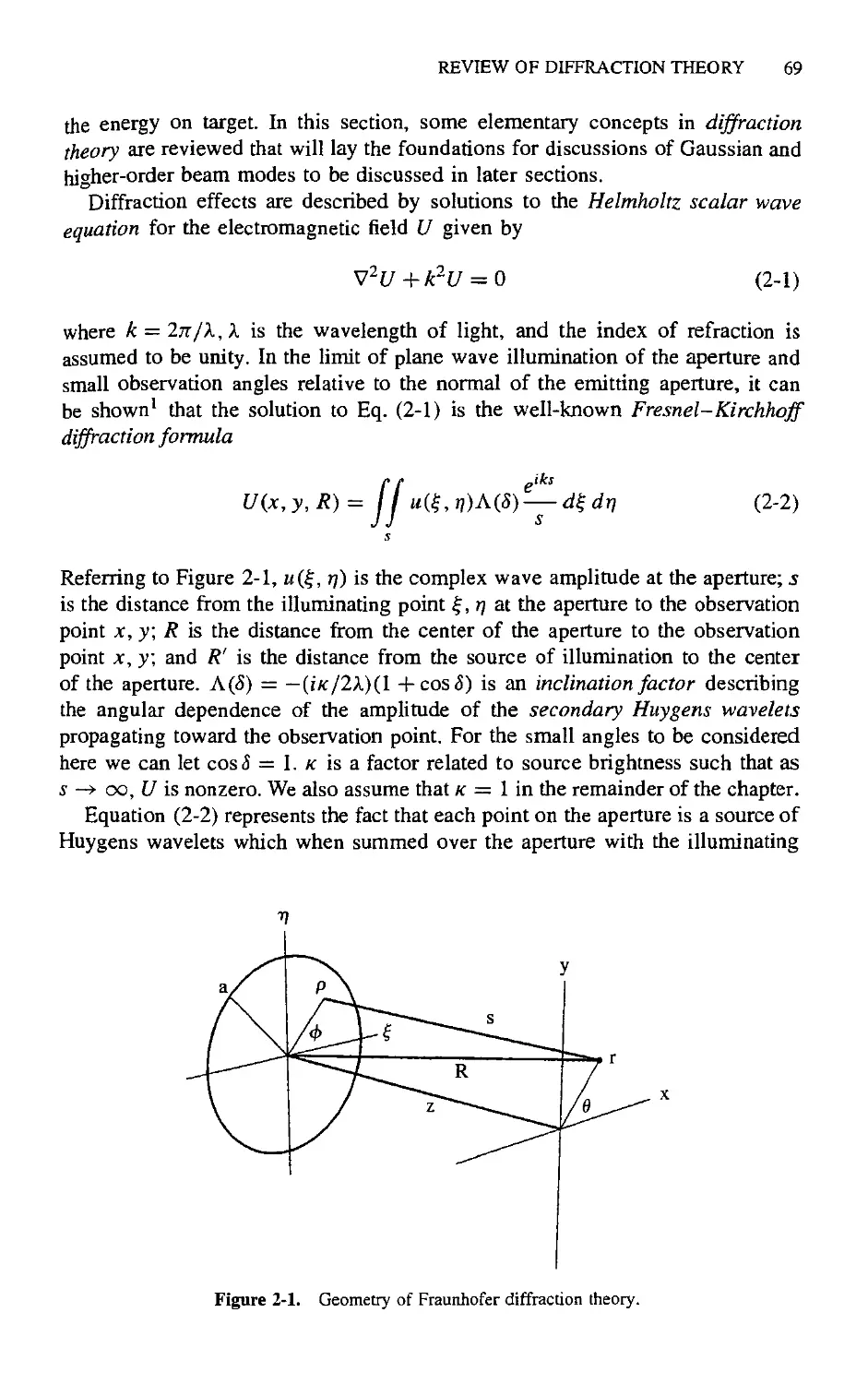
2.2. Review of Diffraction Theory
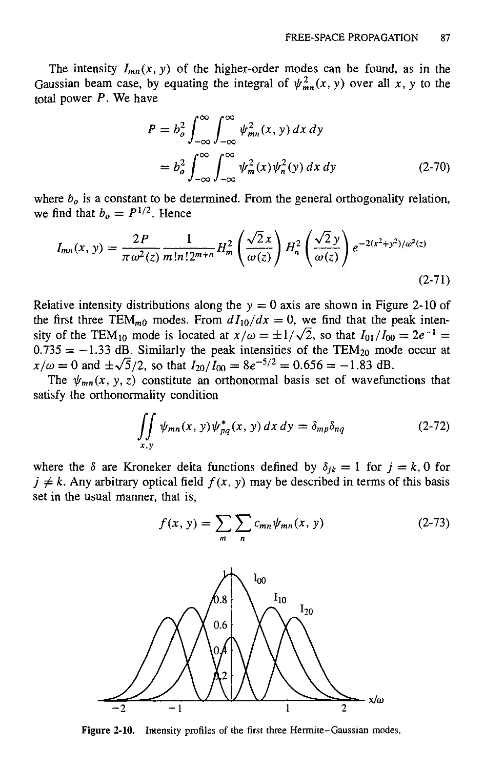
2.3. Free-Space Propagation
2.3.1. Transformation of Gaussian Beams
2.3.2. Untruncated Focused Gaussian Beams
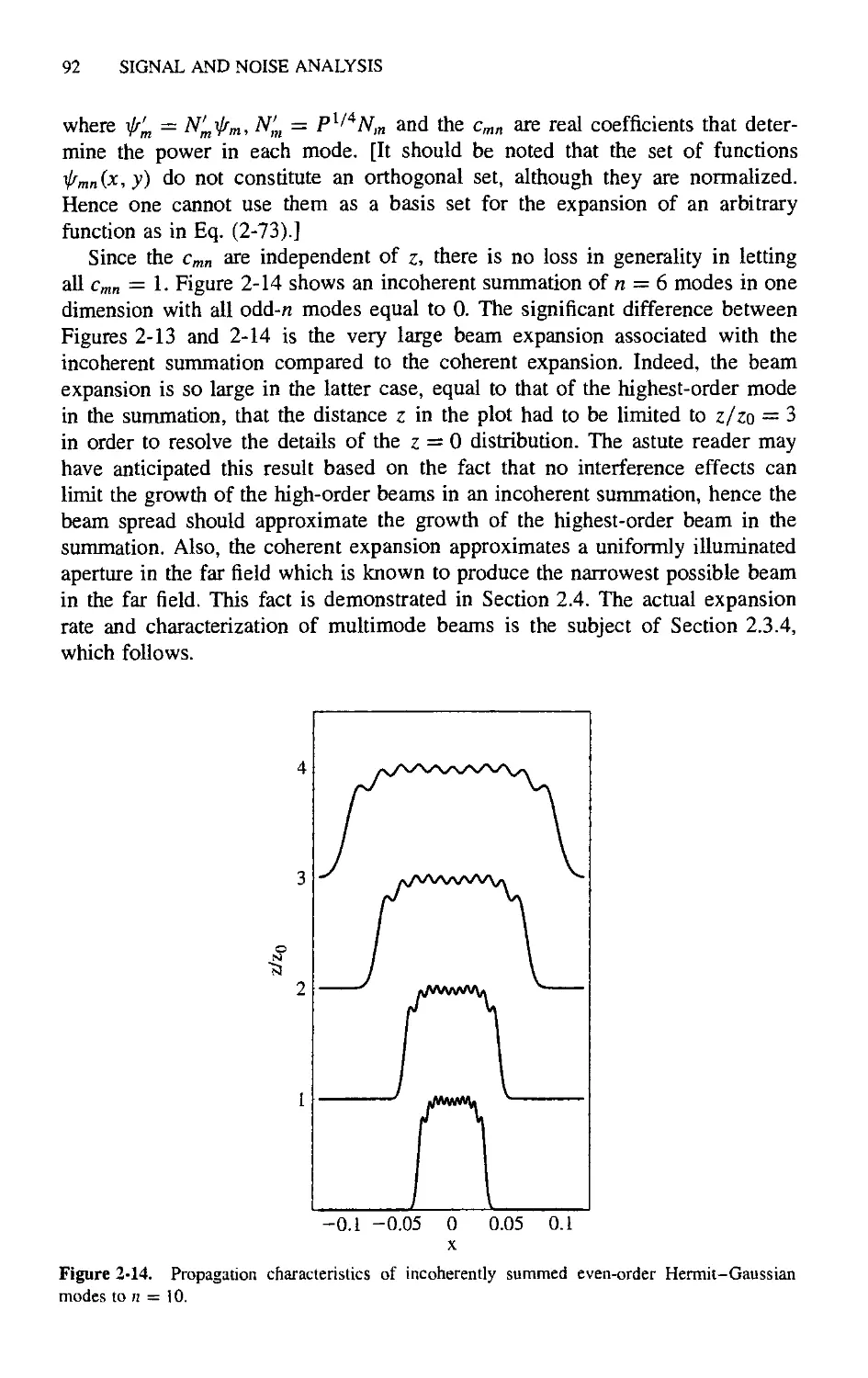
2.3.3. Multimode Beams
2.3.4. Beam Characterization
2.4. Truncated and Obscured Gaussian Beams
2.4.1. Optimum Beam Diameter
2.5. Fourier Optics and the Array Theorem
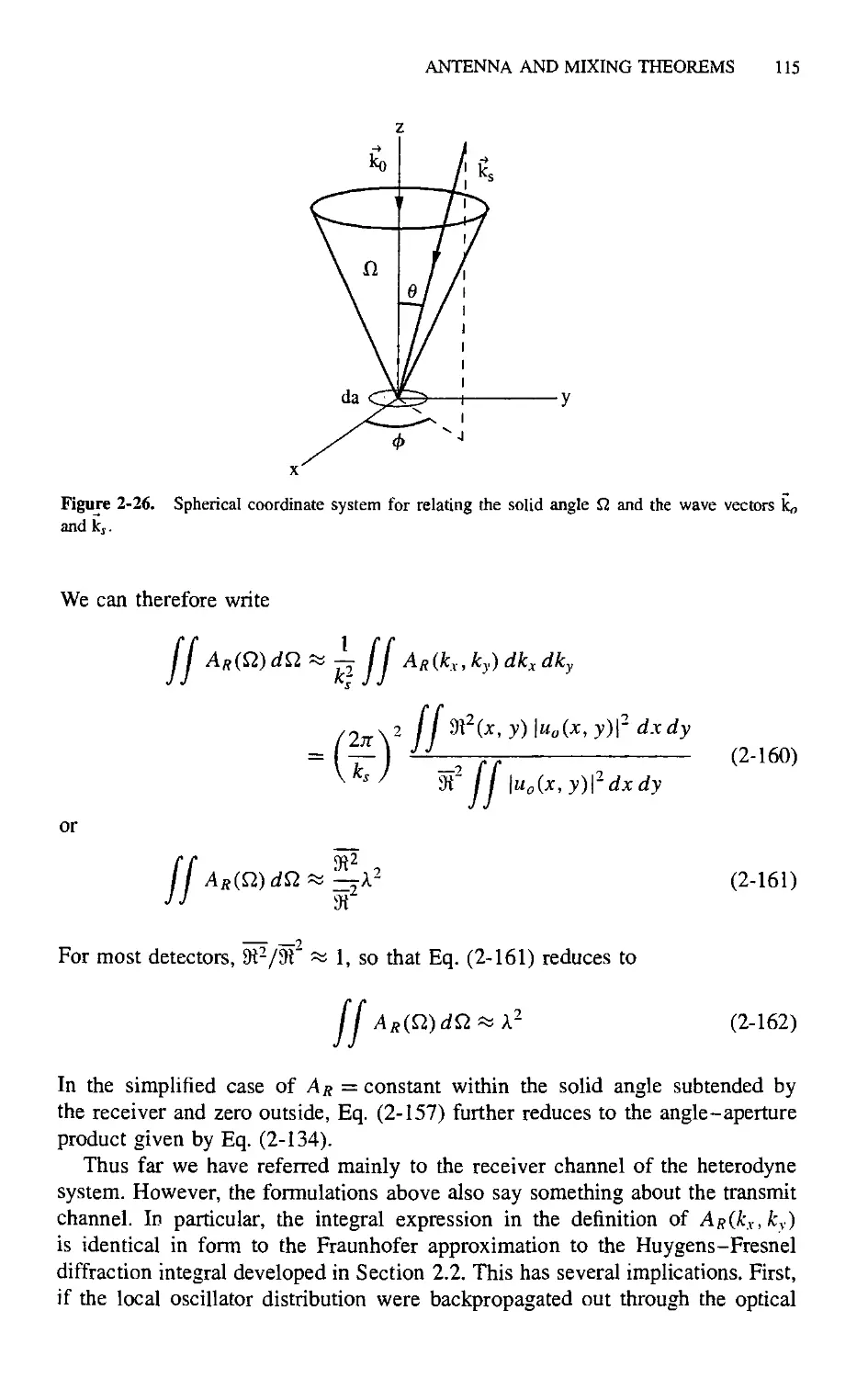
2.6. Antenna and Mixing Theorems
1
4
4
10
16
21
26
30
34
36
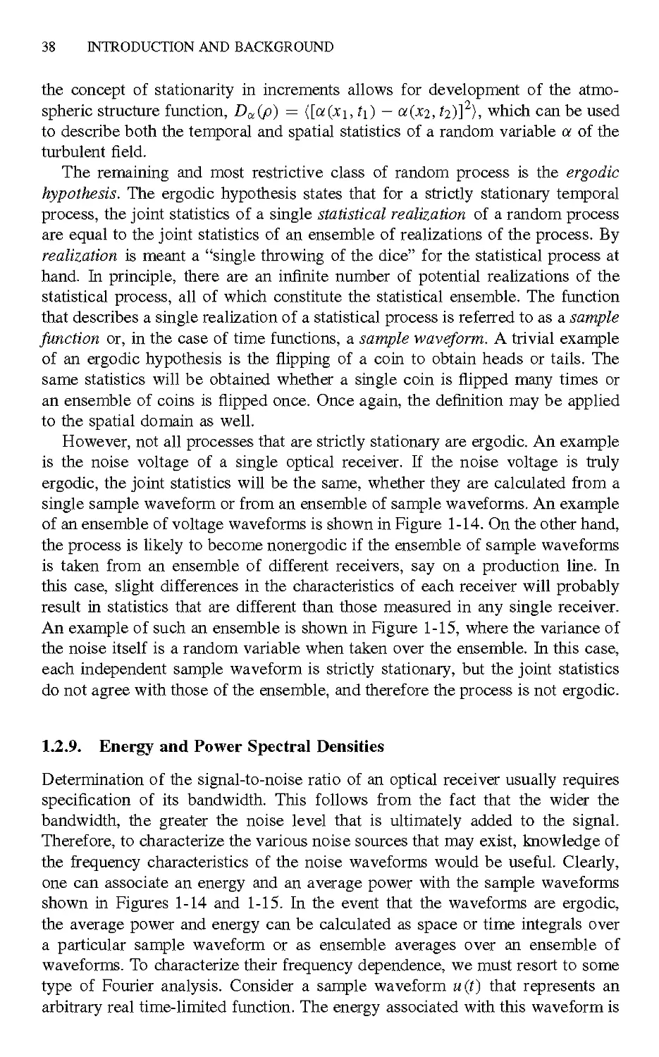
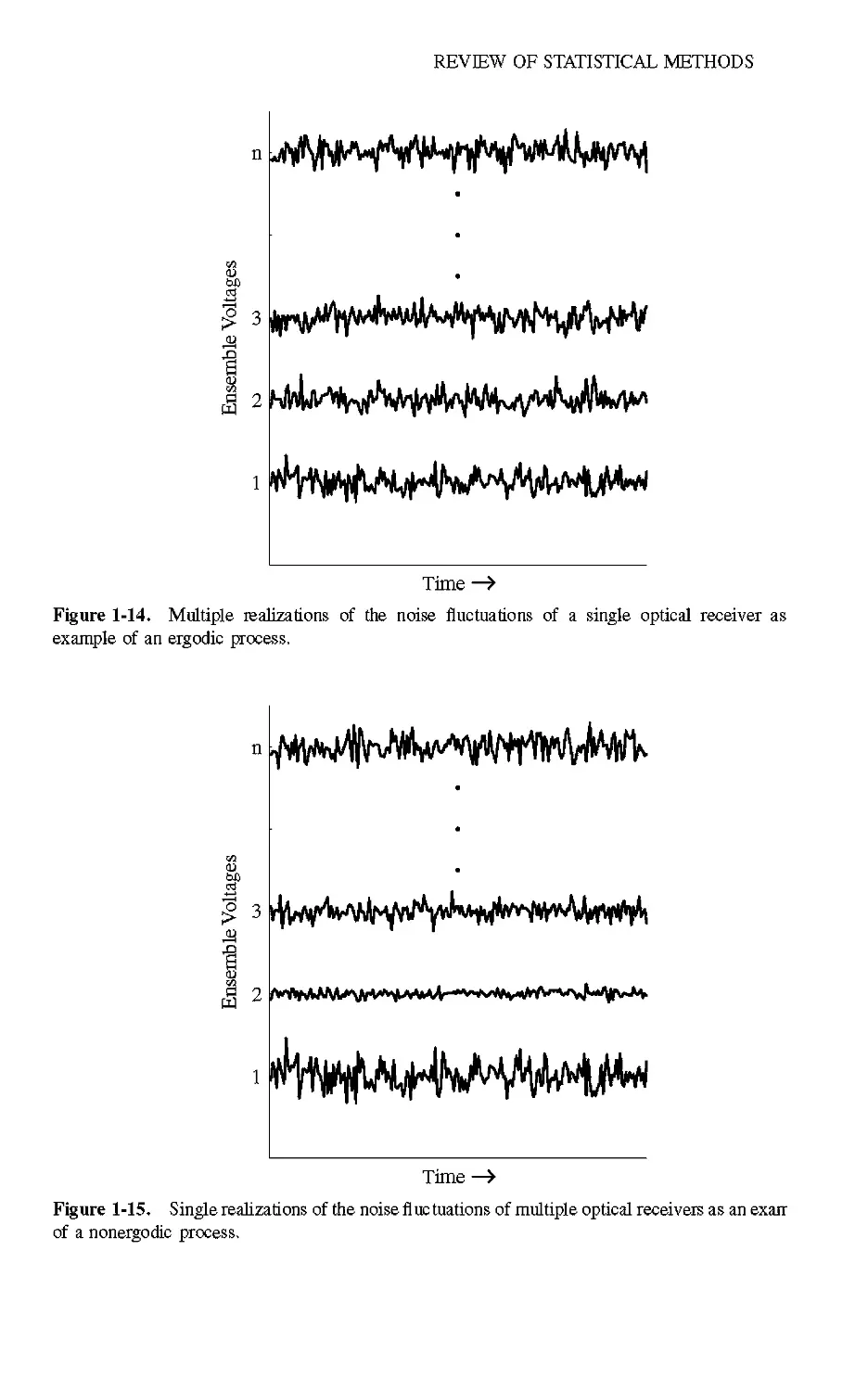
38
42
44
46
47
48
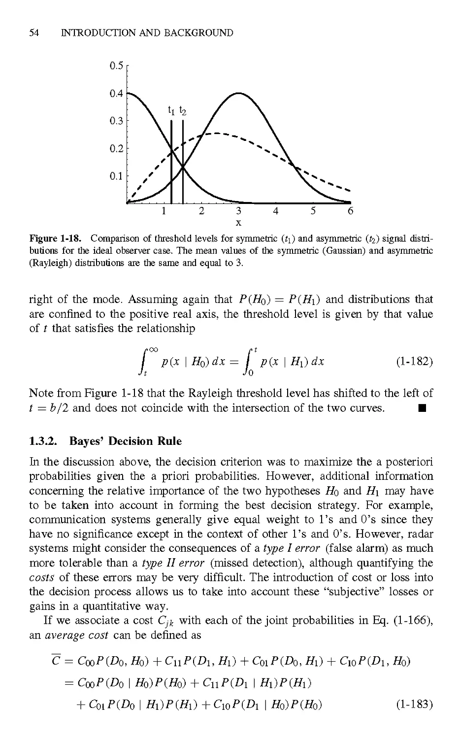
54
58
60
61
66
68
68
68
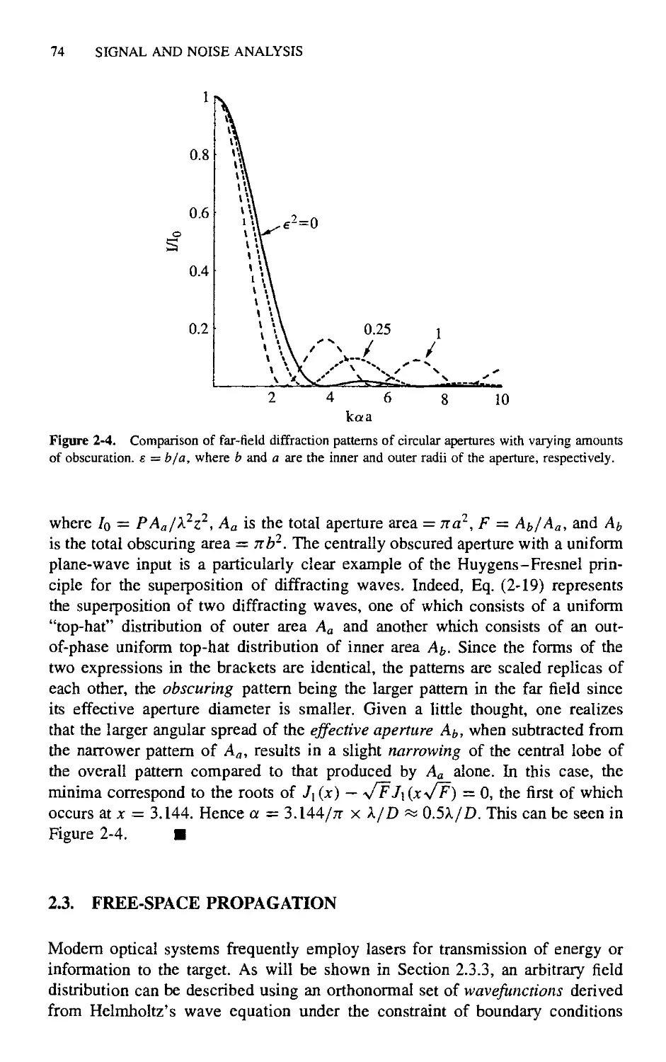
74
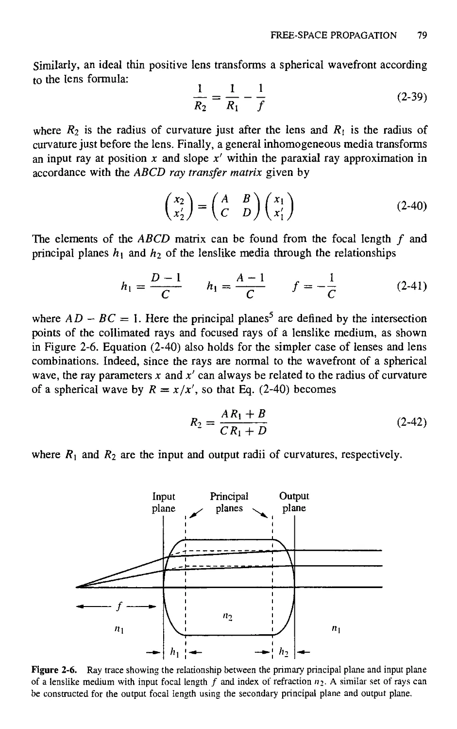
78
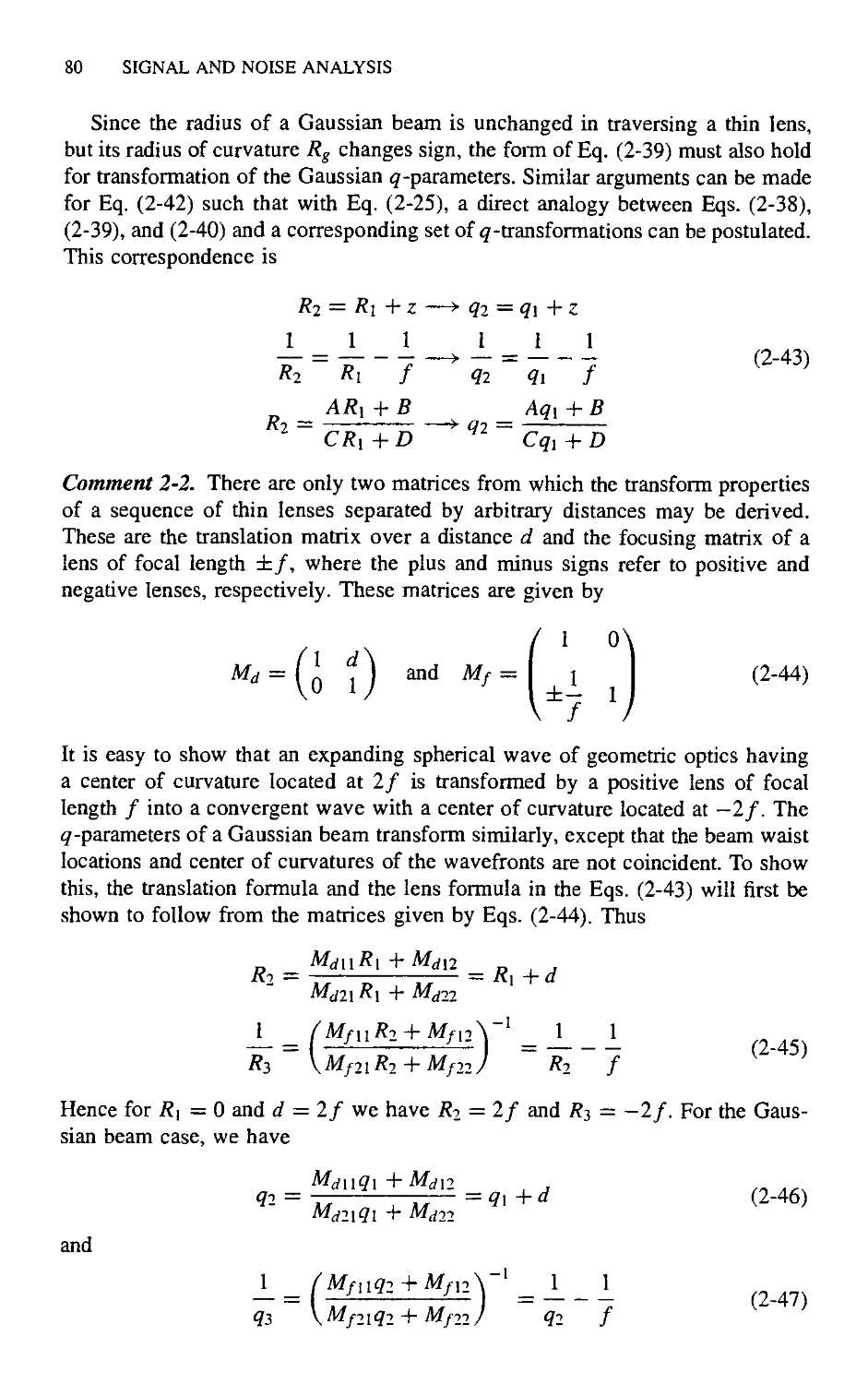
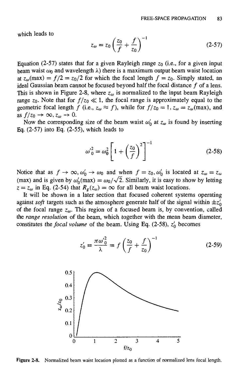
82
84
93
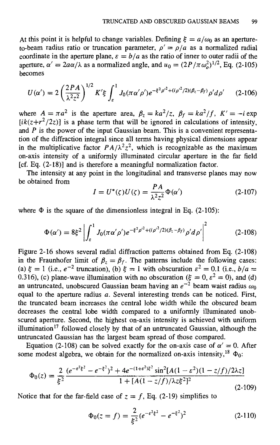
97
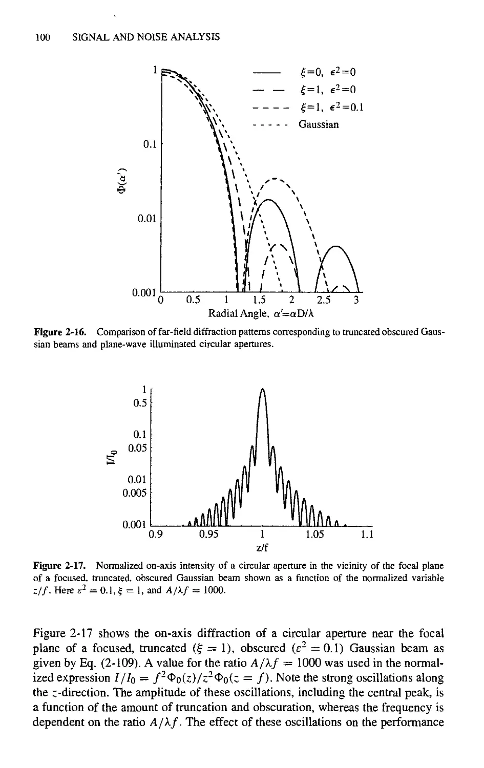
101
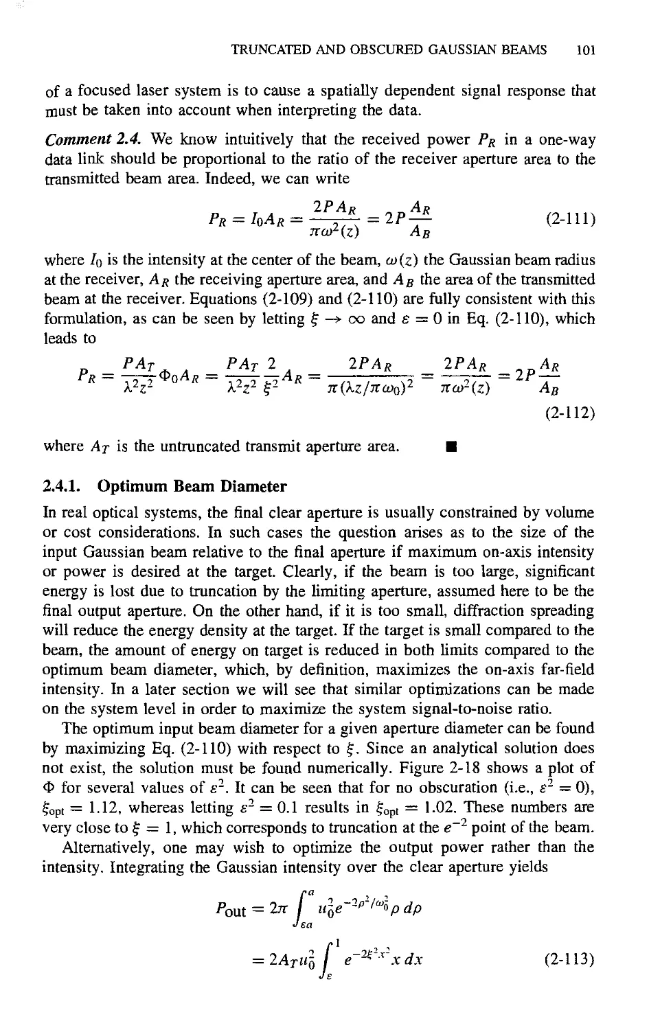
104
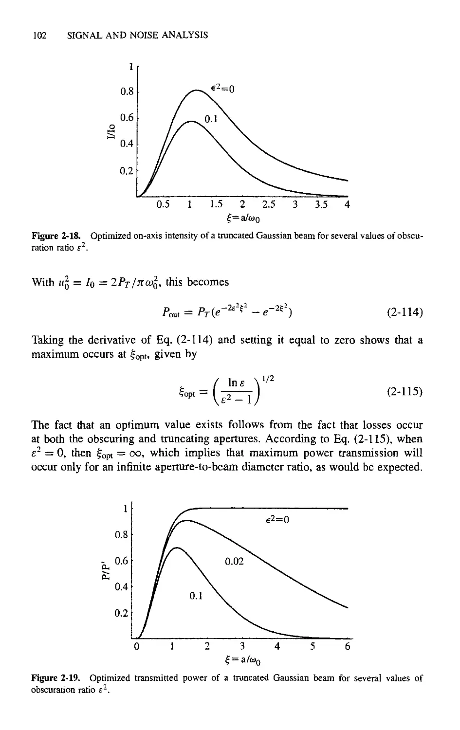
109

viii CONTENTS
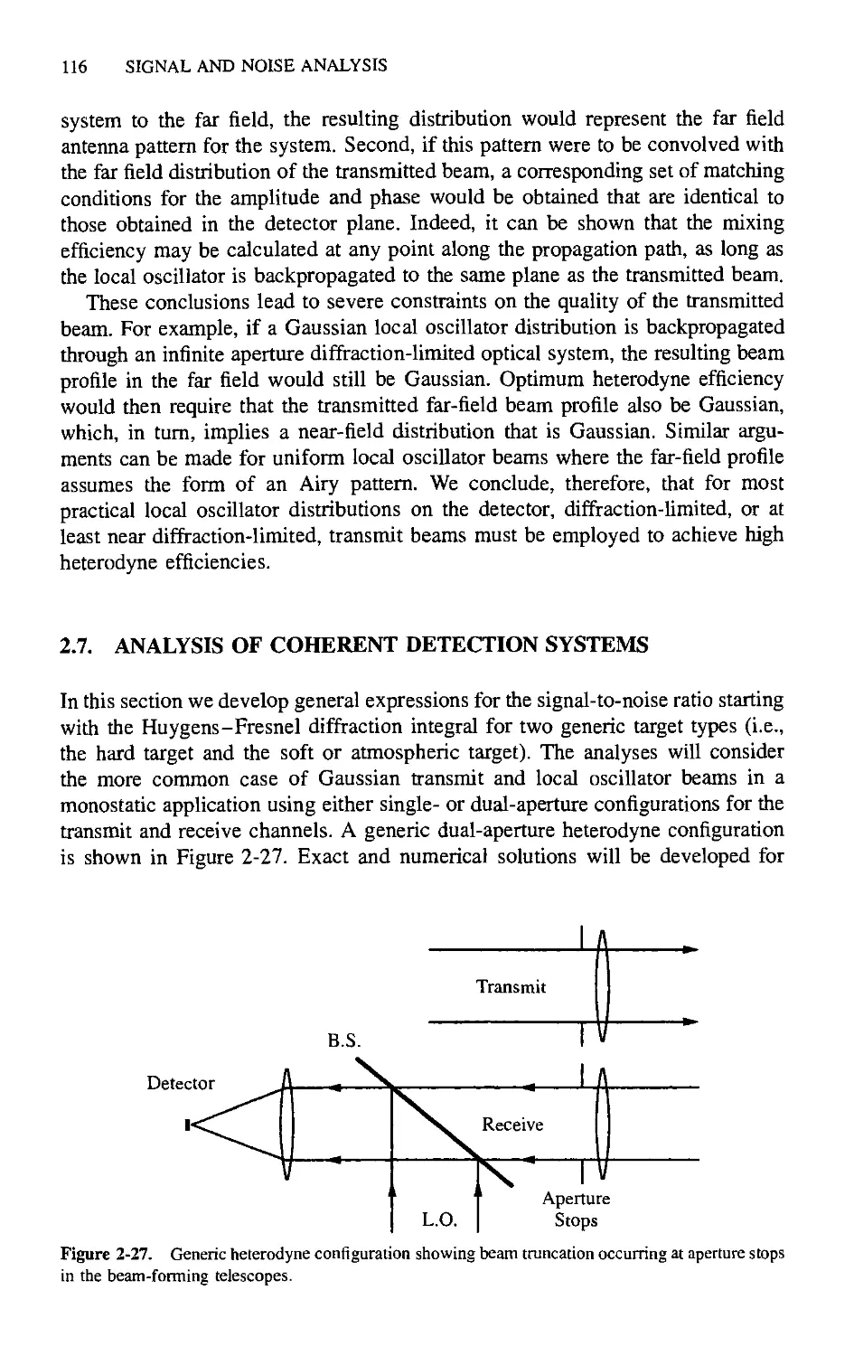
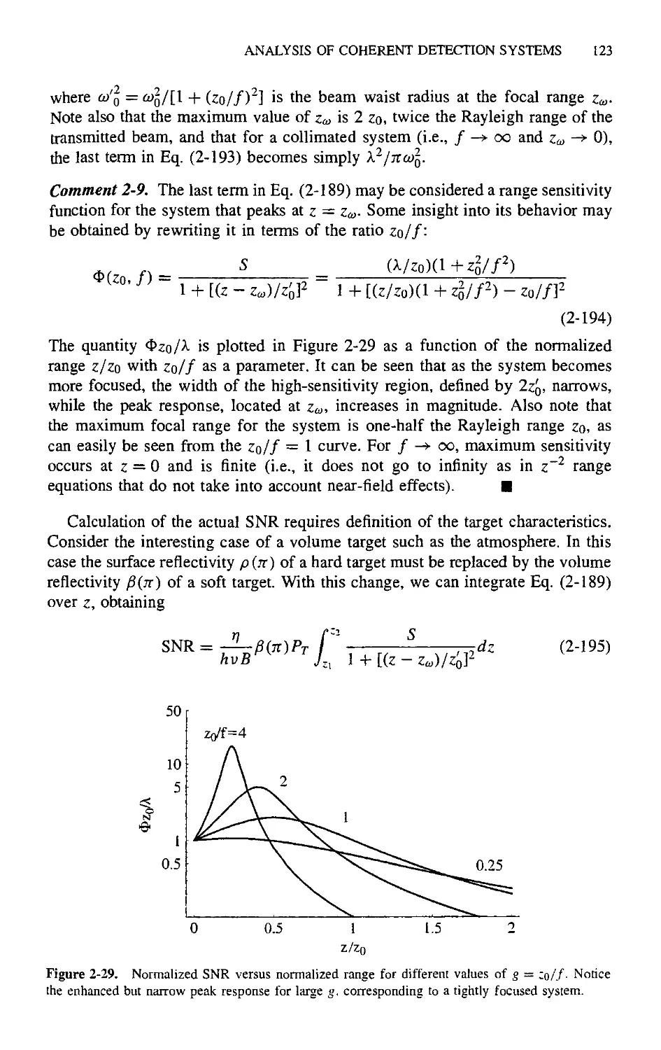
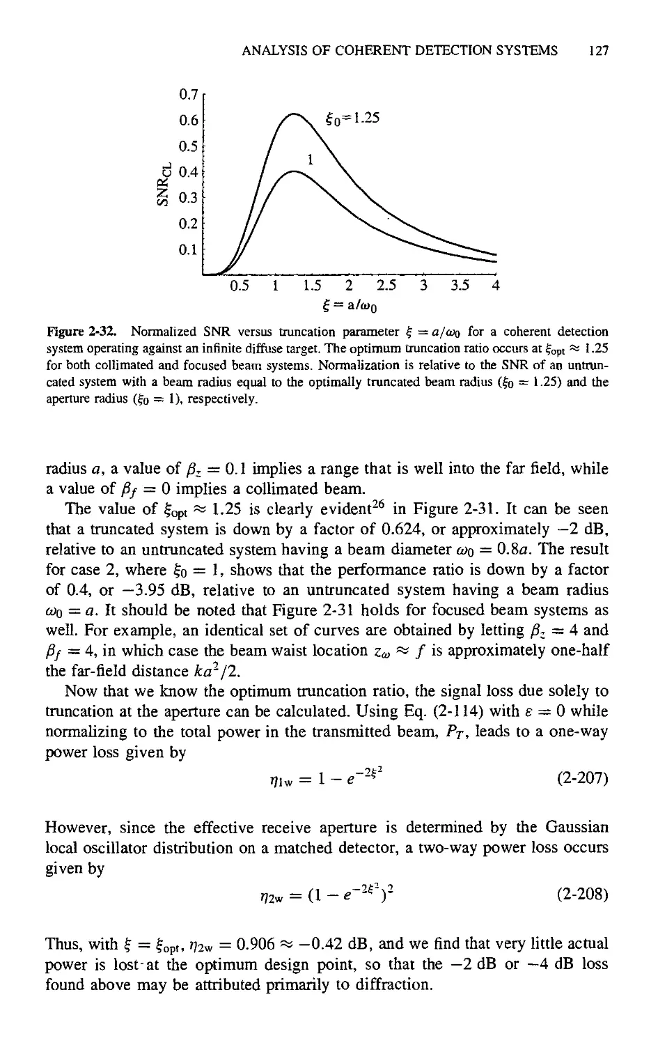
2.7. Analysis of Coherent Detection Systems 116
2.7.1. Untruncated Systems 117
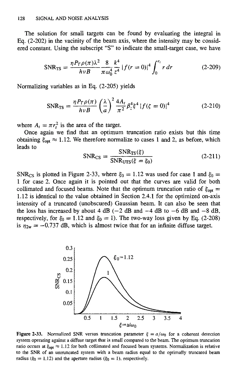
2.7.2. Truncated Systems 125
2.8. Analysis of Direct-Detection Systems 129
2.8.1. Untruncated Systems 129
2.8.2. Truncated Systems 131
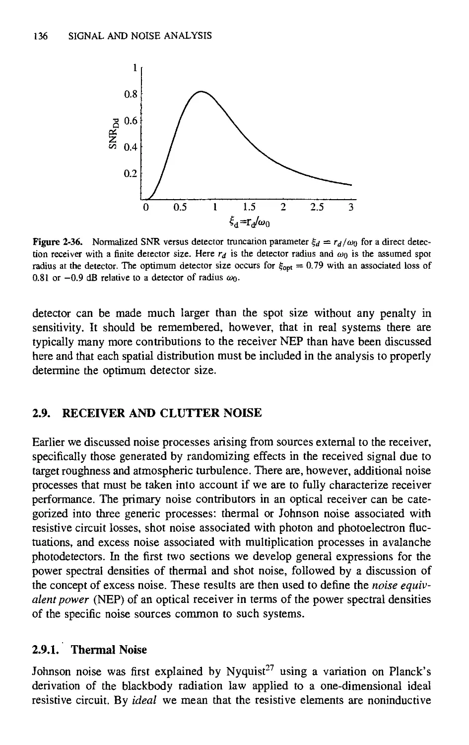
2.9. Receiver and Clutter Noise 136
2.9.1. Thermal Noise 136
2.9.2. Shot Noise 138
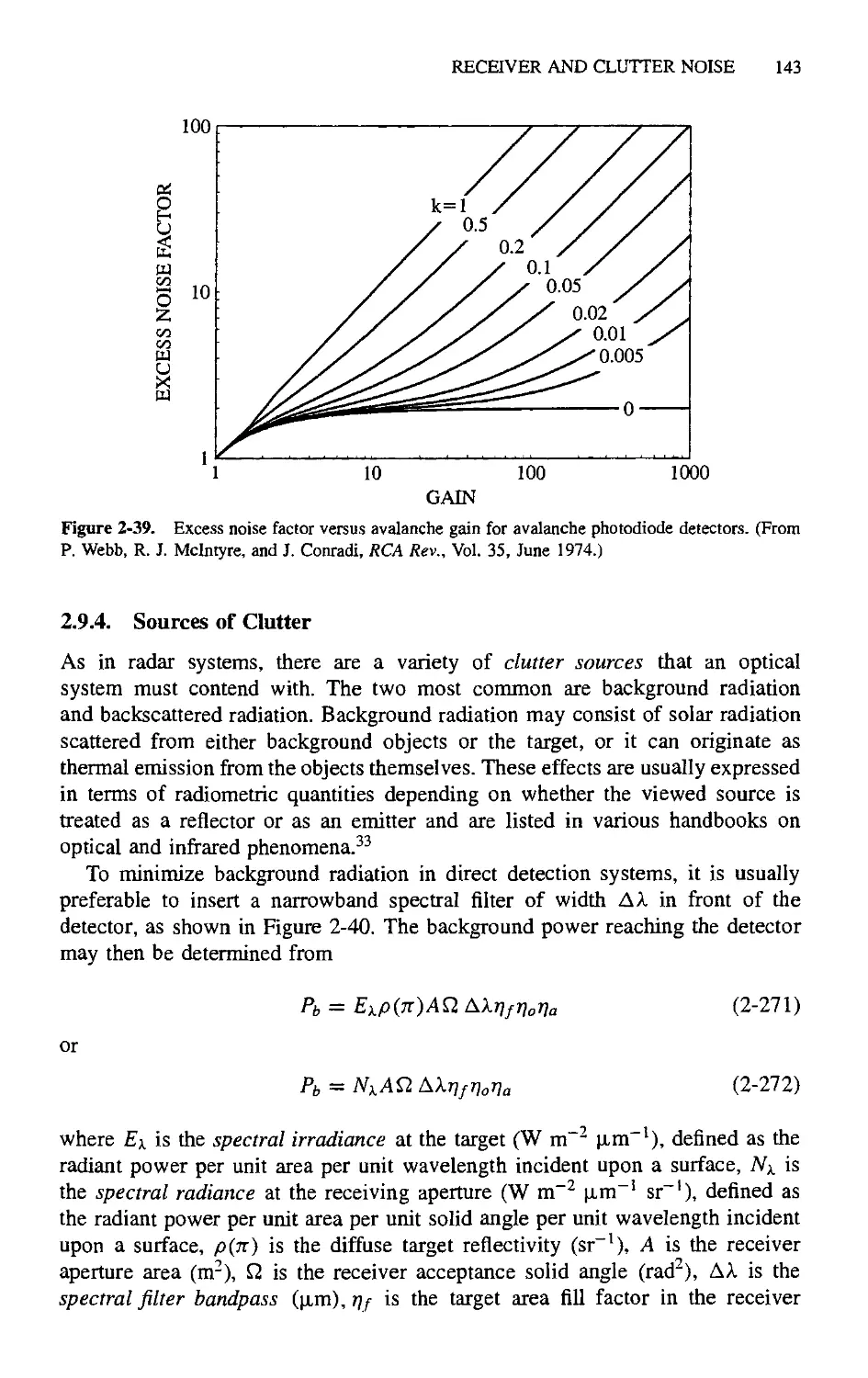
2.9.3. Dark Current and Excess Noise 140
2.9.4. Sources of Clutter 143
2.10. Power Signal-to-Noise-Ratio 145
References 148
Chapter 3. Random Processes in Beam Propagation 150
3.1. Introduction 150
3.2. Review of Optical Coherence Theory 151
3.2.1. Coherence Properties of the Field 151
3.2.2. Van Cittert-Zernike Theorem 155
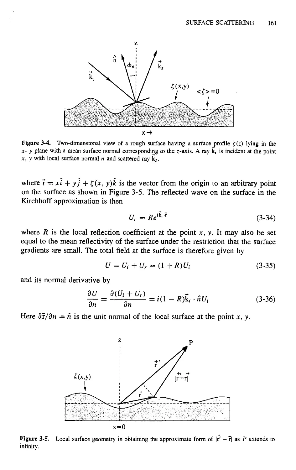
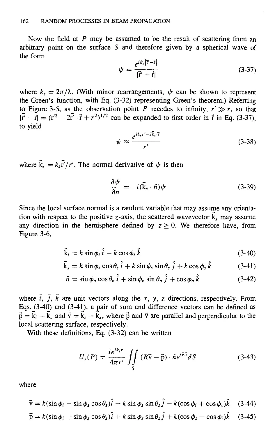
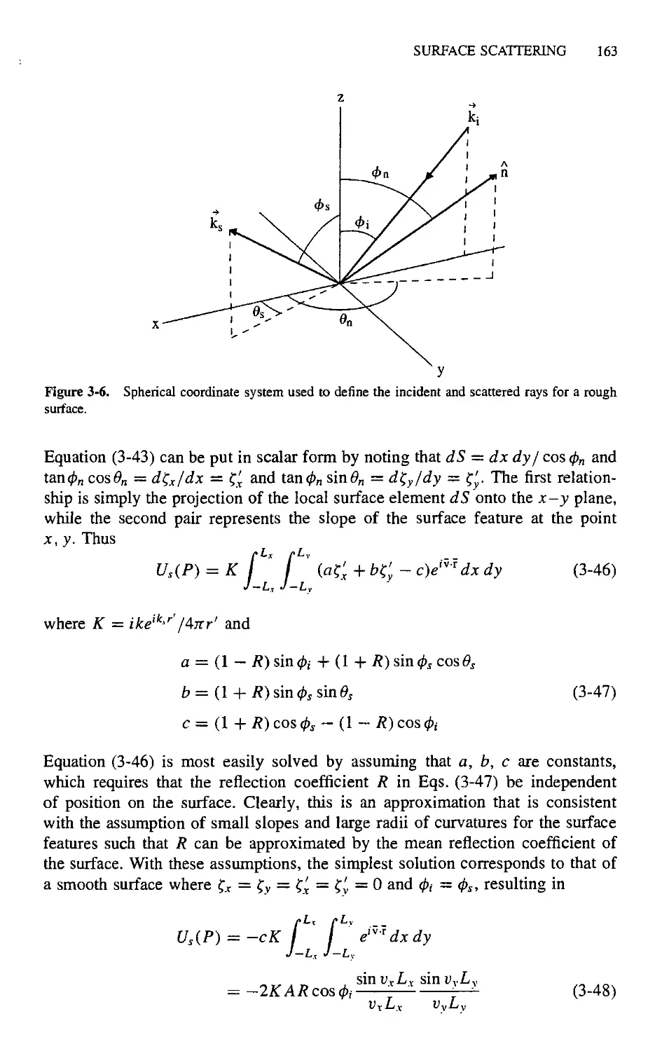
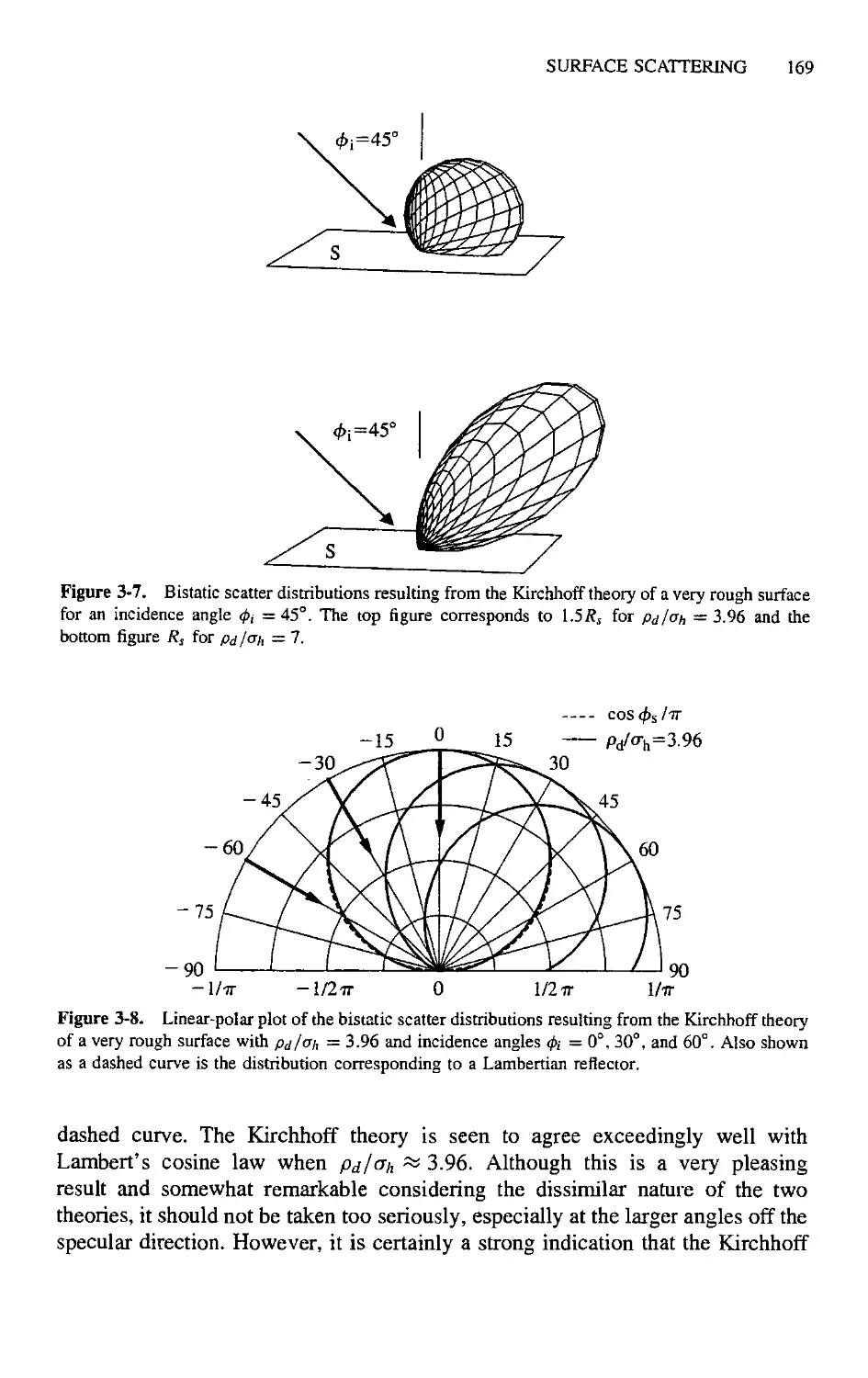
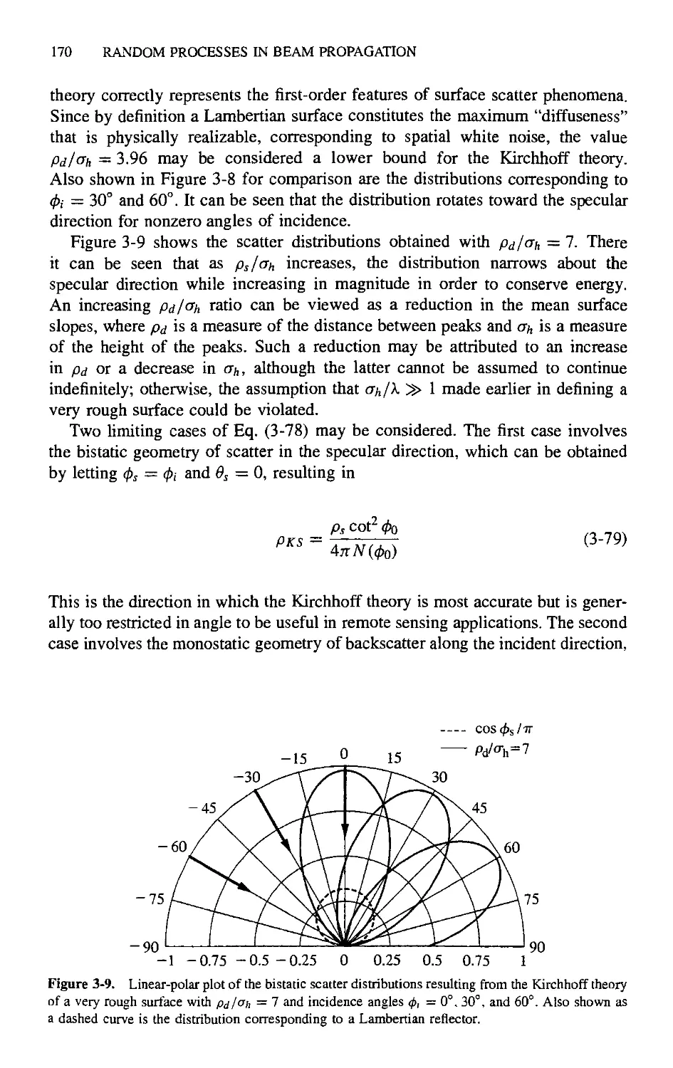
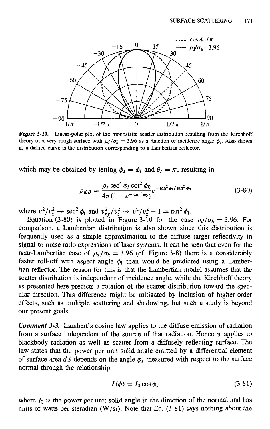
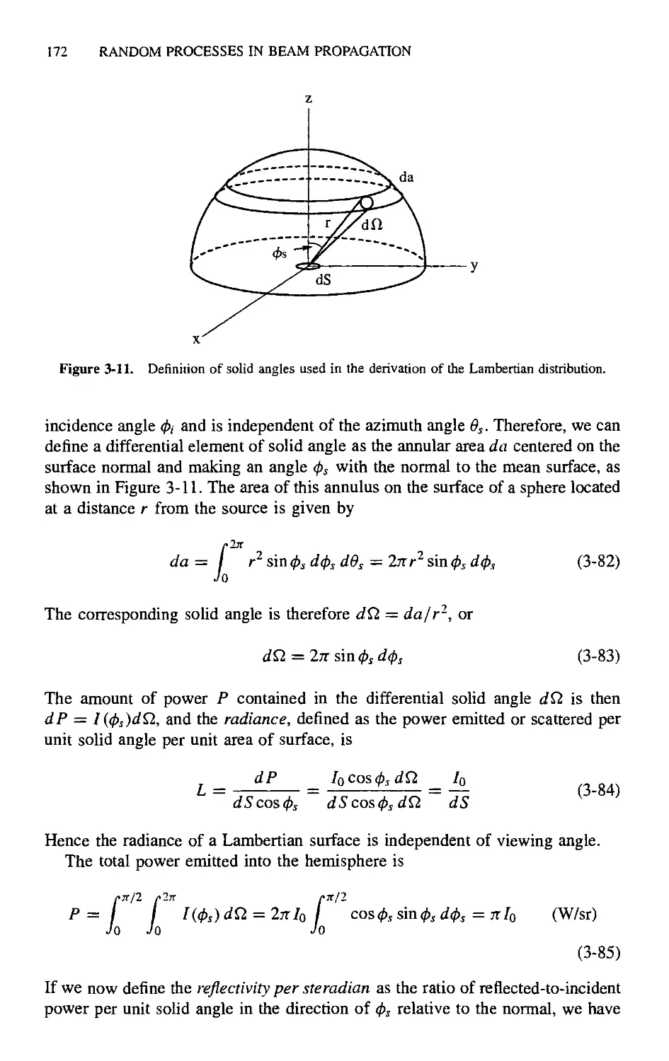
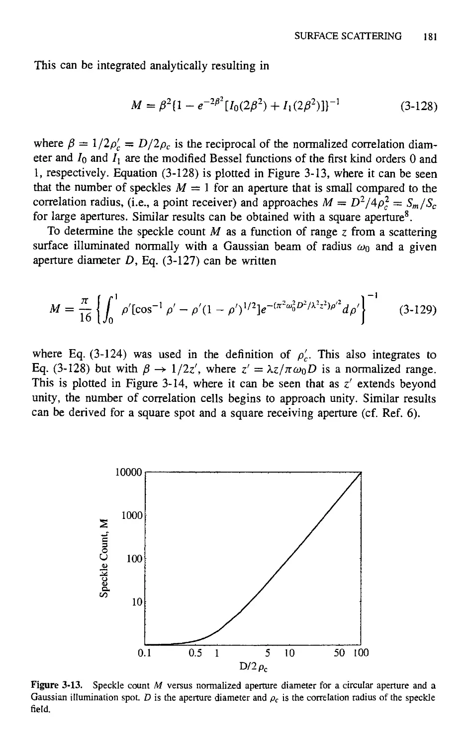
3.3. Surface Scattering 159
3.3.1. Scattering from a Rough Surface 160
3.3.2. Integrated Speckle Intensity 173
3.3.3. Speckle Correlation Diameter 176
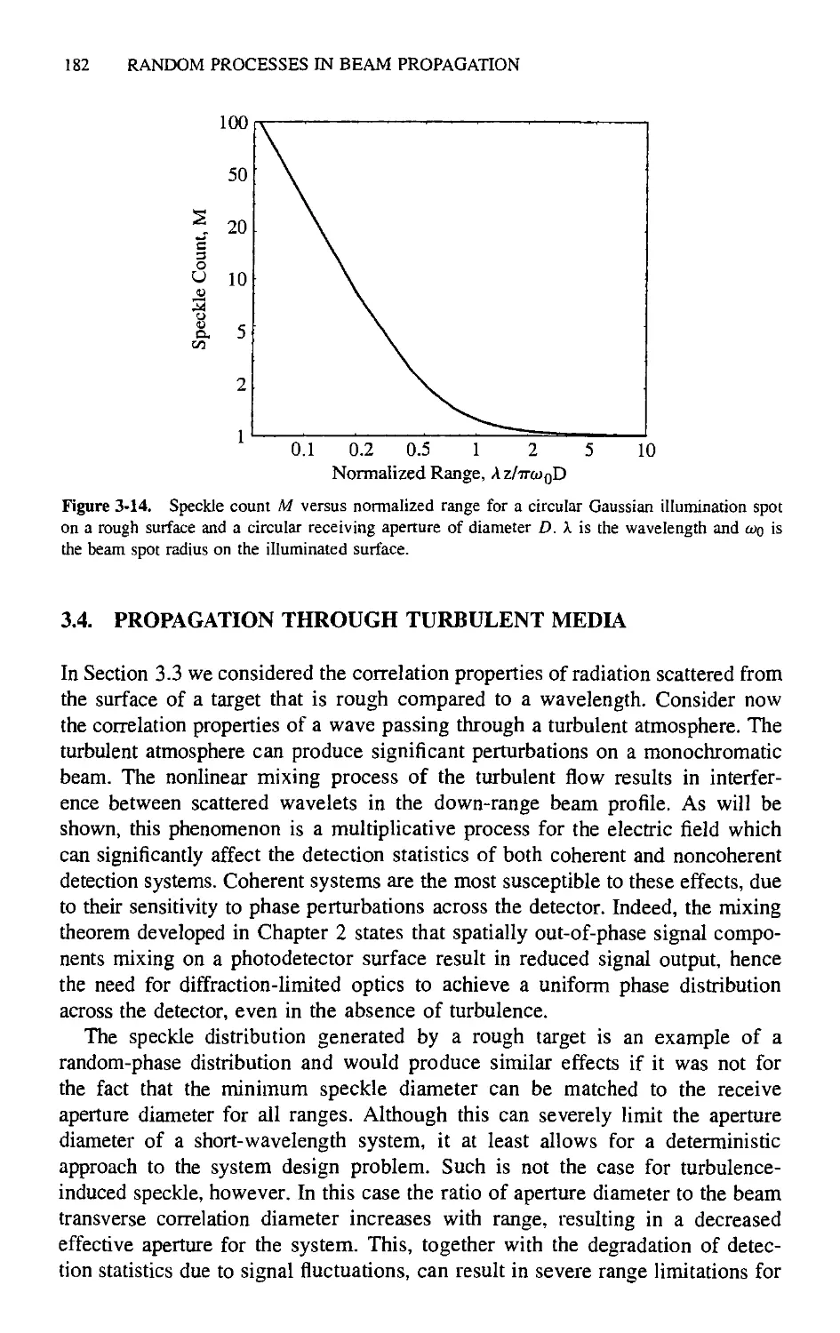
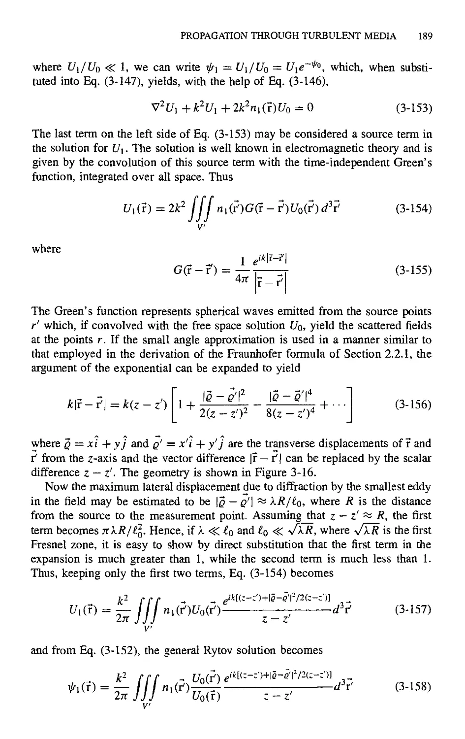
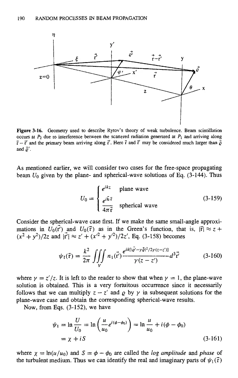
3.4. Propagation through Turbulent Media 182
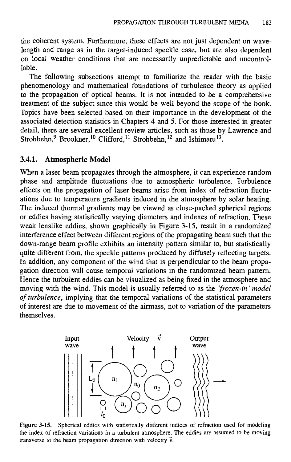
3.4.1. Atmospheric Model 183
3.4.2. Weak Turbulence Theory 187
3.4.2.1. Power Spectral Density 191
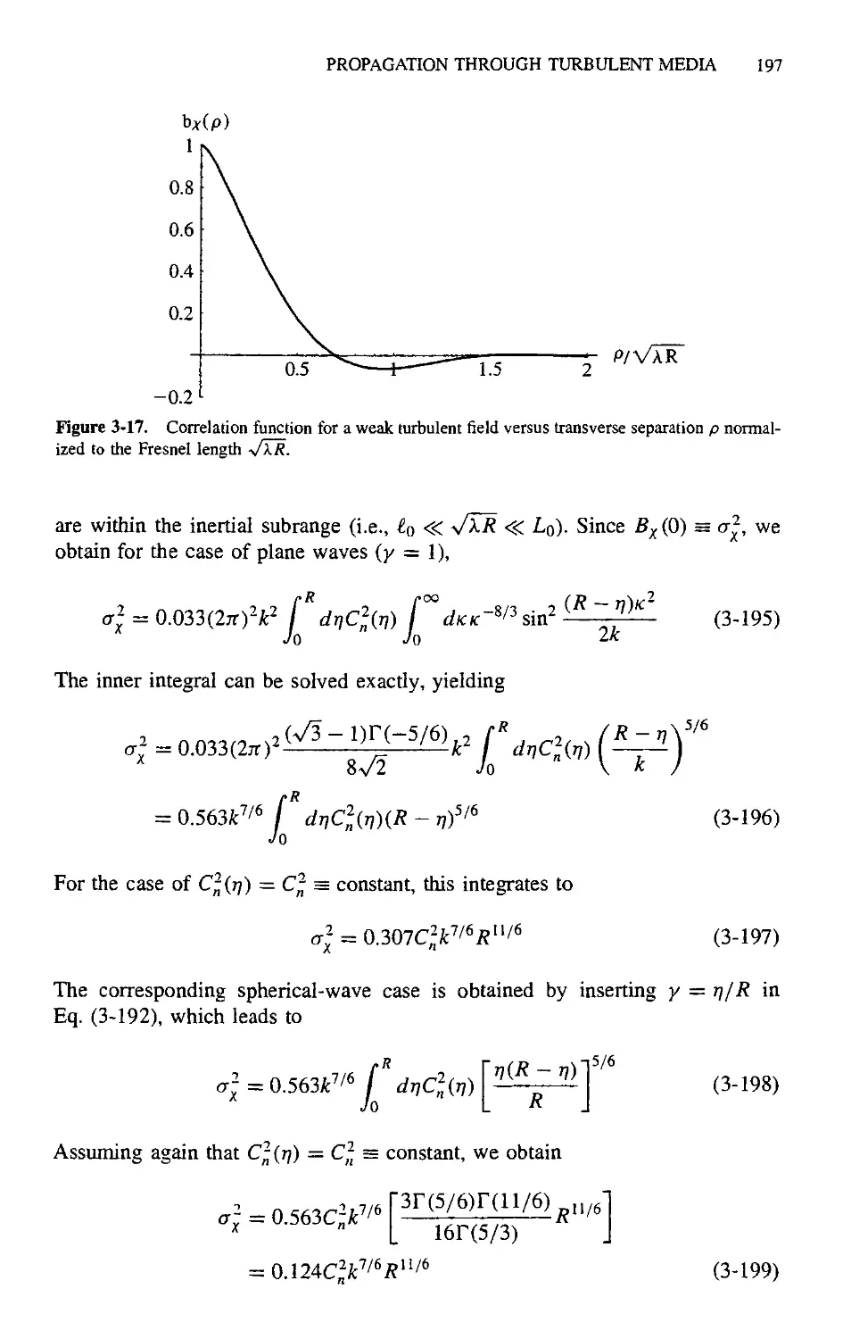
3.4.2.2. Correlation Function 194
3.4.2.3. Mutual Coherence Function 198
3.4.2.4. Statistics of the Turbulent Field 201
3.4.2.5. Aperture Averaging in
Direct-Detection Systems 203
3.4.2.6. Turbulence-Limited Performance of
Coherent Systems 208
3.4.2.7. Beam Wander 212
3.4.3. Strong Turbulence Theory 217
References 224
Chapter 4. Single-Pulse Direct-Detection Statistics 227
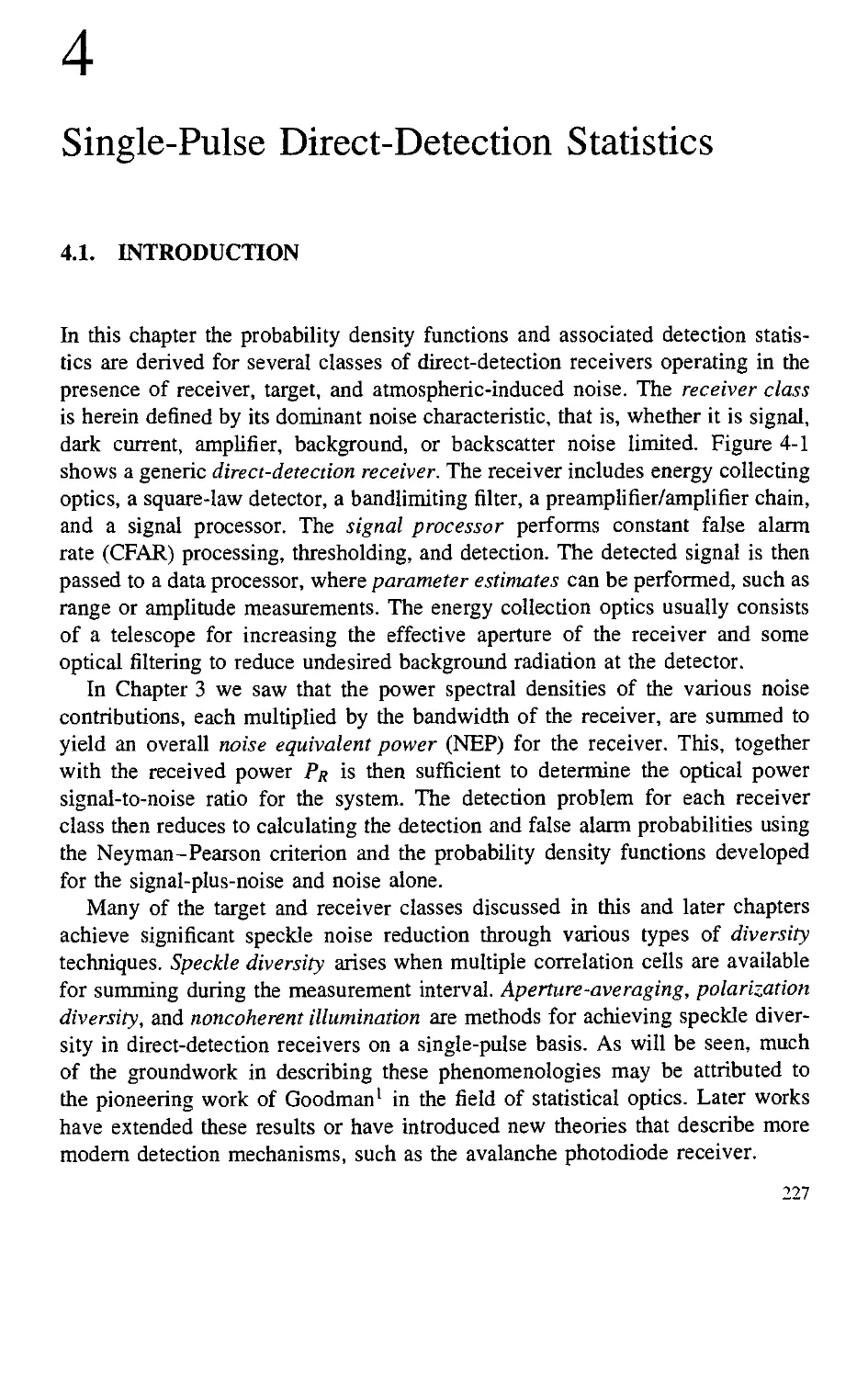
4.1. Introduction 227
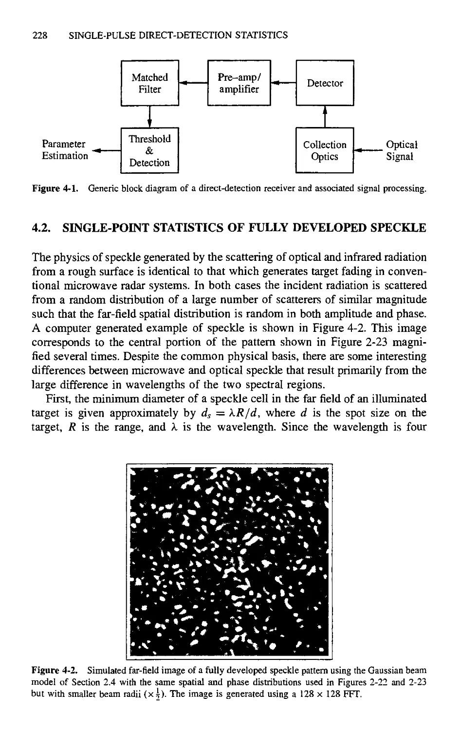
4.2. Single-Point Statistics of Fully Developed Speckle 228
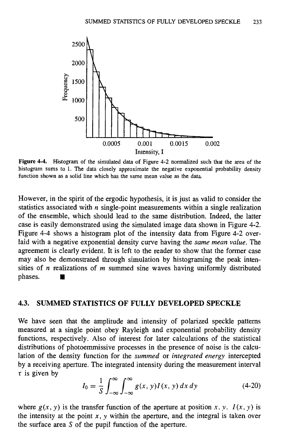
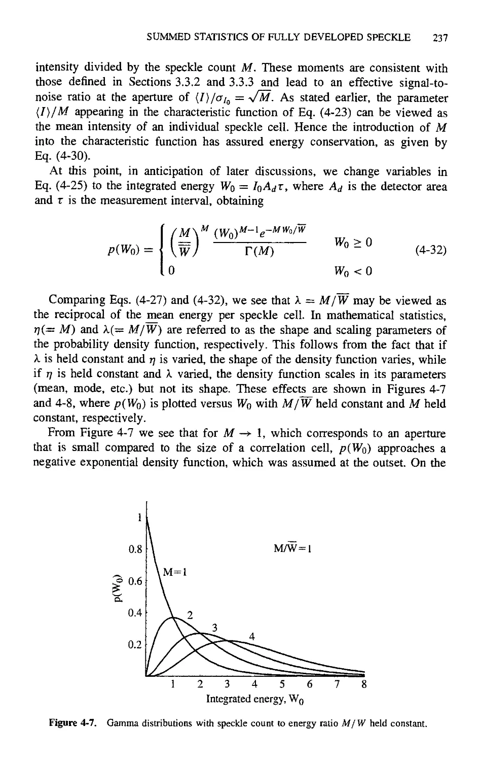
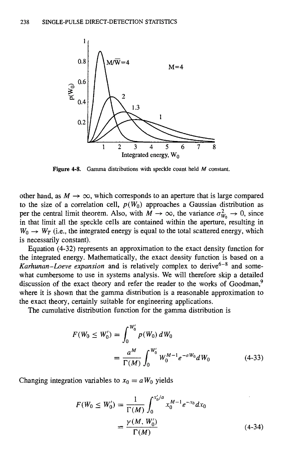
4.3. Summed Statistics of Fully Developed Speckle 233
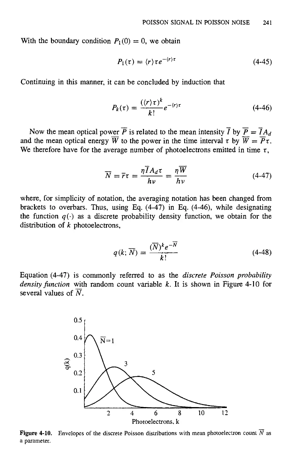
4.4. Poisson Signal in Poisson Noise 239

CONTENTS ix
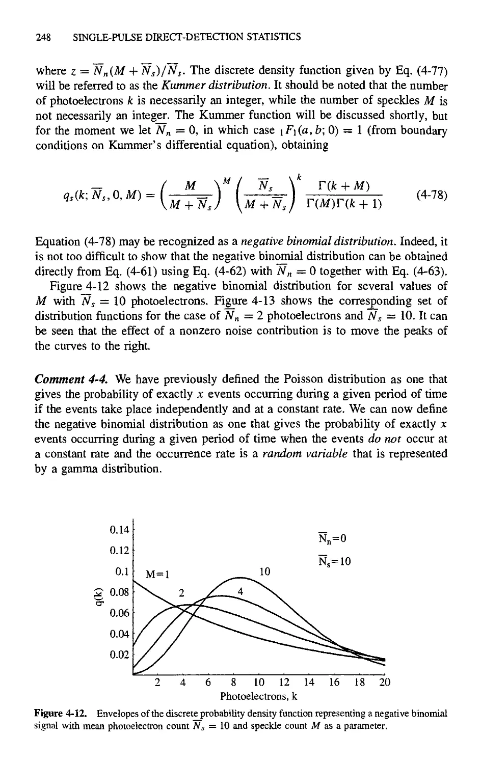
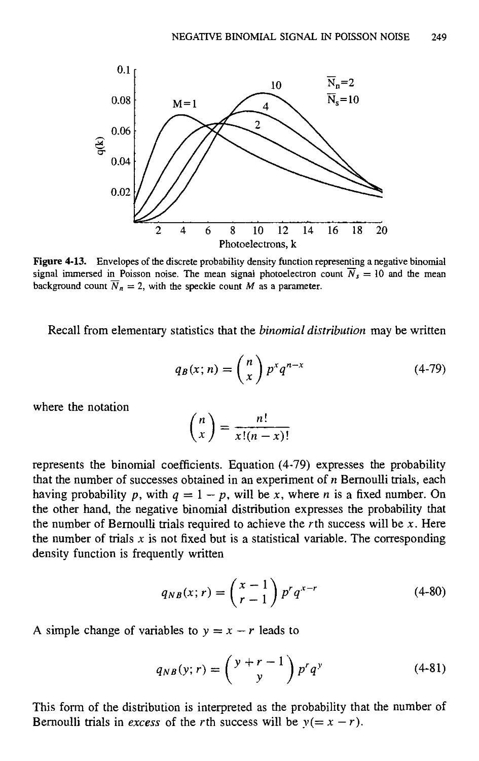
4.5. Negative Binomial Signal in Poisson Noise 245
4.6. Noncentral Negative Binomial Signal in Poisson Noise 255
4.6.1. Summed Statistics of Partially Developed
Speckle 259
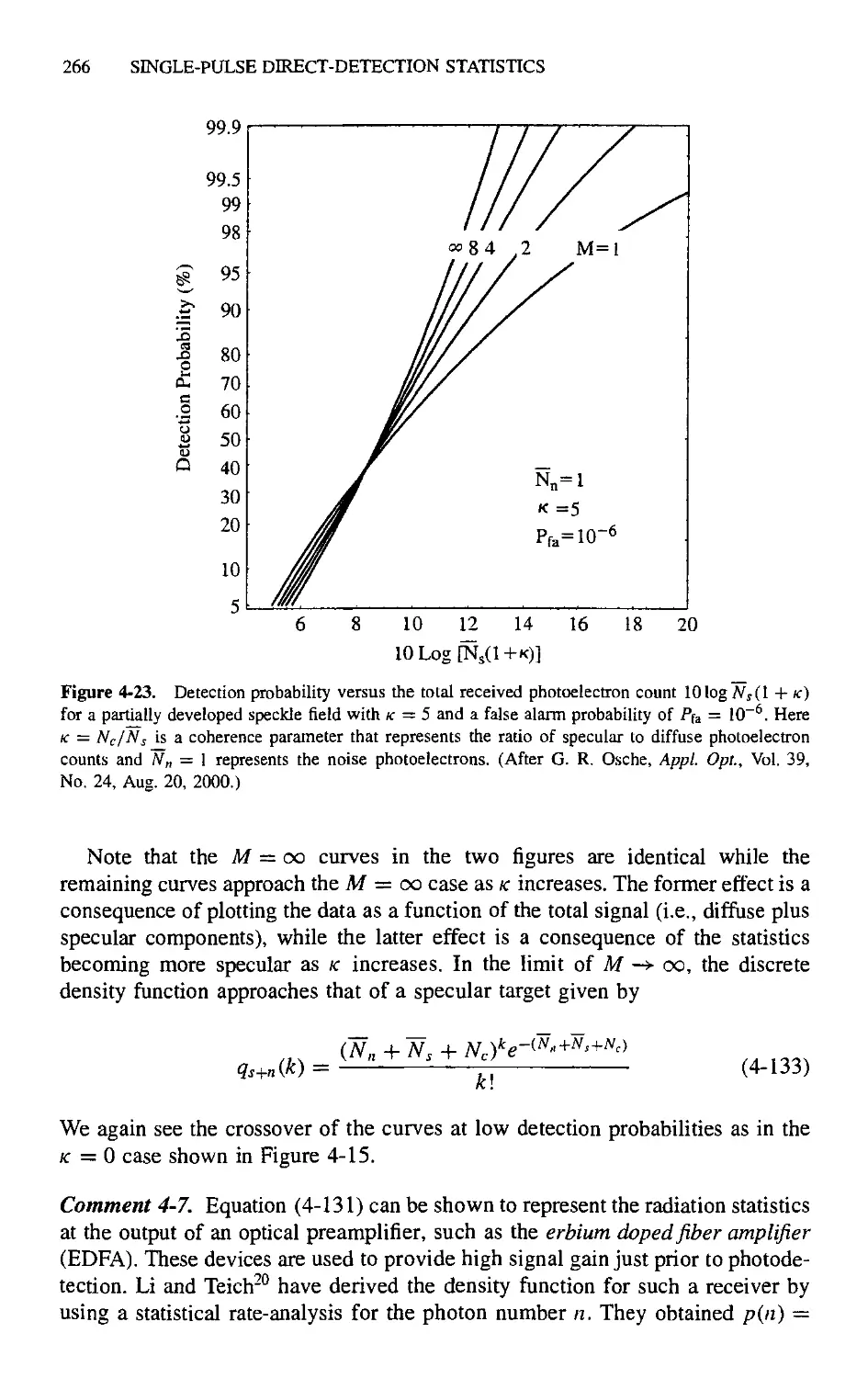
4.6.2. Single-Pulse Detection Statistics 263
4.7. Parabolic-Cylinder Signal in Gaussian Noise 267
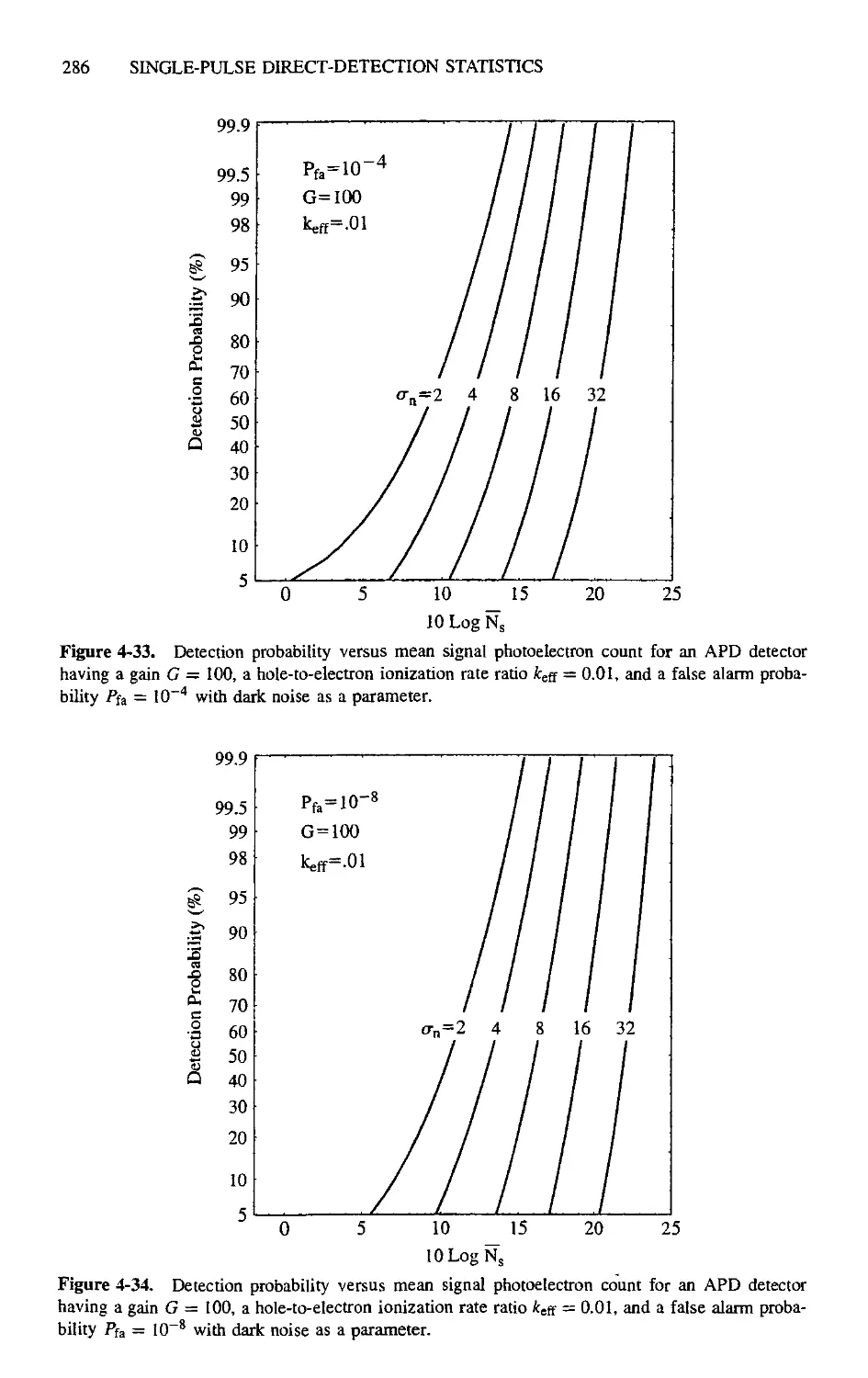
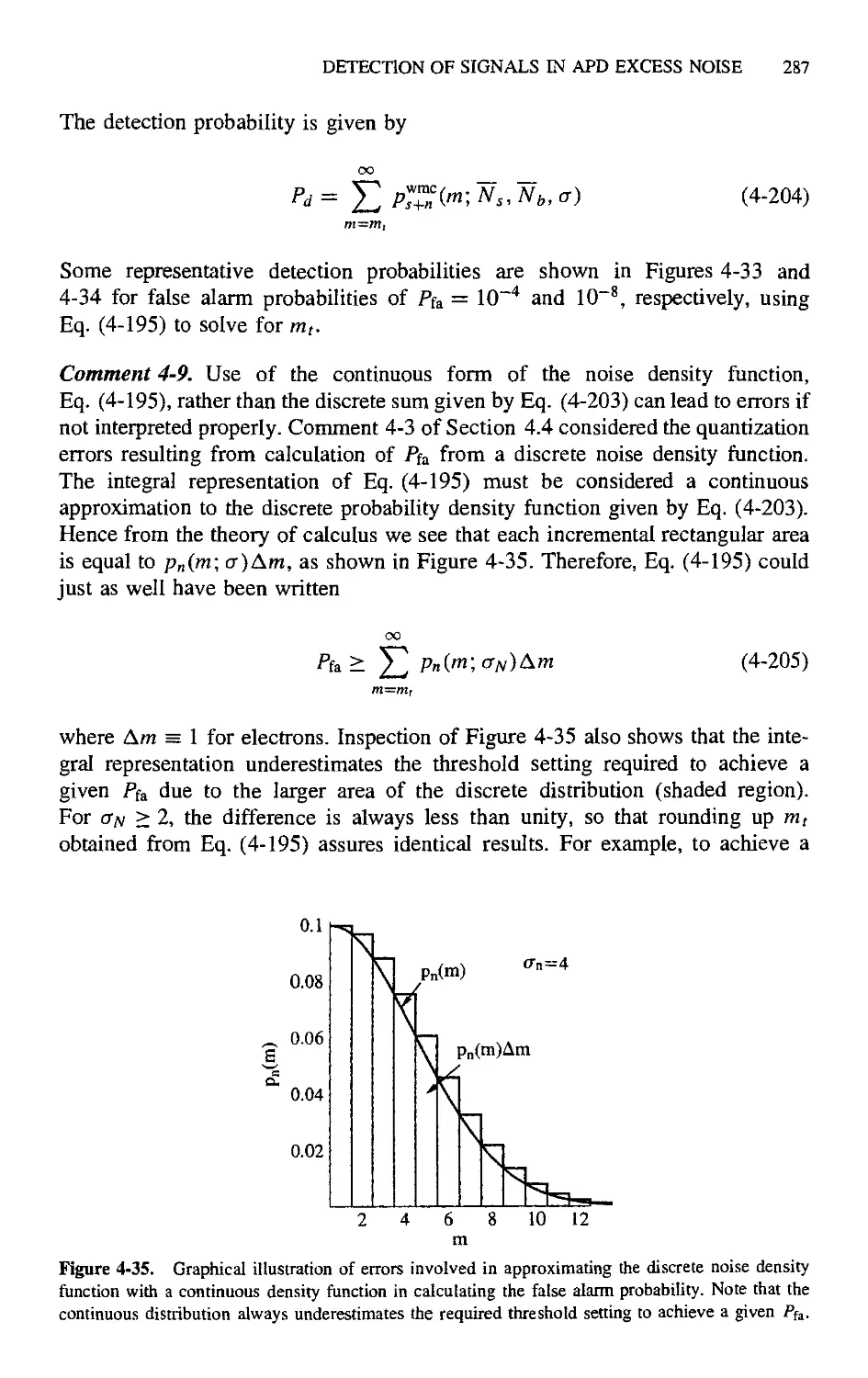
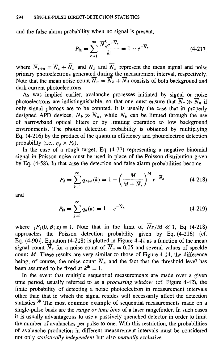
4.8. Detection of Signals in APD Excess Noise 275
4.8.1. Poisson Signal 278
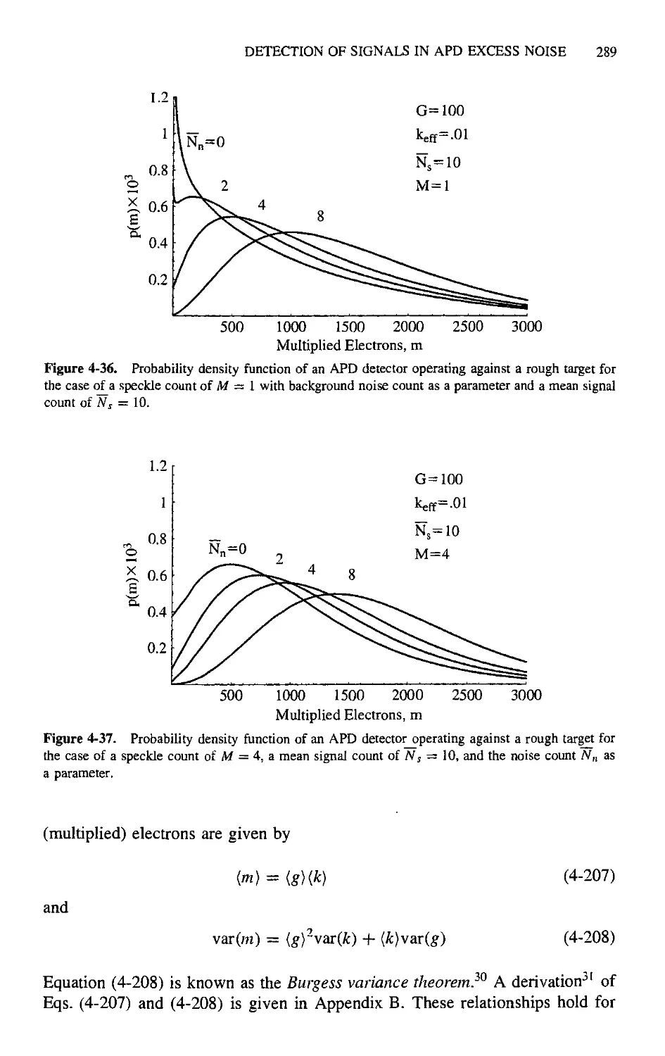
4.8.2. Negative Exponential Signal 288
4.8.3. Geiger-Mode APD Statistics 291
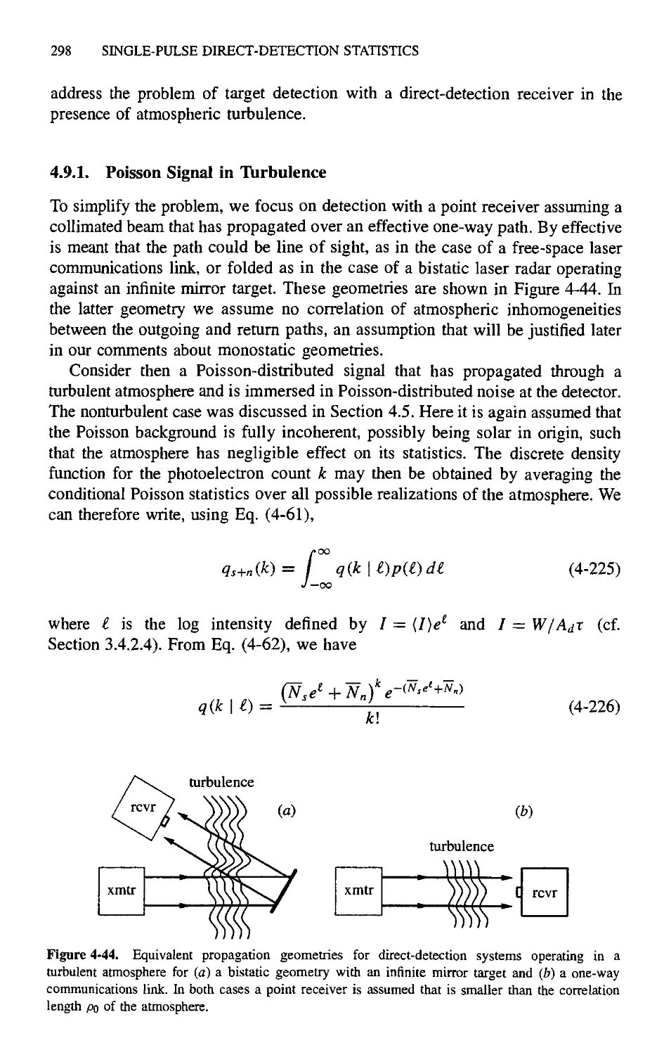
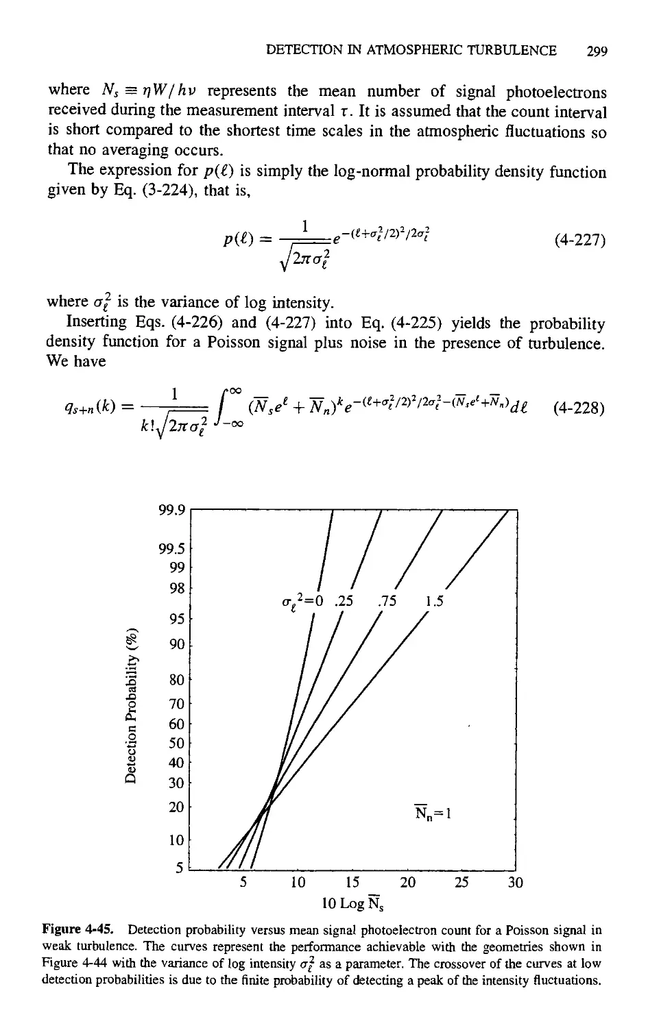
4.9. Detection in Atmospheric Turbulence 297
4.9.1. Poisson Signal in Turbulence 298
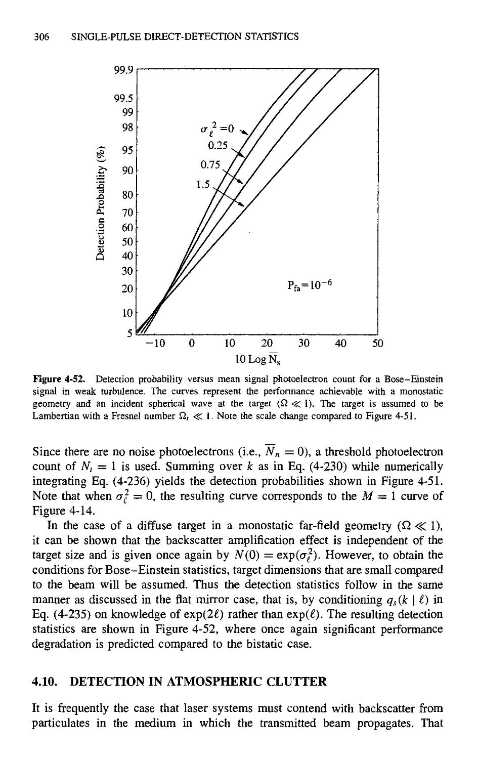
4.9.2. Bose-Einstein Signal in Turbulence 304
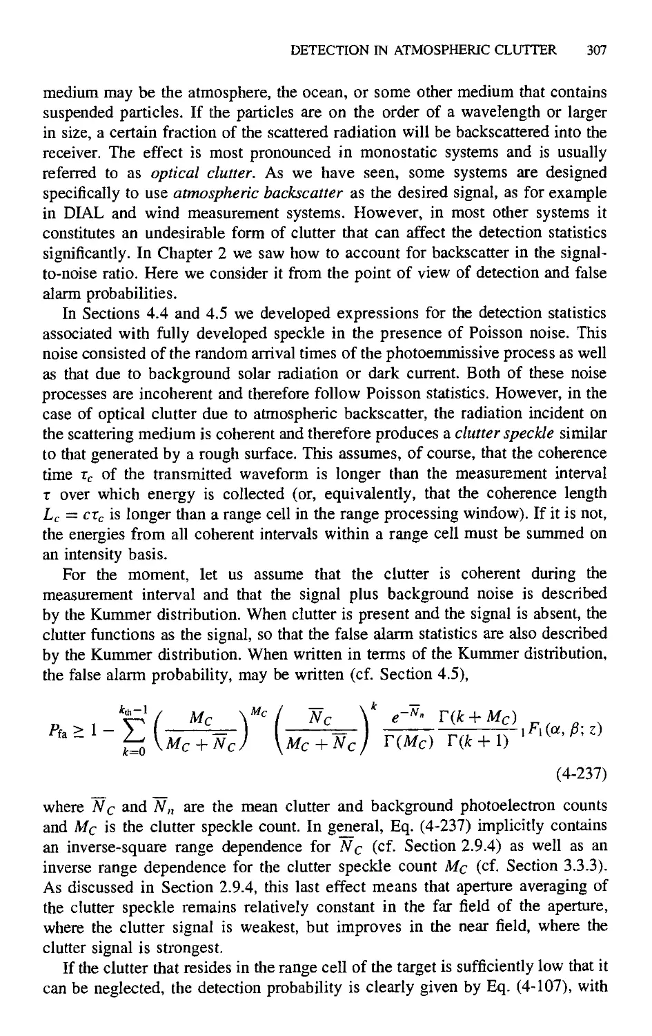
4.10. Detection in Atmospheric Clutter 306
4.11. Polarization Diversity 309
4.12. Multiple Uncorrelated Signals 313
References 315
Chapter 5. Single-Pulse Coherent Detection Statistics 318
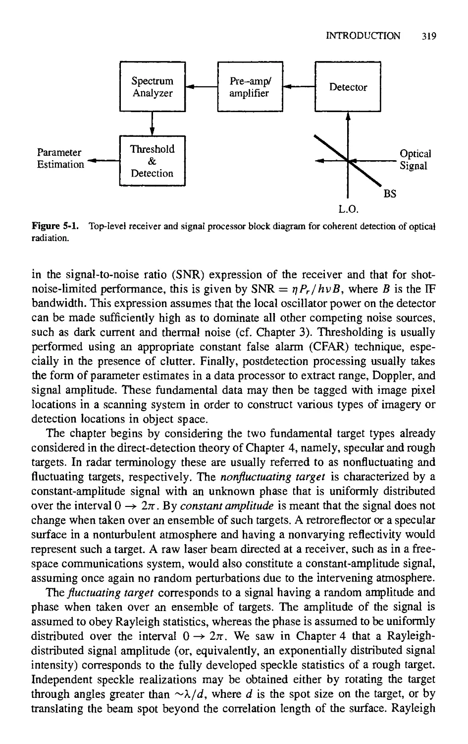
5.1. Introduction 318
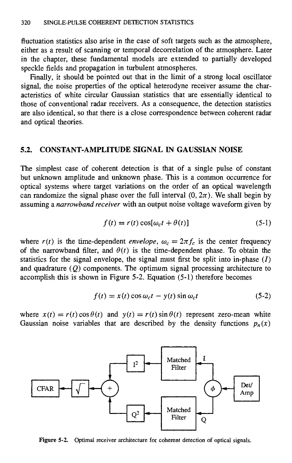
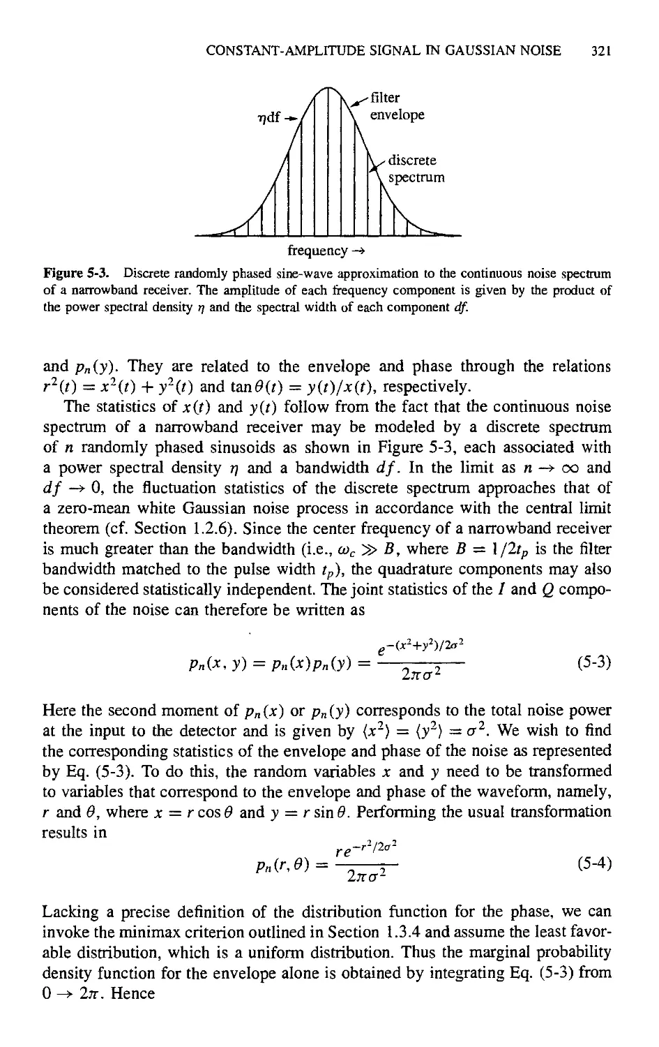
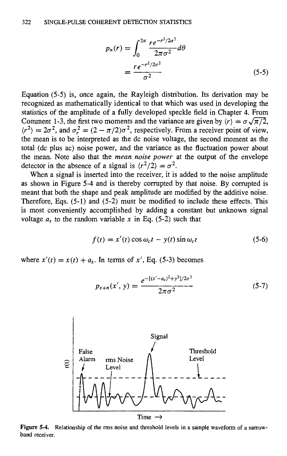
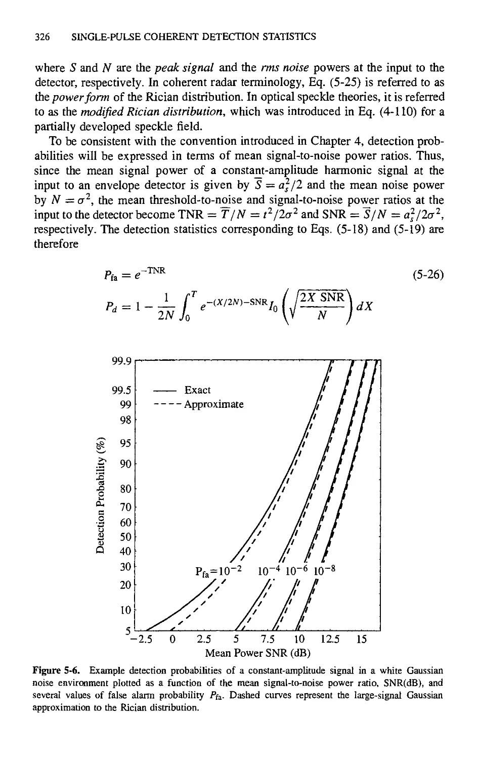
5.2. Constant-Amplitude Signal in Gaussian Noise - 320
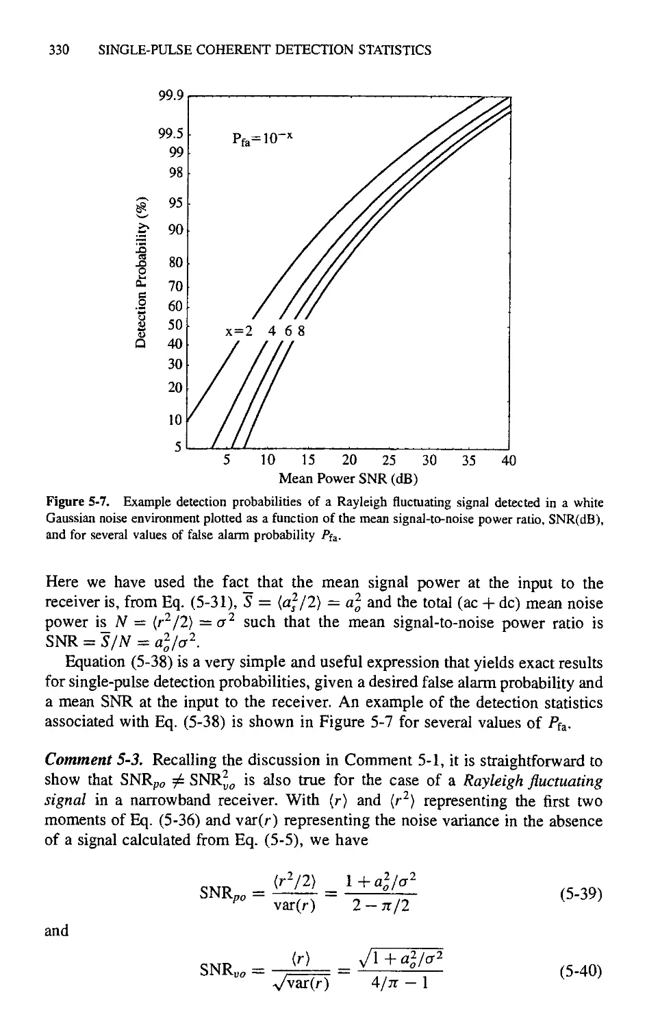
5.3. Rayleigh Fluctuating Signal in Gaussian Noise 328
5.4. One-Dominant-Plus-Rayleigh Signal in Gaussian Noise 331
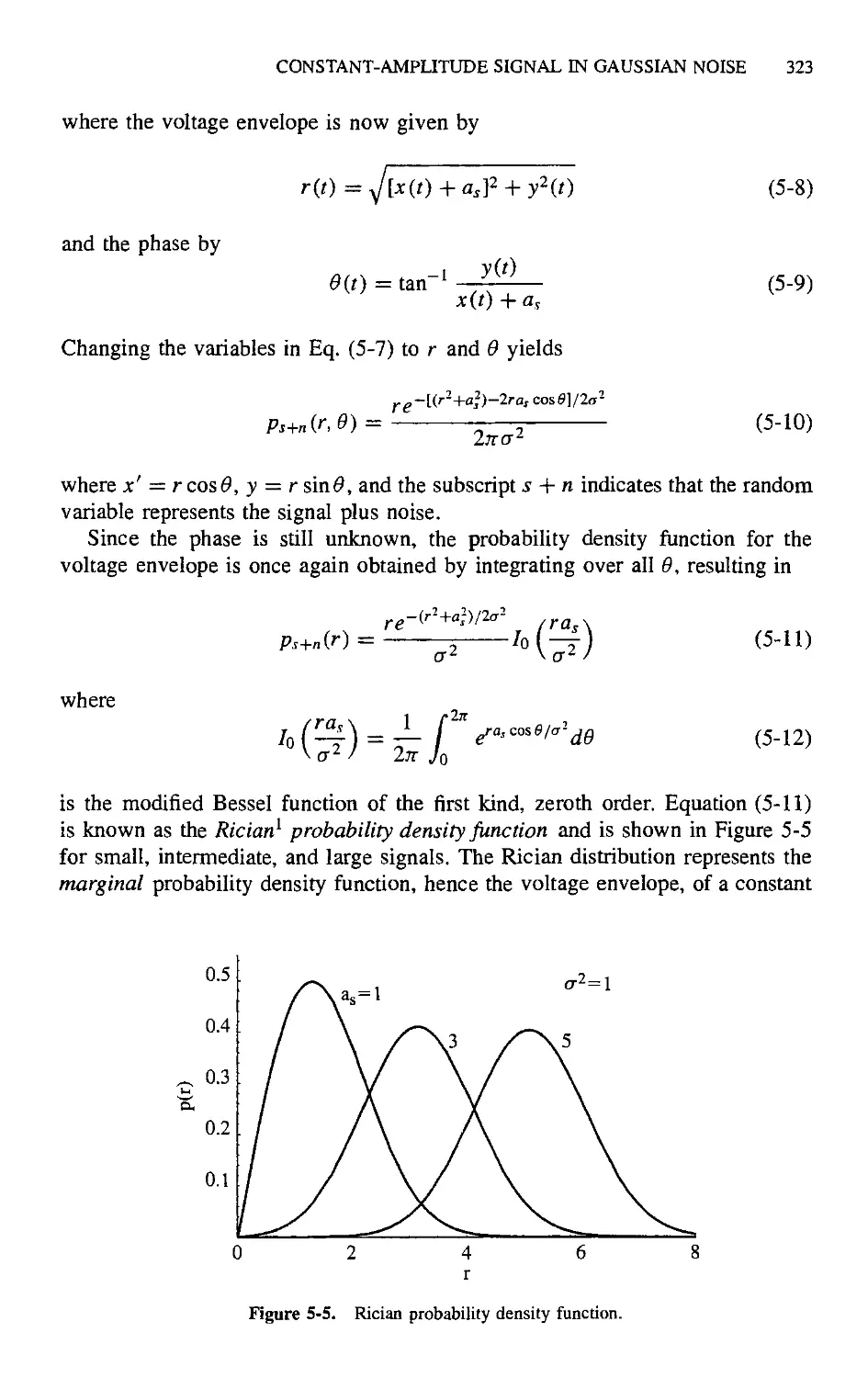
5.5. Rician Signal in Gaussian Noise 334
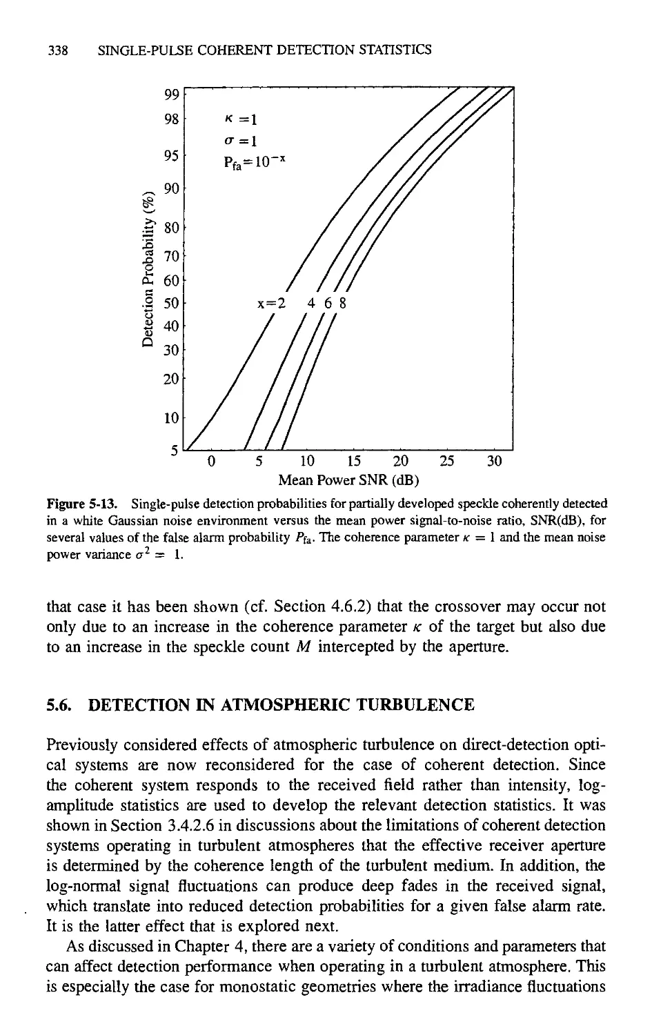
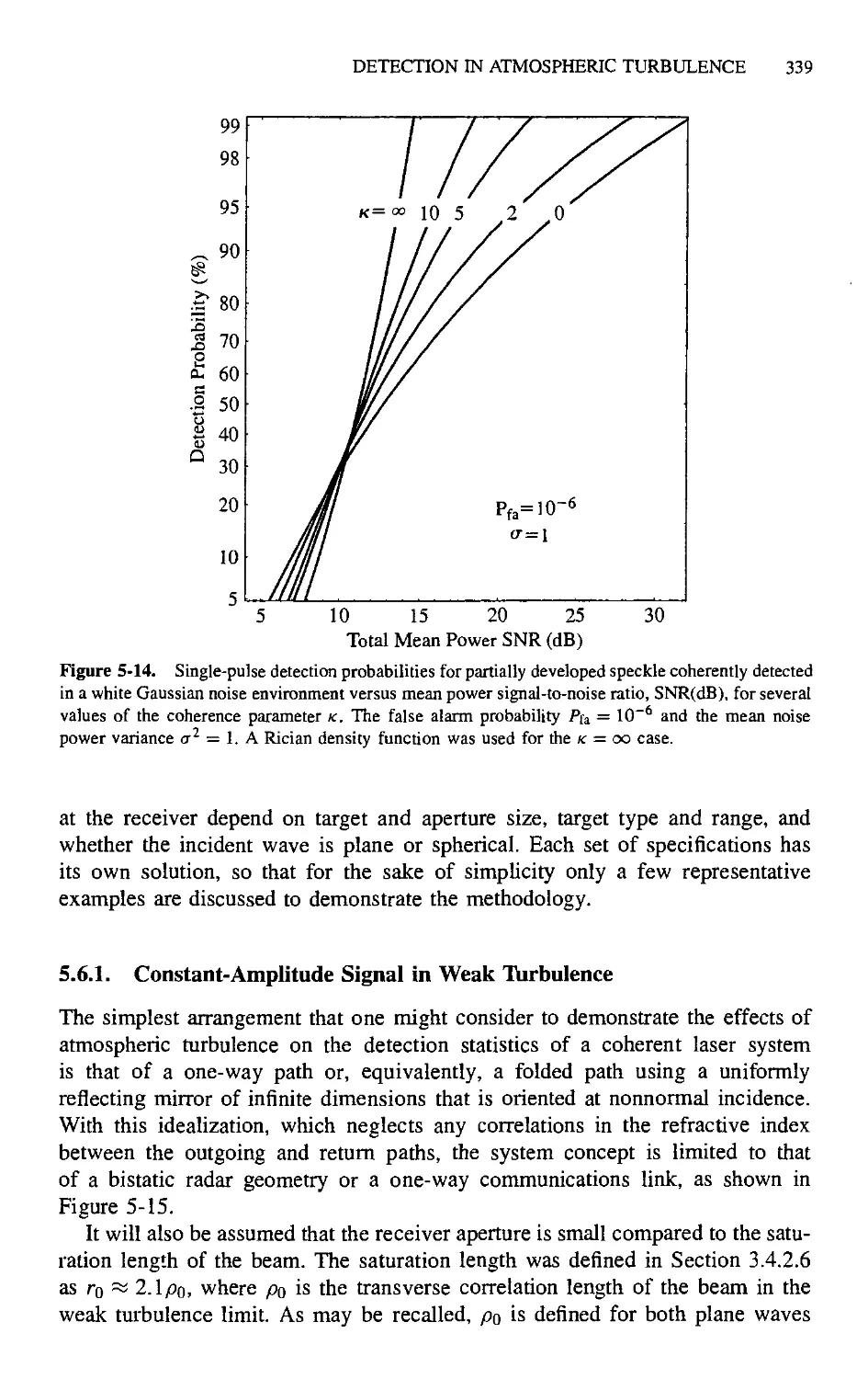
5.6. Detection in Atmospheric Turbulence 338
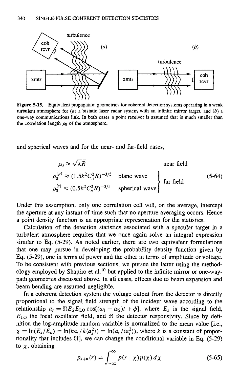
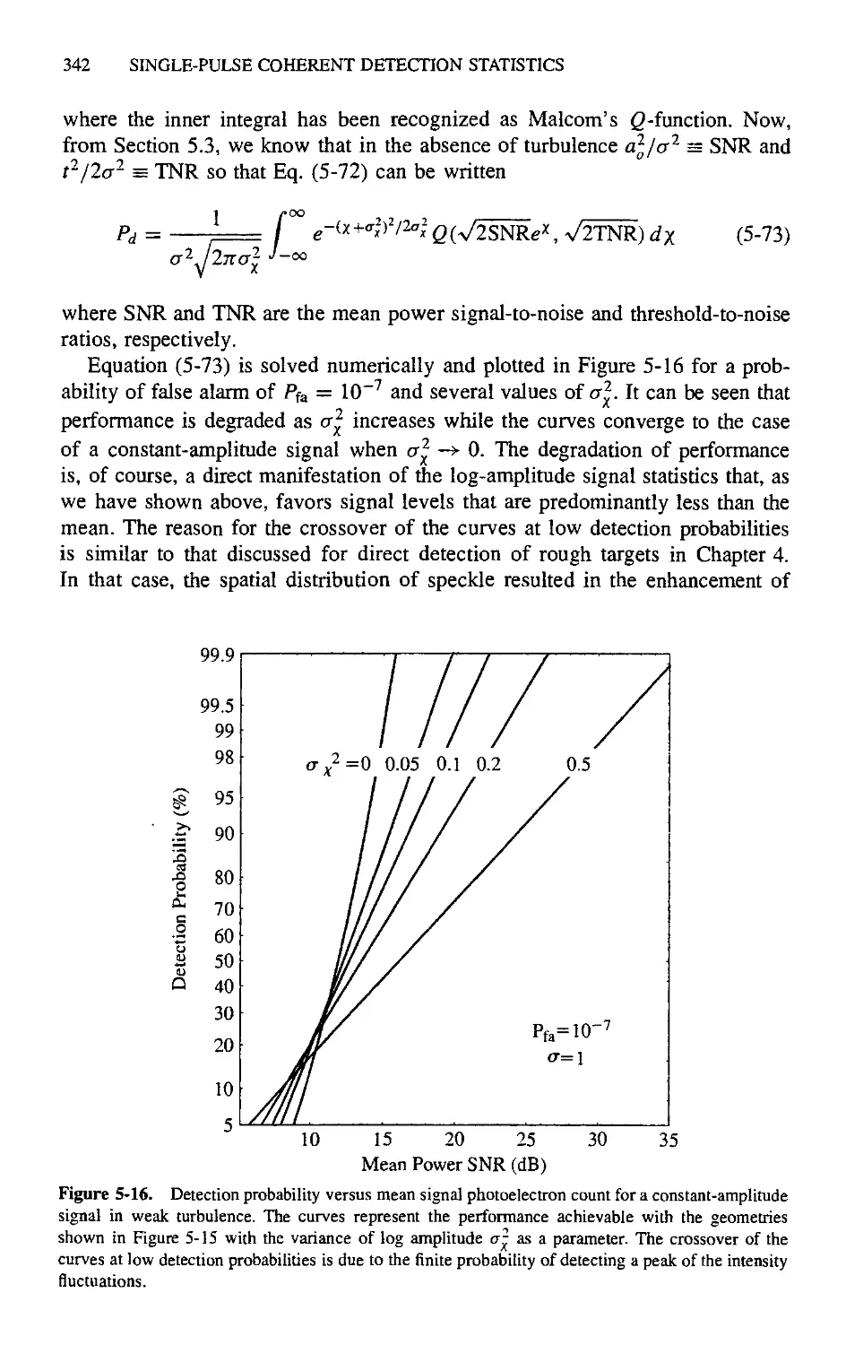
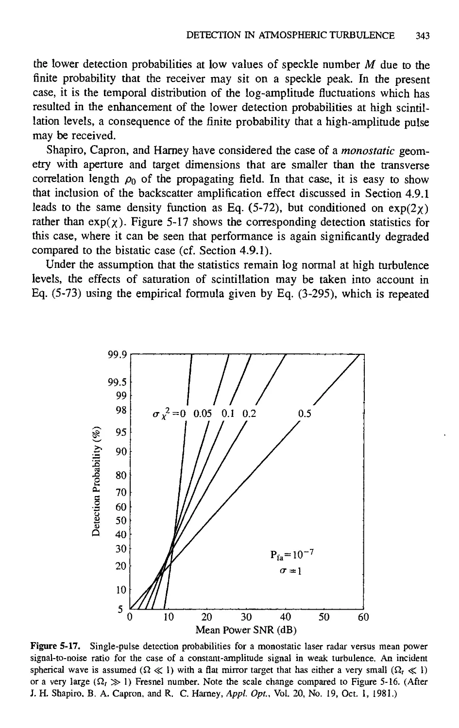
5.6.1. Constant-Amplitude Signal in Weak Turbulence 339
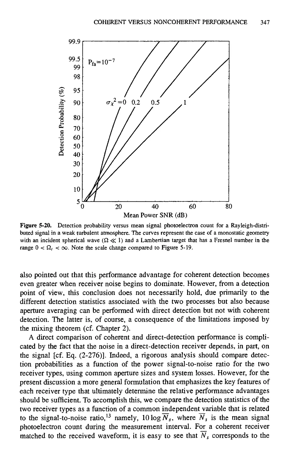
5.6.2. Rayleigh Fluctuating Signal in Weak
Turbulence 344
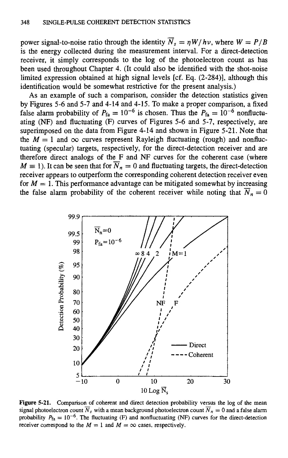
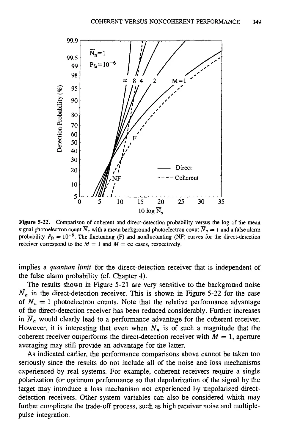
5.7. Coherent versus Noncoherent Performance 346
References 350
Chapter 6. Multiple-Pulse Detection 351
6.1. Introduction 351
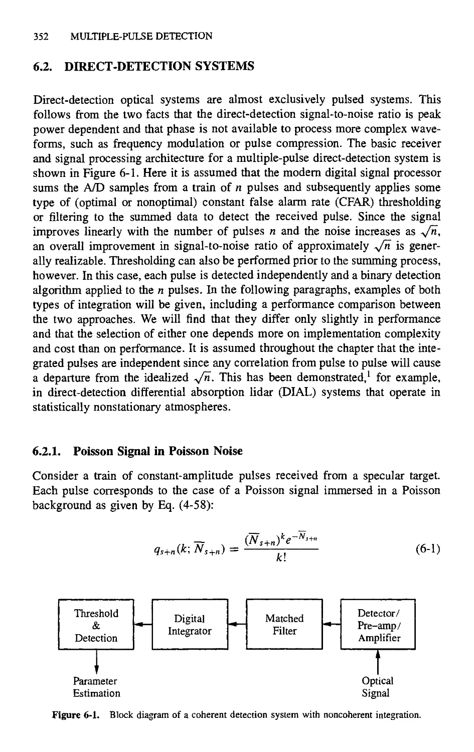
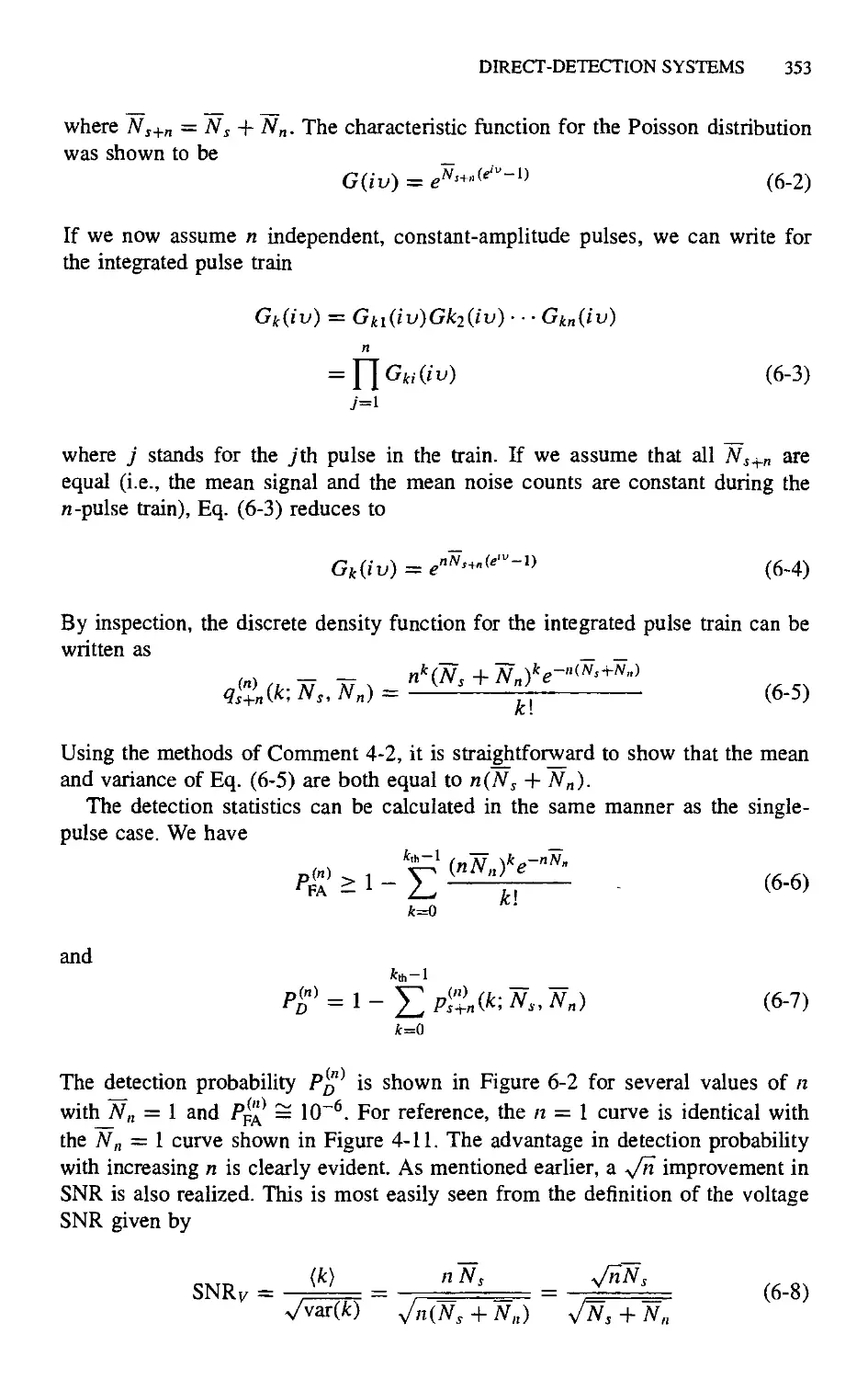
6.2. Direct-Detection Systems 352
6.2.1. Poisson Signal in Poisson Noise 352
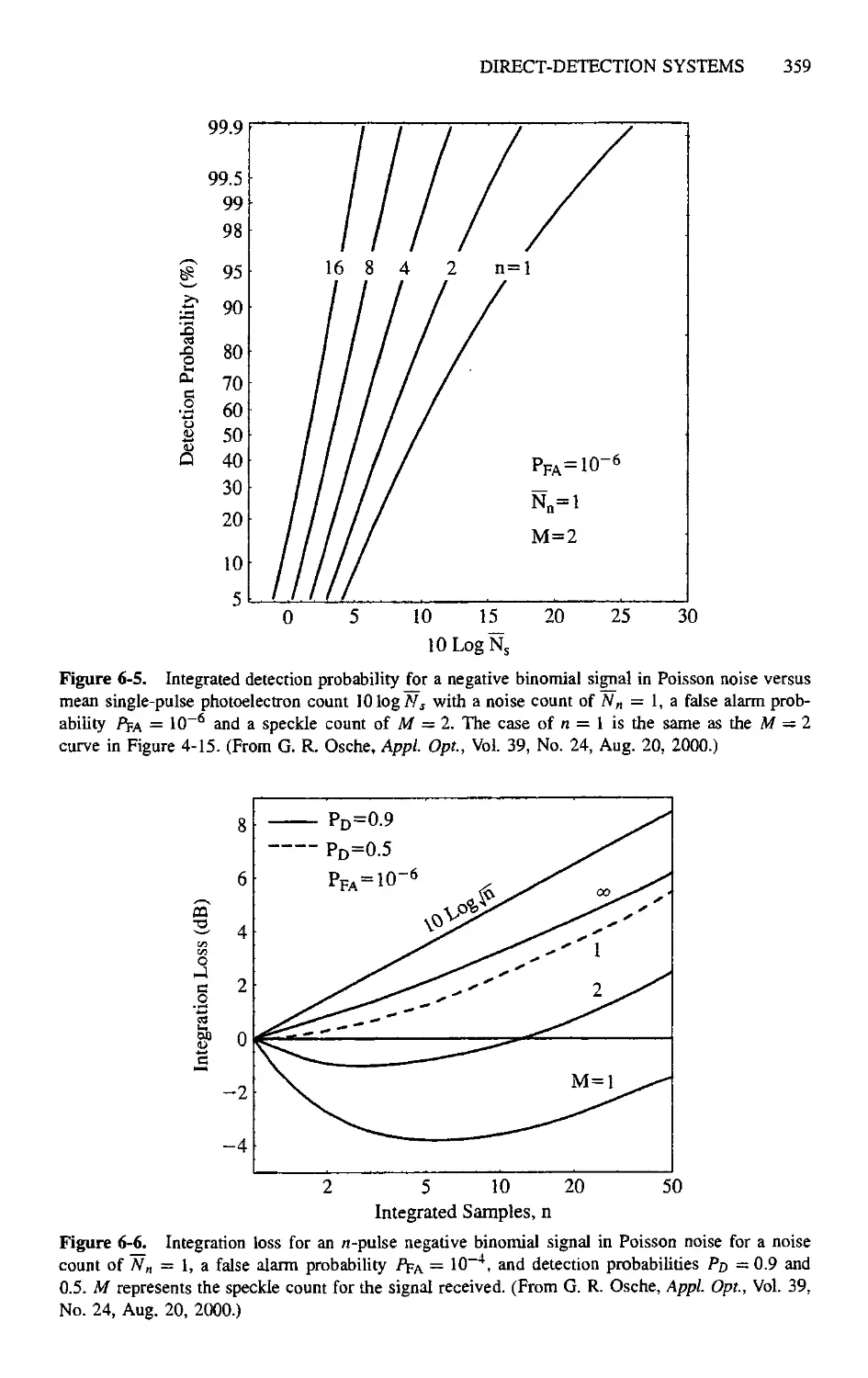
6.2.2. Negative Binomial Signal in Poisson Noise 356
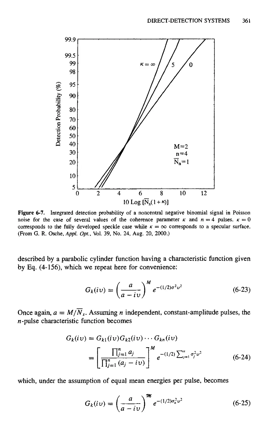
6.2.3. Noncentral Negative Binomial Signal in
Poisson Noise 358
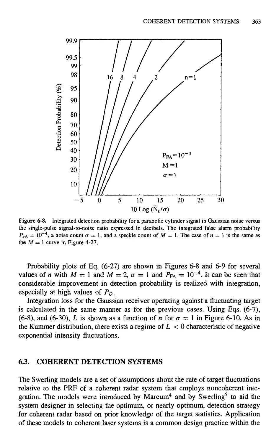
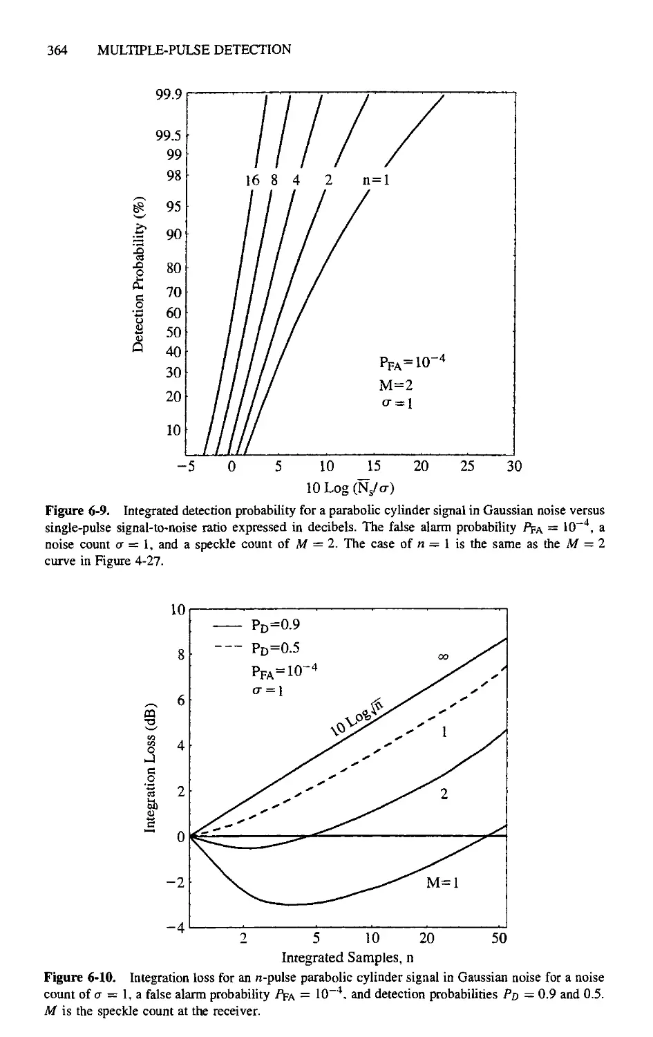
6.2.4. Parabolic Cylinder Signal in Gaussian Noise 360
6.3. Coherent Detection Systems 363
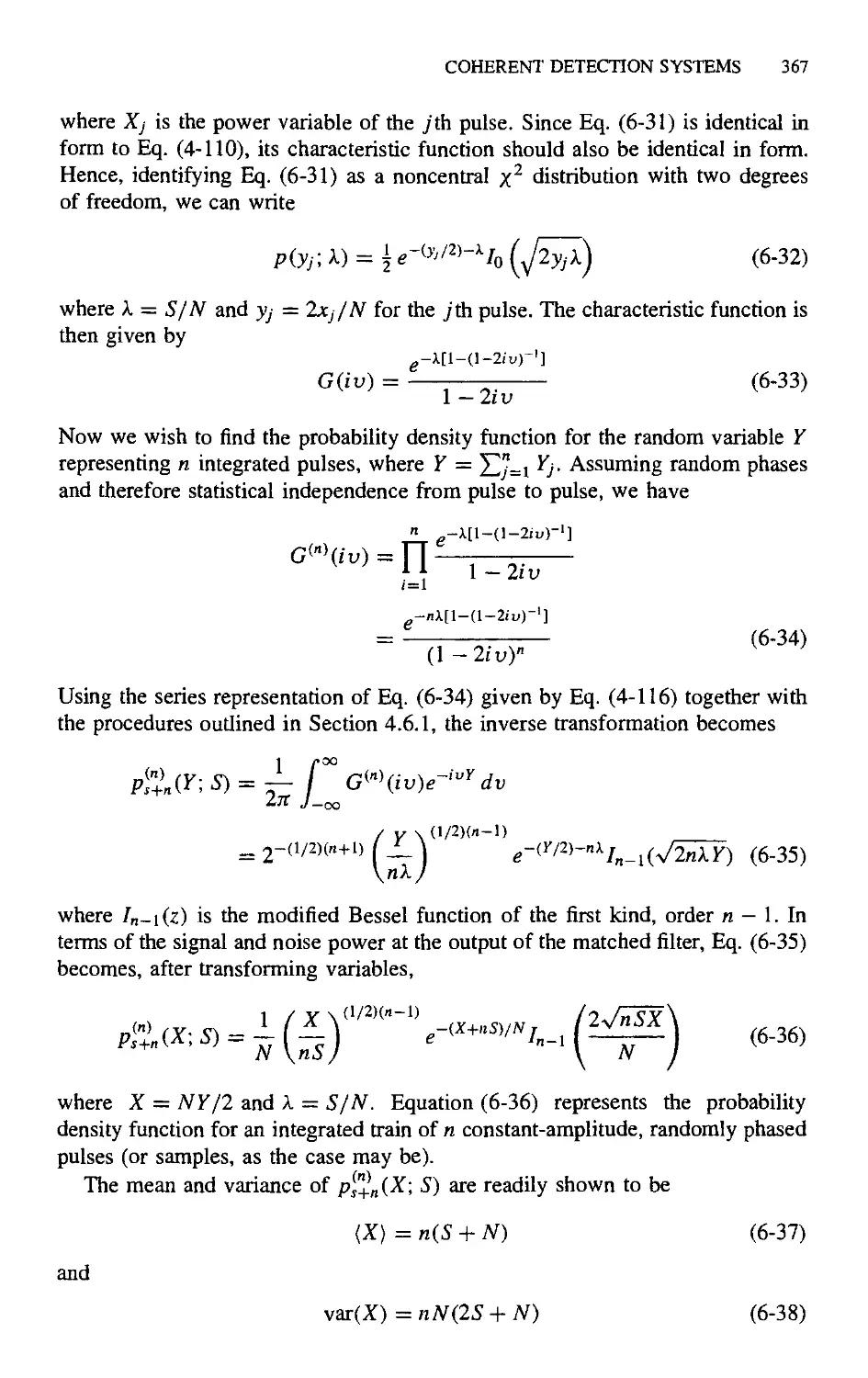
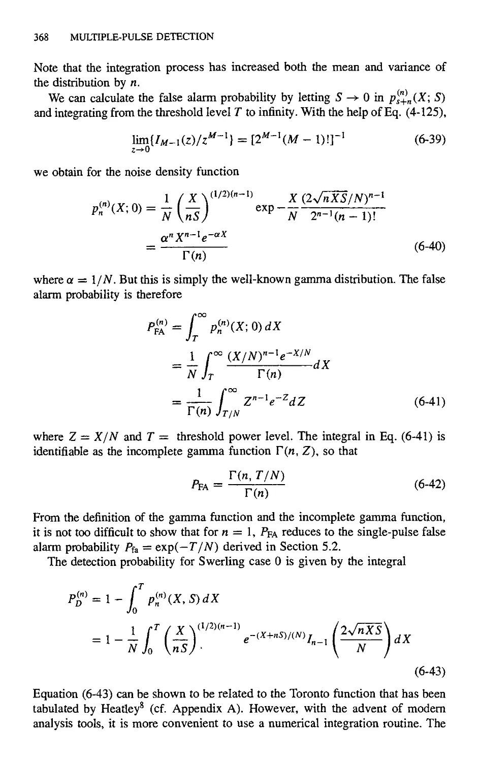
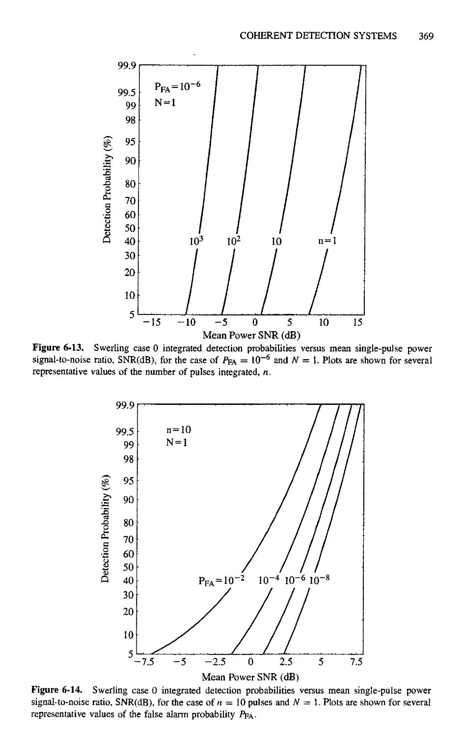
6.3.1. Swerling Case 0 Model 366
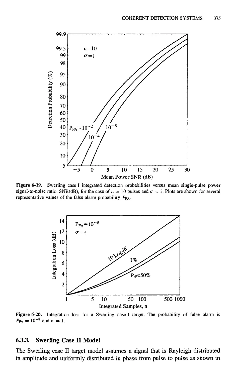
6.3.2. Swerling Case I Model 371
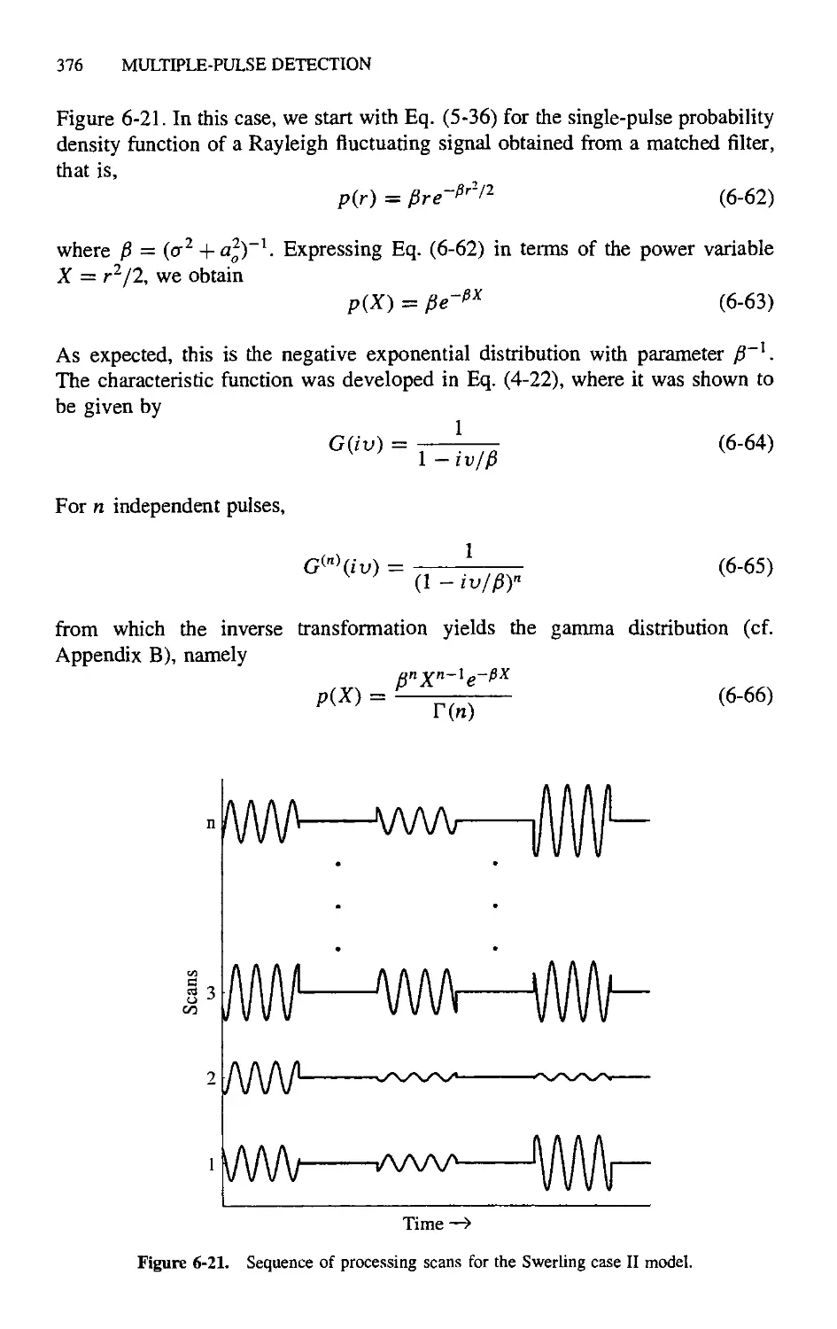
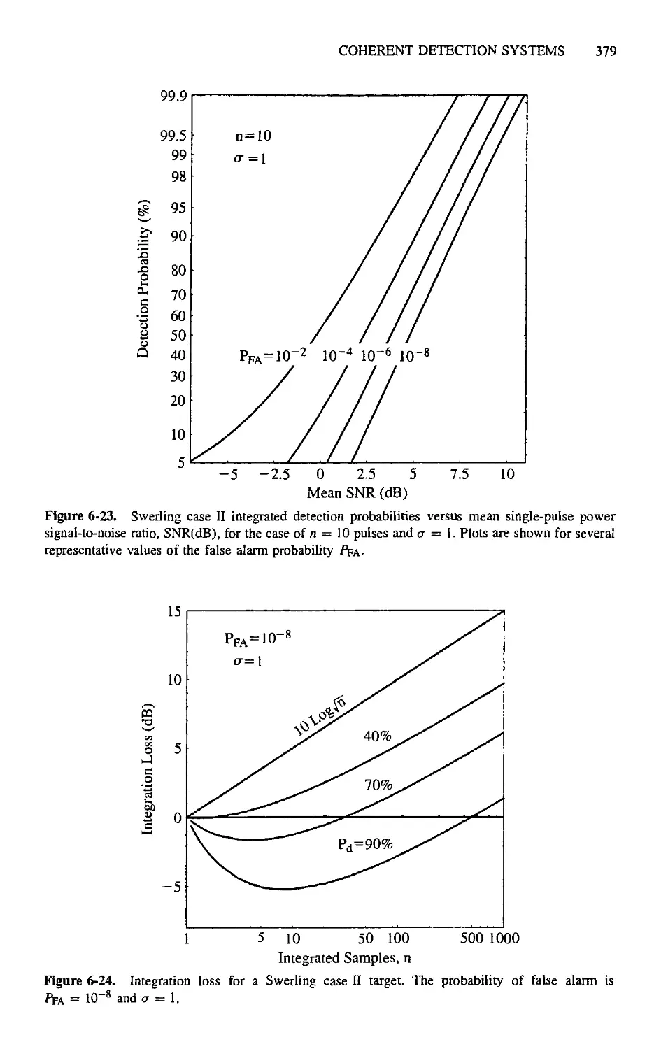
6.3.3. Swerling Case II Model 375
6.3.4. Rician Signal Model ¦ 377

x CONTENTS
6.4. Binary Integration 381
6.4.1. Application to Geiger-Mode APD Detectors 384
References 389
Appendix A. Advanced Mathematical Functions 391
A.I. Dirac Delta and Unit Step Functions 391
A.2. Gamma Function 393
A.3. Confluent Hypergeometric Function 395
A.4. Parabolic Cylinder Functions 397
A.5. Toronto Function 399
References 399
Appendix B. Additional Derivations 401
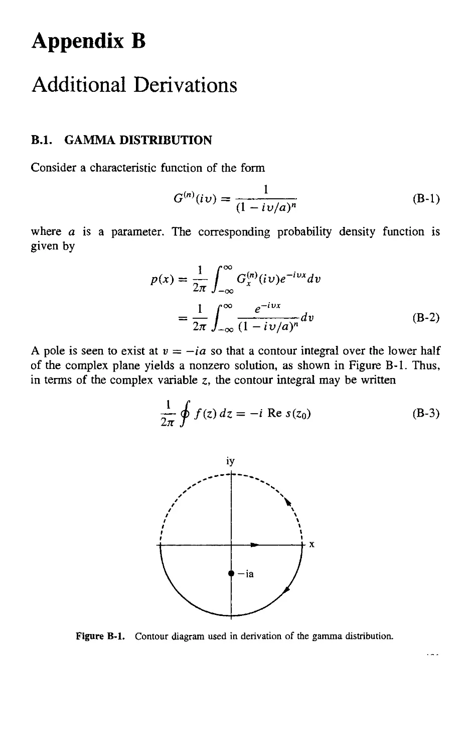
B.I. Gamma Distribution 401
B.2. Burgess Variance Theorem 402
References 403
Index 405

Preface
This book consists of notes and analyses that I have accumulated over the last
30 years while working in the field of laser radar and optical systems. The
purpose of the book is to provide the electro-optics community with a compre-
comprehensive description of optical detection theory and associated phenomenologies.
The current rapid development of active optical systems for both military and
civilian applications has not been accompanied by a corresponding set of books
that address the fundamental issues involved in laser system engineering. This is
especially the case in the area of detection statistics, where the optical engineer
must resort to journal articles or to books on microwave radar or communica-
communications theory in order to compile the necessary data for a detailed understanding
of the field. A great deal of work has been accomplished by many authors in this
field, but to my knowledge it has never been compiled and presented in a single
coherent framework. With this motivation in mind, the book has been designed
to be tutorial, deriving equations from first principles whenever possible so that
the reader can establish a firm conceptual and mathematical understanding of
the subject. A concerted effort has been made to present the theoretical discus-
discussions in a simple and straightforward manner for both clarity and comprehension
by the interested reader. In this regard, I have tried to avoid highly generalized
derivations and notation whenever possible.
The topics selected attempt to lay out the fundamental optical, statistical,
and mathematical principles that are common to most, if not all, laser systems.
Clearly, they are not all-inclusive but have been chosen based primarily on
personal experience, the emphasis thus being on laser radar systems and to a
lesser extent, communications systems. As will be seen, many of the topics have
been derived from papers, textbooks, and monographs from other disciplines,
such as radar, communications theory, statistical optics, diffraction theory, coher-
coherence theory, and atmospheric turbulence theory. Indeed, as with any technical
book, there is very little new that is presented here except possibly the insights
and viewpoints that are offered as an aid to an understanding of the material. To
this end, I have included brief "Comments" or digressions from the main flow
of the text to provide additional perspectives on the topics under discussion.
The book is basically a monograph or reference book for the professional
scientist or engineer but may also be used as a textbook for a senior or graduate-
level courses since it is relatively self-contained. For example, a review of some
of the fundamental mathematical and physical concepts essential to a proper
understanding of related optical phenomenologies comprises the first three chap-
chapters. Chapter 1 provides a brief review of the mathematical and statistical tools

xii PREFACE
assumed in later chapters. These include, among others, mathematical statis-
statistics, matched filter theory, and statistical decision theory. Chapter 2 focuses
on the deterministic processes that affect signal detection, beginning with the
Huygens-Fresnel theory of diffraction, proceeding through both truncated and
untruncated Gaussian beam theory, and ending with a formal development of the
range equations for coherent and direct, truncated and untruncated laser systems.
In Chapter 3 we consider the stochastic processes that affect signal detection,
primarily those related to random fields generated by rough surfaces and turbu-
turbulent atmospheres. Chapters 4, 5, and 6 are then devoted to the main subjects of
the book: direct, coherent, and multiple-pulse detection statistics, respectively.
The appendixes provide additional details on some of the more advanced math-
mathematical functions used in the text. A comprehensive list of references is also
provided at the end of each chapter for those who desire greater detail.
In the process of structuring the book, I have assumed that the reader has
access to a modern high-speed personal computer with appropriate software and
is therefore capable of performing calculations using the equations developed in
the various chapters. For this reason, the need for extensive tabulation or graphical
presentations of detection probabilities for example, as is usually found in classic
radar books, has been avoided. A limited set of graphical examples are given in
each case only as tools for conveying the underlying physical and mathematical
trends that result from the theories derived.
I would like to thank Mike Fallica for his continued support during this project,
as well as Frank Horrigan, Barbara Blyth, and Nancy DiMento Jerome for their
efforts in proofreading the manuscript. A special thank you to Frank for his many
helpful suggestions and thorough review of the mathematics. I would also like to
thank Jeff Shapiro of the Massachusetts Institute of Technology for his helpful
comments on scintillation statistics and Rick Marino of MIT Lincoln Laboratories
for providing some important insights into APD Geiger-mode statistics. Finally,
a word of acknowledgment to my colleagues at Raytheon Company, especially
those from the old Sudbury EO group, for their pioneering work in the field of
laser radar systems and for making my career an interesting and enjoyable one.
Gregory R. Osche
Raytheon Company
Tewksbury, MA
January 2002

1
Introduction and Background
1.1. OVERVIEW OF LASER SYSTEMS
Everyone is familiar with the laser radar system developed for police organi-
organizations to reduce the ambiguities associated with conventional radar systems.
These ambiguities have included multipath effects and poor target discrimination
capabilities that frequently lead to unenforceable speed laws. This is a simple
example of the advantages that can be gained by employing lasers to perform
some of the well-known and well-established microwave radar functions. In this
example the performance advantage arises as a result of the single most distin-
distinguishing feature of the laser, namely, a narrow beam, which in police use allows
for the unambiguous selection of a single vehicle out of many in a heavy traffic
environment. However, there are many more distinguishing features associated
with laser systems that when considered alone or together lead to many more
applications beyond that of simple range-Doppler measurements. Such features
include operation in the infrared and visible portions of the electromagnetic spec-
spectrum, the capability to achieve high modulation bandwidths, and high Doppler
sensitivities. These in turn lead to applications such as spectral probing of the
atmosphere for known or unknown molecular species, high-resolution three-
dimensional and Doppler imaging for use in robotic systems, and measurement
of wind profiles using the backscatter from airborne aerosols and other natu-
naturally occurring particulates in the atmosphere. When combined with the usual
range-Doppler measurement capabilities of a radar system, a multitude of system
applications results, ranging from noninvasive medical diagnostic techniques to
military remote sensing.
The laser radar system used by police is basically a laser rangefinder with
some additional processing to extract the vehicle velocity. Laser rangefinders
are commonly employed by the military, in geodetic surveying, and in space
applications, as evidenced by the Pathfinder mission. Altimeters for low-flying
aircraft and docking sensors for space vehicle rendezvous are obvious exten-
extensions of the rangefinder capabilities. Scanning laser rangefinders are generally
classified as laser radar systems. These systems offer the unique capability of
presenting high-resolution imagery in range, Doppler, or intensity formats, which,
in turn, offers improved databases for processing of automatic target classifica-
classification and identification algorithms. Commercial applications range from automatic

2 INTRODUCTION AND BACKGROUND
part sorting based on shape to detailed mapping of man-made structures such as
buildings and bridges for diagnostic and modeling purposes.
As mentioned earlier, operation in the infrared and visible portions of the
spectrum implies a short wavelength that is on the order of the size of airborne
particles in the atmosphere, such as dust and aerosols. Rayleigh and Mie scattering
theories predict that the backscattered radiation under these conditions will be
strong enough to be detectable with an optical receiver. Since airborne particles
generally have a mean drift velocity equal to the local wind speed, scanning laser
Doppler systems can be designed to map out the local three-dimensional wind
vector. Systems that have been developed with these capabilities have included
pollution monitoring systems, aircraft wake-vortex systems for airports, clear-air
turbulence systems for commercial aircraft, and satellite-based systems designed
to profile Earth's wind flow on a global scale.
The mere fact that laser systems operate in the infrared and optical spectrums
makes them excellent candidates for spectral probing of the atmosphere. Differen-
Differential absorption lidar (DIAL) systems are designed to have wavelength diversity
over a given spectral band in order to map out the absorption profile of the
atmosphere and therefore identify a particular airborne molecular species. Such
systems have found application in monitoring carbon dioxide, water vapor, and
ozone concentrations from airborne and space-based platforms. DIAL systems
can be designed to operate against a hard target background to enhance the
signal level while measuring the two-way integrated absorption at the probing
wavelengths, or they can be designed to use the scattering properties of the
atmosphere to generate the signal.
The optical receivers in all of these applications employ either coherent or
direct detection, depending on the particular requirements of the system. Coherent
detection allows for the extraction of frequency and phase information from the
received signal in addition to amplitude. On the other hand, the direct-detection
receiver is simply an energy-collection device that outputs the received pulse
envelope only. Since phase is not measured, direct-detection is incapable of
providing true Doppler information, although range rate can be estimated using
two or more received pulses. However, the simplicity of the direct-detection
receiver over that of the coherent detection receiver is significant, and usually
leads to an interesting system trade-off between capability and cost.
Systems that operate against soft or volume targets, such as the atmosphere,
may also employ coherent or direct-detection receivers. The former are gener-
generally used when Doppler information is required and are generally limited to
the infrared because of difficulties in maintaining optical alignment and hetero-
heterodyne losses due to atmospheric turbulence. They can be designed to operate
in either a focused or a collimated beam mode, depending on range and aper-
aperture requirements, and are generally limited to either pulsed or continuous-wave
(CW) waveforms. On the other hand, direct-detection receivers are generally
used against soft targets when spectral measurements are required in the near-
infrared or visible regions of the spectrum and Doppler shifts are not an issue.
These systems offer lighter weight and lower cost for airborne or space-based

OVERVIEW OF LASER SYSTEMS 3
applications and are generally limited to pulsed waveforms and collimated beams.
(Some of these system limitations arise from fundamental optical processes
discussed in later chapters.)
Systems that operate against hard targets may also use coherent or direct-
detection receivers. However, in this case the coherent detection system has
available to it a variety of range-Doppler waveforms that are either well known
from the microwave radar community, such as FM-CW and pulse compression,
or are unique to the laser transmitter and modulator technologies, such as the
ultrashort mode-locked pulse waveform.
Optical communications has become a significant application for laser systems.
The enormous growth potential for this market has spurred development of the
photonics and fiber optics industries. On the other hand, long-range terrestrial-
based free-space optical communications systems have not realized much success,
due to obvious weather limitations. However, such limitations are less of an
issue for short-range applications and certainly a nonissue for space-based inter-
satellite and deep-space missions. Indeed, the high-bandwidth and narrow-beam
characteristics of laser systems virtually assures their eventual use as high-
data rate free-space links for global satellite communications while relying on
lower frequencies for downloading data through the atmosphere to ground-based
receivers. Short-range interbuilding free-space links may also prove to be an
important application for relieving the "last mile" problem at city boundaries,
where incoming long-range high-capacity fiber data transmissions require major
improvements in the hardwired communication infrastructures for optimum distri-
distribution.
Finally, we should mention the promising new field of medical imaging using
lasers and fiber optics for noninvasive or minimally invasive surgical and diag-
diagnostic procedures. This field, which may be considered a type of remote sensing,
is already reporting on nonsurgical probing of living tissue using optical tech-
techniques, the theory of which is very similar to that of ground-penetrating radar.
The simplest and best-known success in this area is the pulse oximeter, a small
device placed on a patient's finger to measure heart rate and oxygen content of
the blood. This is accomplished by measuring the difference in absorption at two
wavelengths along a one-way path using light emitting diodes (LED) operating
in the red and infrared regions of the spectrum. It is not inconceivable that in
the future more sophisticated measurements of, say, phase delays through the
tissue will reveal additional information on the health of the tissue or some other
critical parameter.
In this book we focus on the fundamental detection processes that are inherent
in most, if not all, laser applications that involve photodetection processes. The
implications of using direct or coherent detection are addressed separately for
each topic. In the subsections that follow in this chapter we review briefly some
of the fundamental concepts of mathematical statistics, statistical decision theory,
and optical detection techniques, topics that are basic to a proper understanding
of optical detection theory. Those who are already versed in these topics may
proceed directly to later chapters as desired.

4 INTRODUCTION AND BACKGROUND
1.2. REVIEW OF STATISTICAL METHODS
The need for an understanding of statistical analysis follows from the fact that
many of the processes involved in optical detection are random. For example,
receiver noise, target fluctuations, atmospheric perturbations, and clutter noise
are all stochastic processes that can be described only from a statistical point
of view. In this section we provide a brief overview of those aspects of
mathematical statistics that are of particular importance in the description of
phenomenologies associated with optical detection. Both continuous and discrete
statistical processes are described, the latter being of particular importance in
later chapters that address photoelectron counting statistics in direct-detection
receivers. To those who wish a more detailed discussion of probability and
statistics, the works of Kempthorne and Folks1 and Papoulis2 are highly
recommended.
1.2.1. Probability and Univariate Statistics
The concept of probability follows naturally from considerations of the frequen-
frequencies of occurrence of various statistical events compared to the total number of
events that have occurred or are possible. The events themselves are described
by a random variable that varies unpredictably from event to event but in accor-
accordance with some mathematical probability function. Determination of the form
of this function is the ultimate goal of statistical theories since it is then possible
to obtain as complete a description of the random process as possible, at least in
a statistical sense.
A random variable can be associated with a sample space that contains all
possible outcomes of a random event or sample. The events or samples them-
themselves, which we denote with capital letters A, B,C,..., may be continuous
or discrete, with sample spaces that are also continuous or discrete. When the
outcomes of two or more events are considered together, they are referred to as
joint events, the probability of which is written P(AB ...).
If the trial outcomes are mutually exclusive, only one outcome can occur for
any given observation or trial of the random process, so that the probability of
both A and В and ... occurring is P{AB...) = 0. An example of a mutually
exclusive process is the outcome of heads or tails in the flipping of a coin. The
key word here is or, so that the probability of any one of the events occurring is
P(A or В or • • •) = P(A) + P(B) + ¦ ¦ ¦¦ In the case of coin tossing, there are
only two events, heads or tails, so that the sum equates to unity since there are
no other possibilities.
If the events are statistically independent, the outcome of one event is indepen-
independent of the outcomes of any other event. An example of statistically independent
events that can be taken jointly is the flipping of two or more coins, a process in
which coin 1 could yield heads, coin 2 could yield tails, and so on. The key word
in this case is and, so that the probability of occurrence of any particular combina-
combination of heads and tails is P(A, B,...) = P(A and В and ...) = P(A)P(B)....

REVIEW OF STATISTICAL METHODS
If the events are not mutually exclusive [i.e., P(AB ...) ф 0], the probability
that at least one of the events will occur is given by the sum of their individual
probabilities minus their joint probabilities. An example here is once again the
flipping of two coins, but in this case we want the probability of obtaining
heads and/or tails. The key phrase in this case is and/or, so that the probability
of obtaining such an outcome becomes P(A and/or B) = P(A + B) = P(A) +
P(B) - P(AB).
If two or more events are statistically dependent, the outcome of event A
is dependent on the outcome of event B, and vice versa. In this case, their
joint probability is not equal to the product of the individual probabilities [i.e.,
P(A, B) 7= P(A)P(B)]. Rather, it is dependent on the conditional probability
that В will occur given that A has occurred times the probability that
A will occur, and vice versa. This is written P(A,B) = P(A \ B)P(B) =
P(B | A)P(A). Note that when the events are independent, P(A | B) = P(A)
and P(B | A) = P(B). We have more to say about dependent random variables
in the next section.
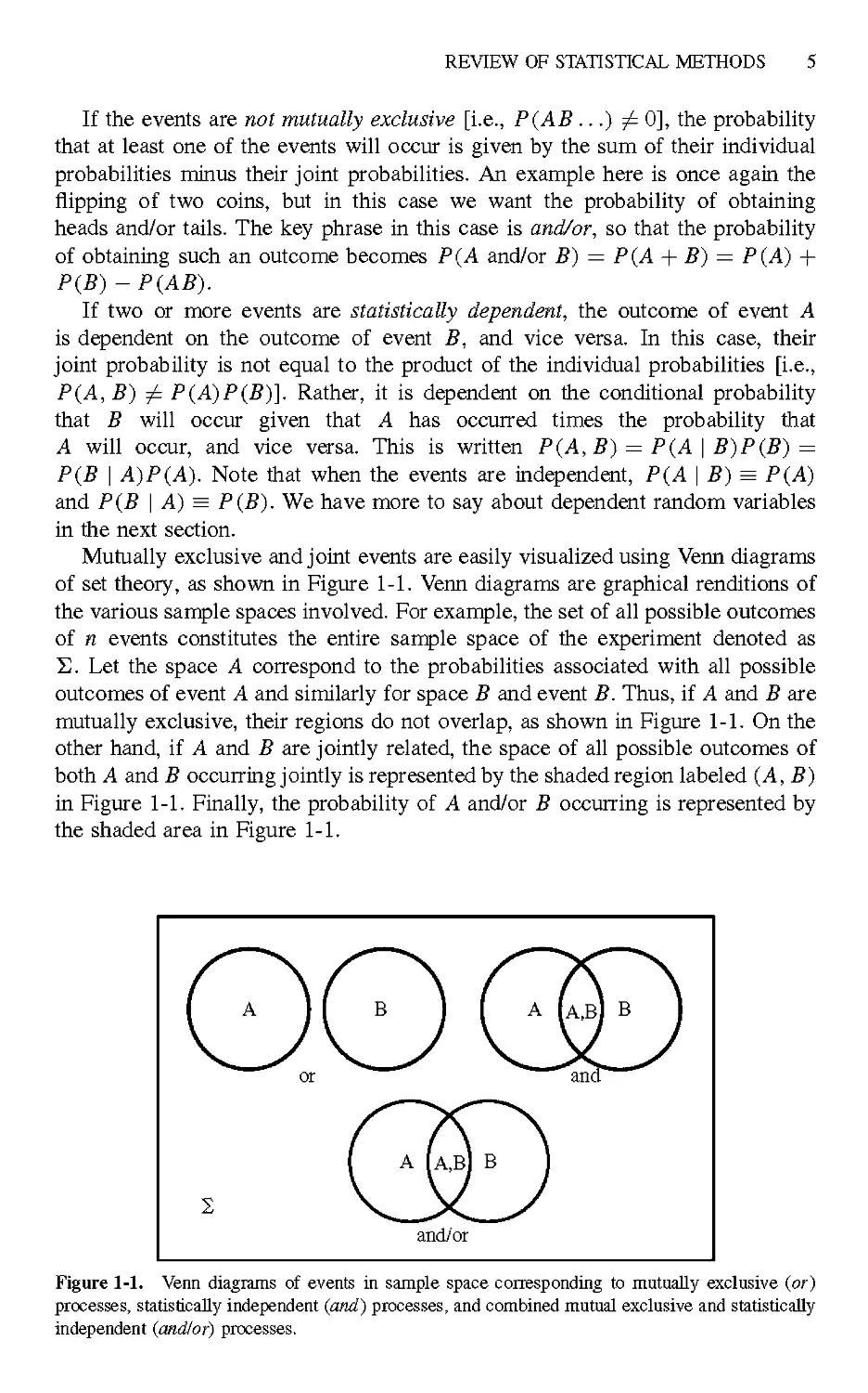
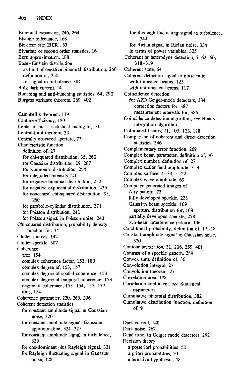
Mutually exclusive and joint events are easily visualized using Venn diagrams
of set theory, as shown in Figure 1-1. Venn diagrams are graphical renditions of
the various sample spaces involved. For example, the set of all possible outcomes
of n events constitutes the entire sample space of the experiment denoted as
S. Let the space A correspond to the probabilities associated with all possible
outcomes of event A and similarly for space В and event B. Thus, if A and В are
mutually exclusive, their regions do not overlap, as shown in Figure 1-1. On the
other hand, if A and В are jointly related, the space of all possible outcomes of
both A and В occurring jointly is represented by the shaded region labeled (A, B)
in Figure 1-1. Finally, the probability of A and/or В occurring is represented by
the shaded area in Figure 1-1.
Figure 1-1. Venn diagrams of events in sample space corresponding to mutually exclusive (or)
processes, statistically independent {and) processes, and combined mutual exclusive and statistically
independent (and/or) processes.

6 INTRODUCTION AND BACKGROUND
Let us define the frequency of occurrence of a random variable x as n(x) and
the total number of occurrences as и. It is intuitively obvious that the probability
that x will occur should then be denned as P(x) =n(x)/n. This is usually
put in graphical form by plotting P(x) as a function of x, where x takes the
form of frequency bins of finite width Ax. As a specific example, consider the
case of a golfer attempting a hole-in-one. Restricting the discussion to a single
dimension for the moment, we could inquire as to the frequency with which
the shots are placed in certain spatial intervals or bins of size Ax at various
distances x from the hole. The relative probability is then P(x) =n(x)/n of
balls falling in spatial bins of width Ax located a distance x from the hole.
However, notice that if we decrease the width Ax of the bins, the number of
balls per bin also decreases such that as Ax -> 0, n(x)/n -> 0. To remove this
dependency on the resolution and to establish the conceptual framework for
some limiting cases, the magnitude of each bin can be redefined as the quantity
A/Ах)[й(х)/й], which is a spatial density. The plot is therefore broken up into
a series of rectangles of height A/Ах)[й(х)/й], width Ax, and area n(x)/n.
The area n(x)/n is then interpreted as the relative probability of event n(x)
occurring in the interval Ax located at position x. The resulting plot is called
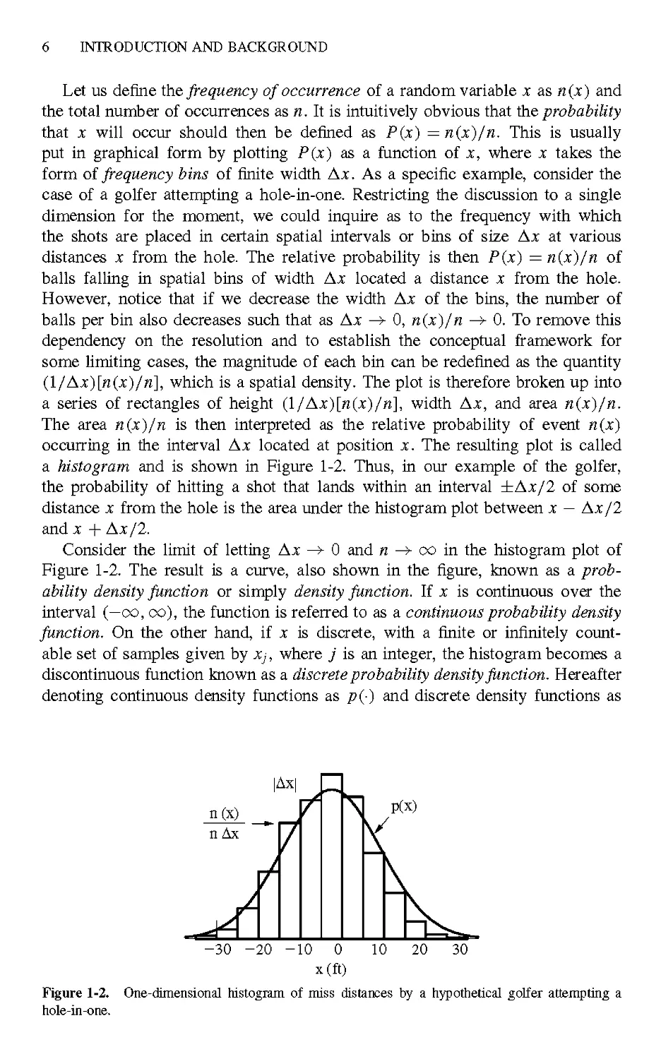
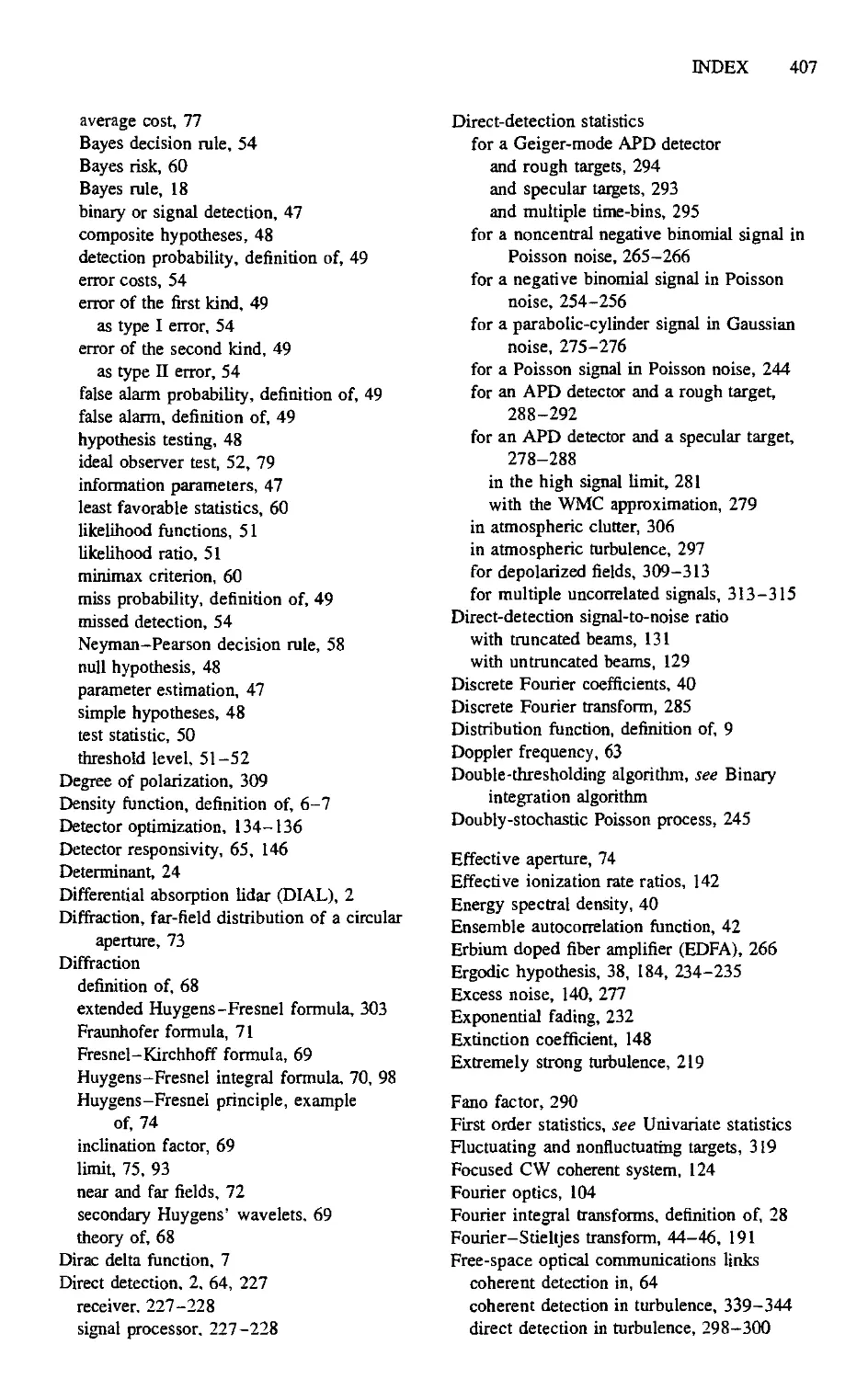
a histogram and is shown in Figure 1-2. Thus, in our example of the golfer,
the probability of hitting a shot that lands within an interval ±Ax/2 of some
distance x from the hole is the area under the histogram plot between x — Ax/2
and x + Ax/2.
Consider the limit of letting Ax -> 0 and n ->¦ oo in the histogram plot of
Figure 1-2. The result is a curve, also shown in the figure, known as a prob-
probability density function or simply density function. If x is continuous over the
interval (—oo, oo), the function is referred to as a continuous probability density
function. On the other hand, if x is discrete, with a finite or infinitely count-
countable set of samples given by Xj, where j is an integer, the histogram becomes a
discontinuous function known as a discrete probability density function. Hereafter
denoting continuous density functions as p{-) and discrete density functions as
n(x)
n Дх
|Дх|
7
P(x)
-30 -20 -10 0 10 20 30
x(ft)
Figure 1-2. One-dimensional histogram of miss distances by a hypothetical golfer attempting a
hole-in-one.

REVIEW OF STATISTICAL METHODS 7
q(-), we have
p(x) = lim
n(x)/Ax
n->oo
CO
continuous
discrete
A-1)
where P(xj) = n(Xj)/n is the probability of occurrence of Xj and 8(x — Xj) is
the Dirac delta or impulse function (cf. Appendix A). For simplicity of notation,
the discrete density function will be assumed to represent an infinitely countable
sample space, that is, j = 1, 2, 3,..., oo. However, it should be recognized that
this is not a necessary condition since the summation index j can be truncated at
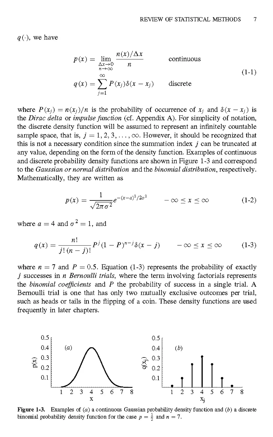
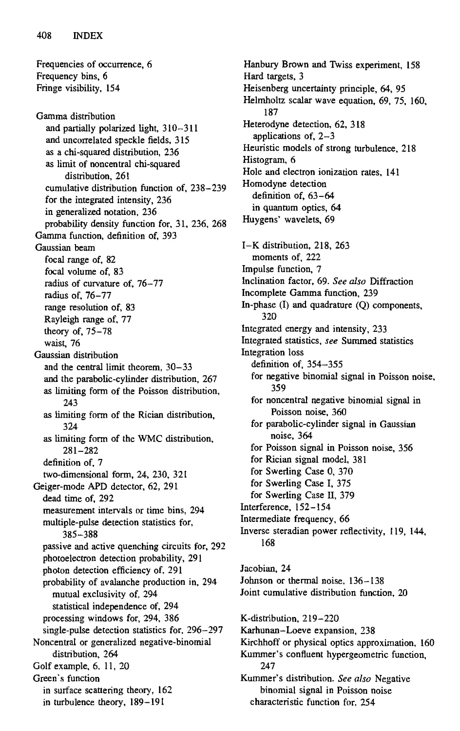
any value, depending on the form of the density function. Examples of continuous
and discrete probability density functions are shown in Figure 1-3 and correspond
to the Gaussian or normal distribution and the binomial distribution, respectively.
Mathematically, they are written as
p(x) =
1
-OO < X < OO
A-2)
where a = 4 and a = 1, and
«CO =
n\
-00<X<00
A-3)
where n =1 and P = 0.5. Equation A-3) represents the probability of exactly
j successes in n Bernoulli trials, where the term involving factorials represents
the binomial coefficients and P the probability of success in a single trial. A
Bernoulli trial is one that has only two mutually exclusive outcomes per trial,
such as heads or tails in the flipping of a coin. These density functions are used
frequently in later chapters.
0.5
0.4
0.3
0.2
0.1
(a)
/
/
J
1 2 3
\
\
V
4 5 6 7 8
X
0.5
0.4
^ 0.2
0.1
(Ь)
1 2 3 4 5 6 7
Figure 1-3. Examples of (a) a continuous Gaussian probability density function and (b) a discrete
binomial probability density function for the case P = \ and n = 7'.

8 INTRODUCTION AND BACKGROUND
With the definitions above, the probability P that the random number x will
lie in the range a ->¦ b is found by integrating p{x) or q(x) over some specified
limits, that is,
rb
p(x)dx continuous
/
Ja
/ #(x)ax = 2_^P(Xj) I
Ja .._, Ja
P(a < x < b) = ¦
: У^ P(xj) discrete
j=m
A-4)
Here it should be noted that in the discrete case the order of summation and
integration has been reversed and the integration region a —>¦ b is assumed to
include the discrete points m < j <n. Thus we see from the definitions above
that when a ->¦ b, p(x) ->¦ 0 for all x in the continuous case, and #(x) ->¦ q(Xj)
in the discrete case. For P to be considered a true probability with a range
0 < P < 1, the integrals above must equate to unity probability when extended
over all sample space; that is,
/>+00
P(—oo < x < oo) = / p(x)dx = 1, p(x) > 0 continuous
i-co
A-5)
CO
x—^
P /y, <-" у . <-" у \ \ P (у . \ 1 P (у . \ ~~~r C\ ГЛЛ Cr'Tt^t*
г \X\ ^ Iт f: -^CO/ — / *{?*]) — -L ) ¦* v*7 / _ ^ QlSCreic
Comment 1-1. Care must be exercised in the interpretation of the integrals asso-
associated with the discrete density functions when using the Dirac delta function
formalism. Specifically, the integrals must totally include the discrete point or
points in question and, to be formally correct, a notation should be used to indi-
indicate precisely the intended range of integration. For example, if #(x) includes
only two discrete points xi and X2, and P(x) in Eq. A-4) is to include only the
discrete point x2, the integral in Eq. A-4) might be written
P{xx < x < x2) = / q(x) dx=J2 p(xj) / *(.*- x}) dx = P(x2)
A-6)
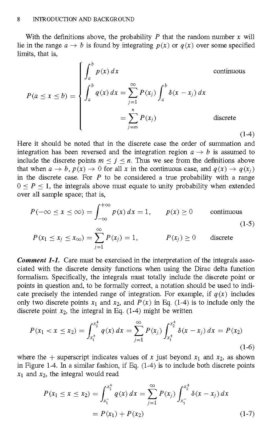
where the + superscript indicates values of x just beyond xi and x2, as shown
in Figure 1-4. In a similar fashion, if Eq. A-4) is to include both discrete points
xi and x2, the integral would read
P(x!<x<x2)= YJJ j
Jxx j=l Jxi
= P(x1) + P(x2) A-7)

REVIEW OF STATISTICAL METHODS
Figure 1-4. Range of integration for evaluating discrete probability density functions.
to indicate that the range of integration begins just before xi and ends just after xj.
However, such -\— notation is cumbersome and usually unnecessary if the range
of integration is stated at the outset, and therefore is omitted in the remaining
discussions. ¦
The probability density function is a fundamental descriptor for statistical
systems. From it other statistical measures can be derived, such as moments,
in order to describe the behavior of a given random variable. Another such
descriptor, the cumulative distribution function, or simply the distribution func-
function, is denned as the probability that x will be less than or equal to some specified
value. Letting F(-) and G(-) represent the continuous and discrete distribution
functions, respectively, we have
F(x') = P(x < x') = /
J—<
p(x) dx
G(xn) = P(x < xn) = ^ P(x})U(x -
continuous
discrete
A-8)
where x' and xn are given samples of the random variable x and U(x — Xj) is the
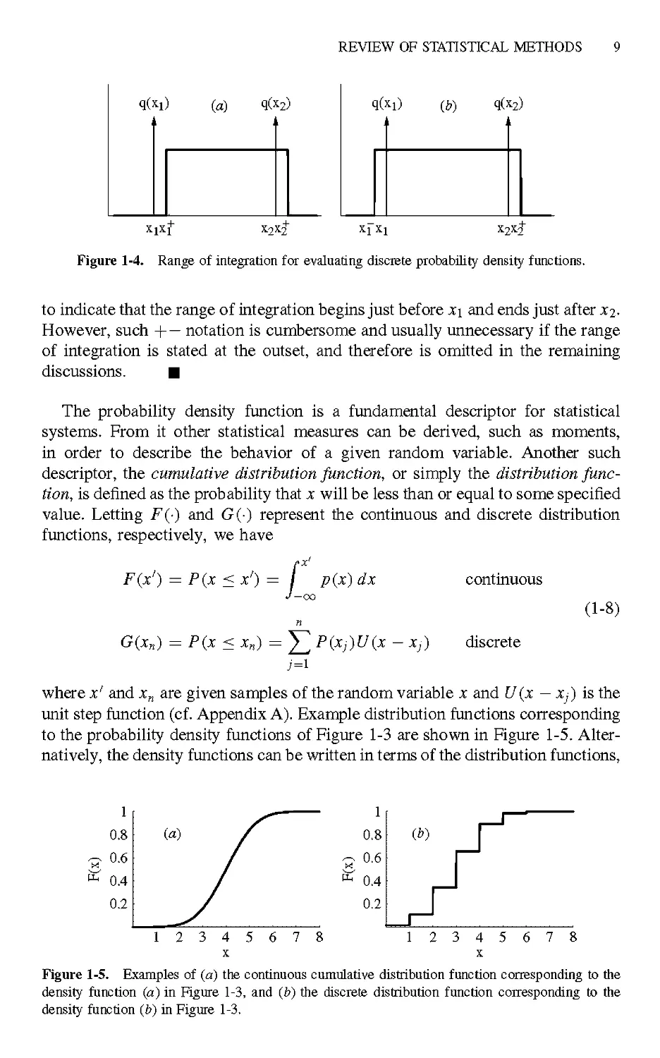
unit step function (cf. Appendix A). Example distribution functions corresponding
to the probability density functions of Figure 1-3 are shown in Figure 1-5. Alter-
Alternatively, the density functions can be written in terms of the distribution functions,
1 2 3
5 6 7
Figure 1-5. Examples of (a) the continuous cumulative distribution function corresponding to the
density function (a) in Figure 1-3, and (b) the discrete distribution function corresponding to the
density function (b) in Figure 1-3.

10 INTRODUCTION AND BACKGROUND
that is,
p(x)
«со
dF(x)
dx
dG(x)
dx
7 = 1
(Xj)S(x -
¦Xj)
continuous
discrete
A-9)
where the delta function and the unit step function are related by 8(x) =
dU(x)/dx.
Comment 1-2. The advantage of using the delta function in the discrete prob-
probability density functions is that it allows for a consistent formalism between
the continuous and discrete cases. This is particularly useful in mixed proba-
probability density functions that contain both continuous and discrete components.
In particular, if p(x) and q(x) represent the probability density functions of the
continuous and discrete components of a single random variable x, then in order
that they truly represent a probability, it is necessary that their sum satisfy the
definition of probability, not their individual density functions, that is,
CO
[p(x)+q(x)]dx = l A-10)
Either the probability density function or the cumulative distribution function
as denned above is sufficient to fully define the first-order statistics of a random
variable; no other descriptors are required. Higher-order statistics are similarly
defined by joint density functions or cumulative distributions, as will be shown
later. It is for this reason that these functions play such a fundamental role in
statistical theories.
1.2.2. Statistical Moments
The concept of statistical moments is analogous to the concept of moments in
mechanics, where, for example, the first moment of a group of masses is just the
weighted average location of these masses, the weights being the masses them-
themselves. This is better known as the center of mass for the system and is written
rc = ^2,mjrj JM, where the mj are discrete masses located a radial distance tj
from the origin and M is the total mass of the system. The concept of center of
mass is applicable to both discrete and continuous mass distributions. In direct
analogy to the center of mass, a statistical average or mean value of a random
variable x is defined as a weighted average of x, with the weighting functions
being the probabilities of occurrence of x. Thus the first moment of x, denoted
as mi, is equal to the expected value of x, which is commonly written as (x),

REVIEW OF STATISTICAL METHODS 11
and is given by
mi = (x) = ¦
J.
xp{x) dx
continuous
— CO
CO
/•CO w /-CO
/ xq(x)dx = ~S~] P{xj) / x8(x — Xj)dx
J—oo . 1 J —со
A-11)
discrete
[Other frequently used representations of the expected or mean value are E(x)
and x", the latter being used interchangeably with (x) in later chapters for
convenience of notation.] In the example of the golfer, (x) defines the center
of the pattern of shots (assuming a symmetric distribution).
The next-higher moment in mechanics is the moment of inertia, defined as the
sum of the products of the masses times the squares of their respective distances
from the axis of rotation, that is, / = Ylmjrf- Once again the analogy with
mechanics leads to the concept of the second moment,
of the square of the random variable x. Thus
2, defined as the average
m2 =
/•CO
J-oo
x p(x) dx
continuous
-co
CO
CO
f
I xlq{x) dx = y^
J-oo j=l
со
¦?
x28(x — Xj)dx
discrete
A-12)
The second moment is usually associated with the spread or width of the proba-
probability density function or, in the case of the golfer, dispersion in range or angle
of the shot.
The moment definitions above can be generalized ad infmitum for any arbitrary
random function of x such that the «th moment mn of the function f(x) becomes
K = (f(x)n) =
L
f(x)"p(x)dx continuous
— CO
CO
/•CO
/ f(x)nq(x)dx discrete
J — CO
A-13)
It is frequently desirable to be able to estimate the spread or width of a distri-
distribution relative to some point in the probability density function as a measure of
the randomness of the processes involved. There are many possible definitions
for such a parameter, the most commonly accepted one being the variance or

12 INTRODUCTION AND BACKGROUND
mean-squared variation of x about the mean. The unique property of this defini-
definition is that it results in the minimum possible spread parameter. To show this,
we define the spread about the point a as a2, where the subscript indicates the
random variable, and write,
a2 = ((x - aJ) = (x2 - 2xa + a2) = (x2) - 2(xa) + (a2) A-14)
Assuming a unimodal distribution (i.e., one that has only a single peak), the
minimum value can be obtained from
do2 d /*+co r+oo r+co
—^ = — / (x-aJp(x)dx=2a p(x)dx-2 xp(x)dx=0
da da J_co J_co J_co
A-15)
Using Eqs. A-5) and A-11), Eq. A-15) yields
a = (x)=mi A-16)
Substituting Eq. A-16) into Eq. A-14), we find that
<?2 = (x2) -{xJ=m2-m\ A-17)
The variance, which will occasionally be denoted as var(x), is also called the
second central moment, fi2- If the probability density function is symmetric and
centered on the origin (i.e., m\ = 0), the variance and second moment are equal
(i.e., a2 = mi). In all other cases, Eq. A-17) is the proper definition. Note that the
derivation above also holds for discrete distributions, as can be seen by replacing
p(jOby«(jc)inEq. A-15).
A parameter closely related to the variance is the standard deviation about
the mean, ax, which is simply the positive square root of the variance. It is
particularly useful because its units are those of the abscissa in the probability
density function and may be measured in both positive and negative directions
about the mean.
Other parameters of use are the median and mode of the distribution. The
median is defined as the value of x that results in the distribution function F (or
G) to be equal to |. It is generally equal to the middle value of the distribution, as
opposed to the mean or average value given above. The mode of the distribution
is defined as the value of x at which the peak of the distribution occurs and
therefore corresponds to the most probable value of x.
Higher-order moments yield information about the symmetry properties of the
distribution. For example, skewness is defined as
3 = Щ A-18)
where fi$ = ((x —m\K) and the denominator is used for normalization. Since
the third central moment of a symmetric probability density function is zero,

REVIEW OF STATISTICAL METHODS 13
the skewness is a direct indication of the departure of the probability density
function from perfect symmetry. The kurtosis is given by the fourth central
moment normalized to the square of the variance, that is,
K = ^-KG A-19)
where /лд = {(x — m\f) and Kg = fi-4/0^ = 3 corresponds to a Gaussian distri-
distribution. With this definition, К describes the "flatness" or "peakedness" of the
distribution relative to a Gaussian or normal distribution. Thus К = 0 corre-
corresponds to a normal distribution, К > 0 a distribution that has a sharper peak
than the normal distribution, and К < 0 a distribution that has a broader peak
than the normal distribution.
Comment 1-3. Consider the continuous Rayleigh probability density function
given by
p(x) = ±e-*2/2°2 0 < x < 00 A-20)
a1
where a2 is the variance of the Gaussian distribution of Eq. A-2) (cf.
Comment 1-9). The various descriptors for this density function can be described
as follows:
(a) The mode of the distribution occurs when dp{x)/dx = 0 or at x = a. The
amplitude at this point is p(a) = o~1e~1/2,
(b) The median is obtained by evaluating the distribution function for the case
F(x) = \. Integrating Eq. A-20) yields F(x) = 1 - e-x^2c\ Solving for
x yields xmed = V21n2 a.
(c) The mean of x is given by
(x) = -1 f+C° x2e-x2l2°2dx = x\^a A-21)
Ol J V 2
-co
(d) The second moment, m2, is given by
(x2) = -I f+x3e-*2?2°2dx = 2a2 A-22)
O2 J
(e) The variance follows from Eqs. A-14), A-21), and A-22), that is,
-2 = ((x - (x)J) = (x2) - (xJ = B - |) o2 A-23)
cr
(f) The standard deviation is simply the positive square root of the variance,
that is,
A-24)

14
INTRODUCTION AND BACKGROUND
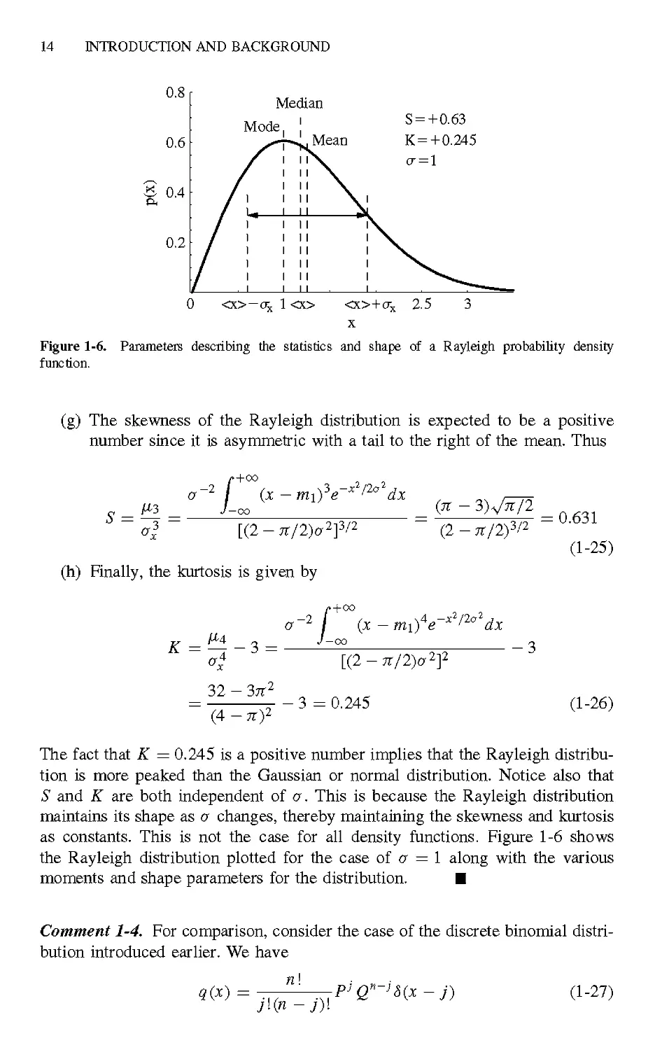
Figure 1-6. Parameters describing the statistics and shape of a Rayleigh probability density
function.
(g) The skewness of the Rayleigh distribution is expected to be a positive
number since it is asymmetric with a tail to the right of the mean. Thus
,-2
/• + 00
J—co
(x -
dx
GГ -
al [B-71/2)о2]У2
(h) Finally, the kurtosis is given by
B - 7Г/2K/2
= 0.631
A-25)
,-2
/• + 00
J—co
(x -
[B-7t/2)o2]2
-3
32 - Зтг2
-7ГJ
D-7Г)
-3 =0.245
A-26)
The fact that К = 0.245 is a positive number implies that the Rayleigh distribu-
distribution is more peaked than the Gaussian or normal distribution. Notice also that
5* and К are both independent of a. This is because the Rayleigh distribution
maintains its shape as a changes, thereby maintaining the skewness and kurtosis
as constants. This is not the case for all density functions. Figure 1-6 shows
the Rayleigh distribution plotted for the case of a = 1 along with the various
moments and shape parameters for the distribution. ¦
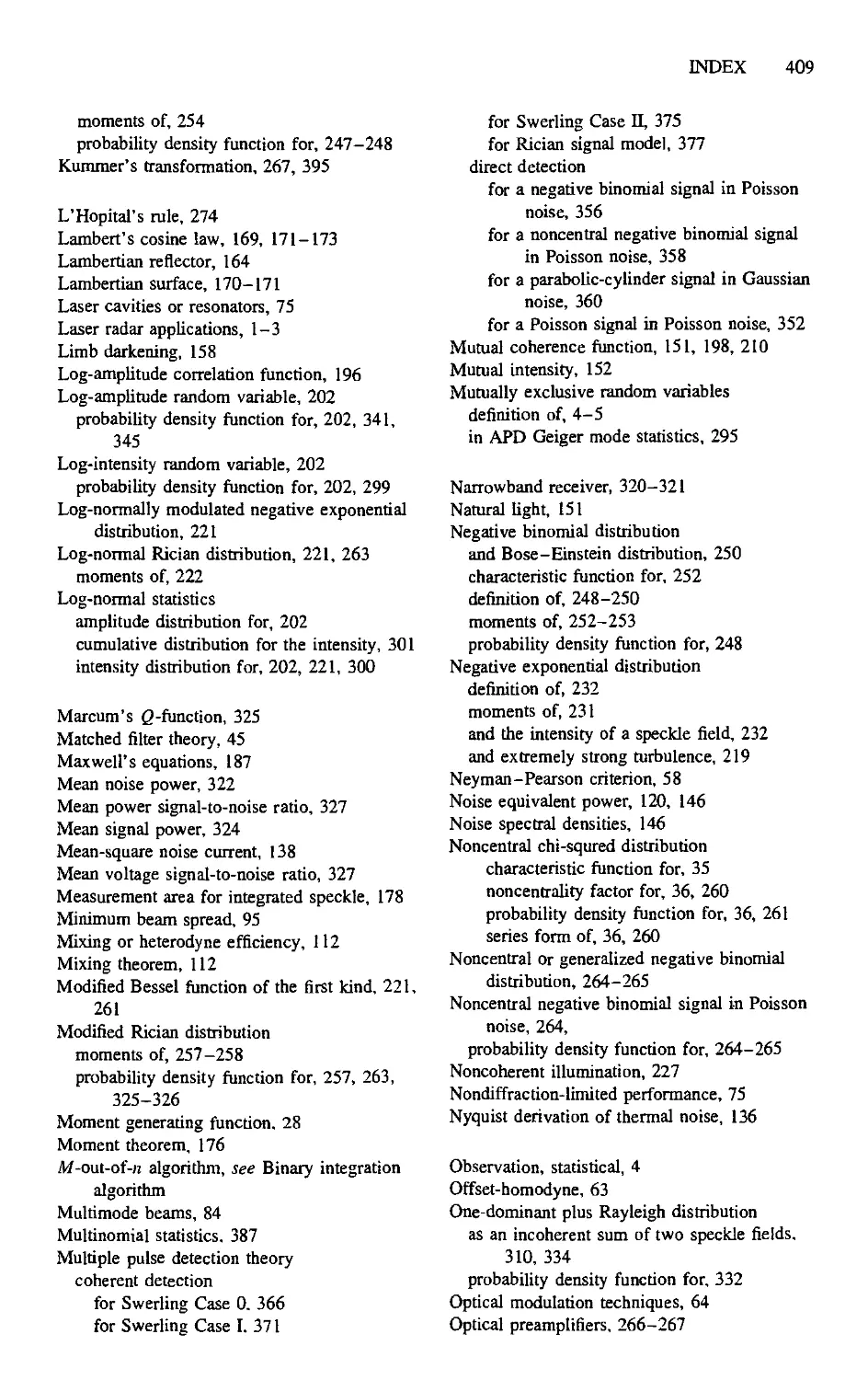
Comment 1-4. For comparison, consider the case of the discrete binomial distri-
distribution introduced earlier. We have
«(*) =
n\
A-27)

REVIEW OF STATISTICAL METHODS 15
0.25
0.2
0.15
0.1
0.05
.,1
1
6 8
10
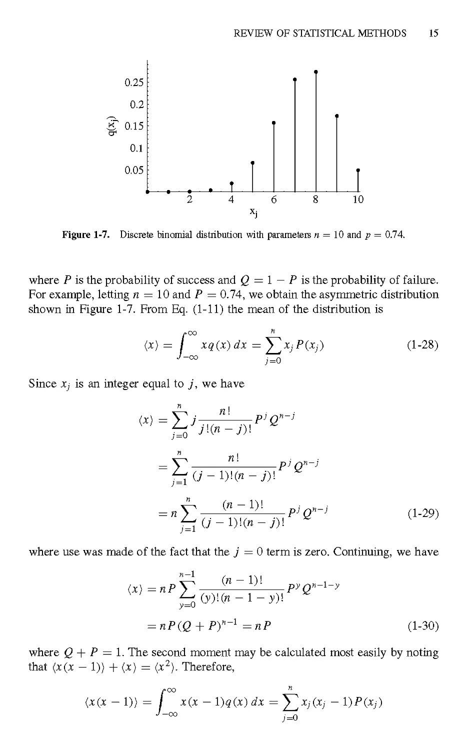
Figure 1-7. Discrete binomial distribution with parameters re = 10 and p = 0.74.
where P is the probability of success and Q = 1 — P is the probability of failure.
For example, letting n = 10 and P = 0.74, we obtain the asymmetric distribution
shown in Figure 1-7. From Eq. A-11) the mean of the distribution is
(x)
= /
J~°
j=0
Since Xj is an integer equal to j, we have
С18)
j=0
n
JKn-j)\
n\
= nT-
A-29)
where use was made of the fact that the j =0 term is zero. Continuing, we have
=пР
A-30)
where Q-\- P = \. The second moment may be calculated most easily by noting
that (x(x - 1)) + (x) = (x2). Therefore,
(x(x - 1)) =
/•C
= /
J—o
;=o

16 INTRODUCTION AND BACKGROUND
У -
j
п-г
= п(п -1)P2V-
= п(п- l)P2(Q + Pf~2 = п(п - 1)Р2 A-31)
Thus
(х2) =п2Р2 -пР2 +пР
= п2Р2 + пРA - Р) A-32)
The variance is therefore given by
var(x) = (x2) - (xJ = nPQ A-33)
Inserting the previous values for n, P, and Q in the moments above results
in (x) = 7.4, (x2) = 56.68, and var(x) = 1.924. Thus we see that the moments
themselves are, in general, not discrete. If it is necessary to have discrete quan-
quantities, the fractional values can be rounded off to the nearest integer. However,
some descriptors, such as the mode and the cumulative distribution function, are
necessarily discrete. For example, the mode is denned as that value of the random
variable that has the greatest probability. For the discrete binomial distribution
shown in Figure 1-7, it is equal to 8, which is necessarily an integer. General
expressions for the 5* and К will not be derived here for the sake of concise-
conciseness, but are instead, calculated using the data shown in Figure 1-7. This yields
5* = -0.34 and К - 3 = -0.0802, thus indicating that the binomial distribution,
with n = 10 and P = 0.74, has a tail to the left of the mean and is slightly less
peaked than the Gaussian distribution. It is easy to show in this manner that
5* < 0 for P < \, S = 0 for P = \, and S > 0 for P > \.
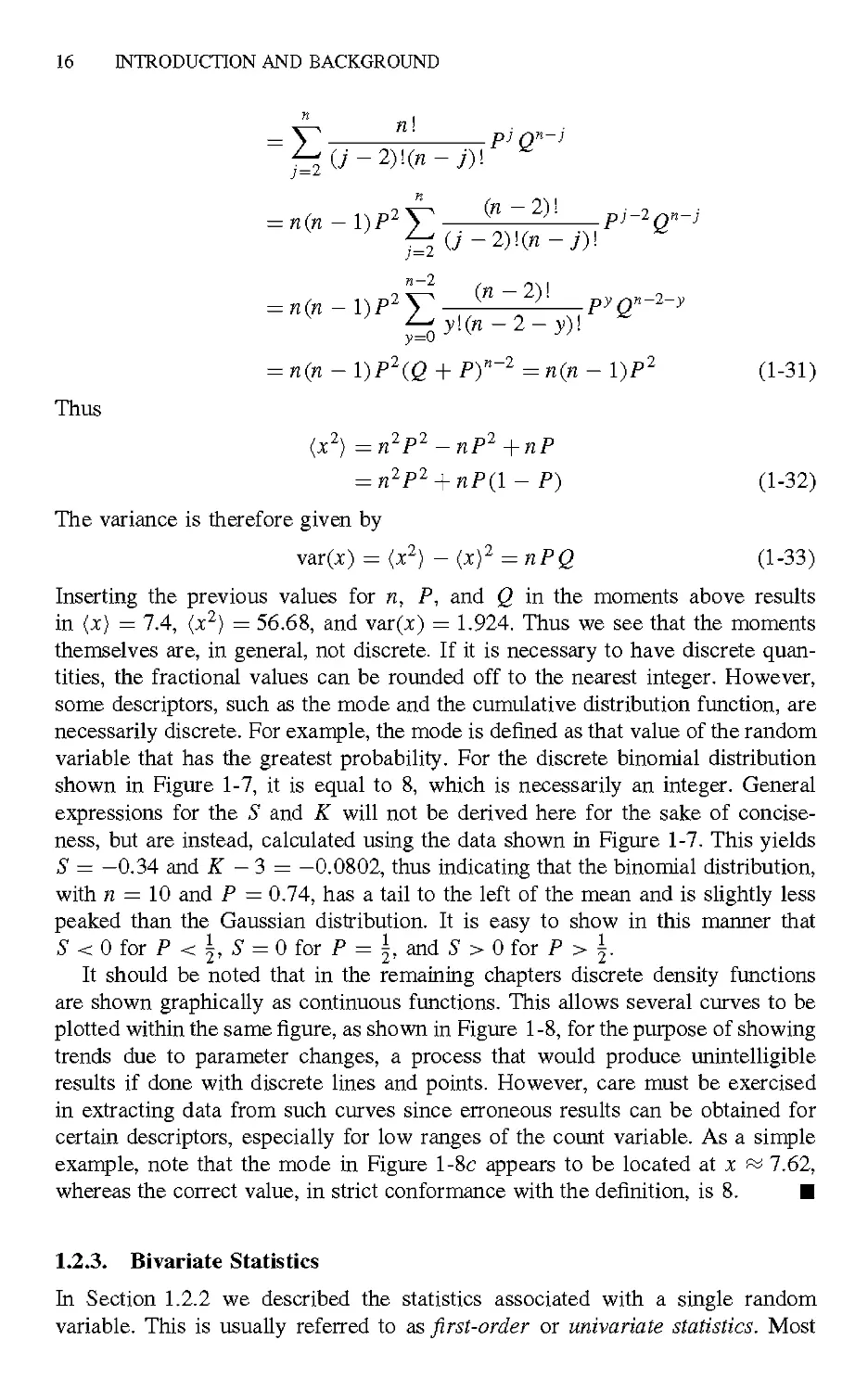
It should be noted that in the remaining chapters discrete density functions
are shown graphically as continuous functions. This allows several curves to be
plotted within the same figure, as shown in Figure 1-8, for the purpose of showing
trends due to parameter changes, a process that would produce unintelligible
results if done with discrete lines and points. However, care must be exercised
in extracting data from such curves since erroneous results can be obtained for
certain descriptors, especially for low ranges of the count variable. As a simple
example, note that the mode in Figure l-8c appears to be located atx^ 7.62,
whereas the correct value, in strict conformance with the definition, is 8. ¦
1.2.3. Bivariate Statistics
In Section 1.2.2 we described the statistics associated with a single random
variable. This is usually referred to as first-order or univariate statistics. Most

REVIEW OF STATISTICAL METHODS 17
0.4
0.3
0.2
0.1
10
Figure 1-8. Continuous envelope representations of the discrete binomial distribution with param-
etere re = 10 and (a) p = 0.74, (Ъ) р = 0.5, and (с) р = 0.74.
systems of interest involve many more variables, requiring at least second-order
or bivariate statistics for an adequate description. Indeed, even our example case
of the golfer attempting to hit a hole-in-one should be described by at least two
independent variables, x and у (x being cross-range miss distance and у being
down-range miss distance). The univariate probability density function is readily
generalized to the bivariate case by requiring that the two-dimensional integral
of the probability density function equates to the probability that the variables x
and у will jointly lie between (xa,xb) and (ya, уь). That is,
a < x < xb,ya <y <yb) =
/•хь гУъ
I I p(x, y)dx dy continuous
гхь гуь
I I q(x, y) dx dy discrete
A-34)
where p(x,y) and q(x,y) represent continuous and discrete joint probability
density functions of the random variables x and y. If x and у are dependent, their
associated probabilities and frequencies of occurrence must be related. Thus, if
P(y) = n(y)/n represents the probability that у will occur, where n is the total
number of events, the probability that x will occur under the condition that
у occurs is given by P(x \ y) = n(x, y)/n(y). Here n{x,y) is the number of
times that x and у occur jointly out of the total number of trials n. Using these
definitions, we can write for the conditional probability that x occurs given that
;y occurs as
n(x,y) n(x,y) n P(x,y)
P{x | y) =
л СУ)
л (У) Р(У)
A-35)
or, in terms of the joint probability of x and у occurring,
P(x,y) = P(x \y)P(y)
A-36)

18 INTRODUCTION AND BACKGROUND
Equation A-36) constitutes the fundamental definition of conditional and joint
probabilities. Since P(x,y) is independent of the order of occurrence of x and
y, we could also have written
P(y,x) = P(y\x)P(x) A-37)
Thus
Р(У)
This is known as Bayes' rule.
The results above also hold for probability density functions. Thus
P(x, У) = P(x I У)Р(у) continuous
A-39)
q (x, y) = q (x | y)q (y) discrete
where p(x | y) and q(x | y) are the conditional probability density Junctions for
x given that у occurs. Note that if x and у are independent, p(x \ y) -> p(x)
and q (x | y) -> q (x), such that
p(x, y) = p(x)p(y) continuous
A-40)
q(x,y) =q(x)q(y) discrete
Equation A-40) is a necessary condition for two variables to be independent
since if it is violated, any probabilities calculated using this assumption will lead
to unphysical results. Using the previous definitions of conditional probability,
Eqs. A-34) may now be written
a <x<xb,ya<y<yb) = -
УЬ
P(x I y)P(y) dx dy continuous
п.
fxb ГУЬ
I I Q(x \ y)Q(y)dx dy discrete
A-41)
Comment 1-5. Before proceeding, it is important to make clear how the Dirac
delta function formalism, introduced earlier for discrete univariate statistics,
generalizes to the case of bivariate statistics. Consider the case of two dependent
random variables, x and y, each being associated with overlapping sample spaces
of discrete points xj and y^. Then the joint probability density function of x and
;y is written
- x;)8(y - yk) A-42)

REVIEW OF STATISTICAL METHODS 19
The marginal probability density function for x is then
/CO CO CO
q(x,y)dy = J2J2P(-xJ \Ук)Р(УкЖх~Ъ) A-43)
and similarly for q(y). The probability of Xj occurring is then
_ I Ук)Р{Ук) A-44)
JxJ-* k=\
and of yk occurring is
Р(Ук-1 <У<Ук) = 1 Q(y)dx = X Р(Ук I xj)P(xj) A-45)
where the ranges of integration are understood to include only Xj and yk, respec-
respectively, in accordance with Comment 1-1. ¦
Using the results of Comments 1-1 and 1-5, the discrete density function in
Eqs. A-41) can be rewritten such that the pair now reads
a:
P(x I У)Р(у) dxdy continuous
P(xa <x<xb,ya<y<yb) = - n s
X2Z P(XJ'' Ук)Р(Ук) discrete
j=m k=r
A-46)
Here the integration regions include the discrete points (m, n) and (r, s). If (m, n)
and (r, s) extend over all sample space, then
P(—oo < x < со, -co < у < со)
/•CO /-CO
= / / P(x \ У)Р(у) dx dy = 1 continuous
<Xj < Хсо.Л <Л < >oo)
CO CO
= X] X! P (XJ \У^Р СУА) = 1 discrete
X] X!

20 INTRODUCTION AND BACKGROUND
as required. For independent variables, Eq. A-47) reduces to products of univari-
ate probabilities, that is,
P(—oo < x < со, —oo < у < со)
/•CO /-CO
= / p(x)dx I p(y)dy = l continuous
J — CO J — CO
A-48)
P{X\ < Xj < Xco, >l < Л < 3>oo)
CO CO
= ^ P (Xj) ^ P(yk) = 1 discrete
Similarly, the joint cumulative distribution function for the bivariate case is a
straightforward generalization of the univariate case, that is,
F(x',y')= I I p(x,y) dxdy continuous
J— CO J— CO
A-49)
№ ГУ,
G (xn, ys) = I I q (x, y) dx dy discrete
J— CO J — С
' —CO J —CO
Comment 1-6. Using Eq. A-42) for the case of two random variables x and y,
the probability of a golfer making exactly a birdie on a par-three hole can be
calculated from the expression P(xi) = P{x\ \ y\)P{y\). Here the x\ are the
events related to putting the ball into the cup and the ;yi are the events related
to driving the ball onto the green. Specifically, having (hypothetically) sampled
the performance of our golfer over many trials, it is found that the probability of
making a birdie on a particular par-three hole is dependent on whether or not the
first shot lands on the green. It is found that the probability of putting the second
shot in the cup, given that the first shot is on the green, is P{x\ \ y{) = 0.1.
Thus if the probability of a successful drive is, say, -P(;yi) = 0.75, the proba-
probability of making a birdie is P{x\) = 0.75 x 0.1 = 0.075 or about 1 chance in
13 tries. ¦
Comment 1-7. Consider now the joint probability of making a birdie given that
the first shot does not land on the green. There are several possibilities for this
case. For example, it might be found that the drive can land in the fairway
with probability Р(уг) =0.1, or in the rough with probability Р(уъ) = 0.1, or
in a bunker with probability P(y4) = 0.05. The probability of the ball landing
on the green is, from Comment 1-6, P(yi) = 0.75, such that X^=i Р(Ук) = 1
as required, since there are no other (hypothesized) possibilities. Thus, if we
assume for simplicity that the probability of making the second shot is about
equally difficult in all the off-green cases, say P(x\ \ y^) = 0.01, the probability
of making a birdie, given that the drive is not on the green, is P(x\) = @.1 +

REVIEW OF STATISTICAL METHODS 21
0.1 +0.05) x @.01) = 0.0025, or about 1 chance in 400 tries! The total prob-
probability of all four events is P(xi) = @.1 +0.1 +0.05+0.75) x @.01) = 0.01,
or 1 chance in 100 tries. Note that the total probability does not sum to 1. That
is because other possibilities Xj have not been accounted for, such as making a
par, a bogey, and so on. ¦
Joint moments are straightforward generalizations of the univariate moments.
Thus, for the moments
Л+СО Л+СО
m}k= / xiykp(x,y)dxdy A-50)
J — CO J — CO
and the central moments
Л+СО Л+СО
H-jk= / (x-тюУ(У-mOi)kp(x,y)dxdy A-51)
J— CO J — CO
where тщ and moi are defined by Eq. A-11). By convention, fi2o and fio2 are
usually referred to as the variances a\ and 0$, respectively, of the random
variables x and y. The discrete moments follow in accordance with the procedures
outlined above.
fin is called the covariance of the two variables x and у and is zero when x
and у are independent [i.e., when p(x, y) = p(x)p(y) or q(x, y) = q(x)q(y)].
When x and у are dependent, fi\\ becomes a measure of the degree of correlation
of the variables with a magnitude determined by the units of measurement for
x and y. If the correlation between x and у is such that a positive change in x
(or y) corresponds to a positive change in у (or x), fin is positive. On the other
hand, if a positive change in x (or y) corresponds to a negative change in у (or
x), fi\\ is negative. To remove the dependence on the measurement units and
obtain a standardized measure of correlation between the variables, a normalized
covariance function called the correlation coefficient, p, is defined as
P = ^- d-52)
G1G2
where a\ and 02 are standard deviations of the random variables and -1 < p <
+1. Thus if p = ±1, the variables are said to be fully correlated, either positively
or negatively, and if p = 0, they are said to be fully uncorrelated.
1.2.4. Transformation of Random Variables
It is frequently the case that one must transform to a new set of variables, or
some function of the original variables, in order to solve a problem of interest. For
example, one may wish to convert the probability density function representing
the amplitude, A, of the radiation field to the intensity, /, where / = A2. This
is a one-to-one transformation, which maps one set of coordinates onto another.

22
INTRODUCTION AND BACKGROUND
We consider the one- and two-dimensional cases, although the procedure can
be generalized to any number of dimensions. For more detailed discussions, the
reader is referred to the many texts on probability theory and integral calculus.
The simplest case is that of a one-dimensional transformation where the prob-
probability density function p(x) of the random variable x is to be converted to a
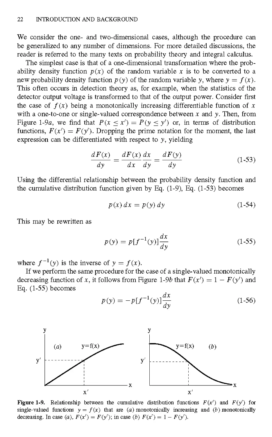
new probability density function p (y) of the random variable y, where у = f(x).
This often occurs in detection theory as, for example, when the statistics of the
detector output voltage is transformed to that of the output power. Consider first
the case of f(x) being a monotonically increasing differentiable function of x
with a one-to-one or single-valued correspondence between x and y. Then, from
Figure l-9a, we find that P(x < x') = P(y < y') or, in terms of distribution
functions, F(x') = F(y'). Dropping the prime notation for the moment, the last
expression can be differentiated with respect to y, yielding
dF(x)
dy
dF(x) dx
dx dy
dF{y)
dy
A-53)
Using the differential relationship between the probability density function and
the cumulative distribution function given by Eq. A-9), Eq. A-53) becomes
p(x)dx =p(y)dy
A-54)
This may be rewritten as
dy
A-55)
where / 1(y) is the inverse of у = f(x).
If we perform the same procedure for the case of a single-valued monotonically
decreasing function of x, it follows from Figure l-9b that F(x') = 1 — F(y') and
Eq. A-55) becomes
p(y) = -
dy
A-56)
Y=f(x) (b)
Figure 1-9. Relationship between the cumulative distribution functions F(x') and F(y') for
single-valued functions у = f(x) that are (a) monotonically increasing and (b) monotonically
decreasing. In case (a), F(x') = F(y'); in case (b) F(x') = 1 - F(y').

REVIEW OF STATISTICAL METHODS
23
P(y)dy
Р(У)
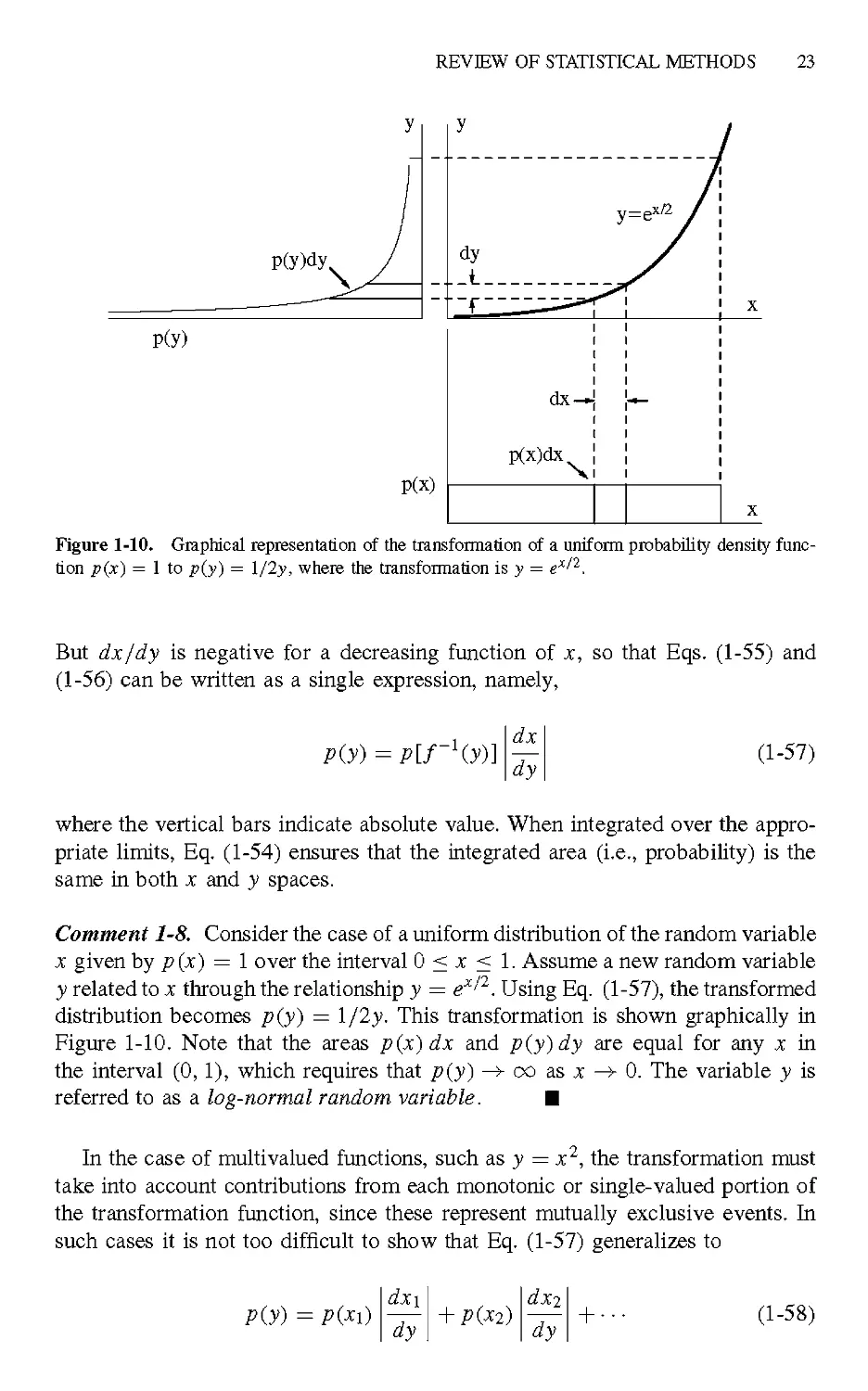
Figure 1-10. Graphical representation of the transformation of a uniform probability density func-
function p(x) = 1 to p(y) = l/2y, where the transformation is у = е*?2.
But dx/dy is negative for a decreasing function of x, so that Eqs. A-55) and
A-56) can be written as a single expression, namely,
dx
dy
A-57)
where the vertical bars indicate absolute value. When integrated over the appro-
appropriate limits, Eq. A-54) ensures that the integrated area (i.e., probability) is the
same in both x and у spaces.
Comment 1-8. Consider the case of a uniform distribution of the random variable
x given by p(x) = 1 over the interval 0 < x < 1. Assume a new random variable
у related to x through the relationship у = exjf2. Using Eq. A-57), the transformed
distribution becomes p(y) = l/2y. This transformation is shown graphically in
Figure 1-10. Note that the areas p(x) dx and p(y)dy are equal for any x in
the interval @,1), which requires that p(y) —>- со as x —>- 0. The variable у is
referred to as a log-normal random variable. ¦
In the case of multivalued functions, such as у = x2, the transformation must
take into account contributions from each monotonic or single-valued portion of
the transformation function, since these represent mutually exclusive events. In
such cases it is not too difficult to show that Eq. A-57) generalizes to
Р(У) =
dx\
~dy~
dy
+ ¦
A-58)

24 INTRODUCTION AND BACKGROUND
where the Xj are the monotonically increasing or decreasing segments of the
function p(x).
Two-dimensional transformations take the form
x=f(u,v) y=g(u,v) A-59)
where the two-dimensional joint probability density function p(x,y) is to be
transformed to a new probability density function p(u, v). Generalization of
Eq. A-54) to two dimensions yields
p(u,v) dudv = p(x, y)dx dy A-60)
Thus the transformation becomes
p(u,v)=p[f(u,v),8(u,v)]\J(x,y:u,v)\ A-61)
where \J(x, у : и, v)\ = \д(х, у)/д(и, v)\ is the absolute value of the Jacobian
of the transformation. The Jacobian is defined by the determinant
Эх
ЭЙ
ду
ди
дх
эп
ду
dv
which is well known from the theory of integral calculus. This type of transfor-
transformation may be generalized to n dimensions via an и-dimensional Jacobian, but
this is not discussed here.
Comment 1-9. For the golf example mentioned earlier, it is instructive to calcu-
calculate the most probable miss distance, the average miss distance, and the prob-
probability of making a hole-in-one if the standard deviation of the shots in the
cross-range and down-range directions are ±10 ft and the radius of the hole is
2 in.
Clearly, this problem must be described by a two-dimensional probability
density function, x representing the cross-range error and у the down-range error.
In order to simplify the problem, we assume that the distributions in x and у are
both Gaussian with zero means and equal variances. The latter restrictions imply
that this particular golfer has no biases in his shots in either the x or у directions
((jc) = (y) = 0), that he has equal spreads in both cross-range and down-range
directions (ax = ay = a), and that there are no external influences, such as wind.
The probability density function becomes
p(x, y) = p(x)p(y) =

REVIEW OF STATISTICAL METHODS
25
where the individual density functions
p(x) =
1
Р(У) =
A-64)
are considered independent. This is the same problem as throwing darts at a
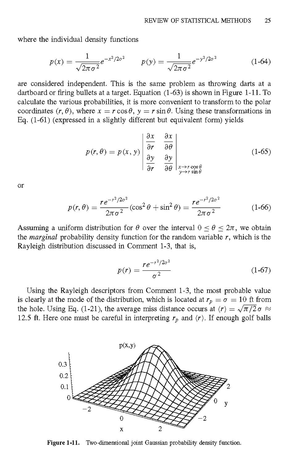
dartboard or firing bullets at a target. Equation A-63) is shown in Figure 1-11. To
calculate the various probabilities, it is more convenient to transform to the polar
coordinates (г, в), where x = r cos#, у = r sin#. Using these transformations in
Eq. A-61) (expressed in a slightly different but equivalent form) yields
р(г,в)=р(х,у)
Эх
~э7
ду
дг
Эх
~дв
ду
дв
A-65)
or
Р(.г,в) =
re
2ЛГ<72
- (cos2 в + sin2 в) =
re
2ЛГ<72
A-66)
Assuming a uniform distribution for в over the interval 0 < в < 2лг, we obtain
the marginal probability density function for the random variable r, which is the
Rayleigh distribution discussed in Comment 1-3, that is,
p(r) =
A-67)
Using the Rayleigh descriptors from Comment 1-3, the most probable value
is clearly at the mode of the distribution, which is located at rp = a = 10 ft from
the hole. Using Eq. A-21), the average miss distance occurs at (r) = s/л/2a рй
12.5 ft. Here one must be careful in interpreting rp and (r). If enough golf balls
P(x,y)
-2
-2
Figure 1-11. Two-dimensional joint Gaussian probability density function.

26 INTRODUCTION AND BACKGROUND
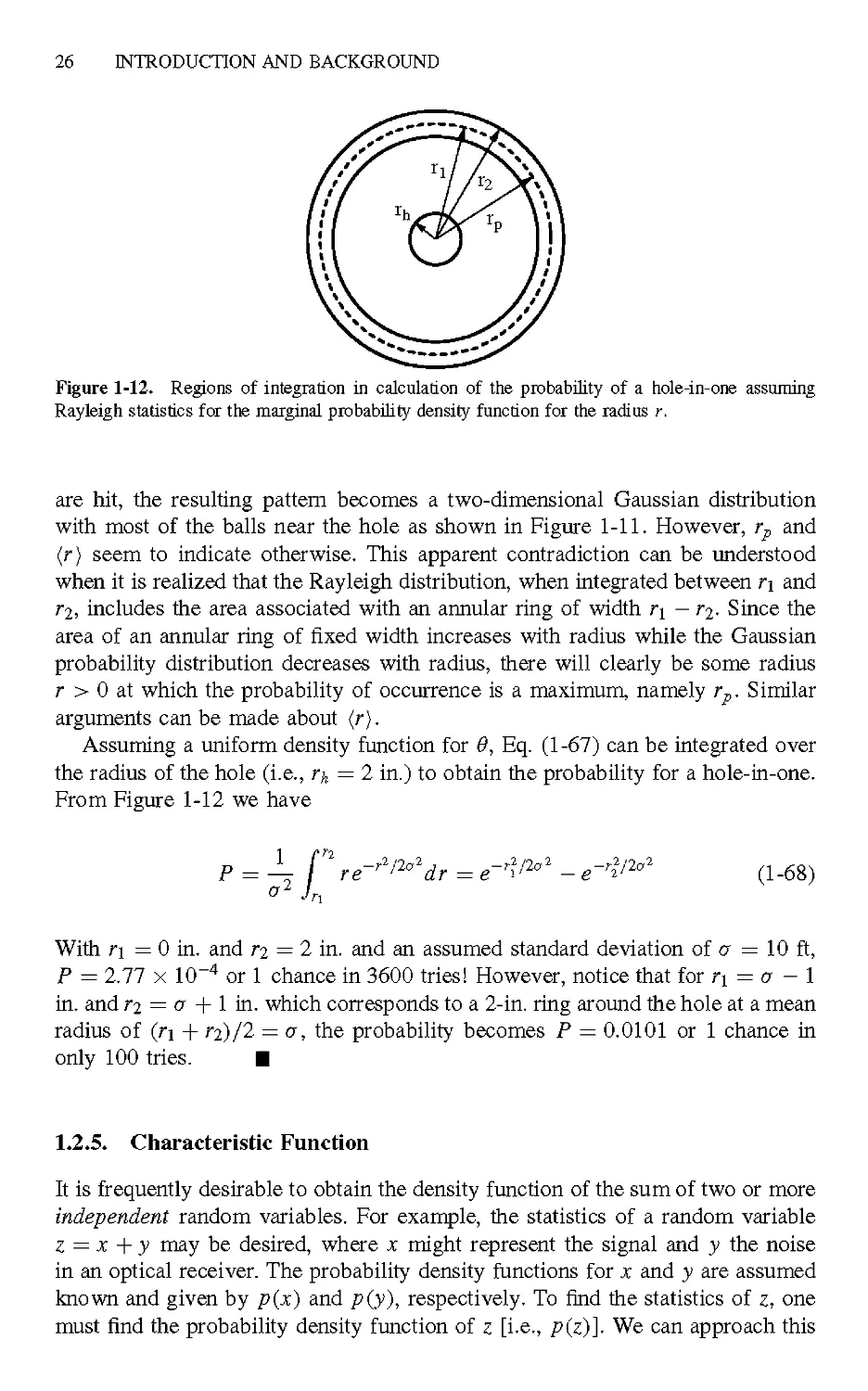
Figure 1-12. Regions of integration in calculation of the probability of a hole-in-one assuming
Rayleigh statistics for the marginal probability density function for the radius r.
are hit, the resulting pattern becomes a two-dimensional Gaussian distribution
with most of the balls near the hole as shown in Figure 1-11. However, rp and
(r) seem to indicate otherwise. This apparent contradiction can be understood
when it is realized that the Rayleigh distribution, when integrated between ri and
Г2, includes the area associated with an annular ring of width r\ — r^- Since the
area of an annular ring of fixed width increases with radius while the Gaussian
probability distribution decreases with radius, there will clearly be some radius
r > 0 at which the probability of occurrence is a maximum, namely rp. Similar
arguments can be made about (r).
Assuming a uniform density function for 9, Eq. A-67) can be integrated over
the radius of the hole (i.e., r^ = 2 in.) to obtain the probability for a hole-in-one.
From Figure 1-12 we have
O2 Л,
(L68)
With r\ = 0 in. and r^ = 2 in. and an assumed standard deviation of a = 10 ft,
P = 2.77 x 10~4 or 1 chance in 3600 tries! However, notice that for r\ = a — 1
in. and Г2 = a + 1 in. which corresponds to a 2-in. ring around the hole at a mean
radius of (ri + гг)/2 = a, the probability becomes P = 0.0101 or 1 chance in
only 100 tries. ¦
1.2.5. Characteristic Function
It is frequently desirable to obtain the density function of the sum of two or more
independent random variables. For example, the statistics of a random variable
z = x + у may be desired, where x might represent the signal and у the noise
in an optical receiver. The probability density functions for x and у are assumed
known and given by p{x) and p(y), respectively. To find the statistics of z, one
must find the probability density function of z [i.e., p(z)]. We can approach this

REVIEW OF STATISTICAL METHODS 27
problem by denning another set of variables:
z = x + y
A-69)
f = x
From Eq. A-60) with p(x, y) = p(x)p(y), we can write
[ [ p(z, f) dz df = [ f P{x)p{y) dx dy A-70)
Jz Jt, Jx Jy
which can be rewritten as
f f p(z, t)dzds= ( ( p(OP(z - f) dz dr; A-71)
h h h h
so that
P(z, f) = P(OP(Z - f) A-72)
Finally, the desired probability density function p(z) can be obtained by inte-
integrating over all values of f, that is,
=/
J—
A-73)
This integral is referred to as a convolution integral. The arguments of the integral
have the interesting and useful property that the Fourier transform of p(z) may
be obtained from the product of the Fourier transforms of p(x) and p(y). This
is known as the convolution theorem and is written
Gz(iv)=Gx(iv)Gy(iv) A-74)
where
л+00
Gx(iv) = / p(x)elvxdx
J —CO
A-75)
/•+00
Gy(iv) = / />О0е^у
^—CO
Gx(iu) and Gy(iu) are referred to as characteristic functions and correspond to
the Fourier transforms of />(дг) and /'(y), respectively. p{z) may then be obtained
from the inverse transform of Gz (i v). The complex number i = V—1 is included
explicitly in the argument of G in order to make clear that the characteristic
function is generally complex, whereas p(x) is always real. Proof that Eq. A-74)
follows from Eq. A-73) is easily shown by taking the Fourier transform of both
sides of Eq. A-73) followed by a change in the order of integration.

28 INTRODUCTION AND BACKGROUND
Comment 1-10. Depending on the sign conventions chosen, the characteristic
function given by Eqs. A-75) may correspond to either forward or reverse Fourier
transforms. In particular, integral Fourier transforms may be defined in a variety
of ways by appropriately defining the arbitrary parameters a and b in the gener-
generalized expressions
¦,1/2
F{<o) =
and
Г \b\ llj/2 f00
/O = kr^r / F(<o)e^dt A-77)
In the chapters that follow we let {a, b) = A, 1) for the Fourier integrals
and (a,b) = (l,— 1) for the characteristic functions, where F(co)^G(iv)
and f{t) —>- p(x) in the latter case. Thus the characteristic function G(iv)
corresponds to a reverse or inverse Fourier transform [i.e., Eq. A-77)] times
2л, a standard convention in probability theory. ¦
From Eqs. A-75) we see that the characteristic function can also be viewed
as the average of ezux via the definition given by Eq. A-11); that is, Gx{iv) =
(elvx). Knowing this, the procedure can be generalized to the sum of an arbitrary
number of statistically independent variables, n, (i.e., z = x\ + хг +хз + ¦ ¦ ¦ +
xn). We have
Gt(iv) = (elvz) = (e^ta+«+-+*.))
= (eivx'){eivxi)--- (eivx")
A-78)
Equation A-78) states that the characteristic function of the sum of n independent
variables is equal to the product of the characteristic functions of the individual
variables.
A power series expansion of Gz (i v) shows that
n=0 ' n=0
This implies that all the moments of a distribution may be obtained directly
from an expansion of the characteristic function of that distribution. Indeed,
a moment generating function can be denned, involving the derivative of the
characteristic function evaluated at и = 0, which generates moments directly

REVIEW OF STATISTICAL METHODS 29
[i.e., without the associated coefficients apparent in Eq. A-79)]. To show this,
successive derivatives of Gz(iv) are taken, yielding
dG
~du
and
d2G
= '/'
=o J-
co
xp(x) dx = im\ A-80)
CO
dv2
/¦CO
=0 J-co
2
xLp(x)dx = -m2 A-81)
Generalizing these results, while taking into account the i" factors, leads to a
moment generating function given by
dnG
тп=Гп— A-82)
dvn
Other moment generating functions can be defined which do not include complex
variables: for example,
/•CO
GXQ) = / P(x)extdx A-83)
J — CO
where
d"G
A84)
However, there is no guarantee that the integral in Eq. A-83) exists, whereas
the integrals in Eq. A-75) always exist and will therefore be used throughout
the book.
Comment 1-11. Equation A-78) implies that the mean and variance of the sum
of n independent variables is equal to the sum of the means and variances of the
individual variables. To show this for the Gaussian probability density function,
we let the random variable be given by z = YTj=\ xj an^ *пе individual Gaussian
probability density functions by
p (x) =
Then, by changing variables to t2 = [(x - (x))/o - iau], we obtain for the
Fourier transform of the probability density function of a single Gaussian variate,
л+оо
Gxj(iv)= elvx>p(x})dx}
J—со
A-86)

30 INTRODUCTION AND BACKGROUND
where Bny^2 f^ e~^2dt = 1. Hence
zei(.{x,)+{x7)-{xa))v-(a?+ol-oZ)v2/2
Using Eq. A-82) we find for the mean and variance of the summed random
variable z'.
n n
J>;) and o2 = J2°j С1"88)
respectively. An inverse transformation on Eq. A-87) will, by definition, produce
a Gaussian distribution with mean г and variance a2, that is,
p(z) = ^^e-fe"fc»W A_89)
1.2.6. Central Limit Theorem
The central limit theorem is probably the most important theorem in statistics. The
theorem states that the probability density function p(z) representing the random
variable z = Y^j=i xj wiU converge to a Gaussian distribution function in the limit
of large n, independent of the form of the probability density functions associated
with the individual Xj. This assumes, of course, that all the random variables that
are to be added have similar magnitudes such that no single density function
will dominate the distribution. The convergence to a Gaussian distribution was
clearly shown in Comment 1-11 for the case of a Gaussian distribution. However,
the fact that the initial function was a Gaussian, whose Fourier transform is
also a Gaussian, may not have convinced the reader of the generality of the
theorem. Two additional examples will now be given that are less obvious in
their conclusions and that will be useful in later chapters.
Consider the case of a set of random variables Xj each of which is described
by a negative exponential probability density function given by
/>;(*;) = -<r*'/e' A-90)
aj
The characteristic function may again be used to calculate the probability density
function corresponding to n random variables that obey Eq. A-90). Thus
/•CO
G}(lU)= Jo UJ в X'a'+lVX'dxJ
= 1-4 A-91)

REVIEW OF STATISTICAL METHODS 31
The characteristic function for the sum of n of such random variables is
n
G{n)(iv) =]~[A -iujv)'1 = A -iav)~" where all ai = a A-92)
The inverse transformation of Eq. A-92) can be performed using a contour inte-
integration in the lower half of the complex plane, (cf. Appendix B). The result
yields the gamma distribution, given by
P(z) = j Г(л) Z ~ A-93)
¦ 0 z <0
where Г(н) is the gamma function defined by the integral Г(н) = /0 tn~le~fdt
(cf. Appendix A) and a is a parameter. As will be seen in Chapter 4, the gamma
distribution plays a fundamental role in the statistical description of radiation
scattered from a rough surface. The question arises as to whether the gamma
distribution can be approximated by a Gaussian distribution as n approaches
infinity in accordance with the central limit theorem. To show that this is indeed
the case, we first note that Eq. A-92) equates to unity at и = 0 and decreases
rapidly away from the origin as n is increased. Thus, for large n we can expand
Eq. A-92) about the origin, obtaining
GM(iu) = 1 + ianu - \n{n - \)a2v2 -\ A-94)
Identifying the right side of Eq. A-94) as the leading terms in the expansion of
a Gaussian function yields
G(n)au)^eIMU-A/2)nau A-95)
where the approximation n(n — 1) & n2 is used. But Eq. A-95) is of the same
form as Eq. A-87) under the substitutions (z) —>- na and a2 —>- n2a2. Thus the
inverse transformation must yield
and we see that the gamma distribution does approach a Gaussian distribution
for large n as required by the central limit theorem. It must be kept in mind,
however, that Eq. A-96) is only an approximation that is valid for large n and
small values of z —na. Equation A-96) is plotted in Figure 1-13 for several

32 INTRODUCTION AND BACKGROUND
0.1
0.08
0.06
0.04
0.02
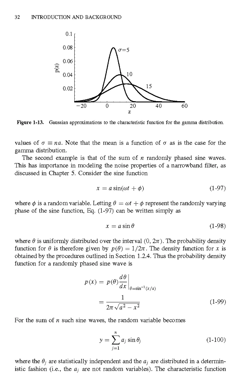
-20
Figure 1-13. Gaussian approximations to the characteristic function for the gamma distribution.
values of a = na. Note that the mean is a function of a as is the case for the
gamma distribution.
The second example is that of the sum of n randomly phased sine waves.
This has importance in modeling the noise properties of a narrowband filter, as
discussed in Chapter 5. Consider the sine function
x = a sin(cot + ф)
A-97)
where ф is a random variable. Letting в = cot + ф represent the randomly varying
phase of the sine function, Eq. A-97) can be written simply as
x = a sin 9
A-S
where в is uniformly distributed over the interval @, 2л). The probability density
function for в is therefore given by p{9) = 1/2л. The density function for x is
obtained by the procedures outlined in Section 1.2.4. Thus the probability density
function for a randomly phased sine wave is
p@)-
?=sin~1 (x/a)
A-99)
For the sum of n such sine waves, the random variable becomes
A-100)
where the 6j axe statistically independent and the a,- are distributed in a determin-
deterministic fashion (i.e., the uj are not random variables). The characteristic function

REVIEW OF STATISTICAL METHODS 33
for the jth sine wave can be most easily obtained by averaging over #,¦, that is,
Gj{iv)= f р(в)е1а'"^вЫв, =— f eia'vsine'de} A-101)
Jo 2я Jo
But this last form may be recognized as the definition of the Bessel function of
the first kind, zeroth order. Thus
Gj(iv) = JoifljV) A-102)
The series expansion for Jq is given by
2
k=0
which to order x2 can be approximated by
A-104)
The characteristic function for the random variable у can therefore be written
iv) =f\Gj(iv) <* f[e-WW1 = e-W*1»1 A-105)
where a2 = naj/2. Thus the inverse transformation once again leads to a Gaus-
Gaussian probability density function given by
p(y) = -L=e-y2'^ A-106)
It can be shown that the procedures above, which do not constitute a rigorous
proof of the central limit theorem, may be generalized to the case of any proba-
probability density function3 and is therefore a strong indication of the validity of the
theorem. In general, it is found that the convergence to the Gaussian distribution
is more rapid near the mean of the distribution than in the wings. Indeed, density
functions with long tails, such as the log-normal distribution, tend to converge
more slowly than more compact functions. In the case of the log-normal distribu-
distribution, which is important for later chapters, it has been shown4 that the convergence
to the Gaussian distribution for large n is so slow that it is usually more correct
to consider the limiting form as remaining log-normal. This behavior has been
observed in numerous physical experiments, including optical propagation in a
turbulent atmosphere and radio-wave propagation in the ionosphere. More will
be said about the log-normal distribution in Chapters 3, 4, and 5.

34 INTRODUCTION AND BACKGROUND
1.2.7. Chi-Squared Distribution
The x2 distribution occurs frequently in detection theory and represents the
distribution of the sum of squares of n normally distributed random variables. A
random variable x is said to have a x2 distribution if its density function is of
the form
rQtf *• 1 л У
L. С-
p(x) =
x >0
2«/2Г(а/2)
I 0 x <0
where the Г (a/2) is the gamma function and a is referred to as the number of
degrees of freedom of the density function p(x). The characteristic function for
p(x) is given by
^oo
J-VX ,
G{iv) = / eluxp{x)dx
Jo
r\—& /2 /»'
= Г (а/2) ]0
Letting z = A — 2iv')x, Eq. A-108) becomes
But the expression under the integral sign is just the definition of the j1 distri-
distribution, which integrates to 1. Thus
To show that the y} distribution represents the sum of squares of n normally
distributed random variables, consider the single random variable у = x2, where
x is normally distributed with zero mean and unity variance:
—x2/2
e A-111)
/2тт
The characteristic function for p(y) is
Gy(iv) = / —dy
= ж1

REVIEW OF STATISTICAL METHODS 35
where a change of variables у = x2 was used. Now for a such random variables,
where у = X)J=i x2> we nave
= п A-ПЗ)
which agrees with Eq. A-110).
Thus far we have shown that the sum of squares of a independent Gaussian
random variables with zero mean and unity variance yields the y2 distribution.
We will now show that the sum of squares of a independent Gaussian random
variables with nonzero mean and unity variance yields the noncentral y2 distri-
distribution.
Consider the characteristic function of a single normally distributed random
variable with mean ji and unity variance:
Gy(iv) = -— / elvx e-^-^ <2dx A-114)
V2jr J—со
Completing the square in the exponent, we have
1 Г°° ¦> ¦>¦> ¦>
(jy{iu) — — / e ax
\I2% J—oo
A-115)
/:
where b2 = 1 — 2iv. Letting z = bx, the integral is readily solved to yield
Finally, the characteristic function for n variables, where у = YlJ=i j2-> is si
и
Gf{iv)=\\Gy](iv)
A -2iv)"/2
Letting к = n/x2/2 in Eq. A-117) yields
g-A.[l-l/(l-2iy)] e2iui/(l-2iu)
A-117)

36 INTRODUCTION AND BACKGROUND
The parameter A, is frequently referred to as the noncentrality factor for the
distribution.
Some insight into Eq. A-118) can be obtained using the series expansion
exp(x) = Yl%i X4P-- The first form of Eq. A-118) can then be written as
™ 1
= e A N —
^ j! |_ A - 2г v) J A - 2г и)"/2
§ j\ A
The coefficients of the terms involving и are known as Poisson probabilities,
which results in the series being a convex sum for A, > 1. A convex sum is
denned as the sum of a series of terms whose largest values are not at the
beginning of the series but at some value of j lying in the range 0 < j < oo.
(Poisson probabilities and statistics are discussed in detail in Chapter 4.)
If we now inverse transform Eq. A-119), we obtain
p(x) =
i Г
~ 2я/-с
But the term in brackets in Eq. A-120) is, from Eq. A-113), just the inverse
transformation of the characteristic function for the x2 distribution with n + 2/
degrees of freedom. Thus, using Eq. A-107) with a = n +2j, we obtain the
series form for the noncentral x2 distribution,
x(«+2j)/2-le-x/2
Notice that for A, = 0, the distribution reduces to the /2 distribution.
1.2.8. Stationary and Ergodic Systems
It is frequently the case that random processes need to be considered over
extended periods of time. Physical processes whose statistics do not vary over
time are called stationary random processes. The assumption of stationarity is
important in the formulation of useful statistical theories since the results assume
a more general character than for nonstationary systems. However, nonstationary

REVIEW OF STATISTICAL METHODS 37
systems can and do frequently arise in the real world. One such example that is
discussed in Chapter 3 is atmospheric turbulence, which is dependent on ambient
conditions such as temperature, humidity, wind, and so on, all of which can vary
significantly with time.
Stationary processes may be denned in the spatial domain as well, although
they are usually not referred to as such. Random processes whose statistics
are invariant over spatial distances can be treated using the same mathemat-
mathematical formalism as the time domain under the replacement t ox. Indeed, the
case of atmospheric turbulence is an example that may (or may not) exhibit both
temporal and spatial stationarity, depending on ambient conditions.
There are several types of stationary processes with varying types of restric-
restrictions. A strictly stationary process is one in which all the joint probability density
functions are independent of the space and time origins. Thus, with u(x,t) repre-
representing the random variable,
p{u\,u2,... ,un;h,t2, ¦¦¦ ,tn> xi,x2,... ,xn)
= p(ui,U2,... ,un;h +x,h + x,... ,tn +t;
*i+?,*2 + S..¦-.*„+?) A-122)
which, of course, implies that the case of a single random variable obeys the
relation p(u, t,x) = p(u, t + x, x + §). It also implies that all the moments asso-
associated with the joint density functions are constant over space and time, which
constitutes a complete statistical description of the random process.
Strictly stationary processes are usually unnecessarily restrictive for the des-
description of most physical systems. A less restrictive definition is that of the
wide-sense stationary process. In this case, a complete statistical description is
usually not possible, so that the description is limited to first- and second-order
statistics that satisfy the conditions
{u(x,t)}= constant A-123)
and
{u(x1,t1),u(x2,t2)) =R(xi -x2\h -t2) A-124)
where R(xi — x-i\ h ~ h) is the autocorrelation function of the random variable
и (cf. Section 1.2.9).
It can also be the case that wide-sense stationary processes may be too restric-
restrictive to allow for an analytical description of some phenomena. In such a case,
some of the restrictions implicit in the wide-sense processes may be removed.
One way to do this is to limit the time over which the process is observed.
Thus a function g(x\, xi, h, h) = f(%2, h) ~ f(x\, h) is considered stationary
in increments if g is strictly stationary for all x\, x%, h, and h- Such processes
find application in stochastic processes that are slowly varying over space or time
such that the definition can be applied locally. It will be shown in Chapter 3 that

38 INTRODUCTION AND BACKGROUND
the concept of stationarity in increments allows for development of the atmo-
atmospheric structure function, Da{p) = ([а(х\, t\) — ы{хг, h)]1), which can be used
to describe both the temporal and spatial statistics of a random variable a of the
turbulent field.
The remaining and most restrictive class of random process is the ergodic
hypothesis. The ergodic hypothesis states that for a strictly stationary temporal
process, the joint statistics of a single statistical realization of a random process
are equal to the joint statistics of an ensemble of realizations of the process. By
realization is meant a "single throwing of the dice" for the statistical process at
hand. In principle, there are an infinite number of potential realizations of the
statistical process, all of which constitute the statistical ensemble. The function
that describes a single realization of a statistical process is referred to as a sample
function or, in the case of time functions, a sample waveform. A trivial example
of an ergodic hypothesis is the flipping of a coin to obtain heads or tails. The
same statistics will be obtained whether a single coin is flipped many times or
an ensemble of coins is flipped once. Once again, the definition may be applied
to the spatial domain as well.
However, not all processes that are strictly stationary are ergodic. An example
is the noise voltage of a single optical receiver. If the noise voltage is truly
ergodic, the joint statistics will be the same, whether they are calculated from a
single sample waveform or from an ensemble of sample waveforms. An example
of an ensemble of voltage waveforms is shown in Figure 1-14. On the other hand,
the process is likely to become nonergodic if the ensemble of sample waveforms
is taken from an ensemble of different receivers, say on a production line. In
this case, slight differences in the characteristics of each receiver will probably
result in statistics that are different than those measured in any single receiver.
An example of such an ensemble is shown in Figure 1-15, where the variance of
the noise itself is a random variable when taken over the ensemble. In this case,
each independent sample waveform is strictly stationary, but the joint statistics
do not agree with those of the ensemble, and therefore the process is not ergodic.
1.2.9. Energy and Power Spectral Densities
Determination of the signal-to-noise ratio of an optical receiver usually requires
specification of its bandwidth. This follows from the fact that the wider the
bandwidth, the greater the noise level that is ultimately added to the signal.
Therefore, to characterize the various noise sources that may exist, knowledge of
the frequency characteristics of the noise waveforms would be useful. Clearly,
one can associate an energy and an average power with the sample waveforms
shown in Figures 1-14 and 1-15. In the event that the waveforms are ergodic,
the average power and energy can be calculated as space or time integrals over
a particular sample waveform or as ensemble averages over an ensemble of
waveforms. To characterize their frequency dependence, we must resort to some
type of Fourier analysis. Consider a sample waveform u(t) that represents an
arbitrary real time-limited function. The energy associated with this waveform is

REVIEW OF STATISTICAL METHODS
I 3
.^fl^y^
^\^Ш^
Time —»
1-14. Multiple realizations of the noise fluctuations of a single optical receiver as
example of an ergodic process.
& 2
Time —>
1-15. Single realizations of the noise fl uc tuations of multiple optical receiveis as an exair
of a nonergodic process.

40 INTRODUCTION AND BACKGROUND
given by
/.CO
E = / u2(t) dt A-125)
J—00
Using Parseval's theorem from Fourier transform theory leads to
лСО лСО /»0О
/ u2(t)dt= \F(co)\2df=2 \F(co)\2df A-126)
J-oo J-oo Jo
where со = 2я/ and u{t) and F{co) are Fourier transform pairs given by
/*CO
F{co) = / u(t)e~ia>tdt
J —CO
1 f
u(t) = — / F(co)eia>tdco
A-127)
'—CO
The function |F(&>)| = F{co)F*{co) has the dimensions of energy spectral den-
density, which will be denoted as S(co) = \F(co)\2. [Parseval's theorem is easily
demonstrated by substituting the first of Eqs. A-127) for F(co) in the second term
of Eq. A-126), interchanging the order of integration, and noting that |F(u>)|2 is
an even function of со for real u(t).]
If u{t) is a periodic function of time, implying that it is denned for all time
T, the limits of the integral in Eq. A-125) must be finite (otherwise, the energy
would be infinite). Thus
E = / u2{t)dt A-128)
J-T/2
which represents the total energy in the interval T.
The average power in the time T can be obtained from Eq. A-128) as
(P) = - u2{t)dt A-129)
T J-T/2
In the case of a spectrum defined for both positive and negative frequencies, a
simple Fourier series analysis can be used to show that
A-130)
where A/ = 1/T and S(con) = \cn\ /T is denned as thepower spectral density
of the waveform u(t). Here the с„ are the discrete Fourier coefficients of the
waveform where \cn\2 = cnc* = cnc-n. If the spectral density is defined for only
positive frequencies, then
A-131)
=l

REVIEW OF STATISTICAL METHODS 41
where the relationship S+{con) = 2S{con) ensures conservation of energy between
the two representations.
To find the power spectral density of random waveforms with continuous
spectra, the Fourier integral representation of the analysis above is required. To
do this, we must evaluate Eq. A-130) in the limit of T ->¦ oo and A/ ->¦ 0,
that is,
= lim
/•CO
J-co
S@)) =
) П = —CO
<S» flf/
lim [F(u))|2
A-132)
A-133)
where
is the power spectral density.
Care must be exercised when using Eq. A-133), for if u(t) is a time-limited
waveform, Eq. A-132) vanishes as T —> oo. Thus the concept of power spectral
density breaks down for time-limited waveforms. However, the true utility of
the formalism is in the description of random processes that remain finite for
T —> oo. In particular, for a random process having a uniform power spectrum
(i.e., white noise), the power spectral density is simply a constant No, that is,
S(oj) = — watts/Hz A-134)
The factor of \ is again due to the fact that S{oS) is defined for positive and
negative frequencies.
In Section 1.2.5 it was shown that the solution to a convolution integral could
be obtained using Fourier transforms. In that case, the transforms were used
in a special way to define characteristic functions. However, the relationship
between convolution integrals and Fourier transforms is a far more general one,
as evidenced by its widespread use in linear filter theory. In a manner similar
to that shown in Section 1.2.5, it may be shown that the output of a linear filter
may be obtained from the inverse transform of the product of the transforms of
the filter function and the input waveform, that is,
Fo(co) = H(co)Fi(co) A-135)
Squaring both sides, dividing by T, and taking the limit as T —> oo yields
lim 1 |F0(u>)|2 = lim 1 |Я(й>)|2 |Fr(u>)|2 A-136)
Г^со / Г^со /
or
)\2St(oj) A-137)

42 INTRODUCTION AND BACKGROUND
Thus the input power spectral density is related to the output power spectral
density via the square of the filter transfer function. Thus, for white noise
S0(oj) = ^ |Я(й>)|2 A-138)
1.2.10. Wiener-Khintchine Theorem
The sample waveforms shown in Figure 1-14 are ergodic and therefore strictly
stationary. The definition of strictly stationary was given in terms of the joint
statistics of the random variables, but very few specifics were given about their
properties. Consider then the second-order statistics as represented by the average
of the products of the sample waveforms evaluated at two instants of time t\ and
?2 (or positions in space Xi and x2, as the case may be). If the process is ergodic,
the average can be calculated as a temporal or spatial average using a single
realization of the statistical process or by sampling many realizations of the
process over the entire ensemble. Limiting our discussions to the time domain
for the moment, the former averaging process becomes
R(x)= lim - / u(t)u(t+x)dt A-139)
where t\ = t and h = h + t = t + x. R(x) is known as the time autocorrelation
function of the waveform over the interval x =h~ t\. For the latter averaging
process, we have
/•CO /-CO
mn = / / u\U2p{u\,U2)du\du2 A-140)
J—со J—со
where u\ and иг are the values of the waveform amplitude at the times t\ and ?2
and p{u\, M2) is the joint probability density function for the random variables
Mi and M2- Since the process is ergodic,
R(x)=mn A-141)
so that mn may be identified as the ensemble autocorrelation function, frequently
referred to simply as the autocorrelation function.
An important and very useful theorem in statistics is the Wiener-Khintchine
theorem. This theorem states that the autocorrelation function and the power
spectral density of a wide-sense stationary process form a Fourier transform pair.
This can be written
S(co) = / R(x)e~lcordx A-142)
and
1 f°°
R(x) = — / S{(o)eia* da) A-143)
lit J-co

REVIEW OF STATISTICAL METHODS 43
where S is the power spectral density of the waveform and со is the angular
frequency 2nr/. As will be shown in Chapter 2, Fourier transform theory may
also be applied in the spatial domain. Thus an analogous Fourier transform pair
may be defined for the spatial autocorrelation Junction R(xj — x{) and the spatial
power spectral density S{cox), where cox = 2nfx and fx is a spatial frequency
measured along the x-axis. More will be said on this topic in Section 2.5.
There are several important and useful properties associated with the autocor-
autocorrelation functions. These are summarized below.
1. When т ->¦ 0, the autocorrelation function reduces to the mean-squared
value or average power of the waveform; that is,
1 fT 2
= lim - / \u(t)\2dt = (P(t)) A-144)
T^co T Jo
2. R(t)/R@) < 1. This follows from the fact that a phase factor does not
affect the absolute value of a quantity. Thus, using Eq. 1-143, it can be seen that
< 1 A-145)
?
*® ' S(a»da>
3. R(r) = R(-t). This follows directly from the definition of the autocorre-
autocorrelation function. Thus, for stationary processes that are, by definition, independent
of the time origin
1 fT
R(r)= lim - / u{t)u{t+x)dt
T^co T Jo
1 fT~T
= lim - / u(t)u(t + r)dt
Г^со Т J-t
1 fT
= lim - / u(t' -
T^co T Jo
x)u{t')dt'
= R{-x) A-146)
where a change in variables t' = t + т was used.
4. The autocorrelation function of a periodic function is also periodic. This
can be shown as follows. Let a waveform be given by u(t) = uosin(u)t + ф).
Inserting this into Eq. A-139) yields
m2 fT
R(r) = lim — / $m{cot + ф) $\n.{cot + ф + cox) dt A-147)
T-kx, T Jo

44 INTRODUCTION AND BACKGROUND
Using the trigonometric identity sin A sin В = [cos(A - B) - cos(A + B)]/2
leads to
u2 fT
R(t) = lim —— / [coscot — cosBcot +2ф + сот)] dt
т^со 2Т Jo
uk uk sinBu)T + 2ф +cot) — sinB0 + сот)
= — coscot - lim — —
Z T^-qo Zl 2co
u2
=-^ cos сот A-148)
Notice that the properties of the autocorrelation function discussed previously are
satisfied by this last result, namely, R@) > R(t), R(t) = R(-t), and R@) =
Mq/2, the latter representing the average power of the waveform.
1.2.11. Fourier- Stieltjes Transform
Fourier transform theory is based on the idea that an arbitrary function /(?)
can be represented as a linear superposition of harmonic functions that, taken
together, comprise a frequency spectrum given by F{co), where /(?) and F{co)
are related through integral transforms such as those of Eqs. A-76) and A-77).
The frequency spectrum so denned may be considered fully determined by /(?)
such that the various spectral components, whether discrete or continuous, are
fully correlated in amplitude and phase.
Consider now the case where f(t) is a stationary random function. In this
case the ordinary Fourier transform cannot be applied to the problem because a
stationary random function does not satisfy the convergence criteria required for
Fourier transforms5, that is
1/@1 Л < oo A-149)
However, we may represent a single realization of such a function as the sum
of harmonic functions, but in this case, the spectral components assume random
amplitudes and phases. The integral transform that relates f(t) with its spectrum
is known as the Fourieri-Stieltjes transform,6 given by
fit) = -= / elMdN{co) A-150)
where dN(co) represents the random amplitudes of the spectral components of
the sample function. Note that in the case of f(t) being real [i.e., /(?) = /*(?)]>
letting со ->¦ -co in f*(t) leads to the important relation dN{co) = dN*{-co).
Consider the one-dimensional case of a stationary random function f{t) with
the properties

REVIEW OF STATISTICAL METHODS 45
</(?)) =0 A-151)
and
t2) A-152)
where R(ti — t2) is the autocorrelation function for the process. Note that
Eqs. A-151) and A-152) satisfy the criteria for a wide-sense stationary process
given by Eqs. A-123) and A-124).
Substituting Eq. A-150) into Eq. A-151) yields
CO
cot
{/@) = -;= \ eia>t(dN(co)} = 0 A-153)
where со and t are nonrandom. From this we clearly have
{dN(co)}=0 A-154)
Substituting Eq. A-150) into Eq. A-152) yields
1 У00
{f{h)f*{h))=— / e-l^+l^{dN(an)dN\<02)) A-155)
lit J-co
Now in order that (f{h)f*{t2)) may be considered an autocorrelation function,
it must be a function only of the time difference t\ - ti- This requires that the
averaging term in Eq. A-155) take the form
{dN(coi)dN*(co2)} = S(coi)8(a)i — co2) dcoi dco2 A-156)
where S(co\) is the power spectral density of the random function f(t). Note that
the definition given by Eq. A-156) implies that
(dN(coi)dN*(co2)) =0 a>i ? co2 A-157)
which states that different spectral components in the spectrum of /(?) are uncor-
related. Thus, using Eq. A-156) in Eq. A-155), we arrive at the familiar Fourier
transform pair
1 f°°
R(r) = — / S((o)eiaKdco
ZsJL J QQ
S(co) = / R{T)e~ia*dT
J-co
which defines the Wiener- Khintchine theorem of Section 1.2.10.

46 INTRODUCTION AND BACKGROUND
The spectral representation of a random variable is particularly useful in
describing turbulent fields and will therefore be seen again in Chapter 3, where
it will be applied in the spatial domain for both two and three dimensions.
1.2.12. Matched Filter Theory
An optical receiver may be viewed as a filter function that performs in accordance
with certain design criteria. The design criteria may be the preservation of the
signal fidelity or in radar terms, the pulse shape, or it may be the maximization
of the signal-to-noise ratio. In general, these two criteria are incompatible since
preservation of pulse shape implies a wide bandwidth that necessarily degrades
the signal-to-noise ratio. From a detection point of view, preservation of the pulse
shape is unimportant but maximizing the signal-to-noise ratio is. Thus, our goal
is to find a filter function for the receiver that maximizes the signal-to-noise ratio.
In Section 1.2.8 it was mentioned that the response of a linear filter with
transfer function H{co) to an input waveform with Fourier transform F{co) is
given by
1 f°°
fo(t) = 7Г / F(co)H(co)elMdco A-159)
'-co
where со = 2лf. For a given input pulse energy Eo, the signal-to-noise ratio at
the peak of the waveform ?q can be maximized by maximizing the ratio
SNRpeak = Щ^ = """" ,oo d-160)
" i / \H(oj)\2df
J-(.
-oo
where Nf is the mean noise power at the output of the filter, given by
Nf = ^- Г \H{co)\2df A-161)
^ J-oo
Now Schwartz's inequality states that for any two complex functions x(t) and
y(t), the following inequality holds:
I лоо 2 лоо лоо
/ x(t)y(t)dt < \x(t)\2dt \y(t)\2dt A-162)
K—00 J—OO J—OO
Thus with x = F(oj)elu>t° and у = H{co) we can immediately write
A-163)
|/(fO)|2 2E0
<

DECISION-MAKING PROCESSES 47
where Eo = /f^ \F{co)\2df. The ratio is a maximum when H{a>) = KF*{co)
е~1Ш", where К is a constant. Filters exhibiting the characteristic above are
known as matched filters and have the following properties:
1. The matched filter optimizes the signal-to-noise ratio.
2. The matched filter does not preserve the input waveform shape.
3. If fit) = /(-?), then h(t) = Кf(t - t0).
4. If f(t) = -fi-t), then hit) = Kfi-t - t0).
The first two properties are self-explanatory. The third property is simply a
statement of the fact that a filter matched to a symmetric input waveform has an
impulse response that is a delayed replica of itself. The fourth property implies
that for an asymmetric input waveform, the impulse response of the filter occurs in
negative time. This last result is clearly unphysical, which suggests that matched
filters are, in general, not realizable in practice. However, they do constitute an
idealized filter function for use in comparison with other more practical filters,
such as the low-pass filter or the Gaussian filter. Such comparisons are not carried
out here but can be found in the works of Skolnik7 and Schwartz.8
1.3. DECISION-MAKING PROCESSES
In optical detection systems, signals are received that must be discriminated
against competing receiver noise and background clutter. Depending on the
system, transmitted waveforms may provide many types of information. These
might include range, Doppler, amplitude, frequency, or phase. In the case of
a communication receiver, it might consist of a simple series of binary digits,
possibly quantized in amplitude for additional information. All of these measur-
measurable quantities fall into the category of information parameters and the actual
measured values, parameter estimates. There are two types of parameter esti-
estimation, one that determines whether a signal is present or not present and one
that measures the parameters to some accuracy. For example, one may wish to
determine solely that a signal was present or absent, regardless of the quality or
form of the signal. This is a two-state process that is known as binary detec-
detection or simply, signal detection. On the other hand, one may wish to know
some of the features of the signal (e.g., its phase, amplitude, Doppler, etc.) to an
arbitrary degree of accuracy or precision. This process is known as parameter
estimation.
The performance of an optical radar system is fundamentally the same as a
conventional microwave radar system in that radiation is reflected off a target
and must be detected in the presence of receiver noise and background clutter. In
the chapters that follow, a problem will repeatedly arise as to the development
of probability density functions that represent either noise alone or signal plus
noise. These density functions may be discrete, as in the case of photon counting

48 INTRODUCTION AND BACKGROUND
direct detection receivers, or they may be continuous, as in the case of coherent
detection receivers, where photon numbers are large and therefore treated as
continuous. The density function for noise alone is important in establishing the
false alarm probability for the receiver, while the density function for signal plus
noise is important in establishing the detection probability of the true signal in the
presence of additive noise. As will be seen, a threshold level must be established
that allows only a small fraction of the noise fluctuations to be detected (i.e.,
cross threshold) while satisfying requirements for detection probability.
Although the binary detection problem appears simple to define in a clutter-
free environment, and the process of establishing a suitable threshold for detection
generally easy to calculate, it is worthwhile to understand the criteria for
detection from a more general decision-theoretic perspective. This is provided
by statistical decision theory. We consider three of these: the Bayes criterion,
the Neyman-Pearson criterion, and the minimax criterion. It will be seen that
the latter two criteria are simply special cases of the Bayes criterion, the
Neyman-Pearson criterion providing the detection criteria that are assumed in
much of the remaining text. For more detailed treatments, the reader is referred
to the textbooks written by DiFranco and Rubin9 and McDonough and Whalen10
or the original works on decision theory by Wald.11
1.3.1. Thresholding and Detection
Any decision-making process requires that a hypothesis be tested as to whether
various alternatives are true or not true. These are then confirmed, or not
confirmed, based on observations of real data. The overall process is referred to
as hypothesis testing. In the case of signal detection the alternatives are usually
classified as simple hypotheses; that is, either a signal is present or it is not, and
therefore the situation reduces to a one-parameter binary problem. There are more
complex hypotheses, however, in which each hypothesis has multiple parameters.
These are called composite hypotheses and are particularly important in parameter
estimation. However, for the binary detection problem, simple hypotheses are
usually sufficient.
The decision as to whether a target is present or not is confronted with four
possible outcomes:
1. A signal is not detected when a signal is absent.
2. A signal is detected when a signal is present.
3. A signal is detected when a signal is absent.
4. A signal is not detected when a signal is present.
Detection theory provides a formal construct from which the most likely outcome
of the four possibilities above may be chosen.
The theory may be put on a more quantitative foundation with the following
definitions. Let ff0 be the null hypothesis that a signal is absent and #i the
alternative hypothesis that a signal is present. Then the probabilities P (Ho) and

DECISION-MAKING PROCESSES
49
P(H\) represent the probabilities that #o and #1 will occur, respectively, where
P(#o) + P(H\) = 1- Let us also define the decision Do as the selection of Щ
as true and D\ the selection of H\ as true. Our four possible outcomes can then
be written as the conditional probabilities
A) P(D0 | Ho)
B) P(A | Hi)
C) P(Dx \ Ho)
D) P{Do | Hi)
A-164)
where from the conservation of probability
P(Do\Ho)
H0) =
A-165)
and
P(D0, Ho) + P{Di,H{) + P(DuHq) + P(D0, Hi) = 1
A-166)
The first two decisions in Eq. A-164) constitute correct decisions, and the last
two constitute errors. Specifically, in the latter two cases, P (?>! | #0) is referred
to as an error of the first kind and corresponds in radar terminology to a false
alarm probability. On the other hand, P(Do \ Hi) is referred to as an error of
the second kind and corresponds to a miss probability. It, of course, follows that
the detection probability is given by P(D\ | Hi) = 1 - P(D0 | Hi).
It was mentioned earlier that the goal of decision theory was to develop a
criterion by which the most likely outcome could be selected. In any statis-
statistical problem, everything that is known about a random variable is contained
in the probability density function (or, equivalently, in the cumulative distribu-
distribution function). Therefore, it is important that the theory be formulated to take
advantage of these functions. Consider a sample point in observation space
defined by the probability density function p{x). Here x is a random vari-
variable that might represent, for example, a voltage waveform at the output of a
receiver. The a priori density function for the null hypothesis is therefore written
p(x |Ho) and the simple alternative as p (x \ Hi). In the case of an optical receiver
employing envelope detection, these might take the form of the Gaussian distri-
distributions shown in Figure 1-16. Although these distributions are continuous, the
processes apply to discrete distributions as well. Note that the height and width
of the distributions are in general different and since x represents the enve-
envelope of the waveform, are confined to the positive x-axis. Thus, if hypothesis
Ho is true, x is equal to the receiver noise и and is described by p(x \ Ho),
while if Hi is true, x is equal to the signal plus noise and is described by
p{x | Hi).

50 INTRODUCTION AND BACKGROUND
P(x|Hx)
x-»
Figure 1-16. Likelihood functions with unequal variances confined to the positive real axis due to
an energy detection process. The sample space is divided by the threshold t into regions where До
is most likely to occur (unshaded area) and H\ is most likely to occur (shaded area).
Now the following question arises: If a single observation of x is made, which
of the hypotheses can be assumed to be true? This can be written as a pair of
conditional probabilities,
P(Ho | x) = conditional probability that Ho occurs given sample x
P{H\ | x) = conditional probability that H\ occurs given sample x
Here x is referred to as the test statistic. It should be noted that P(Hq) and
P(Hi) are a priori probabilities, that is, probabilities that are assigned as a
result of prior knowledge. (Webster's definition of a priori is "to arrive at through
reasoning, not through experience or observation.") On the other hand, P (Ho | x)
and Р(Щ | x) are a posteriori probabilities, that is, probabilities that are assigned
after observations are made. (In this case the definition is "to arrive at through
observation or experience, not through pure reasoning.")
A decision rule can now be formulated as follows:
P(H0 | x) >P(Hi | x) Ho is selected
A-167)
or
P(Hi | x) >P(H0 | x) Hi is selected A-168)
From the definition of conditional probability [cf. Eq. A-36)] we can write
P(H0 | x)P(x) = P(x | Ho)P(Ho) A-169)
and
x)P(x) = P(x \H1)P(H1)
A-170)

DECISION-MAKING PROCESSES
51
Since the sample x is represented by a probability density function p(x),
Eqs. A-169) and A-170) can be written as
and
P(H0\x)p(x)=p(x |Яо)Р(Яо)
х)р(х)=р(х \Н1)Р(Н1)
A-171)
A-172)
respectively, where p(x \ Hj) is the probability density function for x given that
Hj is true. Dividing Eq. A-172) by Eq. A-171) and using the decision rule given
by Eq. A-168) leads to
?(x) =
p(x
p(x
Hi) > Р(Яо)
Но) " P(Hi)
P(Ho)
H\ selected
#o selected
A-173)
Here ?(x) is called, by convention, the likelihood ratio for the estimate and
p(x | Hi) and p{x | #o) are the likelihood functions. If p{x \ Hi) and p{x \ Hq)
are both monotonic functions of x, the inequality in Eq. A-173) can always be
rewritten in terms of x. That is,
x =Г
lp(x
A-174)
where ?(x) = p(x | H\)/p(x \ Щ). This implies that there is a threshold value
of x = t above which Hi is chosen and below which Ho is chosen. This division
of the real axis into two distinct regions is shown graphically in Figure 1-16 for
the assumed Gaussian probability density functions p(x \ Ho) and p(x \ Hi).
To be more specific, the Gaussian probability density functions in Figure 1-16
are described by
and
p(x | Ho) =
P(x I Я0 =
A-175)
A-176)
where <7n2 is the noise variance, a];+n is the signal plus noise variance (here, for
simplicity, we have assumed that the mean noise level is zero, which may not
be true in the most general case), and b represents the mean signal level. The
likelihood ratio becomes
?(x) =
P(Hi)
A-177)

52
INTRODUCTION AND BACKGROUND
P(x|Hx)
Figure 1-17. Likelihood functions with unequal variances confined to the positive real axis due to
an energy detection process. Numbered regions correspond to A) false alarm probability P(Dq | До).
B) miss probability P(D0 \ Hi), and C) detection probability P(Di | ДО.
Consider the case of an = 1 and as+n = 2. Solving Eq. A-177) for x results
in a transcendental equation with two solutions. Thus the inequality becomes
x > t, where
ъ _ ,_„ .. A_1?8)
and for positive values of b, only the positive sign in front of the radical is
physically meaningful. Therefore, given the a priori probabilities P(Hq) and
P(#i), if x > t, the decision rule is to assume that H\ is true (i.e., a signal is
present) and if x < t, Ho is true (i.e., a signal is not present). The parameter t
therefore functions as a threshold level that resolves the sample space into three
physically meaningful regions described by cases B) through D) of Eq. A-164).
These regions are shown in Figure 1-17 and can be seen to correspond to the
false alarm probability P(D\ \ Ho) in region 1, the miss probability P(Dq \ Hi)
in region 2, and the detection probability P(D\ \ H\) in region 3. If the a
priori probabilities are known to be equal, as in a communication system where
P (Ho)IP (Hi) = 1, the threshold t corresponds to the point where the likelihood
functions are equal and the criterion is referred to as the ideal observer test. If
P(H0)/P(Hi) > 1 or < 1, the threshold moves to the right or left, respectively.
It should be noted that the analysis above constitutes a one-sided test of the
hypothesis under the assumption that x is always positive. If x can assume both
positive and negative values, it may be necessary to perform a two-sided test
with somewhat different results, but this is not discussed here.
Comment 1-12. Consider a simple binary optical communications system in
which pulses are transmitted to a receiver at well-defined time intervals. When
a pulse is received, it is decoded as a 1, and when no pulse is received, it is
decoded as a 0. The detection problem in this case is one of quantitatively deter-
determining the reliability of such a system (i.e., its error rate when operated in the

DECISION-MAKING PROCESSES 53
presence of additive noise). In a fiber link, the additive noise usually consists
primarily of receiver noise, although other effects, such as transmitter leakage,
must also be taken into account if present. However, in a free-space link, there
are additional noise sources that can affect system performance besides receiver
noise. These include, among others, atmospheric scintillation, beam wander, and
solar background radiation.
The reliability of a communications link is characterized by its error rate or,
for digital systems, its bit error rate. Abbreviated BER, the latter is denned as
the number of error pulses Ne divided by the number of transmitted pulses, Nt:
N
BER = — A-179)
Typical bit error rates are on the order of 10~6 or less for a good system.
In a binary communication system, the bit error rate is determined by the
probability density functions for the noise alone, p(x \ Ho), and the signal plus
noise, p{x | Hi). Thus the total error probability can be written as the sum of
the individual errors weighted by their a priori probabilities:
/CO ft
p{x | H0)dx +P(H1) / p(x | Hi)dx A-180)
./-co
where t is the threshold voltage. For the ideal observer case, P(Hq) = P(Hi) =
|, which means that as many l's were transmitted as 0's. If we now assume the
Gaussian distributions given by Eqs. A-175) and A-176) to be representative of
the density functions in the off and on states, respectively, for t = b/2 and a
likelihood ratio of I = 1 for optimum performance, Eq. A-180) becomes
BER= -|1 -erff—^-\\ A-181)
2L V2VWJ
Since b represents the mean signal amplitude and a the root-mean-square (rms)
noise voltage, we see that the bit error rate is very dependent on the mean
signal-to-noise ratio as denned by b/a.
The assumption of symmetric probability density functions for the on and
off states above is somewhat simplistic. In practice, most noise sources have
asymmetric density functions, as for example in the case of multiplication noise
in avalanche photodiodes (cf. Section 4.8.1) or atmospheric scintillation (cf.
Section 4.9). In such instances the optimum threshold level will necessarily
be different than t = b/2 to equalize the error probabilities for the two states.
An illustrative example of this is shown in Figure 1-18, where the threshold
levels required by symmetric and asymmetric signal distributions are compared.
For purposes of discussion, the symmetric signal is assumed to be Gaussian
distributed with parameters b = 3 and a = 1, while the asymmetric signal is
assumed to be Rayleigh distributed with the same mean value. As shown earlier,
the latter has a positive skewness, which implies a mean value that lies to the

54 INTRODUCTION AND BACKGROUND
0.5
0.4
0.3
0.2
0.1
Figure 1-18. Comparison of threshold levels for symmetric (fi) and asymmetric (^) signal distri-
distributions for the ideal observer case. The mean values of the symmetric (Gaussian) and asymmetric
(Rayleigh) distributions are the same and equal to 3.
right of the mode. Assuming again that P(Ho) = P(Hi) and distributions that
are confined to the positive real axis, the threshold level is given by that value
of t that satisfies the relationship
f
-r-
p(x I H0)dx= / p(x I Hx)dx
A-182)
Note from Figure 1-18 that the Rayleigh threshold level has shifted to the left of
t = b/2 and does not coincide with the intersection of the two curves. ¦
1.3.2. Bayes' Decision Rule
In the discussion above, the decision criterion was to maximize the a posteriori
probabilities given the a priori probabilities. However, additional information
concerning the relative importance of the two hypotheses #0 and Hi may have
to be taken into account in forming the best decision strategy. For example,
communication systems generally give equal weight to l's and 0's since they
have no significance except in the context of other l's and 0's. However, radar
systems might consider the consequences of a type I error (false alarm) as much
more tolerable than a type II error (missed detection), although quantifying the
costs of these errors may be very difficult. The introduction of cost or loss into
the decision process allows us to take into account these "subjective" losses or
gains in a quantitative way.
If we associate a cost Сд with each of the joint probabilities in Eq. A-166),
an average cost can be denned as
С =
), Но) + CnP(Z>i, Hi) + CoiP(Do, Hi) + C10P(Di,Ho)
Ho)P(Ho) + CnP(Di I Hi)P(Hi)
CoiP(Do I Hi)P(Hi)+CwP(Di I Ho)P(Ho) A-183)

DECISION-MAKING PROCESSES
55
The problem is to minimize the average cost expressed by Eq. A-183) and even-
eventually obtain a likelihood ratio that includes cost. Thus, using the relationships
given by Eqs. A-165), Eq. A-183) reduces to
A-184)
(С01-Сц)Р(Я1)Р(А)|Я1)
(Сю - Coo)P(Ho)P(Do | Ho)
Note that the Сд can assume any value depending on the particular problem.
Since a "cost" is also a "loss," the convention is to assign a positive number to
a loss and a negative number to a gain.
To obtain the desired likelihood ratio, Eq. A-184) needs to be written in terms
of the probability density functions p(x | До) and p(x | Hi). Now since p(x
Ho) represents the sample distribution associated with the null hypothesis Ho
and p(x | H\) represents the simple alternative, the probability that Ho is chosen
correctly is P(Dq | До) and the probability that Hi is not chosen is P(Dq \ Hi).
P(Dq I Ho) and P(Do | Hi) correspond to the shaded areas under the two curves
in Figure 1-16 and are given by the integrals over the corresponding probability
density functions from minus infinity to the threshold value t:
-L
-L
P(Do\Ho)=l p(x\Ho)dx and P(D0 \ Hi) = p(x\Hi)dx
-CO J — CO
A-185)
Therefore,
C = CioP(Ho)+CnP(Hi)
+ f [(Coi - Coo)P(Hi)p(x | Hi)
- (Сю - Coo)P(H0)p(x I Ho)] dx A-186)
The likelihood ratio at x = t can be found by setting the dC/dt = 0. This leads to
(Cm - Coo)P(Hi)p(x \Hi)- (Сю - Coo)P(H0)p(x \ Ho) = 0 A-187)
Therefore,
?(x=t) =
p(x
p(x
Hi) _ Сю - Cqq Р(Яр)
Ho) Coi - Си P(Hi)
where P(H0) + P(Hi) = 1. Thus if
?(x) >?(t) Hi is selected
< I (t) Ho is selected
A-188)
A-189)
Note that the inequalities given by Eq. A-189) are identical to those of Eq. A-173)
except for the addition of cost terms.

56 INTRODUCTION AND BACKGROUND
Consider once again the Gaussian density functions p(x \ Ho) and p(x \ Hi)
defined by Eqs. A-175) and A-176). When inserted in Eq. A-174) with an =
os+n = a, we obtain the threshold condition
This can be rewritten as
, b a2
b
- Ooo
~~ On
\
J
The impact of cost on the threshold t can readily be obtained from Eq. A-191).
Since the cost of making an error is greater than the cost of a correct decision,
it should always be possible to scale the costs such that Coi — Coo > 0 and
Oio ~~ Oil > 0. (Indeed, it is then possible to let Coo = Си = О without loss
of generality.) If Сю - Сц = Coi - Coo, t' = t, and there is no change in the
threshold level compared to the maximum a posteriori test of Section 1.3.1. If, in
addition, the a priori probabilities are known to be equal, the criterion corresponds
to the ideal observer test.
Consider now the radar scenario mentioned earlier where Сю is the cost asso-
associated with false alarms and Cqi is the cost associated with missed detections.
If Сю — Сц < Coi — Ою, then t' < t and the threshold moves to the left in
Figure 1-17. This means that the costs specified have allowed the false alarms
to be increased in order to achieve a higher detection probability. Similarly,
if Сю — Сц > Сад ~~ Coo, as> f°r example, in a scenario where false alarms are
more costly than missed detections (possibly due to operator overload), then t' > t
and the threshold moves to the right or is increased relative to the ideal observer
case. This reduces the false alarms but at the expense of detection probability.
Once again, application of the Bayes criterion to radar scenarios usually reduces
to the problem of assigning specific values to the losses and gains, although it
should be remembered that these need not imply monetary values but can be
other measurable quantities, such as time or energy.
Comment 1-13. A specific example is always helpful. Assume an automated
assembly line that uses a laser system to perform a sorting process on randomly
oriented parts that have to be integrated into a larger system. The parts include
two types of products that are identical in shape but have different reflectivities.
We can label these parts A and B, respectively. The laser sorting system is
designed such that there is only one part in the laser beam at any given time.
Measurements show that the reflectivity varies with orientation and that part A
has a higher mean reflectivity than part B. Measurements also show that the
probability density functions p(x | Hi) and p(x | До) representing reflectivity as

DECISION-MAKING PROCESSES 57
P(x|H0)
P(x|Hx)
4 t 6
Signal-to-noise ratio
10
Figure 1-19. Threshold estimate t for an automated laser sorting process using the Bayes criterion.
a function of receiver signal-to-noise ratio are Gaussian, as shown in Figure 1-19,
with means equal to 7 and 4, respectively, and variances equal to unity. Studies
also show that the manufacturing process results in 1.5 times as many В parts
as A parts. Thus the a priori probabilities are P(H\) = 0.6 and P(#o) = 0.4,
respectively. Now the price for part A in the system is $10 and that for part В
is $6. However, if the sorting process selects the wrong part for integration into
the system, the part is destroyed during the integration process and has to be
sold as scrap metal for $2. Using the signal-to-noise ratio as the test statistic, the
problem is to find the optimum threshold signal-to-noise ratio that will minimize
the loss due to misclassification of the objects. The relevant costs are determined
as follows:
(a) If the part is assumed to be B, and object В occurs, the manufacturer
gains $6. Thus Qo = ~6.
(b) If the part is assumed to be A, and object В occurs, the manufacturer
loses $6 but gains $2. Thus Сю = 6 - 2 = 4.
(c) If the part is assumed to be B, and object A occurs, the manufacturer
loses $10 but gains $2. Thus CM = 10 - 2 = 8.
(d) If the part is assumed to be object A, and object A occurs, the manufacturer
gains $10. Thus Cn = -10.
These results can be put in the form of a cost matrix,
С =
A-192)
Using these cost values, the a priori probabilities given above, and the parame-
parameters for the Gaussian density functions mentioned above, Eq. A-188) predicts a
threshold signal-to-noise ratio t = 5.17. Thus, if a signal-to-noise ratio measure-
measurement is greater than t, the laser system automatically labels the part as A, and
if it is less than t, it labels it as B. Notice that the decision rule greatly favors

58 INTRODUCTION AND BACKGROUND
the A decision. This is due to the high cost of a missed detection P{Dq \ Hi),
namely, Coi =8. ¦
1.3.3. Neyman-Pearson Decision Rule
In the case of a communication system, the a priori probabilities P(Ho) and
P(#i) at the receiver are usually assumed to be equal to \, that is, as many
zeros are received on the average as are ones. This is based on a priori knowledge
derived from information theory as applied to binary-coded messages. However,
in the case of radar, a priori knowledge of such signal statistics are generally
unknown. Also, costs are generally difficult to assign in the radar problem. The
question therefore arises as to how to determine the optimum threshold setting
for a receiver if only the probability density functions of the noise and signal plus
noise are known. Neyman and Pearson12 solved this problem in 1933 prior to the
formal development of statistical decision theory. The Neyman-Pearson rule does
not require a priori probabilities or cost functions and has the distinct advantage
of maximizing the detection probability under the constraint of a prescribed false
alarm probability. It is the decision process employed in most radar systems and
is used as the baseline detection criterion in the remaining chapters.
The decision rule to be developed minimizes the total type II error probability
subject to the constraint of a fixed total type I error probability. Since the type II
error probability is given by P{Dq | Hi), the problem is, in reality, one of maxi-
maximizing the detection probability P(D\ | Hi), where P(D\ | Hi) = 1 - P(D0
Hi). Now the type I error is the false alarm probability P(D\ \ Щ), which is
chosen to be a constant determined by the noise statistics in the absence of a
signal and the desired threshold setting. The average error probability, Pe, to be
minimized is then
Pe = P{DQ\ Hi)+fiP(Di | Ho) A-193)
Here the second term is a constant and does not affect the minimization process.
/л in Eq. A-193) is a Lagrange multiplier13 that has yet to be determined.
However, the right side of Eq. A-193) is also equal to the average cost
given by Eq. A-183) under the substitutions Coo = Cn = 0, P(Hi)COi = 1, and
F(Ho)Cio = /л. Using the solution given by Eq. A-188) with the values of Сд
above yields
Once
again,
k.
l(x)
>t(t)
<?(t)
H
H
Hi
Ho
)
))
is
is
selected
selected
A-195)
Here we see that the likelihood ratio at t is equal to the Lagrange multiplier
ft, while the threshold setting t follows simply from the false alarm probability

DECISION-MAKING PROCESSES 59
Ffa = P(Di | Ho) given by
/CO
p(x\H0)dx A-196)
The corresponding detection probability Pd = 1 - P(Dq \ H\) = P(D\ \ H\) is
given by
/CO
p(x\Hx)dx A-197)
Consider the Gaussian probability density functions shown in Figure 1-16
and described by Eqs. A-175) and A-176). The false alarm probability is, using
Eq. A-196),
=-Ц
V2jra2 Л
where erf(z) is the error function defined by
erf(z) = -|= Г e~y2dy A-199)
V7T JO
The corresponding detection probability is given by
I /-CO
V27ta2 Л
)]
Knowledge of the threshold level t then allows one to calculate the likelihood
ratio fromEq. A-177):
t ) = p(f\Hi) = tH1.b)/o2
P(t\ H0)
Comment 1-14. Assume a desired false alarm probability of Ffa = 10~4, a mean
signal level b = 4, and a noise variance of a = 1. Then the threshold setting
from Eq. A-198) is t ^ 3.72. Hence if the observation is greater than or equal
to 3.72, choose H\, and if it is less than 3.72, choose otherwise. The probability of
detection based on this criterion is, from Eq. A-200), Pd = 0.61. The likelihood
ratio evaluates to expF.88) = 972.6. ¦

60 INTRODUCTION AND BACKGROUND
1.3.4. Minimax Criterion
In Section 1.3.2 it was shown that the average cost of a Bayes decision was given
by Eq. A-183). Let us investigate the meaning of this equation in more detail.
Letting Coo = Си = 0, Eq. A-183) can be written
С = CloP(Ho)P(D1 | Ho) + CoiP(H1)P(Do | Hi)
= CwP(,Ho)Pla + COi[l - P(H0)]Pm A-202)
where from Eqs. A-196) and A-197), the false alarm probability is given by
Pfa = P(Z)i | Ho) and the miss probability by Pm = 1 - Pd = P(D0 | Hi). Now
if we assume Gaussian distributions for the likelihood functions, the Bayes crite-
criterion was shown to yield a threshold level given by Eq. A-190), which in this
case becomes
4^4§v^> i A.203)
Coil-P(HO)J
Thus for given values of b, а, Сю, and Coi, the average cost can be written
solely in terms of the a priori probability P(Ho). To be more specific, let b = 1
and a = 1. Then
f/ = l+1n|"gi2 P{Ho) 1 A-204)
2 |_Cbil-P(H0)J '
The average cost therefore becomes
yco e-x2/2 yco g-(x-lf/2
/ —=dx + COi[l - P(Ho)] / -^^dx A-205)
Jt> v2tt Jt> V2tt
_
С =
Equation A-205) is plotted in Figure 1-20 for C10 = 1 and Сш = 0.5,1, and
2. (Letting Сю = 1 is equivalent to letting С be normalized to Сю.) It can be
seen that a maximum occurs for any value of Coi. This is the maximum Bayes
risk or cost. If, in the general case, the a priori probability P(Ho) is known,
the minimum Bayes risk can be found from data such as that shown in the
Figure 1-19. However, if Р(Нэ) is not known, an alternative method must be
considered.
One such method is the minimax criterion. As shown by Wald14, this criterion
consists of assuming the least favorable statistics for the random variable in
a Bayes decision rule. For systems in which the likelihood functions are not
known, this amounts to choosing the least favorable probability density functions
representing the signal. In cases where the density function is known but the a
priori statistics P(Ho) are not, it amounts to choosing the least favorable value
for P(Ho) in the average Bayes cost. In the latter case, the criterion is then to
choose the value of P (Ho) that corresponds to the peaks of the curves shown in
Figure 1-20. The advantage of such a criterion is that it minimizes any possible
excessive risk that may result from incorrect assumptions about the unknown a
priori statistics.

0.5
0.4
tj 0.3
(U
Ьй
ей
|? 0.2
0.1
rmnimax
OPTICAL DETECTION TECHNIQUES 61
C=2
rmnimax
0.5
Z ^
0.2
0.4 0.6
P(H0)
0.8
Figure 1-20. Minimax detection corresponds to the maximum Bayes criteria for any given cost.
Examples are shown for С = 0.5, 1, and 2.
Comment 1-15. An observable in optical radar, as in microwave radar, that is
best dealt with using the minimax criterion is the phase of the signal. The argu-
argument is usually made in the case of radar that the phase of the signal is uncertain
to within the measurement accuracy of the round-trip time of flight to the target.
It is therefore reasonable to assume that the phase measurement accuracy, when
taken over an ensemble of such measurements, is uniformly distributed over the
interval @, 2n). Clearly, the assumption is even more valid at optical frequencies
where the wavelength is several orders of magnitude smaller. Since the uniform
distribution corresponds to the least favorable distribution that one can assume
for any random variable, the minimax criterion provides the minimum possible
maximum cost, hence the name minimax. Ш
1.4. OPTICAL DETECTION TECHNIQUES
Before concluding this chapter, we will review some basic concepts in optical
detection for a better understanding of the succeeding chapters. The most funda-
fundamental consideration is that of the photodetector, the device that converts light
into an electrical current. There are a variety of detector technologies that show
high performance in the visible and infrared portions of the spectrum for use
by laser radar and communications systems. For reasons of compactness and
performance, most applications rely on modern semiconductor devices based
on the photoelectric effect for the generation of detectable photocurrents. These
photocurrents are comprised of photo-generated primary electrons and holes in
the depletion region of the detector. Modest gains of 10 to 100 can be achieved in
some detectors through avalanche processes, as in photomultiplier tubes (PMT)
and avalanche photodiodes (APD). These devices typically exhibit an excess
noise generated by the multiplication or avalanche process, which must be taken

62
INTRODUCTION AND BACKGROUND
into account in the receiver design (cf. Section 2.9.3). Still higher gains can be
achieved using APD devices operating in a Geiger mode, whereby the detector
is biased well beyond avalanche breakdown, resulting in very high gains (^lO6),
ultra-fast rise-times (picoseconds), and sensitivity to single-photon events. It has
been shown that in all cases, the primary photoelectron statistics are identical
to the Poisson statistics of the impinging photon stream, while more complex
statistical models are required to describe avalanche processes (cf. Chapter 4).
The use of photodetectors in optical receivers can be accomplished in two
fundamental ways, either through direct detection or coherent detection. Direct
detection may be considered a simple energy collection process that only requires
a photodetector placed at the focal plane of a lens, followed by an electronic
amplifier for signal enhancement. In comparison, coherent detection requires the
presence of an optical local oscillator beam to be mixed with the signal beam
on the photodetector surface. The coherent mixing process imposes stringent
requirements on signal and local oscillator beam alignment in order to be effi-
efficient (cf. Section 2.6) and can be implemented in two fundamentally different
ways. If the signal and local oscillator frequencies are different and uncorrelated,
the process is referred to as heterodyne detection, and if they are the same and
correlated, as homodyne detection. Figure 1-21 shows a generic optical hetero-
heterodyne configuration in which the signal and local oscillator beams are generated
by separate lasers of different, uncorrelated frequencies. They are combined at
a beam splitter (BS) that is designed to have a reflectivity high enough to mini-
minimize signal loss but low enough to provide sufficient power for use as the local
oscillator. Figure 1-22 shows a possible homodyne arrangement in which a small
portion of the transmit beam is used for the local oscillator, thereby satisfying
the requirement for correlated frequencies.
In homodyne laser radar applications, correlation between the signal and local
oscillator frequencies over the round trip time-of-fiight to the target Xr is usually
maintained by using a laser transmitter that has a coherence time that is longer
than Xr. In addition, the transmitter and local oscillator frequencies can be the
Laser
Transmit
Beam
L.O.
Laser
" /
1
M
/
o-vs-щ— Det.
B.S.
Receive
Beam
Figure 1-21. A generic heterodyne detection optical configuration.

Laser
H
.S.
V VO
L.O.
* /
l
vd—
N
Det.
OPTICAL DETECTION TECHNIQUES 63
Transmit
Beam
Beam
Figure 1-22. A generic homodyne optical configuration with a signal Doppler shifted away from
baseband by an amount vj.
same or different, depending on whether frequency translators are employed in the
optical system. Single-laser frequency offset systems are sometimes referred to as
offset-homo dyne systems. Frequency offsets can also occur for signals that have
been Doppler-shifted away from baseband by an amount Vd, where va = ±2 \v\ /X
is the Doppler frequency. The negative sign corresponds to motion away from the
source so that the Doppler frequency folds over at baseband to produce a positive
frequency at Vd- These processes may still be viewed as homodyne because of
the inherent correlation between the transmitted and received frequencies.
From a system point of view there are several advantages to using homo-
homodyne detection over heterodyne detection. First, baseband homodyne detection
is potentially a factor of 2 more sensitive than heterodyne detection because
of the narrower (folded) bandwidth which contains the same amount of energy
in half the bandwidth of an unfolded signal, as shown in Figure 1-23. Second,
frequency-stabilized lasers are usually unnecessary to achieve a narrowband IF in
(monostatic) homodyne systems due to the inherent correlation of the transmitted
and received frequencies, whereas frequency-stabilized and frequency-locked
lasers are usually necessary in heterodyne systems. Third, a single laser system
usually offers more compactness and simplicity of design than a two-laser system.
1
Folded |
Spectrum <
1
1
1
1
I
Baseband
i Signal
\
1
Lb
Г2
\
\
V
Offset
Л Signal
Л
/\
bJ U
1 Г
/ \
/ \
/ \
у Л
Av=0
Av —>
Figure 1-23. Typical IF spectra from a homodyne system operating at baseband and a heterodyne
or offset-homodyne system operating at Avif. Note the difference in bandwidth for the two cases.

64 INTRODUCTION AND BACKGROUND
Comment 1-16. Homodyne detection has some unique properties that have
proven valuable in the field of quantum optics for demonstrating the possibility
of achieving photon noise levels below the quantum limit15. Such noise levels
are referred to as squeezed states, whereby the variance of amplitude or phase,
but not both, is reduced below that given by Heisenberg's uncertainty principle
for a coherent state. A coherent state is one in which the uncertainty principle
is a minimum, otherwise known as laser light. These states are closely related
to the bunching and anti-bunching statistics of the photon field, which will be
referred to in Section 4.8.2 on APD detection statistics. ¦
It becomes readily apparent that the versatility of coherent detection in terms
of available modulation formats, and therefore the number of different parameters
capable of being measured by the system (i.e., amplitude, frequency, or phase), is
significantly greater than that of direct detection. Of course these advantages must
be weighed against its higher degree of complexity and greater degree of suscep-
susceptibility to phase perturbations due to atmospheric turbulence and surface scatter
before a selection can be made (cf. Chapter 3). Indeed, one of the major advan-
advantages of direct-detection systems is the ability to smooth such beam perturbations
via aperture averaging techniques (cf. Chapter 4).
Similar conclusions can be drawn for free-space optical communications
systems, but with the additional problem of obtaining a coherent optical
reference at the receiving end of the link to function as the local oscillator.
For example, communication links that employ phase modulation must satisfy
stringent requirements on the frequency and phase stability of the transmitter
and local oscillator. Homodyne detection is particularly stressing in this regard
since optimum performance is achieved when full phase correlation is achieved
between the signal and local oscillator beams. (This is usually mitigated by using
differential techniques, such as differential phase shift keying.)
Mathematically, we can describe direct-detection as a square-law process in
which the photocurrent out of the detector is directly proportional to the square
of the field on the detector surface, that is, the intensity. The field impinging on
the detector surface may be written
E(t) = Es(t) cos[cost + <ps] A-206)
where both the signal frequency &>s and the phase <ps can, in general, be functions
of time. The intensity is proportional to the square of the field, so that
E2(t) = E?(t)ccs2[a)st+4>s]
\ cosKf + 4>s]} A-207)
Since optical frequencies are not directly observable, a limitation imposed by
quantum theory, and since there is no phase reference with which to measure
phase, the cosine term can be dropped leaving
E2(t) = i?2@ = P(t) A-208)

OPTICAL DETECTION TECHNIQUES 65
where P (t) is the incident power on the detector and the factor of 1/2 is identified
as being the result of a time-average process.
The photocurrent out of the detector is proportional to the detector responsivity
and is given by ffi = er\qjhv (amps/Watt), where e is the electronic charge, щ
is the detector quantum efficiency, h is Planck's constant, and v = co/2n is the
optical frequency. We therefore have
^2(t) A-209)
where is(t) is identified as the dc or slowly varying (compared to the optical
frequency) component of the field.
In the case of coherent detection, a local oscillator beam is added to the signal
on the detector surface so that the fields become
E(t) = E0(t) cos(uHf + Фо) + Es(t) cos(cost + <ps) A-210)
where the time dependencies of frequency and phase terms have been suppressed.
The square-law device then yields
E2(t) = [E0(t) cos(co0t + фо) + Es(t) cos(cost + <ps)f
= E$(t) cos2(uHf + Фо) + E2{t) cos2((ost + ф,)
+ 2E0(t)Es(t) cos(uHf + Фо) cos((Dst + ф,) A-211)
Using the trigonometric identity cosx = A +cos2x)/2, Eq. A-211) becomes
E\t) = \E%<!) + \E2(t) + E0(t)Es(t) cos[(ft>0 - o>3)t +Фо~ ФА
x \Е%A)cosBu)or + 2ф0) + \E2s(t) cos2B(ost + 2ф,)
+ Eo(t)Es (t) cos[(ft>0 + oc,s)t + фо + Фз] A-212)
Here the last three terms on the right side of Eq. A-212) correspond to unob-
servable processes and can be neglected. We are therefore left with
E2(t) = \E2{t) + \E2{t) + E0(t)Es(t) cos[(ft>0 - as)t + Фо ~ ФА A-213)
or in terms of the detector current
i(t) = io(t) + is(t) + 2y/io(t)is(t) cos{[u)o - cos]t + фо - ф3] A-214)
where г'о = ШЕ^/2 and is = ШЕ^/2 are the dc contributions from the local oscil-
oscillator and signal beams. It is usually the case that г'о ~Э> is, that is, the local
oscillator power is much greater than the signal power. Since the third term in
Eq. A-214) contains i0 as well as is, increasing the former has the effect of
amplifying the latter above various circuit noises in the receiver. [Of course once

66 INTRODUCTION AND BACKGROUND
the photon- or shot-noise limit has been reached, there is no further advantage
in increasing z'o (cf. Section 2.10)].
Equation A-214) is the fundamental equation representing coherent detection.
We see that the detected signal consists of a dc plus a harmonic component,
the frequency and phase of the latter corresponding to the frequency and phase
differences of the signal and local oscillator beams. The difference or intermediate
frequency (IF) usually resides in the radio frequency (RF) or microwave regions
of the spectrum.
In most applications, the dc terms are filtered out and the local oscillator power
is constant, resulting in
i{t) = 2^/i0is(t)cos{[co0 - cos]t + ф0 - 4>s} A-215)
Equation A -215) represents the IF signal that is characteristic of heterodyne and
offset-homodyne detection in which u)q ф cos. On the other hand, there is no inter-
intermediate frequency for a CW homodyne signal when wq =cos,$o that Eq. A-215)
reduces to
i(t) = 2ji0is(t)cos[<t>o - <ps] A-216)
Since the frequency and phase terms in Eqs. A-215) and A-216) may be made
time-dependent through appropriate optical modulation techniques, we see that
amplitude, frequency, or phase modulation may be used with coherent detection
whereas, according to Eq. A-209), only amplitude modulation can be supported
with direct detection.
The relative sensitivities of coherent and direct detection are discussed
in Section 2.10 and further clarified in the context of detection statistics in
Section 5.7. In the latter discussion it is shown that environmental and system
issues, such as atmospheric turbulence and surface scatter, can strongly impact
the tradeoff between the two approaches.
REFERENCES
1O. Kempthorne and L. Folks, Probability, Statistics, and Data Analysis, Iowa State
University Press, Ames, IA, 1971.
2 A. Papoulis, Probability, Random Variables, and Stochastic Processes, McGraw-Hill
Book Company, New York, 1965.
3A. M. Mood and F. A. Graybill, Introduction to the Theory of Statistics, 2nd ed.,
McGraw-Hill Book Company, New York, 1963, p. 149.
4R. L. Mitchell, Permanence of the log-normal distribution, J. Opt. Soc. Am., Vol. 58,
Sept. 1962, pp. 1267-1272.
5V. I. Tatarskii, The Effects of the Turbulent Atmosphere on Wave Propagation (trans-
(translated by Israel Program for Scientific Translations; originally published in 1967), U.S.
Department of Commerce, National Technical Information Service, Springfield, VA, 1971,
pp. 8-9.

REFERENCES 67
6 A. M. Yaglom, An Introduction to the Theory of Stationary Random Functions, translated
and edited by R. A. Silverman, Prentice Hall, Upper Saddle River, NJ, 1962.
7M. I. Skolnik, Introduction to Radar Systems, McGraw-Hill Book Company, New York,
1962, p. 414.
8M. Schwartz, Information Transmission, Modulation, and Noise, McGraw-Hill Book
Company, New York, 1959, p. 289.
9J. V. DiFranco and W. L. Rubin, Radar Detection, Artech House, Norwood, MA, 1980.
10R. N. McDonough and A. D. Whalen, Detection of Signals in Noise, 2nd ed., Academic
Press, San Diego, CA, 1995, p. 190.
11 A. Wald, Statistical Decision Functions, John Wiley & Sons, New York, 1950.
12J. Neyman and E. S. Pearson, The testing of statistical hypothesis in relation to proba-
probability a priori, Proc. Cambridge Philos. Soc, Vol. 29, 1933.
13H. Goldstein, Classical Mechanics, Addison-Wesley, Reading, MA, 1959.
14Ibid., ref. 11.
15 H. P. Yuen and J. H. Shapiro, "Optical communication with two-photon coherent
states — Part III: Quantum measurements realizable with photoemissive detectors," IEEE
Trans. Inf. Theory, Vol. IT-26, No. 1, Jan., 1980, p. 78.

Signal and Noise Analysis
2.1. INTRODUCTION
Optical radar and communication systems are usually chosen over radio-
frequency systems because of either bandwidth or beamwidth advantages. The
small beamwidths achievable with laser systems, even with apertures on the
order of a few centimeters, allow one to overcome the relatively high photon and
thermal noise characteristics of optical receivers by placing a significant amount
of energy on target. Beamwidths of less than 100 pirad are readily achieved with
the aperture sizes above, so that a significant fraction of the energy transmitted
may be captured by a communications receiver or intercepted by a small reflecting
target in a laser radar application. However, any process that degrades the power
or quality of the propagating beam from the initial design parameters detracts
from the overall performance of the system.
There are many processes both internal and external to a laser system that
can influence detection performance. In this chapter we focus primarily on those
processes that A) determine a system's ability to put energy on target and B) are
the sources of noise that may compete with the signal. The former processes
include beam expansion due to diffraction, beam truncation and obscuration,
and beam quality as determined by the transmitter and internal optics. The latter
processes include internally generated noise sources such as detector and receiver
noise as well as external noise sources such as solar radiation and atmospheric
backscatter. Analysis of these effects allows for the development of signal-
to-noise ratio expressions for coherent and direct detection laser systems that
represent optimum performance for a given aperture size.
2.2. REVIEW OF DIFFRACTION THEORY
Diffraction is the fundamental effect that causes electromagnetic waves to spread
as they propagate. It is the underlying phenomenon that drives aperture size in
microwave or optical systems. In the case of resolved targets, a common mode
of operation for laser radar systems, it is important for image reconstruction
to maximize the number of spatial resolution cells on target. For unresolved
targets, it is important for achieving high detection probabilities to maximize
68

REVIEW OF DIFFRACTION THEORY
69
the energy on target. In this section, some elementary concepts in diffraction
theory are reviewed that will lay the foundations for discussions of Gaussian and
higher-order beam modes to be discussed in later sections.
Diffraction effects are described by solutions to the Helmholtz scalar wave
equation for the electromagnetic field U given by
V2U +k2U = 0
B-1)
where k = In /Л, A is the wavelength of light, and the index of refraction is
assumed to be unity. In the limit of plane wave illumination of the aperture and
small observation angles relative to the normal of the emitting aperture, it can
be shown1 that the solution to Eq. B-1) is the well-known Fresnel-Kirchhoff
diffraction formula
U(x,y,R)
= Jfu{
B-2)
Referring to Figure 2-1, u(?, rj) is the complex wave amplitude at the aperture; л
is the distance from the illuminating point ?, r\ at the aperture to the observation
point x, y\ R is the distance from the center of the aperture to the observation
point x, y\ and R' is the distance from the source of illumination to the center
of the aperture. A(S) = — (i/c/2A)(l + cos<5) is an inclination factor describing
the angular dependence of the amplitude of the secondary Huygens wavelets
propagating toward the observation point. For the small angles to be considered
here we can let cos S = I. к is a factor related to source brightness such that as
s -> oo, U is nonzero. We also assume that к = 1 in the remainder of the chapter.
Equation B-2) represents the fact that each point on the aperture is a source of
Huygens wavelets which when summed over the aperture with the illuminating
Figure 2-1. Geometry of Fraunhofer diffraction theory.

70 SIGNAL AND NOISE ANALYSIS
function yields the diffraction pattern. For the propagation conditions of interest
here, the distance s in the denominator can be assumed to be slowly varying,
compared to the exponential and can therefore be taken outside the integral. Thus
Eq. B-2) reduces to the Huygens-Fresnel diffraction integral, given by
(/(x,y,z) = ^ ff u^,r,)eiksd^dri B-3)
s
From Figure 2-1 we have
s = [(* " IJ + (У - ПJ + Z2]1/2
Since most optical systems employ circular apertures with axially symmetric
beams, we will assume azimuthal symmetry and expand .s in polar coordinates.
Thus, with | = pcos0, r\ = p sin0, x = rcosO, and у = r sin 9,
(r2 + p2 p cos фг cos в + p sin фг sin в \
1 + —2 -2 j B-5)
Under the assumption that the distance z is large compared to either r or p,
commonly referred to as the paraxial approximation, the square root can be
expanded to yield
2z
B.6)
where terms of order z~2 and higher are ignored. With the changes above,
Eq. B-3) becomes
r, 9, z) = ^- Г и(рУк{г2+р2
:rfA dp B-7)
J
where a is the radius of the aperture and u(p) is the complex amplitude and
phase of the source radiation at the aperture. But the integral in brackets can be
identified with the integral representation of the Bessel functions:
Jn(x) =1-- ( eLxcosSeinSdS B-8)
2л Jo
which for n = 0 yields for Eq. B-7),
U(r. z) = Keikrl'2-~ Г W(pO0—e'V/2;P dp B-9)
Jo z

REVIEW OF DIFFRACTION THEORY 71
where
-2тп <?'*'
B-10)
Equation B-9) is a frequently used form of the Huygens-Fresnel formula for the
field distribution at an observation plane located at a distance z from the source
aperture.
Equation B-9) can be generalized to the case of spherical waves by assuming
a convergent wavefront exiting the aperture with a radius of curvature equal to
—/. (Here, radius of curvature is defined as positive for a surface that is concave
when viewed from z = —oo.) This condition is achieved by placing a positive
lens of focal length / just after the aperture. It is accounted for in Eq. B-9) by
including a phase term in u{p) of the form u{p) = uo(p) ex.p(—ikp2/2f), where
uo(p) is the real part of the aperture distribution. This yields
U(r, z) = Keikrl'2-- Г uo(p)Jo—e«kfi2/2W/z-i/f)p dp B-11)
Jo z
Here the form of the phase term may be understood from the geometry of
Figure 2-2, where, for small displacements, the phase shift of the edge of the
beam relative to the center is Дг * p2/2/.
The well-known Fraunhofer formula for the far-field distribution of a circular
aperture may now be obtained for either the case of a collimated beam, by letting
/ -> oo and г -> oo, or a focused beam, by letting z = f- Thus, in either case,
we obtain
U(a) = K f u(p)J0(kap)pdp B-12)
Jo
where a = r/z and K(z) —*¦ K(f) in the focused beam case. The distribution
obtained in the focused beam case is frequently referred to as the simulated
far-field pattern since it does not occur in the far field of the aperture.
Figure 2-2. Phase shift as a function of radius for a focused spherical wavefront.

72 SIGNAL AND NOISE ANALYSIS
One can interpret Eq. B-11) as stating that the Fraunhofer condition occurs
at only one location, namely the geometric focal plane of the lens. (A collimated
beam corresponding to / = oo.) However, one must keep in mind that this
condition occurs only for a uniform phase front at the input to the aperture. Any
other phase front must be accounted for with an additional phase term in u(p).
Thus, for a spherical divergent wavefront input to the aperture-lens assembly
from the left, u(p) = uo(p) exp[ikp2(l/2Rc - 1/2/)], where uo(p) is again the
real part of u(p), Rc is the input radius of curvature, and / is the focal length
of the lens. Equation B-11) then becomes
= K Г
Jo
U(a) = K Г ua{P)Ukap)e^1l2^+llR'-^p dp B-13)
J
The Fraunhofer condition is therefore achieved for a nonplanar input wave-
front when
-Ui + JL B.14)
f z Rc
But this is just the lens formula, which states that the Fraunhofer far-field pattern
occurs, in the more general sense, at the focal range z/ = //A — f/Rc) of the
focusing lens, the focal range being defined as the center of curvature of the exit
rays from the aperture. It occurs at the focal plane of the lens z = / only in
the restricted case of a uniform phase front at the aperture (i.e., Rc -> oo). It is
also important to realize that all locations along the г-axis other than at the focal
range produce near-field patterns, including the location z — oo in the focused
beam case.
In addition, it is not too difficult to show that the Fraunhofer formula corre-
corresponds to a spatial Fourier transform of the aperture distribution and that a lens
system performs nothing other than a Fourier transform of the input distribution
when viewed at the focal plane of the lens. These facts are fundamental to the
field of Fourier optics, which professes a completely analogous set of distance-
spatial frequency transfer functions to the time-frequency transfer functions of
temporal signals (cf. Section 2.5).
An estimate of the distance from the aperture at which the far-field approx-
approximation becomes valid for plane-wave illumination can be obtained from the
quadratic phase term in Eq. B-9) (i.e., when kp2/2z <ZC In or z S> a2/2X), where
a is the radius of the aperture. This is the usual criterion for separating near- and
far-field distances.
Comment 2-1. As an example, consider the case of a uniformly illuminated
circular aperture with and without central obscuration. The Fraunhofer formula
for a uniform plane-wave input becomes
= К [ и
Jo
U(a) = K u(p)J0(kap)pdp B-15)

REVIEW OF DIFFRACTION THEORY 73
A well-known recurrence relation
Jn(x')x'n+ldx' = x"+lJn+,{x) B-16)
Jo
Jo
may be used such that with x' = кар, we obtain
k2a2 Jo
U(a) = -r-^ / J0(x')x'dx'
k2a2 J
-ieik-~
Лг каа
B-17)
Here A = лег and Eq. B-10) was used for K. Recognizing that «q«o must equate
to an intensity so that «o = (P/AI/2> where P is the power out of the aperture,
the intensity I — U*U becomes
Г2МкааУ]2
= 'о —:
L kaa J
B-18)
where Iq — PA/X2z2 is the intensity at the center of the diffraction pattern.
Equation B-18) represents the well-known Airy pattern shown in Figure 2-3. The
first minimum occurs when J\{x) = 0 at x = 3.8328. Hence a = 3.8328/л- х
X/D = 1.22A/D.
The centrally obscured aperture is solved in an identical manner except that
the limits of integration are from b to a, where b is the radius of the obscuration.
It is left to the reader to show that
L kaa kctb J
Figure 2-3. Far-field Airy diffraction pattern due to a circular aperture.

74 SIGNAL AND NOISE ANALYSIS
1
0.8
0.6
О
0.4
0.2
Figure 2-4. Comparison of far-field diffraction patterns of circular apertures with varying amounts
of obscuration, s = b/a, where b and a are the inner and outer radii of the aperture, respectively.
where /o = PAa/X2z2, Aa is the total aperture area = ла2, F = Aj,/Aa, and A/,
is the total obscuring area = лЪ2. The centrally obscured aperture with a uniform
plane-wave input is a particularly clear example of the Huygens-Fresnel prin-
principle for the superposition of diffracting waves. Indeed, Eq. B-19) represents
the superposition of two diffracting waves, one of which consists of a uniform
"top-hat" distribution of outer area Aa and another which consists of an out-
of-phase uniform top-hat distribution of inner area A/,. Since the forms of the
two expressions in the brackets are identical, the patterns are scaled replicas of
each other, the obscuring pattern being the larger pattern in the far field since
its effective aperture diameter is smaller. Given a little thought, one realizes
that the larger angular spread of the effective aperture Ay, when subtracted from
the narrower pattern of Aa, results in a slight narrowing of the central lobe of
the overall pattern compared to that produced by Aa alone. In this case, the
minima correspond to the roots of J\{x) — *J~FJ\ (x-/f) = 0, the first of which
occurs at x = 3.144. Hence a = 3.144/л- x X/D «s 0.5X/D. This can be seen in
Figure 2-4. Ш
2.3. FREE-SPACE PROPAGATION
Modem optical systems frequently employ lasers for transmission of energy or
information to the target. As will be shown in Section 2.3.3, an arbitrary field
distribution can be described using an orthonormal set of wavefunctions derived
from Helmholtz's wave equation under the constraint of boundary conditions

FREE-SPACE PROPAGATION 75
corresponding to a laser cavity of infinite transverse extent. The resultant wave-
functions or beam modes have discrete resonant frequencies in directions both
longitudinal and transverse to the laser cavity. It can be shown that these modes
are also modes of free space, having the characteristic property of propagation
without distortion, except for expansion due to diffraction, in an aberration-free
environment.
A laser system that requires maximum energy density at the target should
be designed with a beam profile that maximizes the on-axis intensity. A key
design requirement to achieving this is to employ an optical system that operates
in the diffraction limit. The diffraction-limited concept applies to both optical
components and beams and is usually defined in terms of the minimum divergence
(or focal spot diameter) that can be achieved for a given wavelength and aperture
diameter. To achieve such a minimum, the beam must have a relatively smooth
phase profile across the aperture. For example, an aperture that is uniformly
illuminated with a plane or spherical phase front results in a diffraction-limited
spot in the far field. On the other hand, an aperture illuminated by a multimode
beam, or even a single high-order beam mode, that has several distinct phase
discontinuities across the aperture (i.e., where the intensity goes to zero) results
in non-diffraction-limited performance. Since the resultant beam divergence (or
focal spot size) is some multiple n times the minimum possible divergence, a non-
diffraction-limited beam is frequently characterized as being n times diffraction
limited.
Some laser applications can tolerate high-order or even multimode beams, such
as those employing direct detection receivers, while others, such as coherent or
heterodyne systems, require diffraction-limited beams for optimal performance.
Multimode beams can be generated in a variety of ways and are frequently
the result of compromise trade-offs between transmitter efficiency and beam
quality. Stable laser resonators will generally operate in multiple transverse modes
unless apertured to restrict the lasing volume to a single mode. Unfortunately,
this approach makes inefficient use of the lasing volume and results in reduced
electrical efficiency. Other cavity configurations can yield high on-axis brightness
in the far-field despite little or no aperturing, such as the unstable resonator,
which is well suited to low-aspect-ratio cavities, where single-mode operation is
inefficient and difficult to sustain. Such resonators can always be described in
terms of orthonormal free-space modes.2 We consider such a set, specifically the
Hermite-Gaussian wavefunctions, in Section 2.3.3. We also explore a simplified
method for characterizing multimode beams that takes advantage of the more
tractable and intuitive parameters of the fundamental Gaussian mode. Presently,
however, we focus on developing the key equations related to the fundamental
Gaussian beam.
Gaussian beam theory follows from a straightforward solution of Helmholz's
equation under the assumption of a slowly varying beam radius.3'4 A general
solution to Eq. B-1) for a wave traveling to the right is
U = aof(x,y,z)e'ik~ B-20)

76 SIGNAL AND NOISE ANALYSIS
where а„ has the dimensions of square root of intensity. Substitution into Eq. B-1)
gives
V2f -2ik— = 0 B-21)
oz
A slowly varying beam profile along the propagation direction z can be assumed
by neglecting Э2^/Эг2 in V2 and postulating a solution of the form
2q) B-22)
where r2 = x2 4- y2 and p = p(z) and <? = q(z). Substituting Eq. B-22) into
Eq. B-21) yields
This yields the solutions
q' = 1 and p =
q
B-23)
B-24)
where the primes indicate differentiation with respect to z. Integrating q' yields
q(zi) =
B-25)
Hence a complex beam parameter q can be defined which propagates linearly
along the z-axis. As will be shown, it is directly analogous to the radius of
curvature as defined in ray optics theory, with the additional feature of accounting
for diffraction effects. With some foresight, two real beam parameters, Rg and
w, will be introduced, which are related to the complex beam parameter q by
1
B-26)
Letting Rg -> oo, we find that q = inw^/X = <7o> where w$ is defined as the
radius of the beam at the beam waist location, that position along г where the
radius w of the beam is a minimum and the phase front is flat. Hence q{z) =
Z 4- qo, which when substituted into Eq. B-26) yields
and
w2(z) =
Rs(z) = ;
1 +
1 +
Xz
7ТШ2
Xz
B-27)
B-28)

FREE-SPACE PROPAGATION
77
The significance of the parameters Rg and со becomes clearer when q is substi-
substituted into Eq. B-22):
i2/2ik2/2R() B-29)
— e-ip-r2/o>2(z)-ikr2/2Rs(z)
We see that the wavefunction \jr is described by a Gaussian amplitude distribution
with beam radius co(z) and a complex phase term having a spherical radius of
curvature Rg(z). Here Rg follows the usual sign convention of a positive number
for a concave phase front when viewed from z = —oo.
Notice from Eq. B-28) that Rg -* oo at the beam waist location z = 0. At
all other locations the radius of curvature Rg ф z (except for the limiting case
of z = oo), meaning that the beam waist location is, in general, not at the center
of curvature of the phase front, as shown in Figure 2-5. It is easy to show that
the difference between Rg and z is greatest when the radius of curvature is a
minimum (i.e., where dRg/dz = 0 or at zo = лсо^/Х). At this point Rg = 2zo
and co(z) = y/2coo, where zo is frequently referred to as the Rayleigh range of
an infinite Gaussian beam. It may also be identified as that range where the near
field begins to evolve into the far field. (Since a pure mode does not change its
intensity distribution as it propagates, the concept of far field has little meaning.
However, the concept will gain meaning when multimode beams are considered
in Section 2.3.3.) The form of the expression for co(z) given by Eq. B-27) is
that of a hyperbola with asymptotes that define the far-field diffraction angle of
the beam (i.e., вв = Х/лсоо), where вв is the half-angle beam divergence. This
is also shown in Figure 2-5.
The factor containing p is arrived at as follows. Substituting for q at the beam
waist in the equation for p' [i.e., Eq. B-24)], we obtain
p =
+ qo Z +i(ira>l/k)
B-30)
Figure 2-5. Evolution of Gaussian beam phase profile as a function of propagation distance z.

78 SIGNAL AND NOISE ANALYSIS
where the beam waist has been positioned at z = 0. Integrating Eq. B-30) yields
р(г) = -tan
Equation B-20) now becomes
_,
-Пп
B-31)
where
= tan
-l
Лг
The intensity of a Gaussian beam is therefore given by
= U*{r.
, z) = f
co2
co2(z)
B-32)
B-33)
B-34)
The constant а„ is obtained by integrating the intensity over all space and setting
it equal to the total optical power P. Hence
B-35)
o Jo
and Eq. B-34) becomes
/ =
B-36)
where /0 = u2 = 2P/nco2(z) is the on-axis intensity of a Gaussian beam at posi-
position z and и is the amplitude of the beam. Using Eq. B-35), the complex wave
amplitude therefore becomes
U(r, Z) = u(z
B-37)
where и = yj2P/7ia>2{z).
2.3.1. Transformation of Gaussian Beams
The ^-parameters introduced above transform in a manner identical to spherical
waves in geometric optics. For example, a spherical wavefront with radius of
curvature R\ at position 1 transforms into a spherical wavefront with radius of
curvature Ri at position 2 according to the relation
B-38)

FREE-SPACE PROPAGATION 79
Similarly, an ideal thin positive lens transforms a spherical wavefront according
to the lens formula:
where Ro is the radius of curvature just after the lens and Л1 is the radius of
curvature just before the lens. Finally, a general inhomogeneous media transforms
an input ray at position x and slope x' within the paraxial ray approximation in
accordance with the ABCD ray transfer matrix given by
B-40)
The elements of the ABCD matrix can be found from the focal length / and
principal planes h\ and hz of the lenslike media through the relationships
D- 1
h, =
A - 1
B-41)
where AD — ВС = 1. Here the principal planes5 are defined by the intersection
points of the collimated rays and focused rays of a lenslike medium, as shown
in Figure 2-6. Equation B-40) also holds for the simpler case of lenses and lens
combinations. Indeed, since the rays are normal to the wavefront of a spherical
wave, the ray parameters x and x' can always be related to the radius of curvature
of a spherical wave by R = x/x', so that Eq. B-40) becomes
Ri =
AR\ +B
B-42)
where Rt and R2 are the input and output radii of curvatures, respectively.
Inr
pla
ft 1
)Ut
ne
1
\
Principal
s planes v.

Uu
ph
tput
me

Figure 2-6. Ray trace showing the relationship between the primary principal plane and input plane
of a lenslike medium with input focal length / and index of refraction n->. A similar set of rays can
be constructed for the output focal length using the secondary principal plane and output plane.

80 SIGNAL AND NOISE ANALYSIS
Since the radius of a Gaussian beam is unchanged in traversing a thin lens,
but its radius of curvature Rg changes sign, the form of Eq. B-39) must also hold
for transformation of the Gaussian ^-parameters. Similar arguments can be made
for Eq. B-42) such that with Eq. B-25), a direct analogy between Eqs. B-38),
B-39), and B-40) and a corresponding set of <?-transformations can be postulated.
This correspondence is
R2 = Яi + z —> <?2 = q\ + z
L Lil ±I B43)
2 ~
f Я2 4i f
+B _ Aq{+B
+ D ~~~* qi ~ Cqi + D
Comment 2-2. There are only two matrices from which the transform properties
of a sequence of thin lenses separated by arbitrary distances may be derived.
These are the translation matrix over a distance d and the focusing matrix of a
lens of focal length ±/, where the plus and minus signs refer to positive and
negative lenses, respectively. These matrices are given by
f)
(
and Mf = lj_ i | B-44)
It is easy to show that an expanding spherical wave of geometric optics having
a center of curvature located at 2/ is transformed by a positive lens of focal
length / into a convergent wave with a center of curvature located at —If. The
^-parameters of a Gaussian beam transform similarly, except that the beam waist
locations and center of curvatures of the wavefronts are not coincident. To show
this, the translation formula and the lens formula in the Eqs. B-43) will first be
shown to follow from the matrices given by Eqs. B-44). Thus
_ MdX\R\ + Mdl2 _ R
M R + Md22
_ 1 1
R2 f '
Hence for R\ = 0 and d = If we have R2 = 2/ and R3 = -If. For the Gaus-
Gaussian beam case, we have
Чг = ' ' " = q\ + d B-46)
™d21<7l + ™rf22
and
/21?2 + Af/22/ ?2 /

FREE-SPACE PROPAGATION 81
From Eq. B-25), q\ = q0 = ijrcol/X at z — 0 and d — If, so that q2 = 2f +
ina>l/X. Using q2 in Eq. B-26), while equating real and imaginary parts, the
beam radius of curvature just before the lens is given by
R2 = If
1 +
2kf
B-48)
B-49)
Equations B-48) and B-49) show that \R2\ and |/?3| can equal 2/ only if / = oo.
This implies that the beam waist location at z — 0 and the center of curvature of
the phase front cannot be coincident. Indeed, if we let d = f rather than 2/, we
obtain
Similarly, using q2 in Eq. B-47) and solving for /?з yields
*з = -2/#-
and
B-50)
B-51)
In this case, R2 and /?з can be made symmetric about the lens plane if the input
beam radius is chosen to be a>o = JXfJjt.
Hence the diffractive effects in the Gaussian beam formalism result in some
marked differences from the spherical waves of geometric optics. In particular,
we have found that the center of curvature of a Gaussian beam phase front does
-2f <;
-f
+f
> +2f
Figure 2-7. Geometry showing symmetric location of radii of curvatures for incoming and outgoing
Gaussian beams propagating through a thin lens.

82 SIGNAL AND NOISE ANALYSIS
not coincide with the beam waist location where the intensity is a maximum. In
addition, to achieve symmetric input and output beam parameters with a positive
lens, the input beam waist must be located at the input focal plane z = / with
a radius equal to щ = y/Xf/тг. Figure 2-7 shows the geometry of the latter
transformation. ¦
2.3.2. Untruncated Focused Gaussian Beams
It will be shown in a later section that coherent detection systems have enhanced
sensitivity when focused. This fact is exploited in atmospheric wind measurement
systems that detect the backscattered radiation from weakly scattering particulates
in the atmosphere. We first explore the beam-focusing capabilities of untruncated,
unobscured Gaussian beams in order to gain insight into the optical limitations
of such systems. Later the effects of truncation and obscuration are included.
A focused optical system usually employs a final telescope that defines the
clear aperture for the system. This can be described using the beam translation
and focusing equations of Section 2.3.1. For a beam waist located at the input to
the focusing lens, the output ^-parameters follow from
where qo = inco^/X and / is the focal length of the lens. Letting zo = nco\jX,
we obtain from Eqs. B-26) and B-52),
i a _z-i4mu-z/f!-izo
Rg(z) ncoHz) z2 + zl(l-z/fJ
Equating real and imaginary parts, the radius of curvature and beam radius at z
become
and
B-55)
At the focal plane z = f we find that Rg(f) = / and co(f) = Xf/жщ.
However, these are not the beam parameters at the beam waist, the latter being
of more interest for optical system design since the intensity is highest at this
point. Thus the focal range is defined as the distance from the lens aperture to
the beam waist position, which, by definition, corresponds to a minimum in the
axial beam radius. This minimum can be found from
dco 1 щ {2 (z Л ..2?ie0

FREE-SPACE PROPAGATION
83
which leads to
Za> = Zo \ — -i
,f ZO
B-57)
Equation B-57) states that for a given Rayleigh range го (i-e-> f°r a given input
beam waist щ and wavelength X) there is a maximum output beam waist location
at z<o(max) = //2 = го/2 for which the focal length / = zo- Simply stated, an
ideal Gaussian beam cannot be focused beyond half the focal distance / of a lens.
This is shown in Figure 2-8, where za is normalized to the input beam Rayleigh
range го- Note that for //го <К 1, the focal range is approximately equal to the
geometric focal length / (i.e., za ~ /), while for //го = 1. ia> — гш(тах), and
as //го -> oo, г» -> О.
Now the corresponding size of the beam waist co'0 at za is found by inserting
Eq. B-57) into Eq. B-55), which leads to
u>l
1 +
(j)
-1
B-58)
Notice that as / ->¦ 00, co'Q ->¦ coq and when f = zq,co'q is located at zm = гш
(max) and is given by co'0(max) = u>o/y/2. Similarly, it is easy to show by letting
г = zm in Eq. B-54) that Rg{zm) = 00 for all beam waist locations.
It will be shown in a later section that focused coherent systems operating
against soft targets such as the atmosphere generate half of the signal within ±z'o
of the focal range zw. This region of a focused beam is, by convention, called
the range resolution of the beam, which together with the mean beam diameter,
constitutes the focal volume of the beam. Using Eq. B-58), г0 becomes
-1
B-59)
-:
0.5
0.4
0'3
0.2
0.1
0
2 3
f/Zo
Figure 2-8. Normalized beam waist location plotted as a function of normalized lens focal length.

84 SIGNAL AND NOISE ANALYSIS
Equations B-57), B-58), and B-59) are fundamental in the design of focused
optical systems and are used later in the development of signal-to-noise ratio
expressions for a heterodyne detection systems operating against soft targets.
It is frequently useful to express Eq. B-55) in terms of the focused beam
parameters zw and z'Q- Expanding the bracketed term in Eq. B-55) results in
B-60)
a a;
where a = f~2 + Zq2 and b — 2//. Completing the square and rearranging
leads to
co2(z) = ^ 1 + (^7^) I B-61)
where
B-62)
Note that S is a dimensionless quantity that increases as / decreases. Thus,
at the beam waist л>(гш) = k/V^tS and the focal volume can be approximated
by Vf = 2z'o x co(za) = 2^/Х/л z'l/2- For / «. zo, Vf *« 2^/Х/л /3, so that the
focal volume decreases with the cube of the focal length /. We will see later
that this /3 dependence allows for significant signal enhancement in coherent
detection systems employing tightly focused beams.
2.3.3. Multimode Beams
There are many laser transmitter configurations that can and will, despite the
best efforts to the contrary, produce poor-quality beams, depending on how the
laser cavity is constructed. For example, a stable laser resonator may prefer-
preferentially operate in the lowest-order Gaussian mode due to either intentional or
unintentional truncation effects occurring within the cavity. Less constrained cavi-
cavities may oscillate in high-order transverse modes, possibly with random mode
orientation and polarization relative to the cavity transverse axes. In addition to
the transverse modes, the cavity may also support multiple longitudinal modes
each having a different frequency separated by Av = c/2L and each associated
with a complete set of transverse modes of yet different frequencies. However,
in general, longitudinal modes do not affect beam propagation and can usually
be constrained to a single wavelength with suitable wavelength-selective devices
such as intracavity Fabry-Perot etalons. As will be seen later, longitudinal modes
are of more concern in systems employing coherent detection where spectral
purity is essential to good performance.
It has been shown by Boyd and Gordon6 that laser cavities exhibiting rectan-
rectangular and cylindrical geometries can be well approximated by transverse eigen-
solutions to the paraxial wave equation in the form of Hermite-Gaussian and

FREE-SPACE PROPAGATION 85
Laguerre-Gaussian functions, respectively. For simplicity we restrict our discus-
discussions to the Hermite-Gaussian functions, in particular their propagation char-
characteristics and their impact on system design. The restriction to rectangular
coordinates does not affect the generality of the results and allows for simple one-
dimensional illustrations of basic concepts. The interested reader is referred to
Casperson and Shekhani7 for details on the Laguerre-Gaussian modes associated
with cylindrical coordinates.
Solutions to the two-dimensional paraxial scalar wave equation, Eq. B-21),
are generalizations of Eq. B-22) to include explicit functions of x and у as
multiplicative factors, that is,
if = g{x)h{y)e-i[p^+kr'l2q<-z)) B-63)
When inserted into Eq. B-21), one obtains second-order differential equations
that can be identified with the Hermite differential equation8
) + 2иЯ„(?) = О B-64)
where #„(?) are the well-known Hermite polynomials of order n. One of the
many generating functions for these polynomials is
Я„№) = (-lrS-f^e-*1 B-65)
dxn
which yields for the first few polynomials
8?3-12? B-66)
As in the Gaussian beam case, the higher-order solutions yield q' = 1 or
q2 = qx + z, while q,a>(z), and Rg(z) are related through Eqs. B-26), B-27),
and B-28). However, the solutions for the phase propagation p(z) become mode
dependent:
ФтЛг) = (m + и + 1) tan - B-67)
го
where m and n are the x and у transverse mode numbers of the propagating
beam. The normalized Hermite-Gaussian functions that satisfy the scalar wave
equation then become
x fj | У ) с-(-^+У-)/":(-)с-'№Су2+.угУ2.'г.]-|Ц"-0„„(:)] B-68)
" \o{z))

86 SIGNAL AND NOISE ANALYSIS
where
n\2*
B-69)
is the normalization factor for x with n ->¦ m for y. Examples of the first three
wavefunctions are shown in Figure 2-9.
Notice that Rg(z), co(z), coq, and zo are all identical to the Gaussian beam
parameters defined earlier. This implies that the higher-order modes irmn(x, y, z),
commonly referred to as transverse electromagnetic (ТЕМ тп) modes, propagate
with the same radius of curvature and scale with distance z via the same quadratic
equation as the TEMoo Gaussian mode. The ABCD beam transformation rales
discussed earlier for the Gaussian beam may be applied to the higher-order modes
as well, the only difference being the increased spot sizes at any location z
along the propagation axis. These modes not only constitute eigensolutions to
stable laser resonators but also constitute modes of free space. The latter implies
that they do not change shape as they propagate but, instead, simply scale with
distance in accordance with Eq. B-68).
However, differences in mode propagation do arise due to the phase term
<t>mn(z) in Eq. B-68), which is mode dependent. This variation in phase velocity
with mode number causes different modes of a stable laser cavity to oscillate
at different frequencies in order to satisfy the boundary conditions at the cavity
mirrors. The specific frequencies associated with the various ТЕМШ„ transverse
modes is strongly dependent on cavity design (i.e., mirror radius of curvature
and separation), but these cavity issues will not be investigated here. It might
be mentioned, however, that they are more closely spaced in frequency than the
longitudinal modes (MHz versus 100 MHz for typical cavity parameters) and can
appear on either side of the longitudinal mode frequencies, once again depending
on cavity design. The reader is referred to the many excellent textbooks on laser
theory for more detail.910
Figure 2-9. First three one-dimensional wavefunctions corresponding to the Hermite-Gaussian
modes.

FREE-SPACE PROPAGATION 87
The intensity Imn(x, y) of the higher-order modes can be found, as in the
Gaussian beam case, by equating the integral of ir^,n(x, y) over all x, у to the
total power P. We have
B-70)
ЛОО ЛОО
P=% / f2mn{x,y)dxdy
J—oo J —oo
= b2o Г Г if2m(x)if2n(y)dxdy
J—OO J—OO
where bo is a constant to be determined. From the general orthogonality relation,
we find that bo = P1'2. Hence
Imn(x,y) =
IP
1
Hi
nuP-{z)m\n\2m+n m\o)(z)
(o(z)
B-71)
Relative intensity distributions along the у = 0 axis are shown in Figure 2-10 of
the first three TEMmo modes. From dho/dx = 0, we find that the peak inten-
intensity of the TEMio mode is located at x/co = ±1/V2, so that /01//00 = 2e~' =
0.735 = -1.33 dB. Similarly the peak intensities of the TEM20 mode occur at
x/a> = 0 and ±V5/2, so that /20//00 = 8e/2 = 0.656 = -1.83 dB.
The irmn(x, y, z) constitute an orthonormal basis set of wavefunctions that
satisfy the orthonormality condition
Х.У
fmn(x, y)ip-*(x, y) dx dy - SmpSnq
B-72)
where the S are Kroneker delta functions defined by 5д = 1 for j — k,Q for
j Ф k. Any arbitrary optical field f(x, y) may be described in terms of this basis
set in the usual manner, that is,
f(x,y) =
B-73)
-2-1 12
Figure 2-10. Intensity profiles of the first three Hermite-Gaussian modes.

SIGNAL AND NOISE ANALYSIS
where the expansion coefficients are obtained from the overlap integral
cmn = JJfix, у)ф;ш (x , y) dx dy B-74)
and the integration is performed over the extent of f(x, y).
Comment 2-3. Consider the one-dimensional case of a top-hat aperture function
as shown in Figure 2-11 and located at z = 0:
/(*) =
a~1/2 for -a < x < a
0
fora > \x\
B-75)
This is similar to the field distribution that we have seen before in two dimen-
dimensions in solving the uniformly illuminated circular aperture. In this case we wish
to expand f(x) in the one-dimensional orthonormal basis set ф„{х), find the
expansion coefficients cn, and plot the function f(x,z) for several values of z.
Therefore, we write
f(x,z) =
n=0
where
O>(Z)
e-.x2/ar-ikx-/2R,-i[kz-<l>.iz)]
B-76)
B-77)
<Pn(z) = (n + 5>tan(z/zo), and Nn is given by Eq. B-69).
We begin by expanding f(x) at the beam waist z = 0 of the basis set where
Rg = со. The basis set ф„(х, 0) then reduces to a set of purely real functions
such that the с„ are all real. Also, it may have been noticed that we have set
f(x) = a~l/2 in the region between —a and a rather than a dimensionless number
+a
Figure 2-11. One-dimensional top-hat aperture function showing the truncated regions of the
lowest-order Gaussian mode (shaded). (After A. E. Siegman. App/. Opt.. Vol. 13. No. 12. Dec. 1974.)

FREE-SPACE PROPAGATION 89
such as 1. The reason for this is to obtain dimensionless cn [i.e., cn = cn(a/a>)].
One could just as well define f(x) = 1, in which case cn = с„(а/ш, со), requiring
specification of со and a individually rather than the ratio а/со. We find for Co,
B-78)
r a \co(Z) /
and for c\,
B-79)
But #i(x) is an odd function and therefore integrates to zero over even limits.
Therefore, since all Hn(x)e~x~ are odd functions for n odd, all cn = 0 for n odd.
For n > 2, the following recursive relations for the Hermite polynomials may
be used to derive a recursive relation" for the cn,
HH+l(x) = 2xHnix) - 2nHn^ix) B-80)
and
—Hnix) = 2nH.,-iix) B-81)
dx
Some modest algebra results in
2U)(Z)VI(.) B-82)
[Similar expressions can be developed for the asymmetric case of f(x) = a I/2
for 0 < x < a whereby cn ф 0 for n odd or even.]
We can now construct f(x, z) using various cn and фп(х, z) and investigate
the propagation of the field f(x, z) or the intensity I(x, г). The first few terms
of f{x, z) are
f{x, z) = coMx, z) + c2f2(x, z) + ¦ • •
= J_ JV2 erf (?) «-*«
• J e-x1/«»!-'-**!/2«,-it
B.83)
Ultimately, the с„ are limited by the ability of the Hermite-Gaussian functions
to fit into fix) without significant truncation. This leads to an approximate upper

90 SIGNAL AND NOISE ANALYSIS
Ш
10 20 30 40
Function Index, n
50
60
Figure 2-12. Expansion coefficients \cn | versus function mode number n for the case of an aperture
extending from —a to a about the origin. Aperture-to-beam radius ratios of а/ш — 5 and 7.07 are
shown. (After A. E. Siegman, Appl. Opt., Vol. 13, No. 12, Dec. 1974.)
-0.1
0.1
Figure 2-13. Propagation characteristics of a top-hat function generated by the coherent superpo-
superposition of even-order Hermite-Gaussian modes to n = 16.

FREE-SPACE PROPAGATION 91
limit for n given by a2/u>2. Clearly, the smaller the initial choice of beam radius со
for a given aperture radius a, the greater the number of modes that will contribute
to the expansion. Figure 2-12 supports these conclusions by showing a fast drop
in \cn\ beyond n « а2/со2 for two different values of а /со.
To investigate the propagation effects on the intensity I(x, z), we construct
I(x,z) using the first n = 16 terms in the expansion of f(x) and plot l{x,z)
for several values of z/zo and a/coo = 5. It can be seen in Figure 2-13 that
/(x, г) starts out at г = 0 as constructed [i.e., a 16-term expansion (actually,
8 since all odd-rc are zero)] in the Hermite-Gaussian functions. The intensity
distribution then evolves through a near-field region at intermediate values of
z/zo. eventually stabilizing to a far-field pattern that approximates the distribution
of a one-dimensional uniformly illuminated rectangular aperture. The difference
between this case and the uniformly illuminated aperture is, of course, the fact
that in the present problem the field is not uniformly distributed, due to the finite
number of terms used in the expansion of f(x). As indicated earlier, increasing
n must be associated with an increase in the ratio a/coo, in order that the higher-
order modes fit into the aperture. ¦
The previous Fresnel-like propagation characteristics for the Hermite-Gaussian
wavefunctions were a consequence of two effects, diffraction due to the real part of
the wavefunctions and interference due to the mode-dependent phase term фп (z)
in the imaginary part. In the case of a laser oscillating simultaneously in a set
of ТЕМ,„„ modes, the cavity boundary conditions together with 4>n(z) usually
force the modes to have well-defined but different frequencies (unless the cavity
happens to be degenerate, in which case all modes have a common frequency). In
this case, at any given plane г along the propagation path, the mode superposition
can be treated as if incoherent [i.e., the intensities Imn(x, y) can simply be added
to obtain the time-averaged resultant intensity]. As a consequence, the modes are
assumed to propagate without coherent interference, and therefore since the modes
all scale with distance according to the same hyperbolic equation, the resultant
time-averaged pattern at the transmitting aperture does not change shape as it
propagates.
To show this, we form the sum of intensities as follows:
Imdx, y, z) = ^2c,mJmn(x, y, z)
mn
= Х>тЛ*;(*. s)iC(*. г)] x [f'n(y, z)f':{y, г)]
Hi (] e B-84)
\co(z)

92
SIGNAL AND NOISE ANALYSIS
where rjr'm = N'mfm, N{n = Pl/ANm and the cmn are real coefficients that deter-
determine the power in each mode. [It should be noted that the set of functions
fmn(x,y) do not constitute an orthogonal set, although they are normalized.
Hence one cannot use them as a basis set for the expansion of an arbitrary
function as in Eq. B-73).]
Since the cmn are independent of z, there is no loss in generality in letting
all cmn = 1. Figure 2-14 shows an incoherent summation of n = 6 modes in one
dimension with all odd-rc modes equal to 0. The significant difference between
Figures 2-13 and 2-14 is the very large beam expansion associated with the
incoherent summation compared to the coherent expansion. Indeed, the beam
expansion is so large in the latter case, equal to that of the highest-order mode
in the summation, that the distance z in the plot had to be limited to z/zo — 3
in order to resolve the details of the z = 0 distribution. The astute reader may
have anticipated this result based on the fact that no interference effects can
limit the growth of the high-order beams in an incoherent summation, hence the
beam spread should approximate the growth of the highest-order beam in the
summation. Also, the coherent expansion approximates a uniformly illuminated
aperture in the far field which is known to produce the narrowest possible beam
in the far field. This fact is demonstrated in Section 2.4. The actual expansion
rate and characterization of multimode beams is the subject of Section 2.3.4,
which follows.
Figure 2-14. Propagation characteristics of incoherently summed even-order Hermit-Gaussian
modes to n = 10.

FREE-SPACE PROPAGATION 93
2.3.4. Beam Characterization
Considerable time was spent developing the multimode concepts of Section 2.3.3
so that the reader could better appreciate the developments of the present section.
As was stated earlier, the use of multimode beams in optical systems is not
uncommon, so that it is important to be able to characterize the divergence
properties of these types of beams as well. Since an orthonormal set of functions
is always a convenient tool for describing an arbitrary aperture distribution, an
understanding of the divergence properties of individual high-order beam modes
will help in the characterization of more arbitrary distributions. In this section
we develop the concept of laser beam divergence in greater detail based on the
analysis of previous sections.
In Section 2.3.2 it was shown that the beam divergence of the lowest-order
Gaussian mode may be defined as the angle of the e~2 asymptote of the propa-
propagation hyperbola with the beam axis, namely
It will become important in later sections to be able to quantitatively characterize
the departure of beam quality from diffraction-limited performance. Here the
diffraction limit is identified with the lowest-order Gaussian mode propagating
through an aberration-free environment. (It should be noted, however, that such
a beam does not necessarily produce the narrowest far-field beam pattern for a
given aperture. As will be shown in the next section, the uniformly illuminated
aperture produces the maximum on-axis intensity of any beam profile, assuming
equal energies through the aperture, including the untruncated Gaussian.)
The definition above for the beam spread of a Gaussian beam is based on a spot
size being defined as the e~2 points of the intensity profile. This is a reasonable
and somewhat natural selection, based on the mathematical form of the Gaussian
function. However, the definition is not so obvious for higher-order modes. For
example, one could select the outermost peaks or minima of the distribution,
or even the outermost e~2 points in analogy with the Gaussian. However, the
more accepted criterion is to choose twice the mean-squared displacement of the
intensity as the definition of spot size (frequently referred to as the variance of
the intensity distribution, in analogy with statistical moments). Considering the
x-dimension for the moment, we have
(AxnJ = / Ф*(х, z)(x - xJx/,,,(x, z) dx B-86)
/•oo
xnJ = / Ф*(х, z)(x - xJx/,,,(x, z) d
J-oo
where x is the mean of the distribution. A similar expression can be written for
the y-coordinate. For simplicity we assume beams centered at x = 0 such that

94
SIGNAL AND NOISE ANALYSIS
Now it is convenient to express the Hermite-Gaussian functions in terms of
the parameter a — -j2/a>:
,-Л2/2
B-87)
where Nn = (а/^/лп\2пI12. Applying the recursion relation of Eq. B-80)
twice leads to the expression x2Hn(x) = \Hn+2(x) + (n + \)Hn(x) +
n(n - l)Hn-2(x). Thus, inserting Eq. B-87) into Eq. B-86) while invoking the
orthogonality relation for the Hermite-Gaussian functions results in
2n + 1
B-88)
The standard deviation of the distribution is therefore
B-89)
From the form of Eq. B-89), we can define a generalized spot size of any mode
of order n as Bn + 1)I/2 times the corresponding Gaussian beam spot radius
co(z) [i.e., con(z) = 2&xn = Bn + l)V2w(z)]. Substituting foro>(z) in Eq. B-27),
results in
o/n(z) = a>lBn
1 +
"On
B-90)
where a>on = a>oBn + 1)I/2 is the beam waist radius of the nth-order mode. The
definition of modal spot size above improves with increasing mode number, that
is, a greater fraction of the energy is contained within the bounds ±ш„ (г) for the
higher-order modes. It is left to the reader to verify that the TEMoo mode contains
91% of the energy, the TEMOl mode 94.5%, and the ТЕМц mode 98.5%, and
so on, within the rectangular spots defined by Eq. B-87).
Equation B-89) implies that the higher-order modes expand by a factor of
Bn + 1I/2 more than the Gaussian beam mode in each direction. From the
large-г limit of Eq. B-90), we obtain for the half-angle beam spread of the
nth-order mode
— B-91)
7ТЩ
where a>o is the radius of the Gaussian beam waist.

FREE-SPACE PROPAGATION 95
The implications of Eq. B-89) can be explored further by taking the Fourier
transform of the Hermite-Gaussian functions, thereby obtaining their distributions
in angle space. It can be shown that the Fourier transform of a Hermite-Gaussian
function is also a Hermite-Gaussian function12 but with a different parameter a
denoted as a. Specifically,
= Г
ik'x dx
= (-!»„ B*,) B-92)
where a = ~j2nco and kx = sin^/X ft* 0x/X.
Defining a corresponding variance in к as
(Akxf = [ f*n(kx)(kx - kxf fn(kx) dkx B-93)
With k~x — 0, procedures similar to those used in obtaining Eq. B-88) can be
applied again to obtain
or
Bn + l)
Д** = - B-95)
2nco
Now in complete analogy with the Hermite-Gaussian wavefunctions of the
quantum mechanical harmonic oscillator, the product of the spreads in x and
kx becomes
AjcAit, = ^-ti B-96)
4л-
Equation B-96) is the analog of the uncertainty principle of quantum mechanics
as applied to classical electromagnetic waves. It states that the more confined the
beam is at the aperture, the greater the angular uncertainty or beam spread due to
diffraction. The minimum uncertainty, or more appropriately, the minimum beam
spread condition, is achieved only for the lowest-order Gaussian mode (n = 0)
and is given by
AjcA/t, = — B-97)
4л-
This relationship will be shown in Section 2.6 to be closely related to the antenna
theorem for coherent detection systems.

96 SIGNAL AND NOISE ANALYSIS
We mentioned briefly at the beginning of Section 2.3 that single-mode opera-
operation in laser transmitters is sometimes difficult to obtain as well as being costly
as far as transmitter efficiency and fabrication complexity is concerned. It is
therefore usually advantageous, at least from a systems point of view, to design
an optical system with the least requirements on diffraction-limited performance.
As discussed in later sections, such a design goal is more easily accommodated
using direct detection receivers than heterodyne receivers.
Arbitrary beam profiles can always be analyzed through an expansion in free-
space modes, but it would be convenient for purposes of system analysis if a
formalism existed that could describe such "real beams" in a fashion similar to
that for the fundamental Gaussian beam mode. Siegman13 has proposed just such
a formulation by identifying the variance of the intensity distribution of all optical
beams as obeying a quadratic propagation rule similar to Eq. B-27) given by
Ax1(z) = Дх2@) + X2Ak1x@)z1 B-98)
where the beam waist location is at z = 0. We have already seen that orthonormal
sets, such as the Hermite-Gaussian modes, obey such a rule and it is reasonable
to expect that any optical beam follows this rule given the shape of the envelope
of rays into and out of the focal plane of a lens. A real-beam quality factor M2
may then be defined as
, ДхД&г(геа1 beam)
Mr =
AxAkx (Gaussian beam)
= 4л- Дx Akx (real beam) B-99)
where Eq. B-97) was used. Thus M2 = 1 for a Gaussian beam and M2 > 1 for
all other beams. By real beam is meant any optical beam, not necessarily pure
modes or modes possessing a high degree of transverse coherence. The advantage
here is that one can describe complex and potentially ill-formed beams, such as
those generated by unstable resonators, using descriptors similar to those used
for Gaussian beams, namely, a)o and co(z), plus a parameter M2 which provides
a measure of the departure from diffraction-limited performance.
Letting Wx(z) = 2Ax(z) and Wqx — 2Дх@) represent the real-beam param-
parameters, Eq. B-90) can be generalized to arbitrary beam profiles by substituting
Eq. B-99) into Eq. B-98), yielding
W;{z) = Wl + -^p-;2 B-100)
Hence one can characterize a low-quality beam by specifying M2, Wo.x, and zo,
or, equivalently, by measuring Wx(z) at any three points14 along z and fitting to
Eq. B-100).

TRUNCATED AND OBSCURED GAUSSIAN BEAMS 97
If we rewrite Eq. B-90) in terms of a>on = a>oBn + l)l/2, we obtain
and compare with Eq. B-100), we see that for a pure Hermite-Gaussian mode,
Equation B-100) suggests that the propagation rule for a low-quality beam
could be modeled as an effective or "embedded" Gaussian beam of wavelength
X' = M2X. For example, an M1 — 10, к = l-|xm wavelength beam will propagate
through an optical system in the same manner as a pure Gaussian beam at a
wavelength of 10 [im. This scaling relationship allows for simplified calculations
of beam radii in any optical system given knowledge of M2, Wx(z), and X. Indeed,
from Eq. B-101) we can write for the half-angle far-field beam divergence of an
nth-order mode,
i ? B-102)
7TQ)On
which states that the nth-order mode diverges as would a beam of wavelength
У = M2k and beam waist diameter а>о„.
The M2 formalism has recently become very popular in characterizing less
than diffraction-limited-quality laser beams, despite the fact that the theory has
not yet been fully developed. It should be understood that the formalism says
nothing about the internal structure of the beam, that is, whether there is a peak
or a hole at the center or how many modes contribute to the value of M2.
Indeed, M2 is ambiguous with regard to the latter since, for example, an M2 =
J2 Bn + 1) = 9 beam could consist of a single TEM04 mode or a combination of
TEMoo, TEM01, and TEM02 modes, or even a more complex unstable resonator
pattern.
2.4. TRUNCATED AND OBSCURED GAUSSIAN BEAMS
The propagation of an infinite Gaussian laser beam was discussed in Section 2.3.1.
However, real systems do not have infinite apertures, so that the question arises as
to the near- and far-field characteristics of truncated Gaussian beams. In addition
to truncation, an optical train may be used which has beam obscuring compo-
components, such as the secondary mirror in a Cassegrain or Matsutov telescope.15
In such cases it is necessary to calculate the diffraction and power losses for
the transmitted beam. As will be seen later, calculation of the intensity distri-
distributions resulting from truncated and obscured Gaussian beams is of particular
importance in the performance characterization of coherent and direct detection
systems (cf. Sections 2.7.2 and 2.8.2).

98 SIGNAL AND NOISE ANALYSIS
For generality, we begin with the Huygens-Fresnel formula derived earlier,
namely Eq. B-9), which may be written
= Keikr2/2zf u{p)jQ{kap)eikl>2l2zpdp B-103)
Jb
where a = r/z and К = —2nietkz/Xz. Here the integration is performed over the
radial coordinate p in the plane of the aperture between the limits b and a, where
a is the aperture outer radius and b is the radius of the central obscuration. The
geometry is shown in Figure 2-15. u(p) represents the amplitude and phase of the
beam pattern at the aperture. If u(p) is constant (i.e., a uniform plane-wave with
no obscuration), it may be taken outside the integral and the solution becomes
the Airy pattern discussed earlier. If the distribution is nonuniform, u(p) must
remain under the integral. In most cases the integral must be solved numerically
(or with approximate analytical forms16) except for some special limiting cases,
as will be shown.
Assume an infinite Gaussian beam with a beam waist a>0 impinging on an
aperture that is followed by a thin lens of focal length /. This is a typical beam
arrangement employed in most optical systems. The Gaussian field exiting the
lens then follows from Eq. B-37) and is given by
u(p) = иое'р1/а>2-'кр^2/ B-104)
Inserting Eq. B-104) into Eq. B-103) results in
U(a) = KuQeikrl'2z Г J0{kap)e^2l<+ikl2^--l^ p dp B-105)
Jb
Figure 2-15. Coordinate system for calculation of far-field оп-axis flux from a centrally obscured
aperture.

TRUNCATED AND OBSCURED GAUSSIAN BEAMS 99
At this point it is helpful to change variables. Defining f = а/щ as an aperture-
to-beam radius ratio or truncation parameter, p' = p/a as a normalized radial
coordinate in the aperture plane, e = b/a as the ratio of inner to outer radii of the
aperture, a' = 2aa/X as a normalized angle, and u0 = BP/лш2I11, Eq. B-105)
becomes
^J КЧ-J
V{a') = 2 \~i\ K'§ Ыла'р')е-!-<> Ml" l^-^p'dp' B-106)
\ л Z / Je
where A = 7га2 is the aperture area, fiz = ka2/z, P/ = ka2/f, K' = — i exp
[ik(z+r2 /2z)] is a phase term that will be ignored in calculations of intensity,
and P is the power of the input Gaussian beam. This is a convenient representa-
representation of the diffraction integral since all terms having physical dimensions appear
in the multiplicative factor PA/X2z2, which is recognizable as the maximum
on-axis intensity of a uniformly illuminated circular aperture in the far field
[cf. Eq. B-18)] and is therefore a meaningful normalization factor.
The intensity at any point in the longitudinal and transverse planes may now
be obtained from
PA
where Ф is the square of the dimensionless integral in Eq. B-105):
(а') = 8f2 I Г
Ф(а') = 8f2 I Г Ытта'y^-fV+flp^xA-fc)p'dp'
B-108)
Figure 2-16 shows several radial diffraction patterns obtained from Eq. B-108)
in the Fraunhofer limit of /6, = fif. The patterns include the following cases:
(a) f = 1 (i.e., e~2 truncation), (b) f = 1 with obscuration e2 = 0.1 (i.e., b/a =
0.316), (c) plane-wave illumination with no obscuration (f = 0, e- = 0), and (d)
an untruncated, unobscured Gaussian beam having an e~2 beam waist radius o>q
equal to the aperture radius a. Several interesting trends can be noticed. First,
the truncated beam increases the central lobe width while the obscured beam
decreases the central lobe width compared to a uniformly illuminated unob-
unobscured aperture. Second, the highest on-axis intensity is achieved with uniform
illumination17 followed closely by that of an untruncated Gaussian, although the
untruncated Gaussian has the largest beam spread of those compared.
Equation B-108) can be solved exactly for the on-axis case of a' — 0. After
some modest algebra, we obtain for the normalized on-axis intensity,18 Фо:
2 (е-*2? - е-?J + 4e-A+?2*2 sin2[A(l - ?2)A - z/f)/2kz]
f- \ + [A(l~z/f)/kzf-]2
B-109)
Notice that for the far-field case of z = /, Eq. B-19) simplifies to
Ф( /) i~?4' ~f'J BU0)

100 SIGNAL AND NOISE ANALYSIS
a
0.001
0.01
О 0.5 1 1.5 2 2.5
Radial Angle, a'=aDM
Figure 2-16. Comparison of far-field diffraction patterns corresponding to truncated obscured Gaus-
Gaussian beams and plane-wave illuminated circular apertures.
1
0.5
0.1
0.05
0.01
0.005
0.001
0.9
0.95
1
z/f
1.05
1.1
Figure 2-17. Normalized on-axis intensity of a circular aperture in the vicinity of the focal plane
of a focused, truncated, obscured Gaussian beam shown as a function of the normalized variable
;//. Here e2 = 0.1, | = 1, and A/Xf = 1000.
Figure 2-17 shows the on-axis diffraction of a circular aperture near the focal
plane of a focused, truncated (f = 1), obscured (e2 =0.1) Gaussian beam as
given by Eq. B-109). A value for the ratio A/Xf = 1000 was used in the normal-
normalized expression ///o = f2<$>o(z)/z2<t>o(z = /). Note the strong oscillations along
the c-direction. The amplitude of these oscillations, including the central peak, is
a function of the amount of truncation and obscuration, whereas the frequency is
dependent on the ratio A/Xf. The effect of these oscillations on the performance

TRUNCATED AND OBSCURED GAUSSIAN BEAMS 101
of a focused laser system is to cause a spatially dependent signal response that
must be taken into account when interpreting the data.
Comment 2.4. We know intuitively that the received power Pr in a one-way
data link should be proportional to the ratio of the receiver aperture area to the
transmitted beam area. Indeed, we can write
^. = 2P^- B-111)
nwz(z) AB
where Iq is the intensity at the center of the beam, a>(z) the Gaussian beam radius
at the receiver, Ад the receiving aperture area, and Ag the area of the transmitted
beam at the receiver. Equations B-109) and B-110) are fully consistent with this
formulation, as can be seen by letting J —> oo and e = 0 in Eq. B-110), which
leads to
PAT PAT 2 2РАд 2РАд Ад
B-112)
where Aj- is the untruncated transmit aperture area. Ш
2.4.1. Optimum Beam Diameter
In real optical systems, the final clear aperture is usually constrained by volume
or cost considerations. In such cases the question arises as to the size of the
input Gaussian beam relative to the final aperture if maximum on-axis intensity
or power is desired at the target. Clearly, if the beam is too large, significant
energy is lost due to truncation by the limiting aperture, assumed here to be the
final output aperture. On the other hand, if it is too small, diffraction spreading
will reduce the energy density at the target. If the target is small compared to the
beam, the amount of energy on target is reduced in both limits compared to the
optimum beam diameter, which, by definition, maximizes the on-axis far-field
intensity. In a later section we will see that similar optimizations can be made
on the system level in order to maximize the system signal-to-noise ratio.
The optimum input beam diameter for a given aperture diameter can be found
by maximizing Eq. B-110) with respect to ?. Since an analytical solution does
not exist, the solution must be found numerically. Figure 2-18 shows a plot of
Ф for several values of e2. It can be seen that for no obscuration (i.e., s1 = 0),
?Opt = 1.12, whereas letting s2 = 0.1 results in ?opt = 1.02. These numbers are
very close to f = 1, which corresponds to truncation at the e~2 point of the beam.
Alternatively, one may wish to optimize the output power rather than the
intensity. Integrating the Gaussian intensity over the clear aperture yields
= 2тг f ule-^Kpdp
Jea
= 2Атщ \ e-^~x~xdx B-113)
Js

102 SIGNAL AND NOISE ANALYSIS
0.5 1 1.5 2 2.5 3 3.5 4
Figure 2-18. Optimized оп-axis intensity of a truncated Gaussian beam for several values of obscu-
obscuration ratio e2.
With u\ = /о = 2?т1жш\, this becomes
")
B-114)
Taking the derivative of Eq. B-114) and setting it equal to zero shows that a
maximum occurs at ?opt, given by
Sopt
—
-i
1/2
B-115)
The fact that an optimum value exists follows from the fact that losses occur
at both the obscuring and truncating apertures. According to Eq. B-115), when
e2 = 0, then fopt = со. which implies that maximum power transmission will
occur only for an infinite aperture-to-beam diameter ratio, as would be expected.
Figure 2-19. Optimized transmitted power of a truncated Gaussian beam for several values of
obscuration ratio e2.

TRUNCATED AND OBSCURED GAUSSIAN BEAMS 103
On the other hand, when s2 is nonzero, finite values of fopt are obtained. For
example, s2 = 0.1 yields fopt = 1-31, which is somewhat larger than that found
above for the optimized intensity (i.e., fopt = 1.02). A plot of Eq. B-115) is
shown in Figure 2-19 for several values of obscuration ratio e2.
Comment 2.5. Based on the analysis above, we can calculate the required trans-
transmitter power of a laser communication link between earth-orbit satellites. Assume
a collimated beam that is well centered on a receiver aperture that is located in
the far field of the transmitted beam. Since for large propagation distances the
received beam diameter will be much larger than the receiver aperture diameter, it
is more important to maximize the on-axis intensity in the far field rather than the
total transmitted power. Hence the optical part of the link budget can be written
PR = 770/оАдФо(г = /), where r\0 is the optical efficiency of the receiver and
Фо is given by Eq. B-110). If we also assume unity optical efficiency for the
receiver, we obtain for the received power
PR = /оляФо(г = /) =
where Ar = 7г?>|/4 is the area of the receive aperture and At = nDT/A is the
area of the transmit aperture. Here Pf is the (peak) power input to the transmit
aperture. Equation B-116) can be rewritten as
Note that Eq. B-117) can also be written in terms of the output power-aperture
product by using Eq. B-114), yielding
Consider an operating wavelength of X = 1.5 p,m, a required mean signal power
of PR = 10~9 W for a unity signal-to-noise ratio, an obscuration ratio of e1 = 0.1,
and an optimum truncation ratio of ?opt = 1.02 in Eq. B-117). We have
PT « 3.9 x 10~21-^— watts B-119)
ARAT
Thus for an intersatellite distance of z — 106 m and equal transmit and receive
aperture diameters of Dr = Dr = 0.01 m, a transmitter peak power of Pj —
0.632 W is required to achieve a minimum detectable signal of 1 nW. Ш

104 SIGNAL AND NOISE ANALYSIS
2.5. FOURIER OPTICS AND THE ARRAY THEOREM
It was mentioned in Section 2.3.1 that Fourier optics is a powerful tool for
describing far field patterns of arbitrary phase and amplitude distributions at
an aperture. In this section we expand on this topic by describing briefly Fourier
transform theory as applied to spatial distributions19-20 and apply the theory to
two-dimensional Gaussian beam arrays. Beam arrays are frequently employed in
laser radar systems as a means for obtaining high power from inherently low-
power sources, such as laser diodes, or reducing scan rates in systems limited by
scanner capabilities or lag-angle effects. (Lag angle is the angular misalignment
of the signal beam and receiver EFOV due to scan motion during the round-trip
time of flight.)
Earlier sections showed that propagation of coherent, coaxial multimode beams
results in a unique beam profile in the far field. From the form of the Fraun-
hofer integral it was shown that such free space propagation corresponds to a
Fourier transform of the aperture distribution. The same argument can be made
for two-dimensional beam arrays, arrays of similar but spatially separated aper-
aperture distributions. Intuitively we expect that n-beam arrays will produce n distinct
spots in the far field if their angular separations are greater than their individual
beam spreads, a result that is easily verified within the theory. However, for beam
spreads that overlap in the far field, Fourier transform theory predicts unique far
field patterns that depend specifically on the details of the array.
Fourier transform theory applied to spatial distributions is completely analo-
analogous to the corresponding theory for temporal distributions under the substitution
of distance x for time t, and spatial frequency cox for temporal frequency to. The
one-dimensional reciprocal transforms become
/*OO
F(cox) = / f{x)e-ia* dx
J-oo
1 f°°
/(x) = — / F(wx)e"°'xdajx B-120)
where F(a>x) is the angular spectrum of radiation in the far field and f(x) is the
complex phase and amplitude distribution in the near field. The corresponding
two-dimensional transforms are
J-oo J-o
poo /»oo
F(a>x
-00 ^-00
(•00 /-0O
F(ia>x,ic0y)el
Bл)-У-ооУ-оо
Noting that a unit amplitude plane-wave propagating with direction cosines
(9x,9y,ez) is written
e-iBn/X)(9sx+Syy+9:z) (9-122)

FOURIER OPTICS AND THE ARRAY THEOREM 105
where 92 + 92 + 9} = 1, the spatial angular frequencies a>x and a>y may be iden-
identified with the angular displacements 9X and 9y through the relationships
a>x = 2nfx = In f, шу = 2nfy = 2тг -f B-123)
such that 9Z = ,/1 - (XfxJ - (A/,,J. [Note that as long as circularly symmetric
beams are considered, the use of a>x and a>y for the spatial angular frequencies
should not lead to confusion with the beam radius a>. In the more general case of
asymmetric beams, problems of identifying variables can be avoided by writing
Eq. B-121) in terms of the frequencies fx = a>x/2n and fy — шу/2п.]
Consider first a beam array consisting of two equal-amplitude circularly
symmetric Gaussian beams arranged symmetrically on the x-axis at x = ±a/2,
as shown in Figure 2-20. Using the Gaussian beam equations of Section 2.3.2,
the aperture distribution is described by
f (x - a/2J + у2 Г{х-а/2J+у2 1]
u(x, y) = exp^ — ik у — + ar,x + ftyj J
+ а/2J+у2
Tr +«^ +
B-124)
!ф \ (x + a/2J + у2 Г(
+ e exp{ j '4
where a.\ 2 and /61,2 are the angles that the individual beams make with the z-axis
(assumed small), w is the radii of the two beams at the aperture (assumed equal),
and ф is an arbitrary phase factor between the two beams. Letting ф = 0 and
applying the first of Eqs. B-121) leads to an angular spectrum given by
F(cox,wy) =
-а/2
ik/2R+l/w2
B-125)
+а/2
Figure 2-20. Aperture distribution consisting of two Gaussian beams located at ±a/2 on the .v-axis.
Beam radii are со = a/10, where a = 2 cm and X = 1 цт.

106 SIGNAL AND NOISE ANALYSIS
where al2, /612 have been set equal to zero. The intensity distribution is obtained
as the square of the absolute magnitude of Eq. B-125). For simplicity, a radius
of curvature R = со will be chosen corresponding to a beam waist located at
z = 0, while the angle variables will be normalized to the angle X/a, resulting
in cox = 2rc®x/a and a>y = 2n®y/a, where 9^ = a9x/X and 9^ = a9y/X. The
intensity distribution in angle space therefore becomes
/(9,, 0,) =
' cos2(^9,)
B-126)
Equation B-126) is plotted in Figure 2-21 for a nominal wavelength of Л =
1 u,m, a spacing of a = 2 cm, and a beam radius w at the aperture of 2 mm. The
cosinusoidal fringing contained in Eq. B-126) is clearly evident. Note that the
fringes are spaced by 9^ = 1 or 9X = X/a. If additional beams were included
in the array with regular spacing along the x-axis, the resultant pattern would
exhibit intensity modulation in accordance with / oc [cos{aa>x/2) + cos{aa>x) +
• • • + cos(nacox /2)]2. Furthermore, if the outgoing beams were to be given small
angular separations (i.e., a, ft ф 0), little change would be found in the far field
pattern, due to the fact that the beams are, to first order, being rotated about their
centers of curvature so that the overlapping phase fronts experience little relative
change. If a and /6 are made large, the beams separate into distinct Gaussian
beams, as mentioned earlier.
The procedures above are a simple example of the array theorem, which states
that the far-field distribution of n apertures having similar distributions is given
by the product of the far-field distributions of one of those apertures and an
array of identically distributed point sources. Since the far field distribution is
given by the Fourier transform of the aperture distribution, the statement above
Figure 2-21. Far-field diffraction pattern of two coherently propagating Gaussian beams with a
2-cm separation, beam radii of 2 mm, and a wavelength of 1 цт.

FOURIER OPTICS AND THE ARRAY THEOREM 107
corresponds to a convolution of a single aperture distribution with an array of
point sources at the given locations. To show this mathematically, consider the
one-dimensional case of an array of identical apertures V(*) given by
B-127)
where n stands for the nth position in the array. From Eq. B-120) the far field
pattern for this array is given by
00
—idixx
F{wx)= l ^{х)е~ш'х dx B-128)
Substituting Eq. B-127) into Eq. B-128) and interchanging the order of summa-
summation and integration results in
F{cox) = 2^ / fi* - хп)е-ш*х dx B-129)
n=l •/-°°
Now we can use the properties of the Dirac delta function to write ijr{x — х„) in
terms of a convolution integral. Thus
POO
iKx-xB)=/ и(х-х'M(х'-х„)^' B-130)
where и(х) is the aperture distribution. But we know from the convolution
theorem that the Fourier transform of the convolution of two functions is equal to
the product of the Fourier transforms of the individual functions. Thus Eq. B-129)
becomes
N /-00 /-OO
F(wx) = J2 u(-x~ x')e~'"''x'dx' I S(x" - xn)e"'^'x"dx"
/1 = 1 °° °°
/>00 /*0O '''
= / u(x - x')e~ia><>x'dx' / ^2&{x" - xn)e~ia>*'x"dx"
= / u(x-x')e-i^'x'dx'J2e~i°'x'Xn B-131)
J —00 i
The first transform in the last line of Eq. B-131) is the far field pattern of an
individual aperture function, while the latter is that associated with an array

108
SIGNAL AND NOISE ANALYSIS
of point sources located at xn. This is readily generalized to two dimensions,
yielding
/•oo /*oo
)x, шу)= / н(х - x')u(y - y'ye-'^
J—oo J—oo
/.00 /.o
x/ /
./-oo J-c „=1 m=,
/•OO /*OO
= / / u(x-x')u(y-y')e-ila>'lX'+a'y'>'')dx'dy'
У—oo J—oo
N M
B-132)
Consider the case of numerous small, co-propagating, randomly phased, equal-
amplitude Gaussian beams randomly located throughout a square aperture. As
the beam radii со —> 0 and the number of beams n becomes large, the array
theorem states that the far-field pattern should consist of a Gaussian beam profile
with an internal pattern that approaches the well-known speckle pattern observed
with coherent light. As shown in Chapter 4, a speckle pattern results from the
interference of a large number of randomly phased and randomly positioned
radiators such as those resulting from the coherent illumination of a surface
that is rough compared to a wavelength. Figure 2-22 shows an array of 100
Gaussian beam positions distributed randomly throughout a square aperture with
the phases distributed uniformly over the interval @, 2л). Figure 2-23 shows the
resultant far-field pattern obtained with a 128 x 128 point fast Fourier transform
(FFT). Here the ratio of the beam radii to aperture width is 0.02, which is
shown to scale in Figure 2-22. Note that the overall beam profile maintains a
Figure 2-22. Aperture distribution of 100 randomly distributed equal-amplitude Gaussian beams
used in Figure 2-23. The ratio of beam diameters to aperture width is as shown in the figure (~0.02).

ANTENNA AND MIXING THEOREMS
109
Figure 2-23. Simulated far-field speckle intensity pattern obtained with the aperture distribution
shown in Figure 2-22. The beams are randomly phased and co-propagating with equal amplitudes
at the aperture. A 128 x 128 FFT was used to generate the pattern.
Gaussian-like falloff with radius while the internal structure of the beam exhibits
the random structure typical of real speckle. Indeed, in Chapter 4 it is shown that
simulated speckle patterns can easily be constructed that exhibit all the statistical
properties of real speckle. This is a consequence of the linear superposition of
fields inherent in the scattering process, which is very amenable to computer
simulation.
2.6. ANTENNA AND MIXING THEOREMS
In Section 2.3.4 we saw that a minimum spread condition could be developed
for any pure mode based on the diffraction characteristics of the beam. For the
fundamental Gaussian mode, this relationship took the form
AxAkx = —
4л-
B-133)
where Ax is the beam diameter at the reference plane and Akx was the angular
spread of the beam as expressed through the wave vector кх = 2л sin#t/A. In
this section we show that a similar relationship holds for the field distribution and
angular sensitivity of a coherent optical system. This is the well-known antenna
theorem first put forth by Siegman21 and is applicable to any coherent detection
system independent of its wavelength or specific optical design. (It should be
noted that the theorem does not apply to direct detection systems, where angular
sensitivities are determined by aperture stops, detector sizes, and so on, not by
amplitude and phase matching conditions on the detector surface.)

ПО SIGNAL AND NOISE ANALYSIS
Consider a heterodyne detection system in which the signal and local oscillator
beams are coaligned in what is usually referred to as the maximum heterodyne
efficiency configuration. That is, the beams are aligned in polarization and phase
such that little or no out-of-phase mixing occurs on the detector surface. Referring
to the plane-wave example in Figure 2-24, we see that if the signal and local
oscillator beams are misaligned by an amount в = nk/2d, where и is an integer,
complete cancellation of the signal by out-of-phase components on the detector
surface can occur. Obviously, this condition is to be avoided in practice, but it
does suggest an upper limit to the phase-matching condition of the signal and
local oscillator beams. Thus, if we allow for misalignment in both directions from
the normal, we obtain for the full-angle central lobe of the receiving antenna,
в *z\/d. Assuming a square detector, this leads to
B-134)
where Ag = d2 is the effective area of the receiving aperture and Q = в2 is the
solid angle defined by the first zero of the phase-matching condition. As with
Eq. B-133), Eq. B-134) expresses an inverse relationship between the effective
aperture and the angular field of view of a heterodyne detection system and
constitutes the fundamental statement of the antenna theorem. A little thought
leads to the conclusion that Eq. B-134) holds even if energy collection optical
elements are placed in front of the detector. This follows from the fact that as Ад
is increased by the insertion of magnifying optics, for example, the instantaneous
field of view is reduced proportionately, thereby maintaining the product equal to
A2. With this simplified picture in mind, we now consider a more general proof
of the theorem.
Consider a heterodyne receiver that performs photomixing on a detector
surface. Assuming identical polarization characteristics for the signal and local
oscillator beams, we can write for the total scalar amplitude
h(x, y, t) = uo(x, у)е'
us(x, y)ei
B-135)
Figure 2-24. Mixing of local oscillator and signal waves on a photodetector surface of diameter d.

ANTENNA AND MIXING THEOREMS 111
where uo and us are the complex field amplitudes of the local oscillator and
signal beams, respectively. The photomixing process then produces an incre-
incremental photocurrent given by
di{t) -b\{x,y)\u{x,y,t)\2dxdy B-136)
where Ш(х, у) = qr]q(x, y)jhv is the spatially dependent detector responsivity,
rjq(x, y) is the quantum efficiency, and q/hv is the electronic charge divided by
the local oscillator photon energy. Substituting for и and integrating leads to
i = ll^(x,y)u(x,y,t)u*(x,y,t)dxdy
= jj 9t(x, y)\uo(x, y)\2 dx dy + jj Щх, у) |и,(х, y)\2dxdy
Щх, у)[ио(х, y)u*s(x, у)^-^У
+ u*0(x, y)us(x, y)e-'<«.-<*>'] dxdy B-137)
The time-independent terms in Eq. B-137) can each be identified with a photocur-
photocurrent as follows:
4 = jj Щх, у) \ua(x, y)|2 dx dy B-138)
4 = jj Щх, у) |Hj(x, y)\2dxdy B-139)
'до. = jj Щх, у)и*{х, y)u,(x, y) dxdy B-140)
'L = // ^(x, y)uo(x,y)u*(x, y)dxdy B-141)
where Aco = wo — (os and ш = 2nf. Here Eqs. B-138) and B-139) correspond
to the dc photomixing currents induced by the local oscillator and signal, respec-
respectively, and Eqs. B-140) and B-141) correspond to the complex phasor amplitudes
of the intermediate frequency (IF). With these definitions we can write
' = '"«* + «», + [i^e-^-^' + ilJ1-""-^'] B-142)
Now the IF signal power is given by
:"H(.x, v)«*(x, y)us(x, y)dxdy
B-143)

112 SIGNAL AND NOISE ANALYSIS
But Schwartz's inequality relating the integral of the products of complex func-
functions states that
I/""
y)g(x, y)dxdy
< j \f{x,y)\2dxdy f\g(x,y)\2dxdy B-144)
Thus Eq. B-143) can be written
|гдш|2 < ff Щх, у) \ua(x, y)\2 dx dy ff Щх, у) \щ(х, у)\2 dx dy B-145)
Equations B-145) andB-143) can therefore be used to define a mixing or hetero-
heterodyne efficiency given by
1e =
\ff Щх. y)K(x, y)u,(x, y) dxdy
ff Щх, У) \UO(X, У)\2 dx dy ff ЩХ, у) \lls{x, У)\2 dX dy
B-146)
where r\e < 1. The equality holds only if uo{x, y) and us(x, y) have identical
amplitude and phase variations over the detector surface. Equation B-146) repre-
represents the mixing theorem21, which states that for any mismatch in phase or
amplitude between the local oscillator and signal beams, the IF signal current
will be less than the optimum value, in accordance with the relationship above.
Comment 2-6. The functional dependence of heterodyne efficiency on angular
misalignment of the signal and local oscillator beams can be calculated using
Eq. B-146). Other effects, such as polarization misalignment and beam quality,
will be neglected. Assume that the signal beam is incident on the detector an
angle в in the x-z plane, as shown in Figure 2-24, and that the local oscillator is
coaligned with the z-axis. Letting the responsivity be uniform across the detector,
we have
1e =
//¦
* y)us{x,y)dxdy
ff \uo{x, y)\2 dx dy ff \us{x, y)\2 dx dy
B-147)
where the integration is taken over the detector surface. Since the y-dependence
of the total field on the detector is constant, Eq. B-147) reduces to
u*0(x)us(x)dx
л
pd rd
/ |mo(.v)|2 dx / \us(x)\2 dx
Jo Jo
B-148)

ANTENNA AND MIXING THEOREMS 113
A
2d
2d
Figure 2-25. Heterodyne efficiency це as a function of misalignment angle в.
Now the components of ua(x) and us(x) along the jc-direction are given by
and
uo(x) = иое
us(x) = ще
= useik"isine
B-149)
B-150)
where k^ = kSI i +ks: k,ko = kozk, and x = x i. Thus
J
B-151)
Note that for в = 0, j]e = 1, and for fcivrfsin0 = nn, rfe = 0. For small angles,
this last condition can be written в « n\/2d. Thus for a given detector size d, the
signal out of a heterodyne detector will periodically go to zero as the misalign-
misalignment angle в is increased, the envelope of the function eventually approaching
zero at large angles. This is shown in Figure 2-25. In practice, r]e is usually not so
deterministic as indicated above, but is, rather, a consequence of a large number
of unknown angle errors distributed throughout the system. ¦
Returning to the antenna theorem and Eq. B-140), we assume a signal wave
given by
и,(х,у,=)=ае-*? B-152)
where a is a complex phasor amplitude. For a detector located at z = 0, we have
us(x, y) = a<r'(/;'v+A-v) B-153)

114 SIGNAL AND NOISE ANALYSIS
and Eq. B-140) becomes
jj Щх, у)и*о(х, у)е'^х+к^ dx dy B-154)
To prove the antenna theorem, a relationship needs to be developed between
the effective aperture Ar of the receiver and the photodetector current гДш. This is
accomplished by noting that the IF signal current is given by |гдш|2 = 1щ,1ш, and
from a strictly dimensional argument we can write Eq. B-139) as iaj = 9t \a |2 AR,
where 9t \a\2 is a current density and AR has units of area. Thus
AR = -^d-; B-155)
««,31 |a |2
Now 91 is the mean responsivity across the detector surface, defined by
ffmx,y)\uo(x,y)\2dxdy
Ш = U—j-f B-156)
JJ \uo(x,y)\2dxdy
Using Eqs. B-138), B-154), and B-156) in Eq. B-155), the effective receiving
aperture takes the form
AR(kx,ky) =
I ff Щх, у)и*(х, y)e-^k'x+k^ dx dy
2
fj\uo(x,
B-157)
y)\2dxdy
It can be seen that the numerator in Eq. B-157) represents the power spectral
density of the spatial distribution Щх, у)и*о{х, у) in the space frequencies ks and
ky. This fact suggests the use of the Wiener-Khintchine theorem to express Ад
in terms of the average power of the surface distribution (cf. Section 1.2.10).
To accomplish this, we first assume a spherical coordinate system centered on
the detector surface as shown in Figure 2-26, the incoming signal wave being
assumed to be a plane wave propagating along the ks -direction at angles в and ф
relative to the z and x axes, respectively. Then it is easy to show from Figure 2-26
that kx = ks sin в cos ф and ky = ks sin в sin ф such that
dkxdky = J(kx,ky : в,ф) = к; cos в sin ф dd йф B-158)
where J is the Jacobian of the transformation and ks = 2n/\. Defining the solid
angle about the ;-direction as dQ. = sin в dO dф, we obtain for small angles with
the ;-axis,
dkxdky^k]du B-159)

ANTENNA AND MIXING THEOREMS
Ш
Figure 2-26. Spherical coordinate system for relating the solid angle Q and the wave vectors kn
andkj.
We can therefore write
- // AR(kX,ky)dkXdky
jfm2(x,y)\ua(x,y)\2dxdy
\uo(x,y)\2dxdy
or
Я
For most detectors, 9i2/9T « 1, so that Eq. B-161) reduces to
B-160)
B-161)
B-162)
In the simplified case of Ад = constant within the solid angle subtended by
the receiver and zero outside, Eq. B-157) further reduces to the angle-aperture
product given by Eq. B-134).
Thus far we have referred mainly to the receiver channel of the heterodyne
system. However, the formulations above also say something about the transmit
channel. In particular, the integral expression in the definition of AR(kx, ky)
is identical in form to the Fraunhofer approximation to the Huygens-Fresnel
diffraction integral developed in Section 2.2. This has several implications. First,
if the local oscillator distribution were backpropagated out thiough the optical

116 SIGNAL AND NOISE ANALYSIS
system to the far field, the resulting distribution would represent the far field
antenna pattern for the system. Second, if this pattern were to be convolved with
the far field distribution of the transmitted beam, a corresponding set of matching
conditions for the amplitude and phase would be obtained that are identical to
those obtained in the detector plane. Indeed, it can be shown that the mixing
efficiency may be calculated at any point along the propagation path, as long as
the local oscillator is backpropagated to the same plane as the transmitted beam.
These conclusions lead to severe constraints on the quality of the transmitted
beam. For example, if a Gaussian local oscillator distribution is backpropagated
through an infinite aperture diffraction-limited optical system, the resulting beam
profile in the far field would still be Gaussian. Optimum heterodyne efficiency
would then require that the transmitted far-field beam profile also be Gaussian,
which, in turn, implies a near-field distribution that is Gaussian. Similar argu-
arguments can be made for uniform local oscillator beams where the far-field profile
assumes the form of an Airy pattern. We conclude, therefore, that for most
practical local oscillator distributions on the detector, diffraction-limited, or at
least near diffraction-limited, transmit beams must be employed to achieve high
heterodyne efficiencies.
2.7. ANALYSIS OF COHERENT DETECTION SYSTEMS
In this section we develop general expressions for the signal-to-noise ratio starting
with the Huygens-Fresnel diffraction integral for two generic target types (i.e.,
the hard target and the soft or atmospheric target). The analyses will consider
the more common case of Gaussian transmit and local oscillator beams in a
monostatic application using either single- or dual-aperture configurations for the
transmit and receive channels. A generic dual-aperture heterodyne configuration
is shown in Figure 2-27. Exact and numerical solutions will be developed for
Detector
Aperture
Stops
Figure 2-27. Generic heterodyne configuration showing beam truncation occurring at aperture stops
in the beam-forming telescopes.
L.O.

ANALYSIS OF COHERENT DETECTION SYSTEMS 117
the untruncated and truncated beam configurations, respectively. Atmospheric
losses due to scattering and absorption will be ignored for the moment, as will
turbulence effects on the beam. Analysis of other beam profiles, such as the
uniform local oscillator beam, may be obtained by straightforward generalization
of the Gaussian beam results.
2.7.1. Untruncated Systems
The mixing efficiency of a coherent optical receiver was considered in
Section 2.6. In this section, the effects of diffraction on the signal level of
a coherent detection system are analyzed for the case of untruncated infinite
Gaussian beams. Although this implies an unphysical situation involving infinite
detector and aperture dimensions, the apertures need only be a few times larger
than the Gaussian beam radius for the theory to be applicable. In addition,
for Gaussian beams the mathematics can be done exactly,23 thereby providing
a convenient set of analytic equations for use in system analysis. Although
large aperture-to-beam diameter ratios occur in many systems, especially during
sensitivity measurements prior to insertion of the final aperture-limiting telescope,
it will be shown in the next section that some truncation is necessary in order to
achieve maximum sensitivity for a given aperture diameter.
The field distribution in the observation or target plane {г, в) located at a
distance z from an emitting aperture plane (p, ф) is given by Eq. B-9), which is
repeated here for reference:
UT(r) = =^-f u(p)J0 №) e^+^pdp B-163)
It was shown previously that the field of a Gaussian beam with its waist located
at the emitting aperture followed by a lens of focal length / is described by
u{p) = ите-р2/<г-^Р2Г-/ B.164)
where ut = JIPtI^^j, p is a radial vector in the aperture plane, / is the focal
length of the output optics, coot is the beam waist radius located at the input to
the focusing optics, and Pj- is the power transmitted. Thus, as in the case of
Eq. B-105), the field at z becomes
-/t Г j0 (к1?\ е-&<ъ+'№п-.Юр dp B-165)
Уо V z )
UT(r) e
А;
Now the field at the receiver plane r' generated by a single scatterer located at r
can be considered the source of a single Huygens' wavelet described by

118 SIGNAL AND NOISE ANALYSIS
where Sc is the scattering amplitude of the particle. This received field mixes
with the local oscillator on the detector plane to produce an IF signal current.
The local oscillator field may be written
UL0(r') = HLo<r''2/u)™-""-'2/2/ B-167)
Г JQ (^-\
where frequency terms have been suppressed and «lo =
(dqlo is the local oscillator beam radius at the detector and Plo is the local
oscillator power. The IF signal current is therefore
1Дш = 2ER jj UR{x')UL0(x')d1v B-168)
where SR = rjqq/hv is the detector responsivity assumed uniform across the
detector surface. Inserting Eq. B-167) into Eq. B-168), performing the integra-
integration over 9, and rearranging yields
B.169)
But the term in brackets is identical in form to Uj{r) under the replacement
r' —> p,ojolo —> "'or, and «lo ~* "r- Hence this expression can be considered
the field at the target due to a backpropagated local oscillator. Such a concept
is frequently referred to as a virtual LO. Thus, designating this field as {/vloO")>
the IF signal current can be written
1да> = -2iNScWT(r)Uvi_0(r) B-170)
From the form of Eq. B-170) we see that knowledge of the transmitted and
backpropagated local oscillator distributions at the target is sufficient, at least for
a single scatterer, to provide the solution. In the case of an untruncated system,
the integral solutions for Uj{r) and ?/vLo(r) can be solved exactly, at least in
the case of Gaussian beams. Indeed, as we know from Section 2.3, Eq. B-37),
which represents a focused Gaussian beam with beam parameters Rg(z) and &>(;)
given by Eqs. B-54) and B-55), is the solution to the Huygens-Fresnel integral
given by Eq. B-165).
The quantity of interest in calculating the power signal-to-noise ratio is the
mean-squared current. Thus, for a single scatterer,
i? = 2K2S;X2 \UTQ-)\2 |t/vLo('0l2 B-171)
where division by a factor of 2 accounts for the time-averaging process.

ANALYSIS OF COHERENT DETECTION SYSTEMS 119
Comment 2-7. The averaging process alluded to here may seem mysterious, but
that is only because we have suppressed the time dependence of f/j-(r) and
i/VLo(/)- If these were made explicit, the averaging process in Eq. B-171) would
lead to terms such as cos2 Acot = \. Ш
The contributions from all scatterers is then the integral over the volume of
the target times the density of scatterers pa on the target surface S, which is
assumed uniform:
7?, = 2SR2p(n)X2 jl \UT{r)\2\Uvbo(r)\2rdrde B-172)
where p(Jt) = paS2 is the inverse steradian power reflectivity of the target,
expressed in units of inverse steradians (sr~'). (The definition of a diffuse Lamber-
tian surface scatterer is one that scatters radiation in accordance with the relation-
relationship p(n) = p cos, ф/п, where pis the reflectivity of the surface. For more detail,
see Section 3.3.1). In the case of a volume target, such as the atmosphere, this
relationship becomes fi{n) = pvS2, which has units of inverse meters-steradians
(m-1 sr).
From Section 2.3, the intensity distributions at the target plane can therefore
be written
IUT (r) \2 = -^j— e-Ar'"°r «» B-173)
and
B-174)
Substituting Eqs. B-173) and B-174) into Eq. B-172) yields
s
B-175)
For the case of perfectly matched beam parameters, ol>t = <wvlo = <*>. Eq. B-175)
reduces to
f|T = 2d\2X2pGi)PTPLO (-^—) (I e'^l^rdrde B-176)
For a circular or "disk" target oriented perpendicular to the beam. Eq. B-176)
integrates to
С ^[l - e-4''>2<~->] B-177)

120 SIGNAL AND NOISE ANALYSIS
Equation B-177) can be rewritten as
i'L = 2JR2PLOP« = 4m2pGi)PTPLO^-—riTr,D B-178)
where Pr is the received optical power, to be defined below, and
riT = 1 - e-2'>2W B-179)
and
rlD = i[l + e-2r'/^)] B-180)
r\j is easily identified as the fractional power intercepted by a uniform circular
target in a Gaussian beam of radius &>(z) and is generally referred to as the
capture efficiency of the target-beam interaction. It is defined mathematically
as the convolution of the target reflectivity and the beam intensity profile over
the geometric extent of the target. Thus, for targets of a more general nature,
Eq. B-179) can be generalized to
r,T = JJ fp{r,e)e-lr'l^-)rdrde B-181)
s
where fp(r, 9) is the reflectivity function of the target surface.
rip assumes values between | and 1 as r goes from infinity to zero. The
case of r = oo corresponds to an infinite diffuse target, while the limiting case
of r —у 0 can be viewed as the fractional power intercepted by a target that
is much smaller than the beam. These interpretations and results are consistent
with results obtained from independent considerations of heterodyne efficiency
associated with glint and diffuse targets.24
At this point, an expression for the power signal-to-noise ratio (SNR) of a
coherent optical system can be developed. The mean-squared noise power out of
a shot-noise-limited photodetector is given by ij, = 2q^RP\_oB, where В is the IF
bandwidth of the receiver. It will be shown in Section 2.10 that the signal-to-noise
ratio can be written __
SNR(z) = Ъ = -?jL B-182)
where NEP = qBfSi is the noise equivalent power of the receiver, flt = i\qqjhv
is the detector responsivity, щ is the detector quantum efficiency, hv is the
photon energy, and
PR=2ripp(n)PT—r—m'lD B-183)
jtu)(c)

ANALYSIS OF COHERENT DETECTION SYSTEMS 121
is the received optical power. Here
A)a®1
is the beam spot radius at the target and r\p is a factor introduced into Eq. B-183)
to account for all power losses internal and external to the system. (jjp does not
include the quantum efficiency since this is included in the expression for NEP.)
For example, r]p = r]or)er\a, where r]0 represents the internal optical losses of the
system, including power loss due to truncation (to be discussed later), r\e repre-
represents the heterodyne or mixing efficiency discussed in Section 2.6, and r\a =
exp(—2az) represents a two-way atmospheric loss due to absorption and scat-
scattering. Equation B-182) is the fundamental power SNR expression for untrun-
untruncated coherent optical systems and is valid for both near- and far field ranges. It is
discussed in greater detail in Section 2.10, where it will be shown to correspond
to the high signal limit of the direct detection signal-to-noise ratio.
Note that for an infinite target (i.e., щ —> 1 and rio —> ;), the received power
is inversely proportional to the area of the transmitted beam at the target [i.e.,
xaJ(z)]. For a small target of radius r, <? o)(z), Eqs. B-179) and B-180) can be
expanded in Taylor series to give щ «a Ъг2 lor and j]d * \- This results in an
inverse fourth-power dependence on beam radius for the received power, that is,
2r2X2
—^— B-185)
jtu>4(z)
Comment 2.8. For collimated beams, / = oo in Eq. B-184). With zo = rtoJ^/X,
it is easy to show that the far field limits of Eqs. B-183) and B-185) can be
written
nD2
ripp(Tr)PT—j- (infinite target) B-186)
'(л-)Рг^Ц (small target) B-187)
where D = 2&>o is identified with the diameter of the receive aperture, A, = nr2
is the area of a circular target on the axis of the beam, and A/, = nQ^z/nooQ)'
is the area of the beam at the target. Note that Eq. B-187) has a z~4 range
dependence when A/, is expanded out and that the ratio 2A,/A/, is the first-order
approximation to the capture efficiency r]T defined earlier. In radar terminology,
Eqs. B-186) and B-187) are usually referred to as the R~2 and R~4 range
equations for targets that are larger than or smaller than the beam,
respectively. ¦

122
SIGNAL AND NOISE ANALYSIS
The SNR expression given by Eq. B-182) can be put in a particularly intuitive
form as follows. Letting r]T = 1, r]o = 5, and inserting Eqs. B-183) and B-184)
into Eq. B-182) yields
B.188)
where r\ = r\qr\p. Using the results of Section 2.3.2, the last two terms can be
rewritten in terms of focused beam variables:
SNR(z) = Л-р(п)Рт S
hvB l + [(z-z
B-189)
where
s'7\f
Za> — Zo I — "I
, / Zo
and
-1
B-190)
B-191)
B-192)
Equations. B-191) and B-192) can be recognized from Section 2.3.2 as the focal
range and Rayleigh range of the focused beam, respectively, and are shown in
Figure 2-28. The quantity S corresponds to the maximum possible signal, which
from the form of Eq. B-189), must occur at z = za, where the beam spot size is
a minimum. That is, using Eq. B-190) in Eq. B-189) yields
hvB
B-193)
Figure 2-28. Gaussian beam parameters for a focused coherent optical system.

ANALYSIS OF COHERENT DETECTION SYSTEMS
123
where ш'о = &>q/[1 + (Zo/fJ] is the beam waist radius at the focal range гш.
Note also that the maximum value of гш is 2 zo, twice the Rayleigh range of the
transmitted beam, and that for a collimated system (i.e., / —> oo and гш —> 0),
the last term in Eq. B-193) becomes simply Х2/лш11.
Comment 2-9. The last term in Eq. B-189) may be considered a range sensitivity
function for the system that peaks at z = zm- Some insight into its behavior may
be obtained by rewriting it in terms of the ratio zo/f'
*(zo,/) =
(X/zo)(l+zl/f2)
1 + Kz - z^/z'o? 1 + [(г/го)A + zllf2) - zo/f]2
B-194)
The quantity ФгоА is plotted in Figure 2-29 as a function of the normalized
range z/zo with zo/f as a parameter. It can be seen that as the system becomes
more focused, the width of the high-sensitivity region, defined by 2zq, narrows,
while the peak response, located at гш. increases in magnitude. Also note that
the maximum focal range for the system is one-half the Rayleigh range zo, as
can easily be seen from the Zolf = 1 curve. For / —*¦ oo, maximum sensitivity
occurs at z = 0 and is finite (i.e., it does not go to infinity as in z~~2 range
equations that do not take into account near-field effects). ¦
Calculation of the actual SNR requires definition of the target characteristics.
Consider the interesting case of a volume target such as the atmosphere. In this
case the surface reflectivity p(jr) of a hard target must be replaced by the volume
reflectivity fi(x) of a soft target. With this change, we can integrate Eq. B-189)
over z, obtaining
1 + [(z -
B-195)
0.25
Figure 2-29. Normalized SNR versus normalized range for different values of g = zo/f- Notice
the enhanced but narrow peak response for large g. corresponding to a tightly focused system.

124 SIGNAL AND NOISE ANALYSIS
Since S is independent of z, this yields the exact solution
SNR=
hvB
(_! Z2 Z<o —1^1 Zm \
tan ¦ tan
to z'q )
B-196)
where Sz'o = Я.
Several interesting cases might be considered. The first is the SNR obtained
from a focused CW system in the range interval 0 < z < oo. Assuming uniformly
distributed scatterers as shown in Figure 2-30, we let Zi = 0 and zi = oo in
Eq. B-196), obtaining
B-197)
But for most tightly focused systems, the focal range is much larger than the
Rayleigh range of the focused beam. Thus, with z^/Zq 2> 1, the second term in
the parentheses on the right-hand side approximates to jr/2, resulting in
hvB
B-198)
(This result would be exact if contributions to the signal extended to z = —oo,
which is clearly not possible for a finite aperture system.)
Consider now the SNR obtained from the focal volume only. In this case,
Zz = Zo> + z'Q and z\ = zM - z'Q, which results in
SNR =
r,PT
hvB
B-199)
Thus, half the signal energy arises from the focal volume. This feature allows
for a certain degree of range resolution achievable with a system employing a
CW waveform.
Finally, consider a collimated system as shown in Figure 2-31, where the beam
waist ш'о = шо and Zt» = 0. With zi = 0 and zi — oo in Eq. B-196), we obtain
SNR =
r,PT
hvB
B-200)
Lidar
7V
Figure 2-30. Focused beam lidar in a volumetric scattering medium.

ANALYSIS OF COHERENT DETECTION SYSTEMS 125
Figure 2-31. Collimated beam lidar in a volumetric scattering medium.
In this case, the factor of ~ results from the fact that contributions to the signal
arise from only one side of the beam waist, which is located at the aperture.
A variety of other configurations might be considered, including the effects of
pulsed waveforms on the system performance.
2.7.2. IVuncated Systems
In this section the effects of beam truncation by the limiting aperture in a coherent
optical system, assumed to be the final output aperture, are considered. It will
be shown that an optimum aperture-to-beam diameter ratio exists similar to that
which was found in Section 2.4.1 for Gaussian beams. In both cases it is assumed
that the aperture is fixed by cost or volume constraints and the beam is adjusted for
maximum signal. The fact that an optimum ratio exists for a coherent detection
system is easily understood. Consider a common aperture monostatic system
where the transmitter and local oscillator beams are optimally matched and totally
intercepted by the detector. If they are also small compared to the clear aperture,
the effective receive aperture, which is determined by the backpropagated local
oscillator distribution, is smaller than that allowed by the output aperture and the
signal is therefore less than optimum. If, on the other hand, the beam is oversized,
truncation occurs and transmitted power is lost. In addition, there is increased
diffraction spreading associated with the truncation process, thereby reducing the
signal even further.
Returning to the case of hard targets, the optimum aperture-to-beam diameter
ratio25 for the case of a large diffuse target, we divide the mean-squared current
given by Eq. B-172) by the mean-squared noise current to obtain
SNRTL =
hvBPbo
/»oo /»2л
Jo Jo
\UT{r)\2 |t/VLo(r)l2 г dr d9
B-201)
where the subscripts in SNRtl refer to "truncated" and "large," respectively,
and r) — щу]р. Uj(r) and f/vLO^) are given by Eqs. B-165) and the bracketed
term in Eq. B-169), respectively, but with the integration limits extending from
zero to the aperture radius a rather than from zero to infinity. If the analysis is
now restricted to a matched monostatic common aperture system, we can let the

126 SIGNAL AND NOISE ANALYSIS
integral expressions in Uj{r) and Uy^o(r) be equal, so that Eq. B-201) becomes,
after integrating over 9,
»**
where
Г
Jo ( — ) e-(^/-o2r)+('^!/2c)(l-Z//)p df)
[Note that the complex term — i exp(ikr2/2z) multiplying the integral in f(r)
can be ignored since its absolute value will be calculated.]
Normalizing variables to the aperture radius a by letting p' = p/a and f =
r/a, Eq. B-203) becomes
B-204)
where § = a/coo is the truncation parameter, /?, = kaz/z, and fy — ka2/f. (Note
that ka2 equals 2x the far field distance of the aperture.) Equation B-202) can
therefore be written as
a/ jt ~ Jo
SNRtl = щт (*V v54 г l/(f „«^ B.205)
hvB \a/ jt ~ J
Some insight into the performance impact of beam truncation may be obtained
by comparing the performance of a truncated system to that of an untruncated
system. To do this, we normalize Eq. B-205) to the signal-to-noise ratio of an
untruncated system with an exit beam diameter equal to A) the optimally trun-
truncated beam diameter, and B) the system aperture diameter. As will be seen, the
former occurs at ?Opt ** 1.25 while the latter corresponds to § = 1. We therefore
obtain
where SNRutl(§ = ?o) is the untruncated signal-to-noise ratio given by
Eq. B-205) but with the integration limit in Eq. B-204) extended to infinity
and evaluated at the beam radius § = ?0- Here §0 = 1-25 for case 1 and §o = 1
for case 2. Equation B-206) is numerically integrated and shown in Figure 2-32
for the two cases above as a function of the parameters ? = a/coo, with fiz =0.1
and Pf = 0. Note that since ka2 is twice the far-field distance of an aperture of

ANALYSIS OF COHERENT DETECTION SYSTEMS
127
3.5 4
Figure 2-32. Normalized SNR versus truncation parameter f = а/сщ for a coherent detection
system operating against an infinite diffuse target. The optimum truncation ratio occurs at fOpt * 1.25
for both collimated and focused beam systems. Normalization is relative to the SNR of an untrun-
cated system with a beam radius equal to the optimally truncated beam radius (?0 = 1 -25) and the
aperture radius (fo =1). respectively.
radius o, a value of pz = 0.1 implies a range that is well into the far field, while
a value of /?/¦ = 0 implies a collimated beam.
The value of §Opt ^ 1-25 is clearly evident26 in Figure 2-31. It can be seen
that a truncated system is down by a factor of 0.624, or approximately —2 dB,
relative to an untruncated system having a beam diameter &>o = 0.8a. The result
for case 2, where §o = 1. shows that the performance ratio is down by a factor
of 0.4, or —3.95 dB, relative to an untruncated system having a beam radius
&>o = a. It should be noted that Figure 2-31 holds for focused beam systems as
well. For example, an identical set of curves are obtained by letting Д, = 4 and
Pf — 4, in which case the beam waist location гш ^ / is approximately one-half
the far-field distance ka2f2.
Now that we know the optimum truncation ratio, the signal loss due solely to
truncation at the aperture can be calculated. Using Eq. B-114) with e = 0 while
normalizing to the total power in the transmitted beam, Pj, leads to a one-way
power loss given by
4lw = 1 - e-2f~ B-207)
However, since the effective receive aperture is determined by the Gaussian
local oscillator distribution on a matched detector, a two-way power loss occurs
given by
1^ = A-в-ад'J B-208)
Thus, with ? = ?opt, /j2w = 0.906 «s -0.42 dB, and we find that very little actual
power is lost-at the optimum design point, so that the —2 dB or —4 dB loss
found above may be attributed primarily to diffraction.

128 SIGNAL AND NOISE ANALYSIS
The solution for small targets can be found by evaluating the integral in
Eq. B-202) in the vacinity of the beam axis, where the intensity may be consid-
considered constant. Using the subscript "S" to indicate the small-target case, we have
B-209)
Normalizing variables as in Eq. B-205) yields
SNRTS =
hvB
- -^#Г1/(? = 0)|4
B-210)
where A, = nrf is the area of the target.
Once again we find that an optimum truncation ratio exists but this time
obtaining ?op( s» 1.12. We therefore normalize to cases 1 and 2, as before, which
leads to
qmp SNRTS(?)
SNRcs =
SNRcs is plotted in Figure 2-33, where ?0 = 1-12 was used for case 1 and ?o =
1 for case 2. Once again it is pointed out that the curves are valid for both
collimated and focused beams. Note that the optimum truncation ratio of ?opt =
1.12 is identical to the value obtained in Section 2.4.1 for the optimized on-axis
intensity of a truncated (unobscured) Gaussian beam. It can also be seen that
the loss has increased by about 4 dB (-2 dB and -4 dB to -6 dB and -8 dB,
respectively, for ?o = 1.12 and ?o = !)• The two-way loss given by Eq. B-208)
is r]2vi = —0.737 dB, which is almost twice that for an infinite diffuse target.
«0=112
Figure 2-33. Normalized SNR versus truncation parameter f = а/шд for a coherent detection
system operating against a diffuse target that is small compared to the beam. The optimum truncation
ratio occurs at ?Opt =« 1.12 for both collimated and focused beam systems. Normalization is relative
to the SNR of an untruncated system with a beam radius equal to the optimally truncated beam
radius (fo = 1.12) and the aperture radius (?o = 1). respectively.

ANALYSIS OF DIRECT-DETECTION SYSTEMS 129
2.8. ANALYSIS OF DIRECT-DETECTION SYSTEMS
The range performance of direct-detection systems can also be developed from the
Huygens-Fresnel integral. In this case, the transmit and receive channels are not
constrained by the antenna theorem, so that they can be designed and optimized
somewhat independently. The word somewhat is used here since an optimal
receiver design must take into account the transmit channel design, despite their
being independent. For example, systems employing aperture averaging of the
speckle fluctuations typically have transmit beam sizes that are small compared
to the receive aperture dimensions. The angular fields of view of the two chan-
channels are then matched with a detector size of the appropriate dimensions. In
other words, the receive channel need not be diffraction limited as in the case
of heterodyne receivers, since there are no stringent mixing requirements. For
simplicity, the following two sections consider only monostatic common aper-
aperture configurations, although the analysis can easily be extended to accommodate
more general designs.
2.8.1. Untruncated Systems
Analysis of the direct-detection system begins with the equivalent of Eq. B-139)
for the signal current in the absence of a local oscillator, that is,
ias = jj Щх, у) \UR(r')\2d27 B-212)
where UR(r') is the field at the receiver plane r' due to a single scatterer at r as
given by Eq. B-166), which will be repeated here for convenience:
From Eq. B-165),
>-Z Jo V Z
)p dp B-214)
As was pointed out earlier, an exact solution can be found for Eq. B-214) in the
form of the propagation equation for Gaussian beams given by Eq. B-37), such
that the intensity is given by Eq. B-173). We have
B-215)
ncofiz)

130 SIGNAL AND NOISE ANALYSIS
Thus, inserting Eqs. B-213) and B-215) into Eq. B-212) while assuming a
uniform detector responsivity yields
z~ Jo Jo
where D = 2a is the diameter of the receive aperture. The current produced by
a diffuse target is then obtained by integrating Eq. B-216) over the target extent:
2PT tcD1 f' С1ж _2 i, 2M
1ш, = 3W,.—;: 7Г I I pae i Mrdrde B-217)
cnco2(z) 4z2 Jo Jo
where pa is the density of scatterers at the target plane and r, is the target radius.
Thus, with р(тс) = paS2, we have
^ - «-*?/¦**>] B-218)
The mean signal power is proportional to the mean-square current, thus
JT = K2P2 = K2p4n)PJ {^j [1 - e-^'l^f B-219)
where Pr is the received optical power. Note that the averaging process does not
result in a factor of j as in coherent detection systems since the energy detection
process does not involve an intermediate frequency.
Now, unlike coherent detection receivers in which local oscillator shot noise
dominates all other noise contributions, the noise in a direct-detection receiver can
arise from a variety of sources. These might include, among others, background
radiation, signal shot noise, dark current noise, backscattered radiation, amplifier
noise, excess noise, and thermal noise. Any one of these can dominate, depending
on the receiver design and operating environment. They are discussed in detail
in Section 2.10, but for the moment we consider, without loss of generality, the
two representative cases of signal and background noise only. The mean-squared
noise current is then given by
1% = 2qm(PR + Pb)B B-220)
where Pr and Рь are the signal and background powers, respectively. The power
signal-to-noise ratio may then be written
B-22i)

ANALYSIS OF DIRECT-DETECTION SYSTEMS 131
where, in agreement with Eq. B-219),
Pr = ПрР(*)Рт^-[1 - e-^'^ B-222)
and T)p accounts for all internal and external losses associated with a direct-
detection system [cf. Eq. B-183)]. The noise equivalent power (NEP) in
Eq. B-221) may be written
;K
Note that unlike the coherent detection case, the received power expression of a
direct detection system is not a function of a>(z), except in the exponential term.
This means that for large targets, where the exponential term vanishes, there is
no signal dependence on the focal length of the transmitting optics. Hence there
is no advantage in using a focused beam in a direct-detection system to enhance
the sensitivity when operating against, say, atmospheric targets. However, when
operating against small targets, the signal can clearly be enhanced by maintaining
the ratio rt/co(z) large (i.e., by focusing the beam, assuming of course, that the
target is within the focusing range of the optics).
The limiting case of an infinite diffuse target yields for the received power
)PTT^t B-224)
while the limiting case of a small on-axis target in the far field can be put into
the form
TtD2 A,
PR=27tr]ppGr)PT^rj- B-225)
Here A, = Ttrj is the area of the on-axis target and A& = 7t(kz/7ta>oJ is the
area of the beam at the target. It might be noted that Eq. B-225) is identical in
form to that found for the coherent detection case given by Eq. B-187). This is
to be expected since the received optical power is independent of the detection
process at the detector.
2.8.2. Truncated Systems
We saw in Section 2.7.2 that for any finite aperture size, a maximum signal-
to-noise ratio exists for a truncation ratio ? = a/a>o less than infinity. This was
attributable to the fact that the effective receiver aperture is determined by the
(backpropagated) local oscillator beam profile, which, for a matched common
aperture system, is identical to the beam profile transmitted, via the mixing
theorem. However, in the case of a direct-detection system, the transmit and
receive apertures are not as coupled as in the coherent case and may be quite

132 SIGNAL AND NOISE ANALYSIS
different, depending on system requirements such as aperture averaging or lag-
angle compensation.
The problem of optimization of the on-axis intensity of a truncated Gaussian
beam has already been solved in Section 2.4.1. There it was shown that a finite
?opt = a/coo exists for a nonzero value of obscuration parameter s = b/a, where
b and a are the inner and outer radii, respectively, and that for e = 0, ?opt occurs
at infinity. The corresponding received power and signal-to-noise ratio may be
developed along similar lines. Consider the signal current produced by a monos-
tatic direct-detection system employing a truncated and obscured Gaussian beam
operating against a single scatterer. We have
im,=mS2~\UT(r)\2 B-226)
where Ur(r) is given by Eq. B-165). The case of a diffuse target of radius r, is
given by
nD2 Г f ¦>
) / / |UT(r)|2rdrdd B-227)
Г' f2"
Jo Jo
where the relationship р(тс) = paS2 was used. The mean-squared signal current
is therefore
2z2 / U
B-228)
where a circularly symmetric target is assumed. Assuming for the moment that
all the energy collected at the aperture reaches the detector, the signal-to-noise
ratio becomes
B-229)
\lNCr/
where
Р„ — r)-rrn(-rr\
4z2
nD2 Cr< ,
PR=27tpGt)-^-r I \UT(r)\2rdr B-230)
and the NEP is given by Eq. B-223). Assuming a Gaussian input beam at the
aperture given by Eq. B-164), Eq. B-229) can be recast in the form
nD2 , k2 /"¦' ,
Ря = 2лр{л)—.-и?- / \f(r)\2rdr B-231)
4Z" Z~ Jo
where f(r) is given by Eq. B-203) and u\ = 2Рт/тгщ. The signal-to-noise ratio
for an infinite diffuse target then becomes

ANALYSIS OF DIRECT-DETECTION SYSTEMS
133
where the integration has been extended over all space in the plane of the target.
Letting p' = p/a and f = r/a, Eq. B-232) becomes
*»-- И^Л"
B-233)
Anticipating that ?opt = oo, we will normalize Eq. B-233) to a single case, that
of an untruncated system with a>o = a. This yields
SNRDl =
SNRTL(?)
B-234)
SNRul(? = 1)
where SNRui_(? = 1) is the infinite aperture limit of Eq. B-232) evaluated at
Numerical integration of Eq. B-233) is shown in Figure 2-34 as a function of
? = a/a>o for the case of a collimated transmit beam (a = 0) and a far field range
(Д. =0.1). It can be seen that the optimum beam radius occurs at infinity; hence
there is no penalty for a large aperture-to-beam ratio. This is consistent with the
notion that the smaller the beam size, the less the truncation, such that all the
energy transmitted reaches the target. However, introducing a central obscuration
into the aperture will result in a finite value for ?Opt- The reasons for this are the
same as those in the related case of optimum power transmission of a truncated,
obscured Gaussian beam discussed in Section 2.4.1 (cf. Figure 2-18).
The case of a small target located on the axis of the beam follows in the same
manner as in the coherent detection case. Equation B-234) becomes
SNRTS =
Г4/о(л-)Ят TtD2
[ NEP ?"
32i-2
1/@I
rr.l
1
B-235)
Hi
1
0.8
0.4
0.2
0.25 0.5 0.75 1 1.25 1.5 1.75 2
Figure 2-34. Normalized SNR versus truncation parameter for a f = a/aio collimated beam direct
detection system operating against a diffuse target that is large compared to the beam. The optimum
truncation ratio occurs at fopt = 00. Normalization is relative to the SNR of an untruncated system
with a beam radius equal to the aperture radius (fo = 1).

134 SIGNAL AND NOISE ANALYSIS
where /(f) is assumed constant in the vicinity of f = 0. Thus
where A,n = г,2/я2 is the normalized area of the target. The normalized small-
target direct-detection signal-to-noise ratio then becomes
SNRDs =
SNRts(?)
SNRUS(? = So)
B-237)
Equation B-237) is numerically integrated and shown in Figure 2-35. Once again
an optimum value occurs at ?opt = 1.12, so that we let ?0 = 1.12, and ?o = 1 in
Eq. B-237) as was done for the truncated coherent system. Note that ?Opt =1-12
is again in agreement with Figure 2-17 for the case of optimized on-axis intensity
of a truncated Gaussian beam, which could have been anticipated. Note also that
performance degradations of —2.9 dB and —3.8 dB occur for cases ?o = 1.12
and So = 1, respectively, due to the loss of power at the target.
The optimization procedure can be taken a step further by considering the
detector size relative to the received spot size. Signal optimization in a mono-
static system usually involves the selection of an aperture size that provides the
desired detection capability or speckle averaging or both. The detector size is
then chosen to optimally match the received beam spot size at the focal plane of
the detector optics. The latter procedure limits the background radiation reaching
the detector to the solid angle subtended by the transmitted beam and there-
therefore maximizes the signal-to-background noise ratio. Clearly, a detector that is
larger than the received spot size potentially introduces additional noise, while
a
z
0.6
0.5
0.4
°-3
0.2
0.1
0.5 1 1.5
2.5
3.5
Figure 2-35. SNR versus truncation parameter ? = a/wo for a collimated direct detection system
operating against a diffuse target that is small compared to the beam. The optimum truncation ratio
occurs at fop, = 1.12. Normalization is relative to the SNR of an untruncated system with a beam
radius equal to the optimally truncated beam radius (^ = 1.12) and the aperture radius (?0 = 1),
respectively.

ANALYSIS OF DIRECT-DETECTION SYSTEMS 135
a detector that is smaller truncates the received beam and sacrifices signal. The
use of low-cost non-diffraction-limited optics can further aggravate the problem
by increasing the received spot size and therefore the detector size.
A simple example highlights the detector optimization trade-offs noted above.
Consider the case of background-limited noise given by Eq. B-223) with
Рь ^ Pr, where Pr and Рь are the signal and background powers that actually
reach the detector. We have
SNR. = JjfL B.238)
For simplicity of argument, let us assume that the signal spot on the detector has
a Gaussian-like beam profile. Then from Eq. B-115) with e = 0, Pr is related to
the total received power Pr by
Pr = PR(l-e~2r>l) B-239)
where щ is the beam spot radius and rj is the detector radius.
Consider first the case where the receiver field-of-view is much larger than
the transmitted beam divergence such that the background radiation is essentially
uniform over the detector surface. Equation B-237) can then be written
SNRD=
A _
where 4 is the uniform background intensity at the detector, Aj = nr% the
detector area, As = ла>1 the area of the spot at the detector plane, and ^ = r^/coo
the defector truncation parameter. The functional dependence of Eq. B-240)
on %i can easily be investigated by normalizing to the multiplicative factor
T)qP\l2hvBhAs and denoting the resultant ratio as SNRd^. SNRd,; is plotted
in Figure 2-36, where it can be seen that an optimum ratio of detector-to-beam
radius occurs at ^opt «s 0.79, at which point a loss of approximately 0.81 or
—0.9 dB results relative to a detector of radius a>o. Similar results would be
obtained for other noise sources that are dependent on the detector area, such as
dark current.
In the case of matched transmit and receive fields of view, the background
radiation can be assumed to have the same spatial distribution as the signal, so
that Eq. B-239) becomes
where Рь = РоьA — e~2^) and Р§ь is the untruncated background power. Note
that in this case the optimum %j is at infinity. Hence in this idealized case the

136 SIGNAL AND NOISE ANALYSIS
1
0.8
°-6
0.4
0.2
О 0.5
1.5
2.5
Figure 2-36. Normalized SNR versus detector truncation parameter fj = rj/aio for a direct detec-
detection receiver with a finite detector size. Here rj is the detector radius and mg is the assumed spot
radius at the detector. The optimum detector size occurs for ?Opt = 0.79 with an associated loss of
0.81 or —0.9 dB relative to a detector of radius дао.
detector can be made much larger than the spot size without any penalty in
sensitivity. It should be remembered, however, that in real systems there are
typically many more contributions to the receiver NEP than have been discussed
here and that each spatial distribution must be included in the analysis to properly
determine the optimum detector size.
2.9. RECEIVER AND CLUTTER NOISE
Earlier we discussed noise processes arising from sources external to the receiver,
specifically those generated by randomizing effects in the received signal due to
target roughness and atmospheric turbulence. There are, however, additional noise
processes that must be taken into account if we are to fully characterize receiver
performance. The primary noise contributors in an optical receiver can be cate-
categorized into three generic processes: thermal or Johnson noise associated with
resistive circuit losses, shot noise associated with photon and photoelectron fluc-
fluctuations, and excess noise associated with multiplication processes in avalanche
photodetectors. In the first two sections we develop general expressions for the
power spectral densities of thermal and shot noise, followed by a discussion of
the concept of excess noise. These results are then used to define the noise equiv-
equivalent power (NEP) of an optical receiver in terms of the power spectral densities
of the specific noise sources common to such systems.
2.9.1. Thermal Noise
Johnson noise was first explained by Nyquist27 using a variation on Planck's
derivation of the blackbody radiation law applied to a one-dimensional ideal
resistive circuit. By ideal we mean that the resistive elements are noninductive

RECEIVER AND CLUTTER NOISE 137
R2 vn2
Figure 2-37. Resistive transmission line used to describe thermal noise according to Nyquist's
theory.
and noncapacitive, which is not a restriction to the generality of the problem, since
power dissipation occurs only in resistive elements. Referring to Figure 2-37, the
instantaneous voltage drops across resistors /?, and Rj due to noise voltages vn\
and vn2 generated in R2 and R\, respectively, are given by
'"'Г2 B-242)
V2 = Vnl
R\ + «2
Thus the average power generated in R\ and /?2 become
Vn Л
Vn2
where (i^,) and (u^2) are the mean-squared noise voltages generated by R\ and
/?2, respectively. In thermal equilibrium Pn\ = Р„2, so that
{v2n2)Ri = A&)Д2 B-244)
As a further simplification, let R\ = R2 = R- The corresponding resistive impe-
impedances are then matched and power dissipation is equal in the two resistors.
At this point it is useful to view the resistive circuit as a transmission line
of length L. The number of electromagnetic modes that can be supported by a
transmission line of length L in a bandwidth Д/ is
An = - B-245)
v
where v is the velocity of propagation. From Planck's radiation law, the number
of photons per mode of vibration is given by
, ь т - B-246)

138 SIGNAL AND NOISE ANALYSIS
where kg = 1.38 x 10~23 J/K is Boltzmann's constant, T is the temperature in
kelvin, h — 6.62 x 10~34 J-s is Planck's constant, and hv is the energy of a
single photon. It is easy to show that the approximation is quite valid for room
temperatures and frequencies normally associated with receiver circuits. Thus the
number of photons is given by
kT 2L kT
An— = — — B-247)
hv v hv
and the total energy in the bandwidth A/ by
Ал—йк = —kBTAf B-248)
hv v
Equation B-248) represents the two-way flow of energy into the two resistors.
Thus the average noise power flowing into one of the resistors is half of this,
and the noise power per unit length per second is
B-249)
It therefore follows that with Л, = R2 = R in Eqs. B-243),
v2
Pn = -!L=kBTbf B-250)
The mean-squared noise current in the bandwidth A/ is therefore
and the thermal noise current
R ) (
From Eq. B-250) and the definition of power spectral density given in Sec-
Section 1.2.9, we can conclude that the one-sided power spectral density of thermal
noise is simply by S+ = квТ, which is independent of frequency and therefore
constitutes a white noise process.
2.9.2. Shot Noise
Shot noise is a consequence of the random occurrence of events that follow
Poisson statistics. As will be seen, there are many noise sources that exhibit
shot noise in optical receivers, including photon fluctuations, dark current, and
photoemmissive processes. Rice28 was first to develop a comprehensive treatment

RECEIVER AND CLUTTER NOISE 139
of the subject using Campbell's theorem, from which we will provide a simplified
derivation for the power spectral density. Campbell's theorem was originally
applied by Rice to the behavior of Poisson-distributed electrons in electron tubes
but may be applied to any Poisson-distributed process.
Consider then a current that is measured at the output of a circuit that has
at its input a stream of electrons obeying Poisson statistics. Assuming that the
effects add linearly at the output, we can write for the instantaneous current at
the output
oo
7@ = X) К1-^ B-253)
*=-oo
where f* corresponds to the arrival time of the fcth electron. Campbell's theorem
then states that the mean and mean-squared noise currents are given by
(in(t)) = k 7@ Л B-254)
/-co
(i2(t)) = X I2U)dt B-255)
/ — CO
respectively, where X = (I)/q is the mean rate of arrival of electrons in the
measurement interval т, q = 1.6 x 10~19 С is the unit of electronic charge, and
in is the noise current. It can be shown (cf. Chapter 4) that the variance equals the
mean for Poisson statistics, which is implicit in the form of Eq. B-255). In the
case of a steady stream of Poisson-distributed electrons (or photons), the current at
any instant is defined as the average current (/) during the measurement interval
r, as shown in Figure 2-38. Based on this model, it is reasonable to assume
that 7@ = G) = q/x, which is a constant. Hence, limiting the integration to the
measurement interval г in Eqs. B-254) and B-255) results in (;„(?)) = kq = I
and (i^(f)> = Xq2/T = <?7/т, respectively, where 7 = G). Applying Parseval's
theorem to the integral in Eq. B-255) results in
(f-{t))=2\\ \F(co)\2df B-256)
/o
where F(co) is an even function. Evaluating F(co) yields
F(co) = f l(t)e-iu"dt = - Г e~ia"dt
Jo * Jo
= -^-(e-""r-l) B-257)
COT
Thus
\F(co)\- = j~2 B-258)

140 SIGNAL AND NOISE ANALYSIS
Time —>
Figure 2-38. Measurement intervals r in a stream of Poisson-distributed electrons of mean
current (/).
For small measurement intervals, сот <JC 1, so that Eq. B-258) reduces to
\F(a>)\2 « q1. Inserting this into Eq. B-256) and integrating over the bandwidth
A/ yields for the mean-squared current due to shot noise,
The average power in the bandwidth A/ is therefore
Pn=2qIRAf
B-259)
B-260)
Once again the one-sided power spectral density can be identified as a white
noise process, in this case
S+ = 2qIR B-261)
The corresponding two-sided spectrum is given by S = qlR such that the average
power remains Р„ = qlR x 2A/ = 2qIR A/.
2.9.3. Dark Current and Excess Noise
Detectors that employ internal avalanche gain mechanisms to boost the signal
above the thermal noise of amplifier stages of the receiver exhibit what is
commonly referred to as excess noise. This class of detectors includes, among
others, the photomultiplier tube, the conventional avalanche photodiode (APD),
and the quantum well APD. We focus on the conventional APD devices, which
includes semiconductor materials such as silicon and germanium, primarily
because of their small size, low cost, and high performance, which makes them
attractive for many laser applications. Excess noise in avalanche photodiodes is
due to the multiplication process in the high-field region of the device, where

RECEIVER AND CLUTTER NOISE 141
each primary electron and hole can generate an additional electron and hole
through impact ionization of bound electrons. These additional carriers can then
create still additional carriers in a cascading or avalanche process. Here gain G
is defined as the ratio of the mean multiplied current to the mean unmultiplied
or primary photocurrent and can be as high as 200 in some semiconductor
devices.
Dark current can also contribute to excess noise. There are two types of dark
current that can generate excess noise, surface dark current and bulk dark current.
Both types generate primary carriers that are Poisson distributed and therefore add
yet another noise process that competes with the signal even without multiplica-
multiplication. Surface dark current, designated as Ids, is usually negligible in well-designed
devices that employ guard rings to bleed off the surface currents. On the other
hand, bulk dark current, designated as 1л,, may be generated throughout the deple-
depletion region and therefore can experience a wide spectrum of gains, thereby adding
to the excess noise. As discussed by Hakim et al.,29 under certain conditions dark
excess noise can be larger than the photoinjected excess noise.
If all primary carriers were to be multiplied equally in an avalanche device,
the mean-square current gain (G2) would equal the mean gain G = (G) and the
excess noise, defined as F = {G2)/G, would be equal to 1. This is the case for
unity-gain devices such as the p-i-n photodiode. However, due to the statistical
nature of the multiplication process, F is always greater than 1 in avalanche
devices. To be able to calculate F, it would be desirable to be able to express F
in terms of measurable parameters of the material. This is achieved by relating the
excess noise to the hole and electron ionization rates of the semiconductor mate-
material. Since this derivation is quite complex,30 only the result is given here. Thus
and
k2-k2 Г b(l-Jfci)! (l-kifk-,
; I 1 ?А L
where k\ and ^2 are weighted hole-to-electron ionization ratios given by
P(x)g(x)dx
f
B-264)
I a(x)g(x)dx
J&.X
and
/ P(x)g2(x)dx
k2 = Ф ; B-265)
a(x)g2(x)dx

142 SIGNAL AND NOISE ANALYSIS
Here a and /? are spatially dependent ionization coefficients for the medium
defined in terms of the probabilities adx and fidx that the electron or hole
will experience an ionizing collision between x and x + dx. The integration is
performed over the high-field region Ax, where g(x) is defined31 as
g(x)=e-Ll"M-'>™dx B-266)
If one makes the simplifying assumption that k\ and кг are constant and equal,
which is generally the case for most practical devices, then Eqs. B-262) and
B-263) can be reduced to
Fe = KsGe + (~p-) A - *eff) B-267)
and
(^) - fceff) B-268)
where fceff and fc?ff are the electron and hole effective ionization rate ratios, respec-
respectively, given by
2 B-269)
,, _ fceff ^ кг
Keff - , 2 ~ ,2
Equation B-267) is plotted in Figure 2-39 as a function of electron gain Ge and
effective ionization ratio &eff. It can be seen that low values of ке« are desirable
if excess noise is to be minimized. Photosensitive materials such as silicon can
be fabricated with effective ionization ratios as low as fceff * 0.01, which, as
can be seen from the curves, results in an excess noise factor of Fe « 3 for a
gain of 100. From Eqs. B-264) and B-265) it can be seen that if the ionization
coefficients a and /? are equal, the excess noise is at its maximum, whereas if /?
decreases, the excess noise also decreases such that in the limit of /? = 0, Fe is
at a minimum of Fe « 2.
The primary photogenerated carriers in an APD device obey Poisson statistics
as in any photodetector. However, when multiplied in the avalanche process, the
probability density function is modified significantly. The resulting distribution
is discussed in Chapter 4. On the other hand, the generalization of the power
spectral density derived in the preceding section for primary photoemmissive
processes assumes a particularly simple form in the case of multiplied electrons.
Specifically, Eq. B-261) becomes
S+ = 2qIR{G2) = 2qIRG2F B-270)
where / = (/) and the last form follows from the definition of F given above.
A formal derivation of Eq. B-270) may be found in the works of Personick.32

RECEIVER AND CLUTTER NOISE
143
100
1000
GAIN
Figure 2-39. Excess noise factor versus avalanche gain for avalanche photodiode detectors. (From
P. Webb, R. J. Mclntyre, and J. Conradi, RCA Rev., Vol. 35, June 1974.)
2.9.4. Sources of Clutter
As in radar systems, there are a variety of clutter sources that an optical
system must contend with. The two most common are background radiation
and backscattered radiation. Background radiation may consist of solar radiation
scattered from either background objects or the target, or it can originate as
thermal emission from the objects themselves. These effects are usually expressed
in terms of radiometric quantities depending on whether the viewed source is
treated as a reflector or as an emitter and are listed in various handbooks on
optical and infrared phenomena.33
To minimize background radiation in direct detection systems, it is usually
preferable to insert a narrowband spectral filter of width Л к in front of the
detector, as shown in Figure 2-40. The background power reaching the detector
may then be determined from
or
Pb =
Pb = Nk
AX7]fJ]oJ]a
B-271)
B-272)
where Ej, is the spectral irradiance at the target (W m 2 }i,m '), denned as the
radiant power per unit area per unit wavelength incident upon a surface, Nk is
the spectral radiance at the receiving aperture (W m~2 и.т~' sr~'), defined as
the radiant power per unit area per unit solid angle per unit wavelength incident
upon a surface, p(n) is the diffuse target reflectivity (sr^1), A is the receiver
aperture area (mr), Q, is the receiver acceptance solid angle (rad2), AX is the
spectral filter bandpass (ji,m), rjf is the target area fill factor in the receiver

144 SIGNAL AND NOISE ANALYSIS
Receiver
Optics
Figure 2-40. Geometry showing background irradiance accepted within the solid angle of a
field of view, r\0 is the receiver optical efficiency, and r\a is the atmospheric
transmission. The acceptance angle of an optical receiver is given by Q. = пв2,
where в is determined by the detector radius rj and the focal length / of the
optics through the relationship в = rj/f. The reflectance of a diffuse Lambertian
surface is given by p(n) = p cos ф5/ж, where p is the power reflectivity and <j>s
is the scattering angle relative to the surface normal (cf. Chapter 3).
In the case of coherent detection receivers the incoherent nature of background
radiation, together with the narrow IF bandwidth typical of such systems, usually
prevents any background radiation from competing with the signal. The exception
is, of course, the sun itself, which can easily saturate the detector if viewed
directly.
Laser radiation backscattered from the intervening atmosphere may also be
considered a source of clutter for some systems, while in others it may be consid-
considered the signal itself (e.g., in wind sensing and DIAL systems) (cf. Section 1.1).
While background clutter can be reduced with narrowband spectral filters, the
spectral width of backscattered radiation is too narrow to be optically filtered.
Since most direct detection systems employ pulsed waveforms, the clutter power
due to backscatter from suspended particles along the propagation path is given by
Pc =
ctD
1
Йо
for Q. > Qo
for Q
B-273)
where tp is the pulse width (s), /3(?r) is the atmospheric backscatter coefficient
(ггГ1 sr~'), z is the range (m), ?2 is the solid-angle field of view of the receiver,
Qo is the solid angle subtended by the transmitted beam, and с = 3 x 10s m/s.
Note that ctp/2 is the range resolution A/? of the waveform such that an effec-
effective reflectivity pe(n) for the medium can be defined as ре(ж) = PGr)ctp/2 =
Р(л)А R.
The dependence of Eq. B-274) on the pulse length implies that considerable
clutter rejection can be achieved by using short pulses. (On the other hand,

TOWER SIGNAL-TO-NOISE-RATIO 145
wind sensing or DIAL systems may want a long pulse.) Note also that in the
case of common aperture systems, a receiver field of view that is larger than the
transmitted beam divergence results in no further increase in backscattered power
beyond that contained within ?2o- This is not necessarily the case for bistatic or
dual-aperture systems.
At this point it is worthwhile to mention briefly the fluctuation statistics
associated with these clutter sources. As discussed in detail in Chapter 4, solar
background radiation is incoherent, with the intensity obeying the same statistics
as that of specularly reflected laser radiation. On the other hand, backscattered
radiation is generated from coherent laser radiation and therefore obeys the
same statistics as that of diffusely reflected laser radiation from a rough surface.
Since Eq. B-273) has a z~2 dependence and, as we have seen earlier in this
chapter, speckle correlation size depends on range in accordance with pc я» Xz/ds,
improved clutter or speckle averaging might be expected at the near-in ranges.
However, since the illuminating beam diameter also decreases with range, the
speckle count at the receiver due to scatter in the far field of the transmitter
remains relatively constant. On the other hand, the beam diameter stays rela-
relatively constant with range in the near field so that improved clutter averaging
can occur in this region.
2.10. POWER SIGNAL-TO-NOISE-RATIO
In Section 2.8.1 it was shown that the electrical power signal-to-noise ratio of a
laser receiver is the ratio of the mean-squared signal current to the mean-squared
noise current. For direct detection receivers it was shown that the mean-squared
signal current was proportional to the square of the product of the received power
and the responsivity of the detector. Since the noise sources are uncorrelated, the
total mean-squared noise current is given by the sum of the mean-squared noise
currents, so that the power signal-to-noise ratio may be written
''*' = Lil C2-274)
(Ф (ф + (ft + (Ф + (Чь) + <'?> + <*?>
where from left to right the various noise currents represent photon shot noise,
background noise, clutter or backscatter noise, bulk dark current noise, surface
dark current noise, and thermal or Johnson noise. Using the results of the
preceding three sections in Eq. B-274), the power signal-to-noise ratio of a direct
detection receiver may be written
Pb + PC)G2FB + 2q(IdbG2F + /dsM + 4kTnB/RL
B-275)

146 SIGNAL AND NOISE ANALYSIS
where (j2) = G29i2.P| is the mean-squared signal current due to received power
PR, В = A/ is the matched bandwidth of the receiver, M = щд/hv = detector
responsivity (A/W), and Rl is the load resistor at the input to the amplifier.
Tn = Td + (Fa — l)Ta is the effective noise temperature of the detector/amplifier
combination, where Тц is the temperature associated with the detector resistance,
Fa the noise figure of the amplifier, and Ta the temperature of the amplifier
load resistance. (It should be noted that the expression for amplifier noise is
very simplistic and usually requires modification when transimpedance or other
specialized amplifiers are employed.34)
Dividing Eq. B-275) by G29t2 results in
P2
SNR = - = B-276)
/B/m)(P + P + P)F(G)B + Bq/m2)(IF(G) ч
\ +lds/G2)B + AkTnB/4R2G2RL
where the functional dependence of F on G is given by Eq. B-267). In this
form, the overall functional dependence of the signal-to-noise ratio on G can be
seen to result in reduced values of SNR at low and high values of G, suggesting
that an optimum value of G exists where the signal-to-noise ratio is a maximum.
Depending on specific values of the noise contributions, the optimum value is
usually found to occur in the range 10 < G < 100.
Comparing Eq. B-276) with the form of Eq. B-221), the SNR can be expres-
expressed in terms of the received power and a noise equivalent (optical) power as
B-277)
where PR is as described in Chapter 2. The NEP can be expressed in terms of
noise spectral densities having units of watts per root hertz bandwidth:
/ \
NEP = NEP* Vb = I J2 nep,*~ I Vs B-278)
\ i I
where NEP*(W/VHz) is the overall spectral density of the receiver and the
nep*(W/VHz) are the individual spectral densities of the various noise contri-
contributions. From Eq. B-276) the latter are
[2ciFPrV2
nep* = -^ = shot noise due to the signal B-279)
r2qFPbV/2
nep! = — = shot noise due to the background B-280)
L Ш J
HaFPrV
nep* = — = shot noise due to backscatter B-281)

POWER SIGNAL-TO-NOISE-RATIO 147
nepj = db = shot noise due to dark current B-282)
L G-vt- J
[4kRT "ll/2
G2^L J = thermal noise
Inspection of Eq. B-276) shows that for low receiver and clutter noise or high
signal levels, the receiver can approach the shot noise limit, (j2) -> 2qPRFB/'3t.
In that case, Eq. B-276) approaches the quantum limit given by
This is very similar to the signal-to-noise ratio of a coherent receiver, as
shown below, a consequence of the fact that a strong signal acts as its
own local oscillator. In comparison, the signal-to-noise ratio of a coherent
receiver is obtained from Eq. B-274) by letting {if} = 2W2G2PL0Pr and (j2) =
2q^G2PLoFB, which yields
Note that Eq. B-285) is twice that of Eq. B-284). This is, of course, due to
the factor of 2 that occurs in (i2) = 2PloPr because of the mixing process.
In addition, for small signals or strong noise sources, direct detection receivers
may not reach the shot noise limit and, consequently, may suffer additional
performance penalties relative to the coherent receiver.
Equations B-284) and B-285) indicate that the presence of avalanche gain
reduces the signal-to-noise ratio of both receiver types in proportion to the amount
of excess noise that is generated. This is one of the reasons that avalanche
detectors are considered nonoptimum for coherent detection. Another reason is
that shot-noise-limited performance can be achieved via a strong local oscillator,
thereby eliminating the need for a high-gain detector to overcome the thermal
noise of the amplifiers.
Note that for F = 1, the last form of Eq. B-285) can be written
B-286)
where NEP = hvB/iiq is the noise equivalent power of a shot-noise-limited
coherent detection receiver. Comparing Eq. B-286) with Eq. B-277) for the non-
shot-noise-limited direct detection receiver, we see that for receivers employing
matched filters, the signal-to-noise ratio of a coherent receiver is proportional
to the received energy (i.e., SNR oc Pr/B = Er), whereas in a direct detection
receiver it is proportional to an energy-peak power product (i.e., SNR oc Pr/B =
ErPr).

148 SIGNAL AND NOISE ANALYSIS
Finally, it should be remembered that the efficiency factor щ = r)or\er)a intro-
introduced in Section 2.7.1 to account for power losses internal and external to the
system needs to be included in Eqs. B-277) and B-286). Recall that r\0 — r\tr\r
represents optical losses internal to the system for both transmit and receive
channels, and r)e accounts for any mismatch between the signal and local oscil-
oscillator in the mixing process of a coherent receiver. In a real system, r\0 and
r\e must be obtained through precise measurements using calibrated targets and
instruments, щ = ехр(—2az) accounts for atmospheric absorption and scattering,
where a(m~l) is an extinction coefficient and z a one-way propagation path.
REFERENCES
'M. Bom and E. Wolf, Principles of Optics, 3rd ed., Pergamon Press, Elmsford, NY,
1964, p. 375.
2A. E. Siegman and E. A. Sziklas, "Mode calculations in unstable resonators with flowing
saturable gain, 1: Hermite-Gaussian expansion," Appl. Opt., Vol. 13, No. 12, Dec. 1974,
pp. 2775-2791.
3H. Kogelnik, "On the propagation of Gaussian beams of light through lenslike media
including those with a loss or gain variation," Appl. Opt., Vol. 4, No. 12, Oct. 1965,
p. 1562.
4H. Kogelnik and T. Li, "Laser beams and resonators," Appl. Opt., Vol. 5, No. 10, Oct.
1966, p. 1550.
5F. A. Jenkins and H. E. White, Fundamentals of Optics, 3rd ed., McGraw-Hill Book
Company, New York, 1957, p. 64.
6G. D. Boyd and J. P. Gordon, "Confocal multimode resonator theory," Bell Syst. Tech.
]., Vol. 40, Mar. 1961, pp. 489-508.
7L. W. Casperson and M. S. Shekhani, "Mode properties of annular gain lasers," Appl.
Opt., Vol. 14, No. 11, Nov. 1975, pp. 2653-2661.
8G. Arfken, Mathematical Methods for Physicists, 2nd ed., Academic Press, San Diego,
CA, 1970, p. 611.
9A. Yariv, Quantum Electronics, 3rd ed., John Wiley & Sons, New York, 1989.
10A. E. Siegman, Lasers, University Science Books, Mill Valley, CA, 1986.
"Ibid., ref. 8, p. 609.
12E. Titchmarsh, Introduction to the Theory of Fourier Integrals, 3rd ed., American Math-
Mathematical Society, Providence, RI, 1986, p. 81.
13A. E. Siegman, "New developments in laser resonators," SPIE/OE LSAE '90, Confer-
Conference on Laser Resonators, Los Angeles, Jan. 1990.
14T. F. Johnston, "Beam propagation (M2) measurement made easy as it gets: the four-cuts
method," Appl. Opt., Vol. 37, No. 21, July 20, 1998, p. 4840.
15Ibid., ref. 1, p. 246.
16G. Oluremi Olaofe, "Diffraction by Gaussian apertures," J. Opt. Soc. Am., Vol. 60,
No. 12, Dec. 1970, pp. 1654-1655.
17R. Barakat, "Solution of the Lnneberg apodization problems," J. Opt. Soc. Am., Vol. 52,
No. 3, Mar. 1962, pp. 264-275.

REFERENCES 149
18D. A. Holmes, P. V. Avizonis, and К. Н. Wrolstad, "On-axis irradiance of a focused,
apertured Gaussian beam," Appl. Opt., Vol. 9, No. 9, Sept. 1970, pp. 2179-2180.
I9J. W. Goodman, Introduction to Fourier Optics, McGraw Hill Book Company, New
York, 1968.
20G. O. Reynolds, J. B. DeVelis, G. B. Parrent, Jr., and B. J. Thompson, The New
Physical Optics Notebook: Tutorials in Fourier Optics, SPIE Optical Engineering Press,
Bellingham, WA, 1989.
21 A. E. Siegman, "The antenna properties of optical heterodyne detection receivers," Proc.
IEEE, Vol. 54, 1966, p. 1350.
22A. H. M. Ross, "Optical heterodyne mixing efficiency invariance," Proc. IEEE, Oct.
1970, p. 1766.
23C. M. Sonnenschein and F. A. Horrigan, "Signal-to-noise relationships for coaxial
systems that heterodyne backscatter from the atmosphere," Appl. Opt., Vol. 10, No. 7, July
1971, p. 1600. This work was later refined by C. DiMarzio and K. Seeber in unpublished
work.
24J. Y. Wang, "Detection efficiency of coherent optical radar," Appl. Opt., Vol. 23, No. 19,
Oct. 1, 1984, p. 3421.
25J. Y. Wang, "Optimum truncation of a lidar transmitted beam," Appl. Opt., Vol. 27,
No. 21, Nov. 1, 1988, p. 4470.
26This value differs from that given by Wang (ref. 25), due to a difference in the definitions
of the <?"' beam radius. Wang's beam radius a = wo/Jl such that r/a = V2r/coo =
л/2х 1.24 r* 1.75.
27H. Nyquist, "Thermal agitation of electric charge in conductors," Phys. Rev., Vol. 32,
July 1928, p. 110.
28S. O. Rice, "Mathematical analysis of random noise," BellSyst. Tech. J., Vol. 23, 1944,
p. 282.
29N. Z. Hakim, B. E. A. Saleh, and M. С Teich, "Generalized excess noise factor for
avalanche photodiodes of arbitrary structure," IEEE Trans. Electron Devices, Vol. 17,
No. 1, Mar. 1990, p. 599.
30P. P. Webb, R. J. Mclntyre, and J. Conradi, "Properties of avalanche photodiodes," RCA
Rev., Vol. 35, June 1974, pp. 234-277.
31R. J. Mclntyre, "Multiplication noise in uniform avalanche junctions," IEEE Trans. Elec-
Electron Devices, Vol. ED-13, 1966, p. 164.
32S. D. Personick, "Receiver design for digital fiber optic communication systems, I," Bell
Syst. Tech. J., Vol. 52, 1973, p. 843.
33W. L. Wolfe and G. J. Zissis, Editors, The Infrared Handbook, 3rd ed., Environmental
Research Institute of Michigan, Ann Arbor, MI, 1989.
34G. Keiser, Optical Fiber Communications, McGraw-Hill Book Company. New York,
1983, p. 302.

Random Processes in Beam Propagation
3.1. INTRODUCTION
The discussions in Chapter 2 considered the propagation of well-behaved deter-
deterministic beams. There are, however, other beam profiles that an optical system
must deal with, especially in the receive channel. The most obvious case is that of
scattered radiation from an object that is rough compared to a wavelength. This
includes volumetric targets such as airborne aerosols, dust, or fog. As shown
in this chapter, such objects produce radiation patterns that exhibit significant
spatial granularity in the plane transverse to the direction of propagation. This
granularity is commonly referred to as target-induced speckle or simply speckle.
Another commonly encountered stochastic process that can randomize a trans-
transmitted beam profile is atmospheric turbulence. Once again the propagated beam
exhibits a granularity that will be referred to as turbulence-induced speckle. In
both cases, the laser receiver can experience deep fades in signal intensity that
can seriously degrade the detection statistics. In addition, these phenomena are
difficult to predict, since in the former case, they depend on the object's orienta-
orientation and surface condition, and in the latter case, the weather. Thus a laser system
must be designed for the worst-case conditions anticipated, while the phenomena
themselves must be dealt with on a statistical basis.
An obvious mechanism for reducing both types of fading in direct-detection
systems is to use a receiver aperture that is large compared to the correlation
size of the pattern. This is a form of averaging commonly referred to as speckle
or aperture averaging. Unfortunately in the case of coherent detection, aperture
averaging of either type of pattern can seriously degrade the signal-to-noise ratio
of the system. In addition, propagation of the correlation functions of the target-
and turbulence-induced speckle are quite different, the former increasing in size
with range and the latter decreasing in size with range. Thus, to properly quantify
the effects of speclde averaging on system performance it will be useful to know
the correlation properties of the field at the receiving aperture. As will be seen,
optical coherence theory provides an ideal framework for accomplishing this,
either in the spatial domain via ensemble averages or in the time domain via
convolution integrals.
150

REVIEW OF OPTICAL COHERENCE THEORY 151
3.2. REVIEW OF OPTICAL COHERENCE THEORY
The interference of light beams requires for a full description a theoretical
construct known as optical coherence theory.1 The most general formulation of
this theory must take into account the spectral width of the illuminating source
since in the limit of white light (or natural light as it has historically been
called), no interference is observed at all. In the following sections we dealing
with quasimonochromatic light, light whose spectral width is small compared
to its mean frequency. Laser light is well known to fall into this category and
can even be considered fully monochromatic for many analytic computations.
However, in the case of spatially randomized beams due to scattering or turbu-
turbulent media, the spatial coherence properties can approach complete incoherence.
This occurs despite the fact that the temporal coherence of the randomized field
remains unchanged.
In the following section we briefly review the statistical descriptors used in
coherence theory to describe quasimonochromatic light. It is not meant to be all-
inclusive as far as topics are concerned but is only meant to review those concepts
pertinent to the phenomenologies associated with optical detection theory. Refer-
References are provided for the reader who wishes to explore the various topics in
greater detail.
3.2.1. Coherence Properties of the Field
The instantaneous intensity of a radiation field has been defined in Chapter 2 as
the quantity
0)\2 C-1)
where U(z, t) is the deterministic complex scalar field amplitude at the point
defined by z and time /. If U(z, t) is a random function of time, one must resort
to statistical moments to describe the behavior of the field. Thus, in the case of
the intensity, we have for the first two moments
C_2)
If U corresponds to a spatially and temporally stationary field, (/) and af
are constants. These expressions constitute, in part, the first-order statistics of
intensity. In this and later chapters we will frequently be concerned with the
second-order statistics of the field, which are required to describe the coherence
properties of scattered and scintillating fields. A fundamental descriptor in this
process is the cross-correlation function (cf. Chapter 1), which when applied to
the complex field amplitudes, is known as the mutual coherence function. Since
we are dealing with second-order statistics, it is important that the fields be at
least wide-sense stationary (i.e., they should possess the property that their mean
values be constant and their autocorrelation functions be dependent only on space

152
RANDOM PROCESSES IN BEAM PROPAGATION
and time differences). With this restriction, the mutual coherence function Г12 is
then defined as the mean value of the product of the fields at a point Q in the
observation plane located at a distance z^ and 2.2 from two points P\ and P2 in
the source plane. The geometry is shown in Figure 3-1. Since the propagation
times from Pi and P2 to Q are in general different and given by ц = \z\\ /c and
h = \%\ /c, we have
C-3)
where т = t2 — h = \z2 — Zj | /c. Here the angle brackets may represent ensemble
or time averages, depending on the process being described, and if it is ergodic,
they are equal and interchangeable.
Experimental verification of Eq. C-3) can be accomplished in a variety of
ways, the most common being that of Young's interference experiment. Young's
experiment involves two overlapping beams in an observation plane located a
distance |z| from an opaque screen containing two pinholes at Pl and Pi that
sample the radiation from a source S. The intensity at a single point Q on the
observation plane is then described by
/(r) = ([I/*(zi, h) + U'&2. h + t)][1/(z,, h) + U(z2, ti + r)])
= (U*&uh)U(zuh)) + {U*(h, h + r)t/(z2, h + r)>
+ ([T(zi, h)U(z2, ti + r)> + (I/*(Z2, h + r)I/(z,, ti))
= h + h + Г12(г) + Г*2(г) C-4)
where 7, = (t/'(zb U)U(zu ti)) and I2 = (t/*(z2, h)U(z2, b)>.
If the measurements are made simultaneously (i.e., r = 0), the mutual coher-
coherence function reduces to the mutual intensity, commonly denoted as Jy. In this
case, the time dependence is usually ignored, resulting in
ее Г12@) = (U*&i)U(z2))
C-5)
Figure 3-1. Young's two-beam experiment demonstrating the coherence properties of light.

REVIEW OF OPTICAL COHERENCE THEORY 153
Ju(zi, Z2) is seen to correspond to the autocorrelation function of the field at the
two points Zi and %_. Similarly, if the measurements are made at a single point
Zi = Z2 = z, the г-dependence may be ignored and Eq. C-3) written as
Гц(г) = (?/*(?,)?/(/,+r)> C-6)
Here Гц(г), sometimes written simply as Г(г), is referred to as the temporal
coherence function of the field at a single point г. It is, once again, the autocor-
autocorrelation function of the field evaluated at the times t\ and t2.
Normalization of Eqs. C-3), C-5), and C-6) leads to several additional descrip-
descriptors that are somewhat simpler to interpret. The normalization factor that will be
chosen is the mutual coherence function when r = 0. Thus
f ^ Г12(г) {U*Gi,tl)U(b,tl + T))
m(r)=жшш=—~тт C-7)
where yn(r) is known as the complex degree of coherence or the complex coher-
coherence factor of the field evaluated at the space-time points z\, t\ and 1.2, t2. The
absolute magnitude of y12(r) = |yi2(r)l is denoted simply as the degree of coher-
coherence. In a similar fashion, the normalized mutual intensity becomes
S У12@) = . = ; — C-8)
7Гп@)Г22@) fhh
which is referred to as the complex degree of spatial coherence or the spatial
coherence factor. Proceeding in this manner, the complex degree of temporal
coherence or the temporal coherence factor is defined by letting Zi = z2 in
Eq. C-8), resulting in
Гц(r) (U(h)UUi+z)) ,, o,
} C'9)
If the field is statistically stationary in the spatial domain, the mean values at the
positions Z[ and z2 are equal, so that
Гц@) = Г22@) = (|?/(z,, fi)|2> = (|t/(z2, t2)\2) = {/) C-10)
Equations C-7), C-8), and C-9) represent normalized correlation functions
and can therefore be used to describe the spatial and temporal correlation proper-
properties of the field. In particular, if the fields are well behaved (i.e., continuous
over the domains of ; and t), it is reasonable to expect that as z2 — Z\ or
h — t\ become large, |/x12| -> 0 and |/x(r)| —*¦ 0, respectively, in which case
the fields are considered spatially and temporally incoherent. On the other hand,
when z2 = Zi or r2 = t\, then |Д12(О)| = 1 and |/z(r)| = 1 and the fields are
considered to be spatially and temporally coherent. Thus the range of values for

154 RANDOM PROCESSES IN BEAM PROPAGATION
the degree of coherence is given by 0 < |/Xi2(r)| < 1, with values in the range
0 < I/L* 12 (r) I < 1 representing partially coherent light.
As shown in Section 3.3.3, a coherence area and a coherence time may be
defined for quasimonochromatic fields given by
/»oo poo
Sc= / 1Д12(Лх, Ay)\2dAxdAy C-11)
and
[ \l*(T)\2dz C-12)
The specific form of the coherence factors will depend on the physical processes
involved but usually take the form of exponential functions such as |/x(r)|2 =
exp(— x/xc), such that Sc and zc are those points where the correlations reach
their e~l value.
If the radiation has a finite coherence time, it follows that the spectral width
is nonzero. Thus the coherence properties of the field can be represented in the
spectral domain as well. In this case a Fourier analysis of the random wavefunc-
tion U(t) can be defined and by using the Wiener-Khintchine theorem, a power
spectral density S(a>) thereby obtained. Proof of this follows procedures similar
to those of Section 1.2.10 and are left to the reader. We have
= /
J—
OO
io>x
S((o)e"°zd(o C-13)
—OO
and
1
S()
/ Гп(т)ешЫт C-14)
2л 7-oo
Comment 3-1. The physical significance of the mutual coherence function and
its derivative functions can be made clearer by rearranging Eq. C-4). We have
2 Re[rI2(r)] = Л + /2 + 2v/7^2Re[KI2(r)]
| C-15)
where Io = I\ + h and Гп(г) + Г*2(г) = 2 Re[r12(r)]. If we now let yI2(r)
be a damped harmonic process, such as might occur in Young's experiment with
a finite coherence time source, given by yi2(t) = Iyi2(r)| exp(/o>r — r/rr), the
intensity is modulated with г in accordance with / = /0(l + ve~T/Tc coswr),
where v = 2 |yi2(r)| y/I\ h/(h + h) is the fringe visibility of the resultant inter-
interference pattern. Note that as г -> rc, the fringes begin to wash out due to the
finite coherence time of the source. For :«rf and I\ = h, the visibility is
equal to the degree of coherence [i.e., v — \yh(*)W- When r -> 0, the visi-
visibility reaches a maximum given by v = 1, in which case the intensity becomes

REVIEW OF OPTICAL COHERENCE THEORY 155
/max = 2/i(l + u) -»¦ 4Ii. Note that this last result is consistent with the defi-
definition of the intensity as the square of the sum of the coherent fields (i.e.,
22
3.2.2. Van Cittert-Zernike Theorem
Probably the most important theorem in classical optics is the van Cittert-Zernike
theorem. The theorem effectively provides a Fourier transform relationship
between the correlation properties of the intensity at an observation plane and
the spatial intensity distribution at the source aperture. As a consequence, it is
very much analogous to the Fraunhofer theory of diffraction, which, as we have
seen in Chapter 2, provides a Fourier transform relationship between the far-
field complex amplitude distribution and the complex field distribution at the
aperture. However, it should be remembered that the analogy does not extend
to the underlying physical processes, which are quite different. In a sense the
van Cittert-Zernike theorem is somewhat more general in that the correlation
properties can be calculated for any point along the propagation path, whereas
the Fraunhofer theory is restricted to the far field (or the focal plane of a lens).
A quasimonochromatic optical source of finite extent can always be consid-
considered as being composed of a large number of small coherent radiators that are
randomly phased over the aperture distribution. If these radiators are unresolv-
able from the observation plane, we can make the simplifying assumption that
the source distribution can be treated as continuous, with each radiator having an
infinitesimal spatial extent. The differential contribution to the mutual intensity
at the points />i and ft in Figure 3-2a may then be attributed to a differential
element of disturbance area dS within the total source area S, that is,
dJu(zuZ2) = (U*Gi)U(z2))dS C-16)
The total mutual intensity at Pi and P2 is then the integral of all such contributions
over the surface area of the source; that is,
h) = jj
(U*{h)U{Z2))dS C-17)
If we now assume that each elemental disturbance on S generates a spherical
wave, the complex amplitudes at Pi and Pi due to an elemental source at (f, /?)
in S become
"JLp^ and uto=«Lp^ C-18)
Substituting Eqs. C-18) into Eq. C-17) yields
ff
JJ
C-19)
Z1Z2

156 RANDOM PROCESSES IN BEAM PROPAGATION
Figure 3-2. Coordinate systems used in describe the van Cittert-Zerniki theorem: (a) illumination
of points Л and A by a source element dS in the f-17 plane; F) expanded view of the observation
plane defined by (x,y).
where the mean frequencies at P\ and Рг are assumed equal. Equation C-19)
can be simplified by applying similar paraxial approximations as were used in
the development of the Fraunhofer diffraction formula, namely, Eqs. B-4) and
B-5). Since in this case the geometry involves coordinate differences, we will
write the corresponding equations explicitly. Thus, beginning with
z\ = (X2 — ?J + (У2 - Г)J + Z2
we have in the large z limit,
(X[ — ?J + (yi — 7jJ
Zl
Hence
2z
(JC2 - |J + (уг ~ ??J
2z
z2 - z\ Ax% + Ayr,
2z
C-20)
where Ax = x\ — x> and Ay = yi — yz- Thus, letting Z\ ^ Z2 '¦
inator of Eq. C-19) and (и(§. )?)н*(|, jj)> = /(|. ))), we have
C-21)
C-22)
in the denom-

REVIEW OF OPTICAL COHERENCE THEORY
157
This expression can be written in terms of the complex degree of coherence by
normalizing to the mutual intensity at a point; that is, we make the identification
= jf
C-24)
Dividing Eq. C-23) by Eq. C-24) results in
ti\i(Ax, Ay) -
//'«¦
C-25)
where дп = Ju&\, Zi) /[Ju @\Л\) Ju &2* ^i)]112 is the complex degree of coher-
coherence, and ijr = (z\ — z\)/2z is a phase term relating the phase of the wave at the
points P\ and Pi-
Equation C-25) can be written in terms of polar coordinates by letting f =
q cos <p, t) = q sin <p, and Ax = p cos #, Ay = p sin ft, where p = *JAx1 + Ay2
and & = tan (Ay/Ax), as shown in Figure 3-2&. This results in
<"'//"«¦
4>)e~
^Qdgdy
//
C-26)
I(Q,(p)Qdgd(p
The absolute magnitude of Eq. C-26) corresponds to the degree of coherence for
the two observation points and is given by
[f
Jf
I(Q,<P)QdQd<p
C-27)
The van Cittert-Zernike theorem is seen to equate the degree of coherence to the
absolute magnitude of the normalized Fourier transform of the intensity distribu-
distribution at the aperture. Using Eq. B-8) for the definition of the Bessel function of
order zero, Eq. C-27) can be written
If
In И l(Q,(p)J0{kQp/z)QdQ
\\
I(Q,(p)Qdgd<p
C-28)

158
RANDOM PROCESSES IN BEAM PROPAGATION
In the case of azimuthal symmetry, this reduces to
I(.Q)MkQp/z)gdQ
f
Jo
I{g)gdg
C-29)
The van Cittert-Zernike theorem provides a framework within which
numerous optical processes can be understood. The most important of these is
the gain in coherence of incoherent radiation as a result of propagation through
free space. In this case the resulting coherence properties of propagated stellar
radiation allow for measurement of the angular width of stars that are unresolvable
with conventional telescopes. Devices that perform this function are the classical
Michelson stellar interferometer and the quantum mechanical Hanbury Brown
and Twiss interferometer. They are designed to measure the spatial coherence of
starlight as a function of the separation of two points on the surface of the earth
and are direct demonstrations of the van Cittert-Zernike theorem. Since laser
light becomes spatially incoherent through scattering and refractive turbulence
effects, it is reasonable to assume that the van Cittert-Zernike theorem will also
be of use in describing these optical phenomena as well. Indeed, this will be
shown in the following sections.
Comment 3-2. The van Cittert-Zernike theorem is even more powerful than that
described above in that it also allows for determination of the internal intensity
profile of the source. Consider a nonuniform incoherent circular disk of radius
a with a quadratic radial intensity profile given by I(g) =mJ«oA —кд2/а2),
where к is a constant that determines the rate of roll-off of the intensity near the
edge of the disk. (In stellar interferometry this is known as limb darkening and is
a consequence of the different temperatures that can be observed when viewing
the center or edge of a star.) Since the problem has azimuthal symmetry, we use
Eq. C-29), obtaining
Д2A-АГ/2)
C-30)
Using the Bessel identity given by Eq. 2-16 for the cases of к = 0 and к = 1,
this integrates to
2Mav)
av
SJ2(av)
(avf-
uniform (к — 0)
nonuniform (к — I)
C-31)
where v = kp/z = inpjXz and J\ and J2 are Bessel functions of the first kind,
first and second order, respectively. These functions are plotted in Figure 3-3 as

SURFACE SCATTERING
159
1
0.8
0.6
0.4
0.2
\\
\\
\\
\
\
\
\
2
Nonuniform
,Disk
^ Uniform
I \ .Disk
w
4 6 8
V
a=l
10 12 14
-0.2
Figure 3-3. Degree of coherence versus v = kp/z for uniform and nonuniform circular disks.
a function of v. For the uniform disk, the Bessel function first goes to zero at
и = 3.83/a or a = Q.6lk/a, where a = Ar/z. Functionally, the uniform case
is identical to that which occurred for the Fraunhofer diffraction pattern of a
uniformly illuminated circular aperture. The difference here is that it is describing
the degree of coherence of the propagating radiation, not the intensity. Thus the
coherence falls off from full coherence to complete incoherence between и = 0
and и = 3.83 and then increases slightly again, as shown in the Figure 3-3. In the
nonuniform case, the coherence first goes to zero at v = 5.14/a or a = O.S2k/a.
Since the aperture distribution is more concentrated near the center in this case,
the result is analogous to the situation of a smaller aperture function producing
a larger far-field central disk. Thus, by comparing the periods of oscillation of
measured data to theory, one can estimate the degree of radial nonuniformity of
the source. ¦
3.3. SURFACE SCATTERING
Laser systems that interrogate solid targets must contend with the fact that most
surfaces are rough or at least partially rough compared to the wavelength of the
light being used. This results in the reflected energy not being contained within a
narrow solid angle as in specular reflection but is, rather, spread over the full 2n
steradian hemisphere bounding the scattering surface. In addition, the coherent
nature of the illuminating laser light results in a random granular or speckle
pattern in the scattered field. Coherent speckle effects play a fundamental role in
optical detection theory and are explored extensively in the sections and chapters
to follow. However, for the moment, we restrict our study to the surface itself
and attempt to characterize the angular distribution of the scattered field and its
dependence on surface structure.

160 RANDOM PROCESSES IN BEAM PROPAGATION
One intuitively expects that a good first-order theory should be able to predict
the dependence of the scatter distribution on the wavelength and angle of the
incident field. Theories attempting to describe these phenomena have met with
varying degrees of success, depending on the validity and generality of the
underlying assumptions. In all such theories, the degree of roughness is usually
restricted either in the maximum slope or the maximum radii of curvature relative
to a wavelength that the spatial fluctuations can assume. The former restriction is
characteristic of the Rayleigh-Rice2'3 perturbation theory approach, and the latter
is employed in the Kirchhoff4 or physical optics approach, which we investigate
in the next section.
For simplicity, the discussion is restricted to scalar fields with the incident
polarization parallel to the surface. A scalar analysis implies that the theory
will be unable to describe polarization effects in the scattered field, but this is
not considered an undue restriction. Also, for the sake of brevity, the statis-
statistical aspects of the theory will be restricted to the limiting case of very rough
normally distributed surfaces in which the specular component is essentially
nonexistent. A more complete analysis that includes slightly rough and moder-
moderately rough surfaces with coexisting specular and diffuse components can be
obtained from the theory5 but is not pursued here. The scatter distribution of a
very rough surface will be shown to compare well with Lambert's cosine law
for the bistatic diffuse radiation emitted from an arbitrary surface and yields
a relatively simple expression for the backscattered radiation associated with
monostatic systems.
3.3.1. Scattering from a Rough Surface
Consider a rough surface 5 lying in the x—y plane and with height variations
given by ?(x,y), as shown in Figure 3-4. The mean height is assumed to be
(?(¦*> y)) — 0, corresponding to the z = 0 plane. The scattered field Us at a point
P in the far field of an illuminated spot on the surface can be found using the
Helmholtz equation, given by
i//H?Os C-32)
where U is the total field on the surface, xfr is the scattered field at a distant
point P, and д/дп is the derivative along the unit local normal to the surface.
The Kirchhoff approximation assumes that the surface in the vicinity of the
point x, у is an infinite plane with slope equal to the tangent plane at x, y. This
assumption requires that the local surface radii of curvature be large compared
to a wavelength; that is, no sharp edges exist on the surface profile.
Consider then a unit amplitude plane wave that is incident on a surface S and
propagating in the x, z plane with wavevector k,. The scalar field on the surface
is described by
?/,-=elV7 C-33)

SURFACE SCATTERING 161
X-»
Figure 3-4. Two-dimensional view of a rough surface having a surface jirofile f (z) lying in the
x-y plane with a mean surface normal corresponding to the г-axis. A ray k,- is incident at the point
x, у with local surface normal л and scattered ray ks.
where r = xi'. + yj + t, (x, y)k is the vector from the origin to an arbitrary point
on the surface as shown in Figure 3-5. The reflected wave on the surface in the
Kirchhoff approximation is then
Ur =
C-34)
where R is the local reflection coefficient at the point x, y. It may also be set
equal to the mean reflectivity of the surface under the restriction that the surface
gradients are small. The total field at the surface is therefore given by
U =
and its normal derivative by
i
дп дп
Here дт/дп = h is the unit normal of the local surface at the point x, y.
C-35)
7
f(x,y)
P
—-гГ-....я^.-.„:";-- ¦¦ ¦ . .¦-' -. :;-.?.'.:-. -'¦':-. -\ ¦...:.¦ .
x=0
Figure 3-5. Local surface geometry in obtaining the approximate form of |r' — r| as P extends to
infinity.

162 RANDOM PROCESSES IN BEAM PROPAGATION
Now the field at P may be assumed to be the result of scattering from an
arbitrary point on the surface S and therefore given by a spherical wave of
the form
* = 1Г-Г C-37)
where ks = 2тт/\. (With minor rearrangements, \jr can be shown to represent
the Green's function, with Eq. C-32) representing Green's theorem.) Referring
to Figure 3-5, as the observation point P recedes to infinity, r'» r, so that
\? - r| = (t12 - 2? ¦ r + r2I/2 can be expanded to first order in r in Eq. C-37),
to yield
xfr ss - C-38)
where ks — ksf/r'. The normal derivative of \jr is then
— =-i(ks ¦ n)\/r C-39)
Since the local surface normal is a random variable that may assume any orienta-
orientation with respect to the positive z-axis, the scattered wavevector kj may assume
any direction in the hemisphere defined by z > 0. We therefore have, from
Figure 3-6,
к, = к sin ф( i — к cos 0, к C-40)
ks = к sin фз cos 6S i + к sin ф^ sin 6S j +k cos ф5 к C-41)
h = sin фп cos Bn i + sin фп sin Bn j + cos фп к C-42)
where i, j, к are unit vectors along the x, y, z directions, respectively. From
Eqs. C-40) and C-41), a pair of sum and difference vectors can be defined as
p = k, + ks and v = k, — ks, where p and v are parallel and perpendicular to the
local scattering surface, respectively.
With these definitions, Eq. C-32) can be written
C-43)
= 4^7 ff
where
v = fc(sin$,- — sin^ cos6s)i — к&тф5 s\ndsj — fc(cos0,- +cos0s)fc C-44)
p = fc(sin0j +sin0j cos#s)i + fcsin0s sm6sj +/t(cos0j — cosф{)к C-45)

SURFACE SCATTERING
163
Figure 3-6.
surface.
Spherical coordinate system used to define the incident and scattered rays for a rough
Equation C-43) can be put in scalar form by noting that dS = dx dy / cos фп and
tan0n cos6n = dt;x/dx = <^ and Ыпф„ sin#n = d$y/dy = t;'y. The first relation-
relationship is simply the projection of the local surface element dS onto the x-y plane,
while the second pair represents the slope of the surface feature at the point
x, y. Thus
US(P) = K f ' f " (a?; + К; - c)e"'dx dy C-46)
J J
= K f ' f "
J-L, J-L,
where К = ikeiky/Anr' and
a = A -
b= A +
c= A +
C-47)
Equation C-46) is most easily solved by assuming that a, b, с are constants,
which requires that the reflection coefficient R in Eqs. C-47) be independent
of position on the surface. Clearly, this is an approximation that is consistent
with the assumption of small slopes and large radii of curvatures for the surface
features such that R can be approximated by the mean reflection coefficient of
the surface. With these assumptions, the simplest solution corresponds to that of
a smooth surface where t;x = ?v = Z'x = f^ = 0 and ф{ = ф5, resulting in
J-L, J-L,
= -2KARcosфi
dx dy
sint>.tL.v sini)vLv
vxLx vwLv
C-48)

164 RANDOM PROCESSES IN BEAM PROPAGATION
where A = ALxLy is the area of the surface. In the case of a perfectly conducting
surface, the reflection coefficient becomes R = ±1, where the plus sign corre-
corresponds to (vertical) polarization in the plane of incidence and the minus sign to
(horizontal) polarization orthogonal to the plane of incidence. Equation C-48)
can then be written
C-49)
where the plus sign in U^(P) corresponds to vertical polarization. Thus we see
that the solution to the surface scattering problem is bounded in the limit of a
smooth surface by the diffraction pattern associated with a rectangular source of
area A = 2LX x 2Ly. This is to be expected since the Kirchhoff theory becomes
exact in this case. Later we will see that the solution is bounded at the other
extreme by the radiation pattern of a diffuse Lambertian reflector.
Returning to Eq. C-46), the integral can be evaluated by parts by letting
dV=a^eiv--( and U = е'щх
C-50)
such that
V =
ae
IV-
and dU = ivxe"
C-51)
which leads to
U,{P)
=-KUVx+bVcv41L^
iK
I
v-
a / e"r
J-Lv
dy
Lx
-Lx
dxdy
+b
f ' e"?
J-Lx
dx
C-52)
The second term in Eq. C-52) is generally attributed to edge effects at the bound-
boundaries of the surface and may be considered small compared to the first term,
especially near the specular direction. Indeed, numerous arguments have been
put forth on the significance of the second term relative to the first. The most
straightforward is the fact that the term ultimately leads to a factor k2A * A/X1
in the denominator after integration, which for practical-sized surfaces results in
the second term being negligible compared to the first. For brevity, we assume
the latter and substitute for vx, vy, and vz from Eq. C-44) in the first term of
Eq. C-52), which yields

SURFACE SCATTERING 165
J-Lx J-L,
US(P) = -2KRF cos ф, I I e'vrdxdy C-53)
where
1 — Sin ф; Sin ф* COS 6S + COS <p; COS ф5
COS ф/ (COS ф[ + COS 0j)
Equation C-53) may be applied to any surface profile, including periodic
surfaces. In that case, the solutions yield the well-known angular spectra of
optical gratings. However, here we are concerned with random rough surfaces,
which require statistical methods for a complete description. A first step in doing
this is to explore the first moment or average value of Us, that is,
(Us) = -2J:/fFcos0,- Iff' e^'dxdy) C-55)
\J-L, J-L, j
This can be rewritten as
at. ft, \
/ el(v'x+v>y)dxdy) C-56)
where
G(ivz)= / ps{z)ei^zdz C-57)
J-00
is the characteristic function of the probability density function ps(z), which
describes the surface statistics, and z = ?(x, y)- It therefore follows that the
mean value of the field at P can be written
(Us) = G(ivz)Us C-58)
where Us is given by Eq. C-48). Note that (Us) is in general complex since
G(ivz) is complex. However, as we have seen in Chapter 1, if ps(z) is symmetric,
then G{ivz) is real.
The quantity of ultimate interest is the mean power reflectivity in a given
direction. This may be obtained by evaluating (USU*) at the point P, that is,
(USU*) =4\K\2 \R\2 F2 cos2 ф, I ff e^dSi ff ervl-dS2 \ C-59)
» s s *
This leads to
\2F2
(USU?) = 4 \K\2\R\2F2 cos2
ff ff G(ivz, -iv-Je^^-^+^^-^dSi dS2 C-60)
x
' s s

166 RANDOM PROCESSES IN BEAM PROPAGATION
where dS\ = dx\ dy\, dS2 = dx2 dy2. Here
G{ivz,-ivz)= / Ps(zl,Z2)e'v^-Z2)dzidz2 C-61)
/-00 J-00
is the two-point characteristic function for the surface with zi = ?Oi, yi) and
zi = S(x2, Уг).
To solve Eq. C-61), we need to specify the statistics of the surface features.
The most common assumption is to assume a homogeneous surface with height
fluctuations described by a zero-mean Gaussian probability density function
given by
ps(z) = , g-;2/2CT* C-62)
where a\ is the variance of the surface height fluctuations. The characteristic
function associated with Eq. C-62) is
G(iv,) = e(-]/2)^v= C-63)
As will be seen repeatedly in the sections to follow, a random process requires at
least first- and second-order statistics if a "complete" description of the process is
to be obtained. In this case it is necessary to characterize not only the variations
in height with position but also the mean distance between peaks or valleys. The
latter is given by the normalized correlation coefficient aj = (,Z\Z2>/(,z\), which
will be assumed to be given by the general expression
where p = [(xi — хг)г + (yi — УгJ]1^2 and pj is the surface height correlation
distance. A two-point probability density function can then be written as
ps(Zu Zi)
This leads to the characteristic function
G(iv:, -iv:) = е-^Ч-О-".2) C-66)
Changing variables to jf] — xi = p cos # and y\ — у? = p sin &, Eq. C-60)
becomes
/•ос р2тт
(USU*)= 4|/i:|2|/?|2F2cos2ф, / / Giiv-.-iv-)elv*''a»*+h'''"iaepdpdfi
Jo Jo
C-67)

SURFACE SCATTERING 167
The integral over # may be identified with * ™ i r • r ¦_ c i ¦ _¦
zeroth order. Thus * *e BesseI functlon of Ле first fand'
(USU?) = 8тг \K\2 \R\2 F2 cos2 ф( Г .. ,_.. . , , ,,„,
/о 4vxyp)G(iv,,-ivz)pdp C-68)
where
1 f00
JoivxyP) = — / elu.Prosi>+i4vpsini?^^ C-69)
and v,, = >i + 4 Substituting Eqs. (щ т& C_66) intQ Eq C_fi8) yie,ds
C-70)
For a very rough surface the quantity y2a2 ¦ . . .
, ,,,7 , TT ,7 , ги/, щ the exponential is large since и. а к
and ar/A/ > 1. Hence the integral will ,„ .
n t* ¦ .l ^ , aPProach zero everywhere except near
p = 0. It is therefore customary to let ехы ¦>,->-. , 2 , ¦> i • •
^ cAp(-.p^p--) ^ j _ plIp-d, resulting m
)e~v-at'l> lp4pdp C-71)
Equation C-71) can be integrated exactly Using the identity
^ C-?2)
yielding
This can be further simplified by definino ¦> i r L r u
t , „ , 5 , J , "s a mean slope for the surface roughness
as tan(po = Txjh pd such that tan<in = v t _ , . r. , „„ _ °o .,.
,T • ^'"с- Substituting for ? from Eq. C-46),
A final rearrangement results in a relatively simple expression for the mean power
at i
at i .
in tj*\ 'Л1со[20Aи4
where
v2 = 2fc2(l - sin0,-sin rj^u
C-76)

168 RANDOM PROCESSES IN BEAM PROPAGATION
To ensure energy conservation between the incident and scattered fields, the
integral of the scattered field over the positive-г hemisphere must equate to unity
when \R\ = 1. This follows from our initial definition of a unit amplitude incident
field given by Eq. C-33), where ([/, U*) = 1. We therefore define a normalization
factor for Eq. C-75) to correspond to the case of normal incidence when \R\ = 1.
Thus, using ф; = О in Eqs. C-76), we obtain
2п ГЛ12 rot2 <Лп Г2я
cot20oeco'2*» Г2*
Г2* Г I
Jo Jo
where v2/v2 = 2/A + cos 0S) and tan2/} = v2y/v2 = u2/ur — 1 were used.
Dividing Eq. C-75) by Eq. C-77) results in an inverse steradian power reflectivity
for the scattered field in the Kirchhoff theory, which we denote as
given by
C'78)
where N(</>q) = 1 — exp(— cot2 фо) and ps = \R\2 is the mean power reflectivity
of the surface. If the surface is not a perfect conductor, ps = 1 — as, where as
is the absorption coefficient of the surface.
Equation C-78) corresponds to the general bistatic reflectance of a rough
surface. Three-dimensional renderings are shown in Figure 3-7 for an incidence
angle of ф, = 45° and two values of фа corresponding to рл/в), — 3-96 and
7. The distribution can be seen to become more specular as pd/oh increases.
However, better insight into the quantitative behavior of the distributions may be
obtained from two-dimensional linear-polar plots. Figure 3-8 shows the distri-
distributions resulting from incidence-plane scatter FS = 0) and perfect reflectivity
(ps = 1). Most presentations of scatter distributions are given on log-polar plots,
but this is considered unnecessary here, for two reasons. First, reflectivity losses
of several orders of magnitude typically cannot be tolerated by real systems, and
second, the theory is not particularly accurate for large angles away from the
specular direction.
An estimate of the lower bound on Pd/<Th may be obtained by comparing
Eq. C-78) with the Pz.(jr) = cos0s/;r distribution of a diffuse Lambertian
surface, where ф5 is the angle relative to the mean surface normal (cf.
Comment 3-3 below). Such a distribution is also shown in Figure 3-8 as a

SURFACE SCATTERING 169
Figure 3-7. Bistatic scatter distributions resulting from the Kirchhoff theory of a very rough surface
for an incidence angle <j>j = 45°. The top figure corresponds to l.5Rs for Pd/oh — 3.96 and the
bottom figure Rs for pd/ai, = 7.
-15
-30
-45
-75
-90
-1/1Г
о
1/2 7Г
Hit
Figure 3-8. Linear-polar plot of the bistatic scatter distributions resulting from the Kirchhoff theory
of a very rough surface with pd/сц, = 3.96 and incidence angles (pi = 0°, 30°, and 60°. Also shown
as a dashed curve is the distribution corresponding to a Lambertian reflector.
dashed curve. The Kirchhoff theory is seen to agree exceedingly well with
Lambert's cosine law when Pd/oh ** 3.96. Although this is a very pleasing
result and somewhat remarkable considering the dissimilar nature of the two
theories, it should not be taken too seriously, especially at the larger angles off the
specular direction. However, it is certainly a strong indication that the Kirchhoff

170 RANDOM PROCESSES IN BEAM PROPAGATION
theory correctly represents the first-order features of surface scatter phenomena.
Since by definition a Lambertian surface constitutes the maximum "diffuseness"
that is physically realizable, corresponding to spatial white noise, the value
pd/oh = 3.96 may be considered a lower bound for the Kirchhoff theory.
Also shown in Figure 3-8 for comparison are the distributions corresponding to
ф{ = 30° and 60°. It can be seen that the distribution rotates toward the specular
direction for nonzero angles of incidence.
Figure 3-9 shows the scatter distributions obtained with Pd/ffh — 1- There
it can be seen that as ps/oh increases, the distribution narrows about the
specular direction while increasing in magnitude in order to conserve energy.
An increasing pd/0h ratio can be viewed as a reduction in the mean surface
slopes, where pj is a measure of the distance between peaks and от, is a measure
of the height of the peaks. Such a reduction may be attributed to an increase
in pj or a decrease in a/,, although the latter cannot be assumed to continue
indefinitely; otherwise, the assumption that вь/Х ^> 1 made earlier in defining a
very rough surface could be violated.
Two limiting cases of Eq. C-78) may be considered. The first case involves
the bistatic geometry of scatter in the specular direction, which can be obtained
by letting 0j = ф; and 6S = 0, resulting in
Pks =
ps cot2
C-79)
This is the direction in which the Kirchhoff theory is most accurate but is gener-
generally too restricted in angle to be useful in remote sensing applications. The second
case involves the monostatic geometry of backscatter along the incident direction,
-45
-75
-90
-60
-1 -0.75 -0.5 -0.25 0 0.25 0.5 0.75 1
Figure 3-9. Linear-polar plot of the bistatic scatter distributions resulting from the Kirchhoff theory
of a very rough surface with pd/<?h = 7 and incidence angles ф, =0°. 30°, and 60°. Also shown as
a dashed curve is the distribution corresponding to a Lambertian reflector.

SURFACE SCATTERING
171
-30
^SJL**5 — Pd/°h=3.96
30
-45
45
-60
60
-75
-1/tt
-1/2 тт
1/2 it
Hit
Figure 3-10. Linear-polar plot of the monostatic scatter distribution resulting from the Kirchhoff
theory of a very rough surface with pd /a/, = 3.96 as a function of incidence angle <ft. Also shown
as a dashed curve is the distribution corresponding to a Lambertian reflector.
which may be obtained by letting <ps = ф,- and Bs = л, resulting in
_ ps sec4 <fc cot2 0o _ti
PKB~ 4л-A-е-со'2*»)е
C-80)
= tan2 (
where v2/vj -»• sec2<?,- and vly/vl ->¦ v2/v} - 1 = tan
Equation C-80) is plotted in Figure 3-10 for the case pd/ah = 3.96. For
comparison, a Lambertian distribution is also shown since this distribution is
frequently used as a simple approximation to the diffuse target reflectivity in
signal-to-noise ratio expressions of laser systems. It can be seen that even for the
near-Lambertian case of Pd/ah = 3.96 (cf. Figure 3-8) there is a considerably
faster roll-off with aspect angle 0,- than would be predicted using a Lamber-
Lambertian reflector. The reason for this is that the Lambertian model assumes that the
scatter distribution is independent of incidence angle, while the Kirchhoff theory
as presented here predicts a rotation of the scatter distribution toward the spec-
specular direction. This difference might be mitigated by inclusion of higher-order
effects, such as multiple scattering and shadowing, but such a study is beyond
our present goals.
Comment 3-3. Lambert's cosine law applies to the diffuse emission of radiation
from a surface independent of the source of that radiation. Hence it applies to
blackbody radiation as well as scatter from a diffusely reflecting surface. The
law states that the power per unit solid angle emitted by a differential element
of surface area dS depends on the angle <j>s measured with respect to the surface
normal through the relationship
C-81)
where Iq is the power per unit solid angle in the direction of the normal and has
units of watts per steradian (W/sr). Note that Eq. C-81) says nothing about the

172 RANDOM PROCESSES IN BEAM PROPAGATION
Figure 3-11. Definition of solid angles used in the derivation of the Lambertian distribution.
incidence angle ф, and is independent of the azimuth angle 9S. Therefore, we can
define a differential element of solid angle as the annular area da centered on the
surface normal and making an angle <f>s with the normal to the mean surface, as
shown in Figure 3-11. The area of this annulus on the surface of a sphere located
at a distance r from the source is given by
da
-г
r2 sin <ps <1ф; d6s = 2л r2 sin ф„ d4>s
The corresponding solid angle is therefore dQ = da/r2, or
dQ = 2jt sin ф5 d§s
C-82)
C-83)
The amount of power P contained in the differential solid angle d?l is then
dP = I (</)s)dQ, and the radiance, defined as the power emitted or scattered per
unit solid angle per unit area of surface, is
L =
dP /qCOS^jI
Io
dS cos ф5
C-84)
Hence the radiance of a Lambertian surface is independent of viewing angle.
The total power emitted into the hemisphere is
/-7Г/2
/•7Г/2 /-2Л- /-7Г
P=l I I^s)du = 2лIo I cosфssmфsdфs = л70 (W/sr)
Jo Jo Jo
C-85)
If we now define the reflectivity per steradian as the ratio of reflected-to-incident
power per unit solid angle in the direction of ф! relative to the normal, we have

SURFACE SCATTERING 173
C-86)
In the case of a surface that is not a perfect reflector, Eq. C-86) can be multiplied
by the mean power reflectivity of the surface, ps, giving
AC»* , C.87)
The Kirchhoff formulation of the surface scattering problem produces some
useful results that provide insight into the general relationship between surface
roughness and scatter distribution that may be observed as first-order effects in
most surface materials. However, it must be recognized that its range of validity
is restricted by the approximations assumed in its formulation. The assumption of
large radii of curvature for the surface features can be shown to result in inequal-
inequalities of the form krc cos ф,- » 1, where rc is the maximum radius of curvature
of the local surface feature. From this expression we see that the Kirchhoff
approximations restrict the theory to nongrazing angles of incidence. However,
this should not be too disturbing, since the theory does not account for multiple
scattering and shadowing effects either, which can be significant at grazing inci-
incidence. Since the Kirchhoff theory is valid only for large radii of curvature,
or equivalently, short wavelengths, the theory is occasionally referred to as a
'high-frequency' theory.
Having gained some insight into the scatter distributions of a rough surface,
the physics associated with the scattered radiation itself now becomes of interest
to establish the fundamentals for optical detection theory. This is the subject of
the next section.
3.3.2. Integrated Speckle Intensity
A laser system typically consists of a transmitter that places a certain amount
of energy on target and a receiver that includes a set of collection optics that
focuses the received radiation onto a photodetector surface. Assuming a stationary
surface and a constant illumination profile, the speckle pattern generated by a
rough surface is time invariant, with a mean granularity size that may or may
not be small compared to the receiver aperture diameter. Hence it is important
to develop a parameter that characterizes this granularity based on the correla-
correlation properties of the scattered field. Goodman6 was the first to accomplish this
using classical coherence theory, which is the primary focus of the sections to
follow.
The simplest problem in detection statistics is that of a point receiver, that
is, one whose aperture diameter is small compared to the smallest granularity of
the pattern. However, of a more practical nature, especially for direct-detection
receivers, are the statistics associated with an area receiver, that is, one in which
the aperture diameter is equal to or larger than the mean granularity size of the

174 RANDOM PROCESSES IN BEAM PROPAGATION
pattern. In this case, the intensity fluctuations due to speckle are smoothed in a
process known as aperture averaging. Such detection statistics are investigated in
detail in Chapter 4. Here we wish to investigate the physical concepts upon which
those statistics will be based. We therefore begin by defining the correlation
diameter of the field scattered from a rough surface.
The correlation diameter of a speckle field may be defined by the number of
correlation cells that fall within a given aperture size. The energy collected by
the aperture is referred to as the integrated energy, or in the case of intensity, the
integrated intensity. Consider a receive aperture of finite (i.e., nonzero) dimen-
dimensions that collects a portion of a randomized beam pattern and passes it through
a telescope assembly, which then focuses the radiation onto a detector, also of
finite dimensions. (In actuality, the acceptance aperture of a telescope is more
properly defined by the pupil function. However, for most telescope assemblies,
the difference is small, so that we will use these terms synonymously.) Let Iq be
the integrated intensity at the aperture. Since the spatial distribution of the inten-
intensity is random, /o must be a random variable. Thus, for a circularly symmetric
aperture,
/ / !(r,0)I(r,B)rdrde C-88)
j Jo Jo
where S is the total area of the aperture and f is a weighting factor that takes
into account spatial nonuniformities in optical transmission through the system
or in detector response. We will assume a uniform weighting such that
{1 within the aperture
C-89)
0 outside the aperture
By taking the average of Eq. C-88) and interchanging the order of integration
and averaging, the mean integrated intensity becomes
= ё/ /
S Jo Jo
2л
C-90)
where (/) is the mean intensity of the total pattern. Since (/) is independent of r
and 9, it may be pulled out of the integral and we find that (Iq) = (/). That is, the
mean of the integrated energy is equal to the mean energy of the total field. (This
is meant in a local sense, of course, since any real and therefore finite speckle
pattern will have a spatially dependent mean. See, for example, Figure B-22.)
Consider now the covariance of the integrated intensity, a statistical quantity
that will also prove useful later in the development of turbulence theory. In vector
notation, we have
/ rffi)['(fi)-(/>]<tf, / /
JO Jo Jo
C-91)

J /-OO р2л /-ОО р2
al = ~&\ / / /
j Jo Jo Jo Jo
(
But the averaging process under the integral is simply the covariance of intensity,
af(TX, Г2), taken at two points in the observation plane. It can be rewritten as
SURFACE SCATTERING 175
where the vectors ?i and ?2 lie in the observation plane as shown in Figure 3-2b
and the averaging brackets indicate an ensemble average over many realizations
of the speckle field. Interchanging the order of integration and averaging results in
C-92)
(/}2 C-93)
where (/(?[)) = (/fe)) = (/) and (/(rO/fe)) is the autocorrelation function of
the intensity at the two points ?! and ?2. Hence Eq. C-92) becomes
1 poo p2n poo p2n
al = S / / / SGiK&tfGi.hXlbdTi C-94)
j Jo Jo Jo Jo
For the moment, let us revert back to the difference coordinates defined by
p = ?i - r2 where p = |?i - r2| = (Ax1 + Ду2I/2 and # = tan (Ay/Ax) (cf.
Figure 3-2b). From the assumption of spatial stationarity, а}(т\,Т2) must be a
function only of these difference coordinates; thus
1 poo /*2jt
ff'o = ^/ / Mp)°}(P)dp C-95)
Л Jo Jo
where
= I f
jo Jo
C-96)
Here i\t may be identified as the autocorrelation function of the aperture or
pupil function. Mathematically, it equates to the overlap integral of the aperture
function with itself, with centers displaced by p. Some specific examples of tJ/
are calculated in the following section.
Since S has units of area and cr^has units of intensity squared, the integral in
Eq. C-95) must have units of intensity squared as well. A normalized integrated
intensity a^,o = ofo/(I}2 can therefore be defined as
pin
1 poo pin
ak = Ti / f(P)°lCp)dp C-97)
>J Jo Jo
where
*ii0>={mi$-p))-l C-98)
is the correlation coefficient for the two points. Since we have said nothing about
the statistics governing the intensity, Eqs. C-95) and C-97) may be applied to

176 RANDOM PROCESSES IN BEAM PROPAGATION
any stationary random field. Indeed, we now apply the concept of a normalized
integrated intensity to the particular problem of a rough surface and later apply
this concept to the problem of a turbulent field.
3.3.3. Speckle Correlation Diameter
The numerator on the right side of Eq. C-98) may be recognized as the autocor-
autocorrelation function of the intensity distribution, which may be written
tf/(ri,r2) = (/(r,)/(r2)) C-99)
This, in turn, may be related to the autocorrelation function of the fields using
the moment theorem for circular complex Gaussian fields.
Comment 3-4. The moment theorem for a circular complex Gaussian process is
similar to that of multivariate normal distributions for real variables, namely, that
the nth-order central product moment is zero if n is odd and is equal to a sum
of products of covariances if n is even. Given a set of sample functions from a
wide-sense stationary circular Gaussian process in either the spatial or temporal
domains [i.e., un = u(tn) or un = u(xn)}, the moment theorem states that:
(a) If s ф t, then
("m.C • • • <«»!«»! • ""»,> = 0 C-100)
where m* and nj are a finite set of integers,
(b) If s - t, then
here m* and nj are
(b) If s - t, then
C-101)
where я is a permutation of the set of integers 1, 2, 3,..., t. Proof of the theorem
above is given by Reed.7 This theorem leads to several useful identities, such as
(W1") = n\ (\u\2)" C-102)
((u\u2)n)=n\(u\u2)n C-103)
(и\и*2иги4) = (и\иъ)(и*2иА) + (и%иъ)(и\щ) C-104)
An infinity of such identities can be generated with appropriate permutations of
the elements; for example, (И|И2"згDиб) results in the sum of 3! = 6 products
of three covariances. ¦
Using the third identity given above, Eq. C-99) becomes
. r2) = (?/*(r,)[/*(r,)t/Gi)?/(r2)>
? ?(r2))
C-105)

SURFACE SCATTERING 177
where Л/(?i, Г2) = {U*(?i)t/(r2)) is the mutual intensity of the complex field
amplitude U at points ?! and ?2- Using Eq. C-99) in Eq. C-105), we obtain
1Л/(?ьг2)|2 = (/(r,)/(r2)) - (/(r.))(/(r2)) C-106)
Equation C-106) can be used to express the square of the absolute magnitude of
the degree of coherence Дп as
"! C07)
Comment 3-5. In Chapter 4 it is shown that for a fully developed speckle field,
the standard deviation of the intensity at a point is equal to the mean. Thus, letting
?, = r2 in Eq. C-107) results in |д12|2 = var(/)/(/J = 1; that is, the point ?!
is fully coherent with itself. On the other hand, if ?i and h are widely sepa-
separated, /(?i) and /(?2) become uncorrelated, with the result that (Z(?i)/(?2)) —*¦
(/(?i))(/(?i)) so that |/хц|2 = 0. The two points defined by ?i and r2 are then
referred to as being incoherent with respect to each other. Therefore, the degree
of coherence satisfies the requirement 0 < I/X12I2 < 1- ¦
Using Eq. C-99) in Eq. C-107) yields for the autocorrelation function of the
intensity
IM.2I2] C-108)
Now it was shown in Section 3.2.2 that as a consequence of the van Cittert—Zer-
nike theorem, the degree of coherence \fJ.n\ is given by the absolute value of
the normalized Fourier transform of the intensity distribution at the aperture.
The relationship involves only difference coordinates such as Ax, Ду or equiv-
alently p, 1?, as defined in Figure 3-2b, for the case of circular symmetry. Thus
Eq. C-108) can be written
R,(p, г?) = (/J[1 + |/x,2(p, #)|2] C-109)
where it is assumed that the mean intensities are equal when r\ —h- Inserting
Eq. C-109) into Eq. C-98) yields
Thus the degree of coherence is equal to the correlation coefficient for the two
points in question. From the van Cittert-Zernike theorem we know that both
of these functions may be obtained from the Fourier transform of the aperture
distribution, or in the case of scattering from a rough surface, the field distribution
just after reflection. Equation C-97) therefore becomes
J /-00 /-2Ж
4, = -??/ / if{p.$)\ti-i2(p,»)\2pdpdd- C-111)
i- JO JO

178 RANDOM PROCESSES IN BEAM PROPAGATION
Since <jfo is a measure of the size of an intensity correlation cell, (IJ/<jf
would be a reasonable estimate of the number of correlation cells M within the
aperture. But this is simply the reciprocal of сгД; hence
Г I rOO pllT -I
M=\s / ir(P,»)\U-u(p,V)\2pdpd&\ C-112)
|_J Jo Jo J
This definition seems intuitively correct since if p and ft increase, then cr^o, a
measure of the correlation of intensity at two points, must necessarily decrease
thereby increasing the speckle count M.
Additional insight into Eq. C-112) may be obtained by considering its limiting
forms. In the limit of large apertures (i.e., large compared to the correlation size
of the speckle), \jr(p, i?) -*¦ constant and can be taken outside the integral. It is
also reasonable to assume that in this limit, fiuip, ft) -*¦ 0. This yields
M=lim l^-1 / \^n(p,ft)\2pdpdft\ =oo C-113)
S->oo|_ S2 Jo Jo J
In the case of ф{р, 9) -*¦ constant, Eq. C-112) can be rearranged to read M =
Sm/Sc, where Sm = 52/^(p, в) may be identified as the effective measurement
area of the receiver aperture and
-Г/
Jo Jo
oo />2jr
2
Sc — I j \ni2(p,ft)\~pdpdft C-114)
as the correlation area of the speckle distribution alluded to in Section 3.2.1.
It should be noted that Sm -*¦ S for a simple aperture function as given by
Eq. C-89).
In the limit of small apertures, fiuip, ft) = Mi2@,0) -> 1; hence
Г 1 f°° Г2ж I
M=lim -pj/ / i/(p,ft)pdpdft\ =1 C-115)
s-'O |_ S- Jo Jo J
and only one correlation cell is intercepted by the aperture. Thus the interpretation
of M as the number of correlation cells within the aperture is consistent with
intuitive expectations.
We are now in a position to calculate the number of speckle cells for a
given aperture function ф and complex coherence factor д^ using Eq. C-112).
Consider the case of a circular aperture of diameter D intercepting the radiation
reflected from a rough surface that is illuminated by a Gaussian beam profile.
The autocorrelation function of the aperture corresponds to the overlap area of
two circles separated by p, ft, which is given by
С0$'1Ъ-Ъ[A-^) J P-D
[() J C-И6)
0 p > D
where p is the radial separation of the centers.

SURFACE SCATTERING
179
Comment 3-6. Since the overlap integral above occurs repeatedly throughout
this chapter, it is worthwhile to outline its derivation. Consider two overlapping
circles lying on the x-axis as shown in Figure 3-12. The equation relating the
radius a and the distance of the center from the origin b is given by
a2 = b2 + r2-2brcos9
This provides two solutions for r, namely,
r =bcose± yja2 - b2 sin2в
C-П7)
C-118)
Letting b = a in Eq. C-118) shows that the plus sign is the correct solution.
Thus the total overlap area becomes
fir/Z
- /
J-Xll
r2d9
= no2 - 2b Ja2 - b2 - 2cr tan
C-119)
Notice that for b ->¦ 0, A$ ->¦ no1 and for b -> a, Ao -> 0 as required. Letting
a = D/2 and b = p/2, where D is the diameter of the circles and p is the
separation of the centers, we have
Aq =
C-120)
Finally, using the identity cos ' x + sin ' x = л/2 in Eq. C-120) leads to
Eq. C-116).
Figure 3-12. Overlap area of integration used in calculating the autocorrelation function of a
circular aperture.

180 RANDOM PROCESSES IN BEAM PROPAGATION
The complex spatial coherence factor jju. 12I for a circularly symmetric Gaussian
illumination spot at normal incidence and with beam waist radius a>o may be
obtained from Eq. C-29) using
Ив) = —ге-^К C-121)
where q is once again a radial coordinate in the source or scattering plane (?, rf)
and I{q) is normalized to the total power P in the beam. We obtain
|Ml2| = «r<V-«5/8z2 C_122)
where p = (Ax2 + Ду2I/2. Using Eq. C-122) in the defining expression for the
coherence area given by Eq. C-114) results in
\2?2
A mean correlation radius pc may be defined through the relationship Sc = np1.
Using the latter equality in Eq. C-123), we find that
ft = — C-124)
JTCOq
The right-hand side of Eq. C-124) also happens to correspond to the far-field
Gaussian beam radius that would have occurred at a distance z from the illumi-
illumination plane if the beam had propagated without scattering. Thus pc can quickly
be estimated given knowledge of the illuminating spot size. With the definitions
above, Eq. C-122) becomes, after squaring,
lAi.2l2 = e-»1/p? C-125)
Equation C-112) can now be written
C-126)
Letting p' — p/D and p'c = pc/D, where D is the aperture diameter, and inte-
integrating over & we obtain an expression for the number of speckles M in terms
of the normalized variable p':
/0'[COS~1 p' ~ p'A ~ /°'2I/2k-p'V^p'| C-127)

SURFACE SCATTERING
181
This can be integrated analytically resulting in
M =
hBp2)]}
-l
C-128)
where /3 = 1 /2p'c = D/2pc is the reciprocal of the normalized correlation diam-
diameter and /o and /] are the modified Bessel functions of the first kind orders 0 and
1, respectively. Equation C-128) is plotted in Figure 3-13, where it can be seen
that the number of speckles M = 1 for an aperture that is small compared to the
correlation radius, (i.e., a point receiver) and approaches M = D2/4p2 = Sm/Sc
for large apertures. Similar results can be obtained with a square aperture8.
To determine the speckle count M as a function of range z from a scattering
surface illuminated normally with a Gaussian beam of radius cdq and a given
aperture diameter D, Eq. C-127) can be written
16
p' -
C-129)
where Eq. C-124) was used in the definition of p'c. This also integrates to
Eq. C-128) but with /? -> 1/2г', where z' = Xz/ttcoqD is a normalized range.
This is plotted in Figure 3-14, where it can be seen that as z' extends beyond
unity, the number of correlation cells begins to approach unity. Similar results
can be derived for a square spot and a square receiving aperture (cf. Ref. 6).
10000
1000
I
0.5 1
5 10
50 100
D/2Pc
Figure 3-13. Speckle count M versus normalized aperture diameter for a circular aperture and a
Gaussian illumination spot. D is the aperture diameter and pc is the correlation radius of the speckle
field.

182 RANDOM PROCESSES IN BEAM PROPAGATION
0.2 0.5 1
Normalized Range,
10
Figure 3-14. Speckle count M versus normalized range for a circular Gaussian illumination spot
on a rough surface and a circular receiving aperture of diameter D. X is the wavelength and too is
the beam spot radius on the illuminated surface.
3.4. PROPAGATION THROUGH TURBULENT MEDIA
In Section 3.3 we considered the correlation properties of radiation scattered from
the surface of a target that is rough compared to a wavelength. Consider now
the correlation properties of a wave passing through a turbulent atmosphere. The
turbulent atmosphere can produce significant perturbations on a monochromatic
beam. The nonlinear mixing process of the turbulent flow results in interfer-
interference between scattered wavelets in the down-range beam profile. As will be
shown, this phenomenon is a multiplicative process for the electric field which
can significantly affect the detection statistics of both coherent and noncoherent
detection systems. Coherent systems are the most susceptible to these effects, due
to their sensitivity to phase perturbations across the detector. Indeed, the mixing
theorem developed in Chapter 2 states that spatially out-of-phase signal compo-
components mixing on a photodetector surface result in reduced signal output, hence
the need for diffraction-limited optics to achieve a uniform phase distribution
across the detector, even in the absence of turbulence.
The speckle distribution generated by a rough target is an example of a
random-phase distribution and would produce similar effects if it was not for
the fact that the minimum speckle diameter can be matched to the receive
aperture diameter for all ranges. Although this can severely limit the aperture
diameter of a short-wavelength system, it at least allows for a deterministic
approach to the system design problem. Such is not the case for turbulence-
induced speckle, however. In this case the ratio of aperture diameter to the beam
transverse correlation diameter increases with range, resulting in a decreased
effective aperture for the system. This, together with the degradation of detec-
detection statistics due to signal fluctuations, can result in severe range limitations for

PROPAGATION THROUGH TURBULENT MEDIA
183
the coherent system. Furthermore, these effects are not just dependent on wave-
wavelength and range as in the target-induced speckle case, but are also dependent
on local weather conditions that are necessarily unpredictable and uncontrol-
uncontrollable.
The following subsections attempt to familiarize the reader with the basic
phenomenology and mathematical foundations of turbulence theory as applied
to the propagation of optical beams. It is not intended to be a comprehensive
treatment of the subject since this would be well beyond the scope of the book.
Topics have been selected based on their importance in the development of the
associated detection statistics in Chapters 4 and 5. For those interested in greater
detail, there are several excellent review articles, such as those by Lawrence and
Strohbehn,9 Brookner,10 Clifford,11 Strohbehn,12 and Ishimaru13.
3.4.1. Atmospheric Model
When a laser beam propagates through the atmosphere, it can experience random
phase and amplitude fluctuations due to atmospheric turbulence. Turbulence
effects on the propagation of laser beams arise from index of refraction fluctu-
fluctuations due to temperature gradients induced in the atmosphere by solar heating.
The induced thermal gradients may be viewed as close-packed spherical regions
or eddies having statistically varying diameters and indexes of refraction. These
weak lenslike eddies, shown graphically in Figure 3-15, result in a randomized
interference effect between different regions of the propagating beam such that the
down-range beam profile exhibits an intensity pattern similar to, but statistically
quite different from, the speckle patterns produced by diffusely reflecting targets.
In addition, any component of the wind that is perpendicular to the beam propa-
propagation direction will cause temporal variations in the randomized beam pattern.
Hence the turbulent eddies can be visualized as being fixed in the atmosphere and
moving with the wind. This model is usually referred to as the 'frozen-in' model
of turbulence, implying that the temporal variations of the statistical parameters
of interest are due to movement of the airmass, not to variation of the parameters
themselves.
Input
wave
Output
wave
Figure 3-15. Spherical eddies with statistically different indices of refraction used for modeling
the index of refraction variations in a turbulent atmosphere. The eddies are assumed to be moving
transverse to the beam propagation direction with velocity v.

184 RANDOM PROCESSES IN BEAM PROPAGATION
Since the granularity of the scintillating beam is similar qualitatively to the
speckle induced by target roughness, the coherence theory formalism discussed
above can be used to describe some of the salient features of turbulence-induced
speckle as well. Before presenting this, however, a brief review of the statistics
associated with turbulence theory is warranted.
Turbulence theory was first developed successfully by Kolmogorov14'15 for the
case of incompressible fluids. Tatarskii1617 then applied the Kolmogorov theory
to propagation of electromagnetic fields and sound waves in the turbulent atmo-
atmosphere. By their very nature, turbulent media are extremely difficult to describe
mathematically, even from a statistical point of view. This is due primarily to
the presence of nonlinear mixing of observable quantities, which is fundamental
to the process. As a result, most theories rely on several simplifying assumptions
in order to reduce the complexity of the mathematics to manageable proportions.
Beam propagation in a turbulent atmosphere is no different in this regard, so that
some of these assumptions need to be discussed.
In almost all cases it is assumed that the atmosphere is a nondissipative
medium for the propagating wave. This has two aspects. First, it does not mean
that atmospheric absorption cannot take place, but rather, that if it does, the heat
so generated is insignificant compared to diurnal contributions. (Such is not the
case for very high powered lasers, however, where thermal blooming can occur.
Thermal blooming arises due to local heating of the atmosphere through absorp-
absorption of radiation from the propagating beam, which in turn perturbs the index
of refraction of the medium.) Second, the process of scattering by the turbu-
turbulent eddies does not result in loss of energy from the beam. Hence the mean
energy in the presence of turbulence is assumed equal to the mean energy in
the absence of turbulence. This assumption is generally valid for plane and
spherical waves but can be violated for finite beams where energy can be scat-
scattered out of the beam. As a consequence, finite-beam or beam-wave theories
are considerably more complex than those for plane or spherical waves and will
therefore not be discussed. Plane-wave theory is generally applicable to starlight
or laser beams propagated over great distances. On the other hand, spherical
waves are good approximations to point sources of light, such as laser beams in
the far field.
The concept of stationarity for the random variables of the field is usually
assumed in order that the mean values of the observable quantities may be consid-
considered invariant with respect to time. Given this assumption, the ergodic hypothesis
may then be invoked, which allows time averages taken at a point in space to
be replaced by ensemble averages over many spatial realizations of the turbulent
field. Indeed, as will be seen in the following pages, most of the statistical descrip-
descriptions of optical turbulence effects are cast in the form of ensemble averages. Thus,
with the ergodic principle in hand, the concept of temporal stationarity is easily
generalized to the concept of spatial homogeneity. Homogeneity of the turbulent
field implies that the mean values of the random variables are constant throughout
the region of interest, and the mixed moments, such as the correlation function,

PROPAGATION THROUGH TURBULENT MEDIA 185
depend only on the difference between two or more points of interest, not where
those points are located. A final concept, that of statistical isotropy, removes any
restrictions as to the directions of the vectors connecting the measurement points,
thereby allowing vector equations to assume a simple scalar form.
Unfortunately, most of the meteorological observables encountered in real
applications are not stationary or homogeneous (but usually isotropic), but exhibit
slowly varying spatial and temporal characteristics. This would be the case, for
example, for propagation paths between two different altitudes, in which case
the medium is said to be inhomogeneous and slowly varying. Observables such
as wind speed, temperature, and the refractive index, are driven by diurnal vari-
variations, local weather patterns, terrain features, and so on, and can therefore be
inhomogeneous even for horizontal propagation paths. As long as these variations
are slowly varying, they can be taken into account by integrating the variables
over the propagation path. However, statistical theories, especially perturbation
theories, may generate large-scale spatial and temporal results that may or may
not have significance in understanding small-scale phenomena (i.e., phenomena
within the bounds of the measurement sensor). Thus it would be highly desirable
to incorporate a statistical measure that functions as a high-pass filter in the sense
of removing uninteresting large-scale effects while retaining those with scales of
importance to the sensor.
Kolmogorov introduced just such a measure, called the structure function
D{p), which for any random variable a takes the form
Da(p) = ([«(xi.f,) -a(x2,t2)]2) C-130)
The interesting feature about the structure function is that the filtering process
mentioned above allows for the description of the field in terms of stationary
random functions when the fundamental parameters (e.g., a) may not be
stationary. Kolmogorov showed that the structure function of turbulent media
conforms to a universal "two-thirds law" for any conservative passive additive
variable, namely
Da(p) = CaV3 C-131)
where С„ is called the structure constant for the random variable a and p is the
scalar distance between two transverse points in the medium. The concept of a
conservative passive additive variable implies that the random variable will not
change its value as it is displaced throughout the medium (i.e., conservative),
and that the addition of such an observable to the medium does not change its
statistics (i.e., passive additive).
Equation C-131) is only valid for values of p within the inertial subrange
(i.e., l0 < p < Lo, where Iq and Lq are defined as the inner and outer scales
of turbulence, respectively. ?o is typically on the order of a few millimeters
and is ultimately limited on the low end by viscous damping in the medium. A
fundamental assumption in all of weak turbulence theory is that X <K to, where
A is the optical wavelength. Lq is usually determined by the largest eddy that

186 RANDOM PROCESSES IN BEAM PROPAGATION
may be considered isotropic and is typically on the order of several meters in
diameter. Both parameters are a function of the height above ground. Phenomena
represented by descriptors that lie outside the inertial subrange violate the basic
assumptions of the Kolmogorov theory of turbulence and must be treated with
care. For the sake of brevity, we consider here only those phenomena that lie
within the inertial subrange.
There are several conservative passive additives relevant to optical prop-
propagation, the most fundamental being temperature, more specifically, potential
temperature, which is primarily responsible for driving the index of refraction
fluctuations of the medium. It should be noted that absolute temperature T is not a
conservative passive additive since it will change its value with altitude as per an
adiabatic process. Hence a potential temperature Tp = T — уф is defined, where
Yh — 9.8 °C/km and h is the altitude, such that Tp is conserved. The structure
function for Tp is then
Or, Go) = С\ррг1ъ C-132)
where C\ is the temperature structure constant for the medium. The relationship
between the temperature of the atmosphere and its index of refraction is given by
n = 1+ 77.6A + 7.52 x KrV2)^ x 1(Г6 C-133)
where P is the pressure of the atmosphere in millibars, T = Tp + уф is the
absolute temperature in kelvin, and X is the wavelength of light in micrometers.
Contributions to Eq. C-133) due to humidity have been neglected since they are
small at optical wavelengths. Taking the derivative of Eq. C-133) for a constant
wavelength while taking note of the fact that pressure changes are negligible
compared to temperature changes leads to
7.9 x 10-sPdTp
dn = ^ p- C-134)
Equation C-134) states that for a fixed height, since dTp is a conservative passive
additive, dn must also be a conservative passive additive. Hence the refraction
index structure function can be written in the form of a two-thirds law:
Dn(p) = С\р-1Ъ C-135)
where C\ is the refractive index structure constant that characterizes the strength
of the refractive index fluctuations in the medium. Since Dn(p) is dimension-
less, C; has units of m~2^3 and is a function of altitude. Equation C-135) is a
fundamental result of the Kolmogorov theory of turbulence and therefore plays
a fundamental role in optical turbulence theory.

PROPAGATION THROUGH TURBULENT MEDIA 187
3.4.2. Weak Turbulence Theory
In this section we show that the solution to the wave equation describing optical
propagation in a turbulent atmosphere leads directly to log-normal statistics. We
begin with Maxwell's equations for the case of a spatially variant dielectric
medium:
УЙ = 0 C-136)
V x Ё = ikH C-137)
V x Й = -ikrrE C-138)
V • (n2E) = 0 C-139)
where к = 2n[X,n is the refractive index of the medium which is a func-
function of position [i.e., n ~n(x,y,z)], and V is the vector gradient operator
(i9/9x, j3/9y, k3/3z) and (i, j, k) are unit vectors in the x, y, z directions. Taking
the curl of Eq. C-137) and substituting into Eq. C-138) yields
V2E - V(V • Ё) = -n2k2E C-140)
Expanding Eq. C-139) and solving for V • Ё yields
V-E = -4-E(Vn2) = -E-Vln(n2) C-141)
n2
where the identity Vln/(;t) = [V ¦ f(x)]f'(x)/f(x) was used. Substituting
Eq. C-141) into Eq. C-140) results in
V2E + k2n2E + 2V[E • V ln(n)] = 0 C-142)
The last term on the left-hand side represents a mixing term that character-
characterizes the depolarization of the wave. Assuming single scattering events which
are characteristic of the weak turbulence approximation being developed here,
one might assume that this term may be set equal to zero. In point of fact, it
has been shown both theoretically18 and experimentally19 that depolarization is
insignificant in even for the strongest turbulence conditions. Thus Eq. C-142)
becomes
2 VE = 0 C-143)
Since there is no coupling between coordinates in Eq. C-143) independent scalar
wave equations can be written for each of the three coordinates. Letting U =
(Ex, Ey, Ez), we have
V2U + k2n2U = 0 C-144)
This, of course, can be recognized as the Helmholtz wave equation [Eq. B-1)]
with a spatially varying index of refraction.

188 RANDOM PROCESSES IN BEAM PROPAGATION
There are several techniques that one may employ in solving Eq. C-144).
These include the geometric optics approach, the Born approximation, and the
Rytov method. Of these, Tatarski has shown that the Rytov method has the wider
range of validity, being dependent on the smallness of the gradients of the field
rather than the smallness of the field itself. Following the methods of Tatarski,
we now introduce the Rytov method by changing variables to ф = In U. This
transformation results in Eq. C-144) being transformed to the Riccati equation:
V2Vr + (Vt/0 • (Vt/O + k2n2 = 0 C-145)
Letting n = no + ni(r), where «o = 1 is the mean index of refraction of the
medium and n\(i) is the fluctuating part, which is assumed small relative to the
mean, we introduce the method of smooth perturbations by letting ijr = ijro +
ф\-\ . Substituting iff into Eq. C-145) and keeping only terms to first order
yields the set of equations
vVo + (V^o) + k2 = 0 C-146)
V2Vn + 2(VVr0) • (V^i) + 2k2ni(r) = 0 C-147)
where it was assumed that n|« 1 and Vijr\ <? Vi/r0, and Eq. C-146) was used
in Eq. C-147). Now since \Vf\ « | Ve'^ | *s k, the second of the assumptions
above leads to the condition
X|V^,|«2jr C-148)
which expresses the smallness of the gradient of ф\ over distances on the order
of a wavelength. Let us also consider the electric field to consist of a series
expansion in which the zeroth-order term corresponds to the field in the absence
of the medium and the first-order term corresponds to the spatially dependent
field perturbed by the medium, that is,
U = U0+Ui C-149)
Then, with the Rytov change of variables, we have
U = ие1ф = еф
C-150)
Uo = ще1фо = ефо
or
ф = In U = In и + 1ф
C-151)
ifo = In С/о = In «о + ' Фо
Thus, since
U Up + U,
f\ = f - fo = In 77- = In
U U

PROPAGATION THROUGH TURBULENT MEDIA 189
where U\[Ua <C 1, we can write ir\ — U\/Uo = U\e~^°, which, when substi-
substituted into Eq. C-147), yields, with the help of Eq. C-146),
V2C/, +k2Ui +2к2щ(т)и0 = О C-153)
The last term on the left side of Eq. C-153) may be considered a source term in
the solution for U\. The solution is well known in electromagnetic theory and is
given by the convolution of this source term with the time-independent Green's
function, integrated over all space. Thus
C/,(r) =2k2 Mn,(?)G(r-?)t/b(?)d3? C-154)
where
1
G(r-7) = -
r — r'
C-155)
The Green's function represents spherical waves emitted from the source points
r' which, if convolved with the free space solution Щ, yield the scattered fields
at the points r. If the small angle approximation is used in a manner similar to
that employed in the derivation of the Fraunhofer formula of Section 2.2.1, the
argument of the exponential can be expanded to yield
where q = xi + yj and q' = x'i + y'j are the transverse displacements of r and
? from the z-axis and the vector difference |r — ?| can be replaced by the scalar
difference z — z'¦ The geometry is shown in Figure 3-16.
Now the maximum lateral displacement due to diffraction by the smallest eddy
in the field may be estimated to be \q - q'\ « XR/Iq, where R is the distance
from the source to the measurement point. Assuming that z — z' ~ R, the first
term becomes nXR/l^. Hence, if X <SC Iq and Iq <g; -/XR, where ~Jx~R is the first
Fresnel zone, it is easy to show by direct substitution that the first term in the
expansion is much greater than 1, while the second term is much less than 1.
Thus, keeping only the first two terms, Eq. C-154) becomes
t/i(r) = ~ JJJ ni<?)U0<?ftK~ ''^J ~(~ ' d3? C-157)
v
and from Eq. C-152), the general Rytov solution becomes
—— d3? C-158)
k1 ere
-h III

190 RANDOM PROCESSES IN BEAM PROPAGATION
Figure 3-16. Geometry used to describe Rytov's theory of weak turbulence. Beam scintillation
occurs at Pi due to interference between the scattered radiation generated at Pi and arriving along
r — r' and the primary beam arriving along r'. Here r and r' may be considered much larger than q
and q' .
As mentioned earlier, we will consider two cases for the free-space propagating
beam Uo given by the plane- and spherical-wave solutions of Eq. C-144). Thus
e'kz plane wave
—- spherical wave
4яг
C-159)
Consider the spherical-wave case first. If we make the same small-angle approxi-
approximations in Uo(?) and C/o(r) as in the Green's function, that is, |r| « г +
(x2 + y2)/2z and |?| *z' + (x/2 + y'2)/2z\ Eq. C-158) becomes
-?///¦
_ eik[\Q'-yg\2/2y(z-z')]
" d3?
У(г-г')
C-160)
where у = z'/z- It is left to the reader to show that when у = 1, the plane-wave
solution is obtained. This is a very fortuitous occurrence since it necessarily
follows that we can multiply z — z' and q by у in subsequent solutions for the
plane-wave case and obtain the corresponding spherical-wave results.
Now, from Eqs. C-152), we have
In ?- - In (-
Uo V«o
= In —
«o
C-161)
where x = 1п(«/ио) and S = ф — фо are called the /og amplitude and pftase of
the turbulent medium. Thus we can identify the real and imaginary parts of ^ (r)

PROPAGATION THROUGH TURBULENT MEDIA 191
with x and S to obtain
k2 Г
= — /
2тт Jv,
k2 Г щ(?) k\Q'-yo\2 ,-
y(z-z') 2y{z-z')
and
. k\Q' ~ YQ\2 л-,
2л Jv y(z-z') 2y(z-zr)
C-163)
Equations C-162) and C-163) may be applied to any propagation problem within
the constraints imposed by the assumptions outlined above.
The advantage of the Rytov method is that it assumes at the outset that the
log-amplitude variable ф must be additive, which implies that the cumulative
effects on the field itself are multiplicative. This can be understood physically
by imagining the turbulent medium to consist of a series of thin slabs through
which the beam propagates. As it does so, each slab modulates the field from the
previous slab's perturbation by some incremental amount. If we represent the jth
incremental field by Uj = e*>, the total multiplicative field is U = e<*<+^+-),
where the t/tj are additive and therefore obey Gaussian statistics. In addition,
the fact that ф is a log-normal random variable is consistent with the central
limit theorem, which states that the sum of a large number of random variables
approaches a Gaussian or normal distribution as the sum approaches infinity.
3.4.2.1. Power Spectral Density. At this point it is worth considering the
spectral nature of the refractive index fluctuations of the turbulent field since
it is frequently the case that the spatial frequency domain is more amenable
to analysis than the spatial domain. To do this we employ some mathematical
procedures similar to the spatial Fourier transforms discussed in Chapter 2 but
modified somewhat to account for the statistical nature of the problem. In partic-
particular, we seek the power spectrum Ф„(К) of the refractive index fluctuations,
where К = Kxi + Kyj + Kzk is a spatial wave number defined by К = 2л/I,
where I is the scale size. We can find Ф„ by developing an expression relating
the covariance of the refractive index to the refractive index structure function.
Consider, then, the index of refraction as consisting of a mean and a fluctuating
part:
(/i(r)>+wi(r) C-164)
where («i(r)> = 0. The spatial spectrum of the fluctuating term can be obtained
via a three-dimensional Fourier-Stieltjes transform yielding
ni(r)= f eiZ'rdN(K) C-165)
where dN(K) is the random spectral amplitude. The Fourier-Stieltjes transform
is the statistical analog of the Fourier transform for deterministic functions. Here,
both n\ and N are random variables in their respective spaces (cf. Section 1.2.11).

192 RANDOM PROCESSES IN BEAM PROPAGATION
Now since (ni(r)) = 0, the со variance of the refractive index for two points
separated by p = rj — ?2 is equal to the refractive index correlation function;
that is,
В,(Й C-166)
where, to be consistent with Tatarski's work, we use the letter В to denote a
correlation function. Substituting Eq. C-165) into Eq. C-166) yields
Bn{p) = ff e'^.-iK'-Ь (dtf(K) dN*(.K')) C-167)
Based on the assumption of homogeneity, we know that Bn must depend only
on p = т\ — ?2 which, in turn, requires that
(dN{K)dN*(K')) = 5(К - К')Ф(К) d3Kd3K' C-168)
Here E is the three-dimensional Dirac delta function and Ф(К) is the power
spectral density of the refractive index fluctuations. Substituting Eq. C-168) into
C-167), we find that the spatial correlation function and the power spectral
density are Fourier transform pairs, a manifestation of the Wiener-Khintchine
theorem (cf. Chapter 1). Thus
Bn(p) = f Ф(К>'КЛ/3К C-169)
and
Ф.(К) = —l-, [ Bn{p)e-'^d3p C-170)
If we now invoke the assumption of statistical isotropy, then Вп(у\,тг)
= B,,(r2,fi) = Bn(p) and only the even (cosine) part of the exponential satis-
satisfies the foregoing condition. With these changes we can convert to spherical
coordinates, where d*K= K2 sin б d9 d(pd К, and integrate Eq. C-169) over the
angular coordinates of the forward hemisphere to obtain
Ait f°°
Bn(p) = — / dK КФп(К) sinKp C-171)
P Jo
It also follows from the assumption of homogeneity that
(n\{rx)) = (n2(r2)) = (и?) = В,,@) C-172)

PROPAGATION THROUGH TURBULENT MEDIA 193
Thus, we can write for the refractive index structure function
= 2В„@) - 2Вп(р) C-173)
where Bn(p) s (п\(г\)п\{г2)). Taking the limit of Eq. C-171) as p -> 0, while
recognizing that lim sin Kp/Kp = 1, and substituting for В„@) in Eq. C-173)
gives
Dn(p) = 8я Г К2Фп(К) (l - ^?\ dK C-174)
Jo \ Kp J
Notice that A — sin Kp/Kp) -> 0 for К < p~\ supporting the notion that Dn(p)
acts as a high-pass filter that rejects spatial periods that are large compared to
the separation of measurement points.
It can be shown through some lengthy arguments that Eq. C-174) can be
inverted to yield20
*^ 1 /-"singp d Г 1dDn(j>)-\J
Ф„(К) = — \r1— \dp C-175)
4tt2K2 Jo Kp dp I dp J
If the Kolmogorov inertial subrange model given by Eq. C-135) is substituted
into Eq. C-175), we obtain
Фп{К) = 4~CnK [ * P~l/3 sin Kp dp
C-176)
Assuming that Itc/Lq <k К ^ 2я/^о and letting the limits go to 0 and oo yields
for the power spectral density of the refractive index fluctuations
C-177)
Equation C-177) was first derived by Kolmogorov and plays a fundamental role
in the descriptions of turbulent phenomena. Unfortunately, the Kolmogorov spec-
spectrum as written allows for infinitely large spatial wavenumbers К that extend well
beyond those given by 2л/Iq. Tatarski resolved this deficiency by requiring that
the spectrum be exponentially limited for scale sizes less than (.q. This modifi-
modification, usually referred to as the Tatarski spectrum, reads
Ф„(К) = 0тЗС;,К-и'ъе-к1'к» C-178)

194 RANDOM PROCESSES IN BEAM PROPAGATION
where Km = 5.92/^o- As the eddy sizes become very large (very small wavenum-
bers), Eq. C-178) suffers from an infinity at К = 0. Others21 have used a modi-
modified form of the von Karman spectrum to further improve the range of usefulness
of the spectrum, resulting in
^*!« C3-.19,
where Kq ~ L^ is a constant that limits the behavior of the expression to scale
sizes no larger than Lq as К —>• 0. Equations C-177) through C-179) are key
to the development of many of the useful properties of electromagnetic waves
propagating in a turbulent medium, as shown in the following sections.
3.4.2.2. Correlation Function. Of fundamental importance to the statistical
description of any random phenomena is the correlation function. In the case of
optical propagation in a turbulent atmosphere, it is generally used as a starting
point in the derivation of the higher-order moments of the turbulent field. In this
section it is used to calculate the variance of the log-amplitude, a2, which plays
a key role in defining the strength of the turbulence in the log-normal proba-
probability density function. Although the derivation of the log-amplitude (and phase)
correlation function is somewhat lengthy, it is included here for completeness
and for the insights that it provides in the description of several key statistical
parameters to follow.
Consider the first Rytov solution given by Eq. C-160):
k2 rrr - e>kl\a'-ye\2ny(z-z')] _
@ *< (
k2 rrr
where у = z'/z or 1 for the spherical- or plane-wave solutions, respectively, and
\q' - yg\2 = (x' - yxJ + (y' - yyJ. We wish to calculate at the position R
along the propagation path the following correlation function:
BK(p) = (x(R,di)x(R,h)) C-181)
where x is again given by Eq. C-162) and p = \q — q'\. Experience has shown
that it is mathematically more convenient to use the spectral representation in
evaluating Eq. C-181) rather than substituting directly from Eqs. C-162) and
C-163). We therefore expand the fluctuating part of the refractive index in terms
of a two-dimensional Fourier-Stieltjes transform at the point z' obtaining,
n\{z', q') = f e'Z-e'dNiz', ic) C-182)
where q' = x'i + y'] and к — Kx'x + Ky). Equation C-180) therefore becomes
after substituting for n\(z'. q') and rearranging,

PROPAGATION THROUGH TURBULENT MEDIA 195
=k*l dz'J
_ - e-kle'-y5\2/2iyiR-z')
C-183)
where dg' = dx'dy'. Letting a = ~Jiy{R — z')/k, the double integral over q' in
Eq. C-183) can be written
Ял 'f ' - ': П > iK-x'1
1с У_оо
C-184)
But these integrals are recognizable as Fourier transforms of Gaussian func-
functions the solutions of which are also Gaussian functions (cf. Chapter 1). Thus
Eq. C-183) reduces to
Ы5) = ik f dz' f dN(z', K)eiyi'Be-aV/2 C-185)
Now we have shown in Eq. C-161) that x and 5 correspond to the real and
imaginary parts of ф\. Hence
1 _ t _
2 C-186)
2i '
Letting к -+ -к in Eq. C-185) and noting that dN{z',lc) = dN*(z',-Z), the
log-amplitude x(d) becomes, after substituting for ф\ and i/r* in Eq. C-186),
rR rr . -io2ic2
X(Q) = k dz' dN{z', K)e'YKa sin C-187)
Jo JJ 2
The log-amplitude correlation function given by Eq. C-181) can now be written
Bx{p) — k I I dz'dz" If Aке'ук"р sin" Fn{\z' — z"\,k) C-188)
Jo Jo JJ 2
where p = Q\ — ~Qt and use has been made of the two-dimensional analog of
Eq. C-168), namely,
{dN(z', K)dN*(z", ic')) = F,,(\z' - z"\, ic)S(jc - ic')dic die' C-189)
Here, Fn(\z' - z"\, ic) is the two-dimensional spectral density of the refractive
index fluctuations. We can put Eq. C-188) into a more useful form by
changing variables to zj = z' — z" and 17 = (z' + z")/2, and by noting that since

196 RANDOM PROCESSES IN BEAM PROPAGATION
sin(—ia2K2/2) = sin[y (R — г')к2/2к] is a slowly varying function of z', we can
let z' —> r). Finally, by noting that
t) C-190)
the log-amplitude correlation function becomes
Bx(p) = Ink1 j"dr,ЦаМ**sin2 Y(R'~кП)к2 Фп(Ю C-191)
where у = ij/R. We can further reduce the number of integrals in Eq. C-191) by
transforming to cylindrical coordinates and by integrating over the azimuth coor-
coordinate ф. Thus with Kx = К cos ф, Ky = К ьхпф, xj = рсоьф', yj = psin^',
we have
pR Г°° v(R — п)к2
Bx{p) = {lTtfk2 \ dr, \ кс1кМукР)м2УУ Фп{к) C-192)
Jo Jo 2A:
where Мукр) = A/2я)/02;г й0е«>*/>«»«-«') is Ле zeroth-order Bessel func-
function of the first kind. A similar derivation yields for the phase correlation function
rR rc
'- dr,
Jo Jo
,2
Г Z0 v(R — t))k
= BтсJк2 dr, I dK к J0(y кр) cos2— — Ф„(к) C-193)
Tatarski has shown via a relatively complex procedure that the normalized func-
function bK(p) = BK(p)/Bx@) can be expanded in an infinite power series in the
normalized variable p/^/XR, yielding
>№'
+ 0.00043 1 ^-) +¦•• C-194)
Equation C-194) is shown in Figure 3-17, where it can be seen that the corre-
correlation function oscillates around zero, first going negative in the vicinity of
p/y/kR "a 1. A negative correlation function implies that for two points sepa-
separated by p* s/XR in the transverse plane, one of the points, on the average,
will be dark when the other is bright, and so on. We will see later that this has
interesting consequences for the aperture-averaging problem.
A measure of the strength of the amplitude fluctuations, which plays a key
role in the detection statistics of later chapters, is the variance of log amplitude
commonly referred to as the Rytov parameter. It is given by Eq. C-192) with
p = 0 and the Kolmogorov spectrum, Eq. C-177), substituted for Ф„(к). The
latter implies that the scale sizes of interest, as defined by the Fresnel length,

PROPAGATION THROUGH TURBULENT MEDIA 197
-0.2
P/VXF
Figure 3-17. Correlation function for a weak turbulent field versus transverse separation p normal-
normalized to the Fresnel length 4
are within the inertial subrange (i.e., ?0 <&
obtain for the case of plane waves (y = 1),
Lo). Since Bx@) = <x2, we
<x\ = 0.033BяJ*2
2 [*'dtiCfa) Г
Jo Jo
sin2 (R ~
2a:
C-195)
The inner integral can be solved exactly, yielding
5/6
= 0.563^6 f dr,C2n(r,)(R - r,M'6
Jo
For the case of C%(r)) = C2 = constant, this integrates to
a: = 0307C:k7'6Rn'6
C-196)
C-197)
The corresponding spherical-wave case is obtained by inserting у = r]/R in
Eq. C-192), which leads to
C-198)
Assuming again that C2Gj) = C2 = constant, we obtain
= 0.124С>7/6Л11/6
C-199)

198 RANDOM PROCESSES IN BEAM PROPAGATION
3.4.2.3. Mutual Coherence Function. As in the theory of scattered radiation
from rough surfaces, mixed moments such as the mutual coherence function
play an important role in turbulence theory as well. In this case it is useful
in defining the correlation length of the propagating field, which, in turn, will
be useful in defining the performance limitations of diffraction-limited systems.
Consider two points in the transverse plane of the propagating field defined by the
complex scalar functions U = ие^х-У)+{*^У> and U' = м'^'-^+'^'Л From
Section 3.2.1, the mutual coherence function is defined as
C-200)
where Щ = и and Uq = u' are the fields in the absence of turbulence. Letting x =
X(x, y), x' = X(x', у'), Ф = Ф(х, у), and ф' = ф(х', у'), and substituting for U
yields
Г12 = ^x+x'+'W-*')) C-201)
Comment 3-7. It is not too difficult to show that x + x' and </> — </>' are statis-
statistically independent, despite the fact that both variables are driven by the same
variations in the refractive index. Consider the joint statistic
<?2xS = «X + Х)(Ф ~ Ф')) = (ХФ) ~ (Х'Ф') + (Х'Ф) ~ (ХФ') C-202)
If X + х' and ф — ф' are correlated, this quantity will be nonzero. For a homo-
homogeneous medium, (хФ) = (х'0'>. and for an isotropic medium (х'Ф) = (хФ')
so that o*s = 0. Hence, x + x' and ф — ф' must be statistically independent
Gaussian random variables. ¦
Now it can be shown that any pair of statistically independent Gaussian random
variables a and ft satisfy the relationship
(а-аJ)+й-{(^-ДJ)]+аг+ВД C-203)
where a and b are constants. Thus
Г12 = g{A/2>[«x+x'-2xJ)-(№-<>'J)]+2x} C-204)
Expanding the first averaging bracket yields
((X + X' - 2XJ> = ([(X - X) + (X' - X7)]2)
= <(X - XJ + (X' - X7J + 2(x - X)(X' - X7)) C-205)
For a homogeneous and isotropic field, the first and second central moments are
independent of position. Hence Eq. C-205) reduces to
((X + X' - 2XJ> = 2a; + 2{(x - x)(x' - X7)) C-206)

PROPAGATION THROUGH TURBULENT MEDIA 199
where cr2 = <(x —XJ) *s me variance of log amplitude. Noting that Оф(р) =
{(<ps — ф'sJ) from Eq. C-116), where Оф(р) is the phase structure function,
Eq. C-204) becomes
Г12 = ?ff*2+((x~^(x'-xT))+2*~('/2)D*('0) C-207)
Now the covariance of log amplitude is given by oHp) = {(x — Y)(x' — X1)) =
ixx') ~ ~X~- Also, it will be shown in the next section that the mean and variance
of the log amplitude are related by(x) = —cr|(O) = — cr2, a well-known relation-
relationship for any log-normal random variable. With these substitutions, Eq. C-207)
becomes
rI2 = ^»-*H'/2)D««» C.208)
In a similar manner, it is straightforward to show from the definition of the
variance of a random variable that
= 2a2-2ff2(/O) C-209)
We therefore obtain
ГпО) = *-O/2Wrt-(I/2)D,W C.2Ю)
The sum of the log amplitude and phase structure functions as derived by the
Rytov method is defined as the wave structure function, D{p). Thus a simple rela-
relationship is found between the mutual coherence function and the wave structure
function, namely,
(/2)D() C-211)
Equation C-211) will prove useful in Section 3.4.2.6 in the study of the sensi-
sensitivity of coherent optical systems operating in turbulent atmospheres.
The form of the wave structure function can be obtained with the help of
Eqs. C-192) and C-193). With Bx(p) = (xx'> and Bx@) = (x2), the second
form of the log amplitude structure function given in Eqs. C-209) can be written
Dx(p) = 2Bx@) - 2Bx(p) C-212)
and similarly for the phase structure function,
Ds(p) = 2B5@) - 2Bs{p) C-213)
Thus
D(p) = 2[flx@) - Bx(p)] + 2[B5@) - Bs(p)] C-214)

200 RANDOM PROCESSES IN BEAM PROPAGATION
Performing these sums,and using Eqs. C-192) and C-193) leads to
D(p) = 8x2k2 drj с1ккФп(к)[1-Ыкру)] C-215)
Jo Jo
Inserting the Kolmogorov spectrum given by Eq. C-177) for the case of homo-
homogeneous turbulence [i.e., C2irj) = C2], gives
Dip) = @.033)8jA2C2 f dr, f dKK-*l\\ - Micpy)] C-216)
Jo Jo
The integral is of the form22
2~TIY1 —
which for plane waves (y = 1) leads to
D{p) = 2.9\k2C2Rp5/3 C-218)
and for spherical waves (y = r)/R),
D{p) = l.09k2C2Rps/3 C-219)
Equations C-218) and C-219) are valid within the inertial subrange (i.e., for
<o « p <C Lq). Tatarski has shown that for both the plane- and spherical-wave
cases, the primary contribution to the wave structure function in the Rytov
approximation is from the phase structure function, the contribution from the
log-amplitude structure function being negligible by comparison.
Lutomirski and Yura23 point out that the Kolmogorov spectrum can lead to
unphysical results when extrapolated to wavenumbers that are large compared to
Lo, despite the convergence of the integrals above. They suggest the use of the
modified von Karman spectrum given by Eq. C-179) in Eq. C-215). This leads
to p1/3 correction terms in Eqs. C-218) and C-219) and a p3!2 dependence for
the wave structure functions. For the sake of simplicity of discussion, we do not
develop these expressions here but refer the interested reader to the article by
Lutomirski and Yura.
Inserting Eqs. C-218) and C-219) into Eq. C-211) and rearranging leads to
C-220)
where we have let Dip) = 2(p/poM/3 with
f A.455ifc2C2tf)-3/5 plane waves
° ~ I @.545Jfc2C,2tfr3/5 spherical waves

PROPAGATION THROUGH TURBULENT MEDIA 201
Неге p = po is the separation in measurement points where the mutual coherence
function falls to the e~l value. It is usually referred to as the transverse coherence
length of the propagating field. It will be shown in Section 3.4.2.6 that p0 places
fundamental limitations on the performance of a coherent optical system.
3.4.2.4. Statistics of the Turbulent Field. Although theoretical treatments of
optical propagation involving diffraction are necessarily discussed in terms of the
amplitude and phase, it is the optical intensity that is ultimately measured and
therefore might be considered the more fundamental descriptor. As stated earlier,
numerous experiments have confirmed that the log intensity obeys a normal
distribution, that is,
pit) = —L^-^-WJ^ C.222)
Here I = ln(//(/)) is the log intensity, I the optical intensity at a point, and of
the variance of log intensity. It is cr/ that is usually measured in characterizing
the strength of the optical turbulence, and for the case of a uniform horizontal
propagation path, are related to the variance of log amplitude derived earlier by
[cf. Eqs. C-197) and C-199)]
, f l.23C?k7'6Rn'6 plane wave
a} = 4cr2 = I C-223)
x l0.496C,;ifc7/6tf11/6 spherical wave
where k = In/A. Here C2 is assumed to be uniform over the propagation path
and typically ranges from 1СГ15 m~2/3 (weak turbulence) to 10~12 m~2/3 (strong
turbulence). The transition from weak to strong turbulence has been found to
occur in the range 1 < a2 < 2.
By noting that {ee) = (//{/)) = 1, it is easily shown using Eq. C-222) that
(?) — -a}/2 such that Eq. C-222) assumes the well-known form
C-224)
The normalized variance of intensity may be related to the variance of log
intensity as follows. Letting the variance of intensity be given by a] and the
mean intensity by (/), we have
o] = (Z2> - (ZJ = (D((e21) - {eeJ) = (I){(eu) - 1) C-225)
Using Eq. C-203) for the case of a single variable, that is,
!<[s-(s)]:> C-226)

202 RANDOM PROCESSES IN BEAM PROPAGATION
with a = 1, we find that (e21) = eai, such that the normalized variance of inten-
intensity becomes
ff2=_? = ^_l C-227)
It is frequently the case in calculating detection statistics that it is more conve-
convenient to work with the density function for the intensity rather than the log
intensity. Following the usual procedures for transformation of random variables,
Eq. C-224) becomes with t -»- //{/),
У/1а' C-228)
By convention, the log amplitude x is defined in terms of the log intensity I
via the relationship
jjj=e' =e2x C-229)
such that x = ^/2. The probability density function for x is therefore obtained
by transforming Eq. C-222) as follows:
P(x) = p(O-
C-230)
If in Eq. C-230) we let a} = \a\ and calculate {e2x) = 1, we find that (x) =
—a2 and the log-amplitude probability density function becomes
P(X) = -2=e~^+"iIl2al C-231)
fil
Using methods similar to those used to develop Eq. C-227), it is straightforward
to show that the normalized variance of amplitude is given by
*,r = ^ = l-e-ff<2 C-232)
where I — u1. The probability density function for the normalized amplitude
follows from Eq. C-231):
P\ — I = <—~z~l
У2
where the transformation x —>• 1п(м/(н)) was used.

PROPAGATION THROUGH TURBULENT MEDIA 203
3.4.2.5. Aperture Averaging in Direct-Detection Systems. We now return to
our general equation for the normalized integrated intensity, Eq. C-97), and
redefine the normalized covariance of intensity a^ (frequently referred to as
covariance of irradiance in turbulence literature) to account for the transverse
correlations of a beam propagating in a turbulent atmosphere. This will then be
used to define an aperture-averaging factor that takes into account the reduced
signal variances associated with apertures that are large compared to the trans-
transverse correlation size of the propagating beam. This factor can easily be included
in the point-detection statistics of the log-intensity field, a relatively straightfor-
straightforward process that is discussed in Chapter 4. Historically, the aperture-averaging
factor was originally introduced by Fried24 in lieu of a more complete theory
describing atmospherically induced speckle analogous to that for surface-induced
speckle and mathematical limitations associated with using log-normal statistics.
For the case of a turbulent atmosphere, the covariance of irradiance <rf(p) in
Eq. C-97) can be calculated as follows. We have seen that
a2{p) = ([[(x, y) - </)][/(*', /) - {/)]) C-234)
where p = x — x'.ln terms of the log intensity t, we have
af(p) = (IJ([ee(x'y) - 1][^'у> - 1]) C-235)
Thus, by adopting the notation t(x,y) = t and t(x', y') = I', and using
Eq. C-203), we obtain
<у}(Р) = UJ({et+e) - iee) - (ee) + 1)
_ у^2{е2(е)ни2)№+е)-(Ш')]г) _ ц C-236)
where the energy relations (el) — (e1') = 1 and (i) = {I') were used. Expanding
the exponent in the exponential and collecting terms reduces Eq. C-236) to
o2{p) = {if{eMt)+a/2)lie2)-m4{en-)-{e'J+2{U')-ni){n] _ ц C-237)
But from the definition of the variance of log intensity (i.e., a\ = {I2) — {iJ) and
with the assumption of the homogeneity of the field, the normalized covariance
of irradiance becomes, with (I) = —of/2,
a2ip) = ?№ = *>?«»-! C-238)
where o}(p) = W) - (i){i'). Note that when p -у 0, Eq. C-238) reduces to
the normalized variance of irradiance given by Eq. C-227) with erf @) = of.

204 RANDOM PROCESSES IN BEAM PROPAGATION
Consider now the normalized integrated intensity given by Eq. C-97) for the
case of a circular aperture. We have
where p' = p/D, p and i? are difference coordinates, and S = nD2/4 is the area
of the aperture. (It is sometimes the case that a^o is identified as the variance of
the signal, but this is true only if we define the signal as the optical intensity at
the aperture, not the electrical signal out of the detector. The latter requires that
we include the statistics of the photoemmissive process as well (cf. Section 4.4).
Using Eq. C-116) for the aperture function while dividing by the normalized
variance of irradiance given by Eq. C-227), we obtain, after integrating over i?,
0 = ^o = 16 /•' Лст-г , _ ,A _ p^f-hEldp> C-240)
OTtf Я Jo ff/@)
0, referred to as an aperture averaging factor, assumes values in the range 0 <
0 < 1. Thus a spatially averaged variance of log intensity crj may be defined as
al = ®(ea? - 1) = e°l - 1 C-241)
or
a\ = \п[в(еа? - 1) + 1] C-242)
where oj, is the normalized variance of intensity and a\ is the single-point
variance of log intensity.
Comment 3-8. The reasons for developing an aperture-averaging factor 0 rather
than a turbulence-induced speckle count Млт analogous to the target-induced
speckle count M are twofold. First, even though the atmosphere is modeled as
a set of closely packed independent spherical eddies, the field does not conform
fully to this model. The very fact that the correlation function of the field is
negative for certain values of p implies that such a simple model is only an
approximation to the real situation. This will become more apparent later in this
section. Second, even if A/alm could be calculated by using the reciprocal of
Eq. C-239), for example, the use of such a parameter in the detection statis-
statistics would require knowledge of the characteristic function for the log intensity
distribution, which has yet to be developed mathematically. ¦
Calculation of 0 is accomplished by substituting Eqs. C-227) and C-238)
into Eq. C-240), which yields
16 f1 erf(Dp') _ i
0 = — уо p'fcos p' - p'{\ - p'I/2]—j-^ dp' C-243)

PROPAGATION THROUGH TURBULENT MEDIA 205
Evaluation of the integral in Eq. C-243) requires calculation of the covariance
of the log intensity, a2{p). Intuitively, one might expect a D~2 dependence25
for 0. However, we will now show26 that by using Eqs. C-227) and C-238) in
the limit of small fluctuations, in which case ff^@) * of @) and a^(p) «* cx2(p),
respectively, the dependence is more like ?>~7/3. When substituted directly into
Eq. C-240), these approximations yield
16 /"' , ,., a}(p')
© = — p'[cos~' p' - p'(\ - p'I/2] V dp' C-244)
n Jo cr/(O)
where cr2@) is given by either of Eqs. C-223).
Under the assumption of (x) =0, the covariance of the log amplitude is
equal to the log-amplitude correlation function. The latter was derived earlier
and is given by Eq. C-193). Thus for the case of a smoothly varying turbu-
turbulent medium, with af(p) = 4a2 (p) = 4Bx(p) and interchanging the order of
integration, we have
f00 CK v(R — п)к2
а?(р) = \6л2к2 ЛккФп{к) I dr]J0(icpy) sin2 — -^— C-245)
Jo Jo 2k
where Jo is the zero-order Bessel function of the first kind, R is the path length, у
is a geometric factor that is unity for a plane wave and r]/R for a spherical wave,
k = 2л/X is the optical wavenumber, and Фп(к) is the spectrum of refractive
index fluctuations, which for a small inner scale of turbulence (i.e., l0 <SC \/R/k),
is given by Eq. C-177). Inserting the latter into Eq. C-245) leads to
f°° fR y(R — v)k2
af(p) = 5.2lk2C2 / Л«-"8/3 / drj J0(Kpy) sin2 C-246)
Jo Jo 2k
[Additional cases may be considered for various ratios of coherence diameter
to inner scale size to and Fresnel zone ^/R/k, in which case Tatarski's power
spectral density, Eq. C-178), is used in Eq. C-245) instead of Eq. C-177).]
Changing variables to p' — p/D in Eq. C-246) and inserting into Eq. C-244)
yields for the plane-wave case,
0-216^6«-"/6 Г^-»/з Глпап^*-1^2
Jo Jo Ik
x / dp'p'J0(icDp')[cos-1 p' - p'(\ - p')x'2] C-247)
./o
where the plane-wave version of Eqs. C-223) was used. The integrals over p'
and rj can be done exactly, the former evaluating to kJ2(icD/2)/k2D2. Letting
и = K2R/k in the resulting expression leads to
/trJ\5/6 ^.oo / ??J 4Rir\
®pw = 8.47 (— duu-^Jtiu) i-_^sin—) C-248)

206 RANDOM PROCESSES IN BEAM PROPAGATION
For small aperture, J\(u) ~ 1/2м, which results in 0 = 1 (i.e., no spatial aver-
averaging). For large apertures, kD2/4R » 1, and и will be small. Expanding the
sine function in powers of и and keeping only the first two terms leads to
г-п2\~7/б г°
®pw«1-41 —) / </mi-s/J/i'(K) = 0.932 -—- C-249)
V 4« / Jo V 4« У
Equation C-249) shows a slight departure from the D~2 behavior that one might
have expected on the basis of intuitive arguments. The reasons for this are that if
the true model of the irradiance fluctuations consisted of independent, nonover-
lapping spherical regions in the spatial domain, the argument for a D~2 law
would be quite valid. However, the effects of small-angle scattering into adja-
adjacent regions of the beam causes the correlation function to go negative for some
separation p (cf. Figure 3-17). It has been suggested that this negative correlation
coefficient is responsible for the departure from the expected D~2 behavior.
Given the limiting behavior of Eq. C-248), a simple interpolation formula
suitable for engineering applications can be developed. Using the results given
by Eq. C-249), we have for the case of infinite plane waves in homogeneous,
isotropic media,
0pw * 1 + 1.07(ifc?>V4«O/6 C50)
A similar analysis may be performed for the case of spherical waves by letting
у = r)/R in Eq. C-246). In that case, using the spherical-wave version of
Eq. C-223), we obtain
(kD2\5^6 f°° Г1
/ duu~H/3J?(u) / dyysft
4л / Jo Jo
,Г14л«2 , , - ,,
...2 1 ; ,i2i C251)
where и — t)kD/2R. Once again, for large D the sine function reduces to its
argument and the integrals can be evaluated exactly, leading to the spherical-wave
interpolation formula
1
The interpolation formulas above are plotted in Figures 3-18 and 3-19 along
with the exact results given by Eqs. C-248) and C-251). It can be seen that
the plane-wave approximation compares well with the exact equation, while
the spherical-wave case is a little less accurate. However, from a systems
point of view, these formulas are perfectly adequate since turbulence conditions
are inherently unpredictable and only gross tiends should be expected for use
in systems modeling. Equations C-250) and C-252) are used in Chapter 4 to

PROPAGATION THROUGH TURBULENT MEDIA 207
ю-1
ш 10"
f
f
g 10-3
I
-4
10
Ю-Д
Plane Waves
Approx.
Exact
ю-1
10° 101
(kD2/4RI/2
102
Figure 3-18. Comparison of exact and approximate formulas for the aperture-averaging function
for plane waves. (From J. H. Chumside, Appl. Opt., Vol. 30, No. 15, May 20, 1991.)
S 10~2
и
io
10"
-3
Spherical Waves
Approx.
Exact
102
10° 101
(kD2/4R)
Figure 3-19. Comparison of exact and approximate formulas for the aperture-averaging function
for spherical waves. (From J. H. Chumside, Appl. Opt., Vol. 30, No. 15, May 20, 1991.)

208 RANDOM PROCESSES IN BEAM PROPAGATION
calculate the detection probability of a direct-detection system operating in the
presence of turbulence.
3.4.2.6. T\irbulence-Limited Performance of Coherent Systems. The impact
of atmospheric turbulence on coherent detection systems is quite different from
that of direct-detection systems. The fact that out-of-phase signal components
mixing on a detector surface of a heterodyne system can cancel suggests that
the random spatial phase fluctuations of a scintillating beam could also limit the
sensitivity of such a system. Indeed, we will now show, by rewriting Eq. C-97)
in terms of the fields, that there is an upper limit to the size of the receiving
aperture, or equivalently, the range performance, of a coherent system operating
in a turbulent atmosphere. In this section we follow Fried's27 original analysis
of the problem that relates the coherence diameter of the field to the aperture
diameter of the system.
Consider an infinitesimal element of current on a photodetector surface. We
can write for the case of a spatially nonuniform signal field mixing with a uniform
local oscillator field,
di = \Щ{х,y)[Eo + Es(x, y)]*[Eo + E,(x, y)]dxdy C-253)
where Eo = иое'ш"'+ф° is the local oscillator field, Es = и!е'а)''+ф> is the signal
field, M = r)qq/hv is the detector responsivity expressed in units of amperes
per watt, and ?(x, y) is a weighting function taking into account any spatial
nonuniformities in the aperture function or the detector response.
For the case of signals propagating through weak turbulence, we can write
Es = usei{co'l+^e^x-y) C-254)
where x is the log amplitude random variable defined by x = 1п(и/п) (cf.
Section 3.4.2). The total current therefore becomes
<Jf rOO rOO
i = - / $(x, y)[u; + 2uousex(*'v) cos(Acot + &<t>)}dxdy C-255)
2 ]-(X J—O0
where Ди = wo — cos and Аф = фо(х, у) — фх(х, у). The signal current is there-
therefore
/•00 pOO
i, = иоп5Ш / / $(x, y)[ex(vv) cos( Acot + Аф)] dx dy C-256)
J-(X J-00
The mean signal power out of the detector is therefore
P. = fi)RL
= (muou,JRL l\ Г Г ?(.*, у){е*и-у1 cos[Au;r + Аф(х. у)]} dx dy]
x I f f Их', y'){ex(v'-v') cos[Au;/ + Аф{х', у')]} dx' dy']\ C-257)

PROPAGATION THROUGH TURBULENT MEDIA 209
where Rl is the load resistor across the detector. Bringing the averaging process
inside the integrals yields
roa />oo roa />oo
P, = K\ / / / dxdydx'dy'l(x,y)l(x',y')
J — OO J—OO J—OO J—OO
C-258)
where К = (dtuolIsJRL. Using the identity cos(a + b)cos(c + d) = i[cos(a +
b + с + d) + i cos(a + b — с — d)], the averaging term in brackets reduces to
|(gX(*,.v)+x(-r'./> СО8[2Дй;Г + Аф(х, у) + Аф(х', у')]
+ са&Шх, у) - ФЛх', У')]) C-259)
But the first cosine term averages to zero due to the presence of 2Awt in the
argument, leaving
tr />oo roa roa roo
P' = T / / / dxdydx'dy'l(x,y)l(x',y')
^ J — OQ J—OO J — OO J — OO
x (eX(v,y)+xU'..v') cos[0s(x, y) - фАх', у')]) C-260)
Now the term in averaging brackets can be shown to be related to the mutual
coherence function Г(р), where p — |x — x'|, as follows. For simplicity of nota-
notation, let x = x(x,y), x' = Х(х',у'),ф = ф(х,у), and ф' = ф(х', у'). Then using
the exponential form for the cosine function, we have
Using Eq. C-203) while noting that {ф5 — ф's) = 0, we find that the two brack-
bracketed terms in Eq. C-261) are identical. Thus
{ex+x' cos(& - 4>'s)) = e{A/2)[((x+x'-27J)-((«,-0',):l)]+2x} C.262)
But the right-hand side of Eq. C-262) is identical in form to right-hand side of
Eq. C-204). We therefore find our sought-after result, namely,
(ex+x cos(& - <f>'s)) = (ех+х'енф-фг)) = Гп(р) C-263)
where Г\2(р) is the mutual coherence function given by Eq. C-211). Returning
to Eq. C-260), we can now write for the mean heterodyne signal.
zr POO POO />OO POO
Ps = - / / d.xdydx'dy'Hx,ymx'.y')ri2(p) C-264)
"*- J — OO J—OO J — OO J — OQ

210 RANDOM PROCESSES IN BEAM PROPAGATION
Converting to the difference coordinates Ax = x — x' and Ay = у — у' followed
by conversion to polar coordinates p and #, we obtain, after integration over #,
Ps=n(diuousJRL f{p,D)Tn{p)pdp C-265)
Jo
Now the mean noise power is obtained by integrating Eq. C-265) for the case
of «j = 0, yielding
N = qftuiRL C-266)
4
The mean signal-to-noise power ratio then becomes
SNR=^f/ f{p,D)Tv{p)pdp C-267)
<??> ./o
For purposes of normalization, we divide Eq. C-267) by the SNR that would
be achieved in the absence of turbulence with an aperture size equal to the
"coherence diameter" of the field. Calling this diameter po. with the understanding
that it has yet to be defined, the signal power becomes Ps = (Шио
and the noise power Л' = q^lii^Rinpo/A, such that
C-268)
Dividing Eq. C-267) by Eq. C-268) results in a normalized signal-to-noise ratio,
SNRW = -^ / f(p, D)Tu{p)pdp C-269)
Jo
For a circular aperture, ty(p, D) is given once again by Eq. C-116). Thus
From Section 3.4.2.3 we know that
C-271)
Letting U = D/po and p' = p/D in Eq. C-260), we obtain
SNrw = i^il / [cos p' - p'(l - p'2)l'2]e-<u»'^p>dp' C-272)
7Г Jo

PROPAGATION THROUGH TURBULENT MEDIA
211
10
Diameter, D/p0
Figure 3-20. Signal-to-noise ratio of a coherent system versus normalized aperture diameter
where po is the transverse correlation length of the medium.
To show a logical progression to our final result, Eq. C-272) is plotted in
Figure 3-20. There it can be seen that the maximum SNR that is achievable by a
coherent detection system operating in a turbulent atmosphere is approximately
7 dB greater than that for a system operating in a nonturbulent atmosphere with
an aperture diameter of D — po. It can also be seen that the knee of the curve
occurs at D % 2.1/Oo, at which point the mutual coherence function assumes the
value Г12О) = e"B1M/3 = e~3M = 0.032. This is a significant loss in spatial
coherence for the signal, which is reflected in the sensitivity loss experienced by
the system.
Physical significance can be placed on the value 2.1 by denning a saturation
length ro = 2.1,00, characterizing the sensitivity of a coherent detection system
to the coherence properties of the medium. In this case, Eq. C-272) becomes
by direct substitution into the exponential and normalizing with SNRo(ro) rather
than SNR0(/Oo),
16C/2
Acos p' - p'd - p'2)ll2]e-iM(U^p'dp' C-273)
Jo
where U — D/r^. This last form of the normalized signal-to-noise ratio is plotted
in Figure 3-21. It can be seen that the knee of the curve now occurs at ?>/''o = 1
and SNRW -* 1 as U -*¦ со. It should also be noted that the vertical asymp-
asymptotes in Figures 3-20 and 3-21 express the D2 dependence of the SNR at small
values of D/ro. Once again we may conclude that there is little to be gained in
sensitivity from further increases in aperture diameter beyond D = r0. This can,
of course, also be interpreted as a limitation in range, where from Eqs. C-273)

212 RANDOM PROCESSES IN BEAM PROPAGATION
Diameter,
Figure 3-21. Signal-to-noise ratio of a coherent system versus normalized aperture diameter D/ra,
where r'Q is Fried's saturation length of the medium given by ro = 2.\pa. (From D. L. Fried, Proc.
IEEE, Vol. 55, No. 1, Jan. 1967.)
with D equal to a constant, U = D/(l.5k2C^Ry3'5 or U = О/@.5?2С2ДГ3/5.
Such behavior has been verified experimentally by varying either the aperture
diameter28 or range.
Also, since the receiver is responding only to an effective aperture diameter
of D = r0, Eq. C-273) can also be viewed as an expression for the limiting
angular resolution of the system in a turbulent atmosphere. Indeed, it can be
shown that when recast in the formalism of the optical transfer function (OTFJ9,
ro constitutes the limiting resolution of any diffraction-limited optical system, not
just heterodyne detection systems.
It should be noted that the coherence diameter po, and therefore ro, are a func-
function of wavelength. This is shown in Figure 3-22, where po for the plane-wave
case in Eq. C-221) is plotted as a function of range for two widely separated
wavelengths, 1.5 and 10.6 u.m, and three values of C2, corresponding to strong,
medium, and weak turbulence levels. (Care must be exercised in using the data
at high range values and strong turbulence levels where the Rytov approxima-
approximation breaks down. This occurs for a\ =» 1. Strong turbulence theory is discussed
in Section 3.4.3.) It can be seen that near-IR and optical coherent systems are
significantly limited in range performance for a given aperture size compared to
the far-IR.
3.4.2.7. Beam Wander. It was shown earlier that turbulent eddies whose size
are within the inertial subrange can significantly affect the coherence proper-
properties and point density functions of a beam propagating in a turbulent medium.

PROPAGATION THROUGH TURBULENT MEDIA 213
f
0.01
0.001
200
5000 10000
Figure 3-22. Transverse coherence length /4 versus range for 1.5- and 10.6-ц.т wavelengths.
500 1000 2000
Range (m)
However, eddies that are equal to or larger than the beam can cause random fluc-
fluctuations in the overall propagation direction of the beam. This effect, commonly
referred to as beam wander, can result in the beam missing the target when
operating against point targets or the generation of Rayleigh fluctuations when
operating against large rough targets.
In this section we wish to develop a simple set of analytic equations that
describe the variance in beam displacement resulting from beam wander for
various beam-focusing geometries. The treatment follows that of Churnside and
Lataitis,30 using a relatively simple geometric optics formulation that produces
results that are within a few percent of more exact calculations. The formulation
is valid under the restriction that XR/po < D <sc Lo, where X is the wavelength of
the propagating beam, R the path length, po the spherical-wave coherence length,
D the aperture diameter, and Lo the outer scale dimension of the turbulence.
For generality, consider a focused optical beam propagating through an
elemental optical wedge as shown in Figure 3-23. Here the wedge is comprised
of an index gradient along the л:-direction perpendicular to the г-axis and has
a constant thickness dz. A beam of diameter D ~ 2a>(z) that traverses the slab
therefore sees a greater optical thickness at the bottom of the slab than at the
top. The slab therefore functions as an optical prism, producing an elemental
deflection angle d6 given by
2co(z)
2co(z)
az
C-274)
The lateral displacement of the beam in the observation plane located a distance
R from the aperture is
dp = (R- z) d9 C-275)

214 RANDOM PROCESSES IN BEAM PROPAGATION
Focused ^"~"-—--^_^
Beam ^—
— T7 to
7
Дп
¦
7
- ~. в
и O>(Z)
Figure 3-23. Beam parameters for a focused propagating beam in the geometric optics approxi-
approximation. The region between zi and zz represents an infinitesimal slab containing a refractive index
gradient transverse to the propagation direction.
The single-axis integrated effect from source to observation plane is then given by
"R &n(z)
-I
Jo
(R-z)dz
C-276)
Assuming that An(z) is a zero-mean random variable determined by the degree
of turbulence, we can write for the variance of the transverse displacement,
<*l = (P\Pi)=t f (An(Zi)AH(z2)). ~Z' ~Z2.dzidz2 C-277)
where the order of integration and averaging has been reversed. The refrac-
refractive index gradients An(z\) and An(zi) in Eq. C-277) involve the four beam
positions ciin, <wi2> «^21, and Ш22 as depicted in Figure 3-23, thus yielding
- n(w22)])
- (n(col2)n(co2l))
C-278)
Now each of the four terms above corresponds to a correlation function. Hence
with the help of Eq. C-173), Eq. C-278) can be written in terms of index struc-
structure functions, that is,
C-279)
(&ll(Z\)An(Zl)) = 5[
- Dn(wu.w2i) -
where the order of the terms has been rearranged and the B@) terms cancel out.
We have also seen in Section 3.3.1 that the Kolmogorov theory of turbulence
predicts a two-thirds power law for the index structure function when separa-
separations are within the inertial subrange. Thus using Eq. C-135) together with the

PROPAGATION THROUGH TURB ULENT MEDIA 215
geometry of Figure 3-23, Eq. C-279) becomes
(Д/г(г,)Д«(г2)> = C\ {(z2 - z,J + [to(zi) + co(z2)]2}l/3
+ C2 {(z2 - г,J + Mz,) - co(z2)]2Y/3 C-280)
Now for large separations of zi — z\ the correlation functions in Eq. C-278)
necessarily go to zero. If we also assume a beam radius that is slowly varying
with propagation distance such that co(z\) ~ w(zz), Eq. C-280) reduces to
(An(z1)An(z2)} =C2[(z2-ziJ+W(z1)]1/3+C2(z2-z1J/3 C-281)
The beam radius со (г) can be written in the geometric optics approximation as
f
C-282)
where F is the focal range of the optics. Thus for homogeneous media,
o Jo о
C-283)
where b = D |1 — z/F\. Performing the Z2-integral first while factoring out Ь2/ъ
and letting у = (гг — z\)/b results in
< = C» / ^TW- / [A +У2I/3 -У2/3]^^: C-284)
Since we have assumed that /о <К гг — zi <JC Lo> the integration limits of the
гг-integral may be extended to ±co without introducing much error. We obtain
J-0
/(У)dy = \ЛУ « 2.91 C-285)
The single-axis variance of beam displacement therefore becomes, after substi-
substituting for b and letting x = z\/R,
al = 2.91C;D~^R3 f A~Х)" w, d.x C-286)
Jo |1 -(R/F).x\l/i
For /?/F < 1, the integral reduces to
al = 0.97С2О-1/3/?32^(|, 1; 4. R/F) C-287)

216 RANDOM PROCESSES IN BEAM PROPAGATION
where 2F1 is the hypergeometric function defined by the series expansion
2F\(8, e; д; z) = 5Z^=o(^)n(?)n/'(l*)nZnI'n\. For a collimated beam, F = 00 and
2F1 = 1, resulting in
C-288)
For a focused beam R = F, we have
2 ,^1
We can use Eq. C-288) to normalize Eq. C-286), obtaining
-(R/F)x\1'3
dx
C-289)
C-290)
Equation C-290) is plotted in Figure 3-24 as a function of the ratio R/F. A
maximum beam deflection is seen to occur for a propagation range R that is
about 2.6 times the focal range F. Negative values of R/F correspond to an
expanded or diverging beam (a virtual focus), which results in zero variance as
R/F -* -co.
It is instructive to consider the linear beam displacement for a collimated
beam relative to the diameter of a Gaussian beam at the same range. Such a
comparison should be allowed for the analysis above given the assumptions of
a slowly varying beam expansion, as long as the Rytov variance is maintained
within the weak turbulence limit (<j[ < 1.2). First, it should be noted that ac
is independent of wavelength and inversely proportional to aperture diameter
(?>~1/6). From Eq. B-27) the e~2 spot diameter of a Gaussian beam can be
Figure 3-24. Single-axis beam wander variance normalized to the collimated variance versus the
range-to-focus ratio R/F. (From J. H. Chumside, Appl. Орг.. Vol. 29. No. 7. Mar. 1. 1990.)

PROPAGATION THROUGH TURBULENT MEDIA 217
written
i{^§) C-291)
Thus
1шШ^ ^'-2 C-292'
where R must be constrained to stay within the weak turbulence limit. In the
near field, D S> ^AkR/n, we find that for all practical values of D and A,
< 1 C-293)
Similarly, in the far field where D «; л/AXRJtt, we find that for modest ranges,
^? « ZLD5/6y^ < i C-294)
Thus in the weak turbulence limit, collimated beam displacements are generally
less than a beamwidth. These results would have to be modified at extended
ranges where cumulative turbulence effects begin to violate the limits of the
Rytov variance.
3.4.3. Strong Turbulence Theory
As described earlier, weak turbulence theory holds only for small values of the
Rytov parameter a^. As a^ increases beyond about a* = 0.3, saturation effects
must be taken into account. Saturation occurs when the coherence diameter of
the beam approaches the inner scale of turbulence. Since a^ is a function of C\,
range, and wavelength, there are a variety of ways that turbulence-induced scin-
scintillation can enter the saturated regime. Thus propagation of short wavelengths
over long ranges can result in saturation even for small-to-moderate values of C%.
Experiments in Russia and the United States have shown that the variance of log
intensity not only saturates at a particular value of the Rytov parameter but also
exhibits the unusual property of reaching a maximum value and then decreasing
as the Rytov parameter continues to increase. This is shown in Figure 3-25. The
region beyond the peak of the curve is usually referred to as the supersatu-
supersaturated regime, where fluctuations of intensity actually decrease with increasing
range. This behavior can be modeled empirically with a two-parameter function
of the form
<? = , . gf .,. C-295)
where A and В are, in general, wavelength dependent.
From a detection theory point of view, obtaining a probability density func-
function that accurately models the statistics of beam propagation in strong turbulence
would be of great use. Early measurements suggested that the statistics remained
log-normal well into the saturated regime, but this was later shown theoretically

218 RANDOM PROCESSES IN BEAM PROPAGATION
1
0.8
0.6
0.4
0.2
12 3 4 5
Rytov parameter, <тх2
Figure 3-2S. Variance of log amplitude versus weak-turbulence Rytov parameter for the case of
saturated optical scintillation.
and experimentally to be only partially true. Indeed, if the resulting field is due
to many scattering events, one would expect that by virtue of the central limit
theorem, circular complex Gaussian statistics should play a fundamental role,
with the Rayleigh and negative exponential statistics representing the amplitude
and intensity, respectively. However, as pointed out by Churnside, this must be
tempered by the fact that if the many scattering amplitudes are log-normal vari-
ates, the slow convergence of the central limit theorem3132 for the log amplitude
distribution could account for the observed component of log amplitude statistics
in the moderately strong turbulence regime. However, in the limit of very large
values of the Rytov parameter, it is generally accepted that the irradiance statis-
statistics approach a negative exponential distribution with the normalized variance of
irradiance erf /(I) ->¦ 1.
Ideally, one would like to have a universal theory that transitions smoothly
from the weak turbulence model to the strong turbulence model and asymptoti-
asymptotically approaches the negative exponential limit as the turbulence level increases
indefinitely. In contrast to the weak turbulence theory, most of the strong turbu-
turbulence theories developed thus far account only for the saturated and supersatu-
supersaturated regimes and are essentially empirical in nature. Indeed, most theories are
constructed to account for a limited set of observed effects, primarily the fluctua-
fluctuation statistics, and are chosen based on best fits to the data. This is understandable
since the strong turbulence regime involves strong nonlinear mixing phenomena,
which remains a difficult area of mathematical physics.
However, a reasonable degree of success in constructing universal theories
capable of accounting for weak as well as strong turbulence effects on beam
propagation has been achieved. Two competing heuristic models of the irradi-
irradiance distribution yield good agreement with experiment while providing plausible
physical arguments for their selection: the log-nomial-Rician distribution33 and
the I-K distribution3*. Here the I and К refer to the fact that the probability

PROPAGATION THROUGH TURBULENT MEDIA 219
density function contains Bessel functions of the first and second kinds, respec-
respectively. Both distribution functions have well-behaved limiting forms. In the limit
of moderately strong turbulence, the log-normal Rician distribution reduces to the
log-normally modulated negative exponential distribution35 and the I-K distribu-
distribution reduces to the К distribution.36-37 In the limit of extremely strong turbulence,
both distributions reduce to the negative exponential distribution, which is the
commonly accepted distribution for extremely strong turbulence. The advantage
of the I-K distribution is the fact that it assumes a closed form that is amenable
to the calculation of detection probabilities and related effects due to turbulence.
Due to the complexity of these theories, especially the many limiting forms of
the probability density functions, only a brief outline of the essential features is
given.
The heuristic argument for the I-K model is based on the nonstationary nature
of the statistics of real meteorological fields that are subjected to diurnal and
wind-speed variations. The I-K distribution is based on the assumption that the
propagating field consists of the vector sum of m scattered waves superimposed
on a coherent background, the coherent component dominating for weak turbu-
turbulent fields and the random or diffuse component dominating for strong turbulent
fields. The statistics of the intensity is then given by the expected value of the
conditional probability for this composite field. Assuming that the mean of the
random component obeys negative exponential statistics, the probability density
function for the intensity is obtained by averaging over the mean value of the
intensity Is of the random component. Thus
p(I) = Г P(l | Is)p(Is) dls C-296)
Jo
where
P(h) = 77Te~/l/(/>> C-297)
is the exponentially distributed mean of the random component with mean value
ih) and
C98)
is the conditional single-point probability density function for the summed
coherent and random components. Here Ic is the intensity of the coherent
component; /,,,_i the modified Bessel function of the first kind, order in — 1;
and m the effective number of scatterers in the volume of interest. Substituting
Eqs. C-297) and C-298) into Eq. C-296) while assuming m to be continuous

220 RANDOM PROCESSES IN BEAM PROPAGATION
results in a known tabulated integral38 that yields
2m
V,
I <IC
т //у*-1)/* / hnlc\
Тп\Тс) Im~l\y'(u)Km~1\yTu) I>Ic
C-299)
where Km-{ is the modified Bessel function of the second kind, order m — 1. It
is easy to show using the series expansion
m-1 oo / 2\J
(У/2)"-' у,/уг
C-300)
that in the limit of /c -*¦ 0, Eq. C-299) reduces to the К distribution:
2 m(m+l)/2
T{m)
(JLY
{(Is))
C-301)
where Г(m) is the gamma function, defined by the integral Г(z) = /0°°e г?- 'Л,
Re z > 0 (cf. Appendix A).
Equation C-299) can be written in terms of normalized variables by letting
у = //{/) = //({/,) + Ic) and к = Icl(h), where к is referred to as the coher-
coherence parameter for the propagating beam, к ranges from 0 when the beam is
totally randomized with Ic = 0 to infinity for a perfectly coherent beam when
</s) = 0 Thus
Р(У) =
2т(\+к)
(m-D/2
x AT,,., B7m*)/w-i{2[my(l + к
v >
C-302)
Clearly, the weak turbulence limit occurs for large к where the coherent compo-
component is dominant and the strong turbulence limit occurs for small к where the
diffuse component is dominant. Note that the I-K and К distributions are deter-
determined by the parameters m, к, and m, respectively. These are chosen based on

PROPAGATION THROUGH TURBULENT MEDIA 221
best fits of the first two normalized moments to experimental data. Given the
closed-form nature of the I-K distribution, the moments become
CO3)
The heuristic argument for the log-normally modulated exponential distribu-
distribution is that the exponential fluctuations are associated with small-scale eddies,
while the log-normal fluctuations are associated with large-scale eddies. Since
most practical measurements are made with relatively large receiving apertures
to maximize signal-to-noise ratio (i.e., apertures on the order of -J\R or larger),
the small-scale effects tend to be averaged out, and the resulting aperture-averaged
statistics appear log-normal, as frequently observed. However, measurements
made using small apertures and photon-counting techniques have resulted in
data that closely fit theoretical predictions. The probability density function for
the normalized intensity is therefore written as a convolution:
r°°
Р(У)= / p{y\z)P(z)dz C-304)
Jo
where
p(y I z) = i±V(<+K,+,)/:Lv,/o {2 [(i+^] j C.305)
is the Rice-Nakagami distribution and
4^lxtl*; C-306)
is the log intensity distribution. Here у and к are as given above, z = expB/), Iq
is the modified Bessel function of the first kind, order zero, and of is the vari-
variance of the irradiance modulation factor z- Inserting Eqs. C-305) and C-306)
into Eq. C-304) results in an integral that cannot be evaluated analytically but is
so constructed as to have useful limiting forms. For example, in the weak turbu-
turbulence limit when к —>• oo, it can be shown that p(y) reduces to the one-parameter
log-intensity distribution given earlier by Eq. C-228). In the strong turbulence
limit when к -*¦ 0, Eq. C-305) reduces to the negative exponential distribution,
which results in Eq. C-304) reducing to the one-parameter log-nomially modu-
modulated exponential distribution given by
p(y) =

222 RANDOM PROCESSES IN BEAM PROPAGATION
An analytic expression for the moments of Eq. C-304) can be obtained and is
given by
Both the I-K and log-normal Rician models are two-parameter models that
require fitting to at least the first three moments of measured normalized intensity
data to obtain a valid solution. Expressions can be derived in both cases that
relate the second and third moments with the model parameters. Estimates of the
moments from measured data then allow for calculation of the various model
parameters, к and m in the case of the I-K model and к and a2 in the case
of the log-normal Rician model. In the former case it is easy to show using the
second and third moments as given by Eq. C-303) that к and m may be obtained
from the polynomial expressions
\{У2J ~ (У2) - \{y3)] (ic3 + 1) + [3<Г>2 - 2{y2) - (у3)](к2 + к) + j = 0
C-309)
and
_[¦„+.,«,,_¦_?__,]
C-310)
In the case of the log-normal Rician distribution, the second and third moments
given by Eq. C-308) lead to
(к2 + 4к + 2K (y2K
; ХУ ' C-311)
A+kLk1+9k2 + \Sk + 6) (y3)
and
Thus, given measured values of the second and third moments of irradiance,
parameter values may be obtained from Eqs. C-309) through C-312), which
may then be used in the corresponding probability density functions for compar-
comparison with measured data. Example density functions are shown in Figures 3-26
through 3-28 for a broad range of log intensity variances.39 Here / (= y) repre-
represents the normalized intensity. The major objection to the I-K model is the pres-
presence of a cusp, which can be seen at the peak of the distributions in Figures 3-26
and 3-27, that tends to overestimate the probability density function in that region.
At high turbulence levels, the cusp disappears and the fit to the data improves.
On the other hand, the log-normal Rician distribution has been shown to under-
underestimate the data in the vicinity of the peak, while both models show excellent

PROPAGATION THROUGH TURBULENT MEDIA 223
IK
Figure 3-26. Linear scale comparisons of the I-K (*: = 23, m = 0.69) and log-normal Rician (LR)
(к = оо, ст.- = 0.12) distributions for the case of weak turbulence having a measured log-irradiance
variance a? = 0.12 and a third moment of 1.43. (After J. H. Chumside, J. Opt. Soc. Am., Vol. 6,
No. 11, Nov. 1, 1989.)
0.5
1
1.5
I
2.5
Figure 3-27. Linear comparisons of the I-K (*: = 0.27, m = 2.3) and log-normal Rician (LR)
(*: = 1.7, a} — 0.36) distributions for the case of strong turbulence having a measured log-irradiance
variance or = 1.3 and a third moment of 10.2. (After J. H. Churnside, J. Opt. Soc. Am., Vol. 6,
No. 11, Nov. 1, 1989.)
fits in the tails of the distributions where turbulence levels are high. However, the
cusp remains in the I-K case. Figure 3-28 shows the density functions for very
strong turbulence, although the process of parameter selection becomes somewhat
arbitrary at this point. Note that the cusp is not present in this case.

224 RANDOM PROCESSES IN BEAM PROPAGATION
10-10
0.01
100 1000
Figure 3-28. Log scale comparison of the I-K (*: = 0, m = 0.48) and log-normal Rician (LR)
(«• = 0, стг = 1.13) distributions for the case of very strong turbulence having a measured
log-irradiance variance ст.2 = 5.2 and a third moment of 122. The third moment was arbitrarily
reduced by 30% for the LR model and increased by 28% for the I-K model to fit the data. (After
J. H. Chumside, J. Opt. Soc. Am., Vol. 6, No. 11, Nov. 1, 1989.)
Despite the partial successes of the theories above, they remain two-parameter
models (that reduce to one-parameter models in the strong turbulence limit) that
must be fit to the data before the parameters can be determined. This makes
their general use in engineering applications not much better than the empirical
formula given by Eq. C-295). Also, it is not clear from the theories above how
the parameters vary with wavelength or how to select such parameters without
extensive curve fitting to data sets. Indeed, the process of parameter selection in
Figure 3-28 was not obvious, corresponding to more of a trial-and-error process
than one would like to see in a rigorous theory. However, these deficiencies
are partially compensated for by the physical insights provided by the heuristic
arguments, which may lead to more general theories in the future.
REFERENCES
'M. Born and E. Wolf, Principles of Optics, 5th ed., Pergamon Press, Elmsford, 1975,
p. 508.
2Lord Rayleigh, "On the dynamical theory of gratings," Proc. R. Soc, Vol. A79, 1907,
pp. 399-416.
3S. O. Rice, "Reflection of electromagnetic waves from slightly rough surfaces," Commun.
Pure Appt. Math., Vol. 4, 1951, pp. 351-378.
4P. Beckmann and A. Spizzichino, The Scattering of Electromagnetic Waves from Rough
Sutfaces, Artech House, Norwood, MA, 1987.
3See the work of Beckmann and Spizzichino (ref. 4) and J. A. Ogilvy, Theory of Wave
Scattering from Random Rough Surfaces, Adam Hilger, New York, 1991.

REFERENCES 225
6J. W. Goodman, "Some effects of target-induced scintillation on optical radar perfor-
performance," Proc. IEEE, Vol. 53, No. 11, Nov. 1963, p.1688.
7I. S. Reed, "On a moment theorem for complex Gaussian processes," IRE Trans. Inf.
Theory, Vol. ГГ-8, Apr. 1962, p. 194.
8J. W. Goodman, "Laser speckle and related phenomena," in Topics in Applied Physics,
2nd ed., Vol. 9, ed. J. С Dainty, Springer-Verlag, New York, 1984, p. 50.
9R. S. Lawrence and J. W. Strohbehn, "A survey of clear-air propagation relevant to
optical communications," Proc. IEEE, Vol. 58, No. 10, Oct. 1970.
l0E. Brookner, "Atmospheric propagation and communication channel model for laser
wavelengths," IEEE Trans. Commun. Technoi, Vol. 18, No. 4, Aug. 1970, p. 396.
"S. F. Clifford, "The classical theory of wave propagation in a turbulent medium,"
in "Laser Beam Propagation in the Atmosphere," Topics in Applied Physics, Vol. 25,
Springer-Verlag, New York, NY, Editor J. W. Strohbehn, 1978, p. 9-43.
12J. W. Strohbehn, "Line-of-sight propagation through the turbulent atmosphere," Proc.
IEEE, Vol. 56, No. 8, Aug. 1968, p. 1301.
13A. Ishimaru, Wave Propagation and Scattering in Random Media, Vol. 2, Academic
Press, San Diego, CA, 1978.
14A. N. Kolmogorov, "The local structure of turbulence in incompressible viscous fluid
for very large Reynolds numbers," Dokl. Akad. Nauk. USSR, Vol. 30, 1941.
15A. Kolmogorov, "Turbulence", in Classic Papers on Statistical Theory, ed. S. K. Fried-
lander and L. Topper, Interscience, New York, 1961, p. 151.
16V. I. Tatarskii, Wave Propagation in a Turbulent Medium (translated by R. A Silverman),
McGraw-Hill Book Company, New York, 1961.
17V. I. Tatarskii, The Effects of the Turbulent Atmosphere on Wave Propagation, (trans-
(translated by Israel Program for Scientific Translations; originally published in 1967), U.S.
Department of Commerce, National Technical Information Service, Springfield, VA, 1971.
I8J. W. Strohbehn and S. F. Clifford, "Polarization and angle of arrival fluctuations for
a plane wave propagated through a turbulent medium," IEEE Trans. Antennas Propag.,
Vol. AP-15, 1967, p. 416.
19D. H. Hohn, "Depolarization of a laser beam at 6328 A due to atmospheric transmis-
transmission," Appl. Opt., Vol. 8, No. 2, Feb. 1969, p. 367.
20Ibid., ref. 17, p. 27.
21 A. Ishimaru, "The beam wave case and remote sensing," in Topics in Applied Physics:
Laser Beam Propagation in the Atmosphere, Vol. 25, Springer-Verlag, New York, 1978
p. 134.
221. S. Gradshteyn and I. M. Ryzhik, Table of Integrals, Series, and Products, 4th ed..
Academic Press, San Deigo, CA, 1965, p. 684, Eq. 6.561.14.
23R. F. Lutomirski and H. T. Yura, "Wave structure function and mutual coherence func-
function of an optical wave in a turbulent atmosphere," J. Opt. Soc. Am., Vol. 61, No. 4, Apr.
1971, p. 482.
24D. L. Fried, "Aperture-averaging of scintillation," J. Opt. Soc. Am., Vol. 57, No. 2, Feb.
1967, p. 169.
25D. L. Fried and J. D. Cloud, "Propagation of an infinite plane wave in a randomly
inhomogeneous medium," J. Opt. Soc. Am., Vol. 56, No. 12, Dec. 1966, p. 1667.
26J. H. Churnside, "Aperture-averaging of optical scintillations in the turbulent atmo-
atmosphere," Appl. Opt., Vol. 30, No. 15, May 20, 1991. p. 1982.

226 RANDOM PROCESSES IN BEAM PROPAGATION
27D. L. Fried, "Optical heterodyne detection of an atmospherically distorted signal wave
front," Proc. IEEE, Vol. 55, No. 1, Jan. 1967, p. 57.
28I. Goldstein, P. A. Miles, and A. Chabot, "Heterodyne measurements of light propaga-
propagation through atmospheric turbulence," Proc. IEEE, Vol. 53, Sept. 1965, p. 1172.
29J. W. Goodman, Statistical Optics, John Wiley & Sons, New York, 1985, p. 429.
30J. H. Churnside and R. J. Lataitis, "Wander of an optical beam in the turbulent atmo-
atmosphere," Appt. Opt., Vol. 29, No. 7, Mar. 1, 1990, p. 926.
31R. Barakat, "Sums of independent log-normally distributed random variables," J. Opt.
Soc. Am., Vol. 66, 1976, pp. 211-216.
32A. Consortini and L. Ronchi, "Probability distribution of the sum of N complex random
variables," J. Opt. Soc. Am., Vol. 67, 1977, pp. 181-185.
33J. H. Churnside and S. F. Clifford, "Log-normal Rician probability-density function of
optical scintillations in the turbulent atmosphere," J. Opt. Soc. Am., Vol. 4, No. 10, Oct.
1987, pp. 1923-1930.
ML. С Andrews and R. L. Phillips, "I-K distribution as a universal propagation model
of laser beams in atmospheric turbulence," J. Opt. Soc. Am., Vol. 2, No. 2, Feb. 1985,
p. 160.
35J. H. Churnside and R. J. Hill, "Probability density of irradiance scintillations for strong
path-integrated refractive turbulence," J. Opt. Soc. Am., Vol. 4, No. 4, Apr. 1987, p. 727.
36G. Parry and P. N. Pusey, "K distributions in atmospheric propagation of laser light,"
J. Opt. Soc. Am, Vol. 69, No. 5, May 1979, p. 796.
37S. F. Clifford and R. J. Hill, "Relation between irradiance and log-amplitude variance
for optical scintillation described by the К distribution," J. Opt. Soc. Am. Lett., Vol. 71,
No. 1, Jan. 1981, p. 113.
38Ibid., ref. 22, p.719, Eq. 6.635-3
39J. H. Churnside and R. G. Frehlich, "Experimental evaluation of log-normally modu-
modulated Rician and IK models of optical scintillation in the atmosphere," J. Opt. Soc. Am.,
Vol. 6, No. 11, Nov. 1989, p. 1760.

Single-Pulse Direct-Detection Statistics
4.1. INTRODUCTION
In this chapter the probability density functions and associated detection statis-
statistics are derived for several classes of direct-detection receivers operating in the
presence of receiver, target, and atmospheric-induced noise. The receiver class
is herein defined by its dominant noise characteristic, that is, whether it is signal,
dark current, amplifier, background, or backscatter noise limited. Figure 4-1
shows a generic direct-detection receiver. The receiver includes energy collecting
optics, a square-law detector, a bandlimiting filter, a preamplifier/amplifier chain,
and a signal processor. The signal processor performs constant false alarm
rate (CFAR) processing, thresholding, and detection. The detected signal is then
passed to a data processor, where parameter estimates can be performed, such as
range or amplitude measurements. The energy collection optics usually consists
of a telescope for increasing the effective aperture of the receiver and some
optical filtering to reduce undesired background radiation at the detector.
In Chapter 3 we saw that the power spectral densities of the various noise
contributions, each multiplied by the bandwidth of the receiver, are summed to
yield an overall noise equivalent power (NEP) for the receiver. This, together
with the received power Pr is then sufficient to determine the optical power
signal-to-noise ratio for the system. The detection problem for each receiver
class then reduces to calculating the detection and false alarm probabilities using
the Neyman-Pearson criterion and the probability density functions developed
for the signal-plus-noise and noise alone.
Many of the target and receiver classes discussed in this and later chapters
achieve significant speckle noise reduction through various types of diversity
techniques. Speckle diversity arises when multiple correlation cells are available
for summing during the measurement interval. Aperture-averaging, polarization
diversity, and noncoherent illumination are methods for achieving speckle diver-
diversity in direct-detection receivers on a single-pulse basis. As will be seen, much
of the groundwork in describing these phenomenologies may be attributed to
the pioneering work of Goodman1 in the field of statistical optics. Later works
have extended these results or have introduced new theories that describe more
modern detection mechanisms, such as the avalanche photodiode receiver.
227

228 SINGLE-PULSE DIRECT-DETECTION STATISTICS
Parameter
Estimation
Matched
Filter
Threshold
&
Detection
Pre-amp/
amplifier
Collection
Optics
_ Optical
Signal
Figure 4-1. Generic block diagram of a direct-detection receiver and associated signal processing.
4.2. SINGLE-POINT STATISTICS OF FULLY DEVELOPED SPECKLE
The physics of speckle generated by the scattering of optical and infrared radiation
from a rough surface is identical to that which generates target fading in conven-
conventional microwave radar systems. In both cases the incident radiation is scattered
from a random distribution of a large number of scatterers of similar magnitude
such that the far-field spatial distribution is random in both amplitude and phase.
A computer generated example of speckle is shown in Figure 4-2. This image
corresponds to the central portion of the pattern shown in Figure 2-23 magni-
magnified several times. Despite the common physical basis, there are some interesting
differences between microwave and optical speckle that result primarily from the
large difference in wavelengths of the two spectral regions.
First, the minimum diameter of a speckle cell in the far field of an illuminated
target is given approximately by ds = XR/d, where d is the spot size on the
target, R is the range, and X is the wavelength. Since the wavelength is four
Figure 4-2. Simulated far-field image of a fully developed speckle pattern using the Gaussian beam
model of Section 2.4 with the same spatial and phase distributions used in Figures 2-22 and 2-23
but with smaller beam radii (x \). The image is generated using a 128 x 128 FFT.

SINGLE-POINT STATISTICS OF FULLY DEVELOPED SPECKLE 229
orders of magnitude smaller in the optical spectrum than in the microwave spec-
spectrum A (Am versus 3 cm, for example), the resulting speckle is proportionately
smaller. Consequently, speckle averaging can be accomplished on a single-pulse
basis with an optical energy receiver that is only a few centimeters in diam-
diameter. This condition usually cannot be satisfied with conventional radar antennas,
due to the large size of the speckle cells or lobes compared to the antenna.
(However, radar systems can achieve speckle averaging in the time domain when
operating against moving targets by using multiple-pulse integration.) Second, the
surface roughness of most man-made materials is essentially zero at conventional
radar wavelengths, implying that target fading is essentially a consequence of the
geometric structure of the target, not the surface finish. At optical wavelengths,
the surface finish can dominate the target signature since few surfaces have a
roughness of less than a wavelength.
Consider the field amplitude at a point x, у in the plane of a receiver aperture
at a distance z from a rough target2 that is illuminated by coherent radiation.
Neglecting frequency-dependent terms, the resultant field is described by a linear
superposition of scattered waves given by
1 И
Y]J* D-1)
where n is the number of scattering elements on the surface, uk = \uk\ is the
absolute magnitude of the field amplitude of the &th scattered wave, and фк is
the phase of the k\h wave. Rewriting Eq. D-1) in terms of its real and imaginary
parts yields
1 "
UR = -7^YlUk cos $к
k=[ D-2)
U ~—Tu sin
*fi k=\
where the resultant complex field amplitude is U = Ur + iU/ and U*U — I,
where / is the intensity of the resultant field. Taking an ensemble average of
Eqs. D-2) over many independent realizations of the scattered field leads to
1 " 1 "
{Ur) = —z= ^P {uk cos<fo) = —— ^P {ик){соьфк) — 0
kT T D)
Here it is assumed that Uk and фк are statistically independent and can therefore
be averaged separately, while letting (cos^t) = (sin<fo) = 0 implies a uniformly
distributed phase over the interval @, 2л).

230
SINGLE-PULSE DIRECT-DETECTION STATISTICS
For a large number of scatterers, the central limit theorem can be invoked to
obtain zero-mean Gaussian probability density functions for the real and imagi-
imaginary components (cf. Section 1.2.6). Thus
where
p(UR) =
and p(U,) =
a\ = vai(UR) = (V\) - (URf = (V\)
k,m
a2 = var(t/7) = (Uj) - (U,I = (Uf)
D-4)
D-5)
Hence
a2R = a,
We can also calculate the mixed moment ащ = (UrUi); that is,
(URU,) = -
) (cos фк sin <pm) = 0
k,m
D-6)
D-7)
To summarize, the real and imaginary parts of the complex field have zero mean,
identical variances, and are uncorrelated.
Since Ur and Uj are uncorrelated, the joint probability density function can
be written as the product of the individual density functions:
P(UR,U<)=
D-8)
where Eq. D-6) was used.
We now wish to express Eq. D-8) in terms of the resultant amplitude U. To
do so requires a transformation of variables as outlined in Section 1.2.4; that is,
) = p(UR,U,)\J\ D-9)
where |7| is the absolute value of the Jacobian of the transformation given by
dUR dUR
dU дв
dU, dU,
D-10)

SINGLE-POINT STATISTICS OF FULLY DEVELOPED SPECKLE 231
With UR = ?/cos0, U, = UsinB, \J\ = U and
D"n)
The marginal probability density function for the amplitude alone is obtained by
integrating Eq. D-11) over all possible phase angles, which yields
¦In Tj -U2/2a2
de
= —j— D-12)
Equation D-12) is the well-known Rayleigh probability density function that
is found to govern the statistics of a wide variety of physical phenomena (cf.
Comment 1-9 for more details).
The probability density function for phase can be obtained in a similar manner,
that is, by integrating over the amplitude U in Eq. D-11), yielding
/>@) = r- D-13)
2.Л
Hence the phase is uniformly distributed as in our original assumption.
The amplitude and phase are not of particular interest in direct-detection
systems because these parameters cannot be measured without a phase refer-
reference such as exists in coherent or heterodyne detection systems. Direct-detection
systems measure intensity I = U2 only so that a transformation of the variable
U to / in Eq. D-12) is warranted. Since this is a single-variable transformation,
we write
D-14)
Pb
The first and second moments
~ Jo
d2) = f
Jo
е-Цга
2o2
become
00
oo
dU
и
=
/ =
Therefore,
D-15)
aj = </2> - (IJ = (I2) . D-16)

232 SINGLE-PULSE DIRECT-DETECTION STATISTICS
Figure 4-3. Negative exponential probability density function.
or
and
a, = (/>
D-17)
D-18)
Equation D-18) is known as the negative exponential probability density function
and represents the statistics of the intensity of a speckle field at a point. It is
determined by the single parameter (/) and is shown in Figure 4-3.
From Eq. D-17) we see that the standard deviation of the intensity is equal to
the mean intensity. From a system point of view this is an important conclusion.
It implies that for a point receiver, increasing the mean signal strength of the
system will not reduce the relative strength of signal fading due to target speckle.
In coherent radar and laser radar terminology this effect is known as Rayleigh
fading, since coherent systems respond to the amplitude of the field, not the
intensity. In direct-detection systems, which respond to the intensity of the field,
the effect might be better characterized as exponential fading.
The cumulative distribution function for the exponential probability density
function is given by
F(/)=
= \-e-4V)
D-19)
and represents the probability of the intensity being less than /.
Comment 4-1. As alluded to above, the negative exponential statistics of the
speckle field is the result of a series of measurements at a single point on
an ensemble of microscopically different surfaces having identical statistics.

SUMMED STATISTICS OF FULLY DEVELOPED SPECKLE 233
2500
2000
g 1500
1000
500
\
0.0005 0.001 0.0015 0.002
Intensity, I
Figure 4-4. Histogram of the simulated data of Figure 4-2 normalized such that the area of the
histogram sums to 1. The data closely approximate the negative exponential probability density
function shown as a solid line which has the same mean value as the data.
However, in the spirit of the ergodic hypothesis, it is just as valid to consider the
statistics associated with n single-point measurements within a single realization
of the ensemble, which should lead to the same distribution. Indeed, the latter
case is easily demonstrated using the simulated image data shown in Figure 4-2.
Figure 4-4 shows a histogram plot of the intensity data from Figure 4-2 over-
overlaid with a negative exponential density curve having the same mean value. The
agreement is clearly evident. It is left to the reader to show that the former case
may also be demonstrated through simulation by histograming the peak inten-
intensities of n realizations of m summed sine waves having uniformly distributed
phases. ¦
4.3. SUMMED STATISTICS OF FULLY DEVELOPED SPECKLE
We have seen that the amplitude and intensity of polarized speckle patterns
measured at a single point obey Rayleigh and exponential probability density
functions, respectively. Also of interest for later calculations of the statistical
distributions of photoemmissive processes in the presence of noise is the calcu-
calculation of the density function for the summed or integrated energy intercepted
by a receiving aperture. The integrated intensity during the measurement interval
г is given by
'o = - / / g{x, у)Цх, у) dx dy D-20)
b J— OO J — OO
where g(x, y) is the transfer function of the aperture at position x. у. 1(х, у) is
the intensity at the point x, у within the aperture, and the integral is taken over
the surface area S of the pupil function of the aperture.

234 SINGLE-PULSE DIRECT-DETECTION STATISTICS
From Eq. D-20) we see that /0 represents the intensity contribution from all
speckle cells falling within the receiver aperture dimensions and is therefore a
random variable when taken over an ensemble of rough targets. Figure 4-2 is an
example of such windowed data where the actual size of the speckle pattern is
much larger than the pattern displayed. An approximate density function for /o has
been derived by Mandel3 and Goodman4 based on the time-domain formulation
of Rice.5 In effect, Goodman's "quasiphysical" approach models the continuous
spatial distribution of speckle intensity with an idealized series of piecewise
continuous functions. However, the summing process need not be solely spatial
in origin but can also be temporal so that a similar piecewise continuous func-
function may be developed in the temporal domain, as indicated in Figure 4-5. This
equivalence of formulations may be viewed as an expression of the ergodic
hypothesis.
When applied to the summed statistics of a speckle field, the ergodic hypothesis
may be interpreted as stating that the area statistics of an ensemble of statisti-
statistically identical stationary rough surfaces are equivalent to the summed statistics
of a single rotating rough surface evaluated at a point in space. In the former
case, the summing process is achieved by using a receiver aperture that is large
compared to the size of a correlation cell. In the latter case, summing is achieved
by rotating the surface about an axis normal to the illuminating beam by an
amount в > k/D, where D is the diameter of the illuminating spot, and elec-
electronically integrating the output from a point detector. This equivalence is shown
schematically in Figure 4-6.
A necessary condition for the ergodic hypothesis to be true is that the mean
intensity of each speckle realization be given by (Im) = (I)/M, where (/) is
the mean intensity of the total field. Since the random variable /0 is the sum of
m independent random variables, Im, we can use the method of characteristic
functions to obtain the density function for the integrated intensity, p(/o) (cf.
\l
и
s intensity profile
piecewise
approximation —».
x,t ¦
Figure 4-5. Piecewise continuous approximation to the intensity profile of a speckle pattern.

SUMMED STATISTICS OF FULLY DEVELOPED SPECKLE 235
stationary
rough
surface
area
detector
rotating
rough
surface
incident
beam
point
detector/
integrator
incident
beam
Figure 4-6. Statistical equivalence of a stationary and a rotating rough surface measured with an
area detector and a point detector-integrator, respectively.
Section 1.2.5). Thus we write for the mth speckle field,
м м
m=l m=l
where, using Eq. D-18),
/»OO
G,Jiv) = p(Im)eivLdIm
Jo
D-21)
1 /¦!»
~ IT \ I
{'m) JO
1
D-22)
Here the fact that lm > 0 restricts the integration to positive values of Im. Since
(lm) = {l)/M, the characteristic function of the integrated intensity becomes,
using Eq. D-21),
GIo(iv) = (l - -
Performing the inverse (Fourier) transform,
1
D-23)
P('o) = i~ I Gl0(iv)e-iv'°dv
= J_ Г ^ ,„
2л- У_оо A - г
D-24)

236 SINGLE-PULSE DIRECT-DETECTION STATISTICS
Equation D-24) has a pole at v = —iM/(I) and can easily be evaluated using a
contour integral over the lower half of the complex plane (cf. Appendix B). This
yields
/tf\M(/8r^w 7 >0
° D-25)
P(/o)=
0 /0 <0
Here Г(М) is the well-known gamma function, defined by
a>Q
D-26)
a = positive integer
Equation D-25) is known as the gamma distribution for the integrated inten-
intensity of a fully developed speckle field. Note that p(/o) represents a continuous
probability density function despite the fact that M is frequently assumed to
be an integer, in which case one can let Г(М) —>¦ (M — 1)!. But even in this
case, p(/o) is still a continuous density function, although with discrete param-
parameters. Note also that the gamma distribution corresponds to a /2 distribution
with 2n degrees of freedom. The latter distribution, introduced in Chapter 1,
will be seen frequently in the sections to follow as a generator of various target
models.
The gamma distribution can be written in generalized notation as
p(x) = —— x > 0 D-27)
Its mean and variance are
(x) = ^ D-28)
and
respectively. Letting x = /0, Ц = M, and A. = M/(I) in Eqs. D-28) and D-29),
we find that
(A)> = (/> D-30)
and
That is, the mean of the integrated intensity is equal to the mean of the total
intensity of the speckle field, and the variance equals the square of the mean

SUMMED STATISTICS OF FULLY DEVELOPED SPECKLE
237
intensity divided by the speckle count M. These moments are consistent with
those defined in Sections 3.3.2 and 3.3.3 and lead to an effective signal-to-
noise ratio at the aperture of (/)/ff/0 = у/М. As stated earlier, the parameter
(I)/M appearing in the characteristic function of Eq. D-23) can be viewed as
the mean intensity of an individual speckle cell. Hence the introduction of M
into the characteristic function has assured energy conservation, as given by
Eq. D-30).
At this point, in anticipation of later discussions, we change variables in
Eq. D-25) to the integrated energy Wq = IqAjz, where Aj is the detector area
and r is the measurement interval, obtaining
P(WO) =
\W/
Г(М)
0
W0>0
W0<0
D-32)
Comparing Eqs. D-27) and D-32), we see that X — M/W may be viewed as
the reciprocal of the mean energy per speckle cell. In mathematical statistics,
rj(= M) and X(— M/W) are referred to as the shape and scaling parameters of
the probability density function, respectively. This follows from the fact that if
к is held constant and r] is varied, the shape of the density function varies, while
if ц is held constant and X varied, the density function scales in its parameters
(mean, mode, etc.) but not its shape. These effects are shown in Figures 4-7
and 4-8, where p(Wq) is plotted versus Wo with M/W held constant and M held
constant, respectively.
From Figure 4-7 we see that for M —> 1, which corresponds to an aperture
that is small compared to the size of a correlation cell, p(Wo) approaches a
negative exponential density function, which was assumed at the outset. On the
M/W=l
2 3 4 5 6
Integrated energy, Wo
Figure 4-7. Gamma distributions with speckle count to energy ratio M/W held constant.

238 SINGLE-PULSE DIRECT-DETECTION STATISTICS
M=4
12 3 4 5 6 7
Integrated energy, Wo
Figure 4-8. Gamma distributions with speckle count held M constant.
other hand, as M ->• oo, which corresponds to an aperture that is large compared
to the size of a correlation cell, p(W0) approaches a Gaussian distribution as
per the central limit theorem. Also, with M —> oo, the variance o^ —> 0, since
in that limit all the speckle cells are contained within the aperture, resulting in
Wo —> Wt (i.e., the integrated energy is equal to the total scattered energy, which
is necessarily constant).
Equation D-32) represents an approximation to the exact density function for
the integrated energy. Mathematically, the exact density function is based on a
Karhunan-Loeve expansion and is relatively complex to derive6"8 and some-
somewhat cumbersome to use in systems analysis. We will therefore skip a detailed
discussion of the exact theory and refer the reader to the works of Goodman,9
where it is shown that the gamma distribution is a reasonable approximation to
the exact theory, certainly suitable for engineering applications.
The cumulative distribution function for the gamma distribution is
[К
F(W0< W^)= / P(W0)dW0
Jo
aM CK M_j _a
~ Г(М) Jo °
D-33)
Changing integration variables to x0 = a Wq yields
Г(М)
D-34)

POISSON SIGNAL IN POISSON NOISE 239
2 4 6
Integrated energy, Wo
10
Figure 4-9. Cumulative gamma distribution with the speckle count M as a parameter,
where Wq = x'Q/a and y(M, Wq) is the incomplete gamma function, defined by
y(a,t)= I xa~le-*dx a>0 D-35)
Jo
Equation D-34) represents the probability that Wo will be less than or equal to
W^. Alternatively, the probability that Wo will be greater than Wq is given by
PiWo
0
Г(М)
D-36)
where Г (М, Wq) is defined through the relationship
T{M) = Г(М, W'o) + y(M, Wq) D-37)
Figure 4-9 shows F(W0 < Wq) plotted as a function of integrated energy Wq.
4.4. POISSON SIGNAL IN POISSON NOISE
Most laser systems detect radiation with photodetectors that are based on the
photoelectric effect. Semiclassical radiation theory predicts, and is indeed based
on the assumption, that the average rate of emission of photoelectrons by a
photoemitting surface which is irradiated with a constant intensity source of
optical radiation is given by
D-38)
(D =
hv
where r\ is the quantum efficiency of the detector, hv the photon energy at
frequency i>, / the optical intensity of the classical wave, and Aj the detector
surface area. 17 is seen to be a semiclassical parameter relating the classical-wave

240 SINGLE-PULSE DIRECT-DETECTION STATISTICS
concept of intensity to the quantum mechanical concept of particle emission. It
is generally identified as the probability of photoelectron emission given incident
energy hv.
The statistics associated with photoemissive processes were originally devel-
developed by Purcell10 and Man del11 within a semiclassical framework. We attempt
to provide a simplified derivation of the probability density function for photoe-
mission based on the probability Pk of к photoemissive events occurring in a
finite time interval dx. From Eq. D-38), the probability of an event occurring in
a small time interval dx is (r) dz, provided that dx is small enough that the prob-
probability of two or more events occurring during dx is negligible. The probability
Pk(x + dx) is then the sum of two mutually exclusive occurrences:
1. к emission events occur by time т with probability Pk(x) and no events
occur during the interval dz, the latter probability being A — (r)r). Since
these events are independent by assumption, their joint probability is
A - (r)r)ft(T).
2. к — 1 emission events occur in time г with probability PA_i(r) and one
emission occurs during the interval dx, the latter probability being (r) dx.
Once again, independence leads to a joint probability of (r) dxPk-\{x).
Thus
Pk(z +dx) = A - (r)dx)Pk(z) + (r)dzPk.x(x) D-39)
or
Pk(x + dx) - Pk(x)
dx
Letting dx —> 0 yields
D-40)
^ = (r)[Pk-i(x) - Pk(x)] D-41)
dx
Assuming that к = 0 emissions occur in the interval dx and P_i (г) = О, we have
dPn
^ D-42)
Integrating with the boundary condition Po(O) = 1 yields
P0(x) = e'{r)x D-43)
Similarly, for к = 1 emissions in dx,
dP\
-r- = (r)[P0(r) - P{(z)]
dx
= (r)[e-{r)T - P,(r)] D-44)

POISSON SIGNAL IN POISSON NOISE 241
With the boundary condition P\ @) = 0, we obtain
/>!(r) = {r)re-{r)T D-45)
Continuing in this manner, it can be concluded by induction that
Pk(x) e
D-46)
Now the mean optical power P is related to the mean intensity / by Pj= IAj
and the mean optical energy W to the power in the time interval г by W = Px.
We therefore have for the average number of photoelectrons emitted in time r,
N =Fr =
r\lAdx
hv
hv
D-47)
where, for simplicity of notation, the averaging notation has been changed from
brackets to overbars. Thus, using Eq. D-47) in Eq. D-46), while designating
the function </(•) as a discrete probability density function, we obtain for the
distribution of к photoelectrons,
)ke-N
D-48)
Equation D-47) is commonly referred to as the discrete Poisson probability
density function with random count variable к. It is shown in Figure 4-10 for
several values of N.
2 4 6
Photoelectrons, к
Figure 4-10. Envelopes of the discrete Poisson distributions with mean photoelectron count N as
a parameter.

242 SINGLE-PULSE DIRECT-DETECTION STATISTICS
Comment 4-2. It can be shown that N is indeed the mean of the random count
variable k, as well as develop an expression for the variance of k, by using the
method of characteristic functions. Since q(k; N) is a discrete probability density
function, we write
J2vk D-49)
*:=0
or, using Eq. D-48),
= e^'"-l) D-50)
The first moment is therefore given by
... .dG(iu)
(к) = -i
du
v=0
= -iN{- sin v + i cos u)eN{cosv+isinv~l)\v=0
= 77 D-51)
Similarly, the second moment is given by
= -{77(-cos и - i sini») + 772(- sin v + i cos u)}ew(cosl'+'sinl'~1)|l,=o
= 772 + 77 D-52)
Hence the variance in photoelectron count is given by
var(*) = (k2) - (kJ
= 77 D-53)
I—
Note that the ratio of the standard deviation to the mean is a/(k) = l/y/N.
From a systems point of view, this means that increasing the mean pulse
energy N can reduce the fluctuations associated with the detector photoemissive
process.

POISSON SIGNAL IN POISSON NOISE 243
Finally, it will be useful in later analysis to derive the limiting form of the
Poisson distribution for large N. From Eq. D-50) we have
N(cosv+i sin и— 1)
_ ei~Nsinv-2Nsirrv/2 D-54)
For large N, the only significant contributions occur when и is small. Thus
G(iv) и e^v-N^-ii D55)
But this is recognizable as the characteristic function of the Gaussian probability
density function; hence
D-56)
Here Eq. D-56) is written as a continuous probability density function since for
N very large, the integer nature of к becomes irrelevant for most calculations.
Note also that p(k) remains a single parameter function, as in the Poisson
distribution. ¦
The Poisson density function of Eq. D-48) represents the distribution of
emitted photoelectrons during the counting interval r, where N is the mean
number of photoelectrons during r. In practice, г is identified with the
measurement interval of the detection process, which for an optimally matched
receiver, is the signal pulse width.
In addition to the signal there are several noise contributions to the photode-
tection statistics. Consider first those noise sources that are Poisson distributed.
These can include background radiation due to solar scatter off clouds, terrain,
or targets and detector dark currents. The latter arise when photoelectrons are
thermally or quantum mechanically generated within the detector material.
Let Ns and Nn be the count variables representing the mean signal and noise
photoelectrons, respectively. Since these processes are statistically independent,
we can write, using Eq. D-50), the characteristic function for the signal plus
noise as a simple product of the individual characteristic functions, that is,
= eU-H.ef"-i> D-57)
where Ns+n — Ns + Nn — the mean signal plus noise photoelectron count
due to photons arriving during the measurement interval r. But Gs+n(iu)
has the same form as G(iu); that is, it is the characteristic function of a

244 SINGLE-PULSE DIRECT-DETECTION STATISTICS
Poisson variate but with different parameters. The inverse transformation is
therefore
qs+n(k\ Ns+n) =
(Ns
k\
D-58)
The probability of detecting a target in the presence of background or dark
noise can be calculated using the Neyman-Pearson criterion of Chapter 1. In this
case the a priori probability density function associated with the hypothesis Ho
that noise alone is present is given by Eq. D-58) with Ns = 0, and the hypothesis
#i that signal plus noise is present is given by Eq. D-58). Thus, for a specified
false alarm probability Pfa, the threshold photoelectron count к& is given by the
largest integer satisfying the inequality
(Nn)k
k\
~
(Nn)k
D-59)
99.9
Figure 4-11. Detection probability versus lOlogiVj for a Poisson signal in Poisson noise, where
Ns is the mean signal photoelectron count, several values of the mean noise photoelectron count N,,,
and a false alarm probability of P& = 1(T6. (After J. W. Goodman, Proc. IEEE, Vol. 53, No. 11.
Nov. 1963.)

NEGATIVE BINOMIAL SIGNAL IN POISSON NOISE 245
The corresponding detection probability is then
ос *л-1
p<t = Y, 1>+«(-к; ^+л) =1 ~ Л ъ+"(к< ^+n) D-60)
Note that the second forms of Eqs. D-59) and D-60) obviate the need for
calculating infinite sums. Equation D-60) is plotted in Figure 4-11 for a
maximum Pfa = 10~6. Threshold settings are N, = 1, 3, 5,10, 29, and 152 for
Nn = 0, 10~2, 0.1,1,10, and 102, respectively.
Comment 4-3. Since the statistical variable к is an integer, a quantization effect
is introduced into the calculation of any arbitrary Pfa. For Nn small, this implies
large differences in Pfa for each integer change in k. For example, for Nn =0.01,
a threshold setting of feui = 3 electrons in Eq. D-60) yields Pfa = 1.65 x 10~7;
for fcui = 2 and 4 electrons, Pfa = 4.97 x 10~5 and 4.13 x 10~10, respectively,
which are significantly different. The sensitivity of Pfa to integer changes in k^
becomes less at higher values of Nn, where the discrete density function becomes
broader. ¦
4.5. NEGATIVE BINOMIAL SIGNAL IN POISSON NOISE
We have seen that the distribution of photoelectrons generated by a photodetector
operating against a specular target is described by Poisson statistics. By definition
the specular target is one that produces a constant intensity signal at the receiver
over the measurement interval r. However, we have also seen in Section 4.3 that
a diffuse or rough target results in a gamma distribution for the integrated intensity
or energy at the receiver. Hence, to calculate the probability of к photoelectrons
being emitted, the conditional probability distribution qs+n(k | W), which repre-
represents the probability of к photoelectrons being emitted given an integrated energy
W, must be averaged over all possible realizations of W. Here, the subscripts in
the integrated variables Wo and /0 have been dropped for conciseness while the
vertical bar in qs+n (к | W) is meant to indicate that W is a (continuous) random
variable. The conditional probability qs+n(k | W) is frequently referred to as a
doubly stochastic Poisson process12 since the rate process W is also a random
variable. We therefore define the Poisson transform of p(W) as
/»OO
q(k)= qs+n(k\W)p(W)dW D-61)
Jo
where, from Eq. D-58),
D-62)

246 SINGLE-PULSE DIRECT-DETECTION STATISTICS
and from Eq. D-32) with a — M/W,
piw)=аМ]?г7меГ D-бз)
Substituting Eqs. D-63) and D-62) into Eq. D-61) yields
*~(k) = Ш&) Г ^ + b^WM-l^a+b)WdW D-64)
where b = r\jhv. Using the binomial expansion13
- * jfci _,-
(Nn + bW)k = J2 .,,. KibWf-l D.65)
Eq. D-64) can be written
D-66)
л 1,1 A/-' UK—] pO
5^7)Ti
But the integral is of the form
/ xa~le~Pxdx = -^— D-67)
Jo pa
Therefore,
4s+n {k) = fe! Г(М) ^ Uk- )! " (а+ЬУ-'ми D8)
Substituting for a and b in the last fraction yields
(a + b)k-'+M (M/W-
= (M + Ns)k-J(M + NS)M D9)
where ^j = rjW/hv. We therefore obtain, after removing j independent terms
from the summation,
"¦ Vе
„-N»
M+NJ \M + NS) T(M)
7=0 У'

NEGATIVE BINOMIAL SIGNAL IN POISSON NOISE 247
Equation D-70) can_be castjn a more useful form by rearranging the summation
term. Letting z = Nn(M + Tfs)/Tfs and pulling the factor (k + M - \)\/k\ out
of the sum leads to
qs+n(k) =
+++
(k + M - l)(fe + M - 2) 2! (* + M-l)!
where К represents all factors prior to the sum in Eq. D-70) and the factorials
have been generalized to gamma functions. Now Eq. D-71) can also be written
Г(* + 1) I (k + M-1) V.
k\(M~\V. 7кЛ
D-71)
D-72)
The summation term can be identified as Rummer's confluent hypergeometric
function iF\(a, /3; z), defined as
I? t a s i , (Qr)lZ , (aJZ2 (а)„г"
^(а,/»;г) = 1 + — +— ^- + щ; D-73)
where
a = -k D-74)
and
0 = -k - M + 1 D-75)
and the notation
(«)„ = of (of + l)(of + 2) ¦ ¦ • (a + n - 1)
D-76)
(?)„= ?06 + 1H6 +2) ¦¦¦(? + «-1)
where (a)o = (/Oo = 1. Equation D-70) can now be written as
D-77)

248 SINGLE-PULSE DIRECT-DETECTION STATISTICS
where z = ~Nn(M + Ns)/Ns. The discrete density function given by Eq. D-77)
will be referred to as the Kummer distribution. It should be noted that the number
of photoelectrons к is necessarily an integer, while the number of speckles M is
not necessarily an integer. The Kummer function will be discussed shortly, but
for the moment we let Nn = 0, in which case \F\{a, b; 0) = 1 (from boundary
conditions on Kummer's differential equation), obtaining
D-78)
Equation D-78) may be recognized as a negative binomial distribution. Indeed, it
is not too difficult to show that the negative binomial distribution can be obtained
directly from Eq. D-61) using Eq. D-62) with Nn = 0 together with Eq. D-63).
Figure 4-12 shows the negative binomial distribution for several values of
M with Ns = 10 photoelectrons. Figure 4-13 shows the corresponding set of
distribution functions for the case of Nn = 2 photoelectrons and Ns = Ю. It can
be seen that the effect of a nonzero noise contribution is to move the peaks of
the curves to the right.
Comment 4-4. We have previously defined the Poisson distribution as one that
gives the probability of exactly x events occurring during a given period of time
if the events take place independently and at a constant rate. We can now define
the negative binomial distribution as one that gives the probability of exactly x
events occurring during a given period of time when the events do not occur at
a constant rate and the occurrence rate is a random variable that is represented
by a gamma distribution.
0.14
0.12
0.1
g 0.08
0.06
0.04
0.02
M=l
>
2
2
/
4
10
^- v
/ 4 \.
——_
6 8 10 12
Photoelectrons, к
N
N
ч
¦——
14
n=0
.= 10
16 18 20
Figure 4-12. Envelopes of the discrete_probability density function representing a negative binomial
signal with mean photoelectron count Ns = 10 and speckle count M as a parameter.

NEGATIVE BINOMIAL SIGNAL IN POISSON NOISE 249
0.1
0.08
0.06
3
0.04
0.02
M=l
Г?
///
l/J
2 4
10
6 8 10 12 14
Photoelectrons, к
N„=2
Ns=10
16 18 20
Figure 4-13. Envelopes of the discrete probability density function representing a negative binomial
signal immersed in Poisson noise. The mean signal photoelectron count Ns = 10 and the mean
background count Nn = 2, with the speckle count M as a parameter.
Recall from elementary statistics that the binomial distribution may be written
D-79)
where the notation
x\(n-x)\
represents the binomial coefficients. Equation D-79) expresses the probability
that the number of successes obtained in an experiment of n Bernoulli trials, each
having probability p, with q = 1 — p, will be x, where n is a fixed number. On
the other hand, the negative binomial distribution expresses the probability that
the number of Bernoulli trials required to achieve the rth success will be x. Here
the number of trials x is not fixed but is a statistical variable. The corresponding
density function is frequently written
D-80)
D-81)
This form of the distribution is interpreted as the probability that the number of
Bernoulli trials in excess of the rth success will be v(= x — r).
A simple change of variables to у = x — r leads to

250 SINGLE-PULSE DIRECT-DETECTION STATISTICS
It should be noted that just as qe(x;n) is generated via an expansion of
(p + q)n, qnB(x\ r) is generated by an expansion of pr{\ — q)~r —hence the
name negative binomial. Indeed, it is not too difficult to show by expansion that
D-82)
such that pr{\ - q)'r = 1.
The discussion thus far has been for the case of r being an integer, which
is actually a special case of the negative binomial distribution known as the
Pascal distribution (but is still frequently referred to as the negative binomial
distribution). When r is not an integer, the factorials in Eq. D-81) must be
replaced with gamma functions. Thus, letting у = к and r = M in Eq. D-81)
and performing this replacement, we obtain the negative binomial distribution
D-83)
which is identical to Eq. D-78) under the substitutions
~N M
q = W and p = - — D-84)
M + Ns M + Ns
It should be noted that the forms above for the binomial probabilities p and q
appear frequently in the statistics associated with speckle fields and should not
be confused with the continuous and discrete probability density functions p(x)
and q(x), which will always be written as functions. ¦
The limiting forms of the Kummer and negative binomial distributions are
worth discussing. When M = 1 and Nn = 0, Eqs. D-77) and D-78) reduce to
the Bose-Einstein distribution, given by
D"85)
where \F\(—k, — k; 0) = 1. Equation D-85) corresponds to the probability distri-
distribution of the occupation number of a single mode of a quantum mechanical boson
gas (i.e., a gas consisting of integral spin particles such as photons) at thermal
equilibrium and is given by the M = 1 curve in Figure 4-12. However, it is
instructive to show that the Bose-Einstein distribution may be obtained directly
from a Poisson transform of the negative exponential distribution of a polarized
speckle pattern measured at a single point. From Eq. D-61) we have
qs(k)= f q(k\Ns)p(Ns)dNs D-86)
Jo

NEGATIVE BINOMIAL SIGNAL IN POISSON NOISE 251
where qs(k) is the discrete density function for the signal photoelectrons,
q(k | Л^) the conditional Poisson probability of obtaining к photoelectrons given
Ns signal photoelectrons, and p{Ns) the gamma distributed signal photoelectron
count given by Eq. D-25) with Iq = I. In the present case of M = 1 and Nn = 0,
p(Ns) reduces to the negative exponential distribution given by Eq. D-18). Thus,
with Ns = r/W/hv = rjIAjr/hv, Eq. D-86) becomes
fc(*)= f
Jo
oo ]^kg-Ns g~N,/Ns
D-87)
k\Ns Jo
where Eq. D-18) has been transformed to the statistical variable Ns. The integral
in Eq. D-87) is of the form
s:
Г"+ *\ " D-88,
Therefore,
— \ k+l
1 ' N' • D-89)
1 + Ns \\+Ns
which is the Bose-Einstein distribution.
When the number of photoelectrons is much smaller than the number of
speckle cells (i.e., Ns/M <§c 1), Eq. D-78) reduces to a Poisson distribution.
To show this, note that in the above limit
M v "" D-90)
and
— \ к /— \ к
D-91)
With к <§с М, the asymptotic form of Г(х) can be used to obtain (cf. Appendix A)
r(k + M) ^i^rV^/1- ,W D92)
T{k + 1)Г(М) к\ spbze-MMM-^P- k\

252 SINGLE-PULSE DIRECT-DETECTION STATISTICS
where к is an integer. Hence
_ Nk -
q(k; N,) = jfe-N'
D-93)
which is identical to Eq. D-18) under the change of variable Ns = r\lAjt/hv.
Thus a single speckle cell obeys the same statistics as that of a point detector
operating against a specular target.
It will be useful for later comparisons to develop expressions for the mean
and variance of the negative binomial distribution. Once again it is convenient to
use the characteristic function for the distribution. Using Eq. D-81) for q(y; r),
we have
'-{qeiv)y
v=0
The moments then follow from the derivatives of G, that is
dG
(x) = -i~r
dv
r d
dv
D-94)
D-95)
Similarly,
{X2) = (-°2 ^7
= pr—[irqeiv{\-qeivy
dv
VL P
Using q + p = 1, the variance becomes
D-96)
var(x) = (x1) - (xJ = Ц;
P-
D-97)

NEGATIVE BINOMIAL SIGNAL IN POISSON NOISE 253
With r = M and Eqs. D-84) of Comment 4-4, we find that
rq — M + ~NS
var(x) = 4 = N, D-98)
p- m
Consider now the Kummer term iF) in the M-dependent density function
given by Eq. D-77). It is a solution to Kummer's differential equation
zy" + (b- z)y' -ay = 0 D-99)
with the boundary conditions iFi(a, fi\ 0) = 1 and Э[^)(а,P; z)]/3z|:=o =
a. I/3. The confluent hypergeometric functions can be related to many other
functions, depending on the parameters a, fi, z and boundary conditions. One of
these functions, the parabolic cylinder functions, is discussed later in the case of
Gaussian speckle signals in Gaussian noise. A brief review of the confluent
hypergeometric functions is given in Appendix A, but the interested reader
who desires a deeper understanding of the confluent hypergeometric functions
is referred to the many excellent textbooks on mathematical functions that are
available.14
For the moment we wish to generalize our previous results for the mean and
variance of the negative binomial distribution corresponding to Nn = 0, to the
more general case of Kummer's distribution wherein Nn ф 0. The characteristic
function may be obtained using Eq. D-81) and the expansion given by Eq. D-71).
With the variables r = M and у = к, we have
\ V Iй
y=0
+ 11!
|
y + r-11! (y+r-l)(y + r-2J!
where z — Nn/q. Using Eq. D-82), the first term becomes
pr{\-qeivyre-qz D-101)
The second term becomes
ze~q:pr Yl[y + r ~ ) Dе'"У : D-102)

254 SINGLE-PULSE DIRECT-DETECTION STATISTICS
Since the first term in the expansion of Eq. D-102) is zero, we let у = s + 1, to
obtain
ze qzpr
s=0
= qze-qzeiupr(l - qeivyr D-103)
The procedure can be continued to higher order such that
/ aze'v a2?2e2iv \
Gy(iv) = p'(l - q^r-e-* ^ + 1^- + ~^— + ¦¦¦)
= pr(l - qjvr'e-**1-) D-104)
Thus, with qz = Nn and r = M, the characteristic function is simply the
product of the characteristic functions of a negative binomial distributed
signal [Eq. D-94)] and a Poisson-distributed noise [Eq. D-50)]. This is a very
interesting but not too surprising result since the Kummer density function
was originally formulated to represent a negative binomial signal immersed in
Poisson noise.
The mean and variance of qs+n(k; Ns, Nn, M) can be obtained from
Eq. D-104) in the usual manner, which yields
(k) = — +'Nn = N's+ ~Nn D-105)
P
and
var(fc) = ~ + ~Nn = ~NS I 1 + -f I + Nn D-106)
P \ I
The detection probability of a negative binomial signal immersed in Poisson
noise can now be calculated in the same manner as was done for the specular
target in Poisson noise [i.e., Eqs. D-59) and D-60), but with Eq. D-60) now
including an M dependence]. We have
Pd = 1 - Yl (?s+«(fe; ~й*>~йп, М) D-107)
k=0
where qs+n(k\ Ns, Nn, M) is given by Eq. D-77). Figures 4-14 and 4-15 show
Eq. D-107) plotted as a function of lOlogiVj for a false alarm probability of
Pfa % 10~6, Nn = 0 and Nn = 1, respectively, and several values of M. The

NONCENTRAL NEGATIVE BINOMIAL SIGNAL IN POISSON NOISE
255
99.9
-10
15
Figure 4-14. Detection probability versus 10 log Ns for a negative binomial signal in Poisson noise,
where Ns is the mean signal photoelectron count, with a mean noise photoelectron count Nn = 0, a
false alarm probability _of Pfa = 10~6, and several values of speckle count M. Note that the M = oo
curve corresponds to Nn = 0 curve of Figure 4-11. (After J. W. Goodman in part, Proc. IEEE,
Vol. 53, No. 11, Nov. 1963.)
curve labeled Nn — 0 corresponds to the negative binomial distribution, while
the curve labeled M —> oo corresponds to the specular target in Poisson noise
discussed earlier.
It can be seen in Figure 4-15 that the case M = 1, which corresponds to a
single speckle realization at the aperture, shows reduced performance compared
to that of the specular target case due to the finite probability that the aperture
can sit in a fade or null of the speckle pattern. This argument reverses at low
probabilities, however, where the finite probability of sitting on a speckle peak
increases the probability of detection over that of the specular target case.
4.6. NONCENTRAL NEGATIVE BINOMIAL SIGNAL IN
POISSON NOISE
In Section 4.5 we dealt with the statistics associated with fully developed speckle,
that is, speckle whose point statistics are described by the negative exponen-
exponential distribution. There are other distributions, however, which are important
in modeling laser radar and communications systems. One such distribution is

256 SINGLE-PULSE DIRECT-DETECTION STATISTICS
99.9
10
15 20 25
10LogNs
30
35
Figure 4-15. Detection probability versus 10 log Ns for a negative binomial signal in Poisson noise,
where Ns is the mean signal photoelectron count, with a mean noise photoelectron count Nn = 1, a
false alarm probability of P;a = 10~6, and several values of speckle count M. Note that the M = oo
curve corresponds to Nn = 1 curve of Figure 4-11. (After J. W. Goodman, Proc. IEEE, Vol. 53,
No. 11, Nov. 1963.)
that resulting from the addition of a coherent component to a fully developed
speckle field. The probability density function in this case does not obey nega-
negative exponential statistics so that the resultant speckle field is referred to as being
partially developed. Examples of such fields are many, including scatter from
surfaces at near-normal incidence in which the RMS (root mean square) surface
roughness is larger than a wavelength but the density of scatterers is low, or
rough surfaces that contain small areas of specular reflection frequently referred
to as glints. Another example is the receiver that employs an optical pream-
preamplifier. In this case, spontaneous emission noise from the amplifier is added
coherently to the signal resulting in partially developed speckle at the ampli-
amplifier output. Optical preamplification is becoming increasingly important as a
means for achieving high sensitivity in both laser radar and communications
systems.
Consider the case of a diffusely reflecting surface with a coherent specular
component. By coherent is meant that there is interference between the spec-
specular and diffuse components. This, of course, implies that the linear dimensions
of the scattering spot must be less than the coherence length and width of the
transmitted beam. Additional assumptions are that the diffuse component is fully

NONCENTRAL NEGATIVE BINOMIAL SIGNAL IN POISSON NOISE 257
developed, which greatly simplifies the mathematical complexity, and that the
scattered radiation is fully polarized. Indeed, many targets exhibit such features
to varying degrees depending on their surface stracture and the angle of incidence
of the illuminating beam.15 In these cases, both the specular and diffuse compo-
components contribute to the signal so that the detection statistics can differ markedly
from that of fully developed speckle alone.
The analysis is accomplished by first generalizing the joint probability density
function given by Eq. D-8) to include a coherent specular component. This is
done, without loss of generality, by adding a constant real vector to the real part
of the random vector U, giving
p(UR, Vi) = ^2 D08)
where lc is the point intensity of the coherent or specular component. With
Ur = y/lcosd and U/ = Vlsin9, the Jacobian for the transformation |/| = i,
so that Eq. D-108) can be transformed to read
f _J_e-(!+ic-2STrccos6)/2oi / > 0, 0 < 6> < 2;r 1q9
10 / <0
where /0°° p(l,6)dl de = 1. Now from Section 4.2 we know that (/) = la1
is the mean intensity of the diffuse component alone. To make the differences
between specular and diffuse components clear in the following discussions,
we let (/) —> Gj), where the subscript s stands for the scattered (or diffuse)
component. The marginal probability density function for the intensity alone of
a partially developed speckle field is then found by integrating Eq. A09) over
the limits of 0 < в < In. This yields16
(Is)"' ' °\ (I,) ) "-" D-1Ю)
0 / <0
where Io(x) is the modified Bessel function of the first kind, zeroth order,
defined by
I0Bx) = — f " eZxcOiede D-111)
2тг Jo
Equation D-110) is known as the modified Rician distribution since it describes
the distribution of intensities rather than the fields. The mean and variance are
readily found to be
(I) = (IS) + IC D-112)

258
SINGLE-PULSE DIRECT-DETECTION STATISTICS
and
varG) =
D-113)
The modified Rician distribution is shown in Figure 4-16 for several values of
the coherent intensity Ic. The case /c = 0 corresponds to the negative exponential
distribution.
A simulated image of partially developed speckle is shown in Figure 4-17.
Here the same random beam pattern was used that generated Figure 4-2 but with
g
ю
12
4 6
Intensity, I
Figure 4-16. Probability density function representing the modified Rician distribution for several
values of the coherent component lc with the diffuse component (ls) held constant. The case lc = 0
corresponds to the negative exponential distribution.
Figure 4-17. Simulated far-field image of a partially developed speckle pattern using the same
parameters for the diffuse component as Figure 4-2 but with an additional beam located at the center
of the aperture and having Юх the mean amplitude of the diffuse component. Note the different inten-
intensity distribution compared to Figure 4-2, a consequence of interference with the coherent component.
The image is again generated using a 128 x 128 FFT.

NONCENTRAL NEGATIVE BINOMIAL SIGNAL IN POISSON NOISE 259
0.001 0.002 0.003 0.004 0.005 0.006 0.007
Intensity, I
Figure 4-18. Histogram of the simulated data of Figure 4-17 normalized such that the area of the
histogram sums to 1. The data closely approximate the modified Bessel distribution, shown as a
solid line, corresponding to (/j) * 0.0015, /c «s 0.006, and a ratio к = lc/(h) K 4.
an additional beam located at the center of the pattern and having 10 times the
mean amplitude of the diffuse beams. Note that the distribution is quite different
and of lower contrast than that of Figure 4-2 despite the fact that the random
phase and spatial distributions of the Gaussian beams at the aperture are iden-
identical. The low contrast is a consequence of the presence of the strong coherent
component, while the redistribution of the speckle pattern compared to that of
Figure 4-2 is a consequence of interference between the diffuse component and
specular components. Figure 4-18 shows the histogram corresponding to the FFT
data of Figure 4-18. A curve fit of Eq. D-110) to the data is also shown where (/)
and (/,), obtained from Figures 4-17 and 4-2, respectively, were used to calcu-
calculate Ic. The resulting ratio /c/(/j) ^ 4 corresponds to the Ic = 4 curve shown in
Figure 4-16.
Comment 4-5. The contrast of an interference pattern is defined by С =
Vvar(/)/(/). Thus, for a partially developed speckle field, С = A + 2/cI/2/(l +
к), where к = IC/{IS) is called17 the coherence parameter for the field. Thus, for a
fully developed speckle field к = 0, so that С = 1, while for a partially developed
speckle field, 0 < к < oo, so that 0 < С < 1. ¦
4.6.1. Summed Statistics of Partially Developed Speckle
As in the case of the gamma distribution, the solution for the integrated inten-
intensity of a partially developed speckle field may also be obtained using contour
integration. However, we will follow the original derivation18 and integrate term
by term in a series expansion. The modified Rician distribution can be put in
the form of a noncentral /2 distribution of order 2 (cf. Chapter 1) by letting
x = 21 /(/,) and Л = Ic/(h) in Eq. D-110), which yields
p(x) = ie
D-114)

260 SINGLE-PULSE DIRECT-DETECTION STATISTICS
where A is the noncentrality factor. Notice that for X = 0, Eq. D-114) reduces
to the x2 distribution of order 2, corresponding to a negative exponential
distribution. The characteristic function corresponding to Eq. D-114) is, from
Eq. A-118),
e2iv\/(l-2iv)
We now wish to find the probability density function for the integrated inten-
intensity of a single partially developed speckle field, assuming uncorrelated speckle
cells within that field. As was pointed out in Section 4.3, the summing of M
speckle cells in a single speckle field of mean intensity (Is) is statistically equiv-
equivalent to the summing of M uncorrelated speckle fields at a single point, each
of mean intensity (/m) = {I)/M. Both approaches yield the Gamma distribu-
distribution for the probability density function. Thus we will require that the mth field
and the integrated field satisfy the energy relationships (lm) = Gsm) + Icm and
(/) = (ls) + /c, respectively, such that (Ism) = {Is)/M and Icm = IJM. With
these definitions in mind, we will use the series form of Eq. D-115) given by
Eq. A-121) with n = 2, to represent the mth speckle field, obtaining
C(iu) = ?^l—(l-2iu)-«+'> D-116)
j=o J ¦
where \m = ICm/{hm) = h/ih)- Assuming M independent speckle fields, the
total characteristic function becomes, after multiplying out the product and
resuming,
м
G(iv) = Г7 Gm{iv)
- 2iv)M
The final density function can now be found by performing an inverse (Fourier)
transform on the individual terms of Eq. D-117), which, after summing, leads to
Recognizing that19
jSh <4-'")

NONCENTRAL NEGATIVE BINOMIAL SIGNAL IN POISSON NOISE 261
where у — ~j2Mx\ and /м-iOO represents the modified Bessel function of the
first kind, order M — 1, the density function becomes a noncentral /2 distribution
with 2M degrees of freedom, that is,
D-120)
Returning to intensity variables with x = 2I/(Ism) — 2MI/(IS) and km =
IC/(IS), Eq. D-120) becomes
/>(/) =
M
i)
0 / <0
D-121)
Equation D-121) is the direct analog of the gamma distribution for fully devel-
developed speckle and leads to moments given by
(I) = (IS) + IC D-122)
and
var(Z) = ^-({Is} +2/c.) D-123)
Note that Eq. D-122) conserves energy, being independent of the speckle count
M, while the variance of the integrated intensity is inversely proportional to the
speckle count M, as expected.
Equation D-121) reduces to the gamma distribution given by Eq. D-32). To
show this, we rewrite Eq. D-121) in terms of energy variables, obtaining
p(W) =a[ — e-^w+Wc)IM^iBa^WcW) D-124)
where W is the integrated energy and a = M/Ws. Using Eq. 9.6.7 of Ref. 19,
-1] = [2M-'(M - I)!] D-125)
Eq. D-124) can easily be shown to reduce to the gamma distribution of Eq. D-32).
Equation D-121) is plotted in Figures 4-19, 4-20, and 4-21 for speckle counts
M = 1,3, and 10 and several values of Ic and (/s). It can be seen that when
{Is) 2> /c, the curves approach the gamma distribution of a fully developed
speckle pattern, and when lc 2> (Is), the distribution function approaches the
delta function of a specular target. From these limiting cases it may be concluded
that Eq. D-121) can be no less accurate than the gamma distribution since, as
Ic increases, the distribution approaches the specular target distribution, which
is exact.

262 SINGLE-PULSE DIRECT-DETECTION STATISTICS
1.4
1.2
1
I0-8
0.6
0.4
0.2
A io
\ L3 \
/No
/ / M=l^
0 12 3 4 5
Integrated intensity, I
Figure 4-19. Probability density function representing the integrated intensity of a partially devel-
developed speckle field for the case (/,) » lc- Here the distributions approach those of the gamma
distribution. (From G. R. Osche, Appl. Opt., Vol. 39, No. 24, Aug. 20, 2000.)
0
12 3 4
Integrated intensity, I
Figure 4-20. Probability density function representing the integrated intensity of a partially devel-
developed speckle field for the case (/s) = /c. (From G. R. Osche, Appl. Opt., Vol. 39, No. 24, Aug. 20,
2000.)
10
M=l
<Is>=0.01
Ic=l
0
1
2 3 4 5
Integrated intensity, I
Figure 4-21. Probability density function representing the integrated intensity of a partially devel-
developed speckle field for the case (/s) <g. lc. Here the distributions approach a delta function. (From G.
R. Osche. Appl. Opt.. Vol. 39. No. 24, Aug. 20, 2000.)

NONCENTRAL NEGATIVE BINOMIAL SIGNAL IN POISSON NOISE 263
Comment 4-6. At this point it is worthwhile pointing out some parallels between
speckle theory and the heuristic theories of strong turbulence theory given in
Section 3.4.3. Specifically, Eq. C-298) was used in the I-K theory to model the
coherent sum of m random scatters superimposed on a coherent background (with
a mean intensity obeying exponential statistics). Therefore, it is not surprising that
Eqs. C-298) and D-121) are identical under the replacements m •«-»• M. Similarly,
the Rice-Nakagami distribution given by Eq. C-305) in the log-normal Rician
model can be rewritten in terms of intensity variables by letting у = 1/A) =
I/iih) + h) and к = IC/(IS), to obtain
where z — expB/) is a log-normal modulation on the mean random component
of the diffuse field. In the absence of turbulence, z = 1, and the Rice-Nakagami
distribution reduces to the modified Rician distribution given above. This close
connection between the formalisms of surface scatter and turbulence theory is
not too surprising since both scattering processes clearly involve, albeit from
physically different processes, the coherent summation of coherent and random
components. ¦
4.6.2. Single-Pulse Detection Statistics
Development of the discrete density function for partially developed speckle in
the presence of Poisson background noise follows the same procedures as those
outlined in Section 4.5 for fully developed speckle. Thus, inserting the Poisson
statistics given by Eq. D-62) and the summed statistics given by Eq. D-124) into
the convolution integral given by Eq. D-61), we obtain for the discrete density
function of k signal plus noise photoelectrons
e-(Nn+aWc) r-oo _
x e-ia+b)wIM-.lBaJWWc)dW D-126)
where_a = M/(IS) = (r)/hv)M/~Ns, b = r)/hv, p = M/(M +~NS), q=~Ns/
(M + Ns), Nc = r}Wc/hv, and W represents the energy in both the specular
and diffuse components. The integral in Eq. D-126) may be solved using the
series form for /M-i given by Eq. D-119) with у = 2a(WWc)l/2. This leads to
-(N,+bWc) fix
/
np-(N,+bWc) fix
qs+n{k) = ^— / (Nn
K\ Jo
-'

264 SINGLE-PULSE DIRECT-DETECTION STATISTICS
Exchanging the order of summation and integration yields
p-(Nn+aWc) oo
y=0
D-128)
The integral in Eq. D-128) can be solved using the binomial expansion given by
Eq. D-65) and the integral identity of Eq. D-67), yielding
a+(k)- е-*-™ Т
or
x if, for, ft;— j D-130)
where the parameters p and q have been defined in Eq. D-84) and a = —k and
Pj = -M-k-j + l.
Consider the limiting forms of Eq. D-130). Letting j=0 and Nc = 0
causes all terms containing iVc to disappear except the first term, where
lmNc-+o.j-+o(Nc)J -»• 0° = 1. This results in the fully developed speckle discrete
density function of Eq. D-77). On the other hand, letting Nn —> 0 leaves
r n T(M)r(Jt + l)
where iFi(a, /S;-; 0) = 1. Equation D-131) represents the signal statistics for
partially developed speckle in the absence of noise and is the direct analog
of the negative binomial distribution for fully developed speckle. Since it is
the Poisson transform of a noncentral x2 distribution of order 2M, it will be
referred to as a noncentral negative binomial distribution (also referred to as a
generalized negative binomial distribution in ref. 18) and therefore the discrete

NONCENTRAL NEGATIVE BINOMIAL SIGNAL IN POISSON NOISE 265
density function of Eq. D-130) as a noncentral negative binomial signal in
Poisson noise.
Since the ratio of specular to diffuse scattered radiation is expected to be a
constant for a given target aspect, we can express Eq. D-130) in terms of the
coherence parameter к = Nc/Ns (cf. Comment 4-5), obtaining
qs+n(k) =
+
TjM
Fi a,A;-
D-132)
The detection probability follows in the usual manner using Eqs. D-61)
and D-62). Examples are plotted in Figures 4-22 and 4-23 as a function of the
total signal photoelectron count Ns + Nc = Ns(l + /c), expressed in decibels,
for the two cases of к =0.1 and 5, and a false alarm probability of Pfa = 10~6.
99.9
5 10 15 20 25
10Log[Ns(l + «)]
Figure 4-22. Detection probability versus the total received photoelectron count lOlog~Ns(l +к)
for a partially developed speckle field with к = 0.1 and a false alarm probability of Pfa = 10~6. Here
к = Nc/N, is a coherence parameter that represents the ratio of specular to diffuse photoelectron
counts and /V,, = 1 represents the noise photoelectrons. (After G. R. Osche. Appl. Орг., Vol. 39,
No. 24, Aug. 20, 2000.)

266 SINGLE-PULSE DIRECT-DETECTION STATISTICS
s
1
tion
etec
Q
УУ.У
99.5
99
98
95
90
80
70
60
50
40
30
20
10
s
II///
= 84 2 M=l
/I/ / /
1///
u// /
////
I////
r
/ Nn=l
Ш Pfa=l(T6
8 10 12 14 16
10Log[Ns(l+K)]
18 20
Figure 4-23. Detection probability versus the total received photoelectron count 101og]Vj(l + к)
for a partially developed speckle field with к = 5 and a false alarm probability of Pfa = 10~6. Here
к = Nc/Ns is a coherence parameter that represents the ratio of specular to diffuse photoelectron
counts and Nn = 1 represents the noise photoelectrons. (After G. R. Osche, Appl. Opt., Vol. 39,
No. 24, Aug. 20, 2000.)
Note that the M = oo curves in the two figures are identical while the
remaining curves approach the M = oo case as к increases. The former effect is a
consequence of plotting the data as a function of the total signal (i.e., diffuse plus
specular components), while the latter effect is a consequence of the statistics
becoming more specular as к increases. In the limit of M -*¦ oo, the discrete
density function approaches that of a specular target given by
qs+n(k) =
(Nn + Ns
k\
D-133)
We again see the crossover of the curves at low detection probabilities as in the
к = 0 case shown in Figure 4-15.
Comment 4-7. Equation D-131) can be shown to represent the radiation statistics
at the output of an optical preamplifier, such as the erbium doped fiber amplifier
(EDFA). These devices are used to provide high signal gain just prior to photode-
tection. Li and Teich20 have derived the density function for such a receiver by
using a statistical rate-analysis for the photon number n. They obtained p{n) —

PARABOLIC-CYLINDER SIGNAL IN GAUSSIAN NOISE 267
1 +/J,Ar<n+M">exp[-GA<W(l +nth)]LiM«-_»(z), where n,h=n0/Mm,
no is the mean spontaneous-emission population, N\n is the mean number of
photons at the amplifier input, Mm is the number of spontaneous-emission modes
emitted by the amplifier, G is the gain of the medium, L^\z) is the general-
generalized Laguerre polynomial, and z = GNin/[N,h(l + N,/,)]. The two formulations
may be shown to be equivalent by using the Kummer-Laguerre function iden-
identity in Table A-l of Appendix A, Kummer's transformation, Eq. (A-30), and
Pochhammer's symbol, Eq. (A-28). Noting that the photon statistics arejpreserved
in the detection process, a change of variables n -*¦ k, Mm —> M, GNin —> Nc
then leads to the desired result. Note that under a similar change of variables,
Eq. D-130) represents the statistics of an optical preamplifier in the presence
of Poisson (background) noise, an important consideration for free-space optical
links. ¦
4.7. PARABOLIC-CYLINDER SIGNAL IN GAUSSIAN NOISE
A receiver may not be Poisson noise limited as in previous section but may
be amplifier noise limited, depending on detector/amplifier parameters. In such
cases, the noise voltage is characterized by a continuous, zero-mean Gaussian
random variable. In addition to amplifier noise, the signal itself may exhibit
Gaussian statistics in the limit of large photoelectron counts к where the Poisson
process of photoemission becomes Gaussian [cf. Comment 4-2, Eq. D-55)]. The
solution therefore establishes a large к performance bound for the general optical
signal detection problem.
Consider then a zero-mean Gaussian noise process described by
pn(k) = -J—e-*2/2"- * > 0 D-134)
where к is treated as a continuous random variable and сг„2 is the dark noise vari-
variance. Dark noise is defined as that noise which remains after the receiver aperture
is closed and usually consists of contributions from dark current and thermal noise
sources only. Consider also a signal that obeys conditionally Gaussian statistics.
We have
ps{k | Ns) = -A—e-C*-*/*.2 D-135)
where a} is the signal variance and iV^ is a continuous random variable repre-
representing the mean signal during the measurement interval. The characteristic
functions for pn(k) and ps(k | Ns) are
Gn(iu) = e-'-V/2 and Gs(iv) = еш^а^'/2 D-136)
respectively. Hence,
Gs+n{iv) = eINsvHa;-+a^-/2 D.137)

268 SINGLE-PULSE DIRECT-DETECTION STATISTICS
and by comparing to Gs(iv), the inverse transform of Eq. D-137) follows imme-
immediately as
Ps+n(k I N,) = —L^-C*-*»1/*1 D-138)
where a2 = a2 + a2.
We are now in a position to calculate the probability density function for the
integrated speckle embedded in Gaussian noise. Since the detectors of interest
here generally have unity gain and are therefore dark-noise limited, we let o^ »
a2 such that a2 = a2. We again begin with Eq. D-61) but with the conditional
probability ps+n(k \ W) being given by
Ps+n{k | W) = —L^-ifc-w'-ww D.139)
/22
which follows from Eq. D-138) with Ns = r)W/hv. The integrated energy is
given by the gamma distribution discussed earlier; Eq. D-63), which is repeated
here for convenience,
, }mwm-i -cw
p{W)' nm D40)
so that
ps+n(k) = -^=e-^- Г W-^vW-WWdw D-141)
¦s/lita1 Г(М) Jo
where a = M/W and b = rj/hv. The integral in Eq. D-141) is of the form
Г yv-xe-^-yydy = BPrv/2r(v)ey2/Sf>D^ f-f=) D-142)
Jo \ v 2^ /
where D-V(z) is a parabolic-cylinder function of order — v (cf. Appendix A
for more details). Letting у = W, v = M, $ — b2/2o2, and у = a - bk/a2,
Eq. D-141) becomes
^ D.143)
Or, by letting a! = a/fr = M/Ns,
Ps+n(k- a', M) = ^?=e-K>/4)«.'.-t/«I-*3/2a»]z,_jif^ _ t} D.144)
/22
Equation A-144) is referred to as & parabolic-cylinder density function and was
first derived by Mecherle.21 Note that for an = 0, a -*¦ as in Eq. D-144), in
which case the expression represents the integrated statistics of a Gaussian signal
in the absence of noise. Referred to as the parabolic-cylinder signal, this is

PARABOLIC-CYLINDER SIGNAL IN GAUSSIAN NOISE 269
analogous to the integrated statistics of a Poisson signal in the absence of noise
(i.e., the negative binomial signal).
Consider the case M = 1. Expanding the exponent in Eq. D-144) and rewriting
in terms of the normalized variables a =¦ Ns/a and x = k/Ns yields
D-145)
D-146)
D-147)
D-148)
Equation D-148) is plotted in Figures 4-24^ 4-25, and 4-26 for several values
of the signal-to-noise ratio parameter a = Nsja and M = 1, 2, and 3, respec-
respectively. It can be seen in Figure 4-24 that the M = 1 case approaches a negative
exponential distribution as expected at high a and a Gaussian distribution at low
a. Figures 4-25 and 4-26 show that, in general, the parabolic density function
approaches a Gaussian distribution as the speckle count M increases.
From Appendix A, Eq. (A-40), we have
where erfc(.t) is the complementary error function, defined by
erfcO:) = 1 - erf(z) = -7= / e^'dt
л/л7 Л
Thus,
L
2
1.75
1.5
* 1.25
a.
1
0.75
0.5
0.25
-1
a =100
M=l
k/N,
Figure 4-24. Parabolic cylinder density function for M = 1. (After G. S. Mecherle, J. Opt. Soc.
Am., Vol. 1, No. 1, Jan. 1984).

270 SINGLE-PULSE DIRECT-DETECTION STATISTICS
= 100
M=2
Figure 4-25. Parabolic cylinder probability density function for speckle count M = 2.
M=5
Figure 4-26. Parabolic cylinder probability density function for speckle count M = 5.
Returning to the general parabolic-cylinder distribution, Eq. D-144), the first
two moments of the distribution are useful in estimating signal-to-noise ratios.
These can be calculated using the method of characteristic functions. We have
Gk(iv) = (e'kv) = / e'kvPs+n(k; a', M) dk D-149)
J — OO
Using the integral form of Dv(z) as given in Appendix A, Eq. (A-37), leads to
'o)M
{a'o)
x e~
? / u
h
D-150)

PARABOLIC-CYLINDER SIGNAL IN GAUSSIAN NOISE 271
or
'„\M
Gk(iv) =
(а'а)
— Г eivl
M)J-oo
>k-k2/2a2
/•оо
Jo
Interchanging the order of integration yields
V27TCT2 1 (M) Jo У-ос
But the integral over к in Eq. D-152) is of the form
J-oo X P
Thus, with 5 = u/o + iv and p = l/y/la, we have
Gk(iv) =
Г(Л/)
Once again the integral has a known solution, namely
Г
Jo
Rev>0,
yielding
a'-jv
D-151)
hiv]kdkdu
D-152)
D-153)
D-155)
D-156)
Using the moment generating function of Section 1.2.5, the mean photoelectron
count becomes, after some straightforward algebra,
(k) = -i
dGk
du
_ M _ —
D-157)
Similarly, the second moment becomes
v=o
D-158)

272 SINGLE-PULSE DIRECT-DETECTION STATISTICS
Thus the variance becomes
var(Jfc) = (к2) - {кJ
—2
= Т7+°2 D-159)
We can now define an output power signal-to-noise ratio as
(кJ ~N2
SNR, = -1-i- = -^ s- D-160)
var(fc) (NJM) + a2
In the limit of small ~NS /M, SNRp ^ NJa1 and the receiver becomes dark-noise
limited, as expected, whereas in the limit of large Ns /M, the receiver becomes
speckle noise limited (i.e., SNRp « M).
The detection statistics associated with the parabolic density function of
Eq. D-144) are obtained in the usual manner. Thus for zero-mean Gaussian noise,
the false alarm probability becomes
and the detection probability
f°°
Pd= / Ps+n(k)dk D-162)
Ал
Mecherle has shown that a closed-form expression for the detection probability
may be obtained using ps+n(k) from Eq. D-144) and the integral representation of
the parabolic cylinder functions, Eq. (A-37) of Appendix A, in Eq. D-162). Thus
^L!/ *w / 4^^m^4) D_163)
1 /*°° -> 1 Г°°
Г(М) Ла, * Jo e
where Eq. D-150) was used. Interchanging the order of integration
Pd = L= / uM-\e-lu-/2)-ua'o I е-{к-/Ът-)-ки1а¦dlcdu D_164)
The integral over к is of the form
/ e-ix~m~YXdx - -JnfieW'trie ( уyffi + —= 1 Re fi > 0, Re д > 0
D-165)

PARABOLIC-CYLINDER SIGNAL IN GAUSSIAN NOISE 273
Letting P — a2/2 and у — —и/а in the integral over k, we have
К V 2 V V2
-Д
Therefore,
(а'аУ
V л/2 л/2ст/
Equation D-167) can be integrated by parts by letting
л/2 л/2сг/
such that
/•СХ)
dV = MM-1e-"aVdtt and V = / uM-xe'ua'adu
Jo
Using the series representation for the integral in V, namely
/e"
x"e"dx = —
we obtain
JT{{n-j)\ cJ
V = e'
(-l)J(Af-l)! a
Now
and
/¦°° /¦
Jo . Jo
VdU
UV
-а!а 2Г(М)
„_,
x erfc — H
/2
- j-\)\ (-a'o)i
л/2 л/2а/
D-166)
D-168)
D-169)
D-170)
D-171)
D-172)

274 SINGLE-PULSE DIRECT-DETECTION STATISTICS
The upper limit in Eq. D-172) forces the entire expression to zero, due to
the exponential multiplier [where erfc(—oo) = 2]. The lower limit needs to be
inspected more closely. Clearly, the series in brackets contains polynomial terms
in powers of u, all of which vanish except for the last one (j = M — 1), which
becomes lima_»0 «°, which is indeterminate. However, by using L'Hopital's rule,
and therefore
и->0
D-173)
D-174)
Thus, for each value of M there is one surviving term in the series, resulting in
UV
where the solution has been restricted to the case of M being an integer via the
assumption Г(М) = (M — 1)!. (Clearly, M is not, in general, an integer since a
nonintegral number of speckles can be intercepted by the aperture. However, for
engineering applications this restriction is quite acceptable.)
We now need to evaluate the second half of the integration by parts, that is
Interchanging the order of summation and integration yields
_ /
Jo
VdU=
-j-iy.(-a'a)J Jo
D-177)

DETECTION OF SIGNALS IN APD EXCESS NOISE
275
But we can employ another integral expression,
Jo
2p
D-178)
to obtain
-f
Jo
VdU =
D_
(a'a - ^
D-179)
The detection probability therefore becomes
D-m
D-180)
The first term in Eq. D-180) is identical to the false alarm probability given
by Eq. D-161) and is therefore negligible for most applications. The detection
probability Pd is plotted in Figures 4-27 and 4-28. The_curves are shown as
a function of the (voltage) signal-to-noise ratio, SNR = Ns/a, for false alarm
probabilities Pfa = 10~4 and Pfa = 10~8, respectively, with M as a parameter.
Equation D-138) was used in Eq. D-162) to calculate the M = oo case. The
corresponding power signal-to-noise ratio curves are obtained by multiplying the
abscissa values by 2.
As in the Poisson case of Section 4.5, we again see a crossover of the curves
at low values of SNR and essentially for the same reason. The advantage of
aperture averaging is clearly evident at the high signal levels where significantly
greater signal levels are required to achieve a given probability of detection for
the M ~ 1 case compared to the M = сю case.
4.8. DETECTION OF SIGNALS IN APD EXCESS NOISE
This section considers the detection statistics associated with receivers that
employ avalanche photodiode (APD) detectors. These devices are useful for

276 SINGLE-PULSE DIRECT-DETECTION STATISTICS
99.9
0
25
30
5 10 15 20
10 Log (Ns/cr)
Figure 4-27. Detection probability for a parabolic-cylinder signal immersed in Gaussian noise with
speckle count M as a parameter and a false alarm probability Pfa = 10~4.
99.9
25
30
5 10 15 20
10 Log (Ns/ff)
Figure 4-28. Detection probability for a parabolic-cylinder signal immersed in Gaussian noise with
speckle count M as a parameter and a false alarm probability Pfa = 10~8.

DETECTION OF SIGNALS IN APD EXCESS NOISE 277
low-level photon detection because of their internal gain mechanisms. Detectors
that exhibit gain offer the potential advantage of shot-noise-limited performance,
whereby signal shot noise dominates internal detector and external circuit noise.
Not all receivers achieve shot-noise-limited performance, however, especially
if preamplifier noise is high. In those cases, Gaussian or other suitable
representations of the receiver statistics must be used.
There are a variety of noise sources that can affect receiver performance.
Since we are concerned with obtaining a discrete density function that may
be used in generating the detection statistics of an APD receiver, we will be
concerned primarily with two sources of noise: A) randomness in the gener-
generation of primary hole-electron carriers, including those generated by photoin-
jection processes, such as signal and background radiation, and those gener-
generated by internal thermal and tunneling processes, such as dark current; and
B) randomness in the carrier multiplication process in the depletion region of
the detector. The first process results in fluctuations in the generation of primary
photoelectrons for injection into the multiplying region. We considered such
processes in previous sections, where it was found that the specular target case
was characterized by Poisson-distributed signal and noise photoelectrons, while
the rough target case was characterized by a product of negative binomial and
Kummer distributions.
The second process (i.e., gain variations within the multiplying region of the
detector) results from the nonuniform fields associated with the finite geometries
of the devices and, more fundamentally, the inherently stochastic nature of the
impact ionization process of the gain mechanism. Characterization of the multi-
multiplication statistics and the associated excess noise properties of APD detectors
has been the subject of continuing study since the devices first became avail-
available. Mclntyre22 was the first to develop a discrete density function representing
the distribution of multiplied photoelectrons generated by an APD detector. This
formulation was later verified experimentally by Conradi23 using a silicon APD.
Mclntyre's somewhat complex formulation was later simplified by Webb et al.24
(WMC). All of the works mentioned above resulted in approximate analytic
expressions that prove useful in calculating detection statistics, as shown in
this section. (These theories are currently being improved upon by more exact
computer simulations that take into account some of the more subtle properties
of APD devices, such as dead space2326 and device thickness.) In this section
we consider the Mclntyre and WMC formulations as well as a simple Gaussian
approximation to the latter, which is useful in modeling performance in the high
signal-to-noise ratio limit.
Most conventional APD devices are designed such that the photoinjection
of either holes or electrons occurs on one side of the multiplying region in
order to minimize or eliminate excess noise due to the other carrier type. For
simplicity, we assume such a device in the following paragraphs. We also assume
that the primary carriers are electrons and that the photoinjected excess noise is

278 SINGLE-PULSE DIRECT-DETECTION STATISTICS
given by
B - 1
F = ktG+[2--)(l-ke) D-181)
where ke is the effective hole/electron ionization rate ratio (ke = кед in Chapter 2)
and G is the average gain. As discussed in Section 2.9.3, excess noise generated
by dark current can generally be neglected.
4.8.1. Poisson Signal
The desired discrete density function that represents the statistics of the multiplied
photoelectrons m follows from
D-182)
where q (m \ к) is the conditional probability of obtaining m multiplied electrons
given к primary photoelectrons and q(k) is the probability of к primary photo-
photoelectrons. The derivation of q(m \ k) is quite complex, taking into account such
issues as the nonuniform fields within the detector as well as the impact ioniza-
ionization processes of semiconductor devices, and is therefore outside the scope of
this book. We therefore use the Mclntyre density function (cf. Ref. 23, Eq. 16a),
given by
*A-*,)"-* Г(т/(\-ке))
qM (m I k) =
kem](m - k)\ Г(к + kem/{\ - ke))
D-183)
Here the random variable has been changed from Mclntyre's r to m — k + r,
where r is the number of ionizations in the multiplying region, m the number of
multiplied electrons, G(= mjN) the average gain, N the mean primary photo-
electron count in the measurement interval, к the photoelectron count number,
ke the effective hole-to-electron ionization rate ratio.
From Eq. D-58) the discrete density fnnction representing the distribution of
signal plus noise photoelectrons is Poisson,
D-184)
Equation D-182), representing the distribution of multiplied electrons, therefore
becomes
CO
qsM(m;N,.Na, G) = Y>(m \ k)q{k)

DETECTION OF SIGNALS IN APD EXCESS NOISE 279
-v k(l — к )т~к T(m/(l — к ))
— ке) + кет](т — к)\ Т(к + кет/{\ — ке))
ce(G — 1I "'
„ ^
D-185)
where the subscript S implies the specular target case. Mclntyre has shown that
the mean multiplied electron count given by Eq. D-185) is G(NS +!/„)¦
Equation D-185) is relatively complex and therefore not very convenient to
use in engineering applications. Recognizing this, Webb, Mclntyre, and Conradi
proposed a much simpler expression that closely approximates Eq. D-185). Deno-
Denoting this density function as the WMC approximation, it is applicable only in the case
of Poisson-distributed primary photoelectrons.27 In principle, these photoelectrons
can be generated by signal, background, and/or dark-current noise sources, as given
by Eq. D-184); however, we will follow conventional usage of the WMC density
function and include only signal and background contributions. (Although dark
current is also characterized by Poisson statistics, it is usually associated with a
different excess noise factor, as mentioned earlier.) Thus, letting Nn —*¦ Nf,,
в-дс'/2A+*/« F-1G-1 x
qsw(x) = V5F<i+/*)* - —— « I < °° D86)
where
m — nJJ JWF — — —
—- N = NS + Nh D-187)
^р^уу /--1
and the subscript W denotes WMC. [Note that although the WMC and related
density functions to follow will be treated mathematically as continuous proba-
probability density functions, they are written explicitly as discrete density functions
q(x) as a reminder of the fact that x represents a discrete random variable.] In
fact, Eq. D-186) can be written explicitly in terms of the multiplied electrons,
m, using standard methods for changing statistical variables; thus
qsw(m) -
dx
D-188)
dm
In this particular case, dx/dm is eqnivalent to a normalization factor 1/VNG2F,
which therefore yields
(m - ~NGf
exp I —=
_ \ 2NG2F{l+[(m-NG)/NGF](F-l)}
qsw(m; N, G, F) = ^
NGF
D-189)

280 SINGLE-PULSE DIRECT-DETECTION STATISTICS
Note that the background noise Nb contained in N constitutes a bias term in
qsw(>n; N, G, F), which shifts the peak or mode of the distribution and there-
therefore can affect the false alarm statistics. This term can be set equal to zero
for ас-coupled receivers depending on the low-frequency cutoff of the receiver
passband.
It is not too difficult to verify that qswQn | Л0 is normalized such that
52^=1 qsw(m\ N, G, F) = 1. One can also treat m as a continuous variable
and, lacking a closed-form expression for the integral over m, numerically
integrate qsy/{m\ N, G, F) to obtain /0°°qsw(m', N, G, F) = 1. Unfortunately,
the intractable nature of the integral expression prevents any analytic calculation
of the moments. However, we do know from Eq. D-185) that in regions where
the approximation is good (i.e., NG ;*> 1), the first moment must approach
~NG. _
Figure 4-29 compares Eqs. D-185) and D-189) for several values of N. It
can be seen that the WMC approximation is quite good for values of Ns + Nb
greater than about 4. Because of the additive property of the Poisson distribution,
Ns and Nb functionally affect the density function in the same way. Another way
of viewing this is that signal and background photons are indistinguishable as far
as the detector is concerned.
It can also be seen in Figure 4-29 that the Mclntyre and WMC distributions
approach a Gaussian distribution for large N. Indeed, in the limit of N/F » 1,
Eq. D-189) may be approximated by a continuous Gaussian density function
given by
psa(m; N) = —__
-(m-NGJ/2NG2F
D-190)
Mclntyre
WMCApprox
G=100
kdf=-01
500 1000 1500 2000
Multiplied Electrons, m
Figure 4-29. Comparison of probability density functions for Mclntyre and WMC approximations
with the total mean signal and mean noise photoelectron counts as a parameter.

DETECTION OF SIGNALS IN APD EXCESS NOISE
281
s
X
p(m)
0.7
0.6
0.5
0.4
0.3
0.2
0.1
ANS+Nb=16
A
/; Vv2
f \
U \/
Mclntyre
Gaussian Approx
G=100
kdf=.01
64
2000 4000 6000
Multiplied Electrons, tn
8000
10000
Figure 4-30. Comparison of probability density functions for Mclntyre and Gaussian approxima-
approximations with the total mean signal and mean noise photoelectron counts as a parameter.
where p() denotes a continuous probability distribution, the subscript G stands
for Gaussian, and the parameters G and F have been dropped in the argument of
Psg for simplicity of notation. Figure 4-30 compares Eq. D-190) with Mclntyre's
distribution for large values of N. At high values of N, the Gaussian approx-
approximation is a reasonable one and is frequently employed for quick performance
estimates of high signal-to-noise ratio systems.
Ultimately, we wish to develop expressions for APD detection and false alarm
probabilities for receivers operating at low photon counts. Before attempting this,
however, it will be instructive to continue developing the Gaussian high signal-
to-noise ratio limit of the theory in order to obtain some analytical insights. This
limiting case is applicable not only to APD detectors operating at high photoelec-
tron counts but also to unity-gain detectors with G = 1 and F = 1. As discussed
in Chapter 3, the central limit theorem may be invoked to characterize the noise in
a direct-detection receiver as a zero-mean Gaussian variate with a noise variance
equal to the sum of the individual noise variances. The receiver noise character-
characteristics will therefore be represented by a continuous Gaussian probability density
function given by
pn(m; a) = —L=e-"l2/2CT» D-191)
where m represents the multiplied noise electrons, a continuous random variable,
and a1- = 07 + of + a} represents the dark noise of the receiver (not to be
confused with the dark current noise), that is, the sum of all noise contributions
that are still present when the receiver aperture is closed. It consists of the sum
of amplifier, thermal, and dark current noise variances, respectively.

282 SINGLE-PULSE DIRECT-DETECTION STATISTICS
The total discrete density function for the signal plus noise can now be obtained
by convolving the probability density function for the signal, Eq. D-190), with
that for the noise, Eq. D-191). The corresponding characteristic functions repre-
representing the noise and the signal are
/•CO
= /
J-oo
Gn(iv)= / e'vmpn(m;an)dm
iv) = /
J —(
Gs(iu)= / pscim; N)etvm dm
J
_ eiGNv-(\/2)FG2Nv2 D-192)
respectively, where N = Ns + Nb- Thus
G,+n(iv) = GAiv)Gn(iv) = eiONv-(W-)^+FG^W- D.193)
The signal-plus-noise probability density function is therefore Gaussian distribu-
distribution, as expected:
_ _ 1 Г
Ps+n(m; Ns,Nb) = — Gs+n(iv)e-lnwdv
In y
D_194)
where a2 = a? + a\ + a}, a] = FGZ17S, a^ = FG2~Nb, and ~N = I/S + Tfb.
Notice that the excess noise factor F multiplies both the multiplied signal and
background photoelectrons. For the case of unity-gain detectors, G = F = 1,
and m = к in Eq. D-194). From Section 4.7 we know that Eq. D-194) should
be applied to APD devices only when N/F s> 1, so that care must be exercised
in its use if accurate results are to be obtained.
The false alarm probability may be obtained by integrating Eq. D-194) over
the range m, < m < oo with Ns = 0. Treating m as a continuous random variable
(see Comment 4-9), this yields
/•C
= /
J m,
Ps+,,(m; 0, Nb)dm

DETECTION OF SIGNALS IN APD EXCESS NOISE
283
where TNRy = (m, — GNb)/
is the voltage threshold-to-noise ratio,
m, is the threshold level of the multiplied electrons, and erfc(^) = 1 — erf(^).
Here we see that the presence of background radiation requires an increase in
the threshold level to achieve any given Pfa. A similar threshold level shift
would occur for atmospheric backscatter. The corresponding detection probability
becomes
-г
ps+n(m', Nst Nb)dm
mt - GNS - GNb
a2 + FG2T/S + FG2Ifb)
D-196)
Here we have written out the noise terms explicitly to emphasize the fact that the
mean primary signal photoelectron count, Ns, contributes not only to the signal
in the numerator but also to the noise in the denominator. An effective voltage
signal-to-noise ratio can be defined as the ratio of the mean electron count to the
square root of the noise variance, that is
SNRV =
GNS
FG2NS + FG2Nb
D-197)
The power signal-to-noise ratio, SNRp, is the square of Eq. D-197). Note that
the signal or shot noise limit of Eq. D-197) yields SNRP = ~NS/F, and for the
dark-noise limit, SNRp = GNs/crn. Hence, a low excess noise factor is important
in maintaining a high SNR in signal-limited systems, while high detector gain
enhances the SNR in amplifier or Gaussian noise-limited systems.
Comment 4-8. Equations D-194), D-195), and D-197) can be written in terms
of primary photoelectrons as follows. Substituting m = Gk, where к = primary
photoelectron count, we have
s+n\K, '• s, '• b) —
m=Gk
D-198)
where a'1 = cr^/G2 + FNS + FNb. Similarly, Eqs. D-195) and D-197) become
k,-Nb
D-199)

284 SINGLE-PULSE DIRECT-DETECTION STATISTICS
SNRV =
: + FNS + FNb
D-200)
Some representative examples of Pj versus SNRy(dB) for nonavalanche
detectors (G = 1, F = 1) and APD detectors (G = 100, F = 3) are shown in
Figure 4-31 with Pfa as a parameter. Here SNRy(dB) = l0log(Ns/an) with
an = 10 and Nb = 2. Notice that 5 to 10 dB of added signal is required by
the unity-gain detector compared to the APD detector for a given probability of
detection.
Given the foregoing insights, the previous procedures can be applied to the
convolution of the WMC density function and the Gaussian noise density func-
function, Eq. D-191), to find the detection statistics associated with low photoelectron
counts. Also, the asymmetric shape of the WMC distribution compared to the
Gaussian distribution at low electron counts can be rather important in optical
communications systems28 where precise threshold levels are required for good
estimates of the bit-error rate of the link (cf. Comment 1-12). As mentioned
a
99.9
99.5
99
98
95
90
80
70
60
50
40
30
20
10
G=100, F=3
G=1,F=1
crn=10
Nb=2
/
//
/ /
//
/ /
Pfa=10-4 Ю"8
/ /
/ /
/ / /
// : i
// //
// ' !
/ : i
/ ! i
' i i
i i
i i
i i
i i
10 10"8
1 1
/ 1
/
-7.5 -5 -2.5 0 2.5
10 Log (Ns/<rn)
7.5 10
Figure 4-31. Comparative detection performance of unity-gain pin and G = 100 gain APD detec-
detectors for the case of a mean background photoelectron count Wj = 2 and a dark noise photoelectron
count a,, = 10. Note that the excess noise. F, is gain dependent.

DETECTION OF SIGNALS IN APD EXCESS NOISE
285
earlier, the integrals related to the WMC density function cannot be solved
exactly, so a more numerical method is required.
One such method is the discrete Fourier transform (DFT). Since the charac-
characteristic function is basically a Fourier transform, the DFT is a convenient tool
for generating these functions. Following the same procedures as with analytic
functions, the inverse transform of the product of the forward transforms should
yield the desired discrete density function. We therefore write
; ~NS, Nb, <т„) =
\ Л„ Tfb)] x F[qn(m; <r,,)
D-201)
where qsw(m; Ns, Nb) is given by Eq. D-189), qn(m; an) is given by
Eq. D-191), and F and F represent the Fourier transform and its inverse,
respectively. Many modern software packages contain DFT_routines that can
easily handle Eq. D-201). A 256-point transform of q™f(m; N, <т„) is shown in
Figure 4-32 for several values of N and an — 5.
The false alarm probability is calculated using the smallest integer m, that
satisfies
oo
flk > У q7Z(тО.Ыь.Ъ) D-202)
If all photoinjected carriers are zero (i.e., Ns = Nb—0),
reduces to qn(m\ <т„) given by Eq. D-201), resulting in
0.14
0.12
0.1
| 0.08
°" 0.06
0.04
0.02
^fa > 2_^ Яп(т;сгп)
1 X
\ 10
д\ 20
G=100
keff=.01
<rn=5
D-203)
10
40
50
20 30
Multiplied Electrons, m
Figure 4-32. Probability density functions for an APD detector operating in Gaussian amplifier
noise. The plots represent convolutions of the WMC and Gaussian density functions with the total
mean signal and mean noise photoelectron counts as a parameter and a dark-noise photoelectron
count of an =5.

286
SINGLE-PULSE DIRECT-DETECTION STATISTICS
99.9
0
20
25
5 10 15
10 Log Ns
Figure 4-33. Detection probability versus mean signal photoelectron count for an APD detector
having a gain G = 100, a hole-to-electron ionization rate ratio ieff = 0.01, and a false alarm proba-
probability Pfo = 10~4 with dark noise as a parameter.
3
I
с
о
1
a
99.9
99.5
99
98
95
90
80
70
60
50
40
30
20
10
5
Pfa=10"
G=100
keff=.01
0
20
25
10 15
10LogNs
Figure 4-34. Detection probability versus mean signal photoelectron count for an APD detector
having a gain G = 100, a hole-to-electron ionization rate ratio kcft = 0.01, and a false alarm proba-
probability Pfa = 10~8 with dark noise as a parameter.

DETECTION OF SIGNALS IN APD EXCESS NOISE
287
The detection probability is given by
D-204)
Some representative detection probabilities are shown in Figures 4-33 and
4-34 for false alarm probabilities of Pfa = 10~4 and 10~8, respectively, using
Eq. D-195) to solve for mt.
Comment 4-9. Use of the continuous form of the noise density function,
Eq. D-195), rather than the discrete sum given by Eq. D-203) can lead to errors if
not interpreted properly. Comment 4-3 of Section 4.4 considered the quantization
errors resulting from calculation of Pfa from a discrete noise density function.
The integral representation of Eq. D-195) must be considered a continuous
approximation to the discrete probability density function given by Eq. D-203).
Hence from the theory of calculus we see that each incremental rectangular area
is equal to pn(m; a)Am, as shown in Figure 4-35. Therefore, Eq. D-195) could
just as well have been written
pn{m\aN)Am
D-205)
where Am = 1 for electrons. Inspection of Figure 4-35 also shows that the inte-
integral representation underestimates the threshold setting required to achieve a
given Pfa due to the larger area of the discrete distribution (shaded region).
For (T/v > 2, the difference is always less than unity, so that rounding up m,
obtained from Eq. D-195) assures identical results. For example, to achieve a
0.1
0.08
0.06
0.04
0.02
ГК1
\ Pn(m)
\
рп(ш)Дт
6 8 10 12
m
Figure 4-35. Graphical illustration of errors involved in approximating the discrete noise density
function with a continuous density function in calculating the false alarm probability. Note that the
continuous distribution always underestimates the required threshold setting to achieve a given P[a.

288 SINGLE-PULSE DIRECT-DETECTION STATISTICS
false alarm probability less than or equal to />fa = 1СГ4 with aN = 2, the discrete
case requires m, = 8 with an associated />fa =5.1 x 1СГ5, whereas Eq. D-195)
predicts m, = 7.44, which, when rounded up, equals 8. The difference between
the two representations decreases at higher values of aN. ¦
4.8.2. Negative Exponential Signal
In the case of a rough target, q (k) in Eq. D-182) assumes the form of the Kummer
distribution given by Eq. D-77). Thus, with q(m \ к) given by Eq. D-183), we
have the rather formidable expression for the multiplied photoelectron count,
| k)q(k)
k=l
k{\ - ke)m~k Г(т/A - ft,))
[k(l - ke)+kem](m - ke)\ Г(k + kem/(I - ke))
e-»° r(ft + M)
Cj J
where the parameters p, q, and M are the same as those defined in
Section 4.5. It was pointed out in Section 4.5 that for Nn = 0, the confluent
hypergeometric distribution i F\ (a, b\ 0) = 1 and e~Nn = 1 such that the last term
in Eq. D-206) can be simplified somewhat to the negative binomial distribution.
Equation D-206) is plotted in Figures 4-36 and 4-37 for several values of the
mean noise count iV,; with M = 1 and 4, respectively. Note once again the
negative exponential-like distribution for Nn =0 and M = 1, as expected for a
single speckle realization. As iVn increases, the mean of the distribution moves
to the right while the shape approaches that of a Gaussian.
Use of Eq. D-206) to calculate the detection statistics is computationally
intensive and will not be explored further. However, a simpler approach is
possible using a modified form of the WMC approximation discussed earlier.
The modification allows the WMC density function to be generalized to the
rough target case by introducing a Fano factor into the definition of the excess
noise.
Consider any point process representing the generation of к primary
photoinjected carriers within a measurement interval т. If the v'th carrier is
multiplied by a gain gj, the total number of multiplied electrons is given by the
sum m = ?*=1 gj. It then follows that if к and g represent stationary processes
that are statistically independent, the mean and variance of the secondary

DETECTION OF SIGNALS IN APD EXCESS NOISE 289
1000 1500 2000 2500 3000
Multiplied Electrons, m
Figure 4-36. Probability density function of an APD detector operating against a rough target for
the case of a speckle count of M — 1 with background noise count as a parameter and a mean signal
count of ~NS = 10.
1.2
1
X 0.6
l0.4
0.2
N„=0
G=100
500
1000 1500 2000 2500 3000
Multiplied Electrons, m
Figure 4-37. Probability density function of an APD detector operating against a rough target for
the case of a speckle count of M = 4, a mean signal count of Ns — 10, and the noise count Nn as
a parameter.
(multiplied) electrons are given by
(«) = (*}(*)
and
var(m) = (gJvar(&) + (fc)var(g)
D-207)
D-208)
Equation D-208) is known as the Burgess variance theorem.30 A derivation^' of
Eqs. D-207) and D-208) is given in Appendix B. These relationships hold for

290 SINGLE-PULSE DIRECT-DETECTION STATISTICS
any arbitrary distribution of g or k. If Eq. D-208) is divided by Eq. D-207), we
obtain
ft D-209)
D-210)
Here / is commonly referred to as a Fano factor, defined as
var(jc)
f
In photon statistics, the Fano factor is a measure of the degree of photon
bunching (/ > 1) or antibunching (/ < 1) of the distribution. For a Poisson
distribution, / = 1.
Earlier, we defined the excess noise factor to be
Fe = ~ D-211)
(gJ
Using Eq. D-211) in Eq. D-209) yields
fm = (g)(fk + Fe-l) D-212)
or, with Eq. D-207) while noting that (g) = G, we have
var(m) = (k)G2(fk + Fe - 1) D-213)
Here fk represents the Fano factor for the primary or photoinjected carriers. For
negative binomial processes,32 the results of Eq. D-98) can be used to obtain
T"+2
where M is the number of speckles intercepted by the receive aperture.
If we now replace Fe in the WMC expression for the multiplied electron
distribution of an APD detector with /* + Fe — 1, the resulting expression
provides a reasonably good approximation to the rough target statistics of
Eq. D-206) for the case of Nn = 0. Since (k) = Ns for a negative binomial
distribution, the modified excess noise factor becomes
D-215)

DETECTION OF SIGNALS IN APD EXCESS NOISE 291
WMC/Fano
Mclntyre
G=100
500 1000 1500 2000 2500
Multiplied Electrons, m
3000
Figure 4-38. Comparison of Mclntrye and WMC-Fano distributions with M as a parameter.
Figure 4-38 compares the Mclntyre distribution with the WMC distribution
using the Fano factor to account for speckle fluctuations. It can be seen that the
mode of the distribution aligns well with the exact distribution as M increases,
although the shape of the distributions are not precisely the same, even at large
electron counts. The latter discrepancy is a minor one, however, compared to the
computational advantages of the approach and affects the detection probability
by only a couple of percent at the lower values of Pj.
The detection probability is calculated from Eq. D-201) with F given by
Eq. D-215). Figures 4-39 and 4-40 show the detection probability plotted as a
function of SNRi/, where SNRy = GNs/an, an = 4, and Pfa = 10~4, with M as
a parameter. As in previous figures with M as a parameter, a crossover of the
curves can be seen at the lower detection probabilities.
4.8.3. Geiger-Mode APD Statistics
The Geiger mode of the APD detector, also called the single-photon avalanche
diode (SPAD), is achieved by raising the bias voltage on the detector above the
breakdown voltage where the gain can reach values on the order of 105 to 107.
At such high gain levels, a single bulk or photo-generated primary carrier can
cause a self-sustaining avalanche that completely depletes the gain region of the
device. As a consequence, the rise time or leading edge of the output pulse is
very short (~100 ps), providing an excellent time reference for range or other
measurements. The performance of these devices is usually characterized by their
photon detection efficiency, which is the product of the probability of a photon

292
SINGLE-PULSE DIRECT-DETECTION STATISTICS
99.9
0
7.5 10 12.5 15
10 Log (Ns/<rn)
Figure 4-39. Detection probability versus signal-to-noise ratio, expressed in decibels, for an APD
detector represented by the WMC-Fano density function with a false alarm probability PC = 10~4.
99.9
О
10
15
10Log(Ns/<rn)
Figure 4-40. Detection probability versus signal-to-noise ratio, expressed in decibels, for an APD
detector represented by the WMC-Fano density function with a false alarm probability />fa = 10~s.

DETECTION OF SIGNALS IN APD EXCESS NOISE 293
being absorbed and creating a primary hole-electron pair (i.e., the quantum
efficiency) and the probability that the pair will trigger an avalanche. The latter
process is usually referred to as the photoelectron detection probability Pe and
can attain values as high as 85% in silicon APD devices33 operating in the visible
region of the spectrum. Considerably lower values have been reported for APD
materials such as indium gallium arsenide/indium phosphide34 (InGaAs/InP) or
germanium35 (Ge) operating in the near-infrared. This high sensitivity to single-
photon events is the primary advantage of Geiger-mode APD detectors over
conventional linear-mode APD devices for low-light-level applications. However,
it is accompanied by some other characteristics that need to be considered if a
practical system is to be obtained.
One such characteristic is the fact that the Geiger-mode APD acts like a "one-
shot" diode in the sense that the output is not proportional to the input. As a
consequence, amplitude data is usually not useful. In addition, the avalanche pulse
is followed by a relatively long recovery time, commonly referred to as dead time,
during which the circuit capacitances must recharge to be ready for the next pulse.
The recovery time depends on how the device circuit is designed (i.e., whether it
employs a passive or active quenching circuit).36 In a passive quenching circuit,
a load resistor limits the APD current to a level at which continuous discharge
cannot occur. In this case, dead times on the order of 300 ns are typical, with
dark-count rates of approximately 106 counts/s. The latter generally limits their
use to low-count-rate applications. In active quenching circuits, the voltage is
dropped just below the breakdown voltage immediately upon initiation of an
avalanche pulse. With this approach, the dead time can be reduced by up to an
order of magnitude (~30 ns). Dark count rates of <1 count/s have been reported
at — 20 °C in silicon APD devices.
If we assume a specular target and a Si:APD device, in which electrons
dominate as the primary carrier, the production rate of photoelectrons is governed
by Poisson statistics, as discussed earlier. Since background and dark current
statistics are also Poisson, the density functions are additive and Eqs. D-59) and
D-60) may be used for the false alarm and detection probabilities, respectively.
(In addition to dark current there are also occurrences of "after pulses" arising
from trapped electrons in impurity sites of the detector material37 that may be
released randomly well after the initial avalanche, but these are not discussed
here.) However, since the full output of the device can be obtained with as little
as one noise photoelectron, thresholding is not very useful as a discriminant
against noise. Hence we set kA — 1 in Eqs. D-59) and D-60) and write for the
probability of detecting at least one signal photoelectron in the presence of noise
photoelectrons,
Pd = J2 s+ * = 1 - e~N'+" D-216)

294 SINGLE-PULSE DIRECT-DETECTION STATISTICS
and the false alarm probability when no signal is present,
ft^E^r1 = i-*-*- D17
where Ns+n = Ns + Nn and Ns and Nn represent the mean signal and noise
primary photoelectrons generated^during thejneasurement interval, respectively.
Note that the mean noise count Nn = Nb + Nd consists of both background and
dark current photoelectrons.
As was implied earlier, avalanche processes initiated by signal or noise
photoelectrons are indistinguishable, so that one must ensure that Ns S> Nn if
only signal photons are to be counted. It js_ usually the case that in properly
designed APD devices, Nb S> Nj, while Nb can be limited through the use
of narrowband optical filters or by limiting operation to low background
environments. The photon detection probability is obtained by multiplying
Eq. D-216) by the product of the quantum efficiency and photoelectron detection
probability (i.e., щ х Pe).
In the case of a rough target, Eq. D-77) representing a negative binomial
signal in Poisson noise must be used in place of the Poisson distribution given
by Eq. D-58). In that case the detection and false alarm probabilities become
^ (^)- D-2.8)
and
Pi* = ^qn(k) = l-e-N- D-219)
where ,F,@, /3; z) = 1. Note that in the limit of Ws/M «C 1, Eq. D-218)
approaches the Poisson detection probability given by Eq. D-216) [cf.
Eq. D-90)]. Equation D-218) is plotted in Figure 4-41 as a function of the mean
signal count Ns for a noise count of Nn = 0.05 and several values of speckle
count M. These results are very similar to those of Figure 4-14, the difference
being, of course, the noise count Nn and the fact that the threshold level has
been assumed to be fixed at kth = 1.
In the event that multiple sequential measurements are made over a given
time period, usually referred to as a processing window (cf. Figure 4-42), the
finite probability of detecting a noise photoelectron in measurement intervals
other than that in which the signal resides will necessarily affect the detection
statistics.38 The most common example of sequential measurements made on a
single-pulse basis are the range or time bins of a laser rangefinder. In such cases
it is usually advantageous to use a passively quenched detector in order to limit
the number of avalanches per pulse to one. With this restriction, the probabilities
of avalanche production in different measurement intervals must be considered
not only statistically independent but also mutually exclusive.

DETECTION OF SIGNALS IN APD EXCESS NOISE 295
99.9
О
0 5 10
10LogNs
15
20
Figure 4-41. Detection probability for an APD detector operating in the Geiger mode against a
rough target. The M = oo curve corresponds to the Poisson statistics of a specular target.
Л
Signal
t=l
Processing window
Figure 4-42. Processing window divided into T measurement intervals, where it is assumed that
the signal resides in a single measurement interval.
To demonstrate the mutual exclusivity of the process, consider a signal from
a specular target that resides in either the first or the last measurement interval
of the processing window. Letting Pd(t) represent the detection probability of a
signal residing in interval t, the former case is given by
D-220)
where Pd is the detection probability given by Eq. D-216). When the signal
resides in the last interval, assuming T — 1 statistically independent intervals

296 SINGLE-PULSE DIRECT-DETECTION STATISTICS
prior to the signal interval,
Pd(T) = Pd x(POfa)r~'
= A_с-ли»)е-лиг-0 D.221)
where Pofa = 1 — Л» is the probability of no false alarms in a single measurement
interval. It should be noted that a noise detection occurring in the signal interval
cannot be distinguished from a true detection and therefore must be treated as a
true detection.
The false alarm probability given by Eq. D-217) must be modified similarly.
When a signal is present, noise detections arriving in time intervals prior to the
signal interval must be treated separately from those arriving after the signal.
In general, this requires expressing the single-interval false alarm probability in
terms of the interval number t and summing over all intervals other than the
signal interval. However, in those cases where the signal resides in either the
first or last interval of the window, the false alarm probability reduces to a pair
of relatively simple expressions that are sufficient to demonstrate the desired
effects. (The more general approach is discussed in Chapter 6.) Thus, in the case
of the signal residing in the first interval, we have, assuming a probability Pm of
a missed signal detection and no false alarms in the signal interval,
ЛаA) = Pm X [1 - (PofaO""']
= [1 - A - e-"*)] x [1 - (е-^»)Г~']
= e~N-+" [1 - e~]7"(r-1)] D-222)
where the term in brackets in the first line represents the probability for a false
alarm in the remaining T — 1 intervals. In the case of the signal residing in the
last interval,
Ры(Т) = 1 -
= i _ e-NAT-D D-223)
Notice that Eq. D-223) is a constant independent of the signal for any given Nn
and T.
Comment 4-10. The form of the expressions containing POfa in Eqs. D-221)
through D-223) can be understood by considering the cumulative binomial
distribution for one or more successes in n Bernoulli trials. To see this, we
write
n /
= E("
j=m ^
m —1
-рУ' =l - E
E (>
(j
j=m ^ ' j=0
= 1 - A - p)" for m = 1 D-224)

DETECTION IN ATMOSPHERIC TURBULENCE
297
99.9
99.5
99
98
95
90
80
70
60
50
40
30
20
10
5
NnT=l
T=100
Pfa(T)
Pfa(D S^~-
/
/
/
/
Pdd) /
/
Pd(T)
4
4
\
-10 -5 0 5
10LogNs
10
Figure 4-43. Single-pulse detection and false alarm probabilities versus signal photoelectron count
lOlogNj for an APD detector operating in the Geiger mode against a specular (Poisson) target
located in the front Px(l) and back PX(T) of a processing window containing T = 100 measurement
intervals. The total background noise count is NnT = 1. (After R. Marino, et al., MIT Line. Lab.
Journ., Vol. 13, No. 2, 2002.)
Figure 4-43 shows the detection probabilities given by Eq. D-220) and D-221)
and the false alarm probabilities given by Eqs. D-222) and D-223) for an
assumed total noise photoelectron count within the processing window of NnT =
1 with T = 100 intervals. It can be seen that when the signal resides in the first
interval, improved detection and false alarm probabilities are obtained, especially
at high signal photoelectron counts. This is a clear manifestation of the mutual
exclusivity of the detection statistics whereby a high detection probability can be
thought of as preventing or suppressing the occurrence of false alarms. A similar
analysis can be performed in the case of rough targets.
4.9. DETECTION IN ATMOSPHERIC TURBULENCE
We saw in Chapter 3 that laser systems operating within the atmosphere
may suffer from a variety of beam-perturbing effects caused by atmospheric
turbulence. From a detection point of view, the most dominant effect is
scintillation, that is, the random fluctuation in intensity of the received beam.
The statistics governing these fluctuations in the weak turbulence limit have
been shown to be log-normal in both amplitude and intensity. Here we wish to

298
SINGLE-PULSE DIRECT-DETECTION STATISTICS
address the problem of target detection with a direct-detection receiver in the
presence of atmospheric turbulence.
4.9.1. Poisson Signal in Turbulence
To simplify the problem, we focus on detection with a point receiver assuming a
coUimated beam that has propagated over an effective one-way path. By effective
is meant that the path could be line of sight, as in the case of a free-space laser
communications link, or folded as in the case of a bistatic laser radar operating
against an infinite mirror target. These geometries are shown in Figure 4-44. In
the latter geometry we assume no correlation of atmospheric inhomogeneities
between the outgoing and return paths, an assumption that will be justified later
in our comments about monostatic geometries.
Consider then a Poisson-distributed signal that has propagated through a
turbulent atmosphere and is immersed in Poisson-distributed noise at the detector.
The nonturbulent case was discussed in Section 4.5. Here it is again assumed that
the Poisson background is fully incoherent, possibly being solar in origin, such
that the atmosphere has negligible effect on its statistics. The discrete density
function for the photoelectron count к may then be obtained by averaging the
conditional Poisson statistics over all possible realizations of the atmosphere. We
can therefore write, using Eq. D-61),
qs+n{k)= Г q{k\t)p(t)dt
J—oo
D-225)
where I is the log intensity defined by / = (I)el and / = W/Adr (cf.
Section 3.4.2.4). From Eq. D-62), we have
q(k I €) =
Nn) k
k\
D-226)
turbulence
(a)
(b)
turbulence
Figure 4-44. Equivalent propagation geometries for direct-detection systems operating in a
turbulent atmosphere for (a) a bistatic geometry with an infinite mirror target and (b) a one-way
communications link. In both cases a point receiver is assumed that is smaller than the correlation
length po of the atmosphere.

DETECTION IN ATMOSPHERIC TURBULENCE
299
where Ns = r\W/hv represents the mean number of signal photoelectrons
received during the measurement interval т. It is assumed that the count interval
is short compared to the shortest time scales in the atmospheric fluctuations so
that no averaging occurs.
The expression for p{t) is simply the log-normal probability density function
given by Eq. C-224), that is,
D.227)
where a^ is the variance of log intensity.
Inserting Eqs. D-226) and D-227) into Eq. D-225) yields the probability
density function for a Poisson signal plus noise in the presence of turbulence.
We have
4-228)
99.9
10 15 20
10LogNs
25
30
Figure 4-45. Detection probability versus mean signal photoelectron count for a Poisson signal in
weak turbulence. The curves represent the performance achievable with the geometries shown in
Figure 4-44 with the variance of log intensity of as a parameter. The crossover of the curves at low
detection probabilities is due to the finite probability of detecting a peak of the intensity fluctuations.

300 SINGLE-PULSE DIRECT-DETECTION STATISTICS
The false alarm probability is again given by Eq. D-58), that is,
/fc=0
k\
— integer
D-229;
and the detection probability by
Pd = 1 -
qs+n{k)
D-230)
k=Q
Numerically integrating Eq. D-228), Eq. D-230) yields the point detection
statistics shown in Figure 4-45. The reason for the crossover of the curves at low
detection probabilities is similar to that observed in the case of area detection of
rough targets (cf. Section 4.5). The reader may recall that in that case the effect
was due to the finite probability that at low values of M, the system would detect
a peak of the scattered spatial distribution. In the present case, the effect is due
to the finite probability that at high values of a}, the receiver may detect a peak
of the atmospheric temporal fluctuations.
Comment 4-11. Some insight into the effects that scintillation can have on
system performance may be obtained by considering the frequency of occurrence
of missed detections. This is best accomplished by transforming Eq. D-227) to
intensity variables, which yields
llTta}
D-231)
0.5
1.5
Figure 4-46. Log intensity probability density function for several values of the variance of log
intensity.

DETECTION IN ATMOSPHERIC TURBULENCE 301
Equation D-231) is plotted in Figure 4-46 for several values of a^. It can be
seen that for large values of of, the most probable value of intensity (i.e., the
mode) is less than the mean value. Temporally, this results in the signal being
less than the mean more often than it is greater than the mean. This can be better
understood using a semilog plot of the cumulative distribution function for the
log intensity. Integrating Eq. D-231), we have
1+erf
D-232)
Equation D-232) is shown in Figure 4-47, where the abscissa represents the
fraction of the time that / is less than the ordinate. Note that all curves are
straight lines, which is characteristic of a log-normal distribution function. It
can be seen that for af = 1.5, / < (/) about 75% of the time. Thus, for any
nonzero value of aj, the intensity at any point in the beam has an increased
probability of being less than the mean intensity (/). This, of course, implies
that deep fades may occur which can extend over many measurement intervals
and during which the signal fails to cross threshold. On the other hand, since
the turbulence-induced fluctuations are assumed to be a nondissipative process,
Eq. D-232) also implies that the occasional fluctuations above the mean must be
sufficiently large as to maintain energy conservation. Such high peak excursions
above the mean are clearly evident in the simulated log-intensity data of
Figure 4-48.
-0.5
0.1 0.51 2 5 10 20 40 60 80 90 95 9899 99.9
Cumulative Percent (%)
Figure 4-47. Cumulative distribution function for the log-intensity distribution showing the
percentage of time in which the log intensity is less than the ordinate. Note that as of increases, the
percent of the time that / is less than (/) also increases. The fact that the curves are straight lines
is characteristic of a Io«-normal distribution.

302 SINGLE-PULSE DIRECT-DETECTION STATISTICS
Time
Figure 4-48. A 200-point sample of simulated log-intensity data. Note the occasional "high flyers"
that occur due to the long tail of the distribution when of is large.
Thus far we have considered the impact of atmospheric scintillation on point
receivers (i.e., receivers that are small compared to the transverse correlation
length po of the turbulence-induced speckle). Consider now the statistics of large
apertures, or equivalently, long ranges, either of which can result in the condition
D > po, where D is the aperture diameter and po is the transverse correlation
length of the received field. In this case, the spatial averaging of uncorrelated
regions of the signal beam results in a reduction of the variance of intensity in
accordance with Eqs. C-241) and C-242):
al = ®{еа1 - 1) = e°e - 1 D-233)
or
ff| = ln[0(e°'2 - 1) + 1] D-234)
where cr^ is the normalized variance of intensity and 0 is the aperture-averaging
factor described in Section 3.4.2.5 for plane and spherical waves. Notice that
when 0 = 1 there is no spatial averaging and ст| = aj, and when 0 = 0 there
is complete spatial averaging and a\ = 0. Hence, for any given af, ст| may be
obtained using the appropriate 0 factor for the range, aperture diameter, and
wavelength under consideration. Replacing a\ with <т| in Eq. D-228) yields,
as a reasonable approximation in the weak turbulence limit, the discrete density
function for a Poisson signal plus noise in the presence of spatially averaged atmo-
atmospheric turbulence. The detection statistics follow immediately from Figure 4-45
simply by replacing a\ with ст|. Note that log-normal statistics have been
assumed here, a consequence of the unusual behavior of the probability density
function with regard to the central limit theorem discussed in Chapters 1 and 3.
Indeed, it has been shown experimentally39 that the distribution function remains
log normal even for apertures that contain a large numbers of correlation cells.
To extend the bistatic results discussed thus far to the case of a mono-
static geometry, account must be taken of the correlation of atmospheric

DETECTION IN ATMOSPHERIC TURBULENCE 303
inhomogeneities between the outgoing and return paths. This is usually
accomplished by using the extended Huygens—Fresnel formula40 and the
reciprocity theorem of Helmholtz to calculate the mean intensity at the receiver
after propagation over a two-way path to the target. The results may be expressed
in terms of a normalized mean radial intensity defined as N(r) = {1(r))/'(/L1,
where r is the distance from the optic axis at the receiver and (/) is the mean
intensity of the total field. It can be shown using the methods above that the
normalized mean on-axis intensity N@) = (/@))/(/) can significantly depart
from unity depending on target type (i.e., mirror, corner reflector, or diffuse
reflector), target range R, and target diameter d,. Here /@) is the intensity in the
immediate vicinity of the optic axis. When N@) > 1, the effect is referred to as
the backscatter amplification effect, which at first glance appears to violate energy
conservation. However, it must be realized that the effect holds only for strictly
backward reflections that reside within a small cone given approximately by
pa/R, where pa is a measure of the correlation distance between transmitted and
received beams in the aperture plane. Reflected rays lying outside this cone can
exhibit N@) < 1 such that energy is conserved overall. Hence the effect averages
to unity amplification for large receiver apertures, such as those employed in
aperture-averaged direct-detection systems.
For the sake of brevity we will not solve the extended Huygen—Fresnel
integrals here since they are quite complex mathematically and somewhat outside
the intended scope of discussion, but will instead, use some of the limiting forms
of the key equations presented in Reference 41 to demonstrate the application to
detection theory. For a laser system with an aperture diameter D, the results are
dependent on whether the incident wave at the target is a plane or spherical wave.
This dependence may be expressed in terms of the aperture and target Fresnel
numbers Q = kD2/4R and П, = kd?/4R, respectively, where к = 2ж/Х. For
example, the incident wave may be considered a plane wave if Q is> 1 (i.e., the
target is in the near field of the aperture), or a spherical wave if П <C 1 (i.e.,
the target is in the far field of the aperture). Similar interpretations may be made
for the aperture lying in the far field (П, <3C 1) or near field (Q, » 1) of the
target.
Consider the case of a flat mirror that has either a very small (П, <C 1) or a
very large (П, » 1) Fresnel number and lies in the far field of the illuminating
beam (П <C 1). In this case, the mean on-axis intensity may be shown to be
N@) = exp(<7?), where a\ is the spherical wave variance of log intensity given
by the second of Eqs. C-223). Now it is easy to show using Eqs. C-224) and
C-226) that if N@) = ехр(стг2), then 1@)/{I) = expB^). Thus in the limit of
D <g po, the detection statistics for a very small or a very large flat mirror target
may be obtained in the same manner as has been outlined in this section but with
Eq. D-226) [and therefore Eq. D-228)] conditioned on knowledge of expB?)
rather than exp(€). Figure 4-49 shows the resulting detection statistics, where it
can be seen that the performance is significantly degraded compared to the bistatic
results. Note that if sufficient aperture averaging is employed (i.e., D 3> Po), the
on-axis amplification is averaged out and the bistatic results of Figure 4-45 apply.

304
SINGLE-PULSE DIRECT-DETECTION STATISTICS
99.9
15 20 25
10LogNs
Figure 4-49. Detection probability versus mean signal photoelectron count for a Poisson signal in
weak turbulence with a receiver that is small compared to po. The curves represent the performance
of a monostatic laser radar geometry with an incident spherical wave at the target (?2 <<C 1). The
target is assumed to be a flat mirror that has either a very small (П, <g 1) or a very large (fi, » 1)
Fresnel number. Note the scale change compared to Figure 4-45.
4.9.2. Bose-Einstein Signal in Turbulence
In the case of a diffuse target we begin once again with a bistatic geometry and
a receiver aperture that is small compared to the transverse correlation length po
of the atmosphere. Let us also assume a condition of zero background noise and
an aperture diameter that is also small compared to the correlation diameter of
the target-induced speckle, as indicated in Figure 4-50. The appropriate density
function representing the statistics of a single speckle of a negative binomial target
has been shown to be the Bose-Einstein probability density function given by
Eq. D-85). In this case it must be conditioned on knowledge of the log-intensity
random variable I. We therefore write
4
q,(k I I) = —4
¦Nsel
D-235)
Inserting Eqs. D-235) and D-227) into Eq. D-225) results in the probability
density function for a pure Bose-Einstein signal in a turbulent atmosphere,

DETECTION IN ATMOSPHERIC TURBULENCE
305
turbulence
speckle
Figure 4-50. Bistatic geometry of a direct-detection laser system operating against a small
Lambertian target S while in the presence of a turbulent atmosphere. The receiver aperture is assumed
small compared to the correlation length po of the atmosphere.
ibil
•8
«E
с
о
tec
u
Q
99.5
99
98
95
90
80
70
60
50
40
30
20
10
5
/y/s
at =0 ^УУ//
0.25 \/^V/
075 ^////
15 -^j/y/
J///
ff//
ff//
Jy/
Jy/
Jf pfa=io-6
ж
-10
10
10LogNs
20
30
Figure 4-51. Detection probability versus mean signal photoelectron count for a Bose-Einstein
signal in weak turbulence. The curves represent the performance achievable with the geometry
shown in Figure 4-50 with the variance of log intensity <j\ as a parameter.
that is,
Г 1
Л J-oo 1 + ~Nse
D-236)

306 SINGLE-PULSE DIRECT-DETECTION STATISTICS
99.9
?• 90
i
-10
10 20
10LogNs
Figure 4-52. Detection probability versus mean signal photoelectron count for a Bose-Einstein
signal in weak turbulence. The curves represent the performance achievable with a monostatic
geometry and an incident spherical wave at the target (fi <sc 1). The target is assumed to be
Lambertian with a Fresnel number Q, <g 1. Note the scale change compared to Figure 4-51.
Since there are no noise photoelectrons (i.e., Nn = 0), a threshold photoelectron
count of N, — 1 is used. Summing over к as in Eq. D-230) while numerically
integrating Eq. D-236) yields the detection probabilities shown in Figure 4-51.
Note that when a} = 0, the resulting curve corresponds to the M = 1 curve of
Figure 4-14.
In the case of a diffuse target in a monostatic far-field geometry (Q <JC 1),
it can be shown that the backscatter amplification effect is independent of the
target size and is given once again by N@) = ехр(стг2). However, to obtain the
conditions for Bose-Einstein statistics, target dimensions that are small compared
to the beam will be assumed. Thus the detection statistics follow in the same
manner as discussed in the flat mirror case, that is, by conditioning qs (к | ?) in
Eq. D-235) on knowledge of expB^) rather than exp(?). The resulting detection
statistics are shown in Figure 4-52, where once again significant performance
degradation is predicted compared to the bistatic case.
4.10. DETECTION IN ATMOSPHERIC CLUTTER
It is frequently the case that laser systems must contend with backscatter from
particulates in the medium in which the transmitted beam propagates. That

DETECTION IN ATMOSPHERIC CLUTTER 307
medium may be the atmosphere, the ocean, or some other medium that contains
suspended particles. If the particles are on the order of a wavelength or larger
in size, a certain fraction of the scattered radiation will be backscattered into the
receiver. The effect is most pronounced in monostatic systems and is usually
referred to as optical clutter. As we have seen, some systems are designed
specifically to use atmospheric backscatter as the desired signal, as for example
in DIAL and wind measurement systems. However, in most other systems it
constitutes an undesirable form of clutter that can affect the detection statistics
significantly. In Chapter 2 we saw how to account for backscatter in the signal-
to-noise ratio. Here we consider it from the point of view of detection and false
alarm probabilities.
In Sections 4.4 and 4.5 we developed expressions for the detection statistics
associated with fully developed speckle in the presence of Poisson noise. This
noise consisted of the random arrival times of the photoemmissive process as well
as that due to background solar radiation or dark current. Both of these noise
processes are incoherent and therefore follow Poisson statistics. However, in the
case of optical clutter due to atmospheric backscatter, the radiation incident on
the scattering medium is coherent and therefore produces a clutter speckle similar
to that generated by a rough surface. This assumes, of course, that the coherence
time тс of the transmitted waveform is longer than the measurement interval
т over which energy is collected (or, equivalently, that the coherence length
Lc — cxc is longer than a range cell in the range processing window). If it is not,
the energies from all coherent intervals within a range cell must be summed on
an intensity basis.
For the moment, let us assume that the clutter is coherent during the
measurement interval and that the signal plus background noise is described
by the Kummer distribution. When clutter is present and the signal is absent, the
clutter functions as the signal, so that the false alarm statistics are also described
by the Kummer distribution. When written in terms of the Kummer distribution,
the false alarm probability, may be written (cf. Section 4.5),
k
D-237)
where Nc and Nn are the mean clutter and background photoelectron counts
and Me is the clutter speckle count. In general, Eq. D-237) implicitly contains
an inverse-square range dependence for Nc (cf. Section 2.9.4) as well as an
inverse range dependence for the clutter speckle count Mc (cf. Section 3.3.3).
As discussed in Section 2.9.4, this last effect means that aperture averaging of
the clutter speckle remains relatively constant in the far field of the aperture,
where the clutter signal is weakest, but improves in the near field, where the
clutter signal is strongest.
If the clutter that resides in the range cell of the target is sufficiently low that it
can be neglected, the detection probability is clearly given by Eq. D-107), with

308
SINGLE-PULSE DIRECT-DETECTION STATISTICS
qs+n(k; Ns, Nn,M) given by Eq. D-77). However, if the clutter in the range
cell of the target cannot be neglected, Eq. D-77) is still applicable, since, by
assumption, both the target and the clutter are within the coherence length of the
transmitted waveform. The resultant signal plus clutter speckle is therefore added
on an amplitude basis so that the resultant density function must be modified via
the replacement Ns ->¦ Ns + Nc-
The detection probability for a negative binomial signal immersed in Poisson
noise, with the false alarm probability given by Eq. D-237), is shown in
Figure 4-53 for a relatively low value of clutter (i.e., Nc = 2), a clutter speckle
count of Me = 4, and a background count of Nn = 1. For simplicity, a hard
target has been assumed that fills the beam completely such that the clutter
contribution to the signal can be neglected in the expression for the detection
probability. (Indeed, in this case there are no clutter contributions to range cells
at or beyond the target.) The detection probability for the case of M = oo is
given by Eq. D-60) using Eq. D-58). Compared with Figure 4-15, it can be seen
that significantly larger signals are required in the presence of clutter to achieve
the same detection probability, a consequence of the increased threshold level to
99.9
•S
15 20
10LogNs
Figure 4-53. Detection probability versus mean signal photoelectron count for a negative binomial
signal immersed in Poisson noise and atmospheric clutter (backscatter). The false alann probability is
Pfa = 10~6, corresponding to a mean photoelectron count for the clutter of Nc — 2 and an assumed
clutter speckle count of Me = 4. The mean photoelectron count for the background radiation is set
at N,, = 1 for both the signal and clutter while the clutter, count is set at ~NC = 0 in calculating the
detection probability.

POLARIZATION DIVERSITY 309
achieve the same false alarm probability. Similar procedures can be applied to
other receiver classes, but these are left to the reader.
4.11. POLARIZATION DIVERSITY
Optical receivers that exhibit polarization diversity are capable of accepting
partially polarized radiation of arbitrary orientation. Partial or fully depolarized
signal returns can be generated to varying degrees, depending on the transmitting
source characteristics, the degree of target roughness, the incident angle to the
surface, and the reflectivity of the individual scatterers. With regard to the last
effect, depolarization from multiple scattering events in either a flat surface
geometry or a volumetric geometry is suppressed for low-reflectivity scatterers.
(For example, a 10% reflectivity would result in only 1% depolarization for two
events.) In this section we consider the impact of unpolarized optical signals on
the detection statistics of polarization diverse optical receivers.
Calculation of the single-point probability density function for a speckle
pattern consisting of partially polarized light is relatively straightforward.42 With
no loss of generality, we assume that the laser transmitter is linearly polarized
in the y-direction. For clarity of definitions, we define the state (Ix) ф {Iy)
as corresponding to a partially polarized field, {Ix) = {ly) = (/)/2 as a fully
depolarized field, and {/,) = {/), (Ix) — 0 as a fully polarized field, where (/) is
the mean intensity of the total scattered field. Since any partially polarized field
can be resolved into uncorrelated orthogonal components through a coordinate
rotation, selection of a coordinate system aligned with the illuminating beam
polarization automatically uncouples the fields. Hence the depolarized component
will appear in the plane orthogonal to the incident plane of polarization, in
this case the x-direction, and will be uncorrelated with the scattered field in
the original polarization direction. Since the underlying fields for each of the
polarization components are uncorrelated circular complex Gaussian random
variables, they are independent and the point density functions for the intensities
are negative exponential distributions given by [cf. Eq. D-18)]
<,-//(/,) е-1/(Ц
Р.Л1) = —у— and ру{1) = —— D-238)
Since Ix and ly are statistically independent, the statistics of the sum of the two
polarizations can be obtained from the characteristic function
[^] D-239)
where P is the degree of polarization of the optical field, defined by
P = MZM D-240)

310 SINGLE-PULSE DIRECT-DETECTION STATISTICS
and (tx) = (l)(l + P)/2, (Iy) = (I)(l-P)/2, and </,) + (/,) = {/). The
integrated intensity is obtained by Fourier-inverting Eq. D-239). This leads to
Г4-241)
If, on the other hand, we take the limit of Eq. D-241) as P ->¦ 0, we obtain
4
</>*" D42)
Equation D-242) corresponds to the x2 function with four degrees of freedom,
p(x) = (x/4)e~x/2, under the change of variables x = 4//{/) and, as discussed
in Chapter 5, is used in radar theory to represent the statistics of a one-dominant
plus Rayleigh target model.
To proceed, we wish to find the probability density function for the integrated
intensity corresponding to Eqs. D-241) and D-242). Following the procedures
used in Section 4.3 for derivation of the gamma distribution, the characteristic
function for the partially polarized case becomes
D-243)
Here, for the sake of generality, the speckle counts in the two orthogonal
polarizations are assumed to be different. This is generally the case for arbitrary
angles of incidence and viewing directions relative to the planes of incidence and
reflection. However, for those geometries in which the degree of polarization P
of the scattered wave approaches zero, it is reasonable to expect that the two
orthogonal speckle counts would become similar if not identical, especially for
a homogeneous surface having uniform roughness in all directions. Assuming
that this is the case, the characteristic function for the integrated intensity of an
unpolarized field becomes
G-(/u) = (l-,u^
D-244)
where Mx = Mv = M and we have let (/,.) = </v) = {/s)/2.
The inverse transformation of Eq. D-244) offers a useful bound to the partially
polarized problem. The Fourier inversion results in
&1 \
М ,2M-\ -2Mll(h)
ГBМ) - D-245)
/ <0

POLARIZATION DIVERSITY 311
which is again the gamma distribution but with M replaced by 2M. The mean
and variance are given by
{/) = {/,) = (/,) + (/,) D-246)
and
var(Z) = ±-j- D-247)
Equations D-246) and D-247) are consistent with our original assumption of
equal means for the two polarizations. Notice that the variance is halved due to
the additional diversity of the two polarizations, [cf. Eqs. D-30) and D-31)]. Thus
we see that the integrated intensity of a completely unpolarized, fully developed
speckle field can be obtained with the parameter replacement M -» 2M in
the fully polarized expression. It therefore follows that the detection statistics
associated with fully developed unpolarized speckle can also be obtained via this
replacement. For example, in the case of a pair of polarized and unpolarized
fields of equal mean total intensity that produce the same signal-to-noise ratio in
a polarization diverse direct detection receiver, the unpolarized field will result in
better detection performance than will the polarized field. This follows from the
fact that unpolarized radiation provides twice the speckle diversity of polarized
radiation, thereby enhancing the detection statistics accordingly.
Given the similarity in the derivations of the detection probabilities for the
various receiver classes considered thus far, it is safe to say that the above
replacement rule can be applied in all cases as long as the fields are completely
depolarized. A couple of examples should demonstrate this. In the first example,
a partially developed speckle field will be assumed to be fully depolarized. In
the second example, a partially developed speckle field will consist of a fully
depolarized diffuse component and a fully polarized specular component.
In the first example, both the specular and diffuse components of the speckle
field are depolarized, so that we can write for the characteristic function of the
two polarizations oriented along the x and у directions, using Eq. D-115) for
each polarization,
Gp(iv) = Gpx{iv)Gpy{iv)
= *'"' -¦"*" *"*"' "'" D-248)
I —2iv 1 — 2i v
where Xx = Icx/{lx) and Xy — lcy/{ly) are the x and у components of the
normalized specular intensities, and (Ix) + {Iy) = (/s) and {/„) + (/c).) = </c).
(Since the specular components are adding on an intensity basis, we must assume
that they are uncorrelated, as is indeed the case for orthogonally polarized beams.)
In the most general case of a nonhomogeneous surface, the number of speckles
Mx and Mv generated for the x and у polarizations will be different. Therefore,

312 SINGLE-PULSE DIRECT-DETECTION STATISTICS
D49)
Assume for simplicity that (lx) = (ly) = (/s)/2 and {/„) = {lcy) = </c)/2. We
can therefore let kx = ky s X, so that for a homogeneous surface, we have
D-250)
But this is just the characteristic function for fully polarized partially developed
speckle, Eq. D-117), with M replaced by 2M. We can therefore immediately
write the inverse transformation in the form of Eq. D-121) with M replaced by
2M, that is,
0 / <0
D-251)
Here we see that the speckle diversity has been increased by a factor of 2 in
the same manner as for depolarized fully developed speckle. From the form of
Eq. D-251) we see that the detection probability may be obtained from the fully
polarized expression given by Eq. D-132) and Figures 4-22 and 4-23 with the
replacement M —>¦ 2M. In such a case, Ns and Nc correspond to the total diffuse
and specular photoelectron counts, respectively.
Consider now the second case of polarization, which is preserved for the
specular component and not for the diffuse component. Assuming complete
depolarization of the diffuse components, the two orthogonal components can
again be assumed to be statistically independent. Therefore, the characteristic
function for the single-point probability density function of the total scattered
field becomes the product of the characteristic functions for a fully polarized
fully developed speckle field and an orthogonally polarized partially developed
speckle field. Using the x2 variables of Section 4.6.1, we have
j e2ivk/(l-2iv) g2ivX/(\-2iv)
D-252)
where since there is no specular component in the лг-direction, Xy = /„/{/,) =
2Ic/{Is)=k and where once again (/,) = (/v) = (Is)/2 for the diffuse

MULTIPLE UNCORRELATED SIGNALS 313
components. Assuming also the case of a homogeneous surface, we arrive at
the characteristic function for M speckles,
We can put this in the same form as Eq. D-248) by redefining the parameter
X = IX'. Then
The inverse transformation follows immediately in the form of Eq. D-251) but
with X = 21C/AS) replaced by k' = lc/(h), that is,
/ ,— \
D-255)
0 / <0
Thus we see by comparing Eqs. D-255) and D-121) that our general replacement
rule M -*¦ 2M does not hold in this case. This is because the specular component
was not depolarized and therefore did not add to the diversity of the field.
4.12. MULTIPLE UNCORRELATED SIGNALS
So far we assumed coherent illumination of the target by the source. In that case,
various scattered fields generated by different regions of the target are coherent
with respect to each other and are therefore summed on an amplitude basis. The
question arises as to the resultant detection statistics if the source has a finite
coherence volume, that is, one in which the transverse coherence length Lc or
coherence time zc is small compared to the target dimensions d or measurement
interval т, respectively. In each case, the coherently illuminated regions Lc and
times тс generate their own speckle pattern, with a mean speckle size determined
by the size of the coherently illuminated region on the target. When several
of these coherent intervals are integrated, either spatially or temporally, the
superposition of the fields at the receiver must be done on an intensity basis
rather than an amplitude basis since the fields are uncorrelated.
It has been shown43 that any arbitrary set of partially correlated intensities
may be described at a point in space by the sum of the component intensities,
that is,
Ш
I = 53 Ij D-256)

314 SINGLE-PULSE DIRECT-DETECTION STATISTICS
If the component intensities are correlated (i.e., (Ijh) ^0) and we let the
corresponding set of complex fields be given by Ль A2,..., Am, where Ij = Л?
represents a basis vector in amplitude space, a unitary transformation can
always be found which transforms this vector to a new vector A\, A'2,..., A'm,
where /;- = Aj, such that all {I'jl'k) = 0. This procedure is mathematically
equivalent to the rotation of a coordinate system in order to decouple the
orthogonal components of a partially polarized beam and ensures that the total
intensity remains constant (i.e., / = /')¦ The component amplitudes A'j are
circular complex Gaussian random variables and, since they are uncorrelated,
are described at any given point by negative exponential probability density
functions. Thus the problem can always be reduced to one of finding the
probability density function for the sum of the transformed intensities:
/ = ?/,' D-257)
7=1
Once again we employ the method characteristic functions and write for
the corresponding single-point probability density functions of the individual
component intensities (while dropping the prime notation),
G; (iu) = (l-iu (/,•))-' D-258)
At this point it must be decided whether the individual {/,) are distinct or are
the same. If they are different, it may be shown that
D-259)
If they are the same, which is the immediate case of interest, we proceed as
before (cf. Section 4.3) and note that for a single illuminating beam, conservation
of energy requires that for m uncorrelated regions on the surface, {/,) ->¦ (l)/m
in the component characteristic functions, that is,
D-260)
Thus the characteristic function for the single-point intensity is
m ,
Gm(iv) = Y[(l--
-'(¦'-*f Г

REFERENCES 315
From the form of Eq. D-261), we know that the inverse transformation is given
by the gamma distribution. Thus we can immediately write for the single-point
probability density function of m uncorrelated speckle fields [cf. Eq. D-32)],
p{W) =
m
W) Г(т) - D-262)
0 W <0
where IV is the mean energy of the total speckle field. To obtain the integrated
energy over a finite aperture, assuming M speckles generated at the receiver per
uncorrelated region, we return to Eq. D-261) and write
The Fourier inversion of Eq. D-263) is also a gamma distribution. Thus
mM
p(W0) =
°
(mM\
\W) Г(тМ) °-° D-264)
0 W0<0
where WQ is the integrated energy and Wo = W. Comparing Eq. D-264) to
Eq. D-32), it can be seen that the specialized case of the sum of m uncorrelated
speckle fields results in an identical expression for the integrated energy as
that obtained for a single fully correlated speckle field under the parameter
replacements M ->¦ mM. As in the case of polarization diversity, which added
two degrees of freedom to the speckle diversity, uncorrelated speckle fields are
seen to add m degrees of freedom to the speckle diversity. As a consequence,
the various detection statistics calculated for a single correlated speckle field are
also applicable to multiple uncorrelated fields, given the parameter replacement
M ->¦ mM. Partially uncorrelated speckle fields may be solved in a similar
manner but are considerable more complex and therefore are not discussed here.
REFERENCES
'J. W. Goodman, "Some effects of target-induced scintillation on optical radar
performance," Proc. IEEE, Vol. 53, No. 11, Nov. 1963, p. 1688.
2P. Beckmann and A. Spizzichino, The Scattering of Electromagnetic Waves from Rough
Surfaces, Artech House, Norwood, MA, 1987.
3L. Mandel, "Fluctuations of photon beams: the distribution of photoelectrons." Proc.
Phys. Soc. (London), Vol. 74, No. 475, 1959, pp. 233-243.
4J. W. Goodman, "Laser speckle and related phenomena," in Topics in Applied Physics.
2nd ed., Vol. 9, ed. J. С Dainty. Springer-Verlag, New York, 1984, pp. 9-74.

316 SINGLE-PULSE DIRECT-DETECTION STATISTICS
5S. O. Rice, "Mathematical analysis of random noise," in Selected Papers on Noise and
Stochastic Processes, ed. N. Wax, Dover, New York, 1954, p. 98.
6R. Barakat, "First-order probability densities of laser speckle patterns observed through
finite-size scanning apertures," Opt. Ada, Vol. 20, No. 9, 1973, p. 729.
7J. C. Dainty, "Detection of images immersed in speckle noise," Opt. Acta, Vol. 18, No. 5,
1971, p. 327.
8A. A. Scribot, "First-order probability density functions of speckle measured with a finite
apertures," Opt. Commun., Vol. 11, No. 3, 1974, p. 238.
9Ibid., Ref. 4, p. 57.
10E. M. Purcell, 'The question of the correlation between photons in coherent light rays,"
Nature, Vol. 178, Dec. 29, 1956, pp. 1449-1450.
"L. Mandel, "Fluctuations of photon beams and their correlations," Proc. Phys. Soc.
(London), Vol. 72, No. 1, Pt. 6, 1958, pp. 1037-1048.
12J. W. Goodman, Statistical Optics, John Wiley & Sons, New York, 1985, p. 95.
13Ibid., Ref. 1.
I4M. Abramowitz and I. A. Stegun, Editors, Handbook of Mathematical Functions,
Applied Mathematics Series 55, U.S. Department of Commerce, National Bureau of
Standards, Washington, DC, June 1964, p. 504.
15G. R. Osche, K. N. Seeber, D. S. Young, and F. Lok, "Laser radar cross-section
estimation from high resolution image data," Appl. Opt., Vol. 31, No. 14, May 10, 1992,
p. 2452.
16J. C. Dainty, "Coherent addition of a uniform beam to a speckle pattern," J. Opt. Soc.
Am., Vol. 62, Apr. 1972, p. 595.
11к has been given various names by various authors. Abramowitz and Stegun (ref. 14)
refer to it as a scattering ratio, whereas Goodman (ref. 4) refers to it as a beam ratio.
However, coherence parameter, as suggested by Clifford and Hill (ref. 37, Chapter 3)
seems best to convey the related physics and is adopted throughout this book.
18G. R. Osche, "Single and multiple-pulse detection statistics associated with partially
developed speckle," Appl. Opt., Vol. 39, No. 24, Aug. 20, 2000, p. 4255. (Errata: A j\
is missing in the denominator of the sum terms in Eqs. 29, 31, 43, and 44, due to a
typographical error. Also, Eq. 30 should contain the term lF\, not ,F\.)
"Ibid., ref. 14, p. 375, Eq. 9.6.10.
20T. Li and M. C. Teich, "Bit-error rate for a lightwave communication system
incorporating an erbium-doped fibre amplifier," Electron Letters, Vol. 27, No. 7, 28 Mar
1991, p. 598.
21G. S. Mecherle, "Signal speckle effects on optical detection with additive Gaussian
noise," J. Opt. Soc. Am., Vol. 1, No. 1, Jan. 1984, p. 68.
22R. J. Mclntyre, 'The distribution of gains in uniformly multiplying avalanche
photodiodes: theory," IEEE Trans. Electron Devices, Vol. ED-19, No. 6, June 1972,
p. 703.
23J. Conradi, "The distribution of gains in uniformly multiplying avalanche photodiodes:
experimental," IEEE Trans. Electron Devices, Vol. ED-19, No. 6, June 1972, p. 713.
24P. P. Webb, R. J. Mclntyre, and J. Conradi, "Properties of avalanche photodiodes," RCA
Rev., Vol. 35, June 1974, p. 234.

REFERENCES 317
25B. E. A Saleh, M. M. Hayat, and M. С Teich, "Effect of dead space on the excess
noise factor and time response of avalanche photodiodes," IEEE Trans. Electron Devices,
Vol. 37, No. 9, Sept. 1990, p. 1976.
26S. A. Plimmer, J. P. R. David, D. S. Ong, and K. F. Li, "A simple model for avalanche
multiplication including deadspace effects," IEEE Trans. Electron Devices, Vol. 46, No. 4,
Apr. 1999, p. 769.
"Ibid., ref. 24.
28P. Balaban, "Statistical evaluation of the error rate of the fiberguide repeater using
importance sampling," Bell Syst. Tech. J., July-Aug. 1976, pp. 745-766.
29D. G. Youmans, "Avalanche photodiode detection statistics for direct detection laser
radar," SPIE, Vol. 1633, Laser Radar VII, 1992.
30R. E. Burgess, "Homophase and heterophase fluctuations in semiconducting crystals,"
Discuss Faraday Soc, Vol. 28, 1959, pp. 151-158.
31L. Mandel, "Image fluctuations in cascade intensifiers," Br. J. Appl. Phys., Vol. 10, 1959,
p. 233.
32M. С Teich and В. Е. Saleh, "Effects of random deletion and additive noise on bunched
and antibunched photon-counting statistics," Opt. Lett., Vol. 7, No. 8, Aug. 1982, p. 365.
33 H. Dautet, P. Deschamps, B. Dion, A. D. MacGregor, D. MacSween, R. J. Mclntyre,
С Trottier, and P. Webb, "Photon counting techniques with silicon avalanche
photodiodes," Appl. Opt., Vol. 32, No. 21, July 20, 1993, pp. 3894-3900.
34A. Lacaita, F. Zappa. S. Cova, and P. Lovati, "Single-photon detection beyond 1 \x,m:
performance of commercially available InGaAs/InP detectors," Appl. Opt., Vol. 35,
No. 16, June 1, 1996, pp. 2986-2996.
35A. L. Lacaita, P. A. Francese, and S. D. Cova, "Single-photon optical-time-domain
reflectometer at 1.3 \xm with 5-cm resolution and high sensitivity," Opt. Lett., Vol. 18,
No. 13, July 1, 1993, pp. 1110-1112.
36S. Cova, M. Ghioni, A. Lacaita, С Samori, and F. Zappa, "Avalanche photodiodes and
quenching circuits for single-photon detection," Appl. Opt., Vol. 35, No. 12, Apr. 20,
1996, pp. 1956-1976.
37EG&G data sheet on silicon avalanche photodiodes.
38R. M. Marino, M. A. Albota, B. F. Aull, G. G. Fouche, R. M. Heinrichs, D. G. Kocher,
J. Mooney, M. O'Brien B. E. Player, В. С Willard, and J. J. Zayhowski, "A three-
dimensional imaging laser radar with Geiger-mode avalanche photodiode arrays," to be
published in the MIT Lincoln Laboratory Journal, Vol. 13, No. 2, 2002.
39D. L. Fried, G. E. Mevers, and M. P. Keister, Jr., "Measurements of laser-beam
scintillation in the atmosphere," J. Opt. Soc. Am., Vol. 57, No. 6, June 1967, p. 787.
40J. H. Shapiro, B. A. Capron, and R. С Harney, "Imaging and target detection with
a heterodyne-reception optical radar," Appl. Opt., Vol. 20, No. 19, Oct. 1, 1981,
pp. 3292-3313.
41V. A. Banakh and V. L. Mironov, Lidar in a Turbulent Atmosphere, Artech House,
Norwood, MA, 1987.
42Ibid., ref. 4.
43J. W. Goodman, "Probability density function of the sum of /V partially correlated
speckle patterns," Opt. Commun., Vol. 13, No. 3, Mar. 1975, p. 244.

Single-Pulse Coherent Detection Statistics
5.1. INTRODUCTION
The coherent-detection receiver differs from the direct-detection receiver in seve-
several important respects. First, it cannot perform spatial averaging of random
speckle fields as can the direct-detection receiver of Chapter 4. This is a conse-
consequence of the coherent mixing process on the detector, which is constrained by the
mixing theorem for maximum heterodyne efficiency. Second, since the coherent
receiver can measure frequency and phase as well as amplitude, the transmitted
waveform need not be a simple pulse as in the direct-detection case, but can
also be a CW-based waveform such as the frequency-modulated and pulse-
compression waveforms. This ability to accommodate a multiplicity of wave-
waveforms greatly expands the versatility and usefulness of the coherently detected
system. As discussed in Section 1.4, there are two fundamentally different config-
configurations for mixing of the signal and local oscillator in a coherent detection
system, depending on the degree of correlation established between the two
beams. These are the heterodyne and homodyne configurations. Differences in
the correlation properties between the signal and local oscillator for these two
configurations lead to different constraints on the available waveforms and asso-
associated signal processing such that each configuration offers unique capabilities
that are particularly suited for certain applications.
Figure 5-1 shows a generic receiver and signal processor architecture. If the
signal frequency is unknown, spectrum analysis must be performed to locate
the signal frequency in the processing band and to center that frequency in the
narrow passband of the receiver. Despite the very high frequencies of optical
radar systems (~1014 Hz), the IF frequencies can, in general, be confined to
the RF spectrum similar to any coherent radar system. However, this is not
always the case if target velocities are high and Doppler frequencies move into
the microwave regime. In such cases, additional optical or microwave down-
conversion techniques may be required. Ultimately, however, the received signal
must pass through a narrowband filter at some IF that is compatible with the
bandwidths of available signal processing technologies.
It is assumed below that the receiver functions as a matched filter for the wave-
waveform being processed. We know from linear filter theory that it is the bandwidth
of the narrowest filter in the receiver chain that determines the noise bandwidth
318

INTRODUCTION 319
Parameter
Estimation *
Spectrum
Analyzer
Thre
Dete
shold
ction
Pre—amp/
amplifier
4
BS
Optical
Signal
Figure 5-1.
radiation.
L.O.
Top-level receiver and signal processor block diagram for coherent detection of optical
in the signal-to-noise ratio (SNR) expression of the receiver and that for shot-
noise-limited performance, this is given by SNR = r)Pr/hvB, where В is the IF
bandwidth. This expression assumes that the local oscillator power on the detector
can be made sufficiently high as to dominate all other competing noise sources,
such as dark current and thermal noise (cf. Chapter 3). Thresholding is usually
performed using an appropriate constant false alarm (CFAR) technique, espe-
especially in the presence of clutter. Finally, postdetection processing usually takes
the form of parameter estimates in a data processor to extract range, Doppler, and
signal amplitude. These fundamental data may then be tagged with image pixel
locations in a scanning system in order to construct various types of imagery or
detection locations in object space.
The chapter begins by considering the two fundamental target types already
considered in the direct-detection theory of Chapter 4, namely, specular and rough
targets. In radar terminology these are usually referred to as nonfluctuating and
fluctuating targets, respectively. The nonfluctuating target is characterized by a
constant-amplitude signal with an unknown phase that is uniformly distributed
over the interval 0 —>¦ 2л-. By constant amplitude is meant that the signal does not
change when taken over an ensemble of such targets. A retroreflector or a specular
surface in a nonturbulent atmosphere and having a nonvarying reflectivity would
represent such a target. A raw laser beam directed at a receiver, such as in a free-
space communications system, would also constitute a constant-amplitude signal,
assuming once again no random perturbations due to the intervening atmosphere.
The fluctuating target corresponds to a signal having a random amplitude and
phase when taken over an ensemble of targets. The amplitude of the signal is
assumed to obey Rayleigh statistics, whereas the phase is assumed to be uniformly
distributed over the interval 0 —> lit. We saw in Chapter 4 that a Rayleigh-
distributed signal amplitude (or, equivalently, an exponentially distributed signal
intensity) corresponds to the fully developed speckle statistics of a rough target.
Independent speckle realizations may be obtained either by rotating the target
through angles greater than ~A./<i, where d is the spot size on the target, or by
translating the beam spot beyond the correlation length of the surface. Rayleigh

320
SINGLE-PULSE COHERENT DETECTION STATISTICS
fluctuation statistics also arise in the case of soft targets such as the atmosphere,
either as a result of scanning or temporal decorrelation of the atmosphere. Later
in the chapter, these fundamental models are extended to partially developed
speckle fields and propagation in turbulent atmospheres.
Finally, it should be pointed out that in the limit of a strong local oscillator
signal, the noise properties of the optical heterodyne receiver assume the char-
characteristics of white circular Gaussian statistics that are essentially identical to
those of conventional radar receivers. As a consequence, the detection statistics
are also identical, so that there is a close correspondence between coherent radar
and optical theories.
5.2. CONSTANT-AMPLITUDE SIGNAL IN GAUSSIAN NOISE
The simplest case of coherent detection is that of a single pulse of constant
but unknown amplitude and unknown phase. This is a common occurrence for
optical systems where target variations on the order of an optical wavelength
can randomize the signal phase over the full interval @, 2jr). We shall begin by
assuming a narrowband receiver with an output noise voltage waveform given by
E-1)
where r(t) is the time-dependent envelope, wc = 2nfc is the center frequency
of the narrowband filter, and 9(t) is the time-dependent phase. To obtain the
statistics for the signal envelope, the signal must first be split into in-phase (/)
and quadrature (Q) components. The optimum signal processing architecture to
accomplish this is shown in Figure 5-2. Equation E-1) therefore becomes
f(t) — x(t) cos u>ct — y(t) sin u>ct
E-2)
where x(t) = r(t) cos в(t) and у(t) = r(t) sin 9(t) represent zero-mean white
Gaussian noise variables that are described by the density functions р„(х)
CFAR
f
Matched
Filter
Matched
Filter
I
Q
Det/
Amp
Figure 5-2. Optimal receiver architecture for coherent detection of optical signals.

CONSTANT-AMPLITUDE SIGNAL IN GAUSSIAN NOISE 321
/
/1
/
V
\
'filter
envelope
discrete
\ spectrum
frequency —»
Figure 5-3. Discrete randomly phased sine-wave approximation to the continuous noise spectrum
of a narrowband receiver. The amplitude of each frequency component is given by the product of
the power spectral density r\ and the spectral width of each component df.
and pn{y)- They are related to the envelope and phase through the relations
r2(t) = x2(t) + y2(t) and tand(t) = y(t)/x(t), respectively.
The statistics of x{t) and y{t) follow from the fact that the continuous noise
spectrum of a narrowband receiver may be modeled by a discrete spectrum
of n randomly phased sinusoids as shown in Figure 5-3, each associated with
a power spectral density r\ and a bandwidth df. In the limit as n-»oo and
df —*¦ 0, the fluctuation statistics of the discrete spectrum approaches that of
a zero-mean white Gaussian noise process in accordance with the central limit
theorem (cf. Section 1.2.6). Since the center frequency of a narrowband receiver
is much greater than the bandwidth (i.e., coc 3> B, where В = l/2tp is the filter
bandwidth matched to the pulse width tp), the quadrature components may also
be considered statistically independent. The joint statistics of the / and Q compo-
components of the noise can therefore be written as
Pn(x, y) = pn(x)pn(y) =
2na2
E-3)
Here the second moment of pn(x) or p,,(y) corresponds to the total noise power
at the input to the detector and is given by (x2) = (y2) — a2. We wish to find
the corresponding statistics of the envelope and phase of the noise as represented
by Eq. E-3). To do this, the random variables x and у need to be transformed
to variables that correspond to the envelope and phase of the waveform, namely,
r and в, where x = r cos в and у = г sin 9. Performing the usual transformation
results in
Lacking a precise definition of the distribution function for the phase, we can
invoke the minimax criterion outlined in Section 1.3.4 and assume the least favor-
favorable distribution, which is a uniform distribution. Thus the marginal probability
density function for the envelope alone is obtained by integrating Eq. E-3) from
0 ^ 2л-. Hence

322
SINGLE-PULSE COHERENT DETECTION STATISTICS
= f
Jo
lM re-r2/2a2
Itzo2
d9
E-5)
Equation E-5) is, once again, the Rayleigh distribution. Its derivation may be
recognized as mathematically identical to that which was used in developing the
statistics of the amplitude of a fully developed speckle field in Chapter 4. From
Comment 1-3, the first two moments and the variance are given by {r) = a^/njl,
(r2) = 2a2, and a2 = B — л/2)а2, respectively. From a receiver point of view,
the mean is to be interpreted as the dc noise voltage, the second moment as the
total (dc plus ac) noise power, and the variance as the fluctuation power about
the mean. Note also that the mean noise power at the output of the envelope
detector in the absence of a signal is (r2/2) = a2.
When a signal is inserted into the receiver, it is added to the noise amplitude
as shown in Figure 5-4 and is thereby corrupted by that noise. By corrupted is
meant that both the shape and peak amplitude are modified by the additive noise.
Therefore, Eqs. E-1) and E-2) must be modified to include these effects. This
is most conveniently accomplished by adding a constant but unknown signal
voltage as to the random variable x in Eq. E-2) such that
f{t) = x'(t) cos wct — y(t)
where x'(t) = x(t) + as. In terms of x', Eq. E-3) becomes
E-6)
Ps+n(x', У) =
2na2
E-7)
False
Alarm rms Noise
/ Level
Signal
/
Threshold
Level
L.
Time —>
Figure 5-4. Relationship of the rms noise and threshold levels in a sample waveform of a narrow-
narrowband receiver.

CONSTANT-AMPLITUDE SIGNAL IN GAUSSIAN NOISE
where the voltage envelope is now given by
and the phase by
9(t) = tan
-l
y(t)
x(t)+as
Changing the variables in Eq. E-7) to r and в yields
re-Ur2+a*)-2ra,
323
E-8)
E-9)
ps+n(r,9) =
2л- а2
E-10)
where x' = rcos.9, у = r sin#, and the subscript s + n indicates that the random
variable represents the signal plus noise.
Since the phase is still unknown, the probability density function for the
voltage envelope is once again obtained by integrating over all 9, resulting in
ps+n{r) =
/0 ^_
where
E-11)
E-12)
is the modified Bessel function of the first kind, zeroth order. Equation E-11)
is known as the Rician1 probability density function and is shown in Figure 5-5
for small, intermediate, and large signals. The Rician distribution represents the
marginal probability density function, hence the voltage envelope, of a constant
0 2 4 6
r
Figure 5-5. Rician probability density function.

324 SINGLE-PULSE COHERENT DETECTION STATISTICS
signal of unknown phase embedded in the Gaussian noise of a narrowband
receiver.
Two limiting cases of Eq. E-11) are worth mentioning. The first is for small
signals (i.e., as -*¦ 0), in which case Iq(x) -> 1 and we obtain the Rayleigh
distribution, as expected. The second is for large signals for which we make use
of the approximation
/o(z) « -?= E-13)
and write ps+n(r) as
ps+n(r) « -EJ===e-0-*>1>*'1 E-14)
Since most of the contribution to ps +n(r) is in the vicinity of r = as, a conse-
consequence of the exponential, we can let r = as and obtain
E-15)
which is a Gaussian distribution. These limiting distributions are clearly evident
in Figure 5-5. From Eq. E-15) it is easy to see that the mean of the Rician
distribution approaches as when a2/2a2 3> 1, while the variance approaches a2.
The first moment of the Rician distribution is relatively complex and therefore
not very useful. On the other hand, the second moment is relatively simple and
is given by (r2) = 2cr2 + a2. This may be rearranged to yield the mean power
out of the envelope detector given by (r2/2) = a2 + a2/2. It is easy to show
that the term a2/2 corresponds to the mean signal power of a constant-amplitude
harmonic signal of the form s = as cos(o>? + ф) by taking the time average of s2.
The probability of detecting a target in the presence of receiver noise can be
calculated using the Neyman-Pearson criterion of Chapter 1. In this case the a
priori probability density function associated with the hypothesis Hq that noise
alone is present is given by Eq. E-5), while the hypothesis H\ that signal plus
noise is present is given by Eq. E-11). Thus the hypothesis Я] is chosen if r > t
and Hq otherwise. Therefore,
/•oo
Pd= / ps+n(r;as)dr E-16)
Jt
and
Pn(r)dr E-17)
Performing the integration in the latter results in
Pfa = e-'2'2°2 E-18)

CONSTANT-AMPLITUDE SIGNAL IN GAUSSIAN NOISE 325
from which the threshold level t may be obtained, given a desired false alarm
probability P[a. Inserting Eq. E-11) into Eq. E-16) and integrating yields the
detection probability,
„,,-(г2+а;)/2<т2
E-19)
\ и о /
where
Q(a, P) = Г ze-^W)'2h(.az) dz E-20)
is the well-known Marcum Q-function.2 Equation E-19) can only be solved
numerically or by using Marcum's table of Q-functions.3 In the former case
it is convenient to put Eq. E-19) in the form
E-21)
= l~ 5 /о (^т) dr
Jo o2 \a2 /
which restricts the integration limits to finite values.
Advantage can be taken of the Gaussian approximation at high signal levels
to obtain an approximate closed-form expression having a more intuitive form.
Substituting Eq. E-15) into Eq. E-16) yields
2l E-22)
Letting у - (r - a^l-Jla2, Eq. E-22) becomes
Рл^Ге-у2<1у E-23)
Jr
where t' = (t - as)j~Jla. Thus
( * ' VI E-24)
VI
It should be kept in mind that Eq. E-24) is valid only for t/a » 1 and as/a » 1.
The reader may have noted that the previous derivations could just as well
have been done in terms of power variables. In that case we treat as as a constant
and let X - r2, S = a2, and N = a2. Thus Eq. E-11) becomes
Ps+n(X) =
IN "V N I ~ E-25)
X <0

326 SINGLE-PULSE COHERENT DETECTION STATISTICS
where S and N are the peak signal and the rms noise powers at the input to the
detector, respectively. In coherent radar terminology, Eq. E-25) is referred to as
the power form of the Rician distribution. In optical speckle theories, it is referred
to as the modified Rician distribution, which was introduced in Eq. D-110) for a
partially developed speckle field.
To be consistent with the convention introduced in Chapter 4, detection prob-
probabilities will be expressed in terms of mean signal-to-noise power ratios. Thus,
since the mean signal power of a constant-amplitude harmonic signal at the
input to an envelope detector is given by S = a2/2 and the mean noise power
by N = a2, the mean threshold-to-noise and signal-to-noise power ratios at the
input to the detector become TNR = T/N = t2/2a2 and SNR = ~S/N = a2/2a2,
respectively. The detection statistics corresponding to Eqs. E-18) and E-19) are
therefore
„-TNR
E-26)
99.9
99.5
99
98
95
90
Q
10
Exact
Approximate
-2.5
15
2.5 5 7.5 10 12.5
Mean Power SNR (dB)
Figure 5-6. Example detection probabilities of a constant-amplitude signal in a white Gaussian
noise environment plotted as a function of the mean signal-to-noise power ratio, SNR(dB), and
several values of false alarm probability /"fa- Dashed curves represent the large-signal Gaussian
approximation to the Rician distribution.

CONSTANT-AMPLITUDE SIGNAL IN GAUSSIAN NOISE 327
/-T/2N
= 1-/ <Tx'-SNR/0BVX' SNR)rfA" E-27)
Jo
where X' = X/2N.
In the high signal limit, the power form of Eq. E-24) assumes the particularly
simple form
Pd « j[l + erf(VSNR - VTNR)] E-28)
It should be noted that the error function is an odd function, so that the order of
the terms in its argument is important.
Figure 5-6 shows an example of the numerically integrated detection statistics
generated by Eq. E-27) plotted as a function of the mean input power SNR
for several values of false alarm probability, Pfa. Superimposed in the figure
are plots of Eq. E-28) (dashed curves) shown for comparison where Eq. E-18)
in the form TNR = - In P{a is used to calculate the threshold-to-noise ratio.
Notice that excellent agreement is obtained for high signals and high detection
probabilities.
Comment 5-1. It is frequently the case that the output signal and noise properties
of a narrowband receiver are measured in terms of voltage rather than power,
such as with a linear spectrum analyzer. In such cases, care must be exercised in
calculating the power signal-to-noise ratio from measured voltage signal-to-noise
ratio data since their relationship is not always obvious. Let us denote the mean
power signal-to-noise ratio out of an envelope detector as SNRpo and the mean
voltage signal-to-noise ratio as SNR,,O. The former can be defined as the mean
signal-plus-noise power divided by the noise variance in the absence of a signal
[i.e., SNRp,, = (r2/2)/var(r)]. On the other hand, the latter can be defined as
the mean signal-plus-noise voltage out of the detector divided by the square root
of the variance, or standard deviation, in the absence of a signal [i.e., SNR,,,, =
(r)/Vvar(r)]. Thus, using the Gaussian high signal limit for the Rician proba-
probability density function as a simple example [i.e., Eq. E-15)], the power signal-
to-noise ratio out of the detector becomes SNRpo = 1 + a2/a2 «s a*/a2 and
the voltage signal-to-noise ratio becomes SNRUO = (as/cr)/B — л/2I/2. Hence
SNRpo = B - tt/2)SNR;;o and SNRpo / SNRj0, as is frequently assumed. This
inequality is due primarily to the fact that receiver noise has been added to
the signal at the output. At the input to the envelope detector, the mean power
signal-to-noise ratio is given by SNRP,- = aq/la2, while the mean voltage signal-
to-noise ratio is SNR,,, =as/-/la. Thus, at the input, SNRP* = SNRj; since
noise has yet to be added to the signal. In the following sections, the subscripts
о and i are dropped, unless specifically required for clarity, and the terms SNR
and SNRU will be used to denote the mean power and voltage signal-to-noise
ratios at the input to the receiver, respectively. ¦

328 SINGLE-PULSE COHERENT DETECTION STATISTICS
5.3. RAYLEIGH FLUCTUATING SIGNAL IN GAUSSIAN NOISE
The previous case of a constant-amplitude signal will now be generalized to the
case of a fluctuating signal. In this case the amplitude of the signal is also a
random variable and is described by Rayleigh statistics. In Section 4.2 it was
shown that the Rayleigh distribution describes the single-point statistics of a
fully developed speckle field, which in the intensity domain becomes negative
exponential. It can also be shown that the negative exponential distribution corre-
corresponds to a x2-distribution with two degrees of freedom. It might be recalled that
the Rayleigh fluctuating target is one in which there are many small randomly
phased scatterers of similar cross section contributing to the total radiation field.
Optically, this corresponds to any surface that has an rms height roughness which
is on the order of a wavelength or larger. Hence a flat paint is considered rough
in the visible portion of the spectrum, but a glossy paint is not.
To find the probability density function for the signal plus noise of a Rayleigh
fluctuating signal in Gaussian noise, Eq. E-11) must be integrated over all
possible realizations of the target signal:
Jo
p(r\as)p(as)das E-29)
./о
where
P(r | as) = 5——¦
and
p(as) = Це-а°/2а° E-31)
a-
Here we have indicated that as is a random variable by letting p(r; as) -> p{r \
as) in Eq. E-30). Since as is a random variable, we define the mean signal
power as a2 = (a2/2), where the brackets indicate averaging over all possible
realizations of the target signal and the factor of 2 indicates a harmonic signal.
Setting dp(as) das = 0 and solving for as yields ao for the most probable value
of the signal.
Comment 5-2. As indicated in Chapter 4, the various target models follow from
the gamma distribution, which also corresponds to the ^-distribution with 2n
degrees of freedom.4 For example, starting with the gamma distribution, anx"~1
exp(—ах)/Г(п), and letting n = 1, we have a exp(—ax), which is the negative
exponential distribution. Letting n = 2 results in a2x exp(—ax), which is the one-
dominant-plus-Rayleigh distribution introduced by Swerling (cf. Section 5.4).
Higher-order target models follow accordingly. ¦

RAYLEIGH FLUCTUATING SIGNAL IN GAUSSIAN NOISE 329
Inserting Eqs. E-30) and E-31) into Eq. E-29) and rearranging yields
fR) E-32)
Changing the variable of integration to у = as/a gives
r(,-r/b! /-oo /rv\
Ps+n(r) = r-^-r- у e-r №-+*;> iJijdy E_33)
a; Jo v CT y
The integral in Eq. E-33) is a tabulated integral5 given by
/•OO
/ e'p40BVai)dt = p'lea/p Re p > 0 E-34)
Jo
Letting t = y2, p — {a2 + a2)/2a2o, and a = гг/4а2, the integral in Eq. E-33)
evaluates to
Г
/00 dy = -A-er4/2^-+ab E.35)
cr2 + u?
We therefore obtain after some minor algebra
-r2/2u2 -2
E-36)
а-ч-а-
This is an interesting result since it demonstrates the additive nature of Gaussian
processes. It is an expression of the fact that a receiver with a Rayleigh-distributed
noise amplitude, when convolved with a target signal that is also Rayleigh
distributed, results in a Rayleigh distribution for the signal plus noise. We see
this again in the case of the Rician target model.
The detection probability follows in the usual manner,
r^2edr
Jt a2 + a2
= е->2П-<°2+°1) E-37)
However, we know from Eq. E-18) that f = aJ2\n P^1, which leads to the
useful result that the detection probability can simply be expressed in terms of
the false alarm probability and the mean input power signal-to-noise ratio, that is
pd — ein/V(i+a02/a-)

330
SINGLE-PULSE COHERENT DETECTION STATISTICS
99.9
8
Q
10 15 20 25 30 35 40
Mean Power SNR (dB)
Figure 5-7. Example detection probabilities of a Rayleigh fluctuating signal detected in a white
Gaussian noise environment plotted as a function of the mean signal-to-noise power ratio, SNR(dB),
and for several values of false alarm probability Pfa.
Here we have used the fact_that the mean signal power at the input to the
receiver is, from Eq. E-31), S = (a2/2) = a2o and the total (ac + dc) mean noise
power is N = (r2/2) = a2 such that the mean signal-to-noise power ratio is
SNR = S/N = alia1.
Equation E-38) is a very simple and useful expression that yields exact results
for single-pulse detection probabilities, given a desired false alarm probability and
a mean SNR at the input to the receiver. An example of the detection statistics
associated with Eq. E-38) is shown in Figure 5-7 for several values of Pfa.
Comment 5-3. Recalling the discussion in Comment 5-1, it is straightforward to
show that SNRpO ф SNR2,,, is also true for the case of a Rayleigh fluctuating
signal in a narrowband receiver. With (r) and (r2) representing the first two
moments of Eq. E-36) and var(r) representing the noise variance in the absence
of a signal calculated from Eq. E-5), we have
and
(r2/2) = l+a>2
2-я/2
var(r)
SNRBO =
(Г)
4/я - 1
E-39)
E-40)

ONE-DOMINANT-PLUS-RAYLEIGH SIGNAL IN GAUSSIAN NOISE 331
which results in
SNRpo = ^SNRj0 E-41)
It is important to note that such comparisons are very dependent on the defi-
definitions of the noise term in the denominator of SNRpo. For example, one might
choose to let the noise power be given by (r2/2) = a1 rather than the variance,
which would lead to
-(H
SNRpo = - - 1 SNR^O E-42)
The difference between Eqs. E-41) and E-42) depends on whether only the ac
or fluctuating noise power is included in the definition of SNRpo, as in the former
case, or whether the total ac plus dc noise power is included, as in the latter case
[cf. discussion following Eq. E-5)]. Thus, failing to consider either Eq. E-41)
or Eq. E-42) in calculations of the power signal-to-noise ratio from measured
voltage data using a linear spectrum analyzer6 can lead to overestimates of 2 dB
or 5.63 dB, respectively, depending on the noise definition employed. In either
case, we find that SNRpo < SNRjo. ¦
5.4. ONE-DOMINANT-PLUS-RAYLEIGH SIGNAL IN
GAUSSIAN NOISE
The one-dominant-plus-Rayleigh probability density function was proposed by
S werling to account for the fluctuating radar signals observed with aircraft targets.
Measurements showed that aircraft radar cross sections tended to consist of one
or more large-amplitude components together with many low-level Rayleigh fluc-
fluctuating components. The proposed signature model was that of a x2-distribution
with four degrees of freedom. In the power domain, the probability density func-
function for the signal is written
p(S) = ^1S^ E-43)
and in the amplitude domain
p(as) = g*-3a'2^ E-44)
where S = a; and (S) = (a^) = 4д„/3. The probability density functions given
by Eqs. E-43) and E-44) have been generally accepted in the radar community

332 SINGLE-PULSE COHERENT DETECTION STATISTICS
1
0.8
0.4
0.2
10
Figure 5-8. Probability density function for the signal of a one-dominant-plus-Rayleigh target
model.
despite the fact that they do not represent mathematically the intended model
(cf. Section 5.5 for a discussion of the latter point).
Equation E-44) represents a one-dominant-plus-Rayleigh signal voltage with
a most probable value of ao, obtained by solving for as in dp(as)/das = 0, and
a mean signal power (a2/2) — 2a2/3. Figure 5-8 shows a plot of Eq. E-44)
for several values of the parameter ao. The probability density function can
be obtained once again by inserting Eqs. E-44) and E-30) into Eq. E-29) and
integrating. Thus
The integral can be evaluated using the identity7
Letting p = [{a1- + 3a2)/{2a2a2)]1/2 and a = r/a2, we obtain
9r
¦2)
E-46)
E-47)
Equation E-47) is shown graphically in Figure 5-9 for a = 1 and several values
of a0.
The detection probability for the one-dominant-plus-Rayleigh signal becomes
= / p{r)dr
9
e-3r2/2K2+

ONE-DOMINANT-PLUS-RAYLEIGH SIGNAL IN GAUSSIAN NOISE 333
Figure 5-9. Probability density function for the signal plus noise of a one-dominant-plus-Rayleigh
target model.
99.9
5 10 15 20 25 30
Mean SNR (dB)
Figure 5-10. Single-pulse detection probability versus mean power signal-to-noise ratio for a
one-dominant-plus-Rayleigh target model.
Changing variables to p = r-JTfb, where b = (a* + 3cr2), the integral reduces to
E-49)

334 SINGLE-PULSE COHERENT DETECTION STATISTICS
This can be solved directly, yielding
The false alarm probability is again given by Eq. E-18). As in the Rayleigh signal
model, we can substitute for the threshold t — cry 2 In P^1 in Eq. E-50) to obtain
the detection probability as a function of the false alarm probability. Thus
d l+SNR/2 1 + 2 l+2/SNR,r PM)
where SNR = (aj)/2a2 = 2а^/Ъа2 is the mean power signal-to-noise ratio at
the input to the envelope detector. Equation E-50) is plotted in Figure 5-10 for
the case a = 1 and several values of false alarm probability, Pfa.
5.5. RICIAN SIGNAL IN GAUSSIAN NOISE
Historically, the one-dominant-plus-Rayleigh distribution was accepted, in part,
because of its ability to yield tractable expressions for the various models, espe-
especially for multiple-pulse integration. However, it is easy to show that Eq. E-43)
represents the probability density function for the incoherent summation of two
equal-intensity fully developed speckle patterns [cf. Section 4.11, specifically
Eq. D-242)], which suggests that the name one dominant plus Rayleigh is some-
somewhat of a misnomer. Indeed, since the one-dominant-plus-Rayleigh distribution
is an attempt to model a target having one large specular component plus many
low-level Rayleigh or diffuse components, it would seem to be more appropriate
to use the partially developed speckle model discussed in Section 4.5. This idea
was originally suggested by Scholefield8 in 1967 from a radar standpoint and
will be given some renewed interest in this section.
In Section 4.5 the complex surface was considered in the context of a direct-
detection receiver in which aperture averaging can occur. Here the situation
must be limited statistically to a single speckle and a single polarization state
at the aperture, a consequence of the mixing theorem for heterodyne detection
(cf. Section 2.6). It might be remembered that a complex surface is defined as
one that exhibits both specular and diffuse components in the scattered radiation,
the resultant speckle pattern being referred to as partially developed. It might
also be recalled that the associated intensity distribution is one for which the
point density function differs from that of a negative exponential distribution.
Once again, the assumption is made that the coherence length of the transmitted
waveform is large compared to the surface depth and that the illuminating beam
is coherent in a plane normal to the direction of propagation.
The probability density function p(r) may be calculated using either the
voltage or power representation. We pursue the voltage representation by starting,

RICIAN SIGNAL IN GAUSSIAN NOISE 335
as in Section 5.4, with Eq. E-29) and with the conditional density function
p(r | as) as given by Eq. E-30). However, the density function for the signal is
now given by the Rician distribution given by Eq. E-11), with as representing
the random variable and ac representing the coherent component of the signal
amplitude. Thus
J^^(^) E-52)
Inserting Eqs. E-52) and E-30) into Eq. E-29), we obtain after some rearrange-
rearrangement
r°°
s+n(r) —I p(r | as)p(as)das
Jo
r
ase-^^^l"^h (^) /o E* ) das E-53)
Letting p = j[(a2+al)/(T2a'2], a = r/a2 and p = ac/al in the integral,
Eq. E-53) can be written as
р!+п(г) = к[ ase-pa'Io(aas)Io(fias)das E-54)
Jo
where
К = -^е-<г2/2<г2+я;/2я„2) E.55)
о
The integral in Eq. E-54) can be found in various tables of integrals9 and is
given by
Rev>-1, Rep>0 E-56)
/
Jo
(—)
Letting t — a2, a = a1/2, and b = fi2/2, Eq. E-54) becomes for the case of
v= 0,
„ (,A - К ° п° г(г2а1П.аг+а1а212аЪПа1+аЪ
Substituting Eq. E-55) for К finally yields
^Шд E-58)

336 SINGLE-PULSE COHERENT DETECTION STATISTICS
Thus we find that a Rician signal convolved with Gaussian noise results in
a Rician density function for the signal plus noise with a variance equal to
the sum of the variances of the Gaussian processes. This is similar to the
Rayleigh signal in Gaussian noise discussed earlier where the variances also
added. Note also that when ac -> 0, the Rayleigh distribution of Eq. E-36) is
obtained corresponding to a Rayleigh fluctuating signal in Gaussian noise. On
the other hand, when ao -> 0, the density function becomes that of a Rician
distribution given by Eq. E-11), corresponding to a constant-amplitude signal in
Gaussian noise.
We can write Eq. E-58) in terms of a coherence parameter к, as was done for
the direct-detection case of partially developed speckle (cf. Section 4.6.2), and
the input power signal-to-noise ratio (SNR). Expressed in terms of amplitude
variables, we have
к = -^ E-59)
and
SNR= ——^- = %(l+/c) E-60)
a2 a1
which results in
„ (r\ _ r(l +K) -fr2(l+»r)/2a2+»rSNRl/(H-»r+SNR)
The Rician distribution was shown in Section 5.2 to approach a Gaussian distri-
distribution at high signal-to-noise ratios and a Rayleigh distribution at low signal-
to-noise ratios. The limiting cases above are clearly evident in Figures 5-11 and
5-12, where Eq. E-61) is plotted for low and high values of к, respectively.
The detection statistics follow in the usual manner. The false alarm probability
is given by Eq. E-18),
/>fa = e~'2'2 E-62)
and the detection probability by
f Ps+n(r)dr E-63)
Jo
Equation E-63), with ps+a(r) given by Eq. E-61), is numerically integrated and
plotted in Figure 5-13 for the case of к = 1 and several values of false alarm
probability.
Figure 5-14 shows the effect of varying the coherence parameter for a fixed
false alarm probability. It can be seen that the statistics approach the fully

RICIAN SIGNAL IN GAUSSIAN NOISE
337
Figure 5-11. Probability density function for partially developed speckle in a white Gaussian
noise environment of variance a1 = 1 for the case of к = 0.01 and several values of the power
signal-to-noise ratio. Here the coherence parameter к is defined as the ratio of specular to diffuse
optical power in the signal received. Note that the distribution corresponds to a Rayleigh distribution
in this limit.
0.5
0.4
0.3
0.2
0.1
/Л0'5
/ л\2
/Ал
к =20
<r2=l
\.SNR=5
д
0 2 4 6 8
г
Figure 5-12. Probability density function for partially developed speckle in a white Gaussian noise
environment of variance a2 = 1 for the case of к = 20 and several values of power signal-to-noise
ratio. Here the coherence parameter к is defined as the ratio of specular to diffuse optical power in
the signal received. Note that the distribution corresponds to a Rician distribution in this limit.
developed speckle case of a pure Rayleigh target in the limit of к -> 0 and
that of a specular target when к -> оо. It can also be seen that the detection
probabilities reverse at low values of detection probability. This is a well-known
manifestation of the finite probability of receiving a peak of a Rayleigh fluc-
fluctuating signal at low signal-to-noise ratio together with the finite probability of
receiving a fade at high signal-to-noise ratios. It also occurs in direct-detection
systems when the statistics transition from Rayleigh fluctuating to specular. In

338 SINGLE-PULSE COHERENT DETECTION STATISTICS
0
25
30
5 10 15 20
Mean Power SNR (dB)
Figure 5-13. Single-pulse detection probabilities for partially developed speckle coherently detected
in a white Gaussian noise environment versus the mean power signal-to-noise ratio, SNR(dB), for
several values of the false alarm probability Pfa. The coherence parameter к = \ and the mean noise
power variance a2 = 1.
that case it has been shown (cf. Section 4.6.2) that the crossover may occur not
only due to an increase in the coherence parameter к of the target but also due
to an increase in the speckle count M intercepted by the aperture.
5.6. DETECTION IN ATMOSPHERIC TURBULENCE
Previously considered effects of atmospheric turbulence on direct-detection opti-
optical systems are now reconsidered for the case of coherent detection. Since
the coherent system responds to the received field rather than intensity, log-
amplitude statistics are used to develop the relevant detection statistics. It was
shown in Section 3.4.2.6 in discussions about the limitations of coherent detection
systems operating in turbulent atmospheres that the effective receiver aperture
is determined by the coherence length of the turbulent medium. In addition, the
log-normal signal fluctuations can produce deep fades in the received signal,
which translate into reduced detection probabilities for a given false alarm rate.
It is the latter effect that is explored next.
As discussed in Chapter 4, there are a variety of conditions and parameters that
can affect detection performance when operating in a turbulent atmosphere. This
is especially the case for monostatic geometries where the irradiance fluctuations

DETECTION IN ATMOSPHERIC TURBULENCE
339
5 10 15 20 25
Total Mean Power SNR (dB)
Figure 5-14. Single-pulse detection probabilities for partially developed speckle coherently detected
in a white Gaussian noise environment versus mean power signal-to-noise ratio, SNR(dB), for several
values of the coherence parameter к. The false alarm probability Р(г = 10~б and the mean noise
power variance a2 = 1. A Rician density function was used for the к = со case.
at the receiver depend on target and aperture size, target type and range, and
whether the incident wave is plane or spherical. Each set of specifications has
its own solution, so that for the sake of simplicity only a few representative
examples are discussed to demonstrate the methodology.
5.6.1. Constant-Amplitude Signal in Weak Turbulence
The simplest arrangement that one might consider to demonstrate the effects of
atmospheric turbulence on the detection statistics of a coherent laser system
is that of a one-way path or, equivalently, a folded path using a uniformly
reflecting mirror of infinite dimensions that is oriented at nonnormal incidence.
With this idealization, which neglects any correlations in the refractive index
between the outgoing and return paths, the system concept is limited to that
of a bistatic radar geometry or a one-way communications link, as shown in
Figure 5-15.
It will also be assumed that the receiver aperture is small compared to the satu-
saturation length of the beam. The saturation length was defined in Section 3.4.2.6
as ro ~ 2.1po. where po is the transverse correlation length of the beam in the
weak turbulence limit. As may be recalled, po is defined for both plane waves

340 SINGLE-PULSE COHERENT DETECTION STATISTICS
turbulence
Figure 5-15. Equivalent propagation geometries for coherent detection systems operating in a weak
turbulent atmosphere for (a) a bistatic laser radar system with an infinite mirror target, and (b) a
one-way communications link. In both cases a point receiver is assumed that is much smaller than
the correlation length po of the atmosphere.
and spherical waves and for the near- and far-field cases,
,0>)
(\.5k2C2Rr3/5 plane wave |
@.5k2C*R)-V5 spherical wave I
near field
far field
E-64)
Under this assumption, only one correlation cell will, on the average, intercept
the aperture at any instant of time such that no aperture averaging occurs. Hence
a point density function is an appropriate representation for the statistics.
Calculation of the detection statistics associated with a specular target in a
turbulent atmosphere requires that we once again solve an integral expression
similar to Eq. E-29). As noted earlier, there are two equivalent formulations
that one may pursue in developing the probability density function given by
Eq. E-29), one in terms of power and the other in terms of amplitude or voltage.
To be consistent with previous sections, we pursue the latter using the method-
methodology employed by Shapiro et al.'° but applied to the infinite mirror or one-way-
path geometries discussed above. In all cases, effects due to beam expansion and
beam bending are assumed negligible.
In a coherent detection system the voltage output from the detector is directly
proportional to the signal field strength of the incident wave according to the
relationship as = SK?j?lo cos[(<w( — u>i)t + ф], where Es is the signal field,
?lo the local oscillator field, and 3t the detector responsivity. Since by defi-
definition the log-amplitude random variable is normalized to the mean value [i.e.,
X = ln(Es/E0) — ln(kas/k(a2)) = ln(as/{a2}), where к is a constant of propor-
proportionality that includes Щ, we can change the conditional variable in Eq. E-29)
to /, obtaining
Ps+,,(r)= Pir\x)P(x)dx E-65)
J—ca

DETECTION IN ATMOSPHERIC TURBULENCE 341
As was pointed out in Chapter 3, the log-amplitude x is related to the log inten-
intensity I by
Dividing the numerator and denominator of the second term in Eq. E-66) by 2
to ensure consistency with the notation of Section 5.3, we obtain
as = -Лаое* E-67)
where a^ — (af/2) is again the mean signal power in the absence of turbu-
turbulence. The probability density function for the log amplitude x was discussed in
Chapter 3 and is given by
P(X) = -fL=e-^+ab2l^l E-68)
The conditional Rician density function, Eq. E-30), can be written in terms of
X by using Eq. E-67) in the definition of the mean amplitude. Thus
p(r I x) = I_e-<rW«>/*'/o f ^_ ) E.69)
Inserting Eqs. E-68) and E-69) into Eq. E-65) yields
/W) = Г2е J e-"«4rr*n-«ic4o-h | '-;- | dx E.70)
The detection probability therefore becomes
Pd=l Ps+n{r)dr
E-71)
Interchanging the order of integration results in
- l Г
rrl /?ttvt2 J-a
a'-Jlno* J-°°
Q (?**. L) dX E-72)

342 SINGLE-PULSE COHERENT DETECTION STATISTICS
where the inner integral has been recognized as Malcom's g-function. Now,
from Section 5.3, we know that in the absence of turbulence a2/a2 = SNR and
t2/2a2 = TNR so that Eq. E-72) can be written
E-73)
where SNR and TNR are the mean power signal-to-noise and threshold-to-noise
ratios, respectively.
Equation E-73) is solved numerically and plotted in Figure 5-16 for a prob-
probability of false alarm of Pfa = 10~7 and several values of a2. It can be seen that
performance is degraded as a2 increases while the curves converge to the case
of a constant-amplitude signal when a2 -> 0. The degradation of performance
is, of course, a direct manifestation of the log-amplitude signal statistics that, as
we have shown above, favors signal levels that are predominantly less than the
mean. The reason for the crossover of the curves at low detection probabilities
is similar to that discussed for direct detection of rough targets in Chapter 4.
In that case, the spatial distribution of speckle resulted in the enhancement of
99.9
10
30
35
15 20 25
Mean Power SNR (dB)
Figure 5-16. Detection probability versus mean signal photoelectron count for a constant-amplitude
signal in weak turbulence. The curves represent the performance achievable with the geometries
shown in Figure 5-15 with the variance of log amplitude a^ as a parameter. The crossover of the
curves at low detection probabilities is due to the finite probability of detecting a peak of the intensity
fluctuations.

DETECTION IN ATMOSPHERIC TURBULENCE
343
the lower detection probabilities at low values of speckle number M due to the
finite probability that the receiver may sit on a speckle peak. In the present
case, it is the temporal distribution of the log-amplitude fluctuations which has
resulted in the enhancement of the lower detection probabilities at high scintil-
scintillation levels, a consequence of the finite probability that a high-amplitude pulse
may be received.
Shapiro, Capron, and Harney have considered the case of a monostatic geom-
geometry with aperture and target dimensions that are smaller than the transverse
correlation length po of the propagating field. In that case, it is easy to show
that inclusion of the backscatter amplification effect discussed in Section 4.9.1
leads to the same density function as Eq. E-72), but conditioned on expBx)
rather than exp(x). Figure 5-17 shows the corresponding detection statistics for
this case, where it can be seen that performance is again significantly degraded
compared to the bistatic case (cf. Section 4.9.1).
Under the assumption that the statistics remain log normal at high turbulence
levels, the effects of saturation of scintillation may be taken into account in
Eq. E-73) using the empirical formula given by Eq. C-295), which is repeated
99.9
g
a,
0
10
50
60
20 30 40
Mean Power SNR (dB)
Figure 5-17. Single-pulse detection probabilities for a monostatic laser radar versus mean power
signal-to-noise ratio for the case of a constant-amplitude signal in weak turbulence. An incident
spherical wave is assumed (Q <K 1) with a flat mirror target that has either a very small (SI, <JC 1)
or a very large (Q, S> 1) Fresnel number. Note the scale change compared to Figure 5-16. (After
J. H. Shapiro. B. A. Capron, and R. С Hamey, Appl. Opt., Vol. 20, No. 19, Oct. 1, 1981.)

344 SINGLE-PULSE COHERENT DETECTION STATISTICS
below for reference,
Aa\B
E-74)
Here A and В are parameters determined by a fit to measured data.
5.6.2. Rayleigh Fluctuating Signal in Weak Turbulence
Detection of rough targets in a turbulent atmosphere requires that both the
Rayleigh fluctuations of the target and the log-normal fluctuations of the atmo-
atmosphere be taken into account.11 The simplest geometry that one might consider
is that of a bistatic system operating against a rough target that has a diameter
d, which is small compared to both the far-field beam diameter со,. This implies
an incident spherical wave at the target with a Fresnel number Q <§; 1 and a
corresponding target Fresnel number ?2, < 1. It is also assumed that the receiver
aperture diameter D is small compared to the transverse correlation length pa
of the received beam. The geometry is shown in Figure 5-18. The assump-
assumption of Q, < 1 necessarily implies that the surface-induced speckle size is large
compared to the receiver aperture diameter, which, together with the condition
D < po, ensures that the heterodyne phase-matching conditions required by the
antenna theorem are satisfied. Assuming a homogeneous and isotropic medium
with no correlation of inhomogeneities between the outgoing and return paths,
the signal fluctuations may be viewed as resulting from a log-normal modulation
of the irradiance of the Rayleigh distributed target (or equivalently, an effective
log-normal modulation of the target reflectivity).
Thus, we again begin with Eq. E-65),
Ps+n(r) = / Р(Г
I — OO
E-75)
turbulence
speckle
Figure 5-18. Bistatic geometry of a coherent detection laser radar operating against a Lambertian
target S of arbitrary dimensions while in the presence of a weak turbulent atmosphere. The receiver
aperture is assumed small compared to the correlation length po of the atmosphere.

DETECTION IN ATMOSPHERIC TURBULENCE 345
where p(x) is given Eq. E-68) and p(r \ x) is the conditional probability density
function representing the envelope of the signal. The latter is obtained by first
applying a log-normal modulation to the mean signal power in Eq. E-31) (i.e.,
we let а2 -» а20е2г), obtaining
Using Eq. E-76) instead of Eq. E-31) in a derivation identical to that leading
up to Eq. E-36) (cf. Section 5.3) yields
P(r I X) = г',^^'1 E-77)
a2 + a^e2x
where x is the log-normal random variable. Inserting Eqs. E-77) and E-68)
into Eq. E-75) results in a probability density function that represents a small
Rayleigh distributed target in a turbulent atmosphere, that is
г /•<
Ps+n(r) = -=]
E-78)
The detection probability follows immediately as
/-oo /-00 re-(X+a;ffol-r1 /2(<т2+а;е2х)
/-oo /-0
J o
dX dr E-79)
x
Interchanging the order of integration yields
-dr dx E-80)
x
As in Section 5.3, the integral over r can be solved exactly, resulting in
f(r)dr = e-'2^a2+a'e2K) =
where t2/2a2 = — In Ffa and SNR = a^/cr2 is the input power signal-to-noise
ratio in the absence of turbulence. The detection probability therefore becomes
J-
Pd = -=L= Г e-^V'2*! P^{l+smelX)dx E-82)
/ J
Equation E-82) is plotted in Figure 5-19 as a function of SNR and a false alarm
probability of Pfa = 1СГ7, where it can be seen that the curves approach the pure

346 SINGLE-PULSE COHERENT DETECTION STATISTICS
99.9
99.5
99
98
g 95
.- 90
a
i
с
.о
и
u
a
Q
80
70
60
50
40
30
20
10
5
Pfa=l(T7
20 30
Mean Power SNR (dB)
40
50
Figure 5-19. Single-pulse detection probabilities for a bistatic laser radar versus mean power
signal-to-noise ratio for the case of a Rayleigh-distnbuted signal in a weak turbulent atmosphere.
The curves represent the performance achievable with the geometry shown in Figure 5-18 with the
variance of log amplitude a^ as a parameter.
Rayleigh target case for x — ax = 0 ('-e-' a nonturbulent atmosphere). It can
also be seen that the curves begin to cross over at very low values of detection
probability where the probability of detecting a peak of the intensity fluctuations
dominates the statistics.
A monostatic geometry must take into account the correlation between out-
outgoing and return paths, despite the randomizing effects of the rough surface.12
As discussed in Section 4.9.2, the backscatter amplification effect for the diffuse
target case is independent of target size, so that in terms of the variance of
log amplitude, the normalized intensity becomes {1/A)) = expDcr2) > 1, where
1/A) = e4x represents the irradiance fluctuations at the receiver. Thus, letting
the conditional variable in Eq. E-77) be given by e4x rather than e2x, we obtain
the detection performance shown in Figure 5-20. Once again it can be seen that
performance is severely degraded relative to the bistatic case.
5.7. COHERENT VERSUS NONCOHERENT PERFORMANCE
In Section 2.10 we saw that coherent detection offers a sensitivity advantage over
direct detection, even when the latter is operated in the shot noise limit. It was

COHERENT VERSUS NONCOHERENT PERFORMANCE
347
99.9
S
a
20 40 60
Mean Power SNR (dB)
80
Figure 5-20. Detection probability versus mean signal photoelectron count for a Rayleigh-distri-
buted signal in a weak turbulent atmosphere. The curves represent the case of a monostauc geometry
with an incident spherical wave (fi « 1) and a Lambertian target that has a Fresnel number in the
range 0 < ?1, < oo. Note the scale change compared to Figure 5-19.
also pointed out that this performance advantage for coherent detection becomes
even greater when receiver noise begins to dominate. However, from a detection
point of view, this conclusion does not necessarily hold, due primarily to the
different detection statistics associated with the two processes but also because
aperture averaging can be performed with direct detection but not with coherent
detection. The latter is, of course, a consequence of the limitations imposed by
the mixing theorem (cf. Chapter 2).
A direct comparison of coherent and direct-detection performance is compli-
complicated by the fact that the noise in a direct-detection receiver depends, in part, on
the signal [cf. Eq. B-276)]. Indeed, a rigorous analysis should compare detec-
detection probabilities as a function of the power signal-to-noise ratio for the two
receiver types, using common aperture sizes and system losses. However, for the
present discussion a more general formulation that emphasizes the key features of
each receiver type that ultimately determine the relative performance advantages
should be sufficient. To accomplish this, we compare the detection statistics of the
two receiver types as a function of a common independent variable that is related
to the signal-to-noise ratio,13 namely, lOlogATj, where Ns is the mean signal
photoelectron count during the measurement interval. For a coherent receiver
matched to the received waveform, it is easy to see that Ns corresponds to the

348 SINGLE-PULSE COHERENT DETECTION STATISTICS
power signal-to-noise ratio through the identity Ns = rjW/hv, where W — P/B
is the energy collected during the measurement interval. For a direct-detection
receiver, it simply corresponds to the log of the photoelectron count as has
been used throughout Chapter 4. (It could also be identified with the shot-noise
limited expression obtained at high signal levels [cf. Eq. B-284)], although this
identification would be somewhat restrictive for the present analysis.)
As an example of such a comparison, consider the detection statistics given
by Figures 5-6 and 5-7 and 4-14 and 4-15. To make a proper comparison, a fixed
false alarm probability of Pfa = 10~6 is chosen. Thus the Pfa = 10 nonfluctu-
ating (NF) and fluctuating (F) curves of Figures 5-6 and 5-7, respectively, are
superimposed on the data from Figure 4-14 and shown in Figure 5-21. Note that
the M = 1 and oo curves represent Rayleigh fluctuating (rough) and nonfluc-
tuating (specular) targets, respectively, for the direct-detection receiver and are
therefore direct analogs of the_F and NF curves for the coherent case (where
M = 1). It can be seen that for Nn = 0 and fluctuating targets, the direct-detection
receiver appears to outperform the corresponding coherent detection receiver even
for M = 1. This performance advantage can be mitigated somewhat by increasing
the false alarm probability of the coherent receiver while noting that Nn = 0
УУ.У
99.5
99
98
95
90
80
70
60
50
40
30
20
10
5
N„=0
pfa=io-«
I
1
III
il/
///
f
/
/
/
I
II/
= 84
/// /
/ /
///
II / /
7/
1 /
/
,;
/:
11
11
i i
i i
/ у /
2 iM=l ,''
У ''
A
/\
i у
i г
i /
i /
i /
NF F
,' /'
i /
i /
i/
'/
Coherent
-10
10
10 Log Ns
20
30
Figure 5-21. Comparison of coherent and direct detection probability versus the log of the mean
signal photoelectron count N, with a mean background photoelectron count Nn = 0 and a false alarm
probability Pfa = 10~6. The fluctuating (F) and nonfluctuating (NF) curves for the direct-detection
receiver correspond to the M = 1 and M — oo cases, respectively.

COHERENT VERSUS NONCOHERENT PERFORMANCE
349
G
a
&
99.5
99
98
95
90
80
70
60
50
40
30
20
10
s
1 // /
Nn=l I i/ /
/ /
Pfa=10-6 / / /
/ r, I
°° 8 4 2
III/ /
17/
if/ /
1 If1 / s
////
l//v
VA;
i/ "
V "
M /'
Ж/NF
Mi
M=l '
//
/ r
//
Direct
Coherent
10
15 20
101ogNs
25
30
35
Figure 5-22. Comparison of coherent and direct-detection probability versus the log of the mean
signal photoelectron count Ns with a mean background photoelectron count N,, = 1 and a false alarm
probability P& = 10. The fluctuating (F) and nonfluctuating (NF) curves for the direct-detection
receiver correspond to the M — 1 and M = oo cases, respectively.
implies a quantum limit for the direct-detection receiver that is independent of
the false alarm probability (cf. Chapter 4).
The results shown in Figure 5-21 are very sensitive to the background noise
Nn in the direct-detection receiver. This is shown in Figure 5-22 for the case
of Nn = 1 photoelectron counts. Note that the relative performance advantage
of the direct-detection receiver has been reduced considerably. Further increases
in Nn would clearly lead to a performance advantage for the coherent receiver.
However, it is interesting that even when Nn is of such a magnitude that the
coherent receiver outperforms the direct-detection receiver with M = 1, aperture
averaging may still provide an advantage for the latter.
As indicated earlier, the performance comparisons above cannot be taken too
seriously since the results do not include all of the noise and loss mechanisms
experienced by real systems. For example, coherent receivers require a single
polarization for optimum performance so that depolarization of the signal by the
target may introduce a loss mechanism not experienced by unpolarized direct-
detection receivers. Other system variables can also be considered which may
further complicate the trade-off process, such as high receiver noise and multiple-
pulse integration.

350 SINGLE-PULSE COHERENT DETECTION STATISTICS
REFERENCES
'S. O. Rice, "Mathematical analysis of random noise," Bell Syst. Tech. J., Vol. 23, July
1944 and Vol. 24, Jan. 1945.
2J. Marcum, "Studies of target detection by pulsed radar," IEEE Trans. Inform. Theory,
Vol. IT-6, No. 2, April 1960.
3J. Marcum, Table of Q-Functions, Memo RM-339, RAND Corporation, Santa Monica,
С A, Jan. 1, 1950.
4R. S. Berkowitz, Editor, Modem Radar: Analysis, Evaluation, and System Design, John
Wiley & Sons, New York, 1965, p. 172.
5A. Erdelyi, Editor, Tables of Integral Transfonns, Vol. I, McGraw-Hill Book Company,
New York, 1954, p. 197, Eq. 14.
6J. H. Shapiro, "Precise comparison of experimental and theoretical SNRs in CO2 laser
heterodyne systems: comments," Appl. Opt., Vol. 24, May 1, 1985, p. 1245.
7I. S. Gradshteyn and I. M. Ryzhik, Tables of Integrals, Series, and Products, Academic
Press, San Diego, CA, 1965, p. 716, Eq. 6.631. This reference expresses the integral in
terms of the Bessel functions Jv(f}x), but it may also be written in terms of the modified
Bessel functions by using the relationship Iv(flx) = i~"J(—ipx).
8P. H. R. Scholefield, "Statistical aspects of ideal radar targets," Proc. IEEE, Apr. 1967,
p. 587.
9Ibid., ref. 5, Eq. 22.
I0J. H. Shapiro, B. A. Capron, and R. C. Hamey, "Imaging and target detection with a
heterodyne-reception optical radar," Appl. Opt., Vol. 20, No. 19, Oct. 1, 1981,
pp. 3292-3313.
"Ibid., Ref. 10.
12V. A. Banakh and V. L. Mironov, Lidar in a Turbulent Atmosphere, Artech House,
Norwood, MA, 1987.
13 J. W. Goodman, "Comparative performance of optical-radar detection techniques," IEEE
Trans. Aerosp. Electron. Syst., Vol. AES-2, No. 5, Sept. 1966, pp. 526-535.

Multiple-Pulse Detection
6.1. INTRODUCTION
Systems that lack sufficient signal-to-noise ratio on a single-pulse basis can
benefit significantly using multiple-pulse integration. Unlike wide-beam search
radar systems that have the luxury of long dwell times to perform integration,
narrow-beam laser radar systems are frequently driven to detection schemes that
rely on single-pulse detection to achieve the requisite scan coverage. However,
there are many laser applications that require multiple-pulse integration to achieve
the necessary sensitivity to perform the intended task. These include, among
others, systems that operate against soft targets, such as Doppler wind-sensing
systems, or search and track systems that employ low-power, high-PRF laser
transmitters. Improved signal-to-noise ratio helps not only detection probabilities
but also range and Doppler measurement accuracies and is therefore a desirable
feature to implement if the cost is not too great.
System efficiency can also be affected by the integration process, either
through the fact that the laser transmitter efficiency depends upon the PRF or
through the losses or gains inherent in the detection statistics. The latter effect is
characterized by a loss factor known as integration loss, which will be described
for each target/receiver class presented. Below, a few representative single-pulse
detection cases discussed in Chapters 4 and 5 are generalized to the case of
integrated pulse trains to demonstrate the general methodology involved as well as
to point out some fundamental differences between fluctuating and nonfluctuating
target detection statistics.
Historically, radar detection theory has considered two types of integrated
pulse trains, those in which there is statistical independence from scan to scan,
each scan consisting of a group of correlated pulses, and those in which there
is complete statistical independence from pulse to pulse throughout the entire
pulse train. These models were first introduced by Swerling and are discussed
in Section 6.3 for the coherent detection receiver. In Section 6.2, in which we
address the direct-detection receiver, we consider only the latter model, that
is, uncorrelated pulse trains. Also, it should be noted that, consistent with
the notation of previous chapters, lowercase subscripts on the detection and
false alarm probabilities represent single-pulse probabilities, while uppercase
subscripts represent integrated or multiple-pulse probabilities.
351

352 MULTIPLE-PULSE DETECTION
6.2. DIRECT-DETECTION SYSTEMS
Direct-detection optical systems are almost exclusively pulsed systems. This
follows from the two facts that the direct-detection signal-to-noise ratio is peak
power dependent and that phase is not available to process more complex wave-
waveforms, such as frequency modulation or pulse compression. The basic receiver
and signal processing architecture for a multiple-pulse direct-detection system is
shown in Figure 6-1. Here it is assumed that the modern digital signal processor
sums the A/D samples from a train of n pulses and subsequently applies some
type of (optimal or nonoptimal) constant false alarm rate (CFAR) thresholding
or filtering to the summed data to detect the received pulse. Since the signal
improves linearly with the number of pulses n and the noise increases as y/n,
an overall improvement in signal-to-noise ratio of approximately y/n is gener-
generally realizable. Thresholding can also be performed prior to the summing process,
however. In this case, each pulse is detected independently and a binary detection
algorithm applied to the n pulses. In the following paragraphs, examples of both
types of integration will be given, including a performance comparison between
the two approaches. We will find that they differ only slightly in performance
and that the selection of either one depends more on implementation complexity
and cost than on performance. It is assumed throughout the chapter that the inte-
integrated pulses are independent since any correlation from pulse to pulse will cause
a departure from the idealized y/n. This has been demonstrated,1 for example,
in direct-detection differential absorption lidar (DIAL) systems that operate in
statistically nonstationary atmospheres.
6.2.1. Poisson Signal in Poisson Noise
Consider a train of constant-amplitude pulses received from a specular target.
Each pulse corresponds to the case of a Poisson signal immersed in a Poisson
background as given by Eq. D-58):
Threshold
&
Detection
1
Parameter
Estimation
qs+n(k; Ns+n)
Digital
Integrator
k\
Matched
Filter
Detector/
Pre-amp/
Amplifier
t
Optical
Signal
F-1)
Figure 6-1. Block diagram of a coherent detection system with noncoherent integration.

DIRECT-DETECTION SYSTEMS 353
where Ns+n = Ns + Nn. The characteristic function for the Poisson distribution
was shown to be _
G(iv) = eN'+"W"-l) F-2)
If we now assume n independent, constant-amplitude pulses, we can write for
the integrated pulse train
Gk(iv) = Gkl(iv)Gk2(iv) ¦ ¦ ¦ Gkn(iv)
П
= Y\Gki(iv) F-3)
where j stands for the 7th pulse in the train. If we assume that all Ns+n are
equal (i.e., the mean signal and the mean noise counts are constant during the
и-pulse train), Eq. F-3) reduces to
Gk(iv) = enN •¦»&"-» F-4)
By inspection, the discrete density function for the integrated pulse train can be
written as _ _
ql+nik; ns, Nn) = F-5)
Using the methods of Comment 4-2, it is straightforward to show that the mean
and variance of Eq. F-5) are both equal to n(Ns + Nn).
The detection statistics can be calculated in the same manner as the single-
pulse case. We have
and
fcui—1
k=0
The detection probability P^ is shown in Figure 6-2 for several values of n
with iV,, = 1 and P^ = 10~6. For reference, the n = 1 curve is identical with
the Nn — 1 curve shown in Figure 4-11. The advantage in detection probability
with increasing n is clearly evident. As mentioned earlier, a ~/n improvement in
SNR is also realized. This is most easily seen from the definition of the voltage
SNR given by
@-8)

354 MULTIPLE-PULSE DETECTION
99.9
12.5
Figure 6-2. Integrated detection probability for a Poisson signal in Poisson noise versus mean
single-pulse photoelectron count lOlogNj with a mean noise count of Nn = 1 and a false alarm
probability /Va = 10~6. The case of n = I is the same as in Figure 4-11.
Comment 6-1. It should be noted that the noise variance increases as ~Jn with
integration. This seems counterintuitive since one would expect that the noise
fluctuations would be reduced with integration. However, one must realize that
this reduction is only relative to the signal, which has increased in ampli-
amplitude by n. Thus, for a constant-amplitude signal and a limited dynamic range
signal processor with variable gain, the noise floor appears to compress as n
increases. ¦
The advantage in SNR noted above comes, however, at a cost in efficiency.
The efficiency loss is directly attributable to the statistics of the noncoherent
integration process and in radar terminology is referred to as integration loss. It
is usually defined for an и-pulse integration process as
L = 10 log
-)dB
F-9)
where SNR,, is the single-pulse signal-to-noise ratio required to achieve a given
detection and false alarm probability when integrating n pulses and SNRt. is
the signal-to-noise ratio required to achieve the same detection parameters with

DIRECT-DETECTION SYSTEMS 355
coherent integration. Thus, if coherent integration is performed, «SNRn = SNRC
and L = 0 dB. However, for noncoherent integration, one suspects that L > 0,
since it requires, in general, more signal energy to achieve a given detection
probability with direct detection than with coherent detection. Also, it seems
reasonable to expect that L cannot be less than zero since coherent integration is
generally assumed to be the more efficient detection process. We will find that
this is not always the case.
The conclusions above can be in error when specific target fluctuations are
considered. Indeed, it will be shown in the following sections that either a direct
or coherent detection system operating against a specular target results in L > 0.
However, that same system operating against a rough target can result in L < 0
over a finite range of the integration parameter n. These results have important
implications for system design. This follows from the fact that for a given detec-
detection and false alarm probability, L less than zero implies that less total energy
is required per dwell (integration period) using an и-pulse waveform than that
required by a single pulse of the same total energy. Thus, advantages in system
power and weight can be achieved through a judicious choice of integration
parameters, such as PRF and dwell time, if the target statistics support an L < 0
regime.
For equal noise contributions to SNRn and SNRC of Eq. F-9), the expression
for L can be rewritten in terms of energy per dwell:
F-10)
where Enp is the individual mean pulse energy in the integrated n -pulse train and
Esp is the energy of a single pulse (n — 1) required to achieve the same detection
statistics. Note that a single pulse of energy Esp may always be considered as a
coherent sum of n pulses of energy Esp/n. In terms of the photoelectron count,
Eq. F-10) becomes
L=101og(^M F-11)
where the relationship N = rjEjhv was used. Note once again that if Nsp =
nTfnp, L = 0 dB.
To calculate L for a specific detection statistic, such as the Poisson distribu-
distribution of Eq. F-5), one must select a Pd and a Pfa using Eqs. F-6) and F-7)
and evaluate L for each value of n. The result of such a process is illustrated
in Figure 6-3, where it can be seen that L is positive for all n > 0. As stated
earlier, this condition leads to a more energy-efficient system for single-pulse
detection than for n-pulse detection. A 101og,/n straight line representing the
performance achievable with a video integrator (e.g., a visual observer on an
integrating display) is also shown and corresponds to the slope of the curves at

356 MULTIPLE-PULSE DETECTION
50
100
2 5 10 20
Integrated Samples, n
Figure 6-3. Integration loss for an integrated Poisson signal in Poisson noise for a noise count of
Nn = 1, a false alarm probability P$A = 10~6, and detection probabilities Pq = 0.9 and 0.5.
large n. The a:-axis corresponds to the integration loss of a coherent integrator
which, by definition, is L = 0 dB. We conclude from the figure that for the
receiver class under consideration, noncoherent integration results in less inte-
integration loss than that for a video integrator but somewhat greater loss than a
coherent integrator or a single pulse of the same total energy.
Comment 6-2. Better insight into the bounding lines L = 10 log J~n and L = 0
in Figure 6-3 can be obtained as follows. If we represent the mean single-pulse
photoelectron count Nsp as the coherent sum of л pulses having counts Nsp/n,
and assume a ^/n performance for the noncoherent integrator, the total count of
the integrator is *Jn(Nsp/n) and, from the definition of integration loss,
F-12)
nNsp/n
A similar thought process for coherent integration results in L — 0 dB for
all п. Ш
6.2.2. Negative Binomial Signal in Poisson Noise
The previous case of a constant-intensity signal immersed in Poisson noise will
now be generalized to a fluctuating signal immersed in Poisson noise. In this
case, each pulse in the integrated pulse train experiences a new and indepen-
independent realization of the target-induced speckle. We saw in Section 4.5 that the
single-pulse case resulted in a discrete density function consisting of the product
of a negative binomial distribution and a confluent hypergeometric distribution.

DIRECT-DETECTION SYSTEMS 357
Indeed, we also found that the corresponding characteristic function consisted
of the product of the characteristic functions of negative binomial and Poisson
distributions [i.e., Eq. D-104)], which is repeated here for convenience:
G(iv) = pr(l - qelv)-re-q*l-'""> F-13)
We can build on this result2 to obtain the characteristic function for an n-pulse
negative binomial signal immersed in Poisson noise. Hence, for n independent,
constant-amplitude pulses, we write
Gk(iu) = Gkl(iv)Gk2(iv) ¦ ¦ ¦ Gkn(iu)
= p*(l - <?e'-»)-**-*»<i-«i") F.14)
where T5 = nr and tln = nqz. Since Eq. F-14) is identical in form to the single-
pulse characteristic function under the parameter replacements r -> TZ and qz -*¦
%„, the inverse transformation of Eq. F-14) should yield an identical discrete
density function but with the foregoing parameter replacements. Thus, with r =
M and z = Na/q, we let Ж = nM and ftn = nNn obtaining
where a = — к and fi' = — к — Ж + 1. Notice that neither p nor q is modi-
modified in this procedure. The detection statistics follow immediately by summing
Eq. F-15) over the appropriate limits.
Using Eq. F-14) to calculate the moments, the mean and variance become
the expected generalizations of Eqs. D-105) and D-106), that is,
(fc> = — + nNn = n(Ns + Nn) F-16)
P
and
~ ~ F-17)
The detection statistics may be calculated in the usual manner using Eqs. F-6)
for the false alarm probability and Eq. F-15) in Eq. F-7) for the detection prob-
probability. Figures 6-4 and 6-5 show the resulting detection statistics for the cases
of M = 1 and 2, respectively, with ~Nn = 1 and PFa = 10~6.
Integration loss for the Kummer distribution is shown in Figure 6-6. We find
that the large exponentially distributed intensity fluctuations associated with a
single speckle realization at the aperture (M = 1) result in L < 0 over a wide
range of the integration parameter n when Pd is large. As noted above, this

358
MULTIPLE-PULSE DETECTION
99.9
Figure 6-4. Integrated detection probability for a negative binomial signal in Poisson noise versus
mean single-pulse photoelectron count 101ogJVs with a noise count of Nn = 1, a false alarm prob-
probability /"fa — 10~6, and a speckle count of M — 1. The case of n = 1 is the same as the M = 1
curve in Figure 4-15.
implies that for the receiver class being considered, the process of noncoherent
integration prior to thresholding and detection allows for a more energy-efficient
system than a coherently integrated pulse train (or a single pulse) of the same
total energy. This advantage is quickly diminished, however, as M increases or
as the detection probability is decreased.
6.2.3. Noncentral Negative Binomial Signal in Poisson Noise
Using procedures similar to that used in Section 6.2.2, the characteristic function
for the discrete density function of a single pulse in partially developed speckle
given by Eq. D-130) becomes3
G(iv) =
F-18)
Once again we assume n statistically independent, constant-amplitude pulses and
obtain
G(iv) -
F-19)

DIRECT-DETECTION SYSTEMS 359
99.9
10 15
10LogNs
Figure 6-5. Integrated detection probability for a negative binomial signal in Poisson noise versus
mean single-pulse photoelectron count 10 log Л/, with a noise count of Nn = 1, a false alarm prob-
probability /"fa = Ю~б and a speckle count of M = 2. The case of n = 1 is the same as the M = 2
curve in Figure 4-15. (From G. R. Osche, Appl. Opt., Vol. 39, No. 24, Aug. 20, 2000.)
-4
50
5 10 20
Integrated Samples, n
Figure 6-6. Integration loss for an n-pulse negative binomial signal in Poisson noise for a noise
count of Nn = 1, a false alarm probability /^a = Ю~4. and detection probabilities Po = 0.9 and
0.5. Л/ represents the speckle count for the signal received. (From G. R. Osche, Appl. Opt., Vol. 39,
No. 24, Aug. 20, 2000.)

360 MULTIPLE-PULSE DETECTION
where ttc = nNc. The inverse transformation assumes the form of Eq. D-130)
so that
а,р'у,—\ F-20)
where fij = — к — Ж — j + 1. Expressing Eq. F-20) in terms of the coherence
parameter к = Nc/Ns yields
F-21)
Figure 6-7 shows the effect of changing к on the multiple-pulse detection
statistics, where detection and false alarm probabilities again follow from
Eqs. F-6) and F-7). A single value of n = 4 has been chosen, but the trend
applies to any n. It can be seen from the figure that for a given M and TV,,, the
detection curves converge to the corresponding Poisson limit as к ->• oo and to
the fully developed speckle results as к -*¦ 0. These limits are consistent with the
n — 1 results of Figures 4-22 and 4-23. In the present case, the n-pulse Poisson
limit is given by
F-22)
where tts = nNs.
Integration loss for the case of partially developed speckle can be understood
by referring to Figure 6-6 for the case of к = 0. Clearly, the M = 1, к = 0 curve
represents a lower bound for the set of к > 0 curves, while we have already
shown that in the limit of к -*¦ oo, the performance of the Poisson distribution
given by Eq. F-22) is obtained. Hence all к curves are contained within these
bounds, and we see that if к is large enough, even the M = 1 curve can have
L > 0 for all n.
6.2.4. Parabolic Cylinder Signal in Gaussian Noise
Consider now the Gaussian receiver operating against a rough target as discussed
in Section 4.7. There it was shown that the probability density function was

DIRECT-DETECTION SYSTEMS
361
8
99.9
99.5
99
98
95
90
80
70
60
50
40
30
20
10
5
K-OO /
/
/
/5 /0
M=2
n=4
N„=1
4 6 8
10Log[Ns(l + <<
10
12
Figure 6-7. Integrated detection probability of a noncential negative binomial signal in Poisson
noise for the case of several values of the coherence parameter к and n = 4 pulses, к — 0
corresponds to the fully developed speckle case while к = со corresponds to a specular surface.
(From G. R. Osche, App/. Opt., Vol. 39, No. 24, Aug. 20, 2000.)
described by a parabolic cylinder function having a characteristic function given
by Eq. D-156), which we repeat here for convenience:
Gk(iv) =
e
-U/2)aV
F-23)
Once again, a = M/Ns. Assuming n independent, constant-amplitude pulses, the
n -pulse characteristic function becomes
Gk(iv) = Gn(iv)Gk2(iv) ¦ ¦ ¦ Gkn(iv)
F-24)
which, under the assumption of equal mean energies per pulse, becomes
7X
Gk(iu) =
a — iv
F-25)

362 MULTIPLE-PULSE DETECTION
where Ж = nM and ст„2 = ?"=I of. If the pulses are not identically distributed,
the simplification of Eq. F-25) could not be assumed and more complex proce-
procedures would have to be invoked.
The probability density function representing n integrated pulses having iden-
identical parabolic density distributions with equal mean values for the statistical
variables can then be obtained from Eq. F-25) by comparing with the original
single-pulse probability density function given by Eq. D-144), yielding
aan - -) F-26)
where, again, a = M/Ns.
Equation F-26) is identical to the single-pulse density function, Eq. D-144),
under the replacements a —>• an and M —*¦ Ж. Once again, since a and M are
parameters, it is reasonable to assume that the single-pulse detection probability,
Eq. D-180), can be generalized with similar replacements. Thus
\ ft / : 1 \ ^П /
F-27)
where an = л/пст and Ж = nM.
The false alarm probability is obtained from an и-pulse generalization of
Eq. D-161) for the zero-mean Gaussian noise probability density function. This
follows in a straightforward manner, that is
G^\iv) = e~A/2)CT»u F-28)
where, again, <r2 = YH=i al — n<y2- The inverse transformation leads to the well-
known zero-mean Gaussian noise probability density function:
р("Чк; 0) = —== F-29)
V27rcrn
The false alarm probability is then
F-30)

COHERENT DETECTION SYSTEMS 363
99.9
<s
-5
О
20 25
5 10 15
10 Log (Ns/<r)
Figure 6-8. Integrated detection probability for a parabolic cylinder signal in Gaussian noise versus
the single-pulse signal-to-noise ratio expressed in decibels. The integrated false alarm probability
Pfa = 10~4, a noise count a — 1, and a speckle count of M = 1. The case of n = 1 is the same as
the M = 1 curve in Figure 4-27.
Probability plots of Eq. F-27) are shown in Figures 6-8 and 6-9 for several
values of n with M — 1 and M = 2, a = 1 and Ррд — Ю~4. It can be seen that
considerable improvement in detection probability is realized with integration,
especially at high values of Pp.
Integration loss for the Gaussian receiver operating against a fluctuating target
is calculated in the same manner as for the previous cases. Using Eqs. F-7),
F-8), and F-30), L is shown as a function of n for a — 1 in Figure 6-10. As in
the Kummer distribution, there exists a regime of L < 0 characteristic of negative
exponential intensity fluctuations.
6.3. COHERENT DETECTION SYSTEMS
The Swerling models are a set of assumptions about the rate of target fluctuations
relative to the PRF of a coherent radar system that employs noncoherent inte-
integration. The models were introduced by Marcum4 and by Swerling5 to aid the
system designer in selecting the optimum, or nearly optimum, detection strategy
for coherent radar based on prior knowledge of the target statistics. Application
of these models to coherent laser systems is a common design practice within the

364 MULTIPLE-PULSE DETECTION
99.9
10
-5
0
25
30
5 10 15
10 Log (Ns/cr)
Figure 6-9. Integrated detection probability for a parabolic cylinder signal in Gaussian noise versus
single-pulse signal-to-noise ratio expressed in decibels. The false alarm probability /"fa = 10~4, a
noise count a = 1, and a speckle count of M = 2. The case of n — 1 is the same as the M = 2
curve in Figure 4-27.
2 5 10 20 50
Integrated Samples, n
Figure 6-10. Integration loss for an /t-pulse parabolic cylinder signal in Gaussian noise for a noise
count of a = 1, a false alarm probability /^a = 10~4. and detection probabilities Pd = 0.9 and 0.5.
M is the speckle count at the receiver.

COHERENT DETECTION SYSTEMS 365
electro-optic community based on well-established measurements6'7 that confirm
the Rayleigh nature of amplitude fluctuations from either rough hard (surface)
targets or soft (volume) targets. Swerling introduced four models for fluctuating
targets, to which was added a fifth representing the nonfluctuating case.
Swerling Case 0. This model assumes a constant, unknown amplitude with
random phase from pulse to pulse throughout the integration period.
Swerling Case I. This model assumes a constant, unknown amplitude with
random phase from pulse to pulse within a scan but random fluctuations
in amplitude from scan to scan for a Rayleigh fluctuating target. Restated,
each scan consists of a constant-amplitude noncoherent pulse train similar
to Swerling case 0.
Swerling Case II. This model assumes random fluctuations in amplitude and
phase from pulse to pulse (and hence scan to scan) for a Rayleigh fluctuating
target.
Swerling Case III. This model is the same as case I except that the target is
a one-dominant-plus-Rayleigh fluctuating target.
Swerling Case TV. This model is the same as case II except that the target is
a one-dominant-plus-Rayleigh fluctuating target.
Since the Swerling III and IV models are based on the one-dominant plus
Rayleigh signal model and we have shown in Section 5.5 that this model does
not properly represent a specular target immersed in a diffuse background, they
will not be discussed here. Instead, multiple-pulse statistics will be developed in
Section 6.3.4 for the Rician signal model corresponding to partially developed
speckle.
Some definitions are warranted here. The word scan is used in the signal
processing context to mean one integration period of, say, n pulses and is not
related to angle scan. Hence the assumption in Swerling's case I is that the target
decorrelation time is slow compared to the interpulse period but fast compared
to the scan or integration time. This clean division of regimes is seldom true, of
course, but it provides a reasonable and intuitive model from which one might
estimate the best detection strategy.
The general assumption in the Swerling models is that the pulses are incoherent
relative to each other. If this is not the case, the pulse train may be considered
coherent with a fixed phase relationship from pulse to pulse, albeit with an
unknown initial phase. But such a coherent pulse train can be optimally processed
with a filter bandwidth matched to the full pulse train, not to an individual pulse.
Thus, when applying the model to laser systems generating coherent pulse trains,
such as those employing mode- or phase-locked transmitters, each pulse train
may be considered a Swerling pulse.
One should also keep in mind that the Swerling models and their associated
detection statistics (PD, P?K, etc) assume an idealized stationary white Gaussian

366 MULTIPLE-PULSE DETECTION
CFAR
Г
I2
Figure 6-11. Receiver architecture for a multiple-pulse coherent detection receiver.
noise environment, which is generally realizable only in a clutter-free environ-
environment. Coherent laser systems operating in the shot-noise-limited regime via a
strong local oscillator usually satisfy these requirements. However, the presence
of rain, atmospheric backscatter, or other volume clutter effects can significantly
alter the noise characteristics of the receiver, so that the Swerling models must
always be considered limited in their range of applicability.
The optimum architecture for multiple-pulse integration in a coherent detection
system is identical to that shown in Figure 5-2 with the addition of a summing
device after the envelope processing. This is shown in Figure 6-11.
6.3.1. Swerling Case 0 Model
Consider a train of constant, but unknown, amplitude pulses each with random
carrier phase as shown in Figure 6-12. The problem at hand is to develop detec-
detection statistics for the noncoherent integration of such a pulse train. Clearly, we
must begin with the probability density function for a single pulse within that
train and then proceed to develop the corresponding density function for n pulses.
We do this by using the method of characteristic functions.
In Section 5.2 we developed the probability density function for a single pulse
obtained from a matched filter, Eq. E-25), which was rewritten in terms of the
signal plus noise power at the output as
F-31)
Time —>
Figure 6-12. Constant amplitude signals with random initial phase assumed in Swerling case 0
model.

COHERENT DETECTION SYSTEMS 367
where Xj is the power variable of the jih pulse. Since Eq. F-31) is identical in
form to Eq. D-110), its characteristic function should also be identical in form.
Hence, identifying Eq. F-31) as a noncentral x2 distribution with two degrees
of freedom, we can write
p(yj; X) = | e-(»/2)-x/0 (fiy^x) F-32)
where X = S/N and yj = 2xj/N for the v'th pulse. The characteristic function is
then given by
в-Л[1-A-2<иГ']
G(iv) = —— F-33)
1 — 2iv
Now we wish to find the probability density function for the random variable Y
representing n integrated pulses, where Y = J2]=i Yj- Assuming random phases
and therefore statistical independence from pulse to pulse, we have
~2iv)n
F-34)
Using the series representation of Eq. F-34) given by Eq. D-116) together with
the procedures outlined in Section 4.6.1, the inverse transformation becomes
2Л J-o
/ у ч
A/2)(я-1)
Vn^Ji F-35)
where In-\(z) is the modified Bessel function of the first kind, order и — 1. In
terms of the signal and noise power at the output of the matched filter, Eq. F-35)
becomes, after transforming variables,
where X = NY/2 and X = S/N. Equation F-36) represents the probability
density function for an integrated train of n constant-amplitude, randomly phased
pulses (or samples, as the case may be).
The mean and variance of pfln(X\ S) are readily shown to be
(X) = n(S + N) F-37)
and
var(X) = n^V B5 + N) F-38)

368 MULTIPLE-PULSE DETECTION
Note that the integration process has increased both the mean and variance of
the distribution by n.
We can calculate the false alarm probability by letting 5 -»• 0 in Ps+n(X; S)
and integrating from the threshold level T to infinity. With the help of Eq. D-125),
lim{/M_,(z)AM-1} = [2M-\M - 1)!]-' F-39)
г-*0
we obtain for the noise density function
aX
F-40)
v N 2п-'(и-1)!
anXn-\e-cX
Г (и)
where a = \/N. But this is simply the well-known gamma distribution. The false
alarm probability is therefore
1 Г
~ N Jt
-dX
Г (и) JT/N
Г(я)
n~le-zdZ F-41)
where Z = X/N and Г = threshold power level. The integral in Eq. F-41) is
identifiable as the incomplete gamma function Г(«, Z), so that
From the definition of the gamma function and the incomplete gamma function,
it is not too difficult to show that for n = 1, Pfa reduces to the single-pulse false
alarm probability Pfa = e\p(—T/N) derived in Section 5.2.
The detection probability for Swerling case 0 is given by the integral
(«) Г M
Jo " '
= • - Щ;§Г''"~ V'"-W>4^b
F-43)
Equation F-43) can be shown to be related to the Toronto function that has been
tabulated by Heatley8 (cf. Appendix A). However, with the advent of modern
analysis tools, it is more convenient to use a numerical integration routine. The

COHERENT DETECTION SYSTEMS
369
-15 -10
15
-5 0 5
Mean Power SNR(dB)
Figure 6-13. Swerling case 0 integrated detection probabilities versus mean single-pulse power
signal-to-noise ratio, SNR(dB), for the case of Pf\ = 10~6 and N = 1. Plots are shown for several
representative values of the number of pulses integrated, n.
99.9
-7.5
7.5
-2.5 0 2.5 5
Mean Power SNR (<ffi)
Figure 6-14. Swerling case 0 integrated detection probabilities versus mean single-pulse power
signal-to-noise ratio, SNR(dB), for the case of n = 10 pulses and N — 1. Plots are shown for several
representative values of the false alarm probability Pf\.

370 MULTIPLE-PULSE DETECTION
0.5 1 1.5 2 2.5 3
Number of pulses integrated, n
Figure 6-15. Integration loss for the Swerling Case 0 model.
result is shown in Figure 6-13 where detection probability is plotted as a function
of mean power SNR for a false alarm probability Pfa = Ю~6 and several values
of n. Figure 6-14 shows the family of false alarm curves associated with the
n = 10 case. Integration loss for the Swerling Case 0 is shown in Figure 6-15.
Comment 6-3. The Swerling statistics frequently exhibit gamma-related func-
functions. Historically, radar detection statistics have been expressed in terms of
Pearson's incomplete gamma function, defined as
/(«./>) =
I Г
+ 1 \ /
t'e-'dt
F-44)
A simple change in variables shows that I(u, p) is related to the more standard
incomplete gamma function Г (a, z) through the relationship
/(и, p) = K(P + I.«^TT) = l _ Г(Р + 1,Н^ТТ) (fr45)
Thus for example, Eq. F-42) for the false alarm probability may be written in
the equivalent forms
Г(я, TIN) y(n,T/N)
= 1 —
Г (и)
Г (и)
F-46)

COHERENT DETECTION SYSTEMS 371
6.3.2. Swerling Case I Model
The Swerling case I model assumes a constant-amplitude, noncoherent (i.e.,
randomly phased) pulse train during each scan period with a Rayleigh distri-
distribution in amplitude from scan to scan. This is shown graphically in Figure 6-16.
But we have already developed the probability density function for a train of
constant-amplitude, randomly phased pulses, namely Eq. F-36). Hence the Swer-
Swerling case I problem becomes one of generalizing Eq. F-36) to the case of the
signal also being a random variable and convolving the resultant density function
with the density function for that signal. To do this, it is convenient to transform
back to the original voltage representation by letting r = y/2X, a = ~/N, and
as = ~J2S, and write
С"
Ps+n{r) = /
Jo
p(r I as)p(as)das
where
and
P(as) = Це
F-47)
F-48)
F-49)
VW ^ЛЛЛ \ЛЛЛ—
Time —?
Figure 6-16. Sequence of processing scans for the Swerling case I model.

372 MULTIPLE-PULSE DETECTION
Inserting Eqs. F-48) and F-49) into Eq. F-47) and rearranging yields
Ps+n(r) = Kj a^e-Wl^r-^jda, F-50)
where
¦Jli and fo=^—^ F-51)
The integral in Eq. F-50) may be found in various tables of integrals9 and eval-
evaluates to
A-п)/2
2 y(n-l^/2to*)]
—^rr:—tt (°-52)
where y(n— l,z) is the alternate incomplete gamma function related to the
gamma and incomplete gamma function through the relation y(n — l,z) =
T{n- 1)-Г(и- l,z). Substituting Eqs. F-51) and F-52) into Eq. F-50)
yields, after some algebra,
l, (па2/2а2)[г2/(а
where again the superscript indicates an и-pulse integration. In terms of the power
variable X = r2/2, Eq. F-53) can be transformed to read
where d = 1 4- a2jna2.
The false alarm probability is the same as that for the Swerling case 0 model
[i.e., Eq. F-42)], while the detection probability becomes
/•OO
Pd= P(st(X)dX
Jt
d"~2
(n —
F-55)

COHERENT DETECTION SYSTEMS 373
Equation F-55) is relatively straightforward to solve.10 Using the integral defi-
definition of the alternative incomplete gamma function given by
y(a,z) = / ta~le-'dt
Jo
in Eq. F-55), we have
dn-2
паЩ
п - 1) JT Jo
X/o2d
«-2e-'
dtt«-2e
F-56)
F-57)
The two-dimensional integration given by Eq. F-57) represents the area under
the curve t — X/a2d and the jc-axis between x = Г and infinity. However, it
can also be represented as the sum of the areas shown in Figure 6-17 as regions 1
and 2. Thus
dt f-V
najF(n - 1) L/o
f° f°° , 1
/ dt f-V / dX e-x>n<d
Jf/^d Jttr2d J
!T/a1d Jta2d
Evaluating the integrals over X results in
This can be rewritten as
PD=r
*)
F-58)
F-59)
F-60)
Figure 6-17. Regions of integration for evaluating the integral in Eq. F-55).

374 MULTIPLE-PULSE DETECTION
or
Pd =
Г(и -
F-61)
where d = 1 + a2 /na*.
Figure 6-18 shows Eq. F-61) plotted as a function of the mean single-pulse
power signal-to-noise ratio given by SNR = a2 /a2 with a = 1, expressed in
decibels, for several values of n and a false alarm probability ffcA = 10~6.
Figure 6-19 shows one set of false alarm curves for the case of n = 10.
Integration loss for Swerling case I is shown in Figure 6-20. Here we have
defined the integration loss L as the ratio rcSNRn/SNRb where SNRn is the
power signal-to-noise ratio required for n pulses with the prescribed detection
probability and false alarm probability, and SNR] is the single-pulse signal-to-
noise ratio required for the same set of detection statistics. It can be seen that L
is positive for all n, implying that single-pulse detection is always more efficient
than multiple-pulse detection when Swerling case I targets are being detected.
The lOlog^/й curve corresponds to a video integrator and the x-axis a coherent
integrator.
99.9
-10
30
40
0 10 20
Mean Power SNR (dB)
Figure 6-18. Swerling case I integrated detection probabilities versus mean single-pulse power
signal-to-noise ratio, SNR(dB), for the case of i^A = 10~6 and a = 1. Plots are shown for several
representative values of the number of pulses integrated, n.

COHERENT DETECTION SYSTEMS
375
99.9
a
с
-5
0
5 10 15 20
Mean Power SNR (dB)
Figure 6-19. Swerling case I integrated detection probabilities versus mean single-pulse power
signal-to-noise ratio, SNR(dB), for the case of n = 10 pulses and a = 1. Plots are shown for several
representative values of the false alarm probability Pf\.
10 50 100
Integrated Samples, n
500 1000
Figure 6-20. Integration loss for a Swerling case I target. The probability of false alarm is
PfA = 1<Г8 and a = 1.
6.3.3. Swerling Case II Model
The Swerling case II target model assumes a signal that is Rayleigh distributed
in amplitude and uniformly distributed in phase from pulse to pulse as shown in

376 MULTIPLE-PULSE DETECTION
Figure 6-21. In this case, we start with Eq. E-36) for the single-pulse probability
density function of a Rayleigh fluctuating signal obtained from a matched filter,
that is,
p(r) = Pre-^-l2 F-62)
where fi — {a2 + a2)~x. Expressing Eq. F-62) in terms of the power variable
X = r2/2, we obtain
p{X) = fie-?* F-63)
As expected, this is the negative exponential distribution with parameter fi~l.
The characteristic function was developed in Eq. D-22), where it was shown to
be given by
l F-64)
For n independent pulses,
G(n\iv) =
1 - iv/0
A - i
F-65)
from which the inverse transformation yields the gamma distribution (cf.
Appendix B), namely
P(X) =
F.66)
Time—>
Figure 6-21. Sequence of processing scans for the Swerling case II model.

COHERENT DETECTION SYSTEMS 377
The detection probability for a Swerling case II target is therefore
_ f00 finXn е
Jt Г(и)
/•oo yn-lg-K
~/зг Г(и)
ST F7)
where the variable of integration Y = fiX was used. Note that for a single pulse,
n = 1, and
= /
/ У dy = e-Tl+a" = e-'2/2(^+a=) F.68)
which is identical to Eq. E-37).
Once again, the false alarm probability is the same as those for Swerling
cases 0 and I [i.e., Eq. F-42)]. The reason for this is that all the receivers have
the same noise properties, only the signal characteristics being different from
model to model: thus for completeness,
Equations F-67) and F-69) were used to generate the detection probabilities
shown in Figures 6-22 and 6-23 as a function of the mean single-pulse power
signal-to-noise ratio defined as SNR = a2/<x2 expressed in decibels and with
<r = 1.
Integration loss for Swerling case II is shown in Figure 6-24. Once again inte-
integration loss L is defined as the ratio «SNRn/SNRb where SNRn is the power
signal-to-noise ratio required for n pulses with the prescribed detection proba-
probability and false alarm probability, and SNRj is the single-pulse signal-to-noise
ratio required for the same set of detection statistics. In this case L < 0 for large
detection probabilities over a broad range of integrated pulses n. In this region
of the curve we can conclude that it is always more efficient to detect using
multiple pulses than a single pulse, a consequence of the fluctuating signal of the
Swerling case II target. The lOlogv'" curve again corresponds to the case of a
video integrator and the jc-axis a coherent integrator.
6.3.4. Rician Signal Model
Section 5.5 addressed the Rician signal model in Gaussian noise for the case of a
single observation. There it was found that an analytic solution for the signal plus
noise resulted in the form of a Rician probability density function. To obtain the

378
MULTIPLE-PULSE DETECTION
¦?
S
s
а
99.9
99.5
99
98
95
90
80
70
60
50
40
30
20
10
5
103
102
/ /
10 n=l
//-
/ / РРА=1<Г6
-10
30
40
0 10 20
Mean Power SNR (dB)
Figure 6-22. Swerling case II integrated detection probabilities versus mean single-pulse power
signal-to-noise ratio, SNR(dB), for the case of PpA = 10~6 and a — 1. Plots are shown for several
representative values of the number of pulses integrated, n.
multiple-pulse statistics for this model, it is convenient to transform Eq. E-52) to
the power domain so that advantage can be taken of results obtained in Chapter 4.
Thus, expressing Eq. E-25) in terms of mean power variables rather than peak
power variables, we can immediately write
±в-(*+х,)/*,/о/2л^;\ х>0
X <0
F-70)
where X = r2/2, Xc = a;/2, and Nn = a2 + a2. But Eq. F-70) is just the modi-
modified Rician distribution given by Eq. D-110), which also corresponds to a noncen-
tral x2-distribution with two degrees of freedom. Following the derivation in
Eqs. D-115) through D-121), the characteristic function for n pulses, when
expressed in terms of x2 variables, is found to be
Gm(iv) =
-2iv)n
F-71)

COHERENT DETECTION SYSTEMS 379
99.9
-5 -2.5
7.5
10
0 2.5 5
Mean SNR (<ffi)
Figure 6-23. Swerling case II integrated detection probabilities versus mean single-pulse power
signal-to-noise ratio, SNR(dB), for the case of n = 10 pulses and a = 1. Plots are shown for several
representative values of the false alarm probability /"fa-
500 1000
10 50 100
Integrated Samples, n
Figure 6-24. Integration loss for a Swerling case II target. The probability of false alarm is
Pt=A = 10~8 and a = 1.

380 MULTIPLE-PULSE DETECTION
where Xn = Xc/Nn. The inverse transformation on Eq. F-71) then becomes"
X <0
F-72)
which is identical in form to Eq. D-121).
To maintain the connection with the single-pulse case of Chapter 5, Eq. F-72)
will be transformed back to the voltage representation, yielding
nr
a2 v-c
r<0
F-73)
This can be written in terms of the coherence parameter к and the input power
signal-to-noise ratio (SNR) in the same manner as in Section 5.5 for the single-
pulse case. Thus we let
к =
2al
and
obtaining
W
пгA
x e-[Hr2(l+«-)/2<r2+H«rSNR]/(l+«-+SNR)j
The detection statistics are given by
Г(и. t2/2a2)
"fa =
and
F-74)
F-75)
ff(l+K+SNR) J
Г(п)
= l- f pl'Ur,K)
Jo
F-77)
F-78)

BINARY INTEGRATION
381
99.9
10 12 14 16 18
Total Mean Power SNR (dB)
20
Figure 6-25. Integrated detection probabilities for the Rician signal model.
Numerical integration of Eq. F-78) is plotted in Figure 6-25 for several values
of к with a = 1 and n = 4. As in the case of Figure 5-14, the curves are seen to
crossover at low values of detection probability for any given n when plotted with
к as a parameter and converge to the Swerling case П curves for к = 0 and to the
constant-amplitude case for к — oo. Given these limiting cases, integration loss
for the Rician signal model will lie between the bounds given by Figures 6-15
and 6-24, depending on the value of к.
6.4. BINARY INTEGRATION
The integration processes discussed thus far represent summing procedures that
are performed prior to thresholding and detection. Other schemes based on algo-
algorithmic techniques are also possible. One such scheme is the binary integration
algorithm, also referred to as the coincidence detection or double-thresholding
algorithm. With this approach, thresholding and detection are done on a pulse-
to-pulse basis followed by a detection criteria based on the number of pulses m
detected out of a total number n transmitted. Algorithmic approaches such as this
offer the potential advantages of reduced signal processing hardware and better
matches to target characteristics, although signal processing speeds must match
the full PRF of the transmitter.

382 MULTIPLE-PULSE DETECTION
The probability P that exactly j out of n pulses will be detected when a signal
is present is given by the binomial distribution,
Pd(j : n) = (" \piA - Pif-J F-79)
where
= .., "' -s. F"8°)
are the binomial coefficients that represent the number of ways in which j
successes out of n trials can occur, Pd represents the single-pulse probability
of detection, and A — Pd) is the single-pulse probability of a miss.
A detection is declared when the number of single-pulse detections, j, satisfies
the condition m < j < n; hence the overall detection probability Pd is given by
the cumulative binomial distribution
j=m
tn — 1
Similarly, the probability that exactly j false alarms will occur out of n trials
when no signal is present is given by
&A - Ры)"~' F-82)
The total false alarm probability is then the sum over all possible false events,
that is,
j=m
where Pfa is the single-pulse false alarm probability and A — Pfa) is the single-
pulse probability of no false alarms.
Equation F-83) can be greatly simplified when it is realized that P& <g 1
(typically, 10~3 or less); hence
РРА(ш:/г)~( " \PS. F-84)

BINARY INTEGRATION 383
Equations F-80) and F-82) constitute the basic algorithms for the binary inte-
integration procedure, given Pj and Pfa as obtained from the probability density
functions for the signal plus noise and the noise, respectively. The algorithm is
frequently referred to as the m-out-of-n algorithm because of its relationship to
binomial statistics.
Schwartz12 has shown that an optimum m exists, which will be denoted as
mopt, that minimizes the required single-pulse signal-to-noise ratio for any given
n. He showed that for a constant-amplitude radar signal, mopt follows closely a
relationship given by b-Jn, where b is a constant approximately equal to 1.5.
However, in general, the constant b depends on the noise characteristics of the
target/receiver system such that each case must be evaluated independently.
As an example of the application of binary integration to the direct-detection
optical receiver, consider the case of the Poisson signal and noise statistics asso-
associated with specular targets. To determine the optimum m, we first choose n = 8
and 16 as two representative examples, and let the mean noise photoelectron
count Nn = 1, and the false alarm probability PFa = 10~6 for comparison with
Figures 4-11 and 6-2. Since Pfa <g 1, we use Eq. F-84) to calculate the single-
pulse false alarm probability for each value of m, that is,
ffa = | K n] Pfa\ F-85)
The corresponding threshold values ?th may be obtained from Eq. D-61), that is,
Having obtained k^, the corresponding single-pulse detection probability given
by Eq. D-62),
can then be used in Eq. F-81) to find the mean signal photoelectron count Ns
that produces the desired integrated detection probability Pq for each value of m.
Figures 6-26 and 6-27 show plots of the required single-pulse photoelectron
count Ns, expressed in decibels, versus m for the cases of n = 8 and n — 16.
Minima are seen to occur in the figures at mopt = 4 and 8, respectively, which are
exactly и/2. Notice that the data points are relatively flat in the vacinity of mopt
when n is large so that the choice of mopt is not critical in such cases. The fact
that an optimum m exists follows from the fact that large signals are required to
overcome the larger thresholds (smaller Р{Я values) that occur for small m, while
large signals are again required to achieve a high percentage of detections as m
approaches n.

384 MULTIPLE-PULSE DETECTION
8
zM
о
6
n=8
PD=0.9
pFA=io-6
. mopt .
0 2 4 6 8
m
Figure 6-26. Optimum m for a binary integrated Poisson signal from a specular target. Mopt = 4
for n — 8 samples.
Figure 6-27. Optimum m for a binary integrated Poisson signal in Poisson noise. Mopt = 8 for
n = 16 samples.
The question now arises as to the signal-to-noise ratio performance of binary
detection compared to conventional integration procedures. Figure 6-28 shows
this comparison wherein the и = 16 curve of Figure 6-2 is compared to the
corresponding 8-out-of-16 curve for the binary detection case. It can be seen
that a little over 1 dB of additional signal is required for the binary detection
process. This is consistent with calculations of other target and receiver configu-
configurations, including coherent detection receivers, where degradations of 1 to 2 dB
are typical.
6.4.1. Application to Geiger-Mode APD Detectors
As was mentioned in Section 4.8.3, background radiation and dark noise are
sources of false alarms for Geiger-mode APD detectors. The achievable dark-
count rates of one per second in silicon devices generally do not present a problem
for laser systems having processing windows on the order of microseconds or less.

BINARY INTEGRATION 385
Prol
tion
;tec
Q
УУ.У
99.5
99
98
95
90
80
70
60
50
40
30
20
1П
PFA=10-6
Nn=l
i
Conventional /
Integration /
n=16 /
\ /
/
/ /
/ /
/ /
/ /
//
/ /
/ /
/ /
/ /
f 1
/
/
^~~~ Binary
Integration
8-out-of-16
0 12 3 4 5 6 7
10LogNs
Figure 6-28. Performance comparison of binary detection and conventional integration for a
Poisson signal in Poisson noise for the case of n = 16 samples.
However, background radiation can present a problem for daytime use despite
the availability of ultra-narrowband (<1 nm) optical filters. Further reduction
in the false alarm probability can be achieved by using various multiple-pulse
integration techniques. In this section we show that coincidence detection offers a
convenient method for achieving acceptable target-to-background discrimination
for a variety of applications.13
Consider a set of n processing windows each with T measurement intervals
as shown in Figure 6-29. If we transmit n pulses and set a coincidence threshold
for detecting at least m out of n pulses that occur in the same measurement
interval, we can use Eqs. F-81) and F-83) to predict the overall detection and
false alarm probabilities. Restricting the analysis once again to the case of the
signal residing in either the first or last measurement intervals of the processing
window, Eq. F-81) can be written as
W
PD(m : n) = 1 -
j=o
и \
T)[l - Pd(l, T)]'"
F-88)
where Pd(l, T) represents the single-pulse detection probabilities for the first and
last measurement intervals, respectively, as given by Eqs. D-220) and D-221).
On the other hand, there are t = T — 1 potential measurement intervals that can

386 MULTIPLE-PULSE DETECTION
.A
Signal
A
A
t = 1 2 3 4 5 6
A
A,
Processing window
Figure 6-29. Processing windows and measurement intervals for a Geiger-mode APD receiver and
processor using n-pulse coincidence detection.
generate a false alarm, so that with the notation of Section 4.8.3 we must write
1
Г)[1 - Ph(t; 1, T)f~' F-89)
J
г-i f m-\ , .
PFA(m : n) = J^ 1 ~ ? ( " ) P?«; 1,
where
f, 1) = Pm X
F-90)
and
f: T) = PU X
F-91)
It is easy to show that summing Eqs. F-90) and F-91) over all measurement
intervals other than the signal interval yields the single-pulse false alarm

BINARY INTEGRATION 387
probabilities given by Eqs. D-222) and D-223); that is,
?,r) F-92)
t=i
Now since it is also possible for noise detections to satisfy the threshold
requirement of m-out-of-и detections in a common time interval, these addi-
additional possibilities must be taken into account in calculating the overall detection
statistics. A little thought shows that if m/n > l/i, n even, there is only one
possible way for an m-out-of-n detection to occur in a single time interval, while
if m/n = l/2, n even, there are two possible ways, and so on. For example, in
the case of m : n = 2 : 3, pulses 1 and 2, 2 and 3, or 1 and 3 may occur in the
same time interval. In the case of m : n = 2 : 4, the signal may reside in 1 and
3 and noise in 2 and 4, each in a separate interval, and so on. Similar analysis
can be done for n odd.
In the case of m/n > 'Д. п even, Eqs. F-88) and F-89) may be used directly
since there are no other possibilities. However, in the case of m/n = '/2, " even,
corrections need to be subtracted from Eq. F-88) and F-89) to account for the
additional possibilities that m : n noise detections may also satisfy the threshold
requirements and result in a no-detection, which we denote as PN. The fact that
multiple detections must be classified as no-detections follows from the ambiguity
in identifying which detection constitutes the signal. Since all possibilities have
been accounted for, we can write Pq + PpA + Pn = 1-
The correction factors may be obtained using multinomial statistics, a gener-
generalization of binomial statistics that is described in Comment 6-4 below. Thus
the probability that both the signal interval and a noise interval will satisfy the
threshold requirements is given by
CD(m, m:n) = —— > P?(f, 1, T)Pg(t; 1, Г) F-93)
m!w! tT
where the factorial fraction is the multinomial coefficient. Similarly, for the false
alarm probability,
, r-i г r-i -|
CFA(m, m : n) = CD(m, m : n) + -^— У] Pf™(f; 1, T) V Pf"(f; 1, Г)
m!m!,=iL f=i J
F-94)
where Со(т,т : n) is given by Eq. F-93).
Equations F-88) through F-94) are used to plot the integrated detection and
false alarm (xlO) probabilities in Figure 6-30 for the case of m : n = 2 : 4,
N,,T — 1, and T = 100. It can be seen that substantial improvement has been
obtained for both statistics compared to the single-pulse probabilities shown in
Figure 4-43.

388
MULTIPLE-PULSE DETECTION
99.9
99.5
99
98
95
90
80
70
60
50
40
30
20
10
5
2
1
NnT=l
m:n=2:4
T=100
/
/
/
/
/
/
/
/ p°A)
/
PD(T)
У
PFA(T)X10
p
4
4
4
-10 -5 0 5
10LogNs
10
Figure 6-30. Detection and false alarm probabilities versus the mean signal photoelectron count
lOlogNj for a Geiger mode detector using an m : n = 2 : 4 coincidence detection algorithm with
T = 100 measurement intervals per processing window. Note that the false alarm curves have been
multiplied by a factor of 10. (After R. Marino, et al., MIT Line. Lab. Journ., Vol. 13, No. 2, 2002.)
Comment 6-4. The binomial distribution describes the probability that x Ber-
Bernoulli events will occur given a probability P for a single event. There are
situations in which more than two mutually exclusive events can occur, as, for
example, the faces on a die for which there are six possible (in this case, equally
probable) outcomes for each trial. Thus if there are к distinct outcomes with
associated probabilities P\, Рг, ¦. ¦, Рь where $ZJ=i Pj = 1, for n independent
trials and jci occurrences of outcome 1, xi occurrences of outcome 2, ...,Xjt
occurrences of outcome k, the probability of a specific sequence of outcomes is
F-95)
where Xw=i xi = n- Now there are
n\
xi\x2l---xk\
F-96)
equally likely ways in which such a sequence can occur. Thus the probability
of exactly x\ occurrences of outcome 1, xi occurrences of outcome 2,..., Xk

REFERENCES 389
occurrences of outcome к in n trials is
C(xi, x2,..., xk : в) = —~ Pf If ¦ ¦ ¦ P? F-97)
xx\x2\---xk\ l
where xu x2,..., xj = 0, 1, 2,..., n and 0 < Рь Рг, ¦ ¦ •, Л' ^ L
For example, in the case of the single die, the probability of rolling a 6 six
times out of six tries is
C@, 0, 0, 0,0, 6 : 6) = ^ (I) (IN = 0.0000214 F-<
whereas the probability of each face appearing once (in any order) in the six
tries is
-j =0.015 F-99)
Clearly, the uniform distribution yields the higher probability, as one would
expect. ¦
REFERENCES
*N. Menyuk, D. K. Killinger, and С R. Menyuk, "Limitations of signal-averaging due to
temporal correlation in laser remote-sensing measurements," Appl. Opt., Vol. 21, No. 18,
Sept. 15, 1982, p. 3377.
2G. R. Osche, "Single- and multiple-pulse noncoherent detection statistics for partially
developed speckle," Appl. Opt., Vol. 39, No. 24, Aug. 20, 2000, pp. 4255-4262.
3Ibid., Ref. 2.
4J. I. Marcum, "A statistical theory of target detection by pulsed radar" Memo RM-
754, RAND Corporation, Santa Monica, CA, Dec. 1947. Also, IRE Trans. Inf. Theory,
Vol. ГГ-6, No. 2, Apr. 1960, pp. 59-144.
5P. Swerling, "Probability of detection for fluctuating targets," Memo RM-1217, RAND
Corporation, Santa Monica, CA, Mar. 1954. Also, IRE Trans. Inf. Theory, Vol. IT-6, No. 2
Apr. 1960, pp. 269-308.
6R. M. Hardesty, R. J. Keeler, M. J. Post, and R. A. Ricter, "Characteristics of coherent
lidar returns from calibration targets and aerosols," Appl. Opt., Vol. 20, No. 21, Nov. 1,
1981, p. 3763.
7J. Y. Wang and P. A. Pruitt, "Laboratory target reflectance measurements for coherent
laser radar applications," Appl. Opt., Vol. 23, No. 15, Aug. 1, 1984, p. 2559.
8A. H. Heatley, "A short table of the Toronto functions," Trans. R. Soc. Canada, Vol. 37
(Sec. Ш), 1943, pp. 13-29.
9M. Abramowitz and I. A. Stegun, Editors, Handbook of Mathematical Functions,
Applied Mathematics Series 55, U.S. Department of Commerce, National Bureau of
standards,Washington, DC, June 1964, p. 486, Eq. 11.4.2.8.
10The author is indebted to F. Horrigan for developing this simple integral solution while
proofreading the manuscript.

390 MULTIPLE-PULSE DETECTION
"P. H. R. Scholefield, "Statistical aspects of ideal radar targets," Proc. IEEE, Apr. 1967,
p. 587.
12M. Schwartz, "A coincidence procedure for signal detection," IEEE Trans. Inf. Theory,
Dec. 1956, p. 135.
13R. M. Marino, M. A. Albota, B. F. Aull, G. G. Fouche, R. M. Heinrichs, D. G. Kocher,
J. Mooney, M. O'Brien, B. E. Player, В. С Willard, and J. J. Zayhowski, "A three-
dimensional imaging laser radar with Geiger-mode avalanche photodiode arrays," to be
published in the MIT Lincoln Laboratory Journal, Vol. 13, No. 2, 2002.

Appendix A
Advanced Mathematical Functions
In this appendix we present a brief overview of some of the key features of
several of the less commonly known mathematical functions referred to in the
text. Sufficient detail is presented to allow the reader some degree of versatility
in working the mathematics, but for more comprehensive treatments, the reader
is referred to the excellent handbooks by Abramowitz and Stegun,1 Gradshteyn
and Ryzhik,2 or Erdelyi.3 The Toronto function can be found in the work of
Heatley.4
A.I. DIRAC DELTA AND UNIT STEP FUNCTIONS
The Dirac delta function is defined by the following properties
S(x) = 0 i^O (A-1)
/•00
/ S(x)dx = l (A-2)
J — ОС
and
/¦00
f(x)S(x)dx = f@) (A-3)
?
where f(x) is assumed to be continuous at x = 0. It should be noted that the
integral expression, Eq. (A-3), is the defining equation for the delta function, not
the function itself. In point of fact, the delta function itself does not exist in
the usual sense of a function, as evidenced by the fact that it is indeterminate
(i.e., infinite) at x = 0. It is more properly defined as the limit of a sequence of
integrals given by
lim f Sn(x)f(x)dx = f@) (A-4)
/1~*'00 J—oc
where Sn(x) is any well-behaved continuous function in the interval (—00, 00).
An example of such a function is the Gaussian function shown in Figure A-1
and given by
Sn(x) = ~e-x2 (A-5)
391

392 ADVANCED MATHEMATICAL FUNCTIONS
Figure A-l. Gaussian approximation to the Dirac delta function as n —* oo.
1.4
1.2
1
S 0.8
«=c 0.6
0.4
0.2
0 12 3
x
Figure A-2. Unit step function.
Equation (A-3) may also be defined for x ф 0 as
Г f(x)8(x-x')dx = f(x')
J — 00
The unit step function U(x — x'), shown in Figure A-2, is defined as
f 0 x < x'
U(x~x') =
I 1 x > x'
It is related to the delta function through the relationships
dU(x-x')
dx
= S(x - x')
U(x
-x')= / 8(x-x')dx
J—OD
(A-6)
(A-7)
(A-8)

GAMMA FUNCTION 393
A.2. GAMMA FUNCTION
The gamma function is defined through integral and infinite product expressions.
The two most useful for this work are the integral expression of Euler,
г?-'Л Rez>0 (A-9)
o
and the product expression by Gauss,
Several useful functional relationships are satisfied by the gamma function. For
example, if we integrate Eq. (A-9) by parts, with U = e~' and dv — ts~l, we
obtain
If we let z = 1, Eq. (A-9) becomes
ГA)= Г e-'dt= 1 (A-12)
Jo
so that with n = positive integer in Eq. (A-ll),
Г (и + 1) = иГ(и) = n(n - 1)Г(и - 1)
= и! (А-13)
More generally, we can write
(А-14)
from which it follows that
Г(г)
= (г - 1)(г - 2) • ¦ ¦ (г - л)
Г(г - л)
= (~1} Г(-г-

394 ADVANCED MATHEMATICAL FUNCTIONS
and
Г(г-л + 1)
Other useful expressions follow from Eq. (A-10):
Г(г)Г(-г) = -г f] (l - Z-~\ (A-17)
But since
we can write
00 / z2\
sinfrz) = тг П I 1 - -r I (A-18)
«-1 V " '
Г(г)Г(-г) = -- csc(ttz) (A-19)
z
or
Г(± + z)T{\ - z) = л sec(n-z) (A-20)
With z — 0 in Eq. (A-20) and z = 5 in Eq. (A-19), we obtain the well-known
identities
ф ^ and T(-i) =
There are many functions related to the gamma function. We list only a few. The
incomplete gamma function and its complement are defined by
Г(а, z) = / e~'r~ldt Re a > 0
/"" , 1
y@,a)=l e~'tz~'dt Re a > 0 (A-22)
Clearly,
= Г(а,г) + К0,а) (А-23)
The regularized incomplete gamma function is defined as
л г<а'г> Г(г)-К0.Д)
F^(A4)
The asymptotic form for the gamma function is
T(az + b) ~ V27te-az(az)az+h~1/2 |argZ| < тт, a > 0 (A-25)

CONFLUENT HYPERGEOMETRIC FUNCTION 395
A.3. CONFLUENT HYPERGEOMETRIC FUNCTION
There are four functions: the confluent hypergeometric functions, Rummer's func-
function, \F\(a, b; z), its associated solution U(a, b; z), and two Whittaker functions,
M^n(x) and Wk ,n(x). Many of the well-known functions of mathematical physics
can be expressed in terms of these functions, indeed, may be considered as subsets
of these functions. The word confluent is used to indicate a confluence or merging
of two regular singularities at b and oo in the more general differential equation of
Gauss. The word hypergeometric arises from the fact that any solution consisting
of an ascending power series of the type
l+x+x2-\ \-xn
is referred to as hypergeometric when coefficients are inserted. We are concerned
here with Rummer's function as it relates to the detection statistics in Chapter 4.
Kummer's differential equation is
d2y dy
х^ + (Ь-х)-?--ау = 0 (А-26)
dx2 dx
Its solutions are confluent hypergeometric functions, written as
a , a(a + l)x2 a(a + l)(fl + 2) x3
;x) l + r + + +
ш?<±* (A-27)
where the (a)n and (Jb)n are Pochhammer symbols, defined by
(z)o = 1
(z)« = z(z + l)(z + 2) - • • (z + n - 1) = ~^p- (A-28)
The series functions \Fi converge absolutely for all values of a, b, and x,
real or complex, excluding b = 0,-1, —2,..., —n, where n is an integer. Other
notations seen in the literature for iF\ are M(a, b; x) and Ф(а, b\ x).
The integral representation is given by
iFi(a, b; x) = — f exuua~\\ - uf'^du Re b > Re a > 0
(A-29)
This expression can be verified by expanding exu in powers of x.
Several useful functional relationships exist for \F\. Kummer's transformation,
also known as Kummer's first theorem, is given by
iFi(a,b;x) = ex\Fx(b - a,b\ -x) (A-30)

396 ADVANCED MATHEMATICAL FUNCTIONS
Since the series given by Eq. (A-27) converges absolutely, it can be differentiated
term by term, yielding
d
Txx
and in general,
(A-31)
(A-32)
Relationships can also be derived for contiguous functions [i.e., functions that
differ from 1 F\{a, b; x) by an integer in a or b]. Thus
(b-a)iFi(a-l,b;x) + Ba-b + x)i Fx (a, b; x) - ax F, {a + 1, b; x) = 0
(A-33)
and
(a-b+l)iFi(a,b;x)- a\F\(a+ l,b;x)-(b- \)\Fx{a,b- l;x) = 0
(A-34)
Several other such relationships can be derived from these two.
Relationships to some other well-known functions of interest here are shown
in Table A-l.
Table A-l. Connections of \F\{a, b; x) to other functions
Relation
Function
1
2
—/l
±a
—n
1
3
2
1
2
±a
« + 1
2/1 + 1
—JC~
?
2
X
lix
iterf (x)
n\ /1\~"
Bn)! U/ ^ *}
(а + 1)„ "
Г (и + 1)«" (^ " Jn{x)
Error integral
Hermite polynomials
Exponential
Laguerre polynomials
Bessel functions

PARABOLIC CYLINDER FUNCTIONS 397
A.4. PARABOLIC CYLINDER FUNCTIONS
The parabolic cylinder functions, also called the Weber-Hermite functions, are
solutions to the differential equation
Иа=о (А-35)
They can be defined in terms of the confluent hypergeometric functions through
the expression
Д() 2/г/[
Г(-1/2) ,. /1-v 3 z2
(A-36)
For v an integer, Dv(z), Dv(—z), D_,,_i(/z), and D_u_i(—;'z) all satisfy
Eq. (A-35). A commonly used integral representation is
D»{z) = ^— J x^+l>e-^l«-«dx Re v < 0 (A-37)
Recursion formulas include
Ah-i(z) -zDv(z) + uDv_i(z) =0
— Dv(z) + \zDv{z) - vDv_i(z) = 0
dz i
— Dv(z) - \zDv(z) + Dv+i(z) =0 (A-38)
The parabolic cylinder functions are connected with the Hermite polynomials
through the expression
Dv(z) = 2-*/2е-^лН„ (-j=\ (A-39)
Equations (A-39) and (A-36) can be used to generate the first two functions
having zero and negative parameters. Thus
DO(Z) = e-*'*
= ,&2/4 erfc f-L) (A-40)
V 2 \V2/

398 ADVANCED MATHEMATICAL FUNCTIONS
where
erf (г) = -= / e-'-dt
л/я Jo
and
= Jr e~'z
Jn Jz
2 Г _ 2
erfc (z) = —== / e ' dt
(A-41)
(A-42)
are the error function and the error function complement, respectively. The first
of Eqs. (A-38) together with Eqs. (A-40) can be used to generate parabolic
cylinder functions recursively to any order. The first five functions are listed
below. Figure A-3 shows these five functions plotted as a function of z.
Dob) = e~z2'A
(A-43)
1.4
1.2
1
°-8
0.6
0.4
0.2
0.5 1 1.5 2 2.5 3 3.5 4
z
Figure A-3. Parabolic cylinder functions of order v — 0, —1, -2, -3, and -4.

REFERENCES 399
A.5. TORONTO FUNCTION
The Toronto functions are defined by the expression
TB(m, n, r) = 2rn~m+xe-r~ / tm~ne'' InBrt)dt (A-44)
Jo
REFERENCES
'M. Abramowitz and I. A. Stegun, Editors, Handbook of Mathematical Functions, Applied
Mathematics Series 55, U.S. Department of Commerce, National Bureau of Standards,
Washington, DC, June 1964.
2I. S. Gradshteyn and I. M. Ryzhik, Tables of Integrals, Series and Products, 4th ed.,
Academic Press, San Diego, CA, 1965.
3H. Bateman manuscript, ed. A. Erdelyi, Higher Transcendental Functions, Vols. 1-3,
McGraw-Hill Book Company, New York, 1953.
4A. H. Heatley, "A short table of the Toronto functions," Trans. R. Soc. Canada, Vol. 37
(Sec. 1П), 1943, p. 13-29.

Appendix В
Additional Derivations
B.I. GAMMA DISTRIBUTION
Consider a characteristic function of the form
GM(iv) =
A - iv/a)"
(B-l)
where a is a parameter. The corresponding probability density function is
given by
1 Г"
Pit) = =- /
Z-П J-o
1 Г
~ In J-o
- iv/a)n
-dv
(B-2)
A pole is seen to exist at i; = —ia so that a contour integral over the lower half
of the complex plane yields a nonzero solution, as shown in Figure B-l. Thus,
in terms of the complex variable z, the contour integral may be written
— <pf{z)dz=-i Res(zo)
(B-3)
Figure B-l. Contour diagram used in derivation of the gamma distribution.

402 ADDITIONAL DERIVATIONS
where
A - iz/a)"
(B-4)
and Re s{zo) is the residue of f{z) with value го- The residue may be calcu-
calculated from
(B-5)
ym- i)i yaz- ¦ j;.=Zo
Thus
-iz/ay\ |г=_,а
too
(B)
Note that we have generalized n to noninteger values by letting (n — 1)! ->¦ Г(л).
Inserting Eq. (B-6) into Eq. (B-3) results in
x>0
p(x) = j I» - (B-7)
lO x <0
which is the gamma distribution.
B.2. BURGESS VARIANCE THEOREM
The Burgess variance theorem1'2 is applicable to any particle interaction in which
a single primary gives rise to g secondary or multiplied particles. Let q(k) be
the discrete probability density function of к primary particles, and let P(g) be
the probability of obtaining g secondaries from any one primary. If q(m | k)
is the conditional probability that к primaries produce m secondaries, assuming
statistical independence and stationarity for the process,
• J2 p(Si)P(g2)-P(gn-i)
xP(m-gi-g2 gn-x) (B-8)
where P(g) = 0 for g < 0.

Hence
(m2) =
=
var(m)
7 ,mk
k=0
mg\
= (m2)
= (gJ
q(k)
) + ((k2)
-(mJ
var(fc) +
-{k))(gf
(k) var(g)
REFERENCES 403
The conditional mean is therefore
OO
(mk) = 2__,m4(m I k)
m=O
OO OO OO
\—^ ^—^ \—^ t 1
g'=Ogi=O gn-i=0
where g' = m - g\ - g2 gn-\. Thus
OO
= (*>(*} (B-10)
The conditional mean square follows similarly:
m=0
OO OO
= k(g2)+k(k-l)(gJ (B-ll)
The second moment is therefore
(B-13)
REFERENCES
'R. E. Burgess, "Homophase and heterophase fluctuations in semiconducting crystals,"
Discuss. Faraday Soc, Vol. 28, 1959, pp. 151-158.
2L. Mandel, "Image fluctuations in cascade intensiflers," Br. J. Appl. Phys., Vol. 10, 1959,
pp. 233-234.

Index
ABCD ray transfer matrix, 79
Additive nature of Gaussian processes, 329
Airy pattern, 73, 98, 116
Alternate incomplete gamma function, 373
Angular uncertainty, beam spread, 95
Aperture averaging
and integrated intensity, 174
factor, 204
in direct detection, 150, 302
incoherent detection, 150, 302
Aperture transfer function, 174, 233
Area receiver, 234
Area statistics of speckle field, see Integrated
statistics
Array theorem, 104
Atmospheric clutter, 306
Atmospheric turbulence
and beam wander, 212
and conservative passive additive, 185
and one-way communication links, 298, 339
as a homogeneous medium, 184
as an inhomogeneous medium, 185
beam-wave theories of. 184
bistatic geometry in, 298, 339
coherent detection in, 338
constant amplitude signal in, 339
correlation function of, 196
direct detection in, 297
frozen-in model, 183
inertia] sub-range, 185
inner and outer scales of turbulence,
definition of, 185
isotropy, 185
Kolmogorov theory of turbulence, 185-186
monostatic geometry in, 302, 306, 343
normalized correlation function for, 196
plane wave theory of, 190
power spectral density of the refractive index
fluctuations, 191
Kolmogorov spectrum, 193, 200
modified von Karman spectrum, 194, 200
Tatarski spectrum, 193
Rayleigh fluctuating signal in, 344
refraction index structure function, 186
refractive index structure constant, 186
Rytov method, 188
Rytov parameter, 196
saturation of scintillation, 217
saturation length, 211
spherical wave theory of, 190
strong turbulence theory, 217
structure constant, definition of, 185
supersaturated regime, 217
Tatarski theory of, 187
transverse correlation length of, 201, 339
turbulence-induced speckle, 182
turbulent eddies, 183, 221
two-dimensional spectral density, 3-67
two-thirds law, 185
universal theory of turbulence, 218
variance
of amplitude and intensity, 201-202
of log amplitude and intensity, 201-202
wave structure function, 199
weak turbulence theory, 187
Autocorrelation function, 42
of the intensity, 175, 177
Avalanche photodiode (APD), 61, 140, 276
Mcintyre distribution, probability density
function for, 278
WMC distribution
for specular targets, 279
for diffuse targets, 288
Avalanche processes, 140-141
Average value, see Statistical parameters
Background radiation, 143
Backpropagated local oscillator, 115, 118
Backscatter amplification effect, 303, 306, 343
Beam wander, see Atmospheric turbulence
Beam modes or wavefunctions, 75
Bernoulli trials, 7, 296, 388
Bessel functions
integral representation of, 70
of the first kind, zeroth order, 33
Binary detection, 47
Binary integration algorithm, 381
and Poisson signal in Poisson noise, 383
Binary optical communications system, 52
Binomial distribution, 7, 249, 382
405

406 INDEX
Binomial expansion, 246, 264
Bistatic reflectance, 168
Bit error rate (BER), 53
Bivariate or second order statistics, 16
Born approximation, 188
Bose-Einstein distribution
as limit of negative binomial distribution, 250
definition of, 250
for signal in turbulence, 304
Bulk dark current, 141
Bunching and anti-bunching statistics, 64, 290
Burgess variance theorem, 289, 402
Campbell's theorem, 139
Capture efficiency, 120
Center of mass, statistical analog of, 10
Central-limit theorem, 30
Centrally obscured aperture, 73
Characteristic function
definition of, 27
for chi-squared distribution, 35, 260
for Gaussian distribution, 29, 267
for Kummer's distribution, 254
for integrated intensity, 235
for negative binomial distribution, 252
for negative exponential distribution, 235
for noncentral chi-squared distribution, 35,
260
for parabolic-cylinder distribution, 271
for Poisson distribution, 242
for Poisson signal in Poisson noise, 243
Chi-squared distribution, probability density
function for, 34
Clutter sources, 142
Clutter speckle, 307
Coherence
area, 154
complex coherence factor, 153, 180
complex degree of, 153, 157
complex degree of spatial coherence, 153
complex degree of temporal coherence, 153
degree of coherence, 153-154, 157, 177
time, 154
Coherence parameter, 220, 265, 336
Coherent detection statistics
for constant amplitude signal in Gaussian
noise, 320
for constant amplitude signal. Gaussian
approximation, 324-325
for constant amplitude signal in turbulence,
339
for one-dominant plus Rayleigh signal. 331
for Rayleigh fluctuating signal in Gaussian
noise, 328
for Rayleigh fluctuating signal in turbulence,
344
for Rician signal in Rician noise, 334
in terms of power variables, 325
Coherent or heterodyne detection, 2, 62-66,
318-319
Coherent state, 64
Coherent-detection signal-to-noise ratio
with truncated beams, 125
with untruncated beams, 117
Coincidence detection
for APD Geiger-mode detectors, 384
correction factors for, 387
measurement intervals for, 386
Coincidence detection algorithm, see Binary
integration algorithm
Collimated beams, 71, 103, 123, 128
Comparison of coherent and direct detection
statistics, 346
Complementary error function, 269
Complex beam parameter, definition of, 76
Complex number, definition of, 27
Complex scalar field amplitude, 3-4
Complex surface, 4-39, 5-22
Complex wave amplitude, 69
Computer generated images of
Airy pattern, 73
fully developed speckle, 228
Gaussian beam speckle, 109
aperture distribution for, 108
partially developed speckle, 258
two-beam interference pattern, 106
Conditional probability, definition of, 17-18
Constant amplitude signal in Gaussian noise,
320
Contour integration, 31, 236, 259, 401
Contrast of a speckle pattern, 259
Convex sum, definition of, 36
Convolution integral, 27
Convolution theorem, 27
Correlation area, 178
Correlation coefficient, see Statistical
parameters
Cumulative binomial distribution, 382
Cumulative distribution function, definition
of, 9
Dark current, 140
Dark noise, 267
Dead time, in Geiger mode detectors. 292
Decision theory
a posteriori probabilities, 50
a priori probabilities, 50
alternative hypothesis, 48

INDEX
407
average cost, 77
Bayes decision rule, 54
Bayes risk, 60
Bayes rule, 18
binary or signal detection, 47
composite hypotheses, 48
detection probability, definition of, 49
error costs, 54
error of the first kind, 49
as type I error, 54
error of the second kind, 49
as type II error, 54
false alarm probability, definition of, 49
false alarm, definition of, 49
hypothesis testing, 48
ideal observer test, 52, 79
information parameters, 47
least favorable statistics, 60
likelihood functions, 51
likelihood ratio, 51
minimax criterion, 60
miss probability, definition of, 49
missed detection, 54
Neyman-Pearson decision rule, 58
null hypothesis, 48
parameter estimation, 47
simple hypotheses, 48
test statistic, 50
threshold level, 51-52
Degree of polarization, 309
Density function, definition of, 6-7
Detector optimization, 134-136
Detector responsivity, 65, 146
Determinant, 24
Differential absorption lidar (DIAL), 2
Diffraction, far-field distribution of a circular
aperture, 73
Diffraction
definition of, 68
extended Huygens-Fresnel formula, 303
Fraunhofer formula, 71
Fresnel-Kirchhoff formula, 69
Huygens-Fresnel integral formula, 70, 98
Huygens-Fresnel principle, example
of, 74
inclination factor, 69
limit, 75, 93
near and far fields, 72
secondary Huygens' wavelets, 69
theory of, 68
Dirac delta function, 7
Direct detection. 2. 64, 227
receiver. 227-228
signal processor. 227-228
Direct-detection statistics
for a Geiger-mode APD detector
and rough targets, 294
and specular targets, 293
and multiple time-bins, 295
for a noncentral negative binomial signal in
Poisson noise, 265-266
for a negative binomial signal in Poisson
noise, 254-256
for a parabolic-cylinder signal in Gaussian
noise, 275-276
for a Poisson signal in Poisson noise, 244
for an APD detector and a rough target,
288-292
for an APD detector and a specular target,
278-288
in the high signal limit, 281
with the WMC approximation, 279
in atmospheric clutter, 306
in atmospheric turbulence, 297
for depolarized fields, 309-313
for multiple uncorrelated signals, 313-315
Direct-detection signal-to-noise ratio
with truncated beams, 131
with untruncated beams, 129
Discrete Fourier coefficients, 40
Discrete Fourier transform, 285
Distribution function, definition of, 9
Doppler frequency, 63
Double-thresholding algorithm, see Binary
integration algorithm
Doubly-stochastic Poisson process, 245
Effective aperture, 74
Effective ionization rate ratios, 142
Energy spectral density, 40
Ensemble autocorrelation function, 42
Erbium doped fiber amplifier (EDFA), 266
Ergodic hypothesis, 38, 184, 234-235
Excess noise, 140, 277
Exponential fading, 232
Extinction coefficient, 148
Extremely strong turbulence, 219
Fano factor, 290
First order statistics, see Univariate statistics
Fluctuating and nonfluctuatmg targets, 319
Focused CW coherent system, 124
Fourier optics, 104
Fourier integral transforms, definition of, 28
Fourier-Stieltjes transform, 44-46, 191
Free-space optical communications links
coherent detection in, 64
coherent detection in turbulence, 339-344
direct detection in turbulence, 298-300

408
INDEX
Frequencies of occurrence, 6
Frequency bins, 6
Fringe visibility, 154
Gamma distribution
and partially polarized light, 310-311
and uncorrelated speckle fields, 315
as a chi-squared distribution, 236
as limit of noncentral chi-squared
distribution, 261
cumulative distribution function of, 238-239
for the integrated intensity, 236
in generalized notation, 236
probability density function for, 31, 236, 268
Gamma function, definition of, 393
Gaussian beam
focal range of, 82
focal volume of, 83
radius of curvature of, 76-77
radius of, 76-77
range resolution of, 83
Rayleigh range of, 77
theory of, 75-78
waist, 76
Gaussian distribution
and the central limit theorem, 30-33
and the parabolic-cylinder distribution, 267
as limiting form of the Poisson distribution,
243
as limiting form of the Rician distribution,
324
as limiting form of the WMC distribution,
281-282
definition of, 7
two-dimensional form, 24, 230, 321
Geiger-mode APD detector, 62, 291
dead time of, 292
measurement intervals or time bins, 294
multiple-pulse detection statistics for,
385-388
passive and active quenching circuits for, 292
photoelectron detection probability, 291
photon detection efficiency of, 291
probability of avalanche production in, 294
mutual exclusivity of, 294
statistical independence of, 294
processing windows for, 294, 386
single-pulse detection statistics for, 296-297
Noncentral or generalized negative-binomial
distribution, 264
Golf example, 6, 11, 20
Green's function
in surface scattering theory, 162
in turbulence theory, 189-191
Hanbury Brown and Twiss experiment, 158
Hard targets, 3
Heisenberg uncertainty principle, 64, 95
Helmholtz scalar wave equation, 69, 75, 160,
187
Heterodyne detection, 62, 318
applications of, 2-3
Heuristic models of strong turbulence, 218
HistogTam, 6
Hole and electron ionization rates, 141
Homodyne detection
definition of, 63-64
in quantum optics, 64
Huygens' wavelets, 69
I-K distribution, 218, 263
moments of, 222
Impulse function, 7
Inclination factor, 69. See also Diffraction
Incomplete Gamma function, 239
In-phase (I) and quadrature (Q) components,
320
Integrated energy and intensity, 233
Integrated statistics, see Summed statistics
Integration loss
definition of, 354-355
for negative binomial signal in Poisson noise,
359
for noncentral negative binomial signal in
Poisson noise, 360
for parabolic-cylinder signal in Gaussian
noise, 364
for Poisson signal in Poisson noise, 356
for Rician signal model, 381
for Swerling Case 0, 370
for Swerling Case I, 375
for Swerling Case П, 379
Interference, 152-154
Intermediate frequency, 66
Inverse steradian power reflectivity, 119, 144,
168
Jacobian, 24
Johnson or thermal noise, 136-138
Joint cumulative distribution function, 20
K-distribution, 219-220
Karhunan-Loeve expansion, 238
Kirchhoff or physical optics approximation, 160
Kummer's confluent hypergeometric function,
247
Kummer's distribution. See also Negative
binomial signal in Poisson noise
characteristic function for, 254

INDEX 409
moments of, 254
probability density function for, 247-248
Kummer's transformation, 267, 395
L'Hopital's rale, 274
Lambert's cosine law, 169, 171-173
Lambertian reflector, 164
Lambertian surface, 170-171
Laser cavities or resonators, 75
Laser radar applications, 1-3
Limb darkening, 158
Log-amplitude correlation function, 196
Log-amplitude random variable, 202
probability density function for, 202, 341,
345
Log-intensity random variable, 202
probability density function for, 202, 299
Log-normally modulated negative exponential
distribution, 221
Log-normal Rician distribution, 221, 263
moments of, 222
Log-normal statistics
amplitude distribution for, 202
cumulative distribution for the intensity, 301
intensity distribution for, 202, 221, 300
Marcum's Q-function, 325
Matched filter theory, 45
Maxwell's equations, 187
Mean noise power, 322
Mean power signal-to-noise ratio, 327
Mean signal power, 324
Mean-square noise current, 138
Mean voltage signal-to-noise ratio, 327
Measurement area for integrated speckle, 178
Minimum beam spread, 95
Mixing or heterodyne efficiency, 112
Mixing theorem, 112
Modified Bessel function of the first kind, 221,
261
Modified Rician distribution
moments of, 257-258
probability density function for, 257, 263,
325-326
Moment generating function. 28
Moment theorem, 176
M-oul-of-n algorithm, see Binary integration
algorithm
Multimode beams, 84
Multinomial statistics. 387
Multiple pulse detection theory
coherent detection
for Swerling Case 0. 366
for Swerling Case I. 371
for Swerling Case П, 375
for Rician signal model, 377
direct detection
for a negative binomial signal in Poisson
noise, 356
for a noncentral negative binomial signal
in Poisson noise, 358
for a parabolic-cylinder signal in Gaussian
noise, 360
for a Poisson signal in Poisson noise, 352
Mutual coherence function, 151, 198, 210
Mutual intensity, 152
Mutually exclusive random variables
definition of, 4-5
in APD Geiger mode statistics, 295
Narrowband receiver, 320-321
Natural light, 151
Negative binomial distribution
and Bose-Einstein distribution, 250
characteristic function for, 252
definition of, 248-250
moments of, 252-253
probability density function for, 248
Negative exponential distribution
definition of, 232
moments of, 231
and the intensity of a speckle field, 232
and extremely strong turbulence, 219
Neyman-Pearson criterion, 58
Noise equivalent power, 120, 146
Noise spectral densities, 146
Noncentral chi-squred distribution
characteristic function for, 35
noncentrality factor for, 36, 260
probability density function for, 36, 261
series form of, 36, 260
Noncentral or generalized negative binomial
distribution, 264-265
Noncentral negative binomial signal in Poisson
noise, 264,
probability density function for, 264-265
Noncoherent illumination, 227
Nondiffraction-limited performance, 75
Nyquist derivation of thermal noise, 136
Observation, statistical, 4
Offset-homodyne, 63
One-dominant plus Rayleigh distribution
as an incoherent sum of two speckle fields.
310, 334
probability density function for, 332
Optical modulation techniques, 64
Optical preamplifiers, 266-267

410 INDEX
Outcomes of a random event, 4
Overlap integral for circular apertures, 179
Parabolic-cylinder distribution
characteristic function for, 271
moments of, 271
probability density function for, 268
Parabolic-cylinder function, 268, 397
Parabolic-cylinder signal in Gaussian noise, 267
detection probability for, 275
Parabolic-cylinder signal, 268
Parameter estimation, 47, 227
Paraxial approximation, 70
Parseval's theorem, 40
Partially coherent light, 154
Partially developed speckle, 256
Pascal distribution, and the negative binomial
distribution, 250
Peak signal power, 325
Pearson's incomplete Gamma function, 370
Phase structure function, 199
Photodetector, 61, 239
Photoelectric effect, 61, 239
Photoelectron detection probability, 291
Photoemissive processes, 233, 239
Photomultiplier tube, 140
Photon bunching and anti-bunching, 64, 290
Planck's radiation law, 137
Poisson distribution
characteristic function of, 242
limiting forms of, 243
moments of, 242
probability density function of, 241
Poisson probabilities, 36
Poisson signal in atmospheric turbulence, 298
Poisson signal in Poisson noise
characteristic function of, 243
probability density function for, 244, 266
Polarization diversity, 227, 309
Potential temperature, 186
Power signal-to-noise ratio, 145
compared to voltage signal-to-noise ratio,
327, 330
Power spectral density
definitions, 38-42
of a turbulent field, 193
Primary carriers, 141, 277
Probability density function
definition of, 6
conditional, 17-18
continuous and discrete, 7
joint. 17-18
marginal, 19
two-dimensional, 17
Probability, 6
Processing scan, 365
Pulse oximeter, 3
Pupil function, 174, 233
Quantum limit
for shot noise limited receivers, 147
for the direct detection receivers, 349
Quantum well APD, 140
Radiance, 172
Random variable, 4
Randomly phased sinusoids, 32, 321
Range or time bins, 294, 386
Rayleigh distribution
definition of, 13
in thresholding example, 53
representing receiver noise, 322
representing speckle amplitude, 231
Rayleigh and exponential signal fading, 228,
232
Rayleigh fluctuating signal, 328
Rayleigh-Rice approximation, 160
Real-beam, definition of, 96
Receiver class, 227
Reciprocity theorem of Helmholtz, 303
Reflectivity per steradian, 172
Replacement rale for depolarized fields, 311
Resolved and unresolved targets, 68
Riccati equation, 188
Rice-Nakagami distribution, 221, 263
Rician distribution
for constant-amplitude signal in Gaussian
noise, 323
limiting cases of, 324
mean noise power of, 322
mean signal power of, 324
moments of, 324
power form of, 325-326
Rician signal in Gaussian noise, probability
density function for, 335
Rician signal model
relationship to one-dominant plus Rayleigh
signal, 334
relationship to partially developed speckle,
336
Rms noise power, 326
Rotating rough surface, 234-235
Rough surface, definition of, 160
Second order or bivariate statistics, 16
in coherence theory, 151
Semiclassical radiation theory, 240

Shot noise, 138
limited performance, 147
Signal envelope, 320
Signal-to-noise ratio
of truncated coherent detection systems,
125-128
of truncated direct-detection systems,
131-134
and detector optimization, 134-136
of untruncated coherent detection systems,
120, 122
far-field limiting cases, 121
soft or volume targets, 123-124
of untruncated direct-detection systems, 131
far-field limiting cases, 131
Simulated far-field pattern, 71
Soft or volume target, 123-125
Solar or background radiation, 143
Spatial and temporal coherence, 153-154
Spatial autocorrelation function, 43
Spatial Fourier transform
and Fraunhofer formula, 72
in Fourier optics, 104
Spatial homogeneity, 184
Spatial power spectral density, 43
Speckle
averaging, 229, 255, 265, 276
diversity, 227, 313, 315
pattern, 109, 228, 258
Spectral filter, 143
Spectral irradiance, 143
Spectral radiance, 143
Specular reflection, 159
Squeezed states, 64
Stationary processes
in increments, 37
in random events, 36-37
in the ergodic sense, 38
in the strict sense, 37
in the wide-sense, 37
in turbulent media, 38, 184
Statistical decision theory, see Decision theory
Statistical dependence and independence, 4
Statistical event, 4
Statistical parameters
correlation coefficient, 21, 175
correlation diameter, 174
correlation radius, 180
covariance, 21
cross-correlation function, 151
degrees of freedom, 34
examples of, 13-14
expected value, 10-11
joint events. 4
joint probability, 17
kurtosis or fourth central moment, 13
mean, 10
median, 12
mode or most probable value, 12
moments, 10
normalized covariance, 21
second moment, 11
skewness or third central moment, 12
standard deviation, 12
variance or second central moment, 12, 21
Statistical realization of a random event, 38
Statistical sample
sample function, 38
sample space, 4
sample waveform, 38
Statistical stationarity, see Stationary processes
Statistical trial, 4
Stellar interferometry, 158
Summed statistics
of a Gaussian signal in Gaussian noise, 267
characteristic function for, 271
probability density function for, 268
of fully developed speckle, 234
characteristic function for, 235
probability density function for, 236
of partially developed speckle, 259,
characteristic function for, 260
probability density function for, 261
Surface dark current, 141
Surface height correlation distance, 166
Surface scatter, 159
Swerling models, 365
Target and turbulence induced speckle, 150
Temporal coherence
factor, 153
function, 153
Time autocorrelation function, 42
Top-hat aperture distribution, 88
Toronto function, 368, 399
Transformation of random variables
one-dimensional, 22
multi-valued functions, 23
two-dimensional, 24
Transverse coherence length, 200
Transverse electromagnetic modes (ТЕМ), 86
Turbulent atmosphere, see Atmospheric
turbulence
Two-parameter atmospheric models, 222-224
Uncorrelated speckle cells, 260
Uncorrelated speckle fields, 313
Univariate statistics, 4

412 INDEX
Van Ottert-Zemike theorem, 155-159, Wave structure function, 199
177 Weighted average, as a statistical moment, 10
Variance, see Statistical parameters White light, see Natural light
Variance, as a measure of beam width, 93 White noise, 138
Variance of turbulence parameters, see Wiener-Khintchine theorem, 42, 45, 154
Atmospheric turbulence WMC distribution for APD detectors, 279
Virtual local oscillator, 118
Volume or soft target, 123-125 Young's two-beam experiment, 152