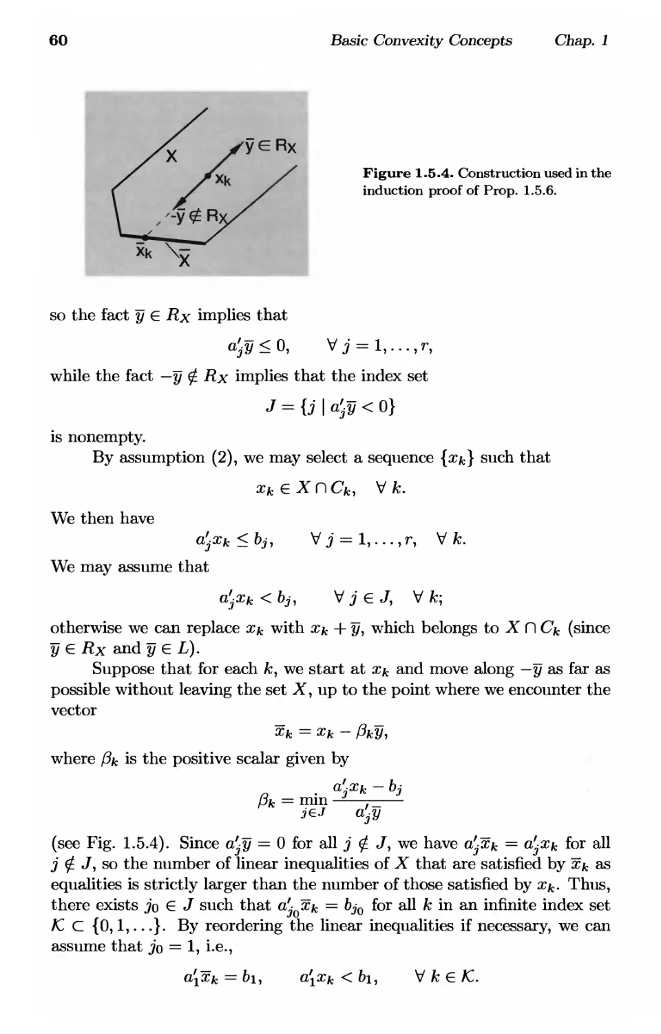
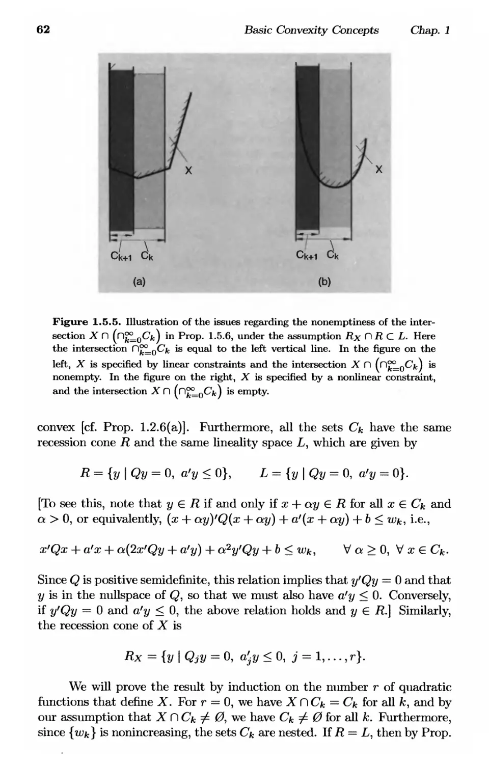
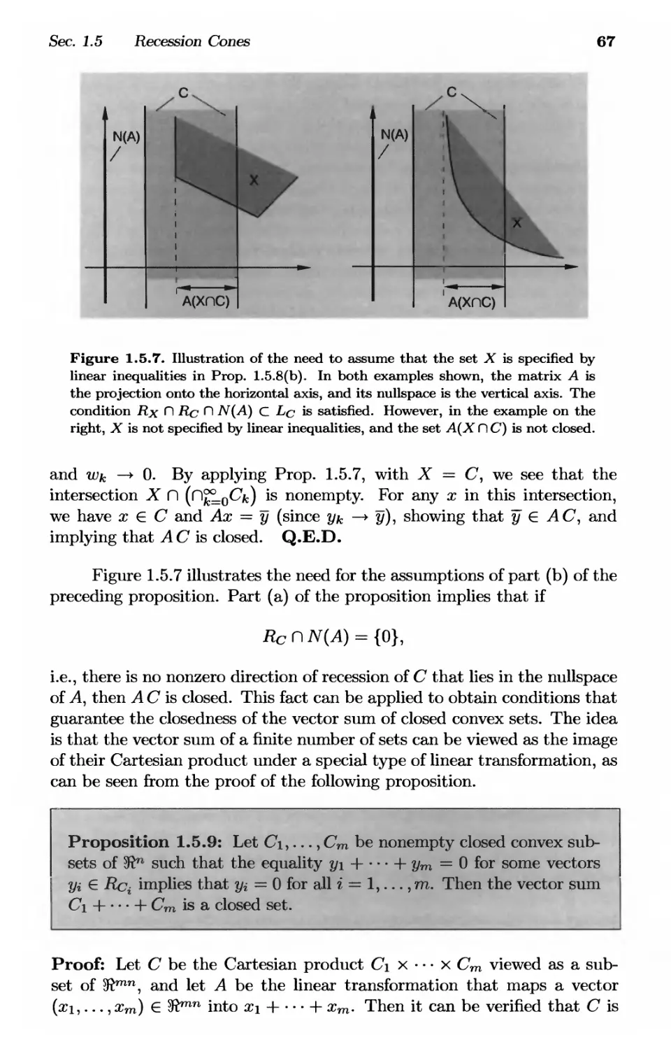
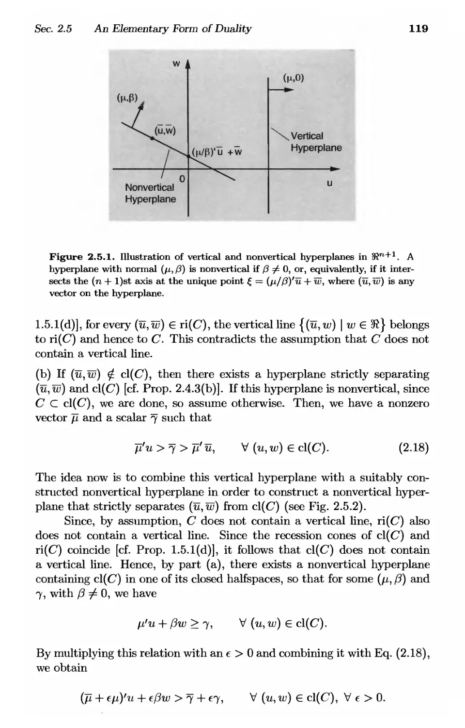
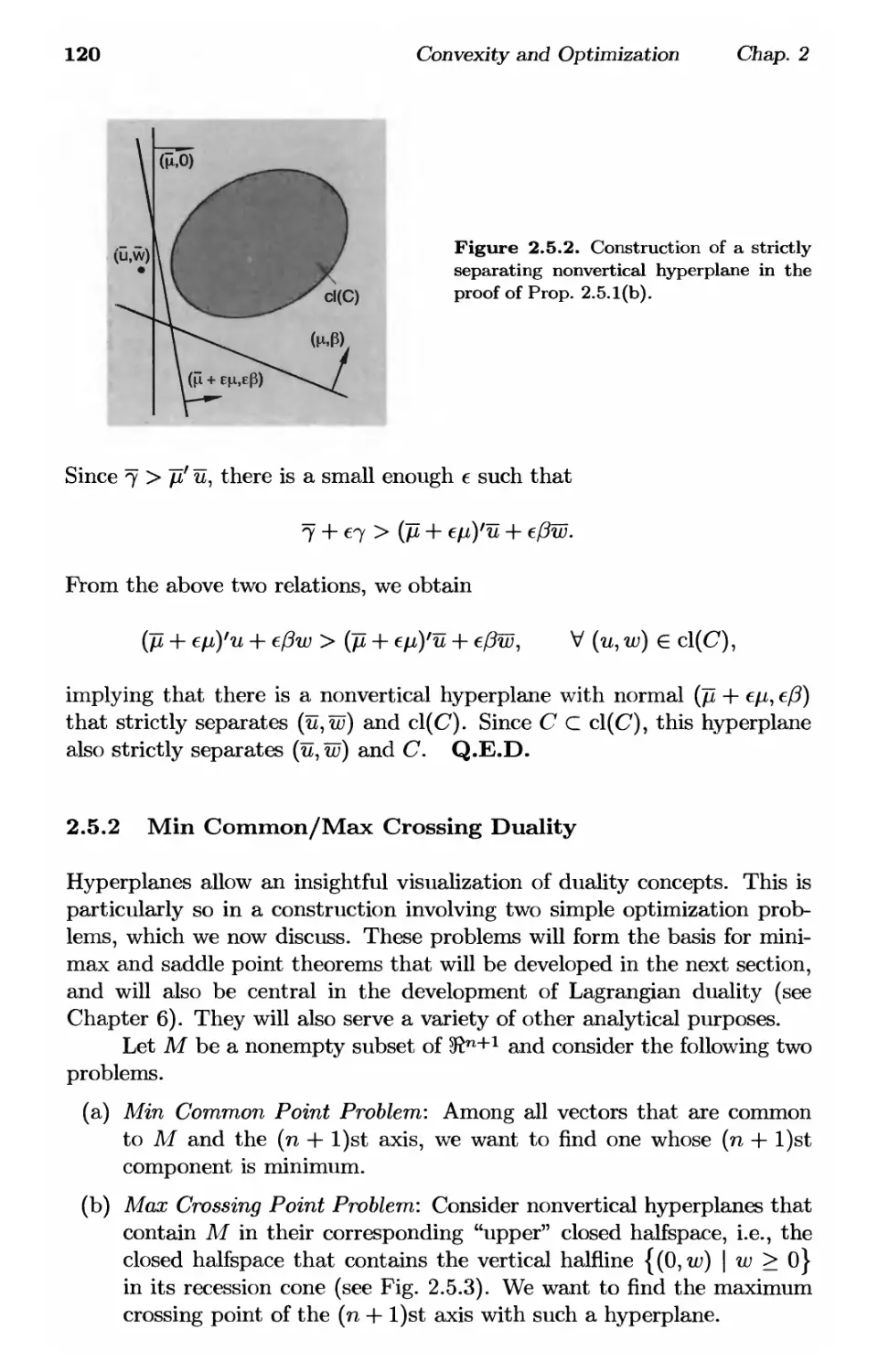
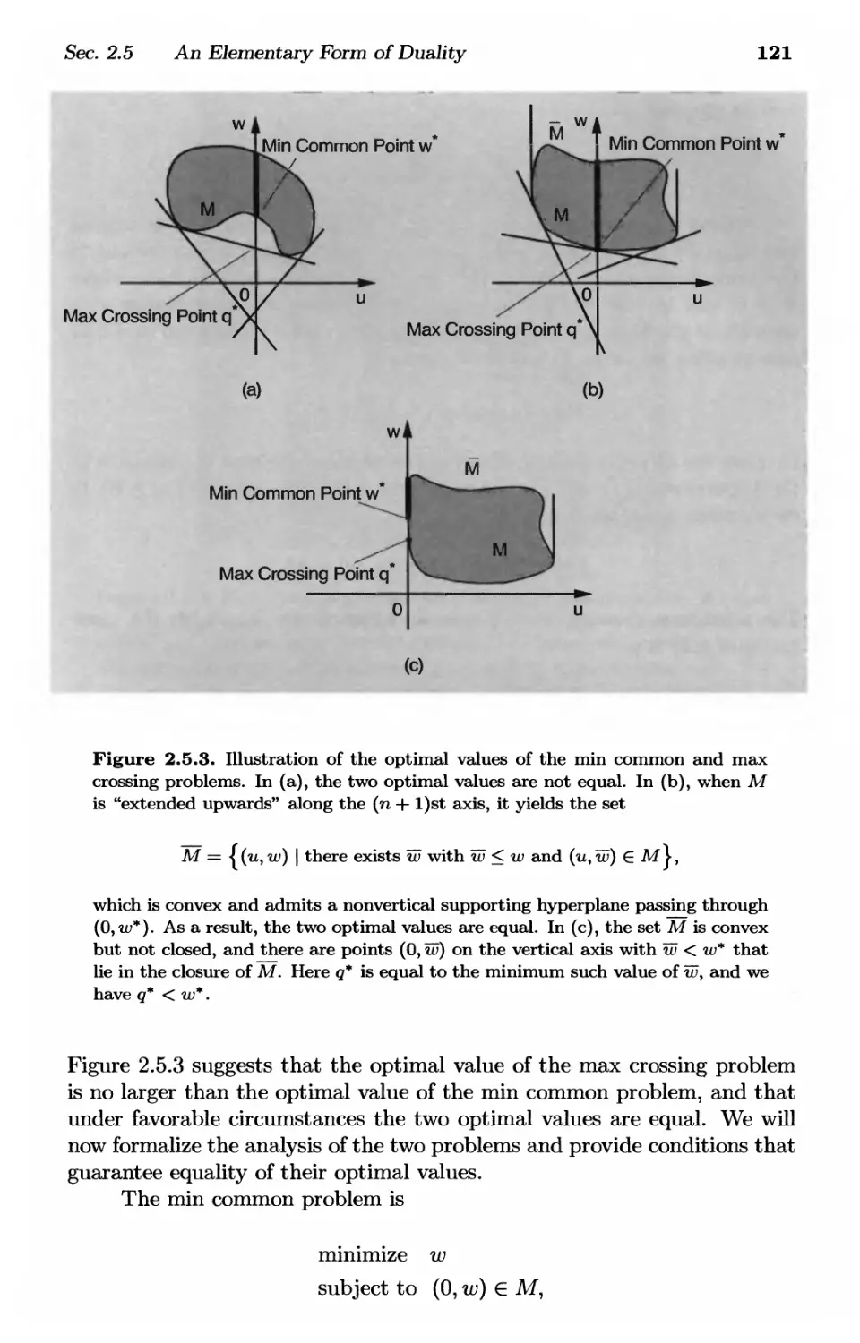
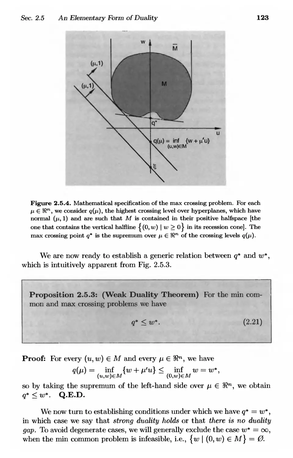
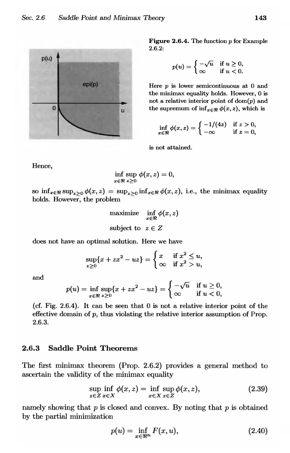
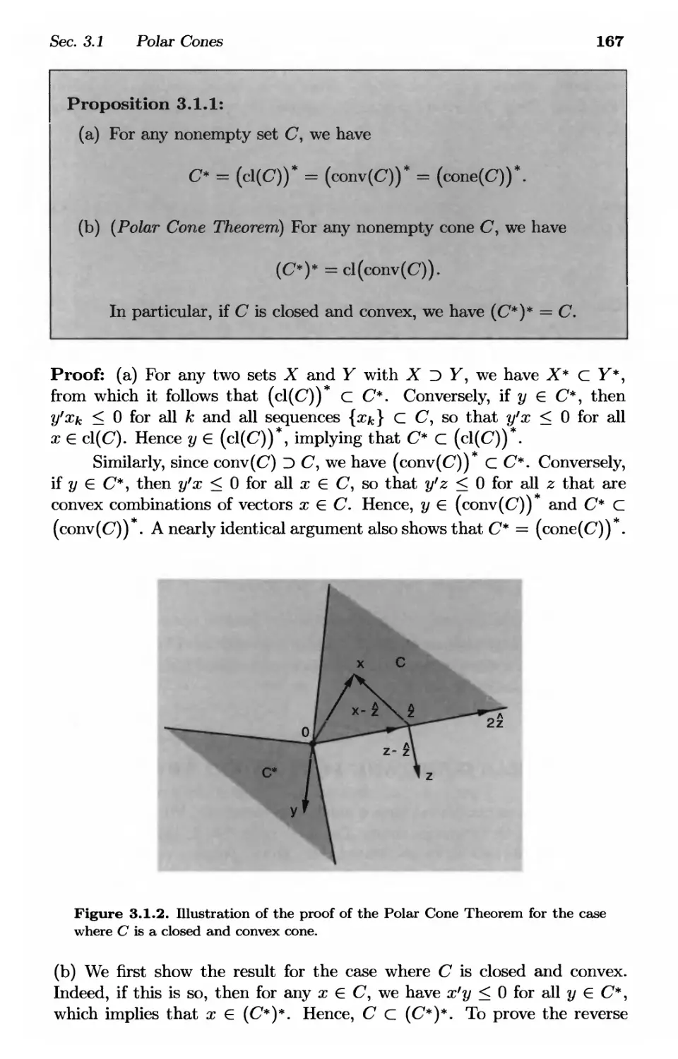
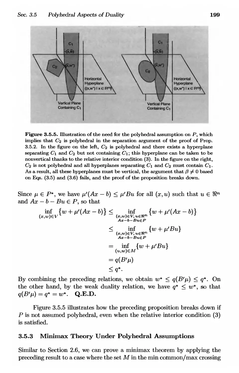
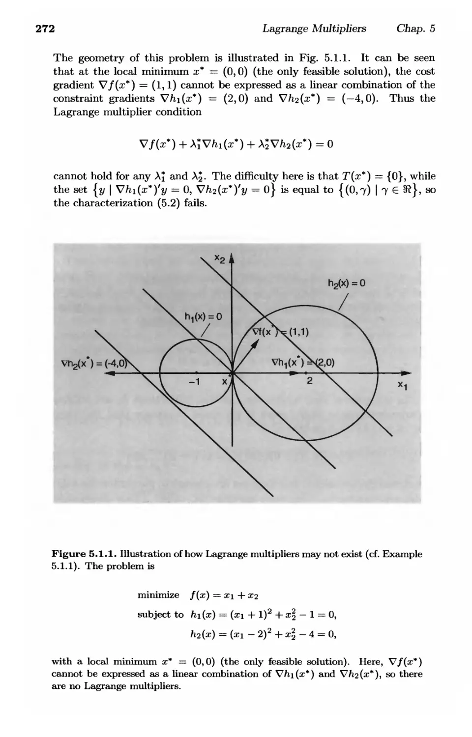
/
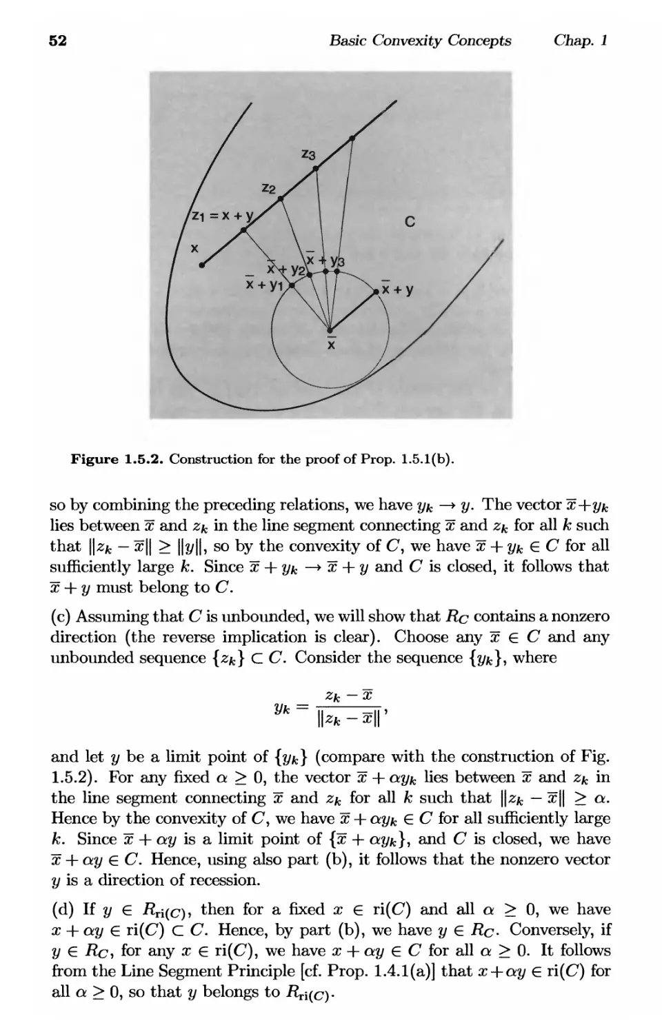


Author: Bertsekas D.P. Nedic A. Ozdaglar A.E.
Tags: mathematics mathematical physics athena scientific optimization convex analysis
ISBN: 1-886529-45-0
Year: 2003


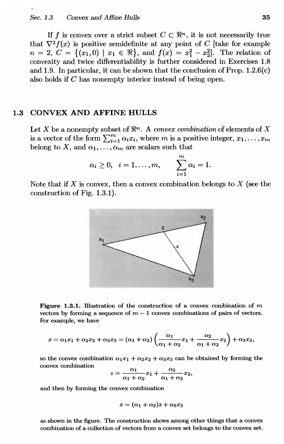
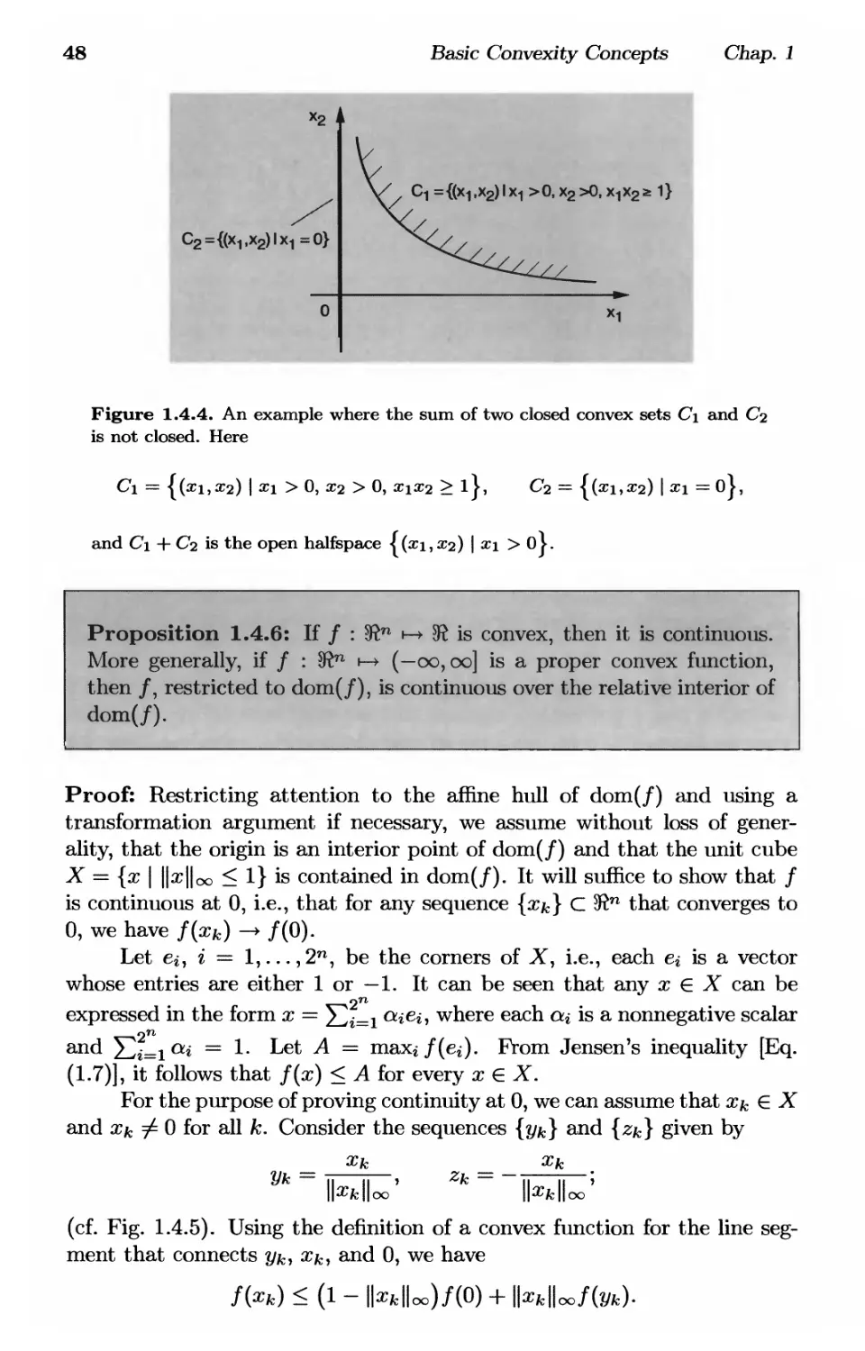
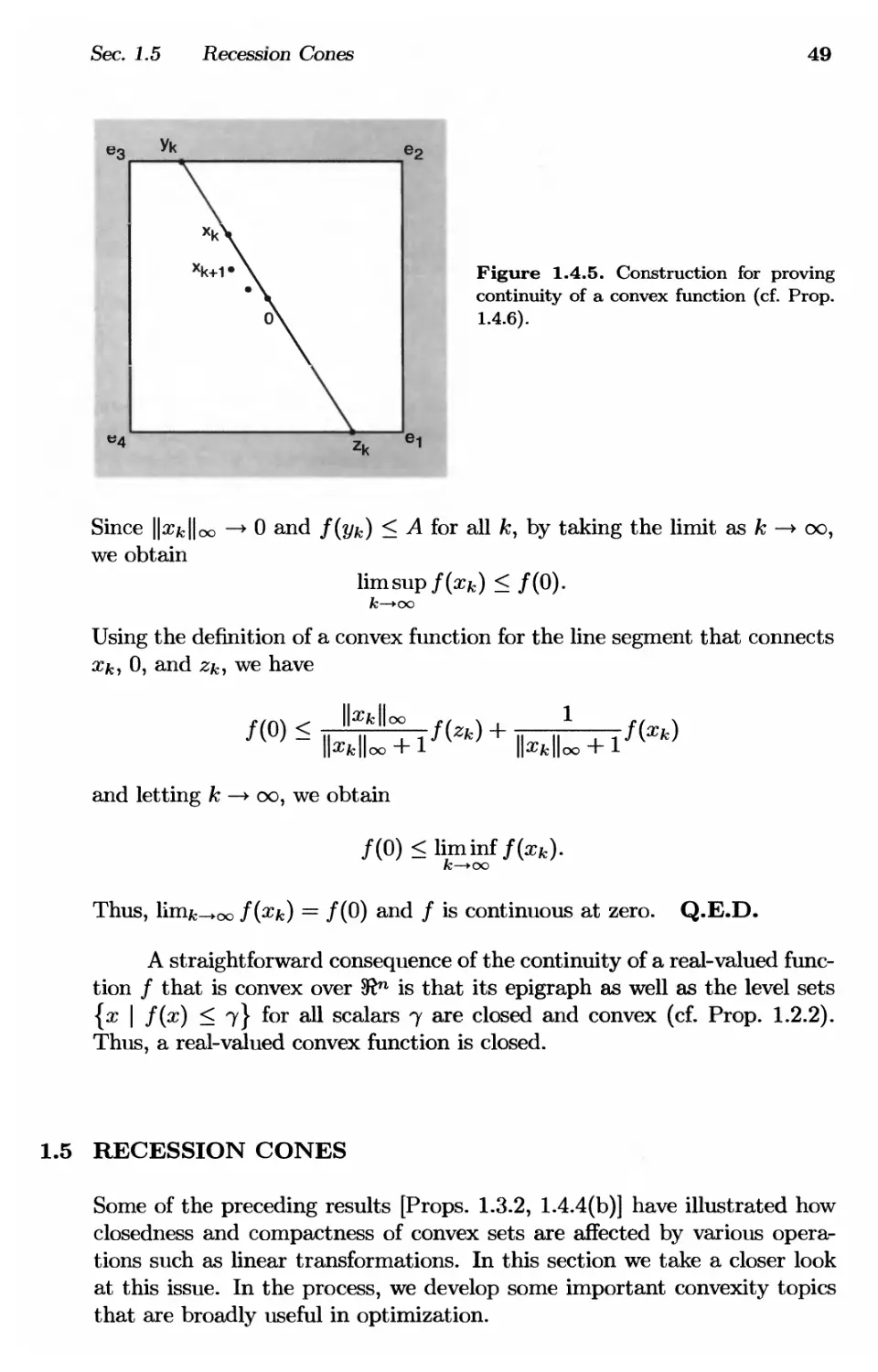
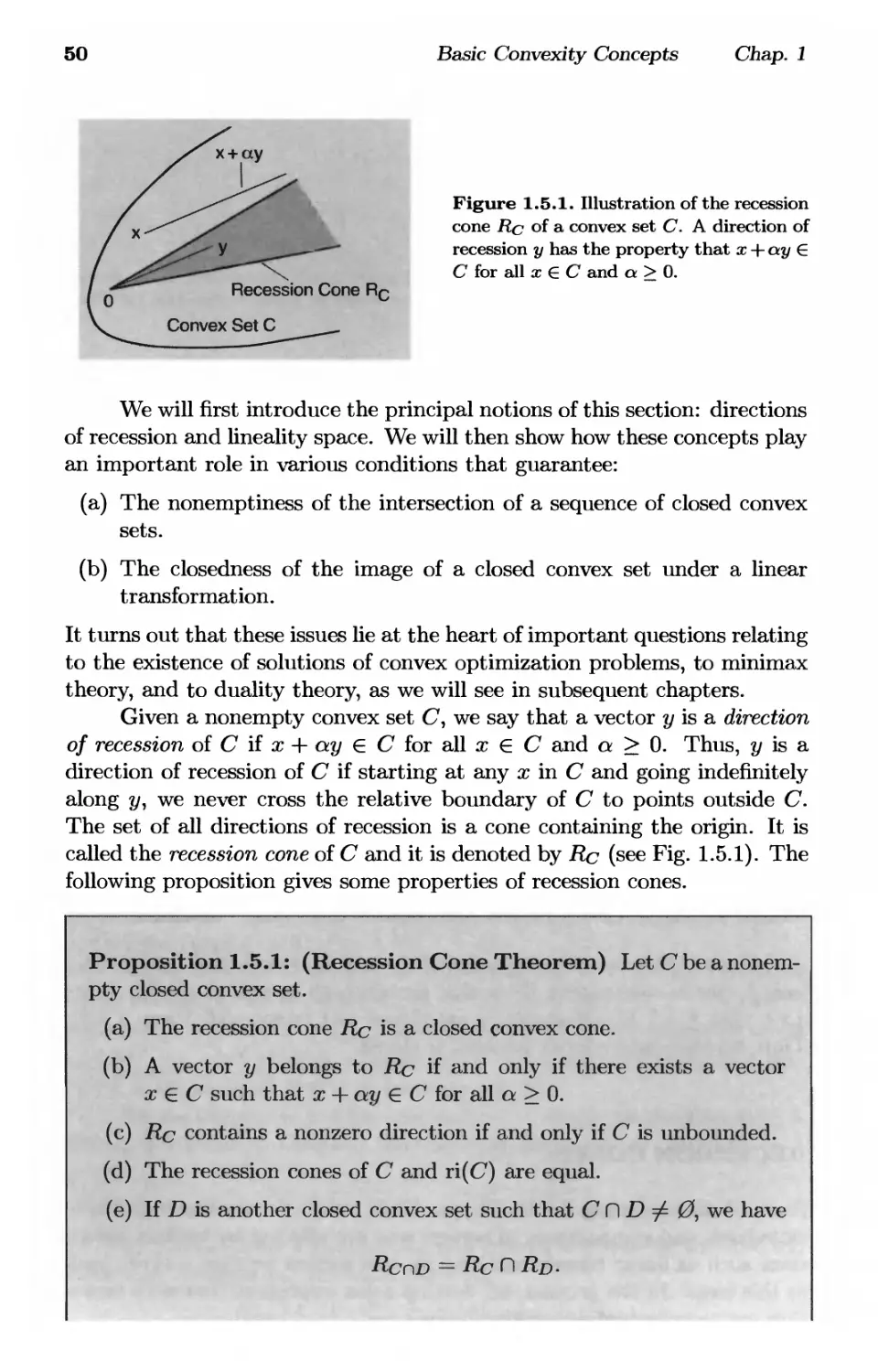
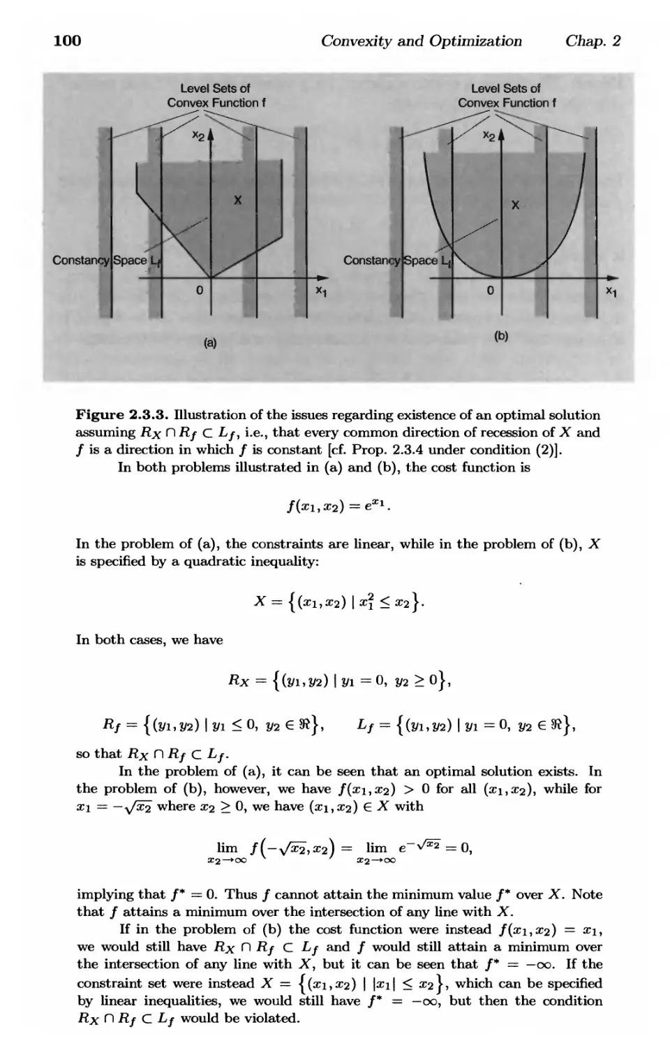
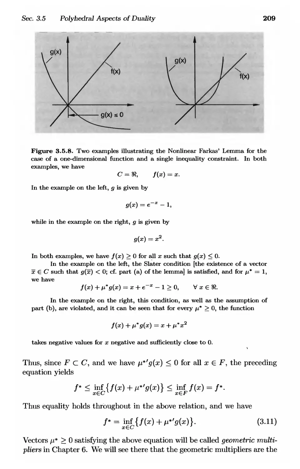
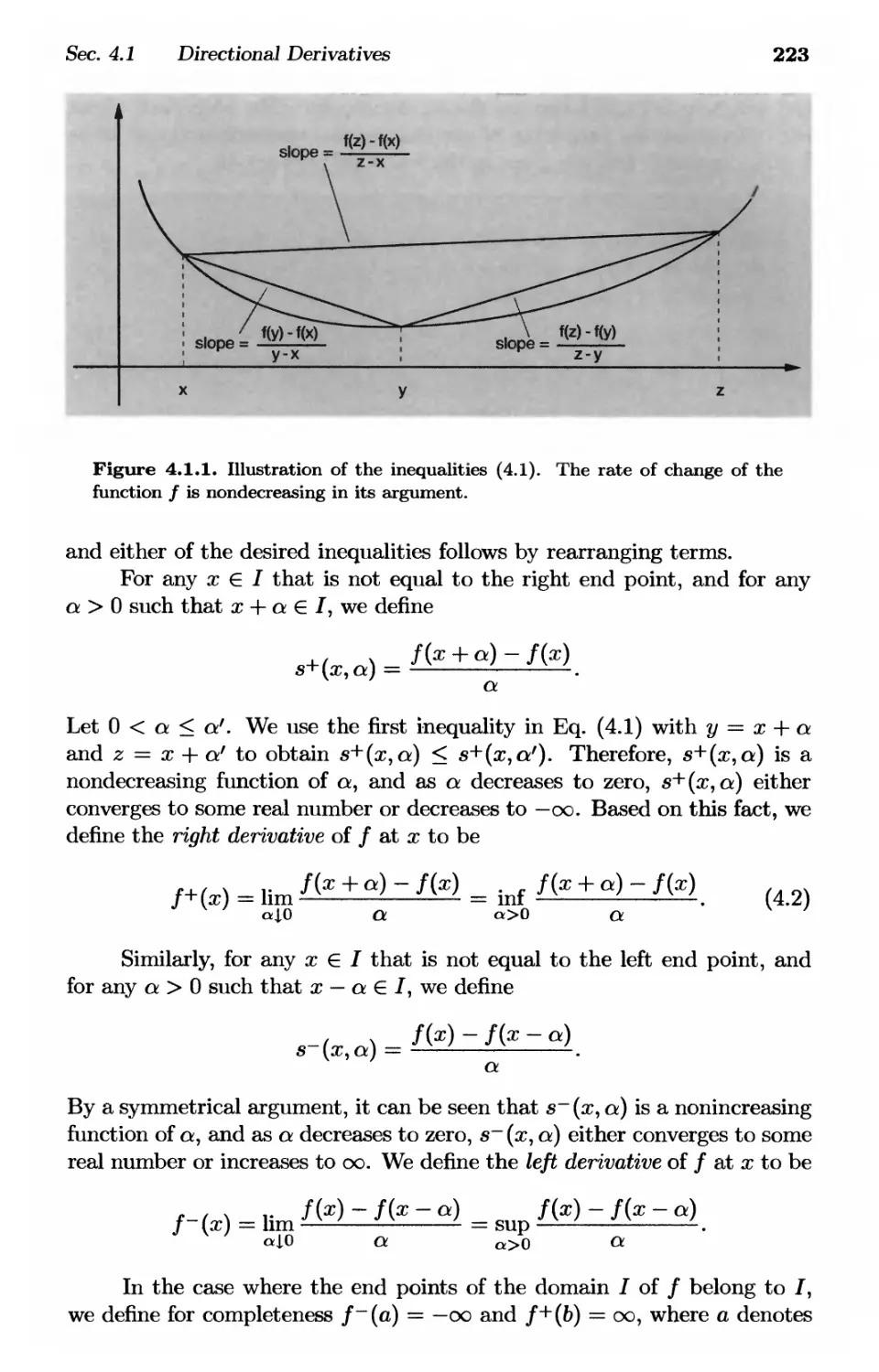
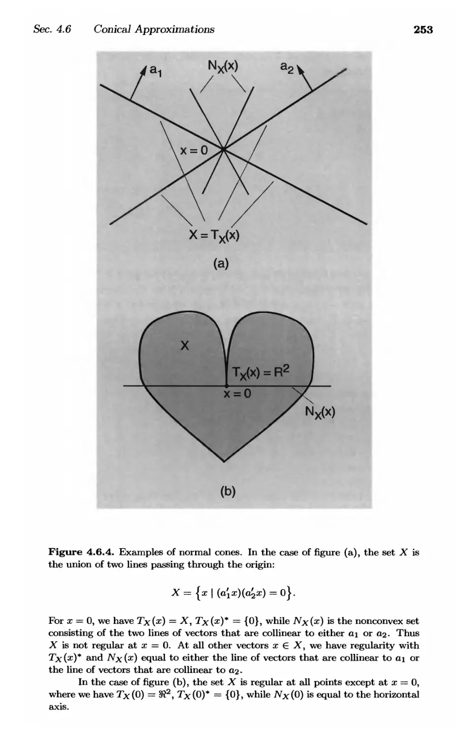
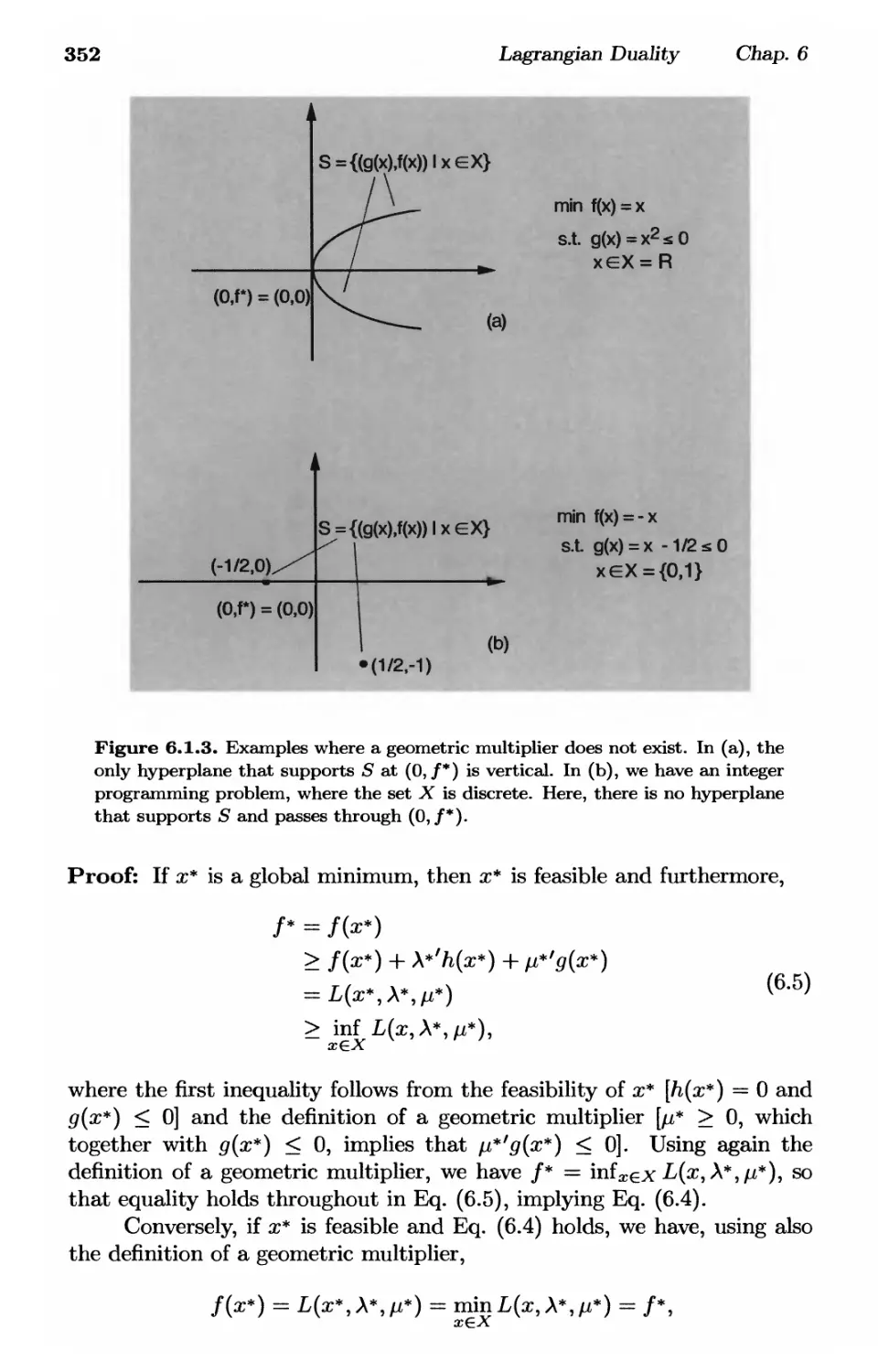
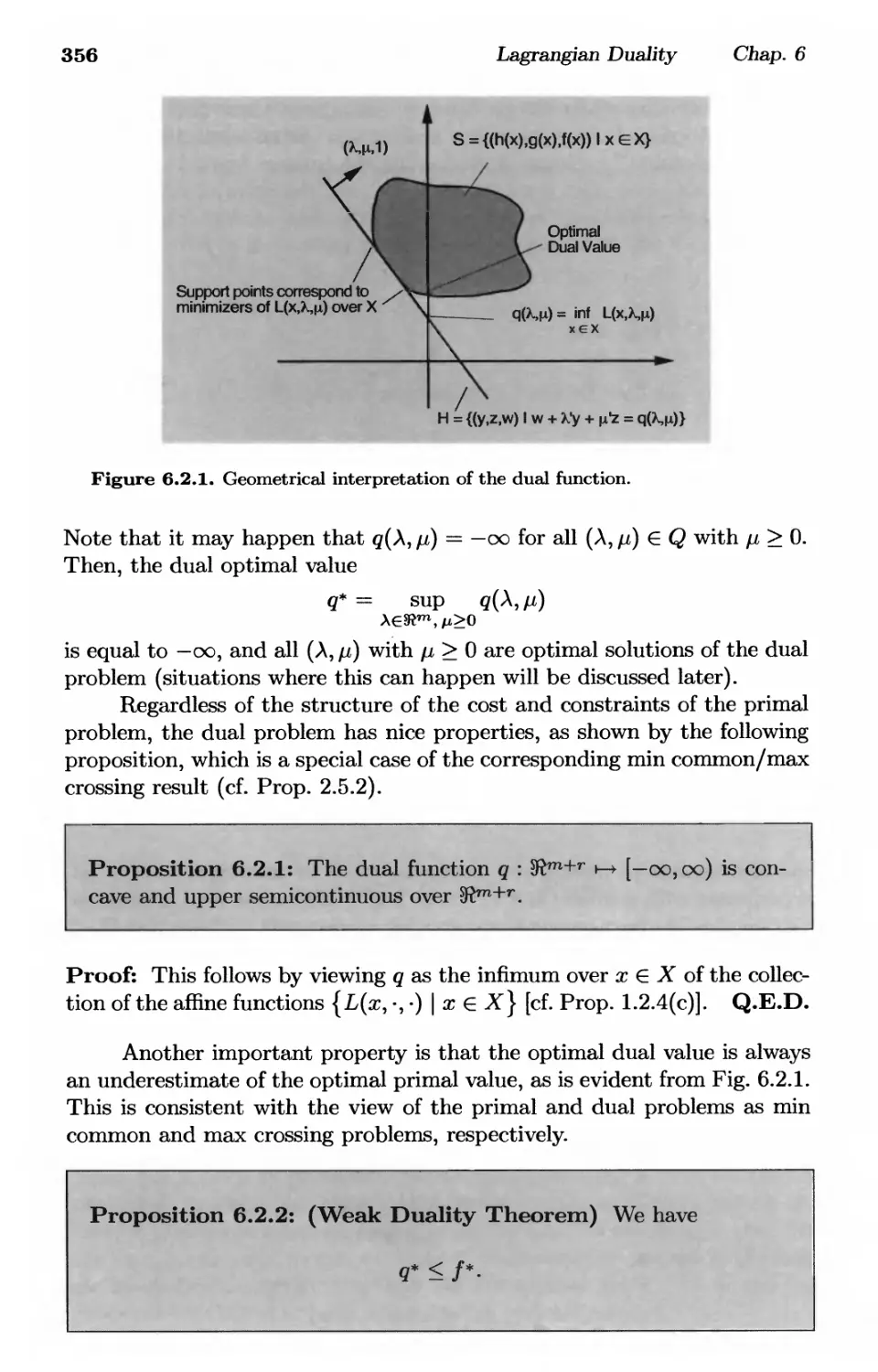
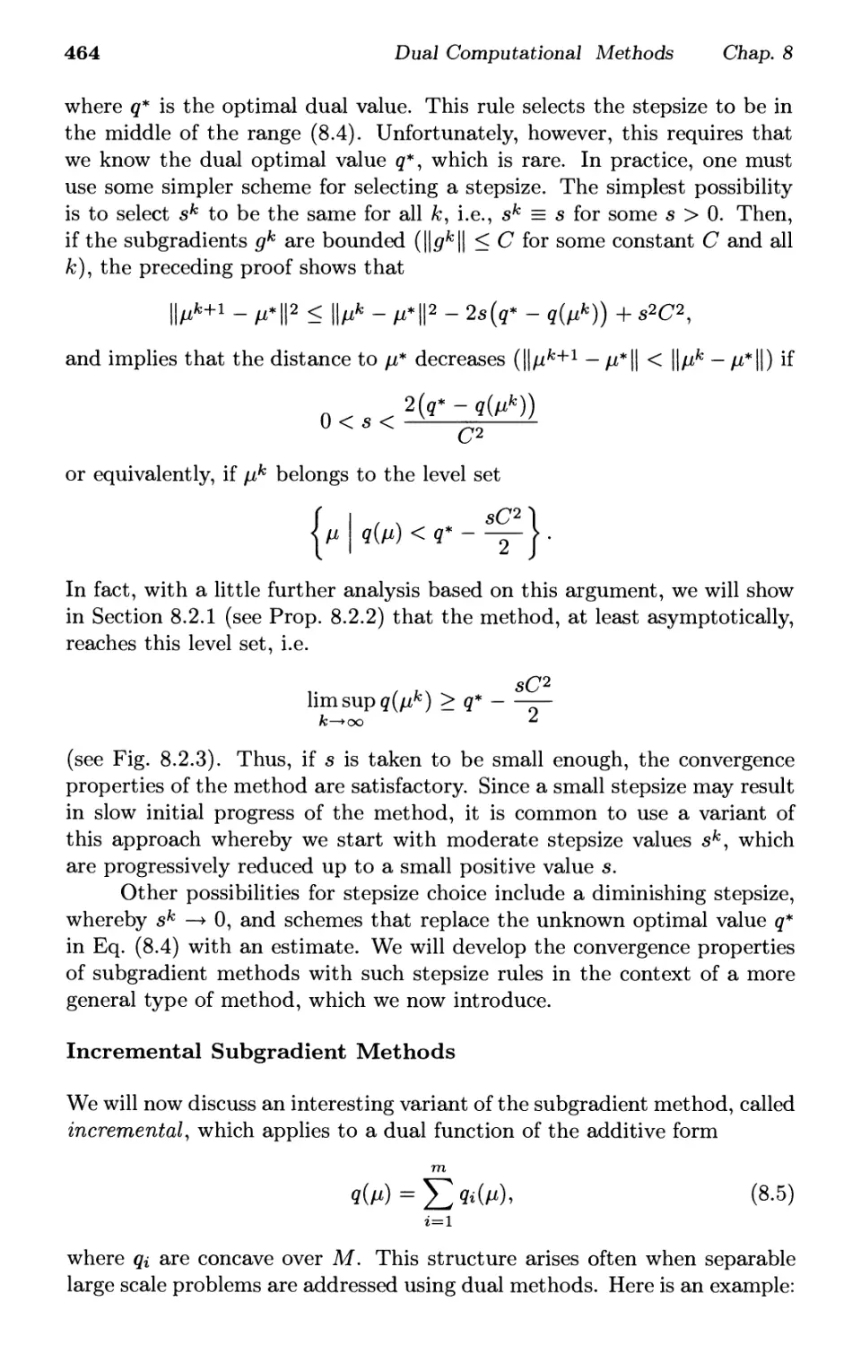
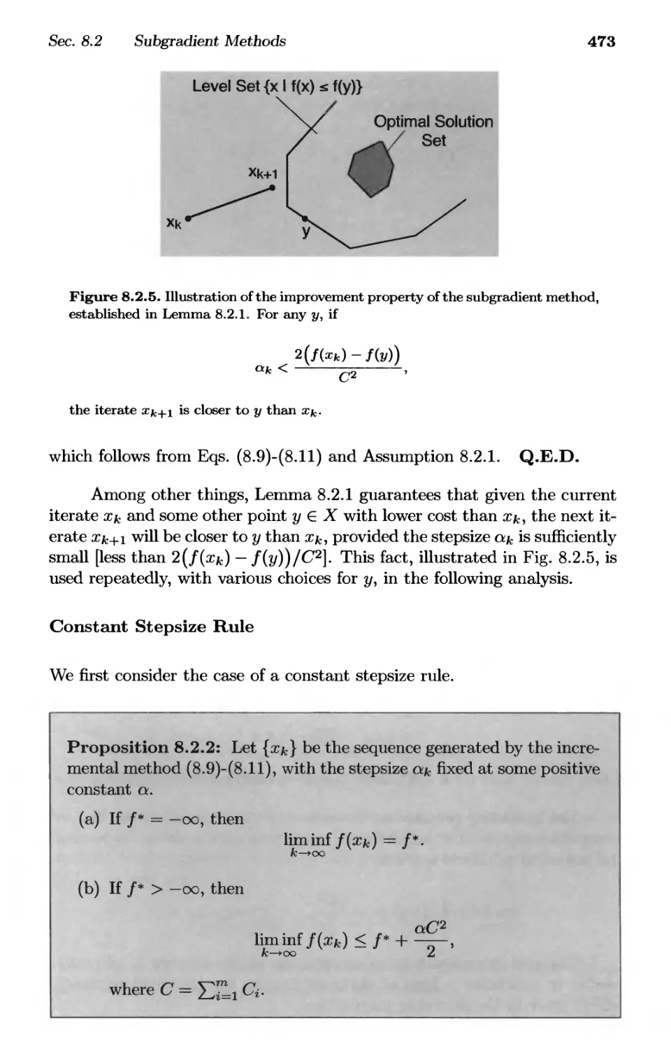
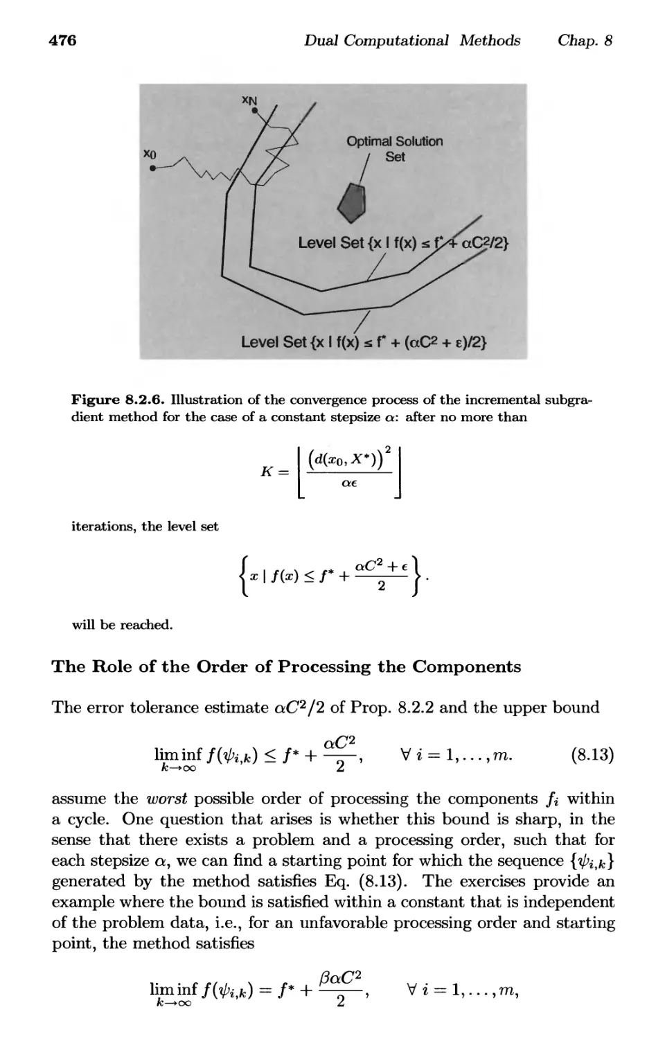
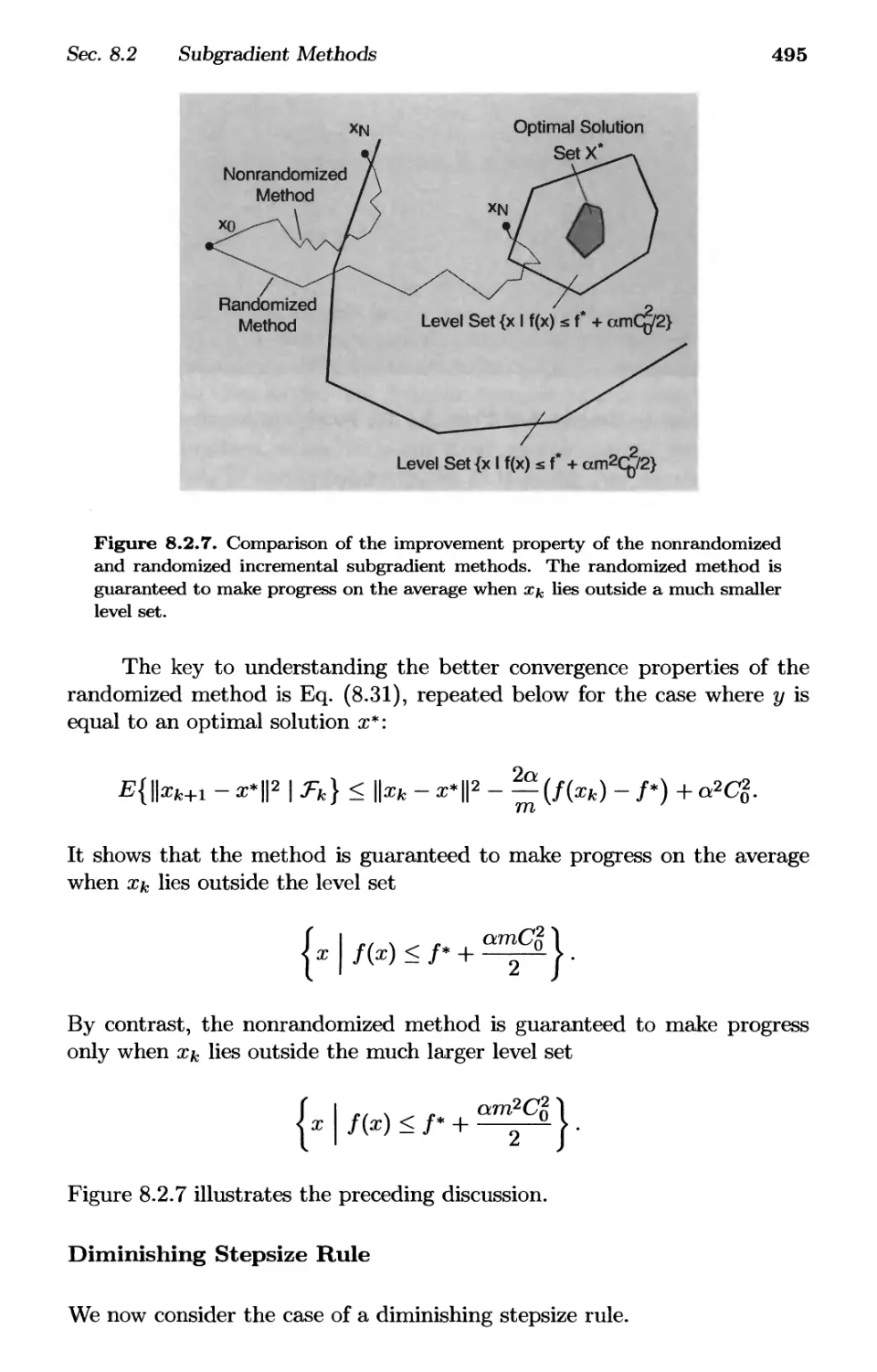
Text
CONVE AN SIS
AND OPT Μ ΑΤΙΟΝ
Dimitri P. Bertsekas with
Angelia Nedic and Asuman E. Ozdaglar
Athena Scientific
Convex Analysis and
Optimization
Dimitri P. Bertsekas
with
Angelia Nedic and Asuman E. Ozdaglar
Massachusetts Institute of Technology
WWW site for book information and orders
http://www.athenasc.com
Athena Scientific, Belmont, Massachusetts
Athena Scientific
Post Office Box 391
Belmont, Mass. 02478-9998
U.S.A.
Email: info@athenasc.com
WWW: http://www.athenasc.com
© 2003 Dimitri P. Bertsekas
All rights reserved. No part of this book may be reproduced in any form
by any electronic or mechanical means (including photocopying, recording,
or information storage and retrieval) without permission in writing from
the publisher.
Publisher's Cataloging-in-Publication Data
Bertsekas, Dimitri P., Nedic, Angelia, Ozdaglar Asuman E.
Convex Analysis and Optimization
Includes bibliographical references and index
1. Nonlinear Programming 2. Mathematical Optimization. I. Title.
T57.8.B475 2003 519.703
Library of Congress Control Number: 2002092168
ISBN 1-886529-45-0
ATHENA SCIENTIFIC
OPTIMIZATION AND COMPUTATION SERIES
1. Convex Analysis and Optimization, by Dimitri P. Bertsekas, with
Angelia Nedic and Asuman E. Ozdaglar, 2003, ISBN 1-886529-
45-0, 560 pages
2. Introduction to Probability, by Dimitri P. Bertsekas and John N.
Tsitsiklis, 2002, ISBN 1-886529-40-X, 430 pages
3. Dynamic Programming and Optimal Control, Two-Volume Set
(2nd Edition), by Dimitri P. Bertsekas, 2001, ISBN 1-886529-08-
6, 840 pages
4. Nonlinear Programming, 2nd Edition, by Dimitri P. Bertsekas,
1999, ISBN 1-886529-00-0, 791 pages
5. Network Optimization: Continuous and Discrete Models by
Dimitri P. Bertsekas, 1998, ISBN 1-886529-02-7, 608 pages
6. Network Flows and Monotropic Optimization by R. Tyrrell Rock-
afellar, 1998, ISBN 1-886529-06-X, 634 pages
7. Introduction to Linear Optimization by Dimitris Bertsimas and
John N. Tsitsiklis, 1997, ISBN 1-886529-19-1, 608 pages
8. Parallel and Distributed Computation: Numerical Methods by
Dimitri P. Bertsekas and John N. Tsitsiklis, 1997, ISBN 1-886529-
01-9, 718 pages
9. Neuro-Dynamic Programming, by Dimitri P. Bertsekas and John
N. Tsitsiklis, 1996, ISBN 1-886529-10-8, 512 pages
10. Constrained Optimization and Lagrange Multiplier Methods, by
Dimitri P. Bertsekas, 1996, ISBN 1-886529-04-3, 410 pages
11. Stochastic Optimal Control: The Discrete-Time Case by Dimitri
P. Bertsekas and Steven E. Shreve, 1996, ISBN 1-886529-03-5,
330 pages
Contents
1. Basic Convexity Concepts p. 1
1.1. Linear Algebra and Real Analysis p. 3
1.1.1. Vectors and Matrices p. 5
1.1.2. Topological Properties p. 8
1.1.3. Square Matrices p. 15
1.1.4. Derivatives p. 16
1.2. Convex Sets and Functions p. 20
1.3. Convex and Affine Hulls p. 35
1.4. Relative Interior, Closure, and Continuity p. 39
1.5. Recession Cones p. 49
1.5.1. Nonemptiness of Intersections of Closed Sets p. 56
1.5.2. Closedness Under Linear Transformations p. 64
1.6. Notes, Sources, and Exercises p. 68
2. Convexity and Optimization p. 83
2.1. Global and Local Minima p. 84
2.2. The Projection Theorem p. 88
2.3. Directions of Recession and Existence of Optimal Solutions . . p. 92
2.3.1. Existence of Solutions of Convex Programs p. 94
2.3.2. Unbounded Optimal Solution Sets p. 97
2.3.3. Partial Minimization of Convex Functions p. 101
2.4. Hyperplanes p. 107
2.5. An Elementary Form of Duality p. 117
2.5.1. Nonvertical Hyperplanes p. 117
2.5.2. Min Common/Max Crossing Duality p. 120
2.6. Saddle Point and Minimax Theory p. 128
2.6.1. Min Common/Max Crossing Framework for Minimax . p. 133
2.6.2. Minimax Theorems p. 139
2.6.3. Saddle Point Theorems p. 143
2.7. Notes, Sources, and Exercises p. 151
ν
vi Contents
3. Polyhedral Convexity p. 165
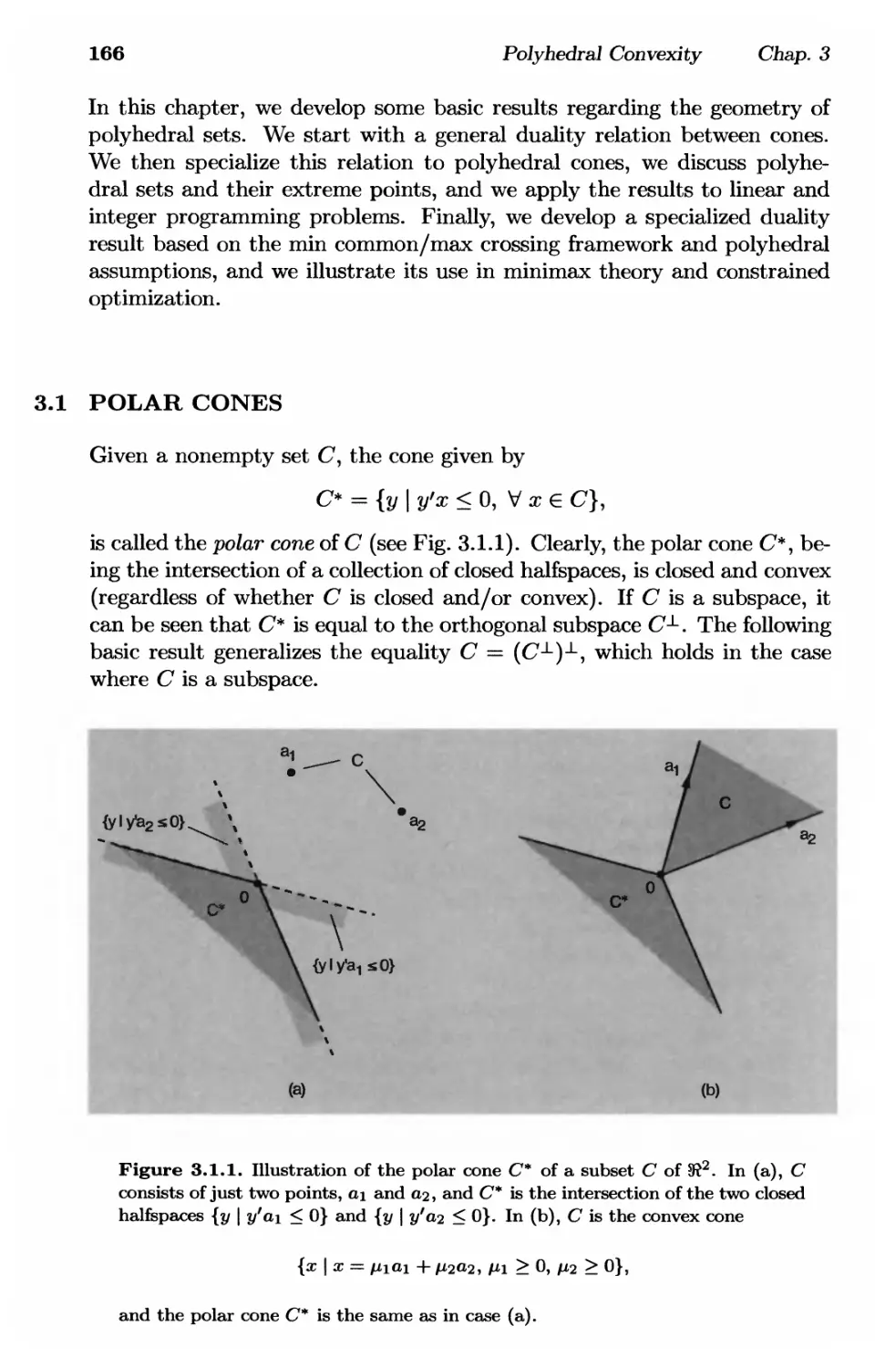
3.1. Polar Cones p. 166
3.2. Polyhedral Cones and Polyhedral Sets p. 168
3.2.1. Farkas' Lemma and Minkowski-Weyl Theorem .... p. 170
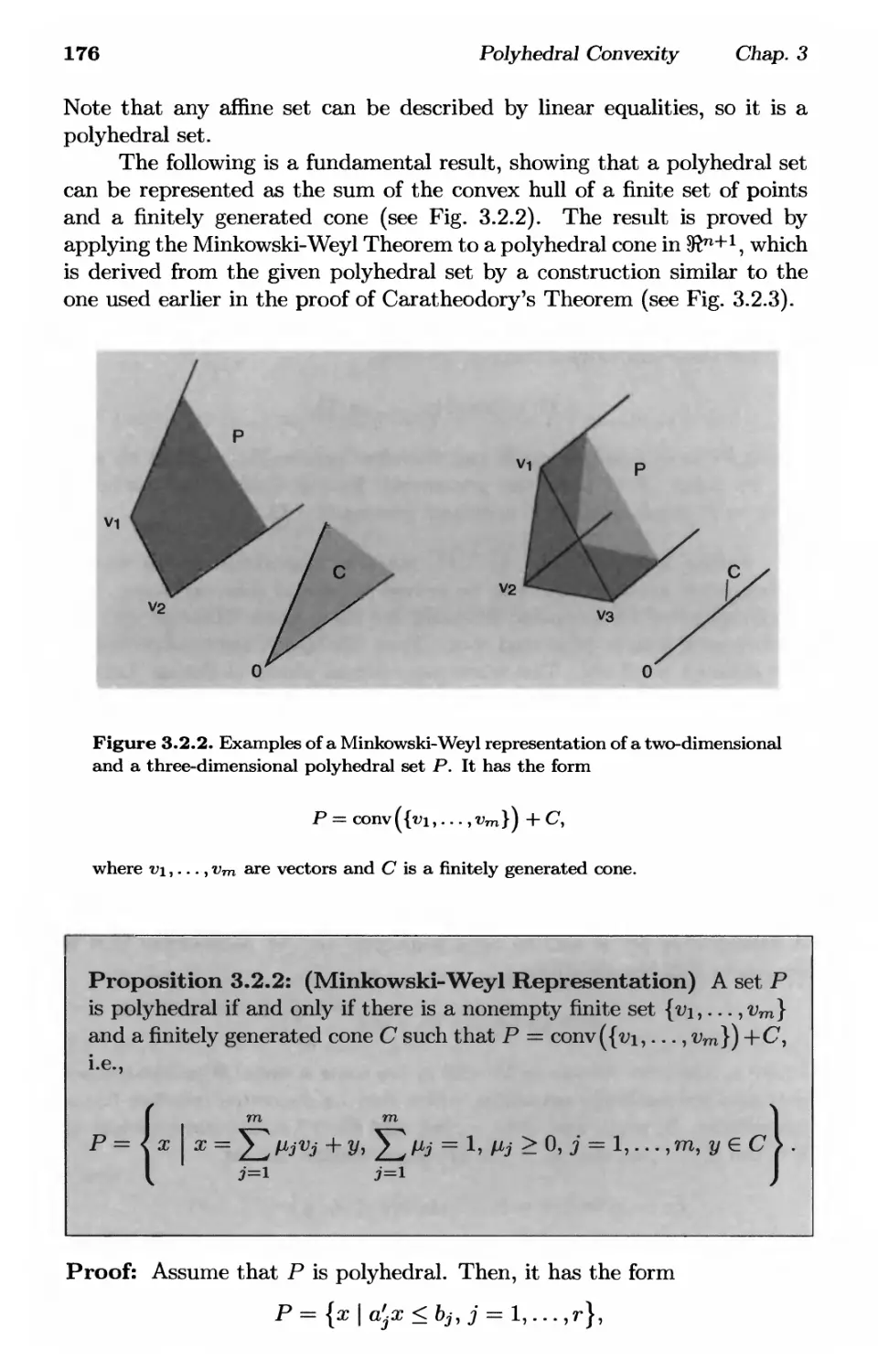
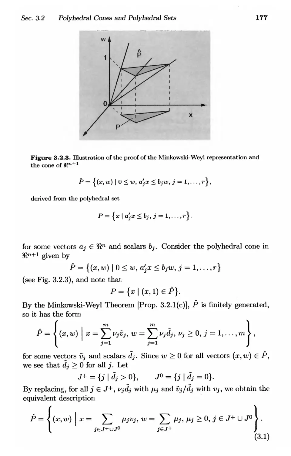
3.2.2. Polyhedral Sets p. 175
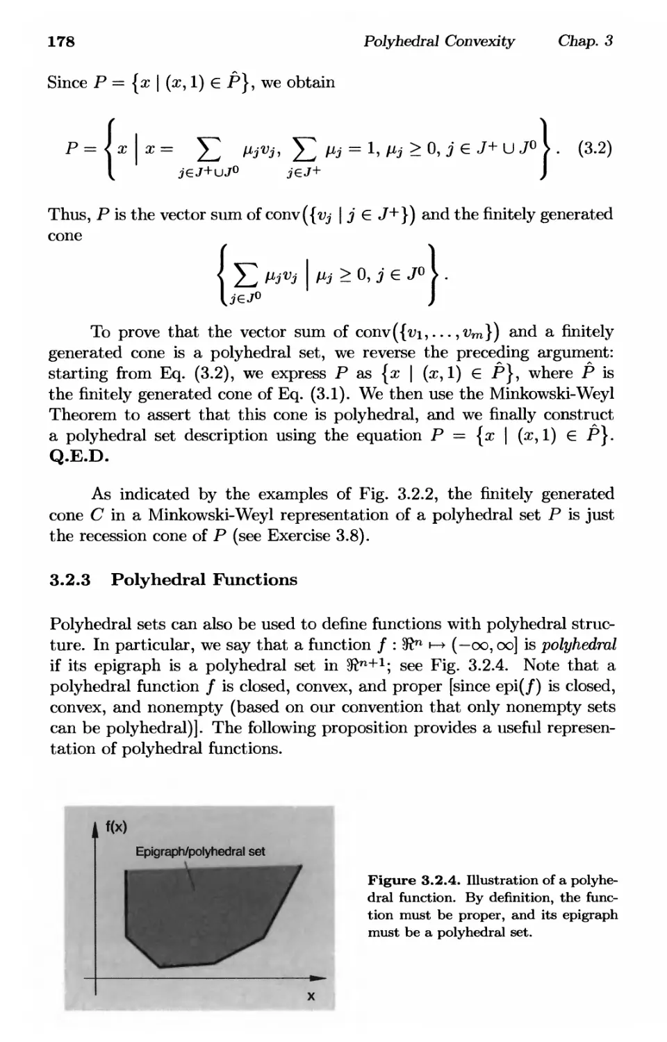
3.2.3. Polyhedral Functions p. 178
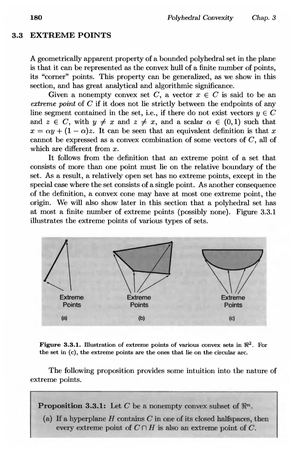
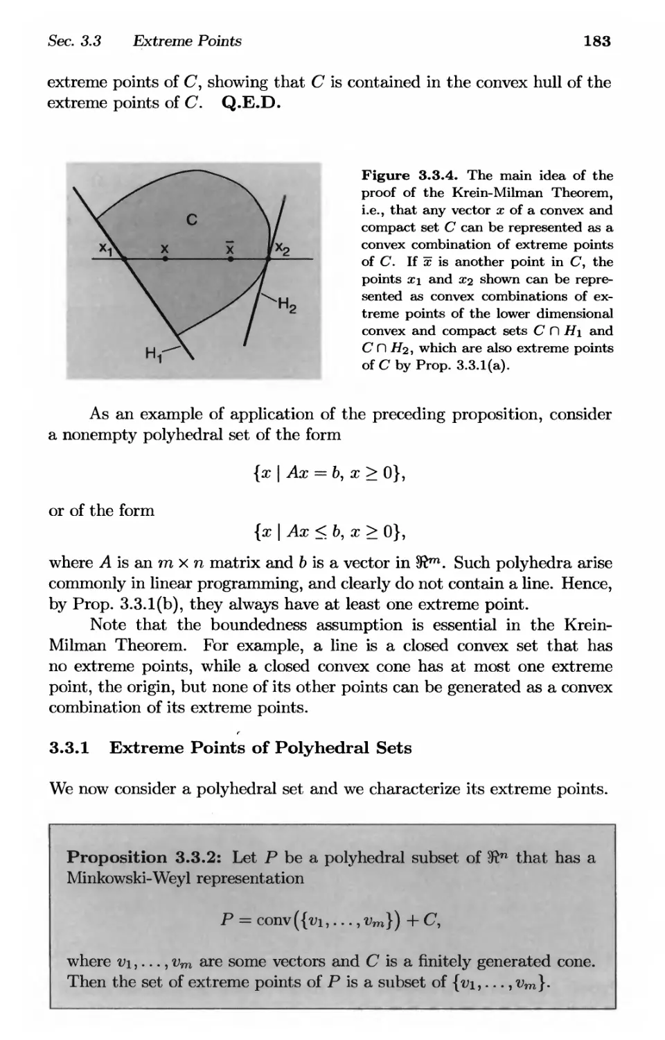
3.3. Extreme Points p. 180
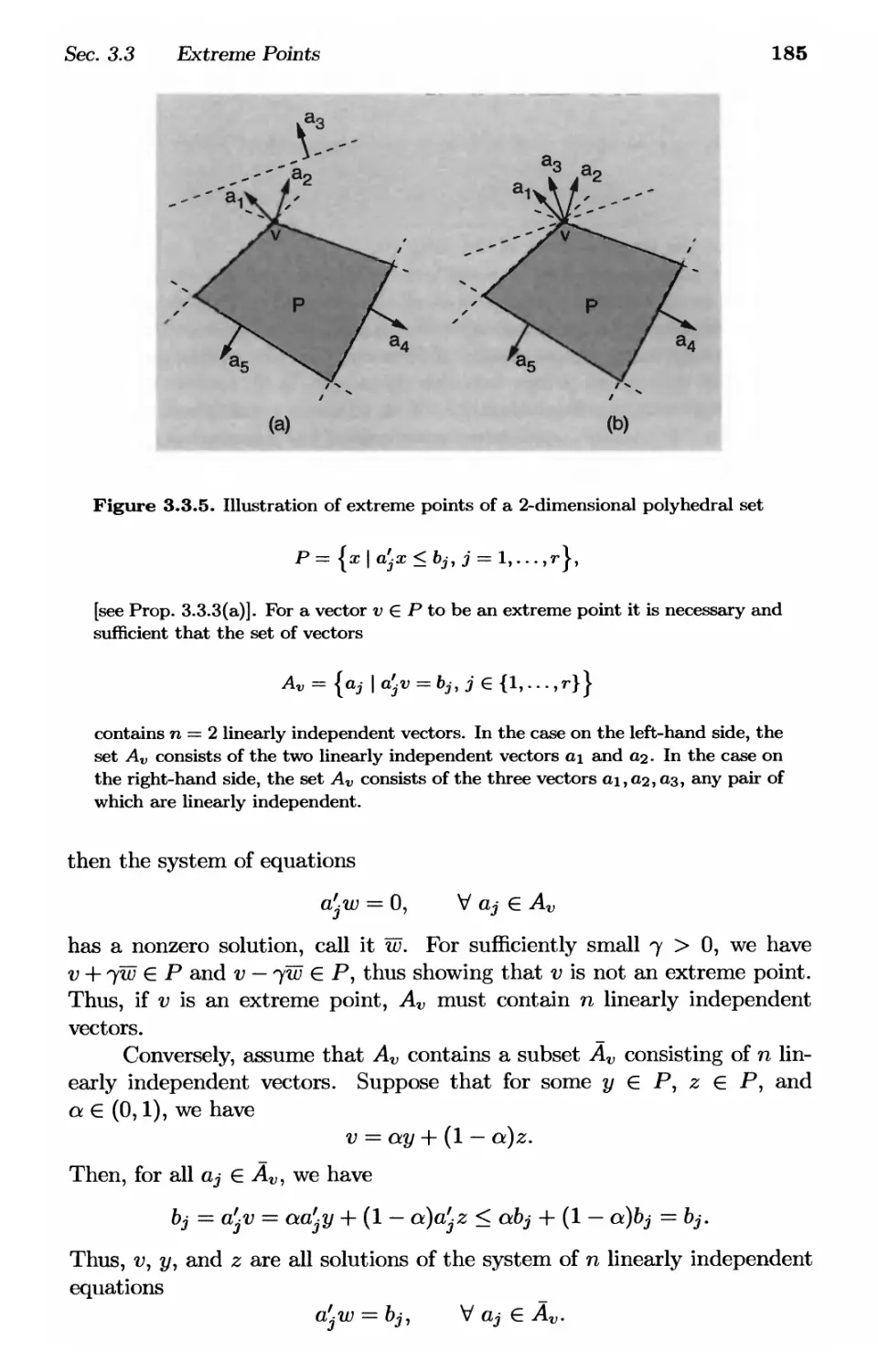
3.3.1. Extreme Points of Polyhedral Sets p. 183
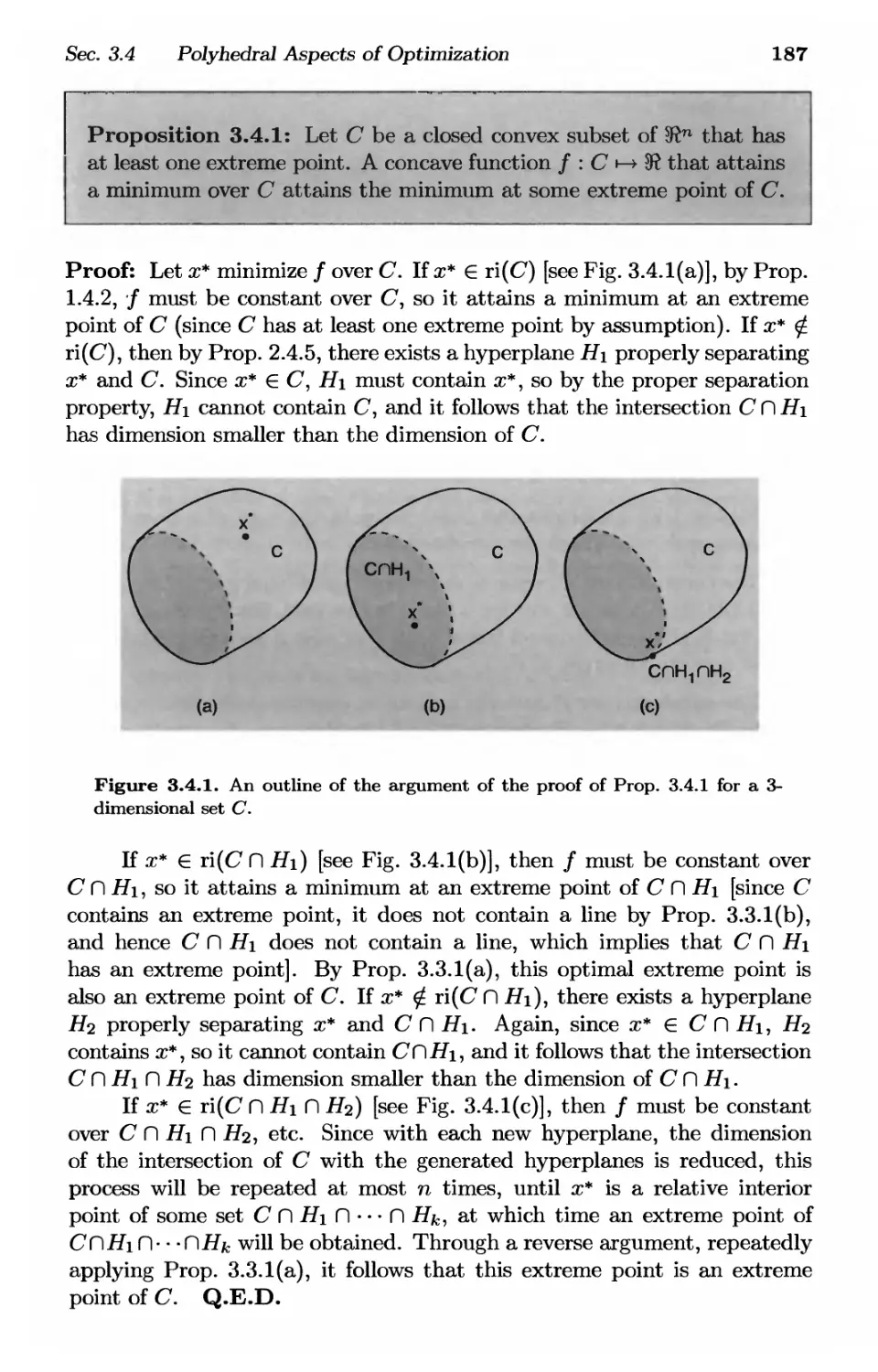
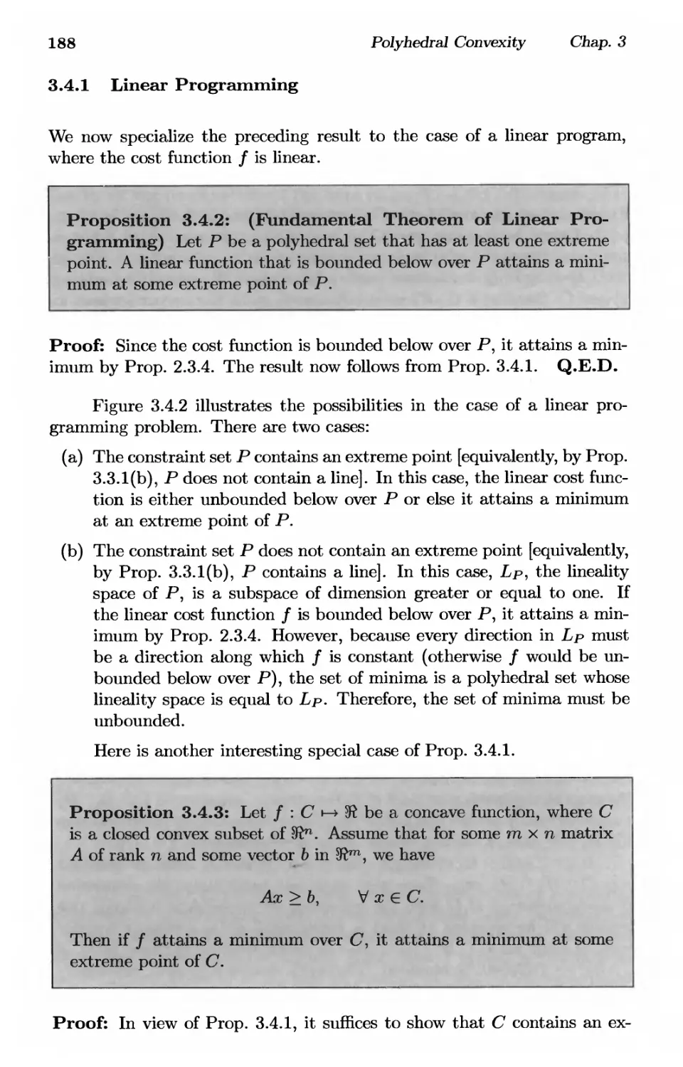
3.4. Polyhedral Aspects of Optimization p. 186
3.4.1. Linear Programming p. 188
3.4.2. Integer Programming p. 189
3.5. Polyhedral Aspects of Duality p. 192
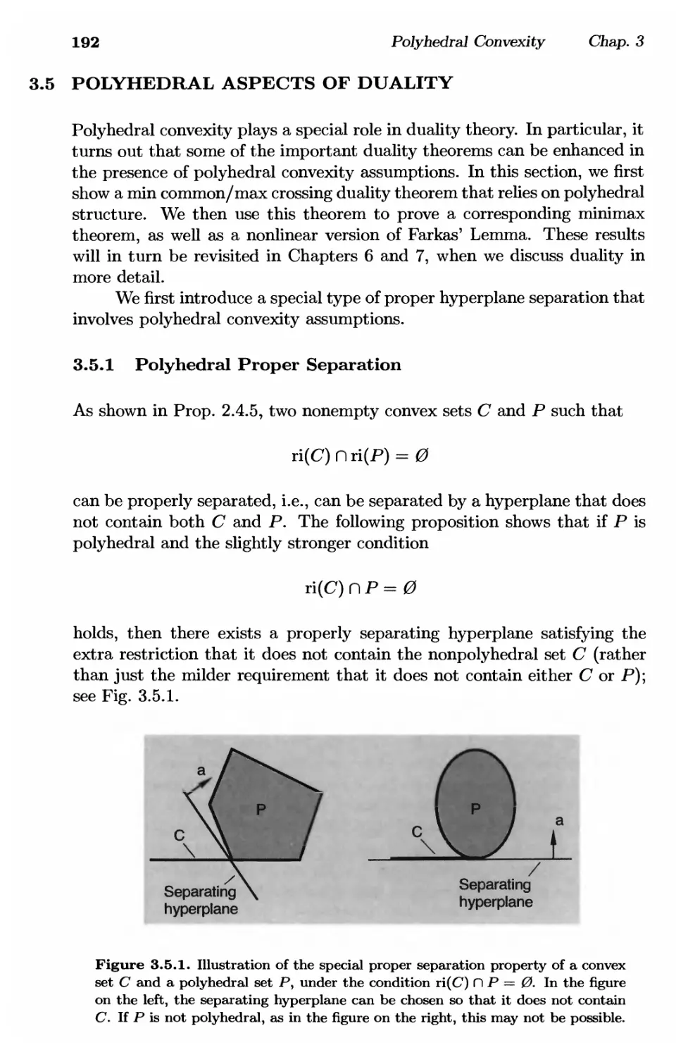
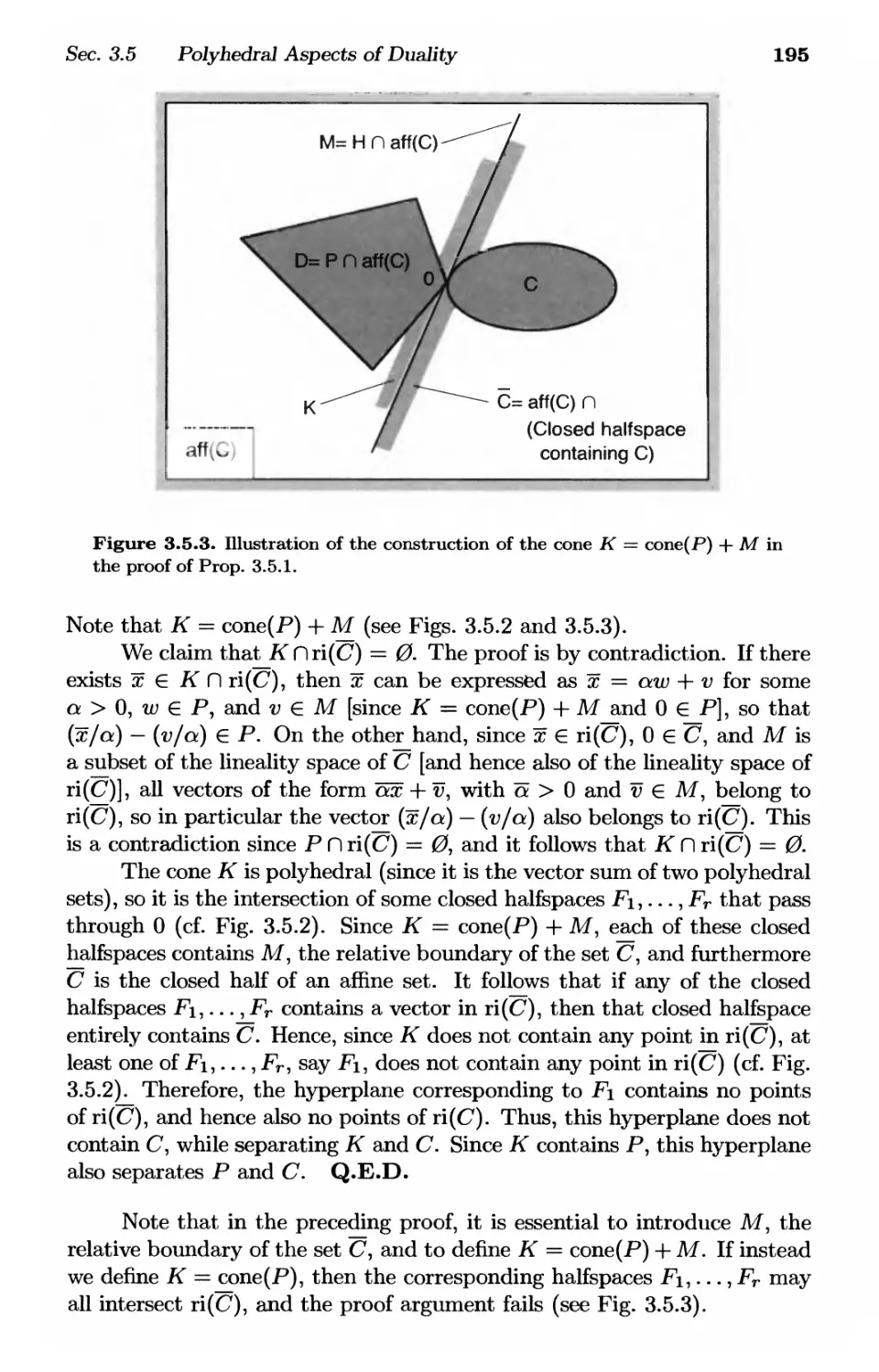
3.5.1. Polyhedral Proper Separation p. 192
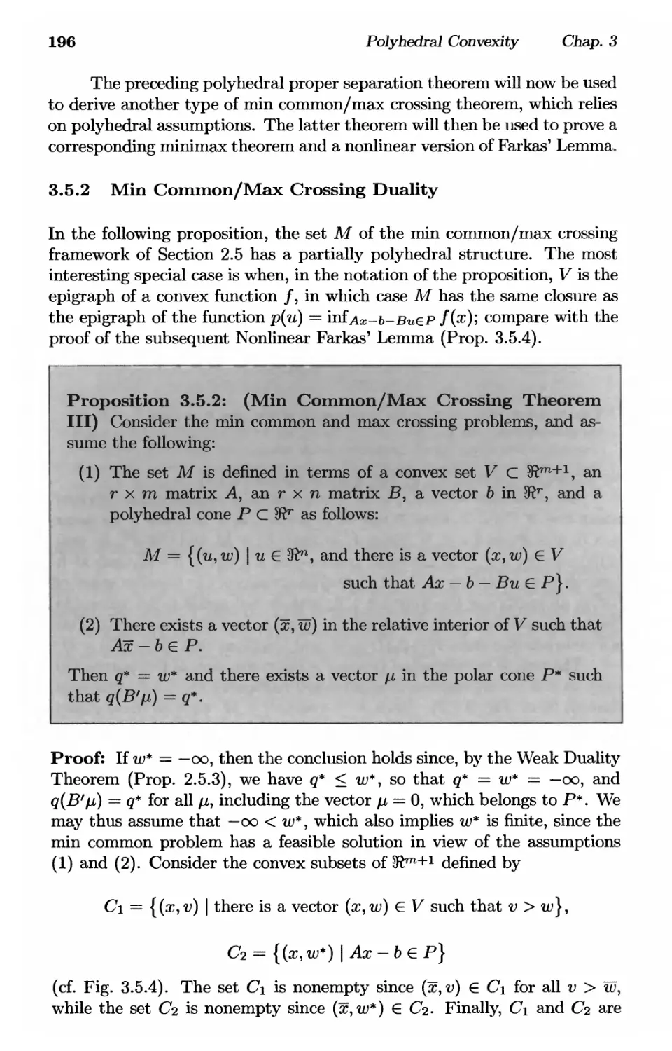
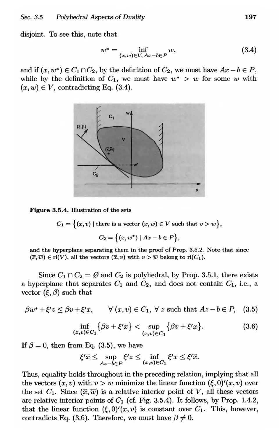
3.5.2. Min Common/Max Crossing Duality p. 196
3.5.3. Minimax Theory Under Polyhedral Assumptions ... p. 199
3.5.4. A Nonlinear Version of Farkas' Lemma p. 203
3.5.5. Convex Programming p. 208
3.6. Notes, Sources, and Exercises p. 210
4. Subgradients and Constrained Optimization p. 221
4.1. Directional Derivatives p. 222
4.2. Subgradients and Subdifferentials p. 227
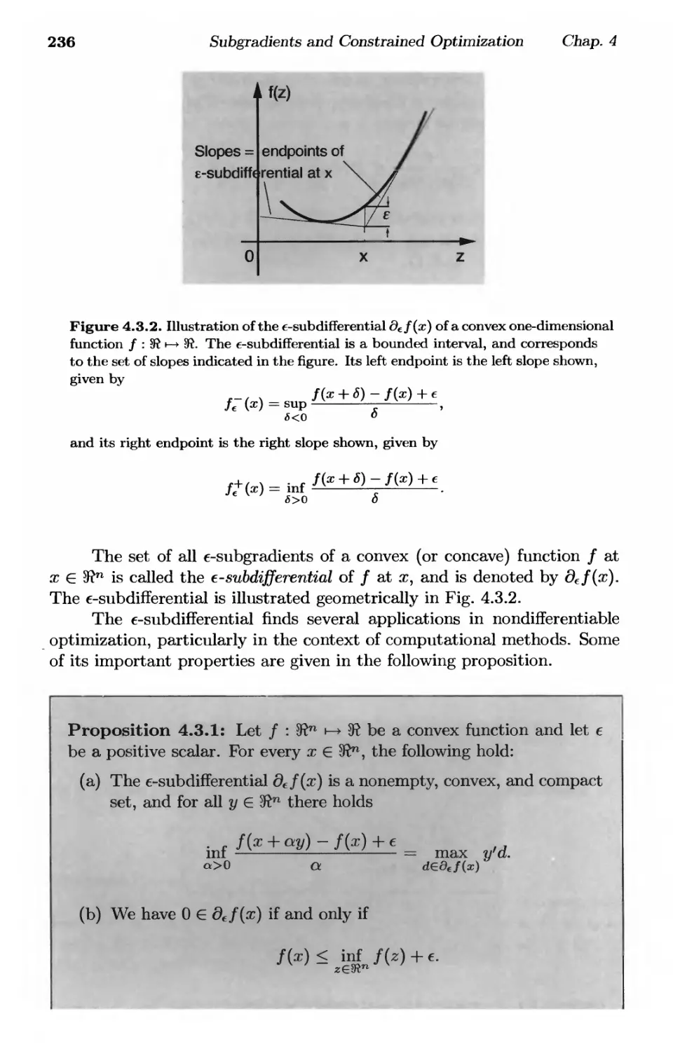
4.3. e-Subgradients p. 235
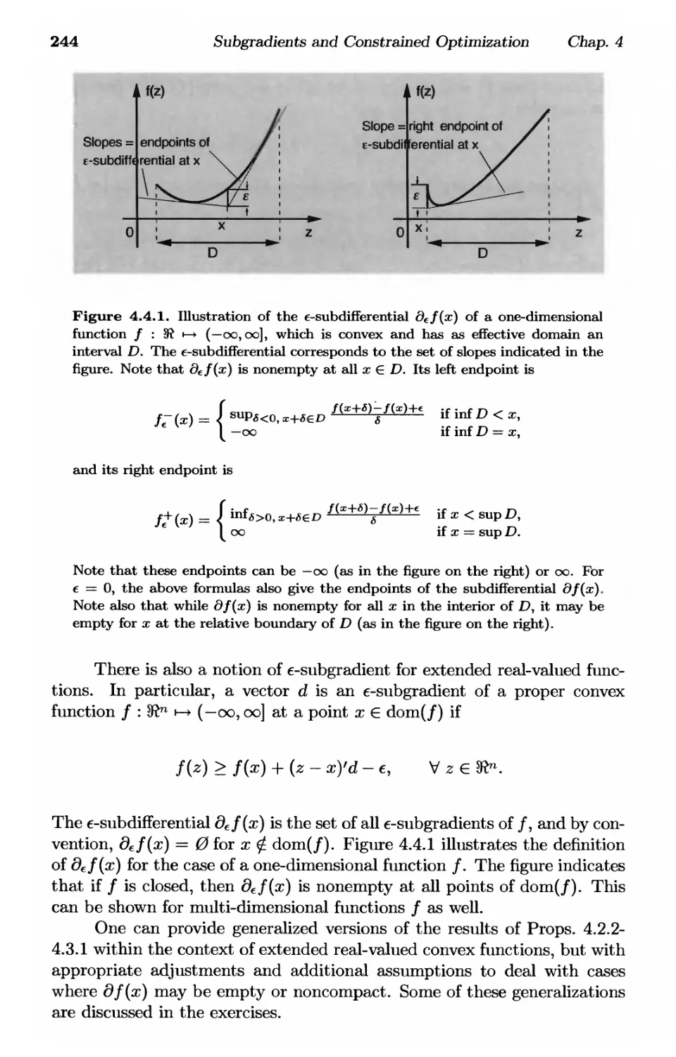
4.4. Subgradients of Extended Real-Valued Functions p. 241
4.5. Directional Derivative of the Max Function p. 245
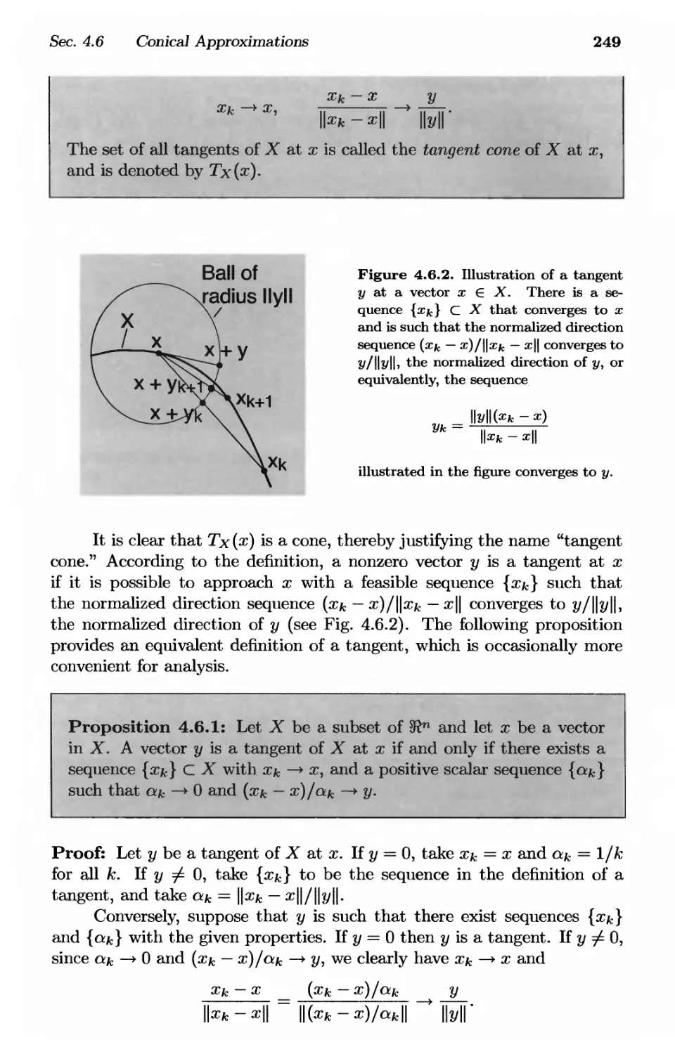
4.6. Conical Approximations p. 248
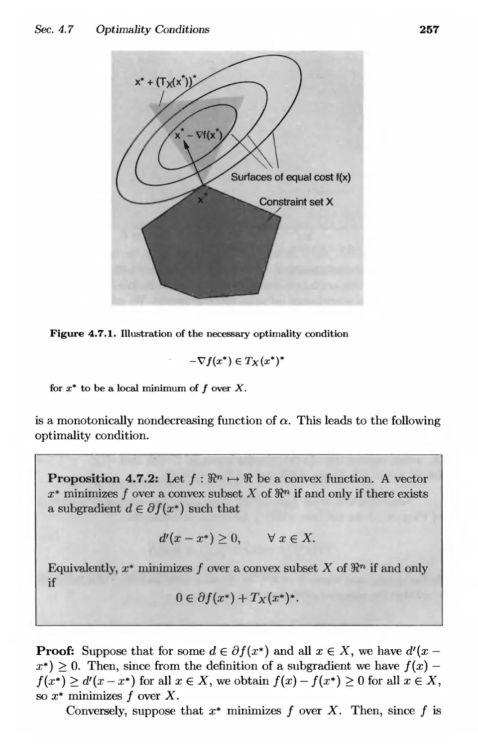
4.7. Optimality Conditions p. 255
4.8. Notes, Sources, and Exercises p. 261
5. Lagrange Multipliers p. 269
5.1. Introduction to Lagrange Multipliers p. 270
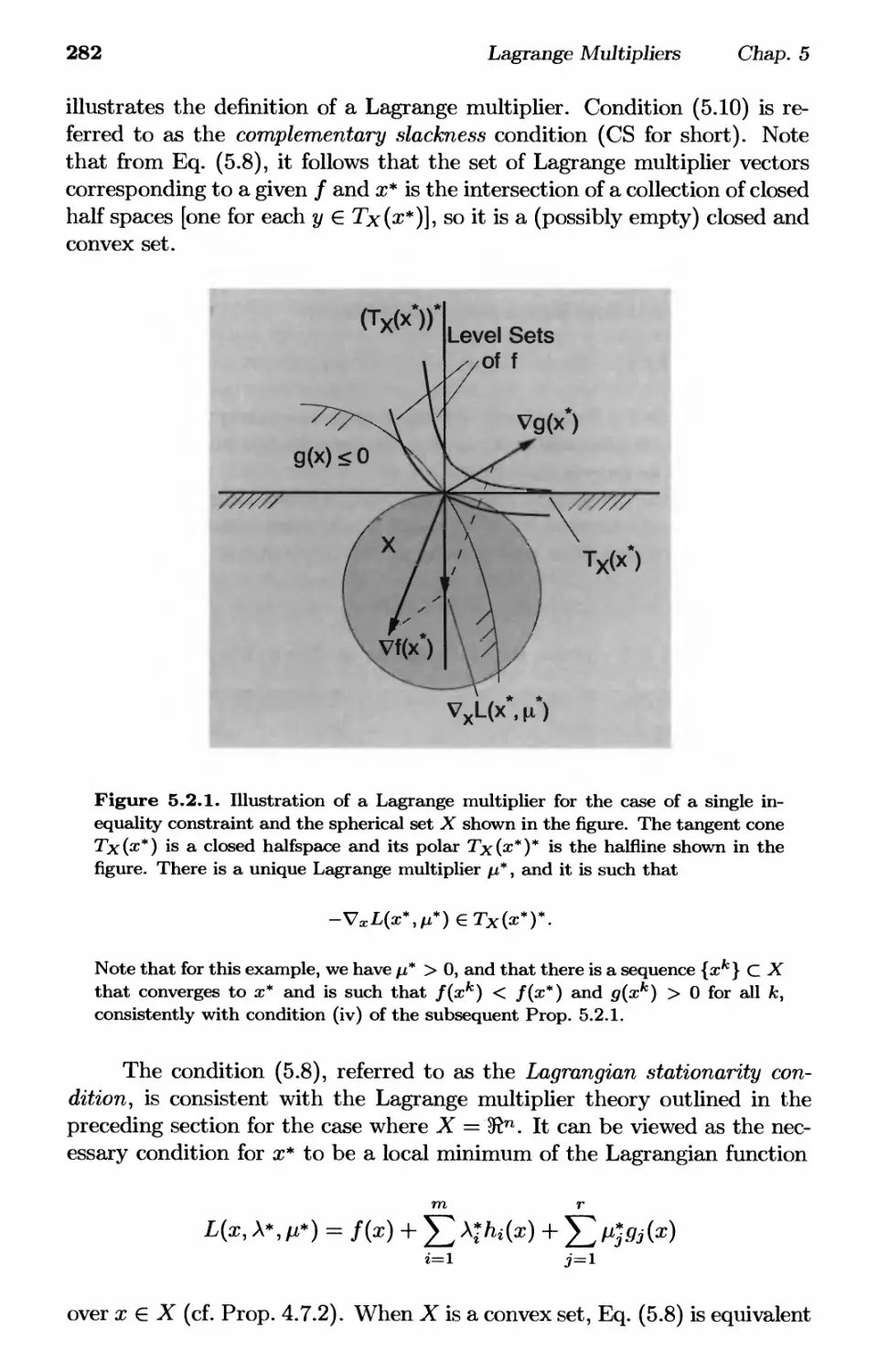
5.2. Enhanced Fritz John Optimality Conditions p. 281
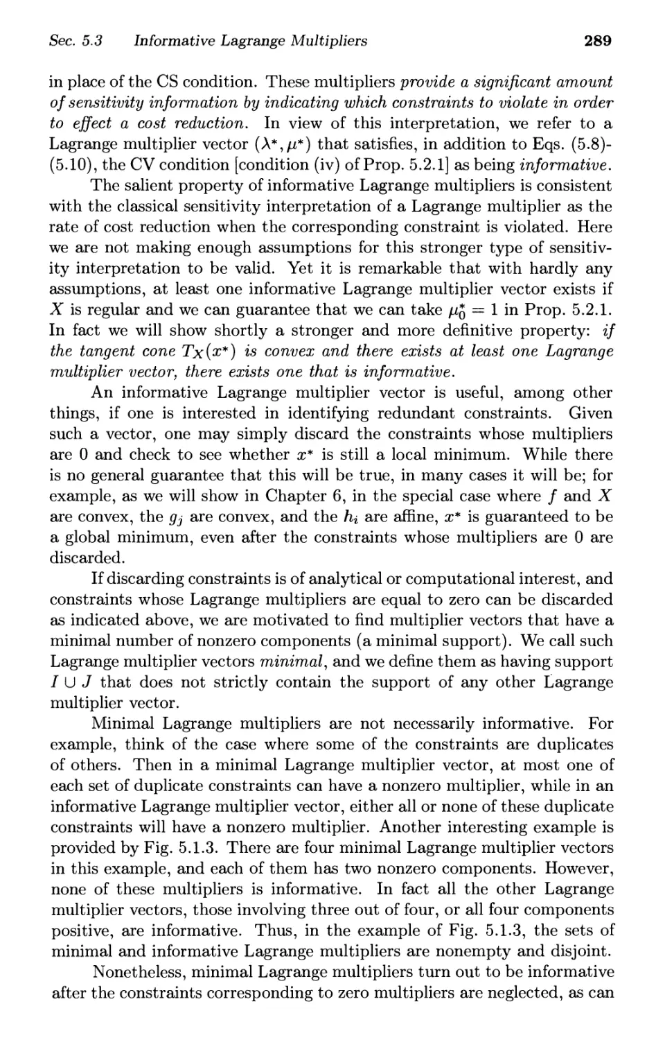
5.3. Informative Lagrange Multipliers p. 288
5.3.1. Sensitivity p. 297
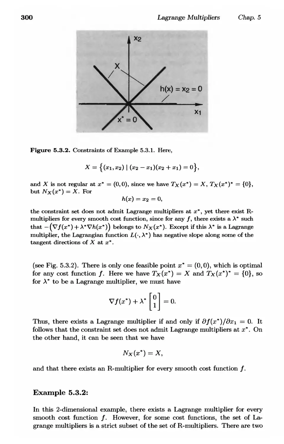
5.3.2. Alternative Lagrange Multipliers p. 299
5.4. Pseudonormality and Constraint Qualifications p. 302
5.5. Exact Penalty Functions p. 313
5.6. Using the Extended Representation p. 319
5.7. Extensions Under Convexity Assumptions p. 324
5.8. Notes, Sources, and Exercises '. . p. 335
Contents vii
6. Lagrangian Duality p. 345
6.1. Geometric Multipliers p. 346
6.2. Duality Theory p. 355
6.3. Linear and Quadratic Programming Duality p. 362
6.4. Existence of Geometric Multipliers p. 367
6.4.1. Convex Cost - Linear Constraints p. 368
6.4.2. Convex Cost - Convex Constraints p. 371
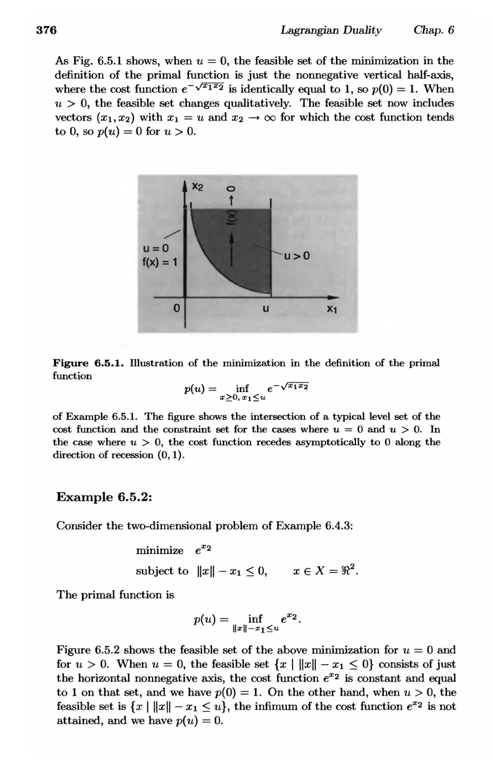
6.5. Strong Duality and the Primal Function p. 374
6.5.1. Duality Gap and the Primal Function p. 374
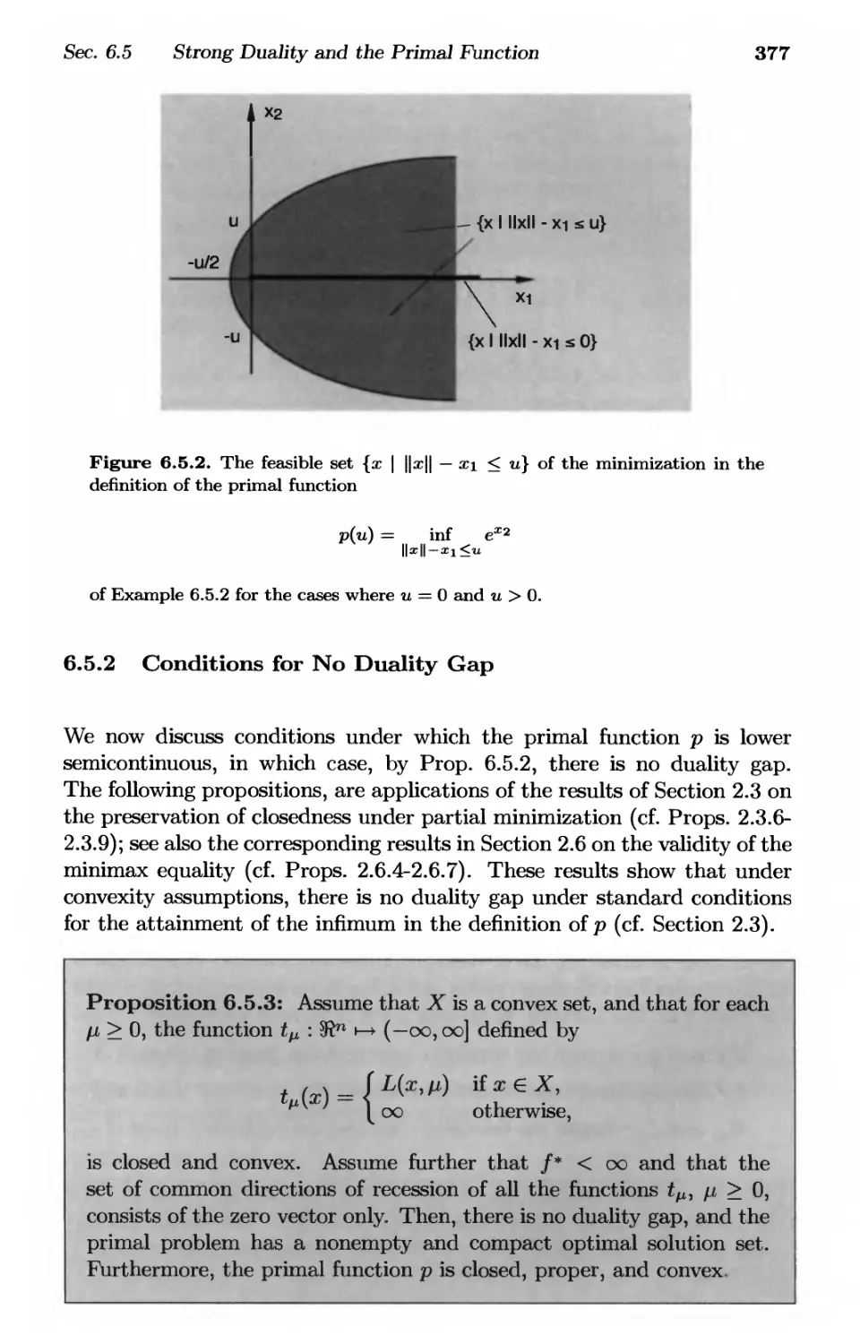
6.5.2. Conditions for No Duality Gap p. 377
6.5.3. Subgradients of the Primal Function p. 382
6.5.4. Sensitivity Analysis p. 383
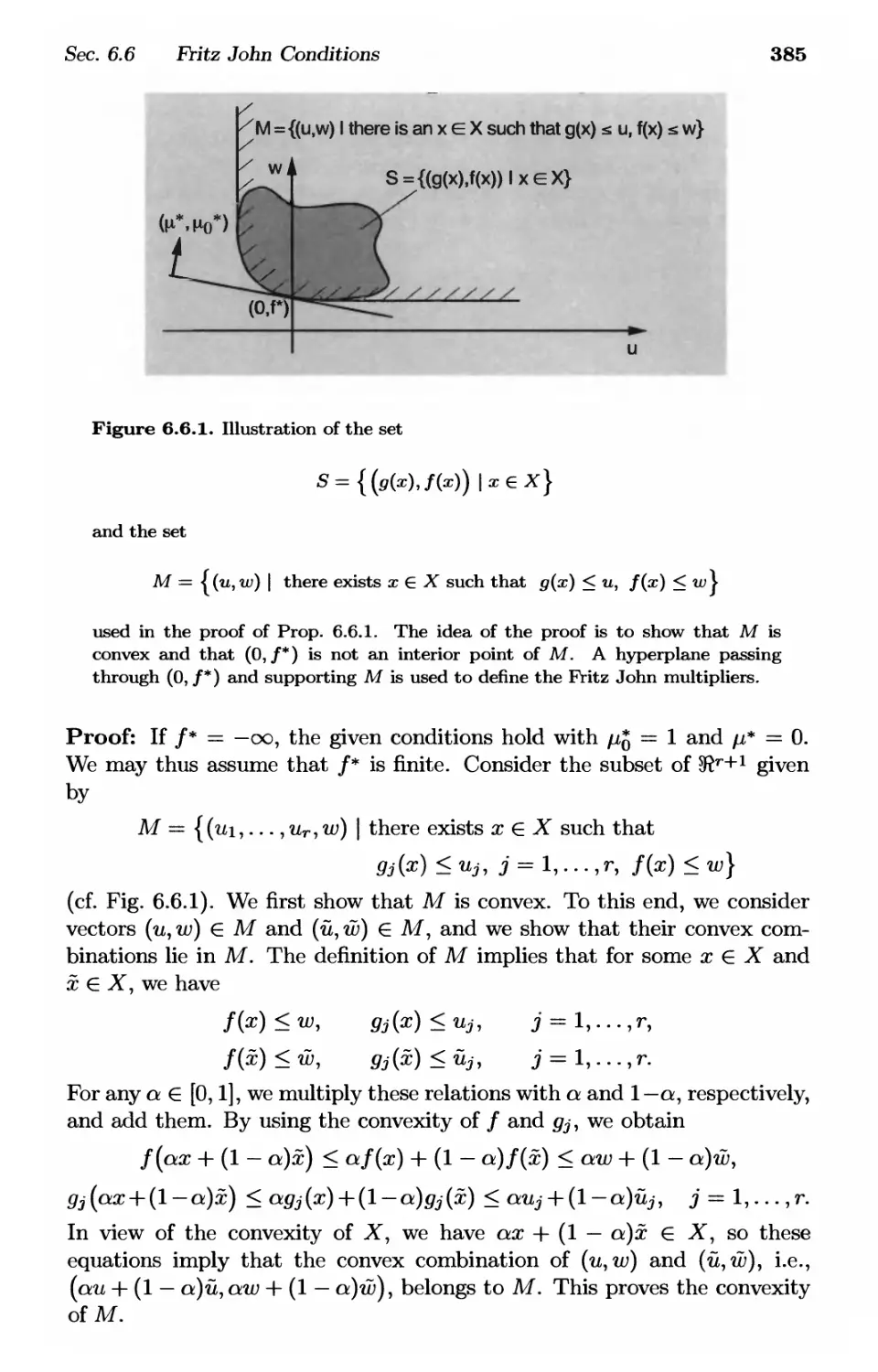
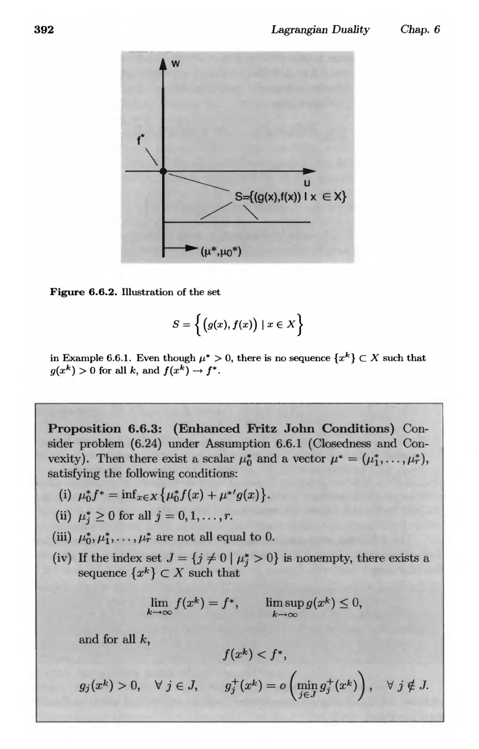
6.6. Fritz John Conditions when there is no Optimal Solution . p. 384
6.6.1. Enhanced Fritz John Conditions p. 390
6.6.2. Informative Geometric Multipliers p. 406
6.7. Notes, Sources, and Exercises p. 413
7. Conjugate Duality p. 421
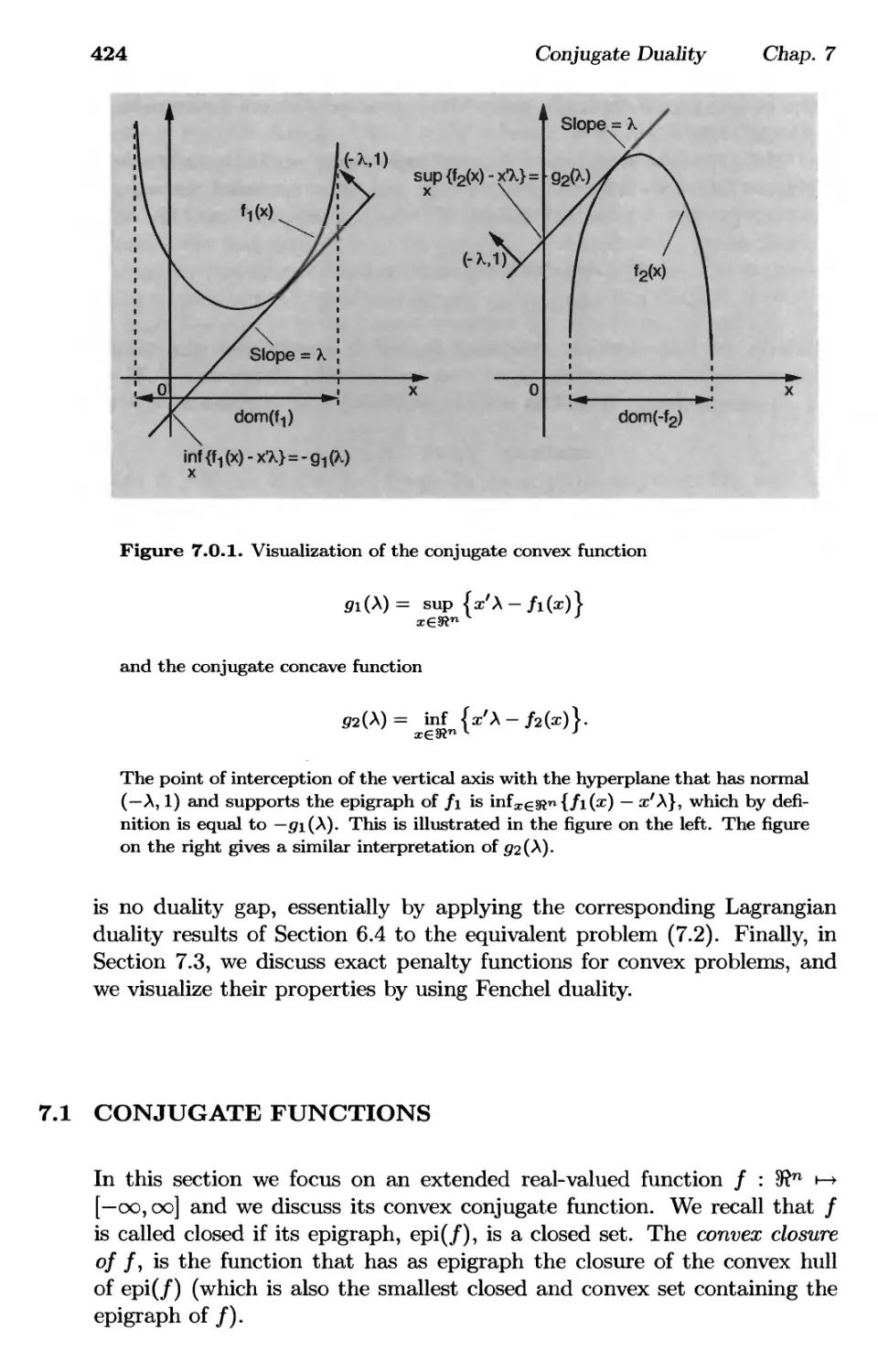
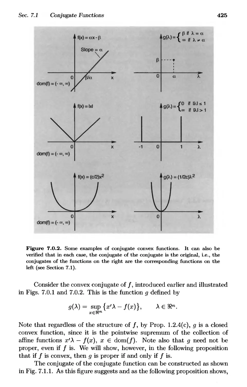
7.1. Conjugate Functions p. 424
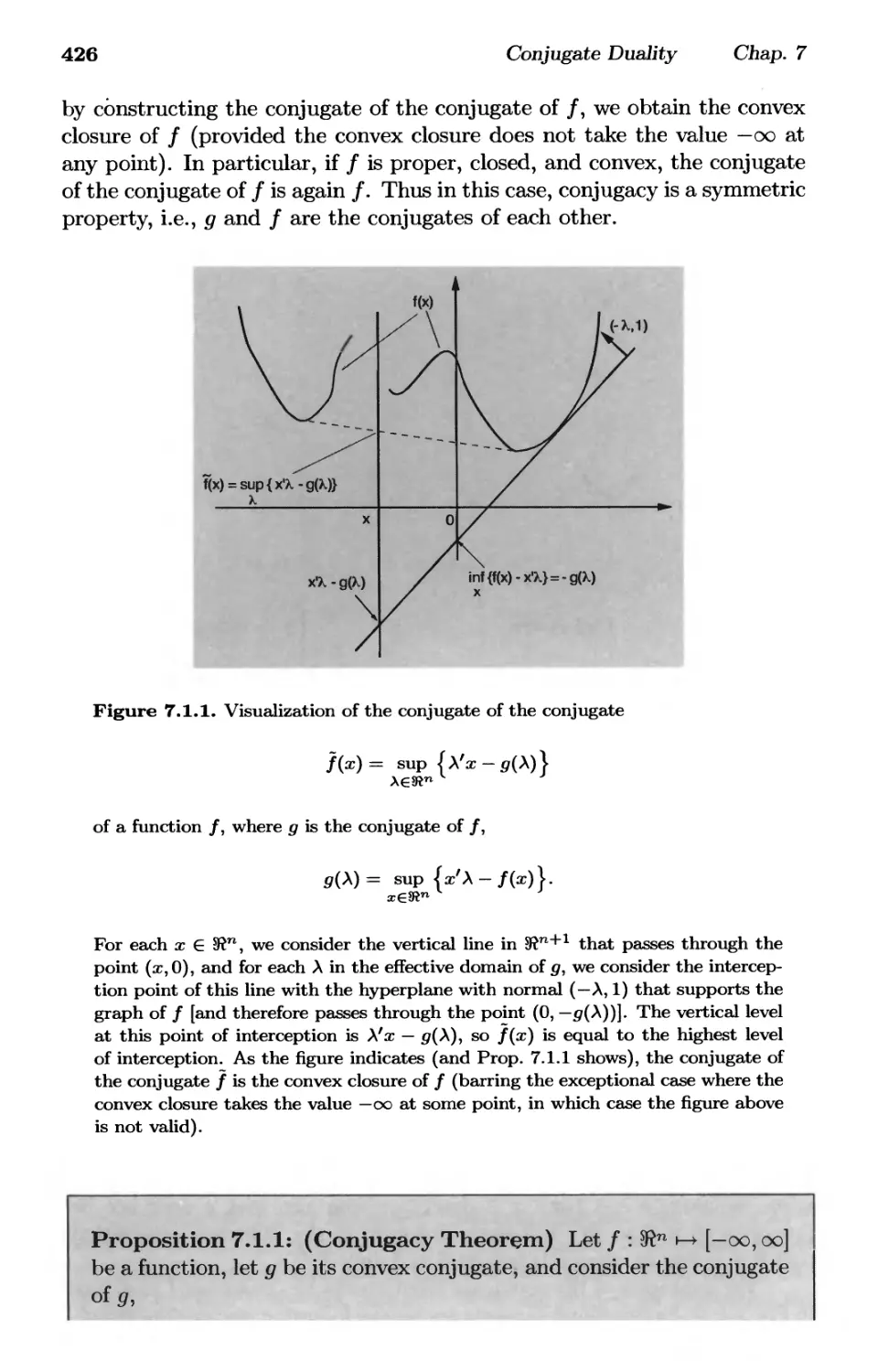
7.2. Fenchel Duality Theorems p. 434
7.2.1. Connection of Fenchel Duality and Minimax Theory . . p. 437
7.2.2. Conic Duality p. 439
7.3. Exact Penalty Functions p. 441
7.4. Notes, Sources, and Exercises p. 446
8. Dual Computational Methods p. 455
8.1. Dual Derivatives and Subgradients p. 457
8.2. Subgradient Methods p. 460
8.2.1. Analysis of Subgradient Methods p. 470
8.2.2. Subgradient Methods with Randomization p. 488
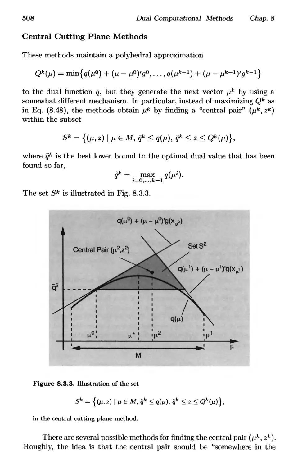
8.3. Cutting Plane Methods p. 504
8.4. Ascent Methods p. 509
8.5. Notes, Sources, and Exercises p. 512
References p. 517
Index p. 529
Preface
The knowledge at which geometry aims is the knowledge of the eternal
(Plato, Republic, VII, 52)
This book focuses on the theory of convex sets and functions, and its
connections with a number of topics that span a broad range from continuous
to discrete optimization. These topics include Lagrange multiplier theory,
Lagrangian and conjugate/Fenchel duality, minimax theory, and nondiffer-
entiable optimization.
The book evolved from a set of lecture notes for a graduate course at
M.I.T. It is widely recognized that, aside from being an eminently useful
subject in engineering, operations research, and economics, convexity is an
excellent vehicle for assimilating some of the basic concepts of real
analysis within an intuitive geometrical setting. Unfortunately, the subject's
coverage in academic curricula is scant and incidental. We believe that at
least part of the reason is the shortage of textbooks that are suitable for
classroom instruction, particularly for nonmathematics majors. We have
therefore tried to make convex analysis accessible to a broader audience
by emphasizing its geometrical character, while maintaining mathematical
rigor. We have included as many insightful illustrations as possible, and we
have used geometric visualization as a principal tool for maintaining the
students' interest in mathematical proofs.
Our treatment of convexity theory is quite comprehensive, with all
major aspects of the subject receiving substantial treatment. The
mathematical prerequisites are a course in linear algebra and a course in real
analysis in finite dimensional spaces (which is the exclusive setting of the
book). A summary of this material, without proofs, is provided in Section
1.1.
The coverage of the theory has been significantly extended in the
exercises, which represent a major component of the book. Detailed solutions
ix
χ
Preface
of all the exercises (nearly 200 pages) are internet-posted in the book's www
page
http://www.athenasc.com/convexity.html
Some of the exercises may be attempted by the reader without looking at
the solutions, while others are challenging but may be solved by the
advanced reader with the assistance of hints. Still other exercises represent
substantial theoretical results, and in some cases include new and
unpublished research. Readers and instructors should decide for themselves how
to make best use of the internet-posted solutions.
An important part of our approach has been to maintain a close link
between the theoretical treatment of convexity and its application to
optimization. For example, in Chapter 2, after the development of some of
the basic facts about convexity, we discuss some of their applications to
optimization and saddle point theory; in Chapter 3, after the discussion
of polyhedral convexity, we discuss its application in linear and integer
programming; and in Chapter 4, after the discussion of subgradients, we
discuss their use in optimality conditions. We follow this style in the
remaining chapters, although having developed in Chapters 1-4 most of the
needed convexity theory, the discussion in the subsequent chapters is more
heavily weighted towards optimization.
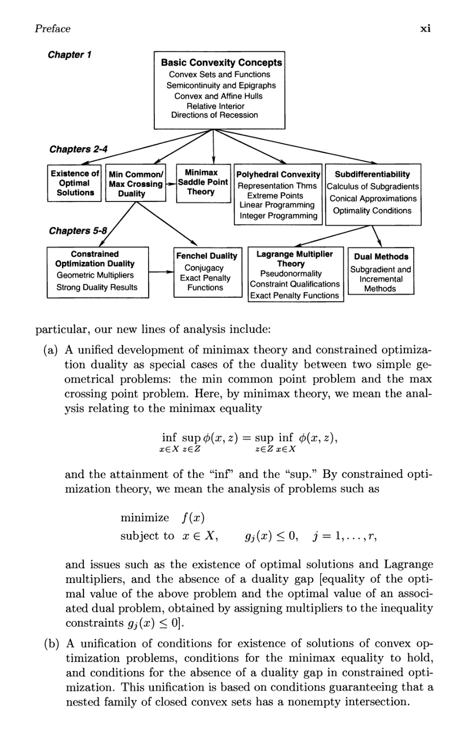
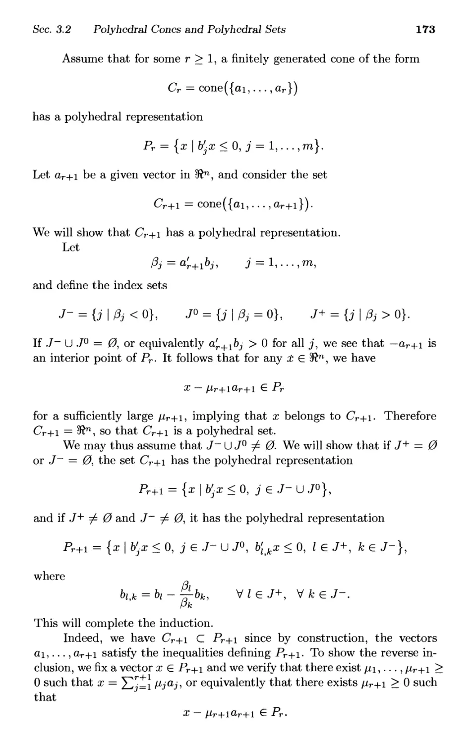
The chart of the opposite page illustrates the main topics covered
in the book, and their interrelations. At the top level, we have the most
basic concepts of convexity theory, which are covered in Chapter 1. At the
middle level, we have fundamental topics of optimization, such as existence
and characterization of solutions, and minimax theory, together with some
supporting convexity concepts such as hyperplane separation, polyhedral
sets, and subdifferentiability (Chapters 2-4). At the lowest level, we have
the core issues of convex optimization: Lagrange multipliers, Lagrange and
Fenchel duality, and numerical dual optimization (Chapters 5-8).
An instructor who wishes to teach a course from the book has a choice
between several different plans. One possibility is to cover in detail just
the first four chapters, perhaps augmented with some selected sections from
the remainder of the book, such as the first section of Chapter 7, which
deals with conjugate convex functions. The idea here is to concentrate on
convex analysis and illustrate its application to minimax theory through
the minimax theorems of Chapters 2 and 3, and to constrained
optimization theory through the Nonlinear Farkas' Lemma of Chapter 3 and the
optimality conditions of Chapter 4. An alternative plan is to cover
Chapters 1-4 in less detail in order to allow some time for Lagrange multiplier
theory and computational methods. Other plans may also be devised,
possibly including some applications or some additional theoretical topics of
the instructor's choice.
While the subject of the book is classical, the treatment of several of
its important topics is new and in some cases relies on new research. In
Preface
Chapter 1
Basic Convexity Concepts
Convex Sets and Functions
Semicontinuity and Epigraphs
Convex and Affine Hulls
Relative Interior
Directions of Recession
Chapters 2-4
Polyhedral Convexity
Representation Thms
Extreme Points
Linear Programming
Integer Programming
Subdifferentiability
Calculus of Subgradients
Conical Approximations
Optimality Conditions
Constrained
Optimization Duality
Geometric Multipliers
Strong Duality Results
Fenchel Duality
Conjugacy
Exact Penalty
Functions
Lagrange Multiplier
Theory
Pseudonormality
Constraint Qualifications
Exact Penalty Functions
Dual Methods
Subgradient and
Incremental
Methods
particular, our new lines of analysis include:
(a) A unified development of minimax theory and constrained
optimization duality as special cases of the duality between two simple
geometrical problems: the min common point problem and the max
crossing point problem. Here, by minimax theory, we mean the
analysis relating to the minimax equality
inf sup φ(χ,ζ) = sup inf φ(χ, ζ),
xex zez zez xex
and the attainment of the "inf and the "sup." By constrained
optimization theory, we mean the analysis of problems such as
minimize f(x)
subject to χ £ X,
9j(x) <0, j = l,...,r,
(b)
and issues such as the existence of optimal solutions and Lagrange
multipliers, and the absence of a duality gap [equality of the
optimal value of the above problem and the optimal value of an
associated dual problem, obtained by assigning multipliers to the inequality
constraints gj(x) < 0].
A unification of conditions for existence of solutions of convex
optimization problems, conditions for the minimax equality to hold,
and conditions for the absence of a duality gap in constrained
optimization. This unification is based on conditions guaranteeing that a
nested family of closed convex sets has a nonempty intersection.
XII
Preface
(c) A unification of the major constraint qualifications that guarantee
the existence of Lagrange multipliers for nonconvex constrained
optimization. This unification is achieved through the notion of constraint
pseudonormality, which is motivated by an enhanced form of the Fritz
John necessary optimality conditions.
(d) The development of incremental subgradient methods for dual
optimization, and the analysis of their advantages over classical
subgradient methods.
We provide some orientation by informally summarizing the main
ideas of each of the above topics.
Min Common/Max Crossing Duality
In this book, duality theory is captured in two easily visualized problems:
the min common point problem and the max crossing point problem,
introduced in Chapter 2. Fundamentally, these problems revolve around the
existence of nonvertical supporting hyperplanes to convex sets that are
unbounded from above along the vertical axis. When properly specialized,
this turns out to be the critical issue in constrained optimization duality
and saddle point/minimax theory, under standard convexity and/or
concavity assumptions.
The salient feature of the min common/max crossing framework is its
simple geometry, in the context of which the fundamental constraint
qualifications needed for strong duality theorems are visually apparent, and
admit straightforward proofs. This allows the development of duality
theory in a unified way: first within the min common/max crossing framework
in Chapters 2 and 3, and then by specialization, to saddle point and
minimax theory in Chapters 2 and 3, and to optimization duality in Chapter
6. All of the major duality theorems discussed in this book are derived in
this way, including the principal Lagrange multiplier and Fenchel duality
theorems for convex programming, and the von Neuman Theorem for zero
sum games.
From an instructional point of view, it is particularly desirable to
unify constrained optimization duality and saddle point/minimax theory
(under convexity/concavity assumptions). Their connection is well known,
but it is hard to understand beyond a superficial level, because there is not
enough overlap between the two theories to develop one in terms of the
other. In our approach, rather than trying to build a closer connection
between constrained optimization duality and saddle point/minimax theory,
we show how they both stem from a common geometrical root: the min
common/max crossing duality.
We note that the constructions involved in the min common and max
crossing problems arise in the theories of subgradients, conjugate convex
functions, and duality. As such they are implicit in several earlier analy-
Preface
xiii
ses; in fact they have been employed for visualization purposes in the first
author's nonlinear programming textbook [Ber99]. However, the two
problems have not been used as a unifying theoretical framework for constrained
optimization duality, saddle point theory, or other contexts, except
implicitly through the theory of conjugate convex functions, and the complicated
and specialized machinery of conjugate saddle functions. Pedagogically, it
appears desirable to postpone the introduction of conjugacy theory until it
is needed for the limited purposes of Fenchel duality (Chapter 7), and to
bypass altogether conjugate saddle function theory, which is what we have
done.
Existence of Solutions and Strong Duality
We show that under convexity assumptions, several fundamental issues in
optimization are intimately related. In particular, we give a unified analysis
of conditions for optimal solutions to exist, for the minimax equality to
hold, and for the absence of a duality gap in constrained optimization.
To provide a sense of the main idea, we note that given a constrained
optimization problem, lower semicontinuity of the cost function and
compactness of the constraint set guarantee the existence of an optimal
solution (the Weierstrass Theorem). On the other hand, the same conditions
plus convexity of the cost and constraint functions guarantee not only the
existence of an optimal solution, but also the absence of a duality gap.
This is not a coincidence, because as it turns out, the conditions for both
cases critically rely on the same fundamental properties of compact sets,
namely that the intersection of a nested family of nonempty compact sets
is nonempty and compact, and that the projections of compact sets on any
subspace are compact.
In our analysis, we extend this line of reasoning under a variety of
assumptions relating to convexity, directions of recession, polyhedral sets, and
special types of sets specified by quadratic and other types of inequalities.
The assumptions are used to establish results asserting that the intersection
of a nested family of closed convex sets is nonempty, and that the function
f(x) = inf2 F(x, z), obtained by partial minimization of a convex function
F, is lower semicontinuous. These results are translated in turn to a broad
variety of conditions that guarantee the existence of optimal solutions, the
minimax equality, and the absence of a duality gap.
Pseudonormality and Lagrange Multipliers
In Chapter 5, we discuss Lagrange multiplier theory in the context of
optimization of a smooth cost function, subject to smooth equality and
inequality constraints, as well as an additional set constraint. Our treatment of
Lagrange multipliers is new, and aims to generalize, unify, and streamline
the theory of constraint qualifications.
xiv
Preface
The starting point for our development is an enhanced set of
necessary conditions of the Fritz John type, that are sharper than the classical
Karush-Kuhn-Tucker conditions (they include extra conditions, which may
narrow down the field of candidate local minima). They are also more
general in that they apply when there is an abstract (possibly nonconvex)
set constraint, in addition to the equality and inequality constraints. To
achieve this level of generality, we bring to bear notions of nonsmooth
analysis, and we find that the notion of regularity of the abstract constraint
set provides the critical distinction between problems that do and do not
admit a satisfactory theory.
Fundamentally, Lagrange multiplier theory should aim to identify the
essential constraint structure that guarantees the existence of Lagrange
multipliers. For smooth problems with equality and inequality constraints,
but no abstract set constraint, this essential structure is captured by the
classical notion of quasiregularity (the tangent cone at a given feasible
point is equal to the cone of first order feasible variations). However, in
the presence of an additional set constraint, the notion of quasiregularity
breaks down as a viable unification vehicle. Our development introduces
the notion of pseudonormality as a substitute for quasiregularity for the
case of an abstract set constraint. Pseudonormality unifies and expands
the major constraint qualifications, and simplifies the proofs of Lagrange
multiplier theorems. In the case of equality constraints only,
pseudonormality is implied by either one of two alternative constraint qualifications:
the linear independendence of the constraint gradients and the linearity
of the constraint functions. In fact, in this case, pseudonormality is not
much different than the union of these two constraint qualifications.
However, pseudonormality is a meaningful unifying property even in the case
of an additional set constraint, where the classical proof arguments based
on quasiregularity fail. Pseudonormality also provides the connecting link
between constraint qualifications and the theory of exact penalty functions.
An interesting byproduct of our analysis is a taxonomy of different
types of Lagrange multipliers for problems with nonunique Lagrange
multipliers. Under some convexity assumptions, we show that if there exists at
least one Lagrange multiplier vector, there exists at least one of a special
type, called informative, which has nice sensitivity properties. The nonzero
components of such a multiplier vector identify the constraints that need
to be violated in order to improve the optimal cost function value.
Furthermore, a particular informative Lagrange multiplier vector characterizes the
direction of steepest rate of improvement of the cost function for a given
level of the norm of the constraint violation. Along that direction, the
equality and inequality constraints are violated consistently with the signs
of the corresponding multipliers.
The theory of enhanced Fritz John conditions and pseudonormality
are extended in Chapter 6 to the case of a convex programming problem,
without assuming the existence of an optimal solution or the absence of
Preface
xv
a duality gap. They form the basis for a new line of analysis for
asserting the existence of informative multipliers under the standard constraint
qualifications.
Incremental Subgradient Methods
In Chapter 8, we discuss one of the most important uses of duality: the
numerical solution of dual problems, often in the context of discrete
optimization and the method of branch-and-bound. These dual problems are
often nondifferentiable and have special structure. Subgradient methods
have been among the most popular for the solution of these problems, but
they often suffer from slow convergence.
We introduce incremental subgradient methods, which aim to
accelerate the convergence by exploiting the additive structure that a dual problem
often inherits from properties of its primal problem, such as separability.
In particular, for the common case where the dual function is the sum of
a large number of component functions, incremental methods consist of a
sequence of incremental steps, each involving a single component of the
dual function, rather than the sum of all components.
Our analysis aims to identify effective variants of incremental
methods, and to quantify their advantages over the standard subgradient
methods. An important question is the selection of the order in which the
components are selected for iteration. A particularly interesting variant
uses randomization of the order to resolve a worst-case complexity
bottleneck associated with the natural deterministic order. According to both
analysis and experiment, this randomized variant performs substantially
better than the standard subgradient methods for large scale problems
that typically arise in the context of duality. The randomized variant is
also particularly well-suited for parallel, possibly asynchronous,
implementation, and is the only available method, to our knowledge, that can be
used efficiently within this context.
We are thankful to a few persons for their contributions to the book.
Several colleagues contributed information, suggestions, and insights. We
would like to single out Paul Tseng, who was extraordinarily helpful by
proofreading portions of the book, and collaborating with us on several
research topics, including the Fritz John theory of Sections 5.7 and 6.6.
We would also like to thank Xin Chen and Janey Yu, who gave us valuable
feedback and some specific suggestions. Finally, we wish to express our
appreciation for the stimulating environment at M.I.Т., which provided an
excellent setting for this work.
Dimitri P. Bertsekas, dimitrib@mit.edu
Angelia Nedic, angelia.nedich@alphatech.com
Asuman E. Ozdaglar, asuman@mit.edu
1
Basic Convexity Concepts
Contents
1.1. Linear Algebra and Real Analysis
1.1.1. Vectors and Matrices
1.1.2. Topological Properties
1.1.3. Square Matrices . .
LI.4. Derivatives
1.2. Convex Sets and Functions
1.3. Convex and Affine Hulls .
1.4. Relative Interior, Closure, and Continuity
1.5. Recession Cones ....
1.5.1. Nonemptiness of Intersections of Closed Sets
1.5.2. Closedness Under Linear Transformations
1.6. Notes, Sources, and Exercises
p.3
p. 5
p. 8
p. 15
p. 16
p. 20
p. 35
p. 39
p. 49
p. 56
p. 64
p. 68
1
2
Basic Convexity Concepts Chap. 1
In this chapter and the following three, we develop the theory of convex
sets, which is the mathematical foundation for minimax theory, Lagrange
multiplier theory, and duality. We assume no prior knowledge of the
subject, and we give a detailed development. As we embark on the study
of convexity, it is worth listing some of the properties of convex sets and
functions that make them so special in optimization.
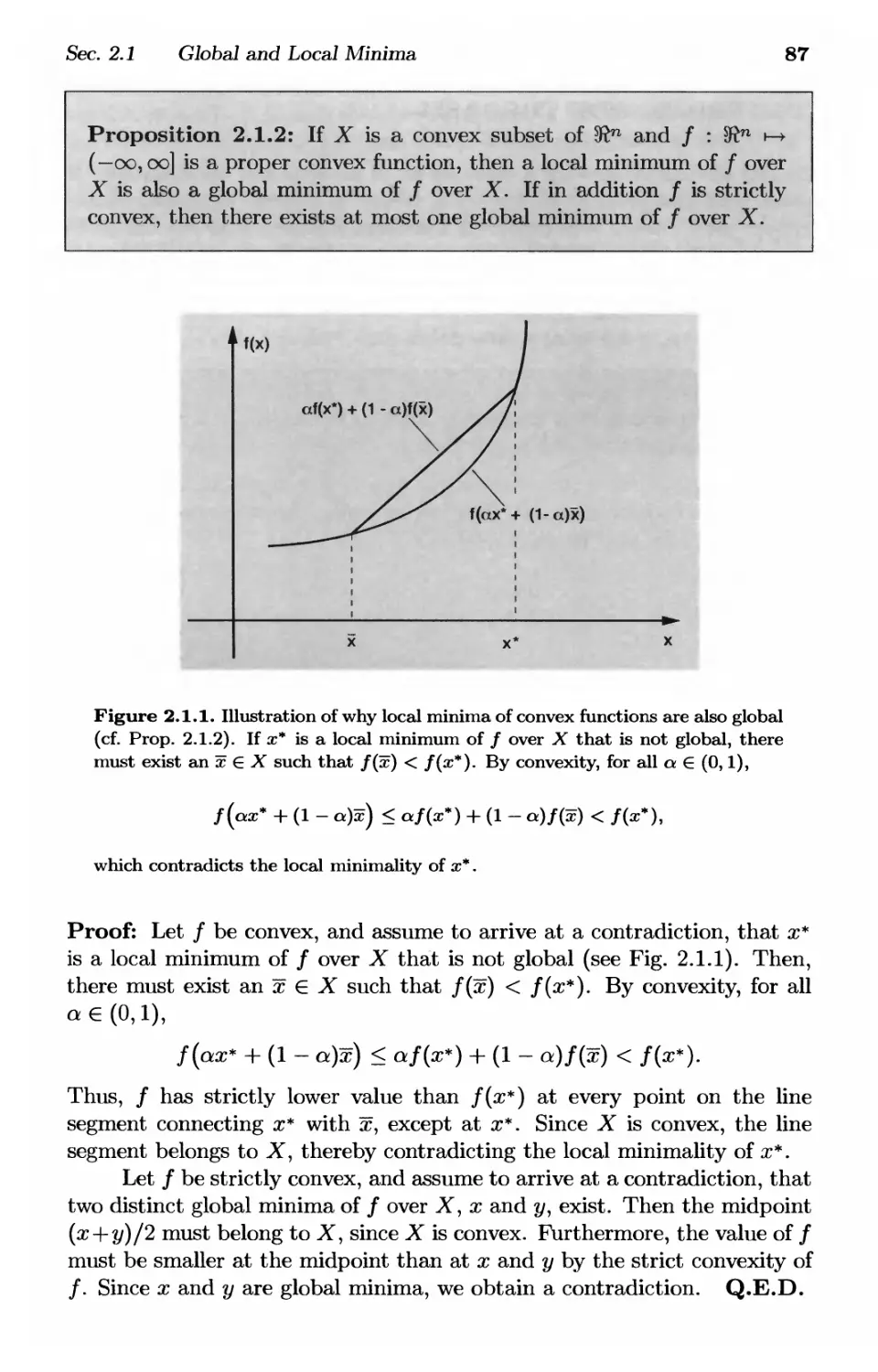
(a) A convex function has no local minima that are not global. Thus the
difficulties associated with multiple disconnected local minima, whose
global optimality is hard to verify in practice, are avoided (see Section
2.1).
(b) A convex set has a nonempty relative interior. In other words, relative
to the smallest affine set containing it, a convex set has a nonempty
interior (see Section 1.4). Thus convex sets avoid the analytical and
computational optimization difficulties associated with "thin" and
"curved" constraint surfaces.
(c) A convex set is connected and has feasible directions at any point
(assuming it consists of more than one point). By this we mean
that given any point χ in a convex set X, it is possible to move
from χ along some directions у and stay within X for at least a
nontrivial interval, i.e., χ + ay Ε Χ for all sufficiently small but
positive stepsizes a (see Section 4.6). In fact a stronger property
holds: given any two distinct points χ and ϊ in I, the direction
χ — χ is a feasible direction at x, and all feasible directions can be
characterized this way. For optimization purposes, this is important
because it allows a calculus-based comparison of the cost of χ with
the cost of its close neighbors, and forms the basis for some important
algorithms. Furthermore, much of the difficulty commonly associated
with discrete constraint sets (arising for example in combinatorial
optimization), is not encountered under convexity.
(d) A nonconvex function can be "convexified" while maintaining the
optimality of its global minima, by forming the convex hull of the epigraph
of the function (see Exercise 1.20).
(e) The existence of a global minimum of a convex function over a convex
set is conveniently characterized in terms of directions of recession
(see Section 2.3).
(f) A polyhedral convex set (one that is specified by linear equality and
inequality constraints) is characterized in terms of a finite set of extreme
points and extreme directions. This is the basis for finitely
terminating methods for linear programming, including the celebrated simplex
method (see Sections 3.3 and 3.4).
(g) A convex function is continuous within the interior of its domain,
and has nice differentiability properties. In particular, a real-valued
Sec. 1.1 Linear Algebra and Real Analysis
3
convex function is directionally differentiable at any point.
Furthermore, while a convex function need not be differentiable, it possesses
subgradients, which are nice and geometrically intuitive substitutes
for a gradient (see Chapter 4). Just like gradients, subgradients figure
prominently in optimality conditions and computational algorithms.
(h) Convex functions are central in duality theory. Indeed, the dual
problem of a given optimization problem (discussed in Chapter 6) consists
of minimization of a convex function over a convex set, even if the
original problem is not convex.
(i) Closed convex cones are self-dual with respect to polarity. In words,
we have С = (С*)* for any closed and convex cone C, where C* is
the polar cone of С (the set of vectors that form a nonpositive inner
product with all vectors in C), and (C*)* is the polar cone of C*. This
simple and geometrically intuitive property (discussed in Section 3.1)
underlies important aspects of Lagrange multiplier theory.
(j) Convex lower semicontinuous functions are self-dual with respect to
conjugacy. It will be seen in Chapter 7 that a certain geometrically
motivated conjugacy operation on a convex, lower semicontinuous
function generates another convex, lower semicontinuous function,
and when applied for the second time regenerates the original
function. The conjugacy operation relies on a fundamental dual
characterization of a closed convex set: as the union of the closures of all line
segments connecting its points, and as the intersection of the closed
halfspaces within which the set is contained. Conjugacy is central in
duality theory, and has a nice interpretation that can be used to
visualize and understand some of the most interesting aspects of convex
optimization.
In this first chapter, after an introductory first section, we focus on
the basic concepts of convex analysis: characterizations of convex sets and
functions, convex and affine hulls, topological concepts such as closure,
continuity, and relative interior, and the important notion of the recession
cone.
1.1 LINEAR ALGEBRA AND REAL ANALYSIS
In this section, we list some basic definitions, notational conventions, and
results from linear algebra and real analysis. We assume that the reader is
familiar with this material, so no proofs are given. For related and
additional material, we recommend the books by Hoffman and Kunze [HoK71],
Lancaster and Tismenetsky [LaT85], and Strang [Str76] (linear algebra),
4
Basic Convexity Concepts Chap. 1
and the books by Ash [Ash72], Ortega and Rheinboldt [OrR70], and Rudin
[Rud76] (real analysis).
Set Notation
If X is a set and χ is an element of X, we write χ Ε X. A set can be
specified in the form X = {χ \ χ satisfies P}, as the set of all elements
satisfying property P. The union of two sets X\ and X2 is denoted by
X\ U X2 and their intersection by Χι П Х2. The symbols 3 and V have
the meanings "there exists" and "for all," respectively. The empty set is
denoted by 0.
The set of real numbers (also referred to as scalars) is denoted by 3?.
The set 3? augmented with +00 and —00 is called the set of extended real
numbers. We write — 00 < χ < oo for all real numbers x, and — 00 < χ < oo
for all extended real numbers x. We denote by [a, b] the set of (possibly
extended) real numbers χ satisfying a < χ < b. A rounded, instead of
square, bracket denotes strict inequality in the definition. Thus (a, 6], [a, 6),
and (a, b) denote the set of all χ satisfying a < χ < b, a < χ < b, and
a < χ < 6, respectively. Furthermore, we use the natural extensions of the
rules of arithmetic: χ · 0 = 0 for every extended real number χ, χ · oo = 00
if χ > 0, χ · 00 = —00 if χ < 0, and χ + oo = 00 and χ — oo = —00 for
every scalar x. The expression 00 — 00 is meaningless and is never allowed
to occur.
Inf and Sup Notation
The swpremum of a nonempty set X of scalars, denoted by sup X, is defined
as the smallest scalar у such that у > χ for all χ Ε Χ. If no such scalar
exists, we say that the supremum of X is 00. Similarly, the infimum of X,
denoted by inf X, is defined as the largest scalar у such that у < χ for all
χ Ε Χ, and is equal to —00 if no such scalar exists. For the empty set, we
use the convention
sup 0 = —00, inf 0 = 00.
If supX is equal to a scalar χ that belongs to the set X, we say that
χ is the maximum point of X and we write χ = max X. Similarly, if inf X is
equal to a scalar χ that belongs to the set X, we say that χ is the minimum
point of X and we write χ = min X. Thus, when we write max X (or min X)
in place of supX (or inf X, respectively), we do so just for emphasis: we
indicate that it is either evident, or it is known through earlier analysis, or
it is about to be shown that the maximum (or minimum, respectively) of
the set X is attained at one of its points.
Sec. 1.1 Linear Algebra and Real Analysis
5
Function Notation
If / is a function, we use the notation / : Χ ν-> Υ to indicate the fact that
/ is defined on a nonempty set X (its domain) and takes values in a set
Υ (its range). Thus when using the notation / : X у-> У, we implicitly
assume that X is nonempty. If / : X y-> Υ is a function, and U and У
are subsets of X and F, respectively, the set {f(x) | χ Ε ί/} is called the
image or forward image of U under /, and the set {xEl | /(χ) Ε V} is
called the inverse image of V under f.
1.1.1 Vectors and Matrices
We denote by 3?n the set of η-dimensional real vectors. For any χ Ε 5ftn,
we use Xi to indicate its zth coordinate, also called its zth component.
Vectors in 3?n will be viewed as column vectors, unless the contrary
is explicitly stated. For any χ Ε 5ftn, χ' denotes the transpose of x, which
is an η-dimensional row vector. The inner product of two vectors x, у Ε 5ftn
is defined by x'y = Σ™-ι ХгУг- Two vectors x,y Ε 5ftn satisfying x'y = 0
are called orthogonal.
If χ is a vector in 3?n, the notations χ > 0 and χ > 0 indicate that all
components of χ are positive and nonnegative, respectively. For any two
vectors χ and y, the notation χ > у means that χ — у > 0. The notations
х>У, x < У, etc., are to be interpreted accordingly.
If X is a set and λ is a scalar, we denote by XX the set {λχ \ χ Ε Χ}.
If Χι and X2 are two subsets of 5ftn, we denote by X\ + X2 the set
{xi + X2 I £l Ε Xl, X2 Ε X2},
which is referred to as the vector sum of X\ and X2· We use a similar
notation for the sum of any finite number of subsets. In the case where
one of the subsets consists of a single vector x, we simplify this notation as
follows:
x + X = {x + x\x£ X}.
We also denote by X\ — X2 the set
{x\ — X2 I X\ Ε Χι, Χ2 Ε X2}.
Given sets Xi С 5Rn*, i = 1,..., m, the Cartesian product of the Xi,
denoted by Χι χ · · · χ Xm, is the set
{(xi,... ,xm) I Xi Ε Xi, г = l,...,m},
which is a subset of !Κηι+···+η™.
6
Basic Convexity Concepts Chap. 1
Subspaces and Linear Independence
A nonempty subset S of 3?n is called a subspace if ax + by Ε S for every
x,y Ε S and every a, 6 Ε 5ft. An aj^ne se£ in 5ftn is a translated subspace,
i.e., a set X of the form X = x + S = {x + x\x£ 5}, where χ is a vector
in 5ftn and 5 is a subspace of 5ftn, called the subspace parallel to X. Note
that there can be only one subspace S associated with an affine set in this
manner. [To see this, let X = χ + S and X = x + S he two representations
of the affine set X. Then, we must have χ = χ + s for some s Ε S (since
χ Ε X), so that X = x+s + S. Since we also have X = χ + S, it follows that
S = S — s = S.] The span of a finite collection {xi,..., xm} of elements of
5ftn is the subspace consisting of all vectors у of the form у = ΣΤ=ι ak%k->
where each a^ is a scalar.
The vectors x\,... ,xm Ε 5ftn are called linearly independent if there
exists no set of scalars αϊ,..., am, at least one of which is nonzero, such
that Σ/fcLi akXk = 0. An equivalent definition is that x\ φ 0, and for every
fe > 1, the vector x^ does not belong to the span of xi,..., Xk-i-
If 5 is a subspace of 5ftn containing at least one nonzero vector, a basis
for S is a collection of vectors that are linearly independent and whose
span is equal to S. Every basis of a given subspace has the same number
of vectors. This number is called the dimension of S. By convention, the
subspace {0} is said to have dimension zero. The dimension of an affine set
χ + S is the dimension of the corresponding subspace S. Every subspace of
nonzero dimension has a basis that is orthogonal (i.e., any pair of distinct
vectors from the basis is orthogonal).
Given any set X, the set of vectors that are orthogonal to all elements
of X is a subspace denoted by X^\
X± = {y\y'x = 0,\/ x£X}.
If S is a subspace, S1- is called the orthogonal complement of S. Any vector
χ can be uniquely decomposed as the sum of a vector from S and a vector
from S-L. Furthermore, we have (5'-L)-L = S.
Matrices
For any matrix A, we use Aij, [A]ij, or aij to denote its ijth element. The
transpose of A, denoted by A', is defined by [A']ij = aji. For any two
matrices A and В of compatible dimensions, the transpose of the product
matrix AB satisfies (AB)' = B'A'.
If X is a subset of 5ftn and A is an πι χ η matrix, then the image of
X under A is denoted by AX (or A · X if this enhances notational clarity):
AX = {Ax | χ Ε Χ}.
Sec. 1.1 Linear Algebra and Real Analysis
7
If Υ is a subset of 5ftm, the inverse image of Υ under A is denoted by A_1Y
or A-i-Y:
A~1Y = {x\AxeY}.
If X and Υ are subspaces, then AX and A~lY are also subspaces.
Let A be a square matrix. We say that A is symmetric if A' = A. We
say that A is diagonal if [i4]ij = 0 whenever г ф j. We use i" to denote the
identity matrix (the diagonal matrix whose diagonal elements are equal to
1). We denote the determinant of A by det(A).
Let A be an πι χ η matrix. The range space of A, denoted by R(A),
is the set of all vectors у £ 5ftm such that у = Ax for some χ £ 5ftn. The
nullspace of A, denoted by iV(i4), is the set of all vectors χ £ 5ftn such
that Ax = 0. It is seen that the range space and the null space of A are
subspaces. The rank of A is the dimension of the range space of A. The
rank of A is equal to the maximal number of linearly independent columns
of A, and is also equal to the maximal number of linearly independent rows
of A. The matrix A and its transpose A' have the same rank. We say that
A has full rank, if its rank is equal to min{m, n}. This is true if and only
if either all the rows of A are linearly independent, or all the columns of A
are linearly independent.
The range space of an m χ η matrix A is equal to the orthogonal
complement of the nullspace of its transpose, i.e.,
R(A) = N(A')-L.
Another way to state this result is that given vectors a\,..., an £ 5ftm (the
columns of A) and a vector χ £ 5ftm, we have x'y = 0 for all у such that
a\y = 0 for all г if and only if χ = λιαι + · · · + \nan for some scalars
λι,..., λη. This is a special case of Farkas' Lemma, an important result
for constrained optimization, which will be discussed in Section 3.2. A
useful application of this result is that if S\ and S2 are two subspaces of
5Rn, then
SjL+S^- = (SinS2)-L.
This follows by introducing matrices B\ and £2 such that S\ = {χ \ B\x =
0} = N(Bi) and S2 = {x\ B2x = 0} = N(B2), and writing
Sjr+Si-= R{[B[ B2])=n(\bI]) ={N(Bi)nN(B2))± = (S1nS2V
A function / : 5ftn 1—> 5ft is said to be affine if it has the form f(x) =
a'x + b for some a £ 5ftn and b £ 5ft. Similarly, a function / : 5ftn н-> 5ftm is
said to be affine if it has the form f(x) = Ax + b for some πι χ η matrix
A and some b £ 5ftm. If b = 0, / is said to be a linear function or linear
transformation. Sometimes, with slight abuse of terminology, an equation
or inequality involving a linear function, such as a'x = b or a'x < 6, is
referred to as a linear equation or inequality, respectively.
8 Basic Convexity Concepts Chap. 1
1.1.2 Topological Properties
Definition 1.1.1: A norm || · || on 5Rn is a function that assigns a
scalar \\x\\ to every χ 6 S?n and that has the following properties:
(a) ||x|| > 0 for all χ e 5Rn.
(b) ||аж|| = \α\ · ||χ|| for every scalar
(c) ||x|| = 0 if and only if χ = 0.
(d) \\z + y\\ < INI + IMI for aUar,j/
triangle inequality).
a and every χ Ε 3ϊη.
G 5Rn (this is referred to as the ι
The Euclidean norm of a vector χ = (χι,- ■ ■, xn) is defined by
/ η \ i/2
\\x\\ = {x'x)^=[Y^\xiV
We will use the Euclidean norm almost exclusively in this book. In
particular, in the absence of a clear indication to the contrary, || · || will denote
the Euclidean norm. Two important results for the Euclidean norm are:
Proposition 1.1.1: (Pythagorean Theorem) For any two vectors
χ and у that are orthogonal, we have
ll* + y||2 = INI2 + IMI2·
Proposition 1.1.2: (Schwarz Inequality) For any two vectors χ
and ?/, we have
\x'y\ < INI · IMI,
with equality holding if and only if χ = ay for some scalar a.
Two other important norms are the maximum norm || · ||oo (also called
sup-norm or £oc-norm), defined by
INloo = max \xi\,
i=l,...,7i
Sec. 1.1 Linear Algebra and Real Analysis
9
and the i\-norm || · ||i, defined by
||χ||ι=Σ>|.
i=l
Sequences
We use both subscripts and superscripts in sequence notation. Generally,
we prefer subscripts, but we use superscripts whenever we need to reserve
the subscript notation for indexing components of vectors and functions.
The meaning of the subscripts and superscripts should be clear from the
context in which they are used.
A sequence {xk | к = 1,2,...} (or {xk} for short) of scalars is said
to converge if there exists a scalar χ such that for every e > 0 we have
\xk — x\ < б for every к greater than some integer К (that depends on
e). The scalar χ is said to be the limit of {#*:}, and the sequence {xk}
is said to converge to x; symbolically, Xk —> x or Ит^-юо Xk = x. If for
every scalar b there exists some К (that depends on b) such that Xk > b
for all к > К, we write Xk —> oo and Шщ;_юо Xk — oo. Similarly, if for
every scalar b there exists some integer К such that Xk <b for all к> К,
we write Xk —> —oo and Ит^-юо χ к = —oo. Note, however, that implicit
in any of the statements u{xk} converges" or "the limit of {xk} exists" or
"{xk} has a limit" is that the limit of {xk} is a scalar.
A scalar sequence {xk} is said to be bounded above (respectively,
below) if there exists some scalar b such that Xk <b (respectively, Xk > b) for
all к. It is said to be bounded if it is bounded above and bounded below.
The sequence {xk} is said to be monotonically nonincreasing (respectively,
nondecreasing) if x^+i < %k (respectively, x^+i i> %k) for all k. If x^ —> x
and {xk} is monotonically nonincreasing (nondecreasing), we also use the
notation Xk | x {xk Τ #> respectively).
I Proposition 1.1.3: Every bounded and monotonically nonincreasing
or nondecreasing scalar sequence converges.
Note that a monotonically nondecreasing sequence {xk} is either
bounded, in which case it converges to some scalar χ by the above
proposition, or else it is unbounded, in which case χ к —> oo. Similarly, a
monotonically nonincreasing sequence {xk} is either bounded and converges, or
it is unbounded, in which case χ к —> —со.
Given a scalar sequence {ж*}, let
Угп = sup{xk | к > m}, · zm = mi{xk \ к > га}.
10 Basic Convexity Concepts Chap. 1
The sequences {уш} and {zm} are nonincreasing and nondecreasing,
respectively, and therefore have a limit whenever {xk} is bounded above or
is bounded below, respectively (Prop. 1.1.3). The limit of уш is denoted
by limsup^^^ Xk, and is referred to as the upper limit of {xk}· The limit
of Zm is denoted by liminffc_>oo #&, and is referred to as the lower limit of
{xk}· If {xk} is unbounded above, we write limsup^^^ Xk = oo, and if it
is unbounded below, we write liminffc^oo Xk = —oo.
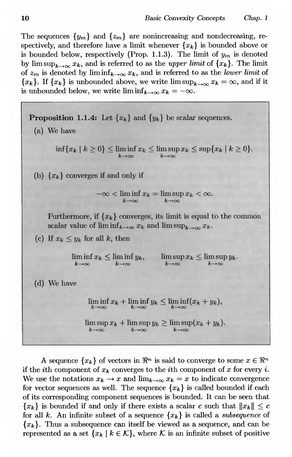
Proposition 1.1.4: Let {xk} and {yk} be scalar sequences.
(a) We have
inf{xfc | к > 0} < liminf xk < lim sup #& < sup{xfc | к > 0}.
к—юо к—юо
(b) {xк} converges if and only if
—oo < liminf Xk = lim sup ж& < oo.
fc—юо k~-*oo
Furthermore, if {xk} converges, its limit is equal to the common
scalar value of liminf&—oo Xk and limsup^^^ Xk-
(c) If Xk < Ук for all к, then
lim inf Xk < lim inf yk, lim sup χ к < lim sup yk
fc—юо к—-юо к—юо fc-юо
(d) We have
liminf Xk + liminf yk < lim inf (ж* + Ук),
к—юо к—-юо fc—юо
lim sup ж* + lim sup yk > lim sup(xfc + Ук)·
fc—юо fc-юо к—юо
A sequence {#&} of vectors in 5?n is said to converge to some χ € 3ϊη
if the ith component of #& converges to the ith component of χ for every г.
We use the notations Xk —> ж and lim^—co ж^ = χ to indicate convergence
for vector sequences as well. The sequence {xk} is called bounded if each
of its corresponding component sequences is bounded. It can be seen that
{xk} is bounded if and only if there exists a scalar с such that ||х^|| < с
for all к. An infinite subset of a sequence {xk} is called a subsequence of
{xk}· Thus a subsequence can itself be viewed as a sequence, and can be
represented as a set {xk \ к € /С}, where /С is an infinite subset of positive
Sec. 1.1 Linear Algebra and Real Analysis
11
integers (the notation {xk}tc will also be used).
A vector χ € Шп is said to be a limit point of a sequence {#&} if
there exists a subsequence of {xk} that converges to x.f The following is a
classical result that will be used often.
I I
l Proposition 1.1.5: (Bolzano-Weierstrass Theorem) A bounded
r sequence in 5Rn has at least one limit point.
o(-) Notation
For a positive integer ρ and a function h : Шп ι—» Шт we write
h(x) = o(||x||p)
if
lim „ „ = 0,
fc-oo \\xk\\P
for all sequences {xk} such that Xk —> 0 and Xk φ 0 for all к.
Closed and Open Sets
We say that χ is a closure point of α subset X of 9ft71 if there exists a
sequence {xk} С X that converges to x. The closure of X, denoted cl(X),
is the set of all closure points of X.
Definition 1.1.2: A subset X of ffin is called closed if it is equal to
its closure. It is called open if its complement, {χ \ χ φ Χ}, is closed.
It is called bounded if there exists a scalar с such that ||x|| < с for all
χ € X. It is called compact if it is closed and bounded.
For any e > 0 and ж* € Шп, consider the sets
{x | ||x — x*|| < e}, {x \ \\x — x*|| < e}.
f Some authors prefer the alternative term "cluster point" of a sequence, and
use the term "limit point of a set S" to indicate a point χ such that χ £ S and
there exists a sequence {хк} С S that converges to x. With this terminology, χ
is a cluster point of a sequence {xk \ к = 1,2,...} if and only if (ж,0) is a limit
point of the set {(xk, 1/fc) | к — 1,2,...}. Our use of the term "limit point" of a
sequence is quite popular in optimization and should not lead to any confusion.
12 Basic Convexity Concepts Chap. 1
The first set is open and is called an open sphere centered at #*, while the
second set is closed and is called a closed sphere centered at x*. Sometimes
the terms open ball and closed ball are used, respectively. A consequence
of the definitions, is that a subset X of ffin is open if and only if for every
χ Ε X there is an open sphere that is centered at χ and is contained in X.
A neighborhood of a vector χ is an open set containing x.
Definition 1.1.3: We say that χ is an interior point of a subset X of
SR71 if there exists a neighborhood of χ that is contained in X. The set
of all interior points of X is called the interior of X, and is denoted
by int(X). A vector χ € cl(X) which is not an interior point of X is
said to be a boundary point of X. The set of all boundary points of X
is called the boundary of X.
Proposition 1.1.6:
(a) The union of a finite collection of closed sets is closed.
(b) The intersection of any collection of closed sets is closed.
(c) The union of any collection of open sets is open.
(d) The intersection of a finite collection of open sets is open.
(e) A set is open if and only if all of its elements are interior points.
(f) Every subspace of 5ft71 is closed.
(g) A set X is compact if and only if every sequence of elements of
X has a subsequence that converges to an element of X.
(h) If {Xk} is a sequence of nonempty and compact sets such that
Xk D Xk+i for all ft, then the intersection C\^L0Xk is nonempty
and compact.
The topological properties of sets in SR71, such as being open, closed,
or compact, do not depend on the norm being used. This is a consequence
of the following proposition, referred to as the norm equivalence property
in 3ϊη, which shows that if a sequence converges with respect to one norm,
it converges with respect to all other norms.
Proposition 1.1.7: For any two norms || · || and || · ||' on 3ϊη, there
exists a scalar с such that ||ж|| < c||x||' for all χ Ε 3ϊη.
Sec. 1.1 Linear Algebra and Real Analysis 13
Using the preceding proposition, we obtain the following.
Proposition 1.1.8: If a subset of 3ϊη is open (respectively, closed,
bounded, or compact) with respect to some norm, it is open
(respectively, closed, bounded, or compact) with respect to all other norms
Sequences of Sets
Let {Xk} be a sequence of nonempty subsets of Шп. The outer limit of
{Xk}, denoted limsup^^^X^, is the set of all χ G 3tn such that every
neighborhood of χ has a nonempty intersection with infinitely many of the
sets Xk, к = 1,2, Equivalently, limsup^.^^ Xk is the set of all limit
points of sequences {xk} such that Xk € Xk for all к = 1,2,
The inner limit of {Xk}, denoted ]immfk-^ocXk, is the set of all
χ € Шп such that every neighborhood of χ has a nonempty intersection
with all except finitely many of the sets Xk, к = 1,2, Equivalently,
liminffc-юо Xk is the set of all limits of convergent sequences {xk} such
that Xk € Xk for all к = 1,2, —
The sequence {Xk} is said to converge to a set X if
X = lim inf Xk = Hm sup X^.
k—+oc fc-+oo
In this case, X is called the limit of {Xk}, and is denoted by limfc->oo Xk-
The inner and outer limits are closed (possibly empty) sets. If each
set Xk consists of a single point Xk, limsup^.^^ Xk is the set of limit points
of {xk}, while Yvonmik^oo Xk is just the limit of {xk} if {%k} converges,
and otherwise it is empty.
Continuity
Let f : X *-> 9ftm be a function, where X is a subset of 9ft71, and let χ be a
vector in X. If there exists a vector у € Шт such that the sequence {f{xk)}
converges to у for every sequence {xk} С X such that Нт^-юо Xk = x, we
write Итг_>х f(z) = y. If there exists a vector у е 9ftm such that the
sequence {f{xk)} converges to у for every sequence {xk} С X such that
limfc_>ooXfc = χ and Xk < x (respectively, Xk > x) for all k, we write
ИтгТх f(z) = у [respectively, limzix f(z)].
14
Basic Convexity Concepts Chap. 1
Definition 1.1.4: Let X be a subset of 5ΐη.
(a) A function f : X *-* 3?m is called continuous at a vector χ € X if
limz^xf(z) = f(x).
(b) A function / : X »—► 9ft™ is called right-continuous (respectively,
left-continuous) at a vector ж € X if Ишг|х f(z) = f(x)
[respectively, ИшгТх f(z) = f(x)].
(c) A real-valued function / : X ь-» 5R is called upper semicontinuous
(respectively, Zower semicontinuous) at a vector ж € X if /(x) >
limsupfc.^ f(xk) [respectively, f(x) < liminffc_oo f(xk)] for
every sequence {#&} С X that converges to x.
If / : X >—> 9ftm is continuous at every vector in a subset of its domain
X, we say that / is continuous over that subset. If / : X >—> 9ftm is
continuous at every vector in its domain X, we say that / is continuous. We
use similar terminology for right-continuous, left-continuous, upper semi-
continuous, and lower semicontinuous functions.
Proposition 1.1.9:
(a) Any vector norm on ffin is a continuous function.
(b) Let / : 3ftm н-* № and g : 5Rn ι-* 5Rm be continuous functions.
The composition f-g : 5Rn ь-> 3fa% defined by {f-g)(x) = f(g(x)),
is a continuous function.
(c) Let / : 5Rn н-> 3ftm be continuous, and let Υ be an open
(respectively, closed) subset of 9ftm. Then the inverse image of У,
{x e ffin | f(x) e Y}, is open (respectively, closed).
(d) Let / : 5Rn н^ 9ftm be continuous, and let X be a compact subset
of ffl1. Then the image of Χ, {f(x) | x G X}, is compact.
Matrix Norms
A norm || · || on the set of η χ η matrices is a real-valued function that
has the same properties as vector norms do when the matrix is viewed as
a vector in 3ftn . The norm of an η χ η matrix A is denoted by ||A||.
An important class of matrix norms are induced norms, which are
constructed as follows. Given any vector norm || · ||, the corresponding
induced matrix norm, also denoted by || · ||, is defined by
|И|| = sup ||Ar||.
IMI=i
Sec. 1.1 Linear Algebra and Real Analysis 15
It is easily verified that for any vector norm, the above equation defines a
matrix norm.
Let || · || denote the Euclidean norm. Then by the Schwarz inequality
(Prop. 1.1.2), we have
\\A\\ = sup \\Ax\\ = sup |г/'Лж|.
IWI=i IMNWI=i
By reversing the roles of χ and у in the above relation and by using the
equality y'Ax = x'A'y, it follows that \\A\\ = \\A'\\.
1.1.3 Square Matrices
Definition 1.1.5: A square matrix A is called singular if its
determinant is zero. Otherwise it is called nonsingular or invertible.
Proposition 1.1.10:
(a) Let A be an η χ η matrix. The following are equivalent:
(i) The matrix A is nonsingular.
(ii) The matrix A' is nonsingular.
(iii) For every nonzero χ € Шп, we have Αχ φ 0.
(iv) For every у € !ffin, there is a unique χ € 9ft71 such that
Ax = y.
(v) There is an η χ η matrix В such that AB — I — В A.
(vi) The columns of A are linearly independent.
(vii) The rows of A are linearly independent.
(b) Assuming that A is nonsingular, the matrix В of statement (v)
(called the inverse of A and denoted by A~l) is unique.
(c) For any two square invertible matrices A and В of the same
dimensions, we have (AB)-1 = B~1A~1.
Definition 1.1.6: A symmetric nxn matrix A is called positive
definite if x'Ax > 0 for all χ € 5ft71, χ φ 0. It is called positive semidefinite
if x'Ax > 0 for all χ e 5Rn.
16
Basic Convexity Concepts Chap. 1
Throughout this book, the notion of positive definiteness applies
exclusively to symmetric matrices. Thus whenever we say that a matrix is
positive (semi)definite, we implicitly assume that the matrix is symmetric,
although we usually add the term "symmetric" for clarity.
Proposition 1.1.11:
(a) A square matrix is symmetric and positive definite if and only if
it is invertible and its inverse is symmetric and positive definite.
(b) The sum of two symmetric positive semidefinite matrices is
positive semidefinite. If one of the two matrices is positive definite,
the sum is positive definite.
(c) If A is a symmetric positive semidefinite η χ η matrix and Τ is
an πι χ η matrix, then the matrix TAT' is positive semidefinite.
If A is positive definite and Τ is invertible, then TAT' is positive
definite.
(d) If A is a symmetric positive definite η χ η matrix, there exist
positive scalars 7 and 7 such that
7||x||2 < x'Ax < 7||ж||2, V χ e 3Rn.
(e) If A is a symmetric positive definite η χ η matrix, there exists
a unique symmetric positive definite matrix that yields A when
multiplied with itself. This matrix is called the square root of A.
It is denoted by Л1/2, and its inverse is denoted by А~г/2
1.1.4 Derivatives
Let / : Шп ь-» 9ft be some function, fix some a; € Sn, and consider the
expression
lim ^X + a6i>> ~ ^
a—>0 a
where ei is the ith unit vector (all components are 0 except for the i\L·
component which is 1). If the above limit exists, it is called the ith
partial derivative of / at the vector χ and it is denoted by (df/dxi){x) or
df(x)/dxi (xi in this section will denote the ith component of the vector
x). Assuming all of these partial derivatives exist, the gradient of / at χ is
defined as the column vector
V/(s)
a/(g)
δχχ
df(x
L dxn
Sec. 1.1 Linear Algebra and Real Analysis
17
For any у Ε 5ftn, we define the one-sided directional derivative of / in
the direction y, to be
,,/ ч r f(x + ay)~ f(x)
f'{x; y) = hm ,
ajO a
provided that the limit exists.
If the directional derivative of / at a vector χ exists in all directions
у and f'(x; y) is a linear function of y, we say that / is differentiable at
x. This type of differentiability is also called Gateaux differentiability. It
is seen that / is differentiable at χ if and only if the gradient V/(x) exists
and satisfies
Vf(xyy = f'(x;y), V у ε 5ft".
The function / is called differentiable over a subset U of 5ftn if it is
differentiable at every χ Ε U. The function / is called differentiable (without
qualification) if it is differentiable at all χ Ε 5ftn.
If / is differentiable over an open set U and V/(·) is continuous at
all χ Ε £/, / is said to be continuously differentiable over U. It can then be
shown that
^/(* + y)-/(*)-v/(*)'g=0> Vx6^ (L1)
y-+o \\y\\
where || · || is an arbitrary vector norm. If / is continuously differentiable
over 5ftn, then / is also called a smooth function. If / is not smooth, it is
referred to as being nonsmooth.
The preceding equation can also be used as an alternative definition
of differentiability. In particular, / is called Frechet differentiable at χ
if there exists a vector д satisfying Eq. (1.1) with V/(x) replaced by д.
If such a vector д exists, it can be seen that all the partial derivatives
(df/dxi)(x) exist and that д = V/(x). Frechet differentiability implies
(Gateaux) differentiability but not conversely (see for example Ortega and
Rheinboldt [OrR70] for a detailed discussion). In this book, when dealing
with a differentiable function /, we will always assume that / is
continuously differentiable over some open set [V/(·) is a continuous function over
that set], in which case / is both Gateaux and Frechet differentiable, and
the distinctions made above are of no consequence.
The definitions of differentiability of / at a vector χ only involve the
values of / in a neighborhood of x. Thus, these definitions can be used
for functions / that are not defined on all of 5ftn, but are defined instead
in a neighborhood of the vector at which the derivative is computed. In
particular, for functions / : X v-> 5ft, where X is a strict subset of 5ftn, we
use the above definition of differentiability of / at a vector x, provided χ is
an interior point of the domain X. Similarly, we use the above definition
of continuous differentiability of / over a subset £/, provided U is an open
subset of the domain X. Thus any mention of continuous differentiability
of a function over a subset implicitly assumes that this subset is open.
18
Basic Convexity Concepts Chap. 1
Differentiation of Vector-Valued Functions
A vector-valued function / : 5ftn ι—> 3?m is called differentiable (or smooth)
if each component fi of / is differentiable (or smooth, respectively). The
gradient matrix of /, denoted V/(x), is the nxm matrix whose zth column
is the gradient V/i(#) of fi. Thus,
V/(x)= V/i(s)-.-V/m(x)
The transpose of V/ is called the Jacobian of / and is a matrix whose ijth
entry is equal to the partial derivative dfi/dxj.
Now suppose that each one of the partial derivatives of a function
/ : 5ftn ι—> 5ft is a smooth function of x. We use the notation (d2f/dxidxj)(x)
to indicate the zth partial derivative of df/dxj at a vector χ Ε 5ftn. The
Hessian of / is the matrix whose ijth entry is equal to (d2f/dxidxj)(x),
and is denoted by V2/(x). We have (d2f/dxidxj)(x) = (d2f/dxjdxi)(x)
for every x, which implies that V2/(x) is symmetric.
If / : 5ftm+n h-> 5ft is a function of (ж, у), where χ Ε 5ftw and у £ 5ftn, and
#i,..., xm and 2/i,..., yn denote the components of χ and y, respectively,
we write
V*/(x,i/) =
Γ Q/(«,y) "I
Οχι
df(x,y)
Vyf(x,y) =
Г 9f(x,y) η
0!/l
df(xty)
L #2M J
We denote by V|x/(x, y), V|2//(x, y), and Vyyf(x,y) the matrices with
components
dxidyj
м>^у%-дШ·
, /r are the component functions of /, we
If /:5ft™+" h->^ and/1,/2,.
write
Vxf{x,y) = [Vxfi(x,y) - - -Vxfrfay)],
Vyf(x,y) = [Vyfi(x,y)-'-Vyfr(x,y)].
Let / : 5ftfc ь-> 5ftm and # : 5ftm ь-> 5ftn be smooth functions, and let ft
be their composition, i.e.,
h(x)=g{f(x)).
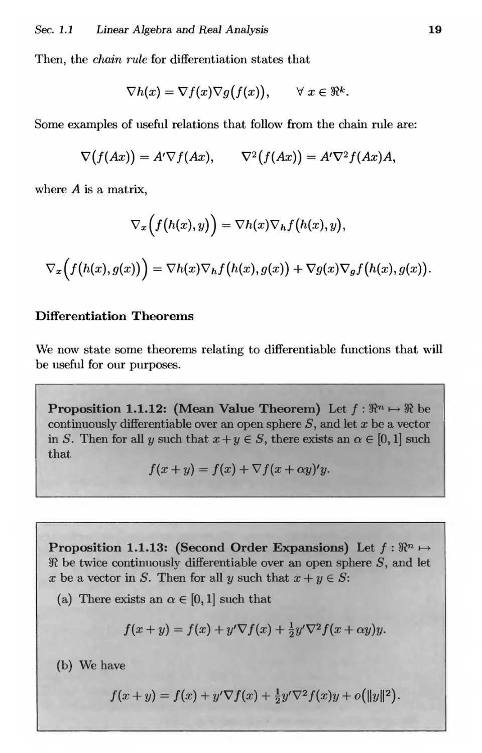
Sec. 1.1 Linear Algebra and Real Analysis 19
Then, the chain rule for differentiation states that
\7h{x) = V/(x)Vp(/(x)), V χ e 3№.
Some examples of useful relations that follow from the chain rule are:
V(/(Ac)) = A'Vf(Ax), V2(f{Ax)) = A>V*f(Ax)A,
where A is a matrix,
Vx(/(/i(*),2/)) = Vh(x)Vhf(h(x),y),
V,(/(%),s(x))) = Vh(x)Vhf(h(x),g(x)) + Vg(x)Vgf(h(x),g(x)).
Differentiation Theorems
We now state some theorems relating to differentiable functions that will
be useful for our purposes.
Proposition 1.1.12: (Mean Value Theorem) Let / : $in »-> $t be I
continuously differentiable over an open sphere S, and let χ be a vector
in S. Then for all у such that χ + у € 5, there exists an a € [0,1] such
I that
/(* + У) = /0*0 + V/(x + <xy)'y.
Proposition 1.1.13: (Second Order Expansions) Let / : 5Rn ·—►
*R be twice continuously differentiable over an open sphere S, and let
ж be a vector in S. Then for all у such that x-\-y Ε S:
(a) There exists an a € [0,1] such that
Я* + У) = f(x) + l/'V/fr) + \yfV*f(x + ay)y.
(b) We have
f(x + У) = /(*) + У'V/(x) + |y'ν2/0φ + o(||2/||2).
20
Basic Convexity Concepts Chap. 1
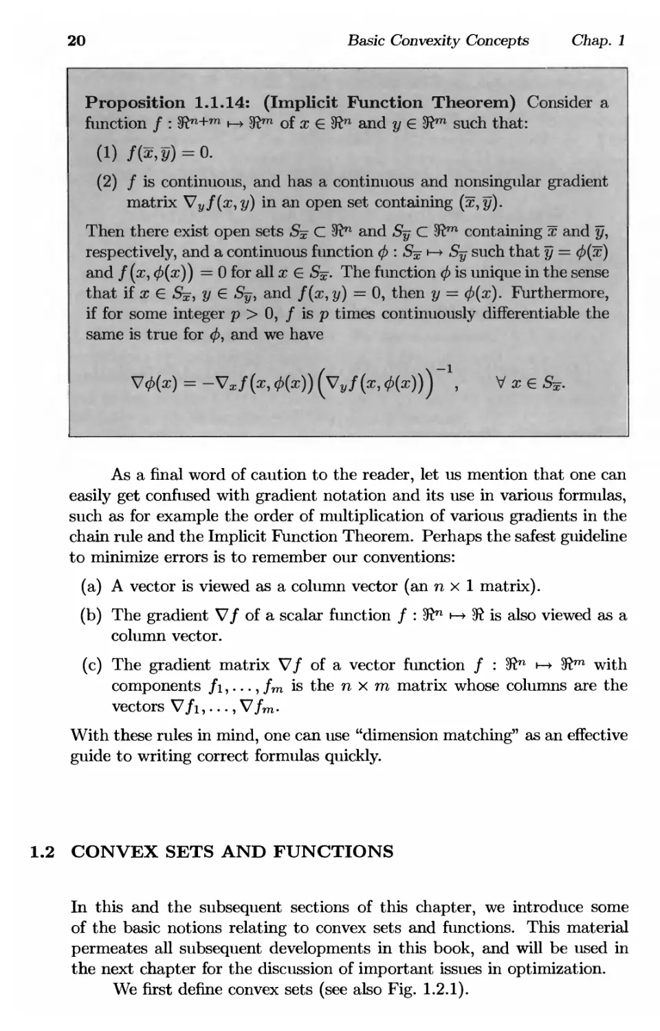
Proposition 1.1.14: (Implicit Function Theorem) Consider a
function / : $R"+m н-> 3?m of χ € 3ϊη and у € 3im such that:
(1) /(ЗД = 0.
(2) / is continuous, and has a continuous and nonsingular gradient
matrix Vyf(x,y) in an open set containing (ж,у).
Then there exist open sets Sx С Шп and S^ С 9?m containing ж and y,
respectively, and a continuous function φ \ S-χ \-± Sy such that ?/ = φ(χ)
and /(x, <£(#)) = 0 for all χ € S^-. The function φ is unique in the sense
that if χ G Sx, у € %, and /(x, y) = 0, then ?/ = ф(х). Furthermore,
if for some integer ρ > 0, / is ρ times continuously differentiable the
same is true for φ, and we have
\/φ(χ) = -νχ/(χ,φ(χ))(νν/(χ,φ{χ))γ\ VxeSx.
As a final word of caution to the reader, let us mention that one can
easily get confused with gradient notation and its use in various formulas,
such as for example the order of multiplication of various gradients in the
chain rule and the Implicit Function Theorem. Perhaps the safest guideline
to minimize errors is to remember our conventions:
(a) A vector is viewed as a column vector (an η χ 1 matrix).
(b) The gradient V/ of a scalar function / : 3ϊη ь-» 5R is also viewed as a
column vector.
(c) The gradient matrix V/ of a vector function / : Шп *-+ Шт with
components /i,..., /m is the η χ m matrix whose columns are the
vectors V/i,...,V/m.
With these rules in mind, one can use "dimension matching" as an effective
guide to writing correct formulas quickly.
1.2 CONVEX SETS AND FUNCTIONS
In this and the subsequent sections of this chapter, we introduce some
of the basic notions relating to convex sets and functions. This material
permeates all subsequent developments in this book, and will be used in
the next chapter for the discussion of important issues in optimization.
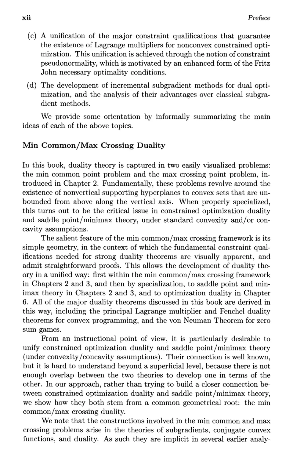
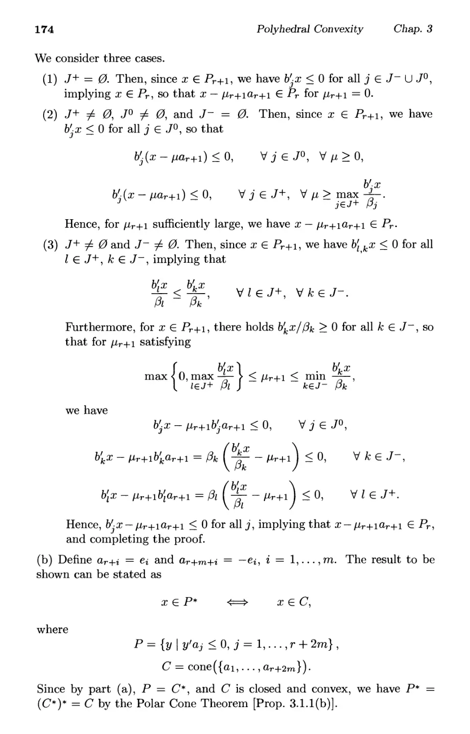
We first define convex sets (see also Fig. 1.2.1).
Sec. 1.2 Convex Sets and Functions
21
αχ + (1 - a)y, 0 < a <: 1
\v
Convex Sets
Nonconvex Sets
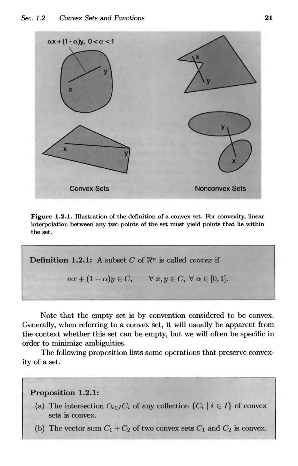
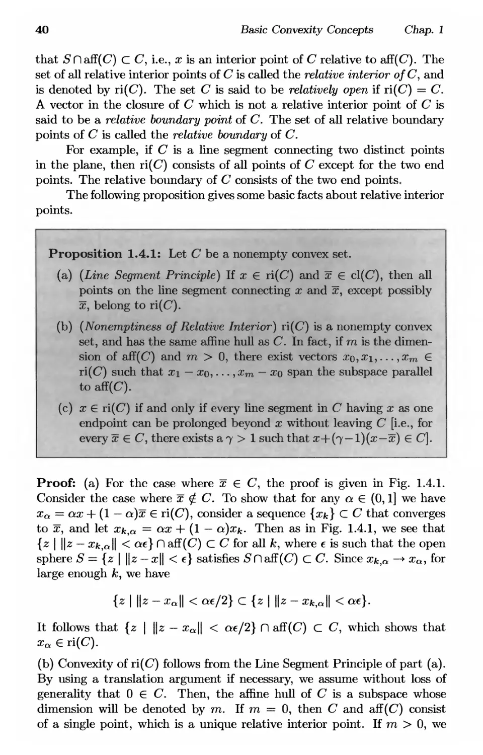
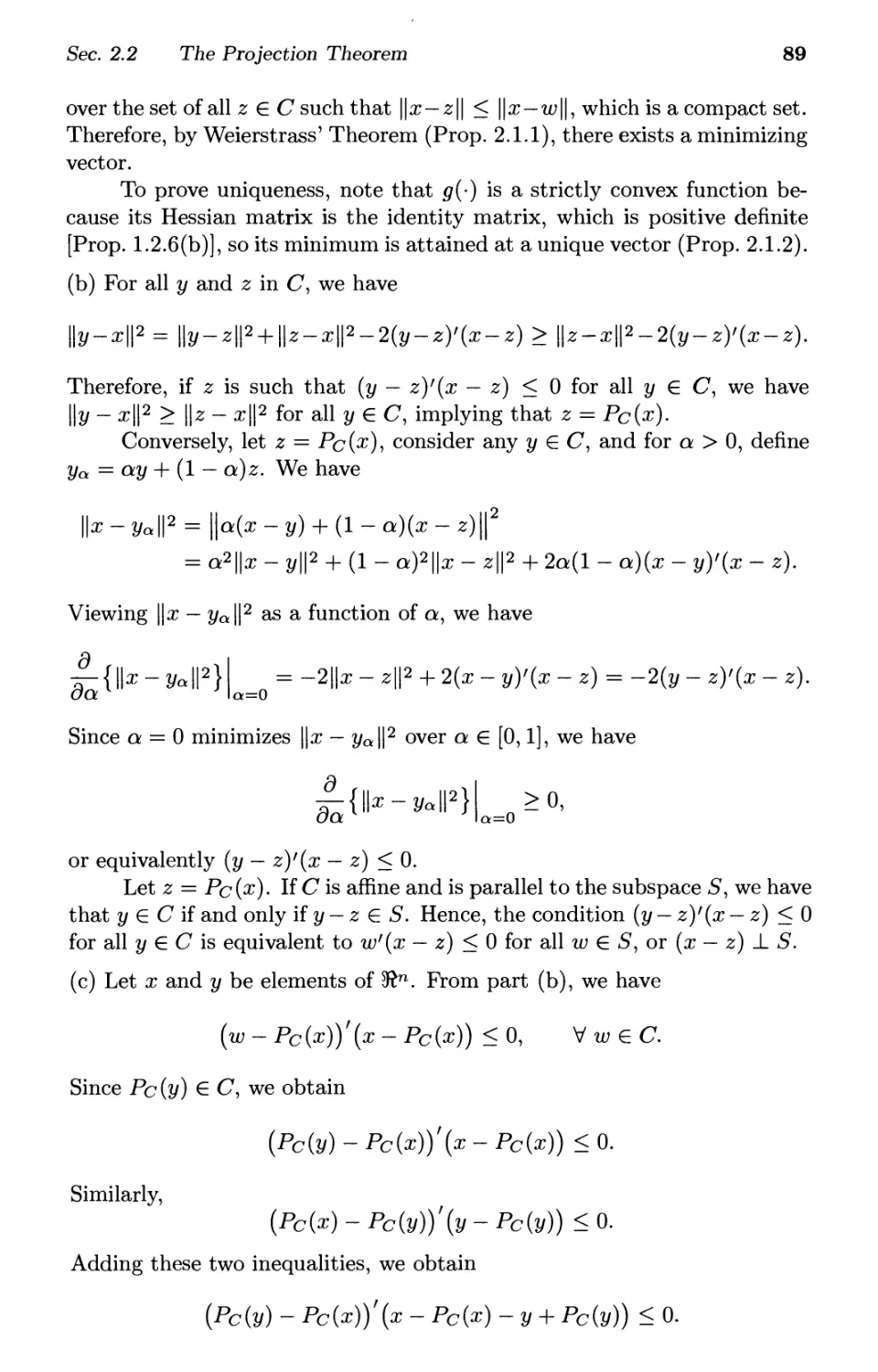
Figure 1.2.1. Illustration of the definition of a convex set. For convexity, linear
interpolation between any two points of the set must yield points that lie within
the set.
Definition 1.2.1: A subset С of 5Rn is called convex if
αχ + (1 - а)у е С, V χ, у е С, V α 6 [0,1].
Note that the empty set is by convention considered to be convex.
Generally, when referring to a convex set, it will usually be apparent from
the context whether this set can be empty, but we will often be specific in
order to minimize ambiguities.
The following proposition lists some operations that preserve
convexity of a set.
Proposition 1.2.1:
(a) The intersection CiieiCi of any collection {d \ г G /} of convex
sets is convex.
(b) The vector sum C\ + Сч of two convex sets C\ and C2 is convex.
22
Basic Convexity Concepts Chap. 1
(c) The set AC is convex for any convex set С and scalar λ.
Furthermore, if С is a convex set and λι, λ2 are positive scalars,
(d) The closure and the interior of a convex set are convex.
(e) The image and the inverse image of a convex set under an affine
function are convex.
Proof: The proof is straightforward using the definition of convexity. For
example, to prove part (a), we take two points χ and у from П^/Сг, and
we use the convexity of d to argue that the line segment connecting χ and
у belongs to all the sets d, and hence, to their intersection.
Similarly, to prove part (b), we take two points of C\ + C2, which we
represent as x\ -\-X2 and yi +2/2, with xi, у ι Ε С ι and x2, Уъ £ С2. For any
α € [0,1], we have
a{xi + X2) + (1 ~ cx){yi + 2/2) = (ctxi + (1 - a)yi) + (ax2 + (1 - a)y2).
By convexity of C\ and C2, the vectors in the two parentheses of the right-
hand side above belong to C\ and C2, respectively, so that their sum belongs
to C\ +C2. Hence C\ Л-Сч is convex. The proof of part (c) is left as Exercise
1.1. The proof of part (e) is similar to the proof of part (b).
To prove part (d), we take two points χ and у from the closure of C,
and sequences {xk} С С and {у к} С С, such that Xk —> x and ук^>У- For
any α 6 [0,1], the sequence {axk + (1 — а)Ук}-> which belongs to С by the
convexity of C, converges to ax + (1 — a)y. Hence ax + (1 — a)y belongs
to the closure of C, showing that the closure of С is convex. Similarly,
we take two points χ and у from the interior of C, and we consider open
balls that are centered at χ and y, and have sufficiently small radius r so
that they are contained in C. For any a G [0,1], consider the open ball
of radius r that is centered at ax + (1 — a)y. Any point in this ball, say
ax-h(l — a)y + z, where ||z|| < r, belongs to X, because it can be expressed
as the convex combination a(x + z) + (1 — a)(y + z) of the vectors χ + ζ
and у + ζ, which belong to X. Hence ax + (1 — a)y belongs to the interior
of C, showing that the interior of С is convex. Q.E.D.
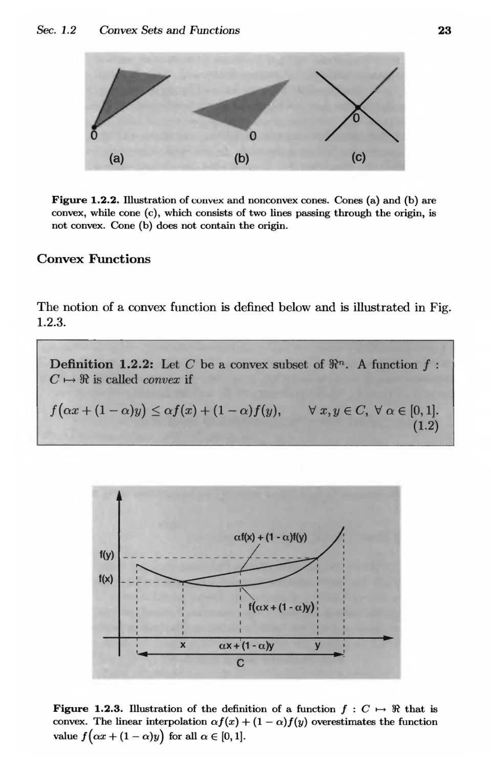
A set С is said to be a cone if for all χ € С and λ > 0, we have
λχ G C. A cone need not be convex and need not contain the origin,
although the origin always lies in the closure of a nonempty cone (see Fig.
1.2.2). Several of the results of the preceding proposition have analogs for
cones (see Exercise 1.2).
Sec. 1.2 Convex Sets and Functions
23
(a)
(b)
(с)
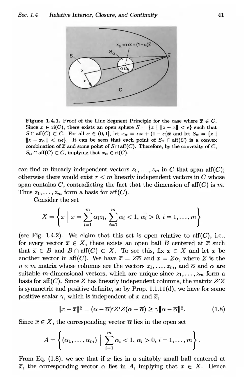
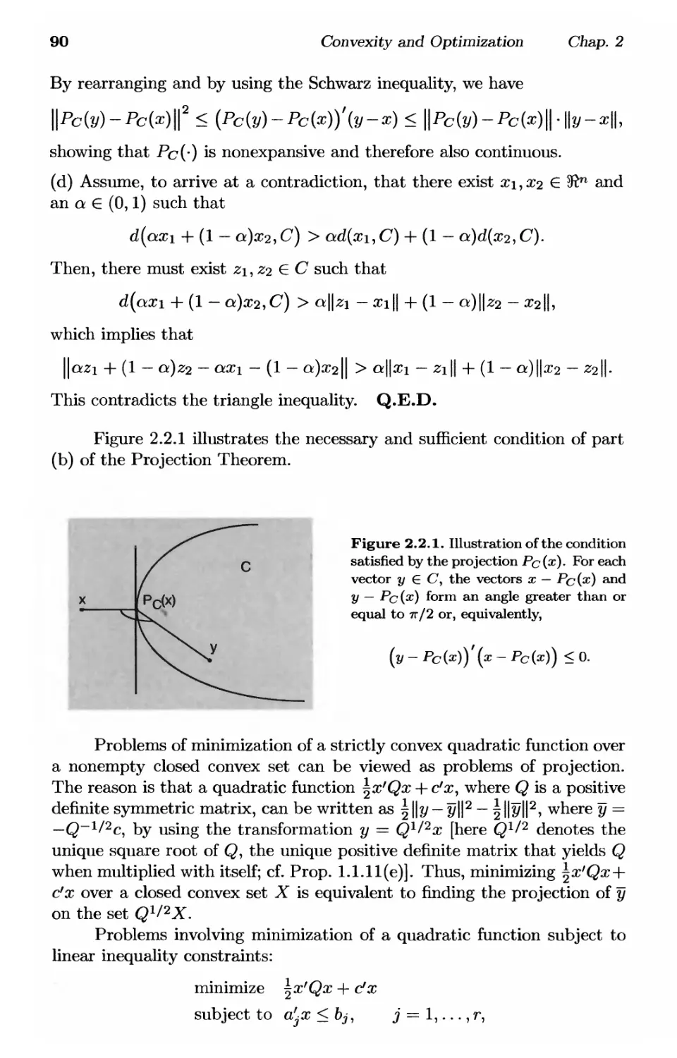
Figure 1.2.2. Illustration of convex and nonconvex cones. Cones (a) and (b) are
convex, while cone (c), which consists of two lines passing through the origin, is
not convex. Cone (b) does not contain the origin.
Convex Functions
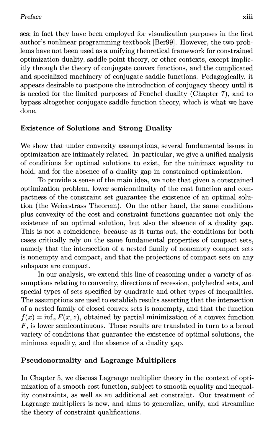
The notion of a convex function is defined below and is illustrated in Fig.
1.2.3.
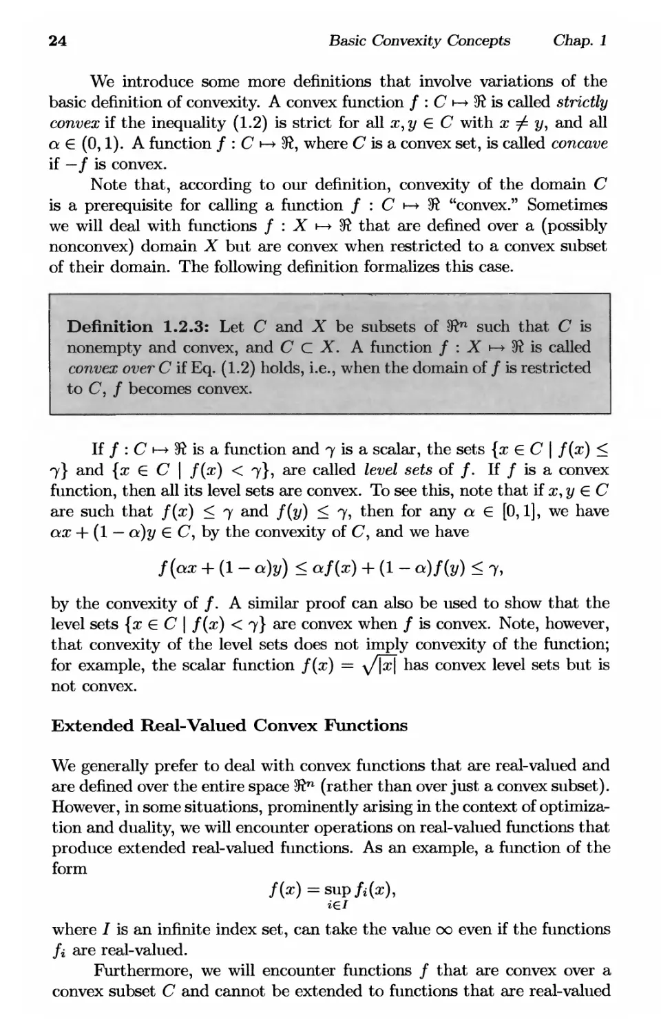
Definition 1.2.2: Let С be a convex subset of 5Rn. A function / :
С ь-> 5R is called convex if
f(ax + (1 - a)y) < af(x) + (1 - a)f(y), V x,y € C, V a e [0,1].
(1.2)
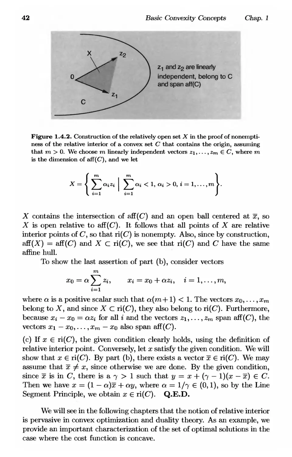
Figure 1.2.3. Illustration of the definition of a function / : С ·—► 5? that is
convex. The linear interpolation af(x) + (1 — ct)f(y) overestimates the function
value f(ax + (1 — a)y\ for all α G [0,1].
24
Basic Convexity Concepts Chap. 1
We introduce some more definitions that involve variations of the
basic definition of convexity. A convex function / : С ь-» Ш is called strictly
convex if the inequality (1.2) is strict for all x,y € С with χ φ у, and all
а € (0,1). A function / : С ь-» 5ΐ, where C is a convex set, is called concave
if — / is convex.
Note that, according to our definition, convexity of the domain С
is a prerequisite for calling a function / : С ь-» Ш "convex." Sometimes
we will deal with functions / : X ь-» 5R that are defined over a (possibly
nonconvex) domain X but are convex when restricted to a convex subset
of their domain. The following definition formalizes this case.
Definition 1.2.3: Let С and X be subsets of 3ΐη such that С is
nonempty and convex, and С С X. A function / : X ь-» Ш is called
convex over С if Eq. (1.2) holds, i.e., when the domain of / is restricted
to C, / becomes convex.
If / : С ь-> Ш is a function and 7 is a scalar, the sets {x € С \ f(x) <
7} and {x 6 С | /(ж) < 7}, are called /ег>е/ sets of /. If / is a convex
function, then all its level sets are convex. To see this, note that if ж, у € С
are such that f(x) < 7 and f(y) < 7, then for any a € [0,1], we have
ax + (1 — а)у € С, by the convexity of C, and we have
f(ax + (1 - a)y) < a/(x) + (1 - a)f(y) < 7,
by the convexity of /. A similar proof can also be used to show that the
level sets {x € С \ f(x) < 7} are convex when / is convex. Note, however,
that convexity of the level sets does not imply convexity of the function;
for example, the scalar function f(x) = л/Щ has convex level sets but is
not convex.
Extended Real-Valued Convex Functions
We generally prefer to deal with convex functions that are real-valued and
are defined over the entire space 3ϊη (rather than over just a convex subset).
However, in some situations, prominently arising in the context of
optimization and duality, we will encounter operations on real-valued functions that
produce extended real-valued functions. As an example, a function of the
form
f{x) = sup fi(x),
iei
where / is an infinite index set, can take the value 00 even if the functions
fi are real-valued.
Furthermore, we will encounter functions / that are convex over a
convex subset С and cannot be extended to functions that are real-valued
Sec. 1.2 Convex Sets and Functions
25
and convex over the entire space 5ftn [e.g., the function / : (0, oo) ь-» 5ft
defined by f(x) = 1/x]. In such situations, it may be convenient, instead
of restricting the domain of / to the subset С where / takes real values, to
extend the domain to all of 5ftn, but allow / to take infinite values.
We are thus motivated to introduce extended real-valued functions
that can take the values of — oo and oo at some points. Such functions can
be characterized using the notions of epigraph and effective domain, which
we now introduce.
f(x)
Epigraph
\
Epigraph
Convex function
Nonconvex function
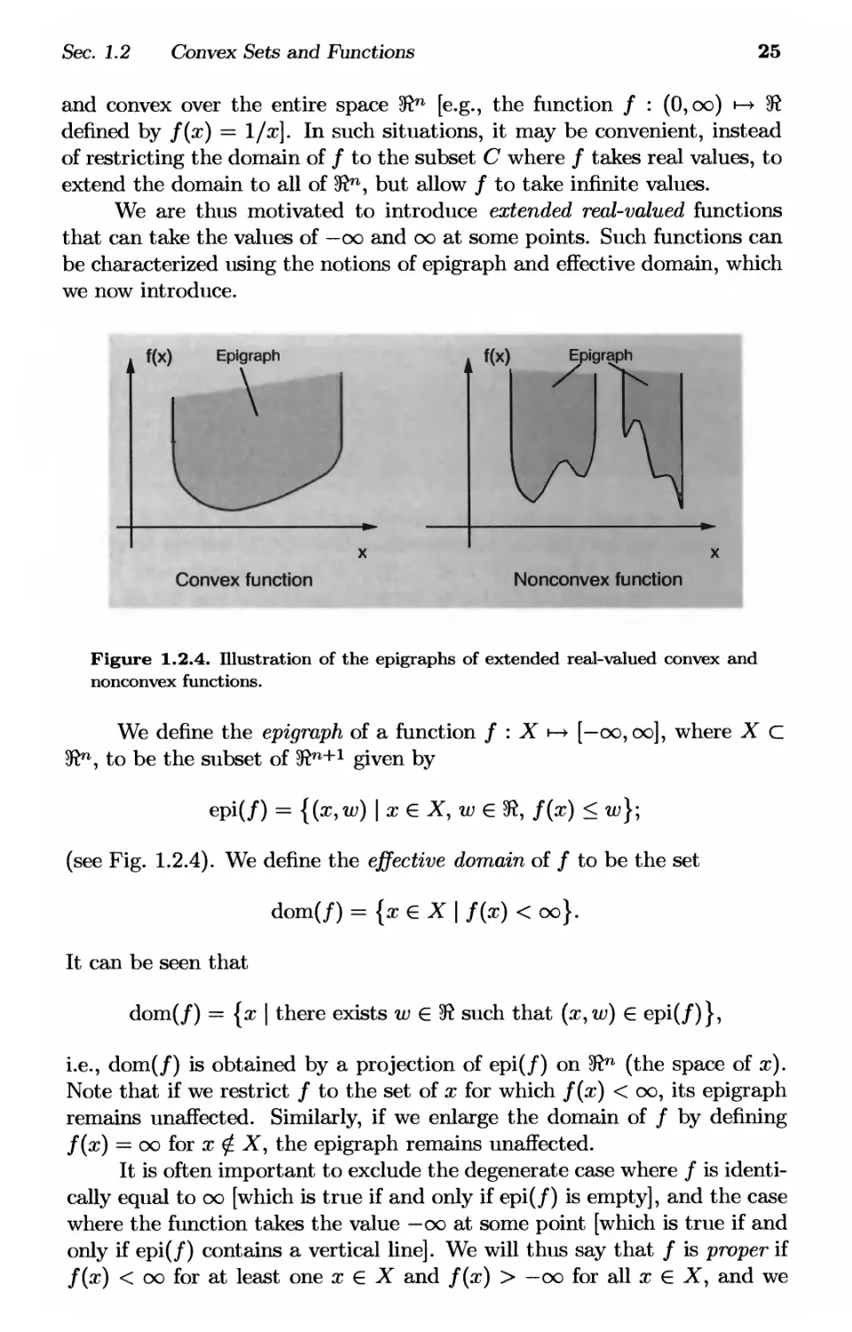
Figure 1.2.4. Illustration of the epigraphs of extended real-valued convex and
nonconvex functions.
We define the epigraph of a function / : X ь-» [—oo, oo], where X С
3^, to be the subset of 3ftn+1 given by
epi(/) = {(x,w) \x€X,w€to, f(x) < w}·
(see Fig. 1.2.4). We define the effective domain of / to be the set
dom(/) = {xeX\ f(x) < oo}.
It can be seen that
dom(/) = {x | there exists w € 5ft such that (x,w) € epi(/)},
i.e., dom(/) is obtained by a projection of epi(/) on 5ftn (the space of x).
Note that if we restrict / to the set of χ for which f(x) < oo, its epigraph
remains unaffected. Similarly, if we enlarge the domain of / by defining
f(x) = oo for χ φ Χ, the epigraph remains unaffected.
It is often important to exclude the degenerate case where / is
identically equal to oo [which is true if and only if epi(/) is empty], and the case
where the function takes the value — oo at some point [which is true if and
only if epi(/) contains a vertical line]. We will thus say that / is proper if
f(x) < oo for at least one χ € X and f(x) > —oo for all χ € X, and we
26
Basic Convexity Concepts Chap. 1
will say that / improper if it is not proper. In words, a function is proper
if and only if its epigraph is nonempty and does not contain a vertical line.
A difficulty in defining extended real-valued convex functions / that
can take both values — oo and oo is that the term af(x) + (1 — o)f{y)
arising in our earlier definition for the real-valued case may involve the
forbidden sum —oo + oo (this, of course, may happen only if / is improper,
but improper functions may arise on occasion in proofs or other analyses, so
we do not wish to exclude α priori such functions). The epigraph provides
an effective way of dealing with this difficulty.
Definition 1.2.4: Let С be a convex subset of 5Rn An extended real-
valued function /:Си [—oo, oo] is called convex if epi(/) is a convex
subset of 5Rn+1.
It can be easily verified that, according to the above definition,
convexity of / implies that its effective domain dom(/) and its level sets
{x G С | f(x) < 7} and {x G С | f(x) < 7} are convex sets for all
scalars 7. Furthermore, if f(x) < 00 for all x, or f(x) > —00 for all ж, we
have
f(ox + (l-a)y) < af(x) + (l-a)f(y), Vx,y G C, Va G [0,1], (1.3)
so the preceding definition is consistent with the earlier definition of
convexity for real-valued functions.
A convex function / : С ь-» (—oo, oo] is called strictly convex if the
inequality (1.3) is strict for all x,y Ε dom(/) with χ фу, and all α G (0,1).
A function / : С ь-> [—oo, 00], where С is a convex set, is called concave if
the function —/ : С \-* [—00,00] is convex as per Definition 1.2.4.
The following definition deals with the case where an extended real-
valued function becomes convex when restricted to a subset of its domain.
Definition 1.2.5: Let С and X be subsets of Шп such that С is
nonempty and convex, and С С X. An extended real-valued function
/ : X ь-> [—00,00] is called convex over С if / becomes convex when the
domain of / is restricted to C, i.e., if the function /:Си [—oo, 00],
defined by f(x) = f(x) for all χ G C, is convex.
Note that by replacing the domain of an extended real-valued proper
convex function with its effective domain, we can convert it to a real-valued
function. In this way, we can use results stated in terms of real-valued
functions, and we can also avoid calculations with 00. Thus, the entire
subject of convex functions can be developed without resorting to extended
Sec. 1.2 Convex Sets and Functions
27
real-valued functions. The reverse is also true, namely that extended real-
valued functions can be adopted as the norm; for example, this approach
is followed by Rockafellar [Roc70].
Generally, functions that are real-valued over the entire space 3ϊη are
more convenient (and even essential) in numerical algorithms and also in
optimization analyses where a calculus-oriented approach based on
differentiability is adopted. This is typically the case in nonconvex optimization,
where nonlinear equality and nonconvex inequality constraints are involved
(see Chapter 5). On the other hand, extended real-valued functions offer
notational advantages in convex optimization, and in fact may be more
natural because some basic constructions around duality involve extended
real-valued functions (see Chapters 6 and 7). Since we plan to deal with
nonconvex as well as convex problems, and with duality theory as well
as numerical methods, we will adopt a flexible approach, and use both
real-valued and extended real-valued functions.
Lower Semicontinuity and Closedness of Convex Functions
An extended real-valued function / : X ь-> [—oo, oo] is called lower semi-
continuous at a vector χ € X if f(x) < liminffc_>oo f(xk) for every sequence
{xk} С X with Xk —> x. This is consistent with the corresponding definition
for real-valued functions [cf. Definition 1.1.4(c)]. If / is lower semicontinu-
ous at every χ in a subset U of X, we say that / is lower semicontinuous
over U. The following proposition relates lower semicontinuity of / with
closedness of its epigraph and its level sets.
Proposition 1.2.2: For a function / : 5in н-> [—οο,οο], the following
are equivalent:
(i) The level set {x \ f(x) < 7} is closed for every scalar 7. |
(ii) / is lower semicontinuous over 5ft71.
(iii) epi(/) is closed.
Proof: If /(ж) = 00 for all x, the result trivially holds We thus assume
that f(x) < 00 for at least one χ € 3ϊη, so that epi(/) is nonempty and
there exist level sets of / that are nonempty.
We first show that (i) implies (ii). Assume that the level set {χ |
/0*0 < 7} is closed for every scalar 7. Suppose, to arrive at a contradiction,
that f(x) > liminffc_>oo f(xk) for some χ and sequence {xk} converging to
of, and let 7 be a scalar such that
:—+00
28
Basic Convexity Concepts Chap. 1
Then, there exists a subsequence {xk}tc such that f(xk) < 7 for all к € /С.
Since the set {x | f(x) < 7} is closed, χ must belong to this set, so
f(x) < 7, a contradiction.
We next show that (ii) implies (iii). Assume that / is lower semicon-
tinuous over 3ϊη, and let (x,w) be the limit of a sequence {(xk,Wk)} С
epi(/). Then we have f(xk) < Wk, and by taking the limit as к —>
oo and by using the lower semicontinuity of / at x, we obtain f(x) <
liminffc_oo f(%k) < w. Hence, (x,w) € epi(/) and epi(/) is closed.
We finally show that (iii) implies (i). Assume that epi(/) is closed,
and let {xk} be a sequence that converges to some χ and belongs to the
level set {x \ f(x) < 7} for some scalar 7. Then (#£,7) £ ePK/) for a^
к and (xk,l) —► (ж,7), so since epi(/) is closed, we have (of,7) € epi(/).
Hence, χ belongs to the level set {χ \ f(x) < 7}, implying that this set is
closed. Q.E.D.
If the epigraph of a function / : X ь-» [—oo, 00] is a closed set, we say
that / is a closed function. To understand the relation between closedness
and lower semicontinuity, let us extend the domain of / to Шп and consider
the function / : 3ϊη ь-» [—oo, 00] given by
/» = {/(*) if*e*-
00 if χ £ X.
Then, we see that / and / have the same epigraph, and according to the
preceding proposition, / is closed if and only if f is lower semicontinuous
over 3in.
Note, however, that if / is lower semicontinuous over dom(/), it is
not necessarily closed; take for example / to be constant for χ in some
nonclosed set and 00 otherwise. Furthermore, if / is closed, dom(/) need
not be closed; for example, the function
/(*) = {* if">0'
(^ 00 otherwise,
is closed but dom(/) is the open half-line of positive numbers. On the other
hand, if dom(/) is closed and / is lower semicontinuous over dom(/), then
/ is closed because epi(/) is closed, as can be seen by reviewing the proof
that (ii) implies (iii) in Prop. 1.2.2. We state this as a proposition.
Proposition 1.2.3: Let / : X ь-» [—oo, oo] be a function. If dom(/)
is closed and / is lower semicontinuous over dom(/), then / is closed.
We finally note that an improper closed convex function is very
peculiar: it cannot take a finite value at any point, so it has the form
f (ηΓ\ _ / -°° if x e dom(/)>
/W loo ifx£dom(/).
Sec. 1.2 Convex Sets and Functions 29
To see this, consider an improper closed convex function / : 3in ь-> [—oo, oo],
and assume that there exists an χ such that f(x) is finite. Let χ be such
that f(x) — —oo (such a point must exist since / is improper and / is not
identically equal to oo). Because / is convex, it can be seen that every
point of the form
Xk = —;—x + тж, V к = 1,2,...
к к
satisfies f(xk) = — oo, while we have Xk —> X- Since / is closed, this implies
that f(x) = —oo, which is a contradiction. In conclusion, a closed convex
function that is improper cannot take a finite value anywhere.
Recognizing Convex Functions
We can verify the convexity of a given function in a number of ways. Several
commonly encountered functions are convex. For example, affine functions
and norms are convex; this is straightforward to verify using the definition
of convexity. In particular, for any x, у € 3ϊη and any а € [0,1], by using
the triangle inequality, we have
\\αχ + (1 - a)y\\ < |M| + ||(1 - a)y\\ = a\\x\\ + (1 - a)\\y\\,
so the norm function || · || is convex. The exercises provide further examples
of useful convex functions.
Starting with some known convex functions, we can generate other
convex functions by using some common algebraic operations that preserve
convexity of a function. The following proposition provides some of the
necessary machinery.
Proposition 1.2.4:
(a) Let fi : 3ϊη >—> (—οο,οο], г = l,...,ra, be given functions, let
λι,..., Xrn be positive scalars, and consider the function g :
3ϊη κ—> (—00,00] given by
g(x) = Xlfl(x) -i h Xmfm(x).
If /1,..., fm are convex, then g is also convex, while if /i,..., /m
are closed, then g is also closed.
30
Basic Convexity Concepts Chap. 1
(b) Let / : 3?m н-> (—00,00] be a given function, let A be an m χ η
matrix, and consider the function g : Шп ь-» (—oo, 00] given by
g{x) = f(Ax).
If / is convex, then g is also convex, while if / is closed, then g
is also closed.
(c) Let fi : 5ft71 ■—► (—00,00] be given functions for г G /, where / is an
arbitrary index set, and consider the function g : Шп ь-» (—со, оо]
given by
g(x) = sup fi{x).
iei
If /i, г Ε /, are convex, then # is also convex, while if fi, i € I,
are closed, then g is also closed.
Proof: (a) Let /1,..., /m be convex. We use the definition of convexity
to write for any x, у G 9ft71 and α G [0,1],
д(ах + (1- а)у) = J^ Xifi (ax + (1 - a)y)
г=1
m
<£>(«/«(*)+ (1-а)Ш)
m m
= aJ2 Ш*) + (1 - «) Σ ^/«ί»)
г=1 i=l
= ар(ж) + (1 - а)£(г/).
Hence p is convex.
Let the functions /1,..., /m be closed. Then they are lower semi-
continuous at every χ G 3ϊη (cf. Prop. 1.2.2), so for every sequence {xk}
converging to ж, we have /г(#) < liminffc-^oo fiip^k) for all г. Hence
m τη
g{x) < У^\iliminf fi(xk) < liminf y^\ifi{xk) = Hminf ρ(^),
*—-' к—юс к-+ос *—"' к—+οο
г=1 г=1
where we have used the assumption Xi > 0 and Prop. 1.1.4(d) (the sum of
the lower limits of sequences is less than or equal to the lower limit of the
sum sequence). Therefore, g is lower semicontinuous at all χ G 3ϊη, so by
Prop. 1.2.2, it is closed.
(b) This is straightforward, along the lines of the proof of part (a).
Sec. 1.2 Convex Sets and Functions
31
f(x) + (z-x)Vf(x)
Figure 1.2.5. Characterization of convexity in terms of first derivatives. The
condition f(z) > f(x) + (z — x)'V f(x) states that a linear approximation, based
on the gradient, underestimates a convex function.
(c) A pair (x, w) belongs to epi(p) if and only if g(x) < w, which is true
if and only if fi(x) < w for all i € /, or equivalently (x,w) € Пге/ер1(/г).
Therefore,
epi(p) - niG/epi(/i).
If the fi are convex, the epigraphs epi(/i) are convex, so epi(p) is convex,
and g is convex. If the fi are closed, then, by definition, the epigraphs
epi(/i) are closed, so epi(p) is closed, and g is closed. Q.E.D.
For once or twice differentiable functions, there are some additional
useful criteria for verifying convexity, as we now proceed to discuss.
Characterizations of Differentiable Convex Functions
For differentiable functions, a useful alternative characterization of
convexity is given in the following proposition and is illustrated in Fig. 1.2.5.
Proposition 1.2.5: Let С be a convex subset of 5Rn and let / : 5in t—>
3ί be differentiable over Si71.
(a) / is convex over С if and only if
f(z) > f(x) + (z - x)'V/(x), \fx,zeC. (1.4)
(b) / is strictly convex over С if and only if the above inequality is
strict whenever χ φ ζ.
32 Basic Convexity Concepts Chap. 1
Proof: The ideas of the proof are geometrically illustrated in Fig. 1.2.6.
We prove (a) and (b) simultaneously. Assume that the inequality (1.4)
holds. Choose any x,y Ε С and α Ε [О,1], and let z = αχ-f (1 -а)у. Using
the inequality (1.4) twice, we obtain
f(x)>f(z) + (x-zyVf(z),
f(y) > № + (y- z)'Vf(z).
We multiply the first inequality by a, the second by (1 — a), and add them
to obtain
αf{x) + (1 - a)f(y) > f(z) + (ax + (1 - a)y - z)'Wf(z) = f(z),
which proves that / is convex. If the inequality (1.4) is strict as stated in
part (b), then if we take χ φ у and a E (0,1) above, the three preceding
inequalities become strict, thus showing the strict convexity of /.
Conversely, assume that / is convex, let χ and ζ be any vectors in С
with χ φ ζ, and for a E (0,1), consider the function
f{x + a(z-x)) - f(x)
g{<*) = — , ol e (0,1.
a
We will show that g(a) is monotonically increasing with a, and is strictly
monotonically increasing if / is strictly convex. This will imply that
(z - x)'Vf(x) = limg(a) < g(l) = f(z) - /(x),
with strict inequality if g is strictly monotonically increasing, thereby
showing that the desired inequality (1.4) holds, and holds strictly if / is strictly
convex. Indeed, consider any αι,α;2, with 0 < a\ < a^ < 1, and let
a =—, ~z = χ + θίϊ{ζ — χ). (1.5)
We have
f(x + a(z - x)) < af(z) + (1 - Э)/(ж),
or
f{x+^Zx))-f{x)<m-m, (1.6)
a
and the above inequalities are strict if / is strictly convex. Substituting the
definitions (1.5) in Eq. (1.6), we obtain after a straightforward calculation
f(x + ai{z-x)) - f(x) f(x + a2{z-x)) - f(x)
αι ~ <%2
Sec. 1.2 Convex Sets and Functions
33
f(z) + (x-
Figure 1.2.6. Geometric illustration of the ideas underlying the proof of Prop.
1.2.5. In figure (a), we linearly approximate / at ζ = аж+(1—а)у. The inequality
(1.4) implies that
/(*) > /W + (* - *)'v/W,
/(»)>/(*) + (w-*)'v/(*).
As can be seen from the figure, it follows that af(x) + (1 — ct)f(y) lies above /(2),
so / is convex.
In figure (b), we assume that / is convex, and from the figure's geometry,
we note that
f(X + CL(z-x))-f{x)
/(*) + —
а
lies below /(2), is monotonically nonincreasing as а | 0, and converges to f(x) +
(z - x)'Vf(x). It follows that f(z) > f(x) + {z- x)'Vf(x).
or
g{on) < 9(0.2),
with strict inequality if / is strictly convex. Hence g is monotonically
increasing with a, and strictly so if / is strictly convex. Q.E.D.
34
Basic Convexity Concepts Chap. 1
Note a simple consequence of Prop. 1.2.5(a): if / : 9tn >—> 9ft is a convex
function and V/(x*) = 0, then x* minimizes / over 9ft71. This is a classical
sufficient condition for unconstrained optimality, originally formulated (in
one dimension) by Fermat in 1637.
For twice differentiable convex functions, there is another
characterization of convexity as shown by the following proposition.
Proposition 1.2.6: Let С be a convex subset of 9ft71 and let / : 5ft71 >->
3ϊ be twice continuously differentiable over 3ϊη.
(a) If V2/(rr) is positive semidefinite for all χ € С, then / is convex
over C.
(b) If V2/(x) is positive definite for all χ G C, then / is strictly
convex over C.
(c) If С is open and / is convex over C, then V2/(x) is positive
semidefinite for all χ 6 С.
Proof: (a) By Prop. 1.1.13(b), for all x, у G С we have
f(y) = f{x) + (У ~ x)'Vf{x) + \{y - x)'V2/(x + a(y - x))(y - x)
for some a € [0,1]. Therefore, using the positive semidefiniteness of V2/,
we obtain
f(y) > f(x) + (У ~ *)'V/(x), Vx,j/€C.
From Prop. 1.2.5(a), we conclude that / is convex.
(b) Similar to the proof of part (a), we have f(y) > f(x) + (y — x)'V/(x)
for all x,|/GC with χ фу, and the result follows from Prop. 1.2.5(b).
(c) Assume, to obtain a contradiction, that there exist some χ € С and
some 2 G SR71 such that zrV2f{x)z < 0. Since С is open and V2/ is
continuous, we can choose ζ to have small enough norm so that χ -f ζ € С
and z'V2/(x + az)z < 0 for every a € [0,1]. Then, using again Prop.
1.1.13(b), we obtain f(x + z) < f(x) -f 2'V/(x), which, in view of Prop.
1.2.5(a), contradicts the convexity of / over C. Q.E.D.
As an example, consider the quadratic function
f(x) = x'Qx + a'x,
where Q is a symmetric η χ η matrix and b is a vector in 3ft71. Since
V2/(x) = 2Q, it follows by using Prop. 1.2.6, that / is convex if and only
if Q is positive semidefinite, and it is strictly convex if and only if Q is
positive definite.
Sec. 1.3 Convex and Affine Hulls
35
If / is convex over a strict subset С С 9ft71, it is not necessarily true
that V2/(x) is positive semidefinite at any point of С [take for example
η = 2, С — {(χι,Ο) I x\ G Щ, and f(x) = x\ — ж|]. The relation of
convexity and twice differentiability is further considered in Exercises 1.8
and 1.9. In particular, it can be shown that the conclusion of Prop. 1.2.6(c)
also holds if С has nonempty interior instead of being open.
1.3 CONVEX AND AFFINE HULLS
Let X be a nonempty subset of 9ft71. A convex combination of elements of X
is a vector of the form Σ™=ι cxiXi-, where m is a positive integer, m,..., хш
belong to X, and αϊ,..., am are scalars such that
771
&i > 0, г = 1,...,га, /^аг = 1-
i=l
Note that if X is convex, then a convex combination belongs to X (see the
construction of Fig. 1.3.1).
x2
x1
Figure 1.3.1. Illustration of the construction of a convex combination of m
vectors by forming a sequence of m — 1 convex combinations of pairs of vectors.
For example, we have
/ \ ( al a2 \
X = OL\X\ + Oi2X2 + «3^3 = («1 + OL2) I #i Η Ж2 J + «3^3,
\ai+a2 ai+c*2 /
so the convex combination ol\x\ + ol^xt, + 0:3x3 can be obtained by forming the
convex combination
Z = ; Χχ Η ; Ж2,
αϊ + OL2 Oil + «2
and then by forming the convex combination
χ = (αϊ + ot.2)z + 03x3
as shown in the figure. The construction shows among other things that a convex
combination of a collection of vectors from a convex set belongs to the convex set
36
Basic Convexity Concepts Chap. 1
For any function / : 5ftn v-> 5ft that is convex over X, we have
(m \ m
5>**1 <5>i/(*o- (ΐ·7)
г=1 / г=1
This follows by using repeatedly the definition of convexity together with
the construction of Fig. 1.3.1. The preceding relation is a special case of a
relation known as Jensen's inequality, and can be used to prove a number
of interesting relations in applied mathematics and probability theory.
The convex hull of a set X, denoted conv(X), is the intersection of
all convex sets containing X, and is a convex set by Prop. 1.2.1(a). It is
straightforward to verify that the set of all convex combinations of elements
of X is convex, and is equal to conv(X) (Exercise 1.14). In particular, if
X consists of a finite number of vectors xi,..., xm, its convex hull is
fm m ^
У^ OLiXi щ > 0, i = 1,..., m, У2 щ = 1 > .
г=1 г=1 J
We recall that an affine set Μ in 5ftn is a set of the form χ + 5, where
χ is some vector and S is a subspace uniquely determined by Μ and called
the subspace parallel to M. If X is a subset of 5ftn, the affine hull of X,
denoted aff(X), is the intersection of all affine sets containing X. Note that
aff(X) is itself an affine set and that it contains conv(X). It can be seen
that
aff(X) = aff(conv(X)) = aff(cl(X)),
(see Exercise 1.18). Furthermore, in the case where 0 G X, aff(X) is the
subspace generated by X. For a convex set C, the dimension of С is defined
to be the dimension of aff(C).
Given a nonempty subset X of 5ftn, a nonnegative combination of
elements of X is a vector of the form Y^LX ЩХг, where m is a positive
integer, x\,..., xm belong to X, and αϊ,..., am are nonnegative scalars. If
the scalars щ are all positive, Σϋι αΐχΐ *s sa^ to ^e a Pos^ve combination.
The cone generated by X, denoted cone(X), is the set of all nonnegative
combinations of elements of X. It is easily seen that cone(X) is a convex
cone containing the origin, although it need not be closed even if X is
compact, as shown in Fig. 1.3.2 [it can be proved that cone(X) is closed in
special cases, such as when X consists of a finite number of elements - this
is one of the central results of polyhedral convexity, which will be shown in
Section 3.2].
The following is a fundamental characterization of convex hulls (see
Fig. 1.3.3).
Sec. 1.3 Convex and Affine Hulls
37
1 *
(0,0) cone(X)
Figure 1.3.2. An example in 3ft2 where X is convex and compact, but cone(X)
is not closed. Here
X = {(xux2) Ι χ\ + (χ2 - i)2 < i},
cone(X) = {(Ж1,ж2) | xi > 0} U {(0,0)}.
cone(X)
X
χ x2
conv(X)
(a) (b)
Figure 1.3.3. Illustration of Caratheodory's Theorem. In (a), X is a nonconvex
set in 3ft2, and a point χ G cone(X) is represented as a positive combination
of the two linearly independent vectors Ж1,Ж2 € X. In (b), X consists of four
points Ж1,Ж2,жз,Ж4 in 3ft2, and the point χ G conv(X) shown in the figure can
be represented as a convex combination of the three vectors Ж1,Ж2,жз. Note
that the vectors X2 — жьжз — x\ are linearly independent. Note also that χ can
alternatively be represented as a convex combination of the vectors χ ι, #2,^4, so
the representation is not unique.
Proposition 1.3.1: (Caratheodory's Theorem) Let X be a
nonempty subset of 5Rn.
(a) Every χ in cone(X) can be represented as a positive combination
of vectors xi,..., xm from X that are linearly independent.
38
Basic Convexity Concepts Chap. 1
(b) Every χ in cogv^Q can be represented as a convex qombination
of vectors x\,..., Xm from X such that X2 — x\,..., x-m — xi are
linearly independent.
Proof: (a) Let ж be a nonzero vector in cone(X), and let m be the
smallest integer such that χ has the form Σ™=± otiXi, where oti > 0 and χι € X
for all г = 1,..., ra. If the vectors χι were linearly dependent, there would
exist scalars Ai,..., Am, with ΣΙϋι XiXi = 0 and at least one Xi is positive.
Consider the linear combination ΣΙϋι(α* ~ lXi)xi, where 7 is the largest
7 such that αϊ — η\ι > 0 for all г. This combination provides a
representation of χ as a positive combination of fewer than m vectors of X - a
contradiction. Therefore, linearly independent.
(b) The proof will be obtained by applying part (a) to the subset of Ш.п+1
given by
y={(i,l)|ieX}.
If χ G conv(X), then for some positive integer / and some positive scalars
7г, г = 1,..., J, with 1 = Σί=ι 7г, we have χ = Σ*=ι 7г#г, so that (χ, 1) €
сопе(У). By part (a), we have (x, 1) = J^Li^O*^»!) f°r some positive
scalars αϊ,..., am and some linearly independent vectors (χι, 1),..., (xm, 1)
ГП 771
г=1 г=1
Assume, to arrive at a contradiction, that #2 — x\, · · ·, %m — xi are
linearly dependent, so that there exist Аг,..., Am, not all 0, with
^Аг(хг — #i) = 0.
i=2
Equivalently, defining λι = —(Аг Η l· Am), we have
771
5^Ai(xi,l) = 0,
г=1
which contradicts the linear independence of (xi, 1),..., (xm, 1). Q.E.D.
Note that in view of the linear independence assertions in Caratheodo-
ry's Theorem, a vector in cone(X) [or conv(X)] may be represented by
no more than η (or η + 1, respectively) vectors of X. Note also that
the proof of the theorem suggests an algorithm to obtain a representation
of a vector χ £ cone(X) in terms of linearly independent vectors. The
typical step in this algorithm is the proof's construction, which starts with
Sec. 1.4 Relative Interior, Closure, and Continuity
39
a representation involving linearly dependent vectors, and yields another
representation involving fewer vectors.
Caratheodory's Theorem can be used to prove several other important
results. An example is the following proposition.
Proposition 1.3.2: The convex hull of a compact set is compact
Proof: Let X be a compact subset of 9ft71. To show that conv(X) is
compact, we will take a sequence in conv(X) and show that it has a convergent
subsequence whose limit is in conv(X). Indeed, by Caratheodory's
Theorem, a sequence in conv(X) can be expressed as < ΣΓ=ι αίχί η where for
all к and г, а% > 0, x\ € X, and ΣΙ^Ί α? = 1· Since the sequence
|(a1,... ,αη+1,χΐ5... ,#n+1) j
is bounded, it has a limit point {(αϊ,..., αη+ι, χι,..., xn+i)}, which must
satisfy J^iLi <*i = 1, and gli > 0, χι € X for all i. Thus, the vector
Σ™=ι QiXi, which belongs to conv(X), is a limit point of the sequence
ι Σ7=ι aixi r > showing that conv(X) is compact. Q.E.D.
Note that it is not generally true that the convex hull of a closed set
is closed. As an example, for the closed subset of 5ft2
X = {(°>°)} U {(sbS2) Ι χΙχ2 > hxl > 0, X2 > 0},
the convex hull is
conv(X) = {(0,0)} U {(xi,x2) | xi > 0, X2 > 0},
which is not closed.
1.4 RELATIVE INTERIOR, CLOSURE, AND CONTINUITY
We now consider some generic topological properties of convex sets and
functions. Let С be a nonempty convex subset of 5ftn. The closure of С is
also a nonempty convex set (Prop. 1.2.1). While the interior of С may be
empty, it turns out that convexity implies the existence of interior points
relative to the affine hull of C. This is an important property, which we
now formalize.
Let С be a nonempty convex set. We say that χ is a relative interior
point of C, if χ € С and there exists an open sphere S centered at χ such
40
Basic Convexity Concepts Chap. 1
that Snaff(C) С С, i.e., χ is an interior point of С relative to aff(C). The
set of all relative interior points of С is called the relative interior o/C, and
is denoted by ri(C). The set С is said to be relatively open if ri(C) = C.
A vector in the closure of С which is not a relative interior point of С is
said to be a relative boundary point of C. The set of all relative boundary
points of С is called the relative boundary of C.
For example, if С is a line segment connecting two distinct points
in the plane, then ri(C) consists of all points of С except for the two end
points. The relative boundary of С consists of the two end points
The following proposition gives some basic facts about relative interior
points.
Proposition 1.4.1: Let С be a nonempty convex set.
(a) {Line Segment Principle) If χ e ri(C) and χ G cl(C), then all
points on the line segment connecting χ and x, except possibly
x, belong to ri(C).
(b) (Nonemptiness of Relative Interior) ri(C) is a nonempty convex |
set, and has the same affine hull as C. In fact, if m is the
dimension of aff(C) and m > 0, there exist vectors xo,xi,...,xm €
ri(C) such that x± — зд,. ·., xm — xo span the subspace parallel
I to aff(C).
(c) χ € ri(C) if and only if every line segment in С having χ as one
endpoint can be prolonged beyond χ without leaving С [i.e., for
every igC, there exists a 7 > 1 such that χ-\-(η— l)(x—x) € C].
Proof: (a) For the case where χ € С, the proof is given in Fig. 1.4.1.
Consider the case where χ φ С. To show that for any a € (0,1] we have
Χα = cxx + (1 — ol)x € ri(C)> consider a sequence {xk} С С that converges
to x, and let x^?a = ax -f (1 — a)xk· Then as in Fig. 1.4.1, we see that
{z I ||ζ — Хк,а\\ < <*e} Π aff(C) С С for all ft, where e is such that the open
sphere S — {z \ \\z — x\\ < e} satisfies SC\aff(C) С С. Since χ^?α —> χα, for
large enough ft, we have
{z I ||* - xa|| < ae/2} С {ζ | \\z - xktCt\\ < ae}.
It follows that {z | \\z — xa|| < ae/2} Π aff(C) С С, which shows that
xa e ri(C).
(b) Convexity of ri(C) follows from the Line Segment Principle of part (a).
By using a translation argument if necessary, we assume without loss of
generality that 0 € C. Then, the affine hull of С is a subspace whose
dimension will be denoted by m. If m = 0, then С and aff(C) consist
of a single point, which is a unique relative interior point. If m > 0, we
Sec. 1.4 Relative Interior, Closure, and Continuity
41
Figure 1.4.1. Proof of the Line Segment Principle for the case where χ G C.
Since χ G ri(C), there exists an open sphere S = {z \ \\z — x\\ < e} such that
S П aff(С) С С. For all α G (0,1], let xa = αχ + (1 - ct)x and let Sa = {ζ \
\\z — xa\\ < ole). It can be seen that each point of 5α Π aff (С) is a convex
combination of χ and some point of S Π aff (С). Therefore, by the convexity of C,
5a П aff (С) С С, implying that ха G ri(C).
can find m linearly independent vectors ζχ,..., zm in С that span aff(C);
otherwise there would exist r < m linearly independent vectors in С whose
span contains C, contradicting the fact that the dimension of aff (C) is m.
Thus zi,..., Zm form a basis for aff (C).
Consider the set
X
-ι-
^2аггг-, ^2ai < 15 «г > 0, г = l,...,m
г=1
(see Fig. 1.4.2). We claim that this set is open relative to aff(C), i.e.,
for every vector χ G X, there exists an open ball В centered at χ such
that χ e В and Β Π aff(C) С X. To see this, fix χ G X and let χ be
another vector in afF(C). We have χ = Ζ a and χ — Ζ a, where Ζ is the
η χ m matrix whose columns are the vectors zi,..., zm, and α and a are
suitable m-dimensional vectors, which are unique since z\,..., zm form a
basis for aff (C). Since Ζ has linearly independent columns, the matrix Z'Z
is symmetric and positive definite, so by Prop. 1.1.11(d), we have for some
positive scalar 7, which is independent of χ and x,
||x - χψ = (a - a)'Z'Z(a -a)> -y\\a - a\\2. (1.8)
Since жбХ, the corresponding vector a lies in the open set
ί ι m 1
A = < (αϊ,..., am) У^ αϊ < 1, olj > 0, г = 1,..., m > .
Prom Eq. (1.8), we see that if χ lies in a suitably small ball centered at
x, the corresponding vector α lies in Л, implying that χ € X. Hence
42
Basic Convexity Concepts Chap. 1
z1 and z2 are linearly
independent, belong to С
and span aff(C)
Figure 1.4.2. Construction of the relatively open set X in the proof of nonempti-
ness of the relative interior of a convex set С that contains the origin, assuming
that m > 0. We choose m linearly independent vectors z\,..., z-m € C, where m
is the dimension of aff(C), and we let
{mm Л
У diZi 2^ α» < 1, α» > 0, i = 1,..., m >.
i=l i=l J
X contains the intersection of aff(C) and an open ball centered at x, so
X is open relative to aff(C). It follows that all points of X are relative
interior points of C, so that ri(C) is nonempty. Also, since by construction,
aff(X) = aff(C) and X С ri(.C), we see that ri(C) and С have the same
affine hull.
To show the last assertion of part (b), consider vectors
771
XQ=OL^2,Zi-> Xi = XQ + CXZi, г = 1,...,Ш,
г=1
where α is a positive scalar such that a(ra-f 1) < 1. The vectors жо, · · ·, Xm,
belong to X, and since X С ri(C), they also belong to ri(C). Furthermore,
because Xi — xq = cxzi for all г and the vectors zi,..., zm span aff(C), the
vectors x\ — a?o,. · ·, x-m — #o also span aff(C).
(c) If χ € ri(C), the given condition clearly holds, using the definition of
relative interior point. Conversely, let χ satisfy the given condition. We will
show that χ € ri(C). By part (b), there exists a vector χ € ri(C). We may
assume that χ φ ж, since otherwise we are done. By the given condition,
since χ is in C, there is a 7 > 1 such that у = χ + (7 — l)(x — χ) € С.
Then we have χ = (1 — а)х + ш/, where а = 1/η € (0,1), so by the Line
Segment Principle, we obtain χ € ri(C). Q.E.D.
We will see in the following chapters that the notion of relative interior
is pervasive in convex optimization and duality theory. As an example, we
provide an important characterization of the set of optimal solutions in the
case where the cost function is concave.
Sec. 1.4 Relative Interior, Closure, and Continuity 43
Proposition 1.4.2: Let X be a nonempty convex subset of 5ftn, let
/ : X h-» 5ft be a concave function, and let X* be the set of vectors
where / attains a minimum over X, i.e.,
If X* contains a relative interior point of X, then / must be constant
over X, i.e., X* = X.
Proof: Let ж* belong to Χ* Π ri(X), and let χ be any vector in X. By
Prop. 1.4.1(c), there exists a 7 > 1 such that the vector
x = χ* -f (7 - 1)(χ* - χ)
belongs to X, implying that
1. 7-1
χ* = —χ -f - χ.
7 7
By the concavity of the function /, we have
/(x*)>-/(x) + 1^/(x),
7 7
and since f(x) > /(ж*) and f(x) > /(#*), we obtain
/(**) > -f(x) + ^/(*) > /(**).
7 7
Hence f(x) = /(ж*). Q.E.D.
One consequence of the preceding proposition is that a linear cost
function f(x) = c!x, with c/0, cannot attain a minimum at some interior
point of a constraint set, since such a function cannot be constant over an
open sphere.
Operations with Relative Interiors and Closures
To deal with set operations such as intersection, vector sum, linear
transformation in the analysis of convex optimization problems, we need tools for
calculating the corresponding relative interiors and closures. These tools
are provided in the next three propositions.
44
Basic Convexity Concepts Chap. 1
Proposition 1.4.3: Let С be a nonempty convex set.
(a) We have cl(C) = cl(ri(C)).
(b) We have ri(C) = ri(cl(C)).
(c) Let С be another nonempty convex set. Then the following three
conditions are equivalent:
(i) С and С have the same relative interior.
(ii) С and С have the same closure.
(iii) ri(C) С С С cl(C).
Proof: (a) Since ri(C) С С, we have cl(ri(C)) С cl(C). Conversely, let
χ € cl(C). We will show that χ € cl(ri(C)). Let χ be any point in
ri(C) [there exists such a point by Prop. 1.4.1(b)], and assume that χ φ χ
(otherwise we are done). By the Line Segment Principle [Prop. 1.4.1(a)],
we have αχ -f (1 — a)x e ri(C) for all α G (0,1]. Thus, χ is the limit of the
sequence {{l/k)x + (1 - l/k)x \k>l} that lies in ri(C), so χ G cl(ri(C)).
(b) The inclusion ri(C) С ri(cl(C)) follows from the definition of a relative
interior point and the fact aff(C) = aff(cl(C)) (see Exercise 1.18). To
prove the reverse inclusion, let ζ e ri(cl(C)). We will show that ζ G ri(C).
By Prop. 1.4.1(b), there exists an χ e ri(C). We may assume that χ φ ζ
(otherwise we are done). We choose 7 > 1, with 7 sufficiently close to 1 so
that the vector у = ζ + (7 — l)(z — χ) belongs to cl(C) [cf. Prop. 1.4.1(c)].
Then we have ζ = (1 — α)χ + ay where а = 1/η € (0,1), so by the Line
Segment Principle [Prop. 1.4.1(a)], we obtain ζ G ri(C).
(c) If ri(C)j= ri(C), part (a) implies that cl(C) j= cl(C). Similarly, if
cl(C) = cl(C), part (b) implies that ri(C) = ri(C). Thus, (i)_and (ii)
are equivalent. Also, (i), (ii), and the relation ri(C) С С С cl(C) imply
condition (iii). Finally, let condition (iii) hold. Then by taking closures,
we have cl(ri(C)) С cl(C) С cl(C), and by using part (a), we obtain
cl(C) С cl(C) С cl(C). Hence cl(C) = cl(C), i.e., (ii) holds. Q.E.D.
Proposition 1.4.4: Let С be a nonempty convex subset of 3?n and
let A be an πι χ η matrix.
(a) We have A · ri(C) = n(A · C).
(b) We have A · cl(C) С c\(A · C). Furthermore, if С is bounded,
then A-cl{C) = c\(A-C).
Sec. 1.4 Relative Interior, Closure, and Continuity
45
x2 f
С = {(x1 ,x2) I Xi > 0, x2 >0, XjX2 г 1}
Figure 1.4.3. An example of a closed convex set С whose image A ■ С under a
linear transformation A is not closed. Here
С = |(Ж1,Ж2) I XI > 0, X2 > 0, Ж1Ж2 > l}
and A acts as projection on the horizontal axis, i.e., A - (χι,Χ2) = (#ι,0). Then
A ■ С is the (nonclosed) halfline {(жьжг) | x\ > 0, X2 = 0|.
Proof: (a) For any set X, we have Л-cl(X) С c\(A *X), since if a sequence
{ж*} С X converges to some ж € cl(X) then the sequence {Ac^}, which
belongs to A · X, converges to Лж, implying that Л ж € с1(Л · X). We use
this fact and Prop. 1.4.3(a) to write
A · ri(C) Ci-Cci· cl(C) = A · cl(ri(C)) С с1(Л · ri(C)).
Thus the convex set A · С lies between the convex set A · ri(C) and the
closure of that set, implying that the relative interiors of the sets A · С and
A-n(C) are equal [Prop. 1.4.3(c)]. Hence ri(A-C) С A-ri(C). To show the
reverse inclusion, we take any ζ € A · ri(C) and we show that ζ € ri(^4 · C).
Let χ be any vector in A * C, and let ~z € ri(C) and ж € С be such that
Az = ζ and Ax = x. By Prop. 1.4.1(c), there exists a 7 > 1 such that the
vector у = ~z -f (7 — 1)(г — x) belongs to C. Thus we have Ay € А-С and
Ay = ζ + (7 — l)(z — ж), so by Prop. 1.4.1(c), it follows that ζ e ή(Α · С).
(b) By the argument given in part (a), we have A · cl(C) С с\(А- С). То
show the converse, assuming that С is bounded, choose any ζ € cl(A · C).
Then, there exists a sequence {ж^} С С such that Axk —> z. Since С is
bounded, {ж^} has a subsequence that converges to some ж € cl(C), and
we must have Ax = z. It follows that ζ e A · cl(C). Q.E.D.
Note that if С is closed and convex but unbounded, the set А-С need
not be closed [cf. part (b) of the above proposition]. An example is given
in Fig. 1.4.3.
46 Basic Convexity Concepts Chap. 1
Proposition 1.4.5: Let C\ and C2 be nonempty convex sets
(a) We have
ri(Ci) Π ri(C2) С ri(Ci Π C2), cl(Ci П C2) С cl(Ci) П cl(C2).
Furthermore, if the sets ri(Ci) and ri(C2) have a nonempty
intersection, then
ri(Ci Π C2) - ri(Ci) Π ri(C2), cl(Ci Π C2) = cl(Ci) Π cl(C2).
(b) We have
ri(Ci + C2) = ri(Ci) + ri(C2), cl(Ci) + cl(C2) С cl(d +C2).
Furthermore, if at least one of the sets C\ and C2 is bounded,
then
d(Ci)+d(C2) = cl(Ci + C2).
Proof: (a) Take any χ e ri(Ci) П ri(C2) and any у G Ci П C2. By Prop.
1.4.1(c), it can be seen that the line segment connecting χ and у can be
prolonged beyond ж by a small amount without leaving C\ and also by
another small amount without leaving C2. Thus, by the same proposition,
it follows that χ € ri(Ci Π C2), so that ri(Ci) Π ri(C2) С ri(Ci Π C2). Also,
since the set C\ ПС2 is contained in the closed set cl(Ci) Пс1(С2), we have
cl(Ci Π C2) С cl(Ci) Π cl(C2).
Assume now that ri(Ci)Dri(C2) is nonempty. Let у G cl(Ci)Dcl(C2),
and let χ G ri(Ci)Dri(C2). By the Line Segment Principle [Prop. 1.4.1(a)],
the vector ax + (1 — a)y belongs to ri(Ci) Dri(C2) for all a G (0,1]. Hence,
у is the limit of a sequence otkX + (1 — otk)y С ri(Ci) Π ri(C2) with ctk —> 0,
implying that у G cl(ri(Ci) Π ri(C2)). Thus,
cl(Ci) Π cl(C2) С cl(ri(Ci) Π ri(C2)) С cl(Ci Π C2).
We showed earlier that cl(Ci Π C2) С cl(Ci) П cl(C2), so equality holds
throughout in the preceding relation, and therefore cl(Ci П C2) = cl(Ci) Π
cl(C2). Furthermore, the sets ri(Ci) Π ri(C2) and C\ Π C2 have the same
closure. Therefore, by Prop. 1.4.3(c), they have the same relative interior,
implying that
ri(Ci Π C2) С ri(Ci) Π ri(C2).
Sec. 1.4 Relative Interior, Closure, and Continuity
47
We showed earlier the reverse inclusion, so we obtain ri(Ci ПС2) = ri(Ci) Π
ri(C2).
(b) Consider the linear transformation A : 5ft2n 1—> 5ftn given by A(xi,£2) =
x\ + X2 for all x\,x2 € 5ftn. The relative interior of the Cartesian product
C\ χ C2 (viewed as a subset of 5ft2n) is ri(Ci) x ri(C2) (see Exercise 1.37).
Since A(Ci x C2) = Ci + C2, from Prop. 1.4.4(a), we obtain ri(Ci + C2) =
ri(Ci) + ri(C2).
Similarly, the closure of the Cartesian product C\ x C2 is cl(Ci) x
cl(C2) (see Exercise 1.37). From Prop. 1.4.4(b), we have A · cl(Ci χ C2) С
cl(A · (Ci χ C2)), or equivalent^, cl(Ci) + cl(C2) С cl(Ci + C2).
Finally, we show the reverse inclusion, assuming that С ι is bounded.
Indeed, if χ € cl(Ci + C2), there exist sequences {x\} С Ci and {x2} С С2
such that x^. + x\ —> x. Since {#£.} is bounded, it follows that {x\} is also
bounded. Thus, {(^,^!)} nas a subsequence that converges to a vector
(x1,^2), and we have x1 -f x2 — x. Since x1 G cl(Ci) and x2 € СЦС2),
it follows that χ € cl(Ci) + cl(C2). Hence cl(Ci + C2) С cl(Ci) + cl(C2).
Q.E.D.
The requirement that ri(Ci) Π ri(C2) φ 0 is essential in part (a) of
the preceding proposition. As an example, consider the following subsets
of 3?:
Ci = {x\x>0}, C2 = {x I x < 0}.
Then we have ri(Ci ПС2) = {О}^0= ri(Ci) nri(C2). Also, consider the
following subsets of 5ft:
Ci = {χ Ι χ > 0}, C2 = {χ Ι χ < 0}.
Then we have cl(Ci Π C2) = 0 ^ {0} = cl(Ci) Π cl(C2).
The requirement that at least one of the sets C\ and C2 be bounded
is essential in part (b) of the preceding proposition. This is illustrated by
the example of Fig. 1.4.4.
We note that the results regarding the closure of the image of a closed
set under a linear transformation [cf. Prop. 1.4.4(b)] and the related result
regarding the closure of the vector sum of two closed sets [cf. Prop. 1.4.5(b)]
will be refined in the next section by using the machinery of recession cones,
which will be developed in that section.
Continuity of Convex Functions
We close this section with a basic result on the continuity properties of
convex functions.
48
Basic Convexity Concepts Chap. 1
x2 A
C2={(x1lx2)lx1=0}
C1={(x1,x2)lxi >0, X2>0, x1X2a 1}
*1
Figure 1.4.4. An example where the sum of two closed convex sets C\ and C^
is not closed. Here
C\ = {(Ж1,Ж2) | XI > О, Х2 > 0, Ж1Ж2 > l}, C-2 = {(Ж1,Ж2) | XI = θ},
and C\ + C2 is the open halfspace |(ж1,Ж2) \ xi > 0|.
Proposition 1.4.6: If / : 5Rn ь-» 3ϊ is convex, then it is continuous.
More generally, if / : 5R71 1—» (—00,00] is a proper convex function,
then /, restricted to dom(/), is continuous over the relative interior of
dom(/).
Proof: Restricting attention to the affine hull of dom(/) and using a
transformation argument if necessary, we assume without loss of
generality, that the origin is an interior point of dom(/) and that the unit cube
X = {x I ||ж||оо < 1} is contained in dom(/). It will suffice to show that /
is continuous at 0, i.e., that for any sequence {xk} С Шп that converges to
0, we have f(xk) -> /(0).
Let вг, г = l,...,2n, be the corners of X, i.e., each ei is a vector
whose entries are either 1 or —1. It can be seen that any χ € X can be
.0^
expressed in the form χ — Σι=ι a*eb where each cxi is a nonnegative scalar
and z2i=iai = 1· ^et ^ = тахг/(ег). From Jensen's inequality [Eq.
(1.7)], it follows that f(x) < Л for every χ € X.
For the purpose of proving continuity at 0, we can assume that xk £ X
and Xk φ 0 for all к. Consider the sequences {уь} and {zk} given by
Xk Xk
У к =
Zk
l|fffc||oo' Ikfclloo'
(cf. Fig. 1.4.5). Using the definition of a convex function for the line
segment that connects y^ Xk, and 0, we have
f(xk) < (1 - 1Ы1оо) ДО) + |Ы|оо/Ы.
Sec. 1.5 Recession Cones
49
e3 Ук е2
Figure 1.4.5. Construction for proving
continuity of a convex function (cf. Prop.
1.4.6).
-4 Zk e1
Since ||ж&||оо —> 0 and f(yk) < Л for all ft, by taking the limit as к —> oo,
we obtain
limsup/(xfc) < /(0).
k—+oo
Using the definition of a convex function for the line segment that connects
ж*:, 0, and Zfc, we have
and letting к —► oo, we obtain
/(0)<limiDf/(xfc).
к—-юо
Thus, Ит^_оо f(xk) = /(0) and / is continuous at zero. Q.E.D.
A straightforward consequence of the continuity of a real-valued
function / that is convex over 5ftn is that its epigraph as well as the level sets
{x | f(x) < 7} for all scalars 7 are closed and convex (cf. Prop. 1.2.2).
Thus, a real-valued convex function is closed.
1.5 RECESSION CONES
Some of the preceding results [Props. 1.3.2, 1.4.4(b)] have illustrated how
closedness and compactness of convex sets are affected by various
operations such as linear transformations. In this section we take a closer look
at this issue. In the process, we develop some important convexity topics
that are broadly useful in optimization.
50
Basic Convexity Concepts Chap. 1
x + ay
Figure 1.5.1. Illustration of the recession
cone Re of a convex set C. A direction of
recession у has the property that χ + ay G
С for all χ € С and α > 0.
We will first introduce the principal notions of this section: directions
of recession and lineality space. We will then show how these concepts play
an important role in various conditions that guarantee:
(a) The nonemptiness of the intersection of a sequence of closed convex
sets.
(b) The closedness of the image of a closed convex set under a linear
t ransformat ion.
It turns out that these issues lie at the heart of important questions relating
to the existence of solutions of convex optimization problems, to minimax
theory, and to duality theory, as we will see in subsequent chapters.
Given a nonempty convex set C, we say that a vector у is a direction
of recession of С if χ 4- ay e С for all χ e С and a > 0. Thus, у is a
direction of recession of С if starting at any ж in С and going indefinitely
along ?/, we never cross the relative boundary of С to points outside C.
The set of all directions of recession is a cone containing the origin. It is
called the recession cone of С and it is denoted by Re (see Fig. 1.5.1). The
following proposition gives some properties of recession cones.
Proposition 1.5.1: (Recession Cone Theorem) Let С be a
nonempty closed convex set.
(a) The recession cone Re is a closed convex cone.
(b) A vector у belongs to Re if and only if there exists a vector
χ £ С such that χ 4- ay € С for all a > 0.
(c) Re contains a nonzero direction if and only if С is unbounded.
(d) The recession cones of С and ri(C) are equal.
(e) If D is another closed convex set such that С DD φ 0, we have
RcnD -Rc^Rd-
Recession Cone Rc
Sec. 1.5 Recession Cones
51
More generally, for any collection of closed convex sets d, г € J,
where / is an arbitrary index set and dieiCi is nonempty, we
have
Proof: (a) If 2/1,2/2 belong to Re and λι, λ2 are positive scalars such that
λι -f A2 = 1, we have for any χ € С and a > 0
χ + α(λΐ2/ι + A22/2) = λι(χ + ayi) + А2(ж + «2/2) € С,
where the last inclusion holds because С is convex, and x-\-ay\ and х-\-осуч
belong to С by the definition of Re- Hence \\y\ + \чУ2 € i?c, implying
that Re is convex.
Let у be in the closure of Дс, and let {2/*} С Re be a sequence
converging to y. For any χ € С and α > 0 we have ж + ayk Е С for all к,
and because С is closed, we have χ + ay € С This implies that 2/ € #c
and that Re is closed.
(b) If у £ i?c, every vector χ £ С has the required property by the
definition of Re. Conversely, let у be such that there exists a vector χ € С with
x + ay € С for all α > 0. With no loss of generality, we assume that у ф 0.
We fix χ € С and α > 0, and we show that χ + ay € С It is sufficient
to show that χ + 2/ G C, i.e., to assume that α = 1, since the general case
where a > 0 can be reduced to the case where a — 1 by replacing у with
?//a.
Let
Zk =x + ky, к = 1,2,...
and note that zk €. С for all ft, since ж G С and 2/ G #c· If ж = zk for some
ft, then χ + ?/ = ж + {к +1)2/, which belongs to С and we are done. We thus
assume that χ φ zk for all fc, and we define
Ук = й^кыи fc = 1'2>···
so that χ + 2/fc lies on the line that starts at ж and passes through zk (see
the construction of Fig. 1.5.2).
We have
Ук _\\zk-x\\ zk~x x-x = \\zk -x\\ у x-x
Ml \\zk-x\\ \\zk~x\\ \\zk-x\\ \\zk-x\\ 112/11 \\zk-x\\
Because {zk} is an unbounded sequence,
\\zk~x\\ α x-x ) ρ
1к*;-ж-|| ' \\zk-x\\
52
Basic Convexity Concepts Chap. 1
Figure 1.5.2. Construction for the proof of Prop. 1.5.1(b).
so by combining the preceding relations, we have yk —> y. The vector x-\-yk
lies between χ and z^ in the line segment connecting χ and z^ for all к such
that \\zk — x\\ > \\y\\, so by the convexity of C, we have χ + уь G С for all
sufficiently large k. Since χ + Ук —># + ?/ and С is closed, it follows that
x + y must belong to C.
(c) Assuming that С is unbounded, we will show that Re contains a nonzero
direction (the reverse implication is clear). Choose any χ G С and any
unbounded sequence {zk} С С. Consider the sequence {ук}, where
_ zk -x
Vk~\\zk-x\V
and let ?/bea limit point of {yk} (compare with the construction of Fig.
1.5.2). For any fixed а > 0, the vector χ + аук lies between χ and zk in
the line segment connecting χ and zk for all к such that \\zk —x\\ > ex-
Hence by the convexity of C, we have χ + аук € С for all sufficiently large
k. Since χ + ш/ is a limit point of {of -f &yk}i and С is closed, we have
x + m/ € С Hence, using also part (b), it follows that the nonzero vector
у is a direction of recession.
(d) If у € йп(с)) then for a fixed χ € ri(C) and all α > 0, we have
x + m/ € ri((7) С С. Hence, by part (b), we have у G Re- Conversely, if
у G Re, for any χ G ri(C), we have ж + ау G С for all a > 0. It follows
from the Line Segment Principle [cf. Prop. 1.4.1(a)] that χ-hay G ri(C) for
all α > 0, so that у belongs to #ri(c)·
Sec. 1.5 Recession Cones
53
(e) By the definition of direction of recession, у € RcnD implies that
x + ay e С Π D for all χ € COD and all a > 0. By part (b), this
in turn implies that у e Re and у e Rd, so that RcnD С Re Π Rd·
Conversely, by the definition of direction of recession, if у € Re Π Rd and
χ G С Π D, we have ж + m/ G С Π D for all α > 0, so у G RcnD- Thus,
#c Π ifo С RcnD· The preceding argument can also be simply adapted
to show that RnieICi = ^ieiRCi- Q.E.D.
It is essential to assume that the set С is closed in the above
proposition. For an example where part (a) fails without this assumption, consider
the set
С = {(xi,x2) | 0 < xi, 0 < x2} U {(0,0)}.
Its recession cone is equal to C, which is not closed. For an example where
parts (b)-(e) fail, consider the unbounded convex set
С = {(xi,x2) I 0 < χι < 1, 0 < x2} U {(1,0)}.
By using the definition of direction of recession, it can be verified that С has
no nonzero directions of recession, so parts (b) and (c) of the proposition
fail. It can also be verified that (0,1) is a direction of recession of ri(C), so
part (d) also fails. Finally, by letting
D = {(xi,x2) | -1 < xi < 0, 0 < ж2},
it can be seen that part (e) fails as well.
Note that part (e) of the preceding proposition implies that if С and
D are nonempty closed and convex sets such that СсД then Re С Rd·
This can be seen by using part (e) to write Re = RcnD = Re Π Rd, from
which we obtain Re С Rd· It is essential that the sets С and D be closed
in order for this property to hold.
Note also that part (c) of the above proposition yields a
characterization of compact and convex sets, namely that a closed convex set С is
bounded if and only if Re = {0}. The following is a useful generalization.
Proposition 1.5.2: Let С be a nonempty closed convex subset of
3ϊη, let W be a nonempty convex compact subset of 5Rm, and let A be
an πι χ η matrix. Consider the set
V = {x e С | Ax e W},
and assume that it is nonempty. Then, V is closed and convex, and
its recession cone is Re Π N(A), where N(A) is the nullspace of A.
Furthermore, V is compact if and only if
RCC\N{A) = {0}.
54
Basic Convexity Concepts Chap. 1
Proof: We note that V = CC\V, where V is the set
V = {xe№\Axe W},
which is closed and convex since it is the inverse image of the closed convex
set W under the continuous linear transformation A. Hence, V is closed
and convex.
The recession cone of V is N(A) [clearly N(A) С Rv; if у φ Ν(Α)
but у € Ry, then for all χ € V, we must have
Ax + otAy e W, V а > 0,
which contradicts the boundedness of W since Ay φ 0]. Hence, since
V = С Π V, V is nonempty, and the sets С and V are closed and convex,
by Prop. 1.5.1(e), the recession cone of V is Re Π Ν(Α). Since У is closed
and convex, by Prop. 1.5.1(c), it follows that V is compact if and only if
Re Π Ν(Α) = {0}. Q.E.D.
Lineality Space
A subset of the recession cone of a convex set С that plays an important
role in a number of interesting contexts is its lineality space, denoted by
Lc· It is defined as the set of directions of recession у whose opposite, —?/,
are also directions of recession:
Lc = RCn {-Re).
Thus, if у G Lc, then for every χ G C, the line {x+ay | a G Щ is contained
inC.
The lineality space inherits several of the properties of the recession
cone that we have shown in the preceding two propositions. We collect
these properties in the following proposition.
Proposition 1.5.3: Let С be a nonempty closed convex subset of
№.
(a) The lineality space of С is a subspace of 5ϊη.
ι (b) The lineality spaces of С and ri(C) are equal.
(c) If D is another closed convex set such that С Π D φ 0, we have
LcnD = Lc Π Ld-
Sec. 1.5 Recession Cones
55
More generally, for any collection of closed convex sets d, г G /,
where / is an arbitrary index set and Пге/Сг is nonempty, we
have
LnieICi^^ieiLci'
(d) Let W be a convex and compact subset of 9?m, and let A be an
m x η matrix. If the set
V^{xeC\AxeW}
is nonempty, it is closed and convex, and its lineality space is
Lc Π N(A), where N(A) is the nullspace of A.
Proof: (a) Let y\ and yi belong to Lc, and let αϊ and a.2 be nonzero
scalars. We will show that cx\y\ + «22/2 belongs to Lc· Indeed, we have
ot\y\ + (Х2У2 = |ai|(sgn(ai)?/i) + |a2|(sgn («2)2/2)
(1.9)
= (Ы + Ы) (ayi + (1 - a)2/2),
where
a = 1—ΓΓι—ί> 2/ι == sgnitti)^! £2 = sgn(a2)s/2,
K*i| + |a2|
and for a nonzero scalar s, we use the notation sgn(s) = 1 or sgn(s) = — 1
depending on whether s is positive or negative, respectively. We now note
that Lc is a convex cone, being the intersection of the convex cones Re
and —Re. Hence, since уг and y2 belong to Lc, any positive multiple of a
convex combination of уг and y2 belongs to Lc- It follows from Eq. (1.9)
that a\y\ -f ОС2У2 € Lc·
(b) We have
^ri(C) = #ri(C) Π (-#ri(C)) =^сП {-Re) = Lc,
where the second equality follows from Prop. 1.5.1(d).
(c) We have
LnieiCi = {RnieICi) Π (-RnieICi)
= {r)ieiRci)r){-nieIRci)
= nieI(Rcin(-Rci))
= OieILci,
where the second equality follows from Prop. 1.5.1(e).
56
Basic Convexity Concepts Chap. 1
(d) We have
Lv = Rv Π (-Rv)
= (Rc Π Ν(Α)) Π ((-Re) Π Ν(Α))
= (Rcn{-Rc))r)N{A)
= LcnN(A),
where the second equality follows from Prop. 1.5.2. Q.E.D.
Let us also prove a useful result that allows the decomposition of
a convex set along a subspace of its lineality space (possibly the entire
lineality space) and its orthogonal complement (see Fig. 1.5.3).
Proposition 1.5.4: (Decomposition of a Convex Set) Let С be
a nonempty convex subset of Шп. Then, for every subspace S that is
contained in the lineality space Lc, we have
C = S + (Cn^).
Proof: We can decompose 9ft71 as the sum of the subspace S and its
orthogonal complement S-L. Let χ € С, so that χ = у + ζ for some у € S
and ζ € S±. Because —y € S and S С Lc, the vector —y is a direction
of recession of C, so the vector χ — ?/, which is equal to г, belongs to С
Thus, ζ e С Π 5х, and we have ж = у + ζ with # € S and ζ e С П S-k
This shows that CcS + fCflS1).
Conversely, if χ € S + (C(1 S'-L), then ж = j/ + ζ with у €. S and
ζ G COS1. Thus, we have ζ G С Furthermore, because ScLc, the
vector ?/ is a direction of recession of C, implying that у + ζ € С. Hence
ж G С, showing that 5 + (С Π S-*-) С С. Q.E.D.
1.5.1 Nonemptiness of Intersections of Closed Sets
The notions of recession cone and lineality space can be used to generalize
some of the fundamental properties of compact sets to closed convex sets.
One such property is that the intersection of a nested sequence of nonempty
compact sets is nonempty and compact [cf. Prop. 1.1.6(h)]. Another
property is that the image of a compact set under a linear transformation is
compact [cf. Prop. 1.1.9(d)]. These properties fail for general closed sets,
but it turns out that they hold under some assumptions involving convexity
and directions of recession.
In what follows in this section, we will generalize the properties of
compact sets just mentioned to closed convex sets. In subsequent chapters,
Sec. 1.5 Recession Cones
57
q Figure 1.5.3. Illustration of the decom-
X position of a convex set С as
y/s С = 5 + (СП51),
where S is a subspace contained in the lin-
eality space Lc- A vector χ G С is
expressed as ж = у + ζ with у Ε S and
ζ € С П 5"1-, as shown.
we will translate these properties into important results relating to the
existence of solutions of convex optimization problems, and to fundamental
issues in minimax theory and duality theory. For a glimpse into this
connection, note that the set of minimizing points of a function is equal to
the intersection of its nonempty level sets, so the question of existence of a
solution to an optimization problem reduces to a question of nonemptiness
of a set intersection.
We consider a nested sequence {Ck} of nonempty closed convex sets,
and in the subsequent propositions, we will derive several alternative
conditions under which the intersection C\^L0Ck is nonempty. These conditions
involve a variety of assumptions about the recession cones, the lineality
spaces, and the structure of the sets C^.
The following result makes no assumptions about the structure of the
sets Cfc, other than closedness and convexity.
Proposition 1.5.5: Let {Ck} be a sequence of nonempty closed
convex subsets of $tn such that Cfc+i С Ck for all к. Let Rk and Lk be
the recession cone and the lineality space of C^, respectively, and let
R = n™=0Rk, L = n™=0Lk.
Assume that
R = L.
Then the intersection n£L0Cfc is nonempty and has the form
ngl0CJb = L + Ci
where С is some nonempty and compact set.
ζ
ens
58
Basic Convexity Concepts Chap. 1
Proof: Since the sets Ck are nested, the lineality spaces Lk are also nested
[cf. Prop. 1.5.1(e)]. Since each Lk is a subspace, it follows that for all A:
sufficiently large, we have Lk = L. Thus, we may assume without loss of
generality that
Lk = L, V к.
We next show by contradiction that for all sufficiently large &, we
have Rk Π ΖΑ = {0}. Indeed, suppose that this is not so. Then since the
Rk are nested [cf. Prop. 1.5.1(e)], for each к there exists some yk € Rk^L1-
such that Изд.|| = 1. Hence the set {y \ \\y\\ = 1} Π Rk Π L1- is nonempty,
and since it is also compact, the intersection {y \ \\y\\ = 1} Π (n^L0Rk) Π L1-
is nonempty. This intersection is equal to {y \ \\y\\ = ljillfll1, since,
by hypothesis, we have n^=0Rk = R = L. But this is a contradiction since
Lf) L1- = {0}. We may thus assume without loss of generality that
ДЛП1А = {0}, Vfc.
By the Recession Cone Theorem [Prop. 1.5.1(e)], for each &, the
recession cone of Ck Π ΙΑ is given by
Кскпь± = Rk П%,
and since RL± = L1- and Rk Π L1- = {0}, it follows that
RCknL± = {ο}, ν k.
Hence, by the Recession Cone Theorem [Prop. 1.5.1(c)], the sets Ck Π L1-
are compact, as well as nested, so that their intersection
c = n-0(Cfen^) (l.io)
is nonempty and compact, which implies in particular that the intersection
Г\™=0Ск is nonempty. Furthermore, since L is the lineality space of all
the sets Ck, it is also the lineality space of n^L0Ck [cf. Prop. 1.5.3(c)].
Therefore, by using the decomposition property of Prop. 1.5.4, we have
n^0C, = L+(n-0Cfc)nM,
implying, by Eq. (1.10), that n^L0Ck = L -f C, as required. Q.E.D.
Note that in the special case where r\^=0Rk = {0}, the preceding
proposition shows that the intersection C\^L0Ck is nonempty and compact.
In fact, the proof of the proposition shows that the set Ck is compact for
all sufficiently large к.
In the following two propositions, we consider the intersection of sets
that are defined, at least in part, in terms of linear and/or quadratic
inequalities.
Sec. 1.5 Recession Cones
59
Proposition 1.5.6: Let {Ck} be a sequence of closed convex sub- I
sets of *Rn, and let X be a subset of Шп specified by linear inequality
constraints, i.e.,
X = {x | aft < bh j = 1,..., r}, (1.11)
where a,j are vectors in ffi1 and bj are scalars. Assume that:
(1) Ck+i С Ck for all k.
(2) The intersection Χ Π Ck is nonempty for all k.
(3) We have
RxC)RcL,
where Rx is the recession cone of X, and
R = n<*L0Rk, L = n?=0Lk,
with Rk and £& denoting the recession cone and the lineality
space of Ck, respectively.
Then the intersection Χ Π (nj£l0Cfc) is nonempty.
Proof: We use induction on the dimension of the set X. Suppose that the
dimension of X is 0. Then, X consists of a single point. By assumption (2),
this point belongs to Χ Π Ck for all k, and hence belongs to the intersection
ХЛ(П£°=(А).
Assume that, for some / < n, the intersection Χ Π (C\^L0Ck) is
nonempty for every set X of dimension less than or equal to / that is
specified by linear inequality constraints, and is such that X DCk is nonempty
for all к and R^HR С L. Let X be of the form (1.11), be such that XC\Ck
is nonempty for all fc, satisfy Rx Π R С L, and have dimension / + 1. We
will show that the intersection Χ Π (nj£L0Cfc) is nonempty.
If Lx C\L = Rx Π R, then by Prop. 1.5.5 applied to the sets XDCk,
we have that Χ Π (r\^L0Ck) is nonempty, and we are done. We may thus
assume that Lx DL/ Rx Π R.
Since we always have LxDL С RxDR, from the assumption RxDR С
L it follows that there exists a nonzero direction у € Rx Π R such that
yiLx, i.e.,
У € Rx, -y & Rx, yeL.
Using Prop. 1.5.1(e), it is seen that the recession cone of X is
Rx = {y\a'jy<{), j = l,...,r},
60
Basic Convexity Concepts Chap. 1
Figure 1.5.4. Construction used in the
induction proof of Prop. 1.5.6.
so the fact у € Rx implies that
а'ау<0, Vj = l,...,r,
while the fact — у ф Rx implies that the index set
J = {j\ a'jy < 0}
is nonempty.
By assumption (2), we may select a sequence {xk} such that
xkexnck, Vfc.
We then have
djXk <bj, V j = 1,..., r, Vfc.
We may assume that
a'jXk < bjj V j e J, Vfc;
otherwise we can replace Xk with xk + ?7, which belongs to Χ Π Ck (since
у e Rx and у е L).
Suppose that for each fc, we start at χ к and move along — у as far as
possible without leaving the set X, up to the point where we encounter the
vector
Хк=Хк- РкУ,
where Pk is the positive scalar given by
. a'jXk-bj
Pk = mm —
J£J аау
(see Fig. 1.5.4). Since α'β} = 0 for all j φ J, we have ofjXk = а'^Хк for all
j £ J, so the number of linear inequalities of X that are satisfied by хк as
equalities is strictly larger than the number of those satisfied by xk- Thus,
there exists jo € J such that a,jQXk = bj0 for all fc in an infinite index set
/С С {0,1,...}. By reordering the linear inequalities if necessary, we can
assume that jo = 1, i-e.,
a'{Xk = 6i, а'гХк < bi, V fc € /C.
Sec. 1.5 Recession Cones
61
To apply the induction hypothesis, consider the set
X = {x | o!xx = fci, a'jX <bj, j = 2,..., r},
and note that {хк}к С X. Since Xk = Xk — PkV with Xk G C& and у Ε L,
we have #& € C& for all k, implying that Xk € X C\Ck for all k € /C. Thus,
IflCfc t^ 0 for all A:. Because the sets Ck are nested, so are the sets
X DCk- Furthermore, the recession cone of X is
Rx = {y\a'iy = 0, α^<0, j = 2,...,r},
which is contained in Rx, so that
RxDRcRxDRcL.
Finally, to show that the dimension of X is smaller than the dimension of
X, note that the set {χ | a[x = 61} contains X, so that a\ is orthogonal to
the subspace S-χ that is parallel to aff(X). Since a'xy < 0, it follows that
у φ Sj£. On the other hand, у belongs to Sx, the subspace that is parallel
to aff(X), since for all k, we have Xk € X and Xk — РкУ £ -^·
Based on the preceding, we can use the induction hypothesis to assert
that the intersection Χ Π {C\^L0Ck) is nonempty. Since X С X, it follows
that Χ Π (n£L0Cfc) is nonempty. Q.E.D.
Figure 1.5.5 illustrates the need for the assumptions of the preceding
proposition.
Proposition 1.5.7: Let {Ck} be a sequence of subsets of 5Rn given
by
Ck = {x\ x'Qx + a'x + b < Wk}^
where Q is a symmetric positive semidefmite nxn matrix, α is a vector
in Sft71, b is a scalar, and {wk} is a nonincreasing scalar sequence that
converges to 0. Let also X be a subset of 5Rn of the form
X = {x I x'QjX + a^x + bj < 0, j = l,...,r}, (1.12)
where Qj are symmetric positive semidefmite nxn matrices, aj are
vectors in 5ftn, and bj are scalars. Assume further that Χ Π Ck is
nonempty for all k. Then, the intersection Χ Π (nj^L0Cfc) is nonempty
Proof: We note that X and all the sets Ck are closed, and that by the
positive semidefmiteness of Q and Qj, the set X and all the sets Ck are
62
Basic Convexity Concepts Chap. 1
\
X
Ck+1 Cr Ck+1 ck
(a) (b)
Figure 1.5.5. Illustration of the issues regarding the nonemptiness of the
intersection X П (njg^Cfc) in Prop. 1.5.6, under the assumption Rx П R С L. Here
the intersection njg_0Cfc is equal to the left vertical line. In the figure on the
left, X is specified by linear constraints and the intersection X П \P^—qC}A is
nonempty. In the figure on the right, X is specified by a nonlinear constraint,
and the intersection X П (njg_0Cfc J is empty.
convex [cf. Prop. 1.2.6(a)]. Furthermore, all the sets Ck have the same
recession cone R and the same lineality space L, which are given by
R = {У I Qv = 0, a'y < 0}, L = {y\Qy = 0, a'y = 0}.
[To see this, note that у € R if and only if χ -f ay € R for all zGft and
α > 0, or equivalently, (x + ay)'Q(x + m/) + а'(ж -f m/) + b < Wk, i.e.,
x'Qx + a'x + a(2x'Qy + a'?/) + oPy'Qy + b<wk, V a > 0, V ж € C*.
Since <5 is positive semidefinite, this relation implies that ?/<2?/ = 0 and that
у is in the nullspace of Q, so that we must also have a'y < 0. Conversely,
if y'Qy = 0 and a'y < 0, the above relation holds and у € R.] Similarly,
the recession cone of X is
Rx = {y\QjV = 0, afjV<0, j = l,...,r}.
We will prove the result by induction on the number r of quadratic
functions that define X. For r = 0, we have XOCk — Ck for all k, and by
our assumption that Χ Π Ck φ 0, we have Скф 0 for all &. Furthermore,
since {wk} is nonincreasing, the sets Ck are nested. If i? = L, then by Prop.
Sec. 1.5 Recession Cones
63
1.5.5, it follows that C\^L0Ck is nonempty and we are done, so assume that
Κφ L. Since we always have Lei?, there exists a nonzero vector у such
that у G R while —y £ R, i.e.,
Qy = 0, oiy < 0.
Consider a point of the form χ -f ay for some χ G 5Rn and a > 0. We have
(x -f ay)'Q(x + ш/) + a;(x -f ay) = x'Qx -f a'^ + αο£?/.
Since oiy < 0, we can choose a > 0 so that
x'Qx + a'x -f αα'?/ + 6 < 0,
and because {wk} is nonincreasing, it follows that χ + ay e П^0С^.
Assume that Χ Π (п^дС^) is nonempty whenever X is given by Eq.
(1.12) in terms of at most r convex quadratic functions and is such that
XC\Ck is nonempty for all к. Suppose that the set X is given by Eq. (1.12)
in terms of r +1 convex quadratic functions. If Rx C\R = Lx П L, by using
Prop. 1.5.5, we see that Χ Π (Г\™=0Сь) φ 0 and we are done, so assume
that there exists a direction у such that у G Rx Π R but — у £ Rx Π R.
For any χ G X, and any у G Rx Π R and a > 0, we have
χ + ay e X,
(x -f ay)'Q(x + ш/) + а7(ж -f ay) = x'Qx + a'ж + aa'y.
If —У ^ R, i.e., a'?/ < 0, it follows that for some sufficiently large a,
x'Qx + a'x + aa'?/ -f 6 < 0,
implying that χ + ay G П^дС/с. Since χ + ш/ G X for all a, it follows
that x + ay e Χ Π (n£L0Cfc). Thus, if J G их П Я but -£ £ R, then
Χ Π (n£L0Cfc) is nonempty.
Assume now that у G Rx Π Я and -у £ Rx. Then Qyy — 0 and
αΐΐ/ < 0 for all j, while a'-y < 0 for at least one j. For convenience, let us
reorder the inequalities of X so that
QjV = ^ <^=0, Vj = l,...,r, (1.13)
Qj£ = 0, a^ < 0, Vj = r + l,...,r + l, (1.14)
where r is an integer with 0 < r < r + 1.
Consider now the set
X = {χ | a/Qj^ + a^ + frj < 0, j = 1,... ,f},
64
Basic Convexity Concepts Chap. 1
where X = Шп if r = 0. Since X С X and Χ Π Ck φ 0 for all fc, the set
XflCfe is nonempty for all &. Thus, by the induction hypothesis, it follows
that the intersection
Xn(n£L0Cfe)
is nonempty. Let χ be a point in this set. Since χ G r\^=0Ck and у G R, it
follows that for all а > 0,
x + al/Gn^Cfc.
Furthermore, since χ G X, by Eq. (1.13), we have that for all а > 0,
(ж + ay)'Qj(x + αχ/) + a'^x + ay) + hj < 0, V j = 1,...,f.
Finally, in view of Eq. (1.14), we can choose a sufficiently large a > 0 so
that
(x + ay)'Qj(x + ay) + a^x + ay) + bj < 0, Vj=f + l,...,r + l.
The preceding three relations imply that x-\-~ay G Χ Π (n^L0Cfc), showing
that Χ Π (n£L0Cfc) is nonempty. Q.E.D.
Note that it is essential to require that {wk} is convergent in Prop.
1.5.7. As an example, consider the subsets of 3?2 given by
X = {(xi,x2) I x\ < ^2}, Ck = {(xi,X2) I xi < -к}, к = 0,1,...
Then all the assumptions of Prop. 1.5.7 are satisfied, except that the right-
hand side, — fe, of the quadratic inequality that defines Ck does not converge
to a scalar. It can be seen that the intersection Χ Π (n^0Cfc) is empty,
since Г\™=0Ск is empty.
1.5.2 Closedness Under Linear Transformations
The conditions just obtained regarding the nonemptiness of the intersection
of a sequence of closed convex sets can be translated to conditions
guaranteeing the closedness of the image, AC, of a closed convex set С under a
linear transformation A. This is the subject of the following proposition.
Sec. 1.5 Recession Cones
65
Proposition 1.5.8: Let С be a nonempty closed convex subset of
9ftn and let A be an πι χ η matrix with nullspace denoted by N(A).
(a) If Rc Π N(A) С Lc, then the set А С is closed.
(b) Let X be a nonempty subset of $tn specified by linear inequality
constraints, i.e.,
X = {x | a,jx<bj,j = l,...Jr},
where a,j are vectors in ffin and bj are scalars. If
Rx Π Rc П N(A) С Lc,
then the set Л(Х П С) is closed.
(c) Let С be specified by convex quadratic inequalities, i.e.,
С = {ж Ι χ'ζλ,χ + с£ж + 6^ < 0, j = 1,... ,r},
where Qj are symmetric positive semidefinite nxn matrices, ctj
are vectors in 5ftn, and 6j are scalars. Then the set А С is closed.
Proof: (a) Let {yk} be a sequence of points in А С converging to some
у € 3ϊη. We will prove that Л С is closed by showing that у €. AC.
We introduce the sets
Wk = {Z\\\Z-y\\<\\yk-y\\},
and
Ck = {xeC\Axe Wk}
(see Fig. 1.5.6). To show that у € AC, it is sufficient to prove that the
intersection D^qCa; is nonempty, since every χ € D^QCk satisfies χ € С
and Ax = у (because yk —> y). To show that П^0Ск is nonempty, we will
use Prop. 1.5.5.
Each set С к is nonempty (since yk Ε AC and yk € W&), and it is
convex and closed by Prop. 1.5.2. By taking an appropriate subsequence if
necessary, we may assume that the sets Ck are nested. It can be seen that
all Ck have the same recession cone, denoted by R, and the same lineality
space, denoted by L, which by Props. 1.5.2 and 1.5.3(d), are given by
R = RCD N(A), L = LCC) N(A). (1.15)
Since Rc Π N(A) С Lc, we have Rc Π N(A) С Lc Π Ν(Α), and in
view of the relation LcC)N(A) С RcC\N(A), which always holds, it follows
that
Rc Π Ν{Α) = LCC) N(A).
66
Basic Convexity Concepts Chap. 1
Wk
Ук+1 [Ук
AC
Figure 1.5.6. Construction used in the
proof of Prop. 1.5.8(a). Here A is the
projection on the horizontal axis of points
in the plane.
This relation and Eq. (1.15) imply that R = L, so that by Prop. 1.5.5, the
intersection nj£l0Cfc is nonempty.
(b) We use a similar argument to the one used for part (a), except that
we assume that {yk} С А(Х DC), and we use Prop. 1.5.6 to show that
Χ Π (n£L0Cfc) is nonempty.
Let Wk and Ck be defined as in part (a). By our choice of {yk}, the
sets Ck are nested, so that assumption (1) of Prop. 1.5.6 is satisfied. Since
у к € A(X Π С) and у к € Wk, it follows that Χ Π С к is nonempty for all k.
Thus assumption (2) of Prop. 1.5.6 is also satisfied.
Since Rx Π i?c Π N(A) С Lc, we also have
RxDRcC) N{A) С Lc Π Ν(Α).
In view of this relation and Eq. (1.15), it follows that Rx Π R С L, thus
implying that assumption (3) of Prop. 1.5.6 is satisfied. Therefore, by
applying Prop. 1.5.6 to the sets X Г)Ск, we see that the intersection Χ Π
(nj£L0Cfc) is nonempty. Every point in this intersection is such that χ € X
and χ € С with Ax = y, showing that у £ A(X Г)С).
(c) Similar to part (a), we let {yk} be a sequence in А С converging to some
у e 5?n. We will show that у G AC. We let
Ck = {x\\\Ax-y\\*<\\yk-y\\*},
or equivalently
Ck = {x | x'A'Ax - 2{A'y)'x + \\y\\* < \\yk - y\\*}.
Thus, Ck has the form given in Prop. 1.5.7, with
Q = A'A, a=-2A% b = \\y\\*, wk = \\yk-y\\*,
Sec. 1.5 Recession Cones
С
1
I
N(A)
/
А(ХПС)
I
i
N(A)
/
i
1
1
*m m
А(ХПС)
л
Figure 1.5.7. Illustration of the need to assume that the set X is specified by
linear inequalities in Prop. 1.5.8(b). In both examples shown, the matrix A is
the projection onto the horizontal axis, and its nullspace is the vertical axis. The
condition Rx Π Re Π N{A) С Lq is satisfied. However, in the example on the
right, X is not specified by linear inequalities, and the set A(X Π С) is not closed.
and Wk —> 0. By applying Prop. 1.5.7, with X = C, we see that the
intersection Χ Π (П^дС*;) is nonempty. For any χ in this intersection,
we have χ € С and Ax = у (since уь —> у), showing that у € AC, and
implying that Л С is closed. Q.E.D.
Figure 1.5.7 illustrates the need for the assumptions of part (b) of the
preceding proposition. Part (a) of the proposition implies that if
RcnN(A) = {0},
i.e., there is no nonzero direction of recession of С that lies in the nullspace
of A, then Л С is closed. This fact can be applied to obtain conditions that
guarantee the closedness of the vector sum of closed convex sets. The idea
is that the vector sum of a finite number of sets can be viewed as the image
of their Cartesian product under a special type of linear transformation, as
can be seen from the proof of the following proposition.
Proposition 1.5.9: Let Ci,..., Cm be nonempty closed convex
subsets of 5Rn such that the equality y\ + · · · -f ym = 0 for some vectors
y% € Rci implies that yi = 0 for all г — 1,..., m. Then the vector sum
C\-\ l· Cm is a closed set.
Proof: Let С be the Cartesian product C\ χ · · · x Сш viewed as a
subset of 9ftmn, and let A be the linear transformation that maps a vector
(#i,..., Xrn) € 3imn into x\ + · · · -f Xm· Then it can be verified that С is
68
Basic Convexity Concepts Chap. 1
closed and convex [see Exercise 1.37(a)]. We have
Rc = Rcx χ · · · χ Rem
[see Exercise 1.37(c)] and
N(A) = {(У1, . . . , ym) I У1 + · · · + Ут = 0, Уг G 3?n },
so under the given condition, we obtain Re Π N(A) = {0}. Since AC =
C\ Η V Cm, the result follows from Prop. 1.5.8(a). Q.E.D.
When specialized to just two sets, the above proposition implies that
if C\ and -C2 are closed convex sets, then C\ — C2 is closed if there is no
common nonzero direction of recession of C\ and C2, i.e.
Re, nRc2 = {0}.
This result can be generalized by using Prop. 1.5.8(a). In particular, by
using the argument of Prop. 1.5.9, we can show that if С ι and С2 are closed
convex sets, the set С ι — C2 is closed if
Rcx Π Rc2 = Lcx Π Lc2
(see Exercise 1.43).
Some other conditions asserting the closedness of vector sums can be
derived from Prop. 1.5.8. For example, by applying Prop. 1.5.8(b), we can
show that if X is specified by linear inequality constraints, and С is a closed
convex set, then X + С is closed if every direction of recession of X whose
opposite is a direction of recession of С lies also in the lineality space of
C. Furthermore, if the sets Ci,..., Cm are specified by convex quadratic
inequalities as in Prop. 1.5.8(c), then, similar to Prop. 1.5.9, we can show
that the vector sum C\ + · · · -f Cm is closed (see Exercise 1.44).
As an illustration of the need for the assumptions of Prop. 1.5.9,
consider the example of Fig. 1.4.4, where C\ and C2 are closed sets, but
C\ + С 2 is not closed. In this example, the set С ι has a nonzero direction
of recession, which is the opposite of a direction of recession of C2·
1.6 NOTES, SOURCES, AND EXERCISES
Among early classical works on convexity, we mention Caratheodory [Carll],
Minkowski [Minll], and Steinitz [Stel3], [Stel4], [Stel6]. In particular,
Caratheodory gave the theorem on convex hulls that carries his name,
while Steinitz developed the theory of relative interiors and recession cones.
Minkowski is credited with initiating the theory of hyperplane separation
Sec. 1.6 Notes, Sources, and Exercises
69
of convex sets and the theory of support functions (a precursor to
conjugate convex functions). Furthermore, Minkowski and Farkas (whose work,
published in Hungarian, spans a 30-year period starting around 1894), are
credited with laying the foundations of polyhedral convexity.
The work of Fenchel was instrumental in launching the modern era
of convex analysis, when the subject came to a sharp focus thanks to its
rich applications in optimization and game theory. In his 1951 lecture notes
[Fen51], Fenchel laid the foundations of convex duality theory, and together
with related works by von Neumann [Neu28], [Neu37] on saddle points and
game theory, and Kuhn and Tucker on nonlinear programming [KuT51],
inspired much subsequent work on convexity and its connections with
optimization. Furthermore, Fenchel introduced several of the topics that are
fundamental in our exposition, such as the theory of subdifferentiability
and the theory of conjugate convex functions.
There are several books that relate to both convex analysis and
optimization. The book by Rockafellar [Roc70], widely viewed as the classic
convex analysis text, contains a detailed development of convexity and
convex optimization (it does not cross over into nonconvex optimization).
The book by Rockafellar and Wets [RoW98] is an extensive treatment of
"variational analysis," a broad spectrum of topics that integrate classical
analysis, convexity, and optimization of both convex and nonconvex
(possibly nonsmooth) functions. The normal cone, introduced by Mordukhovich
[Мог76] and discussed in Chapter 4, and the work of Clarke on nonsmooth
analysis [Cla83] play a central role in this subject.
Among other books with detailed accounts of convexity and
optimization, Stoer and Witzgall [StW70] discuss similar topics as Rockafellar
[Roc70] but less comprehensively. Ekeland and Temam [EkT76] develop
the subject in infinite dimensional spaces. Hiriart-Urruty and Lemarechal
[HiL93] emphasize algorithms for dual and nondifferentiable optimization.
Rockafellar [Roc84] focuses on convexity and duality in network
optimization, and an important generalization, called monotropic programming.
Bertsekas [Ber98] also gives a detailed coverage of this material, which owes
much to the early work of Minty [Min60] on network optimization. Bon-
nans and Shapiro [BoSOO] emphasize sensitivity analysis and discuss infinite
dimensional problems as well. Borwein and Lewis [BoLOO] develop many of
the concepts in Rockafellar and Wets [RoW98], but more succinctly. Schri-
jver [Sch86] provides an extensive account of polyhedral convexity with
applications to integer programming and combinatorial optimization, and
gives many historical references. Ben-Tal and Nemirovski [BeNOl] focus
on conic and semidefinite programming. Auslender and Teboulle [AuT03]
emphasize the question of existence of solutions for convex as well as non-
convex optimization problems, and associated issues in duality theory and
variational inequalities. Finally, let us note a few books that focus
primarily on the geometry and other properties of convex sets, but have limited
connection with duality, game theory, and optimization: Bonnesen and
70
Basic Convexity Concepts Chap. 1
Fenchel [BoF34], Eggleston [Egg58], Grunbaum [Gru67], Klee [Kle63], and
Valentine [Val64].
The development of this chapter mostly follows well-established lines.
The only exception are the conditions guaranteeing the nonemptiness of a
closed set intersection and the closedness of the image of a closed convex
set under a linear transformation (Props. 1.5.5-1.5.8). The associated line
of analysis, together with its use in minimax theory and duality theory in
subsequent chapters (Sections 2.3, 2.6, and 6.5), have not received much
attention, and are largely new (Nedic and Bertsekas BeN02]). Our Props.
1.5.5 and 1.5.6 are new in the level of generality given here. Our Prop.
1.5.7 is due to Luo (see Luo and Zhang [LuZ99]). A generalization of this
result to nonquadratic functions is given in Exercise 2.7 of Chapter 2 (see
the material on bidirectionally flat functions). Our Prop. 1.5.6 may be
derived from a special form of Helly's Theorem (Th. 21.5 in Rockafellar
[Roc70], which deals with the intersection of a possibly uncountable family
of sets; see also Rockafellar [Roc65]). Our induction proof of Prop. 1.5.6
is more elementary, and relies on our assumption that the family of sets is
countable, which is sufficient for the analyses of this book. We note that the
history and range of applications of Helly's Theorem are discussed, among
others, by Danzer, Grunbaum, and Klee [DGK63], and Valentine [Val63],
[Val64]. The use of recession cones in proving refined versions of Helly's
Theorem and closedness of images of sets under a linear transformation
was first studied by Fenchel [Fen51].
EXERCISES
1.1
Let С be a nonempty subset of 3ftn, and let Ai and A2 be positive scalars. Show-
that if С is convex, then (Ai + \2)C = XiC + \2C [cf. Prop. 1.2.1(c)]. Show by
example that this need not be true when С is not convex.
1.2 (Properties of Cones)
Show that:
(a) The intersection Die/Ci of a collection {d | i G /} of cones is a cone.
(b) The Cartesian product C\ x C2 of two cones C\ and C2 is a cone.
(c) The vector sum C\ + Ci of two cones C\ and Ci is a cone.
(d) The closure of a cone is a cone.
Sec. 1.6 Notes, Sources, and Exercises
71
(e) The image and the inverse image of a cone under a linear transformation
is a cone.
1.3 (Lower Semicontinuity under Composition)
(a) Let / : 3ftn ·—> 3ftm be a continuous function and g : 3ftm н> 5Rbea lower
semicontinuous function. Show that the function h defined by h(x) =
9{f(x)) 1S lower semicontinuous.
(b) Let / : 3ftn ·—> 3ft be a lower semicontinuous function, and # : 3ft ·—> 3ft be
a lower semicontinuous and monotonically nondecreasing function. Show
that the function h defined by h(x) = g(f(x)) is lower semicontinuous.
Give an example showing that the monotonic nondecrease assumption is
essential.
1.4 (Convexity under Composition)
Let С be a nonempty convex subset of 3ftn
(a) Let / : С ι—> 3ft be a convex function, and g : 3ft ·—> 3ft be a function
that is convex and monotonically nondecreasing over a convex set that
contains the set of values that / can take, {/(#) | x G C}. Show that the
function h defined by h(x) = g(f(x)) is convex over C. In addition, if g is
monotonically increasing and / is strictly convex, then h is strictly convex.
(b) Let / = (/i,..., /m), where each fi : С >—> 3ft is a convex function, and let
g : 3ftm н^ 3ft be a function that is convex and monotonically nondecreasing
over a convex set that contains the set {/(#) | x G Cj, in the sense that
for all u,u in this set such that и < u, we have g(u) < g(u). Show that the
function h defined by h(x) = g(f(x)) is convex over С χ · · · χ С.
1.5 (Examples of Convex Functions)
Show that the following functions from 3ftn to ( — 00,00] are convex:
(a)
/i(xi,...,xn) = { -(χιχ2'·'χη)" if xi >0,...,xn >0,
100 otherwise.
(b) f2(x)=\n(exi +... + e**).
(c) /3(x) = ||a:||pwithp>l.
(d) fb{x) = jhji where / is concave and f(x) is a positive number for all x.
(e) /5 (x) = af(x) + /5, where / : 3ftn >—> 3ft is a convex function, and α and β
are scalars such that α > 0.
(f) /б (χ) = e^* Λχ, where Л is a positive semidefinite symmetric η χ η matrix
and β is a positive scalar.
72
Basic Convexity Concepts Chap. 1
(g) /ί(χ) = f(Ax + 6), where / : 3ftm ·—> 3ft is a convex function, A is an πι χ η
matrix, and 6 is a vector in 3ftm.
1.6 (Ascent/Descent Behavior of a Convex Function)
Let / : 3ft ·—> 3ft be a convex function.
(a) (Monotropic Property) Use the definition of convexity to show that / is
"turning upwards" in the sense that if £i, £2, #з are three scalars such that
#i < £2 < #з, then
f(x2)-f(xi) <f(xz)~f(x2)
Xl — X\ ~~ Xz — Xl
(b) Use part (a) to show that there are four possibilities as χ increases to oo:
(1) f(x) decreases monotonically to —oo, (2) f(x) decreases monotonically
to a finite value, (3) f(x) reaches some value and stays at that value, (4)
f(x) increases monotonically to oo when χ > χ for some χ G 3ft.
1.7 (Characterization of Dliferentiable Convex Functions)
Let / : 3ftn ·—> 3ft be a difFerentiable function. Show that / is convex over a
nonempty convex set С if and only if
(V/(x) - Vf(y))\x - y) > 0, Vi,»GC.
Note: The condition above says that the function /, restricted to the line segment
connecting χ and t/, has monotonically nondecreasing gradient.
1.8 (Characterization of Twice Continuously Dliferentiable
Convex Functions)
Let С be a nonempty convex subset of 3ftn and let / : 3ftn >—> 3ft be twice
continuously difFerentiable over 3ftn. Let S be the subspace that is parallel to the affine
hull of C. Show that / is convex over С if and only if y'V2f(x)y > 0 for all
χ G С and j/G5. [In particular, when С has nonempty interior, / is convex over
С if and only if \72f(x) is positive semidefinite for all χ G C.)
1.9 (Strong Convexity)
Let / : 3ftn н-> 3ft be a difFerentiable function. We say that / is strongly convex
with coefficient α if
(V/(i)-V/(y))'(x-»)>a||x-»||2, V *,»€»", (1.16)
where a is some positive scalar.
(a) Show that if / is strongly convex with coefficient a, then / is strictly convex.
(b) Assume that / is twice continuously difFerentiable. Show that strong
convexity of / with coefficient α is equivalent to the positive semidefiniteness
of V2f(x) - αϊ for every χ G 3ftn, where / is the identity matrix.
Sec. 1.6 Notes, Sources, and Exercises
73
1.10 (Posynomials)
A posynomial is a function of positive scalar variables у ι,..., yn of the form
g(yi,..., yn) = Σ &У1П ' *' Vnh
where aij and βι are scalars, such that βι > 0 for all i. Show the following:
(a) A posynomial need not be convex.
(b) By a logarithmic change of variables, where we set
f(x) = \n(g(yi,...,yn)), bi = ln/?i, V г, Xj = In од, V j,
we obtain a convex function
/(x) - lnexp(Ar + 6), V я G Э£п,
where ехр(г) = e*1 + · · · + eZrn for all г G 3ftm, Л is an m χ η matrix with
entries α^, and 6 6 3ftm is a vector with components hi.
(c) Every function g : 3ftn ·—> 3ft of the form
0(2/) = £i(2/)71 '-9r(y)lr,
where gk is a posynomial and 7^ > 0 for all /c, can be transformed by a
logarithmic change of variables into a convex function / given by
f(x) = У^ 7fc lnexp(^fco: + bfc),
with the matrix Ak and the vector bk being associated with the posynomial
gk for each к.
1.11 (Arithmetic-Geometric Mean Inequality)
Show that if αϊ,..., αη are positive scalars with Σ™=1 α» = 1, then for every set
of positive scalars x\,..., xn, we have
Xl1 X22 ' ' ' ХпП < CilXl + CL2X2 ~\ h ΟίηΧη,
with equality if and only if x\ = X2 = · · · = xn- Hint: Show that — In χ is a
strictly convex function on (0, 00).
74 Basic Convexity Concepts Chap. 1
1.12 (Young and Holder Inequalities)
xy<— + —, V χ > 0, V у > 0,
Use the result of Exercise 1.11 to verify Young's inequality
xp yq
— + —
p q
where ρ > 0, q > 0, and
l/p +1/<7 = 1.
Then, use Young's inequality to verify Holder's inequality
η /η \1/Ρ / n \1/Ч
1.13
Let С be a nonempty convex set in 3ftn+1, and let / : 3ftn ·—> [—00,00] be the
function defined by
f{x) = ini{w I (x,w) e C}, xe 5Rn.
Show that / is convex.
1.14
Show that the convex hull of a nonempty set coincides with the set of all convex
combinations of its elements.
1.15
Let С be a nonempty convex subset of 5Rn. Show that
cone(C) = ^xec{ix \ 7 > 0}·
1.16 (Convex Cones)
Show that:
(a) For any collection of vectors {аг \ i G /}, the set С = {χ \ агх < 0, i G /}
is a closed convex cone.
(b) A cone С is convex if and only if С + С С С.
(c) For any two convex cones С ι and С 2 containing the origin, we have
d + C2 = conv(Ci U C2),
Ci Π C2 = (J (aCi Π (1 - ot)C2) ·
a€[0,l]
Sec. 1.6 Notes, Sources, and Exercises
75
1.17
Let {Ci | г G /} be an arbitrary collection of convex sets in W1, and let С be the
convex hull of the union of the collection. Show that
C= (J < ^aid Ι ^α< = 1, on > 0, VzG/1,
7c/, 7: finite set ^ ie7 ;e7 J
i.e., the convex hull of the union of the С ι is equal to the set of all convex
combinations of vectors from the d.
1.18 (Convex Hulls, Affine Hulls, and Generated Cones)
Let X be a nonempty set. Show that:
(a) X, conv(X), and c\(X) have the same affine hull.
(b) cone(X) = coneiconv(X)).
(c) aff( conv (X))c afF(conepO). Give an example where the inclusion is
strict, i.e., afT(conv(X)) is a strict subset of afF(cone(X)).
(d) If the origin belongs to conv(X), then afT(conv(X)) = afT(cone(X)).
1.19
Let {fi | i G /} be an arbitrary collection of proper convex functions /г : 3ftn ·—>
( — 00,00]. Define
f(x) = inf {w I (x, w) G conv(UiG/epi(/i)) } , χ G Un.
Show that f(x) is given by
f(x) = inf < 2_\aifi(xi) 2_1αίΧί ~ χι Xi e ^' Z-lai ~ *' ai - °' ^ * e ^'
V гб7 гб7 гб7
/С/, 7 : finite >.
1.20 (Convexification of Nonconvex Functions)
Let X be a nonempty subset of W1 and let / : X 1—> sft De a function that is
bounded below over X. Define the function F : conv(X) 1—> $ft by
F(x) = inf {it; I (x, w) G conv(epi(/)) }.
76
Basic Convexity Concepts Chap. 1
Show that:
(a) F is convex over conv(X) and it is given by
F(x) = inf < 2_\aif(xi) 2_laiXi = x' Xi e ^' 7^ai = *' a* - °' ^ * f '
\ ί ί г )
where the infimum is taken over all representations of χ as a convex
combination of elements of X (i.e., with finitely many nonzero coefficients щ).
(b)
inf F(s)= in!:f(x).
xGconv(X) x€A
(c) Every x* £ X that attains the minimum of / over X, i.e., f(x*) =
infxex /(ж)5 also attains the minimum of F over conv(X).
1.21 (Minimization of Linear Functions)
Show that minimization of a linear function over a set is equivalent to
minimization over its convex hull. In particular, if X С 3ftn and с Ε 3ftn, then
inf c'o: = inf c'x.
x€conv(X) x£X
Furthermore, the infimum in the left-hand side above is attained if and only if
the infimum in the right-hand side is attained.
1.22 (Extension of Car at heo dory's Theorem)
Let Xi and Xi be nonempty subsets of 3ftn, and let X — conv(Xi) + cone(X2).
Show that every vector χ in X can be represented in the form
22aiXi + 2-, aiVii
i=l i=k+l
where m is a positive integer with πι < η +1, the vectors x\,..., Xk belong to X\,
the vectors yk+i,. · ·, Ут belong to X2, and the scalars αϊ,..., am are nonnegative
with αϊ + · · - + afc = 1. Furthermore, the vectors X2 — xi,'..,Xk —xi,yk+i, · · · ,Ут
are linearly independent.
1.23
Let X be a nonempty bounded subset of 3ftn. Show that
cl(conv(X)) = conv(cl(X)).
In particular, if X is compact, then conv(X) is compact (cf. Prop. 1.3.2).
Sec. 1.6 Notes, Sources, and Exercises
77
1.24 (Radon's Theorem)
Let χι,... ,xm be vectors in 3ftn, where m > η + 2. Show that there exists a
partition of the index set {1,..., m} into two disjoint sets / and J such that
conv({xi | г G /}) П сопу({^ | j G J}) φ 0.
Hint: The system of η + 1 equations in the m unknowns Ai,..., Am,
m m
Y^XiXi = 0, ^Ai = 0,
г = 1 г=1
has a nonzero solution A*. Let / = {г | A* > 0} and J = {j \ Xj < 0}.
1.25 (Helly's Theorem [Hel21])
Consider a finite collection of convex subsets of 3ftn, and assume that the
intersection of every subcollection of η + 1 (or fewer) sets has nonempty intersection.
Show that the entire collection has nonempty intersection. Hint: Use induction.
Assume that the conclusion holds for every collection of Μ sets, where Μ > n + 1,
and show that the conclusion holds for every collection of Μ -j- 1 sets. In
particular, let Ci,..., Cm+i be a collection of Μ + 1 convex sets, and consider the
collection of Μ + 1 sets £?i,..., %+i, where
Bj = Пг=1,...,М + 1,Сг, j = 1,...,M + 1.
ΐφύ
Note that, by the induction hypothesis, each set Bj is the intersection of a
collection of Μ sets that have the property that every subcollection of η + 1 (or fewer)
sets has nonempty intersection. Hence each set Bj is nonempty. Let Xj be a
vector in Bj. Apply Radon's Theorem (Exercise 1.24) to the vectors xi,... ,xm+i·
Show that any vector in the intersection of the corresponding convex hulls belongs
to the intersection of С ι,..., См+ι ·
1.26
Consider the problem of minimizing over 5Rn the function
max{/i(a:),...,/M(a:)},
where ft : Шп ι—► (—oo, oo], г = 1,..., Μ, are convex functions, and assume that
the optimal value, denoted /*, is finite. Show that there exists a subset / of
{1,..., M}, containing no more than n + 1 indices, such that
inf \ max/i(x) }► = /*.
Hint: Consider the convex setsXi = {x\ fi(x) </·}, argue by contradiction,
and apply Helly's Theorem (Exercise 1.25).
78 Basic Convexity Concepts Chap. 1
1.27
Let С be a nonempty convex subset of 3ftn, and let / : 3ftn ·—> ( —oo, oo] be a convex
function such that f(x) is finite for all χ G C. Show that if for some scalar 7, we
have f(x) > 7 for all χ G C, then we also have f(x) > 7 for all χ G cl(C).
1.28
Let С be a nonempty convex set, and let 5 be the subspace that is parallel to
the affine hull of C. Show that
n(C) = mt(C + S-L)nC.
1.29
Let xo,... ,Xm be vectors in 5Rn such that x\ — xo,... ,xm — xq are linearly
independent. The convex hull of xo,... ,xm is called an ra-dimensional simplex,
and Xq ,..., Xm are called the vertices of the simplex.
(a) Show that the dimension of a convex set is the maximum of the dimensions
of all the simplices contained in the set.
(b) Use part (a) to show that a nonempty convex set has a nonempty relative
interior.
1.30
Let C\ and C2 be two nonempty convex sets such that C\ С С2.
(a) Give an example showing that ri(Ci) need not be a subset of ri(C2).
(b) Assuming that the sets C\ and C2 have the same affine hull, show that
ri(Ci)Cri(C2).
(c) Assuming that the sets ri(Ci) and 0(6*2) have nonempty intersection, show
that ri(Ci) С ri(C2).
(d) Assuming that the sets C\ and ri(C2) have nonempty intersection, show
that the set ri(Ci) Π 0(6*2) is nonempty.
1.31
Let С be a nonempty convex set.
(a) Show the following refinement of Prop. 1.4.1(c): χ G ri(C) if and only if for
every χ G afT(C), there exists a 7 > 1 such that ж + (7 — l)(x - x) G C.
(b) Assuming that the origin lies in ri(C), show that cone(C) coincides with
aff(C).
Sec. 1.6 Notes, Sources, and Exercises
79
(c) Show the following extension of part (b) to a nonconvex set: If X is a
nonempty set such that the origin lies in the relative interior of conv(X),
then cone(X) coincides with aff(X).
1.32
Let С be a nonempty set.
(a) If С is convex and compact, and the origin is not in the relative boundary
of C, then cone(C) is closed.
(b) Give examples showing that the assertion of part (a) fails if С is unbounded
or the origin is in the relative boundary of C.
(c) If С is compact and the origin is not in the relative boundary of conv(C),
then cone(C) is closed. Hint: Use part (a) and Exercise 1.18(b).
1.33
(a) Let С be a nonempty convex cone. Show that ri(C) is also a convex cone.
(b) Let С = cone({a:i,... ,xm}). Show that
fra
i=l
cti > 0, i = 1,... , ra
1.34
Let A be an πι χ η matrix and let С be a nonempty convex set in 3ftw. Assuming
that Л-1 · ri(C) is nonempty, show that
ri^"1 ■ C) = A'1 · ri(C), cl(A_1 · C) = A'1 · cl(C).
(Compare these relations with those of Prop. 1.4.4.)
1.35 (Closure of a Convex Function)
Consider a proper convex function / : 3ftn >—> ( — 00,00] and the function whose
epigraph is the closure of the epigraph of /. This function is called the closure
of f and is denoted by cl /. Show that:
(a) cl/ is the greatest lower semicontinuous function majorized by /, i.e., if
g : 3ftn >—> [—00, 00] is lower semicontinuous and satisfies g(x) < f(x) for all
χ e 5Rn, then g(x) < (c\f)(x) for all χ G 3£n.
(b) cl / is a closed proper convex function and
(c\f)(x) = /(*), VxG ri(dom(/)).
80 Basic Convexity Concepts Chap. 1
(c) If χ G ri(dom(/)) and у G dom(cl/), we have
(cl f)(y) = lim f(y + ol(x - y)).
(d) Assume that / = /1 + · · · + /m, where fi : 3ftn ·—> (-00, 00], г = 1,..., m,
are proper convex functions such that D^1ri(dom(/i)) φ 0. Show that
(cl /)(*) - (cl/i)(a;) + · · · + (cl/TO)(*), V χ G Ип.
1.36
Let С be a convex set and let Μ be an affine set such that the intersection СПМ
is nonempty and bounded. Show that for every affine set Μ that is parallel to
M, the intersection С Π Μ is bounded.
1.37 (Properties of Cartesian Products)
Given nonempty sets Xi С 3ftni, г = 1,..., m, let X = Χχ χ · · · χ Xm be their
Cartesian product. Show that:
(a) The convex hull (closure, affine hull) of X is equal to the Cartesian product
of the convex hulls (closures, affine hulls, respectively) of the Xi.
(b) If all the sets X\,..., Xm contain the origin, then
cone(X) = cone(Xi) χ · · · χ cone(Xm).
Furthermore, the result fails if one of the sets does not contain the origin.
(c) If all the sets A\,..., Xm are convex, then the relative interior (recession
cone) of X is equal to the Cartesian product of the relative interiors
(recession cones, respectively) of the Xi.
1.38 (Recession Cones of Nonclosed Sets)
Let С be a nonempty convex set.
(a) Show that
Re С ЯС1(С)? c\(Rc) С Rci(c)·
Give an example where the inclusion c\(Rc) С Rc\(c) is strict.
(b) Let С be a closed convex set such that С С С. Show that Re С R^. Give
an example showing that the inclusion can fail if С is not closed.
Sec. 1.6 Notes, Sources, and Exercises
81
1.39 (Recession Cones of Relative Interiors)
Let С be a nonempty convex set.
(a) Show that Rri(c) = Rc\(c)·
(b) Show that a vector у belongs to Rr\(c) if and only if there exists a vector
χ Ε ri(C) such that χ + ay Ε ri(C) for every a > 0.
(c) Let С be a convex set such that С = ri(C) and С С С. Show that Re С
#£7. Give an example showing that the inclusion can fail if С φ ri(C).
1.40
This exercise is a refinement of Prop. 1.5.6. Let {Xk} and {Ck} be sequences of
closed convex subsets of 3ftn, such that the intersection
X = n^Lo^fc
is specified by linear inequality constraints as in Prop. 1.5.6. Assume that:
(1) Xk+i С Xk and Cfc+i С Ck for all k.
(2) Xk Π С к is nonempty for all k.
(3) We have
Rx = Lx, RxHRc С Lc,
where
Then the intersection D^oi^fc Π Cfe) is nonempty. Hint: Consider the sets
Ck = Xk^ Ck and the intersection Χ Π (n^Cfe). Apply Prop. 1.5.6.
1.41
Let С be a nonempty convex subset of 3ftn and let A be an m χ η matrix. Show
that if #ci(c) Π JV(A) = {0}, then
c\(A -C) = A· cl(C), A · Яс1(с) = ЯА.с1(с).
Give an example showing that A · Rc\(c) and fi^-ci(C) may differ when Rc\(c) Π
N(A) φ {0}.
1.42
Let С be a nonempty convex subset of W1'. Show the following refinement of
Prop. 1.5.8(a) and Exercise 1.41: if A is an πι χ η matrix and Rc\(c) Π N(A) is a
subspace of the lineality space of cl(C), then
c\(A -C) = A. cl(C), A · Дс1(с) - ЯА.с1(с).
82
Basic Convexity Concepts Chap. 1
1.43 (Recession Cones of Vector Sums)
This exercise is a refinement of Prop. 1.5.9.
(a) Let Ci,...,Cm be nonempty closed convex subsets of 3ftn such that the
equality yi + · · · + ym = 0 with yi G Rc{ implies that each yi belongs to
the lineality space of d. Then, the vector sum C\ + · · · + Cm is a closed
set and
Rc1 + -+Cm — Rcx Η h Rem-
(b) Show the following extension of part (a) to nonclosed sets: Let Ci,..., Cm
be nonempty convex subsets of 3ftn such that the equality y\-\ Ь у™ = О
with yi Ε Rci(Ci) implies that each yi belongs to the lineality space of
cl(Ci). Then, we have
cl(Ci + · · · + Cm) = cl(Ci) + · · · + cl(Cm),
Яс1(С1+... + Ст) = Яс1(С!) Η Ь Яс1(Ст)·
1.44
Let Ci,..., Cm be nonempty subsets of 3ftn that are specified by convex quadratic
inequalities, i.e., for all г = 1,..., η,
d = {χ I xQi3x + a'ijX + Ьг3 < 0, j = 1,... ,n},
where Qij are symmetric positive semidefinite η χ η matrices, <Hj are vectors in
sRn, and bij are scalars. Show that the vector sum С ι + · · · + Cm is a closed set.
1.45 (Set Intersection and Helly's Theorem)
Show that the conclusions of Props. 1.5.5 and 1.5.6 hold if the assumption that
the sets Ck are nonempty and nested is replaced by the weaker assumption that
any subcollection of η + 1 (or fewer) sets from the sequence {Ck} has nonempty
intersection. Hint: Consider the sets С к given by
Cfc = n?=1Ci, V/c-1,2,...,
and use Helly's Theorem (Exercise 1.25) to show that they are nonempty.
2
Convexity and Optimization
Contents
2.1. Global and Local Minima p. 84
2.2. The Projection Theorem p. 88
2.3. Directions of Recession and Existence of Optimal Solutions p. 92
2.3.1. Existence of Solutions of Convex Programs p. 94
2.3.2. Unbounded Optimal Solution Sets p. 97
2.3.3. Partial Minimization of Convex Functions .... p. 101
2.4. Hyperplanes p. 107
2.5. An Elementary Form of Duality p. 117
2.5.1. Nonvertical Hyperplanes p. 117
2.5.2. Min Common/Max Crossing Duality p. 120
2.6. Saddle Point and Minimax Theory p. 128
2.6.1. Min Common/Max Crossing Framework for Minimax p. 133
2.6.2. Minimax Theorems p. 139
2.6.3. Saddle Point Theorems p. 143
2.7. Notes, Sources, and Exercises p. 151
83
84
Convexity and Optimization Chap. 2
In this chapter we discuss applications of convexity to some basic
optimization issues, such as the existence of optimal solutions. Furthermore,
we develop the theory of hyperplanes and we highlight its special role in
duality theory. In particular, we introduce an elementary form of duality,
and we use it for the analysis of minimax problems and the existence of
saddle points.
2.1 GLOBAL AND LOCAL MINIMA
Consider a nonempty subset X of 5ftn and a function / : 5ftn н-> (—οο,οο].
We focus on the problem of minimizing f(x) over xGl In this context,
we say that any vector χ € X is a feasible solution of the problem (we
also use the terms feasible vector or feasible point). If there is at least one
feasible solution, we say that the problem is feasible; otherwise we say that
the problem is infeasible. We say that a vector x* G X is a minimum of
f over X if f(x*) = 'mixex f{x). We also call x* a minimizing point or
minimizer or global minimum over X. Alternatively, we say that / attains
a minimum over X at χ*, and we indicate this by writing
x* £ argmin/(x).
xEX
If x* is known to be the unique minimizer of / over X, by slight abuse of
notation, we also write
x* == argmin/(x).
xEX
We use similar terminology for maxima, i.e., a vector x* € X such
that f(x*) = sup3.€X f(x) is said to be a maximum of f over X, and we
indicate this by writing
x* € argmax/(x).
If X = 5ftn or if the domain of / is the set X (instead of !Rn), we also call
x* a (global) minimum or (global) maximum of / (without the qualifier
"overX").
A basic question in optimization problems is whether an optimal
solution exists. It can be seen that the set of minima of / over X is equal to
the intersection of X and the nonempty level sets of /. Using this fact, it
can be proved that the set of minima is nonempty if the sets of the form
{χ€Χ\/(χ)<Ί},
where 7 is a scalar, are closed and at least one of them is nonempty and
compact. This is the essence of the classical theorem of Weierstrass, which
states that a continuous function attains a minimum over a compact set.
Sec. 2.1 Global and Local Minima
85
We will provide a more general version of this theorem, and to this end,
we introduce some terminology. We say that a function / : $iP ь-» (—oo, oo]
is coercive over α set X С З?71 if for every sequence {xk} С X such that
\\xk\\ —> oo, we have Hindoo f(xk) = oo. In the case where X = 5Rn, we
just say that / is coercive. Note that as a consequence of the definition, all
the nonempty level sets of a coercive function / are bounded.
Proposition 2.1.1: (Weierstrass9 Theorem) Consider a closed
proper function / : 3tn ι—» (—οο,οο], and assume that one of the
following three conditions holds:
(1) dom(/) is bounded.
(2) There exists a scalar 7 such that the level set
{χ I f{x) < 7}
is nonempty and bounded.
I (3) / is coercive. I
Then the set of minima of / over 5ftn is nonempty and compact.
Proof: Assume that condition (1) holds. Note that since / is proper,
dom(/) is nonempty. Consider a sequence {xk} С dom(/) such that
lim f(xk)= inf f(x).
k—+00 x£Mn
Since dom(/) is bounded, this sequence has at least one limit point x*
[Prop. 1.1.5(a)]. Since / is closed, it is lower semicontinuous at ж* [cf.
Prop. 1.2.2(b)], so that f(x*) < limk-+oc f(xk) = infxGg^n /(ж), and x* is
a minimum of /. Thus, X*, the set of minima of / over 5ft71, is nonempty.
Since X* С dom(/) and dom(/) is bounded, X* is bounded. Also X* is
the intersection of all the level sets {x \ f(x) < 7} where 7 > mixe^n f(x).
These level sets are closed since / is closed [cf. Prop. 1.2.2(c)], so X* is
closed, and hence compact.
Assume that condition (2) holds. Replace / by the function
f{x)=(f(x) if/(«)<7,
100 otherwise.
The domain of / is the set {χ | f(x) < 7}, which is bounded by assumption
and closed by the closedness of /. Hence, using also the closedness of /, it
follows that the function / is closed (cf. Prop. 1.2.3). Furthermore, the set
of minima of / is the same as the one of /. Thus the result shown under
condition (1) applies.
86
Convexity and Optimization Chap. 2
Assume that condition (3) holds. Since / is proper, it has some
nonempty level sets. Since / is coercive, its nonempty level sets are bounded,
so condition (2) is satisfied. Q.E.D.
The most common application of the above proposition is when we
want to minimize a real-valued function / : 5ftn ι—> 5ΐ over a nonempty set
X. Then, by applying the proposition to the extended real-valued function
j(x) = if(x) Ux€X,
\ oo otherwise,
we see that the set of minima of / over X is nonempty and compact if X
is closed, / is lower semicontinuous over X (implying, by Prop. 1.2.3, that
/ is closed), and one of the following conditions holds:
(1) X is bounded.
(2) Some level set {x €. X \ f(x) < 7} is nonempty and bounded.
(3) / is coercive, i.e., for every sequence {xu} С X such that \\xk\\ —> 00,
we have Ит^-юо f(xk) = 00.
Note that with appropriate adjustments, the preceding analysis
applies to the existence of maxima of / over X. For example, if a real-valued
function / is upper semicontinuous at all points of a compact set X, then
the set of maxima of / over X is nonempty and compact.
Local Minima
Often in optimization problems we have to deal with a weaker form of
minimum, one that is optimum only when compared with points that are
"nearby." In particular, given a subset X of !Rn and a function / : !Rn 1—>
(—00, 00], we say that a vector x* £ X is a local minimum of f over X if
there exists some e > 0 such that
f{x*) < f{x), V χ e X with ||x - x*|| < e.
If X = 5ftn or the domain of / is the set X (instead of 5ftn), we also call x* a
local minimum of / (without the qualifier "over X"). A local minimum x*
is said to be strict if there is no other local minimum within a neighborhood
of x*. Local maxima are defined similarly.
In practical applications we are typically interested in global minima,
yet we have to contend with local minima because of the inability of many
optimality conditions and algorithms to distinguish between the two types
of minima. This can be a major practical difficulty, but an important
implication of convexity of / and X is that all local minima are also global,
as shown in the following proposition and in Fig. 2.1.1.
Sec. 2.1 Global and Local Minima
87
Proposition 2.1.2: If X is a convex subset of 5Rn and / : 5Rn ь->
(—oo, oo] is a proper convex function, then a local minimum of / over
X is also a global minimum of / over X. If in addition / is strictly
convex, then there exists at most one global minimum of / over X.
f(x)
af(x*) + (1 - a)f(x)
f(ax*+ (1-a)x)
x*
Figure 2.1.1. Illustration of why local minima of convex functions are also global
(cf. Prop. 2.1.2). If x* is a local minimum of / over X that is not global, there
must exist an χ G X such that f(x) < f(x*). By convexity, for all α G (0,1),
f(ax* + (1 - a)x) < af(x*) + (1 - a)f(x) < /(ж*),
which contradicts the local minimality of x*.
Proof: Let / be convex, and assume to arrive at a contradiction, that ж*
is a local minimum of / over X that is not global (see Fig. 2.1.1). Then,
there must exist anzGl such that f(x) < f(x*). By convexity, for all
α £(0,1),
f(ax* + (1 - a)x) < af(x*) + (1 - a)f(x) < /(x*).
Thus, / has strictly lower value than /(ж*) at every point on the line
segment connecting x* with af, except at ж*. Since X is convex, the line
segment belongs to X, thereby contradicting the local minimality of x*.
Let / be strictly convex, and assume to arrive at a contradiction, that
two distinct global minima of / over Χ, χ and ?/, exist. Then the midpoint
(x + y)/2 must belong to X, since X is convex. Furthermore, the value of /
must be smaller at the midpoint than at χ and у by the strict convexity of
/. Since χ and у are global minima, we obtain a contradiction. Q.E.D.
88
Convexity and Optimization Chap. 2
2.2 THE PROJECTION THEOREM
In this section we develop a basic result of analysis and optimization. It
deals with the problem of finding a vector in a given nonempty closed
convex set C, which is at minimum Euclidean distance from another given
vector x. It turns out that such a vector, called the projection of χ on
C, exists and is unique. This result is very useful in theoretical analyses,
and has wide-ranging applications in a variety of fields, such as function
approximation, least-squares estimation, etc.
Proposition 2.2.1: (Projection Theorem) Let С be a nonempty
closed convex subset of Sft™.
(a) For every χ G 5ft71, there exists a unique vector that minimizes
|| ζ — χ || over all ζ € С This vector, called the projection of χ on
C, is denoted by Pc(x)'
Pc(x) = axgmm||z-x||.
(b) For every χ G 3ϊη, a vector zGCis equal to Pc{x) if and only if
(y - z)'{x - z) < 0, VyeC.
In the case where С is an affine set, the above condition is
equivalent to
where S is the subspace that is parallel to C.
(c) The function Pc : 9?" «—> С is continuous and nonexpansive, i.e.,
\\Pc(y) - Pc(x)\\ < \\y - x\\, \/x,ye№.
(d) The distance function d : 5Rn ι—> 5ft, defined by
d(x, C) = min \\z — x\\,
z€C
is convex.
Proof: (a) Fix χ and let w be some element of С Minimizing \\x — z\\
over all ζ G С is equivalent to minimizing the continuous function
g(z) = l\\Z-X\\2
Sec. 2.2 The Projection Theorem 89
over the set of all ζ € С such that \\x — z\\ < \\x — w\\, which is a compact set.
Therefore, by Weierstrass' Theorem (Prop. 2.1.1), there exists a minimizing
vector.
To prove uniqueness, note that g(·) is a strictly convex function
because its Hessian matrix is the identity matrix, which is positive definite
[Prop. 1.2.6(b)], so its minimum is attained at a unique vector (Prop. 2.1.2).
(b) For all у and ζ in C, we have
\\y-x\\2 = \\y-z\\2 + \\z-x\\2_2(y-zy(x-z) > \\z-x\\2-2(y-z)'(x-z).
Therefore, if ζ is such that (y — z)'{x — z) < 0 for all у € С, we have
\\y — x\\2 > \\z — x\\2 for all у € С, implying that ζ = Pc{x)·
Conversely, let ζ = Pc{x)-> consider any у £ С, and for a > 0, define
ya = ay + (1 — a)z. We have
\\x - y*\\2 = \\a(x - y) + (1 - a)(x - z)\\
= a2\\x — y\\2 + (1 - o;)2||x - z\\2 + 2a(l - a)(x — y)'{x — z).
Viewing \\x — ya\\2 as a function of a, we have
o-{ll* - уЛ2}\ = -2||ж - A\2 + 2(x - y)'(x -z) = -2(з/ - z)'(x - z).
OOL \a=0
Since a = 0 minimizes ||a; — ya\\2 over a G [0,1], we have
д
βα*-*"!!2}
>0,
a=0
or equivalently (y — z)'(x — z) < 0.
Let ζ = Pc(x)' If С is affine and is parallel to the subspace 5, we have
that у Ε С if and only if у — ζ 6 S. Hence, the condition (y — z)'{x — z) < 0
for all у € С is equivalent to w'{x — z) < 0 for all w € 5, or (x — z) _L S\
(c) Let χ and у be elements of 5ftn. From part (b), we have
(w - Pc{x))\x ~ Pc{x)) < 0, V w e C.
Since Pc(y) Ε С, we obtain
Similarly,
Adding these two inequalities, we obtain
(Pc(y) - Pc(x))'{x -Рс(х)-У + Pc(y)) < 0.
90 Convexity and Optimization Chap. 2
By rearranging and by using the Schwarz inequality, we have
\\Pc{y)-Pc(x)\\2 < (Pc(y)-Pc{x))'{y-x) < \\РС(у)-Рс(х)\\-\\у-х\\,
showing that Pc{') is nonexpansive and therefore also continuous.
(d) Assume, to arrive at a contradiction, that there exist xi,#2 € 3ϊη and
an α Ε (0,1) such that
d(cLX\ -f (1 — ol)x2, С) > ad(xi,C) -f (1 — a)d(x2, C).
Then, there must exist z\, ζ<χ £ С such that
d(axi + (1 -a)x2,C) > a\\z\ - x\\\ + (1 - α)\\ζ2 - X2%
which implies that
\\azi + (1 - a)z2 - ax± - (1 - a)x2|| > a\\xi - zi\\ + (1 - a)||x2 - z2\\.
This contradicts the triangle inequality. Q.E.D.
Figure 2.2.1 illustrates the necessary and sufficient condition of part
(b) of the Projection Theorem.
Figure 2.2.1. Illustration of the condition
satisfied by the projection Pc(x). For each
vector у G C, the vectors χ — Pc(x) and
у — Pc(x) form an angle greater than or
equal to π/2 or, equivalently,
(y-Pc(x))'(x-Pc(x)) <0.
Problems of minimization of a strictly convex quadratic function over
a nonempty closed convex set can be viewed as problems of projection.
The reason is that a quadratic function \x'Qx -f с'ж, where Q is a positive
definite symmetric matrix, can be written as \§y — Щ2 — \\\Щ2-> where у =
—Q-1/^, by using the transformation у = Ql/2x [here Q1/2 denotes the
unique square root of Q, the unique positive definite matrix that yields Q
when multiplied with itself; cf. Prop. 1.1.11(e)]. Thus, minimizing \x'Qx +
c'x over a closed convex set X is equivalent to finding the projection of у
on the set Q1/2X.
Problems involving minimization of a quadratic function subject to
linear inequality constraints:
minimize \x'Qx + dx
subject to a'-x <bj, j = 1,..., r,
Sec. 2.2 The Projection Theorem
91
are called quadratic programming problems, and will be discussed in some
detail in the next section. When the quadratic cost function is strictly
convex, these problems can be viewed as problems of projection, and thus
have a unique solution. In practice, this solution usually cannot be
obtained analytically. An exception is when the constraints are equalities, as
discussed in the following example.
Example 2.2.1: (Equality-Const rained Quadratic
Programming)
Consider the quadratic programming problem
minimize k 11 χ 112 + c'x
2" (2.1)
subject to Ax = 0,
where с is a given vector in 3ft n and A is an πι χ η matrix of rank m.
By adding the constant term |||c||2 to the cost function, we can equiv-
alently write this problem as
minimize |||c + a:||2
subject to Ax = 0,
which is the problem of projecting the vector — с on the subspace X = {χ \
Ax = 0}. By Prop. 2.2.1(b), a vector x* such that Ax* = 0 is the unique
projection if and only if
(c + x*)'x = 0, Ух with Ax = 0.
It can be seen that the vector
x* = -(/- A,(AA,y1A)c (2.2)
satisfies this condition and is thus the unique solution of the quadratic
programming problem (2.1). (The matrix AA' is invertible because A has rank
m.)
Consider now the more general quadratic program
minimize \{x - xYQ(x — x) + c'(x — x)
2 (2.3)
subject to Ax = b,
where с and A are as before, Q is a symmetric positive definite matrix, b is a
given vector in 3ftm, and χ is a given vector in 3ftn, which is feasible, that is,
it satisfies Ax = b. By introducing the transformation у = Q1^2(x — x), we
can write this problem as
minimize |||t/||2 + (Q~1/2c)'у
subject to AQ~1/2y = 0.
92
Convexity and Optimization Chap. 2
Using Eq. (2.2) we see that the solution of this problem is
»· = -(/- Q-X'2A' {AQ-'A'Y1 AC?"1/2) Q-l'\
and by passing to the x-coordinate system through the transformation x* —
χ = Q~1^2y*, we obtain the optimal solution
x* =x-Q-1(c-A'\), (2.4)
where the vector A is given by
A- {AQ-lA')~x AQ~lc. (2.5)
The quadratic program (2.3) contains as a special case the program
minimize \x'Qx + c'x
(2.6)
subject to Ax = b.
This special case is obtained when χ is given by
x = Q-1A'(AQ-1A'y1b. (2.7)
Indeed χ as given above satisfies Ax = b as required, and for all χ with Ax = b,
we have
xQx = x'A'(AQ~1A'y1b = b\AQ~l А')~1Ь,
which implies that for all χ with Ax = b,
±(x-xYQ(x-x) + c'(x-x) = ±x'Qx + c'x+(±x'Qx-c'x-b'(AQ-1A')-1b).
The last term in parentheses on the right-hand side above is constant, thus
establishing that the programs (2.3) and (2.6) have the same optimal solution
when χ is given by Eq. (2.7). By combining Eqs. (2.4) and (2.7), we obtain
the optimal solution of program (2.6):
x* = -Q-1 (c - A'\ - A'iAQ-1 A'ylb) ,
where A is given by Eq. (2.5).
2.3 DIRECTIONS OF RECESSION AND EXISTENCE OF
OPTIMAL SOLUTIONS
The question of existence of optimal solutions of convex optimization
problems can be conveniently analyzed by using the theory of recession cone
developed in Section 1.5. A key fact is that a convex function can be
described in terms of its epigraph, which is a convex set. The recession
Sec. 2.2 The Projection Theorem
93
cone of the epigraph can be used to obtain the directions along which the
function decreases monotonically. This is the idea underlying the following
proposition.
Proposition 2.3.1: Let / : 3ϊη ь-> (—oo, oo] be a closed proper convex
function and consider the level sets ΎΊ — {χ \ f(x) < 7}, where 7 is a
scalar. Then:
(a) All the nonempty level sets Vy have the same recession cone,
given by
Rv<y = {y\ (2/,0)€ i?epi(/)},
where Repi(f) is the recession cone of the epigraph of /.
(b) If one nonempty level set νΊ is compact, then all of the level sets
νΊ are compact.
Proof: (a) Fix a 7 such that Vy is nonempty. Let у be a vector in the
recession cone Ry . Then we have f(x + ay) < 7 for all χ G Ry1 and
a > 0, so that (x + ay, 7) G epi(/) for all a > 0. It follows, using also
the Recession Cone Theorem [Prop. 1.5.1(b), which applies since epi(/) is
closed in view of the closedness of /], that (y,0) G Rep\(f), and
Rvy c{y|(i/,0)G/iepi(/)}.
Conversely, let (0,?/) € iiepi(/)> and choose a vector (#,7) € epi(/)
(there exists such a vector since ΫΊ is nonempty). We have (x + ay, η) G
epi(/) for all a > 0, so that f(x + ay) < 7 and (x + ay) G Vy for all a > 0.
By the Recession Cone Theorem [Prop. 1.5.1(b), which applies since ΎΊ is
closed in view of the closedness of /], it follows that у G Ry1. Thus,
Rv1 ^{y\{y^)eRep[(f)}.
(b) Prom Prop. 1.5.1(c), a nonempty level set ΎΊ is compact if and only
if the recession cone Ryy contains no nonzero direction. By part (a), all
nonempty level sets νΊ have the same recession cone, so if one of them is
compact, all of them are compact. Q.E.D.
For a closed proper convex function / : $ftn ь-» (—οο,οο], the
(common) recession cone of the nonempty level sets
V^ = {x\ f{x) < 7}, 7 € »,
is called the recession cone of /, and is denoted by Rf (see Fig. 2.3.1). Each
у G Rf is called a direction of recession of f. Note that the requirement
94
Convexity and Optimization Chap. 2
Figure 2.3.1. Illustration of the recession
cone Rf of a proper closed convex function
/. It is the (common) recession cone of the
nonempty level sets of /.
that / be proper, implies that /(#) < oo for at least one χ € 5ΐη, and
guarantees that there exist some nonempty level sets, so that the preceding
definition makes sense. Note also that the requirement that / be closed is
essential for the level sets νΊ to have a common recession cone, as per Prop.
2.3.1(a). The reader may verify this by using as an example the convex
but not closed function / : W \-± (—oo, oo] given by
{— x\ if x\ > 0, #2 > 0,
x2 if xi = 0, X2 > 0,
oo if x\ < 0 or X2 < 0.
Here, for 7 < 0, we have νΊ = {(#i,#2) | #1 > —7, #2 *> O}, so that
(0,1) € RVl, but V0 = {(xi,X2) I xi > 0, X2 > 0} U {(0,0)}, so that
(0,1) £JV
2.3.1 Existence of Solutions of Convex Programs
We will now discuss the use of directions of recession in asserting the
existence of solutions of convex optimization problems. The most intuitive way
to look at directions of recession of a convex function / is from a descent
viewpoint: if we start at any χ £ 3ϊη and move indefinitely along a
direction of recession y, we must stay within each level set that contains x, or
equivalently we must encounter exclusively points ζ with f(z) < /(#). In
words, α direction of recession of f is α direction of continuous nonascent
for f. Conversely, if we start at some χ € $ftn and while moving along a
direction y, we encounter a point ζ with f(z) > /(#), then у cannot be a
direction of recession. By the convexity of the level sets of /, once we cross
the relative boundary of a level set, we never cross it back again, and with
a little thought, it can be seen that a direction that is not a direction of
recession of f is a direction of eventual continuous ascent of f [see Figs.
2.3.2(e),(f)].
In view of the preceding observations, it is not surprising that
directions of recession play a prominent role in characterizing the existence of
Recession Cone Rf
Level Sets of Convex
Function f
Sec. 2.3 Directions of Recession
95
f(x)
f(x + ay)
A f(x + ay)
(a)
f(x)
f(x + ay)
f(x)
f(x + ay)
(C)
(d)
f(x)
f(x + ay)
f(x + ay)
(e)
Figure 2.3.2. Ascent/descent behavior of a closed proper convex function
starting at some χ £ 9£n and moving along a direction у (see also Exercise 1.6). If у is
a direction of recession of /, there are two possibilities: either / decreases mono-
tonically to a finite value or — oo [figures (a) and (b), respectively], or / reaches
a value that is less or equal to f(x) and stays at that value [figures (c) and (d)].
If у is not a direction of recession of /, then eventually / increases monotonically
to со [figures (e) and (f)], i.e., for some α > 0 and all αι,α2 > α with αϊ < c*2,
we have
f(x + aiy) < f(x + a2y)·
96
Convexity and Optimization Chap. 2
solutions of convex optimization problems. The following proposition deals
with the case where the optimal solution set is bounded.
Proposition 2.3.2: Let X be a closed convex subset of 9ft71, and let
/ : ffin «—> (—oo, oc] be a closed convex function such that XDdom(/) φ
0. The set of minimizing points of / over X is nonempty and compact
if and only if X and / have no common nonzero direction of recession
Proof: Let X* denote the set of minimizing points of / over X. We first
prove the result for the special case where X = Шп. We then use the result
for this special case to prove the result for the general case where Χ φ 3tn.
Assume that X = $ftn. We must then show that X* is nonempty and
compact if and only if / has no nonzero directions of recession. Indeed if
X* is nonempty and compact, we have
X* = {x\№<mfJ(x)},
so the recession cones of X* and / coincide, and consist of just the zero
vector because X* is compact [cf. Prop. 1.5.1(c)]. Conversely, if / has no
nonzero direction of recession, all its nonempty level sets {χ \ f(x) < 7}
are compact, so X* is nonempty and compact by Weierstrass' Theorem
(Prop. 2.1.1).
Consider now the more general case where Χ φ 3Ϊ71. We introduce
the function / : 3ϊη ь-> (—oo, 00] defined by
/» = {/(*) K*€X,
I 00 otherwise.
This function is closed and convex, and it is proper since its domain is
Χ Π dom(/), which is nonempty by assumption. Furthermore, the set of
minimizing points of / over Шп is X*. By the result already shown for the
case where X = 9ft71, X* is nonempty and compact if and only if / has no
nonzero direction of recession. The latter statement is equivalent to X and
/ having no common nonzero direction of recession, since for any scalar 7,
we have
{x\f{x)<j} = xn{x\f(x)<^},
so the recession cones of /, X, and / are related by Ri = Rx Π Rf [cf.
Props. 1.5.1(e) and 2.3.1(a), which apply since X is closed and convex, and
/ and / are closed proper and convex]. Q.E.D.
If the closed convex set X and the closed proper convex function
/ of the above proposition have a common direction of recession, then
either the optimal solution set is empty [take for example, X = (—00,0]
and f(x) = ex] or else it is nonempty and unbounded [take for example,
X = (—00,0] and f(x) = max{0,x}].
Sec. 2.3 Directions of Recession
97
2.3.2 Unbounded Optimal Solution Sets
In our existence analysis so far (Weierstrass' Theorem and Prop. 2.3.2), we
have aimed to derive conditions under which the set of optimal solutions is
not only nonempty, but also compact. We now proceed to obtain conditions
that guarantee the attainment of the minimum over a possibly unbounded
set.
We consider the minimization of a closed proper convex function / :
sjjn y_> (—00,00] over a closed convex set X. The key idea of our approach
is to reduce the question of existence of an optimal solution to a question
about the nonemptiness of a set intersection. In particular, let
/*= inf/(*),
sctA
let {7fc} be a scalar sequence such that 7^ j /*, and consider the level sets
Vk = {xe№\f{x)<lk).
Then the set of minimizers of / over X is equal to njg^Xn Vfc). The
question of nonemptiness of this set can be addressed using the theory developed
in Section 1.5. This theory involves assumptions about the recession cones
and the lineality spaces of X and the level sets Vk. We introduce the
corresponding terminology, and then we prove an existence result under three
different sets of conditions that correspond to the three cases discussed in
Section 1.5 (cf. Props. 1.5.5-1.5.7).
We recall from Section 1.5 that the lineality space of X, denoted by
Lx, is the subspace of all directions у such that both у Ε Rx and — у Ε Rx.
The lineality space of the recession cone Rf of the function /, denoted by
L/, is the set of all у Ε 3?n such that both у and — у are directions of
recession of /, i.e.,
Lf = RfD(-Rf).
Equivalently, у Ε Lf if and only if both у and — у are directions of recession
of each of the nonempty level sets {x \ f(x) < 7} (cf. Prop. 2.3.1). In view
of the convexity of /, we see that у Ε Lf if and only if
f(x + ay) = /(x), V χ Ε dom(/), V a E 5ft.
Consequently, any у Ε Lf is called a direction in which f is constant, and
Lf is also called the constancy space of f.
For example, if / is a linear function given by
f(x) = dx,
where с Ε 5ftn, then its recession cone and constancy space are
Rf = {y\ c'y < 0}, Lf = {y\ c'y = 0}.
98 Convexity and Optimization Chap. 2
If / is a quadratic function given by
f(x) — x'Qx -\-dx-\-b,
where Q is a symmetric positive semidefmite nxn matrix, с is a vector in
5ΐη, and b is a scalar, then its recession cone and constancy space are
Rf = {У I QV = 0, dy < 0}, Lf = {y | Qy = 0, dy = 0}.
The following result provides various conditions for the set of minima
of / over X to be nonempty (but possibly unbounded). The proof is a
straightforward application of Props. 1.5.5-1.5.7, which provide conditions
for nonemptiness of the intersection of closed sets. Some refinements of
this proposition, are given in Exercises 2.6-2.8. In particular, Exercise 2.6
provides a substantial extension of condition (2) of the proposition.
Proposition 2.3.4: Let X be a closed convex subset of Шп, let / :
*Rn l·-» (—oo, oo] be a closed convex function such that Xf]aom(f) φ 0,
and denote /* = infxGx /(#)· The set of minimizing points of / over
X is nonempty under any one of the following conditions:
(1) RxnRf = LxnLf.
(2) RxORf С Lf, and X is specified by linear inequality constraints,
i.e.,
X = {x | a'jX < bjy j — 1,... ,r},
where ctj are vectors in 3Rn and bj are scalars.
(3) /* > —oo, the function / is of the form
f(x) — x'Qx + dx,
and X is of the form
X — {x | x'QjX + a'jX + bj < 0, j = 1,..., r},
where Q and Qj are symmetric positive semidefmite nxn
matrices, с and ctj are vectors in 5ftn, and 6j are scalars.
Under condition (1), the set of minimizing points is of the form
X + (LxnLf),
where X is some nonempty and compact set.
Sec. 2.3 Directions of Recession
99
Proof: We choose a scalar sequence {7^} such that 7fc 1 /*, and we
consider the (nonempty) level sets
Vk = {xe№\f(x)<
"founder each of the conditions (l)-(3), we show that the set of minimizers of
/ over X, which is
x* = n^=1(xnyfc),
is nonempty.
Let condition (1) hold. The sets XC\Vk are nonempty, closed, convex,
and nested. Furthermore, they have the same recession cone, RxC\Rf, and
the same lineality space LxDL/, while by assumption, RxC\Rf = LxC\Lf.
It follows by Prop. 1.5.5 that X* is nonempty and in fact has the form
X*=X + (LxnLf),
where X is some nonempty compact set.
Let condition (2) hold. The sets Vk are nested and the intersection
Χ Π Vk is nonempty for all к. Furthermore, the sets Vk have the same
recession cone, Rf, and the same lineality space, L/, while by assumption,
RxDRf С Lf and X is specified by linear inequality constraints. By Prop.
1.5.6, it follows that X* is nonempty.
Let condition (3) hold. The sets Vk have the form
Vk = {x £ 3?n I x'Qx + c'x < 7fc},
where jk converges to the scalar /*. Furthermore, X is specified by convex
quadratic inequalities, and the intersection Χ Π Vk is nonempty for all k.
By Prop. 1.5.7, it follows that X* is nonempty. Q.E.D.
Figure 2.3.3(b) provides a counterexample showing that if X is
specified by nonlinear constraints, the condition
Rx Π Rf С Lf
is not sufficient to guarantee the existence of optimal solutions or even the
finiteness of /*.
As can be seen from the example of Fig. 2.3.3(b), it is possible for
a convex function to be bounded below and to attain a minimum (in fact
be constant) along any direction of recession of a convex constraint set,
but not to attain a minimum over the entire set. In the special cases of
linear and quadratic programming problems, boundedness from below of
the cost function over the constraint set guarantees the existence of an
optimal solution, as shown by Prop. 2.3.4 under condition (3). The
following proposition gives an alternative proof of this fact, and also provides a
necessary and sufficient condition for attainment of the minimum.
100
Convexity and Optimization Chap. 2
Level Sets of
Convex Function f
Level Sets of
Convex Function f
l,
Constancy
Space Ц
Constancy Space LjIV
Xi 0
x1
(a)
(b)
Figure 2.3.3. Illustration of the issues regarding existence of an optimal solution
assuming Rx П Rf С £/, i.e., that every common direction of recession of X and
/ is a direction in which / is constant [cf. Prop. 2.3.4 under condition (2)].
In both problems illustrated in (a) and (b), the cost function is
f(xux2) = ex*.
In the problem of (a), the constraints are linear, while in the problem of (b), X
is specified by a quadratic inequality:
X = {(жьж2) | x\ < ж2}.
In both cases, we have
Rx = {(2/1,2/2) 12/1 = 0, 2/2 > 0},
Rf = {(2/1,2/2) I 2/1 < 0, 2/2 e 3?}, Lf = {(2/1,2/2) I 2/1 = 0, 2/2 G &},
so that Rx П Rf С Lf.
In the problem of (a), it can be seen that an optimal solution exists. In
the problem of (b), however, we have /(жьжг) > 0 for all (жь^г), while for
χι = —y/x2 where X2 > 0, we have (жьжг) G X with
im f(-y/x2,X2) = lim e ^^ = 0,
—*O0 ^ ' 5C5-+OC
lim
implying that /* = 0. Thus / cannot attain the minimum value /* over X. Note
that / attains a minimum over the intersection of any line with X.
If in the problem of (b) the cost function were instead /(χι,Χ2) = xi,
we would still have Rx Π Rf С Lf and / would still attain a minimum over
the intersection of any line with X, but it can be seen that /* = — 00. If the
constraint set were instead X = {(ж 1,2:2) I \xi\ < #2}, which can be specified
by linear inequalities, we would still have /* = —00, but then the condition
Rx Π Rf С Lf would be violated.
Sec. 2.3 Directions of Recession
101
Proposition 2.3.5: (Existence of Solutions of Quadratic
Programs) Let / : 5Rn н-> Jft be a quadratic function of the form
f(x) = x'Qx -f dx,
where Q is a symmetric positive semidefinite nxn matrix and с is a
vector in ^St71. Let also X be a nonempty set of the form
X = {x | Ax < 6},
where A is an m x η matrix and b is a vector in 3?m The following
are equivalent:
(i) / attains a minimum over X.
(ii) /* > -oo.
(iii) For all у such that Ay < 0 and у G N(Q), we have dy > 0.
Proof: Clearly (i) implies (ii). We next show that (ii) implies (iii). For
all χ € X, у € N(Q) with Ay < 0, and a > 0, we have χ + ay €. X and
/(ж -f ay) = (x -f ay)'Q(x + ay) + с^ж -f ол/) = /(ж) + ady.
If c/y < 0, then lima—oo /(# + ay) = —oo, so that /* = —oo, which
contradicts (ii). Hence, (ii) implies that dy > 0 for all у € N(Q) with
Ay<0.
We finally show that (iii) implies (i). Indeed, we have Rx = {у \
Ay < 0}. Furthermore, if у e Rf, we must have у е N(Q) (by the positive
semidefiniteness of Q), and dy < 0 [since for у € N(Q), f becomes linear
along the direction y, i.e., f(x -f oty) = f(x) -f otdy for all χ € 3tn and
α € й]. Thus Я/ = iV(Q) f){y\dy< 0}, so that
#x Π Rf = {y | Ay < 0} Π iV(<5) D{y\dy< 0}.
In view of condition (iii), it follows that if у € Rx Π Rf, then we have
c'?/ = 0, so that / is constant in the direction y. Thus, Rx Π Rf С L/,
and by Prop. 2.3.4 [under condition (2) of that proposition], / attains a
minimum over X. Q.E.D.
2.3.3 Partial Minimization of Convex Functions
In our development of minimax and duality theory, we will often encounter
functions obtained by minimizing other functions partially, i.e., with
respect to some of their variables. In particular, starting with a function
102
Convexity and Optimization Chap. 2
F : 3ftn+m y-+ [—00,00] of two vectors χ G 9ft71 and ζ G 9ftm, we may consider
the function / : 5ft71 >—> [—00,00] given by
f(x) = inf F(x,z).
It is then useful to be able to deduce properties of /, such as convexity and
closedness, from corresponding properties of F.
We will show in the following proposition that convexity of F implies
convexity of /. Furthermore, we will show that closedness of F together
with conditions that generally imply the attainment of the infimum over
ζ (cf. Props. 2.3.2 and 2.3.4) also imply closedness of /. We will see that
this similarity can be traced to a unifying principle: both questions of
existence of optimal solutions and of preservation of closedness under partial
minimization can be reduced to questions of nonemptiness of intersections
of closed sets, which can be addressed using the theory of Section 1.5.
L 1
Proposition 2.3.6: Let F : 3ftn+m н-> [—00,00] be a convex function.
Then the function / given by
f(x) = inf F(x,z), xe$ln,
is convex.
Proof: If f(x) = oo for all χ Ε 3ϊη, then the epigraph of / is empty and
hence convex, so / is convex. Assume that epi(/) φ 0, and let (x,w) and
(x,w) be two points in epi(/). Then f(x) < 00, f(x) < 00, and there exist
sequences {zk} and {zk} such that
F(x7zk) -> /(ж), F{x,zk) -> /(£).
Using the definition of / and the convexity of F, we have for all α G [0,1]
and к,
f(ax -f (1 — ol)x) < F(ax -f (1 — a)x, oizk + (1 - a)zk)
< aF{x,zk) + (1 - a)F{x,zk).
By taking the limit as к —> со, we obtain
f(ccx -f (1 — a)x) < af(x) -f (1 — a)f(x) < aw -f (1 — a)w.
It follows that the point a(x,w) -f (1 — a)(x,w) belongs to epi(/). Thus
epi(/) is convex, implying that / is convex. Q.E.D.
Sec. 2.3 Directions of Recession
103
It is not necessarily true that closedness of F implies the closedness
of / [this is contrary to the case where F is maximized over z\ cf. Prop.
1.2.4(c)]. The reason is that the level sets {χ | f(x) < 7} are obtained by
projection of level sets of F on Шп: for any 7 € 9ft and sequence {7^} with
Ik 17,
{x I f{x) < 7} = H^Ljx I there exists (ж, ζ) with F(x, z) < 7*}, (2.8)
and the set in the right-hand side is the projection on the space of χ of the
level set {(ж,ζ) | F(x,z) < 7*}. We know from our discussion in Section
1.5 that the projection operation (and more generally a linear
transformation) on an unbounded closed set need not preserve closedness - some
conditions involving directions of recession are required for this. Thus, / is
not guaranteed to be closed, even when F is closed. However, the results
of Section 1.5 (Prop. 1.5.8) can be used to address this situation, as in the
following four propositions, which correspond to different sets of
assumptions that guarantee that the projections of the level sets of F in Eq. (2.8)
are closed.
Proposition 2.3.7: Let F : 5Rn+m »—► (—00,00] be a closed proper
convex function, and consider the function / given by
f(x)= inf F(x,z), хеШп.
v ' zest™
Assume that there exists a vector χ G 3ϊη and a scalar 7 such that the
set
{z\F(x,z)<i}
is nonempty and compact. Then / is convex, closed, and proper.
Furthermore, for each χ € dom(/), the set of points that attain the
infimum of F(x, ·) over 9?m is nonempty and compact.
Proof: We first note that by Prop. 2.3.6, / is convex. Consider any
nonempty level set
V1 = {{x,z)\F{x,z)<1).
Any direction of recession of νΊ of the form (0, y) must also be a direction
of recession of the level set
%={(x,z)|F(x,z)<7},
[cf. Prop. 2.3.1(a)], and hence must satisfy
F(x, z + ay) < 7, V a > 0.
104
Convexity and Optimization Chap. 2
Since, by assumption, the set {ζ \ F(x,z) < 7} is compact, it follows that
у = 0. Thus there is no nonzero direction of recession of νΊ of the form
(0,y).
We now note that the nullspace of the projection operation onto the
space of χ [i.e., the mapping (ж, ζ) ь-» х] is the set of vectors of the form
(0,?/), so this nullspace does not contain any nonzero direction of recession
of νΊ. We can thus use Prop. 1.5.8(a) to assert that the projection of any
level set νΊ onto the space of χ is closed. Prom Eq. (2.8), we see that the
level sets \x \ f(x) < 7} of / are closed and that / is a closed function (cf.
Prop. 1.2.2).
Finally, we have shown that for every χ € dom(/), the function F(x, ·)
has no nonzero direction of recession, so it follows from Prop. 2.3.2 that the
set of points attaining the infimum of F(x, ·) is nonempty and compact.
Thus, f(x) is finite for all χ G dom(/). Furthermore, since f(x) < 7, it
follows that χ belongs to dom(/) and f(x) is finite. Hence, / is proper
[an improper closed convex function takes an infinite value (00 or —00) at
every point]. Q.E.D.
Proposition 2.3.8: Let F : 9£n+m ь-» (—oo, 00] be a closed proper
convex function, and consider the function / given by
f(x)= inf F(x,z), xGfr.
zefft™
Assume that there exists a vector χ € 3ϊη and a scalar 7 such that the
set
I {z\F{x,z)<4}
is nonempty and its recession cone is equal to its lineality space. Then
/ is convex, closed, and proper. Furthermore, for each χ G dom(/), the
set of points that attain the infimum of F(x, ·) over 5Rm is nonempty.
Proof: The proof is similar to the one of the preceding proposition. We
first note that by Prop. 2.3.6, / is convex. Consider any nonempty level
set
V^{(x,z)\F{x,Z)<j}.
Any direction of recession of νΊ of the form (0, y) must also be a direction
of recession of the level set
Vw={(x,z)\F(x,z)<-i},
[cf. Prop. 2.3.1(a)], and hence must satisfy
F(x, ζ + осу) < 7, V а > 0.
Sec. 2.3 Directions of Recession
105
Hence (0, y) is a direction of recession of F(x, ·), so by assumption, it is a
direction along which F(x, ·) is constant. It follows that (0,?/) belongs to
the lineality space of Vy, and hence also to the lineality space of Vy.
In conclusion, we have shown that any direction of recession of Vy of
the form (0,?/) is also in the lineality space of Vy. We can thus use Prop.
1.5.8(a) to assert that the projection of any level set Vy onto the space of
χ is closed, which by Eq. (2.8), implies that / is closed. Finally, we also
use Prop. 2.3.4 [condition (1)] to assert that the set of points attaining
the infimum of F(x, ·) is nonempty for all χ € dom(/). In particular, this
implies that f(x) is finite, which in view of the closedness of /, implies that
/ is proper. Q.E.D.
The following two propositions apply to the case where, for each ж,
a real-valued function F(x, z) is partially minimized over all ζ such that
(ж, ζ) € С, where С is either specified by linear inequalities,
C={{x,z)\ а',{х,z) < bj, j = l,...,r}, (2.9)
or is specified by convex quadratic inequalities,
С={(х,г)|(х,гУ<Э,(х,г)+а;.(х,г)+6,-<0,^ = 1,...,г}, (2.10)
where a,j are vectors in 9ftn+m, bj are scalars, and Qj are symmetric positive
semidefinite (n -f m) x (n -f m) matrices.
Proposition 2.3.9: Let F : 5ftn+m y-+ (-00,00] be a function of the
form _____
ρ fa z\ = f F(x> z) if (я, z)eC,
\ 00 otherwise,
where F : 9ftn+m >—> (—00,00] is a closed proper convex function on
sftn+m an(_ С is a subset of 5ftn+m that is specified by linear inequalities
as in Eq. (2.9). Consider the function / given by
f(x)= inf F(x9z), хеШп.
Assume that there exists a vector χ £ dom(/) such that every
direction of recession of the function F(x, ·) is a direction along which the
function F(x, ·) is constant. Then / is convex, closed, and proper.
Furthermore, for each χ £ dom(/), the set of points that attain the
infimum of F(x, ·) over 9ftm is nonempty.
Proof: The proof is similar to the proofs of the preceding two propositions.
By Prop. 2.3.6, it follows that / is convex. To show that / is closed, we
106
Convexity and Optimization Chap. 2
first note that every level set of F is given by
ν, = Οη{(χ,ζ)\Τ(χ,ζ)<Ί}.
We then show that every direction of recession of a nonempty level set V1
that has the form (0, y) (i.e., belongs to the nullspace of the projection onto
the space of x) is in the lineality space of the level set
{(χ,ζ)\Τ(χΊζ)<Ί}.
We then use Prop. 1.5.8(b) to assert that the projection of any level set V1
onto the space of ж is closed, which by Eq. (2.8), implies that / is closed. We
also use Prop. 2.3.4 [condition (2)] to assert that the set of points attaining
the infimum of F(x, ·) is nonempty for all χ G dom(/), which implies in
particular that f(x) is finite and that / is proper. Q.E.D.
Proposition 2.3.10: Let F : 5Rn+m ь-» (--oo, oo] be a function of the
form _
Fix, z) = [ F(x'Z>) if & *) e C'
\ oo otherwise,
where F is a quadratic convex function on $ftn+m and С is a subset
of 3in+m that is specified by convex quadratic inequalities as in Eq.
(2.10). Consider the function / given by
f(x)= inf F(x,z), хе№.
Assume that there exists a vector χ G 5Rn such that -co < f(x) < oo.
Then / is convex, closed, and proper. Furthermore, for each χ G
dom(/), the set of points that attain the infimum of F(x, ·) over $ftm
is nonempty.
Proof: Similar to the proofs of the preceding three propositions, we use
Prop. 2.3.6 to assert that / is convex, and we use Prop. 1.5.8(c) to assert
that the projection of any level set Vy onto the space of χ is closed. This
implies that / is closed, and it is also proper because, by assumption, there
exists an χ such that f(x) is finite. We also use Prop. 2.3.4 [condition (3)]
to assert that the set of points attaining the infimum of F(x, ·) is nonempty
for all χ G dom(/). Q.E.D.
An interesting generalization of the preceding proposition is given in
Exercise 2.7. In particular, it is shown that / is closed if С and F are
defined in terms of convex functions from a class called bidirectionally flat,
which contains the class of convex quadratic functions as a special case.
Sec. 2.4 Hyperplanes
107
For another view of the question of closedness of a partially minimized
function
f(x)= inf F(x,z),
note that we can prove the following relation:
P(epi(F)) С epi(/) С cl(p(epi(F))), (2.11)
where P(·) denotes projection on the space of (x,w), i.e., P(x,z,w) =
(x,w). [The left-hand side of this relation follows from the definition
epi(/) = | (ж, w) | 2infm F(x, z) < w J .
To show the right-hand side, note that for any (x,w) Ε epi(/) and every fc,
there exists a Zk such that (x, z*;, w -f 1/fc) Ε epi(F), so that (x, г*; -f 1/fc) Ε
P(epi(F)) and (x,w) Ε cl(P(epi(F))).] Equation (2.11), provides some
intuition into Prop. 2.3.6 (convexity of F implies convexity of /). The
equation also implies that if P(epi(F)) is a closed set, then / is closed,
thereby providing an alternative line of proof of the preceding four
propositions based on the analysis of Section 1.5 (cf. Prop. 1.5.8).
2.4 HYPERPLANES
Some of the most important principles in convexity and optimization,
including duality, revolve around the use of hyperplanes, i.e., (n — 1)-
dimensional affine sets. A hyperplane has the property that it divides
the space into two half spaces. We will see shortly that a closed convex set
has an important characterization: it is equal to the intersection of all the
halfspaces that contain it. Thus, any closed convex set can be described in
dual fashion:
(a) As the closure of the union of all line segments connecting the points
of the set.
(b) As the intersection of all closed halfspaces containing the set.
This fundamental principle carries over to a closed convex function, once
the function is specified in terms of its epigraph. In this section, we develop
the principle just outlined, and in the following section, we apply it to some
geometrical constructions that are central in duality theory.
A hyperplane in 5ftn is a set of the form {χ | α'χ = 6}, where a is
nonzero vector in 5ftn and b is a scalar. If χ is any vector in a hyperplane
Η = {χ I a'x = 6}, then we must have a'x = 6, so the hyperplane can be
equivalently described as
Η = {χ I a'x = a'x],
108
Convexity and Optimization Chap. 2
Positive Halfspace
{xlax^b}
Negative Halfspace l^_ {КьГ={х1аУ = а'х}
{χ I a'x as b}
Figure 2.4.1. Illustration of the hyperplane Η = {χ \ α'χ — b} If ж is any vector
in the hyperplane, then the hyperplane can be equivalently described as
Η = {χ Ι α'χ = α'χ} = χ + {χ \ α'χ — 0}.
The hyperplane divides the space into two halfspaces as illustrated.
or
Η = x + {x Ι α'χ = 0}.
Thus, Η is an affine set that is parallel to the subspace {χ | α'χ = 0}. This
subspace is orthogonal to the vector a, and consequently, α is called the
normal vector of if; see Fig. 2.4.1.
The sets
{x | a'x > 6}, {x | a'x < 6},
are called the closed halfspaces associated with the hyperplane (also referred
to as the positive and negative halfspaces, respectively). The sets
{x | a'x > 6}, {x | a'x < 6},
are called the open halfspaces associated with the hyperplane.
We say that two sets C\ and C2 are separated by a hyperplane Η =
{χ I a'x = b} if each lies in a different closed halfspace associated with H,
i.e., if either
a'x\ <b< a'x2, V x\ e Ci, V^G C2,
or
a'x2 < b < a'xi, V x\ G Ci, V^G C2.
We then also say that the hyperplane Η separates C\ and C2, or that Η is
a separating hyperplane of Ci and C2. We use several different variants of
this terminology. For example, the statement that two sets C\ and C2 can
be separated by a hyperplane or that there exists a hyperplane separating
C\ and C2, means that there exists a vector a/0 such that
sup a'x < inf a'x, V x\ G Ci, V^G C2;
Sec. 2.4 Hyperplanes
109
(a) (b)
Figure 2.4.2. (a) Illustration of a hyperplane separating two sets C\ and Ci
(b) Illustration of a hyperplane supporting a set С at a point ж that belongs to
the closure of C.
(see Fig. 2.4.2).
If a vector χ belongs to the closure of a set C, a hyperplane that
separates С and the singleton set {x} is said to be supporting С at x. Thus
the statement that there exists a supporting hyperplane of С at χ means
that there exists a vector a/0 such that
a'x < a'x, V χ £ C,
or equivalently, since χ is a closure point of C,
a'x = inf a'x.
xec
As illustrated in Fig. 2.4.2, a supporting hyperplane is a hyperplane that
"just touches" the set C.
We will prove several results regarding the existence of hyperplanes
that separate two convex sets. Some of these results assert the existence
of separating hyperplanes with special properties that will prove useful in
various specialized contexts to be described later. The following proposition
deals with the basic case where one of the two sets consists of a single
vector. The proof is based on the Projection Theorem and is illustrated in
Fig. 2.4.3.
Proposition 2.4.1: (Supporting Hyperplane Theorem) Let С
be a nonempty convex subset of dtn and let χ be a vector in 5Rn. If
χ is not an interior point of C, there exists a hyperplane that passes
through χ and contains С in one of its closed halfspaces, i.e., there
exists a vector α φ 0 such that
a'x < a'x, V χ Ε С.
(2.12)
110
Convexity and Optimization Chap. 2
Figure 2.4.3. Illustration of the proof of the Supporting Hyperplane Theorem
for the case where the vector χ belongs to cl(C), the closure of C. We choose a
sequence {xk} of vectors that do not belong to cl(C), with Xk —► ж, and we project
Xk on cl(C). We then consider, for each fc, the hyperplane that is orthogonal to
the line segment connecting ж& and its projection ж&, and passes through ж&.
These hyperplanes "converge" to a hyperplane that supports С at x.
Proof: Consider cl(C), the closure of C, which is a convex set by Prop.
1.2.1(d). Let {xk} be a sequence of vectors such that xk —> x and Xk φ cl(C)
for all к; such a sequence exists because χ does not belong to the interior
of C. If Xk is the projection of xk on cl(C), we have by part (b) of the
Projection Theorem (Prop. 2.2.1)
(хк - хк)'(х -хк)>0, V χ G cl(C).
Hence we obtain for all χ € cl(C) and all ft,
(хк-хк)'х > (хк-хк)'хк = (хк-хк)'(хк-хк)+(хк-хк)'хк > {хк-хк)'хк.
We can write this inequality as
а'кх > а'кхк, V χ G cl(C), V к, (2.13)
where
_ хк -хк
\\&к -Хк\\'
We have ||α^|| = 1 for all A:, and hence the sequence {ак} has a subsequence
that converges to a nonzero limit a. By considering Eq. (2.13) for all ак
belonging to this subsequence and by taking the limit as к —> oo, we obtain
Eq. (2.12). Q.E.D.
Note that if χ is a closure point of C, then the hyperplane of the
preceding proposition supports С at x. Note also that if С has empty
interior, then any vector χ can be separated from С as in the proposition.
Sec. 2.4 Hyperplanes
111
Proposition 2.4.2: (Separating Hyperplane Theorem) Let Cx
and Ci be two nonempty convex subsets of 3?n. If С χ and Ci are
disjoint, there exists a hyperplane that separates them, i.e., there exists
a vector a/0 such that
α'χχ < q!xi, V xx e Cx, V x2 G C2. (2.14)
Proof: Consider the convex set
С = Cl — Cx = {x | X = #2 — Xl, Xl € Cx, X2 € C2}.
Since Cx and Ci are disjoint, the origin does not belong to C, so by the
Supporting Hyperplane Theorem (Prop. 2.4.1), there exists a vector o/O
such that
0 < a'x, V χ G C,
which is equivalent to Eq. (2.14). Q.E.D.
We next consider a stronger form of separation of two sets Cx and C2
in 3tn. We say that a hyperplane {χ \ α'χ = b} strictly separates Cx and
Ci if it separates Cx and Ci while containing neither a point of Cx nor a
point of C2, i.e.,
α'χχ <b < α'χι, V xx e Cx, V x2 € C2.
Clearly, Ci and C2 must be disjoint in order that they can be strictly
separated. However, this is not sufficient to guarantee strict separation (see
Fig. 2.4.4). The following proposition provides conditions that guarantee
the existence of a strictly separating hyperplane.
Proposition 2.4.3: (Strict Separation Theorem) Let Cx and
Ci be two disjoint nonempty convex sets. There exists a hyperplane
that strictly separates Cx and Сг under any one of the following five
conditions:
(1) C2 — Cx is closed.
(2) Cx is closed and C2 is compact
(3) Cx and C2 are closed, and
Rcx Π Rc2 = Ld Π 1с2,
where Rci and Lei denote the recession cone and the lineality
space of Ci, г = 1,2.
112
Convexity and Optimization Chap. 2
(4) C\ is closed, and C2 is specified by a finite number of linear
inequality constraints:
ι C2 = {x I a'jX < bj, j = 1,..., r},
where a? are some vectors and 6^ are some scalars. Furthermore,
every common direction of recession of C\ and Ci belongs to the
lineality space of C\.
(5) C\ and C2 are specified by a finite number of convex quadratic
inequality constraints:
d = {x\ x'QijX + a'ijX < bij, j = 1,..., n}, i = 1,2,
where Qij are symmetric positive semidefinite matrices, ац are
some vectors, and bij are some scalars.
Proof: We will show the result under condition (1). The result will then
follow under conditions (2)-(5), because these conditions imply condition
(1) (see Prop. 1.5.9 and the discussion following that proposition).
Assume that Ci — C\ is closed, and consider the vector of minimum
norm (projection of the origin) in Ci — C\. This vector is of the form
x~2 — xi, where x\ e C\ and x~2 G Ci. Let
x~i—~x\ _ х\-\-х~2 , #_
a= , x= , b = a'x.
Then, α φ 0, since ^1 € Ci, Ϊ2 € C2, and C\ and Ci are disjoint. We will
show that the hyperplane
{x I a'x — b}
strictly separates C\ and C2, i.e., that
α'χχ <b< a'x2, V xi G Ci, V x2 G C2. (2.15)
To this end we note that x\ is the projection of χ on cl(Ci), while x~2 is the
projection of χ on cl(C2) [see Fig. 2.4.4(b)]. Thus, we have
(x — хгУ{хг - χι) < 0, V χι G Ci,
or equivalently, since χ — χ ι — α,
α'χ\ < α'χ\ = α'χ + α;(χι — χ) = 6 — ||α||2 < 6, V χι G Ci.
Thus, the left-hand side of Eq. (2.15) is proved. The right-hand side is
proved similarly. Q.E.D.
Sec. 2.4
Hyperplanes
(a) (b)
Figure 2.4.4. (a) An example of two disjoint convex sets that cannot be strictly
separated, (b) Illustration of the construction of a strictly separating hyperplane
of two disjoint closed convex sets C\ and C^.
Note that as a corollary of the preceding proposition, a closed set С
can be strictly separated from a vector χ φ С, i.e., from the singleton set
{x}. We will use this fact to provide a fundamental characterization of
closed convex sets.
Proposition 2.4.4: The closure of the convex hull of a set С is the
intersection of the closed halfspaces that contain С In particular, a
closed and convex set is the intersection of the closed halfspaces that
contain it.
Proof: Assume first that С is closed and convex. Then, С is contained
in the intersection of the closed halfspaces that contain C, so we focus on
proving the reverse inclusion. Let χ φ С By applying the Strict Separation
Theorem [Prop. 2.4.3(b)] to the sets С and {#}, we see that there exists a
closed halfspace containing С but not containing x. Hence, if χ φ С, then
χ cannot belong to the intersection of the closed halfspaces containing C,
proving that С contains that intersection. Thus the result is proved for the
case where С is closed and convex.
Consider the case of a general set С Each closed halfspace Η that
contains С must also contain conv(C) (since Η is convex), as well as
cl(conv(C)) (since Η is closed). Hence, the intersection of all closed
halfspaces containing С and the intersection of all closed halfspaces containing
cl(conv(C)) coincide. From what has been proved for the case of a closed
convex set, the latter intersection is equal to cl(conv(C)). Q.E.D.
114
Convexity and Optimization Chap. 2
The dual characterization of a convex set given in the above
proposition is fundamental for our optimization-related purposes. In the following
section, we use this characterization to investigate two simple geometrical
problems, dual to each other, which capture the essence of two important
optimization topics:
(a) Saddle point and minimax theory (see Sections 2.6 and 3.5).
(b) Lagrangian duality theory (see Chapter 6).
Before doing so, we discuss one additional form of hyperplane separation,
called proper, which turns out to be useful in some important optimization
contexts.
Proper Hyperplane Separation
Let C\ and C2 be two subsets of 9ft71. We say that a hyperplane properly
separates C\ and Ci if it separates C\ and Ci and does not fully contain
both C\ and C2. Thus there exists a hyperplane that properly separates
C\ and C2 if and only if there is a vector a such that
sup a'x\ < inf a'xz,
XlGCi X2^C2
inf a'x\ < sup arX2\
XlECi X2^C2
(see Fig. 2.4.5).
Note that a convex set in Шп that has nonempty interior (and hence
has dimension n) cannot be fully contained in a hyperplane (which has
dimension η — 1). Thus, in view of the Separating Hyperplane Theorem
(Prop. 2.4.2), two disjoint convex sets one of which has nonempty
interior can be properly separated. Similarly and more generally, two disjoint
convex sets such that the affine hull of their union has dimension η can
be properly separated. Figure 2.4.5(b) provides an example of two convex
sets that cannot be properly separated.
Separating
hyperplane ,
\
C2
Separating C1
hyperplane
(a)
(b)
Figure 2.4.5. (a) Illustration of a properly separating hyperplane. (b)
Illustration of two convex sets that cannot be properly separated.
Sec. 2.4 Hyperplanes
115
The existence of a hyperplane that properly separates two convex
sets is intimately tied to conditions involving the relative interiors of the
sets. To understand why, note that, given a nonempty convex set С and a
hyperplane Η that contains С in one of its closed halfspaces, we have
CcH if and only if ri(C) Γ\Η φ 0. (2.16)
To see this, let us represent Η as Η = {χ \ a'x = b} with a'x > b for all
χ € C. Then for a vector χ € ri(C), we have χ € Η if and only if a'x = 6,
i.e., a'x attains its minimum over С at x. By Prop. 1.4.2, this is so if and
only if a'x = b for all χ G C, i.e., С С Н.
If С is a subset of Шп and χ is a vector in 9ft71, we say that a hyperplane
properly separates С and χ if it properly separates С and the singleton set
{x}. Thus there exists a hyperplane that properly separates С and χ if
and only if there exists a vector a such that
a'x < inf a'x, a'x < sup a'x.
xec xec
Based on Eq. (2.16), it can be seen that given a convex set С and a vector
χ in 3ϊη, and a hyperplane Η that separates them, we have
Η is properly separating if and only if χ φ Η or ri(C) Π Η = 0.
In particular, if
χ Ε ri(C),
there cannot exist a hyperplane that properly separates С and x.
The following propositions formalize the preceding discussion and
provide relative interior assumptions that guarantee the existence of properly
separating hyperplanes.
Proposition 2.4.5: (Proper Separation Theorem) Let С be a
nonempty convex subset of 3ϊη and let χ be a vector in 5Rn. There
exists a hyperplane that properly separates С and χ if and only if
χ i ri(C).
Proof: If there exists a hyperplane that properly separates С and x, then
χ φ ri(C), by the discussion that precedes the proposition.
Conversely, assume that χ is not a relative interior point of С То
show the existence of a properly separating hyperplane, we consider two
cases (see Fig. 2.4.6):
116
Convexity and Optimization Chap. 2
Properly separating
hyperplane \
\ / \
aff(C) с aff(C)
(a)
Figure 2.4.6. Illustration of the construction of a hyperplane that properly
separates a convex set С and a point χ that is not in the relative interior of С (cf. the
proof of Prop. 2.4.5). In case (a), where χ £ afF(C), the hyperplane is constructed
as shown. In case (b), where χ G afF(C), we consider the subspace S that is
parallel to aff(C), we set С = С + S-*-, and we use the Supporting Hyperplane
Theorem (Prop. 2.4.1).
(a) x φ aff(C). In this case, since aff(C) is closed and convex, by the
Strict Separation Theorem [Prop. 2.4.3 under condition (2)] there
exists a hyperplane that separates {x} and aff (C) strictly, and hence
also properly separates С and x.
(b) χ € aff(C). In this case, let S be the subspace that is parallel to
aff(C), and consider the set С = С + S'-L. It can be seen that the
interior of С is ri(C) + S-1, so that χ is not an interior point of С
[otherwise there must exist a vector χ € ri(C) such that χ — χ € S-1,
which, since χ e aff(C), χ e aff(C), and χ — χ e S, implies that
χ = 0, thereby contradicting the hypothesis χ φ n(C)]· By the
Supporting Hyperplane Theorem (Prop. 2.4.1), it follows that there
exists a vector α φ 0 such that α'χ > α'χ for all χ € С. Since С has
nonempty interior, a'x cannot be constant over C, and
a'x < sup a'x — sup a'(x -f z) — sup a'x -f sup a'z. (2.17)
xec xeCizes1- *ec zes1-
If we had a'~z φ 0 for some ~z € S'-L, we would also have info^ a'(x -f
oiz) — — oo, which contradicts the fact a'(x -f z) > a'x for all χ € С
and ζ € S'-L. It follows that
a'z = 0, Vzg5-L,
which when combined with Eq. (2.17), yields
a'x < sup a'x.
xec
Thus the hyperplane {x \ a'x = a'x} properly separates С and χ
Q.E.D.
Properly separating
hyperplane \.
Λ ι
С = С + S
(b)
Sec. 2.5 An Elementary Form of Duality 117
Proposition 2.4.6: (Proper Separation of Two Convex Sets)
Let C\ and C2 be two nonempty convex subsets of 5ft71. There exists a
hyperplane that properly separates C\ and C2 if and only if
ri(Ci)nri(C2)=0.
Proof: Consider the convex set
С = Cl — C\ = {x I X = #2 — X\, X\ € Cl, X2 € C2}.
By Prop. 1.4.5(b), we have
ri(C) = {χ Ι χ — X2 — xi, x\ G ri(Ci), X2 € ri(C2)},
so the assumption ri(Ci) Π ri(C2) = 0 is equivalent to 0 ^ ri((7). By using
Prop. 2.4.5, it follows that there exists a hyperplane properly separating С
and the origin, or
0< inf ol(x2— xi), 0< sup o!(x2 — xi),
^l€Ci,X2€C2 xlGCi,iC2€C2
if and only if ri(Ci)Dri(C2) = 0. This is equivalent to the desired assertion.
Q.E.D.
2.5 AN ELEMENTARY FORM OF DUALITY
In this section we introduce a simple type of duality, which forms the
foundation for our development of minimax theory and constrained convex
optimization. This duality is based on geometric constructions involving
special forms of convex sets and hyperplanes in 9ftn+1, which we now
introduce.
2.5.1 Nonvertical Hyperplanes
In the context of optimization, supporting hyperplanes are often used in
conjunction with the epigraph of a function / : Шп ι—> (—oo, 00]. Since the
epigraph is a subset of 5Rn+1, we associate a corresponding hyperplane in
sft™+i with a nonzero vector of the form {μ, β), where μ € Шп and β € Ш.
We say that the hyperplane is horizontal if μ = 0 and we say that it is
vertical if β = 0.
118
Convexity and Optimization Chap. 2
Note that if a hyperplane with normal (μ, β) is nonvertical (i.e., β φ
0), then it crosses the (n-fl)st axis (the axis associated with w) at a unique
point. In particular, if (U, w) is any vector on the hyperplane, the crossing
point has the form (Ο,ξ), where
^ /*'- -
since from the hyperplane equation, we have (Ο,ξ)'(μ,/?) = (ΰ,νϋ)'(μ,β).
If the hyperplane is vertical, it either contains the entire (n -f l)st axis, or
else it does not cross it at all; see Fig. 2.5.1.
Vertical lines in 3tn+1 are sets of the form {(u,w) \ w € 9ft}, where
й is a fixed vector in 5ftn. It can be seen that vertical hyperplanes, as
well as the corresponding closed halfspaces, consist of the union of the
vertical lines that pass through their points. If / : 5ft71 ι—» (—οο,οο] is a
proper function, then epi(/) cannot contain a vertical line, and it appears
plausible that epi(/) is contained in a closed halfspace corresponding to
some nonvertical hyperplane. We prove this fact in greater generality in
the following proposition, which will also be useful as a first step in the
subsequent development.
Proposition 2.5.1: Let С be a nonempty convex subset of 5ftn+1
that contains no vertical lines. Let the vectors in 5ftn+1 be denoted by
{UjW), where wGSn and w G 5ft. Then:
(a) С is contained in a closed halfspace corresponding to a
nonvertical hyperplane, i.e., there exist a vector μ € 5ft71, a scalar β ^ 0,
and a scalar 7 such that
μ'η -f βνο > 7, V (и, w) G С
(b) If (%w) does not belong to cl(C), there exists a nonvertical
hyperplane strictly separating (й, w) and C.
Proof: (a) Assume, to arrive at a contradiction, that every hyperplane
containing С in one of its closed halfspaces is vertical. Then every
hyperplane containing cl(C) in one of its closed halfspaces must also be vertical.
By Prop. 2.4.4, cl(C) is the intersection of all closed halfspaces that contain
it, so we have
cl(C) = nieI{(u,w) Ι μ[η > 7г}
for a collection of nonzero vectors μ$, i € /, and scalars 7$, г € /. Then,
for every (u,w) € cl(C), the vertical line {(%w) | w € 5ft} also belongs
to cl(C). Since the recession cones of cl(C) and ri(C) coincide [cf. Prop.
Sec. 2.5 An Elementary Form of Duality
119
w A
(μ,β)
^"^\(U,W)
Nonvertical
Hyperplane
ίμ/β^ιι +w
| (μ,Ο)
^\ Vertical
Hyperplane
и
Figure 2.5.1. Illustration of vertical and nonvertical hyperplanes in 5?n+1. A
hyperplane with normal (μ, β) is nonvertical if β φ 0, or, equivalently, if it
intersects the (n + l)st axis at the unique point ξ = (μ/β)'ΰ -f- гй, where (u,w) is any
vector on the hyperplane.
1.5.1(d)], for every (й, w) € ri(C), the vertical line {(w, ги) | w € 9ft} belongs
to ri(C) and hence to C. This contradicts the assumption that С does not
contain a vertical line.
(b) If (u,w) φ cl(C), then there exists a hyperplane strictly separating
(u,w) and cl(C) [cf. Prop. 2.4.3(b)]. If this hyperplane is nonvertical, since
С С cl(C), we are done, so assume otherwise. Then, we have a nonzero
vector μ and a scalar 7 such that
-μ,Ίΐ>η>-μ,ΰ, V (u,w) G cl(C). (2.18)
The idea now is to combine this vertical hyperplane with a suitably
constructed nonvertical hyperplane in order to construct a nonvertical
hyperplane that strictly separates (u,w) from cl(C) (see Fig. 2.5.2).
Since, by assumption, С does not contain a vertical line, ri(C) also
does not contain a vertical line. Since the recession cones of cl(C) and
ri(C) coincide [cf. Prop. 1.5.1(d)], it follows that cl(C) does not contain
a vertical line. Hence, by part (a), there exists a nonvertical hyperplane
containing cl(C) in one of its closed halfspaces, so that for some (μ, β) and
7, with β φ 0, we have
μ'и + βιυ>Ί, V (и, w) E cl(C).
By multiplying this relation with an e > 0 and combining it with Eq. (2.18),
we obtain
(μ + €μ)'η + φνο > 7 -f 67, V (и, w) e cl(C), V e > 0.
120
Convexity and Optimization Chap. 2
^л π Figure 2.5.2. Construction of a strictly
• \ separating nonvertical hyperplane in the
\ cl(C) proof of Prop. 2.5.1(b).
]p^>^^ (μ.β)
\(μ + εμ,εβ)^*\/
Since 7 > ~β' й, there is a small enough e such that
7 -f 67 > (μ + б//)'г£ -f б/?гй.
From the above two relations, we obtain
(μ -f б/х)'гг -f φνο > (μ -f б/х)'г7 -f б/?гй, V (гг, ги) G cl(C),
implying that there is a nonvertical hyperplane with normal (p -f б/i, б/?)
that strictly separates (ϊϊ,ΐϋ) and cl(C). Since С С cl(C), this hyperplane
also strictly separates (u,w) and C. Q.E.D.
2.5.2 Min Common/Max Crossing Duality
Hyperplanes allow an insightful visualization of duality concepts. This is
particularly so in a construction involving two simple optimization
problems, which we now discuss. These problems will form the basis for mini-
max and saddle point theorems that will be developed in the next section,
and will also be central in the development of Lagrangian duality (see
Chapter 6). They will also serve a variety of other analytical purposes.
Let Μ be a nonempty subset of 5Rn+1 and consider the following two
problems.
(a) Min Common Point Problem: Among all vectors that are common
to Μ and the (n -f l)st axis, we want to find one whose (n -f l)st
component is minimum.
(b) Max Crossing Point Problem: Consider nonvertical hyperplanes that
contain Μ in their corresponding "upper" closed halfspace, i.e., the
closed halfspace that contains the vertical halnine {(0, w) \ w > 0}
in its recession cone (see Fig. 2.5.3). We want to find the maximum
crossing point of the (n -f l)st axis with such a hyperplane.
Sec. 2.5 An Elementary Form of Duality
121
Min Common Point w
/
mw|
Min Common Point w
Μ
Μ
Max Crossing Point q
Я
V
(a)
Max Crossing Point q
(b)
w
Min Common Point w
Μ
Max Crossing Point q*
Μ
(с)
Figure 2.5.3. Illustration of the optimal values of the min common and max
crossing problems. In (a), the two optimal values are not equal. In (b), when Μ
is "extended upwards" along the (n + l)st axis, it yields the set
Μ = { (w, w) | there exists w with w < w and (w, w) G Μ |,
which is convex and admits a nonvertical supporting hyperplane passing through
(0,ги*). As a result, the two optimal values are equal. In (c), the set M is convex
but not closed, and there are points (0, w) on the vertical axis with w < w* that
lie in the closure of M. Here q* is equal to the minimum such value of wf and we
have q* < w*.
Figure 2.5.3 suggests that the optimal value of the max crossing problem
is no larger than the optimal value of the min common problem, and that
under favorable circumstances the two optimal values are equal. We will
now formalize the analysis of the two problems and provide conditions that
guarantee equality of their optimal values.
The min common problem is
minimize w
subject to (0, w) € M,
122 Convexity and Optimization Chap. 2
and its optimal value is denoted by w*, i.e.,
w* = inf w.
(0,w)€M
Given a nonvertical hyperplane in 9ftn+1, multiplication of its normal
vector (μ, β) by a nonzero scalar produces a vector that is also normal to
the same hyperplane. Hence, the set of nonvertical hyperplanes, where
β φ 0, can be equivalently described as the set of all hyperplanes with
normals of the form (μ, 1). A hyperplane of this type crosses the (n -f l)st
axis at some vector (0, ξ) and is of the form
Ημ£ = {{и, w) | w + μ'η = ξ}.
In order for Μ to be contained in the closed halfspace that corresponds to
the hyperplane Ημ£ and contains the vertical halnine {(0, w) \ w > 0} in
its recession cone, we must have
ξ < w -f μ'η, V (и, w) € Μ.
The maximum crossing level ξ over all hyperplanes Ημ£ with the same
normal (μ, 1) is given by
ς{μ) = ί inf > + μ4; (2-19)
(see Fig. 2.5.4). The problem of maximizing the crossing level over all
nonvertical hyperplanes is to maximize over all μ € $ftn the maximum
crossing level corresponding to μ, i.e.,
maximize <?(μ)
subject to μ € 3ftn.
We denote by q* the corresponding optimal value,
q* = sup ς{μ).
μ€3£η
The following proposition gives a basic property of q.
(2.20)
Proposition 2.5.2: The cost function q of the max crossing problem
is concave and upper semicontinuous over 3ϊη.
Proof: By definition [cf. Eq. (2.19)], q is the infimum of a collection of
afnne functions, and the result follows from Prop. 1.2.4(c). Q.E.D.
Sec. 2.5 An Elementary Form of Duality
123
(μ.1)
(μ.1)
w '
Μ
Μ
q*
inf {W + μ'ΐΐ}
,w)EM
Figure 2.5.4. Mathematical specification of the max crossing problem For each
μ € 9£n, we consider ς(μ), the highest crossing level over hyperplanes, which have
normal (μ, 1) and are such that Μ is contained in their positive halfspace [the
one that contains the vertical halfline {(0, w) \ w > θ\ in its recession cone]. The
max crossing point q* is the supremum over μ G 9£n of the crossing levels ς(μ)
We are now ready to establish a generic relation between q* and w*,
which is intuitively apparent from Fig. 2.5.3.
Proposition 2.5.3: (Weak Duality Theorem) For the min
common and max crossing problems we have
q* < w*.
(2.21)
Proof: For every (u, w) € Μ and every μ € $ftn, we have
q(u) = inf {w -f μ'νλ < inf w = w*.
(u,w)eM (0,w)eM
so by taking the supremum of the left-hand side over μ € !Rn, we obtain
q* < w*. Q.E.D.
We now turn to establishing conditions under which we have q* = w*,
in which case we say that strong duality holds or that there is no duality
gap. To avoid degenerate cases, we will generally exclude the case w* = oo,
when the min common problem is infeasible, i.e., {w \ (0,w) G M} = 0.
124
Convexity and Optimization Chap. 2
An important point, around which much of our analysis revolves, is
that when w* is a scalar, the vector (0, ги*) is a closure point of the set
M, so if we assume that Μ is convex and closed, and admits a nonvertical
supporting hyperplane at (0, w*), then we have q* = w* and the optimal
values q* and w* are attained. Between the "unfavorable" case where q* <
w*, and the "most favorable" case where q* = w* while the optimal values
q* and w* are attained, there are several intermediate cases. The following
proposition provides a necessary and sufficient condition for q* = ги*, but
does not address the attainment of the optimal values.
Proposition 2.5.4: (Min Common/Max Crossing Theorem I)
Consider the min common and max crossing problems, and assume
the following:
(1) w* < oo.
ι (2) The set
Μ — {(и, w) | there exists w with w <w and (u, w) € M}
is convex.
Then, we have q* = w* if and only if for every sequence {(uk,Wk)} С
Μ with Uk —■> 0, there holds w* < liminffc-^oo w^.
Proof: If w* = —oo, by the Weak Duality Theorem (Prop. 2.5.3), we
also have q* = — oo and #(μ) = — oo for all μ € 9ft71, so the conclusion
trivially follows. We thus focus on the case where w* is a real number.
Assume that for every sequence {(v,k,Wk)} С Μ with Uk —* 0, there holds
w* < lim inffc_oo Wk- We first note that (0, ги*) is a closure point of M, since
by the definition of w*, there exists a sequence {(0, Wk)} that belongs to
M, and hence also to M, and is such that Wk —* w*.
We next show by contradiction that Μ does not contain any
vertical lines. If this were not so, by convexity of M, the direction (0,-1)
would be a direction of recession of cl(M) (although not necessarily a
direction of recession of M), and hence also a direction of recession of
ri(M) [cf. Prop. 1.5.1(d)]. Because (0,w*) is a closure point of M, it is
also a closure point of ri(M) [cf. Prop. 1.4.3(a)], and therefore, there
exists a sequence {(v,k,Wk)} С ri(M) converging to (0,w*). Since (0,-1)
is a direction of recession of ri(M), the sequence {(v>k,Wk — 1)} belongs
to ri(M) and consequently, {(uk.Wk — 1)} С М. In view of the
definition of M, there is a sequence {(uk,Wk)} С Μ with Wk < Wk — 1 for
all к, so that lim inf &—oo Wk < w* — 1. This contradicts the assumption
w* < liminffc^oo Wk, since Uk —► 0.
Sec. 2.5 An Elementary Form of Duality
125
We now prove that the vector (0, w* — e) does not belong to cl(M) for
any б > 0. To arrive at a contradiction, suppose that (0, w* — e) is a closure
point of Μ for some e > 0, so that there exists a sequence {(v,k, Wk)} С М
converging to (0,w* — б). In view of the definition of M, this implies the
existence of another sequence {(v,k,Wk)} С Μ with Uk —> 0 and w^ < w^
for all к, and we have that lim inf &—oo Wk < w* — б, which contradicts the
assumption w* < lim inf &—oo ^k ·
Since, as shown above, Μ does not contain any vertical lines and
the vector (0, w* — e) does not belong to cl(M) for any e > 0, by Prop.
2.5.1(b), it follows that there exists a nonvertical hyperplane strictly
separating (0, w* — e) and M. This hyperplane crosses the (n -f l)st axis at
a unique vector (0, ξ), which must lie between (0, w* — e) and (0, w*), i.e.,
w* — e < ξ < w*. Furthermore, ξ cannot exceed the optimal value q* of
the max crossing problem, which, together with weak duality (q* < w*),
implies that ги* — e < q* < w*. Since e can be arbitrarily small, it follows
that q* =w*.
Conversely, assume that q* — w*. Let {(uk,Wk)} be any sequence in
M, which is such that Uk —► 0. Then,
ς(μ) = inf {w -f μ'η} <wk + μ'?/*, V к, V μ € $ln.
(u,w)£M
Taking the limit as к —> oo, we obtain
g(/z) < lim inf wk, V μ Ε 3ft71,
implying that
w* = q* = sup (/(//) < lim inf Wk·
μ£?Κη к-+оо
Q.E.D.
We now provide another version of the Min Common/Max
Crossing Theorem, which in addition to the equality q* = w*, guarantees the
attainment of the maximum crossing point by a nonvertical hyperplane
under an additional relative interior assumption [see condition (3) of the
proposition].
Proposition 2.5.5: (Min Common/Max Crossing Theorem II)
Consider the min common and max crossing problems, and assume the
following:
(1) —oo < w*.
126
Convexity and Optimization Chap. 2
| I
(2) The set
Μ = {(u,w) | there exists w with w <w and (u,w) € M}
is convex.
(3) The set
D = {u | there exists ги € 5ft with (гг, ги) € Μ}
contains the origin in its relative interior.
Then q* — w* and the optimal solution set of the max crossing
problem, Q* = {μ | ς(μ) = #*}, has the form
Q* = (aff(jD))± + Q,
where <5 is a nonempty, convex, and compact set, and (aff(D)) is the
orthogonal complement of aff (D) [which is a subspace by assumption
(3)]. Furthermore, Q* is nonempty and compact if and only if D
contains the origin in its interior.
Proof: We first show that q* = w* and that Q* is nonempty. We note
that condition (3) implies that w* < oo, so in view of condition (1), w*
is a real number. Since w* is the optimal min common value and the line
{(0, w) | w e Щ is contained in the affine hull of Μ, it follows that (0, w*)
is not a relative interior point of M. Therefore, by the Proper Separation
Theorem (cf. Prop. 2.4.5), there exists a hyperplane that passes through
(0, w*), contains Μ in one of its closed halfspaces, but does not fully contain
M, i.e., there exists a vector (μ, β) such that
/Згу* < μ'и + βιν, V (щ w) € Μ, (2.22)
βτυ* < sup_{/z'?i + /Μ· (2·23)
(u,w)£M
Since for any (г£, w) € Μ, the set Μ contains the halfline {(г£, w) | w < ги},
it follows from Eq. (2.22) that β > 0. If β = 0, then from Eq. (2.22), we
have
0 < μ'η, V ueD.
Thus, the linear function μ'η attains its minimum over the set D at 0,
which is a relative interior point of D by condition (3). Since D is convex,
Sec. 2.5 An Elementary Form of Duality 127
being the projection on the space of и of the set M, which is convex by
assumption (2), it follows by Prop. 1.4.2 that μ'и is constant over D, i.e.,
μ'и = 0, VwG D.
This, however, contradicts Eq. (2.23). Therefore, we must have β > 0, and
by appropriate normalization if necessary, we can assume that β = 1. From
Eq. (2.22), we then obtain
w* < inf {μ'η-\-ιυ}< inf {μ'и -f w} = ς(μ) < q*.
(u,w)eM (u,w)eM
Since the inequality q* < w* holds always [cf. Eq. (2.21)], equality holds
throughout in the above relation, and we must have <?(//) = q* = w*. Thus
Q* is nonempty, and since Q* = {μ | <?(//) > q*} and q is concave and
upper semicontinuous (cf. Prop. 2.5.2), it follows that Q* is also convex
and closed.
We next show that Q* = (aff(D)) + Q. We first prove that the
recession cone Rq* and the lineality space Lq* of Q* are both equal to
(aff(D)) . The proof of this is based on the generic relation Lq* С Rq*
and the following two relations
(агТф))-1 С Lq*, Rq* С (aff(D))-\
which we show next.
Let у be a vector in (aff(D)) , so that y'u = 0 for all и Ε D. For
any vector μ Ε Q* and any scalar a, we then have
ς(μ + ay) = inf _{(μ + ay)'u + w} = inf _{μ'η + w} = ί?(μ),
(u,w)EM (u,w)EM
implying that μ + ay is in Q*. Hence у Ε Lq* , and it follows that
Let у be a vector in #q* , so that for any μ £ Q* and o; > 0,
q^ + ay) = inf {(μ + ay)'u + w} = q*.
(u,w)eM
Since 0 Ε ri(D), for any κ Ε aff(D), there exists a positive scalar 7 such
that the vectors ηη and —711 are in D. By the definition of D, there exist
scalars w+ and ги~ such that the pairs {ηιι,ιυ+) and (—ju,w~) are in M.
Using the preceding equation, it follows that for any μ Ε Q*, we have
(μ + ay)'{^u) + г*;+ > <?*, V α > 0,
(μ + m/)'(—7^) + w~ > <?*, V α > 0.
128 Convexity and Optimization Chap. 2
If y'u φ 0, then for sufficiently large а > 0, one of the preceding two
relations will be violated. Thus we must have y'u = 0, showing that у £
(aff (D)) and implying that
Rq. С (aff(£>))\
This relation, together with the generic relation Lq* С Rq* and the
relation (aff(D)) С Lq* shown earlier, shows that
(affOD))-1 С LQ* С Rq* С (aff(£>))\
Therefore
Lq*=Rq* = (sS{D))±.
Based on the decomposition result of Prop. 1.5.5, we have
Q*=LQ*+(Q*nL^)·
Since Lq* = (агГ(£))) , we obtain
Q* = (aff(D))X+Q,
where Q = Q* Π aff(D). Furthermore, by the Recession Cone Theorem
[Prop. 1.5.1(e)], we have
Rq = ^Q* n^aff(D)·
Since Rq* = (afF(D)) , as shown earlier, and #aff(D) — aff(D), the
recession cone Rq consists of the zero vector only, implying by the Recession
Cone Theorem [Prop. 1.5.1(c)] that the set Q is compact.
Finally, to show the last statement in the proposition, we note that
0 is an interior point of D if and only if aff(D) = 3?n, which in turn is
equivalent to Q* being equal to the compact set Q. Q.E.D.
A third version of the min common/max crossing theorem will be
given in the next chapter (Section 3.5), following the development of
polyhedral convexity concepts.
2.6 SADDLE POINT AND MINIMAX THEORY
In this section we consider a function φ : Χ χ Ζ ι—> 3?, where X and Z are
nonempty subsets of 5ftn and 3?m, respectively. We wish to either
minimize sup φ(χ, ζ)
zez
subject to χ Ε Χ
Sec. 2.6 Saddle Point and Minimax Theory
129
or
maximize inf φ(χ, z)
xex
subject to ζ £ Z.
These problems are encountered in at least four major optimization
contexts:
(1) Worst-case design, whereby we view ζ as a parameter and we wish to
minimize over χ a cost function, assuming the worst possible value of
z. A special case of this is the discrete minimax problem, where we
want to minimize over χ £ Χ
max{/i(x),...,/m(x)},
where fi are some given functions. Here, Ζ is the finite set {1,..., m}.
We will revisit this problem in Chapter 4, where we will discuss the
differentiability properties of the function maxzez Ф(х, ζ).
(2) Exact penalty functions, which can be used for example to convert
the constrained optimization problem
minimize fix)
, x (2-24)
subject to χ £ X, 9j(x) < 0> J — 1> · · ·, Λ
to the (less constrained) minimax problem
minimize f(x) + cmax{0,^i(x),... ,gr(x)}
subject to χ £ X,
where с is a large positive penalty parameter. This conversion is
useful for both analytical and computational purposes, and will be
discussed in Chapters 5 and 7.
(3) Duality theory, where using problem (2.24) as an example, we
introduce a vector μ = (μι,..., μτ) £ 3?Γ, and the function
r
Ζ,(χ,μ) = ί{χ) + Σμ^ά{χ),
3 = 1
referred to as the Lagrangian function. We then consider the problem
maximize inf Σ(χ,μ)
xex (2.25)
subject to μ > 0,
referred to as the dual problem. Note that the original problem (2.24)
(referred to as the primal problem) can also be written as
minimize supL(x^)
subject to χ £ X,
130
Convexity and Optimization Chap. 2
[if χ violates any of the constraints gj (x) < 0, we have supM>0 L(x, μ) =
oo, and if it does not, we have supM>0 Ζ/(χ,μ) = /(#)]. Thus the
primal and the dual problems (2.24) and (2.25) can be viewed in terms
of minimax problems.
(4) Zero sum games, where there are two players: the first may choose
one out of η moves and the second may choose one out of m moves.
If moves г and j are selected by the first and the second player,
respectively, the first player gives a specified amount a,ij to the second.
The objective of the first player is to minimize the amount given to
the other player, and the objective of the second player is to
maximize this amount. The players use mixed strategies, whereby the first
player selects a probability distribution χ = (#i,... ,xn) over his η
possible moves and the second player selects a probability distribution
ζ = (zi,..., zm) over his m possible moves. Since the probability of
selecting г and j is x%zj, the expected amount to be paid by the first
player to the second is £^ · · aijXiZj or x'Az, where A is the nxm
matrix with elements a^. If each player adopts a worst case viewpoint,
whereby he optimizes his choice against the worst possible selection
by the other player, the first player must minimize max2 x'Az and the
second player must maximize minx x1 Az. The main result, a special
case of the results we will prove shortly, is that these two optimal
values are equal, implying that there is an amount that can be
meaningfully viewed as the value of the game for its participants.
We will now derive conditions guaranteeing that
sup inf φ(χ,ζ) = inf sup0(x,z), (2.26)
zez xex xex zez
and that the infimum and the supremum above are attained. This is
significant in the zero sum game context discussed above, and it is also a major
issue in duality theory because it connects the primal and the dual
problems [cf. Eqs. (2.24) and (2.25)] through their optimal values and optimal
solutions. In particular, when we discuss duality in Chapter 6, we will see
that a major question is whether there is no duality gap, i.e., whether the
optimal primal and dual values are equal. This is so if and only if
sup inf £(χ,μ) = inf supL(x,//). (2.27)
μ>0χ€Χ χΕΧ μ>0
We will prove in this section a classical result, the Saddle Point
Theorem, which guarantees the equality (2.26), as well as the attainment of the
infimum and the supremum, assuming convexity/concavity assumptions on
0, and (essentially) compactness assumptions on X and Z. Unfortunately,
the Saddle Point Theorem is only partially adequate for the development of
duality theory, because compactness of Ζ and, to some extent, compactness
Sec. 2.6 Saddle Point and Minimax Theory
131
of X turn out to be restrictive assumptions [for example Ζ corresponds to
the set {μ | μ > 0} in Eq. (2.27), which is not compact]. We will prove
two versions of another major result, the Minimax Theorem, which is more
relevant to duality theory and gives conditions guaranteeing the minimax
equality (2.26), although it need not guarantee the attainment of the in-
fimum and the supremum. We will also give additional theorems of the
minimax type in Chapter 6, when we discuss duality and we make a closer
connection between saddle points and Lagrange multipliers.
A first observation regarding the potential validity of the minimax
equality (2.26) is that we always have the inequality
sup inf φ(χ,ζ) < inf sup </>(#, z), (2.28)
zez xex xex zez
[for every ~z € Z, write
inf φ(χ,~ζ) < inf sup </>(#, z)
xex xex zez
and take the supremum over ~z € Ζ of the left-hand side]. We refer to this
relation as the minimax inequality. It is sufficient to show the reverse
inequality in order for the minimax equality (2.26) to hold. However, special
conditions are required for the reverse inequality to be true.
The following definition formalizes pairs of vectors that attain the
infimum and the supremum in the minimax equality (2.26).
Definition 2.6.1: A pair of vectors x* G X and z* G Ζ is called a
saddle point of φ if
φ{χ*, ζ) < φ(χ*,ζ*) < φ{χ, ζ*), V χ e Χ, V ze Ζ.
Note that (χ*, ζ*) is a saddle point if and only if x* € X, z* € Z, and
sup φ(χ*, ζ) = φ(χ*, ζ*) = inf φ(χ, ζ*). (2.29)
zez xex
This equality implies that
inf sup0(x, z) < sup</>(#*,ζ) = φ(χ*,ζ*) = inf φ(χ,ζ*) < sup inf φ(χ,ζ),
xex zez zez xex zez xex
(2.30)
which combined with the minimax inequality (2.28), proves that the
minimax equality holds. Thus if a saddle point exists, the minimax equality
holds. More generally, we have the following characterization of a saddle
point.
132 Convexity and Optimization Chap. 2
Proposition 2.6.1: A pair (x*,z*) is a saddle point of φ if and only
if the minimax equality (2.26) holds, and x* is an optimal solution of
the problem
minimize sup 0(x, z)
z*z (2.31)
subject to χ e. X,
while z* is an optimal solution of the problem
maximize inf 0(x, z)
xeX (2.32)
subject to ζ € Z.
Proof: Suppose that x* is an optimal solution of problem (2.31) and z*
is an optimal solution of problem (2.32). Then we have
sup inf φ(χ, ζ) = inf φ(χ, ζ*) < φ(χ*,ζ*) < sup0(x*,2) = inf sup0(x,z).
zez xex xex zez xex zez
If the minimax equality [cf. Eq. (2.26)] holds, then equality holds
throughout above, so that
sup φ(χ*,ζ) = φ(χ*,ζ*) = inf φ(χ,ζ*),
zez xex
i.e., (x*,2*) is a saddle point of φ [cf. Eq. (2.29)].
Conversely, if (x*,2*) is a saddle point, then Eq. (2.30) holds, and
together with the minimax inequality (2.28), implies that the minimax
equality (2.26) holds. Therefore, equality holds throughout in Eq. (2.30),
which implies that x* and z* are optimal solutions of problems (2.31) and
(2.32), respectively. Q.E.D.
Note a simple consequence of the above proposition: the set of saddle
points, when nonempty, is the Cartesian product X*xZ*, where X* and Z*
are the sets of optimal solutions of problems (2.31) and (2.32), respectively.
In other words x* and z* can be independently chosen from the sets X*
and Z*, respectively, to form a saddle point. Note also that if the minimax
equality (2.26) does not hold, there is no saddle point, even if the sets X*
and Z* are nonempty.
One can visualize saddle points in terms of the sets of minimizing
points over X for fixed ζ € Ζ and maximizing points over Ζ for fixed
xeX:
X(z) = {x | χ minimizes φ(χ, ζ) over X},
Z(x) = {z | ζ maximizes φ(χ, ζ) over Ζ}.
Sec. 2.6 Saddle Point and Minimax Theory
133
The definition implies that the pair (x*,z*) is a saddle point if and only if
it is a "point of intersection" of X(-) and Z(-) in the sense that
x* £ X(z*), z* £ Z(x*)\
see Fig. 2.6.1.
2.6.1 Min Common/Max Crossing Framework for Minimax
We will now provide conditions implying that the minimax equality (2.26)
holds. In our analysis, a critical role is played by the min common/max
crossing framework of Section 2.5 and by the function ρ : 5ftm ι—> [—00,00]
given by
p(u) = inf sup{0(x,z) - u'z), и е 5ftm. (2.33)
xex zez
This function characterizes how the "infsup" of the function φ changes when
the linear perturbation term u'z is subtracted from φ. It turns out that if ρ
changes in a "regular" manner to be specified shortly, the minimax equality
(2.26) is guaranteed. The significance of the function ρ will be elaborated
on and clarified further in connection with convex programming and duality
in Chapters 6 and 7.
In the subsequent applications of the min common/max crossing
framework, the set Μ will be taken to be the epigraph of p,
M = epi(p),
so that the min common value iu* will be equal to p(0), which by the
definition of p, is also equal to the "infsup" value
w* =p(0) = inf sup φ(χ,ζ). (2.34)
xex zez
Under some convexity assumptions with respect to χ (see the subsequent
Lemma 2.6.1), we will show that ρ is convex, so that Μ is convex, which
satisfies a major assumption for the application of the min common/max
crossing theorems of the preceding section (with Μ equal to an epigraph of
a function, the sets Μ and Μ appearing in the min common/max crossing
theorems coincide).
The corresponding max crossing problem is [cf. Eqs. (2.20) and (2.19)]
maximize ς(μ)
subject to μ Ε 5ftn,
where
f {ιυ+μ'η} = inf {ρ(ΐί)-\-μ'ζί}.
134
Convexity and Optimization Chap. 2
I
t Φ(χ,ζ)
Curve of maximaV » · '
. ζ λ, α * * Saddle point
φ(χ,£(χ)) t * * Г
• * / vx »z;
■ и *$
Curve of minim *^
φ(*(ζ),ζ) , ' -^ -
Figure 2.6.1. Illustration of a saddle point of a function φ(χ, ζ) over χ G X and
2 G Z; the function plotted here is φ(χ, ζ) = h(x2 + 2ж2 — ζ2). Let
£(2) (Ξ arg min φ(χ, ζ), z(x) G argтах<£(ж, ζ),
xex zez
In the case illustrated, x(z) and z(x) consist of unique minimizing and maximizing
points, respectively, so x(z) and ζ (χ) are viewed as (single-valued) functions;
otherwise x(z) and z(x) should be viewed as set-valued mappings. We consider
the corresponding curves φΙχ(ζ)Ί ζ) and ф(х, z(x)J. By definition, a pair (ж*, ζ*)
is a saddle point if and only if
тах^(ж*,г) = φ(χ*,ζ*) = πύηφίχ,ζ*),
zez xex
or equivalently, if (x*,z*) lies on both curves [x* = x{z*) and z* = z(x*)\. At
such a pair, we also have
тахЛжЫ,ζ) = max min φ(χ, ζ) = <£(#*, 2*) = min та,хф(х,ζ) = min </>(ж,z(x)),
zez ч ' zez xex xex zez xex v 7
so that
0(ж(2),2) < φ(χ*,ζ*) < φ{χΊζ(χ))Ί V x<EX, z<EZ
(see Prop. 2.6.1). Visually, the curve of maxima φ(χ, ζ(χ)λ must lie "above" the
curve of minima φ(χ(ζ)1ζ) completely (i.e., for all χ G X and ζ G Z), but the
two curves should meet at (ж*, ζ*).
Sec. 2.6 Saddle Point and Minimax Theory
135
Μ
wi
\o
q(i^
ι
M = ept(p) /
У infx supz4>(x,z)
<-*^-- = min common vak
^v U
s. supzinfx φ(χ,ζ)
s max crossing value q
(a)
infx SUp2<j)(x,Z)
= min common value w*
supzinfx φ(χ,ζ)
= max crossing value q*
Μ * epi(p)
/(μ.1)
4
(b)
Figure 2.6.2. Min common/max crossing framework for minimax theory. The
set Μ is taken to be the epigraph of the function
p(u) = inf sup{<£(rr, z) — u'z}.
xex zez
The "infsup" value of φ is equal to the min common value w*. Under suitable
assumptions, the "supinf' values of φ will turn out to be equal to the max crossing
value q*. Figures (a) and (b) illustrate cases where ρ is convex, and the minimax
equality (2.26) holds and does not hold, respectively.
By using this relation and the definition of p, we obtain
ς(μ) = inf inf sup{<£(#, z) -f ν!{μ — z)\.
иея™ xex zez
For every μ € Ζ, by setting ζ — μ in the right-hand side above, we obtain
inf φ(χ, μ) < ς(μ), V μ G Ζ.
χ£Χ
Thus, using also Eq. (2.34) and the weak duality relation q* < w* (Prop
2.5.3), we have
sup inf φ(χ,ζ) < sup ς(μ) = q* < w* = p(0) = inf sup0(x, z). (2.35)
zezxex μΕ3£™ xex zez
This inequality indicates a generic connection of the minimax and the min
common/max crossing frameworks. In particular, if the minimax equality
sup inf φ(χ, ζ) = inf sup φ(χ, ζ)
zez xex xex zez
holds, then q* = w*, i.e., that the optimal values of the min common and
max crossing problems are equal.
136
Convexity and Optimization Chap. 2
An even stronger connection between the minimax and the min
common/max crossing frameworks holds under some convexity and semiconti-
nuity assumptions, as shown in the following two lemmas. Loosely phrased,
these lemmas assert that:
(a) Convexity with respect to χ [convexity of X and φ(·,ζ) for all ζ G Z]
guarantees that epi(p) is a convex set, thereby allowing the use of the
two Min Common/Max Crossing Theorems of the preceding section
(Props. 2.5.4 and 2.5.5).
(b) Concavity and semicontinuity with respect to ζ [convexity of Z, and
concavity and upper semicontinuity of φ(χ, ·) for all iGl] guarantee
that
q(p) — inf φ(χ,μ), q* = sup inf φ(χ, ζ),
xex zezxex
as indicated in Fig. 2.6.2. Thus, under these conditions, the minimax
equality (2.26) is equivalent to the equality q* = w* in the
corresponding min common/max crossing framework.
Thus, if φ is convex with respect to x, and concave and upper semicontin-
uous with respect to z, as specified in the following two lemmas, the min
common/max crossing framework applies in its most powerful form and
provides the answers to the most critical questions within the minimax
framework.
Lemma 2.6.1: Let X be a nonempty convex subset of $ftn, let Ζ be a
nonempty subset of 3?m, and let φ : Χ χ Ζ ь-» $t be a function. Assume
that for each ζ € Ζ, the function φ(·, ζ) : X ь-» Э? is convex. Then the
function ρ of Eq. (2.33) is convex.
Proof: Since taking pointwise supremum preserves convexity [cf. Prop.
1.2.4(c)], our convexity assumption implies that the function F : SRm+n —>
(—00,00] given by
F(„ ?л _ / supzGZ{0(x, z) - u'z) if x e ΧΊ
*(X'U)-\oc ϊϊχφΧ,
is convex. Since
p(u)= inf F(x,u),
x€3xn
and partial minimization preserves convexity (cf. Prop. 2.3.6), the convexity
of ρ follows from the convexity of F. Q.E.D.
The following lemma shows that under some convexity and
semicontinuity assumptions, ρ defines not only the "infsup" of the function φ [cf.
Sec. 2.6 Saddle Point and Minimax Theory 137
Eq. (2.34)], but through its epigraph, it also defines the "supinf (cf. Fig.
2.6.2).
Lemma 2.6.2: Let X be a nonempty subset of 5Rn, let Ζ be a nonempty
convex subset of 3?m, and let φ : Χ χ Ζ ь-» 5ft be a function. Assume
that for each χ G X, the function —φ(χ,·) : Ζ н-» 5R is closed and
convex. Then the function q : 3?m ι—» [—oo, oo] given by
(u,iu)Eepi(p)
where ρ is given by Eq. (2.33), satisfies
0(μ) = |infxGx^,/x)
μG
if μ € Ζ,
if μ φ Ζ.
Furthermore, we have g* = w* if and only if the
(2.26) holds.
К™,
ininimax
(2.36)
equality
Proof: For every μ G 5fm, we have
ς(μ) = inf {w+μ'?/} = inf {™+μ'ΐχ} = inf {ρ(?/)+μ'?χ}.
(u,w)Eepi(p) {(u,™)|p(u)<u>} uE3£m
By using this relation and the definition of p, we obtain for every μ G 3?m,
ς(μ) = inf {p(w) + η'μ)
= inf inf sup{0(x, ζ) + ι*'(μ - ζ)} /2 37)
inf inf sup {<£(#,z) + u'(μ — z)\.
xex иеж™ zez
For μ G Z, we have
sup{0(x,z) + ιζ'(μ-ζ)} > φ{χ,μ), V x G X, VwG Э£т,
ζβΖ
implying that
ς(μ) > inf 0(χ,μ), V μ G Ζ.
Thus, to prove Eq. (2.36), we must show that
ς(μ) < inf 0(χ,μ), V μ G Z, (2.38)
xEX
and
ςτ(μ) = -oo, V μ g Z.
138 Convexity and Optimization Chap. 2
For all χ Ε X and ζ Ε Ζ, denote
rx(z) = -φ(χ,ζ),
so that the function rx : Ζ ι—> !R is closed and convex by assumption.
We will consider separately the two cases where μ £ Ζ and μ £ Ζ. We
first assume that μ Ε Ζ. We fix an arbitrary χ Ε X, and we note that by
assumption, epi(rx) is a closed convex set. Since μ Ε Ζ, the point (μ, τχ(μ))
belongs to epi(rx). For some e > 0, we consider the point (μ,Γχ(μ) — б),
which does not belong to ер1(гж). By the definition of rx, rx(z) is finite
for all ζ Ε Ζ, Ζ is nonempty, and epi(rx) is closed, so that epi(rx) does
not contain any vertical lines. Therefore, by Prop. 2.5.1(b), there exists a
nonvertical hyperplane that strictly separates the point (μ,Γχ(μ) — б) from
epi(rx), i.e., a vector (u, ζ) with ζ φ 0, and a scalar с such that
ϋ!μ -f ζ(τχ(μ) - б) < с < ν!z -f ζιυ, V (z,w) E epi(rx).
Since w can be made arbitrarily large, we have ζ > 0, and without loss of
generality, we can take С = 1· In particular for w = rx{z), with z Ε Ζ, we
have
ΰ'μ + [τχ(μ) - б) < u'z -f г*(ζ), V ζ Ε Ζ,
or equivalent ly,
0(χ, ζ) + ϋ'(μ - ζ) < φ(χ, μ) + б, V z Ε Ζ.
Letting б | 0, we obtain for all χ Ε Χ
inf sup{0(x, ζ) -\-η'{μ — ζ)\ < sup{</>(£,ζ) -\-ΰ'(μ — ζ)\ < φ(χ,μ).
ueu™ zez zez
By taking the infimum over χ Ε X in the above relation, and by using Eq.
(2.37), we see that Eq. (2.38) holds.
We now assume that μ φ Ζ. We consider a sequence {wk} with
Wk —> oo and we fix an arbitrary χ Ε X. Since μ φ Ζ, the sequence
{(μ, г*;*;)} does not belong to epi(rx). Therefore, similar to the argument
above, there exists a sequence of nonvertical hyperplanes with normals
(?/fc, 1) such that
wk + υ!Ημ < -φ(χ, ζ) + u'kz, V ζ Ε Ζ, V fc,
implying that
φ(χ,ζ) +ν!Η(μ - ζ) < -Wk, \/ζ£Ζ, V fc.
Thus, we have
inf sup{0(x,z)+?/'(^- z)\ < sup{0(x,z)+?/'. (μ-z)} < -г*;*;, V fc,
Sec. 2.6 Saddle Point and Minimax Theory
139
and by taking the limit in the preceding inequality as к —> oo, we obtain
inf sup{0(x, z) -f ν<'(μ — z)\ = —oo, V χ G X.
иеж™ zez
Using Eq. (2.37), we see that ς(μ) — —oo. Thus, ς(μ) has the form given in
Eq. (2.36). The equality q* = w* and the minimax equality are equivalent
in view of the discussion following Eq. (2.35). Q.E.D.
The assumption that —φ(χ, ·) is closed and convex in Lemma 2.6.2
is essential for Eq. (2.36) to hold. This can be seen by considering the
special case where φ is independent of x, and by noting that q is concave
and upper semicontinuous (cf. Prop. 2.5.2).
2.6.2 Minimax Theorems
We now use the preceding two lemmas and the Min Common/Max Crossing
Theorem I (cf. Prop. 2.5.4) to prove the following proposition.
Proposition 2.6.2: (Minimax Theorem I) Let X and Ζ be
nonempty convex subsets of 5ftn and 5ftm, respectively, and let φ : Χ χ Ζ ь-> 5ft ι
be a function. Assume that for each ζ G Z, the function </>(-, z) : X »—>
5ft is convex, and for each χ G X, the function ~φ(χ, ·) : Ζ »—► 5ft is
closed and convex. Assume further that
inf sup φ(χ, ζ) < oo.
xex zez
Then, the minimax equality holds, i.e.,
sup inf φ(χ,ζ) — inf sup φ(χ,ζ),
zez xex xex zez
if and only if the function ρ of Eq. (2.33) is lower semicontinuous
at и = 0, i.e., p(0) < liminfk-+oop(v<k) for all sequences {uk} with
uk -»0.
Proof: The proof consists of showing that with an appropriate selection
of the set M, the assumptions of the proposition are essentially
equivalent to the corresponding assumptions of the Min Common/Max Crossing
Theorem I.
We choose the set Μ (as well as the set M) in the Min Common/Max
Crossing Theorem I to be the epigraph of p,
Μ = Μ = {(u,w) | ue 5ftm, p{u) < w},
140
Convexity and Optimization Chap. 2
which is convex in view of the assumed convexity of φ(·,ζ) and Lemma
2.6.1. Thus, assumption (2) of the Min Common/Max Crossing Theorem
I is satisfied.
Prom the definition of p, we have
w* =p(0) = inf sup φ(χ,ζ).
xex zez
It follows that the assumption
inf sup φ(χ, ζ) < со
xex zez
is equivalent to the assumption w* < oo of the Min Common/Max Crossing
Theorem I.
Finally, the condition
p(0) < lim'mfp(uk)
k-+oo
for all sequences {uk} with Uk —> 0 is equivalent to the condition of the Min
Common/Max Crossing Theorem I that for every sequence {(ilk, Wk)} С М
with Uk —> 0, there holds w* < liminffc_>oo ™k- Thus, by the conclusion
of that theorem, the condition p(0) < liminffc_00p(?/fc) holds if and only
if q* = w*, which in turn holds if and only if the minimax equality holds
[cf. Lemma 2.6.2, which applies because of the assumed closedness and
convexity of — φ(χ, ·)]. Q.E.D.
The proof of the preceding proposition can be easily modified to use
the second Min Common/Max Crossing Theorem of the preceding section
[cf. Prop. 2.5.5 and Eq. (2.36)]. What is needed is an assumption that p(0)
is finite and that 0 lies in the relative interior of the effective domain of p.
We then obtain the following result, which also asserts that the supremum
in the minimax equality is attained [this follows from the corresponding
attainment assertion of Prop. 2.5.5 and Eq. (2.36)].
Proposition 2.6.3: (Minimax Theorem II) Let X and Ζ be
nonempty convex subsets of 5Rn and 5ftm, respectively, and let φ :
Χ χ Ζ l·-» Ш be a function. Assume that for each ζ € Ζ, the
function φ(·,ζ) : X »—> Ш is convex, and for each χ G X, the function
—0(ж, ·) : Ζ »—> 5R is closed and convex. Assume further that
—oo < inf sup0(x, z),
xex zez
Sec. 2.6 Saddle Point and Minimax Theory
141
and that 0 lies in the relative interior of the effective domain of
the function ρ of Eq. (2.33). Then, the minimax equality holds,
i.e.,
sup inf φ(χ,ζ) = inf sup </>(#, г),
zezxex xex zez
and the supremum over Ζ in the left-hand side is finite and is
attained. Furthermore, the set of ζ € Ζ attaining this supremum
is compact if and only if 0 lies in the interior of the effective
domain of p.
The preceding two Minimax Theorems indicate that, aside from
convexity and semicontinuity assumptions, the properties of the function ρ
around и = 0 are critical to guarantee the minimax equality. Here is an
illustrative example:
Example 2.6.1:
Let
x = {x e &21 χ > o}, z = {ζ e & I z > о},
and let
φ(χ, ζ) = β~^ΧιΧ2 Η- ζχι,
which can be shown to satisfy the convexity and closedness assumptions of
Prop. 2.6.2. [For every ζ G Z, the Hessian matrix of the function φ(-,ζ) is
positive definite within int(X), so it can be seen that φ(·,ζ) is convex over
int(X). Since φ(·,ζ) is continuous, it is also convex over X.] For all ζ > 0,
we have
inf \e--fxTx2+zx1}=0,
x>0 l J
since the expression in braces is nonnegative for χ > 0 and can approach zero
by taking x\ —> 0 and х\хч —> oo. Hence,
sup inf φ(χ, ζ) = 0.
ζ>0χ>0
We also have for all χ > 0,
suP{e-^ + zx1} = {1 «Х*=°>
z>01 } I OO if X! > 0.
Hence,
inf sup φ(χ,ζ) = 1,
i>0z>0
inf supφ(χ,ζ) > sup inf φ(χ, ζ).
x>0 z>0 2>0i>0
142
Convexity and Optimization Chap. 2
Here, the function ρ is given by
p(u) = inf sup {e vAciX2 + z(xi — u)\
x>Oz>0
00 if и < 0,
1 if и = 0,
. 0 if и > 0,
(cf. Fig. 2.6.3). Thus, it can be seen that even though p(0) is finite, ρ is not
lower semicontinuous at 0. As a result the assumptions of Props. 2.6.2 are
violated, and the minimax equality does not hold.
P(u) ♦
epi(p)
Figure 2.6.3. The function ρ for Example
2.6.1:
p(u)
С oo if и < 0,
= < 1 if и = 0,
I 0 if w > 0.
Here ρ is not lower semicontinuous at 0,
and the minimax equality does not hold.
The following example illustrates how the minimax equality may hold,
while the supremum over ζ € Ζ is not attained because the relative interior
assumption of Prop. 2.6.3 is not satisfied.
Example 2.6.2:
Let
and let
X = &, Ζ = {ζ G & \z > 0},
φ(χ, ζ) = χ + zx ,
which satisfy the convexity and closedness assumptions of Prop. 2.6.3. For
all ζ > 0, we have
Hence,
xesf? L J I —oo if ζ = 0.
sup inf φ{χ, ζ) = 0.
We also have for all χ G 3ft,
r , 2i /0 ifz = 0,
sup \x + zx \ = < .„ , '
z>*q l J I oo if ж # 0.
Sec. 2.6 Saddle Point and Minimax Theory
143
P(u)
epi(p)
Figure 2.6.4. The function ρ for Example
2.6.2:
ptu) = l-Vu ift*>0,
^V ' \oo ifw<0.
Here ρ is lower semicontinuous at 0 and
the minimax equality holds. However, 0 is
not a relative interior point of dom(p) and
the supremum of infxegfc φ(χ, z)f which is
inf
φ(χ, ζ) = \
1/(4*) if ζ > 0,
if ζ = 0,
is not attained.
Hence,
inf sup φ(χ, ζ) = 0,
so infa^gfc sup2>0 φ(χ, ζ) — sup2>0 infxegft φ{χ, ζ), i.e., the minimax equality
holds. However, the problem
maximize inf φ(χ, ζ)
хеэг
subject to ζ G Ζ
does not have an optimal solution. Here we have
fl 2 ι Ι χ if χ < u,
p{x + zx - uz\ = < ._ о — '
►o I oo if χ > u,
and
SU]
z>0
p(u) = inf sup{# + zx — uz}
xe&z>o
_ j —y/u if и > 0,
I oo if и < 0,
(cf. Fig. 2.6.4). It can be seen that 0 is not a relative interior point of the
effective domain of p, thus violating the relative interior assumption of Prop.
2.6.3.
2.6.3 Saddle Point Theorems
The first minimax theorem (Prop. 2.6.2) provides a general method to
ascertain the validity of the minimax equality
sup inf φ(χ,ζ) = inf sup0(x,z),
zez xex xex zez
(2.39)
namely showing that ρ is closed and convex. By noting that ρ is obtained
by the partial minimization
xeffv1
(2.40)
144 Convexity and Optimization Chap. 2
where
F(x,u) = fmVzez{4>fa*) -u'z} ifxel, ^ ^
we see that the closedness of ρ can be guaranteed by using the theory of
Section 2.3, i.e., the conditions of Props. 2.3.7-2.3.10. These conditions
simultaneously guarantee that the infimum in Eq. (2.40) is attained, and
in particular (for и = 0) that the infimum over X in the minimax equality
of Eq. (2.39) is attained. Furthermore, when the roles of minimization and
maximization are reversed, these conditions can be used to guarantee that
the supremum over Ζ in the minimax equality of Eq. (2.39) is attained,
thereby providing conditions for the existence of a saddle point.
To formulate the corresponding results, for each ζ € Ζ, we introduce
the function tz : Шп ι—» (—oo, oo] defined by
[со if
χ e. X,
x<£X,
and for each χ € X, we introduce the function rx : Шт ι—» (—со, со] defined
by
со if ζ φ Ζ.
We also consider the functions t : Шп ι—> (—со, со] and r : 9ftm »—► (—со, со]
given by
t(x) = sup tz(x), χ e 3ϊη,
zez
and
r(z) = sup rx(z), ζ e 5Кт.
xex
We will use the following assumption.
Assumption 2.6.1: (Closedness and Convexity) For each ζ G Z,
the function ^ is closed and convex, and for each χ G X, the function
гж is closed and convex.
Note that if the preceding assumption holds, the function t is closed
and convex [cf. Prop. 1.2.4(c)]. Furthermore, we have t(x) > -co for all
#, so for t to be proper, we must have t(x) < со for some χ € X, or
equivalently
inf sup φ(χ, ζ) < со.
xex zez
Similarly the function r is closed and convex, and it is proper if
-co < sup inf 0(x, z).
zez xex
Sec. 2.6 Saddle Point and Minimax Theory
145
We note that if the minimax equality holds, the set of saddle points
is the set X* x Z*, where X* and Z* are the sets of minimizers of the
functions t and r, respectively (cf. Prop. 2.6.1). Thus, conditions that
guarantee that a saddle point exists, must also guarantee that the set of
minimizers of t is nonempty. Examples of such conditions are that t is
proper with compact level sets, and other conditions for existence of minima
from Section 2.3.1. It turns out that these conditions not only guarantee
that the set of minimizers of t is nonempty, but they also guarantee that
the function ρ is lower semicontinuous at 0, and that the minimax equality
holds. This is the subject of the next four propositions, which correspond
to the four conditions, given in Section 2.3.1, for attainment of minima of
convex functions (see Props. 2.3.2 and 2.3.4).
Proposition 2.6.4: Let Assumption 2.6.1 (Closedness and
Convexity) hold, and assume that
inf sup </>(#, z) < oo,
xex zez
and that the level sets {x \ t(x) < 7}, 7 6 3ϊ, of the function t are
compact. Then the minimax equality
sup inf φ(χ, ζ) = inf sup φ(χ, ζ)
zez xex xex zez
holds and the infimum over X in the right-hand side above is attained
at a set of points that is nonempty and compact.
Proof: The function ρ is defined by partial minimization of the function
FofEq. (2.41), i.e.,
p(u) = inf F(x, u)
xefRn
[cf. Eq. (2.40)]. We note that F is proper, since t is proper, which follows
from the assumption infxGX supzGZ φ(χ, ζ) < oo. Furthermore, we have
i(x) = F(x,0),
so the compactness assumption on the level sets of t can be translated to
the compactness assumption of Prop. 2.3.7 (with 0 playing the role of the
vector χ in Prop. 2.3.7). It follows from the result of the proposition that
ρ is closed and proper. By the Minimax Theorem I (Prop. 2.6.2), using
also the closedness of ρ and the assumption infxGx supzG^ 0(x, z) < 00,
it follows that the minimax equality holds. Finally, the infimum over X
in the right-hand side of the minimax equality is attained at the set of
146
Convexity and Optimization Chap. 2
minimizing points of the function t, which is nonempty and compact since
t is proper and has compact level sets. Q.E.D.
Proposition 2.6.5: Let Assumption 2.6.1 (Closedness and
Convexity) hold, and assume that
inf sup φ(χ, ζ) < со,
xex zez
and that the recession cone and the constancy space of the function t
are equal. Then the minimax equality
sup inf </>(#, z) = inf sup φ(χ, ζ)
zez xex xex zez
holds, and the infimum over X in the right-hand side above is attained.
Proof: The proof is similar to the one of Prop. 2.6.4. We use Prop. 2.3.8
in place of Prop. 2.3.7. Q.E.D.
The next two propositions deal with the case where φ, X, and Ζ
are such that the partial minimization of F over χ is subject to inequality
constraints involving linear or convex quadratic functions.
Proposition 2.6.6: Let Assumption 2.6.1 (Closedness and
Convexity) hold, and assume that
inf sup φ(χ, ζ) < со.
xex zez
Assume further that the function
f(t ?л _ J supzGZ{0(x, z) - u'z] if x e X,
^№?ij"\co ίϊχφΧ,
[cf. Eq. (2.41)] has the form
[со if (x,и
where F is a closed proper convex function on 5ftm+n and С is specified
by linear inequalities, i.e.,
Sec. 2.6 Saddle Point and Minimax Theory
147
C= {(x,u) | Ax + Bu<b},
where A and В are matrices, and b is a vector. Assume further that
every common direction of recession of С and F is a direction along
which F is constant. Then the minimax equality
sup inf ф{х, z) = inf sup φ(χ, ζ)
zez xex xex zez
holds, and the infimum over X in the right-hand side above is attained.
Proof: The proof is similar to the one of Prop. 2.6.4. We use Prop. 2.3.9
in place of Prop. 2.3.7. Q.E.D.
Proposition 2.6.7: Let Assumption 2.6.1 (Closedness and
Convexity) hold, and assume that
—oo < inf sup φ(χ, ζ) < ос.
xex zez I
Assume further that the function φ is quadratic of the form
</>(#, z) = x'Qx + dx + z'Mx - z'Rz - d'z,
where Q and R are symmetric matrices, Μ is a matrix, and с and d
are vectors. Assume further that Ζ = 5ftm, Q is positive semidefmite,
R is positive definite, and X is of the form
X = {x | x'Qjx + a'jX + bj < 0, j — 1,..., r},
where Qj are symmetric positive semidefmite η χ η matrices, с and aj
are vectors in 5ftn, and bj are scalars. Then the minimax equality
sup inf φ(χ,ζ) = inf sup φ(χ, ζ)
zez xex xex zez
holds, and the infimum over X in the right-hand side above is attained, ι
Proof: Because Ζ = 9ftm and R is positive definite, for each (x, u), the
supremum in the expression
sup {φ(χ, ζ) - и'ζ], (2.42)
148 Convexity and Optimization Chap. 2
is attained at some point z(x,u) that depends linearly on (x, u). In
particular, by setting to 0 the gradient with respect to χ of φ(χ, ζ) — и'ζ, we
obtain
z(x,u) = \R-X{c + Mx - d - u).
When this expression for z(x,u) is substituted in place of ζ in Eq. (2.42),
we obtain a quadratic function of (x, u), which is convex (since it is the
pointwise supremum of convex functions). Thus the function F of Eq.
(2.41) has the form
[ oo if χ φ Χ,
where F is a convex quadratic function in (x,u). Using this fact, the proof
is similar to the one of Prop. 2.6.4. We use Prop. 2.3.10 in place of Prop.
2.3.7. Note that the assumption —oo < inf^x supzGZ φ(χ, ζ) < oo is
equivalent to —oo < p(0) < oo, so the vector и = 0 can play the role of χ
in Prop. 2.3.10. Q.E.D.
By reversing the roles of minimization and maximization, we can use
the preceding propositions to guarantee that the supremum over Ζ in the
minimax equality is attained, thereby providing conditions for the existence
of a saddle point.
Proposition 2.6.8: Let Assumption 2.6.1 (Closedness and
Convexity) hold. Assume also that either
inf sup φ(χ7 ζ) < oo,
xex zez
or
—oo < sup inf φ(χ, ζ).
zeZxex
(a) If the level sets {x \ t(x) < 7} and { | r(:g) < 7}, 7 e 5ft, of
the functions t and r are compact, the set of saddle points of φ
is nonempty and compact.
(b) If the recession cones of the functions t and r are equal to the
constancy spaces of t and r, respectively, the set of saddle points
of φ is nonempty.
Proof: (a) If
inf sup φ(χ, ζ) < oo,
xex zez
Sec. 2.6 Saddle Point and Minimax Theory
149
we apply Prop. 2.6.4 to show that the minimax equality holds, and that
the infimum over X is finite and is attained at a nonempty and compact
set. Therefore, we have
—oo < sup inf φ(χ,ζ) = inf sup φ(χ,ζ) < oo.
zez xex xex zez
We can thus reverse the roles of χ and ζ and the sign of 0, and apply Prop.
2.6.4 again to show that the supremum over Ζ is attained at a nonempty
and compact set.
If
inf sup φ(χ,ζ) = oo,
xex zez
then we must have
—oo < sup inf φ(χ,ζ).
zez xex
Therefore
inf sup(—φ(χ,ζ)) < oo.
zeZxex
We then reverse the roles of χ and z, and apply the preceding argument in
conjunction with Prop. 2.6.4.
(b) The proof is similar to the one of part (a), except that we use Prop.
2.6.5 instead of Prop. 2.6.4. Q.E.D.
The existence of a saddle point of φ can also be shown under
assumptions other than those of Prop. 2.6.8 by combining in various ways the
assumptions of Props. 2.6.4-2.6.7, as suggested by the preceding proof.
Note that, under the Closedness and Convexity Assumption, the
nonempty level sets {x \ t(x) < 7} and {ζ | r(z) < 7} are compact
[cf. Prop. 2.6.8(a)] if and only if the set of common directions of recession
of all the functions tz, ζ G Z, consists of the zero vector only, and the set
of common directions of recession of all the functions гж, χ Ε X, consists
of the zero vector only. To see this note that, in view of the definition
t(x) = suptz(x),
zez
a nonempty level set {χ \ t(x) < 7}, is equal to the intersection of the level
sets {x I tz(x) < 7}, as ζ ranges over Z. Since the latter level sets are closed
(in view of the closedness of tz), the recession cone of their intersection,
is equal to the intersection of their recession cones [Prop. 1.5.1(e)], which
consists of just the zero vector. This implies that the nonempty level sets
of the function t are compact if and only if there is no nonzero direction of
recession common to all the functions tz, ζ £ Ζ. (Note, however, that even
if this directions of recession assumption holds, there is no guarantee that
t has some nonempty level sets, i.e., that t is proper.)
150
Convexity and Optimization Chap. 2
The compactness of the level sets of the function t can be guaranteed
by simpler sufficient conditions. In particular, under the Closedness and
Convexity Assumption, the level sets {χ | t(x) < 7} are compact under
any one of the following two conditions:
(1) The set X is compact [since the level sets {χ | t(x) < 7} are closed,
by the closedness of £, and are contained in X].
(2) There exists a vector ~z € Ζ and a scalar 7 such that the set
{χΕΧ\φ(χ,ζ)<η}
is nonempty and compact [since then all the level sets {x € X |
φ(χ,~ζ) < 7} are compact, and a nonempty level set \x \ t(x) < 7} is
contained in the level set {xGX| Φ{χ,~ζ) < 7}]·
Furthermore, any one of above two conditions also guarantees that the
function r is proper; for example under condition (2), the supremum and
infimum over xGlin the relations
r(z) = sup(—φ(χ,~ζ)) = — inf φ(χ,~ζ)
xex xex
is attained by Weierstrass' Theorem, so that r(z) < 00.
By a symmetric argument, we also see that, under the Closedness and
Convexity Assumption, the level sets {χ | t(x) < 7} are compact under
any one of the following two conditions:
(1) The set Ζ is compact.
(2) There exists a vector jGI and a scalar 7 such that the set
{ζΕΖ\φ{χ,ζ)>η}
is nonempty and compact.
Furthermore, any one of above two conditions also guarantees that the
function t is proper.
Thus, by combining the preceding discussion and Prop. 2.6.8(a), we
obtain the following result, an extension of the classical theorem of von
Neumann [Neu28], which provides sufficient conditions for the existence of
a saddle point.
Proposition 2.6.9: (Saddle Point Theorem) Let Assumption
2.6.1 (Closedness and Convexity) hold. The set of saddle points of I
φ is nonempty and compact under any one of the following conditions:
Sec. 2.7 Notesj Sources, and Exercises
151
(1) X and Ζ are compact.
(2) Ζ is compact and there exists a vector Ί (Ξ Ζ and a scalar 7 such
that the level set
{xeX Ι φ(χ,ζ) <7}
is nonempty and compact.
(3) X is compact and there exists a vector χ € X and a scalar 7
such that the level set
{ζΕΖ\φ(χ,ζ)>Ί}
is nonempty and compact.
(4) There exist vectors χ € X and IGZ, and a scalar 7 such that
the level sets
{x € Χ Ι φ{χ,ζ) < 7}, {* € Ζ I 0(x,z) > 7},
are nonempty and compact.
Proof: Prom the discussion preceding the proposition, it is seen that,
under the Closedness and Convexity Assumption, the level sets of t and r are
compact. Furthermore, the functions t and r are proper, which is
equivalent to infxGx supzGZ φ(χ, ζ) < oo, and —00 < supzGZ inf^x φ(χ, ζ),
respectively. The result follows from Prop. 2.6.8(a). Q.E.D.
2.7 NOTES, SOURCES, AND EXERCISES
Our definition and analysis of the recession cone of a function has been
restricted to closed convex functions. This is the most interesting case
because the analysis of the existence of optimal solutions of convex
optimization problems typically assumes that the functions involved are closed.
The recession cone of a convex function that is not closed can be defined,
but the corresponding analysis is more complicated. The reason is that the
Recession Cone Theorem (Prop. 2.7.1), which applies to closed convex sets,
cannot be invoked in the proof of Prop. 2.3.1, and the subsequent definition
of the recession cone of a function.
The result on the attainment of the minimum of a closed convex
function over sets specified by linear inequalities (Prop. 2.3.4 for the case of
152
Convexity and Optimization Chap. 2
linear constraints) is due to Rockafellar ([Roc70], Th. 27.3). His existence
proof is based on a refined version of Helly's Theorem, which applies to
an infinite collection of closed convex sets that are specified in part by
linear inequalities. Our proof is based instead on the more elementary set
intersection result of Prop. 1.5.6. An extension involving directions along
which the cost function is flat is given in Exercise 2.6. The extensions to
quasiconvex functions of the result on existence of optimal solutions for
linear constraints, and the other existence results of Section 2.3.1 [Exercise
2.8(b)], are new.
The result on existence of optimal solutions for the case of quadratic
cost and quadratic constraints (cf. Prop. 2.3.4) is due to Terlaky [Ter85],
who gave a different proof than the one given here. Another proof of
the same result is given by Luo and Zhang [LuZ99], who also consider
extensions to some nonconvex problems with quadratic constraints. More
general versions of parts of Prop. 2.3.4 and some related results are given
by Auslender [Aus96], [Aus97]. The generalization involving bidirectionally
flat functions (Exercise 2.7) is based on the work of Auslender [AusOO], and
Tseng and the authors [TBN02]. Proposition 2.3.5 was shown by Prank
and Wolfe [FrW56] in greater generality, whereby / is a quadratic but not
necessarily convex function. Their proof uses the machinery of polyhedral
convexity (see Exercise 3.15 in Chapter 3).
The closedness of the function f(x) = inf2 F(x, z), obtained by partial
minimization of a function F, has been studied by several authors, but
under assumptions that are too restrictive for our intended use in minimax
and duality theory. In particular, our analysis of Props. 2.3.7-2.3.10, and
its use in guaranteeing that the minimax equality holds (Section 2.6), are
new to our knowledge.
Caratheodory [Carll] and Minkowski [Minll] are credited with the
first investigations of separating and supporting hyperplanes. Klee [Kle68]
and Rockafellar [Roc70] describe and analyze several different notions of
separating hyperplanes. The proper separation theorem (Prop. 2.4.5) is
due to Fenchel [Fen51].
The min common/max crossing duality framework was formalized in
Bertsekas, Nedic, and Ozdaglar [BNO02]. There are many works that treat
duality, including the textbooks by Rockafellar [Roc70], Stoer and Witz-
gall [StW70], Ekeland and Temam [EkT76], Rockafellar [Roc84], Hiriart-
Urruty and Lemarechal [HiL93], Rockafellar and Wets [RoW98], Bertsekas
[Ber99a], Bonnans and Shapiro [BoSOO], Borwein and Lewis [BoLOO], and
Auslender and Teboulle [AuT03]. The constructions involved in the min
common and max crossing problems are implicit in these duality
analyses and have been used for visualization purposes (see e.g., [Ber99a],
Section 5.1). However, the two problems have not been used as an analytical
framework for constrained optimization duality, saddle point theory, or
other contexts, except implicitly through the machinery of conjugate
convex functions, and the complicated theory of convex bifunctions and conju-
Sec. 2.7 Notes, Sources, and Exercises
153
gate saddle functions (given by Rockafellar in [Roc70]). By using the min
common/max crossing duality framework as the foundation of our
analysis, we are able to postpone the introduction of conjugate convex functions
until they are needed for the limited purposes of Fenchel duality (Chapter
7), and to avoid altogether dealing with conjugate saddle functions. This
allows a more intuitive and accessible exposition.
Saddle point analysis originated with von Neumann [Neu28], who
established the existence of a saddle point in finite zero sum games (see the
discussion in Section 2.6). Kakutani [Kak41] extended this result to
infinite games, where X and Ζ are arbitrary convex and compact sets. These
results were sharpened by Moreau [Mor64] and Rockafellar [Roc64],
substituting the compactness assumptions with convex analysis-type assumptions
involving notions of relative interior and directions of recession.
Propositions 2.6.4 and 2.6.8(a) constitute variations of the
corresponding minimax theorems of Rockafellar ([Roc70], Ths. 37.3 and 37.6),
where instead of assuming that the level sets of t (and/or r) are compact, a
stronger condition is assumed, namely that there is no nonzero common
direction of recession of all the functions t2, ζ Ε ri(Z) [and/or гж, χ Ε ri(X),
respectively], but some of the other assumptions of Props. 2.6.4 and 2.6.8(a)
are not made. The conclusions of Prop. 2.6.4 using the condition that there
exists a vector ζ Ε Ζ such that all the sets {χ Ε X \ ф(х^) < 7}, 7 E 3ϊ,
are compact, in place of our compactness of level sets assumption have
been given by Borwein and Lewis ([BoLOO], p. 96). An alternative proof of
the Saddle Point Theorem (Prop. 2.6.9), fundamentally different from ours,
is given by Hiriart-Urruty and Lemarechal [HiL93] (under more restrictive
assumptions on φ). Propositions 2.6.5-2.6.7 and 2.6.8(b) seem to be new
in the form given here.
EXERCISES
2.1
Let / : 3ftn ·—► sft be a given function.
(a) Assume that / is convex. Show that a vector x* is a global minimum of /
if and only if it is a global minimum of / along any line passing through x*
[i.e., for all d Ε 3ftn, the function ^r : 3R »—► 5R, defined by g(a) = f(x* + ad),
has a* = 0 as its global minimum].
(b) Assume that / is not convex. Show that a vector x* need not be a local
minimum of / if it is a local minimum of / along every line passing through
154 Convexity and Optimization Chap. 2
x*. Hint: Use the function / : 3ft2 t—► $ft given by
f(xi,X2) = (x2 -pxl)(x2 -qx\),
where ρ and q are scalars with 0 < ρ < q, and x* = (0,0). Show that
f(y, my2) < 0 for у φ 0 and m satisfying ρ < m < q, while /(0,0) = 0.
2.2 (Lipschitz Continuity of Convex Functions)
Let / : 3ftn i—► 3ft be a convex function and X be a bounded set in *ftn. Show that
/ is Lipschitz continuous over X, i.e., there exists a positive scalar L such that
|/(*)-/Μ|<£||*-ι4 Vx,|/ei
2.3 (Exact Penalty Functions)
Let / : У ·—► 3ft be a function defined on a subset У of 3ftn. Assume that / is
Lipschitz continuous with constant L, i.e.,
|/(*)-/M|<£|l*-wll, VilVey.
Let also X be a nonempty closed subset of У, and с be a scalar with c> L.
(a) Show that if x* minimizes / over X, then x* minimizes
Fc(x) = f{x) + с inf \\y - x\\
over Y.
(b) Show that if x* minimizes Fc(x) over У, then x* G X, so that x* minimizes
/ over X.
2.4 (Ekeland's Variational Principle [Eke74])
This exercise shows how e-optimal solutions of optimization problems can be
approximated by (exactly) optimal solutions of some other slightly perturbed
problems. Let / : 3ftn t—► (—oo, oo] be a closed proper function, and let χ 6 $tn be
a vector such that
f(x) < inf f(x) + €,
where e > 0. Then, for any δ > 0, there exists a vector χ G 3ftn such that
lis-i|| <|, №<№,
and χ is the unique optimal solution of the perturbed problem of minimizing
/(ж)+<*||ж-х|| over sRn.
Sec. 2.7 Notes, Sources, and Exercises
155
2.5 (Approximate Minima of Convex Functions)
Let X be a closed convex subset of 3ftn, and let / : 3ft n ι—► (—00,00] be a closed
convex function such that Χ Π dom(/) Φ 0. Assume that / and X have no
common nonzero direction of recession. Let X* be the set of global minima
of / over X (which is nonempty and compact by Prop. 2.3.2), and let /* =
infxex f(x)· Show that:
(a) For every e > 0 there exists a δ > 0 such that every vector χ G X with
f(x) < /* + ^ satisfies minx*Gx* ||x — x*|| < e.
(b) If / is real-valued, for every δ > 0 there exists a e > 0 such that every
vector χ G X with minx*GX* \\x — x*|| < e satisfies f(x) < /* + δ.
(c) Every sequence {x^} С X satisfying f(xk) —*■ /* is bounded and all its
limit points belong to X*.
2.6 (Directions Along Which a Function is Flat)
The purpose of the exercise is to provide refinements of results relating to set
intersections and existence of optimal solutions (cf. Props. 1.5.6 and 2.3.4). Let
/ : 3ftn t—► (—00,00] be a closed proper convex function, and let F/ be the set
of all directions у such that for every χ G dom(/), the limit lima-+oo f(x + &y)
exists. We refer to F/ as the set of directions along which f is flat. Note that
LfcFfC Rf,
where L/ and Rf are the constancy space and recession cone of /, respectively.
Let X be a subset of 3ftn specified by linear inequality constraints, i.e.,
X = {x I a'jX <bj, j = l,...,r},
where aj are vectors in 3ftn and bj are scalars. Assume that
RxHFf cLf,
where Rx is the recession cone of X.
(a) Let
Ck = {x I f(x) < wk},
where {wk} is a monotonically decreasing and convergent scalar sequence,
and assume that Χ Π С к ф 0 for all k. Show that
Χ η (nr=0Cfc) Φ 0·
(b) Show that if infxex f(x) is finite, the function / attains a minimum over
the set X.
(c) Show by example that / need not attain a minimum over X if we just
assume (as in Prop. 2.3.4) that Χ Π dom(/) φ 0.
156
Convexity and Optimization Chap. 2
2.7 (Bidirectionally Flat Functions)
The purpose of the exercise is to provide refinements of the results involving
convex quadratic functions and relating to set intersections, closedness under
linear transformations, existence of optimal solutions, and closedness under partial
minimization [cf. Props. 1.5.7, 1.5.8(c), 1.5.9, 2.3.4, and 2.3.10].
Let / : 3ftn i—► (—00,00] be a closed proper convex function, and let F/ be
the set of directions along which / is flat (cf. Exercise 2.6). We say that / is
bidirectionally flat if L/ = F/ (i.e., if it is flat in some direction it must be flat,
and hence constant, in the opposite direction). Note that every convex quadratic
function is bidirectionally flat. More generally, a function of the form
f(x) = h(Ax) + ex,
where A is an πι χ η matrix and h : W4 t—► (—00,00] is a coercive closed proper
convex function, is bidirectionally flat. In this case, we have
Lf = Ff = {y\Ay = 0, c'y = 0}.
Let gj : W1 t—► (—00, 00], j = 0,1,..., r, be closed proper convex functions
that are bidirectionally flat.
(a) Assume that each vector χ such that go(x) < 0 belongs to Dj=1dom(pj),
and that for some scalar sequence {wk} with Wk I 0, the set
Cfc = {x I g0(x) < wk, gj(x) < 0, j = 1,... ,r}
is nonempty for each k. Show that the intersection П^=0Ск is nonempty.
(b) Assume that each gj, j = 1,..., r, is real-valued and the set
C= {x\9j(x)<0,j = l,...,r}
is nonempty. Show that for any πι χ η matrix A, the set AC is closed.
(c) Show that a closed proper convex function / : 3ftn ·—► (—00,00] that is
bidirectionally flat attains a minimum over the set С of part (b), provided
that infXGC f(x) is finite.
(d) Let F : Э£п+т 1—► (-00,00] be a function of the form
[ 00
F(x,z) = i λ-\*ίζ) if (х'г) gC'
otherwise,
where F is a bidirectionally flat real-valued convex function on 3ftn+m and
С is a subset of 3ftn+m that is specified by r convex inequalities involving
bidirectionally flat real-valued convex functions on 3ftn+m [cf. part (b)].
Consider the function
p(x) = inf Fix, z).
гея™
Assume that there exists a vector χ Ε 3ftn such that — 00 < p(x) < 00. Show
that ρ is convex, closed, and proper. Furthermore, for each χ G dom(p),
the set of points that attain the infimum of F(x, ·) over 3ftm is nonempty.
Sec. 2.7 Notes, Sources, and Exercises
157
2.8 (Minimization of Quasiconvex Functions)
We say that a function / : 3ftn t—► (—oo, oo] is quasiconvex if all its level sets
Vy = {x\ f(x) < 7}
are convex. Let X be a convex subset of 3ftn, let / be a quasiconvex function such
that Χ Π dom(/) φ 0, and denote /* = infxGx /(#)·
(a) Assume that / is not constant on any line segment of X, i.e., we do not
have f(x) = с for some scalar с and all χ in the line segment connecting
any two distinct points of X. Show that every local minimum of / over X
is also global.
(b) Assume that X is closed, and / is closed and proper. Let Γ be the set of
all 7 > /*, and denote
Rf — П7£гл7, Lf = П-у^г-^7?
where R1 and L1 are the recession cone and the lineality space of У7,
respectively. Use the line of proof of Prop. 2.3.4 and Exercise 2.7 to show
that / attains a minimum over X if any one of the following conditions
holds:
(1) RxnRf = LxnLf.
(2) Rx C\Rf С Lf, and the set X is of the form
X = {x I a'jX < 6j, j = 1,... , r},
where dj are vectors in W1 and bj are scalars.
(3) /* > — 00, the set X is of the form
X = {x I x'QjX + a^x + 6j < 0, j = 1,..., r},
where Qj are symmetric positive semidefinite η χ η matrices, clj are
vectors in 3ftn, and bj are scalars, and for some 7 G Γ and all 7 G Γ
with 7 < 7, the level sets У7 are of the form
νΊ = {χ\ x'Qx + ex + 6(7) < θ},
where Q is a symmetric positive semidefinite η χ η matrix, с is a
vector in 5Rn, and 6(7) is a monotonically nondecreasing function of
7, such that the set {6(7) | /* < 7 < 7} is bounded.
(4) /* > —00, the set X is of the form
X = {x\9j(x)<0, j = l,...,r},
and for some 7 G Г and all 7 G Г with 7 < 7, the level sets νΊ are of
the form
νΊ = {χ\9ο(χ)+ΗΊ)<0},
where Qj, j = 0,1,... ,r, are real-valued, convex, and bidirectionally
flat functions (cf. Exercise 2.7), and 6(7) is a monotonically
nondecreasing function of 7, such that the set {6(7) | /* < 7 < 7} is
bounded.
158
Convexity and Optimization Chap. 2
2.9 (Partial Minimization)
(a) Let / : 3ftn ·—► [—oo, oo] be a function and consider the subset of 3ftn+1 given
by
Ef = {(x,w)\f(x)<w}.
Show that Ef is related to the epigraph of / as follows:
Ef С epi(/) С c\(Ef).
Show also that / is convex if and only if Ef is convex.
(b) Let F : sRm+n <-+ [-oo, oo] be a function and let
f(x) = inf F(x,z), xe$tn.
zest™
Show that Ef is the projection of the set {(x, z,w) \ F(x,z) < w\ on the
space of (x,w).
(c) Use parts (a) and (b) to show that convexity of F implies convexity of /
(cf. Prop. 2.3.6).
2.10 (Partial Minimization of Nonconvex Functions)
Let / : 3ftn χ 3ftm t—► (—00,00] be a closed proper function. Assume that / has
the following property: for all u* G 3ftm and 7 G 3ft, there exists a neighborhood
N of u* such that the set {(x, и) \ и G N,f(x,u) < 7} is bounded, i.e., f(x,u)
is level-bounded in χ locally uniformly in u. Let
p(u) = inf /(x,u), P{u) = argmin/(:c,u), u G 3ftm.
(a) Show that the function ρ is closed and proper. Show also that for each
и G dom(p), the set P(u) is nonempty and compact.
(b) Consider the following weaker assumption: for all и G 3ftm and 7 G 3ft,
the set {x I f(x,u) < 7} is bounded. Show that this assumption is not
sufficient to guarantee the closedness of p.
(c) Let {uk} be a sequence such that Uk —► u* for some u* G dom(p), and
assume that p(uk) —► p(tt*) (which holds when ρ is continuous at u*). Let
also Xk G P(uk) for all /c. Show that the sequence {xk} is bounded and all
its limit points lie in P(u*).
(d) Show that a sufficient condition for ρ to be continuous at u* is the existence
of some x* G P(u*) such that /(x*, ·) is continuous at u*.
Sec. 2.7 Notes, Sources, and Exercises
159
2.11 (Projection on a Nonconvex Set)
Let С be a nonempty closed subset of 3ftn.
(a) Show that the distance function dc(x) : 3£n t—► 3ft, defined by
dc(x) = bf Hit; - x|L
wee
is a continuous function of x.
(b) Show that the projection set Pc(x), defined by
Pc(x) = arg min \\w — x||,
tuGC
is nonempty and compact.
(c) Let {xk} be a sequence that converges to a vector x* and let {wk} be a
sequence with Wk G .Pc(#fc)· Show that the sequence {wk} is bounded and
all its limit points belong to the set Pc(x*).
2.12 (Convergence of Penalty Methods [RoW98])
Let / : 3ftn ι—► (—00,00] be a closed proper function, let F : 3ftn t—► 3ftm be a
continuous function, and let D С 3ftm be a nonempty closed set. Consider the
problem
minimize f(x)
subject to F(x) G D.
Consider also the following approximation of this problem:
minimize f(x) + 0(F(x), c)
subject to χ G 3ftn,
with с G (0,oo), where the function θ : W4 χ (Ο,οο) ι—► (—οο,οο] is lower semi-
continuous, monotonically increasing in с for each и G 3ftm, and satisfies
hm 0(u, c) = ^ '
c-^00 L 00 if it ί D.
Assume that for some с G (0,00) sufficiently large, the level sets of the function
f(x) + #(F(a:),c) are bounded, and consider any sequence of parameter values
Ck >c with Cfc —> 00. Show the following:
(a) The sequence of optimal values of the approximate problems (Pck)
converges to the optimal value of the original problem.
(b) Any sequence {xfc}, where Xk is an optimal solution of the approximate
problem (-PCfc), is bounded and each of its limit points is an optimal solution
of the original problem.
160 Convexity and Optimization Chap. 2
2.13 (Approximation by Envelope Functions [RoW98])
Let / : 3ftn (—► (—00,00] be a closed proper function. For a scalar с > 0, define
the corresponding envelope function ecf and the proximal mapping Pcf by
ecf(x) = wf{f(w) + ±\\w-x\\2},
Pcf(x) = argmin j/(w) + —\\w - x\\2\ .
Assume that there exists some с > 0 with ecf(x) > —00 for some χ G 3ftn. Let
Cf be the supremum of the set of all such с Show the following:
(a) For every с G (0,c/), the set Pcf(x) is nonempty and compact, while the
value ecf(x) is finite and depends continuously on (x, c) with
ecf(x) | f(x) for all x, as с [ 0.
(b) Let {wk} be a sequence such that Wk G PCkf(xk) for some sequences {x^}
and {cfc} such that Xk —► £* and c^ —»- c* G (0,c/). Then {i^fc} is bounded
and all its limit points belong to the set Pc*f(x*).
[Note: The approximation ecf is an underestimate of the function /, i.e., ecf(x) <
f(x) for all χ G 3ftn. Furthermore, ec/ is a real-valued continuous function,
whereas / itself may only be extended real-valued and lower semicontinuous.]
2.14 (Envelopes and Proximal Mappings under Convexity
[RoW98])
Let / : 3ftn 1—► (—00,00] be a closed proper convex function. For с > 0, consider
the envelope function ec/ and the proximal mapping Pcf (cf. Exercise 2.13).
Show the following:
(a) The supremum of the set of all с > 0 such that ecf(x) > —00 for some
χ G 3ftn, is 00.
(b) The proximal mapping Pcf is single-valued and is continuous in the sense
that Pcf(x) —► Pc*f(x*) whenever (x,c) —► (x*,c*) with c* > 0.
(c) The envelope function ecf is convex and smooth, and its gradient is given
by
Vecf(x)=-c(x-Pcf{x)).
Note: The envelope function ecf is smooth, regardless of whether / is nonsmooth.
Sec. 2.7 Notes, Sources, and Exercises
161
2.15
(a) Let C\ be a convex set with nonempty interior and C2 be a nonempty
convex set that does not intersect the interior of C\. Show that there exists
a hyperplane such that one of the associated closed halfspaces contains C2,
and does not intersect the interior of C\.
(b) Show by an example that we cannot replace interior with relative interior
in the statement of part (a).
2.16
Let С be a nonempty convex set in 3ftn, and let Μ be a nonempty affine set in
W1'. Show that Μ Π ri(C) = 0 is a necessary and sufficient condition for the
existence of a hyperplane Η containing M, and such that ri(C) is contained in
one of the open halfspaces associated with H.
2.17 (Strong Separation)
Let C\ and C2 be nonempty convex subsets of 3ftn, and let В denote the unit
ball in W1, В = {χ | ||x|| < 1}. A hyperplane Η is said to separate strongly С ι
and C2 if there exists an e > 0 such that C\ + eB is contained in one of the open
halfspaces associated with Η and C2 + eB is contained in the other. Show that:
(a) The following three conditions are equivalent.
(i) There exists a hyperplane separating strongly С ι and C2.
(ii) There exists a vector a E 3ftn such that mix^Ci o!x > supxGC a'x.
(iii) infXlGCl,x2gc2 H^i - z2|| > °> i-e-> ° t c4d ~ ci)·
(b) If C\ and C2 are disjoint, any one of the five conditions for strict separation,
given in Prop. 2.4.3, implies that C\ and C2 can be strongly separated.
2.18
Let С ι and C2 be nonempty convex subsets of W1 such that C2 is a cone.
(a) Suppose that there exists a hyperplane that separates C\ and Ci properly.
Show that there exists a hyperplane which separates C\ and C2 properly
and passes through the origin.
(b) Suppose that there exists a hyperplane that separates С ι and C2 strictly.
Show that there exists a hyperplane that passes through the origin such
that one of the associated closed halfspaces contains the cone C2 and does
not intersect C\.
162
Convexity and Optimization Chap. 2
2.19 (Separation Properties of Cones)
Define a homogeneous halfspace to be a closed halfspace associated with a hyper-
plane that passes through the origin. Show that:
(a) A nonempty closed convex cone is the intersection of the homogeneous
halfspaces that contain it.
(b) The closure of the convex cone generated by a nonempty set X is the
intersection of all the homogeneous halfspaces containing X.
2.20 (Convex System Alternatives)
Let gj : $tn t—► (—со, со], j = l,...,r, be closed proper convex functions, and
let X be a nonempty closed convex set. Assume that one of the following four
conditions holds:
(1) Rx Π R91 Π · · · Π Rgr = Lx Π L91 Π · · · Π Lgr.
(2) RxC\R9l П· · C\R9r С L9l П· · -C\Lgr and X is specified by linear inequality
constraints.
(3) Each gj is a convex quadratic function and X is specified by convex quadratic
inequality constraints.
(4) Each gj is a convex bidirectionally flat function (see Exercise 2.7) and X
is specified by convex bidirectionally flat functions.
Show that:
(a) If there is no vector χ G X such that
gi(x) < 0,...,flfr(x) < 0,
then there exist a positive scalar e, and a vector μ G 3ftr with μ > 0, such
that
μι9ι(χ) Η h μτ9τ(χ) > e, V χ G X.
#m£: Show that under any one of the conditions (l)-(4), the set
С = |u | there exists anxGX such that ^(x) < Щ, j = 1,..., r|
is closed, by viewing it as the projection of the set
{(x,u) | xGl, gj(x) <Щ, j = l,...,r}
on the space of u. Furthermore, the origin does not belong to C, so it can be
strictly separated from С by a hyperplane. The normal of this hyperplane
provides the desired vector μ.
(b) If for every e > 0, there exists a vector χ G X such that
gi(x) < e,...,gr(x) < e,
then there exists a vector χ G X such that
9i(x) < 0,...,gr(x) < 0.
Hint: Argue by contradiction and use part (a).
Sec. 2.7 Notes, Sources, and Exercises
163
2.21
Let С be a nonempty closed convex subset of 5Rn+1 that contains no vertical lines.
Show that С is equal to the intersection of the closed halfspaces that contain it
and correspond to nonvertical hyperplanes.
2.22 (Min Common/Max Crossing Duality)
Consider the min common/max crossing framework, assuming that w* < oo.
(a) Assume that Μ is compact. Show that q* is equal to the optimal value of
the min common point problem corresponding to conv(M).
(b) Assume that Μ is closed and convex, and does not contain a halfline of the
form {(x, w + a) | a < θ}. Show that Μ is the epigraph of the function
given by
f(x) = inf{w | (x,w) e Μ}, χ e 5Rn,
and that / is closed proper and convex.
(c) Assume that w* is finite, and that Μ is convex and closed. Show that
q* =w*.
2.23 (An Example of Lagrangian Duality)
Consider the problem
minimize f(x)
subject to χ G X, e\x = di, i = 1,..., m,
where / : 3ftn ·—► 3ft is a convex function, X is a convex set, and e% and d% are
given vectors and scalars, respectively. Consider the min common/max crossing
framework where Μ is the subset of 3ftm+1 given by
Μ = I (exx- di,...,emx- dm,f(x)) \ x € X>.
(a) Derive the corresponding max crossing problem.
(b) Show that the corresponding set Μ is convex.
(c) Show that if it;* < oo and X is compact, then q* = w*.
(d) Show that if it;* < oo and there exists a vector χ G ri(X) such that e'i'x = di
for all г = 1,... ,m, then q* = w* and the max crossing problem has an
optimal solution.
164
Convexity and Optimization Chap. 2
2.24 (Saddle Points in Two Dimensions)
Consider a function φ of two real variables χ and ζ taking values in compact
intervals X and Z, respectively. Assume that for each ζ £ Ζ, the function φ(-,ζ)
is minimized over X at a unique point denoted £(2). Similarly, assume that for
each χ G X, the function 0(x, ·) is maximized over Ζ at a unique point denoted
z(x). Assume further that the functions x(z) and z(x) are continuous over Ζ and
X, respectively. Show that φ has a saddle point (a;*,2*). Use this to investigate
the existence of saddle points of φ(χ, ζ) = χ2 + ζ2 over X = [0,1] and Ζ = [0,1].
2.25 (Saddle Points of Quadratic Functions)
Consider a quadratic function φ : Χ χ Ζ ι—► 3ft of the form
0(x, г) = x'Qx + χ Dz — ζ Rz,
where Q and R are symmetric positive semidefinite η χ η and πι χ m matrices,
respectively, £> is some η χ πι matrix, and X and Ζ are subsets of 5Rn and 3ftm,
respectively. Derive conditions under which φ has at least one saddle point.
3
Polyhedral Convexity
Contents
3.1. Polar Cones p. 166
3.2. Polyhedral Cones and Polyhedral Sets p. 168
3.2.1. Farkas' Lemma and Minkowski-Weyl Theorem . . p. 170
3.2.2. Polyhedral Sets p. 175
3.2.3. Polyhedral Functions p. 178
3.3. Extreme Points p. 180
3.3.1. Extreme Points of Polyhedral Sets p. 183
3.4. Polyhedral Aspects of Optimization p. 186
3.4.1. Linear Programming p. 188
3.4.2. Integer Programming p. 189
3.5. Polyhedral Aspects of Duality p. 192
3.5.1. Polyhedral Proper Separation p. 192
3.5.2. Min Common/Max Crossing Duality p. 196
3.5.3. Minimax Theory Under Polyhedral Assumptions . p. 199
3.5.4. A Nonlinear Version of Farkas' Lemma p. 203
3.5.5. Convex Programming p. 208
3.6. Notes, Sources, and Exercises p. 210
166
Polyhedral Convexity Chap. 3
In this chapter, we develop some basic results regarding the geometry of
polyhedral sets. We start with a general duality relation between cones.
We then specialize this relation to polyhedral cones, we discuss
polyhedral sets and their extreme points, and we apply the results to linear and
integer programming problems. Finally, we develop a specialized duality
result based on the min common/max crossing framework and polyhedral
assumptions, and we illustrate its use in minimax theory and constrained
optimization.
3.1 POLAR CONES
Given a nonempty set C, the cone given by
C* = {y | y'x < 0, V χ € C},
is called the polar cone of С (see Fig. 3.1.1). Clearly, the polar cone C*,
being the intersection of a collection of closed halfspaces, is closed and convex
(regardless of whether С is closed and/or convex). If С is a subspace, it
can be seen that C* is equal to the orthogonal subspace C±. The following
basic result generalizes the equality С = (C-L)-L, which holds in the case
where С is a subspace.
a1 _ ρ
{ylyfe2s0k \ a2
\
\
c· -- °
\
(a) (b)
Figure 3.1.1. Illustration of the polar cone C* of a subset С of 3ft2. In (а), С
consists of just two points, a\ and a^, and C* is the intersection of the two closed
halfspaces {y \ y'a\ < 0} and {y \ y'a<2 < 0}. In (b), С is the convex cone
{x | χ = μ\α\ + μ2θ2, μι > 0, μι > 0},
and the polar cone C* is the same as in case (a).
Sec. 3.1 Polar Cones
167
Proposition
(a) For any
3.1.1:
nonempty set C, we have
C* = (cl(C))* =
(b) (Polar Cone Theorem) For
(C*)*
(conv(C))* = (cone(C))*.
any nonempty cone
= cl(conv(C)).
C, we
have
In particular, if С is closed and convex, we have (C*)* = С
Proof: (a) For any two sets X and Υ with X D У, we have X* С У*,
from which it follows that (cl(C)) С С*. Conversely, if у € С*, then
y'xk < 0 for all к and all sequences {xk} С С, so that y'x < 0 for all
χ e cl(C). Hence у G (cl(C))*, implying that С* С (cl(C))*.
Similarly, since conv(C) D C, we have (conv(C)) С С*. Conversely,
if у € С*, then ?/x < 0 for all χ € С, so that y'z < 0 for all ζ that are
convex combinations of vectors χ € С Hence, у € (conv (С))* and С* С
(conv(С)) . A nearly identical argument also shows that C* = (cone(C)) .
0
χ С
χ-ϊ\ί
2z
C*
ζ
Figure 3.1.2. Illustration of the proof of the Polar Cone Theorem for the case
where С is a closed and convex cone.
(b) We first show the result for the case where С is closed and convex.
Indeed, if this is so, then for any χ € С, we have x'y < 0 for all у € С*,
which implies that χ € (С*)*. Hence, С С (С*)*. То prove the reverse
168 Polyhedral Convexity Chap. 3
inclusion, choose any ζ Ε (С*)*. Since С is closed, by the Projection
Theorem (Prop. 2.2.1), there exists a unique projection of ζ on C, denoted
z, which satisfies
(z - z)'(x - z) < 0, ViGC;
see Fig. 3.1.2. By taking in the preceding relation χ = 0 and χ = 2ζ (which
belong to С since С is a closed cone), it is seen that
(z - z)'z = 0.
Combining the last two relations, we obtain (z — z)'x < 0 for all χ Ε С.
Therefore, {ζ — ζ) Ε С*, and since ζ Ε (С*)*, we have {ζ — ζ)'ζ < 0, which
when added to —(z — z)'z = 0 yields \\z — z\\2 < 0. It follows that ζ — ζ
and ζ eC, implying that (С*)* С С.
Using the result just shown for the case where С is closed and convex,
it follows that
(cl(conv(C))V | = cl(conv(C)).
By using part (a), we have
C* = (conv(C))* = (cl(conv(C)))*.
By combining the above two relations, we obtain (C*)* = cl(conv(C)).
Q.E.D.
The polarity relation between cones is a special case of a more general
duality relation, the conjugacy relation between convex functions. We will
discuss this relation in Section 7.1.
3.2 POLYHEDRAL CONES AND POLYHEDRAL SETS
We now focus on cones that have a polyhedral structure. We introduce two
different ways to view such cones. Our first objective in this section is to
show that these two views are related through the polarity relation and are
in some sense equivalent. Subsequently, we will discuss characterizations
of more general polyhedral sets and their extreme points.
We say that a cone С С 5Rn is polyhedral, if it has the form
C={x|a;.x<0,j = l,...,r},
where ai,... ,ar are some vectors in 5ftn, and r is a positive integer; see
Fig. 3.2.1(a).
Sec. 3.2 Polyhedral Cones and Polyhedral Sets
169
a4
a2
°λ
Polyhedral cone Finitely generated cone
{x I aj'x <s 0, j=1,2,3} cone({a1, a2, a3})
(a) (b)
Figure 3.2.1. (a) Polyhedral cone defined by the inequality constraints α'.χ < 0,
j = 1,2,3. (b) Cone generated by the vectors αϊ,02,аз.
We say that a cone С С ffin is finitely generated, if it is generated by
a finite set of vectors, i.e., if it has the form
ί
С — cone({ai,... ,ar}) = < χ \ χ = У^/^а^, μ^ > 0, j = 1,...
I x j χ = ^μόα^ μό > 0, j = l,...,r >,
where αϊ,... ,ar are some vectors in 3ϊη, and r is a positive integer; see
Fig. 3.2.1(b).
Note that sets defined by linear equality constraints of the form e\x —
0 (as well as linear inequality constraints) are also polyhedral cones, since a
linear equality constraint may be converted into two inequality constraints.
In particular, if ei,..., em and αϊ,..., ar are given vectors, the cone
{x I e\x = 0, г = 1,..., m, a'^x < 0, j = 1,..., r}
is polyhedral, since it can be written as
{x I e\x < 0, — e\x < 0, г = 1,..., m, a'^x < 0, j = 1,..., r}.
Using a related conversion, it can be seen that the cone
im r
x\x — ^2 ^iCi + 5^ Mj«j, λ» G 3?, г = 1,..., m, /ij > 0, j = 1,...,
г=1 j=l
is finitely generated, since it can be written as
I·
χ = Σ xtei+Σ xi (~βί)+Σ w°j'
г=1 г=1 j"=l
λ/" > 0, Аг~ > 0, г = 1,..., т, μ^ > 0, j = 1,..., ι
170
Polyhedral Convexity Chap. 3
Since a subspace can be represented by linear equalities and also as the
span of a finite set of vectors, it follows from the preceding conversions
that a subspace is both a polyhedral cone and also a finitely generated
cone. We will see shortly that this property generalizes, and that in fact a
cone is polyhedral if and only if it is finitely generated.
3.2.1 Farkas' Lemma and Minkowski-Weyl Theorem
We will now discuss some fundamental results relating to polyhedral
convexity. It turns out that polyhedral and finitely generated cones, defined
by the same vectors αϊ,..., ar, are polar to each other, i.e.,
{x | a'jX < 0, j = l,...,r} = cone({ai,...,ar})*.
This is the subject of part (a) of the following proposition, which also shows
that cone ({αϊ,... ,ar}) is a closed set (this requires a nontrivial proof as
will be shown below). By considering the polars of the cones in the two
sides of the above relation, and by using the Polar Cone Theorem and the
closedness property of cone ({αϊ,..., ar}) just mentioned, it is seen that
{x | a'5x< 0, j = l,...,r}* =cone({ai,...,ar}).
This is Farkas' Lemma, a very useful result, given as part (b) of the
following proposition (in somewhat more general terms). Finally, part (c) of the
following proposition, the Minkowski-Weyl Theorem, shows that any
polyhedral cone can be represented as a finitely generated cone and conversely.
Proposition 3.2.1:
(a) Let αϊ,..., ar be vectors in 5Rn. Then, the finitely generated cone
С = cone({ai,..., ar})
is closed and its polar cone is the polyhedral cone given by
C* = {y\a'jy<0, j = l,...,r}.
(b) (Farkas' Lemma) Let x, ei,..., em, and αϊ,..., ar be vectors in
Шп. We have x'y < 0 for all vectors у € 5Rn such that
y'ei = Q, Vi = l,...,m, y'aj < 0, Vj=l,...,r,
Sec. 3.2 Polyhedral Cones and Polyhedral Sets
171
if and only if χ can be expressed as
m r
where Ai and μ^ are some scalars with μ$ > 0 for all j
(c) (Minkowski-Weyl Theorem) A cone is polyhedral if and only if it
is finitely generated.
Proof: (a) We first show that C* = {y | a^y < 0, j = 1,..., r}. If a^ < 0
for all j, then x'y < 0 for all χ € С, so у € С* and
С* Э {j, Ι α;-0 < 0, j = l,...,r}.
Conversely, if ?/ G C*, i.e., if ж'?/ < 0 for all ж G C, then, since a^· G C, we
have a^?/ < 0, for all j. Thus,
C*C {|/ | α^ί/ < 0, j = l,...,r}.
There remains to show that С is closed. We will give two proofs of
this fact. The first proof is simpler and suffices for the purpose of showing
Farkas' Lemma [part (b)]. The second proof is more complicated, but
shows a stronger result, namely that С is polyhedral, and in fact provides
an algorithm for constructing a polyhedral representation of the finitely
generated cone С Thus, the second proof not only shows that С is closed,
but also proves half of the Minkowski-Weyl Theorem [part (c)].
The first proof that С is closed is based on induction on the number
of vectors r. When r = 1, С is either {0} (if a\ = 0) or a halfline, and is
therefore closed. Suppose that for some r > 1, all cones generated by at
most r vectors are closed. We consider a cone of the form
Cr+i = cone({ai,..., ar+i})
and we show that it is also closed. In particular, let {xk} be a convergent
sequence belonging to Cr+i, so that for all &, we have
%k =^«г+1 +2/*,
where ^ > 0 and у к Е Cr, where
Cr = cone({ai,. ..,ar}).
We will prove that the limit of {xk} belongs to Cr+i.
172
Polyhedral Convexity Chap. 3
Without loss of generality, we may assume that \\clj\\ = 1 for all j,
and that the negative of one of the vectors, say — ar+i, does not belong to
Cr+i (otherwise, the vectors —αϊ,..., — ar+i belong to Cr+i, so that Cr+i
is the subspace spanned by αϊ,..., ar+i and is therefore closed). Let
7 = min α',ιΧ.
a?€Cr, ||a?|| = l r+1
The set Cr is closed by the induction hypothesis, so the set {x £ Cr \
||x|| = 1} is nonempty and compact. Therefore, by Weierstrass' Theorem,
the minimum in the definition of 7 is attained at some χ* £ Cr with
||x*|| = 1. Using the Schwarz Inequality, we have
7 = <+1x* > HK+iHMI =-1,
with equality if and only if x* = —ar+i. Because χ* £ Cr and — ar+i £ Cr,
equality cannot hold above, so that 7 > — 1.
Using the fact ||ar+i|| = 1, we obtain
1Ы12 = ||&ar+i +Ук\\2
= ek + \\yk\\2+2ika'r+iyk
>^ + 1Ы12 + 27ЫЫ1
= (& -Ы1)2 + 2(1 + 7)&11л1|.
Since £& > 0, 1 + 7 > 0, and {xk} converges, it follows that the sequences
{£&} and {yk} are bounded and hence, they have limit points denoted by
ξ and i/, respectively. The limit of {xk} is
lim (ξ/cGr+i + Ук) = &г+1 + У,
к—*оо
which belongs to Cr+i, since ξ > 0 and у £ Cr (by the closedness hypothesis
on Cr). We conclude that Cr+i is closed, completing the proof.
We now give an alternative proof (due to Wets [Wet90]) that С is
closed, by showing that it is polyhedral. The proof is constructive and also
uses induction on the number of vectors r. When r = 1, there are two
possibilities: (a) αϊ = 0, in which case С is the trivial subspace {0}, which
is polyhedral; (b) αϊ φ 0, in which case С is a closed halfline, which using
the Polar Cone Theorem, is characterized as the set of vectors that are
orthogonal to the subspace orthogonal to αϊ and also make a nonnegative
inner product with αϊ, i.e.,
С = {х\Цх< 0, -Ь\х < 0, г = 1,..., η - 1, -ο!λχ < 0},
where £>i,..., 6n_i are a set of basis vectors for the (n — l)-dimensional
subspace that is orthogonal to the vector αι. Thus, С is polyhedral in case
(b) as well.
Sec. 3.2 Polyhedral Cones and Polyhedral Sets 173
Assume that for some r > 1, a finitely generated cone of the form
Cr = cone({ai,... ,ar})
has a polyhedral representation
Рг = {х\Цх<0, j = l,...,m}.
Let ar+i be a given vector in 5ftn, and consider the set
Cr+i = cone({ai,... ,ar+i}).
We will show that Cr+i has a polyhedral representation.
Let
β3 =а'г+1Ъ3, j = l,...,m,
and define the index sets
J- = {j | ft < 0}, jo = {j | /?,· = 0}, J+ = {j | βί > 0}.
If J- U J° = 0, or equivalently α^+Α > 0 for all j, we see that — ar+i is
an interior point of Pr. It follows that for any χ Ε Шп, we have
χ — //r+iar+i £ Pr
for a sufficiently large μΓ+ι, implying that χ belongs to Сг+ь Therefore
Cr+i = 5ftn, so that Cr+i is a polyhedral set.
We may thus assume that J~ U J° ^ 0. We will show that if J+ = 0
or J- = 0, the set Cr+i has the polyhedral representation
Pr+1 = {χ | y.x < 0, j Ε J" U J0},
and if J+ ^ 0 and J~ φ 0, it has the polyhedral representation
pr+1 = [x | ь^.х <o,j'gJ-u J°, ьЦж < o, ieJ+, ke J-},
where
bi,k = bi-^bk, V/EJ+, V&EJ-.
Р/с
This will complete the induction.
Indeed, we have Cr+i С Pr+i since by construction, the vectors
αϊ,..., ar+i satisfy the inequalities defining Рг+ь To show the reverse
inclusion, we fix a vector χ Ε Pr+i and we verify that there exist μι,..., μΓ+ι >
0 such that χ = Σ^ι Waj> ог equivalently that there exists μΓ+ι > 0 such
that
χ — //r+iar+i Ε ΡΓ.
174
Polyhedral Convexity Chap. 3
We consider three cases.
(1) J+ = 0. Then, since χ Ε Pr+i, we have h'-x < 0 for all j Ε J~ U J°,
implying χ Ε Pr, so that χ — μΓ+ιαΓ+ι Ε Pr for μΓ+ι — 0·
(2) J+ ^ 0, J° Φ 0, and J- = 0. Then, since χ Ε Pr+i, we have
^•x < 0 for all j Ε J°, so that
^(χ-μαΓ+ι)<0, VjEJ°, V//>0,
Ь'Дя - μαΓ+ι) < 0, V j E J+, V μ > max -£-.
J jeJ+ Pj
Hence, for μΓ+ι sufficiently large, we have χ — μΓ+ιαΓ+ι Ε Pr.
(3) J+ 7^ 0 and J- ^ 0. Then, since χ Ε Pr+i, we have 6Jfcx < 0 for all
/ Ε J+, A: E J~, implying that
^<^, WeJ+, VfceJ-.
Pi Pk
Furthermore, for χ Ε Pr+i, there holds brkx/pk > 0 for all A: E J~, so
that for μΓ+ι satisfying
ί ЦЛ . ^
max < 0, max -7— > < μΓ+ι < mm -~—,
I /€J+ βι J fc€J- Pk
we have
bjx - /ir+ibj-ar+i < 0, V j Ε J°,
&'fcx - μΓ+ι^«Γ+ι = Pk ( ~б Mr+i ) < 0, V A: E J-,
fyx - //r+ifyar+i = /3/ ί -*- μΓ+ι j < 0, V / Ε J+.
Hence, V-x — //r+iar+i < 0 for all j, implying that χ — μΓ+ιαΓ+ι Ε Pr,
and completing the proof.
(b) Define ar+i = e{ and аг+т+г = — e%, г = l,...,m. The result to be
shown can be stated as
x £ ρ* φ=> χ ε С,
where
Р={*/1*/Ч <0, j = l,...,r + 2m},
С = сопе({а1,...,аг+2т})·
Since by part (a), P = С*, and С is closed and convex, we have P* =
(С*)* = С by the Polar Cone Theorem [Prop. 3.1.1(b)].
Sec. 3.2 Polyhedral Cones and Polyhedral Sets
175
(c) We have already shown in the alternative proof of part (a) that a finitely
generated cone is polyhedral, so there remains to show the converse. Let
Ρ be a polyhedral cone given by
P={x\afjX<0,j = l,...,r}.
By part (a),
Ρ = cone({ai,...,ar})*,
and by using also the closedness of finitely generated cones [proved in part
(a)] and the Polar Cone Theorem, we have
P* = cone({ai,... ,ar}).
Thus, P* is finitely generated and therefore polyhedral, so that by part
(b), its polar (P*)* is finitely generated. By the Polar Cone Theorem,
(P*)* = P, implying that Ρ is finitely generated. Q.E.D.
Farkas' Lemma [Prop. 3.2.1(b)] plays an important role in various
optimization analyses, and can be proved in several different ways. The
preceding proof was obtained by using the Polar Cone Theorem and the
closedness of finitely generated cones [Prop. 3.2.1(a), which was proved by
two different methods]. Two more independent proofs of Farkas' Lemma
will be given later. The first proof, given in Section 3.5, is based on the min
common/max crossing duality developed in the preceding chapter (Section
2.5). In fact, this latter proof applies to a more general (nonlinear) version
of Farkas' Lemma. The second proof, given in Section 5.4, is based on the
Fritz John theory developed in Chapter 5 and ultimately relies on penalty
function arguments.
3.2.2 Polyhedral Sets
A subset Ρ of 5ftn is said to be a polyhedral set (or polyhedron) if it is
nonempty and has the form
P= {x | α'άχ< bjj = l,...,r},
where ctj are some vectors in 5ftn and bj are some scalars. A polyhedral set
may also involve linear equalities, which may be converted into two linear
inequalities. In particular, if ei,..., em and αϊ,..., ar are some vectors in
5ftn, and di,..., dm and £>i,..., br are some scalars, the set
{x | e\x = di, г = l,...,m, a'-x < bj, j = l,...,r}
is polyhedral, since it can be written as
{x | e\x < di, -e\x < -di, i = l,...,m, af-x < bj, j = l,...,r}.
176
Polyhedral Convexity Chap. 3
Note that any affine set can be described by linear equalities, so it is a
polyhedral set.
The following is a fundamental result, showing that a polyhedral set
can be represented as the sum of the convex hull of a finite set of points
and a finitely generated cone (see Fig. 3.2.2). The result is proved by
applying the Minkowski-Weyl Theorem to a polyhedral cone in 3?n+1, which
is derived from the given polyhedral set by a construction similar to the
one used earlier in the proof of Caratheodory's Theorem (see Fig. 3.2.3).
V1
V1
v2
V2
V3
Figure 3.2.2. Examples of a Minkowski-Weyl representation of a two-dimensional
and a three-dimensional polyhedral set P. It has the form
Ρ = conv({vi,... ,vm}) + C,
where v\,..., v-m are vectors and С is a finitely generated cone.
Proposition 3.2.2: (Minkowski-Weyl Representation) A set Ρ
is polyhedral if and only if there is a nonempty finite set {v\,..., vm}
and a finitely generated cone С such that Ρ = conv({t>i,..., vm}) +C,
i.e.,
Ρ = <| χ J χ = Σ,Μν3 + 2/» X^Mi = *> Mi ^ °> 3 = 15 · · · >m> У £ С
Proof: Assume that Ρ is polyhedral. Then, it has the form
Ρ = {χ | о!^х<Ь^з = 1,...,г},
Sec. 3.2 Polyhedral Cones and Polyhedral Sets
177
Figure 3.2.3. Illustration of the proof of the Minkowski-Weyl representation and
the cone of 3£n+1
Ρ = {(ж, w) | 0 < w, a'-x < bjWy j = 1,... ,r|,
derived from the polyhedral set
P= {x\ a'jX <bj, j = l,...,r}.
for some vectors ctj G 3ϊη and scalars bj. Consider the polyhedral cone in
sftn+i given by
Ρ = {{x,w) | 0 < w, a'jX < bjW, j = l,...,r}
(see Fig. 3.2.3), and note that
p={x\(x,i)eP}.
By the Minkowski-Weyl Theorem [Prop. 3.2.1(c)], Ρ is finitely generated,
so it has the form
{τη τη Ι
(x,w) J x = Y^VjVj, w = Y^Vjdj, Vj > 0, j = l,...,ra >,
for some vectors £j and scalars dj. Since ги > О for all vectors (x,w) € P,
we see that dj > 0 for all j. Let
J+ = {j I 4* > 0}, J° = {j | dj = 0}.
By replacing, for all j € J+, i^dj with /Xj and гу/dj with ty, we obtain the
equivalent description
Ρ = < (ж,ги) | ж = Σ /W> ™ = Σ W' W - °' ■? G J+ U J° f *
[ jEJ+UJ0 JEJ+ J
(3.1)
178
Polyhedral Convexity Chap. 3
Since Ρ = {χ I (ж, 1) G Ρ}, we obtain
{
x\x = Σ W4.Ew = 1'W^°'i€j+UJ° l· (3'2)
jEJ+UJ0 j<EJ+ J
Thus, Ρ is the vector sum of conv({i;j | j € J+}) and the finitely generated
cone
To prove that the vector sum of conv({t>i,... ,t>m}) and a finitely
generated cone is a polyhedral set, we reverse the preceding argument:
starting from Eq. (3.2), we express Ρ as {x | (x, 1) € P}, where Ρ is
the finitely generated cone of Eq. (3.1). We then use the Minkowski-Weyl
Theorem to assert that this cone is polyhedral, and we finally construct
a polyhedral set description using the equation Ρ — {χ | (ж, 1) € P}.
Q.E.D.
As indicated by the examples of Fig. 3.2.2, the finitely generated
cone С in a Minkowski-Weyl representation of a polyhedral set Ρ is just
the recession cone of Ρ (see Exercise 3.8).
3.2.3 Polyhedral Functions
Polyhedral sets can also be used to define functions with polyhedral
structure. In particular, we say that a function / : $ftn ι—> (—οο,οο] is polyhedral
if its epigraph is a polyhedral set in 3?n+1; see Fig. 3.2.4. Note that a
polyhedral function / is closed, convex, and proper [since epi(/) is closed,
convex, and nonempty (based on our convention that only nonempty sets
can be polyhedral)]. The following proposition provides a useful
representation of polyhedral functions.
f(x)
Epigraph/polyhedral set
Figure 3.2.4. Illustration of a
polyhedral function. By definition, the
function must be proper, and its epigraph
must be a polyhedral set.
Sec. 3.2 Polyhedral Cones and Polyhedral Sets 179
Proposition 3.2.3: Let / : !Rn «—> (—οο,οο] be a convex function.
Then / is polyhedral if and only if dom(/) is a polyhedral set and
f(x) = max {α'χ + &,}, VxG dom(/),
where ctj are vectors in 3?™, 6j are scalars, and misa positive integer.
Proof: If / has the representation given above, then epi(/) is nonempty
[since dom(/) is polyhedral and hence nonempty], and can be written as
epi(/) = {(x,w) | x€dom(/)}n {(x,w) | a'jX + bj <w,j = l,...,m}.
Since the two sets in the right-hand side above are polyhedral, their
intersection, epi(/), is also polyhedral (it follows easily from the definitions that
if the intersection of two polyhedral sets is nonempty, then it is polyhedral;
see also Exercise 3.10). Hence / is polyhedral.
Conversely, if / is polyhedral, its epigraph is a polyhedral set, and
can be represented as
{(x,w) la'jx + bj <CjW,j = l,...,r},
where a,j are some vectors in 5Rn, and bj and cj are some scalars. Since for
any (x,w) e epi(/), we have (x,w -f 7) € epi(/) for all 7 > 0, it follows
that Cj > 0, so by normalizing if necessary, we may assume without loss of
generality that either Cj = 0 or Cj = 1. If Cj = 0 for all j, then / would
not be proper, contradicting the fact that a polyhedral function is proper.
Hence we must have, for some m with 1 < m < r, Cj = 1 for j = 1,..., m,
and Cj = 0 for j = m -f 1, · · ■, r, i.e.,
ePK/) = {(xiw) I djx+bj <w,j = l,...,m, a'jX+bj < 0, j = m+1,. - -, r}
Thus the effective domain of / is the polyhedral set
dom(/) = {x I a^x + bj < 0, j = m + 1, ·. ·, r},
and we have
f(x) = max ία'-ж + Ь?}, V χ G dom(/).
j=l,...,ra J
Q.E.D.
Some additional properties of polyhedral functions are discussed in
Exercises 3.12, 3.13. In particular, under mild technical assumptions,
common operations on polyhedral functions, such as convex combination,
composition with a linear transformation, partial minimization, etc., preserve
their polyhedral character.
180
Polyhedral Convexity Chap. 3
3.3 EXTREME POINTS
A geometrically apparent property of a bounded polyhedral set in the plane
is that it can be represented as the convex hull of a finite number of points,
its "corner" points. This property can be generalized, as we show in this
section, and has great analytical and algorithmic significance.
Given a nonempty convex set C, a vector χ € С is said to be an
extreme point of С if it does not lie strictly between the endpoints of any
line segment contained in the set, i.e., if there do not exist vectors у £ С
and ζ € С, with у φ χ and ζ φ χ, and a scalar а € (0,1) such that
χ = ay -f (1 — ο) ζ. It can be seen that an equivalent definition is that χ
cannot be expressed as a convex combination of some vectors of C, all of
which are different from x.
It follows from the definition that an extreme point of a set that
consists of more than one point must lie on the relative boundary of the
set. As a result, a relatively open set has no extreme points, except in the
special case where the set consists of a single point. As another consequence
of the definition, a convex cone may have at most one extreme point, the
origin. We will also show later in this section that a polyhedral set has
at most a finite number of extreme points (possibly none). Figure 3.3.1
illustrates the extreme points of various types of sets.
Extreme Extreme Extreme
Points Points Points
(a) (b) (c)
Figure 3.3.1. Illustration of extreme points of various convex sets in 9£2. For
the set in (c), the extreme points are the ones that lie on the circular arc.
The following proposition provides some intuition into the nature of
extreme points.
Proposition 3.3.1: Let С be a nonempty convex subset of 3ϊη.
I (a) If a hyperplane Η contains С in one of its closed halfspaces, then
every extreme point of С Π Η is also an extreme point of C.
Sec. 3.3 Extreme Points
181
(b) If С is closed, then С has at least one extreme point if and only if
it does not contain a line, i.e., a set of the form {x-\-ad | a G 5ft},
where d is a nonzero vector in 5ftn and χ is some vector in C.
(c) (Krein-Milman Theorem) If С is compact, then С is equal to the
convex hull of its extreme points.
Proof: (a) Let χ be an extreme point of CC\H, and assume, to arrive at a
contradiction, that it is not an extreme point of C. Then, χ = ay + (l — a)z
for some a G (0,1), and some у G С and ζ G С, with у φ χ and ζ φ χ
(see Fig. 3.3.2). Since χ Ε Η, the closed halfspace containing C is of the
form {x | a'x > a'x}, where α φ 0, and Я is of the form {x | a'x = a!x}.
Thus, we have а'у > a'x and a'z > a'x, which in view of χ = ay -f (1 — gO^,
implies that а'у = a'x and α! ζ = a'x. Therefore, у Ε СП Η and ζ Ε С Π Η,
contradicting the assumption that x is an extreme point of С П i/.
(b) Assume, to arrive at a contradiction, that С has an extreme point χ
and contains a line {x -f ad \ α G 9ft}, where χ G С and d φ 0. Then,
by the Recession Cone Theorem [Prop. 1.5.1(b)] and the closedness of C,
both d and — d are directions of recession of C, so the line {x -f ad | α G 9ft}
belongs to С This contradicts the fact that χ is an extreme point.
Conversely, we use induction on the dimension of the space to show
that if С does not contain a line, it must have an extreme point. This result
is true for 5ft, so assume it is true for 5ftn_1, where η > 2. We will show
that any nonempty closed convex subset С of 5ft71, which does not contain
a line, must have an extreme point. Since С does not contain a line, there
must exist points χ G С and у ф С. The line segment connecting χ and
у intersects the relative boundary of С at some point x, which belongs
to C, since С is closed. Consider a hyperplane Η passing through χ and
containing С in one of its closed halfspaces (see Fig. 3.3.3). By using a
translation argument if necessary, we may assume without loss of generality
182
Polyhedral Convexity Chap. 3
that χ = 0. Then Η is an (n — l)-dimensional subspace, so the set С Π Η
lies in an (n — l)-dimensional space and does not contain a line, since С
does not. Hence, by the induction hypothesis, it must have an extreme
point. By part (a), this extreme point must also be an extreme point of С
Figure 3.3.3. Construction used in the
induction proof of Prop. 3.3.1(b) to show
that if a closed convex set С does not
contain a line, it must have an extreme
point. Using the line segment
connecting two points χ Ε С and у £ С, we
obtain a relative boundary point χ of
C. The proof is then reduced to
asserting the existence of an extreme point of
the lower-dimensional set СП//, where
Η is a supporting hyperplane passing
through ж, which is also an extreme
point of С by Prop. 3.3.1(a).
(c) By convexity, С contains the convex hull of its extreme points. To show
the reverse inclusion, we use induction on the dimension of the space. On
the real line, a compact convex set С is a line segment whose endpoints are
the extreme points of C, so every point in С is a convex combination of the
two endpoints. Suppose now that every vector in a compact and convex
subset of 5Rn_1 can be represented as a convex combination of extreme
points of the set. We will show that the same is true for compact and
convex subsets of 5Rn.
Let С be a compact and convex subset of 3in, and choose any χ £ С.
If χ is the only point in C, it is an extreme point and we are done, so
assume that χ is another point in C, and consider the line that passes
through χ and x. Since С is compact, the intersection of this line and С
is a compact line segment whose endpoints, say x\ and #2, belong to the
relative boundary of C. Let H\ be a hyperplane that passes through x\ and
contains С in one of its closed halfspaces. Similarly, let H2 be a hyperplane
that passes through Х2 and contains С in one of its closed halfspaces (see
Fig. 3.3.4). The intersections С П Hi and С П Н2 are compact convex sets
that lie in the hyperplanes Hi and H2, respectively. By viewing Hi and
H2 as (n — l)-dimensional spaces, and by using the induction hypothesis,
we see that each of the sets С Π Hi and С П Н2 is the convex hull of its
extreme points. Hence, χι is a convex combination of some extreme points
of С Π Hi, and X2 is a convex combination of some extreme points of СПН2.
By part (a), all the extreme points of С П Hi and all the extreme points
of С П Я2 are also extreme points of C, so both χι and X2 are convex
combinations of some extreme points of C. Since χ lies in the line segment
connecting χι and #2, it follows that χ is a convex combination of some
Sec. 3.3 Extreme Points
183
extreme points of C, showing that С is contained in the convex hull of the
extreme points of C. Q.E.D.
Figure 3.3.4. The main idea of the
proof of the Krein-Milman Theorem,
i.e., that any vector ж of a convex and
compact set С can be represented as a
convex combination of extreme points
of C. If χ is another point in C, the
points x\ and x-2 shown can be
represented as convex combinations of
extreme points of the lower dimensional
convex and compact sets С Π Η\ and
С П //г, which are also extreme points
of С by Prop. 3.3.1(a).
As an example of application of the preceding proposition, consider
a nonempty polyhedral set of the form
{x | Ax = 6, χ > 0},
or of the form
{x | Ax < 6, χ > 0},
where A is an ra χ η matrix and b is a vector in 5Rm. Such polyhedra arise
commonly in linear programming, and clearly do not contain a line. Hence,
by Prop. 3.3.1(b), they always have at least one extreme point.
Note that the boundedness assumption is essential in the Krein-
Milman Theorem. For example, a line is a closed convex set that has
no extreme points, while a closed convex cone has at most one extreme
point, the origin, but none of its other points can be generated as a convex
combination of its extreme points.
3.3.1 Extreme Points of Polyhedral Sets
We now consider a polyhedral set and we characterize its extreme points.
Proposition 3.3.2: Let Ρ be a polyhedral subset of Шп that has a
Minkowski-Weyl representation
Ρ = COnv({ui, . . . , Vm}) + C,
where v\,..., Vm are some vectors and С is a finitely generated cone.
Then the set of extreme points of Ρ is a subset of {v\,..., ьш}.
184
Polyhedral Convexity Chap. 3
Proof: An extreme point χ of Ρ cannot be of the form χ = χ -f у, where
χ €E conv({^i,..., Vm}) and у φ О, у € С, since in this case χ would be the
midpoint of the line segment connecting the distinct vectors χ and x-\-2y. It
follows that an extreme point of Ρ must belong to conv({^i,..., vm}), and
therefore must be one of the vectors v\,..., г?т, since otherwise this point
would be expressible as a convex combination of v±,..., уш. Q.E.D.
Note that the preceding proposition shows that a polyhedral set can
have at most a finite number of extreme points. The following proposition
gives a characterization of extreme points of polyhedral sets that is central
in the theory of linear programming (see Fig. 3.3.5).
Proposition 3.3.3: Let Ρ be a polyhedral subset of 3£n.
(a) If Ρ has the form
P= {x | а'0х<Ъз,з = l,...,r},
where dj are vectors in Шп and bj are scalars, respectively, then
a vector ν € Ρ is an extreme point of Ρ if and only if the set
Av = {dj {a'jV^bj, j e {l,...,r}}
contains η linearly independent vectors.
(b) If Ρ has the form
Ρ = {χ I Ax = 6, χ > 0},
where A is an m χ η matrix and b is a vector in Jim, then a
vector ν € Ρ is an extreme point of Ρ if and only if the columns
of A corresponding to the nonzero coordinates of ν are linearly
independent.
(c) If Ρ has the form
Ρ = {χ I Ax = b, с < χ < d},
where A is an πι χ η matrix, b is a vector in 5Rm, and c, d are
vectors in 3?n, then a vector ν G Ρ is an extreme point of Ρ if
and only if the columns of A corresponding to the coordinates
of ν that lie strictly between the corresponding coordinates of с
and d are linearly independent.
Proof: (a) If the set Av contains fewer than η linearly independent vectors,
Sec. 3.3 Extreme Points
185
,--' a2
---''ai /
(a)
(b)
Figure 3.3.5. Illustration of extreme points of a 2-dimensional polyhedral set
P= {x\ a'ax<bj, j = l,...,r},
[see Prop. 3.3.3(a)]. For a vector ν G Ρ to be an extreme point it is necessary and
sufficient that the set of vectors
Av = {a,j |a^ = fy, j e {l,...,r}}
contains η = 2 linearly independent vectors. In the case on the left-hand side, the
set Av consists of the two linearly independent vectors a\ and 02. In the case on
the right-hand side, the set Av consists of the three vectors αϊ, 02,03, any pair of
which are linearly independent.
then the system of equations
a'jW = 0, V a,j e Av
has a nonzero solution, call it w. For sufficiently small 7 > 0, we have
ν -f yw € Ρ and ν — yw € P, thus showing that ν is not an extreme point.
Thus, if ν is an extreme point, Av must contain η linearly independent
vectors.
Conversely, assume that Av contains a subset Av consisting of η
linearly independent vectors. Suppose that for some у € Ρ, ζ € Ρ, and
α Ε (0,1), we have
ν = ay -f (1 — a)z.
Then, for all ctj G Λ, we have
bj = a'jV = aa'jy -f (1 — aja^z < abj -f (1 — a)bj — bj.
Thus, v, ?/, and ζ are all solutions of the system of η linearly independent
equations
a'jW = bj, V aj G Av.
186
Polyhedral Convexity Chap. 3
Hence, ν = у = z, implying that ν is an extreme point of P.
(b) We write Ρ in terms of inequalities in the equivalent form
Ρ = {χ I Ax < 6, -Ax < -6, -x < 0}.
Let Rv be the set of vectors of the form (0,..., 0, -1,0,... 0), where -1 is
in a position corresponding to a zero coordinate of v. Consider the matrix
Л, which is the same as A except that all the columns corresponding to the
zero coordinates of ν are set to zero. By applying the result of part (a) to
the above inequality representation of P, we see that ν is an extreme point if
and only if the rows of A together with the vectors in Rv contain η linearly
independent vectors. Equivalently, υ is an extreme point if and only if A
contains η — к linearly independent rows, where к is the number of vectors
in Rv. This is equivalent to the η — к nonzero columns of A (corresponding
to the nonzero coordinates of v) being linearly independent.
(c) The proof is essentially the same as the proof of part (b). Q.E.D.
3.4 POLYHEDRAL ASPECTS OF OPTIMIZATION
Polyhedral convexity plays a very important role in optimization. One
reason is that many practical problems can be formulated in terms of
polyhedral sets and functions. Another reason is that for polyhedral constraint
sets and/or linear cost functions, it is often possible to show stronger
optimization results than those available for general convex constraint sets
and/or general cost functions. We have seen a few such instances so far.
In particular:
(1) A linear or convex quadratic function that is bounded below over
a nonempty polyhedral set Ρ attains a minimum over Ρ (see Prop.
2.3.4).
(2) A linear (or, more generally, concave) function / : 5ftn ι—> 5ft that
attains a minimum over a convex set С at some relative interior point
of С must be constant over С (see Prop. 1.4.2). Thus, a linear function
that is not constant over a convex constraint set C, can only attain
its minimum at a relative boundary point of C.
In this section, we explore some further consequences of polyhedral
convexity in optimization. One of the fundamental linear programming
results is that if a linear function / attains a minimum over a polyhedral
set С that has at least one extreme point, then / attains a minimum at
some extreme point of С (as well as possibly at some other nonextreme
points). This is a special case of a more general result, which holds when
/ is concave, and С is closed and convex.
Sec. 3.4 Polyhedral Aspects of Optimization
187
Proposition 3.4.1: Let С be a closed convex subset of 3ftn that has
at least one extreme point. A concave function / : С »—> 3? that attains
a minimum over С attains the minimum at some extreme point of C.
Proof: Let x* minimize / over С If x* € ri(C) [see Fig. 3.4.1(a)], by Prop.
1.4.2, / must be constant over C, so it attains a minimum at an extreme
point of С (since С has at least one extreme point by assumption). If χ* φ
ri(C), then by Prop. 2.4.5, there exists a hyperplane Hi properly separating
x* and C. Since x* € C, H\ must contain x*, so by the proper separation
property, H\ cannot contain C, and it follows that the intersection С О Hi
has dimension smaller than the dimension of C.
Figure 3.4.1. An outline of the argument of the proof of Prop. 3.4.1 for a 3-
dimensional set C.
If x* € ri(C Π Hi) [see Fig. 3.4.1(b)], then / must be constant over
С Π Hi, so it attains a minimum at an extreme point of С Π Hi [since С
contains an extreme point, it does not contain a line by Prop. 3.3.1(b),
and hence С П Hi does not contain a line, which implies that С П Hi
has an extreme point]. By Prop. 3.3.1(a), this optimal extreme point is
also an extreme point of C. If χ* φ ri(C Π i2i), there exists a hyperplane
Hi properly separating x* and С Π Hi. Again, since x* € С П Hi, Hi
contains x*, so it cannot contain CD Hi, and it follows that the intersection
С Π Hi Π Hi has dimension smaller than the dimension of С П Hi.
If x* e ri(C Π Hi Π Hi) [see Fig. 3.4.1(c)], then / must be constant
over С Π Hi Π Hi, etc. Since with each new hyperplane, the dimension
of the intersection of С with the generated hyperplanes is reduced, this
process will be repeated at most η times, until x* is a relative interior
point of some set С Π Hi Π · · · Π Hk, at which time an extreme point of
С Π Hi Π· · -C\Hk will be obtained. Through a reverse argument, repeatedly
applying Prop. 3.3.1(a), it follows that this extreme point is an extreme
point of С Q.E.D.
188
Polyhedral Convexity Chap. 3
3.4.1 Linear Programming
We now specialize the preceding result to the case of a linear program,
where the cost function / is linear.
Proposition 3.4.2: (Fundamental Theorem of Linear
Programming) Let Ρ be a polyhedral set that has at least one extreme
point. A linear function that is bounded below over Ρ attains a
minimum at some extreme point of P.
Proof: Since the cost function is bounded below over P, it attains a
minimum by Prop. 2.3.4. The result now follows from Prop. 3.4.1. Q.E.D.
Figure 3.4.2 illustrates the possibilities in the case of a linear
programming problem. There are two cases:
(a) The constraint set Ρ contains an extreme point [equivalently, by Prop.
3.3.1(b), Ρ does not contain a line]. In this case, the linear cost
function is either unbounded below over Ρ or else it attains a minimum
at an extreme point of P.
(b) The constraint set Ρ does not contain an extreme point [equivalently,
by Prop. 3.3.1(b), Ρ contains a line]. In this case, Lp, the lineality
space of P, is a subspace of dimension greater or equal to one. If
the linear cost function / is bounded below over P, it attains a
minimum by Prop. 2.3.4. However, because every direction in Lp must
be a direction along which / is constant (otherwise / would be
unbounded below over P), the set of minima is a polyhedral set whose
lineality space is equal to Lp. Therefore, the set of minima must be
unbounded.
Here is another interesting special case of Prop. 3.4.1.
Proposition 3.4.3: Let / : С »—> 3ϊ be a concave function, where С
is a closed convex subset of 3ϊη. Assume that for some m χ η matrix
A of rank η and some vector b in 5ftm, we have
Ax > 6, V χ e С
Then if / attains a minimum over C, it attains a minimum at some
extreme point of C.
Proof: In view of Prop. 3.4.1, it suffices to show that С contains an ex-
Sec. 3.4 Polyhedral Aspects of Optimization
189
-Level sets off "^Level sets of f
/J
t
Ρ
(a) (b) (c)
Figure 3.4.2. Illustration of the fundamental theorem of linear programming.
In (a) and (b), the constraint set Ρ has at least one extreme point and the linear
cost function / is bounded over P. Then / either attains a minimum at a unique
extreme point as in (a), or it attains a minimum at multiple extreme points as
well as at an infinite number of nonextreme points as in (b). In (c), the constraint
set has no extreme points because it contains a line [cf. Prop. 3.3.1(b)], and the
linear cost function is either unbounded below over Ρ or attains a minimum at
an infinite set of (nonextreme) points whose lineality space is the same as the
lineality space of P.
treme point, or equivalently by Prop. 3.3.1(b), that С does not contain a
line. Assume, to obtain a contradiction, that С contains the line
Ь = {х + \а\\еЩ,
where χ € С and d is a nonzero vector. Since A has rank n, the vector Ad
is nonzero, implying that the image
A · L = {Ax + XAd \ХеЩ
is also a line. This contradicts the assumption Ax > b for all χ € С.
Q.E.D.
The theory of polyhedral cones and sets, and their extreme points can
be used for the development of additional algorithmic or analytical aspects
of linear programming, such as the simplex method and the corresponding
duality theory. The simplex method is outside our scope, so we refer to
standard textbooks, such as Dantzig [Dan63], Chvatal [Chv83], and Bertsi-
mas and Tsitsiklis [BeT97]. Linear programming duality will be discussed
in Chapter 6, within the broader context of convex programming duality.
3.4.2 Integer Programming
Many important optimization problems, in addition to the usual equality
and inequality constraints, include the requirement that the optimization
variables take integer values, such as 0 or 1. We refer to such problems
190
Polyhedral Convexity Chap. 3
as integer programming problems, and we note that they arise in a broad
variety of practical settings, such as in scheduling, resource allocation, and
engineering design, as well as in many combinatorial optimization contexts,
such as matching and traveling salesman problems.
The methodology for solving an integer programming problem is very
diverse, but an important subset of this methodology relies on the solution
of a continuous optimization problem, called the relaxed problem, which
is derived from the original by neglecting the integer constraints while
maintaining all the other constraints. In many important situations the
relaxed problem is a linear program that can be solved for an optimal
solution, which is an extreme point, by a variety of algorithms, including the
simplex method. A particularly fortuitous situation arises if this extreme
point optimal solution happens to have integer components, since it will
then solve optimally not just the relaxed problem, but also the original
integer programming problem. Thus, polyhedra whose extreme points have
integer components are of special significance. We will now characterize an
important class of polyhedra with this property.
Consider a polyhedral set Ρ of the form
Ρ = {χ I Ax = 6, с < χ < d},
where A is an m χ η matrix, b is a vector in 9ftm, and с and d are vectors in
5ftn. We assume that all the components of the matrix A and the vectors
6, c, and d are integer. We want to determine conditions under which the
extreme points of Ρ have integer components.
Let us say that a square matrix with integer components is unimodular
if its determinant is 0, 1, or -1, and let us say that a rectangular matrix with
integer components is totally unimodular if each of its square submatrices
is unimodular. We have the following proposition.
Proposition 3.4.4: Let Ρ be a polyhedral set of the form
Ρ = {χ I Ax = 6, с < χ < d},
where A is an rn χ η matrix, b is a vector in 9ftm, and с and d are vectors
in 9?n. Assume that all the components of the matrix A and the vectors
b, c, and d are integer, and that the matrix A is totally unimodular.
Then all the extreme points of Ρ have integer components.
Proof: Let ν be an extreme point of P. Consider the subset of indices
I = {i\ci <Vi < di},
Sec. 3.4 Polyhedral Aspects of Optimization
191
and without loss of generality, assume that
i={i,...,m}
for some integer m. Let A be the matrix consisting of the first m columns
of A and let ν be the vector consisting of the first m components of v.
Note that each of the last η — m components of ν is equal to either the
corresponding component of с or to the corresponding component of d,
which are integer. Thus the extreme point ν has integer components if and
only if the subvector ν has integer components.
By Prop. 3.3.3, A has linearly independent columns, so ν is the unique
solution of the system of equations
Ay = b,
where b is equal to b minus the last η — m columns of A multiplied with
the corresponding components of ν (each of which is equal to either the
corresponding component of с or the corresponding component of d, so
that b has integer components). Equivalently, there exists an invertible
m xm submatrix A of A and a subvector b of b with m components such
that
v = (A)-1b.
The components of ν will be integer if we can guarantee that the
components of the inverse (A)"1 are integer. By Cramer's rule for solving
linear systems of equations, each of the components of the inverse of a
matrix is a fraction with a sum of products of the components of the matrix
in the numerator and the determinant of the matrix in the denominator.
Since by hypothesis, A is totally unimodular, the invertible submatrix A is
unimodular, and its determinant is equal to either 1 or -1. Hence, (A)"1
has integer components, and it follows that ν (and hence also the extreme
point v) has integer components. Q.E.D.
The total unimodularity of the matrix A in the above proposition
can be verified in a number of important special cases, some of which are
discussed in Exercises 3.22-3.25. The most important such case arises in
network optimization problems, where A is the, so-called, arc incidence
matrix of a given directed graph (we refer to network optimization books
such as Rockafellar [Roc84] or Bertsekas [Ber98] for a detailed discussion
of these problems and their broad applications). Here A has a row for each
node and a column for each arc of the graph. The component corresponding
to the ith row and a given arc is a 1 if the arc is outgoing from node г,
is a -1 if the arc is incoming to г, and is a 0 otherwise. Then, it can be
shown, by using induction on the dimension of the submatrix, tfyat the
determinant of each square submatrix of A is 0, 1, or -1. Thus, in linear
network optimization where the only constraints, other than upper and
lower bounds on the variables, are equality constraints corresponding to an
arc incidence matrix, integer extreme point optimal solutions can be found,
assuming a feasible solution exists.
192
Polyhedral Convexity Chap. 3
3.5 POLYHEDRAL ASPECTS OF DUALITY
Polyhedral convexity plays a special role in duality theory. In particular, it
turns out that some of the important duality theorems can be enhanced in
the presence of polyhedral convexity assumptions. In this section, we first
show a min common/max crossing duality theorem that relies on polyhedral
structure. We then use this theorem to prove a corresponding minimax
theorem, as well as a nonlinear version of Farkas' Lemma. These results
will in turn be revisited in Chapters 6 and 7, when we discuss duality in
more detail.
We first introduce a special type of proper hyperplane separation that
involves polyhedral convexity assumptions.
3.5.1 Polyhedral Proper Separation
As shown in Prop. 2.4.5, two nonempty convex sets С and Ρ such that
ri(C)nri(P) = 0
can be properly separated, i.e., can be separated by a hyperplane that does
not contain both С and P. The following proposition shows that if Ρ is
polyhedral and the slightly stronger condition
ri(C) ПР=0
holds, then there exists a properly separating hyperplane satisfying the
extra restriction that it does not contain the nonpolyhedral set С (rather
than just the milder requirement that it does not contain either С or P);
see Fig. 3.5.1.
&LL
/
Separating \ Separating
hyperplane hyperplane
Figure 3.5.1. Illustration of the special proper separation property of a convex
set С and a polyhedral set P, under the condition ri(C) Π Ρ = 0. In the figure
on the left, the separating hyperplane can be chosen so that it does not contain
C. If Ρ is not polyhedral, as in the figure on the right, this may not be possible.
Sec. 3.5 Polyhedral Aspects of Duality
193
Proposition 3.5.1: (Polyhedral Proper Separation Theorem)
Let С and Ρ be two nonempty convex subsets of 3ϊη such that Ρ is
polyhedral. There exists a hyperplane that separates С and P, and
does not contain С if and only if
ri(C) Π Ρ = 0.
Proof: First, as a general observation, we recall from our discussion of
proper separation in Section 2.4 that given a convex set X and a hyperplane
Η that contains X in one of its closed halfspaces, we have
X С Η if and only if ri(X) П Я / 0. (3.3)
We will use this relation in the subsequent proof.
Assume that there exists a hyperplane Η that separates С and P,
and does not contain C. Then, by Eq. (3.3), Η cannot contain a point in
ri(C), and since Η separates С and P, we must have ri(C) Π Ρ = 0.
Conversely, assume that ri(C) Π Ρ = 0. We will show that there
exists a separating hyperplane that does not contain С Denote
£> = Pnaff(C).
If D = 0, then since aff(C) is closed and Ρ is polyhedral, the Strict
Separation Theorem [cf. Prop. 2.4.3 under condition (4)] applies and shows
that there exists a hyperplane Η that separates aff (C) and Ρ strictly, and
hence does not contain C.
We may thus assume that D φ 0. The idea now is to first construct a
hyperplane that properly separates С and D, and then extend this
hyperplane so that it suitably separates С and P. [If С had nonempty interior,
the proof would be much simpler, since then afT(C) = 9in and D = P.]
By assumption, we have ri(C) Π Ρ = 0 implying that
ri(C) Пri(jD) С ri(C) П (ΡΠ afT(C)) = (ri(C) DP) Γ) aff(C) - 0.
Hence, by Prop. 2.4.6, there exists a hyperplane Η that properly separates
С and D. Furthermore, Η does not contain C, since if it would, Η would
also contain aff(C) and hence also D, contradicting the proper separation
property. Thus, С is contained in one of the closed halfspaces of H, but
not in both. Let С be the intersection of aff(C) and the closed halfspace of
Η that contains C; see Fig. 3.5.2. Note that Η does not contain С (since
Η does not contain C), and by Eq. (3.3), we have ЯПп(С) = 0, implying
that
PHri(C) = 0,
194
Polyhedral Convexity Chap. 3
Hyperplane that
properly separates
С and Ρ
Hyperplane Η that
properly separates
■^ С and D
D = PHaff(C)
aff(C)
Figure 3.5.2. Illustration of the proof of Prop. 3.5.1 in the case where D =
Ρ П aff(C) φ 0. The figure shows the construction of a hyperplane that properly
separates С and P, and does not contain C, starting from the hyperplane Η that
properly separates С and D. In this two-dimensional example we have Μ = {0},
so К = cone(P) + Μ = cone(P).
since Ρ and С lie in the opposite closed halfspaces of H.
If Ρ Π С — 0, then by using again the Strict Separation Theorem
[cf. Prop. 2.4.3 under condition (4)], we can construct a hyperplane that
strictly separates Ρ and C. This hyperplane also strictly separates Ρ and
C, and we are done. We thus assume that Ρ П С ф 0, and by using a
translation argument if necessary, we assume that
oePnc,
as indicated in Fig. 3.5.2. The polyhedral set Ρ can be represented as the
intersection of halfspaces {χ \ α'^χ < bj} with bj > 0 (since 0 G P) and
with bj = 0 for at least one j (since otherwise 0 would be in the interior of
P, which is impossible since 0 € Η and Ρ lies in a closed halfspace of H).
Thus, we have
Ρ = {χ I a'jX < 0, j = 1,... ,m} П {x \ a'^x < bj, j = m -f 1,... ,m},
for some integers m > 1 and m>m, vectors a,j, and scalars bj > 0.
Let Μ be the relative boundary of C, i.e.,
М = ЯПагТ(С),
and consider the cone
К = {χ Ι α'χ < 0, j = 1,...,πι} + Μ.
Sec. 3.5 Polyhedral Aspects of Duality
195
M= Η Π aff(C)
D=Pnaff(C)
C= aff(C) Π
(Closed halfspace
containing C)
Figure 3.5.3. Illustration of the construction of the cone К = cone(P) + Μ in
the proof of Prop. 3.5.1.
Note that К = cone(P) + Μ (see Figs. 3.5.2 and 3.5.3).
We claim that К Dri(C) = 0. The proof is by contradiction. If there
exists χ € Κ Π ri(C), then χ can be expressed as χ = aw + υ for some
a > 0, w G P, and ν € Μ [since К = cone(P) + M_and 0 €_P], so that
(x/a) — {v/a) € P. On the other hand, since χ € ri(C), OgC, and Μ is
a subset of the lineality space of С [and hence also of the lineality space of
ri(C)], all vectors of the form ax -f v, with a > 0 and ν € Μ, belong to
ri(C), so in particular the vector {x/a) — (v/a) also belongs to ri(C). This
is a contradiction since Ρ Π ri(C) = 0, and it follows that Κ Π ri(C) = 0.
The cone К is polyhedral (since it is the vector sum of two polyhedral
sets), so it is the intersection of some closed halfspaces Pi,..., Fr that pass
through 0 (cf. Fig. 3.5.2). Since К = cone(P) + M, each of these closed
halfspaces contains M, the relative boundary of the set C, and furthermore
С is the closed half of an affine set. It follows that if any of the closed
halfspaces Pi,..., Fr contains a vector in ri(C), then that closed halfspace
entirely contains C. Hence, since К does not contain any point in ri(C), at
least one of Pi,..., Pr, say Pi, does not contain any point in ri(C) (cf. Fig.
3.5.2). Therefore, the hyperplane corresponding to Pi contains no points
of ri(C), and hence also no points of ri(C). Thus, this hyperplane does not
contain C, while separating К and C. Since К contains P, this hyperplane
also separates Ρ and C. Q.E.D.
Note that in the preceding proof, it is essential to introduce M, the
relative boundary of the set C, and to define К = cone (Ρ) -f M. If instead
we define К = cone (Ρ), then the corresponding halfspaces Pi,..., Pr may
all intersect ri(C), and the proof argument fails (see Fig. 3.5.3).
196
Polyhedral Convexity Chap. 3
The preceding polyhedral proper separation theorem will now be used
to derive another type of min common/max crossing theorem, which relies
on polyhedral assumptions. The latter theorem will then be used to prove a
corresponding minimax theorem and a nonlinear version of Farkas' Lemma
3.5.2 Min Common/Max Crossing Duality
In the following proposition, the set Μ of the min common/max crossing
framework of Section 2.5 has a partially polyhedral structure. The most
interesting special case is when, in the notation of the proposition, V is the
epigraph of a convex function /, in which case Μ has the same closure as
the epigraph of the function p(u) — miAx-ъ-ВиеР fix)'-> compare with the
proof of the subsequent Nonlinear Farkas' Lemma (Prop. 3.5.4).
Proposition 3.5.2: (Min Common/Max Crossing Theorem
III) Consider the min common and max crossing problems, and
assume the following:
(1) The set Μ is denned in terms of a convex set V С 5fm+1, an
r χ m matrix A, an r χ η matrix В, a vector b in 3?r, and a
polyhedral cone PcS^as follows:
Μ = {(w, w) | и e 5^, and there is a vector (xyw) e V
such that Ах — Ь-Вие Р}.
(2) There exists a vector (#, w) in the relative interior of V such that
Ax-be P.
Then q* = w* and there exists a vector μ in the polar cone P* such
that q(B^) =q*.
Proof: If w* — —oo, then the conclusion holds since, by the Weak Duality
Theorem (Prop. 2.5.3), we have q* < w*, so that q* = w* = —oo, and
q(B^) = q* for all μ, including the vector μ = 0, which belongs to P*. We
may thus assume that — oo < w*, which also implies w* is finite, since the
min common problem has a feasible solution in view of the assumptions
(1) and (2). Consider the convex subsets of 5fm+1 defined by
C\ = {(x,v) | there is a vector (x, w) € V such that ν > w},
C2 = {(ж,гу*) \ Ax-be Ρ}
(cf. Fig. 3.5.4). The set C\ is nonempty since (of, v) e C\ for all ν > w,
while the set Ci is nonempty since (of, w*) e Ci. Finally, C\ and Ci are
Sec. 3.5 Polyhedral Aspects of Duality
197
disjoint. To see this, note that
w* = inf w,
(x,w)ev,Ax-beP
(3.4)
and if (ж, w*) € C\ ПС2, by the definition of C2, we must have Ax -6gP,
while by the definition of C\, we must have w* > w for some w with
(x,w) € V, contradicting Eq. (3.4).
f
wi
\\
X^x,w,
7
c2
V
w*
si
\
Figure 3.5.4. Illustration of the sets
C\ = J (ж, г;) I there is a vector (ж, w) G V such that г; > ги j,
С2 = {(ж,™*)| Ac-bGP},
and the hyperplane separating them in the proof of Prop. 3.5.2. Note that since
(x,w) € ri(V), all the vectors (x,v) with ν > w belong to ri(Ci).
Since C\ Π Съ — 0 and C2 is polyhedral, by Prop. 3.5.1, there exists
a hyperplane that separates C\ and C2, and does not contain Ci, i.e., a
vector (ξ, β) such that
/Згу* + f'z < /?w + ξ'χ, V (χ, г>) € d, V ζ such that Az - b e P, (3.5)
inf {/ft; + £'x}< sup {Ζ^ + ξ'χ}. (3.6)
(χ,ν)Εθχ (x,v)eCx
If /3 = 0, then from Eq. (3.5), we have
ξ'χ < sup ζ'ζ < inf ξ'χ < ξ'~χ.
Az-beP (x,v)eC!
Thus, equality holds throughout in the preceding relation, implying that all
the vectors (x, v) with ν > w minimize the linear function (ξ, 0)'(x, v) over
the set C\. Since (x,w) is a relative interior point of V, all these vectors
are relative interior points of C\ (cf. Fig. 3.5.4). It follows, by Prop. 1.4.2,
that the linear function (ξ, 0)'(χ,ν) is constant over C\. This, however,
contradicts Eq. (3.6). Therefore, we must have β / 0.
198
Polyhedral Convexity Chap. 3
By using Eq. (3.5) with ζ = χ and ν > w, we obtain βνο* -f ξ'χ <
βν + ξ'χ, or /Зги* < βν. Since w* < w < ν and β φ 0, it follows that β > 0,
and by normalizing (ξ, /3) if necessary, we may assume that β = 1. Thus,
from Eq. (3.5) and the definition of C\, we have
sup {ιυ*+ξ'ζ}< inf {w + ξ'χ}. (3.7)
Let {y | 1)гу < 0} be a representation of the polyhedral cone Ρ in
terms of a matrix D. Then the maximization problem on the left-hand
side of Eq. (3.7) involves the linear program
maximize £'z
3.8)
subject to DAz - Db < 0.
Since the minimization problem in the right-hand side of Eq. (3.7) is feasible
by assumption, the linear program (3.8) is bounded (as well as feasible) and
therefore, by Prop. 2.3.4, has an optimal solution, which is denoted by z*.
Let с', be the rows of DA, let (Db)j denote the corresponding components
of Db, and let
J={j\c>z* = (Db)j}.
If J = 0, then z* lies in the interior of the constraint set of problem (3.8),
so we must have ξ = 0. If J φ 0 and у is such that c'-y < 0 for all j Ε J,
then there is a small enough e > 0 such that A(z* -f ey) — b Ε Ρ, and
the optimality of z* implies that ξ'(ζ* -f ey) < ξ'ζ* or ζ'у < 0. Hence, by
Farkas' Lemma [Prop. 3.2.1(b)], there exist scalars ζj > 0, j Ε J, such that
jeJ
Thus, by defining ζj = 0 for j £ J, we see that for the vector ζ, we have
ξ = A'D'Q, C'(DAz* - Db) = 0.
Let μ = D'Q, and note that since ζ > 0, by Farkas' Lemma, we have
μ€Ρ*. Furthermore, the preceding relations can be written as
ξ = Α'μ, μ'(Αζ* - b) = 0,
from which we obtain
ξ'ζ* = μ'Αζ* = μ'&.
Thus, from Eq. (3.7) and the equalities ξ = Α1 μ and ξ'ζ* = μ'6, we
have w* -f μ'6 < mi(x,w)ev{w -f μ'Ax} or equivalently,
w* < inf {w -f μ'(Αχ — b)\.
(X,w)evl J
Sec. 3.5 Polyhedral Aspects of Duality
199
Ci
•(ХД )
c2 &w*)
Horizontal
Hyperplane
{(x,w*)lx€Rm}
Ci
fan
Horizontal
Нуреф1апе
{(x,w*)lxeRm}
Vertical Plane
Containing Ci
Vertical Plane
Containing Ci
Figure 3.5.5. Illustration of the need for the polyhedral assumption on P, which
implies that C-2 is polyhedral in the separation argument of the proof of Prop.
3.5.2. In the figure on the left, C2 is polyhedral and there exists a hyperplane
separating C\ and C2 but not containing C\; this hyperplane can be taken to be
nonvertical thanks to the relative interior condition (3). In the figure on the right,
C2 is not polyhedral and all hyperplanes separating C\ and C-2 must contain C\.
As a result, all these hyperplanes must be vertical, the argument that β φ 0 based
on Eqs. (3.5) and (3.6) fails, and the proof of the proposition breaks down.
Since μ G P*, we have μ'{Ax — b)< μ'Βιι for all (x, u) such that и € Шп
and Ax — b — Bu € P, so that
inf {w + μ'(Ax - b)\ < inf {w + μ'(Ax -b)\
Ax—b—BueP
< inf {w -f μ'Βν\
(x,w)ev,ue9tn
Ах-ь-ВиеР
= inf {w + μ'Βη}
(u,w)£M
= ς{Β'μ)
<q*.
By combining the preceding relations, we obtain w* < ς(Β'μ) < q*. On
the other hand, by the weak duality relation, we have q* < w*, so that
q{B^) = q* =w*. Q.E.D.
Figure 3.5.5 illustrates how the preceding proposition breaks down if
Ρ is not assumed polyhedral, even when the relative interior condition (3)
is satisfied.
3.5.3 Minimax Theory Under Polyhedral Assumptions
Similar to Section 2.6, we can prove a minimax theorem by applying the
preceding result to a case where the set Μ in the min common/max crossing
200
Polyhedral Convexity Chap. 3
framework is defined as the epigraph of the function
p(u) = inf Бщ>{ф(х1г) — u'z\.
xex zez
We thus obtain the following minimax theorem, which applies to the case
where χ and ζ are linearly coupled. We state the assumptions of the
theorem with as much generality as possible, and we discuss several simpler
special cases later.
Proposition 3.5.3: (Minimax Theorem III) Let φ : Χ χ Ζ ь-» 3ϊ
be a function of the form
4>{x,z) = f(x) + z'Qx-h(z),
where X and Ζ are convex subsets of uftn and 5ftm, respectively, Q is
an πι χ η matrix, / : X \-» 5ft is a convex function, and h : Ζ н-* ffi is a
closed convex function. Consider the function
ft*(C) = supjz'C - h(z)\, ζ € 5ftm
and assume the following:
(1) X is the intersection of a polyhedron Pi and a convex set Ci, and
/ can be extended to a real-valued convex function over C\ [i.e.,
there exists a convex function / : C\ »-> 3ϊ such that f(x) = f(x)
for all χ € X].
(2) dom(fo*) is the intersection of a polyhedron Pi and a convex set
C2, and h* can be extended to a real-valued convex function over
C2 [i.e., there exists a convex function h : C2 >—> 5ft such that
h*(Q = 7T(C) for all С € dom(/i*)].
(3) The sets Q · (Χ Π ri(Ci)) and dom(h*) Π ri(C2) have nonempty
intersection.
Then the minimax equality holds, i.e.,
sup inf φ(χ,ζ) = inf sup φ(χ,ζ),
zezxex xex zez
and the supremum over Ζ in the left-hand side above is attained by
some vector ζ € Ζ.
Proof: The function p(u) = infxex supzGZ{</>(x, z) — viz} is given by
p(u) = inf sup{/(x) -f z'Qx — h(z) — u'z]
xex zez
Sec. 3.5 Polyhedral Aspects of Duality 201
= inf I f(x) + sup{z'(Qx -u)- h(z)\ 1
xex I zez J
inf {f(x) + h*(Qx-u)}.
x€X, (Qx-tt)€dom(/i*)
Because / is convex, and h is convex and closed, Lemmas 2.6.1 and 2.6.2,
which connect the min common/max crossing framework with minimax
problems apply. Thus, if we can use the Min Common/Max Crossing
Theorem III in conjunction with the set
Μ = epi(p),
the minimax equality will be proved, and the supremum over ζ £ Ζ will be
attained. We will thus show that the assumptions of the Min Common/Max
Crossing Theorem III are satisfied under the assumptions of the present
proposition.
Let P\ and P2 be represented in terms of linear inequalities as
Pi = {x\ a'jx- bj < 0, j = l,...,n},
and
ft = {C|CfcC-*fe<0, fc=l,...,r2}.
We have from the preceding expressions
P^= *6dnU №) + И0},
A(xX)-b-Bu<0
where A(x, ζ) — b — В и < 0 is a matrix representation of the inequalities
a'jx-bj < 0, j = l,...,ri, cfkC-dk < 0, k= l,...,r2,
ζ - Qx + и = 0,
for suitable matrices A and Б, and vector b. Consider the convex set
V= {(x,C,w) \xeCi, ζ£θ2, we», 7(х)+Г(С) <w;},
where / and h are real-valued convex functions, which are the extended
versions of / and h* over С ι and C2, respectively [cf. conditions (1) and
(2)]. Thus, the epigraph of ρ has the form
epi(p) = {(?/, w) I there is a vector (χ, ζ, lu) such that
xeCi, (GC2, А(я,С)-Ь-Яч<0, J(x) + h*(Q<w},
202
Polyhedral Convexity Chap. 3
so it can be written as
epi(p) = {(?/, w) | there is a vector (χ, ζ,ιν) Ε V
such that A(x, ζ) - b - Bu < θ}.
Therefore, epi(p) has the appropriate form for the application of the Min
Common/Max Crossing Theorem III with the polyhedral cone Ρ being the
nonpositive orthant.
Finally, consider condition (3), which in conjunction with conditions
(1) and (2), says that there exists a vector χ Ε Pi Π ri(Ci) such that
Qx Ε P2 П ri(C2). By letting ζ = Qx, this holds if and only if there exist
χ Ε ri(Ci) and ζ Ε ri(C2) such that
χ Ε Pi, С £^2, C = Q*,
or, in view of the definition of A and 6,
A(x,C)-b<0.
Thus, given conditions (1) and (2), condition (3) is equivalent to the
existence of χ Ε ri(Ci) and ζ Ε ri(C2) such that A(x, ζ) — b < 0.
On the other hand, since V is the epigraph of the function f(x) +
h (ζ), whose domain is Ci χ C2, we have
n(V) = {(χ,ζ,ιν) | χ Ε ri(Ci), ζ e ri(C2), w Ε Й, /(χ) + Л*(С) < ti;}.
Therefore, condition (3) is equivalent to the second assumption of the Min
Common/Max Crossing Theorem III, i.e., that there exists a vector of the
form (χ, ζ, w) in n(V) such that A(x, ζ) — b < 0. Thus, all the assumptions
needed for application of the Min Common/Max Crossing Theorem III are
satisfied, and the proof is complete. Q.E.D.
There are several simpler special cases of the above proposition. In
particular, its assumptions (l)-(3) are satisfied if one of the following two
conditions holds:
(a) There exists a vector χ Ε ri(^) such that Qx Ε dom(/i*), and the
function h* is polyhedral. [Take С ι = X, C2 = 5ftm, and Pi = 5Rn,
P2 = dom(/i*) in Prop. 3.5.3.]
(b) There exists a vector χ Ε ri(X) such that Qx Ε ri(dom(/i*)). [Take
Ci = X, C2 = dom(/i*), and Pi = №,P2 = 5Rm in Prop. 3.5.3.]
Another interesting special case arises when the nonempty level sets
{z Ε Ζ I h(z) < 7} have no nonzero directions of recession. Then the
supremum in the definition of h* is attained, so h* is real-valued and
dom(/i*) = 5ftm. In this case, condition (b) above is automatically satisfied,
and the conclusions of Prop. 3.5.3 hold. The following example, which was
also given as Example 2.6.1, illustrates the need for the conditions of the
proposition.
Sec. 3.5 Polyhedral Aspects of Duality
203
Example 3.5.1:
Let χ be two-dimensional, let ζ be scalar, and let
X = {(Ж1,х2) I x > θ}, Ζ = {ζ e ft | ζ > 0}.
Consider the function
</>(a:, г) = е_>/ж1ж2 _|_ га:ь
which can be written as </>(a:, г) = f(x) + z'Qa; — /1(2), with
/(*) - e">^^2, Q = [1,0], /1(2) - О.
We have
0 = sup inf φ(χ, ζ) < inf sup </>(£, г) = 1,
г>0 ж>0 ж>0 г>0
as shown in Example 2.6.1. Here the convexity assumptions of Prop. 3.5.3
are satisfied, and h* is given by
h*i,\ s /° ifC<0,
h (ζ) =sup«C = < .?
z>o 100 otherwise,
so it is a polyhedral function. On the other hand, the conditions of Prop.
3.5.3 are not satisfied because ri(X) = {(xi,X2) | xi > 0, X2 > θ\ and
dom(/i*) = {ζ | ζ < 0}, so Qx £ dom(/i*) for all χ G ri(X).
We finally note that a minimax problem involving a function φ of the
form
φ{χ,ζ) = f{x) + z'Qx-h(z)
is closely related to conjugate functions and Fenchel duality, as will be
discussed in Chapter 7. In fact the conditions of Prop. 3.5.3, which guarantee
that the minimax equality holds, have counterparts, which guarantee that
there is no duality gap in the Fenchel duality context. Within this context,
we will also see that the function h* is the conjugate convex function of /г,
and that the polyhedral assumption on /г* in the preceding proposition is
satisfied if Ζ is a polyhedral set and h is a polyhedral function.
3.5.4 A Nonlinear Version of Farkas' Lemma
We will now use the min common/max crossing duality framework to prove
the following nonlinear version of Farkas' Lemma [if С = 5ftn and the
functions / and gj are linear in the statement below, we obtain the version of
Farkas' Lemma that we have already given in Prop. 3.2.1(b)]. Note that
part (a) of the lemma corresponds to the interior point condition of the
Min Common/Max Crossing Theorem II of Section 2.5. Part (b)
corresponds to the alternative polyhedral/relative interior condition of the Min
204
Polyhedral Convexity Chap. 3
{tewwixec}
{(gtx),rtx)ixeC}
/
♦{(gM.f(x)ixec}
(μ,1)
(μ,1)
(a)
(b)
(c)
Figure 3.5.6. Geometrical interpretation of the Nonlinear Farkas' Lemma.
Assuming that for all χ G С with g(x) < 0, we have f(x) > 0, and other conditions,
the lemma asserts the existence of a nonvertical hyperplane in JR7""*"1, with normal
(μ, 1), that passes through the origin and contains the set
{(»(*),/(*)) I *€C}
in its positive halfspace. Figures (a) and (b) show examples where such a
hyperplane exists, and figure (c) shows an example where it does not.
Common/Max Crossing Theorem III of this section. Figure 3.5.6 interprets
the lemma geometrically, and suggests its strong connection with the min
common/max crossing framework.
Proposition 3.5.4: (Nonlinear Farkas' Lemma) Let С be a
nonempty convex subset of 5ftn, and let / : С ь-» 5ft and д ; С и 5ft,
j = 1,..., r, be convex functions. Consider the set F given by
where g(x) = (pi(tf),.
F - {x 6 С | g(x) < 0},
.., #r(#)), and assume that
f{x) > 0, V χ e F.
Consider the subset Q* of 5ftr given by
Q* = {μ Ι
Then:
μ > 0, f(x) + tfg{x) > 0, V χ <Ξ С}.
(3.9)
Sec. 3.5 Polyhedral Aspects of Duality
205
(a) Q* is nonempty and compact if and only if there exists a vector
χ £ С such that
9j(x)<0, Vj = l,...,r.
(b) Q* is nonempty if the functions p^, j = 1,..., r, are affine, and
F contains a relative interior point of C.
Proof: (a) Assume that there exists a vector χ £ С such that g(x) < 0.
We will apply the Min Common/Max Crossing Theorem II (Prop. 2.5.5)
to the subset of 5Rr+1 given by
Μ = {(и, w) | there exists χ € С such that g(x) < u, f(x) < w}
(cf. Fig. 3.5.7). To this end, we verify that the assumptions of the theorem
are satisfied for the above choice of M.
I^M={(u,w) I there is anxeC such that g(x) as u, f(x) s, w}
{(g(x),f(x))lxGC}
Figure 3.5.7. Illustration of the sets used in the min common/max crossing
framework of the proof of Prop. 3.5.4(a). We have
Μ = Μ = j (и, w) | there exists χ G С such that g(x) < u, f(x) < w\
and
D — lu | there exists w G 5? such that (u,w) G M\
= iu | there exists χ Ε С such that g(x) < u\.
In particular, we will show that:
(i) The optimal value w* of the corresponding min common problem,
w* = mi{w | (0,^) e M},
206 Polyhedral Convexity Chap. 3
is such that — oo < w*.
(ii) The set
Μ = {(?/, w) | there exists w with w < w and (u,w) £ Μ},
is convex. (Note here that Μ = Μ.)
(iii) The set
D = [u\ there exists w £ 5ft such that (?/, w) £ Μ}
contains the origin in its interior.
To show (i), note that since f(x) > 0 for all χ £ F, we have ги > 0
for all (0, w) £ M, so that w* > 0.
To show (iii), note that the set D can also be written as
D = [u | there exists χ £ С such that g(x) < u}.
If g(x) < 0 for some χ £ C, then since D contains the set g(x) + {u \ и > 0},
we have 0 £ int(D).
There remains to show (ii), i.e., that the set Μ is convex. Since
Μ = Μ, we will prove that Μ is convex. To this end, we consider vectors
(?/, w) £ Μ and (u, w) £ M, and we show that their convex combinations
lie in M. By the definition of M, for some χ £ С and χ £ С, we have
f(x)<w, 9j(x)<Uj, Vjf = l,...,r,
f(x)<w, gj{x)<uj, Vjf = l,...,r.
For any ο; Ε [0,1], we multiply these relations with α and 1 — a, respectively,
and add them. By using the convexity of / and gj for all j, we obtain
f(ax -f (1 - ot)x) < af(x) -f (1 - oc)f(x) < aw + (1 - a)w,
gj(ax+(l-a)x) < agj(x) + (l—a)gj(x) < auj + (l — a)uj, V j = 1,... ,r.
By convexity of C, we have ax + (1 — α)χ Ε С for all a £ [0,1], so the
preceding inequalities imply that the convex combination a{u, w) -f (1 —
a)(u, w) belongs to M, showing that Μ is convex.
Thus all the assumptions of the Min Common/Max Crossing Theorem
II hold, and by the conclusions of the theorem, we have ги* = supM<?(//),
where
ς(μ) = inf {ιυ + μ'ιι}.
(u,w)eM
Furthermore, the optimal solution set Q = {μ \ ς(μ) > w*} is nonempty
and compact. Using the definition of M, it can be seen that
q^ = ί MxeC{f(x) + ^g(x)} if μ > 0,
\ — oo otherwise.
Sec. 3.5 Polyhedral Aspects of Duality
207
From the definition of Q*, we have
Q* = {μ | μ > 0, f(x) + μ'9{χ) > 0, V χ Ε С} = {μ | <?(//) > θ},
so Q* and Q are level sets of the proper convex function — q, which is
closed by Prop. 2.5.2. Therefore, since Q is nonempty and compact, Q* is
compact (cf. Prop. 2.3.1). Furthermore, Q* is nonempty since Q* D Q.
Conversely, assuming that Q* is nonempty and compact, we will show
that there exists a vector χ Ε С such that g(x) < 0. Indeed, if this were
not so, then 0 would not be an interior point of the set D. Since D is
convex, there exists a hyperplane that passes through 0 and contains D
in its positive halfspace, i.e., there is a nonzero vector ν Ε 5Rr such that
v'u > 0 for all и Ε D. From the definition of D, it follows that ν > 0.
Since g(x) Ε D for all χ Ε С, we obtain
v'g(x) > 0, V xeC.
Thus, for any μ Ε Q*, we have
f(x) + (μ + 7*/)'#(x) > 0, V χ Ε С, V 7 > 0.
Since we also have ν > 0, it follows that (μ -f 7^) Ε Q* for all 7 > 0, which
contradicts the boundedness of Q*.
(b) We apply the Min Common/Max Crossing Theorem III (cf. Prop.
3.5.2), with the polyhedral cone Ρ in that theorem being equal to the
nonpositive orthant, i.e., Ρ = {и \ и < 0}, and with the matrix В being
the identity matrix. The assumptions of the theorem for this choice of Ρ
and В are:
(i) The subset Μ of JRr+1 is defined in terms of a convex set V of 5Rn+1,
an r χ η matrix A, and a vector b in 5ftr as follows:
Μ = {(и, w) I there is a vector (x, w) GV such that Ax — b < u}.
(ii) There exists a vector (x,w) in the relative interior of V such that
Ax - b < 0.
Let the affine functions gj have the form
gj(x) = a'jx-bj,
where dj are some vectors in 5ftn and bj are some scalars. We choose the
matrix A to have as rows the vectors a', and the vector b to be equal to
(61,..., bry. We also choose the convex set V to be
V = {(x,w) I xeC, f(x) <w}.
208
Polyhedral Convexity Chap. 3
To prove that (ii) holds, note that by our assumptions, there exists
a vector xinFn ri(C), i.e., χ Ε ri(C) and Ax — b < 0. Then, the vector
(x,w) with w > f(x) belongs to ri(F). Hence, all the assumptions of the
Min Common/Max Crossing Theorem III are satisfied, and by using this
theorem, similar to the proof of part (a), we have
inf {f(x) + μ*'9{χ)} = ς(μ*) = q* = w*
for some μ* > 0. Since г*;* > 0, it follows that f(x) -f μ*'#(χ) > 0 for all
χ £ C. Q.E.D.
Figure 3.5.8 illustrates the Nonlinear Farkas' Lemma for the case of a
one-dimensional function and a single inequality constraint. The existence
of a vector χ £ С such that g(x) < 0 [part (a) of the lemma] is known as
the Slater condition, and will be reencountered in Chapters 5 and 6.
3.5.5 Convex Programming
The results of this section are very useful for the analysis of convex
optimization problems, as we will see in Chapter 6, where these problems will
be discussed in greater detail. As a preview of that analysis, let us indicate
how the Nonlinear Farkas' Lemma can be applied to the problem
minimize fix)
V ; , (3.10)
subject to χ Ε С, 9j(x) < 0, j = 1,..., r,
where С is a nonempty convex subset of 5ftn, and / : С ι—> 5ft and Qj : С ι—> 5ft,
j = 1,..., r, are convex functions. Assume that the feasible set
F={xeC\gj(x)<0, j = l,...,r}
is nonempty and that the optimal value
/*= inf/(x)
is finite. Then, we have
0 </(*)-/*, VxGF,
so by replacing f(x) by f(x) — /* and by applying the Nonlinear Farkas'
Lemma [assuming that the assumption of part (a) or part (b) of the lemma
holds], it follows that there exists a vector μ* > 0 such that
/*</(*) + μ*'<?(χ), VxeC.
Sec. 3.5 Polyhedral Aspects of Duality
209
Figure 3.5.8. Two examples illustrating the Nonlinear Farkas' Lemma for the
case of a one-dimensional function and a single inequality constraint. In both
examples, we have
С = 3ft, f(x) = x.
In the example on the left, g is given by
g(x) = e~x - 1,
while in the example on the right, g is given by
g(x) = x2.
In both examples, we have f(x) > 0 for all χ such that g(x) < 0.
In the example on the left, the Slater condition [the existence of a vector
χ G С such that g(x) < 0; cf. part (a) of the lemma] is satisfied, and for μ* = 1,
we have
f(x) + μ*g{x) = χ + e~x - 1 > 0, V χ G 5?.
In the example on the right, this condition, as well as the assumption of
part (b), are violated, and it can be seen that for every μ* > 0, the function
f(x) + μ*g(x) = x + μ*χ2
takes negative values for χ negative and sufficiently close to 0.
Thus, since FcC, and we have μ*^(χ) < 0 for all χ G F, the preceding
equation yields
/* < inf {f(x) + μ*'9(χ)} < inf/(*) = /·.
Thus equality holds throughout in the above relation, and we have
^=ϊηϊ{ηχ)+μ*'9(χ)}. (3.11)
Vectors μ* > 0 satisfying the above equation will be called geometric
multipliers in Chapter 6. We will see there that the geometric multipliers are the
210 Polyhedral Convexity Chap. 3
optimal solutions to a dual problem associated with the original problem
(3.10) (see also the discussion of Section 2.6).
An important property of geometric multipliers is that they relate to
optimal solutions of the original problem (3.10). If x* is such an optimal
solution, we have
/(**) = /* < /(**) + μ*'9(χ*) < /(^*),
where the first inequality follows from Eq. (3.11), and the second inequality
holds since p*j9j(x*) < 0 for all j. We thus obtain the necessary condition
that an optimal solution x* also minimizes f(x) -f μ*'g(x) over C, while
satisfying μ^^(χ*) = 0 for all j:
x* Eargmin{/(x) + //*'£(x)}, μ*&(ζ*) = 0, j = l,...,r.
Vectors μ* > 0 satisfying the above condition will be called Lagrange
multipliers associated with the optimal solution x*, and will be discussed within
a more general context in Chapter 5.
3.6 NOTES, SOURCES, AND EXERCISES
The theory of polar cones is attributed to Voronoi [Vor08], and to Steinitz
[Stel3], [Stel4], [Stel6]. The study of linear inequalities and polyhedral
cones originated with Farkas and Minkowski near the end of the 19th
century. The Minkowski-Weyl Theorem given here is due to Weyl [Wey35].
The Krein-Milman Theorem was first proved by Minkowski [Minll], but it
is named after the infinite dimensional generalization by Krein and Milman
[KrM40].
An extensive source on polyhedral convexity and its applications to
integer programming and combinatorial optimization is Schrijver [Sch86],
which also contains a detailed historical account of the early work on the
subject. The books by Nemhauser and Wolsey [NeW88], Cook,
Cunningham, Pulleyblank, and Schrijver [CCP98], and Wolsey [Wol98] also
discuss integer programming and combinatorial optimization. The Polyhedral
Proper Separation Theorem (Prop. 3.5.1) is due to Rockafellar ([Roc70],
Th. 20.2).
The third min common/max crossing duality theorem (Prop. 3.5.2)
was given in Bertsekas, Nedic, and Ozdaglar [BNO02]. The line of
development of the corresponding minimax theorem (Prop. 3.5.3) is new. The
theorem itself is closely related to Fenchel duality theory (see Chapter 7
and the references given there).
Several versions of the Nonlinear Farkas' Lemma are available in the
literature, dating to Fan, Glicksberg, and Hoffman [FGH57] (who showed
Sec. 3.6 Notes, Sources, and Exercises
211
the result under the Slater condition), and including Berge and Ghouila-
Houri [BeG62], and Rockafellar [Roc70].
EXERCISES
3.1 (Cone Decomposition Theorem)
Let С be a nonempty closed convex cone in 3ftn and let xbea vector in 3ftn. Show-
that:
(a) x is the projection of a; on С if and only if
χ G C, (x — x)'x = 0, x-ieC*.
(b) The following two statements are equivalent:
(i) x\ and X2 are the projections of a: on С and C*, respectively,
(ii) χ = x\ + X2 with x\ G C, X2 G C*, and x[x2 = 0.
3.2
Let С be a nonempty closed convex cone in 3ftn and let α be a vector in 3ftn. Show
that for any positive scalars β and 7, we have
max αχ < j if and only if α G C* + {x I llxll < 7//?}.
||x||</3, xGC l j
(This may be viewed as an "approximate" version of the Polar Cone Theorem.)
3.3
Let С be a nonempty cone in W1. Show that
Lc* = (aff(C))\
dim(C) + dim(Lc*) = n,
dim(C*) + dim(Lconv(C)) < dim(C*) + dim(LcZ(conv(C))) = n,
where Lx denotes the lineality space of a convex set X.
212
Polyhedral Convexity Chap. 3
3.4 (Polar Cone Operations)
Show the following:
(a) For any nonempty cones d С Э£п*, г = 1,..., га, we have
(Ci χ •••xCJ* -Cix-.-xC
(b) For any collection of nonempty cones {d | г G /}, we have
(Uie/Ci) = HieiC*.
(c) For any two nonempty cones C\ and C2, we have
(C1+C2)* = cTnc2*.
(d) For any two nonempty closed convex cones C\ and C2, we have
(С1ПС2)* =с1(СГ+С2*).
Furthermore, if ri(Ci) Π ri(C2) φ 0, then the cone C{ + C% is closed and
the closure operation in the preceding relation can be omitted.
(e) Consider the following cones in 3ft3
C\ = {{х\,Х2,хз) | x\ + xl < ^з> ^з < θ},
C2 = \(X\,X2,X?>) I X2 — — Хъ)·
Verify that ri(Ci)nri(C2)- 0,(1,1,1) G (CiПС2)*, and (1,1,1) £СГ+С2*,
thus showing that the closure operation in the relation of part (c) may not
be omitted when ri(Ci) Π п(С2) = 0.
3.5 (Linear Transformations and Polar Cones)
Let С be a nonempty cone in W1, Κ be a nonempty closed convex cone in 3ftm,
and Л be a linear transformation from 3ftn to 3ftm. Show that
(AC)* = (A'y1 - C\ (A~l · K)* = c\{A'K*).
Show also that if r\(K) Π R(A) φ 0, then the cone AlK* is closed and (A')'1
and the closure operation in the above relation can be omitted.
Sec. 3.6 Notes, Sources, and Exercises
213
3.6 (Pointed Cones and Bases)
Let С be a closed convex cone in 3ftn. We say that С is a pointed cone if СП(—С) =
{0}. A convex set D С 3ftn is said to be a base for С if С = cone(D) and 0 £ c\(D).
Show that the following properties are equivalent:
(a) С is a pointed cone.
(b) с1(С*-С*) = Э£п.
(c) С* -С* = sRn.
(d) C* has nonempty interior.
(e) There exist a nonzero vector χ G 3ftn and a positive scalar δ such that
z'x > δ\\χ\\ for all xGC.
(f) С has a bounded base.
Hint: Use Exercise 3.4 to show the implications (a) => (b) => (c) => (d) => (e)
=» (f) =* (a).
3.7
Show that a closed convex cone is polyhedral if and only if its polar cone is
polyhedral.
3.8
Let Ρ be a polyhedral set in 3ftn, with a Minkowski-Weyl Representation
fm m
x \x = Σ μ*ν*+y> Σμ*= -1'Mj -
0,j=l,...,m,i/GC ,
where vi,..., vm are some vectors in 3ftn and С is a finitely generated cone in 3ftn
(cf. Prop. 3.2.2). Show that:
(a) The recession cone of Ρ is equal to C.
(b) Each extreme point of Ρ is equal to some vector ν ι that cannot be
represented as a convex combination of the remaining vectors Vj, j φ i.
3.9 (Polyhedral Cones and Sets under Linear Transformations)
(a) Show that the image and the inverse image of a polyhedral cone under a
linear transformation are polyhedral cones.
(b) Show that the image and the inverse image of a polyhedral set under a
linear transformation are polyhedral sets.
214
Polyhedral Convexity Chap. 3
3.10
Show the following:
(a) For polyhedral cones d С 3£η*, i = 1,..., m, the Cartesian product C\ χ
• · · χ Cm is a polyhedral cone.
(b) For polyhedral cones d С 3ftn, г = 1... ,m, the intersection Pi^d and
the vector sum 5^™^ C» are polyhedral cones.
(c) For polyhedral sets Pi С 3ftni, г = l,...,m, the Cartesian product Pi χ
• · · χ Рщ is a polyhedral set.
(d) For polyhedral sets Pi С 3ftn, i — 1..., m, the intersection nJixPi and the
vector sum 5^™^ Рг are polyhedral sets.
Hint: In part (b) and in part (d), for the case of the vector sum, use Exercise
3.9.
3.11
Show that if Ρ is a polyhedral set in 3ftn containing the origin, then cone(P) is a
polyhedral cone. Give an example showing that if Ρ does not contain the origin,
then cone(P) may not be a polyhedral cone.
3.12 (Properties of Polyhedral Functions)
Show the following:
(a) The sum of two polyhedral functions /i and /2, such that dom(/i) Π
dom(/2) Φ 0, is a polyhedral function.
(b) If Л is a matrix and ρ is a polyhedral function such that dom(p) contains a
point in the range of A, the function / given by f(x) = g(Ax) is polyhedral.
3.13 (Partial Minimization of Polyhedral Functions)
Let F : Rn+rn >—> (—00, 00] be a polyhedral function. Show that the function /
obtained by the partial minimization
f(x)= inf F(x,z), xe$tn,
2G3£m
has a polyhedral epigraph, and is therefore polyhedral under the additional
assumption f(x) > — 00 for all χ Ε 3ftn. Hint: Use the following relation, shown at
the end of Section 2.3:
P(epi(F)) С epi(/) С cl(p(epi(F))),
where P(·) denotes projection on the space of (x, it;), i.e., P(x,z,w) = (x,w).
Sec. 3.6 Notes, Sources, and Exercises
215
3.14 (Existence of Minima of Polyhedral Functions)
Let Ρ be a polyhedral set in 3ftn, and let / : 3ft n ·—> (—00,00] be a polyhedral
function such that Ρ Π dom(/) φ 0. Show that the set of minima of / over Ρ
is nonempty if and only if infxep f(x) is finite. Hint: Use Prop. 3.2.3 to replace
the problem of minimizing / over Ρ with an equivalent linear program.
3.15 (Existence of Solutions of Quadratic Nonconvex Programs
[FrW56])
This exercise is an extension of Prop. 2.3.4 to the case where the quadratic cost
may not be convex. Let / : 3ftn 1—> 3ft be a quadratic function of the form
f(x) = χ Qx + с x,
where Q is a symmetric η χ η matrix and с is a vector in 3ftn, and let X be a
polyhedral set. Use the Minkowski-Weyl representation of X to show that the
following are equivalent:
(a) / attains a minimum over X.
(b) /* = infxGX f(x) > -00.
(c) For all у such that Ay < 0, we have either y'Qy > 0, or else у G N(Q) and
c'y > 0.
3.16
Let Ρ be a polyhedral set in 3ftn of the form
P= {x I а'0х<Ъ0, j = l,...,r},
where ctj are some vectors in 3ftn and bj are some scalars. Show that Ρ has an
extreme point if and only if the set of vectors {clj | j = 1,..., r} contains a subset
of η linearly independent vectors.
3.17
Let С be a nonempty convex subset of 3ftn, and let A be an m χ η matrix with
linearly independent columns. Show that a vector χ G С is an extreme point of
С if and only if Ax is an extreme point of the image AC. Show by example that
if the columns of A are linearly dependent, then Ax can be an extreme point of
AC, for some non-extreme point a: of С
216
Polyhedral Convexity Chap. 3
3.18
Show by example that the set of extreme points of a nonempty compact set need
not be closed. Hint: Consider a line segment C\ = {(х1,Х2,^з) \ xi = 0,xi —
0,-1 < хъ < l} and a circular disk C2 = \(х1,Х2,хз) | (#1 — l)2 + x\ < 1, хз =
θ}, and verify that the set conv(Ci U C2) is compact, while its set of extreme
points is not closed.
3.19
Show that a nonempty compact convex set is polyhedral if and only if it has a
finite number of extreme points. Give an example showing that the assertion
fails if compactness of the set is replaced by the weaker assumption that the set
is closed and does not contain a line.
3.20 (Faces)
Let Ρ be a polyhedral set. For any hyperplane Η that passes through a boundary
point of Ρ and contains Ρ in one of its halfspaces, we say that the set F = Ρ Π Η
is a face of P. Show the following:
(a) Each face is a polyhedral set.
(b) Each extreme point of P, viewed as a singleton set, is a face.
(c) If Ρ is not an affine set, there is a face of Ρ whose dimension is dim(P) — 1.
(d) The number of distinct faces of Ρ is finite.
3.21 (Isomorphic Polyhedral Sets)
Let Ρ and Q be polyhedral sets in 3ftn and 3ftm, respectively. We say that Ρ and
Q are isomorphic if there exist affine functions / : Ρ ι—> Q and g : Q ι—> Ρ such
that
x = g{f(x)), Vxgp, y = f(g(y)), VyeQ.
(a) Show that if Ρ and Q are isomorphic, then their extreme points are in
one-to-one correspondence.
(b) Let A be an r χ η matrix and b be a vector in 5Rr, and let
Ρ - {χ e 5Rn I Ax < 6, χ > 0},
Q= {(я,*) G5Rn+r I Ar + 2 = 6, x>0, 2>0}.
Show that Ρ and Q are isomorphic.
Sec. 3.6 Notes, Sources, and Exercises
217
3.22 (Unimodularity I)
Let Л be an η χ η invertible matrix with integer entries. Show that A is uni-
modular if and only if the solution of the system Ax = b has integer components
for every vector b G 3ftn with integer components. Hint: To prove that A is
unimodular when the given property holds, use the system Ax = га, where щ is
the zth unit vector, to show that A~l has integer components, and then use the
equality det(A) · det(A_1) = 1. To prove the converse, use Cramer's rule.
3.23 (Unimodularity II)
Let A be an m χ η matrix.
(a) Show that A is totally unimodular if and only if its transpose A' is totally
unimodular.
(b) Show that A is totally unimodular if and only if every subset J of {1,..., n)
can be partitioned into two subsets J\ and J2 such that
Σ αί3 " Σ ак
< 1, Vi = l,...,m.
3.24 (Unimodularity III)
Show that a matrix A is totally unimodular if one of the following holds:
(a) The entries of A are -1, 0, or 1, and there are exactly one 1 and exactly
one -1 in each of its columns.
(b) The entries of A are 0 or 1, and in each of its columns, the entries that are
equal to 1 appear consecutively.
3.25 (Unimodularity IV)
Let Л be a matrix with entries -1, 0, or 1, and exactly two nonzero entries in
each of its columns. Show that A is totally unimodular if and only if the rows of
A can be divided into two subsets such that for each column the following hold:
if the two nonzero entries in the column have the same sign, their rows are in
different subsets, and if they have the opposite sign, their rows are in the same
subset.
3.26 (Gordan's Theorem of the Alternative [Gor73])
Let αϊ,..., аг be vectors in 3ftn.
(a) Show that exactly one of the following two conditions holds:
218 Polyhedral Convexity Chap. 3
(i) There exists a vector χ G 3ftn such that
a[x < 0,..., arx < 0.
(ii) There exists a vector μ G 3ftr such that μ ^ 0, μ > 0, and
μι«ι + · · · + μΓαΓ = 0.
(b) Show that an equivalent statement of part (a) is the following: a polyhedral
cone has nonempty interior if and only if its polar cone does not contain
a line, i.e., a set of the form {x + az \ a G 3ft}, where χ lies in the polar
cone and г is a nonzero vector. (Note: This statement is a special case of
Exercise 3.3.)
3.27 (Linear System Alternatives)
Let αϊ,..., ar be vectors in 3ftn and let bi,... br be scalars. Show that exactly
one of the following two conditions holds:
(i) There exists a vector χ G 3ftn such that
a[x < bi,..., α^,α: < 6r.
(ii) There exists a vector μ G 3ftr such that μ > 0 and
μιαι Η h μΓαΓ = 0, μι6ι Η h μΓ£ν < 0.
3.28 (Convex System Alternatives [FGH57])
Let fi : С ·—> (—со, оо], г = 1,..., r, be convex functions, where С is a nonempty
convex subset of 3ftn such that ri(C) С dom(/i) for all i. Show that exactly one
of the following two conditions holds:
(i) There exists a vector χ G С such that
/i(*)<0,...,/r(a;)<0.
(ii) There exists a vector μ G 3ftr such that μ ^ 0, μ > 0, and
μι/iOr) + · · · + μνίν(χ) > 0, ViGC.
Sec. 3.6 Notes, Sources, and Exercises 219
3.29 (Convex-Affine System Alternatives)
Let fi : С ι—> (—oo, oo], i = 1,... ,r, be convex functions, where С is a convex
set in sRn such that ri(C) С dom(/0 for all i = 1,... ,r. Let fi : С ^ 3£,
i = r + 1,..., r, be affine functions such that the system
/r+i(aO<0,...,/r(a;)<0
has a solution χ G ri(C). Show that exactly one of the following two conditions
holds:
(i) There exists a vector χ G С such that
/ι (χ) < 0,..., /И*) < О, /F+1 (ж) < 0,..., /r Or) < 0.
(ii) There exists a vector μ G 3ftr such that not all μι,... ,μ-f are zero, μ > 0,
and
Mi/i0r) + --- + /*r/r0r) >0, VxGC.
3.30 (Elementary Vectors [Roc69])
Given a vector ζ = (г1,...,гп) in 5Rn, the support of ζ is the set of indices
{ji | Zj φ 0}. We say that a nonzero vector г of a subspace S of 3ftn is elementary
if there is no vector ~z Φ 0 in S that has smaller support than z, i.e., for all
nonzero г G 5, {j | Zj ^ 0} is not a strict subset of {j \ Zj φ 0}. Show that:
(a) Two elementary vectors with the same support are scalar multiples of each
other.
(b) For every nonzero vector y, there exists an elementary vector with support
contained in the support of y.
(c) (Conformal Realization Theorem) We say that a vector χ is in harmony
with a vector ζ if
XjZj > 0, V j = 1,... ,n.
Show that every nonzero vector a: of a subspace 5 can be written in the
form
where г1,..., гт are elementary vectors of 5, and each of them is in
harmony with χ and has support contained in the support of x. Note: Among
other subjects, this result finds significant application in network
optimization algorithms (see Rockafellar [Roc69] and Bertsekas [Ber98]).
220
Polyhedral Convexity Chap. 3
3.31 (Combinatorial Separation Theorem [Cam68], [Roc69])
Let 5 be a subspace of 3ftn. Consider a set В that is a Cartesian product of η
nonempty intervals, and is such that В П 5х = 0 (by an interval, we mean a
convex set of scalars, which may be open, closed, or neither open nor closed.)
Show that there exists an elementary vector г of 5 (cf. Exercise 3.30) such that
t'z<0, V te B,
i.e., a hyperplane that separates В and 5х, and does not contain any point of B.
Note: There are two points here: (1) The set В need not be closed, as required
for application of the Strict Separation Theorem (cf. Prop. 2.4.3), and (2) the
hyperplane normal can be one of the elementary vectors of S (not just any vector
of 5). For application of this result in duality theory for network optimization
and monotropic programming, see Rockafellar [Roc84] and Bertsekas [Ber98].
3.32 (Tucker's Complementarity Theorem)
(a) Let 5 be a subspace of 3ftn. Show that there exist disjoint index sets / and
/ with / U / = {1,..., η}, and vectors χ G S and у G 5х such that
Xi > 0, V г G /, Xi = 0, V г G 7,
2/t = 0, V г G /, уг > 0, V г G 7.
Furthermore, the index sets / and / with this property are unique. In
addition, we have
Xi = 0, V г G 7, V χ G 5 with χ > 0,
yi = 0, V г G /, Vt/GS'1 with j/ > 0.
Hint: Use a hyperplane separation argument based on Exercise 3.31.
(b) Let A be an то χ η matrix and let b be a vector in 3ftn. Assume that the
set F = {x \ Ax = b, χ > 0} is nonempty. Apply part (a) to the subspace
S = {(x,w) | Ax-bw = 0, xe$tn, w G3£},
and show that there exist disjoint index sets / and / with Ю1 = {l,...,n},
and vectors χ G F and г G 3ftm such that 6'г = 0 and
Xi > 0, V г G /, я* = 0, V г G 7,
2/< = 0, V г G /, 2/. > 0, V г G 7,
where t/ = A'z. Note: A special choice of A and b yields an important
result, which relates optimal primal and dual solutions in linear
programming: the Goldman-Tucker Complementarity Theorem (see the exercises
of Chapter 6).
4
Subgradients and Constrained
Optimization
Contents
4.1. Directional Derivatives p. 222
4.2. Subgradients and Subdifferentials p. 227
4.3. £-Subgradients p. 235
4.4. Subgradients of Extended Real-Valued Functions ... p. 241
4.5. Directional Derivative of the Max Function p. 245
4.6. Conical Approximations p. 248
4.7. Optimality Conditions p. 255
4.8. Notes, Sources, and Exercises p. 261
221
222
Subgradients and Constrained Optimization Chap. 4
Much of optimization theory revolves around comparing the value of the
cost function at a given point with its values at neighboring points. This
motivates an analysis that uses derivatives, but such an analysis breaks
down when the cost function is nondifferentiable. Fortunately, however, it
turns out that in the case of a convex cost function there is a convenient
substitute, the notion of directional differentiability and the related notion
of a subgradient.
In this chapter, we develop the theory of subgradients in Sections 4.1-
4.5, and we discuss its application to optimality conditions for constrained
optimization in Section 4.7. We discuss both convex and nonconvex
problems, and in order to treat the latter, we need the machinery of conical
approximations to constraint sets, which we develop in Section 4.6.
4.1 DIRECTIONAL DERIVATIVES
Convex sets and functions can be characterized in many ways by their
behavior along lines. For example, a set is convex if and only if its intersection
with any line is convex, a convex set is bounded if and only if its
intersection with every line is bounded, a function is convex if and only if it is
convex along any line, and a convex function is coercive if and only if it
is coercive along any line. Similarly, it turns out that the differentiability
properties of a convex function are determined by the corresponding
properties along lines. With this in mind, we first consider convex functions of
a single variable.
One-Dimensional Convex Functions
Let / : / ι—► 5ft be a convex function, where / is an interval, i.e., a convex
set of scalars, which may be open, closed, or neither open nor closed. The
infimum and the supremum of / are referred to as its left and right end
points, respectively. Note that since we allow the possibility that / is
unbounded above or below (or both), the end points may be equal to —oo
or oo. The convexity of / implies the following important inequality
m - /и < /(*)-/(») < m-m (41}
у — χ ~ ζ — χ ~ ζ — у
which holds for all ж, у, ζ Ε / such that x <y < ζ, and is illustrated in Fig.
4.1.1 [see also Exercise 1.6(a)]. To see this, note that, using the definition
of a convex function [cf. Eq. (1.3)], we obtain
™*te;)'w+(^)'w
Sec. 4.
\.l Directional Derivatives
223
к
clftnfl f(z)-f(x)
slope = —
к \' .
1 dope'- ^-f(x) Г
; H y-x I
χ у
ΐΧ^Μ-
ζ
Figure 4.1.1. Illustration of the inequalities (4.1). The rate of change of the
function / is nondecreasing in its argument.
and either of the desired inequalities follows by rearranging terms.
For any χ € / that is not equal to the right end point, and for any
а > 0 such that x-faG/,we define
s+(x,a) =
/(x + a)-/(x)
а
Let 0 < а < α'. We use the first inequality in Eq. (4.1) with у = χ -f а
and ζ = χ -f of to obtain s+ (χ, α) < 5+ (χ, α'). Therefore, 5+(χ, α) is a
nondecreasing function of a, and as α decreases to zero, s+(x, a) either
converges to some real number or decreases to — oo. Based on this fact, we
define the right derivative of / at χ to be
/+(*) = Hm /(* + «)-/(*) = inf fix + a)-fix) m (4 2)
<*io α <*>ο α
Similarly, for any χ € J that is not equal to the left end point, and
for any a > 0 such that χ — a € /, we define
s~(x,a) =
/(ж) - f{x - a)
a
By a symmetrical argument, it can be seen that s~(x, a) is a nonincreasing
function of a, and as a decreases to zero, s~ (x, a) either converges to some
real number or increases to oo. We define the left derivative of / at χ to be
/-(*) = lim /(a:)-/(3:-Q) = sup /<*>-/(*-*>.
In the case where the end points of the domain Ι οι f belong to J,
we define for completeness f~(a) — — oo and /+(fc) = oo, where a denotes
224
Subgradients and Constrained Optimization Chap. 4
the left endpoint and b denotes the right endpoint. The basic facts about
the differentiability properties of one-dimensional convex functions can be
easily visualized, and are given in the following proposition.
Proposition 4.1.1: Let J be an interval of real numbers, whose left
and right end points are denoted by α and 6, respectively, and let
/ : / ι—> 3? be a convex function.
(a) We have f~(x) < /+(x) for every χ G I.
(b) If χ belongs to the interior of J, then /+ (x) and f~(x) are finite.
(c) If χ, ζ G J and χ < z, then /+(x) < f~~{z).
(d) The functions /-,/+:/ »—> [— oo, +oo] are nondecreasing.
(e) The function /+ (respectively, /~) is right- (respectively, left-)
continuous at every interior point of /. Furthermore, if а G /
(respectively, b G /) and / is continuous at α (respectively, 6), then
/+ (respectively, /~~) is right- (respectively, left-) continuous at
α (respectively, b).
(f) The function /+ : J ь-> (—oo, oo] [respectively, /- : J н-» [—oo, oo)]
is upper (respectively, lower) semicontinuous at every χ Ε I.
Proof: (a) If χ is an end point of J, the result follows, since if χ — α then
f~(x) = —oo, and if χ = b then /+ (x) = oo. Assume that χ is an interior
point of /. Then we let а > 0, and we use Eq. (4.1), with x,y,z replaced
by χ — α,χ,χ + α, respectively, to obtain s~(x1 a) < s+(x, a). Taking the
limit as a decreases to zero, we obtain f~(x) < f+(x)-
(b) Let χ belong to the interior of J and let a > 0 be such that χ — a G /.
Then f~(x) > s~(x,a) > —oo. Similarly, we obtain /+(#) < oo. Part (a)
then implies that /+(ж) and f~(x) are finite.
(c) We use Eq. (4.1), with у = (ζ -f a?)/2, to obtain s+(x, (z - x)/2) <
s~[z, (z — x)/2). The result then follows because f+(x) < s+(x, (z — x)/2)
and s~(z, (z - x)/2) < f~(z).
(d) This follows by combining parts (a) and (c).
(e) Fix some χ G /, χ Φ 6, and some positive δ and a such that х+й+α < b.
We allow χ to be equal to a, in which case / is assumed to be continuous
at a. We have /+(x + δ) < 5+(χ -f <5, a). We take the limit, as δ decreases
to zero, to obtain limsiof+(x -f δ) < 5+ (χ, α). We have used here the
fact that 5+ (x, a) is a continuous function of x, which is a consequence of
the continuity of / (Prop. 1.4.6). We now let α decrease to zero to obtain
lim^jo /+(x + δ) < /+(x). The reverse inequality also holds because /+ is
Sec. 4.1 Directional Derivatives
225
nondecreasing by part (d) and this proves the right-continuity of /+. The
proof for /_ is similar.
(f) This follows from parts (a), (d), (e), and the defining property of semi-
continuity (Definition 1.1.5). Q.E.D.
Multi-Dimensional Convex Functions
We will now discuss notions of directional differentiability of
multidimensional real-valued functions (the extended real-valued case will be discussed
later). Recall from Section 1.1.4 that the directional derivative of a function
/ : 5ftn ι—> !R at a point χ Ε Шп in the direction у Ε Шп is given by
provided that the limit exists, in which case we say that / is directionally
differentiable at χ in the direction y, and we call f'{x\y) the directional
derivative of f at χ in the direction y. We say that / is directionally
differentiable at χ if it is directionally differentiable at χ in all directions.
Recall also from Section 1.1.4 that / is differentiable at χ if it is directionally
differentiable at χ and fr(x; y) is linear, as a function of y, of the form
where V/(x) is the gradient of / at x.
An important property is that if / is convex, it is directionally
differentiable at all points. This is a consequence of the directional
differentiability of scalar convex functions, as can be seen from the relation
Пх, y) = lim /(* + <*)-/(*) = lim Fy(a)-Fy(0) =
«10 a a[o a
where Fy~(0) is the right derivative of the convex scalar function
Fy(a) = f(x + ay)
at a = 0. Note that the above calculation also shows that the left derivative
jFjJ"(0) of Fy is equal to —f'(x\ —y) and, by using Prop. 4.1.1(a), we obtain
Fy(0) < F+(0), or equivalent^,
-f'(x;-y)<f'(x;y), V у е«». (4.4)
Note also that for a convex function, an equivalent definition of the
directional derivative is
,,/ ч . г /(x + m/)- f(x) (
f'(x; y) = inf ; (4.5)
a>0 OL
226 Subgradients and Constrained Optimization Chap. 4
[cf. Eq. (4.2)]. The exercises elaborate further on the properties of
directional derivatives for real-valued convex functions, and their extension to
extended real-valued functions.
The following proposition generalizes the upper semicontinuity
property of right derivatives of scalar convex functions [Prop. 4.1.1(f)], and
shows that if / is differentiable, then its gradient is continuous over 5Rn.
Proposition 4.1.2: Let / : !Rn »—► Jft be a convex function, and let
{fk} be a sequence of convex functions Д : 5Rn »—► 5ft with the property
that limfc_^oo fkfak) = f(%) for every χ еШп and every sequence {#&}
that converges to x. Then, for any χ Ε 3ϊη and у € 3ft71, and any
sequences {xk} and {y^} converging to χ and ул respectively, we have
lim sup f'k {xk; yk) < /' (x; y).
fc—юо
Furthermore, if / is differentiable over 5Rn, then it is continuously
differentiable over 9ftn.
Proof: Prom the definition of directional derivative [cf. Eq. (4.3)], it
follows that for any e > 0, there exists an а > 0 such that
f (*+<*)-fw<rix.y)+e.
Hence, for all sufficiently large k, we have, using also Eq. (4.5),
f,{xk.yk) < Ыхк+ауь)-Мхк) < ft{x;y)+et
so by taking the limit as к —> oo,
lim sup Гк(хк'-,Ук) < f'(x',y)+e.
k—+oo
Since this is true for all e > 0, we obtain limsup^..^^ f'k(xk\yk) < f'(x',y).
If / is differentiable at all χ € 3£n, then using the continuity of / and
the part of the proposition just proved, we have for every sequence {xk}
converging to χ and every у € 5Rn,
lim sup Vf(xk)'y = limsup/'(zfc;?/) < f'(x;y) = Vf(x)'y.
к—-юо к—*oo
By replacing у with — ?/ in the preceding argument, we obtain
-liminfV/(xfc)/?/ = limsup(-V/(xfc)/y) < -Vf{x)'y.
k—*oo k—*oo
Therefore, we have V f{xk)'y —► V/(x)'y for every y, which implies that
V/(#fc) —► V/(z). Hence, V/(·) is continuous. Q.E.D.
As a special case, when fk = f for all k, Prop. 4.1.2 shows that
f'(x\y) is upper semicontinuous as a function of (x,y).
Sec. 4.2 Subgradients and Subdifferentials
227
4.2 SUBGRADIENTS AND SUBDIFFERENTIALS
Let / : 3ϊη ь-» 9ft be a convex function. We say that a vector d G 3ϊη is a
subgmdient of / at a point χ € 3ϊη if
/(*) > /(ж) + (ζ - x)rd, V ζ e 3ίη· (4.6)
If instead / is a concave function, we say that d is a subgradient of / at
χ if — d is a subgradient of the convex function — / at x. The set of all
subgradients of a convex (or concave) function / at χ G 9ft71 is called the
subdifferential off at x, and is denoted by df(x).
A subgradient admits an intuitive geometrical interpretation: it can
be identified with a nonvertical supporting hyperplane to the epigraph of
/ at (ж,/(ж)), as illustrated in Fig. 4.2.1. Such a hyperplane provides a
linear approximation to the function /, which is an underestimate of / if
/ is convex and an overestimate of / if / is concave. Figure 4.2.2 provides
some examples of subdifferentials.
♦ад
Figure 4.2.1. Illustration of a subgradient of a convex function /. The defining
relation (4.6) can be written as
f(z) - z'd > f(x) - x'd, V ζ e 5?n.
Equivalently, d is a subgradient of / at χ if and only if the hyperplane in 3ftn+1
that has normal (—d, 1) and passes through (ж, f(x)j supports the epigraph of /,
as shown in the figure.
The question of existence of a nonvertical hyperplane supporting the
epigraph of / can be addressed within the min common/max crossing
framework of Section 2.5, with a special choice of the set Μ in that
framework. This is the basis for the proof of the following proposition.
228
Subgradients and Constrained Optimization Chap. 4
f(x) = max{0, (1/2)(x2-1)}
-1
0 1 χ
/
af(x)
A
1 I
—I *»
01 χ
дЦх)
A
с
0 1
Figure 4.2.2. The subdifferential of some scalar convex functions as a function
of the argument x.
Proposition 4.2.1: Let / : 3ϊη *-» 5ft be a convex function. The
subdifferential df(x) is nonempty, convex, and compact for all χ G 3ϊη.
Proof: Let the set Μ in the min common/max crossing framework of
Section 2.5 be
Μ = {{u,w) | и e 5ftn, f(x + u) < w}.
Then the min common value is
w* = inf w = /(x),
(0,™)<em
and the max crossing value is
where
q* = supg(/z),
0M = io£ {w + μ'ύ}.
{u,w)£M
Thus, for a given μ, we have w* = q* = ς(μ) if and only if
(4.7)
/0*0= mf {w + μ'η},
{u,w)£M
Sec. 4.2 Subgradients and Subdifferentials 229
or equivalently, if and only if
f(x) < f{x + u) + μ'η, V ие№.
It follows that the set of optimal solutions of the max crossing problem is
precisely —df(x). By using the Min Common/Max Crossing Theorem II
(Prop. 2.5.5), it follows that if the set
D = {u | there exists w G 9ft with (u, w)eM}
contains the origin in its interior, then the set of optimal solutions of the
max crossing problem is nonempty, convex, and compact. Since / is real-
valued over $ftn, D is equal to 3?n, so it contains the origin in its interior,
and the result follows. Q.E.D.
The directional derivative and the subdifferential of a convex function
are closely linked. To see this, note that the subgradient inequality (4.6) is
equivalent to
f(x + *y)-f(x) Vye^VaX).
a
Since the quotient on the left above decreases monotonically to f'(x;y) as
α | 0, we conclude that the subgradient inequality (4.6) is equivalent to
f'(x',y) > y'd for all у G 3ϊη. Therefore, we obtain
d e df{x) ^ /'(x; y) > y'd, V у е Й-, (4.8)
and it follows that
f'fay) > max y'd.
d£df(x)
The following proposition shows that in fact equality holds in the above
relation.
Proposition 4.2.2: Let / : 5Rn ь-» 5ft be a convex function. For every
χ € 5Rn, we have
f'(x;y) = max y'd, V у G 5R". (4.9)
dedf(x)
In particular, / is differentiable at χ with gradient V/(x) if and only
if it has V/(x) as its unique subgradient at x.
Proof: We have already shown that f'{x',y) > шах^еа/(ж) y'd for all у G
3ίη [cf. Eq. (4.8)]. To show the reverse inequality, we take any χ and у in
3ϊη, and we consider the subset of 5Rn+1
Ci = {{z,w)\f{z)<w),
230
Subgradients and Constrained Optimization Chap. 4
•t
Figure 4.2.3. Illustration of the sets C\ and C2 used in the hyperplane separation
argument of the proof of Prop. 4.2.2.
and the half-line
C2 = {(z,w) \z = x + ay, w = f(x)+af'(x;y), a > θ};
see Fig. 4.2.3. Using the definition of directional derivative and the
convexity of /, it follows that these two sets are nonempty, convex, and disjoint.
Thus we can use the Separating Hyperplane Theorem (Prop. 2.4.2), to
assert the existence of a nonzero vector (μ, 7) € 9ftn+1 such that
ηιυ + μ'ζ > 7(/(#) + α/'(χ;^))+/x'(x + m/), V a > 0, ζ € 3ίη, w > f(z).
(4.10)
We cannot have 7 < 0 since then the left-hand side above could be made
arbitrarily small by choosing w sufficiently large. Also if 7 = 0, then Eq.
(4.10) implies that μ = 0, which is a contradiction. Therefore, 7 > 0 and
by dividing with 7 in Eq. (4.10) if necessary, we may assume that 7 = 1,
i.e.,
νο+(ζ-χ)'μ > f(x)+af'(x;y)+ay^1 Va > 0, ζ e 3in, w > f(z). (4.11)
By setting a = 0 in the above relation and by taking the limit as w [ /(г),
we obtain
f(z) > f(x) -(ζ- χ)'μ, V ζ e R»,
implying that — μ G df(x). By setting ζ = χ and α = 1 in Eq. (4.11), and
by taking the limit as w j /(#), we obtain — y'μ > /'(x;?/), which implies
that
max tfd>f'(x;y),
dedf(x)
and completes the proof of Eq. (4.9).
Prom the definition of directional derivative, we see that / is differ-
entiable at χ if and only if the directional derivative f'(x',y) is a linear
Sec. 4.2 Subgradients and Subdifferentials 231
function of the form f'{xm,y) = V' f{x)'y. Thus, from Eq. (4.9), / is
different iable at χ if and only if it has V/(x) as its unique subgradient at x.
Q.E.D.
The following proposition provides some important boundedness and
continuity properties of the subdifferential.
Proposition 4.2.3: Let / : 5in ь-» 3£ be a convex function.
(a) If X is a bounded set, then the set Uxexdf(x) is bounded.
(b) If a sequence {xk} converges to a vector χ G 3?n and dk G df(xk)
for all k, then the sequence {dk} is bounded and each of its limit
points is a subgradient of / at x.
Proof: (a) Assume the contrary, i.e., that there exists a sequence {xk} С
X, and an unbounded sequence {dk} with dk G df(xk) for all k.
Without loss of generality, we assume that dk φ 0 for all k, and we denote
Ук — dfc/||dfc||. Since both {xk} and {yk} are bounded, they must contain
convergent subsequences. We assume without loss of generality that {xk}
converges to some χ and {yk} converges to some y. Since dk G df(xk), we
have
f(xk + Ук) ~ f(xk) > d'kyk = ||4||.
Since {xk} and {yk} converge, by the continuity of / (cf. Prop. 1.4.6), the
left-hand side above is bounded. This implies that the right-hand side is
bounded, thereby contradicting the unboundedness of {dk}·
(b) By Prop. 4.2.2, we have
y'dk<f'{xk;y), VyG3i".
By part (a), the sequence {dk} is bounded, so let d be a limit point of {dk}.
By taking limit along the relevant subsequence in the above relation and
by using Prop. 4.1.2, it follows that
y'd < limsup f'{xk;y) < f'{x\y), V у G 3in.
k—*oo
Therefore, by Eq. (4.8), we have d G df(x). Q.E.D.
The subdifferential of the sum of convex functions is obtained as the
vector sum of the corresponding subdifferentials, as shown in the following
proposition.
232 Subgradients and Constrained Optimization Chap. 4
Proposition 4.2.4: Let fj : 5ftn н-* 5R, j = 1,..., ra, be convex
functions and let / = f\ Η h /m. Then
9/(x) = a/i(x) + ...+a/m(x).
Proof: It will suffice to prove the result for the case where / = /i 4- /2· If
d\ € df\(x) and c?2 € df2(x), then from the subgradient inequality (4.6),
we have
fi(z) > fi(x) + (z - x)'du V ζ e R»,
/2W > /2(x) +.(*-x)'d2, V^efr,
so by adding, we obtain
f(z) > f{x) + {z - x)'(di + d2), V ζ e №.
Hence, di + c?2 G df(x), implying that dfi(x) + df2{x) С df(x).
To prove the reverse inclusion, assume to arrive at a contradiction,
that there exists a d e 9/(ж) such that d ^ df\(x)-\-df2{x). Since by Prop.
4.2.1, the sets df\(x) and df2(x) are compact, the set df\(x) -f 9/2(ж) is
compact (cf. Prop. 1.5.4), and by the Strict Separation Theorem (Prop.
2.4.3), there exists a hyperplane strictly separating d from 9/i(x) + 9/2(x),
i.e., a vector у and a scalar b such that
y*(di + d2) < 6 < y'd, V di € 9/i(x), V d2 € 9/2(x).
Therefore,
sup y'd\ -f sup y'd2 < 2/;d,
rfiea/i(x) d2edf2(x)
and by Prop. 4.2.2,
/i(»;y) + /i(a:;y)<^d.
By using the definition of directional derivative, we have f[(x; у)+/2(#; у) —
Р(х\у)ч so that
f'{x',y)<y'd,
which contradicts the assumption d G df(x), in view of Prop. 4.2.2. Q.E.D.
Finally, we present some versions of the chain rule for directional
derivatives and subgradients.
Sec. 4.2 Subgradients and Subdifferentials
233
Proposition 4.2.5: (Chain Rule)
(a) Let / : 5ftm »-> ffi be a convex function, and let A be an πι χ η
matrix. Then, the subdifferential of the function F, defined by
F(x) = /(At),
is given by
dF(x) = A'df{Ax) = {A'q | д е Of {Ax)}.
(b) Let / : 5Rn i-> 3i be a convex function and let д : 9? »-> 5ft be a
smooth scalar function. Then the function F, defined by
F(x)=g(f(x)),
is directionally differentiable at all x, and its directional
derivative is given by
F'{x;y) = Vg{f(xj)f'(x;y), V χ e 5ft", V у Ε 5R". (4.12)
Furthermore, if g is convex and monotonically nondecreasing,
then F is convex and its subdifferential is given by
dF(x) = \?g(f(xj)df{x), \/xe$ln. (4.13)
Proof: (a) Prom the definition of directional derivative, it can be seen that
F'{x;y) = f'{Ax;Ay), V у е 5ft".
Let g e df(Ax). Then by Prop. 4.2.2, we have
g'z<f'(Ax;z), V^GSm,
and in particular,
g?Ay<f'(Ax\Ay), V у е 5ft",
or
{A'g)'y<F'(x;y), \/ye№.
Hence, by Eq. (4.8), we have A'g e dF{x), so that A'df{Ax) С dF(x).
To prove the reverse inclusion, assume to arrive at a contradiction,
that there exists a d G dF(x) such that d £ A'df(Ax). Since by Prop.
234 Subgradients and Constrained Optimization Chap. 4
4.2.1, the set df(Ax) is compact, the set A'df{Ax) is also compact [cf.
Prop. 1.1.9(d)], and by the Strict Separation Theorem (Prop. 2.4.3), there
exists a hyperplane strictly separating d from A'df(Ax), i.e., a vector у
and a scalar с such that
у'{А'д) < с < y'd, V g£ df(Ax).
From this we obtain
max (AyYq < y'd,
9edf(AXy υ)*
or, by using Prop. 4.2.2,
f'(Ax;Ay) <yfd.
Since ff(Ax; Ay) = Ff(x;y), it follows that
F'{x-y)<y>d,
which contradicts the assumption d £ dF(x), in view of Prop. 4.2.2.
(b) We have F'(x;y) = lima|o ^(χ,^,ο;), provided the limit exists, where
,(*,„, a) = ^ + ay)-F(X) = g{f(x + ay)) - g(/W)
a a
From the convexity of / it follows that there are three possibilities (see
Exercise 1.6): (1) for some a > 0, f(x + ay) = f(x) for all a £ (Ο,α], (2)
for some a > 0, f(x + ay) > f(x) for all α Ε (Ο,α], (3) for some a > 0,
f(x + ay) < f(x) for all α Ε (Ο,α].
In case (1), from Eq. (4.14), we have lima|o s(x, 2/, a) = 0 and Fr(x; y) =
f'(x;y) = 0, so Eq. (4.12) holds. In case (2), Eq. (4.14) is written as
f(x + ay)- f(x) g(f(x + ay)) -g(f(x))
s{x,y,a) = —■ —— .
a f(x + ay)- f(x)
As a I 0, we have f(x + ay) —> /(#), so the preceding equation yields
F'(x; y) = lim s(x, y, a) = Vg(f(x))f'(x; y).
The proof for case (3) is similar.
If g is convex and monotonically nondecreasing, then F is convex (see
Exercise 1.4). To obtain the equation for the subdifferential of F, we note
that by Eq. (4.8), d £ dF(x) if and only if y'd < F'(x; y) for all у £ 5ft", or
equivalently (from what has already been shown)
y'd<Vg(f(x))f'(x;y), V у £ 5ft-.
Sec. 4.3 e-Subgradients
235
If V^(/(x)) = 0, this relation yields d = 0, so dF(x) = {0} and the
desired Eq. (4.13) holds. If Wg(f{x)) Φ 0, we have Vg(f(x)) > 0 by the
monotonicity of g, so we obtain
У'
M№)
</'(*; y)> V</e5ft",
which, by Eq. (4.8), is equivalent to d/Vg(f(x)) G df(x). Thus, we have
shown that d e dF(x) if and only if d/Vg(f(x)) € df(x), which proves the
desired Eq. (4.13). Q.E.D.
4.3 e-SUBGRADIENTS
We now consider a notion of approximate subgradient. Given a convex
function / : 5ftn ь-> 5ft and a positive scalar e, we say that a vector d € 5ftn
is an e-subgradient of / at a point χ G 5ftn if
f(z) > f{x) + (z - x)'d - e, V ζ € 5ft".
(4.15)
If instead / is a concave function, we say that d is an e-subgradient of / at
χ if — d is a subgradient of the convex function —/ at x.
To interpret geometrically an e-subgradient, note that the defining
relation (4.15) can be written as
f(z) - z'd > (f{x) - e) - x'd, V ζ <Ξ 5ft".
Thus d is an e-subgradient at χ if and only if the epigraph of / is contained
in the positive halfspace corresponding to the hyperplane in 5ftn+1 that has
normal (—d, 1) and passes through (x, f(x) — e), as illustrated in Fig. 4.3.1.
Figure 4.3.1. Illustration of an e-subgradient of a convex function /
236
Subgradients and Constrained Optimization Chap. 4
Hz)
Slopes =
ε-ι
endpoints of
subdifferential at χ
Figure 4.3.2. Illustration of the e-subdifferential def(x) of a convex one-dimensional
function / : 3ft t—> 9£. The e-subdifferential is a bounded interval, and corresponds
to the set of slopes indicated in the figure. Its left endpoint is the left slope shown,
given by
δ<ο °
and its right endpoint is the right slope shown, given by
/+(*)= inf^ + V^.
<5>0 δ
The set of all e-subgradients of a convex (or concave) function / at
χ G 3?n is called the e-subdifferential of / at ж, and is denoted by def(x).
The e-subdifferential is illustrated geometrically in Fig. 4.3.2.
The e-subdifferential finds several applications in nondifferentiable
optimization, particularly in the context of computational methods. Some
of its important properties are given in the following proposition.
Proposition 4.3.1: Let / : 5Rn v-» 3? be a convex function and let e
be a positive scalar. For every χ € 5Rn, the following hold:
(a) The e-subdifferential def(x) is a nonempty, convex, and compact
set, and for all у £ 9ft71 there holds
. f(x + ay) - f(x) + e
mf — — == max у 'а.
<*>o α dedef(x)
(b) We have 0 G def{x) if and only if
fix) < inf f(z) + e.
Sec. 4.3 e-Subgradients
237
(с) If a direction у is such that y'd < 0 for all d G def{%), then
inf f(x + ay) < f(x) - e.
a>0
(d) If 0 ^ def(x), then the direction у = —d, where
d = arg min ||d||,
dedef{x)
satisfies y'd < 0 for all d G def{x).
(e) If / is equal to the sum /i + · · · + /m of convex functions fj
5Rn h-+ 5R, j = 1,..., m, then
&/(ж) С defi(x) + - - - + ft/m(a?) С ат€/(ж).
Proof: (a) We have
d G 0€/(ж) <^=> /(ж + ay) > f(x) + m/'d - e, V α > 0, V у е R».
(4.16)
Hence
ded(f{x) ^ mif{X + ay)~f{x) + e>y>d, VyeSft". (4.17)
<*>o α
It follows that def(x) is the intersection of the closed halfspaces
as у ranges over 5Rn. Hence, def{x) is closed and convex. To show that
def(x) is also bounded, suppose to arrive at a contradiction that there is
a sequence {dk} С def(x) with ||dfc|| —> со. Let уъ — тпЛг· Then, from Eq.
(4.16), we have for a = 1,
/(* + !*)>/(*) + l|dfc||-c, Vfc,
so it follows that f(x -f yO —► oo. This is a contradiction since / is convex
and hence continuous, so it is bounded on any bounded set. Thus def(x)
is bounded.
To show that def(x) is nonempty and satisfies
Mf(x + cty)-f(x)+e= ^
<*>o a dedef(x)
238 Subgradients and Constrained Optimization Chap. 4
we argue similar to the proof of Prop. 4.2.2. Consider the subset of 5ftn+1
Ci = {(z,w) | f(z) <w},
and the half-line
η \( \\ t( \ , α · r f(x + ay)-f(x) + e
02 = < {z,w) \ w = f(x) - e + β inf ,
Ι Ι α>ο α
ζ = χ + βυ,β>θ\.
These sets are nonempty and convex. They are also disjoint, since we have
for all (z,w) G C2,
w = f(x)-e + fiMfix + ay)-f{x) + e
<f(x)-€ + 0
a>0 a
/(χ + βν)-/(χ) + £
β
= f(x + py)
= f(z).
Hence, there exists a hyperplane separating them, i.e., a vector (μ, 7) φ
(0,0) such that for all β > 0, ζ G 5ft", and w > f(z),
Ίιν + μ>ζ>Ί (f{x) - e + β inf /(* +<*У) "/(*) +Λ + /(χ + βυ)
\ α>0 a J
(4.18)
We cannot have 7 < 0, since then the left-hand side above could be made
arbitrarily small by choosing w to be sufficiently large. Also, if 7 = 0,
Eq. (4.18) implies that μ = 0, contradicting the fact that (μ, 7) φ (0,0).
Therefore, 7 > 0 and after dividing Eq. (4.18) by 7, we obtain for all β > 0,
ζ G 5ftn, and w > f(z)
w+(»)\z-x)>f(x)-e + pinff{x + ay)-f{x) + e+p(»\y.
\7/ «>o a \7/
(4.19)
Taking the limit above as w j f(z) and setting /3 = 0, we obtain
f(z)>f(x)-€+(-£} {z-x), Vzg№\
Hence, —μ/7 belongs to d€f(x), showing that d€f(x) is nonempty. Also by
taking ζ = χ in Eq. (4.19), and by letting w j f(x) and by dividing with
/3, we obtain
_^' > _- + inf /fo + <*У) ~ /0*0 + €
7 "" /3 a>0 Q;
Sec. 4.3 e-Subgradients 239
Since β can be chosen as large as desired, we see that
_μ; > inf /(x + <*У) ~ f(x) + 6
η ~ a>0 а
Combining this relation with Eq. (4.17), we obtain
j, · г f(x + аУ) ~ f(x) ~ e
max dfy = inf — — .
ded<:f(x) a>0 Q;
(b) By definition, 0 G 0€/(ж) if and only if f(z) > f(x) - e for all ζ £ ft»,
which is equivalent to infz€sRn /(2) > /(x) — e.
(c) Assume that a direction у is such that
max y'd<0, (4.20)
ded€f(x)
while infa>o /(ж + m/) > f(x) — e. Then f(x + ay) — /(x) > — e for all
а > 0, or equivalently
/(* + qg)-/(*) +β Va>0
Consequently, using part (a), we have
max y'd = inf — — > 0,
dedef(x) «>o а
which contradicts Eq. (4.20).
(d) The vector d is the projection of the zero vector on the convex and
compact set def(x). If 0 0 def(x), we have ||d|| > 0, while by the Projection
Theorem (Prop. 2.2.1),
(d-d)'d>0, V dedef(x),
implying that
d'd > 1ЙР > 0, V d£ d€f(x).
(e) It will suffice to prove the result for the case where / = /1 + /2. If
d\ Ε d€f\(x) and d2 £ def2(x), then from Eq. (4.16), we have
fi(x + ay)>fi(x) + ay'di-e, V a > 0, VyG^,
f2{x + ay)>f2(x) + ay'd2-e, V α > 0, VyG»n,
so by adding, we obtain
f(x + ay) > f(x) + ay'(d1+d2)-2e, V a > 0, V у G ftn.
240 Subgradients and Constrained Optimization Chap. 4
Hence from Eq. (4.16), we have d\ + d<i € d2ef(x), implying that d€fi(x) +
de/2(*)Cd2e/(x).
To prove that d€f(x) С d€fi(x)-\-d€f2(x), we use an argument similar
to the one of the proof of Prop. 4.2.4. Assume to arrive at a contradiction,
that there exists a d Ε d€f(x) such that d £ def\(x) + def2(x)- Since by
part (a), the sets d€f\(x) and d€J2{x) are compact, the set defi(x)+def2(x)
is compact (cf. Prop. 1.5.4), and by the Strict Separation Theorem (Prop.
2.4.3), there exists a hyperplane strictly separating d from d€fi (x)+d€f2(x),
i.e., a vector у and a scalar b such that
y'(di +d2)<b< y'd, Vie θ€/ι(χ), Vd2e d€f2(x).
From this we obtain
sup y'd\ + sup y'd2 < y'd,
d\edefi(x) d2edef2(x)
and by part (a),
inf /i(^ + ^)-/i(x) + 6 + .nf f2(x + ay) - f2(x) + e ^
a>0 a a>0 a
Let ol\ and 0,2 be positive scalars such that
fi{x + aiy) - h{x) + e + f2(x + &2У) - f2(x) + 6 ^ 2
Oil C*2
and let
1
a
1/αι + l/a2'
As a consequence of the convexity of /j, jf = 1, 2, the ratio (/j(x + ay) —
fj(x))/a is monotonically nondecreasing in a. Thus, since aj > a, we have
fj(x + ajy)-fj(x) fj(x + ay)- fj(x) _
aj a
and Eq. (4.21) together with the definition of α yields
,,^ fi(x + aiy) - fi(x) + e f2(x + a2y) - /2(ж) + е
y'd > 1
a\ a2
> € hjx + ay)- /λ(χ) /2 (ж + m/) - /2 (ж)
> inf /(ж + m/) - f(x) + б
"" α>0 a
This contradicts Eq. (4.17), thus implying that d€f(x) С d€fi(x) + d€f2(x)·
Q.E.D.
Sec. 4.4 Subgradients of Extended Real-Valued Functions 241
б-Descent Algorithm
Parts (b)-(d) of Prop. 4.3.1 contain the elements of an important iterative
algorithm (called the e-descent algorithm and introduced by Bertsekas and
Mitter [BeM71], [BeM73]) for minimizing convex functions to within a
tolerance of e. In this algorithm, at the current iterate ж, we check whether
0 Ε d€f(x). If this is so, then by Prop. 4.3.1(b), χ is an e-optimal solution.
If not, then by going along the direction opposite to the vector of minimum
norm in 96/(x), we are guaranteed a cost improvement of at least e. Thus,
the algorithm is guaranteed to find an e-optimal solution, assuming that /
is bounded below, and to yield a sequence {xk} with f(xk) —* — oo, if / is
unbounded below.
One may use Prop. 4.3.1(e) to approximate d€f(x) in cases where /
is the sum of convex functions whose e-subdifferential is easily computed.
In particular, by using d€f\(x) + ■·· + d€fm{x) in place of (the
potentially harder to compute) d€f(x), the e-descent algorithm yields a cost
improvement of at least e at all points χ where f(x)> infz€sRn f(z)+ me.
This idea finds application in several contexts, including monotropic
programming and network optimization (see Rockafellar [Roc84] or Bertsekas
[Ber98]). An implementation of the e-descent algorithm (due to Lemarechal
[Lem74], [Lem75]), which does not require the computation of the full e-
subdifferential, is given in Exercise 4.17.
4.4 SUBGRADIENTS OF EXTENDED REAL-VALUED
FUNCTIONS
We have focused so far on real-valued convex functions / : 5ftn ь-► 5ft, which
are defined over the entire space 5ftn and are convex over 5ftn. The notion
of a subdifferential and a subgradient of an extended real-valued proper
convex function / : 5ftn ·—> (—00,00] can be developed along similar lines.
In particular, a vector d is a subgradient of / at a point χ С dom(/) if the
subgradient inequality holds, i.e.,
f(z) > f(x) + (z- x)'d, V ζ £ 5ft".
If the extended real-valued function / : 5ftn 1—> [—00,00) is concave, d is
said to be a subgradient of / at a point χ with f(x) > — 00 if — d is a
subgradient of the convex function — / at x.
The subdifferential df(x) is the set of all subgradients of the convex
(or concave) function / at x. By convention, df(x) is considered empty
for all χ £ dom(/). Note that contrary to the case of real-valued functions,
df(x) may be empty, or unbounded. For example, the extended real-valued
convex function given by
£( \ f —\fx if 0 < χ < 1,
fix) = < v ,"".""
[00 otherwise,
242
Subgradients and Constrained Optimization Chap. 4
has the subdifferential
f-sfe ifo<*<i,
df(x)=\ [-1/2, oo) ifx = l,
{0 if χ < 0 or 1 < ж.
Thus, df(x) can be empty or unbounded at points χ within dom(/) (as in
the cases χ = 0 and χ — 1, respectively, of the above example).
The nonemptiness of the subdifferential df(x) is closely related to
existence of a nonvertical hyperplane supporting the epigraph of / at the
point (ж,/(ж)), as shown in the following proposition.
Proposition 4.4.1: Let / : 5Rn «—> (—00,00] be a proper convex
function and let χ be a vector in dom(/). Then df(x) is closed and convex,
and it is nonempty if and only if there exists a nonvertical hyperplane
that supports epi(/) at the point (ж,/(ж)).
Proof: Clearly, df(x) is closed and convex, since it is defined as the
intersection of the collection of closed halfspaces {μ | f(x) -f μ'(ζ — χ) < f(z)}
as ζ ranges over 5ftn.
Suppose that there exists a nonvertical hyperplane supporting epi(/)
at (ж, /(ж)), i.e., there exists a vector (ά,β) G 5ftn+1 such that β φ 0 and
d'x + β/(χ) < d'z + /Згу, V (ζ, w) G epi(/). (4.22)
We must have β > 0, since otherwise the preceding relation would be
contradicted for sufficiently large w. Thus, since β φ 0, we must have
β > 0. By dividing with β, and by setting w = f(z) and d = d/β in Eq.
(4.22), we obtain
lx + f(x) < d'z + /(z), V ζ e dom(/),
or equivalently,
f(z) > f(x) + (-d)'{z - ж), V ζ e dom(/).
Since f(z) = 00 for all ζ φ dom(/), the preceding inequality holds for all
ζ € 5ftn, so that (—d) € df (ж), and df(x) is nonempty.
The converse is a direct consequence of the definition of the subgra-
dient (compare with Fig. 4.2.1). In particular, if d € df(x), we have
f(z) > /(ж) + d'(z - ж), V ζ e 5Rn.
By restricting ζ to be in dom(/) and by rearranging terms, we see that
f(z) - d'z > /(ж) - d'x, V ζ e dom(/).
Sec. 4.4 Subgradients of Extended Real-Valued Functions 243
Since ζ € dom(/) and f(z) < w for all (z,w) G epi(/), the preceding
relation yields
w — d'z> f(x) — d'x, V (z, w) e epi(/),
showing that the hyperplane with normal (—d, 1) supports epi(/) at (x, f{x))
Q.E.D.
As in the case of real-valued functions (cf. Prop. 4.2.1), the question
of existence of a nonvertical hyperplane supporting the epigraph of a proper
convex function / : 3ίη н-> (—oo, oo] at (x, f(x)) can be addressed within the
min common/max crossing framework of Section 2.5, with a special choice
of the set Μ in that framework. We thus obtain the following proposition.
Proposition 4.4.2: Let / : 9?™«—> (—oo, oo] be a proper convex
function. For every χ in the relative interior of dom(/), the subdiiferential
df(x) has the form
where S is the subspace that is parallel to the afnne hull of dom(/), and
G is a nonempty and compact set. Furthermore, df(x) is nonempty
and compact if and only if χ is in the interior of dom(/).
Proof: Let the set Μ in the min common/max crossing framework of
Section 2.5 be
Μ = {{u,w) | ue 5Rn, f(x + u) <w}. (4.23)
Then the min common value is w* = f(x) and the max crossing value is
q* = βηρμ ς(μ), where ς(μ) = inf{Ulw)eM{w + μ'и}. For a given μ, we have
w* = q* = ς(μ) if and only if
/0*0= urf {™ + μΜ>
(u,w)€M
or equivalently, if and only if
/0*0 < f{x + u) + μ4 VwG»1.
Thus, the set of optimal solutions of the max crossing problem is precisely
—df(x). Furthermore, we have Μ — Μ and
D — {u | there exists w € 5ft with (u, w) G M} = dom(/) — {#}.
With the preceding identifications, the result follows from the Min
Common/Max Crossing Theorem II (Prop. 2.5.5). Q.E.D.
244
Subgradients and Constrained Optimization Chap. 4
Figure 4.4.1. Illustration of the e-subdifferential def(x) of a one-dimensional
function / : SR ·—► (—00,00], which is convex and has as effective domain an
interval D. The e-subdifferential corresponds to the set of slopes indicated in the
figure. Note that def(x) is nonempty at all χ G D. Its left endpoint is
/Γ(*)
Г Ч1т /(*+г)-/(*)+е
= J SUP5<0, x+8<ED s
if inf D < ж,
if inf D = x,
and its right endpoint is
Л+(*)
-{
mf<5>0,x+<5eD
OO
f(x+6)-f{x)+e
δ
if χ < sup D,
if χ = sup D.
Note that these endpoints can be —00 (as in the figure on the right) or 00. For
e = 0, the above formulas also give the endpoints of the subdifferential df(x)
Note also that while df(x) is nonempty for all χ in the interior of D, it may be
empty for χ at the relative boundary of D (as in the figure on the right).
There is also a notion of e-subgradient for extended real-valued
functions. In particular, a vector d is an e-subgradient of a proper convex
function / : 5Rn ь-» (—oo, 00] at a point χ € dom(/) if
f(z) > f{x) + (z- x)'d - e, V ζ e SK
The e-subdifferential def{x) is the set of all e-subgradients of /, and by
convention, def{x) = 0 for χ φ dom(/). Figure 4.4.1 illustrates the definition
of def(x) for the case of a one-dimensional function /. The figure indicates
that if / is closed, then def(x) is nonempty at all points of dom(/). This
can be shown for multi-dimensional functions / as well.
One can provide generalized versions of the results of Props. 4.2.2-
4.3.1 within the context of extended real-valued convex functions, but with
appropriate adjustments and additional assumptions to deal with cases
where df(x) may be empty or noncompact. Some of these generalizations
are discussed in the exercises.
Sec. 4.5 Directional Derivative of the Max Function
245
4.5 DIRECTIONAL DERIVATIVE OF THE MAX FUNCTION
As mentioned in Section 2.6, the max function f(x) = тахге^ 0(х, z)
arises in a variety of interesting contexts, including duality. It is therefore
important to characterize this function, and the following proposition gives
the directional derivative and the subdifferential of / for the case where
0(·, z) is convex for all zGZ.
Proposition 4.5.1: (Danskin's Theorem) Let Ζ be a compact
subset of *ftm, and let φ : 5ftn χ Ζ ь-» 5R be continuous and such that
0(·, z) : Шп >—> 5ft is convex for each ζ G Z.
(a) The function / : 5ftn »—► 5ft given by
f(x) = max 0(x, z) (4.24)
ΖζζΖ
is convex and has directional derivative given by
f'{x;y) = max d/(x,z;y), (4.25)
z£Z(x)
where φ/(χ, z\ y) is the directional derivative of the function φ(·,ζ)
at ж in the direction y, and Z(x) is the set of maximizing points
in Eq. (4.24)
Z(x) = < ~z \ ф(х, ~z) = max φ(χ, ζ) > .
In particular, if Z(x) consists of a unique point ~z and 0(·,ζ) is
differentiable at x, then / is differentiable at x, and V/(x) =
^/хф(х, ζ), where Vx0(x,z) is the vector with components
ft* ' ϊ-1'···'η·
(b) If 0(·, ζ) is differentiable for all ζ € Ζ and Vx0(x, ·) is continuous
on Ζ for each x, then
9/(x) = conv{Va;0(x, z)\ze Z(x)}, V χ e 5ftn.
Proof: (a) The convexity of / has been established in Prop. 1.2.4(c). We
note that since φ is continuous and Ζ is compact, the set Z(x) is nonempty
246 Subgradients and Constrained Optimization Chap. 4
by Weierstrass' Theorem (Prop. 2.1.1) and / takes real values. For any
ζ £ Z(x), у £ 5ftn, and а > 0, we use the definition of / to write
f(x + ay) - f(x) ф(х + ay, ζ) - φ(χ, ζ)
a ~~ a
Taking the limit as a decreases to zero, we obtain f'{x\y) > (j)r(x,z;y).
Since this is true for every ζ £ Ζ (χ), we conclude that
f'(x;y)> sup <//(x,z;y), V у £ Й». (4.26)
zez(x)
To prove the reverse inequality and that the supremum in the right-
hand side of the above inequality is attained, consider a sequence {ak} with
ak 1 0 and let xk = χ + аку. For each /c, let zk be a vector in Z(xk). Since
{zfc} belongs to the compact set Z, it has a subsequence converging to some
~z £ Z. Without loss of generality, we assume that the entire sequence {zk}
converges to ~z. We have
Ф(хк, ^) > ф(хк, ζ), V ζ £ Ζ,
so by taking the limit as к —> oo and by using the continuity of 0, we obtain
φ{χ,~ζ) > φ(χ, ζ), V ζ £ Ζ.
Therefore, ~ζ £ Ζ (χ). We now have
f'(x;y)<f{x + aky)~f{x)
OLk
_ ф(х + акУ,*к) ~ Φ(χ,ζ)
OLk
< ф(х + акУ,гк)-ф(х^к)
~ ak \ · )
= Ф(х + акУ + ak(-y), zk) - ф(х + ац#, zk)
Oik
< -ф'(х + аку^к;-у)
< ф'{х + аку^к-,у),
where the last inequality follows from Eq. (4.4). By letting к —> oo, we
obtain
f'(x;y) < \im sup φ'(x + aky,zk;y) <ф'{х,~2;у),
к—>оо
where the right inequality in the preceding relation follows from Prop. 4.1.2
with /fc(·) = 0(-,Zfc), xk = x + aky, and yk = y. This relation together
with inequality (4.26) proves Eq. (4.25).
Sec. 4.5 Directional Derivative of the Max Function
247
For the last statement of part (a), if Z{x) consists of the unique point
z, Eq. (4.25) and the differentiability assumption on φ yield
f'(x;y) = <//(x,z;y) = y'Vx<j){x,z), V у Ε 5ft",
which implies that / is differentiable at χ and Vf(x) = Vx0(x,z).
(b) By part (a), we have
f'(x;y)= max Vx<j){x,z)'y,
zez(x)
while by Prop. 4.2.2,
f'(x;y)= max d'y.
zedf(x)
For all ~z Ε Z(x) and у Ε 5ftn, we have
f(y) = max ф(у,г)
> Ф(у,Ю
> φ(χ,ζ) + νχφ(χ, ζ)'(у - χ)
= ί(χ) + νχφ(χ,ζ)>(υ-χ).
Therefore, \7χφ(χ, ~z) is a subgradient of / at я, implying that
conv{Vx0(x, z) | ζ Ε Z(x)} С df(x).
To prove the reverse inclusion, we use a hyperplane separation
argument. Since </>(#, ·) is continuous and Ζ is compact, from Weierstrass'
Theorem it follows that Z(x) is compact, so since Vx0(x, ·) is
continuous, the set \νχφ(χ,ζ) \ ζ Ε Ζ(χ)} is compact. By Prop. 1.3.2, it
follows that conv{Vx0(x, z) | ζ Ε Z(x)} is compact. If d E df(x) while
d £ conv{Vχφ(χ,ζ) | ζ Ε Ζ(χ)}, by the Strict Separation Theorem (Prop.
2.4.3), there exist у φ 0 and 7 Ε 5ft, such that
d'y > 7 > \7χφ(χ, z)'?/, V ζ Ε Z(z).
Therefore, we have
d'y > max Vx0(z, z)'y = f'(x; y),
zez(x)
contradicting Prop. 4.2.2. Thus, df(x) С conv{Vx0(x, ζ) \ ζ Ε Ζ (χ)} and
the proof is complete. Q.E.D.
A simple but important application of the above proposition is when
Ζ is a finite set and φ is linear in χ for all z. In this case, f(x) can be
represented as
f(x) = max^x + 61,..., a'mx + bm},
where αϊ,..., am are some vectors in 5ftn and 61,..., bm are some scalars.
Then, using Prop. 4.5.1(b), it follows that df(x) is a polyhedral set. It is
the convex hull of the set of all vectors a* for which the above maximum is
attained:
a\x + hi = тах{а[х + bi,... ,a'mx + bm}.
248
Subgradients and Constrained Optimization Chap. 4
4.6 CONICAL APPROXIMATIONS
The analysis of a constrained optimization problem often revolves around
the behavior of the cost function along directions leading away from a local
minimum to some neighboring feasible points. For example, suppose that
x* minimizes a smooth function / : !ffin ι—► 5ft over a convex set X. Then,
for any iGl, the function
д(а) == f(x* + ol(x - #*))
is minimized over а € [0,1] at а = 0, so ν</(α)| 0 = V/(x*)'(x — x*) > 0.
We thus obtain the necessary optimality condition
Vf{x*)'{x - x*) > 0, V χ e X,
which expresses the fact that the slope of / along any direction leading
from the minimum x* to any other vector χ Ε Χ should be nonnegative.
The preceding argument can be used, even when X is not convex, to
show that Vf(x*)'y > 0 for any direction у such that x* -f ay € X for a
in some nontrivial interval [Ο,α]. Directions having this property or other
related properties constitute cones that can be viewed as approximations
to the constraint set, locally near a point of interest. We will introduce two
such cones, and in the next section, we will discuss their use in connection
with optimality conditions.
Definition 4.6.1: Given a subset X of 5Rn and a vector χ in X, a
vector у € 5Rn is said to be a feasible direction of X at χ if there exists
an 57 > 0 such that χ-f ay G X for all a G [0, a]. The set of all feasible
directions of X at χ is denoted by Fx(x).
Clearly, Fx(x) is a cone containing the origin. It can be seen that
if X is convex, Fx(x) consists of all vectors of the form a (x — x) with
α > 0 and χ £ X. However, when X is nonconvex, Fx(x) may not provide
interesting information about the local structure of the set X near the point
x. For example, often there is no nonzero feasible direction at χ when X
is nonconvex [think of the set X = {x | h(x) = 0}, where h : 5Rn ь-» 5ft is
a nonlinear function]. The next definition introduces a cone that provides
information on the local structure of X even when there are no feasible
directions other than zero.
Definition 4.6.2: Given a subset X of 5Rn and a vector χ in Xy a
vector у G 5Rn is said to be a tangent of X at χ if either у = 0 or there
exists a sequence {xk} С X such that х^фх for all к and
Sec. 4.6 Conical Approximations
249
Xk
Xk~X
\\xk-x\\
J/_
llwll"
The set of all tangents of X at χ is called the tangent cone of X at x,
and is denoted by Τχ(χ).
Ball of
radius llyll
Figure 4.6.2. Illustration of a tangent
у at a vector χ G X. There is a
sequence {хк} С X that converges to χ
and is such that the normalized direction
sequence (x^ — ж)/||ж^ — ж|| converges to
УI11У lb tne normalized direction of у, or
equivalently, the sequence
Ук
Ы\(хк-х)
ll*fc ~ x\\
illustrated in the figure converges to y.
It is clear that Τχ(χ) is a cone, thereby justifying the name "tangent
cone." According to the definition, a nonzero vector у is a tangent at χ
if it is possible to approach χ with a feasible sequence {xk} such that
the normalized direction sequence (хь — x)/\\xk — x\\ converges to 2//||j/||,
the normalized direction of у (see Fig. 4.6.2). The following proposition
provides an equivalent definition of a tangent, which is occasionally more
convenient for analysis.
Proposition 4.6.1: Let X be a subset of ffin and let χ be a vector
in X. A vector у is a tangent of X at χ if and only if there exists a
sequence {#&} С X with хь —> χ, and a positive scalar sequence {&k}
such that ctk —> 0 and (xk — x)/oLk —» У·
Proof: Let у be a tangent of X at x. If у = 0, take Xk = x and a& = 1/k
for all k. If у φ 0, take {#&} to be the sequence in the definition of a
tangent, and take &ъ = \\хь — x\\/\\y\\-
Conversely, suppose that у is such that there exist sequences {xk}
and {ctk} with the given properties. If у = 0 then у is a tangent. If у ф О,
since otk —> 0 and (a^ — x)/ctk —> 2/, we clearly have #& —> χ and
a?fc -x = {xk ~ aQ A*fc У
\\xk~x\\ ~ \\(xk-x)/ak\\ ~* \\y\\'
250 Subgradients and Constrained Optimization Chap. 4
It follows that у is a tangent of X at x. Q.E.D.
Figure 4.6.3 illustrates with examples the cones Fx(x) and Τχ(χ),
and the following proposition establishes some of their properties
i
x2
x = (CVju
/
1
/ Tx(x)
\
x1
x2
x) = cl(Fx(x))\
x = (0,1)
I
^(1,2)
x1
(a) (b)
Figure 4.6.3. Examples of the cones Fx(x) and Τχ(χ) of a set X at the vector
χ = (0,1). In (a), we have
X = {(xi,x2) | (xi + l)2 - X2 < 0, (xi - l)2 - X2 < θ}.
Here the set X is convex and the tangent cone Τχ(χ) is equal to the closure of
the cone of feasible directions Fx(x). Note, however, that the vectors (1,2) and
(—1,2) belong to Τχ(χ) and also to the closure of Fx(x), but are not feasible
directions. In (b), we have
X = {(X1.X2) I ((^1 + I)2 - X2) ((XI ~ I)2 - Xi) = θ}-
Here the set X is nonconvex, and Τχ (χ) is closed but not convex. On the other
hand, Fx(x) consists of just the origin.
Proposition 4.6.2: Let X be a subset of 5Rn and let χ be a vector in
X. The following hold regarding the cone of feasible directions Fx(x)
and the tangent cone Τχ(χ).
(a) Τχ(χ) is a closed cone.
(b) cl(Fx(x))cTx(x).
(c) If X is convex, then Fx(x) and Τχ(χ) are convex, and we have
cl(Fx{x))=Tx(x).
Sec. 4.6 Conical Approximations
251
Proof: (a) Let {yk} be a sequence in Τχ (χ) that converges to some у £ 5ftn.
We will show that у £ Τχ(χ). If у = 0, then у Ε Τχ(#), so assume that
у ф 0. By the definition of a tangent, for every к there is a sequence
{хгк} С X with x\ φ χ such that
lim x\ = x,
lim
Ук
\\Ук\
For each /с, choose an index %k such that i\ < г 2 < ... < ik and
lim χ
For all /c, we have
*fc _
lim
fc—юс
X%u — X
Ук
\Ы
0.
X и Χ
гк
JL
Ы\
<
гк
Хк ~ X
Ук
*к
\\Ук\
+
Ук
\\Ук\
У
\\у\\
and by combining the preceding two relations with the fact ук
obtain
II iu
У
у, we
lim x%£ = x,
lim
fc—ЮС
гк
Хк ~ X
lli/ll
= 0.
Hence у £ Τχ(χ), thereby showing that Τχ(χ) is closed.
(b) It is easy to see, using Prop. 4.6.1, that every feasible direction is a
tangent, so Fx(x) С Τχ(χ). Since by part (a), Τχ(χ) is closed, the result
follows.
(c) Since X is convex, the set Fx(x) consists of all vectors of the form
a(x — x) with a > 0 and χ £ X. To show that Fx(x) is convex, let y\ and
2/2 be vectors in Fx(x), so that y\ = a\(x\ — x) and 2/2 = a2(x~2 - x), with
a\ > 0, oli > 0, and χι,^2 Ε Χ. Let also 71 and 72 be nonnegative scalars
with 71+72 = 1. We will show that 712/1 +722/2 belongs to Fx(x). Indeed,
we have
712/1 + 722/2 = 71^1 (χ1 ~ x) + 72^2(^2 - X)
7i Qi
71*21 +72^2
= (71 αι +72^2)
= a(x — ж),
X\ +
72<*2
71 Oil +72^2
X2 — X
where
a = 71 a\ +72^2,
χ =
71 Qi
71 Oil +72^2
-Ж1 +
72Qi2
71 Oil + 72Qi2
X2-
By the convexity of X, a: belongs to X, and since 712/1 + 722/2 = a(# — x),
it follows that 712/1 + 722/2 Ε Fx(aj). Therefore, Fx(x) is convex.
252
Subgradients and Constrained Optimization Chap. 4
Convexity of Τχ(χ) will follow from the convexity of Fx(x) once
we show that cl(Fx(x)) — Τχ(χ), since the closure of a convex set is
convex [Prop. 1.2.1(d)]. In view of part (b), it will suffice to show that
Τχ(χ) С cl(Fx(x)). Let у € Τχ(χ) and, using Prop. 4.6.1, let {xk} be a
sequence in X and {a^} be a positive scalar sequence such that зд —> 0
and (xk — x)/oik —> ?/. Since X is a convex set, the direction (xk — х)/&к
is feasible at χ for all к. Hence у € cl(Fx(x)), and it follows that Τχ(χ) С
cl(Fx(x)). Q.E.D.
Note that if X is polyhedral, it can be seen that the cones Fx(x)
and Τχ(χ) are polyhedral and hence closed, so by Prop. 4.6.2(c), they are
equal. This is essentially the only case of interest where Fx(x) = Τχ(χ)
for all ж € X. Nonetheless, when X is convex, Fx(x) is as useful as
Τχ(χ) [since its closure yields Τχ(χ)], and is often easier to work with. For
example, an important class of iterative methods for minimizing a smooth
cost function over a convex set X, called methods of feasible directions,
involves the calculation of a feasible direction of X at the current iterate,
and a movement along that direction by an amount that improves the cost
function value (see, for example, Bertsekas [Ber99a], Chapter 2).
The Normal Cone
In addition to the cone of feasible directions and the tangent cone, there
is one more conical approximation that is of special interest for the
optimization topics covered in this book.
Definition 4.6.3: Given a subset X of $ln and a vector χ € X, a
vector ζ € 5ft71 is said to be a normal of X at χ if there exist sequences
{хк} С X and {zk} with
Xfz > X, Z]z > Z, Zk етх(хк)*, У к.
The set of all normals of X at χ is called the normal cone of X at x,
and is denoted by Νχ(χ). If
Νχ(χ) = Τχ{χ)*,
X is said to be regular at x.
It can be seen that Νχ(χ) is a closed cone containing Τχ(χ)*, but it
need not be convex like Τχ(χ)*> so it may strictly contain Τχ(χ)* (see the
examples of Fig. 4.6.4). The notion of regularity will prove to be of special
interest in the Lagrange multiplier theory of Chapter 5. An important
Sec. 4.6 Conical Approximations
(b)
Figure 4.6.4. Examples of normal cones. In the case of figure (a), the set X is
the union of two lines passing through the origin:
X= {x\ (α'1χ)(α'2χ) = θ}.
For χ — 0, we have Τχ(χ) = Χ, Τχ(χ)* = {0}, while Νχ(χ) is the nonconvex set
consisting of the two lines of vectors that are collinear to either a\ or a-2. Thus
X is not regular at χ = 0. At all other vectors χ G X, we have regularity with
Τχ(χ)* and Νχ(χ) equal to either the line of vectors that are collinear to a\ or
the line of vectors that are collinear to a^.
In the case of figure (b), the set X is regular at all points except at χ = 0,
where we have Tx(0) = 3ft2, Tx(0)* = {0}, while Nx(0) is equal to the horizontal
axis.
254 Subgradients and Constrained Optimization Chap. 4
consequence of convexity of X is that it implies regularity, as shown in the
following proposition.
Proposition 4.6.3: Let X be a nonempty convex subset of 5ftn Then
for all χ G X, we have
zeTx(x)* if and only if z'(x-x)<0, MxeX. (4.28)
Furthermore, X is regular at all χ € X. In particular, we have
Tx{xY = Νχ(χ)7 Τχ{χ) = Νχ{ζ)*.
Proof: Since Fx(x) С Τχ(χ) and (χ — χ) £ Fx(x) for all χ Ε X, it follows
that if ζ € Τχ(χ)*, then ζ'(χ — χ) < 0 for all χ € X. Conversely, let ζ
be such that z'(x — x) < 0 for all χ € X, and to arrive at a contradiction,
assume that ζ φ Τχ(χ)*. Then there exists some у € Τχ(χ) such that
z'y > 0. Since cl(Fx(#)) = Τχ(χ) [cf. Prop. 4.6.2(c)], there exists a
sequence {yk} С Fx(x) such that у* —+ ?/, so that for all к, we have
У к = &к{%к — %) for some зд > 0 and #& G X. Since z'y > 0, we have
OLkz'{xk — x) > 0 for large enough к, which is a contradiction.
To show regularity of X at ж, note that if χ € X and ζ € Νχ(χ),
there exist sequences {ж&} С X and {zk} such that a^ —► x, Zk —> 2, and
2* G Tx(xfc)*· By Eq. (4.28), we must have z'k(x - xk) < 0 for all χ G X.
Taking the limit as fc —> 00, we obtain z'(x — x) < 0 for all χ G X, which
by Eq. (4.28), implies that ζ e Tx(x)*. Thus, we have Nx(x) С Τχ(χ)*.
Since the reverse inclusion always holds, it follows that Τχ(χ)* = Νχ(χ),
i.e., X is regular at x.
Finally, note that the convexity of X implies that Τχ (χ) is a closed
convex cone [cf. Prop. 4.6.2(a) and (c)], so by using the relation Τχ(χ)* =
Νχ(χ) and the Polar Cone Theorem (Prop. 3.1.1), we obtain Τχ(χ) =
Νχ(χ)*. Q.E.D.
Note that convexity of Τχ(χ) does not imply regularity of X at ж, as
the example of Fig. 4.6.4(b) shows. However, it can be shown that if X is
closed and regular at ж, then Τχ(χ) is equal to the polar of Νχ(χ):
Τχ(χ) = iVx(x)* if X is closed and regular at x.
This result, which will not be needed in our development, requires an
elaborate proof (see Rockafellar and Wets [RoW98], p. 221). One interesting
implication of the result is that for a closed set X, regularity at χ implies
that Τχ (χ) is convex.
Sec. 4.7 Optimality Conditions
255
4.7 OPTIMALITY CONDITIONS
In this section we derive constrained optimality conditions for three types
of problems, respectively involving:
(a) A smooth cost function and an arbitrary constraint set.
(b) A convex, possibly nonsmooth, cost function and a convex constraint
set.
(c) A cost function consisting of the sum of a smooth function and a
convex function, and an arbitrary constraint set.
The necessary conditions of this section relating to a local minimum can
also be shown to hold if the cost function is defined and is continuously
differentiable within just an open set containing the local minimum, instead
of being smooth. The proofs are essentially identical to those given here.
When the constraint set is nonconvex, the tangent cone can be used as
a suitable approximation to the constraint set, as illustrated in the following
basic necessary condition for local optimality.
Proposition 4.7.1: Let / : 5ftn ь-» 5ft be a smooth function, and let j
x* be a local minimum of / over a subset X of 5ftn. Then
Vf(x*)'V>0, VyeTx(x*).
If X is convex, this condition can be equivalently written as
V/(x*)'(x-a;*)>0, VxGl,
and in the case where X = 5ft71, it reduces to V/(x*) = 0.
Proof: Let у be a nonzero tangent of X at x*. Then, there exist a sequence
{€k} С 5ft and a sequence {xk} С X such that Xk φ x* for all ft,
&->0, xk-+x*,
and
%k -x* _ _y_
ιι**-*·ιι~ιμι ^k'
By the Mean Value Theorem (Prop. 1.1.12), we have for all k,
f(xk) = f(x*) + Vf(xk)'(xk - x*),
where xk is a vector that lies on the line segment joining xk and x*.
Combining the last two equations, we obtain
f(xk) = Я*·) + Щр^Ч/Ш'Ук, (4-29)
256
Subgradients and Constrained Optimization Chap. 4
where
Ук = У+ hUk.
If Vf(x*)ry < 0, since xk —> x* and yk —> у, it follows that for all
sufficiently large k, Vf{xkyyk < 0 and [from Eq. (4.29)] f(xk) < /(ж*). This
contradicts the local optimality of x*.
When X is convex, by Prop. 4.6.2, we have c\(Fx(x)) = Tx(x).
Thus the condition already shown, \7f(x*)fy > 0 for all у G Τχ(χ*), can
be written as
V/(s*)'s, > 0, Vyed(Fx(x)),
which in turn is equivalent to
Vf(x*y(x - x*) > 0, V χ e X.
If X = 5ftn, by setting χ = χ* + e* and χ = χ* — e%, where e* is the zth
unit vector (all components are 0 except for the zth, which is 1), we obtain
df(x*)/dxi = 0 for all г = 1,..., η, so that V/(z*) = 0. Q.E.D.
A direction у for which V'f(x*)'y < 0 may be viewed as a descent
direction of / at ж*, in the sense that we have (by the definition of a
gradient)
f(x* + ay) = f(x*) + aVf(x*)'y + o(a) < /(ж*)
for all sufficiently small but positive a. Thus, Prop. 4.7.1 says that if x*
is a local minimum, there is no descent direction within the tangent cone
Τχ(χ*).
Note that the necessary condition of Prop. 4.7.1 can equivalently be
written as
-V/(z*) £Tx(x*)*
(see Fig. 4.7.1). There is an interesting converse of this result, namely that
given any vector ζ £ Τχ(#*)*, there exists a smooth function / such that
— V/(x*) = ζ and ж* is a local minimum of / over X (see Gould and Tolle
[GoT71] for the original version of this result, and Rockafellar and Wets
[RoW98] for a refinement, given here as Exercise 4.24).
We now use directional derivatives to provide a necessary and
sufficient condition for optimality in the problem of minimizing a (possibly
nondifferentiable) convex function / : 5ftn ι—> 5ft over a convex subset X of
5ftn. It can be seen that x* is a global minimum of / over X if and only if
f'(x*;x-x*) >0, \/ xeX.
This follows using the definition (4.3) of directional derivative and the fact
that the difference quotient
/(ж* + a(x - x*)) - f(x*)
a
Sec. 4.7 Optimality Conditions
257
x* + (TX(x)
Surfaces of equal cost f(x)
Constraint set X
Figure 4.7.1. Illustration of the necessary optimality condition
-v/(*·) e 2M*·)·
for x* to be a local minimum of / over X.
is a monotonically nondecreasing function of a. This leads to the following
optimality condition.
Proposition 4.7.2: Let / : $tn «--* Ш be a convex function. A vector
x* minimizes / over a convex subset X of 3?n if and only if there exists
a subgradient d G df(x*) such that
d'(x-x*)>0, VxgX
Equivalently, x* minimizes / over a convex subset X of 5Rn if and only
if
Оед/(ж*)+Тх(ж*)*.
Proof: Suppose that for some d € df(x*) and all χ € X, we have d'{x —
x*) > 0. Then, since from the definition of a subgradient we have f(x) —
f(x*) > d'{x - x*) for all iGl,we obtain f(x) - f(x*) > 0 for all χ e X,
so x* minimizes / over X.
Conversely, suppose that ж* minimizes / over X. Then, since / is
258
Subgradients and Constrained Optimization Chap. 4
convex and hence continuous, ж* minimizes / over the closure of X, and
we have /'(ж*; χ - χ*) > 0 for all x e c\(X). By Prop. 4.2.2, we have
f'(x*;x — x*) = sup d'(x — x*)i
dedf(x*)
so it follows that
sup d'(x-x*)>0, VzEcl(X).
dedf(x*)
Therefore,
inf sup d'{x — x*) = 0.
xec\(x)n{z\\\z-x*\\<i} dedf(x*)
In view of the compactness and convexity of the sets over which the infimum
and the supremum are taken above, we can apply the Saddle Point Theorem
(Prop. 2.6.9) to interchange infimum and supremum. We conclude that
sup inf d'{x — ж*) = 0,
dedf(x*) xec\(X)n{z\\\z-x*\\<l}
and that the supremum is attained by some d G df(x*). Thus, we have
d'(x - x*) > 0 for all χ £ c\(X) Π {ζ \ \\z - x*\\ < 1}. Since X is convex,
this implies that
d'(x-x*)>0, \fxeX.
The final statement in the proposition follows from the convexity of
X, which implies that Τχ(χ*)* is the set of all ζ such that z'(x — x*) < 0
for all χ Ε X (cf. Props. 4.6.2 and 4.6.3). Q.E.D.
Note that the above proposition generalizes the optimality condition
of Prop. 4.7.1 for the case where / is convex and smooth:
Vf(x*)'(x - x*) > 0, V χ £ X.
In the special case where X = 5ftn, we obtain a basic necessary and sufficient
condition for unconstrained optimality of x*:
0edf(x*).
This optimality condition is also evident from the subgradient inequality
(4.6).
We finally extend the optimality conditions of Props. 4.7.1 and 4.7.2
to the case where the cost function involves a (possibly nonconvex) smooth
component and a convex (possibly nondifferentiable) component.
Sec. 4.7 Optimality Conditions 259
Proposition 4.7.3: Let x* be a local minimum of a function / :
3?n ь-> Ш over a subset X of 5ftn. Assume that the tangent cone Τχ(χ*)
is convex, and that / has the form
f(x) = fl{x) + f2{x),
where /i is convex and /2 is smooth. Then
-V/2(x*) £d/i(x*) + Tx(x*)*.
Proof: The proof is analogous to the one of Prop. 4.7.1. Let у be a
nonzero tangent of X at ж*. Then there exists a sequence {ξ^} and a
sequence {xk} С X such that a^ φ χ* for all ft,
& -+0, ж* -> ж*,
and
Xk - x* У . с
= 7Г~м +sfc·
IN-** II 1Ы1
We write this equation as
xk-x* = ^p-yk, (4.30)
where
Ук=У+ \\yUk-
By the convexity of /1, we have
-fi(xk;xk-x*) < Л(жл;ж* -ж*)
and
/i(a?*) + f[{xk\x* ~ Xk) < /i(a?*),
and by adding these inequalities, we obtain
h(xk) < fi{x*) + /i(xfc; a* - **), V k.
Also, by the Mean Value Theorem (Prop. 1.1.12), we have
/2(xfc) = /2(x*) + V/2(5fc)'(sfc - »*), V k,
where #& is a vector on the line segment joining xk and ж*. By adding the
last two relations, we see that
f(xk) < /(**) + f[{xk\ Xk ~ x*) + V/2(ifc)'(sfc ~ **), V fc,
260 Subgradients and Constrained Optimization Chap. 4
so using Eq. (4.30), we obtain
f(xk) < f(x*) + ^Xyfhfi(x*'>yk) + V/2(ifc)'2te), V k. (4.31)
We now show by contradiction that /{(ж*; y)+Vf2(x*)fy > 0. Indeed,
assume that f[(x*;y) + ν/2(£*)'ΐ/ < 0. Then since x^ —* #*, уь —> у, and
/2 is smooth, it follows using also Prop. 4.1.2, that for sufficiently large /c,
/i(^;2/fc) + v/2(xfc),^<o,
and [from Eq. (4.31)] f(xk) < /(#*)· This contradicts the local optimality
of ж*.
We have thus shown that
f[{x*\y) + Vf2{x*)'y > 0, V у Ε Тх(ж*),
or equivalently, by Prop. 4.2.2,
max d'y + Vf2(x*)'y>0, V у Ε Τχ(χ*),
dedf\(x*)
or equivalently, since Τχ(χ*) is a cone,
min max (d + V/*2(ж*)) 2/ = 0.
imi<i d€a/!(x*)v /y
We can now apply the Saddle Point Theorem in the above equation (cf.
Prop. 2.6.9; the convexity/concavity and compactness assumptions of that
proposition are satisfied). We can thus assert that there exists a d Ε
dfi(x*) such that
min (d + V/2(z*))\/ = 0.
Ilvll<i V J
Уетх(х*)
This implies that
-(d + V/2(a;*)) eTx(z*)*,
which in turn is equivalent to -V/2(x*) Ε dfi(x*) + Tx(x*)*. Q.E.D.
Note that in the special case where /1 (x) = 0, the preceding
proposition yields Prop. 4.7.1. The convexity assumption on Τχ(χ*) is unnecessary
in this case, but is essential in general. As an example, consider the subset
X = {(Ж1,ж2) I x\X2 = 0} of и2. Then Tx(0)* = {0}, and any convex
nondifferentiable function / for which x* = 0 is a global minimum over X,
but x* = 0 is not an unconstrained global minimum [so that 0 £ df(0)]
violates the necessary condition of Prop. 4.7.3.
In the special case where /2 (ж) = 0 and X is convex, Prop. 4.7.3
yields the necessity part of Prop. 4.7.2. More generally, when X is convex,
an equivalent statement of Prop. 4.7.3 is that if ж* is a local minimum of
/ over X, there exists a subgradient d Ε dfi(x*) such that
(d + Vf2(x*))'(x - x*) > 0, V χ e X.
This is because for a convex set X, we have ζ Ε Τχ(χ*)* if and only if
z'{x - x*) < 0 for all χ Ε X (cf. Prop. 4.6.3).
Sec. 4.8 Notes, Sources, and Exercises
261
4.8 NOTES, SOURCES, AND EXERCISES
Subdifferential theory was systematically developed in Fenchel's 1951
lecture notes [Fen51]. There are some interesting results relating to differen-
tiable convex functions, which we have not covered. For example, the set
of points D where a convex function / : 5ftn н-> 5ft is differentiable is a dense
set, and its complement has measure zero. Furthermore, the gradient
mapping is continuous over D. These and other related results can be found in
Rockafellar [Roc70].
The notion of a tangent and the tangent cone originated with Bouli-
gand [ВоиЗО], [Вои32]. The normal cone was introduced by Mordukhovich
[Мог76]. Related conical approximations are central in the work of Clarke
on nonsmooth analysis [Cla83]. Our definition of regularity is related to
the definition of "regularity in the sense of Clarke" used by Rockafellar
and Wets [RoW98]: the two definitions coincide in the case where X is
locally closed at ж, i.e., there is a closed sphere S centered at χ such that
Χ Π S is closed. The book by Rockafellar and Wets [RoW98] contains a
lot of material on conical approximations. See also Aubin and Frankowska
[AuF90], and Borwein and Lewis [BoLOO].
EXERCISES
4.1 (Directional Derivative of Extended Real-Valued Functions)
Let / : W1 ·—> (—00,00] be a convex function, and let χ be a vector in dom(/).
Define
/(*;») =inf f(x + av)-f(*) χη
α>0 α
Show the following:
(a) /'(ж; \y) = λ/'(ж; у) for all A > 0 and у G $tn.
(b) f(x; ·) is a convex function.
(c) -fix; -y) < f(x-y) for all у G Kn.
(d) If dom(/) = sRn, then the level set {y \ f'(x;y) < θ} is a closed convex
cone and its polar is given by
({У I f'(x;y) < 0})* = cl(cone(e/(x))).
262
Subgradients and Constrained Optimization Chap. 4
4.2 (Chain Rule for Directional Derivatives)
Let / : 3ftn ·—> 3ftm and д : 3ftm >—> $ft be some functions, and let xbea vector in
W1. Suppose that all the components of / and д are directionally difFerentiable
at x, and that д is such that for all w G 3ftm,
/, ν .. 9(У + <*z) - g(y)
g {y;w) = km .
aiO, z—>w a
Then, the composite function F(x) = p(/(x)) is directionally difFerentiable at χ
and the following chain rule holds:
F\x-d) = g\f{x)-f\x-d)), VdeBn.
4.3
Let / : W1 ·—> sft be a convex function. Show that a vector d G 3ftn is a subgradient
of / at a: if and only if the function d't/ — f(y) attains its maximum at у = χ.
4.4
Show that:
(a) For the function f(x) = ||x||, we have
a/(*) = |
{χ/||χ||} ifa^O,
{d| ||4 < 1} ifx = 0.
(b) For a nonempty convex subset С of 3ftn and the function / : 3ftn ·—> (—oo, oo]
given by
f / \ _ / ° if ж G C,
;W~\oo ifz^C,
we have
OJW-\0 ifx£C.
4.5
Show that for a scalar convex function / : 3? н> 5R, we have
df(x) = {d\f~(x)<d< f+(x)}, У хеШ.
Sec. 4.8 Notes, Sources, and Exercises
263
4.6
Let / : 5ftn ·—> 5ft be a convex function, and let χ and у be given vectors in 5ftn.
Consider the scalar function φ : 5ft ι—> 5ft defined by </?(i) = /(fcr + (1 — t)y} for all
t G 5ft, and show that
0<p(t) - {(x - y)'d\d e df(tx + (1 - t)y)}, Vt G5ft.
Ят£: Apply the Chain Rule [Prop. 4.2.5(a)].
4.7
Let / : 5ftn ·—> 5ft be a convex function, and let X be a nonempty bounded subset
of 5ftn. Show that / is Lipschitz continuous over X, i.e., that there exists a scalar
L such that
\f(x)-f(y)\<L\\x-y\\, Vx,y£X.
Show also that
f'(x\y)<L\\yl Ух eX, Vt/e5ftn.
Hint: Use the boundedness property of the subdifFerential (Prop. 4.2.3).
4.8 (Nonemptiness of Subdifferential)
Let / : 5ftn ·—> (—00,00] be a proper convex function, and let a; be a vector in
dom(/). Show that df(x) is nonempty if and only if /'(χ; ζ — χ) is finite for all
ζ e dom(/).
4.9 (Subdifferential of Sum of Extended Real-Valued Functions)
This exercise is a refinement of Prop. 4.2.4. Let /* : 5ftn ·—> (—00, 00], г = 1,..., m,
be convex functions, and let / = /1 + · · · + /m. Show that
dh(x) + · · · + dfm(x) с df(x), ν χ e 5ftn.
Furthermore, if
nr=iri(dom(/i)) ф 0,
then
dfi(x) + · · · + dfm(x) = β/(*), V a; G 5ftn.
In addition, if the functions /г, г = г + 1,... , га, are polyhedral, the preceding
relation holds under the weaker assumption that
( rf=1 ri(dom(/0)) Π ( П™ r+1 dom(/0) ф 0, V я; G 5ftn.
264
Subgradients and Constrained Optimization Chap. 4
4.10 (Chain Rule for Extended Real-Valued Functions)
This exercise is a refinement of Prop. 4.2.5(a). Let / : 3ftm ·—> (—00,00] be a
convex function, and let A be an πι χ η matrix. Assume that the range of A
contains a point in the relative interior of dom(/). Then, the subdifFerential of
the function F, defined by
F(x) = /(At),
is given by
dF(x) = A'df(Ax).
4.11
Let / : W1 1—> 3ft be a convex function, and let X be a bounded subset of 3ftn.
Show that for all e > 0, the set Uxexdef(x) is bounded.
4.12
Let / : 3ftn 1—> 3ft be a convex function. Show that for all χ G 3ftn, we have
Пе>о0с/(а;) - 0/(a?).
4.13 (Continuity Properties of e-Sub differential [Nur77])
Let / : 3ftn >—> 3ft be a convex function and let e be a positive scalar. Show that
for every χ G 3ftn, the following hold:
(a) If a sequence {xk} converges to χ and dk G def(xk) for all /c, then the
sequence {eta} is bounded and each of its limit points is an e-subgradient
of / at x.
(b) If d G def(x), then for every sequence {xk} converging to x, there exists a
subsequence {dk}ic converging to d with dk G d€f(xk) for all к G /C.
4.14 (Subgradient Mean Value Theorem)
(a) Scalar Case: Let </? : 3ft >—> 3ft be a scalar convex function, and let α and Ь
be scalars with a < b. Show that there exists a scalar t* G (a, b) such that
b — a
Hint: Show that the scalar convex function
g(0 = y(t)-y(a)-y^-y(o)(t-a)
0 — a
Sec. 4.8 Notes, Sources, and Exercises
265
has a minimum t* G (a,b), and use the optimality condition 0 G dg(t*).
(b) Vector Case: Let / : 3ftn ·—> 3ft be a convex function, and let a: and t/ be
vectors in $tn. Show that there exist a scalar α G (0,1) and a subgradient
d G df(ax + (1 — a)t/) such that
f(y)=f(x) + d'(y-x).
Hint: Apply part (a) to the scalar function φ(ί) = f(tx + (1 — t)y^j, t G 3ft.
4.15 (Steepest Descent Direction of a Convex Function)
Let / : W1 ·—> 3ft be a convex function and let a: be a vector in W1. Show that a
vector d is the vector of minimum norm in df(x) if and only if either d = 0 or
else d/\\d\\ minimizes f'(x;d) over all d with ||d|| < 1.
4.16 (Generating Descent Directions of Convex Functions)
This exercise provides a method for generating a descent direction in
circumstances where obtaining a single subgradient is relatively easy.
Let / : W1 >—> 3ft be a convex function, and let xbe a fixed vector in W1.
A vector d G 3ftn is said to be a descent direction of / at χ if the corresponding
directional derivative of / satisfies
Assume that χ does not minimize /, and let g\ be a subgradient of / at
x. For /c = 2,3,..., let Wk be the vector of minimum norm in the convex hull of
9i,··· ,9k-i,
wk = arg min \\g\\.
geconv{gl,...,gk_l}
If — Wk is a descent direction of / at x, then stop; else let gk be a vector in df(x)
such that
gk'wk = min g'wk·
gedf(x)
Show that this process terminates in a finite number of steps with a descent
direction of / at x. Hint: If — Wk is not a descent direction, then g/wk >
||wfc||2 > \\g* ||2 > 0 for all г = 1,..., к — 1, where g* is the subgradient of / at χ
with minimum norm, while at the same time gk'wk < 0. Consider a limit point
of {(wk,gk)}·
266 Subgradients and Constrained Optimization Chap. 4
4.17 (Generating e-Descent Directions of Convex Functions
[Lem74])
This exercise shows how the procedure of Exercise 4.16 can be modified so that
it generates an e-descent direction.
Let / : 3ftn ·—> Ш be a convex function, and let a; be a fixed vector in W1.
Assume that χ is not an e-minimizer of the function /, i.e., f(x) > mfze^n f(z) +
e, and let #i be an e-subgradient of / at x. For к = 2,3,..., let Wk be the vector
of minimum norm in the convex hull of #i,..., #fc-i,
wk = arg min ||#||.
geconv{gl,...,gk_1}
By a search along the direction — Wk, determine whether there exists a scalar α
such that f(x — awk) < f(x) — e. If such an a exists, then stop (—Wk is an
e-descent direction of / at x); otherwise, let gk be a vector in def(x) such that
gk'wk = min g'wk.
9edef(x)
Show that this process will terminate in a finite number of steps with an e-descent
direction of / at x.
4.18
For the following subsets С of W1, specify the tangent cone and the normal cone
at every point of C.
(a) С is the unit ball.
(b) С is a subspace.
(c) С is a closed halfspace, i.e., С = {x \ a'x < b} for a nonzero vector a E 3ftn
and a scalar b.
(d) С = {χ Ι χι > 0, i G /} with / С {1,..., n}.
4.19
Let С be a convex subset of 3ftn, and let χ be a vector in C. Show that the
following properties are equivalent:
(a) x lies in the relative interior of C.
(b) Tc(x) is a subspace.
(c) Nc(x) is a subspace.
4.20 (Tangent and Normal Cones of Affine Sets)
Let A be an πι χ η matrix and b be a vector in 3ftm. Show that the tangent cone
and the normal cone of the set {χ \ Ax = b} at any of its points are the null
space of A and the range space of A', respectively.
Sec. 4.8 Notes, Sources, and Exercises
267
4.21 (Tangent and Normal Cones of Level Sets)
Let / : 3ftn ·—> 3ft be a convex function, and let χ be a vector in $tn such that
the level set |г | f(z) < f(x)} is nonempty. Show that the tangent cone and
the normal cone of the level set |г | f(z) < f(x)} at the point χ coincide with
\У I f'{x\y) < θ} and cl(cone(d/(a:))), respectively. Furthermore, if χ does not
minimize / over 3ftn, the closure operation is unnecessary.
4.22
Let Ci С 3£η*, г = 1,..., га, be convex sets and let χ ι G Ci for all г. Show that
Tb^-xCm^lj·· · ,Ят) = Tc^l) X · ·· X Tcm(Xm),
iVqx.-xCm^l,···,^) = Nc^l) X ··· X NCrn(Xm).
4.23 (Tangent and Normal Cone Relations)
Let Ci, C2, and С be nonempty convex subsets of 3ftn. Show the following
properties:
(a) We have
NClnc2 (x) D NCl (x) + Nc2 (x), V χ G Ci Π C2,
TClnc2(x) С ТС1(а:)ПТс2(а:), V χ G Ci Π C2.
Furthermore, if ri(Ci) Пп(С2) is nonempty, the preceding relations hold
with equality. This is also true if ri(Ci) Π Сг is nonempty and the set C2
is polyhedral.
(b) For xi GCi and X2 G C2, we have
NCl+c2(xi +X2) = NCl(xi)nNc2(x2),
TCl+c2(xi + X2) = c\(TCl(xi) +Tc2(x2)).
(c) For an ra χ η matrix A and any χ G C, we have
ЛГдс(Аг) - (A')"1 · Nc(x), Tac(Ax) = cl(A · Tc(x)).
4.24 [GoT71], [RoW98]
Let С be a subset of 3ftn and let x* G С Show that for every у G Tc(x*)* there
is a smooth function / with — V/(x*) = t/, and such that x* is the unique global
minimum of / over C.
268
Subgradients and Constrained Optimization Chap. 4
4.25
Let Ci, C2, and C3 be nonempty closed subsets of 3ftn. Consider the problem of
finding a triangle with minimum perimeter that has one vertex on each of the
sets, i.e., the problem of minimizing ||xi — хг|| + \\x2 — хз|| + ||#з — xi\\ subject
to Xi 6 Ci, г = 1,2,3, and the additional condition that x\, X2, and X3 do not
lie on the same line. Show that if (x\, x\, x\) defines an optimal triangle, there
exists a vector г* in the triangle such that
(г*-х*)еТсг(х*)\ » = 1,2,3.
4.26
Consider the problem of minimizing a convex function / : 3ftn 1—> 3ft over the
polyhedral set
X — {x\ a'jX <bj,j = l,...,r}.
Show that x* is an optimal solution if and only if there exist scalars μ[,..., μ*
such that
(i) μ* > 0 for all j, and μ* = 0 for all j such that α'^χ* < b3.
(и) оевд**)+£;;=1/*,ч··
#mi: Characterize the cone Τχ(χ*)*, and use Prop. 4.7.2 and Farkas' Lemma.
4.27 (Quasiregularity)
Let / : W1 1—> 3ft be a smooth function, let X be a subset of 3£η, and let x* be a
local minimum of / over X. Denote D(x) = {у \ Vf(x)'y < θ}.
(a) Show that D(x*) Π Τχ(χ*) = 0.
(b) Suppose that X has the form
X = {x\ hi(x) = 0,...,hm(x) = 0, gi(x) <0,...,pr(x) < θ},
where the functions hi : 3ftn 1—> Э£, г = 1,... ,m, and #j : 3ftn 1—> 3ft, j =
1,..., r, are smooth. For any χ G X consider the cone
V(x) = {y\ Vhi(x)'y = 0, г = 1,...,т, V#(*)'2/< 0, jeA(x)},
where A(x) = {j \ g0(x) = θ}. Show that Tx{x) С V(x).
(c) Use Farkas' Lemma and part (a) to show that if Τχ(χ*) = V(x*), then
there exist scalars At,..., A^ and μ\,..., μ*, satisfying
m r
V/OO + J^A?VMO + ^μ*ν^(**) - О,
г=1 j=l
μ,*>0, Vj = l,...,r, μ* -0, VjeA(a:*).
A/"oie: The condition Τχ(χ*) = V(x*) is called quasiregularity at x*, and
will be discussed further in Chapter 5.
5
Lagrange Multipliers
Contents
5.1. Introduction to Lagrange Multipliers p. 270
5.2. Enhanced Fritz John Optimality Conditions p. 281
5.3. Informative Lagrange Multipliers p. 288
5.3.1. Sensitivity p. 297
5.3.2. Alternative Lagrange Multipliers p. 299
5.4. Pseudonormality and Constraint Qualifications .... p. 302
5.5. Exact Penalty Functions p. 313
5.6. Using the Extended Representation p. 319
5.7. Extensions Under Convexity Assumptions p. 324
5.8. Notes, Sources, and Exercises p. 335
269
270
Lagrange Multipliers Chap. 5
The optimality conditions developed in Section 4.7 apply to any type of
constraint set. On the other hand, the constraint set of an optimization
problem is usually specified in terms of equality and inequality constraints.
If we take into account this structure, we can obtain more refined optimality
conditions, involving Lagrange multipliers. These multipliers facilitate the
characterization of optimal solutions and often play an important role in
computational methods. They are also central in duality theory, as will be
discussed in Chapter 6.
In this chapter, we provide a new treatment of Lagrange multiplier
theory. It is simple and it is also more powerful than the classical
treatments. In particular, it establishes new necessary conditions that non-
trivially supplement the classical Karush-Kuhn-Tucker conditions. It also
deals effectively with problems where in addition to equality and inequality
constraints, there is an additional abstract set constraint.
The starting point for our development is an enhanced version of the
classical Fritz John necessary conditions, which is given in Section 5.2.
In Section 5.3, we provide a classification of different types of Lagrange
multipliers, and in Section 5.4, we introduce the notion of pseudonormality,
which unifies and expands the conditions that guarantee the existence of
Lagrange multipliers. In the final sections of the chapter, we discuss various
topics related to Lagrange multipliers, including their connection with exact
penalty functions.
5.1 INTRODUCTION TO LAGRANGE MULTIPLIERS
Let us provide some orientation by first considering a problem with equality
constraints of the form
minimize f(x)
subject to hi(x) = 0, г = 1,..., га.
We assume that / : 5ftn ι—> 5ft and hi : 5ftn ь-> 5ft, i = 1,..., m, are smooth
functions. The basic Lagrange multiplier theorem for this problem states
that, under appropriate assumptions, for a given local minimum #*, there
exist scalars AJ,..., Am, called Lagrange multipliers, such that
m
V/(x*) + Σ λ* VM**) = 0. (5.1)
г=1
This condition can be viewed as η equations, which together with the
ra constraints hi(x*) = 0, form a system of η + га equations with η +
га unknowns, the vector x* and the multipliers A*. Thus, a constrained
optimization problem can be "transformed" into a problem of solving a
Sec. 5.1 Introduction to Lagrange Multipliers 271
system of nonlinear equations. This is the traditional rationale for the
importance of Lagrange multipliers.
To see why Lagrange multipliers may ordinarily be expected to exist,
consider the case where the functions hi are affine, so that
hi(x) = a[x — bi, г = 1,..., га,
for some vectors ai and scalars bi. Then it can be seen that the tangent
cone of the constraint set at a local minimum x* is
T(x*) = {y | a[y = 0, г = 1,..., га},
and according to the necessary conditions of Section 4.7, we have
-V/(x*) ET(x*)*.
Since T(x*) is the nullspace of the ra χ η matrix having a'1?..., arm as rows,
T(x*)* is the range space of the matrix having ai,...,am as columns.
It follows that — V/(x*) can be expressed as a linear combination of the
vectors αϊ,..., am, so that for some scalars λ*, we have
m
i=l
In the general case where the constraint functions hi are nonlinear,
the argument above would work if we could guarantee that the tangent
cone T(x*) can be represented as
T(x*) = {y | Vhi{x*)>y = 0, i = 1,..., m}. (5.2)
Unfortunately, additional assumptions are needed to guarantee the validity
of this representation. One such assumption, called Linear Independence
Constraint Qualification (LICQ), is that the gradients Vhi(x*) are linearly
independent; this will be shown in Section 5.4. Thus, when x* satisfies the
LICQ, there exist Lagrange multipliers. However, in general the equality
(5.2) may fail, and there may not exist Lagrange multipliers, as shown by
the following example.
Example 5.1.1: (A Problem with no Lagrange Multipliers)
Consider the problem of minimizing
f(x) = xi-\-x2
subject to the two constraints
hi(x) = (χι + 1)2 +x%- 1 -0, h2(x) = (xi - 2)2 + x\ - 4 = 0.
272
Lagrange Multipliers Chap. 5
The geometry of this problem is illustrated in Fig. 5.1.1. It can be seen
that at the local minimum x* = (0,0) (the only feasible solution), the cost
gradient V/(x*) = (1,1) cannot be expressed as a linear combination of the
constraint gradients Vhi(x*) = (2,0) and Vh2(x*) = (-4,0). Thus the
Lagrange multiplier condition
ν/οο + λίν/uOO + x*2vh2(x*) = о
cannot hold for any XI and λ^· The difficulty here is that T(x*) — {0}, while
the set \y \ Vhi(x*)'y = 0, Vh2(x*)'y = θ} is equal to {(0,7) | 7 G Щ, so
the characterization (5.2) fails.
Figure 5.1.1. Illustration of how Lagrange multipliers may not exist (cf. Example
5.1.1). The problem is
minimize f(x) = x\ + x2
subject to h\(x) = (χι + l)2 + x\ - 1 = 0,
h2(x) = (χχ - 2)2 + x\ - 4 = 0,
with a local minimum x* = (0,0) (the only feasible solution). Here, V/(x*)
cannot be expressed as a linear combination of V/ii(x*) and Vh2(x*), so there
are no Lagrange multipliers.
Sec. 5.1 Introduction to Lagrange Multipliers
273
Fritz John Conditions
In summary, based on the preceding discussion, there are two possibilities
at a local minimum x*:
(a) The gradients Vhi(x*) are linearly independent. Then, there exist
scalars/Lagrange multipliers A£,..., Am such that
m
V/(x*) + 5^AJVfti(x*) = 0.
i=l
(b) The gradients Vhi(x*) are linearly dependent, so there exist scalars
Aj,..., Am, not all equal to 0, such that
m
i=l
These two possibilities can be lumped into a single condition: at a local
minimum x*, there exist scalars μο, Αι,..., Am, not all equal to 0, such that
μο > 0 and
m
μ0ν/(χ*) + Σ λ» Vft»(a:*) = 0. (5.3)
i=l
Possibility (a) corresponds to the case where μο > 0, in which case the
scalars A* = Аг/μο are Lagrange multipliers. Possibility (b) corresponds
to the case where μο = 0, in which case the condition (5.3) provides no
information regarding the existence of Lagrange multipliers.
Necessary conditions that involve a multiplier μο for the cost gradient,
such as the one of Eq. (5.3), are known as Fritz John necessary conditions,
and were first given by John [Joh48]. These conditions can be extended
to inequality-constrained problems, and they hold without any further
assumptions on x* (such as the LICQ). However, this extra generality comes
at a price, because the issue of whether the cost multiplier μο can be taken
to be positive is left unresolved. Unfortunately, asserting that μο > 0 is
nontrivial under some commonly used assumptions, and for this reason,
traditionally Fritz John conditions in their classical form have played a
somewhat peripheral role in the development of Lagrange multiplier
theory. Nonetheless, the Fritz John conditions, when properly strengthened,
can provide a simple and powerful line of analysis, as we will see in the
next section.
Sensitivity
Lagrange multipliers frequently have an interesting interpretation in
specific practical contexts. In economic applications they can often be
interpreted as prices, while in other problems they represent quantities with
274
Lagrange Multipliers Chap. 5
concrete physical meaning. It turns out that within our mathematical
framework, they can be viewed as rates of change of the optimal cost as
the level of constraint changes. This is fairly easy to show for the case of
linear and independent constraints, as indicated in Fig. 5.1.2.
When the constraints are nonlinear, the sensitivity interpretation
of Lagrange multipliers is valid, provided some assumptions are satisfied.
Typically, these assumptions include the linear independence of the
constraint gradients, but also additional conditions involving second
derivatives (see Exercises 5.1-5.3, or a nonlinear programming textbook, such as
Bertsekas [Ber99a]).
Inequality Constraints
The preceding discussion can be extended to the case where there are both
equality and inequality constraints. Consider for example the case of linear
inequality constraints:
minimize f(x)
subject to a'-x <bj, j = 1,..., r.
The tangent cone of the constraint set at a local minimum x* is given by
T(x*) = {y\a'jy<0,jeA(x*)},
where A(x*) is the set of indices of the active constraints, i.e., those
constraints that are satisfied as equations at x*,
A(x*) = {j | aft* = 0}.
The necessary condition — V/(x*) Ε Τ(χ*)* can be shown to be equivalent
to the existence of scalars μ* such that
r
v/(**) + 5>ia; = o,
i=i
μ*>0, Vj = l,...,r, μ* = 0, V j £ A(x*).
This follows from the characterization of the cone T(x*)* as the cone
generated by the vectors ay, j Ε Α(χ*) (Farkas' Lemma). The above necessary
conditions, properly generalized for nonlinear constraints, are known as the
Karush-Kuhn- Tucker conditions.
Similar to the equality-constrained case, the typical method to
ascertain existence of Lagrange multipliers for the general nonlinearly-constrained
problem
minimize f(x)
subject to hi(x) = 0, г = 1,...,га, 9j(x) < 0, j = l,...,r,
Sec. 5.1 Introduction to Lagrange Multipliers
275
Figure 5.1.2. Sensitivity interpretation of Lagrange multipliers. Consider first a
problem involving a single linear constraint,
minimize f(x)
subject to a'x = 6,
where α φ 0. Let x* be a local minimum and λ* be the unique corresponding
Lagrange multiplier. If the level of constraint b is changed to 6+Δ6, the minimum
x* will change to x* +Ax. Since b+Ab = a'(x* +Ax) = a'x* +a'Ax = Ь+α'Δχ,
we see that the variations Ax and Ab are related by
a! Ax — Ab.
Using the Lagrange multiplier condition V/(x*) = —λ*α, the corresponding cost
change can be written as
Acost = f(x* + Ax) - f(x*) = Vf(x*)'Ax + о(||Лж||) = -\*a'Ax + о(||Лж||).
By combining the above two relations, we obtain Acost = — λ*Δ6 + ο(||Δχ||), so
up to first order we have
_ Acost
Thus, the Lagrange multiplier λ* gives the rate of optimal cost decrease as the
level of constraint increases.
In the case of multiple constraints a'^x = 6^, г = 1,... ,m, the preceding
argument can be appropriately modified. In particular, assuming that the щ are
linearly independent, the system a^x = bi + Abi has a solution χ + Ax for any set
for changes ЛЬ^, and we have
m
Acost = f(x* + Ax)-f(x*) = ν/(χ*)'Δχ+ο(||Δχ||) = - ^Аг*а^ЛЖ+о(||ЛЖ||),
and a^Ax = Abi for all г, so we obtain Acost = — Στ^ι ^Abi + о(||Лгс||).
276
Lagrange Multipliers Chap. 5
is to assume structure which guarantees that the tangent cone has the form
T(x*) = {y | Vhi{x*)'y = 0, г = 1,..., m, Vgj(x*yy <0,jG A(x*)};
(5.5)
a condition known as quasiregularity (see also Exercise 4.27). This is the
classical line of development of Lagrange multiplier theory: easily verifiable
conditions implying quasiregularity (known as constraint qualifications) are
established, and the existence of Lagrange multipliers is then inferred
using Farkas' Lemma. This line of analysis is insightful and intuitive, but
has traditionally required fairly complex proofs to show that specific
constraint qualifications imply the quasiregularity condition (5.5). A more
serious difficulty, however, is that the analysis based on quasiregularity does
not extend to the case where, in addition to the equality and inequality
constraints, there is an additional abstract set constraint χ Ε Χ.
Uniqueness of Lagrange Multipliers
For a given local minimum, the set of Lagrange multiplier vectors, call
it M, may contain more than one element. In the case of equality
constraints only, Μ contains a single element if and only if the gradients
V/ii(x*),..., V/im(x*) are linearly independent. In fact, in this case, if
Μ is nonempty, it is an affine set, which is a translation of the nullspace
of the η χ m matrix
V/i(x*) = [Vfei(x*) ··· V/im(x*)].
For the mixed equality/inequality constrained case of problem (5.4), it can
be seen that the set of Lagrange multipliers
m r
Μ = {(λ,μ) J V/(x*) + ^2\г\/Ы(х-) + 5^μ^ν&·(χ*) = 0,
i=l j=l
μ>0, μ3 =0, j £ A(x*)}
is a polyhedral set, which (if nonempty) may be bounded or unbounded.
What kind of sensitivity information do Lagrange multipliers convey
when they are not unique? The classical theory does not offer satisfactory
answers to this question. The following example and the accompanying
Fig. 5.1.3 indicate that while some of the Lagrange multipliers are special
and provide some sensitivity information, other Lagrange multipliers are
meaningless from a sensitivity point of view.
Example 5.1.2:
Assume that there are no equality constraints, that / and Qj are affine
functions,
f(x) = c'x, gj(x) = αόχ - bj, j = 1,... ,r,
Sec. 5.1 Introduction to Lagrange Multipliers
Hyperplane with
normal у
Constraint set
Figure 5.1.3. Illustration of Lagrange multipliers for the case of a two-dimensional
problem with linear cost and four linear inequality constraints (cf. Example 5.1.2).
We assume that — с and 01,02,03,04 lie in the same halfspace, and — с lies
"between" αϊ and θ2 on one side, and 03 and 04 on the other side, as shown in
the figure. For (μι,μ2, Α*3, A*4) to be a Lagrange multiplier vector, we must have
/ij > 0 for all j, and
—с = μι αϊ + μ2<*2 + μ3θ3 + μ4^4·
There exist exactly four Lagrange multiplier vectors with two positive
multipliers/components and the other two components equal to zero. It can be seen that
it is impossible to improve the cost by moving away from χ*, while violating the
constraints with positive multipliers but not violating any constraints with zero
multipliers. For example, when
μι =0, μ2 > 0, μ3 > 0, μ4 = 0,
moving from χ* along a direction у such that c'y < 0 will violate either the 1st
or the 4th inequality constraint. To see this, note that to improve the cost while
violating only the constraints with positive multipliers, the direction у must be
the normal of a hyperplane that contains the vectors —c, 02, and 03 in one of its
closed halfspaces, and the vectors αϊ and 04 in the complementary subspace (see
the figure).
There also exist an infinite number of Lagrange multiplier vectors where all
four multipliers are positive, or any three multipliers are positive and the fourth
is zero. For any one of these vectors, it is possible to find a direction у such that
c'y < 0 and moving from x* in the direction of у will violate only the constraints
that have positive multipliers.
and that all inequality constraints are active at a minimum x* (cf. Fig. 5.1.3).
The Lagrange multiplier vectors are the vectors μ* = (μϊ,... ,μ£) such that
μ* > 0 and
с + μ\α\ -\ \- μ*α,τ = 0.
In a naive extension of the classical sensitivity interpretation, a positive (or
278
Lagrange Multipliers Chap. 5
zero) multiplier μ^ would indicate that the jth inequality is "significant" (or
"insignificant") in that the cost can be improved (or cannot be improved)
through its violation. Figure 5.1.3, however, indicates that for each j, one
can find a Lagrange multiplier vector where μ^ > 0 and another Lagrange
multiplier vector where μ^ = 0. Furthermore, one can find Lagrange
multiplier vectors where the signs of the multipliers are "wrong" in the sense that
it is impossible to improve the cost while violating only constraints with
positive multipliers. Thus the classical sensitivity interpretation may fail when
there are multiple Lagrange multipliers.
Exact Penalty Functions
An important analytical and algorithmic technique in nonlinear
programming involves the use of penalty functions, whereby the equality and
inequality constraints are discarded, and simultaneously some terms are
added in the cost function that penalize the violation of the constraints.
An important example for the mixed equality and inequality constraint
problem (5.4) is the quadratic penalty function
(m r \
Σ(Μζ))2 + £(<?;(ζ))Ί,
where с is a positive penalty parameter, and we use the notation
g+(x) = max{0,#(x)}.
We may expect that by minimizing Qck(x) over χ £ 5Rn for a sequence {ck}
of penalty parameters with ck —> oo, we will obtain in the limit a solution
of the original problem. Indeed, convergence of this type can generically
be shown, and it turns out that typically a Lagrange multiplier vector can
also be simultaneously obtained (assuming such a vector exists); see e.g.,
Bertsekas [Ber82], [Ber99a]. We will use these convergence ideas in various
proofs, starting with the next section.
The quadratic penalty function is not exact in the sense that a local
minimum x* of the constrained minimization problem is typically not a
local minimum of Qc(x) for any value of c. A different type of penalty
function is given by
(m r \
i=l 3=l j
where с is a positive penalty parameter. It can be shown that x* is typically
a local minimum of Fc, provided с is larger than some threshold value. The
Sec. 5.1 Introduction to Lagrange Multipliers
279
conditions under which this is true, as well as the threshold value for с bear
an intimate connection with Lagrange multipliers. Figure 5.1.4 illustrates
this connection for the case of a problem with a single inequality constraint.
In particular, it can be seen that if the penalty parameter exceeds the value
of a Lagrange multiplier, x* usually (though not always) is also a local
minimum of Fc.
(a) (b)
Figure 5.1.4. Illustration of an exact penalty function for the case of a one-
dimensional problem with a single inequality constraint. Figure (a) illustrates
that, typically, if с is sufficiently large, then x* is also a local minimum of
Fc(x) = f(x) + cg+(x). (The threshold value for с in this figure is с > μ*,
where μ* is a Lagrange multiplier, and this observation can be generalized, as
will be seen in Section 7.3.) Figure (b) illustrates an exceptional case where the
penalty function is not exact, even though there exists a Lagrange multiplier. In
this case, Vp(x*) = 0, thus violating the condition of constraint gradient linear
independence (we will show later that one condition guaranteeing the exactness of
Fc is that x* is a strict local minimum and that the constraint gradients at x* are
linearly independent). Here we have V/(a;*) = Vp(x*) = 0, so any nonnegative
scalar μ* is a Lagrange multiplier. However, it is possible that Fc(x) does not
have a local minimum at x* for any с > 0 (if for example, as ж* decreases, the
downward order of growth rate of / exceeds the upward order of growth of g).
Our Treatment of Lagrange Multipliers
Our development of Lagrange multiplier theory in this chapter differs from
the classical treatment in a number of ways:
(a) The optimality conditions of the Lagrange multiplier type that we
will develop are sharper than the classical Karush-Kuhn-Tucker
conditions (they include extra conditions, which may narrow down the
field of candidate local minima). They are also more general in that
280 Lagrange Multipliers Chap. 5
they apply when in addition to the equality and inequality constraints,
there is an abstract set constraint. To achieve this level of generality,
we will bring to bear some of the theory of nonsmooth analysis that
we developed in Chapter 4. We will find that the notion of
regularity of the abstract constraint set, introduced in Section 4.6, provides
the critical distinction between problems that do and do not admit a
satisfactory Lagrange multiplier theory.
(b) We will simplify the proofs of various Lagrange multiplier theorems
by introducing the notion of pseudonormality, which serves as a
connecting link between the major constraint qualifications and the
existence of Lagrange multipliers. In the case of equality constraints only,
pseudonormality is a property of the constraint set that is implied by
either one of the two major constraint qualifications mentioned in the
beginning of this section: the LICQ and the linearity of the constraint
functions. In fact for equality constraints only, pseudonormality is not
much different than the union of these two constraint qualifications.
However, pseudonormality is an effective unifying property that is
meaningful in the case of inequality constraints and an additional set
constraint, where the classical proof arguments based on quasiregu-
larity fail.
(c) We will see in Section 5.3 that there may be several different types of
Lagrange multipliers for a given problem, which can be characterized
in terms of their sensitivity properties and the information they
provide regarding the significance of the corresponding constraints. We
show that one particular Lagrange multiplier vector, the one that has
minimum norm, has nice sensitivity properties in that it characterizes
the direction of steepest rate of improvement of the cost function for a
given level of constraint violation. Along that direction, the equality
and inequality constraints are violated consistently with the signs of
the corresponding multipliers.
(d) We will make a connection between pseudonormality, the existence
of Lagrange multipliers, and the unconstrained minimization of the
penalty function
(m r
Σιμ*)ι+Σ*;>)
i=l j=l
where с is a positive penalty parameter. In particular, we will show
in Section 5.5 that pseudonormality implies that strict local minima
of the general nonlinear programming problem (5.4) are also
unconstrained local minima of Fc when с is large enough. We will also show
that this in turn implies the existence of Lagrange multipliers.
Much of our analysis is based on an enhanced set of Fritz John
necessary conditions that are introduced in the next section.
Sec. 5.2 Enhanced Fritz John Optimality Conditions
281
5.2 ENHANCED FRITZ JOHN OPTIMALITY CONDITIONS
Throughout this chapter we will focus on optimization problems of the
form
minimize f(x)
K } (5.6)
subject to χ G C,
where the constraint set С consists of equality and inequality constraints
as well as an additional abstract set constraint X:
С = Χ Π {χ I hi{x) = 0,..., hm(x) = 0} η {χ \ gi{x) < 0,..., gr{x) < 0}.
(5-7)
Except for Section 5.7, where we introduce some convexity conditions, we
assume in this chapter that f, hi, and gj are smooth functions from 3ϊη to
3i, and X is a nonempty closed set.
We will use frequently the tangent and normal cone of X at any
χ € X, which are denoted by Τχ(χ) and Νχ(χ), respectively. We recall
from Section 4.6 that X is said to be regular at a point xeXif
Nx(x)=Tx(x)*.
Furthermore, if X is convex, then it is regular at all χ € X (cf. Prop. 4.6.3).
Definition 5.2.1: We say that the constraint set C, as represented
by Eq. (5.7), admits Lagrange multipliers at a point x* £ С if for every
smooth cost function / for which x* is a local minimum of problem
(5.6) there exist vectors λ* = (AJ,..., λ^) and μ* — (μ£,..., μ*) that
satisfy the following conditions:
V/(rr*) + ^A*V^(x*) + ^/i*V^(x*) i/>0, V?/eTx(x*),
i=l j=l }
(5.8)
μ*>05 Vj = l,...,r, (5.9)
μ*=0, Чэ<£А{х% (5.10)
where A(x*) = {j \ gj{x*) = 0} is the index set of inequality
constraints that are active at x*. A pair (λ*,μ*) satisfying Eqs. (5.8)-
(5.10) is called a Lagrange multiplier vector corresponding to f and
x*.
When there is no danger of confusion, we refer to (λ*, μ*) simply as
a Lagrange multiplier vector or a Lagrange multiplier, without reference
to the corresponding local minimum x* and the function /. Figure 5.2.1
282
Lagrange Multipliers Chap. 5
illustrates the definition of a Lagrange multiplier. Condition (5.10) is
referred to as the complementary slackness condition (CS for short). Note
that from Eq. (5.8), it follows that the set of Lagrange multiplier vectors
corresponding to a given / and x* is the intersection of a collection of closed
half spaces [one for each у € Τχ(χ*)], so it is a (possibly empty) closed and
convex set.
|Level Sets
/Of f
///
νχί(χ,μ)
Figure 5.2.1. Illustration of a Lagrange multiplier for the case of a single
inequality constraint and the spherical set X shown in the figure. The tangent cone
^Гх(ж*) is a closed halfspace and its polar Τχ(χ*)* is the halfline shown in the
figure. There is a unique Lagrange multiplier μ*, and it is such that
-VxL(x*^*)eTx{x*)\
Note that for this example, we have μ* > 0, and that there is a sequence {xk} С X
that converges to x* and is such that f(xk) < f(x*) and д(хк) > О for all fc,
consistently with condition (iv) of the subsequent Prop. 5.2.1.
The condition (5.8), referred to as the Lagrangian stationarity
condition, is consistent with the Lagrange multiplier theory outlined in the
preceding section for the case where X = 3in. It can be viewed as the
necessary condition for x* to be a local minimum of the Lagrangian function
L(x, λ*, μ*) = f(x) + J] λ*Μ*) + j^ift'i*)
г=1
over χ Ε X (cf. Prop. 4.7.2). When X is a convex set, Eq. (5.8) is equivalent
Sec. 5.2 Enhanced Fritz John Optimality Conditions
283
to
V/(x*) + 5^AJVft»(x*) + 5^^Vft-(x*) J (ж-ж*) >0, Vxel
*=i j=i /
(5.11)
This is because when X is convex, Τχ(χ*) is equal to the closure of the set
of feasible directions at x* [cf. Prop. 4.6.2(c)], which is in turn equal to the
closure of the set of vectors of the form a(x — x*), where a > 0 and xGl.
If X = №\ Eq. (5.11) becomes
m r
V/(x*) + ^ λ? Vfti(x*) + Σ /*i V» (χ*) = 0.
г=1 з=1
This equation, the nonnegativity condition (5.9), and the CS condition
(5.10) comprise the classical Karush-Kuhn-Tucker conditions.
Note that the Lagrangian stationarity condition,
V/(x*) + Σ AJVfti(x*) + Σ^д3(х*) ] у > 0, V у € Τχ(χ*),
г=1 j=l
can equivalent ly be written as
г=1 j=l
Thus, the negative gradient of the Lagrangian function must lie in the polar
of the tangent cone Τχ(χ*)*, and therefore must also lie in the normal
cone Νχ(χ*) [since Τχ(χ*)* С Λ/χ (χ*), with equality if X is regular at
x*]. The following proposition revolves around this form of the Lagrangian
stationarity condition.
The proposition enhances the classical Fritz John optimality
conditions, and forms the basis for enhancing the Karush-Kuhn-Tucker
conditions as well. It asserts the existence of multipliers corresponding to a
local minimum x*, including a multiplier μ$ for the cost function
gradient. These multipliers have standard properties [conditions (i)-(iii) below],
but they also have a special nonstandard property [condition (iv) below].
This condition implies that by violating the constraints corresponding to
nonzero multipliers, we can improve the optimal cost (the remaining
constraints, may also need to be violated, but the degree of their violation is
arbitrarily small relative to the other constraints).
284
Lagrange Multipliers Chap. 5
Proposition 5.2.1: Let x* be a local minimum of problem (5 6)-
(5.7), Then there exist scalars /ig, ^J,..., Am, μ\, · ·., μ?, satisfying
the following conditions:
(0 - (/W(**) + ΣΖι AfVM**) + E,r=i /*JVa-(«*)) e ад*·)·
(ii) /x|>0forall j = 0,l,...,r.
(Hi) μρι λί,..., Am,Mi» · · · >M* ^e not au equal to 0.
(iv) If the index set I Li J is nonempty, where
Ι = {Ϊ\ΚΦ0}, J={jφ0\μ*j>0},
there exists a sequence {xk} С X that converges to x* and is
such that for all fc,
f(xk) < /(я*),
А?/ц(а;*)>0, ViG/, Mj<fc(sfc) >0, VjEJ, (5.12)
\hi{xb)\ = o(w(xk)), V г £ I, gf{xk) = o(w(xk)), V j £ J,
(5.13)
where #+(x) = max{0, 9j(x)} and
w(x) = min < min |^i(#)|, minpt(x) I. (5.14)
Proof: We use a quadratic penalty function approach. For each к =
1,2,..., let
f*(x) = f{x) + - Σ(Η*))2 + \ 5>/(*))2 + 2"x -ж*"2'
г=1 j=l
and consider the "penalized" problem
minimize Fk(x)
subject to xGlflS,
where
S = {x\\\x-x*\\<e},
and б is a positive scalar such that f(x*) < f{x) for all feasible χ with
χ € S. Since Χ Γ) S is compact, by Weierstrass' Theorem, there exists an
optimal solution xk of the above problem. We have
Fk{xk) < Fk{x*), V fc,
Sec. 5.2 Enhanced Fritz John Optimality Conditions 285
which can be written as
ι m , r -
f(*k) + 2 Σ(^(^))2 + 2 Σ(^+(^))2 + 2Ι|Χ" " Χψ - f{x*]- (5Л5)
г=1 j=l
Since f(xk) is bounded over Χ Π S, it follows that
lim |fe(^fc)| =0, i = l,...,ra, lim #+(xfc) =0, j = l,...,r;
otherwise the left-hand side of Eq. (5.15) would tend to oo as к —> oo.
Therefore, every limit point χ of {xk} is feasible, i.e., χ € С. Furthermore,
Eq. (5.15) yields f(xk) + (l/2)||zfc - x*\\2 < /(x*) for all k, so by taking
the limit as к —> oo, we obtain
№ + %\\χ-χψ<ί(χ·).
Since χ €. S and ж is feasible, we have /(ж*) < /(ж), which when combined
with the preceding inequality yields \\x — x*|| = 0 so that χ = χ*. Thus the
sequence {xk} converges to ж*, and it follows that xk is an interior point
of the closed sphere S for all к greater than some k.
For к > к, the optimality condition of Prop. 4.7.2,
-VFk(xk) eTx(xk)*,
can be written [by using the formula V(^(x)) = 2g^(x)Vgj(x)] as
m r \
Vf(xk) + Y^$Vhi(xk) + Σ С^(^) + (xk - x*) e Tx{xky,
i=l j=l J
(5.16)
tf = A^(*fc), # = *#(**)- (5.17)
where
Denote
Sk =
111 I
λ,ι+Σ(^)2+Σ(Φ2' (5·18)
1 £fc <*
(5.19)
Then by dividing Eq. (5.16) with Sk, we obtain for all к > к,
(m r \
Mc$V/(xfc) + J^AjVfttfr*) + ^MjVft(xfc) + ^(xfc - x*) I € Tx(x*)*
г=1 j=l /
(5.20)
286
Lagrange Multipliers Chap. 5
Since by construction we have
m r
(μ§)2 + Σ(Λ")2 + EW =!' (5·21)
the sequence \/^0' ^i ·> · · · ι ^m-, μξ\ ... ,μ£} is bounded and must contain a
subsequence that converges to some limit {μ^, AJ,..., λ™, μί,..., μ£}.
From Eq. (5.20), the relation <5fc > 1, and the defining property of
the normal cone Νχ(χ*) [xk -+ x*, zk -+ z*, and zk Ε Tx(xk)* for all k,
imply that z* G Νχ(χ*)], we see that μ|$, λ*, and μ*· must satisfy condition
(i). From Eqs. (5.17) and (5.19), μ$ and μ*- must satisfy condition (ii), and
from Eq. (5.21), μ£, Κ·> апс* A*j must satisfy condition (iii).
Finally, to show that condition (iv) is satisfied, assume that / U J is
nonempty, and note that for all sufficiently large к within the index set /C
of the convergent subsequence, we must have λ*λ^ > 0 for all г Ε / and
μ^μ^ > 0 for all j G J. Therefore, for these k, from Eqs. (5.17) and (5.19),
we must have X*hi(xk) > 0 for all г € J and μ^Ο*'*) > 0 for all j G J,
while from Eq. (5.15), we have f(xk) < f(x*) for к sufficiently large (the
case where xk = x* for infinitely many к is excluded by the assumption that
/ U J is nonempty). Furthermore, in view of the definitions (5.17)-(5.19)
of λ^ and μ^, and the definition (5.14) of w(xk), the conditions
and
are equivalent to
\hi(xk)\ = o(w(xk)), Vi^/,
9+(xk)<o{w{xk)), V Ji J,
\Xk\ = o(min |тт|А*|, min/Mj , V г £ /,
and
μ) < о ( min j min |λ£|, πήημΜ j , V j £ J,
respectively, so they hold for к G 1С. This proves condition (iv). Q.E.D.
Note that condition (iv) of Prop. 5.2.1 is stronger than the CS
condition (5.10): if μ*- > 0, then according to condition (iv), the corresponding
jth inequality constraint must be violated arbitrarily close to x* [cf. Eq.
(5.12)], implying that gj(x*) = 0. For ease of reference, we refer to
condition (iv) as the complementary violation condition (CV for short).f This
f This term is in analogy with "complementary slackness," which is the
condition that for all j, μ!· > 0 implies gj(x*) — 0. Thus "complementary violation"
reflects the condition that for all j, μ!· > 0 implies gj(x) > 0 for some χ arbitrarily
close to x*.
Sec. 5.2 Enhanced Fritz John Optimality Conditions
287
Level Sets
off
Vg2(x)
Level Sets
off
(a)
(b)
Figure 5.2.2. Illustration of the CV condition. In the example of (a), where
X = 9£2, the triplets that satisfy the enhanced Fritz John conditions are the
positive multiples of a unique vector of the form (Ι,μ^,μ^) where μ£ > 0 and
μ% > 0. It is possible to reduce the cost function while violating both constraints
by approaching x* along the sequence {xk } shown. The example of (b) is the one
of Fig. 5.2.1, and is similar to the one of (a), except that X is the shaded sphere
shown rather than X = 9£2.
condition is illustrated in the examples of Fig. 5.2.2. It will turn out to be
of crucial significance in the following sections.
If X is regular at x*, i.e., Νχ(χ*) = Τχ(χ*)*, condition (i) of Prop.
5.2.1 becomes
i=l j=l
or equivalently
fiVf(x*) + Σ ΚVM**) + Σ $V9j(x*) ) У > 0, V у е Τχ(χ*).
г=1
If in addition, the scalar ^q is strictly positive, then by normalization we
can choose μ% = 1, and condition (i) of Prop. 5.2.1 becomes equivalent to
the Lagrangian stationarity condition (5.8). Thus, if X is regular at x*
and ^q = 1, the vector (λ*, μ*) = {λ^,..., Am, μ\,..., μ*} is a Lagrange
multiplier that satisfies the CV condition (which is stronger than the CS
condition, as mentioned earlier).
As an example, if there is no abstract set constraint (X = 5Rn), and
the gradients Vhi(x*), г = 1,... ,m, and Vgj(x*), j G A(x*), are linearly
288
Lagrange Multipliers Chap. 5
independent, we cannot have μ$ = 0, since then condition (i) of Prop.
5.2.1 would be violated. It follows that there exists a Lagrange multiplier
vector, which in this case is unique in view of the linear independence
assumption. We thus obtain the Lagrange multiplier theorem alluded to
in Section 5.1. This is a classical result, found in almost all nonlinear
programming textbooks, but it is obtained here in a stronger form, which
includes the assertion that the multipliers satisfy the CV condition in place
of the CS condition.
To illustrate the use of the generalized Fritz John conditions of Prop.
5.2.1 and the CV condition in particular, consider the following example.
Example 5.2.1:
Suppose that we convert the problem min/l(x)=0 f(x), involving a single
equality constraint, to the inequality constrained problem
minimize f{x)
subject to h(x) < 0, —h(x) < 0.
The Fritz John conditions, in their classical form, assert the existence of
nonnegative μ£,λ+,λ~~, not all zero, such that
MSV/(x*) + \+Vh(x*) - X~Vh(x*) = 0. (5.22)
The candidate multipliers that satisfy the above condition as well as the
CS condition X+h(x*) = X~h(x*) = 0, include those of the form μ£ = 0
and A+ = A- > 0, which provide no relevant information about the
problem. However, these multipliers fail the stronger CV condition of Prop. 5.2.1,
showing that if μ£ = 0, we must have either λ+ φ 0 and A- = 0, or A+ = 0
and λ- φ 0. Assuming Vh(x*) Φ 0, this violates Eq. (5.22), so it follows
that μο > 0. Thus, by dividing Eq. (5.22) with μ£, we recover the familiar
first order condition V/(x*) + \*Vh(x*) = 0 with A* = (A+ - A~)//^, under
the assumption Vh(x*) φ 0. Note that this deduction would not have been
possible without the CV condition.
We will further explore the CV condition as a vehicle for
characterizing Lagrange multipliers in the next section. Subsequently, in Section 5.4,
we will derive conditions guaranteeing that one can take μ^ = 1 in Prop.
5.2.1, by using the notion of pseudonormality, which is motivated by the
CV condition.
5.3 INFORMATIVE LAGRANGE MULTIPLIERS
The Lagrange multipliers whose existence is guaranteed by Prop. 5.2.1
(assuming that μ$ = 1) are special: they satisfy the stronger CV condition
Sec. 5.3 Informative Lagrange Multipliers
289
in place of the CS condition. These multipliers provide α significant amount
of sensitivity information by indicating which constraints to violate in order
to effect a cost reduction. In view of this interpretation, we refer to a
Lagrange multiplier vector (λ*,μ*) that satisfies, in addition to Eqs. (5.8)-
(5.10), the CV condition [condition (iv) of Prop. 5.2.1] as being informative.
The salient property of informative Lagrange multipliers is consistent
with the classical sensitivity interpretation of a Lagrange multiplier as the
rate of cost reduction when the corresponding constraint is violated. Here
we are not making enough assumptions for this stronger type of
sensitivity interpretation to be valid. Yet it is remarkable that with hardly any
assumptions, at least one informative Lagrange multiplier vector exists if
X is regular and we can guarantee that we can take μ$ = 1 in Prop. 5.2.1.
In fact we will show shortly a stronger and more definitive property: if
the tangent cone Τχ(χ*) is convex and there exists at least one Lagrange
multiplier vector, there exists one that is informative.
An informative Lagrange multiplier vector is useful, among other
things, if one is interested in identifying redundant constraints. Given
such a vector, one may simply discard the constraints whose multipliers
are 0 and check to see whether ж* is still a local minimum. While there
is no general guarantee that this will be true, in many cases it will be; for
example, as we will show in Chapter 6, in the special case where / and X
are convex, the gj are convex, and the hi are affine, ж* is guaranteed to be
a global minimum, even after the constraints whose multipliers are 0 are
discarded.
If discarding constraints is of analytical or computational interest, and
constraints whose Lagrange multipliers are equal to zero can be discarded
as indicated above, we are motivated to find multiplier vectors that have a
minimal number of nonzero components (a minimal support). We call such
Lagrange multiplier vectors minimal, and we define them as having support
I U J that does not strictly contain the support of any other Lagrange
multiplier vector.
Minimal Lagrange multipliers are not necessarily informative. For
example, think of the case where some of the constraints are duplicates
of others. Then in a minimal Lagrange multiplier vector, at most one of
each set of duplicate constraints can have a nonzero multiplier, while in an
informative Lagrange multiplier vector, either all or none of these duplicate
constraints will have a nonzero multiplier. Another interesting example is
provided by Fig. 5.1.3. There are four minimal Lagrange multiplier vectors
in this example, and each of them has two nonzero components. However,
none of these multipliers is informative. In fact all the other Lagrange
multiplier vectors, those involving three out of four, or all four components
positive, are informative. Thus, in the example of Fig. 5.1.3, the sets of
minimal and informative Lagrange multipliers are nonempty and disjoint.
Nonetheless, minimal Lagrange multipliers turn out to be informative
after the constraints corresponding to zero multipliers are neglected, as can
290
Lagrange Multipliers Chap. 5
be inferred by the subsequent Prop. 5.3.1. In particular, let us say that a
Lagrange multiplier (λ*, μ*) is strong if in addition to Eqs. (5.8)-(5.10), it
satisfies the condition
(iv') If the set IU J is nonempty, where I = {i \ X* ^ 0} and J = {j ^ 0 |
μ*· > 0}, there exists a sequence {xk} С X that converges to x* and
is such that for all fc,
f(xk)<f(x*), X*hi(xk)>0, ViG/, μ*^(χΌ>0, VjeJ.
(5.23)
This condition resembles the CV condition, but is weaker in that it makes
no provision for negligibly small violation of the constraints corresponding
to zero multipliers, as per Eqs. (5.13) and (5.14). As a result, informative
Lagrange multipliers are also strong, but not reversely.
The following proposition, illustrated in Fig. 5.3.1, clarifies the
relationships between different types of Lagrange multipliers, and shows the
existence of an informative multiplier, assuming there exists at least one
Lagrange multiplier. For this, the tangent cone Τχ(χ*) should be convex,
which is true in particular if X is convex. In fact regularity of X at x*
guarantees that Τχ{χ*) is convex, as mentioned in Section 4.6.
Strong
Informative Minimal
Lagrange multipliers
Figure 5.3.1. Relations of different types of Lagrange multipliers, assuming that
the tangent cone Τχ(χ*) is convex (this is true in particular if X is regular at
Proposition 5.3.1: Let x* be a local minimum of problem (5.6)-
(5.7). Assume that the tangent cone Τχ(χ*) is convex and that the
set of Lagrange multipliers is nonempty. Then:
(a) The set of informative Lagrange multiplier vectors is nonempty,
and in fact the Lagrange multiplier vector that has minimum
norm is informative.
^
(b) Each minimal Lagrange multiplier vector is strong.
Sec. 5.3 Informative Lagrange Multipliers 291
Proof: (a) We summarize the essence of the proof argument in the
following lemma.
Lemma 5.3.1: Let N be a closed convex cone in 3tn, and let ao,..., ar
be given vectors in 5ftn. Suppose that the set
Μ
Ι μ > 0 | - ( ao + j^Mjaj I € Ν \
is nonempty. Then there exists a sequence {dk} С Ν* such that
<W - -\\μ*ψ, (5.24)
Щ&)+-* μ], j = l,...,r, (5.25)
where (a'-dfc)+ = max{0, a'-dfc} and μ* is the vector of minimum norm
in Μ. Furthermore, we have
-пир=j*. {<#+ις;=ι(κ^)+)2}
= Xm^ {a'0S + \ Ε ·=1 ((<^*)+)2} ·
In addition, if the problem
minimize a'0d + \ Υ^=ι ((°^)+)
subject to de N*,
(5.26)
(5.27)
has an optimal solution, denoted d*, we have
о^ = -|И|2, (α'άά*)+= μ], j = l,...,r. (5.28)
Proof: We first note that the set Μ is closed and convex, so that there
exists a vector μ* of minimum norm on M. For any 7 > 0, consider the
function
ΣΊ{ά,μ) = ί ао + £>а, ) d+ l\\d\\* - |||μ||2. (5.29)
Our proof will revolve around saddle point properties of the convex/concave
function Lo, but to derive these properties, we will work with its 7-perturbed
and coercive version L7 for 7 > 0, and then take the limit as 7 —► 0.
292
Lagrange Multipliers Chap. 5
From the Saddle Point Theorem (Prop. 2.6.9), for all 7 > 0, the
coercive convex/concave quadratic function L7 has a unique saddle point,
denoted {dH , μ7), over d Ε Ν* and μ > 0. We will characterize this saddle
point by using the quadratic nature of L7. In particular, the maximization
over μ > 0 when d = d^ yields
μ] = (α'^)+, j = l,...,r; (5.30)
[to maximize μ^α'Α^ — {1 /2) μ2 subject to the constraint μ$ > 0, we calculate
the unconstrained maximum, which is α'^άΠ', and if it is negative we set it
to 0, so that the maximum subject to μ^ > 0 is attained for μ^ = (α'·(#?)+].
The minimization over d G N* when μ = μ^ is equivalent to
projecting the vector
7
on the closed convex cone A/"*, since by adding and subtracting — (7/2)||s^||2,
we can write L7(d, μΐ) as
L,{d^i) = I ||d- S7||2 - 2||β7||2 - Ι||μ7||2. (5.31)
It follows that
drt = PN*(s-r), (5.32)
where P/v* (·) denotes projection on N*. Furthermore, using the Projection
Theorem and the fact that TV* is a closed and convex cone, we have
||e7||2_||rfy_e7||2 = ||cfr||2 = ||pJv.(e7)||2,
so Eq. (5.31) yields
L7(d7,M7) = -2 \\PN*(s4)f - |||μ7||2, (5.33)
or equivalently using the definition of st,
Pn* (- (во + Ej=i M>j) ) I 1
L7(d7,M7) = -H ^ __l /νη___||μ7||2. (5.34)
We will use the preceding facts to show that μ^ —* μ* as 7 —> 0, while
<i^ yields the desired sequence dk, satisfying Eqs. (5.24)-(5.26).
Furthermore, we will show that if d* is an optimal solution of problem (5.27), then
(d*, μ*) is a saddle point of the function Lq .
We note that
inf ЬоКм) = (-|1И2 if?eM'
deN* I — 00 otherwise.
Sec. 5.3 Informative Lagrange Multipliers 293
Since μ* is the vector of minimum norm in M, we obtain for all 7 > 0,
-^||μ*||2 = sup inf L0(d,ji)
μ>0ά^Ν*
< inf sup Lo(d, μ)
deN* ^° (5.35)
< inf sup L7(d,ji)
d£N* μ>0
Combining Eqs. (5.34) and (5.35), we obtain
\\Pn* (- Uo + Ejr=i A#aj)) II 1 1
27 2"^ " ~ 2'
(5.36)
From this, we see that ||μ^|| < ||μ*||, so that μ^ remains bounded as 7 —> 0.
By taking the limit in Eq. (5.36) as 7 —> 0, we see that
lim PN* I - Ι α0 + ^ μ^α?
so (by the continuity of the projection operation) any limit point of μ^, call
it μ, satisfies PN* (- (a0 + Σ^=ι Pjaj) ) = 0, or - (a0 + Σ^=ι Pjaj) G
TV. Since μ7 > 0, it follows that μ > 0, so μ G M. We also have ||μ|| < ||μ* ||
(since ||μ^|| < ||μ*||), so by using the minimum norm property of μ*, we
conclude that any limit point μ of μ^ must be equal to μ*, i.e., μ^ -* μ*.
From Eq. (5.36) we then obtain
£7(^,μ7)^_1||μ*||2, (5.37)
while from Eqs. (5.32) and (5.33), we have
|l№-0. (5.38)
We also have
1,Ί{άΓΐ,μ4) = sup L7(efr, μ)
μ>0
= α'0Φ + 1\\Φ\\* + \ Σ((α'^)+γ (5.39)
294 Lagrange Multipliers Chap. 5
Taking the limit as 7 -* 0 and using the fact μ"? -* μ* and (7/2)||efr||2 —> 0
[cf. Eq. (5.38)], it follows that
lim L7(d7,j*7) = lim α^7 + Ι||μ*||2.
7—>0 7—>0
Combining this equation with Eq. (5.37), we obtain
limo&cf7 = -|HI2,
7—>0
which together with the fact a'.dn = μΊ. -+ μ*, shown earlier, proves Eqs.
(5.24) and (5.25).
The maximum of Lq over μ > 0 for fixed d is attained at μ^ = {α'·ά) +
[compare with Eq. (5.30)], so that
sup Lo(d^) = a'0d+\ Σ^=ι(Κ^)+) ·
μ>0
Hence
inf sup Lo(d,μ) = inf Ud + \ E,-=i(W+)2} · (5.40)
Combining this with the equation
inf sup Σο(ά,μ) = lim L7(efr^) = -^||μ*||2
deN* μ>0 7->0
[cf. Eqs. (5.35) and (5.37)], and Eqs. (5.38) and (5.39), we obtain
-УИ12 = dgf. {<**+\ ς;=1(κ·^)+)2}
= 1πη{α^ + ΐΣ;=1(Κ·^)+)2}
[cf. Eq. (5.26)].
Finally, if d* attains the infimum in the right-hand side above, from
Eqs. (5.35), (5.37), and (5.40), we see that (ά*,μ*) is a saddle point of Lo,
and that
α^ = -\\μ*ψ, (a$d*)+=^, j = l,...,r.
Q.E.D.
We now return to the proof of Prop. 5.3.1(a). For simplicity, we
assume that all the constraints are inequalities that are active at ж* (equality
constraints can be handled by conversion to two inequalities, and inactive
Sec. 5.3 Informative Lagrange Multipliers 295
inequality constraints are inconsequential, since the subsequent analysis
focuses in a small neighborhood of x*, within which these constraints remain
inactive). We will use Lemma 5.3.1 with the following identifications:
Ν = Τχ(χ*)*, αο = V/(x*), a3 = V&-(x*), j = 1,..., r,
Μ = set of Lagrange multipliers,
μ* = Lagrange multiplier of minimum norm.
If μ* = 0, then μ* is an informative Lagrange multiplier and we are done.
We may thus assume that μ* φ 0, and that the set
J* = {j | μ* > 0}
is nonempty.
We note that since Τχ(χ*) is assumed convex, we have TV* = Τχ(χ*).
Let {ek} be a sequence with 0 < ek < 1 for all k, and ek —> 0. By Lemma
5.3.1 [cf. (5.24) and (5.25)], for each k, we can select a vector dk G Τχ(χ*)
such that
Vf(x*)'dk < -(1 - €*)||μ*||2, (5.41)
Vgj(x*ydk > (1 - 6*0μ], V j G J*, (5.42)
Vgj(x*)fdk < ek ιηίημ*, V j g J*. (5.43)
Since dfc G Τχ(χ*), for each к we can select a sequence {хк>*} С X such
that xkJ φ χ* for all t and
qr*K,t or·*
lim ж*»* = ж*, lim —г- rr = dk. (5.44)
Denote
||ж^*-ж*||
Using a first order expansion for the cost function /, we have for each
к and £,
f(xk^) - f(x*) = Vf{x*)'{xk* - ж*) + о(\\хк>* - x*\\)
= Vf(x*y (dk +£*·*) \\хк>* -ж* || + о(\\хк>* -ж* ||)
о(\\хк* -χ*||)
ЖМ - ж*|| [ Vf(x*)'dk + У/(ж*)'€*·* +
rfc,t _ ~* ι
or
ffi^ = V№,,< + V«,«» + *^. ,,45,
296
Lagrange Multipliers Chap. 5
Similarly, we have for each к and t,
да{хк*) - 9j(x*) = Vgj(x*y(xk^ - x*) + о(\\хк>* - x*\\)
= Vgj(x*)' (dk + £*»*) \\хк>* - ж*|| + о(\\хк>* - χ*
= НжМ
- *·|| (ν»(*·)'# + VuiW'p.* + η^τ^ίΓ) ■
or, using also the fact gj(x*) = 0 for all j = 1,..., r,
]FJ_^I - V«,(*.y# + V»(*.)'f *■' + ^,^"· (5.46)
Using Eqs. (5.41)-(5.46), and the fact
lim £M = 0,
t—>oo
we can select for each fc, an index tk such that for all к = 1,2,..., we have,
ЦяМа. — ж*|| < efc,
i.b* ·· < \Vgj(x*)'dk\ + €fc min /if < 2efc min μ,*, V j Φ J*.
||a;Mfc _ж*|| - ' wv ' ' iej*^i ~ iej*ri' J ψ
From these relations, we see that the sequence {хк>*к } can be used to
establish the CV condition for μ*, so μ* is an informative Lagrange multiplier.
(b) We summarize the essence of the proof argument of this part in the
following lemma.
Lemma 5.3.2: Let N be a closed convex cone in 5Rn, and let go? · · · > ar
be given vectors in 3Rn. Suppose that the set
M =
Ι μ > 0 I - ί a0 + X^jGj ) € iV
is nonempty. Among index sets J С {l,...,r} such that for some
μ € Μ we have J = {j \ μ^ > 0}, let J С {1,... ,r} have a minimal
number of elements. Then if J is nonempty, there exists a vector
de N* such that
a'0d < 0, a'2 > 0, V j e J. (5.47)
Sec. 5.3 Informative Lagrange Multipliers
297
Proof: We apply Lemma 5.3.1 with the vectors αχ,..., аг replaced by the
vectors aj, j G J. The subset of Μ given by
Μ = < μ > 0 - αο + > №аэ е N> Vi = О, V j g J
is nonempty by assumption. Let μ be the vector of minimum norm in the
closed and convex set M. Since J has a minimal number of indices, we
must have μ ■ > 0 for all j Ε J. If J is nonempty, Lemma 5.3.1 implies that
there exists adGiV* such that Eq. (5.47) holds. Q.E.D.
Given Lemma 5.3.2, the proof of Prop. 5.3.1(b) is very similar to the
corresponding part of the proof of Prop. 5.3.1(a). Q.E.D.
5.3.1 Sensitivity
Let us consider now the special direction d* that appears in Lemma 5.3.1,
and is a solution of problem (5.27) (assuming that this problem has an
optimal solution). Let us note that this problem is guaranteed to have at
least one solution when N* is a polyhedral cone. This is because problem
(5.27) can be written as
minimize a'Qd+\ Σ^=χ ζ]
subject to d G iV*, 0 < zj, a'-d < Zj, j = 1,..., r,
where Zj are auxiliary variables. Thus, if N* is polyhedral, then problem
(5.27) is a convex quadratic program with a cost function that is bounded
below by Eq. (5.26), and as shown in Prop. 2.3.4, it has an optimal solution.
An important context where this is relevant is when X = Kn in which case
Νχ(χ*)* = Τχ(χ*) = Жп, or more generally when X is polyhedral, in
which case Τχ(χ*) is polyhedral.
It can also be proved that problem (5.27) has an optimal solution if
there exists a vector ~β G Μ such that the vector
r
lies in the relative interior of the cone N. This result, which is due to
Xin Chen (private communication), will be shown in Section 6.4, after we
develop more fully the theory of Lagrange multipliers for convex problems.
Assuming now that Τχ(χ*) is polyhedral [or more generally, that
problem (5.27) has an optimal solution], the line of proof of Prop. 5.3.1(a)
298
Lagrange Multipliers Chap. 5
[combine Eqs. (5.45) and (5.46)] can be used to show that if the Lagrange
multiplier of minimum norm, denoted by (λ*, μ*), is nonzero, there exists a
sequence {xk} С X, corresponding to the vector d* G Τχ(χ*) of Eq. (5.28)
such that
m r
Furthermore, the vector d* solves problem (5.27), from which it can be seen
that d* also solves the problem
minimize Vf(x*)'d
subject to Σ(νΜ**)'<02+ Σ ((V&(x*)/d)+) =^' i/GTx(x*)
where /3 is given by
m 2
β = Σ(™*(χ')'*)2 + £ ((V9j(x*yd*)+) .
i=l jeA(x*)
More generally, it can be seen that for any positive scalar /3, a positive
multiple of d* solves the problem
minimize Vf(x*)'d
m
subject to ]T(V/l*(x*У0)* + Σ ((^(χ*)'ά)+)2 = β, dGTx(x*).
г=1 jGA(x*)
Thus, d* is the tangent direction that maximizes the cost function
improvement (calculated up to first order) for a given value of the norm of
the constraint violation (calculated up to first order). From Eq. (5.48), this
first order cost improvement is equal to
m r
Σ\?μ**)+Σ^(**)·
г=1 j=l
Thus, the minimum norm multipliers λ* and μ*· express the rate of
improvement per unit constraint violation, along the maximum improvement
(or steepest descent) direction d*. This is consistent with the traditional
sensitivity interpretation of Lagrange multipliers.
Sec. 5.3 Informative Lagrange Multipliers
299
5.3.2 Alternative Lagrange Multipliers
Finally, let us make the connection with another treatment of Lagrange
multipliers. Consider vectors λ* = (λJ,..., λ™) and μ* = (μ|,..., μ?) that
satisfy the conditions
(m r \
ν/(χ*) + ^λ*ν^(χ*) + ^μ]ν^(χ*) eNx(x*), (5.49)
i=l j = l /
μ*>0, Vj = l,...,r, μ*=0, Vj£A(x*). (5.50)
Such vectors are called "Lagrange multipliers" by Rockafellar [Roc93], but
here we will refer to them as R-multipliers, to distinguish them from
Lagrange multipliers as we have defined them [cf. Eqs. (5.8)-(5.10)].
When X is regular at ж*, the sets of Lagrange multipliers and R-
multipliers coincide. In general, however, the set of Lagrange multipliers
is a (possibly strict) subset of the set of R-multipliers, since Τχ(χ*)* С
Νχ(χ*) with inequality holding when X is not regular at ж*. Note that
multipliers satisfying the enhanced Fritz John conditions of Prop. 5.2.1
with μ^ = I are R-multipliers, and they still have the extra sensitivity-like
property embodied in the CV condition.
However, R-multipliers have a serious conceptual limitation. If X is
not regular at χ*, an R-multiplier may be such that the Lagrangian function
has a negative slope along some tangent directions of I at x*. This is in
sharp contrast with Lagrange multipliers, whose salient defining property
is that they render the slope of the Lagrangian function nonnegative along
all tangent directions. Note also that the existence of R-multipliers does
not guarantee the existence of Lagrange multipliers. Furthermore, even
if Lagrange multipliers exist, none of them may be informative or strong.
Thus regularity of X at the given local minimum is the property that
separates problems that possess a satisfactory Lagrange multiplier theory
and problems that do not.
The following examples illustrate the preceding discussion.
Example 5.3.1:
In this 2-dimensional example, there exists an R-multiplier for every smooth
cost function /, but the constraint set does not admit Lagrange multipliers.
Let X be the subset of 3ft2 given by
X = {(xi,X2) | (X2 -X\){X2 +Xl) = 0},
and let there be a single equality constraint
h(x) = X2 — 0
300
Lagrange Multipliers Chap. 5
Figure 5.3.2. Constraints of Example 5.3.1. Here,
X = {(ж1,ж2) | (x2 -Ж1)(ж2 + xi) = θ},
and X is not regular at x* = (0,0), since we have Τχ(χ*) = Χ, Τχ(χ*)* = {0},
but Nx(x*) = X. For
h(x) = X2 = 0,
the constraint set does not admit Lagrange multipliers at ж*, yet there exist R-
multipliers for every smooth cost function, since for any /, there exists a λ* such
that — (Vf(x*) + \*Vh(x*Y\ belongs to Nx(x*). Except if this λ* is a Lagrange
multiplier, the Lagrangian function L(-, λ*) has negative slope along some of the
tangent directions of X at x*.
(see Fig. 5.3.2). There is only one feasible point x* = (0,0), which is optimal
for any cost function /. Here we have Τχ(χ*) = X and Τχ(χ*)* = {0}, so
for λ* to be a Lagrange multiplier, we must have
V/(o:*) + A*
0.
Thus, there exists a Lagrange multiplier if and only if df(x*)/dx\ = 0. It
follows that the constraint set does not admit Lagrange multipliers at x*. On
the other hand, it can be seen that we have
Nx(x*) = X,
and that there exists an R-multiplier for every smooth cost function /.
Example 5.3.2:
In this 2-dimensional example, there exists a Lagrange multiplier for every
smooth cost function /. However, for some cost functions, the set of
Lagrange multipliers is a strict subset of the set of R-multipliers. There are two
Sec. 5.3 Informative Lagrange Multipliers 301
Χ = Τχ(χ*)
Figure 5.3.3. Constraints of Example 5.3.2. We have
Tx(x*) = X = {x | (а'1Х)(а^х) = θ}
and Νχ(χ*) is the nonconvex set consisting of the two rays of vectors that
are colinear to either a\ or аг-
linear constraints α'χχ < 0 and а2ж < 0 with the vectors a\ and аг linearly
independent. The set X is the (nonconvex) cone
X = {x | (α1χ)(α2χ) = θ}.
Consider the vector x* = (0,0). Here Tx{x*) = X and Tx{x*)* = {0}.
However, it can be seen that Νχ(χ*) consists of the two rays of vectors that
are colinear to either a\ or 02:
Nx(x*) = {701 I 7 € Щ U {7α2 Ι 7 € &}
(see Fig. 5.3.3).
Because Νχ(χ*) φ Τχ(χ*)*, X is not regular at χ*. Furthermore,
Τχ(χ*) and Νχ(χ*) are not convex. For any / for which x* is a local
minimum, there exists a unique Lagrange multiplier (μί,μ^) satisfying Eqs. (5.8)-
(5.10). The scalars μΐ, μ\ are determined from the requirement
V/(x*) + μ\αχ + μΙα2 = 0. (5.51)
Except in the cases where V/(x*) is equal to 0 or to —a\ or to — 02, we have
μ\ > 0 and μ\ > 0, but the Lagrange multiplier (μ\, μ%) is neither informative
nor strong, because there is no χ € X that simultaneously violates both
inequality constraints. The R-multipliers here are the vectors (μΐ,μ^) such
that ν/(χ*)+μίαι +μ%αζ is either equal to a multiple of a\ or to a multiple of
θ2· Except for the Lagrange multipliers, which satisfy Eq. (5.51), all other R-
multipliers are such that the Lagrangian function L(-,/x*) has negative slope
along some of the tangent directions of X at x*.
302
Lagrange Multipliers Chap. 5
5.4 PSEUDONORMALITY AND CONSTRAINT
QUALIFICATIONS
In this section, we use the enhanced Fritz-John conditions of Section 5.2
to derive conditions on the constraint functions hi and gj, and the set X,
which guarantee the existence of Lagrange multipliers for any smooth cost
function /. Several such conditions, known as constraint qualifications,
have been developed and have been the subject of extensive research.
In the standard line of analysis, the existence of Lagrange
multipliers is proved separately for each constraint qualification. We will follow
a simpler and more insightful approach. In particular, we will first
introduce a general property of the constraint set, called pseudonormality,
which implies the existence of Lagrange multipliers, based on the enhanced
Fritz-John conditions, because it guarantees that the cost multiplier μζ of
Prop. 5.2.1 cannot be 0. We will then show that the most popular
constraint qualifications, together with some new ones, are special cases of
pseudonormality.
Definition 5.4.1: We say that a feasible vector x* of problem (5.6)-
(5.7) is pseudonormal if one cannot find scalars λι,..., Am, μι,..., μτ,
and a sequence {xk} С X such that:
(0 - (Σ,?=ι AiV/ii(a:*) + ^=1 HV9j(x*)) € Nx(x*).
(ii) μ$ > 0 for all j = 1,..., r, and μ$ — 0 for all j $. A(x*), where '
A(x*) = {j\gj(x*)}.
(iii) {xk} converges to x* and
m r
Σ\Μχη + Σμ393(χη>0, Vfc. (5.52)
i=l 3=1
The salient point of the above definition is that if x* is a pseudonormal
local minimum, the enhanced Fritz John conditions of Prop. 5.2.1 cannot be
satisfied with μ% = 0, so that μ£ can be taken equal to 1. Then, if X is
regular at x* so that Νχ(χ*) = Τχ(χ*)*, the vector (λ|,..., Am, μ\, · ·.,μ?)
obtained from the enhanced Fritz John conditions is an informative
Lagrange multiplier.
To get some insight into pseudonormality, consider the case where
X = 5Rn and there are no inequality constraints. Then it can be seen that
x* is pseudonormal if and only if one of the following two conditions holds:
Sec. 5.4 Pseudonormality and Constraint Qualifications
303
(1) The gradients \7hi(x*), г = 1,..., га, are linearly independent.
(2) For every nonzero λ = (λι,..., Am) such that Y^LX XiVhi(x*) = 0,
the hyperplane through the origin with normal λ contains all vectors
h(x) for χ within some sphere centered at x* (see Fig. 5.4.1).
U2
U1
Pseudonormal Pseudonormal
Vhj: Linearly Indep. hi: Affine
Not Pseudonormal
Figure 5.4.1. Geometrical interpretation of pseudonormality of x* in the case
where X = 9ftn and there are no inequality constraints. Consider the set
T€ = {h(x)\\\x-x*\\<e}
for a small positive scalar e. The vector x* is pseudonormal if and only if either
(1) the gradients Vhi(x*), i= 1,... ,ra, are linearly independent (in this case, it
follows from the Implicit Function Theorem that the origin is an interior point of
T6), or (2) for every nonzero λ satisfying Σ™_λ \ι^Ηχ{χ*) = 0, there is a small
enough €, such that the set Te lies in the hyperplane through the origin whose
normal is λ.
Note that condition (2) above is satisfied in particular if the functions hi
are affine. To see this, note that if hi(x) = a\x — hi and Y™=x \%а% = О,
then we have \'h(x) = Y^LX Xia'^x — x*) = 0. It can also be argued that
the only interesting special case where condition (2) is satisfied is when
the functions hi are affine (see Fig. 5.4.1). Thus, for the case of equality
constraints only and X = 5Rn, pseudonormality is not much more general
than the union of the two major constraint qualifications that guarantee
that the constraint set admits Lagrange multipliers (cf. the discussion in
the beginning of Section 5.1).
Figure 5.4.2 illustrates pseudonormality for the case where there are
inequality constraints (but no abstract set constraint). Clearly, from the
definition of pseudonormality, we have that x* is pseudonormal if the
gradients V^j(x*), j G A(x*), are linearly independent. It can also be seen
from the figure that x* is pseudonormal if the functions gj, j G A(x*), are
concave. There are also other interesting situations where pseudonormality
holds, and they will be discussed and analyzed shortly.
304
Lagrange Multipliers Chap. 5
U2
AU2
μ
1U2
ϊ
U1
U1
U1
Pseudonormal
Vgj: Linearly Indep.
Pseudonormal
gj: Concave
Not Pseudonormal
Figure 5.4.2. Geometrical interpretation of pseudonormality of x* in the case
where X = 9ftn, and all the constraints are inequalities that are active [Л(ж*) =
{1,..., г}]. Consider the set
Те = {д(х)\\\х-х*\\<е}
for a small positive scalar e. The vector ж* is pseudonormal if and only if either
(1) the gradients Vpi(a:*), j = 1,... ,r, are linearly independent (in this case, it
follows from the Implicit Function Theorem that the origin is an interior point
of T6), or (2) for every nonzero μ > 0 satisfying У^г д?Ур?(ж*) = 0, there
is a small enough €, such that the set Te does not cross into the positive open
halfspace of the hyper plane through the origin whose normal is μ.
If the functions gj are concave, the condition J^r=1 μjЧgj(x*) = 0 implies
that x* maximizes д'р(ж), so that
μ'ρ(^) < μ'ϋ{χ*) = 0, V χ € 3£n.
Therefore, as illustrated in the figure, the set Te does not cross into the positive
open halfspace of the hyperplane through the origin whose normal is μ. This
implies that x* is pseudonormal.
For the case where there is an abstract constraint set (X ^ 3?n), we
will provide a geometric interpretation of pseudonormality in Section 5.7,
after we specialize the enhanced Fritz John conditions to the case where X
and the functions gj are convex, and the functions hi are affine.
We now introduce some constraint qualifications (CQ for short), which
will be shown to imply pseudonormality of x* and hence also existence of
informative Lagrange multipliers (assuming also regularity of X at x*).
CQ1: X = 5Rn and x* satisfies the LICQ, i.e., the equality constraint
gradients Vhi(x*), г = 1,... ,m, and the active inequality constraint
gradients Vgj(x*)y j G A(x*), are linearly independent.
Sec. 5.4 Pseudonormality and Constraint Qualifications
305
CQ2: X = 9?n, the equality constraint gradients Vhi(x*), i = 1,..., ra,
are linearly independent, and there exists а у G 5Rn such that
V7ii(z*)'?/ = 0, i = l,...,m, Vgj(x*)'y < 0, VjGi(i*).
For the case where there are no equality constraints, CQ2 is known as
the Arrow-Hurwitz-Uzawa constraint qualification, introduced in [AHU61].
In the more general case where there are equality constraints, it is known as
the Mangasarian-Fromovitz constraint qualification, introduced in [MaF67].
CQ3: X = 5ftn, the functions hi, г = l,...,ra, are affine, and the
functions gj, j = 1,... ,r, are concave.
CQ4: X = Jft™ and for some integer r < r, the following superset С
of the constraint set C,
C= {x | hi(x) =0, i = l,...,m, gj{x) < 0, j = r +l,...,r},
is pseudonormal at x*. Furthermore, there exists a ?/ G 5Rn such that
Vhi{x*)'y = 0, i = 1,..., m, Vft-(ar*)'i/ < 0, VjG Л(ж*),
Vgj{x*yy < 0, V j G {1,..., r} Π Л(х*).
Note that since CQ1-CQ3 imply pseudonormality, a fact to be shown
in the subsequent Prop. 5.4.1, it can be seen that CQ4 generalizes CQ1-
CQ3. The next constraint qualification applies to the case where X is a
strict subset of 3?n, and reduces to CQ2 when X = 5Rn and none of the
equality constraints is linear.
CQ5:
(a) The equality constraints with index above some m <m:
hi(x) = 0, i = m-|-l,...,m,
are linear.
306
Lagrange Multipliers Chap. 5
(b) There does not exist a vector λ = (λι,..., Am) such that
m
-^2\iVhi{x*) e Nx(x*) (5.53)
and at least one of the scalars λι,..., λ^η is nonzero.
(c) The subspace
VL(x*) = {y | Vhi(x*)'y = 0, г = m + 1,...,m}
has a nonempty intersection with either the interior of Νχ(χ*)*,
or, in the case where X is convex, with the relative interior of
Νχ(χ*)*.
(d) There exists а у G Νχ(χ*)* such that
Vhi(x*)'y = 0, z = l,...,m, Vgj(x*)'y < 0, Vj € А(ж*).
The above constraint qualification has several special cases:
CQ5a:
(a) There does not exist a nonzero vector λ = (λι,..., Хш) such that
m
-Y^XiVhi(x*) e Nx(x*).
i=l
(b) There exists aj/G Νχ(χ*)* such that
Vhi(x*)'y = 0, i=l,...,ra, Vft-(x*);2/<0, Vj € Л(ж*)
CQ5b: There are no inequality constraints, the gradients \7hi{x*),
г = 1,... ,ra, are linearly independent, and the subspace
V(x*) = {y | Vhi(x*)'y = 0, г = 1,..., m}
contains a point in the interior of Νχ(χ*)*.
Sec. 5.4 Pseudonormality and Constraint Qualifications
307
CQ5c: X is convex, the functions h», г = 1,..., m, are affine, and the
affine set
L = {x | hi(x) = 0, i = 1,..., m}
contains a point in the relative interior of X. Furthermore, the
functions gj are convex and there exists a feasible vector χ satisfying
»(x)<0, VjgA(x*).
CQ5a is the special case of CQ5 where all equality constraints are
assumed nonlinear. CQ5b is a special case of CQ5, where there are no
inequality constraints and no linear equality constraints, based on the fact
that if Vhi(x*), i = 1,... , m, are linearly independent and the subspace
V(x*) contains a point in the interior of Νχ(χ*)*, then it can be shown
that assumption (b) of CQ5 is satisfied. Finally, the convexity assumptions
in CQ5c can be used to establish the corresponding assumptions (c) and
(d) of CQ5. In particular, if X is convex, we have
{У I x* + у G X} С Τχ{χ*) = Νχ(χ*)*,
so the relative interior of {y \ x*+y G X} is contained in the relative interior
of Νχ(χ*)* [since these two sets have the same affine hull; cf. Exercise
1.30(b)]. It can be seen that this implies that if the affine set L contains a
point in the relative interior of X, the subspace Vl(x*) contains a point in
the relative interior of Νχ(χ*)*. When there are no equality constraints,
CQ5c is a classical constraint qualification, introduced by Slater [Sla50]
and known as the Slater condition [see also the discussion following the
Nonlinear Farkas' Lemma (Prop. 3.5.4)].
Note that in the case where X is convex, condition (c) of CQ5 applies
even when the interior of Νχ(χ*)* is empty. Actually, the proof of the
subsequent proposition shows that convexity of X is not a strict requirement.
It is possible to replace the convexity assumption on X with the
assumption that Νχ(χ*)* is convex and contains the set {y \ x* + у G Χ Π 5}, for
some open sphere S that is centered at x*.
The following constraint qualification is simpler than the preceding
ones, and it is designed so that it immediately implies pseudonormality.
CQ6: The set
W = {(λ, μ) Ι λι,..., Am, μι,..., μτ satisfy conditions (i) and (ii)
of the definition of pseudonormality}
(5.54)
consists of just the origin (0,0).
308
Lagrange Multipliers Chap. 5
It can be shown that the set W of Eq. (5.54) is the recession cone of
the set of R-multipliers, provided that the set of R-multipliers is a nonempty
closed convex set (so that we can talk about its recession cone). To see
this, note that for any R-multiplier (λ*, μ*), and any (λ, μ) G W, we have
for all α > 0,
' m r \
V/(**) + Σ(Κ + a\i)Vhi(x*) + ^(μ* + αμό)ν9ό{χ*) G Νχ(χ*),
i=l j=l J
since Νχ(χ*) is a cone. Furthermore, we have μ| + αμ0· > 0 for all j
and μ| + αμ3· = 0 for all j £ A(x*). Thus, (λ* + αλ,μ* + αμ) is an R-
multiplier for all α > 0, and (λ, μ) is a direction of recession of the set of
R-multipliers. Conversely, if (λ, μ) is a direction of recession, then for all
R-multipliers (λ*,μ*) and all a > 0, we have
+ Σ (^J + «J va(^) J e iVx(x*),
as well as (1/α)μ| +μ^· > 0 for all jf, and (1/α)μ| +μ^· = 0 for all j ^ Л(ж*).
Taking the limit as a —> oo and using the closedness of Νχ(χ*), we see
that (λ, μ) G W.
Since compactness of a closed convex set is equivalent to its recession
cone consisting of just the origin [cf. Prop. 1.5.1(c)], it follows that if the
set of R-multipliers is nonempty, convex, and compact, then CQ6 holds.
In view of Prop. 5.2.1, the reverse is also true, provided that the set of R-
multipliers is guaranteed to be convex, which is true in particular if Νχ(χ*)
is convex. Thus, if Νχ(χ*) is convex, CQ6 is equivalent to the set of R-
multipliers being nonempty and compact. It can also be shown that if X is
regular at x*, then CQ6 is equivalent to CQ5a (see Exercise 5.8).
Clearly CQ6 implies pseudonormality, since the vectors in W are not
required to satisfy condition (iii) of the definition of pseudonormality.
However, CQ3, CQ4, and CQ5 do not preclude unboundedness of the set of
Lagrange multipliers and hence do not imply CQ6.
Proposition 5.4.1: A feasible point x* of problem (5.6)-(5.7) is pseu-
donormal if any one of the constraint qualifications CQ1-CQ6 is
satisfied.
Proof: We will not consider CQ2 since it is a special case of CQ5. It is
also evident that CQ6 implies pseudonormality. Thus we will prove the
Sec. 5.4 Pseudonormality and Constraint Qualifications 309
result for the cases CQ1, CQ3, CQ4, and CQ5 in that order. In all cases,
the method of proof is by contradiction, i.e., we assume that there are
scalars λι,..., Am, and μι,..., μΓ, which satisfy conditions (i)-(iii) of the
definition of pseudonormality. We then assume that each of the constraint
qualifications CQ1, CQ3, CQ4, and CQ5 is in turn also satisfied, and in
each case we arrive at a contradiction.
CQ1: Since X = 3?n, implying that Νχ(χ*) = {0}, and we also have
μ^ = 0 for all j £ A(x*) by condition (ii), we can write condition (i) as
m
5^AiVfti(x*)+ Σ ^-Vft-(x*) = 0.
i=l jeA(x*)
Linear independence of V/ii(x*), г = l,...,m, and V#j(x*), j G A(x*),
implies that A; = 0 for all г and μ^ = 0 for all j G A(x*). This, together
with the condition μ^ = 0 for all j £ A(x*), contradicts condition (iii).
CQ3: By the linearity of hi and the concavity oigj, we have for all χ G 3?n,
hi{x) = hi(x*) + Vhi(x*)'(x- ж*), г = l,...,m,
9j{x) < gj(x*) + Vgj(x*)'(x - ж*), j = 1,...,r.
By multiplying these two relations with A* and μ^, and by adding over г
and j, respectively, we obtain
m r m r
]Г ХгЫ(х) + ]Γ μ^(χ) < ]Г \гЫ(х*) + ]Г Vj9j{x*)
г=1 j = l г=1 .7 = 1
(m r \
i=l i=l /
= 0,
(5.55)
where the last equality holds because we have \ihi(x*) = 0 for all г and
НдАх*) — 0 f°r aU ^ [by condition (ii)], and
m r
г=1 j=l
[by condition (i)]. On the other hand, by condition (iii), there is an χ
satisfying Σ™=1 Xihi(x) + Σ^=χ /J>j9j(x) > 0, which contradicts Eq. (5.55).
CQ4: It is not possible that μ^ = 0 for all j G {1,..., F}, since if this were
so, the pseudonormality assumption for С would be violated. Thus we
have μ^ > 0 for some j G {1,... ,f} Π Α(χ*). It follows that for the vector
310
Lagrange Multipliers Chap. 5
у appearing in the statement of CQ4, we have Σ*=ι №з^9з(х*Уу < 0, so
that
m r
5^ AiVftiix*)^ + ^ μ3ν93{χ^Υν < 0.
»=i i=i
This contradicts the equation
m r
5^AiVht(x*) + 5^MjVft-(x*)=0,
i=l j=l
[cf. condition (i)].
CQ5: We first show by contradiction that at least one of λi,..., λ^ and
μ3, j G A(x*) must be nonzero. If this is not so, then by using a translation
argument we may assume that ж* is the origin, and the linear constraints
have the form a\x = 0, г = m + 1,..., m. Using condition (i) we have
m
- Σ Xiai e Ν*(χ*)- (5·56)
i=ra-f-l
Consider first the case where X is not necessarily convex and there is
an interior point у of Νχ(χ*)* that satisfies а'{у = 0 for all г = ra+1,..., m.
Let 5 be an open sphere centered at the origin such that у + d G Νχ(χ*)*
for all d€S. We have from Eq. (5.56),
m
i=m+l
from which we obtain J^m+i ^idi = 0. This contradicts condition (iii),
which requires that for some χ G 5 Π X we have ]CI!Lm+i λ^χ > 0.
Consider now the alternative case where X is convex and there is
a relative interior point у of Νχ(χ*)* that satisfies a[y = 0 for all г =
m + 1,..., m. Then, we have
m
]T \ia'iy = 0,
i=m+l
while from Eq. (5.56), we have
m
]Г АХз/>0' VyeNx(x*)*.
i=m+l
The convexity of X implies that X - {ж*} С Τ (χ*) = ΛΓχ(χ*)* and that
Ν χ (χ*)* is convex. Since the linear function Σϋ?ή+ι A^y attains a
minimum over Νχ(χ*)* at the relative interior point y, it follows from Prop.
Sec. 5.4 Pseudonormality and Constraint Qualifications 311
1.4.2 that this linear function is constant over Νχ{χ*)*. Thus, we have
J]^_+1Az<y = 0 for all у G Νχ(χ*)*, and hence [since X - {ж*} С
Nx(x*)* and λ;α-ж* = 0 for all г]
m
]Г \ia\x = ο, ν χ е х.
г=т-+-1
This contradicts condition (Hi), which requires that for some χ G X we
have Σϋ?ή+ι λια^χ > 0. We have thus completed the proof that at least
one of λι,..., Χγη and μ3, j G A(x*) must be nonzero.
Next we show by contradiction that we cannot have μ3 = 0 for all
j. If this were so, by condition (i) there would exist a nonzero vector
Λ = (λι,..., Xm) such that
m
- Σ \iVhi(x*) G Νχ(χ-). (5.57)
г=1
By what we have proved above, the multipliers λι,..., λ^ of the nonlinear
constraints cannot be all zero, so Eq. (5.57) contradicts assumption (b) of
CQ5.
Hence we must have μ3· > 0 for at least one j, and since μ^ > 0 for
all j with μ^ = 0 for j £ A(x*), we obtain
m r
Σ XiVhi(x*)'y + Σ^9з{х*)'У < 0,
t=l 3 = 1
for the vector у of Νχ(χ*)* that appears in assumption (d) of CQ5. Thus,
(m r \
i=l 3=1 J
Since Nx(x*) С (Νχ(ζ*)*)*, this contradicts condition (i). Q.E.D.
Note that the constraint qualifications CQ5 and CQ6 guarantee
pseudonormality, as per the preceding proposition, but do not guarantee that
the constraint set admits Lagrange multipliers at a point ж*, unless X is
regular at ж*. As an illustration, in Example 5.3.1, it can be verified that
x* satisfies CQ5 and CQ6, and is therefore pseudonormal. However, as
we have seen, in this example, the constraint set does not admit Lagrange
multipliers, although there do exist R-multipliers for every smooth cost
function /, consistently with the pseudonormality of ж*.
As an example of application of Prop. 5.4.1, let us show a strengthened
version of Farkas' Lemma.
312 Lagrange Multipliers Chap. 5
Proposition 5.4.2: (Enhanced Farkas' Lemma) Let ai,...,ar
and с be given vectors in 3tn, and assume that с ^ 0. We have
' dy < 0, for all у such that a'^y < 0, V j = 1,..., r,
if and only if there exist nonnegative scalars μι,..., μτ and a vector
I у е 3?n such that
с = μιαι + * * * + μτο>η
dy > 0, α^ > 0 for all j with μ^ > 0, and a'^y < 0 for all j with
μ^ =0.
Proof: If с = 5^Г=1 ^jdj for some scalars ^j > 0, then for every ?/
satisfying a^?/ < 0 for all j, we have c's/ = $^=1 μ^^2/ < 0.
Conversely, if с satisfies c'?/ < 0 for all у such that a'-y < 0 for all j,
then ?/* = 0 minimizes —dy subject to a^ < 0, j = 1,... ,r. Since the
constraint qualification CQ3 holds for this problem, by Prop. 5.4.1, there
is a nonempty set of Lagrange multipliers M, which has the form
Μ = {μ > 0 I с = μιαχ -\ + μτο>τ}·
Lemma 5.3.1 applies with N = {0}, so we have
-||μ*||2 < _dy+ ι £;=1((a^)+)2, V у € Я»,
where μ* is the Lagrange multiplier vector of minimum norm. Minimization
of the right-hand side above over у G 5Rn is a quadratic program, which is
bounded below, so it follows from the results of Section 2.3 that there is a
vector у G 5Rn that minimizes this right-hand side. Applying Lemma 5.3.1
again, we have
-Сй=-|И|2, (α^)+ = μ*, j = l,...,r.
Since by assumption с ^ 0, we have μ* ^ 0 and the result follows. Q.E.D.
The classical version of Farkas' Lemma does not include the assertion
on the existence of а у that satisfies dy > 0 while violating precisely those
inequalities that correspond to positive multipliers. Another way to state
this assertion is that given a nonzero vector с in cone ({αϊ,... ,ar}), there
is a nonempty index set J С {1,..., r} such that:
(1) The vector с can be represented as a positive combination of the
vectors dj, j G J.
(2) There is a hyperplane that passes through the origin, and contains
the vectors clj, j e J in one of its open halfspaces and the vectors ctj,
j' ^ J in the complementary closed halfspace
Sec. 5.5 Exact Penalty Functions 313
The above two conditions capture the essence of an informative Lagrange
multiplier in the case where there is no abstract constraint set (X = !ftn);
see also Fig. 5.1.3.
It is interesting to note that Farkas' Lemma can be proved in many
different ways, and it can in turn be used to prove the existence of Lagrange
multipliers for problems with linear constraints. We have followed here the
reverse route: starting from the enhanced Fritz John conditions, we showed
the existence of informative Lagrange multipliers for problems with linear
constraints, and from there, we showed the enhanced version of the Farkas'
Lemma given above. Note that the CV condition (iv) of Prop. 5.2.1 is
critical for this line of development.
Proposition 5.4.1 does not apply to the important class of problems
where the constraint functions hi and gj are affine, and the set X is a
polyhedral strict subset of !ftn. Unfortunately, in this case pseudonormality
may be violated, as will be shown by an example later. However, it turns
out that there always exists a Lagrange multiplier vector for this class of
problems. We can show this from first principles, by using Farkas' Lemma,
but we can also show it by applying Prop. 5.4.1 to a problem involving
an "extended" representation of the problem constraints. In particular, we
introduce an auxiliary and equivalent problem where the linear constraints
embodied in X are added to the other linear constraints corresponding to
hi and #j, so that there is no abstract set constraint. For the auxiliary
problem, CQ3 is satisfied and Prop. 5.4.1 guarantees the existence of
Lagrange multipliers. We can then show that the multipliers corresponding
to hi and gj form a Lagrange multiplier vector for the original problem. We
defer to Section 5.6 a fuller and more general discussion of this approach.
Finally, let us mention the connection between pseudonormality and
the classical notion of quasiregularity. When X = Kn, a local minimum is
called quasiregular if
T(x*) = {y | Vhi{x*)>y = 0, V t, Х7д5{х*)'у < 0, V j with 9j(x*) = 0}.
It can be shown, using a line a proof of Hestenes [Hes75] (also reproduced
in Bertsekas [Ber99a]) that quasiregularity is implied by a property called
quasinormality, which is in turn implied by pseudonormality.
Unfortunately, however, in the case where I ^If", there is no useful extension
of the notion of quasiregularity that can serve as a unifying constraint
qualification (see the discussion and the references given at the end of the
chapter).
5.5 EXACT PENALTY FUNCTIONS
In this section, we relate the problem
minimize f(x)
subject to χ e C,
(5.58)
314
Lagrange Multipliers Chap. 5
where
С = Χ Π {χ I fti(x) = 0,..., hm(x) = 0} Π {χ I ^i(x) < 0,...,pr(x) < 0},
(5.59)
with another problem that involves minimization over X of the cost
function
(m r
t=l j=l
where с is a positive scalar, and as earlier, we use the notation
gj(x) = max{0,^(x)}.
Here the equality and inequality constraints are eliminated, and instead
the cost is augmented with a term that penalizes the violation of these
constraints. The severity of the penalty is controlled by c, which is called
the penalty parameter.
Let us say that the constraint set С admits an exact penalty at the
feasible point ж* if for every smooth function / for which x* is a strict
local minimum of / over C, there is a scalar с > 0 such that x* is also
a local minimum of the function Fc over X. In the absence of additional
assumptions, it is essential for our analysis to require that ж* be a strict
local minimum in the definition of admittance of an exact penalty. This
restriction may not be important in analytical studies, since we can replace
a cost function f(x) with the cost function f(x) + \\x — ж*||2 without
affecting the problem's Lagrange multipliers. On the other hand, if we allow
functions / involving multiple local minima, it is hard to relate constraint
qualifications such as the ones of the preceding section, the admittance
of an exact penalty, and the admittance of Lagrange multipliers. This is
illustrated in the following example.
Example 5.5.1:
Consider the 2-dimensional constraint set specified by
Ηλ(χ) = -p— = 0, xeX = $t2.
Χχ + 1
The feasible points are of the form χ = (χι,Ο) with x\ G 3ft, and at each of
them the gradient Vhi(x) is nonzero, so χ satisfies the LICQ (CQ1 holds).
If f(x) = χ2, every feasible point is a local minimum, yet for any с > 0, we
have
' f J -L. 1^1 1
inf < X2 + C—5 > = — OO
xG3?2 ^ X\ + 1 J
(take x\ — X2 as x2 —* —oo). Thus, the penalty function is not exact for
any с > 0. It follows that the LICQ would not imply the admittance of an
Sec. 5.5 Exact Penalty Functions
315
exact penalty if we were to change the definition of the latter to allow cost
functions with nonstrict local minima.
We will show that pseudonormality of x* implies that the constraint
set admits an exact penalty, which in turn, together with regularity of X
at x*, implies that the constraint set admits Lagrange multipliers. We first
use the constraint qualification CQ5 to obtain a necessary condition for a
local minimum of the exact penalty function.
Proposition 5.5.1: Let x* be a local minimum of
(m r
over X. Then there exist AJ,..., A™ and μ^,..., μ* such that
- ί ν/(χ*) + οί£λ*ν^(^) + ^μ*νΡ,·(χ*)) J eNx(x*),
At = 1 if hi{x*) > 0, X* = -1 if hi{x*) < 0,
AJ G [-1,1] iffti(a;*)=0,
μ* = 1 ifft(x*)>0, μ* = 0 ifft-(a;*)<0,
μ; €[0,1] ifa-(a:*)=0.
Proof: The problem of minimizing Fc(x) over χ ζ Χ can be converted to
the problem
minimize f(x) + с I 2^ wi + J^ Vj
subject to χ G X, /ii(x) < г^г, —hi(x) < Wi, г — 1,..., га,
ft-(ж) < ^-, 0<^·, j = l,...,r,
which involves the auxiliary variables ад and Vj. It can be seen that the
constraint qualification CQ5 is satisfied at the local minimum of this
problem that corresponds to x*. Thus, by Prop. 5.4.1, this local minimum is
pseudonormal, and hence there exist multipliers satisfying the enhanced
Fritz John conditions (Prop. 5.2.1) with μ£ = 1. With straightforward
316
Lagrange Multipliers Chap. 5
calculation, these conditions yield scalars A|,..., Am, and μ|,..., μ*,
satisfying the desired conditions. Q.E.D.
Proposition 5.5.2: If ж* is a pseudonormal vector of problem (5.58)-
(5.59), the constraint set admits an exact penalty at x*.
Proof: Assume the contrary, i.e., that there exists a smooth / such that
x* is a strict local minimum of / over the constraint set C, while x* is not
a local minimum over xGlof the function
(m r \
Σιμ*)ι+Σ^Η>
г=1 j=l J
for all к = 1,2, Let e > 0 be such that
f(x*) < f(x), V xeC with x^x* and \\x - x*\\ < e. (5.60)
Suppose that xk minimizes Fk(x) over the (compact) set of all χ G X
satisfying ||rr — ж*|| < е. Then, since x* is not a local minimum of Fk over
Xy we must have that хк ^ x*, and that xk is infeasible for problem (5.59),
i.e.,
m r
Σ μ**)ι+£<?;(**) >o- mi)
г=1 j=l
We have
Fk(x*) = f(xk)+к ς im**)i+Σ^+(^) ^ /(**)> (5·62)
\i=l i=l /
so it follows that Ы(хк) —> 0 for all г and g^{xk) —> 0 for all j. The
sequence {xfc} is bounded and if ж is any of its limit points, we have that χ
is feasible. From Eqs. (5.60) and (5.62) it then follows that χ = x*. Thus
{xk} converges to x* and we have \\xk — x*\\ < e for all sufficiently large
k. This implies the following necessary condition for optimality of xk (cf.
Prop. 5.5.1):
(m r \
-Vf(xk) + Σλ?ν/4(**) + 5>*V»(**) e Νχ(χ"), (5.63)
г=1 j=l J
where
A* = 1 if Ы(хк) > 0, λ* = -1 if hi{xk) < 0,
Sec. 5.5 Exact Penalty Functions
317
Afe[-l,l] if Ы(хк) = 0,
μ) = 1 if5j(xfc)>0, μ) = ΰ if д,-(яг*) < 0,
μ* €[0,1] if&-(*fc) = 0.
In view of Eq. (5.61), we can find a subsequence {(λ^,μ^)}^ such that
|Af| = 1 and hi(xk) φ 0 for some equality constraint index г and all к £ 1С,
or μ^ = 1 and gj(xk) > 0 for some inequality constraint index j and all
к G /C. Let (λ, μ) be a limit point of this subsequence. We then have
(Λ, μ) φ (0,0), μ > 0. By taking the limit in Eq. (5.63), using also the
definition of the normal cone, we obtain
(m r \
£A<V/ii(i*)+£WV»(x·) G ЛЪ(я*). (5.64)
t=l j=l /
Finally, for all к е JC, we have \%hi(xk) > 0 for all г, and μ^^{χ}ς) > 0
for all j. Thus, for all к е JC, we have Xihi{xk) > 0 for all г, μjgj(xk) > 0
for all j. Since by construction of the subsequence {λ^,μ^}^, we have for
some г and all /г G JC, |λ£| = 1 and hi(xk) Φ 0, or for some j and all к Ε JC,
μ^ = 1 and gj(xk) > 0, it follows that for all к Ε JC,
m r
^\гЫ(хк) + ^м91(хк) > 0. (5.65)
t=l j=l
Thus, Eqs. (5.64) and (5.65) violate the hypothesis that x* is pseudonormal.
Q.E.D.
The following example shows that the converse of Prop. 5.5.2 does
not hold. In particular, the admittance of an exact penalty function at a
point ж* does not imply pseudonormality.
Example 5.5.2:
Here we provide a case where X = 3ftn, and the admittance of an exact
penalty function does not imply quasiregularity. Since as mentioned at the
end of Section 5.4, pseudonormality implies quasiregularity, it follows that
admittance of an exact penalty function does not imply pseudonormality.
Let
С = {χ e SR2 | 9l(x) < 0, g2(x) < 0, g3(x) < θ},
where
gi(x) = -(xi + l)2 - (x2)2 + 1,
02(*) = x\ + (X2 + I)2 - 1,
9з (x) = —X2,
318
Lagrange Multipliers Chap. 5
(see Fig. 5.5.1). The only feasible solution is x* = (0,0) and the constraint
gradients are given by
Vgi(x·) = (-2,0), Vg2(x') = (0,2), Vfl3(x*) = (0,-1).
At x* = (0,0), the cone of first order feasible variations V(x*) is equal to the
nonnegative portion of the x\ axis and strictly contains T(x*), which is equal
to { (0,0)}. Therefore x* is not a quasiregular point.
i
g1(x) = 0
Γ vg^x*) /^ J
\^^ 1 S^ \
/V
g2W = o ^-—
iX2
vg2(x*)
χ*=0=Τχ(χ*)
vg3(x*) \
V(x*)
/
x1
Figure 5.5.1. Constraints of Example 5.5.2. The only feasible point is x* =
(0,0). The tangent cone T(x*) and the cone of first order feasible variations
V(x*) are also illustrated in the figure.
However, it can be seen that the directional derivative of the function
P(x) = Σ =ι 9Ϊ (x) a^ x* 1S positive in all directions. This implies that
for any smooth function / with a local minimum at x*, we can choose a
sufficiently large penalty parameter c, so that x* is a local minimum of the
function Fc(x). Therefore, the constraint set admits an exact penalty function
at x*.
The following proposition establishes the connection between
admittance of an exact penalty and admittance of Lagrange multipliers.
Regularity of X is an important condition for this connection.
Proposition 5.5.3: Let x* be a feasible vector of problem (5.58)-
(5.59), and let X be regular at x*. If the constraint set admits an
exact penalty at ж*, it admits Lagrange multipliers at x*.
Sec. 5.6 Using the Extended Representation
319
Proof: Suppose that a given smooth function f{x) has a local minimum
at x*. Then the function f(x) + \\x — x*\\2 has a strict local minimum at
x*. Since С admits an exact penalty at x*, there exist λ* and μ*- satisfying
the conditions of Prop. 5.5.1. (The term ||ж — χ*ψ in the cost function is
inconsequential, since its gradient at x* is 0.) In view of the regularity of
X at ж*, the λ? and μ*- are Lagrange multipliers. Q.E.D.
Note that because Prop. 5.5.1 does not require regularity of X, the
proof of Prop. 5.5.3 can be used to establish that admittance of an exact
penalty implies the admittance of R-multipliers, as defined in Section 5.3.
On the other hand, Example 5.3.1 shows that the regularity assumption
on X in Prop. 5.5.3 cannot be dispensed with. Indeed, in that example, x*
is pseudonormal, the constraint set admits an exact penalty at x*
(consistently with Prop. 5.5.2), but it does not admit Lagrange multipliers.
The relations shown thus far are summarized in Fig. 5.5.2, which
illustrates the unifying role of pseudonormality. In this figure, unless indicated
otherwise, the implications cannot be established in the opposite direction
without additional assumptions (based on the preceding examples and the
discussion).
5.6 USING THE EXTENDED REPRESENTATION
In practice, the set X can often be described in terms of smooth equality
and inequality constraints:
X = {x | hi(x) =0, i = m+ l,...,m, gj(x) < 0, j = r + l,...,r}.
Then the constraint set С can alternatively be described without an
abstract set constraint, in terms of all of the constraint functions
Ы(х) = 0, z = l,...,m, gj(x)<0, j = l,...,r.
We call this the extended representation of C, to contrast it with the
representation (5.59), which we call the original representation. Issues relating
to exact penalty functions and Lagrange multipliers can be investigated for
the extended representation, and results can be carried over to the original
representation by using the following proposition.
Proposition 5.6.1:
(a) If the constraint set admits Lagrange multipliers in the extended
representation, it admits Lagrange multipliers in the original
representation.
(b) If the constraint set admits an exact penalty in the extended
representation, it admits an exact penalty in the original
representation.
320
X = Rn
Lagrange Multipliers Chap. 5
X * Rn and Regular
Constraint Qualifications
CQ1-CQ4
Constraint Qualifications
CQ5, CQ6
Pseudonormality
Pseudonormality
Quasiregularity
Admittance of an Exact
Penalty
Admittance of an Exact
Penalty
Admittance of Informative
Lagrange Multipliers
Admittance of Informative
Lagrange Multipliers
Admittance of Lagrange
Multipliers
Admittance of Lagrange
Multipliers
X^Rn
Constraint Qualifications
CQ5, CQ6
'
'
Pseudonormality
у
]
Admittance of an Exact
Penalty
\
]
Admittance of R-multipliers
Figure 5.5.2. Relations between various conditions, which when satisfied at a
local minimum ж*, guarantee the admittance of an exact penalty and
corresponding multipliers. In the case where X is regular, the tangent and normal cones
are convex. Hence, by Prop. 5.3.1(a), the admittance of Lagrange multipliers
implies the admittance of an informative Lagrange multiplier, while by Prop. 5.5.1,
pseudonormality implies the admittance of an exact penalty.
Sec. 5.6 Using the Extended Representation
321
Proof: (a) The hypothesis implies that for every smooth cost function
/ for which x* is a local minimum, there exist scalars λ£,...,λ^, and
μί,...,μ£ satisfying
m r
V/(x*) + ]T AJVfti(x*) + 5>iV»(x*) = 0, (5.66)
*=1 j=l
μ*>0, Vj = 0,l,...,F,
μ; = 0, Vj^x*),
where
Ж**) = {J I 9j(z*) = 0, j = 1,... ,r}.
It can be shown that for all у G Τχ(χ*), we have Vhi{x*)'y = 0 for all
г = ra+ 1,... ,ra, and ^9j{x*)'y < 0 for all j = r + 1,... ,F with j G А (ж*)
[this is given as Exercise 4.27(b)]. Hence Eq. (5.66) implies that
V/(x*) + Σ λ*Vfti(x*) + ^μ*ν^(^) ) У > 0, V у G Τχ(χ*),
and it follows that λ£,..., Am, μ\,... ,μϊ are Lagrange multipliers for the
original representation.
(b) Consider the exact penalty function for the extended representation:
Fc(x) = /(*) + c [ 5^|/ц(х)| + 5>/(x)
We have Fc(x) = Fc(x) for all ж G X. Hence if x* is an unconstrained
local minimum of Fc(x), it is also a local minimum of Fc(x) over χ G X.
Thus, for a given с > 0, if ж* is both a strict local minimum of / over С
and an unconstrained local minimum of Fc(x), it is also a local minimum
of Fc(x) over χ G X. Q.E.D.
Proposition 5.6.1 can be used to assert the existence of Lagrange
multipliers in some cases where the constraint set is not pseudonormal. An
important such case is when all the constraints are linear and X is a
polyhedral set. Here, the constraint set need not satisfy pseudonormality (see
the following example). However, by Prop. 5.4.1, it satisfies
pseudonormality in the extended representation, so in view of Prop. 5.6.1, it admits
Lagrange multipliers and an exact penalty at any feasible point in the
original representation.
Lagrange Multipliers Chap. 5
Figure 5.6.1. Constraints of Example 5.6.1. The only feasible point is x* = (0,0).
The tangent cone Τχ(χ*) and its polar Τχ(χ*)* are shown in the figure.
Example 5.6.1:
Let the constraint set be
C= {xeX \ах<0, b'x < θ},
where a = (1, —1), b = (—1, —1), and
X = {χ Ε sft2 | ax> 0, b'x > 0} ;
see Fig. 5.6.1. Thus the constraints are linear and X is polyhedral.
The only feasible point is x* = (0,0). By choosing μ = (1,1), we get
-(μια + μ26) = - (α + 6) € Τχ{χ*)\
while in every neighborhood N of x* there is an χ G Χ Π iV such that a'x > 0
and b'x > 0 simultaneously. Hence x* is not pseudonormal. This constraint
set, however, admits Lagrange multipliers at x* = (0,0) with respect to its
extended representation (cf. Prop. 5.6.1), and hence it admits Lagrange
multipliers at x* = (0,0) with respect to the original representation.
Note that part (a) of Prop. 5.6.1 does not guarantee the existence of
informative Lagrange multipliers in the original representation, and indeed
in the following example, there exists an informative Lagrange multiplier
in the extended representation, but there exists none in the original
representation. For this to happen, of course, the tangent cone Τχ(χ*) must be
nonconvex, for otherwise Prop. 5.3.1(a) applies.
Sec. 5.6 Using the Extended Representation
323
X2 *
Χ = Τχ(χ*) = Νχ(χ*)
C = TC(x*)
x* = 0
X1
Vf (x*)
(TC(x ))"
* a2
Figure 5.6.2.
5.6.2.
Constraints and relevant cones for the problem in Example
Example 5.6.2:
Let the constraint set be represented in extended form without an abstract
set constraint as
С = |x G 3ft | a\x < 0, d2x < 0, (αΊχ)(α'2χ) = θ},
where αϊ = (—1,0) and a2 = (0,-1). Consider the vector x* = (0,0). It can
be verified that the constraint set admits Lagrange multipliers at x* in the
extended representation, so it also admits informative Lagrange multipliers,
as shown by Prop. 5.3.1(a). Indeed, for any / for which x* is a local minimum,
we must have -V/(x*) G Tc(x*)* (see Fig. 5.6.2). Thus, -V/(x*) must lie in
the nonpositive orthant and can be represented as a nonnegative combination
of the two constraint gradients αϊ and a2 [the third constraint, (αΊχ)(α'2χ) = 0,
has gradient equal to 0 at a;*].
Now let the same constraint set be specified by the two linear constraints
α'χχ < 0 and a2x < 0 together with the abstract constraint set
X = {χ \ (αΊχ)(α2χ) = θ} = {x | x\ = 0 or x2 = 0}.
Here Τχ(χ*) = X and Τχ(χ*)* = {0}. The normal cone Νχ(χ*) is also equal
to X, so that Νχ(χ*) φ Τχ(χ*)* and X is not regular at x*. Furthermore,
Τχ(χ*) is not convex, so Prop. 5.3.1(a) cannot be used to guarantee the
admittance of an informative Lagrange multiplier. Again, for any / for which
x* is a local minimum, we must have —V/(x*) G Tc(x*)*. The candidate
multipliers are determined from the requirement that
-ίν/(χ*) + ]Γμ,αΠ
€ΤχΟΟ* = {0},
324
Lagrange Multipliers Chap. 5
which uniquely determines μι and μι. If V/(x*) lies in the interior of the
positive orthant, we must have μ\ > 0 and μι > 0. However, there exists no
χ G X that violates both constraints α'χχ < 0 and a'2x < 0, so the
multipliers do not qualify as informative. Thus, the constraint set does not admit
informative Lagrange multipliers in the original representation.
5.7 EXTENSIONS UNDER CONVEXITY ASSUMPTIONS
In this section, we extend the theory of the preceding sections to the case
where some or all of the functions / and gj are nondifferentiable but are
instead assumed convex. We thus consider the problem
minimize f(x)
subject to χ G C,
where
С = X П {χ I hi(x) = 0,..., hm{x) = 0} П {χ I gi{x) < 0,.. .,gr(x) < 0},
(5.68)
X is a subset of 5Rn, and / and gj are real-valued functions defined on 3?n.
We introduce the following assumption:
Assumption 5.7Л: (Smoothness or Convexity) The set X is
nonempty and closed, the functions hi are smooth, and each of the
functions / and gj is either smooth or is real-valued and convex over
№.
The theory of the preceding sections can be generalized under the
above assumption, once we substitute the gradients of the convex but
nondifferentiable functions with subgradients. To see this, we recall the
necessary optimality condition given in Section 4.7 for the problem of minimizing
a sum F±(x) + F2(x) over X, where F\ is convex and F^ is smooth: if x* is
a local minimum and the tangent cone Τχ(χ*) is convex, then
-VF2(x*) e dF^x*) + Tx{x*y. (5.69)
For a smooth convex function F, we will use the notation
dF(x) = (VF(z)}
even if F is not convex, so the necessary condition (5.69) can be written
as
0 G dFi(x*) + dF2(x*) + Tx(x*)*. (5.70)
Sec. 5.7 Extensions Under Convexity Assumptions
325
By a nearly verbatim repetition of the proof of Prop. 5.2.1, while using the
preceding necessary condition in place of —VFk(xk) G Tx(xk)*, together
with the closedness of Νχ(χ*), we obtain the following extension.
Proposition 5.7.1: Let x* be a local minimum of problem (5.67)-
(5.68). Let Assumption 5.7.1 (Smoothness or Convexity) hold and
assume that the tangent cone Τχ(χ*) is convex. Then there exist
scalars μ£, λ^,..., λ^, μ|,..., μ?, satisfying the following conditions:
(i) 0 G fidf(x*) + Σ™ ι КдЫ(х*) + Σ;=ι μ;β»(**) + Nx{x*).
(ϋ) μ* >0forall j = 0,l,...,r.
(iii) μ^, AJ,..., \m, μί, ...,μί are not all equal to 0.
(iv) If the index set J U J is nonempty where
I = {i I \* Φ 0}, J={jJίO\μ*j> 0},
there exists a sequence {xk} С X that converges to x* and is
such that for all fc,
f(xk) < /(**),
\*ihi{xk)>o, Vie ι, μ;»(**)>ο, VjeJ7
\hi(xk)\=o(w(xk)), Vi^J, gf(xk) = o(w(xk)), Vj£J,
where
w(x) = min < min |/ii(a;)|, mingf(x) > .
(^ iei jeJ J J
The natural definition of a Lagrange multiplier is as follows.
Definition 5.7.1: Consider problem (5.58) under Assumption 5.7.1
(Smoothness or Convexity), and let x* be a local minimum. A pair
(λ*,μ*) is called a Lagrange multiplier vector corresponding to f and
x* if
m r
0 G df(x*) + J2\*dhi(x*) + Σμ*άΒ9ά{χ*) + Τχ{χ*Υ, (5.71)
i=l j=l
μ* > 0, μ*'#(ζ*) = 0. (5.72)
326
Lagrange Multipliers Chap. 5
If we can guarantee that the multiplier μ^ in Prop. 5.7.1 is nonzero,
and the tangent cone Τχ{χ*) is convex, then there exists a Lagrange
multiplier vector corresponding to x*, which also satisfies the extra condition
(iv) of the proposition.
The Convex Case
We now consider the problem
minimize fix) ,
, ч (5.73)
subject to χ G X, 9j(x) < 0, j = 1,..., r,
under some convexity assumptions. The extension of the analysis to the
case where there are affine equality constraints is straightforward: we
replace each equality constraint with two affine inequality constraints, f
Assumption 5.7.2: (Closedness and Convexity) The set X is
convex, and the functions / and <#, viewed as functions from X to 3ft,
are closed and convex.
Under the preceding assumption, we can show the following version
of the enhanced Fritz John conditions. Because the assumption does not
require that / and qj be convex over 5Rn as in Prop. 5.7.1, the line of proof
of Props. 5.2.1 and 5.7.1 breaks down. We use a different line of proof,
which does not rely on gradients and subgradients, and is based instead on
the minimax theory of Section 2.6.
Proposition 5.7.2: Consider problem (5.73) under Assumption 5.7.2
(Closedness and Convexity), and let x* be a global minimum. Then
there exist a scalar μ£ and a vector μ* = (μ^,... ,μ£), satisfying the
following conditions:
0) ^№*) = πήηχ(Ξχ{μ*/(χ) + μ*,9(χ)}.
(и) μ£ > 0 for all j = 0,1,...,г.
(iii) μ^, μ*,..., μΐ- are not all equal to 0.
f Note that the domain of the real-valued functions / and Qj is W1. What
is meant in Assumption 5.7.2 is that the functions / : Χ κ-> 3ft and Qj : Χ κ-> 9ft,
defined by f(x) = f(x) and (jj(x) = 9j{x) for all χ G X, are closed and convex.
Sec. 5.7 Extensions Under Convexity Assumptions 327
(iv) If the index set J = {j φ Ο | μ*· > 0} is nonempty, there exists a
sequence {xk} С X that converges to x* and is such that
lim f(xk) = /(#*), \imsupg(xk) < 0,
and for all k,
f(xk) < /(**),
9j
(xk) > 0, V j G J, gj{xk) = о (ming+(xkyj , V j£ J.
Proof: The line of proof is similar to the one used for the enhanced Fritz
John conditions of Section 5.2. However, we introduce a quadratic
perturbation/penalty indirectly, through a minimax framework, thereby
bypassing the need to use gradients, subgradients, and necessary optimality
conditions.
For positive integers к and ra, we consider the function
1 llfll2
b*,m(*,o = fix) + pll* - **H2 + Ы*) - ^
We note that, for fixed ξ > 0, Lfc}m(x, ξ), viewed as a function from X to 5ft,
is closed and convex, because of the Closedness and Convexity Assumption.
Furthermore, for fixed x, Lklm(x,Q is negative definite quadratic in ξ. For
each k, we consider the set
Xk = Xn{x\ \\x-x*\\ <k).
Since / and Qj are closed and convex when restricted to X, they are closed,
convex, and coercive when restricted to Xk. Hence, we can use the Saddle
Point Theorem (Prop. 2.6.9) to assert that Lfc,m has a saddle point over
xeXk and ξ > 0. This saddle point is denoted by (ж*.™,£*.™).
The infimum of Lfc,m0E»£fc,m) over χ G Xk is attained at хк>ш,
implying that
f{xk^rn) + — \\xki™> - X* ||2 + £fc,m'g(xfc,m)
kr
= u£k {/(*) + plk - χψ + tk'm'g(x)}
< inf lf(x) + i;\\x-x*\\2 + tbm'g(x)\ (5·74)
xeXk,g(x)<0 [ № J
< inf {/(*) + l||x-x*||2J
xeXk,g(x)<0 I № J
328
Lagrange Multipliers Chap. 5
Hence, we have
Ι ι
Lkm(xk>m,£k>™) = /(xfc'm) + T^||xfc'm -x*||2+£fc'm'#(xfc'm) - — ||ifc'm||2
' k6 2m
< f(xk>m) + — ||xfc'm - Ж*||2 + ξ*>*™'д(Хк,т)
к6
< /(**)·
(5.75)
Since Lfc,m is quadratic in ξ, the supremum of Lfcjm(xfc'm,£) over ξ > 0 is
attained at
#m = Tngt^m), j = l,...,r. (5.76)
This implies that
1 777-
bfc,m(xfc'm,ifc'm) = f(xk>m) + —||xfc'm - x*||2 + тг\\9+(хк>т)\\2
Κό Ζ
> f(xk>™) + J- ||xfc,m _ χ* ||2 (5.77)
> /(xfc>m).
From Eqs. (5.75) and (5.77), we see that the sequence {xk>m} belongs
to the set {x G Xk \ f(x) < /(ж*)}, which is compact. Hence, {xk>m} has
a limit point (asm^ oo), denoted by xk, which belongs to {x G Xk \
f(x) < f(x*)}- By passing to a subsequence if necessary, we can assume
without loss of generality that {xk>m} converges to xh as m —-> oo. For
each k, the sequence {f(xk>m)} is bounded from below by infxGXfc /(ж),
which is finite by Weierstrass' Theorem since / is closed and coercive when
restricted to Xk. Also, for each k, Lfcjm(xfc>m,£fc'm) is bounded from above
by f(x*) [cf. Eq. (5.75)], so the equality in Eq. (5.77) implies that
limsup^j(xfe'm) < 0, Vj = l,...,r.
т—юо
Therefore, by using the lower semicontinuity of gj, we obtain g(xh) < 0,
implying that xk is a feasible point of problem (5.73), so that f(xk) >
/(ж*). Using Eqs. (5.75) and (5.77) together with the lower semicontinuity
of /, we also have
f(xk) < liminf /(xfc>m) < limsup/(xfc>m) < /(ж*),
m-»oo m-*oo
thereby showing that for each k,
lim f(xk>™>) = f(x*).
rn—»oo
Together with Eqs. (5.75) and (5.77), this also implies that for each k,
lim xk>m = ж*.
m—»oo
Sec. 5.7 Extensions Under Convexity Assumptions
329
Combining the preceding relations with Eqs. (5.75) and (5.77), for
each £;, we obtain
lim (/(xfc'm) - f(x*) + £fc>m'#(xfc>m)) = 0. (5.78)
Denote
fik,m —
N
μ0 =
ffc,m
(5.79)
Since <5fc'm is bounded from below, by dividing Eq. (5.78) by <5fc»m, we obtain
lim MS'm/(*fc'm) - l4-mf(x·) + £ μ;·™»^'™) = О-
3=1
We now use the preceding relation to fix, for each &, an integer ra&
such that
u'mkf(xk,mk) _ μ^/(**) + ^μ^^·(Λ)
3=1
< \, (5.80)
and
\\хк,тк _ ж* II < |/(a;fc,mfc) - /(ж*)| < Г, ||#+(xfc'mfc ) || < -. (5.81)
/с /с /с
Dividing both sides of the first relation in Eq. (5.74) by <5fc'mfc, and using
the definition of Xfc, we get
1 r
A#mfc/(**'m*) + 1ЖЖ^\\хк^к ~ X*W2 +S^,mfc»(^mfc)
i=i
< ^,mV(*) + E/*;,m*»(*) + -J^. VxeP.
i=i
Since the sequence {(μ0'ηΐΑ:,μ1'ηΐΑ:,... ,^r'mfc)} is bounded, it has a limit
point, denoted by (μ^,μ^,... ,μ*)· Taking the limit along the relevant
subsequence in the preceding relation, and using Eq. (5.80), we obtain
μ№*) < μ№) + μ*'9(χ), V χ G X.
330
Lagrange Multipliers Chap. 5
This implies that
μ$/(χ*)< inf {μ5/(χ) + μ*^(χ)}
Thus we have
xexy
< ini {μ*/(χ) + μ*'9(χ)}
х£Х,д(х)<0
< inf Unf(x)
~ хеХ,д(х)<0 Ό
= μ$/(**).
μ£/(**) = ω{μ5/(χ) + μ*^(χ)},
so that μ5, μί,..., μ? satisfy conditions (i), (ii), and (iii) of the proposition.
Assume now that the index set J = {j ^ 0 | μ!· > 0} is nonempty.
Then, for sufficiently large k, we have £-'mfc > 0 and hence gj(xk>mk) > 0
for all j G J. Thus, for each A:, we can choose the index m^ so that we have
xk,mk ^ x*? in addition to Eq. (5.81). Dividing both sides of Eq. (5.76)
by <5fc'mfc, and using Eq. (5.79) and the fact that μ^·'™* —> μ*, along the
relevant subsequence, we obtain
ткдихк>шк)
hm ^r = μ*, 7 = 1,...,r.
From Eqs. (5.75) and (5.77), we also have
f(xk'™k)<f(X*),
while from Eq. (5.81), we have f{xk^rnk) -+ /(ж*), д+{хк>шк) -+ 0, and
xk,mk —> χ*, it follows that the sequence {xfc'mfc} satisfies condition (iv)
of the proposition as well, concluding the proof. Q.E.D.
The proof of the preceding proposition can be explained in terms of
the construction shown in Fig. 5.7.1. Consider the function Lfc?m introduced
in the proof,
1 llfll2
A;3" " StfW 2m'
Note that the term (l/k3)\\x—x* ||2 ensures that x* is a strict local minimum
of the function f(x)-\-(l/k3)\\x — x*\\2. To simplify the following discussion,
let us assume that / is strictly convex, so that this term can be omitted
from the definition of Lfc,m.
For any nonnegative vector wGSr, let pk(u) denote the optimal value
of the problem
minimize f(x)
subject to g(x) < u, (5.82)
χ e Xk = Χ Π {χ I 11ж - ж* || < /с} .
Sec. 5.7 Extensions Under Convexity Assumptions
331
For each к and m, the saddle point of the function 1/^т(ж,£), denoted by
(xfc»m,£fc»m), can be characterized in terms of pk(u) as follows.
The maximization of 1/^?т(ж, ξ) over ξ > 0 for any fixed χ € Xk yields
£j =mgUx)y
l,...,r,
so that we have
Lk,rn(xk>m, Μ = inf sup if(x) + ?g(x) - β
xexk ξ>ο L ^^i
}
infk{f(x) + ^\\g+(xW}.
texk
This minimization can also be written as
Lk,m(xk'm>tk'm) = ω ω {/(*) +?IMI2}
xexfc ueSir, s(x)<it I- 2 J
= inf inf {f(x) + ^\\u+\\2\
= mfp{p*(«) + =||«+|p}.
(5.83)
(5.84)
The vector izfc»m = g{xk^rn) attains the infimum in the preceding relation.
This minimization can be visualized geometrically as in Fig. 5.7.1. The
point of contact of the functions pk(u) and Lk,m{xk'm,Zk'm) - га/2||гл+||2
corresponds to the vector ик>ш that attains the infimum in Eq. (5.84).
pk(u)
Lk,m(xk'm, £k-m)
slope = - |k.m
- m/2 llu+112 + Lk,m(xk-m, lk-m)
uk,m - g(Xk,m)
Figure 5.7.1. Illustration of the saddle point of the function Lkyrn(x,ξ) over
χ G Xk and ξ > 0 in terms of the function pk(u), which is the optimal value of
problem (5.82) as a function of u.
332 Lagrange Multipliers Chap. 5
We can also interpret £fc>m in terms of the function pk. In particular,
the infimum of I/fc,m(#,ifc,m) over χ € Xk is attained at xfc'm, implying
that
f{xk^rn) + ξ^(ιΜ) = inf {f(x) + £fc'm'#(x)}
x£Xk
= inf {р*(гО + £*'ш'гл}.
Replacing д(хк>ш) by izfc»m in the preceding relation, and using the fact
that хк>ш is feasible for problem (5.82) with и = ик>ш, we obtain
pk(uk^rn) < f{xk^rn) = inf {pk{u) + £fc>m'(w - ик>ш)}.
Thus, we see that
pk(uk,rn} < pk(u) _j_ £fc,m'(w - ?Am), V W € 9ftr,
which, by the definition of the subgradient of a function, implies that
_£fc,m £ дрк{ик^ш)
(cf. Fig. 5.7.1). It can be seen from this interpretation that the limit of
Lk,rn{xk'rn,£fc'm) as m —> oo is equal to pfc(0), which is equal to f(x*) for
each k. The limit of the normalized sequence
(i,€*'TO)
л/1 + Н€*'т112
ι
as fc —> oc and m —► oc yields the Fritz John multipliers that satisfy
conditions (i)-(iii) of Prop. 5.7.2, and the sequence {хк>ш} is used to construct
the sequence that satisfies condition (iv) of the proposition.
Lagrange Multipliers and Pseudonormality
Under the Closedness and Convexity Assumption, the definition of a
Lagrange multiplier is adapted as follows, so that it does not involve gradients
or subgradients.
Definition 5.7.2: Consider problem (5.73) under Assumption 5.7.2
(Closedness and Convexity), and let x* be a global minimum. A vector
μ* > 0 is called a Lagrange multiplier vector corresponding to f and
x* if
f(x*) - niin{/(x) + μ*'0(ζ)}, μ+'gix*) = 0. (5.85)
Sec. 5.7 Extensions Under Convexity Assumptions 333
Note that given the feasibility of ж*, which implies g(x*) < 0, and the
nonnegativity of μ*, the condition μ*^(χ*) = 0 of Eq. (5.85) is equivalent
to the complementary slackness condition μ*- = 0 for j G A(x*) [cf. Eq.
(5.72)]. Furthermore, when / and gj are real-valued and convex over 5in,
the condition that x* minimizes f(x) + μ*^(χ) over a convex set X is
equivalent to the condition
r
0 G df(x*) + ^μ;β»Μ + Τχ(χ*)*
j=l
[cf. Eq. (5.71)].
Similarly, the definition of pseudonormality is adapted as follows.
Definition 5.7.3: Consider problem (5.73), and assume that the set
ι X is convex, and the functions pj, viewed as functions from X to 9ί, ι
are convex. The constraint set of the problem is said to be pseudo-
I normal if one cannot find a vector μ > 0 and a vector χ G X such
that:
(i) 0 = mfxeX^g(x).
(ii) μ'9(χ) > 0.
To provide a geometric interpretation of pseudonormality in the
convex case, let us introduce the set
G = {g(x) \xeX}
and consider hyperplanes that support this set and pass through 0. As Fig.
5.7.2 illustrates, pseudonormality means that there is no hyperplane with a
normal μ > 0 that properly separates the sets {0} and G, and contains G
in its positive half space.
Consider now a global minimum x*, and multipliers ^q and μ*
satisfying the enhanced Fritz John conditions of Prop. 5.7.2. If the constraint
set is pseudonormal, we cannot have ^q = 0, since otherwise, μ* ^ 0 and
the vectors of the sequence {xk} would satisfy ^*'p(xfc) > 0, thereby
violating condition (ii) of pseudonormality. It follows that μ*/μ^ is a Lagrange
multiplier vector, which also satisfies the extra CV condition (iv) of Prop.
5.7.2.
The analysis of Section 5.4 is easily extended to show that the
constraint set is pseudonormal under either one of the following two criteria:
(a) Linearity criterion: X = 3tn and the functions gj are affine.
(b) Slater criterion: X is convex, the functions gj are convex, and there
exists a feasible vector χ such that
gj(x) <0, j = l,...,r.
334
Lagrange Multipliers Chap. 5
x*. pseudonormal
(Slater criterion)
G={g(x)lxGX>
χ : pseudonormal
(Linearity criterion)
A
i_
g(x*) о
g(x:
G={g(x)ixex>
/ ?
(a)
(b)
1Z
χ : not pseudonormal
G={g(x)lxeX>
g(x*) °
/
(c)
Figure 5.7.2. Geometric interpretation of pseudonormality. Consider the set
G={g(x)\x£X}
and hyperplanes that support this set. For feasibility, G should intersect the
nonpositive orthant {ζ \ ζ < 0}. The first condition [0 = infxex μ^(χ)] in the
definition of pseudonormality means that there is a hyperplane with normal μ > 0,
which passes through 0, supports G, and contains G in its positive halfspace [note
that, as illustrated in figure (a), this cannot happen if G intersects the interior
of the nonpositive orthant; cf. the Slater criterion]. The second condition means
that Η does not fully contain G [cf. figures (b) and (c)]. If the Slater criterion
holds, the first condition cannot be satisfied. If the linearity criterion holds, the
set G is an affine set and the second condition cannot be satisfied (this depends
critically on X = 9ftn rather than X being a general polyhedron).
Thus, under either one of these criteria, and assuming the Convexity and
Closedness Assumption, by Prop. 5.7.2, a Lagrange multiplier vector,
satisfying the extra CV condition (iv) of that proposition, is guaranteed to
exist.
Figure 5.7.2 illustrates why the linearity and Slater criteria guarantee
pseudonormality. In particular, the Slater criterion is equivalent to the
statement that the set G intersects the interior of the nonpositive orthant.
Clearly, if this is so, there cannot exist a hyperplane with a normal μ > 0
Sec. 5.8 Notes, Sources, and Exercises
335
that simultaneously supports G and passes through 0. Similarly, if X = $tn
and gj are affine, the set G is affine, and is fully contained in H. Thus the
linearity and Slater criteria imply pseudonormality.
If X is a polyhedron (rather than X = !ftn) and the functions gj are
affine, the constraint set need not be pseudonormal. The reason is that
there may exist a hyperplane with a normal μ > 0 that properly separates
the sets {0} and G, and contains G in its positive halfspace, as Fig. 5.7.2(c)
illustrates (compare also with the discussion in Section 5.6). However, we
can prove existence of a Lagrange multiplier, by combining the linearity
criterion with the extended representation of the problem as in Section
5.6. Furthermore, we can extend the Slater criterion to the case where
there are additional linear equality constraints. Then, for existence of a
Lagrange multiplier, we should require that there exists a feasible point in
the relative interior of X, in addition to the condition gj(x) < 0 for all j
(see the constraint qualification CQ5c in Section 5.4; also the analysis of
the next chapter).
5.8 NOTES, SOURCES, AND EXERCISES
Lagrange multipliers were originally introduced for problems with equality
constraints. Research on inequality constrained problems started
considerably later, and highlighted the major role of convexity in optimization.
Important early works are those of Karush [Kar39] (an unpublished MS
thesis), John [Joh48], and Kuhn and Tucker [KuT51]. The survey by Kuhn
[Kuh76] gives a historical view of the development of the subject.
There has been much work in the 60s and early 70s on constraint
qualifications. Important examples are those of Arrow, Hurwicz, and Uzawa
[AHU61], Abadie [Aba67], Mangasarian and Fromovitz [MaF67], and Guig-
nard [Gui69]. For textbook treatments, see Mangasarian [Man69] and
Hestenes [Hes75]. There has been much subsequent work on the subject,
some of which addresses nondifferentiable problems, e.g., Gould and Tolle
[GoT71], [GoT72], Bazaraa, Goode, and Shetty [BGS72], Clarke [Cla83],
Demjanov and Vasilev [DeV85], Mordukhovich [Mor88], and Rockafellar
[Roc93].
In the case where there are just equality and inequality constraints
(X = Kn), the classical lines of analysis (which are either based on quasireg-
ularity, or show existence of Lagrange multipliers using a distinct proof
for each constraint qualification) are cumbersome and long-winded. Our
approach, based on the unifying power of pseudonormality, results in
substantially shorter proofs, and is more general because it applies to the case
where X ^ !ftn as well.
Most of the works mentioned above consider problems with equality
and inequality constraints only. Abstract set constraints (in addition to
336
Lagrange Multipliers Chap. 5
equality and inequality constraints) have been considered along two
different lines:
(a) For convex programs (convex /, gj, and X, and afnne hi), and in
the context of the geometric multiplier theory to be developed in
Chapter 6. Here the abstract set constraint does not cause significant
complications, because for convex X, the tangent cone is conveniently
defined in terms of feasible directions, and nonsmooth analysis issues
of nonregularity do not arise.
(b) For the nonconvex setting of this chapter, where the abstract set
constraint causes significant difficulties because the classical approach
that is based on quasiregularity is not fully satisfactory.
The difficulties in case (b) above may be addressed using classical
concepts in the case where the abstract set constraint X is convex (the
textbook by Bertsekas [Ber99a] gives the corresponding analysis).
However, for a general set X, a resort to nonsmooth analysis ideas appears
to be necessary. In particular, the concepts of the normal cone Νχ(χ*)
(Mordukhovich [Мог76]) and regularity [Νχ(χ*) = Τχ(χ*)*] are
essential for delineating the class of problems for which a satisfactory Lagrange
multiplier theory exists. Rockafellar [Roc93], following the work of Clarke
[Cla83] and other researchers, used the Lagrange multiplier definition given
in Section 5.3 (what we have called R-multiplier), but he did not develop
or use the main ideas of this chapter, i.e., the enhanced Fritz John
conditions, informative Lagrange multipliers, and pseudonormality. Instead he
assumed the constraint qualification CQ6, which, as discussed in Section
5.4, is restrictive because, when X is regular, it implies that the set of
Lagrange multipliers is not only nonempty but also compact.
The starting point for the line of analysis of this chapter may be traced
to the penalty-based proof of the classical Fritz John conditions given by
McShane [McS73]. Hestenes [Hes75] observed that McShane's proof can
be used to strengthen the CS condition to assert the existence, within any
neighborhood В of x*, of an χ G Β Π Χ such that
λ*/ϋ(χ)>ο, Vze/, 9j(x)>o, VjeJ,
which is slightly weaker than CV as defined here [there is no requirement
that ж, simultaneously with violation of the constraints with nonzero
multipliers, satisfies f(x) < f(x*) and Eq. (5.13)]. Furthermore, Hestenes
showed the existence of Lagrange multipliers under the constraint
qualifications CQ1-CQ3 by using his enhanced Fritz John conditions.
McShane and Hestenes considered only the case where X = Kn. The
case where X is a closed convex set was considered in Bertsekas [Ber99a],
where a special case of CQ5 was also proved. The extension to the case
where X is a general closed set and the strengthened version of condition
(iv) were given in Bertsekas and Ozdaglar [BeOOOa], [BeOOOb]. In
particular, these works first gave the enhanced Fritz John conditions of Prop. 5.2.1,
Sec. 5.8 Notes, Sources, and Exercises
337
introduced the notion of an informative Lagrange multiplier and the
notion of pseudonormality, and established the constraint qualification results
of Section 5.4 (including the introduction of CQ5) and the exact penalty
results of Section 5.5.
A notion that is related to pseudonormality, called quasinormality
and implied by pseudonormality, is given by Hestenes [Hes75] (for the
case where X = Kn) and Bertsekas [Ber99a] (for the case where X is a
closed convex set). It is argued in Bertsekas and Ozdaglar [BeOOOa] that
pseudonormality is better suited as a unifying vehicle for Lagrange
multiplier theory. In particular, some of the relations shown in Fig. 5.5.2 do
not hold if pseudonormality is replaced by quasinormality. Furthermore,
quasinormality does not admit an intuitive geometric interpretation.
There is an interesting relation between pseudonormality and an
extension of the notion of quasiregularity, proposed by Gould and Tolle
[GoT72], and Guignard [Gui69], to the more general setting where X may
be a strict subset of !ftn. In this extension, x* is said to be quasiregular if
Tc(x*) = V(x*) Π Тх(ж*), (5.86)
where V(x*) is the cone of first order feasible variations
V(x*) = {y | \7Ы(х*)'у = 0, V г, Vgj(x*)'y < 0, V j with gj(x*) = 0}.
It is shown by Ozdaglar [Ozd03], and Ozdaglar and Bertsekas [OzB03]
that under a regularity assumption on X, quasiregularity is implied by
pseudonormality. It is also shown in these references that contrary to the
case where X = Kn, quasiregularity is not sufficient to guarantee the
existence of a Lagrange multiplier. Thus the importance of quasiregularity, the
classical pathway to Lagrange multipliers when X = Kn, diminishes when
Χ/ϋη. By contrast, pseudonormality provides satisfactory unification
of the theory. What is happening here is that the constraint set admits
Lagrange multipliers at ж* if and only if
Tc(x*)* = Tx(x*)* + V(x*)*; (5.87)
this is a classical result derived in various forms by Gould and Tolle [GoT72],
Guignard [Gui69], and Rockafellar [Roc93]. When X = 3?n, this
condition reduces to Tc(x*)* = V(x*)*, and is implied by quasiregularity
[Tc(x*) = V(x*)]. However, when X ^ !ftn the natural definition of
quasiregularity, given by Eq. (5.86), does not imply the Lagrange multiplier
condition (5.87), unless substantial additional assumptions are imposed.
The study of exact penalty functions was initiated by Zangwill [Zan67],
who treated the case of the constraint qualification CQ2. The case of CQ1
was treated by Pietrzykowski [Pie69]. Han and Mangasarian [HaM79]
provide a survey of research on the subject. Exact penalty functions have
338
Lagrange Multipliers Chap. 5
traditionally been viewed as a computational device and they have not
been integrated earlier within the theory of constraint qualifications in the
manner described here.
Exact penalty functions are related to the notion of calmness,
introduced and suggested as a constraint qualification by Clarke [Cla76],
[Cla83]. However, there are some important differences between the notions
of calmness and admittance of an exact penalty. In particular, calmness is
a property of the problem (5.58) and depends on the cost function /, while
admittance of an exact penalty is a property of the constraint set and is
independent of the cost function. More importantly for the purposes of
this work, calmness is not useful as a unifying theoretical vehicle because it
does not relate well with other major constraint qualifications. For
example, it can be shown that CQl, the most common constraint qualification,
does not imply calmness of problem (5.58), and reversely problem calmness
does not imply CQl.
The enhanced Fritz John conditions of Section 5.7 for problems
simultaneously involving convex, possibly nonsmooth functions, and the
associated notions of pseudonormality are new, and have been developed by
Bertsekas, Ozdaglar, and Tseng [BOT02]. Further analysis of enhanced
Fritz John conditions for the case of convex problems, but in the absence
of an optimal solution ж*, will be given in Section 6.6.
Nonsmoothness in optimization arises in a variety of ways, most
importantly in the context of duality (see Chapter 6). Within this latter
context, nonsmoothness is accompanied by convexity, so the framework
of Section 5.7 applies. It is possible to derive optimality conditions,
including Lagrange multiplier theorems, for problems involving nonsmooth
and nonconvex functions (see e.g., Clarke [Cla83], Rockafellar and Wets
[RoW98]), but we have not pursued this subject here: it requires the full
machinery of nonsmooth analysis, and the conditions obtained are not as
convenient as the ones for the smooth case. It should also be noted that
nonsmooth/nonconvex problems are not nearly as interesting or important
as their convex counterparts. Not only they do not arise as dual problems,
but also they can often be converted to smooth problems. For example,
the minimax problem
minimize F(x)
subject to hi{x) = О, г = 1,..., га,
where
F(x) = max{/i(x),..., /р(ж)},
and the functions fj and hi are smooth, can be converted to the smooth
problem
minimize ζ
subject to fj(x)<z, j = l,...,p, hi(x) = 0, г = 1,...,га.
Sec. 5.8 Notes, Sources, and Exercises
339
Similar transformations are possible in many practical nonsmooth contexts
where duality is not involved.
EXERCISES
5.1 (Second Order Sufficiency Conditions for Equality-
Constrained Problems)
Define the Lagrangian function L(x, A) to be
L(x,\) = f(x) + \'h(x).
Assume that / and h are twice continuously differentiable, and let x* G 3ftn and
A* G 5Rm satisfy
VxL(x*,X*) = 0, VxL(x*,X*) = 0,
y'VlxL{x*,\*)y > 0, Vy^O with Vh{x*)'y = 0.
Show that x* is a strict local minimum of / subject to h(x) = 0.
5.2 (Second Order Sufficiency Conditions for Inequality-
Constrained Problems)
Define the Lagrangian function L(x, λ, μ) to be
L(x, λ, μ) = f(x) + X'h(x) + μ'ρ(χ).
Assume that /, /ι, and g are twice continuously differentiable, and let x* G 3ftn,
λ* G 9fcm, and μ* G 3£r satisfy
V*L0r*, λ*, μ*) = 0, Λ(χ*) = 0, g(x*) < 0,
μ*>0, VjGA(0, μ; = 0, V^A(x*),
y'S72xxL(x*,\*^*)y > 0,
for all t/ φ 0 such that
VMO'l/ = 0> Vi=l,...,m, νΛ·(θΊ/ = 0, VjgA(x*).
Show that x* is a strict local minimum of / subject to h(x) = 0, g(x) < 0.
340
Lagrange Multipliers Chap. 5
5.3 (Sensitivity Under Second Order Conditions)
Let x* and (Α*, μ*) be a local minimum and Lagrange multiplier, respectively, of
the problem
minimize f(x)
subject to hi (x) = 0,..., hm (x) = 0, (5.88)
9i(x) < 0,...,gr(x) < 0,
satisfying the second order sufficiency conditions of Exercise 5.2. Assume that the
gradients V/ii(x*), г = l,...,m, Vpj(a:*), j G A(x*), are linearly independent.
Consider the family of problems
minimize fix)
JK J (5.89)
subject to h(x) = u, g(x) < v,
parameterized by the vectors и G 3ftm and ν G W. Then there exists an open
sphere S centered at (u, v) = (0,0) such that for every (u, v) G S there is an
x(u, v) G W1 and A(u, v) G 3ftm, μ(η,ν) G 3ftr, which are a local minimum and
associated Lagrange multiplier vectors of problem (5.89). Furthermore, x(·, ·),
A(·, ·), and μ(·,·) are continuously difFerentiable in S and we have x(0,0) = x*,
A(0, 0) = λ*, μ(0,0) = μ*. In addition, for all (u,v) G 5, there holds
Vup(u,v) = -A(u,v),
Vvp(u, ν) = -μ(η, ν),
where p(u,v) is the optimal cost parameterized by (u,v),
p(u,v) = /(x(u,v)).
5.4 (General Sufficiency Condition)
Consider the problem
minimize f(x)
subject to xGl, gj(x) < 0, j = 1,..., r,
where / and gj are real valued functions on 3ftn, and X is a subset of 3ftn. Let x*
be a feasible point, which together with a vector μ* = (μϊ,... ,μ£), satisfies
Mj > 0, j = l,...,r,
μ* = 0, Vjg A(0,
and minimizes the Lagrangian function L(x, μ*) over χ £ X:
χ* G argminL(a;^*).
жЕЛГ
Show that x* is a global minimum of the problem.
Sec. 5.8 Notes, Sources, and Exercises
341
5.5
The purpose of this exercise is to work out an alternative proof of Lemma 5.3.1,
assuming that N = {0} [which corresponds to the case where there is no abstract
set constraint (X = 3ftn)]. Let ao,..., ar be given vectors in 3ftn. Suppose that
the set
M= <μ> 0
αο + ^2μάα3 = 0
j=i J
is nonempty, and let μ* be the vector of minimum norm in M. For any 7 > 0,
consider the function
L7(d,M) = [αο + ^μάαά J d+J||d||2-I|
3 = 1
(a) Show that
ΊΙΙμΊΙ2 = SUP inf ^ο(ά,μ)
μ>0ά£&η
< inf sup Lo(d, μ)
dG3f?n μ>0
(5.90)
= ^{^+^ς;=ι((^+)2}-
(b) Use the lower bound of part (a) and the theory of Section 2.3 on the
existence of solutions of quadratic programs to conclude that the infimum
in the right-hand side above is attained for some d* G 3ftn.
(c) Show that for every 7 > 0, L1 has a saddle point (d1 ,μΊ) such that
μ] = (cLjdTy, j = l,...,i
Furthermore,
ΏΊ(<Γ,μ1) = -
«o + Σ^=ι Mj«j
27
-|||/*1а>4|1Л12·
(d) Use part (c) to show that ||μ7|| < ||μ*||, and use the minimum norm
property of μ* to conclude that as 7 —► 0, we have μ1 —► μ* and L1(d1, μ1) —►
-(1/2)НЛ12·
(e) Use part (d) and Eq. (5.90) to show that (d*, μ*) is a saddle point of Lo,
and that
a0d* = -\\μ*\\
(a'jd*)+ = μ*, j = l,...,r.
342
Lagrange Multipliers Chap. 5
5.6 (Strict Complementarity)
Consider the problem
minimize f(x)
subject to gj(x) < 0, j = 1,..., r,
where / : 3ftn t—► 3ft and gj : 3ftn ι—► 3ft are smooth functions. A Lagrange
multiplier {μί,..., μ£}, corresponding to a local minimum a;*, is said to satisfy strict
complementarity if for all j such that gj(x*) = 0, we have μ* > 0. Show that a
Lagrange multiplier that satisfies strict complementarity need not be informative,
and conversely, a Lagrange multiplier that is informative need not satisfy strict
complementarity.
5.7
Consider the problem
l>(*o
minimize
i=l
subject to iGS, XjG X%, i— 1,..., n,
where fi : 3ft t—► 3ft are smooth functions, X» are closed intervals of real numbers
of 3ftn, and 5 is a subspace of 3ftn. Let x* be a local minimum. Introduce artificial
optimization variables z\,..., zn and the linear constraints Xi = Zi, i = 1,..., n,
while replacing the constraint χ G S with г £ 5, so that the problem becomes
Y^fiM
minimize
г=1
subject to ζ G 5, Хг G Хг, #г = ^г, г = 1,..., η.
Show that there exists a Lagrange multiplier vector A* = (AJ,..., A£) such that
A* G 5X and
(ν/»(χ?) + λ?)(χ*-χ?) >0, ViiGXi,i=l,...,n.
5.8
Show that if X is regular at x* the constraint qualifications CQ5a and CQ6 are
equivalent.
Sec. 5.8 Notes, Sources, and Exercises
343
5.9 (Minimax Problems)
Derive Lagrange multiplier-like optimality conditions for the minimax problem
minimize max { /ι (#),···, /P (x)}
subject to χ G X,
where X is a closed set, and the functions fi are smooth. Hint: Convert the
problem to the smooth problem
minimize ζ
subject to χ G X, fi(x) < z, г = 1,... ,p,
and show that CQ5 holds.
5.10 (Exact Penalty Functions)
Consider the problem
minimize fix)
' (5-91)
subject to xGC,
where
С = Xn{x\ hi(x) = 0, ...,hm(x) = 0} n{x | pi(x) < 0,... ,gr(x) < θ},
and assume that /, /ii, and pj are smooth functions. Let Fc be the exact penalty
function, i.e.,
(m r
ΣΜχ)\ + Σ9Ϊ(χ)
i=l j=l
where с is a positive scalar.
(a) Suppose that x* is a local minimum of problem (5.91), and that for some
given с > 0, χ* is also a local minimum of Fc over X. Show that there
exists an R-multiplier vector (Α*, μ*) for problem (5.91) such that
\K\<c, i=l,...,m, M*G[0,c], j = l,...,r. (5.92)
(b) Derive conditions that guarantee that if x* is a local minimum of problem
(5.91) and (Α*, μ*) is a corresponding Lagrange multiplier vector, then x*
is also a local minimum of Fc over X for all с such that Eq. (5.92) holds.
344 Lagrange Multipliers Chap. 5
5.11 (Extended Representations)
This exercise generalizes Prop. 5.6.1 by including an additional set constraint in
the extended representation. Assume that the set constraint can be described as
X = {x G X | Ы(х) = О, г = m + 1,..., ra, Qj(x) < 0, j = r + 1,... ,f},
so that С is represented alternatively as
С = ~X П {X I h!(x) = 0, . . . , hrn(x) = 0} П {Χ Ι 01 (χ) < 0, . . . , ^τ(χ) < О}.
We call this the extended representation of C. Assuming that X is closed and
that all the functions hi and gj are smooth, show the following:
(a) If the constraint set admits Lagrange multipliers in the extended
representation, it admits Lagrange multipliers in the original representation.
(b) If the constraint set admits an exact penalty in the extended representation,
it admits an exact penalty in the original representation.
6
Lagrangian Duality
Contents
6.1. Geometric Multipliers p. 346
6.2. Duality Theory p. 355
6.3. Linear and Quadratic Programming Duality p. 362
6.4. Existence of Geometric Multipliers p. 367
6.4.1. Convex Cost - Linear Constraints p. 368
6.4.2. Convex Cost - Convex Constraints p. 371
6.5. Strong Duality and the Primal Function p. 374
6.5.1. Duality Gap and the Primal Function p. 374
6.5.2. Conditions for No Duality Gap p. 377
6.5.3. Subgradients of the Primal Function p. 382
6.5.4. Sensitivity Analysis p. 383
6.6. Fritz John Conditions when there is no Optimal Solution p. 384
6.6.1. Enhanced Fritz John Conditions p. 390
6.6.2. Informative Geometric Multipliers p. 406
6.7. Notes. Sources, and Exercises p. 413
346
Lagrangian Duality Chap. 6
In this chapter, we take a geometric approach towards Lagrange
multipliers, with a view towards duality. Because of its geometric character, duality
theory admits insightful visualization, through the use of hyperplanes, and
their convex set support and separation properties. The min common and
max crossing problems, discussed in Section 2.6 are principal examples of
the geometric constructions that underlie the theory. Using such
constructions, we will interpret multipliers in terms of hyperplanes and we will view
the dual problem as a special case of the max crossing problem.
We will first introduce a certain type of multipliers, called geometric,
in Section 6.1, and we will highlight how under convexity assumptions, they
are related to the Lagrange multipliers of the preceding chapter. In Section
6.2, we will define the dual function and the associated dual optimization
problem, and we will relate its optimal solutions to geometric and Lagrange
multipliers. In Section 6.3, we will consider the special cases of linear and
quadratic programs with finite optimal value, and we will show that the
sets of Lagrange multipliers, geometric multipliers, and dual optimal
solutions coincide. In Section 6.4, we will delineate other conditions that
guarantee that the sets of geometric multipliers and dual optimal solutions
are nonempty and coincide, and also coincide with the set of Lagrange
multipliers. In Section 6.5, we relate the duality theory of this chapter with the
min common/max crossing duality of Section 2.5 and the minimax theory
of Section 2.6, and we derive conditions under which there is no duality
gap (the optimal values of the original problem and the dual problem are
equal). In the process, we introduce the primal function, which captures
many of the important characteristics of the problem structure. Finally, in
Section 6.6, we will derive enhanced Fritz John conditions, similar to the
ones of Chapter 5, but modified to conform to the geometric spirit of the
present chapter.
6.1 GEOMETRIC MULTIPLIERS
We consider the problem
minimize f(x) , x
JK } (P)
subject to χ G X, h(x) = 0, g(x) < 0,
where / : $tn v-> 3?, hi : !ftn ι—> Ж, gj : $tn ι—> Ж are given functions, and X
is a nonempty subset of !ftn, and we use the notation
h(x) = (hi(x),...,hm(x)), g(x) = (gi(x),... ,gr(x)).
We refer to this as the primal problem and we denote by /* its optimal
value:
/· = inf /(x).
h^(x)=0, i=l,...,m
9j(x)<0,j = l,...,r
Sec. 6.1 Geometric Multipliers
347
Note that, throughout this chapter, the functions /, hi, and gj are defined
on all of 5Rn and are real-valued. On occasion, however, we will make
assumptions about properties of these functions, such as convexity, that
hold over only some subset of 5Rn.
For many of the results of this chapter, we will assume that the cost
function of the primal problem (P) is bounded from below, i.e., -co < /*.
We will also mostly assume that the primal problem is feasible, in which
case by our convention regarding minimization over the empty set, we write
/* < со.
We want to define a notion of multiplier vector that is not tied to
a specific local or global minimum, and does not assume differentiability
or even continuity of the cost and constraint functions. To motivate the
definition, we take as a starting point the Lagrange multiplier theory of
Chapter 5, and consider the special case where X is closed and convex, hi
are affine, and / and gj are convex and smooth. If we know that there is
a minimizer x*, the theory of Chapter 5 asserts that under any one of the
constraint qualifications that imply pseudonormality, there exist vectors
λ* = (AJ,..., Am) and μ* = (μ{,..., μ*) that satisfy the conditions
V*L(x*, \*,μ*)'(χ - x*) > 0, V χ G X, (6.1)
μ* > 0, μ*'#(ζ*) = 0, (6.2)
where L : $р+т+г ι—>► Э? is the Lagrangian function
L(x, λ, μ) = f(x) + \'h{x) + μ'9(χ).
In view of the convexity of X and the function L(·, λ*, μ*), Eq. (6.1) implies
that x* minimizes £(·,λ*,μ*) over X (cf. Prop. 4.7.2). By using also the
optimality of x*, and the conditions h(x*) = 0 and μ*'#(χ*) = 0 [cf. Eq.
(6.2)], we obtain
/* = /(**)
= f(x*) + X*'h(x*) + μ*'#(χ*)
= L(a;*,A*,/i*)
= minL(x,A*,^*).
xEX
This condition does not depend on the differentiability of the cost and
constraint functions, and is the basis for the following alternative multiplier
definition:
Definition 6.1.1: A vector (λ*,μ*) = (AJ,..., Am,/xf,..., μ*) is said
to be a geometric multiplier vector (or simply a geometric multiplier)
for the primal problem (P) if μ* > 0 and
/* = inf Ζ,(χ,λ*,μ*).
348 Lagrangian Duality Chap. 6
To visualize the definition of a geometric multiplier and other concepts
related to duality, we consider hyperplanes in the space of constraint-cost
pairs (h{x),g{x),f{xY) (viewed as vectors in 5Rm+r+1). A hyperplane Η
of this type is specified by a linear equation involving a nonzero normal
vector (λ, μ,μο), where λ G 9?m, μ G №, μο G 9ϊ, and by a scalar c:
Η = {(v,u,w) | υ G 3fm, и G 3ftr, w G Э?, μο^ + λ'ΐ; + μ'^ = ο}.
Any vector (г;, ?Z, w) that belongs to /f specifies с as
с = μοΰϊ + А'г; + μ'ΐΖ.
Thus, the hyperplane with normal (λ, μ, μο) that passes through a vector
(v,u,w) is the set of vectors (v,u,w) that satisfy the equation
μοίν + А'г> + μ'ΐ/ = μοϊΰ + А'г; + μ'ΐΖ.
This hyperplane defines two closed halfspaces: the positive closed halfspace
{(г>, и, w) | μοίυ + А'г> + μ'?/ > μ^νύ + А'г; + μ'?/}
and the negative closed halfspace
{(v, u, w) | μονϋ + А'г> + μ'ΐχ < μονό + А'г; + μ'?/}.
As in Section 2.5, a hyperplane with normal (λ, μ, μο) where μο φ 0 is
referred to as nonvertical. By dividing the normal vector of such a hyperplane
by μο, we can restrict attention to the case where μο = 1.
We will now use the above definitions to interpret geometric
multipliers as nonvertical hyperplanes with a certain orientation to the set of all
constraint-cost pairs as χ ranges over X, i.e., the subset of 9?™+*"+! given
by
S = {(h(x),g(x),f(x)) \X€X). (6.3)
We have the following lemma, which is graphically illustrated in Fig. 6.1.1.
Visualization Lemma: Assume that — oo < /* < oo.
(a) The hyperplane with normal (λ, μ, 1) that passes through a
vector (^(#),#(#),/(#)) intercepts the vertical axis {(0,0,ги) | w G
Щ at the level Ζ^(χ,λ,μ).
(b) Among all hyperplanes with a given normal (λ,μ, 1) that
contain in their positive closed halfspace the set S of Eq. (6.3),
the highest attained level of interception of the vertical axis is
infa.exL(a;,A,/z).
(c) The vector (λ*, μ*) is a geometric multiplier if and only if μ* > 0
and among all hyperplanes with normal (λ*,μ*, 1) that contain
in their positive closed halfspace the set S, the highest attained
level of interception of the vertical axis is /*.
Sec. 6.1 Geometric Multipliers
349
(λ,μ,1)
/w
,„^ # w« S={(h(x),g(x),f(x))lxeX}
(h(x),g(x), (x))
S
iO,0,f
■
0
- Μχ,λ,μ)=f(x) + λΤι(χ) + ц'д(х)
-'η!χθ<Μχ.λ.μ)
(У,2)
(УД)
(a)
(b)
S
(9П
(μΜ)
(СП
H={(z,w)lf = w + E^]Zj}
(c)
Set of pairs (g(x),f(x)) corresponding to χ
that minimize L(x, μ*) over X
(d)
Figure 6.1.1. (a) Geometrical interpretation of the Lagrangian value L(x, λ, μ)
as the level of interception of the vertical axis with the hyperplane with normal
(λ, μ, 1) that passes through (h(x)jg(x),f(x)j.
(b) A case where there is no geometric multiplier. Here, there is no hyperplane
that passes through the point (0,0, /* ) and contains S in its positive closed half-
space.
(c), (d) Illustration of a geometric multiplier vector μ* in the cases μ* φ 0 and
μ* = 0, respectively, assuming no equality constraints. It defines a hyperplane
Η that has normal (μ*, 1), passes through (0,/*), and contains S in its positive
closed halfspace. Note that the common points of Η and S (if any) are the pairs
(g(x), f(x)) corresponding to points χ that minimize the Lagrangian L(x, μ*) over
χ G X. Some of these χ may be infeasible as in (c). Note that in (c), the point
(0, /*) belongs to S and corresponds to optimal primal solutions for which the
constraint is active, while in (d), the point (0,/*) does not belong to S and
corresponds to an optimal primal solution for which the constraint is inactive.
350
Lagrangian Duality Chap. 6
Proof: (a) As discussed earlier, the hyperplane with normal (λ, μ, 1) that
passes through (h(x), g(x), f'(x)) is the set of vectors (v,u,w) satisfying
w + X'v + μ'η = f(x) + X'h(x) + ^g(x) = L(x, λ, μ).
It is seen that the only vector on the vertical axis that satisfies this equation
is (θ,0,£(χ,λ,μ)).
(b) The hyperplane with normal (λ, μ, 1) that intercepts the vertical axis
at level с is the set of vectors (v,u,w) that satisfy the equation
w + X'v + μ'η = с.
This hyperplane contains 5 in its positive closed halfspace if and only if
L(x, λ, μ) = f(x) + \'h(x) + μ'9{χ) > с, V χ G Χ.
Therefore the maximum point of interception is infxGx L(x, λ, μ).
(c) Follows from the definition of a geometric multiplier and part (b).
Q.E.D.
The hyperplane with normal (λ, μ, 1) that attains the highest level of
interception of the vertical axis, as in part (b) of the Visualization Lemma,
is seen to support the set 5 in the sense of Section 2.4. Figure 6.1.2 gives
some examples where there exist one or more geometric multipliers. Figure
6.1.3 shows cases where there is no geometric multiplier.
The Visualization Lemma also shows that a geometric multiplier can
be interpreted as an optimal solution of a max crossing problem. Indeed,
consider the subset Μ of Km+r+1 given by
Μ = {(v,u,w) | χ G X, h(x) = v, g(x) < u, f(x) < w}
= {{v,u, w) I for some (ϋ,ΰ,ϊϋ) G 5, ν = ν, й < и, w < w}.
Then it can be seen that the optimal value of the corresponding min
common problem is equal to /*. Furthermore, μ* is a geometric multiplier if
and only if the min common and max crossing values are equal, and μ*
solves the max crossing problem.
Primal Optimality Condition
Suppose that a geometric multiplier (λ*, μ*) is known. Then all optimal
solutions ж* can be obtained by minimizing the Lagrangian L(x, λ*, μ*) over
χ G X, as indicated in Fig. 6.1.1(c) and shown in the following
proposition. However, there may be vectors that minimize £(χ,λ*,μ*) over
χ G X but are not optimal solutions because they do not satisfy the
constraints h(x) = 0 and g(x) < 0, or the complementary slackness condition
μ*'#(χ) = 0 [cf. Figs. 6.1.1(c) and 6.1.2(a)].
Sec. 6.1 Geometric Multipliers
351
(hM)
4 * (0,1)
(-1,0) 0
(0,-1)
S={(g(x),f(x))lxeX}
(a)
min f(x)=x-j -x2
s.t g(x) = x1 +x2-1 ^0
XGX = {(X1 ,X2) I Xf а О, Х2 г 0}
(μΜ)
Μ,Ο)
S={(g(x),f(x))lxex}
(b)
min f(x)= {M2) {хл2+x£)
s.t g(x) =xr1s0
xeX = R2
min f(x) = lxil+x2
s.t g(x)=x1s0
v. χ GX = {(хл ,x2) I x2 at 0}
S={(g(x),f(x))lxex}
(c)
Figure 6.1.2. Examples where a geometric multiplier exists. In (a), there is a
unique geometric multiplier, μ* = 1. In (b), there is a unique geometric multiplier,
μ* = 0. In (c), the set of geometric multipliers is the interval [0,1].
Proposition 6.1.1: Let (λ*,μ*) be a geometric multiplier. Then x*
is a global minimum of the primal problem if and only if x* is feasible
and
L(x*, λ*, μ*) = min L(x, λ*, μ*),
μ*'9{χ*) — 0.
(6.4)
352
Lagrangian Duality Chap. 6
s={(g(x),f(x))ixex}
min f(x) = x
s.t. g(x) = x2s0
xeX = R
(-1/2,0)/^i
(0,f*) = (0,0)
S={(g(x),f(x))lxeX}
•(1/2.-1)
(b)
min f(x) = -x
S.t. g(x) = x -1/2«;0
xGX={0,1}
Figure 6.1.3. Examples where a geometric multiplier does not exist. In (a), the
only hyperplane that supports S at (0,/*) is vertical. In (b), we have an integer
programming problem, where the set X is discrete. Here, there is no hyperplane
that supports S and passes through (0,/*).
Proof: If x* is a global minimum, then x* is feasible and furthermore,
> f(x*) + \*'h(x*) + μ*Ό{χ*)
= L(x*,A*,^*)
> inf L(x, λ*,μ*),
x£X
(6.5)
where the first inequality follows from the feasibility of x* [h(x*) = 0 and
g{x*) < 0] and the definition of a geometric multiplier [μ* > 0, which
together with g{x*) < 0, implies that μ*^(χ*) < 0]. Using again the
definition of a geometric multiplier, we have /* = inf^x L(x, λ*, μ*), so
that equality holds throughout in Eq. (6.5), implying Eq. (6.4).
Conversely, if x* is feasible and Eq. (6.4) holds, we have, using also
the definition of a geometric multiplier,
f{x*) = Ζ^(χ*,λ*,μ*) = minL(x,A*,^*) = /*,
x£X
Sec. 6.1 Geometric Multipliers
353
so x* is a global minimum. Q.E.D.
As Prop. 6.1.1 indicates, a geometric multiplier can be very useful
for finding an optimal solution of the primal problem. We will see in the
next section, that geometric multipliers, when they exist, can be found by
solving a certain dual problem. However, as shown by the examples of Fig.
6.1.3, a geometric multiplier is by no means guaranteed to exist. In fact
when X is a finite set as in discrete optimization problems, typically there
is no geometric multiplier. Still, however, even in this case, we will see
that the dual problem is useful and forms the basis for important discrete
optimization methods.
Relation Between Geometric and Lagrange Multipliers
As indicated by the preceding discussion, there is a strong relation between
geometric and Lagrange multipliers for problems with a convex structure.
We introduce some types of problems for which Lagrange multipliers were
defined in Chapter 5.
Definition 6.1.2: We say that the primal problem (P) is:
(a) Semiconvex if each of the functions / and Qj is either convex or
smooth, the functions h% are smooth, and X is a closed set
(b) Convex if each of the functions / and gj is convex, the functions
hi are affine, and X is a closed convex set.
Let us restate for convenience the definition of Lagrange multiplier,
introduced in Section 5.7, so that it applies to semiconvex problems.
Definition 6.1.3: Given an optimal solution x* of a primal problem
(P), which is semiconvex, we say that (λ*, μ*) is a Lagrange multiplier
associated with x* if
m r
0 G 3f(x*) + ^,Х?дЫ(х*) + Σμ*όδ9ύ{χ*) + Τχ{χ*)% (6.6)
μ* > 0, μ*'9{χ*) = 0, (6.7)
where for a function F : 9?n ь-* 5ft, we denote by 8F{x) the subdiffer-
ential of F at x, if F is convex, and the singleton set {VF(#)}, if F
is smooth.
354 Lagrangian Duality Chap. 6
The following proposition shows how geometric multipliers are related
to Lagrange multipliers.
Proposition 6.1.2: Assume that the primal problem (P) has at least
one optimal solution x*.
(a) If the problem is semiconvex and the tangent cone Τχ(χ*) is
convex, then every geometric multiplier is a Lagrange multiplier
associated with x*.
(b) If the problem is convex, the set of Lagrange multipliers
associated with x* and the set of geometric multipliers coincide.
Proof: (a) Let (λ*,μ*) be a geometric multiplier. Then, μ* > 0, and
furthermore, by Prop. 6.1.1, we have μ*'<;(χ*) = 0, and x* minimizes
Ζ^(·,λ*,μ*) over X. Hence, by the necessary condition of Prop. 4.7.3, we
obtain
m r
0 G df{x*) + Y^\ldhi{x*) + Σμ*89ό(χ*) +Tx{x*y.
i=l j=\
Thus, all the conditions of Definition 6.1.3 are fulfilled and (λ*,μ*) is a
Lagrange multiplier.
(b) Let (λ*,μ*) be a Lagrange multiplier. Then Definition 6.1.3 and the
convexity assumption imply that x* minimizes Ζ^(·,λ*,μ*) over X. Hence,
using also the conditions h(x*) = 0 and μ*'<;(χ*) = 0, we have
/* = /(**)
= f(x*) + \*'h(x*) + μ*,9(χ*)
= L{x*,\*^*)
= minL(x, λ*,μ*).
It follows that (λ*, μ*) is a geometric multiplier. Q.E.D.
Note an implication of Prop. 6.1.2(b): for a convex problem that has
multiple optimal solutions, all the optimal solutions have the same set of
associated Lagrange multipliers, namely the set of geometric multipliers.
Despite the connections, however, there is still considerable difference
between the notions of geometric and Lagrange multipliers, even for convex
problems. In particular, there may exist geometric multipliers, but no
optimal solution and hence no Lagrange multipliers. As an example, consider
the one-dimensional convex problem of minimizing ex subject to the
single inequality constraint χ < 0; it has the optimal value /* = 0 and the
geometric multiplier μ* = 0, but it has no optimal solution.
Sec. 6.2 Duality Theory
355
Furthermore, when the problem is semiconvex, there may exist
Lagrange multipliers but no geometric multipliers. As an example, consider
the one-dimensional problem of minimizing the concave function —x2
subject to the single equality constraint χ = 0; it has the optimal value /* = 0
and the Lagrange multiplier λ* = 0, but it has no geometric multiplier
because for all λ G Й, we have mfxe^{-x2 + λχ} = -oo < /*.
6.2 DUALITY THEORY
We consider the dual function q defined for (λ, μ) Ε !ftm+r by
?(λ,μ) = inf £(χ,λ,μ).
This definition is illustrated in Fig. 6.2.1, where (?(λ,μ) is interpreted as
the highest point of interception with the vertical axis over all hyperplanes
with normal (λ,μ, 1), which contain the set
S={(h(x),g(x)J(x))\xex}
in their positive closed halfspace [compare also with the Visualization Lemma
and Fig. 6.1.1(a)]. The dual problem is
maximize q(\, a)
v J (D)
subject to λ e №m, μ G $r, μ > 0,
and corresponds to finding the maximum point of interception, over all
hyperplanes with normal (λ, μ, 1) where μ > 0. Thus, the dual problem is
equivalent to the max crossing problem that corresponds to the subset Μ of
Sftm+r+l given by
Μ = {(v,u,w) | χ e X, h(x) = v, g(x) < u, f(x) < w}
= {(v,u, w) I for some (v,u,w) £S,v = v,u<u,w<w}.
The dual value <?(λ,μ) may be equal to —oo for some (λ, μ), so the
dual problem embodies in effect the additional constraint
(λ,μ)<Ξ<3,
where Q is the set
<2={(λ,μ) |?(λ,μ)>-οο}.
356
Lagrangian Duality Chap. 6
(λμ1) S={(h(x),g(x),f(x))lxeX}
I Optimal
/ Dual Value
/ l **
Support points correspond to у w
minimizersof Μχ,λ,μ)overX 1 ς(λμ)β jnf Μχλμ)
xex
/
Η = {(y,Z,W) I W + XV + μ'Ζ = ς(λ,μ)}
Figure 6.2.1. Geometrical interpretation of the dual function.
Note that it may happen that q(X, μ) = —сю for all (λ, μ) G Q with μ > 0.
Then, the dual optimal value
q* = sup ς(λ,μ)
is equal to —сю, and all (λ, μ) with μ > 0 are optimal solutions of the dual
problem (situations where this can happen will be discussed later).
Regardless of the structure of the cost and constraints of the primal
problem, the dual problem has nice properties, as shown by the following
proposition, which is a special case of the corresponding min common/max
crossing result (cf. Prop. 2.5.2).
Proposition 6.2.1: The dual function q : 5ftm+r ь-> [—оо,сю) is
concave and upper semicontinuous over S?m+r.
Proof: This follows by viewing q as the infimum over χ G X of the
collection of the affine functions {L(x, ·, ·) | χ G X} [cf. Prop. 1.2.4(c)]. Q.E.D.
Another important property is that the optimal dual value is always
an underestimate of the optimal primal value, as is evident from Fig. 6.2.1.
This is consistent with the view of the primal and dual problems as min
common and max crossing problems, respectively.
Proposition 6.2.2: (Weak Duality Theorem) We have
q* < /*·
Sec. 6.2 Duality Theory
357
Proof: This is a special case of Prop. 2.5.3, but for convenience we repeat
the proof argument. For all λ G 3?m, μ > 0, and χ e X with h(x) = 0 and
g(x) < 0, we have
q(X,μ) = ιψχ L(z, λ,μ) < L(x, λ, μ) = f(x) + \'h(x) + μ'^(χ) < /(χ),
so
Г = sup q(X, μ) < inf /(χ) = /*.
λ€»",μ>0 Μ*)^(*)<0
Q.E.D.
If ς* = у* we say that there is no duality gap or that strong duality
holds, and if q* < f* we say that there is a duality gap. Note that if there
exists a geometric multiplier μ*, the Weak Duality Theorem (q* < /*) and
the definition of a geometric multiplier [/* = #(λ*,μ*) < q*] imply that
there is no duality gap. However, the converse is not true. In particular,
it is possible that no geometric multiplier exists even though there is no
duality gap [cf. Fig. 6.1.3(a)]; in this case the dual problem does not have
an optimal solution, as implied by the following proposition.
Proposition 6.2.3: '
(a) If there is no duality gap, the set of geometric multipliers is equal
to the set of optimal dual solutions.
(b) If there is a duality gap, the set of geometric multipliers is empty.
Proof: By definition, a vector (λ*, μ*) with μ* > 0 is a geometric
multiplier if and only if /* = ς(λ*,μ*) < q*, which by the Weak Duality
Theorem, holds if and only if there is no duality gap and (λ*, μ*) is a dual
optimal solution. Q.E.D.
The preceding results are illustrated in Figs. 6.2.2 and 6.2.3 for the
problems of Figs. 6.1.2 and 6.1.3, respectively.
Duality theory is most useful when there is no duality gap, since then
the dual problem can be solved to yield q* (which is also equal to the
optimal primal value /*) and to help obtain an optimal primal solution
(via the optimality conditions of Prop. 6.1.1). To guarantee that there
is no duality gap and that a geometric/ multiplier exists, it is typically
necessary to impose various types of convexity conditions on the cost and
the constraints of the primal problem; we will develop in Section 6.4 some
conditions of this type. However, even with a duality gap, the dual problem
can be useful, as indicated by the following example.
358
Lagrangian Duality Chap. 6
ς(μ)
f* = -1
N
(a)
min f(x) = x-|-x2
s.t. g(x) = X! + x2 -1 <;0
X6X = {(x1 ,Χ2) Ι Χι as О, Х2 a 0}
, Г-μ if μϊ1
ς(μ) = min {Χ! -Χ2 + μ^ + X2 -1)} =4 .,
x^O V-00 if μ<1
x2;>0
-1
ς(μ)Α
г = о
Ν
min f(x)= (V2)(x^2+x22)
s.t. g(x) = xr1sO
xex = R2
μ ς(μ)= ПИП {(^(χ,Ζ+χ^ + μίχ, -1)} = -(1/2)μ2 - μ
xeR2
(b)
ς(μ)*
f*=()
(с)
min f(x) = lx-jl+x2
s.t. g(x)=x1iS0
xGX={(x1,x2)l х2*0}
/ ч л ι , /0 if ΙμΙ as 1
ς(μ)= min {Ιχ1Ι+χ2 + μχ1} =4 ^
x2a:0 Uo° ,f H>1
Figure 6.2.2. The duals of the problems of Fig. 6.1.2. In all these problems,
there is no duality gap and the set of geometric multipliers is equal to the set of
dual optimal solutions (cf. Prop. 6.2.3). In (a), there is a unique dual optimal
solution μ* = 1. In (b), there is a unique dual optimal solution μ* = 0; at the
corresponding primal optimal solution (x* = 0) the constraint is inactive. In (c),
the set of dual optimal solutions is {μ* | 0 < μ* < 1}.
Example 6.2.1: (Integer Programming, and Branch-and-
Bound)
Many important practical optimization problems of the form
minimize f(x)
subject to χ G X, 9j(x) < 0, j = 1,...,r,
have a finite constraint set X. An example is integer programming, where the
components of χ must be integers from a bounded range (usually 0 or 1). An
important special case is the linear 0-1 integer programming problem
minimize с х
subject to Ax <b, Xi = 0 or 1, г = 1,..., η.
Sec. 6.2 Duality Theory
359
qMA
r=o
(a)
min f(x) = x
s.t. g(x) = x2s0
xeX = R
ς(μ)= min {χ + μχ;
>:GR
*4
1/(4 μ) if μ > 0
oo if μ s; 0
ς(μ)Α
r = o
min f(x) = -x
s.t. g(x) = x -1/2*0
χ EX ={0,1}
ς(μ) = min { - χ + μ(χ -1/2)} = min{ - μ/2, μ/2-1}
xe{0,1}
Figure 6.2.3. The duals of the problems of Fig. 6.1.3. In these problems, there is
no geometric multiplier. In (a), there is no duality gap and the dual problem has
no optimal solution (cf. Prop. 6.2.2). In (b), there is a duality gap (/* — q* = 1/2).
A principal approach for solving such problems is the branch-and-bound
method. This method relies on obtaining lower bounds to the optimal cost of
restricted problems of the form
minimize f(x)
subject to χ Ε X, 9j(x) < 0, j = 1,..., r,
where X is a subset of X; for example in the 0-1 integer case where X specifies
that all Xi should be 0 or 1, X may be the set of all 0-1 vectors χ such that
one or more components Xi are restricted to satisfy Xi = 0 for all χ G X or
Xi = 1 for all χ G X. These lower bounds can often be obtained by finding
a dual-feasible (possibly dual-optimal) solution μ of this problem and the
corresponding dual value
?M
inf
xex
{
М9э(х)
3=1
)·
which by the Weak Duality Theorem, is a lower bound to the optimal value
of the restricted problem пппхех,дгх\<о f(x)-
One is interested in finding as tight lower bounds as possible, so the
usual approach is to start with some dual feasible solution and iteratively
improve it by using some algorithm. A major difficulty here is that the
dual function ς(μ) is typically nondifferentiable, so the methods developed
360
Lagrangian Duality Chap. 6
so far cannot be used. We will discuss special methods for optimization of
nondifferentiable cost functions in Chapter 8. Note that in many problems of
interest that have favorable structure, the value ς(μ) can be calculated easily,
and we will see in Chapter 8 that other quantities, such as subgradients, that
are needed for application of nondifferentiable optimization methods are also
easily obtained together with ς(μ).
Connection with Minimax Theory
As discussed in Section 2.6, the primal and dual problems can be viewed in
terms of the minimax problem involving the Lagrangian function L(x, λ, μ).
In particular, since we have
sup {f(x) + X'h(x) + ^9(x)}^l·^ Xh{x) = 0,g(x)<0,
Ае&т,ме&г,м>о I^oq otherwise,
the primal problem (P) is equivalent to
minimize sup L(x, λ, μ)
subject to χ G X,
while the dual problem (D) is, by definition,
maximize inf L(x, λ, μ)
subject to λ G 3?m, μ G Sfr", μ > 0.
Based on this view, we can obtain powerful characterizations of primal and
dual optimal solution pairs, given in the following two propositions. Note,
however, that these characterizations are useful only if there is no duality
gap, since otherwise there is no geometric multiplier [cf. Prop. 6.1.3(b)],
even if the dual problem has an optimal solution.
Proposition 6.2.4: (Lagrangian Saddle Point Theorem) The
vectors (ж*, λ*,μ*) form an optimal solution-geometric multiplier pair
if and only if (χ*,λ*,μ*) is a saddle point of the Lagrangian in the
sense that x* G Χ, μ* > 0, and
Ζ,(χ*,λ,μ) <£(χ*,λ*,μ*) < Ζ,(χ,λ*,μ*), V χ G X, λ G &m, μ > 0. Ι
(6.8)
Proof: By Prop. 2.6.1, (ж*, λ*, μ*) is a saddle point of L if and only if the
following three conditions hold:
inf sup L(x, λ, μ) = sup inf L(x, λ, μ), (6.9)
xex Ae&m,,x>o Ае&т,м>о xex
Sec. 6.2 Duality Theory 361
sup L(x*, λ, μ) = min < sup L(x, λ, μ) > , (6.10)
We have
, λ, μ) > ,
inf L(x, λ*,μ*) = max < inf L(x, λ,μ) > . (6.11)
tGX λ(Ξ3*™,μ>0 [xGX J
inf L(x, λ, μ) = ςτ(Α, μ)
ΧξζΧ
and
sup £(ζ,λ,μ) = (/(*) tfMs) = O,0(aO<O,
Аезе™, μ>ο L ос otherwise.
Thus the minimax equality (6.9) is equivalent to q* = /*, the condition
(6.10) is equivalent to x* being an optimal solution, while the condition
(6.11) is equivalent to (λ*,μ*) being a dual optimal solution, and hence
also a geometric multiplier since q* = f*. Q.E.D.
Proposition 6.2.5: (Necessary and Sufficient Optimality
Conditions) The vectors (ж*, λ*, μ*) form an optimal solution-geometric
multiplier pair if and only if the following four conditions hold:
x* G X, h{x*) = 0, g(x*) < 0, (Primal Feasibility),
μ* > 0, (Dual Feasibility),
L(x*, λ*, μ*) = min L(x, Χ*, μ*), (Lagrangian Optimality),
μ*^(χ*) = 0, (Complementary Slackness).
Proof: If (ж*, λ*, μ*) is an optimal solution-geometric multiplier pair, then
x* is primal feasible and (λ*, μ*) is dual feasible. The Lagrangian
optimality and complementary slackness conditions follow from Prop. 6.1.1.
Conversely, using the four conditions, we obtain
/* < f(x*) = L(x*, λ*, μ*) = min L(x, λ*, μ*) = ςτ(λ*, μ*) < q*.
Using the Weak Duality Theorem (Prop. 6.2.2), we see that equality holds
throughout in the preceding relation. It follows that x* is primal optimal
and (λ*, μ*) is dual optimal, while there is no duality gap. Q.E.D.
An alternative proof of the preceding proposition is to verify that its
four conditions hold if and only if ж* minimizes L(x, λ*, μ*) over χ G X, and
(λ*, μ*) maximizes Ζ/(χ*,λ,μ) over λ G 9?m, μ > 0. The latter statement
362
Lagrangian Duality Chap. 6
is in turn true if and only if (ж*, λ*, μ*) is a saddle point of L over χ Ε Χ
and λ G Km, μ > 0, or equivalently, by the preceding Lagrangian Saddle
Point Theorem, if and only if (ж*, λ*, μ*) is an optimal solution-geometric
multiplier pair.
The Case of an Infeasible or Unbounded Primal Problem
Let us now consider what happens when /* is not finite. Suppose that the
primal problem is unbounded, i.e.,
/* = -oo.
Then, the Weak Duality Theorem still applies and we have ς(\,μ) = —oo
for all λ G Km and μ > 0. As a result the dual problem is infeasible.
Suppose now that X is nonempty but the primal problem is infeasible,
i.e.,
/* = oo.
The dual function ς(\,μ) = infxGx L(x, λ,μ) satisfies q(\, μ) < oo for
all (λ, μ) (since X has been assumed nonempty), but it is possible that
q* = oo, in which case the dual problem is unbounded. It is also possible,
however, that q* < oo or even that q* = — oo, as the examples of Fig. 6.2.4
show. For linear and convex quadratic programs, it will be shown in the
next section that if — oo < /* < oo, then there is no duality gap. However,
even for linear programs, it is possible that both the primal and the dual
problems are infeasible, i.e., /* = oo and q* = — oo (see Exercise 6.1).
6.3 LINEAR AND QUADRATIC PROGRAMMING DUALITY
We will now derive the dual problems for linear and for convex quadratic
programs. These problems are special because they are guaranteed to
possess optimal solutions as long as their optimal values are finite (cf. Prop.
2.3.4). We will take advantage of this property in our analysis.
The Dual of a Linear Program
Consider the linear program
minimize c'x
(LP)
subject to χ > 0, e\x = di, г = 1,..., m,
where с and ei are vectors in Kn, and di are scalars. We consider the dual
function
(η / πι \ m j
Sec. 6.3 Linear and Quadratic Programming Duality
363
S={(g(x),f(x))lxeX}
min f(x) = 1/x
s.t. g(x) = χ * 0
xGX={xlx>0}
f* = oo, q* = .
ζ A
min f (x) = χ
/S={(x2x)lx>0} s.t.g(x) = x2s0
Ζ ► xGX = {xlx>0}
w
(b)
f* = oo, q* = o
ζ 4
у
у
у
' S={(g(x),f(x))lxeX}
={(z,w)lz>0}
t7~
W
(с)
min f(x) = x1 + x2
s.t. д(х) = хт ^0
xGX={(x1,x2)lx1 >0}
f* = oo5 q* = -oo
Figure 6.2.4. Examples where X is nonempty but the primal problem is infea-
sible. In (a), we have f*=q* = oo. In (b), we have /* = oo and —oo < q* < oo.
In (c), we have /* = oo and q* = —oo.
where ец is the jth component of the vector a. We see that if
m
Cj - ^2 ^iCij > 0, Vj = l,...,n,
i=l
the infimum above is attained for χ = 0, and we have
772
i=l
364 Lagrangian Duality Chap. 6
On the other hand, if
Cj — 2_" Xi^ij < 0, for some j,
we can make the expression in braces in the definition of the dual function
[cf. Eq. (6.12)] arbitrarily small by taking Xj sufficiently large, so that we
have
q(X) = — oo.
Thus, the dual problem is
m
maximize
Ζ' (DLP)
subject to 2_2 ^ieij < Cj, j = 1,..., n.
г=1
By the optimality conditions of Prop. 6.2.5, (ж*, λ*) is a primal and
dual optimal solution pair if and only if x* is primal feasible, and the
Lagrangian optimality condition
x* GargmirJ ( c-J^AJeij χ + ^λ*^>
holds. The above condition is equivalent to x* > 0, с > Σΐ=ι Кe*
(otherwise the minimum above would not be achieved at ж*), and the following
two relations
m
x*>0 => Y^\-eij = ch j = l,...,n, (6.13)
i=l
m
Y^X^eijKCj => x*=0, j = l,...,n, (6.14)
i=l
known as the complementary slackness conditions for linear programming.
Let us see now what happens when we dualize the dual problem
(DLP). We first convert this program into the equivalent minimization
problem
minimize /Д—dj)Xj
i=l
m
Subject tO 2_\ ^ieij < Cj, j = 1, . . . , П.
i=l
Sec. 6.3 Linear and Quadratic Programming Duality 365
Assigning a geometric multiplier Xj to the jth inequality constraint, the
dual function of this problem is given by
πι ι η
Ae№
—c'x 'ή е[х = di, г=1,...,га,
—oo otherwise.
The corresponding dual problem is
maximize p(x)
subject to χ > 0,
or equivalently
minimize c'x
subject to χ > 0, е^ж = с?г, г = 1,..., га,
which is identical to the primal problem (LP). We have thus shown that
the duality is symmetric, i.e., the dual of the dual linear program (DLP) is
the primal problem (LP).
The pair of primal and dual linear programs (LP) and (DLP) can
also be written compactly in terms of the τη χ η matrix Ε having rows
e[,..., e'rn, and the vector d having components d\,..., dm:
min c'x <=Φ- max d'X.
Ex=d, x>0 E'\<c
Other linear programming duality relations that can be verified by the
reader include the following:
max b'u,
A'x>b Λμ=ο, μ>0
max Ъ1 μ\
А'х>Ь, х>0 Λμ<ο, μ>Ό
see Exercise 6.4.
The Dual of a Quadratic Program
Consider the quadratic programming problem
minimize ^x'Qx + c'x
subject to Ax < 6,
(QP)
366
Lagrangian Duality Chap. 6
where Q is a symmetric positive definite nxn matrix, A is an r χ η matrix,
b is a vector in $ir, and с is a vector in 3?n. The dual function is
ς(μ) = inf { \x'Qx + dx + μ'{Ax - b)} .
The infimum is attained for χ = —Q~1(c-\-A^), and a straightforward
calculation after substituting this expression in the preceding relation, yields
ς(μ) = -\μ'Αςϊ-ΐΑ'μ - ^(b + AQ^c) - \dQ~^c.
The dual problem, after dropping the constant \dQ~xc and changing the
minus sign to convert the maximization to a minimization, can be written
as
minimize \μ'Ρμ + υμ (DQP)
subject to μ > 0,
where
Ρ = AQ-^A', t = b + AQ-^c.
If μ* is any dual optimal solution, then the optimal solution of the primal
problem is
x* = -Q-1(c +Α'μ*).
Note that the dual problem is also a quadratic program, but it has simpler
constraints than the primal. Furthermore, if the row dimension r of A
is smaller than its column dimension n, the dual problem is defined on a
space of smaller dimension than the primal, and this can be algorithmically
significant.
Let us now relax the assumption that Q is positive definite, and
assume instead that Q is positive semidefinite. We know from Prop. 2.3.4
that a feasible positive semidefinite quadratic program (including the
special case of a linear program) possesses an optimal solution if and only if
its optimal value is finite. We also know that for any optimal solution x*
there exist Lagrange multipliers associated with ж*, since the constraints
are linear (cf. the constraint qualification CQ3 in Section 5.4).
Furthermore, based on Prop. 6.1.2(b), the set of Lagrange multipliers associated
with every optimal solution, and the set of geometric multipliers coincide.
We thus obtain the following.
Proposition 6.3.1: Consider the quadratic program
minimize dx + \xrQx
subject to o!aX <bj, j = 1,..., r,
where Q is a symmetric positive semidefinite nxn matrix, с,а\,...,ar
are vectors in 3?n, and bi,..., br are scalars, and assume that its
optimal value is finite. Then there exist at least one optimal primal
solution and at least one geometric multiplier.
Sec. 6.4 Existence of Geometric Multipliers
367
The preceding proposition can be extended to the case where there are
linear equality constraints e[x = di, by representing every such constraint
as two inequalities е\х < di and — е\х < — di. It can also be extended to
the case where there is an additional abstract set constraint χ G X, where
X is a polyhedral set; see Exercise 6.3.
6.4 EXISTENCE OF GEOMETRIC MULTIPLIERS
In this section we will develop conditions that guarantee the existence of
a geometric multiplier. These conditions parallel some of the constraint
qualifications of Section 5.4, but do not require that the primal problem
has at least one optimal solution. It is possible to use the theory of the min
common/max crossing framework (e.g., the theorems proved in Sections 2.5
and 3.5) to analyze the existence of geometric multipliers. However, all the
necessary machinery has already been captured in the nonlinear version of
Farkas' Lemma of Section 3.5 (Prop. 3.5.4). It will suffice for our purposes
to use this lemma, which we repeat for the purpose of easy reference.
Proposition 6.4.1: (Nonlinear Farkas' Lemma) Let С be a
nonempty convex subset of ffin, and let / : С »-» 3i and gj : С ь-> Ш,
j = 1,..., r, be convex functions. Consider the set F given by
F={xeC\g(x)<0},
where g(x) = (gi(x),. ·. ,gr(x)), and assume that
f(x) > 0, WxeF. (6.15)
Consider the subset Q* of 9?r given by
Q* = {μ | μ > 0, f{x) + μ'(?(χ) > 0, V χ G С).
(a) Q* is nonempty and compact if and only if there exists a vector
χ G С such that
#(x)<0, Vj = l,...,r.
(b) Q* is nonempty if the functions gj, j = 1,... ,r, are affine, and
F contains a relative interior point of C.
368 Lagrangian Duality Chap. 6
We now use the preceding Nonlinear Farkas' Lemma to assert the
existence of geometric multipliers under some specific assumptions.
6.4.1 Convex Cost — Linear Constraints
We first consider the linearly constrained problem
minimize f(x)
subject to χ G X, e[x — di = 0, г = 1,..., m, (6.16)
a'jx-bj <0, j = l,...,r,
where X is the intersection of a polyhedral set with some other convex set.
We will show that problem (6.16) possesses geometric multipliers under
a convexity assumption on / and an assumption that involves a relative
interior condition. This latter assumption is not needed when X itself is a
polyhedral set.
Assumption 6.4.1: (Convexity and Linear Constraints) The
optimal value /* of problem (6.16) is finite, and the following hold: I
(1) The set X is the intersection of a polyhedral set and a convex
I set C.
(2) The cost function / : 5Rn «—» Ш is convex over C.
(3) There exists a feasible solution of the problem that belongs to
the relative interior of C.
The following is the main result of this section.
Proposition 6.4.2: (Strong Duality Theorem - Linear Con- ι
straints) Let Assumption 6.4.1 hold for problem (6.16). Then there
is no duality gap and there exists at least one geometric multiplier.
Proof: The proof is based on the Nonlinear Farkas' Lemma [Prop. 6.4.1(b)].
Without loss of generality, we assume that there are no equality constraints,
so we are dealing with the problem
minimize f(x)
subject to χ G X, a'jX — b3-, < 0, j = 1,..., r,
(each equality constraint can be converted into two inequality constraints,
as discussed earlier). Also without loss of generality, we assume that /* = 0
[otherwise, we replace f(x) by f(x) — /*].
Sec. 6.4 Existence of Geometric Multipliers
369
Let X = РПС, where Ρ is a polyhedral set that is expressed in terms
of linear inequalities as
P = {x\ a'jX - bj < 0, j = r + 1,... ,p}
for some integer ρ > r. By applying the Nonlinear Farkas' Lemma (Prop.
6.4.1) with F being the set
{xeCla'jX-bj <0, j = l,...,p},
we see that there exist nonnegative μ\,..., μ£ sucn that
ρ
f(x) + Σμ){α'άχ - bj) > 0, V χ G C.
i=i
Since for χ G P, we have μ*(α'ж — bj;) < 0 for all j = r +1,..., p, the above
equation yields
r
f(x) + ^ μ*(^χ - bj) > 0, V χ G Ρ Π С = X,
from which we obtain
inf'Ι,(χ,μ*) = ς(μ·)>0 = /*.
Prom the Weak Duality Theorem (Prop. 6.2.2) we have ς(μ*) < q* < /*,
so it follows that q* = /* and that μ* is a geometric multiplier. Q.E.D.
We note that convexity of / over X is not enough for Prop. 6.4.2 to
hold; it is essential that / be convex over the entire set C, as the following
example shows.
Example 6.4.1:
Consider the two-dimensional problem
minimize f(x)
subject to ii < 0, χ G X = {χ \ χ > 0},
where
/(*) = e-^i^, V χ 6 X,
and f(x) is arbitrarily defined for χ £ X. Here it can be verified that / is
convex over X (its Hessian matrix is positive definite in the interior of X, so
it is convex over int(X), and since it is also continuous, it is convex over X).
370
Lagrangian Duality Chap. 6
Since for feasibility, we must have x\ = 0, we see that /* = 1. On the other
hand, for all μ > 0 we have
ς(μ) = inf {e"^^2 + μχΛ = о,
since the expression in braces is nonnegative for χ > 0 and can approach zero
by taking x\ —» 0 and 0:1X2 —► 00. It follows that q* = 0, so there is a duality
-0=1·
The difficulty here is that if we let С = X, then there is no feasible
solution that belongs to the relative interior of C. On the other hand, if we
let С = 3ft2, then f(x) cannot be defined as a convex function over C. In
either case, Assumption 6.4.1 is violated.
Finally, let us use the Strong Duality Theorem of this section to show
a result (due to Xin Chen - private communication), which we stated in
Section 5.3 in connection with sensitivity of nonconvex problems.
Example 6.4.2: (Existence of the Steepest Descent Direction)
Consider the problem
minimize aQd+ ^ Y]r . ((a'ci)+)
subject to d G iV*,
given in Lemma 5.3.1, where ao,ai,...,ar are given vectors and AT is a
nonempty closed convex cone. We assume that there exists a vector μ > 0
such that
ao
+ Σ^·α'Ί ег^)' (6Л8)
where ri(JV) denotes the relative interior of A/", and we will use a duality
argument to show that problem (6.17) has at least one optimal solution. This
solution was interpreted as the steepest descent direction in the sensitivity
context of Section 5.3.
Consider the problem
subject to у = - I a0 + VJ μ^α, j (6.19)
yeN, μ > 0.
Let us view the set {(t/,μ) | у £ AT, μ > θ} as the abstract set constraint of
this problem, and view the equation
y + ao + ^Vjaj I = °
Sec. 6.4 Existence of Geometric Multipliers 371
as a linear equality constraint. The abstract set constraint {(y,μ) \ у G
TV, μ > 0} can be written as the intersection of the polyhedral set | (y, μ) \
μ > 0} and the set С = {(у,μ) \ у G iV}. Since ri(C) = {(*/,μ) | у G ri(JV)},
based on the relative interior assumption (6.18), we can apply Prop. 6.4.2,
and assert the existence of a geometric multiplier.
Denoting by d the multiplier that corresponds to the equality constraint,
we see that the dual function is given by
q№ = ye™l>o {*"μ"2 " V + a° + Σ^=ι μ*α*) d}
= jgf ΗΛΟ + mf {||Ы|2 - (αο + Σ^ι μ^)'d] .
The minimization over у Ε Ν of —y'd yields a value of —oo if d £ N* and
a value of 0 otherwise. For each j, the minimum over μ^ > 0 is attained at
Iхj — (ajd)+, so after a straightforward calculation, we obtain
g{d) = / -aid - I E;=1 ((«W)+)2 if d e N\
^ — oo otherwise.
Thus the dual problem of maximizing q(d) over d G 3ftr is equivalent to
problem (6.17), and the set of geometric multipliers of problem (6.19), which is
nonempty as discussed earlier, coincides with the set of optimal solutions of
problem (6.17).
6.4.2 Convex Cost — Convex Constraints
We now consider the nonlinearly constrained problem
minimize f(x)
subject to χ G X, 9j(x) < 0, j = 1,..., r,
under the following assumption.
Assumption 6.4.2: (Slater Condition) The optimal value /* of
problem (6.20) is finite, the set X is convex, and the functions / :
Sftn h~> 5R and gj : 5Rn h~> 9? are convex over X. Furthermore, there
exists a vector χ G X such that gj(x) < 0 for all j = 1,..., r.
We have the following proposition.
Proposition 6.4.3: (Strong Duality Theorem - Nonlinear
Constraints) Let Assumption 6.4.2 hold for problem (6.20). Then there
is no duality gap, and the set of geometric multipliers is nonempty and
compact.
(6.20)
372
Lagrangian Duality Chap. 6
Proof: Similar to the proof of Prop. 6.4.2, the result follows by applying
the Nonlinear Farkas' Lemma [Prop. 6.4.1(a)]. Q.E.D.
As can be inferred from part (a) of the Nonlinear Farkas' Lemma, a
converse to the above proposition can be shown, namely that if /* is finite,
X is convex, the functions / : Жп н-> Ж and gj : Жп н-> !ft are convex over
X, and the set of geometric multipliers is nonempty and compact, then the
Slater condition must hold. We leave this as an exercise for the reader.
Here is an example where g is nonlinear, and there is a duality gap,
even though X = !ftn, and / and g are convex over Kn.
Example 6.4.3:
Consider the two-dimensional problem
minimize eX2
subject to \\x\\ - xx < 0, χ G X = 3ft2.
It can be seen that a vector (χι, Χ2) is feasible if and only if
X\ > 0, X2 — 0.
Furthermore, all feasible points attain the optimal value, which is /* = 1.
Consider now the dual function
ς(μ)= inf {eX2 +μ(^χ\+χΙ-Χι)}.
We claim that ς(μ) = 0 for all μ > 0. Indeed, we clearly have <?(μ) > 0 for all
μ > 0. To prove the reverse relation, we note that if we restrict χ to vary so
that x\ = x\, we have
2 2
\Jx\ + X\ - X\ - 2 : = 2 .
^/xf + x\+x\ >Jx\ + xl+x\
Thus,
γ xf + x\ — x\ —> 0, as £2 —► -co and x\ = x\,
and it follows that
ς(μ)< inf {e*2 + μ(\Α2 + *£ " *i)} = 0, V μ G 9ft.
χ2<0, χ\=χ^
showing that <?(μ) = 0 for all μ > 0. Thus,
g* = supg(/z) = 0,
and there is a duality gap, f* — q* = 1. The difficulty here is that # is
nonlinear and there is no χ £ X such that g(x) < 0, so the Slater condition
(Assumption 6.4.2) is violated.
Sec. 6.4 Existence of Geometric Multipliers 373
We finally consider a generalization of problems (6.16) and (6.20),
where there are linear equality and inequality constraints, as well as convex
inequality constraints:
minimize f(x)
subject to χ G X, gj(x) < 0, j = 1,... ,r,
e\x — di = 0, г = 1,..., m, a'^x — fy < 0, j = r + 1,..., r.
(6.21)
To cover this case, we suitably extend Assumptions 6.4.1 and 6.4.2.
Assumption 6.4.3: (Linear and Nonlinear Constraints) The
optimal value /* of problem (6.21) is finite, and the following hold:
(1) The set X is the intersection of a polyhedral set and a convex
set C.
(2) The functions / : 5ftn h-> 5ft and gj : 5ftn h-> 3? are convex over С
(3) There exists a feasible vector χ such that Qj(x) < 0 for all j =
l,...,r.
(4) There exists a vector that satisfies the linear constraints [but not
necessarily the constraints Qj{x) < 0, j = 1,... ,r], and belongs
to X and to the relative interior of С
Proposition 6.4.4: (Strong Duality Theorem - For Linear and
Nonlinear Constraints) Let Assumption 6.4.3 hold for problem
(6.21). Then there is no duality gap and there exists at least one
geometric multiplier.
Proof: Using Prop. 6.4.3, we argue that there exist μ*- > 0, j — 1,..., r,
such that
xeX,a'.x-bj<0,j=r+l,...,r
ef.x—dj=0, i=l,...,m
3=1 J
Then we apply Prop. 6.4.2 to the minimization problem in the right-hand
side of the above equation to show that there exist λ*, г = 1,... ,m, and
№j > 0, j = r + 1,..., r, such that
{m r ^1
f(x) + J2xt(e!ix-di)+ J2 μ*Μχ-*ί) + Σ,»*Μχη-
i=l j=r+l J=l J
374 Lagrangian Duality Chap. 6
Thus, the vector (A|,..., Am, μί,..., μ?) is a geometric multiplier. Q.E.D
6.5 STRONG DUALITY AND THE PRIMAL FUNCTION
The primal and dual problems can be viewed in terms of a minimax problem
involving the Lagrangian function L(x, λ, μ). We discussed this viewpoint
in Section 2.6 and also in connection with the Lagrangian Saddle Point
Theorem (Prop. 6.2.4). Furthermore, we showed in Section 2.6 that the
properties of the function
p(v,u) = inf sup {L(x,A, μ) — X'v — μ7 г/}
χΕΧ λ€3£™, μ€3£Γ, μ>0
around (г>, и) = (О,0) are critical in analyzing the existence of dual optimal
solutions and the presence of a duality gap.
The function ρ is known as the primal function of the constrained
optimization problem (P). Note that we have
sup {L(x, λ, μ) — Xfv — μ' u\
ХЕШ™, μ€3^, μ>0
sup {f(x) + \'(h(x) -v)+ μ'(9{χ) - и)}
ХЕШ™, μ€3Τ, μ>0
{/(ж) if h(x) = ν, д(х) < и,
оо otherwise,
so the primal function has the form
p(v,u) = inf f(x)·
x€X, h(x)=v, g(x)<u
Thus p(v, u) can be interpreted as the optimal value of a modified version
of the primal problem (P), where the right hand sides of the equality and
inequality constraints have been perturbed by ν and г/, respectively.
In this section, we will discuss several issues relating to the primal
function, including the presence of a duality gap.
6.5.1 Duality Gap and the Primal Function
We will first use the minimax theory of Section 2.6 to derive conditions
under which there is no duality gap. For simplicity, we assume that there
are just inequality constraints, but as usual, the theory readily extends to
the case where there are equality constraints as well. We thus consider the
problem
minimize f(x)
subject to χ G X, g(x) < 0,
Sec. 6.5 Strong Duality and the Primal Function
375
where / : 3?n h~> 3? is a function, X is a nonempty subset of 3?n,
0(я) = (#i(x),...,#r(z)),
and ^- : 3i" h~> 3i, j = 1,..., r, are some functions.
The primal function then takes the form
p(u)= inf /(ж).
We view ρ as a function mapping 3?r into [—00,00]. The properties of ρ
and the connection with the issue of existence of a duality gap have been
discussed in Section 2.6. We have the following two propositions.
Proposition 6.5.1: Assume that the set X is convex, and / and gj
are convex over X. Then ρ is convex.
Proof: Apply Lemma 2.6.1 (or Prop. 2.3.5, on which Lemma 2.6.1 is
based). Q.E.D.
Proposition 6.5.2: Assume that /* < 00, the set X is convex, and
/ and gj are convex over X. Then, there is no duality gap if and only
if ρ is lower semicontinuous at и = 0.
Proof: Apply Prop. 2.6.2. Q.E.D.
Let us illustrate how ρ fails to be lower semicontinuous at и = 0 for
the two examples of the preceding section where there is a duality gap. In
both cases, there is a strong qualitative change in the minimization defining
p(u) as и increases from 0 to positive values.
Example 6.5.1:
Consider the two-dimensional problem of Example 6.4.1:
minimize e ~ ^XlX2
subject to xi < 0, χ G X = {χ \ χ > 0}.
The primal function is
p(u) = inf ί
ж>0, χι <u
376
Lagrangian Duality Chap. 6
As Fig. 6.5.1 shows, when и = 0, the feasible set of the minimization in the
definition of the primal function is just the nonnegative vertical half-axis,
where the cost function e~^XlX2 is identically equal to 1, so p(0) = 1. When
и > 0, the feasible set changes qualitatively. The feasible set now includes
vectors (xi,X2) with χ ι = и and ж 2 —» oo for which the cost function tends
to 0, so p{u) = 0 for и > 0.
X2 о
t I
u = 0
f(x) = 1
u>0
X1
Figure 6.5.1. Illustration of the minimization in the definition of the primal
function
p(u) = inf e"v^^
ac>0, x\<u
of Example 6.5.1. The figure shows the intersection of a typical level set of the
cost function and the constraint set for the cases where и = 0 and и > 0. In
the case where и > 0, the cost function recedes asymptotically to 0 along the
direction of recession (0,1).
Example 6.5.2:
Consider the two-dimensional problem of Example 6.4.3:
minimize eX2
subject to ||x|| - xi < 0, χ e X = 5R2.
The primal function is
p(u) = inf eX2.
||ac||— x±<u
Figure 6.5.2 shows the feasible set of the above minimization for и = 0 and
for и > 0. When и = 0, the feasible set {x \ \\x\\ — x\ < 0} consists of just
the horizontal nonnegative axis, the cost function e*2 is constant and equal
to 1 on that set, and we have p(0) = 1. On the other hand, when и > 0, the
feasible set is {x | ||ж|| — χι <u}, the infimum of the cost function eX2 is not
attained, and we have p(u) = 0.
Sec. 6.5 Strong Duality and the Primal Function
377
Γ
- {χ I llxll - χι * u}
V
{x I llxll - χι ^ 0}
Figure 6.5.2. The feasible set {x | ||ж|| — χι < и} of the minimization in the
definition of the primal function
p(u) = inf eX2
\\x\\-xi<u
of Example 6.5.2 for the cases where и = 0 and и > 0.
6.5.2 Conditions for No Duality Gap
We now discuss conditions under which the primal function ρ is lower
semicontinuous, in which case, by Prop. 6.5.2, there is no duality gap.
The following propositions, are applications of the results of Section 2.3 on
the preservation of closedness under partial minimization (cf. Props. 2.3.6-
2.3.9); see also the corresponding results in Section 2.6 on the validity of the
minimax equality (cf. Props. 2.6.4-2.6.7). These results show that under
convexity assumptions, there is no duality gap under standard conditions
for the attainment of the infimum in the definition of ρ (cf. Section 2.3).
Proposition 6.5.3: Assume that X is a convex set, and that for each
μ > 0, the function ίμ : 3ϊη ь-+ (—oo, сю] defined by
t ,^ίΗχ,μ) iixeX,
μ \ oc otherwise,
is closed and convex. Assume further that /* < oc and that the
set of common directions of recession of all the functions ίμ, μ > 0,
consists of the zero vector only. Then, there is no duality gap, and the
primal problem has a nonempty and compact optimal solution set.
Furthermore, the primal function ρ is closed, proper, and convex
-u/2
378
Lagrangian Duality Chap. 6
Proof: We consider the minimax problem associated with the Lagrangian
function L, and we apply Prop. 2.6.4, and the proposition on the
preservation of closedness under partial minimization, on which Prop. 2.6.4 relies
(Prop. 2.3.6). The directions of recession assumption of the present
proposition is equivalent to the function t given by
t(x) = sup^(x)
μ>0
= J δυΡμ>ο L(x> μ) if x e x>
\ со otherwise,
= {f{x) ИхеХ,д(х)<0,
\ oc otherwise,
having compact level sets. It can thus be seen that our assumptions are
equivalent to the assumptions of Prop. 2.6.4, and from the conclusions of
that proposition, it follows that there is no duality gap, and that the primal
problem has a nonempty and compact optimal solution set. The convexity
and closedness properties of ρ follow from Prop. 2.3.6. Q.E.D.
Note that if X is compact, and / and gj are convex functions, the
condition on directions of recession of the above proposition is satisfied.
The same is true if instead of assuming that X is compact, we assume
that X is closed, and that the primal optimal solution set is nonempty
and compact (which is equivalent to X, /, and gj having no common
nonzero direction of recession). Note also that while these conditions imply
that there is no duality gap, as per the above proposition, they do not
guarantee the existence of a geometric multiplier/optimal dual solution
[see the example of Fig. 6.2.3(a)].
We will now establish that there is no duality gap under convexity
assumptions together with some assumption involving directions of
recession, which guarantees that the primal problem has an optimal solution.
The analysis involves the use of recession cones and lineality spaces, and is
patterned after the existence results of Section 2.3 and the minimax results
of Section 2.6. The notation of Section 2.3 will be used as follows:
Rx and Lx denote the recession cone and the lineality space of X.
Rf and Lf denote the recession cone and the constancy space of /.
Rg. and L9j denote the recession cone and the constancy space of gj.
Proposition 6.5.4: Assume that the set X is closed and convex , and
that the functions / and gj are convex. Assume further that /* < со
and that
Sec. 6.5 Strong Duality and the Primal Function
379
RxHRfD (nrj=zlR9j) =LxnLfn {nrj=1L9j).
Then, there is no duality gap, and the primal problem has a nonempty
optimal solution set. Furthermore, the primal function ρ is closed,
proper, and convex.
Proof: Similar to the proof of Prop. 6.5.3, apply Prop. 2.6.5 and Prop.
2.3.7. Q.E.D.
By using a similar proof, it can be shown that the result of the
preceding proposition also holds under a slightly weaker assumption: instead
of assuming that / and Qj are convex, we may assume that if we restrict
/ and Qj to have domain X, they are closed, proper, and convex, i.e., that
the functions / and <#, defined by
frx\ = { f(x) if x G *> a(x) = { 9j^ if X e X'
\ oc otherwise, 3 \ oc otherwise,
are closed, proper, and convex.
If the set X is polyhedral, the assumptions of Prop. 6.5.4 can be
weakened, as shown in the following proposition.
Proposition 6.5.5: Assume that the set X is polyhedral, and that
the functions / and gj are convex. Assume further that /* < oo and
that
RxDRfD (Drj=1Rgj) С Lf П (nrj=1Lgj).
Then, there is no duality gap, and the primal problem has a nonempty
optimal solution set. Furthermore, the primal function ρ is closed,
proper, and convex.
Proof: Similar to the proof of Prop. 6.5.3, apply Prop. 2.6.6 and Prop.
2.3.8. Q.E.D.
Here is an example where the recession cone assumptions of the
preceding two propositions are violated, and there is a duality gap, even though
the set of primal optimal solutions is nonempty.
Example 6.5.3:
Consider the two-dimensional problem
minimize eX2
subject to ||x|| - xi < 0, χ e X = 5R2.
380
Lagrangian Duality Chap. 6
As discussed in Example 6.4.3, the set of optimal solutions of this problem
coincides with the set of feasible points,
{x \ Xl > О, Х2 = 0},
but there is a duality gap. Here, the condition on common directions of
recession of Prop. 6.5.4 is violated, while the other conditions hold. In particular,
we have
Rx = 5R2, Rf = {y | j/i e Я, 2/2 < 0}, R91 = {y | yi > 0, y2 = 0},
so that
RxHRfH R91 = {y | yi > 0, уз = 0}.
On the other hand, we have Lx П L/ П L91 = {0}, since L9l = {0}, so
RxDRfD R91 φ Lx Π L5 Π L91,
and the assumption of Prop. 6.5.4 is violated. Furthermore, Rx Π Rf Π R9l
is not contained in L/ Π L91, so the assumption of Prop. 6.5.5 is violated.
We next consider the case where / and Qj are convex quadratic
functions.
Proposition 6.5.6: Assume that X = 3£n, and that the functions /
and gjy j = 1,..., r, are quadratic of the form
f(x) = x'Qx + a'x + b,
gj(x) = x'QjX + a'jX + bj < 0, V jf — 1,..., r,
where Q and Qjy j — l,...,r, are symmetric positive semidefinite
η χ η matrices, a and ctj, j = 1,... ,r, are vectors in ffin, and b and
b^ j = l,...,r, are scalars. Assume further that — oo < /* < oo.
Then, there is no duality gap, and the primal problem has a nonempty
optimal solution set. Furthermore, the primal function ρ is closed,
proper, and convex.
Proof: Similar to the proof of Prop. 6.5.3, apply Prop. 2.6.7 or Prop. 2.3.9.
Q.E.D.
Note that under the assumptions of the preceding proposition, a
geometric multiplier may not exist, as illustrated by the example of Fig.
6.2.3(a). The following proposition provides a generalization to the case
where X is given in terms of convex quadratic inequalities (rather than
X = K").
Sec. 6.5 Strong Duality and the Primal Function
381
Proposition 6.5.7: Assume that X has the form
X = {x | x'Qix + a[x + k < 0, V Ζ = 1,... ,r},
where Qj, Ζ — 1,... ,r, are symmetric positive semidefinite η χ η
matrices, οι, Ζ = l,...,r, are vectors in 3?™, and fy, Ζ = l,...,r, are
scalars. Let / and <#, j — 1,... ,r, be as in Prop. 6.5.6, and assume
that — oc < /* < ос. Then, there is no duality gap, and the
primal problem has a nonempty optimal solution set. Furthermore, the
primal function ρ is closed, proper, and convex.
Proof: Let us denote
gr+i{x) = x'Qix + a[x + bi < 0, V Ζ = 1,... ,r,
and view the problem as minimizing / subject to gj(x) < 0, j = 1,..., r-hr.
Then, by Prop. 6.5.6, there is no duality gap, so that
/* = sup inf
μ>0,ι/>0 χ
{r r+r
j=l j=r+l J
where μ G 9?r, i^ G 9?r, μ > 0, and i/ > 0. We have
{r r+r 1 I r
J=l J=r+1 J Ж I ^"=1
= ?M·
and therefore,
{r r+r
This and the weak duality relation q* < f* imply that q* = /*. Q.E.D.
The preceding proposition can be generalized to the case where / and
gj are bidirectionally flat functions (see Exercise 2.7), since the key result
on preservation of closedness under partial minimization (Prop. 2.3.9) holds
for such functions as well.
382
Lagrangian Duality Chap. 6
6.5.3 Subgradients of the Primal Function
If the primal function ρ is convex and p(0) is finite, the subdifferential dp(0)
is closely related to the set of geometric multipliers. To show this, we first
note that for any μ > 0, we have
яМ = ™fx{f(x) + μ'9(χ)}
= ^п|г СЬ* {/(*) +/^O*)} (6.22)
= inf ip(u) + u'u\.
Thus, if μ is a geometric multiplier, we have q(p) = f* = p(0), and from
Eq. (6.22) we see that
p(0) < p(u) + μ4 V u € SF. (6.23)
This implies that ρ is proper and that —μ is a subgradient of p{u) at 0.
Conversely, if ρ is proper and the above equation holds for some μ, then
since p(u) is monotonically nonincreasing with respect to the components
of u, we have μ > 0 [otherwise the right-hand side of Eq. (6.23) would be
unbounded below]. Furthermore, from Eqs. (6.23) and (6.22), it follows
that
/* = p(0) < inf {p(u) + μ'η] = ς(μ),
which, in view of the Weak Duality Theorem, implies that μ is a geometric
multiplier. We thus obtain the following proposition:
Proposition 6.5.8: Assume that ρ is convex and p(0) is finite. Then:
(a) The vector μ is a geometric multiplier if and only if ρ is proper
and —μ is a subgradient of ρ at и = 0.
(b) If the origin lies in the relative interior of the effective domain of
p, then there exists a geometric multiplier.
(c) If the origin lies in the interior of the effective domain of p, the
set of geometric multipliers is nonempty and compact.
Proof: Part (a) follows from the analysis preceding the proposition. Parts
(b) and (c) follow from part (a) and Prop. 4.4.2. Q.E.D.
More generally, by replacing the constraint д{х) < О with a constraint
g(x) < u, where и is such that p(u) is finite, we see that under the
assumptions of Prop. 6.5.8, the subdifferential of ρ at и is equal to the set of
geometric multipliers of the problem mmxeXig(x)<u f(x). This
subdifferential is in turn nonempty if и is in the relative interior of dom(p), and is
also compact if и is in the interior of dom(p).
Sec. 6.5 Strong Duality and the Primal Function 383
6.5.4 Sensitivity Analysis
The preceding analysis also points to a sensitivity interpretation of
geometric multipliers. In particular, if ρ is convex and differentiable at 0,
then — Vp(0) is equal to the unique geometric multiplier. If μ*- is the jth
component of this multiplier, we have
Эр(0)
~3
ди3
so μ* (being nonnegative) gives the rate of improvement of ρ (the optimal
cost) as the constraint д(х) < О is violated.
For another sensitivity view, let μ* be a geometric multiplier, and
consider a vector u1· of the form
u7 = (0,...,0,7,0,...,0)
where 7 is a scalar in the jth position. Then from Eq. (6.23), which is just
the subgradient inequality at и = 0, we obtain
p(0)-p(u]) p(0)-p(u])
hm — < μ- < hm —,
7I0 7 J 7T0 7
or
r P(u])-P(0) ^ „ _ P(u])-P(0)
hm < — μ*- < hm .
7T0 7 3 7I0 7
Thus — μ*- lies between the left and the right slope of ρ in the direction of
the jth axis starting at и = 0.
Finally, assume that ρ is convex and finite in a neighborhood of 0.
Then the subdifTerential dp(0) is nonempty and compact (cf. Prop. 4.4.2),
and the directional derivative pr(0;y) is a real-valued convex function of у
satisfying
p'(0;y)= max y'g
gedP(o)
(cf. Prop. 4.2.2). Consider the direction of steepest descent of ρ at 0, i.e.,
the vector у that minimizes pr(0;y) subject to \\y\\ < 1. We have
pr(0;y) = min pf(0:y) = min max y'q = max min y'q,
У J \\v\\<i V ; \\y\\<i9edP(o)y* 9edP(0)\\y\\<iyu'
where the last equality follows from the Saddle Point Theorem of Section
2.6 (Prop. 2.6.9). The minimum over \\y\\ < 1 in the right-hand side above
is attained for у = —g/\\g\\ (assuming g ^ 0), and if 0 ^ dp(0), it can be
seen that у = —g*/\\g*\\, where g* is the subgradient of minimum norm in
dp(0). Furthermore, we have
рЧ0;Р) = -|И|.
384
Lagrangian Duality Chap. 6
Equivalently, if μ* is the geometric multiplier of minimum norm and μ* ^ 0,
the direction of steepest descent of ρ at 0 is
У ΙΙμίΓ
while the rate of steepest descent (per unit norm of constraint violation)
is ||μ*||. This result is consistent with the theory of informative Lagrange
multipliers of Section 5.2, where the Lagrange multiplier of minimum norm
was interpreted as providing the rate of improvement of the cost function
per unit constraint violation along the direction of steepest descent.
6.6 FRITZ JOHN CONDITIONS WHEN THERE IS
NO OPTIMAL SOLUTION
In this section, we consider the problem
minimize fix) ,
, x (6.24)
subject to χ G X, дух) < О,
where g(x) — (gi(x)y... ,<7r(#)). We denote by /* the optimal value of
the problem. Under various convexity assumptions, we derive optimality
conditions similar to the Fritz John conditions of Chapter 5. For simplicity,
we assume no equality constraints. Our analysis extends to the case where
we have linear equality constraints, by replacing each equality constraint
by two linear inequality constraints.
We have already derived in Section 5.7 the Fritz John conditions in
the case where there exists an optimal solution ж*, and furthermore X is
convex, and / and gj are convex (over 5Rn). These conditions were shown
in their enhanced form, which includes the CV condition and relates to the
notion of pseudonormality (see also the discussion in Section 6.1).
In this section, consistent with the spirit of the present chapter, we
do not associate the Fritz John multipliers with any particular optimal
solution, and in fact we allow the problem to have no optimal solution
at all. We develop several results under a variety of assumptions. The
following, a classical result, requires no assumptions other than convexity.
Proposition 6.6.1: (Fritz John Conditions) Consider problem
(6.24), and assume that the set X is convex, the functions / and g,- I
are convex over X} and /* < oc. Then there exist a scalar μ^ and a
vector μ* = (μ^,..., μ*) satisfying the following conditions:
(i) μΐί* - infxexy*Qf(x) + μ*'9{χ)}.
(ii) μ*ά > 0 for all j ^ 0,1,... ,r.
I (iii) μ^μ\,...,μ% are not all equal to 0. '
Sec. 6.6 Fritz John Conditions
385
(μ*,μ0*)
L
I/
KM={(u,w) I there is an χ G X such that g(x) <; u, f(x) <; w}
V Wf S-{(g(x)ff(x))lxeX}
(0Л
Figure 6.6.1. Illustration of the set
S={(g(x),Hx))\xex}
and the set
Μ = |(w,iu) | there exists χ £ X such that g(x) < щ f(x) < w\
used in the proof of Prop. 6.6.1. The idea of the proof is to show that Μ is
convex and that (0,/*) is not an interior point of M. A hyperplane passing
through (0, /*) and supporting Μ is used to define the Fritz John multipliers.
Proof: If /* = — oo, the given conditions hold with μ£ = 1 and μ* = 0.
We may thus assume that /* is finite. Consider the subset of 9?r+1 given
by
Μ = {(г/i,..., ur, w) I there exists χ £ X such that
9з(х) < Щ, J = 1, · · · ,r, f(x) < w}
(cf. Fig. 6.6.1). We first show that Μ is convex. To this end, we consider
vectors (гл, w) £ Μ and (ϋ, w) G M, and we show that their convex
combinations lie in M. The definition of Μ implies that for some χ G X and
χ G X, we have
f(x)<w, gj(x)<Uj, j = l,...,r,
f(x) < w, gj(x) < uj, j = 1,..., r.
For any a G [0,1], we multiply these relations with α and 1 —a, respectively,
and add them. By using the convexity of / and gj, we obtain
f(ax + (1 — a)x) < af(x) + (1 — a)f(x) < aw + (1 — a)w,
gj(ax + (l-a)x) < agj(x) + (l-a)gj(x) < otuj + (1 -a)uj, j = l,...,r.
In view of the convexity of X, we have ax + (1 — a)x G X, so these
equations imply that the convex combination of (u, w) and (ϋ, w)y i.e.,
[au + (1 — α)ϋ, aw + (1 — а)гй), belongs to M. This proves the convexity
of M.
386
Lagrangian Duality Chap. 6
We next observe that (0, /*) is not an interior point of M\ otherwise,
for some e > 0, the point (0, /* — e) would belong to M, contradicting the
definition of /* as the optimal value. Therefore, there exists a hyperplane
passing through (0,/*) and containing Μ in one of its closed halfspaces,
i.e., there exists a vector (μ*,μ|$) φ (0,0) such that
μ£/* < μ^ιν + μ*4 V (щ w) G Μ. (6.25)
This equation implies that
μ£>0, μ*>0, Vj = l,...,r,
since for each (г/, ги) G Μ, we have that (г/, ги + 7) G Μ and (г/ι,..., г^ +
7,..., г/г, гу) G Μ for all 7 > 0 and j.
Finally, since for all χ G X, we have (д(ж),/(ж)) G M, Eq. (6.25)
implies that
μ*0Ι*<μ*0/(χ)+μ*'9(χ), VxGl
Taking the infimum over all ж е X, it follows that
- cvinf ^η{Α*ο/(*)+Α*·'0(*)}
xGX, p(^)<0
< inf μΐ)/(χ)
Hence, equality holds throughout above, proving the desired result. Q.E.D.
If the multiplier μ$ in the preceding proposition can be proved to be
positive, then μ*/μ$ is a geometric multiplier for problem (6.24). This can
be used to show the existence of a geometric multiplier in the case where
the Slater condition holds (cf. Assumption 6.4.2). Indeed, if there exists a
vector χ G X such that g(x) < 0, the multiplier μ$ cannot be 0, since if it
were, then according to the proposition, we would have
0= infΙμ*'9(χ)
for some vector μ* > 0 with μ* φ 0, while for this vector, we would also
have μ*'g(x) < 0, a contradiction.
On the other hand, the preceding proposition is insufficient to show
the existence of a geometric multiplier in the case of linear constraints (cf.
Assumption 6.4.3). The following proposition strengthens the Fritz John
conditions for this case, so that they suffice for the proof of the
corresponding existence result.
Sec. 6.6 Fritz John Conditions
387
Proposition 6.6.2: (Fritz John Conditions for Linear
Constraints) Consider problem (6.24), and assume that the set X is
convex, the function / is convex over X, the functions gj are affine, and
/* < oo. Then there exist a scalar μ£ and a vector μ* = (μ|,...,, μ£),
satisfying the following conditions:
(i) μΐί* = Ίπίχεχ{μΖ/(χ)+μ*'9(χ)}.
(η) μ*ά > 0 for all j = 0,1,...,r.
(iii) μ^, μ J,..., μ* are not all equal to 0.
(iv) If the index set J = {j ^ 0 | μ!· > 0} is nonempty, there exists a
vector χ G X such that
/(£)</*, μ*'9(χ)>0.
Proof: In the case where inf^x f(x) = /*, we may choose μ£ = 1, and
μ* = 0, and conditions (i)-(iv) are automatically satisfied. We will thus
assume that inf^x f(x) < /*, which also implies that /* is finite.
Let the affine constraint function be represented as
g(x) = Ax — b.
Consider the nonempty convex sets
C\ — {(x,w) | there is a vector χ G X such that f(x) < w},
C2 = {(xJ*)\Ax-b<0}.
Note that C\ and C2 are disjoint. The reason is that if (x,f*) G C\ Π C<i,
then we must have χ G X, Ax — b < 0, and f(x) < /*, contradicting the
fact that /* is the optimal value of the problem.
Since C2 is polyhedral, by the Polyhedral Proper Separation Theorem
(cf. Prop. 3.5.1), there exists a hyperplane that separates C\ and C2 and
does not contain Ci, i.e., a vector (£,μ2) such that
μ5/*+£'* < tfiw+gx, VxeX,w,z with f(x) < w, Az-b < 0, (6.26)
inf {μ^ + ζ'χ} < sup {μ^υυ + £'#}·
(x,w)eCi (x,w)eCi
These relations imply that
μ£/* + sup ξ'ζ< inf {μ*Μ + ξ'χ} < sup {μ*νυ + £'ж}, (6.27)
Аг-6<0 (a:,iu)GCi (a;,iu)eCi
388 Lagrangian Duality Chap. 6
and that μ^ > 0 [since w can be taken arbitrarily large in Eq. (6.26)].
Consider the linear program in Eq. (6.27):
maximize ξ'ζ
subject to Az — b < 0.
By Eq. (6.27), this program is bounded and therefore, by Prop. 2.3.4, it
has an optimal solution, which we denote by z*. The dual of this program
is
minimize b'μ
subject to ξ = Α'μ, μ > 0,
(see Section 6.3). By linear programming duality (cf. Prop. 6.3.1), it follows
that this problem has a dual optimal solution μ* > 0 satisfying
sup ξ'ζ = ξ'ζ* = μ+'b, ξ = Α'μ*. (6.28)
Az-b<0
Note that μ$ and μ* satisfy the nonnegativity condition (ii). Furthermore,
we cannot have both μ$ = 0 and μ* = 0, since then by Eq. (6.28), we would
also have ξ = 0, and Eq. (6.27) would be violated. Thus, μ^ and μ* also
satisfy condition (iii) of the proposition.
Prom Eq. (6.27), we have
μο/* + sup ξ'ζ < μ^χυ + £'ж, V χ G X with f(x) < w,
Az-b<0
which together with Eq. (6.28), implies that
Mo/* + μ*'& ^ Vvw + μ*Άχ, ν χ e x with f(x) < w,
or
μ£/*< inf {μ*0νϋ+μ*\Αχ-ν}. (6.29)
xex, f(x)<w
Similarly, from Eqs. (6.27) and (6.28), we have
μ£/* < sup {μ*,™ + μ*'(Αζ-6)}. (6.30)
xex,f{x)<w
Using Eq. (6.29), we obtain
μ*0/* < inf {μ*/(χ) +μ*'(Αχ - b)}
x€ X
< inf {μ5/(χ)+μ*'(Αχ-6)}
x<EX,Ax-b<0 l U V /J
< inf μη fix)
~ xeX,Ax-b<0^OJ V J
Sec. 6.6 Fritz John Conditions
389
Hence, equality holds throughout above, which proves condition (i) of the
proposition.
We will finally show that the vector μ* also satisfies condition (iv).
To this end, we consider separately the cases where μζ > 0 and μ% = 0.
If μ% > 0, let χ G X be such that f(x) < f* [based on our earlier
assumption that inf^x f(x) < /*]. Then condition (i) yields
μΙί*<μΜ{χ)+μ*'{Αχ-ν),
implying that 0 < μ^(/* — /(#)) < μ*'{Αχ — 6), and showing condition
(iv).
If μζ = 0, condition (i) together with Eq. (6.30) yields
0 = inf μ*'(Αχ -b) < sup μ*'(Αχ - b). (6.31)
The above relation implies the existence of a vector χ G X such that
μ* {Ax — b) > 0. Let χ G X be such that f(x) < /*, and consider a vector
of the form
χ = ax + (1 — a)x,
where a G (0,1). Note that χ G X for all a G (0,1), since X is
convex. From Eq. (6.31), we have μ*,(Αχ — b) > 0, which combined with the
inequality μ* (Αχ — b) > 0, implies that
μ*,(Λχ-6)=αμ*,(Αχ-6) + (1-α)μ*'(Λχ-6) > 0, VqG (0,1). (6.32)
Furthermore, since / is convex, we have
№ < af(x)+(l-a)f(x) = /·+(/(χ)-/*)+α(/(*)-/(3?)), Va € (0,1).
Thus, for a small enough so that a(f(x) — /(#)) < f* — /0*0, we have
/(£) < /* as well as μ*'(Ax - b) > 0 [cf. Eq. (6.32)]. Q.E.D.
Let us now recall the definition of pseudonormality, given in Section
5.7.
Definition 6.6.1: Consider problem (6.24), and assume that the set
X is convex, and the functions <#, viewed as functions from X to 9i,
are convex. The constraint set of the problem is said to be pseudo-
normal if one cannot find a vector μ > 0 and a vector χ G X such
that:
(i) 0 = mfxex^g(x).
(ii) μ'9{χ) > 0.
390
Lagrangian Duality Chap. 6
Proposition 6.6.2 shows that if the problem has a convex cost function
/, affine constraint functions #j, and a pseudonormal constraint set, there
exists a geometric multiplier satisfying the special condition (iv) of Prop.
6.6.2. As discussed in Section 5.7, the constraint set is pseudonormal if
X = Kn and #j, j = 1,..., r, are affine.
Consider now the question of pseudonormality and existence of
geometric multipliers in the case of Assumption 6.4.1, where Χ φ Κη, but
instead X is the intersection of a polyhedral set and a convex set C, and
there exists a feasible solution that belongs to the relative interior of C.
Then, as discussed in Section 5.7, the constraint set need not be
pseudonormal. However, it is pseudonormal in the extended representation (i.e., when
the linear inequalities that represent the polyhedral part are lumped with
the remaining linear inequality constraints and we have X = C.) To see
this, let gj(x) = o!-x — bj, and assume that there is a vector μ that satisfies
condition (i) of the pseudonormality definition, i.e.,
r
Since there exists some χ G ri(C) such that
relation implies that
r
Υ^μ^χ-bj) =
3 = 1
thus showing, by Prop. 1.4.2, that
r
i=i
This, however, contradicts condition (ii) of pseudonormality. Thus, the
constraint set is pseudonormal in the extended representation, and from
Prop. 6.6.2, it follows that there exists a geometric multiplier. From this, as
in the proof of Prop. 6.4.2, it follows that there exists a geometric multiplier
in the original representation as well (see also Exercise 6.2).
The preceding analysis shows that the Fritz John conditions of Props.
6.6.1 and 6.6.2 are sufficiently powerful to provide alternative proofs of the
results on the existence of geometric multiplier (cf. Props. 6.4.2-6.4.4 in
Section 6.4, where a line of proof based on the Nonlinear Farkas' Lemma
was used). Note, however, that in the case of linear constraints, both lines
of proof ultimately rely on the fundamental Polyhedral Proper Separation
Theorem (Prop. 3.5.1).
6.6.1 Enhanced Fritz John Conditions
The Fritz John conditions of the preceding two propositions are weaker
than the ones that we have encountered so far in that they do not include
o!-x — bj < 0, the preceding
o,
Sec. 6.6 Fritz John Conditions
391
conditions analogous to the CV condition, which formed the basis for the
notion of pseudonormality and the developments of Chapter 5. A natural
form of this condition would assert, assuming that μ* ^ 0, the existence of
a sequence {xk} С X such that
lim f(xk) = /*, \imsupg(xk) < 0, (6.33)
and for all fc,
f(xk) < /*, (6.34)
Ш(хк)>0, VjeJ, g+(xb) = o(rmng+(xb)\, V j £ J, (6.35)
where J = {j ^ 0 | μ*· > 0}. Unfortunately, such a condition does not hold
in the absence of additional assumptions, as can be seen from the following
example.
Example 6.6.1
Consider the one-dimensional problem
minimize f(x)
subject to g(x) = x<0, xEX = {x\x> 0},
where
{-1 ifx>0,
0 if χ = 0,
1 if χ < 0.
Then / is convex over X and the assumptions of Props. 6.6.1 and 6.6.2 are
satisfied. Indeed the Fritz John multipliers that satisfy conditions (i)-(iii) of
Prop. 6.6.1 or conditions (i)-(iv) of Prop. 6.6.2 must have the form μ£ = 0
and μ* > 0 (cf. Fig. 6.6.2). However, here we have /* = 0, and for all χ
with g(x) > 0, we have χ > 0 and f(x) = — 1. Thus, there is no sequence
{xk} С X satisfying the CV conditions (6.33)- (6.35).
The following proposition imposes stronger assumptions in order to
derive an enhanced set of Fritz John conditions. In particular, we assume
the following:
Assumption 6.6.1: (Closedness and Convexity) The set X is
convex, and the functions / and gj, viewed as functions from X to Si,
are closed and convex. Furthermore we have /* < oo.
The proof of the following proposition bears similarity with the proof
of Prop. 5.7.2, but is more complicated because an optimal primal solution
may not exist.
392
Lagrangian Duality Chap. 6
\
w
,s={(g(x),f(x))ixex}
\
' (μ*.μο*)
Figure 6.6.2. Illustration of the set
8={(д(х),Пх))\хех}
in Example 6.6.1. Even though μ* > 0, there is no sequence {xk} С X such that
g(xk) > 0 for all k, and f(xk) -> /*.
Proposition 6.6.3: (Enhanced Fritz John Conditions)
Consider problem (6.24) under Assumption 6.6.1 (Closedness and
Convexity). Then there exist a scalar μ^ and a vector μ* = (μ|,...,μί),
satisfying the following conditions:
(i) μΐί* = ΊηίχζΧ{μ*0Κχ)+μ*'9(χ)}.
(ϋ) μ| > 0 for all j = 0,1,... ,r.
(iii) μρ, μ|,..., μ? are not all equal to 0.
(iv) If the index set J = {j' ^ 0 | μ^ > 0} is nonempty, there exists a
sequence {xk} С X such that
lim f(xk) = /*, limsupp(a;fc) < 0,
and for all fc,
»
(rrfe) > 0, V j e J, ^(a;fc) = о imin^+(^) J , V j i J.
Sec. 6.6 Fritz John Conditions
393
Proof: If f(x) > /* for all χ G X, then we set μ^ = 1 and μ* = 0, and
we are done. We will thus assume that there exists some χ ζ Χ such that
f(x) < /*. In this case, /* is finite. Consider the problem
minimize fix)
(6.36)
subject to g{x) < 0, χ G Xk,
where
Ife = lnjx I ||x|| </?*}, fc = l,2,...,
where β is a scalar that is large enough so that for all &, the constraint
set {x G Xk | g(x) < 0} is nonempty. By the Closedness and Convexity
Assumption, / and gj are closed and convex when restricted to X, so they
are closed, convex, and coercive when restricted to Xk. Hence, problem
(6.36) has an optimal solution, which we denote by xk. Since this is a more
constrained problem than the original, we have /* < f(xk) and f(xk) 1 /*
as A: —-> oo. Let 7fe = f(xk) — /*. Note that if ^k = 0 for some &, then
xk is an optimal solution for problem (6.24), and the result follows by
the enhanced Fritz John conditions for convex problems with an optimal
solution (cf. Prop. 5.7.2). Therefore, we assume that ^k > 0 for all k.
For positive integers к and positive scalars ra, we consider the function
hk)2 ι ll£ll2
We note that L^?m(x, ξ), viewed as a function from Xk to Ж, for fixed ξ > 0,
is closed, convex, and coercive, in view of the Closedness and Convexity
Assumption. Furthermore, L^?m(x,^) is negative definite quadratic in ξ,
for fixed x. Hence, we can use the Saddle Point Theorem (Prop. 2.6.9)
to assert that Lfc,m has a saddle point over χ G Xk and ξ > 0, which we
denote by (ж*.т,£*,т).
We now derive several properties of the saddle points (xfc'm,£fc'm),
which set the stage for the main argument. The first of these properties is
/(ж*»т) < Lkim(xk>m^k>m) < f(xk),
which is shown in the next paragraph.
The infimum of Z/fc>m(x,£fc'm) over χ G Xk is attained at xk>m,
implying that
(ryk)2
f(xk>m) + 4-4-\\xk>m - xk\\2 + ξ*>™ g(xk>m)
4k2
= w£k {/(ζ) + ^f \\x-xk\\2 +ξ"·*η'9(χ)\
< inf if(x) + &\\x-x^2+e,m'g{x)\ (6.37)
xexfc,s(x)<o t 4fc^ J
= f(xh)-
394
Lagrangian Duality Chap. 6
Hence, we have
^||2+£fc,m'£(Xfc,m)
(6.38)
xk\\2 + £fe'm''g(xk>m)
Since Lk,m is quadratic in ξ, the supremum of L^?m(x/c'm,^) over ξ > 0 is
attained at
#TO = rngj{x^\ j = 1,..., r. (6.39)
This implies that
ifc,m(^m,^m) = /(**■") + ^p4l^'m - *fell2 + у №+(**'w)ll2
> f(xk'm).
(6.40)
We next show another property of the saddle points (xfc'm,£fc»m),
namely that for each £;, we have
lim f(xk>™) = f(xk) = /* +7fc. (6.41)
m—>oo
For a fixed A: and any sequence of integers m that tends to сю, consider the
corresponding sequence {xk>m}. From Eqs. (6.38) and (6.40), we see that
{xk>m} belongs to the set {x G Xk \ f(x) < f(xk)}, which is compact, since
/ is closed. Hence, {xk>m} has a limit point, denoted by £fe, which belongs
to {x G Xk | f(x) < f(xk)}. By passing to a subsequence if necessary,
we can assume without loss of generality that {xk'm} converges to xk. We
claim that xk is feasible for problem (6.36), i.e., xk G Xk and g(xk) < 0.
Indeed, the sequence {f(xk>m)} is bounded from below by infxeXfc /(ж),
which is finite by Weierstrass' Theorem since / is closed and coercive when
restricted to Xk. Also, for each &, Lk,m(xk,rni£k,rn) IS bounded from above
by f(xk) [cf. Eq. (6.38)], so Eq. (6.40) implies that
lim sup gj(xk'm) < 0, V j = 1,... ,r.
m—>oo
Therefore, by using the closedness of #j, we obtain g(xk) < 0, implying
that xk is a feasible point of problem (6.36). Thus, f(xk) > f(xk)· Using
Eqs. (6.38) and (6.40) together with the closedness of /, we also have
f(xk) < liminf f(xk>m) < lim sup f(xk'm) < f(xk),
m—>oo m—>oo
1 η,^ηο
Ah2
__||£fc,m||2
2m"4 "
\xk">rn
(yk)2
< f(xk>m) + ±j-^-\\xk>m
< f(xk)·
Sec. 6.6 Fritz John Conditions
395
thereby showing Eq. (6.41).
The next step in the proof is given in the following lemma:
Lemma 6.6.1: For all sufficiently large fc, and for all scalars m <
ι/λ/τ*> we nave
f(xk>m) < f* ~ у - (6.42)
Furthermore, there exists a scalar rrik > 1/\/т^ such that
/Or*'TO0 = /*-y· (6.43)
Proof: Let 7 = /* — f(x), where χ was defined earlier as the vector in X
such that f(x) < /*. For sufficiently large fc, we have ж G Xfc and 7fc < 7.
Consider the vector
which belongs to Xk for sufficiently large к [by the convexity of Xk and
the fact that 27^/(7^ + 7) < 1]. By the convexity of /, we have
27fc {t. .л (6.44)
суАс _j_ /-у
= /* - 7fc·
(!-^) (/·+-**> frrO
Similarly, by the convexity of ^, we have
*(**) * (* - ^) *(^) + ^®(*> * ^®^· (6·45)
Using Eq. (6.40), we obtain
f{xk^) < LKrn{xk^^k^)
= inf supLfcjm(x,i)
= inf {
xGXfc I
Κχ) + ^\\χ-*Ψ + ^\\9+(χ)\\2]
τη
<f(x) + Wlk)2 + ^\\g+(xW, Vx£^,
396 Lagrangian Duality Chap. 6
where in the last inequality we also use the definition of Xk so that ||ж —
xk\\ < 2pk for all χ G Xk. Substituting χ = zk in the preceding relation,
and using Eqs. (6.44) and (6.45), we see that for large &,
/(Xfc,m) < /* _ ус + φηκγ + У^)22||^+(ж)
12
Since 7fc —> 0, this implies that for sufficiently large A: and for all scalars
m < l/ут^, we have
f(xk,m) < /* " у,
i.e., Eq. (6.42) holds.
We next show that there exists a scalar тк > l/γτ^ such that Eq.
(6.43) holds. In the process, we show that, for fixed &, Lk,m(xk,mi£k,m)
changes continuously with m, i.e, for all m > 0, we have L^?m(x/c'm, £^m) —»
£>к,т(хк'ш,£к,ш) as га —► га. [By this we mean, for every sequence {ra*}
that converges to ra, the corresponding sequence Lkmt (xk'm , £fc'm )
converges to Ьи,т{хк>шЛк'ш)-\ Denote
7{x) = f{x) + {^r\\x-xk\\2-
Note that we have
Lk,m(xk'mAk'm) = 1(хк'т)+^\\9+(хк'т)\\2 = inf {/» + ^||<?+(*)||2}
* xexk ^2, )
so that for all m > ra, we obtain
γγι
Ьк,т(хк'тЛк'т) = f(xk'm) + -^\\9+(xk'mW
γγι
<1(хк'т) + ^\\д+(хк'т)\\2
777
<f(xk,™) + -\\g+(xk,™)\\2.
It follows that Lk^{xk^m^k^m) -* Ьк^{хкщ Лк;т) as ra j ra. Similarly,
we have for all ra < ra,
777 777
f(xk,m) + _||з+(ж*,т)||2 < f(xk,m) + _||fl+(xfc,m)||2
777
<1(хк'т)п--\\д+(хк'т)\\2
777 777 777
= f(xk'm) + j\\9+(xk'mW + -^—\\9+(xk'mW
777 777 — 777
< f(xk·™) + у ||ff+(xfe-™)||2 + —$— ll<?+(xfe'm)ll2·
Sec. 6.6 Fritz John Conditions
397
For each &, gj(xk>m) is bounded from below by inixeXk gj(x), which is finite
by Weierstrass' Theorem since gj is closed and coercive when restricted to
Xk. Therefore, we have from the preceding relation that L^?m(x/c'm, £^m) —»
1^к,т(хк,™,£к,ш) asmfm, which shows that Lktm(xk'm^k'm) changes
continuously with m.
Next, we show that, for fixed A:, xk^m —> xk,m asm-^m. Since, for
each &, xk>m belongs to the compact set [x G Xk \ f(x) < f(xk)}, it has a
limit point asm-^m. Let ж be a limit point of xk>m. Using the continuity
of Lfc?m(x/c'm,^/c'm) in m, and the closedness of / and #j, we obtain
Ьк,т(хк'Ш^к'™) = lim ^,m(^'m,^'m)
m—*m
= lim_{7(xfe.-) + ^||5+(^.-)||2)
m—+m κ Δ )
777
> Μ h(x) + ^\\g+(x)\
xexk { *
= Lk,rn(xk>™^k>™).
This shows that χ attains the infimum of f(x) + γ||<7+0ζ)||2 over χ G Xk.
Since this function is strictly convex, it has a unique optimal solution,
showing that χ = xk>™.
Finally, we show that f(xk>m) —> f{xk^) as m —> m. Assume that
f{xk>™) < limsupm_^/(xfe>m). Using the continuity of Lk^m(xk^rn^k^m)
in m and the fact that xk^m —> xk,m asm->m, we have
f(xk'm) -hliminf \\g+(xk'm)\\2 < \imsupLkim(xk'm,£k>m)
= Lkirn(xk>™^k>™)
= J(xk>™) + \\g+(xk'™)\\2.
But this contradicts the lower semicontinuity of g^ hence showing that
f(xk'™) > limsupm_>^/(x/c'm), which together with the lower
semicontinuity of / yields the desired result. Thus f(xk>m) is continuous in m.
From Eqs. (6.41), (6.42), and the continuity of f(xk>m) in m, we see
that there exists some scalar mk > Ι/χ/τ^ such that Eq. (6.43) holds.
Q.E.D.
We are now ready to construct Fritz John multipliers with the desired
properties. By combining Eqs. (6.43), (6.38), and (6.40) (for m = mk),
together with the facts that f(xk) —> /* and ^k —> 0 as A: —> oo, we obtain
lim (f(xk>™k) - /* + lLZ||x*,mfc _ sfc||2 +jfc,4^(a;Mfc)] = 0.
fc->oo γ \Κλ )
(6.46)
398 Lagrangian Duality Chap. 6
Denote
Sk =
N
/4=5*. /** = "7Е-. i = l,...,r. (6-47)
Since 6fc is bounded from below, Eq. (6.46) yields
JKm^ ί μ*/(^>™*) - μ^/* + ^5^ll^Wfc " **||2 + E^(^'mfc) I = 0.
(6.48)
Substituting m = ra& in the first relation of Eq. (6.37) and dividing
by 6k, we obtain
t£f(xk>mb) + |j^ll**'TOfc ~ *k\\2 + Σ^'(χΛ,ηΐΛ)
< μ*/(χ) + 5>J#(*) + ^-, V x G X*,
.7 = 1
where we also use the fact that \\x — xk\\ < 2pk for all χ G Xk (cf. the
definition of Xk). Since the sequence {μ^, μ^,..., μ£} is bounded, it has a
limit point, denoted by {μ£, μ\,..., μ*}, which satisfies conditions (ii) and
(iii) of the proposition. Without loss of generality, we will assume that the
entire sequence {μ§, μ^,..., μ£} converges to {μ^, μ\,..., μ*}. Taking the
limit as /г —> oo in the preceding relation together with Eq. (6.48) yields
μί/*<μ$/(χ)+μ*'<7(χ), V χ G X,
which implies that
MS/*< ίηί:{μ£/(ζ)+μ*'<7(ζ)}
XfcA
< inf {*$/(*)+μ*'ί/(χ)}
x€X, р(ж)<0
< inf μη fix)
Thus we have
= М5/*
μ*0/* = Μχ{μ*0/(χ) + μ*'9(χ)},
so that μ^, Μι ι · · ч М? satisfy condition (i) of the proposition.
Sec. 6.6 Fritz John Conditions
399
Finally, we use the relation
^-'mfc =mkgf{xk>mk), j = l,...,r,
[cf. Eq. (6.39)] to establish condition (iv). Dividing by Sk, and using Eq.
(6.47) and the fact that μ^ —► μ*·, as к —► ос, we obtain
mkgf(xk>™k)
"' = & Ρ ■ j = i,-.-,r.
Note that the existence of χ G X such that f(x) < /*, together with
condition (i), imply that μ^,... ,μ* cannot all be equal to 0, i.e. J ^ 0.
From Eqs. (6.38) and (6.40) with m = rrik, we have
Since f(xk) —► /* and mk > 1/л/т* "^ °°> tnis yields д+(хк>шк) —► 0.
Since, we also have from Eq. (6.43) that
f(xk,mk) < y*5 iim f(xk,mk) = y*5
it follows that the sequence {xfc'mfc } satisfies condition (iv) of the
proposition, thereby completing the proof. Q.E.D.
The Fritz John multipliers of Props. 6.6.1-6.6.3 define a hyperplane
with normal (μ*,μ£) that supports the set of constraint-cost pairs (i.e., the
set Μ of Fig. 6.6.1) at (0, /*). On the other hand, it is possible to construct
a hyperplane that supports the set Μ at the point (0, ρ*), where q* is the
optimal dual value
q* = supqfa) = sup inf {f(x) + tfg(x)},
μ>0 μ>0χ€χ
while asserting the existence of a sequence that satisfies a condition
analogous to the CV condition. This is the subject of the next proposition.
Proposition 6.6.4: (Enhanced Dual Fritz John Conditions)
Consider problem (6.24) under Assumption 6.6.1 (Closedness and
Convexity), and assume that — oo < q*. Then there exists a scalar μζ and
a vector μ* = (μ|,..., μ*), satisfying the following conditions:
(i) /xjfa* = ϊηϊχ€Χ{μ*/(χ) + μ*^(χ)}.
(ii) μ* > 0 for all j = 0,l,...,r.
(iii) μ^μ\,...,μ% are not all equal to 0.
400
Lagrangian Duality Chap. 6
(iv) If the index set J = {j'^ 0 | μ| > 0} is nonempty, there exists a
sequence {xk} С X such that
lim f(xk) = ς*, limsup^(xfc) < 0,
fc-*oo /c^oo
and for all k,
9j(xk) > 0, V j € J, 0+(xfc) = ο f mm Λ·(χ*)J , V j ^ J.
Proof: We first show the following lemma.
Lemma 6.6.2: Consider problem (6.24), and assume
is convex, the functions / and gj are convex over X,
where /* is the optimal value. For each δ > 0, let
/«= mf f{x).
gj{n)<s,j=i>-,r
that the set X
and /* < oo,
(6.49)
Then the dual optimal value q* satisfies f6 < q* for all δ > 0 and
q* = lim/5.
Proof: We first note that either lim^o f6 exists and is a scalar, or else
Игщхо/*5 = —ос, since f6 is monotonically nondecreasing as δ | 0, and
f6 < /* for all δ > 0. Since /* < со, there exists some χ G X such that
g(x) < 0. Thus, for each δ > 0 such that f6 > -co, the Slater condition is
satisfied for problem (6.49), and by Prop. 6.4.3, there exists a nonnegative
geometric multiplier μδ such that
f*=mi {ηχ) + μ*'9ω-δΣ
<mfχ{fix) + μ6'gix)}
< q*·
?}
Sec. 6.6 Fritz John Conditions
401
For each δ > 0 such that fs = — oo, we also have fs < q*, so that
fs<q*, Vi>0.
By taking the limit as δ j 0, we obtain
Km/5 < g*.
To show the reverse inequality, we consider two cases: (1) fs > — oo
for all δ > 0 that are sufficiently small, and (2) fs = — oo for all δ > 0. In
case (1), for each δ > 0 with /5 > —oo, choose χδ G X such that gj(xs) < δ
for all j and f(xs) < fs + 6. Then, for any μ > 0,
r
ς(μ) = inf {/(x) +^(х)} < /(χ*) + μ'9(χη </6 + δ + δΣμί.
хбл
J = l
Taking the limit as δ j 0, we obtain
so that #* < lim<5jo fs- In case (2), choose χδ £ X such that gj(xs) < δ for
all j and f(xs) < —l/δ. Then, similarly, for any μ > 0, we have
1 r
<ζ(μ) < /(**) + μ'9(χδ) <"j+*EW'
so by taking ί | 0, we obtain #(μ) = — oo for all μ > 0, and hence also
q* = -oo = Нт<цо f6· Q.E.D.
We now return to the proof of the proposition. Since by assumption,
we have — oo < q* and /* < oo, it follows from the weak duality relation
Q* < /* that both q* and /* are finite. For A: = 1,2,..., consider the
problem
minimize f(x)
subject toieXjj(i)<-, j = 1,..., r.
By the preceding lemma, for each £;, the optimal value of this problem is
less than or equal to q*. For each £;, let xk G X be a vector that satisfies
/(£*) < q* + ^2 , &■(£*) < ^, j = 1,..., r.
Consider also the problem
minimize f(x)
subject to gj(x) < —, j = 1,... ,r, ,g ^
χ G Xk = Χ Π |x I ||x|| < к ( max ||ж*|| + 1 j 1.
402 Lagrangian Duality Chap. 6
Since / and gj are closed and convex when restricted to X, they are closed,
convex, and coercive when restricted to Xk. Hence, problem (6.50) has an
optimal solution, which we denote by xk. Note that since xk belongs to
the feasible set of this problem, we have
fCxk)<№k)<Q* + ^. (6.51)
For each &, we consider the function
ll£ll2
Lk(x^) = f(x) + ?g(x)-^,
and the set
Xk = j(k π {ж ι g.(x) < fe, j = 1,...,r}. (6.52)
We note that Ζ/&(χ,ξ), for fixed ξ > 0, is closed, convex, and coercive in
ж, when restricted to Xk, and negative definite quadratic in ξ for fixed x.
Hence, using the Saddle Point Theorem (Prop. 2.6.9), we can assert that
Lk has a saddle point over χ G Xh and ξ > 0, denoted by (хк^к).
Since Lk is quadratic in ξ, the supremum of Lk(xh,£) over ξ > 0 is
attained at
# = *$+(**), j = l,...,r. (6.53)
Similarly, the infimum of Lk(x, £fe) over χ S Xk is attained at xk, implying
that
f(xk) + Cfe'<?(*fe)= inf U(x) + ^'ff(x)}
x€Xk
= inf {f(x) + kg+(xk)'g(x)}
x€Xk
< t inf, 1/(х) + кУ]д+(хкУдЛх)
xexk, flj(x)<^,j=i,...,r ^ fr{
^ „ inf, {№ + h)
x€Xk, gj(x)<-^,j = l,...,r ·· KZ)
= f(*k) + γ2
r + 1
(6.54)
where the second inequality follows using the fact д^(хк) < &, j = 1,..., r
[cf. Eq. (6.52)], and the third inequality follows from Eq. (6.51).
Since q* is finite, we may select a nonnegative sequence {Ck} such
that
IICfcll2
Sec. 6.6 Fritz John Conditions
403
[For example, we can take £fc to be any maximizer of ς(ζ) subject to ζ > 0
and ЦСУ < k1/3.} Then, we have for all /c,
Lk(xk^k)=sup inf Lk(x^)
£>oxexk
> sup inf Lk{x,i)
Z>oxex
sup
(inf{/(x
)+?9{x)}
Ml
2k
(6.56)
> <z(Cfe)
IIC
■fc||2
2k
Combining Eqs. (6.56) and (6.54), we obtain
<Z(Cfc)
k\-
IIC
fe 112
2k
<bfe(xfc,ifc)
= /(*fe) + £fe'<?(*fe)
r + 1
Uk\
2k
(6.57)
<q* +
k2 '
Taking the limit in the preceding relation, and using Eq. (6.55), we obtain
lim {f(xk) - q* + ξ*'g{xk)} = 0. (6.58)
k—*oo
Denote
Sk =
\ J = l
1 £k
^o - fiki Vj; - ^ J - i,...,r.
Since 6fc is bounded from below, Eq. (6.58) yields
(6.59)
,_>η° i=i
к—>оо
(6.60)
Dividing both sides of the first relation in Eq. (6.54) by 6k, we get
A*№fe) + Σt*j9j(*k) < A*№) + Σ MjffiW. V χ G Xfe.
404 Lagrangian Duality Chap. 6
Since the sequence {μ$, μ\,..., μ$} is bounded, it has a limit point, denoted
by {μ^ μ\·> · · · ·> μ*}· This limit point satisfies conditions (ii) and (iii) of the
proposition. Without loss of generality, we assume that the entire sequence
converges. Taking the limit as A: —> oo in the preceding relation and using
Eq. (6.60) yields
μ*°ς* - lex Ί μ№) + Σ^&"(χ) f *
We consider separately the two cases, μ$ > 0 and μ$ = 0, in the above
relation to show that μ^,.,.,μ* satisfy condition (i) of the proposition.
Indeed, if μ^ > 0? by dividing with μ$, we have
«•*й{'<"+Σ &<«}-«(*)
< q*
Similarly, if μ^ = 0, it can be seen that
0= inf μ*'§{χ)
хбл
[since /* < oo, so that there exists an χ G X such that g(x) < 0 and
μ*'9(%) < 0]. Hence, in both cases, we have
thus showing condition (i).
Assume that the index set
3 = {3φβ\μ*> 0}
is nonempty. Dividing both sides of Eq. (6.53) by Sk, and using Eq. (6.59)
and the fact that μ^ —> μ*, for all j = 1,...,r, we obtain
r *#(**) * · -,
,llm ~xk = K' J = 1,..., r.
This implies that for all sufficiently large &,
9j(xk)>o, Vje J,
and
0j(xk) = ο ( min # (xfc) J , V j i J.
Sec. 6.6 Fritz John Conditions 405
Note also that from Eq. (6.57) we have
k(f(xk) - q*) + ik'kg{xk) < ^Λ V к = 1,2,....
к
Using Eq. (6.53), this yields
Dividing by (6fc)2 and taking the limit, we obtain, using also Eq. (6.59),
Вшвир fc(/(ff)2" ^ < - Σ>*)2, (6·61)
implying that f(xk) < q* for all sufficiently large &, since the index set J
is nonempty.
We finally show that f(xk) —> q* and limsup^^ g(xk) < 0. By Eqs.
(6.57) and (6.55), we have
||£fc||2
lim i!5-!L = 0. (6.62)
fc—>oo 2k
By Eq. (6.53), we have
e'9{xk) = \\\e\\2,
so using also Eqs. (6.57) and (6.55), we obtain
lim (f(xk) - q*) + "1JL = o,
which together with Eq. (6.62) shows that f(xk) —> q*. Moreover, Eqs.
(6.62) and (6.53) imply that
r
lim/e5>+(**))2=0,
k—>oo *—' ■*
J = l
showing that limsup^^ g(xk) < 0. Therefore, the sequence {xk} satisfies
condition (iv) of the proposition, completing the proof. Q.E.D.
Note that the proof of Prop. 6.6.4 is similar to the proof of Prop.
5.7.2. The idea is to generate saddle points of the function
ll£ll2
Lk(x^) = f(x) + ?g(x)-^,
406
Lagrangian Duality Chap. 6
over χ G Xk [cf. Eq. (6.52)] and ξ > 0. It can be shown that
where pk (u) is the optimal value of the problem
minimize f(x)
subject to g(x) < u, χ G Xk,
(6.63)
(see the discussion following the proof of Prop. 5.7.2 in Chapter 5). For
each fc, the value Lk(xk, £fc) can be visualized geometrically as in Fig. 5.7.1.
However, here the rate at which Xk approaches X is chosen high enough
so that Lk(xk,£k) converges to q* as к —* ос [cf. Eq. (6.57)], and not to /*,
as in the proof of Prop. 5.7.2 of Chapter 5.
6.6.2 Informative Geometric Multipliers
We will now focus on geometric multipliers and dual optimal solutions,
which are special in that they satisfy conditions analogous to the CV
condition. Consistent with our analysis in Chapter 5, we refer to such
multipliers as being informative, since they provide sensitivity information by
indicating the constraints to violate in order to effect a cost reduction.
Definition 6.6.2: A vector μ* > 0 is said to be an informative
geometric multiplier if the following two conditions hold:
(i) f* = mixex{f{x) + μ*'9{χ)}.
(ii) If the index set J = {j φ Ο | μ| > 0} is nonempty, there exists a
sequence {xk} С X such that
lim f(xk) = /*, limsup0(afc) < 0,
and for all k,
f(xk) < /*,
9j(xk) > 0, V j G J, gf(xk) = о (гтпд3(хк)\ , V j £ J.
In the next proposition, assuming there exists at least one geometric
multiplier, we show the existence of an informative geometric multiplier
under very general assumptions.
Sec. 6.6 Fritz John Conditions
407
Proposition 6.6.5: (Existence of Informative Geometric
Multipliers) Consider problem (6.24) under Assumption 6.6.1 (Closed-
ness and Convexity). If the set of geometric multipliers is nonempty,
then the vector of minimum norm in this set is an informative
geometric multiplier.
Proof: If /* = — oo, the vector μ* = 0 is the geometric multiplier of
minimum norm, and is also informative. We may thus assume that /* >
—oo, in which case /* is finite, in view of the Closedness and Convexity
Assumption. Let {xk} be a sequence of feasible points for problem (6.24)
such that f(xk) —> /* and
f(xk)<f* + ^, fc=l,2,...
Consider the problem
minimize f(x)
subject to g(x) < 0,
χ e Xk = X П <x I ||x|| < к ( max \\x*\\ + 1 J 1.
By the Closedness and Convexity Assumption, / and gj are closed and
convex when restricted to X, so they are closed, convex, and coercive when
restricted to Xk. Thus the above problem has an optimal solution, which
is denoted by xk. Note that since xk belongs to the feasible set of this
problem, we have
f(xk) < f(xk) < f* + p- (6.64)
For each fc, we consider the function
Lk(x^) = f(x) + rfg(x) - т^;1Ы12,
and we note that Ζ/^χ,μ), for fixed μ > 0, is closed, convex, and coercive
in ж, when restricted to Xk, and negative definite quadratic in μ for fixed
x. Hence, using the Saddle Point Theorem (Prop. 2.6.9), we can assert
that Lk has a saddle point over χ G Xk and μ > 0, denoted by (xk^k).
Let Μ be the set of geometric multipliers,
Μ
= {μ > 0 Ι /* = inf {/(*) + μ'9(χ)}\ ,
408 Lagrangian Duality Chap. 6
and let μ* be the vector of minimum norm in Μ. If μ* = 0, then μ* is an
informative geometric multiplier and we are done, so assume that μ* ^ 0.
For any μ G M, we have
inf {/(*) +μ'$(χ)} = /*,
ж€Х
so that
Therefore,
inf Lk(x^) > inf Ζ^(χ,μ) = /* - ^IHI2·
cexfc xex Ik
(6.65)
Lk(xk^k) = sup inf Lk(x^)
^>0a:€Xfc
> sup inf Ζ/&(χ,μ)
^€Mx€Xfc
> sup (V-l-IHp
Since (xfc, μ'0) is a saddle point of Lk over iGlfe and μ > 0, the infimum
in the left hand side of
inf Lfe(z,Mfe) = inf {/(*) + μ*'<?(*)} - ^;||Mfe||2
xexk xexk 2k
is attained at xk, implying that
/(x*0 + μ*^(χ*0= inf {/(χ) + μ^^(χ)}
x€Xfc
< inf {/(χ)+μ*'<?(χ)}
a;€Xfc, р(ж)<0
< inf f(x) (6.66)
xexk, g(x)<o
= f(xk)
where the last inequality follows from Eq. (6.64). Combining Eqs. (6.65)
and (6.66), we obtain
/*--^llM*ll2<bfc(zfe,Mfe)
= /(**)+ Αί*'<7(**)-^||μ*||2 (6-67)
Sec. 6.6 Fritz John Conditions 409
This relation shows that ||^fc||2 < ||μ*||2 + 2/fc, so the sequence {μ^} is
bounded. Let μ be a limit point of {μ^}, and without loss of generality,
assume that the entire sequence {μ*0} converges to μ. It follows from the
preceding relation that
lim {/(xfe) + Mfe/p(xfe)} = /*,
k—*oo
so taking the limit as к —> oo in Eq. (6.66) yields
/* < mf{f(x)+JLfg(x)} = q(jl) < /*,
where the last inequality follows from the weak duality relation. Hence
μ belongs to the set M, and since ||μ|| < ||μ*|| [which follows by taking
the limit in Eq. (6.67)], by using the minimum norm property of μ*, we
conclude that any limit point μ of μ1^ must be equal to μ*. Thus μ1^ —> μ*,
and using Eq. (6.67), we obtain
lim k(Lk(xk^k) - /*) = -^||μ*||2· (6.68)
Since Lk is quadratic in μ, the supremum in supM>0 Lk(xk^) is
attained at
μk = kgj(xk)+, j = l,...,r, (6.69)
so that
μ*'9{χ*) = \\\μψ
and hence
Lk(xk^k) = supLk(xk^)
= Пхк)+Ик'д(хк)-±\№\\*
= f(^) + ~bk\\2-
Combining this relation with Eq. (6.68) and the fact that μ1^ —> μ*, we
obtain
lim *(/(**)-/*)=-||μ*||2,
к—*oo
implying that f(xk) < q* for all sufficiently large fc, since μ* ^ 0. We have
μk —► μ*5 so Eq. (6.69) implies that
lim kgUxk) = μ*, j = l,...,r.
It follows that the sequence {xk} fulfills condition (ii) of the definition of
informative geometric multiplier, thereby completing the proof. Q.E.D.
410
Lagrangian Duality Chap. 6
When there is a duality gap, there exists no geometric multiplier,
even if there is a dual optimal solution. In this case, we are motivated to
investigate the existence of a special dual optimal solution, which satisfies
condition (iv) of Prop. 6.6.4. We call such a dual optimal solution
informative, since it indicates the constraints to violate in order to obtain a cost
reduction by an amount that is strictly greater than the size of the duality
gap/*-9*.
Definition 6.6.3: A vector μ* is said to be an informative dual
optimal solution if the following two conditions hold:
(i) q(jj,*) = ςτ*.
(ii) If the index set J = {j ^ 0 | μ* > 0} is nonempty, there exists a
sequence {xk} С X such that
1
and for all к
9j{xk) > 0,
lim f(xk) =
fc—>oo
VjeJ,
q*r lim sup д(х
k—+oo
f(*k) < <r,
gt(xk) = о 1 mini
fc) < 0,
Ы*к)\ vj^j.
We have the following result, which provides a dual counterpart of
the preceding proposition.
Proposition 6.6.6: (Existence of Informative Dual Optimal
Solutions) Consider problem (6.24) under Assumption 6.6.1 (Closed-
ness and Convexity), and assume that — сю < q*. If the set of dual
optimal solutions is nonempty, then the vector of minimum norm in
this set is an informative dual optimal solution.
Proof: Let μ* be the dual optimal solution of minimum norm. If μ* = 0,
then μ* is an informative dual optimal solution and we are done, so assume
that μ* 7^ 0. Consider the problem
minimize f{x)
subject to χ G X, gj{x) < —, j = 1,..
Sec. 6.6 Fritz John Conditions
411
By Lemma 6.6.2, for each &, the optimal value of this problem is less than
or equal to q*. Since q* is finite (in view of the assumptions — oo < q* and
/* < oo, and the weak duality relation q* < /*), we may select for each fc,
a vector xk £ X that satisfies
f(xk) < q* +
A;2'
9j(xk) < ^j, j = l,...,r.
Consider also the problem
minimize f(x)
subject to gj(x) < —, j = 1,..., r,
χ G Xfc = Χ Π I x I ||x|| < Jk ( max ||^|| + 1 j 1
By the Closedness and Convexity Assumption, / and gj are closed and
convex when restricted to X, so they are closed, convex, and coercive when
restricted to Xk. Thus, the problem has an optimal solution, which we
denote by xk. Note that since xk belongs to the feasible set of this problem,
we have
f(xk) < f(xk) < q* + l
k2'
For each &, we consider the function
(6.70)
Lk(x^) = f(x) + ^g(x)
IMP
2k '
and the set
Xk = Xkn{x\9j(x)<k, j = l,...,r}.
We note that L^(x,^), for fixed μ > 0, is closed, convex, and coercive in
ж, when restricted to Xk, and negative definite quadratic in μ for fixed x.
Hence, using the Saddle Point Theorem (Prop. 2.6.9), we can assert that
Lk has a saddle point over χ G Xh and μ > 0, denoted by (xfc, μ1^).
Since Lk is quadratic in μ, the supremum in
sup Lk(xk, μ)
μ>0
is attained at
μ1- =kgUxk),
1 r
j., ..., /.
(6.71)
412 Lagrangian Duality Chap. 6
Similarly, the infimum in inixeXk Lk{x, Цк) is attained at xk, implying that
f(xk) + μ*1д(хк) = inf {/(ж) + μ^9{χ)}
xexk
= inf {f{x)+kg+{xk)'g{x)}
xexk
< u inf {f(x)+kY^g+(xky9j(x)
^ и infi {/(χ) + έΙ
= f(xk) + r
^ 4- L·
k2
r + 1
(6.72)
where the second inequality holds in view of the fact xk G Xk, implying
that g^(xk) < k, j = l,...,r, and the third inequality follows from Eq.
(6.70).
We also have
Lk(xk^k)= sup inf Lk(x^)
M>0a;<EXfc
> sup inf Lk(x,μ)
μ>0χ£Χ
= sup(inf{/(x) + Ai'fl(x)}-M^}
μ>0 [xeX 2fc J
-s{««-^}
(6.73)
>*·)>·''
2fc
*l!2
2fc '
where we recall that μ* is the dual optimal solution with the minimum
norm.
Combining Eqs. (6.73) and (6.72), we obtain
q*-^№\\2<Lk(xk^k)
= /(χη+μ^9{χη_±_11μψ (6.74)
This relation shows that ||^fc||2 < \\μ*\\2 + 2(r + l)/fc, so the sequence {μ^}
is bounded. Let μ be a limit point of {μ^}. Without loss of generality, we
Sec. 6.7 Notes, Sources, and Exercises 413
assume that the entire sequence {μ^} converges to μ. We also have from
Eq. (6.74) that
lim {f(xk) + μΗ'9{χΗ)} = q*.
k—+oo
Hence, taking the limit as A: -* oo in Eq. (6.72) yields
q* < inf {f(x) +Jig{x)} = q(fi) < q*.
Hence μ is a dual optimal solution, and since ||μ|| < ||μ*|| [which follows
by taking the limit in Eq. (6.74)], by using the minimum norm property of
μ*, we conclude that any limit point μ of μΙί must be equal to μ*. Thus
μ1^ —> μ*, and using Eq. (6.74), we obtain
lim k(Lk(xk^k) - q*) = --||μ*||2. (6.75)
к—>оо 2
Using Eq. (6.71), it follows that
Lk(xk^k) = supLk(xk^) = f(xk) + — ||μ^||2,
μ>0 №
which combined with Eq. (6.75) yields
lim k(f(xk) - q*) = -||μ*||2,
к—>оо
implying that f(xk) < q* for all sufficiently large &, since μ* ^ 0. Since,
μ1^ —> μ*, Eq. (6.71) also implies that
lim kgUxk) = μ*, j = l,...,r.
k—>oo J J
It follows that the sequence {xk} fulfills condition (ii) of the definition of
informative dual optimal solution, thereby completing the proof. Q.E.D.
6.7 NOTES, SOURCES, AND EXERCISES
Duality theory has its origins in the work of von Neuman on zero sum
games. Linear programming duality was formulated by Gale, Kuhn, and
Tucker [GKT51]. The connection between Lagrange multipliers and
saddle points of the Lagrangian function was articulated by Kuhn and Tucker
[KuT51], who also focused attention on the role of convexity. The paper by
Slater [Sla50] gave the first constraint qualification for (not necessarily dif-
ferentiable) convex programs. The constraint qualification of Assumption
414
Lagrangian Duality Chap. 6
6.4.3 and the corresponding strong duality result of Prop. 6.4.4 are slightly
more general than those found in the literature.
The question of absence of a duality gap has been addressed in the
literature primarily through strong duality theorems that assert the existence
of geometric multipliers (cf. the theory of Section 6.4). As a result, it has
not been sufficiently recognized that absence of a duality gap and existence
of geometric multipliers are separate issues, which require different lines of
analysis. In particular, the absence of duality gap is intimately connected
with questions of preservation of closedness under partial minimization
(the closedness of the primal function, cf. Sections 2.3 and 6.5.1), while
the existence of geometric multipliers is tied to the existence of nonverti-
cal max crossing hyperplanes in the min common/max crossing framework
(the subdifferentiability of the primal function, cf. Sections 2.5 and 6.5.2).
Proposition 6.5.3, which asserts that there is no duality gap if the set
of optimal primal solutions is nonempty and compact is given by Rockafel-
lar [Roc70]. Proposition 6.5.6, which deals with the case where the cost
function and the constraints are quadratic, is due to Terlaky [Ter85], who
proved it by using a different method. Propositions 6.5.4 and 6.5.5 are
new. Some other conditions that guarantee the absence of a duality gap
are given by Rockafellar [Roc71], and by Auslender and Teboulle ([AuT03],
p. 162).
The Fritz John conditions of Section 6.6^ except for Prop. 6.6.1, which
is classical, are new and have been developed by Bertsekas, Ozdaglar, and
Tseng [BOT02]. These conditions provide a fully satisfactory alternative
line of analysis of the existence of geometric multipliers under the standard
conditions (the Slater and linearity criteria). The results on the existence
of informative geometric multipliers and informative dual optimal solutions
for convex programming problems are also new, and are due to Bertsekas,
Ozdaglar, and Tseng [BOT02].
EXERCISES
6.1
Show that the dual of the (infeasible) linear program
minimize x\ — X2
subject to χ G X = {x \ x\ > 0, X2 > 0}, x\ + 1 < 0, 1 — x\ — X2 < 0
Sec. 6.7 Notes, Sources, and Exercises
415
is the (infeasible) linear program
maximize μι + μι
subject to μι > 0, μ2 > 0, —μι + μι — 1 < 0, μι + 1 < 0.
6.2 (Extended Representation)
Consider problem (Ρ) and assume that the set X is described by equality and
inequality constraints as
X = [x | hi(x) = 0, г = ra + 1,. . .,ra, pj(x) < 0, j = r + 1,... ,r}.
Then the problem can alternatively be described without an abstract set
constraint, in terms of all of the constraint functions
Ы(х) = 0, г=1,...,га, gj(x)<0, j = l,...,r.
We call this the extended representation of (P). Show if there exists a geometric
multiplier for the extended representation, there exists a geometric multiplier for
the original problem (P).
6.3 (Quadratic Programming Duality)
This exercise is an extension of Prop. 6.3.1. Consider the quadratic program
minimize ex + \x'Qx
subject to χ G X, a'jX < bj, j = 1,..., r,
where X is a polyhedral set, Q is a symmetric positive semidefinite nxn matrix,
c, αϊ,..., ar are vectors in 5Rn, and bi,..., br are scalars, and assume that its
optimal value is finite. Then there exist at least one optimal solution and at least
one geometric multiplier. Hint: Use the extended representation of Exercise 6.2.
6.4 (Sensitivity)
Consider the class of problems
minimize f(x)
subject to χ G X, 9j{x) < Щ, j = 1,..., r,
where и = (ui,..., ur) is a vector parameterizing the right-hand side of the
constraints. Given two distinct values й and й of u, let / and / be the corresponding
optimal values, and assume that — oo < / < oo and — oo < / < oo, and that μ
and μ are corresponding geometric multipliers. Show that
μ(ύ -и) < f - f < μ(ύ - и).
416
Lagrangian Duality Chap. 6
6.5
Verify the linear programming duality relations
min ex <=5> max b'μ,
А'х>Ъ Αμ = 0, μ>0
min ex <=5> max 6'μ,
Л'х>Ь, X>0 Λμ<0, μ>0
show that they are symmetric, and derive the corresponding complementary
slackness conditions [cf. Eqs. (6.13) and (6.14)].
6.6 (Duality and Zero Sum Games)
Let A be an η χ πι matrix, and let X and Ζ be the unit simplices in 3ftn and W
respectively:
X
ί if 1
= < χ \ > Xi = 1, Xi > 0, г = 1,..., η >
I 'tr /
{m
Η Σ^ = -1'Zj - °'
j = l,...,m
Show that the minimax equality
max min χ'Α2 = min max χ Αζ
zez xex xex zez
is a special case of linear programming duality. Hint: For a fixed 2, minxGx x'Az
is equal to the minimum component of the vector Az, so
maxminx'Az = maxmm\(Az)i,... ,(Az)n\ = max f, (6.76)
where e is the unit vector in 3ftn (all components are equal to 1). Similarly,
min max x'Az= min ζ. (6.77)
xGX 2GZ ζβ>Α'χ,χΕΧ
Show that the linear programs in the right-hand sides of Eqs. (6.76) and (6.77)
are dual to each other.
Sec. 6.7 Notes, Sources, and Exercises
417
6.7 (Goldman-Tucker Complementarity Theorem [GoT56])
Consider the linear programming problem
minimize с χ
(LP)
subject to Ax = 6, χ > 0,
where A is an πι χ η matrix, с is a vector in 3ftn, and b is a vector in 3ftm. Consider
also the dual problem
maximize b A
(DLP)
subject to Α'A < с.
Assume that the sets of optimal solutions of LP and DLP, denoted X* and Л*,
respectively, are nonempty. Show that the index set {1,..., n} can be partitioned
into two disjoint subsets / and / with the following two properties:
(1) For all x* e X* and A* G Л*, we have
x* = o, Vie/, {A'x*)i = a, Vie/,
where x* and (A'X*)i are the ith components of x* and A'A*, respectively.
(2) There exist vectors x* G X* and A* G Л* such that
x* > o, Vie /, χ* = o, Vie T,
(Λ'λ*)» = C», ViG/, (A'A*)i<Ci, ViG/.
#m£: Apply the Tucker Complementarity Theorem (Exercise 3.32).
6.8
Use duality to show that in three-dimensional space, the (minimum) distance
from the origin to a line is equal to the maximum over all (minimum) distances
of the origin from planes that contain the line.
6.9
Consider the problem
m
minimize N fi{x)
г=0
subject to χ G Xi, г = 0,1,..., m,
where /г : 3ftn ·—► Ш are convex functions and Xi are bounded polyhedral subsets
of $tn with nonempty intersection. Show that a dual problem is given by
m
maximize qo{Xi + · · · + Am) + N^ ^г(Аг)
г=1
subject to Аг G 3ftn, г = 1,..., m,
418
Lagrangian Duality Chap. 6
where the functions qi : 3ftn t—► 3ft are given by
qo(X) = min \fo{x) - X'x\,
xeXoK J
qdX) = min {fiix) + λ'α:), г = 1,..., га.
Show also that the primal and dual problems have optimal solutions, and that
there is no duality gap. Hint: Introduce artificial optimization variables z\,..., гш
and the linear constraints χ = Zi, г = 1,..., га.
6.10
Consider the problem
minimize f(x)
subject to χ G X, 9j(x) < 0, j = 1,..., r,
and assume that /* is finite, X is convex, and the functions / : 3ftn ·—► 3ft and
#j : 3ftn ι—► 3ft are convex over X. Show that if the set of geometric multipliers is
nonempty and compact, then the Slater condition holds.
6.11 (Inconsistent Convex Systems of Inequalities)
Let gj : 3ftn ·—► 3ft, j = 1,... ,r, be convex functions over the nonempty convex
subset of 3ftn. Show that the system
gj{x) <0, j = l,...,r,
has no solution within X if and only if there exists a vector μ G 3ftr such that
r
/z'flf(x) > 0, VxGX
Hint: Consider the convex program
minimize у
subject to xGl, у G 3ft, 9j(x) < У, j = 1? · · ·,r.
Sec. 6.7 Notes, Sources, and Exercises
419
6.12
This exercise is a refinement of the Enhanced Farkas' Lemma (Prop. 5.4.2). Let
AT be a closed cone in 3ftn, let αϊ,...,аг be vectors in 3ftn, and let с be a vector
in cone({ai,... , ar}) + ri(JV) such that с £ N. Show that there is a nonempty
index set J С {1,..., r} such that:
(1) The vector с can be represented as a positive combination of the vectors
a3i 3 £ J, plus a vector in N.
(2) There is a hyperplane that passes through the origin, and contains the
vectors dj, j G J, in one of its open halfspaces and the vectors «j, J ^ J,
in the complementary closed halfspace.
Hint: Combine Example 6.4.2 with Lemma 5.3.1.
6.13 (Pareto Optimality)
A decisionmaker wishes to choose a vector χ G X, which keeps the values of two
cost functions /i : 3ftn ·—► 3ft and /2 : 3ftn 1—► 3ft reasonably small. Since a vector x*
minimizing simultaneously both /1 and /2 over X need not exist, he/she decides
to settle for a Pareto optimal solution, i.e., a vector x* G X with the property
that there does not exist any vector xGl that is strictly better than χ*, in the
sense that either
/i(«)</i(0, Л(г) < /2(χ·),
or
Л(г) < Λ (χ*), Л(г) < Λ(χ*).
(a) Show that if x* is a vector in X, and A J and A2 are two positive scalars
such that
λί/ι(χ*) + A2/2(a:*) = ππη{λί/ι(χ) + Aj/2(x)},
then x* is a Pareto optimal solution.
(b) Assume that X is convex and /1, /2 are convex over X. Show that if x*
is a Pareto optimal solution, then there exist non-negative scalars AJ, A^,
not both zero, such that
λί/ι(χ*) + Kf2{x*) = min{Ai/i(x) + A2/20r)}.
#m£: Consider the set
Λ = {(z\,Z2) I there exists χ G X such that /i(x) < 21, /г(^) < 22}
and show that it is a convex set. Use hyperplane separation arguments.
(c) Generalize the results of (a) and (b) to the case where there are m cost
functions rather than two.
420
Lagrangian Duality Chap. 6
6.14 (Polyhedral Programming)
Consider the problem
minimize f(x)
subject to χ G X, 9j{x) < 0, j ^= 1,..., r,
where X is a polyhedral set, and / and gj are real-valued polyhedral functions.
Assume that the optimal value is finite. Show that the primal function is proper
and polyhedral.
7
Conjugate Duality
Contents
7.1. Conjugate Functions p. 424
7.2. Fenchel Duality Theorems p. 434
7.2.1. Connection of Fenchel Duality and Minimax Theory p. 437
7.2.2. Conic Duality p. 439
7.3. Exact Penalty Functions p. 441
7.4. Notes, Sources, and Exercises p. 446
421
422
Conjugate Duality Chap. 7
In this chapter we will develop an alternative form of duality, called
conjugate or Fenchel duality. This duality is based on an important convexity
notion, the conjugacy transformation, which associates with any function
/, a convex function, called the conjugate of /. Under convexity
assumptions, the transformation is typically symmetric, in that / can be recovered
by taking the conjugate of the conjugate of /. Aside from its use in Fenchel
duality, the conjugacy transformation has many applications. For example,
in the context of the Lagrangian duality of the preceding chapter, it relates
the dual function with the primal function, introduced in Section 6.5.
The basic context for Fenchel duality is the problem
minimize f1(x)-f2(x)
subject to iGliDl2,
where /i : !ftn н-> !ft and /2 : Kn ι—> Ж are given functions on Kn, and X\
and X2 are given subsets of !ftn. While this problem may appear quite
different from other constrained optimization problems discussed so far, it
may be more conveniently applicable depending on the context. We will
see examples where this is so in what follows.
It is important to realize that Fenchel duality is not fundamentally
different from the Lagrangian duality of Chapter 6. In fact, we can derive
Fenchel duality via Lagrangian duality, by converting problem (7.1) to the
following equivalent problem in the variables у £ $tn and zGKn
(7.2)
minimize fi(y) - f2(z)
subject to ζ = у, ye Χι, ζ G X2,
and by dualizing the constraint ζ = у. The dual function is
q(X) = inf {Д(») - h(z) + (z- y)'X}
J/€Ai, ζ€Λ2
= inf {z'X - f2(z)} + inf {/!(») - y'X}
г€А2 2/€Λι
= #2(λ)-#ΐ(λ),
where the functions g\ and gi are defined by
gi(X) = sup {x'\ - /i(x)}, gi(λ) = inf [x'X - /2(ж)}·
xeXi xex2
The dual problem is given by
maximize g2 (λ) - g\ (λ)
subject to λ G Λι Π Λ2,
where Λι and Λ2 are the sets
Λι = {λ I 01 (λ) < oo}, Λ2 = {λ I 02(λ) > -oo}.
Sec. 7.0
423
It can be seen that there is symmetry between the primal and dual problems
(7.1) and (7.3).
Note that the sets Λι and Λ2 need not appear explicitly in the dual
problem (7.3) if we are willing to view gi and g2 as extended real-valued
functions g\ : !ftn н-> (—00,00] and gi : !ftn 1—> [—00,00), and write the dual
problem as
maximize g2(X) — gi(X)
subject to λ G !ftn.
Similarly, we may view the functions /1 and /2 as extended real-valued
functions that take the values 00 or —00, respectively, whenever χ £ X\ or
χ £ X2, respectively. With this convention, the primal problem is written
as
minimize /1 (x) - /2 (x)
subject to iGSn,
where /1 : !ftn 1—> (—00,00] and /2 : $tn 1—> [—00,00) are given functions,
while the definitions of g\ and #2 become
£i(A)= sup{x'A-/i(x)}, g2(X)= inf {ж'А-/2(ж)}. (7.5)
By suppressing the constraints χ G Χι Π X2 and λ G Λι Π Λ2, and
replacing /1, /2, #1, #2 with the corresponding extended real-valued versions,
we gain some notational simplification, while maintaining the symmetry
between the primal and dual problems. Furthermore, despite the fact that
the Lagrangian duality theory of Chapter 6 involves real-valued functions,
it can still be applied to problem (7.4) once this problem is written in the
form
minimize fi(y) - f2(z)
subject to ζ = у, у Ε dom(/i), ζ G dom(—/2),
[cf. Eq. (7.2)]. Thus, it is convenient to formulate Fenchel duality in terms
of extended real-valued functions, and this is the convention that we will
adopt in this chapter.
The function g\ of Eq. (7.5) is called the conjugate convex function
of /1, while the function g2 is called the conjugate concave function of /2
(see Fig. 7.0.1 for a geometrical interpretation of these conjugates). Figure
7.0.2 shows some examples of conjugate convex functions. In this figure,
all the functions are convex, and it can be verified that the conjugate of the
conjugate yields the original function. This is a manifestation of a more
general result to be shown in the next section.
The conjugacy operations just described are central to this chapter.
We develop some of their theory in the next section. In Section 7.2, we
return to Fenchel duality. We derive conditions that guarantee that there
424
Conjugate Duality Chap. 7
(-λ
i
-χ·λ}=
*>
0
[ Slope
92(λ)>
■\λ
A
dom(-f2)
X
dom(f.j)
χ
Figure 7.0.1. Visualization of the conjugate convex function
Pi (λ) = sup {x'\ - f\(x)\
хежп
and the conjugate concave function
<72(λ) = inf {af\-f2(x)}.
The point of interception of the vertical axis with the hyperplane that has normal
(—λ, 1) and supports the epigraph of f\ is infxGg£Ti{/i(a:) — a/λ}, which by
definition is equal to —pi(λ). This is illustrated in the figure on the left. The figure
on the right gives a similar interpretation of рг(А).
is no duality gap, essentially by applying the corresponding Lagrangian
duality results of Section 6.4 to the equivalent problem (7.2). Finally, in
Section 7.3, we discuss exact penalty functions for convex problems, and
we visualize their properties by using Fenchel duality.
7.1 CONJUGATE FUNCTIONS
In this section we focus on an extended real-valued function / : 9ϊη h~>
[—οο,οο] and we discuss its convex conjugate function. We recall that /
is called closed if its epigraph, epi(/), is a closed set. The convex closure
of f, is the function that has as epigraph the closure of the convex hull
of epi(/) (which is also the smallest closed and convex set containing the
epigraph of /).
Sec. 7.1 Conjugate Functions
425
ψί(χ) = αχ-β
Slope = α
\
dom(f) = (- oo, oo)
О Ло.
A f (χ) = 1x1
{к it Κ = α
dom(f) = (- oo, oo)
-1 О
gw={°
VOQ
if ΙλΙ ^ 1
oo if ΙλΙ > 1
1 λ
♦ f(x) = (c/2)x2
dom(f) = (- oo, oo)
|д(Х) = (1У2с)Х2
Figure 7.0.2. Some examples of conjugate convex functions. It can also be
verified that in each case, the conjugate of the conjugate is the original, i.e., the
conjugates of the functions on the right are the corresponding functions on the
left (see Section 7.1).
Consider the convex conjugate of /, introduced earlier and illustrated
in Figs. 7.0.1 and 7.0.2. This is the function д defined by
9{X)= sup{x'A-/(x)}, АбЯ».
Note that regardless of the structure of /, by Prop. 1.2.4(c), д is a closed
convex function, since it is the pointwise supremum of the collection of
affine functions x'X — f(x), x € dom(/). Note also that д need not be
proper, even if / is. We will show, however, in the following proposition
that if / is convex, then д is proper if and only if / is.
The conjugate of the conjugate function can be constructed as shown
in Fig. 7.1.1. As this figure suggests and as the following proposition shows,
426
Conjugate Duality Chap. 7
by constructing the conjugate of the conjugate of /, we obtain the convex
closure of / (provided the convex closure does not take the value — oo at
any point). In particular, if / is proper, closed, and convex, the conjugate
of the conjugate of / is again /. Thus in this case, conjugacy is a symmetric
property, i.e., д and / are the conjugates of each other.
Figure 7.1.1. Visualization of the conjugate of the conjugate
f(x) = sup {\'x-g(\)\
хежп
of a function /, where g is the conjugate of /,
g(X) = sup {x'\ - f(x)\.
For each χ G $tn, we consider the vertical line in 9ftn+1 that passes through the
point (x, 0), and for each λ in the effective domain of p, we consider the
interception point of this line with the hyperplane with normal (—λ, 1) that supports the
graph of / [and therefore passes through the point (0, — <?(λ))]. The vertical level
at this point of interception is \'x — <?(λ), so f(x) is equal to the highest level
of interception. As the figure indicates (and Prop. 7.1.1 shows), the conjugate of
the conjugate / is the convex closure of / (barring the exceptional case where the
convex closure takes the value — oo at some point, in which case the figure above
is not valid).
Proposition 7.1.1: (Conjugacy Theorem) Let / : 5Rn »-» [—oo, oo]
be a function, let g be its convex conjugate, and consider the conjugate
of £,
Sec. 7.1 Conjugate Functions
427
f(x) = sup {X'x - g(X)\, x G №.
(a) We have
/0*0 > /(ж), V ж G 3K
(b) If / is convex, then properness of any one of the functions /, g,
and / implies properness of the other two.
(c) If / is closed, proper, and convex, then
f(x) = /(я), V χ G Й".
(d) Let / be the convex closure of /. If / satisfies f(x) > —oo for
all χ G 3?n, then
f(x) = /(x), V χ G St".
Proof: (a) For all χ and λ, we have
g(X)>x'X-f(x),
so that
/(ж) > x'X - g(X), V χ, X G ft".
Hence
/(ж) > sup {χ'λ - g(X)\ = f(x), V ж G 3K
(b) Assume that / is proper, in addition to being convex. Then its
epigraph is nonempty and convex, and contains no vertical line. By applying
Prop. 2.5.1(a), with С being the set epi(/), it follows that there exists a
nonvertical hyperplane with normal (λ, 1) that contains epi(/) in its
positive halfspace. In particular, this implies the existence of a vector λ and a
scalar с such that
X'x + f(x) > c, V χ G ft».
We thus obtain
g(-X) = sup {-X'x - f(x)\ < -c,
xefRn
so that g is not identically equal to oo. Also, by the properness of /,
there exists a vector χ such that f(x) is finite. For every λ G ftn, we have
g(X) > X'x — f{x), so g(X) > —oo for all λ G ftn. Thus, g is proper.
428
Conjugate Duality Chap. 7
Conversely, assume that д is proper. The preceding argument shows
that properness of д implies properness of its conjugate, /, so that f(x) >
—oo for all χ G !ftn. In view of part (a), it follows that f(x) > —oo for
all χ G Kn. Also, / cannot be identically equal to oo, since then by its
definition, д would be identically equal to — oo. Thus / is proper.
We have thus shown that a convex function is proper if and only if
its conjugate is proper, and the result follows in view of the conjugacy
relations between /, g, and /.
(c) We will apply Prop. 2.5.1, with С being the closed and convex set epi(/),
which contains no vertical line since / is proper. Let (ж, 7) belong to epi(/),
i.e., χ G dom(/), 7 > /(ж), and suppose, to arrive at a contradiction, that
(ж,7) does not belong to epi(/). Then by Prop. 2.5.1(b), there exists a
nonvertical hyperplane with normal (λ, ζ), where ( / 0, and a scalar с
such that
X'z + ζυ) < с < Χ'χ + £7, V (z, w) G epi(/).
Since w can be made arbitrarily large, we have ζ < 0, and we can take
ζ = —1, so that
X'z - w < с < X'x - 7, V (z, w) G epi(/).
Since 7 > f(x) and (z,f(z)) G epi(/) for all z G dom(/), we obtain
X'z - f(z) <c<X'x- /(x), V z e dom(/).
Hence
sup {X'z - f(z)} < с < X'x - /(ж),
ze$tn
or
g(X)<X'x-f(x),
which contradicts the definition f(x) = supXe^n{X'x — #(λ)}. Thus, we
have epi(/) С epi(/), which implies that f(x) < f(x) for all χ G $tn. This,
together with part (a), shows that f(x) = f(x) for all x.
(d) If / is identically equal to 00, then it can be verified that both / and
/ are identically equal to 00, so the result holds. We thus assume that /
is not identically equal to 00, so in view of the assumption f(x) > —00
for all x, we may assume that / is proper. Let g be the conjugate of the
convex closure /. For any λ, —g(X) and — ^(λ) are the supremum levels
of interception of the vertical axis with the nonvertical hyperplanes that
contain the sets epi(/) and cl(conv(epi(/))), respectively, in one of their
closed halfspaces (cf. Fig. 7.0.1). Since the nonvertical hyperplanes that
contain these two sets are the same, it follows that #(λ) = ^(λ) for all λ.
Thus, the conjugate of g is equal to the conjugate of g, which is equal to
Sec. 7.1 Conjugate Functions
429
/ by part (c) [we can use this part because of the properness of /, which
together with the assumption f(x) > — oo for all ж, implies properness of
/]. Q.E.D.
Note that the assumption f(x) > —oo for all χ is essential for the
validity of part (d) of the preceding proposition, as illustrated by the following
example.
Example 7.1.1:
Consider the function / : 3R ι—► (—00,00] given by
ПХ)~ too ifx<0.
Then, it can be seen that the convex closure of / is given by
;(ал Г-00 if*>o,
JK ' loo ifx<0.
The conjugate of / is given by
g(\) = 00, V A e sRn,
and its conjugate takes the value —00 everywhere, so it is not equal to the
convex closure of /.
The exceptional behavior in the above example can be attributed to
a subtle difference between the construction of the conjugate of a
conjugate function and the construction of the convex closure: while the
conjugate functions g and / are defined exclusively in terms of nonvertical
hyperplanes, via the construction of Fig. 7.1.1, the epigraph of the convex
closure / is defined in terms of nonvertical and vertical hyperplanes. This
difference is inconsequential when there exists at least one nonvertical hy-
perplane containing the epigraph of / in one of its closed halfspaces [this
is equivalent to f(x) > —00 for all χ G !ftn; see Prop. 2.5.1(a)]. The reason
is that, in this case, the epigraph of / can equivalently be defined by using
just nonvertical hyperplanes [this can be seen using Prop. 2.5.1(b)].
Note that as Fig. 7.1.1 suggests, there is a close connection between
the construction of the conjugate function and the construction underlying
the min common/max crossing duality theory discussed in Section 2.5. In
particular, for a given ж G Sn, we can view f(x) as the minimum common
point of the epigraph of/ and the (translated) axis {(x,w) \ w G Щ. Each
AG$n defines a nonvertical supporting hyperplane with normal (—λ, 1),
whose corresponding crossing point is equal to x'X — g(x) (cf. Fig. 7.1.1).
Thus the maximum crossing point is supA{x;A — g(x)}, and when there is
no duality gap, it is equal to the minimum common point /(ж). According
430
Conjugate Duality Chap. 7
to the Conjugacy Theorem (Prop. 7.1.1), this is so when f(x) is equal to the
value of the convex closure of / at x. This assertion is also the essence of
the first min common/max crossing duality theorem of Section 2.5 (Prop.
2.5.4).
There are several interesting types of conjugate pairs. For example,
it can be verified that the conjugate of a strictly convex quadratic function
is also strictly convex quadratic (cf. Fig. 7.0.2). The following examples
discuss some other important cases.
Example 7.1.2: (Support Functions)
Given a nonempty set X, consider the indicator function of X, given by
χ ( \ /0 if x {
Sx{x) = <
I oo if α: ι
The conjugate of δχ, is given by
el,
σχ-(λ) = sup \'x
xex
and is called the support function of X.
Note that the support function satisfies
σχ(αλ) = ασχ(λ), V α > 0, V A G Э£п.
This is called positive homogeneity. Formally, an extended real-valued
function is said to be positively homogeneous if its epigraph is a cone. Note also
that if X is closed and convex, then δχ is closed and convex, and by the
Conjugacy Theorem (cf. Prop. 7.1.1), the conjugate of its support function is
the indicator function of δχ. If X is not closed and convex, it has the same
support function as cl(conv(X)) (cf. Prop. 7.1.1).
For an example, consider the case where X is a bounded ellipsoid of the
form
X = {x\{x- x)'Q(x -x)< b},
where Q is a symmetric positive definite matrix, χ is a vector, and b is a
positive scalar. The support function is given by
σχ(λ) = sup \'x,
{x~x)fQ{x~x)<b
and can be calculated by solving the maximization problem above for each A.
By introducing a Lagrange multiplier μ for the inequality constraint, and by
setting the gradient of the corresponding Lagrangian function to 0, we obtain
the maximizing point
2μ
It can be seen that for λ φ 0, the inequality constraint is active at x(A), so
we can determine μ by solving the equation
(x(X) -x)'q(x(\) -x) =b,
Sec. 7.1 Conjugate Functions
431
/Л-Ь\ Χ/2
which yields
By combining the preceding equations, we thus obtain
ЫА) = АЭД = V (I+ JLg-Ά) = A' (I+ __i-_g-.A) ,
and finally
σχ(λ) = λ/χ+(6λ/ς"1λ)1/2.
Example 7.1.3: (Support Function of a Cone)
Consider a cone С in 3ftn and its support function
0"c(A) = sup Ух.
xec
If Ух < 0 for all χ G C, i.e., if A belongs to the polar cone C*, we have
0"c(A) = 0, since 0 is a closure point of C. On the other hand, if Ух > О for
some χ G C, we have σο (λ) = oo, since С is a cone and therefore contains
αχ for all α > 0. Thus, we have
„c,..-.-° ««c··
'<*>-{:
oo ifA^C*,
i.e., the support function of С is equal to the indicator function of the polar
cone of C. In view of the characterization of the preceding example, we see
that the indicator functions of a closed convex cone С and its polar C* are
conjugate to each other. Thus, the Conjugacy Theorem [cf. Prop. 7.1.1(c)],
when specialized to the case of the indicator function of a closed convex cone
C, yields С = (C*)*, which is the Polar Cone Theorem [Prop. 3.1.1(b)].
Example 7.1.4: (Support Function of a Polyhedral Set)
Consider a polyhedral set X, and let it have a Minkowski-Weyl representation
of the form
X = conv({t>i,.. .,Vrn}) +cone({t/i,.. .,t/r})
for some vectors г>1,..., г>т, t/i,..., yr (cf. Prop. 3.2.2). The support function
of X takes the form
<7x(A) = sup Ух
xex
sup
a1,...,am,/31,...,/3r>0
Στη
г=1а
{га г
г=1 j=\
= 1
_ J maxi=i,...,m v'iA if y'jX < 0, j = 1,..., r,
oo otherwise.
{:
432
Conjugate Duality Chap. 7
Thus the support function of a polyhedral set is a polyhedral function that is
positively homogeneous. By using a similar argument, or by appealing to the
Conjugacy Theorem [Prop. 7.1.1(c)], it can be seen that the conjugate of a
positively homogeneous polyhedral function is the support function of some
polyhedral set.
Example 7.1.5: (Conjugates of Polyhedral Functions)
We know that a function can be equivalently specified in terms of its epigraph.
As a consequence, we will see that the conjugate of a function can be specified
in terms of the support function of its epigraph. We will derive the
corresponding formula, and we will apply it to the case of a polyhedral function,
in order to show that the conjugate of a polyhedral function is polyhedral.
Indeed, the expression for the conjugate of /,
g(X) = sup {x'X- f(x)\,
can equivalently be written as
g(X) = sup {x'X — w}.
(x,tu)Gepi(/)
Since the expression in braces in the right-hand side is the inner product of
the vectors (x, w) and (A, —1), the supremum above is the value of the support
function of epi(/) evaluated at (A, —1):
<?(λ) = σβρί(/)(λ,-1), VAeST.
Consider now the case where / is a polyhedral function, so that epi(/)
is a polyhedral set. Then it follows from the analysis of Example 7.1.4 that
the support function σβρί(/) is a polyhedral function, and it can be seen that
the function σβρΐ(/)(·, —1), viewed as a function of A, is polyhedral. We thus
conclude that the conjugate of a polyhedral function is polyhedral.
Example 7.1.6: (Conjugacy Correspondence of Primal and
Dual Functions)
Consider the problem
minimize f(x)
subject to χ e X, 9j(x) < 0, 3 — 1? · · · ·> r,
where / : 3ftn ·—► $ft ancj £j : sftn ι—► $ft, ji = 1,..., r, are given functions, and X
is a given subset of 3ftn. The primal function is given by
p{u) = inf f(x).
xeX, gj(x)<uj
j = l,...,r
Sec. 7.1 Conjugate Functions 433
Consider the dual function q. For every μ > 0, we have
j=i J
у(х)<па,3=1,...,г} у ^ J
i=l,...,r ( 3=1 )
inf I f(x) +
{(u,x)\xeX, 9j(x)<Uj, j=l,...,r} I
{(tt,x)|xGX, 9j(
= inf
and finally
q(l·) = Jnf r (p(w) + μ'ϊζ}, V μ > 0,
as illustrated in Fig. 7.1.2.
Thus, we have ς(μ) = — sup^^r {— μ'и — p(u)} or
q{ji) = -Λ(-μ), V μ > 0,
where /г is the conjugate convex function of p:
h(v) = sup \y'u — p(u)\.
(μ.ΐ)Ι Τ
w
S=i(g(x),f(x))ixex}
P(u)
^ ς(μ) = ΐη4ρ(υ) + μ'υ} u
Figure 7.1.2. Illustration of the primal function and its conjugacy relation with
the dual function.
434
Conjugate Duality Chap. 7
7.2 FENCHEL DUALITY THEOREMS
We will now consider a slightly more general version of the Fenchel
duality framework, which we discussed in the introduction to this chapter.
Consider the problem
minimize /i (x) - f2 (Qx)
subject to χ G ϊΐη,
where Q is an m χ η matrix, and /i : $tn \—> (—00,00] and f2 : Km 1—>
[—οο,οο) are extended real-valued functions.
As mentioned in the introduction to this chapter, the Lagrangian
duality theory, developed in Chapter 6, can be applied to problem (7.6),
once this problem is written in terms of the effective domains of /1 and
-/2 as
minimize fi(y) - f2(z)
subject to ζ — Qy = 0, у G dom(/i), ζ G dom(—/2).
By dualizing the equality constraint z — Qy = 0, we obtain the dual function
= in*U*'A - /2(2)>+Л"{лы - ylQ'x)
= 92(X)-9i(Q'X),
where g\ : !ftn 1—> (—00,00] and g2 : Km 1—> [—00,00) are given by
01 (A) = sup {ζ'λ - /!(*)}, ^2(λ) = infJs'A - f2(z)}.
The dual problem is
maximize g2 (A) - g\ (Q;A)
subject to A G $m.
We can thus apply the theory of Chapter 6 to problem (7.7), which
involves the optimization variables (y, 2), the linear equality constraint ζ —
Qy = 0, and the abstract set constraint (y,z) G dom(/i) χ dom(—/2).
Using Prop. 6.2.5, we obtain necessary and sufficient conditions for (2/*, 2;*)
and A* to be optimal primal and dual solutions, respectively. When these
conditions are translated to the framework of the original problem (7.6),
we obtain that (ж*, A*) is an optimal primal and dual solution pair, and
there is no duality gap, if and only if
ж* G dom(/i), Qx* G dom(—/2), (primal feasibility),
Sec. 7.2 Fenchel Duality Theorem
435
92(λ)"9ι(λ)
92ΡΟ-9ι(λ*)
Slope = λ*
Figure 7.2.1. Illustration of Fenchel' s duality theory for the case where Q is the
identity matrix. The dual value «72(A) — pi (λ) becomes maximal when hyperplanes
with a common normal (—λ, 1) support the graphs of Д and /2 at a common point
x* [cf. the Lagrangian optimality condition (7.9)].
Q'X* e dom(#i), λ* e dom(-#2), (dual feasibility),
x* £ arg maxix'Q'A* — fi(x)\,
Qx* G arg min iz'X* — f2(z)\.
(Lagrangian optimality) (7.9)
The duality between the problems (7.6) and (7.8), and the Lagrangian
optimality condition (7.9) are illustrated in Fig. 7.2.1 for the case where Q
is the identity matrix.
Note that the first half of the Lagrangian optimality condition (7.9)
can be written as
x*'Q'\* - fi(x*) = max{x'Q'A* - fi(x)} = #i(Q'A*),
or
h(x*)+gi(Q'X*) = x*'Q'b*-
(7.10)
Similarly, the second half of the Lagrangian optimality condition (7.9) can
be written as
f2(Qx*) + 02(λ*) = x*'Q'\*. (7.11)
When the functions /i and —/2 are proper and convex, conditions
(7.10) and (7.11) are equivalent to
Q'\*edfi(x*),
436
Conjugate Duality Chap. 7
and
Qx* G cMA*),
respectively (see Exercise 7.1). It can be seen that there is a remarkable
symmetry in the necessary and sufficient conditions for x* and λ* to be
optimal solutions of the primal and dual problems, respectively.
Under convexity assumptions, we can also apply the theory of Section
6.4 to problem (7.7) (cf. Prop. 6.4.4), to ascertain that there is no duality
gap and that there exists a solution to the dual problem.
Proposition 7.2.1: (Primal Fenchel Duality Theorem) Let the
functions /i and —/2 be proper and convex. Then we have
inf {/i(aO-/2(Q*)}= sup {(72(A)-(71 (Q'A)}
and the supremum in the right-hand side above is attained, if the
following conditions hold:
1 (1) dom(/i) is the intersection of a polyhedron Pi and a convex set
Ciy and /1 can be extended to a real-valued convex function
over C\. [By this we mean that there exists a convex function
/i : C\ ь-> Ш such that fi{x) = f\{x) for all χ G dom(/i).]
(2) dom(—/2) is the intersection of a polyhedron P2 and a convex
set C2, and /2 can be extended to a real-valued concave function
over €2-
(3) The sets Q · (dom(/i) η ri(d)) and dom(-/2) Π ri(C2) have
nonempty intersection.
Proof: Condition (3) guarantees that /*, the infimum of fi(x) — f2(Qx)
over χ G 5Rn, satisfies /* < 00 (i.e., the corresponding minimization
problem is feasible). If /* is finite, the result follows from the theory of Section
6.4 (cf. Prop. 6.4.4). If/* = —00, the supremum of (72(A) — gi(Q'\) is also
—00 (by weak duality), and it is attained by all λ. Q.E.D.
We note some special cases of the above proposition. Its assumptions
(l)-(3) are satisfied if /1 and —/2 are proper and convex, and if one of the
following two conditions holds:
(a) The sets Q · ri(dom(/i)) and ri(dom(—/2)) have nonempty
intersection. [Take Ci = dom(/i), C2 = dom(-/2), and Pi = №, P2 = 5ftm
in Prop. 7.2.1.]
(b) The sets dom(/i) and dom(—/2) are polyhedral, the sets Q · dom(/i)
and dom(—/2) have nonempty intersection, and /1 and /2 can be
Sec. 7.2 Fenchel Duality Theorem
437
extended to real-valued convex and concave functions over 5Rn and
*ftm, respectively. [Take C\ = 3^, C2 = 5ftm, and Pi = dom(/i),
P2 = dom(-/2) in Prop. 7.2.1.]
Suppose now that the functions /i and —f2 are closed, proper, and
convex. Then the Conjugacy Theorem (cf. Prop. 7.1.1) shows that the
conjugate convex function of g\ is /i and the conjugate concave function
of g2 is /2- Under these circumstances, the duality is symmetric; i.e., the
dual problem is of the same type as the primal problem, and by dualizing
the dual problem, we obtain the primal. Thus, by applying Prop. 7.2.1,
with the roles of χ and λ reversed, we obtain the following:
Proposition 7.2.2: (Dual Fenchel Duality Theorem) Let the
functions /i and —/2 be closed, proper, and convex. Then we have
inf {h(x) - f2(Qx)} = sup {(72(A) - gi{Qf\)}
xefitn A€9*m
and the infimum in the left-hand side above is attained, if the following
conditions hold:
(1) dom(pi) is the intersection of a polyhedron Pi and a convex set
d, and g\ can be extended to a real-valued convex function over
Сь
(2) dom(—(72) is the intersection of a polyhedron P2 and a convex
set C2, and g2 can be extended to a real-valued concave function
over C2.
(3) The sets dom(#i) Π ri(Ci) and Q' · (dom(-<gr2) Π ri(C2)) have
nonempty intersection.
As special cases, the assumptions (l)-(3) of the above proposition are
satisfied if one of the following two conditions holds:
(a) The sets ri(dom(^i)) and Q' · ri(dom(—(72)) have nonempty
intersection. [Take Ci = dom(#i), C2 = dom(-#2), and Рг = К", Р2 = 5Rm
in Prop. 7.2.2.]
(b) The sets dom(^i) and dom(—g2) are polyhedral, the sets dom(^i)
and Q' · dom(—g2) have nonempty intersection, and g\ and g2 can be
extended to real-valued convex and concave functions over 5Rn and
5Rm, respectively. [Take С ι = №\ C2 = 5Rm, and Pi = dom(#i),
P2 = dom(-#2) in Prop. 7.2.2.]
7.2.1 Connection of Fenchel Duality and Minimax Theory
We will now discuss a connection of Fenchel duality with the special min-
438
Conjugate Duality Chap. 7
imax theory, developed under polyhedral assumptions in Chapter 3 [see
Section 3.5 and Minimax Theorem III (Prop. 3.5.3)]. We will show that
the Primal Fenchel Duality Theorem and Minimax Theorem III are
essentially equivalent, in the sense that one can be derived from the other. The
following discussion assumes that the function — f2 in the Fenchel duality
framework is closed, in order to derive the Primal Fenchel Duality Theorem
from Minimax Theorem III. This assumption is not needed for the reverse
derivation, and can be bypassed to a great extent by using some further
analysis (see Exercise 7.6).
Let us return to the problem
minimize /1 (x) - f2 (Qx)
subject to iGifn,
where Q is an m χ η matrix, and /1 : Kn 1—> (—00,00] and f2 : Km н->
[—00, 00) are extended real-valued functions. We assume that the functions
/1 and —/2 are proper and convex. Furthermore, we assume that —/2
is closed. Consider also the function h : !ftm н-> (—00,00], which is the
conjugate of -/2, so that
h(z) = sup {z'y + f2(y)}.
Using the Conjugacy Theorem (cf. Prop. 7.1.1), the conjugate of /1, denoted
by /1*, satisfies
h*(Qx) = -f2(Qx) = sup {z'Qx - h(z)},
z€3£m
so that problem (7.12) can be written as
minimize sup {fi(x) + z'Qx — h(z)}
zeM™ (7.13)
subject to χ e$in.
This problem is equivalent to the special minimax problem with linear
coupling between χ and 2, whose theory has been addressed by the Minimax
Theorem III of Section 3.5 (cf. Prop. 3.5.3). This theory can be used to
analyze the preceding Fenchel duality framework.
If we use the equivalence of problems (7.12) and (7.13), we see that
under the assumptions of Prop. 7.2.1, we can apply Minimax Theorem III.
We then obtain
inf {/i(x) - f2(Qx)} = inf sup {/i(x) + z'Qx - h(z)}
xe$tn xe$tn z€^m
= sup inf {fi(x) + z'Qx — h(z)\
sup { inf {fi(x) + z'Qx) - sup {z'y + f2(y)}\
eft™ lx€5Rn 2/€5R™ J
sup {- sup{(-z)'Qx-/i(x)}+ inf {(-zyy-f2(y)}\
z€^m ^ xe^n yew
sup {g2(\)-gi(Q'\)},
Sec. 7.2 Fenchel Duality Theorem
439
and that the supremum over λ G Km above is attained. This is exactly
what Prop. 7.2.1 asserts. We thus conclude that the Primal Fenchel Duality
Theorem of Prop. 7.2.1 can be derived from Minimax Theorem III. The
preceding analysis can also be used to obtain a reverse derivation, so the
two theorems are essentially equivalent.
The preceding derivation of Fenchel duality theory, via Minimax
Theorem III, is an alternative to our earlier proof, which is based on the
theory of existence of geometric multipliers and the Nonlinear Farkas' Lemma
(Section 6.4). Note, however, that both proofs ultimately rely on the ideas
embodied in the min common/max crossing framework and the associated
analysis.
7.2.2 Conic Duality
Let us now discuss the application of Fenchel duality to a special type of
convex programming problem. Consider the problem
minimize f(x)
subject to χ G Χ Π C,
where X is a convex subset of !ftn, С is a convex cone in Kn, and /:1ь>й
is convex. We apply Fenchel duality with the definitions
Jl(X) \oo ifxgX, J2[X> I-oo ifxgC.
The corresponding conjugates are given by
01 (λ) = sup{A'z - /(*)}, g2(X) = inf ζ'λ = { ° if * <= С
xex xec I-oo if λ φ С,
where С is the negative polar cone (sometimes called the dual cone of C):
С = -С* = {λ Ι χ'Χ > О, V χ G С}.
Thus the equation expressing Fenchel duality can be written as
inf f(x) = sup-flf(A),
xexnc Xec
where
g(\) = sup{\'x- f(x)}.
xex
Proposition 7.2.1 provides conditions guaranteeing that there is no
duality gap and the supremum in the dual problem is attained. For
example, it is sufficient that one of the following two conditions holds:
440
Conjugate Duality Chap. 7
(a) The relative interiors of X and С have nonempty intersection.
(b) / can be extended to a real-valued convex function over !ftn, and X
and С are polyhedral.
Similarly, assuming that / is closed and С is closed, Prop. 7.2.2 provides
conditions guaranteeing that there is no duality gap and the infimum in
the primal problem is attained. For example, it is sufficient that one of the
following two conditions holds:
(a) The relative interiors of the sets dom(g) and С have nonempty
intersection.
(b) д can be extended to a real-valued convex function over Kn, and
dom(g) and С are polyhedral.
Conic duality has surprisingly many applications, and has been the
subject of considerable research. The exercises provide a discussion of a
few examples. A special case that has received a lot of attention arises
when / is a linear function, i.e.,
f(x) = c'x,
where с is a vector, and X is an affine set, i.e.,
X = b + S,
where b is a vector and S is a subspace. Then the primal problem can be
written as
minimize c'x
(7.14)
subject to χ — b G 5, χ G С
To derive the dual problem, we note that
g{\) = sup (λ - c)'x
x-bes
= sup(A- c)'(y + b)
yes
= ((\-c)'b ifA-cGS-L,
\ oo if λ - с £ S.
Thus it can be seen that the dual problem, maxA€£ — #(λ), after converting
to minimization, is equivalent to
minimize b'\
(7.15)
subject to A-CG51, λ G C.
By comparing the primal problem (7.14) and the dual problem (7.15),
we see that they have the same form, and that if С is closed, then the
dual of the dual yields the primal. Note, however, that there may still be
a duality gap, unless one of the conditions given earlier is satisfied [e.g.,
Χ η ri(C) Φ 0 or С is polyhedral].
Sec. 7.3 Exact Penalty Functions
441
7.3 EXACT PENALTY FUNCTIONS
In this section, we return to the exact penalty function theory that we
developed in Section 5.5. Under convexity assumptions, we relate a constrained
optimization problem with a penalized and less constrained problem. The
results that we obtain have similar flavor to those of Section 5.5, but they
are more powerful in a number of ways. In particular, there is no
assumption that a strict local minimum exists, and indeed for part of the theory
there is no need for any kind of optimal solution to exist. Furthermore, the
threshold that the penalty parameter must exceed in order for the penalty
function to be exact is characterized in terms of the geometric multipliers
of the problem. In addition, the results admit an insightful visualization
via the Fenchel duality theory.
We consider the problem
minimize f(x)
subject to χ G X, 9j(x) < 0» j ^ 1,...,r,
where X is a convex subset of Kn, and / and g3 are real-valued functions
that are convex over X. We denote
9(x) = (9i(x),--">9r(x))·
We consider penalty functions Ρ : !ftr ι—> !ft that are convex and satisfy
P(u) = 0, Vw<0, (7.17)
P(u) > 0, if uj > 0 for some j = 1,..., r. (7.18)
Such functions impose a penalty only for infeasible points. Examples are
the quadratic penalty function,
r
PH = ^(max{0,^})2,
and the nondifferentiable exact penalty of Section 5.5,
r
P(u) = c^Pmax{0,i/j},
i=i
where с is a positive penalty parameter. The conjugate convex function of
Ρ is given by
ζ)(μ) = sup {α'μ-Ρ{ν)},
ueur
and it can be seen that
<2(μ) > 0, V μ e №,
Conjugate Duality Chap. 7
k P(u) = max{0, au}
♦ θ(μ)
A P(u) = max{0, au +u2}
Slope = a
|θ(μ)
a μ
AP(u)
f(c/2)u2
♦ Ο(μ)
(1/2θ)μ2
Figure 7.3.1. Illustration of conjugates of various penalty functions
ζ)(μ) = oo, if μ^ < 0 for some j = 1,..., r.
Some interesting penalty functions Ρ are shown in Fig. 7.3.1, together with
their conjugates.
We now consider the "penalized" problem
minimize f(x) + P[g{x))
subject to χ G X,
(7.19)
and the primal function of the original constrained problem, given by
p(u) = inf f(x), ue№.
x£X,g(x)<u
We will assume that the problem has at least one feasible solution, so that
p(0) < oo. We will also assume that p(u) > —сю for all и G 9?r, so that ρ is
proper (this will be needed for application of the Fenchel Duality Theorem).
Exercise 7.4 shows that this assumption is equivalent to the optimal dual
Sec. 7.3 Exact Penalty Functions
443
value q* being finite. We have
inf{f(x) + P{g(x))}
We can now use the Primal Fenchel Duality Theorem (Prop. 7.2.1)
with the identifications /i = p, /2 = — Py and Q — I. We use the conjugacy
relation between the primal function ρ and the dual function q to write
inf {p(u) + P(u)} = sup{tfM - <2(μ)},
uefitr μ>0
so that, in view of Eq. (7.20), we obtain
inf {f(x) + P(g(x))} = sup{<zOu) - Q(M)}; (7.21)
see Fig. 7.3.2. Note that the conditions for application of the Primal Fenchel
Duality Theorem are satisfied since the penalty function Ρ is real-valued,
so that the relative interiors of dom(p) and dom(P) have nonempty
intersection. Furthermore, as part of the conclusions of the Primal Fenchel
Duality Theorem, it follows that the supremum over μ > 0 in Eq. (7.21) is
attained.
It can be seen from Fig. 7.3.2 that in order for the penalized problem
(7.19) to have the same optimal value as the original constrained problem
(7.16), the conjugate Q must be "flat" along a sufficiently large "area,"
the size of which is related to the "size" of the dual optimal solutions. In
particular, we have the following proposition.
Proposition 7.3.1: Assume that p(0) < oo and that p(u) > —oo for
all и € Шг.
(a) In order for the penalized problem (7.19) and the original
constrained problem (7.16) to have equal optimal values, it is
necessary and sufficient that there exists a geometric multiplier μ*
such that
<α'μ* < P(u), V и G 5Rr. (7.22)
inf inf {f(x) + P(u)\
x€X u€9tr,g(x)<ul }
inf {f(x) + P(u)\
х€Х,ие9Р,д(х)<и1 J
inf inf {f(x) + P(u)\
«€Sir x€X,g(x)<ul '
inf {p(u) + P(u)\.
(7.20)
444
Conjugate Duality Chap. 7
i
q* = f*=T
0
I
'/-τ-
Ι/ »
Τ+0(μ)
■Χμ)
V .
\ "
i
f
0
I
\7
171
^Γ+0(μ)
ι—ν
ϊ \ μ
j
Γ
0
ι
/^ I
/ Ρ
Λ-Τ+0(μ)
яМ
\ μ
Figure 7.3.2. Illustration of the
duality relation (7.21), and the
optimal values of the penalized and the
dual problem. Here /* is the
optimal value of the original problem,
which is assumed to be equal to the
optimal dual value q*, while f is the
optimal value of the penalized
problem,
f=in(x{f(x) + P(g(x))}.
The point of contact of the graphs
of the functions / + <2(μ) and ς(μ)
corresponds to the vector μ that
attains the maximum in the relation
/ = max{gM-QM}.
μ>0 L J
(b) In order for some optimal solution of the penalized problem (7.19)
to be an optimal solution of the constrained problem (7.16), it is
necessary that there exists a geometric multiplier μ* such that
η'μ* < P(u), V и е №.
(c) In order for the penalized problem (7.19) and the constrained
problem (7.16) to have the same set of optimal solutions, it is
sufficient that there exists a geometric multiplier μ* such that
ιι'μ* < P(u), V и 6 9ir with щ > 0 for some j. (7.23)
Sec. 7.3 Exact Penalty Functions
445
Proof: (a) Since P[g{x)) = 0 for all feasible solutions of the constrained
problem (7.16), we have
/* = inf {/(*) + P(g(x))} > inf {/(*) + P(g(x))}.
x£X,g(x)<0 x€A
In view of the Fenchel duality relation (7.21), it follows that for equality
to hold in the above relation (i.e., for the optimal values of the penalized
problem and the original constrained problem to be equal) it is necessary
and sufficient that
/* = <?(μ*) " <2(μ*), V μ* e argmax{<^) - Qfa)}.
Since <2(μ*) > 0 for all μ* > 0 and we have /* > ς(μ*) with equality if and
only if μ* is a geometric multiplier, it follows that the penalized problem
and the original constrained problem have equal optimal values if and only
if there exists a geometric multiplier μ* satisfying ζ?(μ*) = 0. Using the
definition of Q, we see that the relation £?(μ*) = 0 is equivalent to the
desired relation (7.22).
(b) If ж* is an optimal solution of both problems (7.16) and (7.19), then by
feasibility of ж*, we have Р(#(ж*)) = О, so these two problems have equal
optimal values. The result then follows from part (a).
(c) If ж* is an optimal solution of the constrained problem (7.16), then
Р(#(ж*)) = О, so we have
/* = f(x*) = f(x*) + P{g(x*)) > inf {/(*) + P{g(x))}.
xEX
The condition (7.23) implies the condition (7.22), so that by part (a),
equality holds throughout in the above relation, showing that ж* is also
an optimal solution of the penalized problem (7.19).
Conversely, if ж* is an optimal solution of the penalized problem
(7.19), then x* is either feasible [satisfies g(x*) < 0], in which case it is an
optimal solution of the constrained problem (7.16) [in view of P(g(x)) = 0
for all feasible vectors x], or it is infeasible in which case gj(x*) > 0 for
some j. In the latter case, by using the given condition (7.23), it follows
that there exists an e > 0 such that
μ*'#(χ*) + 6 < P(g(x*)).
Let χ be a feasible vector such that f(x) < /* + e. Since P[g(x)) = 0 and
/* = mmxeX{f(x) + μ*'#(χ)}, we obtain
f(x) + P{g(x)) = f(x) < /* + β < /(χ*) + μ*^(χ*) + β.
446 Conjugate Duality Chap. 7
By combining the last two equations, we obtain
f(x) + P{g(x)) < /(x*) + Р($(я*)),
which contradicts the hypothesis that ж* is an optimal solution of the
penalized problem (7.19). This completes the proof. Q.E.D.
Note that in the case where the necessary condition (7.22) holds but
the sufficient condition (7.23) does not, it is possible that the constrained
problem (7.16) has optimal solutions that are not optimal solutions of the
penalized problem (7.19), even though the two problems have the same
optimal value.
To elaborate on Prop. 7.3.1, consider the penalty function
r
P{u) = cV^maxjO, Uj},
3=1
where c> 0. The condition u'μ* < Ρ {и) for all и е Жг [cf. Eq. (7.22)], is
equivalent to
μ* < с, Vj = l,...,r.
Similarly, the condition г/'μ* < P(u) for all иЕ^ with Uj > 0 for some j
[cf. Eq. (7.23)], is equivalent to
μ) <c, V j = l,...,r.
7.4 NOTES, SOURCES, AND EXERCISES
The conjugacy transformation was introduced by Fenchel [Fen49] and was
further developed in his lecture notes [Fen51]. The Fenchel duality theory
is also contained in these notes, together with a lot of other supporting
material. The conjugacy transformation was extended to infinite-dimensional
spaces by Moreau [Mor62] and by Bronsted [Bro64] (publication from his
dissertation written under Fenchel's supervision). A classical version of
the conjugacy transformation is the Legendre transformation, which
applies to coercive twice continuously differentiable functions with everywhere
positive definite Hessian matrix. Support functions were introduced by
Minkowski for bounded convex sets. They were also studied for general
convex sets by Fenchel [Fen51].
The Fenchel Duality Theorems (Props. 7.2.1 and 7.2.2) are given in
[Fen51] for the case where Q is the identity matrix. Refinements that
involve a more general Q and some polyhedral conditions were given by Rock-
afellar [Roc70]. The assumptions of the theorems given here are slightly
Sec. 7.4 Notes, Sources, and Exercises
447
Closed Set
Intersection
Results
Preservation of
Closedness
Under Partial
Minimization
Minimax
Theory
Min Common/
Max Crossing
Theory
Enhanced
Fritz John
Conditions
Absence of
Duality Gap
Fenchel
Duality
Theory
Existence of
Geometric
Multipliers
Existence of
Informative
Geometric
Multipliers
Figure 7.4.1. Lines of analysis for deriving the main results of constrained
optimization duality. The broken lines indicate alternative methods of proof using
minimax theory.
different than those in [Roc70]. A convex programming problem that fits
nicely into the framework of Fenchel duality, but also admits a sharper
duality result, is monotropic programming - the minimization of a
separable convex function subject to linear equality constraints; see the exercises.
The corresponding duality theory was developed by Rockafellar [Roc70],
[Roc84] (a textbook treatment is also given in Bertsekas [Ber98]). Conic
duality and its application to semidefinite programming and other topics
have been discussed extensively. A textbook treatment is given by Ben-
Tal and Nemirovski [BeNOl] (see also Bonnans and Shapiro [BoSOO], and
Borwein and Lewis [BoLOO]).
The interpretation and analysis of exact penalty functions of Section
7.3, using the Fenchel duality theory, was first given in Bertsekas [Ber75].
With this chapter, we have concluded our discussion of the two
fundamental issues of constrained optimization duality: the absence of a duality
gap and the existence of a geometric multiplier. As mentioned earlier, these
two issues are distinct and require different lines of analysis. In
particular, the absence of a duality gap is equivalent to lower semicontinuity of
the primal function ρ at the origin, and can be addressed as a question of
preservation of closedness under partial minimization. On the other hand,
the existence of a geometric multiplier is equivalent to subdifferentiability
of ρ at the origin, i.e., existence of a nonvertical support hyperplane to the
epigraph of ρ at (0,/*). Figure 7.4.1 illustrates the corresponding lines of
proof that we have used in this book.
Figure 7.4.1 also illustrates the relations between minimax theory and
constrained optimization duality. The issue of existence of a duality gap
448
Conjugate Duality Chap. 7
can be addressed as a special case of validity of the minimax equality, and
indeed this is the approach that we used in Section 6.5.1. Furthermore,
the Primal Fenchel Duality Theorem can essentially be obtained from the
special minimax theorem of Section 3.5.3 (cf. Section 7.2.1). Alternatively,
the Primal Fenchel Duality Theorem can be derived using the Nonlinear
Farkas' Lemma or, equivalently, from the results of Section 6.4 on the
existence of a geometric multiplier.
Finally, let us note in Fig. 7.4.1 the two distinct and independent
methods by which we have derived the constraint qualifications (Slater
condition and linearity of constraint functions) that guarantee the existence
of a geometric multiplier. These two methods are based on the Nonlinear
Farkas' Lemma of Section 3.5.4, and on the enhanced Fritz John conditions
of Section 6.6, respectively. The Fritz John conditions, while requiring a
long (yet not unintuitive) proof, also guarantee the existence of an
informative geometric multiplier, assuming at least one geometric multiplier
exists.
EXERCISES
7.1 (Fenchel's Inequality)
Let / : 3ftn ·—> (—00,00] be a closed proper convex function and let д be its convex
conjugate.
(a) For any χ G 3ftn and A G 3ftn, we have
*'λ </(*) +0(A).
Furthermore, the following are equivalent:
(i) x'\ = f{x) + g{\).
(ii) A G df(x).
(iii) χ G dg(X).
(b) The set of minima of / over 3ftn is dg(0).
(c) The set of minima of / over 3ftn is nonempty if 0 G ri(dom(^)), and it is
nonempty and compact if and only if 0 G int(dom(^)).
Sec. 7.4 Notes, Sources, and Exercises
449
7.2
Let / : 3ftn ·—> (—00,00] be a proper convex function, and let g be its conjugate.
Show that the lineality space of g is equal to the orthogonal complement of the
subspace parallel to aff(dom(/)).
7.3
Let fi : 3£n 1—> (—00,00], г = l,...,m, be proper convex functions, and let
/ = /H h frn. Show that if n£1ri(dom(/i)) is nonempty, then we have
g(X) = inf bi(Ai) + ' *' + 9m(Xm)\, V λ G Ип,
Aj_H |-Am=A
where g, #i,..., g™, are the conjugates of /, /1,..., /m, respectively.
7.4 (Finiteness of the Optimal Dual Value)
Consider the problem
minimize f(x)
subject to xGl, gj(x) < 0, j = 1,..., r,
where X is a convex set, and / and gj are convex over X. Assume that the
problem has at least one feasible solution. Show that the following are equivalent.
(i) The dual optimal value q* = sup^o #(μ) is finite.
(ii) The primal function ρ is proper.
(iii) The set
M= {(u,w)eftr+1 I there is an χ G X such that g(x) < u, f(x) < it;}
does not contain a vertical line.
7.5 (General Perturbations and Min Common/Max Crossing
Duality)
Let F : $tn+rn ·-> (-00,00] be a proper function, and let G : Э£п+т i-> (-00,00]
be its conjugate. Let also ρ be the function defined by
p(u)= inf F(x,u\ иеШ™.
хемп
Consider the min common/max crossing framework for the set Μ = epi(p), and
the cost function of the max crossing problem, <?(A) = 'mf^UiW^eM{w + X'u}.
450
Conjugate Duality Chap. 7
(a) Show that q and the conjugate h of ρ satisfy
/i(A) = G(0,A), <?(A) =-G(0,-А), VAeSRm.
Show also that these relations generalize Example 7.1.6.
(b) Consider the alternative min common/max crossing framework where
Μ = {(u,w) | there is an χ such that F(x,u) < it;}.
Show that the optimal values of the corresponding min common and max
crossing problems are the same as those corresponding to Μ = epi(p).
(c) Show that with F(x, u) = fi{x) — /2(Qa: + ^), the min common/max
crossing framework corresponds to the Fenchel duality framework. What are the
forms of F that correspond to the minimax and constrained optimization
frameworks of Sections 2.6.1 and 6.1?
7.6
Use Minimax Theorem III (Prop. 3.5.3) to derive the following version of the
Primal Fenchel Duality Theorem: Let the functions /i and —/2 be proper and
convex. Then we have
inf {Mx)-f2(x)}= sup {92(X)-gi(X)},
хемп хем™
and the supremum in the right-hand side above is attained, if
ri(dom(/i)) nri(dom(-/2)) φ 0.
Hint: In view of the results of Exercise 1.35, it is sufficient to show the above
equality when /1 and —/2 are replaced by their closures.
7.7 (Monotropic Programming Duality)
Consider the problem
Y^h{xi)
minimize
г=1
subject to χ G 5, Xj G Xj, i = 1,..., n,
where /г : 3ft >—> 3ft are given functions, Xi are intervals of real numbers, and S is
a subspace of 3ftn. Assume that the problem is feasible and that its optimal value
is finite.
(a) Show that a dual problem is
У^£г(Аг)
minimize
1 = 1
subject to A G 5X,
Sec. 7.4 Notes, Sources, and Exercises
451
where the functions gi : 3ft ·—> (—00,00] are the conjugate convex functions
gi(Xi) = sup {XiXi - fi(xi)}, i=l,...,n.
X{£Xi
(b) Show that the dual problem has an optimal solution and there is no duality
gap under one of the following two conditions:
(1) Each function fi is convex over Xi and S contains a point in the
relative interior of X\ χ · · · χ Χη.
(2) The intervals Xi are closed and the functions fi are convex over the
entire real line.
7.8 (Network Optimization and Kirchhoff's Laws)
Consider a linear resistive electric network with node set λί and arc set A. Let
Vi be the voltage of node г and let Xij be the current of arc (z,j). KirchhofF's
current law says that for each node г, the total outgoing current is equal to the
total incoming current
{j\(iJ)eA} {j\U,i)eA}
Ohm's law says that the current хц and the voltage drop Vi — Vj along each arc
(г,^) are related by
V{ Vj — IhijXij Ζΐ jI,
where Rij > 0 is a resistance parameter and tij is another parameter that is
nonzero when there is a voltage source along the arc (г,^) (tij is positive if the
voltage source pushes current in the direction from г to j). Consider the problem
minimize \_. {^^ijX^j — tijXij)
{%A „ (7-24)
subject to 2_. xij — У, xji ? V г G λί.
{j\(iJ)eA} {j\U,i)eA}
Show that a set of variables {x^ \ (i,j) G A\ and {vi \ г G λί} are an
optimal solution-Lagrange multiplier pair for this problem if and only if they satisfy
KirchhofF's current law and Ohm's law.
7.9 (Symmetry of Duality)
Consider the primal function
p(u) = inf f(x)
452
Conjugate Duality Chap. 7
of the problem
minimize f(x)
subject to χ G X, 9j(x) < 0, j = 1, · · · ? r.
(7.25)
Consider also the problem
(7.26)
minimize p(u)
subject to нбР, и < 0,
where Ρ is the effective domain of p,
Ρ = {ι/, I there exists χ £ X with g(a:) < гЛ.
Assume that — oo < p(0) < oo.
(a) Show that problems (7.25) and (7.26) have equal optimal values, and the
same sets of geometric multipliers.
(b) Consider the dual functions of problems (7.25) and (7.26) and show that
they are equal on the positive orthant, i.e., for all μ > 0,
ς(μ) = inf \ f(x) + VVj£j(a:) > = inf {p(u)+μ u}.
\ 3 = 1 )
(c) Assume that ρ is a closed and convex function. Show that u* is an optimal
solution of problem (7.26) if and only if — u* is a geometric multiplier for
the dual problem
maximize ς(μ)
subject to μ > 0,
in the sense that
q* = sup{g(/i) - μν*}.
7.10 (Second Order Cone Programming)
Consider the problem
minimize с х
subject to \\AjX + bj \\ < e'jX + dj, j = 1,..., r,
where χ Ε 3ftn, and c, Aj, bj, ej, and d3 are given, and have appropriate dimension.
Assume that the problem is feasible. Consider the equivalent problem
minimize ex
(7.27)
subject to ||uj|| < £j, щ = A3x + bj, t3 — e3x + d3, j = 1,..., r,
Sec. 7.4 Notes, Sources, and Exercises
453
where Uj and tj are auxiliary optimization variables.
(a) Show that problem (7.27) has cone constraints of the type described in
Section 7.2.2.
(b) Use the conic duality theory of Section 7.2.2 to show that a dual problem
is given by
minimize N (b'jZj + djWj)
r
subject to ^(A'jZj + ejWj) = c, \\zj\\ < Wj, j = 1,..., r.
Furthermore, show that there is no duality gap if either there exists a
feasible solution of problem (7.27) or a feasible solution of problem (7.28)
satisfying strictly all the corresponding inequality constraints.
7.11 (Quadratically Constrained Quadratic Problems [LVB98])
Consider the quadratically constrained quadratic problem
minimize χ Pqx + 2q'0x + ro
subject to χ Ριχ + 2q[x + η < 0, г = 1,..., ρ,
where Po,Pi,...,Pp are symmetric positive definite matrices. Show that the
problem can be converted to one of the type described in Exercise 7.10, and
derive the corresponding dual problem. Hint: Consider the equivalent problem
minimize \\Pq/2x + Р0~1/2И|
subject to \\P'/2x + РГ1/2дг\\ < (η - q'^'qi)1'2, t = 1,... ,p.
7.12 (Minimizing the Sum or the Maximum of Norms [LVB98])
Consider the problems
minimize \. \\FiX + Qi
i=l
subject to χ Ε 3ftn,
ρ
'WFiX + QiW
(7.29)
and
minimize max ||i*iX + 0i||
г = 1,...,р
subject to χ G 3ftn,
where Fi and дг are given matrices and vectors, respectively. Convert these
problems to second-order cone programming problems (cf. Exercise 7.10) and
derive the corresponding dual problems.
454
Conjugate Duality Chap. 7
7.13 (Complex l\ and Zoo Approximation [LVB98])
Consider the complex h approximation problem
minimize ||Ar —b||i
subject to xGCn,
where Cn is the set of η-dimensional vectors whose components are complex
numbers. Show that it is a special case of problem (7.29) and derive the corresponding
dual problem. Repeat for the complex Zoo approximation problem
minimize \\Ax — b||oo
subject to χ G Cn.
7.14
Consider the case where in Prop. 7.3.1 the function Ρ has the form
r
Ρ(ζ) = ΣΡά(ζά),
where Pj : 3ft ·—> 3ft are convex real-valued functions satisfying
Ρά(ζά) = 0, V^<0, JM*j)>0, V^>0.
Show that the conditions (7.22) and (7.23) of Prop. 7.3.1 are equivalent to
M*<lim^fel, Vj = l,...,r,
and
μ* < lim SlM, Vj = l,...,r,
respectively.
7.15 [Ber99b]
For a vector t/ G 3ftn, let <i(t/) be the optimal value of the projection problem
minimize \\y — x\\
subject to χ G X, 9j(x) < 0, j = 1? · · · ? r,
where X is a convex subset of 3ftn, and the functions gj : 3^^ ι—^ 5R are convex
over X. Assuming that the problem is feasible, show that there exists a constant
с such that
d(y)<c\\(g(y)) + \\, Vjel,
if and only if the projection problem has a geometric multiplier μ*(ν) such that
the set {μ*(ν) \ у G X} is bounded.
8
Dual Computational
Methods
Contents
8.1. Dual Derivatives and Subgradients p. 457
8.2. Subgradient Methods p. 460
8.2.1. Analysis of Subgradient Methods p. 470
8.2.2. Subgradient Methods with Randomization .... p. 488
8.3. Cutting Plane Methods p. 504
8.4. Ascent Methods p. 509
8.5. Notes, Sources, and Exercises p. 512
456
Dual Computational Methods Chap. 8
In this chapter we consider dual methods, i.e., computational methods for
solving dual problems. In particular, we focus on the primal problem
minimize f(x)
subject to χ G X, 9j(%) < 0, j = 1,..., r,
and its dual
maximize ς(μ)
subject to μ > 0,
(P)
(D)
where / : !ftn н-> Ж, #j : !ΐΐη ι—> Ж are given functions, X is a subset of !ftn,
and
is the dual function, while
Ζ,(χ,μ) = f(x)+tfg(x)
is the Lagrangian function. Our algorithms and analysis have
straightforward extensions for the case where there are additional equality constraints
in the primal problem.
Here are some of the potential incentives for solving the dual problem
in place of the primal:
(a) The dual is a concave problem (concave cost, convex constraint set).
By contrast, the primal need not be convex.
(b) The dual may have smaller dimension and/or simpler constraints than
the primal.
(c) If there is no duality gap and the dual is solved exactly to yield a
geometric multiplier μ*, all optimal primal solutions can be obtained
by minimizing the Lagrangian Σ(χ,μ*) over χ G X [however, there
may be additional minimizers of Ζ/(χ,μ*) that are primal-infeasible].
Furthermore, if the dual is solved approximately to yield an
approximate geometric multiplier μ, and χμ minimizes 1*(χ,μ) over χ G X,
then it can be seen that χμ also solves the problem
minimize f(x)
subject to χ G X, gj(x) < ^(χμ), j = 1,..., r.
Thus if the constraint violations 9^{χμ) are not too large, χμ may be
an acceptable practical solution.
(d) Even if there is a duality gap, for every μ > 0, the dual value ς(μ) is a
lower bound to the optimal primal value (the weak duality theorem).
This lower bound may be useful in the context of discrete optimization
and branch-and-bound procedures.
Sec. 8.1 Dual Derivatives and Subgradients
457
We should also consider some of the difficulties in solving the dual
problem. The most important ones are the following:
(a) To evaluate the dual function at any μ requires minimization of the
Lagrangian Ι,(χ,μ) over χ G X. In effect, this restricts the utility
of dual methods to problems where this minimization can either be
done in closed form or else is relatively simple.
(b) In many types of problems, the dual function is nondifFerentiable, in
which case we need special algorithms that can cope with nondifFer-
entiability.
(c) Even if we find an optimal dual solution μ*, it may be difficult to
obtain a primal feasible vector χ from the minimization of £(χ,μ*)
over χ G X as required by the primal-dual optimality conditions of
Section 6.2, since this minimization can also yield primal-infeasible
vectors.
Naturally, the differentiability properties of dual functions are an
important determinant of the type of dual method that is appropriate for a
given problem. We consequently develop these properties first in Section
8.1. In Sections 8.2 and 8.3, we consider methods for nondifFerentiable
optimization.
8.1 DUAL DERIVATIVES AND SUBGRADIENTS
For a given μ G !ftr, suppose that χμ minimizes the Lagrangian L(x, μ) over
xeX,
ί(Χμ,μ) = ηιίη£(χ,μ) = min{/(x) + μ'#(χ)}.
An important fact for our purposes is that 9{χμ) is α subgradient of the
dual function q at μ, i.e.,
q(fi) < ς(μ) + (μ - μ)'<?(*μ), V μ G 3*\ (8.1)
To see this, we use the definition of q and χμ to write for all μ G !ftr,
<l(~P) = inf {f(x)+Jifg(x)}
< ί(Χμ) + ~&9(Χμ)
= ί(χμ) + μ'9(χμ) + (Ρ - μ)'9(χμ)
= ς(μ) + (μ-μ)'9(χμ).
Note that this calculation is valid for all μ G !ftr for which there is a
minimizing vector χμ, regardless of whether μ > 0.
458
Dual Computational Methods Chap. 8
What is particularly important here is that we need to compute χμ
anyway in order to evaluate the dual function at μ, so α subgradient д(хц)
is obtained essentially at no cost. The dual methods to be discussed solve
the dual problem by computing the dual function value and a subgradient
at a sequence of vectors {μ*2}. It is not necessary to compute the set of all
subgradients at μ*2 in these methods; a single subgradient is sufficient.
Despite the fact that the following methodology does not require the
full set of subgradients at a point, it is still useful to have characterizations
of this set. For example it is important to derive conditions under which
q is difFerentiable. We know from our preceding discussion that if q is dif-
ferentiable at μ, there can be at most one value of g{xy) corresponding to
vectors χμ € X minimizing Ζ/(χ,μ). This suggests that q is everywhere
differentiable (as well real-valued and concave) if for all μ, L(x, μ) is
minimized at a unique χμ G X. Indeed this is so, as shown in the following
proposition that relies on Danskin's Theorem (Prop. 4.5.1).
Proposition 8.1.1: Let X be a nonempty and compact, and let /
and g be continuous over X. Assume also that for every μ G 3?r,
£(#, μ) is minimized over χ G X at a unique point χμ. Then, q is
everywhere continuously differentiable and
Vq&) = ρ(χμ), V μ G 3fr\
Proof: To assert the uniqueness of the subgradient of q at μ, apply Dan-
skin's Theorem with the identifications χ ~ ζ, Χ ~ Ζ, μ ~ ж, and
—Ζ/(χ,μ) ~ φ(χ, ζ). The assumptions of this theorem are satisfied because
X is compact, while L(x, μ) is continuous as a function of χ and concave
(in fact linear) as a function of μ. The continuity of the dual gradient Vq
follows from Prop. 4.1.2. Q.E.D.
Note that if the constraint functions g3 are affine, X is convex and
compact, and / is strictly convex, then the assumptions of Prop. 8.1.1 are
satisfied and the dual function q is differentiable. We will focus on this
and other related cases in the next section, where we discuss methods for
difFerentiable dual functions.
In the case where X is a discrete set, as for example in integer
programming, the continuity and compactness assumptions of Prop. 8.1.1 are
satisfied, but there typically exist some μ for which Σ,{χ,μ) has multiple
minima, leading to nondiflerentiabilities. In fact, it can be shown under
some reasonable conditions that if there exists a duality gap, the dual
function is nondifferentiable at every dual optimal solution; see Exercise 8.1 and
Fig. 8.1.1. Thus, nondiflerentiabilities tend to arise at the most interesting
Sec. 8.1 Dual Derivatives and Subgradients
459
J Set of pairs ((g(x),f(x))
(μΜ)
q
Slopel
Dual Function
ς(μ)
у^т*
μ*
Figure 8.1.1. Illustration of the nondifferentiability of the dual function when
there is a duality gap.
points and cannot be ignored in dual methods.
An important special case of a nondifferentiable dual function is when
q is polyhedral, i.e., it has the form
0M = mm{a> + bi},
(8.2)
where / is a finite index set, and щ and bi are given vectors in 5Rr and
scalars, respectively. This case arises, for example, when dealing with a
discrete problem where X is a finite set. The set of all subgradients of q
at μ is then the convex hull of the vectors αι for which the minimum is
attained in Eq. (8.2), as shown in the following proposition.
Proposition 8.1.2: Let the dual function q be polyhedral of the form
(8.2), and for every μ € 5ftr, let Ιμ be the set of indices attaining the
minimum in Eq. (8.2),
Ιμ = {i e I \ a'^ + bi = ς(μ)}.
The set of all subgradients of q at μ is given by
{
9ς(μ) = < д \д = ]Γ &αί, ξι > 0, Σ ξί =
ге!и
ieiu
-}
460
Dual Computational Methods Chap. 8
Proof: We apply Danskin's Theorem (Prop. 4.5.1) to the negative of the
dual function:
-ς(μ) = max{-a'^-bi}.
Since / is finite, it may be viewed as a compact set, which is embedded
in some Euclidean space. We consider -α·μ - 6i to be a function
mapping !ftr χ / to !ft. This function is continuous over Kr χ /, and is convex
and differentiable in μ for each fixed i G /. Thus Danskin's Theorem
[part (b)] applies, and provides a characterization of the subdifferential of
maxie/{ —α^μ —6г} as the convex hull of the set { — ai \ г G Ιμ}. This in turn
yields the desired characterization of the subdifferential of q. Q.E.D.
Even though a subgradient may not be a direction of ascent at points
μ where ς(μ) is nondifFerentiable, it still maintains an important property
of the gradient: it makes an angle less than 90 degrees with all ascent
directions at μ, i.e., all the vectors α(μ—μ) such that a > 0 and q(]l) > q^).
In particular, a small move from μ along any subgradient at μ decreases the
distance to any maximizer μ* of q. This property follows from Eq. (8.1)
and is illustrated in Fig. 8.1.2. It will form the basis for a number of dual
methods that use subgradients.
8.2 SUBGRADIENT METHODS
If the dual function is differentiable, some of the classical computational
methods, such as steepest descent and Newton's method (in case where
second derivatives exist as well), may be used. In this chapter, we focus
on the case of a nondifFerentiable dual function, where the computational
methods rely more strongly on the convexity properties of the dual
problem. Note that the dual function is typically nondifFerentiable for problems
where the constraint set X is discrete and there is a duality gap (cf. Fig.
8.1.1).
We consider the dual problem
maximize ^(μ)
subject to μ € M,
where
tfM = mf Ζ/(χ,μ)= inf {f(x) + tfg(x)}
and the constraint set Μ is given by
Μ = {μ Ι μ > 0, ς(μ) > -οο}. (8.3)
We assume that for every μ G M, some vector χμ that minimizes Σ{χ,μ)
over χ G X can be calculated, yielding a subgradient g(xμ) of q at μ [cf. Eq.
Sec. 8.2 Subgradient Methods
461
(-2,1
Direction of ascent
3ΐμ = (0,γ)
(2,-1)
Set of all subgradients
θς(μ)3ΐμ = (0,γ),γ >0
μι
Figure 8.1.2. Illustration of the set of all subgradients dqfa) at μ = (0,1) of the
function
ς(μ) = -2|μι| - |μ2|.
By expressing this function as
ς(μ) = πιίη{-2μι - μ2,2μι - μ2, -2μι + μ2,2μι + μ2},
we see that δς(μ) is the convex hull of the gradients of the functions attaining
the above minimum (cf. Prop. 8.1.2). Thus, for μ = (0,7), 7 > 0, the minimum
is attained by the first two functions having gradients (—2, —1) and (2, —1). As
a result, δς(μ) is as shown in the figure. Note that a subgradient at μ makes
an angle less than 90 degrees with every ascent direction at μ. As a result, a
small move along a subgradient decreases the distance from the maximizing point
μ* = (0,0).
(8.1)]. We also assume that the set Μ of Eq. (8.3) is closed. This will be
true in particular if X is compact, and / and gj are continuous functions,
in which case q is real-valued, so that Μ = {μ \ μ > 0}.
Subgradient methods are the simplest and among the most popular
methods for dual optimization. They generate a sequence of dual feasible
points, using a single subgradient at each iteration. The simplest type of
subgradient method is given by
μ^+ι = ΡΜ(μΚ + skgk),
where gk denotes the subgradient g{xyk), Рм(·) denotes projection on the
closed convex set M, and sk is a positive scalar stepsize. Note that the new
iterate may not improve the dual cost for all values of the stepsize; i.e., for
some fc, we may have
д(Рм№ + sgk)) < ?(μ*0, VOO;
462
Dual Computational Methods Chap. 8
see Fig. 8.2.1. However, if the stepsize is small enough, the distance of the
current iterate to the optimal solution set is reduced (this was illustrated
in Fig. 8.1.2 and is also shown in Fig. 8.2.2 for the case where a projection
is involved). The following proposition provides a formal proof and also
provides an estimate for the range of appropriate stepsizes.
Proposition 8.2.1: If μ^ is not optimal, then for every dual optimal
solution μ*, we have
\\μι+1-μ·\\<\\μ*-μ·1
for all stepsizes sk such that
π < sk < v } (H 41
O<S < 11/1*112 * ^"4'
Proof: We have
U^fc + 3kgk _ μ*||2 = yk _ μ*||2 _ 2^(μ* - μkygk + (βΛ)2||^||2?
and by using the subgradient inequality,
(μ*-μ*)'^><?(μ*)-<ζ(μ*),
we obtain
||μ* + skgk - μ*||2 < ||μ* - μ*||2 - 2sk(qfa*) - qfak)) + (sk)2\\gk\\2
We can be seen that for the range of stepsizes of Eq. (8.4), the sum of the
last two terms in the above relation is negative, so that
||^fc _|_ skgk - μ*|| < ||μ* - μ*||.
We now observe that since μ* G Μ and the projection operation is nonex-
pansive, we have
Hftf (μ* + skgk) ~μ*\\< ||μ* + skgk - μ*||.
By combining the last two inequalities, the result follows. Q.E.D.
The above proposition suggests the stepsize rule
+ = <?* ~ №)
Ш2 '
Sec. 8.2 Subgradient Methods
463
Level sets of q
Fk+1=PM(Hk + sgk)
μκ + sgk
Figure 8.2.1. Illustration of how the iterate Рм(цк +sgk) may not improve the
dual function with a particular choice of subgradient gk, regardless of the value
of the stepsize s.
Level sets of q
Μ
<90°
V
μΜ=ΡΜίμ^5^)
μ|< + Skgk
Figure 8.2.2. Illustration of how, given a nonoptimal μ**, the distance to any
optimal solution μ* is reduced using a subgradient iteration with a sufficiently
small stepsize. The crucial fact, which follows from the definition of a subgradient,
is that the angle between the subgradient gk and the vector μ* — μ^ is less than
90 degrees. As a result, if sk is small enough, the vector μ^ Η- skgk is closer to μ*
than μ*\ Through the projection on M, РмЫк + skgk) gets even closer to μ*.
464
Dual Computational Methods Chap. 8
where q* is the optimal dual value. This rule selects the stepsize to be in
the middle of the range (8.4). Unfortunately, however, this requires that
we know the dual optimal value g*, which is rare. In practice, one must
use some simpler scheme for selecting a stepsize. The simplest possibility
is to select sk to be the same for all k, i.e., sk = s for some s > 0. Then,
if the subgradients gk are bounded (||<7fc|| < С for some constant С and all
&), the preceding proof shows that
||μΜ-ι _ μ*||2 < ||μ* _ μ*||2 _ 2s(q* - ς(μ*)) + s2C2,
and implies that the distance to μ* decreases (||/^+i — μ*|| < ||μ& — μ*||) if
2(,Γ-g(^))
υ < s < C2
or equivalently, if μΗ belongs to the level set
μ
sC2\
In fact, with a little further analysis based on this argument, we will show
in Section 8.2.1 (see Prop. 8.2.2) that the method, at least asymptotically,
reaches this level set, i.e.
sC2
limsupg^) > q* —
k—>oo ^
(see Fig. 8.2.3). Thus, if s is taken to be small enough, the convergence
properties of the method are satisfactory. Since a small stepsize may result
in slow initial progress of the method, it is common to use a variant of
this approach whereby we start with moderate stepsize values sfc, which
are progressively reduced up to a small positive value s.
Other possibilities for stepsize choice include a diminishing stepsize,
whereby sk —> 0, and schemes that replace the unknown optimal value q*
in Eq. (8.4) with an estimate. We will develop the convergence properties
of subgradient methods with such stepsize rules in the context of a more
general type of method, which we now introduce.
Incremental Subgradient Methods
We will now discuss an interesting variant of the subgradient method, called
incremental, which applies to a dual function of the additive form
m
where qi are concave over M. This structure arises often when separable
large scale problems are addressed using dual methods. Here is an example:
Sec. 8.2 Subgradient Methods
465
Level Set {μ Ι ς(μ) * q* - sC2/2>
Optimal Solution
Set
Figure 8.2.3. Illustration of a principal convergence property of the subgradient
method with a constant stepsize s, and assuming a bound С on the subgradient
norms ||<7fc||. When the current iterate is outside the level set
/l/ч * sC2\
< μ 4{μ) <q —— >,
the distance to any optimal solution is reduced at the next iteration As a result
the method gets arbitrarily close to (or inside) this level set.
Example 8.2.1: (Discrete Separable Problems)
Consider a discrete optimization problem of the form
minimize
i=l
Σ/
C^Xi
i=l
m
subject to Xi G Xi, г = 1,..., га, \ AiXi < b.
(8.6)
Here Ci are given vectors in 3ftp, Xi is a given finite subset of 3ftp, Ai are given
η χ ρ matrices, and b is a given vector in 3ftn. By dualizing the coupling
constraint Y^L.1 AiXi < b, we obtain a dual problem of the form (8.5), where
φ (μ) = min (а + А'ф)'хг - β[μ, г = 1,..., га, (8.7)
хг^Хг
and Pi are vectors in 3ftn such that β\ -\ \- /?m = b. In this case, the set Μ
is given by Μ — {μ G 3ftn | μ > 0}. Solving dual problems of the type above,
possibly within an integer programming context of branch-and-bound, is one
of the most important and challenging algorithmic areas of optimization.
Here is another example where the additive structure (8.5) arises in
a somewhat different context.
466
Dual Computational Methods Chap. 8
Example 8.2.2: (Stochastic Programming)
A frequently encountered type of large scale optimization problem is stochastic
programming, which can also be viewed as a two-stage stochastic optimal
control problem. Here, a vector χ G 3ftn is first selected from a constraint set
X, and following this, a random event occurs that has m possible outcomes
numbered 1,..., m. Another vector yi С 3ftm is then selected with knowledge
of the outcome i that occurred, subject to constraints of the form
AX + BiVi = Ы, Уг > 0, 2=1,..., ΎΠ,
where the matrices A and Bi, and the vectors bi are given. The problem is
then to minimize the expected cost
fo(x) +У/Кга[уг,
where }o(x) is a cost for the choice of x, б!гуг is the cost associated with the
occurrence of i and the attendant choice of yi, and щ is the corresponding
probability. Thus the problem can be written as
minimize fo(x) + > min Kid'-Vi
Δ^ вт = Ь{-Ах,У1>0
г=1
subject to χ 6 X.
Alternatively, by using linear programming duality to replace the
minimization over yi above by its dual, we can write the problem as
β'λ7<7Γ9·θί9·
г=1 г г~ г г
minimize fo(x) + / max (bi — Ax)'Xi
subject to χ G X.
If we introduce the convex functions
fi(x) = max (bi — Ax)'Xi, г = 1,.
S'A7<7r,cL·
we can write the problem in the form
X>(*)
minimize
г=0
subject to χ G X.
Thus the cost function of the problem is additive of the form (8.5).
Sec. 8.2 Subgradient Methods
467
ψθ = μκ
= uk+1
Ψ1 skg2 ψ2
sk· (Subgradient of Σ\ q\)
Ψ5 = μ'
ncremental Subgradient
Iteration
Ordinary Subgradient
Iteration
Figure 8.2.4. Illustration of the fcth iteration of an incremental subgradient
method (here πι = 5, and we ignore the projection operation, assuming that
Μ = 3£η). The method produces
μΛ+ι = μ* + sk
Σ
9i
after 77i incremental steps of size skgi, where gi is a subgradient of qi at грг—1-
By contrast, the ordinary subgradient method produces μ^1 = μ** Η- sfcp, where
ρ is a subgradient of q = 5^ _, <7i at μ*\ When there is no projection (i.e.,
Μ = 9f?n), the difference between the two methods is that the subgradient of qi,
i = 1,..., 77i, is evaluated at ipi-i in the incremental method versus at ψο in the
ordinary method.
The idea of the incremental method is to sequentially take steps along
the subgradients of the component functions <#, with intermediate
adjustment of μ after processing each component function. Thus, an iteration is
viewed as a cycle of m subiterations. If μ1* is the vector obtained after к
cycles, the vector μ^1 obtained after one more cycle is
where ^m is obtained after the m steps
Ψ% = Ρμ(Ψ%-ι + skgi), i = l,...,m,
(8.8)
with gi being a subgradient of qi at ψι-ι (see Fig. 8.2.4). The cycle starts
with
ψο = μ]£.
The motivation for the incremental subgradient method is faster
convergence. In particular, we hope that far from the solution, a single cycle
of the incremental subgradient method will be as effective as several (as
many as ra) iterations of the ordinary subgradient method. This type of
behavior is illustrated in the following example.
468
Dual Computational Methods Chap. 8
Example 8.2.3: (Incremental Method Behavior)
Assume that μ is a scalar, and that the problem has the form
2(M + N)
maximize ς(μ) = } mil·1)
subject to μ 6 3ft,
where the component functions ft are given by
Г — l/x — 1| forz= 1,...,M,
ft (μ) = Ι -|μ + 1| for i = Μ + 1,..., 2M,
[ -|μ| for i = 2M + 1,..., 2(M + iV),
and, to illustrate most prominently the effects of incrementalism, we assume
that the integers Μ and JV are large and comparable, in the sense that
M/N = O(l). For simplicity here, we assume that μ is unconstrained; a
similar example can be constructed when there are constraints. The
maximum of q is attained for μ* = 0.
Consider the incremental subgradient method with a constant stepsize
s 6 (0,1). Then for μ outside the interval [—1,1] that contains the maxima
of the component functions ft, the subgradient of ft is
{-.
if μ< -1,
if μ> 1.
Thus each of the steps
Ψτ = Фг-1 + Sgi
of Eq. (8.8) makes progress towards the maximum μ* = 0 when μ £ [—1,1],
and in fact we have \ψ{\ = \φί-ι\ — s.
However, once the method enters the interval [—1,1], it exhibits
oscillatory behavior. In particular, when a function ft of the form — \μ — 1| (or
— \μ + 1|) is processed, the method takes a step of size s towards 1 (or -1,
respectively). Thus the method generically oscillates, and the asymptotic size
of the oscillation within a cycle is roughly proportional to s.
It is important to note that the size of the oscillation also depends
substantially on the order in which the functions ft are processed within
a cycle. The maximum oscillation size occurs when iV functions — |μ| are
processed, followed by the Μ functions —\μ + 1|, followed by N functions
— |μ|, and followed by the Μ functions — |μ— 1|. Then it can be seen that the
size of the oscillation is of order Ms. The minimum oscillation size occurs
when the processing of the Μ functions — |μ + 1| is interleaved with the
processing of the Μ functions — |μ — 1|. Then within the interval [—1,1], the
steps corresponding to the functions — |μ + 1| are essentially canceled by the
steps corresponding to the functions — |μ — 1|, and asymptotically the size of
the oscillation is a small integer multiple of s (depending on the details of
when the component functions — |μ| are processed).
Sec. 8.2 Subgradient Methods
469
The preceding example illustrates several characteristics of the
incremental method, which tend to manifest themselves in some generality:
(a) When far from the solution, the method can make much faster progress
than the nonincremental subgradient method, particularly if the
number of component functions m is large. The rate of progress also
depends on the stepsize.
(b) When close to the solution, the method oscillates and the size of the
oscillation (from start to end of a cycle) is proportional to the step-
size. Thus there is a tradeoff between rapid initial convergence (large
stepsize) and size of asymptotic oscillation (small stepsize). With a
diminishing stepsize the method is capable of attaining convergence
(no asymptotic oscillation).
(c) The size of the oscillation depends also on the order in which the
component functions qi are processed within a cycle.
Order Randomization
To address the potentially detrimental effect of an unfavorable order of
processing the component functions, we will introduce randomization. In
particular, rather than pick each qi exactly once in each cycle, we will
choose the function qi at random (according to a uniform distribution).
We will analyze the potential gains from this approach shortly, but let us
first illustrate this idea for the function of Example 8.2.3. In particular,
consider a method that at each step, selects independently and with equal
probability 1/2(M + TV) an index г from the range [1,2(M + TV)], and
executes the iteration
μ = μ + sgi,
where s is a small constant stepsize s.
If the starting point is an integer multiple of s, then all the points
generated by the algorithm will be integer multiples of s. As a result, the
algorithm can be modeled by a Markov chain of the random walk type. The
stationary probability distribution of the chain can be easily calculated,
and one can show that asymptotically, the expected value of μ will be
the optimal μ* = 0, and that its variance will be within a small integer
multiple of s, which does not depend on the number of components m =
2(M + N) (for large Μ and N, it essentially depends on the probabilities
with which the various components are selected, i.e., the ratio M/N). This
is in contrast with the worst-case deterministic processing order, for which,
as discussed above, the size of the oscillation is proportional to m (as well
as s). Thus, the effect on the oscillation size of a poor order of processing
of the components qt within a cycle is mitigated by randomization.
470
Dual Computational Methods Chap. 8
8.2.1 Analysis of Subgradient Methods
We will now discuss the convergence of subgradient methods. We will
provide an analysis of incremental methods, which as a special case, when
m = 1, applies to the standard (nonincremental) versions as well. We
start with methods that use a deterministic fixed order for selecting the
component functions qt for iteration, and we analyze the convergence for
three different types of stepsize rules:
(a) A constant stepsize.
(b) A diminishing stepsize.
(c) A dynamically chosen stepsize based on the exact optimal value (cf.
Prop. 8.2.1) or a suitable estimate.
We will subsequently, in the next subsection, consider randomized
variants of incremental methods with the above stepsize rules. We will
analyze the convergence (with probability one) of these methods. For this
analysis, we assume that the reader has some knowledge of the concepts
and tools of stochastic convergence, and the Supermartingale Convergence
Theorem in particular. We will aim to make an important point, namely
that the use of randomization enhances the performance of the method,
and mitigates the effects of a poor order for processing the components, as
illustrated in the preceding example.
Rather than focus on the case of a dual problem, we will instead
consider a general minimization problem involving a convex nondifferentiable
cost function (optimization algorithms are usually analyzed in the context
of a minimization). This problem is
m
minimize f{x) = /] fi(x)
subject to χ G X,
where fi : Kn —> !ft are convex functions, and X is a nonempty, closed, and
convex subset of !ftn.
The (nonincremental) subgradient method is given by
xk+i = Ρχ (xk - oik Σ, di>k 1»
where di^ is a subgradient of fi at Xk, otk is a positive stepsize, and Ρχ(·)
denotes projection on the set X.
In the incremental subgradient method, an iteration is viewed as a
cycle of m, subiterations. If Xk is the vector obtained after к cycles, the
vector ж/c-f-i obtained after one more cycle is
Хк+l = Фт,к,
(8.9)
Sec. 8.2 Subgradient Methods 471
where ^Vn,fc is obtained after the ra steps
Ψ%# = Ρχ (Ψί-ι* - Oikgifk), giik € δ/ί(^ί-ι,*)> г = 1,... ,m,
(8.10)
starting with
Фо,к = ж*, (8.H)
where dfi(il>i-i,k) denotes the subdifferential (set of all subgradients) of fi
at the point ψι-ι^· The updates described by Eq. (8.10) are referred to as
the subiterations of the fcth cycle.
We use the notation
/*=mf./(x), X*^{xeX\f(x)^f*}, d(x,X*) = JnfxJx-x*\\,
where || · || denotes the standard Euclidean norm. For all the convergence
results in this subsection we assume the following:
Assumption 8.2-1: (Subgradient Boundedness) We have
Ci >sup{||#|| | g e dfi(xk) Udfi(^i-hk)}, i = l,...,m,
fc>0
for some scalars C\,..., Cm.
We note that Assumption 8.2.1 is satisfied if each fi is real-valued and
polyhedral (i.e., fi is the pointwise maximum of a finite number of affine
functions). In particular, Assumption 8.2.1 holds for the dual of an integer
programming problem [cf. Eqs. (8.6) and (8.7)], where for each г and all χ
the set of subgradients dfi(x) is the convex hull of a finite number of points.
More generally, since each component fi is real-valued and convex over the
entire space 5Rn, the subdifferential dfi{x) is nonempty and compact for all
χ and г (cf. Prop. 4.2.1). If the set X is compact or the sequences {фг^к}
are bounded, then Assumption 8.2.1 is satisfied since the set UxeBdfi(x)
is bounded for any bounded set В [Prop. 4.2.3(a)].
The following is a key lemma that will be used repeatedly in the
subsequent convergence analysis.
Lemma 8.2.1: Let {xk} be the sequence generated by the
incremental method (8.9)-(8.11). Then for all у e X and к > 0, we have
Цзд+i - У\\2 < \\xk - У\\2 - 2a*(/(**) - №) + a*C*f
where С = ^™=г Ci and d is as in Assumption 8.2.1.
472 Dual Computational Methods Chap. 8
Proof: Using the nonexpansion property of the projection, the subgradi-
ent boundedness (cf. Assumption 8.2.1), and the subgradient inequality for
each component function /j, we obtain for all у G X,
\\Фг,к - y\\2 = \\Ρχ (Фг-1,к - OLkgi,k) - y\\
< ||^t-i,fc - (*кд%,к - y\\2
< ||^t-i,fc - У\\2 - 2afc^>fc(^i-i,fc - y) + ol\CI
< Ui-iik - y\\2 - 2afc(/ity>i-i,*) - fi(y)) + a2kCl V t,fc.
Adding these inequalities over г = 1,..., га, we have for all у G X and £;,
m m
||xfc+i - У\\2 < \\xk - νψ - 2afe ^(/4(^_1>fe) - My)) + af Σ Cf
= ||a* - y||2 - 2afe ( /(xfc) - f(y) + f^(Mi>i-i,k) - Mxk)) J
m
By strengthening the above inequality, we have for all у G X and A:
||xfc+i - УII2 < IN - У\\2 - 2afc(/(xfc) - /(</))
m m
+ 2akYjCiUi-l,k-xk\\+a2kY^C2
i=l i=l
< ||xfc - y||2 - 2ak(f(xk) - f(y))
(m I i — 1 \ m
2Σσ« Σ^)+Έ°?
i=2 \j = l ) i=\
= \\xk - νψ - 2ak(f(xk) - f(y))+a2k ( Σ^)
= ||η* - y||2 - 2afc(/(xfc) - f(y)) +a2kC*,
where in the first inequality we use the relation
fi{xk) - fi(ipi-i,k) < \\д%М\ * ll^t-i.fc - xk\\ < Ci\\il>i-itk - xk\\
with gi^k G dfi(xk), and in the second inequality we use the relation
г
Ыг,к ~Xk\\ < OLkY^Cj, Z = l,...,m, fc>0,
J = l
Sec. 8.2 Subgradient Methods
LevelSet{xlf(x)^f(y)}
473
Optimal Solution
Set
Figure 8.2.5. Illustration of the improvement property of the subgradient method,
established in Lemma 8.2.1. For any г/, if
«fc <
2(f(xk)-f(y))
C2
the iterate Xk+i is closer to у than x^.
which follows from Eqs. (8.9)-(8.11) and Assumption 8.2.1. Q.E.D.
Among other things, Lemma 8.2.1 guarantees that given the current
iterate χ к and some other point у £ X with lower cost than ж*;, the next
iterate Xfc+i will be closer to у than Xk, provided the stepsize o^ is sufficiently
small [less than 2(f(xk) - f(y))/C2]. This fact, illustrated in Fig. 8.2.5, is
used repeatedly, with various choices for yy in the following analysis.
Constant Stepsize Rule
We first consider the case of a constant stepsize rule.
Proposition 8.2.2: Let {xk} be the sequence generated by the
incremental method (8.9)-(8.11), with the stepsize o^ fixed at some positive
constant a.
(a) If /* = —oo, then
(b) If /* > -oo, then
\im'mff(xk) = f*.
k—*oo
olC2
\immif(xk) </* + -—
k—>oo ζ
where С = Y™=1 Ci.
474 Dual Computational Methods Chap. 8
Proof: We prove (a) and (b) simultaneously. If the result does not hold,
there must exist an e > 0 such that
liminf f(xk)>f* + ?— +2e.
k —>οο Δ
Let у £ X he such that
aC2
liminf/(xfc) >/(£) + —+2e,
k—>oo Δ
and let &o be large enough so that for all к > ко we have
f(xk) > liminf f(xk) - e.
k—>oo
By adding the preceding two relations, we obtain for all к > ко,
f(*k)-№)>-£-+€.
Using Lemma 8.2.1 for the case where у = у together with the above
relation, we obtain for all к > ко,
||a*+i - ϋ\\2 < \\хк - ϋ\\2 - 2ae.
Thus we have
||a*+i " У\\2 < \\xk ~ У\\2 ~ 2^6
< ||^fc-i -y\\2 -Aae
< ...
< \\xkQ - y\\2 - 2{k + 1 - ko)ae,
which cannot hold for A: sufficiently large - a contradiction. Q.E.D.
The preceding proposition involves only the iterates at the end of
cycles. However, by shifting the starting index in each cycle and repeating
the preceding proof, we see that
aC2
liminff(ipi,k) < /* + -^-, Vz = l,...,m.
The next proposition gives an estimate of the number К of cycles
needed to guarantee a level of optimality up to the threshold tolerance
olC2/2 given in the preceding proposition.
Sec. 8.2 Subgradient Methods
475
Proposition 8.2.3: Assume that X* is nonempty. Let {xk} be the
sequence generated by the incremental method (8.9)-(8.11) with the
stepsize ak fixed to some positive constant a. Then for any positive
scalar €, we have
ominK/(xfe)</* +
aC* + e
where К is given by
К
(8.12)
Proof: Assume, to arrive at a contradiction, that Eq. (8.12) does not hold,
so that for all к with 0 < к < К, we have
f(xk) >f* + .
By using this relation in Lemma 8.2.1 with ak is replaced by a, we obtain
for all к with 0 < к < К,
(d(xk+uX*))2 < (d(xk,X*)Y - 2a(f(xk) - /*)+a2C2
< (d(xfc, X*))2 - (a*C2 + ae) + o?C2
= (d(xk,X*))2-ae.
Summation of the above inequalities over к for к = 0,..., Κ, yields
(φκ+ι,Ι*))2 < (фоД*))2 - (K+ 1)ае,
so that
(d(xo,X*))2-(K + l)ae>0,
which contradicts the definition of K. Q.E.D.
Note that the estimate (8.12) involves only the iterates obtained at
the end of cycles. Since every cycle consists of ra subiterations, the total
number N of component functions that must be processed in order for Eq.
(8.12) to hold is given by
(ФоД*))2
N = mK
m
ae
Figure 8.2.6 illustrates the convergence and rate of convergence
properties established in the preceding two propositions.
476
Dual Computational Methods Chap. 8
Optimal Solution
Set
aC2/2}
Level Set {x I f (x) * Г + (aC2 + ε)/2}
Figure 8.2.6. Illustration of the convergence process of the incremental subgra-
dient method for the case of a constant stepsize a: after no more than
K =
(d(x0,X*))2
iterations, the level set
will be reached.
{,„(,) <r + S^±i}.
The Role of the Order of Processing the Components
The error tolerance estimate ctC2/2 of Prop. 8.2.2 and the upper bound
aC2
liminf/(^,fe)</*+ о
к—»oo Ζ
Vi = l,...,m.
(8.13)
assume the worst possible order of processing the components fi within
a cycle. One question that arises is whether this bound is sharp, in the
sense that there exists a problem and a processing order, such that for
each stepsize a, we can find a starting point for which the sequence {фг,к}
generated by the method satisfies Eq. (8.13). The exercises provide an
example where the bound is satisfied within a constant that is independent
of the problem data, i.e., for an unfavorable processing order and starting
point, the method satisfies
liminf/(^)fc) = /* + ^,
k—+oo δ
V* = l,
Sec. 8.2 Subgradient Methods
477
where β is a positive constant that is fairly close to 1. Thus, there is not
much room for improvement of the worst-order error tolerance estimate
aC2/2.
On the other hand, suppose that we are able to choose the best
possible order of processing the components fi within a cycle. Would it then
be possible to lower the tolerance estimate olC2 /2, and by how much? We
claim that with such an optimal choice, it is impossible to lower the
tolerance estimate by more than a factor of m. To see this, consider the case
where the fi are the one-dimensional functions fi{x) = (C/m)\x\. Then,
because all functions fi are identical, the order of processing the
components is immaterial. If we start at xo = (aC)/2ra, then it can be seen that
the method oscillates between xo and — xo, and the corresponding function
value is
/ы = k-xo) = ς -
г=1
aC
2m
aC2
2m '
Since /* = 0, this example shows that there exists a problem and a starting
point such that
aC2
liminf/(Vm) = /* + ^—, V г = 1,... ,m. (8.14)
k—>oo Zm
Thus from Eqs. (8.13) and (8.14), we see that for a given stepsize a,
the achievable range for the bound
liminf/(V>i,fc) - /*
k—>oo
corresponding to the incremental subgradient method with a fixed
processing order is
\aC2 aC2'
2m
(8.15)
By this we mean that there exists a choice of problem for which we can
do no better that the lower end of the above range, even with optimal
processing order choice; moreover, for all problems and processing orders,
we will do no worse than the upper end of the above range.
From the bound range (8.15), it can be seen that for a given stepsize
a, there is significant difference in the performance of the method with the
best and the worst processing orders. Unfortunately, it is difficult to find
the best processing order for a given problem. In the next section, we will
show that, remarkably, by randomizing the order, we can achieve the lower
tolerance error estimate
aC2
2m
in an expected sense.
478
Dual Computational Methods Chap. 8
Diminishing Stepsize Rule
We now consider the case where the stepsize ak diminishes to zero, but
satisfies Y^=0ak = oo (so that the method can "travel" infinitely far if
necessary to attain convergence). An example of such a stepsize is ak =
P/(k + 7), where β and 7 are some positive scalars.
Proposition 8.2.4: Assume that the stepsize ak satisfies
00
lim ak = 0, y^ак = 00.
к—+oo Ζ—/
к=0
Then, for the sequence {xk} generated by the incremental method
(8.9)-(8.11), we have
liminf/(zfc) = /*.
Proof: Assume, to arrive at a contradiction, that the above relation does
not hold, so there exists an e > 0 such that
liminf/(xfc)-2€>/*.
Then, using the convexity of / and X, there exists a point у G X such that
liminf/(xfc)-2e> f(y)>f*.
ft—ЮО
Let ко be large enough so that for all к > ко, we have
f(xk) > liminf f(xk) - e.
к—+00
By combining the preceding two relations, we obtain for all к > ко,
f(xk) - f(y) > liminf f(xk) - € - f(y) > e.
k-+oc
By setting у = у in Lemma 8.2.1, and by using the above relation, we have
for all к > ко,
lkfc+ι - у\\2 < \\xk - У\\2 - 2afce + a|C2 = \\xk - y\\2 - ak (2e - akC*).
Since ak —> 0, without loss of generality, we may assume that ко is large
enough so that
2e - akC2 > €, V к > k0.
Sec. 8.2 Subgradient Methods 479
Therefore for all к > ко we have
к
INfc+i - y\\2 < \\xk - y\\2 - OLke < · · ■ < \\xko - y\\2 - e ]Г аз,
3=k0
which cannot hold for к sufficiently large. Q.E.D.
If we assume in addition that X* is nonempty and bounded, Prop.
8.2.4 can be strengthened as follows.
Proposition 8.2.5: Assume that X* is nonempty and bounded, and
that the stepsize otk is such that
lim ak = 0, y^otk — oo.
fc—»00
k=0
Then, for the sequence {xk} generated by the incremental method
(8.9)-(8.11), we have
lim d{xk,X*) = 0, lim f(xk) = /*.
k—*oo к—»оо
Proof: The idea is to show that, once xk enters a certain level set, it
cannot get too far away from that set. Fix a 7 > 0, consider the level set
ΣΊ = {ν&Χ\/(ν)</*+Ί},
which is compact (in view of the boundedness of X* and the continuity of
/), and denote
d(7) = maxdQ/,X*).
Consider iterations к > ко, where ко is such that 7 > akC2 for all к > ко-
We distinguish two cases:
Case 1: xx G L7. From the iteration (8.9)-(8.11), we have \\xk+i — xk\\ <
akC, implying that for all x* G X*,
\\xk+i -x*\\ < \\xk-x*\\ + \\xk+i -Xk\\ < \\xk- x*II +OLkC.
By taking the minimum above over x* G X*, we obtain
d(xfc+i,X*)<d(7)+afcC. (8.16)
480
Dual Computational Methods Chap. 8
Case 2: Xk φ Z/7. From Lemma 8.2.1 we have for all x* G X* and k,
Ikfc+i - ζψ < \\xk - x*\\2 - 2ak(f(xk) - /*) + α\&. (8.17)
Hence, using the fact 7 > OLkC2, we have
||я*+1 - яг*||2 < \\хк - χψ - 27afc + a|C2
= ||xfc-x*||2-afc(27-afcC2)
< ||xfc -x*\\2 -ОД7,
implying that
d(a;fc+i,X*) < d(a;fc, X*) - afc7. (8.18)
Thus, for sufficiently large fc, when the current iterate xk is in L7,
and hence its distance d(xk,X*) is within d(7), the distance of the next
iterate d(xk+i,X*) remains within d(7) + адС [cf. Eq. (8.16)], and when
Xk gets outside L7, the distance й(ж^+1,Х*) decreases [cf. Eq. (8.18)].
Furthermore, Xk eventually gets within L7, in view of Eq. (8.18) and the
fact Y^Lq &k = 00. It follows that for all sufficiently large fc, we have
d(xk,X*) <d(-y) + akC.
Therefore, since a^ —► 0,
limsupd(xfc,X*) < d(7), V 7 > 0.
fc—ЮО
In view of the compactness of the level sets of /, we have lim7_>o ^(7) = 0, so
that d(xk,X*) —> 0. This relation also implies that f(xk) —> /*· Q.E.D.
Proposition 8.2.5 does not guarantee convergence of the entire
sequence {xk}· With slightly different assumptions that include an
additional mild restriction on o^, this convergence is guaranteed, as indicated
in the following proposition.
Proposition 8.2.6: Assume that X* is nonempty and that the step-
size a.k is such that
00 00
^2 ak = 00, У^ a| < 00.
fc=0 fc=0
Then the sequence {#&} generated by the incremental method (8.9)-
(8.11) converges to some optimal solution.
Sec. 8.2 Subgradient Methods 481
Proof: From Eq. (8.17), we have for any x* e X* and k,
lkfc+i - **ll2 < \\xk - **ll2 - 2afc(/(xfc) - /*) + ol\C>. (8.19)
Hence for any integer k, we have
fc-1
\\χΈ-χ*\\2< \\χ0-χψ+Ο*ΣαΙ>
fc=0
and since J^fcLfc-i ol\ < oo, it follows that the sequence {ж&} is bounded.
Let {xk } be a subsequence converging to a limit point #*, which in view
of Prop. 8.2.5, must belong to X*. From Eq. (8.19), we have for all j and
all integers к > kj,
fc-l
k=kj
and by taking the limit as к —> oo, we obtain for all j,
oo
limsup||x^-x*||2 < ||xfcj -af*||2 + C2 ^ a£.
k->oo k=kj
The right-hand side tends to 0 as j —> oo, so that limsup^^ ||ж^ —ж*||2 =
0, implying that the entire sequence {xk} converges to x*. Q.E.D.
Dynamic Stepsize Rule for Known /*
The preceding results apply to the constant and the diminishing stepsize
choices. An interesting alternative for the ordinary subgradient method is
the dynamic stepsize rule
f(xk) - /*
ock = lk-
\\9k\? '
with дк е df(xk), 0<7<7fc<7<2, motivated by Prop. 8.2.1. For the
incremental method, we introduce a variant of this stepsize where \\gk\\ is
replaced by the upper bound С = Σΐ^ι Ci °f Assumption 8.2.1:
<*k = lk^Xk)c~f\ 0<7<7fc<7<2, (8.20)
where
m
С = ^Сг (8.21)
482
Dual Computational Methods Chap. 8
and
d > sup{\\g\\ | g G dfi{xk) U e/iftfc-i,*)}, % = 1, . . - ,m. (8.22)
fc>0
For this choice of stepsize we must be able to calculate suitable upper
bounds d, which can be done, for example, when the components fi are
polyhedral.
We first consider the case where /* is known. We later modify the
stepsize, so that /* can be replaced by a dynamically updated estimate.
Proposition 8.2.7: Assume that X* is nonempty. Then the sequence
{xk} generated by the incremental method (8.9)-(8.11) with the
dynamic stepsize rule (8.20)-(8.22) converges to some optimal solution.
Proof: From Lemma 8.2.1 with у = ж* G X*, we have
\\хк+1-х*\\2<\\хк~х*\\2-2ак(/(хк)-^)-^а1С^ Vz*GX*, к > 0,
and by using the definition of ак [cf. Eq. (8.20)], we obtain
||a*+i-**||2 < lkfc-x*ll2-7(2-7)^(^~/^ , Vx* G X*, к > 0.
This implies that {xk} is bounded. Furthermore, f(xk) —► /*, since
otherwise we would have \\xk+i — x*\\ < \\xk — x*\\ — e for some suitably small
€ > 0 and infinitely many k. Hence for any limit point χ of {xk}, we have
χ G X*, and since the sequence {\\xk — #*||} is decreasing, it converges to
||ж — ж* || for every x* G X*. If there are two distinct limit points χ and χ
of {xk}, we must have χ G Χ*, χ G X*, and ||ж — ж*|| = ||ж — ж*|| for all
ж* G X*, which is possible only if χ = χ. Q.E.D.
Dynamic Stepsize Rule for Unknown /*
In most practical problems the value /* is not known. In this case we may
modify the dynamic stepsize (8.20) by replacing /* with an estimate. This
leads to the stepsize rule
ak = 7kf^~fk, 0<7<7fc<7<2, Vfc>0, (8.23)
where С = Σ™=ι Ci is the upper bound of Assumption 8.2.1, and fk is an
estimate of /*.
Sec. 8.2 Subgradient Methods
483
We discuss two procedures for updating Д. In both procedures, Д
is equal to the best function value mino<j<fc ffaj) achieved up to the kth
iteration minus a positive amount <5fc, which is adjusted based on the
algorithm's progress. The first adjustment procedure is simple but is only
guaranteed to yield a <5-optimal objective function value, with δ positive
and arbitrarily small (unless /* = — oo in which case the procedure yields
the optimal function value). The second adjustment procedure for Д is
more complex but is guaranteed to yield the optimal value /* in the limit.
In the first adjustment procedure, Д is given by
fk = mm f(xj) - Sk, (8.24)
0<j<k
and Sk is updated according to
л _ / fa if /Ы+ι) < Л, ,R 9-х
dk+1 ~ \ max{/%, δ} if /(xfc+1) > Λ, V-W
where δ, β, and ρ are fixed positive constants with β < 1 and ρ > 1. Thus
in this procedure, we essentially "aspire" to reach a target level that is
smaller by δκ over the best value achieved thus far. Whenever the target
level is achieved, we increase <5fc or we keep it at the same value depending
on the choice of p. If the target level is not attained at a given iteration, <5fc
is reduced up to a threshold δ. This threshold guarantees that the stepsize
a.k of Eq. (8.23) is bounded away from zero, since from Eq. (8.24), we have
f(xk) - fk>S and hence
δ
As a result, the method behaves similar to the one with a constant stepsize
(cf. Prop. 8.2.2), as indicated by the following proposition.
Proposition 8.2.8: Let {xk} be the sequence generated by the in- .
cremental method (8.9)-(8.11), and the dynamic stepsize rule (8.23)
with the adjustment procedure (8.24)-(8.25).
(a) If /* = —oo, then
(b) If /* > -co, then
inf f(xk) = /*.
k>oJK } J
inf Дед) </*+*.
fc>0
Proof: To arrive at a contradiction, assume that
inf/(a*) >/*+*· (8-26)
fc>0
484 Dual Computational Methods Chap. 8
Each time the target level is attained [i.e., f(xk) < fk-i\, the current best
function value mino<j<fc f(xj) decreases by at least δ [cf. Eqs. (8.24) and
(8.25)], so in view of Eq. (8.26), the target value can be attained only a
finite number of times. From Eq. (8.25) it follows that after finitely many
iterations, 6k is decreased to the threshold value and remains at that value
for all subsequent iterations, i.e., there is an index к such that
Sk = S, V к>к. (8.27)
In view of Eq. (8.26), there exists у £ X such that inffc>0 f(xk) - δ >
f{y). From Eqs. (8.24) and (8.27), we have
fk = min f(xj) - δ > inf f(xk) - δ > /(у), V к > к,
0<j<k k>0
so that
ak{f(xk) - f(y)) > ak(f(xk) - Д) = 7fc (/(3^~ /fc) , Ук>к.
By using Lemma 8.2.1 with у = у, we have
Ikfc+i - V\\2 < \\xk - V\\2 - 2ak{f(xk) - f(y)) + aj>C2, V к > 0.
By combining the preceding two relations and the definition of Oik [cf.
Eq. (8.23)], we obtain
<lkfe-y||2-7(2-7)^, Vfc>fc,
where the last inequality follows from the facts 7& G [7,7] and f(xk) — fk >
δ for all k. By summing the above inequalities over k, we have
\\xk ~ V\\2 < \\χτ - V\\2 ~(k- fc)7(2 -7)7^ V k > ^
'C2'
which cannot hold for sufficiently large A: - a contradiction. Q.E.D.
We now consider another procedure for adjusting Д, which
guarantees that fk —> /*, and that the associated method converges to the
optimum. In this procedure we reduce 6k whenever the method "travels"
for a long distance without reaching the corresponding target level.
Sec. 8.2 Subgradient Methods
485
Path-Based Incremental Target Level Algorithm
Step 0: (Initialization) Select жо, <5o > 0, and В > 0. Set σο = 0,
/_i = oo. Set к = 0,1 = 0, and k(l) = 0 [k(l) will denote the iteration
number when the Z-th update of Д occurs].
Step 1: (Function evaluation) Calculate f(xk)· If f(%k) < fk-i, then
set fk = f(xk)· Otherwise set Д = fk-ι [so that Д keeps the record
of the smallest value attained by the iterates that are generated so far,
i.e., fk = min0<j<kf(xj)]·
Step 2: (Sufficient descent) If f(xk) < fk(i) ~~2> then set k(l + l) = fc,
Ok = 0, <5/_|_i = δι, increase Ζ by 1, and go to Step 4.
Step 3: (Oscillation detection) If Ok > B, then set /c(Z -h 1) = fc,
Gk = 0, <5/+i = -^, and increase I by 1.
Step 4: (Iterate update) Set Д = fk{i) — δι. Select 7^ G [7,7] and
compute Xk+ι via Eqs. (8.9)-(8.11) using the stepsize (8.23).
Step 5: (Path length update) Set Ок+i = σ& -f α&(7. Increase fc by 1
and go to Step 1.
The algorithm uses the same target level Д = fk(i) — δι for к =
k(l), k(l) + 1,..., k(l + 1) — 1. The target level is updated only if sufficient
descent or oscillation is detected (Step 2 or Step 3, respectively). It can
be shown that the value Gk is an upper bound on the length of the path
traveled by iterates хщ), · · · ,#fc for к < k(l + 1). Whenever Ok exceeds
the prescribed upper bound В on the path length, the parameter δι is
decreased, which (possibly) increases the target level Д.
We will show that inf^>o f(xk) = f* even if /* is not finite. First,
we give a preliminary result showing that the target values Д are updated
infinitely often (i.e., / —► 00), and that mfk>o f(xk) = —00 if δι is nondi-
minishing.
Lemma 8.2.2: Let {xk} be the sequence generated by the path-based
incremental target level algorithm. Then, we have Ζ —> 00, and either
inffc>0 f(xk) = -00 or lim^oo δι = 0.
Proof: Assume that I takes only a finite number of values, say / = 0,1,..., 7.
In this case we have ak + ctkC = <7fc+i < Β for all к > fc(7), so that
linifc-^oo ak = 0. But this is impossible, since for all k> k(J) we have
f(xk) ~ fk ^ л δτ
ak = Ik £2 > 7 £2 > °-
Hence we must have / —► 00.
486 Dual Computational Methods Chap. 8
Let δ = lim/_-oo δι. If δ > 0, then from Steps 2 and 3 it follows that
for all / large enough, we have δι = δ and
/fc(z+i) — fk(i) — ~ о'
implying that inffc>0 f(xk) = — oo. Q.E.D.
We have the following convergence result.
Proposition 8.2.9: Let {xk} be the sequence generated by the path-
based incremental target level algorithm. Then, we have
mf/(**) = /*■
fe>0
Proof: If Игт-юо δι > 0, then, according to Lemma 8.2.2, we have
inf f(xk) = -oo
k>0
and we are done, so assume that lim/_>oo δι = 0. Consider the set L given
by
L={i€{l,2,...}|iI = ^l},
and note that L is an infinite set. Then, from Steps 3 and 5, we obtain
k-l
Ok = °k-i + Oik-iC = 22 C&ji
so that k(l + 1) = к and / + 1 G L whenever ΣϊΖμι) &jC > В at Step 3.
Hence
ВД-1 B
Σ аз>с' V/GL·
j=k(l-l)
Since δι =—► 0 and L is an infinite set, we have
oo k(l)-l
Σα*^Σ Σ ч>Ес = 00· (8·28)
k=o leL j=k(i-i) leL
Now, in order to arrive at a contradiction, assume that inffc>o f(xk) >
/*, so that for some у G X and some e > 0
mif(xk)-e>f(y). (8.29)
fc>0
Sec. 8.2 Subgradient Methods 487
Since δι —> 0, there is a large enough I such that δι < e for all / > /, implying
that for all к > k(l)
fk = fk(i) -δι> inf f(xk) - e > f(y).
Using this relation, Lemma 8.2.1 with у = у, and the definition of α&, we
obtain
||xfc+i - У\? < Ikfe - У\\2 - 2ak(f(xk) - №) + a\C\
< \\xk - y|p - 2afc(/(a;fc) - Д) + a\C>
= \\хк-у\\>-Ы2-1к){/(Хк)с~1к)2
<||xfc-g||a-2(2-7)(/(afc^/fc)a.
By summing these inequalities over A: > &(/), we have
" C2 Σ {1Ы-1к)2< \\χ4ΐ)-ϋ\\2·
k=k(l)
By the definition of au in Eq. (8.23), it follows that Y^Lkn\ ol\ < oo,
implying that ak —> 0. Since ]CfcLoafc = °° №- ^* (8-28)], according to
Prop. 8.2.4, we must have
liminf/(ж*) = /*.
к—>оо
Hence inffc>0 f(xk) = /*, which contradicts Eq. (8.29). Q.E.D.
In an attempt to improve the efficiency of the path-based incremental
target level algorithm, one may introduce parameters /3, r G (0,1) and ρ > 1
(whose values will be fixed at Step 0), and modify Steps 2 and 3 as follows:
Step 2': If f(xk) < fk(i) - rSu then set к (I + 1) = k, ok = 0,
<5/+i = ρδι, increase I by 1, and go to Step 4.
Step 3': If ak > £, then set k(l + 1) = k, ak = 0, <5/+i = βδι, and
increase I by 1.
It can be seen that the result of Prop. 8.2.9 still holds for this modified
algorithm. If we choose ρ > 1 at Step 3', then in the proofs of Lemma 8.2.2
and Prop. 8.2.9 we have to replace lim^oo δι with limsup^^ δι.
Let us remark that there is no need to keep the path bound В fixed.
Instead, we can decrease В as the method progresses. However, in order
to preserve the convergence result of Prop. 8.2.9, we have to ensure that
488
Dual Computational Methods Chap. 8
В remains bounded away from zero for otherwise fk might converge to a
nonoptimal value.
We finally note that all the results presented in this section are valid
for the variant of the incremental method that does not use projections
within the cycles, but rather employs projections at the end of cycles:
Фг,к = Фг-1,к - OLkgi,k, 9%tk € dfi(ipi-i,k), г = l,...,m,
where ipo,k = %k and the iterate Xk+ι is given by
Xk+l = Px(lpm,k).
This variant may be of interest if the projection is a relatively expensive
operation.
8.2.2 Subgradient Methods with Randomization
It can be verified that the convergence analysis of the preceding subsection
goes through assuming any order for processing the component functions
/г, as long as each component is taken into account exactly once within
a cycle. In particular, at the beginning of each cycle, we could reorder
the components fi by either shifting or reshuffling and then proceed with
the calculations until the end of the cycle. However, the order used can
significantly affect the rate of convergence of the method. Unfortunately,
determining the most favorable order may be very difficult in practice. A
technique that is popular in practice for incremental methods is to reshuffle
randomly the order of the functions ft at the beginning of each cycle. A
variation of this method is to pick randomly a function fi at each iteration
rather than to pick each fi exactly once in every cycle according to a
randomized order. In this section, we analyze this type of method for the
constant, diminishing, and dynamic stepsize rules.
We focus on the randomized method given by
xk+i = Ρχ (xk - ockg(uk, xk)), (8.30)
where uk is a random variable taking equiprobable values from the set
{l,...,m}, and д(ик,хк) is a subgradient of the component fUk at xk.
This simply means that if the random variable uk takes a value j, then the
vector g(ujk,xk) is a subgradient of fj at xk. Throughout this section we
assume the following.
Sec. 8.2 Subgradient Methods
489
Assumption 8.2.2: For the randomized method (8.30):
(a) {a;^} is a sequence of independent random variables, each
uniformly distributed over the set {l,...,m}. Furthermore, the
sequence {uJk} is independent of the sequence {xk}-
(b) The set of subgradients {д(и>к, Xk) | fc = 0,1,...} is bounded, i.e.,
there exists a positive constant Co such that with probability 1
||<7(^,^)||<Со, Vfc>0.
Note that if the set X is compact or the components fi are polyhedral,
then Assumption 8.2.2(b) is satisfied. The proofs of several propositions
in this section rely on the following slight generalization of the Super-
martingale Convergence Theorem given by Neveu ([Neu75], p. 33, see also
Bertsekas and Tsitsiklis [BeT96], p. 148).
Proposition 8.2.10: (Supermartingale Convergence Theorem)
Let Yfc, Zfc, and W^, к = 0,1,2,..., be three sequences of random
variables and let Tk, к = 0,1,2,..., be sets of random variables such
that Tk С Тк+\ for all k. Suppose that:
(1) The random variables Yk, Zk, and Wk are nonnegative, and are
functions of the random variables in Tk-
(2) For each fc, we have E{Yk+1 \ Tk} <Yk~ Zk + Wk.
(3) There holds J^fcLo w* < °°-
Then, we have Y^?=0Zk < oo, and the sequence Yk converges to a
nonnegative random variable Y, with probability 1.
Constant Stepsize Rule
The following proposition addresses the constant stepsize rule
Proposition 8.2.11: Let {xk} be the sequence generated by the
randomized incremental method (8.30), with the stepsize α& fixed to some
positive constant a.
490 Dual Computational Methods Chap. 8
(a) If /* = — oo, then with probability 1
inf f(xk) = /*.
(b) If /* > —oc, then with probability 1
amCn
inf/(**)</* +
fc>0 Ζ
Proof: By adapting Lemma 8.2.1 to the case where / is replaced by /u,fc,
we have
Ikfc+i-i/H2 < \\xk-y\\2-2a(f„k(xk)-f„k(y))+a*Cl У у G X, k>0.
By taking the conditional expectation with respect to Tk = {^o, · · · ->xk\->
the method's history up to xk, we obtain for all у G X and к
E{\\xk+1 - „||2 \Tk}< \\Xk - у||2 _ 2aE{f„k{xk) - f„k(y) \ Tk) +а*С*
m 1
= \\xk - »||2 - 2q^ -(/4(xfc) - /„(»)) + α2(702
г=1
2rv
= ||xfe - i,|p - — (f(Xk) - /(„)) + rfCg,
(8.31)
where the first equality follows since uk takes the values 1,..., ra with equal
probability 1/m.
Now, fix a positive scalar 7, consider the level set L7 defined by
_ i{xel|/W<-7 + i + ^} if/* = -00,
i7 l{xeX|/(*)</* + f + ^} if/·>-«>,
and let |/7 G I be such that
., 4 f-7 if/* = -00,
/UW-|/* + I if/* >-oc.
Note that ?/7 G L7 by construction. Define a new process {xk} as follows
^ = f Ρχ (xfc - ag(ujk,xk)) if £fc ^ L7,
+ \ ϊ/7 otherwise,
Sec. 8.2 Subgradient Methods 491
where жо = жо· Thus the process {xk} is identical to {xk}, except that once
Xk enters the level set L7, the process terminates with xk = νΊ (since y1 G
L7). We will now argue that {xk} (and hence also {xk}) will eventually
enter each of the sets L7.
Using Eq. (8.31) with у = y1, we have
£?{||xfc+i - з/7||2 | Fk) < \\xk - y7|p - —(f(xk) - f(y-y))+a^Cl
or equivalently
E{\\xk+1 - 2/7P | Fk) < \\xk - y7p - Zk, (8.32)
where
Zk = { £ (/(**) " /(2/7)) " <*2C02 if xk ί L7,
The idea of the subsequent argument is to show that as long as xk £ L7, the
scalar zk (which is a measure of progress) is strictly positive and bounded
away from 0.
(a) Let /* = —00. Then if xk £ L7, we have
2a
zk = —{f{xk)-f{yi))-^Cl
^ 2a f amCri \ 0^,9
- 2^
m
Since 2:^ = 0 for ffe G L7, we have zk > 0 for all &, and by Eq. (8.32)
and the Supermartingale Convergence Theorem, ]CbL0 Zk < °° imPlymS
that xk G L7 for sufficiently large k, with probability 1. Therefore, in the
original process we have
mf/(xfc)<-7+l + ^
k>0 Δ
with probability 1. Letting 7 —> 00, we obtain inik>o f(xk) = —°° with
probability 1.
(b) Let /* > —00. Then if xk £ L7, we have
2a
zk = -{f(xk)-f(y,))-aiC*
^ 2a / 2 araC;? „ 1\ 0^9
> — (/* + - + —^ "Ζ*"-)- <*2C2
m
_ 2a
7727
/, 2 amC2 „ 1\
492
Dual Computational Methods Chap. 8
Hence, zk > 0 for all fc, and by the Supermartingale Convergence Theorem,
we have Y^L0zk < oo implying that xk G L7 for sufficiently large /c, so
that in the original process,
mf/(*fc)</* + - + ^
with probability 1. Letting 7 —► 00, we obtain inffc>o f(xk) < /*+атС%/2.
Q.E.D.
From Prop. 8.2.11(b), it can be seen that when /* > —00, the
randomized method (8.30) with a fixed stepsize has a better error bound (by
a factor m, since С2 и т2С%) than the one of the nonrandomized method
(8.9)-(8.11) with the same stepsize (cf. Prop. 8.2.2). In effect, the
randomized method achieves in an expected sense the error tolerance of the
nonrandomized method with the best processing order [compare with the
discussion in the preceding subsection and Eqs. (8.13) and (8.14)]. Thus
when randomization is used, one can afford to use a larger stepsize α than in
the nonrandomized method. This suggests a rate of convergence advantage
in favor of the randomized method.
A related result is provided by the following proposition, which
parallels Prop. 8.2.3 for the nonrandomized method.
Proposition 8.2.12: Let Assumption 8.2.2 hold, and let {xk} be
the sequence generated by the randomized incremental method (8.30),
with the stepsize ак fixed to some positive constant a. Then, for any
positive scalar e, we have with probability 1
ounnNf(xk)<f* + - ,
where N is a random variable with
m{d(x0,X*))
1 * ae
* _ j Px {%k - <*д{шк, xk)) if xk £ L7,
Proof: Define a new process {xk} by
^ y7 otherwise,
where xo = xo and у is some fixed vector in X*. The process {xk} is
identical to {xk}, except that once xk enters the level set
атС% -f- €'
xeX \f(x)<f* +
■}■
Sec. 8.2 Subgradient Methods 493
the process {xk} terminates at the point y. Similar to the proof of Prop.
8.2.11 [cf. Eq. (8.31) with у £ X*], for the process {xk} we obtain for all
К
E{{d(xk+uX*))2 | Fk} < (d(xbX*))2 - ^(/(**) - /*) +<*2C02
= (d(xk,X*)) - zk,
where Tk = {xo,..., Xk} and
\ 0 otherwise.
In the case where xk 0 L, we have
(8.33)
-^^ + ^^^-/-j-«^=^ (8.34)
By the Supermartingale Convergence Theorem, from Eq. (8.33) we have
oo
fc=0
with probability 1, so that zk = 0 for all /c > N, where N is a random
variable. Hence χ ν £ L with probability 1, implying that in the original
process we have
with probability 1. Furthermore, by taking the total expectation in Eq.
(8.33), we obtain for all k,
E{(d(xk+uX*))2} < E{(d(xk,X*))2} - E{zk}
<(d(*o,X*))2-£J^>|>
where in the last inequality we use the facts χ ο = xo and
Ε {(d(x0,X*))2} = (ά(χ0,Χ*)γ.
Therefore
where the last inequality above follows from Eq. (8.34). Q.E.D.
494
Dual Computational Methods Chap. 8
Comparison of Deterministic and Randomized Methods
Let us now compare the estimate of the above proposition with the
corresponding estimate for the deterministic incremental method. We showed in
Prop. 8.2.3 that the deterministic method is guaranteed to reach the level
set
after no more than (d(xo,X*)) /{cxe) cycles, where С = Σΐ=1 Сг· То
compare this estimate with the one for the randomized method, we note
that Ci < Co, so that С can be estimated as raCo, while each cycle requires
the processing of m component functions. Thus, the deterministic method,
in order to reach the level set
/(*) < /· +
ат2С% + б
}·
it must process a total of
n< m(d(xo,X*))2
ae
component functions (this bound is essentially sharp, as shown in the
exercises).
If in the randomized method we use the same stepsize a, then
according to Prop. 8.2.12, we will reach with probability 1 the (much smaller) level
set
/w</* + ^f^}
after processing N component functions, where the expected value of N
satisfies
m{d(x0,X*))2
1 J ae
Thus, for the same value of a and e, the bound on the number of component
functions that must be processed in the deterministic method is the same
as the bound on the expected number of component functions that must
be processed in the randomized method. However, the error term ат2С%
in the deterministic method is m times larger than the corresponding error
term in the randomized method.
Similarly, if we choose the stepsize a in the randomized method to
achieve the same error level (in cost function value) as in the deterministic
method, then the corresponding expected number of iterations becomes m
times smaller. Thus it appears that there is a substantial advantage in
favor of the randomized methods, particularly when m is large; see Nedic
and Bertsekas [NeBOla] for supporting computational results.
Sec. 8.2 Subgradient Methods
495
Randomized
Method
Optimal Solution
SetX*
Level Set {x I f(x) <: f* + am($2}
Level Set {x I f(x) =s f* + am2(^2}
Figure 8.2.7. Comparison of the improvement property of the nonrandomized
and randomized incremental subgradient methods. The randomized method is
guaranteed to make progress on the average when x^ lies outside a much smaller
level set.
The key to understanding the better convergence properties of the
randomized method is Eq. (8.31), repeated below for the case where у is
equal to an optimal solution x*:
2rv
E{\\xk+l - χ*ψ | Tk) < \\xk - χψ - — (f(xk) - /·) + o?C%.
It shows that the method is guaranteed to make progress on the average
when Xk lies outside the level set
amCg Ί
x f{x) <f* +
By contrast, the nonrandomized method is guaranteed to make progress
only when xk lies outside the much larger level set
x fix) <f* +
*Cg\
2 J
Figure 8.2.7 illustrates the preceding discussion.
Diminishing Stepsize Rule
We now consider the case of a diminishing stepsize rule.
496
Dual Computational Methods Chap. 8
Proposition 8.2.13: Assume that the optimal set X* is nonempty,
I and that the stepsize otk in Eq. (8.30) is such that
oo oo
У^ gk = со, У^ ol\ < oo.
fc=0 fc=0
Then the sequence {#&} generated by the randomized method (8.30)
converges to some optimal solution with probability 1.
Proof: Similar to the proof of Prop. 8.2.11, we obtain for all к and x* G
χ*,
E{\\xk+1 - x*|p | Fk) < \\xk - χψ - ^p(/(**) - /·) + a|Cg
[cf. Eq. (8.31) with α and у replaced by α& and ж*, respectively], where
Tk = {xo,... ,Xk}· By the Supermartingale Convergence Theorem (Prop.
8.2.10), for each x* G X*, we have for all sample paths in a set Ωχ* of
probability 1
£^(/Ы-/*)<оо, (8.35)
^—' га v 7
fc=0
and the sequence {\\xk — x*\\} converges.
Let {vi} be a countable subset of the relative interior ή(Χ*) that is
dense in X* [such a set exists since ri(X*) is a relatively open subset of the
affine hull of X*; an example of such a set is the intersection of X* with the
set of vectors of the form ж* + Σ?=1 п&, where ξι,..., ξρ are basis vectors
for the affine hull of X* and η are rational numbers]. The intersection
has probability 1, since its complement Ω is equal to the union of the
complements Ωνί of Ωνί, and we have
oo
Prob (Ω) = Prob (Ц^Щ") < Σ Prob (Щ) = °·
г=1
For each sample path in Ω, the sequences \\xk — Vi\\ converge so that
{xk} is bounded. Furthermore, from Eq. (8.35) we see that
lim (f(xk) - /·) = 0,
which by the continuity of /, implies that all the limit points of {xk} belong
to X*. Since {vi} is a dense subset of X* and the sequences \\xk — Vi\\
converge, it follows that {xk} cannot have more than one limit point, so it
must converge to some vector χ G X*. Q.E.D.
Sec. 8.2 Subgradient Methods
497
Dynamic Stepsize Rule for Known /*
One possible version of the dynamic stepsize rule for the method (8.30) has
the form
f(xk) - f*
ak = lk mC2 ' 0<7<7fc<7<2,
where {7^} is a deterministic sequence, and requires knowledge of the cost
function value f(xk) at the current iterate Xk· However, it would be
inefficient to compute f(xk) at each iteration since that iteration involves a
single component /i, while the computation of f(xk) requires all the
components. We thus modify the dynamic stepsize rule so that the value of
/ and the parameter 7^ that are used in the stepsize formula are updated
every Μ iterations, where Μ is any fixed positive integer, rather than at
each iteration. In particular, assuming /* is known, we use the stepsize
J\XMp) ~~ f* ~ ^ / ^-^o
ак=Ъ mMCl ' °<2<7p<7<2,
fc = Mp,...,M(p+l)-l, ρ = 0,1,...,
(8.36)
where {ηρ} is a deterministic sequence. We can choose Μ greater than ra,
if ra is relatively small, or we can select Μ smaller than ra, if ra is very
large.
Proposition 8.2.14: Assume that X* is nonempty. The sequence
{xk} generated by the randomized method (8.30) with the stepsize
(8.36) converges to some optimal solution with probability 1.
Proof: By adapting Lemma 8.2.1 to the case where у = χ* G X* and /
is replaced by /ωΛ;, we have for all ж* G X* and all fc,
K+i -**||2 < IN -x*||2 - 2afe(U(xk) - f„k(**)) +a2kCl
By summing this inequality over к = Mp,..., M(p + 1) — 1 (i.e., over the
Μ iterations of a cycle), we obtain for all x* G X* and all p,
M(p+1)-1
H*M(p+i) ~ X*W2 Ϊ WXMP ~ x*W2 ~ 2αΜρ Σ (/**(**) - /«**(**))
к=Мр
+ Ma2MpCl
since a.k = aM for к = Mp,..., M(p + 1) — 1. By taking the conditional
expectation with respect to Qp = {xo, ...,:rM, . 1\_1}, we have for all x* G
498
Dual Computational Methods Chap. 8
X* and p,
E{\\xm{p+i)-**\\2\Gp} <\\*ΜΡ-Χψ
M(p+1)-1
~2амр Σ Е{ик{хк)-/Шк(х*)\хк}
к=Мр
+ М*а*МрС*
2 Μ(ρ+ΐ)-ι
<1кмР-**112-
Μ ρ
т
к—М-р
+ М*а*МрС1
(8.37)
We now relate /(xfc) and f(xMp) for A; = Mp,..., M(p + 1) - 1. We
have
/(**) - /* = (/(**) - /M + (/(%) - /*)
> ^Mp(xfc - xMp) + /(xMp) - /* (8.38)
> /(%P) - /* - rnC0\\xk ~ xMp\l
where gM is a subgradient of / at xM and in the last inequality we use
the fact
УМр\\
Mp
< mCo
(8.39)
[cf. Assumption 8.2.2(b)] with giMv being a subgradient of fi at xMp.
Furthermore, we have for all ρ and к = Μ ρ,..., Μ(ρ + 1) — 1,
IN - XMpll ^ IN - X^-lll + \\xk-l - XMp\\
< ak-i\\g(uJk-i,Xk-i)\\ + \\xk-i - хмР\\
< ...
fc-l
>. 11^(^,^)11
< (k- Mp)aMpCo,
which when substituted in Eq. (8.38) yields
f(xk) - /* > /(%p) - /* " (fe " Mp)maMpC02.
From the preceding relation and Eq. (8.37) we have
Qp+i) < \\χΜρ - χψ - 2^E(f(^Mp) - /*)
E\\\x
M(p+1)
- 7!*l|2
m
M(p+1)-1
+ 2<*2MpC02 Σ (^-Mp)+Ma2MpC02.
fc=Mp
(8.40)
Sec. 8.2 Subgradient Methods 499
Since
M(p+1)-1
2<*2MpC02 £ (* " Mp) + Ma2MpC02
fc=Mp
M-l
= 2α2Μ/?02 Е/ + МаМРСо
1=1
= m*o?Mpci
it follows that for all ж* G X* and ρ
Mll^M(P+i) - *i2 \Sp}< \\*MP - *i2 - —^ №мР) - /*)
This relation and the definition of оси [cf. Eq. (8.36)] yield
S{ll*M(,H.i) -*ia I ft·} * H*mp-*1I2-7p(2-7p) (f(X2lof*) ■
By the Supermartingale Convergence Theorem, we have
and for each ж* G X* the sequence {||#д/р — х*\\} is convergent, with
probability 1. Because 7P G [7,7] С (0,2), it follows that
Дт(/(*Мр)-/*)=()
with probability 1. Convergence of xM to some optimal solution with
probability 1 now follows similar to the proof of Prop. 8.2.13. Since with
probability 1
IIя* - xMpll < МамрСо, к = Mp,..., Μ(ρ + 1) - 1,
[cf. Eq. (8.39)], we see that the entire sequence {xk} converges to some
optimal solution with probability 1. Q.E.D.
Dynamic Stepsize Rule for Unknown /*
In the case where /* is not known, we modify the dynamic stepsize (8.36)
by replacing /* with a target level estimate /p. Thus the stepsize is
f\XMp) fp n ^ . ^ ^ n
<*к=Ъ _л^2 » 0<7<7p<7<2,
y0
mMCl
к = Mp,..., M(p + 1) - 1, ρ = 0,1,....
(8.41)
500
Dual Computational Methods Chap. 8
To update the target values /p, we may use the adjustment procedures
described in Section 8.2.1.
In the first adjustment procedure, fp is given by
fv = ™}*pf(xMj) ~ *p> (8·42)
and δρ is updated according to
Vn = iip Глг г1 *АХм(р+1)\ ~fr (8·43)
ι
where δ and β are fixed positive constants with β < 1. Thus all the
parameters of the stepsize are updated every Μ iterations. Note that
here the parameter ρ of Eq. (8.25) has been set to 1. Our proof relies on
this (relatively mild) restriction. Since the stepsize is bounded away from
zero, the method behaves similar to the one with a constant stepsize (cf.
Prop. 8.2.12). More precisely, we have the following result.
Proposition 8.2.15: Let Assumption 8.2.2 hold, and let {xk} be the
sequence generated by the randomized method (8.30), and the stepsize
rule (8 41) with the adjustment procedure (8.42)-(8.43).
(a) If /* = —oo, then with probability 1
inf f(xk) = f*.
k>oJK K) J
(b) If /* > — oo, then with probability 1
inf/(a*) </* + *·
fc>0
Proof: (a) Define the events
Hi = < Hm δρ > δ > , Я2 = < lim δρ = δ > .
Given that H\ occurred there is an integer R such that 6r > δ and
δΡ = <5я, V ρ > R.
We let R be the smallest integer with the above property and we note that
R is a discrete random variable taking nonnegative integer values. In view
of Eq. (8.43), we have for all p>R,
f\xM(P+i)) — fp·
Sec. 8.2 Subgradient Methods 501
Then from the definition of fp [cf. Eq. (8.42)], the relation
minpf(xMj)<f(xMp),
and the fact δρ = 6r for all ρ > R, we obtain
/(*M(p+i)) ^ f(xMP) ~6R, V ρ > R.
Summation of the above inequalities yields
}{χΜΡ) < /(«ми) - (Ρ - *)*«. Vp>£
Therefore, given that H\ occurred, we have
with probability 1, i.e.,
P I mf f(xMp) = -oo | Я11 = 1. (8.44)
Now assume that H2 occurred. The event H2 occurs if and only if,
after finitely many iterations, δρ is decreased to the threshold value δ and
remains at that value for all subsequent iterations. Thus H2 occurs if and
only if there is an index 5 such that
δρ = δ, V ρ > 5. (8.45)
Let 5 be the smallest integer with the above property (a random variable),
and note that we have H2 = Us>oBs, where for all integers s, Bs is the
event {5 = s}.
Similar to the proof of Prop. 8.2.14 [cf. Eq. (8.40)], we have for all
у £ X and p,
£{ll*M(P+i) - У\\2 I ft», В,} = Е{\\хЩр+1) - y\\2 I Gp)
< \\xMp ~ У\\2 ~ 27p/(*^/p(/(*mp) - /(У))
+ 7p
(f(XMp) - fp)
2
(8.46)
where Qv = {xo,... ,xmp-i}- Now, fix a nonnegative integer 7 and let
y-y € X be such that
fiVi) = -Ί-δ.
502 Dual Computational Methods Chap. 8
Consider a new process {xk} defined by
£ l = {Px (*k ~ <*kg(uk,Xk)) if f(xMp) ^ ~7,
+ \ι/Ί otherwise,
for /г = Mp,..., M(p+1) -1, ρ = 0,1,..., and xo = xq. The process {£&}
is identical to {xk} up to the point when xM enters the level set
L7 = {xeX|/(x)<-7},
in which case the process {£&} terminates at the point y7. Therefore, given
Bs, the process {xMp} satisfies Eq. (8.46) for all ρ > s and у = y7, i.e., we
have
E{\\*M{P+i)-yi\\2 \Gp) ^ \\^мр-У1\\2
- 27p m»Cg ^^ " /Ы) +7P ^ '
or equivalently
в{14м(р+1) " 2Ь112 I ft>} < Pmp ~ Vi\\2 - zp,
where
.%^(/(*MP) - /Ы) - 7| (ЛЪРУ)2 if %p ^7,
CMp = 2/7·
if x л
By using the definition of fp [cf. Eq. (8.42)] and the fact δρ = δ for
all ρ > s [cf. Eq. (8.45)], we have for ρ > s and xMp £ L7,
/(2/7) < 0™}%pf(xmj) ~δ = fp,
which when substituted in the preceding relation yields for ρ > s and
%p Τ ^7>
*p>7p^ 7p) m2C2 >7(^ T)m2C2·
The last inequality above follows from the facts 7P 6 [7,7] and f{xMp) —
fp > δ for all ρ [cf. Eqs. (8.42)-(8.43)]. Hence zp > 0 for all A:, and by
the Super martingale Convergence Theorem, we obtain Σ/pLs zp < 00 with
probability 1. Thus, given Bs and for sufficiently large p, we have xM G L7
with probability 1, implying that in the original process
p{inf/(*Mp)<-7
bs\ = 1.
Sec. 8.2 Subgradient Methods 503
By letting 7 —> oo in the preceding relation, we obtain
ρ{ω/(χΜρ) = -οο|β.} = ι.
Since H2 = Us>qBs, it follows that
Ρ inf/(zMp) = -oo|tf2
f>{mf/(o;Mp) = -00 I Bs}p(Bs)
OO
ΣΡ(Β.) = 1.
s=0
Combining this equation with Eq. (8.44), we have with probability 1
pnf/(*Mp) = -°°>
so that inffc>o f(xk) = — 00 with probability 1.
(b) Using the proof of part (a), we see that if /* > —00, then H2 occurs
with probability 1. Thus, as in part (a), we have H2 = Us>oBs, where for
all integers s > 0, Bs is the event {S = s} and S is as in Eq. (8.45).
Fix a positive integer 7 and let y1 6 X be such that
7
Consider the process {xk} defined by
ik iPx{xk-(*kg(uk,Xk)) if/(xMp) >/*+(5 + ^,
\ y1 otherwise,
for A: = Mp,..., M(p+1) — 1, ρ = 0,1,..., and xo = xo. The process {£&}
is the same as the process {xk} up to the point where xMp enters the level
set
L7 = LeX Ι /(χ)</* + ί + Ι|
in which case the process {xk} terminates at the point y7. The remainder
of the proof is similar to the proof of part (a). Q.E.D.
The target level fp can also be updated according to the second
adjustment procedure discussed in the preceding subsection. In this case, it
can be shown that a convergence (with probability 1) result analogous to
Prop. 8.2.9 holds. We omit the lengthy details.
504
Dual Computational Methods Chap. 8
8.3 CUTTING PLANE METHODS
In this section, we will discuss the cutting plane method, which (like the
subgradient method) calculates a single subgradient at each iteration, but
(unlike the subgradient method) uses all the subgradients previously
calculated. Consider again the dual problem
maximize #(μ)
subject to μ £ M.
We continue to assume that Μ is closed, and that at each μ G M, a
subgradient of q can be calculated. The cutting plane method consists of
solving at the kth iteration the problem
maximize Qk (μ)
subject to μ G Μ,
where the dual function is replaced by a polyhedral approximation Qk,
constructed using the points μ1 generated so far and their subgradients
#(χμ0' wmcn are denoted by gl. In particular, for fc = 1, 2,...,
Qk^) = min{q№) + (μ - μθ)'<Λ ... , qfrk-i) + (μ - μ*-ΐ)/^-ι} (8.47)
and μ1^ maximizes Qkfa) over μ G Μ,
Qk (μ*) = max Qk (μ); (8.48)
μΕΜ
see Fig. 8.3.1. We assume that the maximum of Qk^) above is attained
for all k. For those A: for which this is not guaranteed, artificial bounds may
be placed on the components of μ, so that the maximization will be carried
out over a compact set and consequently the maximum will be attained.
The following proposition establishes the convergence properties of
the cutting plane method. An important special case arises when the primal
problem is a linear program, in which case the dual function is polyhedral
and can be put in the form
q^) = πήη{α'·μ + Ь»}, (8.49)
where / is a finite index set, and ai G !ftr and bi are given vectors and
scalars, respectively. Then, the subgradient gk in the cutting plane method
is a vector a{k for which the minimum in Eq. (8.49) is attained (cf. Prop.
8.1.2). In this case, the following proposition shows that the cutting plane
method converges finitely; see also Fig. 8.3.2.
Sec. 8.3 Cutting Plane Methods
505
4(μ°) + (μ-μ°)№μ<>)
(μ-μ1)'9(χμ0
Figure 8.3.1. Illustration of the cutting plane method. With each new iterate
μ*, a new hyperplane ς(μτ) Η-(μ — №г)'дг is added to the polyhedral approximation
of the dual function.
Figure 8.3.2. Illustration of the finite convergence property of the cutting plane
method in the case where q is polyhedral. What happens here is that if μ^ is not
optimal, a new cutting plane will be added at the corresponding iteration, and
there can be only a finite number of cutting planes.
506
Dual Computational Methods Chap. 8
Proposition 8.3.1:
(a) Assume that {gk} is a bounded sequence. Then every limit point
of a sequence {μΗ} generated by the cutting plane method is a
dual optimal solution.
(b) Assume that the dual function q is polyhedral of the form (8.49).
Then the cutting plane method terminates finitely; that is, for
some fc, μΗ is a dual optimal solution.
Proof: (a) Since for all г, gi is a subgradient of q at μ1, we have
ς(μ*) + (μ - μί)/9ί > ς(μ), V μ G Μ,
so from the definitions (8.47) and (8.48) of Qk and μ*% it follows that
Qk№) > Qk№ > ς(μ), V μ G Μ. (8.50)
Suppose that a subsequence {μ1*}κ converges to μ· Then, since Μ is
closed, we have μ G M, and by using Eq. (8.50) and the definitions (8.47)
and (8.48) of Qk and μ*2, we obtain for all k and all г < k,
q№) + (μ* - μ*)'φ > Qk№) > Qk{V) > яФ)· (8.51)
By taking the limit superior above as г —► ос, г G К, and k —► ос, k G K,
we obtain
limsup {q№) + {μ1* - μ1)'g1} > limsup Qk^k).
г—*оо, fc-»oo, fc—кх>, fcGi^
By using the assumption that the subgradient sequence {g*} is bounded,
we have
lim (μ*2 - μί)^ί = 0,
i-+oo, k—►oo,
implying that
limsup ^(μ*) > limsup Qkfak).
i-+oo,i£K k-+oo,k£K
Furthermore, from Eq. (8.51) it follows that
liminf 0*(μ*) > g(/Z).
fc—юо, k£K
Moreover, by the upper-semicontinuity of qy we have
q(V) > limsup ^(μ*).
г—>оо,ieK
Sec. 8.3 Cutting Plane Methods
507
The preceding three relations imply that
lim Qk№) = <?(μ).
к-+оо,кек
Combining this equation with Eq. (8.50), we obtain
showing that μ is a dual optimal solution.
(b) Let ik be an index attaining the minimum in the equation
qfak) = mm{a'^k + Ы},
so that a{k is a subgradient at μ1*. From Eq. (8.50), we see that if Qkfak) =
q^k), then μ1^ is a dual optimal solution. Therefore, if μ1^ is not dual
optimal, we must have Qk^k) > q^k) = о!к№к + Ъ{к. Since
Qk№) = min {a^k + tHm},
0<m<k—l
the pair [a{k, btk) is not equal to any of the pairs (a^o, b^),..., (a^k-i, Ъ{к-1).
It follows that there can be only a finite number of iterations for which μ1^
is not dual optimal. Q.E.D.
The reader may verify that the boundedness assumption in Prop.
8.3.1(a) can be replaced by the assumption that ς(μ) is real-valued for
all μ G !ftr, which can be ascertained if X is a finite set, or alternatively
if / and gj are continuous, and X is a compact set. Despite the finite
convergence property shown in Prop. 8.3.1(b), the cutting plane method
often tends to converge slowly, even for problems where the dual function
is polyhedral. Indeed, typically one should base termination on the upper
and lower bounds
Qk№) > maxq^) > max ?(μ*),
μ€Μ 0<г<к-1
[cf. Eq. (8.50)], rather that wait for finite termination to occur.
Nonetheless, the method is often much better suited for solution of particular types
of large problems than its competitors.
We note that a number of variants of the cutting plane method have
been proposed, for which we refer to the specialized literature cited at the
end of the chapter. We discuss one of these variants, which can be combined
with the methodology of interior point methods for linear programming.
508 Dual Computational Methods Chap. 8
Central Cutting Plane Methods
These methods maintain a polyhedral approximation
<2*(μ) = πύη{ς(μ°) + (μ _ μο)^ο?... ? q{jlk-i) + (μ _ μΗ-ΐ),9Η-ι}
to the dual function #, but they generate the next vector μ1* by using a
somewhat different mechanism. In particular, instead of maximizing Qk as
in Eq. (8.48), the methods obtain μίς: by finding a "central pair" (μ^,ζ*1)
within the subset
Sk = {(μ,ζ) | μ G M, $* < (?(μ), $* < г < Qfc(^)}·
where #fc is the best lower bound to the optimal dual value that has been
found so far,
qk = max ς(μί).
г=0,...,«—1
The set Sk is illustrated in Fig. 8.3.3.
q(μ0) + (μ-μ0)^Q(Xαo)
\
Central Pair (μ2,ζ2)
SetS2
ς(μ1) + (μ-μ1),9(Χμι)
Μ
Figure 8.3.3. Illustration of the set
Sk = {(μ, ζ) | μ e Λί, 9* < ς(μ), 9* < ζ < Q*M},
in the central cutting plane method.
There are several possible methods for finding the central pair (μ^, zk).
Roughly, the idea is that the central pair should be "somewhere in the
Sec. 8.4 Ascent Methods
509
middle" of 5. For example, consider the case where 5 is polyhedral with
nonempty interior. Then (μ^,ζ^) COuld be the analytic center of 5, where
for any polyhedron
Ρ = {y \ a'py < cp, ρ = 1,... ,m}
with nonempty interior, its analytic center is the unique maximizer of
m
]T ln(cp - a'py)
over у £ P. Another possibility is the ball center of 5, i.e., the center of the
largest inscribed sphere in 5; for the polyhedron Ρ given above, the ball
center can be obtained by solving the following problem with optimization
variables (y,cr):
maximize σ
subject to afp(y + d) < cp, V d with ||d|| < σ, ρ = 1,..., га.
It can be seen that this problem is equivalent to the linear program
maximize σ
subject to a'py + ||«р||сг < cp, ρ = 1,..., га.
The convergence properties of central cutting plane methods are
satisfactory, even though they do not terminate finitely in the case of a
polyhedral q. Furthermore, these methods have benefited from advances in the
implementation of interior point methods; see the references cited at the
end of the chapter.
8.4 ASCENT METHODS
The cutting plane and subgradient methods are not monotonic in the sense
that they do not guarantee a dual function improvement at each iteration.
We will now briefly discuss some of the difficulties in constructing ascent
methods, i.e., methods where the dual function is increased at each iterate.
For simplicity, we will restrict ourselves to the case where the dual function
is real-valued, and the dual problem is unconstrained (i.e., Μ = !ftr). Note,
however, that constraints may be lumped into the dual function by using
an exact penalty.
510 Dual Computational Methods Chap. 8
Steepest Ascent
The steepest ascent direction άμ of a concave function ^ : Sn ь> fi at a
vector μ is obtained by solving the problem
maximize γ{μ;ά)
subject to ||d|| < 1,
where
is the directional derivative of q at μ in the direction d. Using Prop. 4.2.2
(and making an adjustment for the concavity of q), we have
ς'(μ;ά)= min d'g,
and by the saddle point result of Prop. 2.6.9 [using also the compactness
of θς(μ)], we have
max qr(u:d) = max min d'q = min max ci'o = min \\q\\.
1И<1 \\ά\\<19Εδ4{μ) 0€09(μ)||<ί||<1 9&4{μ)"
It follows that the steepest ascent direction is
du
9μ
μ \\5μ\
where gp is the unique minimum-norm subgradient at μ,
IIM= min ||3||. (8.52)
9£δς(μ)
The steepest ascent method has the form
μ/c+i = μ\ι +акдк,
where gk is the vector of minimum norm in dq^k), and ak is a positive
stepsize that guarantees that
<7(μ*+1) > 4{μΗ)
if μ1^ is not optimal. A potentially important disadvantage of this method
is that to calculate the steepest ascent direction, one needs to compute all
the subgradients at the current iterate. It is possible, however, to compute
an approximate steepest ascent direction by employing approximations to
the subdifFerential that involve only a finite number of subgradients (see
Exercise 4.16).
Sec. 8.4 Ascent Methods
511
6-Ascent Methods
The steepest ascent method also suffers from a theoretical disadvantage: if
the stepsize ak is chosen by optimization along the steepest ascent
direction, i.e.,
ak e argmaxtf^ +agk),
oc>0
the method may fail to converge to the optimum (see Wolfe [W6175] for
an example). To correct this flaw, one may use a slightly different ascent
direction, obtained by projecting in the manner of Eq. (8.52) on a set that
is larger than the subdifferential. Such a set should include not only the
subgradients at the current iterate, but also the subgradients of
neighboring points. One possibility is to replace the subdifferential dq(μ) in the
projection of Eq. (8.52) with the e-subdifferential 56#(μ) at μ, where 6 is a
positive scalar. The resulting method, called the e-ascent method, has the
form
μ^+ι = μ& +akgk,
where gk is the minimum norm e-subgradient at μ1*,
\m\= min Hffll. (8.53)
gedeqfa")
This method was discussed in Section 4.3. It can be implemented by
either calculating explicitly the e-subdifferential δ€ς(μ) (in problems with
favorable structure) or by approximating 3€ς(μ) with a finite number of e-
subgradients, generated with a procedure described in Exercise 4.17. This
procedure is central in a class of methods, called bundle methods, which are
closely related to the 6-ascent method. We refer to the specialized literature
given at the end of the chapter for further discussion.
An interesting variation of the e-ascent method applies to the case
where the dual function consists of the sum of several concave functions:
As we have seen, this is very common, particularly for problems with
separable structure. Then, as discussed in Section 4.3, we can approximate the
e-subdifferential of q with the vector sum
δ€ς(μ) = 3€ςι(μ) Η h δ^γη{μ)
in the projection problem (8.53). The method consists of the iteration
μ&+ι = μίζ _^_ (ykgk ^
where gk is the minimum norm vector in deqfak),
||S*||= min ||£||.
gedeq^k)
In many cases, the approximation Β€ς(μ) may be obtained much more easily
than the exact e-subdifferential 3€ς(μ), thereby resulting in an algorithm
that is much easier to implement.
512
Dual Computational Methods Chap. 8
8.5 NOTES, SOURCES, AND EXERCISES
Subgradient methods were first introduced in the former Soviet Union
during the middle 60s by Shor; the works of Ermoliev and Polyak were also
particularly influential. Description of these works are found in many sources,
including Shor [Sho85], Ermoliev [Erm83], and Polyak [Pol87]. An
extensive bibliography for the early period of the subject, together with some
important early papers are given in the edited volume by Balinski and
Wolfe [BaW75].
Incremental gradient methods for differentiable cost functions have a
long history and find extensive application in the training of neural
networks, among other areas. Incremental subgradient methods and their
analysis are more recent. They were first proposed by Kibardin [Kib79],
although his work went largely unnoticed outside the former Soviet Union.
They were studied more recently by Solodov and Zavriev [SoZ98], Ben-Tal,
Margalit, and Nemirovski [BMNOO], and Nedic and Bertsekas [NeBOla].
Incremental subgradient methods that are somewhat different from the ones
discussed here have been proposed by Kaskavelis and Caramanis [KaC98],
and Zhao, Luh, and Wang [ZLW99]. The analysis given here is due to
Nedic and Bertsekas [NeBOla] (also partly reproduced in the textbook by
Bertsekas [Ber99a]).
The first dynamic stepsize adjustment procedure of Section 8.2.1 was
proposed by Nedic and Bertsekas [NeBOla] (this rule is new even when
specialized to the ordinary subgradient method). The second adjustment
procedure is based on the ideas and algorithms of Brannlund [Bra93] (see
also Gofnn and Kiwiel [GoK99]). The idea of randomization of the
component selection and the corresponding convergence analysis are due to Nedic
and Bertsekas [NeBOla] (also reported in [Ber99a]). The analysis of the
convergence rate of incremental subgradient methods is due to Nedic and
Bertsekas [NeBOlb].
A distributed asynchronous implementation of incremental
subgradient methods, with and without randomization, was given by Nedic,
Bertsekas, and Borkar [NBB01]. In the randomized distributed version, the
multiple processors, whenever they become available, select at random a
component /$, calculate the subgradient gi, and execute the
corresponding incremental subgradient step. The algorithm is asynchronous in that
different processors use slightly differing copies of the current iterate Xk\
this contributes to the efficiency of the method, because there is no waiting
time for processors to synchronize at the end of iterations. Despite the
asynchronism, convergence can be shown thanks to the use of a
diminishing stepsize, similar to related distributed asynchronous gradient method
analyses for differentiable optimization problems (see Tsitsiklis, Bertsekas,
and Athans [TBA86], and Bertsekas and Tsitsiklis [BeT89]).
There are several other subgradient-like methods that we have not
discussed. For example, in place of a subgradient, one may use an e-
Sec. 8.5 Notes, Sources, and Exercises
513
subgradient that is obtained by approximate minimization of the Lagrangian
L(-^k) (see Exercise 8.6). This method also admits an incremental
versions (see Nedic [Ned02], which provides an analysis of several variations
of subgradient methods).
Another important class of methods, which we have not discussed,
are the, so called, subgradient methods with space dilation, which were
proposed and developed extensively by Shor; see his textbooks [Sho85] and
[Sho98].
Cutting plane methods were introduced by Cheney and Goldstein
[ChG59], and by Kelley [Kel60]. For analysis of related methods, see
Ruszczynski [Rus89], Lemarechal and Sagastizabal [LeS93], Mifflin [Mif96],
Bonnans et. al. [BGL95], Kiwiel [Kiw97], Burke and Qian [BuQ98], and
Mifflin, Sun, and Qi [MSQ98]. Central cutting plane methods were
introduced by Elzinga and Moore [E1M75]. More recent proposals, some of
which relate to interior point methods, are described in the textbook by
Ye [Ye97], and the survey by Goffin and Vial [GoV02].
Ascent methods for minimax problems and the steepest ascent method
in particular, were proposed by Demjanov [Dem66], [Dem68], and Grinold
[Gri72]. The general forms of the steepest ascent and e-ascent methods,
based on projection on the subdifFerential and e-subdifFerential,
respectively, were first proposed by Bertsekas and Mitter [BeM71], [BeM73].
Bundle methods, proposed by Lemarechal [Lem74], [Lem75], and Wolfe
[Wol75], provided effective implementations of e-ascent ideas (see Exercises
4.16 and 4.17).
EXERCISES
8.1
This exercise shows that nondifferentiabilities of the dual function often tend to
arise at the most interesting points and thus cannot be ignored. Consider problem
(P) and assume that for all μ > 0, the infimum of the Lagrangian L(x, μ) over X
is attained by at least one χμ G X. Show that if there is a duality gap, then the
dual function ς(μ) = mfxex L(x, μ) is nondifFerentiable at every dual optimal
solution. Hint: If q is differentiable at a dual optimal solution μ*, by the theory
of Section 4.2, we must have дq(μ*)/дμj < 0 and μ*дq(μ*)/дμj = 0 for all j.
Use this to show that μ* together with any vector χμ* that minimizes L(x,μ*)
over X satisfy the conditions for an optimal solution-geometric multiplier pair.
514
Dual Computational Methods Chap. 8
8.2 (Sharpness of the Error Tolerance Estimate)
Consider the unconstrained optimization of the two-dimensional function
Μ
f(xi,x2) = Y^C0(\xi + 1| + 2|xi| + \xi - 1| + \x2 + 1| + 2\x2\ + \x2 - 1|),
i=l
where Co is a positive constant, by using the incremental subgradient method
with a constant stepsize a. Show that there exists a component processing order
such that when the method starts a cycle at the point χ = (χι,χ2), where χ ι =
x~2 = аМСо with аМСо < 1, it returns to χ at the end of the cycle. Use this
example to show that starting from 5;, we have
liminf /(фг,к) > /* Η ~—, V г = l,...,m,
к—юо Δ
for some constant β (independent of Co and M), where С = mCo and m = 8M
[cf. Eq. (8.13)].
8.3 (A Variation of the Subgradient Method [CFM75])
Consider the dual problem and the following variation of the subgradient method
μ"+1 = Ρχ{μ,'+3,'ά*),
where
d* = JV iffc = 0,
\gk + Pkdk-1 if fc > 0,
gk is a subgradient of q at μ*, and sfc and /3fc are scalers satisfying
„ < Jfc < g(/Q ~ g(Mfc)
- ikii2 '
10 otherwise,
with 7 G [0, 2], and μ* is an optimal dual solution. Assuming μ1* φ μ*, show that
||μ·-/+1||<||μ*-μ*||.
Furthermore,
(μ'-μ'Ύά" (μ*-μ*)'/
1И11 - llpfcll '
i.e., the angle between dk and μ* — ^fc is no larger than the angle between gk and
μ* - μ\
Sec. 8.5 Notes, Sources, and Exercises
515
8.4 (Subgradient Randomization for Stochastic Programming)
Consider the stochastic programming problem of Example 8.2.2. Derive and
justify a randomized incremental subgradient method that samples the different
component functions /г using the probabilities π».
8.5
Give an example of a one-dimensional problem where the cutting plane method
is started at an optimal solution but does not terminate finitely.
8.6 (Approximate Subgradient Method)
This exercise deals with a variant of the subgradient method whereby we minimize
approximately L(x^k) over χ G X, thereby obtaining a vector xk G X with
L(a:fc,//)< inf L(a:,//) + €.
(a) Show that the corresponding constraint vector, g(xk), is an €-subgradient
at μ*\
(b) Consider the iteration
, fc+i _ ρ (nk , qW)-qfak) k\
where μ* is a dual optimal solution, gh is an €-subgradient at ^fc, and
€ > 0. Show that as long as ^fc is such that ς(μ1ί) < <?(μ*) — 2€, we have
||μ*+1 - μ*|| < ||μ* - μ*||.
я
References
[AHU61] Arrow, К. J., Hurwicz, L., and Uzawa, H., 1961. "Constraint
Qualifications in Maximization Problems," Naval Research Logistics
Quarterly, Vol. 8, pp. 175-191.
[Aba67] Abadie, J., 1967. "On the Kuhn-Tucker Theorem," in Nonlinear
Programming, Abadie, J., (Ed.), North Holland, Amsterdam.
[Ash72] Ash, R. В., 1972. Real Analysis and Probability, Academic Press,
N. Y.
[AuF90] Aubin, J.-P., and Frankowska, H., 1990. Set-Valued Analysis,
Birkhauser, Boston.
[AuT03] Auslender, Α., and Teboulle, M., 2003. Asymptotic Cones and
Functions in Optimization and Variational Inequalities, Springer, N. Y.
[Aus96] Auslender, Α., 1996. "Non Coercive Optimization Problems," Math,
of Operations Research, Vol. 21, pp. 769-782.
[Aus97] Auslender, Α., 1997. "How to Deal with the Unbounded in
Optimization: Theory and Algorithms," Math. Programing, Vol. 79, pp. 3-18.
[AusOO] Auslender, Α., 2000. "Existence of Optimal Solutions and Duality
Results Under Weak Conditions," Math. Programing, Vol. 88, pp. 45-59.
[BGL95] Bonnans, J. F., Gilbert, J. C, Lemarechal, C, Sagastizabal, S.
C, 1995. "A Family of Variable Metric Proximal Methods," Math.
Programming, Vol. 68, pp. 15-47.
[BGS72] Bazaraa, M. S., Goode, J. J., and Shetty, С. М., 1972. "Constraint
Qualifications Revisited," Management Science, Vol. 18, pp. 567-573.
[BMN01] Ben-Tal, Α., Margalit, Т., and Nemirovski, Α., 2001. "The
Ordered Subsets Mirror Descent Optimization Method and its Use for the
Positron Emission Tomography Reconstruction," in Inherently Parallel
Algorithms in Feasibility and Optimization and Their Applications, Eds.,
Butnariu, D., Censor, Y., and Reich, S., Elsevier Science, Amsterdam,
Netherlands.
[BNO02] Bertsekas, D. P., Nedic, Α., and Ozdaglar, A. E., 2002. "Min
Common/Max Crossing Duality: A Simple Geometric Framework for Convex
517
518
References
Optimization and Minimax Theory," Lab. for Information and Decision
Systems Report LIDS-P-2536, M.I.T., Cambridge, MA; to appear in J.
Opt. Theory and Appl.
[BOT02] Bertsekas, D. P., Ozdaglar, A. E., and Tseng, P., 2002.
Unpublished research.
[BaW75] Balinski, M., and Wolfe, P., (Eds.), 1975. Nondifferentiable
Optimization, Math. Programming Study 3, North-Holland, Amsterdam.
[BeG62] Berge, C, and Ghouila-Houri, Α., 1962. Programmes, Jeux et
Reseau de Transport, Dunod, Paris.
[BeM71] Bertsekas, D. P, and Mitter, S. K., 1971. "Steepest Descent for
Optimization Problems with Nondifferentiable Cost Functional," Proc.
5th Annual Princeton Confer. Inform. Sci. Systems, Princeton, N. J., pp.
347-351.
[BeM73] Bertsekas, D. P., and Mitter, S. K., 1973. "A Descent Numerical
Method for Optimization Problems with Nondifferentiable Cost Function-
als," SIAM J. on Control, Vol. 11, pp. 637-652.
[BeNOl] Ben-Tal, Α., and Nemirovski, Α., 2001. Lectures on Modern
Convex Optimization: Analysis, Algorithms, and Engineering Applications,
SIAM, Philadelphia.
[BeN02] Bertsekas, D. P., and Nedic, Α., 2002. "A Unified Framework for
Existence of Solutions and Absence of Duality Gap in Convex Programs,
and Minimax Theory," Unpublished Research.
[BeOOOa] Bertsekas, D. P, and Ozdaglar, A. E., 2000. "Pseudonormality
and a Lagrange Multiplier Theory for Constrained Optimization," Lab.
for Information and Decision Systems Report LIDS-P-2489, M.I.Т.,
Cambridge, MA; J. Opt. Theory and Appl., Vol. 114, 2002, pp. 287-343.
[BeOOOb] Bertsekas, D. P, and Ozdaglar, A. E., 2000. "Enhanced
Optimally Conditions and Exact Penalty Functions," Proceedings of Allerton
Conference, Allerton Park, 111.
[BeT89] Bertsekas, D. P., and Tsitsiklis, J. N., 1989. Parallel and
Distributed Computation: Numerical Methods, Prentice-Hall, Englewood Cliffs
N. J; republished by Athena Scientific, Belmont, MA, 1997.
[BeT96] Bertsekas, D. P., and Tsitsiklis, J. N., 1996. Neuro-Dynamic
Programming, Athena Scientific, Belmont, MA.
[BeT97] Bertsimas, D., and Tsitsiklis, J. N., 1997. Introduction to Linear
Optimization, Athena Scientific, Belmont, MA.
[Ber75] Bertsekas, D. P., 1975. "Necessary and Sufficient Conditions for a
Penalty Method to be Exact," Math. Programming, Vol. 9, pp. 87-99.
[Ber82] Bertsekas, D. P., 1982. Constrained Optimization and Lagrange
References
519
Multiplier Methods, Academic Press, N. Y; republished by Athena
Scientific, Belmont, MA, 1997.
[Ber98] Bertsekas, D. P., 1998. Network Optimization: Continuous and
Discrete Models, Athena Scientific, Belmont, MA.
[Ber99a] Bertsekas, D. P., 1999. Nonlinear Programming: 2nd Edition,
Athena Scientific, Belmont, MA.
[Ber99b] Bertsekas, D. P., 1999. "A Note on Error Bounds for Convex
and Nonconvex Problems", Computational Optimization and Applications,
Vol. 12, 1999, pp. 41-51.
[BoF34] Bonnesen, Т., and Fenchel, W., 1934. Theorie der Konvexen Kor-
per, Springer, Berlin; republished by Chelsea, N. Y., 1948.
[BoLOO] Borwein, J. M., and Lewis, A. S., 2000. Convex Analysis and
Nonlinear Optimization, Springer-Verlag, N. Y.
[BoSOO] Bonnans, J. F., and Shapiro, Α., 2000. Perturbation Analysis of
Optimization Problems, Springer-Verlag, N. Y.
[ВоиЗО] Bouligand, G., 1930. "Sur les Surfaces Depourvues de Points Hy-
perlimites," Annales de la Societe Polonaise de Mathematique, Vol. 9, pp.
32-41.
[Bou32] Bouligand, G., 1932. Introduction a la Geometrie Infinitesimale
Directe, Gauthiers-Villars, Paris.
[Bra93] Brannlund, U., 1993. "On Relaxation Methods for Nonsmooth
Convex Optimization," Doctoral Thesis, Royal Institute of Technology,
Stockholm, Sweden.
[Bro64] Bronsted, Α., 1964. "Conjugate Convex Functions in Topological
Vector Spaces," Fys. Medd. Dans. Vid. Selsk., Vol. 34, pp. 1-26.
[BuQ98] Burke, J. V., and Qian, M., 1998. "A Variable Metric Proximal
Point Algorithm for Monotone Operators," SI AM J. on Control and
Optimization, Vol. 37, pp. 353-375.
[CCP98] Cook, W., Cunningham, W., Pulleyblank, W., and Schrijver, Α.,
1998. Combinatorial Optimization, Wiley, N. Y.
[CFM75] Camerini, P. M., Fratta, L., and Maffioli, F., 1975. "On Improving
Relaxation Methods by Modified Gradient Techniques," Math.
Programming Studies, Vol. 3, pp. 26-34.
[Cam68] Camion, P., 1968. "Modules Unimodulaires," J. Comb. Theory,
Vol. 4, pp. 301-362.
[Car 11] Caratheodory, C, 1911. "Uber den Variabilitatsbereich der Fouri-
erschen Konstanten von Positiven Harmonischen Funktionen," Rendiconto
del Circolo Matematico di Palermo, Vol. 32, pp. 193-217; reprinted in Con-
520
References
stantin Caratheodory, Gesammelte Mathematische Schriften, Band III (H.
Tietze, ed.), С. Н. Beck'sche Verlagsbuchhandlung, Munchen, 1955, pp.
78-110.
[ChG59] Cheney, E. W., and Goldstein, Α. Α., 1959. "Newton's Method
for Convex Programming and Tchebycheff Approximation," Numer. Math.,
Vol. I, pp. 253-268.
[Chv83] Chvatal, V., 1983. Linear Programming, W. H. Freeman and Co.,
N. Y.
[Cla76] Clarke, F. H., 1976. "A New Approach to Lagrange Multipliers,"
Math, of Operations Research, Vol. 1, pp. 165-174.
[Cla83] Clarke, F. H., 1983. Optimization and Nonsmooth Analysis, J.
Wiley, N. Y.
[DGK63] Danzer, L., Grunbaum, В., and Klee, V. L., 1963. "Helly's
Theorem and its Relatives," in Convexity, by Klee, V. L., (Ed.), American
Math. Society, Providence, R. I., pp. 101-180.
[Dan63] Dantzig, G. В., 1963. Linear Programming and Extensions,
Princeton Univ. Press, Princeton, N. J.
[DeV85] Demjanov, V. F., and Vasilev, L. V., 1985. Nondifferentiable
Optimization, Optimization Software Inc., N. Y.
[Dem66] Demjanov, V. F., 1966. "The Solution of Several Minimax
Problems," Kibernetika, Vol. 2, pp. 58-66.
[Dem68] Demjanov, V. F., 1968. "Algorithms for Some Minimax
Problems," J. of Computer and Systems Science, Vol. 2, pp. 342-380.
[Egg58] Eggleston, H. G., 1958. Convexity, Cambridge Univ. Press,
Cambridge.
[EkT76] Ekeland, I., and Temam, R., 1976. Convex Analysis and
Variational Problems, North-Holland Publ., Amsterdam.
[Eke74] Ekeland, I., 1974. "On the Variational Principle," J. of Math.
Analysis and Applications, Vol. 47, pp. 324-353.
[E1M75] Elzinga, J., and Moore, T. G., 1975. "A Central Cutting Plane
Algorithm for the Convex Programming Problem," Math. Programming,
Vol. 8, pp. 134-145.
[Erm83] Ermoliev, Yu. M., 1983. "Stochastic Quasigradient Methods and
Their Application to System Optimization," Stochastics, Vol. 9, pp. 1-36.
[FGH57] Fan, K., Glicksberg, I., and Hoffman, A. J., 1957. "Systems of
Inequalities Involving Convex Functions," Proc. Amer. Math. Soc, Vol. 8,
pp. 617-622.
[Fan52] Fan, K., 1952. "Fixed-Point and Minimax Theorems in Locally
References
521
Convex Topological Linear Spaces," Proc. Nat. Acad. Sci. USA, Vol. 38,
pp. 121-126.
[Fen49] Fenchel, W., 1949. "On Conjugate Convex Functions," Canad. J.
of Math., Vol. 1, pp. 73-77.
[Fen51] Fenchel, W., 1951. "Convex Cones, Sets, and Functions,"
Mimeographed Notes, Princeton Univ.
[FrW56] Frank, M., and Wolfe, P., 1956. "An Algorithm for Quadratic
Programming," Naval Research Logistics Quarterly, Vol. 3, pp. 95-110.
[GKT51] Gale, D., Kuhn, H. W., and Tucker, A. W., 1951. "Linear
Programming and the Theory of Games," in Activity Analysis of Production
and Allocation, Koopmans, T. C, (Ed.), Wiley, N. Y.
[GoK99] Goffin, J. L., and Kiwiel, К. С, 1999. "Convergence of a Simple
Subgradient Level Method," Math. Programming, Vol. 85, pp. 207-211.
[GoT56] Goldman, A. J., and Tucker, A. W., 1956. "Theory of Linear
Programming," in Linear Inequalities and Related Systems, H. W. Kuhn
and A. W. Tucker, eds., Princeton University Press, Princeton, N.J., pp.
53-97.
[GoT71] Gould, F. J., and Tolle, J., 1971. "A Necessary and Sufficient
Condition for Constrained Optimization," SI AM J. Applied Math., Vol.
20, pp. 164-172.
[GoT72] Gould, F. J., and Tolle, J., 1972. "Geometry of Optimality
Conditions and Constraint Qualifications," Math. Programming, Vol. 2, pp.
1-18.
[GoV02] Goffin, J. L., and Vial, J. P., 2002. "Convex Nondifferentiable
Optimization: A Survey Focussed on the Analytic Center Cutting Plane
Method," Optimization Methods and Software, Vol. 17, pp. 805-867.
[Gor73] Gordan, P., 1873. "Uber die Auflosung Linearer Gleichungen mit
Reelen Coefficienten," Mathematische Annalen, Vol. 6, pp. 23-28.
[Gri72] Grinold, R. C, 1972. "Steepest Ascent for Large-Scale Linear
Programs," SIAM Review, Vol. 14, pp. 447-464.
[Gru67] Grunbaum, В., 1967. Convex Polytopes, Wiley, N. Y.
[Gui69] Guignard, M., 1969. "Generalized Kuhn-Tucker Conditions for
Mathematical Programming Problems in a Banach Space," SIAM J. on
Control, Vol. 7, pp. 232-241.
[HaM79] Han, S. P., and Mangasarian, O. L., 1979. "Exact Penalty
Functions in Nonlinear Programming," Math. Programming, Vol. 17, pp. 251-
269.
522
References
[Hel21] Helly, E., 1921. "Uber Systeme Linearer Gleichungen mit Unendlich
Vielen Unbekannten," Monatschr. Math. Phys., Vol. 31, pp. 60-91.
[Hes75] Hestenes, M. R., 1975. Optimization Theory: The Finite
Dimensional Case, Wiley, N. Y.
[HiL93] Hiriart-Urruty, J.-B., and Lemarechal, C, 1993. Convex Analysis
and Minimization Algorithms, Vols. I and II, Springer-Verlag, Berlin and
N. Y.
[HoK71] Hoffman, K., and Kunze, R., 1971. Linear Algebra, Prentice-Hall,
Englewood Cliffs, N. J.
[Joh48] John, F., 1948. "Extremum Problems with Inequalities as
Subsidiary Conditions," in Studies and Essays: Courant Anniversary Volume,
Friedrichs, K. O., Neugebauer, O. E., and Stoker, J. J., (Eds.), Wiley-
Interscience, N. Y., pp. 187-204.
[KaC98] Kaskavelis, С Α., and Caramanis, M. C, 1998. "Efficient La-
grangian Relaxation Algorithms for Industry Size Job-Shop Scheduling
Problems," HE Transactions on Scheduling and Logistics, Vol. 30, pp.
1085-1097.
[Kak41] Kakutani, S., 1941. "A Generalization of Brouwer's Fixed Point
Theorem," Duke Mathematical Journal, Vol. 8, pp. 457-459.
[Kar39] Karush, W., 1939. "Minima of Functions of Several Variables with
Inequalities as Side Conditions," M.S. Thesis, Department of Math.,
University of Chicago.
[Kel60] Kelley, J. E., I960. "The Cutting-Plane Method for Solving Convex
Programs," J. Soc. Indust. Appl. Math., Vol. 8, pp. 703-712.
[Kib79] Kibardin, V. M., 1979. "Decomposition into Functions in the
Minimization Problem," Automation and Remote Control, Vol. 40, pp. 1311-
1323.
[Kiw97] Kiwiel, К. С, 1997. "Efficiency of the Analytic Center Cutting
Plane Method for Convex Minimization," SI AM J. on Optimization, Vol.
7, pp. 336-346.
[Kle63] Klee, V. L., (Ed.), 1963. Convexity, American Math. Society,
Providence, R. I.
[Kle68] Klee, V. L., 1968. "Maximal Separation Theorems for Convex Sets,"
Trans. Amer. Math. Soc, Vol. 134, pp. 133-148.
[KrM40] Krein, M., and Millman, D., 1940. "On Extreme Points of Regular
Convex Sets," Studia Math., Vol. 9, pp. 133-138.
[KuT51] Kuhn, H. W., and Tucker, A. W., 1951. "Nonlinear
Programming," in Proc. of the Second Berkeley Symposium on Math. Statistics
and Probability, Neyman, J., (Ed.), Univ. of California Press, Berkeley,
References
523
CA, pp. 481-492.
[Kuh76] Kuhn, H. W., 1976. "Nonlinear Programming: A Historical View,"
in Nonlinear Programming, Cottle, R. W., and Lemke, С Ε., (Eds.), SIAM-
AMS Proc, Vol. IX, American Math. Soc, Providence, RI, pp. 1-26.
[LVB98] Lobo, M. S., Vandenberghe, L., Boyd, S., and Lebret, H., 1998.
"Applications of Second-Order Cone Programming," Linear Algebra and
Applications, Vol. 284, pp. 193-228.
[LaT85] Lancaster, P., and Tismenetsky, M., 1985. The Theory of Matrices,
Academic Press, N. Y.
[LeS93] Lemarechal, C, and Sagastizabal, C, 1993. "An Approach to
Variable Metric Bundle Methods," in Systems Modelling and Optimization,
Proc. of the 16th IFIP-TC7 Conference, Compiegne, Henry, J., and Yvon,
J.-P., (Eds.), Lecture Notes in Control and Information Sciences 197, pp.
144-162.
[Lem74] Lemarechal, C, 1974. "An Algorithm for Minimizing Convex
Functions," in Information Processing '74, Rosenfeld, J. L., (Ed.), pp. 552-556,
North-Holland, Amsterdam.
[Lem75] Lemarechal, C, 1975. "An Extension of Davidon Methods to Non-
differentiable Problems," Math. Programming Study 3, Balinski, M., and
Wolfe, P., (Eds.), North-Holland, Amsterdam, pp. 95-109.
[LuZ99] Luo, Z.-Q., and Zhang, S. Z., 1999. "On the Extension of Frank-
Wolfe Theorem," Comput. Optim. Appl., Vol. 13, pp. 87-110.
[MSQ98] Mifflin, R., Sun, D., and Qi, L., 1998. "Quasi-Newton Bundle-
Type Methods for Nondifferentiable Convex Optimization, SI AM J. on
Optimization, Vol. 8, pp. 583-603.
[MaF67] Mangasarian, O. L., and Fromovitz, S., 1967. "The Fritz John
Necessary Optimality Conditions in the Presence of Equality and Inequality
Constraints," J. Math. Anal, and Appl., Vol. 17, pp. 37-47.
[McS73] McShane, E. J., 1973. "The Lagrange Multiplier Rule," Amer.
Mathematical Monthly, Vol. 80, pp. 922-925.
[Man69] Mangasarian, O. L., 1969. Nonlinear Programming, Prentice-Hall,
Englewood Cliffs, N. J.; also SIAM, Classics in Applied Mathematics 10,
Phila., PA., 1994.
[Mif96] Mifflin, R., 1996. "A Quasi-Second-Order Proximal Bundle
Algorithm," Math. Programming, Vol. 73, pp. 51-72.
[Minll] Minkowski, H., 1911. "Theorie der Konvexen Korper, Insbesondere
Begrundung Ihres Ober Flachenbegriffs," Gesammelte Abhandlungen, II,
Teubner, Leipsig.
524
References
[Min60] Minty, G. J., I960. "Monotone Networks," Proc. Roy. Soc. London,
A, Vol. 257, pp. 194-212.
[Mor62] Moreau, J.-J., 1962. "Fonctions Convexes Duales et Points Prox-
imaux dans en Espace Hilbertien," Comptes Rendus de l'Academie des
Sciences de Paris, 255, pp. 2897-2899.
[Mor64] Moreau, J.-J., 1964. "Theoremes 'inf-sup'," Comptes Rendus de
l'Academie des Sciences de Paris, 258, pp. 2720-2722.
[Mor76] Mordukhovich, B. S., 1976. "Maximum Principle in the Problem
of Time Optimal Response with Nonsmooth Constraints," J. of Applied
Mathematics and Mechanics, Vol. 40, pp. 960-969.
[Mor88] Mordukhovich, B. S., 1988. Approximation Methods in Problems
of Optimization and Control, Nauka, Moscow.
[NBB01] Nedic, Α., Bertsekas, D. P., and Borkar, V. S., 2001. "Distributed
Asynchronous Incremental Subgradient Methods," in Inherently Parallel
Algorithms in Feasibility and Optimization and Their Applications, But-
nariu, D., Censor, Y., and Reich, S., (Eds.), Elsevier Science, Amsterdam,
Netherlands.
[NeBOla] Nedic, Α., and Bertsekas, D. P., 2001. "Incremental Subgradient
Methods for Nondifferentiable Optimization," SIAM J. on Optim., Vol. 12,
pp. 109-138.
[NeBOlb] Nedic, Α., and Bertsekas, D. P., 2001. "Convergence Rate of
Incremental Subgradient Algorithms," in Stochastic Optimization:
Algorithms and Applications, Uryasev, S., and Pardalos, P. M., (Eds.), Kluwer
Academic Publishers, Dordrecht, Netherlands, pp. 223-264.
[NeB02] Nedic, Α., and Bertsekas, D. P., 2002. "A Unified Framework for
Minimax Theory, and for Existence of Solutions and Absence of Duality
Gap in Convex Programs," Unpublished Research.
[NeW88] Nemhauser, G. L., and Wolsey, L. Α., 1988. Integer and
Combinatorial Optimization, Wiley, N. Y.
[Ned02] Nedic, Α., 2002. Subgradient Methods for Convex Minimization,
Ph.D. Thesis, Mass. Institute of Technology, Cambridge, MA.
[Neu28] Neumann, J. von, 1928. "Zur Theorie der Gesellschaftsspiele,"
Math. Ann., Vol. 100, pp. 295-320.
[Neu37] Neumann, J. von, 1937. "Ueber ein Okonomisches Gleichungssys-
tem und eine Verallgemeinerung des Brouwerschen Fixpunktsatzes," En-
gebn. Math. Kolloq. Wien, Vol. 8, pp. 73-83.
[Nev75] Neveu, J., 1975. Discrete Parameter Martingales, North-Holland,
Amsterdam.
References
525
[Nur77] Nurminskii, Ε. Α., 1977. "The Continuity of e-Subgradient
Mappings," (Russian) Kibernetika (Kiev), pp. 148-149.
[OrR70] Ortega, J. M., and Rheinboldt, W. C, 1970. Iterative Solution of
Nonlinear Equations in Several Variables, Academic Press, N. Y.
[OzB03] Ozdaglar, A. E., and Bertsekas, D. P., 2003. "The Relation
Between Pseudonormality and Quasiregularity in Constrained Optimization,"
report in preparation.
[Ozd03] Ozdaglar, A. E., 2003. Pseudonormality and a Lagrange Multiplier
Theory for Constrained Optimization, Ph.D. Thesis, Mass. Institute of
Technology, Cambridge, MA.
[Pie69] Pietrzykowski, Т., 1969. "An Exact Potential Method for
Constrained Maxima," SIAM J. Numer. Anal., Vol. 6, pp. 294-304.
[Pol87] Polyak, В. Т., 1987. Introduction to Optimization, Optimization
Software Inc., N.Y.
[RoW98] Rockafellar, R. Т., and Wets, R. J.-B., 1998. Variational Analysis,
Springer-Verlag, Berlin.
[Roc64] Rockafellar, R. Т., 1964. "Minimax Theorems and Conjugate
Saddle Functions," Math. Scand., Vol. 14, pp. 151-173.
[Roc65] Rockafellar, R. Т., 1965. "Helly's Theorem and Minima of Convex
Functions," Duke Math. J., Vol. 33, pp. 81-90.
[Roc69] Rockafellar, R. Т., 1969. "The Elementary Vectors of a Subspace
of RN," in Combinatorial Mathematics and its Applications, by Bose, R.
C, and Dowling, Τ. Α., (Eds.), University of North Carolina Press, pp.
104-127.
[Roc70] Rockafellar, R. Т., 1970. Convex Analysis, Princeton Univ. Press,
Princeton, N. J.
[Roc71] Rockafellar, R. Т., 1971. "Ordinary Convex Programs Without a
Duality Gap," J. Opt. Theory and Appl., Vol. 7, pp. 143-148.
[Roc84] Rockafellar, R. Т., 1984. Network Flows and Monotropic
Optimization, Wiley, N. Y.; republished by Athena Scientific, Belmont, MA,
1998.
[Roc93] Rockafellar, R. Т., 1993. "Lagrange Multipliers and Optimality,"
SIAM Review, Vol. 35, pp. 183-238.
[Rud76] Rudin, W., 1976. Principles of Mathematical Analysis, McGraw-
Hill, N. Y.
[Rus89] Ruszczynski, Α., 1989. "An Augmented Lagrangian Decomposition
Method for Block Diagonal Linear Programming Problems," Operations
Res. Letters, Vol. 8, pp. 287-294.
526
References
[Sch86] Schrijver, Α., 1986. Theory of Linear and Integer Programming,
Wiley, N. Y.
[Sho85] Shor, N. Z., 1985. Minimization Methods for Nondifferentiable
Functions, Springer-Verlag, Berlin.
[Sho98] Shor, N. Z., 1998. Nondifferentiable Optimization and Polynomial
Problems, Kluwer, Dordrecht, the Netherlands.
[Sla50] Slater, M., 1950. "Lagrange Multipliers Revisited: A
Contribution to Non-Linear Programming," Cowles Commission Discussion Paper,
Math. 403.
[SoZ98] Solodov, M. V., and Zavriev, S. K., 1998. "Error Stability
Properties of Generalized Gradient-Type Algorithms," J. Opt. Theory and Appl.,
Vol. 98, pp. 663-680.
[Stel3] Steinitz, H., 1913. "Bedingt Konvergente Reihen und Konvexe
System, I," J. of Math., Vol. 143, pp. 128-175.
[Stel4] Steinitz, H., 1914. "Bedingt Konvergente Reihen und Konvexe
System, II," J. of Math., Vol. 144, pp. 1-40.
[Stel6] Steinitz, H., 1916. "Bedingt Konvergente Reihen und Konvexe
System, III," J. of Math., Vol. 146, pp. 1-52.
[StW70] Stoer, J., and Witzgall, C, 1970. Convexity and Optimization in
Finite Dimensions, Springer-Verlag, Berlin.
[Str76] Strang, G., 1976. Linear Algebra and its Applications, Academic
Press, N. Y.
[TBA86] Tsitsiklis, J. N., Bertsekas, D. P., and Athans, M., 1986.
"Distributed Asynchronous Deterministic and Stochastic Gradient
Optimization Algorithms," IEEE Trans, on Aut. Control, Vol. AC-31, pp. 803-812.
[TBN82] Tseng, P., Bertsekas, D. P., Nedic, Α., and Ozdaglar, A. E., 2002.
Unpublished research.
[Ter85] Terlaky, Т., 1985. "On lp Programming," European J. of
Operational Research, Vol. 22, pp. 70-100.
[Val63] Valentine, F. Α., 1963. "The Dual Cone and Helly Type Theorems,"
in Convexity, by Klee, V. L., (Ed.), American Math. Society, Providence,
R. I, pp. 473-493.
[Val64] Valentine, F. Α., 1964. Convex Sets, McGraw-Hill, N.Y.
[Vor08] Voronoi, G., 1908. "Nouvelles Applications des Parametres
Continue a la Theorie des Formes Quadratiques - Premier Memoire. Sur
Quelques Proprietes des Formes Quadratiques Positives Parfaites," Journal
fur die Reine und Angewandte Mathematik, Vol. 133, pp. 97-178.
[Wet90] Wets, R. J., 1990. "Elementary Constructive Proofs of the The-
References
527
orems of Farkas, Minkowski and Weyl," in Economic Decision Making:
Games, Econometrics and Optimization. Contributions in Honour of
Jacques Dreze, Gabszewicz, J. J., Richard, J.-F., and Wolsey, L. Α., (Eds.),
North-Holland, Elsevier-Science, Amsterdam, pp. 427-432.
[Wey35] Weyl, H., 1935. "Elementare Theorie der Konvexen Polyeder,"
Commentarii Mathematici Helvetici, Vol. 7, pp. 290-306.
[W6175] Wolfe, P., 1975. "A Method of Conjugate Subgradients for
Minimizing Nondifferentiable Functions," Math. Programming Study 3, Balin-
ski, M., and Wolfe, P., (Eds.), North-Holland, Amsterdam, pp. 145-173.
[Wol98] Wolsey, L. Α., 1998. Integer Programming, Wiley, N. Y.
[Ye97] Ye, Y., 1997. Interior Point Algorithms: Theory and Analysis, Wiley
Interscience, N. Y.
[ZLW99] Zhao, X., Luh, P. В., and Wang, J., 1999. "Surrogate Gradient
Algorithm for Lagrangian Relaxation," J. Opt. Theory and Appl., Vol. 100,
pp. 699-712.
[Zan67] Zangwill, W. I., 1967. "Nonlinear Programming via Penalty
Functions," Management Sci., Vol. 13, pp. 344-358.
я
INDEX
Affine function 7, 29
Affine hull 36, 75
Affine set 6, 36
Analytic center 509
Approximate minima 155
Arithmetic-geometric mean 73
Arrow-Hurwitz-Uzawa constraint
qualification 305
Ascent Methods 509, 513
Base of a cone 213
Basis 6
Bidirectionally flat functions 106,
156, 162, 381
Bifunction 152
Bolzano-Weierstrass Theorem 11
Boundary of a set 12
Boundary point 12
Bounded sequence 9
Bounded set 11
Branch-and-bound 358
Bundle methods 511
Caratheodory's Theorem 37-39, 68,
76
Cartesian product 5, 80, 132, 214
Central cutting plane methods 508
Chain rule 19, 233, 262, 264
Clarke regularity 261
Closed ball 12
Closed function 28-30
Closed halfspace 108, 113
Closed set 11
Closed set intersection 56-64, 70,
82
Closed sphere 12
Closedness under linear
transformation 64-68
Closure of a function 79
Closure of a set 11, 43-47
Closure point 11
Cluster point 11
Coercive function 85
Combinatorial Separation Theorem
220
Combinatorial optimization 210
Compact set 11
Complementary slackness 282, 286,
364
Complementary violation 286
Component of a vector 5
Composition of functions 14, 71
Concave function 24, 26
Cone 22, 36, 70, 74
Cone decomposition 211
Cone generated by a set 36, 37, 75
Cone of feasible directions 248, 250
Cone programming 451
Conic duality 439
Conjugacy Theorem 426
Conjugate functions 422-424, 432
Conjugate duality 421-422
Conjugate saddle function 153
Constancy space of a function 97
Constant stepsize rule 470, 473
Constraint qualification 276, 302,
320
Continuity 14, 48, 264
Continuous differentiability 17
Convergent sequence 9
Convex combination 35
Convex function 23-26, 29-31, 34,
48, 71, 72
Convex hull 36-39, 75, 113, 176
Convex programming 208
529
530
Index
Convex set 21, 22
Convex system alternatives 162, 218
Convex-affine system alternatives
218
Convexification of a function 75
Coordinate 5
Cutting plane methods 504-509, 513,
514
D
Danskin's Theorem 245
Decomposition of a convex set 56
Derivative 16
Descent direction 265
Determinant 7
Diagonal matrix 7
Differentiability 17, 229
Differentiable convex functions 31,
261
Differentiation theorems 19, 20
Dimension of a convex set 36
Dimension of a subspace 6
Dimension of an affine set 6
Diminishing stepsize rule 464, 470,
478
Direction of recession 50, 92
Directional derivative 17, 222, 225,
245, 261, 262
Directional differentiaWlity 225
Discrete minimax problem 129
Discrete separable problems 465
Distance function 88
Domain 5
Dual derivative 457
Dual function 346, 355, 356, 432
Duality gap 123, 357, 374, 375, 377-
381
Dual problem 129, 346, 355, 414-
417, 422, 456
Duality theory 129, 355, 362, 415,
416
Ε
б-ascent methods 241, 511, 513
б-descent algorithm 241
e-descent direction 266
6-subdifFerential 235-237, 264
e-subgradient 235
Effective domain 25, 26
Ekeland's variational principle 154
Elementary vector 219
Empty set 4, 21
Enhanced Farkas' Lemma 312, 419
Enhanced Fritz John conditions 281,
325, 326, 390-392
Enhanced dual Fritz John
conditions 399
Envelope function 160
Epigraph 25, 27, 28, 93
Exact penalty function 154, 270,
278, 313, 316-318, 320, 343, 441
Existence of geometric multipliers
366-374
Existence of solutions 85, 94-101,
215, 366, 377-381
Extended real number 4
Extended real-valued function 24,
241, 261, 263, 264
Extended representation 313, 319,
344, 415
Extreme point 180, 183, 184, 187,
188
Euclidean norm 8
F
Face 216
Farkas' Lemma 7, 170, 175, 204,
312, 419
Feasible direction 248
Feasible direction methods 252
Feasible solution 84
Fenchel duality 422
Fenchel duality theorems 434-437
Fenchel's Inequality 448
Finitely generated cone 169, 176
Forward image 5
Frechet differentiability 17
Fritz John conditions for linear
contracts 387
Fritz John optimality conditions 270,
Index
531
273, 281, 325, 326, 384, 387, 390-
392, 399
Full rank 7
Fundamental Theorem of Linear
Programming 188
G
Gateaux differentiability 17
Generated cone 36-38, 75
Geometric multiplier 209, 346, 347,
353, 367
Global minimum 84
Goldman-Tucker Complementarity
Theorem 220, 417
Gordan's Theorem 217
Gradient 16, 20
Gradient matrix 18, 20
Η
Halfspace 108
Helly's Theorem 70, 77, 82, 152
Hessian matrix 18
Holder Inequality 74
Horizontal hyperplane 117
Hyperplane 107
Hyperplane separation 108
I
Image 5-7
Implicit Function Theorem 20
Improper function 26, 28
Incremental subgradient methods
464, 512
Indicator function 430
Induced norm 14
Infeasible problem 84, 362
Infimum 4
Informative Lagrange multipliers 288-
290, 320
Informative dual optimal solutions
410
Informative geometric multipliers
406, 407
Inner limit 13
Inner product 5
Integer programming 189, 210, 358
Interior of a set 12, 39
Interior point 12
Inverse image 5, 7
Inverse matrix 15
Invertible matrix 15
Isomorphic polyhedral sets 216
J
Jacobian matrix 18
Jensen's Inequality 36
К
Karush-Kuhn-Tucker conditions 270,
274
Krein-Milman Theorem 181, 183,
210
KirchhofF's Laws 449
/i-norm 9, 452
Zoo-norm 8, 452
Lagrange multiplier 270, 281, 299,
318, 320, 325, 332, 353
Lagrangian function 129, 282, 347
Lagrangian Saddle Point Theorem
360
Lagrangian stationarity 282
Left derivative 225
Left continuous function 14
Level set 24-27, 93, 103, 267
Limit 9, 13
Limit point 11
Line segment principle 40
Lineality space 54, 211
Linear equation 7
Linear function 7, 76
Linear independence constraint
qualification (LICQ) 271, 304
Linear inequality 7
Linear programming 184, 188, 362
Linear programming duality 362
Linear system alternatives 218
Linear transformation 7, 19, 30, 44,
53, 55, 65, 79, 81, 212, 213, 233,
532
Index
264
Linearity criterion 333, 334
Linearly independent vectors 6
Lipschitz continuity 154, 263
Local maximum 86
Local minimum 86
Lower limit 10
Lower semicontinuous function 14,
27, 28, 71, 224
Μ
N
Negative halfspace 108
Neighborhood 12
Network optimization 69, 191, 220,
449
Nonexpansive mapping 88
Nonlinear Farkas' Lemma 204-210,
367
Nonnegative combination 36
Nonsingular matrix 15
Nonsmooth 17
Nonsmooth analysis 69
Nonvertical hyperplane 117, 118
Norm 8, 29, 452
Norm equivalence 12
Normal 252
Normal cone 252, 266, 267
Normal of a hyperplane 108
Nullspace 7, 53, 65
О
Open ball 12
Open halfspace 108
Open set 11
Open sphere 12
Optimality conditions 34, 255-260,
268, 350, 351, 361
Orthogonal complement 6
Orthogonal vectors 5
Outer limit 13
Ρ
Parallel subspace 6
Pareto optimality 419
Partial derivative 16
Partial minimization 101-107, 158,
214
Penalty methods 159, 278
Penalty parameter 278, 314, 446
Pointed cone 213
Polar cone 166, 212
Polar Cone Theorem 167
Polyhedral Proper Separation
Theorem 193, 210
Polyhedral cone 168, 213
Polyhedral function 178, 214, 215,
432
Polyhedral programming 420
Polyhedral set 175, 213
Positive combination 36
Positive definite matrix 15, 16, 34
Mangasarian-Fromowitz constraint
qualification 305
Matrix norm 14
Max crossing point problem 120
Max function 245
Maximum norm 8
Maximum point 4, 84
Mean Value Theorem 19, 264
Min common point problem 120
Min common/max crossing duality
120-128, 163, 196-199, 449
Minimal Lagrange multipliers 289,
290
Minimax inequality 131
Minimax problems 77, 343
Minimax theory 128-151, 199-203,
343, 360-362, 437-439
Minimum point 4, 84
Minkowski-Weyl Representation 176
Minkowski-Weyl Theorem 171, 210
Monotonically nondecreasing sequence
9
Monotonically nonincreasing sequence
9
Monotropic programming 69, 220,
241, 450
Index
533
Positive halfspace 108
Positive homogeneity 430
Positive semidefinite matrix 15, 16,
34
Posynomial 73
Primal function 346, 374, 375, 382,
420, 432
Primal problem 346, 365
Projection theorem 88
Proper Separation Theorem 115, 117
Proper function 25
Properly separating hyperplane 114
Proximal mapping 160
Pseudonormality 280, 288, 302, 308,
316, 317, 320, 332-334, 389
Pythagorean Theorem 8
Q
Quadratic function 34
Quadratic penalty function 278
Quadratic programming 91, 100, 215,
365, 415
Quadratic programming duality 365,
415
Quasiconvex function 157
Quasinormality 313
Quasiregularity 268, 276, 313, 320
R
R-multipliers 299, 308, 319, 320
Radon's Theorem 77
Range 5
Range space 7
Rank 7
Recession cone of a function 93
Recession cone of a set 50, 80-82,
93
Recession Cone Theorem 50
Regular 69, 252-254, 261
Relative boundary 40
Relative boundary point 40
Relative interior 40, 43-47, 78, 79
Relative interior point 40
Relatively open 40
Relaxed problem 190
Right derivative 225
Right continuous function 14
S
Saddle Point Theorem 150
Saddle Point Theory 128-151
Saddle point 131, 164
Schwarz Inequality 8, 15
Second order expansions 19
Second order cone programming 451
Semiconvex problem 353
Semidefinite programming 69
Sensitivity 273, 275, 297, 340, 383,
415
Separable problems 465
Separating Hyperplane Theorem 111
Separating hyperplane 108
Sequence 9
Set intersection 56-64, 82
Simplex method 189, 190
Singular matrix 15
Slater condition 208, 307, 333-335,
371
Smooth 17
Span 6
Sphere 12
Steepest ascent methods 510, 513
Steepest descent direction 265, 370
Stochastic programming 466
Strict complementarity 342
Strict local minimum 86
Strictly convex function 24, 26, 31,
34
Strict Separation Theorem 111
Strictly separating hyperplane 111
Strong duality 123, 368, 371, 373,
374
Strong Lagrange multipliers 290
Strong separation 161
Strongly convex function 72
Subdifferential 227, 228, 231-233,
262, 263
Subgradient 227, 241-243, 382
Subgradient methods 460, 512-515
534
Index
Subgradient methods with random- Ζ
ization 488, 494, 512 η 1Qn лла
' ' Zero-sum games 130, 416
Subsequence 10
Subspace 6
Sufficient optimality conditions 34,
339, 340
Supermartingale Convergence
Theorem 489
Support 219
Support function 69, 430, 431
Supporting Hyperplane Theorem 109
Supporting hyperplane 109
Supremum 4
Symmetric matrix 7, 16
Tangent 248
Tangent cone 248-250, 266, 267
Target level algorithm 485
Theorems of the alternative 217-
219
Total unimodularity 190
Triangle inequality 8
Tucker's Complementarity Theorem
220
U
Unbounded problem 362
Unimodularity 190, 217
Upper limit 10
Upper semicontinuous function 14,
224, 226
V
Variational analysis 69
Vector sum of sets 5, 67, 68, 82
Vertex 78
Visualization Lemma 348
W
Weak Duality Theorem 123, 356
Weierstrass' Theorem 85
Young Inequality 74
CONVEX ANALYSIS AND OPTIMIZATION
An insightful, comprehensive, and up-to-date treatment of the theory of
convex sets and functions, and some of the fundamental topics of
optimization, such as duality, minimax/saddle point theory, and Lagrange multipliers.
The book aims to restructure the subject using a handful of unifying
principles that can be easily visualized and readily understood. The coverage is
comprehensive and is significantly extended in the exercises, detailed
solutions of which are posted in the book's www page.
Among its features the book
■ develops comprehensively the theory of convex sets and functions.
■ provides a geometrical, highly visual treatment of convex and nonconvex
optimization problems, including the existence of solutions, optimality
conditions, Lagrange multipliers, and duality.
■ includes an insightful and comprehensive presentation of minimax and
saddle point theory, and its connection with duality.
■ describes dual optimization, the associated computational methods, and
applications in linear, quadratic, and integer programming.
■ contains much new research, and many examples, illustrations,
and exercises.
About the authors
Dimitri P. Bertsekas, a member of the U.S. National Academy of
Engineering, is McAfee Professor of Engineering at the Massachusetts Institute of
Technology. Angelia Nedic and Asuman E. Ozdaglar hold PhDs from the
Massachusetts Institute of Technology.
ISBN l-flflbS24-45-D
Find out about other books β^
from Athena Scientific at
http://www.athenasc.com/ saenmL