Turbulent Flows
Stephen B. Pope
Cornell University
Cambridge
UNIVERSITY PRESS

Contents
List of tables page xv
Preface xvii
Nomenclature xxi
PART ONE: FUNDAMENTALS 1
1 Introduction 3
1.1 The nature of turbulent flows 3
1.2 The study of turbulent flows 7
2 The equations of fluid motion 10
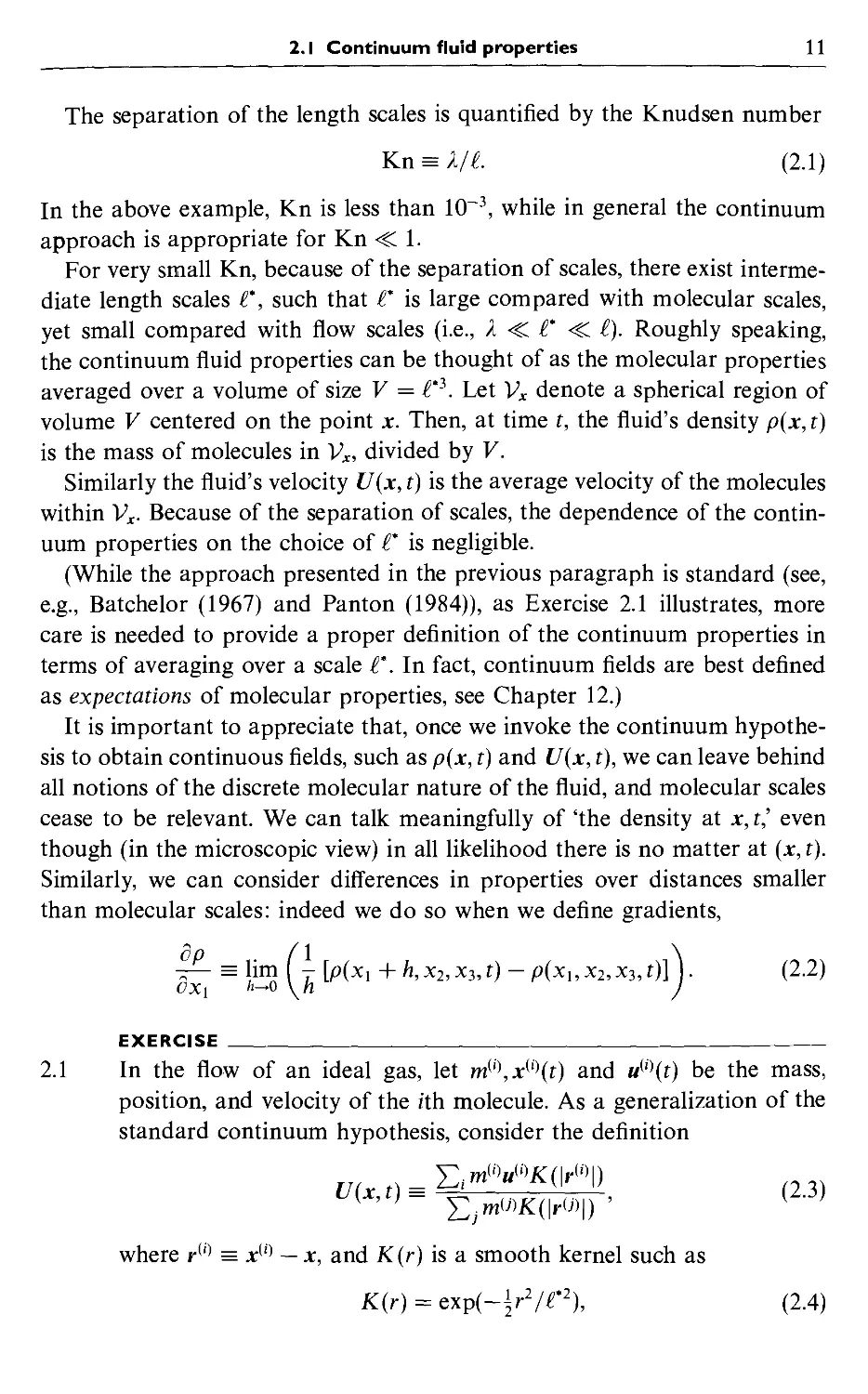
2.1 Continuum fluid properties 10
2.2 Eulerian and Lagrangian fields 12
2.3 The continuity equation 14
2.4 The momentum equation 16
2.5 The role of pressure 18
2.6 Conserved passive scalars 21
2.7 The vorticity equation 22
2.8 Rates of strain and rotation 23
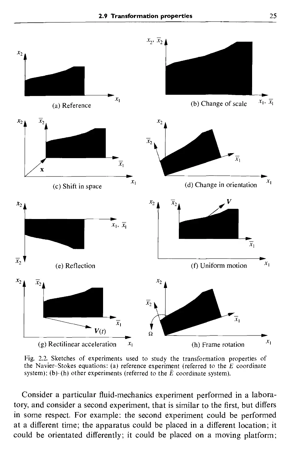
2.9 Transformation properties 24
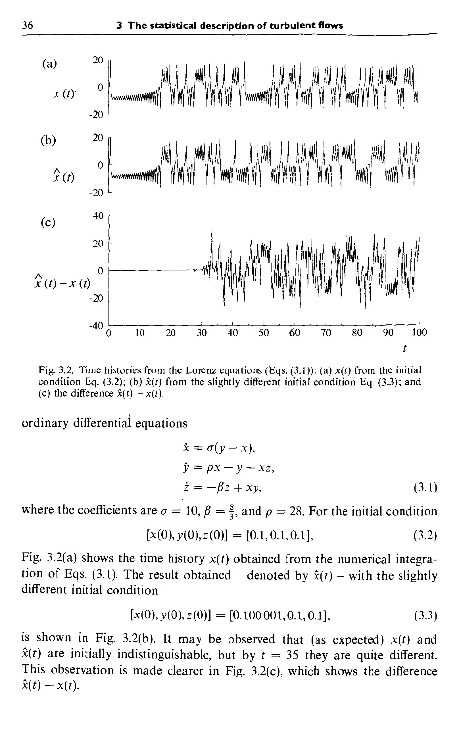
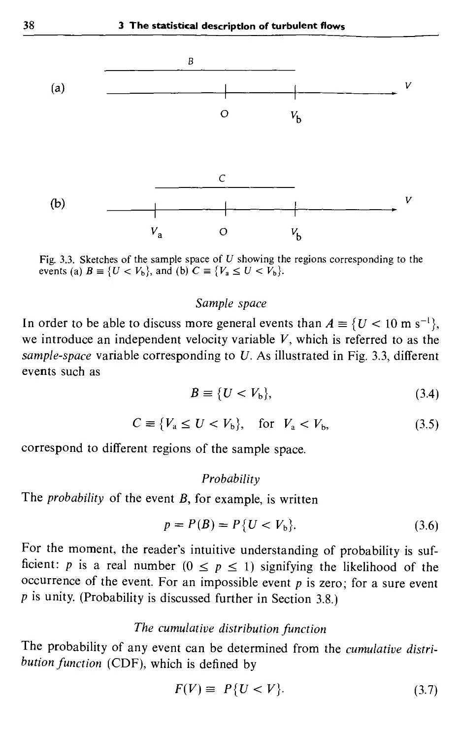
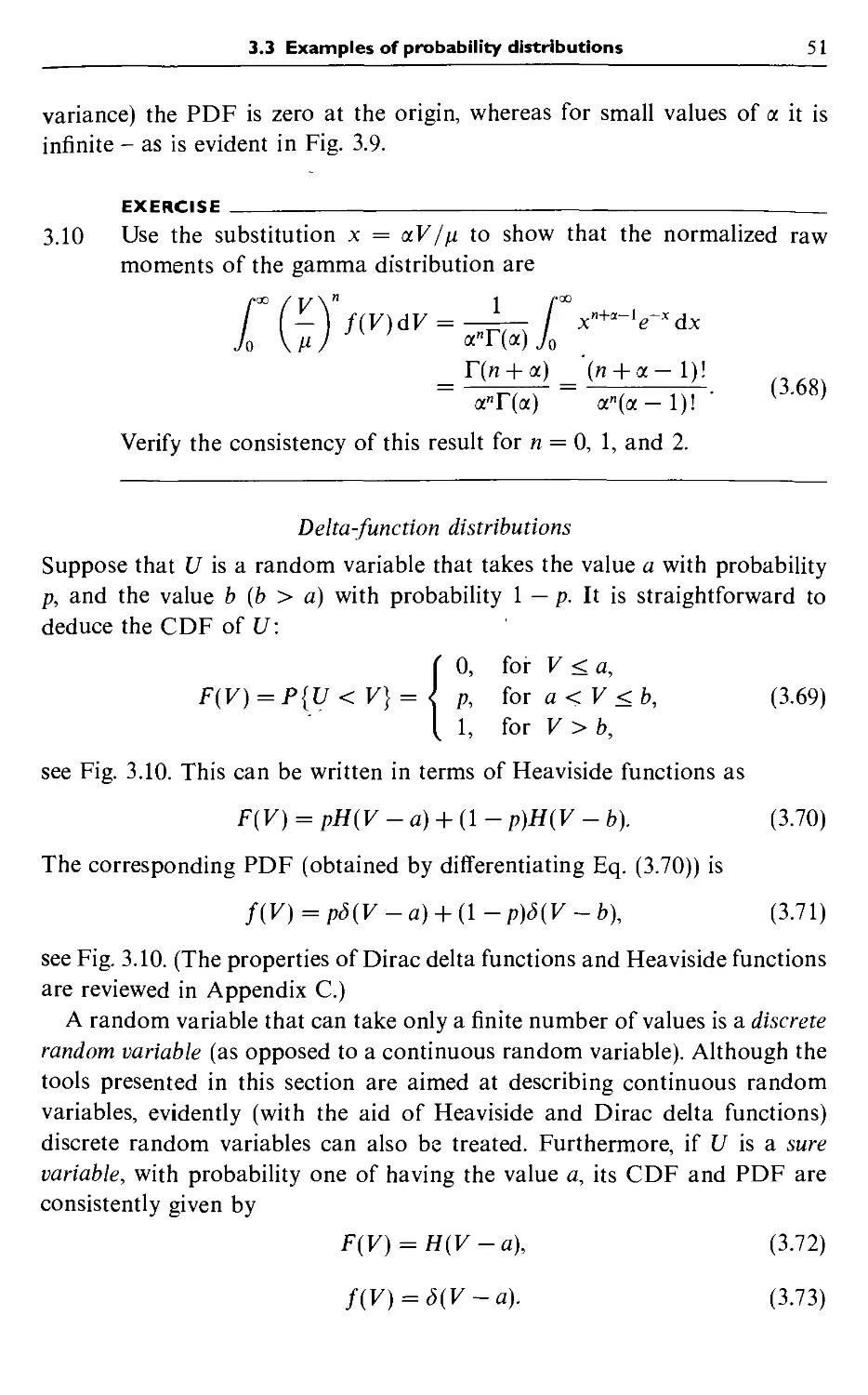
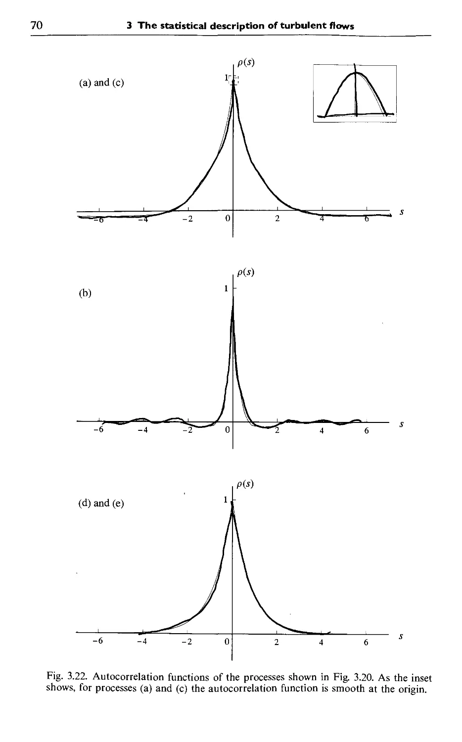
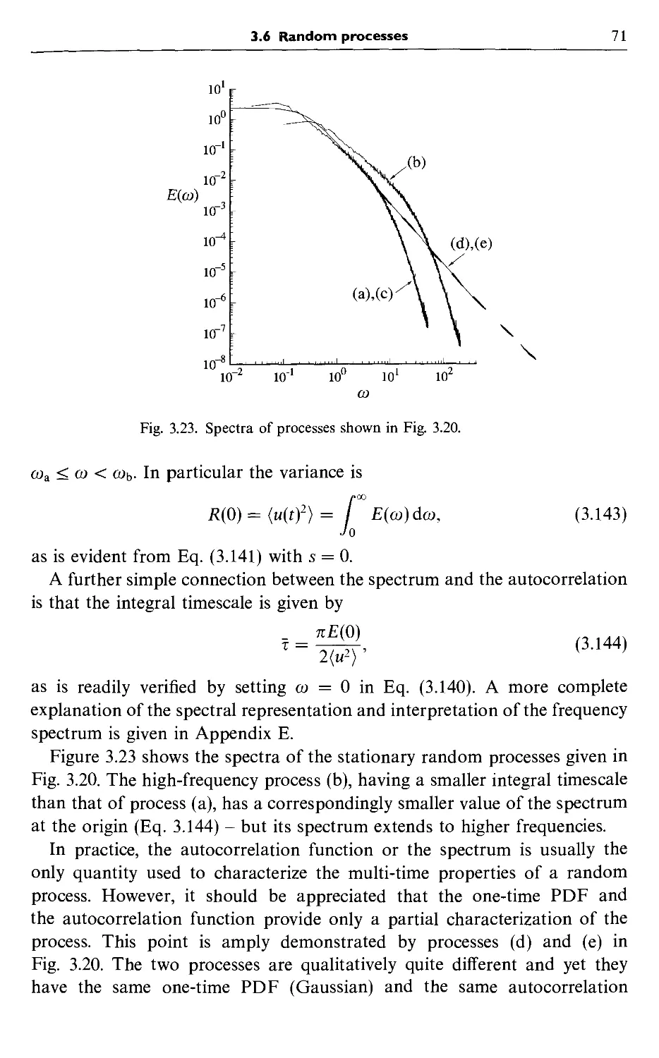
3 The statistical description of turbulent flows 34
3.1 The random nature of turbulence 34
3.2 Characterization of random variables 37
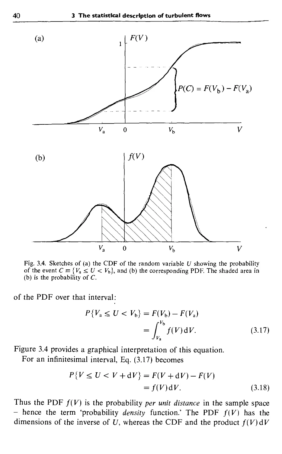
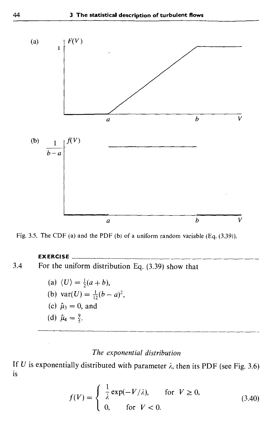
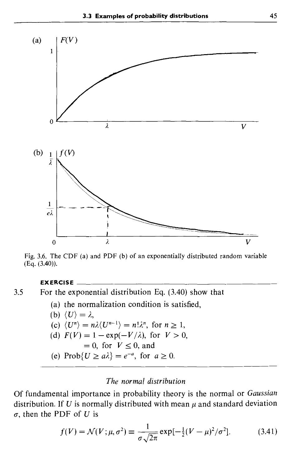
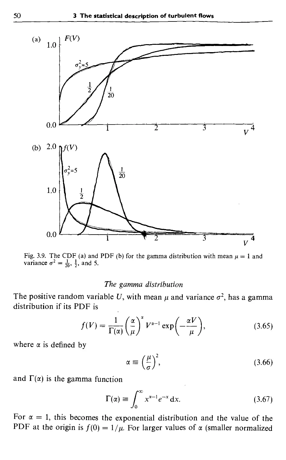
3.3 Examples of probability distributions 43
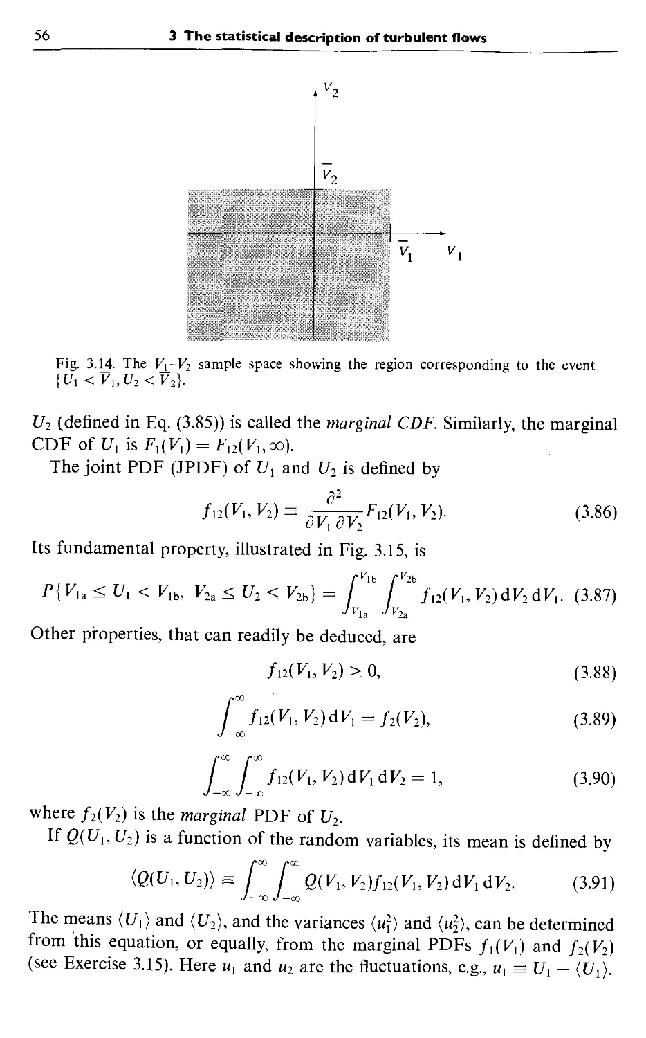
3.4 Joint random variables 54
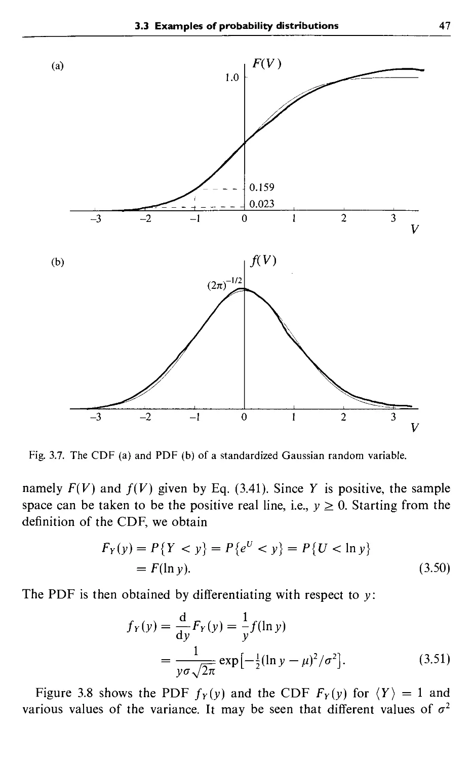
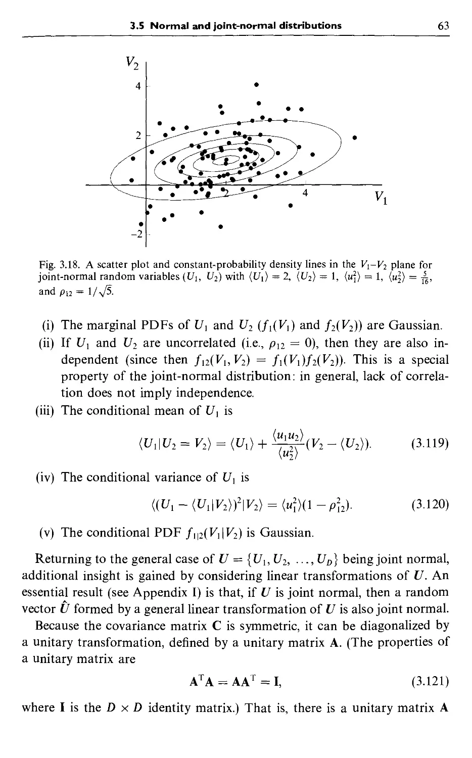
3.5 Normal and joint-normal distributions 61
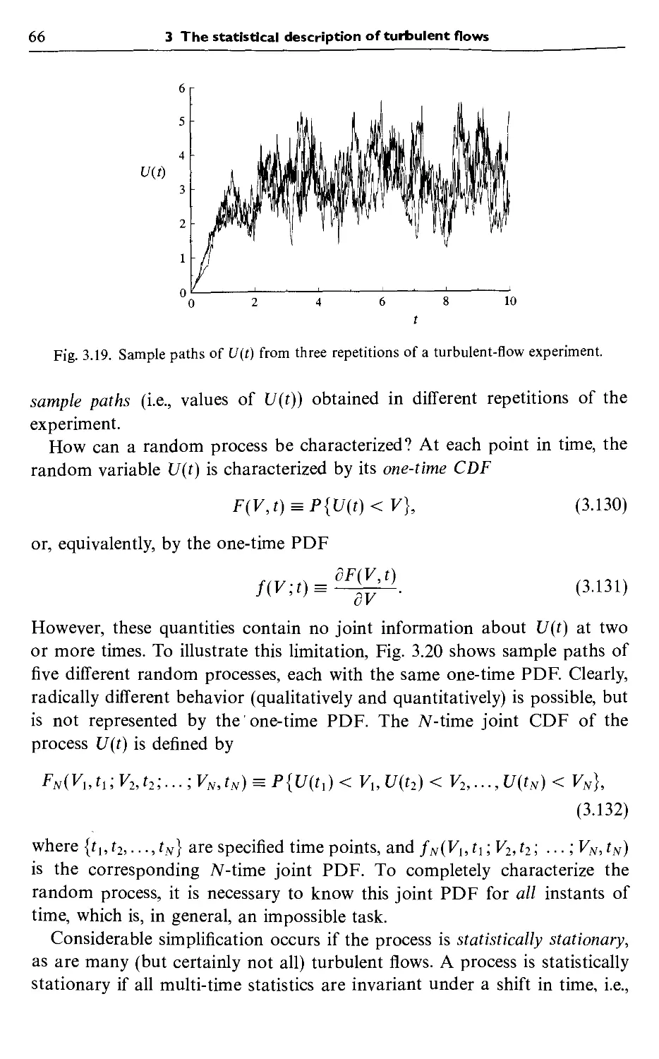
3.6 Random processes 65
3.7 Random fields 74
3.8 Probability and averaging 79

Contents
Mean-flow equations 83
4.1 Reynolds equations 83
4.2 Reynolds stresses 86
4.3 The mean scalar equation 91
4.4 Gradient-diffusion and turbulent-viscosity hypotheses 92
Free shear flows 96
5.1 The round jet: experimental observations 96
5.1.1 A description of the flow 96
5.1.2 The mean velocity field 97
5.1.3 Reynolds stresses 105
5.2 The round jet: mean momentum 111
5.2.1 Boundary-layer equations 111
5.2.2 Flow rates of mass, momentum, and energy 115
5.2.3 Self-similarity 116
5.2.4 Uniform turbulent viscosity 118
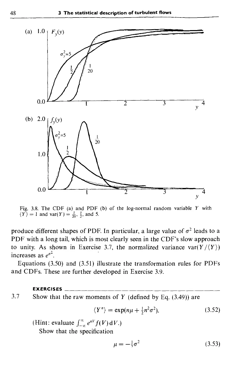
5.3 The round jet: kinetic energy 122
5.4 Other self-similar flows 134
5.4.1 The plane jet 134
5.4.2 The plane mixing layer 139
5.4.3 The plane wake 147
5.4.4 The axisymmetric wake 151
5.4.5 Homogeneous shear flow 154
5.4.6 Grid turbulence 158
5.5 Further observations 161
5.5.1 A conserved scalar 161
5.5.2 Intermittency 167
5.5.3 PDFs and higher moments 173
5.5.4 Large-scale turbulent motion 178
The scales of turbulent motion 182
6.1 The energy cascade and Kolmogorov hypotheses 182
6.1.1 The energy cascade 183
6.1.2 The Kolmogorov hypotheses 184
6.1.3 The energy spectrum 188
6.1.4 Restatement of the Kolmogorov hypotheses 189
6.2 Structure functions 191
6.3 Two-point correlation 195
6.4 Fourier modes 207
6.4.1 Fourier-series representation 207
6.4.2 The evolution of Fourier modes 211

Contents
6.5
6.6
6.7
6.4.3
The kinetic energy of Fourier modes
Velocity spectra
6.5.1
6.5.2
6.5.3
6.5.4
6.5.5
6.5.6
6.5.7
6.5.8
Definitions and properties
Kolmogorov spectra
A model spectrum
Dissipation spectra
The inertial subrange
The energy-containing range
Effects of the Reynolds number
The shear-stress spectrum
The spectral view of the energy cascade
Limitations, shortcomings, and refinements
6.7.1
6.7.2
6.7.3
6.7.4
6.7.5
Wall flows
7.1
7.2
7.3
7.4
The Reynolds number
Higher-order statistics
Internal intermittency
Refined similarity hypotheses
Closing remarks
Channel flow
7.1.1
7.1.2
7.1.3
7.1.4
7.1.5
7.1.6
7.1.7
A description of the flow
The balance of mean forces
The near-wall shear stress
Mean velocity profiles
The friction law and the Reynolds number
Reynolds stresses
Lengthscales and the mixing length
Pipe flow
7.2.1
7.2.2
The friction law for smooth pipes
Wall roughness
Boundary layers
7.3.1
7.3.2
7.3.3
7.3.4
7.3.5
7.3.6
A description of the flow
Mean-momentum equations
Mean velocity profiles
The overlap region reconsidered
Reynolds-stress balances
Additional effects
Turbulent structures
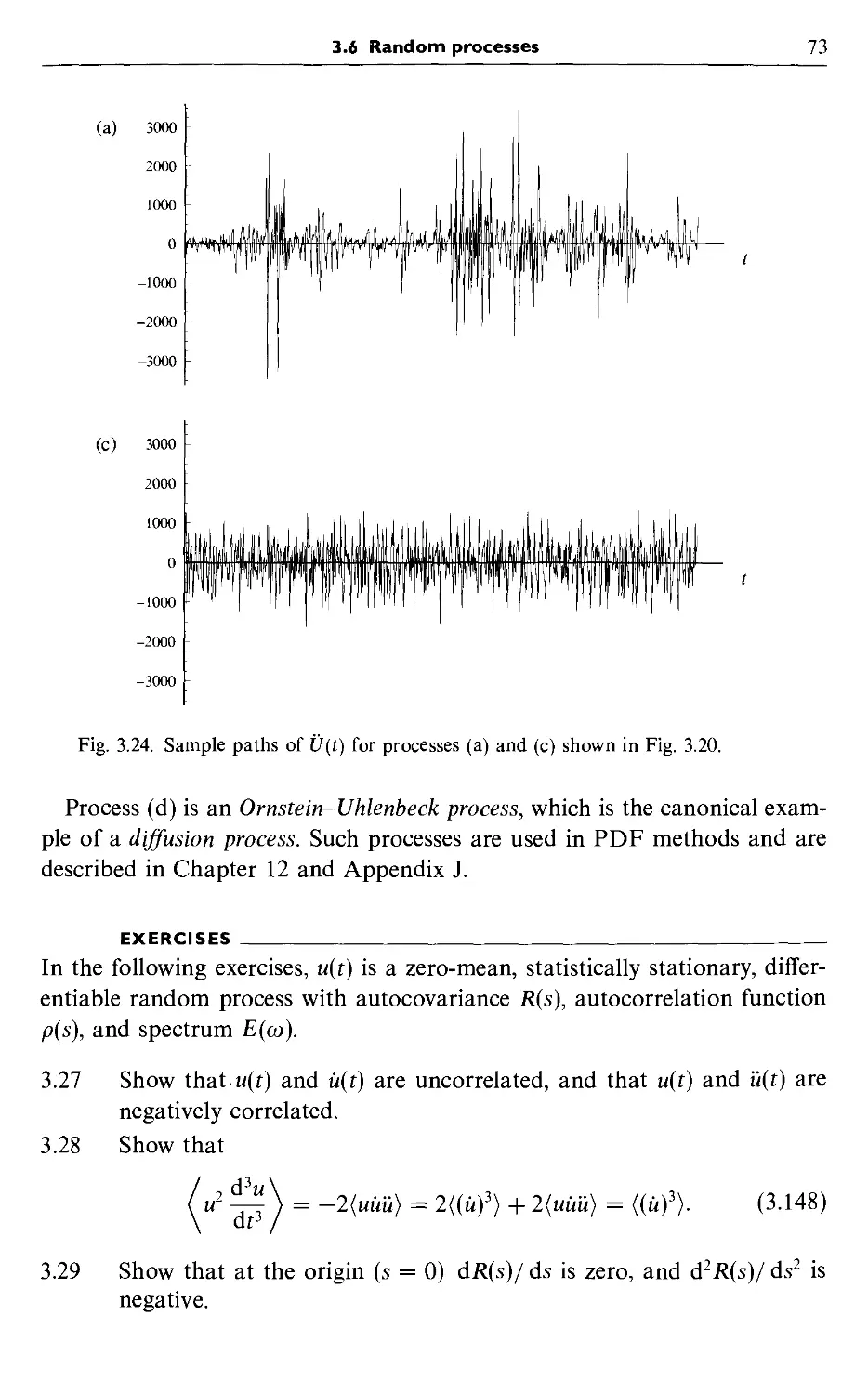
215
219
220
229
232
234
238
240
242
246
249
254
254
255
258
260
263
264
264
264
266
268
271
278
281
288
290
290
295
298
299
300
302
308
313
320
322

X Contents
PART TWO: MODELLING AND SIMULATION 333
8 An introduction to modelling and simulation 335
8.1 The challenge 335
8.2 An overview of approaches 336
8.3 Criteria for appraising models 336
9 Direct numerical simulation 344
9.1 Homogeneous turbulence 344
9.1.1 Pseudo-spectral methods 344
9.1.2 The computational cost 346
9.1.3 Artificial modifications and incomplete resolution 352
9.2 Inhomogeneous flows 353
9.2.1 Channel flow 353
9.2.2 Free shear flows 354
9.2.3 Flow over a backward-facing step 355
9.3 Discussion 356
10 Turbulent-viscosity models 358
10.1 The turbulent-viscosity hypothesis 359
10.1.1 The intrinsic assumption 359
10.1.2 The specific assumption 364
10.2 Algebraic models 365
10.2.1 Uniform turbulent viscosity 365
10.2.2 The mixing-length model 366
10.3 Turbulent-kinetic-energy models 369
10.4 The fe-e model 373
10.4.1 An overview 373
10.4.2 The model equation for e 375
10.4.3 Discussion 382
10.5 Further turbulent-viscosity models 383
10.5.1 The k-cQ model 383
10.5.2 The Spalart-Allmaras model 385
11 Reynolds-stress and related models 387
11.1 Introduction 387
11.2 The pressure-rate-of-strain tensor 388
11.3 Return-to-isotropy models 392
11.3.1 Rotta's model 392
11.3.2 The characterization of Reynolds-stress anisotropy 393
11.3.3 Nonlinear return-to-isotropy models 398
11.4 Rapid-distortion theory 404
11.4.1 Rapid-distortion equations 405

Contents xi
11.4.2 The evolution of a Fourier mode 406
11.4.3 The evolution of the spectrum 411
11.4.4 Rapid distortion of initially isotropic turbulence 415
11.4.5 Final remarks 421
11.5 Pressure-rate-of-strain models 422
11.5.1 The basic model (LRR-IP) 423
11.5.2 Other pressure-rate-of-strain models 425
11.6 Extension to inhomogeneous flows 428
11.6.1 Redistribution 428
11.6.2 Reynolds-stress transport 429
11.6.3 The dissipation equation 432
11.7 Near-wall treatments 433
11.7.1 Near-wall eff"ects 433
11.7.2 Turbulent viscosity 434
11.7.3 Model equations for k and e 435
11.7.4 The dissipation tensor 436
11.7.5 Fluctuating pressure 439
11.7.6 Wall functions 442
11.8 Elliptic relaxation models 445
11.9 Algebraic stress and nonlinear viscosity models 448
11.9.1 Algebraic stress models 448
11.9.2 Nonlinear turbulent viscosity 452
11.10 Discussion 457
12 PDF methods 463
12.1 The Eulerian PDF of velocity 464
12.1.1 Definitions and properties 464
12.1.2 The PDF transport equation 465
12.1.3 The PDF of the fluctuating velocity 467
12.2 The model velocity PDF equation 468
12.2.1 The generalized Langevin model 469
12.2.2 The evolution of the PDF 470
12.2.3 Corresponding Reynolds-stress models 475
12.2.4 Eulerian and Lagrangian modelling approaches 479
12.2.5 Relationships between Lagrangian and Eulerian
PDFs 480
12.3 Langevin equations 483
12.3.1 Stationary isotropic turbulence 484
12.3.2 The generalized Langevin model 489
12.4 Turbulent dispersion 494

xll Contents
12.5 The velocity-frequency joint PDF 506
12.5.1 Complete PDF closure 506
12.5.2 The log-normal model for the turbulence frequency 507
12.5.3 The gamma-distribution model 511
12.5.4 The model joint PDF equation 514
12.6 The Lagrangian particle method 516
12.6.1 Fluid and particle systems 516
12.6.2 Corresponding equations 519
12.6.3 Estimation of means 523
12.6.4 Summary 526
12.7 Extensions 529
12.7.1 Wall functions 529
12.7.2 The near-wall elliptic-relaxation model 534
12.7.3 The wavevector model 540
12.7.4 Mixing and reaction 545
12.8 Discussion 555
13 Large-eddy simulation 558
13.1 Introduction 558
13.2 Filtering 561
13.2.1 The general definition 561
13.2.2 Filtering in one dimension 562
13.2.3 Spectral representation 565
13.2.4 The filtered energy spectrum 568
13.2.5 The resolution of filtered fields 571
13.2.6 Filtering in three dimensions 575
13.2.7 The filtered rate of strain 578
13.3 Filtered conservation equations 581
13.3.1 Conservation of momentum 581
13.3.2 Decomposition of the residual stress 582
13.3.3 Conservation of energy 585
13.4 The Smagorinsky model 587
13.4.1 The definition of the model 587
13.4.2 Behavior in the inertial subrange 587
13.4.3 The Smagorinsky filter 590
13.4.4 Limiting behaviors 594
13.4.5 Near-wall resolution 598
13.4.6 Tests of model performance 601
13.5 LES in wavenumber space 604
13.5.1 Filtered equations 604

Contents xiii
13.5.2 Triad interactions 606
13.5.3 The spectral energy balance 609
13.5.4 The spectral eddy viscosity 610
13.5.5 Backscatter 611
13.5.6 A statistical view of LES 612
13.5.7 Resolution and modelling 615
13.6 Further residual-stress models 619
13.6.1 The dynamic model 619
13.6.2 Mixed models and variants 627
13.6.3 Transport-equation models 629
13.6.4 Implicit numerical filters 631
13.6.5 Near-wall treatments 634
13.7 Discussion 635
13.7.1 An appraisal of LES 635
13.7.2 Final perspectives 638
PART THREE: APPENDICES 641
Appendix A Cartesian tensors 643
A.l Cartesian coordinates and vectors 643
A.2 The definition of Cartesian tensors 647
A.3 Tensor operations 649
A.4 The vector cross product 654
A.5 A summary of Cartesian-tensor suffix notation 659
Appendix B Properties of second-order tensors 661
Appendix C Dirac delta functions 670
C.l The definition of d{x) 670
C.2 Properties of S{x) 672
C.3 Derivatives of d{x) 673
C.4 Taylor series 675
C.5 The Heaviside function 675
C.6 Multiple dimensions 677
Appendix D Fourier transforms 678
Appendix E Spectral representation of stationary random processes 683
E.l Fourier series 683
E.2 Periodic random processes 686
E.3 Non-periodic random processes 689
E.4 Derivatives of the process 690
Appendix F The discrete Fourier transform 692

xiv Contents
Appendix G Power-law spectra 696
Appendix H Derivation of Eulerian PDF equations 702
Appendix I Characteristic functions 707
Appendix J Diffusion processes 713
Bibliography 727
Author index 749
Subject index ISA

List of tables
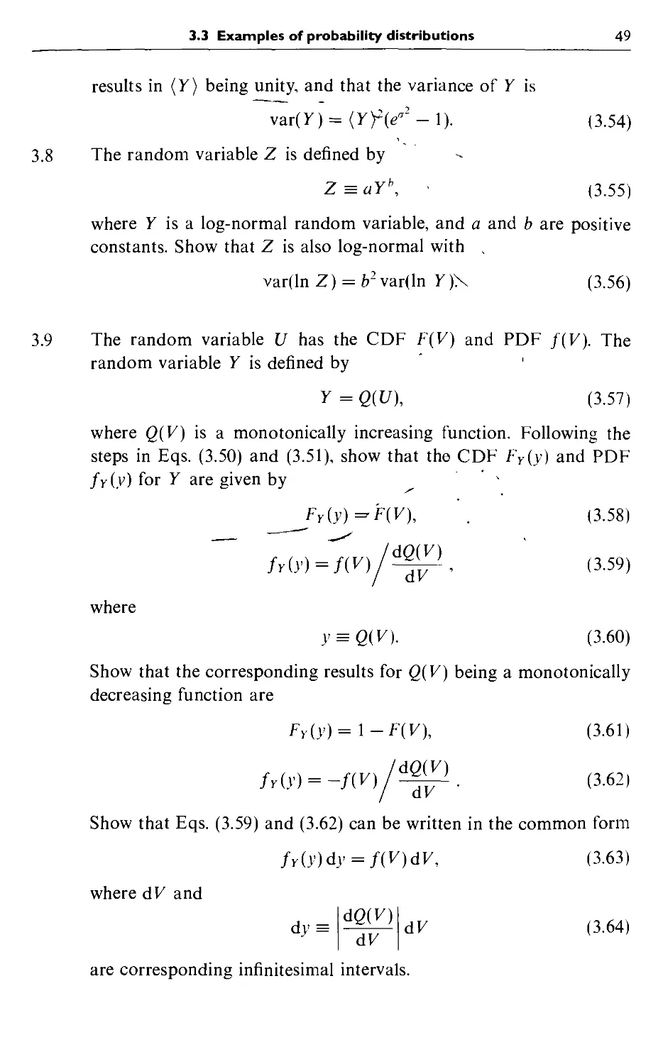
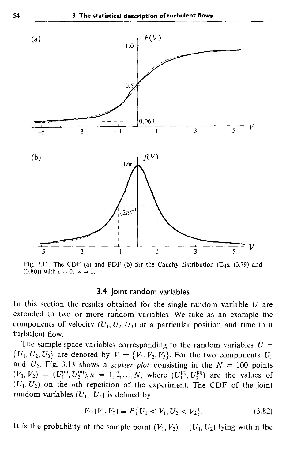
5.1 Spreading rate parameters of turbulent round jets 101
5.2 Timescales in turbulent round jets 131
5.3 Spreading parameters of turbulent axisymmetric wakes 153
5.4 Statistics in homogeneous turbulent shear flow 157
6.1 Characteristic scales of the dissipation spectrum 238
6.2 Characteristic scales of the energy spectrum 240
6.3 Tail contributions to velocity-derivative moments 259
7.1 Wall regions and layers and their defining properties 275
7.2 Statistics in turbulent channel flow 283
8.1 Computational difficulty of different turbulent flows 338
9.1 Numerical parameters for DNS of isotropic turbulence 349
9.2 Numerical parameters for DNS of channel flow 355
9.3 Numerical parameter for DNS of the flow over a backward-facing step 356
10.1 The turbulent Reynolds number of self-similar free shear flows 366
10.2 Definition of variables in two-equation models 384
11.1 Special states of the Reynolds-stress tensor 394
11.2 Mean velocity gradients for simple deformations 415
11.3 Tensors used in pressure-rate-of-strain models 426
11.4 Coefficients in pressure-rate-of-strain models 427
11.5 Coefficients in algebraic stress models 452
11.6 Integrity basis for turbulent viscosity models 453
11.7 Attributes of different RANS turbulence models 457
12.1 Comparison between fluid and particle systems 518
12.2 Different levels of PDF models 555
13.1 Resolution in DNS and in some variants of LES 560
13.2 Filter functions and transfer functions 563
13.3 Estimates of filtered and residual quantities in the inertial subrange 589
13.4 Definition of the different types of triad interactions 608
B.l Operations between first- and second-order tensors 662
D.l Fourier-transform pairs 679
E.l Spectral properties of random processes 689
G.l Power-law spectra and structure functions 700
I.l Relationships between characteristic functions and PDFs 710

XX Preface
knowledge of probability theory, and consequently the necessary material is
provided in the text (e.g.. Sections 3.2-3.5).
For a less demanding pace. Parts I and II can be covered in two semesters
- there is ample material. Alternatively, if a coverage of modelling is not
required, Part I by itself provides a reasonably complete introduction to
turbulent flows.
Many of the exercises ask the reader to 'show that...,' and thereby
introduce additional results and observations. Consequently, it is recommended
that all the exercises be read, even if they are not performed. The book is
designed to be a self-contained text, but sufficient references are given to
provide an entry into the research literature.
However much care is taken in the preparation of a book of this nature,
it is inevitable that there will be errors in the first printing. A list of known
corrections is given at http://mae.cornell.edu/~pope/TurbulentFlows.
The reader is asked to report any further corrections to the author at
popeOmae.Cornell.edu.
I am profoundly grateful to many people for their help in the
preparation of this work. For their support and technical input I thank my
colleagues at Cornell, David Caughey, Sidney Leibovich, John Lumley, Di-
etmar Rempfer, and Zellman Warhaft. For their valuable suggestions based
on reading draft chapters, I am grateful to Peter Bradshaw, Paul Durbin,
Rodney Fox, Kemo Hanjalic, Charles Meneveau, Robert Moser, Blair Perot,
Ugo Piomelli, P. K. Yeung, and Norman Zabusky. Similarly, I am grateful
to the following Cornell graduates for their feedback on drafts of the book:
Bertrand Delarue, Thomas Dreeben, Matthew Overholt, Paul Van Slooten,
Jun Xu, Cem Albukrek, Dawn Chamberlain, Timothy Fisher, Laurent Myd-
larski, Gad Reinhorn, Shankar Subramaniam, and Walter Welton. The first
five mentioned are also thanked for their assistance in producing the figures.
Most of the typescript was prepared by June Meyermann, whose patience,
accuracy, and enthusiasm are greatly appreciated. The accuracy of the
bibliography has been much improved by the careful checking performed by
Sarah Pope. Above all, I wish to thank my wife, Linda, for her patience,
support, and encouragement during this project and over the years.

Nomenclature
The notation used is given here in the following order: upper-case Roman,
lower-case Roman, upper-case Greek, lower-case Greek, superscripts,
subscripts, symbols, and abbreviations. Then the symbols 0{ ), o( ), and ~ that
are used to denote the order of a quantity are explained.
Upper-case Roman
A'^ van Driest constant (Eq. G.145))
A control surface bounding V
B log-law constant (Eq. G.43))
Bi constant in the velocity-defect law (Eq. G.50))
B2 Loitsyanskii integral (Eq. F.92))
Bj log-law constant for fully-rough walls (Eq. G.120))
B{s/Sy) log-law constant for rough walls (Eq. G.121))
C Kolmogorov constant related to E{k) (Eq. F.16))
Co coefficient in the Langevin equation (Eqs. A2.26) and
A2.100))
C[ Kolmogorov constant related to £n('<:i) (Eq. F.228))
Ci Kolmogorov constant related to EjiiKi) (Eq. F.231))
C2 Kolmogorov constant related to Dll (Eq. F.30))
C2 constant in the IP model (Eq. A1.129))
C3 constant in the model equation for co' (Eq. A2.194))
^E LES dissipation coefficient (Eq. A3.285))
^( skin-friction coefficient (T„/(ipC/^))
Cr Rotta constant (Eq. A1.24))
Cs Smagorinsky coefficient (Eq. A3.128))
Q constant in Reynolds-stress transport models
(Eq. A1.147))

xxu Nomenclature
C: constant in the model equation for e (Eq. A1.150))
Cci, Cs2 constants in the model equation for e (Eq. A0.53))
C,, turbulent-viscosity constant in the fe-e model
(Eq. A0.47))
C, LES eddy-viscosity coefficient (Eq. A3.286))
Q constant in the lEM mixing model (Eq. A2.326))
Cn constant in the definition of Q (Eq. A2.193))
C„A, Cio2 constants in the model equation for co (Eq. A0.93))
Co Kolmogorov constant (Eq. A2.96))
Cf. cross stress (Eq. A3.101))
D pipe diameter
Dij second-order velocity structure function (Eq. F.23))
Dl(s) second-order Lagrangian structure function (Eq. A2.95))
Dll longitudinal second-order velocity structure function
Dlll longitudinal third-order velocity structure function
(Eq. F.86))
Dmn transverse second-order velocity structure function
D„{r) nth-order longitudinal velocity structure function
(Eq. F.304))
D/Dr substantial derivative (d/dt + f/ • V)
D/Dr mean substantial derivative {8/8t + (f/) • V)
D/Dr substantial derivative based on filtered velocity
E Cartesian coordinate system with basis vectors ^,
E Cartesian coordinate system with basis vectors ^,
E{x,t) kinetic energy {\U• U)
E{x, t) kinetic energy of the mean flow {\{U) • {U))
E{x) kinetic energy flow rate of the mean flow
E{k) energy-spectrum function (Eq. C.166))
Eij{Ki) one-dimensional energy spectrum (Eq. F.206))
E{k) energy-spectrum function of filtered velocity (Eq. A3.62))
E{<d) frequency spectrum (defined for positive frequencies,
Eq. C.140))
Eico) frequency spectrum (defined for positive and negative
frequencies, Eq. (E.31))
F determinant of the normalized Reynolds stress
(Eq. A1.52))
E{V) cumulative distribution function (CDF) of U (Eq. C.7))
^d(>'/<5) velocity-defect law (Eq. G.46))
•^ Fourier transform (Eq. (D.l))
•^^ inverse Fourier transform (Eq. (D.2))

Nomenclature
T^ Fourier integral operator (Eq. F.116))
Gy coefficient in the GLM (Eqs. A2.26) and A2.110))
G(r) LES filter function
G{k) LES filter transfer function
U shape factor (b' jd)
H{x) Heaviside function (Eq. (C.33))
I identity matrix
I{x,t) indicator function for intermittency (Eq. E.299))
Ij JLs, lUs principal invariants of the second-order tensor .v
(Eqs. (B.31)-(B.33))
K kurtosis of the longitudinal velocity derivative
K^ kurtosis of </>
Kn Knudsen number
Ky{z) modified Bessel function of the second kind
L lengthscale {ki/s)
L lengthscale (u'^/e)
Lii longitudinal integral lengthscale (Eq. C.161))
L22 lateral integral lengthscale (Eq. F.48))
C characteristic lengthscale of the flow
£ length of side of cube in physical space
Cij resolved stress (Eq. A3.252))
C°j Leonard stress (Eq. A3.100))
M{x) momentum flow rate of the mean flow
Mjj scaled composite rate-of-strain tensor (Eq. A3.255))
M„ normalized nth moment of the longitudinal velocity
derivative (Eq. F.303))
Ma Mach number
M{n,a^) normal distribution with mean jx and variance a^
0{h) quantity of big order h
o{h) quantity of little order h
P pressure (Eq. B.32))
P{A) probability of event/I
P{x,t) particle pressure (Eq. A2.225))
Pjk{K) projection tensor (Eq. F.133))
V production: rate of production of turbulent kinetic
energy (Eq. E.133))
'Pij rate of production of Reynolds stress (Eq. G.179))
Vr rate of production of residual kinetic energy
(Eq. A3.123))
V^ rate of production of scalar variance (Eq. E.282))

XXIV Nomenclature
R pipe radius
R(s) autocovariance (Eq. C.134))
Rij{r,x;t) two-point velocity correlation (Eq. C.160))
^, (jc) Fourier coefficient of two-point velocity correlation
(Eq. F.152))
R^ turbulent Reynolds number (Eq. E.85))
R^ Taylor-scale Reynolds number (Eq. F.63))
Re Reynolds number
Re Reynolds number {2tJd/v)
Reo Reynolds number (UoS/v)
Re^ turbulence Reynolds number (fe'/^L/v = fe^/(ev))
Rej turbulence Reynolds number (u'Lu/v)
Re^ Reynolds number {Uox/v)
Re^ Reynolds number (Uod/v)
Rqs' Reynolds number (Uod'/v)
Re0 Reynolds number {Uo9/v)
Re^ Reynolds number based on friction velocity {u^S/v)
TZij pressure-rate-of-strain tensor (Eq. G.187))
n°j SGS Reynolds stress (Eq. A3.102))
72.|y' redistribution term (anisotropic part of n,y, Eq. A1.6))
'lV^j{v,x,t) conditional pressure-rate-of-strain tensor (Eq. A2.20))
72.y' redistribution term used in elliptic-relaxation model
(Eq. A1.198))
TZ^ij rapid pressure-rate-of-strain tensor (Eq. A1.13))
TZfj slow pressure-rate-of-strain tensor
S spreading rate of a free shear flow
S velocity-derivative skewness (Eq. F.85))
S((^) chemical source term (Eq. A2.321))
S' velocity structure function skewness (Eq. F.89))
Sij rate-of-strain tensor i\{dUi/dxj + dJJj/dXi))
Sij mean rate-of-strain tensor {\{d{Ui)/8xj + 8{Uj)/8xi))
Sij normalized mean rate-of-strain tensor ((fe/e)S,y)
Si; filtered rate-of-strain tensor (Eq. A3.73))
Sjj doubly filtered rate-of-strain tensor
Sijk{r, t) two-point triple velocity correlation (Eq. F.72))
S^ skewness of (j)
Sw mean source of turbulence frequency (Eq. A2.184))
S characteristic mean strain rate BSySy)j (S = d{U{)/dx2
in simple shear flow)

Nomenclature
S filtered rate-of-strain invariant BS,ySyJ
'S doubly filtered rate-of-strain invariant BSyS,yJ
S{k) sphere in wavenumber space of radius k
Sx principal mean strain rate: largest eigenvalue of S,y
T time interval
T turbulent timescale defined by Eq. A1.163)
f{K) rate of energy transfer to Fourier mode of wavenumber
K from other modes (Eq. 6.162)
Tkij flux of Reynolds stress (Eq. G.195))
flux of Reynolds stress due to fluctuating pressure
(Eq. G.193))
T*^!' isotropic flux of Reynolds stress due to fluctuating
' kij
pressure (Eq. A1.140))
T*".' flux of Reynolds stress due to turbulent convection
{{UkUiUj))
Tllj diff"usive flux of Reynolds stress (Eq. G.196))
Tl Lagrangian integral timescale (Eq. A2.93))
T{£) rate of transfer of energy from eddies larger than £ to
those smaller than i
7^1 rate of transfer of energy from large eddies to small
eddies
Tui rate of transfer of energy into the dissipation range
{£ < ^Di) from larger scales
U{t) random process
U{x, t) Eulerian velocity
U{x,y,z) X component of velocity
U{x, r, 6) X component of velocity
V bulk velocity in channel (Eq. G.3)) and pipe flow
(Eq. G.94))
V^{t) fluid-particle velocity
V{t) model for the fluid-particle velocity
U{x, t) filtered (resolved) velocity field
Vq mean centerline velocity in channel and pipe flow
U(i(x) mean centerline velocity in a jet
Vq{x) freestream velocity
{/c(^) characteristic convective velocity
Ui jet-nozzle velocity
{7h velocity of high-speed stream in a mixing layer
Ui velocity of low-speed stream in a mixing layer
Us(x) characteristic velocity difference

Nomenclature
U characteristic velocity scale of the flow
V sample space variable corresponding to U
V sample space variable corresponding to velocity U
V{x, r, 6) r component of velocity
V{x,y,z) J'component of velocity
V control volume in physical space bounded by A
W{t) Wiener process
W{t) vector-valued Wiener process
W{x, r, 6) 6 component of velocity
W(x,y,z) z component of velocity
X^{t, Y) fluid-particle position: position at time t of fluid particle
that is at Y at the reference time Iq
X'{t) model for fluid-particle position (Eq. A2.108))
V fluid particle position at the reference time Iq
Lower-case Roman
a drift coefficient of a diffusion process (Eq. (J.27))
Uij anisotropic Reynolds stresses {{ujUj) — ^kSjj)
Uij direction cosines (Eq. (A.ll))
Uf LESfilter constant (Eq. A3.77))
b^ diffusion coefficient of a diffusion process (Eq. (J.27))
bij normalized Reynolds-stress anisotropy (C,y/Bfe))
Cf skin-friction coefficient (Tw/(ipGo))
cs Smagorinsky coefficient (Eq. A3.253))
d jet-nozzle diameter
e{t) unit wavevector (Eq. A1.84))
Ci unit vector in the /-coordinate direction
/ friction factor (Eq. G.97))
/, / self-similar mean axial velocity profile
f{r, t) longitudinal velocity autocorrelation function (Eq. F.45))
f{V) probability density function (PDF) of U (Eq. C.14))
f{V;x,t) Eulerian PDF of velocity (Eq. C.153))
f'{V;x, t) fine-grained Eulerian PDF of velocity (Eq. (H.l))
f'{V;x,t) modelled Eulerian PDF of velocity (Eq. A2.116))
/*( V\x;t) conditional PDF of particle velocity (Eq. A2.205))
f{V;x,t) filtered density function (Eq. A3.287))
/(V,6;x,t) joint PDF of velocity and turbulence frequency
f{V,ilf; X, t) velocity-composition joint PDF
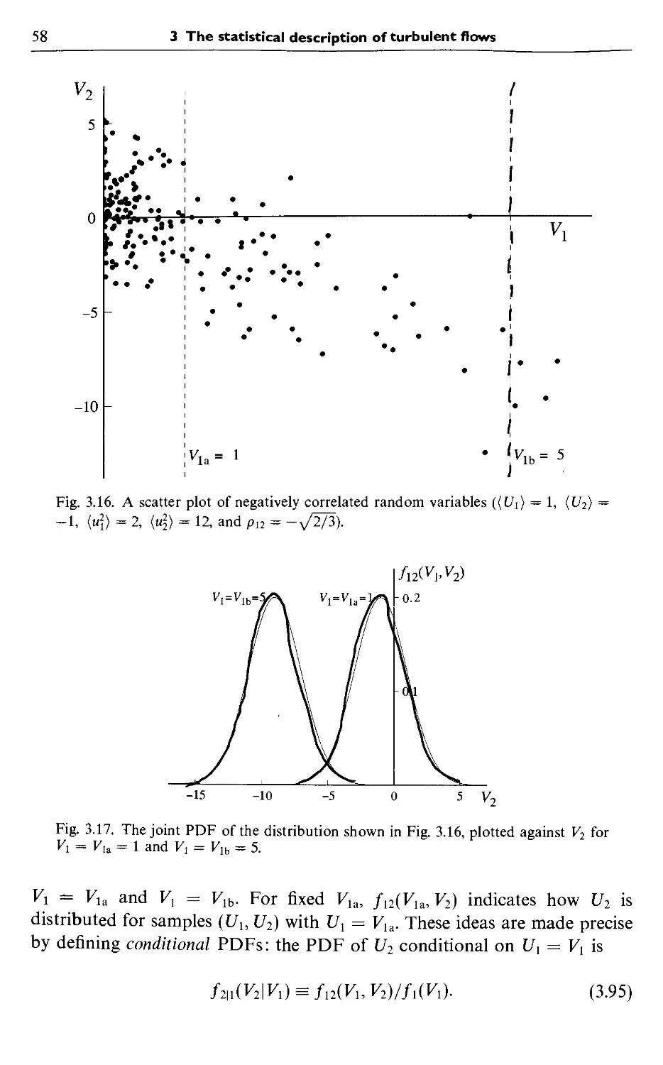
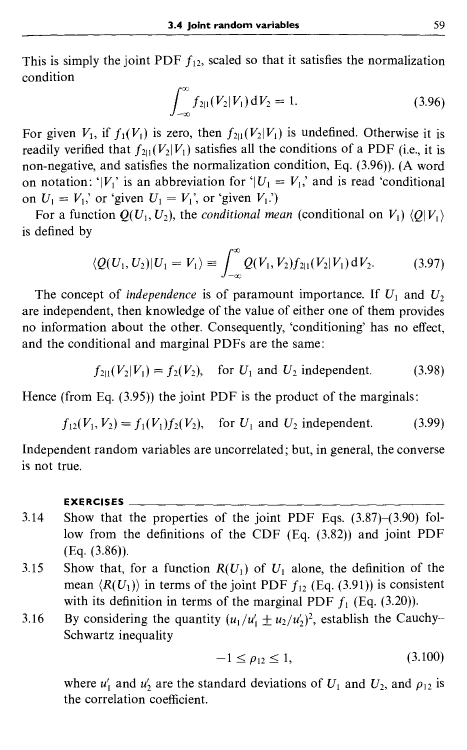
f2]i{V2]Vi) PDF of U2 conditional on G, = F, (Eq. C.95))

Nomenclature xxvii
/l( V, x; t\ Y) Lagrangian velocity-position joint PDF (Eq. A2.76))
fl{V,x;t) joint PDF of U'{t) and X'{t)
f^{\p; X, t) non-turbulent conditional PDF of scalar (f){x, t)
fjixp; X, t) turbulent conditional PDF of scalar 4){x, t)
f^{y+) law of the wall (Eq. G.37))
fx{x; t\ Y) PDF of fluid-particle position
f'x{x;t) PDFofJ^'@
/^ damping function in k-s model (Eq. A1.155))
f^{ip; X, t) PDF of scalar (f){x, t)
f^@;x,t) PDF of turbulence frequency
g, g self-similar shear-stress profile in a free shear flow
g gravitational acceleration
g gravitational force per unit mass
g(r, t) transverse velocity autocorrelation function (Eq. F.45))
g{v;x, t) Eulerian PDF of the fluctuating velocity
h, h self-similar mean lateral velocity profile
h grid spacing
k turbulent kinetic energy (^(h • «))
k{r,t) longitudinal two-point triple correlation (Eq. F.73))
fef residual kinetic energy (Eq. A3.92))
fe(K^_Kb) turbulent kinetic energy in the wavenumber range
I lengthscale defined as vt/m'
i lengthscale
i characteristic eddy size
£o lengthscale of the largest eddies
im demarcation lengthscale between the dissipation range
{£ < £ui) and the inertial subrange {£ > ioi)
^Ei demarcation lengthscale between the energy-containing
range of eddies {£ > i^i) and smaller eddies {£ < i^i)
C mixing length (Eq. G.91))
^^ mixing length in wall units {Im/^v)
is Smagorinsky lengthscale (Eq. A3.128))
i^{x) distance between x and the nearest solid surface
m(x) mass flow rate of the mean flow
n unit normal vector
o{h) small order h (Eq. (J.34))
p exponent in power-law spectrum (Eq. (G.5))
p{x, t) modified pressure
p'{x, t) fluctuating (modified) pressure

xxviii Nomenclature
p^^\x, t) harmonic pressure (Eq. B.49))
p^^\x,t) rapid pressure (Eq. A1.11))
p^'\x, t) slow pressure (Eq. A1.12))
P(,{x) freestream pressure
p„(x) wall pressure
q exponent in power-law structure function (Eq. (G.6))
r radial coordinate
n/jix) half-width of jet or wake
s time interval
s lengthscale of wall roughness
s-j fluctuating rate-of-strain tensor {-{dui/dxj + duj/dxt))
t time
u X component of fluctuating velocity
u{t} characteristic velocity of an eddy of size (.
u(x, t) fluctuating velocity
u{K,t) Fourier coefficient of velocity (Eq. F.102))
u' r.m.s. velocity
u'it) fluctuating component of particle velocity (Eq. A2.207))
M+ mean velocity normalized by the friction velocity
u'{x, t) residual (SOS) velocity field (Eq. A3.3))
Mo(x) r.m.s. axial velocity
mq velocity scale of the largest eddies
Mg propagation velocity of the viscous superlayer
u^ Kolmogorov velocity (Eq. E.151))
Wr friction velocity (y^T^/v)
V y or r component of fluctuating velocity
V sample space variable corresponding to «
w z or 0 component of fluctuating velocity
w{y/5) law of the wake function (Eq. G.149))
X position
X Cartesian or polar cylindrical coordinate
^0 virtual origin
y Cartesian coordinate
y distance from the wall normalized by the viscous
lengthscale, 5^
>'o.i(^) cross-stream location in mixing layer (also y(j<){x) etc.,
see Eq. E.203))
y\/2(x) half-width of jet or wake
y^ distance from the wall at which wall functions are
applied

Nomenclature xxix
y4>
half-width of scalar profile
z Cartesian coordinate
Upper-case Greek
r molecular diffusivity
r(z) gamma function (Eq. C.67))
Teff effective diffusivity (rx + F)
Ft turbulent diff"usivity (Eq. D.42))
A, A filter width
A grid filter width in the dynamic model
A test filter width in the dynamic model
A effective width of combined test and grid filters
(Eq. A3.247))
Ah temporal increment operator (Eq. (J.4))
Aj filter width in direction /
ArU longitudinal velocity increment (Eq. F.305))
n wake-strength parameter (Eq. G.148))
Uij velocity-pressure-gradient tensor (Eq. G.180))
"^ 1 1~' T ) universal velocity-gradient function for channel flow
^^ ^/ (Eq. G.31))
<^{k, t) kinetic energy of Fourier mode with wavenumber k
(Eq. F.103))
^ij{K) velocity-spectrum tensor (Eq. C.163))
*F gravitational potential {g = —V*F)
*F(s) characteristic function (Eq. (I.l))
i3 characteristic mean rotation rate BQ,yQ,y)'/^
^{x,t) conditional mean turbulence frequency (Eq. A2.193))
il,7 rate-of-rotation tensor {^{dUt/dXj — dUj/dxt))
Clij mean rate-of-rotation tensor {~{d{Ui)/dxj — d{Uj)/dxi))
^ij normalized mean rate-of-rotation tensor ((fe/e)Q,y)
^ij rate of rotation of coordinate axes (Eq. B.97))
Lower-case Greek
Po constant in the exponential spectrum (Eq. F.253))
y{x, t) intermittency factor (Eq. E.300))
S half-height of channel
S{x) Dirac delta function
S{x) characteristic flow width

XXX Nomenclature
S{x) boundary-layer thickness
S'ix) displacement thickness
Sij Kronecker delta (Eq. (A.l))
d^y Kronecker delta defined by Eq. F.111)
S^ viscous lengthscale (Eq. G.26))
e error
e rate of dissipation of turbulent kinetic energy Bv(s,ys,y))
, dui dui,
p pseudo-dissipation v(-
\ OXjOXj '
g, ^ , dissipation in the wavenumber range {k^, k^,)
sq instantaneous dissipation rate Bvs,yS,y)
gg one-dimensional surrogate for eo (Eq. F.314))
dissipation tensor (^2v( — —)
Eiji, alternating symbol (Eq. (A.56))
s':{v,x,t) conditional dissipation tensor (Eq. A2.21))
el{ip,x,t) conditional scalar dissipation rate (Eq. A2.346))
e,. average of eo over volume of radius r (Eq. F.313))
Sr one-dimensional surrogate for e^ (Eq. F.315))
e^ scalar dissipation rate (Eq. E.283))
C„ nth-order structure function exponent (Eq. F.307))
r] Kolmogorov lengthscale (Eq. E.149))
r] normalized lateral coordinate in free shear flows
r] invariant of the Reynolds-stress anisotropy tensor
(Eq. A1.28))
9 circumferential coordinate
9 sample-space variable corresponding to co'
6{x) displacernent thickness (Eq. G.127))
i9 specific volume (9 = 1/p)
K von Karman constant (Eq. G.43))
K wavenumber
K wavenumber vector
k@ time-dependent wavenumber vector (Eq. A1.80))
kq lowest wavenumber
Kc filter cutoff wavenumber (k^ = tt/A)
'^'di demarcation wavenumber between the dissipation range
(k > kqi) and the inertial subrange (k < kqi)
'^'ei demarcation wavenumber between the energy-containing
range (k < kei) and the inertial subrange (k > kei)
A mean free path

Nomenclature xxxi
Xj longitudinal Taylor microscale (Eq. F.53))
Xg transverse Taylor microscale (Eq. F.57))
H viscosity
H internal intermittency exponent (Eq. F.317))
H mean of a distribution
H„ nth central moment (Eq. C.25))
/i„ standardized nth central moment (Eq. C.37))
V kinematic viscosity (v = n/p)
Veff effective viscosity (vx + v)
V, residual (SGS) eddy viscosity (Eq. A3.127))
vt turbulent viscosity (Eq. D.45))
^ normalized lateral coordinate in free shear flows
^ invariant of the Reynolds-stress anisotropy tensor
(Eq. A1.29))
p density
p{s) autocorrelation function (Eq. C.135))
Pi2 correlation coefficient between u\ and Uj (Eq. C.93))
puv correlation coefficient between u and v (Eq. C.93))
<T standard deviation
<T Prandtl number
<Tk turbulent Prandtl number for kinetic energy (Eq. A0.41))
<tt turbulent Prandtl number (vt/Ft)
(Tx r.m.s. fluid-particle dispersion (Eq. A2.149))
<Te turbulent Prandtl number for dissipation (Eq. A0.53))
T turbulence timescale (fe/e)
T integral timescale (Eq. C.139))
t(^) characteristic timescale of an eddy of size I
x(y) total shear stress in simple shear flow (Eq. G.10))
To timescale of largest eddies («o/4)
Ty stress tensor (Eq. B.32))
Ty residual (SGS) stress tensor (Eq. A3.90))
T-y deviatoric residual (SGS) stress tensor (Eq. A3.93))
Tw wall shear stress
T,, Kolmogorov timescale (Eq. E.150))
T^ scalar timescale {{(j)'^)/s^)
4>{x, t) conserved passive scalar
<p self-similar profile of a conserved passive scalar
xp sample-space variable corresponding to cj)
tp{x,r) Stokes stream function (Eq. E.86))
CO frequency

CO turbulence frequency s/k
Q){x, t) vorticity (o> = V x £/)
co^ enstrophy (w^ = o> • o>)
co'{t) model for turbulence frequency
Superscripts
(I)' complex conjugate of (/)
,^+ indicates Lagrangian variable (Eq. B.9))
^(k) indicates Fourier coefficient at wavenumber k of
function (^(x) (Eq. F.113))
^ indicates standardized random variable or PDF
^ rate of change of (p {(/) = d(f)/dt)
(f)' fluctuating component {(f)' = (/) — ((^))
(p'j conditional turbulent r.m.s. of (/) (Eq. E.304))
(j)'^ conditional non-turbulent r.m.s. of (j)
f derivative {f'{x) = df{x)/dx)
u' residual (from filtering, Eq. A3.3))
t;"(K) component of v{k) parallel to k (Eq. F.129))
v-^{k) component of v{k) perpendicular to k (Eq. F.131))
A^ transpose of ^
U filtered quantity (filter width A or A)
U filtered quantity (filter width A)
U filtered quantity (filter width A)
Subscripts
{Q)c volume average of Q{x) over a cube of side C
(Eq. C.175))
{Q)n mean of Q over an ensemble of Af samples (Eq. C.108))
B)n non-turbulent conditional mean of Q
Qp quantity evaluated at yp in wall functions
{Q)t time average of Q{t) over time interval T (Eq. C.173))
F)t turbulent conditional mean of Q
{Q)y quantity evaluated at y
Symbols
det(^) determinant of/4
5(^) imaginary part of z

Nomenclature
XXXlll
lim
HO
max{a, b)
min{a, b)
lR(z)
sdey(U)
trace(^)
var(t/)
V
V-
Vx
X
f{ )dSir)
@
{Q\v)
f ~g
the limit as the positive quantity h tends to zero
the greater of a and b
the lesser of a and b
real part of z
standard deviation of U (Eq. C.24))
trace of tensor A (Eq. (B.3))
variance of U (Eq. C.23))
gradient operator (Eq. (A.48))
divergence operator (Eq. (A.52))
curl operator (Eq. (A.60))
Laplacian operator (Eq. (A.53))
vector cross product (Eq. (A.57))
integral over the surface of the sphere of radius r
mean or expectation of Q
mean of Q conditional on U = V (Eq. C.97))
the random variable U has the distribution /
/ varies as (or scales with) g
Abbreviations
ASM algebraic stress model
CFD computational fluid dynamics
DFT discrete Fourier transform
DNS direct numerical simulation
FFT fast Fourier transform
GLM generalized Langevin model
lEM interaction by exchange with the mean
i.i.d. independent and identically distributed
IP isotropization of production
LES large-eddy simulation
LES-NWM LES with near-wall modelling
LES-NWR LES with near-wall resolution
LIPM Lagrangian isotropization of production model
LMSE linear mean-square estimation
LRR Reynolds-stress model of Launder, Reece, and Rodi
A975)
PDF probability density function
POD proper orthogonal decomposition
RANS Reynolds-averaged Navier-Stokes

xxxiv Nomenclature
RDT rapid distortion theory
r.m.s. root-mean square
SGS subgrid scale
SLM simplified Langevin model
SSG Reynolds-stress model of Speziale, Sarkar, and Gatski
A991)
VLES very-large-eddy simulation
Use of symbols for order and scaling
The statement that 'the variable / is of order g' has different meanings
depending on the context and the type of 'order' implied. The symbols 0{h)
(read 'big order h' or 'big O of h') and o{h) (read 'little order h' or 'little O
of h') indicate quantities, dependent on h, such that
lim —,— = A, for \A\ < oo,
h^O h
h^O h
Thus, for example, the Taylor series for a function f{x) can be written
f{x + h) = f{x) + hf'{x) + 0{h')
= f{x) + hf'{x) + o{h).
In the expression f{h) ~ ¥, the symbol ~ can be read 'varies as' or 'scales
with', and it indicates that the quantity f(h)/y is approximately constant
(possibly over a limited range of h). In some contexts this type of relation is
also stated as '/(/j) is of order /jf": for example, the FFT of N data points
can be computed in of order N log N operations.
A statement such as '/ is of order 100' is used to indicate the approximate
magnitude of / to the nearest power of ten. Thus, in this case, the value of
/ is roughly between 30 and 300.

Part one
Fundamentals

1
Introduction
I. I The nature of turbulent flows
There are many opportunities to observe turbulent flows in our everyday
surroundings, whether it be smoke from a chimney, water in a river or
waterfall, or the buffeting of a strong wind. In observing a waterfall, we
immediately see that the flow is unsteady, irregular, seemingly random and
chaotic, and surely the motion of every eddy or droplet is unpredictable. In
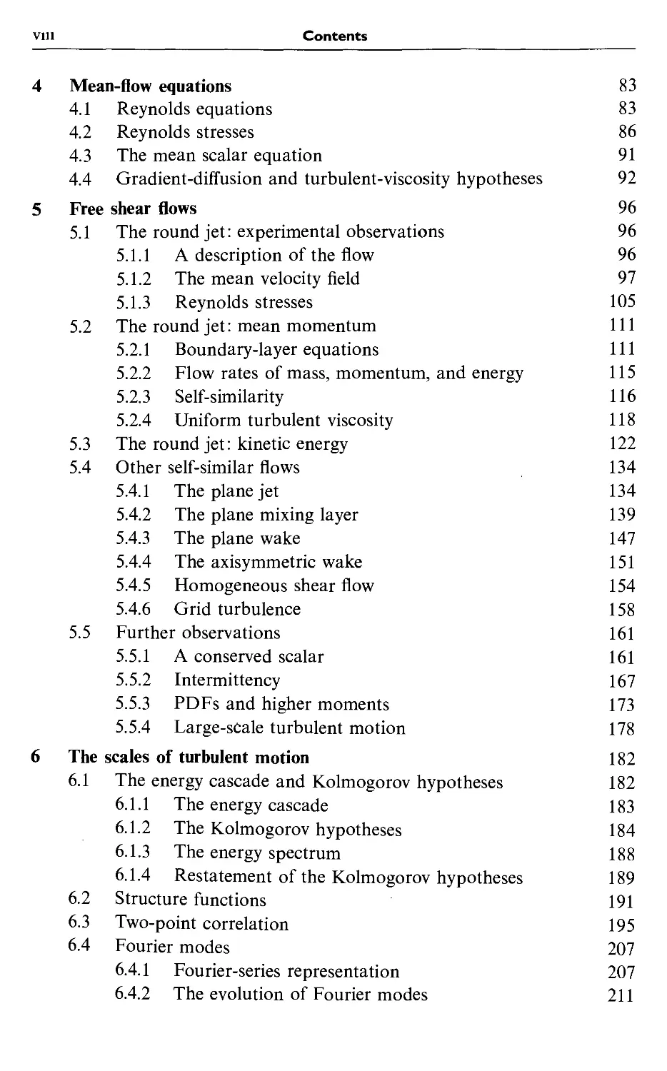
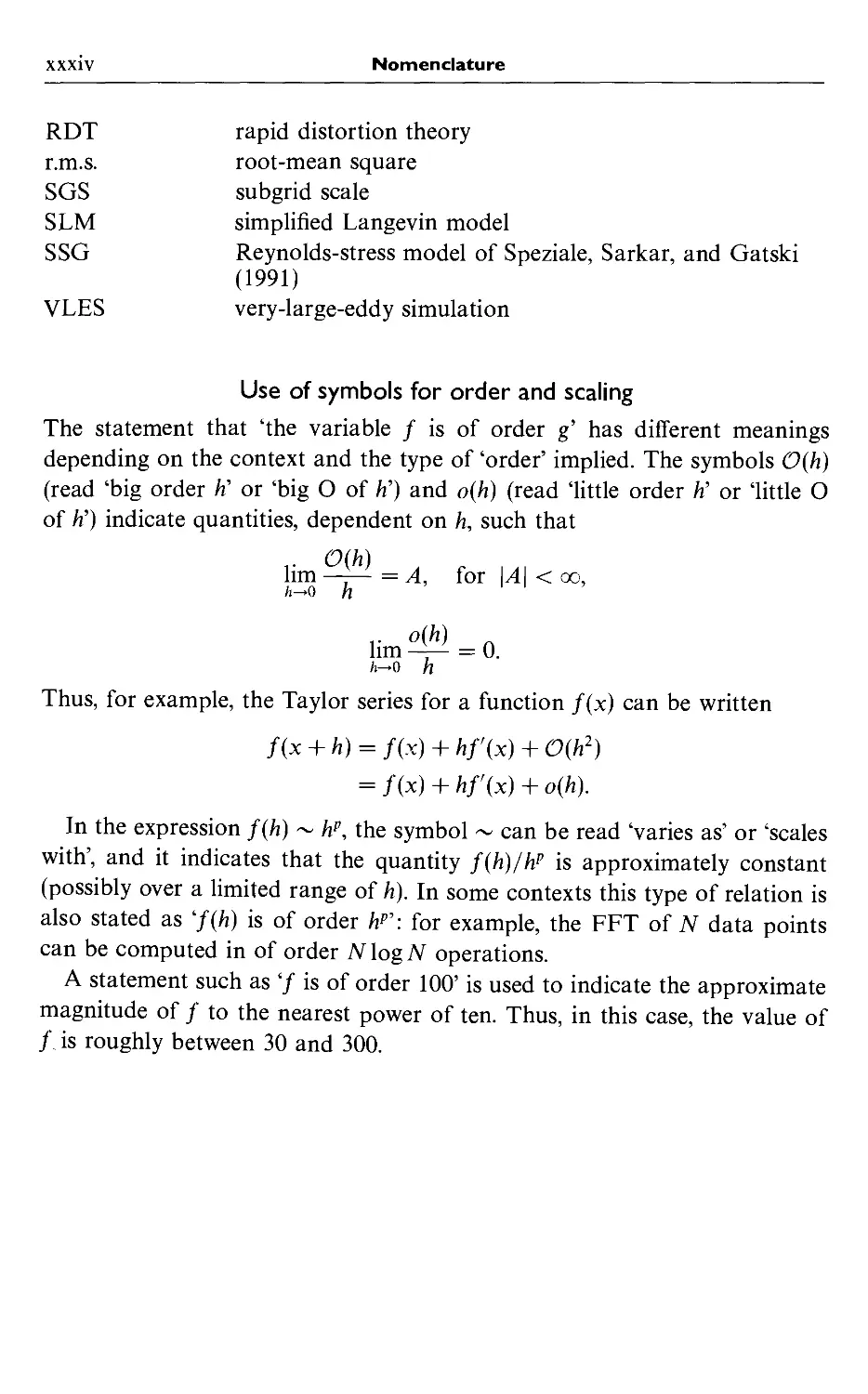
the plume formed by a solid rocket motor (see Fig. 1.1), turbulent motions
of many scales can be observed, from eddies and bulges comparable in size
to the width of the plume, to the smallest scales the camera can resolve. The
features mentioned in these two examples are common to all turbulent flows.
More detailed and careful observations can be made in laboratory
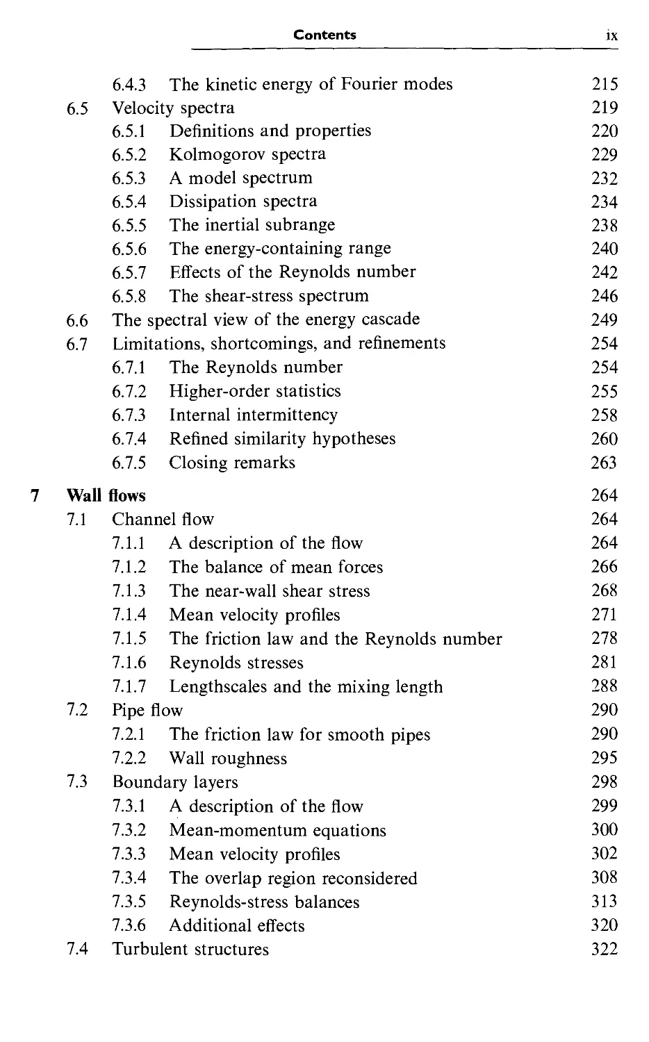
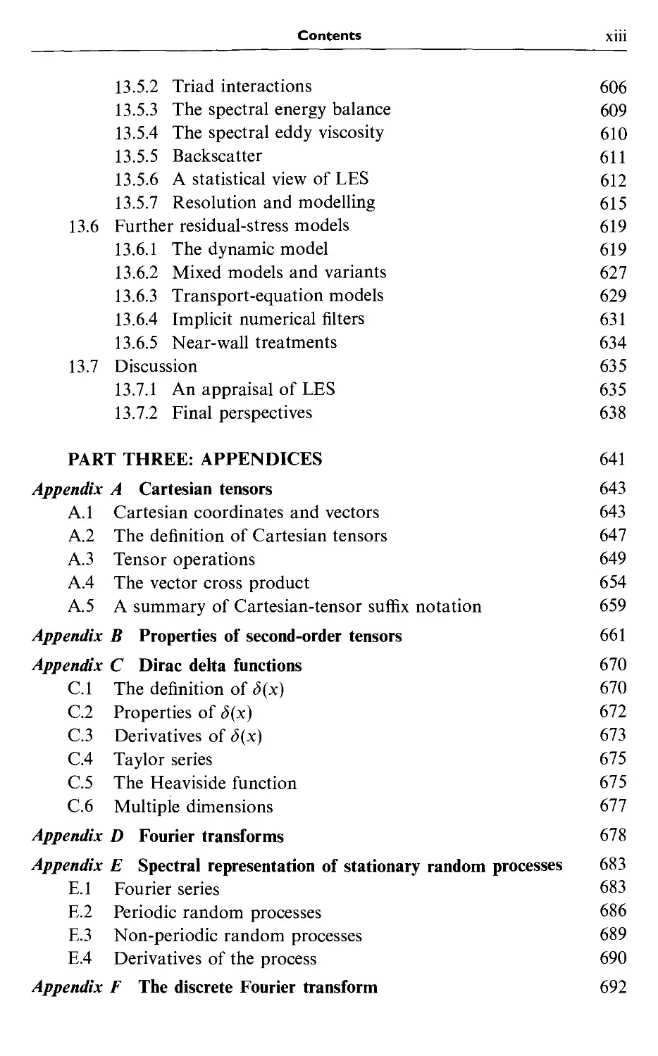
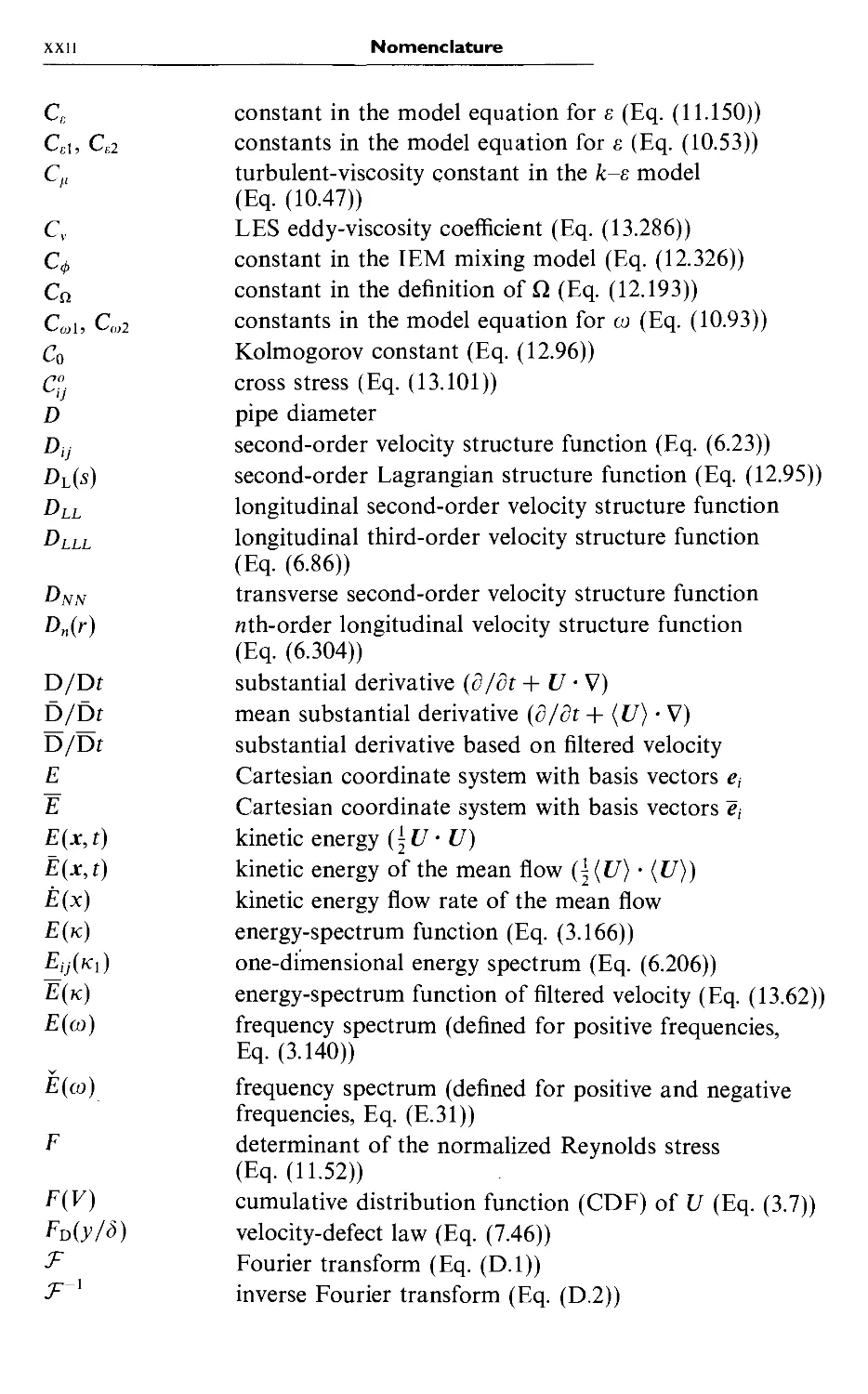
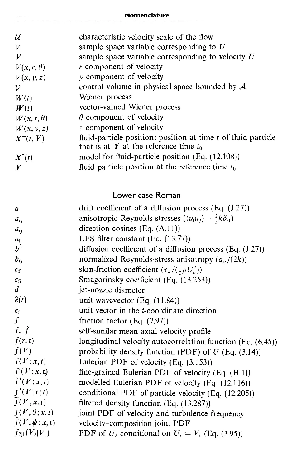
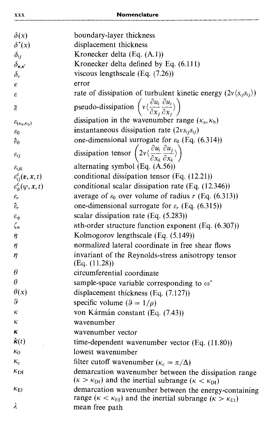
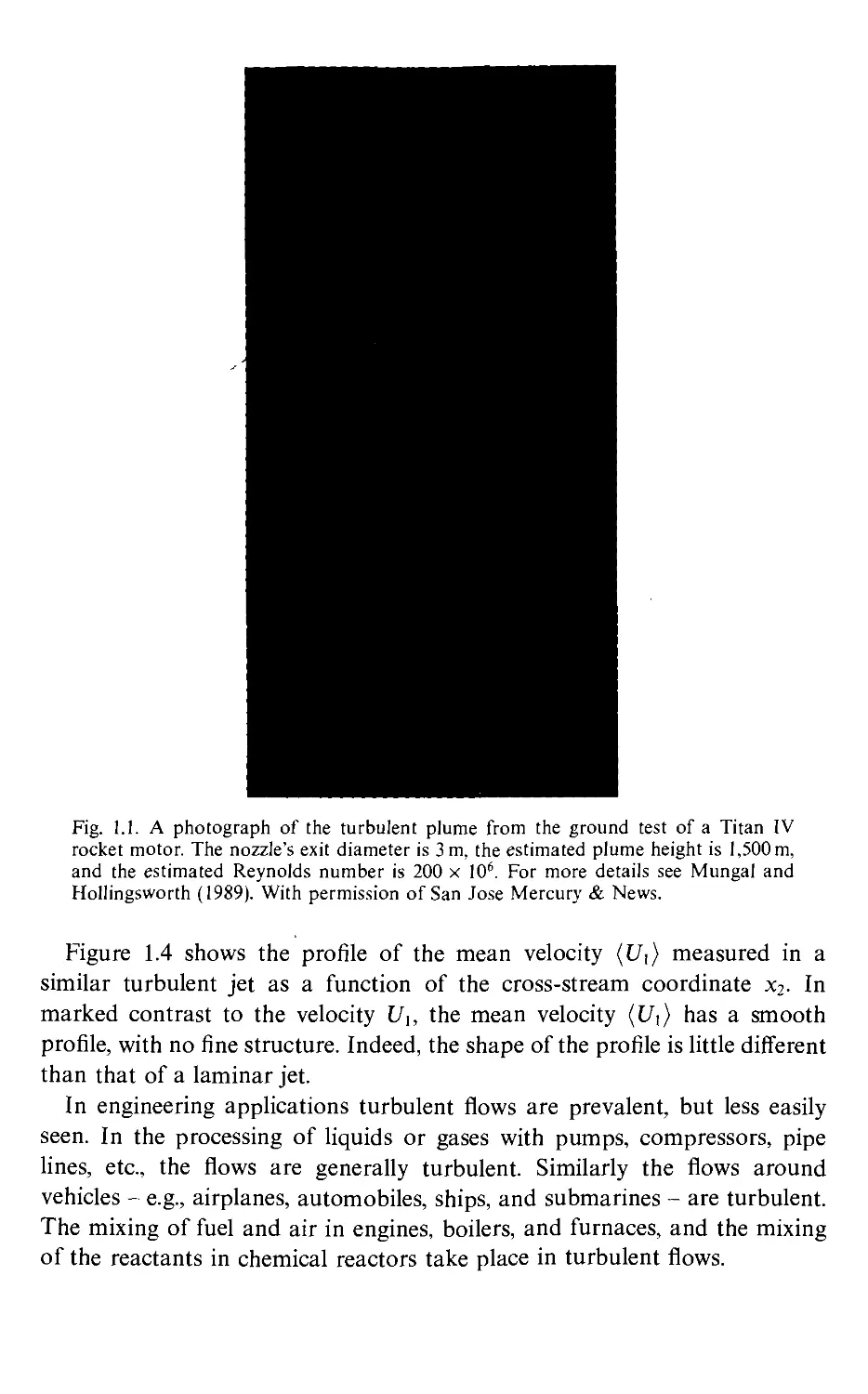
experiments. Figure 1.2 shows planar images of a turbulent jet at two different
Reynolds numbers. Again, the concentration fields are irregular, and a large
range of length scales can be observed.
As implied by the above discussion, an essential feature of turbulent flows
is that the fluid velocity field varies significantly and irregularly in both
position and time. The velocity field (which is properly introduced in Section
2.1) is denoted by U{x,t), where x is the position and t is time.
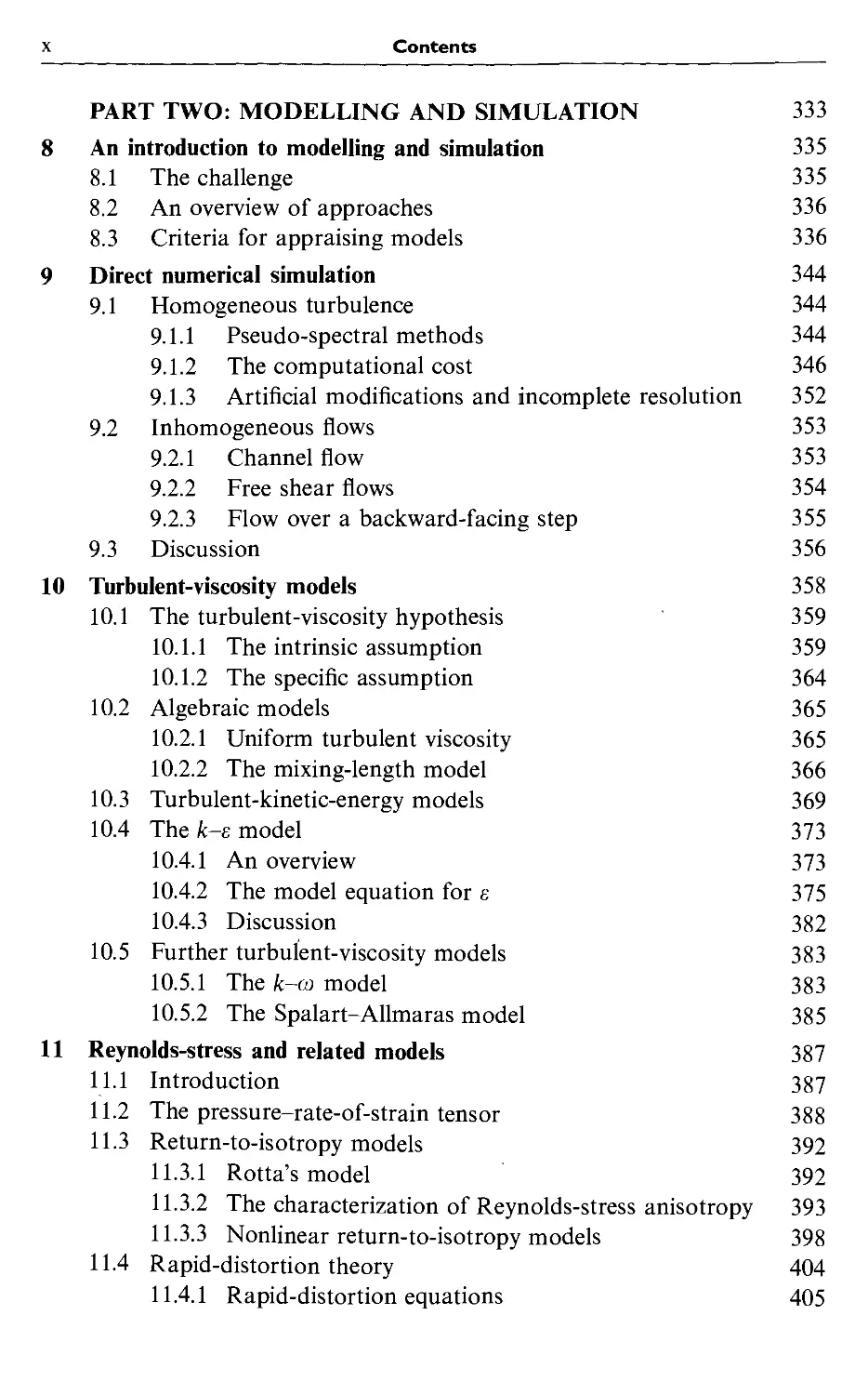
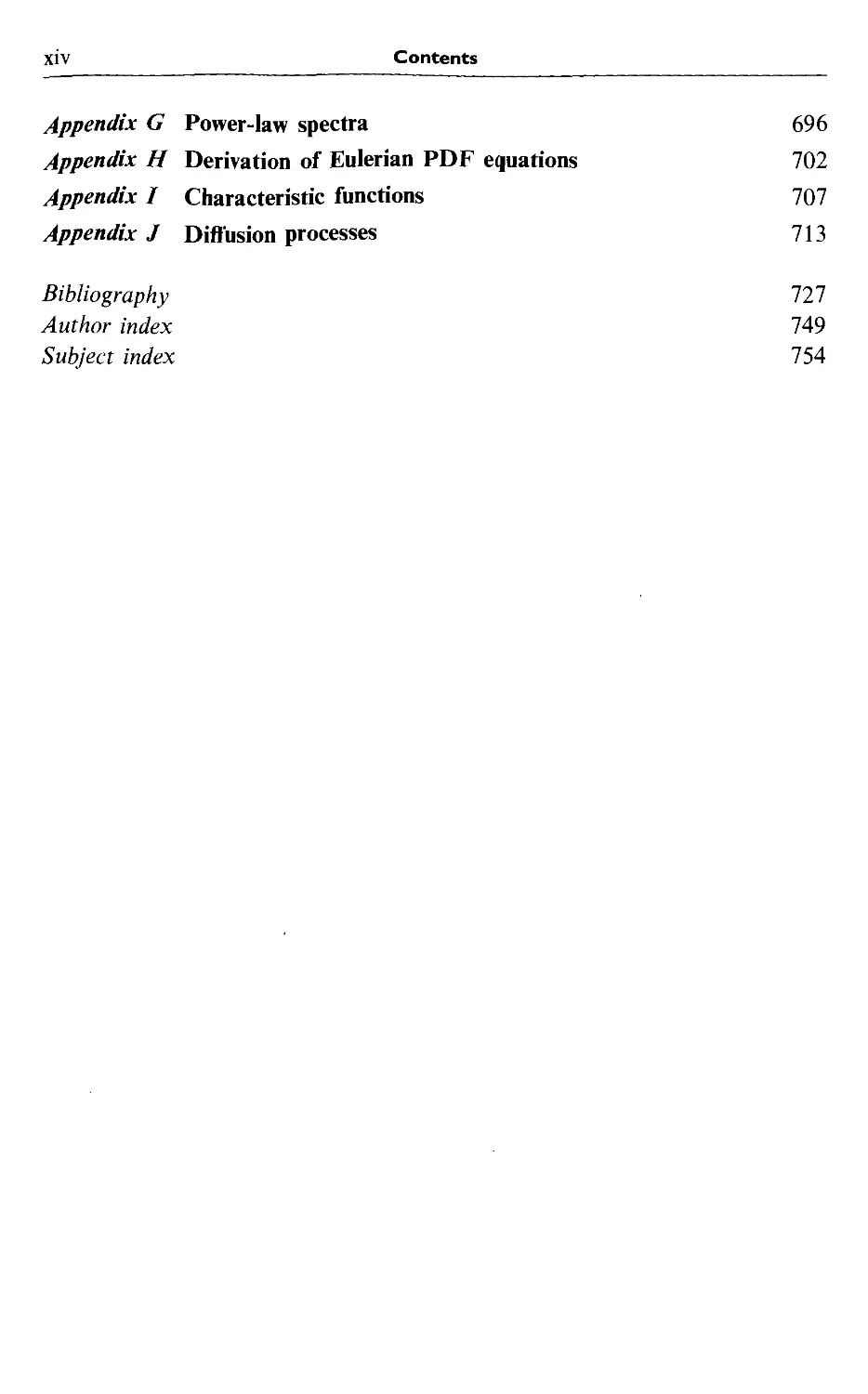
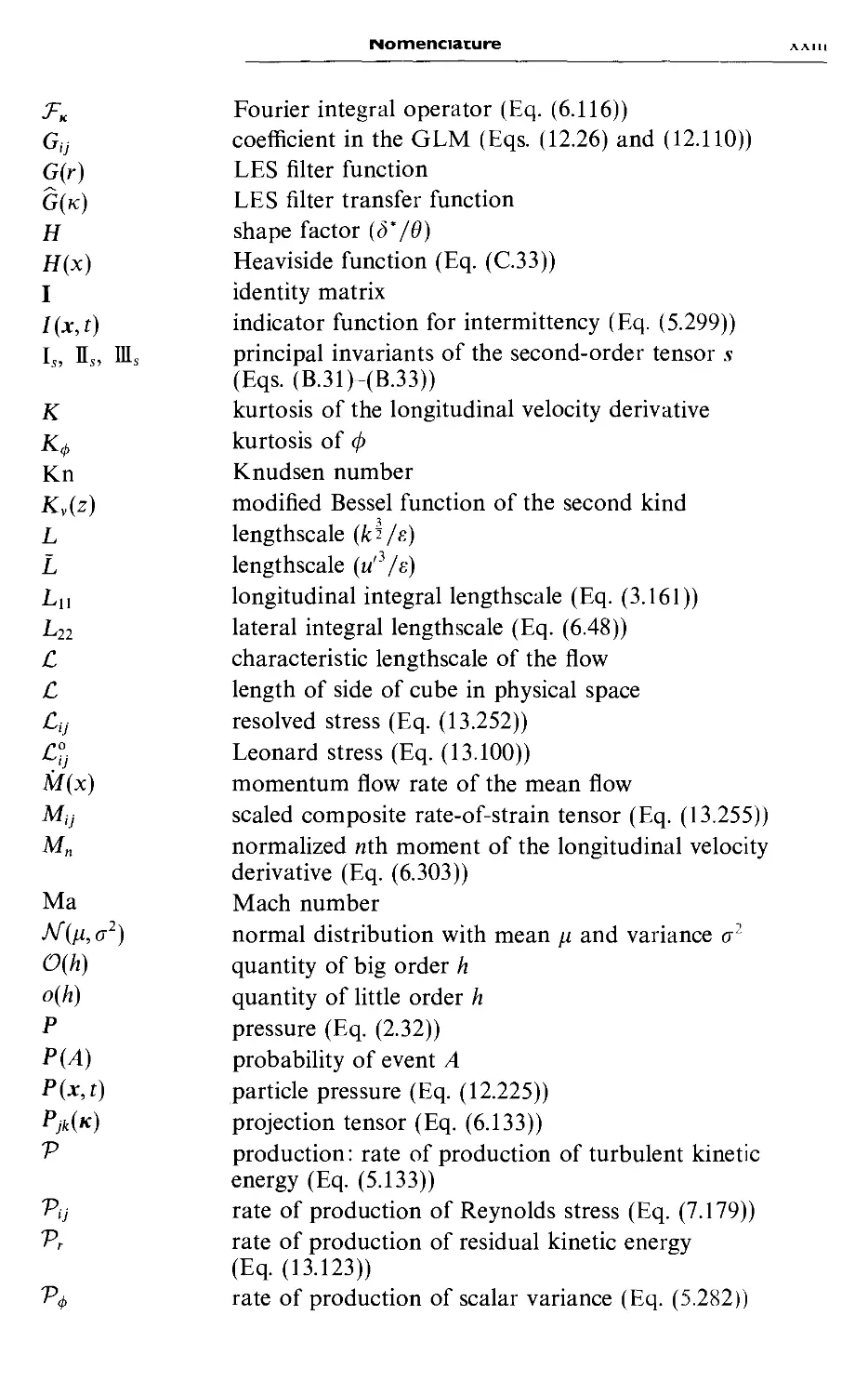
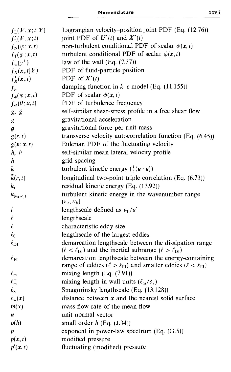
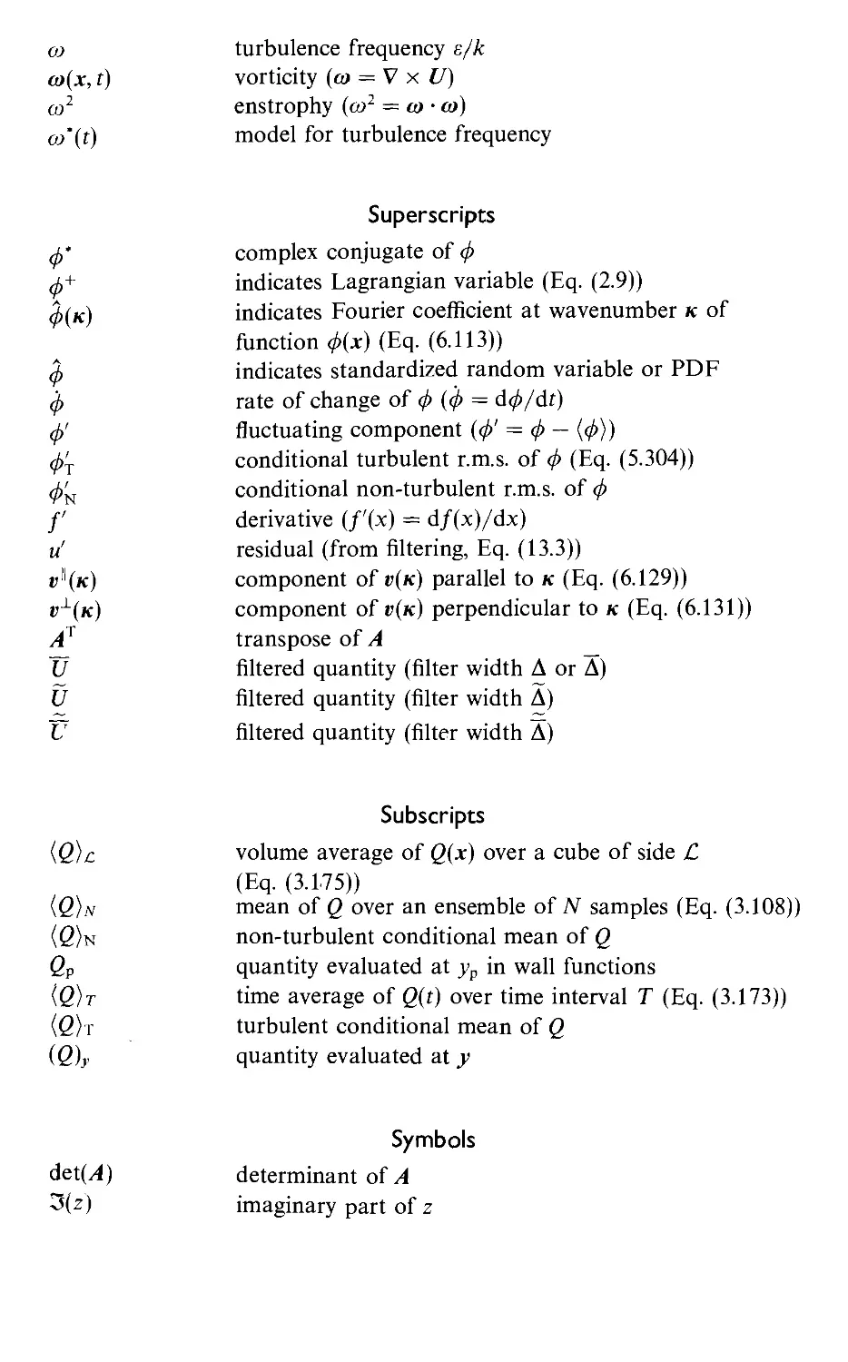
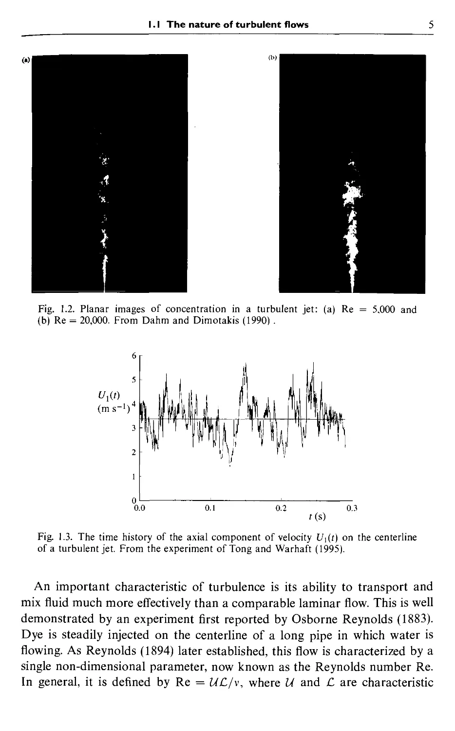
Figure 1.3 shows the time history Ui{t) of the axial component of velocity
measured on the centerline of a turbulent jet (similar to that shown in
Fig. 1.2). The horizontal line (in Fig. 1.3) shows the mean velocity denoted
by {Ui), and defined in Section 3.2. It may be observed that the velocity
Ui{t) displays significant fluctuations (about 25% of {Ui)), and that, far
from being periodic, the time history exhibits variations on a wide range of
timescales. Very importantly, we observe that Ui (t) and its mean (Ui) are in
some sense 'stable': huge variations in Ui{t) are not observed; neither does
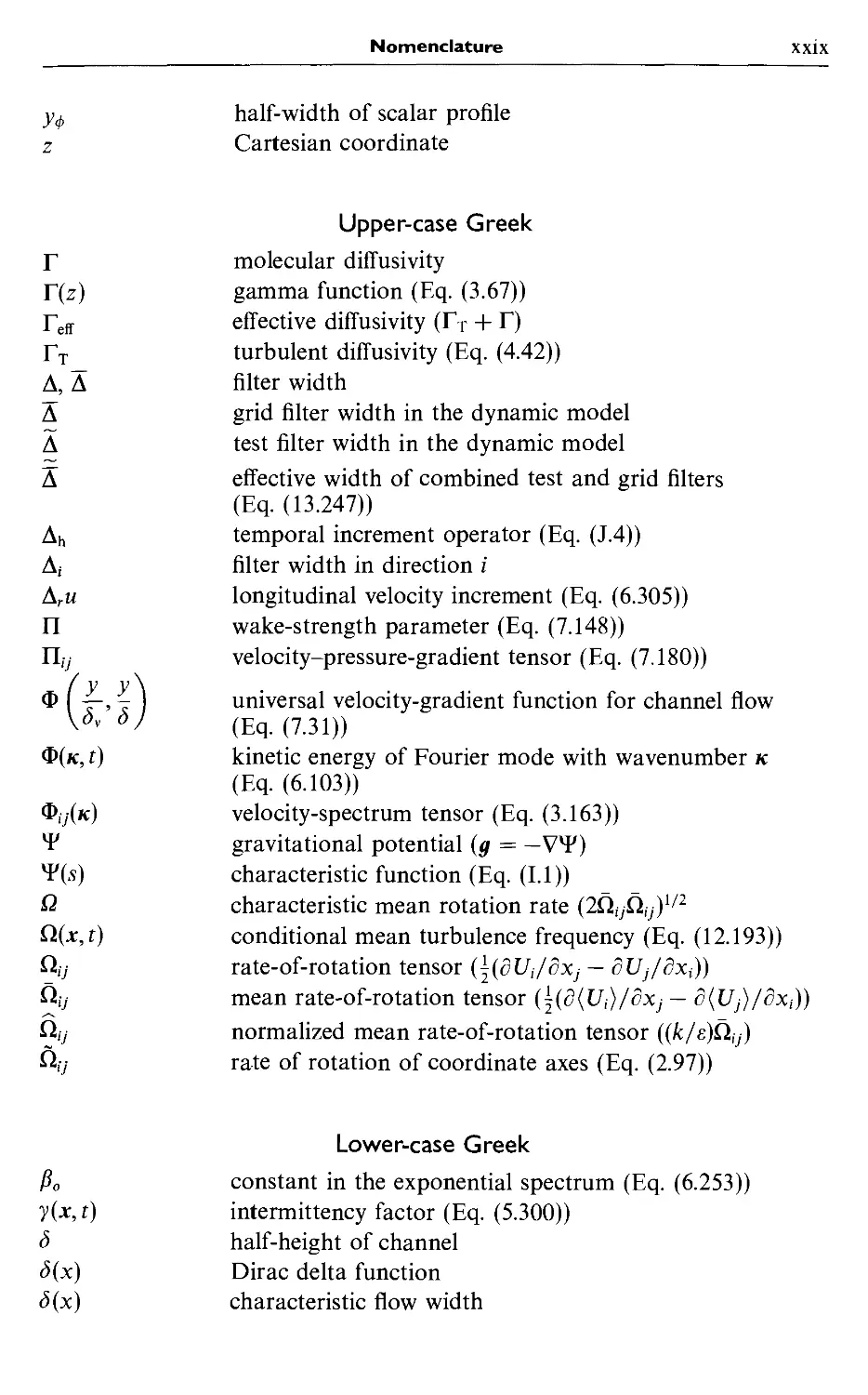
Ui{t) spend long periods of time near values different than (Ui).

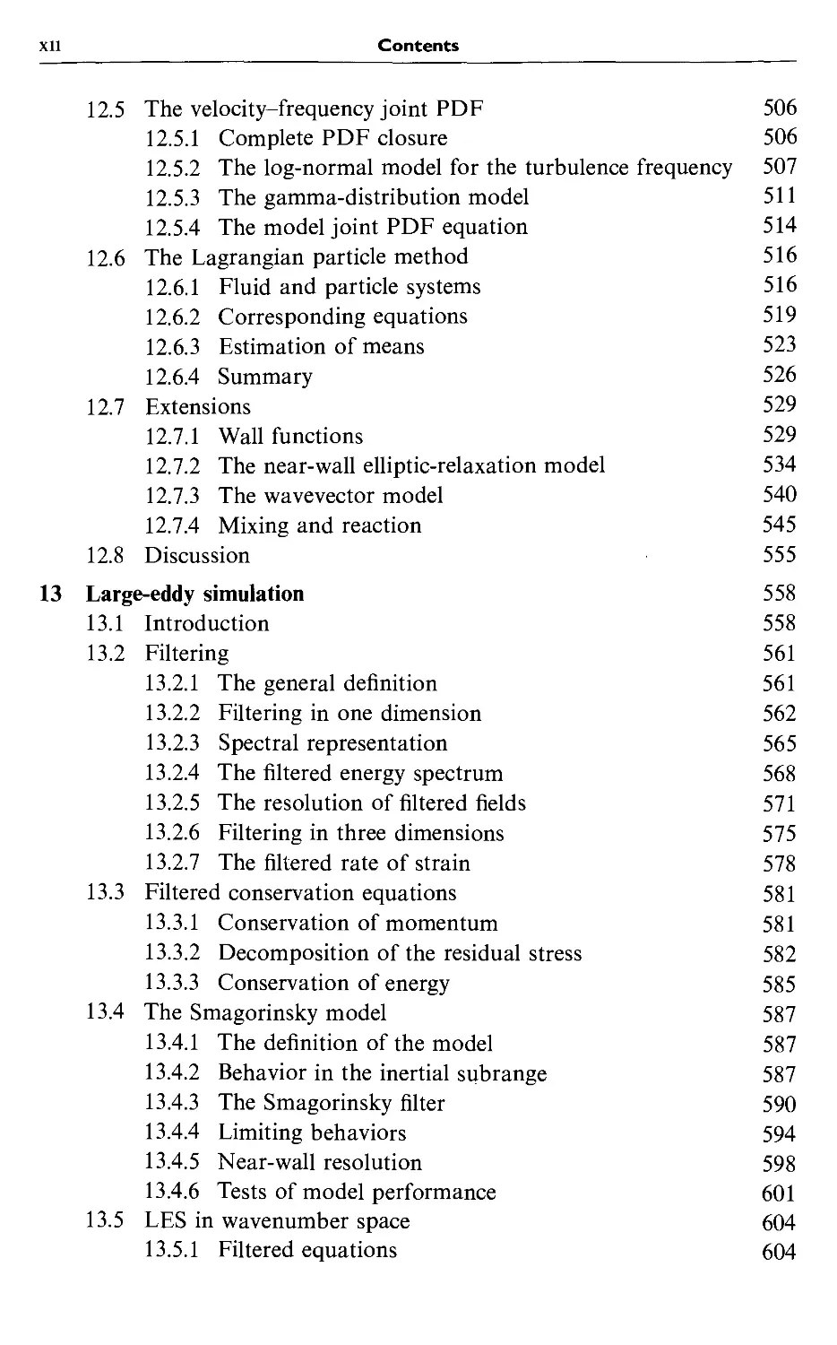
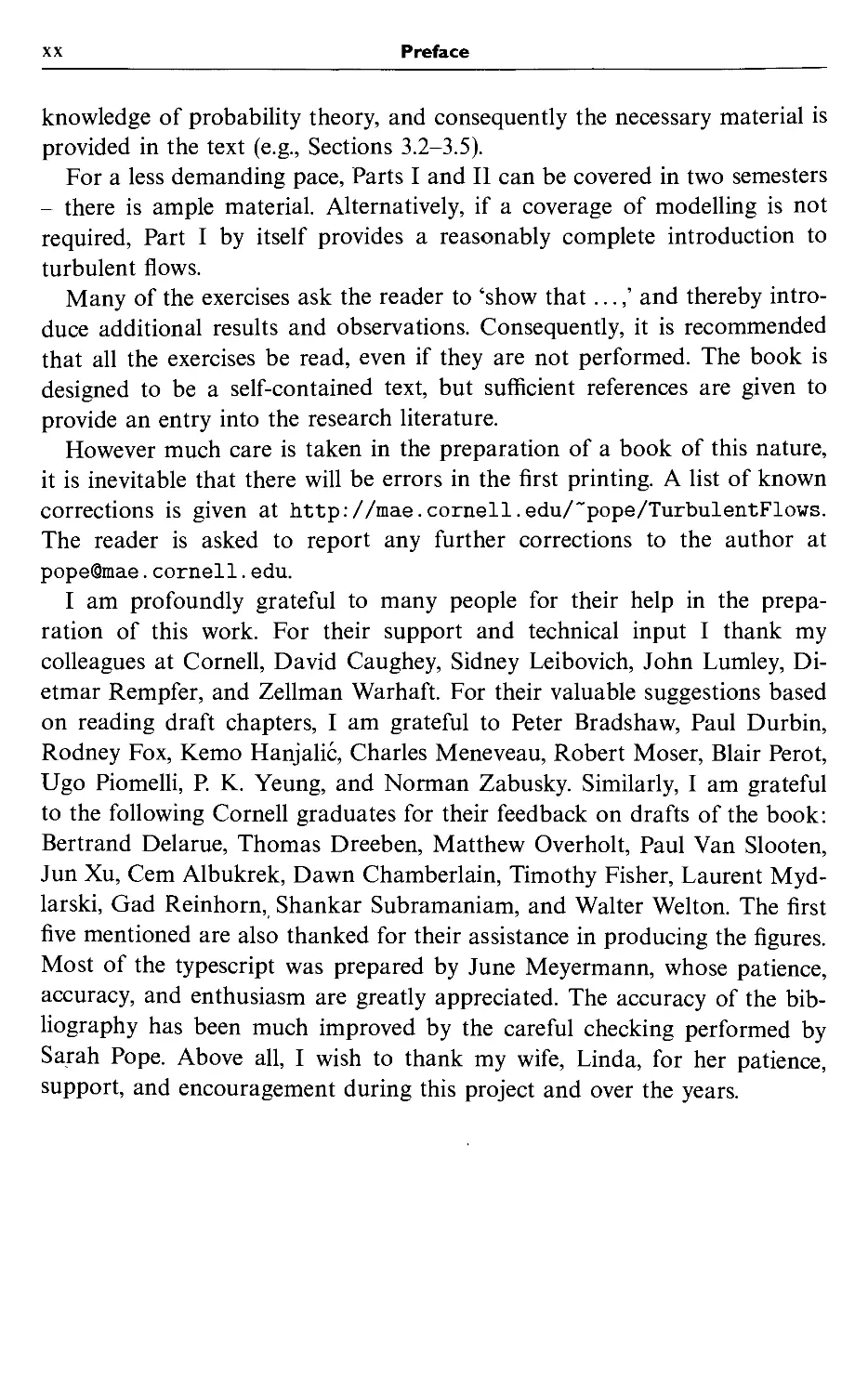
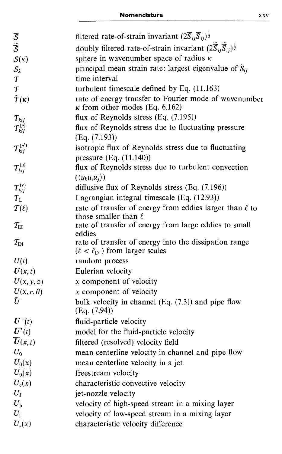
Fig. 1.1. A photograph of the turbulent plume from the ground test of a Titan IV
rocket motor. The nozzle's exit diameter is 3 m, the estimated plume height is 1,500 m,
and the estimated Reynolds number is 200 x 10^. For more details see Mungal and
Hollingsworth A989). With permission of San Jose Mercury & News.
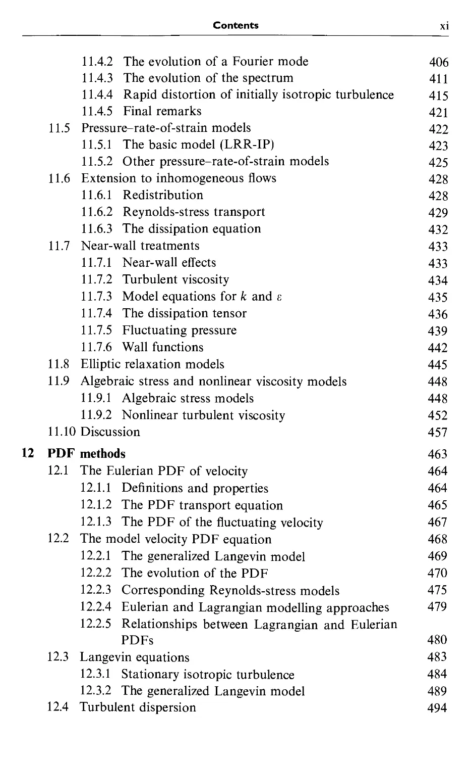
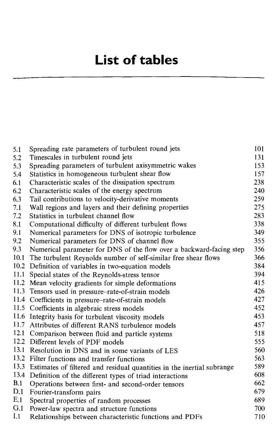
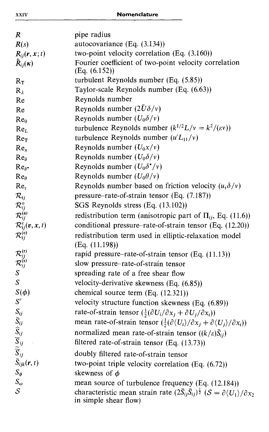
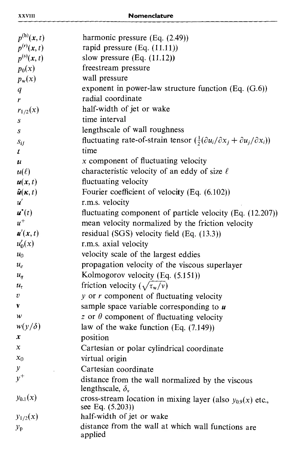
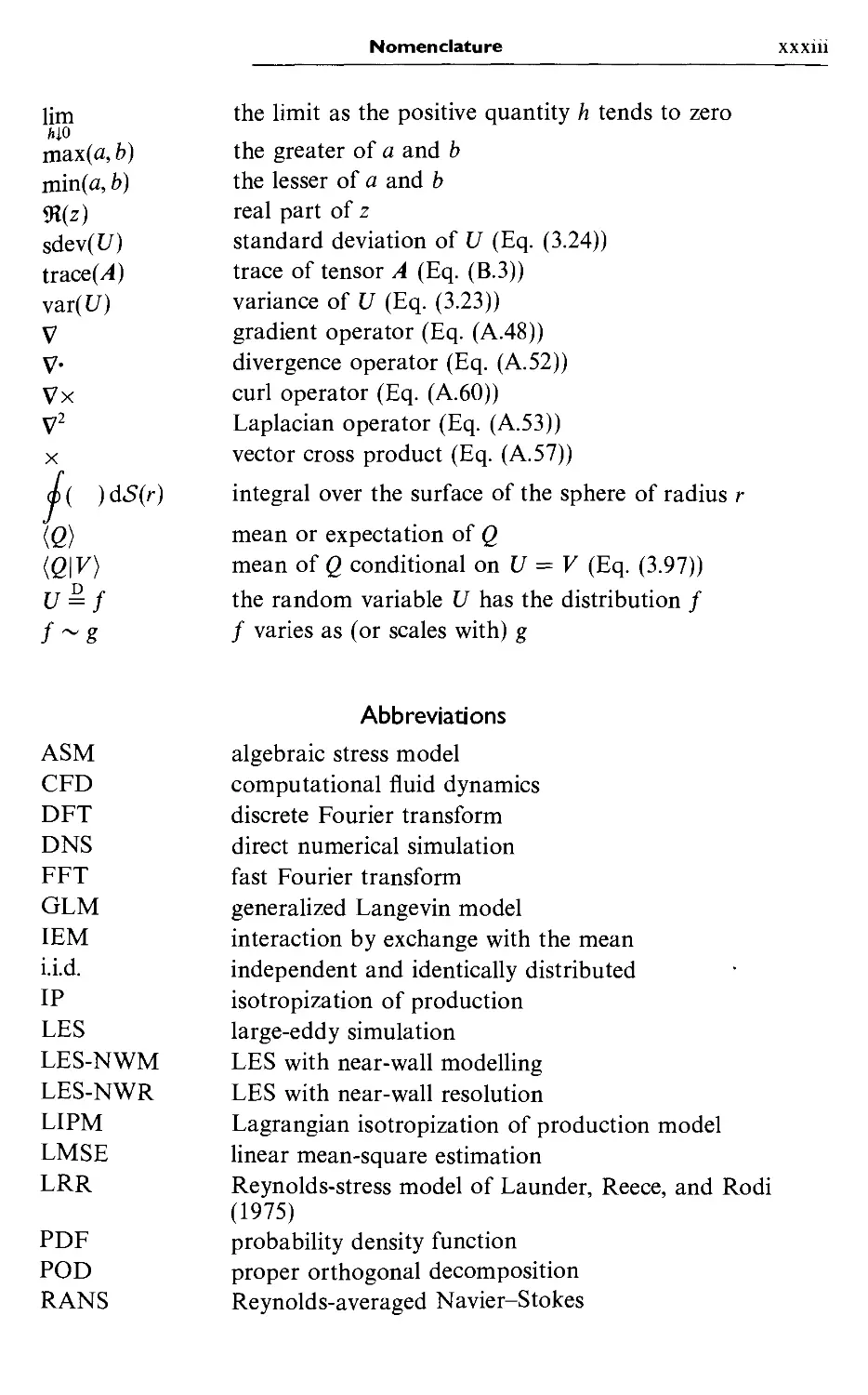
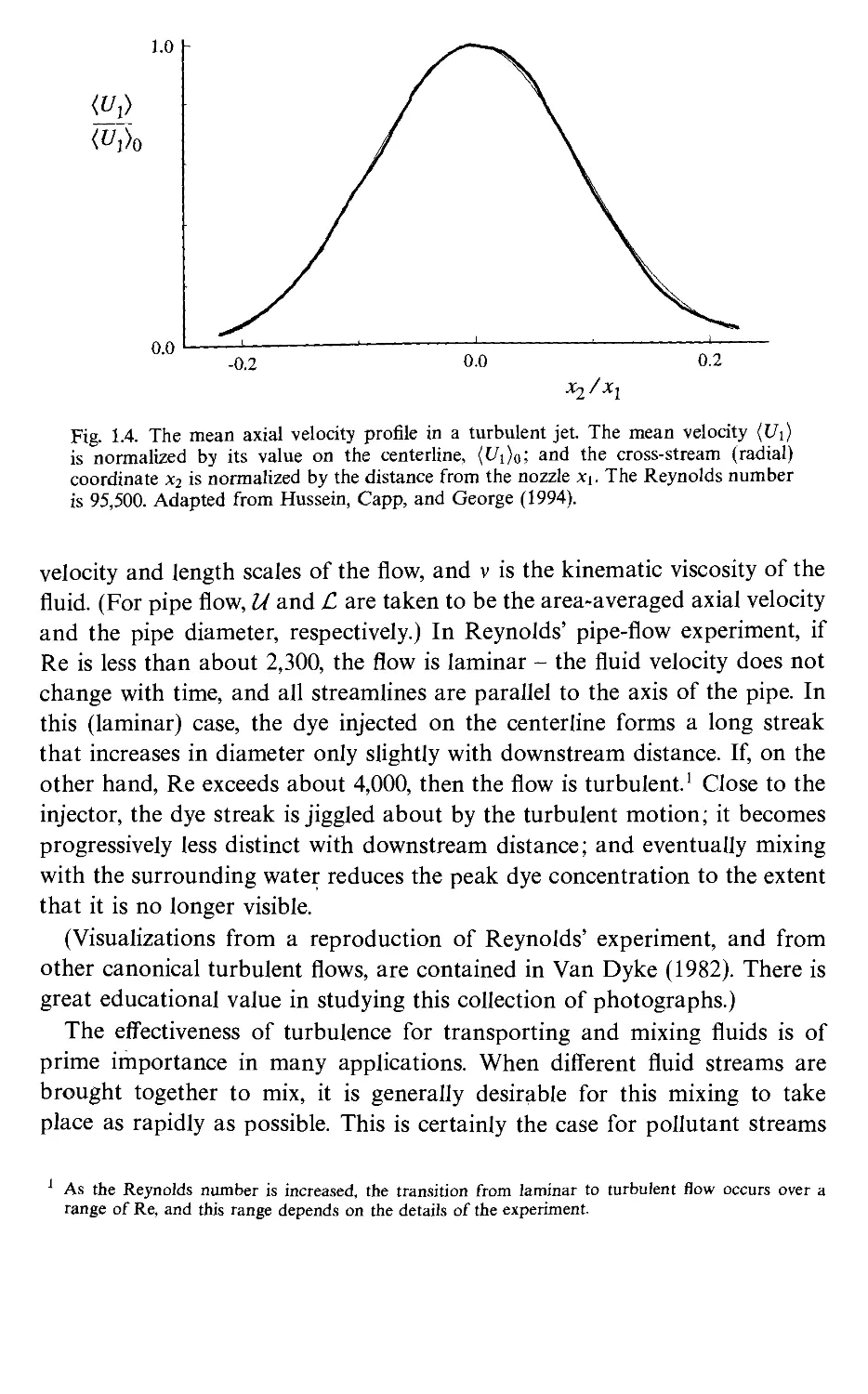
Figure 1.4 shows the profile of the mean velocity (G,) measured in a
similar turbulent jet as a function of the cross-stream coordinate xi. In
marked contrast to the velocity U\, the mean velocity (G,) has a smooth
profile, with no fine structure. Indeed, the shape of the profile is little different
than that of a laminar jet.
In engineering applications turbulent flows are prevalent, but less easily
seen. In the processing of liquids or gases with pumps, compressors, pipe
lines, etc., the flows are generally turbulent. Similarly the flows around
vehicles - e.g., airplanes, automobiles, ships, and submarines - are turbulent.
The mixing of fuel and air in engines, boilers, and furnaces, and the mixing
of the reactants in chemical reactors take place in turbulent flows.

The nature of turbulent flows
Fig. 1.2. Planar images of concentration in a turbulent jet: (a)
(b) Re = 20,000. From Dahm and Dimotakis A990) .
Re
5,000 and
t(s)
Fig. 1.3. The time history of the axial component of velocity Ui{t) on the centerline
of a turbulent jet. From the experiment of Tong and Warhaft A995).
An important characteristic of turbulence is its ability to transport and
mix fluid much more eff"ectively than a comparable laminar flow. This is well
demonstrated by an experiment first reported by Osborne Reynolds A883).
Dye is steadily injected on the centerline of a long pipe in which water is
flowing. As Reynolds A894) later established, this flow is characterized by a
single non-dimensional parameter, now known as the Reynolds number Re.
In general, it is defined by Re = UC/v, where U and £ are characteristic

1.0
0^
<t^i)o
0.0
-0.2
0.0
0.2
Xi/ X^
Fig. 1.4. The mean axial velocity profile in a turbulent jet. The mean velocity (Ui)
is normalized by its value on the centerline, (l/i)o; and the cross-stream (radial)
coordinate Xj is normalized by the distance from the nozzle Xj. The Reynolds number
is 95,500. Adapted from Hussein, Capp, and George A994).
velocity and length scales of the flow, and v is the kinematic viscosity of the
fluid. (For pipe flow, U and L are taken to be the area-averaged axial velocity
and the pipe diameter, respectively.) In Reynolds' pipe-flow experiment, if
Re is less than about 2,300, the flow is laminar - the fluid velocity does not
change with time, and all streamlines are parallel to the axis of the pipe. In
this (laminar) case, the dye injected on the centerline forms a long streak
that increases in diameter only slightly with downstream distance. If, on the
other hand, Re exceeds about 4,000, then the flow is turbulent.' Close to the
injector, the dye streak is jiggled about by the turbulent motion; it becomes
progressively less distinct with downstream distance; and eventually mixing
with the surrounding water reduces the peak dye concentration to the extent
that it is no longer visible.
(Visualizations from a reproduction of Reynolds' experiment, and from
other canonical turbulent flows, are contained in Van Dyke A982). There is
great educational value in studying this collection of photographs.)
The effectiveness of turbulence for transporting and mixing fluids is of
prime importance in many applications. When different fluid streams are
brought together to mix, it is generally desirable for this mixing to take
place as rapidly as possible. This is certainly the case for pollutant streams
As the Reynolds number is increased, the transition from laminar to turbulent flow occurs over a
range of Re, and this range depends on the details of the experiment.

.2 The study of turbulent flows
released into the atmosphere or into bodies of water, and for the mixing of
different reactants in combustion devices and chemical reactors.
Turbulence is also effective at 'mixing' the momentum of the fluid. As a
consequence, on aircraft's wing and ships' hulls the wall shear stress (and
hence the drag) is much larger than it would be if the flow were laminar.
Similarly, compared with laminar flow, rates of heat and mass transfer at
solid-fluid and liquid-gas interfaces are much enhanced in turbulent flows.
The major motivation for the study of turbulent flows is the combination
of the three preceding observations: the vast majority of flows is turbulent;
the transport and mixing of matter, momentum, and heat in flows is of great
practical importance; and turbulence greatly enhances the rates of these
processes.
1.2 The study of turbulent flows
Many different techniques have been used to address many different
questions concerning turbulence and turbulent flows. The first step toward
providing a categorization of these studies is to distinguish between small-scale
turbulence and the large-scale motions in turbulent flows.
As is discussed in detail in Chapter 6, at high Reynolds number there is a
separation of scales. The large-scale motions are strongly influenced by the
geometry of the flow (i.e., by the boundary conditions), and they control the
transport and mixing. The behavior of the small-scale motions, on the other
hand, is determined almost entirely by the rate at which they receive energy
from the large scales, and by the viscosity. Hence these small-scale motions
have a universal character, independent of the flow geometry. It is natural
to ask what the characteristics of the small-scale motions are. Can they be
predicted from the equations governing fluid motion? These are questions
of turbulence theory, which are addressed in the books of Batchelor A953),
Monin and Yaglom A975), Panchev A971), Lesieur A990), McComb A990),
and others, and that are touched on only slightly in this book (in Chapter
6).
The focus of this book is on turbulent flows, studies of which can be
divided into three categories.
(i) Discovery: experimental (or simulation) studies aimed at providing
qualitative or quantitative information about particular flows.
(ii) Modelling: theoretical (or modelling) studies, aimed at developing
tractable mathematical models that can accurately predict properties
of turbulent flows.

Introduction
(iii) Control: studies (usually involving both experimental and theoretical
components) aimed at manipulating or controlling the flow or the
turbulence in a beneficial way - for example, changing the boundary
geometry to enhance mixing; or using active control to reduce drag.
The remainder of Part I of this book is based primarily on studies in the
first category, the objective being to develop in the reader an understanding
for the important characteristics of simple turbulent flows, of the dominant
physical processes, and how they are related to the equations of fluid motion.
The description of turbulent flows contained in Part I is not comprehensive:
additional material can be found in the books of Monin and Yaglom A971),
Townsend A976), Hinze A975), and Schlichting A979).
For studies in the second category, that aim at developing tractable
mathematical models, the word 'tractable' is crucial. For fluid flows, be they
laminar or turbulent, the governing laws are embodied in the Navier-Stokes
equations, which have been known for over a century. (These equations
are reviewed in Chapter 2.) Considering the diversity and complexity of
fluid flows, it is quite remarkable that the relatively simple Navier-Stokes
equations describe them accurately and in complete detail. However, in the
context of turbulent flows, their power is also their weakness: the equations
describe every detail of the turbulent velocity field from the largest to the
smallest length and time scales. The amount of information contained in the
velocity field is vast, and as a consequence (in general) the direct approach
of solving the Navier-Stokes equations is impossible. So, while the Navier-
Stokes equations accurately describe turbulent flows, they do not provide a
tractable model for them.
The direct approach of solving the Navier-Stokes equations for
turbulent flows is called direct numerical simulation (DNS), and is described in
Chapter 9. While DNS is intractable for the high-Reynolds-number flows of
practical interest, it is nevertheless a powerful research tool for investigating
simple turbulent flows at moderate Reynolds numbers. In the description
of wall-bounded flows in Chapter 7, DNS results are used extensively to
investigate the physical processes involved.
For the high-Reynolds-number flows that are prevalent in applications,
the natural alternative is to pursue a statistical approach. That is, to describe
the turbulent flow, not in terms of the velocity U{x, t), but in terms of some
statistics, the simplest being the mean velocity field {U{x,t)). A model based
on such statistics can lead to a tractable set of equations, because statistical
fields vary smoothly (if at all) in position and time. In Chapter 3 we present
the concepts and techniques used in the statistical representation of turbulent

.2 The study of turbulent flows
flow fields; while in Part II we describe statistical models that can be used to
calculate the properties of turbulent flows. The approaches described include:
turbulent viscosity models, e.g., the k-s model (Chapter 10); Reynolds-stress
models (Chapter 11); models based on the probability density function (PDF)
of velocity (Chapter 12); and large-eddy-simulations (LES) (Chapter 13).
The statistical models described in Part II can be used in some studies in
the third category mentioned above - that is, studies aimed at manipulating
or controlling the flow or the turbulence. However, such studies are not
explicitly discussed here.
A broad range of mathematical techniques is used to describe and model
turbulent flows. Appendices on several of these techniques are provided to
serve as brief tutorials and summaries. The first of these is on Cartesian
tensors, which are used extensively. The reader may wish to review this
material (Appendix A) before proceeding. There are exercises throughout
the book, which provide the reader with the opportunity to practice the
mathematical techniques employed. Most of these exercises also contain
additional results and observations. A list of nomenclature and abbreviations
is provided on page xxi.

2
The equations of fluid motion
In this chapter we briefly review the Navier-Stokes equations which
govern the flow of constant-property Newtonian fluids. More comprehensive
accounts can be found in the texts of Batchelor A967), Panton A984), and
Tritton A988). Two topics that are important in the study of turbulent flows,
that are not extensively discussed in these texts, are the Poisson equation
for pressure (Section 2.5), and the transformation properties of the Navier-
Stokes equations (Section 2.9). The equations of fluid motion are expressed
either in vector notation or in Cartesian tensor notation, which is reviewed
in Appendix A.
2.1 Continuum fluid properties
The idea of treating fluids as continuous media is both natural and familiar.
It is, however, worthwhile to review the continuum hypothesis - that reconciles
the discrete molecular nature of fluids with the continuum view - so as to
avoid confusion when quantities such as 'fluid particles' and 'infinitesimal
material elements' are introduced.
The length and time scales of molecular motion are extremely small
compared with human scales. Taking air under atmospheric conditions as
an example, the average spacing between molecules is 3 x 10~' m, the mean
free path. A, is 6 x 10~^ m, and the mean time between successive collision
of a molecule is 10""'° s. In comparison, the smallest geometric length scale
in a flow, £, is seldom less than 0.1 mm = lO^"* m, which, for flow velocities
up to 100 m s~', yields a flow timescale larger than 10~^ s. Thus, 6ven for
this example of a flow with small length and time scales, these flow scales
exceed the molecular scales by three or more orders of magnitude.

2.1 Continuum fluid properties 11
The separation of the length scales is quantified by the Knudsen number
Kn = XIL B.1)
In the above example, Kn is less than 10~^ while in general the continuum
approach is appropriate for Kn <C 1.
For very small Kn, because of the separation of scales, there exist
intermediate length scales V, such that C is large compared with molecular scales,
yet small compared with flow scales (i.e., /. <C ^* <C i). Roughly speaking,
the continuum fluid properties can be thought of as the molecular properties
averaged over a volume of size V = t^. Let Vx denote a spherical region of
volume V centered on the point x. Then, at time t, the fluid's density p{x, t)
is the mass of molecules in Vx, divided by V.
Similarly the fluid's velocity U{x, t) is the average velocity of the molecules
within Vx- Because of the separation of scales, the dependence of the
continuum properties on the choice of t is negligible.
(While the approach presented in the previous paragraph is standard (see,
e.g., Batchelor A967) and Panton A984)), as Exercise 2.1 illustrates, more
care is needed to provide a proper definition of the continuum properties in
terms of averaging over a scale t. In fact, continuum fields are best defined
as expectations of molecular properties, see Chapter 12.)
It is important to appreciate that, once we invoke the continuum
hypothesis to obtain continuous fields, such as p{x, t) and U{x, t), we can leave behind
all notions of the discrete molecular nature of the fluid, and molecular scales
cease to be relevant. We can talk meaningfully of 'the density at x,t' even
though (in the microscopic view) in all likelihood there is no matter at {x, t).
Similarly, we can consider differences in properties over distances smaller
than molecular scales: indeed we do so when we define gradients,
^ = lim ( ^ [p(^i + h, X2, X3, t) - p{xi, X2, X3, t)] j. B.2)
EXERCISE
2.1 In the flow of an ideal gas, let m*'',x*''(r) and «*''@ be the mass,
position, and velocity of the ith molecule. As a generalization of the
standard continuum hypothesis, consider the definition
y".m<''«<''Kd»-<''l)
}Zjm(J^K{\y(})\)
where r*'' = x*'' — x, and K{r) is a smooth kernel such as
K{r) = exp{~{r'/t'), B.4)

with t being a specified length scale. Show that the velocity gradients
are
8u, E,-'"*'''D'-t/.)^'(l'-*'''lL'Vl'-<'''l
oxe
E,mO)K(|r(/)|)
B.5)
where K'{r) = dK{r)/dr.
(Evidently, the continuum field defined by Eq. B.3) inherits the
mathematical continuity properties of the kernel. If, as in the standard
treatment, K{r) is piece wise constant, i.e..
K{r) =
1, if r < r,
0, if r > r.
B.6)
then U{x, t) is piecewise constant, and hence not continuously differ-
entiable.)
2.2 Eulerian and Lagrangian fields
The continuum density and velocity fields, p{x,t) and U{x,t), are Eulerian
fields in that they are indexed by the position x in an inertial frame. The
starting point for the alternative Lagrangian description is the definition of
a fluid panicle - which is a continuum concept. By definition, a fluid particle
is a point that moves with the local fluid velocity: A'+(r, Y) denotes the
position at time t of the fluid particle that is located at Y at the specified
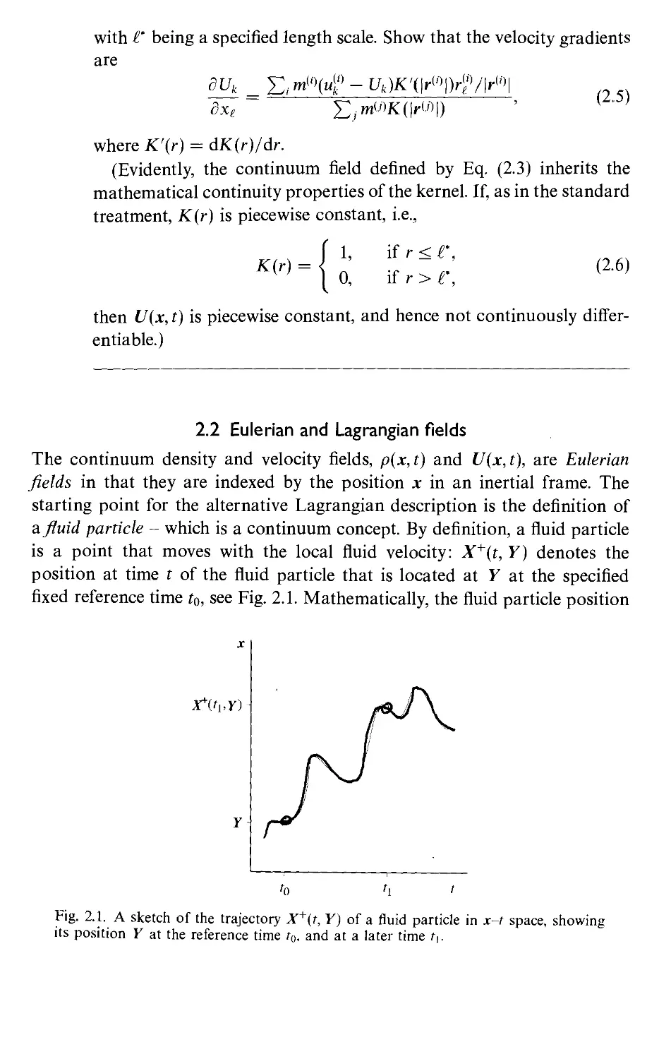
fixed reference time Iq, see Fig. 2.1. Mathematically, the fluid particle position
r(h,Y)
to
Fig. 2.1. A sketch of the trajectory A'+(f, Y) of a fluid particle in x~t space, showing
its position Y at the reference time to. and at a later time f|.

2.2 Eulerian and Lagrangian fields 13
X'^{t, Y) is defined by two equations. First, the position at the reference time
to is defined to be
X+{to, Y) = Y. B.7)
Second, the equation
j^X+{t,Y)=U{X^t,Y),t), B.8)
expresses the fact that the fluid particle moves with the local fluid velocity.
Given the Eulerian velocity field U{x,t), then, for any Y, Eq. B.8) can be
integrated backward and forward in time to obtain X'^{t, Y) for all t.
Lagrangian fields of density and velocity, for example, are defined in terms
of their Eulerian counterparts by
p+{t,Y)^p{X+{t,Y),t), B.9)
U+{t,Y)=U{X+{t,Y),t). B.10)
Note that the Lagrangian fields p+ and V^ are indexed not by the current
position of the fluid particle, but by its position Y at the reference time to.
Hence, Y is called the Lagrangian coordinate or the material coordinate.
For fixed Y, X'^{t, Y) defines a trajectory (in x~t space) that is the fluid-
particle path, and similarly p+(r, Y) is the fluid-particle density. The partial
derivative 5p+(r, Y)/8t is the rate of change of density at fixed Y, i.e.,
following a fluid particle. From Eq. B.9) we obtain
|p+(r,F) = |p(X+(r,F),r)
= (^p{x, t)) + |j^+(r, Y) (^p{x, t))
p{x, t) + Ui{x, t) ^p{x, t)
S^ S^> / x=X+[t,Y)
^P(^,0) , B.11)
^'^ J x=X+(t,Y)
where the material derivative, or substantial derivative, is defined by
-^^ + C/,A = i + (/.v B.12)
Dr 8t ' 8xi dt ^ '
Thus the rate of change of density following a fluid particle is given by the
partial derivative of the Lagrangian field (i.e., 8p+/d't) and by the substantial
derivative of the Eulerian field (i.e., Dp/Dr).

14 2 The equations of fluid motion
Similarly, for fixed Y, U'^{t, Y) is the fluid particle velocity , and
lu\t,Y)=(~U{x,t)) B.13)
is the rate of change of fluid particle velocity, i.e., the fluid particle
acceleration.
A fluid particle is also called a material point and we have seen that it
is defined by its position Y at time to and by its movement with the local
fluid velocity (Eq. B.8)). Material lines, surfaces, and volumes are defined
similarly. For example, consider at time to a simple closed surface So that
encloses the volume Vo. The corresponding material surface S{t) is defined
to be coincident with So at time to, and by the property that every point of
S(t) moves with the local fluid velocity. Thus Sit) is composed of the fluid
particles A"^(r, Y), which at to compose the surface So'-
S(t)^{X+(t,Y):Y eSo). B.14)
Because a material surface moves with the fluid, the relative velocity between
the surface and the fluid is zero. Consequently a fluid particle cannot cross
a material surface; neither is there a mass flux across a material surface.
EXERCISE
2.2 Consider two fluid particles that, at the reference time to are located
at Y and F + dF, where dF is an infinitesimal displacement. At time
t, the line between the two particles forms the infinitesimal line element
s{t) = X+(t, F + dF) - X+{t, Y). B.15)
Show that s{t) evolves by
■ ^ = *-(Vf/),=;,+„^,. B.16)
(Hint: expand f/+(r, F+dF) = U{X+{t, Y)+s(t), t) in a Taylor series.
Since * is infinitesimal, only the leading-order terms need be retained.)
2.3 The continuity equation
The mass-conservation or continuity equation is
^ + V-(pf/) = 0. B.17)
The derivation and interpretation of this equation in terms of control volumes
and material volumes should be familiar to the reader and are not repeated

2.3 The continuity equation 15
here. A further useful interpretation is in terms of the specific volume of the
fluid &{x,t) = l/p{x,t). Manipulation of Eq. B.17) yields
-^=V.f/. B.18)
The left-hand side is the logarithmic rate of increase of the specific volume,
while (as Exercises 2.3 and 2.4 show) the dilatation V* f/ gives the logarithmic
rate of increase of the volume of an infinitesimal material volume. Hence
the continuity equation can be viewed as a consistency condition between
the change of the specific volume following a fluid particle, and the change
in the volume of an infinitesimal material volume element.
In this book we consider constant-density flows (i.e., flows in which p is
independent both of x and of r). In this case the evolution equation Eq. B.17)
degenerates to the kinematic condition that the velocity field be solenoidal
or divergence-free:
V • f/ = 0. B.19)
EXERCISES
2.3 Let V(r) be a material volume bounded by the material surface S{t).
Show from geometry that the volume of fluid V{t) within V{t) evolves
by
dV{t)
J J Si
df -/ Js(t)
U-ndA, B.20)
where dA is an area element on S{t), and n is the outward pointing
normal. Use the divergence theorem to obtain
dV{t)
J J Jvit)
dt ./././v(t)
Udx. B.21)
Show that, for the infinitesimal volume dV{t) of an infinitesimal
material volume dV,
-^lndF(r) = V-f/. B.22)
dt
2.4 The determinant of the Jacobian
.ft.,.de.(^) B.23,
gives the volume ratio between an infinitesimal material volume
dV{t) at time t, and its volume dF(ro) at time to. To first order in
the infinitesimal dr, show that
X+{to + dt,Y) = Yi + U,{ Y, to) dt, B.24)

JO 2 The equations of fluid motion
J {to + dr, F) - 1 + (V • f/) K,fo dr. B.26)
Hence show that
(lln J{t,Y)\ ={VU)y,^. B.27)
2.5 The volume F(r) defined in Exercise 2.3 can be written
V{t)= [[[ dx= [[[ J{t,Y)dY. B.28)
J J Jv(t) J J Jv(to)
Differentiate the first and last expressions in this equation with
respect to time, and compare the result with Eq. B.21) to obtain
I lnJ(r,F) = (V. {/);,+„„. B.29)
Hence argue that, in constant-density flows, J{t, Y) is unity.
2.4 The momentum equation
The momentum equation, based on Newton's second law, relates the fluid
particle acceleration Df//Dr to the surface forces and body forces
experienced by the fluid. In general, the surface forces, which are of molecular
origin, are described by the stress tensor T,y(x, t) - which is symmetric, i.e.,
T,y = Ty,. The body force of interest is gravity. With ^F being the gravitational
potential (i.e., the potential energy per unit mass associated with gravity), the
body force per unit mass is
g = _v^. B.30)
(For a constant gravitational field the potential is ^F = gz, where g is the
gravitational acceleration, and z is the vertical coordinate.) These forces
cause the fluid to accelerate according to the momentum equation
We now specialize the momentum equation to flows of constant-property
Newtonian fluids - the fundamental class of flows considered in this book.
In this case, the stress tensor is
.„ = -/><!„+.A1 + ^). B.32)

2.4 The momentum equation 17
where P is the pressure, and jU is the (constant) coefficient of viscosity.
Recalling that (for the constant-density flows considered) the velocity field is
solenoidal (i.e., dUi/dxi = 0), we observe that Eq. B.32) expresses the stress
as the sum of isotropic (—PSij) and deviatoric contributions.
By substituting this expression for the stress tensor (Eq. B.32)) into the
general momentum equation Eq. B.31) (and exploiting the facts that p and
jU are uniform and that V • f/ = 0), we obtain the Navier-Stokes equations
BUi d^Uj 8P 8'¥
Further, defining the modified pressure, p, by
p = P + p^, B.34)
this equation simplifies to
^ = _ivp + vV^f/, B.35)
where v = p./p is the kinematic viscosity. In summary: the flow of constant-
property Newtonian fluids is governed by the Navier-Stokes equations
Eq. B.35) together with the solenoidal condition V • f/ = 0 stemming from
mass conservation.
At a stationary solid wall with unit normal n, the boundary conditions
satisfied by the velocity are the impermeability condition
n • f/ = 0, B.36)
and the no-slip condition
U-n{n-U) = 0, B.37)
(which together yield U = 0).
It is sometimes useful to consider the hypothetical case of an ideal (inviscid)
fluid, which is defined to have the isotropic stress tensor
Xij = -PS,j. B.38)
The conservation of momentum is given by the Euler equations
DU 1
Dr p
Vp, B.39)
which follow from Eqs. B.31), B.34), and B.38). Because the Euler equations
do not contain second spatial derivatives of velocity, they require different

2 The equations of fluid motion
boundary conditions than those of the Navier-Stokes equations. At a
stationary solid wall, for example, only the impermeability condition can be
applied, and in general the tangential components of velocity are non-zero.
While it is preferable to obtain the Euler equations (and other
equations derived from them) directly from the definition of t,; being isotropic
(Eq. B.38)), it may nevertheless be observed that the Euler equations can
be obtained from the Navier-Stokes equations by setting v to zero. It is
important to appreciate, however, that v = 0 is a singular limit: solutions to
the Navier-Stokes equations in the limit of vanishing viscosity (v -^ 0) are
different than solutions to the Euler equations. For one thing, even in this
limit, the equations require different boundary conditions.
2.5 The role of pressure
The role of pressure in the (constant-density) Navier-Stokes equations
requires further comment. First we observe that isotropic stresses and
conservative body forces have the same effect, which is expressed by the modified
pressure gradient. Hence the body force has no effect on the velocity field
and on the modified pressure field. (This is, of course, in contrast to variable-
density flows, in which buoyancy forces can be important.) Henceforth, we
refer to p simply as 'pressure'.
We may be accustomed to thinking of pressure as a thermodynamic
variable, related to density and temperature by an equation of state. However,
for constant-density flows, there is no connection between pressure and
density, and a different understanding of pressure is required.
To this end, we take the divergence of the Navier-Stokes equations
Eq. B.35), without assuming the velocity field to be solenoidal, but instead
writing A for the dilatation rate (i.e., A = V • f/). The result is
^-vV^^A-/?, B.40)
where
^ = —VV-^^. B.41
p OXj OXj
Consider the solution to Eq. B.40) with initial and boundary conditions
A = 0. The solution is A = 0 if and only if, R is zero everywhere, which in
turn implies (from Eq. B.41)) that p satisfies the Poisson equation
VV^S.-p|^|^. B.42)
OXj OXi

2.5 The role of pressure 19
Thus, we conclude that the satisfaction of this Poisson equation is a necessary
and sufficient condition for a solenoidal velocity field to remain solenoidal.
At a stationary, plane solid surface, the Navier-Stokes equations Eq. B.35)
reduce to
dp d^Un
on on^ ^ '
where n is a coordinate in the wall-normal direction, and Ua is the velocity
component normal to the wall. This equation provides a Neumann boundary
condition for the Poisson equation, Eq. B.42). Given Neumann conditions of
this form, the Poisson equation Eq. B.42) determines the pressure field p(x, t)
(to within a constant) in terms of the velocity field at the same instant of time.
Thus, Vp is uniquely determined by the current velocity field, independent
of the flow's history.
The solution to the Poisson equation Eq. B.42) can be written explicitly
in terms of Green's functions. Consider the Poisson equation
VV(x) = Six). B.44)
in a domain V. The source S{x) can be written
S(x) = JJJ S{y)S{x - y) dy, B.45)
where j is a point in V, and d{x — y) is the three-dimensional Dirac delta
function' at y. A solution to the Poisson equation
y'giMy) = Six - y) B.46)
is
g{x\y) = , ,~^ ,. B.47)
An\x-y\
(As implied by the notation, the solution depends both on x and on the
location of the delta function, y.) When it is multiplied by S{y) and integrated
over V, Eq. B.46) becomes V^f = S (i.e., Eq. B.44)), and hence Eq. B,47)
becomes a solution:
/(., = /// .(.WS,.)d. = =1IJJ^ JiZL ,,^ (,48,
The solution to the Poisson equation for pressure Eq. B.42) is, therefore,
' The properties of Dirac delta functions are reviewed in Appendix C.

20 2 The equations of fluid motion
where p***' is a harmonic function (V^p**"' = 0) dependent on the boundary
conditions. (It is possible to express p**"' in terms of surface integrals over the
boundary of V, see e.g., Kellogg A967).)
EXERCISES
2.6 Show that (away from the origin)
^'i^i"-a5s<^>'=''""=°- •"«
2.7 A simple numerical method for solving the Navier-Stokes equations
for constant-property flow advances the solution in small time steps
Ar, starting from the initial condition U{x,0). On the nth step the
numerical solution is denoted by U^"\x), which is an approximation
to U{x,nAt). Each time step consists of two sub-steps, the first of
which yields an intermediate result U (x) defined by
^r-'T + A.'^-^r^l B.5.)
The second sub-step is
dxj
t/<"+" = t/(."+"-Ar^, B.52)
where (f)^"'{x) is a scalar field.
(a) Comment on the connection between Eq. B.51) and the
Navier-Stokes equations.
(b) Assuming that i/*"' is divergence-free, obtain from Eq. B.51)
an expression (in terms of f/*"') for the divergence of u" .
(c) Obtain from Eq. B.52) an expression for the divergence of
(/(n+l)
(d) Hence show that the requirement V • f/<"+'' = 0 is satisfied if,
and only if, (/)<"'(x) satisfies the Poisson equation
VV<"' = -^ -P-. B.53)
OXj OXk
(e) What is the connection between (/)*"'(x) and the pressure?

2.6 Conserved passive scalars 21
2.6 Conserved passive scalars
In addition to the velocity U(x,t), we consider a conserved passive scalar
denoted by (/)(x, r). In a constant-property flow, the conservation equation
for (p is
where F is the (constant and uniform) diffusivity. The scalar </> is conserved,
because there is no source or sink term in Eq. B.54). It is passive because
(by assumption) its value has no effect on material properties (i.e., p, v, and
r), and hence it has no effect on the flow.
The scalar </> can represent various physical properties. It can be a small
excess in temperature - sufficiently small that its effect on material properties
is negligible. In this case F is the thermal diffusivity, and the ratio v/F is
the Prandtl number, Pr. Alternatively, (p can be the concentration of a trace
species, in which case F is the molecular diffusivity, and v/F is the Schmidt
number, Sc.
An important property of the scalar is its boundedness. If the initial and
boundary values of </> lie within a given range
(pmm < 0 < (Amax, B.55)
then (/)(x, r) for all {x,t) also lies in this range: values of </> greater than (/)n,ax
or less that </)„,!„ cannot occur.
To show this result we examine local maxima in the scalar field. Suppose
that there is a local maximum at x at time 1, and we choose a coordinate
system such that 8^(f)/{8xi8xj) is in principal axes there. The mathematical
properties of a maximum imply that
(V<A),j = 0, B.56)
and that the second derivatives 8^(f)/8x\, 8^(f)/8x\, and 8'^(pl8x\ are negative
or zero. Consequently, for their sum, the Laplacian, we have
(V2<A)j,7 < 0. B.57)
Then, from the conservation equation for </> (Eq. B.54)), we obtain
for every vector F; showing that, following any trajectory from the local
maximum, the value of </> does not increase. Consequently, there is no way
in which </> can increase beyond the upper bound (/)max imposed by the initial

2 The equations of fluid motion
and boundary conditions. Obviously, a similar argument applies to the lower
bound, (/)min-
2.7 The vorticity equation
An essential feature of turbulent flows is that they are rotational: that is,
they have non-zero vorticity. The vorticity o){x, t) is the curl of the velocity
to = V X f/, B.59)
and it equals twice the rate of rotation of the fluid at (x, t).
The equation for the evolution of the vorticity is obtained by taking the
curl of the Navier-Stokes equations Eq. B.35):
— = vV^o) + (o-VU. B.60)
The pressure term (—V x Vp/p) vanishes for constant-density flows.
The equation for the evolution of an infinitesimal line element of material
s{t) (see Eq. B.16)) is
d«
— = s-VU, B.61)
at
which, apart from the viscous term, is identical to the vorticity equation.
Hence, in inviscid flow, the vorticity vector behaves in the same way as
an infinitesimal material line element (Helmholtz theorem). If the strain
rate produced by the velocity gradients acts to stretch the material line
element aligned with to, then the magnitude of co increases correspondingly.
This is the phenomenon of vortex stretching, which is an important
process in turbulent flows, and co • Vf/ is referred to as the vortex-stretching
term.
For two-dimensional flows, the vortex-stretching term vanishes, and the
one non-zero component of vorticity evolves as a conserved scalar. Because of
the absence of vortex stretching, two-dimensional turbulence (which can
occur in special circumstances) is qualitatively different than three-dimensional
turbulence.
EXERCISES
2.8 Use suffix notation to verify the relations:
V • to = 0, B.62)
V X V(/) = 0, B.63)

U xoi + V{\U'U + -] =vWU. B.66)
2.8 Rates of strain and rotation 23
Vx(Vx f/) = V(V-f/)-V2f/, B.64)
U xo) = \V{U-U)-U-VU. B.65)
Are the expressions in Eqs. B.64) and B.65) tensors?
2.9 Show that the Navier-Stokes equations (Eq. B.35)) can be written
in the Stokes form
dt V p
Hence obtain Bernoulli's theorem: for a steady, inviscid, constant-
density flow, the Bernoulli integral,
H = \U-U+^, B.67)
P
is constant
(a) along streamlines,
(b) along vortex lines (i.e., lines parallel to to), and
(c) everywhere in irrotational flow (to = 0).
2.10 Show that the vorticity squared - or enstrophy ~ co^ = at • at evolves
by
—-_ = V V^co^ + 2(y,(yy 2v ^-—. B.68)
Dr dXj dxj dxj
2.8 Rates of strain and rotation
The velocity gradients dUi/dxj are the components of a second-order tensor,
the general properties of which are described in Appendix B. The
decomposition of 8Ui/8xj into isotropic, symmetric-deviatoric, and antisymmetric
parts is
8Ui_ 1
dxj 3—v^-*;^"y
-^ = \Adij + Su + Qu, B.69)
where the dilatation A = V • f/ is zero for constant-density flow, Sy is the
symmetric, deviatoric rate-of-strain tensor
and Qjy is the antisymmetric rate-of-rotation tensor

2 The equations of fluid motion
It may be observed that the Newtonian stress law (Eq. B.32)) can be
re-expressed as
t,-. = -P5,j + 2;^% B.72)
showing that the viscous stress depends linearly on the rate of strain,
independent of the rate of rotation.
The vorticity and the rate of rotation are related by
<y,- = -^ijk^jk, B.73)
Q,y = -\s,jk(Ok, B.74)
where £,y^ is the alternating symbol. Thus Q,y and oj, contain the same
information, but (as discussed in Appendix A) Q,y is a tensor whereas co, is
not.
EXERCISES
2.11 From Eq. B.16), derive an equation for the evolution of the length of
an infinitesimal material line element. Show that the rate of growth
of the line depends linearly on the rate of strain, and is independent
of the rate of rotation.
2.12 Show that the vorticity equation (Eq. B.60)) can alternatively be
written
32,
Deo, o-coi
-fr- = V ^;—-— + SijCOj. 2.75)
Dr oXjOXj ' '
Re-express the source in the Poisson equation for pressure (Eq. B.42))
in terms of S,y and Q,y.
2.13 In a simple shear flow, all the velocity gradients are zero except for
dUy/dxj. For this case write down the components of S,y and Q,y (as
matrices) and of to.
2.9 Transformation properties
By studying the behavior of the Navier-Stokes equations when they are
subjected to various transformations, we are able to deduce important
properties of the fluid flows that they describe. The most important of these
properties are Reynolds number similarity, invariance under fixed rotations
and reflections of the coordinate axes, Galilean invariance, and the lack of
invariance under frame rotations.

2.9 Transformation properties
25
x„ x.
(a) Reference
(b) Change of scale '^'' -^i
(c) Shift in space
(d) Change in orientation
x^
k X2
(e) Reflection
Xf, X.
(g) Rectilinear acceleration Xf
(h) Frame rotation
Fig. 2.2. Sketches of experiments used to study the transformation properties of
the Navier-Stokes equations: (a) reference experiment (referred to the E coordinate
system): (bHh) other experiments (referred to the £ coordinate system).
Consider a particular fluid-mechanics experiment performed in a
laboratory, and consider a second experiment, that is similar to the first, but differs
in some respect. For example: the second experiment could be performed
at a different time; the apparatus could be placed in a different location; it
could be orientated differently; it could be placed on a moving platform;

2 The equations of fluid motion
a different fluid could be used; or a second apparatus that is geometrically
similar to the first, but of a different scale, could be constructed. For each
of these differences we can ask whether the velocity fields in the two
experiments are similar. That is, are the velocity fields the same when they are
appropriately scaled and referred to appropriate coordinate systems? These
questions can be answered by studying the transformation properties (also
called invariance properties or symmetries) of the Navier-Stokes equations.
These are important considerations in the modelling of turbulent flows. A
model will be qualitatively incorrect unless its transformation properties are
consistent with those of the Navier-Stokes equations.
Figure 2.2(a) is a sketch of the apparatus considered in the first (reference)
experiment. The size of the apparatus is characterized by the length scale C,
and the initial and boundary conditions on the velocity are characterized by
the velocity scale U. The coordinate system (denoted by E, with orthonormal
basis vectors ^,) has its origin and axes fixed relative to the apparatus, which
is at rest in an inertial frame.
The length scale C and the velocity scale U are used to define the non-
dimensional independent variables
x = x/C, t = tU/C, B.76)
ind dependent variables
U{x, r) = U{x, t)IU, p(x, t) = p{x, t)/ipU'~). A.11)
Dn applying these simple scaling transformations to the continuity equation
iq. B.19), the Navier-Stokes equations Eq. B.35), and the Poisson equation
Eq. 2.42), we obtain
8Uj -y dUj _ 1 d'-ilj dp
Pit /^ "v- D la P\-\/- Pi-if P-\/- ^ '
dt dxi Re Bxi dxi dxj'
d^p dUi dfjj
dxi dxi 8xj dxi'
here the Reynolds number is
B.80)
Re^UC/v. B.81)
vidently, the Reynolds number is the only parameter appearing in these
luations.

2.9 Transformation properties 27
Reynolds-number similarity
The experiment shown in Fig. 2.2(b) has a different length scale C^, velocity
scale Hb, and fluid properties, Vb and Pb- If the scaled variables are defined in
an analogous way (x = x/C^, U = U/Ub, etc.) then the boundary conditions
(expressed in terms of (/(i,r)) in two experiments are the same, and the
transformed Navier-Stokes equations are the same as Eqs. B.78)-B.80),
except that Re is replaced by
Reb = ZVbA/vb. B.82)
Thus, if the Reynolds numbers are the same (Re = Rcb), then the scaled
velocity fields ij{x,l:) are also the same, because they are governed by
identical equations with identical initial and boundary conditions. This is the
property of Reynolds-number similarity.
The scaled Euler equations are the same as Eq. B.79), but with the
omission of the term in Re. The scaled velocity fields (/(i,r) given by the
Euler equations are therefore the same, irrespective of C\„ U\„ and Pb: they
exhibit scale similarity and the Euler equations are said to be invariant with
respect to scale transformations.
Time and space invariance
The simplest invariance properties of the Navier-Stokes equations are their
invariances with respect to shifts in time and space. As depicted in Fig. 2.2(c)
we consider the second experiment performed a time T later than the
reference experiment, with the apparatus translated by an amount X. The
velocity field in the second experiment is referred to the E coordinate system
shown in the Fig. 2.2(c), which has orthonormal basis vectors ^,. With the
scaled independent variables defined by
x = x/C = {x-X)/C, B.83)
} = (t-T)U/C, B.84)
it is trivial to show that the transformed Navier Stokes equations are
identical to Eqs. B.78)-B.80).
Rotational and reflectional invariance
Figure 2.2(d) shows the apparatus with a different orientation than that in
the reference experiment; the appropriate E coordinate system is obtained
by a rotation of the reference (£) coordinate axes. Figure 2.2(e) shows a
different apparatus, constructed to be the mirror image of the reference

1. I ne equations of fluid motion
apparatus. In this case, the appropriate E coordinate system is obtained by
a reflection of a coordinate axis.
These coordinate transformations - rotations and reflections of the axes -
are precisely those considered in Cartesian tensors (see Appendix A). With
a.y = d • dj being the direction cosines, the scaled variables are
Xj = Xj/C = ajiXj/C, B.85)
IJi = aj,Uj. B.86)
It follows immediately from the fact that the Navier-Stokes equations can
be written in Cartesian tensor notation that the transformed equations
are identical to those in the reference system (Eqs. B.78)-B.80)). Thus
the Navier-Stokes equations are invariant with respect to rotations and
reflections of the coordinate axes.
In these considerations it is important to distinguish between two kinds of
'rotations.' Here we are considering the E coordinate system obtained by a
fixed rotation of the E coordinate axes. By 'fixed' we mean that the direction
cosines a,y do not depend on time. In contrast, we consider below rotating
frames, so that the direction cosines are time dependent.
The invariance with respect to reflections has a physical significance and
a mathematical consequence which are discussed at greater length in
Appendix A. The physical significance is that the Navier-Stokes equations
contain no bias toward right-handed or left-handed motions. Of course such
bias can occur in a flow - most dramatically in a tornado - but it arises
from the initial or boundary conditions, or from frame rotation, not from
the equations of motion (expressed in an inertia! frame).
Any equation written in Cartesian tensor notation ensures invariance
under rotations and reflections of coordinate axes. In contrast, an equation
written in vector notation and involving pseudovectors (e.g., vorticity), or
written in sufiix notation using the alternating symbol e,yi., does not ensure
these invariance properties.
Time reversal
Analogous to the reflection of a coordinate axis (e.g., xj = —X2), we can
:onsider the reversal of time by defining
t = ~tU/C, B.87)
U{x,t)==-~Uix,t)/U. B.88)
t is readily shown that the corresponding transformed Navier-Stokes equa-
ions are the same as Eqs. B.78)-B.80), except that the sign of the viscous

2.9 Transformation properties 29
term (proportional to Re~') is altered. Thus, the Navier Stokes equations
are not invariant under a time reversal; but the Euler equations are.
Galilean invariance
The remaining topics in this section are concerned with moving frames. We
consider first, as depicted in Fig. 2.2(f), the apparatus moving at a fixed
velocity V, so that both coordinate systems {E and E) are in inertial frames.
The transformations between the coordinate systems are
X = X- Vt, ~t = t, B.89)
U{x,~t)=U{x,t)-V. B.90)
A quantity that is the same in different inertial frames is said to be Galilean
invariant. From Eqs. B.89) and B.90) we obtain
B.91)
B.92)
Dr
dUi
d't
1
dxj
dt
dXj '
ox J
dUi - dU, _
dt ^ dxj
J
Dt
B.93)
showing that the velocity gradients and the fluid acceleration are Galilean
invariant, whereas the velocity and its partial time derivative are not. Other
quantities that are Galilean invariant include scalars such as (p{x,t) and
pressure p{x,t), and quantities related to velocity gradients, e.g., S,y, Q,j, and
the vorticity a.
It is simply shown that the transformed Navier-Stokes equations (written
for U = U/U in terms of i = x/C, etc.) are identical to Eqs. B.78)-B.80),
and hence are Galilean invariant. Just like all phenomena described by
classical mechanics, the behavior of fluid flows is the same in all inertial
frames.
EXERCISE
2.14 Which of the following are Galilean invariant:
(a) a streamline (which by definition is a curve that is everywhere
parallel to the velocity vector),
(b) a vortex line (which by definition is a curve that is everywhere
parallel to the vorticity vector),

30 2 The equations of fluid motion
(c) the helicity, which is defined as U • co
(d) the enstrophy, which is defined as a> • to
(e) material lines, surfaces, and volumes and,
(f) for a scalar field: dcp/dt, d(p/dxi, and D(/)/Dr?
Extended Galilean invariance
A peculiar property of the Navier-Stokes equations is that they are invariant
under rectilinear accelerations of the frame. We consider, as depicted in
Fig. 2.2(g), the second experiment being performed on a platform moving
at a variable velocity V{t), but with no rotation of the frame, so that the
coordinate directions (e.g., e\ and Ci) remain parallel. With the transformed
variables x, 1, and U defined by Eqs. B.89) and B.90), the transformed
Navier-Stokes equations are
dUi - dtj, dW: 1 dp
V + t// ^ = V —-i- - - ^ - Aj, B.94
Ot ox, OXjOXi p OXj
where the additional term on the right-hand side is the acceleration of the
frame, A = dV/dt. The last two terms can be written
I dp 18
showing that the frame acceleration can be absorbed in a modified pressure.
Consequently the Navier-Stokes equations for the transformed variables
IJ=U/U, p^{p + px-A)/ipU\ B.96)
are identical to Eqs. B.76)-B.80). Thus the scaled velocity U and modified
pressure p fields in the experiment in the frame with arbitrary rectilinear
acceleration are identical to those in the inertial flame. This is extended
Galilean invariance (which applies only to constant-density flows).
Frame rotation
Finally, we consider the second experiment being performed in a non-inertial
rotating frame. Fig. 2.2(h). In the E coordinate system, the time-dependent
basis vectors e,(r) evolve by
^^, = ^ifej, B.97)
where Q,y(r) = -Q;,@ is the rate of rotation of the frame. Note that, in this
case, the direction cosines a,y(f) = ^, • ej{t) are time-dependent.
The Navier-Stokes equations transformed to the non-inertial frame are

2.9 Transformation properties 31
the same as Eq. B.94), but with the frame acceleration —Aj replaced by the
fictitious force
~ ~ - ~ da,
Fj = -x,QrtQ*y - lUiQij - X, ~~^ B.98)
(see Exercise 2.15). The three contributions to F represent the centrifugal
force, the Coriolis force, and the angular acceleration force. The centrifugal
force can be absorbed into a modified pressure, but the remaining two forces
cannot. As is well known in meteorology and turbomachinery, Coriolis forces
can have significant effects on flows in rotating frames.
A quantity that is the same in rotating and non-rotating frames is said to
possess material-frame indifference. Evidently, the Navier-Stokes equations
do not have this property.
The effect of frame rotation is also evident in the vorticity equation. In
the non-inertial E coordinate system, the equation for the evolution of the
vorticity
CO, ^ 8^j, -^, B.99)
obtained from the Navier-Stokes equations (i.e., Eq. B.94) with Fj in place
of —Aj), is
Evidently, because of the last two terms - which correspond to Coriolis and
angular acceleration forces - the vorticity equation in a rotating frame is
different than that in an inertial frame (Eq. B.60)).
EXERCISE
2.15 Let X{t) be the position of a moving point relative to the origin of
the E coordinate system in an inertial frame. Let Y{t) — ei{t)Yj{t) be
the position of the same point relative to the non-inertial frame E.
The origin of the E frame moves with velocity V{t), and its basis
vectors ^, evolve according to Eq. B.97). If the origins are coincident
at time r = 0, then
X{t)= Y{t)+ f V{t')dt'. B.101)
Jo
Show that the velocity and acceleration (relative to the inertial

32 2 The equations of fluid motion
frames) are
X= V + ejiYj + YiQ.j), B.102)
X=V + Cji Yj + yA;^; + 2 YAj + J'/^,/), B.103)
where an overdot indicates differentiation with respect to time.
Two-dimensional flows
Another peculiar property of the Navier-Stokes equations is that, for two-
dimensional flow (in the X1-X2 plane, say), they are invariant with respect to
steady rotations of the frame in the plane of the flow (i.e., rotations about
the X3 axis), see Speziale A981). For two-dimensional flows, it is sometimes
useful to re-express the Navier-Stokes equations in terms of streamfunction
and vorticity. The streamfunction xp{xi,X2,t) is such that the velocities are
given by
l,, = |»i, v, = -p^. B.104)
0X2 OXi
and the only non-zero component of the vorticity is
C03 = ^-. B.105)
0X1 0x2
For steady rotations of the frame, the final term in Eq. B.100) is zero,
and, for the two-dimensional flows considered, explicit evaluation of the
penultimate term reveals that it too is zero (see Exercise 2.17). Thus, for
this special case, the vorticity is unaffected by frame rotation, and it follows
that the Navier-Stokes equations exhibit material-frame indifference (in this
restricted sense).
EXERCISES
2.16 For two-dimensional flow, with U3 = 0 and Ui and U2 given by
Eqs. B.104), show that the divergence of velocity is zero for all
streamfunctions. Show that the streamfunction and vorticity are
related by the Poisson equation
2.17 With reference to the penultimate term in Eq. B.100), consider the
quantity
ii; = e,;.^fi.;-, B.107)

2.9 Transformation properties 33
for a two-dimensional flow (in the Xi-Xi plane), and for frame
rotations in the same plane. Which components of dVe/dxj and Qek are
zero? Show that Q\ and Qj ^r^ zero. Obtain the result
^. A fSUi dU2\
and hence argue that il' is zero for the class of flows considered.

3
The statistical description of turbulent
flows
3.1 The random nature of turbulence
In a turbulent flow, the velocity field U{x,t) is random. What does this
statement mean? Why is it so?
As a first step we need to understand the word 'random.' Consider a
fluid-flow experiment that can be repeated many times under a specified set
of conditions, C, and consider an event A, such as /I = {G < 10 m s^'},
where G is a specified component of velocity at a specified position and time
(measured from the initiation of the experiment). If the event A inevitably
occurs, then A is certain or sure. If the event A cannot occur, then it is
impossible. The third possibility is that A may occur or it may but need not
occur. In this case the event A is random. Then, in the example A = {U < 10
m s~'}, G is a random variable.
A mistake that is sometimes made is to attribute incorrectly additional
significance to the designation 'random,' and then to dispute the fact that
turbulence is a random phenomenon. That the event A is random means
only that it is neither certain nor impossible. That G is a random variable
means only that it does not have a unique value - the same every time
the experiment is repeated under the same set of conditions, C. Figure 3.1
illustrates the values U^"\n = 1, 2,...,40) taken by the random variable U
on 40 repetitions of the experiment.
The next issue to resolve is the consistency between the random nature of
turbulent flows, and the deterministic nature of classical mechanics embodied
in the Navier-Stokes equations. If the equations of motion are deterministic,
why are the solutions random? The answer lies in the combination of two
observations.
(i) In any turbulent flow there are, unavoidably, perturbations in initial
conditions, boundary conditions, and material properties.
34

3.1 The random nature of turbulence 35
15
10
0
0 20 40 n
Fig. 3.1. A sketch of the value C/'"' of the random velocity variable U on the nth
repetition of a turbulent-flow experiment.
(ii) Turbulent flow fields display an acute sensitivity to such perturbations.
At the outset of our discussion on randomness, we considered 'a fluid-
flow experiment that can be repeated many times under a specified set of
conditions C An example is the flow of pure water at 20 °C through a smooth
straight pipe. It should be appreciated that the conditions, C, thus defined
are incomplete: in practice there are, inevitably, perturbations from these
nominal conditions. There can be perturbations in boundary conditions, for
example, through vibration of the apparatus, or from the detailed finish of
nominally smooth surfaces. There can be perturbations in fluid properties
caused by small inhomogeneities in temperature or by the presence of
impurities, and there can be perturbations in the initial state of the flow.
With care and effort these perturbations can be reduced, but they cannot
be eliminated. Consequently, the nominal conditions C are incomplete, and
hence do not uniquely determine the evolution of the turbulent flow.
The presence of perturbations does not by itself explain the random
nature of turbulent flows - for, indeed, such perturbations are also present
in laminar flows. However, at the high Reynolds numbers of turbulent
flows, the evolution of the flow field is extremely sensitive to small changes
in initial conditions, boundary conditions, and material properties. This
sensitivity is well understood in the study of dynamical systems, and has
been popularized in books on chaos (e.g., Gleick A988) and Moon A992)).
It is now demonstrated using the Lorenz equations.
Lorenz A963) studied a time-dependent system, characterized by three
state variables, x{t),y{t), and z{t). These variables evolve according to the

36
3 The statistical description of turbulent flows
(a)
X
(b)
A
X
(c)
x{i)

COCO
-X
20
0
-20
20
0
-20
40
20
0
CO
-20
-40
I , I !
10
20
30
40
50
60
70
80
90 100
t
Fig. 3.2. Time histories from the Lorenz equations (Eqs. C.1)): (a) x(r) from the initial
condition Eq. C.2); (b) x(r) from the slightly different initial condition Eq. C.3); and
(c) the difference x(r) — x(r).
ordinary differential equations
x = a{y- x),
y = px-y-xz,
z = ~pz + xy, C.1)
where the coefficients are ct = 10, ^ = |, and p = 28. For the initial condition
[x@),y@),z@)] = [0.1,0.1,0.1], C.2)
Fig. 3.2(a) shows the time history x{t) obtained from the numerical
integration of Eqs. C.1). The result obtained - denoted by x{t) - with the slightly
different initial condition
[x@),y@),z@)] = [0.100001,0.1,0.1],
C.3)
is shown in Fig. 3.2(b). It may be observed that (as expected) x{t) and
x{t) are initially indistinguishable, but by t = 35 they are quite different.
This observation is made clearer in Fig. 3.2(c), which shows the difference
x{t) ~ x{t).

3.2 Characterization of random variables 37
A consequence of this extreme sensitivity to initial conditions is that -
beyond some point - the state of the system cannot be predicted. In this
example, if the initial state is known only to within 10~^ then Fig. 3.2 clearly
shows that no useful prediction can be made beyond t = 35.
This example serves to demonstrate that a simple set of deterministic
equations - much simpler than the Navier-Stokes equations - can exhibit
acute sensitivity to initial conditions, and hence unpredictability.
The qualitative behavior of the Lorenz system depends on the coefficients.
In particular, for the fixed values c = 10 and i? = |, the behavior depends
on p. If p is less than a critical value p* « 24.74, then the system goes to a
stable fixed point, i.e., the state variables [x{t),y{t),z{t)] tend asymptotically
to fixed values. However, for p > p' (e.g., p = 28 as in Fig. 3.2) chaotic
behavior ensues. Again, there is a similarity to the Navier-Stokes equations,
which (with steady boundary conditions) have steady solutions at sufficiently
low Reynolds number, but chaotic, turbulent solutions at high Re. Further
discussions of the Lorenz equations, dynamical systems and equations,
dynamical systems, and chaos are contained in the books of Guckenheimer
and Holmes A983), Moon A992), and Gleick A988).
3.2 Characterization of random variables
For a laminar flow, we can use theory (i.e., the Navier-Stokes equations) to
calculate U (a particular component of the velocity at a specified position
and time), and we can perform an experiment to measure U. From a century
of experience, we have a high degree of confidence that the calculated and
measured values of U will agree (to within small numerical and experimental
errors).
The Navier-Stokes equations apply equally to turbulent flows, but here
the aim of theory must be different. Since G is a random variable, its value
is inherently unpredictable: a theory that predicts a particular value for U is
almost certain to be wrong. A theory can, however, aim at determining the
probability of events such as /I = {G < 10 m s~'}.
In this section we develop the concepts and tools used to characterize
a random variable such as U. In particular U is completely characterized
by its probability density function (PDF). The random velocity field U{x,t)
in a turbulent flow is a much more complicated mathematical object than
the single random variable U. In subsequent sections we introduce some
quantities used to characterize sets of random variables (e.g., U[, JJi, and
Uy), random functions of time (e.g., U{t)), and random functions of position
(e.g., U{x)).

38 3 The statistical description of turbulent flows
(a)
O v^
(b)
^a O v^
Fig. 3.3. Sketches of the sample space of U showing the regions corresponding to the
events (a) B = {U < Kb}, and (h)C = {V^<V< V^].
Sample space
In order to be able to discuss more general events than /I = {G < 10 m s"'},
we introduce an independent velocity variable V, which is referred to as the
sample-space variable corresponding to U. As illustrated in Fig. 3.3, different
events such as
B = {U<V^}, C.4)
C = {V,<U <Vk}, for n < Fb, C.5)
correspond to different regions of the sample space.
Probability
The probability of the event B, for example, is written
p = P{B) = P{V <V^}. C.6)
For the moment, the reader's intuitive understanding of probability is
sufficient: p is a real number @ < p < 1) signifying the likelihood of the
occurrence of the event. For an impossible event p is zero; for a sure event
p is unity. (Probability is discussed further in Section 3.8.)
The cumulative distribution function
The probability of any event can be determined from the cumulative
distribution function (CDF), which is defined by
F(F)= P{U < V}. C.7)

3.2 Characterization of random variables 39
For example, we have
P(B) = P{t/<Fb}=f(Fb), C.8)
P{C) = P{V,<U<Vk}=P{U< Fb}-P{t/<n}
= F(Fb) - F(Fa). C.9)
The three basic properties of the CDF are
F(-oo) = 0, C.10)
since {U < —oo} is impossible;
P(co) = l, C.11)
since {U < cc} is certain; and,
F(Fb)>F(n), for Fb>n, C.12)
since the probability of every event is non-negative, i.e.
F(Fb)-F(F,) = P{n <t/<Fb}>0. C.13)
The third property (Eq. C.12)) expresses the fact that the CDF is a non-
decreasing function.
The probability density function
The probability density function (PDF) is defined to be the derivative of the
CDF:
fiV)^'-^- C.H)
It follows simply from the properties of the CDF that the PDF is non-
negative
nV)>0, C.15)
it satisfies the normalization condition
/oo
f{V)dV = l, C.16)
■00
and /(—00) = /(oo) = 0. Further, from Eq. C.13) it follows that the
probability of the random variable being in a particular interval equals the integral

40
3 The statistical description of turbulent flows
(a)
F(V)
P@ = F(Vb)-F(V,)
V
Fig. 3.4. Sketches of (a) the CDF of the random variable U showing the probability
of the event C = {Ka < U < Kb), and (b) the corresponding PDF. The shaded area in
(b) is the probability of C.
of the PDF over that interval:
P{n<t/<Fb} = F(Fb)-F(Fa)
f{V)dV.
-f
Figure 3.4 provides a graphical interpretation of this equation.
For an infinitesimal interval, Eq. C.17) becomes
P{V <U < V + dV} = F{V + dV) - F{V)
= f{V)dV.
C.17)
C.18)
Thus the PDF f{V) is the probability per unit distance in the sample space
- hence the term 'probability density function.' The PDF f(V) has the
dimensions of the inverse of U, whereas the CDF and the product /(F) dF

3.2 Characterization of random variables 41
are non-dimensional. Under a change of variables, the transformation rule for
densities (such as PDF's) is different than that for functions: see Exercise 3.9
on page 49.
It is emphasized that the PDF f{V) (or equally the CDF) fully
characterizes the random variable U. Two or more random variables that have the
same PDF are said to be identically distributed, or equivalently statistically
identical.
Means and moments
The mean (or expectation) of the random variable U is defined by
<''>^£
Vf{V)dV. C.19)
It is the probability-weighted average of all possible values of U. More
generally, if Q{U) is a function of U, the mean of Q{U) is
{Q{U))^ J'Q{V)f{V)dV. C.20)
Even when the condition is not stated explicitly, it should be understood
(here and below) that the mean {Q{U)) exists only if the integral in Eq. C.20)
converges absolutely.
The rules for taking means are quite simple. If Q{U) and R{U) are functions
of U, and if a and b are constants, then
{[aQiU) + bR{U)]) = a{Q{U)) + b{R{U)), C.21)
as may readily be verified from Eq. C.20). Thus the angled brackets ( )
behave as a linear operator. While U, Q{U), and R{U) are all random
variables, {U), {Q{U)), and {R{U)) are not. Hence the mean of the mean is
the mean: {{U)) = {U).
The fluctuation in U is defined by
u=U-{U), C.22)
and the variance is defined to be the mean-square fluctuation:
warm = ill') = f {V-{U)ff{V)dV. C.23)
J —TO
The square-root of the variance is the standard deviation
sdev(t/) = Vvar {U) = {u-) '/^ C.24)
and is also denoted by u' and Cu, and is also referred to as the r.m.s. {root
mean square) of U.

i The statistical description of turbulent flows
The nth central moment is defined to be
/ao
iV~{U)rfiV)dV. C.25)
OC
Evidently we have hq = I, ii[ = 0, and fXi = (^l-
(In contrast, the «th moment about the origin - or the «th raw moment -
is defined to be iJJ").)
EXERCISES
3.1 With Q and R being random variables, and a and b being constants,
use Eq. C.20) to verify the relations
[a) = a, {aQ) = a{Q), C.26)
(Q + R} = {Q) + W, m) = {Q\ C.27)
((e)W) = (e)W> ((ew = (e)(«), C-28)
(^)=0, {q{R))=0, C.29)
where q^Q- (g).
3.2 Let Q be defined by
Q = a + bU, C.30)
where U is a random variable, and a and b are constants. Show that
{Q)=a + b{U), C.31)
var(e) = b^ var(t/), C.32)
■sdev@ = b sdev(t/). C.33)
Show also that
var{U) = (U^) - {Uy. C.34)
Standardization
It is often convenient to work in terms of standardized random variables,
which, by definition, have zero mean and unit variance. The standardized
random variable U corresponding to U is
U = {U-{U))/au, C.35)

3.3 Examples of probability distributions 43
and its PDF - the standardized PDF of {7 - is
f{V) = CTuf{{U)+auV). C.36)
The moments of U - the standardized moments of U - are
h = ^ = -„= r V"fiV)dV- C.37)
Evidently we have /io = 1> Ai = 0 and '\i2 = 1. The third standardized moment
p.j is called the skewness, and the fourth fi4 is the flatness or kurtosis.
EXERCISE
3.3 Show that the standardized moments of U and Q (defined by
Eq. C.30)) are identical.
The characteristic function
The characteristic function of the random variable U is defined by
J —0
^(s)=@=/ f{V)e"''dV. C.38)
.7—00
It may be recognized that the integral in Eq. C.38) is an inverse Fourier
transform: ^'{s) and f{V) form a Fourier-transform pair, and consequently
they contain the same information.
The characteristic function is a mathematical device that facilitates some
derivations and proofs. Its properties are described in Appendix I.
Characteristic functions are used extensively in Chapter 12, but not before.
Consequently a study of Appendix I can be deferred.
3.3 Examples of probability distributions
To consolidate the notions developed, and to illustrate some qualitatively
different behaviors, we now give some specific examples of probability
distributions. These distributions are encountered in later chapters.
The uniform distribution
If U is uniformly distributed in the interval a < V < b, then the PDF of U
is
1
for a <V < b.
f{V)= { b-a' '-'"-'--, C 39)
0, for V <a and V >b.
This PDF and the corresponding CDF are shown in Fig. 3.5.

44
3 The statistical description of turbulent flows
(a)
F(V)
(b)
b-a
f(V)
a b V
Fig. 3.5. The CDF (a) and the PDF (b) of a uniform random variable (Eq. C.39)).
EXERCISE
3.4 For the uniform distribution Eq. C.39) show that
(a) {U) = {{a + b),
(b) var(t/) = ^(b-.a)^
(c) fiT, = 0, and
(d) /i4 = f.
The exponential distribution
If U is exponentially distributed with parameter 2, then its PDF (see Fig. 3.6)
is
1
exp(-F//), for F > 0,
f{V)={ I
0, for F < 0
C.40)

3.3 Examples of probability distributions
45
(a)
(b)
1
X
1
e/^
|/(V0
\y
1
0
I
Fig. 3.6. The CDF (a) and PDF (b) of an exponentially distributed random variable
(Eq. C.40)).
EXERCISE
3.5 For the exponential distribution Eq. C.40) show that
(a) the normalization condition is satisfied,
(b) {U) = K
(c) (t/") = «;.(t/"-') = n\l\ for « > 1,
(d) F(F) = 1 -exp(-F/;.), for F > 0,
= 0, for F < 0, and
(e) Prob{t/ > aX) = e"", for a>0.
The normal distribution
Of fundamental importance in probability theory is the normal or Gaussian
distribution. If U is normally distributed with mean n and standard deviation
a, then the PDF of U is
1
f{V)=MV;n,a')^
exp[-i(F
MO^'].
C.41)

3 The statistical description of turbulent flows
Here ^(F;jU,c^) - or sometimes A/'CjU,c^) - denotes the normal distribution
with mean n and variance o^. We can also write
•-. U^Mn,a\ C.42)
to indicate that U is equal in distribution to a normal random variable, i.e.,
the PDF of U is given by Eq. C.41).
If U is normally distributed according to Eq. C.41) then
tj = {U-n)/a C.43)
is a standardized Gaussian random variable with PDF
f^V)=M{V;0,l) = -^e-'''^\ C.44)
This PDF and the corresponding CDF
-^ e--'/Mx = i 1 + erf(F/V2)
are shown in Fig. 3.7.
EXERCISE '.
C.45)
3.6 By considering the quantity
obtain a recurrence relation for the standardized moments p.„ of the
Gaussian distribution. Show that the odd moments {p.^, p-s, ...) are
zero, that the kurtosis is
p4 = 3, C.47)
and that the superskewness is
Ae = 15. C.48)
The log-normal distribution
We again take U to be normally distributed with mean jj. and variance a^.
Then the positive random variable
Y =e" C.49)
is, by definition, log-normally distributed.
The CDF Fyiy) and PDF /y(y) of Y can be deduced from those of U,

3.3 Examples of probability distributions
47
(a)
FiV)
(b)
f(V)
Fig. 3.7. The CDF (a) and PDF (b) of a standardized Gaussian random variable.
namely F{V) and f{V) given by Eq. C.41). Since Y is positive, the sample
space can be taken to be the positive real line, i.e., y > 0. Starting from the
definition of the CDF, we obtain
Fy{y) = P{Y <y} = Pie"" < y} = P{U < \ny}
= F{\ny).
The PDF is then obtained by differentiating with respect to y:
fY{y) = ^Fy{y) = -f{\ny)
dy y
1
exp[-{{\ny-^i)'/a'].
C.50)
,, C-51)
Figure 3.8 shows the PDF /y(y) and the CDF Fy(y) for G) = 1 and
various values of the variance. It may be seen that different values of c^

48
3 The statistical description of turbulent flows
(a) 1.0 r F^.iy)
Fig. 3.8. The CDF (a) and PDF (b) of the log-normal random variable Y with
(Y) = 1 and var(r) = ^, |, and 5.
produce different shapes of PDF. In particular, a large value of c- leads to a
PDF with a long tail, which is most clearly seen in the CDF's slow approach
to unity. As shown in Exercise 3.7, the normalized variance var(y/(y))
mcreases as e"'.
Equations C.50) and C.51) illustrate the transformation rules for PDFs
and CDFs. These are further developed in Exercise 3.9.
EXERCISES
3.7 Show that the raw moments of Y (defined by Eq. C.49)) are
(y")=exp(«;i+i«V). C.52)
(Hint: evaluate JZ^ e"^f(V)dV.)
Show that the specification
1^
-w-
C.53)

3.3 Examples of probability distributions 49
results in (Y) being unity, and that the variance of Y is
var(y) = (y)^(e--l). C.54)
3.8 The random variable Z is defined by
Z=aY\ ■ C.55)
where 7 is a log-normal random variable, and a and b are positive
constants. Show that Z is also log-normal with ,
var(ln Z) = b^vsir{\n YJs. C.56)
3.9 The random variable U has the CDF F{V) and PDF f{V). The
random variable Y is defined by
Y = Q{U), C.57)
where Q{V) is a monotonically increasing function. Following the
steps in Eqs. C.50) and C.51), show that the CDF FY{y) and PDF
friy) for Y are given by '
^^y{y)^F{V), \ C.58)
fyiy) = fiV)^^^, C.59)
where
y = Q(V). C.60)
Show that the corresponding results for Q{V) being a monotonically
decreasing function are
Fy{y)=\-F{V), C.61)
/y(.v) = -/(l^)/^^. C.62)
Show that Eqs. C.59) and C.62) can be written in the common form
fy{y)dy = f{V)dV, C.63)
where dV and
dy =
dQ{V)
dV
are corresponding infinitesimal intervals.
dV C.64)

50
3 The statistical description of turbuient flows
(a) F(V)
(b) 2.0
Fig. 3.9. The CDF (a) and PDF (b) for the gamma distribution with mean fi = I and
variance ff^ = ^, 5, and 5.
The gamma distribution
The positive random variable U, with mean ^u and variance o^, has a gamma
distribution if its PDF is
where a is defined by
.-(«y, C.66)
and r(a) is the gamma function
r(a)= / x"-'e-"dx. C.67)
Jo
For a = 1, this becomes the exponential distribution and the value of the
PDF at the origin is /(O) = l/i^. For larger values of a (smaller normalized

3.3 Examples of probability distributions S1
variance) the PDF is zero at the origin, whereas for small values of a it is
infinite - as is evident in Fig. 3.9.
EXERCISE
3.10 Use the substitution x = aV/n to show that the normalized raw
moments of the gamma distribution are
r{i=)'''''''"''^} I
x"+'-^e~'dx
_ r(n + a) _'(n + a- 1)!
~ a"r(a) ~ a"(a- 1)!
Verify the consistency of this result for n = 0, 1, and 2.
C.68)
Delta-function distributions
Suppose that G is a random variable that takes the value a with probability
p, and the value b {b > a) with probability 1 — p. It is straightforward to
deduce the CDF of L^:
F{V) = P{U < V}
0,
p,
1,
for V <a.
for a < V <b,
for V >b.
C.69)
see Fig. 3.10. This can be written in terms of Heaviside functions as
F{V) = pH{V-a) + {l-p)H{V-b). C.70)
The corresponding PDF (obtained by differentiating Eq. C.70)) is
f{V) = pd{V-a) + {\-p)d{V-b), C.71)
see Fig. 3.10. (The properties of Dirac delta functions and Heaviside functions
are reviewed in Appendix C.)
A random variable that can take only a finite number of values is a discrete
random variable (as opposed to a continuous random variable). Although the
tools presented in this section are aimed at describing continuous random
variables, evidently (with the aid of Heaviside and Dirac delta functions)
discrete random variables can also be treated. Furthermore, if G is a sure
variable, with probability one of having the value a, its CDF and PDF are
consistently given by
F{V) = H{V-a), C.72)
f{V) = S{V~a). C.73)

52
3 The statistical description of turbulent flows
(a)
(b)
1.0
F(V)
11
f(V)
t i
1-p
V
a D y
Fig. 3.10. The CDF (a) and the PDF (b) of the discrete random variable U, Eq. C.69).
EXERCISES
3.11 Let U be the outcome of the toss of a fair die, i.e., U = \, 2, 3, 4, 5,
or 6 with equal probability. Show that the CDF and PDF of U are
1 ^
F{V) = --^H{V-n),
C.74)
«=i
1 *
fiV) = -,^d{V-n).
C.75)
«=i
Sketch these distributions.
3.12 Let /^(i/:>) be the PDF of a scalar (p that satisfies the boundedness
condition (p^^ < (p < (pma^. For a given value of the mean (</>), the

3.3 Examples of probability distributions 53
maximum possible value of the variance {(p'^) occurs when /^(ip)
adopts the double-delta-function distribution
/.^(V) = P^{<Pm!LX -ip) + {\- p)^((Amin " V). C.76)
For this distribution show that
P=-7 _ , > C.77)
Y^max Y^min
(<A") = (<Amax - (<A))((<A) - <Am>n). C.78)
Note: for (/)min = 0, (/)max = 1, these results are p = @) and @'^) =
The Cauchy distribution
The mean, variance, and other moments are defined as integrals of the PDF
(Eq. C.20)). We have implicitly assumed that all such integrals converge; and,
indeed, with few exceptions, this is true for PDFs encountered in turbulence
research. It is useful to have a simple counter-example; this is provided by
the Cauchy distribution.
The PDF of the Cauchy distribution centered at c and with half-width w
is
w /n
fiV) = j^ '-^-—,. C.79)
(F — c)^ + w^
For large V, f varies as F~^, and hence the integral of Vf{V) diverges as
In V. Hence, although the distribution is symmetric about its center V = c,
nevertheless the mean (defined by Eq. C.19)) does not exist. The variance is
infinite.
Figure 3.11 shows the Cauchy density (Eq. C.79)) and the corresponding
CDF
1 1 /F-c\
F(F) = - + - arctan ), C.80)
2 TT \ ^ /
for c = 0, w = 1.
EXERCISE
3.13 The PDF sketched in Fig. 3.12 has mean zero and unit variance (i.e.,
it is standardized). Show that the variables defined in the sketch are
given by
a' = Ul+2^), b^^a, h=—i—. C.81)
a + {b

54
3 The statistical description of turbulent flows
(a)
F(V)
V
(b)
V
Fig. 3.11. The CDF (a) and PDF (b) for the Cauchy distribution (Eqs. C.79) and
C.80)) with c = 0, w = 1.
3.4 Joint random variables
In this section the results obtained for the single random variable U are
extended to two or more random variables. We take as an example the
components of velocity {Uu Ui, U^) at a particular position and time in a
turbulent flow.
The sample-space variables corresponding to the random variables U =
{Ui,U2,Ui} are denoted by F = {^1,^2,^3}. For the two components Ui
and U2, Fig. 3.13 shows a scatter plot consisting in the N = \00 points
(Fi,F2) = (t/{"',t/<"'),n = l,2,...,N, where ({7{"',{7f') are the values of
{Ui, U2) on the nth repetition of the experiment. The CDF of the joint
random variables {Ui, U2) is defined by
FniVu V2) = P{Ui < Fi, U2 < V2}. C.82)
It is the probability of the sample point (Fi, V2) = {Ui, U2) lying within the

3.4 Joint random variables
55
-a 0 b
Fig. 3.12. A sketch of the standardized PDF in Exercise 3.13.
y.
• * • • ••«
••
% •<
-s*
• • •• •
I* •
•#•2 • .
Vi
Fig. 3.13. A scatter plot in the Kj-Kj sample space of 100 samples of the joint random
variables (Ui,U2). (In this example U\ and Ui are jointly normal with (C/i> = 2,
(C/2> = 1, {u\) = 1, (m^> = ^, and pi2 = 1/V5.)
shaded area of Fig. 3.14. Clearly, FniVi, Vi) is a non-decreasing function of
each of its arguments:
Fn{Vi +5Fi, F2 + 5F2) > Fn(Vu Vj), for all 5Fi > 0 and 5^2 > 0. C.83)
Other properties of the CDF are
f"i2(-co, F2) = P{t/i < -00, U2 < V2] = 0, C.84)
since [Uy < —00} is impossible; and
f"l2@0, F2) = P{t/i < 00, U2 < V2]
= P{V2<V2} = F2{V2), C.85)
since {U\ < go} is certain. The CDF ^2A^2) of the single random variable

56
3 The statistical description of turbulent flows
^1 ^1
Fig. 3.14. The VV-l^2 sample space showing the region corresponding to the event
{Ui < VuU2<V2}.
Ui (defined in Eq. C.85)) is called the marginal CDF. Similarly, the marginal
CDF of t/i is Fi(Fi) = Fi2(l^i,oo).
The joint PDF (JPDF) of U^ and t/j is defined by
fn{Vu V2) =
-Fn(Vi,V2).
C.86)
dVidVi
Its fundamental property, illustrated in Fig. 3.15, is
P{F„ < t/i < Fib, V2, <U2< F2b} = / / /i2(Fi, V2) AV2 dFi. C.87)
Other properties, that can readily be deduced, are
/l2(F,,F2)>0.
/oo
fniVuV2)dV,=f2{V2\
00
/CO /•oo
/ fn{VuV2)dVidV2=\,
00 J—GO
C.88)
C.89)
C.90)
where 72(^2) is the marginal PDF of JJ2-
If 6(^1, ^^2) is a function of the random variables, its mean is defined by
/CO /-GO
/ Q{VuV2)fn{VuV2)dVidV2. C.91)
GO ^—00
The means {Uy) and (t/2), and the variances {u\) and {ul), can be determined
from this equation, or equally, from the marginal PDFs /i(Fi) and 72(^2)
(see Exercise 3.15). Here u^ and M2 are the fluctuations, e.g., ui = L^i - (L^i).

3.4 Joint random variables
57
Fig. 3.15. The K1-K2 sample space showing the region corresponding to the event
{Vu < C/i < K,b, V2, <U2< Kjb}, see Eq. C.87).
The covariance of Ui and U2 is the mixed second moment
/OO /"OO
/ (Vl - {U,)){V2- {U2))fi2{VuV2)dV,dV2,
00 >/ —00
C.92)
and the correlation coefficient is
Pn^{u,U2)/[{u\){u\)y'\ C.93)
As illustrated by the scatter plot in Fig. 3.13, a positive correlation coefficient
arises when positive excursions from the mean for one random variable (e.g.,
Ml > 0) are preferentially associated with positive excursions for the other
(i.e., M2 > 0). Conversely, if positive excursions for Mi are preferentially
associated with negative excursions of M2, as in Fig. 3.16, then the correlation
coefficient is negative. In general, we have the Cauchy-Schwartz inequality
-1 <Pi2< 1,
C.94)
see Exercise 3.16.
If the correlation coefficient pn is zero (which implies that the covariance
(M1M2) is zero) then the random variables Ui and U2 are uncorrelated. In
contrast, if pi2 is unity, U^ and U2 are perfectly correlated; and, if pi2 equals
— 1, they are perfectly negatively correlated. Examples of these correlations
are given in Exercise 3.17.
For the scatter plot shown in Fig. 3.16, it is clear that the samples with
Ui « Fia and those with G, « Fib are likely to have significantly different
values of U2. This is confirmed in Fig. 3.17, which shows /i2(Fi,F2) for

58
3 The statistical description of turbulent flows
V,.= 1
V,
nb= 5
Fig. 3.16. A scatter plot of negatively correlated random variables {{Ui) = 1, (C/2)
-1, {u]} = 2, (uj) = 12, and pi2 = -y^)-
v,=v.
Fig. 3.17. The joint PDF of the distribution shown in Fig. 3.16, plotted against V2 for
K, = K,a = 1 and K, = Kit = 5.
Fi = Fia and Fi = Fib. For fixed Fi^, /nC^^ia, 1^2) indicates how t/2 is
distributed for samples (UuUi) with Ui = Vu- These ideas are made precise
by defining conditional PDFs: the PDF of U2 conditional on L^i = Fi is
/2|l(F2|F,) = /l2(Fi,F2)//l(F,).
C.95)

3.4 Joint random variables 59
This is simply the joint PDF /n, scaled so that it satisfies the normalization
condition
J —o
/2l,(F2|F,)dF2 = l. C.96)
For given Fj, if/i(Fi) is zero, then /2|i(l^2|l^i) is undefined. Otherwise it is
readily verified that ji\\{yj\V^) satisfies all the conditions of a PDF (i.e., it is
non-negative, and satisfies the normalization condition, Eq. C.96)). (A word
on notation: '|Fi' is an abbreviation for '|Gi = V^l and is read 'conditional
on Gi = Fi,' or 'given Vx = F/, or 'given Fj.')
For a function Q,(lJu Ui), the conditional mean (conditional on Fj) {Q\Vi)
is defined by
/ao
Q{VuV2)fMV2\Vx)dV2. C.97)
-00
The concept of independence is of paramount importance. If Ui and U2
are independent, then knowledge of the value of either one of them provides
no information about the other. Consequently, 'conditioning' has no effect,
and the conditional and marginal PDFs are the same:
/2|i(F2|Fi) = /2(F2), for Ui and U2 independent. C.98)
Hence (from Eq. C.95)) the joint PDF is the product of the marginals:
fiiiVu V2) = /i(Fi)/2(F2), for Ux and U2 independent. C.99)
Independent random variables are uncorrelated; but, in general, the converse
is not true.
EXERCISES
3.14 Show that the properties of the joint PDF Eqs. C.87)-C.90)
follow from the definitions of the CDF (Eq. C.82)) and joint PDF
(Eq. C.86)).
3.15 Show that, for a function R{Ui) of Ui alone, the definition of the
mean {R{Ui)) in terms of the joint PDF /12 (Eq. C.91)) is consistent
with its definition in terms of the marginal PDF /i (Eq. C.20)).
3.16 By considering the quantity (Ui/u\ ± U2/u'2f, establish the Cauchy-
Schwartz inequality
-l<Pi2<l, C.100)
where u\ and u'2 are the standard deviations of Ui and U2, and pn is
the correlation coefficient.

60 3 The statistical description of turbulent flows
3.17 Let Ui and U3 be uncorrelated random variables, and let U2 be
defined by
U2 = a + bUi+cUi, C.101)
where a, b, and c are constants. Show that the correlation coefficient
Pn is
Hence show that Ui and U2 are
(a) uncorrelated (pn = 0) if b is zero and c is non-zero,
(b) perfectly correlated (p^ = 1) if c is zero and b is positive, and
(c) perfectly negatively correlated (pn = — 1) if c is zero and b is
negative.
3.18 For the sum of two random variables, obtain the result
var(t/i + t/2) = var(t/i) + var(t/2) + 2cov({7i,{72). C.103)
For the sum of TV independent random variables obtain the result
(N \ N
^^,J =^var(t/,). C.104)
3.19 Let Ui be a standardized Gaussian random variable, and let U2 be
defined by U2 = \Ui\. Sketch the possible values of (U 1,1/2) in the
F1-F2 sample space. Show that Ui and U2 are uncorrelated. Argue
that the conditional PDF of U2 is
/2|i(F2|F,) = ^(F2-|Fi|), C.105)
and hence that U2 and Ui are not independent.
3.20 For any function R{Ui), starting from Eq. C.97), verify the result
{R{U,)\V,) = R{V,). C.106)
3.21 Show that the unconditional mean can be obtained from the
conditional mean by
F(^1,^2))= r {Q\V,)f,iVy)dVy. C.107)

3.5 Normal and joint-normal distributions 61
3.5 Normal and joint-normal distributions
In this section we introduce the central-limit theorem which (among other
things) shows that the normal or Gaussian distribution (Eq. C.41)) plays a
central role in probability theory. Then the joint-normal distribution and its
special properties are described. Many of the results given are most easily
obtained via characteristic functions (Appendix I).
We begin by examining ensemble averages. Let U denote a component
of velocity at a particular position and time in a repeatable turbulent-flow
experiment, and let G*"' denote U on the nth repetition. Each repetition is
performed under the same nominal conditions, and there is no dependence
between different repetitions. Hence, the random variables {G*^\ G*^\ U^^\...}
are independent and have the same distribution (i.e., that of U): they are
said to be independent and identically distributed (i.i.d.).
The ensemble average (over TV repetitions) is defined by
1 ^
(^)^^}^E^*"'- C-108)
The ensemble average is itself a random variable, and it is simple to show
that its mean and variance are
{{U)^) = {U), C.109)
var((t/)^) = ivar(t/) = ^. C.110)
Consequently (see Exercise 3.22) tj defined by
U=[{U)N-{U)]N'^'/a, C.111)
is a standardized random variable (i.e., ([/) = 0, (U^) = 1).
The central-limit theorem states that, as TV tends to infinity, the PDF of
lJ,f{V), tends to the standardized normal distribution
f{V) = -l=cxp{-^^V'), C.112)
(see Fig. 3.7 on page 47 and Exercise 1.3 on page 709). This result depends
on {G*^', G*^', ..., G*'^'} being i.i.d. but the only restriction it places on the
underlying random variable, U, is that it have finite variance.
We turn now to the joint-normal distribution, which is important both in
probability theory and in turbulent flows. For example, in experiments on
homogeneous turbulence the velocity components and a conserved passive
scalar {Ui, Ui, C/3, </>} are found to be joint-normally distributed (see Fig. 5.46

62 3 The statistical description of turbulent flows
on page 175). The definition and properties of the joint-normal distribution
are now given for a general set of D random variables U = {Ui,U2,---,Ud}.
For D = 2 or 3, U can be thought of as components of velocity in a turbulent
flow.
It is convenient to use matrix notation. The mean and fluctuation of the
random vector U are denoted by
H={U), C.113)
u==U-{U). C.114)
The (symmetric D x D) covariance matrix is then
C=(««^), C.115)
If U = {Ui, U2,1/3} is the velocity, then the covariance matrix is a second-
order tensor with components C^ = {uiUj).
If U = {Ui,U2,..., Ud} is joint-normally distributed, then (by definition)
its joint PDF is
f{V)=[{2nfdct{C)Vexp[-{{V~fi)''C~\V~ti)] . C.116)
Note that the F-dependence of the joint PDF is contained in the quadratic
form
g{V)^{V-fifC-\V~fi). C.117)
For D = 2, a constant value of g - corresponding to a constant probability
density - is an ellipse in the F1-F2 plane. For D = 3, a constant-probability-
surface is an ellipsoid in F-space.
We now examine the pair {Ui, U2} of joint-normal random variables (i.e.,
D = 2) in more detail. Figure 3.18 shows a scatter plot and constant-
probability-density lines for a particular choice of fi and C.
In terms of the variances (uj) and {uD, and the correlation coefficient pn,
the joint normal PDF (Eq. C.116)) is
fn{V,,V2)=[4n'{ul){ul){l-pl,)]-'''cxp
-1
2A-py
..:iy^-{U^)f 2p,,iV,-{U,))iV2-{U2)) , {V2-{U2))'^^
{ui) {{ul){ui)y^' {uD
C.118)
From this equation, the following properties can be deduced.

3.5 Normal and joint-normal distributions
63
Fig. 3.18. A scatter plot and constant-probability density lines in the K1-K2 plane for
joint-normal random variables {Ui, U2) with (C/i) = 2, {U2) = 1, {u]) = 1, (uj) = j^,
and pu = l/VS.
(i) The marginal PDFs of Ui and U2 {fi{Vi) and fiiyi)) are Gaussian.
(ii) If Ui and U2 are uncorrected (i.e., p^ = 0), then they are also
independent (since then fniVuVi) = /i(l^i)/2(^2))- This is a special
property of the joint-normal distribution: in general, lack of
correlation does not imply independence.
(iii) The conditional mean of Ui is
{U,\U2 = V2) = {Uy) + %5^(F2 - {U2)).
iul)
(iv) The conditional variance of Ui is
{(U,-{U,\V2)f\V2) = {u]){l-p]2).
(v) The conditional PDF /i|2(l^i|l^2) is Gaussian.
C.119)
C.120)
Returning to the general case of U = {Ui,U2, ...,Ud} being joint normal,
additional insight is gained by considering linear transformations of U. An
essential result (see Appendix I) is that, if U is joint normal, then a random
vector U formed by a general linear transformation of U is also joint normal.
Because the covariance matrix C is symmetric, it can be diagonalized by
a unitary transformation, defined by a unitary matrix A. (The properties of
a unitary matrix are
ATa = AA^ = I, C.121)
where I is the D x D identity matrix.) That is, there is a unitary matrix A

S I he statistical description of turbulent flows
such that
A^CA = A,
where A is the diagonal matrix containing the eigenvalues of C
C.122)
A, 0
0 /2
0
0
0 0 ■■■ Ab
Consequently the transformed random vector
C.123)
^ i T
« = A «
has a diagonal covariance matrix A:
C = (««^) = (A^ww^A) = A^CA = A.
C.124)
C.125)
There are several observations to be made and results to be deduced from
this transformation.
(i) If U is the velocity vector, then « is the fluctuating velocity in a
particular coordinate system - namely the principal axes of {uiUj).
(ii) The eigenvalues of C, A,, are
Aj = (m(oW(o) >■ 0.
C.126)
(where bracketed suffixes are excluded from the summation
convention). Thus, since each eigenvalue is non-negative, C is symmetric
positive semi-definite,
(iii) That the covariance matrix C is diagonal indicates that the
transformed random variables {mi,M2,...,M3} are uncorrected.
These three observations apply irrespective of whether U is joint normal. In
addition we have the following
(iv) If U is joint normal, then {mi,M2,...,mb} are independent Gaussian
random variables.
EXERCISES
3.22 From the definition of the ensemble average (Eq. C.108)) show that
{{U)l) = {U)' + ^yaT{U),
C.127)

3.6 Random processes 65
and hence verify Eq. C.110). Hint:
(^)n = ]^EE^*"'^""'- C.128)
3.23 Obtain an explicit expression for the kurtosis of {U)m in terms of
TV and the kurtosis of U. Comment on the result in light of the
central-limit theorem.
3.24 Show that, for large TV, the ensemble mean (Eq. C.108)) can be
written
(t/)^ = (t/) + TV-'/V^,
where u' = sdev(G) and (^ is a standardized Gaussian random
variable.
3.25 Let f/ be a joint-normal random vector with mean fi and positive-
definite covariance matrix C = AAA^, where A is unitary and A is
diagonal. Show that the random variable
is a standardized joint normal, i.e., it has mean zero, identity
covariance, and joint PDF
/(h=(^^j exp(-iF^F). C.129)
3.26 A Gaussian random-number generator produces a sequence of
independent standardized Gaussian random numbers: ^*", ^*^', ^*^',....
How can these be used to generate a joint-normal random vector U
with specified mean fi and covariance matrix C?
(Hint: this can be achieved in a number of ways, the best of which
involves the Cholesky decomposition, i.e., a symmetric semi-definite
matrix can be decomposed as C = LL^, where L is lower triangular.)
3.6 Random processes
As an example of a random variable, we considered (in Section 3.2) a
component of velocity U in a repeatable turbulent-flow experiment, at a
particular location and time (relative to the initiation of the experiment). The
random variable U is completely characterized by its PDF, f{V). Consider
now the same velocity, but as a function of time, i.e., U{t). Such a time-
dependent random variable is called a random process. Figure 3.19 illustrates

66
3 The statistical description of turbulent flows
U{t)
Fig. 3.19. Sample paths of U(t) from three repetitions of a turbulent-flow experiment.
sample paths (i.e., values of U{t)) obtained in different repetitions of the
experiment.
How can a random process be characterized? At each point in time, the
random variable U{t) is characterized by its one-time CDF
F{V,t)^P{U{t)<V},
or, equivalently, by the one-time PDF
8F{V,t)
f{V;t)^
dV
C.130)
C.131)
However, these quantities contain no joint information about U{t) at two
or more times. To illustrate this limitation. Fig. 3.20 shows sample paths of
five different random processes, each with the same one-time PDF. Clearly,
radically different behavior (qualitatively and quantitatively) is possible, but
is not represented by the one-time PDF. The TV-time joint CDF of the
process U{t) is defined by
FN{Vi,tr,V2,t2;-.-;VN,tN) = P{U{ti)< Vi,U{t2)< V2,...,U{tM)< Vm},
C.132)
where {ti, t2,..., tf^} are specified time points, and /^(Fi, t]; V2, t2; ■ ■ ■,' Vn, t^)
is the corresponding TV-time joint PDF. To completely characterize the
random process, it is necessary to know this joint PDF for all instants of
time, which is, in general, an impossible task.
Considerable simplification occurs if the process is statistically stationary,
as are many (but certainly not all) turbulent flows. A process is statistically
stationary if all multi-time statistics are invariant under a shift in time, i.e..

3.6 Random processes
67
(a)
(b)
(c)
(d)
(e)
2
0
-2|-
10
10
9 10
0123456789 10 f
Fig. 3.20. Sample paths of five statistically stationary random processes. The one-time
PDF of each is a standardized Gaussian, (a) A measured turbulent velocity, (b) A
measured turbulent velocity of a higher frequency than that of (a), (c) A Gaussian
process with the same spectrum as that of (a), (d) An Ornstein-Uhlenbeck process
(see Chapter 12) with the same integral timescale as that of (a), (e) A jump process
with the same spectrum as that of (d).
for all positive time intervals T, and all choices of {^1,^2,•••,^n}, we have
f{Vuh + T;V2,t2 + T;...;VM,tN + T) = f{Vi,h;V2,t2,...,VN,tN).
C.133)
After a laminar flow has been initiated, it can pass through an initial
transient period and then reach a steady state, in which the flow variables

i0.08
Fig. 3.21. The mean {U{t)) (solid line) and variance {M(f)-^) of the process shown in
Fig. 3.19.
are independent of time. A turbulent flow, after an initial transient period,
can reach a statistically stationary state in which, even though the flow
variables (e.g., U{t)) vary with time, the statistics are independent of time.
This is the case for the process shown in Fig. 3.19. The mean {U{t)) and
variance {u{tY) of this process are shown in Fig. 3.21. Evidently, after r « 5,
the statistics become independent of time, even though the process itself U{t)
continues to vary significantly.
For a statistically stationary process, the simplest multi-time statistic that
can be considered is the autocovariance
R{s) = {u{t)u{t + s)), C.134)
or, in normalized form, the autocorrelation function
p{s)^{u{t)u{t + s))/{uitf), C.135)
where u{t) ~ U{t) ~{U) is the fluctuation. (Note that, in view of the assumed
statistical stationarity, the mean (U), the variance (u^), R{s), and p(s) do not
depend upon t.) The autocorrelation function is the correlation coefficient
between the process at times t and t + s. Consequently it has the properties
P@) - 1, C.136)
\p{s)\ < 1. C.137)
Further, putting r' = r + s, we obtain
p{s) = {u{t'-s)u{t'))/{u')
= pi-s), C.138)
i.e., p{s) is an even function.
If U{t) is periodic with period T (i.e., U{t + T) = U{t)), then so also is

3.6 Random processes 69
p{s) (i.e., p{s + T) = p{s)). However, for processes arising in turbulent flows,
we expect the correlation to diminish a§ the lag time s increases. Usually p{s)
decreases sufficiently rapidly that the integral
J poo -
' p{s)ds C.139)
0
converges: then f is the integral timescale of the process.
Figure 3.22 shows the autocorrelation functions for the five processes
given in Fig. 3.20. Notice in particular that the high-frequency process
(b) has a narrower autocorrelation function (and hence a smaller f) than
does the low-frequency process (a). By construction, process (c) has the
same autocorrelation as that of (a). Processes (d) and (e) both have the
autocorrelation function p{s) = exp(—|s|/f), with the same integral timescale
as that of process (a). Hence, apart from (b), all the processes have the same
integral timescale.
The autocovariance R{s) = {u{t)u{t + s)) = {u{tY)p{s) and (twice) the
frequency spectrum E{co) form a Fourier-transform pair:
1 r
E{a)) = - / R{s)e-""'ds
T^ 7-00
2 r
= -/ /?(s) cos((ys) ds, C.140)
T^ Jo
and
R{s)= i I E{co)e''"'dco
/•oo
= / £((y)cos((ys)d(y. C.141)
Jo
(The definitions and properties of Fourier transforms are given in Appendix
D.) Clearly R{s) and £(co) contain the same information, just in different
forms. Because R{s) is real and even, so also is £(co).
As discussed more fully in Appendix E, the velocity fluctuation u{t) has
a spectral representaition as the weighted sum of Fourier modes of different
frequencies co, i.e., e'"" = cos (cor) -|- i sin (cor). The fundamental property of
the frequency spectrum is that (for coa < cOb) the integral
/
£(co)dco C.142)
is the contribution to the variance {u(tY) of all modes in the frequency range

70
3 The statistical description of turbulent flows
(a) and (c)
(d) and (e)
Fig. 3.22. Autocorrelation functions of the processes shown in Fig. 3.20. As the inset
shows, for processes (a) and (c) the autocorrelation function is smooth at the origin.

3.6 Random processes
71
E(co)
(cl),(e)
\
\
Fig. 3.23. Spectra of processes shown in Fig. 3.20.
coa < CO < (Ob. In particular the variance is
R{0) = {u{tf
f
Jo
£(co)d(y,
C.143)
as is evident from Eq. C.141) with s = 0.
A further simple connection between the spectrum and the autocorrelation
is that the integral timescale is given by
nE{0)
T =
2(m2
C.144)
as is readily verified by setting co = 0 in Eq. C.140). A more complete
explanation of the spectral representation and interpretation of the frequency
spectrum is given in Appendix E.
Figure 3.23 shows the spectra of the stationary random processes given in
Fig. 3.20. The high-frequency process (b), having a smaller integral timescale
than that of process (a), has a correspondingly smaller value of the spectrum
at the origin (Eq. 3.144) - but its spectrum extends to higher frequencies.
In practice, the autocorrelation function or the spectrum is usually the
only quantity used to characterize the multi-time properties of a random
process. However, it should be appreciated that the one-time PDF and
the autocorrelation function provide only a partial characterization of the
process. This point is amply demonstrated by processes (d) and (e) in
Fig. 3.20. The two processes are qualitatively quite different and yet they
have the same one-time PDF (Gaussian) and the same autocorrelation

72 3 The statistical description of turbulent flows
function (p(s) = e"'"*'/'). To repeat, in general, the one-time PDF and the
autocorrelation function do not completely characterize a random process.
A Gaussian process is an important but very special case. If a process is
Gaussian then, by definition, the general TV-time PDF (Eq. C.133)) is joint
normal. Now the joint-normal distribution is fully characterized by its means
{U{t„)), and its covariances {u{t„)u{tm)). For a statistically stationary process,
we have
{uitM^m)) = R{tn - t^) = {u{tf) p{t„ - t^). C.145)
Hence a statistically stationary Gaussian process is completely characterized
by its mean {U{t)), its variance {u{tY), and the autocorrelation function p{s)
(or equivalently the spectrum £(co)).
In Fig. 3.20, process (c) is defined to be the Gaussian process with the
same spectrum as that of the turbulent velocity, process (a). Some differences
between processes (a) and (c) may be discernible; and these differences
can be clearly revealed by, for example, examining the sample paths of
U{t) = d^U{t)/dt^, see Fig. 3.24. For the Gaussian process (c) it follows that
U{t) is also Gaussian and so the kurtosis of U{t) is 3. However, for the
turbulent velocity, process (a), U{t) is far from Gaussian, and has a kurtosis
of 11.
Random processes arising from turbulence (e.g., process (a)) are differen-
tiable, i.e., for each sample path the following limit exists:
df A4o\^ At J ^ '
In this case, taking the mean and taking the limit commute, so that
\ dt / Ytio\ At J
^^.^,{U{t + At))-{U{t))
C.147)
AtiO Y At
d{U{t))
dt ■
Synthetic processes (such as processes (d) and (e)) need not be differentiable
(i.e., the limit Eq. C.146) does not exist). It may be observed that the
spectra of these processes decay as £((y) ~ a)~^ at high frequencies, and
that (correspondingly) their autocorrelation function p{s) = e '''''* is not
differentiable at the origin.

3.6 Random processes
73
(a)
3000
2000
1000
^
-1000
-2000
-3000
-
IHlHrfWljlllw
VWl|Wm|f
1 '
(C) 3000
2000
1000
0
-1000
-2000
-3000
Fig. 3.24. Sample paths of U(t) for processes (a) and (c) shown in Fig. 3.20.
Process (d) is an Ornstein-Uhlenbeck process, which is the canonical
example of a diffusion process. Such processes are used in PDF methods and are
described in Chapter 12 and Appendix J.
EXERCISES
In the following exercises, u{t) is a zero-mean, statistically stationary, diifer-
entiable random process with autocovariance R{s), autocorrelation function
p(s), and spectrum £(co).
3.27 Show that M(r) and u{t) are uncorrelated, and that u{t) and u{t) are
negatively correlated.
3.28 Show that
d^M
dr3
—2{uuu) = 2((u)^) +2{uuu) = {{ii)^
C.148)
3.29 Show that at the origin (s = 0) dR{s)/ ds is zero, and d^R{s)/ ds^ is
negative.

74 3 The statistical description of turbulent flows
3.30 Show that the autocovariance B{s) of the process u{t) is
i<W = -^. C.149,
3.51 Show that the integral timescale of u{t) is zero.
3.32 Show that the spectrum of u{t) is a)^E{a)).
3.33 If M(r) is a Gaussian process, show that
{u{t)\u{t) = v)=0, C.150)
{u{t)\u{t) = v) = -v{u(tf)/{u^). C.151)
3.7 Random fields
In a turbulent flow, the velocity U{x, t) is a time-dependent random vector
field. It can be described - i.e., partially characterized - by extensions of the
tools presented in the previous sections.
One-point statistics
The one-point, one-time joint CDF of velocity is
F{V,x,t) = P{U,{x,t) < Vi, i = 1,2,3}, C.152)
and then the joint PDF is
8^F(V X t)
/(F;x,r)= Ypt/;i/-- C.153)
At each point and time this PDF fully characterizes the random velocity
vector, but it contains no joint information at two or more times or positions.
In terms of this PDF, the mean velocity field is
00
{U{x,t))= JJJ Vf{V;x,t)dVidV2dV, C.154)
— 00
= J Vf{V;x,t)dV. C.155)
The second line of this equation introduces an abbreviated notation: f{)dV
is written for
00
///
( )dFidF2dF3.

3.7 Random fields 75
The fluctuating velocity field is defined by
u{x, t) = U{x, t) - {U{x, t)). C.156)
The (one-point, one-time) covariance of the velocity is {u;{x,t)uj{x,t)). For
reasons given in the next chapter, these covariances are called Reynolds
stresses, and are written {uiUj), with the dependences on x and t being
understood.
A word on notation: the semi-colon in f{V;x,t) indicates that / is a
density with respect to the sample-space variables that appear to the left
of the semi-colon (i.e., Vi, V2, and F3), whereas / is a function with respect
to the remaining variables (i.e., Xi, X2, X3, and t). This distinction is useful
because densities and functions have diiferent transformation properties (see
Exercise 3.9 on page 49).
Turbulent velocity fields are diiferentiable, and (as discussed in Section 3.6)
diiferentiation and taking the mean commute:
' ^ - ^ '' C.157)
C.158)
dt I dt
dxj I dxj
N-point statistics
The TV-point, TV-time joint PDF can be defined as a simple extension of
Eq. C.132). Let {(x<"',r<"'),n = 1,2,...,TV} be a specified set of positions and
times. Then we define
/jv(F<",x<",r<", F<'\x<^rP';...; F<^\x<^),r<^') C.159)
to be the joint PDF of U{x,t) at these TV space-time points. To determine
this TV-point PDF for all space-time points is obviously impossible, and
hence in practice a random velocity field cannot be fully characterized.
Turbulent velocity fields are found not to be Gaussian: a Gaussian
field is fully characterized by the mean {U{x,t)) and the autocovariance
(M;(x<'),r<'*)My(x<2),r<^))).
Statistical stationarity and homogeneity
The random field U{x, t) is statistically stationary if all statistics are invariant
under a shift in time. In terms of the TV-point PDF, this means that /n is
unchanged if {x^"\ r<"') is replaced by {x^"\ r*"' + T) for all TV points, where T
is the time shift.
Similarly, the field is statistically homogeneous if all statistics are invariants

76 3 The statistical description of turbulent flows
Fig. 3.25. A sketch of a turbulent-channel-flow apparatus.
under a shift in position. Then f^ is unchanged if (x'"',?'"') is replaced by
(x<"' + X t*"'), for all TV points, where X is the shift in position. If the
velocity field U{x,t) is statistically homogeneous, it follows that the mean
velocity {U) is uniform; and, with an appropriate choice of frame, {U)
can be taken to be zero. The definition of homogeneous turbulence is less
restrictive: specifically, in homogeneous turbulence the fluctuating velocity
field u{x,t) is statistically homogeneous. It is consistent with this definition
for the mean velocity gradients d{Ui)/dxj to be non-zero, but uniform (see
Section 5.4.5). A good approximation to homogeneous turbulence can be
achieved in wind-tunnel experiments; and homogeneous turbulence is the
simplest class of flows to study using direct numerical simulation.
In a similar way, turbulent flows can be statistically two-dimensional
or one-dimensional. For example. Fig. 3.25 is a sketch of a channel flow
apparatus. For a large aspect ratio (b/h > 1), and remote from the end walls
(Ixsl/b < 1), the statistics of the flow vary little in the spanwise (X3) direction.
To within an approximation, then, the velocity field U{x,t) is statistically
two-dimensional - statistics being independent of X3. Sufficiently far down
the channel (xi/h > 1) the flow becomes (statistically) fully developed.
Then the velocity field is statistically one-dimensional, with statistics being
independent both of xi and of X3. Similarly, the turbulent flow in a pipe is
statistically axisymmetric in that (in polar-cylindrical coordinates) all statistics
are independent for the circumferential coordinate.
It should be emphasized that, even if a flow is statistically homogeneous
or one-dimensional, nevertheless all three components of U{x,t) vary in
all three coordinate directions and time. It is only the statistics that are
independent of some coordinate directions.
Isotropic turbulence
A statistically homogeneous field U(x, t) is, by definition, statistically
invariant under translations (i.e., shifts in the origin of the coordinate system). If
the field is also statistically invariant under rotations and reflections of the

3.7 Random fields 77
coordinate system, then it is (statistically) isotropic. The concept of isotropy
is extremely important in turbulence: hundreds of wind-tunnel experiments
have been performed on (approximately) isotropic turbulence, and much of
turbulence theory centers on it. In terms of the TV-point PDF (Eq. C.159)), in
isotropic turbulence /n is unchanged if U{x^"\ t*"') is replaced by f/(jc'"', t<"'),
where x and U denote the position and velocity in any coordinate system
obtained by rotation and reflections of the coordinate axes.
Two-point correlation
The simplest statistic containing some information on the spatial structure
of the random field is the two-point, one-time autocovariance
R,j{r,x,t)= {ui{x,t)uj{x + r,t)), C.160)
which is often referred to as the two-point correlation. From this it is possible
to define various integral lengthscales, for example
1 r
^ii(j^,f)=-^^7^ r, Rn{eir,x,t)dr, C.161)
Kii(V,X,t) Jo
where Ci is the unit vector in the Xi-coordinate direction.
Wavenumber spectra
For homogeneous turbulence the two-point correlation Rij{r,t) is
independent of X, and the information it contains can be re-expressed in terms of
the wavenumber spectrum. The spatial Fourier mode
e'"''' = cos(k • x)-\- i sin(K • x), C.162)
is a function that varies sinusoidally (with wavelength £ = 2n/\K\) in the
direction of the wavenumber vector k, and that is constant in planes normal
to K. The velocity spectrum tensor $;;(«, t) is the Fourier transform of the
two-point correlation
00
^ijiK,t) = ^ l[je-'^'-'R,{r,t)dr, C.163)
—00
and the inverse transform is
00
Rjir, t) = JJJ e"'--$y(K, 0 dK, C.164)

3 The statistical description of turbulent flows
where dr and dx are written for dri dr2 drs and dKi dK2 dK^, respectively.
Setting »- = 0 in this equation yields
i?y@, t) = {uiUj) = jjj ^ij{K, t) dK. C.165)
—00
and so ^ij{K, t) represents the contribution to the covariance {uiUj) of velocity
modes with wavenumber k.
The two-point correlation and the spectrum contain two diiferent kinds of
directional information. The dependences of Rij{r, t) on r, and of 3)j;(k, t) on
K, give information about the directional dependence of correlation; while
the components of Rtj and $,; give information about the directions of the
velocities.
A useful quantity, especially for qualitative discussions, is the energy
spectrum function:
00
E{K,t) = jjj {^n{K,tM{\K\ - K)dK, C.166)
—00
which may be viewed as $,;(«, t) stripped of all directional information.
Integration of Eq. C.166) over all scalar wavenumbers, k, yields
Jo
E{K,t)dK = jRu{0,t) = ^(m,m,). C.167)
Thus, E{K,t)dK represents the contribution to the turbulent kinetic energy
\{uiU;) from all modes with |k| in the range k < |k| < k+ dK. Velocity
spectra in turbulence are examined in some detail in Section 6.5.
EXERCISES
3.34 From the substitution x' = x + y and the definition of the two-point
correlation (Eq. C.160)), show that
Rij{r,x,t) = Rjt{-r,x',t), C.168)
and hence, for a statistically homogeneous field,
Rij{r,t) = Rji{-r,t). C.169)
3.35 If u{x, t) is divergence-free (i.e., V • « = 0), show that the two-point

3.8 Probability and averaging 79
correlation (Eq. C.160)) satisfies
--Rij{x,r,t) = Q. C.170)
orj
Show that, if, in addition, u{x, t) is statistically homogeneous, then
5;r«.;('%0=5;:^;('-,0 = 0. C.171)
3.8 Probability and averaging
Having developed the tools to describe random variables, random processes,
and random fields, we now return to the starting point in order to clarify
the notion of probability, on which everything has been built. Physical
quantities such as density and velocity are defined operationally (e.g., in
Section 2.1), so that (at least in principle) their values can be determined by
measurement. Operational definitions of probability - for example, in terms
of time averages or ensemble averages - although they are often used, are
unsatisfactory. Instead, in modern treatments, probability theory is axiomatic.
The purpose of this section is to describe this axiomatic approach, and to
explain the connection to measurable quantities (such as time averages). For
the sake of simplicity, we start the discussion in the context of a coin-tossing
experiment.
Consider a coin that can be tossed any number of times, with the two
possible outcomes 'heads' and 'tails.' We define the variable p to be the
probability of'heads.' (It is assumed that each toss is statistically independent
and indistinguishable from every other toss.)
Suppose that an experiment in which the coin is tossed TV = 1,000,000
times is patiently performed. The fraction of tosses resulting in heads is a
random variable denoted by pf^. In this particular experiment, suppose that
the measured value of pat is 0.5024.
The coin-tossing experiment is an example of Bernoulli trials, for which
there is a complete theory. For example, suppose that we hypothesize that
the coin is 'fair,' i.e., p — \. Then a simple statistical calculation shows that
(for TV = 1,000,000) with 99% probability p^ lies in the range
0.4987 <Pn < 0.5013.
Since the measured value pj^ = 0.5024 lies outside this range, we can have
high confidence that the hypothesis p = ^ is false. Instead, a further statistical

80 3 The statistical description of turbulent flows
calculation, based on the observed value of Pn, shows that, with 99%
confidence, p lies in the range
0.5011 <p< 0.5037.
To summarize:
(i) p is defined to be the probability of 'heads,'
(ii) Pn is the measured frequency of 'heads,'
(iii) given a hypothesis about p, a range for p^ can be predicted, and
(iv) given the measured value of p^, a confidence interval for p can be
determined.
The two most important points to appreciate are that p cannot be measured
- it can only be estimated with some confidence level; and that, although p^
tends to p as TV tends to infinity, this is not taken as the definition of p.
In considering the velocity U{t) as a turbulent flow, we define f{V; t) to
be its PDF, and then define the mean by
{U{t)) ^ /
J —c
Vf{V;t)dV. C.172)
In turbulent-flow experiments and simulations, several kinds of averaging
are used to define other means that can be related to {U{t)). For statistically
stationary flows the time average (over a time interval T] is defined by
{U(t))T^-j G@ dt'. C.173)
For flows that can be repeated or replicated TV times, the ensemble average
is defined by
1 ^
(G(t))N^-J]c/<m C-174)
11=1
where C/*"'(t) is the measurement on the nth realization. In simulations of
homogeneous turbulence in a cubic domain of side C, the spatial average of
U{x, t) is defined by
{U{t))c = ^^Jfj U{x,t) dxidxjdx,. C.175)
Similar spatial averages can be defined for statistically one- and two-
dimensional flows.
These averages {U)t, {U)n, and {U)c are (like Pn) random variables. They
can be used to estimate (U), but not to measure it with certainty. Most
importantly, {U) is well defined for all flows, even those that are not stationary

3.8 Probability and averaging
o
o
o
o
o
f^/f^ref
o
o o
o
•<
o
«
1.0
0.8
o
0.6
o
0.4
1
0^
«
0.0
-
-
1
_o
«
o
s
o
.«i
o
?
o
S
o
•
A
S
i
•
A
cP
oo
1.0
-0.5
0.0
0.5 1.0
y/H
Fig. 3.26. Velocity profiles measured by Durst et ah A974) in the steady laminar
flow downstream of a symmetric expansion in a rectangular duct. The geometry and
boundary conditions are symmetric about the plane y = Q. Symbols: O, stable state
1; A, stable state 2; •, reflection of profile 1 about the y axis.
or homogeneous, or that cannot be repeated or replicated. For statistically
stationary flows (barring exceptional circumstances) {U)t tends to {U) as T
tends to infinity, but this is not taken as the definition of the mean.
EXERCISES
3.36 In a turbulent-flow experiment the ensemble mean {U)n obtained
from TV = 1,000 measurements is 11,24 m s ', and the standard
deviation of U is estimated to be 2.5 m s"'. Determine the 95%
confidence interval for {U).
3.37 For a statistically stationary flow show that
l-T rT
var((G(t))T) =
var(G)
72
p{t — s)dsdt,
0 ./O
where p{s) is the autocorrelation function of U{t). Assuming that the
integral timescale t exists and is positive (Eq. C.139)), obtain the
long-time result
var((G(t))r)~ Yvar(G). C,176)
3.38 Figure 3.26 shows velocity profiles measured in the steady laminar

S2 3 The statistical description of turbulent flows
flow downstream of a symmetric expansion in a rectangular duct.
Although the geometry and boundary conditions are symmetric about
the plane y = 0, the flow is not symmetric. Each time the flow is
started from rest, after an initial transient, the flow reaches one of two
stable steady states. For this flow, discuss the relationship among the
expectation {U), the time average (C/)j, and the ensemble average

Mean-flow equations
4.1 Reynolds equations
In the previous chapter, various statistical quantities were introduced to
describe turbulent velocity fields - means, PDFs, two-point correlations, etc.
It is possible to derive equations for the evolution of all of these quantities,
starting from the Navier-Stokes equations that govern the underlying
turbulent velocity field U{x, t). The most basic of these equations (first derived
by Reynolds A894)) are those that govern the mean velocity field {U{x,t)).
The decomposition of the velocity U{x,t) into its mean {U{x,t)) and the
fluctuation
u{x,t)^U{x,t)-mx,t)) D.1)
is referred to as the Reynolds decomposition, i.e.,
U{x,t)={U{x,t)) + u{x,t). D.2)
It follows from the continuity equation (Eq. B.19))
V-f/ = V-(({/)+«) = 0 D.3)
that both {U{x,t)) and u{x,t) are solenoidal. For the mean of this equation
is simply
V-(f/) = 0, D.4)
and then by subtraction we obtain
V • « = 0. D.5)
(Note that taking the mean and diiferentiation commute so that (V • f/) =
V • {U) and also (V • «) = V • («) = 0.)
Taking the mean of the momentum equation (Eq. B.35)) is less simple
83

84 4 Mean-flow equations
because of the nonlinear convective term. The first step is to write the
substantial derivative in conservative form,
P^ = £^ + jL,^,„,,. D6)
Dt ot oxi
so that the mean is
^'''\-'<"'K^iU^U,). D.7,
Dt / dt dXi
Then, substituting the Reynolds decomposition for G, and Uj, the nonlinear
term becomes
(G,G,) = (({G,) + «,)((t^;) +";•))
= {{U,){Uj) + i,i{Uj) + iij{U,) + u,uj)
= {U,){Uj) + {u,u,-). D.8)
For reasons soon to be given, the velocity covariances («,W;) are called
Reynolds stresses. Thus, from the previous two equations, we obtain
the second step following from d{Ui)/dXj = 0 (Eq. D.4)).
The final result can be usefully re-expressed by defining the mean
substantial derivative
£.| + OT.V. D.10)
For any property Q{x,t), Dg/Dt represents its rate of change following
a point moving with the local mean velocity {U{xJ)). In terms of this
derivative, Eq. D.9) is
Evidently the mean of the substantial derivative {DUj/Dt) does not equal
the mean substantial derivative of the mean D{Uj)/Dt.
It is now a simple matter to take the mean of the momentum equation
(Eq. B.35)) since the other terms are linear in if and p. The result is the

4.1 Reynolds equations 85
Fig. 4.1. A sketch of a control volume V, with bounding control surface A, showing
the outward pointing unit normal n.
mean-momentum or Reynolds equations
D(C/,) ^2, ,, d{u,Uj) 1 dip)
-^ = v^'{Uj)-^~^-~^- D.12)
Df oxj p dXj '
In appearance, the Reynolds equations (Eq. D.12)) and the Navier-Stokes
equations (Eq. B.35)) are the same, except for the term in the Reynolds
stresses - a crucial difference.
Like p{x, f), the mean pressure field (p(x, f)) satisfies a Poisson equation.
This may be obtained either by taking the mean of V^p (Eq. B.42)), or by
taking the divergence of the Reynolds equations:
_ivH.) = (§^^
p \ OXj OX,
dXj dXj dXi dxj
EXERCISES
4.1 Obtain from the Reynolds equations (Eq. D.12)) an equation for the
rate of change of mean momentum in a fixed control volume V (see
Fig. 4.1). Where possible express terms as integrals over the bounding
control surface A.
4.2 For a random field (p(x, t), obtain the results
^ = |^+V-(»# D.14,

86 4 Mean-flow equations
4.3 The mean rate of strain S,; and mean rate of rotation Qy are defined
n,Mf^-^)- <4.n)
Obtain the results
2 \ dxj dxi
1 /djUi) d(u
2 \ dXj dxi
S,j-(%>. 0,7= {"v>, H-18)
^^=V„-M,V, D.19)
C7Xy OX;
5x, 2 dxidxi'
D.20)
4.2 Reynolds stresses
Evidently the Reynolds stresses {ujUj) play a crucial role in the equations for
the mean velocity field {U). If {uiUj) were zero, then the equations for U{x, t)
and {U{x,t)) would be identical. The very diiferent behavior of U{x,t) and
{U{x,t)) (see, e.g.. Fig. 1.4 on page 6) are therefore attributable to the effect
of the Reynolds stresses. Some of their properties are now described.
Interpretation as stresses
The Reynolds equations can be rewritten
B{Uj) _ 8
P
Dt dXi
• fd{UAd{Uj)\ , ,_, , ,
D.21)
This is the general form of a momentum conservation equation (cf Eq. B.31)),
with the term in square brackets representing the sum of three stresses: the
viscous stress, the isotropic stress —{p)Sij from the mean pressure field, and
the apparent stress arising from the fluctuating velocity field, —p{uiUj). Even
though this apparent stress is —p{uiUj), it is convenient and conventional to
refer to {uiUj) as the Reynolds stress.
The viscous stress (i.e., force per unit area) ultimately stems from
momentum transfer at the molecular level. So also the Reynolds stress stems from

4.2 Reynolds stresses 87
momentum transfer by the fluctuating velocity field. Referring to Fig. 4.1,
the rate of gain of momentum within a fixed control volume V due to flow
through the bounding surface A is
M = ff pU{-U-n)dA. D.22)
(The momentum per unit volume is pU, and the volume flow rate per unit
area into V through A is —U'tt.) The mean of the ; component of this
equation is
(My) = jj -p{{U,){Uj) + (M,U;)Kd^
-III
-p—((t/i)(t/y)+ («,«;)) dF, D.23)
V '^^i
the last step following from the divergence theorem. Thus, for the control
volume V, the Reynolds stress as it appears in the Reynolds equations (i.e.,
—pd{uiUj)/dXi) arises from the mean momentum flux due to the fluctuating
velocity on the boundary A, —p{ujUj)ni.
The closure problem
For a general statistically three-dimensional flow, there are four independent
equations governing the mean velocity field; namely three components of
the Reynolds equations (Eq. D.12)) together with either the mean continuity
equation (Eq. D.4)) or the Poisson equation for {p) (Eq. D.13)). However,
these four equations contain more than four unknowns. In addition to (U)
and {p) (four quantities), there are also the Reynolds stresses.
This is a manifestation of the closure problem. In general, the evolution
equations (obtained from the Navier-Stokes equations) for a set of statistics
contain additional statistics to those in the set considered. Consequently, in
the absence of separate information to determine the additional statistics, the
set of equations cannot be solved. Such a set of equations - with more
unknowns than equations - is said to be unclosed. The Reynolds equations are
unclosed: they cannot be solved unless the Reynolds stresses are somehow
determined.
Tensor properties
The Reynolds stresses are the components of a second-order tensor,' which
is obviously symmetric, i.e., {ujUj) = {ujUi). The diagonal components ((ui) =
(uiMi), (uj), and {u])) are normal stresses, while the oif-diagonal components
(e.g., (M1M2)) are shear stresses.
' The properties of second-order tensors are reviewed in Appendix B.

88 4 Mean-flow equations
The turbulent kinetic energy k{x, t) is defined to be half the trace of the
Reynolds stress tensor:
k = {{u-u)^{{uiUi). D.24)
It is the mean kinetic energy per unit mass in the fluctuating velocity field.
In the principal axes of the Reynolds stress tensor, the shear stresses are
zero, and the normal stresses are the eigenvalues, which are non-negative
(i.e., (uf) > 0). Thus the Reynolds stress tensor is symmetric positive semi-
definite. In general, all eigenvalues are strictly positive; but, in special or
extreme circumstances, one or more of the eigenvalues can be zero.
Anisotropy
The distinction between shear stresses and normal stresses is dependent
on the choice of coordinate system. An intrinsic distinction can be made
between isotropic and anisotropic stresses. The isotropic stress is |fe^,y, and
then the deviatoric anisotropic part is
Uij = {uiUj) - jkSij. D.25)
The normalized anisotropy tensor - used extensively below - is defined by
In terms of these anisotropy tensors, the Reynolds stress tensor is
(uiUj) = Ikdij + Uij
= 2k{\dij + b,j). D.27)
It is only the anisotropic component Utj that is effective in transporting
momentum. For we have
d{uiUj) dip) duii S ,, ■, T ,
showing that the isotropic component (|fe) can be absorbed in a modified
mean pressure.
Irrotational motion
An essential feature of turbulent flows is that they are rotational. Consider
instead an irrotational random velocity field - such as (to within an
approximation) the flow of water waves. The vorticity is zero, and so in turn the

4.2 Reynolds stresses 89
mean vorticity, the fluctuating vorticity, and dui/dxj - duj/dxi are also zero.
Hence we have
from which follows the Consin-Kistler equation (Corrsin and Kistler 1954)
d , , dk
a^^"-"^> = a^ D.30)
for irrotational flow. In this case the Reynolds stress {ujUj) has the same effect
as the isotropic stress kS,j, which can be absorbed in a modified pressure. In
other words, the Reynolds stresses arising from an irrotational field u{x,t)
have absolutely no effect on the mean velocity field.
Symmetries
For some flows, symmetries in the flow geometry determine properties of the
Reynolds stresses.
Consider a statistically two-dimensional flow in which statistics are
independent of X3, and which is statistically invariant under reflections of the
X3 coordinate axis. For the PDF of velocity f{V;x,t), these two conditions
imply that
f{Vu V2, F3;xi,X2,X3,t) = /(Fi, F2,-F3;xi,X2,-X3,t). D.32)
At X3 = 0, this last equation yields {Ui) = —{Uj,), i.e., {Uj,) =0; it similarly
yields (M1M3) = 0 and (M2M3) = 0. The first equation (Eq. D.31)) indicates that
these relations hold for all x. Thus, for such a statistically two-dimensional
flow, (C/3) is zero and the Reynolds-stress tensor is
("i) (W1W2) 0
(M1M2) {uD 0 . D.33)
0 0 {uj) _
In addition to being statistically two-dimensional, the turbulent channel
flow sketched in Fig. 3.25 on page 76 is statistically symmetric about the
plane X2 = 0. This symmetry implies that
/(l^l,l^2, l^3;Xl,X2,X3,t) = /(Fi,-F2, F3;Xi,-X2,X3,t), D.34)
from which it follows that {U2) and (M1M2) are odd functions of X2, whereas
(Ui) and the normal stresses are even functions.

90
4 Mean-flow equations
4.4
4.5
EXERCISES
Each of the following equations is incorrect. Why?
0.5 0.1 0
(a) (m,M;
(b)
(c)
(d)
(e)
0.1
0
0.3
0.1
0.1
-0.1
{UiUj) =
(UiUj)
au
0.21
-0.06
0.01
-0.05
0.5
0
0.01
0
1.0
1 1.5
1.5 1
0.2 0
0.2
0
1
1.8 0.2 0
0.2 -1.6 0.1
0 0.1 -0.3
-0.4
0
0.1
0
0.2
0
0.1
0
0.2
In an experiment on homogeneous turbulent shear flow (in which
d{Ui)/dx2 is the only non-zero mean velocity gradient) the Reynolds
stresses (normalized by k) are measured to be
(m,M;)
1.08 -0.32 0
-0.32 0.40 0
0 0 0.52
D.35)
(a) Determine the corresponding anisotropy tensors a,; and bjj.
(b) What is the correlation coefficient between Ui and M2?
(c) A matrix of the form of Eq. D.35) can be transformed into
principal axes by a unitary matrix of the form
A =
cos 6 sin 6 0
- sin 6 cos 9 0
0 0 1
That is, for particular values of the angle 6, Aki{ukUj)Aje is
diagonal. Determine the angle 6 = Or {0 < Or < n/l) that
transforms {ujUj) to principal axes.

4.3 The mean scalar equation 91
(d) Determine the angle 6 = 6s {0 < 6s < n/2) that transforms
the mean rate of strain S,; to principal axes.
(e) Determine the eigenvalues of {uiUj).
4.3 The mean scalar equation
Just as the most basic description of the turbulent velocity field U{x, t) is
provided by the mean velocity {U{x,t)), so also the most basic description
of a conserved passive scalar field (p{x,t) is provided by its mean ((/)(x,t)).
The conservation equation for {(f){x, t)) is obtained by the same procedure as
that used to obtain the Reynolds equations.
The fluctuating scalar field is defined by
<t>'{x,t) = (l,{x,t)-{(l,{x,t)), D.36)
so that the Reynolds decomposition of the scalar field is
<P{x,t) = {(l){x,t)) + (l)'{x,t). D.37)
The conservation equation for (f){x, t) (Eq. B.54)) can be written
^+V-(f/</)) = rvV. D.38)
The only nonlinear term is that involving the convective flux U(p, the mean
of which is
(f/<A) = (((f/) + «)((<A) + 0'))
= (f/)(<A)+ (#'). D.39)
The velocity-scalar covariance («</>') is a vector, which is called the scalar
flux: it represents the flux (flow rate per unit area) of the scalar due to
the fluctuating velocity field (see Exercise 4.6). Thus, taking the mean of
Eq. D.38), we obtain
M + V. ((f/)@) + („0')) = r v^<A), D.40)
or, in terms of the mean substantial derivative (Eq. D.10)),
^ = V(rv(<A)-(«0')). D.41)
Evidently, in this mean-scalar equation, the scalar fluxes play an analogous
role to that of the Reynolds stresses in the Reynolds equations. In particular

92 4 Mean-flow equations
they give rise to a closure problem: even if ((/) is known, Eq. D.41) cannot
be solved for (</>), without a prescription for («</>')•
EXERCISES
4.6 Let $(t) be the integral of a conserved passive scalar field (p{x,t)
over a fixed control volume V (see Fig. 4.1). Obtain an equation
for dC)(t))/df. Where possible express each term as an integral over
the bounding control surface A, and describe the significance of the
term.
4.7 Consider a statistically two-dimensional flow in which the statistics of
the velocity and scalar fields are independent of X3 and are invariant
under a reflection of the X3 coordinate axis. Write down the symmetry
conditions satisfied by the one-point joint PDF of U{x, t) and (f){x, t).
Show that 5((/))/5x3 and (m3(/)') are zero. If, further, X2 = 0 is a plane
of statistical symmetry, show that {(f)) is an even function of X2 and
that (m2<A') is an odd function.
4.4 Gradient-diffusion and turbulent-viscosity hypotheses
In the historical development of a scientific field of inquiry, it is usual for
there to be a succession of models proposed to describe the phenomena
being studied. Often - such as in the study of turbulent flows - the early
models are simple, but are subsequently found to be lacking both in physical
content and in predictive accuracy. Later models may be superior in physical
content and predictive accuracy, but lack simplicity. In spite of their flaws, it
is valuable to have an appreciation for the early, simple models. One reason
is that the behavior implied by the models may be determined by simple
reasoning or simple analysis - as opposed to the numerical solutions usually
required for more complex models. Second, the simple models can provide
a reference against which the phenomena being studied - and also more
complex models - can be compared.
It is in this spirit that we introduce the gradient-diffusion hypothesis, the
turbulent-viscosity hypothesis, and related ideas. These are valuable concepts,
whose limitations should always be borne in mind.
The scalar flux («</)') vector gives both the direction and the magnitude of
the turbulent transport of the conserved scalar </>. According to the gradient-
diifusion hypothesis, this transport is down the mean scalar gradient - that
is, in the direction of —V(</>). Thus, according to the hypothesis, there is a

4.4 Gradient-diffusion and turbulent-viscosity hypotheses 93
positive scalar rT(:»:, t) - the turbulent diffusivity - such that
(«</)') = -rTV((A). D.42)
with the effective diffusivity defined as the sum of the molecular and turbulent
diffusivities
Y,n(x,t) = Y + Yj(x,t\ D.43)
the mean scalar conservation equation (Eq. D.41)) incorporating the gradient-
diffusion hypothesis (Eq. D.42)) is
^=V(r,ffV(<A)). D.44)
It may be seen, then, that this equation is the same as the conservation
equation for </> (Eq. B.54)) but with (f/), (</>), and Y^^ in place of U, </>, and
r.
Mathematically, the gradient-diffusion hypothesis (Eq. D.42)) is analogous
to Fourier's law of heat conduction and Pick's law of molecular diffusion.
Similarly, the turbulent-viscosity hypothesis - introduced by Boussinesq in
1877 - is mathematically analogous to the stress-rate-of-strain relation for
a Newtonian fluid (Eq. B.32)). According to the hypothesis, the deviatoric
Reynolds stress (—p(u,My) + jpkSij) is proportional to the mean rate of strain,
= 2pvrS,j, D.45)
where the positive scalar coefficient Vx is the turbulent viscosity (also called
the eddy viscosity).
The mean-momentum equation incorporating the turbulent-viscosity
hypothesis (i.e., Eq. D.45) substituted into Eq. D.12)) is
or ^'
where
d
8xj
; /5(C/,.) 1 d{Uj)\-
\ dxj dxj J
V'eff(-*:, t) = V + Vi
1 8
p dXj
ix, t),
Up) + fp/c), D.46)
D.47)
is the effective viscosity. This is the same as the Navier-Stokes equations with
(f/) and Veff in place of U and v, with {p) + |pfe the modified mean pressure.
The gradient-diffusion and turbulent-viscosity hypotheses have been
introduced without justification or criticism so far. A thorough appraisal of
the hypotheses is postponed to Chapter 10. At this stage, the following
observations suffice.

94 4 Mean-flow equations
(i) The gradient-diifusion hypothesis implies that the scalar flux vector is
aligned with the mean scalar gradient vector. Even in simple turbulent
flows this is found not be the case. For example, in an experiment on
homogeneous turbulent shear flow (Tavoularis and Corrsin 1981) the
angle between V((/)) and —(«</)') was measured to be 65°.
(ii) Similarly, the turbulent-viscosity hypothesis implies that the anisotropy
tensor a^ is aligned with the mean rate-of-strain tensor, i.e..
{uiUj) - \k5,
i'^^'j
.8{Ul^8{U,)
dxj dxi
= -IvjSij. D.48)
Being symmetric and deviatoric, both Utj and the mean rate of
strain have five independent components. According to the turbulent-
viscosity hypothesis, these five components are related to each other
through the scalar coefficient Vj. Again, even in simple shear flow, it
is found that this alignment does not occur (see Exercise 4.5).
(iii) An important class of flows consists of those that can be described
by the two-dimensional turbulent-boundary-layer equations (which
are presented in Chapter 5). In these flows, the mean velocity is
predominantly in the Xj-coordinate direction, while variations in mean
quantities are predominantly in the X2-coordinate direction. Only one
component (m2(/)') of the scalar flux, and one Reynolds stress (uiUi),
appear in the boundary-layer equations. Consequently, the gradient-
diffusion hypothesis reduces to
(«2<A') = -Tj ^, D.49)
and the turbulent-viscosity hypothesis to
(M1M2) = -Vt ^j^. D.50)
Both of these equations relate a single covariance to a single gradient.
Providing that the covariance and the gradient have opposite signs -
which is almost always the case - then, rather than being hypotheses
or assumptions, these equations can be taken as definitions of Tj and
Vx.
(iv) Specification of Vt(x, t) and rT(x, t) solves the closure problem. That is,
if Vt and Fj can somehow be specified, then the mean flow equations
for {U) (Eq. D.46)) and for @) (Eq. D.44)) can be solved.

4.4 Gradient-diffusion and turbulent-viscosity hypotheses 95
(v) At high Reynolds number, and remote from walls, Vj and Fj are
found to scale with the velocity scale K and the length scale C of the
flow, independent from the molecular properties of the fluid v and P.
Consequently, the ratios vj/v and Fj/T both increase linearly with
Reynolds number, and so (in the given circumstances) the molecular
transport is negligible.
(vi) The turbulent Prandtl number aj is defined by
ffj = vt/Fx. D.51)
In most simple turbulent flows ctj is found to be of order unity.
EXERCISES
4.8 Show that, according to the gradient-diifusion hypothesis, in a
statistically stationary flow the maximum and minimum values of @)
occur at the boundaries.
(Hint: modify the boundedness argument used in Section 2.6 to apply
it to Eq. D.44).)
4.9 Show that, in order for the turbulent-viscosity hypothesis (Eq. D.45))
to yield non-negative normal stresses, it is necessary and sufficient
for the turbulent viscosity to satisfy
vt < ~, D.52)
where Sx is the largest eigenvalue of the mean rate-of-strain tensor.

5
Free shear flows
The most commonly studied turbulent free shear flows are jets, wakes, and
mixing layers. As the name 'free' implies, these flows are remote from walls,
and the turbulent flow arises because of mean-velocity differences.
We begin by examining the round jet. By combining experimental
observations (Section 5.1) with the Reynolds equations (Section 5.2), a good deal
can be learned, not only about the round jet, but also about the behavior
of turbulent flows in general. In Section 5.3, we study the turbulent kinetic
energy in the round jet, and the important processes of production and
dissipation of energy. Other self-similar free shear flows are briefly described
in Section 5.4; and further observations about the behavior of free shear
flows are made in Section 5.5.
5.1 The round jet: experimental observations
5.1.1 A description of the flow
We have already encountered the round jet in Chapter 1, for example,
Figs. 1.1-1.4. The ideal experimental configuration and the coordinate system
employed are shown in Fig. 5.1. A Newtonian fluid steadily flows through a
nozzle of diameter d, which produces (approximately) a flat-topped velocity
profile, with velocity C/j. The jet from the nozzle flows into an ambient of the
same fluid, which is at rest at infinity. The flow is statistically stationary and
axisymmetric. Hence statistics depend on the axial and radial coordinates (x
and r), but are independent of time and of the circumferential coordinate, 6.
The velocity components in the x,r, and 9 coordinate directions are denoted
by U, V, and W.
In the ideal experiment, the flow is completely defined by Gj, d, and v, and
hence the only non-dimensional parameter is the Reynolds number, defined

5.1 The round jet: experimental observations
97
Quiescent
surrounding.s
Nozzle
Fluid
supply
Fig. 5.1. A sketch of a round-jet experiment, showing the polar-cylindrical coordinate
system employed.
by Re = Ujrf/v. (In practice, the details of the nozzle and the surroundings
have some effect, as discussed by Schneider A985) and Hussein et al. A994).)
5.1.2 The mean velocity field
As might be expected from the visual appearance of the flow (Figs. 1.1 and 1.2
on pages 4 and 5), the mean velocity is predominantly in the axial direction.
Measured radial profiles of the mean axial velocity are shown in Fig. 5.2.
(Note that /• = 0 is the axis, about which the profile of {U) is symmetric.)
Not shown in Fig. 5.2 is the initial development region @ < x/d < 25,
say), in which the profile changes from being (approximately) square to the
rounded shape seen in Fig. 5.2. The mean circumferential velocity is zero
(i.e., {W) =0), while - as shown in Exercise 5.5 - the mean radial velocity
(F) is smaller than {U) by an order of magnitude.
The axial velocity
In terms of the mean axial velocity field {U{x,i\6)) (which is independent
of 6), the centerline velocity is
t/o(x) = (t/(x,0,0)), E.1)
and the jet's half-width fi/iix) is defined such that
(t/(x,r,/2(x),0)) = it/o(.x). E.2)
Two clear observations from Fig. 5.2 are that, with increasing axial distance,
the jet decays (i.e., Uo{x) decreases), and that it spreads (i.e., /•i/2(x) increases).

98
5 Free shear flows
Fig. 5.2. Radial profiles of mean axial velocity in a turbulent round jet. Re = 95,500.
The dashed lines indicate the half-width, r\/2(x), of the profiles. (Adapted from the
data of Hussein et al. A994).)
l.OK
0.5
0.0
0.0
1.0
r/r,.
2.0
Fig. 5.3; Mean axial velocity against radial distance in a turbulent round jet. Re « 10';
measurements of Wygnanski and Fiedler A969). Symbols: o, x/d = 40; A, x/d = 50;
□, x/d = 60; O, x/d = 75; •, x/d = 97.5.
As the jet decays and spreads, the mean velocity profiles change, as shown
in Fig. 5.2, but the shape of the profiles does not change. Beyond the
developing region (x/d > 30, say), the profiles of {U)/Uo{x), plotted against
f/r[/2{x) collapse onto a single curve. Figure 5.3 shows the experimental data

5.1 The round jet: experimental observations 99
of Wygnanski and Fiedler A969) plotted this way for x/d between 40 and
100. The important conclusion is that the mean velocity profile becomes
self-similar.
Self-similarity
Self-similarity is an important concept that arises in several different contexts
in the study of turbulent flows. To explore the general ideas, consider a
quantity Q{x,y) that depends on two independent variables (i.e., x and y).
As functions of x, characteristic scales 2o(^) and 5{x) are defined for the
dependent variable Q and the independent variable y, respectively. Then
scaled variables are defined by
If the scaled dependent variable is independent of x, i.e., there is a function
Q{Q such that
Q(Lx) = Q(Q, E.5)
then Q{x,y) is self-similar. In this case, Q{x,y) can be expressed in terms of
functions of single independent variables - Qq{x), 5{x), and 2(<J).
Several comments and qualifications are in order:
(i) the scales Qoix) and 5{x) must be chosen appropriately - they usually
have power-law dependences on x;
(ii) in some circumstances, more general transformations are required,
e.g.,
Q{Lx)^[Q{x,y)-Q^{x)]/Q,{x)-
(iii) self-similar behavior may be observed (to within a good
approximation) over a range of x (but not for all x); and
(iv) if a self-similar quantity Qix,y) is governed by a partial
differential equation, then 2o(^),^(^), and g((J) are governed by ordinary
differential equations.
Axial variation of scales
Returning to the round jet, to complete the picture we need to determine the
axial variation of Uq{x) and r^iiix). Figure 5.4 shows the inverse of Uq{x),
specifically Ui/Uq{x), plotted against x/d. Evidently, over the x/d range
considered, the experimental data lie on a straight line. The intercept of this

100
5 Free shear flows
25 r
f/oW
Fig. 5.4. The variation with axial distance of the mean velocity along the centerline
in a turbulent round jet. Re = 95,500: symbols, experimental data of Hussein et al.
A994); and line, Eq. E.6) with xo/d = 4 and S = 5.8.
line with the abscissa defines the virtual origin, denoted by Xq; so that the
straight line in Fig. 5.4 corresponds to
B
Uojx) ^
Uj (x - xo)/^'
E.6)
where B is an empirical constant. (Obviously the straight-line behavior and
Eq. E.6) do not hold in the developing region close to the nozzle.)
It is found that the jet spreads linearly: the spreading rate
S =
dri/2(x)
dx
is a constant. Or, put another way, the empirical law for ri/2(x) is
r,/2(x) = S(x - .xo),
E.7)
E.8)
for X in the self-similar region. We shall see in Section 5.2 that momentum
conservation implies that the product r,/2(x)Go(^) is independent of x; and
so the variations ri/j ~ x and Go ~ ^~' go hand in hand. These variations
also show that the local Reynolds number, defined by
Reo(x) = r,/2(x)t/o(x)/v, E.9)
is independent of x.

5.1 The round jet: experimental observations 101
Table 5.1. The spreading rate S (Eq. E.7)) and velocity-decay constant
B (Eq. E.6)) for turbulent round jets (from Panchapakesan and Lumley
A993a))
Panchapakesan and Hussein et al. A994), Hussein et al. A994),
Lumley A993a) hot-wire data laser-DoppIer data
~Re 11,000 95,500 95,500
S 0.096 0.102 0.094
B 6.06 5.9 5.8
Reynolds number
In the ideal round-jet experiment, the only non-dimensional parameter is the
jet's Reynolds number. Re. We should ask, therefore; how the self-similar
profile shape, the velocity-decay constant B, and the spreading rate S vary
with Re. The answer is simple and profound: there is no dependence on Re.
Table 5.1 shows that, for jets with Re differing by a factor of almost ten, the
small differences in the measured values of B and S are within experimental
uncertainties. Also, from visual observations, the spreading rate for jets with
Re larger by a factor of a thousand is the same (see Fig. 1.1 on page 4 and
Mungal and Hollingsworth A989)). It is evident from Fig. 1.2 on page 5
that the Reynolds number does affect the flow, the small-scale structures are
smaller at larger Reynolds number. However, to repeat, the mean velocity
profile and the spreading rate are independent of Re.
Summary
In the self-similar region {x/d > 30) of high-Reynolds-number turbulent
jets (Re > 10"*), the centerline velocity Uo{x) and the half width ri/2(x) vary
according to Eqs. E.6) and E.8). The empirical constants in these laws are
independent of Re: for definiteness we take their values to be B = 5.8 and
S = 0.094 (see Table 5,1). The cross-stream similarity variable can be taken
to be either
^ = r/r,/2, E.10)
or
V = r/(x-Xo), E.11)
the two being related by ^/ = Sq. The self-similar mean velocity profile is
defined by
firi) = m = {U{x,r,0))/Uo{x), E.12)
and is shown in Fig. 5.5.

102
5 Free shear flows
Fig. 5.5. The self-similar profile of the mean axial velocity in the self-similar round
jet: curve fit to the LDA data of Hussein et al. A994).
{V)/Uo
Fig. 5.6. The mean lateral velocity in the self-similar round jet. From the LDA data
of Hussein et al. A994).
The lateral velocity
In the self-similar region of the round jet, the mean lateral velocity {V) can
be determined from (G) via the continuity equation (see Exercises 5.4 and
5.5). Figure 5.6 shows the self-similar profile of {V)/Uq obtained in this way.
It should be observed that (F) is very small - less than Uq by a factor of
40. Notice also that (F) is negative at the edge of the jet, indicating that
ambient fluid is flowing into the jet and being entrained.

5.1 The round jet: experimental observations 103
EXERCISES
5.1 From the empirical laws for Uo{x) and r,/2(x) (taking xo = 0), show
that
dx X
and hence
ri/2 dt/o-'
E.13)
S. E.14)
Uo dx
5.2 From the self-similar velocity profile /(^/) in the turbulent round jet
(Eqs. E.11) and E.12)) show that
n/2 d{u)
Uo dx
'•1/2 d{U)
= -S{rif)', E.15)
Uo 8r 'f' ^'-''^
(where a prime denotes differentiation with respect to ^/).
5.3 An approximation to the self-similar velocity profile is
/(v) = (l + avV- E-17)
Show that (from the definition of ri/2) the constant a is given by
a = (V2-l)/S^«47. E.18)
Show that, according to this approximation,
'jl^-'-^ = -4a,S/il + a,y, E.19)
Uq or
and that
'-^('-^) =-2+V2«-0.59. E.20)
(Note that E(G)/5r)r=r,/2 is about six times {8{U)/dx)r=o at the same
axial location.)
5.4 For the turbulent round jet, in polar-cylindrical coordinates, the mean
continuity equation is
fl^'-UiV)) = 0. ,5.20
OX r or
Show that, if (G) is self-similar with
{U)/Uo = m, E.22)

104 5 Free shear flows
then (F) is also self-similar with
{V)/Uo = h{ri), E.23)
where /(^/) and h{f]) are related by
riiM = {hri)'. E.24)
5.5 If the self-similar axial velocity profile /(?/) is given by Eq. E.17),
show from Eq. E.24) that the lateral velocity profile h{r]) is
h{rj) = \{rj-ari')/{l+arj'f. E.25)
Show that, according to this equation, the lateral velocity at the
half-width is
{VUr,,^ = UoHS) = (i - i^/2)St/o « 0.014t/o. E.26)
Show that, for large r/rip, Eq. E.25) implies that
UoS 1
iv)
2(V2-l)('-Ai/2)
«-0.1t/o/(r/r,/2). E.27)
5.6 Let f{U, V, W;x,r,e) denote the joint PDF of U, V, and W in the
turbulent round jet: U, V, and W are the sample-space variables.
The flow is statistically axisymmetric:
1-0, E.28)
and it is invariant under a reflection of the circumferential coordinate
direction:
f{U,V,W;x,r,e) = f{V,V,-W-x,r,-e). E.29)
Show that, for 0 = 0, Eq. E.29) implies that {W), {UW), and {VW)
are zero, and that (in view of Eq. E.28)) these quantities are zero
everywhere.
Draw a sketch of the r-6 plane and show that (for given x,
r, and 9) the directions corresponding to V{x,r,9), — V{x,r,6 + n),
W{x,r,6 — n/2), and —W{x,r,9 + n/2) are the same. Hence argue
that (for statistically axisymmetric flows)
f{U,±V,±W;xA6) = f{U,±W,±V;x,0,0)- E.30)
Show that on the axis (F^) and (W^) are equal, and that (F) and
{UV) are zero.

5.1 The round jet: experimental observations 105
5.1.3 Reynolds stresses
The fluctuating velocity components in the x, r, and 6 coordinate directions
are denoted by u, v, and w. In the turbulent round jet, the Reynolds-stress
tensor is
{u^) {uv) 0
{uv) {v^) 0 . E.31)
0 0 (U'2) _
That is, because of the circumferential symmetry, (uw) and (yw) are zero (see
Exercise 5.6). The geometry of the flow also dictates that the normal stresses
are even functions of r, while the shear stress {uv) is an odd function. As the
axis r = 0 is approached, the radial V and circumferential W components
of velocity become indistinguishable. Hence {v~) and {w~) are equal on the
axis.
Consider the r.m.s. axial velocity on the centerline
u,{x) ^ {u')lLi E.32)
How does Uq{x) vary with x? Or, in terms of non-dimensional quantities, how
does u'q{x)/Uo{x) vary with x/d and Re? Again the answer is simple, but very
revealing. After the development region, Uq{x)/Uo{x) tends asymptotically to
a constant value of approximately 0.25 (see, e.g., Panchapakesan and Lumley
A993a)). Thus, like Uo{x),u'q{x) decays as x~'. There is some variation in
u'q/Uo from experiment to experiment, but no systematic dependence on Re
has been documented.
As might be expected from the above observations, it is found that the
Reynolds stresses become self-similar. That is, the profiles of {njUj)/Uo{xf
plotted against r/r^^j or ^/ = r/(x — Xo) collapse for all x beyond the
development region. Figure 5.7 shows the self-similar profiles measured by
Hussein et al. A994). Some important observations from these data are the
following.
(i) On the centerline, the r.m.s. velocity is about 25% of the mean,
(ii) Toward the edge of the jet, although the Reynolds stresses decay (with
increasing rjr^ii), the ratio of the r.m.s. to the local mean increases
without bound (see Fig. 5.8).
(iii) The Reynolds stresses exhibit significant anisotropy, which is revealed
both by the shear stress and by the differences in the normal stresses,
(iv) The relative magnitude of the shear stress can be quantified by the
ratio {uv) /k, and by the u-v correlation coefficient, puv (see Fig. 5.9).
The two curves have the same shape with a flat central portion, with
{uv)/k « 0.27 and p„, « 0.4.

106
5 Free shear flows
0.10
Fig. 5.7. Profiles of Reynolds stresses in the self-similar round jet: curve fit to the
LDA data of Hussein et al. A994).
2.0 , 3.0
r/r,/2
0.0
0.1
0.2 0.3
Fig, 5.8. The profile of the local turbulence intensity - (u-^y^^/(U) - in the self-similar
round jet. From the curve fit to the experimental data of Hussein et al. A994).
(v) The shear stress is positive where d{U)/8r is negative, and goes to
zero where d{U)/8r goes to zero. Hence, for this flow, there is a
positive turbulent viscosity vj such that
{uv) = — vt
8{U)
E.33)

5.1 The round jet: experimental observations
107
0.5 r
Fig. 5.9, Profiles of {uv}/k and the u-v correlation coeflScient p^c in the self-similar
round jet. From the curve fit to the experimental data of Hussein et al. A994).
(vi) Since the profiles of {uv) and 8{U)/dr are self-similar, evidently the
profile of turbulent viscosity defined by Eq. E.33) is also self-similar.
Specifically
VT(x,r) = {7o(x)r,/2(x) Vt(v),
E.34)
where vj is the normalized profile - which is shown in Fig. 5.10. It
may be observed that Vj is fairly uniform over the bulk of the jet -
within 15% of 0.028 for 0.1 < r/r,/2 < 1.5 - but that it decreases to
zero toward the edge.
(vii) The turbulent viscosity has dimensions of velocity times length.
Consequently a local lengthscale, l{x,r), can be defined by
Vx = u'l.
E.35)
where u'{x,r) is the local r.m.s. axial velocity (u^)'/^. Clearly / is self-
similar. The profile of//ri/2 (Fig. 5.11) is quite flat, being within 15%
of the value 0.12 over most of the jet @.1 < r/ri/2 < 2.1).
The lengthscale, /, defined in Eq. E.35) is a derived quantity, rather
than being directly measurable and having a clear physical significance.
On the other hand, the integral lengthscales (obtained from the two-point

108
5 Free shear flows
Fig. 5.10. The normalized turbulent diffusivity vj (Eq. E.34)) in the self-similar round
jet. From the curve fit to the experimental data of Hussein et al. A994).
0.15 r
1/2
0.10
0.05
0.00
0.0
0.0
1.0 r/r 2.0
0.2
Fig. 5.11. The profile of the lengthscale defined by Eq. E.35) in the self-similar round
jet. From the curve fit to the experimental data of Hussein et al. A994).
velocity correlations) are measurable and characterize the distance over
which the fluctuating velocity field is correlated. Wygnanski and Fiedler
A969) measured two-point correlations of the axial velocity, and found them
to be self-similar for x/d > 30. The longitudinal and lateral correlations are

5.1 The round jet: experimental Observations
109
Fig. 5.12. Self-similar profiles of the integral lengthscales in the turbulent round jet.
From Wygnanski and Fiedler A969).
defined by
{u{x+\s,r,e)u{x-{s,r,e))
[(M(x + is,r,0P)(M(x-ls,r,0J)]'/2'
(u(x,r + ^g)u(x,r-is,g))
[(M(x,r+is,0P)(M(x,r-is,0J)]'/2'
and then the corresponding integral lengthscales are
Ri{x,r,s)
Riix, r, s)
L,,(x,r)
/•oo
/ Ri{x,r,
Jo
s)ds.
/•OO
Liiix, r)= I Riix, r, s) ds.
Ja
E.36)
E.37)
E.38)
E.39)
Figure 5.12 shows the measured self-similar profiles of these integral length-
scales. It may be seen that Lu and L22 are typically 0.7ri/2 and 0.3ri/2,
respectively - considerably larger than / w O.lri/2. It should also be
appreciated that there can be significant correlation for separation distances greater
than Lii, as Fig. 5.13 shows. Some further characteristics of the self-similar
round jet are described in Section 5.4.
EXERCISES
5.7 At r/ri/2 = 1, the principal axes of the mean rate-of-strain tensor are
at approximately 45° to the x axis. Show (from the measurements in

no
5 Free shear flows
R„(xAs)
Fig. 5.13. The longitudinal autocorrelation of the axial velocity in the self-similar
round jet. From Wygnanski and Fiedler A969).
Fig. 5.7) that the principal axes of the Reynolds-stress tensor are at
an angle of less than 30° to the x axis.
5.8 Compare Ln with the visible widths of the jets in Figs. 1.1 and 1.2.
5.9 In polar-cyHndrical coordinates {x,r, and 6), the continuity equation
is
dU 15,,,, I dW ^
ox r or r od
E.40)
(where U, V, and W are the velocities in the three coordinate
directions); and the Navier-Stokes equations are
1 dp
dU ^dU dU W dU
ot Ox Or r dd p dx
+ vV'U,
E.41)
dV ^dV dV W dV W^ 1 dp
dt dx 8r r 89 r p dr
V 2 dW\
+ v V'F----
do r
E.42)
where
dW ^dW ^dW W dW VW
ot ox or r od r
8^f 15/ df
dr
+
1^
r2 502'
J_ dp
'Vp^
E.43)
E.44)
(see Batchelor A967)). In non-swirling statistically axisymmetric flows,

5.2 The round jet: mean momentum 111
{W), {uw), and {vw) are zero. Show that the Reynolds equations for
such flows are:
^ + 1|«K„ = 0, ,5.5,
poo =_i^_^(„„)_i !(.(„.),+ (??!>
Dt p 8r dx^ ' r dr^ ^ " r
+ v(^V^(F)-^), E.47)
where
5.2 The round jet: mean momentum
5.2.1 Boundary-layer equations
In the turbulent round jet, there is a dominant mean-flow direction (x), the
mean lateral velocity is relatively small (|(F)| « 0.03|(G)|), the flow spreads
gradually (dri/2/dx « 0.1), and so (for means) axial gradients are small
compared with lateral gradients. These features - which are shared by all
free shear flows - allow boundary-layer equations to be used in place of the
full Reynolds equations. Of course, the turbulent boundary-layer equations
also apply to turbulent boundary layers, and to some other wall-bounded
flows as well. These flows are discussed in Chapter 7.
We begin by considering statistically two-dimensional, stationary flows in
which X is the dominant direction of flow, gradients of means are
predominately in the y direction, and statistics do not vary in the z direction. The
velocity components are U,V, and W, with {W) zero. Examples of such
flows are sketched in Fig. 5.14. We consider cases - such as in Fig. 5.14
- in which the upper boundary (y -^ 00) is quiescent or a non-turbulent
free stream. For each flow, as functions of x we can define ^(x) to be the
characteristic flow width, Uc{x) to be the characteristic convective velocity,
and U^(x) to be the characteristic velocity difference.
For these flows, the mean continuity and momentum equations are
^ + ^=0, E49,
OX oy

112
5 Free shear flows
(a)
Plane jet
(b)
Plane mixing layer
(c)
Plane wake
(d)
Fig. 5.14. Sketches of plane two-dimensional shear flows showing the characteristic
flow width d(x), the characteristic convective velocity U^, and the characteristic velocity
difference U,.

5.2 The round jet: mean momentum 1 13
5y^ J 5x 5y '
These equations also apply to laminar flow, in which case the Reynolds
stresses are zero. The terms in braces ({ }) are neglected in the boundary-
layer approximation.
The turbulent boundary-layer equations are obtained simply by neglecting
the terms in braces - for the same reasons that they are neglected in the
laminar case - and by neglecting the axial derivatives of the Reynolds stresses,
on the grounds that they are small compared with the lateral gradients. The
lateral momentum equation (Eq. E.51)) then becomes
if^ + ^=a E.52,
p oy oy
In the free stream (y -^ oo) the pressure is denoted by p^ix), and (f^) is
zero. Consequently the equation can be integrated to yield
(p)/p = Po/p-(A E.53)
and then the axial pressure gradient is
15(p)^ldA,_5(i^^ ^554^
p dx p dx 8x
For flows with quiescent or uniform free streams, the pressure gradient
dpo/dx is zero. In general, dpo/dx is given in terms of the free-stream
velocity by Bernoulli's equation.
In the axial-momentum equation, Eq. E.50), neglecting the term in braces
and substituting Eq. E.54), we obtain
(a) f^ + (K> f^ = V !M _ i ^ _ ^ _ ^((„., _ („.». E.55)
OX oy cy^ p dx oy ox
The first and last terms on the right-hand side require further discussion.
In turbulent free shear flows, vd'^{U)/dy^ is of order vUs/d'^, so that,
compared with the dominant terms in Eq. E.55), it is of order Re ', and
hence is negligible. On the other hand, close to the wall in a turbulent

114 5 Free shear flows
boundary layer, the velocity derivatives are very large, and do not scale with
Us and S. In this case the viscous term v d^{U)/dy^ is of leading order in
Eq. E.55).
In the laminar boundary-layer equations, the axial diffusion term v d^U/dx'^
is of relative order Re~', and therefore negligibly small. The comparable
axial-stress-gradient term in turbulent boundary-layer flows is the final term
in Eq. E.55). It is consistent to neglect this term; but it should be appreciated
that this is not an insignificant approximation. As Exercise 5.11 illustrates,
in free shear flows the neglected term can be on the order of 10% of the
dominant terms in the equation.
In summary: for statistically two-dimensional, stationary flows that are
bounded by quiescent fluid or a uniform stream, the turbulent boundary-
layer equations consist of the continuity equation (Eq. E.49)) and the axial
momentum equation
Except near walls, the viscous term is negligible. The mean pressure
distribution is given by Eq. E.53).
For statistically axisymmetric, stationary non-swirling flows - such as
the round jet or the wake behind a sphere - the corresponding turbulent
boundary-layer equations are
8(U) 1 8{r(V))
ox r dr
The mean pressure distribution is
{P)/P = Po/P ~ {v') + f ^^^!b^ dr', E.59)
and the axial-stress-gradient term, neglected on the right-hand side of
Eq. E.58), is
__d_
dx'
^((„V(..^>+f>^d/). ,5.60,
EXERCISES
5.10 Starting from the Reynolds equations in polar-cylindrical coordinates
(Eqs. E.45)-E.47)), verify that the corresponding boundary-layer
equations are Eqs. E.57)-E.60)).

5.2 The round jet: mean momentum 115
5.11 For the centerline of the self-similar round jet, obtain the
following estimates for terms in - or omitted from - the boundary-layer
equations:
r^l^ (\ d(r{m))\ _ r^/i (^d{uv)\ ^^^
Ul\r Br ^0 Ul\- dr ,^^
5(«')\ _ .e(«')-o
fAltlr-'^'if-'-'''■ <"'•
5.2.2 Flow rates of mass, momentum, and energy
We return to the turbulent round jet to make some fundamental observations
that stem from conservation of momentum. Neglecting the viscous term and
multiplying by r, the momentum equation (Eq. E.58)) becomes
^(r(t/)^) + Y^{r{U){V) + r{uv)) = 0. E.62)
(The continuity equation Eq. E.57) is used to write the convective term in
conservative form.) Integrating with respect to r we obtain
/•OO
/ r{U)'dr = -[r{U){V)+r{uv)];
Jo
= 0, E.63)
since, for large r,{UV) tends to zero more rapidly than does r '. The
momentum flow rate of the mean flow is
/•OO
M{x)= / 2nrp{U)^dr. E.64)
Jo
We see then from Eq. E.63) that the momentum flow rate is conserved: M{x)
is independent of x. The same conclusion holds for all jets (issuing into
quiescent surroundings or uniform streams) and wakes (in uniform streams).
The mean velocity profile in the self-similar round jet can be written
{U{x,r,0)) = Uo{x)m, E.65)
where
^ = r/ri/2{x), E.66)

1 16 5 Free shear flows
and fi^) is the similarity profile (as a function of ^ rather than rj, Eq. E.12)).
The momentum flow rate (Eq. E.64)) can then be rewritten
M
2np{n/2Uo)' r Cmfdl E.67)
The integral is a non-dimensional constant, determined by the shape of the
profile, but independent of x. Since M is independent of x, the product
rii2ix)U(i{x) must therefore also be independent of x. Given the experimental
observation that the jet spreads linearly (dri/2/dx = S = constant), it is
inevitable then that the mean velocity IJq{x) decays as x~'.
For the self-similar round jet, the flow rates of mass m(x) and kinetic
energy £(x) associated with the mean velocity field are
/•OO
m{x) = j 2nrp{U)dr
Jo
= 27rpn/2(r,/2t/o) rm)d^, E.68)
JO
/•OO
£(x)= / 2nrp{{Uydr
Jo
= —(n/2^0)' rm?d^. E.69)
fi/i Jo
Since the integrals of/ and the product ri/iUo are independent of x, it may
be seen that the mass flow rate is linearly proportional to ri/2 - and therefore
to X - and the energy flow rate is inversely proportional to ri/2 (and x).
5.2.3 Self-similarity
For the turbulent round jet, an empirical observation is that the profiles of
{U)/Uo{x) and {uiUj)/Uo{x)^ as functions ^ = r/ri/j{x) become self-similar
(i.e., independent of x). The self-similar profile of {U) is ]{£,), Eq. E.65), and
we define that of {uv) to be
g(<^) = {uv)/U,{x)\ . E.70)
We now show, from the boundary-layer equations, that this self-similar
behavior implies that the jet spreads linearly (dri/2/dx = S = constant), and
consequently that Uaix) decays as x~' - as is of course observed.
Assuming the flow to be self-similar, and neglecting the viscous term, the

5.2 The round jet: mean momentum 117
boundary-layer momentum equation (Eq. E.58)) can be written
where a prime denotes differentiation with respect to if,. (The steps involved
in deriving this equation are given in Exercise 5.12.) The terms in square
brackets ([ ]) depend only on if,, while those in braces ({ }) depend only on x.
Since the right-hand side depends only on ^, there can be no x dependence
on the left-hand side. Hence the terms in braces are independent of x, i.e.,
^<1^ + 25^=C + 2S, ,5.73)
JJq dx dx ^ '
where C and S are constants. (This argument depends upon the fact that
the (^-dependent terms are not identically zero.)
By eliminating C from the above two equations we obtain
'-^^S, ,5.74,
showing that the linear spreading rate of the jet is an inevitable consequence
of self-similarity. Equation E.72) implies that Uq{x) varies as a power of x,
but it does not identify the power. However, given that r^/i varies linearly
with X, we have already observed that conservation of momentum requires
that U(i{x) vary as x~'. From this it follows that the constant C is
C ^ !iZi ^ = _S. E.75)
Uq dx
EXERCISE
5.12 Starting from the equations {U) = Uo{x)f{^) and ^ = r/ri/2{x), show
that the derivatives of (U) in a self-similar round jet are
9^2^=/', E.77)
a prime denoting differentiation with respect to £,. From the conti-

118 5 Free shear flows
nuity equation (Eq. E.57)), show that the mean lateral velocity is
Un rUo J a dx
i/f^vfe^+2f^ii/ j/d{. ("8)
dx / \U(j dx dx
where r and 3 are integration variables. By substituting these relations
into the boundary-layer momentum equation (Eq. E.58), neglecting
the viscous term), verify Eq. E,71).
5.2.4 Uniform turbulent viscosity
The turbulent boundary-layer equations exhibit the closure problem: there
are two equations (continuity and axial momentum), involving three
dependent variables (G),(F), and {uv). This closure problem is overcome if
the turbulent viscosity vt(x, r) can be specified, for then the shear stress is
determined by
{uv) = -vj ^. E.79)
or
For the self-similar round jet we have observed, first, that Vj scales with
ri/2 and Uq, i.e.,
VT(x,r) = ri/2(x)t/o(x)vT(v), E.80)
and, second, that over the bulk of the jet Vx(^/) is within 15% of the value
0.028. It is reasonable, therefore, to investigate the solution to the boundary-
layer equations with Vj{r]) taken to be constant, independent of rj. In fact,
since the product ri/2{x)Uo{x) is independent of x, this corresponds to taking
Vj to be uniform - independent of both x and r - and so the boundary-layer
momentum equation becomes
(In view of the high Reynolds number assumed, the viscous term has been
neglected, although it can be retained simply by replacing Vj by Veff.) This is
precisely the laminar boundary-layer equation with {U), (F), and Vx in place
of U, V, and v.
The solution to Eq. E.81) (together with the continuity equation Eq. E.57))

5.2 The round jet: mean momentum
119
Fig. 5.15. The mean velocity profile in the self-similar round jet: solid line, curve fit to
the experimental data of Hussein et al. A994); dashed line, uniform turbulent viscosity
solution (Eq. 5.82).
was first obtained by Schlichting A933). Here we give the solution, discuss
some of its consequences, and then give the derivation.
In terms of the similarity profile /(^/) = {U)/Uo with ^/ = r/{x — Xq), the
solution is
m = .,J ,,,, E.82)
A +ar]^y
where the coefficient a is given in terms of the spreading rate S by
-l]/S\ E.83)
(see Exercise 5.3).
This profile (with S = 0.094) is compared with the measurements of
{U)/Uo in Fig. 5.15. There is good agreement between the profiles except
at the edge of the jet, where the empirically determined turbulent viscosity
Vx(^/) decays to zero (see Fig. 5.10). The spreading rate is determined by the
specified normalized viscosity according to
S =
2-1 Vt.
E.84)
The spreading rate S — 0.094 is obtained with Vj « 0.028, which (not
surprisingly) is the average value obtained from the measurements (Fig. 5.10).
The value of Vx is sometimes expressed in terms of the turbulent Reynolds

120 5 Free shear flows
number
Vj Vj
Thus, in the uniform-turbulent-viscosity approximation, the mean velocity
field in the turbulent round jet is the same as the velocity field in a laminar
jet of Reynolds number 35.
The solution for uniform turbulent viscosity
The Stokes stream function xp{x, r) is introduced with
so that the continuity equation (Eq. E.57)) is automatically satisfied. With x
measured from the virtual origin (so that ^/ = r/x), Eq. E.86) leads to
xp= I r{U)dr
Jo
= x'Uo{x) f\mdr]. E.88)
Jo
Since x^Uo{x) varies linearly with x, it is evident that there is a self-similar
scaled stream function F(^/) such that
xp = VjxFir]). E.89)
(The constant Vj is included so that F{^/) is non-dimensional.)
From the above equations we obtain
Vt F
(U) = ^-, ,5.90)
(F> = =(r-£), E.91,
where F' = dF/d^/. To satisfy the condition that (F) is zero on the axis, F
must satisfy
F@) = F'@) = 0. E.92)
All the terms in the boundary-layer equation (Eq. E.81)) can be expressed
in terms of F and its derivatives. After simplification the result is
££;_^_^ = ('r-q'. ,5.93)

5.2 The round jet: mean momentum 121
The left-hand side is {—FF'/r})', so that the equation can be integrated to
yield
FF' = F' - rjF". E.94)
In view of Eq. E.92), the constant of integration is zero. The equation can
be rewritten
{\F')' = 2F' - (riF')', E.95)
and then integrated a second time, the constant of integration again being
zero:
If 2 = 2F- r]F', E.96)
or
1 dF _ 1
2F - \F^ d^ ~ v" ^^"^"^^
Integrating a third time, with a constant of integration c, we obtain
Setting a = e^', the solution is
Aarf-
1 +at]^
By differentiating this solution, we find the mean velocity profile (Eq. E.90))
to be
8avx 1
'x~(l -^ar]^Y
Hence the centerline velocity is
Pin) = TT^2- E-99)
(^) = ^7.-7^- E-100)
U,(x) = ^, E.101)
/(V) = ., , ..2,2- E.102)
and the self-similar profile is
1
A ^ari^f
The constant a and the turbulent viscosity Vx can be related to the
spreading rate S = r\/2/x. Noting that r = r^ii corresponds to ^/ = S, from
the definition of r^ji we require /(S) = \. This leads to
2-lVsl E.103)

122 5 Free shear flows
Then, from Eq. E.101), we obtain
vt = -r-^ ^- E.104)
/2-1
5.3 The round jet: kinetic energy
The decomposition of the kinetic energy
The kinetic energy of the fluid (per unit mass) is
E{x, t) = \ U{x, t) • U{x, t). E.105)
The mean of E can be decomposed into two parts:
{E{x,t)) = E{x,t)+k{x,t), E.106)
where E{x, t) is the kinetic energy of the mean flow
E^\{U)'{U), E.107)
and k{x, t) is the turbulent kinetic energy
fe^i («.«) = ! («,.«,.). E.108)
(This decomposition may be verified by substituting the Reynolds
decomposition U = (U) + u into Eq. E.105) and taking the mean.)
The turbulent kinetic energy k determines the isotropic part of the
Reynolds stress tensor (i.e., |fe^,j); but we also find that the anisotropic
part scales with k. For example, over much of the turbulent round jet we
observe (uv) « 0.27fe (Fig. 5.9), and a mathematical bound on the shear
stress is \uv\ < k (Exercise 5.13). Consequently fe is a quantity of
considerable importance. In this section we consider the processes in turbulent flows
that generate and dissipate turbulent kinetic energy. This leads also to a
consideration of E, (£), and E.
EXERCISES
5.13 From the Cauchy-Schwartz inequality and the definition of fe, show
that
|(Mi!)|<fe. E.109)
5.14 Show that (for incompressible flow)

5.3 The round jet kinetic energy 123
E.111)
From the momentum equation
DUj _ dxij_
^ ~Dr ~ dXi'
where t^ is the stress tensor, show that
where S,; = \{dlJi/dXj + dUj/dXi) is the rate-of-strain tensor. For a
Newtonian fluid, t^ is given by
T,y = -pSij + IpvSij. E.113)
Show then that the kinetic-energy equation is
D£
— +V-T = -2vSijSij, E.114)
where
T,= Uip/p-2vUjSij. E.115)
The instantaneous kinetic energy
The equation for the evolution of E, obtained from the Navier-Stokes
equations, is
D£
— +V'T = -2vS,jS^, E.116)
where S,j = ^{dUi/dxj + dUj/dXi) is the rate-of-strain tensor, and
Ti = Uip/p-2vUjSij, E.117)
is the flux of energy, see Exercise 5.14. The integral of the equation for E
over a fixed control volume is
^ /// EdV+ ff{UE + T)-ndA = - fff 2vSijSij dV. E.118)
The surface integral accounts for inflow, outflow, and work done on the
control surface: it represents a transfer of E from one region to another, It
is important to observe that there is no 'source' of energy within the flow,
The quantity SySy - being the sum of squares of components - is positive
(or zero if all components of Sy are zero). Consequently the right-hand side
is a 'sink' of energy: it represents viscous dissipation - the conversion of
mechanical energy into internal energy (heat).

124 5 Free shear flows
EXERCISES
5.15 By expanding V^{\UiUi), show that
f/-V^f/ = V^£-|^|^, E.119)
OXj OXj
Using this result, obtain from the Navier-Stokes equation (Eq. B.35))
an alternative form of the kinetic-energy equation:
Dr OXj OXj
where _
T = Up/p-vVE. E.121)
5.16 With Sij being the rate-of-strain tensor and Q;^ = \{dUi/dXj —
dUj/dXi) being the rate-of-rotation tensor, show that
5.17
5.18
'•* '•' dXj dXj dXjdXj'
' ' dXj dXj dXi dXj
Show that Eqs. E.114) and E.120) are identical.
Show that
/D£\ D(£) , ^,
and hence (from Eq. E.114)) show that
D(£)
-^+V'{{uE) + {T)) = -s-s,
where e and e are defined by Eqs. E.127) and E,128).
E.122)
E.123)
E.124)
E.125)
The mean kinetic energy
The equation for the mean kinetic energy (£) is simply obtained by taking
the mean of Eq. E.116):
^+V-((«£) +G)) = -£-£, E.126)
see Exercise 5.18. The two terms on the right-hand side are
e = IvSijSij, E.127)
s = 2v{SijSij), E.128)

5.3 The round jet: kinetic energy 125
where Stj and Sij are the mean and fluctuating rates of strain:
^« = S.-{S„) = ^(^ + ^). E.130)
The first contribution, e, is the dissipation due to the mean flow: in general
it is of order Re~' compared with the other terms, and therefore negligible.
As we shall see, the second contribution, e, is of central importance.
Mean-flow and turbulent kinetic energy
The equations for £ = |(f/) • (f/) and k = \{u- u) can be written
D£
^+V7 = -P-e, E.131)
Dr
Dfe
^ + V7' = P-e, E.132)
see Exercises 5.19 and 5.20 (where f and T' are defined by Eqs. E.136) and
5.140). The quantity
V ^ -{u,uj) ^, E.133)
is generally positive, and hence is a 'source' in the k equation: it is called the
production of turbulent kinetic energy - or simply production.
EXERCISES
5.19 Starting from the Reynolds equation (Eq. D.12)) show that the mean-
kinetic-energy equation (for £ = |(f/) • (f/)) is
^^y.T = -V-l, E.134)
where
V ^ -{u,uj) ^, E.135)
f,. = {Uj){u,uj) + {Ui){p)/p - 2v{Uj)S^j. E.136)

1 26 5 Free shear flows
5,20 By subtracting the Reynolds equations (Eq. D.12)) from the Navier-
Stokes equation (Eq. B.35)), show that the fluctuating velocity u{x, t)
evolves by
^^^(V,V,-iU.U,)) = .V\-'-^. E.137)
or
where p' is the fluctuating pressure field {p' = p — {p)). Hence show
that the turbulent kinetic energy evolves by
!dl+y.T' = V-e, E.139)
where
T; = i {u^ujuj) + {u^p') IP - 2v {u,s,,). E.140)
Production
The equations for £ and k clearly show the important role played by
production. The action of the mean velocity gradients working against
the Reynolds stresses removes kinetic energy from the mean flow {—V in
Eq. E.131) for E) and transfers it to the fluctuating velocity field {V in
Eq. E.133) for k).
Some observations concerning production are the following.
(i) Only the symmetric part of the velocity-gradient tensor affects
production, i.e.,
P = -(m,m^)S,v. E.141)
(ii) Only the anisotropic part of the Reynolds-stress tensor affects
production, i.e.,
V = -a,jSij, E.142)
where a,-,- = {utUj) — ^kSij.
(iii) According to the turbulent-viscosity hypothesis (i.e., a,y = —IvjSij,
Eq. D.48)) the production is
V = 2vT~Stj~S;j > 0. E.143)
It may be observed that this expression for V is the same as the
dissipation by the mean flow e (Eq. E.127)), but with Vj replacing v.

5.3 The round jet kinetic energy 127
(iv) In the boundary-layer approximation - in which all mean velocity
gradients are neglected except for d{U)/8y (or d{U)/dr) - the production
is
r = -{uv) ^, E.144)
{oTr = -{uv)8{U)/dr).
(v) According to the turbulent-viscosity hypothesis, in the boundary-layer
approximation the production is
EXERCISE
5.21 Show that the production V is bounded by
\V\ < 2kS,,
where S;, is the largest absolute value of the eigenvalues of the mean
rate-of-strain tensor.
Dissipation
In the k equation, the sink e is the dissipation of turbulent kinetic energy,
or simply dissipation. The fluctuating velocity gradients (dui/dxj) working
against the fluctuating deviatoric stresses {2vSij) transform kinetic energy
into internal energy. (As illustrated in Exercise 5.22, the resulting rise in
temperature is almost always negligibly small.) It may be seen from its
definition, e = 2v{sijSij), that dissipation is non-negative.
To understand the most important characteristic of e, we return to the self-
similar round jet. We have seen that the profiles of {U)/U(, and {uiUj)/Ul
(as functions of (J = r/ri/i) are self-similar and independent of Re (for
sufficiently large x/d and Re). Consequently k/Ul and
r3/„ ^_ (Mf) ri/2 d{U)
Vl Uo 8r
P = P/(L/3/n/,)«-^VrT^ E-146)
are also self-similar and independent of Re. In the balance equation for k,
since both Dfe/Dr and V scale as UQ/ri/2, it is almost inevitable that e has
the same scaling: that is
e^s/{U'jr,/2) E.147)
is self-similar, independent of Re. This is confirmed by measurements (e.g.,
Panchapakesan and Lumley A993a) and Hussein et al. A994)).

128 5 Free shear flows
At first sight, this behavior of e presents a puzzle. Suppose that two high-
Reynolds-number round-jet experiments are performed - denoted by a and
t» - with the same nozzle diameter d and jet velocity Uj, but with fluids of
different viscosities Va and Vb. At a given x (in the self-similar region) the
velocities Uo{x) and half-widths ri/2(x) in the two experiments are the same.
Consequently, at given (x, r), the dissipation in the two experiments is also
the same, i.e.,
ea(x, r) = eb(x, r) = e(r/r,/2(x)) ^^. E.148)
However, by its definition e = 2v(SyS,y), e is directly proportional to v, which
is different in the two experiments! How then can s^ and eb be equal? The
seed of the answer can be found in Fig. 1.2 on page 5. It may be seen
that the jet with the higher Reynolds number has a finer scale of small
structure, and, plausibly, therefore, steeper gradients and higher values of
1
Sij = \{dui/dXj + duj/dxi).
EXERCISE
5.22 Consider a self-similar round jet of an ideal gas. Because of dissipative
heating, the centerline temperature To{x) is very slightly higher than
the temperature of the ambient. Too. Use a simple energy balance to
obtain the rough estimate
To-Too UjUo-U^
T C T
and hence obtain the estimate for the maximum temperature excess
' 0,max
To.max - Too Ma^
Too 4G-1)'
where Ma is the Mach number based on Uj. (Cp is the constant-
pressure specific heat, and y is the ratio of specific heats.)
Kolmogowv scales
In Chapter 6 we shall see that the characteristic scales of the smallest
turbulent motions are the Kolmogowv scales. These are the length (^/), time
(t^) and velocity (u^) scales formed from e and v.
n^h) > E.149)

5.3 The round jet kinetic energy 129
T, = (-) , E.150)
u, = {vsy/\ E.151)
From these definitions and Eq. E.147) it follows that, compared with the
mean-flow scales ri/2 and Uq, the Kolmogorov scales vary with the Reynolds
number Rcq = Uori/2/v according to
V/r,/2 = Reo'/'r'/\ E.152)
T,/(n/2/^o) = Re-'^'e"'^', E.153)
u,/Uo = Re-'^'s'/\ E.154)
(Recall that e is non-dimensional and independent of the Reynolds number.)
Thus, consistent with visual observations, we see that (relative to the mean
flow scales) the smallest motions decrease in size and timescale as the
Reynolds number increases.
Two revealing identities stemming from the definitions of the Kolmogorov
scales are
^ = 1, E.155)
V
= ^ = e. E.156)
The first shows that - however large Rcq is - the Reynolds number based on
the Kolmogorov scales is unity, indicating that motions on these scales are
strongly affected by viscosity. The second shows that the velocity gradients
scale in such a way (as u^/r] = 1/t^) that e is independent of v.
The solution to the puzzle mentioned above is, therefore, that the mean-
square strain rate {SijSij) scales as t^^ - inversely proportional to v - so that
fia = Va(s,yS,^)a and fib = Vb{SijS!j)b are equal. The remaining question - why do
the small-scale turbulent motions scale this way? - is addressed in Chapter
6.
The budget of the turbulent kinetic energy
For the self-similar round jet. Fig. 5.16 shows the turbulent kinetic-energy
budget. The quantities plotted are the four terms in the k equation
(Eq. E.132)) normalized by U^/ri/i. The contributions are production, V;
dissipation, —e; mean-flow convection, —Dfe/Dr, and turbulent transport,
—V • T'. (Production and mean-flow convection can be measured reliably,

13U
5 Free shear flows
0.02 r-
Production
Mean-flow
convection
Fig. 5.16. The turbulent-kinetic-energy budget in the self-similar round jet. Quantities
are normalized by C/q and r^/^. (From Panchapakesan and Lumley A993a).)
and there is agreement (to within 20%, say) between different
investigations. However, the other two terms are subject to considerable uncertainty,
with measurements in different experiments varying by a factor of two or
more.) Throughout the jet, dissipation is a dominant term. The production
peaks at r/ri/2 « 0.6, where the ratio V/& is about 0.8. On the centerline,
— (mi;) 8{U)/8r is zero (and varies as r^), so that the production there is due
to the term —((u^) — {v^))d{U)/dx (which is neglected in the boundary-layer
approximation). At the edge of the jet V/e goes to zero, and it is the turbulent
transport that balances e.
Comparison of scales
It is informative to evaluate and compare different rates and timescales
associated with the mean flow and k. This is done in Table 5.2 and Fig. 5.17.
The timescales t and Tp provide measures of the lifetime of the turbulence in
the jet. It takes a time t to dissipate an amount of energy k at the constant
rate e; and similarly a time Tp to produce k at the rate V. These timescales
are large and approximately equal: they are comparable to the flight time
from the virtual origin tj of a particle moving on the centerline at speed
Uo{x); and they are about three times the timescale of the imposed shear
»S~'. Turbulence is long-lived.
Figure 5.18 shows a comparison of lengthscales. While the integral scales

5.3 The round jet: kinetic energy
131
I * ■
0 1
—•—•—
10
Fig. 5.17. Timescales in the self-similar round jet in units of Tq. See Table 5.2 for
definitions.
L22
r\/2
L
0.1
1
10
Fig. 5.18. Lengthscaies in the self-similar round jet in units of ri/2. L\\ and L12 are the
longitudinal and lateral integral scales; L = k^^^/e;l = vj/u'; evaluated at r/ri/2 x 0.7.
(Note the logarithmic scale.)
Table 5.2. Timescales, rates, and ratios in the self-similar round jet: the first
four entries are evaluated from Uo{x), ri/2{x) and the spreading rate S; the
remaining entries are estimated from experimental data at r/ri/2 « 0.7, where
{uv) and \8{U)/8r\ peak
Definition
Description
To = ri/2/C^o Reference timescale
used for normalization
Tj = \x/Uo
Mean flight time from
virtual origin
^ Uo dm „
ilm = r- En trainmen t rate
m dx
fiA =
dx
0 = (zSijSij
«
d{U)
dr
CO = e/k
fip =
V/s
S/co--
V/k
= Sk/
Axial strain rate
)'/^ Strain rate
Turbulence decay rate
Turbulence-production rate
Ratio of production to
dissipation
£ Ratio of strain rate to
decay rate
Timescale
To
Tj
T -fi-'
TA = i^X'
xs = 5-'
T = w"' = k/e
X-p = flp'
Value in
self-similar round
jet, normalized
by To
1
5.3
10.6
10.6
1.7
4.5
5.7
0.8
2.6

132 5 Free shear flows
Lii and L22 have a direct physical significance, / = vj/u' and
L = e'^/e E.157)
do not.
EXERCISES
5.23 Referring to Table 5.2, verify that
T, = \x/V^, E.158)
5.24 For the normalized velocity profile /(^/) = 1/A -\-ar]'^Y, show that the
maximum of \d{U)/dr\ is
d{U)
dr
25
55^G50-5) » 0.67.
and occurs at
r/ri/2= ^750-5) «0.69.
Pseudo-dissipation
The pseudo-dissipation e is defined by
, 5m/ 5m,'. ^^ , ^„,
5Xy dXj
and is related to the true dissipation e by
e = ,_,^, E.160)
(see Exercise 5.25). In virtually all circumstances, the final term in Eq. E.160)
is small (at most a few percent of e) and consequently the distinction between
e and e is seldom important. Indeed, many authors refer to e as 'dissipation.'
As Exercise 5.27 illustrates, some equations have a simpler form when e is
used in place of e.

5.3 The round jet: kinetic energy 133
EXERCISES —__— __
5.25 Obtain the following relationship between the dissipation e and the
pseudo-dissipation e:
= 2 ( )= /^"' ^"' ^"' ^"y
~ '•* '•* \Sxj dXj dxj dxi
5.26 The dissipation and viscous-diffusion terms in the turbulent-kinetic-
energy equation arise from the expression v(m, V^Uj). Show that this
can be re-expressed in the alternative forms
= vV^fe-e, E.162)
and
-, , / d f dui du.
v(u,Vu,) = v(u.-^- + ^^^
= 2v—{uiS,j)-e. E.163)
5.27 Show that the turbulent-kinetic-energy equation (Eq. E.139)) can
alternatively be written
W + y- [i ("'"/";) + i^iP')/p] = vV'/c + P - e. E.164)
5.28 In homogeneous isotropic turbulence, the fourth-order tensor
dUi duk
^ 8xj dxf
is isotropic, and hence can be written
dUi duk
, =ciSijSke+pSikSje+ySieSjk, E.165)
where ix,P, and y are scalars. In view of the continuity equation
8ui/8xi = 0, show that a relation between the scalars is
3a + ^+y = 0. E.166)

134 5 Free shear flows
By considering {8/dXj){uiduj/8xe) (which is zero on account of
homogeneity) show that
dui duj
, Sxj dxt
is zero, and hence
cc + ^ + 37 = 0. E.167)
Show that Eq. E.165) then becomes
|!li ^\ = ^(^^,^., _ I3,^s,, - \d,,d^u). E.168)
oXj oxe j
Show that
WS)^^' imyimy
/dui 8u2\ _ / dui du2\ _ i//^^"iy\
\dxi dxij \8x2 dxi / ^\\8xiJ /'
-"(l||> = TV/>^-((|^))
E.169)
E.170)
E.171)
5.4 Other self-similar flows
We have looked in some detail at the mean velocity and Reynolds stresses
in the self-similar round jet. We now examine briefly the other classical free
shear flows - the plane jet,- the mixing layer, the plane and axisymmetric
wakes - and also homogeneous shear flow (i.e., homogeneous turbulence
subjected to a constant and uniform mean shear). Then, in Section 5.5, some
other features of these flows are described.
5.4.1 The plane jet
The ideal plane jet (which is sketched in Fig. 5.14 on page 112) is statistically
two-dimensional. The dominant direction of mean flow is x, the cross-stream
coordinate is y, and statistics are independent of the span wise coordinate, z.
There is statistical symmetry about the plane y = 0. In laboratory
experiments, there is a rectangular nozzle with slot height d (in the y direction), and
width w (in the z direction). The aspect ratio w/d must be large (typically

5.4 Other self-similar flows
135
f(i) =
Fig. 5.19. The mean velocity profile in the self-similar plane jet. Symbols, experimental
data of Heskestad A965); line, uniform turbulent-viscosity solution, Eq. E.187) (with
permission of ASME).
50) SO that, for z = 0 (to a good approximation), the flow is statistically
two-dimensional and free of end effects, at least for x/w not too large.
Just as in the round jet, the centerline velocity, U(,{x), and half-width,
yi/2{x), are defined by
[/o(x) = ([/(x,0,0)).
E.172)
;[/o(x) = ([/(x,y,/2(x),0)).
E.173)
In experiments (e.g., Heskestad A965), Bradbury A965), and Gutmark and
Wygnanski A976)) it is found that the mean-velocity and Reynolds-stress
profiles become self-similar (beyond about x/d = 40) when they are scaled
with Uo{x) and yi/jix). These profiles are shown in Figs. 5.19 and 5.20. It
may be seen that the profile shapes and the levels of the Reynolds stresses
are comparable to those observed in the round jet.
The variation of yi/2(x) is found to be linear, i.e..
dy
1/2
dx
= S,
E.174)
where the rate of spreading S is a constant, S « 0.10. However, in contrast
to the round jet, it is found that Uo{x) varies as x~'/^. As is now shown, these
variations are consequences of self-similarity.
In conservative form, the boundary-layer equation (neglecting the viscous
term) is
iiur+f^imv))
dy
(uv).
E.175)

136
5 Free shear flows
<";";)
0.08
o («'>
t/n
0.06
0.04
0.02
0.00
qO D
. *. .•• • .•*
<v ^) 0 o e*
•O, •, DD
--^ . • 0 8°
^^ {uv)
'-^v,**^* .
<J
Fig. 5.20. Reynolds-stress profiles in the self-similar plane jet. From the measurements
of Heskestad A965) (with permission of ASME).
Integrating with respect to y, we obtain
_d_
dx
/ao
■00
E.176)
since ([/) and {uv) are zero for y -^ +oo. Hence the momentum flow rate
(per unit span)
M^ / p{UYdy,
is conserved (independent of x).
In the self-similar region, the mean axial-velocity profile is
([/) = uo{x)~m,
where
^ = y/yi/2{x),
and so the momentum flow rate is
E.177)
M = p[/o(x)^yi/2(x) / m^d^
f
J —0
E.178)
E.179)
E.180)
Evidently the product [/o(^)^yi/2(^) is independent of x - consistent with the

5.4 Other self-similar flows 137
observations - from which we deduce that
yU2 dUo _ _i^ dyip^
Uo dx ~ 2 dx ■ ^^-^^^^
On substituting the self-similar profiles for {U), Eq. E.178), and (uv),
{uv) = U'^mi E.182)
into the boundary-layer equation, we obtain
(This involves the same manipulations as those for the round jet, see
Exercise 5.12.) In Eq. E.183), since the right-hand side and the term in parentheses
are independent of x, it follows that dyi/j/dx must also be independent of
X. Thus, self-similarity requires that the rate of spreading S = dyi/2/dx be
constant; and then conservation of momentum requires that Uo vary as x~'/^
(Eq. E.180)).
The self-similarity of ([/) and {uv) imply the self-similarity of the turbulent
viscosity, i.e.,
VT(x,y)=[/o(x)y,/2(x)vT@. E.184)
It may be seen that vx for the self-similar plane jet increases as x'^^, as does
the local Reynolds number
Reo(x) = [/o(x)y,/2(x)/v. E.185)
On the other hand, the turbulent Reynolds number
Rt = t/o(x)y,/2(x)/vT(x,y,/2), E.186)
is independent of x.
If the turbulent viscosity is taken to be uniform across the flow (i.e.,
Vx = constant), then the self-similar form of the boundary-layer equation
(Eq. E.183)) can be solved (see below) to yield
/(O = sech'(a<J), E.187)
where a = 5 ln(l + >/2)^. This result is compared with experimental data in
Fig. 5.19. Just like with the round jet, the agreement between the profiles is
excellent, except at the edge, where the diminishing turbulent viscosity causes
the experimental profiles to tend to zero more rapidly than Eq. E.187). The

138 5 Free shear flows
scaled turbulent viscosity vt that yields the observed rate of spreading S « 0.1
corresponds to
Rt = :^ « 31,
(see Eq. E.200)). This can be compared with Rj « 35 for the round jet.
The solution for uniform turbulent viscosity
We now obtain the solution to the self-similar boundary-layer equation
(Eq. E.183)), with the shear stress given by the turbulent-viscosity hypothesis
and with vx taken to be uniform, i.e., independent of ^. The equation is
^v f f2 4- f' f
'Sip + r I fdn=-vrf". E.188)
/o
It is convenient to substitute
F{^)^ [ ~f{s)ds. E.189)
Jo
Since f{^) is an even function, F{^) is odd. In particular F@) = F"@) = 0.
With this substitution we obtain
\S [{Ff + F"F] = -VxF'". E.190)
Noting that the term in square brackets is
{Fy + F"F = {FFJ = i(F')", E.191)
we can integrate twice to obtain
LSF^ = -VrF' + a + b^. E.192)
Since F^ and F' are even functions, the integration constant b is zero, while
the boundary condition F'@) = 1 determines a = vj. Defining
E.193)
E.194)
E.195)
and hence
f = F' = sech^(a(J). E.196)
Eq. E.192) then becomes
which can be integrated to
a
F' =
yield
F =
V4vx'
= 1 - («F)^
- tanh((X(J),

5.4 Other self-similar flows 139
From the definition of yi/2 we have
/(I) = i = sech^(a), E.197)
from which we obtain
a = iln(^l + V2) «0.88. E.198)
This, together with Eq. E.193), relates the spreading rate S to the scaled
turbulent viscosity Vx by
S = [ln(l + V2)']'vt, E.199)
or
1 [ln(l + J2J]' ,,
Rt = — = -*—^—^^ ^ « 31, E.200)
Vx S
taking the experimental value S « 0.1.
5.4.2 The plane mixing layer
As sketched in Fig. 5.14 on page 112, the mixing layer is the turbulent
flow that forms between two uniform, nearly parallel streams of different
velocities, [/h and Ui (Uh > Ui > 0). Such a mixing layer forms at the edge
(and in the initial region) of a plane jet (Uh = Uj) flowing into quiescent
surroundings (t/i = 0). Alternatively the flow can be created in a wind
tunnel, with a splitter plate separating the two streams for x < 0, and then
the mixing layer develops for x > 0.
Just as in the plane jet, the dominant direction of flow is x; the cross-stream
coordinate is y; and statistics are independent of the spanwise coordinate,
z. In contrast to the round and plane jets, for the mixing layer there are
two imposed velocities, [/h and Ui. Consequently the flow depends on the
non-dimensional parameter Ui/Uh, and two characteristic velocities can be
defined; the characteristic convection velocity
[/, = i([/h+[/,), E.201)
and the characteristic velocity difference
[/, = [/h - [/,. E.202)
All the velocities mentioned (Uh, Ui, U^ and Us) are constant - independent
of X.
The characteristic width of the flow ^(x) can be defined in a number of

140
5 Free shear flows
f^h
f/| + a9(f/t-f/|)
f/| + 0.1(f/t-f/|)
/
< ^
;>o.i
I
-
yo9 y
M)
0.5
0.4
- 0.0
-Vs
-1.0
-0.5
0.0
0.5
(fl.O
Fig. 5.21. A sketch of the mean velocity (C/) against y, and of the scaled mean velocity
profile f(^), showing the definitions of yo.i, yo.9, and d-
ways based on the mean velocity profile {U{x,y,z)) - which is independent
of z. For 0 < oc < 1 we define the cross-stream location ya(^) such that
([/(x,y.(x),0)) = [/, + a([/h - [/,), E.203)
and then take 6{x) to be
^(x) = yo.9(x)-yo.i(x), E.204)
see Fig. 5.21. Ifi addition, a reference lateral position y{x) is defined by'
PW = 5bo.9W + yo.iW]. E.205)
The scaled cross-stream coordinate (J is then defined by
^ = [y-y{x)]/5{x), E.206)
and the scaled velocity by
/(<J) = (([/)-[/,)/[/,. E.207)
From these definitions we have /(+oo) = +i, and f{+\) = +0.4 - see
Fig. 5.21.
For the case t/i/t/h = 0, there are many experiments that confirm that
the mixing layer is self-similar (e.g., Wygnanski and Fiedler A970) and
Champagne et al. A976)). Figure 5.22 shows that the mean velocity profiles
measured at different axial locations collapse when they are scaled according
Note that a different definition of y(x) is used in Exercises 5.29-5.32 where the equations governing
self-similar mixing layers are developed.

5.4 Other self-similar flows
141
Fig. 5.22. Scaled velocity profiles in a plane mixing layer. Symbols, experimental data
of Champagne et al. A976) {o,x = 39.5 cm; 0,x = 49.5 cm; o,x = 59.5 cm); line,
error-function profile (Eq. E.224)) shown for reference.
fl.ST
x(cm)
Fig. 5.23. Axial variations of yQ,i,yo.s, and yo.gs in the plane mixing layer, showing the
linear spreading. Experimental data of Champagne et al. A976).
to Eq. E.207); and Figure 5.23 clearly shows that the mixing layer spreads
linearly. The experiments also show that the Reynolds stresses are self-
similar. It should be noted that the flow is not symmetric about y = 0 - nor
even about ^ = 0 - and it spreads preferentially into the low-speed stream.
Just as with the round and plane jets, the linear spreading of the mixing
layer is an inevitable consequence of self-similarity. As shown in Exercise 5.29,
with a different definition of y{x), and with g{^) = {uv)/Uj being the scaled
shear stress, the boundary-layer equation for the self-similar mixing layer is
Since nothing in this equation depends upon x except for S, the spreading

5 Free shear flows
rate d^ /dx and the parameter
S . g g E.209,
must be constant - independent of x - as is observed.
To an observer travelling in the x direction at the speed U^, the fractional
growth rate of the mixing layer is U^dlnS/dx. If this rate is normalized by
the local timescale S/U^, the resulting non-dimensional parameter is
Us ax Us dx
As may therefore be expected, it is found that S is approximately independent
of the velocity ratio, so that d^/dx varies (approximately) as Us/U^. There
is considerable variation in the measured value of S from one experiment
to another, which is attributable - at least in part - to the state of the flow
as it leaves the splitter plate (x = 0). The range of reported values is from
S « 0.06 to S « 0.11 (Dimotakis 1991). In the experiment of Champagne et
al. A976), the value is S « 0.097.
An interesting limit to consider is Us/U^ -^ 0, corresponding to Ui/Uh -^ 1.
In this limit, the term in U^/U^ in the boundary layer equation Eq. E.208)
vanishes. The equation then corresponds to
C/.f^=-^. E.2,1,
OX dy
with the remaining convective terms, (([/) — U^) d{U)/8x and (F) 8{U)/dy,
being negligible compared with Uc 8{U)/dx. An observer travelling in the x
direction at speed U^ sees the two streams (y ^ oo and y —>■ —oo) moving to
the right and left, with velocities \Us and —\Us, respectively. Gradients of
means in the x direction are vanishingly small (of order U^/U^) compared
with gradients in the y direction. The thickness of the layer grows in time at
the rate SU^. Thus, in the moving frame, as Us/U^ tends to zero, the flow
becomes statistically one-dimensional and time-dependent. It is called the
temporal mixing layer (as opposed to the spatial mixing layer in laboratory
coordinates). The temporal mixing layer is statistically symmetric about y = 0.
A direct numerical simulation (DNS) of the temporal mixing layer is
described by Rogers and Moser A994). The Navier-Stokes equations are
solved by a spectral method with 512 x 210 x 192 modes (in the x,y,
and z directions). After an initial transient, the mixing layer becomes self-
similar, and the width S increases linearly with time. The observed spreading
parameter S « 0.062 is toward the low end of the experimentally observed
range @.06-0.11). In experiments it is difficult to approach the limit t/i/t/h —>■

5.4 Other self-similar flows
143
Fig. 5.24. The scaled mean velocity profile in self-similar plane mixing layers. Symbols,
experiment of Bell and Mehta A990) (Gi/Gh = 0.6); solid line, DNS data for the
temporal mixing layer (Rogers and Moser 1994); dashed line, error-function profile
with width chosen to match data in the center of the layer.
1 corresponding to the temporal mixing layer. However, the experiment of
Bell and Mehta A990) with Ui/Uh = 0.6 produces results similar to those for
the temporal mixing layer of Rogers and Moser A994). In the experiment
the spreading parameter is S « 0.069.
Figure 5.24 shows that the scaled mean velocity profile for the temporal
mixing layer and that for the spatial mixing layer with t/i/t/h = 0.6 are
indistinguishable. Also shown in Fig. 5.24 is an error-function profile, which
is the constant-turbulent-viscosity solution for the temporal mixing layer
(see Exercise 5.33). Just as with jets, compared with the measurements,
the mean velocity profile given by the constant-turbulent-viscosity solution
tends more slowly to the free-stream velocity. Figure 5.25 shows the scaled
Reynolds-stress profiles, which are little different for the two mixing layers.
For mixing layers, since U^ is fixed and 5 varies linearly with x, the
Reynolds number Reo(x) = U^d /v and the turbulent viscosity also increase
linearly with x. The flow rate of turbulent kinetic energy K{x) = J^^{U)k dy
scales as 11^11^3 and hence also increases linearly with x. This is in contrast to
jets and wakes, in which K decreases with x. Because K increases with x in the
mixing layer, averaged across the flow, production V must exceed dissipation
e. In the center of the layer Rogers and Moser A994) observe V/s « 1.4.
In the following exercises, the similarity equations for spatial and temporal
mixing layers are developed. The temporal mixing layer is symmetric (i.e., y
is zero and f{<f,) is an odd function), and the free streams are parallel (i.e.,
{V)y=rjo = {V)y=^aD = 0). The spatial mixing layer is not symmetric, it spreads
preferentially into the low-speed stream (dy/dx is negative), and it entrains
fluid (i.e., with {V)y=ao being zero, {V)y=_^ is positive). Consequently the two
free streams are not exactly parallel. (In experiments, the free streams can be

144
5 Free shear flows
0.030
0.015
0.000
■• {u^-)/u'
(vVc/s'
(UiUp
IF
0.015
0.000
% • / 2v„,2
-0.015
Fig. 5.25. Scaled Reynolds-stress profiles in self-similar plane mixing layers. Symbols,
experiment of Bell and Mehta A990) (Gi/Gh = 0.6); solid line, DNS data for the
temporal mixing layer (Rogers and Moser 1994).
maintained at approximately uniform velocities by adjusting the inclination
of the wind tunnel's walls.)
EXERCISES
5.29 From the definition of (J and the scaled velocity /((J) (Eqs. E.206)
and E.207)) show that
dx 5^ V dx dx
E.212)

5.4 Other self-similar flows 145
in a self-similar mixing layer, irrespective of the definition of y{x).
Hence, from the mean continuity equation, show that
((F)„=^,-(F),=_^)/[/,
(l+/)d<J + y"ji-/)dA E.213)
=s{-r<
Let the coordinate system be chosen so that the x axis is parallel to
the velocity in the high-speed free stream, and consequently (F)y=^
is zero. Show then that the lateral mean velocity is
t/. =dji«<^^^) + y^(/-i)«j + Hj(/-U E.214)
Hence show that the boundary-layer equation can be written
d-U'"
^D(^^-£'--"^-^'-^
/' = g', E.215)
where
gi^)^{uv)/Ul E.216)
The preceding results apply to any specification of y{x). We now
make the particular specification that y{x) is the location of the peak
shear stress \g\. By considering Eq. E.215) at (J = 0, show that
Show that, with this specification of ^(x), the boundary-layer equation
becomes
5.30 Show that the entrainment velocity is
Discuss the sign of (F)^,=_oo for the temporal and spatial mixing
layers.

146 5 Free shear flows
5.31 By integrating Eq. E.218) from i = —oo to (J = oo, obtain the relation
+ rf{i-f)di+ f° -f(i+f)di=0. E.
Jo J-ao
El
220)
Hence show that the spatial mixing layer cannot be symmetric.
5.32 If/(O is approximated by an error function, then
/O /»ao
(i + /) d<J = / (i - /) d<^ = /o « 0.24. E.221)
00 Jo
With this approximation, obtain the result
For a mixing layer with Uh/U] = 2, taking the spreading rate S to
be 0.09, evaluate the right-hand side of Eq. E.222) and show that,
in the low-speed stream, the angle between the streamlines and the
X axis is about i°.
5.33 With the turbulent-viscosity hypothesis, g = —v^f, and assuming Vj
to be uniform, show that the momentum equation (Eq. 5.208) for the
temporal mixing layer reduces to
S^f = ~vjf". E.223)
Show that the solution to this equation (satisfying the appropriate
boundary conditions) is
/@= r-^exp(-iC>')dC
Jo aJ2%
erf( ~j, E.224,
where
a^ = Vt/S, E.225)
and that the condition / (+i) = +0.4 is satisfied by
2V2erf-' (|)]"' « 0.3902. E.226)
o =

5.4 Other self-similar flows 147
5.34 For the self-similar temporal mixing layer, starting from the
momentum equation (Eq. E.218)), show that the normalized shear stress at
the center of the layer is given by
/•GO /"OO
-g@) = S ^f'd^=S (i - /) d<J. E.227)
Jo Jo
If /((J) is approximated by the error function profile (Eq. E.224)),
show that
-g@) - 4= * 0-156S. E.228)
Jin
How well do the measured values of g@) and S agree with this
relation?
5.4.3 The plane wake
As sketched in Fig. 5.14(c) (on page 112), a plane wake is formed when a
uniform stream (of velocity U^ in the x direction) flows over a cylinder (that is
aligned with the z axis). The flow is statistically stationary, two-dimensional,
and symmetric about the plane y = 0.
The characteristic convective velocity is the free-stream velocity Uc, while
the characteristic velocity difference is
[/,(x)= [/e-([/(x,0,0)). E.229)
The half-width, yi/iix), is defined such that
(t/(x,+y 1/2,0)) = [/c - i[/,(x). E.230)
As expected, with increasing downstream distance, the wake spreads (yi/j
increases) and decays {11^/11^ decreases toward zero).
Just as with the mixing layer, there are two different velocity scales, U^
and Uc- In the mixing layer, these have a constant ratio, independent of x.
In the wake, the ratio evolves as Us/Uc decays. Because of this, the flow
cannot be exactly self-similar; but it does become asymptotically self-similar
in the far wake as U^/U^ tends to zero. In experiments, self-similar behavior
is observed when this velocity ratio is less than about -j^.
With ^ = y/yi/iix) being the scaled cross-stream variable, the self-similar
velocity defect f{^) is defined by
/(<J) = [C7e - ([/(x,y,0))]/f/,(x), E.231)

148 5 Free shear flows
SO that the mean velocity is
([/) = [/c-[/s(x)/(e). E.232)
From these definitions we have /(O) = 1 and /(+1) = \-
The momentum-deficit flow rate (per unit span), M(x), is defined by
M{x)= r p{U){U,-{U))dy, E.233)
./ —OC
and, in the self-similar region, this is
M(.x) = pU,U.{x)y„2{x) p {\ - ^/(<^jV(<^)dc. E.234)
Application of the momentum theorem to the cylinder and wake (see Batch-
elor A967)) shows that the momentum deficit flow rate M(x) is conserved
(independent of x) and equals the drag (per unit span) on the cylinder (see
also Exercise 5.35). Consequently, it is evident from Eq. E.234) that, in the
far wake {U^/U^ -^ 0), the product U^{x)y^/2{x) is independent of x.
In the far wake, the mean convection term D(G)/DZ: reduces to U^ d{U)/8x
so the boundary-layer equation becomes
ox dy
In terms of the similarity variables f{^) and g{^) = {uv)/Uj, this equation is
S{W = -g, E.236)
where the spreading parameter is
S - ^ ^, E.237)
c/s dx
(see Exercise 5.36). Equation E.236) shows that self-similarity dictates that
S be constant. This, together with the constancy of {7s(x)yi/2(x), implies that
U,(x) and y,/2(x) vary as x"'/^ and x'/^ respectively. Note that Eq. E.236)
can be integrated to yield a simple relationship among the shear stress, the
mean velocity, and the spreading rate:
g = -S^f. E.238)
The turbulent viscosity Vx scales with Gs(x)yi/2(x), and is therefore
independent of X. With the assumption of a constant turbulent viscosity, i.e.,
Vt = VT{7s(x)yi/2(x), E.239)

5.4 Other self-similar flows
149
/(C)
Fig. 5.26. The normalized velocity defect profile in the self-similar plane wake. Solid
line, from experimental data of Wygnanski et al. A986); dashed line, constant-
turbulent-viscosity solution, Eq. E.240).
the solution to Eq. E.238) is
/(<J) = exp(-a<J^),
E.240)
where a = ln2 « 0.693 (see Exercise 5.37). The turbulent Reynolds number
is
IV-p =
V,{x)yM2{x) 1 2 In 2
Vx
Vx
E.241)
Revealing experiments were reported by Wygnanski, Champagne, and
Marasli A986). In addition to a circular cylinder, these investigators also
used a symmetric airfoil and a thin rectangular plate to generate plane
wakes. In each case the flow is found (convincingly) to be self-similar, with
the mean velocity profile shown in Fig. 5.26. It may be seen that the constant-
turbulent-viscosity solution agrees well with the data, except at the edges -
as is the case with jets.
However, it appears that the wakes from the different generators do not
tend to precisely the same self-similar state. The spreading-rate parameters
are Spiate = 0.073, ScyHnder = 0.083, and SaMoii = 0.103. Consistent with
Eq. E.238), the shear-stress profiles exhibit the same level of difference. For
the plate the peak axial r.m.s. velocity is {u^)mlx/Us = 0.32, whereas for the
airfoil it is 0.41. As discussed by George A989), the different states observed
are completely consistent with self-similarity. However, they indicate that,
as the turbulent fluid is convected downstream, it retains information about
how the wake was generated, rather than tending to a universal state.

ISO 5 Free shear flows
EXERCISES
5.35 Starting from the boundary-layer equations, show that
|-[(t/)(t/c - {U))] + -^[{V){U. - {U))] = -^{uv) E.242)
for the plane wake; and hence show that the momentum deficit flow
rate is conserved (Eq. E.233)).
5.36 For the self-similar plane wake, since yif2{x)Us{x) is independent of
X, show that
^^^ ^ - -S E 243)
where the spreading parameter S is defined by Eq. E.237). From
Eq. E.232) show that
aM_,«i^A^j;. ,5.244,
OX ax yi/2 dx
and hence
^'-f^-sm. E.245)
With the scaled shear stress being
g(<^) = {uv)/Ul E.246)
show that the (approximate) boundary-layer equation
^^Sm^SM ,5.247,
OX oy
can be written
SiW = -g'. E.248)
5.37 Show that the turbulent viscosity hypothesis (with uniform Vx)
amounts to
g = Vx/'. E.249)
Substituting Eq. E.249) into Eq. E.248), obtain the solution
fiO = sxpi-^e), E.250)
where

5.4 Other self-similar flows 151
Show that a = In 2, and hence that
1 21n2
5.4.4 The axisymmetric wake
The analysis of the axisymmetric wake parallels closely that of the plane
wake. However, the experimental data reveal striking differences.
An axisymmetric wake forms behind a round object - a sphere, spheroid,
or disk, for example - held in a uniform stream, flowing with velocity
Gc in the x direction. The flow is statistically axisymmetric, with statistics
depending on x and r, but being independent of 6. The centerline velocity
deficit U^{x) and flow half-width r^jiix) are defined in the obvious manner.
Just as with the plane wake, self-similarity is possible only as UJU,, tends
to zero, and then the spreading parameter S = (Gc/f^s)dri/2/dx is constant.
For this flow, however, the momentum deficit flow rate - which equals the
drag on the body - is proportional to pGc^s''i/2- ^s a consequence JJ^
varies as x~^/^ and r^jj as x'^^, so that the Reynolds number decreases as
x~'/^. The assumption that the turbulent viscosity is uniform across the flow
leads to the same mean velocity-deficit profile as that for the plane wake
(Eqs. E.239H5.241)).
Uberoi and Freymuth A970) reported measurements made in the wake
of a sphere (of diameter d), with Reynolds number Re^ = U^djv = 8,600.
After a development distance {x/d < 50), self-similarity in the mean velocity
and Reynolds stresses is observed over the range of x/d examined E0 <
x/d < 150). The measured mean velocity-deficit profile is compared with the
constant-turbulent-viscosity solution in Fig. 5.27, and the profiles of r.m.s.
velocities are shown in Fig. 5.28. It should be observed that the peak value
of (m^)'/^/Gs is about 0.9, much higher than those in the other flows we have
examined. Correspondingly, the spreading parameter is S « 0.51 - at least
five times larger than that observed in plane wakes.
The balance of the turbulent kinetic energy (Fig. 5.29) is also substantially
different than those of other flows. The dominant term is convection from
upstream (i.e., —{U)8k/dx), with dissipation e and lateral transport each
being about half as large. In contrast, at its peak, the production V is just
20%) of e, and 15%o of convection. The dominance of convection, and the
relatively small amount of production, suggest that the turbulence is strongly
influenced by conditions upstream.
This hypothesis is strengthened by the observation that the measured

152
5 Free shear flows
Fig. 5.27. Mean velocity-deficit profiles in a self-similar axisymmetric wake. Symbols,
experimental data of Uberoi and Freymuth A970); line, constant-turbulent-viscosity
solution /({) = exp(-{21^ j).
l.Oi-
0.5
0.0
\'^^^
o
fo
gg'^^.
-4.0
-2.0
0.0
2.0
4.0
Fig. 5.28. R.m.s. velocity profiles in a self-similar axisymmetric wake. Experimental
data of Uberoi and Freymuth A970): x,{uy^^ /U,;;{v^y^^ IU,;o,{w^yi^ /U,.
spreading parameter and turbulence level depend very significantly on the
geometry of the body that generates the wake (see Table 5.3). On going
from streamlined bodies to bluif bodies, S increases by a factor of ten, and
the relative turbulence intensity by a factor of three. These observations are
discussed further in Section 5.5.4.
Of the free shear flows examined in this chapter, only in the axisymmetric
wake does the Reynolds number decrease with x (as x^'^^). Consequently,

5.4 Other self-similar flows
153
Mean-flow
convection
Production
Dissipation
Turbulent
transport
Fig. 5.29. The turbulent kinetic energy budget in a self-similar axisymmetric wake.
Experimental data of Uberoi and Freymuth A970).
Table 5.3. The spreading parameter and turbulence intensity for axisymmetric
wakes behind various bodies
Body
49% blockage-screen
6:1 spheroid
84% blockage-screen
Sphere
Disk
Disk
Spreading
parameter S
0.064
0.11
0.34
0.51
0.71
0.8
Turbulence
intensity
on centerline
0.3
0.3
0.75
0.84
1.1
0.94
Investigation
Cannon and Champagne A991)
Chevray A968)
Cannon and Champagne A991)
Uberoi and Freymuth A970)
Cannon and Champagne A991)
Carmody A964)
only over a limited range of x can self-similarity (independent of Re) be
expected; for, at sufficiently large x, the flow can be assumed to relaminarizes.
The laminar wake admits the same self-similar velocity profile, but with U^
and ri/2 varying as x~' and x'^^, respectively. Some experimental data (e.g.,
Cannon and Champagne A991)) suggest that modest departures from self-
similarity (based on high-Reynolds-number scaling) occur.

154 5 Free shear flows
EXERCISES
5.38 Starting from the approximate boundary-layer equation for the far
axisymmetric wake
U,^=-~Ur{uv)), E.253)
ox r or
show that the momentum-deficit flow rate
/»00
M= / 2TtrpU,(U,-{U))dr E.254)
is conserved.
For the self-similar wake, re-express M in terms of U^ and f{^) =
(Gc — {U))/Us, where if, = r/ri/2. Hence show that
ri/2Gc dU,
rn ^=-2S, E.255)
t/2 dx
where the spreading parameter is
S = § ^. E.256)
Us ax
5.39 Starting from Eq. E.253), show that
-S{^f + en = i^gy E.257)
for the self-similar axisymmetric wake, where g{<f) = {uv)/U^. Hence
show that
g = -Sf^. E.258)
Show that, if the uniform-turbulent-viscosity hypothesis is invoked
(i.e., g = 6t/'), the solution to Eq. E.258) is
m) = exp{-e\n2), E.259)
and that
S=2 1n2vT. E.260)
5.4.5 Homogeneous shear flow
As visual observation suggests, the free shear flows we have examined
are inherently statistically inhomogeneous. In the center of the temporal
mixing layer the mean shear rate d{U)/8y appears to be fairly uniform, but
the Reynolds stresses exhibit appreciable spatial variation. The turbulent

5.4 Other self-similar flows
155
Fig. 5.30. A sketch of the mean velocity profile in homogeneous shear flow.
kinetic energy does not change with time, yet production exceeds dissipation
by 40%. This excess of energy produced is transported outward, and the
transport processes involved depend essentially on statistical inhomogeneity.
In contrast to these flows, it is informative to study homogeneous turbulence,
from which this type of transport process is absent. By the definition of
homogeneous turbulence, the fluctuating components of velocity u{x, t) and
pressure p'{x, t) are statistically homogeneous. It follows that imposed mean
velocity gradients d{Ui)/dXj must be uniform, although they can vary with
time (see Exercises 5.40 and 5.41). Here we examine homogeneous shear flow
in which the single imposed mean velocity gradient S = d{U)/dy is constant.
Homogeneous shear flow can be reasonably well approximated in wind-
tunnel experiments. By controlling the flow resistance upstream, a turbulent
flow with the mean velocity profile sketched in Fig. 5.30 can be produced.
(The mean flow is entirely in the x direction, i.e., (F) = {W) = 0, and
(U) varies only in the y direction.) At the beginning of the flow (x/h = 0),
the Reynolds stresses are uniform normal to the direction of flow, and this
uniformity persists downstream. Figure 5.31 shows the axial variation of
the Reynolds stresses measured by Tavoularis and Corrsin A981). In spite
of this axial variation, in a frame moving with the mean velocity Uc, the
turbulence is approximately homogeneous. Direct numerical simulations of
homogeneous shear flow have also been performed (e.g., Rogallo A981)
and Rogers and Moin A987)), with results in broad agreement with the
experiments.

156
5 Free shear flows
0.003
0.002
0.001 I- ft
4
JB-
.^
,-8'
2)
,8-'
^<»
6'
,A
A-
fl-d2P-
7 8
x/h
Fig. 5.31. Reynolds stresses against axial distance in the homogeneous-shear-flow
experiment of Tavoularis and Corrsin A981): O, (m^>; D, (i'^>; A, {w^}.
The important conclusion from these studies is that, after a development
time, homogeneous turbulent shear flow becomes self-similar. That is, when
statistics are normalized by the imposed shear rate S and the kinetic energy
k{t), they become independent of time. Table 5.4 compares some of these
statistics at two locations in the experiments of Tavoularis and Corrsin A981)
and from the DNS study of Rogers and Moin A987). Between x/h = 7.5
and x/h = 11.0, the kinetic energy increases by 65%, yet the normalized
Reynolds stresses barely change at all. The turbulence timescale t = k/s does
not change appreciably, but is in a fixed proportion to the imposed mean-
flow timescale S~^. Between the two measurement locations the longitudinal
integral lengthscale Ln increases by 30%), but remains constant when scaled
by S and k.
The equation for the evolution of the turbulent kinetic energy is, simply,
'^'^ - E.261)
dt
V
see Exercise 5.40. This can be rewritten
T dfe _ 7'_
fe dt ~ 7 ~ ^'
which - since t and V/£ are constant - has the solution
fe(t) = fe@)exp
E.262)
E.263)
Thus, since V/e « 1.7 is greater than unity, the kinetic energy grows
exponentially in time. Consequently, both e and L = fe^^^/e = fe'/^/i also grow

5.4 Other self-similar flows 157
Table 5.4. Statistics in homogeneous turbulent shear flow from the experiments
of Tavoularis and Corrsin A981) and the DNS of Rogers and Moin A987)
{u')/k
{v')/k
{w^)/k
—{uv)/k
-Puv
Sk/s
P/e
LuS/k^'^
Ln/(ky'/e)
Tavoularis
x/h = 7.5
1.04
0.37
0.58
0.28
0.45
6.5
1.8
4.0
0.62
and Corrsin
x/h= 11.0
1.07
0.37
0.56
0.28
0.45
6.1
1.7
4.0
0.66
Rogers and Moin
St = 8.0
1.06
0.32
0.62
0.33
0.57
4.3
1.4
3.7
0.86
exponentially. Additional experiments and DNS on homogeneous shear flow
have been performed by Tavoularis and Karnik A989), de Souza et al. A995),
and Lee et al. A990).
EXERCISES
5.40 By subtracting the Reynolds equations (Eq. D.12)) from the Navier-
Stokes equations (Eq. B.35)), show that the fluctuating velocity u{x, t)
evolves by
Dw/ SiUi) d , , . I dp' ,rr,..,
-^ = -w, —^ + ^ {uiUj) + V V'u; --—. E.264
Dt dXi oXj p oxj
Show that, for homogeneous turbulence.
Dm A _ dfe
U;—^) = —, E.265)
^ Dt / dt '
uj^)=0, E.266)
8xj
v{ujV^Uj) = -e, E.267)
and hence that the kinetic energy evolves by
dfe
where
^^=r-8, E.268)
r = -(«,.«,) ^. E.269)

158 5 Free shear flows
(Note that this implies that a necessary condition for homogeneous
turbulence is that the mean velocity gradients be uniform.)
5.41 By differentiating with respect to Xi, the Reynolds equations (Eq. D.12)
written for (Uj), show that, in homogeneous turbulence, the velocity
gradients evolve by
d 8{Uj) ^ W) ^M = _i g'(P) . E.270)
dt dxk dxk dXj p Bxjdxk
Hence show that the mean rate of strain
and rotation
2 V Sxk dXj
_ lf8{Uj) 8{Uk)
2 V Sxk dXj
evolve by
^ + S,,S,, + Q„Q,,. = -- -p^, . E.271)
dt p oXj oxk
+ S„Q;,- + Q,-,S;,. = 0. E.272)
(Note that the mean pressure field is of the form {p{x, t)) = A{t) +
Bi{t)Xi + Cij{t)XiXj, and that Cij{t) can be chosen to produce any
desired evolution dSj^/dt. On the other hand, the evolution of the
mean rotation rate is entirely determined by Sy and Q,y.)
5.4.6 Grid turbulence
In the absence of mean velocity gradients, homogeneous turbulence decays
because there is no production (V = 0). A good approximation to decaying
homogeneous turbulence can be achieved in wind-tunnel experiments by
passing a uniform stream (of velocity Uq in the x direction) through a grid
similar to that shown in Fig. 5.32 (which is characterized by the mesh spacing
M). In the laboratory frame, the flow is statistically stationary and (in the
center of the flow) statistics vary only in the .x direction. In the frame moving
with the mean velocity Uq, the turbulence is (to an adequate approximation)
homogeneous, and it evolves with time (t = x/Uo)-
Figure 5.33 shows measurements of (u^) and (i;^) from the grid-turbulence
experiments of Comte-Bellot and Corrsin A966). The symmetries in the

5.4 Other self-similar flows
159
tilHi«^
^•nhf*
Fig. 5.32. A sketch of a turbulence-generating grid composed of bars of diameter d,
with mesh spacing M.
10"
(u'}
10
10
500
x/M
Fig. 5.33. The decay of Reynolds stresses in grid turbulence: squares, {u^}/U^; circles
{v^)/Ul; triangles k/Ul; lines, proportional to (x/M)"'^ (From Comte-Bellot and
Corrsin A966).)
(ideal) experiment dictate that (i;^) and (w^) are equal, and that all of the
shear stresses are zero. It may be seen that the r.m.s. axial velocity {u^y^ is
10% greater than the lateral r.m.s. {v^^. (Comte-Bellot and Corrsin A966)
demonstrated a modification to the experiment that yields equal normal
stresses, thus providing a better approximation to the ideal of homogeneous
isotropic turbulence.)
It is evident from Fig. 5.33 that the normal stresses and k decay as power

lou 5 Free shear flows
laws, which, in the laboratory frame, can be written
k /x—Xq
V5
'<^y- <""»
where Xq is the virtual origin. Values of the decay exponent n between 1.15
and 1.45 are reported in the literature; but Mohamed and LaRue A990)
suggest that nearly all of the data are consistent with n = 1.3 (and Xq = 0).
(The value of A varies widely depending on the geometry of the grid and
the Reynolds number.)
In the moving frame, the power law (Eq. E.273)) can be written
k{t) = ko(Q , E.274)
where to is an arbitrary reference time, and feo is the value of k at that time.
On diiferentiating we obtain
dfe /nfeo\/t^'*"^''
dt V ^0 / V^o,
Now, for decaying homogeneous turbulence, the exact equation for the
evolution of fe (Eq. E.261)) reduces to
^ = -. E.276)
Hence, a comparison of the last two equations shows that e also decays as
a power law:
e{t) = eo(-] , E.277)
with eo = nko/to. The decay exponents for other quantities are given in
Exercise 5.42.
As the turbulence decays, the Reynolds number decreases so that
eventually eifects of viscosity dominate. This leads to the final period of decay,
discussed in Section 6.3, in which the decay exponent is n = | (see
Exercise 6.10 on page 205).
In a sense, grid turbulence (as an approximation to homogeneous isotropic
turbulence) is the most fundamental turbulent flow, and consequently it has
been studied extensively both experimentally and theoretically. However, in
another sense it is pathological: in contrast to turbulent shear flows, there is
no turbulence-production mechanism (downstream of the grid).
'Active' grids, consisting of an array of moving flaps, that produce
significantly higher turbulence levels, and thus higher Reynolds numbers, have
been developed (e.g., Makita A991), and Mydlarski and Warhaft A996)).

5.5 Further observations 161
EXERCISE
5.42 For grid turbulence, given the decay laws for k and e (Eqs. E.274)
and E.277), and taking n = 1.3), verify the following behaviors:
k
T = - ~ t,
e
'^■fc^
L =
(Note that the Reynolds number k^^^L/v decreases. The increase of
L and t should not be misunderstood. It is not that the turbulent
motions become larger and slower. Rather, the smaller, faster motions
decay more rapidly, leaving behind the larger, slower motions.)
5.5 Further observations
Our examination of free shear flows has focused mainly on the mean
velocity field and the Reynolds stresses. In this section we first extend these
considerations to a conserved passive scalar (j), by considering its mean {(j)),
its variance {(f>'^), and the scalar flux {u(j)'). Then we examine quantities and
phenomena that are not described by first and second moments.
5.5.1 A conserved scalar
The behavior of a conserved passive scalar (t>{x, t) has been studied
experimentally in all of the free shear flows discussed in this chapter. In jets,
the jet fluid can have a small temperature excess, or a slightly diiferent
chemical composition than the ambient. It is convenient to normalize the
resulting scalar field so that (j) is unity in the jet and zero in the ambient.
Such a normalized scalar is sometimes referred to (especially in the
combustion literature) as the mixture fraction. Similarly, in mixing layers, (j) can be
normalized to be zero and one in the two streams.
For plane flows, the boundary-layer equation for the mean ((^) is
This equation is very similar to that for the axial velocity {U) (Eq. E.56)),
and similar conserved quantities arise from it. Taking the plane jet as

162
5 Free shear flows
Fig. 5.34. The normalized mean velocity deficit /({) and scalar, (p(i) = {(j))/{(p)y=o in
the self-similar plane wake. Symbols (solid /, open (p) experimental data of Fabris
A979); solid line, /({) = exp(-{2ln2); dashed line, (p{i) = exp(-{VTln2) with
c-r = 0.7.
an example, we have seen that the momentum flow rate J^^p{uydy is
conserved, from which we deduced that {U) scales as x"^^^. Similarly, it
follows from Eq. E.278) that the scalar flow rate J^^p{U){(l)) dy is also
conserved, and hence {(j)) must scale in the same way as (U), i.e., as x^'^^.
The same conclusion applies to all the self-similar free shear flows: {(p) scales
with X in the same way as (U) does.
The lateral profiles of {(p) are again similar to those of (U), but in all
cases they are found to be somewhat wider. For example. Fig. 5.34 shows
the profiles of {U) and {(j)) measured by Fabris A979) in the self-similar
plane wake. The assumption of a constant turbulent viscosity Vj leads to
the normalized velocity profile f{^) = exp(—(J^ln2) shown in Fig. 5.34 (see
Eq. E.240)). Similarly, the assumption of a constant turbulent diff"usivity
1 X — Vj/(Jj,
leads to the normalized scalar profile
(<^)/(<^),=o = exp(-<^^c7Tln2)
E.279)
E.280)
(see Exercise 5.43). This profile, with the turbulent Prandtl number set to
a J = 0.7, agrees quite well with the data. (As shown in Exercise 5.43, the
ratio of the widths of the scalar and velocity profiles is proportional to (Tj^^^)-
It should be appreciated that, in self-similar free shear flows, the gradient-

5.5 Further observations
163
Fig. 5.35. Normalized r.m.s. scalar fluctuations in a round jet. From the experimental
data of Panchapakesan and Lumley A993b).
diff"usion and turbulent-viscosity hypotheses are successful only in a limited
sense - namely in approximating the lateral fluxes (i!(^') and {uv). In the
plane wake, \8{(f))/8x\ is vanishingly small compared with \d{(j))/dy\ as
Us/Uc tends to zero. Yet the experimental data (e.g., Fabris A979)) show
\{u(j)')\ to be comparable to \{v(j)')\. The lack of alignment between V((^) and
—{u(f>') is also clearly demonstrated in homogeneous shear flow. Tavoularis
and Corrsin A981) imposed a mean scalar gradient in the y direction, and
yet found \{u(f>')\ to be more than twice \{v(l)')\: the angle between V((^) and
~{u(t>') is 65°.
As the turbulent kinetic energy k = \{u ■ u) characterizes the energy in
the fluctuating velocity field, the scalar variance ((^'^) - or the r.m.s (<^'^)''^^
- characterizes the level of scalar fluctuations. Figure 5.35 shows the r.m.s.
measured by Panchapakesan and Lumley A993 b) in a helium jet in air.^
The shape of the profile and the level of the fluctuations (up to 25%) are
comparable to those of the r.m.s axial velocity (u^)'/^ (see Fig. 5.7).
The equation for the evolution of the scalar variance can be written
Dt
+ V • T^ = P^ - e^
E.281)
(see Exercise 5.44), where the scalar-variance production is
P^ = -2(«<^')-V(<^),
^ Over the range of the measurements x/d = 50-120, the mean density varies by as much as 13%,
which has some effect on the flow; i.e., <j) is not entirely passive.
E.282)

164
5 Free shear flows
0.02
Production
Mean-flow
convection
-0.02
Fig. 5.36. The scalar-variance budget in a round jet: terms in Eq. E.281) normalized
by {<f))y=o, C/j and ri/2- (From the experimental data of Panchapakesan and Lumley
A993b).)
T/Tj,
2.0
1.5
1.0
0.5
0.0
1.0 , 2.0
r/r,„
Fig. 5.37. The scalar-to-velocity timescale ratio for a round jet. (From the experimental
data of Panchapakesan and Lumley A993b).)
the scalar dissipation is
and the flux is
e^ = 2r(V<^'-V,^'),
T, = {u<i>")-rv{<j>%
E.283)
E.284)
(Sometimes the equation is written for \ {<t>'^), and the factors of 2 are omitted
from the definitions of V^ and e^.)
For the round jet, the terms in Eq. E.281) are shown in Fig. 5.36. A

5.5 Further observations
165
0.20
0.15
0.10
0.05
0.00
10'
0
^
€»
>^
lO"
Re
lo-'
Fig. 5.38. The normalized scalar variances on the axes of self-similar round jets at
various Reynolds numbers. Triangles, air jets (experiments of Dowling and Dimotakis
A990)); circles, water jets (experiments of Miller A991)). (From Miller A991).)
comparison with Fig. 5.16 shows that the balance of the terms is very similar
to the kinetic-energy balance. Where V^ peaks, the ratio P^/e^ is 0.85.
The quantity t = fe/e defines a characteristic timescale of the velocity
fluctuations, and similarly t^ s ((^'^)/e^ defines the analogous scalar timescale.
The profile of the timescale ratio t/t^ in the round jet is shown in Fig. 5.37.
Over most of the profile t/t^ is within 15% of 1.5. In many other shear
flows this timescale ratio is found to be in the range 1.5-2.5 (Beguier et al.
1978).
What is the influence of the molecular diff"usivity F? This question can
be rephrased in terms of the Reynolds number UC/v, and the Prandtl or
Schmidt number a = v/F. Values of a from 0.3 (for helium in air) to 1,500
(for dyes in water) are encountered in experiments. Figure 5.38 provides
valuable information to address the question. It shows the scalar variance
normalized by the mean scalar on the centerline of self-similar round jets at
various Reynolds numbers. For the air jet {o ^ 1), there is no influence of
Re over the decade studied. For the water jet {o ~ 10^), the scalar variance
decreases with increasing Re, and appears to tend asymptotically to the same
value as that in the air jet. These data are therefore consistent with the view
that, at sufficiently high Reynolds number (here Re > 30,000), the means
and variances of the velocities and scalar are unaff"ected by Re and a.
As is evident from its definition (Eq. E.283)), scalar dissipation is inherently
a molecular process. However, as Fig. 1.2 on page 5 illustrates, in a given

166 5 Free shear flows
flow (characterized by U,C,v, and o), as the Reynolds number increases,
so also do the normalized scalar gradients CV(t>. As a consequence, instead
of scaling with Y/ C^ as is vaguely suggested by its definition, e^ scales as
U/ C, independent of F (at sufficiently high Reynolds number). The processes
causing this behavior are described in the next chapter.
With xp being a specified value of the scalar, the points x satisfying the
equation
(f>{x,t) = xp, E.285)
define an isoscalar surface. At high Reynolds numbers, such surfaces exhibit a
fractal nature over an intermediate range of scales, with a fractal dimension
of about 2.36 (see, e.g., Sreenivasan A991)). Careful examination reveals,
however, that the surface geometry departs significantly from a perfect
fractal (Frederiksen et al. 1997).
EXERCISES
5.43 For the self-similar plane wake, neglecting the molecular diifusivity
F, the mean scalar equation (Eq. E.278)) is
^^M._^(,^'). E.286)
ox oy
Let (j)o{x) denote the value of {(j)) on the plane of symmetry; and,
with ^ = y/yi/2, let the self-similar scalar profile be
(piO = {<P)/<l>o. E.287)
By integrating Eq. E.286) over all y, show that {7c<^o(x)yi/2(^) is
conserved, and hence that
U,yi/2 d(^o _ ^ _ U, dy,/2
Show that
Us(j)o dx Us dx
Ucyi/2 S{4>)
The constant-turbulent-diifusivity hypothesis can be written
, ,,, ^ d{<j)) vt 8((f>) vj , , did))
where cjj is the turbulent Prandtl number. Show that, with this
assumption, the scalar equation (Eq. E.286)) becomes
-Si^cp)' = ^(p". E.291)

5.5 Further observations 167
Show that the solution to this equation is
(p{^) = exp{-pe), E.292)
where
S(jj
P = 2^. E.293)
Use the results of Exercise 5.36 to show that this can be rewritten
(p(^) = txp(-eoj\n2)
= /(^V^)- E.294)
Let ^1/2 be the half-width of the normalized scalar profile (i.e.,
(pi^i/i) = {)■ Show that ^1/2 and uj are related by
C7T = l/^f/2. E.295)
5.44 From the Reynolds decompositions U = (U) + u and (^ = ((^) + (j)',
show that
U(f>-{U(j)) = U(f>' + u{(f>)-{u(f>'). E.296)
Hence, from the conservation equation for (l>{x,t) (Eq. D.38)), show
that the scalar fluctuation evolves by
^ = -„. V(<^) + V • {u(f>') + r VV- E.297)
Show that
2A)' VV = V^((^'^) - 2 V(^' • Vcp'. E.298)
By multiplying Eq. E.297) by 2(^' and taking the mean, show that
the scalar variance evolves according to Eq. E.281).
5.5.2 Intermittency
Visual observations of free shear flows at an instant of time (e.g.. Figs. 1.1 and
1.2 on pages 4 and 5) suggest that there is a sharp (but highly irregular)
interface between the turbulent flow and the ambient fluid. Many experiments,
starting with those of Corrsin A943), have confirmed this picture: there
is a highly contorted moving surface - called the viscous superlayer - that
separates regions of turbulent and non-turbulent flow. Regions of turbulent
flow are characterized by large vorticity: the r.m.s. vorticity co', like the strain
rate, scales with the Kolmogorov scales, i.e., co' ~ 1/t, ~ {Us/S)Re^^^. In
contrast, the non-turbulent flow is essentially irrotational. At a fixed location

168 5 Free shear flows
(a) 1
'«0
(b) 1
'«0
7=0.0
-^ t
=0.25
(c) 1
0'
_7=0.75
■ t
7=0.95
Fig. 5.39. A sketch of the intermittency function versus time in a free shear flow (a) in
the irrotational non-turbulent surroundings, (b) in the outer part of the intermittent
region, (c) in the inner part of the intermittent region, and (d) close to the center of
the flow.
toward the edge of a free shear flow, the motion is sometimes turbulent and
sometimes non-turbulent - the flow there is intermittent.
To avoid misconceptions, it is emphasized that there are no discontinuities
across the viscous superlayer. In the mathematical sense, the vdrticity and
all other fields vary smoothly across the layer: but the layer is very thin
compared with the flow width S.
The starting point for the quantitative description of intermittency is the
indicator function - or intermittency function - I{x,t). This is defined to be
/ = 1 in turbulent flow, and / = 0 in non-turbulent flow. Operationally it
can be obtained in terms of the Heaviside function as
I{X, t) = H{\Oi{x, t)\ - tUthresh), E.299)
where cothresh is a small positive threshold. Figure 5.39 shows a sketch of time
series of I{t) at various locations in a free shear flow.
The intermittency factor y{x,t) is the probability that the flow at {x,t) is
turbulent:
y{x, t) = {I{x, t)) = Prob{|a>(x, 01 > cojhresh}. E.300)
For all the free shear flows, experiments show that the profiles of y become
self-similar. As an example. Fig. 5.40 shows the profile of y measured in the
plane wake. In other flows, the profiles are similar in shape, but in jets and
mixing layers the intermittent region @.1 < y < 0.9, say) occupies a smaller
fraction of the flow's width.
The intermittency function can be used to obtain conditional statistics. We
take the scalar (f>{x, t) as an example. With xp being the sample-space variable,
the PDF of (f>{x,t) is denoted by f^{xp;x,t). This can be decomposed into a

5.5 Further observations
169
U 1 , Z
Fig. 5.40. The profile of the intermittency factor in the self-similar plane wake. The
mean scalar profile is shown for comparison: y^ is the half-width. (From the
experimental data of LaRue and Libby A974, 1976).)
contribution from turbulent flow, y{x,t)fj{\p;x,t), and a contribution from
non-turbulent flow;
f4> = yh + A - y)/N.
E.301)
Thus /t and /n are the PDFs of (j) conditional upon turbulent flow G = 1),
and upon non-turbulent flow G = 0), respectively.
In the non-turbulent region, just as the vorticity is essentially zero, so
also the scalar is essentially equal to the free-stream value, (f)^. In fact,
the condition \(t> — (t>^\ > (^thresh is often used as an alternative indicator of
turbulent flow. Thus, to within an approximation, the non-turbulent PDF is
f^{xp;x,t) = 5{xp-4>^).
The turbulent mean and variance of <(> are defined by
/ao
\ph(\p;x,t)d\p,
■00
/CO
{xp-{ct>hfhdxp.
■00
E.302)
E.303)
E.304)
The non-turbulent moments {(j))^ and {(j)'-^f are defined similarly, and if /n
is given by Eq. E.302) they are {(j))^ = (poo and (^^ = 0- It follows from
Eq. E.301) that the unconditional mean and variance are given in terms of

170
5 Free shear flows
Fig. 5.41. A comparison of normalized unconditional and turbulent mean (a) and
r.m.s. (b) scalar profiles in the self-similar plane wake. From the experimental data of
LaRue and Libby A974).
the conditional moments by
{<j>) = y{ct>)j + {l-ym^, E.305)
{<(>") = y(<^T)' + A - yM^f + y(^- y)(WT - i<t>M'- E-306)
Notice that the unconditional variance contains a contribution from the
diiference between the conditional means.
For the turbulent wake, (poo, (<^)n and (f)'^ are all zero. The turbulent mean
{(j))j and r.m.s. (f>j are compared with their unconditional counterparts in
Fig. 5.41. As may be seen, both in terms of the mean and in terms of the
r.m.s., the state of the turbulent flow is much more uniform across the flow
than is suggested by the unconditional profiles.
Having described some of the features of the intermittent region, we
now return to some of the fundamental questions concerning intermittency.
Why is the turbulent/non-turbulent interface so sharp? What is the nature
and behavior of the viscous superlayer? What are the characteristics of the
fluctuations in velocity in the non-turbulent region?
A feature of all turbulent shear flows is that they entrain fluid. In the
round jet, for example, the mass flow rate increases linearly with the axial
distance x. Since the intermittency factor is self-similar, it follows that the
mass flow rate of turbulent fluid also increases linearly with x. Consequently,
at x/d = 100, 80% of the fluid in turbulent motion has been entrained
between x/d = 20 and x/d = 100. The entrained fluid originates from the
ambient, where to and (/) are zero. Only by molecular diifusion can co and
(/) depart from zero^ and, at the high Reynolds numbers of turbulent flows,
^ Where co is zero, so also is the vortex-stretching term <o ■ VU.

5.5 Further observations
171
Viscous
superlayer
Fig. 5.42. A sketch of a turbulent round jet showing the viscous superlayer, and the
path of a fluid particle from a point in the quiescent ambient, O, to the superlayer, E.
molecular diifusion can have a significant eifect only if gradients are very
steep. Hence, in the viscous superlayer, \oi\ and (f) rise steeply from zero, and
the thickness of the layer (being inversely proportional to \V(f>\) is small.
Some characteristics of the viscous superlayer are known from experiments
(e.g., LaRue and Libby A976)), but some are not. The large-scale turbulent
motions convect the superlayer so that the PDF of its lateral position
is quite accurately given by a Gaussian distribution. Correspondingly, the
profile of y is close to an error function (see Fig. 5.40). The turbulent
motions also deform the superlayer so that it is randomly corrugated, and
over an intermediate range of length scales it is approximately fractal, with
a fractal dimension of 2.36 (Sreenivasan et al. 1989). Since the mass flow
rate of turbulent fluid increases with downstream distance, it follows that
the superlayer propagates relative to the fluid into the irrotational ambient:
the product of the superlayer's area and this propagation speed gives the
volumetric entrainment rate, which scales as U^5'^ (independent of Re).
A consistent picture emerges if (as first suggested by Corrsin and Kistler
A954)) we suppose that the propagation speed u^ of the superlayer relative
to the fluid scales with the Kolmogorov velocity u, ~ Us^q~^'^ (Eq. E.154)).
Then, so that the overall entrainment rate is independent of Re, the
superlayer's area scales as ^^Re'^"*. The following crude model then suggests
that the superlayer thickness scales with the Kolmogorov scale r\ ~ ^Re"^^"*
(Eq. E.152)).
Figure 5.42 is a sketch of a turbulent round jet showing the path of a
fluid particle from a point O in the ambient to a point E in the viscous

172
5 Free shear flows
Fig. 5.43. Profiles of the intermittency factor y, the unconditional mean axial velocity
{U) and the turbulent (C/)t and non-turbulent (C/)n conditional mean velocities in
a self-similar mixing layer. From the experimental data of Wygnanski and Fiedler
A970).
superlayer. Let s denote the arclength along the fluid particle's path measured
from E in the direction of O. The scalar equation Dcp/Dt = FV^c^is crudely
approximated along this path by the ordinary diff"erential equation
.„ ^ = r ^
ds ds^'
E.307)
The appropriate boundary conditions are (^(oo) = 0 (in the ambient) and
(f>@) = 4>Q of order unity, in the superlayer. The solution to Eq. E.307) is
(^(s) = (^0 exp(-s/A),
E.308)
where the lengthscale A -
viscous superlayer - is A
lengthscale is
A _
proportional to the estimated thickness of the
= r/ue. Relative to the local flow width 6, this
V
- ^ = cRe
.-3/4
E.309)
where c is a constant, and the Reynolds number is Us6/v. (Recall that u^/U^
scales as Re"'/"*.) Thus, according to this model, the superlayer thickness
scales with the Kolmogorov scales, as ^Re"^/"*. The experimental evidence
(e.g., LaRue and Libby A976)) is consistent with this picture, but insufficient
to be deemed convincing confirmation.
We have focused on the vorticity to and the scalar (j) because, in the
non-turbulent region, their values can be changed only by molecular eff"ects
(v V^to and F V^(^), and these are negligible. The velocity, on the other hand,
is aifected also by pressure gradients. The turbulent motions in the core of

5.5 Further observations
173
0.03
<«2>
U:
s 0.02
0.01
Fig. 5.44. Profiles of unconditional (u^), turbulent (u'-^Y, and non-turbulent (u'^)^
variances of axial velocity in a self-similar mixing layer. From the experimental data
of Wygnanski and Fiedler A970).
the flow induce pressure fluctuations which lead to velocity fluctuations in
the non-turbulent region.
Figure 5.43 shows conditional and unconditional mean velocities measured
in a self-similar mixing layer. It may be seen that the non-turbulent velocity
(G)n is appreciably diiferent than the free-stream velocity. For the same
flow, Fig. 5.44 shows the conditional and unconditional variances of the
axial velocity. As may be seen, the r.m.s. of the non-turbulent velocity u'^
is not insignificant. A remarkably successful theory due to Phillips A955)
indicates that the non-turbulent normal stresses (e.g., {u'-^Y) decrease with
lateral distance (y) as y^"*.
EXERCISE -
5.45 Consider the non-turbulent irrotational flow outside the the temporal
mixing layer. (The flow is statistically homogeneous in the x = Xi and
z = X3 directions.) Show from the Corrsin-Kistler equation (Section
4.2, Eq. D.30)) that
A;^) = (u^) + (w^). E.310)
(This relation is found experimentally to be accurate for other free
shear flows, e.g., Wygnanski and Fiedler A970).)
5.5.3 PDFs and higher moments
An examination of one-point PDFs measured in shear flows leads to a simple
conclusion: in homogeneous shear flow with a uniform mean scalar gradient

5 Free shear flows
Fig. 5.45. Standardized PDFs of (a) w, (b) v, (c) w, and (d) (j) in homogeneous shear
flow. Dashed lines are standardized Gaussians. (From Tavoularis and Corrsin A981).)
the joint PDF of velocity and the scalar is joint normal; whereas in free
shear flows the PDFs are not Gaussian. Figure 5.45 shows the standardized
marginal PDFs of u,v,w and (/) measured by Tavoularis and Corrsin A981)
in homogeneous shear flow. No appreciable departure from the standardized
Gaussian is evident. For the same flow, Fig. 5.46 shows velocity-velocity
and velocity-scalar joint PDFs. Again, these are accurately described by
joint-normal distributions. This is an important and valuable observation.
In free shear flows the picture is quite diff"erent. Figure 5.47 shows the
scalar PDFs f^{\p;^) in the temporal mixing layer. The scalar values in
the two streams are (^ = 0 and 4> = \; and, because of the boundedness
property (see Section 2.6), (j){x,t) everywhere lies between zero and unity.
Consequently f^(\p\<^) is zero for i/) < 0 and xp > \.
As may be seen from Fig. 5.47, in the center of the layer there is a broad,
roughly bell-shaped, distribution that spans the entire range of values. As
the measurement location moves toward the high-speed stream, the PDF
moves to higher values of xp, and develops a spike of increasing magnitude
at the upper bound xp = \.
Qualitatively similar PDF shapes are found in jets (e.g., Dahm and Dimo-
takis A990)) and wakes (e.g., LaRue and Libby A974)). The measurements
of Dowling and Dimotakis A990) in the round jet are particularly valuable
in clearly showing the self-similarity of scalar PDFs.

5.5 Further observations
175
(a)
^.^'^ooi
t2
I f
-®^1«.
-1®"®,.
-Z —1 © %a U , i
•—L.
^e
0
V
(b)
.oa
0_Q0,
/
/
I
o
J ii
Oo2
4a o .co^^-'
V^2
-\ 1 e
«-
2"' -cr'
(c)
aoLJoP
V' «ocron&tx
-2 "-1'
o ' m9.
o
■5b- .• a
.;:^
i3
V'
Fig. 5.46. Contour plots of joint PDFs of standardized variables measured in
homogeneous shear flow: (a) u and v, (b) (/> and v, (c) u and (/>. Contour values are
0.15,0.10,0.05, and 0.01. Dashed lines are corresponding contours for joint-normal
distributions with the same correlation coefficients. (From Tavoularis and Corrsin
A981).)
Toward the edge of free shear flows, the changing shape of the PDF
strongly influences the higher moments. Figure 5.48 shows the skewness
and the kurtosis
of the scalar measured in a plane wake. In the center of the flow, these are

176
5 Free shear flows
fiW
Fig. 5.47. PDFs of a conserved passive scalar in the self-similar temporal mixing layer
at various lateral positions. From direct numerical simulations of Rogers and Moser
A994).
4.0
3.0
2.0
1.0
0.0
1.0
-
h
1
/
1 1 1 1
9.0 -
7.0
5.0
3.0
1.0
0.0
1.0
yhs
2.0
0.0
1.0
y'y^,
2.0
Fig. 5.48. Profiles of unconditional (S^ and K^) and conditional turbulent (S^t and
K^-x) skewness and kurtosis of a conserved passive scalar in the self-similar plane
wake. From the experimental data of LaRue and Libby A974).
not too far from the Gaussian values (S^ = 0,^^ = 3), but they increase
to much larger values at the edge of the flow. Also shown in Fig. 5.48 are
the values S^x and K^-x obtained by conditionally averaging in the turbulent
region. These remain closer to the Gaussian values throughout the flow.
We now turn to the PDF /„ of the axial velocity \J(x, t) in free shear flows.
Figure 5.49 shows fu{V) at various cross-stream locations in a temporal
mixing layer. In the center of the layer the familiar bell-shaped curve is
observed; but at the edges, the PDF is considerably skewed toward the
velocities within the layer. Unlike the scalar (j), the velocities are not subject
to boundedness conditions. Also it is evident from Fig. 5.49 that, toward the

5.5 Further observations
177
^s/u(^
V/tA
Fig. 5.49. PDFs of axial velocity in a temporal mixing layer. The distance from the
center of the layer is { = y/5. The dashed line corresponds to the freestream velocity
Gh. From the DNS data of Rogers and Moser A994).
20
K„
u
4.0
2.0
-
1
1
1
1
1
1
1 /
1 1 1
1.0
2.0
r/r.
- 10
- 3
3.0
Fig. 5.50. Profiles of skewness (solid line) and kurtosis (dashed line) in the self-similar
round jet. From the experimental data of Wygnanski and Fiedler A969).
edge of the layer, velocities higher than the free-stream velocity occur with
significant probability.
As is the case for the scalar 4>, the skewness S^ and the kurtosis K^ of the
axial velocity deviate significantly from Gaussian values @ and 3) toward
the edges of the flow. For example, Fig. 5.50 shows the values measured by
Wygnanski and Fiedler A969) in the self-similar round jet.
In summary: in homogeneous turbulence, the velocity-scalar joint PDF
is joint normal. In the center of free shear flows, the PDFs are bell-shaped,
but not exactly Gaussian, and the departure from Gaussianity becomes

17S 5 Free shear flows
Fig. 5.51. A visualization of ihe flow of a plane mixing layer. A spark shadow graph of
a mixing layer between helium (upper) Uh = 10.1 m s~' and nitrogen (lower) U] = 3.8
m s~' at a pressure of 8 atm. (From Brown and Roshko A974).)
pronounced in the intermittent region toward the edge of the flow. In the
intermittent region the PDF of the scalar has a spike at the bound, whereas
the PDF of velocity is unbounded.
5.5.4 Large-scale turbulent motion
Important though they are, the one-point statistics we have examined (e.g.,
{U), {u;Uj),y, etc.) provide only a very limited description of turbulent flows.
Measurements of the two-point velocity correlations (e.g., Fig. 5.13) show
that the velocity is appreciably correlated over distances comparable to the
flow width. However, even these two-point statistics give little information
about the structure of the instantaneous flow fields that give rise to these
long-range correlations.
Some information on the large-scale turbulent motions is provided by
flow visualization. Examples for a mixing layer and axisymmetric wakes are
shown in Figs. 5.51 and 5.52. The predominant features visible in the mixing
layer are the large 'rollers.' These are found to be regions of concentrated
spanwise vorticity that are coherent over substantial spanwise distances. As
the rollers are convected downstream they grow in size and spacing, and
hence decrease in number. A roller can merge with an adjacent roller in
a 'pairing' process, or it can be torn apart and its vorticity absorbed by
adjacent rollers.
Large-scale motions have been studied in other free shear flows. Because
they are of the size of the flow's width, it is inevitable that they are strongly
influenced by the flow's geometry and boundary conditions, and
consequently are different in different flows. To some extent, stability theory has
been successful in explaining the structure of the large-scale motions, hence

5.5 Further observations
179
Fig. 5.52. A visualization of statistically axisymmetric wakes: (a) 50%-blockage
screen, (b) 60%, (c) 85%, (d) 100% (i.e., a disk). The momentum thickness of the
wake is 6; smoke wires are located at x/6 = 10 and x/6 = 85. (From Cannon et al.
A993) with permission of Springer-Verlag.)
supporting the view that these motions arise from the instabilities inherent
in the various flows.
There are several phenomena that are plausibly explained in terms of
the large-scale motions. As a clear example, Oster and Wygnanski A982)
performed experiments on turbulent mixing layers both with and without
small-amplitude forcing. The forcing consists in oscillating a flap at the
trailing edge of the splitter plate. The amplitude of the flap's motion (typically
1.5 mm) is quite small, so that in the initial region of the mixing layer
(x < 100 mm) the effects on the mean-velocity and Reynolds-stress profiles
are imperceptible. However, as Fig. 5.53 shows, further downstream there is
a large effect on the growth of the layer. After some distance (x « 300 mm)

180
5 Free shear flows
eimm)
1000 1500
X (mm)
Fig. 5.53. The thickness of the mixing layer, 6, against the axial distance, x, for various
forcing frequencies, /: —, 0 Hz, x,60 Hz; A,50 Hz; o,40 Hz; A,30 Hz. (From Oster
and Wygnanski A982).)
the layer forced at 60 Hz begins to spread at almost twice the rate at which
the unforced layer is spreading. However, then (at x « 900 mm) the layer
ceases to grow, and in fact contracts slightly, before resuming its growth (at
X « 1,500 mm). At lower forcing frequencies the same phenomenon occurs,
but at larger distances downstream, where the characteristic timescale of
the layer S/Us is larger. In the region where the layer ceases to grow, it is
found that the shear stress (uv) changes sign, so that the production V is
negative: energy is extracted from the turbulence and returned to the mean
flow.
It is clear that the turbulent-viscosity hypothesis cannot explain these
observations, especially the negative production V. However, a plausible
picture connecting the forcing, the inherent instabilities in the flow, and
the large-scale turbulent motions emerges. Forcing at frequency / can be
expected to excite modes of lengthscale £ proportional to Ug/f. Close to the
splitter plate the layer thickness d is small compared with £. As S increases
toward £, the larger-scale motions are excited, and pairings or amalgamations
of rollers are promoted, thus increasing the scale of the motions and the
width of the layer. A resonance is achieved, whereby the large-scale motions
lock on to the scale of the forcing. Subsequent pairing or amalgamation
leading to larger scales is inhibited, and hence the layer ceases to grow. In
this region, the structure of the large-scale motions is found to resemble
closely the patterns predicted by stability theory.
For unforced mixing layers, the spreading parameter S varies considerably
from experiment to experiment, from S « 0.06 to S « 0.11 (Dimotakis 1991).
Oster and Wygnanski A982) suggested that this is due to the sensitivity of

5.5 Further observations 181
the mixing layer to the spectrum of small, uncontrollable disturbances of the
flow, that depend upon the particular apparatus.
In the near field of wakes of bluff bodies (e.g., cylinders and spheres) there
are large-scale motions with preferred frequencies, the clearest example being
vortex shedding from a cylinder. These motions depend, of course, on the
geometry of the body - they are different for screens, spheres, and disks. It is
evident from Fig. 5.52 that differences in the large-scale motions persist into
the far wake. Again, these motions have been linked to basic instabilities,
and deemed responsible for the large differences among observed spreading
rates (Cannon and Champagne A991), see Table 5.3).
At a minimum there are two lessons to be learned from studies of large-
scale structures. The first is that turbulence and turbulent flows can exhibit
a much richer range of behavior than is admitted by the turbulent-viscosity
hypothesis. The second is that turbulent processes are non-local in space
and time: turbulence has a long memory, and its behavior at a point can be
strongly influenced by the flow remote from that point.

6
The scales of turbulent motion
In examining free shear flows, we have observed that the turbulent motions
range in size from the width of the flow S to much smaller scales, which
become progressively smaller (relative to ^) as the Reynolds number increases.
We have also seen the importance of the turbulent kinetic energy and of
the anisotropy in the Reynolds stresses. In this chapter we consider how the
energy and anisotropy are distributed among the various scales of motion;
and we examine the different physical processes occurring on these scales.
Two repeating themes in the chapter are the energy cascade and the
Kolmogowv hypotheses. In brief, the idea of the energy cascade (introduced
by Richardson A922)) is that kinetic energy enters the turbulence (through
the production mechanism) at the largest scales of motion. This energy is
then transferred (by inviscid processes) to smaller and smaller scales until, at
the smallest scales, the energy is dissipated by viscous action. Kolmogorov
A941b) added to and quantified this picture. In particular he identified the
smallest scales of turbulence to be those that now bear his name.
In the first section, the energy cascade and Kolmogorov hypotheses are
described in more detail. Then various statistics that discriminate among
the various scales of motion are examined; namely, structure functions
(Section 6.2), two-point correlations (Section 6.3), and spectra (Section 6.5).
As a prelude to the discussion of spectra, in Section 6.4 the turbulent velocity
field is expressed as the sum of Fourier modes, and the evolution of these
modes according to the Navier-Stokes equations is deduced. The remaining
sections give the spectral view of the energy cascade (Section 6.6), and discuss
limitations of the Kolmogorov hypotheses (Section 6.7).
6.1 The energy cascade and Kolmogorov hypotheses
We consider a fully turbulent flow at high Reynolds number with
characteristic velocity H and lengthscale C. It is emphasized that the Reynolds

6.1 The energy cascade and Kolmogorov hypotheses 183
number Re = L/£/v is large; and in fact the concepts are easiest to grasp if
a very high Reynolds number is considered.
6.1.1 The energy cascade
The first concept in Richardson's view of the energy cascade is that the
turbulence can be considered to be composed of eddies of different sizes.
Eddies of size £ have a characteristic velocity u{l) and timescale x{t) = £/u{£).
An 'eddy' eludes precise definition, but it is conceived to be a turbulent
motion, localized within a region of size i, that is at least moderately
coherent over this region. The region occupied by a large eddy can also
contain smaller eddies.
The eddies in the largest size range are characterized by the lengthscale
io which is comparable to the flow scale C, and their characteristic velocity
Mo = u{io) is on the order of the r.m.s. turbulence intensity u' = (|fe)'/^ which
is comparable to U. The Reynolds number of these eddies Rcq = uqIq/v is
therefore large (i.e., comparable to Re), so the direct effects of viscosity are
negligibly small.
Richardson's notion is that the large eddies are unstable and break up,
transferring their energy to somewhat smaller eddies. These smaller eddies
undergo a similar break-up process, and transfer their energy to yet smaller
eddies. This energy cascade - in which energy is transferred to successively
smaller and smaller eddies - continues until the Reynolds number Re(^) =
u{l)l/v is sufficiently small that the eddy motion is stable, and molecular
viscosity is effective in dissipating the kinetic energy. Richardson A922)
succinctly summarized the matter thus:
Big whorls have little whorls,
Which feed on their velocity;
And little whorls have lesser whorls,
And so on to viscosity
(in the molecular sense).
One reason that this picture is of importance is that it places dissipation at
the end of a sequence of processes. The rate of dissipation e is determined,
therefore, by the first process in the sequence, which is the transfer of energy
from the largest eddies. These eddies have energy of order u\ and timescale
To = ^o/uo, so the rate of transfer of energy can be supposed to scale as
u\/to = Mq/^o- Consequently, consistent with the experimental observations
in free shear flows, this picture of the cascade indicates that e scales as Mq/^,
independent of v (at the high Reynolds numbers being considered).

184 6 The scales of turbulent motion
6.1.2 The Kolmogorov hypotheses
Several fundamental questions remain unanswered. What is the size of the
smallest eddies that are responsible for dissipating the energy? As ^ decreases,
do the characteristic velocity and timescales u{t) and t(^) increase, decrease,
or remain the same? (The assumed decrease of the Reynolds number u{€)l/v
with i is not sufficient to determine these trends.)
These questions and more are answered by the theory advanced by
Kolmogorov A941b)' which is stated in the form of three hypotheses. A
consequence of the theory - which Kolmogorov used to motivate the hypotheses -
is that both the velocity and timescales u{l) and t{€) decrease as I decreases.
The first hypothesis concerns the isotropy of the small-scale motions. In
general, the large eddies are anisotropic and are affected by the boundary
conditions of the flow. Kolmogorov argued that the directional biases of the
large scales are lost in the chaotic scale-reduction process, by which energy is
transferred to successively smaller and smaller eddies,. Hence (approximately
stated):
Kolmogorov's hypothesis of local isotropy. At sufficiently high Reynolds
number, the small-scale turbulent motions ((. <. to) are statistically isotropic.
(The term 'local isotropy' means isotropy only at small scales, and is defined
more precisely in Section 6.1.4.) It is useful to introduce a lengthscale ^ei
(with ^Ei ^ i^-o, say) as the demarcation between the anisotropic large eddies
{I > 4i) and the isotropic small eddies (^ < ^ei)- (Justification for this
specification of ^ei, and of other scales introduced below, is provided in
Section 6.5.)
Just ds the directional information of the large scales is lost as the energy
passes down the cascade, Kolmogorov argued that all information about
the geometry of the large eddies - determined by the mean flow field and
boundary conditions - is also lost. As a consequence, the statistics of the
small-scale motions are in a sense universal - similar in every high-Reynolds-
number turbulent flow.
On what parameters does this statistically universal state depend? In the
energy cascade (for (. < ^ei) the two dominant processes are the transfer
of energy to successively smaller scales, and viscous dissipation. A plausible
hypothesis, then, is that the important parameters are the rate at which
the small scales receive energy from the large scales (which we denote by
"Tei), and the kinematic viscosity v. As we shall see, the dissipation rate e
An English translation of this paper is reproduced as Kolmogorov A991) in a special issue of the
Proceedings of the Royal Society published to mark the fiftieth anniversary of the original publication.
The other papers in this issue, which relate to the Kolmogorov hypotheses, are also of interest.

6.1 The energy cascade and Kolmogorov hypotheses 185
is determined by the energy transfer rate T^i, so that these two rates are
nearly equal, i.e., e « 7^i. Consequently, the hypothesis that the statistically
universal state of the small scales is determined by v and the rate of energy
transfer from the large scales T^i can be stated as:
Kolmogorov's first similarity hypothesis. In every turbulent flow at sufficiently
high Reynolds number, the statistics of the small-scale motions (i < £ei)
have a universal form that is uniquely determined by v and e.
The size range £ < i^i is referred to as the universal equilibrium range. In
this range, the timescales £/u{£) are small compared with ^o/wo. so that the
small eddies can adapt quickly to maintain a dynamic equilibrium with the
energy-transfer rate %i imposed by the large eddies.
Given the two parameters e and v, there are (to within multiplicative
constants) unique length, velocity, and time scales that can be formed. These
are the Kolmogorov scales:
rj ^ (vVe)'^ F.1)
", = (ev)'/^ F.2)
h = (v/e)^/l F.3)
Two identities stemming from these definitions clearly indicate that the
Kolmogorov scales characterize the very smallest, dissipative eddies. First, the
Reynolds number based on the Kolmogorov scales is unity, i.e., t]u^/v = 1,
which is consistent with the notion that the cascade proceeds to smaller
and smaller scales until the Reynolds number u{£)£/v is small enough for
dissipation to be effective. Second, the dissipation rate is given by
e = v{uJrif = v/Tl, F.4)
showing that {u^/t]) = 1/t^ provides a consistent characterization of the
velocity gradients of the dissipative eddies.
Having identified the Kolmogorov scales, we can now state a consequence
of the hypotheses that demonstrates their potency, and clarifies the meaning
of the phrases 'similarity hypothesis' and 'universal form.' Consider a point
xq in a high-Reynolds-number turbulent flow at a time to- In terms of the
Kolmogorov scales at {xq, to), non-dimensional coordinates are defined by
y = {x-xo)/r], F.5)
and the non-dimensional velocity-difference field is defined by
w{y) = [U{x, to) - U{xo, to)]/M,. F.6)

186 6 The scales of turbulent motion
It is not possible to form a non-dimensional parameter from e and v; so
(on dimensional grounds) the 'universal form' of the statistics of the non-
dimensional field w{y) cannot depend on e and v. Consequently, according
to the Kolmogorov hypotheses stated above, when the non-dimensional
velocity field w{y) is examined on not too large a scale (specifically |j| <
£ei/ri), it is statistically isotropic and statistically identical at all points
{xo,to) in all high-Reynolds-number turbulent flows. On the small scales, all
high-Reynolds-number turbulent velocity fields are statistically similar; that is,
they are statistically identical when they are scaled by the Kolmogorov scales
(Eqs. F.5) and F.6)).
The ratios of the smallest to largest scales are readily determined from
the definitions of the Kolmogorov scales and from the scaling e ~ u^/^q. The
results are
,7/4-Re-'/', F.7)
M,/Mo~Re-'/', F.8)
T,/To~Re-'/l F.9)
Evidently, at high Reynolds number, the velocity scales and timescales of the
smallest eddies (u^ and t^) are - as previously supposed - small compared
with those of the largest eddies (mq and tq).
Inevitably, as is evident from flow visualization (e.g.. Fig. 1.2 on page 5),
the ratio r] /(.q decreases with increasing Re. As a consequence, at sufficiently
high Reynolds number, there is a range of scales (. that are very small
compared with Iq, and yet very large compared with >/, i.e., 4 > ^ > >/.
Since eddies in this range are much bigger than the dissipative eddies, it may
be supposed that their Reynolds number lu{()/v is large, and consequently
that their motion is little affected by viscosity. Hence, following from this
and from the first similarity hypothesis, we have (approximately stated):
Kolmogorov's second similarity hypothesis. In every turbulent flow at
sufficiently high Reynolds number, the statistics of the motions of scale £ in the
range £o > ^ > >? have a universal form that is uniquely determined by e,
independent of v.
It is convenient to introduce a lengthscale ^qi (with ^di = 60>/, say), so
that the range in the above hypothesis can be written i^i > I > l^i- This
lengthscale ^q, splits the universal equilibrium range {I < ^ei) into two
subranges: the inertial subrange (^ei > ^ > ^di) and the dissipation range
{£ < ^Di). As the names imply, according to the second similarity hypothesis,
motions in the inertial subrange are determined by inertial effects - viscous

6.1 The energy cascade and Kolmogorov hypotheses 187
Universal equilibrium range
I
Dissipation range I Inertial subrange
Energy-containing
range
^ I I I 1
Fig. 6.1. Eddy sizes £ (on a logarithmic scale) at very high Reynolds number, showing
the various lengthscales and ranges.
effects being negligible - whereas only motions in the dissipation range
experience significant viscous effects, and so are responsible for essentially
all of the dissipation. The various lengthscales and ranges are sketched in
Fig. 6.1. (We shall see that the bulk of the energy is contained in the larger
eddies in the size range Iei = i^o < ^ < 6^o, which is therefore called
the energy-containing range. The suffixes EI and DI indicate that l^i is the
demarcation line between energy (E) and inertial (I) ranges, as ^di is that
between the dissipation (D) and inertial (I) subranges.)
Lengthscales, velocity scales, and timescales cannot be formed from e
alone. However, given an eddy size i (in the inertial subrange), characteristic
velocity scales and timescales for the eddy are those formed from e and i:
u{£) = (e^)'/3 = u^i^Mf" ~ Uo(^/4)'/\ F.10)
T(l) = {f/^r' = T,{e/rif' ~ xo{i/eof\ F.11)
A consequence, then, of the second similarity hypothesis is that (in the
inertial subrange) the velocity scales and timescales u{£) and t{£) decrease as
£ decreases.
In the conception of the energy cascade, a quantity of central importance
- denoted by T{i) - is the rate at which energy is transferred from eddies
larger than i to those smaller than i. If this transfer process is accomplished
primarily by eddies of size comparable to i, then T{£) can be expected to be
of order m(^)Vt(^). The identity
m(^)Vt(^) = e, F.12)
stemming from Eqs. F.10) and F.11), is particularly revealing, therefore,
since it suggests that T{£) is independent of £ (for £ in the inertial subrange).
As we shall see, this is the case, and furthermore T{£) is equal to e. Hence

188
6 The scales of turbulent motion
Dissipation e
Production V
Transfer of energy to
successively smaller scales
im
^EI
Dissipation
range
Energy-containing
range
Inertia! subrange
Fig. 6.2. A schematic diagram of the energy cascade at very high Reynolds number.
we have
Tei = TD,) = T{£) = Td, = T{iui) = s.
F.13)
(for Iei > ^ > ^Di)- That is, the rate of energy transfer from the large scales,
Tei, determines the constant rate of energy transfer through the inertia!
subrange, T{£); hence the rate at which energy leaves the inertia! subrange
and enters the dissipation range 7J)i; and hence the dissipation rate e. This
picture is slcetched in Fig. 6.2.
6.1.3 The energy spectrum
It remains to be determined how the turbulent Icinetic energy is distributed
among the eddies of different sizes. This is most easily done for homogeneous
turbulence by considering the energy spectrum function E{k) introduced in
Chapter 3 (Eq. C.166)).
Recall from Section 3.7 that motions of lengthscale £ correspond to
wavenumber k = In/l, and that the energy in the wavenumber range
, ^a
, Kb) is
fe(K,
(KaAb)
/■Kb
J Ka
E{K)dK.
F.14)
[n Section 6.5, E{k) is considered in some detail, and one result of interest
lere is that the contribution to the dissipation rate e from motions in the
■ange {K^,Kb) is
/■Kb
fi(KaA-b) = / 2vK^E{K)dK. F.15)
It follows from Kolmogorov's first similarity hypothesis that, in the univer-
ial equilibrium range {k > k^i s In/i^i) the spectrum is a universal function

6.1 The energy cascade and Kolmogorov hypotheses 189
of e and v. From the second hypothesis it follows that, in the inertial range
(kei < k < kdi = 2n/£oi), the spectrum is
E{k) = Ce^^^K''^\ F.16)
where C is a universal constant. (These assertions are justified in Section 6.5.)
To understand some basic features of the Kolmogorov — | spectrum, we
consider the general power-law spectrum
E{k) = Ak-'', F.17)
where A and p are constants. The energy contained in wavenumbers greater
than K is
/CO ^
E{K')dK'=^-jK-^''-'\ F.18)
for p > 1, while the integral diverges for p < 1. Similarly the dissipation in
wavenumbers less than k is
e,o,,, = r 2vk"E{k') dK' = ^k'-", F.19)
Jo J ~ P
for p < 3, while the integral diverges for p > 3. Thus, p = f, corresponding
to the Kolmogorov spectrum, is around the middle of the range A,3) for
which the integrals fe(K,oo) and e(o,K) converge. The amount of energy in the
high wavenumbers decreases as k(^K,oo) ~ k~^^^ as k increases, whereas the
dissipation in the low wavenumbers decreases as e(o,K) ~ k"^^^ as k decreases
toward zero.
Although the Kolmogorov — | spectrum applies only to the inertial range,
the observations made are consistent with the notion that the bulk of the
energy is in the large scales {£ > £ei or k < Iu/Iei), and that the bulk of the
dissipation is in the small scales {£ < ^di or k; > 2n/£ui)-
6.1.4 Restatement of the Kolmogorov hypotheses
In order to deduce precise consequences from them, it is worthwhile to
provide here more precise statements of the Kolmogorov A941) hypotheses.
Kolmogorov presented these in terms of an TV-point distribution in the four-
dimensional x-t space. Here, however, we consider the TV-point distribution
in physical space {x) at a fixed time t - which is sufficiently general for most
purposes.
Consider a simple domain Q within the turbulent flow, and let x*°',
x*'',...,x*'^' be a specified set of points within Q. New coordinates and

190 6 The scales of turbulent motion
velocity differences are defined by
y = x- x<°', F.20)
v{y)=U{x,t)-U{x^'\t), F.21)
and the joint PDF of v at the TV points y^^\y^^\..., j*'^' is denoted by f^-
The definition of local homogeneity. The turbulence is locally
homogeneous in the domain Q, if for every fixed TV and j<"'(n = 1,2,..., TV),
the TV-point PDF /at is independent of x<°' and f/(x*°', t).
The definition of local isotropy. The turbulence is locally isotropic in
the domain G if it is locally homogeneous and if in addition the
PDF /at is invariant with respect to rotations and reflections of the
coordinate axes.
The hypothesis of local isotropy. In any turbulent flow with a
sufficiently large Reynolds number (Re = UC/v), the turbulence is, to a
good approximation, locally isotropic if the domain Q is sufficiently
small (i.e., |y*"'| < C, for all n) and is not near the boundary of the
flow or its other singularities.
The first similarity hypothesis. For locally isotropic turbulence, the
TV-point PDF f^ is uniquely determined by the viscosity v and the
dissipation rate e.
The second similarity hypothesis. If the moduli of the vectors j*™' and
of their differences j*™' — j*"^ (w ^ n) are large compared with the
Kolmogorov scale >/, then the TV-point PDF /^r is uniquely determined
by e and does not depend on v.
It is important to observe that the hypotheses apply specifically to velocity
differences. The use of the TV-point PDF f^ allows the hypotheses to be
applied to any turbulent flow, whereas statements in terms of wavenumber
spectra apply only to flows that are statistically homogeneous (in at least
one direction).
For inhomogeneous flows, local isotropy is possible only 'to a good
approximation' (as stated in the hypothesis). For example, taking j*'' = e^ and
J*^' = —e^ (where ^ is a specified length and e a specified unit vector), we
have
(,(y'))-,(y2))) = (f/Cy(')))-(f/(j,B)))
«2^^-£V(f/).
Evidently this simple statistic is not exactly isotropic, but instead has a
2-^-£V(f/). F.22)

6.2 Structure functions 191
Fig. 6.3. A sketch showing the points x and x + r in terms of x'"' and >>'"'. All points
are within the domain Q.
small anisotropic component - of order ^/C - arising from large-scale
inhomogeneities.
6.2 Structure functions
To illustrate the correct application of the Kolmogorov hypotheses, we
consider - as did Kolmogorov A941b) - the second-order velocity structure
functions. The predictions of the hypotheses are deduced, and then compared
with experimental data.
By definition, the second-order velocity structure function is the covariance
of the difference in velocity between two points x + r and x:
Dy(r, X, t) ^ ([t/,(x + r,t)- U,{x, t)][Uj{x + r,t)~ Uj{x, t)]). F.23)
It is rather obvious that the Kolmogorov hypotheses are applicable to this
statistic, but this can be verified by re-expressing it in terms of the position
and velocity differences y and v defined by Eqs. F.20) and F.21):
Diji/'^ - j»),x@' +y", t) = (b,(y'') - v,{y^'^)][vj{y^'^) - .,(j'")]), F.24)
see Fig. 6.3. We assume that all other conditions (e.g., sufficiently large
Reynolds number) are satisfied.
The first implication of the hypothesis of local isotropy is that (for r =
|»-| < £ ) Dij is independent of x*°'. Equation F.24) shows, then, that Dy
does not depend on its second argument, i.e., Dy(»-, x, t) is independent of
X. It is then evident from its definition (Eq. F.23)) that Dij{r, t) depends on
r = j*^' —J*'', but not on j*'' and j<^' separately. Thus Dij{r, t) is an isotropic
function of r.
To within scalar multiples, the only second-order tensors that can be

192
6 The scales of turbulent motion
Ui
• ►—
Ui
Ui
t U2
X + e\r
Dn =Dii
D22 = Dmn
Da — Dnn
U,
Ui
Fig. 6.4. A sketch of the velocity components involved in the longitudinal and
transverse structure functions for r = eir.
formed from the vector r are Sjj and ViVj. Consequently Dy can be written
nrj
Dijir, t) = DMN{r, t)dij + [0^^^ t) - Df,f,{r, t)] -^
F.25)
where the scalar functions D^i and D^n are called, respectively, the
longitudinal and transverse structure functions. If the coordinate system is chosen
so that r is in the Xi direction (i.e., r = e\r) then we obtain
Dn — Dii, D22 — Dji — D^TAT,
D,j = 0,
for /^^j.
F.26)
which, together with Fig. 6.4, shows the significance of D^i and Dnn-
In homogeneous turbulence with (U) = 0, a consequence of the continuity
equation is
—D,j{y,t) = 0,
F.27)
see Exercise 6.1. In the present context, this equation also applies (to a
good approximation) because of local homogeneity. It then follows from
Eqs. F.25) and F.27) (see Exercise 6.2) that D^n is uniquely determined by
Dii according to
1 r)
D^Nir, t) = Dii(r, t) + -r —D^^{r, t).
2 or
F.28)
Thus, in locally isotropic turbulence, Dij(r,t) is determined by the single
scalar function Di^i^{r, t).
According to the first similarity hypothesis, given r (\r\ < C), Dij is
uniquely determined by e and v. The quantity (er)^/^ has dimensions of
velocity squared, and so can be used to make D,j non-dimensional. There is
only one independent non-dimensional group that can be formed from r,s

6.2 Structure functions 193
and V, which can conveniently be taken to be re'^'^/v^/'' = r/r]. Thus,
according to the first similarity hypothesis, there is a universal, non-dimensional
function Dii{r/r]) such that (subject to the conditions of the hypothesis)
D:^dr,t) = {Erf"DLL{r/r])- F.29)
According to the second similarity hypothesis, for large r/>/ ( £ > r > >/),
Dll is independent of v. In this case there is no non-dimensional group that
can be formed from e and r, so Di^i^ is given by
DLL{r,t) = C2isrf^\ F.30)
where Ci is a universal constant . (This implies that, for large r/r\, Dn tends
asymptotically to the constant value C2-) The transverse structure function
is, from Eq. F.28),
D^r, t) = |£>LL(^ f) = -,C2{srf\ F.31)
and hence, from Eq. F.25), Djj is given by
D,j{r,t) = C2{8rf' (^~S,j " ^^t) • F-32)
Thus, in the inertial subrange (£ > r > >/), the Kolmogorov hypotheses are
sufficient to determine the second-order structure function in terms of e, r
and the universal constant C2.
The predictions of the Kolmogorov hypotheses embodied in Eq. F.32) have
been tested by Saddoughi and Veeravalli A994) in a turbulent boundary layer
- claimed to be the highest-Reynolds-'number boundary layer ever attained
in a laboratory. The principal direction of flow is x = xi, and the distance
normal to the wall is y = X2. Measurements are reported at y = 400 mm, at a
location where the boundary layer thickness is ^ = 1,090 mm, the Reynolds
number (based on ^) is 3.6 x 10^, and the Kolmogorov scale is measured to
he t] = 0.09 mm. Taking £ = ^ as the characteristic flow length, the ratio
C/rj « 12,000 shows that there is a very large separation of scales.
With y = eir, and £ > r > >/, the prediction from Eq. F.32) can be
written
Dii/{srf' = C2, F.33)
D22/{srf' = D,,/{srf" = \C2, F.34)
Dy = 0, for i^;. F.35)
Figure 6.5 shows the measured structure functions divided by (er)^/\ so that

194
6 The scales of turbulent motion
Fig. 6.5. Second-order velocity structure functions measured in a high-Reynolds-
number turbulent boundary layer. The horizontal lines show the predictions of the
Kolmogorov hypotheses in the inertial subrange, Eqs. F.33) and F.34). (From Sad-
doughi and Veeravalli A994).)
the above predictions can readily be examined. Taking the value C2 = 2.0
suggested by these and other data, we draw the following conclusions.
(i) For 7,000 rj » \C > r > 20r], Dn/Cer)^/^ is within +15% of C2.
(ii) There is no perceptible difference between D22 and D33.
(iii) For 1,200 rj » ^C > r > Ut], Dii/isrf^^ is within +15% of |C2.
Over the ranges of r given above, Dn and D22 change by factors of 50 and 20,
respectively, and so +15% variations can be considered small in comparison.
Clearly, these experimental observations provide substantial support for
the Kolmogorov hypotheses. However, other flows need to be considered in
order to test the universality of C2, and there are many other statistics that

6.3 Two-point correlation 195
can be examined. Further comparisons with experimental data are given in
Section 6.5.
EXERCISES
6.1 For homogeneous turbulence with {U) =0, show that the
structure function Dij{r) (Eq. F.23)) and the two-point correlation Rij{r)
(Eq. C.160)) are related by
D,j{y) = 2R,j{0) ~ R^jir) - Rj,{r)
= 2i?y@) - RiM) - «o(-'-)- F.36)
Show that a consequence of the continuity equation is
dDu dDu ^
-^ = ^ = 0. F.37)
(Hint: refer to Exercises 3.34 and 3.35 on page 78.)
6.2 Differentiate Eq. F.25) to obtain
Hence verify Eq. F.28).
6.3 Show that, for small r (r <C >/), in isotropic turbulence the second-
order velocity structure functions are
"-^^^-im
''»»«=K(s)}=
1 15v'
15v
F.39)
F.40)
6.3 Two-point correlation
The Kolmogorov hypotheses, and deductions drawn from them, have no
direct connection to the Navier-Stokes equations (although, as in the previous
section, the continuity equation is usually invoked). Although, in the
description of the energy cascade, the transfer of energy to successively smaller
scales has been identified as a phenomenon of prime importance, the precise
mechanism by which this transfer takes place has not been identified or
quantified. It is natural, therefore, to try to extract from the Navier-Stokes
equations useful information about the energy cascade. The earliest attempts

196 6 The scales of turbulent motion
(outlined in this section) are those of Taylor A935a) and of von Karman
and Howarth A938), which are based on the two-point correlation. The next
two sections give the view from wavenumber space in terms of the energy
spectrum - the Fourier transform of the two-point correlation.
Autocorrelation functions
Consider homogeneous isotropic turbulence, with zero mean velocity, r.m.s.
velocity u'{t), and dissipation rate e(t). Because of homogeneity, the two-point
correlation
Rij{r, t) = (u,(x + r, t)Uj(x, t)), F.41)
is independent of x. At the origin it is
RijiO, t) = (UiUj) = u%j. F.42)
There is neither production nor transport, so the equation for the evolution
of the turbulent kinetic energy k{t) = |u'(t)^ (Eq. E.132)) reduces to
Just as with the structure function Dy, a consequence of isotropy is that
Rij can be expressed in terms of tWo scalar functions f{r, t) and g(r, t):
Rijir, t) = u" (g(r, t)d>j + [fir, 0 - g{r, t)] ^), F.44)
(cf. Eq. F.25)). With r = eir, this equation becomes
Rn/u'^ = f{r, t) = {ui{x + eir, t)ui{x, t))/{u\),
Rii/u'^ = g{r, t) = {U2{x + eir, t)u2{x, t))/{uf), F.45)
■R33 = -^22,, Rij = 0, for i ^ j,
thus identifying / and g as the longitudinal and transverse autocorrelation
functions, respectively. (Note that / and g are non-dimensional with /(O, t) =
g@, t) = 1.) Again in parallel with the properties of D^, the continuity
equation implies that dRij/dr, = 0 (see Exercise 3.35), which, in combination
with Eq. F.44), leads to
g{r,t) = f{r,t) + \r^J{r,t). F.46)
Thus, in isotropic turbulence the two-point correlation Rij{r, t) is completely
determined by the longitudinal autocorrelation function f(r,t). Figure 6.6
shows the measurements of /(r, t) in nearly isotropic grid-generated
turbulence obtained by Comte-Bellot and Corrsin A971).

6.3 Two-point correlation
197
r/M
Fig. 6.6. Measurements of the longitudinal velocity autocorrelation functions j{r,t) in
grid turbulence; x./M = 42,o;98,n; 172, A. (From Comte-Bellot and Corrsin A971).)
There are two distinct longitudinal lengthscales, Ln(t) and k^{t), that can
be defined from /; and then there are corresponding transverse lengthscales
Ln(t) and k^(t) defined from g.
Integral lengthscales
The first of the lengthscales obtained from f{r, t) is the longitudinal integral
scale
Ln{t)
/•OO
^ / f{r,t)dr,
Jo
F.47)
which we have already encountered (e.g., in Section 5.1, Fig. 5.13 on page
110). The integral scale Ln(t) is simply the area under the curve of f{r,t), so
inspection of Fig. 6.6 immediately reveals that Ln grows with time (in grid
turbulence). As previously observed, Ln is characteristic of the larger eddies.
In isotropic turbulence, the transverse integral scale
/
Jo
^22@= / g{r,t)dr
F.48)
is just half of Ln(f) (see Exercise 6.4).
EXERCISES
6.4 Show that Eq. F.46) can be rewritten
g{r,t) = \(f{r,t) + ^[rf{r,t)]
F.49)

198 6 The scales of turbulent motion
and hence that, in isotropic turbulence, the transverse integral scale
/•OO
^22@= / g{r,t)dr F.50)
Jo
is half of the longitudinal scale, i.e.,
Liiit) = \Ln{t). F.51)
Jo
6.5 Show from Eq. F.46) that
fOO
rg{r,t)dr = 0, F.52)
(assuming that f{r, t) decays more rapidly than r~^ for large r).
Taylor microscales
The second lengthscale obtained from f{r,t) is the longitudinal Taylor mi-
croscale ^f{t). Since f{r,t) is an even function of r and no greater than
unity, the first derivative at the origin /'(O, t) = {df/dr)r=o is zero, while the
second derivative f"{0,t) = (d^f/dr\=Q is non-positive. As we shall see, in
turbulence /"(O) is strictly negative, so Xf{t) defined by
M0=[-i/"(O,f)]"'^' F.53)
is real, positive, and has dimensions of length.
A geometric construction makes this abstruse definition clear. Let p{r) be
the parabola osculating f{r) at r = 0 (i.e., the parabola with p@) = /(O),
p'@) = /'(O), and p"@) = /"(O)). Evidently p{r) is
p{r) = 1 + i/"@)r^
= 1 - rV4. F.54)
Thus, as sketched in Fig. 6.7, the osculating parabola intersects the axis at
r = Xp
As the following manipulation shows, /"(O, i) (and hence A/(t)) is related
to velocity derivatives:
-u'V"@,t) = -«"lim|^/(r,t)
r-»o dr^
= -\m\—-,{ui{x + eyr,t)uiix,t))
r->o dr^
"■^6 \ V 8x'
= -lirn( ( -j-y ) ui{x,t)
1 / x+eir

6.3 Two-point correlation
199
Fig. 6.7. A sketch of the longitudinal velocity autocorrelation function showing the
definition of the Taylor microscale kf.
'dxf

\5xi V dxij \dxij I
dxj /
Thus we obtain
dxJ /~lf
F.55)
F.56)
The transverse Taylor microscale ^g{t), defined by
^g(f)=[-ig"@,f)]"'^', F.57)
is, in isotropic turbulence, equal to Xf{t)/y/2 (see Exercise 6.6). It then follows
from these two equations and the relation e = I5v{{dui/dxi)^) (Eq. E.171))
that the dissipation is given by
e=15vu'V4 F.58)
In a classic paper marking the start of the study of isotropic turbulence,
Taylor A935a) defined Xg and obtained the above equation for e. He then
stated that Ug may roughly be regarded as a measure of the diameter of

200 6 The scales of turbulent motion
thie smallest eddies which are responsible for the dissipation of energy.' This
deduction from Eq. F.58) is incorrect, because it incorrectly supposes that
u' is the characteristic velocity of the dissipative eddies. Instead, the
characteristic length and velocity scales of the smallest eddies are the Kolmogorov
scales t] and u^.
To determine the relationship between the Taylor and Kolmogorov scales,
we define L = fe^/^/e to be the lengthscale characterizing the large eddies,
and the turbulence Reynolds number to be
Re, ^ '^ = -. F.59)
V ev
Then the microscales are given by
/lg/L = VlOReL'^^ F.60)
t]/L = Re~^/^ F.61)
Ag = VlO>7'/^L'/3. F.62)
Thus, at high Reynolds number, Xg is intermediate in size between rj and L.
The Taylor scale does not have a clear physical interpretation. It is,
however, a well-defined quantity that is often used. In particular, the Taylor-
scale Reynolds number
R^ = u'/lg/v, F.63)
is traditionally used to characterize grid turbulence. Observe, from Eq. F.60),
that R^ varies as the square-root of the integral-scale Reynolds number
R,= (fRe,)^/^ F.64)
In addition, it may be observed that the ratio
Ag/u' = A5v/e)'/^ = V15t, F.65)
correctly characterizes the timescale of the small eddies.
EXERCISE
6.6 Show from Eq. F.46) that
g"{r,t) = 2f"{r,t) + \rf"'{r,t), F.66)
and hence that the transverse Taylor microscale
Ag(t)=[-ig"@,t)]"'^' F.67)
is related to the longitudinal scale Xf{t) by
Ag(t) = A/(t)/V2. F.68)

6.3 Two-point correlation 201
Show that
I ^ 1 > = —^. F.69)
The Kdrmdn-Howarth equation
von Karman and Howarth A938) obtained from the Navier-Stokes equation
an evolution equation for f{r, t). We outline here the principal steps, the result,
and some implications: a detailed derivation can be found in the original
work or in standard references (e.g., Hinze A975), Monin and Yaglom
A975)).
The time derivative of Rij{r, x, t) can be expressed as
Uj{x,t)—Ui{x + r,t)
+ /ui{x + y,t)~uj{x,t)\, F.70)
and then the Navier-Stokes equations, i.e.,
duj ^ djutuj) 1 gp I ^. d^uj ^^.^^^
dt dxi p dxj dxidxi'
can be used to eliminate the time derivatives on the right-hand side of
Eq. F.70). Three types of terms arise, corresponding to the convection,
pressure-gradient, and viscous terms in Eq. F.71). For isotropic turbulence
the pressure-gradient term in the equation for Rij{r, t) is zero.
The convective term involves two-point triple velocity correlations, such
as
Sijkir, t) = {Ui{x, t)uj{x, t)Uk{x + r, t)). F.72)
Just as Rij is uniquely determined by / (Eq. F.44)), in isotropic turbulence
Sjjk is uniquely determined by the longitudinal correlation
k{r,t) = Sni{eir,t)/u'^
= {ui{x, tfuiix + eir, t))/u'\ F.73)
It can be shown that k{r, t) is an odd function of r, and that the continuity
equation implies that fe'@, t) = 0, so that its series expansion is
~k(r, t) = k"VV3! + kVV5! • • • F.74)
(k" is the fifth derivative of k{r, t) at r = 0).

202 6 The scales of turbulent motion
By this procedure, an exact equation for f{r, t) is obtained from the
Navier-Stokes equations: it is the Kdrmdn-Howarth equation
l^,.,^_^U'k)='-^l(r''^). F.75)
dt r^ dr ' r'* dr\ dr J
The principal observations to be made are the following.
(i) There is a closure problem. This single equation involves two unknown
functions, f{r, t) and k{r, t).
(ii) The terms in k and v represent inertial and viscous processes,
respectively.
(iii) At r = 0, the term in k vanishes (on account of Eq. F.74)); while,
from the fact that / is even in r, we obtain
r'^ drV dr
= 5r\Q,t) = -——. F.76)
=0 ^zy'^'
Hence, for r = 0, the Karman-Howarth equation reduces to (| times)
the kinetic-energy equation:
^uW = -10v^ = -|e. F.77)
(iv) In the Richardson-Kolmogorov view of the energy cascade at high
Reynolds number, the transfer of energy from larger to smaller scales
is an inertial process (at least for r > >/). Consequently, this transfer
of energy to smaller scales is accomplished by the term in k in the
Karman-Howarth equation.
(v) If u{x, t) were a Gaussian field then k(r, t) - like all third moments -
would be zero. Hence the energy cascade depends on non-Gaussian
aspects of the velocity field.
EXERCISES
6.7 By following a procedure similar to Eq. F.55), show that
u"k"'{Q, t) =
\\OXiJ I
where S is the skewness of the velocity derivative (Eq. F.85)). (Hint:
see also Eq. C.148).)
-(

6.3 Iwo-point correlation 203
6.8 Show that, in isotropic turbulence, the longitudinal structure function
and autocorrelation function are related by
u'{tff{r, t) = u'itf - {D^Ur, t). F.79)
With the third-order structure function being defined by
DiLLir, t) = {[Ui{x + e,r, t) - u,{x, t)]^), F.80)
show that
u'(t)'fc('-,t) = i£>LLL('-,f)- F.81)
6.9 Show that the Karman-Howarth equation (Eq. F.75)) re-expressed
in terms of structure functions is
5 ^
Integrate this equation to obtain
r f
IV -
dr
-sj s^^Dias,f)ds = 6v^-Diii-fer. F.83)
Further observations
The Karman-Howarth equation has been studied extensively, and many
more results have been obtained than can be mentioned here. Some of the
better known and most informative results are now given; more
comprehensive accounts are provided by Batchelor A953), Monin and Yaglom A975),
and Hinze A975).
The skewness of the velocity derivative
The quantity fe"'@, t), which determines k{r, t) to leading order (Eq. F.74)),
can be re-expressed as
where
= -^(o^iO^J^)' F-84)
F.85)
35 \ dxj
^-m/(mT'

204 6 The scales of turbulent motion
is the velocity-derivative skewness (which is found to be negative), see
Exercise 6.7. So, there is a connection among this skewness, vortex stretching,
and the transfer of energy between different scales.
The Kolmogorov | law
The Karman-Howarth equation can be re-expressed in terms of the structure
functions Diiir, t) and Dmir, t),
DLLiir, t) = {[u,(x + e,r, t) - u,{x, t)]'). F.86)
The result (see Exercise 6.9) is the Kolmogorov equation (Kolmogorov 1941a)
-, / s' ^Dll(s, t) ds = 6v —i^ - D^ii - \er, F.87)
r^ Jo 8t 8r
from which several useful results can be deduced. Kolmogorov argued that
in locally isotropic turbulence, the unsteady term on the left-hand side is
zero, and that the viscous term is negligible in the inertial subrange. This
leads to the Kolmogorov 5 law:
DLLLir, t) = -f er. F.88)
Kolmogorov further argued that the structure-function skewness
S' = DiLL('•,f)/£>LL(^0'/^ F.89)
is constant, leading to
£>LL('-,f)=(^557J {srf\ F.90)
which is the same as the prediction from the Kolmogorov hypotheses
(Eq. F.30)). For ^^^(r, t) in the inertial subrange, this development shows,
therefore, the consistency between the Kolmogorov hypotheses and the
Navier-Stokes equations. It also relates the constant C2 to the skewness
S'.
The Loitsyanskii integral
On multiplying the Karman-Howarth equation (Eq. F.75)) by r" and
integrating between zero and R we obtain
^ / u'^r'fir, t) dr - u"R'k{R, t) = 2vu"R'f'{R, t). F.91)

6.3 Two-point correlation 205
Loitsyanskii A939) considered the limit R —>^ oo, and assumed that / and k
decrease sufficiently rapidly with r that the Loitsyanskii integral
/■OO
52= / u'Vf{r,t)dr F.92)
Jo
converges, so that the terms in k{R,t) and f'{R,t) vanish. With these
assumptions, Eq. F.91) indicates that B2 does not change with time, and so
B2 became known as the Loitsyanskii invariant. However, the assumptions
made are incorrect. Depending on how the isotropic turbulence is created,
the Loitsyanskii integral can be finite or it can diverge (SafFman 1967). When
it is finite, it is found that the term in k in Eq. F.91) does not vanish as
R tends to infinity, and in fact B2 increases with time (see, e.g., Chasnov
A993)).
The final period of decay
As isotropic turbulence decays the Reynolds number decreases so that inertial
effects diminish relative to viscous processes. Eventually, when the Reynolds
number is sufficiently small, inertial effects become negligible.
For this final period of decay, Batchelor and Townsend A948) showed that
the Karman-Howarth equation - with neglect of the inertial term - admits
the self-similar solution
/(r,t) = exp[-rV(8vt)], F.93)
which is in excellent agreement with experimental data. It is emphasized that
this solution applies to very low Reynolds number - much lower than is
generally of interest.
EXERCISES
6.10 Verify that Eq. F.93) satisfies the Karman-Howarth equation for
the final period in which the inertial term involving k is negligible.
Show that the turbulent kinetic energy decays as fe ~ t~^^^ in the final
period.
6.11 For homogeneous isotropic turbulence, consider the sixth-order
tensor
H,,,,. ^ A^ 1^ l^y F.94)
\ OXp dXq OXf I
This is an isotropic tensor and hence can be written as the sum
of scalar coefficients multiplying Kronecker delta products, e.g.,
a[SipSjqSkr- There are 15 distinct Kronecker delta products
(corresponding to different orderings of the suffixes). Argue, however, that

206 6 The scales of turbulent motion
in view of symmetries (e.g., Hijkpqr = Tipkqpr), a general representation
is
Ti-ljkpqr = aidipdjqdkr + a2{Sipdjkdqr + Sjq5ikdpr + 5krSijSpq)
+ UiiSipSjrSqk + SjqSirSpk + hr^iqdpj) + a^{5iq8pk^jr + dirdpjdqk)
+ asiSijSpkSqr + SijSqkSpr + SikSpjSqr
+ ^ik^rj^pq + ^jk^qi^pr + ^;fc^n-^p,). F.95)
Show that the continuity equation implies that H,;fc,vjr = 0, which
leads to the relations
3Ci + 2C2 + 2C3 = 0)
3^2 + 4^5 = 0, F.96)
3a3 + 2a4 + 2a5 = 0.
By considering the quantity
d I duj duj
dxj \ dxj dxk
(which is zero in homogeneous turbulence) show that Htjkjki is zero,
and that this leads to the relation
ai + 7a2 + 5a3 + 4a4 + ISaj = 0. F.97)
Show that the four relations Eqs. F.96)-F.97) determine all of the
coefficients in terms of ai as
«2 = -|«i, a3 = -|«i, 6D =-|«i, a5 = ai. F.98)
Hence show that
((^)}=« -.-(ii^r. <"'•
where S is the velocity-derivative skewness (see Eqs. F.84) and F.85)).
(Thus, in isotropic turbulence, the 729 components of Htjkpqr are
completely determined by the velocity-derivative skewness S, and the
Kolmogorov timescale t^ = (v/e)'/^.)
Use Eqs. F.95) and F.99) to obtain the resuhs
o)i(Oj^)=-fai, F.100)

6.4 Fourier modes 207
6.4 Fourier modes
For isotropic turbulence, the Karman-Howarth equation (Eq. F.75)), which
stems from the Navier-Stokes equations, fully describes the dynamics of
the two-point velocity correlation. It does not, however, provide a very clear
picture of the processes involved in the energy cascade. Some further insights
can be gained by examining the Navier-Stokes equations in wavenumber
space. In this section we examine the behavior of discrete Fourier modes
dictated by the Navier-Stokes equations for homogeneous turbulence in
which the mean velocity is zero.
The first subsection provides the mathematical background for the
representation of the velocity field as the three-dimensional Fourier series
«(x,t) = ^e'''"«(K,t). F.102)
K
(This extends the material of Appendix E to three-dimensional vector fields.)
Then the equation for the evolution of the Fourier modes «(k, t) is deduced
from the Navier-Stokes equations. Finally, the balance equation for the
kinetic energy at wavenumber k,
E{K,t) = {u{K,t)-u{K,t)), F.103)
is derived and discussed.
In addition to the insights that it provides on the energy cascade, there
are other motivations for studying the Fourier representation of the Navier-
Stokes equations. As is discussed in Chapter 9, direct numerical simulations
(DNS) of homogeneous turbulence are usually performed in wavenumber
space (i.e., by solving for «(k, t)); and rapid-distortion theory (RDT) - which
in Chapter 11 is applied to homogeneous turbulence subjected to very large
mean velocity gradients - is also set in wavenumber space.
6.4.1 Fourier-series representation
An implication of the Fourier series Eq. F.102) is that the turbulent velocity
field is periodic. Accordingly we consider the cube 0 < x, < £ in physical
space, where the length of the side C is large compared with the turbulent
integral scale Ln. Then the velocity field is supposed to be periodic, i.e.,
u(x + NC,t) = u{x,t), F.104)
for all integer vectors A'^. The effects of this artificially imposed periodicity
vanish as C/Ln tends to infinity.

208 6 The scales of turbulent motion
In the xi direction, Fourier modes are of the form
cosB7rniXi/£) = cos(KoniXi), F.105)
and sin(KoniXi), for integer rii, where kq is the lowest wavenumber:
Ko = 2n/C. F.106)
Or, in complex form, the Fourier modes are
g"co«ix, ^ cos(KoniXi) + (sin(KoniXi), F.107)
for positive and negative integers rii. Similarly, in the other two directions
the Fourier modes are e"'o''2 and e'^o"^""^; and the general three-dimensional
mode is just the product of the one-dimensional modes. By defining the
wavenumber vector
K = Kott = KoieiHi + ^2«2 + ^3«3), F.108)
we can write the general Fourier mode succinctly as
giK-jT _ gi)ConiXigiKon2X2giKon3X3_ F.109)
The Fourier mode given by Eq. F.109) can be interpreted in terms of the
magnitude k = \k\ and direction e = k/k of the wavenumber vector. Let s
be a coordinate in physical space in the direction of e, i.e., s = e-x. Then we
observe that
K-x = Ke'x = KS. F.110)
Thus e'"'-' is constant in the plane normal to k (constant s), while in the
direction of k it varies as a one-dimensional Fourier mode of wavenumber k.
As an illustration. Fig. 6.8 shows the Fourier mode with (ni,n2,«3) = D,2,0).
The Fourier modes are orthonormal. To state this property simply in
equations, we introduce two definitions. First, given two wavenumber vectors
K and k', we define
K^'={ n :. . / ; F.111)
1, if K = k',
0, if K ^ k'.
Second, we denote by ( )c the volume average over the cube 0 < x, < C.
The orthonormality property is then
(e"'"e-"''--')£ = ^K,K' F.112)
(see Exercise 6.12).

6.4 Fourier modes
209
Fig. 6.8. A sketch of the Fourier mode corresponding to k = KoD, 2,0). The oblique
lines show the crests, where ^{e'"'') = cosk • x is unity.
For a periodic function g{x) (e.g., a component of velocity at a given time),
its Fourier series is
g(x) = ^e"'-g(K),
F.113)
where the sum is over the infinite number of discrete wavenumbers k = kqh,
and g(K) is the complex Fourier coefficient at wavenumber k. Since g{x) is
real, g(K) satisfies conjugate symmetry.
g(K) = g'i-K),
F.114)
where an asterisk denotes the complex conjugate.
Given g{x), the Fourier coefficients can be determined from the
orthogonality condition (Eq. F.111)):
(g(x)e-"''-)£ = /^g(KN
= Y^g{K)S^y =g(K').
F.115)
It is convenient to define the operator J^k{ } by
= {g{x)e-^nc
^ £3 / / / ^^^^^''"'^ '^^i ^^^ ^^^
rC rC rC
F.116)

LurDuient motion
SO that the previous equation can be written, simply, as
^K{gW} = gW. F.117)
Thus the operator .7\{ } determines the coefficient of the Fourier mode of
wavenumber k.
One of the principal reasons for invoking the Fourier representation is the
form taken by derivatives. In Eq. F.116), if g(x) is replaced by dg/8xj, we
obtain
dg{x)
dxj J \ dxj
d
gixy^e-'"-'^
OXj I £
= (/K,g(x)e-'''-)^
= /K;g(K). F.118)
Differentiation with respect to x^ in physical space corresponds to multipli-
:;ation by iKj in wavenumber space.
The Fourier series of the turbulent velocity field is
«(x, t) = 5^ e'''-'«(K, t), F.119)
K
vhere the Fourier coefficients of velocity are
M,(K,t) = J^K {";(:«:, t)}- F.120)
'he Fourier modes e'"'-' are non-random and fixed in time. Hence the time-
ependent, random nature of the turbulent velocity field u(x, t) implies that
le Fourier coefficients «(k, t) are time-dependent and random. Since the
lean {u{x,t)) is zero, it follows from Eq. F.120) that the means {u{K,t))
re also zero. Note that, for each k, u{k, t) is a complex vector that satisfies
jnjugate symmetry, i.e.,
u{K,t) = u{-K,t). F.121)
EXERCISES
12 Show that, for integer n,
f^-d.= {»^ mi F..22,
and hence establish the orthonormality property Eq. F.112).

6.4 Fourier modes 211
6.13 Show from Eq. F.118) that
^K{V'g(x)} = -k'Uk). F.123)
6.14 Given that the volume-average velocity {u{x,t))c is zero, show that
the coefficient of the zeroth Fourier mode is zero:
«@,t) = 0. F.124)
6.15 Show that the Fourier coefficient o){k) of the vorticity to = V x « is
d){K) = J^^{o){x)] = m X «(k). F.125)
Show that K, u{k), and (b{K) are mutually orthogonal.
6.16 In general, an incompressible velocity field can be written as the sum
of an irrotational component V(f) and a rotational component V x B,
where (f){x) is the velocity potential, and B{x) is the vector potential,
which is divergence free (V • 5 = 0):
u = V<j) + V xB. F.126)
For a periodic velocity field, show that (/) is zero, and obtain a
relationship between B{k) = ^k{B{x)} and (b{K) = ^k{(o{x)}.
6.4.2 The evolution of Fourier modes
In wavenumber space, the divergence of velocity is
duj
so that the continuity equation V • « = 0 indicates that « is normal to k:
K-u = Q. F.128)
^k\ -^ \ = iKjUj = Ik• a, F.127)
There is reason to examine in more detail the orientation of a vector (such
as «) relative to the wavenumber k. Any vector G can be decomposed into
a component G that is parallel to k, and a component G that is normal to
K, i.e., G = G + G , see Fig. 6.9. With e = k/k being the unit vector in the
direction of k, we have
G^^ =e{e-G) = K(K'G)/K^, F.129)
or
G] = ^G,. F.130)

212
6 The scales of turbulent motion
Fig. 6.9. A sketch (in two-dimensional wavenumber space) showing the decomposition
of any vector G into a component G parallel to k, and a component G perpendicular
to K.
Hence, from G — G — G , we obtain
G-k{k' G)/k\
or
Gj = PjkGk,
where the projection tensor Pjk{K) is
Pik =^ Sib —
KjKk
jk = Ojk -^.
F.131)
F.132)
F.133)
The principal observation is that the projection tensor PjkiK.) determines
Gf — PjkGk to be the projection of G onto the plane normal to k. This
projection tensor is used below in writing the Navier-Stokes equations in
wavenumber space.
The equation for the evolution of the velocity vector in wavenumber space
u{K,t) is obtained by applying the operator J^^{ } (Eq. F.116)) term by
term to the Navier-Stokes equations:
8uj d{ujUi,) d^Uj 1 dp
8t dxk dXk dxk p dxj'
The time derivative is simply
. duj^l _ du,
"^ dt i' dt'
F.134)
F.135)
while, for the viscous term, application of Eq. F.118) twice produces

6.4 Fourier modes 213
With p{K,t) = T^{p{x,t)/p} being the Fourier coefficient of the dynamic
pressure {p/p), the pressure-gradient term is
For the moment, the nonlinear convection term is written
^k|^(W;%)| = Gj{K,t), F.138)
thus defining the Fourier coefficients G. On combining these results we obtain
-i^ + vK^Uj = -iKjp - Gj. F.139)
When Eq. F.139) is multiplied by Kj, the left-hand side vanishes (on
account of the continuity equation KjUj = 0, Eq. F.128)), leaving
K^p = iKjGj. F.140)
This is, in wavenumber space, the Poisson equation for pressure obtained
from the Navier-Stokes equations, i.e..
By solving Eq. F.140) for p, we obtain for the pressure term in Eq. F.139)
-iKjP='^G, = G]. F.142)
-^ II '^ .
That IS, the pressure term exactly balances —G , the component of —G in
the direction of k. What remains, then, on the right-hand side of Eq. F.139)
IS —G , the component of —G perpendicular to k:
= -PjA = -Gf. F.143)
The viscous term in this equation has a simple effect. Consider, for example,
the final period of decay of isotropic turbulence in which the Reynolds
number is so low that convection is negligible relative to the effects of
viscosity. Then, from a specified initial condition «(k, 0), Eq. F.143) with
neglect of the term G has the solution
u{K,t) = u{K,0)e-"'''. F.144)

- . ..w »«.cH«39 uf Luruuienc motion
Thus, in the final period of decay, each Fourier coefficient evolves
independently of all other modes, decaying exponentially with time at the rate
VK-^. High-wavenumber modes decay more rapidly than do low-wavenumber
modes.
Expressed in terms of «(k) (the dependence on t being implicit), the
nonlinear convective term is
Gj{K,t) = J^^l a^^"^"*^^ f "" i^k^A^j^k]
= i^k E E Uj{'c')MK'W"''^''"'''e-^''"')c
k' k"
= IKk ^ ^ Uj{K')Uk{K")S^y+^'
k' k"
= iKk Y^ Uj{K')Uk{K - k'). F.145)
(The six steps in this development invoke Eqs. F.138), F.118), F.119), F.116),
F.112) and F.111), respectively.) On substituting this result into Eq. F.143)
we obtain, in its final form, the evolution equation for u{K,t):
(j+ vkM Uj{k, t) = -iKiPjkiK) J2 Mk', t)MK - k\ t). F.146)
The left-hand side involves u only at k. In contrast, the right-hand side
involves u at k' and k", such that k' + k" = k; and, in fact, the contributions
from k' = K and k" = k are zero. Thus in wavenumber space the convection
term is nonlinear and non-local, involving the interaction of wavenumber
triads, k, k', and k", such that «' + «" = k.
EXERCISE
6.17 Let K^,K^, and k" be three wavenumber vectors such that
k^ + k^ + k'' = 0, F.147)
and define a{t) = «(k% t), b{t) = u{k^, t), and c{t) = u{i^, t). Consider
a periodic velocity field, which at time t = 0 has non-zero Fourier
coefficient only at the six wavenumbers +Kaj i^bj and +Kc. Consider
the initial evolution of the velocity field governed by the Euler
equations. Use Eq. F.146) with v = 0 to show that, at t = 0;

6.4 Fourier modes 215
(a)
(b)
(c)
^ = -f<P,.,(K^)(b-c; + clb}), F.148)
^ (ifl-fl*) =-3{fl-A K^'C + a-c K^-b], F.149)
d . . .
— (fl-fl +A-A +C-C ) = 0, F.150)
(d) there are 24 modes with non-zero rates of change. Sketch their
locations in wavenumber space.
6.4.3 The kinetic energy of Fourier modes
For the periodic case being considered, Eq. F.146) is the Navier-Stokes
equations in wavenumber space. It is a deterministic set of ordinary
differential equations for the Fourier coefficients «(k, t). In order to describe the
turbulence statistically, we now consider various means.
Since (by assumption) the mean velocity {U{x,t)) is zero everywhere, the
Fourier coefficients of {U{x,t)) - i.e., («(k,t)) - are also zero. The next
simplest statistic to consider is the covariance of two Fourier coefficients, i.e.,
{Ui{K',t)Uj{K,t)). F.151)
It is shown in Exercise 6.18 that these coefficients are uncorrelated, unless
the wavenumbers sum to zero, i.e., k' + k = 0, or equivalently, k' = —k. Thus,
all the covariance information is contained in
Rij{K,t)= {u'{K,t)Uj{K,t))
= {M-K,t)uj{K,t)). F.152)
It is readily shown that Rij{K, t) are the Fourier coefficients of the two-point
velocity correlation
Rij{K,t) = J^4R,j{x,t)} F.153)
(see Exercise 6.18) so that Rij{x,t) has the Fourier series
Rij{r, t) = {Ui{x, t)uj{x + r, t))
= Y.Rij{K,t)e'''\ F.154)
K
(see Exercise 6.19).

216 6 The scales of turbulent motion
The velocity-spectrum tensor is defined by
^.Xic, t) = Y, ^(« - «)^u(K' f), F.155)
K
where ic is a continuous wavenumber variable. Evidently the spectrum tensor
is the Fourier transform of the two-point correlation, since Eqs. F.154) and
F.L55) yield
Ruiy, t) = JJJ ^ijiic, ty^-' die. F.156)
—00
Setting r = 0 in Eqs. F.154) and F.156), we then obtain
00
Thus Rij{K,t) is identified as the contribution to the Reynolds stress from
the Fourier mode with wavenumber k; while
lit"'"'
t)dk
is the contribution to (uiUj) from modes in a specified region K. of
wavenumber space. Other properties of Rij and 3)y are given in Exercise 6.20.
Of particular interest is the kinetic energy of the Fourier mode, defined as
E{K, t) = \{u;{K, t)MK, t)) = iRi,(K, t). F.158)
The turbulent kinetic energy is
k{t)
00
which identifies E{k, t) as the contribution to k from wavenumber k.
The dissipation rate e(t) is also related to E{k, t), by
«@ = -v(u,VS) = -vlim^i?,XM)
= ~^ 1^^ IZ e"'"''(-KtKO^yX'f' 0
K
00
= ^2vK^£(K,t)= III 2vk^\^„(K,t)dk, F.160)
" -00
(see also Exercise 6.23). Thus £(k, t) and 2vk^£(k, t) are the contributions to

6.4 Fourier modes 217
the kinetic energy and dissipation rate, respectively, from the Fourier mode
K.
The evolution equation for E{k, t) can be deduced from that for u{k, t)
(Eq. F.146)):
—E{k, t) = f{K, t) ~ 2vk^E{k, t), F.161)
where
t(K) = KePjkiK)^ I i^{Uj{K)ul{K')u]{K - k')) i, F.162)
and 1R{ } denotes the real part. When it is summed over all k, the left-hand
side of Eq. F.161) is dk/dt, while the last term on the right-hand side sums
to —e. For isotropic turbulence dk/dt equals —e, and so (as can be confirmed
directly) the sum of T is zero:
^f(K,t) = 0. F.163)
K
Thus the term T{k, t) represents a transfer of energy between modes.
There is a direct correspondence between Eq. F.161) for £(k, t) and the
Karman-Howarth equation for f{r, t), Eq. F.75). They contain essentially the
same information, but expressed differently. An advantage of the formulation
in terms of Fourier modes is that it provides a clear quantification of the
energy at different scales of motion, and that an explicit expression for
the energy-transfer rate T{k, t), which plays a central role in the energy
cascade, is obtained. Indeed, using direct numerical simulations of isotropic
turbulence, it is possible to measure T{k, t) and related quantities (see e.g.,
Domaradzki A992)).
EXERCISES .
6.18 Show that the covariance of two Fourier coefficients of velocity can
be expressed as
{%{K',t)Uj{K,t)) = {J^,,{u,{x',t)}j^,{Uj{x,t)})
= {{u,{x',t)e-'''-^')c{uj{x,t)e~"'-^)c)
= l%f ■■■I {uiix',t)Ujix,t))e~'^'^-'^+''-''^dxdx'.
^ Jo Jo
F.164)
With the substitution x = x' -i- r, and from the fact that in
homogeneous turbulence the two-point correlation Rij{r, t) is independent of

218 6 The scales of turbulent motion
position, show that the last result can be re-expressed as
= .^Ji?,y(r,t)}^K,-K'. F.165)
(Hint: see Eq. (E.22).) Hence, by setting k' = —k, verify Eq. F.153).
6.19 Through the substitutions
ui{x) = Y^ e'"'"' m,(k') = ^ e-'"'--' m;(k'), F.166)
uj{x + r) = Y^ e"'-^''+'%{K), F.167)
K
show that, in homogeneous turbulence,
Rjir) = {Rj{y))c = Yl e"'-'{u:{K)uj{K)), F.168)
K
hence establishing Eq. F.154).
6.20 From the definition of Rij{K) (Eq. F.152)) show that
Rij{K)>0, for i = j, F.169)
Rii{K)>0. F.170)
From conjugate symmetry show that
R,j{K) = Rj,{-K) = r;{k). F.171)
From the incompressibility condition k • u{k) = 0 show that
KiRijiK) = KjRijiK) = 0. F.172)
Note that all of these properties also apply to the velocity-spectrum
tensor 3),-y(K).
6.21 Let Y be any constant vector, and define g(K) = Y ■«(«). Obtain the
result
Y,YjR,j{K) = {r{K)g{K))>0, F.173)
to show that both i?y(K) and 3)j;(k) are positive semi-definite, i.e.,
y, YjRj{k) > 0, Y, Yj%{k) > 0, F.174)
for all Y. (This is a stronger result than Eq. F.169).)

6.5 Velocity spectra 219
6.22 Show that £(k) (Eq. F.158)) is real, non-negative, with
E{k) = E{-k). F.175)
6.23 Starting from the spectral representation for u{x) (Eq. F.119)), show
that the spectral representation of dui/dxk is
dxk
K.
Hence show the relations
dUi dUj \ yr—^ f.
"'■ = ^ iK,M,(K)e'''". F.176)
= [[[kkke^ij{k)dk, F.177)
—00
e = ^2vK^£(K)
K
00
= fff2vk^{Q>u{k)dk. F.178)
6.5 Velocity spectra
In the previous section, the velocity-spectrum tensor $;;(«, t) is defined (for
homogeneous turbulence) as the Fourier transform of the two-point velocity
correlation Rij{r). (We now use k for the continuous wavenumber
variable, in place of k used above.) In Section 6.5.1 the properties of 3)y(K, t)
are reviewed and related quantities are introduced; primarily, the energy-
spectrum function E{K,t) and the one-dimensional spectra £y(Ki,t)- The
Kolmogorov hypotheses have implications for the forms of these spectra at
high wavenumber (i.e., in the universal equilibrium range). These
implications are presented in Section 6.5.2, and experimentally measured spectra
are presented as further tests of the hypotheses. Section 6.6 describes the
energy cascade in wavenumber space in terms of the energy-spectrum function
E{K,t).

220 6 The scales of turbulent motion
6.5.1 Definitions and properties
The velocity-spectrum tensor
In homogeneous turbulence, the two-point velocity correlation and the
velocity-spectrum tensor form a Fourier-transform pair:
^ii{K) = ^ jjj i?,;(r)e-- dr, F.179)
—00
00
RiM) = jjj 3),;(K)e"'-' dK. F.180)
—00
Here k = {ki,K2, K3} is the (continuous) wavenumber vector; and, to
abbreviate the notation, the dependences of i?,y and 3),^ on time are not shown
explicitly. The velocity-spectrum tensor ^ij{K) is a complex quantity that has
the properties
$,,(K) = $-,(K) = $,,(-K), F.181)
k,$,Xk) = k,$,;(k) = 0. F.182)
Equation F.181) stems from the symmetry properties of i?,y(j-) and from the
fact .that Rij{r) is real; while Eq. F.182) is a result of incompressibility (see
Exercise 6.20). In addition ^ijik) is positive semi-definite, i.e.,
%j{K)YJs>Q, F.183)
for all vectors Y (see Exercise 6.21). It then follows that the diagonal
components of $,/«) (i.e., / = j) are real and non-negative, and therefore so
also is the trace:
$;,(k) = $*.(k) > 0. F.184)
The velocity-spectrum tensor ^ij{K) is a useful quantity to consider
because (as shown in Section 6.4.3) it represents the Reynolds-stress density in
wavenumber space: that is, 3)y(K;) is the contribution (per unit volume in
wavenumber space) from the Fourier mode e'"'"" to the Reynolds stress {ujUj).
In particular, on setting r = 0 in Eq. F.180) we obtain
00
i?„.@) = {uiUj) = jjf $o(k) d/c. F.185)
—00
(Note that $y has dimensions of (velocity)^/(wavenumber)^ or equivalently
(velocity)^ x (length)l)

6.5 Velocity spectra 221
The information contained in $,;(«) can be considered in three parts.
First, the subscripts (/ and j) give the directions of the velocity in physical
space. So, for example, (^22{k) pertains entirely to the field U2{x). Second,
the wavenumber direction k/\k\ gives the direction in physical space of the
Fourier mode. Third, the wavenumber's magnitude determines the lengthscale
of the mode, i.e., i = 2n/\K\ (see Fig. 6.8).
Velocity-derivative information is also contained in (^ij{K), in particular,
—00
so that the dissipation rate is
e= fff2vK^{Q>u{K)dK, F.187)
(see Exercise 6.23). The relationship between 3)j;(k;) and the integral length-
scales is given below (Eqs. F.210) and F.213)).
The energy-spectrum function
Being a second-order tensor function of a vector, (^ij{K) contains a great deal
of information. A simpler though less complete description is provided by
the energy-spectrum function E{k), which is a scalar function of a scalar.
The energy-spectrum function is obtained from (^ij{K) by removing all
directional information. The information about the direction of the velocities
is removed by considering (half) the trace, i.e., ^$,,(«). The information
about the direction of the Fourier modes is removed by integrating over
all wavenumbers k of magnitude |k| = k. To express this mathematically,
we denote by S{k) the sphere in wavenumber space, centered at the origin,
with radius k ; and integration 'Over the surface of this sphere is denoted by
§{ )dS{K). Thus the energy spectrum function is defined as
£(k)= / i$i,(K) d5(K). F.188)
Alternatively, on account of the sifting property of the Dirac delta function
(see Eq. (C.ll)), an equivalent expression is
00
E{K) = III ^$„(K)^(|K| - K)dK, F.189)
—00
where k is here an independent variable (i.e., independent of k).

222 6 The scales of turbulent motion
The properties of E{k) follow straightforwardly from those of <^ij{K):
E(k) is real, non-negative, and, for negative k, it is undefined according to
Eq. F.188), or zero according to Eq. F.189). Integration of E{k) over all k
is the same as integration of \(i>ii{K) over all k. Thus, from Eqs. F.185) and
F.187), we obtain for the turbulent kinetic energy
/
Jo
k= / £(K)dK, F.190)
and for the dissipation
/•CO
s= / 2vK^E{K)dK. F.191)
Jo
Evidently, E(K)dK is the contribution to k from all wavenumbers k in the
infinitesimal shell k < \k\ < k + dK in wavenumber space.
In general, 3),j(k) contains much more information than does E{k); but,
in isotropic turbulence, ^ij{K) is completely determined by E{k). If the
turbulence is isotropic, the directional information in 3),;(k) can depend only
on K, and, to within scalar multiples, the only second-order tensors that can
be formed from k are Sij and KiKj. Consequently, in isotropic turbulence,
$,-;(k) is given by
Q>,j{k) = A{K)dij + B{K)KiKj, F.192)
where A{k) and B{k) are scalar functions of k. These scalar functions are
readily determined (see Exercise 6.25), to yield the result that, in isotropic
turbulence, the velocity-spectrum tensor is
■ = |i§/.„(K), F.193)
where P;j{k) is the projection tensor (Eq. F.133)).
If it is assumed that (^ij{K) is analytic at the origin, then £(k) varies as
k'^ for small k (see Exercise 6.26). However, it is possible for <^ij{K) to be
non-analytic, with £(k) varying as k^ (Saffman 1967). In direct numerical
simulations both k^ and k'^ behaviors can be obtained (Chasnov 1995). There
have been suggestions (e.g., Reynolds A987)) that grid turbulence produces
K^ behavior, but the evidence is not conclusive.
EXERCISES
6.24 Show that
§dS{K) = 4nK\ F.194)
f KiKjdS{K) = fTTK^^y. F.195)

6.5 Velocity spectra 223
(Hint: argue that the integral in Eq. F.195) must be isotropic, i.e., a
scalar multiple of dtj.)
6.25 Show that application of the incompressibihty condition Kj^./k) = 0
to Eq. F.192) yields
B{k) = -A{k)/k\ F.196)
Using the results of Exercise F.24), show that the energy-spectrum
function corresponding to Eq. F.192) is
E{k) = 6nK^A{K) + luK'^BiK). F.197)
Hence deduce Eq. F.193).
6.26 If 3),j(k) is analytic at the origin, it has an expansion of the form
$,Xk) = ^f + $<]'k, + ^%K,Ke + ..., F.198)
where ^*"' are constant tensors. Show that incompressibihty
dictates $1°' = 0, and that the positive semi-definiteness of (^ij{K) (see
Eq. F.183)) dictates 3)*],^ = 0. Then show that (to leading order for
small k) the energy-spectrum function is
E{K) = lnK''^^>, + .... F.199)
Taylor's hypothesis
In direct numerical simulations of turbulence it is possible to extract the
velocity-spectrum tensor 3)j;(k) and the energy-spectrum function E{k). To
determine these quantities experimentally requires the measurement of the
two-point velocity correlation Rij{r) for all r ~ which clearly is not feasible.
However, with a single probe (e.g., a hot-wire anemometer) it is possible, to
an approximation, to measure Rij{r) along a line.
One technique is to use a 'flying hot wire.' The probe is moved rapidly
through the turbulence at a constant speed V, along a straight line that we
take to be parallel to the Xj axis (i.e., the probe moves in the direction of the
ei basis vector). If the probe is located at Xq at time t = 0, then at time t it
is at
X{t) = Xo + eiVt, F.200)
and the velocity measured by the probe is
U^'"\t) = U{X{t), t) - ei V. F.201)

224 6 The scales of turbulent motion
The temporal autocovariance obtained from U'-'"\t) is
Rl;\s) = {[Ul'"\t)-{Ul'"\t))] [U^r\t + s)-{U^p\t + s))])
= {ui{X{t), t)uj{X{t + s),t + s))
= (M,(Z(t), t)uj{X{t) + ^,r„ t + r,/F)), F.202)
where ri = Vs is the distance moved by the probe in time s. If the turbulence
is statistically homogeneous in the Xj direction, then, in the hypothetical
limit of the probe's speed V tending to infinity, we obtain
«lr'(s) = Hxo + eiVt,0)uj{xo + e,Vt + e,ry,Q))
= (Mj(Xo,0)My(Xo +^1^1,0))
= i?,/^iri,Xo,0). F.203)
Thus, in these circumstances, the temporal autocovariance measured by the
probe yields the spatial autocovariance at (xo,0). For the practical case of
finite V, clearly Eq. F.203) is an approximation - one that improves as V
increases.
A simpler and much more common technique is to use a single stationary
probe. This method is applicable to statistically stationary flows in which
(at the measurement location) the turbulence intensity u' is small compared
with the mean velocity (f/), which we take to be in the Xi direction. In
a frame moving with the mean velocity, the probe is moving with velocity
CiV = —{U) = —ei{Ui). Hence the flying-hot-wire analysis applies (with
n = ~{Ui)s).
The approximation of spatial correlations by temporal correlations - e.g.,
Eq. F.203) - is known as Taylor's hypothesis (Taylor 1938) or the frozen-
turbulence approximation. Its accuracy depends both upon the properties
of the flow and on the statistic being measured. In grid turbulence with
"'/(^i) ^ 1) it is quite accurate, and higher-order corrections can be made
(Lumley 1965). In free shear flows, on the other hand, many experiments
(e.g., Tong and Warhaft A995)) have shown Taylor's hypothesis to fail.
One-dimensional spectra
Nearly all the existing experimental data on turbulence spectra come from
stationary hot-wire measurements. The quantities deduced from the
measurements (using Taylor's hypothesis) are of the form
Rn{e,rut) = {u\)f{ri,t\ F.204)
i?22(^in,f) = ()g(n,t)> F.205)

6.5 Velocity spectra 225
where / and g are the longitudinal and transverse autocorrelation functions
(Eq. F.45)). Here we define and deduce the properties of the one-dimensional
spectra £y(Ki,t) obtained from Rij{eiri,t), and show their relationship to
(^ij{K,t) and E{K,t) in isotropic turbulence. In the next section, experimental
data on Eij{Ki,t) are used to assess the Kolmogorov hypotheses.
The one-dimensional spectra £j;(ki) are defined to be twice the one-
dimensional Fourier transform of i?y(^iri):
1 /■"
E,j{K,) = - i?,X^,r,)e-"''^'dr,. F.206)
(Henceforth the dependence on t is not shown explicitly.) For the diagonal
components - taking i = j = 2 as an example - i?22(^i''i) is real, and an even
function of r^. Consequently £22('<^i) is also real and even, so that Eq. F.206)
can be rewritten
2 r
E22{ki)=- R22{eiri)cos{Kiri)dri, F.207)
^ Jo
with the inversion formula
/•OO
R22{eiri)= £22(^1) cos(Kiri)dKi, F.208)
Jo
(cf. Eqs. (D.8) and (D.9)). The factor of two in the definition of Eij{Ki) is
added so that (setting rj = 0 in Eq. F.208)) we obtain
/•ao
i?22@) = (M'2) = / £22(^1) dKi. F.209)
Jo
The one-dimensional spectrum is related to the velocity-spectrum tensor
by
£22(Ki ) = 2 yy $22(K) dK2 dKj, F.210)
—00
(see Exercise 6.27). It should be appreciated that £22(^1) has contributions
from all wavenumbers k in the plane Ci • k = Ki, so that the wavenumber
magnitude |k| of the Fourier modes contributing to £22(^1) can be appreciably
larger than Kj.
The one-dimensional spectrum £ii(ki) is related to the longitudinal
autocorrelation function by
2 f^
En{Ki) =-{u]) /(ri)cos(Kiri)dri, F.211)
^ Jo

226
6 The scales of turbulent motion
Fig. 6.10. A sketch of wavenumber space showing the definition of the radial
coordinate Kr.
and to the longitudinal structure function by
/•ao
Dii{eiri) = 2 / £ii(ki)[1-cos(Kiri)] dKj.
Jo
With Ki = 0, Eq. F.211) yields for the longitudinal integral scale
nEniO)
/o
/•ao
Jo
2K)
F.212)
F.213)
There are similar results for the transverse correlations.
In isotropic turbulence the one-dimensional spectra are determined by the
energy-spectrum function E{k). Writing Eq. F.210) for £n(Ki) and
substituting Eq. F.193) for 3),7(k), we obtain
Eui
^'^ = //fSf^--»^^^^^^-
F.214)
The integration is over the plane of fixed Ki, and the integrand is radially
symmetric about the Ki axis. Hence, introducing the radial coordinate k^ (see
Fig. 6.10)
fv- — fV2 ~r •vt — fv fV|,
F.215)
and noting that Itzk^ dK^ = luKdK (for fixed Ki), Eq. F.214) can be rewritten
£n(KO = J^"^(l-|)dK. F.216)
This formula underscores the previous observation that £ii(ki) contains
contributions from wavenumbers k greater than ki - a phenomenon called
aliasing. Indeed, it is readily shown (see Exercise 6.28) that £n(Ki) is a

6.5 Velocity spectra 227
monotonically decreasing function of Ki, so that En is maximum at zero
wavenumber, irrespective of the shape of E{k).
The above formula can be inverted (see Exercise 6.28) to obtain E{k) in
terms of £ii('<^i) (for isotropic turbulence):
Just as the transverse velocity autocorrelation function g(r) is, in isotropic
turbulence, determined by its longitudinal counterpart (Eq. F.46)), so also
£22(^1) is determined by £ii(ki). The relationship can be obtained by taking
the cosine Fourier transform of Eq. F.46) (see also Eq. F.211)):
£22(K,)=i (£11(^1)-K.^^ii^Y F.218)
dKi
EXERCISES
6.27 From Eq. F.180) show that
«22(^l'-l) = J [jj 3J2(k) dK2 dK3 j e"^'^' dK,, F.219)
and from Eq. F.208) show that
/ao
i£22(K,)e"''^'dK,. F.220)
-00
Hence verify Eq. F.210).
6.28 Differentiate Eq. F.216) to obtain
^^^ = -2k, r E{K)K-' dK, F.221)
.2 = —rri 2 / E{k)k dK. F.222)
Hence verify Eq. F.217). Use Eq. F.221) to show that £ii(ki) is a
monotonically decreasing function of Ki, and hence is maximum at
Ki =0.
6.29 Show that in isotropic turbulence,
£('c) = -K^i£,(K) F.223)
= ~K~{{En{K) + E22{K)). F.224)

228 6 The scales of turbulent motion
6.30 Show that, in isotropic turbulence, the longitudinal integral scale is
6.31 Show that, in isotropic turbulence, £22(^1) and E{k) are related by
£22(K0 = i^"^(l + ^)dK, F.226)
fd£22(K) , r 1 d£22(Ki)^ \ ^__
Power-law spectra
In examining the Kolmogorov hypotheses (in Section 6.5.2), we are interested
in power-law spectra of the form
£n(Ki) = CiAk;", F.228)
(over some range of Ki), where Ci is a constant and ^ is a normalization
factor (e.g., A = (mi)L[7''). Such spectra are examined in detail in Appendix G.
If £11 (ki) is given by Eq. F.228) then it follows from Eq. F.217) that £(k) is
£(k) = CAk-', F.229)
with
C = \p{2-\-p)Ci F.230)
and from Eq. F.218) that £22(ki) is
■ £22 (k) = C;^K-^ F.231)
with
C; = i(l+p)C,. F.232)
Thus the power-law exponent p is the same for the three spectra, and the
constants C, Cj, and C[ are related.
Comparison of spectra
In Section 6.5.3, we introduce a model spectrum (Eq. F.246)) which
provides a reasonably accurate representation of measured turbulence spectra.
Figure 6.11 shows the various spectra - £(k), £n(Ki), and £22(ki) - given
by this model for isotropic turbulence at Reynolds number R^ = 500. The
following observations are made.

6.5 Velocity spectra
229
slope —5/3
Fig. 6.11. Comparison of spectra in isotropic turbulence at R^ = 500: solid line, £(k);
dashed line, £h(K|); dot-dashed line, £22(^1). From the model spectrum, Eq. F.246).
(Arbitrary units.)
(i) In the center of the wavenumber range, all the spectra exhibit power-
law behavior with p = |. In this range, consistent with Eqs. F.230)
and F.232), the values of E^, £22 and £ are in the ratios 1 :| :^.
(ii) At high wavenumber, the spectra decay more rapidly than a power
of K, consistent with the underlying velocity field being infinitely
diiferentiable.
(iii) At low wavenumber, £(k) tends to zero as k^. In contrast, the one-
dimensional spectra are maximum at zero wavenumber. This again
illustrates the fact that the one-dimensional spectra contain
contributions from wavenumbers k greater than ki (see Eq. F.216)).
(iv) At low wavenumber, the one-dimensional spectra £n and £22 are in
the ratio 2:1 - consistent with the ratios of the integral length scales
Lii and L22 (see Eqs. F.51) and F.213)).
6.5.2 Kolmogorov spectra
According to the Kolmogorov hypotheses, in any turbulent flow at
sufficiently high Reynolds number, the high-wavenumber portion of the velocity

230 6 The scales of turbulent motion
spectra adopts particular universal forms. This conclusion, and the forms of
the Kolmogowv spectra, can be obtained via two diiferent routes. The
implications of the Kolmogorov hypotheses for the second-order velocity structure
functions are given in Section 6.2 (e.g., Eqs. F.29) and F.30)). The first route
is to obtain the Kolmogorov spectra as the appropriate Fourier transforms
of the structure functions. However, we follow the second route, which is
simpler though less rigorous: this is to apply the Kolmogorov hypotheses
directly to the spectra.
Recall that (for any turbulent flow at sufficiently high Reynolds number)
the Kolmogorov hypotheses apply to the velocity field on small length-
scales, specifically in the universal equilibrium range defined by ^ < i^i- In
wavenumber space the corresponding range is k > Kei = 27r/^Ei-
According to the hypothesis of local isotropy, velocity statistics pertaining
to the universal equilibrium range are isotropic. Consequently, for k > kei,
the velocity-spectrum tensor 3)y(K) is given in terms of the energy-spectrum
function E{k) by Eq. F.193); and the isotropic relations among £ii('<^i),
E22{Ki), and £(k) apply (see Eqs. F.214)-F.218)).
According to the first similarity hypothesis, velocity statistics pertaining
to the universal equilibrium range have a universal form that is uniquely
determined by e and v. Consequently, for k > Kei, E{k) is a universal
function of k, e, and v. Using e and v to non-dimensionalize k and E{k),
simple dimensional analysis shows that this universal relation can be written
£(K) = {svY'cpiKrj)
= ^Invi^nl F.233)
where (p(Kt]) is a universal non-dimensional function - the Kolmogorov
spectrum function. Alternatively, if e and k are used to non-dimensionalize
£(k), the relation is
£(k) = e^/^K-^/^^(K^/), F.234)
where ^{Kt]) is the compensated Kolmogorov spectrum function. These
universal functions are related by
^(KV) = (Krif'cpiKrj), F.235)
and Eqs. F.233) and F.234) apply for k > Kei, which corresponds to
2nr]
The second similarity hypothesis applies to scales in the inertial subrange.
Kv > —^. F.236)
*-EI

6.5 Velocity spectra
231
Energy-containing
range i
1 1
/Co Kei
Universal equilibrium range
1
Inertial subrange 1 Dissipation range
1 1
jcdi k^
In/l-Qi 2n/r]
Fig. 6.12. Wavenumbers (on a logarithmic scale) at very high Reynolds number
showing the various ranges.
i.e., ^/ < ^ <C 4, or more precisely l^i < £ < l^i- The corresponding range in
wavenumber space is Kei < k < Kdi, see Fig. 6.12; or, in terms of K^/,
or
1 > Kv > v/4.
2nri 2nri
KdiV = -J— > Kr]> —— = K^irj.
<-DI <-EI
F.237)
F.238)
In the inertial subrange, according to the second similarity hypothesis,
E{k) has a universal form uniquely determined by e, independent of v.
In Eq. F.234) for £(k), v enters solely through rj. Hence the hypothesis
implies that, as its argument Krj tends to zero (i.e., Krj <C 1, cf Eq. F.237)),
the function ^F becomes independent of its argument, i.e., it tends to a
constant, C. Hence the second similarity hypothesis predicts that, in the
inertial subrange, the energy-spectrum function is
E{k) = Ce^l\-'l\
F.239)
(i.e., Eq. F.234) with ^F = C.) This is the famous Kolmogorov —| spectrum,
and C is a universal Kolmogorov constant. Experimental data support the
value C = 1.5 (see e.g.. Fig. 6.17 below, and Sreenivasan A995)).
According to the hypothesis, in the inertial subrange, ^ij{K) is an isotropic
tensor function and £(k) is a power-law spectrum (i.e., Eq. F.228) with
p = |). Consequently, as shown in Section 6.5.1, the one-dimensional spectra
are given by
F.240)
£n(Ki) = C,e^/\7'/\
£22(Ki) = C;e^/^K;
-5/3
F.241)

232 6 The scales of turbulent motion
where
r. —
55
C; = |Ci = ^C«0.65 F.243)
Ci = if C « 0.49, F.242)
■-1 — 3'-'l ~ 55'
(see Eqs. F.228)-F.232)).
Some properties of power-law spectra are given in Appendix G. There is
a direct correspondence between the form of £ii(ki) (Eq. F.240)) and that
of the second-order velocity structure function
l)LL(r) = C^{^rfl\ F.244)
(Eq. F.30)) in the inertial range. The powers p and q (£(k) ~ kt^, Dii{r) ~ r*)
are related byp = | = l+g = l + |; and the constants (to an excellent
approximation) by
C2 « 4Ci « 2.0 F.245)
(see Eq. (G.25)).
6.5.3 A model spectrum
Before examining experimental data to test further the Kolmogorov
hypotheses, we introduce a simple model spectrum that is used for comparison. The
model for the energy-spectrum function is
E{k) = Ce'''K-'^'fdKL)f,iKrj), F.246)
where fi and /^ are specified non-dimensional functions. The function /^
determines the shape of the energy-containing range, and tends to unity
for large kL. Similarly, /^ determines the shape of the dissipation range,
and it tends to unity for small Kt]. In the inertial subrange both /^ and /^
are essentially unity, so the Kolmogorov — | spectrum with constant C is
recovered.
The specification of /^ is
where po is taken to be 2, and Ci is a positive constant. Clearly fi tends to
unity for large kL, while the exponent | +Po leads to £(k) varying as k''o = k^
for small kL. (With the alternative choice po = 4, Eq. F.247) is known as the
von Kdrmdn spectrum (von Karman 1948), which has E{k) ~ k"* for small k)

6.5 Velocity spectra
233
E(k)
lope -5/3
Fig. 6.13. The model spectrum (Eq. F.246)) for R^ = 500 normalized by the Kol-
mogorov scales.
The specification of /^ is
f,{Kn) = ^xp{-mm)' + c\]"'-c,]l
F.248)
where j? and c^ are positive constants. Note that, for c^ = 0, this reduces to
/^(k?/) = exp(-j?K?/).
F.249)
Because the velocity field u{x) is infinitely differentiable, it follows that,
for large k, the energy-spectrum function decays more rapidly than any
power of K (see Appendix G). Hence the exponential decay (as suggested
by Kraichnan A959)). Several experiments support the exponential form
with j? = 5.2 (see Saddoughi and VeeravalH A994)). However, the simple
exponential (Eq. F.249)) departs from unity too rapidly for small kt], and the
value of j? is constrained to be j? « 2.1 (see Exercise 6.33). These deficiencies
are remedied by Eq. F.248).
For specified values of k, e, and v, the model spectrum is determined
by Eqs. F.246)-F.248) with C = 1.5 and j? = 5.2. Alternatively, the non-
dimensional model spectrum is uniquely determined by a specified value of
R^. The constants Cl and c^ are determined by the requirements that E{k)
and 2vk^E{k) integrate to k and e, respectively: at high Reynolds number
their values are C/, « 6.78 and c^ « 0.40 (see Exercise 6.32). For isotropic
turbulence, corresponding models for the one-dimensional spectra £n(Ki)
and £22(^2) are obtained from Eqs. F.216)-F.218).
Figure 6.13 is a log-log plot of the model spectrum (with Kolmogorov
scaHng) for R^ = 500. The power laws E{k) ~ k^ at low wavenumber and

234 6 The scales of turbulent motion
E(k) ~ K'^^^ in the inertial subrange are evident, as is the exponential decay
at large k.
EXERCISE
6.32 Show that, at very high Reynolds number, the integral of the model
spectrum (Eq. F.246)) over all k yields
/»00
7 ^'^
Jo
k = C{eLy" {KL)-'^'fdKL)d(KL). F.250)
Show that, with /^ given by Eq. F.247) (with po = 2), the integral in
Eq. F.250) is
(^2 +1I1/6 ^^ " 5r(|)r(|)
^f'f 7T.^Tuv.dx = cZ-_;iilL_«i.262cZ-. F.251)
Hence show that, for C = 1.5, the high-Reynolds-number asymptote
of C£ is
Cl « A.262 Cf « 6.783. F.252)
6.5.4 Dissipation spectra
In this and the next four subsections, experimental data, the Kolmogorov
hypotheses, and the model spectrum are used to examine velocity spectra
in turbulent flows. In most of the relevant experiments, Taylor's hypothesis
is invoked in order to obtain measurements of the one-dimensional spectra
£,y(Ki).
Figure 6.14 is a compilation of measurements of £ii(ki), plotted with
Kolmogorov scaling. As is the case with E(k) (Eq. F.233)), the Kolmogorov
hypotheses imply that the scaled spectrum cpn = £ii(Ki)/(ev^)'/'' is a universal
function of Kit], at sufficiently high Reynolds number, and for ki > Kei. The
data shown in Fig. 6.14 come from many different flows, with Taylor-scale
Reynolds numbers from 23 to 3,180. It may be seen that, for Kirj > 0.1, all the
data lie on a single curve. The high-Reynolds-number data exhibit power-
law behavior for kiTj < 0.1, the extent of the power-law region generally
increasing with R^. Thus the data are consistent with £ii(Ki)/(ev^)'/'' being
a universal function of Kirj for ki > Kei, with the departures from universal
behavior in Fig. 6.14 arising from the energy-containing range k < kei- The
model spectra (also shown in Fig. 6.14 for various R^) appear to represent
the data quite accurately.
5/3
Compensated one-dimensional spectra (i.e., Kj Eii{ki)) with Kolmogorov

6.5 VSelocity spectra
235
10''
- 7
10^
10%
10"
10"
10
10"
10"
10
,-3
,-6
U&F 1969, wake 23
U&F 1969, wake 308
CBC 1971, grid turb. 72
Champagne 1970, horn, shear 130
S&M 1965, BL401
Laufer 1954, pipe 170
Tielman 1967, BL 282
K&V 1966, grid turb. 540
K&A 1991, channel 53
CAHI1991, return channel 3180
Grant 1962, tidal channel 2000
Gibson 1963, round jet 780
C&F 1974, BL 850
Tielman 1967, BL 23
CBC 1971, grid turb. 37
S&V 1994, BL 600
S&V 1994, BL 1500
I I I I 1 ml I I I I I iiil
mil
10"
10"^ 10"
10"
10"
10
-1
10'
10^
K^ri
Fig. 6.14. Measurements of one-dimensional longitudinal velocity spectra (symbols),
and model spectra (Eq. F.246)) for R^ = 30,70,130,300,600, and 1,500 (lines). The
experimental data are taken from Saddoughi and Veeravalli A994) where references
to the various experiments are given. For each experiment, the final number in the
key is the value of R^.
scaling are shown in Fig. 6.15 on a linear-log plot, which emphasizes the
dissipation range. For Kirj > 0.1, there is close agreement between
measurements in grid turbulence (R^ « 60) and in a turbulent boundary layer
(R; « 600), again supporting the universality of the high-wavenumber
spectra. The straight-line behavior evident in this plot for Kit] > 0.3 corresponds

236
6 The scales of turbulent motion
Fig. 6.15. Compensated one-dimensional velocity spectra. Measurements of Comte-
Bellot and Corrsin A971) in grid turbulence at R^ » 60 (triangles), and of Saddoughi
and Veeravalli A994) in a turbulent boundary layer at R^ » 600 (circles). Solid
line, model spectrum Eq. F.246) for R^ = 600; dashed line, exponential spectrum
Eq. F.253); dot-dashed line, Pao's spectrum, Eq. F.254).
to exponential decay of the spectrum at the highest wavenumbers. Again,
the model spectrum represents the data accurately.
Also shown in Fig. 6.15 are the one-dimensional spectra deduced from
two alternative models for /^(k>/). These are the exponential
fr,{Kr]) = expi-PoKrj),
where Po is given by Eq. F.258), and the Pao spectrum
F.253)
F.254)
(see Pao A965) and Section 6.6). It is evident from Fig. 6.15 that these
alternatives do not represent the data as well as the model spectrum does.
Having established that the model spectrum describes the dissipation range
accurately, we now use it to quantify the scales of the dissipative motions.
Figure 6.16 shows the dissipative spectrum D{k) = 2vk^£(k) according to
the model for R;. = 600, and also the cumulative dissipation
e(o,K)
r D{K')dK'.
Jo
F.255)

6.5 Velocity spectra
237
2.01-
1.8
3 1.4
"^ 1.2
1.0
^@,KH.8
^ 0.6
0.4
0.2
0.0
0
-
-
-
/
0
/
/
1
0.2
\ -*-—*■'
1 1 1 1 ^^r***
0.4 0.6 0.8 1.0 1.2
■—»--—•
1.4 1.6
KT]
50 20
10
e/rj
Fig. 6.16. The dissipation spectrum (solid line) and cumulative dissipation (dashed
line) corresponding to the model spectrum Eq. F.246) for R^ = 600. £ = 2n/K is the
wavelength corresponding to wavenumber k.
The abscissa shows the wavenumber k and the corresponding wavelength
£ = 2n/K, both normalized by the Kolmogorov scale r]. Characteristic
wavenumbers and wavelengths obtained from these curves are given in
Table 6.1. It may be seen that the peak of the dissipation spectrum
occurs at Kr] « 0.26, corresponding to i/rj « 24, while the centroid (where
e(o,K) = 2^) occurs at Kr] « 0.34, corresponding to £/r] « 18. Thus the
motions responsible for the bulk of the dissipation @.1 < Kr] < 0.75, or
60 > i/r] > 8) are considerably larger than the Kolmogorov scale. (There is
no inconsistency between this observation and the Kolmogorov hypotheses:
the hypotheses imply that the characteristic size of the dissipative motions
scale with r], not that it be equal to r].) On the basis of these observations
we take the demarcation lengthscale between the inertial and dissipative
ranges to be ^di = 60?/. (The significance of ^di is illustrated in Figs. 6.2 and
6.12.)
EXERCISE
6.33 Show that, at high Reynolds number, the expression for dissipation
obtained from integration of the model spectrum (Eq. F.246)) is
/■OO
e = 2C ve^/3?/-^/3 / (^K^y/^f^(Kr])d{Kr]). F.256)
Jo

238 6 The scales of turbulent motion
Table 6.1. Characteristic wavenumbers and lengthscales of the dissipation
spectrum (based on the model spectrum Eq. F.246) at R^ = 600^
Defining wavenumbers kt] i/tj
Peak of dissipation spectrum 0.26 24
e@K)=0.1e 0.10 63
e(o'K)=0.5e 0.34 18
e(OK) = 0.9e 0.73 8.6
Show that, if /^ is given by the exponential Eq. F.253), then the
integral in Eq. F.256) is
/»00
/ x^'^e^l'°''dx = p-^'^Y{^^). F.257)
Jo
Hence show that the high-Reynolds-number asymptote of fio is
P, = [IC r(|)]'/3 « 2.094, F.258)
for C = 1.5. Confirm that the Pao spectrum (Eq. F.254)) satisfies
Eq. F.256).
6.5.5 The inertial subrange
The second Kolmogorov hypothesis predicts a — | spectrum in the inertial
subrange. The power-law behavior evident in Fig. 6.14 is best examined by
plotting the compensated spectrum e~^'^K\'^Eii{K\). For then the Kolmogorov
hypotheses predict that this quantity adopts the constant value C\ (see
Eq. F.240)) in the inertial range. The compensated spectra measured in a
high-Reynolds-number boundary layer are compared with the Kolmogorov
prediction in Fig. 6.17. It may be seen that the data are within 20% of the
predicted value over two decades of wavenumbers - over which range k\
increases by more than a factor of 2,000.
The model spectrum is, of course, constructed to yield the Kolmogorov
behavior in the inertial subrange, and this behavior is evident in Fig. 6.17.
Figure 6.17 also provides some evidence of local isotropy in this distinctly
anisotropic turbulent flow: for ki?/ > 2 x 10^^,£22 and £33 are very similar,
and (as predicted by local isotropy) the plateau value of their compensated
spectra is | that of £11 (Eq. F.243)). A more direct test (that includes
the dissipation range) is to compare the measured value of £22(^1) with

6.5 Velocity spectra
239
(b)
'^ 0.8
^
est
(M
^^ 0.6
^
ro
?^ 0.4
CO
0.2
(c)
10 10
Fig. 6.17. Compensated one-dimensional spectra measured in a turbulent boundary
layer at Ri « 1,450. Solid lines, experimental data Saddoughi and Veeravalli A994);
dashed lines, model spectra from Eq. F.246); long dashed lines, Ci and C[
corresponding to Kolmogorov inertial-range spectra. (For £) i, £22 and £33 the model spectra are
for R^ = 1,450, 690, and 910, respectively, corresponding to the measured values of
{uD, D), and {uj}.)
that calculated from £u(ki) with the assumption of isotropy, Eq. F.218).
Saddoughi and Veeravalli A994) performed this test and found that the
measured and calculated values dififei by no more than 10% throughout the
equilibrium range.

240 6 The scales of turbulent motion
Table 6.2. Characteristic wavenumbers and lengthscales of the energy
spectrum (based on the model spectrum Eq. F.246) at R^ = 600^
Defining wavenumber
Peak of energy spectrum
fe(o,K-) = 0.1fe
ho.K) = 0.5k
fc@,K) = O.Sk
k(o,K) = 0.9k
kLu
1.3
1.0
3.9
15
38
£/Ln
5.0
6.1
1.6
0.42
0.16
6.5.6 The energy-containing range
Two factors make the examination of the energy-containing range more
difficult. First, unlike the universal equiHbrium range, the energy-containing
range depends on the particular flow. Second, the one-dimensional spectra
provide little direct information. This is because £||(ki) contains
contributions from all wavenumbers of magnitude greater than Ki (i.e., \k\ > k,).
The energy-spectrum function E{k) is the most informative quantity. For
isotropic turbulence this can be obtained experimentally by differentiating
one-dimensional spectra (see Eqs. F.217) and F.223)) - although this is a
poorly conditioned process. With these difficulties in mind, we examine E{k)
in grid turbulence (which is reasonably isotropic).
Appropriate scales for normalization are the turbulent kinetic energy k,
and the longitudinal integral length scale Lu. For, in isotropic turbulence,
E{k) has the integral properties
./n
E{K)dK = k, F.259)
0
E(k) 4
-±2(iK = —kLu- F.260)
K 3n
With these scaHngs, Fig. 6.18 shows measurements of E{k) in grid turbulence
at R;. « 60, and also the model spectrum for R;. = 60 and R;. = 1,000. It
may be seen that (with this scaHng) the shape of the spectrum does not
vary strongly with the Reynolds number, and that the model provides a
reasonable representation of the data. Also shown in Fig. 6.18 is the model
spectrum Eq. F.246) with po = 4 (which gives E{k) ~ k"* for small kL).
Compared with po = 2, the shape is Httle different, and the 10% difference
in the peak values is most likely within experimental uncertainties.

6.5 Velocity spectra
241
0.25
0.20
0.15h
0.10
0.05
0.00
o
f
- f 1
/
r 1 1
^^^^■^fe^
I 1 1 .. 1
1,1
1
1
0 12 3
4 5 6 7 8 9 10
Fig. 6.18. The energy-spectrum function in isotropic turbulence normalized by k
and Lii. Symbols, grid-turbulence experiments of Comte-Bellot and Corrsin A971):
0,Rx = Vl;n,R;, = 65; A,Ra = 61. Lines, model spectrum, Eq. F.246): solid, po = 2,
Rx = 60; dashed, po = 2, R;. = 1,000; dot-dashed po = 4, R;. = 60.
J. 0.8
10 4
Fig. 6.19. The cumulative turbulent kinetic energy /c(o,^) against wavenumber k and
wavelength £ = Iu/k for the model spectrum.
For the model spectrum, Fig. 6.19 shows the cumulative kinetic energy
/c(o,,)= rE{K')dK\ F.261)
Jo
plotted against ^/Ln = 2n/{KLn), and some of the numerical characteristics
of /c(o,K) are given in Table 6.2. The centroid of the spectrum is at kLu «
4 {i/Ln « Ij), and 80% of the energy is contained in motions of lengthscale

242
6 The scales of turbulent motion
Fig. 6.20. The model spectrum for various Reynolds numbers, scaled by (a) k and Ln,
and (b) Kolmogorov scales.
<
< 6Ln. On this basis we take the lengthscales characterizing the
energy-containing motions to be Iq = Ln and ^ei = |^
u-
6.5.7 Effects of the Reynolds number
Figure 6.20(a) shows the model spectrum normalized by k and Ln for a range
of Reynolds numbers. It may be seen that the energy-containing ranges of
the spectra @.1 < kLu < 10, say) are very similar, whereas, with increasing
R^, the extent of the — | region increases, and the dissipation range (where
the spectrum rolls off) moves to higher values of kL^.
The same spectra, but normalized by the Kolmogorov scales, are shown in
Fig. 6.20(b). Now the dissipation ranges {kt] > 0.1, say) are very similar, while
the energy-containing range moves to lower values of ktj as R^ increases.
Figure 6.21 contrasts high-Reynolds-number (R;. = 1,000) and low-
Reynolds-number (R; = 30) energy and dissipation spectra. As is the usual
practice with log-linear plots such as this, the spectra are multipHed by k so
that the area under the curve kE{k) represents energy. That is, the energy in
the wavenumber range ((Ca, Kb) is
^(Ka,Kb)
/•Kb /-Kb
= / E{K)dK= / KE{K)d\nK.
F.262)
With the Kolmogorov scaHng employed, the high-Reynolds-number spectrum
contains more energy (i.e., a greater value of/c/w^). Consequently the energy
spectra are scaled by different numerical factors so that they can be compared
on the same plot. The important observation to be made with Fig. 6.21 is
that, at low Reynolds number, the energy and dissipation spectra overlap
significantly: there is no clear separation of scales.
The overlap between the energy and dissipation spectra can be quantified

6.5 Velocity spectra
243
Fig. 6.21. Model energy and dissipation spectra normalized by the Kolmogorov scales
at R^ = 1,000 (solid lines) and R;. = 30 (dashed lines). (Note the scaling of £(k).)
^(K.-)^
^@,k)/^
Fig. 6.22. The fraction of the energy at wavenumbers greater than k (/c(k,k)/'c) and
the fraction of the dissipation at wavenumbers less than k (e(o,K)/6) for the model
spectrum at R^ = 1,000 (solid line) and at R^ = 30 (dashed line). For the two Reynolds
numbers, the horizontal bars identify the 'decade of wavenumbers of most overlap'
between the energy and dissipation spectra.
as shown in Fig. 6.22. For R;. = 30 and 1,000, Fig. 6.22 shows the fraction of
the energy due to wavenumbers greater than k (i.e., /C(k,oo) A) and the fraction
of dissipation due to wavenumbers less than k (i.e., £(o,k)/£)- If there were a
complete separation of scales then, with increasing k, /C(K,oo)/fc would decrease
to zero before £(o,k)/£ rose from zero. It may be seen from Fig. 6.22 that there
is considerable overlap for R;. = 30, whereas at R^ = 1,000 there is much
less - but it is not negligible.
As shown in Fig. 6.22, for given R^, a 'decade of maximum overlap'

244
6 The scales of turbulent motion
/o
Fig. 6.23. The fraction /o of the energy and dissipation contributed by the wavenumber
decade of maximum overlap as a function of R^ for the model spectrum.
(k„, lOKm) and an 'overlap fraction' /o can be identified and defined by
/o — K(K„,oo)A — £(o,iok„)/£-
F.263)
Thus the decade of wavenumbers {Km, IOk™) contributes a fraction a Httle
less than /o both to the energy and to the dissipation. For R^ = 30 and
1,000 the values of/o are 0.75 and 0.11. Figure 6.23 shows /o as a function
of R^ for the model spectrum. Evidently very large Reynolds numbers are
required in order for there to be a decade of wavenumbers in which both
energy and dissipation are negHgible.
An important tenet in the picture of the energy cascade is that (at high
Reynolds number) the rate of energy dissipation £ scales as Wg/^, where
Wo and £o are characteristic velocity scales and lengthscales of the energy-
containing eddies. Taking Uq = /c'^^ and £o = ^ii> this tenet is e
Now, from the definition L = k^^^/a, we have
ky^L
II-
L
F.264)
so that the scaling of e with k'^'-/L\\ is equivalent to the constancy of LyJL.
Figure 6.24 shows the lengthscale ratio L\JL as a function of R^. Evidently,
according to the model spectrum, at high Reynolds number L\JL tends
asymptotically to a value of 0.43. However, this ratio increases significantly
as R^ decreases - for example, it exceeds the asymptotic value by 50% at
Ra = 50.
Finally, Fig. 6.25 shows the relationship between the diiferent turbulence
Reynolds numbers. From the definitions of Rbl, R^, and Eq. F.64) we have
Rei,=
- J-r2
F.265)

6.5 Velocity spectra
245
1.0
Li/L
0.6
0.4
0.2
0.0
10
10^ R 10'
10'
Fig. 6.24. The ratio of the longitudinal integral lengthscale Ln to L = /c'/-/e as a
function of the Reynolds number for the model spectrum.
Re
Re
10°
■L |q6
T 10^
10
10^
10
10'
10"
R
■;.
10-"
10
Fig. 6.25. Turbulence Reynolds numbers Rex, (solid line) and Rej (dashed line) as
functions of R^ for the model spectrum.
Whereas, based on u' and L,,, we have
w'Lii /2 L||
ReT
±p2
V V 3 L ""^ 20
Re,
-.K
F.266)
In turbulent flows, the flow Reynolds number Re = UC/v is typically an
order of magnitude greater than Rex (e.g., u'/U « 0.2, L||/£ = 0.5), leading
to the rough estimate R; « >/2Re.
EXERCISE
6.34 For a high Reynolds number, and for wavenumber k in the inertial
subrange, use the Kolmogorov spectrum (Eq. F.239)) to estimate that
the fraction of energy arising from motions of wavenumber greater
than K is
1-
<-@,K)
IC{kL)-^I'
« 1.28(kL,,)-2/1 F.268)
How does this estimate compare with the values given in Table 6.2?

246 6 The scales of turbulent motion
6.5.8 The shear-stress spectrum
Thus far we have examined the velocity spectra only for isotropic turbulence,
or the isotropic portions of the spectra for locally isotropic turbulence. In
these cases the shear-stress spectra, e.g., ^n{K) and £|2(ki), are zero. In simple
shear flows with S = d{l}\)/dx2 > 0 being the only significant mean velocity
gradient, the mean shear rate S causes the turbulence to be anisotropic. This
anisotropy is evident in the Reynolds stresses (e.g., {u\U2)/k « —0.3) and, in
view of the relation
/»00
(W|W2) = / £12(^1) dKi, F.269)
Ja
the spectrum must therefore also be anisotropic over at least part of the
wavenumber range. Given the prominent role played by the shear stress
both in momentum transport and in production of turbulence energy, it is
important to ascertain the contributions to (M1M2) from the various scales
of motion. The simple, consistent picture that emerges is that (inevitably)
the dominant contribution to {uiUi) is from wavenumbers in the energy-
containing range, and at higher wavenumbers £12(^1) decays more rapidly
than does £u('<^i) (consistent with local isotropy).
If t(k) is the characteristic timescale of motions of wavenumber k, then
the influence of the mean shear S is characterized by the non-dimensional
parameter Sx{k). It is reasonable to suppose that, if Sx{k) is small, then so
also is the level of anisotropy created by the mean shear.
In the dissipation range the appropriate timescale is t^. Hence, as first
suggested by Corrsin A958), a criterion for the isotropy of the smallest scales is
5t, < 1. F.270)
The parameter 5t^ varies as Rj' (see Exercise 6.35), so that Eq. F.270)
amounts to a high-Reynolds-nUmber requirement.
In the inertial subrange, the appropriate timescale is that formed from k
and £, i.e., t{k) = (k^e)"'/^ Hence the criterion for isotropy at wavenumber
K is
Sx{k) = SK-^'h"^'^ < 1. F.271)
With the lengthscale L5 defined by
Ls = e''^S-'I\ F.272)
this criterion can be re-expressed as
KL5 > 1. F.273)
(Exercise 6.35 shows that Ls is typically a sixth of L = k^^^/E.)

6.5 Velocity spectra 247
At very high Reynolds number there is a wavenumber range
L5' < K < ^"' F.274)
within the inertial subrange. The small level of anisotropy in this range can
be hypothesized to be a small perturbation (caused by S) of the background
isotropic state ~ which is characterized by e. It follows from this hypothesis
that the shear-stress spectrum £12(^1) is determined by K|, e, and S, and,
furthermore, that - as a small perturbation ~ it varies linearly with S.
Dimensional analysis then yields
^^ = EaiK^Ls), F.275)
where £,2 is a non-dimensional function and the velocity scale Us is
Us = (e/5)'/l F.276)
(Exercise 6.35 shows that Ug is typically |/c'/^.) The linearity of £,2 with S
then determines £,2, yielding
M^ = _C,2(K,L,)-^/^ F.277)
or
£12(^1) = -C,25e'/V7'/', F.278)
where C12 is a constant. This result is due to Lumley A967a).
Figure 6.26 shows £12(^1) (scaled by Lg and Us) measured at four diiferent
locations and Reynolds numbers in turbulent boundary layers. Evidently,
for K1L5 >' i, the data are in reasonable agreement with Eq. F.277) with
C,2=0.15.
It is of course significant that £12(^1) decays more rapidly than does
£ii(k|) (as k7 ^^ compared with k^ ^^) so that the anisotropy decreases with
K|. This can be seen directly in the spectral coherency f/|2(K|), which is
the W|-W2 correlation coefficient of the Fourier modes. Figure 6.27 shows
measurements of H^2{k\) in a turbulent boundary layer. On the basis of this
and other data Saddoughi and VeeravalH A994) propose the criterion
K,L5 > 3 F.279)
for the locally isotropic region of the spectrum. This is consistent with
Iei = ^^11 marking the start of the inertial subrange, since (with some

248
6 The scales of turbulent motion
10
"s^5 1
10-'
10-2
10-^
10^
10'
!—r-
r
r
r
r
r
;
r
- ,
TTTI m
1 1 1 111
'1
v^^
.1
i\i| 1 r r nr
M.I
 '1 '
°W\
1 ll 1 1 1 1 1 f 1 ll 1
!
-|
-j
~|
"!
:
\ 
, .\„i
10-
10-
10-
10
10'
K,Ls
Fig. 6.26. Shear-stress spectra scaled by us and Ls'- line, Eq. F.277) with C\2 =
0.15; symbols, experimental data of Saddoughi and Veeravalli A994) from turbulent
boundary layers with R;. » 500 to 1,450.
H,2(K,)
Fig. 6.27. The spectral coherency measured in a turbulent boundary layer at R^ =
1,400 (Saddoughi and Veeravalli 1994).
assumptions) the data of Saddoughi and VeeravalH A994) suggest that
EXERCISE
6.35 For a simple turbulent shear flow with S = d{U^)/dx2,'P/e « 1, and
a = — (w|W2)//c « 0.3, obtain the following results:
d £
F.280)

6.6 The spectral view of the energy cascade 249
5T, = i^ReZ'^^«3ReZ'/^
Ls = S-^h'^' = (^) '" a^'L « iL, F.282)
Us = (e/5)'/^ = a'/^ ('^'j /c'/^ « i/c'^l F.283)
6.6 The spectral view of the energy cascade
In Sections 6.2-6.5 we introduced several statistics used to quantify turbulent
motions on various scales, and we examined these statistics through
experimental data, the Kolmogorov hypotheses, and a simple model spectrum.
We are now in a position to provide a fuller account of the energy cascade
than is given in Section 6.1. This section therefore serves to summarize and
consolidate the preceding development.
Energy-containing motions
We again consider very-high-Reynolds-number flow, so that there is a clear
separation between the energy-containing and dissipative scales of motion
(i.e., L||/?/ ~ Re^/"* > 1). The bulk of the turbulent kinetic energy is contained
in motions of lengthscale i, comparable to the integral lengthscale L,, FL|| >
i > ^L|| = £^i, say), whose characteristic velocity is of order /c'^^. Since their
size is comparable to the flow dimensions C, these large-scale motions can be
strongly influenced by the geometry of the flow. Furthermore, their timescale
L||A'/^ is large compared with the mean-flow timescale (see Table 5.2
on page 131), so that they are significantly aifected by the flow's history.
In other words, and in contrast to the universal equilibrium range, the
energy-containing motions do not have a universal form brought about by
a statistical equilibrium.
All of the anisotropy is confined to the energy-containing motions, and
consequently so also is all of the production of turbulence. On the other hand,
the viscous dissipation is negligible. Instead, during the initial steps in the
cascade, energy is removed by inviscid processes and transferred to smaller
scales {£ < £ei) at a rate 7^,, which scales as /c^/^/L,,. This transfer process
depends on the non-universal energy-containing motions, and consequently
the non-dimensional ratio 7^i/(/c^/^/L||) is not universal.

250 6 The scales of turbulent motion
The energy-spectrum balance
For homogeneous turbulence (with imposed mean velocity gradients) this
picture is quantified by the balance equation for the energy-spectrum function
E{K,t). This equation (derived in detail in Hinze A975) and Monin and
Yaglom A975)) can be written
^E{K, t) = V^K, t) - —T,(K, t) - 2vk'E{k, t). F.284)
Ot OK
The three terms on the right-hand side represent production, spectral transfer,
and dissipation.
The production spectrum Vk is given by the product of the mean velocity
gradients d{Ui)/dxj and an anisotropic part of the spectrum tensor. The
contribution to the production from the wavenumber range {k^, Kb) is denoted
by
/•Kb
^(.a..,)= / 'Pk^k, F.285)
and, to the extent that all of the anisotropy is contained in the energy-
containing range, we therefore have
V = ^@.00) ~ ^(o,.E,)> F.286)
^(.Ei.oo)/^ < 1- F.287)
In the second term on the right-hand side of Eq. F.284), %{k) is the
spectral energy transfer rate: it is the net rate at which energy is transferred
from modes of lower wavenumber than k to those with wavenumbers higher
than K. This is simply related to T{i) - the rate of transfer of energy from
eddies larger than i to those smaller than £ - by
T{i) = TJO-nji). F.288)
The rate of gain of energy in the wavenumber range {k^, Kb) due to this
spectral transfer is
/
-^%{k) dK - T,(Ka) - T,(Kb). F.289)
Ka ^^
Since T^, vanishes at zero and infinite wavenumber, this transfer term makes
no contribution to the balance of turbulent kinetic energy k.
An exact expression for T^ can be obtained from the Navier-Stokes
equations (see, e.g., Hinze A975)). There are two contributions: one resulting
from interactions of triads of wavenumber modes, similar to Eq. F.162); the
other (examined in detail in Section 11.4) expressing a primarily kinematic

6.6 The spectral view of the energy cascade
251
^EI
^DI
Fig. 6.28. For homogeneous turbulence at very high Reynolds number, sketches of (a)
the energy and dissipation spectra, (b) the contributions to the balance equation for
E{K,t) (Eq. F.284)), and (c) the spectral energy-transfer rate.
eifect that mean velocity gradients have on the spectrum. The final term in
Eq. F.284) is the dissipation spectrum D{K,t) = 2vK^E{K,t).
Figure 6.28 is a sketch of the quantities appearing in the balance equation
for E(K,t). In the energy-containing range, all the terms are significant
except for dissipation. With the approximations /C(o,ke,) ~ '^'£(o,kei) ~ 0 and
"^coaei) ~ ^' when it is integrated over the energy-containing range @, Kei),
Eq'. F.284) yields
d/c
dt
V-Tf
EI)
F.290)
where %i = 7^-(kei). In the inertial subrange, spectral transfer is the only
significant process so that (when it is integrated from Kei to Kqi) Eq. F.284)
yields
0 « Tei — ^i.
F.291)
where T^j = %{ku\). Whereas in the dissipation range, spectral transfer
balances dissipation so that (when it is integrated from Kdi to infinity)
Eq. F.284) yields
0 « Tdi - £. F.292)

252 6 The scales of turbulent motion
When they are added together, the last three equations give (without
approximation) the turbulent-kinetic-energy equation dk/dt = V — e.
The above equations again highlight the essential characteristics of the
energy cascade. The rate of energy transfer from the energy-containing
range T^i depends, in a non-universal way, on several factors including the
mean velocity gradients and the details of the energy-containing range of the
spectrum. However, this transfer rate then establishes an inertial subrange
of universal character with Ti,(k) = T^u and finally the high wavenumber
part of the spectrum dissipates the energy at the same rate as that at which
it receives it. Thus both T^^i and £ are determined by, and are equal to, Tii-
Quite often, when 'dissipation' is being considered - e.g., in characterizing
the inertial range spectrum as E{k) = Ce^^'^K"^^^ - it is conceptually superior
to consider T^i in place of e.
The cascade timescale
An analogy of questionable validity is that the flow of energy in the inertial
subrange is Hke the flow of an incompressible fluid through a variable-area
duct. The constant flow rate is T^i (in units of energy per time) while the
capacity of the cascade (analogous to the duct's area) is E{k) (in units of
energy per wavenumber). So the speed (in units of wavenumber per time) at
which the energy travels through the cascade is
k{K) = Tn/E{K) = k^/^e'^VC, F.293)
the latter expression being obtained from the Kolmogorov spectrum and the
substitution Tii = £. Notice that this speed increases rapidly with increasing
wavenumber.
It follows from the solution of the equation dn/dt = k that, according to
this analogy, the time t(Ka,K^) that it takes for energy to flow from wavenumber
Ka to the higher wavenumber Kb is
= t|C [(KaL)-^/^ - (KbL)-^/']. F.294)
With the relations kei = 27c/4i,4i = iL,,, and Ln/L « 0.4, this formula
yields
'^(KEi.oc) * i^T^' F.295)
giving the estimate that the Hfetime of the energy once it enters the inertial
subrange is just a tenth of its total lifetime t = fc/e.

6.6 The spectral view of the energy cascade 253
Spectral energy-transfer models
In the universal equilibrium range (k > Kei), the balance in the spectral
energy equation (Eq. F.284)) is between the energy transfer and the dissipation,
see Fig. 6.28(b). Hence (at any time t) Eq. F.284) reduces to
d
0 = —^'^k{'c) - 2vk^E(k). F.296)
During the period from 1940 to 1970 many models for the spectral energy
transfer rate % were proposed, which allow the form of the spectrum E(k) to
be deduced from Eq. F.296). The proposals of Obukhov A941), Heisenberg
A948), and many others are reviewed by Panchev A971). Appropriate to the
physics of the cascade, most of these models are non-local in the sense that
%(k) is postulated to depend on £(k'), for k' ^ k. However, to illustrate the
approach, we consider the simple local model due to Pao A965). Similar to
Eq. F.293), the speed of energy transfer k(k) is defined by
k{k) ^ %{k)/E{k). F.297)
The single (though strong) assumption in Pao's model is that k depends
solely on e and k. Dimensional analysis then determines
%{k) = E{K)k{K) = £(K)a~'£'/\5/^ F.298)
where a is a constant. With this expression for %, Eq. F.296) can be
integrated (see Exercise 6.36) to yield the Pao spectrum
E{k) = C£^/\-5/'exp[-|C(K^)^/^], F.299)
cf Eq. F.254). This is compared with experimental data in Fig. 6.15.
EXERCISE
6.36 Substitute Eq. F.298) into Eq. F.296) to obtain
^ ln\E{K)K'^'] = -2ave-'/\'/^ F.300)
QK
and then integrate to obtain
E{k) = )gK-^/'exp(-|av£-'/\^/^),
= Pk'^^'exp[-loi{Krif'], F.301)
where ^g is a (dimensional) constant of integration. Argue that, for
consistency with the Kolmogorov spectrum (for small Ktj), jff is
required to be /3 = Ce^/^ Show that the dissipation given by Eq. F.301)

254 6 The scales of turbulent motion
IS
2vk^E(k) dK = e'^^p/a, F.302)
f
Jo
and hence that a is identical to the Kolmogorov constant C. Confirm
that, with P = Ce^/-' and a = C, Eq. F.301) yields the Pao spectrum,
Eq. F.299).
6.7 Limitations, shortcomings, and refinements
In considerations of turbulent motions of various scales, the notions of the
energy cascade, vortex stretching, and the Kolmogorov hypotheses provide
an invaluable conceptual framework. However, both conceptually and
empirically, there are some shortcomings. Indeed, since around 1960, a major
line of research (theoretical, experimental, and computational) has been to
examine these shortcomings and to attempt to improve on the Kolmogorov
hypotheses. While it is appropriate to provide some discussion of these issues
here, it should be appreciated that they have minor impact on the study and
modeUing of turbulent flows. This is simply because the small scales (i < £^i)
contain little energy (and less anisotropy) and so have little direct eifect on
the flow.
6.7,1 The Reynolds number
A limitation of the Kolmogorov hypotheses is that they apply only to high-
Reynolds-number flows, and that a criterion for 'sufficiently high Reynolds
number' is not provided. Many laboratory and practical flows have
reasonably high Reynolds number (e.g., Re « 10,000, R; « 150), and yet even
the motions on the dissipative scales are found to be anisotropic (see, e.g.,
George and Hussein A991)).
Close scrutiny of the inertial range spectra show that the Kolmogorov
—I spectrum is approached slowly as the Reynolds number increases. From
experiments on grid turbulence at quite high Reynolds number (R;. « 50-
500) Mydlarski and Warhaft A998) conclude that the inertial-range spectrum
is indeed a power law, E{k) ~ k'P, but that the exponent p depends on R;.
(see Fig. 6.29). As the curve in Fig. 6.29 illustrates, it is quite plausible that
p approaches \ at very large R;, but, at R; « 200 (which is typical of many
laboratory flows), p is around 1.5.
It is certainly an oversimplification to suppose that the energy cascade
consists of the one-way transfer of energy from eddies of size i to those

6.7 Limitations, shortcomings, and refinements
255
Fig. 6.29. The spectrum power-law exponent p {E{k) ~ k p) as a function of the
Reynolds number in grid turbulence: symbols, experimental data of Mydlarski and
Warhaft A998); dashed line, p = f; solid line, empirical curve p = f - SR^'^'*.
of a somewhat smaller size (e.g., ^i), and that this energy transfer depends
solely on motions of size i. Spectral energy transfer is almost impossible
to measure experimentally (but see Kellogg and Corrsin A980)), whereas
it can be extracted from direct numerical simulations (which are restricted
to moderate or low Reynolds numbers). The picture that emerges from the
DNS study of Domaradzki and Rogallo A990) is that there is energy transfer
both to smaller and to larger scales, with the net transfer being toward
smaller scales. In wavenumber space, the energy transfer is accomplished by
triad interactions, that is, interactions among three modes with wavenumbers
k\k^, and k" such that k^ + k^ + k'' = 0 (see Eq. F.162)). The DNS results
suggest that the transfer is predominantly local (e.g., between modes a and
b with Ik''I « Ik''I), but that it is eifected by interactions with a third mode
of significantly smaller wavenumber (i.e., |k'^| <C |k''|). (Further studies have
been performed by Domaradzki A992) and Zhou A993).)
6.7.2 Higher-order statistics
All the experimental data considered so far in this chapter pertain to second-
order velocity statistics (i.e., statistics that are quadratic in velocity). These
are the most important quantities since they determine the kinetic energy
and the Reynolds stresses.
The simplest examples of higher-order statistics are the normalized velocity-
derivative moments
M„ =
F.303)

256
6 The scales of turbulent motion
K
Fig. 6.30. Measurements (symbols) compiled by Van Atta and Antonia A980) of
the velocity-derivative kurtosis as a function of Reynolds number. The solid line is
X~R
3/8
For n = 3 and n = A these are the velocity-derivative skewness S and
kurtosis K. (Recall that, for a Gaussian random variable, S is zero and K is
3.) According to the Kolmogorov hypotheses, for each n, M„ is a universal
constant. However, it is found that S and K ate not constant, but increase
with Reynolds number. Figure 6.30, for example, shows that measurements
of the kurtosis increase from K « 4 in low-Reynolds-number grid turbulence
to K « 40 at the highest Reynolds numbers measured. In contrast to the
Reynolds-number effects discussed previously, here K does not appear to
reach an asymptote, but instead the data are consistent with an indefinite
increase, possibly as X ~ Rf ^.
The velocity-derivative moments M„ (e.g., the skewness S and the kurtosis
K) pertain to the dissipative range. The simplest higher-order statistics
pertaining to the inertial subrange are the longitudinal velocity structure
functions.
D„{r) = {{\ur},
F.304)
ie., the moments of the velocity difference defined (at x, t) by
ArU = Ui{x + eir, t) - Ui{x, t).
F.305)
Recall that the second- and third-order structure functions Diir) and D^ir)
are considered in Sections 6.2 and 6.3, where they are denoted by Dll and
DLLdr).
According to Kolmogorov's second hypothesis, for inertial-range
separations (L :> r :^ rj) Dn{r) depends only on e and r, and hence dimensional

6.7 Limitations, shortcomings, and refinements
257
^„
Fig. 6.31. Measurements (symbols) compiled by Anselmet et al. A984) of the
longitudinal velocity structure function exponent Cn in the inertial subrange, D„{r) ~ r^".
The solid line is the Kolmogorov A941) prediction, Cn = \n; the dashed line is the
prediction of the refined similarity hypothesis, Eq. F.323) with n = 0.25.
analysis yields
Z)„(r) = C„(er)
"/3
F.306)
where C2,C3,...
n = 2 (with C2 =
are constants. Measurements confirm this prediction for
: 2.0, see Fig. 6.5 on page 194); and also for n = 3, for which
the Kolmogorov \ law (Eq. F.88)) yields C3 = —|. Higher-order structure
functions, for n up to 18 have been measured by Anselmet et al. A984). In
the inertial subrange, a power-law dependence on r is observed,
D„{r)
F.307)
but the measured exponents, shown in Fig. 6.31, diifer from the Kolmogorov
prediction Eq. F.306), i.e., („ = n/3.
It is instructive to examine the PDFs that underlie these higher-order
moments. Figure 6.32 shows the standardized PDF of du\/dx\ measured in
the atmospheric boundary layer a very-high-Reynolds-number flow. This
PDF is denoted by fz{z), where Z is the standardized derivative
F.308)
Observe that the tails of the distribution (beyond four standard derivations,
say) are close to straight lines on this plot, corresponding to exponential tails:
the dashed Hnes shown in Fig. 6.32 are the approximations
/z(z) = 0.2exp(-l.l|z|), for z > 4,
F.309)
fz{z) = 0.2exp(-1.0|z|), for z < -4.
F.310)

2.58
6 The scales of turbulent motion
lO'
/zB)
10"
10-31
lO-'
10"
OOCO CEDO
>ODXXOO—L
-12
Fig. 6.32. The PDF fz{z) of the normalized velocity derivative Z =
E«i/5xi)/(E«i/5xi)^)'/^ measured by Van Atta and Chen A970) in the atmospheric
boundary layer (high Re). The solid line is a Gaussian; the dashed lines correspond
to exponential tails (Eqs. F.309) and F.310)).
(Note that the slower decay for negative z is consistent with the observed
negative skewness S.) This exponential decay is of course much slower than
that of the standardized Gaussian, which is also shown in Fig. 6.32.
What is the significance of these tails? First, they correspond to rare
events; taking Eq. F.310) as an approximation for large |z|, it follows that
there is less than 0.3% probability of \Z\ exceeding 5. However, these low-
probability tails can make vast contributions to higher moments. Table 6.3
shows the tail contribution (|Z| > 5) to the moments
^''"^r
z7z(z)dz.
F.311)
for fz{z) being given by Eq. F.310). Observe, for example, that the
contribution to the superskewness Mg is 220, compared with the Gaussian value of
15. Some laboratory measurements of the PDF of dui/dx^ and its moments
over a range of Reynolds number are described by Belin et al. A997).
6.7.3 Internal intermittency
The discrepancies between the Kolmogorov predictions and the experimental
values of the higher-order moments M„ and D„{r) are attributed to the
phenomenon of internal intermittency, and are largely accounted for in the
refined similarity hypotheses proposed by Obukhov A962) and Kolmogorov

6.7 Limitations, shortcomings, and refinements 259
Table 6.3. Contributions M^^^ from the exponential tails (|Z| > 5) of the
PDF of Z to the moments M„ according to Eqs. F.310) and F.311)
Moment n
0
2
4
6
8
10
Tail contribution
M^
0.003
0.1
4.2
220
1.5 X lO"*
1.4 X 10^
Gaussian value
M„
1
1
3
15
105
945
A962). To describe these ideas it is necessary to introduce several quantities
related to dissipation.
The instantaneous dissipation eo(x, t) is defined by
Eo = 2vSijSij, F.312)
and, for a given distance r, the average of eq over a sphere V(r) of radius r
is given by
E,(x, t) = ^ III eo(x + r, t) dr. F.313)
Unfortunately, for practical purposes, it is impossible to measure eq and e^.
Instead, one-dimensional surrogates are used, namely
^ = 15.(|^y, F.314,
= -/'
'•Jo
e,{x,t) = - eQ{x + e^r,t)dr. F.315)
'■ Jo
In locally isotropic turbulence, each of these quantities has mean e. It is
generally supposed that the statistics of eq and % are qualitatively similar,
but there are certainly substantial quantitative diiferences.
As early as 1949 (e.g., Batchelor and Townsend A949)) experiments
revealed that the instantaneous dissipation eq intermittently attains very large
values. The peak value of eq/e observed increases with Reynolds number: in
a laboratory experiment (moderate R^) Meneveau and Sreenivasan A991)
observed a peak value of eq/e « 15, whereas in the atmosphere's surface
layer (high R^) the corresponding observation was 50. Kolmogorov A962)
conjectured that mean-square dissipation fluctuations scale as
(Eg)/E^ ~ {L/nf, F.316)

260 6 The scales of turbulent motion
and similarly
{eD/e^ ~ {L/rf, for f| < /• < L, F.317)
where /i is a positive constant - the intermittency exponent. Experiments
confirm Eq. F.317) for the surrogate £r, and determine fi = 0.25 + 0.05
(Sreenivasan and Kailasnath 1993). It may be seen from the definition of
eo (Eq. F.314)) that {sD/s^ is precisely the velocity-derivative kurtosis K.
Thus, taking fi = \ and recalling the relation L/r] ~ rI^ , Eq. F.316) for the
surrogate leads to
which is consistent with experimental data (see Fig. 6.30).
K ~ Rf^^ = Rf ^ F.318)
6.7.4 Refined similarity hypotheses
Considering the velocity increment ArU (Eq. F.305)), the first (original)
Kolmogorov hypothesis states that the statistics of ArU (for r <^ L) are
universal, determined by the mean dissipation £ and v. The idea behind the
refined similarity hypotheses (Obukhov 1962, Kolmogorov 1962) is that ArW
is influenced not by the mean dissipation £, but by the local value (averaged
over the distance r), namely £r. Thus the first refined similarity hypothesis
is that (for r <^ L) the statistics of ArU conditional on Er are universal,
determined by £r and v. The second refined similarity hypothesis is that, for
rj <^ r <: L, these conditional statistics depend only on £r, independent of v.
Application of the second refined similarity hypothesis to the moments of
Art! yields
(Dti)"|£, = e) = C„(er)"/^ F.319)
where C„ are universal constants (cf Eq. F.306)), and e is a sample-space
variable. The structure function D„{r), which is the unconditional mean, is
then obtained as
D„{r) = (Dti)") = (((A.ti)"|£,))
= C„{e"/y"^\ F.320)
For n = 3, since (£r) equals £, the original and the refined hypotheses make the
same prediction; which, with d = -|, is the Kolmogorov | law (Eq. F.88)).
For n = 6, and using Eq. F.317) for (£^), the prediction is
Deir) ~ e'Lf'r'-'', F.321)
i.e., a power law in r (Eq. F.307)) with exponent (^ = 2 — /i = 1.75 for
H = 0.25. This value of Ce is in agreement with the data shown in Fig. 6.31.

6.7 Limitations, shortcomings, and refinements 261
For other values of n, {e"/^) can be determined from the PDF of e^.
Obukhov A962) and Kolmogorov A962) conjectured that £r is log-normally
distributed, i.e., ln(£r/£) has a Gaussian distribution. From this assumption
of log-normality, and from the scaling of (e^) (Eq. F.317)), it follows (see
Exercise 6.37) that the moments of e^ scale as
(en/e" ~ (L/r)'"""-'"'/l F.322)
Consequently, the structure function (Eq. F.320)) is predicted to scale as
D„{r) ~ r^", with
C„ = |n[l-i/i(«-3)]. F.323)
For n not too large (n < 10, say), this prediction is in reasonable agreement
with the data shown in Fig. 6.31. For large n, the discrepancies are attributed
to the deficiencies in the log-normal assumption, which has been roundly
criticized by Mandelbrot A974) and others.
For the second-order structure function D2{r), Eq. F.323) yields
G = I + |/^ « I + 3^. F.324)
Correspondingly, the inertial-range spectrum is predicted to be a power law
E{k) ~ K-P with
P = l + lt'~l + T6- F-325)
Hence the predicted modification to the —3 spectrum is very small.
For the velocity-derivative moments, the refined hypotheses yield
where C„ are constants, and hence
' dui\"
Using the log-normal assumption to evaluate the moments of e^ (Eq. F.322)),
for the skewness and kurtosis we obtain
-S ~ {L/rf^'l^, F.328)
K ~ {L/rf. F.329)
Hence, irrespective of the value of /i, a prediction is
~S~K^'\ F.330)

262
6 The scales of turbulent motion
1
0.9
0.8
0.7
0.6
0.5
0.4
0.3
10
20
30 40 50
K
Fig. 6.33. Measurements of the velocity-derivative skewness S and kurtosis K compiled
by Van Atta and Antonia A980). The line is -S ^K^'l
Figure 6.33 shows that the data are indeed consistent with this prediction,
although there is considerable scatter.
The research literature in this area is vast. Useful reviews are provided by
Nelkin A994) and Stolovitzky et al. A995).
EXERCISE
6.37 The positive random variable £r is log-normally distributed if
(/. = ln(e,/e,ef) F.331)
is Gaussian, where £ref is a positive constant. Let </> be Gaussian with
variance a^.
(a) Show that the moments of e^ are
(e:) = Cexp(n(c/.) + inV).
(b) Show that, if £ref is taken to be (£r), then
(e;)/(e,r = exp[itT^n(n-l)].
F.332)
F.333)
(c) If the mean square of e^ depends on the parameter r according
to
{Bl)/{Erf=A{L/rY, F.334)
where A, L, and /i are positive constants, show that
0-^ = \nA + n\n{L/r),
(£;')/(£^)" = ^"("-»/2(L/r)''"("-
l)/2
F.335)
F.336)

*.7 Limitations, shortcomings, and refinements 263
6.7.5 Closing remarks
A great deal of research work has focused on the shortcomings of the
original Kolmogorov hypotheses, and on the details of the refined similarity
hypotheses. It is again emphasized, however, that, in the context of the mean
velocity field and Reynolds stresses in turbulent flows, these issues are of
minor significance. The turbulence energy and anisotropy are predominantly
contained in the large-scale motions. Internal intermittency, on the other
hand, concerns rare events that are manifest only in high-order statistics of
small-scale quantities. In the context of the energy cascade and turbulent
flows, of much more importance than internal intermittency is the question
of what determines the rate of energy transfer %i from the energy-containing
scales. It is a difficult question, because the large scales are not universal.
This question is addressed in Chapter 10.

7
Wall flows
In contrast to the free shear flows considered in Chapter 5, most turbulent
flows are bounded (at least in part) by one or more solid surfaces. Examples
include internal flows such as the flow through pipes and ducts; external
flows such as the flow around aircraft and ships' hulls; and flows in the
environment such as the atmospheric boundary layer, and the flow of rivers.
We consider three of the simplest of these flows (sketched in Fig. 7.1),
namely: fully developed channel flow; fully developed pipe flow; and the
flat-plate boundary layer. In each of these flows the mean velocity vector is
(or is nearly) parallel to the wall, and, as we shall see, the near-wall behaviors
in each of these cases are very similar. These simple flows are of practical
importance and played a prominent role in the historical development of the
study of turbulent flows.
Central issues are the forms of the mean velocity profiles, and the friction
laws, which describe the shear stress exerted by the fluid on the wall. In
addition the mixing length is introduced in Section 7.1.7; the balance equations
for the Reynolds stresses are derived and examined in Section 7.3.5; and the
proper orthogonal decomposition (POD) is described in Section 7.4.
7.1 Channel flow
7.1.1 A description of the flow
As sketched in Fig. 7.1, we consider the flow through a rectangular duct of
height h = lb. The duct is long {Ljb > 1) and has a large aspect ratio
{bjb » 1). The mean flow is predominantly in the axial (x = X|) direction,
with the mean velocity varying mainly in the cross-stream {y = X2) direction.
The bottom and top walls are at >' = 0 and y = 23, respectively, with the
mid-plane being y = b. The extent of the channel in the spanwise (z = X3)
direction is large compared with b so that (remote from the end walls) the

7.1 Channel flow
265
/!=2<5
flow
(a)
R=3
flow
(b)
Un
(C)
Fig. 7.1. Sketches of (a) channel flow, (b) pipe flow, and (c) a flat-plate boundary
layer.
flow is statistically independent of z. The centerline is defined by >' = ^, z = 0.
The velocities in the three coordinate directions are {U, V, W) = (Gi, U2, t/3)
with fluctuations {u,v,w) = (wi,W2,W3). The mean cross-stream velocity (W)
is zero.
Near the entry of the duct (x = 0) there is a flow-development region.
We, however, confine our attention to the fully developed region (large x),
in which velocity statistics no longer vary with x. Hence the fully developed
channel flow being considered is statistically stationary and statistically
one-dimensional, with velocity statistics depending only on y. Experiments
confirm the natural expectation that the flow is statistically symmetric about
the mid-plane y = 3: the statistics of {U, V, W) at y are the same as those
o{{U,-V, W) at 2^ ->; (see Eqs. D.31H4.34)).
The Reynolds numbers used to characterize the flow are
Re = {2d)U/v,
G.1)
Reo = Uod/v,
G.2)

266 7 Wall flows
where Uo = {U)y=s is the centerline velocity, and U is the bulk velocity
U^^-j {U)dy. G.3)
The flow is laminar for Re < 1, 350, and fully turbulent for Re > 1,800,
although transitional eifects are evident up to Re = 3,000 (see Patel and
Head A969)).
7.7.2 The balance of mean forces
The mean continuity equation reduces to
^=0. G.4)
dy
since {W) is zero, and [U) is independent of x. With the boundary condition
{V)y=o, this dictates that (F) is zero for all y, so that the boundary condition
at the top wall {V)y=2i = 0 is also satisfied.
The lateral mean-momentum equation reduces to
0 = -A(„vlM, ,7.5)
dy p dy
which, with the boundary condition {v^)y=Q = 0, integrates to
{v') + {p)/p = p^{x)/p, G.6)
where p^ = {p{x, 0,0)) is the mean pressure on the bottom wall. An important
deduction from this equation is that the mean axial pressure gradient is
uniform across the flow:
d{p} dp„
ox dx '
The axial mean-momentum equation.
G.7)
'>-''-P->-m'
can be rewritten
dx dp„
dy dx '
where the total shear stress T:(y) is
G.9)
T = pv^-^-p{uv}. G.10)
For this flow there is no mean acceleration, so the mean momentum equation

7.1 Channel flow 267
(Eq. G.9)) amounts to a balance of forces: the axial normal stress gradient
is balanced by the cross-stream shear-stress gradient.
Since t is a function only of y, and p„ is a function only of x, it is evident
from Eq. G.9) that both dr/dy and dp^/dx are constant. The solutions for
T{y) and dp„/dx can be written explicitly in terms of the wall shear stress
Tw = t@). G.11)
Because t(j) is antisymmetric about the mid-plane, it follows that t(^) is
zero; and at the top wall the stress is tB^) = —Tw. Hence, the solution to
Eq. G.9) is
dpw _ T^v
dx 3 '
and
G.12)
t(>;) = t.,(i-|). G.13)
The wall shear stress normalized by a reference velocity is called a skin-
friction coefficient. On the basis of Uq and U we define
Cf = T„/(ipi7o'), G.14)
Q^T^/{\pU'). G.15)
To summarize: the flow is driven by the drop in pressure between the
entrance and the exit of the channel. In the fully developed region there is
a constant (negative) mean pressure gradient d{p)/dx = dp^/dx, which is
balanced by the shear-stress gradient dz/dy = —T„/d. For a given pressure
gradient dp^/dx and channel half-width 6, the linear shear-stress profile is
given by Eqs. G.12) and G.13) - independent of the fluid properties (e.g.,
p and v), and independent of the state of fluid motion (i.e., laminar or
turbulent). Note that, if the flow is defined by p,v,d, and dp^/dx, then Uq
and U are not known a priori. Alternatively, in an experiment U can be
imposed and then the pressure gradient is unknown. In both cases the skin-
friction coefficient is not known a priori. Of course, as the following exercise
demonstrates, all of these quantities are readily determined for laminar flow.
EXERCISES
7.1 For laminar flow, from Eqs. G.10) and G.13), show that the mean
velocity profile is
Tw^ y
^w-i^f(^-f)- <'-'^'

268
7 Wall flows
7.2
Fig. 7.2. Mean velocity profiles in fully developed turbulent channel flow from the
DNS of Kim et al. A987): dashed line. Re = 5,600; solid line. Re = 13,750.
Hence obtain the following results:
G.17)
G.18)
G.19)
G.20)
G.21)
G.22)
G.23)
Evaluate uJUq for the upper limit of laminar flow, i.e.. Re = 1,350.
The friction
velocity is
Show that, in general.
t/o =
2pv
Re = \
Cf =
Cf =
4
9
" R^
defined by
"r
Cf =
and that for lamihar flow
-x/^
= 2(ti.
/Reo
= lu.
Reo,
16
3Re'
12
~ Re'
w/p.
/Uo)\
1 '
V3Re
7.1.3 The near-wall shear stress
Figure 7.2 shows the mean velocity profiles obtained by Kim et al. A987)
from direct numerical simulations of fully developed turbulent channel flow

7.1 Channel flow
269
0.8 1.0
y/6
Fig. 7.3. Profiles of the viscous shear stress, and the Reynolds shear stress in turbulent
channel flow: DNS data of Kim et al. A987): dashed line, Re = 5,600; solid line,
Re =13,750.
at Re = 5,600 and Re = 13,750.' The objective of this and the next subsection
is to explain and quantify these profiles.
The total shear stress t(>') (Eq. G.10)) is the sum of the viscous stress
pvd{U)/dy and the Reynolds stress ~p{uv). At the wall, the boundary
condition U(x, t) = 0 dictates that all the Reynolds stresses are zero.
Consequently the wall shear stress is due entirely to the viscous contribution.
I.e.,
= pv
dy
G.24)
.v=0
Profiles of the viscous and Reynolds shear stresses are shown in Fig. 7.3.
The important observation that the viscous stress dominates at the wall
is in contrast to the situation in free shear flows. There, at high Reynolds
number, the viscous stresses are everywhere negligibly small compared with
the Reynolds stresses. Also, near the wall, since the viscosity is an influential
parameter, the velocity profile depends upon the Reynolds number (as may
be observed in Fig. 7.2) - again in contrast to free shear flows.
It is evident that, close to the wall, the viscosity v and the wall shear
stress Tw are important parameters. From these quantities (and p) we define
viscous scales that are the appropriate velocity scales and lengthscales in the
near-wall region. These are the friction velocity
G.25)
' The higher-Reynolds number data are briefly presented by Moser, Kim, and Mansour A999). A
description of DNS of channel flow is given in Chapter 9.

270
7 Wall flows
Fig. 7.4. Profiles of the fractional contributions of the viscous and Reynolds stresses
to the total stress. DNS data of Kim et al. A987): dashed lines, Re = 5,600; solid
lines, Re = 13,750.
and the viscous lengthscale
Ev = V
V
G.26)
The Reynolds number based on the viscous scales u^SJv is identically unity,
while the friction Reynolds number is defined by
u.,5 5
Re, =
G.27)
(In the DNS of Kim et al. 1987, the friction Reynolds numbers are Re, = 180
at Re = 5,600, and Re, = 395 at Re = 13,750.)
The distance from the wall measured in viscous lengths - or wall units -
is denoted by
y ^tv
y =
G.28)
Notice that y~^ is similar to a local Reynolds number, so its magnitude can
be expected to determine the relative importance of viscous and turbulent
processes. In support of this supposition. Fig. 7.4 shows the fractional
contributions to the total stress from the viscous and Reynolds stresses in the
near-wall region of channel flow. When thay are plotted against y^, the
profiles for the two Reynolds numbers almost collapse. The viscous contribution
drops from 100% at the wall {y+ = 0) to 50% at y+ « 12 and is less than
10% by y+ = 50.
Different regions, or layers, in the near-wall flow are defined on the basis
of >'+. In the viscous wall region y~^ < 50, there is a direct eff"ect of molecular
viscosity on the shear stress; whereas, conversely, in the outer layer y^ > 50

7.1 Channel flow 271
the direct effect of viscosity is negligible. Within the viscous wall region, in
the viscous sublayer y+ < 5, the Reynolds shear stress is negligible compared
with the viscous stress. As the Reynolds number of the flow increases, the
fraction of the channel occupied by the viscous wall region decreases, since
5,/S varies as Re^' (Eq. G.27)).
EXERCISE
7.3 An experiment is performed on fully developed turbulent channel
flow at Re = 10^ The fluid is water (v = 1.14 x 10"^^ m^ s"') and the
channel half-height is E = 2 cm. The skin-friction coefficient is found
to be Cf = 4.4 X lO'l Determine: V, u,/U, Re„ and E^/E. What are
the thicknesses of the viscous wall region and of the viscous sublayer,
both as fractions of S and in millimeters?
7.1.4 Mean velocity profiles
Fully developed channel flow is completely specified by p,v,S, and dp^/dx;
or, equivalently, by p,v,S, and w^, since we have
There are just two independent non-dimensional groups that can be formed
from p,v,E,Wt, and y (e.g., y/S and Re^ = u.,S/v) and consequently the mean
velocity profile can be written
([/) = ti,Fo(|,Re,), G.30)
where Fq is a universal non-dimensional function to be determined.
While this approach to determining the mean velocity profile appears
natural, it is, however, preferable to proceed somewhat diff"erently. Instead
of ([/), we consider the velocity gradient d{U}/dy, which is the dynamically
important quantity. The viscous stress and the turbulence production, for
example, are both determined by d{U}/dy. Again on dimensional grounds,
d{U)/dy depends on just two non-dimensional parameters, so that (without
any assumption) we can write
'"'"K'lJyiY ,7.31)
dy y V'5v'<5,
where O is a universal non-dimensional function. The idea behind the choice
of the two parameters is that S, is the appropriate lengthscale in the viscous

272 7 Wall flows
wall region (>'+ < 50) while S is the appropriate scale in the outer layer
{y-^ > 50). The relation
(i^)/(f)=Re.
shows, as is inevitable, that these two parameters contain the same
information as y/5 and Re, (Eq. G.30)).
The law of the wall
Prandtl A925) postulated that, at high Reynolds number, close to the wall
{y/3 <C 1) there is an inner layer in which the mean velocity profile is
determined by the viscous scales, independent of S and [/q- Mathematically,
this implies that the function (^{y/S„y/5) in Eq. G.31) tends asymptotically
to a function of y/S,, only, as y/S tends to zero, so that Eq. G.31) becomes
d^^) = !lla,Yz\ for?«l, G.33)
dy y \^v J ^
where
With >'+ = y/S^. and u~^{y'^) defined by
Oil ^ ) = lim of^,^ ). G.34)
u = , G-35)
Eq. G.33) can alternatively be written
The integral of Eq. G.36) is the law of the wall:
«+ = Uy^), G.37)
where
Uy^)= f -My')^y'- G-38)
Jo y
The important point is not Eq. G.38), but the fact that (according to Prandtl's
hypothesis) w+ depends solely on y+ for y/b < 1.
For Reynolds numbers not too close to transition, there is abundant
experimental verification that the function f^. is universal, not only for
channel flow, but also for pipe flow and boundary layers. As is now shown,
the form of the function f^{y^) can be determined for small and large values
of >;+.

7.1 Channel flow
273
Fig. 7.5. Near-wall profiles of mean velocity from the DNS data of Kim et al. A987):
dashed hne. Re = 5,600; solid Une, Re = 13,750; dot-dashed Une, «+ = y+.
The viscous sublayer
The no-slip condition (C/)y=o = 0 corresponds to /w@) = 0, while the viscous
stress law at the wall (Eq. G.24)) yields for the derivative
/:(o) = 1.
G.39)
(This is simply a result of the normalization by the viscous scales.) Hence,
the Taylor-series expansion for fw{y~^) for small y'^ is
Uy^) = y^ + 0{y^').
G.40)
(In fact, closer examination reveals that, after the linear term, the next
non-zero term is of order y'^'^, see Exercise 7.9.)
Figure 7.5 shows the profiles of w""" in the near-wall region obtained from
direct numerical simulations. The departures from the linear relation w"*" = y^
are negHgible in the viscous sublayer (>'+ < 5), but are significant (greater
than 25%) for >;+ > 12.
The log law
The inner layer is usually defined as >'/E < 0.1. At high Reynolds number,
the outer part of the inner layer corresponds to large y~^, i.e., y~^ « 0.1E/E,, =
0.1 Re^ » 1. As has already been discussed, for large y~^ it can be supposed
that viscosity has little effect. Hence, in Eq. G.33), the dependence of Oi(>'/E,)
on V (through S^) vanishes, so that Oi adopts a constant value denoted by
K~
-I.
^liy^) = K
for Y < 1 and y~^ > 1.
G.41)

274
7 Wall flows
10 20 30 40 50 60 70 80
+
y
Fig. 7.6. Near-wall profiles of mean velocity: solid line, DNS data of Kim et al. A987):
Re = 13,750; dot-dashed line, m+ = y+; dashed line, the log law, Eqs. G.43)-G.44).
Thus, in this region, the mean velocity gradient is
du+ _ 1
dy+ Ky^'
which integrates to
u+ = -lny+ +B,
K
G.42)
G.43)
where B is a constant. This is the logarithmic law of the wall due to von
Karman A930) - or simply, the log law - and k is the von Karman constant.
In the literature, there is some variation in the values ascribed to the log-law
constants, but generally they are within 5% of
0.41,
B = 5.2.
G.44)
Figure 7.6 shows a comparison between the log law and the DNS data in the
inner part of the channel (y/S < 0.25). Clearly there is excellent agreement
for y+ > 30.
The log law is more clearly revealed in a semi-log plot. Figure 7.7 shows
measured profiles of »+(>'+) for turbulent channel flow at Reynolds numbers
between Reo « 3,000 and Reo « 40,000. It may be seen that the data collapse
to a single curve - in confirmation of the law of the wall - and that for
y^ > 30 the data conform to the log law, except near the channel's mid-plane
(the last few data points for each Reynolds number).
The region between the viscous sublayer (y'^ < 5) and the log-law region
{y~^ > 30) is called the buffer layer. It is the transition region between the
viscosity-dominated and the turbulence-dominated parts of the flow. The
various regions and layers that are used to describe near-wall flows are
summarized in Table 7.1 and Fig. 7.8.

7.1 Channel flow
275
25
20
15
10
10"
10'
10"
y
10"
Fig. 7.7. Mean velocity profiles in fully developed turbulent channel flow measured
by Wei and Willmarth A989): 0,Reo = 2,970; D, Reo = 14,914; A, Reg = 22,776;
V, Reo = 39,582; Une, the log law, Eqs. G.43H7.44).
Table 7.1. Wall regions and layers and their defining properties
Region
Location
Defining property
(U) determined by m^ and y+,
independent of Uo and S
The viscous contribution to the shear
stress is significant
The Reynolds shear stress is neghgible
compared with the viscous stress
Direct effects of viscosity on (U) are
negligible
y+ > 50, y/S < 0.1 Region of overlap between inner and
outer layers (at large Reynolds numbers)
y+ > 30, y/d < 0.3 The log-law holds
5 < y+ < 30 The region between the viscous sublayer
and the log-law region
Inner layer
Viscous wall region
Viscous sublayer
Outer layer
Overlap region
Log-law region
Buffer layer
y/d < 0.1
y+<50
y+<5
y+ > 50
The velocity-defect law
In the outer layer {y+ > 50), the assumption that (^{y/5^,y/5) is independent
of V implies that, for large y/S^, O tends asymptotically to a function of y/5

276 7
10"^ 10"^
1 1
INNER LAYER
viscous wall region
buffer layer
viscous sublayer
1 III
Wall flows
0.01 0.1 0.3
1 1 1
OUTER LAYER
overlap region
log-law region
1
1 „/^
yjb
1
1
10
30 50 100
1,000
10,000
Fig. 7.8. A sketch showing the various wall regions and layers defined in terms of
y+ = y jb^ and ylb, for turbulent channel flow at high Reynolds number (Re^ = 10*).
only, i.e.,
lim O
y_ y_
<)■
G.45)
Substituting Oq for O in Eq. G.31) and integrating between y and b then
yields the velocity-defect law due to von Karman A930):
Uo-{U)
"t
-Ml)-
where
"^(^)=£>^^'^'^'-
G.46)
G.47)
By definition, the velocity defect is the difference between the mean velocity
([/) and the centerline value Uq. The velocity-defect law states that this
velocity defect normalized by u, depends on y/b only. Unlike the law-of-the-
wall function f„{y^), here there is no suggestion that Fd(>'/<5) is universal:
it is different in different flows.
At sufficiently high Reynolds number (approximately Re > 20,000) there
is an overlap region between the inner layer {y/b < 0.1) and the outer layer
{y/b, > 50) (see Fig. 7.8). In this region, both Eqs. G.33) and G.45) are valid,
yielding (from Eq. G.31))
y d{U)
u^ dy
= 0,
if) ^ "^"(D' ^°'' -^v <>' < <5. G.48)

7.1 Channel flow
277
MizlM
Fig. 7.9. The mean velocity defect in turbulent channel flow. SoUd Une, DNS of Kim
et al. A987), Re = 13,750; dashed Une, log law, Eqs. G.43H7.44).
This equation can be satisfied in the overlap region only by Oj and Oq being
constant, which leads to
L ^ = i, for S,<y^S.
u^ ay K
G.49)
This argument, due to Millikan A938), provides an alternative derivation of
the log law. It also establishes the form of the velocity-defect law for small
y/S, i.e..
'H^->{^-^- f-f«'-
G.50)
where B, is a flow-dependent constant. (The overlap region and the
arguments leading to the log law are considered further in Section 7.3.4.)
Figure 7.9 shows the velocity defect in the DNS of turbulent channel
flow. It may be seen that the log law is followed quite closely between
y/5 = 0.08 (>'+ « 30) and y/5 = 0.3. Even in the central part of the channel
@.3 < y/5 < 1.0) the deviations from the log law are quite small; but it
should be appreciated that the arguments leading to the log law are not
applicable in this region.
Let [/o,iog denote the value of ([/) on the centerline obtained by
extrapolation of the log law. For y/S = 1, Eq. G.50) then yields
Uo - C/oj
Jog
= B,
G.51)
which provides a convenient way of determining Bj. It may be seen from
Fig. 7.9 that the difference Uq — Go,iog is very small - about 1% of Uq -
which makes B| difficult to measure. The DNS data yield B| « 0.2, but,

278 7 Wall flows
from a survey of many measurements, Dean A978) suggests B| « 0.7. The
uncertainty in B, is of little consequence: the point is that it is small.
In the outer layer of boundary layers, the deviations from the log law are
more substantial. Consequently the velocity defect law is discussed further
in that context (Section 7.3) .
7.1.5 The friction law and the Reynolds number
Having characterized the mean velocity profile, we are now in a position to
determine the Reynolds-number dependence of the skin-friction coefficient
and other quantities. The primary task is to establish relationships among
the velocities Uq, U, and u^.
A good estimate of the bulk velocity U is obtained by using the log law
(Eq. G.50)) to approximate ([/) over the whole channel. (For consistency at
y = d, this requires taking B, = 0.) As we have seen, in the center of the
channel, the departures from the log law are quite small (Fig. 7.9): near the
wall (y~^ < 30) the approximation is poor (Fig. 7.6), but this region makes a
negligible contribution to the integral of ([/) (except at very low Reynolds
number). The result obtained with this approximation is
Uo-u _i r Uo-{u) ^
•5 To
Wt <5 Jo u^
This estimate agrees well with the experimental data which are scattered
between 2 and 3 (Dean 1978), and the DNS value of 2.6.
The log law in the inner layer (Eq. G.43)) can be written
^ = i.n(|)+i,, ,7.53,
vhereas in the outer layer it is (Eq. G.50))
^^^^^=-i.n(|)+«,. G.54,
Vhen these two equations are added together the y dependence vanishes to
ield
C/o 1
— = - In — +B + B,
K
^-if^"'
+ B+Bu G.55)

7.1 Channel flow
279
0.010
0.008
Cf
0.006
0.004
0.002
0.000
10'
10"
10"
lo-"
10"
Re
Fig. 7.10. The skin-friction coefficient C( = T„/{^pU^) against the Reynolds number
(Re = 2US/v) for channel flow: symbols, experimental data compiled by Dean A978);
solid line, from Eq. G.55); dashed Une, laminar friction law, C( = 16/CRe).
For given Reo this equation can be solved for Uq/u^, hence determining
the skin-friction coefficient Cf = x^/{^pUl) = 2{u^/UqY. With the aid of the
approximation Eq. G.52), Re = 2VS/v and Cf = T„/(|pL/^) can then also be
determined.
Figure 7.10 shows the skin friction coefficient Cf obtained from Eq. G.55)
as a function of Re. Also shown is the laminar relation and the experimental
data compiled by Dean A978). For Re > 3,000, Eq. G.55) provides a good
representation of the skin-friction coefficient. It is interesting to note that
Patel and Head A969) found that Re = 3,000 is the lowest Reynolds number
at which a log law with universal constants is observed.
The ratios of the mean flow to viscous scales are shown in Figs. 7.11 and
7.12. The lengthscale ratio S/S, = Ke^ increases almost Hnearly with Re - a
good approximation being Re^ « 0.09Re^'^^. Consequently, at high Reynolds
number the viscous lengthscale can be very small. As an example, for a
channel with S = 2 cm, at Re = 10^ the viscosity scale is S, « 10"^ m, so
the location y^ = 100 is just 1 mm from the wall. Needless to say, there are
considerable difficulties in making measurements in the viscous wall region
of high-Reynolds-number laboratory flows.
In contrast, the velocity ratios increase very slowly with Re (Fig. 7.12)
- a simple approximation being [/q/Wt * 5 log|oRe. As a consequence, a
significant fraction of the increase in mean velocity between the wall and
the centerline occurs in the viscous wall region. In the example introduced

280
7 Wall flows
Re.
10=
10"
10"
10^
10'
10
10*
10=
10"
Re
Fig. 7.11. The outer-to-inner lengthscale ratio 6/6, = Re^ for turbulent channel flow
as a function of the Reynolds number (obtained from Eq. G.55)).
30
Ulu^
15
20
15
^
/
/
V/u^
y
X
y
10=
10"
10=
10°
Re
Fig. 7.12. Outer-to-inner velocity-scale ratios for turbulent channelflow as functions
of the Reynolds number (obtained from Eq. G.55)): solid line, t//«^; dashed line
t/o/"^.
ibove (E=2 cm. Re = 10^) it follows that, at >'+ = 10 (i.e., >' « 0.1 mm), the
nean velocity is over 30% of the centerHne value, [/q-
Figure 7.13 shows the Reynolds-number dependence of the y locations
;hat delineate the various regions and layers. According to this plot, a log-
aw region C0E^ < >' < 0.3<5) exists for Re > 3,000 - in agreement with the
experimental observations of Patel and Head A969). On the other hand, a
R-eynolds number in excess of 20,000 is required for there to be an overlap
•egion, according to the criterion 50Ev < y < 0.1E. As has already been

7.1 Channel flow
281
ylS
y.3=o.3
Fig. 7.13. Regions and layers in turbulent channel flow as functions of the Reynolds
number.
observed, the log law persists beyond the region suggested by the overlap
argument.
7,7,6 Reynolds stresses
Figures 7.14-7.16 show the Reynolds stresses and some related statistics
obtained from the DNS of channel flow at Re = 13,750. In order to discuss
these statistics, it is useful to divide the flow into three regions: the viscous
wall region (y'^ < 50); the log-law region {503, < y < 0.3E, or 50 < ^'^ < 120
at this Reynolds number); and the core {y > 0.3E).
In the log-law region there is approximate self-similarity. The normalized
Reynolds stresses {UiUj)/k are essentially uniform, as are the production-
to-dissipation ratio, V/e, and the normalized mean shear rate, Sk/e (where
S = d{U)/dy). Their values are given in Table 7.2. It is interesting to observe
that the values of (w,w^)//c are within a few percent of those measured by
Tavoularis and Corrsin A981) in homogeneous shear flow (see Table 5.4 on
page 157). Production V and dissipation e are almost in balance, the viscous
and turbulent transport of k being very small in comparison.
On the centerline, both the mean velocity gradient and the shear stress
vanish, so that the production V is zero. Figure 7.16 shows the gradual

282
7 Wall flows
("i«;>
Fig. 7.14. Reynolds stresses and kinetic energy normalized by the friction velocity
against y+ from DNS of channel flow at Re = 13,750 (Kim et al. 1987).
Fig. 7.15. Profiles of Reynolds stresses normalized by the turbulent kinetic energy
from DNS of channel flow at Re = 13,750 (Kim et al. 1987).
Fig. 7.16. Profiles of the ratio of production to dissipation {V/e), normalized mean
shear rate (Sk/e), and shear stress correlation coefficient (p„„) from DNS of channel
flow at Re = 13,750 (Kim et a/. 1987).

7,1 Channel flow 283
Table 7.2. Statistics in turbulent channel flow, obtained from the DNS data of
Kim et al. A987), Re = 13,750
Location
Peak production Log law, ■ Centerline
y+= n.8 y+ = 98 y+= 395
{u^)/k
{v'}/k
{^')/k
{uv)/k
Puv
Skfe
V/e
' L70
0.04
0.26
-0.116
-0.44
15.6
1.81
1.02
0.39
0.59
-0.285
-0.45
3.2
0.91
0.84
0.57
0.59
0
0
0
0
changes of "P/e, iS/c/e, and p„„ from their log-law values to zero on the
centerline. Figure 7.15 indicates that the Reynolds stresses are anisotropic
on the centerline, but considerably less so than in the log-law region (see
also Table 7.2).
The viscous wall region {y^ < 50) contains the most vigorous turbulent
activity. The production, dissipation, turbulent kinetic energy and anisotropy
all achieve their peak values at y'^ less than 20. We shall examine the behavior
in this region in more detail.
The boundary condition U = 0 at the wall determines the way in which
the Reynolds stresses depart from zero for small y. For fixed x, z, and t, and
for small y, the fluctuating velocity components can be written as Taylor
series of the forms
u = ai+biy + Ciy^ + ..., G.56)
v = a2 + b2y + C2y^ + ..., G.57)
w = ai + biy + Ciy^ + .... G.58)
The coefficients are zero-mean random variables, and, for fully developed
channel flow, they are statistically independent of x, z, and t. For >' = 0,
the no-sHp condition yields w = ^i = 0 and w = a^ = 0; and similarly the
impermeability condition yields v = a2 = 0. At the wall, since u and w are
zero for all x and z, the derivatives {du/dx)y=o and {dw/dz)y=o are also zero.
Hence the continuity equation yields
1^) =b2 = 0. G.59)

284
7 Wall flows
Fig. 7.17. Profiles of Reynolds stresses and kinetic energy normalized by the friction
velocity in the viscous wall region of turbulent channel flow: DNS data of Kim et al.
A987). Re= 13,750.
The significance of the coefficient bi being zero is that, very close to the
kvall, there is two-component flow. That is, to order y, v is zero whereas u and
■V are non-zero. The resulting motion corresponds to flow in planes parallel
;o the wall. (This is called two-component flow, rather than two-dimensional
3ow, because u and w vary in the y direction.)
The Reynolds stresses can be obtained from the expansions (Eqs. G.56)-
7.58)) simply by taking the means of the products of the series. Taking
iccount of the coefficients that are zero (i.e., Ui, ai, a^, and hi), to leading
Drder in y the Reynolds stresses are
{UV)= (b,C2)/ + ....
G.60)
G.61)
G.62)
G.63)
Thus, while (w^), (w^), and k increase from zero as y^,—{uv) and {v^) increase
nore slowly - as y^ and y'^, respectively. These behaviors can be clearly seen
n log-log plots of {UiUj) against y (not shown), and they are also evident in
^ig. 7.17, which shows the profiles of (w,W;) and k in the viscous wall region.
For fully developed channel flow, the balance equation for turbulent kinetic
;nergy is
d^/c d ,, , Id,,,
0 = V-e + v^^-—(hu-u)-~ —ivp'), G.64)
ee Exercise 7.4. Figure 7.18 shows the terms in this equation for the viscous

7.1 Channel flow
285
Gain
Loss
0.20'*
0.10
0.00
-0.10
-0.20-
Viscous
diffusioa.
^^
>v,^Production
/Pressure transport "——«,_____
^ - - - C""^ Dissipation
^ Turbulent convection
10
20
25 30
+
y
40 45
50
Fig. 7.18. The turbulent-kinetic-energy budget in the viscous wall region of channel
flow: terms in Eq. G.64) normalized by viscous scales. From the DNS data of Kim et
a/. A987). Re= 13,750.
wall region. In order, the terms are production, pseudo-dissipation, viscous
diffusion, turbulent convection, and pressure transport.
Like —{uv}, the production V increases from zero as y^. It reaches its
peak value well within the buffer layer, at y^ « 12. In fact, it can be
shown (Exercise 7.6) that the peak production occurs precisely where the
viscous stress and the Reynolds shear stress are equal. Around this peak,
production exceeds dissipation ("P/e « 1.8), and the excess energy produced
is transported away. Pressure transport is small, while turbulent convection
transports energy both toward the wall and into the log-law region. Viscous
transport - v d^k/dy^ - transports kinetic energy all the way to the wall.
Perhaps surprisingly, the peak dissipation occurs at the wall, where the
kinetic energy is zero. Although the fluctuating velocity vanishes at ^^ = 0,
the fluctuating strain rate s,^ and hence the dissipation do not (Exercise 7.7).
The dissipation at the wall is balanced by viscous transport,
d^k
for >; = 0, G.65)
e = s = V
dy^'
the other terms in Eq. G.64) being zero. (See also Exercises 7.5 and 7.7.)
For fully turbulent flow, the statistics considered here (normalized by the
viscous scales) have only a weak dependence on Reynolds number in the
inner layer {y/S < 0.1). Figure 7.19 shows profiles of the r.m.s. of u and v
measured at various Reynolds numbers. The peak value of u'/u., appears
independent of Re; but at y^ = 50 (which is within the inner layer for all but
the lowest Reynolds number) the value of u'/u., increases by 20% between
Reo = 14,914 and Reo = 39,582. These and other Reynolds-number effects
are discussed by Wei and Willmarth A989) and Antonia et al. A992).

286
7 Wall flows
3.0
2.5
r
2.0
1.5
1.0
0.5
0.0
D ^ V
O V
A V^
On 4^. ^-^Y,
«-'V#c^ .
10"
10'
10"
10^
Fig. 7.19. Profiles of r.m.s. velocity measured in channel flow at various Reynolds
numbers by Wei and Willmarth A989). Open symbols: u'/u, = («2)i/2/„ . Q, Reo =
2,970; D.Reo = 14,914; A,Reo = 22,776; V,Reo = 39,582. Solid symbols: v'/u, =
{v^y^^/u.; at the same Reynolds numbers.
7.4
7.5
EXERCISES
Starting from Eqs. E.139) and E.164), show that the turbulent kinetic
energy equation for fully developed channel flow can be written
d_
dy
U{vu-u}+^-^-v^{k + {v'})\ =V-s, G.
66)
or
— I i /nu • lA 4- -^-^-L _ V ='P — I.
dy\
2 {VU ' U) +
dy)
G.67)
For this flow, determine the relationship between e and e (see
Exercise 5.25 on page 133).
By using the expansions Eqs. G.56)-G.58), show that, very close to
the wall, the orders of the terms in the kinetic-energy equation are
V=0{y% e = 0(l),
d^/c
V ^ = 0A),
dy^
G.68)
^^{\vu-u) = 0{y\, iA(ty) = ©(;;).
7.6 For fully developed turbulent channel flow, show that the Reynolds

7.1 Channel flow
287
7.7
7.8
shear stress can be written
and hence that the production rate is
G.69)
G.70)
From this expression for V, show that the peak production V occurs
at the location y where the viscous and Reynolds stresses are equal.
Show that this peak value is
vV
^ = \{<y)h.f<\.
G.71)
Show that the fluctuating rate of strain at a stationary solid wall
{y = 0) is
0 b, 0
b, 0 ^3
0 bs 0
G.72)
where b\ and h^ are the coefficients in Eqs. G.56) and G.58). Hence,
obtain the following result due to Hanjalic and Launder A976): for
>' = 0
1 / dU; dU;\
Sij = h ^
2 \ dxj dxj J
1
^ —
2
0
du
By
0
du
dy
0
8w
'dy
-
0
8w
—
By
0
1
^ —
2
s^2v{s,jstj) = v{{b]) + {bl))
G.73)
Show that e and e are equal at ^^ = 0.
Let ej denote the dissipation at the wall normalized by the viscous
scales, i.e..
+ ''v
G.74)
Use Fig. 7.18 to estimate the value of ej. Show that the Kolmogorov
scale at the wall is
5,. '~^^''
1.5.
G.75)

288 7 Wall flows
7.9 The expansion for the Reynolds shear stress at the wall (Eq. G.63))
can be written
{uv) =-auly+\ .., G.76)
where the non-dimensional coefficient a may be assumed to be
independent of the Reynolds number. Show from the momentum
equation (Eqs. G.10) and G.13)) that this implies the following expansion
for ([/):
Why does it follow that the expansion for the law of the wall is
/w(>'+) = >'+-k>'+'...? G.78)
7.7.7 Lengthscales and the mixing length
Three fundamental properties of the log-law region are the form of the mean
velocity gradient,
diU) u, du+ 1
S=-^ = -, or-^ = ^; G.79)
ay Ky dy+ Ky+
the fact that production and dissipation are almost in balance,
V/e^l; G.80)
and the near constancy of the normalized Reynolds shear stress,
-{uv)/k^0.3. G.81)
A fourth property, that follows, from these three, is the near constancy of the
turbulence-to-mean-shear timescale ratio
Sk
e
V
- « 3. G.82)
e
{uv)
From these relations, it is a matter of algebra to deduce that the turbulence
lengthscale L = k^^^/e varies as
Ky
\{uv}\''' fV
{uv}
k
-3/2
G.83)
At high Reynolds number, in the overlap region E0Sy < y < 0.1E), the
Reynolds stress is essentially constant, so that then L varies linearly with y:
L = C^y, G.84)

7.1 Channel flow
289
with
C,
{uv}
-3/2
2.5.
G.85)
Notice that S, V, and e vary inversely with y, whereas L and t = k/e vary
linearly with y.
(At the moderate Reynolds numbers accessible in DNS, there is no overlap
region, and the shear stress changes appreciably over the log-law region. This,
together with imperfections in the approximations Eqs. G.79)-G.81), results
in Eq. G.84) providing a poor approximation to L obtained from DNS.)
The turbulent viscosity vt(>') is defined so that the Reynolds shear stress
is given by
/ ^ d([/)
-{uv) = vt^^. G.86)
dy
It can be expressed as the product of a velocity scale u' and a lengthscale
Vy = U
G.87)
One of these scales can be specified at will, and then the other determines
vj. A propitious (implicit) specification is
u=\{uv)\^'\ G.88)
By substituting Eqs. G.87) and G.88) into Eq. G.86) and taking the absolute
value we obtain the explicit relation
d{U}
u =
dy
G.89)
(In the upper half of the channel {S < y < 2S) the velocity gradient d{U}/dy
is negative and the Reynolds stress {uv) is positive. The absolute values in
Eqs. G.88) and G.89) ensure that u' is non-negative for all y.)
In the overlap region {50Sy < y < 0.1E) that occurs at high Reynolds
number, the shear stress —{uv) differs little from wj, and the mean velocity
gradient is u.:/(Ky). Consequently, u' equals u.,, and then Eq. G.89) determines
Im to be
C = Ky. G.90)
Like L = fc^^^/e, the lengthscale ^m varies linearly with y.
The above relations constitute Prandtl's mixing-length hypothesis (Prandtl
1925). In summary, the turbulent viscosity is given by
a d(C/)
Vj = U
dy
G.91)

290 7 Wall flows
where (.^ is the mixing length. In the overlap region, l^ varies linear with y,
the constant of proportionality being the Karman constant, k.
In order to use the mixing-length hypothesis as a model of turbulence, it
is necessary to specify (.^ outside the overlap region, i.e., in the viscous wall
region and in the core. The discussion of this topic is deferred to Section 7.3.
EXERCISE
7.10 From Eqs. G.79H7.80), obtain the following estimates for the Kol-
mogorov scale in the log-law region:
7.2 Pipe flow
Since Reynolds' experiment in 1883, pipe flow has played an important role
in the development of our understanding of turbulent flows. In particular, it is
quite simple to measure the drop in pressure over a length of fully developed
turbulent pipe flow, and hence to determine the skin-friction coefficient, C(.
In an influential set of experiments performed during the 1930s, Nikuradse^
measured Cf as a function of the Reynolds number for smooth pipes, and
for pipes with varying amounts of wall roughness.
The main purpose of this section is to describe the eff"ects of wall roughness,
which are similar in pipe, channel, and boundary-layer flows. First the
smooth-wall case is briefly outlined.
7.2.7 The friction law for smooth pipes
We consider the fully developed turbulent flow in a long straight pipe of
circular cross section, with internal diameter D - see Fig. 7.1. In polar-
cylindrical coordinates (x, r, 9\ velocity statistics depend solely on the radial
coordinate, r. The mean centerline velocity is denoted by Uq,
t/o = ([/(x,O,0)), G.93)
and the bulk velocity is
U^^^J {UJnrdr, G.94)
^ See Schlichting A979) for a description of Nikuradse's experiments and for references.

7.2 Pipe flow
291
Fig. 7.20. Mean velocity profiles in fully developed turbulent pipe flow. Symbols,
experimental data of Zagarola and Smits A997) at six Reynolds numbers (Re «
32 X m\ 99 X m\ 409 x 10\ 1.79 x 10^ 7.71 x 10^ 29.9 x 10**). Solid line, log law with
K = 0.436 and B = 6.13; dashed line, log law with k = 0.41, B = 5.2.
where R = ^D is the pipe's radius. We take E = R to be the characteristic
flow width, and then the conventionally defined Reynolds number is
Re =
UD 2U5
G.95)
As for channel flow, we define y to be the distance from the wall, i.e..
y = R~r.
G.96)
There is an abundance of experimental data showing that the mean velocity
profile in the inner region {y/S < 0.1) is in accord with the universal law
of the wall W*" = fwiy^)- Figure 7.20 shows mean velocity profiles measured
by Zagarola and Smits A997) in fully developed turbulent pipe flow at
Reynolds numbers from Re « 30 x 10^ to Re « 30 x 10^. For comparison,
the log law is shown with the standard constants (k = 0.41, B = 5.2) and
with those that best fit the data (k = 0.436, B = 6.13). It may be seen that,
for y^ > 30, the profiles follow the log law for a range of y^ that increases
with Re; and, as expected, the profiles deviate from the log law as the pipe's
centerline is approached. The same data restricted to >'/R < 0.1 are shown
in Fig. 7.21. Clearly, for all Reynolds numbers, the measured velocities for
y+ > 30 and y/R < 0.1 diff"er little from the log law.
The friction law for pipe flo^v is traditionally expressed in terms of the

292
7 Wall flow*
35
30
25
20
15
10
5|_
10^
10'
10"
10"
10'
10"
Fig. 7.21, Mean velocity profiles in fully developed turbulent pipe flow. Symbols,
experimental data of Zagarola and Smits A997) for y/R < 0.1, for the same values of
Re as in Fig. 7.20. Line, log law with k = 0.436 and B = 6.13.
friction factor f
/ =
ApD
G.97)
where Ap is the drop in pressure over an axial distance C. This is just four
times the skin-friction coefficient C( (see Exercise 7.12). Just as with channel
flow, a friction law can be obtained by using the log law to approximate
the velocity profile over the whole flow (see Exercises 7.14 and 7.15). With a
small adjustment to the constants, the result (Eq. G.110)) is Prandtl's friction
law for smooth pipes
1
^
= 2.01og,o(/fRe)-0.8,
G.98)
which implicitly yields / as a function of Re. As may be seen from Fig. 7.22,
this friction law is in excellent agreement with experimental data over the
entire range of turbulent Reynolds numbers.
EXERCISES
7.11 Starting from the Reynolds equations in polar-cylindrical coordinates
(Eqs. E.45)-E.47)), show that, for fully developed turbulent pipe flow,
the shear stress
d{U)
T(r) = pv
dr
■p{uv}
G.99)

7.2 Pipe flow
293
/
0.10
0.07
0.04
0.01 -
Prandtl
10"
10"
10' 10"
Re
10'
Fig. 7.22. The friction factor / against the Reynolds number for fully developed flow
in smooth pipes. Dashed line, Hagen-PoiseuiUe friction law for laminar flow; solid line,
Prandtl friction law for turbulent flow, Eq. G.98); symbols, measurements compiled
by Schlichting A979). (Reproduced with permission of McGraw-Hill.)
is given by
t ^ 1 dpw
G.100)
where p„{x) is the mean pressure at the wall (cf Eq. G.9) for channel
flow). Hence obtain the relation
dp.
where the wall shear stress t„
dx ^ r"'
, - a positive quantity
w = -t{R).
G.101)
is defined as
G.102)
7.12
(Note that, with the coordinate system used here, (uv) is positive,
and the velocity gradient d{U)/dr is negative.)
With the friction factor / being defined by Eq. G.97), and the skin-
friction coefficient Cf by Eq. G.15), obtain the relations
/
D
4Cf,
ff
G.103)
G.104)
7.13
where u^ = ^/t^/p is the friction velocity.
For laminar flow, solve Eq. G.99) to show that the velocity profile
is parabolic, and that the centerline velocity Uq is twice the bulk

294 7 Wall flows
velocity. Obtain the Hagen-Poiseuille friction law for fully developed
laminar pipe flow,
64
/=-. G.,05)
7.14 By approximating the mean velocity profile by the logarithmic defect
law (Eq. G.50)) with Bi = 0, i.e.,
^!i^M = _i ,„(!), p,06)
Ur K \R/
obtain the estimate
^^5^ = f « 3.66, G.107)
(cf Eq. G.52) for channel flow). (According to Schlichting A979), the
value 4.07 is in better agreement with experimental data.)
7.15 With y = R — r being the distance from the wall, the log law Eq.
G.43) is
u-^ ^-^ = ^-ln('-^) + B. G.108)
Wj K \ V /
By assuming that this holds on the axis, and by using Eqs. G.104),
obtain the friction law
or
-^ « 1.99 log,o(ReV7)-0.95, G.110)
for K = 0.41 and B = 5.2.
7.16 Let y denote the y location at which the mean velocity gradient
d{U}/dy is equal to V/S. Assuming that y lies in the log-law region,
show that
Z = i,/{«0.86V7,
<5 K
G.111)
y'-l = ^-'-''^^f- (^-ii^)
Estimate y/5 and y+ for Re = W and 10^

7.2 Pipe flow
295
/
0.10
0.07
0.04
0.01
* 64
" Vrc
*
•
V
\
\
V
w
1 1
R/s
^«i«><M. ■«»••.«••>'Mi- 15
^
.i/ ,^.X"M*«»—.-V 31
^^iV^*'
'XT^ ^»*—•■•^^ 60
>!••■**"• , ^26
^W--'- 507
Prandtl ^^^
10"
10"*
10"
Re
10°
Fig. 7.23. The friction factor / against the Reynolds number for fully developed flow
in pipes of various roughnesses. Dashed line, friction law for laminar flow; solid
Une, Prandtl friction law for turbulent flow in smooth pipes, Eq. G.98); symbols,
measurements of Nikuradse. (Adapted from Schlichting A979) with permission of
McGraw-Hill.)
7.2.2 Wall roughness
Up to this point we have assumed that the walls of channels and pipes are
completely smooth. Of course, in practice every surface departs from the ideal
to some extent, and to a first approximation this departure is characterized
by a lengthscale of protrusions or indentations, s. For a given flow (i.e., given
R,IJ, and v), the primary questions to address are the following: Is there a
value of s, (s*, say), below which the flow is independent of s, so that the wall
is eff"ectively smooth? For s> s', how does the roughness aff"ect the flow?
Nikuradse performed experiments on pipes with sand glued to the wall
as densely as possible, with grain sizes s varying from s/R = 1/15 to s/R =
1/500. The measurements of the friction factor / are shown in Fig. 7.23.
It may be seen that the roughness has little eff"ect in the laminar regime,
and apparently little eff"ect on transition. Then the curves for each roughness
follow the same line - namely the Prandtl law for smooth pipes - up to
some Reynolds number before turning upward, and reaching an asymptote.
At the highest Reynolds numbers, the friction factor is independent of Re,
with an asymptotic value that increases with s/R.
The observed behavior is explained by the extension of the law of the
wall to incorporate roughness. For a given geometry of the surface (so that
the roughness is fully characterized by s) the mean velocity gradient can be

296 7 Wall flows
written
d{U}^u^^(yy ^^_^^3^
dy y \Ev' <5' Ev
where $ is a universal non-dimensional function (cf. Eq. G.31)). Just as
before, it is postulated that there is no dependence of ^ on y/S in the inner
layer {y/5 < 0.1).
At high Reynolds number, two extreme cases can be considered. If s/5,,
is very small, there is every reason to suppose that the flow is unaff"ected by
the roughness, and then the standard law of the wall is recovered:
^M = ^$if f \ for s < <5, and >; < <5, G.114)
where
d>' y \S
3.,(f )= lim ^Ll^]. G.115)
For large y/^v, the supposition that the dependence on viscosity vanishes
implies that $1 tends asymptotically to a constant, $1 ~ 1/k, and then
Eq. G.114) integrates to the log law, i.e.,
M=ti+ = i Inf^ )+B, for s < <5, < >; < <5, G.116)
where
y —►oo
i ^'^^^
B = lim ^ f $!(>;+) ^ - i ln>;+ V, G.117)
is a universal constant.
In the second extreme case, the roughness scale s is large compared with
the viscous scale b^. Then the local Reynolds number of the flow over the
roughness elements is large (w^s/v = s/6, > 1). The transfer of momentum
from the fluid to the wall is accomplished by the drag on the roughness
elements, which at high Reynolds number is predominantly by pressure
forces, rather than by viscous stresses. It can be supposed, then, that v and
hence b, are not relevant parameters, so that Eq. G.113) can be rewritten
-^ = -$r(^), for <5, < s and >; < <5, G.118)
where $r is a universal non-dimensional function (for a given roughness
geometry).
For }; > s it can be supposed that the turbulence is determined by local

7.2 Pipe flow
297
10"
*/E„
10^
Fig. 7.24. The additive constant in the log law B (Eq. G.121)) as a function of
the roughness scale s normalized by the viscous length Sy. Dashed line, fully rough
B = 8.5; solid line, smooth (Eq. G.122)); symbols, from Nikuradse's data. (Adapted
from Schlichting A979) with permission of McGraw-Hill.)
processes, independent of s - the same processes as those that occur for a
smooth wall - which implies that $r tends asymptotically to the constant
1/k. Then Eq. G.118) integrates to the log law
u+= - In(-) + B2, for E, < s <>; < E, G.119)
where
B2 = lim
Jo \s/ y K \s/
G.120)
is a universal constant.
For the general case in which s is comparable to S,, similar arguments
lead to the conclusion that (for y large compared both with E, and with
s) there is a log law with constant k and additive constant B that depends
upon s/Ev, i.e.,
"-^"©-«G
G.121)
For the smooth wall {s/5, < 1), Eq. G.116) corresponds to Eq. G.121) with
s
B
«+^"ii'
G.122)
whereas for a fully rough wal) (s/5, > 1) Eq. G.119) corresponds to

298 7 Wall flows
Eq. G.121) with
B{j]=B2. G.123)
Experiments indeed confirm the log law (Eq. G.121)) for rough walls, and
the additive constant B has been determined as a function of s/S, from
Nikuradse's data, see Fig. 7.24. Evidently, for s/S,, > 70, say, the wall is fully
rough with B2 = B(co) = 8.5. At the other extreme, the measured values
of B agree with Eq. G.122) up to s/5y « 5, say, giving this as the limit of
admissible roughness - the limit s* below which the wall is effectively smooth.
The log law for the fully rough case leads to an accurate friction law
(Eq. G.124) of Exercise 7.17), giving the friction factor / as a function of the
roughness s/R (independent of the Reynolds number).
EXERCISE
7.17 Show that the log law for a fully rough wall Eq. G.119) together with
Eq. G.107) yields the friction law
/ =
[1 . fR^
- In -
[k \sj
+ B2-
3
Ik
[1.99 log,o(R/s)+1.71]
G.124)
Compare this law with the experimental data in Fig. 7.23.
(Schlichting A979) suggests the slightly modified values of 2.0 and
1.74 in place of 1.99 and 1.71.)
7.3 Boundary layers
The simplest boundary layer to consider is that which is formed when a
uniform-velocity non-turbulent stream flows over a smooth flat plate (see
Fig. 7.1). Compared with fully developed channel flow with a given mean
pressure gradient, the primary differences are:
(i) the boundary layer develops continuously in the flow direction, with
the boundary-layer thickness S(x) increasing with x;
(ii) the wall shear stress t„(x) is not known a priori; and
(iii) the outer part of the flow consists of intermittent turbulent/non-
turbulent motion (see Section 5.5.2).

7.3 Boundary layers 299
In spite of these diiferences, the behavior in the inner layer {y/d{x) < 0.1) is
essentially the same as that in channel flow. This is demonstrated, and the
behavior in the buifer layer is examined in more detail. In the defect layer
(y/S{x) > 0.1), the departures from the log law are more significant, which
warrants a closer examination of the velocity-defect law.
7.3.1 A description of the flow
As sketched in Fig. 7.1, the coordinate system is the same as that used for
channel flow. The surface of the plate (i.e., the wall) is at X2 = >' = 0 for
xi = X > 0, with the leading edge being x = 0, >' = 0. The mean flow
is predominantly in the x direction, with the free-stream velocity (outside
the boundary layer) being denoted by Uo{x). Statistics vary primarily in the
y direction, and are independent of z. Unlike channel flow, however, the
boundary layer continually develops, so that statistics depend both upon x
and upon y. The velocity components are U, V, and W, with (W) being zero.
The free-stream pressure Po{x) is linked to the velocity Uo{x) by Bernoulli's
equation (Eq. B.67)) - po{x) + ^pUo{xf = constant - so that the pressure
gradient is
dpo .. dUo /Tnc^
-d7 = ^^«-d7- ^'-'^'^
Accelerating flow {dUo/dx > 0) corresponds to a negative - or favorable
- pressure gradient. Conversely, decelerating flow yields a positive, adverse
pressure gradient, so called because it can lead to separation of the boundary
layer from the surface. In aeronautical applications, it is generally desirable
for boundary layers to be attached. Most of our attention is focused on the
zero-pressure-gradient case, corresponding to Uq{x) being constant.
The boundary-layer thickness 5{x) is generally defined as the value of y
at which {U{x,y)) equals 99% of the free-stream velocity Uo(x). This is
a poorly conditioned quantity, since it depends on the measurement of a
small velocity diiference. More reHable are integral measures such as the
displacement thickness
and the momentum thickness
Various Reynolds numbers are defined on the basis of these thicknesses and

300 7 Wall flows
als o of X:
Re^ s —, Re^ = , Re^i* = , Ree = . G.128)
V V V V
In a zero-pressure-gradient boundary layer, there is laminar flow from
the leading edge (x = 0) until the location at which Re^ reaches a critical
value Recrit « 10^ marking the start of transition. (The value of Recrit varies
considerably, depending on the nature and level of the disturbances in the
free stream, see, e.g., Schlichting A979).) Transition occurs over some
distance (maybe 30% of the distance from the leading edge), after which the
boundary layer is fully turbulent. In some experiments a wire or other device
is placed across the flow in order to trip the laminar boundary layer, i.e.,
to promote the transition to turbulence. (For more information on the topic
of transition the reader is referred to Arnal and Michel A990), Kachanov
A994) and references therein.)
7.3.2 Mean-momentum equations
Naturally, the boundary-layer equations apply - the flow develops slowly
in the x direction, with axial stress gradients being small compared with
cross-stream gradients. The lateral mean momentum equation (Eq. E.52))
integrates to
ip) + p{v'} = po{x). G.129)
Notice that, since {v^} is zero at the wall, the wall pressure p„(x) equals the
free-stream pressure, po{x).
In the boundary-layer approximation, the mean-axial-momentum equation
is
(J7) ^ + (v) ^M. = V ^^ _ 5M _ 1 dpo
dx dy dy^ dy p dx
= i|^ + ^o^, G.130)
p oy dx
where t(x, y) is the total shear stress,
T = pv^^-p{uv), G.131)
dy
(see Eq. E.55)). At the wall the convective terms are zero, so that the shear
stress and pressure gradients balance. If the pressure gradient is zero, then
\ ^ I -1^2; =0 G.132)
P\SyJy=o V Sy^ /y=o
(since {uv} increases from zero as y^).

7.3 Boundary layers
301
1.0'
0.8
0.6
0.4
0?
00
X
/ 1 1
\
\ t/t
\^ ^
V
— - I 1
3 4
Fig. 7.25. Normalized velocity and shear-stress profiles from the Blasius solution for
the zero-pressure-gradient laminar boundary layer on a flat plate: y is normalized by
5, = x/Rey2 = (xv/t/o)'/2.
The boundary-layer momentum equation (Eq. G.130)) can be integrated
to obtain von Kdrmdn's integral momentum equation (see Exercise 7.18). For
the zero-pressure-gradient case the result is
d , -ydO
G.133)
or, for the skin-friction coefficient.
'^f=T„.r2
pUl dx
G.134)
Equation G.133) quantifies the decrease in the momentum-flow rate of the
stream - or the increase in the momentum deficit - caused by the wall shear
stress.
For the laminar zero-pressure-gradient boundary layer, there is a similarity
solution to Eq. G.130) due to Blasius A908), described in detail by Schlichting
A979). The scaled velocity U{x,y)/UQ depends solely on the scaled cross-
stream coordinate y/6^, where the lengthscale 6^ is 6^ = (xv/Go)'^^ =
x/Re^^. This solution is shown in Fig. 7.25. The various thicknesses obtained
from the solution are
^;.4.9Re;'/^ ^
X o
0.35, ? « 0.14.
o
G.135)
The skin-friction coefficient is
Cf « 0.664 Re:
-1/2
G.136)

302
7 Wall flows
Fig. 7.26. Profiles of the mean velocity, shear stress and intermittency factor in a
zero-pressure-gradient turbulent boundary layer, Re^ = 8,000. (From the experimental
data of Klebanoff A954).)
EXERCISE
7.18 From the mean continuity (Eq. E.49)) and momentum (Eq. E.55))
equations, obtain the result
p Sy'
G.137)
Integrate from ^^ = 0 to ^^ = oo to obtain
A[(t/)(J7o-([/))]+ |;[(F)([/o-(C/))] + [[/o-([/)]^
d -1 d[/n Tu,
dx dx p
and hence obtain von Kdrmdn's integral momentum equation
C[^^-^ = 2~ + —r-r --T-- G-138)
\pUq dx Uo dx '
(Recall that 3' and 0 are the displacement and momentum
thicknesses, Eqs. G.126) and G.127).)
7.3.3 Mean velocity profiles ,
Figure 7.26 shows the profiles of the mean velocity, shear stress and
intermittency factor y (defined in Section 5.5.2) measured by Klebanoif A954) in
a zero-pressure-gradient turbulent boundary layer of momentum-thickness
Reynolds number Reg = 8,000. Notice that the mean velocity profile rises
much more steeply from the wall than does the Blasius profile (Fig. 7.25),

7.3 Boundary layers
303
Fig. 7.27. Mean velocity profiles in wall units. Circles, boundary-layer experiments of
Klebanoff A954), Re^ = 8,000; dashed line, boundary-layer DNS of Spalart A988),
Ree = 1,410; dot-dashed line, channel flow DNS of Kim et al. A987), Re = 13,750;
solid line, van Driest's law of the wall, Eqs. G.144)-G.145).
and then it is flatter away from the wall. This 'flatness' of the mean
velocity profile is quantified by the shape factor H, defined as the ratio of the
displacement and momentum thicknesses:
H = S'/e.
G.139)
For the Blasius profile the flatness factor is if « 2.6: for the Klebanoff"
boundary layer it is if « 1.3. The mean velocity profile appears very similar
to that in channel flow (Fig. 7.2); and, just as with channel flow, with
increasing Reynolds number, the profiles of {U)/Uo plotted against y/S
steepen at the wall and become flatter away from the wall. Correspondingly,
the shape factor H decreases with Re.
The shear-stress profile is similar to the corresponding laminar profile
(Fig. 7.25), even though the origin of the shear stress is entirely diff"erent.
The velocity profiles in the various layers are now examined in more detail.
The law of the wall
Velocity profiles, normalized by the viscous scales u^ and S^, are shown
in Fig. 7.27 for three flows: Klebanoif's boundary layer (Reg = 8,000);
a boundary-layer DNS (Re,, = 1,410) performed by Spalart A988); and
channel flow (Re = 13,750). The agreement between the profiles illustrates
the universality of the law of the wall, not only in the log-law region, but
also in the buifer layer. In the viscous sublayer (>'+ < 5) the law of the wall
is /w(>'"'") « y^, while the log law holds for y^ greater than 30 or 50 (and
y/S < 1). What form does the law of the wall take in the buff"er layer E <

304 7 Wall flows
y+ < 50)? A purely empirical answer - but an inspired one nonetheless - is
provided by van Driest A956), in the context of the mixing-length hypothesis.
For a boundary layer (with 8{U)/dy > 0), according to the mixing-length
hypothesis, the total shear stress is
8{U) 8{U)
With the definition
C ^ C/<5v, G.141)
when it is normalized by viscous scales, Eq. G.140) becomes
3y*^[''W)- "■"'>
This is a quadratic equation for 8u+/8y'^, which has the solution
5w+ 2t/t„
G.143)
8y+ 1 + [1+Dt/tJ(CJ]'/2'
In the inner layer, the ratio t/t„ is essentially unity, so that the law of the
wall is obtained in terms of the mixing length as the integral of Eq. G.143):
In the log-law region, the appropriate specification of the mixing length is
^m = Ky or equivalently ^+ = Ky^ (Eq. G.90)). If the same specification were
used in the viscous sublayer, the implied turbulent stress vj8{U)/8y would
increase as y, whereas —(wf)'increases more slowly, as y^. Evidently, then,
the specification l^ = Ky needs to be reduced, or damped, near the wall.
Accordingly, van Driest A956) proposed the specification
C = Ky+[l-exp{-y+/A+)], G.145)
where A+ is a constant ascribed the value ^+ = 26. The term in square
brackets ([ ]) is referred to as the van Driest damping function.
The law of the wall given by Eqs. G.144) and G.145) is shown in Fig. 7.27.
Clearly, it provides an excellent representation of the data.
For large y+, the damping function tends to unity and the log law is
recovered. Notice that (for given k) there is a one-to-one correspondence
between the van Driest constant A+ and the additive constant B in the log
law. With K = 0.41, the specification /!+ = 26 corresponds to B = 5.3.

7.3 Boundary layers
305
Fig. 7.28. The mean velocity profile in a turbulent boundary layer showing the law
of the wake. Symbols, experimental data of Klebanoff A954); dashed hne, log law
(k = 0.41,B = 5.2); dot-dashed line, wake contribution Uw{y/d)/K {U = 0.5); solid
line, sum of log law and wake contribution (Eq. G.148)).
The universality of the law of the wall has been considered extensively
in the literature (see, e.g., Bradshaw and Huang A995)). In boundary layers
and duct flows with various pressure gradients dpo/dx (and hence shear
stress gradients {8T/dy)y=o) the log law is observed with k close to k =
0.41. However, /!+ increases significantly when the wall shear-stress gradient
{—dT/dy)y=Q exceeds 2 x 10~^t„/E„ (Huifman and Bradshaw 1972).
EXERCISE
7.19 Show that, according to the mixing-length hypothesis, very close to
the wall (}'+ <c 1) the Reynolds shear stress is
{uv)
(O'-
G.146)
Show that the van Driest specification (Eq. G.145)) yields
{^)
+4
G.147)
Contrast this result to the correct dependence of {uv) on y (for very
small y), Eq. G.63).
The velocity-defect law
In the defect layer {y/b > 0.2, say), the mean velocity deviates from the log
law. This may be seen in Fig. 7.27, and more clearly in Fig. 7.28.
From an extensive examination of boundary-layer data. Coles A956)
showed that the mean velocity profile (over the whole boundary layer) is

306 7 Wall flows
well represented by the sum of two functions. The first function is the law
of the wall /«(>'"'"), which depends on y/6^: the second function, called the
law of the wake, depends on y/8. This representation is written
=^«(i)-"KD- "■-
i^) _ . ^ >' A , n
The wake function w{y/b) is assumed to be universal (the same for all
boundary layers) and is defined to satisfy the normalization conditions
w@) = 0 and w(l) = 2. Coles A956) tabulated w{y/b) (based on experimental
data), but a more convenient approximation is
w
(f)--'"'GI)- <'■'«)
The non-dimensional quantity IT is called the wake strength parameter, and
its value is flow dependent.
For Klebanoif's boundary layer, Fig. 7.28 illustrates the representation of
{U)/u^ as the sum of these two 'laws.' The dashed line is the log l^w (i.e., an
excellent approximation to f„ for y+ > 50, y/S < 0.2), while the dot-dashed
line is the law of the wake. Their sum, the solid line, agrees well with the
experimental data. As the name implies, the shape of the function w(y/5)
is similar to the velocity profile in a plane wake, with a symmetry plane at
^^ = 0. However, there is no implication of a detailed similarity between these
two flows.
Equation G.148) can also be written in the form of a velocity-defect law.
Approximating /„ by the log law, and imposing the condition {U}y=s = Uq,
we obtain
Uo-{U)
u.
= i.{-I„(i).n[2-„(i)]}. ,7.150,
This law is compared with Klebanoif's data in Fig. 7.29.
With the same approximations, Eq. G.148) evaluated Sii y = 6 leads to a
friction law:
i^ = i,„(^UB+?n ,,.,51)
U^ K \ V I K
'-ln(
Re,M+B + ^. G.152)
For given Re^ this equation can be solved for u^/Uo, hence determining
the skin-friction coefficient C( = 2{u-:/Uof. More convenient explicit forms
of the friction law can be found in Schlichting A979). Among these is the

7.3 Boundary layers
307
^o-W
Fig. 7.29. The velocity-defect law. Symbols, experimental data of Klebanoff A954);
dashed line, log law; solid line, sum of log law and wake contribution nw{y/d)/K.
0.16 r
0.12
u^d
0.08
0.04
0.00
Fig. 7.30. Turbulent viscosity and mixing length deduced from direct numerical
simulations of a turbulent boundary layer (Spalart 1988). Solid line, vx from DNS;
dot-dashed line, l^ from DNS; dashed line £^ and Vx according to van Driest's
specification (Eq. G.145)).
Schultz-Grunow formula.
Cf = 0.370(log,oRe,)
-2.584
G.153)
In the defect layer, the shear stress T{y) is less than t„, and the velocity
gradient d{U)/dy is greater than the value uJ{Ky) given by the log law.
Clearly, then, the value of the turbulent viscosity vt = T/{d{U)/dy) is less
than that given by the log-law formula vt = u-,Ky; and, consequently, the
mixing length is less than Ky. This is confirmed by Fig. 7.30, which shows
vt(>') and iraiy) deduced from the DNS boundary-layer data of Spalart
A988).
In applying the mixing-length model to boundary layers, it is necessary

308 7 Wall flows
therefore to modify the formula ^m = Ky in the defect layer. A simple
modification, proposed by Escudier A966), is to set ^^ to the minimum of
Ky and 0.09E. Other variants of the mixing-length model (e.g.. Smith and
Cebeci A967) and Baldwin and Lomax A978)) achieve a similar eifect by
different means (see Wilcox A993)).
7.3.4 The overlap region reconsidered
Given the complexity of near-wall turbulent motions and the processes
involved, it is remarkable how the mean velocity profiles in pipe flow,
channel flow and boundary layers are well represented by simple formulae
- especially the universal log law. However, the empirical success of a
theory does not necessarily imply the validity of the assumptions on which
it is based: diff"erent assumptions may lead to predictions of comparable
accuracy.
Over the years, arguments against the log law have been advanced by
Barenblatt and Monin A979), Long and Chen A981), and George, Castillo,
and Knecht A996), among others. A central issue is the influence of the
Reynolds number in the overlap region. The strong assumption made in
the argument leading to the log law (see Eq. G.41)), is that (for Re > 1,
y^ > 1, and y/S <C 1) ydu~^/dy is independent of Uq, S, and v, and hence
of the Reynolds number. It is clear from experiments (see, e.g.. Fig. 7.19 and
Gad-el-Hak and Bandyopadhyay A994)) that the Reynolds-stress profiles in
the overlap region depend on the Reynolds number, and hence the turbulent
processes involved are not completely independent of Re.
We now consider weaker alternative assumptions in the context of fully
developed turbulent pipe flow at high Reynolds number. The velocity profile
in the inner layer is expressed as
u+=fi{y^), G.154)
(cf. Eq. G.37)), where the function /i may depend on the Reynolds number.
In the outer layer, the defect law is rewritten
=Fo(>/), G.155)
Wo
with rj = y/5 (cf Eq. G.46)), where Wo is a velocity scale for the outer layer,
which may be diff"erent than u^, and the function Fo may depend on the
Reynolds number.
In the overlap region (^v < >' < ^\ the asymptotic forms of /i(>'+) (for
large y+) and Fo{r]) (for small ?/) must match. There are two forms of velocity

7.3 Boundary layers
309
20 r
15
10^
10^
10"
10"
y
Fig. 7.31. A log-log plot of mean velocity profiles in turbulent pipe flow at six
Reynolds number (from left to right: Re » 32 x 10^ 99 x 10^ 409 x 10^ 1.79 x 10^
7.71 X 10*, and 29.9 x 10*). The scale for m+ pertains to the lowest Reynolds number:
subsequent profiles are shifted down successively by a factor of 1.1. The range shown
is the overlap region, 50E,, < y < 0.1 R. Symbols, experimental data of Zagarola and
Smits A997); dashed lines, log law with k = 0.436 and B = 6.13; solid lines, power
law (Eq. G.157)) with the power a determined by the best fit to the data.
profile that are consistent with this matching requirement: the log law
and the power law
u+ = -lnv+ + B,
K
u+ = C{y+Y,
G.156)
G.157)
(see Exercise 7.20 and Barenblatt A993)). The assumptions made in this
development allow the positive coefficients k, B, a, and C to depend on the
Reynolds number. If, to the contrary, the coefficients are independent of the
Reynolds number, then the laws are said to be universal.
Figure 7.31 shows measured mean velocity profiles in the overlap region
of turbulent pipe flow at various Reynolds numbers. The data are compared
with the universal log law (with :c = 0.436 and B = 6.13), and the power law
(Eq. G.157)) with the exponent a determined from the data at each Reynolds

310
7 Wall flows
Fig. 7.32. The exponent a = l/n (Eq. G.158)) in the power-law relationship m+
Ciy^f = Ciy^y^" for pipe flow as a function of the Reynolds number.
number. It is clear that a decreases significantly with Re: Zagarola, Perry,
and Smits A997) showed that the empirically determined values are well
approximated by the formula
1.085
6.535
In Re (In Re)
2'
G.158)
which is shown in Fig. 7.32.
It may be observed from Fig. 7.31 that both the log law and the power
law provide quite accurate representations of the measured velocity profiles.
Although the data have been carefully scrutinized (e.g., Zagarola et al.
A997)), because of the small differences between the log-law and power-law
predictions, the conclusions drawn are likely to remain controversial (see,
e.g., Barenblatt and Chorin A998)). Whatever the merits of the underlying
assumptions, the log law has the practical advantage of being universal.
Another issue that arises is the appropriate choice of the velocity scale
Wo in the outer layer. A universal log law implies that Uo = u^; whereas a
universal power law (which, as Fig. 7.31 shows, does not exist) would imply
that Wo = Uo (see Exercise 7.20). Various suggestions have been made: for
example Uo = Uq-U for pipe flow (Zagarola and Smits 1997), and Wo = Uq
for boundary layers (George et al. 1996).

7.3 Boundary layers 311
EXERCISES
7.20 Consider fully developed turbulent pipe flow at high Reynolds
number. In the inner and outer layers, the mean velocity profile is given
by Eqs. G.154) and G.155), respectively.
(a) Show that the matching of (U) and d{U)/dy given by
Eqs. G.154) and G.155) yields
My^) = ~- r^''('?)' G.159)
In the overlap region
(for large y^) and Fg
assumptions
and
y
(<5„
(for
d>;+
Wo dFoirj)
Ut: dr]
G.160)
<C ^^ <C E), diff"erent asymptotic forms of/j
• small r]) are
+ dfi{y+)
^ dy+
obtained from the alternative
1
K
G.161)
y^^^f~=^C{y+f, G.162)
where k, C, and a are positive constants (i.e., independent of y, but
not necessarily of Re).
(b) Show that general solutions to Eqs. G.160) and G.161) are
My+) = -lny+ + B G.163)
K
(cf. Eq. G.43)) and
Fo{ri) = -{--lnrj + B,], G.164)
(cf. Eq, G.50)) where B and B^ are constants of integration.
Show that Eq. G.159) then yields the friction law Eq. G.55).
(c) Show that general solutions to Eqs. G.160) and G.162) are
My+) = C{y+r + b, G.165)
Fo(>/) = bi - Cf>/% G.166)
where
'^'^^Slt'- "■"^"

312 7 Wall flows
and b and b^ are constants of integration. Show that Eq. G.159)
then determines
b^='^^^^^. .. G.168)
Mo
(d) Show that Eqs. G.163) and G.164) are universal log laws (i.e.,
the coefficients are independent of Re) if, and only if, k, B, and
Bi are independent of Re, Ug scales with u^, and the friction
law Eq. G.55) is satisfied.
(e) Show that Eqs. G.165) and G.166) are universal power laws
if, and only if, C and a are independent of Re, b is zero, Wo
scales with Uq, and the friction law
is satisfied, for some constant ^2. (Note: experimental data
clearly show to the contrary that a depends on Re, see
Fig. 7.32.)
(f) Take a = ^ and neglect the variation of Uo/U with Re. Show
then that Eq. G.169) yields for the friction factor
/ = b,Re-'^\ G.170)
where bs is a constant.
(Note: with b^ = 0.3164, Eq. G.170) is the empirical Blasius resistance
formula, which agrees with the Prandtl formula (Eq. G.98)) to within
3% for 10"* < Re < 10^, but is in error by 30% at Re = 10^ It
is stressed that this derivation incorrectly assumes the existence of
universal power laws.)
7.21 Consider the power law
^ ' ' " ' G.171)
as an approximation to the velocity profile (for 0 < ^^ < R) in fully
developed turbulent pipe flow. Show that the area-averaged velocity
is
U _ 2
i7o~(l + a)B + a)- _ ^^-^^^^
7.22 As an approximation to the mean velocity profile in a boundary

7.3 Boundary layers
313
Fig. 7.33. Profiles of Reynolds stresses and kinetic energy normalized by the friction
velocity in a turbulent boundary layer at Re^ = 1,410: (a) across the boundary layer
and (b) in the viscous near-wall region. From the DNS data of Spalart A988).
layer, consider the power-law profile
/v\'/" V
where n
is
positive
for I ^ 1.
For this profile show that
E*
J
9
1
n+V
n
5 (n + l)(n + 2)'
and hence that the shape factor is
H = i + -.
n
G.173)
G.174)
G.175)
G.176)
7.3.5 Reynolds-stress balances
Both for free shear flows and for channel flow we have examined the
balance of the turbulent kinetic energy. Here, using the boundary-layer
DNS data of Spalart A988), we go further to examine the balance of the
individual Reynolds stresses. First, the Reynolds-stress profiles and kinetic-
energy balance are briefly described.
In the inner layer, the Reynolds-stress profiles (shown in Fig. 7.33) are

314
7 Wall flows
0.20
gain
0.10
0.00 '
-0.10
loss
-0.20
V
n.
viscous
3iffusion
s^roduction
/pressure transport — i
^2^
- mean
f-ftnvpf-finn .j
^p-^ turbulent convection
rf**'''^dissipation
. , 1 . , , , 1 . , , . 1
10
20
30
40
50
Fig. 7.34. The turbulent-kinetic-energy budget in a turbulent boundary layer at Re^ =
1,410: terms in Eq. G.177) (a) normalized as a function of y so that the sum of the
squares of the terms is unity and (b) normalized by the viscous scales. From the DNS
data of Spalart A988).
little diff"erent than those in channel flow (cf. Figs. 7.14 and 7.17). As the
edge of the boundary layer is approached, all the Reynolds stresses tend
smoothly to zero (corresponding to the non-turbulent free stream). Just as in
channel flow, the Reynolds-stress profiles exhibit a weak Reynolds-number
dependence (see, e.g., Marusic, Uddin, and Perry A997)).
The kinetic-energy balance
In the boundary-layer approximation, the equation for the turbulent kinetic
energy (Eq. E.164)) is
0
- — {\vu-u)--—{vp).
dy
P Sy
G.177)
In order, the terms in this balance equation are mean-flow convection,
production, pseudo-dissipation, viscous diff"usion, turbulent convection, and
pressure transport. This equation is essentially the same as that for channel
flow (Eq. G.64)), but with the addition of the mean-flow-convection term.
The profiles of the various contributions to Eq. G.177) are shown in
Fig. 7.34. In the near-wall region {y+ < 50, Fig, 7.34(b)), the profiles are
normalized by the viscous scales, and are again very similar to those in
channel flow (Fig. 7.18). In this region, mean-flow convection is negligible.
With increasing y/5, the magnitudes of the terms in Eq. G.177) decrease.
For example, in the log-law region both V and e decrease inversely with y.
In order to show the relative importance of the terms as functions of y, in

7.3 Boundary layers 315
Fig. 7.34(a) the contributions have been normalized locally, so that the sum
of their squares is unity. From y+ « 40 to >'/<5 « 0.4 the domint^nt balance
is between production and- dissipation. Further, out in the boundary layer,
production becomes small,, and the balance is between dissipation and the
various transport terms. ,• ._ -
The Reynolds-stress equation
The transport equation Tor the Reynolds stresses deduced from the Navier-
Stokes equations (see Exercise 7.23) is
0 = -g-(m,-M;) - ^ (uiUjUk) + V y^UiUj) + Vij + Uij - Eij, G.178)
where Vij is the production tensor
OXk OXk
ITy is the velocity-pressure-gradient tensor
V,. = -(m,m,) 4-^ - {uju,} ^, G.179)
U>j^--(ui^+uj^), G.180)
p \ OXj OXi I
e.v—2v(^^). G.181)
and £y is the dissipation tensor
dui 8uj
dxk dxk,
To relate these symmetric second-order tensors to more familiar quantities,
we observe that half the trace of the Reynolds-stress equation is the kinetic
energy equation, and, in particular, we have
{Vu = V, ie, = e, G.182)
\nu = -^^-{u,p'/p). G.183)
Figures 7.35-7.38 show the profiles of the terms in Eq. G.178) for each of
the non-zero Reynolds stresses. In order, the terms are referred to as mean
convection, turbulent convection, viscous diff"usion, production, pressure, and
dissipation. The normal stresses (u^), {v^}, and (w^) are examined first.
Normal-stress balances
In simple shear flows, in which 8{U}/dy is the only significant mean velocity
gradient, the normal-stress productions are
V,,=2V = -2{uv)^, G.184)

316
7 Wall flows
turbulent gain
convection
(b) 0.50
0.25 -
O.OO
-0.25
loss
-0.50
Fig. 7.35. The budget of («^) in a turbulent boundary layer; conditions and
normalization are the same as those in Fig. 7.34.
(b) 0.04
-1.0
gam
0.02
0.00
-0.02
dissipation
loss
0.0 0.2 0.4 0.6 0.8 1.0
yl6
-0.04
dissipation
0 10 20 30 40 50
+
y
Fig. 7.36. The budget of (y^) in a turbulent boundary layer: conditions and
normalization are the same as those in Fig. 7.34.
.7^22=7^33=0,
G.185)
i.e., all the kinetic-energy production is in (u^). As expected, therefore, over
most of the boundary layer, "P,, is the dominant source of (u^) (see Fig. 7.35).
In the turbulent kinetic energy balance, p' appears only as a transport
term (i.e., in,, = —V • {up/p)), which is relatively small over most of the
boundary layer (see Fig. 7.34). In contrast, in the Reynolds-stress equations
the pressure term 11^ plays a central role. Over most of the boundary layer
n,, is the dominant sink in the (u^) balance, while 1122 and 1133 are the
dominant sources in the {v^) and (w^) balances. Thus the primary eff"ect of
the fluctuating pressure is to redistribute the energy among the components
- to extract energy from (u^) and to transfer it to [v-) and''(w^).
The redistributive eff"ect of the fluctuating pressure is revealed by the

7.3 Boundary layers
317
turbulent (b) ^-^
convection
gain
loss
0.0 0.2 Oi.4 0.6 0.8 1.0
y/S
Fig. 7.37. The budget of (w^) in a turbulent boundary layer: conditions and
normalization are the same as those in Fig. 7.34.
Fig. 7.38. The budget of —(uv) in a turbulent boundary layer: conditions and
normalization are the same as those in Fig. 7.34.
decomposition
n . — 7?. t'p'
G.186)
where the pressure~rate-of-strain tensor TZtj is
_ / p' f dui 8uj"
''~\p\dxj dxij/'
G.187)
and r/?. is the pressure transport (see Exercise 7.24). In view of the continuity
equation V-w = 0, the pressure-rate-of-strain tensor contracts to zero, and so
vanishes from the turbulent-kinetic-energy equation. In the boundary layer,
there is a transfer of energy, at the rate —Tin = Tlii + 7?.33, from {u}) to {v^)
and (w^).

318
7 Wall flows
Fig. 7.39. Normalized dissipation components in a turbulent boundary layer at Re^ =
1,410: from the DNS data of Spalart A988), for which S = 650^,,.
The shear-stress balance
Figure 7.38 shows the budget for —{uv}. Since (uv) is negative, a 'gain' in
— (mi;) corresponds to an increase in the magnitude of the shear stress. It may
be seen that, over the bulk of the boundary layer {y^ « 40 to y/S « 0.5), there
is an approximate balance between production (i.e., —"Pn = {v^} d{U}/dy)
and the pressure term —ni2. In contrast to the normal-stress balances, except
near the wall, the dissipation £,2 is relatively small.
In locally isotropic turbulence the dissipation tensor is isotropic, i.e..
leSij.
G.188)
Figure 7.39 shows the profiles of £y normalized by |g. Close to the wall,
the anisotropy in £y is clearly large; but, for y/S > 0.2 {y+ > 130), there is
approximate isotropy (i.e., the diagonal components of £,7/(fe) are close to
unity, and the off-diagonal component is close to zero). The small but distinct
level of anisotropy in £,y (for y/S > 0.1) is attributable to the relatively low
Reynolds number of the simulations: the boundary-layer experiments of
Saddoughi and VeeravalH A994) clearly show that there is local isotropy at
high Reynolds number.
It is clear from the Reynolds-stress budgets that the velocity-pressure-
gradient correlation IT,, is an important quantity, as of course are the
production "Py and dissipation £,7. The Reynolds-stress equations and IT,; are
discussed at length in Chapter U.

7.3 Boundary layers 319
EXERCISES
7.23 From the Reynolds decomposition U = (U) + u and from the
definitions D/Dt = d/dt + C/ • V and D/Dt = d/dt + (U) ■ V show
that
DU; Dm,\ D(MiM,) 8 ,
Hence, from the transport equation for the fluctuating velocity u{x, t)
(Eq. E.138)), obtain the Reynolds-stress equation
^^^ + ^ (UiUjUk) = Vij + n,.; + V («,. V'uj + uj V'u,-), G.190)
where Vij and n^ are defined by Eqs. G.179) and G.180). Show that
the viscous term in Eq. G.190) can be re-expressed as
v{Ui y^Uj + Uj V^M,) = -Eij + V y^UiUj), G.191)
where e^ is defined by Eq. G.181). Hence verify Eq. G.178).
7.24 Show that H,; (Eq. G.180)) can be decomposed as
ny = 7^,-,-^, G.192)
where 7?.y is the pressure-rate-of-strain tensor defined by Eq. G.187),
and
Tlfj = -{u,p'}5j, + -{ujp'M^. G.193)
Show that Kij is deviatoric, and that Hy and 7?.,; are equal in
homogeneous turbulence.
7.25 From the above results, show that the Reynolds-stress equation can
be written
G.195)
where the
with
Reynolds
-stress flux T
T — t'"'
t- kij — i kij
= {UiUjUk),
'kij is
1 T^P)
7-(v)
•' kij
4- T'"'
_ d{UiUj)
G.196)

320 7 Wall flows
7.26 Show that
\Vii = V, \sii = l, G.197)
and hence show that half the trace of the Reynolds-stress equation
(Eq. G.194)) is identical to the kinetic energy equation (Eq. E.164)).
7.27 For simple shear flow with d{U\)/dx2 being the only non-zero mean
velocity gradient, show that the production tensor V is
diUy) "^^"') -() 0
dxi
-{u\) 0 0
0 0 0
G.198)
7.28 In terms of the Reynolds-stress anisotropy a^ = (UiUj) — |/cEy, show
that the production tensor is
_ 4 a(t/,) 8{Uj) 8{U,)
J OXj OX)^ OX^j
Give an example of a flow in which the normal-stress production "P,,
is negative.
7.29 Discuss the eff"ect of the pressure-rate-of-strain tensor on the Reynolds
shear stresses
(a) in the principal axes of TZij, and
(b) in the principal axes of (ujUy).
7.30 From the definition of e,y (Eq. G.181)), show that, at a wall,
Sij = V ^^^, for y = 0. G.200)
Which components are non-zero at the wall?
7.3.6 Additional effects
So far in this section we have considered the zero-pressure-gradient turbulent
boundary layer on a flat plate. Now briefly described are the eff"ects of
nonzero pressure gradients, and of surface curvature.
Mean pressure gradients
The eff"ects of mean pressure gradients on boundary layers are mentioned,
first, because in applications they are present more often than not, and second
because the eff"ects can be large. A favorable pressure gradient {dpo/dx < 0)
corresponds to an accelerating free stream {dUo/dx > 0) and occurs, for

7.3 Boundary layers 321
example, on the forward part of an airfoil. Conversely, an adverse pressure
gradient {dpc/dx > 0) corresponds to a decelerating free steam (dUo/dx < 0)
and occurs in a diff"user or on the aft part of an airfoil.
A favorable mean pressure gradient causes the mean velocity profile to
steepen, so that the shape factor H decreases and the skin-friction coefficient
C[ increases. The width of the intermittent region increases (Fiedler and Head
1966), and non-turbulent fluid can penetrate all the way to the wall. Indeed,
at low Reynolds number, a sufficiently strong favorable pressure gradient
can cause the boundary layer to relaminarize (Narasimha and Sreenivasan
1979).
As might be expected, a mild adverse pressure gradient has the opposite
eff"ect: the mean velocity profile flattens, with the shape factor H increasing
and the skin friction coefficient C[ decreasing (Bradshaw 1967, Spalart and
Watmuff" 1993). However, a strong, prolonged adverse pressure gradient
causes the boundary layer to separate, or break away from the surface
(Simpson 1989). The separation is accompanied by large-scale unsteadiness
of the flow, and reverse flow ({U) < 0) downstream of the separation.
Surface curvature
Boundary layers on curved surfaces are important in many applications,
such as the flow over compressor and turbine blades in turbomachinery. In
these applications, the curvature is in the dominant flow direction. On the
upper (suction) surface of an airfoil the curvature is convex; whereas there
is concave curvature over part of the lower (pressure) surface of a highly
cambered airfoil.
, In the flow over airfoils, the boundary layer is simultaneously subjected
to the eff"ects of curvature and a mean pressure gradient. These eff"ects
can- be studied separately in laboratory experiments. Muck, Hoff"mann, and
Bradshaw A985) performed experiments on a boundary layer, of constant
free-stream velocity, that develops on a surface with a plane upstream section
followed by a section of convex curvature (of constant radius of curvature
Re). A similar experiment with a concave surface is described by Hoff"mann,
Muck, and Bradshaw A985).
In these experiments the ratio of the boundary-layer thickness S to the
radius of curvature Re is about 0.01. Experiments with convex curvature as
large as 5/Re « 0.1 are reported by Gillis and Johnston A983).
Rayleigh's criterion (Rayleigh 1916) correctly predicts the stabilizing or
destabilizing eff"ect of curvature. For convex curvature, the center of curvature
is beneath the surface, and in ihe boundary layer the angular momentum
of the fluid increases with radius (measured from the center of curvature).

322 7 Wall flows
According to Rayleigh's criterion, this increasing angular momentum is
stabilizing, and indeed the experimental data show that there is a reduction
in the Reynolds stresses and skin-friction coefficient compared with the plane
boundary layer.
In the Reynolds-stress equations (written in the appropriate curvilinear
coordinate system) there are additional production terms (due to curvature)
of relative magnitude 5/Re- However, as pointed out by Bradshaw A973),
the effects of curvature on the turbulence are an order of magnitude larger
than can be explained by this direct mechanism.
For flow over a surface of concave curvature, the center of curvature
is within the fluid above the surface. In the boundary layer, the angular
momentum of the fluid decreases with radius (i.e., it decreases as the surface
is approached). This, according to the Rayleigh criterion, is destabilizing.
The experimental observations are that longitudinal Taylor-Gortler vortices
form, and that the Reynolds stresses and the skin-friction coefficient increase
(compared with the plane boundary layer). Again, the magnitude of the
eff"ect is much larger than simple scaling arguments suggest.
For boundary layers on mildly curved surfaces, the non-zer6 mean rates
of strain are
(This is in a local Cartesian coordinate system in which the basis vector 62
is normal to the surface, e, and ^3 are tangential to the surface, and the
mean flow is in the e, direction.) It may be seen that the curvature creates
the extra rate of strain — i(G|)/i?c, which is small compared with d{Uy)/dx2
- of order b/R^. It is generally found that turbulent shear flows exhibit a
disproportionately large response to such extra rates of strain (Bradshaw
1973).
7.4 Turbulent structures
As is the case with free shear flows, since 1960 a good fraction of the
experimental eff"ort on wall-bounded flows has been directed at turbulent
structures or quasi-coherent structures. These structures are identified by
flow visualization, by conditional sampling techniques, or by other eduction
methodologies (described below); but they are difficult to define precisely.
The idea is that they are regions of space and time (significantly larger than
the smallest flow or turbulence scales) within which tjje flow field has a
characteristic coherent pattern. Diff"erent instances of the structure occur at

7.4 Turbulent structures 323
different positions and times, and their flow fields certainly differ in detail:
but they possess a common characteristic coherent pattern.
Among the motivations for experimental studies of turbulent structures
are the desires
(i) to seek order within apparent chaos,
(ii) to 'explain' patterns seen in flow visuaHzation,
(iii) to 'explain' important 'mechanisms' in the flow in terms of elemental
structures, and
(iv) to identify 'important' structures with a view to modifying them in
order to achieve engineering goals such as reduction of drag and
augmentation of heat transfer.
Without doubt, these studies have yielded valuable results, and have achieved
some of their objectives. However, other objectives have not been, and will
not be, achieved. The mind imbued with Newtonian mechanics seeks simple
deterministic explanations of phenomena. Only in a very limited sense can
coherent structures simply 'explain' the behavior of near-wall turbulent
flows. There are many structures within the random background, and the
deterministic and stochastic interactions among them are far from clear,
and unlikely to be simple. The goal of developing a quantitative theory of
near-wall turbulence based on the dynamical interaction of a small number
of structures has not been attained, and is likely unattainable.
Description of structures in wall flows
Kline and Robinson A990) and Robinson A991) provide a useful
categorization of quasi-coherent structures in channel flow and boundary layers.
The eight categories identified are the following:
1. Low-speed streaks in the region 0 < ^'^ < 10.
2. Ejections of low-speed fluid outward from the wall.
3. Sweeps of high-speed fluid toward the wall.
4. Vortical structures of several proposed forms.
5. Strong internal shear layers in the wall zone (y+ < 80).
6. Near-wall pockets, observed as areas clear of marked fluid in certain
types of flow visualizations.
7. Backs: surfaces (of scale S) across which the stream wise velocity
changes abruptly.
8. Large-scale motions in the outer layers (including, for boundary
layers, bulges, superlayers, and deep valleys of free-stream fluid).

324 7 Wall flows
100 -
y^
50 -
Fig. 7.40. A dye streak in a turbulent boundary layer showing the ejection of low-speed
near-wall fluid. (From the experiment of Kline et al. A967).)
Reviews of experimental work and discussion on these structures are
provided by Kline and Robinson A990), Robinson A991), Sreenivasan A989),
Cantwell A981), and Gad-el-Hak and Bandyopadhyay A994), among many
others. Here we mention just some of the principal findings.
Numerous flow-visualization experiments have revealed streaks in the
near-wall region, y~^ < 40. In one experiment on a boundary layer in a water
channel, KHne et al. A967) used a fine wire placed across the flow (in the
z direction) as an electrode to generate tiny hydrogen bubbles. With the
wire placed between the wall and y^ = 10, clearly visible in the plane of
the wall are long streaks in the streamwise (x) direction, corresponding to
an accumulation of hydrogen bubbles. These and subsequent experiments
(e.g., Kim, Kline, and Reynolds A971) and Smith and Metzler A983)) haVe
determined many of the characteristics of these structures. Near the wall
(>'+ < 7) the spacing between the streaks is randomly distributed between
about 80^v and 120^v, independent of the Reynolds number, and their
length (in the x direction) can exceed l,OOO^v The streaks correspond to
relatively slow-moving fluid - with streamwise velocity about half of the
local mean - while the fluid between the streaks (inevitably) is relatively fast
moving.
The streaks have a characteristic behavior, known as bursting. With
increasing downstream distance, a streak migrates slowly away from the wall;
but then, at some point (typically around y+ « 10), it turns and moves
away from the wall more rapidly - a process referred to as streak lifting, or
ejection. As it is lifted, the streak exhibits a rapid oscillation followed by a
breakdown into finer-scale motions. Figure 7.40 shows a dye streak from a
typical ejection.
With fluid moving away from the wall in ejections, continuity demands
a flow toward the wall in some other regions. Corino and Brodkey A969)
identified regions of high-speed fluid (i.e., u > 0) moving toward the wall in
events called sweeps.

7.4 Turbulent structures
325
2
Ejection
3
1
!
4
Sweep
Fig. 7.41. The u-v sample space showing the numbering of the four quadrants, and
the quadrants corresponding to ejections and sweeps.
An important issue is the significance of ejections and sweeps in turbulence
production. The u-v sample space of the fluctuating velocities is divided by
the axes into four quadrants, shown in Fig. 7.41. In quadrants 2 and 4, the
product uv is negative, and consequently events in these regions correspond
to positive production (recall that V = —{uv} d{U)/dy). Thus both ejections
(quadrant 2) and sweeps (quadrant 4) produce turbulent energy.
Measurements of the contributions to [uv] from the various quadrants (e.g., Wallace,
Eckelmann, and Brodkey A972) and Willmarth and Lu A972)) have been
cited as evidence for the importance of ejections and sweeps to production.
It should be recognized, however, that a quadrant-2 event is not necessarily
an ejection; and the simple fact that the u~v correlation coefficient is around
—0.5 suggests that quadrant-2 and -4 events are twice as likely as quadrant-1
and -3 events, irrespective of the turbulence structure (see Exercise 7.31).
In the near-wall region {y^ < 100), pairs of counter-rotating streamwise
vortices or rolls - depicted in Fig. 7.42 - have been identified as the dominant
'vortical structures' (Bakewell and Lumley 1967, Blackwelder and Haritonidis
1983). Close to the wall, between the rolls, there is a convergence of the flow
in the plane of the wall {dW/dz < 0), which accounts for the observed
streaks. In the simplified picture of Fig. 7.42, the fluid moving away from the
wall between the rolls has a relatively reduced axial velocity, which leads to
the velocity profiles shown in Fig. 7.42. These profiles contain inflexion points
and so are inviscidly unstable, and have been conjectured to be associated
with bursting (Holmes, Lumley, and Berkooz A996)).
Head and Bandyopadhyay A981) suggested that the dominant vortical
structures further out from the wall in the boundary layer are horseshoe or
hairpin vortices as sketched in Fig. 7.43. The cross-stream dimensions scale

326
7 Wall flows
Fig. 7.42. A sketch of counter-rotating rolls in the near-wall region. (From Holmes et
al. A996).)
Fig. 7.43. The hairpin vortex suggested by Head and Bandyopadhyay A981).
with dv, but the overall length can be of order 3, so that they are extremely
elongated at high Reynolds,number. As had previously been predicted by
Theodorsen A952), they are inclined at approximately 45° to the wall.
Head and Bandyopadhyay A981) suggested that larger structures can be
composed of an ensemble of hairpin vortices; and indeed Perry and
coworkers have demonstrated that a suitable distribution of such elemental
vortical structures can account for measured statistics in boundary layers
(Perry and Chong 1982, Perry, Henbest, and Chong 1986, Perry and Marusic
1995).
In the outermost part of boundary layers the flow is intermittent. As
described in Section 5.5.2, there is a thin turbulence front - the viscous super-
layer - separating the turbulent boundary-layer fluid from the irrotational
free-stream fluid. The large-scale characteristics of the yiscous superlayer
can be seen in flow visualizations in which the boundary-layer fluid contains

7.4 Turbulent structures
327
Large eddy
or bulge
Fig. 7.44. The large-scale features of a turbulent boundary layer at Re^ « 4,000.
The irregular line - approximating the viscous superlayer - is the boundary between
smoke-filled turbulent fluid and clear free-stream fluid. (From the experiment of Falco
1977.)
smoke, while the free-stream fluid is clear. As an example. Fig. 7.44 shows the
outline of the smoke-filled region (interpreted as the location of the viscous
superlayer) from the experiment of Falco A977).
The nature and behavior of the features identified in Fig. 7.44 have been
quantified in a number of experiments based on conditional sampling of
hotwire measurements (e.g., Corrsin and Kistler A954), Kovasznay, Kibens, and
Blackwelder A970), Blackwelder and Kovasznay A972), and Murlis, Tsai,
and Bradshaw A982)). For given x, the y location of the superlayer is (to
a good approximation) normally distributed with mean 0.8^ and standard
deviation 0.15^. Correspondingly, the intermittency factor y has an error-
function profile (see Fig. 7.26). There are valleys of non-turbulent fluid that
penetrate deep into the boundary layer. These valleys separate large eddies
or bulges that are inclined at a characteristic angle of 20-25°. The bulges are
typically of length 3 to 3^ (in the x direction) and about half as wide (in
the z direction). As they are convected downstream - at a speed of 0.9Go to
0.97 Go - they slowly evolve, and slowly rotate in the same sense as the mean
rotation (clockwise in Fig. 7.44). The large-scale behavior of the bulges is
characterized by the outer scales Uo and 3.
The large eddies and the superlayer also contain finer-scale structures:
Falco A974) called these typical eddies, whereas, as previously mentioned.
Head and Bandyopadhyay A981) suggested that they are hairpin vortices
incHned at 45°. The measurements of Murlis et al. A982) support these
authors' contention that the fine-scale structures have lengths of order 3, but
widths of order ^v
EXERCISE
7.31 Suppose that u and v are joint normal with correlation coefficient
Puv Show that the probability P, of a quadrant-1 event (i.e., u > 0

328 7 Wall flows
and p > 0) is
Pi = 7 + :r- sin-' p,„. G.202)
For joint normal u and v, and for p„„ = —0.5 (typical of a boundary
layer), show that the probabilities of quadrant-1 and -2 events are
P, = iandP2 = ^
(Hint: consider the joint normal random variables u = u and v =
oiu + Pv, where a and P are chosen so that the u-v covariance matrix
is isotropic.)
Eduction techniques
The quasi-coherent structures described above have been identified mainly
through visualizations of low-Reynolds-number turbulent flows (either from
experiments or from DNS). Such a subjective approach inevitably leads
to controversy over the nature and significance of the structures. As a
consequence, over the years, there have been many suggestions for objective
eduction techniques, to identify structures and to quantify their importance.
Examples of eduction techniques based on conditional single-point
measurements are quadrant analysis (Willmarth and Lu 1972) and variable-
interval time averaging (VITA) (Blackwelder and Kaplan 1976). The access
to flow-field information aff"orded by DNS allows eduction techniques based
on pressure (Robinson 1991), and various invariants of the velocity-gradient
tensor (e.g., Blackburn, Mansour, and Cantwell A996) and Jeong et al.
A997)).
Proper orthogonal decomposition (POD)
The POD is an eduction technique based on the two-point velocity
correlation. It identifies the motions which, on average, contain the most energy.
The POD, also known as the Karhunen-Loeve decomposition, was
introduced into the study of turbulent flows by Lumley A967b), and complete
descriptions are given by Berkooz, Holmes, and Lumley A993) and Holmes
et al. A996).
For turbulent flows the POD provides a representation for the fluctuating
velocity field u{x, t). However, for ease of explanation, it is described here for
a random scalar function m(x) in the interval 0 < x < £.
An orthogonal decomposition of m(x) is
00
u{x) = ^a„(p„{x), ' G.203)

7.4 Turbulent structures 329
where {(p„(x), n = 1,2,...} is a set of real basis functions, satisfying the
orthonormality condition
1 /■^
2 (Pn(x)(pM)<ix = ^nm, G.204)
and {a„,n = 1,2,...} are the basis-function coefficients. These are given by
1 f^
«m = 7 / u{x)(p^(x)dx, G.205)
as is readily deduced by multiplying Eq. G.203) by (pm{x) and integrating. The
basis functions (p„{x) are non-random, whereas the coefficients a„ are random.
There are infinitely many choices of the basis functions, the most famiHar
being the Fourier modes, which (to conform with the present notation) can
be written
(p„(x) = cos[7i;(n — l)x/£], for nodd,
G.206)
= sinGi;nx/£), for neven.
The average mean energy of u{x) over the domain is defined by
Substituting Eq. G.203) for m(x) and invoking Eq. G.204), we obtain
. £ . OD CO
00
= Ei(«")- G.208)
n=l
Thus, I {al) is the contribution to the energy from the nth mode a„(p„{x), and
the partial sum
N
£^-Ei(«") G.209)
is the energy contained in the first N modes. This development applies to
any orthogonal decomposition; that is, to any choice of (p„(x) consistent
with Eq. G.204).
A defining property of the proper orthogonal decomposition is that the
basis functions are chosen to maximize the partial sums En (for N =
1,2,...): the first N modes of the POD contain more energy than do the
first N modes of any other orthogonal decomposition. The nth POD basis

330 7 Wall flows
function is therefore determined to be the function (p„{x) which satisfies the
orthonormality condition (Eq. G.204) for m < n), and which maximizes
(al) = ^2/ J {u{x)u{y))(p„{x)cp„{y)dxdy. G.210)
Evidently, knowledge of the two-point correlation is sufficient to determine
(p„(x); and a straightforward application of the calculus of variations (see
Holmes et al. A996)) shows that (p„(x) are the eigenfunctions of the integral
equation
1 f^
- {u{x)u{y))(p„{y)dy = 2.^„^(p„(x). G.211)
The eigenvalue A(„) is equal to (al) (see Exercise 7.32); so that the eigenvalues
must be ordered in decreasing magnitude (A(|) > AB) > '^C)...) so that the
partial sums E^ are maximal.
The application of POD to turbulent flows requires the extension of these
ideas to the three-dimensional velocity field u{x, t) - see Holmes et al. A996).
Usually the decomposition is in space only (rather than in time and space),
so that the POD is of the form
00
u{x,t) = J2a„{t)(p„{x). G.212)
The basis functions (p„(x) are incompressible vector fields that in some sense
are 'characteristic eddies' (Moin and Moser 1989). The coefficients a„{t) are
random functions of time.
Bakewell and Lumley A967) deduced from measured two-point
correlations that the first POD basis function in fully developed turbulent pipe flow
corresponds to a pair of counter-rotating rolls, similar to those shown in
Fig. 7.42. Moin and Moser A989) used DNS data for fully developed channel
flow to perform and analyze a comprehensive POD. The first eigenfunction
is shown to account for 50% of the energy and 75% of the production. Also
for channel flow, Sirovich, Ball, and Keefe A990) examined time series of
the coefficients a„(t) deduced from DNS. Other POD studies are reviewed
by Berkooz et al. A993) and Holmes et al. A996).
EXERCISE
7.32 By substituting Eq. G.203), show that the left-hand side of Eq. G.211)
can be re-expressed as
2 {u{x)u{y))(p„{y)dy = {u{x)a„} = J^(an,a„)<Pm(x). G.213)

7.4 Turbulent structures 331
Multiply Eq. G.211) by (pe{x) and integrate to obtain
{aea„) = yl(„)Se„, G.214)
showing that different POD coefficients are uncorrelated, and that
the POD eigenvalues are
^W = (al). G.215)
Show that the two-point correlation is given in terms of the POD
eigenvalues and eigenfunctions as
00
{u{x)u{y)} = '^A(„^(p„{x)(p„{y). G.216)
Dynamical models
It may be recalled from Section 6.4.2 that the Navier-Stokes equations in
wavenumber space consist of an infinite set of ordinary differential equations
for the Fourier coefficients (Eq. F.146)). These equations are nonHnear and
involve triadic interactions between the modes. In the same way, for the
orthogonal decomposition Eq. G.212), the Navier-Stokes equations imply
an infinite set of nonlinear ordinary differential equations that describe the
evolution of the coefficients a„{t). It is natural to attempt to describe the
interactions among the dominant structures in terms of a truncated set of
N ordinary differential equations for N coefficients a„{t) of an orthogonal
decomposition.
Aubry et al. A988) developed a dynamical model for the near-wall region
on the basis of the first five POD modes. This model had some success in
describing quaHtatively some features of near-wall behavior, including the
phenomenon of bursting. The further development of this approach is the
subject of the book of Holmes, Lumley, and Berkooz A996).
A somewhat different model, but again based on orthogonal modes, has
been developed by Waleffe A997). This model exhibits a self-sustaining
process in which an interaction between streamwise rolls and the mean shear
leads to the development of streaks. The streaks then become unstable and
break down to recreate rolls.
Conclusions
Experiments and DNS (mainly at low Reynolds numbers) have revealed
several quasi-coherent structure^ in wall-bounded flows (at least eight
according to the categorization of Kline and Robinson A990)). Some objective

332 ^ Wall flows
eduction techniques, notably the proper orthogonal decomposition, have
been developed to identify and quantify the characteristics of the structures.
The insights gained have been useful, for example in the development of
drag-reduction devices (see, e.g., Bushnell and McGinley A989), Choi A991),
and Schoppa and Hussain A998)). However, it should be appreciated that
a complete quantitative picture of near-wall turbulence behavior is far from
being obtained. In particular the dynamics of most of the structures and
the interactions between them are largely unknown, and are likely to be
complex.

^
Part two
Modelling and Simulation

8
An introduction to modelling and
simulation
8.1 The challenge
In the study of turbulent flows - as in other fields of scientific inquiry -
the ultimate objective is to obtain a tractable quantitative theory or model
that can be used to calculate quantities of interest and practical relevance. A
century of experience has shown the 'turbulence problem' to be notoriously
difficult, and there are no prospects of a simple analytic theory. Instead,
the hope is to use the ever-increasing power of digital computers to achieve
the objective of calculating the relevant properties of turbulent flows. In
the subsequent chapters, five of the leading computational approaches to
turbulent flows are described and examined.
It is worthwhile at the outset to reflect on the particular properties of
turbulent flows that make it difficult to develop an accurate tractable theory
or model. The velocity field U{x,t) is three-dimensional, time-dependent,
and random. The largest turbulent motions are almost as large as the
characteristic width of the flow, and consequently are directly aff"ected by the
boundary geometry (and hence are not universal). There is a large range of
timescales and lengthscales. Relative to the largest scales, the Kolmogorov
timescale decreases as Re^'^^, and the Kolmogorov lengthscale as Re"^^"*. In
wall-bounded flows, the most energetic motions (that are responsible for the
peak turbulence production) scale with the viscous lengthscale ^v which is
small compared with the outer scale 3, and which decreases (relative to 5)
approximately as Re""^.
Difficulties arise from the nonlinear convective term in the Navier-Stokes
equations, and much more so from the pressure-gradient term. When it is
expressed in terms of velocity (via the solution to the Poisson equation,
Eq. B.49) on page 19), the pressure-gradient term is both nonlinear and
non-local.

336 8 An introduction to modelling and simulation
8.2 An overview of approaches
The methodologies described in the subsequent chapters take the form of
sets of partial diff"erential equations, in some cases supplemented by algebraic
equations. For a given flow, with the specification of the appropriate initial
and boundary conditions, these equations are solved numerically.
In a turbulent-flow simulation, equations are solved for a time-dependent
velocity field that, to some extent, represents the velocity field U{x, t) for one
realization of the turbulent flow. In contrast, in a turbulence model, equations
are solved for some mean quantities, for example (U), (uiUj), and e. (The
word 'models' is used to refer both to simulations and to turbulence models,
when the distinction is not needed.)
The two simulation approaches described are direct numerical simulation
(DNS, Chapter 9), and large-eddy simulation (LES, Chapter 13). In DNS, the
Navier-Stokes equations are solved to determine U{x, t) for one realization
of the flow. Because all lengthscales and timescales have to be resolved, DNS
is computationally expensive; and, because the computational cost increases
as Re^, this approach is restricted to flows with low-to-moderate Reynolds
number. In LES, equations are solved for a 'filtered' velocity field U{x,t),
which is representative of the larger-scale turbulent motions. The equations
solved include a model for the influence of the smaller-scale motions which
are not directly represented.
The approaches described in Chapters 10 and 11 are called (Reynolds-
averaged Navier-Stokes) (RANS), since they involve the solution of the
Reynolds equations to determine the mean velocity field (U). In the first
of these approaches, the Reynolds stresses are obtained from a turbulent-
viscosity model. The turbulent viscosity can be obtained from an algebraic
relation (such as in the mixing-length model) or it can be obtained from
turbulence quantities such as /c and £ for which modelled transport equations
are solved. In Reynolds-stress models (Chapter 11), modelled transport
equations are solved for the Reynolds stresses, thus obviating the need for a
turbulent viscosity.
The mean velocity (U) and the Reynolds stresses (UiUj) are the first and
second moments of the Eulerian PDF of velocity f{V;x, t). In PDF methods
(Chapter 12), a model transport equation is solved for a PDF such as
f(y;x,t).
8.3 Criteria for appraising models
The purpose of this section is to provide an overview of tiie criteria used in
appraising models. Historically, many models have been proposed and many

8.3 Criteria for appraising models 337
are currently in use. It is important to appreciate that there is a broad range
of turbulent flows, and also a broad range of questions to be addressed.
Consequently it is useful and appropriate to have a broad range of models,
that vary in complexity, accuracy, and other attributes.
The principal criteria that can be used to assess diff"erent models are the
(i) level of description,
(ii) completeness,
(iii) cost and ease of use,
(iv) range of applicability, and
(v) accuracy.
As examples to elaborate on these criteria, we consider two models - the
mixing-length model and DNS - which are at the extremes of the range of
approaches.
Recall that DNS (direct numerical simulation) consists in solving the
Navier-Stokes equations to determine the instantaneous velocity field U{x, t)
for one realization of the flow. The mixing-length model (applied to
statistically stationary two-dimensional boundary-layer flows) consists of the
boundary-layer equations for {U{x,y)} and {V{x,y)}, with the Reynolds
shear stress and the turbulent viscosity being obtained from the model
equations
M = -VT^, (8.1)
dy
VT = e
d{U}
By
The mixing length lm{x,y) is specified as a function of position.
(8.2)
The level of description
In DNS, the flow is described by the instantaneous velocity U(x,t), from
which all other information can be determined. For example, flow
visualizations can be performed to examine turbulent structures, and multi-time,
multi-point statistics can be extracted. In the mixing-length model, on the
other hand, the description is at the mean-flow level: apart from the
specified mixing length, the only quantities represented directly are (U) and (F).
No information is provided about PDFs of velocity, two-point correlations,
or turbulence structures, for example. The limited description provided by
mean-flow closures (such as the mixing-length model) is adequate in many
applications. The issue is more that a higher level of description can provide

338
8 An introduction to modelling and simulation
Table 8.1. Examples of turbulent flows of various levels of computational
difficulty (the difficulty increases downward and to the right)
Dimensionality
(number of
directions of
statistical
inhomogeneity)
Boundary layer
(statistically
stationary,
boundary-layer
approximations
apply)
Statistically stationary
Not statistically
stationary
Flat-plate
boundary layer;
jet in a co-flow
Boundary layer
on a wing
Fully developed pipe or
channel flow; self-similar
free shear flows"
Flow through a sudden
expansion in a two-
dimensional duct
Jet in a cross-flow; flow
over an aircraft or building
Homogeneous shear flow
Temporal mixing layer
Flow over an
oscillating cylinder
Flow in the cylinder of a
reciprocating engine
" In similarity variables, turbulence-model equations for two-dimensional self-similar free shear flows
have a single independent variable.
a more complete characterization of the turbulence, leading to models of
greater accuracy and wider applicability.
Completeness
A model is deemed complete if its constituent equations are free from flow-
dependent specifications. One flow is distinguished from another solely by
the specification of material properties (i.e., p and v) and of initial and
boundary conditions. DNS is complete, whereas the mixing-length model is
incomplete: the mixing length C(^, y) has to be specified, and the appropriate
specification is flow dependent.
Incomplete models can be useful for flows within a narrow class (e.g.,
attached boundary layers on airfoils) for which there is a body of semi-
empirical knowledge on the appropriate flow-dependent specifications.
However, in general, completeness is clearly desirable.
Cost and ease of use
For all but the simplest of flows, numerical methods are required to solve the
model equations. The difficulty of performing a turbulence-model calculation
depends both on the flow and on the model.
Table 8.1 provides a categorization of turbulent flows-according to their
geometries. The computational difficulty increases with the statistical dimen-

8.3 Criteria for appraising models 339
sionality of the flow: it decreases if the flow is statistically stationary, and
decreases further if boundary-layer equations can be used. In some approaches
(e.g., DNS) the computational cost is a rapidly increasing function of the
Reynolds number of the flow; whereas in others (e.g., the mixing length) the
increase in cost with Reynolds number is insignificant or nonexistent.
The task of performing a turbulent-flow calculation for a particular flow
can be considered in two parts. First, the computer program to solve the
model equations has to be obtained or developed, and set up for the flow
at hand (e.g., by specifying appropriate boundary conditions). Second, the
computer program is executed to perform the calculation, and the required
results are extracted. The cost and difficulty of the first step depend on
the available software and algorithms, and on the complexity of the model.
The effort required to develop a computer program for a particular class
of ffows and models can be very significant, and is therefore a substantial
impediment to the evaluation and use of new models requiring new programs.
It is, however, a 'one-time cost.'
The cost and difficulty of the second part - performing the computation
- depend on the scale of computer required (e.g., a workstation or a
supercomputer), on the amount of human time and skill needed to perform the
computation, and on the computer resources consumed. These are 'recurrent
costs.'
In terms of computer time consumed, what computational cost is
acceptable? The answer can vary by a factor of a million, depending on the
context. Peterson et al. A989) suggest that about 200 h of CPU time on the
most powerful supercomputers is the upper reasonable limit on 'large-scale
research' calculations. (The channel-flow DNS of Kim et al. A987) required
250 h.) Very few calculations of this scale are performed. For 'applications'
Peterson et al. A989) suggest that a more reasonable time is 15 min CPU time
on the most powerful supercomputers, which corresponds to 25 h of CPU
time on a workstation of one hundredth the speed. To perform engineering
design studies on a workstation - requiring 'repetitive' turbulent-flow
calculations - CPU times of a minute or less per calculation are desirable. The
ratio of the sizes Of these 'repetitive,' 'application,' and 'large-scale research'
computations is 1:1.5 x 10^: 1.2 xlO^
The amount of computation measured in flops (floating-point operations)
that can be performed in a given time is determined by the speed of the
computer, measured in megaflops, gigaflops, or teraflops, i.e., 10^, 10', or
10'^ flops per second.' Figure 8.1 shows the peak speed of the largest
Note that flops is number of operations, whereas megaflops is a rate, i.e., the number of operations
(in millions) per second.

340
8 An introduction to modelling and simulation
teraflop 10'^
gigaflop lo'
megaflop 10^
IBM SP2 /^
Intel DELTA /^
/ CRAY C90
/ CRAY Y-MP
/ CRAYX-MP
/^CRAY-1
y CDC 7600
" /CDC 6000
■ ■ 1 . . ' ^ 1 . . ■ ■ 1 — ' ■ i ■ ■
1960 1970 1980 1990 2000
Fig. 8.1. The speed (flops per second) of the fastest supercomputers against the year
of their introduction. The line shows a growth rate of a factor of 30 per decade.
(Adapted from Foster A995) with permission of Addison Wesley Longman.)
supercomputers over a 30-year period. It may be seen that the speed has
increased exponentially, by a factor of 30 per decade. This is a remarkable
rate of increase - a factor of a thousand in 20 years, and a million in 40
years. Although there is no sound basis for extrapolation beyond a few
years, it is nevertheless generally supposed that this trend will continue
(Foster 1995). Consequently, today's 'research' approaches may be feasible
for 'applications' in 20 years, and for 'repetitive' calculations in 40 years.
On the other hand, this 40 year span between 'large-scale research' and
'repetitive' computations again illustrates the need for a range of models,
differing in their computational requirements.
(The absolute speeds shown in Fig. 8.1 need to be viewed with caution.
The speed achieved in practice may be less than the peak speed by one or
even two orders of magnitude. Typically only a fraction (e.g., one eighth)
of the processors of a parallel computer are used, and only 20-50% of the
peak speed is achieved on each processor. It should also be appreciated that,
while here the focus of the discussion is on CPU time, memory can also be
a limiting factor.)
Range of applicability
Not all models are applicable to all flows. For example, there are many
models based on velocity spectra or two-point correlations, which are
applicable to homogeneous turbulence only. (Such models are not considered
here, but are described in the books of Lesieur A990) and McComb A990).)

8.3 Criteria for appraising models 341
As a second example, particular mixing-length models typically make
assumptions about the flow geometry in the specification of the mixing length,
so that their applicability is confined to flows of that geometry.
Computational requirements place another - though nonetheless real - limitation on
the applicability of some models. In particular, for DNS the computational
requirements rise so steeply with Reynolds number that the approach is
applicable only to flows of low or moderate Reynolds number. This limitation
is examined in more detail in Chapter 9.
In this book, attention is focused on the velocity field in constant-density
flows. It should be appreciated, however, that, in many flows to which
turbulence models are applied, there are additional phenomena, such as heat
and mass transfer, chemical reactions, buoyancy, compressibiHty, and
multiphase flow. An important consideration, therefore, is the extent to which the
approaches considered here are applicable to - or can be extended to - these
more complex flows.
It is emphasized that, in these considerations, we separate applicability
from accuracy. A model is applicable to a flow if the model equations are
well posed and can be solved, irrespective of whether the solutions are
accurate.
Accuracy
It goes without saying that accuracy is a desirable attribute of any model. In
application to a particular flow, the accuracy of a model can be determined
by comparing model calculations with experimental measurements. This
process of model testing is of fundamental importance and deserves careful
consideration. As shown in Fig. 8.2, the process consists in a number of
steps, several of which introduce errors.
For a number of reasons, the boundary conditions in the calculations
need not correspond exactly to those of the measured flow. A flow may be
approximately two-dimensional, but may be assumed to be exactly so in the
calculations. Boundary conditions on some properties will not necessarily be
known, and so have to be estimated; or, they may be taken from experimental
data that contain some measurement error.
The numerical solution of the model equations inevitably contains
numerical error. This may be from a number of sources, but it is often dominated
by spatial truncation error. In a finite-diff"erence or finite-element method, for
example, this error scales as a positive power of the grid spacing. Ax, while
the computational cost increases with 1/Ax - possibly as a positive power.
Many published turbulence-motlel calculations contain significant
numerical errors, either because the available computer resources do not allow a

342
8 An introduction to modelling and simulation
experimental
realization of
the flow
experimental
boundary
conditions
boundary
conditions for
the calculation
fb.c.
model equations
fmodel
measurements
numerical solutions
fnum
measured flow
properties
calculated flow
properties
discrepancy e between measured and
calculated flow properties
f ^^ f model + f num + ^meas T f b.c.
Fig. 8.2. A chart illustrating that the discrepancy e between measured and calculated
flow properties stems from inaccuracies of the model, emodei; numerical errors, e„um;
measurement errors emeas; and discrepancies in the boundary conditions, eb.c.. (The
equation given for e is merely suggestive: the errors do not add linearly.)
sufficiently fine grid spacing, or, put bluntly, because the calculations are
performed with insufficient care or regard for numerical accuracy.
In summary, as depicted in Fig. 8.2, the discrepancy between measured
and calculated flow properties arises from
(i) inaccuracies of the model,
(ii) numerical error,
(iii) measurement error, and
(iv) discrepancies in the boundary conditions.
The important conclusion is that a comparison between measured and
calculated flow properties determines the accuracy of the rnodel only if the
errors arising from (ii)-(iv) are relatively small. In particular, there is a
danger of drawing false conclusions about the accuracy of a model from

8.3 Criteria for appraising models 343
calculations containing large or unquantified numerical errors. These issues
are discussed further by Coleman and Stern A997).
Final remarks
The suitabiHty of a particular model for a particular turbulent-flow problem
depends on a weighted combination of the criteria discussed above; and
the relative weighting of the importances of the various criteria depends
significantly on the problem. Consequently, as mentioned at the outset, now
and into the future, there is no one 'best' model, but rather there is a range
of models that can usefully be applied to the broad range of turbulent-flow
problems.

9
Direct numerical simulation
Direct numerical simulation (DNS) consists in solving the Navier-Stokes
equations, resolving all the scales of motion, with initial and boundary
conditions appropriate to the flow considered. Each simulation produces a
single realization of the flow. The DNS approach was infeasible until the
1970s when computers of sufficient power becafne available. Even though
it is a latecomer among modelling approaches, it is logical to discuss DNS
first. Conceptually it is the simplest approach and, when it can be applied, it
is unrivalled in accuracy and in the level of description provided. However, it
is important to appreciate that the cost is extremely high; and the computer
requirements increase so rapidly with Reynolds number that the applicability
of the approach is limited to flows of low or moderate Reynolds numbers.
In this chapter, we first describe DNS appHed to homogeneous turbulence
and examine in some detail the computational requirements. Then we
consider DNS for inhomogeneous turbulent flows, for which rather diff"erent
numerical methods are required.
9.1 Homogeneous turbulence
For homogeneous turbulence, pseudo-spectral methods (pioneered by Orszag
and Patterson A972) and Rogallo A981)) are the preferred numerical
approach, because of their superior accuracy. The rudiments of these methods
are described in Section 9.1.1, which allows the computational cost of DNS
to be estimated (in Section 9.1.2).
9.1.1 Pseudo-spectral methods
In a DNS of homogeneous isotropic turbulence, the solution domain is a
cube of side C, and the velocity field u{x, t) is represented as a finite Fourier

9.1 Homogeneous turbulence 345
senes
„(x,t) = 5Z^"'"«(K,0, (9.1)
K
see Section 6.4.1. In total N^ wavenumbers are represented, where the even
number N determines the size of the simulation, and consequently the
Reynolds number that can be attained. Typically N is chosen to be rich in
powers of 2 (e.g., N = 12S or N = 192). In magnitude, the lowest non-zero
wavenumber is Kq = 2n/C, and the N^ wavenumbers represented are
K = Kq/i = Ko(ei«i + eitii + e^n^), (9.2)
for integer values of n, between —\N + 1 and ^N. In each direction, the
largest wavenumber represented is
Kmax = J^Ko = —. (9.3)
This spectral representation is equivalent to representing u{x, t) ill physical
space on an N^ grid of uniform spacing
Ax = ^ = -^. (9.4)
^' "-max
The discrete Fourier transform (DFT, see Appendix F) gives a one-to-one
mapping between the Fourier coefficients «(k, t) and the velocities u{x, t) at
the N^ grid nodes; and the fast Fourier transform (FFT) can be used to
transform between wavenumber space (i.e., u{k, t)) and physical space (i.e.,
u{x, t)) in on the order of N^ log N operations.
A spectral method involves advancing the Fourier modes u{K,t) in small
time steps At according to the Navier-Stokes equations in wavenumber space
(Eq. F.146)). Summing the triad interactions in this equation requires on the
order of N^ operations. To avoid this large cost, in pseudo-spectral methods
the nonlinear terms in the Navier-Stokes equations are evaluated differently:
the velocity field is transformed into physical space; the nonlinear terms (i.e.,
UiUj) are formed; and then they are transformed to wavenumber space. This
procedure requires on the order of N^ log N operations. An aliasing error
(see Appendix F) that must be removed or controlled is also introduced.
The main numerical and computational issues in pseudo-spectral methods
are the time-stepping strategy, the control of aliasing errors, and
implementation on distributed-memory parallel computers. Each of these issues is
elegantly treated in the algorithiii developed by Rogallo A981), which forms
the basis of many other DNS codes for homogeneous turbulence.

346 9 Direct numerical simulation
In addition to isotropic turbulence, DNS has been applied to
homogeneous turbulence with a variety of imposed mean velocity gradients (see
Exercise 5.41 on page 158). This includes isotropic turbulence subjected to
a mean rotation (Bardina, Ferziger, and Rogallo 1985), homogeneous shear
flow (Rogers and Moin 1987, Lee et al. 1990), and irrotational mean straining
(Lee and Reynolds 1985). For these cases, the periodic solution domain and
the wavenumber vectors are distorted by the mean deformation, as described
in Section 11.4.
9.1.2 The computational cost
The computational cost of a simulation is largely determined by the
resolution requirements. The'box size C must be large enough to represent the
energy-containing motions; and the grid spacing Ax must be small enough
to resolve the dissipative scales. In addition, the time step At used to advance
the solution is limited by considerations of numerical accuracy. These factors
are now examined in greater detail.
For isotropic turbulence with a given spectrum, a reasonable lower limit
on C is eight integral length scales (£ = 8Lii), which, in terms of the lowest
wavenumber Kq, implies that
KoLn = ^ « 0.8. (9.5)
From Fig. 6.18 (on page 241) and Table 6.2 (on page 240) it may be observed
that the peak of the energy spectrum is at kLu « 1-3, and that 10% of the
energy is at wavenumbers below kLu « 1.0: with KqLh « 0.8, approximately
5% of the energy at the low-wavenumber end of the spectrum is not resolved.
The Fourier representation of the velocity field implies that one must
impose periodic boundary conditions on the solution domain. Figure 9.1
shows how these artificial conditions are manifested in the autocorrelation
function f{r). With infinite low-wavenumber resolution {C/Ln -^ oo), the
autocorrelation function tends monotonically to zero, whereas for C/L^ = 8
it is periodic with significant differences apparent for \r\/Ln > 3. The effect
of a finite box size has not been studied systematically; but, at a price, the
artificial effects can be reduced by increasing C/Ln-
The resolution of the smallest, dissipative motions (which are characterized
by the Kolmogorov scale rj) requires a sufficiently small grid spacing Ax/tj
or, correspondingly, a sufficiently large maximum wavenumber Kmax'/- It may
be observed from Fig. 6.16 (on page 237) that the dissipation spectrum
is extremely small beyond Kf] = 1.5, and indeed experiehce shows that
Kmax'/ > 1-5 is the criterion for good resolution of the smallest scales (see.

9.1 Homogeneous turbulence
347
f(r) 0.8
Fig. 9.1. The effect of periodicity on the longitudinal velocity autocorrelation function.
Dashed line, f{r) for the model spectrum at R; = 40; solid line, /(r) for the periodic
velocity field {C = 8Ln), with approximately the same spectrum.
e.g., Yeung and Pope A989)). The corresponding grid spacing in physical
space is
^ = A«2.1.
tj 1.5
(9.6)
This may appear large, but recall that rj underestimates the size of the
dissipative motions (see Fig. 6.16 and Table 6.1 on page 238).
The two spatial-resolution requirements C/Ln = 8 and Kmax'/ = 1-5
determine the necessary number of Fourier modes (or grid nodes) N^ as a
function of the Reynolds number. The above equations yield
N = 2 = 2-
Ko
KqLi
Ln
L
12/Ln
n\ L
(9.7)
(where L = k^^'^/e). Using the model spectrum to obtain L^/L, the value of
N obtained is shown as a function of the Reynolds number in Fig. 9.2. At
high Reynolds number Ln/L has the asymptotic value 0.43 (see Fig. 6.24 on
page 245), so that Eq. (9.7) becomes
N
- 1.6Ref «
Hence the total number of modes increases as
0.4 R
3/2
(9.8)
N^ ~ 4.4 Rer« 0.06 r!/'.
(9.9)

348
9 Direct numerical simulation
Fig. 9.2. The number of Fourier modes (or grid nodes) N in each direction required
for adequate resolution of isotropic turbulence. Solid line, Eq. (9.7); dashed line,
asymptote, Eq. (9.8). The right-hand axis shows the total number of modes required,
(This is in reasonable agreement with the estimate N^ ~ 0.1 R' made by
Reynolds A990).)
For the advance of the solution in time to be accurate, it is necessary that
a fluid particle move only a fraction of the grid spacing Ax in a time step At.
In practice, the C&urant number thus imposed is found to be approximately
Ax
1
20'
(9.10)
The duration of a simulation is typically on the order of four times the
turbulence time scale, t = fc/e. Hence the number of time steps required is
4t L 120 L
M= — = 80— =
At Ax Ti t]
9.2R;_
3/2
(9.11)
(Exercise 9.1 gives an alternative estimate for At and hence for M.)
To an approximation, the number of floating-point operations required to
perform a simulation is proportional to the product of the number of modes
and the number of steps, N^M (mode-steps). The preceding results yield
N^M ~ 160Re^ « O.SSR^
(9.12)
showing the very steep rise with the Reynolds number.
To complete the picture, with justification to follow, we suppose that 1,000
floating point operations per mode per time step are needed. Then the time

9.1 Homogeneous turbulence 349
Table 9.1. Estimates, for DNS of isotropic turbulence at various Reynolds
numbers, of modes required in each direction, N (Eq. (9.7)); total number
of modes, N^; number of time steps, M (Eq. (9.11)); number of mode-steps,
N^M; and the time to perform a simulation at 1 gigaflop (assuming 1,000
operations per mode per step)
Ra
25
50
100
200
400
800
Ret
94
375
1,500
6,000
24,000
96,000
N
104
214
498
1,260
3,360
9,218
N3
1.1 X 10^
1.0 X 10^
1.2 X 10^
2.0 X 10'
3.8 X 10'°
7.8 X lO'i
M
1.2 X 10^
3.3 X 10^
9.2 X 10^
2.6 X lO"*
7.4 X lO"*
2.1 X 10'
N^M
1.3 X 10'
3.2 X 10^0
1.1 X 10'^
5.2 X 10^3
2.8 X 10''
1.6 X 10"
CPU
20
9
13
20
90
5,000
Time
min
h
days
months
years
years
in days, Tg, needed to perform a simulation at a computing rate of 1 gigaflop
is
r, = '-^^^ (^)'^(^\ ,9,13,
° 10" X 60 X 60 X 24 V^OOy \70J ^ '
Figure 9.3 shows this estimate as a function of R^, together with timings of a
DNS code that lend support to the assumptions made. A summary of these
estimates is given in Table 9.1.
The obvious conclusion from these estimates is that the computational
cost increases so steeply with the Reynolds number (as R^ or Re^) that it
is impracticable to go much higher than R^ « 100 with gigMop computers.
The ordinate (Tg) in Fig. 9.3 has another interpretation: it is the factor
of improvement (over a gigaflop computer, and in numerical methods) that
is needed to perform a DNS in one day. Thus, to achieve R;. = 1,000, a
millionfold improvement is needed.
It is reveahng to examine the distribution of the computational eff"ort over
the various scales of turbulent motion. In the three-dimensional wavenumber
space, the modes represented he within the cube of side 2Ktnax. In a well-
resolved simulation (Kmax'/ = 1-5, say), only modes within the sphere of radius
Ktnax are dynamically significant. As depicted in Fig. 9.4, the dissipation range
corresponds to the spherical shell of wavenumbers \k\ between kdi and Kmax,
where Kdi =0.1/rj is the wavenumber of the largest dissipative motions (see
Section 6.5.4). Within the sphere of radius Kdi lie the energy-containing and
(at sufficiently high Reynolds number) the inertial-range motions. In Fig. 9.4
the inner sphere of radius Ke corresponds to the peak in the energy spectrum
for isotropic turbulence at R; = 70: at higher Reynolds number, this sphere

350
9 Direct numerical simulation
Fig. 9.3. The time in days Tq required to perform DNS of homogeneous isotropic
turbulence on a gigaflop computer as a function of the Reynolds number. Solid line,
estimate from Eqs. (9.7), (9.11), and (9.13); dashed line, asymptote (R^/70)*'; symbols,
based on DNS timings for a 40-node IBM SP2.
is smaller. It is a matter of simple arithmetic (Exercise 9.2) to show that
99.98% of the modes represented have wavenumbers \k\ greater than kdi;
less than 0.02% of the modes represent motions in the energy-containing
range or in the inertial subrange.
EXERCISES
9.1 The time step At dictated by the Courant number (Eq. (9.10)) is
a restriction imposed by the numerical methods that are currently
employed. The intrinsic restriction on At imposed by the turbulence
is that At/t^ should be small. If the Courant-number restriction (Eq.
(9.10)) is replaced by
-=0.1,
(9.14)
obtain the revised estimates
M = 4V15Ra,
N^M ~ 0.93Rl'^^
Ra ^ "''
100,
(9.15)
(9.16)
(9.17)

9.1 Homogeneous turbulence
351
Fig. 9.4. The solution domain in wavenumber space for a pseudo-spectral DNS of
isotropic turbulence. The modes represented lie within the cube of side Ik^^^ (dashed
line). The three spheres shown are: of radius K^ax, the maximum wavenumber resolved
in all directions (Kmaxl = 1-5); of radius kdi, the wavenumber of the largest dissipative
motions (kdiI = 0.1); and of radius ke, the wavenumber corresponding to the peak of
the energy spectrum at R^ = 70 (keLu = 1.3). Only 0.016% of the modes represented
lie within the sphere of radius kdj, corresponding to motions in the energy-containing
range and in the inertial subrange.
(For R;, = 1,000, this estimate yields Tq « 0.3 x 10^ compared with
the value Tq = 8.5 x 10^ given by Eq. (9.13).)
9.2 Consider DNS of homogeneous isotropic turbulence in which the
small-scale resolution is characterized by Kmax'7 = 1-5, as depicted
in Fig. 9.4. The dissipation range is defined (see Section 6.5.4) as
\k\ > Kdi, where kdi'7 = O-l- Show that the fraction of the N^
wavenumber modes represented that are not in the dissipation range
is 15'-^7c/6 « 0.00016; and correspondingly that 99.98% of the modes
are in the dissipation range. Estimate that, at R^ = 70, the peak of
the energy spectrum occurs at ke « O.OlKmax- What fraction of the
modes is insignificant, i.?., with \k\ > Kmax?

352 9 Direct numerical simulation
9.1.3 Artificial modifications and incomplete resolution
The high cost of DNS has motivated several different approaches to attaining
higher Reynolds numbers (with a given number of modes) by incompletely
resolving either the low-wavenumber or the high-wavenumber modes.
Low-wavenumber forcing
Statistically stationary homogeneous turbulence can be obtained in DNS by
artificially forcing the low-wavenumber modes, so as to supply energy to
them. The energy-containing motions are, therefore, unnatural and are not
governed by the Navier-Stokes equations. However, insofar as the small-
scale motions are universal, useful information about them can be extracted.
As an example, in a simulation using 256^ modes and forcing, it is possible
to achieve R;. = 180 with a — | spectrum over a decade of wavenumbers
(Overholt and Pope 1996): without forcing, the Reynolds number that can
be attained is R^ = 60 (Fig. 9.2). Chen et al. A993) reported a forced 512^
simulation with Reynolds number R^ = 202.
Large-eddy simulation
In wavenumber space, the number of discrete wavenumber modes k = K^n
of magnitude \k\ less than k increases as k^. Consequently, in a fully resolved
DNS, the vast majority of modes is in the dissipative range (see Fig. 9.4 and
Exercise 9.2). This observation provides strong motivation for approaches
that reduce the resolution requirements in the dissipative range, especially if
the energy-containing scales are of primary interest.
In large-eddy simulation (LES) only the energy-containing motions are
resolved, and the effects of the unresolved modes are modelled. This LES
approach is the subject of Chapter 13.
Hyperviscosity
A different approach is to replace the viscous term v V^« by vh(—l)""*"' V^^w,
for integer w > 1, where vh is a hyperviscosity coefficient (see, e.g., Borue
and Orszag A996)). In wavenumber space, this corresponds to changing
vk^u{k) to vhK^'"«(k), which causes the dissipation range to be narrower,
hence requiring fewer modes to resolve.
Sparse-mode methods
In this approach, the energy-containing motions (|k| < kei) are fully resolved,
whereas in shells of higher wavenumber (I^-'kei < \k\ < 2'"keu m = 1,2,...)
only a fraction 2~^'" of the Fourier modes is represented (see, e.g., Meneguzzi
et al. A996)).

9.2 Inhomogeneous flows 353
Caveat
It should be appreciated that all of the approaches mentioned above -
forcing, LES, hyperviscosity, and use of sparse modes - amount to substantial
departures from the Navier-Stokes equations. They are not, therefore, direct
numerical simulations of turbulence, but rather each is a model whose
accuracy is not known a priori.
9.2 Inhomogeneous flows
Compared with homogeneous turbulence, the principal differences in
applying DNS to inhomogeneous flows are that
(i) Fourier representations cannot be used in directions of inhomogeneity,
(ii) physical boundary conditions (as opposed to periodic conditions) are
required, and
(iii) near-wall motions, characterized by the viscous length scale S^, impose
an additional resolution requirement.
Some of these issues are now illustrated for particular flows.
9.2.1 Channel flow
In the DNS of channel flow performed by Kim et al. A987), the solution
domain is a rectangular box with dimensions C^ y- h x C^. The flow is
statistically homogeneous in the mean-flow (x) and spanwise (z) directions,
allowing Fourier representations with N^ and N^ modes, respectively.
Correspondingly, in physical space, there are grid nodes with uniform spacings
Ax = C„/N^ and Az = CJN^, in the x and z directions. As is the case for
homogeneous turbulence, the periodic boundary conditions implied by the
Fourier representation are artificial, but their influence is small provided that
the periods C^ and £z are sufficiently large compared with flow scales.
In the cross-stream direction, the solution domain extends from the bottom
>' = 0 to the top wall y = h. Ai both boundaries the no-slip condition U — 0
applies.
The essential characteristic of the N^ and N~, Fourier modes in the x and z
directions is that they provide a set of orthogonal basis functions. In the non-
periodic y direction, the same is achieved through the use of Ny Chebyshev
polynomials T„{S,) (which are defined on the interval — 1 < (^ < 1). Thus the
velocity field U{x, y, z, t) is represented as the sum of N^ x Ny x N^ modes

354 9 Direct numerical simulation
of the form
U(n^, Hy, n„ t) exp{2nin^x/C,:) ^«> ( y ~ 0 expB7cm,z/A). (9.18)
A fast transform (involving FFTs) is used to transform between the basis-
function coefficients U(n,:,ny,n^,t) and the velocity U{x,y,z,t) in physical
space on an N^ x Ny x N^ grid. In the y direction the grid spacing is
nonuniform with, conveniently, a finer grid spacing near the boundaries. The
fast transform allows the use of a pseudo-spectral method to advance the
velocity field according to the Navier-Stokes equations.
From specified initial conditions, the solution is advanced in time until the
statistically stationary state is reached. The initial conditions specified may
affect the number of steps Mo required to reach stationarity, but they do not
affect the statistics in the stationary state. The solution is then continued (for
another M7- time steps) so that statistics can be time averaged. (One-point
statistics are also averaged over the two homogeneous directions.) Table 9.2
shows numerical parameters used in DNS of channel flow at two different
Reynolds numbers. Notice that a grid spacing of about ^Ej, in the y direction
is necessary at the wall, where Sy = v/u-c in the viscous lengthscale. (Notice
also that the larger-Reynolds-number simulation is performed on a domain
one quarter of the size and for a time duration one quarter as long as that
in the lower-Reynolds-number simulation.) From the resolution requirement
based on 5^, Reynolds A990) estimates that the total number of modes
required increases as Re^'^ (cf Re^^' for homogeneous turbulence).
9.2.2 Free shear flows
The temporally evolving mixing layer and plane wake are examples of
statistically one-dimensional free shear flows that have been studied using
DNS. For the mixing layer, Rogers and Moser A994) used a pseudo-spectral
method with Fourier modes in the x and z directions, and Jacobi polynomials
in y. Because of the imposition of periodicity, the dimensions of the domain
Cx and Cz must be large compared with the mixing-layer thickness 3(t),
which increases with time. The Jacobi polynomials extend to >' = +00,
facilitating the specification of the boundary conditions in the free streams,
namely uniform flow parallel to the x axis.
For temporally evolving flows, the specification of appropriate initial
conditions is crucial. For the duration of the mixing-layer simulations, over
which time S{t) increases by a factor of three, the initial conditions are found
to have a first-order effect on the evolution.

9.2 Inhomogeneous flows 355
Table 9.2. Numerical parameters for DNS of channel flow at Re^ = 180 (Kim
et al. 1987) and Re^ = 595 (Dr N N Mansour, personal communication) (the
variables not defined in the text are the total number of modes, N^y^; maximum
and minimum grid spacings in y,^ymax (ind A^'tnin,' and the time duration of the
simulation, T)
Ny
^ xyz
C,/h
CJh
Ax/Sv
Aymiii/<5v
Aytnax/<5v
Az/<5v
Tujh
M
N,yr_M
Computer
CPU time (h)
180
192
129
160
4 X 10^
2n
n
12
0.05
4.4
6
5
22,500
9 X 10'°
Cray XMP
250
Re,
595
384
256
384
38 X 10^
n
9.7
0.04
4.9
7.3
1.1
12,000
45 X 10'°
IBM SP2 F4 processors)
185
The spatially developing mixing layer is statistically stationary and two-
dimensional. In DNS, inflow boundary conditions (at x = 0, say) and outflow
conditions (at x = C^) are required. Roughly speaking, the inflow conditions
here play the same role as that of the initial conditions in the temporal
mixing layer. Not surprisingly, it is found that the flow is sensitive to the
details of these inflow conditions (Buell and Mansour 1989).
9.2.5 Flow over a backward-facing step
DNS for this flow, sketched in Fig. 9.5, has been performed by Le, Moin,
and Kim A997). A turbulent boundary layer (of thickness 8 « l.lh and free-
stream velocity Uq) enters at the left-hand boundary, it separates at the step
(x = 0), and then reattaches downstream (at x « Ih). The flow is statistically
stationary and two-dimensional. The Reynolds number considered Re =
Uoh/v = 5,100, is quite low compared, for example, with Re = 500,000 in
the experiments of Durst and Schmitt A985).

356
9 Direct numerical simulation
t/n
20/!
Fig. 9.5. A sketch of the solution domain used by Le et al. A997) for DNS of flow
over a backward-facing step. Dimensions are in units of the step height, h.
Table 9.3. Numerical parameters for DNS of the flow over a backward-facing
step (Le et al. 1997)
Number of nodes in x, N^ 786
Number of nodes in y, Ny 192
Number of nodes in z, N^ 64
Total number of nodes, N^y^ 8.3 x 10^
Number of time steps, M 2.1 x 10'
Node-steps, N^y.M 1.8 x 10^^
Computer Cray C-90
CPU time (h) 1,300
Some of the numerical characteristics of the DNS are given in Table 9.3.
In spite of the low Reynolds number and the vast amount of computer
time consumed (about 54 days), the resolution is marginal. According to
the authors, it would be desirable to double the inlet length (upstream of
the step), and to double the number of nodes N^ in the spanwise direction.
In addition, the relatively short length C^ = Ah in the periodic spanwise
direction results in the two^point velocity autocorrelation at some locations
exceeding 0.7 for all spanwise separations r (rather than being negligible for
r = j£j). The results of the simulations are in excellent agreement with the
experiments of Jovic and Driver A994) and include Reynolds-stress budgets.
9.3 Discussion
Where it can be applied, DNS provides a level of description and accuracy
that cannot be equalled with other approaches. Highly accurate numerical
methods have been developed to solve the Navier-Stokes equations, and
the practitioners of DNS generally have high standards with respect to
numerical accuracy.
DNS studies have proved extremely valuable in supplementing our knowl-

9.3 Discussion 357
edge from experiments of turbulence and turbulent flows. For example, DNS
has been used to extract Lagrangian statistics (e.g., Yeung and Pope A989)),
and statistics of pressure fluctuations (e.g., the pressure-rate-of-strain tensor,
Spalart ■A988)), which are all but impossible to obtain experimentally. The
details of near-wall flows, and homogeneous turbulence subjected to various
deformations, are also more easily studied in DNS than in experiments.
Some DNS results are presented in Chapters 5 and 7; but the reader is
referred to Moin and Mahesh A998) for a more comprehensive review of
the contributions made by DNS studies to our understanding of turbulence
and turbulent flows.
It should be appreciated that not all simulations based on the Navier-
Stokes equations are 'direct.' Because of artificial modifications, incomplete
resolution, or non-physical boundary conditions, a simulation need not
directly correspond to a realizable turbulent flow. Non-physical simulations
can, however, be used judiciously to isolate and study particular phenomena
(see, e.g., Jimenez and Moin A991) and Perot and Moin A995)).
The drawback of DNS is of course its very large computational cost,
and the fact that this cost increases rapidly with the Reynolds number
(approximately as Re^). Computer times are typically of order 200 h on a
supercomputer, and then only flows with low or moderate Reynolds numbers
can be simulated.
The observations about the computational cost of DNS signify more
than the limitations of current computers. They signify also that there is a
mismatch between DNS and the objective of determining the mean velocity
and energy-containing motions in a turbulent flow. In DNS, over 99% of
the effort is devoted to the dissipation range (see Fig. 9.4 and Exercise 9.2)
and this effort increases strongly with the Reynolds number. By contrast, the
mean flow arid the statistics of the energy-containing motions exhibit only
weak Reynolds-number dependences.

10
Turbulent-viscosity models
In this chapter and the next we consider RANS models in which the Reynolds
equations are solved for the mean velocity field. The Reynolds stresses ~
which appear as unknowns in the Reynolds equations - are determined by
a turbulence model, either via the turbulent viscosity hypothesis or more
directly from modelled Reynolds-stress transport equations (Chapter 11).
Turbulent-viscosity models are based on the turbulent-viscosity hypothesis,
which was introduced in Chapter 4 and has been used in subsequent chapters.
According to the hypothesis, the Reynolds stresses are given by
2.. , ,8{Ud 8{Uj}
{u,Uj) = lkS,^vJ^ + '^), A0.1)
or, in simple shear flow, the shear stress is given by
{uv) = -vj^. A0.2)
By
Given the turbulent viscosity field vt(x, t), Eq. A0.1) provides a most
convenient closure to the Reynolds equations, which then have the same form
as the Navier-Stokes equations (Eq. D.46) on page 93). It is unfortunate,
therefore, that for many flows the accuracy of the hypothesis is poor. The
deficiencies of the turbulent-viscosity hypothesis - many of which have been
mentioned above - are reviewed in Section 10.1.
If the turbulent-viscosity hypothesis is accepted as an adequate
approximation, all that remains is to determine an appropriate specification of the
turbulent viscosity vj(x, t). This can be written as the product of a velocity
u'{x,t) and a length t{x,t):
VT = u't, A0.3)
and the task of specifying vt is generally approached through specifications
of u' and t. In algebraic models (Section 10.2) - the mixing-length model.

10.1 The turbulent-viscosity hypothesis 359
for example - £' is specified on the basis of the geometry of the flow. In
two-equation models (Section 10.4) - the /c-e model being the prime example
- u' and i' are related to k and e, for which modelled transport equations
are solved.
10.1 The turbulent-viscosity hypothesis
The turbulent-viscosity hypothesis can be viewed in two parts. First, there
is the intrinsic assumption that (at each point and time) the Reynolds-stress
anisotropy a^ = (UiUj) — |fcEy- is determined by the mean velocity gradients
d{Ui)/8xj. Second, there is the specific assumption that the relationship
between Utj and 8{Ui}/dXj is
,„,„,_|,,,._.,(^,^),
or, equivalently,
Uij = -2vtS,;, A0.5)
where Sij is the mean rate-of-strain tensor. This is, of course, directly
analogous to the relation for the viscous stress in a Newtonian fluid:
-(Tij + P5<j)/p = -2vS,j. A0.6)
10.1.1 The intrinsic assumption
To discuss the intrinsic assumption we first describe a simple flow for which
it is entirely incorrect. Then it is shown that, in a crucial respect, the physics
of turbulence is vastly diff"erent than the physics of the molecular processes
that lead to the viscous stress law (Eq. A0.6)). However, finally, it is observed
that, for simple shear flows, the turbulent viscosity hypothesis is nevertheless
quite reasonable.
Axisymmetric contraction
Figure 10.1 is a sketch of a wind-tunnel experiment, first performed by Uberoi
A956), to study the eff"ect on turbulence of an axisymmetric contraction. The
air flows through the turbulence-generating grid into the first straight section,
in which the mean velocity (f/i) is (ideally) uniform. In this section there is
no mean straining (Sy = 0), and the turbulence (which is almost isotropic)
begins to decay.
Following the first straight section there is an axisymmetric
contraction, which is designed to produce a uniform extensive axial strain rate.

360 10 Turbulent-viscosity models
Straight section
° Turbulence
o generating
o
o grid
o
o
o
o
o
Sij=0
Axi symmetric
^V^ontraction
■^22 = "^33
Straigiit section
2 *■
Fig. 10.1. A sketch of an apparatus, similar to that used by Uberoi A956) and Tucker
A970), to study the effect of axisymmetric mean straining on grid turbulence.
5'jj = d{l}\)/dxx = Si, and hence uniform compressive lateral strain rates,
^■22 = ^33 = —\Si. The quantity S^k/e (evaluated at the beginning of
the contraction) measures the mean strain rate relative to the turbulence
timescale. Figure 10.2 shows measurements of the normalized anisotropies
{bij = {UiUj)/{UkUk) — \^ij = jciij/k) from the experiment of Tucker A970)
with Sik/e = 2.1. Also shown in Fig. 10.2 are DNS results for Sfk/e = 55.7
obtained by Lee and Reynolds A985). For this large value of S^k/e, rapid-
distortion theory (RDT, see Section 11.4) accurately describes the evolution
of the Reynolds stresses. According to RDT, the Reynolds stresses are
determined not by the rate of strain, but by the total amount of mean strain
experienced by the turbulence. In these circumstances the turbulence
behaves not like a viscous fluid, but more Hke an elastic soHd (Crow 1968): the
turbulent viscosity hypothesis is qualitatively incorrect.
In the experiment depicted in Fig. 10.1, following the contraction there is
a second straight section. Since there is no mean straining in this section, the
turbulent-viscosity hypothesis inevitably predicts that the Reynolds-stress
anisotropies are zero. However, the experimental data of Warhaft A980)
show instead that the anisotropies generated in the contraction decay quite
slowly, on the turbulence timescale k/e (see Fig. 10.2). These persisting
anisotropies exist not because of the local mean strain rates (which are zero),
but because of the prior history of straining to which the turbulence has
been subjected.
Evidently, for this flow, both in the contraction section and in the
downstream straight section, the intrinsic assumption of the turbulent-viscosity
hypothesis is incorrect: the Reynolds-stress anisotropies are not determined
by the local mean rates of strain.

10.1 The turbulent-viscosity hypothesis
361
h
0.20
0.10
7
0.001
-0.10
-0.20
-0.30
f ■
■
-
1
9
Contraction
V
■
V
■ ■ ^B ■■■
■■■■
■
V
V
V <••••
V ((•••
Straight secti
•
•
^22
bii
•
•
on
• •
• •
0.0 0.5 1.0 0.0
0.2 0.4
te/k
0.6
Fig. 10.2. Reynolds-stress anisotropies during and after axisymmetric straining.
Contraction: experimental data of Tucker A970), S^k/e = 2.1; A DNS data of Lee and
Reynolds A985), S^k/e = 55.7; the flight time t from the beginning of the
contraction is normalized by the mean strain rate Sx. Straight section: experimental data of
Warhaft A980); the flight time from the beginning of the straight section is normalized
by the turbulence timescale there.
Comparison with kinetic theory
Simple kinetic theory for ideal gases (see, e.g., Vincenti and Kruger A965)
and Chapman and Cowling A970)) yields the Newtonian viscous stress law
(Eq. A0.6)), with the kinematic viscosity given by
he I
A0.7)
where C is the mean molecular speed, and A is the mean free path. It is
natural to seek to justify the turbulent-viscosity hypothesis through analogy
with kinetic theory, and hence to give physical significance to w* and t by
analogy to C and A. However, a simple examination of the various timescales
involved shows that such an analogy has no general vaHdity.
In simple laminar shear flow (with shear rate dUx/dxi = S = U/C), the
ratio of the molecular timescale X/C and the shear timescale S~^ is
—S = —— ~ KnMa,
C CC
A0.8)
which is typically very small (e.g., 10~'°, see Exercise 10.1). The significance of
the molecular timescale being relatively minute is that the statistical state of
the molecular motion rapidly adjusts to the imposed straining. By contrast,
for turbulent shear flows, the ratio of the turbulence timescale t = k/e to the
mean shear timescale S~^ is not small: in the self-similar round jet Sk/e is

362 10 Turbulent-viscosity models
about 3 (Table 5.2 on page 131); in experiments on homogeneous turbulent
shear flow it is typically 6 (Table 5.4 on page 157); and in turbulence subjected
to rapid distortions it can be orders of magnitude larger. Consequently,
as already observed, turbulence does not adjust rapidly to imposed mean
straining, and so (in contrast to the case of molecular motion) there is no
general basis for a local relationship between the stress and the rate of strain.
Simple shear flows
The example of rapid axisymmetric distortion and the timescale
considerations given above show that, in general, the turbulent-viscosity hypothesis
is incorrect. These general objections notwithstanding, there are important
particular flows for which the hypothesis is more reasonable. In simple
turbulent shear flows (e.g., the round jet, mixing layer, channel flow, and
boundary layer) the turbulence characteristics and mean velocity gradients
change relatively slowly (following the mean flow). As a consequence, the
local mean velocity gradients characterize the history of the mean distortion to
which the turbulence has been subjected; and the Reynolds-stress balance is
dominated by local processes - production, dissipation, the pressure-rate-of-
strain tensor - the non-local transport processes being small in comparison
(see e.g.. Figs. 7.35-7.38 on pages 316-317). In these circumstances, then, it
is more reasonable to hypothesize that there is a relationship between the
Reynolds stresses and the local mean velocity gradients.
An important observation is that in these particular flows (in which the
turbulence characteristics change slowly following the mean flow), the
production and dissipation of turbulent kinetic energy are approximately in
balance, i.e., P/e « 1. By contrast, in the axisymmetric-contraction
experiment (Fig. 10.1), in the contraction section V/e is much greater than unity,
whereas in the downstream'straight section V/e is zero: in both of these
cases the turbulent-viscosity hypothesis is incorrect.
The gradient-diffusion hypothesis
Related to the turbulent-viscosity hypothesis is the gradient-diff"usion
hypothesis
(«(/.') =-Ft V((/.), A0.9)
according to which the scalar flux («(/)') is aligned with the mean scalar
gradient (see Section 4.4). Most of the observations made above apply equally to
the gradient-diff"usion hypothesis. In homogeneous shear flow it is found that
the direction of the scalar flux is significantly diff"erent than that of the mean
gradient (Tavoularis and Corrsin 1985). However, in simple two-dimensional

10.1 The turbulent-viscosity hypothesis 363
turbulent shear flows (in the usual coordinate system) the scalar equation
{v4>') = -Tt^-^, A0.10)
can be used to define Tt, and thus no assumption is involved (for this
component). The turbulent Prandtl number ctt can be used to relate vt and
Ft, ie., Ft = vx/ffT; and for simple shear flows, ctt is of order unity (see,
e.g., Fig. 5.34 on page 162).
Both Vt and Ft can be written as the product of a velocity scale and a
lengthscale (Eq. A0.3)). They can also be expressed as the product of the
square of a velocity scale and a timescale:
FT = w*^r*. A0.11)
As shown in Section 12.4, in ideal circumstances. Ft can be related to
statistics of the turbulence: u' is the r.m.s. velocity u', and T' is the Lagrangian
integral timescale T^ (see Eq. A2.158) on page 500).
EXERCISE
10.1 According to simple kinetic theory (see, e.g., Vincenti and Kruger
A965)) the kinematic viscosity of an ideal gas is
Ca, A0.12)
and the mean molecular speed C is 1.35 times the speed of sound
a. Show that the shear rate S = U/C normalized by the molecular
timescale X/C is
^«0.7MaKn, A0.13)
where the Mach number and Knudsen number are defined by Ma =
U/a and Kn = A/C.
Use the relation a^ = yp/p (with y = 1.4) to show that the ratio of
the viscous shear stress t^ to the normal stress (pressure) is
— «0.9MaKn. A0.14)
P
Using the values a = 332 m s~' and v = 1.33 x 10~' m^ s~'
(corresponding to air under atmospheric conditions) and 5 = 1 s~\
obtain the following estimates:
A = 5.9 X 10-' m, A/C = 1.3 x lO"'" s,
^ = 1.3 X 10-'°, ^ = 1.7 X 10-'°. A0.15)
C p

364 10 Turbulent-viscosity models
10.1.2 The specific assumption
We turn now to the specific assumption that the relationship between the
Reynolds stresses and mean velocity gradients is that given by Eq. A0.1) (or,
equivalently, Eq. A0.4) or A0.5)).
For simple shear flows, the single Reynolds stress of interest {uv) is
related to the single significant mean velocity gradient d{U)/dyhy Eq. A0.2).
In essence, no assumption is involved, but rather the equation defines vt.
Examples of profiles of vt thus obtained are given in Fig. 5.10 (on page 108)
for the round jet, and in Fig. 7.30 (on page 307) for the boundary layer.
In general, the specific assumption in the turbulent-viscosity hypothesis is
that the Reynolds-stress-anisotropy tensor a,y is Hnearly related to the mean
rate-of-strain tensor S.y via the scalar turbulent viscosity, Eq. A0.5). Even
for the simplest of flows, this is patently incorrect. In turbulent shear flow
the normal strain rates are zero (Sn = S22 = S33 = 0) and yet the normal
Reynolds stresses are significantly diff"erent from each other (see Table 5.4
on page 157). An alternative perspective on the same observation is that the
principal axes of aij are (by a significant amount) misaligned with those of
Sij (see Exercise 4.5 on page 90).
The reason that the simple Hnear stress law applies to the viscous stresses
(Eq. A0.6)) but not to the Reynolds stresses can again be understood in terms
of the timescale ratio, and in terms of the level of anisotropy. Compared with
the molecular scales, the straining is very weak {SX/C < 1), and consequently
it produces a very small departure from isotropy: in simple laminar shear
flow the ratio of anisotropic and isotropic molecular stresses is
Tit ^CAU
— « ^—j- ~ KnMa, A0.16)
(see Exercise 10.1), which is typically very small. As a consequence, there
is every reason to expect the anisotropic stresses to depend linearly on the
velocity gradients. The Newtonian viscous stress law (Eq. A0.6)) is the most
general possible linear relation consistent with the mathematical properties
of the stress tensor. By contrast, in turbulent shear flow, the anisotropic-to-
isotropic stress ratio -(wi;)/(|fc) is close to 0.5. In the turbulent case, then,
the rate of straining is relatively large {Sk/e > 1) and it leads to relatively
large anisotropies. Consequently, there is no reason to suppose that the
relationship is linear.
There are several classes of flows in which the mean velocity gradient
tensor is more complex than that in simple shear flow, and in which the
turbulent-viscosity hypothesis is known to fail significantly. Examples are
strongly swirling flows (Weber, Visser, and Boysan 1990), flows with signif-

10.2 Algebraic models 365
icant streamline curvature (Bradshaw 1973, Patel and Sotiropoulos 1997),
and fully developed flow in ducts of non-circular cross-section (MelHng and
Whitelaw 1976, Bradshaw 1987).
In place of Eq. A0.5), a possible nonlinear turbulent viscosity hypothesis
is
ay = -2vTiSy + VT2(Sj,Qy - ClikSkj) + vjiiSa^Skj - |S^\<5jy), A0.17)
where the coefficients vti, vt2 and vt3 may depend on the mean-velocity-
gradient invariants such as S^ (as well as on turbulence quantities). Note
that a dependence of Uij on the mean rate of rotation Clij (e.g., through the
term in vt2) is required so that the principal axes of Uij are not aligned with
those of Sij. Rational means of obtaining nonlinear turbulent viscosity laws
have been developed, and are described in Section 11.9.
In summary: the intrinsic assumption of the turbulent-viscosity
hypothesis - that Oij is locally determined by d{Ui)/dxj - has no general vaHdity.
However, for simple shear flows, in which the mean velocity gradients and
turbulence characteristics evolve slowly (following the mean flow), the
hypothesis is more reasonable. In such flows V/e is close to unity, which is
indicative of an approximate local balance in the Reynolds-stress equations
between production by the mean shear and the other local processes -
redistribution and dissipation.
10.2 Algebraic models
The algebraic models that have been introduced in previous chapters are
the uniform turbulent viscosity and the mixing-length model. These models are
now appraised relative to the criteria described in Chapter 8.
10.2.1 Uniform turbulent viscosity
In applications to a planar two-dimensional free shear flow, the uniform-
turbulent-viscosity model can be written
Uo(xM{x)
VT{x,y)= , A0.1«)
where Uo{x) and S{x) are the characteristic velocity scale and lengthscale of
the mean flow, and Rt - which has the interpretation of a turbulent Reynolds
number - is a flow-dependent constant. Thus the turbulent viscosity is taken
to be constant across the flow (in the y direction), but it varies in the
mean-flow direction.
The range of applicability of this model is extremely limited. In order to

366 10 Turbulent-viscosity models
Table 10.1. Measured spreading rates S and corresponding values of the
turbulent Reynolds number Rj for self-similar free shear flows
Flow
Round jet
Plane jet
Mixing layer
Plane wake
Axisymmetric wake
Spreading rate
S
0.094
0.10
0.06-0.11
0.073-0.103
0.064-0.8
Turbulent Reynolds
number, Rt
35
31
60-110
13-19
2-22
Equation relating
S to Rt
5.84
5.200
5.225
5.241
5.260
apply the model, it is necessary to define unambiguously the direction of
flow, x; the characteristic flow width <5(x); and the characteristic velocity
L''o(x). This is possible only for the simplest of flows.
For the simple free shear flows to which it is applicable, the model is
incomplete, in that Rt has to be specified. The appropriate value depends
both upon the nature of the flow and on the definitions chosen for ^(x) and
Uo{x). In Chapter 5, it is shown that, for each self-similar free shear flow,
there is an inverse relation between the rate of spreading S and the turbulent
Reynolds number Rt. Table 10.1 summarizes the measured spreading rates
and the corresponding values of Rt. (For each flow, the definitions of S, 5,
and Uo are given in Chapter 5.)
In self-similar free shear flows, the empirically determined turbulent
viscosity is fairly uniform over the bulk of the flow, but it decreases to zero as the
free stream is approached (see, e.g.. Fig. 5.10 on page 108). Correspondingly,
the mean velocity profile predicted by the uniform viscosity model agrees
well with experimental data except at the edge of the flow (e.g.. Fig. 5.15 on
page 119).
In principle, the uniform-turbulent-viscosity model could be applied to
simple wall-bounded flows. However, since the turbulent viscosity in fact varies
significantly across the flow (see Fig. 7.30 on page 307), the resulting predicted
mean velocity profile would be, for most purposes, uselessly inaccurate.
In summary, the uniform-turbulent-viscosity model provides a useful basic
description of the mean velocity profiles in self-similar free shear flows.
However, it is an incomplete model with a very limited range of applicability.
10.2.2 The mixing-length model
In application to two-dimensional boundary-layer flows, tjie mixing length
^(x,^) is specified as a function of position, and then the turbulent viscosity

10.2 Algebraic models 367
is obtained as
d{U)
VT = ^l
dy
A0.19)
As shown in Section 7.1.7, in the log-law region, the appropriate specification
of the mixing length is l^ = Ky, and then the turbulent viscosity is vt = u^Ky.
Several generalizations of Eq. A0.19) have been proposed in order to allow
the application of the mixing-length hypothesis to all flows. On the basis of
the mean rate of strain S,y Smagorinsky A963) proposed
VT = 4BS,A)'''= 45, A0.20)
whereas, on the basis of the mean rate of rotation Qj^, Baldwin and Lomax
A978) proposed
vj = t{2a,,Cl,jfl^ = tQ. A0.21)
(Both of these formulae reduce to Eq. A0.19) in the case that d{Ui)/dx2 is
the only non-zero mean velocity gradient.)
In its generalized form, the mixing-length model is applicable to all
turbulent flows, and it is arguably the simplest turbulence model. Its major
drawback, however, is its incompleteness: the mixing length £m{x) has to
be specified, and the appropriate specification is inevitably dependent on
the geometry of the flow. For a complex flow that has not been studied
before, the specification of lra{x) requires a large measure of guesswork, and
consequently one should have little confidence in the accuracy of the
resulting calculated mean velocity field. On the other hand, there are classes of
technologically important flows that have been studied extensively, so that
the appropriate specifications of lm{x) are well established. The prime
example is boundary-layer flows in aeronautical applications. The Cebeci-Smith
model (Smith and Cebeci 1967) and the Baldwin-Lomax model (Baldwin
and Lomax 1978) provide mixing-length specifications that yield quite
accurate calculations of attached boundary layers. Details of these models and
their performance are provided by Wilcox A993).
As illustrated in the following exercise, the mixing-length model can also
be applied to free shear flows. The predicted mean velocity profile agrees well
with experimental data (see, e.g., Schlichting A979)). An interesting (though
non-physical) feature of the solution is that the mixing layer has a definite
edge at which the mean velocitv goes to the free-stream velocity with zero
slope but non-zero curvature.

368 10 Turbulent-viscosity models
EXERCISE
10.2 Consider the self-similar temporal mixing layer in which the mean
lateral velocity (F) is zero, and the axial velocity (U) depends on
y and t only. The velocity difference is U^, so that the boundary
conditions are (U) = +{Us at y = +oo. The thickness of the layer
S{t) is defined (as in Fig. 5.21 on page 140) such that ([/) = +|[/s at
The mixing-length model is applied to this flow, with the mixing
length being uniform across the flow and proportional to the flow's
width, i.e., i^ = aS, where a is a specified constant.
Starting from the Reynolds equations
^=-^. ,10,22)
tit oy
show that the mixing-length hypothesis implies that
^=2«VM>^, ,10,23)
tit tiy tiy^
Show that this equation admits a self-similar solution of the form
([/) = Usf(^), where ^ = y/5; and that /(^) satisfies the ordinary
differential equation
-S^f = 2a.^f'f", A0.24)
where S = f/^' d5/dt is the spreading rate.
Show that Eq. A0.24) admits two diff"erent solutions (denoted by
/i and/2):
fi = -j^,e + Ai + B, A0.25)
fi = C, A0.26)
where A, B, and C are arbitrary constants.
The appropriate solution for / is made up of three parts. For |^|
greater than a particular value ^',f is constant (i.e., /2):
r -i for ^ < -c*,
[ { for c > T-
Show that the appropriate solution for —c* < ^ < q' satisfying
n+n = 0 is
3 if ^ f i,V

10.3 Turbulent-kinetic-energy models 369
Show that the spreading rate is related to the mixing-length constant
by
S = 3aV^^ A0.29)
and use the definition of S (i.e., /(i) = |) to obtain
r« 0.8450. A0.30)
How does Vt vary across the flow?
10.3 Turbulent-kinetic-energy models
With the turbulent viscosity written as
VT = ru\ A0.31)
in the mixing-length model the lengthscale is t = i^ and the velocity scale
is (in simple shear flow)
... . 8{U)
, . A0.32)
By
The implication is that the velocity scale is locally determined by the mean
velocity gradient; and, in particular, w* is zero where d{U)/dy is zero. In
fact, contrary to this implication, there are several circumstances in which the
velocity gradient is zero and yet the turbulent velocity scale is non-zero. One
example is decaying grid turbulence; another is the centerline of the round
jet, where direct measurement shows vt to be far from zero (see Fig. 5.10 on
page 108).
Independently, Kolmogorov A942) and Prandtl A945) suggested that it is
better to base the velocity scale on the turbulent kinetic energy, i.e.,
u = ck"\ A0.33)
where c is a constant. If the lengthscale is again taken to be the mixing
length, then the turbulent viscosity becomes
Vt
ck"H^. A0.34)
As shown in Exercise 10.3, the value of the constant c « 0.55 yields the
correct behavior in the log-law region.
In order for Eq. A0.34) to be used, the value of k{x,t) must be known
or estimated. Kolmogorov and Prandtl suggested achieving this by solving a
model transport equation for k. This is called a one-equation model, because a

model transport equation is solved for just one turbulence quantity, namely,
k.
Before discussing the model transport equation for k, it is helpful to itemize
all the components of the model:
(i) the mixing length im{x,t) is specified;
(ii) a model transport equation is solved for k{x, t);
(iii) the turbulent viscosity is defined by vt = ck^^'^lml
(iv) the Reynolds stresses are obtained from the turbulent-viscosity
hypothesis, Eq. A0.1); and
(v) the Reynolds equations are solved for {U{x,t)) and {p{x,t)).
Thus, from the specification of i^ and from the solutions to the exact and
model equations, the following fields are determined: (U), (p), l^, k, vj, and
(UiUj). These are referred to as 'knowns.'
We now consider the model transport equation for k. The exact equation
(Eq. E.132)) is
^k dk ,^^, „,
= ~W-r + V-e, A0.35)
where the flux T' (Eq. E.140)) is
T; = 'jiu^ujuj) + {Uip')/p - 2v{ujSij). A0.36)
In Eq. A0.35), any term that is completely determined by the 'knowns' is
said to be 'in closed form.' Specifically, Dfc/Dt and V are in closed form.
Conversely, the remaining terms (e and V • T') are 'unknown' and, in order
to obtain a closed set of model equations, these terms must be modelled.
That is, 'closure approximations' that model the unknowns in terms of the
knowns are required.
As discussed extensively in Chapter 6, at high Reynolds number the
dissipation rate £ scales as w^/4, where Wq and 4 are the velocity scale and
lengthscale of the energy-containing motions. Consequently, it is reasonable
to model e as
£ = Cofc^/VC, A0.37)
where Cq is a model constant. Indeed, an examination of the log-law region
(Exercise 10.3) yields this relation with Co = c".
Modelling assumptions such as Eq. A0.37) deserve close scrutiny.
Equations A0.34) and A0.37) can be combined to eliminate l^ to yield
VT = cCo/cVe, A0.38)

0.10 r
v^e
0.08 -
0.06 -
0.04
0.02
0.00
400
Fig. 10.3. The profile of vjs/k^ (see Eq. A0.39)) from DNS of channel flow at
Re = 13,750 (Kim er al. 1987).
or, equivalently,
cCd.
A0.39)
For simple shear flows, k, e, and vt = —{uv)/{d{U)/dy) can be measured, so
that this modelling assumption can be tested directly. Figure 10.3 shows the
left-hand side of Eq. A0.39) extracted from DNS data of fully developed
turbulent channel flow. It may be seen that (except close to the wall, y^ < 50)
this quantity is indeed approximately constant, with a value around 0.09.
Figure 10.4 shows the same quantity for the temporal-mixing layer: except
near the edges, the value is everywhere close to 0.08.
The remaining unknown in the turbulent-kinetic-energy equation is the
energy flux T' (Eq. A0.36)). This is modelled with a gradient-diffusion
hypothesis as
A0.40)
r = -^vfc.
where the 'turbulent Prandtl number' for kinetic energy' is generally taken to
be at = 1.0. Physically, Eq. A0.40) asserts that (due to velocity and pressure
fluctuations) there is a flux of k down the gradient of k. Mathematically, the
term ensures that the resulting model transport equation for k yields smooth
solutions, and that a boundary condition can be imposed on k everywhere
on the boundary of the solution domain.
' The symbol a^ is standard notation. Note, however, that at- is a scalar, and that 'k' is not a suffix in
the sense of Cartesian-tensor suffix notation.

372
10 Turbulent-viscosity models
0.16
Vj£
0.12
0.08
0.04 -
0.00
-2.0
Fig. 10.4. The profile of vje/k^ (see Eq. A0.39)) from DNS of the temporal mixing
layer. (From data of Rogers and Moser A994)).)
In summary, the one-equation model based on k consists of the model
transport equation
Dk
D7
= V
Vt
Vk]+V-e,
A0.41)
with Vt = ck^^'^im and e = C-ok'^l^/(,m, together with the turbulent-viscosity
hypothesis (Eq. A0.1)) and the specification of C-
A comparison of model predictions with experimental data (Wilcox 1993)
shows that this one-equation model has a modest advantage in accuracy
over mixing-length models. However, the major drawback of incompleteness
remains; the length scale (.J^x) must be specified.
EXERCISES
10.3 Consider the log-law region of a wall-bounded flow. Use the log-law
and the specification (.^ = Ky to show that the appropriate value of
the constant c (in the relation vt = ck^^^im) is
Use the relation V
c= \{uv)/k\^'^^
e to show that
£ = c^k^^^/e„
0.55.
A0.42)
A0.43)

10.4 The fc-£ model 373
and hence
VT = c'k^/E. A0.44)
10.4 For the one-equation model applied to simple shear flow, express the
production V in terms of fc,C and d{U)/8y. Hence (taking Co = c^
in Eq. A0.37)) show that the velocity scales u' in the one-equation
model and in the mixing-length model are related by
ck^'^ = L
d{U) fv^~"^
A0-45)
dy
Show that the corresponding relation for a general flow is
-1/2
cfc'/' = C5(-) A0.46)
(cf. Eq. A0.20)).
10.4 The /c-e model
10.4.1 An overview
The k-e model belongs to the class of two-equation models, in which model
transport equations are solved for two turbulence quantities - i.e., k and £
in the k-e model. From these two quantities can be formed a lengthscale
(L = k^^^/e), a timescale (t = k/e), a quantity of dimension vj {k^/s), etc.
As a consequence, two-equation models can be complete - flow-dependent
specifications such as im{x) are not required.
The fc-£ model is the most widely used complete turbulence model, and
it is incorporated in most commercial CFD codes. As is the case with all
turbulence models, both the concepts and the details evolved over time; but
Jones and Launder A972) are appropriately credited with developing the
'standard' k-e model, with Launder and Sharma A974) providing improved
values of the model constants. Significant earlier contributions are due to
Davidov A961), Harlow and Nakayama A968), Hanjalic A970), and others
cited by Launder and Spalding A972).
In addition to the turbulent viscosity hypothesis, the k-e model consists of
(i) the model transport equation for k (which is the same as that in the
one-equation model, Eq. A0.41));
(ii) the model transport equation for £ (which is described below); and

374 10 lUrbulent-viscosity models
(iii) the specification of the turbulent viscosity as
vj = C^/cVe, A0.47)
where C^ = 0.09 is one of five model constants.
If it is supposed that vj depends only on the turbulence quantities k and
e (independent of d{Ui)/dxj etc.), then Eq. A0.47) is inevitable. The one-
equation model implies the similar relation Vj = c*k^/e (see Exercise 10.3),
so the model constants are related by c = Cy^.
In simple turbulent shear flow, the k-e model yields
1^ = C;"f, A0.48)
(see Exercise 10.5) so that the specification C^ = 0.09 = @.3)^ stems from the
empirical observation \{uv}\/k « 0.3 in regions where V/e is close to unity.
The quantity vje/k^ plotted in Figs. 10.3 and 10.4 is a 'measurement' of C^
for channel flow and for the temporal mixing layer. As may be seen, vje/k^
is close to the value 0.09 everywhere except near the boundaries of the flows.
EXERCISE
10.5 Consider the k-e model applied to a simple turbulent shear flow with
S = 8{U)/8y being the only non-zero mean velocity gradient. Obtain
the relations
\(uv)\ Sk
'^ ^' =C,—, A0.49)
k " e
V /SkV
-=C,- , A0.50)
and hence verify Eq. A0.48).
Show that {uv) satisfies the Cauchy-Schwartz inequality (Eq. C.100)
if, and only if C^ satisfies
2/3
Sk/e'
or, equivalently.
Q < ^, A0.51)
4/9
Q < ^- A0.52)
Show that Eq. A0.50) also holds for a general flow.

10.4 The/c-£ model 375
10.4.2 The model equation for e
Quite diiferent approaches are taken in developing the model transport
equations for k and £. The k equation amounts to the exact equation (Eq. A0.35))
with the turbulent flux 7" modelled as gradient diiTusion (Eq. A0.40)).
The three other terms - Dfc/Dt, V, and £ - are in closed form (given the
turbulent-viscosity hypothesis).
The exact equation for £ can also be derived, but it is not a useful starting
point for a model equation. This is because (as discussed in Chapter 6) £ is
best viewed as the energy-flow rate in the cascade, and it is determined by the
large-scale motions, independent of the viscosity (at high Reynolds number).
By contrast, the exact equation for £ pertains to processes in the dissipative
range. Consequently, rather than being based on the exact equation, the
standard model equation for £ is best viewed as being entirely empirical: it
is
The standard values of all the model constants due to Launder and Sharma
A974) are
C^ = 0.09, C,i = 1.44, C,2 = 1.92, a^ = 1.0, a, = 1.3. A0.54)
An understanding of the £ equation can be gained by studying its behaviors
in various flows. We first examine homogeneous turbulence, for which the k
and £ equations become
dk
^ = ^-e, A0.55)
^ = Q,^-Cj~. A0.56)
at k k
Decaying turbulence
In the absence of mean velocity gradients, the production is zero, and the
turbulence decays. The equations then have the solutions
k{t) = kJj\ , E{t) = BJj\ , A0.57)
where k and £ have the values k^ and £o at the reference time
to = «-, A0.58)
£o

376 10 Turbulent-viscosity models
anid the decay exponent n is
1
,. ^_^^^. A0^59)
This power-law decay is precisely that observed in grid turbulence (see
Section 5.4.6, Eqs. E.274) and E.277)), and so the behavior of the e equation
is correct for this flow.
The experimental values reported for the decay exponent n are generally
in the range 1.15-1.45, and Mohamed and LaRue A990) suggest that most
of the data are consistent with n = 1.3. Equation A0.59) can be rearranged
to give Ca in terms of n :
Ca = ^^, A0.60)
n
and the values of Ce2 corresponding to n = 1.15, 1.3, and 1.45, are 1.87,
1.77, and 1.69. It may be seen, then, that the standard value {Cd = 1.92) lies
somewhat outside of the experimentally observed range. The reason for this
is discussed below.
EXERCISES
10.6 Consider the k-e model applied to decaying turbulence. Let s(t) be
the normalized time defined by
(a) Obtain an explicit expression for s(t).
(b) Derive and solve evolution equations in s for k and e (i.e.,
dk/ds = ...).
(c) Grid turbulence is examined between x/M = 40 and x/M =
200. To what interval in normalized time does this correspond?
10.7 Show that the k-e model gives the correct behavior for the final
period of decay (see Exercise 6.11 on page 205), if €^2 is modified to
Homogeneous shear flow
As observed in Section 5.4.5, in homogeneous turbulent shear flow, the
principal experimental observations are that the Reynolds stresses become
self-similar, and that the non-dimensional parameters Sk/e and V/e become
constant: Sk/E « 6 and V/e « 1.7. Since the imposed mean shear rate S is

10.4 The/c-£ model 377
constant, the constancy of Sk/e implies that the turbulence timescale t = k/e
is also fixed. From the k and e equations (Eqs. A0.55) and A0.56)) we obtain
s(*) = s=<^-"-<'--'-"(f)- <">■"'
Evidently the model predicts that t does not change with time for the
particular value of V/e,
V\' C,2-l ,,
- 2.1, A0.62)
£ y Cei -1
a considerably higher value than is observed in experiments and DNS.
Interpretation of the e equation
We now off"er an interpretation of the £ equation based on the relationship
between the turbulence frequency (o = e/k and the characteristic mean strain
rate S.
An overly simple model is
co = -, A0.63)
where ^ff is a constant; equal to 3, say. This model then predicts that
Sk/e = S/co is equal to the constant value ^g = 3 in all flows. In several
shear flows this value of Sk/e is indeed measured (see Tables 5.2, 5.4, and 7.2
on pages 131, 157 and 283). However, for other flows the model is wrong: in
grid turbulence E = 0) co is not zero; and in homogeneous shear flow Sk/e
is approximately 6.
Instead of setting o) equal to S/fi, consider instead a model that makes
CO relax toward S/[i. Or (as a contrivance to produce the required result)
consider the model that makes co^ relax toward (S/P)^. When it is applied
to homogeneous turbulence, this model is described by the equation
= -ixcolo)^ - —r ], A0.64)
dt V P^y
where a is a constant and cnco is the relaxation rate. It is a matter of algebra
(see Exercise 10.8) to show that this equation is exactly equivalent to the £
equation (Eq. A0.56)) if the constants are specified as
a = 2(C,2 - 1) « 1.84, A0.65)
^=<c,lt^) -^•^^- ^''-'^^

378 10 Turbulent-viscosity models
Thus the £ equation can be interpreted through Eq. A0.64): at the rate ctco,
the turbulence frequency (squared) relaxes toward S/p (squared).
EXERCISE
= (i + :T^)t^-A + Ht- A0-68)
10.8 For homogeneous turbulence, from the model equations for k
(Eq. A0.55)) and for oj^ (Eq. A0.64)), show that the
corresponding model equation for £ is
d£ Ve akS^ ,, , £^ .,^^^^
By using Eq. A0.50) to eliminate S, re-express the equation as
d£ /, a \'P£ ^, , ^£^
d^ = (^ + 2^jT-(^ + ^^^l
By comparing this result with the standard £ equation (Eq. A0.56)),
verify the relationships between a and p, and Qi and Q2 (Eqs. A0.65)
and A0.66)).
The behavior in the log-law region
For inhomogeneous flows, the diffusion term in the £ equation (i.e., V •
[(vT/fJ^£)V£]) has the same benefits as the analogous term in the k equation: it
ensures that we obtain smooth solutions and it allows the specification of a
boundary condition on £ everywhere on the boundary. As is now illustrated,
the diffusion term plays an important role in near-wall flows.
Consider high-Reynolds-number, fully developed channel flow. The
quantities of interest ((G), k, and e) depend only on y, so that the k-E equations
reduce to
We now focus on the log-law region. Production and dissipation balance,
both being equal to u^/{Ky). Hence in the k equation the diffusion term is
zero, which implies that k is uniform, which is approximately correct. In the £
equation, the equality of "P and £ leads to a net sink (equal to —(^2 —Ca)£'A)
that varies as y~'^. This is balanced by the diffusion of £ away from the wall.

10.4 The A;-£ model 379
It is shown in Exercise 10.9 that the £ equation (Eq. A0.70)) is satisfied by
e=^ , A0.71)
Ky
and that the constants are related by
k' = o,C'J\Ca - Gi). A0.72)
Equation A0.72) yields a value of the von Karman constant implied by the
fc-£ model (k « 0.43): or, alternatively, it can be used to adjust a model
constant (e.g., a^ to produce a particular value of k.
EXERCISE
10.9 Consider the log-law region of a wall-bounded turbulent flow. Show
that the turbulent viscosity hypothesis with vj = CJ<} /e and the
log-law imply that
£=^^. A0.73)
u^Ky
Given "P = £, from the expression for V obtain the result
E = -^ -. A0.74)
Ky
Hence verify Eq. A0.71) and compare it with Eq. A0.43). Substitute
Eq. A0.71) for £ into the £ equation (Eq. A0.70), with k independent
of y) to obtain Eq. A0.72). Verify that these equations yield the
variation of the lengthscale
t3/2
L= = C'J'Ky. A0.75)
The behavior at the free-stream edge
As described in Section 5.5.2, there is an intermittent region between a
turbulent flow and an irrotational, non-turbulent free stream or quiescent
surroundings. In the non-turbulent fluid (y -^ oo), both k and £ are zero.
The k-E model does not account for intermittency, and it yields solutions in
which there is a sharp edge between the turbulent and non-turbulent regions
(Cazalbou, Spalart, and Bradshaw 1994). For a statistically two-dimensional
boundary layer or free shear flow, let y^ix) denote the location of the edge.
Then, for y > ys{x), k and £ are zero, and the mean flow is irrotational. Just
inside of the turbulent region, k, e, and d{U)/dy vary as positive powers of
the distance to the edge ye{x) — y.

380 10 Turbulent-viscosity models
Because of entrainment, there is a mean flow through the edge from
the non-turbulent side. The edge therefore corresponds to a turbulent front
that propagates (relative to the fluid) by turbulent diff"usion. The solutions
to the k-E model equations for such a propagating front are developed in
Exercise 10.10.
EXERCISES
10.10 Consider a statistically stationary one-dimensional flow without
turbulence production in which the k-E equations reduce to
dfc _ _d_ /vt dfe\ _
dx dx\GkdxJ
de d /vj d£\ £^
° dx dx \(Te dx/ "^fc'
where Uo is the uniform mean velocity, which is positive. These
equations admit a weak solution (with k = 0 and e = 0 for x < 0
and k > 0 and £ > 0 for x > 0) corresponding to a front between
turbulent flow (x > 0) and non-turbulent flow (x < 0). For small
positive X the solutions are
£ = £o@, A0.79)
where p, q, ko, £o, and. So are positive constants, with Eo = k^J'''/eq.
By substituting Eqs. A0.78) and A0.79) into Eqs. A0.76) and A0.77),
obtain the results
q = 2p-l, A0.80)
Up ^ C^ ^ C^{2p - 1)
k'J' Ok O, '
A0.81)
^0
and show that (for small x) convection and diffusion balance, with the
dissipation terms being negligible in comparison. From Eq. A0.81)
obtain
Gk 1
P = ^ = 1. , A0.82)

10.4 The/c-e model 381
where a = a^Joi,. Show that (for small x) k, e, L = k^^^/e, oj = e/k,
and vt vary as the following powers of x:
1 a I — G a — I ,
~ , :s ' \ ' 5 ' 1' A0.83)
2 — (T 1 — a I —a 2 —a '
respectively, and hence that all of these quantities are zero in the
limit as x approaches zero provided that a is between 1 and 1^.
Show that the speed of propagation of the turbulence front (relative
to the mean flow) is
f7o = ^ f ^"i . A0.84)
10.11 Show that the k-e model equations applied to the self-similar
temporal mixing layer can be written
dk __ d fC^ ^\_ (]_'P
ot oy \ a^e oy J \ e
dt dy \ ai,e dyj k \ '' e
With 5(t) being the width of the layer, the similarity variables are
defined by
where Us is the (constant) velocity diff"erence. Transform Eqs. A0.85)
and A0.86) to obtain
where S is the spreading rate S = U~^ dS/dt.
Let <^e denote the edge of the turbulent region (so that k and £ are
zero for ^ > (^e) and let x be the distance from the edge,
x = L-^. A0.90)
Show that the left-hand side of Eq. A0.88) can be written
-Sc| = Sfc-.)^. A0.91)

3<82 10 Turbulent-viscosity models
Hence show that (for small :x) the equations have the power-law
solutions given in Exercise 10.10 (k ~ x'' and e ~ x*).
10.4.3 Discussion
The k-e model is arguably the simplest complete turbulence model, and
hence it has the broadest range of applicability^. It is incorporated in most
commercial CFD codes, and has been applied to a diverse range of problems
including heat transfer, combustion, and multi-phase flows.
A discussion of its accuracy is deferred to the next chapter (Section 11.10),
where its performance is compared with that of other turbulence models.
Briefly; although it is usually acceptably accurate for simple flows, it can be
quite inaccurate for complex flows, to the extent that the calculated mean
flow patterns can be qualitatively incorrect. The inaccuracies stem from the
turbulent-viscosity hypothesis and from the e equation.
Also deferred to the next chapter (Section 11.7) is a discussion of near-wall
treatments. Modifications to the standard k-e model are required in order to
apply it to the viscous near-wall region. For example, it may be seen from
Fig. 10.3 that the appropriate value of C^ decreases as y+ decreases below 50,
The values of the standard k-e model constants (Eq. 10.54) represent
a compromise. For any particular flow it is likely that the accuracy of the
model calculations can be improved by adjusting the constants. For decaying
turbulence, C^2 = 1-77 (corresponding to the value of the decay exponent
n = 1.3) is more suitable than C,2 = 1.92 (corresponding to the value of the
decay exponent n = 1.09). A well-known deficiency of the k~e model is that it
significantly overpredicts the rate of spreading for the round jet. This problem
can be remedied (for the round jet) by adjusting the value of C,i or C,2-
However, such ad hoc flow-dependent adjustments are of limited value. For a
complete, generally applicable model, a single specification of the constants
is required; and the standard values represent a compromise chosen (with
subjective judgement) to give the 'best' performance for a range of flows.
Over the years, many 'modifications' to the standard k-e model have been
proposed, the usual motivation being to remedy poor performance for a
particular class of flows. For example. Pope A978) proposed an additional
source term in the e equation of the form SijQ.jkQkik^/e, so that the modified
model yields the correct spreading rate for the round jet. Other modifications
to the £ equation (based on Qy) have been proposed by, for example, Hanjalic
and Launder A980) and Bardina, Ferziger, and Reynolds A983). When these
^ Recall from Section 8.3 that applicability does not imply accuracy.

10.5 Further turbulent-viscosity models 383
modified models are applied to a range of flows, the general experience
(Launder 1990, Hanjalic 1994) is that their overall performance is inferior
to that of the standard model.
The model equation for £ has been presented here as being entirely
empirical; but this is only one viewpoint. The renormalization group method
(RNG) has been used to obtain the k-e equation from the Navier-Stokes
equations (see, e.g., Yakhot and Orszag A986), Smith and Reynolds A992),
Smith and Woodruff" A998), and references therein). The values of the
constants stemming from the RNG analysis are
C;, = 0.0845, C,i = 1.42, C,2 = 1.68, a^ = a, = 0.72 A0.92)
(Orszag et al. 1996), cf Eq. A0.54). In the RNG k-e model there is also an
additional term in the £ equation, which is an ad hoc model, not derived from
RNG theory. It is this term which is largely responsible for the difference in
performance of the standard and RNG models.
10.5 Further turbulent-viscosity models
10.5.1 The k-o) model
Historically, many two-equation models have been proposed. In most of
these, k is taken as one of the variables, but there are diverse choices for
the second. Examples are quantities with dimensions of fcL (Rotta 1951), o)
(Kolmogorov 1942), o)^ (Saffman 1970), and t (Speziale, Abid, and Anderson
1992).
For homogeneous turbulence, the choice of the second variable is
immaterial, since there is an exact correspondence among the various equations, and
their forms are essentially the same (see Exercise 10.12). For inhomogeneous
flows, the difference lies in the diffusion term. Consider, for example, the
following model equation for o) = e/k:
Deo ^ f '^T ^ \ . ^ ^(^ ^ 2
= V -^Voj +C„,---C„2 0J^ A0.93)
Dt \(Ja, J k
How does the k-o) model based on this equation differ from the k-e model?
One way to answer this question is to derive the (o equation implied by the
k-e model (see Exercise 10.13). Taking (Jk = (^e = ^oi for simplicity, the result
is
P^=vf^vJ+(C,-l)^-(C.-l)o.^
+ -^Vco-Vfc. A0.94)

384 10 Turbulent-viscosity models
Table 10.2. Values of Cz\ and Czi for various specifications of Z = Czk^'e''
(see Exercise 10.12)
z
k
e
CO = s/k
T = k/e
L = k^^/e
kL = /c^/Ve
Vt = C^k'^/e
P
1
0
-1
1
3
2
5
2
2
q
0
—1
-1
—1
—1
Czi
1.0
1.44
0.44
-0.44
0.06
1.06
0.56
Cz2
1.0
1.92
0.92
-0.92
-0.42
0.58
0.08
Evidently, for homogeneous turbulence, the choices C„i = Ci — 1 and
C(u2 = Ce2 — 1 make the models identical. However, for inhomogeneous
flows, the k-e model (written as a k-co model) contains an additional term -
the final term in Eq. A0.94).
The second most widely used two-equation model is the k-co model that
has been developed for over 20 years by Wilcox and others (see Wilcox
A993)). In this model, the expression for vj and the k equation are the same
as those in the k~e model. The difference lies in the use of Eq. A0.93) for
0) rather than Eq. A0.53) for £ (or the implied o) equation, Eq. A0.94)).
As described in detail by Wilcox A993), for boundary-layer flows, the k-o)
model is superior both in its treatment of the viscous near-wall region, and
in its accounting for the effects of streamwise pressure gradients. However,
the treatment of non-turbulent free-stream boundaries is problematic: a
nonzero (non-physical) boundary condition on (o is required, and the calculated
flow is sensitive to the value specified.
Menter A994) proposed a' two-equation model designed to yield the best
behavior of the k-e and k-o) models. It is written as a (non-standard) k-o)
model, with the (o equation of the form of Eq. A0.94), but with the final
term multiplied by a 'blending function.' Close to walls the blending function
is zero (leading to the standard (a equation), whereas remote from walls the
blending function is unity (corresponding to the standard e equation). (The
behavior of the k~e model at a free-stream boundary has been analyzed by
Cazalbou et al. A994); see also Exercise 10.11.)
EXERCISES
10.12 Consider the quantity Z defined by
Z = CzFe«, A0.95)

10.5 Further turbulent-viscosity models 385
for given Cz, p and q. From the standard k-E model equations, show
that, in homogeneous turbulence, the implied model equation for Z is
dZ ^ ZV ^ Ze
^ = C.,—-C..-, A0.96)
where
Czi=p + qC,i, A0.97)
Cz2 = P + qC,2. A0.98)
Hence verify the values of Cz\ and Czi in Table 10.2.
10.13 Given the standard k-z model equations, show that the implied model
equation for oj = e/fc is
+ cY- + —)-Vco-Vfc
\a^ Ok J CO
10.5.2 The Spalart—AUmaras model
Spalart and AUmaras A994) described a one-equation model developed for
aerodynamic applications, in which a single model transport equation is
solved for the turbulent viscosity vj. Earlier proposals for such a model are
described by Nee and Kovasznay A969) and Baldwin and Barth A990).
It is useful at the outset to appreciate the context of the development
of the Spalart-AUmaras model. There is a natural progression in the
models described above - algebraic, one-equation, two-equation - on to the
Reynolds-stress models described in the next chapter. Each successive level
provides a fuller description of the turbulence, and thereby removes a
qualitative deficiency of its predecessor. If accuracy were the only criterion in
the selection of models for development and application, then the choice
would naturally tend toward the models with the higher level of description.
However, as discussed in Section 8.3, cost and ease of use are also important
criteria that favor the simpler models. It is useful, therefore, for model
developers to work toward the best possible model at each level of description.
Arguably, a one-equation model for vj is the lowest level at which a
model can be complete. Spalart and AUmaras A994) developed the model to

386 10 Turbulent-viscosity models
remove the incompleteness of algebraic and one-equation models based on
k, and yet have a model computationally simpler than two-equation models.
The model is designed for aerodynamic flows, such as transonic flow over
airfoils, including boundary-layer separation.
The model equation is of the form
^""^ = V • (— VvtI + Sv, A0.100)
Dt V^v
where the source term Sy depends on the laminar and turbulent viscosities,
T and vt ; the mean vorticity (or rate of rotation) Q; the turbulent viscosity
gradient |Vvt|; and the distance to the nearest wall, C- The details of the
model are quite complicated: the reader is referred to the original paper
which provides an enlightening account of the construction of the model to
achieve particular desired behaviors.
In applications to the aerodynamic flows for which it is intended, the model
has proved quite successful (see, e.g., Godin, Zingg, and Nelson A997)).
However, it has clear limitations as a general model. For example; it is incapable
of accounting for the decay of vj in isotropic turbulence, it implies that,
ini homogeneous turbulence, vj is unaffected by irrotational mean straining;
and it overpredicts the rate of spreading of the plane jet by almost 40%.
EXERCISE
10.14 Consider the Spalart-AUmaras model applied to high-Reynolds-
number homogeneous turbulence. Argue that the laminar viscosity
V and the distance to the nearest wall l„ are not relevant
quantities. Hence show that dimensional and other considerations reduce
Eq. A0.100) to
dvT
^ = Sv(vT,fi) = CblVxfi, A0.101)
where Cbi is a constant. Comment on the form of this equation for
irrotational mean straining.
For self-similar homogeneous turbulent shear flow (in which Q
and S are equal), from the relation —{uv) = vid{U)/dy, show that
Vt evolves by Eq. A0.101) with
Use experimental data (Table 5.4 on page 157) to estimate q,\
according to Eq. A0.102) and compare it with the Spalart-AUmaras
value of Cbi = 0.135.

11
Reynolds-stress and related models
• {uiUj) + -j^ Tkij = Vij + n,j - Eij. A1.1)
I I.I Introduction
Reynolds-stress closure
In Reynolds-stress models, model transport equations are solved for the
individual Reynolds stresses (w,Wy) and for the dissipation £ (or for another
quantity, e.g., (o, that provides a length or time scale of the turbulence).
Consequently, the turbulent-viscosity hypothesis is not needed; so one of the
major defects of the models described in the previous chapter is eliminated.
The exact transport equation for the Reynolds stresses is obtained from
the Navier-Stokes equations in Exercises 7.23-7.25 on pages 319-319: it is
D , . 8
In a Reynolds-stress model, the 'knowns' are {U}, {p}, (UiUj), and e. Thus
in Eq. A1.1) both the mean-flow convection, D(w;W;)/Dt, and the
production tensor, "Py (Eq. G.179)), are in closed form. However, models for the
dissipation tensor e,-^ (Eq. G.181)), the pressure-rate-of-strain tensor 7?.y
(Eq. G.187)), and the Reynolds-stress flux Tkij (Eq. G.195)) are required.
An outline of the chapter
By far the most important quantity to be modelled is the pressure-rate-of-
strain tensor, 7?.y. This term is considered extensively in the next four sections
in the context of homogeneous turbulence. This includes (in Section 11.4)
a description of rapid-distortion theory (RDT), which applies to a limiting
case, and provides useful insights. The extension to inhomogeneous flows is
described in Section 11.6, and special near-wall treatments - both for k-e
and for Reynolds-stress models - are described in Section 11.7. There is a
vast literature on Reynolds-stress models, with many dilferent proposals and
variants: the emphasis here is on the fundamental concepts and approaches.

388 I I Reynolds-stress and related models
In Reynolds-stress models, TZij is modelled as a local function of (wjW^),
e, and d{U^/dXj. Elliptic relaxation models (Section 11.8) provide a higher
level of closure and thereby allow the model for TZ;j to be non-local.
Algebraic stress models and nonlinear turbulent-viscosity models are
described in Section 11.9. These are simpler models that can be derived from
Reynolds-stress closures. The chapter concludes with an appraisal of the
relative merits of the range of models described.
Dissipation
The dissipation is treated summarily here. For high-Reynolds-number flows,
a consequence of local isotropy is'
^ij = \^?>ij. A1.2)
This is taken as the model for £y. For moderate-Reynolds-number flows,
this isotropic relation is not completely accurate (see, e.g.. Fig. 7.39 on page
318). However, to an extent this is of no consequence because the anisotropic
component (i.e., £y — 3£<5y) has the same mathematical properties as TZij, and
so can be absorbed into the model for 7?.y. As discussed in Section 11.7, close
to walls the dissipation is anisotropic, and different models are appropriate.
The Reynolds number
Most Reynolds-stress models contain no Reynolds-number dependence
(except for near-wall treatments), and therefore they implicitly assume that the
terms being modelled are independent of the Reynolds number. For
simplicity of exposition, we follow this expedient assumption. However, it is good to
remember that, in moderate-Reynolds-number experiments, and especially
in DNS, there can be (usually modest) Reynolds-number effects.
11.2 The pressure-rate-of-strain tensor
The fluctuating pressure appears in the Reynolds-stress equation (Eq. G.178))
most directly as the velocity-pressure-gradient tensor
1 / Bp' dp'
p \ oXj dxi
ny = --(«<^+«;~)- A1.3)
In this context it is not necessary to distinguish between the dissipation e and the pseudo-dissipation

^.-(^(^ + B)>- A1.4)
11.2 The pressure-rate-of-strain tensor 389
This can be decomposed (see Exercise 7.24 on page 319) into the pressure-
transport term —BT^f./dXh, Eq. G.192), and the pressure-rate-of-strain tensor
'p' fdUj ^ 8uj
p \dxj dxi
The trace of T^y is zero (Tin = 2{p'W • u/p) = 0), and consequently the
term does not appear in the kinetic-energy equation: it serves to redistribute
energy among the Reynolds stresses.
As observed by Lumley A975), the decomposition of n,; into a
redistribution term and a transport term is not unique. For example, an alternative
decomposition is
n,; = 7^Sf-^(|,5,T<'"), A1.5)
with
'R}^^ = Uij-\nuSij, A1.6)
T^^^^{up')/p. A1.7)
The significance of J*'"' is that the source of kinetic energy due to pressure
transport is
^n„ = -v-J<'". A1.8)
In homogeneous turbulence the pressure transport is zero, and all redis-
tributive terms are equivalent (e.g., n,; = 7?.y = 7?.|^'). In examining such
flows (in this and the next three sections) we focus on the pressure-rate-
of-strain tensor TZij. For inhomogeneous flows it is a matter of convenience
which decomposition to use; and in this case, as discussed in Section 11.6,
there are reasons to favor the decomposition in terms of 7?.^', Eq. A1.5).
The importance of redistribution
It is worth recalling the behavior of 11^ in the turbulent boundary layer. In
the budget for (w^) (Fig. 7.35 on page 316), rin removes energy at about
twice the rate of En. These two sinks are (approximately) balanced by the
production Vu- In the budgets for {v^} and (w^) (Figs. 7.36 and 7.37) there is
no production, but 1122 and 1133 are sources that approximately balance £22
and £33. Thus energy is redistributed from the largest normal stress (which
has all of the energy production) to the smaller normal stresses (which
have no production). In the shear-stress budget (Fig. 7.38 on page 317), the
production 7^12 is approximately balanced by —Yin, the dissipation being
small in comparison.

390 I I Reynolds-stress and related models
Evidently, along with production and dissipation, redistribution is a
dominant process in the balance of the Reynolds stresses. Consequently, its
modelling is crucial, and the subject of extensive research.
The Poisson equation for p'
Some insight into the pressure-rate-of-strain tensor can be gained by
examining the Poisson equation for pressure (see Section 2.5). The Reynolds
decomposition of this equation (performed in Exercise 11.1) leads to a
Poisson equation for p' with two source terms:
i vv' = -2 f^ 1^ - J^^-,, - im)). A1.9)
p dxj oxi oXiOXj
On the basis of this equation, the fluctuating pressure field can be
decomposed into three contributions:
p'= pM + p(^) + p<h). A1.10)
The rapid pressure p*'"' satisfies
lvV^> = -2^f^, A1.11)
p OXj OXi
the slow pressure /?•*' satisfies
- VV^' = --i—(ti^ti, - {u,uj)), A1.12)
P OXi OXj
and the harmonic contribution p*'''satisfies Laplace's equation V^p"'' = 0.
Boundary conditions are specified on /?•''' - dependent on those on p''' and
p'*' - so that p' satisfies the required boundary conditions.
The rapid pressure is so called because (unlike p'*') it responds immediately
to a change in the mean velocity gradients. Also, in the rapid-distortion
limit (i.e., Sk/e -^ oo), the rapid pressure field p*'"' has a leading-order
effect, whereas p**' is negligible (Section 11.4). Corresponding to p''', p^^\ and
p^^\ the pressure-rate-of-strain tensor can also be decomposed into three
contributions, 7?.[J', 7?.|]', and Tl^^\ with obvious definitions, e.g.,
As shown in the seminal work of Chou A945), the Green-function solution
to the Poisson equation (Eq. B.48)) can be used to express the pressure-rate-
of-strain tensor in terms of two-point velocity correlations. For example, in

1.2 The pressure-rate-of-strain tensor 391
homogeneous turbulence, one contribution to 7?.|j' is
^— ^ ) = 2 -^ Mitjk, A1-14)
where the fourth-order tensor M is given by an integral of the two-point
velocity correlation Rij{r) = {Ui(x)uj(x + r)):
1 f 1 d^Rii ,
4n J \r\ Brj Br,, '
(see Exercise 11.2).
The valuable conclusions from these considerations are that there are three
qualitatively diiferent contributions to 7?.^. The rapid pressure involves the
mean velocity gradients, and in homogeneous turbulence 7?.|J' is directly
proportional to 5([/fc)/5xf (Eq. A1.14)). The slow pressure-rate-of-strain tensor
7?.y' can be expected to be significant in most circumstances (except rapid
distortion); and, indeed, in decaying homogeneous anisotropic turbulence,
Vif- is the only one of the three contributions that is non-zero. The harmonic
component 7?.|^' is zero in homogeneous turbulence, and is important only
near walls: it is discussed in Section 11.7.5.
EXERCISES
11.1 Show that the Poisson equation for pressure (Eq. B.42)) can
alternatively be written
p oxj oXi dXj oxj
Hence show that the mean pressure satisfies
iv'W=_f^^_f(i|i). A1.17,
p oXj oXj OXi oxj
and that the fluctuation pressure satisfies Eq. A1.9).
11.2 Consider homogeneous turbulence (in which the mean velocity
gradient d{Uk}/dxe is uniform). From Eqs. B.48) and A1.11), show that
the correlation at x between the rapid pressure and a random field
(/)(x) is given by
—00
where integration is over all y. Comment on the behavior of the

392 11 Re]rnolds-stress and related models
two-point correlation necessary for the integral to converge. Show
that a contribution to 7?.|J' is
^|^\ '4^///^(„,W„,W)^. (,U9)
p dxjl In dxg JJJ dxjdyk \x - y\
—OO
With the separation vector defined hy r = y — x, show that this
equation can be rewritten in terms of the two-point velocity correlation
Rij{r) = {Ui{x)Uj{x + r)) as
P
s^\^_±iMfffll3;Li,^ ,11.20)
dxj / In dxn JJJ \r\ drjdrk
—CO
Hence verify Eq. A1.14).
11.3 Return-to-isotropy models
11.3.1 Rotta's model
The simplest situation in which to examine the slow pressure-rate-of-strain
tensor is decaying homogeneous anisotropic turbulence. In this case, there
is no production or transport, and 7?.|j' and 7?.J^' are zero, so that the exact
Reynolds-stress equation is
dt'
-(ti,ti;) = 7^|]'-ey. A1.21)
Since the trace of 7?.^' is zero, the term has no effect on the turbulent
kinetic energy. Its effect is on the distribution of energy among the Reynolds
stresses, which can be examined through the normalized anisotropy tensor
b.. = i!li!lA_i^.. = ^ A122)
Taking £,; to be isotropic (Eq. 11.2), the evolution equation for bij is
dbu e f 7^<f \
(see Exercise 11.3).
It is natural to suppose that the turbulence has a tendency to become less
anisotropic as it decays, and indeed such a tendency to return to isotropy is
evident in Fig, 10.2 on page 361. On the basis of this notion, Rotta A951)

1.3 Return-to-isotropy models 393
proposed the model
= -2CREbij, A1.24)
where Cr is the 'Rotta constant.' Substituting this into Eq. A1.23) yields
^ =-(Cr - l)|fc,, A1.25)
showing that Rotta's model corresponds to a linear return to isotropy.
Evidently a value of Cr greater than unity is required.
EXERCISE
11.3 From the definition of btj (Eq. A1.22)) and from the Reynolds-stress-
evolution equation (Eq. A1.21)), show that the exact equation for bij
in decaying turbulence is
Hence show that Eq. A1.23) follows from the assumed isotropy of
Show that, if, instead, £y is taken to be proportional to (w,Wy), then
the resulting equation for bjj is
Show that, if Rotta's model is used in this equation, the result is the
same as Eq. A1.25) but with Cr in place of Cr — 1.
11.3.2 The characterization of Reynolds-stress anisotropy
To examine the behavior of Rotta's model (and other return-to-isotropy
models) it is useful to bei able to characterize the Reynolds-stress anisotropy more
simply than by the six components fcy of the anisotropy tensor b. In fact, as
now described, the state of anisotropy can be characterized by just two
variables (denoted by ^ and rj), which allows a simple graphical representation.
The anisotropy tensor has zero trace (fc„ = 0) and consequently it has just
two independent invariants (see Appendix B). It is convenient to take as
these two independent invariants the quantities ^ and rj defined by
6rj' = -2Jit = bl = bybj,, A1.28)

394
Reynolds-stress and related models
Table 11.1. Special states of the Reynolds-stress tensor in terms of the
invariants ^ and rj, the eigenvalues of b, and the shape of the Reynolds-stress
ellipsoid defined in Exercise 11.8 (see also Fig. 11.1 and Exercise 11.4)
State of
turbulence
Isotropic
Two-component
axisymmetric
One-component
Axisymmetric
(one large
eigenvalue)
Axisymmetric
(one small
eigenvalue)
Two-component
Invariants
^ = ^ = 0
^=-1^=1
^-in=\
ri = ^
fl = -i
Eigenvalues of b
ij = i2 = is = 0
h=h=i
i — 2
^1 — 3,
h = h = —3
-5 < ii = /I2 < 0
0<X,=h<i
il -1- ^2 = 3
Shape of
Reynolds-
stress
ellipsoid
Sphere
Disk
Line
Prolate
spheroid
Oblate
spheroid
Ellipse
Designation
in Fig. 11.1
iso
2C, axi
IC
axi, (^ < 0
axi, (^ > 0
2C
6^^ = 3111), = bl = bijbjkbki.
A1.29)
A related observation is that the sum of the eigenvalues (Aj, A2, and A3) of b
is zero, so that, in its principal axes, b is
b,=^
Ai 0 0
0 A2 0
0 0 -/li - /I2
A1.30)
Thus, in terms of ^ and r], JLt and IHi,, or Ai and A2, the state of anisotropy
of the Reynolds stresses can be characterized by two invariants.
At any point and time in any turbulent flow, ^ and rj can be determined
from the Reynolds stresses, and the result plotted as a point on the ^-rj plane.
There are some special states of the Reynolds-stress tensor that correspond
to particular points and curves in this plane. These states are determined in
Exercise 11.4, summarized in Table 11.1, and plotted in Fig. 11.1 - which is
known as the Lumley triangle (even though one side is not straight).^
Every Reynolds stress that can occur in a turbulent flow (i.e., that is
^ In fact Lumley A978) used Mi and —IIj as coordinates (rather than { and rj), in which case none of
the three sides of the triangle is straight.

1.3 Return-to-isotropy models
395
Fig. 11.1. The Lumley triangle on the plane of the invariants £, and y} of the Reynolds-
stress anisotropy tensor. The lines and vertices correspond to special states (see
Table 11.1). Circles: from DNS of channel flow (Kim et al. 1987). Squares: from
experiments on a turbulent mixing layer (Bell and Mehta 1990). IC, one-component;
2C, two-component.
realizable) corresponds to a point in the Lumley triangle. Points outside
correspond to non-realizable Reynolds stresses - with negative or complex
eigenvalues.
Also shown in Fig. 11.1 are values of {^,r]) obtained in turbulent channel
flow and in a turbulent mixing layer. Very close to the wall in channel
flow {y+ < 5, say) the turbulence is essentially two-component, {v^} being
much smaller than (w^) and (w^). The anisotropy (measured by ?/) reaches
a peak at y^ « 7. Throughout the remainder of the channel the Reynolds
stress is close to being axisymmetric with ^ positive. In the center of the
turbulent mixing layer, the Reynolds stresses are close to axisymmetric with
^ positive, with somewhat lower anisotropy than in the log-region of the
channel flow. At the edges of the mixing layer, the Reynolds stresses are
close to axisymmetric with ^ negative.
EXERCISES
11.4 Show that ^ and rj (Eqs. A1.28) and A1.29)) are related to the
eigenvalues of b (Eq. A1.30)) by
,^' = l(A\ + A,h + 4), A1-31)
e =-\^M^^+^2). A1.32)
Let {u\), (ul) and (ul) be the eigenvalues of the Reynolds-stress

396 II Reynolds-stress and related models
tensor (i.e., the normal stresses in principal axes). Verify the entries
in Table 11.1 for the following states of the Reynolds stresses:
(a) isotropic; {u\) = {uD = (w|);
(b) two-component, axisymmetric; (wj) = (ul), (ul) = 0; and
(c) one-component; {uD = {ul) = 0.
Show for axisymmetric Reynolds stresses (i.e., (iij) = {ul), Xx = A2)
that
,/^ = 4 e = -xi A1.33)
and hence verify the axisymmetric states given in Table 11.1.
The quantity F is defined as the determinant of the normalized
Reynolds-stress tensor
F = iJpt\ ,11.34)
so that it is unity in isotropic turbulence. Derive the following
equivalent expressions for F
21{u\){ul){ul)
{{u\) + {uD + {ul)f
= A + 3Ai)(l + 3A2)A - 3^1 - 3^2)
- 1 _ Ih^-UQh^
.2
1 _ 2^2 ^ 9^3
= l-27r]' + 54^\ A1.35)
Observe that F is zero in two-component turbulence (e.g., (wj) = 0),
and hence verify that the equation for the two-component curve in
Fig. 11.1 is
rj = {^^+2ey^\ A1.36)
11.5 Evaluate ^ and rj for homogeneous shear flow (i) from experimental
data (see Table 5.4 on page 157), and (ii) according to the k-e model.
Locate the corresponding points on Fig. 11.1.
11.6 Show that, according to the Rotta model (Eq. A1.25)), the invariants
bu (e.g., H = bijbjkhi) evolve by
^ = -n{C^-i)'-bl A1.37)

1.3 Retum-to-isotropy models 397
Hence show that (^ and t] (Eqs. A1.28) and A1.29)) evolve by
^=-(Ca-l)|^, A1.38)
dti ,^ ., £
dJ =-(Ca - 1)^^. A1.39)
How does the ratio i^jt] evolve? Show that the trajectories in the i,-r\
plane generated by Eqs. A1.38) and A1.39) are straight lines directed
toward the origin (for Cr > 1).
11.7 Show that
are necessary and sufficient conditions, respectively, for the Reynolds
stresses given by the k-z model to be realizable.
11.8 At a given point in a turbulent flow, and for given a > 0, consider
the quantity
£( F, a) ^ 1c,7HF,-([/J )(F,--([/,)), A1.41)
where C~^ is the x-j component of the inverse of the Reynolds-stress
tensor, Cy = (w,Wy). Verify that the equation
£(F,a)<l A1.42)
defines an elHpsoid in velocity space, centered at (t/), with principal
axes aligned with those of (w,w^), and with the half-lengths of the
principal axes being awj,), where wj^j (i = 1,2,3) are the eigenvalues
of (wjW^). Verify the shapes of the Reynolds-stress ellipsoids given in
Table 11.1.
If JJ is joint normally distributed (see Eq. C.116)), show that the
surface of the ellipsoid - which is given by £( F, a) = 1 - is a surface
of constant probability density. Show that the probabiHty of IJ lying
within the elHpsoid is
^(«) = vf/"^'^"'^' ds = 1 - B(|, ia^), A1.43)
where Q is the incomplete gamma function defined by Eq. A2.202).
(This is the ;ij^ distribution with three degrees of freedom.)

39:8
Re/nolds-stress and related models
-1/6
0
1/6
1/3
Fig. 11.2. Trajectories on the i-t] plane given by the model of Sarkar and Speziale
A990) (Eqs. A1.51) and A1.57)).
11.3.3 Nonlinear return-to-isotropy models
When homogeneous anisotropic turbulence decays, its evolving state
corresponds to a trajectory on the ^~r] plane. According to Rotta's model, these
trajectories are straight Hnes directed toward the origin (see Exercise 11.6);
and the normalized rate of return to isotropy
-;^lnfc^. = -2(CR-l),
£ at
A1.44)
is independent of ^ and ?/. A careful examination of the available
experimental data (see Chung and Kim A995)) reveals a different behavior. The
principal observations are the following.
(i) Rather than being straight Hnes, the return-to-isotropy trajectories
are more Hke those shown in Fig. 11.2: there is a tendency toward the
axisymmetric state with ^ positive.
(ii) The normalized rate of return to isotropy is not independent of S, and
rj. In particular, the rate of return is typically larger (e.g., by a factor
of two) for ^ negative than it is for ^ positive.
(iii) Over the Reynolds-number range of grid-turbulence experiments and
DNS, the rate of return depends significantly on the Reynolds
number.

.3 Return-to-isotropy models 399
The shortcomings of Rotta's model have motivated the consideration of
more general models for the slow pressure-rate-of-strain tensor Kf^ (e.g.,
Shih and Lumley A985), Sarkar and Speziale A990), and Chung and Kim
A995)). The development of these models illustrates, in a relatively simple
setting, several of the general principles used in Reynolds-stress modelling.
It is useful, therefore, to elaborate on the steps involved.
In a Reynolds-stress model applied to decaying anisotropic turbulence,
the turbulence is characterized by (w,W;) and e, and the only relevant
material property is v. Hence, a general model can be written (in terms of an
unspecified tensor function J^f) as
n^^ = J^\{ukUt),E,v). A1.45)
In a wind-tunnel experiment on decaying anisotropic turbulence, the mean
velocity {U) is also represented in a Reynolds-stress closure, and so the
dependence of 7?.|]' on {U) could also be considered. However, the principle
of Galilean invariance precludes such a dependence: TZfj' is the same in all
inertial frames, whereas {U) obviously is not (see Section 2.9). Although it
is not explicit in the notation, it should also be appreciated that Eq. A1.45)
contains the assumption of localness: TZfj* at position x and time t is supposed
to depend on (w,Wj) and £ at the same position and time.
Simple application of dimensional analysis allows Eq. A1.45) to be re-
expressed in non-dimensional form as
^=J^/'(b,ReL), A1.46)
where fjj' is a non-dimensional tensor function, and the Reynolds number is
ReL = fc^/(£v). It may be noted that Rotta's model (Eq. A1.24)) corresponds
to the specification
J^/' = -2CRfc„. A1.47)
The quantity Tlf/fe is a second-order tensor, and (as already implied by the
notation) it is only reasonable for the model (Tjf) also to be a second-order
tensor. This may seem too obvious to mention. However, it is important to
recognize that insistence on tensorially correct models guarantees that the
behavior implied by the model is independent of the choice of coordinate
system. Models not written in tensor form (e.g., those written for specific
components, or that involve pseudovectors or the alternating symbol E^k)
do not guarantee coordinate-system invariance and should be viewed with
suspicion. Additionally, to reproduce the properties of Tlf^/e, the model ^/'
has to be a symmetric tensor with zero trace.

400 11 Re/nolds-stress and related models
The next issue is the representation of tensor functions. Going beyond
Eq. A1.47), what is the most general representation of the tensor :F'^' in
terms of the tensor b and the scalar ReL ? Formally, we can write
^/) = ^/("O-]"', A1.48)
n
where 7^"', n = 1,2,3,... are all the symmetric, deviatoric tensors that can
be formed from b, and the scalar coefficients /*"' depend on ReL and the
invariants of b. The only form of tensor that can be formed from b is powers
of b. Thus, the deviatoric tensors 7^]"' can be taken to be
7^' = M^-iK,S,. A1.49)
However, in view of the Cayley-Hamilton theorem (see Appendix B), it is
suificient to include just T'^' and T<^' in Eq. A1.48), because all the other
tensors (i.e., T*"', n > 2) can be expressed as linear combinations of these
two. Thus Eq. A1.48) can be reduced to
J^/'(b,ReL) = r\^,r^,ReObij+f'\^,>l,ReL){bl - l^L-^,;)- A1-50)
This equation shows that J^jj^ (which is a tensor function of a tensor) is
given by two known tensors, multiplied by scalar coefficients. Consequently,
the modelling task has been reduced to the determination of these two scalar
coefficients (/<'• and /*^'). Clearly, this procedure (introduced by
Robertson A940)) of using the Cayley-Hamilton theorem to obtain such tensor
representations is of great value in turbulence modelling.
In the present case, the procedure is straightforward. In other cases that
arise in the study of turbulence it is far from simple. For such cases, there
is a substantial body of work in the mechanics literature describing a range
of tensor-representation theorems (e.g., Spencer A971), Pennisi and Trovato
A987), Pennisi A992), and references therein).
The steps taken so far have reduced the general model (Eq. A1.45)) to
the more specific form (Eq. A1.50)), which (with Eq. A1.23)) leads to the
modelled equation for the evolution of bij
7 ^ = A + \P'')bu + \f^% - \biS,). A1.51)
A particular model corresponds to a particular specification of /*'' and /*^'
as functions of ^, rj and ReL. Rotta's model is given by /''' = -2Cr, /'^' = 0.
Considerations of realizability impose constraints on the specifications
of /('' and /'^'. For a given specification, and for a given initial condition
on bij, Eq. A1.51) defines the trajectory on the ^-rj plane followed by the

.3 Return-to-isotropy models
401
Fig. 11.3. The Lumley triangle showing trajectories of three types: (a) violates realiz-
ability; (b) satisfies weak realizability; (c) satisfies strong realizability. (Note that other
types of trajectories are possible.)
Reynolds-Stress anisotropy as the turbulence decays. With an inappropriate
specification of /*'' and /*^' it is possible for a trajectory to pass from the
realizable region (i.e., the Lumley triangle) into the non-realizable region.
Trajectory (a) in Fig. 11.3 illustrates this non-realizable behavior.
A convenient quantity to consider in the present discussion of realizability
is the determinant of the normalized Reynolds-stress tensor:
det
{uMj}_\
A1.52)
see Exercise 11.4. Within the Lumley triangle F is positive; on the two-
component line F is zero; and in the non-realizable region, across the
two-component Hne, F is negative.^ As shown in Exercise 11.10, the model
equation for bij (Eq. A1.51)) leads to a corresponding equation for F of the
form
f4^-(^,.,Re.),
A1.53)
where the non-dimensional function :F*^' is determined by /*'• and /*^'
(Eq. A1.64)).
■* Above and to the right of the one-component point there is a non-realizable region with positive F.
corresponding to a Reynolds-stress tensor with two negative eigenvalues.

402 I I Re/nolds-stress and related models
The three trajectories shown in Fig. 11.3 are distinguished by the behavior
of dF/dt on the two-component line (F = 0). Trajectory (a) has
leading to negative F and non-realizability. Trajectory (b) is characterized
by
§) >0. A1.55)
df Jf=o
Clearly, if this condition is satisfied all along the two-component line, no
trajectory can cross the line and realizability is guaranteed."* Trajectory (c)
osculates the two-component line and is characterized by
Schumann A977) and Lumley A978) introduced the concept of
realizability into Reynolds-stress modelling, and argued that models should yield
trajectories of type (c). Many model developers have followed this idea, and
accordingly have constructed models that satisfy Eq. A1.56). Such models
are said to satisfy strong realizability. On the other hand. Pope A985) argued
that trajectories of type (b) do not violate realizability, and so (in general)
the strong realizability conditions are too strong. Models with type (b) or
(c) behavior, that satisfy either Eq. A1.55) or Eq. A1.56), are said to satisfy
weak realizability.
For the nonlinear return-to-isotropy model (Eq. A1.50)), the constraints
on /*'• and /*^' imposed by weak realizabiHty are described by Sarkar and
Speziale A990), and those for strong realizability by Chung and Kim A995).
RealizabiHty is described here for the particular case of the Reynolds stresses
given by a return-to-isotropy model. It should be appreciated, however,
that realizability is a general concept, applicable to all models and to all
statistics.
The final step in the development of the return-to-isotropy model is the
specification of the model coefficients /'''(<^, 1, R^l) and f^\^, rj, ReL). For
this step, experimental data play a crucial role both in suggesting appropriate
specifications, and in testing the resulting model. In the model of Sarkar and
* Excepting singular behavior at the one-component point.

.3 Return-to-isotropy models
403
Fig. 11.4. A sketch of trajectories (A and B) on the i-rj plane for two experiments
(or DNS) in which the initial spectra are different, but the initial values of b are the
same. A Reynolds-stress model yields a unique trajectory from an initial point O.
Speziale A990), the specifications are simply
/n) = -3.4, /'^' = 4.2,
A1.57)
whereas in the model of Chung and Kim A995) the specifications are
complicated functions of <^, rj, and ReL- The trajectories generated by the
former model are shown in Fig. 11.2 on page 398.
We end this section with a note of caution. The seemingly flawless logic
in the rational procedure of developing the general model can lead to
an overestimation of the model's abiHty to describe the phenomenon at
hand. Consider two direct numerical simulations of decaying homogeneous
anisotropic turbulence. The initial conditions are chosen so that {UjUj), e,
and V are the same in the two simulations, but such that the spectra are
radically diff"erent. Inevitably, the subsequent evolution of the turbulence is
diff"erent in the two simulations, leading to diff"erent trajectories on the ^-rj
plane, as sketched in Fig. 11.4. However, regardless of how /''' and /'^' are
specified, the general model (Eq. A1.50)) inevitably yields a unique trajectory
from the initial condition, and hence is incapable of describing the diff"erent
behaviors of the two simulations. The reason, of course, is that the state of
the turbulence is only partially characterized by the variables represented in
the model (i.e, (w,Wy), e, and v).

404 I I Reynolds-stress and related models
EXERCISES
11.9 Show that the three principal invariants of b (see Eqs. (B.31)-(B.33))
are
lb = 0, A1.58)
II. = -|fea = -V, A1-59)
m, = \bl = 2e. A1.60)
Use the Cayley-Hamilton theorem (Eq. (B.39)) to show that
bL = \(blf = W. A1-61)
11.10 Show that Eq. A1.51) implies the following evolution equations for
r] and ^:
-^rj^={i + \P'W + \P''e, A1-62)
-^^§=(l + l/''')^^ + i/'V- A1-63)
E at
Hence show that F (Eq. A1.35)) evolves by
^ ^ = 54[A + iP'^m' - rj') + \P'\3rj' - ^^)]. A1.64)
11.4 Rapid-distortion theory
Homogeneous turbulence can be subjected to time-dependent uniform mean
velocity gradients, the magnitude of which can be characterized by
5@ = BS,A)'/' A1-65)
(see Exercise 5.41 on page 158).' As observed above, in turbulent-shear
flows, the turbulence-to-mean-shear time scale ratio xS = Sk/e is typically
in the range 3-6. In contrast, in this section we consider the rapid-distortion
limit in which Sk/e is arbitrarily large. In this limiting case, the evolution
of the turbulence is described exactly by rapid-distortion theory (RDT).
RDT provides several useful insights, especially with regard to the rapid
pressure-rate-of-strain tensor, models for which are considered in the next
section.
^ Obviously a different characterization, e.g., (QijQjjf^^, is needed for solid-body rotation in which 5,/
1Q "rt^m

.4 Rapid-distortion theory 405
11.4.1 Rapid-distortion equations
In homogeneous turbulence, the fluctuating velocity evolves by (Eq. E.138))
Dt dXi dxi p dxj '
and the Poisson equation for p' = p*'"' + p'*' is (Eq. A1.9))
lvV + p'^') = -2f^t^-|^. A1.67)
p OXj OXi OXiOXj
On the right-hand sides of both of these equations, the first terms represent
interactions between the turbulence field u and the mean velocity
gradients ; whereas the second terms represent turbulence turbulence interactions.
Given the turbulence field u{x, t) at time t, the turbulence turbulence terms
are determined, and are independent of d{Ui)/8xj. On the other hand, the
mean-velocity-gradient terms scale linearly with S. Clearly, therefore, in the
rapid-distortion limit (i.e., S -^ oo), the terms that scale with S dominate, all
others being negligible in comparison. Hence, in this Hmit, Eqs. A1.66) and
A1.67) reduce to the rapid-distortion equations
a5=_„,^_i^, ,11.68,
Dt OXi p OXj
lvV) = -2^|^. A1.69)
p OXj OXj
The deformation caused by the mean velocity gradients can be considered
in terms of the rate S(t), the amount (from time 0 to t)
s{t)^ / S{t')dt', A1.70)
Jo
and the geometry of the deformation
a,@--^^. A1.71)
"^ ' S{t) dxj ^
Note that both s and Qij are non-dimensional quantities. An interesting
feature of rapid-distortion theory is that the turbulence field depends on the
geometry and the amount of distortion, but it is independent of the rate S{t)
- showing that the turbulent-viscosity hypothesis is quaHtatively incorrect for
rapid distortions (Crow 1968). To show this property of the rapid-distortion
equations, we use s in place of t as an independent variable, and define
n{x,s)^u{x,t), gij{s)^gij{t), p{x,s)^^^^^. A1.72)

4UO I I Re/nolds-stress and related models
Then (when divided by S) the rapid distortion equations (Eqs. A1.68) and
A1.69)) become '
= -iiiGji-^, A1.73)
V^p = -2a;^, A1.74)
Given the initial turbulence field u(x,0) and the distortion geometry ^,7E),
these equations can be integrated forward in s to determine the subsequent
turbulence field as a function of the amount of distortion s (independent of
S(t) and t). (Having made this observation, we revert to the more famiHar
variables of Eqs. A1.68) and A1.69).)
To make progress analytically with the rapid distortion equations, it is
necessary to circumvent or to solve the Poisson equation for p*'''. In the
first works on RDT, Prandtl A933) and Taylor A935b) considered the
turbulent-vorticity equation (the curl of Eq. A1.68)), thus eliminating p*'''.
For irrotational mean distortions (Qy = 0), this vorticity equation is
-^ = o)i -^ = (OiSij. 11.75
Dt dxi
Thus, vortex Hnes (of the fluctuating vorticity field) move with, and are
stretched by, the mean velocity field; and (as in inviscid flow) the vorticity
|o>| increases in proportion to the amount of stretching.
In an axisymmetric contraction with S^ > 0 and S22 = S33 = —\Su (see
Figs. 10.1 and 10.2 on pages 360 and 361), the vortex lines are tilted toward
the xi axis, and are stretched in the Xj direction, leading to an intensification
of |coi|. As a consequence {uD and {uD increase relative to (wj), as is observed
in Fig. 10.2.
11.4.2 The evolution of a Fourier mode
In place of the vorticity equation, an alternative approach to RDT, introduced
by Taylor and Batchelor A949) (and developed further by Batchelor and
Proudman A954) and Craya A958)), is to consider Fourier modes. The
initial turbulent velocity field «(x, 0) can be represented as the sum of
Fourier modes (see Section 6.4). The rapid distortion equations (Eqs. A1.68)
and A1.69)) are linear in u and p''^', and consequently each Fourier mode
evolves independently. We start, therefore, by considering a single mode,
which initially is specified to be
K(X,0) = K@)£?"'°^ A1.76)

1.4 Rapid-distortion theory
407
(a)
(b)
(c)
Fig. 11.5. Crests of the fields <t>(x,t) evolving by Dcfi/Dt = 0: (a) the initial condition,
(jye'"''', Kj = K2 > 0, K3 = 0; (b) after plane straining (Sn = —^22 > 0); (c) after
shearing 8(Ui)/dx2 > 0.
with K°' «@) = 0 in order to satisfy the continuity equation, Eq. F.128). (It
should be understood that there is also a conjugate mode «*@)e^"'°'-', so that
the sum of these two modes results in a real velocity field.)
Before treating the rapid-distortion equations, in order to develop the
necessary concepts, we first consider a much simpler equation. Specifically,
let (t){x, t) be a scalar field fixed to the mean flow, i.e..
= 0,
and which is initially the Fourier mode
A1.77)
A1.78)
for some specified ^ and k°. Since (f) does not change following the mean
flow, the maximum value of (f) remains equal to ^ for all time.
Figure 11.5(a) shows the crests of (/)(x,0) (where (f) = 4>) for k\ = kI> 0,
K3 = 0. These are parallel planes (that appear as lines in Fig. 11.5(a)).
Figure 11.5 also shows the crests of the field (t){x,t) after (b) plain straining
and (c) shearing. The crests remain parallel, but their spacing and orientation
are changed by the deformations.
On the basis of these observations it may be hypothesized that the field
(t){x,t) evolves as a Fcurier mode, but with a time-dependent wavenumber.

40S I I Re/nolds-stress and related models
i.e.,
</)(x,0 = <^e''*'"", A1-79)
for some k(t). It is readily shown (Exercise 11.11) that this is indeed a
solution to D(f)/'Dt = 0, provided that the wavenumber evolves according to
with the initial condition k:@) = k°.
The same type of solution is obtained for the rapid-distortion equations,
namely
«(x, 0 = «@e*'"", A1-81)
p«(x, t) = p(t)e*W-^ A1.82)
with the Fourier coefficient u(t) evolving by
(see Exercise 11.13). Thus, in the rapid-distortion limit, each Fourier mode
of the turbulent velocity field (Eq. A1.81)) evolves independently according
to the pair of ordinary differential equations for k{t) and u{t), Eqs. A1.80)
and A1.83).
The wavenumber vector k{t) can be decomposed into its magnitude k{t) =
\K{t)\ and its direction
aw^l;. (.1.84)
which is referred to as the unit wavevector. It is immediately apparent from
Eq. A1.83) that the evolution of the Fourier coefficient u{t) is independent
of the wavenumber's magnitude: the equation can be rewritten in terms of
the unit wavevector as
duj ^ d{Ue) .. ~. . s .., „^.
dT =-"^-5^ ^^^-^ - ^'^•'^^- ^^^-^^^
Also, it follows from Eq. A1.80) that the unit wavenumber evolves by
~rr = 5 ^m{^u - eiet). A1.86)
at oxi
This pair of equations fully determines the evolution ofu(t), which, evidently,
does not depend on the wavenumber's magnitude k(t).
A unit vector can be represented as a point on the unit sphere, and
correspondingly the evolution of e@ given by Eq. A1.86) can be represented

.4 Rapid-distortion theory
409
Fig. 11.6. Trajectories of the unit wavevector i(t) on the unit sphere from random
initial conditions for (a) axisymmetric contraction, (b) axisymmetric expansion, (c)
plane strain, and (d) shear. The ei direction is horizontal, the 62 direction is vertical,
and the ej direction is into the page. The symbols mark the ends of the trajectories
after distortion.
as a trajectory' on the unit sphere. These trajectories for the various mean
velocity gradients defined in Table 11.2 (on page 415) (from different initial
conditions) are shown in Fig. 11.6.
The Fourier coefficient u(t) is orthogonal to k(t), and hence to e{t) (because
of continuity). Consequently, as depicted in Fig. 11.7, u{t) can be represented
as a vector in the tangent plane of the unit sphere at e{t). As the point e(t)
moves on the unit sphere, the coefficient «(t) evolves according to Eq. A1.85),
and remains in the local tangent plane.
EXERCISES
11.11 Consider homogeneous turbulence with uniform mean velocity
gradients. The mean velocity is zero at the origin, so that the mean

410 11 Re/noIds-stress and related models
Fig. 11.7. A sketch of the unit sphere showing the unit wavevector e(t). The Fourier
component of velocity u(t) is orthogonal to e(t), and so it is in the tangent plane of
the unit sphere at e{t).
velocity field is
([/;■) = ^x,. A1.87)
Show that (t){x,t) given by Eq. A1.79) evolves by
Dt ~ 8t ^^^^hxj
H^-^'W-
Hence show that D(/)/Dt is zero if k{t) evolves by Eq. A1.80).
11.12 Show that, if </) evolves by D(/)/Dt = 0, then its gradient g evolves by
Comment on the connection between this result and Eq. A1.80).
11.13 With «, p'^> and k{t) given by Eqs. A1.81), A1.82), and A1.80), show
that the Poisson equation for p''* (Eq. A1.69)) can be written in terms
of the Fourier coefficients as
k^p = i2pkf,Uk-~-. A1.90)
OXk
Hence show that the rapid pressure gradient is
p dxj K^ 8xk ' y ■ >

1.4 Rapid-distortion theory 411
Show that
D"; _ jm-x dw/
_ _e>«w-^, A1.92)
Dt dt ^ '
and hence that the rapid-distortion equation is satisfied if u{t) evolves
by
duj __ 8{Uj) kjk, 8{U,)
~rr=-Hk-: ^^^^^k-:—• A1.93)
at oxk K^ oxk
11.14 With u{x,t) being the Fourier mode Eq. A1.81), show that the
continuity equation requires that k{t) and u{t) be orthogonal (i.e.,
k{t)' u{t) = 0). Given that this condition is satisfied initially (i.e.,
k@) • «@) = 0), show that the evolution equations for k(t) and u{t)
(Eqs. A1.80) and A1.83)) maintain this orthogonality.
11.4.3 The evolution of the spectrum
Rather than a single Fourier mode, we now consider a random fluctuating
velocity field composed of many modes. The velocity-spectrum tensor 3)y(K, t)
provides a statistical description of the field; and, remarkably, the evolution
of the spectrum is determined exactly by RDT
The initial condition {t = 0) of the fluctuating velocity field can be
expressed as the sum of Fourier modes
„(x,0) = ^e*°"«(K°,0), A1.94)
where k° denotes one of a set of wavenumbers (that can be random), and
«(k°,0) is the corresponding (random) Fourier coefficient. The requirements
on these initial conditions are that k° and « be orthogonal (to satisfy
continuity), and that the modes be in complex conjugate pairs (so that
«(x,0) is real).
Each mode evolves independently according to the rapid-distortion
equations, as described in the previous subsection. Consequently, the velocity field
at subsequent times is simply
„(x,0 = ^e''^""«(K°,0- A1-95)
Recall that the wavenumber k{t) evolves according to Eq. A1.80) from the
initial condition k@) = k°, and the Fourier coefficient u{K°,t) evolves by
Eq. A1.83).
The velocity-spectrum tensor Oy(K, t) provides a statistical description

412 II Reynolds-stress and related models
of the turbulent velocity field (see Section 6.5). In terms of the Fourier
representation of the velocity field (Eq. A1.95)) it is given explicitly by
which is Eq. F.155) adapted to the present context. In computations it
is convenient also to consider the spectrum parametrized by the initial
wavenumber:
mK,t) = (y2S{K-K°)u;{K°,t)Uj{K°,t)\. A1.97)
One of the important properties of the velocity-spectrum tensor is that it
represents the Reynolds-stress density in wavenumber space: on integrating
Eq. A1.96) or A1.97) over all k we obtain
00 CO
{u,Uj} = JJJ Q>ij{K, t) dK = JJJ (D°.(K, t) dK
—00 —00
= ls2u:{K°,t)uj{K°,t)\. A1.98)
The equation for the evolution of the velocity-spectrum tensor can be derived
(see Exercise 11.15) from its definition (Eq. A1.96)) and from the evolution
equations for k and «. The result is
aO),, d{U^} acDy d{U,} d{Uj}
-^ 5 ^m -T. 5" ^kj 5 '^ik
Ot OXf^ OKg OXk OXk
This is a closed statistical equation that describes exactly the evolution of the
turbulence spectrum in the rapid-distortion limit. Apart from the specified
mean velocity gradients and the independent variables (k and t), the only
quantity involved in the equation is the spectrum itself
The first term on the right-hand side of Eq. A1.99) represents transport
of the spectrum in wavenumber space, which is a result of the distortion of
the wavenumber vector k(t) by the mean velocity gradients. The evolution
equation for %{K,t) (Eq. A1.97)) is the same as that for O./k,?) (Eq. A1.99)),
except for the omission of this first term.
The next two terms in Eq. A1.99) represent production, and the remaining
term stems from the rapid-pressure. Note that the rapid pressure term
depends on the wavenumber's direction k/\k\, but not on its magnitude, \k\.

1.4 Rapid-distortion theory 413
When the equation for Oy is integrated over wavenumber space, the
transport term vanishes, leaving the Reynolds-stress equation in the form
+ 2 ^^ {Mum + M^jd = Vij + T^, A1.100)
where the fourth-order tensor M is
>2
''' ^ JJJ '^"^ = ( Z^">"^^
= (J2u;ujekei\ A1.101)
(It can be verified (see Exercise 11.16) that this definition of My^^ is equivalent
to that introduced above, Eq. A1.15).) The Reynolds-stress equation is
not in closed form, because the tensor M involves information about the
direction of the Fourier modes that is not contained in the Reynolds-stresses
themselves.
EXERCISES
11.15 Differentiate Eq. A1.96) to obtain the result
+ X:^('c-«)(".f+";f)). A1-102)
Substitute Eq. A1.80) for dk/dt in order to re-express the first term
on the right-hand side as
^-=^,„„^,^). „U03)
(Hint: use the fact that k is independent of k, and the sifting property
of the delta function.)
Substitute Eq. A1.83) for duj/dt in order to obtain the result
(X:^(«-*..;§)=-^*.(..-2f^). ,.U04,
Use these results to verify Eq. A1.99).

414 II Re/nolds-stress and related models
11.16 Consider the function mijki{r) which is defined as the solution to the
Poisson equation
Using Eq. B.48), write down the Green's function solution to this
equation, and hence show that the solution at the origin is
».,,,@) = -ij///i||^d, = M,,,. ,11.106)
—OO
Show that the Fourier transform of Eq. A1.105) is
-K^Wyw(K) = -KkKi,(i>ij{K), A1.107)
where Wy;^^(k) denotes the Fourier transform of mijki{r). Hence obtain
m,jkm = jjj Wyw(K)dK = /// 'I'y ^dK = Miju, A1-108)
—OO —OC
showing that the two definitions of Mijki (Eqs. 11.15 and 11.101) are
consistent.
11.17 From the expressions for Mijki, show that it satisfies the following
conditions:
Mijki = Mjiki, Miju = Mijik,
Mijjt = 0, M,jkk = {uiUj}.
11.18 For isotropic turbulence, the most general possible (isotropic)
expression for Mijkf, is
Mij-kn = k(a5ij5ki> + pSikSj,, + ybu^jk), A1.110)
where a, fi, and y are constants. Show that Eq. A1.109) determines
these constants to be
« = ^, P = y = -Ty A1-111)
11.19 For isotropic turbulence, show that the Reynolds-stress production
is
Vtj = -\k%. A1.112)
Use the results of Exercise 11.18 to show that the rapid pressure-
rate-of-strain tensor (for isotropic turbulence) is
< = ffcSy = -fP,,. A1.113)

.4 Rapld-dlstortlon theory 415
Table 11.2. Non-zero mean velocity gradients for simple deformations: Sx is
the largest eigenvalue ofStj
Axisymmetric Axisymmetric Plane
contraction expansion strain Shear
8{Ui)/8xi
8{U2)/dx2
8{Ui)/8x3
8{Ui)/8x2
S =BSySy)V2
Sx
— 2'5/l
-i^.
0
^fl^^
-2Sx
Sx
Sx
0
25;.
Sx
-Sx
0
0
^Sx
0
0
0
s
s
11,4.4 Rapid distortion of initially isotropic turbulence
We now describe the evolution of initially isotropic turbulence subjected to
rapid distortion by the simple mean velocity gradients given in Table 11.2.
Analytic solutions for the spectrum for some of these distortions are given
in Townsend A976), Reynolds A987), Hunt and Carruthers A990), and
references therein. The results presented here are obtained from the numerical
integration of the equation for Oy(K, t) (which is similar to Eq. A1.99)).
The initial response
At the initial instant when the distortion is applied, the turbulence is isotropic
and its relevant statistics can be determined explicitly (Crow 1968). The
fourth-order tensor Miju (Eq. A1.101)) is
Miju = ^^k{4SijSki - SikSj^ - 5u5jk), A1.114)
and the rapid pressure-rate-of-strain tensor is
7^<;'= |fcSy =-fT'y, A1.115)
(see Exercises 11.18 and 11.19). Thus, initially, the effect of the rapid pressure
on the Reynolds stresses is to counteract 60% of the production. After the
initial instant, the turbulence becomes anisotropic and these equations cease
to be valid. For later reference, we note that the production of kinetic energy
V = ^Vr, is zero at the initial instant, so that Eq. A1.115) can also be written
T^ = -liT^ij-lPd,). A1.116)

416
Re/nolds-stress and related models
Fig. 11.8. The evolution of the Reynolds stresses for axisymmetric contraction rapid
distortion. Dashed line («?)//c@), solid line («^)//c@) = («^)//c@).
Axisymmetric contraction
For the axisymmetric contraction, the wavenumbers evolve (Eq. A1.80)) by
dt
= -KlSx,
dK2 _ ,.
dK3 ,
A1.117)
Evidently, K2 and K3 grow exponentially, while k\ decreases. Consequently,
as shown in Fig. 11.6(a), the trajectories of the unit wavevectors e(t) tend
toward the prime meridian corresponding to ei = 0.
The production of {u\} is negative {Vn = —2{u\)S,), while that of {u\) is
positive G^22 = {uDSxY {u\) is statistically identical to {u\). The Reynolds-
stress evolution (Fig. 11.8) is therefore as expected. As may be seen from
Fig. 11.9, at large times {u\) increases as expE;t). This is as a result of
production: the rapid pressure-rate-of-stain tensor tends to zero in
comparison. At early times, {u\) increases more slowly than exponentially, as the
pressure-rate-of-strain tensor redistributes energy to {u\). At large times the
wavevectors tend to the prime meridian (ei
it are aligned with the meridian (tii = 0).
0), and the Fourier components
Axisymmetric expansion
Whereas rapid distortion in an axisymmetric contraction can be
approximated in an experiment, rapid axisymmetric expansion in a diffuser is not
possible because of flow separation. Nevertheless, the flow can be studied by
DNS and RDT

1.4 Rapid-distortion theory
417
Fig. 11.9. The evolution of {uD (on a logarithmic scale) for axisymmetric contraction
rapid distortion (solid line). The dashed line is i expE^t), indicating the asymptotic
growth rate.
In some respects, this flow is the opposite of the axisymmetric contraction.
The wavenumber k, grows exponentially, whereas ki and K3 decrease, so
that the trajectories of e{t) on the unit sphere (Fig. 11.6(b)) tend to the poles
ei = +1. The production of {u\} is positive {Vn — 4{u\}S^), whereas those
of {uD and (wj) are negative G^22 = V^^ = —2{ul)Sx). However, for this flow,
the rapid pressure strongly suppresses the growth of {u\}. As the wavevectors
tend to ei = +1, the continuity equation (which is enforced by the rapid
pressure) requires that u\ tend to zero.
Figure 11.10 shows the evolution of the Reynolds stresses. At large times
these are in the proportions
{u\} = 2{ul} = 2{ul},
A1.118)
and each grows as expE;.t). It can be deduced, therefore, that the terms in
the Reynolds-stress balance
^(ti,ti,.)=P,v + ^l^
A1.119)
when they are divided by S^k, are
10 0'
0 i 0
0 0 i .
=
■ 4
0
0
0
-1
0
0 "
0
-1
+
" -3 0 0 ■
0 1 0
0 0 I
A1.120)

418
Rejrnolds-stress and related nriodels
Fig. 11.10. The evolution of the Reynolds stresses for axisymmetric expansion rapid
distortion. The dashed lines show the asymptotic growth as exp(S;,t).
The rapid pressure removes energy from {u\) at three quarters of the rate at
which it is added by production.
The production not only adds energy, but also tends to increase the
anisotropy. For this flow (at large times), Vij and TZ\f given by Eq. A1.120)
are related by
n\
(r)
(Vij-IVS,)
A1.121)
showing that the rapid pressure counteracts 90% of the anisotropy
production (cf Eq. A1.116)).
A1.122)
Plane strain
For plane strain, the wavenumbers evolve by
dKi . dK2
leading to the trajectories shown in Fig. 11.6(c). At large times the
wavevectors tend to the poles €2 = ±1-
The rates of Reynolds-stress production are
Vn = -2{ul)S,, V22 = 2{ul)S,, 7^33 = 0. A1.123)
The decay of (wf) and the growth of {uD observed in Fig. 11.11 are therefore
to be expected. However, as the wavevectors tend to the poles 62 = +1 (at
which W2 is forced to be zero) the rapid pressure redistributes the energy

.4 Rapld-dlstortlon theory
419
Fig. 11.11. The evolution of the Reynolds stresses for plane strain rapid distortion.
The dashed line is | exp(S;,t).
from {ul) into (wj). Evidently, at large times, TZii extracts energy from {uD
at about 50% of the production rate 7^225 so that the net rate of gain in (wj)
(i.e., 7^33) is sHghtly greater than that in {uD (i.e., 7^22 + 7^22)-
Shear
In shear, the wavenumbers evolve by
d/C] dK2
d, »• 17 = -^-^- f =»■
A1.124)
Consequently, as shown in Fig. 11.6, wavevectors in the western hemisphere
(ei < 0) move upward toward the north pole {€2 = 1); whereas the motion
in the eastern hemisphere is downward toward the south pole.
The non-zero rates of Reynolds-stress production are
Vn = -2(ti,ti2)<S, Vn = -{ul}S.
A1.125)
The evolution of the Reynolds-stress anisotropies fey- is shown in Fig. 11.12,
and the corresponding states are shown on the Lumley triangle in Fig. 11.13.
Early on, the state is close to being axisymmetric with a negative third
invariant A^ < 0). This is in contrast to the state in non-rapid homogeneous
shear, in which the third invariant is positive. At large times, the state
moves toward the two-component limit ({uD « 0), and eventually to the
one-component limit {{u]) > 0).
As is the case for axisymmetric expansion and plane strain, at large times

420
Re/nolds-stress and related models
0.4
0.2
0.0
-0.2
^^^h^
. h2._^
■ ' ' ■ 1
0 2 4 6 8 10
St
Fig. 11.12. The evolution of the Reynolds-stress anisotropies for shear rapid distortion.
Fig. 11,13. The evolution of the Reynolds-stress invariants for shear rapid distortion.
Starting from the origin (corresponding to isotropy), each symbol gives the state after
an amount of shear St = 0.5.
the rapid pressure has the effect of suppressing the rate of growth of the
largest Reynolds stress. In fact, the asymptotic growth appears to be linear
rather than exponential (Fig. 11.14). However, for shear, the suppression is
indirect. At the poles ei = +1, the continuity equation does not preclude
til, and indeed the asymptotic one-component state is ei = +l,|wi| > 0.

1.4 Rapid-distortion theory
421
Fig. 11.14. The evolution of the turbulent kinetic energy for shearing with rapid
distortion.
However, at these poles W2 is precluded, so the shear stress {u\U2) (and the
production Vn) are suppressed. At large times 7Z22 is negative, constantly
removing energy from the already small normal stress (ul).
11,4,5 Final remarks
The principal conclusions on the application of RDT to homogeneous
turbulence are as follows.
(i) RDT applies in the limit as the magnitude of the mean velocity
gradients becomes very large compared with turbulence rates. The
condition Sx = Sk/e > 1 is required in order to apply RDT to
the energy-containing motions: to apply it to all scales of motion,
the more stringent condition <St^ » 1 is required. How well RDT
represents turbulence when these conditions are not met is discussed
by Savill A987) and Hunt and Carruthers A990).
(ii) The evolution of the turbulence depends on the geometry and the
amount of the deformation, but it is independent of the rate.
(iii) In the rapid-distortion equations (Eqs. A1.68) and A1.69)), the role
of the rapid pressure is to enforce the continuity equation V • « = 0.
(iv) The rapid-distortion equations are linear, and consequently Fourier
modes (Eq. A1.71)) evolve independently: the wavenumber k(t) and

422 11 Re/nolds-stress and related models
coefficient u{t) evolve by the ordinary differential equations Eqs. A1.80)
and A1.83).
(v) The evolution of the Fourier coefficient depends on the unit wavevec-
tor e = k/\k\, but not on the wavenumber's magnitude |ic|.
(vi) In the rapid-distortion Hmit, the velocity-spectrum tensor $,■;(«,?)
evolves by an exact closed equation (Eq, A1.99)).
(vii) The Reynolds-stress equation (Eq. A1.100)) is not in closed form,
because the fourth-order tensor Mijki (that determines the rapid
pressure-rate-of-strain tensor, TZ'fj) involves information about the
direction of the Fourier modes (Eq. A1.101)). Two fields of
homogeneous turbulence can have the same Reynolds-stress tensor
{u;uj} = ^{u:uj}, A1.126)
but different values of
Mjjke = y^^ju'ujekei)- A1.127)
Consequently the Reynolds-stress evolution is not uniquely
determined by the Reynolds stresses,
(viii) The solution of the rapid-distortion equations for four simple
deformations reveals quite different behaviors depending on the geometry.
For the axisymmetric expansion at large times, the rapid pressure
counteracts 90% of the anisotropy production (Eq, A1.121)), At the
initial instant when isotropic turbulence is subject to any distortion,
the corresponding figure is 60%. However, for the axisymmetric
contraction (at large times) it is zero: the rapid pressure-rate-of-strain
tensor vanishes relative to production. In shear, the component (ul)
has no production, and yet the rapid pressure removes energy from
that component.
Some different approaches to RDT for homogeneous turbulence have
been developed by Kassinos and Reynolds A994) and Van Slooten and
Pope A997). As described by Hunt A973) and Hunt and Carruthers A990),
RDT can also be applied to inhomogeneous flows.
11.5 Pressure-rate-of-strain models
The previous two sections consider homogeneous turbulence in the limiting
cases of zero mean velocity gradients {Sk/e = 0) and very large mean velocity
gradients {Sk/e —*■ oo). In the first case, the pressure-rate-of-strain tensor is

11.5 Pressure-rate-of-strain models 423
due entirely to the slow pressure (i.e., TZij = Tlfj'); in the second case it is due
entirely to the rapid pressure (i.e., TZij = TZfj). Here we consider the case of
more relevance to turbulent shear flows in which Sk/e is of order unity, and
both the slow and the rapid pressure fields are significant.
For homogeneous turbulence, with the dissipation taken to be isotropic,
the Reynolds-stress equation (Eq. A1.1)) is
j^iu^uj) = V,j + n^j - fe<5y. A1.128)
The pressure-rate-of-strain tensor Tlij is the only term that is not in closed
form.
11.5.1 The basic model (LRR-IP)
The basic model for T?.,-; is
7e,7 = -C^^{{u,uj) - lk5,j) - C2(V,j - lV5,j). A1.129)
The first term is Rotta's model for TZf^, and the second term is the isotropiza-
tion of production (IP) model for 7?.|y proposed by Naot, Shavit, and Wolf-
shtein A970). The IP model supposes that the rapid pressure partially
counteracts the effect of production to increase the Reynolds-stress anisotropy.
This is indeed the effect observed for rapid distortion axisymmetric
expansion (see Eq. A1.121)). Also, if the model constant is taken to be C2 = |,
then the IP model yields the correct initial response of isotropic turbulence
to all rapid distortions (see Eq. A1.116)).
This combination of Rotta's model and the IP model is the first of two
models proposed by Launder, Reece, and Rodi A975), and is also referred
to as LRR-IP. Launder A996) suggests the value Cr = 1.8 for the Rotta
constant; and the IP constant is taken to be C2 = |, consistent with RDT
Figure 11.15 shows calculations of the LRR-IP model compared with
DNS data for homogeneous shear flow. A closed set of ordinary differential
equations is obtained from the Reynolds-stress equation (Eq. A1.128)) with
the model for Utj (Eq. A1.129)), together with the modelled e equation
(Eq. A0.56)). The only non-zero mean velocity gradient, 8{Ui)/dx2 = S
is constant; the Reynolds stresses are initially isotropic; and so the single
non-dimensional parameter characterizing the solutions to the equations is
the initial value of Sk/e, which is taken to be 2.36 to match the DNS.
It may be seen from Fig. 11.15 that the evolution of bn and bn is
reasonably represented by the LRR-IP model, the discrepancies being typically less
than 15%. On the other hand, the model predicts that ^22 and ba are equal.

424
Re/nolds-stress and related models
St
Fig. 11.15. Reynolds-stress anisotropies in homogeneous shear flow. Comparison of
LRR-IP model calculations (lines) with the DNS data of Rogers and Moin A987)
(symbols): •, bn; o, bn', triangles, ^22; squares, ^33.
whereas the DNS data show that ^22 is substantially smaller. (Because the
£ equation predicts an asymptotic value of V/e that is considerably higher
than that observed (see Eq. A0.62)), the calculations of k are quite
inaccurate: but the calculated values of by are insensitive to this deficiency.) In
Exercise 11.20 analytic solutions for the asymptotic values of the components
of by are obtained, Eqs. A1.133)-A1.134).
EXERCISE
11.20 In homogeneous turbulent shear flow at large times, the Reynolds-
stress tensor becomes self-similar (i.e., (w,W;)/fc tends to a constant
tensor). In such a self-sirhilar state, the rate of change of the Reynolds-
stress tensor is
{UiUj} dk
k dt
(UiUj)
iV-e).
A1.130)
Write down the Reynolds-stress equation (Eq. A1.128)) for
homogeneous turbulence, with the rate of change approximated by
Eq. A1.130), and 7^,y modelled by LRR-IP (Eq. A1.129)).
Manipulate this equation to obtain the result
(UiUj)
= f <5,v + 0
iVij-Irs,)
A1.131)

where
Hence obtain
1.5 Pressure-rate-of-strain models 425
bn = l&, b22 = bii = -\&, A1.133)
bn = -J-,Q(l-e). A1.134)
11.5.2 Other pressure-rate-of-strain models
Many other pressure-rate-of-strain models have been proposed, including:
the HL model of Hanjalic and Launder A972); the quasi-isotropic model
(LRR-QI) of Launder et al. A975); the SL model of Shih and Lumley
A985); the JM model of Jones and Musonge A988); the SSG model of
Speziale, Sarkar, and Gatski A991); and the FLT model of Fu, Launder,
and Tselepidakis A987). The first five of these (and the LRR-IP model) can
be written
where the non-dimensional, symmetric, deviatoric tensors T^j"' are given in
Table 11.3, and are defined in terms of the normalized mean rate of strain
k-^^ ^lk/8{U,} ^ 8{Uj)
£ '■' 2 £ y dxj dx,
and the normalized mean rate of rotation
^^ ^^k/8{U,} BjUj)
£ '■' 2 £ y dxj dxi
S, = :^S, = ^^(^ii^ + ^^], A1.136)
^, = -^, = ^-A-^--^Y A1-137)
The coefficients /*"' defining some of the models are given in Table 11.4.
(The FLT model involves additional tensors.)
The term in T^p corresponds to the Rotta-model contribution, the Rotta
coefficient being —^/*''. The LRR and JM models take the Rotta coefficient
to be constant, whereas the SSG and SL models incorporate a dependence
of the coefficient on V/e. Of the models shown in Table 11.4, only the
SSG model has a non-zero value of /'^', which leads to the non-linear

426 I I Re/nolds-stress and related models
Table 11.3. Definitions of the non-dimensional, symmetric, deviatoric tensors
in Eq. A1.135)
T^j = Sikbkj + bikSkj — ^SkibikSij
T^j = Clikbkj — bikClkj
T^P = %kbl^ + blSkj-\Skibl5^j
7:p = n,kbl.-bicikj
T{j = bikSkibij — ^Skibji^dij
return to isotropy depicted in Fig. 11.2. The remaining tensors 7if~^^ provide
contributions to the model for the rapid pressure-rate-of-strain tensor.
The LRR-IP model is the first Reynolds-stress model to be widely used,
but it should be appreciated that all of these models build on earlier
contributions. For example, the LRR, JM, and SSG models are all particular
cases of the general model proposed by Hanjalic and Launder A972); and
the particular form of the HL model includes the same dependence of the
Rotta coefficient on V/e as appears in the SSG model .
The ideal pressure-rate-of-strain model would be accurate in all
circumstances, and would therefore conform with all known properties of TZ;j. These
properties are as follows.
(i) In the rapid-distortion limit (Sk/s —» oo), TZ;j is linear in the mean
velocity gradients,
(ii) nf) is determined by the tensor Mijke (Eqs. A1.14)-A1.15)), which
satisfies the exact relations given in Eq. A1.109).
(iii) Tlfj* is linear in the Reynolds stresses, because Mijki is linear in the
spectrum (Eq. A1.101)).
(iv) TZij is such that the Reynolds-stress tensor remains realizable,
(v) In the limit of two-dimensional turbulence, T?.,-; satisfies material-frame
indifference (see Section B.9) and Speziale A981)).
To a large extent, research in this area has been motivated by the desire to
develop models that conform to these properties. The basic model (LRR-IP)
does not satisfy (ii), and LRR-QI was developed to do so. The Shih-Lumley
model was developed to satisfy strong realizability; but, in doing so, terms
nonlinear in bij were introduced (i.e., T^^-T^P) in opposition to (iii). In fact.

1.5 Pressure-rate-of-strain models
427
Table 11.4. Specifications of the coefficients /*"' in Eq. A1.135) for various
pressure-rate-of-strain models
LRR-IP
Launder
et al.
A975)
LRR-QI
Launder
et al.
A975)
JM
Jones and
Musonge
A988)
SSG
Speziale
et al.
A991)
SL
Shih and
Lumley
A985)
/(.)
/B)
/C)
|D)
/E)
/F)
fO)
/(8)
Values
of
constants
-2Cr
0
tC2
ICi
ICi
0
0
0
Cr = 1.8,
C2 = 0.6
-2Cr
0
4
5
^B + 3C2)
^A0-7C2)
0
0
0
Cr = 1.5,
C2 = 0.4
-2Ci
0
2(C4 - C2)
-3C2
3C2 + 4C3
0
0
0
C, = 1.5,
C2 = -0.53,
C3 = 0.67,
C4 = -0.12
-c,-c\'-
Ci
c-i — V^Cjf/
C4
C5
0
0
0
C, = 3.4,
C- = 1.8,
Ci = 4.2,
C3 = 0.8,
C3 = 0.8,
C4 = 1.25,
C5 = 0.4
5 £
0
4
5
I2C2
3B-7C2)
4
5
4
5
8
5
J? - see Shih
and Lumley
A985), Ci =
^ A + \^'")
the other models satisfy weak realizability in all but pathologic circumstances,
and their coeflBcients can be modified to satisfy it in all circumstances (Durbin
and Speziale 1994). None of the models mentioned satisfies (v), but models
that do have been proposed by Haworth and Pope A986) and Ristorcelli,
Lumley, and Abid A995).
A subtle but important point to appreciate is that the properties
enumerated above pertain to the ideal pressure-rate-of-strain model. However, no
such model exists. As already observed (see Fig. 11.4), the decay of anisotropic
turbulence is not uniquely determined by the 'knowns' in a Reynolds-stress
closure. Similarly, the tensor M-rjU is not uniquely determined by (w;W;) (see
Eqs. A1.126) and A1.127)). In the absence of the ideal model, it is natural
to seek the 'best' model - 'best' in the sense that the model is as accurate
as possible when it is applied to the range of flows of interest. Many of
the properties enumerated above pertain to extreme situations - the rapid-
distortion limit, two-dimensional turbulence, two-component turbulence -
that have limited relevance to the flows of interest. Arguably, therefore, in

42S 11 Re/nolds-stress and related models
the specification of the form of the model and of the coefficients /'"', the
quantitative performance of the model when applied to flows of interest is of
more importance than the satisfaction of exact constraints in extreme limits.
In comparison to LRR-IP, the LRR-QI model has the theoretical
advantage of conforming to property (ii). However, experience shows that,
in practice, LRR-IP is distinctly superior (Launder 1996). The SSG model
conforms to yet fewer of the properties than does LRR-IP - it is nonlinear
in bij.
EXERCISES
11.21
(a) Which of the models given in Table 11.4 is consistent with
properties (i) and (iii)?
(b) Which of the models is correct for the initial rapid distortion
of isotropic turbulence?
(c) Which of the models is correct for arbitrary rapid distortions?
11.22 Show that LRR-QI is the most general model that is linear in bij
and d{Ui}/dxj and that is consistent with the properties of Mijke
(Eq. A1.101)).
I 1.6 Extension to inhomogeneous flows
The development in the previous sections has focused on homogeneous
turbulence, whereas the principal application of Reynolds-stress models is to
inhomogeneous turbulent flows. Described in this section are the remaining
steps leading to complete Reynolds-stress models for inhomogeneous flows.
Additional treatments for near-wall regions are described in the next section.
The terms to be modelled in the exact Reynolds-stress equations (Eq. A1.1))
are the dissipation tensor £y, the pressure-rate-of-strain tensor TZij, and the
transport T^,^. As discussed in Section 11.1, the dissipation £y can be taken to
be isotropic, |£Ey (except close to walls). The form of the model dissipation
equation used is described later in this section.
11.6.1 Redistribution
As discussed in Section 11.2, there are different decompositions of the
velocity-pressure-gradient tensor ITy into redistributive and transport terms;
for example, Eq. G.187) in terms of 7?.^, and Eq. A1.5) in terms o^Tlf. The

11.6 Extension to inhomogeneous flows 429
analysis of the channel-flow DNS data performed by Mansour, Kim, and
Moin A988) suggests strongly that, for such near-wall flows, it is preferable
to use the decomposition in terms of Tl\f rather than that in terms of 7?.y. It
is found that the pressure transport of kinetic energy jUn is quite small (see
Figs. 7.18 and 7.34 on pages 285 and 314), so that in fact Uij is itself almost
redistributive. The profiles of 11^ (Figs. 7.35-7.38 on pages 316-317) exhibit
simple behavior with Ily being zero at the wall (because « is zero there).
In contrast, 'R.22 and BTjjl/dy exhibit much more complicated behavior,
including several sign changes. Although both terms are zero at the wall,
within the viscous sublayer they are large, but almost cancel. In view of these
considerations, we henceforth use the decomposition Eq. A1.5) in terms of
7^*f and J*"'.
For inhomogeneous flows, the redistribution 7?.|y' is modelled in terms of
local quantities. That is, Tl\f(x,t) is modelled in terms of (UiUj), d{Ui)/dXj,
and £, evaluated at (x, t), just as in homogeneous turbulence (Eq. A1.135)). In
terms of the ease of solution of the resulting model equations, this is certainly
an expedient assumption compared with the alternative of including
nonlocal quantities. However, it should be recognized that p'{x, t) is governed by
a Poisson equation (Eq. A1.9)), so that it is influenced by quantities such as
d{Ui)/dxj some distance from x. As a consequence, the modelling of 7?.*^' is
less secure for inhomogeneous flows than it is for homogeneous turbulence.
(In contrast, in elliptic relaxation models - Section 11.8 - the modelling of
nf) is non-local.)
11.6.2 Reynolds-stress transport
With the velocity-pressure-gradient tensor Ily decomposed according to
Eq. A1.5), the exact equation for the evolution of Reynolds stresses is
^("/",) + ^la] + Tlf; + Tl::j) =V, + l^ - e„ A1.138)
where the three fluxes are viscous diff"usion
8{UiUj)
pressure transport
and turbulent convection
Tl;j = -v^-^, A1.139)
Tt^^ = l5;j{u,p')/p, A1.140)
Tf:] =: (uiUjUk). A1.141)

430 11 Reynolds-stress and related models
Viscous diff"usion is negligible except in the viscous wall region; and, since
the term is in closed form, it requires no further discussion.
Pressure transport
Before the advent of DNS, there was little rehable information about pressure
correlations. On the basis of an analysis of nearly homogeneous turbulence,
Lumley A978) proposed the model
-{Uip'} = -\{UiUjUj}. A1.142)
Since the pressure transport given by Eq. A1.140) is isotropic, it can be
examined through the corresponding term in the kinetic-energy equation
\nf;^ = {u,p')/p, A1.143)
for which Lumley's model is
ir,f = -i(ti,M,.M,). A1.144)
This is —3 of the convective flux
ir<,:;' = i(M,M,ti,). A1.145)
The kinetic-energy budgets for channel flow (Fig. 7.18 on page 285) and for
the boundary layer (Fig. 7.34 on page 314) show that pressure transport is
not very significant close to the wall, and that Lumley's model is qualitatively
incorrect. At the edge of the boundary layer, however, the pressure transport
is more important, and Lumley's model is at least quaHtatively correct.
To examine the pressure transport for free shear flows, the kinetic-energy
budget for the self-similar temporal-mixing layer is shown in Fig. 11.16. It
may be seen from Fig. 11.16(a) that the pressure transport is relatively small
over most of the layer, and that Lumley's model is quite reasonable.
The edge of the layer is examined in more detail in Fig. 11.16(b). The
rotational turbulent fluctuations within the layer induce irrotational fluctuations
in the non-turbulent region {y/S > 1, say). This transfer of energy is eff"ected
by the fluctuating pressure field, and hence it appears in the kinetic-energy
budget as pressure transport. As may be seen from Fig. 11.16(b), at the edge
of the layer this pressure transport becomes dominant.
Demuren et al. A996) used DNS data to examine separately the pressure
transport due to the slow and the rapid pressure, and proposed models for
each contribution. In most Reynolds-stress models the pressure transport is
either neglected or (implicitly or explicitly) it is modelled together with the
turbulent convection by a gradient-diff"usion assumption.

.6 Extension to Inhomogeneous flows
431
(a)
0.010
0.000
-0.010
-1.0
vc\
/ pressure
/T( transport
-
production
\ turbulent
V^ transport
/ -dytfdf
dissipation
,,,.,.
(b) 0.002
0.000
-0.5
0.0
0.5
yl5
1.0
-0.002
turbulent transport
pressure transport
Fig. 11.16. The kinetic energy budget in the temporal mixing layer from the DNS
data of Rogers and Moser A994): (a) across the whole flow; (b) an expanded view of
the edge of the layer. The contributions to the budget are production V, dissipation
—e, rate of ciiange —dfe/dt, turbulent transport, and pressure transport (dashed line).
All quantities are normalized by the velocity difference and the layer thickness b (see
Fig. 5.21 on page 140).
Gradient-diffusion models
The simplest gradient-diffusion model for 7/,^ = r/"j + Tlfj\ due to Shir
A973), is
k^ d{UiUj)
T'
•' kij
-c.
A1.146)
e dxk
where Cj is a model constant. In more general use is the model of Daly and
Harlow A970), which uses the Reynolds-stress tensor to define an anisotropic
diffusion coefficient:
Tkii = -Q-{ukUt)
dxt
A1.147)
For this model Launder A990) suggests the value of the constant C^ = 0.22.
If Tl"j = (ukUiUj) is to be modelled separately, then a consistent model is
required to be symmetric with respect to all three indices. Such symmetric
models, necessarily involving cross-diffusion, have been proposed by Mellor
and Herring A973),
/„ ., „ \ r ^^ f^i^J^k) , djUjUk) d{u,Uj)
\UiUjUk) = —Cs— r 1 r 1 r
e y oxi oxj oxk
and by Hanjalic and Launder A972),
{uM^u,) = -q\ ((.,...) ^ + (.,..) ^ + (....)
A1.148)
d{U;Uj)
dxi
A1.149)

432 11 Re/nolds-stress and related models
However, consistent models for T^',^ are required to be symmetric with respect
to I and j only - a requirement that is satisfied by all four of the above
models.
Examination of the transport equation for the triple correlation {uiUjUk)
can motivate yet more elaborate models, involving the mean velocity
gradients. However, the general experience of practitioners is that the modelHng
of Tl- is not a critical ingredient in the overall model, and that the rel-
atively simple Daly-Harlow model is adequate (Launder 1990). This view
is questioned by Parneix, Laurence, and Durbin A998b), who suggest that
deficiencies in the transport model are responsible for inaccuracies in the
calculation of the flow over a backward-facing step. Direct tests of the models
for r/"- against experimental data can be found in Schwarz and Bradshaw
A994) and references therein.
11.6.3 The dissipation equation
The standard model equation for £ used in Reynolds-stress models is that
proposed by Hanjalic and Launder A972),
E^ = A (c'^iu.uj} P-) + Q^ - Cjj, A1.150)
Dt dxi \ e dxjj k k
with C, = 0.15, C,i = 1.44, and C,2 = 1.92 (Launder 1990). There are two
differences between this equation and that used in the k-e model (Eq. A0.53)).
First, the production V is evaluated directly from the Reynolds stresses
rather than as IvjSijSjj. Second, the diffusion term involves an anisotropic
diffusivity.
As mentioned in Section 10.4.3, several modifications to the dissipation
equation have been proposed. In a Reynolds-stress model, the invariants of
the anisotropy tensor hjj can be used in such modifications. For example.
Launder A996) suggested modifying the coefficients to
Ci = 1.0, Ca = 1.92/A + 3.4?/F), A1.151)
where the invariants t] and F are defined by Eqs. A1.28) and A1.34). Other
modifications were suggested by Hanjalic, Jakirlic, and Hadzic A997).
EXERCISE ^
11.23 Show that the dissipation equation Eq. A1.150) is consistent with the
log-law, with the Karman constant given by
(--£(,022 + t)

.7 Near-wall treatments 433
Evaluate k for bij given by the LRR-IP model (Eq. A1.133) with
V/e = 1).
I 1.7 Near-wall treatments
11.7.1 Near- wall effects
In a turbulent flow, the presence of a wall causes a number of different
effects. For a boundary layer in the usual coordinate system, for example,
some of these effects are:
(i) low Reynolds number - the turbulence Reynolds number ReL =
k^/{&v) tends to zero as the wall is approached;
(ii) high shear rate - the highest mean shear rate d{U)/dy occurs at the
wall (see Exercise 11.24);
(iii) two-component turbulence - for small y, {v^) varies as y"^ whereas (w^)
and (w^) vary as y-^ (Eqs. G.60)-G.63)), so that, as the wall is
approached, the turbulence tends to the two-component limit (Fig. U.l);
and
(iv) wall blocking - through the pressure field (/?'*'', Eq. A1.10)), the
impermeability condition F = 0 (at y = 0) affects the flow up to (of
order) an integral scale from the wall (Hunt and Graham 1978).
These effects necessitate modifications to the basic k-E and Reynolds-stress
turbulence models. (It is informative also to study turbulent flows from
which one or both of (i) and (ii) are absent, e.g., turbulence at a free surface
(Brumley 1984) and shear-free turbulence near a wall (Thomas and Hancock
1977, Perot and Moin 1995, Aronson, Johansson, and Lofdahl 1997).)
The forms of the basic k~e and Reynolds-stress models have not changed
since the 1970s. The same is not true for the near-wall treatments. In the
late 1980s, detailed DNS data for the viscous near-wall region, which is
very difficult to study experimentally, became available. These data showed
existing models to be qualitatively incorrect, and led to new and continuing
developments.
EXERCISE —
11.24 Consider x,,d{U)/dy si?, a. non-dimensional measure of the shear rate.
Show that its value at the wall is
^ = D)-/^«2, A1.153)

434 I I Re/nolds-stress and related models
(see Exercise 7.8 on page 287); whereas in the log-law region it is
T,
8{U}
{Ky'-V, A1.154)
" By
which is less than 0.3 (for >>+ > 30). An alternative non-dimensional
measure of the shear rate is Sk/e. How does this vary close to the
wall?
11.7.2 Turbulent viscosity
It may be recalled that the mixing-length specification ^n, = Ky is too large
in the near-wall region (y"*" < 30, say), and a much improved specification
is obtained from the van Driest damping function, Eq. G.145). So also, the
standard k-e specification vj = C^k^/e yields too large a turbulent viscosity
in the near-wall region, as may be seen from Fig. 10.3.
The original k-e model of Jones and Launder A972) includes various
damping functions to allow the model to be used within the viscous near-
wall region. The turbulent viscosity is given by
Vt = /,C,^, A1.155)
where the damping function /^ depends on the turbulence Reynolds number
according to
At the wall /^ is small, and it tends to unity at large Ret, so that the standard
k-e formula is recovered.
The quantity vje/k^ plotted in Fig. 10.3 (on page 371) is a 'measurement'
of f^Cfi for channel flow. Rodi and Mansour A993) assessed a number of
proposals for /^ on the basis of similar DNS data: most early proposals, such
as Eq. A1.156), are quite inaccurate. Rodi and Mansour A993) suggested
instead the empirical relation
/;, = !- exp(-0.0002y+ - 0.00065};+'). A1.157)
A tenable view on this approach is that the damping function /^ is devoid of
physical justification, and it is used to compensate for the incorrect physics in
the basic model. There is no reason to suppose that Eq. A1.157) is accurate
in application to other flows - near a separation or reattachment point, for
example.

.7 Near-wall treatments
435
Fig. 11.17. The turbulent viscosity against y+ for channel flow at Re = 13,750.
Symbols, DNS data of Kim et al. A987); solid line, omk^/e; dashed line, 0.22{v^)k/e.
Durbin A991) argued that it is the cross-stream velocity v that is
responsible for turbulent transport in a boundary-layer flow, and that the appropriate
expression for the turbulent viscosity is
vt = c;
, {v'}k
A1.158)
where C|, is a constant. (This is also the cross-stream diffusion coefficient in
the Daly-Harlow model, Eq. A1.147).) Figure 11.17 shows that Eq. A1.158)
does indeed provide an excellent representation of vj throughout the near-
wall region. This implies - as noted by Launder A986) - that the shapes of
the profiles of/^ and {v'^}/k are similar.
The strong suppression of {v^} (relative to k) in the near-wall region (see
Figs. 7.14 and 7.33 on pages 282 and 313) is due to the inviscid wall-blocking
effect, not to viscous effects. It is inappropriate, therefore, to refer to /^ as a
'low-Reynolds number correction.'
11.7.3 Model equations for k and e
Most proposed model equations for k and e have the same form as the
original suggestions of Jones and Launder A972). The equation for k, which
includes transport by the molecular viscosity, is
D/c
v + ^Vk
+ V-e.
A1.159)

436 II Re/nolds-stress and related models
At the wall, the value of the dissipation is
(see Eq. G.73)). Jones and Launder A972) choose as the second variable
e = £-£o, A1.161)
so that the simpler boundary condition e_y=o = 0 can be applied. The model
eqiiation for s is
De
Df
(-S)
Vs
fV f^
+ C,J,^-Qaf2j + E. A1.162)
DiiFerent specifications of the damping functions /i and fj and of the
additional term E are given in Patel, Rodi, and Scheuerer A985) and Rodi
and Mansour A993). The DNS data reveal substantial discrepancies in all
of the proposed models (Rodi and Mansour 1993).
The turbulence timescale x = k/e tends to zero at the wall, and yet of
course all relevant physical timescales are strictly positive. Durbin A991)
argued that (a constant times) the Kolmogorov timescale t^ = {v /ef/^ is the
smallest relevant scale, and thereby defined the modified timescale
r = max(T,CrT,), A1.163)
taking Cr = 6. (T is determined by C^t^ up to >>+ « 5, and by t for larger
>"+.) The standard dissipation equation written with T replacing t is
V + — 1 Ve
+ Q,'^-CaY- A1164)
De
The solution to this equation - without damping functions or additional
terms - yields profiles of £ that are in good agreement with DNS data
(Durbin 1991).
11.7.4 The dissipation tensor
In Reynolds-stress models, the dissipation tensor £y and the pressure-rate-
of-strain tensor 7?.^ are the quantities primarily affected by the presence of
walls. At high Reynolds number and remote from walls, the dissipation is
taken to be isotropic,
£,; = |eEy. A1.165)
However, as observed in Chapter 7 (e.g.. Fig. 7.39 on page 318), as the wall
is approached, £,; becomes distinctly anisotropic.

1.7 Near-wall treatments 437
From the definition of E;^ (Eq. G.181)) and from the series expansions
for Ui (Eqs. G.56)-G.58)), it is straightforward to show that, as the wall is
approached (y -^ 0), e,^ is given by
£ k
sa ^ 2^, for i ^ 2, A1.166)
£ k
£22 ^ ^{UD
£ k
Rotta A951) proposed the simple model
£„ = ^£ A1.167)
for the limit of low-Reynolds number turbulence. At a wall, this is consistent
with Eq. A1.166), since {v^)/k and {uv)/k are zero at y = 0. However,
for small y, Eq. A1.167) underestimates £12 and £22 by factors of 2 and 4,
respectively.
To provide a more accurate approximation to £y for small y, consistent
with Eq. A1.166), Launder and Reynolds A983) and Kebede, Launder, and
Younis A985) introduced the quantity
E{{uiUj) + tijUeiueUi) + tiineiueUj) + ?>ijn^n^{UiU^))/k
£i; — 7—1, -, vj, 5 (ii.ibS)
where n is the unit normal to the wall. The denominator is unity at the wall,
and is specified so that the trace of e'j is 2£. It is readily verified that, for a
wall aty = 0 (i.e., rij = dji), Eq. A1.168) reverts to Eq. A1.166).
With Eq. A1.168) giving the value of Zij at the wall, and Eq. A1.165)
holding remote from the wall, it is natural to model £jy as a blending of these
two functions:
£„=/,£;^ + (l-/,)|£,5;^, AL169)
where the blending function /s decreases from unity at the wall to zero far
from the wall. Lai and So A990) propose
/s = exp
RclV
150 j
A1.170)
Figure 11.18 shows the profiles of £,^/(|£) from the boundary-layer data of
Spalart A988) compared with Rotta's model (Eq. A1.167)) and Eq. A1.169).

438;
Re/nolds-stress and related models
Fig. 11.18. Normalized dissipation components in a turbulent boundary layer at
Ree = 1,410: symbols, DNS data of Spalart A988); dashed lines, Rotta's model,
Eq. A1.167); solid lines, Eq. A1.169).
It may be seen that both models are reasonably accurate for the viscous
sublayer, the more complicated model (Eq. A1.169)) having no
perceptible advantage. Further out in the flow (y"*" > 200), the dissipation is less
anisotropic than is predicted by Rotta's model. On the other hand, for
this low-Reynolds-number flow, it is evident that the blending function in
Eq. A1.169) causes the modelled stj to become isotropic more rapidly than
the data as y increases. (There are more complicated proposals for /s due
to Hanjalic and Jakirlic A993) and Launder A996), which yield somewhat
better agreement with the data.)
Some of the near-wall treatments described above involve the distance
from the wall y (e.g., Eq. A1.157)) or the normal to the wall n (e.g.,
Eq. A1.168)). For geometrically simple flows, such as the flat-plate boundary
layer, it is trivial to define and evaluate these quantities. For the general case
^w(jc) - defined as the distance from the point x to the closest point on a
wall - can be used in place of y; and the vector
n^{x) ^ VUx)
A1.171)
can be used in place of n. The properties of n* are that it equals n at every
point on a smooth surface, its magnitude |n"| is less than or equal to unity,
and it can vary discontinuously with x.
There are differing opinions about the desirability of using £^ and n*' in
near-wall treatments. An alternative is to use instead local quantities with

1.7 Near-wall treatments 439
similar behaviors. For example, at a wall V/c^^^ is a vector in the direction of
n, and Eq. A1.160) can be used to give
This relation is exact at the wall, and provides a good approximation through
the viscous sublayer. Craft and Launder A996) use this approximation to
mrij in Eq. A1.168) so that Eq. A1.169) becomes a local model for e;;.
11.7.5 Fluctuating pressure
Harmonic pressure
To make precise the decomposition of the fluctuating pressure p' into rapid
pW, slow p^^\ and harmonic p^^^ contributions (Eqs. A1.10)-A1.12)), it is
necessary to specify boundary conditions. The boundary condition on p'
is obtained from the equation for the evolution of the fluctuating velocity,
Eq. E.138). In the usual coordinate system, the normal component of this
equation evaluated at the wall {y = 0) yields the Neumann condition
p dy dy^'
Evidently the normal pressure gradient at the wall is due entirely to viscous
effects: for inviscid flow dp'/dy would be zero.
The source term in the Poisson equation for p' (Eq. A1.9)) is independent
of the viscosity. It is natural, therefore, to specify zero-normal-gradient
(inviscid) boundary conditions on p^ and p^^\ and to specify the viscous
condition (Eq. A1.173)) on the harmonic contribution p^^\ (Mansour et al.
A988) refer to p*''' as the Stokes pressure.)
An examination of DNS data of channel flow (Mansour et al. 1988)
reveals that the harmonic pressure plays a minor role in the Reynolds-stress
budgets, and is insignificant beyond >>+ « 15. This confirms the fact that the
significant effect of the wall on the fluctuating pressure field is an inviscid
blocking effect arising from the impermeability condition, rather than a
viscous effect due to the no-slip condition.
EXERCISE -
11.25 Consider a semi-infinite body of turbulence above an infinite plane
wall at y = 0. The turbulence is statistically homogeneous in the x
and z directions. A Fourier mode of the normal velocity derivative

440 I I Reynolds-stress and related models
at the wall is
where k\ and K3 are normalized wavenumbers and v is the normalized
Fourier coefficient. Determine the corresponding harmonic pressure
field p*', and hence show that it decays exponentially with y.
Wall reflection
The 'inertial' pressure is defined by
p(i) = p(r) + p(s) ^p' _ ^(h) A1.175)
The Green's function solution for p*'' provides some insight into the blocking
efifect of a wall. Consider a turbulent flow above an infinite plane wall at
y = 0. The inertial pressure is governed by the same Poisson equation as p'
(Eq. A1.9)), which is written
VV = S. A1.176)
The source S{x,t) is given by the right-hand side of Eq. A1.9) (multiplied
by p). For simplicity, it is assumed that, far from the region of interest
(|x| -^ 00), the flow is non-turbulent so that p*" is zero there. The boundary
condition at the wall is
, , =0. A1.177)
^y Jy=Q
The source is defined in the upper half-space y > 0. This definition is
extended by reflecting S about the wall:
S{x,y,z,t) = S{x,\y\,z,t), for y < 0. A1.178)
Since S is symmetric about y = 0, the solution p''' to the Poisson equation
in the whole domain is also symmetric about y = 0, and so satisfies the
boundary condition, Eq. A1.177). This solution is
—00
(cf Eq. B.49)).
As shown in Fig. 11.19, for every point x' = (x',>'',z') in the upper half-
space, the image point x" = (x", y", z") is defined by
(x",/',z") = (x',-/,z'). A1.180)

.7 Near-wall treatments 441
Fig. 11.19. A sketch of the point x' and its image x", showing the vectors »•' and r"
that appear in the Green's function solutions, Eqs. A1.181) and A1.182).
Then with the definitions r' = x' — x and r" = x" — x, the solution can be
re-written
So the correlation at x between p*'' and a random field (f){x, t) is
ip"v,HM} = -i £ f £ (s(^.<)*(...)) (^+^) d.'^
A1.182)
Substituting the fluctuating rate of strain s,j for (f) yields the pressure-
rate-of-strain tensor 7?.,^, and a similar formula can be obtained for the
velocity-pressure-gradient tensor 11^.
Equation A1.182) shows that pressure correlations can be viewed as having
two contributions: one due to the free-space Green's function \r'\~^; the
second due to \r"\'\ which is called the wall reflection contribution (or wall
echo). It is a simple matter to estimate that the relative magnitudes of these
twci contributions are in the ratio of Lj^ to y'\ where L^ is the characteristic
correlation lengthscale of S and </). Thus remote from a wall (LJy < 1) the
wall reflection is negHgible, but it may be significant when the turbulence
lengthscale is comparable to the distance from the wall - as it is throughout
the log-law region.
In some Reynolds-stress closures additional redistribution terms are used
to account for wall reflections. With the LRR-IP model, Gibson and Launder
A978) propose additional slow 7?.|J'*' and rapid T^-jJ'"^' terms, the former being
£ L
T?-!]''"' = 0.2--((w£Wm)«£«m<5y - liUiUijnjHe - \{UjUi)nini), A1.183)
K y
where the turbulence lengthscale is L = k'^l^/z. The factor L/y is consistent
with the preceding Green's function analysis, and it is essentially uniform in

iteynoids-stress and related models
the log-law region, L/y « 2.5 (see Eq. G.84)). The effect of this term is to
reduce {v^} and {uv) and to increase (w^) and (w^) (see Exercise 11.26).
The SSG model (without wall-reflection terms) performs quite well in the
log-Law region; and Speziale A996) suggests that the need for wall reflection
terms in other models is due to deficiencies in their pressure-rate-of-strain
models Tlf^ and 7^'^
ij-
EXERCISE
11.26 For a near-wall flow in the usual coordinate system, write in matrix
form the components of T^Jj'"' given by Eq. A1.183).
For the log-law region of a boundary layer, estimate L/y and
compare the relative magnitudes of the terms TZ^^, TZ^^'^K and —1£ in
the LRR-IP model.
11.7.6 Wall functions
The near-wall region adds complication and expense to the task of
performing turbulence-model calculations of turbulent flows. As described in the
previous subsections, near-wall eff"ects require additions or modifications to
the basic models; and the need to resolve the steep profiles (of ([/) and £
for y^ < 30, for example) can lead to a substantial fraction of the
computational eff"ort being devoted to the near-wall region. At the same time, if the
mean flow is approximately parallel to the wall, then the log-law relations
apply, giving simple algebraic relations for turbulence-model variables in the
log-law region.
The idea of the 'wall-function' approach (Launder and Spalding 1972) is
to apply boundary conditions (based on log-law relations) some distance
away from the wall, so that the,turbulence-model equations are not solved
close to the wall (i.e., between the wall and the location at which boundary
conditions are applied).
The implementation of wall functions for a statistically-two-dimensional
flow in the usual coordinate system is now described. The wall-function
boundary conditions are applied at a location y = y^'m. the log-law region
(e.g., where y^ is around 50). The subscript 'p' indicates quantities evaluated
at yp, e.g., {U)p, kp and £p.
For a high-Reynolds-number zero-pressure-gradient boundary layer, the
log-law (Eq. G.43)) is
{U) = uj^ Iny+ + B\ A1.184)

.7 Near-wall treatments 443
the balance of production and dissipation yields
e = -^, A1.185)
Ky
and the k-E expression for the turbulent viscosity yields (Eq. A0.48))
-{uv}=u^, = C'J^k. A1.186)
Rather than using these equations directly, wall functions are designed to
provide 'robust' boundary conditions under all circumstances, and to revert
to the above relations under the ideal conditions.
Equation A1.186) is used to define the nominal friction velocity as
u:^Cl%'\ A1.187)
and the corresponding estimate of >>+ is
y;-^. A1.188)
The nominal mean velocity is then obtained from the log-law:
{U); = u:(^^lny; + By A1.189)
In the mean-momentum equation, the boundary condition is applied not
by specifying ([/)p, but by specifying the shear stress as
-Mp = ";'|^- A1-190)
This is a robust condition in that the shear stress is of the opposite sign to the
velocity ([/)p; at a separation or reattachment point (([/)p = 0) everything is
well defined (even where u^ is zero); if ([/)p exceeds the nominal value (C/)p,
then —{uv) exceeds u'^ and thus provides a 'restoring force.'
On the basis of Eq. A1.185), the boundary condition on e is
ep = ^, A1.191)
Kyp
while zero-normal gradient conditions are applied to k and to the normal
stresses.
It is usual for wall functions to be implemented in a more complicated
way than that described above, the treatment being incorporated within
the finite-volume equations used in the numerical solution procedure (Jones
1994). The location yp is taken to be the first grid node away from the wall.
The simplifications and economies provided by wall functions are very

444 I I Re/nolds-stress and related models
attractive, and they are widely used in the application of commercial CFD
codes to complex turbulent flows. However, under many flow conditions -
e.g., strong pressure gradients, separated and impinging flows - their physical
basis is uncertain and their accuracy is poor (see, e.g., Wilcox A993)).
Wall functions introduce yp as an artificial parameter. For boundary-layer
flows for which the log-law relations are accurate, the overall solution is
insensitive to the choice of yp (within the log-law region). However, in other
flows it is found that the overall solution is sensitive to this choice. As a
consequence it might not be possible to obtain numerically accurate, grid-
independent solutions (since refining the grid generally implies reducing yp).
EXERCISES
11.27 The k~E or Reynolds-stress model equations are to be solved by a
finite-diff"erence method for fully developed channel flow without the
use of wall functions. To provide adequate spatial resolution, the grid
spacing Ay is specified as
Ay = mm[max(a5y, by), c5], A1.192)
where S is the channel half-height, and a, b, and c are positive
constants (with b > c). Show that the number of grid points Ny
required is
Use the relation Re, = E/Ev « 0.09Re°^^ (see Section 7.1.5 on page
278) to estimate the high-Reynolds-number asymptote
Ny^~ In(Re). A1.194)
b
11.28 Further to Exercise 11.27, consider turbulence-model calculations of
fully developed channel flow, with wall functions applied at y = yp.
The finite-diff"erence grid - which extends from y = yp to y = S ~ has
the spacing
Ay = mm(by,c5), A1.195)
with 0 < c < b. Show that the number Ny of grid points required is
f^ Av 1 1 r / r^ N 1
A1.196)
r dy 1 ir, /c<5\ ;
Show that, if yp is specified as a fraction of 5, then Ny is independent

.8 Elliptic relaxation models 445
of the Reynolds number; whereas, if yp is specified as a multiple of
S, (e.g., y+ = yp/5y = 50), then Ny increases as In(Re).
I 1.8 Elliptic relaxation models
From a theoretical viewpoint, the modelling of the redistribution 7?.^' in
terms of local quantities is dubious for strongly inhomogeneous flows. From
a practical viewpoint, for near-wall flows, the various damping functions and
wall-reflection terms are not very satisfactory. The damping functions are
essentially ad hoc corrections that are often found to be inaccurate beyond
the flow used in their development (e.g., Rodi and Scheuerer A986)). The use
of the distance from the wall l^, and the normal direction n is an imperfect
way to incorporate non-local information into otherwise local models. In the
model equations, it would be preferable for the presence of walls to be felt
solely through boundary conditions imposed at the walls.
Durbin A993) proposed a higher level of closure to address these issues.
The essential innovation is that - rather than being local - the pressure-rate-
of-strain model is based on the solution of an elliptic equation (similar to
the Poisson equation^). This, and related elliptic relaxation models (Durbin
1991, Dreeben and Pope 1997a), which use neither damping functions nor
wall-reflection terms, have met with considerable success in the calculation
of a variety of near-wall flows.
Durbin's A993) model is now described. The starting point is the exact
Reynolds-stress equation written
^^ + ^{T^j + Tl^;' + Tt:j)=V, + 'R^-^e, A1.197)
(cf Eq. A1.138)) with
7^<]' = (n,.-|n,„5,)- (e,-^e). A1.198)
The primary quantity to be modelled is the redistribution term TZ^^\ which
consists of two contributions: the deviatoric part of the velocity-pressure-
gradient tensor Tl^ (which is zero at a wall); and the difference between
Eij and the simple anisotropic (Rotta) model e{UiUj}/k. The dissipation is
decomposed in this way so that, at a wall, the dissipation in Eq. A1.197) is
exact, and correspondingly 7?.^' is zero.
* In fact, the elliptic equation solved (Eq. A1.203)) is closer to the modified Helmholtz equation, which
is easier to solve numerii-ally than the Poisson equation.

446 I I Re/nolds-stress and related models
The turbulent-transport term is modelled as
where the timescale is T = max(fc/£,6T;,), as previously defined (see
Eq. A1.163)). Except in the viscous sublayer, this transport model is identical
to the Daly-Harlow model (Eq. A1.147)).
The quantity TZtj is defined as
n,j = -^^''~^\{u;uj) - Ik5,j) - C^{V,j - \Vb,;). A1.200)
This is the same as the basic LRR-IP model for 7?.,; (Eq. A1.129)), except
that 1/r is used in place of e/k, and Cr — 1 is used in place of Cr to account
for the anisotropic dissipation in Eq. A1.197) (see Exercise 11.3).
Outside of the viscous sublayer (so that T = k/e), if the local model
T^ = nii, A1.201)
were used, then the resulting Reynolds-stress model would be identical to the
basic LRR-IP model. However, in place of Eq. A1.201), Tlf^ is determined
by the equations
nf)=kf,,, A1.202)
(/-L^V^)/o = ^, A1.203)
where the lengthscale Ld is obtained from L = k'^''^/^ and the Kolmogorov
scale r] as
Ld = CLmax(L, C^tj), A1.204)
with Cl = 0.2 and C^ = 80. Equation A1.203) is the elliptic relaxation
equation for the quantity /y. The elliptic operator consists of the identity
operator / and the Laplacian scaled by Ld- In homogeneous turbulence
(where V^/^ is zero), or if Ld is taken to be zero, then Eq. A1.203) simply
yields /^ = Tltj/k, so that the local model Eq. A1.201) is recovered. In general,
however, because of the Laplacian in Eq. A1.203), fij{x,t) is determined non-
locally by 1Zij{x', f), and by the boundary conditions imposed on /y.
For inhomogeneous flows, it is rarely possible to provide convincing
justification for a model, either from the Navier-Stokes equations, or from
experimental observations; and certainly there is no such justification for
Eq. A1.203). However, some understanding is provided by a manipulation

.8 Elliptic relaxation models 447
of the Poisson equation for pressure (Durbin 1991, 1993). If the Poisson
equation is written
VV(x) = S(x), A1.205)
and (t){x) is a random field, then a solution for the correlation (p'(x)(/)(x)) is
{p\x)ct>(x)) = -^ III{S{yL>(x)) ^^, A1.206)
cf Eqs. A1.179) and A1.182). (The integration is over the flow domain, and
a harmonic component {p^^\x)(f){x)} can be added to satisfy the appropriate
boundary conditions.) Now suppose that the two-point correlation can be
approximated by
(S(j)^(x)) = (S(j),/.(j))£'-l-^l/^«. A1.207)
Then, Eq. A1.206) becomes
(Ax^x)) = |||(S(j)^(j))|-i-^^^^| dj. A1.208)
When it is multiplied by —L^, the term in braces ({ }) is the Green's function
for the operator in Eq. A1.203). Thus, a loose connection between the Poisson
equation for pressure and the elliptic relaxation equation is established.
Perhaps more important than the specific form of the elliptic relaxation
equation is the fact that it allows additional boundary conditions to be
applied. In a local Reynolds-stress model, only one boundary condition per
Reynolds stress can be applied at a wall (i.e., {UiUj) = 0), and then the
asymptotic variation of the Reynolds stresses with distance is determined by
the model. In an elliptic relaxation model, on the other hand, two boundary
conditions can be applied to each (UiUj) and /,; pair. The additional boundary
condition can be used to ensure the correct asymptotic Reynolds-stress
variation.
Reynolds-stress models using elliptic relaxation have been used with
success to calculate boundary layers with adverse pressure gradients and convex
curvatures (Durbin 1993). For channel flow (for which DNS data are
available) the Reynolds-stress budgets are reproduced quite accurately (Dreeben
and Pope 1997a).
The k-e-v"^ model with elliptic relaxation
Prior to the elliptic-relaxation Reynolds-stress model, Durbin A991)
introduced elliptic relaxation for a k-e-v^ model. For the boundary-layer flows

448 11 Reynolds-stress and related models
considered, v^ is a model for {v^}, and the turbulent viscosity model is used
with _
vt = C;^ A1.209)
(seeEq. A1.158) and Fig. 11.17).
This model has also been applied successfully to a number of complex
flows (e.g., Durbin A995) and Parneix, Durbin, and Behnia A998a)). There
t^ is interpreted as a scalar which, adjacent to a wall, is a model for the
variance of the normal velocity, i.e., v^ = {UiUj)ninj.
EXERCISE
11.29 As a generalization of the elliptic relaxation equation (Eq. A1.203)),
consider the equation
?(e)
■T?(e)
/ 7^■
^. A1.210)
Durbin's model has exponents p — q = 0, whereas Wizman et al.
A996) suggest a 'neutral' model with p = 0 and q = 2, and another
model with p = —2 and q = 2. Consider the log-law region in the
usual coordinates, and assume that the turbulence statistics are self-
similar (with Ld ~ y. A: ~ y°, Tlf/ ~ y'\ and Htj ~ y"'). Show that
a solution to Eq. A1.210) is
CJK'
ij — i^ij I y^ ^3
?(e)
nr; = n,j/[\-^{q-l){p + q-2)j. A1.211)
Comment on the effects of the three models mentioned above.
I 1.9 Algebraic stress and nonlinear viscosity models
11.9.1 Algebraic stress models
By the introduction of an approximation for the transport terms, a Reynolds-
stress model can be reduced to a set of algebraic equations. These
equations form an algebraic stress model (ASM), which implicitly determines the
Reynolds stresses (locally) as functions of k, e, and the mean velocity
gradients. Because of the approximation involved, algebraic stress models are
inherently less general and less accurate than Reynolds-stress models.
However, because of their relative simplicity, they have been used as turbulence
models (in conjunction with the model equations for k and s). In addition,
an algebraic stress model provides some insights into the Reynolds-stress

I 1.9 Algebraic stress and nonlinear viscosity models 449
model from which it is derived; and it can also be used to obtain a nonlinear
turbulent-viscosity model.
A standard model Reynolds-stress transport equation is
This is a coupled set of six partial differential equations. The terms on the
right-hand side are local, algebraic functions of 8{Ui}/dxj, {uiUj}, and e -
they do not involve derivatives of the Reynolds stresses. In algebraic stress
models, the transport terms Vjj (on the left-hand side of Eq. A1.212)) are
approximated by an algebraic expression, so that the entire equation becomes
algebraic. Specifically, Eq. A1.212) becomes a set of six algebraic equations
that implicitly determines the Reynolds stresses as functions of k, e, and the
mean velocity gradients.
In some circumstances (e.g., the log-law region of high-Reynolds-number
fully developed channel flow), the transport terms in Eq. A1.212) are
negligible, so that (in a sense) the Reynolds stresses are in local equilibrium with
the imposed mean velocity gradient. However, the complete neglect of the
transport terms is inconsistent unless V/e is unity, since half the trace of
Eq. A1.212) is
iT)u=V^E. A1.213)
Rodi A972) introduced the more general weak-equilibrium assumption. The
Reynolds stress can be decomposed as
{u-uj) = k'^ = k{2b>j + IS,j), A1.214)
and so spatial and temporal variations in (w,Wj) can be considered to be due
to variations in k and by. In the weak-equilibrium assumption, the variations
in {UiUj)/k (or equivalently in bij) are neglected, but the variations in (w,Wj)
due to those in k are retained. For the mean convection term this leads to the
approximation
Dr '^ k Dt Dt\ k
«i^2^. A1.215)
k Dt ^ '
The sames approximation applied to the entire transport term yields
Uij» ^-~-Vu =—j^(V-e), A1.216)
where the last step follows from Eq. A1.213).

450i I I Reynolds-stress and related models
The use of the weak-equilibrium assumption (Eq. A1.216)) in the model
Reynolds-stress equation (Eq. A1.212)) leads to the algebraic stress model
^(P - e) = Vii + n,j - le5,j. A1.217)
This comprises five independent algebraic equations (since the trace contains
no information), which can be used to determine {UiUj)/k (or equivalently
hij) in terms of fc, e, and 8{Ui)/dxj.
As an example of the insights that an ASM can provide, if TZij is given by
the LRR-IP model, then Eq. A1.217) can be manipulated to yield
see Exercise 11.20. Consequently it may be seen that an implication of the
model is that the Reynolds stress anisotropy is directly proportional to the
production anisotropy.
For simple shear flow, Eq. A1.218) is readily solved to obtain the
anisotropies bij as functions of "P/e (see Exercise 11.20): these are plotted in
Fig. 11.20. For large V/e, \bn\ tends to the asymptote J^Ciil - Cj) = \,
whereas the value given by the k-e model continually increases and becomes
non-realizable.
Again, for simple shear flow, if the relation
-(,„> = ^^ ,1U19)
e oy
is used to define C^, then it can be deduced (Exercise 11.31) that the ASM
(Eq. A1.218)) yields
|A-Q)(C.-1 + C.PA)
^'- (C^-i+V/eJ ■ A1-220)
Consequently, as shown in Fig. 11.21, the value of C^ implied by the LRR-IP
model decreases with V/e, corresponding to 'shear-thinning' behavior - C^
decreases with increasing shearing, Sk/e.
With respect to the mean flow convection, the weak equilibrium
assumption (Eq. A1.215)) amounts to
£^■ = 0, A1.221)
where bij are the components of the Reynolds-stress anisotropy tensor b,
referred to an inertial frame. Part of the assumption embodied in Eq. A1.221)
is, therefore, that the principal axes of b do not rotate (relative to an inertial

.9 Algebraic stress and nonlinear viscosity models
451
-0.1
-0.2
Fig. 11.20. Reynolds-stress anisotropies as functions oiV/e. according to the LRR-IP
algebraic stress model. The dashed line shows hn according to the k-e. model.
0,30
0.20
0.10
0.00
Fig. 11.21. The value of C^ as a function of P/e given by the LRR-IP algebraic stress
model (Eq. A1.220)).
frame, following the mean flow). For some flows, for example those with
significant mean streamHne curvature, Girimaji A997) argues that a better
assumption is that the components of b are fixed relative to a particular
rotating frame.

452 I I Reynolds-stress and related models
Table 11.5. Coefficients in Eq. A1.223) for various models
Coefficient
71
72
73
General
-i/'"-l +
2 1 fC)
3 IJ
l-i/<4)
1 - i/<5)
V
e
LRR-IP
r
C« - 1 + -
1A - C2)
1-C2
1-C2
LRR-QI
V
Cr-1 + -
8
4
15
1^E-9C2)
1^A+7C2)
EXERCISES
11.30 Consider the algebraic stress model based on LRR-IP applied to
a simple shear flow (Eqs. A1.130)-A1.134)), and obtain expressions
for bij in the limit V/s -^ 00. Are these values realizable? Are they
consistent with RDT?
11.31 Manipulate Eq. A1.219) to obtain
C, = ^. A1.222)
Hence use Eq. A1.134) to verify the expression for C^, Eq. A1.220).
11.32 Consider a general model for the pressure-rate-of-strain tensor that
is linear in by and in the mean velocity gradients, i.e., Eq. A1.135)
with /*^' = /(^^^' = 0. Show that the corresponding algebraic stress
model (Eq. A1.217)) can be written
bij = -g[y\Sij + jiiSikhkj + bikSkj - iSubekdij)
+yi{akbkj - biAj)l A1.223)
where the coefficients (ill general, and for the LRR models) are those
given in Table 11.5.
11.9.2 Nonlinear turbulent viscosity
The algebraic stress model equation Eq. A1.217) is an implicit equation for
{uiUj)/k, or equivalently for the anisotropy bij. Clearly, there is benefit in
obtaining an explicit relation of the form
by = 5y(S,n), A1.224)
where S and tl are the normalized mean rate-of-strain and rotation tensors
(Eqs. A1.136) and A1.137)).

11.9 Algebraic stress and nonlinear viscosity models 453
Table 11.6. The complete set of independent, symmetric, deviatoric functions
t" of a deviatoric symmetric tensor S and an antisymmetric tensor SI, shown
in matrix notation: braces denote traces, e.g., {S^} = SijSji
T(" = S, T*^' = ft^S + SO? - |{Sft2}I,
-fW = ft2 _ 1 |j|2|i^ ^(9' _ j|2§2 + §2j|2 _ 2 (§2^2}!,
The most general possible expression of the form Eq. A1.224) can be
written
10
Bij{%, ^) = Y^ G*"'^]"'' A1.225)
11=1
where the tensors T are given in Table 11.6, and the coefficients can depend
upon the five invariants Sl, Q?, % QjjSji, and Qf^Sj. (Pope 1975). Like by, each
of the tensors T is non-dimensional, symmetric, and deviatoric. As a set
they form an integrity basis, meaning that every symmetric deviatoric second-
order tensor formed from S and SI can be expressed as a linear combination
of these ten. (The proof of this is based on the Cayley-Hamilton theorem.
Pope A975).)
With the specification G'" = -C^, G'"' = 0 for n > 1, Eq. A1.225) reverts
to the linear k-e turbulent-viscosity formula
bij = -C,Sij, A1.226)
or, equivalently,
^ e \ oxj oxi )
A non-trivial specification of G'"' for n > 1 yields a nonlinear turbulent-
viscosity model, i.e., an explicit formula for (WjW^) that is nonlinear in the
mean velocity gradients.
For flows that are statistically two-dimensional, the situation is
considerably simpler. The tensors T , T , and T form an integrity basis, and
there are just two independent invariants S^ and Q^^ (Pope 1975, Gatski and
Speziale 1993). Consequently G*"" -G"°' can be set to zero. Furthermore, the

454 11 Reynolds-stress and related models
teim in T can be absorbed into the modified pressure (see Exercise 11.33)
so that the value of G'^' has no eff"ect on the mean velocity field. With
qO) = 0, the nonlinear viscosity model for statistically two-dimensional flows
is
bij = G"'7:j'' + G'^'T^f', A1.228)
or, equivalently,
{u^uj} - Ikdij = IG^^^jSij + 2G(^'^E^a,. - d^tStj). A1.229)
One way to obtain a suitable specification of the coefficients G*"' is from
an algebraic stress model. Since the nonlinear turbulent-viscosity formula
Eq. A1.225) provides a completely general expression for by in terms of
mean velocity gradients, it follows that to every algebraic stress model
there corresponds a nonlinear viscosity model. It is a matter of algebra to
determine the corresponding coefficients G*"'. For example, for statistically
two-dimensional flows, the coefficients G*"' corresponding to the LRR-IP
algebraic stress model are
G('' = -C^, G<^' = -AC^, G<^' = 2AC^, G(^-'°'=0, A1.230)
where
-A
C = T-4- —, A1.232)
se& Exercise 11.36. Figure 11.22 shows -G*'' = C^ and -G'^' = AC^ as
functions of Sk/e and Qk/e (where Q = BQyQiy)'/^).
The nonlinear viscosity model defined by Eqs. A1.230)-A1.232) is not
completely explicit, because the definition of 2. contains V/e = —IbijSij.
Girimaji A996) gives fully explicit formulae, obtained by solving the cubic
equation for X, see Exercise 11.36. Taulbee A992) and Gatski and Speziale
A993) extend this approach to three-dimensional flows, where, in general, all
ten coefficients G*"' are non-zero.
Nonlinear viscosity models, not based on algebraic stress models, have
been proposed by Yoshizawa A984), Speziale A987), Rubinstein and Barton
A990), Craft, Launder, and Suga A996), and others. The first three mentioned
are quadratic in the mean velocity gradients, and so G''' — G'"*' are non-zero.
In the model of Craft et al. G*^' is also non-zero. In addition to mean velocity
gradients, the models of Yoshizawa and Speziale also involve DSy/Dt

I 1.9 Algebraic stress and nonlinear viscosity models
455
15 20
Sk/e
Fig. 11.22. Contour plots of (a) C,, = -G"», and (b) -G'^>, for the LRR-IP nonlinear
viscosity model (Eqs. A1.230H11.232)).
EXERCISES
11.33 Consider a statistically two-dimensional turbulent flow in the Xi-X2
plane (so that {11^} = 0 and d{U-)/dxi = 0). By evaluating each
component, show that
C2 _ i^B)c2
where
^'^' =
1 0 0
0 1 0
0 0 0
Hence show that
where
n-i^) _ _c2 /f @)
■'ij ~ '^kk-'ij '
i^B)
A1.233)
A1.234)
A1.2.35)
A1.236)
11.34 In the nonlinear viscosity model (Eq. A1.225)), the contribution from
^C) .
T in the mean-momentum equation is
8 . ,,.. d
^(.,<> = ^B.0'"^/'). A1.237,
For the two-dimensional flows being considered, show that this can
be re-expressed as
!-(„,„,,.=. = ^(i,C'='S4). A1.238)

456 I I Re/nolds-stress and related models
(This term can be absorbed into the modified pressure, so that G*^'
has no eff"ect on the mean velocity field.)
11.35 Evaluate T for simple shear flow in which d{U\)/dx2 = 5 is the
only non-zero mean velocity gradient. Hence show that (for this
flow) the shear stress [uiUi) given by the nonlinear viscosity model
(Eq. A1.229)) depends on C', but is independent of G'^'.
11.36 Consider a pressure-rate-of-strain model that is linear both in the
mean velocity gradients and in the anisotropy. The corresponding
algebraic stress model is Eq. A1.223). For turbulent flows that are
statistically two-dimensional, the corresponding nonHnear viscosity
model is given by (Pope 1975)
G(" = -C„ G<^' = -C^gy^,
A1.239)
G(^' = 2C,gy2, G(^-'°'=0,
where g, yi, yi, and y^ are defined in Table 11.5. Use this result to
verify Eq. A1.230).
By using the relation V/s = -2b,jSij, show that A (Eq. A1.231))
satisfies a cubic equation.
11.37 The model of Rubinstein and Barton A990) can be written
(.„.,)-|M, = -2vA+*;[- ^<'''>^(''''
c,
dxk 5x,
\ dxk dxj dxk dxi J
dxi dxj
-Q8ij, A1.240)
where Q is defined such that the trace of the right-hand side vanishes,
and the constants are C,i = 0.034, C,2 = 0.104, and C,3 = -0.014.
Re-express this model in the form of Eq. A1.225) and determine the
coefficients G'"'.
11.38 Craft et al. A996) propose a nonHnear viscosity model involving the
tensors T'^"^' and also
f^^ Si-1^18,. A1.241)
Re-express 7TJ in terms of T^p.

10 Discussion
457
Table 11.7. Attributes of various RANS turbulence models (the first four are
turbulent-viscosity models)
Model
Specified
fields
Fields from
differential
equations used
in modelling
Primary
quantities
modelled
Mixing length
One-equation (vt)
One-equation {k-£m)
Two-equation (/c-e)
isotropic viscosity
nonlinear viscosity
algebraic stress
Reynolds stress
Reynolds stress/
elliptic relaxation
VT
k, e.
djUi)
dxj
SjUi)
dxj
SjUi)
dxj
<5 ([/,■)
dxj
{uiUj), e.
SjUi)
dxi
(uiUj), fij, e,
SjUi)
dxj
(UiUj),
UiUj)
Dvx
Dt
UiUj), E
Dg
Dt
(UiUj),
Tlij,
De
5t
De
Dt
11.10 Discussion
Table 11.7 shows attributes of the principal turbulence models introduced
in this and the previous chapter. All of these are RANS models, in that the
turbulence-model equations are solved together with the Reynolds-averaged
Navier-Stokes equations, to which they provide closure. These models -
especially the k-e and Reynolds-stress models - are discussed in this section
with respect to the criteria for appraising models described in Chapter 8.
The level of description
In Table 11.7, the models are Hsted in order of increasing level of description.
The first two models Hsted are intended solely to determine a turbulent
viscosity Vt, and they provide little information about the turbulence. In the /c-e
model, the dependent variables provide a description of the turbulent scales
of velocity (fc'^^), length (L = fc^^^/e), and time (t = k/e). The one-equation
k-(.m model provides the same level of description, but the lengthscale (.^ is
prescribed rather than calculated.

45S I I Re/nolds-stress and related models
The models mentioned thus far (the first four in Table 11.7) are turbulent-
viscosity models. The all-important Reynolds-stress tensor is not represented
directly, but is modelled as a local function of k, e and d{Ui)/dxj. However
this is done - by an isotropic or nonlinear viscosity model, or by an algebraic
stress model - the level of description is the same; and the assumption that
(uiUj) is locally determined by 8{Ui)/8xf is unavoidable.
In Reynolds-stress models, the direct representation of the Reynolds
stiesses removes this intrinsic assumption of turbulent-viscosity models - that
(uiUj) is locally determined by 8{Ui)/dxj. In the Reynolds-stress equation,
the mean convection D(w,w^)/Df is balanced by four processes - production,
dissipation, redistribution, and turbulent transport - of which the first three
arc usually dominant (and comparable). At this level of closure, production
and dissipation (at least its isotropic part) are in closed form, so the principal
quantity to be modelled is the redistribution due to the fluctuating pressure
field, TZij.
In regions of strong inhomogeneity, especially near walls, the assumption
that TZjj is locally determined (by (UjUj), e, and 8{Ui)/8xj) is questionable.
The fluctuating pressure field p' is governed by a Poisson equation, so that
there can be substantial non-local eff"ects such as wall-blocking. The higher
level of description in elliptic relaxation models allows non-local eff"ects to be
incorporated into the modelling of redistribution (as 7?.|y' = fc/y, Eq. A1.202)).
In particular, near a wall, 7?.^' is strongly aff"ected by the boundary conditions
imposed on fij at the wall.
In the last three models listed, the lengthscales and timescales used in the
modelling are obtained from e (through L = k^^'^/e and t = k/e). In some
situations - for example, when the turbulence is approximately self-similar
- a single scale may be adequate to parametrize the state of the turbulence.
However, in general, especially for rapidly changing flows, more than one
parameter may be required to characterize the states and responses of the
various scales of turbulent motion. Models that introduce additional scales
have been proposed by Hanjalic, Launder, and Schiestel A980), Wilcox
A988), and Lumley A992), among others. These models have not found
widespread use.
EXERCISE :
11.39 Under what circumstances, or with what assumptions or choice of
parameters, does each model in the following Hst reduce to its
successor?
(a) An elliptic-relaxation Reynolds-stress model.

1.10 Discussion 459
(b) A Reynolds-stress model.
(c) An algebraic stress model (using k-e).
(d) A nonlinear viscosity model (using k-e).
(e) The standard (isotropic viscosity) k-e model.
(f) The one-equation k-i^i model.
(g) The mixing-length model.
Completeness
The mixing-length and one-equation k-i^a models are not complete, because
they require the specification of ira{x,t). The remaining models are complete.
The Spalart-Allmaras model for vt involves the distance to the wall i^,;
and some near-wall treatments in other models involve ^„ and the normal
n. Since iy, and n can be defined unambiguously for general flows (e.g.,
Eq. A1.171)), their use does not render the models incomplete.
Cost and ease of use
In this discussion we take the k-e model as a reference: the model is
incorporated into most commercial CFD codes, and it is generally regarded
as being easy to use and computationally inexpensive when it is used in
conjunction with wall functions.
If wall functions are not employed, the task of performing k-e calculations
for the viscous near-wall region is significantly more difficult and expensive.
This is due to the need to resolve k and e (which vary strongly in the near-
wall region); and also to the fact that the source terms in these equations
become very large close to the wall. (In the log-law region, the term C^^ jk
varies as w^/y^.)
The Spalart-Allmaras model is - by design - much simpler and less
expensive for near-wall aerodynamic flows. This is because, compared with
k and e, the turbulent viscosity vt behaves benignly in the near-wall region,
and is more easily resolved.
In comparison with the k-e model, Reynolds-stress models are somewhat
more difficult and costly because
(i) in general there are seven turbulence equations to be solved (for (w,w^)
and e) instead of two (for k and e);
(ii) the model Reynolds-stre:is equation is substantially more complicated
than the k equation (and hence requires coding eff"ort); and

46G) I I Re/nolds-stress and related models
(iii) in the mean-momentum equation, the term
-^(wiw;) A1.242)
results in a less favorable numerical coupHng between the flow and
turbulence equations than does the corresponding term
8xj dxi
A1.243)
in the k-e model.
Typically, the CPU time required for a Reynolds-stress-model calculation
can be more than that for a k-e calculation by a factor of two.
The primary motivation for the use of algebraic stress models is to avoid
the cost and difficulty of solving the Reynolds-stress model equations.
However, the general experience is that these benefits are not realized. The
algebraic stress model equations are coupled nonlinear equations, often with
multiple roots, which are non-trivial to solve economically. In addition, with
respect to item (iii) above, algebraic stress models have the same
disadvantage as Reynolds-stress models. As discussed in the previous section,
algebraic stress models can be recast as nonHnear viscosity models. These
add little cost and difficulty to fc-e-model calculations.
The further six fields fij(x,t) introduced by elliptic relaxation
models clearly result in additional computational cost. The elliptic equation
(Eq. A1.203)) is not particularly difficult or expensive to solve, but it is of a
different structure than the convective-diffusive equations that CFD codes
are usually designed to solve.
Range of applicability
The basic k-e and Reynolds-stress models can be applied to any turbulent
flow. They also provide lengthscale and timescale information that can be
used in the modelling of additional processes. Consequently, they provide a
basis for the modelling of turbulent reactive flows, multi-phase flows, etc.
Model transport equations for the scalar flux can be solved in conjunction
with a Reynolds-stress model to provide closure to the mean scalar equations.
Such so-called second-moment closures have successfully been extended to
atmospheric flows in which buoyancy effects are significant (e.g., Zeman and
Lumley A976)). Although it can, in principle, be applied to any turbulent
flow (in the class considered), the Spalart-Allmaras model is intended only
for aerodynamic applications.

10 Discussion 461
Accuracy
The ideal way to assess their accuracies is to compare the performances
of various turbulence models for a broad range of test flows. Extraneous
errors (Fig. 8.2) must be shown to be small; the test flows should be diff"erent
than those used in development of the model; and the tests should not be
performed by the model's developers. Even though they do not conform
to this ideal in all respects, the following works are useful in assessing the
accuracies of various turbulence models; Bradshaw, Launder, and Lumley
A996), Luo and Lakshminarayana A997), Krai, Mani, and Ladd A996),
Behnia, Parneix, and Durbin A998), Godin et al. A997), Menter A994),
and Kline, Cantwell, and Lilley A982). Also valuable are the reviews and
assessments of Hanjalic A994) and Wilcox A993).
The works cited support the following conclusions.
(i) The fe-e model performs reasonably well for two-dimensional thin
shear flows in which the mean streamline curvature and mean pressure
gradient are small,
(ii) For boundary layers with strong pressure gradients the k-e model
performs poorly. However, the k-co model performs satisfactorily,
and indeed its performance is superior for many flows.
(iii) For flows far removed from simple shear (e.g., the impinging jet and
three-dimensional flows), the k-e model can fail profoundly.
(iv) The use of nonlinear viscosity models is beneficial and allows the
calculation of secondary flows (which cannot be calculated using the
isotropic viscosity hypothesis),
(v) Reynolds-stress models can be successful (whereas turbulent viscosity
models are not) in calculating flows with significant mean streamline
curvature, flows with strong swirl or mean rotation, secondary flows
in ducts, and flows with rapid variations in the mean flow.
(vi) Reynolds-stress-model calculations are sensitive to the details of
the modelling of the pressure-rate-of-strain tensor, including wall-
reflection terms.
(vii) The elHptic relaxation models (both Reynolds-stress and fc-e-f ^) have
been quite successful in application to a number of challenging two-
dimensional flows, including the impinging jet, and separated
boundary layers,
(viii) The dissipation equation is frequently blamed for poor performance
of a model. For many Cows, much improved performance can be
obtained by altering the model constants {C,i or Q2) or by adding

toz 11 Reynolds-stress and related models
correction terms. No correction to the dissipation equation that is
effective in all flows has been found.
In summary, especially for complex flows, Reynolds-stress models have
been demonstrated to be superior to two-equation models. Until around
1990 this superiority was not well established, because of deficiencies in
the models used, and because there had been Httle testing on complex flows.
RANS models have improved considerably in the time since Bradshaw A987)
wrote 'the best modern methods allow almost all flows to be calculated to
higher accuracy than the best-informed guess, which means that the methods
are genuinely useful even if they cannot replace experiments.'

12
PDF methods
The mean velocity {U{x,t)} and the Reynolds stresses (WjWj) are the first and
second moments of the Eulerian PDF of velocity f(V;x,t) (Eq. C.153)),
In PDF methods, a model transport equation is solved for a PDF such as
f(V;x,t).
The exact transport equation for f{V;x, t) is derived from the Navier-
Stokes equations in Appendix H, and discussed in Section 12.1. In this
equation, all convective transport is in closed form - in contrast to the
term d{UjUj}/dXi in the mean-momentum equation, and d{UiUjUi,)/8xi in the
Reynolds-stress equation. A closed model equation for the PDF - based on
the generalized Langevin model (GLM) - is given in Section 12.2, and it is
shown how this is closely related to models for the pressure-rate-of-strain
tensor, TZij.
Central to PDF methods are stochastic Lagrangian models, which involve
new concepts and require additional mathematical tools. The necessary
background on diffusion processes and stochastic differential equations is given in
Appendix J. The simplest stochastic Lagrangian model is the Langevin
equation, which provides a model for the velocity following a fluid particle. This
model is introduced and examined in Section 12.3.
A closure cannot be based on the PDF of velocity alone, because this
PDF contains no information on the turbulence timescale. One way to
obtain closure is to supplement the PDF equation with the model dissipation
equation. A superior way, described in Section 12.5, is to consider the joint
PDF of velocity and a turbulence frequency.
In practice, model PDF equations are solved by Lagrangian particle
methods (Section 12.6), which themselves provide valuable insights. Further
models (beyond GLM) are described in Section 12.7.

464 I 2 PDF methods
12.1 The Eulerian PDF of velocity
12.1.1 Definitions and properties
As defined by Eq. C.153), f{V;x,t) is the one-point, one-time, Eulerian PDF
of the velocity U{x,t), where V = (FuFj, F3} is the independent variable
in the sample space - velocity space. Integration over the entire velocity
space /^^ JZ, X!x( ) dFi dF2 dF3 is abbreviated to /( ) d V, so that the
normalization condition is written
/
f{V;x,t)dV = L A2.1)
For any function Q{U{x,t)), its mean (or expectation) is defined by
{Q(U(x,t)))^ lQ{V)f{V;x,t)dV, A2.2)
so that the mean velocity and Reynolds stresses are given by
{U{x,t)) = J Vf(V;x,t)dV, A2.3)
and (with abbreviated notation)
{u,uj) = J{V, - {U,)){Vj - {Uj))fdV. A2.4)
The issue of realizability for PDFs is much simpler than that for Reynolds
stresses. For /(V; x, t) to be a realizable PDF, it has to be non-negative for
all V, and to satisfy the normalization condition, Eq. A2.1). In addition,
since momentum and energy are bounded, f(V;x,t) must be such that {U)
and {UiUj) (Eqs. A2.3) and A2.4)) are bounded .
In exact PDF transport equations, the 'unknowns' appear as conditional
expectations, the definitions and properties of which are now reviewed. Let
(t){x,t) be a random field, and let fu4,(^,W',x,t) be the (one-point,
onetime) Eulerian joint PDF of U(x, t) and (t)(x, t), where xi) is the sample-space
variable corresponding to (f). The PDF of (t)(x, t) conditional on U(x, t) = V
is defined by
f^^^{y,\V,X,t) = ^-jr^y~-^, A2.5)
(cf. Eq. C.95)); and the conditional mean of </) is defined by
{(l){x,t)\U{x,t)=V)^ J wfm{w\V,x,t)dw, A2.6)
which may be abbreviated to {(t)\V). The unconditional mean is then

12.1 The Eulerian PDF of velocity
465
obtained as
(</) {x, f)) = // Wfu4 V,w;x,t)dwdV
= j{4>{x,t)\U{x,t)= V)f{V-x,t)dV
= J{cl>\V)fdV.
A2.7)
12.1.2 The PDF transport equation
The exact transport equation for f{V;x,t) is derived in Appendix H. The
equation can be expressed in several informative ways, two of which are
and
dt dxj
dt dxj
1 d{p) 8f
p dXj dVj
0
d
f
(vy'U;
^>]
1
p
'
dp'
dXj
^>]
A2.8)
A2.9)
and a third is Eq. (H.25) on page 706.
The terms on the left-hand sides represent the rate of change and
convection. They involve only the subject of the equation, /, and the independent
variables x, V and t: consequently these terms are in closed form.
The first equation, Eq. A2.8), is a mathematical identity and so contains no
physics (except that incompressibility is assumed). It indicates, however, that
the fundamental quantity determining the evolution of the PDF is the
conditional acceleration (Dt//Dt| V). The physics enters when the Navier-Stokes
equations are used to replace the acceleration (Dt//Dt) by the specific force
{vV^U — Vp/p) causing the acceleration. This, together with the Reynolds
decomposition of the pressure, leads to the second equation, Eq. A2.9).
Also in closed form is the mean pressure gradient term - the first term
or the right-hand side of Eq. A2.9). (This is so because; given f(V;x,t),
the mean velocity and Reynolds-stress fields are known (from Eqs. A2.3)
and A2.4)); hence the source in the Poisson equation for (p) (Eq. D.13))
is known; and so d{p)/dxi is determined from the solution to the Poisson
equation.)
Exercises 12.3 and 12.4 illustrate how the equations for the evolution
of the moments of / (e.g., (U) and (w/W^)) can be obtained from the PDF
transport equation. An important technical point that arises is the evaluation

466 12 PDF methods
of quantities of the form
Qij^J^ifAj{V)]dV. A2.10)
In all circumstances encountered here, quantities of this form are zero: as
shown in Exercise 12.1, a sufficient condition for Q,j to be zero is that the
mean (|A|) exists.
EXERCISES
(I
12.1 With Qij defined by Eq. A2.10), use Gauss's theorem to show that
Q,j=hrnJfAj^dS(V), A2.11)
where /( )dS{V) denotes integration over the surface of a sphere of
radius V in velocity space. Hence obtain
|Q,7l< lim 4nV\f\A\}siv), A2.12)
V—*!X}
where { }s{V) denotes the area average over the sphere of radius V.
Show that (|A|) is given by
A|)= / 4nV\f\\\}s^v)dV, A2.13)
Jo
and hence that the existence of (|A|) is a sufficient condition for Qij
to be zero.
12.2 Obtain the general result
Bk{V)^yMn]dV = -{Aj{U{x,t))B,j{U[x,t])), A2.14)
where B^i denotes the derivative
■ B,,n^'-^^ A2,15.
12.3 Multiply Eq. A2.9) by Vj and integrate over velocity space to
obtain the mean-momentum equation. Show that this is identical to
Eq; D.12) on page 85. What is the result when the same procedure
is applied to Eq. A2.8)?
12.4 The exact Reynolds-stress equation (for {ujUk)) can be derived by
multiplying Eq. A2.9) by VjVj, and integrating over velocity space,
where i; is defined by
v{V,x,t)=V -{U{x,t)). A2.16)
When this is done, show that
/

12.1 The Eulerian PDF of velocity
467
(a) the term djjdt leads to d{UjUk)/dt;
(b) the convection term can be re-expressed as
Sf
dJUj) , „ 8{U,)\
A2.17)
and hence that this term accounts for mean convection,
turbulent transport, and production; and
(c) the mean pressure-gradient term vanishes.
12.1.3 The PDF of the fluctuating velocity
The PDF of the fluctuating velocity u{x,t) is denoted by g{v;x,t), where v is
the sample-space variable. The first moment of g is zero,
/
Vig{v;x,t)dv = {Ui(x,t)) =0,
A2.18)
and g contains no information about the mean velocity. However, the
information contained in {U{x,t)) and g{v;x,t) together is identical to that
contained in /(V; x, t).
The transport equation for g{v;x,t), derived in Appendix H, is
dg
dt
+ {{U,)+v,)
8g_ djUjUj) 8g__^ 8{Uj) dg_
dxj 8vj ' dxi dvj
dVj
vV'g +
8xi 8vi
8xi
2 1 dp'
P Sx,
l
P
+ ^^[gG^?,-4)], A2.19)
2 dvidvj
where the conditional pressure~rate-of-strain tensor is
and the conditional dissipation tensor is
8ui 8uj
^8xt 8xi^
It may be seen that the left-hand side of the equation for g (Eq. A2.19))
is considerably more complicated than that for / (Eq. A2.9)). The final term
(on the left-hand side) corresnonds to production in the Reynolds-stress
equation. The first form given for the right-hand side is similar to that in
EUv,x,t) = 2v
A2.21)

468 12 PDF methods
the equation for /. The second form shows a decomposition of the terms
corresponding to viscous diffusion, pressure transport, redistribution, and
dissipation in the Reynolds-stress equations.
In homogeneous turbulence, Eq. A2.19) simplifies considerably to
| = „,^|i + l^[g(R;-4)]. A2.22)
dt dXj dvj 2 dViOVj ' ■* ^
EXERCISES
12.5 For a non-symmetric tensor function Hij{v), integrate by parts to
show that
8vi 8vj
I
Vk^r^[gHij{v)]dv = 0, A2.23)
= {HUu)) + {H,M)- A2.24)
12.6 Show that consistent results are obtained when Eq. A2.19) is
integrated over velocity space, and when it is multiplied by Vk and
integrated over velocity space.
12.7 Show that
{n'r^{u{x,t),x,t))=nij{x,t), A2.25)
and similarly for e^.
12.8 Multiply Eq. A2.19) by vuPi and integrate over velocity space to
obtain the exact transport equation for the Reynolds-stress tensor
{UkUg). Perform a term-by-term comparison with Eq. G.194) on page
319.
12.2 The model velocity PDF equation
In the PDF transport equation (Eq. A2.9)) derived from the Navier-Stokes
equations, convection and the mean pressure appear in closed form, whereas
models are required for the conditional expectations of the viscous term and
the fluctuating pressure. Diff"erent types of models have been proposed by
Lundgren A969) and Pope A981b); but since its introduction (Pope 1983b)
the prevalent type of model has been the generalized Langevin model (GLM).
In this section, the behavior and properties of the PDF equation with GLM
are discussed. The physical basis for the model is discussed in Section 12.3.

12.2 The model velocity PDF equation 469
12.2.1 The generalized Langevin model
The PDF transport equation incorporating the generalized Langevin model
is
dt ' dxi p dxj 8Vi
= -^L/G,(F, - (t/,))] + {Cos^^, A2.26)
where Co{x,t) and Gij{x,t) are coefficients that define the particular model:
Co is non-dimensional, whereas Gy has dimensions of inverse time. For
homogeneous turbulence, the corresponding equation for the PDF of the
fluctuating velocity is
dg d{Uj) dg S , S2g
Before discussing the specification of the coefficients and the behavior of
these equations, we make the following general observations.
(i) When the mean-momentum equation is formed from Eq. A2.26)
(by multiplying by V and integrating), the modelled terms vanish,
correctly leaving the Reynolds equations. (The viscous term v V^(t/)
has been omitted for simplicity, but can readily be included.)
(ii) Because of the appearance of the dissipation e{x,t), Eq. A2.26) by
itself is not closed, but, together, the model equations for / and e are
closed.
(iii) In general, the coefficients Co{x,t) and Gjj{x,t) depend on the local
values of {UjUj), e, and d{Uj)/dxj, but they are independent of V.
(iv) The two terms in G.^ and Co jointly model the exact terms in v and
p'. Each model term does not correspond to one of the exact terms,
(v) As is shown later in this section, the coefficients are subject to the
constraint
(l + |Co)e + G,^(ti,ti,)=0, A2.28)
which ensures that the kinetic energy evolves correctly in
homogeneous turbulence,
(vi) A very important observation (Pope 1985, Durbin and Speziale 1994)
is that the GLM equation (Eq. A2.26)) ensures realizability, provided
only that Co is non-negative and that Co and G,; are bounded. (This
result is explained in Section 12.6.)

470
12 PDF methods
Fig. 12.1. The effect of diffusion on the shape of the PDF: the solutions to Eq. A2.29)
for Vt = 0, 0.02, 0.2, and 1. The dashed line is the Gaussian with the same mean @)
and variance C) as those of the PDF at Ut = 1.
(vii) The generaHzed Langevin model is, in fact, a class of models: a
particular model corresponds to a particular specification of Co and
Gn.
12.2.2 The evolution of the PDF
The GLM PDF equation (Eq. A2.26)) consists of the drift term (involving
Gij) and the diffusion term (involving Co). The latter causes the PDF to
diffuse in velocity space. To illustrate this effect, we consider the simpler
equation
8gu
dt
V
A2.29)
where gu{v',t) is the PDF of a scalar-valued random process u{t), and V is
the (constant) diffusion coefficient which, like £, has dimensions of velocity
squared per time. It is simply shown that Eq. A2.29) causes the mean {u{t))
to be conserved and the variance to increase at the rate IV.
Figure 12.1 shows the evolution of g„(t);t) given by this equation from the
non-physical initial condition given in Exercise 3.13 on page 53. Even at a
very early time {Vt = 0.02), the effect of diffusion smoothing the PDF is
evident. At the latest time shown (Vt = 1) the PDF is close to Gaussian. In
fact, the analytic solution to Eq. A2.29) (obtained in Exercise 12.9) shows
that, from any initial condition, diffusion causes the PDF to tend to a
Gaussian.

12.2 The model velocity PDF equation 471
For several PDF equations, such as Eq. A2.29), analytic solutions can be
obtained for the corresponding characteristic function. In Appendix I, the
properties of characteristic functions are reviewed, and Table I.l on page
710 provides a summary of useful results.
The simplest specification of the drift coefficient is that it is isotropic, i.e.,
' S
Gij = -^, A2.30)
where the constraint Eq. A2.28) determines the timescale Tl to be
fL' = i\ + lCo)'^- A2.31)
This specification, with Co a constant, is called the simplified Langevin model
(SLM).
To illustrate the eff"ect of the drift term, we consider the equation
for the PDF of a zero-mean random process u(t), taking Tl to be constant.
It is readily shown that the zero mean is preserved, and that the variance
decreases exponentially as
a{tf ^ {u{tf) = {u{Of)e-''^^\ A2.33)
so that the standard deviation is a{t) — a{0)e~^^^^.
The distinctive behavior of Eq. A2.32) is that it preserves the shape of the
PDF. As may readily be verified, the solution at time t is given in terms of
the initial condition (at t = 0) by
For the non-physical initial condition considered previously, this solution is
shown in Fig. 12.2 at j/Tl = 0, \ and 1.
For decaying homogeneous turbulence (with d{Ui)/dxj = 0), the simplified
Langevin model (SLM) reduces to
l"'^ + -<«^<«"'' + 5C..^^ A2.35,
This can be integrated over V2 and V3, to yield the equation for the marginal
PDF of Wi, denoted by gu{v;t):
f-(i + ic4lta.) + iC,J-^^ A2.36)

472
12 PDF methods
l.Or
Fig. 12.2. Solutions (Eq. A2.34)) to Eq. A2.32) for t/Ti, = 0, \, 1.
8u
Fig. 12.3. The PDF ga{v;t) evolving according to the simplified Langevin model,
Eq. A2.36). The PDF is shown at times at which the standard deviations are 1, 0.99,
0.9, 0.75, and 0.5. (The constant Co is taken to be 2.1.)
Both terms preserve the mean (wi) = 0. The diffusion term causes the
variance (w^) to increase at the rate CqE, while the drift term causes it to
decrease at the rate (Co + |)£ - assuming that {u]) = \k. The net effect is to
produce the correct rate of decay of the variance {u]), namely |£.
Figure 12.3 shows the solution to Eq. A2.36) from the non-physical initial
condition. As may be seen, as time proceeds the PDF tends to a Gaussian
and becomes narrower. The analytic solution to Eq. A2.36) is developed in
Exercise 12.11.

12.2 The model velocity PDF equation 473
For the general case, the qualitative behavior of the generalized Langevin
model is the same as that in the examples above. The drift term deforms the
PDF g{v;t) without qualitatively affecting its shape; while the diffusion term
makes it tend toward an isotropic joint normal. For homogeneous turbulence,
as shown in Exercise 12.12, the GLM admits joint-normal solutions, and the
solution tends to a joint normal from any initial condition. This is the correct
physical behavior, since measurements in homogeneous turbulence indeed
show the one-point PDF of velocity to be joint normal (see Section 5.5.3
and Fig. 5.46 on page 175).
EXERCISES
12.9 By integrating Eq. A2.29) show that it (a) satisfies the normalization
condition, (b) conserves the mean of u{t), and (c) causes the variance
to increase at the rate 2V.
Show that, corresponding to Eq. A2.29), the characteristic function
4'„(s,0=(^'"', A2.37)
evolves by
-^ = -Vs^W,. A2.38)
(Hint: refer to Table I.l on page 710.) By differentiating this equation
with respect to s, verify the properties (a), (b), and (c). Show that the
solution to Eq. A2.38) is
^u{s,t) = '¥u{s,0)e-^^''. A2.39)
Show that (for t > 0) the characteristic function of the random
variable
u
A2.40)
.JWt
is
^,{s,t) = exp{-{f)^u{^^,0\. A2.41)
Use this result to show that, from any initial PDF, the solution to
the diffusion equation Eq. A2.29) tends to a Gaussian at large time.
12.10 Show that, if the PDF gu{v;t) evolves by Eq. A2.32), then
correspondingly the characteristic function (Eq. A2.37)) evolves by

474 12 PDF methods
Hence obtain the solution
'¥,{s,t) = ^u(se-'^^\0). A2.43)
12.11 Let g{v;t) be the standardized PDF of u(t), i.e.,
g(v;t) = gu(v<y(t),t)(T(t), A2.44)
where a(tf = {u{tf), and
dt^lCo^dt. A2.45)
Show that, if g„ evolves according to the SLM (Eq. A2.36)), then g
evolves by
With ^u(s,t) being the characteristic function of u(t)/a(t), show that
it evolves by
^^ = -s ^:^ - s'^^u. A2.47
Use the method of characteristics to obtain the solution
'i'uisj) = ^u{se-',0)exp[-\s\i - e-'')]. A2.48)
Comment on the long-time behavior. Determine ct as a function of
t, and hence obtain the solution for 4'„(s, t).
12.12 With the definition
A,= -Gu + ^, A2.49)
show that the GLM for g{v,t) (Eq. A2.27)) can be rewritten
|=^,|-W + iQ.^, A2.50)
and that the corresponding equation for the characteristic function
^{s, t) is
(l + '''"'|:)^ = -5c.-'P. A2-51)
where s^ = s,s,.
Show that, along the trajectories s{so, t) given by
s(so, 0 = B(t)So, A2.52)

12.2 The model velocity PDF equation 475
with
(p,od.).
B(t) = exp / A{t')dt'], A2.53)
4^ evolves by
-^- = -iCoSs\ A2.54)
Hence show that the solution to Eq. A2.51) is
4'(s,t) = 4'(B-'s,0)£?-'^^'/^ A2.55)
where
C{t) = {B-'f f CoEBB^dt'B-'. A2.56)
Jo
Show that, if g{v, t) is initially joint normal, then it remains joint
normal for all time. Show also that, from any initial condition, the
distribution tends to a joint normal (with covariance C), provided
that B~' tends to zero.
12.2.3 Corresponding Reynolds'stress models
From the GLM equation for the PDF (Eq. A2.26)), it is straightforward to
derive the corresponding equations for the first and second moments (U{x, t))
and (w;Wj). As already observed, the first moment equation is the Reynolds
equation (Eq. D.12) with the viscous term neglected). The second-moment
equation is the partially modelled Reynolds-stress equation
-=--{UiUj) + j—{uiUjUk) = Vij + Gik{UjUk) + GjkiUiUk) + CoeSij. A2.57)
The first three terms - mean convection, turbulent transport, and production
- are exact.
The above equation can be compared with the exact Reynolds-stress
equation Eq. G.194) on page 319. If viscous and pressure transport are neglected,
then the model terms (those in Gy and Co in Eq. A2.57)) correspond to
redistribution and dissipation, i.e.,
T^ij - £ij = Gik{UjUk) + Gjk{UiUk) + Coe5ij. A2.58)
Thus, taking dissipation to be isotropic, the pressure-rate-of-strain model
implied by the GLM is
Tlij = GikiujUk) + Gjk{UiUk) + (I + Co)e<5,-^. A2.59)

476 12 PDF methods
The requirement that TZju be redistributive (i.e., TZu = 0) leads to the
constraint Eq. A2.28) on the GLM coefficients.
The simplified Langevin model (SLM)
This model is defined by the simplest possible choice of Gjj, namely
Gij = -{-2 + |Co)^<5,v. A2.60)
Substituting this specification into Eq. A2.59) yields
-Ru = -A + iCo)e(^ - |<5,), A2.61)
which is Rotta's model (Eq. A1.24) on page 393) with the coefficient
Cr = 1 + f Co. A2.62)
Thus, the simpHfied Langevin model corresponds (at the Reynolds-stress
level) to Rotta's model, with Cr = A + |Co). When it is applied to
homogeneous turbulence, the SLM yields the same Reynolds-stress evolution as
does Rotta's model.
The isotropization-of-producdon model
What specification of G^ and Co corresponds to the LRR-IP model? The
GLM equation for g{v,t) in homogeneous turbulence (Eq. A2.27)) can be
written
8t dvi
+ iCoa^. A2.63)
G;. = C2 4r^ A2.64)
The term in the mean velocity gradient leads to production Vij in the
Reynolds-stress equations. Obviously, therefore, a contribution to G,j of
leads to the term —CiVij in the Reynolds-stress equations, i.e., the
counteraction of production according to the IP model. Thus the specification of
Gjj corresponding to the LRR-IP model is the sum of this IP contribution
(Eq. A2.64)) and an isotropic contribution corresponding to Rotta's model:
G,, = -iCR^,5,, + C2^. A2.65)
k oxj
The constraint Eq. A2.28) then yields
Cr = I + IC0-C2-, A2.66)

12.2 The model velocity PDF equation 477
or, rearrangmg.
Ojk
Co = |('cr-1 + C2^). A2.67)
To summarize: for given values of Cr and Ci, the specification of G,j and
Co according to Eqs. A2.65) and A2.67) produces the generalized Langevin
model corresponding to LRR-IP. In homogeneous turbulence, the evolution
of the Reynolds stresses given by the two models is identical.
The Haworth~Pope model
Haworth and Pope A986) proposed the model'
Gij = j{ai,5,j + ai2b,j + a^bl) + H^ju ^^ A2.68)
where the fourth-order tensor H is
Hijke = PiSij5ke + Pi^ik^a + fiiSmdj
+ YiSijbki + yi^ikbje + y^^ifbj,
+ yAbijSke + ysbikSje + y6b,f5jk. A2.69)
The terms in «(,) are the most general possible involving the Reynolds-stress
anisotropy btj alone, while the term in H is Hnear both in the mean velocity
gradients and in the anisotropy. Values of the coefficients (taken to be
constants) are given by Haworth and Pope A986) and Haworth and Pope
A987).
The corresponding model for the pressure-rate-of-strain tensor is readily
deduced from Eq. A2.59). It is of the general form Eq. A1.135), with
the coefficients /*"* determined by «(,),)&(/), and )>(,) (see Pope A994b) and
Exercise 12.13, Eq. A2.72)).
The Lagrangian IP model (LIPM)
A useful model in this class is LIPM, proposed by Pope A994b). Three
constants are specified: Co = 2.1, C2 = 0.6, and 1x2 = 3.5. The remaining
coefficients are then given by aj, = —3a2, P\ = —^, Pi = 5A + C2), fi^, =
-5A - C2), )'i_4 = 0, ys = -76 = |A - C2), and
£
The performance of this model is little diff"erent than that of the LRR-IP
model (Eqs. A2.65)-A2.67)), but it has the virtue of having a constant value
' It is useful to include the term in aj which is not in the original proposal of Haworth and Pope A986).
a, = -ih + |Co) + ^C2- + 3a2b--. A2.70)

478 12 PDF methods
of Co- The implied value of the Rotta constant is
V
£
CR = l + |Co-C2--fa2f, A2.71)
(cf. Eq. A2.66)), where F is the determinant of the normalized Reynolds-
stress tensor, Eq. A1.34).
The general case
Equation A2.59) shows that to each GLM there corresponds a unique model
for the redistribution 7?.,;. Furthermore, the model is realizable (subject only
to the conditions that the coefficients are bounded, and that Co is non-
negative).
The converse is more subtle. We have determined specifications of Co
and Gij corresponding to Rotta's model and to the LRR-IP model, but
these specifications are not unique: note that TZij has only five independent
components, whereas G,; has nine. These issues are discussed in more depth
by Pope A994b).
EXERCISES
12.13 From Eq. A2.59) show that the pressure-rate-of-strain model
corresponding to the Haworth-Pope model Eq. A2.68) is Eq. A1.135)
with the coefficients /*"* given by
^B)
p)..
r-
fiS).,
^F)
fil)..
fW:
= 4a2 + fas,
= t(M2 + M
= 2{P, + P,) +
= 2(;g2 - P3) +
= 2()'2 + ys),
= 2G2 - Yi),
= 4G5 + ye)-
|()'2
liyi
+ 73 + 75 + 76),
-73-
-75 + ye),
A2.72)
12.14 Show that, for arbitrary y^, the remaining coefficients ()&,,)',) in the
Haworth-Pope model can be specified so that the corresponding
pressure-rate-of-strain model is LRR-IP.
12.15 Show that the coefficients /<"> (Eq. A2.72)) corresponding to the
Haworth-Pope model satisfy
3^C) _/D) + i^(e,^ 1^,8) _0_ (^2.73)

12.2 The model velocity PDF equation
479
Navier-Stokes equations
Exact unclosed equations for statistics
e. g.,{uiUj),f(V;x,t)
Model 'unknowns
8xj
e.g.,nij, {~\V
Closed model equations for statistics
Fig. 12.4. The Eulerian modelling approach.
Discuss the significance of this linear dependence for the coefficients
/'
(n)
12.2.4 Eulerian and Lagrangian modelling approaches
Up to this point, in considering Reynolds-stress and PDF closures, we
have followed the JEulerian approach to modelling, which is summarized in
Fig. 12.4. Starting from the Navier-Stokes equations, exact transport
equations for statistics such as (WjWj) and f{V\x,t) are derived. These equations
are unclosed; they contain, as unknowns, Eulerian statistics such as TZij
and {8p/8xj\ V). The 'modelling' consists in approximating these unknown
statistics by functions of the knowns, which leads to a closed set of modelled
equations.
An alternative approach is to perform the modelling directly on the

480 12 PDF methods
Navier-Stokes equations. Consider, for example, the following model
equation for the evolution of velocity following a fluid particle:
where the coefficient Gij(x,t) is a local function of {utUj), d{Ui)/dxj, and e.
The term in Gy models the specific force (due to the fluctuating pressure
gradient and to viscosity) as a Hnear function of the velocity fluctuation.
The equation for the evolution of the Eulerian PDF f{V;x,t) derived
from this model equation is
f + P-, |/ . i ^ |i - A^UCAV, - iU,))l A2.75)
dt dXi p oxi oVi oVi
which follows directly from Eq. A2.8). This equation and the model
dissipation equation form a closed set. Indeed, Eq. A2.75) is identical to the
generalized Langevin model equation (Eq. A2.26)) with the diff"usion
coefficient set to zero (i.e., Co = 0). Thus, a closed model PDF equation can also
be obtained from a model for the fluid particle velocity such as Eq. A2.74).
The right-hand side of Eq. A2.74) is a deterministic model for the specific
forces on a fluid particle. As it stands, it is not a satisfactory model, since there
is no diff"usion term in Eq. A2.75) causing the shape of the PDF to relax to a
joint normal. In the next section, Langevin equations are introduced. These
are stochastic models for the specific forces on a fluid particle that result
in satisfactory behavior of the PDF. This alternative Lagrangian modelling
approach is summarized in Fig. 12.5.
EXERCISES
12.16 What are the necessary conditions for the mean velocity given by
Eq. A2.75) to be solenoidal? Write down the steps in the argument
showing that the equations for / and £ (Eqs. A2.75) and A0.53))
form a closed set.
12.17 Derive the mean-momentum and Reynolds-stress equations from
Eq. A2.75). Show that the equations for (w,W;) and £ are closed for
homogeneous turbulence, but not for the general case.
12.2.5 Relationships between Lagrangian and Eulerian PDFs
Although the models described in the subsequent sections are Lagrangian, it
is of course essential to understand their implications for Eulerian quantities.
This can be achieved through consideration of the relationships between

12.2 The model velocity PDF equation
481
Navier-Stokes equations
Dt7
Dt
= A
Model for specific forces A
Closed model equation for PDF of
velocity
Fig. 12.5. The Lagrangian modelling approach.
Lagrangian and Eulerian PDFs which are established here, Eqs. A2.80) and
A2.87).
It may be recalled from Section 2.2 that X'^{t, Y) and U'^{t, Y) denote the
position and velocity of the fluid particle originating from position Y at
the reference time to. These are Lagrangian quantities, and their joint PDF
is accordingly called the Lagrangian PDF and is denoted by fi^{V,x;t\Y).
This can be expressed in terms of the fine-grained Lagrangian PDF f'^ as
where
MV,x;t\Y) = {fi{V,x;t\Y)}, A2.76)
/a V,x;t\ Y) = 5(U+{t, Y) - VM(X+{t, Y) - x). A2.77)
(The properties of fine-grained PDF's such as f'^ are described in
Appendix H.)
Now consider the integral of/l over all initial points, i.e., J f^dY. Since
there is a one-to-one mapping between points Y and X'^{t, Y), this integral
can be re-expressed as
JfidY = JfiJ-^dX\ A2.78)
where J is the determinant of the Jacobian dX+/dYj (Eq. B.23)). For

482 12 PDF methods
the incompressible flows being considered, a consequence of the continuity
equation is that J is unity (see Exercise 2.5 on page 16). Thus Eq. A2.78)
becomes
f fidY = f S(U+(t,Y)- V)S(X+{t,Y)-x)dX+
= ,5(t/+(f,y))-F)|;,+(,,y)=.
= S{U{x,t)-V). A2.79)
The sifting property of the delta function singles out the fluid particle
located at X~^(t, Y) = x, which has velocity U{x, t). It may be recognized
that S{U{x,t)- V) is the fine-grained Eulerian PDF (Eq. (H.l)), so that the
expectation of Eq. A2.79) leads to the required result:
/
ft{V,x;t\Y)dY = f{V;x,t). A2.80)
It is usual to think of Y as the fixed initial position, so that (in a turbulent
flow) X'^{t, Y) is random. However, we can instead consider A'"'" to be fixed
(i.e., X'^{t, Y) = x), in which case Y is the random initial position of the
fluid particle that is at x at time t. From this viewpoint it may be seen that
fi^{V,x;t\Y) has a second interpretation: namely, for fixed x and t, ft is
the joint PDF of the velocity U~^(t, Y) = U(x, t) and initial position Y of
fluid particles that are at X'^{t, Y) = x at time t. Thus the left-hand side of
Eq. A2.80) represents the marginal PDF of velocity of the fluid particle at x
(irrespective of its initial position), which is identical to the Eulerian PDF.
The result Eq. A2.80) applies equally to the PDFs of the fluctuating
velocities. The PDF g{v;x,t) of the Eulerian velocity fluctuation u{x,t) is
related to / simply by
g{v;x,t) = f{{U{x,t)) + v;x,t). A2.81)
The joint PDF of X+{t, Y) and the fluctuation
u+(t,Y)^ U+{t,Y)-{U{X+{t,Y),t)) A2.82)
is denoted by g+{v,x;t\Y) and is related to /l by
g+{v,x;t\Y) = ft{{U{x,t)} + v,x;t\Y). A2.83)
It follows straightforwardly from Eqs. A2.80)-( 12.83) that g+ and g are
related by
/
g+{v,x;t\Y)dY = g{v;x,t). A2.84)

12.3 Langevin equations 483
Homogeneous turbulence
By definition, in homogeneous turbulence the fluctuating Eulerian velocity
field u{x,t) is statistically homogeneous; its PDF g(v;t) is independent of x.
The appropriate Lagrangian quantities to consider are the velocity
fluctuation «+(t, Y) and the displacement
R+{t,Y)^X+{t,Y)~Y. A2.85)
Because of statistical homogeneity, the joint PDF of u+{t, Y) and R'^{t, Y) ~
denoted by g^{v,r;t) - is independent of Y. The marginal PDF of u+{t, Y)
gt{v;t)
J g+{v,r;t)dr A2.86)
is also independent of Y.
With these definitions, for homogeneous turbulence, Eq. A2.84) can be
re-expressed as
g{v;t)= g+{v,x;t\Y)dY
= JgUv,x-Y;t)dY
= gi.(v;t). A2.87)
Thus, in homogeneous turbulence, the PDFs of u{x,t) and «+(t, Y) are the
same, independent of x and Y. As far as one-point, one-time statistics are
concerned, all points - whether fixed (x) or moving (A'"'") - are
statistically equivalent. In the simpler case of homogeneous turbulence with zero
mean velocity, the one-point, one-time PDFs of U(x, t), u(x, t), U~^(t, Y), and
u+(t, Y) are all equal:
f(V-x,t) = g(v;t) = g^{v;t) = J MV,x;t\Y)dx
= J MV,x;t\Y)dY, A2.88)
for V = V.
12.3 Langevin equations
The Langevin equation was originally proposed (Langevin 1908) as a
stochastic model for the velocity of a microscopic particle undergoing Brownian
motion. In this section the equation is described and shown to provide a
good model for the velocity of a fluid particle in turbulence.
The stochastic process U'{t) generated by the Langevin equation is called

484 12 PDF methods
the Ornstein-Uhlenbeck (OU) process, and its PDF evolves by the Fokker-
Planck equation. In the terminology of stochastic processes, U'{t) is a
diffusion process, and the Langevin equation is a stochastic differential equation
(SDE). The necessary mathematics connected with diff"usion processes is
summarized in Appendix J, where the properties of the OU process are
described.
12.3.1 Stationary isotropic turbulence
We begin by considering the simplest case of homogeneous isotropic
turbulence, made statistically stationary by artificial forcing. The mean velocity is
zero, and the values of k and £ are constant. In these circumstances all fluid
particles are statistically identical, and their three components of velocity are
also statistically identical. It is sufficient, therefore, to consider one
component of the fluid particle velocity, which is denoted^ by U'^{t). The model for
G+(t) given by the Langevin equation is denoted by U'{t).
The Langevin equation is the stochastic diff"erential equation
dU-{t)^-U-(t)^ + (^^ dW{t), A2.89)
where Tl and a^ are positive constants. For the reader unfamiHar with
stochastic diff"erential equations, this equation can be understood through
the finite-diff"erence equation
U'(t + At) = U'{t)-U'{t)~ + (^^^^ Ut), A2.90)
in the limit as At tends to zero. Here ^(t) is a standardized Gaussian random
variable ({^(t)) = 0, {^{tf) = 1) which is independent of itself at diff"erent
times ({^{t)^{t')) = 0, for t ^ t'), and which is independent of U'(t) at past
times (e.g., {^{t)U'{t')) = 0 for t' < t). In Eq. A2.89), the deterministic drift
term (—U'dt/Ti) causes the velocity to relax toward zero on the timescale
Tl, whereas the diff"usion term adds a zero-mean random increment of
standard deviation a^/2dt/Tl^.
Figure 12.6 shows realizations, or sample paths, of the OU process U'(t)
generated by the Langevin equation. Because Eq. A2.89) is stochastic (i.e., it
contains randomness), two sample paths from the same initial condition are
diff"erent.
^ Here the superscript + denotes a Lagrangian quantity, and is not to be confused with normalization
by viscous wall scales.

12.3 Langevin equations
485
u (t)
a
jf^
Fig. 12.6. Sample paths of the Ornstein-Uhlenbeck process generated by the Langevin
equation, Eq. A2.89).
The PDF fl{V;t) of U'{t) evolves by the Fokker-Planck equation
8t Tl 8V^ ^' Tt dV^
A2.91)
The properties of the OU process are described in Appendix J. Briefly,
U'{t) is a statistically stationary, Gaussian, Markov process, with continuous
sample paths that are nowhere differentiable. As a stationary Gaussian
process, it is completely characterized by its mean (zero), its variance ct^, and
its autocorrelation function, which is
P{s)
WTl
A2.92)
If p{s) is the Lagrangian velocity autocorrelation function, then the La-
grangian integral timescale is defined by
Tl
p{s) ds.
A2.93)
Evidently, Eq. A2.92) is consistent with this definition, so the coefficient Tl
in the Langevin equation (Eq. A2.89)) is indeed the integral timescale of the
process.
Comparison with observations
To what extent does the OU process U'{t) model the behavior of the velocity
U+{t) of a fluid particle in turbulent flow? The Langevin equation is correct

486 12 PDF methods
in yielding a Gaussian PDF of velocity. In isotropic turbulence, the one-time
PDF of the Lagrangian velocity G+@ is identical to the one-point, one-time
Eulerian PDF (Eq. A2.88)). The clear evidence from experiments and DNS
(e.g., Yeung and Pope A989)) is that these PDFs are very close to Gaussian.
The specification
a'' = Ik A2.94)
produces the correct velocity variance.
A limitation of the Langevin equation is that U^{t) is differentiable,
whereas U'{t) is not. Hence the model is qualitatively incorrect if U'{t) is
examined on an infinitesimal timescale. However, consider high-Reynolds-
number turbulence in which there is a large separation between the integral
timescale Tl and the Kolmogorov timescale t^; and let us examine U+{t)
on inertial-range timescales s, Tl > s > t^. This is best done through the
Lagrangian structure function
Dds)^{WHt + s)-U+(t)f). A2.95)
The Kolmogorov hypotheses (both original, from 1941, and refined, in 1962)
predict
Z)l(s) = Co£s, for T, < s < Tl, A2.96)
where Cq is a universal constant; whereas the Langevin equation yields
Di{s)^{[U'{t + s)-U\t)Y)
= -—s, for s < Tl, A2.97)
(see Eq. (J.46)). Thus the Langevin equation is consistent with the
Kolmogorov hypotheses in yielding a linear dependence of Dl on s in the
inertial range.
In place of ct^ and Tl, the two parameters in the Langevin equation can
be expressed in terms of k and e. Equation A2.94) gives ct^ in terms of k,
and we introduce the model coefficient^ Co through the relation
-7f- = Coe, A2.98)
SO that the timescale is given by
T.-' = gl = |C.^. A2,99)
' Note the distinction between the Kolmogorov constant Co and the Langevin-model constant Cq.

12.3 Langevin equations
487
Fig. 12.7. The Lagrangian velocity autocorrelation function. Line, Langevin model
p(s) = exp(—s/T]_); solid symbols, experimental data of Sato and Yamamoto A987)
>, Ri = 46 and <l, R^ = 66; open symbols, DNS data of Yeung and Pope A989),
Ri = 90.
With the coefficients re-expressed in this way, the Langevin equation
becomes
dU'{t) = -ICo-U'{t)dt + {Coey^'dW{t).
A2.100)
The Langevin equation is quantitatively consistent with the Kolmogorov
hypotheses if the model coefficient Co is taken to be the Kolmogorov constant
Co. For then Z)l(s) (given by Eq. A2.96)) and Z)*(s) (given by Eq. A2.97))
are identical (for t^ < s <C Tl). The value of Co and the choice of Co are
discussed in Section 12.4.
Lagrangian statistics in high-Reynolds-number flows have proven
inaccessible both to experiment and to DNS. However, at low or moderate
Reynolds number both techniques have been used to measure the
Lagrangian autocorrelation function p{s). Figure 12.7 shows measurements of
p{s) in isotropic turbulence compared with the exponential (Eq. A2.92))
given by the Langevin equation. At very small times (s/Tl < 1) the
exponential arising from the Langevin equation is qualitatively incorrect in that
it has a negative slope which is a consequence of U'{t) not being diff"eren-
tiable. However, for larger times, the exponential provides a very reasonable
approximation to the observed autocorrelations.

488 12 PDF methods
EXERCISES
12.18 In the finite-difference form of the Langevin equation (Eq. A2.90)),
the random variable ^(t) is defined to be independent of U'(t') for
t' < t. Show that ^(t) and U'(t + At) are correlated.
12.19 By taking the mean of Eq. A2.90), show that the mean {U'{t)) evolves
by
d{U') iU')
dt Tl •
Show that the mean of the square of Eq. A2.90) is
A2.101)
{U'(t + Atf) = {U'itf) (l - ^)' + ^- A2.102)
Hence show that the variance (u*^) = {V^} — {Vy evolves by
^^{u'') = ^y - {u'')). A2.103)
From the initial conditions {U') = Vi and (w*^) = 0 at t = ti, obtain
solutions to Eqs. A2.101) and A2.102). Show that these are consistent
with Eq. (J.41) on page 720.
12.20 For to < t, multiply Eq. A2.90) by U*(to) and take the mean to obtain
i(^/-«)(/-„,)> = -«M. A1104)
Hence show that, for stationary U'it), the autocovariance is
R(s) = (tV"'^S for s>0. A2.105)
How can R(s) be determined for s < 0?
12.21 With ^(s,t) being the characteristic function of U'{t), show that
Eq. A2.90) corresponds to
T(s, t + At) = ^'
r-~]s,t
, S^G^At\
exp( ^). A2.106)
By expanding the right-hand side to first order in At, show that
T(s, t) evolves by
^ = -7^^-^=-^. A2.107
ot Tl OS Tl
Show that the Fourier transform of this equation is the Fokker-
Planck equation, Eq. A2.91). (See Exercise J.4 on page 725 for a
solution to this equation.)

12.3 Langevin equations 489
12.3.2 The generalized Langevin model
The rudimentary extension of the Langevin equation (Eq. A2.100)) to inho-
mogeneous turbulent flows is now described, the result being the simplified
Langevin model (SLM). The generalized Langevin model (GLM) is then
obtained as an extension of the SLM.
The subject of these Langevin equations is the velocity U*{t) of a particle
with position X'{t). The particle models the behavior of fluid particles and
consequently it moves with its own velocity, i.e.,
^ = u\t). in.m)
The simplified Langevin model is written as the stochastic diff"erential
equation
+ (CoeY^'dWt(t), A2.109)
where tV{t) is a vector-valued Wiener process (with the property {dWjdWj) =
dtSij, and the coefficients (d{p}/dxi, k, e, and (Gj)) are evaluated at the
particle's location X'{t). Compared with the scalar Langevin equation
(Eq. A2,100)) for stationary isotropic turbulence, the diff"erences in the SLM
model are as follows.
(i) The SLM applies to the particle vector velocity U'(t).
(ii) The drift term in the mean pressure gradient is added: this is an exact
term from the Navier-Stokes equations (written in terms of (p) +p').
(iii) In the second drift term, the particle velocity U'{t) relaxes toward the
local Eulerian mean (U). (In the stationary isotropic turbulence, to
which Eq. A2.100) pertains, the mean velocity is zero.)
(iv) The additional \ in the coefficient {\ + |Co) leads to the correct
energy-dissipation rate e, as is shown below. (Or, conversely, this ^
is omitted from Eq. A2.100) because the artificial forcing exactly
balances e.)
These modifications (relative to Eq. A2.100)) are the minimum necessary for
consistency with the mean momentum and kinetic energy equations.
The generalized Langevin model (Pope 1983b) is
dU;(t) = -1 ^ df + G,j{U-(t) - {Uj))dt + {Cosf'dWit), A2.110)
where the coefficient Gij(x,t) (which is evaluated at X'(t)) depends on the

't-rv 12 PDF methods
local values of {ujUj), s, and d{Ui)/dxj. As mentioned above, GLM is a class
of models; a particular model corresponds to a particular specification of
Gij and Cq. Examples of particular models are SLM for which G,; is given
by
Gy =-E + |Co)^<5,y, A2.111)
and the IP model for which G,; and Co are given by Eqs. A2.65) and A2.67).
The GLM is characterized by the drift term being linear in U', and
the diffusion coefficient being isotropic, i.e., {CoeY^^dij. Consider instead the
general diffusion coefficient denoted by Bij, so that the diffusion term is
Bij dWj. In this case, the second-order Lagrangian structure function given
by the diffusion process is
D:jis) ^ {[u;{t + s)- u;{t)][u'j{t + s)~ u'jit)])
= BikBjkS, for s< - A2.112)
£
(cf. Eq. A2.97)); whereas the Kolmogorov hypotheses yield
Dljis) = {[U+(t + s)- U+{t)] [U+it + s)~ U+m
= Co£SE,y, for T, < s < Tu A2.113)
(cf. Eq. A2.96)). Thus, the choice of an isotropic diffusion coefficient in GLM
is necessary for consistency with local isotropy; and, as is evident from a
comparison of these equations for D'j{s) and Djj{s), consistency with the
Kolmogorov hypotheses is achieved by the specification
B,j = iCosY^%j, A2.114)
with Co = Co.
Given the form of the diffusion term, the linearity of G,y in U' ensures
that the GLM yields joint-normal velocity distributions in homogeneous
turbulence, in accord with observations. (Durbin and Speziale A994) consider
further the use of anisotropic diffusion in Langevin models.)
The Lagrangian PDF equation
In the generalized Langevin model, X'(t) and U'{t) model the fluid-particle
properties and hence their joint PDF /* is a model for /l. Since the fluid
particle is defined to originate from Y at time to (i.e., X+{to, Y) = Y), the
appropriate definition of fl{V,x;t\Y) is the joint PDF of X'{t) and U'{t)
conditional on X'{to) = Y.
The evolution equation for fl is simply the Fokker-Planck equation

12.3 Langevin equations 491
(Eq. (J.56)) obtained from the equations for X'it) and U'(t) (Eqs. A2.108)
and A2.110)). It is
A2.115)
where all the coefficients are evaluated at (x,t) (see Exercise 12.22).
The Eulerian PDF equation
On the basis of the relationship between Lagrangian and Eulerian PDFs
(Eq. A2.80)), the model Eulerian PDF corresponding to the generalized
Langevin model is
riV;x,t) = Jfl(V,x;t\Y)dY. A2.116)
The evolution equation for /' is readily obtained by integrating the equation
for /l (Eq. A2.115)) over all Y. Since this equation contains no dependence
on Y (other than in fl), the result is simply
dt ' dxi p 8Vi dxi " dVi ^ ' ' "" 2 u dVidvi
A2.117)
This equation is precisely the model Eulerian PDF equation examined in
Section 12.2, namely Eq. A2.26) (although here the PDF is denoted by /' to
emphasize that it originates from the stochastic Lagrangian model equations
for X'{t) and U'{t), Eqs. A2.108) and A2.110)). As a consequence, all of
the deductions made in Section 12.2 stemming from Eq. A2.26) reflect the
properties of the stochastic Lagrangian models.
Figure 12.8 summarizes the connections between the stochastic Lagrangian
model (GLM) and the evolution equations for various statistics. In particular,
the GLM equation for U'{t) (Eq. A2.110)), implies that the Reynolds stresses
{uiUj) evolve according to Eq. A2.57).
Realizability
The stochastic Lagrangian models X'{t) and U'{t) are realizable, subject
only to the minimal conditions that the coefficients in the GLM equation
(Eq. A2.110)) be real and bounded. Given that X'{t) and U'{t) are
realizable, it follows that all of their statistics are also realizable, including
the Lagrangian and Eulerian PDFs fl and /*, and the Reynolds stresses
obtained from them.

492
12 PDF methods
Stochastic Lagrangian model (GLM)
X'{t), U'(t), Eqs. A2.108) and A2.110)
Lagrangian PDF equation
/aF,x;t|F),Eq. A2.115)
Eulerian PDF equation
r(F;x,t),Eq. A2.117)
Eulerian moment equations
{U{x,t)), (uiUj), Eq. A2.57)
Fig. 12.8. Evolution equations for statistics that follow from stochastic Lagrangian
models.
Thus, not only is realizability readily achieved in PDF methods, but
the route from stochastic models to Reynolds-stress equations depicted in
Fig. 12.8 provides a simple way to address realizability issues in Reynolds-
stress closures. In particular, a pressure-rate-of-strain model that can be
written as the right-hand side of Eq. A2.59) is realizable providing that Gy
is bounded and that Co is positive and bounded. These issues are considered
further by Pope A994b) and Durbin and Speziale A994).
EXERCISES
12.22
12.23
Consider the six-dimensional diffusion process Z'{t), where the
components of z' are (z;, z^, z;, z;, z;, z;} = {xi, x;, x;, u[, u;,
U;}. With X'{t) and U'(t) evolving according to Eqs. A2.108) and
A2.110), show that Z'(t) evolves by the general diffusion equation
dz; = a,(Z\ t) dt + BijiZ', t) dWj,
A2.118)
and write down explicit expressions for the drift vector a,, the
diffusion matrix Btj, and the diffusion coefficient Btj = BiuBjk. Hence use
the general form of the Fokker-Planck equation (Eq. (J.56)) to verify
Eq. A2.115).
In place of the Navier-Stokes equations, and as a generalization of
Eq. A2.74), consider the equation
^Ui ^ 1 d{p)
Y>t p dxi
+ Ai{U,x,t),
A2.119)

12.3 Langevfn equations 493
where At is a differentiable function. Show that the corresponding
Eulerian PDF of U{x,t), f{V;x,t), evolves by
?L^v,f-LlLm = .A.V-My..,n. A2.120,
dt oXi p dVi dXj oVj
Show that the Eulerian PDF equation (Eq. A2.117)) stemming from
the GLM can be written in the same form with
Ai = GijiV, - (L/,)) + iCo£ -^. A2.121)
Show that, if /* is joint normal, then A is given by
Ai = (G^j - iCo£C,7^)(F, - {Uj)), A2.122)
where C,^' is the i-j component of the inverse of the Reynolds-stress
tensor C^ = {u,Uj). Hence argue that, for homogeneous turbulence,
in which /* is joint normal, Eqs. A2.119) and A2.122) provide a
deterministic model with the same Eulerian PDF evolution as that
of the GLM. For general flows, what are the shortcomings of this
deterministic model?
12.24 By comparing the Navier-Stokes equations (Eq. B.35)) with the
GLM equation (Eq. A2.110)), show that the generalized Langevin
model amounts to modelling the fluctuating pressure gradient and
viscous terms as
-- ^+vV'Ui = A,iU,x,t) ^ G,j{Uj~{U,)) + {Coef'W^, A2.123)
P OXj
where W is white noise (see Eq. (J.29)).
12.25 Let u'(t) be the fluctuating component of velocity following the
particle, which is defined by
uit)^U'it)-{UiX\t),t)). A2.124)
For X\t) evolving by Eq. A2.108), and U'{t) evolving by a diffusion
process, show that u'{t) evolves by
= d^'W-„;f^d,-5<i«d. A2.125,
^ OXj Dt
For homogeneous turbulence, and for U'{t) evolving by the GLM

12 PDF methods
(Eq. A2.110)), show that u'(t) evolves by
dw* = -M* ^^ df + GijUj dt + (Coe)'/MVF,(r). A2.126)
Verify that the equation for the evolution of the Reynolds-stress
tensor (m*m*) obtained from Eq. A2.126) is consistent with Eq. A2.57).
In particular, show that the first term on the right-hand side of
Eq. A2.126) leads to the production Vtj.
Obtain from Eq. A2.126) the evolution equation for g*{v;t), the
PDF of H*(f). Verify that this equation is identical to Eq. A2.27).
12.4 Turbulent dispersion
In the preceding sections, stochastic Lagrangian models (such as the GLM)
have been used as a basis for turbulence modelling - specifically to obtain
a closed model equation for the Eulerian PDF of velocity. Historically,
stochastic Lagrangian models were used much earlier and more extensively
in the context of turbulent dispersion. In this section, the simplest case of
dispersion behind a line source in grid turbulence is considered, both because
of its historical significance and because it sheds light on the performance
of the Langevin equation.
The problem considered
A simple statement of the usual problem addressed in the application of
turbulence modelling is this: given the geometry and initial and boundary
conditions of a flow, determine the mean velocity field {U{x,t)) and some
turbulence characteristics (e.g., (M,My) and s). Studies in turbulent dispersion
address a different problem, namely: given a turbulent flow field (in terms of
{U{x, t)), (uiUj) and e, say), determine the mean field ((/)(x, t)) of a conserved
passive scalar that originates from a specified source. The principal
applications of such studies concern the dispersion of pollutants in the atmosphere
and in rivers, lakes, and oceans (see, e.g., Fischer et al. A979) and Hunt
A985)). In these applications the source may be continuous in time (e.g., an
effluent discharging from a pipe into the ocean) or it may be confined to a
short duration of time (e.g., an accidental release of toxic gases). The size
of the source is usually very small compared with the size of the domain
studied, and so may be approximated as a point source.

12.4 Turbulent dispersion 495
The Eulerian approach
One approach to determining the mean scalar field @(x, t)) is to solve the
transport equation for @) (Eq. D.41)), with a model for the scalar flux {ucf)').
For example, if the turbulent diff"usion hypothesis (Eq. D.42)) is used, the
resulting model equation is
^=v[(r + rT)V@)], A2.127)
where F and Fj are the molecular and turbulent diffusivities, respectively.
The Lagrangian approach
The alternative, Lagrangian, approach to turbulent dispersion originated
with G. I. Taylor's classic A921) paper 'Diffusion by continuous movements.'
Taylor argued that (at high Reynolds number) the spatial transport of
(j) due to molecular diffusion is negligible compared with the convective
transport by the mean flow and turbulent motions. With complete neglect of
molecular diffusion, 0 is conserved following a fluid particle (D^/D? = 0),
and consequently the evolution of the mean field @) can be determined
from the statistics of the motion of fluid particles. The relevant statistics are
now considered.
PDFs of particle position
Recall that X~^{t, Y) denotes the position at time t of the fluid particle
originating from position Y at time to. The PDF of X~^{t, Y) is called the
forward PDF of particle position, and can be expressed as
fx{x;t\Y) = {f'^{x;t\Y)), A2.128)
where the fine-grained PDF is
f^ix;t\Y) = diX+{t,Y)-x). A2.129)
It is related to the Lagrangian PDF /l (Eq. A2.76)) by
fAx;t\Y) = JhiV,x;t\Y)dV. A2.130)
In these definitions, Y is considered to be a (non-random) independent
variable, and then X'^{t, Y) gives the random trajectory of the fluid particle
forward in time, for t > to.
It is useful also to consider fluid particle trajectories backward in time. To
do so we define Y~^{t, x) to be the position at time ^o of the fluid particle that
is at X at time t (for t > to). Here x is the non-random forward position, and

496
12 PDF methods
V*(t,x)
X^(t,Y)
Fig. 12.9. Sketches of forward (a) and backward (b) fluid-particle trajectories (on
difi'erent realizations of the turbulent flow), (a) Forward trajectories - fluid-particle
paths originating at Y at time to- (b) Backward trajectories - fluid-particle paths that
reach x at time t.
Y^(t,x) is the random initial position. Forward and backward fluid-particle
trajectories are illustrated in Fig. 12.9.
The function X'^{t, Y) provides a one-to-one mapping between initial
points Y and final points X~^; and similarly, Y~^{t,x) provides a one-to-one
mapping between final points x and initial points F"*". These functions are,
of course, inverses of each other; that is
X+{t,Y+{t,x)) = x,
Y+(t,X+{t,Y))=Y.
A2.131)
A2.132)
For the constant-density flows being considered, the Jacobian of the mapping
X+(t, Y) is unity:
det(^^^^)=J(^F)=l A2.133)
(see Exercise 2.5). Consequently, the Jacobian of the inverse is also unity:
( ex ) " •^^^' ^ (^'^^^ = ^- A2.134)
The PDF of Y~^{t, x) is called the backward PDF of fluid particle position,
and can be written
fy{Y;t\x) = {fy{Y;t\x)),
A2.135)

12.4 Turbulent dispersion 497
where the fine-grained PDF is
f'y{Y;t\x) = diY+{t,x) - Y). A2.136)
A simple and valuable - though by no means obvious - relationship is
that the backward and forward PDFs are equal:
fx{x;t\Y) = fy{Y;t\x). A2.137)
This is shown by the development
Ux;t,Y)^diX+it,Y)-x)
= Jd{Y-y)d{X+it,y)-x)dy
= JSiY -y)diX+{t,y)-x)Jit,y)-'dX+
= diY-Y+it,x))=f'y(Y;t\x). A2.138)
In the third line, the integral over all y is re-expressed as an integral over
all X'^. The Jacobian is unity, so that the next line follows from the sifting
property of the delta function; where X'^{t,y) equals x and y equals Y'^{t,x).
The Lagrangian formulation
Returning to the problem of turbulent dispersion, we consider an unbounded
turbulent flow in which a source at the time to initializes the scalar field
deterministically to some value
0(x,^o) = 0o(x). A2.139)
If molecular diff"usion is completely neglected, then (f) is conserved following
a fluid particle. Thus, 0 has the same value at the initial and final points of
a fluid-particle trajectory:
(l){X+{t, Y),t) = (l)(Y,to) = MY), A2.140)
or conversely
(l)ix,t) = (l>iY+it,x),to) = MY+it,x)). A2.141)
The expectation of this last equation yields the required result
@(x,O) = {MY^it,x))) = Jfy{Y;t\x)MY)dY
== J Mx;t\Y)MY)dY. A2.142)

498 12 PDF methods
In the particular case of a unit point source at a location Yo, i.e.,
0o(x) = <5(x - Fo), A2.143)
Eq. A2.142) yields
{(l){x,t)) = fx{x;t\Yo). A2.144)
Thus, the mean conserved scalar field resulting from a unit point source is
given by the PDF of position of the fluid particles originating at the source.
It is important to appreciate that the neglect of molecular diff"usion in this
development is justifiable only insofar as spatial transport of (j) is concerned.
Molecular diff"usion has a first-order eff"ect on the scalar variance @'^) and
the scalar PDF f^{\p;x,t), for example, even at high Reynolds numbers.
Consequently, even though expressions for these quantities can be obtained
from Eq. A2.141), they have no physical validity. (The eff"ects of molecular
diff"usion are considered by Saff"man A960) and Pope A998b).)
Dispersion from a point source
The simplest case to consider is dispersion from a point source in statistically
stationary isotropic turbulence. The unit source (Eq. A2.143)) is located at
the origin (Fq = 0), and the release occurs at time Iq = 0. The isotropic
turbulent velocity field has zero mean {{U{x,t)) = 0), and is maintained
statistically stationary (by artificial forcing). The r.m.s. velocity is w' so that
the Reynolds stresses are (m,M;) = ul^dij.
For this case, the mean scalar field @(x, t)) is equal to the PDF fx{x;t\Q) of
the position X^{t,G) of fluid particles originating from the source
(Eq. A2.144)). The dispersion can therefore be characterized by the first
and second moments of this PDF, namely the mean and variance o^ X^{t,Q).
(If/x is joint normal - as the Langevin model predicts - then these moments
fully characterize the dispersion.)
The equation for fluid-particle motion dX^/dt = f/+ can be integrated,
X+{t,0)= f U+{t',0)dt', A2.145)
JO
so that statistics of X'^ can be expressed in terms of Lagrangian velocity
statistics. The mean is zero
{X+(t,0)) = f'{U+it',0))dt' = 0, A2.146)
Jo
simply because the mean velocity is taken to be zero.

12.4 Turbulent dispersfon 499
The covariance of the fluid-particle position is
{X+it,0)Xl{t,0)) = f f\u+{t',0)Ul{t",0))dt'dt". A2.147)
Jo Jo
Given that the turbulence is stationary and isotropic, the two-time
Lagrangian velocity correlation can be written
{U+(t',0)Ulif,0)) = u"p{t' - nStj, A2.148)
where p{s) is the Lagrangian velocity autocorrelation function. Thus the
covariance of position is also isotropic,
{X+it,0)X+it,0))=al{t)d^j, A2.149)
and is characterized by the standard derivation Gx{t). From these three
equations we obtain
nt pi
GJ,{t) = u" p{t'-t")dt'dt". A2.150)
0 JO
By a non-trivial manipulation (see Exercise 12.26), the double integral can
be reduced to a single integral to yield
(Tlit) = 2u'^ f it-s)pis)ds. A2.151)
For very short times (t <C Tl, so that p{s) is adequately approximated by
p@) = 1) the integral in Eq. A2.151) is ^F, which leads to the result
axit)^u't, for?<TL. A2.152)
For the short times considered, there is a negligible change in the fluid-
particle velocity (p(s) « 1), so that there is essentially straight-line motion
^+(^,0) « U+@,0)t, for t < Tl A2.153)
(from which Eq. A2.152) follows immediately).
At the other extreme, for very large times {t > Tl), the integral in
Eq. A2.151) can be approximated by
it-s)p{s)ds^t p(s)ds = tTi^, for?>TL, A2.154)
JO JO
which leads to the square-root spreading
axit) « V2m'2T]7, for t > Tl. A2.155)

500
12 PDF methods
Fig. 12.10. The standard deviation ax of dispersion from a point source given by the
Langevin model (Eq. A2.159)).
This is precisely the spreading given by the diffusion equation with the
constant turbulent diffusivity
rT=M"TL,
A2.156)
see Exercise 12.27.
In fact, for all times, the dispersion can be expressed in terms of a
diffusivity rT@ defined by
and from Eq. A2.151) we obtain
rTit) = u'^ [ p{s)ds.
A2.157)
A2.158)
To summarize: fluid particles disperse from the origin isotropically
(Eqs. A2.146) and A2.149)). In each coordinate direction, the standard
deviation of the particle's displacement is axit), which is given in terms of the
Lagrangian velocity autocorrelation function p(s) by Eq. A2.151). At large
times {t > Tl) the dispersion corresponds to diffusion with the constant
turbulent diffusivity Ft = m'^Tl, so that ax increases as the square-root of time
(Eq. A2.155)). For small times {t < Tl), straight-line fluid particle motion
leads to the linear increase ox * u't, which corresponds to a time-dependent
diffusivity f t@ « u'^t.

12.4 Turbulent dispersion
501
Fig. 12.11. Samples of fluid-particle paths given by the Langevin model, shown for
(a) moderate times and (b) long times. The dashed lines show +ax{t)-
The Langevin equation
The Langevin model for the fluid-particle velocity yields a complete
prediction for turbulent dispersion. According to the model, the Lagrangian
velocity autocorrelation function is the exponential p(s) = exp(—|s1/Tl).
With this expression for p{s), Eq. A2.151) can be integrated to yield
al{t) = 2u"n[t-
TlA
A2.159)
Figure 12.10 shows oxit) given by this formula: the linear and square-root
behaviors at small and large times, respectively, are clearly visible.
According to the Langevin model, each component of the fluid-particle

502 12 PDF methods
velocity is an Ornstein-Uhlenbeck process - which is a Gaussian process. It
follows that the fluid particle position (i.e., the integral of the OU process)
is also a Gaussian process. Thus, the mean scalar field predicted by the
Langevin model is the Gaussian distribution
@(x,O) = (axV2^)-'exp(-ix,x,/4), A2.160)
with ax(t) given by Eq. A2.159). Figure 12.11 shows fluid particle paths
generated by the Langevin equation.
EXERCISES
12.26 From Eq. A2.150), with the substitutions r = t" and s = t" - f, and
recalling that p{s) is an even function, obtain
al{t) = 2u'^ f f p{s)dsdr. A2.161)
JO JO
Manipulate the expression
to show that
pis)dsdr = t f pis)ds- f rp{r)dr. A2.162)
Jo JO
/o Jo
Hence verify Eq. A2.151).
12.27 Show that the diffusion equation
^=fT(OV^@) A2.163)
ot
admits the Gaussian solution, Eq. A2.160), with axit) varying
according to Eq. A2.157).
12.28 Show that the exponential approximation p{s) = exp(—|s|/Tl) yields
f t@ = w"TlA - g-'/^L) A2.164)
and Eq. A2.159) for axitf. Verify the short-time and long-time
behaviors of these expressions.
12.29 Let X'{t) and U'{t) be components of position and velocity of a fluid
particle evolving according to the Langevin model, Eq. A2.89). Show
that their covariance is
{X'U') =m'2TlA -e-'/^L). A2.165)
Determine the correlation coefficient pxu- How does this behave at
small and large times?

12.4 Turbulent dispersion 503
Grid
-%
Source
u
y=0
M
Fig. 12.12. A sketch of a thermal line-source experiment, showing a heated wire
downstream of a turbulence-generating grid.
12.30 Taylor A921) proposed a stochastic model for one component of
position of a fluid particle X'{t). According to the model, X'{t) is
a Markov process, and over a small time interval A? the increment
^.^tX'{t) has the properties
{^^X{t)) = 0, {[^^X{t)f) = d\
{^AXit + At) A^Xit)) = cd\ A2.166)
where the variance d^ and correlation coefficient c depend on At.
Show that, with a suitable specification of d^ and c, in the limit
At -^ 0 this model is equivalent to the Langevin equation, Eq. A2.89).
(Hint: show that U'{t) = A^tX'{t)/At tends to a dilfusion process.)
A line source in grid turbulence
The simplest experiment used to study turbulent dispersion is the thermal
wake sketched in Fig. 12.12. A fine heated wire is placed normal to the mean
flow, a distance Xq downstream of a turbulence-generating grid of mesh size
M. The wire is intended to be sufficiently fine that it does not significantly
alfect the velocity field. Although the wire may be quite hot, the excess
temperature of the air passing by it rapidly falls to a few degrees. Consequently,
except in the immediate vicinity of the wire, the excess temperature (/)(x, t) is
a conserved passive scalar.
In experiments (e.g., Warhaft A984) and Stapountzis et al. A986)) the
mean profile is found to be Gaussian,
@(x)) ^ —l^expf^\ A2.167)
(Jy J2n '^ V '''y

504 12 PDF methods
with a characteristic width (Ty(Xw) that increases with distance downstream
of the wire, x^. (The integral of @) across the flow is conserved, and, as
implied by Eq. A2.167), (j) is normalized so that this integral is unity.)
In the laboratory frame, the thermal wake is statistically stationary and
two-dimensional: statistics depend solely on Xw and y. To a good
approximation, in a frame moving with the mean velocity, the temperature field is
statistically one-dimensional: statistics depend solely on y and t - the mean
flight time from the source. This temporally evolving problem corresponds
to dispersion from a plane source (at _v = 0 and t = 0), and can be
analyzed in much the same way as dispersion from a point source. Indeed, if
the turbulence were non-decaying, the expressions obtained in the previous
subsection for ax (Eqs. A2.151) and A2.159)) would apply to the thickness
of the thermal wake dy.
Anand and Pope A985) applied the Langevin model to the thermal wake,
taking into account the decay of the turbulence, and the non-negligible effects
of molecular diffusion close to the source. Their result is
^ = 2— -I- — f^^ +^w/^o)'' ' (I + x^/xq) ' _ 1
Lq U 3 \ r(r — s) rs s{r — s)
where Lq is the lengthscale k^^^/e at the wire, F is the molecular diffusivity,
n is the turbulence-decay exponent, and the constants r and s are given in
terms of the Langevin model constant Co by
r = |«(fCo-l) + l, A2.169)
s = |«(|Co + l)-l. A2.170)
Figure 12.13 compares the Langevin model prediction of dy (Eq. A2.168))
with the experimental data. Even though the value Co = 2.1 was selected
with respect to these data, the agreement over a substantial range may be
seen to be excellent.
The values of Co and Co
Given the consistency between the Langevin equation and the Kolmogorov
hypotheses, it might be thought that the value Co = 2.1 obtained from
thermal-wake data would provide a good estimate for the Kolmogorov
constant Cq. This is not the case, because the experiments are at fairly low
Reynolds numbers, and the predictions of a^ depend on the autocorrelation
function p{s) for time intervals s outside the inertial subrange. Although Co
is difficult to determine, there are indications that its value is greater than
4, possibly around 6 (Pope 1994a). It is for this reason that the notation

12.4 Turbulent dispersion
505
CT,
Ln
Fig. 12.13. The thickness of the thermal wake ffy (normahzed by the turbulence
lengthscale Lo) as a function of the distance x^ downstream of the wire (normahzed
by the distance from the grid to the wire Xo). Line, Langevin model Eq. A2.168);
symbols, experimental data of Warhaft A984), xo/M = 20(«), 52 (D), and 60(A).
distinguishes between the Langevin-model constant Co and the Kolmogorov
constant Cq. The extent of the consistency between the Langevin model and
the Kolmogorov hypotheses (at high Reynolds number) is an open question.
EXERCISE
12.31 Consider the gradient-diffusion hypothesis applied to the thermal
wake, with the turbulent diffusivity given by
C fe2
It — ■
(Tt £
Show that the predicted thickness of the thermal wake is
A2.171)
LI
2rx„
+
2«C,,
B — n)aj
2-n
l + ^\ -1
^0/
A2.172)
(cf Eq. A2.168)). Show that, both qualitatively and quantitatively,
this result is significantly at variance with the experimental data
(Fig. 12.13).

506 12 PDF methods
12.5 The velocity-frequency joint PDF
12.5.1 Complete PDF closure
The generalized Langevin model provides a model equation for the PDF
of velocity f{V;x,t), Eq A2.26). By itself, this equation does not provide a
complete closure because the coefficients in the equation involve quantities
(e.g., £ and t = k/&) that are not known in terms of/. Together, the model
equations for / and £ (or / and to = e/k) do provide a complete closure;
and the calculations of Haworth and El Tahry A991) provide an example of
the application of this approach.
The alternative approach (described here) to obtaining a complete closure
is to incorporate information about the distribution of the turbulent scales
within the PDF framework. Specifically, we consider the joint PDF of
velocity and the turbulent frequency (defined below). A model equation for
this joint PDF provides a complete closure.
Beyond providing a complete closure, there are additional benefits to
describing the distribution of turbulent frequency. Large fluctuations in
dissipation rate (i.e., internal intermittency) can be accounted for; and, in
inhomogeneous flows, fuller account can be taken of the diff"erent behavior
of turbulent fluid depending on its origin and history. For non-turbulent
fluid the turbulence frequency is zero, whereas for turbulent fluid it is strictly
positive. By exploiting this property, it is possible to obtain (from the velocity-
frequency joint PDF) the intermittency factor y{x, t), and the turbulent and
non-turbulent conditional PDFs.
We redefine co{x, t) to be the instantaneous turbulent frequency
coix,t) = eo{x,t)/k{x,t), A2.173)
where Eo(x,t) is the instantaneous dissipation rate (Eq. F.312)). Its mean is
which is identical to the second variable in the A: to model. The Eulerian
PDF of co(x, ?) is denoted by fa,{9;x,t) (where 6 is the sample-space variable
corresponding to to) so that the mean is also given by
Mx,0)= / 9/^F ■,x,t)de. A2.175)
Jo
Because o) is, by definition, non-negative, the lower limit of the sample space
is zero.
The velocity-frequency joint PDF - the Eulerian joint PDF of U(x, t)

12.5 The velocfty-frequency joint PDF
507
and o){x,t) - is denoted by f{V,6;x,t). As usual, the marginal PDFs are
obtained as
f{V,x,t)= r J{V,e-x,t)dd, A2.176)
Jo
/„@;x,O = Jf(V,e;x,t)dV. A2.177)
As with the velocity, models for the turbulent frequency are developed
from the Lagrangian viewpoint. In the next two subsections, stochastic
models o)'{t) for the turbulent frequency following a fluid particle, co+(;:, Y),
are described. The model proposed by Pope and Chen A990) yields a log-
normal PDF of CO in homogeneous turbulence, whereas that proposed by
Jayesh and Pope A995) yields a gamma distribution. Stochastic Lagrangian
models for U'{t) and co'it) lead to a closed model equation for the Eulerian
velocity-frequency joint PDF, /(V,6;x, t).
12.5.2 The log-normal model for the turbulence frequency
As discussed in Section 6.7, the instantaneous dissipation exhibits intermittent
behavior, and is approximately log-normally distributed. Pope and Chen
A990) designed a stochastic model for oj'(t) to incorporate these properties.
To begin with, we consider statistically stationary homogeneous
turbulence, so that the mean turbulence frequency (to) is constant. (For this
case, the Eulerian mean (to) and Lagrangian mean (to*) are equal.) If to* is
log-normally distributed, then (by definition) the quantity
X{t)^ln[co'{t)/{co)] A2.178)
is normally distributed. Hence a log-normal model for co'it) is obtained by
taking x'{t) to be an Ornstein-Uhlenbeck process (since this yields a normal
distribution for x*@)-
The OU process for x'it) is written
dx =-{x+ k^)^ + (^^y dW, A2.179)
where the coefficients to be specified are the variance of x'^ (^^^ ^^d its
autocorrelation timescale, Ty. By reference to moderate-Reynolds-number
DNS data, these coefficients are taken to be
^2 = 1.0, T-' = C,{co), A2.180)
with Q = 1.6. It follows from its definition (Eq. A2.178)) and the assumption

508
12 PDF methods
5
co*it) 0
(w) 5
0
5
0
5
0
5
0
Fig. 12.14. Sample paths of the log-normal stochastic model for the turbulence
frequency, Eq. A2.181).
of normality that the mean of %* is —\<^^ (see Exercise 12.32). The factor of
\a^ in the drift term in Eq. A2.179) ensures that {x') has the correct value
(in the stationary state).
The corresponding stochastic differential equation for co'it) = (to) exp[x'{t)]
obtained from Eq. A2.179) by using the Ito transformation (Eq. (J.52)), is
dco* = —Qco'(a))
In
CO
1
dt + o/{2C,{(a)a^Y^^dW. A2.181)
Sample paths of this process are shown in Fig. 12.14. It may be seen that
the process is indeed highly variable and intermittent. There are sustained
tranquil periods of small amplitude; and also periods of large fluctuations,
with CO* achieving ten times its mean value.
When it is extended to non-stationary and inhomogeneous flows (Pope
1991a), the stochastic differential equation for o/it) is
dco* = —co*(co)'| Sa, + Cj,
In
0)
CO / CO
dt
+{(oYh dt + o)'{2C^{(a)ay^ dW.
A2.182)
The diffusion term is unaltered; the drift term is re-expressed (so that its mean
is zero even if co* is not log-normal); and additional drift terms involving
the coefficients h and S„ are included. According to Eq. A2.182), if h is
zero, then a non-turbulent particle (i.e., oi' = 0) remains non-turbulent for

12.5 The velocity-frequency joint PDF
509
all time. The term in h is therefore included in order to allow non-turbulent
fluid to become turbulent: the details are given by Pope A991a).
For homogeneous turbulence, the term in h is negligible, and the evolution
of the mean (to) implied by Eq. A2.182) is
^ = -HX. A2.183)
Thus, So, determines the evolution of the mean, and, for consistency with the
k-s and k-co models, this can be specified as
So, = -C„i- + C„2, A2.184)
£
with C„i = C,i - 1 and C^ = Ca - 1, cf Eq. A0.94).
In addition to the model for (o'{t) described above. Pope and Chen A990)
proposed a refined Langevin model (for the velocity lJ'{t)) in which the
coefficients depend on (o'{t) (among other quantities). In particular, in place
of Co£ = Cokico), the diff"usion coefficient is C^kco': that is, it is based on
the instantaneous dissipation, consistent with ideas of internal intermittency
and the refined similarity hypotheses.
The log-normal model for to*, together with the refined Langevin model
for U'{t), yields a closed model equation for the velocity-frequency joint
PDF. This model has been applied to a number of flows by Pope A991a),
Anand, Pope, and Mongia A993), and Minier and Pozorski A995). As an
example. Fig. 12.15 shows profiles of the skewness and kurtosis of velocity
in the self-similar plane mixing layer. Clearly these higher moments are
calculated quite accurately.
EXERCISES
12.32 Consider to* to be log-normally distributed, and j' defined by
Eq. A2.178) to have variance a^. Show that the normalization
condition
{e'-) = \ A2.185)
(stemming from Eq. 12.178) implies that the mean of x* is
{l)=-\o\ A2.186)
Also obtain the result

510
12 PDF methods
Fig. 12.15. Profiles of skewness and flatness of the axial (u) and lateral (v) velocities
in the self-similar plane mixing layer. Lines, calculations by Minier and Pozorski
A995) based on the log-normal/refined Langevin model of Pope A991a); symbols,
experimental data of Wygnanski and Fiedler A970) (•) and of Champagne et al.
A976) (□). The abscissa is a normalized cross-stream coordinate. (From Minier and
Pozorski A995).)
12.33 Given N independent samples to*"*, « = 1,2,..., iV, of to* drawn from
the same distribution fo}{9), the mean (co) is estimated by taking the
ensemble average
(o;)«H^ = -J] («(">.
A2.188)
Show that the normalized r.m.s. error €m in this approximation
(CO)
A2.189)
is given by
^^ = ^""'"(^)-
A2.190)

12.5 The velocity-frequency joint PDF 511
How many samples N are needed in order for the error e^ to be 1 %
if
(a) f„{6) is the log-normal distribution with var[ln(co7(co))] =
(j^ = 1, and
(b) f(oiG) is the gamma distribution with var(co*/(t«)) = o'^ = |?
12.5.3 The gamma-distribution model
Although it is physically accurate (compared with DNS data), the log-normal
model has several undesirable features: the ad hoc term in h (in Eq. A2.182))
is required in order to entrain non-turbulent fluid; the stochastic diff"erential
equation is complicated, making it difficult to analyze and implement
numerically; and the very long tails of the underlying log-normal distribution
lead to substantial statistical fluctuations in numerical implementations (see
Exercise 12.33). Jayesh and Pope A995) developed an alternative model for
co'{t), designed to avoid these difficulties and to be as simple as possible.
Beginning again with statistically stationary isotropic turbulence, the
Jayesh-Pope model is
do.- = -ico' - {CO)) ^ + {^^^Y dPr, A2.191)
where the timescale is taken to be T^^ = C^io)) with C3 = 1.0, and a^ is the
variance of co'/{co), which is taken to be a^ = i. Because the drift term is
linear in co', the autocorrelation function is the exponential exp(—|s|/T(u).
The stationary distribution of co* (see Exercise 12.34) is
where a = I/ct^ = 4, and r(a) is the gamma function. This is indeed the
gamma distribution with mean (co) and variance (co)^(T^ (see Exercise 12.35).
Sample paths of co*@ generated by Eq. A2.191) are shown in Fig. 12.16.
Clearly these do not exhibit intermittency, and excursions beyond 3(co) are
rare.
The log-normal and gamma PDFs are compared in Fig. 12.17. At first sight
it may be surprising that these distributions have the same mean and that
the log-normal's variance is over six times that of the gamma distribution.
The explanation lies in the long tail of the log-normal: in the integrals of
Ofcoid) and 6^foji6), 13% and 45%, respectively, of the contributions are
from the tails 6 > 5(co) (i.e., beyond the range shown in Fig. 12.17).

512
12 PDF methods
a}*{t)
Fig. 12.16. Sample paths of the gamma-distribution model for the turbulence
frequency, Eq. A2.191).
/J^)
Fig. 12.17. Stationary PDFs of the turbulence frequency given by the log-normal
model (dashed hne) and the gamma-distribution model (solid line).
The extension of the gamma-distribution model to inhomogeneous flows
involves the straightforward addition of the source S^ (just as in the log-
normal model, Eq. A2.182)), and the redefinition of the timescale T„ in
terms of a conditional mean turbulence frequency Q.
To explain the definition of Q and the rationale for its use, we show in

12.5 The velocfty-frequency jofnt PDF
513
10'
w
<W>0
10"
10"
10"
10'
10^
''-&- ' ■'-'^Sfe
,•' --^f
_.* .fi'.'
'•' ;fr«^
fjy
T'
w
i'--
1 , ,
-1.0
-0.5
0,0
0.5
;:>§, ^
..','/iCft '•
■■rf.*:;- •
;;t
■.St
■1
■^
1.0
Fig. 12.18. A scatter plot of the turbulence frequency co' (normalized by {oj) at (^ = 0)
against the normalized lateral distance in the self-similar temporal shear layer. The
dashed line is the unconditional mean, {m). The solid line is the conditional mean, Q,
Eq. A2.193), (From Van Slooten, Jayesh, and Pope A998),)
Fig. 12.18 a scatter plot of co' obtained from an application of the model
to the temporal mixing layer. Note that co' is shown on a logarithmic scale,
and that the range of the cross-stream coordinate ^ extends well into the
intermittent turbulent/non-turbulent region. In the center of the layer, the
PDF of CO* is found, as expected, to be a gamma distribution: there are no
samples with co' less than -j^(co). At the edges of the layer (e.g., ^ = +0.8),
the situation is quite diff"erent. There is a band of particles with very small
values of a>', which correspond to non-turbulent fluid being entrained, and
there is a scattering of particles with higher values of co', comparable to
those in the center of the layer, which correspond to fully turbulent fluid. It
may be seen that the profile of the mean (oj) provides a separation between
the non-turbulent and turbulent samples.
Jayesh and Pope A995) argued that the appropriate rate Q for modelling
turbulence processes in intermittent regions is that of the turbulent fluid.
(In contrast, the unconditional mean (co) is based on turbulent and non-
turbulent fluid.) Accordingly, Q is defined by
n = Ca{co'\o/ >{oj))
/•CO / „oo
= Ca / eue)de/ / u{e)de,
where Cq « 0.69 is a constant, explained below.
A2.193)

514 12 PDF methods
In the intermittent region, the condition to* > (to) excludes the non-
turbulent particles. Consequently, as may be seen in Fig. 12.18, at the edge
of the layer Q is about half of its peak value, and is two orders of magnitude
greater than (to). In the center of the layer, the condition to* > (to) excludes
some turbulent particles, so that, if Cn were unity, Q would exceed (to).
Instead, Cq is specified so that Q and (to) are equal when the PDF of to* is
the gamma distribution (see Exercise 12.36).
The model for inhomogeneous flows (Van Slooten and Pope 1999) is
obtained from Eq. A2.191) by including the source term Soj, and redefining
T^' = c,n-
dco' = -C3(co* - (co))n dt - nco'So> dt + BC3(T^co)nco'Y^^ dW. A2.194)
Because the gamma distribution for co' is substantially diff"erent than
the observed approximately log-normal distribution for the instantaneous
dissipation (see Fig. 12.17), it is best to abandon the precise definition of
CO* (Eq. A2.173)). Instead, co' can be considered an imprecisely defined
characteristic rate of turbulence processes, which is related to the mean
dissipation by
s = kn. A2.195)
12.5.4 The model joint PDF equation
The generalized Langevin model for U'{t), Eq. A2.110), and Eq. A2.194)
for oi'{t) yield the following equation for the velocity-frequency joint PDF
J{V,e;x,t):
+ C,<r^co)n^-^. A2.196)
From the joint PDF f{V,e;x,t) the fields of {U), (co), Q, k, and (w.My) can
be determined, so that all the coefficients in Eq. A2.196) are known in terms
of /. Thus this single model equation is closed. Turbulent-flow calculations
based on this equation have been performed by, for example, Anand, Hsu,
and Pope A997) and Van Slooten et al. A998).
It may be recalled from Section 10.5 on page 383 that the A:-co model has
difficulty in treating non-turbulent free-streams. Because of the use of the

12.5 The velocity-frequency joint PDF 515
conditional mean Q, the velocity-frequency joint PDF model experiences no
such difficulties.
EXERCISES
12.34 Identify the coefficients a{9) and b{6f defined by writing the Jayesh-
Pope model (Eq. A2.191)) in the general form
do/^a{oj')dt + b{co')dW. A2.197)
Use Eq. (J.21) to show that the stationary distribution of to* is
Ue) = C0"-i exp {-^, A2.198)
where a = l/c^ and C is a constant. Use the substitution x = a0/(co)
to show that the normalization condition yields
' i^m de^i = c (^J £ x-^e- dx = c (^)" r(a),
A2.199)
where r(a) is the gamma function. Hence verify Eq. A2.192).
12.35 Use the results of Exercise 3.10 on page 51 to show that the moments
of the gamma distribution (Eq. A2.192)) are
jco") ^Tjn + cc) ^{n + cc-l)\
(to)" a"r(a) a"(a-l)! ' ( ■ >
Compare the values of the higher moments (e.g., n = 4) with those
of the log-normal distribution (see Eq. F.333)).
12.36 With fo}(9) being the gamma distribution, Eq. A2.192), obtain the
result
I
<,.,„,«.« = ,'^J2^<-..«.^), (."o>,
where Q{a,z) is the incomplete gamma function defined by
Q(a,z) = -— / x^-'e-^dx. A2.202)
Hence show that (to) and Q (Eq. A2.193)) are equal if Cn is specified
as
6(a+l,a)
(For a = 4, this equation yields Ca « 0.6893.)

516 12 PDF methods
12-6 The Lagrangian particle method
In the previous section, a model equation (Eq. A2.196)) for the velocity-
frequency joint PDF f{V,9; x, t) based on stochastic models for the evolution
of fluid-particle properties was obtained. For a general three-dimensional
flow, at a given time t, this joint PDF is a function of seven independent
variables (i.e., Fj, V2, Vi,9,Xi,X2, and JC3). It is not feasible, computationally,
to represent the joint PDF accurately through a discretization of the seven-
dimensional V-6-X space, as is required in finite-diff"erence, finite-volume,
and finite-element methods. Instead, the model PDF equations are solved by
particle methods. (The book by Hockney and Eastwood A998) provides an
introduction to the use of particle methods in various applications.)
Some aspects of the particle method are simple and obvious. For example,
there is a large number of particles, each of which evolves according to the
stochastic model equations. However, there are other important aspects that
are less obvious. The purpose of this section is to describe the conceptual
basis for the particle methods. For the most part, this is most simply done at
the level of the velocity PDF fiV;x, t) (as opposed to the velocity-frequency
PDF /).
12.6.1 Fluid and particle systems
It is important to make a clear distinction between the turbulent flow and
the particle method used to model it. We refer to these as the fluid system
and the particle system, respectively.
The fluid system
The basic representation of the turbulent flow is in terms of the Eulerian
velocity field U{x, t). This is governed by the continuity and Navier-Stokes
equations, and the pressure field p{x, t) is determined from it by the Poisson
equation, Eq. B.42). The basic probabiHstic description considered is the
one-point one-time Eulerian PDF f{V;x,t), the first two moments of which
are the fields of the mean velocity {U{x,t)) and the Reynolds stresses (m,m;).
For simplicity we consider the flow in a fixed closed region of volume V, with
no flow through the boundary of the region, so the mass of fluid M = pV
is constant.
The particle system
The basic representation in the particle system is in terms of the properties of
a large number (N) of particles. Each particle represents a mass m = M/N
of fluid. The nth particle has position X^"\t) and velocity U^"\t). The particles

12.6 The Lagrangian particle method 517
are statistically identical, so that in some analyses it is sufficient to consider
a single particle, whose properties are denoted by X'{t), U'{t), etc.
The one-time joint PDF of X'{t) and U'{t) is denoted by fl{V,x;t). The
marginal PDF of position is then
r^ix;t) = Jfl(V,x;t)dV, A2.204)
and the PDF of U'{t) conditional on X'(t) = a: is
r (V\x;t) = /•( V,x;t)/r^{x; t). A2.205)
The first moment of this PDF is the conditional mean particle velocity
{U'{t)\X'{t) = x) = j vr{V\x;t)dV, A2.206)
which is abbreviated to {U'\x). The fluctuating particle velocity is defined
by
H*@ = U'(t) - {U'(t)\X-it)), A2.207)
so that the conditional covariance of the particle velocity is
(m*m*|x) = {u'{t)u'j(t)\X'{t) = x)
= j(V,-{u;\x)){Vj-{U;\x))riV\x;t)dV. A2.208)
Correspondence
It is important to recognize that there are fundamental diff"erences between
the fluid and particle systems. In the fluid system there is an
underlying instantaneous velocity field U{x,t), from which velocity gradients (e.g.,
d^Ui/{dXj dxk)), the pressure field p{x,t), and multi-point, multi-time statistics
(e.g., {Ui{x,t)Uj{x + r,t + s))) can be determined. In the particle system, on
the other hand, there is no underlying instantaneous velocity field. The only
fields pertaining to the particles are mean fields such as {U'{t)\x).
Given these inherent diff"erences, only in a limited way can the particle
system model the fluid system. Specifically, we seek a correspondence between
the systems at the level of one-point, one-time statistics. That is, if the models
were perfect, then the conditional PDF of the particle velocity f{V\x;t)
would be equal to the PDF of the fluid velocity f(V;x,t), and consequently
the moments of the particle velocity, {U*\x) and (m*m*|x), would be equal
to the mean velocity {U{x,t)) and the Reynolds stresses («,«;). Some of the
distinctions and correspondences between the fluid and particle systems are
shown in Table 12.1.

518
12 PDF methods
Table 12.1. A comparison between the fluid system and the particle system
showing: the fundamentally different basic representations; the correspondence
at the level of one-point, one-time statistics; and the correspondence between
the governing equations for these statistics
Basic representation
Governing equations
Corresponding
velocity statistics
Pressure
PDF equation
Mean continuity
Mean momentum
Poisson equation
Reynolds-stress equation
Fluid system
Uix,t)
Navier-Stokes
fiV;x,t)
{Uix,t))
(UiUj)
{Pix,t))
Eq. A2.9)
V-((/)=0
Eq. A2.224)
Eq. D.13)
Eq. G.194)
^
^
Particle system
X'it), U'(t)
dX'/dt=U',
Stochastic model for U'
riV\x;t)
{U'it)\X'it)=x)
{u;u'j\x)
P(x,0
Eq. A2.221)
V-{U'\x)=0
Eq. A2.222)
Eq. A2.227)
Eq. A2.229)
Some fluid statistics (e.g., {dUi/dxj dUu/dxg)) have no equivalents in the
particle system. For others (for example, the two-point, two-time correlation
{Ui{x,t)Uj{x + r,t + s))) an equivalent quantity in the particle system can
be defined (i.e., {U\''\t)Uf\t + s)\X^"\t) = x,X^'"\t + s) = x + r), where n
and m denote two diff"erent particles). However, equality of such multi-point,
multi-time statistics is not required - they are not intended to correspond.
In most particle methods, the particles are statistically independent (or,
more precisely, they have a weak dependence that vanishes in the limit
N —>■ oo). Consequently, the particles are best conceived as being (models for)
fluid particles on different realizations of the turbulent flow. Two particles
at (or very close to) the same location x are likely to have completely
diff"erent velocities, i.e., independent samples from f(V;x,t). In view of this
independence, the two-particle correlation introduced above is
{U'';'\t)UY\t + s)|X*"'@ = X, X^'"\t + s) = x + r)
= {U;{t)\x){U]{t + s)\x + r), A2.209)
which clearly does not correspond to the two-point, two-time correlation in
the fluid system, ([/.(x, t)Uj(x + r,t + s)).

12.6 The Lagrangian particle method 519
12.6.2 Corresponding equations
In order for fluid and particle statistics to correspond, their governing
equations must also correspond. For example, the mean continuity equation is
V-(f/(x,0)=0, A2.210)
and therefore a necessary condition for {U{x,t)) and {U'{t)\x) to correspond
is
V-{U'it)\x) = 0. A2.211)
The satisfaction of equations such as this imposes constraints on the particle
system, which are now discussed.
Particle equations
Each particle - like a fluid particle - moves with its own velocity
^ = U'it), A2.212)
while its velocity is taken to evolve by the diff"usion process
dU'(t) = a(U'(t),X'(t), t) dt + b(X'(t), t)dW, A2.213)
where a{ V, x, t) and b{x, t) are the drift and diff"usion coefficients. This form
is sufficiently general to include the generalized Langevin model; and the
results obtained below are unchanged if a completely general diff"usion term
is used instead. The Fokker-Planck equation for fl{V,x;t) obtained from
these particle equations is
f + »'^ S = —l/L-.C-.')] + \H^,'f 4Jfy. A2.214,
The particle-position density
The correspondence between f{V;x, t) and f'{V\x;t) = fH V, x; t)/fxix;t) is
not sufficient to determine the particle position density in physical space /^:
the condition / = /' is satisfied by fl = ff'^ for any positive specification of
f'x- However, as is now shown, the evolution equations dictate that f'xix, t)
must be constant and uniform, i.e.,
rAx;t) = V-\ A2.215)
When the equation for /' is derived from the Fokker-Planck equation for
fl, the term
iV,~{u;\x))^^ A2.216)
fx S^i

520 12 PDF methods
arises, see Exercise 12.38. There is no equivalent of /^ in the fluid system,
so, clearly, in order for the equations for / and /' to correspond, this term
must be zero. This occurs if, and only if, /^ is uniform.
Also obtained from the Fokker-Planck equation (see Exercise 12.37) is the
equation for the evolution of /^:
|,(.;,)^),„;,._^.
For the particle-mean-continuity equation (Eq. A2.211)) to be satisfied, it is
necessary and sufficient for the left-hand side of Eq. A2.217) to be zero. Given
that f'x is uniform, this condition then requires that f'x also be constant.
(This result is also implied by the normalization condition Jf'^dx = I.)
EXERCISES
12.37 From the definitions Eqs. A2.204)^A2.206) obtain the results
Vfl{V,x;t)dV=rAx;t){U'it)\x). A2.218)
/
By integrating the Fokker-Planck equation for fl Eq. A2.214) over
all V, show that the particle-position density fx{x;t) evolves by
f+ |-((t/;w/;) = o. A2.219)
Divide by /^ to verify Eq. A2.217).
12.38 The equation for the evolution of the conditional PDF of the particle
velocity f'{V\x;t) is obtained from the Fokker-Planck equation for
fl(V,x-t) (Eq. A2.214)) by dividing throughout by the PDF of
position /^. Assuming that the particle-mean continuity equation
(Eq. A2.211)) is satisfied, obtain the result
J X \ (^^ SXi J ot dxi ]X oxi
PDF equations
The equation for the evolution of the conditional PDF of the particle velocity
/*( V\x;t) is obtained by dividing the Fokker-Planck equation (Eq. A2.214))
by f'x. Given that /^ is uniform, the result is simply
Since /' corresponds to the Eulerian velocity PDF f{V;x, t), this equation

12.6 The Lagrangian particle method 521
for /* corresponds to the evolution equation for /, Eq. A2.9) or equivalently
Eq. (H.25) on page 706. If the diff"usion model for U'(t) were perfect, then the
right-hand sides of these equations would be equal. This condition provides a
relationship between the model coefficients a and b and conditional statistics
of the fluid velocity field - which in general are not known. More definite
information is provided by comparing the moment equations.
The mean momentum equation
The particle-mean-momentum equation is obtained by multiplying
Eq. A2.221) by F,- and integrating:
^(^;i^) + ^^{U;U'j\x)=Ajix,t), A2.222)
where A{x, t) is the conditional mean drift
A(x,t) = {a{U'(t),X'{t),t)\X'(t) = x)
a{V,x,t)f'{V;x,t)dV. A2.223)
I'
This particle-mean-momentum equation corresponds to the Reynolds
equations, which (with neglect of the viscous term) can be written
lm + ±{U,U,) = -^'M^ A2.224)
ot oxi p dxj
(The incorporation of viscous eff"ects in the near-wall region is described in
Section 12.7.2.)
The right-hand side of the Reynolds equations (i.e., — V(p)/p) is the
irrotational vector field given by the gradient of the scalar —{p)/p- For the
particle- and fluid-mean-momentum equations to correspond, the conditional
drift A must also be irrotational, and hence can be written as the gradient
of a scalar. When. multiplied by —p, this scalar field is denoted by P{x,t)
and is called the particle-pressure field, so that A is given by
A = --VP. A2.225)
P
Clearly then, the particle- and fluid-mean-momentum equations correspond
if, and only if, the mean fluid pressure {p{x,t)) and the particle pressure
P{x,t) correspond.

OI.L 12 PDF methods
The Poisson equation for pressure
With A{x,t) given by Eq. A2.225), the divergence of Eq. A2.222) is
dt oxj oXiOXj p oXjdXj
In view of the particle-mean-continuity equation (Eq. A2.211)), the first term
is zero, so that P{x,t) is determined by the Poisson equation:
V^P = ~p ^ ' ^' \ A2.227)
OX; OXj
Both sides of this equation correspond directly to the Poisson equation for
{p(x,t)),Eq.D.n).
In the particle system, there are no underlying instantaneous fields, but
there are mean fields (e.g., {U'{t)\X'{t) = x)) defined as conditional means
of the particle properties. For pressure, neither is there an underlying
instantaneous field nor is pressure a particle property from which a conditional
mean field can be obtained. Thus the word 'mean' is avoided in describing
the particle-pressure field P{x,t), because it is not the mean of an underlying
random object. It is instead obtained as the solution to the Poisson equation.
It is clear from Eq. A2.226) that the satisfaction of the Poisson equation is
a necessary condition for the particle mean continuity equation to be satisfied.
Thus the conditional mean of the drift coefficient {A = {a\x) = —VP/p) is
determined by this condition.
The generalized Langevin model
As previously written (Eq. A2.110)), the generalized Langevin model contains
quantities pertaining both to the fluid system and to the particle system.
Written consistently in terms of particle properties, it is
1 dP
du;(t) = — — d^ + G^jiU'jit) ~ {U'j{t)\X-it)))dt
+ [CosiX'{t),t)]'/^dWi. A2.228)
EXERCISES .
12.39 For the fluid system, the instantaneous continuity equation isV-U = 0
and, stemming from this, the Jacobian J{t, Y) (Eq. B.23)) is unity.
Is there an equation corresponding to V • f/ = 0 and a quantity
corresponding to J{t, Y) for the particle system?
Compare the steps involved in relating Lagrangian and Eulerian
PDFs for the fluid and particle systems.

12.6 The Lagrangian particle method 523
12.40 Identify the drift a{V,x,t) and diffusion b{x,t) coefficients
corresponding to the GLM, Eq. A2.228). Verify that the conditional mean
drift is —VP/p. Write down the evolution equation for f*{V\x,t) and
verify that the first moment equation for {U'{t)\x) corresponds to
the Reynolds equation. Show that the second moment equation is
+ («,.«Jx)-^^ + («,«,|x)^--
= Gik{u'jul\x) + Gjk{u'ul\x) + Cosdij. A2.229)
Compare this equation with the exact Reynolds-stress equation,
Eq. G.194). Which terms correspond?
12.6.3 Estimation of means
The development so far in this section has involved conditional means,
such as {U'\x), and (m'm*|x) which appear in the generalized Langevin
model. In a numerical implementation, with a large number N of particles,
these conditional means have to be estimated from the particle properties,
X^''\t), U^"\t), n = 1,2,...,N. Usually a kernel estimator (described below)
is used. The purpose here is not to describe the details of a particular
numerical method; but the estimation of conditional means is, conceptually,
an important ingredient in the particle implementation of PDF methods.
Kernel estimation
With Q{ V) being a given function of velocity, we consider the estimation
of the conditional mean {Q{U'[t])\X'(t) = x) from the properties of the
ensemble of N particles. The particles' positions X^"\t) are random, uniformly
distributed in the flow domain. Since (with probability one) there are no
particles at the point of interest x, it is inevitable that the estimate must
involve particles in the vicinity of x. A kernel estimate is a weighted mean
over the particles in the vicinity of x, the weight being proportional to a
specified kernel function, K(r, h). A simple example of a kernel function in
D dimensions is
^ "^ " A2.230)
K{r,h)
0, for f > 1,
h

524 12 PDF methods
where h is the specified (positive) bandwidth and r = \r\. In general, a kernel
function is required to integrate to unity:
/
K(r,h)dr=l. A2.231)
For the kernel given by Eq. A2.230), this condition determines the coefficient
(Xd for the cases D = 1,2, and 3 (see Exercise 12.41). It is usually also required
that K be non-negative, and that it have bounded support (i.e., K = 0 for
\r\ > h).
For simplicity we consider a point x that is at least a distance h from the
boundary, and we consider a fixed time t (which is not indicated explicitly
in the notation). The kernel estimate for
{Q\x)^{Q{U'[t\)\X'{t) = x) A2.232)
is
where Q*"' is written for g(f7*"'M). It may be seen that {Q\x)N,h is the
ensemble average of the particle values Q*"', weighted by the kernel which is
centered at x. Indeed, Eq. A2.233) can alternatively be written
N
(ei>:)w = ^w("'B"", A2.234)
where the weights are
w*"' = ^, ' ' ^ '~-\—, A2.235)
and evidently they sum to unity, YH^^ w*"' = 1.
Estimation errors
The error eg in the kernel estimate
eQ = {Q\x)N,h~{Q\x), A2.236)
can be decomposed into a deterministic part - called the bias -
Bq = {{Q\x)N,h) - {Q\x) = (eg), A2.237)
and a random part, i.e.,
eQ = BQ + e,^, A2.2.^8)

12.6 The Lagrangian particle method 525
where (^ is a standardized random variable {{£,) = 0, (i^^) = 1) and e^ is the
r.m.s. error
e^ = var((B|x)^,,), A2.239)
see Exercise 12.42. The bias arises because the estimate is based on particles
aX X + r (for |»-| < h) where the mean {Q\x + r) differs from {Q\x). As
shown in Exercise 12.43, to leading order the bias varies as /j^ V^(Q|x). The
statistical error arises because of the finite number N^^ of samples with
non-zero weights. As shown in Exercise 12.44, to a first approximation the
variance of {Q,\x)N,h varies as
fs ~ ^ var(B) ~ ^ var(B). A2.240)
The bias increases with h while the statistical error decreases with h.
Consequently, as shown in Exercise 12.45, for a given N there is an optimal
choice of h, and this varies as 7V~'/*^+'''. With this choice, the total error
varies as
F^)'/'~iV-'/*'+^'. A2.241)
The conclusion is that kernel estimation can be used to estimate mean
fields from particle values. As the number of particles N tends to infinity, the
error involved tends to zero, but it does so rather slowly. Further information
about kernel estimation can be found in Eubank A988) and Hardle A990),
where better kernel functions than Eq. A2.230) are discussed.
Particle and particle-mesh methods
In order to integrate the generalized Langevin equation (Eq. A2.228)), means
such as {U{t)'\X^''\t)) must be evaluated at every particle location {n =
1,2,...,N). The direct approach is to perform a kernel estimation at every
particle location. It appears at first sight that to perform this estimation for
every particle requires on the order of iV^ operations. However, it is possible
to perform the task in on the order of iV operations (Welton and Pope 1997,
Welton 1998). The resulting method is a pure particle method, resembhng
smoothed particle hydrodynamics (SPH, see, e.g., Monaghan A992)).
The generally used alternative is to use a particle-mesh method, resembling
the cloud-in-cell method (Birdsall and Fuss 1969). The solution domain is
covered with a mesh, and kernel estimates of mean fields are formed at the
mesh nodes. On the basis of these values, the mean fields over the whole field
are represented by linear splines, so that the values at the particle locations
are simply obtained by linear interpolation.

526 12 PDF methods
12.6.4 Summary
The following points summarize the theoretical basis of particle methods for
the numerical solution of model PDF equations.
(i) An ensemble of N particles with properties X^''\t), f/'"'@, « =
1,2,...,N can consistently represent a turbulent flow. The
particles can be thought of as (models for) fluid particles on diff"erent
realizations of the flow.
(ii) The fluid system and the particle system correspond at the level of
one-point, one-time Eulerian PDFs (see Table 12.1). Multi-particle
statistics do not correspond to multi-point fluid statistics.
(iii) Particle methods are used to obtain numerical solutions to the model
PDF equations. In these methods, model equations (e.g., Eqs. A2.212),
A2.213), and A2.228)) are integrated forward in time to determine
the evolution of the particle properties.
(iv) Several important properties of the particle system are determined
from the correspondence between the evolution equations for the
fluid and particle PDFs, f{V;x,t) and /*(V\x,t).
(a) The PDF of the particle position f'x is uniform. An initially
uniform distribution remains uniform if the particle mean
continuity equation is satisfied (see Eq. A2.217)).
(b) In the stochastic model equation for velocity (Eq. A2.213)), the
conditional mean drift A (Eq. A2.223)) is given by ^ = —VP/p,
where P{x, t) is the particle pressure.
(c) The particle pressure (which corresponds to the mean fluid
pressure {p{x,t))) is determined by a Poisson equation,
Eq. A2.227). The satisfaction of the Poisson equation is
necessary to the continued satisfaction of the particle mean
continuity equation.
(v) Equation A2.228) gives the generalized Langevin model written
exclusively in terms of particle properties.
(vi) Conditional means (e.g., {U'{t)\x)) can be determined using kernel
estimation. The errors in such estimates tend to zero as the number of
particles N tends to infinity, but they do so quite slowly (Eq. A2.241)).
EXERCISES
12.41 For the kernel K(r,h) given by Eq. A2.230), show that the
normalization condition Eq. A2.231) determines the coefficients Kd to

12.6 The Lagrangian particle method 527
be
ai = l, a2 = a3=(^j. A2.242)
Show that the first moments of the kernel are zero,
Ki = / r^Kir, h) dr = 0, A2.243)
oments are
Ktj = f r^rjKir, h) dr = Puh^dij, A2.244)
P^ = -6' P2 = i' P3 = f-y A2.245)
and that the second moments are
where
1 « _ 3 ft _ 2
Obtain the result
K{r,hfdr = h-^yD, A2.246)
/
where
y, = l ,, = i-, ,, = i-. A2.247)
12.42 From the definition of eg (Eq. A2.236)), show that the mean-square
error in the kernel estimate is
{el)=Bl + el A2.248)
Hence confirm the validity of the decomposition eg = Bq + e^^
(Eq. A2.238)).
12.43 Recalling that the joint PDF of X^"\t) and U^"\t) is fl{V,x,t) =
fxix;t)f'{V\x;t), and that fx is the uniform distribution V~\ show
that the expectation of the numerator in the kernel estimate
(Eq. A2.233)) is
/v ^ \
Y,Kix-X^"\t),h)Q(U^"nt])) =
N
//
K{r, h)Q{ V)f{ V\x-r;t)dV dr. A2.249)
Show that the expectation of the denominator in Eq. A2.233) is
unity. By expanding /*( V\x — r;t) in a Taylor series about x, obtain
//
K{r,h)Q{ V)f'( V\x - r; t)dVdr =
(ew-K,i<M 1^ #<M..., ,,2250)
oXi 2! oXiOXj

528 12 PDF methods
where the moments of the kernel, K, and Kjj, are defined by
Eqs. A2.243) and A2.244). Hence show that, in the limit N -^ co, the
bias in the kernel estimate is
Bq = {Q\x)^,h - {Q\x)
= \PDh'^'{Q\x) + Oih'), A2.251)
where the coefficient Pd is defined by Eq. A2.244).
12.44 Let w* denote any one of the weights defined by Eq. A2.235). Show
that the mean is
(w("») = (W-) = i A2.252)
Noting that, because of the normalization condition J2n=i ^'"' ~ ^'
the weights are not mutually independent, obtain the result
(w'-'wC"') = i^ + ^^^-_~ ^^ var(w-). A2.253)
Consider the statistically homogeneous case in which {Q\x) is
independent of X, and in which w*"' and Q'"' are independent. Obtain the
result
_g^ ^ var(F|.W) ^ J_
var(B) var(B) N^ ^ '
From Eq. A2.235), argue that, for large N, the weight w* (which is a
random variable) can be written
w' = ^Kir',h), A2.255)
where r' is a uniformly distributed random variable with density
1/V. Hence obtain
(-•^) = ]^/^(^^)^d.= ^, A2.256)
where the coefficient yo is defined by Eq. A2.246).
With C = V'/^ being a characteristic dimension of the solution
domain, show that the variance of the kernel estimate is
6? =
1(f) var(e). A2.257)

12.7 Extensions 529
Show that this can be re-expressed as
fs = ^var(e), A2.258)
where Nh is the expected number of particles within the support of
the kernel, and y^ is a constant.
12.45 The results above show that, to leading order, the mean square error
in the kernel estimate is of the form
i4) = C.h' + -^, A2.259)
where Cb and Cs are positive coefficients (independent of N and h)
describing the bias and statistical errors. Show that the choice of h
that minimizes the error is
Determine (eg) for this choice of h, and hence confirm Eq. A2.241).
12.7 Extensions
In this section we describe various extensions to the model based on the
joint PDF of velocity and the turbulence frequency. As is the case with other
turbulence models, in PDF methods walls can be treated either by using
wall functions or by solving the model equations (with some modifications)
through the viscous wall region, with boundary conditions imposed at the
wall. These two approaches are described in the first two subsections. By
adding a random unit vector - the wavevector - to the PDF formulation
(Section 12.7.3), it is possible to provide a much more accurate representation
of rapid distortions. In Section 12.7.4 we briefly describe the extension of PDF
methods to flows with chemical reactions. This involves adding composition
variables to the PDF formulation.
12.7.1 Wall functions
We consider a statistically two-dimensional flow in the usual coordinate
system, so that U and V are the components of velocity parallel and normal
to the wall located at _v = 0. As described in Section 11.7.6, the idea of
the wall-function approach is tc impose boundary conditions at a location
_V = ^p in the log-law region (e.g., where _v+ is around 50), so that the

5JU
12 PDF methods
Incident
Reflected
Fig. 12.19. Incident and reflected particle velocities for wall functions imposed at
y = yv
model equations do not have to be solved in the viscous near-wall region.
For the velocity-frequency joint-PDF equation, a satisfactory wall-function
treatment has been developed by Dreeben and Pope A997b). This is best
described in terms of the behavior of the particles used in the numerical
solution of the model PDF equation.
The general particle has position X'{t), velocity U'{t), and frequency (o'{t);
its distance from the wall is Y'{t) = X^t) > _Vp. The wall-function boundary
conditions are imposed by reflecting the particle off the boundary y = _Vp,
as depicted in Fig. 12.19.
Suppose that the particle hits the boundary at time t = t, (i.e., Y'(i) =
_Vp). The particle properties immediately prior to t are called the incident
properties, and are indicated by the subscript I (e.g., G/, F/ and col). Note
that V{ is negative, since the particle hits the boundary (_v = ^p) by moving
downwards from above (_v > _Vp). The boundary conditions are imposed
by specifying the particle properties immediately after t. These reflected
properties are denoted by the subscript R.
Every incident particle results in a reflected particle so that, in an
infinitesimal region at the wall, incident and reflected particles occur with equal
probability. Hence, mean properties at the wall are the average of incident
and reflected properties. For example, the mean normal velocity is
{V), = \[{v;) + {vi)].
A2.261)
(Recall that the subscript p denotes quantities evaluated at y = ^p.)
The particle position is continuous (i.e., X'^ — Xl), while the normal
component of velocity is specified by
^R = ~v;.
A2.262)

12.7 Extensions 531
This condition appropriately ensures that Fr is positive, and that the mean
normal velocity is zero.
In standard wall functions, the boundary condition for the axial
momentum equation amounts to a specification of the shear stress {uv)p - according
to Eq. A1.190), for example. In PDF methods, the same effect is achieved
through the specification
U^ = u;+ocV;. A2.263)
A straightforward analysis of the resulting Reynolds stresses (Exercise 12.46)
shows that the appropriate specification of the coefficient a is
The shear stress arises because, in being reflected from the wall, the particle's
specific axial momentum decreases by a| Fj'|. As shown in Exercise 12.47, these
boundary conditions are consistent with U' being joint-normally distributed.
For the statistically two-dimensional flows considered, the spanwise velocity
is conserved on reflection, i.e.,
PFr = W;. A2.265)
The wall-function boundary condition imposed on the turbulence
frequency co' is based on similar ideas, but the details are less straightforward. In
the log-law region, the mean (co) increases (as y~') as the wall is approached,
and there is a positive flux {vco) away from the wall. Consequently, an
appropriate boundary condition causes co' to increase on reflection (co^ > co'^), at
least in the mean. The condition proposed by Dreeben and Pope A997b) is
cor = coi'exp( —-i-), A2.266)
where jS is a non-dimensional (negative) coefficient that is specified to yield
the appropriate flux (t;co)p. The exponential form is consistent with a joint-
normal distribution of U' and Into*.
The wall-function boundary conditions have been described as they are
implemented in the particle method used to solve the model PDF transport
equation. In terms of the joint PDF of U and co, /(V,6;x, t), the boundary
condition is (see Exercise 12.48) that for V2 > 0,
/(Fi, V2, Vi,6;xuyp,X3,t) = exp
yM)
x/
Fi+aF2,-F2, K3,0exp('-^Yxi,3;p,X3,^
A2.267)

532
12 PDF methods
100
200
+
y
300
400
Fig. 12.20. The turbulent-kinetic-energy profile (in wall units) for fully developed
channel flow at Re = 13,750. Symbols, DNS data of Kim et al. A987); line, velocity-
frequency joint PDF calculation using wall functions (from Dreeben and Pope A997b)).
Figures 12.20 and 12.21 illustrate velocity-frequency joint-PDF model
calculations of channel flow using wall functions (imposed at y"*" « 40). It may
be seen from Fig 12.20 that the turbulent kinetic energy is well represented
in the outer region (_v+ > 50), and that no calculation is performed for the
viscous near-wall region. The main requirement on wall functions is that
they yield the correct wall shear stress. Figure 12.21 shows that, for channel
flow, these wall functions are successful in that respect.
The advantages and disadvantages of the use of wall functions in PDF
methods are the same as with other turbulence models. Compared with
solving the model equations through the viscous wall region, there is a very
considerable saving in the amount of computation required. However, in
near-wall flow regions where the profiles differ from the log-law, the wall
functions have little physical basis, and may be quite inaccurate.
EXERCISES
12.46 From Eqs. A2.261)^A2.263) obtain the results
{uv)p = -^ac{v^)p.
A2.268)
A2.269)
A2.270)

12.7 Extensions
533
0.008
0.006
0.004 -
0.002
lO"
10"
10-^
Re
Fig. 12.21. The skin-friction coefficient C( = T^/{^pUl) against the Reynolds number
(Re = 2US/v) for channel flow: symbols, experimental data compiled by Dean A978);
solid line, velocity-frequency joint-PDF calculations using wall functions (Dreeben and
Pope 1997b); dashed line, near-wall joint-PDF calculations using elliptic relaxation
(Section 12.7.2, Dreeben and Pope A998)).
12.48
If V is normally distributed, show that
'2(t;2)^'/'
A2.271)
12.47 Let U and V be correlated, jointly normal random variables with
(F) =0, and for specified a let U' and V be defined by
U' = U + (x.V,
F* = -V.
A2.272)
A2.273)
Show that, for a particular choice of a, the random variables {V,
V'} and {U, F) are identically distributed. Argue on the basis of this
result that the wall functions Eqs. A2.262)-( 12.264) are consistent
with the particle velocity being joint normally distributed.
A sample of {U, F) corresponds to a point in the sample space,
which lies on an ellipse of constant probability density. Show that
the point corresponding to {U\ V'} (obtained from {U, F) through
Eqs. A2.272) and A2.273) with the appropriate choice of a) lies on
the same ellipse. What u the significance of this observation?
Write down expressions for {7,*, F,*, W^', and to,* in terms of {7r,

534 12 PDF methods
Fr, W^, and co^. Show that the determinant of the Jacobian of the
transformation between these variables is exp[)9FR/(_Vp(co))]. Hence
verify Eq. A2.267).
12.7.2 The near-wall elliptic-relaxation model
The alternative to wall functions is to solve the model PDF equation through
the viscous near-wall region, so that boundary conditions are imposed at the
wall. We describe here the extensions to the velocity-frequency joint-PDF
model developed by Dreeben and Pope A998) that account for near-wall
effects. The three extensions are to incorporate the direct effects of viscosity,
to determine the GLM coefficients Co and G,; via an elliptic relaxation
equation, and to modify the defining equation relating (to) to k and e.
Viscous transport
The exact evolution equation for the PDF of velocity f{V; x, t) deduced
from the Navier-Stokes equations is
| + r,|i = vVV + if!^f+/., A2.274)
ot oxi p oxi dVi
where /r is written for the pressure-fluctuation and dissipative terms
(identified in Eq. (H.25)).
The GLM model described in previous sections is appropriate to high-
Reynolds-number regions, and the viscous transport term v V^/ (on the
right-hand side of Eq. A2.274)) is absent from the corresponding model
PDF equation, Eq. A2.26). However, this viscous term is, of course, of prime
importance in the viscous sublayer, and must be included in a successful
near-wall model.
From the microscopic viewpoint, viscous effects arise from the random
motion of molecules; so a natural and convenient way to include viscous
effects in the particle implementation of PDF methods is to add a random
motion to the particles. Specifically, the particle position X'{t) is redefined
to evolve by the diffusion process
dX'{t)=U(t)dt + ^dW'., A2.275)
where W'{t) is a Wiener process (independent of that appearing in GLM).
With this definition, X'{t) is no longer the position of a fluid particle: it is
instead a model for the position of a molecule that diffuses with diffusion
coefficient v (see Exercise 12.49).

12.7 Extensions 535
As before, U'{t) is a model for the continuum fluid velocity following the
particle, i.e., it is a model for"*
U*{t)=UiX'it),t). A2.276)
Even though U{x, t) is differentiable, U*{t) is not, because the argument X'{t)
is not differentiable. Instead, U*{t) is a diffusion process with infinitesimal
increment
' dt dxj ' 2 dxj dxk '
= P^ d^ + V v^jy, d^ + 72^ ^ dw,
Dt oxj '
= --^dt + 2v V^t/, dt + ^v^4^ dW' A2.277)
p OXi OXj '
(The first line is the increment obtained from Eq. A2.276), the second line
is obtained by substituting Eq. A2.275) for d^*, and the final expression is
obtained by using the Navier-Stokes equation to substitute for T>Ui/T>t.)
On the right-hand side of Eq. A2.277), the velocity can be decomposed
into its mean and fluctuation. The GLM for U'{t) is extended by including
the resulting mean terms, i.e., the extended model is
du:{t) = --^-^dt + 2vV\U,)dt + ^v^-^dW'.
p OXi dXj '
+ Gij{U] - {Uj))dt + (Co£)'/' dWi. A2.278)
(Note that this equation is written in the relatively simple notation used
in Sections 12.1-12.5. In the more precise but cumbersome notation of
Section 12.6, {U) is replaced by {U'{t)\X'{t)), and {p) is replaced by the
particle pressure, P.)
The model equation for the PDF of velocity (deduced from the stochastic
models for X' and U') is precisely of the form of that obtained from
the Navier-Stokes equations, Eq. A2.274). In particular, it contains the
exact viscous transport term vV^f (see Exercise 12.50, Eq. A2.282)). As
a consequence, both the model mean-momentum and the Reynolds-stress
equations contain the exact viscous-transport terms (see Exercise 12.51).
EXERCISES
12.49 Consider a mixture of ideal gases in laminar flow, so that the
velocity U(x,t) is non-random. The position X'{t) of a molecule of a
'' Note the distinction between the fluid velocity t/*(t) obtained from U{x,t) and which evolves by
Eq. A2.277), and the stochastic process U'{t) which evolves by the model Eq. A2.278).

536 12 PDF methods
particular species is modelled by the stochastic differential equation
dX'it) = UiX'{t),t)dt + ^ dW{t), A2.279)
where F is a positive constant. The concentration of the species is
denoted by (/)(x, t). This is simply the expected number density of the
molecules of the species, which is the product of the total number
of such molecules and the PDF of X'{t). From the Fokker-Planck
equation for this PDF, show that (/)(x, t) evolves by
d(t> dd) d^6
^ + J7,/=r^-^. A2.280)
Comment on the validity of the model of molecular motion,
Eq. A2.279), and on the coefficient F. How can the same result
be obtained for turbulent flow?
12.50 Consider the six-dimensional diffusion process Z'{t), where the
components of z' are {zf, z;, z;, z;, z\, z;} = {x;, x;, x;, u;, u;,
U'j}. With X'(t) and U'{t) evolving according to Eqs. A2.275) and
A2.278), show that Z'{t) evolves by the general diffusion equation
dz; = at{Z', t) dt + Bij{Z', t)dW^', A2.281)
where {W^', W'{, W^ Wl W^', W;;} = { W[, W^, W^, Wu W2, W^}.
Write down explicit expressions for the drift vector a,, the diffusion
matrix Bij, and the diffusion coefficient B,y = BiuBjk- Hence use the
general form of the Fokker-Planck equation (Eq. (J.56)) to show that
the joint PDF oiX'{t) and U'{t), fl{V,x;t), evolves by
dt ' dxi ^^^p dxi dv,
^llO„iV,-iU,WU+2,'^^ ''fi
dVi "' ' ' ""^' dxi dxidVj
^,fl>mi^^'c„.J^^ ,,2.282)
oxk oxk oVidVj 2 dViOVi
Integrate this equation over all V to obtain the equation for the
evolution of the PDF of position, fxix;t). Show that this equation is
consistent with /^ being uniform, and hence that the PDF of velocity
conditional on X'{t) = x,f'{V\x;t), also evolves by Eq. A2.282).
12.51 From the model PDF equation, Eq. A2.282) written for f'iV\x; t),
show that the model mean-momentum equation is identical to the
Reynolds equations (including the viscous term).
Similarly, show that the model equation for the Reynolds stress

12.7 Extensions 537
(wiMy) is the same as that given by the GLM (Eq. A2.57)), but with
the addition of the exact viscous-transport term v V^(M,My) on the
right-hand side.
Elliptic relaxation
Dreeben and Pope A998) developed an elliptic relaxation model to determine
the GLM coefficients G,y and Cq on the basis of Durbin's A991, 1993)
approach (section 11.8). The elHptic equation solved for the tensor field
gij(x, t) is
gij - Ld y\Logij) = k{Gij + ^,{co)d,j), A2.283)
where G,y is a local model for G,y (very similar to LIPM), and the lengthscale
Ld is defined by Eq. A1.204). The solution g,y is then used to specify G,y as
G,7=(g,7-i£<5,7)//c. A2.284)
It may be seen that, for homogeneous turbulence, and with £ = fe(co), these
two equations revert to the local model, i.e., G,y = G,y.
Let Co denote the value of Co used in the local model. By construction, like
every consistent GLM, the local model satisfied the constraint Eq. A2.28)
relating its coefficients Co and G,y. However, with Co = Co, the model G^ most
likely does not satisfy the constraint (except in homogeneous turbulence).
This difficulty is overcome by determining the value of Co used in the GLM
(Eq. A2.278)) via the constraint
C, = -I {^m!^^ + i") = _A^iM!}^_ A2.285)
3 \ £ / 3 fc£
At the wall, boundary conditions are required on each component of g,;.
Satisfactory conditions are found to be
gij =-YoSontrij, A2.286)
where £o is the dissipation rate at the wall, n is the unit normal, and the
constant is taken to be y^ = 4.5. In the usual coordinate system in which the
wall is at _v = 0, this condition yields g22 = —yo^o, and all other components
are zero.
An analysis of the resulting model Reynolds stress equations shows that
the Reynolds-stress components very close to the wall scale as (w^) ~ y^,
(v^) ~ _v^ (w^) ~ y^, and (wt;) ~ y^ (providing that yo is at least 2). These
scalings are correct (see Eqs. G.60)-G.63)) except for (t;^), for which the
correct scaHng is (r^) ~ y'^.

538 12 PDF methods
The turbulence frequency and dissipation
As discussed in Section 11.7, very close to a wall, the Kolmogorov timescale
X =: (v/e)'/^ is the relevant physical timescale, whereas t = k/s is zero at the
wall. It is appropriate, therefore, to modify the definition of the turbulence
frequency so that (to) is of order 1/t, at the wall (rather than being infinite
according to the relation (to) = s/k). To this end, Dreeben and Pope A998)
relate (to) and £ by
s = {co){k + vCj{oj)), A2.287)
with Cj = 6. In high-Reynolds-number regions this reverts to the original
relation ((to) = s/k), while at a wall it yields (to)"' = Ctt, - just as in
Durbin's model, Eq. A1.163). The value of (to) at the wall, denoted by (co)o,
is known from Eqs. A1.160) and A2.287) :
Boundary conditions
At the wall (_v = 0), boundary conditions on the joint PDF of U and co,
f{V,9;x,t) are required (in addition to the boundary conditions on gy,
Eq. A2.286), which have already been discussed). The specified boundary
condition is
f(V,e;xuO,x,,t) = 5(V)fl(e), A2.289)
where /° is the gamma distribution with mean (co)o (Eq. A2.288)) and
variance <t^{o}I. The term d{V) corresponds to the deterministic no-slip and
impermeability conditions U{xuO,X3,t) = 0.
It is instructive to examine the behavior of particles very close to the wall,
for y+ < 1, say. The evolution of the particle position X'{t) (Eq. A2.275)) is
dominated by diffusion, the convection by the fluid velocity being small in
comparison (for y+ < 1).
We consider the distance of the particle from the wall in wall units
Y+it+) = x;it)/d,, A2.290)
as a function of time in wall units,
t+ = tv/5l A2.291)
With the neglect of the fluid velocity U2, Eq. A2.275) transforms into
dY+{t+) = ^dW+(t+), A2.292)

12.7 Extensions
539
0.08
Fig. 12.22. The distance 7"'"(t"'") of a particle from the wall (in wall units) as a function
of time: a sample path of reflected Brownian motion, Eq. A2.293). For the given level
j'j", there is a down-crossing at tj and the subsequent up-crossing is at t+.
where the Wiener process W^+ is such that {dW+{t~^)^) = dt~^. The particle is
reflected from the wall, so that the stochastic process for 7+ can be written
Y+(t+ + dt+) = \Y+{t+) + ^dW+{t+)\.
A2.293)
A sample path of this process, which is called reflected Brownian motion, is
shown in Fig. 12.22.
For a given distance from the wall _v+ = 0.2, Fig. 12.22 shows a down-
crossing at f^ (i.e., where the sample path Y^if^) crosses the line _v+ — y+
from above) and the subsequent up-crossing at t^. It may be observed that
in the time interval {f^, t+), the particle hits the wall numerous times. In fact,
a remarkable property of reflected Brownian motion is that, if the particle
hits the wall in the time interval {f^, t+), then (with probability one) it does
so an infinite number of times (see Exercise J.2 on page 724). This property
holds for all positive _v+, no matter how small.
The incident properties U\ and col of the particle are those immediately
before the wall is hit, and the reflected properties, U'^ and co^, are those
immediately after. The reflected velocity is specified to be zero (f/^ = 0),
while cor is sampled from the appropriate gamma distribution. What is
known about the incident properties, U\ and (ol ? Because of the behavior of
reflected Brownian motion, U\ and coj are statistically identical to U\ and
cOr. For, if the particle hits the wall at some time f^, with probability one

540
12 PDF methods
400
Fig. 12.23. Reynolds stresses in fully developed turbulent channel flow at Re = 13,750.
Symbols, DNS data of Kim et al. A987), A (u^), O {v^), O (w^), D k; lines, near-wall
velocity-frequency joint-PDF calculations (from Dreeben and Pope A998)).
it also hit the wall in the arbitrarily small preceding time interval, at which
time the particle properties had been set to f/^ and co^. Consequently, the
boundary condition on the joint PDF at the wall (Eq. A2.289)) is enforced
by the specification of the reflected properties f/^ = 0 and co^. (Note that,
in the wall-function treatment, the joint PDF at _Vp is different than the joint
PDF of the reflected-particle properties.)
Application to channel flow
Figure 12.23 illustrates the application of the near-wall velocity-frequency
joint-PDF model to fully developed turbulent channel flow. It may be seen
that the Reynolds stresses are calculated reasonably accurately throughout
the channel, and that there is excellent agreement with the DNS data in the
viscous near-wall region. The skin-friction coefficient given by the model is
shown in Fig. 12.21.
12.7.3 The wavevector model
As discussed in Chapter 11, it is not possible to construct a Reynolds-stress
model that is accurate for arbitrary rapid distortions of homogeneous
turbulence. This is because the rapid pressure-rate-of-strain tensor TZ\f depends
on the orientation of the velocity correlations - information that is not
contained in the Reynolds stresses. On the basis of ideas advanced by Kassinos

12.7 Extensions 541
and Reynolds A994) and Reynolds and Kassinos A995), Van Slooten and
Pope A997) developed a PDF model that yields the exact evolution of the
Reynolds stresses in rapidly distorted homogeneous turbulence. The model
is for the joint PDF of velocity, the turbulence frequency, and a unit vector
- the wavevectoT which contains the directional information needed to
describe rapid distortions. The development of the model is now described,
first for rapid distortions, and then for the general case.
Rapid distortion of homogeneous turbulence
We recall from Section 11.4 that, for the case being considered, the fluctuating
velocity field can be expressed as the sum of Fourier modes:
u{x, t) = J2 «(«°' Oe'*'""- A2.294)
K°
Each Fourier mode evolves independently: the time-dependent wavenumber
vector k(t) evolves by the ordinary differential equation Eq. A1.80) from the
initial condition k@) = k° ; and the corresponding Fourier coefficient u{k°, t)
evolves by Eq. A1.83).
The evolution of u{k°, t) depends on the direction of the wavenumber
vector, given by the unit wavevector
Ht)^^^, A2.295)
but it does not depend on its magnitude k{t) = \k(t)\. The two quantities
u{k°, t) and e{t) evolve according to the closed pair of ordinary differential
equations.
dw,- , d{Ue)
dt ' dxj
and
dh . d{Ue)
{ba-TeCed A2.296)
d. - ax, ^^>-'^^ ^''-'"'^
(see Eqs. A1.85) and A1.86)). Because of the continuity equation, u is
orthogonal to k and e:
e-u = 0. A2.298)
The Reynolds-stress tensor is given by
WiUj) = /^M;(ic°,Owy(«°,o) • A2.299)
Thus, given the initial Fourier modes (h(k°,0) and k°), the evolution of

542 12 PDF methods
the Reynolds stresses can be determined from the solution of the ordinary
differential equations for « and e.
This description of the effect of rapid distortions is in wavenumber
space, whereas PDF methods are based in physical space. Consequently,
the velocity-wavevector PDF method of Van Slooten and Pope A997) is not
a direct implementation of the preceding development: it is instead an exact
mathematical analogy, based on Eqs. A2.296)-( 12.299).
In the particle implementation of the PDF method, the general particle
has a fluctuating velocity u'{t) and a unit vector (called the wavevector)
e'{t).^ In accord with Eq. A2.298), these vectors are orthogonal,
e'{t)-u{t) = Q, A2.300)
and they are prescribed to evolve according to Eqs. A2.296) and A2.297):
dw* . d{U()
-^ = -uj -j^ {Ste ~ 2e. e^), A2.301)
de- , d{Ue) .
- = -.,^^(^,-.,..,). A2.302)
It follows from the exact analogy between Eqs. A2.296)-( 12.298) for
«(k°,0 and e(t) and Eqs. A2.300)-( 12.302) for u'(t) and e'(t) that (given
appropriate initial conditions) the Reynolds-stress tensor determined from
the particles (i.e., (m*m*)) is identical to that obtained from the Fourier
coefficients (Eq. A2.299)). The evolution of the Reynolds stresses {u'u'-)
given by the model is therefore exact for arbitrary rapid distortions of
homogeneous turbulence.
Equation A2.301) can be rewritten
^ = -„;^.o,>;.
G:j^2e;el^. A2.304)
with
In the rapid-distortion limit, the diffusion in the generalized Langevin model
vanishes, so that the GLM equation for u'{t), Eq. A2.126), becomes
dw* . d{u^)
= —u-
dt ' dxj
+ Giju': A2.305)
Evidently, the wavevector model and GLM have similar forms. However,
' Here, and for the remainder of the section, the superscript * indicates a particle property. In Eq. A2.299)
it denotes the complex conjugate.

12.7 Extensions 543
the coefficient G'j, that yields the correct behavior for rapid distortions,
depends on e'{t); whereas, in GLM, G,y is modelled in terms of {uiUj), s, and
d{Ui)/dxj.
Homogeneous turbulence
For the case of homogeneous turbulence (not in the rapid-distortion limit)
the velocity model proposed by Van Slooten and Pope A997) can be written
dM*@ = (gI- - ^^ j M* dt + (Coef^dWt, A2.306)
Gl = ^ [-B + Ko) ^- + «2(^'> - b'eM + ^^>e ^' A2-307)
with Co = 2.1 and 0C2 = 2.0. In Eq. A2.306), the term in the mean velocity
gradient is exact, and corresponds to production. In the expression for G'j,
the term in the mean velocity gradient represents the rapid pressure (cf
Eq. A2.304)); while the remaining terms represent the slow pressure, and
correspond to a nonlinear return-to-isotropy model (for non-zero a2)-
In the absence of mean velocity gradients, Eq. A2.306) becomes a Langevin
equation with no dependence on e'{t); whereas in the rapid-distortion limit,
all terms involving £ are negligible, and the equation correctly reverts to
Eq. A2.303).
A general diffusion process for e'{t) can be written
de*@ = Ei dt + Bij dWj + B'^jdW^-, A2.308)
where the Wiener process W'{t) is independent of that in the velocity
equation, W{t), and the coefficients £,-, B,y and B,y can depend both on u'{t)
and on e'{t). The model of Van Slooten and Pope A997) corresponds to the
simplest specifications of the coefficients that is consistent with e'{t) being a
unit vector orthogonal to u'{t). The resulting coefficients (see Exercise 12.52)
are
^' = -|(c- + C.-?.)-*^(g;.-4^), A2309)
2k V UjUj J u„u„ \ dxk J
B,j =-'^,{C,ef'\ A2.310)
UuU
k'^k
u.u'\ fCe^^'^
''''=(*'-<^;-5i ti • <'""»
where the new model constant is taken to be C. = 0.03.

544
12 PDF methods
-0.1
-0.2
Fig. 12.24. The evolution of Reynolds-stress anisotropies in homogeneous shear flow
with (Sk/e)o = 2.36. Velocity-wavevector PDF model calculations of Van Slooten
and Pope A997) (lines) compared with the DNS data of Rogers and Moin A987)
(symbols): ( - ,•), fen; (—,V), bn, (-,□), fe; (• • ^A), fcjs-
Van Slooten and Pope A997) applied this model to a wide range of
homogeneous turbulent flows, and found good agreement with experimental and
DNS data. As an example. Fig. 12.24 shows the Reynolds-stress anisotropies
calculated in a homogeneous shear flow.
Inhomogeneous flows
In a straightforward way. Van Slooten et al. A998) extend the model to
inhomogeneous flows and combine it with the turbulent frequency to obtain a
model equation for the joint PDF of velocity, wavevector, and the turbulence
frequency. The model has been applied to a number of flows, including
swirling jets (Van Slooten and Pope 1999). While the performance of the
model for these flows is quite good, so also is that of the simpler LIPM.
Nevertheless, the wavevector has the advantage of being exact for the rapid
distortion of homogeneous turbulence, and its performance can be expected
to be superior for flows closer to this limit.
EXERCISES
12.52 Consider the general model for e'{t), Eq. A2.308), and the model for
u'{t), Eq. A2.306), rewritten (for simplicity) as
dM'@ = Aiju'j dt + b dWi. A2.312)
Show that the requirement that e'{t) remain of unit length leads to

12.7 Extensions 545
the following constraints on the coefficients:
e;B,y = 0, e;B[j = 0, A2.313)
2e;£, + B,yB,y + B'^jB'.j = 0. A2.314)
Similarly, show that the orthogonality of u'{t) and e'{t) leads to the
constraints
u]B[j = 0, M.'B.y + be} = 0, A2.315)
«;£, + e'-UjAij + bBu = 0. A2.316)
Show that the specifications of B,y and B[j by Eqs. A2.310) and
A2.311) satisfy Eqs. A2.313) and A2.315). From these specifications,
obtain the results
B'jBij = ~, A2.317)
B^B;, = ^, A2.318)
and B„ = 0. Hence show that the constraints Eqs. A2.314) and
A2.316) can be rewritten
e:E^ = -U^ + ^\ A2.319)
u'Ei = —e'iU'jAij, A2.320)
and that these are satisfied by the specification of £, (Eq. A2.309)).
12.53 In the general diff"usion process for e'{t), Eq. A2.308), take B,y = 0,
and determine the coefficients £, and B[j corresponding to e'{t) being
an isotropic diff"usion on the unit sphere.
12.7.4 Mixing and reaction
PDF methods are particularly attractive for deahng with turbulent reactive
flows because nonhnear chemical reactions appear in closed form in the PDF
equations. Reviews of PDF methods for reactive flows are provided by Pope
A985), Kuznetsov and Sabel'nikov A990), and Dopazo A994). The principal
ideas are presented here first fo^- the PDF of a single scalar (/)(x, t), and then
for the joint PDF of velocity and a set of scalars.

546
12 PDF methods
The composition PDF
In the simplest case, the conservation equation for a reactive scalar (/)(x, t) is
^ = rv^0 + s@(x,O),
A2.321)
where S is the source due to chemical reaction, which is a known function of
(j). In many applications, especially combustion, S{(f)) is a highly nonlinear
function, so that the source based on the mean S{{(l))) does not provide a
realistic approximation to the mean source {S{(l))). As a consequence, the
chemical source term results in a severe closure problem in mean-flow and
second-moment closures.
The one-point, one-time Eulerian PDF of (l)(x,t) is denoted by f^{\p;x,t),
where xp is the sample-space variable. The evolution equation for /^ deduced
from Eq. A2.321) is
dt
+
dxi
[um) + {uM)]=-^(^
^Kd7
y)
-^{/4(rvVlv)+s(v)]},
A2.322)
or alternatively
P/0
Dt
= rv'u~—(U{u,\xp))
dXi
~5^(^^
r
50 50
y)
-^lf*SM].
A2.323)
dXi dXi
where {ui\xp) denotes {ui{x,t)\4){x,t) = xp), etc. (see Exercise 12.54). The most
important observation is that, because of the relation
(S@)|0 = v) = S(v), A2.324)
the chemical source appears in closed form.
The fluctuating velocity field leads to the turbulent convective flux
~f^{u\xp), which is not in closed form. A gradient-diffusion model (with
the usual deficiencies) is
~fMw) = TT^f^, A2.325)
where Tt{x, t) is the turbulent diff"usivity.
The effects of molecular diffusion, which are also not in closed form,
appear in terms of the conditional Laplacian (rv^0|t/j), or alternatively in
terms of the conditional scalar dissipation BrV0 • V0|t/j). Models for the
effects of molecular diffusion are called mixing models^ and are discussed
They are also called molecular-mixing models and micromixing models.

12.7 Extensions 547
below. An early and simple mixing model is
£
(rvVlv) = -iQ^(V-@)), A2.326)
where the model constant Q - generally taken to be 2.0 - is the mechanical-
to-scalar timescale ratio t/t^ (see Section 5.5, and Exercise 12.55). This
linear deterministic model is called the lEM model (interaction by exchange
with the mean, Villermaux and Devillon A972)) or the LMSE model (linear
mean-square estimation, Dopazo and O'Brien A974)).
With the incorporation of these models, the composition-PDF equation
(Eq. A2.322)) becomes
m_ s fr^^JA+ ^
Dt dxi \ dxj J dip
/^(iQ^(V-@))-S(v))]. A2.327)
Assuming that {U), k, e and Fj are known from a turbulence-model
calculation, then Eq. A2.327) is a closed model equation that can be solved to
determine f^{xp; x, t).
This equation is readily extended to a set of compositions, and many
reactive-flow calculations have been based on it, e.g., Chen, Dibble, and
Bilger A990), Roekaerts A991), Hsu, Anand, and Razdan A990), and Jones
and Kakhi A997). These calculations employ a node-based particle method
(Pope A981a)), in which there is an ensemble of particles at each node of
a finite-diff"erence grid. Alternatively, a distributed-particle algorithm (Pope
A985), see Exercise 12.56) - similar to that described in Section 12.6 - has
also been used, e.g., Tsai and Fox A996) and Colucci et al. A998).
EXERCISES
12.54 With
/;(v;x,O = <5@(x,O-v) A2.328)
being the fine-grained PDF of composition, obtain the results
^A-_±ff'^A\ A2329)
dxi
Dt
dxpy'f' dxJ'
dxpy* DtJ'
A2.330)
A2.331)

548 12 PDF methods
(Hint: see Eq. (H.8) on page 703.) Similar to Eq. A2.3) on page 464,
obtain the result
if'^U) = Ui{U) + {u\rp)), A2.332)
where {u\\p) is an abbreviation for {u{x,t)\(f){x,t) = xp). Hence verify
Eq. A2.322). Differentiate Eq. A2.330) with respect to x, to obtain
^x = -|; (/; ^'<^)+^(/; ^-^ • ^<t>). A2.333)
By taking the mean of this equation, verify Eq. A2.323).
12.55 Show that the equations for the evolution of the mean {(f)) and
variance @'^) obtained from the model PDF equation (Eq. A2.327))
are
D@'^) _ d f^^d{^\_^^^^ 5@) 5@)
Dt dxi \ dxj J dxj dxi
-Q^@'2) + 2@'S@)). A2.335)
12.56 Consider a particle method in which the position X'{t) and
composition (l)'it) of a particle evolve by
dX' = a(X\t)'dt + b(X',t)dW, A2.336)
del)' = c{(l)\X',t)dt, A2.337)
where a, b, and c are coefficients, and W{t) is an isotropic Wiener
process. Show that the. joint PDF of X* and 0* - f^xiw, ^■^ 0 - evolves
by
-—UlxCiW^^M- A2.338)
dip'
Integrate this equation over all \p to obtain the evolution equation
for the particle-position density f]^{x]t). Show that, if/^ is initially
uniform, then it will remain uniform, provided that the coefficients
satisfy
V-a = iV^5. A2.339)
The PDF of 0*(O conditional on X'{t) = x is f'^{xp;x,t) = f'^xiv,x;t)/

12.7 Extensfons 549
f'^{x;t). Take /^ to be uniform, and show that /^ evolves by the
model PDF equation Eq. A2.327) provided that the coefficients are
specified by
a{x,t) = {U)+yrT, A2.340)
b{x,t) = 2TT, A2.341)
c(ip,x,t) = -\C^-r{xp-{(l)'\x)) + S(ip). A2.342)
The conserved scalar PDF in isotropic turbulence
The central issue in composition-PDF approaches is the modelling of the
effects of molecular diff"usion. The simplest case to consider is the decay
(from a specified initial condition) of the statistically homogeneous field of a
single conserved passive scalar in homogeneous isotropic turbulence. A DNS
Study of this case is described by Eswaran and Pope A988) for an initial
condition corresponding to statistically identical blobs of fluid with 0 = 0
and 0 = 1, for which the initial PDF is
Uirp;0) = l[dixp) + d(l-xp)]. A2.343)
As the field (l){x,t) evolves, the mean is conserved, the variance decays
according to
dm
dt
=-£^ =-2r(V0'• V0'), A2.344)
(cf. Eq. E.281) on page 163), and the shapes adopted by the evolving PDF
f,j,{xp,t) are those shown in Fig. 12.25(a). The DNS data show that the PDF
f4,{\p,t) tends to a Gaussian at large times.
For this case of a statistically homogeneous conserved scalar field, the
composition PDF equations (Eqs. A2.322) and A2.323)) reduce to
^ = -^(^(rV^^IV)) = -\ ^,U,^',{W,t)], A2.345)
where e^ is the conditional scalar dissipation
4(V, 0 = Br V0' • V0'|0 = xp). A2.346)

550
12 PDF methods
(a) 2.0
1.5
1.0
0.5
0.0
I I
\
M-'\M
>f—
:XV
IJJ//
0
(b) 2.0
1.5
1.0
0.5
0.0
/ \
\A
■"X \ \
(Ay
V. M
0
w
Fig. 12.25. The evolution of the PDF /^(ip; t) of a conserved passive scalar in isotropic
turbulence from a double-delta-function initial condition: (a) DNS of Eswaran and
Pope A988); (b) calculated from the mapping closure (Pope 1991b).
Gaussian-field models
It is very informative to study three different models based on Gaussian
fields. First, the assumption that (l){x,t) is a Gaussian field implies that the
conditional Laplacian is precisely that given by the lEM model, Eq. A2.326)
- see Exercise 12.57. This model is directly analogous to the degenerate
Langevin equation in which the diffusion coefficient is zero (Eq. A2.32)
on page 471). We have seen that this model has the serious deficiency of
preserving the shape of the PDF. From a Gaussian initial condition it gives
correctly a Gaussian evolution. However, from a double-delta-function initial
condition, there is no relaxation to a Gaussian. Instead, the delta functions
persist and move toward each other in composition space.
The second model considered, which also follows from the assumption that
<j>{x,t) is a Gaussian field (see Exercise 12.57), is that the conditional and
unconditional scalar dissipations are equal. The PDF equation (Eq. A2.345))
then reduces to
dt
dxp^'
A2.347)
which is the diffusion equation, but with a negative diffusion coefficient, (i.e.,
— 2£</,). This is a classic example of an unstable differential equation: the
analytic solution to Eq. A2.347) (see Exercise 12.9 on page 473) shows that
the Fourier coefficients of the solution diverge exponentially in time, most
rapidly for the highest modes. Except when one starts from the particular
initial condition of a Gaussian, the PDF f^(xp;t) becomes negative, and
hence non-realizable.

12.7 Extensions 551
The assumption of a Gaussian field for (/)(x, t) leads to different flawed
mixing models based on the conditional Laplacian and on the conditional
dissipation. For a Gaussian initial condition, both models correctly predict
a Gaussian evolution. However, for other initial conditions, the two models
display diff"erent kinds of unsatisfactory behavior.
EXERCISE
12.57 Let 0(x) be a statistically homogeneous Gaussian field. Then, at
every location, the quantities 0, d(j)/dxi, and V^^ are jointly normal
random variables. Show that the covariance between 0 and FV^c/) is
@FV20) = -(FV0-V0) = -i£^. A2.348)
Hence, using Eq. C.119) on page 63, show that the conditional
Laplacian is
{YV^\xp) = -^^(V - @))- A2.349)
Show that this is identical to the lEM model, Eq. A2.326). Show
that 0 and d4)/dxi are uncorrected and hence independent (because
they are jointly normal). Hence show that the conditional scalar
dissipation &1f,{\p) (Eq. A2.346)) is equal to the unconditional scalar
dissipation e^. (It is stressed that these results are specific to a
Gaussian field, and do not apply in general.)
The mapping closure
For a non-Gaussian initial PDF f^{xp;0) the assumption that (l){x,t) is a
Gaussian field is clearly inconsistent. In contrast, the mapping closure (Chen,
Chen, and Kraichnan 1989, Pope 1991b, Gao and O'Brien 1991) provides a
consistent Gaussian assumption and leads to a satisfactory model.
Let 9{x) be a statistically homogeneous Gaussian field, and let rj be
the sample-space variable corresponding to 6. At every time t there is a
uniquely-defined non-decreasing function X{t],t) - the 'mapping' - such that
the surrogate field
(l)\x,t) = X{e(x),t) A2.350)
has the same one-point PDF as that of the composition field 0(x, t). The
closure is achieved through the assumption that the statistics of the
composition field 0(x, t) are the same as those of the (non-Gaussian) surrogate
field (l)^ix,t): in particular that (FVVlv) is equal to (FV^c/)') - which is

12 PDF methods
known in terms of the mapping. This assumption leads to an equation for
the evolution of the mapping X{t],t), which implicitly determines the PDF.
For the test case of a double-delta-function initial condition. Fig. 12.25(b)
shows the evolution of the PDF's shape predicted by the mapping closure.
Clearly there is excellent agreement with the DNS data. At large times,
the PDF given by the mapping closure tends to a Gaussian. For a single
composition, a particle implementation of the mapping closure is described
by Pope A991b).
The velocity-composition PDF
The thermochemical composition of the fluid in chemically reacting turbulent
flows can be described by scalars «^ = {0i,02>---'>0n^}- Depending on the
chemistry involved, the number of scalars n^ can be two or three, about ten,
or even on the order of 100. We now extend the previous considerations to
the joint PDF of velocity and a set of scalars. For simplicity we take the
scalars to evolve according to the conservation equation
D0. _^^2
Dt
= rV^0, + S,(«^), A2.351)
where the source due to reaction 5 is a known function of the compositions.
The molecular diffusion F is taken to be constant, uniform, and the same
for each composition. (In practice, the differential diffusion of species can be
important; see, e.g., Yeung A998), Nilsen and Kosaly A999), and references
therein.)
The one-point, one-time Eulerian joint PDF of velocity U{x, t) and
composition (^{x,t) is denoted by f{V,il/;x,t), where ij/ - {t/Ji,t/j2,...,t/j„^} are
the sample-space variables for composition. The evolution equation for
f{V,il/;x,t) deduced from the Navier-Stokes equations and Eq. A2.351) is
5 ('^/..^2r, 1 Sp'
evA'r''^--pt
V,^)]-^U{TV'4>AV,ii,)]. A2.352)
The terms on the left-hand side are in closed form, most notably convection
and reaction. Thus, the gradient-diffusion model used in the composition
PDF model is obviated, while the benefit of the reaction being in closed
form is retained.
For the unclosed terms on the right-hand side, the expectations are
conditioned on U(x, t) = V and <j){x, t) = ^. Since, by assumption, the compo-

12.7 Extensions 553
sitions are passive, their values have no effect on p, v, U, and p'. Hence the
first term on the right-hand side can be modelled, independent of iji, by the
generalized Langevin model.
The simplest mixing model is again lEM
(rv20.|f',^) = -iQ^(V«-@.)), A2.353)
cf Eq. A2.326). According to this model, the conditional Laplacian is
independent oi V - which is incorrect (Pope 1998b). Several other models
containing a dependence on V have been proposed (e.g., Pope A985) and
Fox A996)).
This approach is readily extended to the joint PDF of velocity, turbulence
frequency, and composition to produce a simple closed model PDF equation
for turbulent reactive flows. The particle method described in Section 12.6
allows this equation to be solved, even though the joint PDF is a function of
many independent variables. For example, Saxena and Pope A998) describe
calculations of a (statistically stationary and axisymmetric) methane-air jet
flame based on the joint PDF of velocity, turbulence frequency, and 14
compositions, i.e., /j;,„^(Fi, V2, V^,d,\px,\p2,...,\pu;x,r).
EXERCISE
12.58 Write down the velocity-composition joint-PDF equation (Eq.
12.352)), with the generalized Langevin model (see Eq. A2.26)) and
the lEM model (Eq. A2.353)) substituted for the two unclosed terms
on the right-hand side. Multiply by the appropriate sample-space
variables and integrate to obtain the mean evolution equations
^H + ^^^ + iM=o, A2.354)
T>t dxi p dxj
m + 'Jf!l-{sm=0. A2.355)
Multiply the model joint-PDF equation by Vjipp and integrate to
obtain
= G,,{u,<j>^)^\C^'-{U^<j>'^). A2.356)

554 12 PDF methods
Hence obtain the model scalar flux equation
D?: 5x,- dxi ^ 5xj
£
Gje-\C^UjMue(l)'p). A2.357)
Mixing models
Because of the deficiencies of I EM and other simple models, there have been
many attempts to develop better mixing models (most of which are reviewed
by Dopazo A994)). Although improvements have been made, there is no
model that is satisfactory in all respects.
Some of the behaviors and properties of an ideal mixing model can be
deduced from the conservation equations, and others from experimental and
DNS data. For a set of conserved scalars with equal diifusivities the following
should hold.
(i) The means {(j)^) are not directly affected by mixing.
(ii) Mixing causes the variances (^J^^^Jj)) to decrease with time. (A
stronger condition is that it causes the eigenvalues of the covari-
ance matrix @'j,0'^) to decrease.)
(iii) A generalization of the boundedness condition (Eq. B.55) on page
21) is that the convex region in the sample space occupied by the
scalars decreases with time. Let C{t) denote the smallest convex region
in the sample space occupied by the compositions at time t, so that
the PDF is zero for all compositions outside C{t). Then, for t2 > ti,
C{t2) is contained within C{ti).
(iv) An ideal mixing model satisfies the invariance properties of linearity
and independence implied by the conservation equation for «^ (Pope
1983a).
(v) For statistically homogeneous scalar fields in homogeneous
turbulence, the joint PDF f^{^;t) tends to a joint normal (Juneja and
Pope 1996).
In more general circumstances, an ideal mixing model would accurately
account for
(vi) differential diffusion
(vii) the influence of the lengthscales of the scalar fields, and
(viii) the influence of reaction on mixing.

12.8 Discussion 555
Table 12.2. Different levels of PDF models
Model
Composition PDF
Velocity PDF
Velocity-frequency PDF
Velocity-frequency PDF
with elliptic relaxation
Velocity-frequency-
wavevector PDF
PDF
ftl,i^\x,t)
fiV;x,t)
fiV,e;x,t)
fiV,e;x,t)
fuo>ei^,6,fl',X,t)
Additional fields
required for closure
k, e, iU)
£
-
g'7
—
As previously noted, the lEM model preserves the shape of the PDF, in
opposition to (v). This deficiency could be remedied by adding a diffusion term,
so that ^^{t) is modelled by a Langevin equation, but then the boundedness
condition (iii) would be violated. For simple bounds, a diffusion process that
satisfies boundedness can be constructed (e.g., Valiiio and Dopazo A991) and
Fox A992,1994)) but the general case remains problematic. A satisfactory,
tractable extension of the closure of mapping for the general case has also
proved elusive.
The particle implementation of PDF methods allows the use of models
based on particle interactions (Curl 1963, Janicka, Kolbe, and Kollmann
1977, Pope 1985, Subramaniam and Pope 1998). These models readily satisfy
the general boundedness condition (iii), and provide a relaxation of the PDF's
shape. To address (vii). Fox A997) has developed a model that incorporates
spectral information about the scalar field.
12.8 Discussion
Table 12.2 shows some of the PDF models introduced in this chapter. For
simplicity, compositions are shown only in the first of these models, but it
should be appreciated that all of the other models are readily extended also
to include compositions. These PDF models are discussed in this section
with respect to the criteria for appraising models described in Chapter 8. In
this discussion it is natural to compare PDF methods with Reynolds-stress
closures.

556 12 PDF methods
Level of description
The various joint PDFs provide complete one-point, one-time, statistical
descriptions of the flow quantities considered. In general, this is much more
information than is contained in the means and covariances. For some flows
(e.g., homogeneous turbulence) this higher level of description may provide
little benefit over second-moment closures. However, in general, the fuller
description is beneficial in allowing more processes to be treated exactly,
and in providing more information that can be used in the construction of
closure models. Specifically,
(i) in PDF models that include velocity, turbulent convection is in closed
form and so gradient-diff"usion models (e.g., for {uiUjUk) and (mj(/)'))
are avoided;
(ii) with the inclusion of composition, the reaction is in closed form,
in marked contrast to the closure problem encountered in moment
closures;
(iii) in the wavevector model, the pressure-rate-of-strain tensor is treated
exactly in the rapid-distortion limit (for homogeneous turbulence);
and
(iv) from the distribution of the turbulence frequency, the conditional
mean turbulence frequency Q can be obtained and used in the
modelling, thereby removing the free-stream boundary-condition problem
encountered in the fc-co model.
Completeness
All the PDF models considered are complete.
Cost and ease of use
Compared with Reynolds-stress models, PDF methods are here at a
disadvantage. The particle methods described in Section 12.6 are less well
developed - both in terms of algorithms and in terms of availability of codes
- than the finite-volume methods generally used for k-& and Reynolds-stress
calculations. In a typical particle-method calculation, the number of particles
may be more by a factor of 100 than the number of cells in a typical finite-
volume calculation. Not surprisingly, therefore, the CPU time requirements
of particle methods are larger - but not by a factor of 100. For example,
Hsu et al. A990) quote a factor of five in comparing a composition PDF
calculation with a fc-£ calculation.
Compared with LES, however, the computational cost of PDF methods
is modest. Just as in all one-point statistical models, in PDF methods scales

12.8 Discussion 557
much below the integral scale do not need to be resolved, and statistical
symmetries can be exploited to reduce the dimensionality of the problem.
The range of applicability
Like k-e. and Reynolds-stress models, PDF methods can be applied to any
turbulent flow (within the class considered in this book). PDF methods
have found most application in reactive flows because nonlinear chemical
reactions can be treated without closure approximations.
Accuracy
PDF methods for treating homogeneous turbulence can be constructed to
be equivalent to any realizable Reynolds-stress closure, and consequently
(for these flows) the accuracies of the two methods are comparable. For
inhomogeneous flows, velocity-PDF methods have the theoretical advantage
that turbulent convective transport is in closed form; and the wavevector
model has theoretical advantages for flows approaching rapid distortions.
However, in the absence of a comparative study of Reynolds-stress and
PDF-model calculations, the gains in accuracy achieved by PDF methods in
treating various flows are difficult to assess.

13
Large-eddy simulation
13.1 Introduction
In large-eddy simulation (LES), the larger three-dimensional unsteady
turbulent motions are directly represented, whereas the eff"ects of the smaller-
scale motions are modelled. In computational expense, LES lies between
Reynolds-stress models and DNS, and it is motivated by the limitations
of each of these approaches. Because the large-scale unsteady motions are
represented explicitly, LES can be expected to be more accurate and reliable
than Reynolds-stress models for flows in which large-scale unsteadiness is
significant - such as the flow over bluff" bodies, which involves unsteady
separation and vortex shedding.
As discussed in Chapter 9, the computational cost of DNS is high, and it
increases as the cube of the Reynolds number, so that DNS is inapplicable to
high-Reynolds-number flows. Nearly all of the computational eff"ort in DNS
is expended on the smallest, dissipative motions (see Fig 9.4 on page 351),
whereas the energy and anisotropy are contained predominantly in the larger
scales of motion. In LES, the dynamics of the larger-scale motions (which are
aff"ected by the flow geometry and are not universal) are computed explicitly,
the influence of the smaller scales (which have, to some extent, a universal
character) being represented by simple models. Thus, compared with DNS,
the vast computational cost of explicitly representing the small-scale motions
is avoided.
There are four conceptual steps in LES.
(i) A filtering operation is defined to decompose the velocity U{x,t) into
the sum of a filtered (or resolved) component U{x, t) and a residual
(or subgrid-scale, SGS) component u'{x, t). The filtered velocity field
Vix, t) - which is three-dimensional and time-dependent - represents
the motion of the large eddies.

Introduction 559
(ii) The equations for the evolution of the filtered velocity field are
derived from the Navier-Stokes equations. These equations are of the
standard form, with the momentum equation containing the residual-
stress tensor (or SGS stress tensor) that arises from the residual
motions.
(iii) Closure is obtained by modelling the residual-stress tensor, most
simply by an eddy-viscosity model.
(iv) The model filtered equations are solved numerically for U(x, t), which
provides an approximation to the large-scale motions in one
realization of the turbulent flow.
There are two viewpoints on the separation of the modelling issues (i)-(iii)
from the numerical solution (iv). In one viewpoint, expressed by Reynolds
A990), the issues are quite separate. The filtering and modelling are
independent of the numerical method, and in particular they are independent of the
grid employed. Hence 'filtered' and 'residual' are the appropriate terms, not
'resolved' or 'subgrid.' The numerical method is then supposed to provide
an accurate solution to the filtered equations. In practice, the modelling and
numerical issues are interwoven to some extent; and (as discussed in
Section 13.5) even in principle they are connected. (The alternative viewpoint,
discussed in Section 13.6.4, is that modelling and numerical issues should
deliberately be combined.)
Much of the pioneering work on LES (e.g., Smagorinsky A963), Lilly
A967), and Deardorff" A974)) was motivated by meteorological applications,
and atmospheric boundary layers remain a focus of LES activities (e.g..
Mason A994)). The development and testing of LES methodologies has
focused primarily on isotropic turbulence (e.g., Kraichnan A976) and Chasnov
A991)), and on fully developed turbulent channel flow (e.g., Deardorff" A970),
Schumann A975), Moin and Kim A982) and Piomelli A993)). A primary
goal of work in this area is to apply LES to flows in complex geometries
that occur in engineering applications (e.g., Akselvoll and Moin A996) and
Haworth and Jansen B000)). The collection of works compiled by Galperin
and Orszag A993) provides an overview of the history of LES and its range
of applications.
The LES methodologies that have been developed depend to some extent
on the type of flow considered and on the numerical method used. It is
useful, therefore, to keep in mind the following examples of LES which span
the range of flows and numerical methods:
(i) isotropic turbulence using a pseud.o-spectral method (i.e., in wavenum-
ber space).

560
13 Large-eddy simulation
Table 13.1. Resolution in DNS and in some variants of LES
Model
Acronym Resolution
Direct numerical simulation DNS
Large-eddy simulation with LES-NWR
near-wall resolution
Large-eddy simulation with LES-NWM
near-wall modelling
Very-large-eddy simulation VLES
Turbulent motions of all scales are
fully resolved
The filter and grid are sufficiently
fine to resolve 80% of the energy
everywhere
The filter and grid are sufficiently fine
to resolve 80% of the energy remote
from the wall, but not in the near-wall
region
The filter and grid are too coarse to
resolve 80%o of the energy
(ii) isotropic turbulence using a finite-difference method (in physical
space),
(iii) a free shear flow using a uniform rectangular grid,
(iv) fully developed turbulent channel flow using a non-uniform
rectangular grid,
(v) an atmospheric boundary layer using a rectangular grid,
(vi) the flow over a bluff body using a structured grid, and
(vii) flow in a complex geometry using an unstructured grid.
There are important distinctions among variants of LES, which are
summarized in Table 13.1. Considering, first, the flow remote from walls, we
make a distinction between LES and VLES (very-large-eddy simulation).
In LES, the filtered velocity field accounts for the bulk (say 80%) of the
turbulent kinetic energy everywhere in the flow field. In VLES the grid and
filter are too large to resolve the energy-containing motions, and instead a
substantial fraction of the energy resides in the residual motions. Although
VLES can be performed on coarser grids, and therefore is less expensive,
the simulation is more strongly dependent on the modelling of the residual
motions. In practice, the fraction of energy resolved is seldom estimated, so
that it is not always clear whether a particular simulation is LES or VLES.
For wall-bounded flows, the same distinction between LES and VLES
applies with respect to the flow remote from the wall; and a further distinction
depends on the treatment of the near-wall motions. For smooth walls, the
near-wall motions scale with the viscous lengthscale dy (which decreases with
the Reynolds number compared with the flow scale 5). If the filter and grid
are chosen so that the bulk (say 80%) of the energy in these motions is

13.2 Fflterfng 561
resolved, then the result is a large-eddy simulation with near-wall resolution,
LES-NWR. This requires a very fine grid near the wall, and the
computational cost increases as a power of the Reynolds number (Section 13.4.5),
so that, like DNS, LES-NWR is infeasible for high-Reynolds-number flows.
The alternative is large-eddy simulation with near-wall modelling, LES-
NWM, in which the filter and grid are too coarse to resolve the near-wall
motions, so that their influence is modelled (either explicitly or implicitly).
Meteorological applications of LES are either LES-NWM or VLES.
An outline of the chapter
In the next two sections, the LES formulation is developed by examining
the filtering operation and its application to the Navier-Stokes equations.
For LES performed in physical space, the basic residual-stress model is the
eddy-viscosity model proposed by Smagorinsky A963), which is described
and examined in Section 13.4. Further residual-stress models are described
in Section 13.6, following a consideration of LES in wavenumber space
(Section 13.5). The chapter concludes with an appraisal of LES and its
variants.
13.2 Filtering
In DNS, the velocity field U{x, t) has to be resolved on lengthscales down to
the Kolmogorov scale rj. In LES, a low-pass filtering operation is performed
so that the resulting filtered velocity field U{x, t) can be adequately resolved
on a relatively coarse grid. Specifically, the required grid spacing h is
proportional to the specified filter width A. In the ideal case the filter width
is somewhat smaller than i^i - the size of the smallest energy-containing
motions (see Fig. 6.2 on page 188). For then the grid spacing is as large
as possible, subject to the condition that the energy-containing motions are
resolved.
13.2.1 The general definition
The general filtering operation (introduced by Leonard A974)) is defined by
Uix, t)
f G{r,x)Uix-r,t)dr, A3.1)
where integration is over the entire flow domain, and the specified filter
function G satisfies the normalization condition
/
G{r,x)dr=l. A3.2)

562 13 Large-eddy simulation
In the simplest case, the filter function is homogeneous, i.e., independent of
X.
The residual field is defined by
i^(x,t)^U(x,t)-V{x,t), A3.3)
so that the velocity field has the decomposition
U(x, t) = F(x, t) + u'(x, t). A3.4)
This appears analogous to the Reynolds decomposition. Important
differences, however, are that U{x,t) is a random field, and that (in general) the
filtered residual is not zero:
u'ix,t)^0. A3.5)
EXERCISE
13.1 Show from Eq. A3.1) that the operations of filtering and
differentiating with respect to time commute, i.e..
Show that the operations of filtering and taking the mean commute,
i.e..
i{U)) = {U). A3.7)
Differentiate Eq. A3.1) with respect to Xj to obtain the result
showing that the operations of filtering and differentiation with
respect to position do not commute in general, but do so for
homogeneous filters.
13.2.2 Filtering in one dimension
The properties of the various filters are most simply examined in one
dimension. We consider, therefore, a random scalar function U{x) defined for
all X (—00 < X < oo). The extension to the three-dimensional vector case
is straightforward; and, with this in mind, we refer to U(x) as the 'velocity
field.' With G{r) being a homogeneous filter, the filtered velocity field is given

13.2 Filterfng 563
Table 13.2. Filter functions and transfer functions for one-dimensional filters:
the box filter function has the same second moment as the Gaussian (^A^); the
other filters have the same value of the transfer function at the characteristic
wavenumber k^ = n/A, i.e., G(Kc) = exp(—7c^/24)
Name
General
Box
Gaussian
Sharp spectral
Cauchy
Pao
Filter function
G(r)
^Hi\A-\r\)
(^) ^^K"^)
sinGrr/A)
nr
a n
7rA[(r/AJ + a2]' ^ 24
Transfer function
G{k)= / e"^^G(r)dr
J—00
sin(jKA)
\kA
^^H 24 J
H(Kc - |K|),
Kc = n/A
exp(—aA K)
exp(-^(A|K|r/^)
by the convolution
/oo
G(r)Uix-r)dr. A3.9)
-00
The most commonly used filters (which are defined in Table 13.2 and
shown in Fig. 13.1) are the box filter, the Gaussian filter; and the sharp
spectral filter. With the box filter, U{x) is simply the average of U(x') in the
interval x — ^A < x' < x + ^A. The Gaussian filter function is the Gaussian
distribution with mean zero and variance ct^ = ^A^. This value of (J^ was
chosen by Leonard A974) so as to match the second moments J^^r^G{r)dr
of the Gaussian and box filters. (The other filters defined in Table 13.2 are
discussed below.)
Figure 13.2 shows a sample velocity field U(x) and the corresponding
filtered field U{x) obtained using the Gaussian filter with A « 0.35. It is
evident that C/(x) follows the general- trends of C/(x), but that the short
lengthscale fluctuations have been removed. These appear in the residual

564
13 Large-eddy simulation
1.0
<l
0.0
-4
0
r/A
Fig. 13.1. Filters G{r): box filter, dashed line; Gaussian filter, solid Une; sharp spectral
filter, dot-dashed Une.
u,u
u , u
Fig. 13.2. Upper curves: a sample of the velocity field U[x) and the corresponding
filtered field U{x) (bold Une), using the Gaussian filter with A a 0.35. Lower curves:
the residual field m'(x) and the filtered residual field u'(x) (bold line).

13.2 Filtering
565
1.0
G{K)
0.5
0.0
-10
i_ \^ —' —' ^ ^ '~—~
0
Fig. 13.3. Filter transfer functions G{k): box filter, dashed line; Gaussian filter, solid
line; sharp spectral filter, dot-dashed Une.
field m'(x) which is also shown in Fig. 13.2. As previously noted, the filtered
residual is non-zero - as may be observed.
13.2.3 Spectral representation
The effects of the filter are most clearly revealed in wavenumber space.
Suppose that U{x) has a Fourier transform
U{k) = T{U{x)}. A3.10)
Then the Fourier transform of the filtered velocity is
ViK) ^ T{U{X)}
= G{k)U{k), A3.11)
where the transfer function G{k) is 2n times the Fourier transfer of the filter:
G{k)= I G(r)e-"^^ dr = 27c,F{G(r)}. A3.12)
This result follows directly from the filtering equation (Eq. A3.9)) and the
convolution theorem (Eq. (D.15) on page 681).
The transfer functions for the various filters are given in Table 13.2 and

5616 13 Large-eddy simulation
are shown in Fig. 13.3. Since the filter functions G(r) considered are real and
even, so also are the transfer functions. At the origin the transfer functions
are unity, because the normalization condition is
J —0
G(r)dr = G@) = 1. A3.13)
The significance of the sharp spectral filter is now apparent: it annihilates
all Fourier modes of wavenumber \k\ greater than the cutoif wavenumber
/Cc^^, A3.14)
whereas it has no effect on lower wavenumber modes. However, although
it is sharp in wavenumber space, the sharp spectral filter is decidedly
nonlocal in physical space. The converse is true for the box filter. Of the filters
considered, only the Gaussian is reasonably compact both in physical space
and in wavenumber space.
(The Cauchy and Pao filters defined in Table 13.2 are not used in practice,
but they have a theoretical significance that is revealed in Section 13.4.
Their transfer functions and filter functions are compared with those of the
Gaussian in Figs. 13.8 and 13.9, below.)
EXERCISES
13.2 Let U{x) have the Fourier transform U{k) (Eq. A3.10)), so that I7(x)
has the Fourier transform F(/c) = G(k)U{k) (Eq. A3.11)). Show that
the Fourier transform of the residual u'(x) is
u'{k) = T{u'{x)} = [l- G{k)]U{k), A3.15)
that the Fourier transform of the filtered residual u' is
^(/c) = .F{I?(x)} = G(/c)[l - G{k)] UiK), A3.16)
and that the Fourier transform of the doubly filtered field U(x) is
U{k) = T{U{x)} = G{KfU{K). A3.17)
Show that both Eq. A3.4) and the above equations lead to the result
I?(x) = I7(x) - F(x). A3.18)
13.3 For the sharp spectral filter, show that
G(/cJ = G(/c). A3.19)

13.2 Fflterfng 567
Hence obtain the results (for the sharp spectral filter)
Vix)=U{x), A3.20)
^(x) = 0. A3.21)
More generally, show that the filtered residual is zero (Eq. A3.21))
if, and only if, the filtering operation is a projection, i.e., it yields
Eq. A3.20).
13.4 Let ( )a denote the operation of applying the Gaussian filter of width
A, i.e.,
(C/(x))a = ^ (^^) exp(^^)c/(x-r)dr, A3.22)
and let G(/c; A) denote the corresponding transfer function, i.e.,
G(/c;A) = exp(^-^^j. A3.23)
Obtain the result
G(/c;Aa)G(/c;Ab) = G(/c;A,), A3.24)
where
A, = (A^ + A2)'/2. A3.25)
Hence show that
((^(x))a)a = (C/(x))^^. A3.26)
13.5 Show that the second moment of the filter function is
/
''oi'^^'-r^] <'«7)
\ / K=0
Hence verify that the second moments of the box and Gaussian filters
are A^/12. Comment on the implications for the sharp spectral and
Cauchy filters.
13.6 A set of N basis functions (p„(x), n= 1,2,...,N, is defined on the
interval 0 < x < £. Given the velocity U(x), the filtered velocity
U{x) is defined as the least-square projection of U{x) onto the basis
functions. That is, U{x) is given by
N
C/(x)="^a„(p„(x), A3.28)
n=I

56S 13 Large-eddy simulation
where the basis-function coefficients a„ are determined by the
condition that they minimize the mean-square residual
X^^J [U{x)-U(x)]'dx. A3.29)
By substituting Eq. A3.28) into Eq. A3.29) and diff"erentiating with
respect to Om, show that the coefficients satisfy the matrix equation
^B„„a„ = t;n„ A3.30)
with
1 r
Bm« = 7 / (Pmi^)(PnM dx, A3.31)
1 /-^
^"^ = 2 (Pm{x)U{x)dx. A3.32)
Show that the matrix B is symmetric positive definite. Show that
U{x) can be expressed as the result of a filtering operation
V{x)= f G{r,x)Uix-r)dr, A3.33)
Jx-C
where the filter is
N N
G{r,x) ^ ^^B->„(x)(p„,(x-r), A3.34)
n=\ m=l
and B~„' denotes the m-n element of the inverse of the matrix B.
Argue, both from Eq. A3.33) and from the equation for dx/da^, that
the filtered residual u{x) is zero.
13.2.4 The filtered energy spectrum
In order to examine the important issue of the effect of filtering on the
spectrum, we now take U{x) to be statistically homogeneous and consider
the fluctuating field u{x) = U{x) — {U). We can think of m(x) as a component
of the velocity u(x) along a line in statistically homogeneous turbulence, e.g.,
u{x) = Mi(^ix). The autocovariance is
i?(r) = (m(x + r)M(x)), A3.35)

13.2 Ffltering
569
GiK)
Fig. 13.4. Attenuation factors G(k)^: box filter, dasiied line; Gaussian filter, solid line;
sharp spectral filter, dot-dashed line.
and, consistent with the notation in Chapter 6, the spectrum £ii(k:) is defined
as twice its Fourier transform:
£ii(
1 r
7C J-oo
r)e-"'' dr.
A3.36)
It follows that the filtered fluctuation u(x) is also statistically stationary; and,
as shown in Exercise 13.7, its spectrum is
En{K) = \G{KfEn{K).
A3.37)
The attenuation factors G(Kf for the various filters are shown in Fig. 13.4.
Clearly, the box filter is not very eff"ective at attenuating high wavenumber
modes.
To illustrate the eff"ect of filtering on a turbulence spectrum. Fig. 13.5 shows
the one-dimensional spectrum Eii{k) obtained from the model spectrum
(Eq. F.246)) at Reynolds number R;. = 500, and the corresponding filtered
spectrum £ii(k:). This is obtained from Eq. A3.37) by using the Gaussian
filter with A = ^ei = ^£ii, where Ln is the integral length scale
(^
1 r
r)dr.
A3.38)
With this specification of A, the energy in the fihered velocity field \{u^)

570
13 Large-eddy simulation
K—fv^
Fig. 13.5. The one-dimensional spectrum £ii(k) (solid line) obtained for the model
spectrum at R^ = 500; and the filtered spectrum £ii(k) (dashed Une) obtained using
the Gaussian filter with A = \Lii.
is 92% of the total energy \{u^). (Note that this result is based on one-
dimensional filtering and on the one-dimensional spectrum. In the more
relevant three-dimensional case, with the corresponding three-dimensional
filter of width A = ^ei approximately 80% of the energy is resolved, see
Exercise 13.10.)
EXERCISE
13.7 Show that the autocovariance of the filtered fluctuation is
^(r) = {u(x + r)u{r))
/OO f"X)
/ G{y)G{z)Rir + z-y)dydz.
-00 J—00
Show that the spectrum of u{x) can be written
EniK) = - I ^{r)e-"''dr
1 r^ r^ r^
= - / / G{y)e-"'>'Gizy'''
*^ J—OO J—ao «/—00
R{r + z-y)e-"'^'+'-'^dydzdr.
A3.39)
A3.40)

13.2 Filtering 571
For fixed y and z show
1 r^
- R(r + z - y)e-'''^'+'-'^ dr = En(K), A3.41)
^ J-OO
and hence obtain the result
EniK) = GiK)G'iK)EniK) = |G(k)P£„(k). A3.42)
13.2.5 The resolution of filtered fields
Consider the statistically homogeneous field u{x) in the interval 0 < x < C,
and let the filtered field u{x) be represented discretely by its values at the N
nodes of a uniform grid of spacing h = C/N. What grid spacing h is required
(or equivalently how many nodes are required) to resolve u{x) adequately?
This is, of course, an important question because the cost of a LES calculation
increases (at least linearly) with the number of nodes. The answer depends
both on the choice of filter and on the information to be extracted from u(x).
To address the issues of filtering and resolution, we suppose u{x) to be
periodic (with period C) and consider the Fourier series of m(x) and u{x). The
Fourier series for u{x) is written in the form of an inverse discrete Fourier
transform (see Eq. (F.6) on page 693)
u{x)= Yl '^"^'""^ A3.43)
where c„ is the Fourier coefficient corresponding to the nth wavenumber
2nn ,, ^ . .,
Kn = -^. A3.44)
The even integer iVmax determines the maximum resolved wavenumber,
Kmax = Kn^^^/2 = ^ , A3.45)
which is chosen to be sufficiently large to resolve u{x). (As discussed in
Chapter 9, isotropic turbulence is adequately resolved with Kmax^? > 1-5.)
The discrete Fourier transform (see Appendix F) provides a one-to-one
mapping between these Fourier coefficients and the values of u{x) on a
uniform grid with iVmax nodes, i.e., uinhmux), n = 0, 1,..., iVmax — 1, where
/Imax ^-f~ = ^^. A3.46)
■"'max Kmax
Thus /jmax is the largest grid spacing that can resolve m(x).

572 13 Large-eddy simulation
The Fourier series of the filtered field u(x) can be written
u{x)= ^ c„e"^"\ A3.47)
n=l-hN^
where the coefficients c„ are those of m(x) attenuated by the transfer function
of the filter:
c„ = G(K„)c„, A3.48)
seeEq. A3.11).
The sharp spectral filter
We consider first the sharp spectral filter with cutoff wavenumber k^ < Kmax-
For simplicity we suppose that k^ is chosen so that
N = — A3.49)
is an even integer. Then the coefficients c„ produced by the sharp spectral
filter with G{k) = H{k^ — \k\) are
c„ = c„, for \n\ < {N,
A3.50)
c„ = 0, for \n\ > \N.
Thus the Fourier series for u(x) (Eq. A3.47)) can be re-expressed as
ti{x)= ^ c„e"^"^ A3.51)
Correspondingly, without loss of information, the discrete Fourier transform
allows u(x) to be represented in physical space on a grid of spacing
*4 = ^. ,13.52)
It is for this reason that the characteristic filter width is defined as A = tc/kc.
To summarize: the filtered field given by the sharp spectral filter can be
represented exactly hy N = KcC/n Fourier modes, or equivalently by the N
values u(nh), n = 0, I,...,N — I, on a grid of spacing h = A = u/k^. More
Fourier modes, or more grid points, provide no further information.

13.2 Filtering 573
The Gaussian filter
We turn our attention now to the Gaussian filter, for which the transfer
function G(fc) is strictly positive for all k. As a consequence, the Fourier
series for m(x) and u(x) (Eq. A3.47)) contain the same information: given the
Fourier coefficients of u{x), those of u{x) can be recovered as
c„ = cJG(k). A3.53)
This is a well-conditioned operation. On the other hand, if u(x) is represented
in physical space by the iVmax values of u(«/imax), « = 0,1,..., iVmax — 1, then
the process of recovering u{nhmax) (or c„) is poorly conditioned.
In LES, the objective of filtering is to allow the filtered field u{x) to be
adequately resolved with fewer modes or nodes than are required to resolve
m(x). To examine the issues involved, we consider the modified series
u{x)xu{x)~ J2 ^«^""'' A3-54)
for some even N {N < N^^^), and the corresponding representation in
physical space on a grid of spacing h = C/N. The wavenumber k^ of the
highest resolved mode is
n
Kr = KN/2 = T- A3.55)
The appropriate coefficients c„ to consider depend on whether u{x) is
known in wavenumber space or in physical space. If u(x) is known in
wavenumber space, the best approximation is obtained with c„ = c„ for
\n\ < ^N and Cf^^2 = 0 (to ensure that m(x) is real). Then the spectrum of
u(x), Eu(k), is identical to that of u(x), £ii(k'), for k < k, and is zero at
higher wavenumbers.
The resolution is characterized by /j/A = k^/k,. For the model spectrum.
Fig. 13.6 shows the spectrum k^Exx{k) of the filtered velocity derivative
du(x)/dx. Resolving up to wavenumber k, means neglecting all contributions
with K > K,. As shown in Exercise 13.8, the resolutions k^/k, = /j/A = ^ and
1 lead to the neglect of 2% and 28%, respectively, of the contributions to
{{du/dxf). Hence /j = jA is deemed to yield good resolution, whereas /j = A
yields poor resolution.
If, on the other hand, u(x) is known on the grid in physical space, then
the coefficients c„ can be obtained from the discrete Fourier transform of
u{nh) = u{nh) for « = 0, 1,...,iV — 1. In this case, Fourier modes in u(x) at
higher wavenumbers than are resolved by the grid (|k:| > k,) are aliased to
resolved wavenumbers (see Appendix F). For the model spectrum. Fig. 13.6

574
13 Large-eddy simulation
Fig. 13.6. The spectrum o{ du(x)/dx, k^£ii(k) (dotted line); aliased spectra k^£ii(k)
for h/A = \ and 1 (dashed lines); and the spectra bu(K) (Eq. A3.57)) of the finite-
difference approximation to du/dx (Eq. A3.56)) for /i/A = | and 1 (solid lines), for
the model spectrum (R; = 500) and the Gaussian filter. (The spectra are scaled so
that k^Eii(k) integrates to unity.)
shows the aliased spectra £n(/c) (multiplied by k^) for two choices of N
corresponding to /j/A = Kc/k^ = \ and I. Clearly, for /j/A = 1, the aliased
spectrum £n(/c) is a poor approximation to £n(/c).
If the LES equations are solved in physical space, then spatial derivatives
have to be approximated, and the accuracy of the approximation depends on
the resolution. An indication of the errors involved is obtained by studying
the approximation of the derivative du(x)/dx by the simple finite-difference
formula
VhU{x) = [u{x + \h) - u{x - \h)]/h.
The spectrum of du(x)/dx is k^Eu{k), whereas that of P;,u(x) is
DhiK)
sin(i/c/j)
K^EniK)
A3.56)
A3.57)
(see Exercise 13.9). For the model spectrum. Fig. 13.6 shows the spectrum of
du(x)/dx, /c^£n(/c), and its approximation by DhiK) for h/A = \ and h/A = 1.
It may clearly be seen that the error in the approximation is greatest at high
wavenumber, and that it decreases as h/A decreases. A quantitative indicator

13.2 Fllterfng 575
of the accuracy is the variance of Vhuix) relative to that of du(x)/dx (which
is the ratio of the integrals of the spectra). For h/A = 1, 5, and \, the values
of this ratio are 0.60, 0.86, and 0.96, respectively.
In an LES calculation of a turbulent flow with a fixed filter width A,
the computational cost is roughly proportional to (/i/A)"'' - since the time
step and number of nodes in each direction scale as h~\ Good resolution
therefore comes at a high price: doubling the resolution - say from h/A = 1
to h/A = \- increases the cost by a factor of 16.
EXERCISES .
13.8 Suppose that m(x) has the Kolmogorov spectrum £n(/c) given by
Eq. F.240) on page 231. Show that, for the Gaussian filter, the
spectrum of du(x)/dx is
/c2£„(/c) = Qe^/^/c'/^expf-^Y A3.58)
If m(x) is represented by its Fourier coefficients up to wavenumber
/Cf, show that the fraction of [du(x)/dx]^ resolved is
j:K^En{K)dK Crv3.-.d^ ^3' 12 Uc; y
A3.59)
where P is the incomplete gamma function. Hence show that, for
/Cc//Cr = h/A = \ and 1, this fraction is 0.98 and 0.72, respectively.
13.9 Show that the Fourier transform of u(x + \h) is
jr{u(x + \h)]= ^'''''/2jr{u(x)}. A3.60)
Hence show that the Fourier transform of P;,u(x) (Eq. A3.56)) is
\h
i sin( \ Kh)
^<!^^^}, A3.61)
J^{P,m(x)} = ^-^j^{u{x))
2
sin(|/c/i) rdfi(x)
\Kh I d^
and verify Eq. A3.57).
13.2.6 Filtering in three dimensions
For the general case, the filtered velocity field F(x,t) is defined by Eq. A3.1)
in terms of the filter function G{r, x). The filter may be uniform (i.e., G(r, x)

IJ Large-eddy simulation
does not depend on x) or it may be non-uniform. It may be isotropic (i.e.,
G{r,x) depends on r only through r = \r\) or it may be anisotropic.
All of the filters introduced in one dimension can be used to generate
uniform, isotropic three-dimensional filters. The box filter becomes a volume
average over the sphere of radius |A; the Gaussian filter function is the
joint normal with mean zero and covariance E,yA^/12; and the sharp
spectral filter annihilates all Fourier modes with |k:| > /Cc. Most of the results
obtained in one dimension carry through straightforwardly for these three-
dimensional filters. In particular, for homogeneous turbulence, the filtered
energy spectrum function is
£(/c) = G(/cf £(/c). A3.62)
This relation can be used (see Exercise 13.10) to estimate that, in high-
Reynolds-number isotropic turbulence, 80% of the kinetic energy is resolved
if the filter width is taken to be A « 1.2£ei for the sharp spectral filter, or
A « O.S^Ei for the Gaussian filter.
For some inhomogeneous flows, the LES equations may be solved on
a uniform anisotropic rectangular grid, with grid spacings /ii, /12, and hi
in the three coordinate directions. Then, an anisotropic filter is used, with
the characteristic filter widths Ai, A2, and A3 generally being proportional
to hi, /j2, and h^. For example, the anisotropic Gaussian filter function
is joint normal with covariance SijAf^^/ll. Some of the models described
below involve a characteristic filter width A that, with anisotropic filters, is
generally taken to be A = (AiA2A3)'/^ as suggested by Deardorff" A970).
Scotti, Meneveau, and Lilly A993) provide some theoretical support for this
choice, and the issue is addressed further by Scotti, Meneveau, and Fatica
A997).
Historically, before the general filtering formalism was introduced by
Leonard A974), one view of LES (e.g., Deardorff" A970)) was that F(x,0
represents the velocity U{x, t) averaged over a cell of a rectangular grid.
That is, for the cell centered at x, Vix, t) is
I r^i+hT,l2 /.X2+A2/2 /.x,+Ai/2
^(^'t)=-r-rT / / Uix',t)dx\dx'2dx'^. A3.63)
'Jl'l2'l3 JX3-A3/2 Jx2-h2/2 Jxt-hi/2
The corresponding filter is
3
G(r) = YlH{\A^,~\r^,\), A3.64)
1=1
with A = /r, which is anisotropic even if the grid spacings are the same (i.e.,
hi=h2 = hi).

13.2 Fflterfng 577
In LES-NWR for wall-bounded flows, the grid spacing is taken to be
finer close to the wall, so that the near-wall structures can be resolved (see,
e.g., Piomelli A993)). This leads to a non-uniform filter (if the filter width
is taken to be proportional to the grid spacing). For non-uniform filters,
the operations of filtering and spatial differentiation do not commute (see
Exercise 13.1), an issue which is discussed further by Ghosal and Moin
A995) and Vasilyev, Lund, and Moin A998). These authors also address the
issues of filtering near boundaries, and the discrete implementation of the
filtering operation. To avoid these difficulties, in LES of channel flow the
usual practice is to have a non-uniform grid in the wall-normal (y) direction,
but to filter only in x-z planes (see Exercise 13.13).
EXERCISES ^___
13.10 Consider high-Reynolds-number homogeneous isotropic turbulence
and an isotropic filter of width A and characteristic wavenumber
/Cc = n/A. The kinetic energy of the residual motions is
{kr)= [l-G(/cJ]£(/c)d/c. A3.65)
Jo
For the sharp spectral filter with cutoff /Cc in the inertial subrange,
use the Kolmogorov spectrum to obtain the estimate for the fraction
of the energy in the residual motions
^ = lC{K,L)-y\ A3.66)
where the lengthscale is L = k^^^/s. Show that 80% of the energy is
resolved (i.e., {kr)/-k = 0.1) if/Cc is chosen by
/CcL = (f C)^/2 « 38. A3.67)
Using the relations £ei = ^^n and Lu = 0.43L from Section 6.5,
show that the corresponding filter width is
^ ^" 1.16. A3.68)
4i 0.43/CeL
Perform the same analysis for the Gaussian filter to obtain
^ = C/o96-'/3(A/LJ/^ A3.69)
k
where /q is given by
J/* 00
' (l-e-^)x-^/Mx« 4.062, A3.70)
0

578 13 Large-eddy simulation
and show that 80% of the energy is resolved for /Cc = tt/A given by
3/2
/CeL = TT 1^^^ C/oJ «54. A3.71)
13.11 Consider solving the LES equations by a pseudo-spectral method in
which wavenumbers with \k\ < /c, are resolved. Argue that, for the
Gaussian filter and for (corresponding to poor spatial
resolution), a factor of E4/38)^ « 2.9 more nodes is required than would
be required if the sharp spectral filter were used (with k^ chosen to
resolve 80% of the energy in each case). Show that the corresponding
factor is 23 if the better resolution /c, = 2/Cc {h = |A) is used.
13.12 Consider the LES of high-Reynolds-number isotropic turbulence
using a pseudo-spectral method and the sharp spectral filter with cutoff
wavenumber k^ = /c, in the inertial subrange. Show that, if 90% of
the energy is to be resolved, then a factor of
22 «23
more modes is required than would be needed if only 80% of the
energy were to be resolved.
13.13 Consider isotropic turbulence with energy-spectrum function E{k).
A sharp spectral filter with cutoff wavenumber k^ is used in the 1-2
plane, but no filtering is performed in the 3 direction. That is, the filter
annihilates modes with kj + kI> k^. Show that the energy-spectrum
function E{k) of the filtered field is
£(/c)= { l-HiK-K,)
1
m
1/2^
'E{k). A3.72)
Show that the attenuation factor has the high-wavenumber
asymptote i(/Cc//c)^. Show that, if filtering is performed in one direction
only, the corresponding asymptote is (Kc/k).
13.2.7 The filtered rate of strain
From the filtered velocity field U{x, t) we can form the filtered velocity
gradients dUi/dxj and the filtered rate-of-strain tensor^
- 1 fdVt d'U:\
^'■^•-2te + ^J' A3.73)
^ Note that S,; (with a long overbar) is based on U, whereas Sij (with a short overbar) is based on (t7>.

13.2 Filtering 579
and, on this basis, the characteristic filtered rate of strain is defined by
5^BSySy)'/l A3.74)
Both of these quantities are prominent in the SGS models described below,
and it is instructive to examine their dependences on the type of filter and
filter width.
We consider high-Reynolds-number isotropic turbulence so that there is
an inertial subrange in which the energy-spectrum function E{k) adopts
the Kolmogorov form Ce^^^K"^^^ (Eq. F.239)). The mean-square of S is
determined by the spectrum E{k) and the filter transfer function G(/c) by
K E(K)dK
poo
= 2 K^G(KfE(K)dK. A3.75)
Jo
The second line is the standard relationship between the mean-square rate of
strain of an isotropic velocity field and its spectrum E{k); the final expression
follows from Eq. A3.62).
The factor of k^ weights the integral toward high wavenumbers, whereas
the factor G(/c)^ attenuates it beyond the cutoff wavenumber k^. Conse-
—2
quently, the contributions to {S ) are predominantly from wavenumbers
around k^.
If the cutoff wavenumber k^ is in the inertial subrange, the integral
in Eq. A3.75) can be well approximated by substituting the Kolmogorov
spectrum for E{k). This leads to the estimate
/•oo
Jo
= a(Ce^^'A-'^\ A3.76)
where the constant flf is defined by
/•oo
Of = 2/ (KAy^^G{KfAdK, A3.77)
Jo
and depends on the filter type, but is independent of A. (Values of Of are
deduced in Exercise 13.14.)
This type of analysis originated^ with Lilly A967). The most important
deduction is that the r.m.s. of S scales as A/3 (foj- ^ jn the inertial
subrange).

580 13 Large-eddy simulation
EXERCISES
13.14 Show that, for the sharp spectral filter, the constant flf defined by
Eq. A3.77) is
flf = In'l^ « 6.90 A3.78)
and that for the Gaussian filter it is
Of = 12'/^r(f) « 7.10. A3.79)
13.15 Consider
£(/c) = Cs}I^K'^l^ expi-poKt]), A3.80)
as a model for the high-wavenumber spectrum (see Eq. F.249) and
Exercise 6.33 on page 237). For this spectrum, and for the Cauchy
filter (see Table 13.2), show that Eq. A3.75) leads to
A3.81)
(^ + iAL/3'
(for C = 1.5). Show that for the Cauchy filter
af = 2l — \ r(f)« 10.66. A3.82)
13.16 Show that, with the Pao spectrum
£(/c)= C£'/3/c-5/3exp[-|C(/cf?)^/^], A3.83)
and the Pao filter
d{K) = cxp(--~(KATA, A3.84)
Eq. A3.75) leads to
p2/3
A3.85)
~f?4/3 + A^L/3' ,
(for C = 1.5). Show that, for the Pao filter,
flf = 1871^2/3 « 8.39. A3.86)

13.3 Filtered conservation equations 581
13.3 Filtered conservation equations
The conservation equations governing the filtered velocity field U(x,t) are
obtained by applying the filtering operation to the Navier-Stokes equations.
We consider spatially uniform filters, so that filtering and differentiation
commute.
The filtered continuity equation is
from which we obtain
^ = /-(G,-C/,) = 0. A3.88)
OX: OXi
Thus both the filtered field U and the residual field «' are solenoidal.
13.3.1 Conservation of momentum
The filtered momentum equation (written in conservative form) is simply
£^ + ^.,i!^_i|?, 03.89)
Ot OXi OXi OXi p OXj
where p{x,t) is the filtered pressure field. This equation differs from the
Navier-Stokes equations because the filtered product G,G; is different thafl
the product of the filtered velocities G,Gy. The difference is the residual-stress
tensor defined by
t^^TWj-U.Vj, A3.90)
which is analogous to the Reynolds-stress tensor
{uiUj) = {UiUj) - {Ui){Uj). A3.91)
(Strictly, the stress tensors are —ptfj and —p{uiUj).) The residual kinetic
energy is
K^\4, A3.92)
and the anisotropic residual-stress tensor is defined by
t].^rf^-lk,3ij. A3.93)
The isotropic residual stress is included in the modified filtered pressure
P^P + lkr. A3.94)

582 13 Large-eddy simulation
With these definitions, the filtered momentum equation (Eq. A3.91)) can be
rewritten
^=./|L_^_i|£. ,13.95)
where the substantial derivative based on the filtered velocity is
^ = -+F-V. A3.96)
As usual, the divergence of the momentum equation yields a Poisson equation
for the modified pressure p.
Like the Reynolds equations for (U), the filtered equations for U
(Eqs. A3.87) and A3.95)) are unclosed. Closure is achieved by modelling
the residual (or SGS) stress tensor t^: this is the topic of Sections 13.4 and
13.6.
In several important respects, however, the filtered equations are quite
different than the Reynolds equations. The fields involved - U{x, t), p{x, t),
and tij{x,t) - are random, three-dimensional, and unsteady, even if the
flow is statistically stationary or homogeneous. Also the stress tensor to be
modelled depends on the specification of the type and width of the filter.
(In fact, only for positive filters, G > 0, is it guaranteed that k^ and t^ are
positive semi-definite, see Exercise 13.21.)
With t'jj{x,t) being given by a residual-stress model, Eqs. A3.87) and
A3.95) can be solved to determine U{x,t) and p{x,t). The filtered velocity
field depends on the type of filter and the filter width A, yet these quantities
do not appear directly in the equations - they appear only indirectly through
the model for Tfy(x, t).
EXERCISE ,
13.17 Consider high-Reynolds-number homogeneous turbulence with the
sharp spectral filter in the inertial subrange. Use the Kolmogorov
spectrum to obtain the estimate for the mean residual kinetic energy
2/3
{k,)=l £(/c)d/c«|c(—j . A3.97)
13.3.2 Decomposition of the residual stress
The closure problem in LES arises from the nonlinear convective term in the
Navier-Stokes equations, which (via Eqs. A3.90) and A3.93)) is decomposed

13.3 Filtered conservation equations 583
as
Ui Uj = Ui Uj + T,^ = Ui Uj + T-j + ikrSij. A3.98)
Other decompositions can be considered. Leonard A974) introduced a
decomposition of Ty into three component stresses, as described in
Exercise 13.18. However, since two of these component stresses are not Galilean-
invariant (Speziale A985), Exercise 13.19), a preferred Galilean-invariant
decomposition is that proposed by Germano A986):
Tl5 = /:°+c^ + 7^^, A3.99)
where the Leonard stresses are
C°j^U^Uj-UiUj, A3.100)
the cross stresses are
C°j = Uiu'j + «; Uj - Uiu'j -u\Uj, A3.101)
and the SGS Reynolds stresses are
n°j = u^j-u[u^j. A3.102)
The significance of these stresses is discussed in Section 13.5.2.
With the sharp spectral filter, a preferable decomposition is
UiUj = UiUj + T'^j, A3.103)
with
Ty = Ui Uj + Uj Ui + UiUj
= q + n^j. A3.104)
This is preferable because each component stress is a filtered quantity and
hence can be represented exactly in terms of the resolved modes, i.e., the
Fourier modes with wavenumber \k\ < k^. This decomposition is also
preferable (for the same reason) for other projections, such as the least-square
projection (Exercise 13.6).
EXERCISES
13.18 From the decomposition U = Tl + 1/, show that (as originally
proposed by Leonard A974)) the residual stress tensor can be
decomposed as
xfj ^ Lij + Qj + Rij, A3.105)

584 13 Large-eddy simulation
where the Leonard stresses are
L,j=UiUj-UiUj, A3.106)
the cross stresses are
Qj = U,u'j + u\Uj, A3.107)
and the SGS Reynolds stresses are
Rij = ^ilj. A3.108)
(Note that, although the same names are used, these three stresses
are different than those defined by Eqs. A3.100)-A3.102).) Show that
Ty and Ty differ by the Leonard stress, i.e.,
T^-T^ = Ly. A3.109)
13.19 In order to consider the Galilean in variance of the various stresses
in the original Leonard decomposition, Eq. A3.105), consider the
transformed velocity field
Wix,t)= U{x,t)+ V, A3.110)
where f' is a constant velocity difference. Obtain the result
Wi Wj - Wi Wj = UiUj -UiUj, A3.111)
showing that the residual stress t^ is Galilean invariant; and also
Wi Wj - Wi Wj = Ui Uj - Ui Uj - ViU'j - Vju'i, A3.112)
showing that (in general) the Leonard stresses are not Galilean-
invariant. For the other stresses in Eq. A3.105), show that Rtj is
Galilean invariant whereas (in general) C,y is not.
13.20 Verify the validity of Germano's decomposition, Eq. A3.99). Show
that the Leonard stresses, cross stresses and SGS Reynolds stresses
defined by Eqs. A3.100)-A3.102) are Galilean invariant. Show that, if
the filter is a projection, then Germano's decomposition (Eqs. A3.99)-
A3.102)) is identical to Leonard's (Eqs. A3.105)-A3.108)).
13.21 For a general filter G{r,x) satisfying the normalization condition
Eq. A3.2), the filtered density function (Pope 1990) is defined by
J{V;x,t)= f Gir,x)S[U{x-r,t)-V]dr. A3.113)
Obtain the results
11 = j Vj{V;x,t)dV, A3.114)

13.3 Ffltered conservatfon equatfons
585
Ujrj= fv,VjfiV;x,t)dV, A3.115)
4-jiv,
U>){Vj-Uj)f{V;x,t)dV,
A3.116)
where integration is over all V; and U, UtUj, and t^ are evaluated
at x,t. Show that / satisfies the normalization condition Eq. A2.1)
and that, if the filter is everywhere non-negative, then f is also non-
negatiye, and hence has the properties of a joint PDF. Argue that,
for such positive filters, the residual stress t^ is positive semi-definite
(Gao and O'Brien 1993). Use similar reasoning to show that C°j and
n°j (Eqs. A3.100) and A3.102)) are also positive semi-definite for
positive filters.
13.3.3 Conservation of energy
An important issue is the transfer of kinetic energy between the filtered
velocity field and the residual motions. The filtered kinetic energy E{x, t) is
obtained by filtering the kinetic-energy field E{x,t)= \U' U, i.e..
This can be decomposed as
where
E = \U-U.
E = E( + kr,
A3.117)
A3.118)
E[ = \U-U, A3.119)
is the kinetic energy of the filtered velocity field, and fc, is the residual kinetic
energy
A3.120)
k,^\U-U-\U-U = \tI
The conservation equation for E{ is obtained by multiplying Eq. A3.95)
by Uj. The result can be written
D£f
Dt dxi
where £f and V^ arc defined by
Uj[2vS,-r]j-^S,
-£f - Vr,
A3.121)
A3.122)
A3.123)

586 13 Large-eddy simulation
The terms on the left-hand side of Eq. A3.121) represent transport; but of
most interest are the source or sink terms on the right-hand side. The sink
—£f represents viscous dissipation directly from the filtered velocity field. For
a high-Reynolds-number flow, with the filter width much larger than the
Kolmogorov scale, this term is relatively small (see Exercise 13.23).
The final term in Eq. A3.121), Vr, is the rate of production of residual
kinetic energy. The term appears as a sink {—Vr) in the equation for E( and
as a source (+7^1) in the equation for fc,. It represents, therefore, the rate of
transfer of energy from the filtered motions to the residual motions.
Sometimes Vr is called the SGS dissipation and denoted by £5. This terminology is
inappropriate because, unlike true dissipation, V^ is due entirely to inviscid,
inertial processes, and it can be negative.
At high Reynolds number, with the filter in the inertial subrange, the
filtered velocity field accounts for nearly all of the kinetic energy, i.e.,
(£) « (£). A3.124)
The dominant sink in the equation for (£) is {Vr), whereas that in the
equation for (£) (Eq. E.125) on page 124) is the rate of dissipation of
kinetic energy, e. Consequently, in the circumstances considered, these two
quantities are nearly equal:
{V,)^s. A3.125)
An equivalent view of this result (which is due to Lilly A967)) is that, in the
equation for the mean residual kinetic energy (fcr), there is a close balance
between production (Pr) and dissipation e.
While, in the mean, energy is transferred from the large scales, {Vr) > 0,
nevertheless, locally there can be hackscatter - i.e., transfer of energy from
the residual motions to the filtered velocity field, V^ < 0. This is discussed in
Section 13.5.
EXERCISES
13.22 For isotropic turbulence, verify that (£), (£f), (fc,), and (£f) are given
by integrals over all k of the spectrum £(/c) multiplied by 1, G(/c)^
1 — G{Kf, and 2v/c^G(/c)^, respectively.
13.23 Consider LES of a high-Reynolds-number flow with the filter width
A less than ^ei- Use the results of Exercise 13.15 to estimate that
-T-y'^Tn) • (^3.126)

13.4 The Smagorinsky model 587
13.4 The Smagorinsky model
In order to close the equations for the filtered velocity, a model for the
anisotropic residual stress tensor ty is needed. The simplest model is that
proposed by Smagorinsky A963), which also forms the basis for several of
the more advanced models described in Section 13.6.
13.4.1 The definition of the model
The model can be viewed in two parts. First, the linear eddy-viscosity model
T^ = -2v,Siy, A3.127)
is used to relate the residual stress to the filtered rate of strain. The coefficient
of proportionality v^{x, t) is the eddy viscosity of the residual motions. Second,
by analogy to the mixing-length hypothesis (Eq. A0.20)), the eddy viscosity
is modelled as
V, = e^
= (CsAJ5, A3.128)
where S is the characteristic filtered rate of strain (Eq. A3.74)), 4 is the
Smagorinsky lengthscale (analogous to the mixing length) which, through the
Smagorinsky coefficient Cs, is taken to be proportional to the filter width A.
According to the eddy-viscosity model (Eq. A3.127)), the rate of transfer
of energy to the residual motions is
V, = -tljS^j = 2v,SyS,v = v,s\ A3.129)
For the Smagorinsky model (or for any other eddy-viscosity model with
Vr > 0), this energy transfer is everywhere from the filtered motions to the
residual motions: there is no backscatter.
13.4.2 Behavior in the inertial subrange
It is informative to study the Smagorinsky model applied to high-Reynolds-
number turbulence, with the filter width A in the inertial subrange (i.e.,
^Ei > A > ^Di). For this case, in the mean, the transfer of energy to the
residual motions ("Pr) is balanced by the dissipation £:
s = {Vr) = {v,t) = il{s'). A3.130)

588
13 Large-eddy simulation
lo-'
10^
10^
ion
10"
10
10"
10"
10"
lo"-"
lO"''
A/L
Ji-LJ
10"
Fig. 13.7. Estimates of normalized filtered and residual quantities as functions of the
filter width A for the sharp spectral filter in the inertial subrange of high-Reynolds-
number turbulence. The normalizations and estimates are given in Table 13.3.
Using the estimate of {S ) obtained from the Kolmogorov spectrum
(Eq. A3.76)), this equation can be solved for the Smagorinsky length:
(S'>
-1/2
(CafK/4 \(sy/\
A3.131)
where C is the Kolmogorov constant, and Of is the filter-dependent constant
defined by Eq. A3.77). This analysis originated with Lilly A967), who used
the sharp spectral filter (see Eq. A3.78)) and the approximation E ) « E )^/^
to obtain the result
Cc
1 / 2 \'/'
A3.132)
Thus, the supposition of the Smagorinsky model that 4 scales with A is
confirmed for A in the inertial subrange.
From the scalings 4 ~ ^ and S ~ e'/^A"^/^ the scalings of other quantities
in the inertial subrange are readily deduced. For example, the eddy viscosity
scales as v.
ilS
£1/3^4/3 ^jj(j tj^g residual stresses as t'-
£IS' ~ E^'Ay^

13.4 The Smagorinsky model 589
Table 13.3. Estimates of filtered and residual quantities for the sharp spectral
filter in the inertial subrange of high-Reynolds-number turbulence. Quantities
are normalized by k, e, and L = k^^^/s. The estimates of the last three quantities
are based on the Smagorinsky model
-
Quantity
Residual kinetic energy
Rate of transfer of energy to
residual motions
Dissipation from filtered
motions
Filtered rate of strain
Residual stress
Residual eddy viscosity
Smagorinsky lengthscale
Normalized
quantity
{kr)
k
(^
£
(£f>
(s'y^^k
£
k
k2
4
L
Estimate of
normalized quantity
K^S'
1
'^'"'<T
\n J
ny^i\cr{^''"
2 ( aV"
{iCyi\nL)
i / 2 y/' A
n\3c) L
Equation
used
13.97
13.125
13.122
13.76
13.78
13.127
13.128
13.129
13.132
A summary of these scalings is given in Table 13.3 aiid they are depicted in
Fig. 13.7.
EXERCISES
2 2
13.24 Suppose that S is log-normally distributed with var[lnE /{S ))]
(T^. Obtain the result
^=exp(^0. A3.133)
{S K/2
Show that, if this estimate is used with o^ = \, then the Smagorinsky
constant given by Lilly's analysis is reduced by about 20%. Discuss
the dependence of a^ on A/L, and hence the possibility of a weak
dependence of Cs on A/L due to internal intermittency (Novikov
1990).

590 13 Large-eddy simulation
13.25 Show that the Lilly analysis based on the Pao filter (see Table 13.2)
yields
Cs=7r'/2(l8C)-^/'«0.15. A3.134)
13.4.3 The Smagorinsky filter
With a specification of the Smagorinsky lengthscale ^s, the LES equations
using the Smagorinsky model can be solved to determine the filtered velocity
field Tl{x,t). This can be done without the explicit specification of the
filter: for the filter appears neither in the LES equations (Eqs. A3.87) and
A3.95)) nor in the Smagorinsky model with the residual viscosity specified
as Vr = lis.
For homogeneous isotropic turbulence there is a unique implied filter -
the Smagorinsky filter -for which the calculated spectra are consistent (Pope
1998a). Suppose that the isotropic turbulence is computed using DNS, which
yields (at a particular time) the energy-spectrum function E{k); and the same
flow is computed using LES (with the Smagorinsky model and specified ^s),
which yields the energy spectrum of the filtered field E{k). Thus, in principle
(and in practice at moderate Reynolds numbers) the spectra E{k) and E{k)
can be computed. These spectra are related by the filter-transfer function
G(k) according to Eq, A3.62), which can be inverted to yield
This is the transfer function of the Smagorinsky filter: only with this filter
does the filtered DNS velocity field have the same spectrum as that of
the filtered velocity field obtained from LES. (While with this filter the
Smagorinsky model produces the correct spectrum, there is no implication
that it is accurate with respect to other statistics.)
The Smagorinsky filter can be roughly estimated for high-Reynolds-
number isotropic turbulence and for 4 smaller than the integral lengthscale
D/^11 < 1). This is accomplished by estimating E{k) and E{k). For £(/c) we
assume the model spectrum with Pao's form (Eq. F.254)) for the dissipation
range, i.e.,
E{k) = /i(/cL)C£2/3/c-V3exp[-|C(/cf?)^/3]. A3.136)
(Pao's form, rather than Eq. F.248), is used to simplify the algebra.)
In order to estimate £(/c), in the Smagorinsky model S is approximated

13.4 The Smagorlnsky model 591
by {S yi^. Then, the residual viscosity
v, = 4E'>'/^ A3.137)
is non-random and uniform, and the LES momentum equation (Eq. A3.95))
becomes
DFy _ d^Jjj 1 dp
"Dt ' dxidxj p dxj'
This is identical to the Navier-Stokes equation except that the eff"ective
viscosity is v + v,, so that the LES solution of Eq. A3.138) is the same as
the DNS solution of the Navier-Stokes equations at a Reynolds number -
lower by a factor of A + v^/v). The eff"ective Kolmogorov scale is defined by
(see Exercise 13.26). Provided that ff is small compared with the integral
scale, it is consistent with Eq. A3.136) to suppose that the LES yields the
spectrum
E{k) = /i(/cL)C22/3K-5/3exp[-|C(/c?/)'/3]. A3.140)
With these estimates of E{k) and E{k), the transfer function of the
Smagorinsky filter deduced from Eq. A3.135) is
G(/c) = exp[-|C/c^/^(ff'/3 - n'^')]. A3.141)
This corresponds to the Pao filter defined in Table 13.2, with filter width
A = £s/Cs, where
^ A8CK/4 [ + ^2/3 \/^)
«0.15 1 + ff j , A3.142)
see Exercise 13.26.
The important point is that there is a unique filter given by Eq. A3.135).
The particular filter deduced from the preceding argument is an
approximation (because fluctuations in S are neglected), and it depends on the form
assumed for the dissipation spectrum. As shown here, the Pao spectrum leads
to the Pao filter, whereas the exponential spectrum exp(—j^o^f?) leads to the
Cauchy filter, and the model spectrum leads to the filter Eq. A3.150) deduced
in Exercise 13.27. These filter-transfer functions are shown in Fig. 13.8, and
the corresponding filter functions (obtained as inverse Fourier transforms)

592
13 Large-eddy simulation
1.0 r
G{K)
0.8
0.6
0.4
0.2
0.0
-10
kIk^
10
Fig. 13.8. Filter-transfer functions: Gaussian, solid line; Cauchy, dashed line; Pao,
dot-dashed line; implied by model spectrum (Eq. A3.150)), dotted line.
arc shown in Fig. 13.9. The model spectrum provides the most accurate
representation of the dissipation spectrum (see Fig. 6.15 on page 236), and
so the filter deduced from it is the best estimate of the Smagorinsky filter. It
is interesting to observe from Figs. 13.8 and 13.9 that, in many respects, this
filter is quite similar to the Gaussian filter.
(In this discussion it is implicitly assumed that the LES equations are
solved accurately. It is common practice, however, to perform LES of
isotropic turbulence using the sharp spectral filter with cutoff k^ equal to the
largest represented wavenumber Kmax (see, e.g., Meneveau, Lund, and Cabot
A996)). Such simulations are under-resolved since the true spectrum extends
beyond K^ax- As a consequence, the computed spectrum exhibits a cusp at
Kmax rather than a dissipation range of the form of Eq. A3.140).)
EXERCISES
13.26 Show that G{k) given by Eq. A3.141) is the transfer function of the
Pao filter with
A^/-' = 18C7r-2/3(jf/3_^4/3)_
ISv,
.2/3.1/3-
A3.143)

13.4 The Smagorfnsky model
593
Fig. 13.9. Filter functions: Gaussian, solid line; Cauchy, dashed line; Pao, dot-dashed
line; implied by model spectrum (Eq. A3.150)), dotted line.
Show that the value of {S ) obtained from Eq. A3.140) is
A3.144)
and hence obtain the result
e = (v + V,){S\
A3.145)
Starting from Eq. A3.137) with is = C^A, i.e.,
^2>
V, = {CsAYiS )
1/2
A3.146)
,^2,
use Eqs. A3.143) and A3.145) to eliminate Vj and {S ), and hence to
obtain
cl = y
y +
1\
a)
4/3'
1/2
where y is defined by
ISC'
A3.147)
A3.148)
Hence verify Eq. A3.142). From the definition off? (Eq. A3.139)),

594 13 Large-eddy simulation
from Eq. A3.145), and from v^ = 4('5V^^ obtain the result
f[ = is(l + ^) . A3.149)
13.27 Consider LES of homogeneous isotropic turbulence using the
Smagorinsky model with the filter in the inertial subrange so that
4 is much larger than the Kolmogorov scale {is » rj :> t]). Show
that, if £(k:) is approximated by the model spectrum (Eqs. F.246)
and F.248)), then the implied Smagorinsky filter has the transfer
function
G(K) = exp{-ij3{[(K4)' + <]^/' - c,}}. A3.150)
If the filter is scaled such that G(Kc) = exp(—7i;^/24) (as it is for the
Gaussian, Cauchy, and Pao filters), show that the implied value of
the Smagorinsky constant is
n
n'
^+12^' -'
1/4
«0.16, A3.151)
for p = 5.2 and c„ = 0.4.
13.4.4 Limiting behaviors
An ideal application of LES is to high-Reynolds-number turbulent flow with
the filter in the inertial subrange. However, in practice, departures from this
ideal are the norm; and some insights are gained by considering extreme
departures. Specifically we consider the three cases of the filter being in the
dissipative range; the filter being large compared with the integral scale; and
laminar flow.
A very small filter width
If the filter is in the far dissipation range (i.e., A/t] < 1), a Taylor-series
analysis can be performed to show that the residual-stress tensor is (to
leading order)
(see Exercise 13.28). This result applies to filters with finite moments such
as the Gaussian, but not to the sharp spectral filter. Like the Smagorinsky

13.4 The Smagorinsky model 595
model, this expression for t^ is quadratic in A and in the filtered velocity
gradients, but the tensorial form is different.
Despite this difference, a value of the Smagorinsky coefficient can be
determined such that the mean rate of transfer of energy to the residual scales
[Vr) is consistent with Eq. A3.152) (see Exercise 13.28 and Eq. A3.160)). For
high-Reynolds-number turbulence, the resulting estimate of Cs « 0.13 is
somewhat lower than the inertial-range value of Cs « 0.17. Presumably,
around A/>; = 1, there is a transition of the Smagorinsky coefficient between
the constant values in the inertial and far-dissipation ranges.
In the limit considered (A/fj -^ 0), the filtered rate of strain S^ tends to
Sij, and hence {S ) tends to (SyS,;) « E,75,7) = e/v. Thus, the Smagorinsky
model yields
n J \n
in the far-dissipation range - a more rapid decrease with A than v, ~ A"*/^
in the inertial subrange.
In contrast to the result obtained here, the analysis in Section 13.4.3
predicts that Cs increases with decreasing A/fj (Eqs. A3.142) and A3.147)). On
the other hand, Lilly-type analyses (using the sharp spectral filter) performed
by Voke A996) and Meneveau and Lund A997) suggest that Cs decreases
with A/fj. These differences can be attributed, in part, to the fact that the
Smagorinsky model provides a poor description of the residual stresses at a
detailed level - as discussed below. As a consequence, different results can be
obtained when different aspects of the model's behavior are used to estimate
Cs. From a practical viewpoint, the uncertainty in this limiting behavior of
the Smagorinsky model is not of great concern since, for small A/fj, the
viscous stresses dominate the residual stresses.
EXERCISE
13.28 Consider an isotropic filter (such as the Gaussian) which has the
second moments
/
rirjG(r)dr=^dij, A3.154)
and finite higher moments. This is applied to a turbulent flow, with
the filter width A being much smaller than the Kolmogorov scale r\.
For given x, and for r on the order of A (i.e., |»-| < t]), the velocity

596 13 Large-eddy simulation
U(x + »*) can be expanded in the Taylor series
^ T T 1 ^2T7"
Uiix + r) = Ui{x) + —^rk + ^^^rkr(..., A3.155)
dxk 2! dxkdx(
where the velocity gradients are evaluated at x. By multiplying
Eq. A3.155) by G{r) and integrating, show that the filtered
velocity field is (to leading order)
Follow a similar procedure to show that the residual-stress tensor is
,« = ITO-17,17. = ^gg+0(A^). A3.157)
Show that the mean rate of transfer of energy to the residual motions
Use the results of Exercise 6.11 on page 205 to show that, in high-
Reynolds-number, locally isotropic turbulence (and for A/rj < 1),
7 / F \ 3/2
where S is the velocity-derivative skewness (which is negative). By
comparing this result with Eq. A3.130), show that it is consistent
with the Smagorinsky model with
Cl = ——(-S)^-:^. A3.160)
72 VI5 E)
;5') « {S')y^ and ^
obtain
Take {s') « {S^^^ and S « -0.7 (see Fig. 6.33 on page 262) to
Cs«0.13. A3.161)
A very large filter width
The opposite extreme, of the filter width A being large compared with the
turbulence integral scale L, can be analysed for the case of homogeneous
turbulence. In the limit as A/L tends to infinity, the filtered velocity Tl{x, t)
tends to the mean {U{x,t)), so the residual velocity u'(x,t) tends to the

13.4 The Smagorinsky model
597
fluctuation u{x,t). Consequently, the residual stress tensor t^ tends to the
Reynolds-stress tensor (wjMy). For homogeneous turbulent shear flow, the
residual shear stress given by the Smagorinsky model is
To = —V
5X2
— *-s
dU^
8X2
dx2 '
A3.162)
whereas the Reynolds shear stress given by the mixing-length model is
(MiMz) = -Vt -^ = -i^
d{U,)
5X2
5X2
A3.163)
Evidently, in the limit considered (A/L -^ oo), the residual eddy viscosity Vj
is the turbulent viscosity Vx, and the Smagorinsky length is is the mixing
length i^. The mixing length can be evaluated as
dm
L = |(MiM2)|'/V
5X2
A3.164)
and it is, of course, independent of A. Hence, as A/L tends to infinity, the
Smagorinsky coefficient tends to zero as
P
Cc
A3.165)
Laminar flow
For laminar flow, the Reynolds equations revert to the Navier-Stokes
equations, and the Reynolds stresses are zero. In contrast, in general, the residual-
stress tensor is non-zero in laminar flow. For filter widths A that are small
compared with the lengthscales of the laminar velocity field, the Taylor-series
analysis of Exercise 13.28 is valid, and it leads to Eq. A3.157) for the residual
stress tensor t,^.
This general result notwithstanding, for several important flows the
residual stresses are essentially zero. Consider, for example, unidirectional flow
in which the sole component of velocity, U\, depends only on X2 and X3.
It is evident from Eq. A3.157) that the only non-zero residual stress is tfj,
whereas the shear stresses that eff"ect momentum transport are zero. The
same is true for two- and three-dimensional boundary-layer flows (to within
the boundary-layer approximations).
For the laminar shear flows in which the residual shear stresses are zero,
the appropriate value of the Smagorinsky coefficient is Cs = 0: a
nonzero value of Cs would lead, incorrectly, to residual shear stresses on the
order of A^ Consequently, the Smagorinsky model with a constant non-zero

598 13 Large-eddy siinulation
value of Cs is incorrect for laminar flow. In some implementations (e.g.,
Schumann A975) and Moin and Kim A982)) the Smagorinsky model is
based on S.y — (Sy) rather than on Sy, so that v, is zero in laminar flow.
Note, however, that means such as (Sy) are not readily accessible in LES,
but have to be estimated by calculating an appropriate type of average.
13.4.5 Near-wall resolution
As discussed in the introduction to the chapter, in LES there are two distinct
ways to treat near-wall regions (see Table 13.1 on page 560). In LES-
NWR (LES with near-wall resolution) the filter and grid are sufficiently
fine to resolve 80% of the energy everywhere, including in the viscous wall
region; whereas in LES-NWM (LES with near-wall modelling) the near-wall
motions are not resolved. In this section, we examine the computational
costs of these two approaches, and we consider the use of the Smagorinsky
model in LES-NWR.
First, we recall from Chapter 7 that, in boundary-layer-type flows, the
viscous wall region is very important: the production, dissipation, kinetic
energy, and Reynolds-stress anisotropy all achieve their peak values at _v+
less than 20, i.e., within 20 viscous lengthscales ^v of the wall. Relative to the
flow lengthscale d, the viscous lengthscale Sy is small, and it decreases with
the Reynolds number approximately as djd ~ Re~°'*^
In LES-NWR, in order to resolve the near-wall motions, the filter width
and grid spacing in the viscous near-wall region must be on the order of ^v-
From this it can be estimated that the number of grid nodes required
increases as Re'-^^ (see Chapman A979) and Exercise 13.29). As a consequence,
LES-NWR is infeasible for high-Reynolds-number flows such as occur in
aeronautical and meteorological applications.
In contrast, in LES-NWM, the filter width and grid spacing scale with
the flow lengthscale d, and consequently the computational requirements are
independent of the Reynolds number (see Exercise 13.29). However, then the
important near-wall processes are not resolved, and instead are modelled.
Some of the near-wall treatments used in LES-NWM are described in
Section 13.6.5.
In the near-wall region (just like elsewhere) the residual stresses t^ depend
on the type and width of the filter. In LES of channel flow, the usual
practice is to filter only in x-z planes. If this is done with a uniform filter
(in particular with A independent of y) then it can be shown that, very close
to the wall, the components of Ty vary with the same powers of y as do the

13.4 The Smagorinsky model 599
Reynolds stresses {muj) (see Exercise 13.30). In particular, the shear stress
tfj varies as y^ (to leading order).
In the Smagorinsky model, the specification ^s = QA (for constant Cs) is
justifiable for A in the inertial subrange of high-Reynolds-number turbulence.
These circumstances do not pertain to the viscous wall region, and this
specification of is leads, incorrectly, to a non-zero residual viscosity and
shear stress at the wall (see Exercise 13.31). Instead, Moin and Kim A982)
use a van Driest damping function to specify is as
4 = CsA[l - exp(y+/A+)] A3.166)
(cf Eq. G.145)).
EXERCISES
13.29 The purpose of this exercise is to investigate the computational cost of
LES-NWR and LES-NWM for wall-bounded flows, in particular to
determine how the required number of grid points N^yz scales with
the Reynolds number. Consider LES of fully developed turbulent
channel flow using four different grids.
(A) Conventional LES-NWR using a structured grid with
Ax = UxS,, Az = a^S,, A3.167)
A_v = mm[max(aSy,by),cS], A3.168)
where a^, flz, a, b, and c are positive constants, with b > c.
Note that the scaling of Ax and Az with S, allows resolution
of near-wall structures, but leads to over-resolution away from
the wall.
(B) Optimal-resolution LES-NWR using an irregular grid
(Chapman 1979): A_v is again specified by Eq. A3.168), but Ax and
Az are taken to scale with Ay as
Ax = a^Ay, Az = a^Ay. A3.169)
(C) LES-NWM with resolution of near-wall mean profiles: A_v is
again specified by Eq. A3.168) so that the profiles of mean
velocity, Reynolds stresses, etc. are resolved in the viscous
near-wall region, but Ax and Az are specified as
Ax = aj, Az = a,d, A3.170)
so that, for fixed positive values of a^ and a, (no matter how

600 13 Large-eddy simulation
small), as the Reynolds number tends to infinity {5Jd -^ 0),
the near-wall structures are not resolved.
(D) LES-NWM without resolution of near-wall mean profiles: Ax
and Az are specified by Eq. A3.170), and A_v is specified by
A_v = min[max(a^,5_v),c^], A3.171)
for a < c < 5.
For each of these four specifications, evaluate the approximate
number of grid points as
expressing the result in terms of Re^ = 6/5^. Using the empirical
relation (for high Reynolds number) Re^ « 0.09 Re°^^ obtain the
following scalings for the four grids:
N%, ~ Re^' In Re, ~ Re' ^^ In Re, A3.173)
Nl^~R^l~R^''\ A3.174)
N%^ ~ In Re, ~ In Re, A3.175)
N^^, independent of Re. A3.176)
(Note that the biggest difference is between B and C, which results
from the different near-wall x-z resolutions, which scale with d^, for
B, and with d for C.)
13.30 Consider turbulent channel flow in the usual coordinate system, so
that _v = X2 is the normal distance from the wall. Very close to the
wall, to leading order in y, the velocity field can be written
Ux{x,t) = a{x,z,t)y, A3.177)
U2{x,t) = b{x,z,t)y^, A3.178)
U^(x,t) = c{x,z,t)y, A3.179)
where a, b, and c are random functions, cf Eqs. G.56)-G.58). Filtering
is applied in x-z planes only, using a uniform filter of width A. Show
that the filtered velocity field is
Fi = ay, Fz = by-, U, = cy, A3.180)
and that the residual stresses are
Tf,=(^-a')y\ tf, = (¥~b')y\
tl2 = {ab-ab)y\ etc. A3.181)

13.4 The Smagorinsky model 601
Confirm that (for the filter considered) the residual stresses t,^ vary
with the same powers of y as do the Reynolds stresses (wjMy).
Argue that, in an LES, since U is solenoidal and vanishes at the
wall, its leading-order behavior is given by Eq. A3.180), whereas the
behavior of t,^ depends on the residual-stress model employed.
13.31 Further to Exercise 13.30, consider the performance of the
Smagorinsky model in an LES of turbulent channel flow. Show that dlJJdx2 =
a and 311^/3x2 = c are the only leading-order velocity gradients.
Show that the modelled residual shear stress is
T\2 = -ilia^ + cy^'a, A3.182)
and hence the variation 4 ~ y^^^ is required in order to produce the
correct behavior. In contrast, show that the standard specification
^s = CsA leads to Vj and 1^2 being independent of y (to leading
order). By neglecting the fluctuations in a and c, obtain the estimate
Vr CsA
V
valid for A >^„ = v/(t„/p)'/1
A3.183)
13.4.6 Tests of model performance
In general, a model can be tested in two rather diff"erent ways. In the context
of LES, these two ways are known as a priori and a posteriori testing. An a
priori test uses experimental or DNS data to measure directly the accuracy
of a modelling assumption, for example, the relation for the residual-stress
tensor t'j given by the Smagorinsky model (Eqs. A3.127) and A3.128)).
In an a posteriori test, the model is used to perform a calculation for a
turbulent flow, and the accuracy of calculated statistics (e.g., (U) and (m,m;))
is assessed, again by reference to experimental or DNS data. It is natural
and appropriate to perform a priori tests to assess directly the validity and
accuracy of approximations being made. However, for the LES approach to
be useful, it is success in a posteriori tests that is needed.
For homogeneous turbulence, a priori tests of the Smagorinsky model
are reported by Clark, Ferziger, and Reynolds A979) and McMillan and
Ferziger A979). For a 64^ DNS with R;. « 38, the filtered velocity field
U{x, t) is extracted, and the Smagorinsky prediction of the residual stresses
^r,smag j^ determined from it. This is then compared with the residual stresses
t]f^^ obtained directly from the DNS velocity field. It is found by McMillan

602 13 Large-eddy simulation
and Ferziger A979) that the correlation between T[^^'"''« and T^f^^ is greatest
when the Smagorinsky coefficient is taken to be Cs = 0.17, in agreement with
the Lilly analysis. However, the correlation coefficient is quite small, around
-. A higher correlation coefficient, around \, is found for the scalar quantity
which is related to the transfer of energy to the residual motions, Vi.
Subsequent to these early works, there have been numerous studies in
which a priori testing of the Smagorinsky model has been performed, which
support the conclusions drawn. For example, from experiments in a round
jet at R^ « 310, Liu, Meneveau, and Katz A994) show that the correlation
coefficient between the Smagorinsky-model stresses and measured residual
stresses is no greater than ^. As discussed in Section 13.5.6, the significance
of a priori testing (especially the measurement of correlation coefficients) is
not as obvious as it may appear.
In a posteriori testing, statistics from an LES calculation are compared
with those obtained from experiment or from DNS. For LES of a statistically
stationary flow, long-time averaging can be performed to obtain estimates
of the mean filtered velocity field (U), and of the resolved Reynolds stresses
4 ^ ((F, - {U,))(Uj - (Uj))). A3.185)
In a posteriori testing, it is common for (U) and TZ^j from the LES to
be compared with (U) and («,«;) from experiments or DNS. It should be
recognized, however, that these quantities are not directly equivalent (see
Exercise 13.32), although the diff"erence between them decreases with decreasing
filter width. DNS data can be filtered to obtain a direct comparison between
filtered quantities such as R^j.
For inhomogeneous flows, the general conclusion from a posteriori testing
is that the Smagorinsky model is too dissipative - that is, it transfers
too much energy to the residual motions. In channel-flow calculations, the
Smagorinsky coefficient is generally decreased, e.g., to Cs = 0.1 (Deardorff"
1970, Piomelli, Moin, and Ferziger A988)) or to Cs = 0.065 (Moin and
Kim 1982). Because the Smagorinsky model yields a spurious residual stress
in laminar flow, the model is, again, much too dissipative in transitional
flows. A detailed a posteriori study of the turbulent mixing layer by Vreman,
Geurts, and Kuerten A997) reveals similar deficiencies.
It is important to recognize that the performance of a residual-stress
model depends on the Reynolds number and on the choice of the type and
width of the filter. When LES is tested against DNS, inevitably the Reynolds

13.4 The Smagorinsky model 603
numbers are low. Consequently there is considerable overlap between the
energy-containing and dissipative ranges of scales, and the filter is likely to
be placed in this overlap region: the residual viscosity v, is typically about
twice the molecular viscosity v. This situation is quite diff"erent than the ideal
of a high-Reynolds-number flow, with the filter being placed toward the
beginning of a substantial inertial subrange. For such an ideal application
of LES to high-Reynolds-number free shear flow, there is every reason
to suppose that the Smagorinsky model is satisfactory; for the resulting
equations are similar to the Navier-Stokes equations at a lower Reynolds
number, and the one-point statistics of free shear flows are known to be
insensitive to the Reynolds number.
In LES-NWM of atmospheric boundary layers, the filter width and grid
spacing scale with the boundary-layer thickness, and so, at the ground, they
are large compared with the energy-containing turbulent motions. As in
LES-NWR, is is attenuated close to the wall (but in a diff"erent way). Mason
and Thomson A992) investigated various blendings of CsA and the mixing
length, £m, but concluded that the Smagorinsky model is inherently incapable
of yielding the correct logarithmic velocity profiles.
In LES, a primary function of the residual-stress model is to remove energy
from the resolved scales at the appropriate rate, this rate being Vr = —i^'ijSij
(Eq. A3.123)). According to the Smagorinsky model, —t-y and S,; are almost
perfectly correlated (see Exercise 13.33), whereas a priori testing shows that
in fact the correlation is substantially weaker. Consequently, as observed
by Jimenez and Moser A998), if the Smagorinsky coefficient is set to yield
the appropriate value of {Vr), then the magnitudes of the modelled residual
stresses are too low. Close to a wall, if the filter width is not small compared
with the energy-containing scales, then a substantial fraction of the shear
stress arises from the residual-stress model. It is understandable, therefore,
that in such circumstances the Smagorinsky model performs poorly, since
no choice of Cs can produce the correct levels both of {Vr) and of (t52)-
EXERCISES
13.32 Mean quantities {Q{x,t)) (e.g., {U) and (mjM;)) vary on a lengthscale
L comparable to that of the energy-containing motions. Argxie that,
for A <C L, such means are little aff"ected by filtering, i.e.,
{Q)^W) = {Q)- A3.186)
Hence argue that, in LES of a statistically stationary flow, {U) can
be accurately approximated as the long-time average of U.
Write down an exact expression for the Reynolds stresses {uiUj)

604 13 Large-eddy simulation
in terms of means of U and «'. Use Eq. A3.186) to obtain the
approximation
(«,.«;)« 4 + (C,.y) + {/?,v), A3.187)
where R^j are the resolved Reynolds stresses, Eq. A3.185), and C,y
and Rij are the cross stresses and SGS Reynolds stresses given by
Eqs. A3.107) and A3.108), respectively.
13.33 Let pr denote the correlation coefficient between the residual stresses
and the filtered rate of strain:
p, = {t[^S,,)/((t^,t^,)(S™S™))'/'. A3.188)
Show that the Smagorinsky model yields
p, = -{s')/i{s'){s')y^\ A3.189)
2 2
By taking S to be log-normal with var[lnE /{S ))] = ct^ = 1, obtain
the estimate (for the Smagorinsky model)
p, = -exp(-^a2)«-0.88. A3.190)
13.5 LES in wavenumber space
Like DNS, LES is used as a research tool to study homogeneous
turbulence. In this application, the modelling and numerical solution are
usually performed in wavenurnber space. The residual-stress models used in
wavenumber space are different from those used in physical space, and they
cannot be used for inhomogeneous turbulent flows. The rudiments of LES
in wavenumber space are given here, since they provide a useful alternative
viewpoint on several issues.
For the most part we consider the sharp spectral filter, which is the natural
choice for LES in wavenumber space. However, in the final subsection, the
Gaussian filter is considered in order to examine further the issues of
resolution and modelling - which are qualitatively different for this type of filter.
13.5.1 Filtered equations
As in Section 6.4, we consider homogeneous turbulence with zero mean
velocity, in which the velocity field is periodic (with period C) in each of

13.5 LES in wavenumber space 605
the three coordinate directions. Then the velocity field u{x, t) has the Fourier
series
h(x,0 = ^ «'"■"«( K,0, A3.191)
K
where the wavenumber vectors k are integer multiples of kq = 2n/C
(Eqs. F.105)-F.109)). The Fourier coefficients u{K,t) satisfy conjugate
symmetry (Eq. F.121)) and are orthogonal to k.
For the sharp spectral filter with cutoff wavenumber k^, the Fourier
coefficients of the filtered velocity field are
t{K,t) = H{K,-K)u{K,t), A3.192)
where H is the Heaviside function and k = |k| is the magnitude of the
wavenumber. The Fourier series for the filtered velocity is then
u{x,t) = y]e"'-^^(K,0 = ^ «""«(«, 0. A3.193)
K K
K<Kc
In an LES computation, the N^ wavenumbers k represented lie on a
uniform grid within a cube of side Ik^ in wavenumber space. In each
coordinate direction, the wavenumbers represented are —(^N— 1)ko,—{\N —
2)ko,...,—ko,0,ko,...,{\N — 1)ko,\Nko. The cutoff wavenumber k^ and the
number of modes N^ are related by
k, = \Nko. A3.194)
Note that the filter is taken to be isotropic, so that the second sum
in Eq. A3.193) is restricted to wavenumbers within the sphere of
radius Kc (which is within the cube of side Ik^). Equivalently, the fraction
of the represented coefficients u{K,t) that are non-zero is approximately
^,nKl/i2K,y = 71/6.
The Navier-Stokes equations in wavenumber space (Eq. F.145) on page
214) can be written
( ^ + VkM Uj{k, t) = -iKePjkiK) Y^ d^y+^"Uk{K, t)U({K", t), A3.195)
where Pjk is the projection tensor (Eq. F.133)). The Kronecker delta is unity
for triadic interactions, i.e.,
k = k+k", A3.196)
and is zero otherwise. Equation A3.195) is a coupled set of ordinary
differential equations, one equation for each of the infinite number of modes.

606 13 Large-eddy simulation
The filtered equation obtained from Eq. A3.195) is, for the non-zero
coefficients (k < k^),
( — + VkM Uj{K,t) = -iKiPjkiK)'^d^y+^'H{Kc - K)Uk{K ,t)Ui{K",t).
A3.197)
This is a finite set of (approximately nN^/6) ordinary differential equations,
but it is unclosed. The closure problem arises because the nonlinear term (on
the right-hand side of Eq. A3.197)) includes unknown Fourier coefficients,
namely u{k') and u{k") for k' = \k'\ > k^ and k" = \k"\ > k^.
EXERCISE
13.34 Consider LES of high-Reynolds-number homogeneous isotropic
turbulence using the sharp spectral filter and a pseudo-spectral method
with largest resolved wavenumber k^^x = k^. As in DNS, adequate
resolution of the large scales requires the size C of the domain to be
eight integral lengthscales, i.e., C = 8Ln (see Eq. (9.5)). So that no
more than 20% of the energy is in the residual motions, the cutoff
wavenumber is taken to be KcLh = 15 (see Table 6.2 on page 240).
Show that these requirements determine
^^ = ii « 19, A3.198)
Kq 71/4 '
as the ratio of the resolved wavenumbers, corresponding to a 38^
simulation.
13.5.2 Triad interactions
There is, of course, a direct connection between the nonlinear term in
Eq. A3.197), the velocity product in physical space UkU(, and various stresses
formed from it (e.g., u[u^). From Eq. A3.191) we obtain
k' k"
= ^ ^K,K'+K" e'"-' Mk, t)MK", t). A3.199)
k',k"
Figure 13.10 is a sketch of qualitatively different triad interactions. These
are referred to as types (a)-(d), and are defined in Table 13.4. In terms of
the modes represented in the LES (i.e., \k\ < k^), only interactions of type
(a) can be represented exactly. Consider the summation in Eq. A3.199) for

13.5 LES in wavenumber space
607
(a)
(b)
(c)
(d)
Fig. 13.10. Sketches of the various types of triad interactions defined in Table 13.4:
(a) resolved, (b) Leonard, (c) cross, (d) SGS.
UkU( restricted to these wavenumbers. The restrictions k' < Kc and k" < k^
amount to replacing Uk by Uk and ue by ue, and the restriction k < Kc amounts
to filtering the result. Thus, the sum of the interactions of type (a) yields
UkUe = ^ ^k,k'+k"W(Kc - k)H(Kc — k)H{Kc — K")UkiK)Ue(K")
k',ic"
= Yl ^-y+'c-HiKc - Kpkik^iK"). A3.200)

608
13 Large-eddy simulation
Table 13.4. Definitions of the types of triad interactions sketched in Fig. 13.10,
and their contributions to UkUg (Eq. A3.199)) (all possible interactions with
K <Kc are included, but there are additional interactions with k > k^)
Type
designation
Type (a),
resolved
Type (b),
Leonard
Type (c),
cross
Type (d),
SGS
Defining wavenumber
ranges
k' < Kc
k" < Kc
Kc < K < 2Kc
k' < Kc
k" < Kc
K <Kc
Kc < max(K:', k") < 2kc
min(K:', k") < Kc
K < Kc
k! > Kc
k" > Kc
Contribution
to UkUe
UkU(
UkUe — UkUe
Uku'i + u'fie
u'^u'i
Given the Fourier coefficients u{k, t), the triad interactions of type (b)
are known, but they yield contributions of wavenumber k beyond the filter
cutoff (k > Kc). The sum of the contributions of types (a) and (b) to UkU( in
Eq. A3.199) is u^u^: hence the contribution from type (b) alone is
UkU( — UkU( — —'~'k(^
A3.201)
i.e., the negative of the Leonard stress (Eq. A3.100)). (Recall that, with the
sharp spectral filter, the two different definitions of the Leonard, cross, and
SGS Reynolds stresses are equivalent.)
As previously mentioned, for LES in wavenumber space, the residual-stress
tensor is best defined as
Xj^l = UkU( — UkU(,
so that the filtered product is decomposed as
A3.202)
UkUe = UkUe + t^^ = UkUe + C^e + "^w- A3.203)
In this way, each of the terms in Eq. A3.203) is a filtered quantity, and hence
has no contribution from wavenumbers greater than Kc. In contrast, in the
decomposition
uj^ = UkUe + xf^, A3.204)
the term UkUe includes contributions of type (b) from wavenumber Kc < k <

13.5 LES fn wavenumber space 609
2kc; and (since wpij contains no such modes), the residual-stress model is
required to cancel these contributions exactly - a tall order!
Triad interactions of type (c) are interactions between a represented mode
(e.g., k' < Kc) and a residual mode {k" > k^) that produce contributions with
K < Kc- Such interactions give rise to the cross stresses (Eq. A3.101)).
In interactions of type (d), two residual modes (k' > k^ and k" > k^) give
rise to a represented contribution (k < k^). These interactions produce the
SGS Reynolds stresses u^u'^. Together, the triad interactions of types (c) and
(d) produce t^^ (Eq. A3.202)).
The filtered Navier-Stokes equations (Eq. A3.197)) can be rewritten on
the basis of these different types of triad interactions (for k < k^) as
(^ + ^'^ J ^y(«' 0 = F^iK, t) + FfiK, 0, A3.205)
where F^ arises from the resolved interactions of type (a),
FfiK) = -iKePj.iK) J2 ^K,K'+K" Uk(K')UeiK"X A3.206)
k',k"
and is in closed form; whereas Fj'{K,t) arises from interactions of types (c)
and (d),
FfiK) = -iK(PjkiK) Yl V+k"H(k, - k)m,(ic')m^(ic"), A3.207)
and has to be modelled.
13.5.3 The spectral energy balance
Various energy and spectral equations can be derived from Eq. A3.205).
Most simply, let
E{k, t) = iS*(ic, t)fl,iK, t) A3.208)
denote the instantaneous energy of the mode of wavenumber k. Then, from
Eq. A3.205), we have
^ =-IvK^E + Tf + Z, A3.209)
at
where Tf(ic, t) and T,(k, t) are defined by
Tf = i(S*F; + S,F<'), A3.210)
T,= i(S*F;+S,Ff'). A3.211)

610 13 Large-eddy simulation
The first term on the right-hand side of Eq. A3.209) is molecular dissipation
from the resolved motions, and is always negative. The second term, Tf (k, t),
represents the rate of transfer to wavenumber k of energy from other resolved
modes by triad interactions of type (a). The total energy is conserved in such
interactions (see Exercise 6.17 on page 214), so the term vanishes when it is
summed over all resolved modes:
^Tf(ic,0 = 0. A3.212)
K
The final term in Eq. A3.209), T,{K,t), represents the rate of gain of energy
from the residual motions via triad interactions of types (c) and (d). Positive
values (Tr > 0) correspond to backscatter, whereas the term is predominantly
negative (forward scatter). The expected rate of transfer of energy to the
residual motions is
{V.) = -(TT,iK,t)\. A3.213)
13.5.4 The spectral eddy viscosity
In order to perform a large-eddy simulation, the unclosed term F^{K,t) in
Eq. A3.205) has to be modelled. The simplest type of model, and that which
is generally used, is based on a spectral eddy viscosity. The net effect of the
residual motions is supposed to be similar to that of molecular dissipation,
but with a spectral viscosity Ve(K|K;c) that depends both on the wavenumber
K and on the cutoff k^. Thus the model is
F>(ic,0 = ~v,{K\K,yt{K,t). A3.214)
Starting with the work of Kraichnan A976), various turbulence theories
have been used to estimate Ve(K|Kc). Chollet and Lesieur A981) proposed the
form
Ve(K|Ke) = V,+ (K/Ke)^^^, A3.215)
which is based on the value of the energy-spectrum function at the cutoff
wavenumber E{Kc,t); and the form of the non-dimensional function v+
proposed by Chollet A984) is
v+(k/k,) = C-3/2 ^0441 ^ i5.2exp (^-3.03^)], A3.216)
which is shown in Fig. 13.11. As first predicted by Kraichnan A976), for k^
in the inertial subrange, the appropriate specification of Ve(K|Kc) rises sharply

13.5 LES in wavenumber space
611
0.5
0.0
10"
kIk^
10"
Fig. 13.11'. The non-dimensional spectral viscosity v+(k;|k;c), Eq. A3.216).
as K approaches k^. According to the spectral-eddy-viscosity model, there is
only forward scatter, with E{k, t) decreasing at the rate
-T, = 2veK^E{K,t),
A3.217)
due to this modelled term.
13.5.5 Backscatter
The expected rate of transfer of energy (Vr) can be decomposed into forward-
scatter and backscatter contributions:
with
(n) = (^f) - (^b),
(nr) = - (E 7^r('c,0H(-T,(ic,0)\,
i^b) = (y2T,{K,t)H(T,iK,t))\.
A3.218)
A3.219)
A3.220)
Leslie and Quarini A979) found that backscatter can be very significant,
with the ratio {Vib)/{'Pi) being g'-eater than unity.
Backscatter can be included in the model for F^{K,t) by adding a white-
noise contribution (Chasnov 1991). Then u(K,t) becomes a diffusion process,

612 13 Large-eddy simulation
and its governing stochastic differential equation can be written
dujiK, t) = -[v + vM\Kc)Wuj dt + Ff dt
+ E^(K\K,f/^Pjk{K)dW,{K,t), A3.221)
where the isotropic Wiener processes W{k, t) are independent for each mode,
{dWi(K, t)dWj(k,t)) = 3,y 3^j dt, A3.222)
and £b is a specified coefficient. The expected energy of the mode {E{k, t))
deduced from Eq. A3.221) evolves by
^ = ~2vk\v + Ve)(£) + (Tf) + E„ A3.223)
dt
so £b is identified as the mean rate of addition of energy by backscatter (see
Exercise 13.35).
EXERCISE
13.35 Verify that Eq. A3.221) is consistent with the continuity equation
in that kj dUj(K, t) is identically zero. Recalling the definition of P,y
(Eq. F.133)), obtain the result
{Pjk(K)dWk(K, t)Pje(K)dWe{K, t)) = 2 dt. A3.224)
Hence verify Eq. A3.223).
13.5.6 A statistical view of LES
What is the ideal LES model for the residual motions? That is, in physical
space, what is the ideal model for the residual stresses t^j ? Or, in waven umber
space, what is the ideal model for F^ ?
The corresponding question is easy to answer for the turbulence models
considered in the previous chapters. For example, the ideal turbulent-viscosity
model yields the correct Reynolds-stress field (that which occurs in the flow
considered). However, for LES the question is more difficult to answer.
To examine the issues involved, consider an accurate DNS of homogeneous
isotropic turbulence performed with a pseudo-spectral method with N^ns
modes. We also consider a LES of the same flow using a cutoff wavenumber
Kc so that the number of modes represented Nl^^ is significantly decreased
(-^LES < -^DNs)- As is often done in practice, the initial conditions for
the DNS (at t = 0) are set by specifying the Fourier amplitudes |h(ic,0)|
deterministically to obtain a specified spectrum £(k,0), while the Fourier

13.5 LES in wavenumber space
613
{«@}
{s@}
{a(t)}
{a(t)}
(a) DNS
(b) Filtered DNS
(c) Deterministic LES
(d) Stochastic LES
Fig. 13.12. Sketches of DNS and LES sample paths for simulations of isotropic
turbulence; (a) DNS, {«(ic,t)}; (b) filtered DNS, {S(ic,t)}; (c) LES with a
deterministic residual-stress model, {«(ic, t)}; (d) LES with a stochastic backscattering model,
{«(ic,t)}. The paths in (a) are in the iVp^s-dimensional state space; those in (b)-(d)
are in the iVLEs-dimensional state space.
phases are set at random. We consider different realizations of the DNS, in
which the initial conditions h(ic,0), are identical for \k\ < k^, but different for
\k\ > Kc (as suggested by Piomelli and Chasnov A996)).
Figure 13.12(a) is a sketch of the evolution of the flow (in the iV^Ns"
dimensional state space) on different realizations of the DNS. The initial
states differ (because of the different phases for \k\ > k^), and consequently
the sample paths are different. (The state {u{K,t)} evolves deterministically
according to the Navier Stokes equations, hence the sample paths do not
cross in the iV^NS'^^^^^sional state space.)
Figure 13.12(b) shows the evolution of the filtered DNS fields in the N^les"
dimensional state space. These sample paths are the projections of the DNS
sample paths shown in Fig. 13.12(a) onto the lower-dimensional LES state
space. The initial states {«(«, 0)} are identical - by construction. However, as
time evolves, the states of the different realizations disperse.
For a deterministic LES model - such as that of the spectral eddy viscosity,
Eq. A3.214) - there is a unique evolution of the state {^{K,t)} from the given

614 13 Large-eddy simulation
initial condition, as depicted in Fig. 13.12(c). For a stochastic LES model -
such as Eq. A3.221) - we have that states of different realizations disperse
(Fig. 13.12(d)); but the cause of the dispersion (i.e., white noise) is entirely
different than that in the case of the filtered DNS fields.
The following conclusions can be drawn from these considerations.
(i) The filtered DNS fields {n{K, t)} are not uniquely determined by the
filtered initial condition {n{K, 0)}.
(ii) Hence, it is impossible to construct a LES model that produces filtered
velocity fields that match those from DNS realization by realization,
(iii) Instead, the best that can be achieved is a statistical correspondence
between the LES and DNS filtered fields,
(iv) Correspondence can (in principle) be achieved at the level of one-time
statistics by the deterministic model in which F^{k, t) is replaced by
its conditional expectation
{F^iK,tMK',t)). A3.225)
(This result follows directly from the equation for the evolution of
the one-time joint PDF of the Fourier coefficients {«(«, t)}, and it
depends on the initial joint PDF being continuous - as opposed to
the sharp initial condition on {u{k,0)} considered above: see Adrian
A990) and Exercise 13.36.)
(v) A priori testing of the correlation coefficient between modelled and
measured residual stresses is of questionable significance. With the
ideal model, Eq. A3.225), the correlation coefficient for F^ obtained
from DNS and from the model may be significantly less than unity.
The matching is only for conditional means - that is, means
conditioned on the entire field. More meaningful, therefore, is a priori
testing based on conditional statistics, as performed by Piomelli, Yu,
and Adrian A996), for example.
EXERCISE
13.36 Consider a random vector process u{t) = {ui{t),U2{t),...,UN{t)} that
evolves from a random initial condition h@) according to the ordinary
differential equation
-^ = m, A3.226)
where A{t) is a differentiable random vector. Show that the PDF of

13.5 LES in wavenumber space 615
u{t),f{v;t), evolves by
^^ = --^Uiv;miv,t)], A3.227)
with
Biv,t)={A{t)\u(t) = v). A3.228)
Consider a second vector process u(t) = {ui{t),u2{t),...,u!^{t)} that
evolves from the same initial condition as u (i.e., h@) = h@)),
according to the deterministic equation
dH
— =B{u{t),t). A3.229)
Show that the one-time PDF of u{t) is identical to that of u{t).
Argue that this observation justifies the claim made in item (iv) on
page 614.
13.5.7 Resolution and modelling
With the sharp spectral filter (with cutoff wavenumber Kc), the issues of
resolution and modelling are clear and separate. All wavenumbers \k\ < k^
have to be represented, and there is no benefit in representing higher-
wavenumber modes. The filtered velocity field is represented with complete
accuracy by the Fourier modes u{K,t) for \k\ < k^. The filtered velocity field
contains no direct information^ about the residual motions \k\ > Kc, hence
the effect of these residual motions has to be modelled.
For the Gaussian filter - or for any other filter with a strictly positive
transfer function G{k) - the issues of resolution and modelling are less clear
and separate. Consider DNS and LES of homogeneous turbulence (with
(U) =0) using a pseudo-spectral method. In the DNS, all wavenumbers up
to kdns are represented, whereby, to ensure adequate resolution of the
instantaneous velocity field, kdns is chosen so that kdns?? is greater than 1.5, say.
From a given initial condition, the Navier-Stokes equations (Eq. A3.195))
are integrated forward in time to determine the Fourier coefficients ii{K,t)
for \k\ < Kdns-
The LES is performed using the Gaussian filter with characteristic wave-
^ Direct information, as

616 13 Large-eddy simulation
number k^, for which the transfer function is
G{k) = exp
24 Uc y
A3.230)
As discussed in Section 13.2, the resulting filtered velocity field u{x,t) has
spectral content beyond k^. Consequently, in the LES, modes are represented
up to a higher wavenumber kles, e.g., kles = 2kc.
The form of the LES equations depends on the choice of decomposition of
^m". With the decomposition w^ = uiUj + t,^, the equation is (for \k\ < kles)
[-7-+ VK^j^iK, t) = -iKePjk(K) ^ S^y+^>'lii,(K', ^^^(k", 0 + FfiK, t).
A3.231)
This is the same as the Navier-Stokes equations (Eq. A3.195)) except that it
is written for the Fourier coefficients u of the filtered field; the wavenumbers
K, k', and k" are restricted to be within the sphere of radius kles ; and the
term Ff{K,t) representing the residual model has been added.
In a typical application, the relative magnitudes of the wavenumbers might
be Kc = ^kdns and kles = i^DNSj SO that the LES requires fewer modes
by a factor of 4^ = 64. This saving comes at the cost of the uncertainties
involved in the modelling of Fj'{K,t). It should be observed, howevex, that
the apparent closure problem - the need to model F^ - can alternatively be
viewed as a resolution problem. For, if the filtered field is fully resolved, F^
can be determined - as is now shown.
The Fourier coefficients of the instantaneous u(x,t) and filtered u{x,t)
velocity fields are related by
t{K,t) = GiK)u{K,t). A3.232)
Since (for the Gaussian filter) G(k) is strictly positive, this relation can be
inverted to yield
«(K,0=^. A3.233)
An exact closed set of equations for the coefficients V(k, t) is obtained by
multiplying the Navier-Stokes equations (Eq. A3.195)) by G{k):
f d 7\ '• , X .r./^V^<: G{K)tk{K', t)fif(K", t)
(^^ + VK^j ujM = -.K.P,.(K)g^,.,.,-L^^|^^^'^|j^^^ r A3.234)

13.5 LES in wavenumber space 617
By comparing this equation with the LES equation (Eq. A3.231)), the
following exact equation for the residual motions is obtained:
Fj-iK, t) = -iKePj,{K) Y^ <5,y+,« ; - 1 Mk', t)lie(K", t). A3.235)
K',K"
These results are exact only if the filtered velocity fields are fully resolved,
so that the wavenumbers considered extend to kdns and beyond. If, instead,
the filtered velocity coefficients are represented only up to kles < kdns, then
F^{K,t) (for \k\ < kles) can be decomposed as
Ff{K,t) = F]{K,t) + Ff>{K,t), A3.236)
where Fj(ic, ?:) is defined by the right-hand side of Eq. A3.235) but with the
sum restricted to k' and k" being within in the sphere of radius kles- Thus
F^ is known in terms of the represented coefficients whereas F^^ has to be
modelled. As kles increases, the relative contribution of F^^ decreases, and
becomes negligible for kles = kdns-
For large values of \k\/kc, the transfer function G{k) is very small, which
raises questions of ill-conditioning of Eqs. A3.234) and A3.235). If the
filtered velocity field is represented by its Fourier coefficients u{k, t), then ill-
conditioning can be avoided (see Exercise 13.38), but if m(x, ?:) is represented
on a grid in physical space - as it would be in the LES of an inhomogeneous
flow - then the task of determining t^ from u{x, t) is certainly ill-conditioned,
however fine the grid. Consequently, if, by analogy to Eq. A3.236), t^ is
decomposed as
f^ = rli + Tr, A3.237)
'^ij -ij ' -ij
then the contribution t[, cannot be reliably determined for motions of
wavelength kles much larger than k^ (see Exercises 13.37 and 13.39).
We now draw the important conclusions from these considerations.
For LES using the sharp spectral filter (or other projection) the conclusions
are as follows.
(i) The filtered velocity field is represented with complete accuracy by a
finite set of modes,
(ii) The filtered velocity field provides no direct information about the
residual motions,
(iii) The issues of modelling and resolution are separate.
For LES using the Gaussian filter (or other invertible filter, G{k) > 0) the
conclusions are as follows.

618 13 Large-eddy simulation
(iv) The filtered velocity field cannot be represented with complete
accuracy by a finite set of modes. The accuracy increases with kles/kc.
(v) The filtered velocity field contains information about the residual
motions. The extent to which this information can be used in a
LES to represent the effects of the residual motions depends on the
resolution of the filtered fields, and on whether they are known on a
grid in physical space or in wavenumber space.
(vi) Resolution and modelling are inherently connected: if the filtered
fields are fully resolved in wavenumber space (at the same expense
as DNS) then the effects of the residual motions are known, and no
modelling is required.
EXERCISES
13.37 Show that, for the Gaussian filter (Eq. A3.230)), the transfer function
in Eq. A3.234) can be re-expressed as
= <5Ky+K"exp rTT~ • A3.238)
G{K')G{K") ■ " "V 12k2
If k' and k" lie within the sphere of radius Ik^, show that the
exponential term is greater than 0.037; and show that, for a sphere
of radius 4kc, the corresponding bound is 1.9 x 10~^.
13.38 Computations involving variables of greatly different magnitudes
can be ill-conditioned. This problem can be alleviated by scaling
the variables so that they are comparable in magnitude. Show that
solving the LES equation (Eq. A3.234)) for the scaled variables
li{K,t)/G{K) is equivalent to solving the DNS equation, Eq. A3.231).
13.39 Given the fully resolved filtered velocity field u(x,t) obtained with
the Gaussian filter, show that the residual stress t,^ can (in principle)
be obtained as
T,^ = T-'{GJ^[r-'{G-^T{ui)}J^'{G-'Hui)}]} - UiUj. A3.239)
For kles > Kc, H(k) is defined by
H(ic) ^ H(kles - iKl). A3.240)
Show that t[, (Eq. A3.237)) - the contribution to t,^ from modes of
wavenumber less than kles - can be obtained from u(x, t) as
x\. = T~^{MnJ'~'{HG''Hui)}:F^'{HG-'T{uj)}]}-%uj. A3.241)
Comment on the conditioning of these operations.

13.6 Further residual-stress models 619
13.6 Further residual-stress models
We now return to physical space to consider residual-stress models
applicable to inhomogeneous turbulent flows. These models are motivated by the
shortcomings of the Smagorinsky model.
13.6.1 The dynamic model
One of the problems with the Smagorinsky model is that the appropriate
value of the coefficient Cs is diff"erent in diff"erent flow regimes. In particular,
it is zero in laminar flow, and it is attenuated near walls compared with
its value (Cs ~ 0.15) in high-Reynolds-number free turbulent flows. The
dynamic model provides a methodology for determining an appropriate local
value of the Smagorinsky coefficient. The model was proposed by Germano
et al. A991), with important modifications and extensions provided by Lilly
A992) and Meneveau et al. A996).
Grid and test filters
The dynamic model involves filters of diff"erent filter widths. For simplicity,
we consider homogeneous isotropic filters, and denote by G(r; A) and G(k; A)
the filter of width A and its transfer function.
The grid filter has filter width A, which is proportional to the grid spacing
h (e.g., A = h, or, for better resolution, A = 2/j). The operation of grid
filtering is denoted by an overbar, e.g.,
lJ{x,t)= f U{x-r,t)G{\r\;A)dr. A3.242)
The LES equations are deemed to be solved for U(x, t), although this filtering
operation is not explicitly performed.
The test filter has filter width A, which is typically taken to be twice A,
and test filtering is denoted by a tilde, e.g..
U{x, t)
f U{x-r,t)G{\r\;A)dr. A3.243)
In fact, since U is unknown in a LES calculation, it is more relevant ^o
consider the test filter applied to U, to yield the doubly filtered quantity U.
Note that, if the sharp spectral filter is used, U is the same as U, since the
product of the transfer functions is
G{k; A)G(k; A) = H{n/A - |ic|)HGc/A - \k\)
= H{n/A-\K\) = G(K;A) A3.244)

620 13 Large-eddy simulation
(for A > A). On the other hand, for the Gaussian filter we have
G(k;A)G{k;A) = G(k; (A^ + A^^), A3.245)
see Exercise 13.4 on page 567. Thus, for both filters, the double-filtering
operation can be written
ll{x,t)= l'lJ{x-r,t)G{\r\;A)dr
Uix~r,t)Gi\r\;^)dr, A3.246)
/
where the effective double-filter width is
A, for the sharp spectral filter
(A^ + A y'^, for the Gaussian filter.
A3.247)
The smallest resolved motions
The decomposition of the velocity U = U + u' is readily extended to
U =U + (U-Tl) + u', A3.248)
where the three contributions represent (loosely) motions larger than A,
motions between A and A; and motions smaller than A. The smallest resolved
motions U — U can be determined from U and are conceptually important
in several models, including the dynamic model.
In physical space, U — U is given by the convolution of U with the
filter difference G(r; A) — G(r; A). For homogeneous turbulence, the Fourier
coefficients of f/ — (/ are those of U multiplied by the transfer-function
difference G(k;A) — G(k;A). This difference is shown in Fig. 13.13 for the
sharp spectral and Gaussian filters with A = 2A: as may be seen, these
correspond to perfect and imperfect band-pass filters, respectively.
If the test and grid filters are taken to be the same (i.e., A = A), then we
have
U-U=U-U = u. A3.249)
For the sharp spectral filter u' is zero- but, for the Gaussian filter, the
corresponding transfer-function difference is similar in shape to that for
A = 2A (seeFig. 13.13).
We have interpreted U — U as the ^mallest resolved motions - resolved
by a grid of spacing A. Equally, U —U represents the largest motions that
are not resolved on a grid of spacing A.

13.6 Further residual-stress models
621
Fig. 13.13. Filter-transfer-function differences corresponding to the smallest resolved
motions. Solid line, Gaussian filter with A = 2A; dot-dashed hne, sharp spectral filter
with A = 2A; dashed hne, Gaussian filter with A = A.
EXERCISE
13.40 Consider high-Reynolds-number isotropic turbulence with the sharp
spectral grid and test filters applied within the inertial subrange.
Use the Kolmogorov spectrum to estimate that the ratio of the
energy in the smallest resolved scales to the residual kinetic energy
is (A/AJ/3 - 1. Show that this ratio is 0.59 and 1 for A/A = 2 and
2.8, respectively.
Germano's identity
The residual stresses based on the single- and double-filtering operations are
defined by
Tf^^TWj-U,Vj, A3.250)
T,j=U,Uj-UiUj.
A3.251)
An identity due to Germano A992) is obtained by applying the test filter to
Eq. A3.250) and subtracting the result from Eq. A3.251):
Cij^T,j-Tfj^U,Uj-UiUj.
A3.252)

622 13 Large-eddy simulation
The significance of this identity is that dj - which is called the resolved stress
- is known in terms of U, whereas T,; and t,^ are not.
The right-hand side of Eq. A3.252) is in the form of a residual stress
(relative to the test filter) based on the grid-filtered velocity. Hence, with
respect to the test filter, dj can loosely be interpreted as the contribution to
the residual stress from the largest unresolved motions. Also, for A = A, dj
defined here by Eq. A3.252) is identical to the Leonard stress C°j defined by
Eq. A3.100).
The Smagorinsky coefficient
The Smagorinsky model (Eqs. A3.127) and A3.128)) for the deviatoric part
of T^ can be written
<j = ^u - -AAj = -2csA'5S,.;. A3.253)
The coefficient has been redefined as Cs (in place of C^) to allow for the
possibility of negative values, corresponding to backscatter. The same model
equation written for the filter of width A is
T;] = T^j - i T,,S,j = -IcsAMj, A3.254)
where S,y and S are defined straightforwardly based on U, similarly to
Eqs. A3.73) and A3.74). Taking Cs to be uniform, and defining
M,j = 2A^S Sij - 2K f Sij, A3.255)
Eqs. A3.253) and A3.254) lead to
4 = T,^ - T^. = CsM,;, A3.256)
which is the Smagorinsky model for the deviatoric part of dj (Eq. A3.252)),
4 = dj-ldkSu. A3.257)
In a LES, both M,y and Cfj (which are functions of x and t) are known
in terms of U{x,t). This information can be used to determine the value
of the Smagorinsky coefficient cs for which the model Cfj provides the best
approximation to Cfj. Of course, the single coefficient Cs cannot be chosen to
match the five independent components of Cfj and Cfj. However, as shown
by Lilly A992), the mean-square error is minimized by the specification
Cs = Mijdj/MuMu, A3.258)
see Exercise 13.41. (Note that, since M,y is deviatoric, Mudj is equal to
MiiCfj.)

13.6 Further residual-stress models 623
EXERCISES _^
13.41 The mean-square error between the deviatoric stress Cfj and the
Smagorinsky model prediction £? (Eq. A3.256)) is defined by
6=D-4)D-4). A3.259)
Diff"erentiate with respect to cs to obtain
1 de
- = M,jm -
15^
2 ^^^ - MijiCfj - 4) = CsMyMy - M,v4, A3.260)
2 5,2=Af„^y- A3.261)
Hence argue that the specification of Cs according to Eq. A3.258)
minimizes e.
13.42 Consider the application of the dynamic model to a laminar flow.
Over distances on the order of the filter width A, the velocity can be
assumed to vary linearly with x. Use the results of Exercise 13.28 to
show that the various stresses are
,R = ~R ^ ^ i^ ^
'^ '' 12 dxk dxk'
= To/a^ =/lyAa^ - 1), A3.262)
where a is the filter width ratio a = A/A. Show that the tensor My
(Eq. A3.255)) is
Mij = -2A\oc^ - l)SSij. A3.263)
Hence show from Eq. A3.258) that the dynamic model yields
S,j dUj dUj
12S^ ^^k dxk
Verify the values of Cs for the following homogeneous laminar
deformations (see Table 11.2 on page 415): axisymmetric contraction,
Cs = —0.012; axisymmetric expansion; Cs = 0.012; plane strain,
Cs = 0; and shear, Cs = 0.
Application to channel flow
Given the low correlation between the stress and the rate of strain observed
in a priori tests, it is not surprising that the values of Cs obtained from
Eq. A3.258) exhibit very large fluctuations, including negative values. As a
consequence, LES calculations using Eq. A3.248) are found to be unstable.
Cs = -^~^~^. A3.264)

To overcome this problem, in their calculations of fully developed turbulent
channel flow, Germano et al. A991) and Piomelli A993) averaged the
numerator and denominator in Eq. A3.258).^ Thus, denoting this averaging by
( )ave, the Smagorinsky coefficient is obtained as
cs = {MijCij\yJ(MkeMki\v^. A3.265)
With this implementation, the dynamic model leads to good calculations of
transitional and fully turbulent channel flow, provided that the grid is fine
enough to resolve the near-wall energy-containing motions. Thus the need
for damping functions or other special near-wall treatments is obviated. In
part, the success of the model can be attributed to the fact that it correctly
yields Cs = 0 for laminar shear flow (see Exercise 13.42), and that, close to
the wall, the mean residual shear stress {xf^) correctly varies with the cube
of the distance from the wall (see Exercise 13.43).
The same methodology has been applied successfully to temporally
evolving free shear flows (e.g., Ghosal and Rogers A997) and Vreman et al. A997)),
and also to statistically axisymmetric flows (Akselvoll and Moin 1996), in
which case the averaging in Eq. A3.265) is performed in the circumferential
direction. In some implementations 'clipping' is performed by setting
negative values of cs to zero, so that backscatter is eliminated (Vreman et al.
1997, Zang, Street, and Koseff" 1993).
EXERCISE
13.43 Consider turbulent channel flow in the usual coordinate system so
that _v = X2 is the normal distance from the wall. As shown in
Exercise 13.30 on page 600, the LES velocity field very close to the
wall (to leading order in _v) can be written
TJ, = ay, U2 = by\ U3 = cy, A3.266)
where a, Ti, and c are random functions of x, z, and t. Throughout
this exercise we consider the region very close to the wall such that
Eq. A3.266) is valid, and only the leading terms in y need be retained.
Filtering is applied in x-z planes only, using uniform filters of width
A and A. From Eq. A3.252) obtain the result
C,2 = {ab~^l)y\ A3.267)
and show that the components of dj vary with the same power
of y as do the Reynolds stresses and the true residual stresses,
' The equation for i-g used by Germano et al. A991) is not exactly the same as Eq. A3.258).

13.6 Further residual-stress models 625
Eq. A3.181). Show that the leading-order velocity gradients dUi/dxj
are independent of y, and therefore so also is M,y, Eq. A3.255). Hence
show that, according to the dynamic model, cs, v^, and tJj all vary
correctly as y^. Compare the modelled and correct behaviors of the
other components of t^^.
The localized dynamic model
For general flows (without directions of statistical homogeneity) an
alternative approach is needed in order to obtain stable fields of the Smagorinsky
coefficient cs. Ghosal et al. A995) developed such an approach, starting
from the observation that there is an inconsistency in the standard
derivation of the dynamic model. Specifically, since Cs varies in space, there is
little justification for assuming it to be uniform in order to evaluate t]j (see
Eqs. A3.253)-A3.256)).
If the spatial variation of cs is taken into account in the analysis, then
the difference (error) between Cfj and Cfj is no longer determined by the
local value of cs. Instead, a constrained variational problem can be solved
to determine the non-negative field Cs{x) that minimizes the global difference
between Cfj and Cfj. The Smagorinsky model with Cs{x) determined in this
way is called the localized dynamic model. Piomelli and Liu A995) describe
a simpler model based on similar ideas.
The Lagrangian dynamic model
For general inhomogeneous flows, one might consider using the dynamic
model with the averaging in Eq. A3.265) for Cs{x) being performed over
some volume around x. However, there is some arbitrariness and difficulty in
specifying the volume (especially near walls), and the evaluation of a volume
average at each grid point incurs a computational cost. Instead, Meneveau
et al. A996) developed the Lagrangian dynamic model, in which weighted
averages are formed backward in time along fluid-particle paths (based on
the filtered velocity field).
According to this model, the Smagorinsky coefficient is evaluated as
Cs = Jlm/Jmm, A3.268)
where Jlm and Jmm represent the averages {MijC,j)^yc and (M,yM,y)ave- The
simple relaxation equation
DiTmm
Dt
-(Jmm-M,;M,;)/T A3.269)

626 13 Large-eddy simulation
is solved for Jmm, where T is a specified relaxation time. This is equivalent
to averaging along the particle path, with relative weight exp[—{t — t')/T] at
the earlier time t'. The similar equation that is solved for Jlm is
Di/lm
= -/o(Jlm - MijCij)/T, A3.270)
Dt
where the indicator function
/o = 1 - H{-Ji^M)Hi-M,jCij) A3.271)
prevents Jlm (and hence cs) from becoming negative.
The Lagrangian dynamic model has been applied by its originators to
transitional and fully turbulent channel flow with similar success to that
obtained with the original plane-averaged dynamic model. A clear
demonstration of its general applicability is provided by the LES calculations of
the flow in the cylinder of a spark-ignition engine performed by Haworth
and Jansen B000).
Discussion
The general conclusion of a posteriori tests is that the dynamic model is
quite successful, provided that the energy-containing motions are resolved.
This proviso necessitates resolution on the order of the viscous lengthscale
d, close to walls (i.e., LES-NWR).
In view of this success, it is useful to review the physical basis of the two
components of the model. The first component is the basic Smagorinsky-
model assumption that the residual stress t'j is aligned with the filtered
rate of strain S,y, Eq. A3.253). As discussed in Section 13.4.6, a priori tests
reveal that there is a much weaker correlation between t[, and Sy than the
near-perfect correlation implied by the Smagorinsky model. Hence no value
of the Smagorinsky coefficient cs can yield the correct levels both of tjy and
the rate of energy transfer of V^ = —T[,-5,y.
The second component of the model - the dynamic aspect - is based
on the assumption that the Smagorinsky coefficient is independent of the
filter width (see Eqs. A3.253) and A3.254)). Equivalently, the assumption
is that the Smagorinsky lengthscale ^s is proportional to the filter width A.
This assumption is well founded for the case of the filter being within the
inertial subrange of high-Reynolds-number turbulence, as demonstrated by
Eq. A3.131). However, the success of the model is attributed to its behavior
for flow regimes for which the assumption lacks justification - laminar flow,
transitional flow, and flow in the viscous wall region. Such considerations
lead Jimenez and Moser A998) to conclude that 'the physical basis for the

13.6 Further residual-stress models 627
good a posteriori performance of the dynamic-Smagorinsky subgrid models
in LES [...] appears to be only weakly related to their ability to correctly
represent the subgrid physics.'
Porte-Agel, Meneveau, and Parlange B000) describe a scale-dependent
dynamic model in which the Smagorinsky coeflBcient cs is assumed to vary
as an unknown power of the filter width A. By filtering at three levels, it
is possible to deduce the exponent in the assumed power law, and hence to
determine cs.
13.6.2 Mixed models and variants
Over the years, many residual-stress models based on gradients of the filtered
velocity dUi/dxj and on the doubly filtered velocity U or U have been
proposed. Often these models are used in combination with the Smagorinsky
model, to form so-called mixed models. The dynamic procedure can be used
to determine the model coeflBcients. A priori tests of several of these models
and their variants have been performed by Liu et al. A994).
The Bardina model
A model proposed by Bardina, Ferziger, and Reynolds A980) - also called
the scale-similarity model - is most simply interpreted as an explicit
incorporation of the Leonard stresses (although different physical interpretations
of the model have been suggested by its originators and others). As
discussed in Section 13.3, the residual stress can be decomposed in different
ways into the Leonard stress, the cross stress, and the SGS Reynolds stress
(see Eqs. A3.105) and A3.99)). Because each component of the
decomposition is Galilean invariant, the preferred decomposition is that proposed by
Germano A986);
T,'5 = /:°+C° + 7^°., A3.272)
in which the Leonard stress is
C°j=UiUj-UiUj. A3.273)
In an LES, U is known, and hence C?j can be evaluated.
Previously, we have taken the Smagorinsky model as a model for t'j, the
deviatoric part of t^ (Eq. A3.127)). If, instead, we take the Smagorinsky
model as a model for C° + TZfj and include the Leonard stresses explicitly,
then the resulting model is
T]j = (/:° - \Ct,5,j) - 2csA'5S,,. A3.274)
The term in C° is the Bardina (or scale-similarity) model.

628 13 Large-eddy simulation
Successful LES calculations using this mixed model, in which the dynamic
procedure is used to determine cs, are reported by Zang et al. A993) and
Vreman et al. A997). Indeed, for the turbulent-mixing layer, this is the most
successful of six models evaluated by Vreman et al. A997).
The Clark model
As observed by Clark et al. A979), for a filter such as the Gaussian, an
approximation for the Leonard stress is
(This can be shown by an adaptation of the Taylor-series analysis performed
in Exercise 13.28 on page 595.) If this approximation is used in Eq. A3.274),
the result is the mixed model
^r. = ^ (^ ^ _ 1 ^ ^s) - IcsA'sSr A3 276)
The first term on the right-hand side is the Clark model. Vreman et al. A997)
applied this model (with use of the dynamic procedure to determine cs) to
the turbulent-mixing layer and obtained good results, comparable to those
with the Bardina mixed model.
Alternative residual velocity scales
The eddy viscosity v, given by the Smagorinsky model can be written
Vr = Aqr, A3.277)
where the velocity scale is
qr = csAS. A3.278)
Several eddy-viscosity models based on different definitions of the velocity
scale q^ have been proposed.
Arguably, the velocity scale q, should be representative of the residual
motions. Using a filter such as the Gaussian, an estimate of the residual
velocity is provided by the identity
u^=U-V. A3.279)
On the basis of this observation, Bardina et al. A980) define the velocity
scale q^ as
q, = c^ V-V -V-V , A3.280)

13.6 Further residual-stress models 629
with Cq = 0.126. LES calculations using a Galilean-invariant version of this
model are described by Colucci et al. A998).
The structure-function model
In the structure-function model of Metais and Lesieur A992) the velocity
scale is obtained from the second-order structure function defined as
F2{x) = ^z^ <f\Uix + r)-U(x)\^dS(A). A3.281)
4nA J
This is the area average, over the surface of the sphere of radius A centered
at X, of the square of the difference in velocity over the distance A. The
velocity scale used to define v, (Eq. 13.277) is then
qr = c^f'J\ A3.282)
with Cq = 0.063. A description of the theoretical basis for the structure-
function model, as well as a review of extensions and applications, is provided
by Lesieur and Metais A998).
EXERCISE
13.44 Show that a first-order estimate of F2 (Eq. A3.281)) based on a
Taylor-series expansion of U{x + r) is
F2 « |a'(S,.;S,-,- + Q,.;Q,;), A3.283)
where Q,y is the rate of rotation of the filtered velocity field. If the
rate-of-strain and rate-of-rotation invariants are equal, show that
the structure-function model (based on Eq. A3.283)) reduces to the
Smagorinsky model with
Cs = 3-'/V/2 « 0.19. A3.284)
13.6.3 Transport-equation models
All of the models for the residual-stress tensor considered above relate
t'ij{x,t) to the filtered velocity field U{x',t) at the same time t and in the
neighborhood of x. In the pursuit of more accurate models, it is natural
to incorporate history and non-local effects through transport equations for
t]j and other quantities related to the residual motions. Such approaches
parallel conventional turbulence modelling: just as the Smagorinsky model
is analogous to the mixing-length model, transport-equation models that are

630 13 Large-eddy simulation
analogous to one-equation models, algebraic stress models, Reynolds-stress
models, and PDF models have been proposed. A difference, however, is that,
in each case, the filter width A is taken as the characteristic lengthscale of the
residual motions, so that a scale equation (analogous to the model equation
for £ or m) is not used.
One of the few examples of LES in which a model transport equation is
solved for the residual stress t^ is the early work of Deardorff A974). The
model equation is of the same form as a Reynolds-stress closure: production
is in closed form; redistribution is modelled by Rotta's model and by a
simple rapid model; transport is by gradient diffusion; and the dissipation is
taken to be isotropic. The instantaneous rate of dissipation s^ of the residual
kinetic energy fcr = \'^^ is related to k^ and the filter width A by
C,k^^'
A3.285)
A '
where the constant C^ is taken to be C^ = 0.7. As shown in Exercise 13.45,
under the ideal conditions of a high Reynolds number and the sharp spectral
filter in the inertial subrange, this form can be justified, and the constant C^
can be related to the Kolmogorov constant C.
In order to decrease the computational cost, subsequently Deardorff A980)
reverted to an isotropic eddy-viscosity model, with the eddy viscosity Vr given
by
Vr = Qky^A, A3.286)
and with a model transport equation used to determine the residual kinetic
energy. Again, under ideal conditions, this form for Vr can be justified, and
the value of the constant C^ « 0.1 can be estimated (see Exercise 13.45). This
type of model has been used extensively by the meteorological community,
for example. Mason A989), Schmidt and Schumann A989) and Sullivan,
McWilliams, and Moeng A994). Rather than using an eddy-viscosity model,
Schmidt and Schumann A989) obtain the residual stress from an algebraic
approximation to its transport equation - analogous to the algebraic stress
model.
Wong A992) describes (but does not demonstrate) a method in which
equations are solved for the residual kinetic energies fcr and k^, corresponding
to two different filter widths, A and A. The dynamic procedure can be used
to determine both coefficients, Ce and Q. A different use of the equation for
fer in combination with the localized dynamic model is described by Ghosal
et al. A995).
Analogous to the joint PDF of velocity, the filtered density function (FDF)

13.6 Further residual-stress models 631
is defined by
J{V;x,t) = jG{rM{U{x-r,t)- V)dr. A3.287)
For positive filters (G > 0), / has all of the properties of a PDF (see
Exercise 13.21 on page 584). The first moments of / are the components
of the filtered velocity U; the second moments are the residual stresses xf-.
Gicquel et al. A998) performed LES calculations using a model equation for
f{V;x,t), analogous to the Langevin model.
LES approaches incorporating a model equation for k^ have proved
advantageous in meteorological applications in which other effects (e.g., buoyancy)
are present. Approaches based on the filtered density function are
advantageous also for reactive flows in which the important processes of mixing
and reaction occur on subgrid scales. However, with these exceptions, the
general experience is that, in LES, the additional computational cost and
complexity involved in solving additional transport equations is not justified
by an assured increase in accuracy. The benefits of using additional
transport equations are more evident in VLES, in which a greater fraction of the
energy is in the subgrid-scale motions.
EXERCISE
13.45 Consider high-Reynolds-number homogeneous turbulence with the
sharp spectral filter in the inertial subrange. Use the Kolmogorov
spectrum (with C = 1.5) and the relation (s^) « e to obtain the
estimate for Ce (Eq. A3.285))
CE«7r(|C)"^^'«0.93. A3.288)
With the eddy viscosity given by Eq. A3.286), show that the
approximations
e « {Vr) = {vrS') « C,A(fc,)'/^E') A3.289)
lead to the estimate
Cv « (fC)"'^'/?^ « 0.094. A3.290)
13.6.4 Implicit numerical filters
In the numerical solution of the LES momentum equation, Eq. A3.95),
various numerical errors are incurred, the most important being the spatial-
truncation error. One way to express this error is through the modified

632 13 Large-eddy simulation
equation, which is the partial differential equation satisfied by the
numerical solution. The modified equation corresponding to the LES momentum
equation can be written
BS=„i!^_^„.+,|.,_i|?. 0,291)
Dt oxj oxi ox, -' ^ p dxj
so that the spatial-truncation error appears as an additional numerical stress,
T^, which depends on the grid spacing h. If the spatial discretization is pth-
order accurate, then tfy is of order h''. (A simple example of a first-order
accurate scheme is given in Exercise 13.46, in which the numerical stress can
be expressed as an additional viscous term, with the numerical viscosity Vnum
being proportional to h.)
There are differing viewpoints on the role of the numerical stress in LES.
The simplest (which is implicitly assumed in the preceding discussion) is that
the LES equations should be solved accurately. That is, for a given filter
width A, the grid spacing h should be chosen to be sufficiently small that the
numerical stress tfy is negligible compared with the modelled residual stress
The opposite viewpoint, advocated by Boris et al. A992), is that no explicit
filtering should be performed and no explicit residual stress model should be
used (t;^ = 0). Instead, an appropriate numerical method is used to attempt
to solve the Navier-Stokes equations for U. Because the grid is not fine
enough to resolve the solution to the Navier-Stokes equations, significant
numerical stresses tf, arise. Thus, filtering and residual-stress modelling are
performed implicitly by the numerical method.
The numerical stress tfy depends on the type of numerical method used,
and hence this choice is crucial. The ideal scheme is accurate (i.e., tf, is small)
for the well-resolved contributions to U{x, t) (with long wavelength relative
to h), while it attenuates poorly resolved shorter-wavelength contributions
(and prevents aliasing errors from contaminating the well-resolved modes).
Energy is removed from the resolved motions by numerical dissipation at
the rate
£„um =-T!;.S,y. A3.292)
Boris et al A992) use so-called monotone numerical methods, and refer
to their approach as MILES - monotone integrated large-eddy simulation.
In addition to the works cited by Boris et al. A992), representative LES
calculations using this approach are described by Tamura and Kuwahara
A989), Knight et al. A998), and Okong'o and Knight A998).
Compared with explicit modelling of the residual stresses, the MILES

13.6 Further residual-stress models 633
approach has advantages and disadvantages, advocates and detractors. The
advantages are that (for a given grid size) as much as possible of the turbulent
motion is represented explicitly by the LES velocity field U{x,t), and that
energy is removed from U only where and when it is necessary to do so.
It is argued that the details of how energy is removed are unimportant,
just so long as there is a mechanism to remove energy from the smallest
resolved scales without contaminating the larger scales. (This is similar to
the argument used to justify the use of residual-stress models that perform
poorly in a priori tests.) A further advantage is that the time and effort
required to develop and test a residual-stress model are eliminated.
The primary disadvantage is that the modelling and the numerics are
inseparably coupled. Sometimes the approach is referred to as 'no model,'
but it should be appreciated that this is an inadequate description: for a given
flow the simulation results depend both on the numerical method and on
the grid used. It is not possible to refine the grid to obtain grid-independent
solutions (short of performing DNS). Another disadvantage is that there
is no representation or estimation of the subgrid-scale motions that can be
used for defiltering or in models for other subgrid-scale processes.
EXERCISE
13.46 Consider the numerical solution of the Burgers equation (Burgers
1940)
du du d^u ,,^^,^^^
at ox ox^
for the positive velocity m(x, t) > 0. A crude finite-difference method
is used, in which the spatial derivatives at x are approximated by
du __ ^ ^ m(x) — m(x — h)
— « P;, m(x) =
ox h
V^ m(x) = -_ , A3.294)
5^w T.2 / X m(x + /j)-2m(x) + m(x-/j) (\'xia^\
^ - 2?.«(x) ^ , A3.295)
where h is the grid spacing. Use a Taylor-series analysis to determine
the leading-order truncation errors in these approximations. Hence
show that the equation solved, i.e.,
du
Tt
is equivalent to the modified equation
du du , . d^u
37 + M 3- = (V + Vnum) ^"^
dt dx dx^
~+uV^u = vVlu, A3.296)
+ M—= (v + v„u„,)^3 + 0(/j2), A3.297)

634 13 Large-eddy simulation
where the numerical viscosity is
Vnum = iuh. A3.298)
(Thus the leading-order truncation error is equivalent to an additional
viscous term.)
13.6.5 Near-wall treatments
In LES with near-wall resolution, no-slip and impermeability boundary
conditions are applied to the filtered velocity at the wall. The correct behavior
of the Smagorinsky lengthscale ^s near the wall is ^s ~ y^^^, which leads
to Vr « y^ and t[2 ~ y^ (see Exercise 13.31 on page 601). In contrast, for
constant Cs, the Smagorinsky model yields, incorrectly, constant values of
^s, Vr, and tJj- One approach to overcome this deficiency is to damp is by, for
example, the van Driest damping function (Eq. A3.166)). More satisfactory
is to determine cs from the dynamic model. This yields the correct near-wall
scalings, and quite satisfactory results for channel flow (see, e.g., Piomelli
A993)).
A substantial computational saving accrues if the viscous wall region
is not resolved, and, indeed, this is the only feasible approach at high
Reynolds number (see Section 13.4.5). In this case of LES-NWM, the effects
of the unresolved motions are usually modelled through the use of boundary
conditions similar to the wall functions used in turbulent-viscosity and
Reynolds-stress models (Section 11.7.6). These conditions are applied either
at the wall (_v = 0) or at the first grid node away from the wall {y = yp).
The impermeability condition, U2 = 0, is applied to the normal
velocity. Boundary conditions on the tangential components of U are applied
implicitly through the specification of the shear stresses as
TUx,0,z) = u'ix,z)Ui{x,yp,z), fori=land3. A3.299)
The velocity scale w* is obtained by assuming that, instantaneously, U satisfies
the log law (Grotzbach 1981, Mason and Callen 1986), or a power law
(Werner and Wengle 1989). A modification suggested by Piomelli, Ferziger,
and Moin A989) is to base the shear stress at x on the filtered velocity
Ui{x + As,_Vp,z) some distance As downstream of x.
The assumptions embodied in the specification of u' and the assumption
that the shear stress is aligned with the tangential velocity are of course
subject to criticism. In addition, the impermeability condition Fz = 0 is less
innocuous than it may appear. The Reynolds stress (w.-Wy) can be decomposed

13.7 Discussion 635
into the resolved Reynolds stress R^^j (Eq. A3.185)) and the mean residual
Reynolds stress {t]j); and in LES ideally Rlj is the dominant contribution.
However, the specification (C/2)p = 0 forces {Rl2)p to be zero, so that the
shear stresses (m,M2) arise entirely from the modelled boundary condition,
Eq. A3.299).
For channel flow up to Re^ = 5,000, Balaras, Benocci, and Piomelli A995)
obtained satisfactory results using the dynamic model combined with this
type of near-wall treatment. It is generally recognized, however, that, for
complex flows - with separation, reattachment, impingement, etc. - these
wall treatments are the least satisfactory aspect of LES-NWM.
13.7 Discussion
In this section the LES methodology is discussed with respect to the criteria
for appraising models described in Chapter 8; and then a final perspective
on the simulation and modelling of turbulent flows is given.
13.7.1 An appraisal of LES
The level of description
Since the filtered velocity field provides a direct representation of the energy-
containing motions, the level of description in LES is more than sufficient for
most purposes. Because the resolved fields are filtered, some approximations
are involved in extracting unfiltered one-point statistics such as (U) and
{ujUj) (see Exercise 13.32); but in practice this is not a major concern.
Compared with RANS, LES has the advantage of describing the unsteady,
large-scale turbulent structures, and hence can be used to study phenomena
such as unsteady aerodynamic loads on structures and the generation of
sound.
Completeness
The mixing-length model is incomplete (because imix) has to be specified),
whereas the k-s and Reynolds-stress models are complete. Is LES complete?
Or are flow-dependent specifications required? The answer hinges on the
specification of the filter width A - in general as a function of position and
time.
In applying LES to a complex flow, the usual practice is to specify the
grid to be used in the numerical solution, and then (implicitly or explicitly)
to take the filter width A to be proportional to the local grid size h. If the
LES solution depends on the specification of the grid, then the model is

636 13 Large-eddy simulation
incomplete. Experience shows that LES calculations are likely to depend on
the grid if the energy-containing motions are poorly resolved (i.e., VLES).
To be complete, this approach therefore requires prior knowledge of the flow
so that the grid (and filter) can be appropriately specified to ensure that
the bulk of the turbulence energy is resolved throughout the domain. The
ideal numerical method for LES would include adaptive gridding to ensure
automatically that the grid, and hence the filter, are everywhere sufficiently
fine to resolve the energy-containing motions.
Cost and ease of use
The computational cost of LES requires careful consideration, especially for
wall-bounded flows. For homogeneous isotropic turbulence, 40^ modes are
sufficient to resolve 80% of the energy, even at high Reynolds number (see
Exercise 13.34). (Sometimes fewer modes (e.g., 32^) are used so that there is
less resolution of the spectrum either at high or at low wavenumbers.)
For free shear flows, the number of modes or grid points generally used is
comparable. Hence, LES of such flows is quite practicable; and, in marked
contrast to DNS, the computational cost is independent of the Reynolds
number. On the other hand, compared with a Reynolds-stress model, LES is
more expensive by approximately two orders of magnitude for each direction
of statistical homogeneity.
For LES of wall-bounded flows, the resolution requirements are
qualitatively diff"erent, because the size of the important near-wall motions scales
with the viscous lengthscale S^ (which decreases with the Reynolds number
relative to the flow lengthscale 5). Chapman A979) estimates that the cost
of LES with near-wall resolution (LES-NWR) in aerodynamic applications
increases with the Reynolds number as Re'^; that is, the cost increases by a
factor of 60 for each decade increase in Reynolds number. (Essentially the
same result is obtained in Exercise 13.29 on page 599.) Thus, while LES-
NWR has been applied successfully to boundary layers and channel flows
with low and moderate Reynolds numbers, its application to high-Reynolds-
number flows such as those over aircrafts' wings, ships' hulls, and in the
atmospheric boundary layer is infeasible.
The alternative is LES with near-wall modelling (LES-NWM), in which
the near-wall energy-containing motions are not resolved. Then, depending
on the implementation, the computational cost is either independent of the
Reynolds number, or it increases weakly as In Re (see Exercise 13.29).
Since LES - even for isotropic turbulence - requires a time-dependent
three-dimensional computation, its cost penalty compared with a Reynolds-
stress calculation is least for statistically three-dimensional and non-stationary

13.7 Discussion 637
flows (for which the Reynolds-stress-model calculation is also three-
dimensional and unsteady). Hence, for example, LES is an attractive
approach for the inherently three-dimensional and unsteady flow in spark-
ignition engines (Haworth and Jansen 2000). For statistically stationary
three-dimensional flows (e.g., Rodi et al. A997)), the LES computation is
generally performed for several flow-transit times so that time averaging
can be used to estimate means. This need for time averaging increases the
computational cost relative to that of a Reynolds-stress calculation.
For the three-dimensional flows generally encountered in engineering
applications, the numerical task of solving the LES equation is substantially
the same as that of solving the Navier-Stokes or turbulence-model equa-
tions."* Consequently the availability of codes to perform LES is comparable
to that for turbulence models. Many commercial CFD codes include an
'LES option.' It should be appreciated, however, that on the grids generally
employed, the calculations are VLES, and the spatial truncation errors may
be substantial (compared with the modelled residual stresses).
The range of applicability
For constant-density inert flows, LES is generally applicable - although, as
discussed above, computational cost dictates the use of LES-NWM rather
than LES-NWR for high-Reynolds-number, wall-bounded flows. Compared
with RANS, the higher level of description provided by LES increases its
range of applicability to aeroacoustics and other phenomena associated with
the unsteady turbulent motions.
Methodologies based on LES have also been developed for more complex
turbulent-flow phenomena, such as high-speed compressible flows (see Hus-
saini A998)), and reacting flows (e.g.. Cook and Riley A994) and Colucci
et al. A998)). Some of the important processes involved (e.g., molecular
mixing and reaction) can occur predominantly on subgrid scales, and hence
statistical modelling is required.
Accuracy
As with other turbulence approaches, the ideal way to assess the accuracies
of various LES methodologies is to compare their performances over a
broad range of test flows. Extraneous errors (see Fig. 8.2 on page 342)
must be shown to be small; the test flows should be different than those
used in the model's development; and the tests should not be performed
by the model's developers. An additional requirement particular to LES is
that the calculation should be performed for the filter width being varied
'' However, see Boris et al, A992) for a discussion of the numerical issues particular to LES.

I s Large-eddy simulation
over some range, to allow an assessment of the sensitivity of the calculation
to the specification of the filter. Tests satisfying these requirements have
not been performed, so an assessment of the accuracy of LES is subject to
considerable uncertainty. Nevertheless, some useful comparative results are
presented by Fureby et al. A997) (for isotropic turbulence), by Vreman et al.
A997) (for the mixing layer), and by Rodi et al. A997) (for two flows over
square obstacles).
The mixing-layer comparisons of Vreman et al. A997) demonstrate that
quite accurate results can be obtained by using, for example, the dynamic
mixed model (Eq. A3.274)). These and other calculations support the view
that LES can be reasonably accurate for free shear flows.
For simple boundary-layer-type flows at moderate Reynolds number, there
are numerous LES-NWR calculations based on the dynamic model that
support a similar conclusion for these flows (e.g., Komelli A993)). However,
it should be acknowledged that the number of different flows (used both for
development and testing) is not large.
For more complex and higher-Reynolds-number flows, the limited evidence
suggests that the accuracy of LES-NWM is less certain. For example, on
the basis of a comparative study of various LES-NWM calculations of flow
over obstacles, Rodi et al. A997) conclude that the 'results are sensitive to
the grid and numerical method' and that the wall treatments used are 'not
reliable to be used with confidence in separated flows.'
13.7.2 Final perspectives
In the context of turbulent flows, a continuing major challenge to research
is to develop methodologies (using the ever increasing available computer
power) to calculate the flow and turbulence properties of practical relevance
in engineering, atmospheric sciences, and elsewhere. This is the theme of Part
II of this book.
There is a broad range of turbulent flow problems, varying in geometrical
complexity, many involving additional physical and chemical processes, for
which various levels of description and accuracy are sought. Consequently,
it is valuable to have a broad range of approaches with various attributes,
whose computational costs vary by as much as a factor of 10^ Each of the
approaches described in Chapters 10-13 has its place: no one approach will
supplant all others.
Furthermore, there is a useful synergy among the approaches. While the
computational cost of DNS precludes its use for high-Reynolds-number
flows, it provides invaluable information for the development and testing of

13.7 Discussion 639
Other approaches. RANS modelling can be expected to contribute to the
major outstanding issue in LES - the modelling of the near wall region in
high-Reynolds-number flows. Statistical approaches, such as PDF methods,
can be used in conjunction with LES for the treatment of turbulent reactive
flows, and other flows in which important processes occur on subgrid scales.
For some turbulent-flow problems, existing methodologies are acceptably
accurate, and have an acceptable computational cost. For many others,
substantial advances are required. Consequently, turbulent flows will remain
a worthwhile and challenging area for research for some time to come.

Appendix A
Cartesian tensors
From vector calculus we are familiar with scalars and vectors. A scalar has
a single value, which is the same in any coordinate system. A vector has
a magnitude and a direction, and (in any given coordinate system) it has
three components.' With Cartesian tensors, we can represent not only scalar
and vectors, but also quantities with more directions associated with them.
Specifically, an Nth-order tensor {N > 0) has N directions associated with
it, and (in a given Cartesian coordinate system) it has 3'^ components. A
zeroth-order tensor is a scalar, and a first-order tensor is a vector. Before
defining higher-order tensors, we briefly review the representation of vectors
in Cartesian coordinates.
A. I Cartesian coordinates and vectors
Fluid flows (and other phenomena in classical mechanics) take place in the
three-dimensional, Euclidean, physical space. As sketched in Fig. A.l, let E
denote a Cartesian coordinate system in physical space. This is defined by
the position of the origin 0, and by the directions of the three mutually
perpendicular axes. The unit vectors in the three coordinate directions are
denoted by ei, e2, and e^. We write et to refer to any one of these, with the
understanding that the suffix i (or any other suffix) takes the value 1, 2, or 3.
The basic properties of the unit vectors g, are succinctly expressed in terms
of the Kronecker delta dij. This is defined by
1, if i = j,
0, if i + j.
^>j = { n :.:^.' (A.1)
' We consider here three-dimensional space. The extension of tensors to spaces of different dimensions
is straightforward.

644
A Cartesian tensors
Fig. A.l. A sketch of the E coordinate system showing the origin 0, the three
orthonormal basis vectors, e;, and the general point P with position jr = XiCi +X2e2 +
or, in matrix notation.
<5n
E21
<531
<5l2
E22
E32
<5u "
E23
<533
=
■ 1
0
0
0
1
0
0
0
1
(A.2)
It is evident from their construction that the vectors Ci have the orthonor-
mality property:
ei • e:
<5,-.
(A.3)
For, if i = j, then the dot product is unity (since they are unit vectors),
whereas, for i ^ j, the dot product is zero (since the vectors are orthogonal).
Thus ^1,^2, and e^ form a set of orthonormal basis vectors.
Referring to Fig. A.l, x is the position vector, giving the position of the
general point P relative to the origin 0. This vector can be written
X = CiXi + 62X2 + e^X}, (A.4)
where Xi, X2, and X3 are the components of x in the E coordinate system.
The summation convention
The notation of Cartesian tensors is considerably simplified by use of the
Einstein summation convention. According to this convention, if a suffix is
repeated (e.g., the suffix i in ^,x,), then summation over all three values of
the suffix (i = 1, 2 and 3) is implied. Hence, with this implied summation,
Eq. (A.4) is written
■»: = eiXi. (A.5)

A. I Cartesian coordinates and vectors 645
Note that the symbol ascribed to the repeated or dummy suffix is irrelevant
(i.e., CiXi = ejXj).
In tensor equations, +, —, and = signs separate diff"erent expressions. In
a given expression, a suffix that is not repeated is called a. free suffix . An
important rule associated with the summation convention is that a suffix
cannot appear more than twice in an expression.
EXERCISES
A.l By explicitly expanding the summations, show the substitution rule
dijXj = X,. (A.6)
Obtain the results
<5,-,- = 3, (A.7)
SijSjk = E,7,. (A.8)
A.2 Show that the components of a vector can be obtained by
ej- X = ej • {ejXi) = Xj. (A.9)
Let u and v be vectors with components (mi,M2, M3) and {vuV2,Vi).
Show that the dot product is
w V = (CiUi) • (ejVj) = UiVi = {et • H)(g, • v). (A. 10)
Coordinate transformations
Tensors are defined in terms of their transformation properties. We now
introduce a second Cartesian coordinate system (denoted by -E) and determine
the transformation rules for the components of a vector.
The E system is obtained from E by any combination of rotations and
reflections of the axes; an example is shown in Fig. A.2. It should be noted
that, if there is an odd number of reflections, then the handednesses of E
and E will be diff"erent. That is, if £ is a right-handed system, and E is
obtained by reflecting one axis, then £ is a left-handed system. In Cartesian
tensors, both right-handed and left-handed systems are valid, and there is
no necessity to distinguish between them.
Let eu ^2, and e^ be the orthonormal basis vectors of the E system. The
nine quantities defined by the dot products
aij = ei-ej (A. 11)
are the direction cosines: atj is the cosine of the angle between the i axis in

646
A Cartesian tensors
O
Fig. A.2. A sketch of the E (solid lines) and E (dashed lines) coordinate systems. In
this particular example, E is obtained from £ by a reflection of the 63 axis, and a
rotation in the ej-«2 plane.
the E system and the j axis in the E system. Further, a,; is the i component
in the E system of ^; (see Eq. (A.9)). From this interpretation we obtain a
fundamental property of the direction cosines: the dot product of ^y and ^^
is (see Eq. (A. 10))
ej • ek = (Ci • ej)(e, • e^)
= aijUik.
Hence, because the vectors ej are orthonormal, we obtain
and similarly it can be shown that
(A.12)
(A.13)
(A. 14)
The vector x is the same in the E and E systems, but its components
(xi, X2, X3) and (xi, X2, X3) are different:
A^ t J JC / " j J\ i t
(A.15)
The transformation rules are obtained by taking the dot product of this
equation with Ck and 'e^:
Xk = ttkjXj,
Xk = aikXi.
(A.16)
(A.17)

A.2 The definition of Cartesian tensors 647
Derivatives
The components of x are coordinates in the E system. We can therefore
differentiate with respect to x, functions defined in physical space. Some
useful results are contained in the following exercises.
EXERCISE
A.3 Obtain the following results:
—^ = E,7, -^ =ei, ^ = -, where r = (x- xY^^,
dxi dxi dxi r
d'Xj dxj _ dXi dxj _ y ■ )
-z— = ttij, -TIT — aji, —— —r — Oik.
OXi OXi OXj OXk
A.2 The definition of Cartesian tensors
A zeroth-order tensor is a scalar. It has 3° = 1 component, which has the
same value in every coordinate system. Examples are physical quantities such
as density, temperature, and pressure, as well as dot products of vectors.
A first-order tensor, u,
u = eiUi = IjUj, (A. 19)
has 3' = 3 components which transform by
Uj = UijUi, (A.20)
(cf. Eq. (A.17)). As illustrated in the next two exercises, the way to determine
whether a quantity of the form of Eq. (A. 19) is a first-order tensor is
to determine its transformation rule, and then to compare this rule with
Eq. (A.20).
EXERCISE
A.4 Let X{t) and U(t) = dX{t)/dt be the position and velocity of a
particle. Determine the transformation rule between the components
Ui{t) and Ui{t), and hence show that velocity is a first-order tensor.
A.5 Let (/)(x) be a scalar field. Determine the transformation rule between
gj = 50/5x, and gj = d4>/dxi, and hence show that the scalar gradient
V0 = «7 = ^ig, = ^,& (A.21)
is a first-order tensor.

648 A Cartesian tensors
Second-order tensors
A second-order tensor, b,
b = eiejbij = eke(bke, (A.22)
has 3^ = 9 components which transform by
bke = aikUjubij. (A.23)
There are several observations to be made about the expression eiejbij in
Eq. (A.22). There is no operator (e.g., dot) between g, and ej, and the quantity
eiej has no equivalent in standard vector notation. As always, the symbol
used for the dummy suffixes is irrelevant, i.e.,
epeqbpq = eiejbij, (A.24)
but the ordering of the unit vectors is important, i.e.,
e/ejbij ^ ejeibij. (A.25)
In fact, the right-hand side of Eq. (A.25) defines a different second-order
tensor, namely the transpose of b:
b^ = eiejbjj = etejbjt = Cjetbij. (A.26)
To determine whether a quantity of the form of Eq. (A.22) is a second-
order tensor, the transformation rule needs to be determined and compared
with Eq. (A.23). For example, consider the quantities c,y and Ike defined by
Cij = UiVj, Ck( = UkV(, (A.27)
where « and v are vectors. Are these the components of a second-order
tensor? To determine the answer, we need to determine the transformation
rule for Ck(, which we obtain from those of u^ and V( (Eq. (A.19)):
Cke = UkVe = iaikUi){ajeVj)
= UikUjeCij. (A.28)
This is indeed the transformation rule Eq. (A.23): thus c = ^,^yC,y = ekeeCke
is a second-order tensor.
EXERCISE
A.6 Show that the following are the components of second-order tensors:
d^cj) dUi^
'''' dxidxj' dxj'
where (f){x) is a scalar field and u(x) is a vector field.

A.3 Tensor operations 649
Tensors of higher order
Extension to higher-order tensors is straightforward. A third-order tensor
d = etejek d^vc = eee^en 2(mn (A.29)
has 3^ = 27 components, which transform by
'demn = auajmakndijk- (A.30)
An Nth-order tensor {N > 0) is of the form
/ = etej... ejij,„k = eee^... eJi„ „ (A.31)
and has 3'^ components, which transform by
lem...„ = auajn,... ak„fij...k- (A.32)
A.3 Tensor operations
We now describe the operations that can be performed with tensors. If the
operands are tensors, then so also is the result. It is left to the reader to
demonstrate this fact.
Addition
Two tensors of the same order can be added or subtracted. For example, if b
and c are second-order tensors, then their sum s is given by
s eie jS\j
= b + c = eiej bij + etejCij
= eiej {bij + c,y). (A.33)
Thus, in terms of components, we have, simply,
Sij = bij + Cij. (A.34)
Tensor products
As an example, the tensor product of a first-order tensor u and the second-
order tensor b is the third-order tensor d;
d = eiejek djjk
= uh = ieiUi)(eje;,bjk)
= eiejek Utbjk- (A.35)
Hence, in terms of components,
dijk = Uibjk. (A.36)

650 A Cartesian tensors
In general, the tensor product of an Nth-order tensor and an Mth-order
tensor is a tensor of order N + M.
The product of a scalar (i.e., a zeroth-order tensor) and an Nth-order
tensor is an Nth-order tensor. In particular (taking the scalar to be —1) if 5^
is a tensor, so also is —5,y, and hence subtraction is a valid operation, e.g.,
hij = bij - c,j. (A.37)
Equations (A.34), (A.36), and (A.37) are examples of tensor equations in
component form. In these equations, the various expressions are separated
by +, —, or =. In any tensor equation, each expression has the same free
suffixes, e.g., i,j, and k in Eq. (A.36). The ordering of the suffixes is significant,
but it does not need to be the same in each expression. So, for example, the
equations
dijk = Ujbjk, (A.38)
d[jk = ^jbik, (A.39)
d'fj, = ujbki (A.40)
are all valid tensor equations, but they define different tensors d, d', and d".
Contraction
Given the components d^jk of a third-order tensor, consider
Wk = diik. (A.41)
Are wi,W2, and w^ the components of a first-order tensor? In the E system
we have
de„,n = auaj^akn dijk, (A.42)
vv„ = dan- (A.43)
Now in Eq. (A.42), setting m to i, we obtain
dun = diiajiakndijk
= dijakndijk
= akJuk. {AAA)
Thus we obtain
vv„ = aknWk, (A.45)
which is indeed the transformation rule for a first-order tensor.
The process of 'setting m to f is referred to as 'contracting m and € In

A.3 Tensor operations 651
general, when any two indices of an Nth-order tensor {N > 2) are contracted,
the result is a tensor of order N — 2. Note that duk, d.yj, and dijj are all valid
(but different) contractions of djjk.
Inner products
If b and c are second- and third-order tensors, respectively, then their inner
product is the third-order tensor d:
d = b' c
= (eiejbij) • {ekeeemCum)
= eteee^djkbijCkem
= eieeeJjijCji^. (A.46)
Thus, in terms of components,
dum = bijCji^. (A.47)
In general, taking the inner product of an Nth order tensor and an Mth-
order tensor {N,M > 1) results in a tensor of order N + M — 2. The most
familiar inner product is, of course, the dot product of two vectors.
Division
There is no tensor operation corresponding to division. (However, as
discussed in Appendix B, a second-order tensor may have an inverse.)
Gradients
Gradients are obtained by applying the gradient operator
V = ^,^ (A.48)
OXi
to a tensor field. For example, if b(x) is a second-order tensor field,
hix) = eiejb,jix), (A.49)
then the gradient of b is the third-order tensor h given by
h = eketej htj
dxk'
= Vh = ek^^ [eiej 5,-,(x)]
^.^.^y^. (A.50)

652 A Cartesian tensors
Or, in terms of components,
dxk'
hii = ^. (A.51)
A shorthand notation that is sometimes useful is to write bijj, for dbjj/dxk-
It may be seen from Eq. (A.50) that the gradient of b is similar to the tensor
product of V and b. In general, the gradient of an iVth order tensor (iV > 0)
is a tensor of order N + I. Repeated application of the gradient operator V
yields successively higher derivatives - d^bij/{dxk dx(), for example.
Divergence
The divergence of the tensor b is the inner product of V and b:
V • b = g^ — [etej bij(x)]
dbjj _ dbi^
dxk ' dxi
^kiej -^ = ej ^. (A.52)
In general the divergence of an Nth-order tensor {N > 1) is a tensor of order
N — I. In particular, the divergence of a vector is a scalar.
The Laplacian
The Laplacian is the scalar operator
d^ _ d^
'' dxi dxj dxj dxi'
Taylor Series
If h{x) is a smooth second-order tensor field, then the value of b at position
y + r can be obtained from b and its derivatives at y from a Taylor series.
In terms of components the series is
and similarly for tensors of different orders.

A.3 Tensor operations 653
Gauss's theorem
This applies to (once continuously differentiable) tensor fields of any order.
We use the second-order tensor h{x) as an example.
Let ^ be a piecewise smooth closed orientable surface that encloses a
volume V, and let n denote the outward-pointing unit normal on A (see
Fig. 4.1 on page 85). Then,
V A
where dA and dV are elements of area and volume. If i and k are contracted,
the result is the divergence theorem.
Notation
Equations involving tensors can be written either in direct notation, e.g., b = c,
or in suffix notation, e.g., 5,y = c,y. We follow the tradition in fluid mechanics
of using suffix notation for tensors of order two or higher, and of using both
notations interchangeably for first-order tensors (e.g., V • « = duj/dxj).
In using suffix notation we follow the normal practice of referring to 'the
tensor bi/. However, it should be understood that, more correctly, bij is the
i~j component of the tensor b in the E coordinate system.
EXERCISES
A.7 With u{x) being a vector field, and (/)(x) and 6{x) being scalar fields,
write in Cartesian tensor suffix notation
(a) H = V0,
(b) e = y-u, and
(c) an equation, deduced from (a) and (b), relating (f) to 9.
A.8 The quantities Uj, Aij, Bij^, and Cij^e are given tensors (not tensor
fields). In each of (a)-(e), use every one of these tensors to complete
a valid equation for the indicated quantity:
(a) a scalar: (j) =
(b) a first-order tensor: Vj =
(c) a second-order tensor: T^^ =
(d) a third-order tensor: Fpqr =
(e) a fourth-order tensor: Vtjke =
(for example, a possible answer to (a) is (j) ='^n + "fBivy + Cujj)-
A.9 Let u{x, t) be the velocity field, and let « be a given unit vector. Using
Cartesian tensor suffix notation, write down expressions for

654 A Cartesian tensors
(a) the fluid acceleration,
(b) the component of acceleration in the direction of n, and
(c) the components of velocity in the plane perpendicular to n.
A.IO Consider two moving points A and B whose positions are X'^it) and
X^{t), and whose velocities are u^{t) and u^{t). Let s{t) denote the
distance between A and B, and let n{t) be the unit vector in the
direction of X'^(t) — ^^@- Using Cartesian tensor suffix notation,
obtain expressions for
(a) s in terms of Xf and X^,
(b) Hi in terms of Xf, Xf and s,
ds
(c) -7- in terms of «,, uf and uf, and
dt
(d) -r^ in terms of «,, uf, uf and s.
A.4 The vector cross product
In developing Cartesian tensors we have introduced many quantities that
have direct equivalents in vector calculus - scalars, vector, dot products,
gradient and divergence. However, for Cartesian tensors there is no
equivalent to the cross product or to the curl. The considerations surrounding this
observation are somewhat subtle, and often unappreciated or misunderstood.
In the context of modelling turbulent flows it is an important issue, which
we illustrate and clarify in this section.
The cross product can be written in suffix notation by using the alternating
symbol (or Levi-Civita symbol) defined by
'1, if {i,j,k) are cyclic,
Sijk = < — 1, if ii,j,k) are anticyclic, (A.56)
^ 0, otherwise.
Cyclic orderings are 123, 231, and 312; anticyclic orderings are 321, 132, and
213; otherwise two or more of the suffixes are the same. The cross product
of two vectors u and v is then
r = u X V = det
ei e2 ^3
Ui U2 U3
t^i V2 Vi
= Eij-k eiUjVk. (A.57)

A.4 The vector cross product 655
Thus the components are
rt = Sijk UjVk, (A.58)
and, for example,
n = £l23 1^3 + £l32 1^2
= U2Vi — Ujvj. (A.59)
Similarly, if U{x) is a vector field (e.g., velocity) then its curl, to(x) = V x t/
(i.e., vorticity), is
oi = eiSijk-z—, (A.60)
with components
dUk
(Oi = £i]k -z—. (A.61)
Are r and to first-order tensors? It is evident from Eqs. (A.58) and (A.61)
that the answer depends upon whether or not eijk is a third-order tensor. A
simple example suffices to show that £,y/j is not a tensor. Let the E system be
obtained from the E system by a reflection of each axis, i.e., li = —Ci. The
direction cosines are then
Uij = d • ej = ei • {-ej) = -dij. (A.62)
Hence
aipajqUkrSiji, = (—5ip)(—5jq)(—dkr)£ijk
= -Spgr, (A.63)
which, because of the minus sign, is diff"erent than the transformation rule
for a third-order tensor. (It can be shown that, if there is an even number
of reflections (i.e., 0 or 2), then Sijk transforms as a tensor, but, if there is an
odd number (i.e., 1 or 3), it transforms according to Eq. (A.63).)
We conclude, then, that the cross product r = uxv and the curl to = V x t/
are not first-order tensors: they are more properly called pseudovectors.
The concept of handedness is central to the issues surrounding vectors and
pseudovectors. In vector calculus we insist on using coordinate systems of
fixed handedness - usually right-handed, as depicted in Fig. A.I. Objects,
motions and flows can also exhibit handedness, the primary example being
right-handed and left-handed screws.
Figure A.3 shows (in a right-handed coordinate system) a spinning arrow
moving away from the observer toward a mirror. The velocity of the arrow is
represented by the vector u, and the rate of rotation by the pseudovector a).

656
A Cartesian tensors
Fig. A.3. A sketch in a right-handed coordinate system of a spinning arrow (bottom
left) moving toward a mirror, and its image in the mirror (top right). The velocity
vector u changes direction but the rotation pseudovector co does not.
Fig. A.4. A sketch in a left-handed coordinate system of the same spinning arrow and
mirror as those depicted in Fig. A.3. Note the direction of the rotation pseudovector
Both H and to are parallel to the axis of the arrow, pointing from tail to head.
The product «• co is positive, corresponding to motion as a right-handed
screw. Also shown in Fig. A. 3 is the reflection of the arrow in the mirror.
The reflected image is of an arrow moving toward the observer with velocity
«r = —M, and rotating at the rate tOr = a- This illustrates the diff"erence
between the behavior of a vector and a pseudovector under a reflection.
Note that, for the image arrow, Ur • (o, is negative and correspondingly the
motion is as a left-handed screw.
Figure A.4 shows the same motion but in a left-handed coordinate system.

A.4 The vector cross product 657
(a) (b)
Fig. A.5. Sketches of helical motion (a) with positive helicity («• ft» > 0) and (b) with
negative helicity (« • ft» < 0).
The direction of m is reversed, and the right-handed screw motion of the
arrow now corresponds to a negative value of «• to.
The reason that these are important considerations is that neither the
laws of mechanics nor the properties of Newtonian fluids are biased toward
right-handed or left-handed motion.^ To illustrate the contrary behavior we
consider the equation
do)
-— = u(o-(o, (A.64)
ot
purporting to model some aspect of fluid behavior (with u{x, t) and (o{x, t)
being the velocity and vorticity fields). Apart from its lack of a physical basis,
this equation is an atrocious model, because it is dimensionally incorrect,
and it violates the principle of Galilean invariance (see Section 2.9). Pertinent
to the present discussion is that the equation incorrectly biases the implied
motion to a particular handedness. To see this, let a local right-handed
coordinate system be chosen such that (at the moment and location of
observation) the velocity is in the e\ direction. Then, according to Eq. (A.64),
the components of m evolve by
-^ = \u\\oi\^>0, (A.65)
^ = ^=0. (A.66)
dt dt
- A flow may be biased one way or the other, but this is brought about by the initial and boundary
conditions, not by the governing equations.

658 A Cartesian tensors
It may be seen from Eq. (A.65) that the model implies that the component
of to in the direction of u always increases, and hence is biased toward
positive values; or, equivalently, the helicity wco is biased to positive values
corresponding to right-handed screw motion, as depicted in Fig. A.5(a). If
a left-handed coordinate system were used instead, then Eq. (A.64) would
imply a bias toward left-handed screw motion.
Since both the laws of mechanics and the properties of Newtonian fluids
are unbiased with respect to handedness, a biased equation such as Eq. (A.64)
is fundamentally wrong. In constructing model equations to describe
turbulent flows we want to ensure that there is no bias of handedness. This
is simply achieved by demanding that equations be written in Cartesian
tensor notation. For then, the implied motion is the same in right-handed
and left-handed coordinate systems; so that, because of this symmetry,
there can be no bias. The handedness symmetry of Cartesian tensors stems
from the inclusion of reflections in their required transformation
properties.
The conclusions are summarized as follows.
(i) The alternating symbol etj^ is not a third order tensor, and r = u x v
and 0) = y xuare not first-order tensors. They are pseudovectors that
do not transform as tensors under a reflection of (an odd number of)
coordinate axes.
(ii) The physical behavior implied by an equation written (legitimately)
in Cartesian tensors is unbiased with respect to handedness, and is
independent of the handedness of the coordinate system.
(iii) In contrast to (ii), an equation written in vector notation involving
pseudovectors, or equivalently an equation written in suffix notation
involving £;y^ or pseudovectors, can incorrectly imply an asymmetry
in the handedness in the physical behavior that depends on the
handedness of the coordinate system.
While (in view of (iii) above) Sijk and pseudovectors are to be avoided in
the construction of equations describing fluid behavior, they can legitimately
and usefully be employed in other circumstances. In particular, vorticity and
the vorticity equation are central to our understanding of many phenomena
in fluid mechanics.
It may also be observed that an expression containing the alternation
symbol an even number of times transforms like a tensor - because
the minus signs cancel. Hence such expressions can be re-expressed as
tensors.

A.5 A summary of Cartesian-tensor suffix notation 659
EXERCISES
A. 11 Show the following:
£ijk = fiyVci = £kij = ~£jik, (A.67)
Siik = 0, (A.68)
eijkSemk = <5« Eym — ^im^je, (A.69)
Sijk &ijk = 6. (A.70)
A. 12 Use Eq. (A.61) to show that
(Oi = -eijk -^ = -£ijk i^jk, (A.71)
where the rate-of-rotation tensor is
and write explicit expressions for coi, coi and C03.
A. 13 Show that
nij = -^^SijkO}k, (A.73)
and rewrite this equation expressing each side explicitly as a 3 x 3
matrix.
A. 14 Verify that
— <5,„Eym<5w — <5jm<5y^<5^„ — Sudj„dkm- (A.74)
A.5 A summary of Cartesian-tensor suffix notation
The definitions, rules, and operations involved with Cartesian tensors using
suffix notation can be summarized thus.
1. In a tensor equation, tensor expressions are separated by +, —, or =.
For example;
bij + Cij = fijkk- (A.75)
2. In a tensor expression, a suffix that appears.once is a free suffix (e.g.,
i and ; in Eq. (A.75)).
3. In a tensor expression, a suffix that appears twice is a repeated suffix

660 A Cartesian tensors
or a dummy suffix (e.g., the suffixes k in dijj,k)- The symbol used for a
dummy suffix is immaterial, i.e., dtjkk = dfjpp.
4. Summation convention: a repeated suffix implies summation, i.e.,
3
dijkk ~ 22 '^'i^^- (A.76)
;c=i
5. In a tensor expression, a suffix cannot appear more than twice. For
example, the expression fiju is invalid.
6. A tensor expression with N free suffixes is (or, more correctly,
represents the components of) an iVth-order tensor. For exarnple, each
expression in Eq. (A.75) is a second-order tensor.
7. Each expression in a tensor equation must be a tensor of the same
order, with the same free suffixes (not necessarily in the same order).
Equation (A.75) is valid, whereas 5,y = dijk and 5,y = c,^ are both
invalid.
8. The Kronecker delta E,y is defined by
'' = !: ^''Z'- (A.77)
= 0, for i^;.
It is a second-order tensor. Note that E„ = 3.
9. The alternation symbol Sjjk in Eq. (A.56) is NOT a tensor.
10. Addition, e.g., btjk = Cijk + dikj. Each tensor must be of the same order
with the same free suffixes.
11. The tensor product of an Nth-order tensor and an Mth-order tensor
is an (N + M)th-order tensor, e.g., bijktm = Cijdktm-
12. An iVth-order tensor {N >2) can be contracted by changing two free
suffixes into repeated suffixes. The result is a tensor of order N — 2.
Different contractions of dtjk are duk, djji, and dtjj.
13. The inner product of an iVth-order tensor and an Mth-order tensor
(iV > 1, M > 1) is a tensor of order N + M -2: e.g., ftke = Cjjdjkt.
14. The substitution rule is that the inner product with the Kronecker
delta is, for example,
^ijCjk = Cik. (A.78)
15. There is no tensor operation corresponding to division.
16. The gradient of a tensor is a tensor of one order higher, e.g., djke =
dcke/dxj.
17. The divergence of an iVth-order tensor {N > 1) is a tensor of order
(N -I), e.g., t;^ = dCjk/dXj.
18. There are no tensor operations corresponding to the vector cross
product or to the curl.

Appendix B
Properties of second-order tensors
In the study of turbulent flows, we encounter several second-order tensors,
notably the velocity-gradient tensor dUi/dxj, the viscous-stress tensor x,j,
and the Reynolds-stress tensor (u,uy). The purpose of this appendix is to
review some of the properties of these tensors that are used in the text.
Matrix notation
The first observation is that the components btj of a second-order tensor b
form a 3 X 3 matrix,
^11 ^12 ^13
B= ^21 b22 ^23 , (B.l)
^31 ^32 ^33 .
and similarly the components u, of a first-order tensor u form a column
vector
U
"i


(B.2)
Consequently, the properties of matrices - that are familiar from the study
of linear algebra - apply directly to second-order tensors.
Before proceeding, we clarify two aspects of notation and terminology.
First, in this appendix we use lower case letters (e.g., b and u) for tensors,
and upper-case letters for the corresponding matrices and column vectors
(i.e., B and U). Second, the term 'vector' is used both in Cartesian tensors
and in matrix analysis. When necessary the two diff"erent meanings are
distinguished by using the terms 'first-order tensor' and 'column vector'.
Table B.l shows various operations expressed in the three notations being
considered.

662
B Properties of second-order tensors
Table B.l. Operations involving first- and second-order tensors expressed in
various notations
Operation
Inner product
of two vectors
Tensor product
of two vectors
Inner product of
second-order tensor
and vector
Inner product of
transpose of second-order
tensor and vector
Inner product of two
second-order tensors
Addition of two
second-order tensors
Cartesian tensor:
direct notation
«• V
uv
b • u
bT-H
be
b-hc
Cartesian tensor:
suffix notation
UiVi
UiVj
bijUj
bjiUj
bijCjk
t>ij + Cij
Matrix notation
U'^V
UV^
BU
B^U
BC
B-hC
Decomposition
The unique contraction 5„ of a second-order tensor corresponds to the trace
of the matrix B, trace(B), i.e., the sum of the diagonal components :
bii = trace(B) = bn + b22 + b
33-
(B.3)
The trace can be used to decompose the tensor into an isotropic part and a
deviatoric part. By definition, ati isotropic tensor has the same components in
every coordinate system. There are no odd-order isotropic tensors, whereas
isotropic second-order tensors are scalar multiples of the Kronecker delta.
The isotropic part of b is
b]j = |^«<5y.
(B.4)
By definition, a deviatoric tensor has zero trace, so that the deviatoric part
of b is
^7 = ^7 ~ \budij.
Thus, b has the decomposition
bij = \baSij + b[j,
(B.5)
(B.6)

B Properties of second-order tensors 663
Or, in matrix notation, with I being the 3x3 unit matrix (corresponding to
5ij), the decomposition is:
B = I trace(B) I + B', (B.7)
with
B' = B - I trace(B) I. (B.8)
The deviatoric part can be further decomposed into symmetric (S) and
antisymmetric (R) parts :
'>J = lif^ij + l^ji) = Sp, (B.9)
r,j = \{y..-};.^ = -rj„ (B.IO)
or, in matrix notation,
S = i(B'+B'^) = ST, (B.U)
R = i(B'-B'^) = -RT. (B.12)
Thus the second-order tensor b can be decomposed as the sum of an isotropic
part \b((dij, a symmetric deviatoric part Sy, and an antisymmetric deviatoric
part fy!
bij = \ bii dij + Sij + rij. (B. 13)
EXERCISE
B.l With Sij being symmetric and r^ being antisymmetric, use both suffix
and matrix notation to show that
(a) the diagonal components of r,y are zero,
(b) SikSkj, rikVkj, and Sj^r^y + Sy^r^, are symmetric,
(c) Sikrk] — SjkVki is antisymmetric, and
(d) SijYji = 0.
Unitary transformations
The matrix A of the direction cosines a^ is a unitary matrix. Recalling the
definition a,; = ^, • ej, we may observe that the jth column of A is the
column vector corresponding to the components of Bj in the E coordinate
system. Thus the columns of A are mutually orthogonal unit vectors. Hence,
in accord with Eqs. (A. 13) and ^A.14), we obtain
A^A = AA^ = I. (B.14)

664 B Properties of second-order tensors
The transformation rules for first- and second-order tensors (Eqs. (A. 17) and
(A.23)) correspond therefore to the unitary transformations
X-A^X, (B.15)
B = A^BA. (B.16)
Principal axes
We now consider further the properties of symmetric (not necessarily devi-
atoric) second-order tensors. From linear algebra (see e.g., Franklin A968),
p. 100) we have the following important result. If S is a real symmetric
matrix, then there exist unitary matrices A that diagonalize S:
A^SA - A =
Ai 0 0
0 ^2 0
0 0 A3
(B.17)
The diagonal components Ay, A2, and /I3 (which are real) are the eigenvalues
of S, and the columns of A (denoted by ?i, ?2, and e^) are the corresponding
eigenvectors. By their definition, the eigenvalues and eigenvectors satisfy the
equation
where bracketed suffixes are excluded from the summation convention. The
eigenvectors ?i, ej, and e^ provide an orthonormal basis for a special
coordinate system - called the principal axes of S.
If the eigenvalues are distinct, then the unit eigenvectors are determined
up to their ordering and their sign. Hence the principal axes are determined
up to reflections and 90° rotations of the axes. If two eigenvalues are equal,
h= hi= h say, then every vector orthogonal to ^3 is an eigenvector. Hence,
any coordinate system containing e^ as a basis vector provides principal axes
of S. If all three eigenvalues are equal, Aj = A2 = -^3 = K then S = AI, every
vector is an eigenvector, and every coordinate system provides principal axes.
The distinction between diagonal and off"-diagonal components is often
made. For example, for the stress tensor, the diagonal components are
the normal stresses, and the off"-diagonal components are the shear stresses.
The above result shows that this distinction is not intrinsic, but rather
depends entirely on the coordinate system: in principal axes, the off"-diagonal
components are zero. The intrinsic distinction is between the isotropic part
of the tensor and the anisotropic deviatoric part.

B Properties of second-order tensors
665
B.2
B.3
B.4
B.5
EXERCISES
Given that the columns of A are the eigenvectors ?i, ?2, and e^, obtain
the results
" 1
AJe,
AAJe,
0
0 _
0
0
AAA^?i = /l,?i.
(B.19)
(B.20)
(B.21)
What is the significance of the last result?
From Eq. (B.17) obtain the results
AA
0
0
0
0
0
0
S = AAA^,
s2 = ss
AA^A\
(B.22)
(B.23)
(B.24)
Hence argue that the principal axes of S are also principal axes of
S\ and (by induction) of S^ S\ ....
Let i?*"*', a = 1,2, and 3 be mutually orthogonal vectors, and define
the symmetric second-order tensor s by
s,j = v\'^vf^ + vfvf^ + vf^vf\
(B.25)
By considering s in principal axes, show that its eigenvalues are
An
V
M . „M
u<"' > 0,
and (for A^ ^ 0) the corresponding unit eigenvectors are
(B.26)
(Hence every symmetric positive semi-definite second-order tensor
has the decomposition Eq. (B.25).)
Let /, g, and h be mutually orthogonal unit vectors. Use the results
of Exercise B.4 to show that
/./; + gigj + hihj = E
'J-
(B.27)

566 B Properties of second-order tensors
Invariants
For any second-order tensor b, powers are defined by
b^ = b • b, b^ = b • b • b, (B.28)
etc., corresponding to the matrix expressions
B^ = BB, B^ = BBB, (B.29)
etc. In terms of the components btj, Eq. (B.28) is
bjj = bikbkj, bl = bikbkebij, (B.30)
etc. Note that b]j denotes the i-j component of b^, which is different than
the square of the i-j component of b, i.e., {bijf. (The nine quantities {bijf
are not the components of a tensor.)
Any scalar obtained from a tensor (e.g., 5„, b\ = bij-bp, bl = bybj-kb^i) is
called an invariant, because its value is the same in any coordinate system.
For a symmetric second-order tensor s (with corresponding matrix S), three
principal invariants are defined by
I, = su = trace(S), (B.31)
H. = '2 K'ii)' - 4] = H[trace(S)]2 - trace(S2)}, (B.32)
m. = iisu? - \susjj + 14 = det(S), (B.33)
where det denotes the determinant.
Invariants are, by definition, the same in every coordinate system. On
evaluating the principal invariants in principal axes, we obtain
I. = ^1 + ^2 + h, (B.34)
E, = 2^2 + ^3+ ^^3, (B.35)
HI, = hhh- (B.36)
It may be noted that I^, E^, and Ms are the simplest possible linear, quadratic,
and cubic combinations of the eigenvalues that do not depend on their
ordering.

B Properties of second-order tensors
667
The characteristic equation
The eigenvalue-eigenvector equation (Eq. (B.18)) can be written
(S - Al)e = 0, (B.37)
and we know from the theory of linear equations that a non-trivial solution
exists only if the determinant of (S—AI) is zero. Evaluation of the determinant
(Exercise B.6) leads to the cubic characteristic equation
X^ - 1,^2 + E,A - m, = 0. (B.38)
Hence the significance of the principal invariants.
EXERCISE
B.6 Evaluate the determinant
Sn-A Si2 Si3
S21 S22 - A S23
S31 S32 S33 - A
and hence verify Eq. (B.38). Evaluate (Ai
discuss its significance.
A){A2 — ^){h — ^) and
The Cayley-Hamilton theorem
In the present context, the important Cayley-Hamilton theorem states that
the matrix S satisfies its own characteristic equation:
S^ - I.S^ + E,S - mj = 0, (B.39)
(see Exercise B.7). This equation shows that S^ can be expressed as a linear
combination of S^, S, and I.
Further, by premultiplying the equation by S, we find that S"* can also be
expressed in the same way. Hence, by induction, S" {n > 3) can be expressed
as a linear combination of S^, S, and I, where the three coefficients of
these matrices are invariants of S. These observations are fundamental to
representation theorems.
If all the eigenvalues Ai, ki, and X^ are non-zero, then so also is det(S), and
then S is non-singular. In this case there is an inverse S~' such that S~'S = I.
When it is transformed to principal axes, S becomes the diagonal matrix of
eigenvalues (Eq. (B.17)), and then evidently S~' is
A^S-'A = A-
K'
0
0
0
^2'
0
0 1
0
V J
(B.40)

66i8 B Properties of second-order tensors
An explicit expression for S~' is obtained by premultiplying Eq. (B.39) by
S^'. In terms of tensor components s^' of the inverse s~', the result is
sy'= D - U; + HAVni.- (B.41)
On the other hand, if one or more of the eigenvalues is zero, then S
is singular, and S^' is undefined. The rank deficiency of S is equal to the
number of zero eigenvalues.
The tensor s is positive definite if, for every non-zero vector v, the quantity
Q(v) = s^jvivj {BAD
is strictly positive. Since Q{v) is a scalar, its value is unaffected by a change
of coordinates. In the principal axes of s, with 5, being the components of v,
Qis
Qiv) = AijV/Vj = Xiv; + X2VI + hvj. (B.43)
Clearly s is positive definite if, and only if, all of the eigenvalues are strictly
positive. If the eigenvalues are non-negative (A, > 0) then Q{v) is non-
negative, and s is then positive semi-definite.
EXERCISES
B.7 Transform Eq. (B.39) to principal axes by premultiplying by A^ and
postmultiplying by A, expressing the result with terms of A. Compare
the result with the characteristic equation (Eq. B.38) and hence verify
the Cayley-Hamilton theorem.
B.8 For positive semi-definite S, define
l/'2
A\"
0
0
0
Al''
0
0
0
,1/2
/t3
(B.44)
Si/2 = aa'/^at. (B.45)
Show that s'/^ is a symmetric tensor with the property
s;/'slf = s,,, (B.46)
i.e., s'/^ is the (symmetric) square root of s.
B.9 With s~' being the inverse of the symmetric positive definite second-
order tensor s, consider the equation
s-/xiXj = 1. (B.47)

B Properties of second-order tensors 669
By considering principal axes, show that this equation defines an
ellipsoid whose principal axes are aligned with the eigenvectors of s,
and that the lengths of the axes are equal to the square roots of the
eigenvalues of s.

Appendix C
Dirac delta functions
In the text, we make extensive use of the delta function d{x) and related
quantities such as the Heaviside function H{x). In this appendix, the basic
properties of these generalized functions are reviewed, and some particularly
useful results are derived.
C. I The definition of d{x)
The Dirac delta function has the properties
0, forx^O^
' 00, for X = 0,
f
J —c
<5(x)dx=l. (C.2)
However, it should be appreciated that d{x) is not a function in the usual
sense, and the above equations do not provide an adequate definition. Instead,
E(x) is a generalized function. As such, its definition and properties depend
on the integral
J —Q
<5(x)g(x)dx, (C.3)
where g(x) is any test function (with appropriate differentiability and
behavior at infinity).
As a way to approach the Dirac delta function, consider the functions
0„(x) = -j=. exp(-ix^«^), (C.4)
for « = 1,2,3,.... This is an example of a delta sequence. It may be recognized
670

C. I The definition of S{x)
671
-3-2-10123
Fig. C.l. The functions D„{x) (Eq. (C.4)) for n = 1,4, and 16.
that Z)„(x) is the Gaussian distribution with mean zero and standard deviation
l/n (see Eq. C.41)). Thus we have
J —0
Z)„(x)dx = 1,
and, more generally, for m > 0,
x'"Z)„(x)dx = «"'"/im,
J ~o
(C.5)
(C.6)
where {p.Q,p.\,p.2,p.T„p.i,..-} = {1,0,1,0,3,...} are the moments of the
standardized Gaussian distribution. Figure C.l shows Z)„(x) for several values of
n.
For the test function g(x), with the Taylor series
gW=g@) + X^g""'@)x'"/m!
{C.l)
(where g''"'(x) denotes the mth derivative of g(x)), and for the integral of the
form of Eq. (C.3), we obtain
Z)„(x)g(x) dx = g@) + J2 ^^ / ^'"D.ix) dx,
X
= g@) + ^g""'@)«-'"A«,/m!. (C.8)

C Dirac delta functions
While the limit lim„^oo 0„(x) does not exist, evidently we have
/OO
Z)„(x)g(x)dx = g@). (C.9)
■GO
By definition, the Dirac delta function is the generalized function that has
precisely this property :
J —o
<5(x)g(x)dx = g@). (CIO)
C.2 Properties of E(x)
The basic properties of E(x) are now itemized.
(i) By a simple change of variable, it follows from Eq. (CIO) that, for
any constant a,
/'OO
<5(x-a)g(x)dx = g(a). (CU)
r
J a—
This is the sifting property of the delta function: 5{x — a) is referred
to as a 'delta function at a,' and, from the function g(x), the integral
in Eq. (CU) sifts out the particular value g{a).
(ii) More generally, if the function /(x) is continuous at a, then, for ei > 0
and 62 > 0,
I'a+e2
E(x-a)/(x)dx = /(a). (C12)
This integral is not defined if ei or ej is zero, or if/(x) is discontinuous
at a.
(iii) Legitimate operations include multiplying by a function, e. g., f(x)d{x—
a) (provided that /(x) is continuous at a), and addition, e.g., f{xM{x —
a) + h{x)8{x~b). Illegitimate operations include multiplying two delta
functions of the same variable, e.g., 8{x — aM{x — b), and division by
a delta function.
(iv) The only significance of an expression involving delta functions, e.g.,
/(x)E(x — a), is the value obtained when it is multiplied by a test
function g(x) and integrated. For example, we have
J—0
g(x)|/(x)<5(x - a)] dx = g{a)f{a), (C13)
J—oc
and also
/•OO
g(x)|/(fl)E(x - a)] dx = g(a)f{a). (C14)
f
J—0

C.3 Derivatives of E(x) 673
Consequently, the equation
f(x)d{x-a) = f{aMix~a) (C.15)
is correct. (Recall that division by d{x — a) is not legitimate, so there
is no implication that /(x) equals f{a).)
(v) It is evident from the normalization condition J^^d{x)dx = 1 that
E(x) is a density - as are PDFs. So, if x has dimensions of length,
E(x) has dimensions of inverse length. Under a change of independent
variable, d{x) transforms as a density. For example, consider 5[(x —
a)/b] for b >0. On setting _v = (x — a)/b, we obtain
£ g(x)<5 (^) dx = £ g{a + by)d(y)b dy
= gia)b
g{x)bd{x-a)dx. (C.16)
/
J —0
By comparing the first and last expressions in this equation, and by
repeating the analysis for 5 < 0, we conclude that the transformation
rule is (for b ^0)
<5(^)-|^|<5(x-a). (C.17)
Note that, for b = —1, this equation shows the delta function to be
symmetric:
d(x - a) = 5(a - x). (C.18)
C.3 Derivatives of d{x)
The derivatives of the delta sequence Z)„(x) (Eq. (C.4)) are defined by
Z)i"(x) = ^D^{x). (C.19)
dx
It is shown in Fig. C.2 for three values of n. On integrating by parts, we
obtain
£ Dl!\x)gix)dx = £ ^^g(x)dx
r de(x)
= [Z)„(x)g(x)]^^-y Z)„(x)^dx
= - rZ)„(x)g"'(x)dx. (C.20)
-7—00

Di'\x)
Fig. C.2. The functions i)|,»(x) (Eq. (C.19)) for n = 1,2, and 4.
(The test functions satisfy the weak conditions required for D„{x)g{x) to
vanish at infinity.) The derivative of the delta function E*"(x) is then defined
such that
/OO Z'X)
E^"(x)g(x)dx = lim / Z)l"(x)g(x) dx
-E(x)g*"(x)dx
-g'"@).
(C.21)
It may be observed then that —E*"(x — a) sifts the derivative at a, i.e.,
g'^'(fl); and also that E*'' is anti-symmetric:
,5("(x - a) =-E'"(a - ^)
(C.22)
(see also Fig. C.2).
Higher derivatives are defined similarly. For the mth derivative we obtain
E<""(x)g(x)dx = lim / Z)!,""(x)g(x)dx = (-l)'"g*""@). (C.23)
The transformation rule is (for 5^0)
5<""(^) = ^'"|^l^*""(x - a) (C.24)

c.4 Taylor series 675
(see Exercise C.l), and hence
£ 5'™'(^)g(x)dx = (~br\b\g'"(a). (C.25)
EXERCISE
C.l Following the method employed in Eq. (C.l6), show that the
transformation rule for E*'' is (for b ^0)
S(^)(^^^=t\b\M^Kx~a). (C.26)
C.4 Taylor series
A possibly surprising observation is that d{x) has a Taylor-series expansion.
The Taylor series for the test function g(x) is
g(/i) = g@) + ^-g""'@). (C.27)
In terms of delta functions, the left-hand side is
/OC
<5(x-%(x)dx, (C.28)
■00
while the right-hand side is
g@) + J2 -^""'@) = / ^^^^ + E W-'5""'(^) six) dx. (C.29)
Hence we obtain
6{x-h) = 6{x) + S"^-—^<5''"'(x). (C.30)
ml
C.5 The Heaviside function
Corresponding to the delta sequence Z)„(x) (Eq. (C.4)), the sequence 5„(x) is
defined by
S„(x)= / D,iy)dy, (C.31)
and is shown in Fig. C.3. Evidently, as n tends to infinity, S„{x) tends to the
unit step function with
r c t \ / 0' for X < 0, " /r-in\
lim5„(x)^-| ^^ ^^^_^^Q_ (C.32)

676
C Dirac delta functions
1.0
Snix)
n=16
Fig. C.3. The functions S„(x) (Eq. (C.31)) for n = 1,4, and 16.
The Heaviside function H{x) is defined as the generalized function with
the property
H{x)g{x)dx = lim S„(x)g(x)dx = / g(x)dx. (C.33)
GO "^"^ J-QO Jo
The derivative of H(x) is E(x); and, conversely, H{x) is the integral J^^ 5{y) dy
This is evident from the above definitions, or, alternatively, from
— y H(x~y)g(x)dx^ j -H^'\x-y)g{x)dx
= —J g{x)dx = -giy). (C.34)
EXERCISES
C.2 Show that the transformation rule for the Heaviside function is
H[{x-a)/b] = H(x~a), for b > 0,
= l~H{x-a), for 5<0. ^ ' '
C.3 Consider the sequence of functions
S„(x) = exp(-e--).
(C.36)

C.6 Multiple dimensions 677
How do S„{x) and S„(x) differ as n tends to infinity? Show that
S„(x)g(x)dx= / H(x)g(x)dx. (C.37)
-CX! '^ —!X.'
C.6 Multiple dimensions
Let J by a point in three-dimensional Euclidean space. The three-dimensional
delta function at y is written d{x — y), and is just the product of the three
one-dimensional delta functions:
5(x -y) = E(xi - yiM{x2 - y2)<5(x3 - ^3). (C.38)
It has the sifting property
00
///
g{x)dix-y)dx = giy). (C.39)
where dx is written for dxi dx2 dx3. (Note that it is legitimate to form the
product of delta functions of different variables, e.g., d{xi — a)d{x2 — b), but
not of delta functions of the same variable, e.g., d{x — a)d{x — b).)

Appendix D
Fourier transforms
The purpose of this appendix is to provide definitions and a summary of
the properties of the Fourier transforms used elsewhere in this book. For
further explanations and results, the reader may refer to standard texts, e.g.,
Bracewell A965), Lighthill A970), and Priestley A981).
Definition
Given a function f{t), its Fourier transform is
g{oj) = j^im} = i^y" me'-" dt, (D.l)
and the inverse transform is
/oo
gico)e'"'dco. (D.2)
-00
For f{t) and g(o}) to form a Fourier-transform pair it is necessary that the
above integrals converge, at least as generalized functions. The transforms
shown here are between the time domain (t) and the frequency domain
(a»); the corresponding formulae for transforms between physical space (x)
and wavenumber space (k) are obvious. Some useful Fourier-transform pairs
are given in Table D.l on page 679, and a comprehensive compilation is
provided by Erdelyi, Oberhettinger, and Tricomi A954).
There is not a unique convention for the definition of Fourier transforms.
In some definitions the negative exponent —ieot appears in the inverse
transform, and the factor of 2n can be split in different ways between ^ and
J^'^ The convention used here is the same as that used by Batchelor A953),
Monin and Yaglom A975), and Tennekes and Lumley A972).
678

D Fourier transforms 679
Table D.l. Fourier-transform pairs {a, b, and v are real constants with b > 0
m
1
Sit-a)
S'"\t-a)
p-m
1 g-fVBfe^)
H{b-\t\)
(^2 + ^2)-(v+l/2)
and V > -
2^
r(v + ^
4)
g(«)
6(o})
p-ma
In
In
b
nib^+co^)
2n
sinibco)
nco
M-i
y)
Derivatives
The Fourier transforms of derivatives are
-?^<i^}=M"gM, (D.3)
-ijd"g((«)
^ i -J^ > = (-'0"/@- (D.4)
The cosine transform
If/(O is real, then g(co) has conjugate symmetry:
g(oj) = g'(-oj), for fit) real, (D.5)
as may be seen by taking the complex conjugate of Eq. (D.2). If f{t) is real
and even (i.e., f{t) = /(—0). then Eq. (D.l) can be rewritten
gM = 2;^/ fit)cos(ojt)dt
f{t) cos{cot) dt, (D.6)
n Jo

680 D Fourier transforms
showing that g{o}) is also real and even. The inverse transform is
/•OO
f(t) = 2 g{o))cos{o)t)doj. (D.7)
•/o
Equations (D.6) and (D.7) define the cosine Fourier transform and its inverse.
In considering spectra, it is sometimes convenient to consider twice the
Fourier transform of a real even function f{t), i.e.,
g{co) = 2g(co)
= - f fit)cos{(at)dt, (D.8)
^ Jo
so that the inversion formula
' g(co)cosicot)dco, (D.9)
0
does not contain a factor of 2 (cf Eq. (D.7)).
The delta function
The Fourier transform of the delta function d{t — a) is (from Eq. (D.l) and
invoking the sifting property Eq. (CU))
J'{d{t-a)} = ^e-''"', (D.IO)
and, in particular.
J^{3it)} = ^. (D.U)
Setting g(co) = (l/27c)e-""^ the inversion formula (Eq. (D.2)) yields
S{t-a)= / —e""*'-'"d(«. (D.12)
J-oo27C
This is a remarkable and valuable result. However, since the integral in
Eq. (D.12) is clearly divergent, it - like S{t — a) - must be viewed as a
generalized function. That is, with G{t) being a test function, Eq. (D.12) has
the meaning
/CO /«00 /-CX! I
G{tM(t-a)dt= / / —G{t)e'"^'-''^dcodt
= G{a). (D.13)
Further explanation is provided by Lighthill A970) and Butkov A968).

D Fourier transforms 681
Convolution
Given two functions f^{t) and /b@ (both of which have Fourier transforms)
their convolution is defined by
h{t)^ rUt-s)Ms)ds. (D.14)
With the substitution r = t — s, the Fourier transform of the convolution is
Hhit)} = ^ e-'™'/ Ut-s)Ms)dsdt
^^ J-00 J-00
1 POO POO
= ^ e-"a(f)dr / e-"b(s)ds
^^J-OO J-00
= 27r^{/,@}-F{/b@}. (D.15)
That is, the Fourier transform of the convolution is equal to the product of
2n and the Fourier transforms of the functions.
Parseval's theorems
We consider the integral of the product of two functions f^{t) and /b@ that
have Fourier transforms guico) and gbio})- By writing /^ and /b as inverse
Fourier transforms, we obtain
/OO /*00 /»00 /»00
Ut)Mt)dt= / g,(co)e''"'doj g.iojy''dco'dt (D.16)
GO J ~O0 J—OO J ~O0
/GO /»GO /»00
/ / ga((«)gb(-(«"y'"^'"""d(«d(«"d^(D.17)
00 J ~O0 J—OO
The integral of the exponential term over all t yields India) — co"), see
Eq. (D.12), so that the integration of all co" is readily performed, producing
/CTj /»00
Ut)Mt)dt = 2n g,ico)g^i-oj)dco. (DAS)
X' J—CO
This is Parseval's second theorem.
For the case in which /a and /b are the same function (i.e., fs, = fb=f and
correspondingly ga = gb = g)> Eq. (D.18) becomes Parseval's first theorem:
/GO /-OO
f{tfdt = 2n g{oi)g{-oi)d(D. (D.19)
GO ./—00

682 D Fourier transforms
U fit) is real, this can be re-expressed as
/OO /"CO
f{tfdt = 2n g{oj)g'{co)dco
00 t/ —GC
J/»GO
' g(co)g'{oj)d(a. (D.20)
0
EXERCISES
D.l With f{t) being a diiferentiable function with Fourier transform gico),
obtain the following results:
/OO
gioj)dco, (D.21)
■00
/GO
/@d^ = 27rg@), (D.22)
■00
r i^) d^ = 27ry"(«2"g(^)g(-(«)d(«. (D.23)
Re-express the right-hand sides for the case of f{t) being real.
D.2 Let fi,{t) be the zero-mean Gaussian distribution with standard
deviation a, i.e.,
Ut) = Af{t;0, a') = -^ e-''/'2«2', (D.24)
aJ2n
and let /b@ = M{t; 0,5^), where a and b are positive constants. Show
that the convolution of/a and /,, is J\f{t;0,a^ + b^).

Appendix E
Spectral representation of stationary
random processes
The purpose of this appendix is to show the connections among a statistically-
stationary random process U{t), its spectral representation (in terms of
Fourier modes), its frequency spectrum -E(co), and its autocorrelation function
R{s).
A statistically stationary random process has a constant variance, and
hence does not decay to zero as \t\ tends to infinity. As a consequence, the
Fourier transform of U{t) does not exist. This fact causes significant technical
difficulties, which can be overcome only with more elaborate mathematical
tools than are appropriate here. We circumvent this difficulty by first
developing the ideas for periodic functions, and then extending the results to the
non-periodic functions of interest.
E. I Fourier series
We start by considering a non-random real process U{t) in the time interval
0 <t < T. The process is continued periodically by defining
Uit + NT)=Uit), (E.l)
for all non-zero integer N.
The time average of U{t) over the period is defined by
{U(t))r^jJ U{t)dt, (E.2)
and time averages of other quantities are defined in a similar way. The
fluctuation in U{t) is defined by
uit)=U{t)-{U{t))r, (E.3)
and clearly its time average, («(?:)) t, is zero.

uot t Spectral representation of stationary random processes
For each integer n, the frequency co„ is defined by
o)„ = 2nn/T. (E.4)
We consider both positive and negative n, and observe that
CO-,, = -a»„. (E.5)
The nth complex Fourier mode is
e"""' = cos{ojj) + ism{ojj)
= cos{2nnt/T) + ism{2nnt/T). (E.6)
Its time average is
(e"""')r = 1, for « = 0,
= 0, for n^O, (E.7)
= <5nO>
and hence the modes satisfy the orthogonality condition
The process u{t) can be expressed as a Fourier series,
00 00
u{t) = ^ (a„ + iK)e'^"' = Y, c„e'""', (E.9)
n=—00 n=—CO
where {a„,b„] are real, and {c„} are the complex Fourier coefficients. Since
the time average (m(O)t is zero, it follows from Eq. (E.7) that cq is also zero.
Expanded in sines and cosines, Eq. (E.9) is
00
u(t) = ^[(a„ + a-„) + i{bn + 5-„)] cos(co„0
n=l
00
+ ^['(fl„ - fl-) - (^„ - K)] sin((«„?). (E.10)
Since u{t) is real, c„ satisfies conjugate symmetry,
Cn=c\, (E.U)
(i.e., a„ = a_„ and 5„ = —5_„) so that the imaginary terms on the right-hand
side of Eq. (E.IO) vanish. Thus the Fourier series (Eq. (E.IO)) becomes
00
u{t) = 2^[a„cos(co„0-fe„sin(co„0], (E.12)

E.I Fourier series 685
which can also be written
00
m(O = 2^|c„|cos((«„? + 0„), (E.13)
where the amplitude of the «th Fourier mode is
and its phase is
e„ = tan~\K/a„). (E.15)
An explicit expression for the Fourier coefficients is obtained by
multiplying Eq. (E.9) by the —mth mode and averaging:
{e-""'"'uit))T = (Y1 c„e"""'e-''""'\
\n=—GO / Y
00
= Y^ c„E„„, = c„. (E.16)
It is convenient to introduce the operator J^ai„{ } defined by
J'J^u(t)} ^ {u(t)e''^"')T = ^J u{t)e-"^"' dt, (E.17)
so that Eq. (E.16) can be written
J'Jyuit)} = c„. (E.18)
Thus, the operator .F„„{ } determines the Fourier coefficient of the mode
with frequency co„.
Equation (E.9) is the spectral representation of u{t), giving u{t) as the sum
of discrete Fourier modes e''""', weighted with Fourier coefficients, c„. With
the extension to the non-periodic case in mind, the spectral representation
can also be written
/OO
z((«)e""'dw, (E.19)
-00
where
GO
z{co) = Y^ c„d{co - &)„), (E.20)
n=—00
with CO being the continuous frequency. The integral in Eq. (E.19) is an
inverse Fourier transform (cf Eq. (D.2)), and hence z{o}) is identified as the
Fourier transform of u{t). (See also Exercise E.l.)

686 E Spectral representation of stationary random processes
E.2 Periodic random processes
We now consider u(t) to be a statistically stationary, periodic random process.
All the results obtained above are valid for each realization of the process. In
particular, the Fourier coefficients c„ are given by Eq. (E.16). However, since
u(t) is random, the Fourier coefficients c„ are random variables. We now
show that the means (c„) are zero, and that the coefficients corresponding to
different frequencies are uncorrelated.
The mean of Eq. (E.9) is
00
Recall that cq is zero, and that for n ^ 0, the stationarity condition - that
{u{t)) be independent of t - evidently implies that (c„) is zero.
The covariance of the Fourier modes is
{c„c„,) = {{e~"^Mt))T{e~"""'u(t))r)
= ^f f e~'""''e~''"'"''{u{t)u{t'))dt'dt
T Jo Jo
= ~ I e^'*'""+'""'"( ^ / e~"'""'R{s)ds\ dt
- <5„(-„„-^.J/?(s)}. (E.22)
The third line follows from the substitution t' = t + s, and from the definition
of the autocovariance
R{s) = {u{t)u{t + s)), (E.23)
which (because of stationarity) is independent of t. The integrand e^'"''"'7?(s)
is periodic in s, with period T, so the integral in large parentheses is
independent oU. The last line then follows from Eqs. (E.8) and (E.17).
It is immediately evident from Eq. (E.22) that the covariance {c„c,„) is
zero unless m equals —n: that is, Fourier coefficients corresponding to different
frequencies are uncorrelated. For m = -n, Eq. (E.22) becomes
{c,c^„) = {c„c:) = (|c„p) = ^4/?(s)}. (E.24)
Thus the variances (|c„p) are the Fourier coefficients of R{s), which can
therefore be expressed as
oc oc
R(s) = Yl i^'^Oe'"'"' = 2^;] (|c„|)'cos((«„s). (E.25)

E.2 Periodic random processes 687
It may be observed that R{s) is real and an even function of s, and that it
depends only on the amplitudes |c„| independent of the phases 0„.
Again with the extension to the non-periodic case in mind, we define the
frequency spectrum by
00
Eico) = Y^ {cnc„)d{w - w„), (E.26)
SO that the autocovariance can be written
°0 /.OO
R{s)=Y,i(^nc'n)e"""'= E{oi)e'""doi (E.27)
(cf Eq. E.19).
V
It may be seen from its definition that -E(co) is a real, even function of
V V
CO (i.e., -E(co) = E{—(i))). It is convenient, then, to define the (alternative)
frequency spectrum by
E{(o) = 2E{(o), for w > 0, (E.28)
and to rewrite Eq. (E.27) as the inverse cosine transform (Eq. (D.9))
/»00
R{s)= £(co)cos(cos)dco. (E.29)
Setting s = 0 in the above equation, we obtain
00 /.OO
RiO) = {u{tf) = J2 (c-O = / E{co)dco
^ J —00
£(co)dco. (E.30)
/
JO
/O
Consequently, {cncD represents the contribution to the variance from the «th
mode, and similarly
E{o})do}
/(Oa
is the contributiori to {u{t)^) from the frequency range coa < |co| < cOb. It is
clear from Eq. (E.26) that, like R{s), the spectrum -E(co) is independent of
the phases.
It may be observed that Eq. (E.27) identifies R(s) as the inverse Fourier
transform of -E(co) (cf Eq. (D.2)). Hence, as may be verified directly from
Eq. (E.25), -E(co) is the Fourier transform of R{s):
E{o}) = — / R{s)e~'''" ds. (E.31)
27c7_ao

E apecirai representation of Stationary random processes
Similarly, E{co) is twice the Fourier transform of R(s):
£(co) = -/ /?(s) cos(cos) ds. (E.32)
n Jo
Having identified R{s) and -E(co) as a Fourier-transform pair, we now take
Eq. (E.31) as the definition of £(«) (rather than Eq. (E.26)).
The spectrum -E(co) can also be expressed in terms of the Fourier transform
z(o)), defined in Eq. (E.20). Consider the infinitesimal interval (to, co + dco),
which contains either zero or one of the discrete frequencies co„. If it contains
none of the discrete frequencies, then
z(co)dco=0, E(o))do) = 0. (E.33)
On the other hand, if it contains the discrete frequency co„, then
z(co)dco = c„, £(co)dco = (c„c„). (E.34)
Thus, in general,
E{oj)dco = {z(oj)z(ojy)doj\ (E.35)
The essential properties of the spectrum are that
(i) £(co) is non-negative (£(co) > 0) (see Eq. (E.35));
(ii) E(o)) is real (because R{s) is even, i.e., R{s) = R(—s)); and
(iii) £(co) is even, i.e., E{co) = E{-co) (because R(s) is real).
Table E.l provides a summary of the relationships among u{t), c„, z{o}), R{s),
and £(co).
EXERCISES
E.l By taking the Fourier transform of Eq. (E.9), show that z(oj) given
by Eq. (E.20) is the Fourier transform of m@. (Hint: see Eq. (D.12).)
E.2 Show that the Fourier coefficients Cn = a^ + ib^ of a statistically
stationary, periodic random process satisfy
{cD = 0, (al) = (bl), {a„b„) = 0, (E.36)
{a„a„,) = (a„b„,) = {b„b„,) = 0, for n ^ m. (E.37)

E.3 Non-periodic random processes
689
Table E.l. Spectral properties of periodic and non-periodic statistically
stationary random processes
Periodic
Non-periodic
Autocovariance
Spectrum
Fourier
coefficient
Fourier
transform
Spectral
representation
Spectrum
R{s) = {u(t)u(t + s)),
periodic
Eico) = ^J R{s)e~'"''ds,
discrete
E{oj) = 2E{oj)
2 r
= — / /?(s) cos(ttM) ds
^ Jo
R(s) = f E(a))e'"" dm
roo
= / E(o))cos(o)s)d(o
Jo
c„ = {e~"'Mt))T
= J^a,„{M(t)}
CO
Z(<X)) = 2, CnSioJ — COn)
/oo
e''"'z{o}) dm
-oc
GO
E{m) doi = {z{oi)z{oi)') dto^
R(s) = {u(t)u(t + s)),
R(±co) = 0
£(«) = ^ / R(s)e~'""' ds,
continuous
E(m) = 2E(m)
2 r
= - / R(s) cos{ojs) ds
^ Jo
R(s)= f E(m)e'""'dm
r
= / E{oj)cos{ms)dm
Jo
u(t) = r
J —c
e"'"dZ{oj)
E(m)dm= {dZ(m)dZ{oj)')
E.3 Non-periodic random processes
We now consider u(t) to be a non-periodic, statistically stationary random
process. Instead of being periodic, the autocovariance R{s) decays to zero as
\s\ tends to infinity. Just as in the periodic case, the spectrum -E(co) is defined
to be the Fourier transform of R{s), but now -E(co) is a continuous function
of CO, rather than being composed of delta functions.
In an approximate sense, tbs non-periodic case can be viewed as the
periodic case in the limit as the period T tends to infinity. The difference

690 E Spectral representation of stationary random processes
between adjacent discrete frequencies is
Aco = co„+i — co„ = 2ti/T, (E.38)
which tends to zero as T tends to infinity. Consequently, within any given
frequency range (coa < o) < o)^,), the number of discrete frequencies («
(ftjb — cOa)/Aco) tends to infinity, so that (in an approximate sense) the
spectrum becomes continuous in to.
Mathematically rigorous treatments of the non-periodic case are given
by Monin and Yaglom A975) and Priestley A981). Briefly, while the non-
periodic process u{t) does not have a Fourier transform, it does have a
spectral representation in terms of the Fourier-Stieltjes integral
u{t)= /
J —c
e'"'dZ{(o), (E.39)
where Z{(o) is a non-diff"erentiable complex random function. It may be
observed that dZ{(o) (in the non-periodic case) corresponds to z(co)dco
(in the periodic case, Eq, (E.20)). The spectrum for the non-periodic case
corresponding to Eq. (E.35) for the periodic case is
E{oi) d(o = (dZ{oi) dZ{oi)'). (E.40)
In Table E.l the spectral representations for the periodic and non-periodic
cases are compared.
E.4 Derivatives of the process
For the periodic case, the process u{t) has the spectral representation
Eq. (E.9). On diff"erentiating with respect to time, we obtain the spectral
representation o^ du/df.
-^ = 5] mncj'""'. (E.41)
Similarly, the spectral representation of the fcth derivative is
u^%) ^t^=J2 {io^nfcm^'""'. (E.42)
Because «"''(?) is determined by the Fourier coefficients of u{t) (i.e., c„ in
Eq. (E.42)), the autocovariance and spectrum of u^''\t) are determined by
R{s) and £(co).

E.4 Derivatives of the process 691
It follows from the same procedure as that which leads to Eq. (E.25) that
the autocorrelation of «*'''(?:) is
R,is) ^ {a%W% + s))
CO
= ^ col'{c„cy-"\ (E.43)
By comparing this with the Bfc)th derivative of Eq. (E.25),
d^^R(s)
we obtain the result
= (-l)''5](«f(c„c;)e''""^ (E.44)
The spectrum of u^^\t) is (cf. Eq. (E.26))
Ekico) = ^ a»f (c„c;)E(co - a»„),
n=—CO
00
= 0}^'' ^ (c„c;)E(co - co„)
n=—CO
= co^'^Eico), (E.46)
a result that can, alternatively, be obtained by taking the Fourier transform
ofEq. (E.45).
In summary, for the fcth derivative «*'''(?:) of the process u{t), the autoco-
variance Rkis) is given by Eq. (E.45), while the spectrum is
Ekico) = co^'^Eico). (E.47)
These two results apply both to the periodic and to non-periodic cases.

Appendix F
The discrete Fourier transform
We consider a periodic function u{t), with period T, sampled at N equally
spaced times within the period, where N is an even integer. On the basis of
these samples, the discrete Fourier transform defines N Fourier coefficients
(related to the coefficients of the Fourier series) and thus provides a discrete
spectral representation of u{t).
The fast Fourier transform (FFT) is an efficient implementation of the
discrete Fourier transform. In numerical methods, the FFT and its inverse
can be used to transform between time and frequency domains, and between
physical space and wavenumber space. In DNS and LES of flows with
one or more directions of statistical homogeneity, pseudo-spectral methods
are generally used (in the homogeneous directions), with FFTs being used
extensively to transform between physical and wavenumber spaces.
The time interval At is defined by
the sampling times are
tj = jAt, for ; = 0,1,...,N-1, (F.2)
and the samples are denoted by
uj = uitj). (F3)
The complex coefficients c^ of the discrete Fourier transform are then defined
for 1 - iAT < fc < l^v by
692

F The discrete Fourier transform 693
where (as with Fourier series) the frequency cok is defined by
Ink
As demonstrated below, the inverse transform is
cOk = -jr- (F5)
ue
= Yl he'"''''= E he'"'''^''. (F6)
k=l~^N k=l~^N
In order to confirm the form of the inverse transform, we consider the
quantity
Viewed in the complex plane, Ijm is the centroid of the N points e^tyV'/'^ for
the N values of k. For j being zero or an integer multiple of N, each point
is located at A,0), so Ij^m is unity. For j not being an integer multiple of
N, the points are distributed symmetrically about the origin, so Ij^n is zero.
Thus
T - / ^' ^^^ j/N integer,
^^•^ - \ 0, otherwise. ^^'^^
With this result, the right-hand side of Eq. (F.6) can be written
In
E"^]^ E
i=0 k=\~iN
g2mk(e~j)/N
N-l
E '■^j'^iMlN = M^ (F-9)
In the final sum, the only non-zero contribution is for j = i. This verifies the
inverse transform, Eq. (F6).
It is informative to study the relationship between the coefficients of the
discrete Fourier transform c^ and those of the Fourier series q. From the

r ■ ne aiscrete Fourier transform
definitions of these quantities (Eqs. (F6) and (E.9)) we have
\N
ue
= Y^ Cke""k'e = Y^ Cke""'^'^. (FIO)
k=l-^N ''=-■»
Before considering the general case, we consider the simpler situation in
which the Fourier coefficients c^ are zero for all modes with |co^| > cOmax,
where comax is the highest frequency represented in the discrete Fourier
transform ,
71
ttfrnax = V- = tt'N/2- (F.H)
In this case, the sums in Eq. (FIO) are both effectively from —{\N — 1) to
{\N — 1), so the coefficients c^ and c^ are identical.
For the general case, we need to consider frequencies higher than comax-
For k in the range —{^N — I) < k < ^N, and for a non-zero integer rn, the
{k + mN)th mode has the frequency
o)k+„,N = Oik +2mo)mn, (F-12)
with
(F.13)
At the sampling times tj, the (fc + mN)\.h mode is indistinguishable from the
fcth mode, since
g'o^k+mN'j = g2Kij(k+mN)/N __ ^Inijk/N _ ^ico^ij /p ^^\
The (fc + mN)\h mode is said to be aliased to the fcth mode.
The coefficients c^ can be determined from their definition (Eq. (F.4)) with
the Fourier series substituted for Uj:
Ck = ^Y{ J]c„e2-"ne-2.i,/c/N
J'
=0
— 2^ ^n-k,NCn — /_^ Ck+mN- (E15)
n=—GO m=—cc
Thus the coefficient cu is the sum of the Fourier coefficients of all the modes
that are aliased to the fcth mode.
In view of conjugate symmetry, the N complex coefficient c^. can be
expressed in terms of N real numbers (e.g., 9l{c4 for fc = 0, l,...,iAr and
3{cJ for fc = 1,2,..., \N-\, see Exercise F.l). The discrete Fourier transform
and its inverse provide a one-to-one mapping between uj and c^. On the order

F The discrete Fourier transform 695
of N^ operations are required in order to evaluate C;, directly from the sum in
Eq. (F,4). However, the same result can be obtained in on the order of N log N
operations by using the fast Fourier transform (FFT) (see, e.g., Brigham
A974)). Thus, for periodic data sampled at sufficiently small time intervals,
the FFT is an efficient tool for evaluating Fourier coefficients, spectra,
autocorrelations (as inverse Fourier transforms of spectra), convolutions,
and derivatives as
^=:F~'{iicor:F{u(t)}}. (F16)
As with the Fourier transform, there are various definitions of the discrete
Fourier transform. The definition used here makes the most direct connection
with Fourier series. In numerical implementations, the alternative definition
given in Exercise F.2 is usually used,
EXERCISES
F.l Show that, for real u{t), the coefficients c^ satisfy
Ck = cl^, for |fc| < \N, (F17)
and that cq and ci^j are real,
2
Show that
cosico^,,tj) = i-iy, (F18)
sin(«„axO) = 0. (F19)
F,2 An alternative definition of the discrete Fourier transform is
N-l
Ck = Y^ Myg-^"'^''/^, for fc = 0,1,..,, AT - 1. (F20)
Show that the inverse is
;c=o
What is the relationship between the coefficients Ci, and q ?

Appendix G
Powei^law spectra
In the study of turbulence, considerable attention is paid to the shape
of spectra at high frequency (or large wavenumber). The purpose of this
appendix is to show the relationships among a power-law spectrum (-E(co) ~
CO"'', for large co), the underlying random process u{t), and the second-order
structure function D{s).
We consider a statistically stationary process u{t) with finite variance (u^)
and integral timescale f. The autocorrelation function
Ris) = {uit)u(t + s)) (G.l)
and half the frequency spectrum form a Fourier-cosine-transform pair;
R{s)= / £(co)cos(cos)dco, (G.2)
JO
E{o})=~[ R{s)cos{(as)ds. (G.3)
n Jo
The third quantity of interest is the second-order structure function
Dis) = {[u{t + s) - uit)]')
= 2[R{0) - R{s)]
/•GO
= 2/ [l-cos(cos)]£(co)dco. (G.4)
JO
By definition, a power-law spectrum varies as
E(oj) ~ or'', for large co, (G.5)
whereas a power-law structure function varies as
D{s) ~ s*, for small s. (G.6)

G Power-law spectra 697
The aim here is to understand the significances of particular values of p and
q and the connection between them.
The first observation - obtained by setting s = 0 in Eq. (G.2) - is that the
variance is
J/»00
' E(oj)doj. (G.7)
0
By assumption (w^) is finite. Hence, if -E(co) is a power-law spectrum, the
requirement that the integral converges dictates p > 1.
A sequence of similar results stems from the spectra of the derivatives of
u{t). Suppose that the nth derivative of u{t) exists, and denote it by
.'■'@=^. (G.8,
The autocorrelation of u^"\t) is
R„{s) ^ {u^"\t)u^"\t + s))
. ,-!,- ^ ,G.,
(see Appendix E, Eq. (E.45)), and its frequency spectrum is
£„((«) = oj^"Eioj) (G.IO)
(see Eq. (E.47)). Hence we obtain
= /?„@)= / E,{co)dco
Jo
= / oj^"Eico)do}. (G.U)
JO
The left-hand side is finite if u{t) is diiferentiable n times (in a mean-square
sense). Then, if E{co) is a power-law spectrum, the requirement that the
integral in Eq. (G.U) converges dictates
p>2n+l. (G.12)
For an infinitely diiferentiable process - such as the velocity evolving by
the Navier-Stokes equations - it follows from Eq. (G.12) that (for large co)
the spectrum decays more rapidly than any power of co: it may instead decay
as exp(—co) or exp(—co^), for example. Nevertheless, over a significant range
of frequencies (coi < co < coh, say) a power-law spectrum may occur, with
exponential decay beyond cOh-

698
G Power-law spectra
£(co)
Fig. G.l. Non-dimensional power-law spectra E{w): Eq. (G.14) for v = ^, 5,..., 1|,2.
If the process u{t) is at least once continuously differentiable, then, for
small s, the structure function is
■>i, »(I'i
s\
(G.13)
i.e., a power law (Eq. (G.6)) with q = 2.
It is instructive to examine the non-dimensional power-law spectrum
,(l+2v)/2
E{co) = -
n \oc'^ + oj'
(G.14)
for various values of the positive parameter v. The non-dimensional integral
timescale is unity, i.e..
R{s)ds = ~E{0) = l
0 ^
(G.15)
while (for given v) a is specified (see Eq. (G.18) below) so that the variance
is unity. Figure G.l shows £(co) for v between i and 2. For large co, the
straight lines on the log-log plot clearly show the power-law behavior with
p = 1 + 2v.
(G.16)
The corresponding autocorrelation (obtained as the inverse transform of
Eq. (G.14)) is
2a ,
^(') = 7^n7T^^2^°'^'''^v(sa), (G.17)

G Power-law spectra
699
Ris)
Fig. G.2. Autocorrelation functions R(s), Eq. (G.19), for
1^ 2
where X, is the modified Bessel function of the second kind. The
normalization condition (w^) = R{0) = 1 yields
a=V^r(v + i)/r(v), (G.18)
so that Eq. (G.17) can be rewritten
Ris) = ^{IsayK^sa), (G.19)
r(v)
These autocorrelations are shown in Fig. G.2. (For v = |, the autocorrelation
given by Eq. (G.19) is simply R{s) = exp(—|s|).)
The expression for the autocorrelation is far from revealing. However,
the expansion for X,,(sa) (for small argument) leads to very informative
expressions for the structure function (for small s):
D{s)={ ~r(i + v)^2
{\oisf'..., for V < 1,
(G.20)
2(v- l)(ias)'..., for v > 1.
Hence the structure function varies as a power-law with exponent
2v, for V < 1,
q =
2, for V > 1.
(G.21)
This behavior is evident in Fig. G.3.
The conclusions to be drawn from the expressions for the power-law
exponents p and q (Eqs. (G.16) and (G.21)) are straightforward. The case

G Power-law spectra
Dis)
Fig. G.3. Second-order structure functions D{s), Eq. (G.20), for v = i, j,..., lf,2.
Observe that, for v > 1 and small s, all the structure functions vary as s^.
Table G.l. The relationships among the spectral exponent p, the structure-
function exponent q, and the differentiability of the underlying process u{t) for
the power-law spectrum Eq. (G.14)
Structure
Parameter in Spectrum function
Eq. (G.14) E{m) ~ m'P D(s) ~ s«
V p q
1
3
i
2
> 1
>2
5
3
2
>3
> 5
Process u{t)
Ad?' '<"
0
0
> 1
>2
V > 1 corresponds to an underlying process that is at least once continuously
differentiable, for which p is greater than 3 and q is 2. The case 0 < v < 1
corresponds to a non-differentiable process u{t), and the power laws are
connected by
p = q + l.
Table G.l displays these results for particular cases.
For V < 1, for large to the power-law spectrum is
(G.22)
(G.23)

G Power-law spectra 701
while for small s the structure function is
D{s) « Cjs". (G.24)
These relations stem from Eqs. (G.14) and (G.20), from which Cj and Cj
(which depend upon q) can be deduced. It is a matter of algebra (see
Exercise G.l) to show that Ci and C2 are related by
C2
For the particular case ^ = |, this ratio is 0.2489; or, to an excellent
approximation.
-r(l+^)sin(^). (G.25)
(Ci/C2),=2/3 « i (G.26)
Although we have considered a specific example of a power-law spectrum
(i.e., Eq. (G.14)), the conclusions drawn are general. If a spectrum exhibits the
power-law behavior -E(co) « CiO}~'' over a significant range of frequencies,
then there is corresponding power-law behavior D{s) « C2S'' for the structure
function with q = min(p — 1,2). (This assertion can be verified by analysis of
Eq. (G.4), see Monin and Yaglom A975).) For q < 2, Ci and C2 are related
by Eq. (G.25).
EXERCISE
G.l Identify Ci and C2 in Eqs. (G.23) and (G.24). With the use of the
following properties of the gamma function:
r(l + v)-vr(v), (G.27)
r(v)r(l -v) = n/ sinGcv), (G.28)
r(v)r(v + i) = B7cJ2*'/2-2^'rBv), (G.29)
verify Eq. (G.25).

Appendix H
Derivation of Eulerian PDF equations
In this appendix, the transport equation for the Eulerian PDF of velocity
f{V;x,t) is derived from the Navier-Stokes equations. This derivation is
based on the properties of the fine-grained PDF; some other techniques are
described by Dopazo A994).
The fine-grained PDF
For a given realization of the flow, the (one-point, one-time, Eulerian)
finegrained PDF of velocity is defined by
3
f{V;x,t) = diU{x,t) -V) = ]\8{U,{x,t) - V,). (H.l)
1=1
At each point x and time t, f is a three-dimensional delta function in velocity
space located at F = U{x, t). (Appendix C reviews the properties of delta
functions.)
The fine-grained PDF is very useful in obtaining and manipulating PDF
equations, because of the following two properties :
if'iV;x,t))=fiV;x,t), (H.2)
{cl,ix,t)f'{V;x,t)) = {(l,ix,t)\Uix,t) = V)f{V;x,t). (H.3)
The first of these relations is obtained from the general expression for
a mean {Q{U{x,t))), Eq. A2.2) on page 464, by replacing the integration
variable V by V, making the substitution Q{U{x,t)) = 8{U{x,t) - V), and
correspondingly Q(V') = 5{V' -- V):
{f'iV;x,t)) = {3iUix,t)-V))
= fsiV- V)f(V';x,t)dV'
= f(V;x,t). (H.4)
702

H Derivation of Eulerian PDF equations 703
The last step follows from the sifting property of delta functions (Eq. (C.39)).
The second relation, Eq. (H.3), is obtained in an analogous way by
{^{x,t)f'{V;x,t)) = {cl,{x,t)SiUix,t)-V))
X
= ff wH y - y)fuA v, w ■x,tN. v dip
= f{V-x,t) ipf^^u{v\V;x,t)dip
= f{V;xj){cl){x,t)\Uix,t)= V). (H.5)
These five steps follow from the definition of/', Eq. (H.l); the definition
of an unconditional mean of a function of U and </>; the sifting property;
the substitution of Eq. A2.3); and the definition of a conditional mean,
Eq. A2.4).
Derivatives of the fine-grained PDF
The temporal and spatial derivatives of the fine-grained PDF /'(V;x,t) are
required in the derivation of the PDF transport equation. As a simpler
preliminary, consider a scalar-valued differentiable process u{t) with
finegrained PDF,
/>;0 = <5(M@-i'), (H.6)
where v is the sample-space variable. The derivative of the delta function
d{v — a) (with a being a constant) is denoted by E*"(d — a) (Eq. (C.21)), and
it is an odd function (Eq. (C.22)):
^5{v -a) = ~d{a -v) = d^'Uv - a) = -d^'Ua - v). (H.l)
dv dv
Thus, differentiating Eq. (H.6) with respect to t (using the chain rule), we
obtain
lav;t) = 5-Ut)-v)'^ = -5^%^-uit))'^
ct dt dt
dflXv-t) du{t) S /^. ^ du{t)\
dv dt dv
The last step follows because u(t) is independent of v.
(/>..) ^). (H.«

704
H Derivation of Eulerian PDF equations
For the fine-grained PDF of velocity, the same procedure yields the
required derivatives:
^^71/ A df'iV;x,t)dUix,t)
AfVF t\= Sf{V;x,t)dUjix,t)
dx/^ '""'' dVj dx, ■
(H.9)
(H.IO)
A final result required in the derivation that follows is
U,ix, t) —/'(V;x,t) = — [Ui{x, t)f{ V; x, t)]
vXi OXj
= T- [^<f'iy;x,t)] = V~f'(V;x,t). (H.ll)
The first step relies on incompressibility (V- f/ = 0), the second follows from
the sifting property (Eq. (C.15)), and the third step follows because F, is an
independent variable.
The PDF transport equation
With the results already obtained, the derivation of the transport equation for
the PDF f{V ;x, t) is straightforward. The substantial derivative of/'(V ■,x,t)
is obtained from Eqs. (H.9)-(H.ll), is
Dt dt dxi dVi V D^
and the mean of this equation yields
^ + F.i^ = -A^/^
dt ' dxi dVi V \ D?
(H.12)
(H.13)
In Eq. (H.ll) it is assumed that the velocity field is incompressible; but
otherwise, this PDF equation (Eq. (H.13)) is quite general, and contains no
physics. The physics enters when the Navier-Stokes equations (Eq. B.35) on
page 17) are used to substitute for DG;/D?:
dt ' dxj
dVi\ \ p dxi
The Reynolds decomposition of pressure {p = {p) + p') leads to
dxj
SJP) , /g/
Sxi \ dXi
(H.14)
(H.15)

H Derivation of Eulerian PDF equations
705
Note that d{p)/dxi is non-random, and so is unaffected by the mean and
conditional-mean operations; i.e.,
dxi \ dxi / \ dxi
(H.16)
The substitution of the decomposition Eq. (H.15) into Eq. (H.14) yields the
PDF equation given in the text, Eq. A2.9).
The following exercises treat the derivation of the transport equation
for the PDF g{v;x,t) of the fluctuating velocity, and also develop various
decompositions of the terms arising in the equations for / and g.
H.l
EXERCISES
By following the same procedure as that used to derive the transport
equation [or f{V;x,t), Eq. (H.14), show that the equation for g{v;x,t)
(the PDF of the fluctuating velocity) is
at oxi
dvi
Dwj
'Dt
(H.17)
Use Eq. E.138) on page 126 to substitute for Dm,/D;:, and hence
obtain the result
^S , //Tr\ , ^ ^S
d{Uj) dg d{uiUj) dg
dt
dx>
dvi\ \ ' p dxj
dxi dVj dXj dvj
V ) ). (H.18)
H.2 From the relationship
g{v;x,t) = f{{U) + v;x,t)
(H.19)
between the PDFs of u{x, t) and U{x, t) show that their evolution
equations are related by
5/
dt
-«-'>-^)|-|(^-«^'>-')f^)
dg 5(t/,;
dVi dxj dVj
DUj
Dt
D{Uj)
Dt
(H.20)
Show that this is equivalent to Eq. (H.18).

706
H Derivation of Eulerian PDF equations
H.3
H.4
H.5
With g'{v;x,t) being the fine-grained PDF 3{u{x,t) — v), obtain the
result
, dp' 5 , , „ , dg' duj
(H.21)
Hence show that the term in dp'/dxj in Eq. (HI8) can be re-expressed
as
dvi \ \p dxi
52
4a5^[^^''(^^]'
dXj dvj \ \ p
(H.22)
where the conditional pressure-rate-of-strain tensor TZ';j{v,x,t) is
defined by Eq. A2.20).
Obtain the relation
2'
V^g
d^g' duj duk dg'
y^uj,
(H.23)
dVj dVk dxi dxi dVj
and hence show that the viscous term in Eq. (H.18) can be re-
expressed as
P 1 p2
-—(g(vVV)) = V V^g - _^[g £;.(„)],
ovi 2 cWjOVj ^
(H.24)
where the conditional dissipation tensor e'rj(v,x,t) is defined by
Eq. A2.21).
By using the techniques of Exercises H.3 and H.4, show that the PDF
transport equation, Eq. (H.18), can be re-expressed as
df ,, 8f , 1 d{p) df d^
dt ' dXi ^ p dx, dV, dxtdVi
f
2dVidVj[^\p \dxj dx,-
p
8xk dxu
. (H25)

Appendix I
Characteristic functions
For the random variable U, the characteristic function is defined by
ns)^{e'''^). A.1)
It is a non-dimensional complex function of the real variable s (which has
the dimensions of G~'). Like the PDF of G,/(F), the characteristic function
fully characterizes the random variable U.
In some circumstances, results can be obtained more simply in terms of
the characteristic function than in terms of the PDF. These circumstances
include calculation of moments, transformation of random variables, sums of
independent random variables, normal and joint-normal distributions, and
solutions to model PDF equations. The basic properties of characteristic
functions used in the text are now given.
The relationship to the PDF
Using the definition of the mean as an integral over the PDF (Eq. C.20) on
page 41), the equation (Eq. (I.l)) defining the characteristic function can be
rewritten
*PE)= / /(F)e"'MF. A.2)
This may be recognized as an inverse Fourier transform (cf Eq. (D.2) on
page 678) so that /(F) and ^{s) form a Fourier-transform pair :
/(F) = J^{^{s)} = i- £ H^is)e-"' ds, A.3)
4>(s) = ^-={/(F)}. . A.4)
Because /(F) is real, ^{s) has conjugate symmetry: ^{s) = ^'{—s).

708 I Characteristic functions
The behavior at the origin
Setting s to zero in Eq. (I.l) yields the important result
^@) = 1, A.5)
which corresponds to the normalization condition for the PDF. The kih
derivative of *P(s) is
4><'"(s) = ^^=/''(t/V^'). A.6)
as''
Thus, the moments of V (about the origin) are given by
(t/'') = (-0''*P"''@). A.7)
Linear transformations
With a and b being constants, the random variable
U = a + bU A.8)
has the characteristic function
= e""'¥{bs). A.9)
Sums of independent random variables
If G] and U2 are independent random variables with characteristic functions
4'i (s) and ^lis), then the characteristic function of their sum U ^ Ui + U2
is
=.(e'^iO(e'^2^) = *Fi(s)*F2(s), A.10)
i.e., the product of the characteristic functions.
The normal distribution
If G is a standardized normal random variable, so that its PDF is
/(F) = 4=^'^"'' (I-ll)
then taking the inverse Fourier transform (see Table D.l on page 679) yields
*P(s) = e-^'/2 A.12)
More generally, if U is normal with mean /i and variance a^, then Eqs. A.9)
and A.12) yield

Characteristic functions 709
The fine-grained characteristic function
Just as the fine-grained PDF f'{V) = d{U — V) is defined so that its mean is
the PDF /(F), so also the fine-grained characteristic function is defined by
*F'(s) = e'^^, A.14)
so that its mean is *F(s). Consistently, /'(F) and *F'(s) form a Fourier-
transform pair. With Q being a second random variable, we have (see
Eq. (H.5))
{Qf'iV)) = {Q\V)fiV). A.15)
Correspondingly, for the fine-grained characteristic function we have
/GO
{Q^"(s)\V)fiV) dV
-GO
/GO
{Q\V)f(V)e'^''dV
GO
= ^-'{(e|F)/(F)}. A.16)
Thus (Qf) and (Q*F') also form a Fourier-transform pair.
Summary
Table I.l summarizes several of the useful properties of the characteristic
function, and its relationship to the PDF.
EXERCISES
1.1 On the basis of the Fourier transforms Eqs. A.3) and A.4), verify the
relations
1.2 Use Eqs. A.7) and A.12) to determine the first six moments of the
standardized normal distribution.
1.3 Let Ui, U2,...,Um be independent, identically distributed,
standardized random variables. Show that
1 ^

710 I Characteristic functions
Table I.l. Relationships between characteristic functions and probability
density functions {the quantities on the right-hand side are the Fourier transforms
of those on the left-hand side)
Characteristic function
^{s) = T''{f(V)}
T(s) = e""
7—CO
^ ' ds"
(-isms)
d>F(s)
as
(e^'(s))
(-is)"{Q^'(s))
exp(!/is — ja's^)
Probability density function
f(V) = T{ns)}
f'{V) = d{U-V)
f(V) = {f'(V))
V"f(V)
d"f{V)
dV"
^^VfiV)]
{Qf'(V)) = {Q\v)f(V)
-^i(Q\y)fiy)]
-^c^p(-{[V-^iy-/a')
is a standardized random variable. Show that the characteristic
function oi Xf^,^'f^{s), is related to that of G„*P„(s), by
^>^{s) = ^,(N'"h)'', A.20)
and therefore
\n^^{s) = N\n(\-\^ + ^^f{0)^+.\ A.21)
Hence obtain the result
lim *F^E) = e-^'/^ A.22)
that is, Xj^ tends to a standardized normal random variable. (This is
a simple version of the central-limit theorem.)
1.4 Let JJ and Q be random variables, with f(V) and *F'(s) being the

I Characteristic functions 711
PDF and fine-grained characteristic function of U, respectively. Show
that the characteristic function of G + Q is
and correspondingly that the PDF of G + Q is
(,-s,^+e.) = ^(M!(g>'(.)), A.23)
(-1)" d"
(<5(t/ + e-F)) = J]5_L_|y(K)(Q"|F)]. (L24)
G=0
Joint random variables
Let U = {Ui,U2,..., U[,} be a set of Z) random variables. The corresponding
characteristic function is defined by
4/(,) ^ (e^^,.v), A.25)
where s = {s^,S2,...,Si)} are the independent variables.
Let ^ be a constant Z)-vector, and let B be a constant D xD matrix, which
are used to define the linear transformation
U = A+BU. (L26)
Then the characteristic function *F(s) of U is
^'(s) = (e'^j'j) = e'^j'j {e'^j'^^'j) = e'-^^*'*FE^s). (L27)
The characteristic function ^(j)is) of the single random variable Uj can be
obtained from *F(s) by setting Sk =0,k ^ j (as is evident from Eq. (L25)).
If the D random variables are mutually independent then
/ D \ D D
\y=i / 7=1 7=1
where suflBxes in brackets are excluded from the summation convention.
It follows from Eqs. A.12) and A.28) that the characteristic function of D
jointly normal standardized random variables U is
*P(s) = e-VV/2 = e-'V2_ A29)
If these random variables are subjected to the linear transformation Eq. A.26),
then the resulting random vector U has mean
{U) = A, A.30)

712 I Characteristic functions
co"variance matrix
C = BB\ A31)
and characteristic function (from Eqs. A.27) and A.29))
*F(s) = exp{iAjSj ~ \CjkSjSk)
= exp(iA^s~\s^Cs). A.32)
In fact, this equation is usually taken as the definition of jointly normal
random variables.

Appendix J
Diffusion processes
This appendix provides a brief introduction to diffusion processes and to
some of the mathematical techniques used in their description and analysis.
More comprehensive and rigorous accounts are provided by Gardiner A985),
Gillespie A992), Arnold A974), and Karlin and Taylor A981).
A diffusion process is a particular kind of stochastic process. It is a
continuous-time Markov process with continuous sample paths (and other
properties described below).
Markov processes
Let U(t) for t > to he a stochastic process with one-time PDF f{V;t). We
introduce N times ti < t2 < ... < t^, (with ti > to), and consider the PDF of
U{tM) conditioned on U{t) at the earlier times {U(tM-i),U(tM-2),-..,U{ti)},
which is denoted by
The PDF of U{t) conditioned on a single past time is denoted by, for
example,
By definition, if U{t) is a Markov process then these conditional PDFs are
equal:
fN~liVN',tN\VN-l,tN~U VN~2,tN-2,---, V\,t\) = /l (^N ;'^nI I^N-1,'^N-l )• (J-^)
This means that, given U{tN-x) = V^-u knowledge of the previous values
U{tN-2), U{tM-3),..., U{ti) provides no further information about the future
value U{tM)-
713

7L4 J Diffusion processes
The Chapman-Kolmogorov equation
For any process, from the definition of conditional PDFs, we have
fx(V,-MVuti)= [ f2{V,;t,\V2,t2,V„t:)fAV2;t2\Vuti)dV2, (J.2)
J—x:
(see Exercise J.l). For a Markov process, Eq. (J.l) can be used to replace /2
t>y fi{V3',t3\y2,t2) which leads to the Chapman-Kolmogorov equation
fx{V3;h\v„t,)= r MV3;h\V2,t2)MV2;t2\Vut,)dV2. (J.3)
Increments
A useful concept is the increment in a process: the increment in a positive
time interval h is defined by
AhU{t)=U{t + h)-Uit). (J.4)
It is important to note that h is positive and that the increment is defined
forward in time. A process can be considered as a sum of its increments, e.g.,
U(tM) = U{to) + A„-,,U{to) + A,,„„ U(t,) + ... + A,^„,,_, t/(^_i). (J.5)
The PDF of the increment AhU{t), conditional on G(f) = V, is denoted
by giV;h, V,t). If h is taken to be t^ — t2, then U{t2) can be re-expressed as
Uit2)^U{t,)-A,Uit2), (J.6)
and the first conditional PDF on the right-hand side of Eq. (J.3) is
MVy,t2 + h\V,- V,t2) = g(V-h,V,- V,t2). (J.7)
Thus the Chapman-Kolmogorov equation can be rewritten as
/X
g{V;h, V - V,t2)MV - V;t2\V,,ti)dV. (J.8)
Diffusion processes
There are qualitatively different kinds of continuous-time Markov processes,
which are distinguished from each other by the behaviors of their increments
A.hU{t) in the limit as h tends to zero. One defining property of a diffusion
process is that its sample paths are continuous. More precisely, for every
e>0,
lim ]-P{\A,Mt)\ > e\U{t) =V} = 0. (J.9)
hio n

J Diffusion processes 715
If they exist, the infinitesimal parameters of a process are defined by
B„(F,0 = lim^([A„t/@]"|t/@ = F),
= lim- / V"g{V;h,V,t)dV, (J. 10)
'UO n j_y-
for n = 1,2,.... In addition to Eq. (J.9), the defining properties of a diffusion
process are that the drift coefficient,
a(V,t)^B,iV,t), (J.ll)
and the diffusion coefficient,
biV,tf^B2iV,t), (J. 12)
exist, and that the remaining infinitesimal parameters are zero:
B„(V,t) = 0, for «>3. (J. 13)
A difFerentiable deterministic process governed by the ordinary differential
equation
dUit)
dt
a(Uit),t) (J. 14)
is a degenerate diffusion process, with drift a{V,t) and diffusion coeflBcient
b{V,t)^ = 0. A non-degenerate diffusion process (i.e., b{V,t) > 0) is clearly
nowhere differentiable, for the fact that {[AhU{t)]^ /h) tends to a positive
limit implies that {[AhU{t)/h] ) tends to infinity.
The Kramers-Moyal equation
In the Chapman-Kolmogorov equation (Eq. (J.8)), both g and /, on the
right-hand side involve the argument V — V. Expanding these quantities in
a Taylor series about V yields
fi(V;t2 + h\V,,t,) = f,(V;t2\V,,t,)
+ rfl^-^-^.[siy-,h,V,t2)MV-,t2\Vut,)\dV. (J.15)
■^"^- 11=1
By dividing by h, taking the limit h ^ 0, and using Eq. (J. 10), we obtain the
Kramers-Moyal equation

716 J Diffusion processes
This equation applies to processes for which the parameters B„(V,t) exist,
and for t > ti. The appropriate initial condition is
f,(V;t,\Vuh) = diV-V,). (J.17)
The Fokker-Planck equation
For a diffusion process, all of the parameters B„ are zero, except for the drift,
Bi = a, and the diffusion, B2 = b^. In this case, Eq. (J. 16) reduces to the
Fokker-Planck or forward Kolmogorov equation:
^^fiiV;t\Vut,) = -^[a{V,t)fdV;t\Vuh)]
+ \^^HV,t)'f,(V;t\Vuh)]. (J.18)
This equation determines the evolution of the conditional PDF.
The corresponding equation for the marginal PDF fiV;t) is obtained by
multiplying by f(Vi;ti) and integrating over Fj. Since, in Eq. (J.18), only /i
has any dependence on Fj, the result is simply
^^f{V;t) = - — [a{V,t)f{V;t)] + -—^[b{V,t)'f{V;t)]. (J.19)
For the deterministic process governed by the ordinary differential equation
Eq. (J. 14), the diffusion coefficient is zero, and hence the last terms in
Eqs. (J.18) and (J.19) vanish. The resulting equations are called the Liouville
equations.
The stationary distribution
If the coefficients a and b are independent of time, it is possible for the
diffusion process to be statistically stationary. In this case, the Fokker-
Planck equation (Eq. (J.19)) reduces to
^ = -^[«(^)/(^)] + ^ d^N^)V(^)], (J-20)
which has the solution
where the lower limit Fq can be chosen for convenience, and the constant C is
determined by the normalization condition. (If the integral of the right-hand
side of Eq. (J.21) over all F does not converge, then U{t) does not have a
stationary distribution.)

J Diffusion processes
717
Wit)
10 12 14 16
Fig. J.l. Three sample paths of the Wiener process.
The Wiener process
The most fundamental diffusion process, from which all others can be
derived, is the Wiener process, denoted by W{t). This is defined (for t > 0)
by the initial condition W{0) = 0, and by the specification of the drift and
diffusion coefficients,
fl(F,0 = 0, b{V,tf=l.
(J.22)
Some sample paths of W{t) are shown in Fig. J.l.
As may readily be verified, the solution to the Fokker-Planck equation
(Eq. (J.18)) with a = 0 and b^ = I from the initial condition Eq. (J.17) is
MV;t\V„h)
1
exp
\iV-V,f
(J.23)
^2nit-t:) ^ \ t-t,
i.e., a normal distribution with mean Fj and variance t — ty. Thus, for all
h > 0, the increment l!s.hW{t) is normally distributed with mean zero and
variance h:
^,w(t) = ^f{o,h)■
(J.24)
(The symbol = is read 'is equal in distribution to,' and A/"(/i, a^) denotes the
normal with mean /i and variance a^, Eq. C.41).) .
Some important properties (not all independent) of Wiener-process
increments are

718 J Diffusion processes
(i) {W(t2)-Wit,))=0,
(ii) {[W{t2) - Witi)]^) = var [W{t2) - W{h)] = t.^ f„
(iii) W{t2)-W{U) = M{Q,t2-h\
(iv) h^'/^KW{t) = M{Q,\),
(v) W{t2) - W{tx) is independent of W{t) for t < t^,
(vi) ([M^(?3)— W{t2)\[W{t2)— W{ti)]) = 0 - increments in non-overlapping
time intervals are independent,
(vii) {[W{U) - W{t2)\[W{ti,) - W{ti)]) = ti -t2- the covariance of
increments equals the duration of the overlap of the time intervals,
(viii) ELi[^(^n) - ^^(^„-l)]') =tM- to, and
(ix) W{t) is a Gaussian process: the joint PDF of W(t^), W(t2),..., W{tf^)
is a joint normal.
Several other interesting properties of the Wiener process are deduced in
Exercise J.2.
Stochastic differential equations
Because diffusion processes are not differentiable, the standard tools of
differential calculus cannot be applied. Instead of differential calculus, the
appropriate method is the Ito calculus; and, instead of being described by
ordinary differential equations, diffusion processes are described by stochastic
differential equations.
The infinitesimal increment of the process U{t) is defined by
dU(t) = U{t + dt)-U(t), (J.25)
where dt is a positive infinitesimal time interval. For the Wiener process in
particular, we have
dW(t) = W{t + dt) - W{t) = MiO,dt). (J.26)
Now consider the process U{t) defined by the initial condition U{to) = Uo,
and by the increment
dU(t) = a[U{t), t] dt + b[U{t), t] dW{t), (J.27)
for given functions a( V, t) and b{ V, t). It is readily verified that the process
U{t) defined by this stochastic differential equation is a diffusion process;
and, as implied by the notation, the drift and diffusion coefficients are a(V,t)
and b{V,tf.
A random variable is fully characterized by its PDF; and two random
variables with the same PDF are statistically identical. Similarly, a diffusion
process is fully characterized by its drift and diffusion coefficients; and two

J Diffusion processes 719
diffusion processes with the same coefficients are statistically identical. Thus
the stochastic differential equation Eq. (J.27) provides a general expression
for a diffusion process.
The stochastic differential equation Eq. (J.27) shows that the infinitesimal
increment of a diffusion process is Gaussian, i.e.,
dl/@ = f^ia[Uit), t] dt, b[U{t), t]^dt). (J.28)
This Gaussianity is not a defining property of diffusion processes, but rather
a deduction from their definition.
White noise
Prior to the development of the theory of stochastic differential equations,
diffusion processes were commonly expressed as ordinary differential
equations involving white noise. On dividing Eq. (J.27) by dt we obtain
^^ = a[U{t), t] + b[U{t), t] W{t), (J.29)
where the white noise W{t) is dW{t)/dt. Since neither dU/dt nor dW/dt
exists, this equation cannot be interpreted in the usual way. Consequently it
is preferable not to use the concept of white noise, but instead to express
diffusion processes as stochastic differential equations.
The evolution of moments
Equations for the evolution of the unconditional moments (G@") can be
derived from the Fokker-Planck equation (Eq. (J. 19)), or from the stochastic
differential equation (Eq. (J.27)). The latter approach is instructive.
Taking the mean of Eq. (J.25) and substituting Eq. (J.27), we obtain
{Uit + dt)) - {U{t)) = {dU{t))
= {a[U(t), t])dt + {b[U{t), t] dW{t)). (J.30)
Now dW(t) has zero mean, and it is independent of U{t') for t' < t. Thus
the last term vanishes, leading to
j^{U(t)) = {a[Uit)j]). (J.31)
Similarly, the mean of the square of U{t + dt) is
{Uit + dt)') = {[U{t) + dU{t)]')
= {Uit)') + 2{Uit)dU{t)) + {dU{t)'). (J.32)

J L/iTTUsion processes
The cross-term is 2{Ua) dt, while the final term is
(dUitf) = {a{U[t],tf)dt' + {biU[tltfdW{t)')
= {biU[t],tf){dW{tf) + oidt)
= {biU[t],tf)dt + oidt), (J.33)
where o{h) denotes a quantity such that
lim4^ = 0, (J.34)
hlO h
(e.g., /i'"*"^ = o{h), for all e > 0). Thus the mean square of U{t) evolves by
^(t/@') = 2{Uit)a[U{t),t]) + {b[U(t),t]'). (J.35)
Notice that, for a differentiable process {dU{ty)/dt is zero, but, for a diffusion
process, it is E^), and this leads to the final term in Eq. (J.35).
The Ornstein-Uhlenbeck (OU) process
The OU process is the simplest statistically stationary diffusion process. It is
defined by the linear drift coefficient
a(F,0 = -y, (J.36)
the constant diffusion coefficient
9 2
biV,t)' = -^, (J.37)
and the initial condition
U{0)^M{0,G% (J.38)
where T is a positive timescale, and (T is a constant. The corresponding
stochastic differential equation is the Langevin equation
dV{t) = -U{t)j + i-^\ dW{t). (J.39)
For the OU process, the Fokker-Planck equation (Eq. (J. 18)) for the PDF
of U{t) conditional on U(t^) = Fi (for t > t^), /,(F;?|Fi,?i), is
dt - T dV^^^'^^ T 5F2- ^-^-^"^
With the deterministic initial condition Eq. (J. 17), the solution to this
equation is the normal distribution
fdV;t\Vuti)=M[Vie-^'-"y^, a2(l-e-2«-<,)/r)]^ (j_4,)

J Diffusion processes 721
(see Exercise J.4). This solution, which fully characterizes the process, shows
that the conditional mean {U(t)\Vi) decays from V\ to 0 on the timescale
T; while the conditional variance increases from 0 to a^ on the timescale
\T. At large times, the conditional PDF tends to the stationary distribution
An important deduction from Eq. (J.41) is that the OU process is a
Gaussian process. A consequence of the Markov property is that the joint
PDF of U{t) at the N + 1 times {to = 0,ti,t2,...,tM} can be written as the
product of the marginal PDF at to, and the N conditional PDFs /i(F„;f„ |
F„_i,f„_i) for n = 1,2,...,N. Since each of these PDFs is normal (see
Eqs. (J.38) and (J.41)), the {N + l)-time joint PDF is joint normal, satisfying
the definition of a Gaussian process.
Since the mean (U{t)) is zero, the autocovariance (for s > 0) is
R{s) = {U(t,+s)U(ti)). (J.42)
This is readily evaluated from the conditional mean {U{ti +s)\Vi) = Fie~^/^
by
R(s) = {{Uit,+s)\Uiti))U(t,))
= {U{tif)e-'^'^ = aV^/^. (J.43)
For any statistically stationary process, the autocovariance R{s) and the
autocorrelation function p{s) are even functions. Hence, for the OU process,
we have
R{s) = a^e-l^l/r^ (J.44)
p(s) = g-l^l/^. (J.45)
Notice that the integral timescale defined by J^ p{s) ds is T.
The second-order structure function Diis) and the frequency spectrum
£(co) contain the same information as does the autocovariance R(s). For the
OU process, the structure function is
D2is) = {[Uit + s)- U(t)]') = 2[a' - Ris)]
= 2a\\ - e-l'l/^) = ^|s| + 0{s\ (J.46)
while the spectrum (twice the Fourier transform of R{s)) is
£(«.) = e^. (J.47,
1 + T^oi^
The lack of differentiability of G(f) manifests itself in the discontinuous

J uinusion processes
slope of p(s) at the origin, and in the variations Diis) ~ s (for small s) and
E(oj) ~ co~^ (for large co).
In summary; the Ornstein-Uhlenbeck process (which is generated by the
Langevin equation, Eq. (J.39)) is a statistically stationary Gaussian process.
As such, it is fully characterized by its mean (which is zero), the variance ct^,
and the autocorrelation function p{s) = e~'''/^.
The I to transformation
Consider the process q{t) defined by
qit) = Q[U(t)], (J.48)
where G(f) is a diffusion process (with drift a{V,t) and diffusion b{V,tY),
and QiV) is a differentiable function, with derivatives Q'(V), Q"iV), etc. The
infinitesimal increment in q is
dqit) = Q[Uit) + dU{t)] - Q[Uit)]. (J.49)
By expanding Q{U + dU) in a Taylor series about U{t), and substituting
Eq. (J.27) for dU, we obtain
dq{t) = Q'[U{t)] dU + lQ"[U(t)] dU' + o(dt)
= (Q'a + \Q"b^) dt + Q'b dW + o{dt). (J.50)
Thus, q{t) is itself a diffusion process, with stochastic differential equation
dq{t) = aMt\ t\ d? + b,[q{tl t] dW{t), (J.51)
where the coefficients are
a, = Q'a + \Q"b\ (J.52)
b, = Q'b. (J.53)
These relations form the Ito transformation. The essential difference -
compared with the transformation rule for ordinary differential equations - is
the additional drift \Q"b^.
Vector-valued diffusion processes
The development presented above for the scalar-valued diffusion process
extends straightforwardly to the vector-valued process U{t) = {Ui{t),
Uiit),..., Uoit)}. Only the principal results are given here.
The drift coefficient is the vector
a{V,t) = hm^{[A,U{t)]\U{t) = V), (J.54)

J Diffusion processes 723
while the diffusion coefficient is the D x D matrix B, with elements
B>j{V,t) = lim{(A„t/,(f) A„t/,|f/@ = V). (J.55)
It follows from its definition that B is symmetric positive semi-definite.
The Fokker-Planck equation for the PDF of U(t),f{V;t), and also for
the conditional PDF, is
f = -^(a,/) + ^^E,/), (J.56)
cf Eq. (J. 19).
The vector-valued Wiener process W{t) = {Wi{t), Wiit),..., Woit)} is
simply composed of the independent scalar processes Wi{t). The increment
dW{t) is a joint normal, with zero mean, and covariance
{dWidWj) = dtd^j. (J. 57)
The process is statistically isotropic: if A is a unitary matrix, then W{t) =
AW{t) is also a vector-valued Wiener process.
The stochastic differential equation for U{t) is written
dU,it) = ai[U(t),t] dt + b,j[Uit),t] dWj(t), (J.58)
where (for consistency with Eq. (J.55)) the coefficients bij satisfy
bikbjk = B,j. (J.59)
Notice that the non-symmetric matrix b is not uniquely determined by the
symmetric matrix B. Two possible choices of b are the symmetric square root
of B and the lower triangular matrix given by the Cholesky decomposition of
B. All choices of b (consistent with Eq. (J.59)) result in statistically identical
diffusion processes.
EXERCiSES
J.l
Consider three random variables Gi, U2, and Uy. Conditional PDFs
are defined from the joint PDFs by, for example.
/3|.(F3|F,) = /n(F„F3)//,(F,),
hM{V,\V,, V2) = fnAVu V2, V,)/fniV„ V2).
Obtain the result
rfvAVuV2,V,)fniK,V2)
and hence verify Eq. (J.2).
(J.60)
(J.61)
(J.62)

724 J Diffusion processes
J.2 Let the time interval @, T) be divided into M equal sub-intervals of
duration h = T/M. For the discrete times nh (n = 0,1,...,M), the
process W is defined by 1^@) = 0 and
n
W{nh) = ^h'^^^i, for«>l, (J.63)
where ^i,^2,---,^m are independent standardized normal random
variables.
(a) Show that W is statistically identical to a Wiener process
sampled at the same times.
(b) Let Sm denote the sum of the squares of the increments of the
Wiener process
M-l
SM^^l^hWinht. (J.64)
Obtain the results (Sm) = T and var(SM) = IhT = IT^/M.
Hence argue that the random variable Sm has the non-random
limit S^ = T.
(c) Consider a plot of W against t, in which successive values are
connected by straight line segments. Show that the expected
length of each line segment exceeds ^Jlhln, and that the
expectation of the sum of the lengths exceeds y/2MT/n.
Hence argue that, in every positive interval, the sample path
of a Wiener process has infinite arc length.
(d) What is the joint PDF /„(F, V ■,h) of W{nh) and A;,IF(«/j)? For
n>\, consider the event C„ defined by W(nh) and W[(n+\)h]
having opposite signs. What region of the V —V sample space
corresponds to the event C„? Show that the probability of C„
is
P(C„) = -tan-'f-^) >-V. (J.65)
(Hint: consider the simple transformation that transforms /„
to a standardized joint normal.) The expected number of
times that W changes sign is Nm = Yl'^Ji P{Cn). How does
Nm behave as M increases? Hence argue that, in any positive
interval (fi,f2), the Wiener process takes every value between
W{ti) and W(t2) an infinite number of times.

J Diffusion processes 725
(e) For any positive constant c, show that, in the transformed
time t = ct, the process
wCt) = ^Wict) (J.66)
is a Wiener process.
J.3 For the diffusion process defined by Eq. (J.27), which of the following
quantities are correlated: W{t), dW{t), G(f), dU(t), and G(f+ df)?
J.4 Let *F(s,f) (for f > f,) be the characteristic function of the OU
process from the deterministic initial condition U{ti) = F,; so that
its Fourier transform is the conditional PDF fi(V;t\Vi, f,). From the
Fokker-Planck equation for /, (Eq. (J.40)), show that *F(s, t) evolves
by
Use the method of characteristics to obtain the solution
^{s,t) = *F(se-('-'i'/^,f,)exp(-is^Z(f)^), (J.68)
where
^tf = a\l-e-^^'-'''>^'^). (J.69)
Show that, with the initial condition *P(s, fi) = e""^', this solution
corresponds to the normal distribution with mean
^(t) = F,e-('-"'/^ (J.70)
and variance 2(f)^.
J.5 Let each component of the velocity U{t) = {Ui{t), Uiit), U^it)} evolve
by an independent Langevin equation, i.e.,
dt (la^^"^
df/ = -f/-+( — 1 d^r. (J.71)
What is the joint PDF of f/? The speed q(t) is defined by
^@ = [t/,(Ot/,@]'^'. (J-72)
Show that q{t) evolves by the stochastic differential equation

J iviiiuaivii processes
Show that the stationary distribution of q is
m=\--e-^""""- (J-74)
V 11 a-
J.6 Let *F(*, f) be the characteristic function of the general vector-valued
diffusion process given by Eq. (J.58). By expanding (exp(/s.[f/(f) +
df7@])) (see Eq. A.23)), obtain the result
^>{s, t + dt) = ^{s, t) + isjiaje"-"^'^) dt - \sjs,{bjehee''-''^'^) dt + o(df),
(J.75)
where the coefficients are, for example, aj = aj[U{t), t]. Show that the
Fourier transform of this equation (when it is divided by dt) is the
Fokker-Planck equation, Eq. (J.56).

Bibliography
Adrian, R. J. A990). Stochastic estimation of sub-grid scale motions. Appl. Mech.
Rev. 43, S214-S218.
Akselvoll, K. and P. Moin A996). Large-eddy simulation of turbulent confined
coannular jets. J. Fluid Mech. 315, 387-411.
Anand, M. S., A. T. Hsu, and S. B. Pope A997). Calculations of swirl combustors
using joint velocity-scalar probability density function method. AIAA J. 35,
1143-1150.
Anand, M. S. and S. B. Pope A985). Diffusion behind a line source in grid
turbulence. In L. J. S. Bradbury et al. (Eds.), Turbulent Shear Flows 4, pp.
46-61. Berlin: Springer-Verlag.
Anand, M. S., S. B. Pope, and H. C. Mongia A993). PDF calculations of swirling
flows. Paper 93-0106, AIAA.
Anselmet, F, Y. Gagne, E. J. Hopfinger, and R. A. Antonia A984). High-order
velocity structure functions in turbulent shear flows. J. Fluid Mech. 140, 63-89.
Antonia, R. A., M. Teitel, J. Kim, and L. W. B. Browne A992). Low-Reynolds-
number effects in a fully developed turbulent channel flow. J. Fluid Mech. 236,
579-605.
Arnal, D. and R. Michel A990). Laminar-Turbulent Transition. Heidelberg:
Springer-Verlag.
Arnold, L. A974). Stochastic Differential Equations: Theory and Applications. New
York: John Wiley.
Aronson, D., A. V. Johansson, and L. Lofdahl A997). Shear-free turbulence near
a wall. J. Fluid Mech. 338, 363-385.
Aubry, N., P. Holmes, J. L. Lumley, and E. Stone A988). The dynamics of coherent
structures in the wall region of a turbulent boundary layer. J. Fluid Mech. 192,
II5-I73.
Bakewell, H. P. and J. L. Lumley A967). Viscous sublayer and adjacent wall
region in turbulent pipe flow. Phys. Fluids 10, I880-I889.
Balaras, E., C. Benocci, and U. Piomelli A995). Finite-difference computations of
high Reynolds number flows using the dynamic subgrid-scale model. Theor.
Comput. Fluid Dyn. 1, KSl-lXd.
Baldwin, B. S. and T. J. Barth A990). A one-equation turbulence transport model
for high Reynolds number wall-bounded i^ows. TM 102847, NASA.
Baldwin, B. S. and H. Lomax A978). Thin-layer approximation and algebraic
model for separated turbulent flows. Paper 78-257, AIAA.
727

728 Bibliography
Bardina, J., J. Ferziger, and W. C. Reynolds A983). Improved turbulence models
based on large-eddy simulation of homogeneous, incompressible, turbulent
flows. Mechanical Engineering Department TF-19, Stanford University.
Bardina, J., J. H. Ferziger, and W. C. Reynolds A980). Improved subgrid models
for large eddy simulation. Paper 80-1357, AIAA.
Bardina, J., J. H. Ferziger, and R. S. Rogallo A985). Effect of rotation on isotropic
turbulence: computation and modelling. J. Fluid Mech. 154, 321-336.
Barenblatt, G. I. A993). Scaling laws for fully developed turbulent shear flows.
Part 1. Basic hypotheses and analysis. J. Fluid Mech. 248, 513-520.
Barenblatt, G. I. and A. J. Chorin A998). Scaling of the intermediate region in
wall-bounded turbulence: the power law. Pkys. Fluids 10, 1043-1044.
Barenblatt, G. I. and A. S. Monin A979). Similarity laws for turbulent stratified
flows. Arch. Ration. Mech. Anal. 70, 307-317.
Batchelor, G. K. A953). The Theory of Homogeneous Turbulence. Cambridge:
Cambridge University Press.
Batchelor, G. K. A967). An Introduction to Fluid Dynamics. Cambridge:
Cambridge University Press.
Batchelor, G. K. and I. Proudman A954). The effect of rapid distortion of a fluid
in turbulent motion. Q. J. Appl. Math. 7, 83-103.
Batchelor, G. K. and A. A. Townsend A948). Decay of turbulence in the final
period. Proc. R. Soc. London Ser. A 194, 527-543.
Batchelor, G. K. and A. A. Townsend A949). The nature of turbulent motion at
large wave-numbers. Proc. R. Soc. London Ser. A 199, 238-255.
Beguier, C, I. Dekeyser, and B. E. Launder A978). Ratio of scalar and velocity
dissipation time scales in shear flow turbulence. Phys. Fluids 21, 307-310.
Behnia, M., S. Parneix, and P. A. Durbin A998). Prediction of heat transfer in
an axisymmetric turbulent jet impinging on a flat plate. Int. J. Heat Mass
Transfer 41, 1845-1855.
Belin, F, J. Maurer, P. Tabeling, and H. Willaime A997). Velocity gradient
distributions in fully developed turbulence: an experimental study. Phys.
Fluids 9, 3843-3850.
Bell, J. H. and R. D. Mehta A990). Development of a two-stream mixing layer
from tripped and untripped boundary layers. AIAA J. 28, 2034-2042.
Berkooz, G., P. Holmes, and J. L. Lumley A993). The proper orthogonal
decomposition in the analysis of turbulent flows. Annu. Rev. Fluid. Mech. 25,
539-575.
Birdsall, C. K. and D. Fuss A969). Clouds-in-clouds, clouds-in-cells physics for
many-body plasma simulation. J. Comput. Phys. 3, 494-511.
Blackburn, H. M., N. N. Mansour, and B. J. Cantwell A996). Topology of
fine-scale motions in turbulent channel flow. J. Fluid Mech. 310, 269-292.
Blackwelder, R. F and J. H. Haritonidis A983). Scaling of the bursting frequency
in turbulent boundary layers. J. Fluid Mech. 132, 87-103.
Blackwelder, R. F and R. E. Kaplan A976). On the wall structure of the turbulent
boundary layer. J. Fluid Mech. 76, 89-112.
Blackwelder, R. F and L. S. G. Kovasznay A972). Time scales and correlations
in a turbulent boundary layer. Phys. Fluids 15, 1545-1554.
Blasius, H. A908). Grenzschichten in Fliissigkeiten mit kleiner Reibung. Z. Math.
Phys. 56, 1-37.
Boris, J. P., F. F Grinstein, E. S. Oran, and R. L. Kolbe A992). New insights into
large eddy simulation. Fluid Dyn. Res. 10, 199-228.

Bibiiography 729
Borue, V. and S. A. Orszag A996). Numerical study of three-dimensional
Kolmogorov flow at high Reynolds numbers. J. Fluid Mech. 306, 293-323.
Bracewell, R. N. A965). The Fourier Transform and its Applications. New York;
McGraw Hill.
Bradbury, L. J. S. A965). The structure of a self-preserving turbulent plane jet. J.
Fluid Mech. 23, 31-64.
Bradshaw, P. A967). The structure of equilibrium boundary layers. J. Fluid
Mech. 29, 625-645.
Bradshaw, P. A973). Effects of streamline curvature on turbulent flow. AGAR-
Dograph 169, AGARD, Paris.
Bradshaw, P. A987). Turbulent secondary flows. Annu. Rev. Fluid. Mech. 19, 53-74.
Bradshaw, P. and G. P. Huang A995). The law of the wall in turbulent flow. Proc.
R. Soc. London Ser. A 451, 165-188.
Bradshaw, P., B. E. Launder, and J. L. Lumley A996). Collaborative testing of
turbulence models. J. Fluids Eng. Trans. ASME 118, 243-247.
Brigham, E. O. A974). The Fast Fourier Transform. Englewood Cliffs, NJ:
Prentice-Hall.
Brown, G L. and A. Roshko A974). On density effects and large structure in
turbulent mixing layers. J. Fluid Mech. 64, 775-816.
Brumley, B. A984). Turbulence measurements near the free surface in stirred tank
experiments. In W. Brutsaert and G. H. Jirka (Eds.), Gas Transfer at Water
Surfaces, pp. 83-92. Dordrecht: Reidel.
Buell, J. C. and N. N. Mansour A989). Asymmetric effects in three-dimensional
spatially-developing mixing layers. In Proc. Seventh Symp. Turbulent Shear
Flows, Stanford University, pp. 9.2.1-9.2.6.
Burgers, J. M. A940). Application of a model system to illustrate some points
of the statistical theory of free turbulence. Proc. Koninklijke Nederlandse
Academic van Wetenschappen XLIII, 2-12.
Bushnell, D. M. and C. B. McGinley A989). Turbulence control in wall flows.
Annu. Rev. Fluid. Mech. 21, 1-20.
Butkov, E. A968). Mathematical Physics. Reading MA: Addison-Wesley.
Cannon, S. and F. Champagne A991). Large-scale structures in wakes behind
axisymmetric bodies. In Proc. Eighth Symp. Turbulent Shear Flows, Munich,
pp. 6.5.1-6.5.6.
Cannon, S., F. Champagne, and A. Glezer A993). Observations of large-scale
structures in wakes behind axisymmetric bodies. Exp. Fluids 14, 447-450.
Cantwell, B. J. A981). Organized motion in turbulent flow. Annu. Rev. Fluid.
Mech. 75,457-515.
Carmody, T A964). Establishment of the wake behind a disk. ASME J. Basic
Eng. 86, 869-882.
Cazalbou, J. B., P. R. Spalart, and P. Bradshaw A994). On the behavior of two-
equation models at the edge of a turbulent region. Phys. Fluids 6, 1797-1804.
Champagne, F H., Y. H. Pao, and I. J. Wygnanski A976). On the two-dimensional
mixing region. J. Fluid Mech. 74, 209-250.
Chapman, D. R. A979). Computational aerodynamics development and outlook.
AIAA J. 17, 1293-1313.
Chapman, S. and T G, Cowling A970). The Mathematical Theory of Non-Uniform
Gases Crd ed.). Cambridge: Cambridge University Press.
Chasnov, J. R. A991). Simulation of the Kolmogorov inertial subrange using an
improved subgrid model. Phys. Fluids A 3, 188-200.

730 Bibliography
Chasnov, J. R. A993). Computation of the Loitsianski integral in decaying
isotropic turbulence. Phys. Fluids 5, 2579-2581.
Chasnov, J. R. A995). The decay of axisymmetric homogeneous turbulence. Phys.
Fluids 7, 600-605.
Chen, H., S. Chen, and R. H. Kraichnan A989). Probability distribution of a
stochastically advected scalar field. Phys. Rev. Lett. 63, 2657-2660.
Chen, J.-Y., R. W. Dibble, and R. W. Bilger A990). PDF modeling of turbulent
nonpremixed CO/H2/N2 jet flames with reduced mechanisms. In Twenty-
Third Symp. (Int.) on Combustion, pp. 775-780. Pittsburgh: The Combustion
Institute.
Chen, S., G. D. Doolen, R. H. Kraichnan, and Z.-S. She A993). On statistical
correlations between velocity increments and locally averaged dissipation in
homogeneous turbulence. Phys. Fluids A 5, 458-463.
Chevray, R. A968). The turbulent wake of a body of revolution. ASME J. Basic
Eng. 90, 275-284.
Choi, K.-S. (Ed.) A991). Recent Developments in Turbulence Management.
Dordrecht; Kluwer.
Chollet, J. P. A984). Two-point closures as a subgrid scale modelling for large
eddy simulations. In F. Durst and B. E. Launder (Eds.), Turbulent Shear Flows
IV, pp. 62-72. Heidelberg: Springer-Verlag.
Chollet, J.-P. and M. Lesieur A981). Parameterization of small scales of three-
dimensional isotropic turbulence utilizing spectral closures. J. Atmos. Sci. 38,
2747-2757.
Chou, P. Y A945). On velocity correlations and the solution of the equations of
turbulent fluctuation. Quart. Appl. Math. 3, 38-54.
Chung, M. K. and S. K. Kim A995). A nonlinear return-to-isotropy model with
Reynolds number and anisotropy dependency. Phys. Fluids 7, 1425-1436.
Clark, R. A., J. H. Ferziger, and W. C. Reynolds A979). Evaluation of subgrid-
scale models using an accurately simulated turbulent flow. J. Fluid Mech. 91,
1-16.
Coleman, H. W. and F. Stern A997). Uncertainties and CFD code validation. J.
Fluids Eng. Trans. ASME 119, 795-807.
Coles, D. A956). The law of the wake in the turbulent boundary layer. J. Fluid
Mech. 1, 191-226.
Colucci, P J., F. A. Jaberi, P Givi, and S. B. Pope A998). Filtered density function
for large eddy simulation of turbulent reacting flows. Phys. Fluids 10, 499-515.
Comte-Bellot, G. and S. Corrsin A966). The use of a contraction to improve the
isotropy of grid-generated turbulence. J. Fluid Mech. 25, 657-682.
Comte-Bellot, G. and S. Corrsin A971). Simple Eulerian time correlations of full-
and narrow-band velocity signals in grid-generated isotropic turbulence. J.
Fluid Mech. 48, 273-337.
Cook, A. W. and J. J. Riley A994). A subgrid model for equilibrium chemistry in
turbulent flows. Phys. Fluids 6, 2868-2870.
Corino, E. R. and R. S. Brodkey A969). A visual investigation of the wall region
in turbulent flow. J. Fluid Mech. 37, 1-30.
Corrsin, S. A943). Investigation of flow in an axially symmetrical heated jet of
air. Technical Report W-94, NACA.
Corrsin, S. A958). On local isotropy in turbulent shear flow. R&M 58B11, NACA.
Corrsin, S. and A. L. Kistler A954). The free-stream boundaries of turbulent
flows. Technical Note 3133, NACA.

Bibliography 731
Craft, T. J. and B. E. Launder A996). A Reynolds stress closure designed for
complex geometries. Int. J. Heat Fluid Flow 17, 245-254.
Craft, T. I, B. E. Launder, and K. Suga A996). Development and application of a
cubic eddy-viscosity model of turbulence. Int. J. Heat Fluid Flow 17, 108-115.
Craya, A. A958). Contribution a I'analyse de la turbulence associee a des vitesses
moyennes. Publications scientifiques et techniques 345, Ministere de fair,
France.
Crow, S. C. A968). Viscoelastic properties of fine-grained incompressible
turbulence. J. Fluid Mech. 33, 1-20.
Curl, R. L. A963). Dispersed phase mixing; I. Theory and effects of simple
reactors. AIChE J. 9, 175-181.
Dahm, W. J. A. and P. E. Dimotakis A990). Mixing at large Schmidt number in
the self-similar far field of turbulent jets. J. Fluid Mech. 217, 299-330.
Daly, B. J. and F. H. Harlow A970). Transport equations in turbulence. Phys.
Fluids 13, 2634-2649.
Davidov, B. I. A961). On the statistical dynamics of an incompressible turbulent
fluid. Dokl. Akad. Nauk S.S.S.R. 136, 47-50.
de Souza, F A., V. D. Nguyen, and S. Tavoularis A995). The structure of highly
sheared turbulence. J. Fluid Mech. 303, 155-167.
Dean, R. B. A978). Reynolds number dependence of skin friction and other bulk
flow variables in two-dimensional rectangular duct flow. J. Fluids Eng. Trans.
ASME 100, 215-223.
Deardorff, J. W. A970). A numerical study of three-dimensional turbulent channel
flow at large Reynolds numbers. J. Fluid Mech. 41, 453-480.
Deardorff, J. W. A974). Three-dimensional numerical study of the height and
mean structure of a heated planetary boundary layer. Boundary-Layer Mete-
orol. 7, 81-106.
Deardorff, J. W. A980). Stratocumulus-capped mixed layers derived from a three-
dimensional model. Boundary-Layer Meteorol. 18, 495-527.
Demuren, A. O., M. M. Rogers, P. Durbin, and S. K. Lele A996). On modeling
pressure diffusion in non-homogeneous shear flows. In Studying Turbulence
Using Numerical Simulation Databases VI: Proceedings of the 1996 Summer
Program, pp. 63-72. Center for Turbulence Research, Stanford University.
Dimotakis, P. E. A991). Turbulent free shear layer mixing and combustion.
In S. N. B. Murthy and E. T Curran (Eds.), High-Speed Flight Propulsion
Systems, pp. 265-340. Washington: AIAA.
Domaradzki, J. A. A992). Nonlocal triad interactions and the dissipation range
of isotropic turbulence. Phys. Fluids 4, 2037-2045.
Domaradzki, J. A. and R. S. Rogallo A990). Local energy transfer and nonlocal
interactions in homogeneous, isotropic turbulence. Phys. Fluids A 2, 413-426.
Dopazo, C. A994). Recent developments in PDF methods. In P. A. Libby and
F. A. Williams (Eds.), Turbulent Reacting Flows, Chapter 7, pp. 375-474.
London: Academic Press.
Dopazo, C. and E. E. O'Brien A974). An approach to the autoignition of a
turbulent mixture. Acta Astronaut. 1, 1239-1266.
Dowling, D. R. and P. E. Dimotakis A990). Similarity of the concentration field
of gas-phase turbulent jets. J. Fluid Mech. 218, 109-141.
Dreeben, T D. and S. B. Pope A997a). Probability density function and Reynolds-
stress modeling of near-wfll turbulent flows. Phys. Fluids 9, 154-163.

732 Bibliography
Dreeben, T. D. and S. B. Pope A997b). Wall-function treatment in PDF methods
for turbulent flows. Phys. Fluids 9, 2692-2703.
Dreeben, T. D. and S. B. Pope A998). PDF/Monte Carlo simulation of near-wall
turbulent flows. J. Fluid Meek 357, 141-166.
Durbin, P. A. A991). Near-wall turbulence closure modeling without damping
functions. Theor. Comput. Fluid Dyn. 3, 1-13.
Durbin, P. A. A993). A Reynolds stress model for near-wall turbulence. J. Fluid
Meek 249, 465-498.
Durbin, P. A. A995). Separated flow computations with the k-e-v'^ model. AIAA
J. 33, 659-664.
Durbin, P. A. and C. G. Speziale A994). Realizability of second-moment closure
via stochastic analysis. J. Fluid Meek 280, 395-407.
Durst, F, A. Melling, and J. H. Whitelaw A974). Low Reynolds number flow
over a plane symmetric sudden expansion. J. Fluid Meek 64, 111-128.
Durst, F and F Schmitt A985). Experimental studies of high Reynolds number
backward-facing step flow. In Froe. Fifth Syrnp. Turbulent Shear Flows, Cornell
University, pp. 5.19-5.24.
Erdelyi, A., F Oberhettinger, and F. G. Tricomi A954). Tables of Integral
Transforms, Volume I. New York: McGraw-Hill.
Escudier, M. P. A966). The distribution of mixing length in turbulent flows near
walls. Heat Transfer Section TWF/TN/12, Imperial College, London.
Eswaran, V. and S. B. Pope A988). Direct numerical simulations of the turbulent
mixing of a passive scalar. Phys. Fluids 31, 506-520.
Eubank, R. L. A988). Spline Smoothing and Nonparametric Regression. New York:
Marcel Dekker.
Fabris, G. A979). Conditional sampling study of the turbulent wake of a cylinder.
Part 1. J. Fluid Meek 94, 673-709.
Falco, R. E. A974). Some comments on turbulent boundary layer structure
inferred from the movements of a passive contaminant. Paper 74-99, AIAA.
Falco, R. E. A977). Coherent motions in the outer region of turbulent boundary
layers. Phys. Fluids 20, S124-S132.
Fiedler, H. and M. R. Head A966). Intermittency measurements in the turbulent
boundary layer. J. Fluid Meek 25, 719-735.
Fischer, H. B., E. J. List, R. C. Y Koh, J. Imberger, and N. H. Brooks A979).
Mixing in Inland and Coastal Waters. New York: Academic Press.
Foster, I. A995). Designing and Building Parallel Programs. Addison-Wesley.
Fox, R. O. A992). The Fokker-Planck closure for turbulent molecular mixing:
passive scalars. Phys. Fluids A 4, 1230-1244.
Fox, R. O. A994). Improved Fokker-Planck model for the joint scalar, scalar
gradient PDF. Phys. Fluids 6, 334-348.
Fox, R. O. A996). On velocity-conditioned scalar mixing in homogeneous
turbulence. P/iys. Fluids 8, 2678-2691.
Fox, R. O. A997). The Lagrangian spectral relaxation model of the scalar
dissipation in homogeneous turbulence. Phys. Fluids 9, 2364-2386.
Franklin, J. N. A968). Matrix theory. Englewood Cliffs, N.J.: Prentice-Hall.
Frederiksen, R. D., W. J. A. Dahm, and D. R. Dowling A997). Experimental
assessment of fractal scale similarity in turbulent flows. Part 2. Higher-
dimensional intersections and non-fractal inclusions. J. Fluid Meek 338, 89-
126.
Fu, S., B. E. Launder, and D. P. Tselepidakis A987). Accommodating the effects

Bibiiography 733
of high strain rates in modelling the pressure-strain correlation. Mechanical
Engineering Department Report TFD/87/5, UMIST.
Fureby, C, G. Tabor, H. G. Weller, and A. D. Gosman A997). A comparative
study of subgrid scale models in homogeneous isotropic turbulence. Phys.
Fluids 9, 1416-1429.
Gad-el-Hak, M. and P. R. Bandyopadhyay A994). Reynolds number effects in
wall-bounded turbulent flows. Appl. Mech. Rev. 47, 307-365.
Galperin, B. and S. A. Orszag A993). Large Eddy Simulation of Complex
Engineering and Geophysical Flows. Cambridge: Cambridge University Press.
Gao, F and E. E. O'Brien A991). A mapping closure for multispecies Fickian
diffusion. Phys. Fluids A 3, 956-959.
Gao, F and E. E. O'Brien A993). A large-eddy simulation scheme for turbulent
reacting flows. Phys. Fluids A 5, 1282-1284.
Gardiner, C. W. A985). Handbook of Stochastic Methods for Physics, Chemistry
and the Natural Sciences Bnd ed.). Berlin: Springer-Verlag.
Gatski, T B. and C. G. Speziale A993). On explicit algebraic stress models for
complex turbulent flows. J. Fluid Mech. 254, 59-78.
George, W. K. A989). The self-preservation of turbulent flows and its relation
to initial conditions and coherent structures. In W. K. George and R. Arndt
(Eds.), Advances in Turbulence, pp. 39-73. New York: Hemisphere.
George, W. K., L. Castillo, and P. Knecht A996). The zero pressure-gradient
turbulent boundary layer. TRL 153, State University of New York at Buffalo.
George, W. K. and H. J. Hussein A991). Locally axisymmetric turbulence. J. Fluid
Mech. 233, 1-23.
Germano, M. A986). A proposal for a redefinition of the turbulent stresses in the
filtered Navier-Stokes equations. Phys. Fluids 29, 2323-2324.
Germano, M. A992). Turbulence: the filtering approach. J. Fluid Mech. 238,
325-336.
Germano, M., U. Komelli, P. Moin, and W. H. Cabot A991). A dynamic subgrid-
scale eddy viscosity model. Phys. Fluids A 3, 1760-1765.
Ghosal, S., T S. Lund, P. Moin, and K. Akselvoll A995). A dynamic localization
model for large-eddy simulation of turbulent flows. J. Fluid Mech. 286, 229-
255.
Ghosal, S. and P. Moin A995). The basic equations for the large eddy simulation
of turbulent flows in complex geometry. J. Comput. Phys. 118, 24-37.
Ghosal, S. and M. M. Rogers A997). A numerical study of self-similarity in a
turbulent plane wake using large-eddy simulation. Phys. Fluids 9, 1729-1739.
Gibson, M. M. and B. E. Launder A978). Ground effects on pressure fluctuations
in the atmospheric boundary layer. J. Fluid Mech. 86, 491-511.
Gicquel, L. Y M., F A. Jaberi, P Givi, and S. B. Pope A998). Filtered density
function of velocity for large eddy simulation of turbulent flows. Bull. Am.
Phys. Soc. 43, 2120.
Gillespie, D. T A992). Markov Processes: An Introduction for Physical Scientists.
Boston: Academic Press.
Gillis, J. C. and J. P. Johnston A983). Turbulent boundary-layer flow and structure
on a convex wall and its redevelopment on a flat wall. J. Fluid Mech. 135,
123-153.
Girimaji, S. S. A996). Fully explicit and self-consisten-t algebraic Reynolds stress
model. Theor. Comput. Fluid Dyn. 8, 387-402.

734 Bibliography
Girimaji, S. S. A997). A Galilean invariant explicit algebraic Reynolds stress
model for turbulent curved l^ows. Phys. Fluids 9, 1067-1077.
Gleick, J. A988). Chaos: Making a New Science. New York: Penguin.
Godin, P., D. W. Zingg, and T. E. Nelson A997). High-lift aerodynamic
computations with one- and two-equation turbulence models. AIAA J. 35, 237-243.
Grotzbach, G. A981). Numerical simulation of turbulent temperature fluctuations
in liquid metals. Int. J. Heat Mass Transfer 24, 475-490.
Guckenheimer, J. and P. Holmes A983). Nonlinear Oscillations, Dynamical Systems,
and Bifurcations of Vector Fields. New York: Springer-Verlag.
Gutmark, E. and I. Wygnanski A976). The planar turbulent jet. J. Fluid Mech. 73,
465-495.
Hanjalic, K. A970). Two-dimensional Asymmetric Turbulent Flow in Ducts. Ph. D.
thesis. University of London.
Hanjalic, K. A994). Advanced turbulence closure models; a view of current status
and future prospects. J. Heat Fluid Flow 15, 178-203.
Hanjalic, K. and S. Jakirlic A993). A model of stress dissipation in second-
moment closures. Appl. Sci. Res. 51, 513-518,
Hanjalic, K., S. Jakirlic, and I. Hadzic A997). Expanding the limits of equilibrium
second-moment turbulence closures. Fluid Dyn. Res. 20, 25-41.
Hanjalic, K. and B. E. Launder A972). A Reynolds stress model of turbulence
and its application to thin shear l^ows. J. Fluid Mech. 52, 609-638.
Hanjalic, K. and B. E. Launder A976). Contribution towards a Reynolds-stress
closure for low-Reynolds-number turbulence. J. Fluid Mech. 74, 593-610.
Hanjalic, K. and B. E. Launder A980). Sensitizing the dissipation equation to
irrotational strains. J. Fluids Eng. Trans. ASME 102, 34—40.
Hanjalic, K., B. E. Launder, and R. Schiestel A980). Multiple-time-scale concepts
in turbulent transport modelling. In L. J. S. Bradbury et al. (Eds.), Turbulent
Shear Flows 2, pp. 36^9. Berlin: Springer-Verlag.
Hardle, W. A990). Applied Nonparametric Regression. Cambridge: Cambridge
University Press.
Harlow, F. H. and P. I. Nakayama A968). Transport of turbulence energy decay
rate. University of California Report LA-3854, Los Alamos Science
Laboratory.
Haworth, D. C. and S. H. El Tahry A991). Probability density function
approach for multidimensional turbulent l^ow calculations with application to
in-cylinder flows in reciprocating engines. AIAA J. 29, 208-218.
Haworth, D. C. and K. Jansen B000). Large-eddy simulation on unstructured
deforming meshes: toward reciprocating IC engines. Computers and Fluids 29,
493-524.
Haworth, D. C. and S. B. Pope A986). A generalized Langevin model for turbulent
flows. Phys. Fluids 29, 387-405.
Haworth, D. C. and S. B. Pope A987). A PDF modelling study of self-similar
turbulent free shear flow. Phys. Fluids 30, 1026-1044.
Head, M. R. and P. Bandyopadhyay A981). New aspects of turbulent boundary-
layer structure. J. Fluid Mech. 107, 297-338.
Heisenberg, W. A948). On the theory of statistical and isotropic turbulence. Proc.
R. Soc. London Ser. A 195, 402-406.
Heskestad, G. A965). Hot-wire measurements in a plane turbulent jet. J. Appl.
Mech. 32, 721-734.
Hinze, J. O. A975). Turbulence Bnd ed.). New York: McGraw-Hill.

Bibliography 735
Hockney, R. W. and J. W. Eastwood A998). Computer Simulation Using Particles.
Bristol: Adam Hilger.
Hoffmann, P H., K. C. Muck, and P Bradshaw A985). The effect of concave
surface curvature on turbulent boundary layers. J. Fluid Mech. 161, 371-403.
Holmes, P., J. L. Lumley, and G. Berkooz A996). Turbulence, Coherent Structures,
Dynamical Systems, and Symmetry. New York: Cambridge University Press.
Hsu, A. T., M. S. Anand, and M. K. Razdan A990). An assessment of PDF
versus finite-volume methods for turbulent reacting flow calculations. Paper
96-0523, AIAA.
Huffman, G. D. and P. Bradshaw A972). A note on von Karman's constant in
low Reynolds number turbulent flows. J. Fluid Mech. 53, 45-60.
Hunt, J. C. R. A973). A theory of turbulent flow round two-dimensional bluff
bodies. J. Fluid Mech. 61, 625-706.
Hunt, J. C. R. A985). Turbulent diffusion from sources in complex flows. Annu.
Rev. Fluid. Mech. 17, 447-485.
Hunt, J. C. R. and D. J. Carruthers A990). Rapid distortion theory and the
'problems' of turbulence. J. Fluid Mech. 212, 497-532.
Hunt, J. C. R. and J. M. R. Graham A978). Free-stream turbulence near plane
boundaries. J. Fluid Mech. 84, 209-235.
Hussaini, M. Y. A998). On large-eddy simulation of compressible flows. Paper
98-2802, AIAA.
Hussein, H. J., S. Capp, and W. K. George A994). Velocity measurements in a
high-Reynolds-number, momentum-conserving, axisymmetric, turbulent jet.
J. Fluid Mech. 258, 31-75.
Janicka, J., W. Kolbe, and W. Kollmann A977). Closure of the transport equation
for the probability density function of turbulent scalar fields. J. Non-Equilib.
Thermodyn. 4, 47-66.
Jayesh and S. B. Pope A995). Stochastic model for turbulent frequency. FDA
95-05, Cornell University.
Jeong, J., F Hussain, W. Schoppa, and J. Kim A997). Coherent structures near
the wall in a turbulent channel flow. J. Fluid Mech. 332, 185-214.
Jimenez, J. and P. Moin A991). The minimal flow unit in near-wall turbulence. J.
Fluid Mech. 225, 213-240.
Jimenez, J. and R. D. Moser A998). LES: where are we and what can we expect?
Paper 98-2891, AIAA.
Jones, W. P. A994). Turbulence modelling and numerical solution methods for
variable density and combusting flows. In P. A. Libby and F. A. Williams
(Eds.), Turbulent Reacting Flows, Chapter 6, pp. 309-374. London; Academic
Press.
Jones, W. P. and M. Kakhi A997). Application of the transported PDF approach
to hydrocarbon turbulent jet diffusion flames. Combust. Sci. Technol. 129,
393-430.
Jones, W. P. and B. E. Launder A972). The prediction of laminarization with a
two-equation model of turbulence. Int. J. Heat Mass Transfer 15, 301-314.
Jones, W. P. and P. Musonge A988). Closure of the Reynolds stress and scalar
flux equations. Phys. Fluids 31, 3589-3604.
Jovic, S. and D. M. Driver A994). Backward-facing step measurements at low
Reynolds number, Ren = 5000. TM 108807, NASA.
Juneja, A. and S. B. Pope A996). A DNS study of turbulent mixing of two passive
scalars. Phys. Fluids 8, 2161-2184.

736 Bfbiiography
Kachanov, Y. S. A994). Physical mechanisms of laminar-boundary-layer
transition. Annu. Rev. Fluid. Mech. 26, 411-482.
Karlin, S. and H. M. Taylor A981). A Second Course in Stochastic Processes. New
York: Academic Press.
Kassinos, S. C. and W. C. Reynolds A994). A structure-based model for the rapid
distortion of homogeneous turbulence. TF 61, Stanford University.
Kebede, W., B. E. Launder, and B. A. Younis A985). Large-amplitude periodic
pipe flow, a second-moment closure study. In F. Durst (Ed.), Proc. Fifth Symp.
Turbulent Shear Flows, Ithaca, pp. 16.23-16.29. Cornell University.
Kellogg, O. D. A967). Foundations of Potential Theory. Berlin: Springer-Verlag.
Kellogg, R. M. and S. Corrsin A980). Evolution of a spectrally local disturbance
in grid-generated, nearly isotropic turbulence. J. Fluid Mech. 96, 641-669.
Kim, H. T, S. J. Kline, and W. C. Reynolds A971). The production of turbulence
near a smooth wall in a turbulent boundary layer. J. Fluid Mech. 50, 133-160.
Kim, J., P. Moin, and R. Moser A987). Turbulence statistics in fully developed
channel flow at low Reynolds number. J. Fluid Mech. 177, 133-166.
Klebanoff, P. S. A954). Characteristics of turbulence in a boundary layer with
zero pressure gradient. TN 3178, NACA.
Kline, S. J., B. J. Cantwell, and G. M. Lilley A982). Proceedings of the 1980-81
AFOSR-HTTM-Stanford conference on complex turbulent flows. Technical
report, Stanford University.
Kline, S. J., W. C. Reynolds, F. A. Schraub, and P W. Runstadler A967). The
structure of turbulent boundary layers. J. Fluid Mech. 30, 741-773.
Kline, S. J. and S. K. Robinson A990). Quasi-coherent structures in the turbulent
boundary layer: part I. Status report on a community-wide summary of the
data. In S. J. Kline and N. H. Afgan (Eds.), Near-wall Turbulence, pp. 200-217.
New York: Hemisphere.
Knight, D., G. Zhou, N. Okong'o, and V. Shukla A998). Compressible large eddy
simulation using unstructured grids. Paper 98-0535, AIAA.
Kolmogorov, A. N. A941a). Dissipation of energy in locally isotropic turbulence.
Dokl. Akad. Nauk SSSR 32, 19-21 [in Russian].
Kolmogorov, A. N. A941b). The local structure of turbulence in incompressible
viscous fluid for very large Reynolds numbers. Dokl. Akad. Nauk SSSR 30,
299-303 [in Russian].
Kolmogorov, A. N. A942). The equations of turbulent motion in an
incompressible fluid. Izvestia Acad. Sci., USSR; Phys. 6, 56-58 [in Russian].
Kolmogorov, A. N. A962). A refinement of previous hypotheses concerning the
local structure of turbulence in a viscous incompressible fluid at high Reynolds
number. J. Fluid Mech. 13, 82-85.
Kolmogorov, A. N. A991). The local structure of turbulence in incompressible
viscous fluid for very large Reynolds numbers. Proc. R. Soc. London Ser.
A 434, 9-13.
Kovasznay, L. S. G., V. Kibens, and R. F. Blackwelder A970). Large-scale motion
in the intermittent region of a turbulent boundary layer. J. Fluid Mech. 41,
283-325.
Kraichnan, R. H. A959). The structure of isotropic turbulence at very high
Reynolds numbers. J. Fluid Mech. 5, 497-543.
Kraichnan, R. H. A976). Eddy viscosity in two and three dimensions. J. Atmos.
Sci. 33. 1521-1536.

Bibliography 737
Krai, L. D., M. Mani, and J. A. Ladd A996). Application of turbulence models
for aerodynamic and propulsion flowfields. AIAA J. 34, 2291-2298.
Kuznetsov, V. R. and V. A. Sabel'nikov A990). Turbulence and Combustion. New
York: Hemisphere.
Lai, Y. G. and R. M. C. So A990). On near-wall turbulent flow modelling. J
Fluid Mech. 221, 641-673.
Langevin, R A908). Sur la theorie du mouvement Brownien. Comptes Rendus
Acad. Set, Paris 146, 530-533.
LaRue, J. C. and R A. Libby A974). Temperature fluctuations in the plane
turbulent wake. Phys. Fluids 17, 1956-1967.
LaRue, J. C. and R A. Libby A976). Statistical properties of the interface in the
turbulent wake of a heated cylinder. Phys. Fluids 19, 1864-1875.
Launder, B. E. A986). Low-Reynolds-number turbulence near walls. Mechanical
Engineering Department. Report TFD/86/4, UMIST.
Launder, B. E. A990). Phenomenological modelling: present... and future? In J. L.
Lumley (Ed.), Whither Turbulence? Turbulence at the Crossroads, pp. 439-485.
Berlin: Springer-Verlag.
Launder, B. E. A996). An introduction to single-point closure methodology. In
T. B. Gatski, M. Y Hussaini, and J. L. Lumley (Eds.), Simulation and Modeling
of Turbulent Flows, Chapter 6, pp. 243-310. New York: Oxford University
Press.
Launder, B. E., G. J. Reece, and W. Rodi A975). Progress in the development of
a Reynolds-stress turbulence closure. J. Fluid Mech. 68, 537-566.
Launder, B. E. and W. C. Reynolds A983). Asymptotic near-wall stress dissipation
rates in a turbulent flow. Phys. Fluids 26, 1157-1158.
Launder, B. E. and B. I. Sharma A974). Application of the energy-dissipation
model of turbulence to the calculation of flow near a spinning disc. Lett. Heat
Mass Transf. 1, 131-138.
Launder, B. E. and D. B. Spalding A972). Mathematical Models of Turbulence.
London: Academic Press.
Le, H., P. Moin, and J. Kim A997). Direct numerical simulation of turbulent flow
over a backward-facing step. J. Fluid Mech. 330, 349-374.
Lee, M. J., J. Kim, and P. Moin A990). Structure of turbulence at high shear rate.
J. Fluid Mech. 216, 561-583.
Lee, M. J. and W. C. Reynolds A985). Numerical experiments on the structure
of homogeneous turbulence. Technical Report TF-24, Stanford University.
Leonard, A. A974). Energy cascade in large eddy simulation of turbulent fluid
flow. Adv. Geophys. 18A, 237-248.
Lesieur, M. A990). Turbulence in Fluids Bnd ed.). Dordrecht: Kluwer.
Lesieur, M. and O. Metais A998). New trends in large-eddy simulations of
turbulence. Annu. Rev. Fluid. Mech. 28, 45-82.
Leslie, D. C. and G. L. Quarini A979). The application of turbulence theory to
the formulation of subgrid modelling procedures. J. Fluid Mech. 91, 65-91.
Lighthill, M. J. A970). Introduction to Fourier Analysis and Generalized Functions.
Cambridge: Cambridge University Press.
Lilly, D. K. A967). The representation of small-scale turbulence in numerical
simulation experiments. In H. H. Goldstine (Ed.), Proc. IBM Scientific Computing
Symp. on Environmental Sciences, pp. 195-210. Yorktown Heights, NY: IBM
Lilly, D. K. A992). A proposed modification of the Germano subgrid-scale closure
method. Phys. Fluids A 4, 633-635.

738 Bfbifography
Liu, S., C. Meneveau, and J. Katz A994). On the properties of similarity subgrid-
scale models as deduced from measurements in a turbulent jet. J. Fluid
Mech. 275, 83-119.
Loitsyanskii, L. G. A939). Some basic laws for isotropic turbulent flow. Trudy
Tsentr. Aero.-Giedrodin. Inst. 440, 3-23 [in Russian].
Long, R. R. and T.-C. Chen A981). Experimental evidence for the existence of
the 'mesolayer' in turbulent systems. J. Fluid Mech. 105, 19-59.
Lorenz, E. N. A963). Deterministic non-periodic flow. J. Atmos. Sci. 20, 130-141.
Lumley, J. L. A965). Interpretation of time spectra measured in high-intensity
shear flows. Phys. Fluids 8, 1056-1062.
Lumley, J. L. A967a). Similarity and the turbulent energy spectrum. Phys.
Fluids 10, 855-858.
Lumley, J. L. A967b). The structure of inhomogeneous turbulence. In A. M.
Monin and V. I. Tatarski (Eds.), Atmospheric Turbulence and Wave
Propagation, pp. 166-178. Moscow: Nauka.
Lumley, J. L. A975). Pressure-strain correlation. Phys. Fluids 18, 750.
Lumley, J. L. A978). Computational modeling of turbulent flows. Adv. Appl.
Mech. 18, 123-176.
Lumley, J. L. A992). Some comments on turbulence. Phys. Fluids A 4, 203-211.
Lundgren, T S. A969). Model equation for nonhomogeneous turbulence. Phys.
Fluids 12, 485-497.
Luo, J. and B. Lakshminarayana A997). Prediction of strongly curved turbulent
duct flows with Reynolds stress model. AlAA J. 35, 91-98.
Makita, H. A991). Realization of a large-scale turbulence field in a small wind
tunnel. Fluid Dyn. Res. 8, 53-64.
Mandelbrot, B. B. A974). Intermittent turbulence in self-similar cascades:
divergence of high moments and dimension of the carrier. J. Fluid Mech. 62,
331-358.
Mansour, N. N., J. Kim, and P. Moin A988). Reynolds-stress and dissipation-rate
budgets in a turbulent channel flow. J. Fluid Mech. 194, 15-44.
Marusic, I., A. K. M. Uddin, and A. E. Perry A997). Similarity law for the
streamwise turbulence intensity in zero-pressure-gradient turbulent boundary
layers. Phys. Fluids 9, 3718-3726.
Mason, P. J. A989). Large-eddy simulation of the convective atmospheric
boundary layer. J. Atmos. Sci. 46; 1492-1516.
Mason, P. J. A994). Large-eddy simulation: a critical review of the technique.
Quart. J. R. Meteorol. Soc. 120, 1-26.
Mason, P J. and N. S. Callen A986). On the magnitude of the subgrid-scale
eddy coefficient in large-eddy simulations of turbulent channel flow. J. Fluid
Mech. 162, 439-462.
Mason, P J. and D. J. Thomson A992). Stochastic backscatter in large-eddy
simulations of boundary layers. J. Fluid Mech. 242, 51-78.
McComb, W. D. A990). The Physics of Fluid Turbulence. Oxford: Oxford
University Press.
McMillan, O. J. and J. H. Ferziger A979). Direct testing of subgrid-scale models.
AIAAJ. 17, 1340-1346.
Melling, A. and J. H. Whitelaw A976). Turbulent flow in a rectangular duct. J.
Fluid Mech. 78, 289-315.
Mellor, G. L. and H. J. Herring A973). A survey of the mean turbulent field
closure models. AIAA J. 11, 590-599.

Bibiiography 739
Meneguzzi, M., H. Politano, A. Pouquet, and M. Zolver A996). A sparse-mode
spectral method for the simulation of turbulent flows. J. Comput. Phys. 123,
32-44.
Meneveau, C. and T. S. Lund A997). The dynamic Smagorinsky model and
scale-dependent coefficients in the viscous range of turbulence. Phys. Fluids 9
3932-3934.
Meneveau, C, T. S. Lund, and W. H. Cabot A996). A Lagrangian dynamic
subgrid-scale model of turbulence. J. Fluid Mech. 319, 353-385.
Meneveau, C. and K. R. Sreenivasan A991). The multifractal nature of turbulent
energy dissipation. J. Fluid Mech. 224, 429-484.
Menter, F. A994). Two-equation eddy-viscosity turbulence models for engineering
applications. AIAA J. 32, 1598-1605.
Metais, O. and M. Lesieur A992). Spectral large-eddy simulation of isotropic and
stably stratified turbulence. J. Fluid Mech. 239, 157-194.
Miller, P. L. A991). Mixing in High Schmidt Number Turbulent Jets. Ph. D. thesis,
California Institute of Technology.
Millikan, C. B. A938). A critical discussion of turbulent flows in channels and
circular tubes. In J. P. Den Hartog and H. Peters (Eds.), Proc. 5th Int. Congr.
Applied Mechanics, New York, pp. 386-392. New York: Wiley.
Minier, J.-P and J. Pozorski A995). Analysis of a PDF model in a mixing
layer case. In Proc. Tenth Symp. Turbulent Shear Flows, Pennsylvania State
University, pp. 26.25-26.30.
Mohamed, M. S. and J. C. LaRue A990). The decay power law in grid-generated
turbulence. J. Fluid Mech. 219, 195-214.
Moin, P. and J. Kim A982). Numerical investigation of turbulent channel flow. J.
Fluid Mech. 118, 341-377.
Moin, P. and K. Mahesh A998). Direct numerical simulation: a tool for turbulence
research. Annu. Rev. Fluid. Mech. 30, 539-578.
Moin, P. and R. D. Moser A989). Characteristic-eddy decomposition of turbulence
in a channel. J. Fluid Mech. 200, 471-509.
Monaghan, J. J. A992). Smoothed particle hydrodynamics. Annu. Rev. Astron.
Astrophys. 30, 543-574.
Monin, A. S. and A. M. Yaglom A971). Statistical Fluid Mechanics: Mechanics of
Turbulence, Volume 1. Cambridge, MA: MIT Press.
Monin, A. S. and A. M. Yaglom A975). Statistical Fluid Mechanics: Mechanics of
Turbulence, Volume 2. Cambridge, MA: MIT Press.
Moon, F C. A992). Chaotic and fractal dynamics : an introduction for applied
scientists and engineers. New York: Wiley.
Moser, R. D., J. Kim, and N. N. Mansour A999). Direct numerical simulation of
turbulent channel flow up to Re, = 590. Phys. Fluids 11, 943-946.
Muck, K. C, P H. Hoff'mann, and P Bradshaw A985). The eff'ect of convex
surface curvature on turbulent boundary layers. J. Fluid Mech. 161, 347-369.
Mungal, M. G. and D. Hollingsworth A989). Organized motion in a very high
Reynolds number jet. Phys. Fluids A 1, 1615-1623.
Murlis, J., H. M. Tsai, and P. Bradshaw A982). The structure of turbulent
boundary layers at low Reynolds numbers. J. Fluid Mech. 122, 13-56.
Mydlarski, L. and Z. Warhaft A996). On the onset of high-Reynolds-number
grid-generated wind tunnel turbulence. J. Fluid Mech. 320, 331-368.
Mydlarski, L. and Z. Warhaf; A998). Passive scalar statistics in high Peclet
number grid turbulence. J. Fluid Mech. 358, 135-175.

740 Bibiiography
Naot, D., A. Shavit, and M. Wolfshtein A970). Interactions between components
of the turbulent velocity correlation tensor due to pressure fluctuations. Israel
J. Technol. 8, 259-269.
Narasimha, R. and K. R. Sreenivasan A979). Relaminarization of fluid flows.
Adv. Appl. Mech. 19, 222-309.
Nee, V. W. and L. S. G. Kovasznay A969). Simple phenomenological theory of
turbulent shear flows. Phys. Fluids 12, 473-484.
Nelkin, M. A994). Universality and scaling in fully developed turbulence. Adv.
Phys. 43, 143-181.
Nilsen, V. and G. Kosaly A999). Differential diffusion in turbulent reacting flows.
Combust. Flame 117, 493-513.
Novikov, E. A. A990). The effects of intermittency on statistical characteristics
of turbulence and scale similarity of breakdown coefficients. Phys. Fluids A 2,
814-820.
Obukhov, A. M. A941). The spectral energy distribution in a turbulent flow. Dokl.
Akad. Nauk SSSR 32, 22-24 [in Russian].
Obukhov, A. M. A962). Some specific features of atmospheric turbulence. J. Fluid
Mech. 13, 77-81.
Okong'o, N. and D. Knight A998). Compressible large eddy simulation using
unstructured grids: channel and boundary layer flows. Paper 98-3315, AIAA.
Orszag, S. A. and G. S. Patterson A972). Numerical simulation of three-
dimensional homogeneous isotropic turbulence. Phys. Rev. Lett. 28, 76-79.
Orszag, S. A., I. Staroselsky, W. S. Flannery, and Y. Zhang A996). Introduction
to renormalization group modeling of turbulence. In T B. Gatski, M. Y.
Hussaini, and J. L. Lumley (Eds.), Simulation and Modeling of Turbulent
Flows, Chapter 4, pp. 155-183. New York: Oxford University Press.
Oster, D. and I. Wygnanski A982). The forced mixing layer between parallel
streams. J. Fluid Mech. 123, 91-130.
Overholt, M. R. and S. B. Pope A996). Direct numerical simulation of a passive
scalar with imposed mean gradient in isotropic turbulence. Phys. Fluids 8,
3128-3148.
Panchapakesan, N. R. and J. L. Lumley A993a). Turbulence measurements in
axisymmetric jets of air and helium. Part 1. Air jet. J. Fluid Mech. 246,
197-223.
Panchapakesan, N. R. and J. L. Lumley A993b). Turbulence measurements in
axisymmetric jets of air and helium. Part 2. Helium jet. J. Fluid Mech. 246,
225-247.
Panchev, S. A971). Random Functions and Turbulence. Oxford: Pergamon Press.
Panton, R. L. A984). Incompressible Flow. New York: Wiley.
Pao, Y.-H. A965). Structure of turbulent velocity and scalar fields at large
wavenumbers. Phys. Fluids 8, 1063-1075.
Parneix, S., P. A. Durbin, and M. Behnia A998). Computation of 3-D turbulent
boundary layers using the V2F model. Flow, Turbulence Combust. 60, 19-46.
Parneix, S., D. Laurence, and P. A. Durbin A998). A procedure for using DNS
databases. J. Fluids Eng. Trans. ASME 120, 40-47.
Patel, V. C. and M. R. Head A969). Some observations on skin friction and
velocity profiles in fully developed pipe and channel flows. J. Fluid Mech. 38,
181-201.
Patel, V. C, W. Rodi, and G. Scheuerer A985). Turbulence models for near-wall
and low Reynolds number flows: a review. AIAA J. 23, 1308-1319.

Bibliography 741
Patel, V. C. and F. Sotiropoulos A997). Longitudinal curvature effects in turbulent
boundary layers. Proc. Aerospace Sci. 33, 1-70.
Pennisi, S. A992). On third order tensor-valued isotropic functions. Int. J. Eng.
Sci. 30, 679-692.
Pennisi, S. and M. Trovato A987). On the irreducibility of Professor G. F. Smith's
representations for isotropic functions. Int. J. Eng. Sci. 25, 1059-1065.
Perot, B. and P. Moin A995). Shear-free turbulent boundary layers. Part 1.
Physical insights into near-wall turbulence. J. Fluid Mech. 295, 199-227.
Perry, A. E. and M. S. Chong A982). On the mechanism of wall turbulence. J.
Fluid Mech. 779, 173-217.
Perry, A. E., S. Henbest, and M. S. Chong A986). A theoretical and experimental
study of wall turbulence. J. Fluid Mech. 165, 163-199.
Perry, A. E. and I. Marusic A995). A wall-wake model for the turbulence structure
of boundary layers. Part I. Extension of the attached eddy hypothesis. J. Fluid
Mech. 298, 361-388.
Peterson, V. L., J. Kim, T. L. Hoist, G. S. Deiwert, D. M. Cooper, A. B. Watson,
and F. R. Bailey A989). Supercomputer requirements for selected disciplines
important to aerospace. Proc. IEEE 77, 1038-1055.
Phillips, O. M. A955). The irrotational motion outside a free turbulent boundary.
Proc. Camhr. Phil. Soc. 51, 220-229.
Piomelli, U. A993). High Reynolds number calculations using the dynamic
subgrid-scale stress model. Phys. Fluids A 5, 1484-1490.
Piomelli, U. and J. R. Chasnov A996). Large-eddy simulations: theory and
applications. In M. Hallback, D. S. Henningson, A. V. Johansson, and P. H.
Alfredsson (Eds.), Turbulence and Transition Modelling, Chapter 7, pp. 269-
336. Dordrecht: Kluwer.
Piomelli, U., J. Ferziger, and P. Moin A989). New approximate boundary
conditions for large eddy simulations of wall-bounded flows. Phys. Fluids A 6,
1061-1068.
Piomelli, U. and J. Liu A995). Large-eddy simulation of rotating channel flow
using a localized dynamic model. Phys. Fluids 7, 839-848.
Piomelli, U., P. Moin, and J. H. Ferziger A988). Model consistency in the large
eddy simulation of turbulent channel flows. Phys. Fluids 31, 1884-1891.
Piomelli, U., Y. Yu, and R. J. Adrian A996). Subgrid-scale energy transfer and
near-wall turbulence structure. Phys. Fluids 8, 215-224.
Pope, S. B. A975). A more general effective-viscosity hypothesis. J. Fluid Mech. 72,
331-340.
Pope, S. B. A978). An explanation of the turbulent round-jet/plane-jet anomaly.
AIAA J. 16, 279-281.
Pope, S. B. A981a). A Monte Carlo method for the PDF equations of turbulent
reactive flow. Combust. Sci. Technol. 25, 159-174.
Pope, S. B. A981b). Transport equation for the joint probability density function
of velocity and scalars in turbulent flow. Phys. Fluids 24, 588-596.
Pope, S. B. A983a). Consistent modeling of scalars in turbulent flows. Phys.
Fluids 26, 404-408.
Pope, S. B. A983b). A Lagrangian two-time probability density function equation
for inhomogeneous turbulent flows. Phys. Fluids 26, 3448-3450.
Pope, S. B. A985). PDF methods for turbulent reactive flows. Prog. Energy
Combust. Sci. 11, 119-192.
Pope, S. B. A990). Computations of turbulent combustion: progress and chal-

Bibiiography
lenges. In Twenty-Third Symp. (Int.) on Combustion, pp. 591-612. Pittsburgh:
The Combustion Institute.
Pope, S. B. A991a). Application of the velocity-dissipation probability density
function model to inhomogeneous turbulent flows. Phys. Fluids A 3, 1947-
1957.
Pope, S. B. A991b). Mapping closures for turbulent mixing and reaction. Theor.
Comput. Fluid Dyn. 2, 255-270.
Pope, S. B. A994a). Lagrangian PDF methods for turbulent flows. Annu. Rev.
Fluid. Meek 26, 23-63.
Pope, S. B. A994b). On the relationship between stochastic Lagrangian models
of turbulence and second-moment closures. Phys. Fluids 6, 973-985.
Pope, S. B. A998a). The implied filter in large-eddy simulations of turbulence.
Bull. Am. Phys. Soc. 43, 2087-2088.
Pope, S. B. A998b). The vanishing effect of molecular diffusivity on turbulent
dispersion: implications for turbulent mixing and the scalar flux. J. Fluid
Meek 359, 299-312.
Pope, S. B. and Y. L. Chen A990). The velocity-dissipation probability density
function model for turbulent flows. Phys. Fluids A 2, 1437-1449.
Porte-Agel, F, C. Meneveau, and M. B. Parlange B000). A scale-dependent
dynamic model for large-eddy simulation; application to the atmospheric
boundary layer. J. Fluid Meek (in press).
Prandtl, L. A925). Bericht iiber die Entstehung der Turbulenz. Z. Angew. Math.
Meek 5, 136-139.
Prandtl, L. A933). Attaining a steady air stream in wind tunnels. TM 726, NACA.
Prandtl, L. A945). Uber ein neues Formelsystem fiir die ausgebildete Turbulenz.
Naehr. Akad. Wiss. Gottingen Math-Phys. Kl, 6-19.
Priestley, M. B. A981). Speetral Analysis and Time Series. London; Academic
Press.
Rayleigh, Lord A916). On the dynamics of revolving fluids. Proc. R. Soc. London
Ser. A 93, 148-154.
Reynolds, O. A883). An experimental investigation of the circumstances which
determine whether the motion of water shall be direct or sinuous, and the law
of resistance in parallel channels. Philos. Trans. R. Soc. London Ser. A 174,
935-982.
Reynolds, O. A894). On the dynamical theory of incompressible viscous flows and
the determination of the <;'riterion. Philos. Trans. R. Soc. London Ser. A 186,
123-161.
Reynolds, W. C. A987). Fundamentals of turbulence for turbulence modeling
and simulation. In Special Course on Modern Theoretical and Experimental
Approaches to Turbulent Flow Structure and its Modelling, AGARD-R-755,
Neuilly-sur-Seine, pp. 1-65.
Reynolds, W. C. A990). The potential and limitations of direct and large eddy
simulations. In J. L. Lumley (Ed.), Whither Turbulence? Turbulence at the
Crossroads, pp. 313-343. Berlin: Springer-Verlag.
Reynolds, W. C. and S. C. Kassinos A995). A one-point modelling of rapidly
deformed homogeneous turbulence. Proc. R. Soc. London Ser. A 451, 87-104.
Richardson, L. F A922). Weather Prediction by Numerical Process. Cambridge:
Cambridge University Press.
Ristorcelli, J. R., J. L. Lumley, and R. Abid A995). A rapid-pressure covari-

Bibliography 743
ance representation consistent with the Taylor-Proudman theorem materially
frame indifferent in the 2-D limit. J. Fluid Mech. 292, 111-152.
Robertson, H. P. A940). The invariant theory of isotropic turbulence. Proc. Camhr.
Phil. Soc. 36, 209-223.
Robinson, S. K. A991). Coherent motions in the turbulent boundary layer. Annu.
Rev. Fluid. Mech. 23, 601-639.
Rodi, W. A972). The Prediction of Free Turbulent Boundary Layers Using a Two-
equation Model of Turbulence. Ph. D. thesis, Imperial College, London.
Rodi, W., J. H. Ferziger, M. Breuer, and M. Pourquie A997). Status of large eddy
simulation; results of a workshop. J. Fluids Eng. Trans. ASME 119, 248-262.
Rodi, W. and N. N. Mansour A993). Low Reynolds number k~B modelling with
the aid of direct numerical simulation data. J. Fluid Mech. 250, 509-529.
Rodi, W. and G. Scheuerer A986). Scrutinizing the k-e. turbulence model under
adverse pressure gradient conditions. J. Fluids Eng. Trans. ASME 108, 174-
179.
Roekaerts, D. A991). Use of a Monte Carlo PDF method in a study of the
influence of turbulent fluctuations on selectivity in a jet-stirred reactor. Appl.
Sci. Res. 48, 271-300.
Rogallo, R. S. A981). Numerical experiments in homogeneous turbulence.
Technical Report TM81315, NASA.
Rogers, M. M. and P. Moin A987). The structure of the vorticity field in
homogeneous turbulent flows. J. Fluid Mech. 176, 33-66.
Rogers, M. M. and R. D. Moser A994). Direct simulation of a self-similar
turbulent mixing layer. Phys. Fluids 6, 903-923.
Rotta, J. C. A951). Statistische Theorie nichthomogener Turbulenz. Z. Phys. 129,
547-572.
Rubinstein, R. and J. M. Barton A990). Nonlinear Reynolds stress models and
the renormalization group. Phys. Fluids A 2, 1472-1476.
Saddoughi, S. G. and S. V. Veeravalli A994). Local isotropy in turbulent boundary
layers at high Reynolds number. J. Fluid Mech. 268, 333-372.
Saffman, P. G. A960). On the effect of the molecular diffusivity in turbulent
diffusion. J. Fluid Mech. 8, 273-283.
Saffman, P. G. A967). The large-scale structure of homogeneous turbulence. J.
Fluid Mech. 27, 581-593.
Saffman, P. G. A970). A model for inhomogeneous turbulent flow. Proc. R. Soc.
London Ser. A 317, 417-433.
Sarkar, S. and C. G. Speziale A990). A simple nonlinear model for the return to
isotropy in turbulence. Phys. Fluids A 2, 84—93.
Sato, Y. and K. Yamamoto A987). Lagrangian measurement of fluid-particle
motion in an isotropic turbulent field. J. Fluid Mech. 175, 183-199.
Savin, A. M. A987). Recent developments in rapid-distortion theory. Annu. Rev.
Fluid. Mech. 19, 531-575.
Saxena, V. and S. B. Pope A998). PDF calculations of major and minor species in
a turbulent piloted jet flame. In Twenty-Seventh Symp. (Int.) on Combustion,
pp. 1081-1086. Pittsburgh: The Combustion Institute.
Schlichting, H. A933). Laminare Strahlenausbreitung. Z. Angew. Math. Mech. 13,
260-263.
Schlichting, H. A979). Boundary-Layer Theory Gth ed.). New York: McGraw-
Hill.

744 Bibiiography
Schmidt, H. and U. Schumann A989). Coherent structure of the covective
boundary layer derived from large-eddy simulations. J. Fluid Mech. 200, 511-562.
Schneider, W. A985). Decay of momentum in submerged jets. J. Fluid Mech. 154,
91-110.
Schoppa, W. and F. Hussain A998). A large-scale control strategy for drag
reduction in turbulent boundary layers. Phys. Fluids 10, 1049-1051.
Schumann, U. A975). Subgrid scale model for finite difference simulations of
turbulent flows in plane channels and annuli. J. Comput. Phys. 18, 376-404.
Schumann, U. A977). Realizability of Reynolds-stress turbulence models. Phys.
Fluids 20, 721-725.
Schwarz, W. R. and P. Bradshaw A994). Term-by-term tests of stress-transport
turbulence models in a three-dimensional boundary layer. Phys. Fluids 6,
986-998.
Scotti, A., C. Meneveau, and M. Fatica A997). Dynamic Smagorinsky model on
anisotropic grids. Phys. Fluids 9, 1856-1858.
Scotti, A., C. Meneveau, and D. K. Lilly A993). Generalized Smagorinsky model
for anisotropic grids. Phys. Fluids A 5, 2306-2308.
Shih, T.-H. and J. L. Lumley A985). Modeling of pressure correlation terms in
Reynolds stress and scalar flux equations. FDA 85-3, Cornell University.
Shir, C. C. A973). A preliminary study of atmospheric turbulent flow in the
idealized planetary boundary layer. J. Atmos. Sci. 30, 1327-1339.
Simpson, R. L. A989). Turbulent boundary-layer separation. Annu. Rev. Fluid.
Mech. 21, 205-34.
Sirovich, L., K. S. Ball, and L. R. Keefe A990). Plane waves and structures in
turbulent channel flow. Phys. Fluids A 2, 2217-2226.
Smagorinsky, J. A963). General circulation experiments with the primitive
equations: I. The basic equations. Mon. Weather Rev. 91, 99-164.
Smith, A. M. O. and T. Cebeci A967). Numerical solution of the turbulent
boundary layer equations. Report DAC 33735, Douglas Aircraft Division.
Smith, C. R. and S. P. Metzler A983). The characteristics of low-speed streaks in
the near wall region of a turbulent boundary layer. J. Fluid Mech. 129, 27-54.
Smith, L. M. and W. C. Reynolds A992). On the Yakhot-Orszag renormalization
group method for deriving turbulence statistics and models. Phys. Fluids A 4,
364-390.
Smith, LV; M. and S. L. Woodruff A998). Renormalization-group analysis of
turbulence. Annu. Rev.' Fluid. Mech. 30, 275-310.
Spalart, P. R. A988). Direct simulation of a turbulent boundary layer up to
Re = 1410. J. Fluid Mech. 187, 61-98.
Spalart, P. R. and S. R. Allmaras A994). A one-equation turbulence model for
aerodynamic flows. Recherche Aerospatiale 1, 5-21.
Spalart, P. R. and J. H. Watmuff A993). Experimental and numerical study of a
turbulent boundary layer with pressure gradients. J. Fluid Mech. 249, 337-371.
Spencer, A. J. M. A971). Theory of invariants. In A. C. Eringen (Ed.), Continuum
Physics, Volume 1, pp. 240-352. New York: Academic.
Speziale, C. G. A981). Some interesting properties of twq-dimensional turbulence.
Phys. Fluids 24, 1425-1427. ,
Speziale, C. G. A985). Galilean invariance of subgrid-scale stress models in
large-eddy simulation of turbulence. J. Fluid Mech. 156, 55-62.
Speziale, C. G. A987). On nonlinear k-l and k-e models of turbulence. J. Fluid
Mech. 178,459-475.

Bibliography 745
Speziale, C. G. A996). Modeling of turbulent transport equations. In T. B. Gatski,
M. Y. Hussaini, and J. L. Lumley (Eds.), Simulation and Modeling of Turbulent
Flows, Chapter 5, pp. 185-242. New York: Oxford University Press.
Speziale, C. G., R. Abid, and E. C. Anderson A992). Critical evaluation of
two-equation models for near-wall turbulence. AIAA J. 30, 324-331.
Speziale, C. G., S. Sarkar, and T. B. Gatski A991). Modelling the pressure-strain
correlation of turbulence: an invariant dynamical systems approach. J Fluid
Meek 227, 245-272.
Sreenivasan, K. R. A989). The turbulent boundary layer. In M. Gad-el-Hak
(Ed.), Frontiers in Experimental Fluid Mechanics, Chapter 4, pp. 159-209.
Berlin: Springer-Verlag.
Sreenivasan, K. R. A991). Fractals and multifractals in fluid turbulence. Annu.
Rev. Fluid. Mech. 23, 539-600.
Sreenivasan, K. R. A995). On the universality of the Kolmogorov constant. Phys.
Fluids 7, 2778-2784.
Sreenivasan, K. R. and P. Kailasnath A993). An update on the intermittency
exponent in turbulence. Phys. Fluids A 5, 512-514.
Sreenivasan, K. R., R. Ramshankar, and C. Meneveau A989). Mixing, entrain-
ment and fractal dimensions of surfaces in turbulent flows. Proc. R. Soc.
London Ser. A 421, 79-108.
Stapountzis, H., B. L. Sawford, J. C. R. Hunt, and R. E. Britter A986). Structure
of the temperature field downwind of a line source in grid turbulence. J. Fluid
Mech. 165, 401-424.
Stolovitzky, G., P. Kailasnath, and K. R. Sreenivasan A995). Refined similarity
hypotheses for passive scalars mixed by turbulence. J. Fluid Mech. 297, 275-
291.
Subramaniam, S. and S. B. Pope A998). A mixing model for turbulent reactive
flows based on Euclidean minimum spanning trees. Combust. Flame 115,
487-514.
Sullivari, P. P., J. C. McWilliams, and C.-H. Moeng A994). A subgrid-scale model
fOJf'large-eddy simulation of planetary boundary-layer flows. Boundary-Layer
Meteorol. 71, I'M-216.
Tamura, T. and K. Kuwahara A989). Numerical analysis on aerodynamic
characteristics of an inclined square cylinder. Paper 89-1805, AIAA.
Taulbee, D. B. A992). An improved algebraic Reynolds stress model and
corresponding nonlinear stress model. Phys. Fluids A 4, 2555-2561.
Tavoularis, S. and S. Corrsin A981). Experiments in nearly homogeneous
turbulent shear flow with a uniform mean temperature gradient. Part 1. J. Fluid
Mech. 104, 311-347.
Tavoularis, S. and S. Corrsin A985). Effects of shear on the turbulent diffusivity
tensor. Int. J. Heat Mass Transfer 28, 265-276.
Tavoularis, S. and U. Karnik A989). Further experiments on the evolution of
turbulent stresses and scales in uniformly sheared turbulence. J. Fluid Mech. 204,
457-478.
Taylor, G. I. A921). Diffusion by continuous movements. Proc. London Math.
Soc. 20, 196-212.
Taylor, G. I. A935a). Statistical theory of turbulence: Parts I-III. Proc. R. Soc.
London Ser. A 151, 421-464.
Taylor, G. I. A935b). Turbulence in a contracting stream. Z. Angew. Math.
Mech. 15. 91-96.

746 Bfbiiography
Taylor, G. I. A938). The spectrum of turbulence. Proc. R. Soc. London Ser. A 164,
476-490.
Taylor, G. I. and G. K. Batchelor A949). The effect of wire gauze on small
disturbances in a uniform stream. Quart. J. Appl. Math. 2, 1-26.
Tennekes, H. and J. L. Lumley A972). A First Course in Turbulence. Cambridge,
MA: MIT Press.
Theodorsen, T A952). Mechanism of turbulence. In Proc. Second Midwestern
Conf. on Fluid Mechanics, Ohio. Ohio State University.
Thomas, N. H. and P. E. Hancock A977). Grid turbulence near a moving wall. J.
Fluid Mech. 82,481-496.
Tong, C. and Z. Warhaft A995). Passive scalar dispersion and mixing in a
turbulent jet. J. Fluid Mech. 292, 1-38.
Townsend, A. A. A976). The Structure of Turbulent Shear Flow Bnd ed.).
Cambridge: Cambridge University Press.
Tritton, D. J. A988). Physical Fluid Dynamics Bnd ed.). Oxford: Oxford University
Press.
Tsai, K. and R. O. Fox A996). PDF modeling of turbulent mixing effects on
initiator efficiency in a tubular LDPE reactor. AlChE J. 42, 2926-2940.
Tucker, H. J. A970). The distortion of turbulence by irrotational strain.
Mechanical Engineering 70-7, McGill University.
Uberoi, M. S. A956). Effect of wind-tunnel contraction on free-stream turbulence.
J. Aerospace Sci. 23, 754-764.
Uberoi, M. S. and P. Freymuth A970). Turbulent energy balance and spectra of
the axisymmetric wake. Phys. Fluids 13, 2205-2210.
Valino, L. and C. Dopazo A991). A binomial Langevin model for turbulent
mixing. Phys. Fluids A 3, 3034-3037.
Van Atta, C. W. and R. A. Antonia A980). Reynolds number dependence of
skewness and flatness factors of turbulent velocity derivatives. Phys. Fluids 23,
252-257.
Van Atta, C. W. and W. Y. Chen A970). Structure functions of turbulence in the
atmospheric boundary layer over the ocean. J. Fluid Mech. 44, 145-159.
van Driest, E. R. A956). On turbulent flow near a wall. J. Aerospace Sci. 23,
1007-1011.
Van Dyke, M. A982). An Album of Fluid Motion. Stanford, CA: Parabolic Press.
Van Slooten, P R., Jayesh, and S. B. Pope A998). Advances in PDF modeling for
inhomogeneous turbulent flows. Phys. Fluids 10, 246-265.
Van Slooten, P R. and S. B. Pope A997). PDF modeling of inhomogeneous
turbulence with exact representation of rapid distortions. Phys. Fluids 9,
1085-1105.
Van Slooten, P R. and S. B. Pope A999). Application of PDF modeling to swirling
arid nonswirling turbulent jets. Flow. Turbulence Combust. 62, 295-333.
Vasilyev, O. V, T S. Lund, and P. Moin A998). A general class of commutative
filters for LES in complex geometries. J. Comput. Phys. 146, 82-104.
Villermaux, J. and J. C. Devillon A972). In Proc. Second Int. Symp. on Chemical
Reaction Engineering, New York: Elsevier.
Vincenti, W. G. and C. H. Kruger Jr A965). Introduction to Physical Gas Dynamics.
Malabar, FL: Krieger.
Voke, P. R. A996). Subgrid-scale modelling at low mesh Reynolds numbers.
Theor. Comput. Fluid Dyn. 8, 131-143.

Bfbifography 747
von Karman, T. A930). Mechanische Ahnlichkeit und Turbulenz. In Proc. Third
Int. Congr. Applied Mechanics, Stockholm, pp. 85-105.
von Karman, T. A948). Progress in the statistical theory of turbulence. Proc. Natl.
Acad. Sci. USA 34, 530-539.
von Karman, T. and L. Howarth A938). On the statistical theory of isotropic
turbulence. Proc. R. Soc. London Ser. A 164, 192-215.
Vreman, B., B. Geurts, and H. Kuerten A997). Large-eddy simulation of the
turbulent mixing layer. J. Fluid Mech. 339, 357-390.
Waleffe, F. A997). On a self-sustaining process in shear flows. Phys. Fluids 9,
883-900.
Wallace, J. M., H. Eckelmann, and R. S. Brodkey A972). The wall region in
turbulent shear flow. J. Fluid Mech. 54, 39-48.
Warhaft, Z. A980). An experimental study of the effect of uniform strain on
thermal fluctuations in grid-generated turbulence. J. Fluid Mech. 99, 545-573.
Warhaft, Z. A984). The interference of thermal fields from line sources in grid
turbulence. J. Fluid Mech. 144, 363-387.
Weber, R., B. M. Visser, and F. Boysan A990). Assessment of turbulence modeling
for engineering prediction of swirling vortices in the near burner zone. Int. J.
Heat Fluid Flow 11, 225-235.
Wei, T and W. W. Willmarth A989). Reynolds-number effects on the structure of
a turbulent channel flow. J. Fluid Mech. 204, 57-95.
Welton, W. C. A998). Two-dimensional PDF/SPH simulations of compressible
turbulent flows. J. Comput. Phys. 139, 410-443.
Welton, W. C. and S. B. Pope A997). PDF model calculations of compressible
turbulent flows using smoothed particle hydrodynamics. J. Comput. Phys. 134,
150-168.
Werner, H. and H. Wengle A989). Large-eddy simulation of the flow over a
square rib in a channel. In Proc. Seventh Symp. Turbulent Shear Flows, pp.
10.2.1-10.2.6. Stanford University.
Wilcox, D. C. A988). Multiscale model for turbulent flows. AIAA J. 26, 1311-1320.
Wilcox, D. C. A993). Turbulence modeling for CFD. La Caiiada, CA: DCW
Industries.
Willmarth, W. W. and S. S. Lu A972). Structure of the Reynolds stress near the
wall. J. Fluid Mech. 55, 65-92.
Wizman, V., D. Laurence, M. Kanniche, P. Durbin, and A. Demuren A996).
Modeling near-wall effects in second-moment closures by elliptic relaxation.
Int. J. Heat Fluid Flow 17, 255-266.
Wong, V. C. A992). A proposed statistical-dynamic closure method for the linear
or non-linear subgrid-scale stresses. Phys. Fluids A 4, 1080-1082.
Wygnanski, I., F. Ghampagne, and B. Marasli A986). On the large-scale structures
in two-dimensional, small-deficit, turbulent wakes. J. Fluid Mech. 168, 31-71.
Wygnanski, I. and H. Fiedler A969). Some measurements in the self-preserving
jet. J. Fluid Mech. 38, 577-612.
Wygnanski, I. and H. E. Fiedler A970). The two-dimensional mixing region. J.
Fluid Mech. 41, 327-361.
Yakhot, V. and S. A. Orszag A986). Renormalization group analysis of turbulence.
I. Basic theory. J. Sci. Comput. 1, 3-51.
Yeung, P. K. A998). Correlations and conditional statistics in differential diffusion:
scalars with uniform mean gradients. Phys. Fluids 10, 2621-2635.

748 Bfbiiography
Yeung, P. K. and S. B. Pope A989). Lagrangian statistics from direct numerical
simulations of isotropic turbulence. J. Fluid Mech. 207, 531-586.
Yoshizawa, A. A984). Statistical analysis of the deviation of the Reynolds stress
from its eddy-viscosity representation. Phys. Fluids 27, 1377-1387.
Zagarola, M. V., A. E. Perry, and A. J. Smits A997). Log laws or power laws: the
scaling in the overlap region. Phys. Fluids 9, 2094-2100.
Zagarola, M. V. and A. J. Smits A997). Scaling of the mean velocity profile for
turbulent pipe flow. Phys. Rev. Lett. 78, 239-242.
Zang, Y, R. L. Street, and J. R. Koseff A993). A dynamic mixed subgrid-scale
model and its application to turbulent recirculating flows. Phys. Fluids A 5,
3186-3196.
Zeman, O. and J. L. Lumley A976). Modeling buoyancy driven mixed layers. J.
Atmos. Sci. 33, 1974-1988.
Zhou, Y. A993). Interacting scales and energy transfer in isotropic turbulence.
Phys. Fluids 5,2511-2524.

Author index
Abid, R., 383, 427
Adrian, R. J., 613
AkselvoU, K., 558, 623, 624, 629
Allmaras, S. R., 385
Anand, M. S., 504, 509, 514, 547, 556
Anderson, E. C, 383
Anselmet, F., 256
Antonia, R. A., 255, 256, 261, 284
Arnal, D., 299
Arnold, L., 711
Aronson, D., 433
Aubry, N., 330
Bailey, F. R., 339
Bakewell, H. P., 324, 329
Balaras, E., 634
Baldwin, B. S., 307, 367, 385
Ball, K. S., 329
Bandyopadhyay, P R., 307, 323-326
Bardina, J., 346, 382, 626, 627
Barenblatt, G. I., 307-309
Barth, T. J., 385
Barton, J. M, 455, 456
Batchelor, G. K., 7, 10, 11, 110, 147, 202, 204, 258,
406, 676
Beguier, C, 164
Behnia, M., 448, 461
Belin, F, 257
Bell, J. H., 142, 143, 395
Benocci, C, 634
Berkooz, G., xviii, 324, 325, 327, 329, 330
Bilger, R. W., 547
Birdsall, C. K., 525
Blackburn, H. M., 327
Blackwelder, R. F., 324, 326, 327
Blasius, H., 300
Boris, J. P., 631, 636
Borue, V., 352
Boysan, F, 364
Bracewell, R. N., 676
Bradbury, L. J. S., 134
Bradshaw, P., 304, 320, 321, 326, 365, 379, 384,
432, 461, 462
Breuer, M., 636, 637
Brigham, E. O., 693
Britter, R. E., 503
Brodkey, R. S., 323, 324
Brooks, N. H., 494
Brown, G. L., 178
Browne, L. W. B., 284
Brumley, B., 433
Buell, J. C, 355
Burgers, J. M., 632
Bushnell, D. M., 331
Butkov, E., 678
Cabot, W. H., 591, 618, 623, 624
Callen, N. S., 633
Cannon, S., 152, 153, 178, 180
Cantwell, B. J., 323, 327, 461
Capp, S., 6, 97, 98, 100, 102, 105-108, 119, 127
Carmody, T., 152
Carruthers, D. J., 415, 422, 423
Castillo, L., 307, 309
Cazalbou, J. B., 379, 384
Cebeci, T., 307, 367
Champagne, F. H., 140, 141, 148, 149, 152, 153,
178, 180, 510
Chapman, D. R., 597, 598, 635
Chapman, S., 361
Chasnov, J. R., 204, 221, 558, 610
Chen, H., 551
Chen, J.-Y., 547
Chen, S., 352, 551
Chen, T.-C, 307
Chen, W. Y, 257
Chen, Y L., 507, 509
Chevray, R., 152
Choi, K.-S., 331
Chollet, J.-P, 609
Chong, M. S., 325
Chorin, A. J., 309
Chou, P Y., 390
Chung, M. K., 398, 399, 402, 403
Clark, R. A., 600, 627
Coleman, H. W., 343