The Haskell School of Expression
LEARNING FUNCTIONAL PROGRAMMING
THROUGH MULTIMEDIA
PAUL HUDAK

The Haskell School of
Expression
LEARNING FUNCTIONAL PROGRAMMING
THROUGH MULTIMEDIA
PAUL HUDAK
Yale University
CAMBRIDGE
UNIVERSITY PRESS

CAMBRIDGE UNIVERSITY PRESS
Cambridge, New York, Melbourne, Madrid, Cape Town, Singapore, Sao Paulo
Cambridge University Press
32 Avenue of the Americas, New York, NY 10013-2473, USA
www.cambridge.org
Information on this title: www.cambridge.org/9780521643382
© Cambridge University Press 2000
This publication is in copyright. Subject to statutory exception
and to the provisions of relevant collective licensing agreements,
no reproduction of any part may take place without
the written permission of Cambridge University Press.
First published 2000
8th printing 2007
Printed in the United States of America
A catalog record for this publication is available from the British Library.
Library of Congress Cataloging in Publication Data
Hudak, Paul.
The Haskell school of expression: learning functional programming through
multimedia / Paul Hudak.
p. cm.
ISBN 0-521-64338-4 (hardback)-ISBN 0-521-64408-9 (pbk.)
1. Functional programming (Computer science) 2. Multimedia systems. I. Title.
QA76.62H83 2000
005.1'14 21- dc21 99-045529
ISBN 978-0-521-64338-2 hardback
ISBN 978-0-521-64408-2 paperback
Cambridge University Press has no responsibility for
the persistence or accuracy of URLs for external or
third-party Internet Web sites referred to in this publication
and does not guarantee that any content on such
Web sites is, or will remain, accurate or appropriate.

This book is dedicated to
Cathy, Cristina, Jennifer, and Rusty

Contents
Preface
1 Problem Solving, Programming, and Calculation
1.1 Computation by Calculation in Haskell
1.2 Expressions, Values, and Types
1.3 Function Types and Type Signatures
1.4 Abstraction, Abstraction, Abstraction
1.4.1 Naming
1.4.2 Functional Abstraction
1.4.3 Data Abstraction
1.5 Code Reuse and Modularity
1.6 Beware of Programming with Numbers
2 A Module of Shapes: Part I
2.1 Geometric Shapes
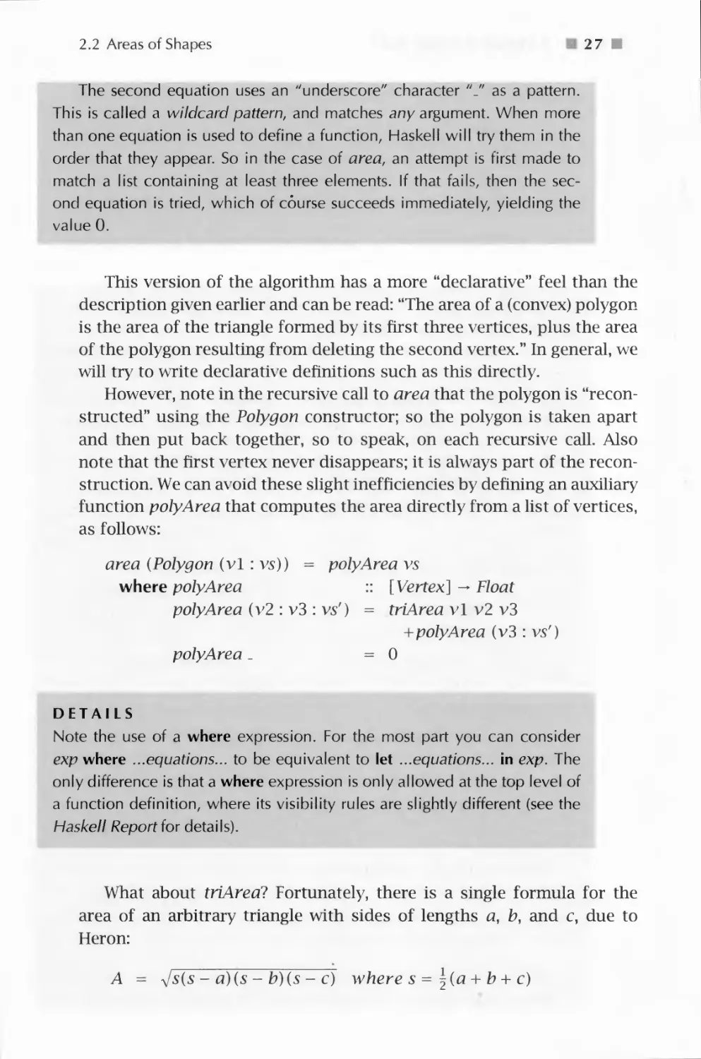
2.2 Areas of Shapes
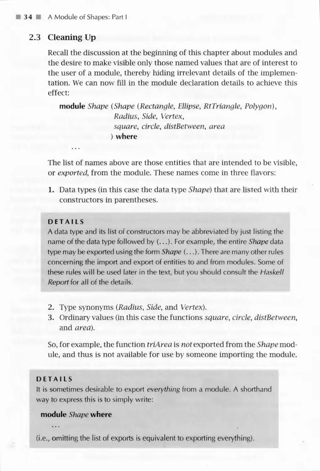
2.3 Cleaning Up
3 Simple Graphics
3.1 Basic Input/Output
3.2 Graphics Windows
3.3 Drawing Graphics Other Than Text
3.4 Some Examples
4 Shapes II: Drawing Shapes
4.1 Dealing With Different Coordinate Systems
4.2 Converting Shapes to Graphics
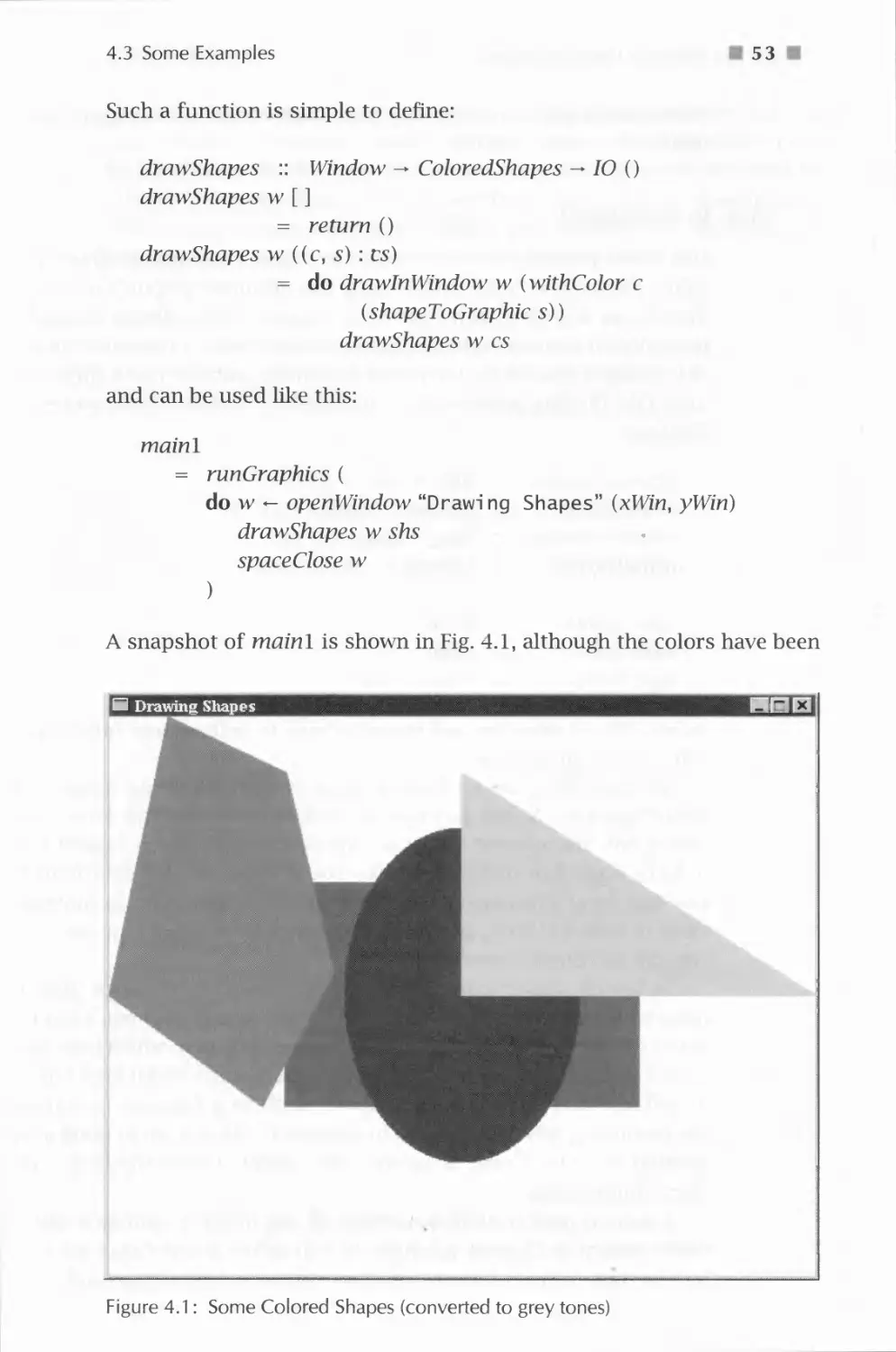
4.3 Some Examples
4.4 In Retrospect
5 Polymorphic and Higher-Order Functions
5.1 Polymorphic Types

vi ii
Contents
5.2 Abstraction Over Recursive Definitions 58
5.2.1 Map is Polymorphic 5 9
5.2.2 Using map 60
5.3 Append 63
5.3.1 The Efficiency and Fixity of Append 64
5.4 Fold 65
5.4.1 Haskell's Folds 67
5.4.2 Why Two Folds? 68
5.5 A Final Example: Reverse 69
5.6 Errors 71
6 Shapes III: Perimeters of Shapes 74
6.1 Perimeters of Shapes 74
7 Trees 81
7.1 A Tree Data Type 81
7.2 Operations on Trees 83
7.3 Arithmetic Expressions 84
8 A Module of Regions 87
8.1 The Region Data Type 87
8.2 The Meaning of Shapes and Regions 91
8.2.1 The Meaning of Shapes 92
8.2.2 The Encoding of the Meaning of Shapes 93
8.2.3 The Meaning of Regions 96
8.2.4 The Encoding of the Meaning of Regions 97
8.3 Algebraic Properties of Regions 99
8.4 In Retrospect 101
9 More About Higher-Order Functions 105
9.1 Currying 105
9.2 Sections 108
9.3 Anonymous Functions 110
9.4 Function Composition 111
10 Drawing Regions 114
10.1 The Picture Data Type 115
10.2 Drawing Pictures 115
10.3 Drawing Regions 116
10.3.1 From Regions to Graphics Regions: First Attempt 117
10.3.2 From Regions to Graphics Regions: Second Attempt 119
10.3.3 Translating Shapes into Graphics Regions 121
10.3.4 Examples 123

Contents ix
10.4 User Interaction 126
10.5 Putting it all Together 127
10.5.1 Examples 128
11 Proof by Induction 131
11.1 Induction and Recursion 131
11.2 Examples of List Induction 132
11.2.1 Proving Function Equivalences 133
11.3 Useful Properties on Lists 137
11.3.1 Function Strictness 137
11.4 Induction on Other Data Types 141
11.4.1 A More Efficient Exponentiation Function 143
12 Qualified Types 147
12.1 Equality 148
12.2 Defining Your Own Type Classes 150
12.3 Inheritance • 153
12.4 Haskell's Standard Type Classes 154
12.5 Derived Instances 157
12.6 Reasoning With Type Classes 160
13 A Module of Simple Animations 163
13.1 What is an Animation? 163
13.2 Representing an Animation 165
13.3 An Animator 167
13.4 Fun With Type Classes 172
13.4.1 Rising to the Level of Animations 172
13.4.2 Type Classes to the Rescue 172
13.4.3 Defining New Type Classes for Behaviors 176
13.5 Lifting to the Limit 177
13.6 Time Transformation 179
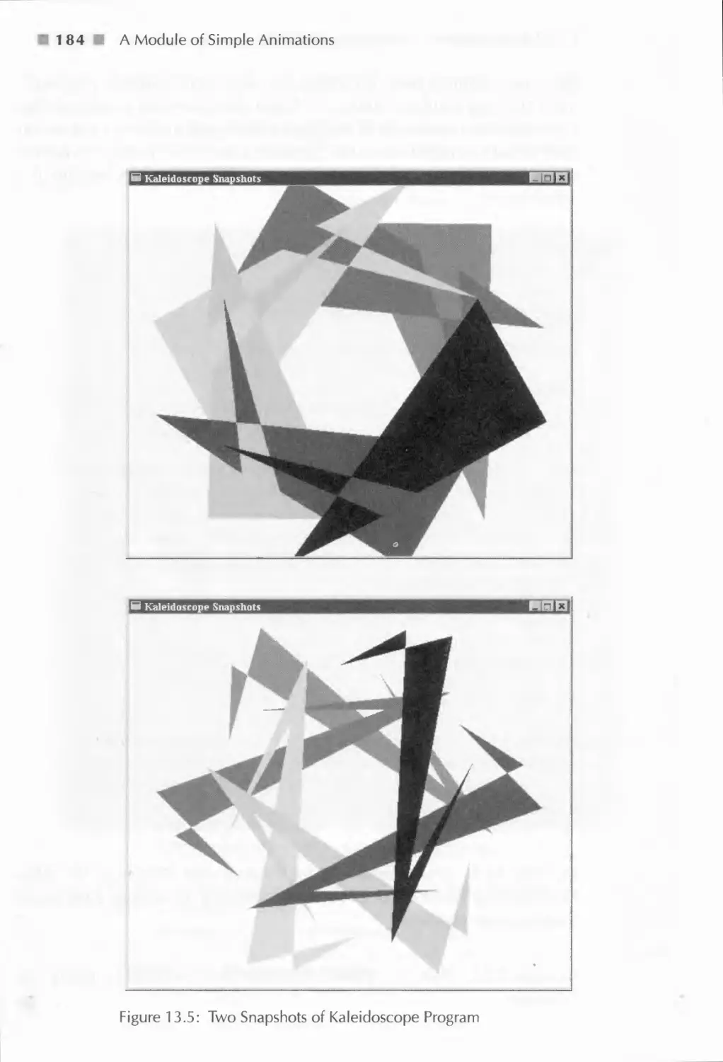
13.7 A Final Example: A Kaleidoscope Program 180
14 Programming With Streams 187
14.1 Lazy Evaluation 187
14.2 Recursive Streams 190
14.3 Stream Diagrams 193
14.4 Lazy Patterns 195
14.5 Memoization 198
14.6 Inductive Properties of Infinite Lists 201
15 A Module of Reactive Animations 208
15.1 FAL by Example 209

x Contents
15.1.1 Basic Reactivity 209
15.1.2 Event Choice 210
15.1.3 Recursive Event Processing 211
15.1.4 Events with Data 212
15.1.5 Snapshot 212
15.1.6 Boolean Events 212
15.1.7 Integration 213
15.2 Implementing FAL 214
15.2.1 An Implementation Strategy 215
15.2.2 Incremental Sampling 217
15.2.3 Final Refinements 219
15.2.4 Representing Events 220
15.3 The Implementation 220
15.3.1 Behaviors 221
15.3.2 Events 225
15.3.3 An Example 228
15.4 Extensions 229
15.4.1 Variations on switch 231
15.4.2 Mouse Motion 232
15.5 Paddleball in Twenty Lines 233
16 Communicating With the Outside World 236
16.1 Files, Channels, and Handles 236
16.1.1 Why Use Handles? 238
16.1.2 Channels 238
16.2 Exception Handling 239
16.3 First-Class Channels and Concurrency 242
17 Rendering Reactive Animations 245
17.1 Preliminaries 245
17.2 Reactimate 246
17.3 Window User 247
18 Higher-Order Types 249
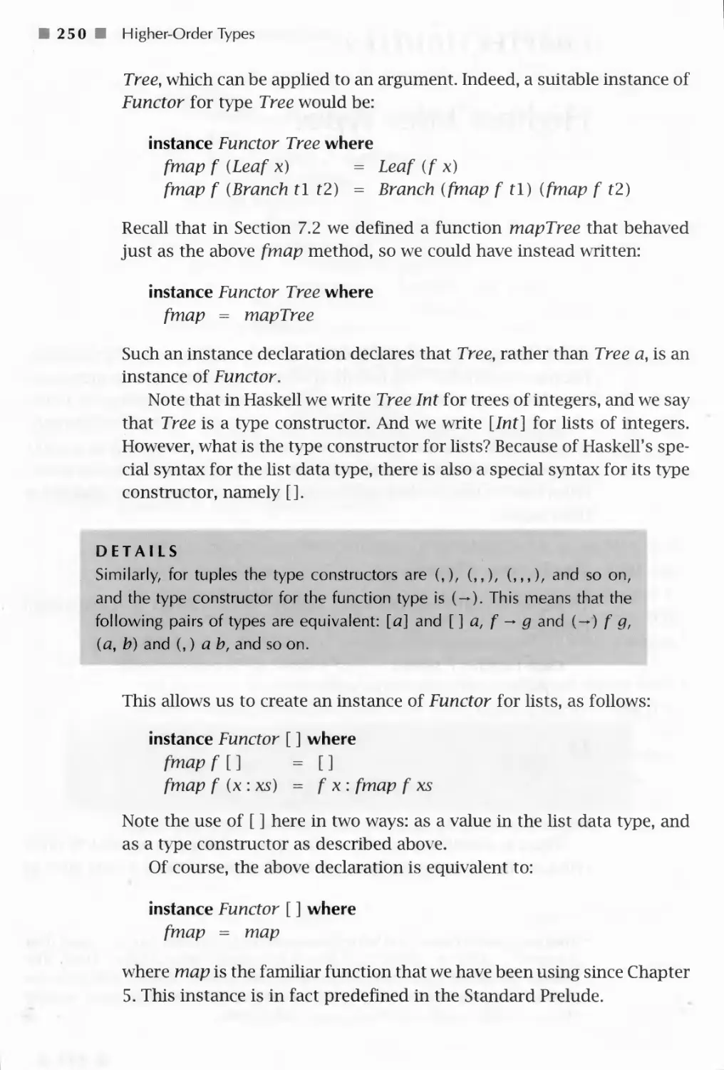
18.1 The Functor Class 249
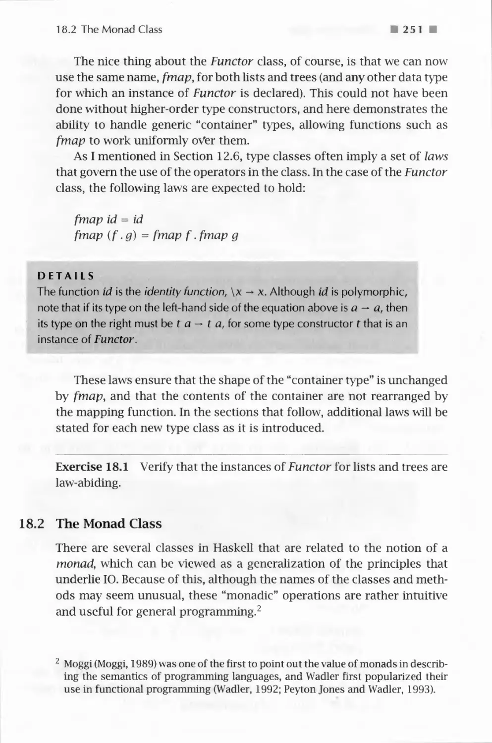
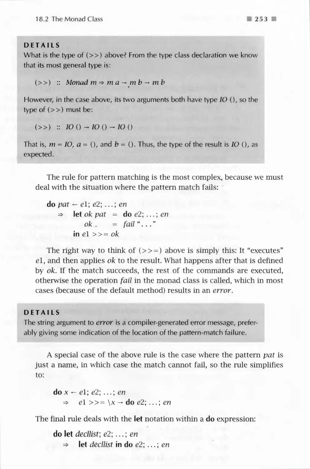
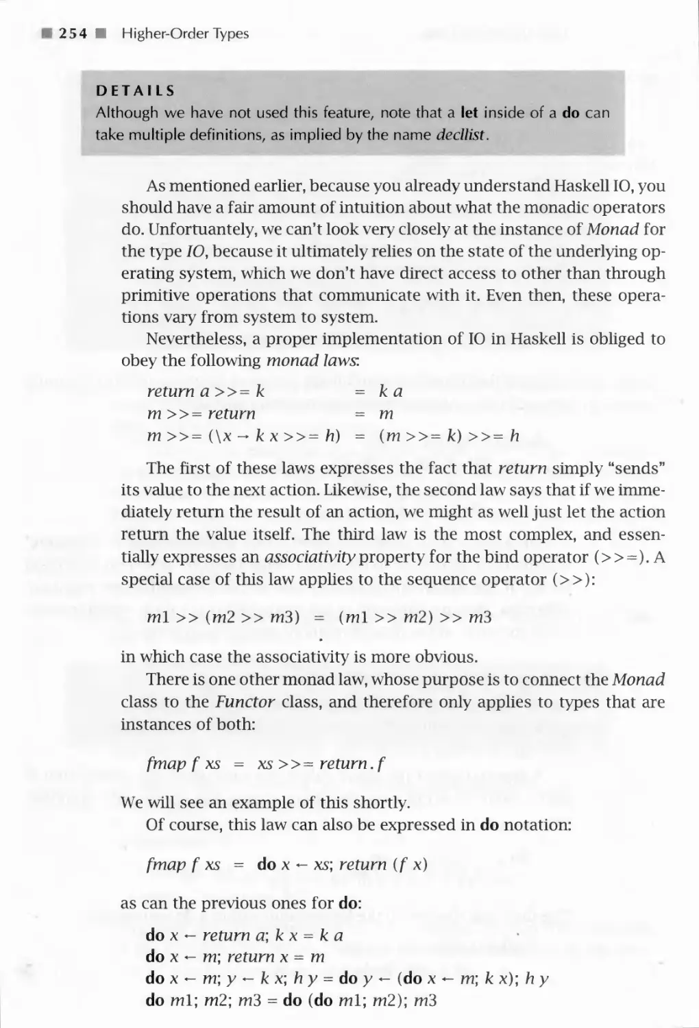
18.2 The Monad Class 251
18.2.1 Other Instances of Monad 255
18.2.2 Other Monadic Operations 259
18.3 The MonadPlus Class 259
18.4 State Monads 261
18.5 Type Class Type Errors 263

Contents
XI
19 An Imperative Robot Language 265
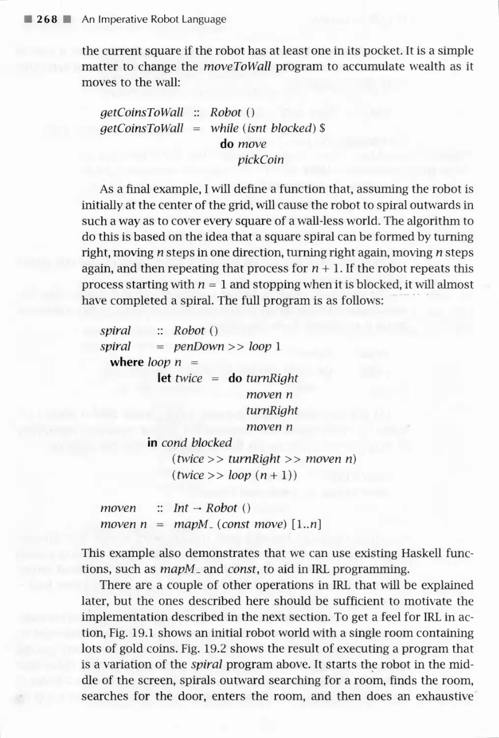
19.1 IRL by Example 266
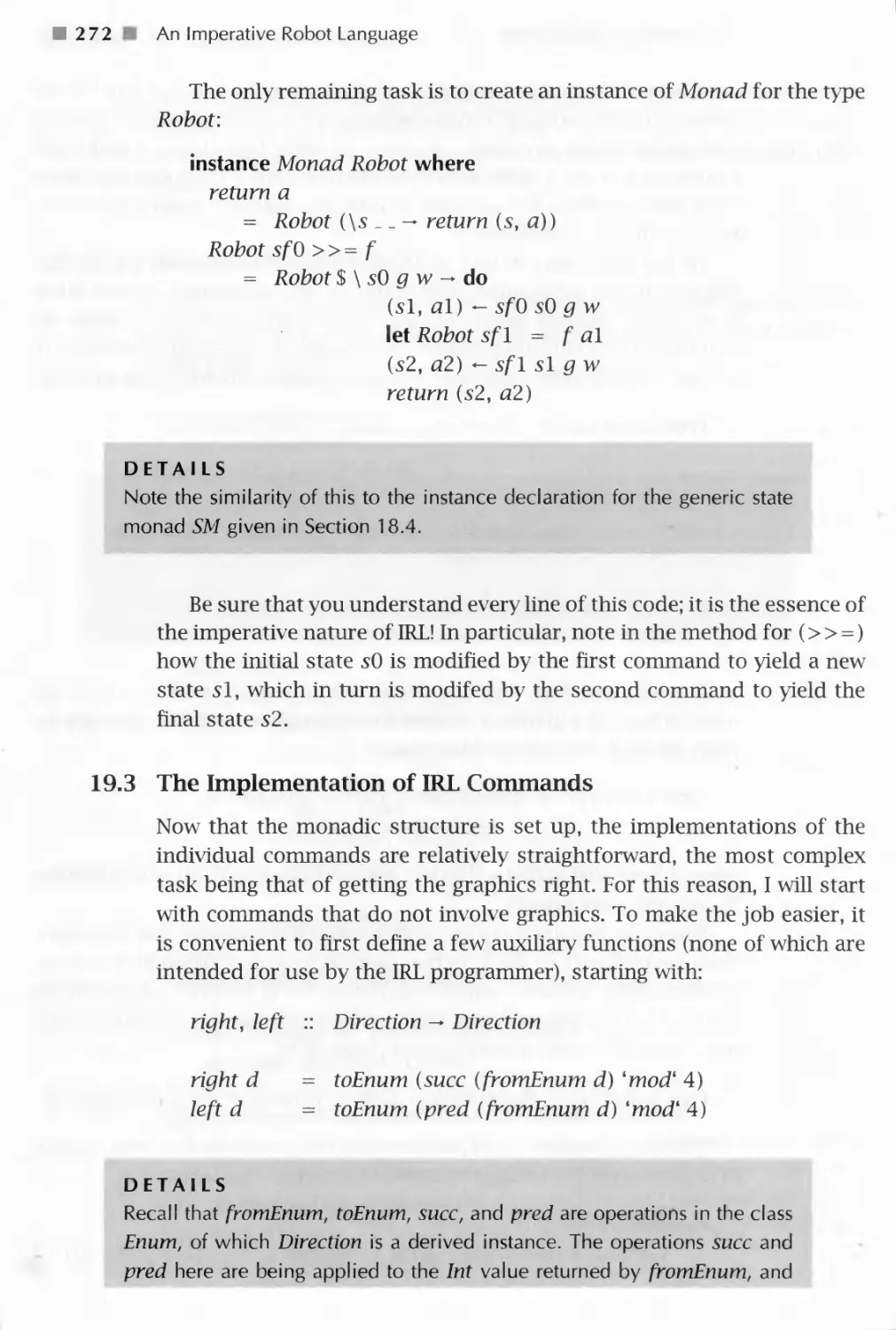
19.2 Robot is a State Monad 270
19.3 The Implementation of IRL Commands 2 72
19.3.1 Robot Orientation 273
19.3.2 Using the Pen 274
19.3.3 Playing With Coins 274
19.3.4 Logic and Control 274
19.4 All the World is a Grid 276
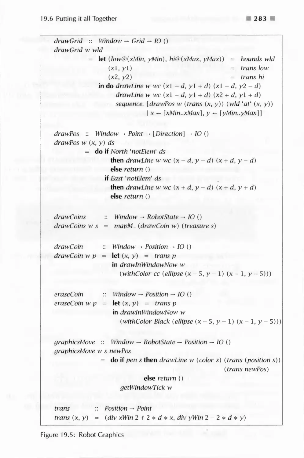
19.5 Robot Graphics 281
19.6 Putting it all Together 282
20 Functional Music Composition 287
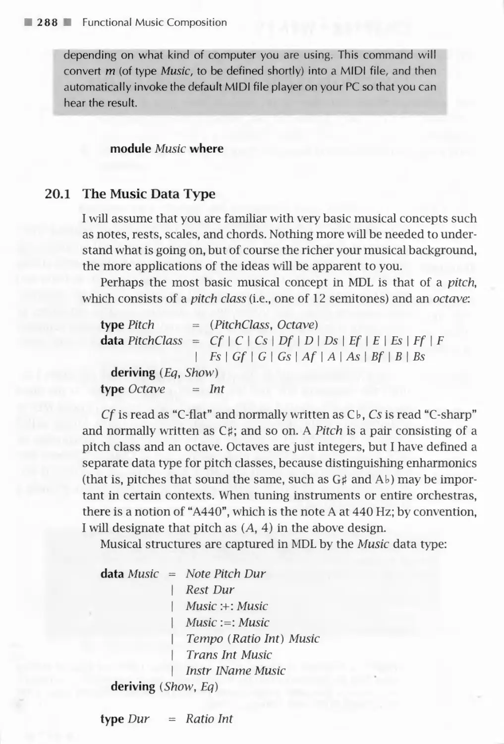
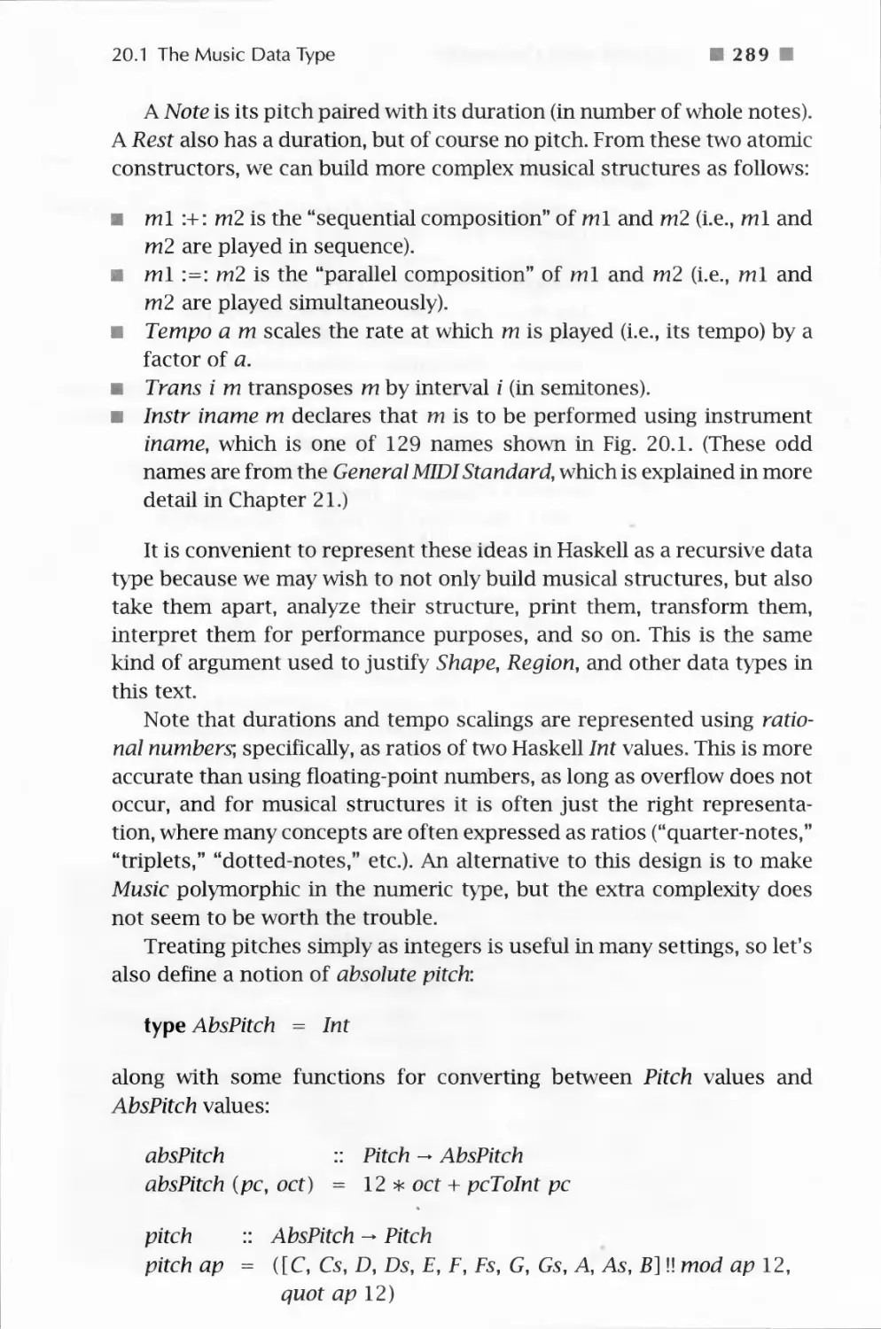
20.1 The Music Data Type 288
20.2 Higher-Level Constructions 293
20.2.1 Lines and Chords 293
20.2.2 Delay and Repeat 293
20.2.3 Polyrhythms 294
20.2.4 Determining Duration 295
20.2.5 Reversing Musical Structure 295
20.2.6 Truncating Parallel Composition 296
20.2.7 Trills 297
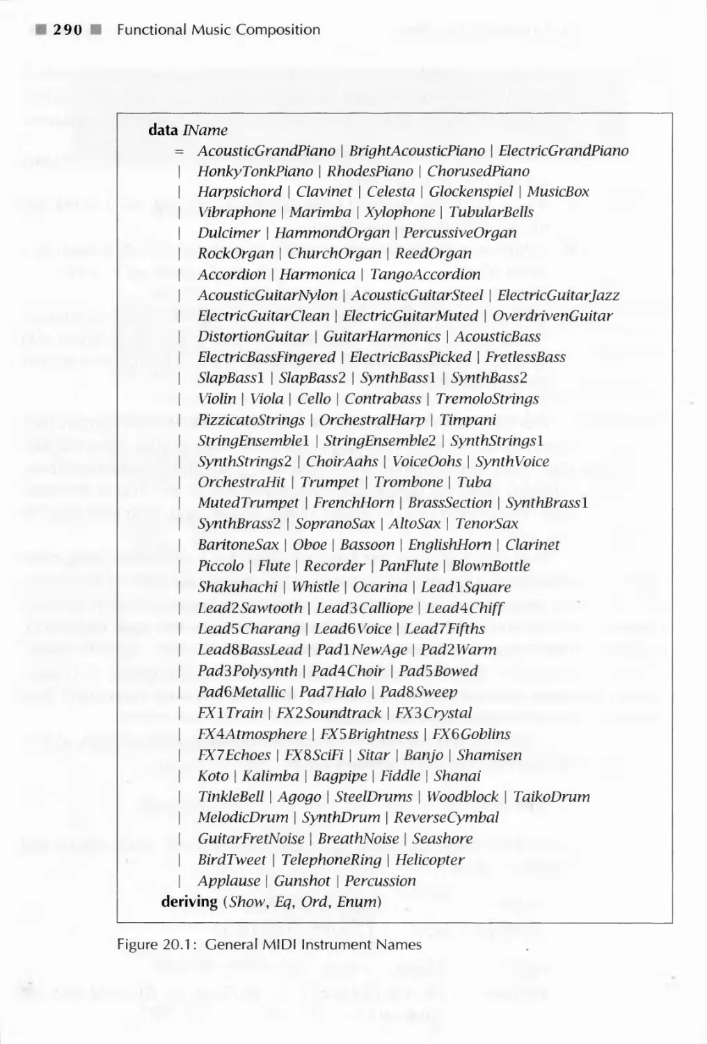
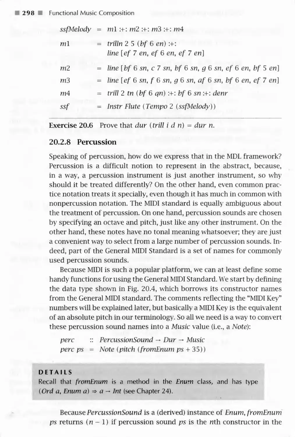
20.2.8 Percussion 298
20.3 A Couple of Final Examples 300
20.3.1 Cascades 300
20.3.2 Self-Similar (Fractal) Music 301
21 Interpreting Functional Music 304
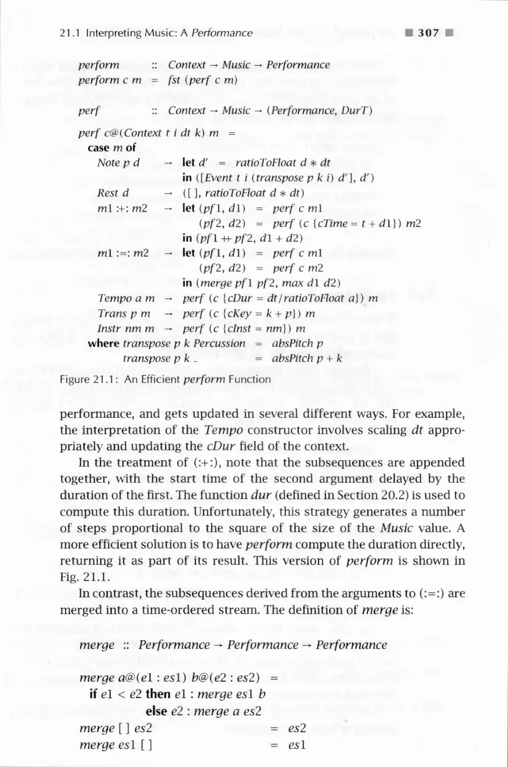
21.1 Interpreting Music: A Performance 305
21.2 An Algebra of Music 308
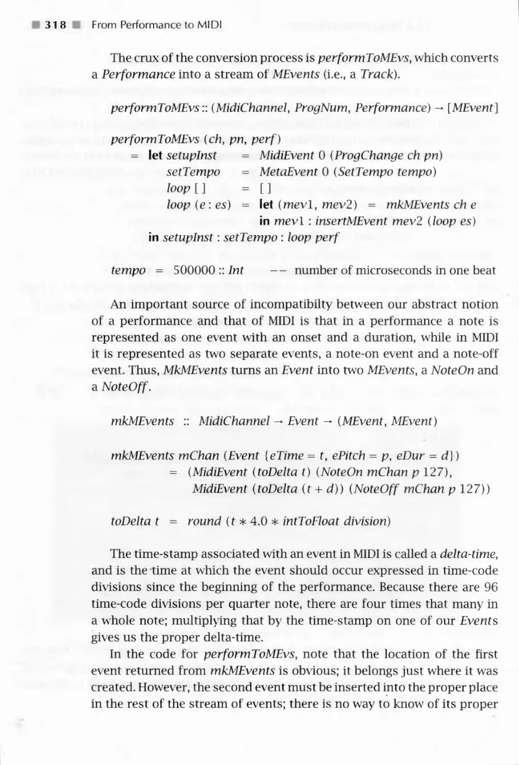
22 From Performance to MIDI 313
22.1 An Introduction to MIDI 313
22.2 The Conversion Process 314
22.3 Putting It All Together 319
23 A Tour of the PreludeList Module 321
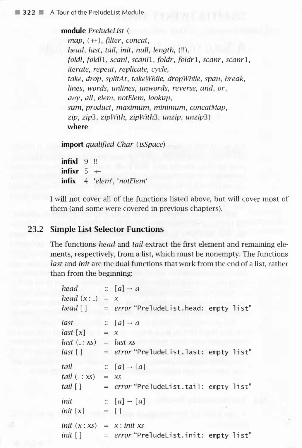
23.1 The PreludeList Module 321
23.2 Simple List Selector Functions 322
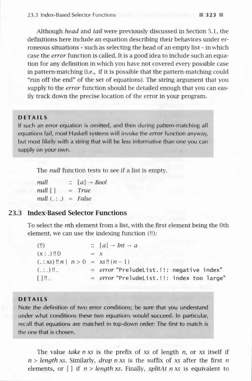
23.3 Index-Based Selector Functions 323
23.4 Predicate-Based Selector Functions 324
23.5 Fold-like Functions * 325
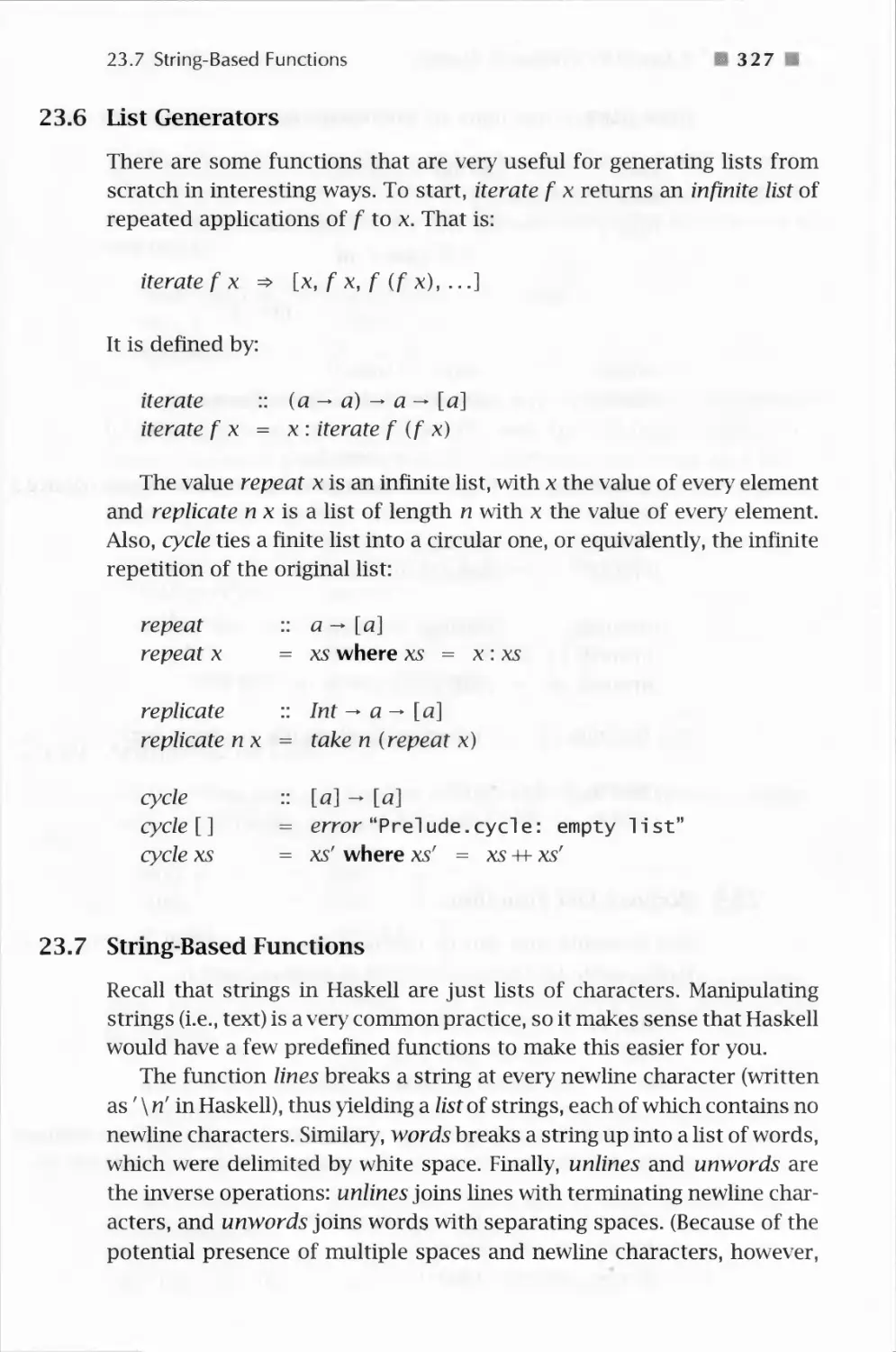
23.6 List Generators 327

Contents
23.7 String-Based Functions
23.8 Boolean List Functions
23.9 List Membership Functions
23.10 Arithmetic on Lists
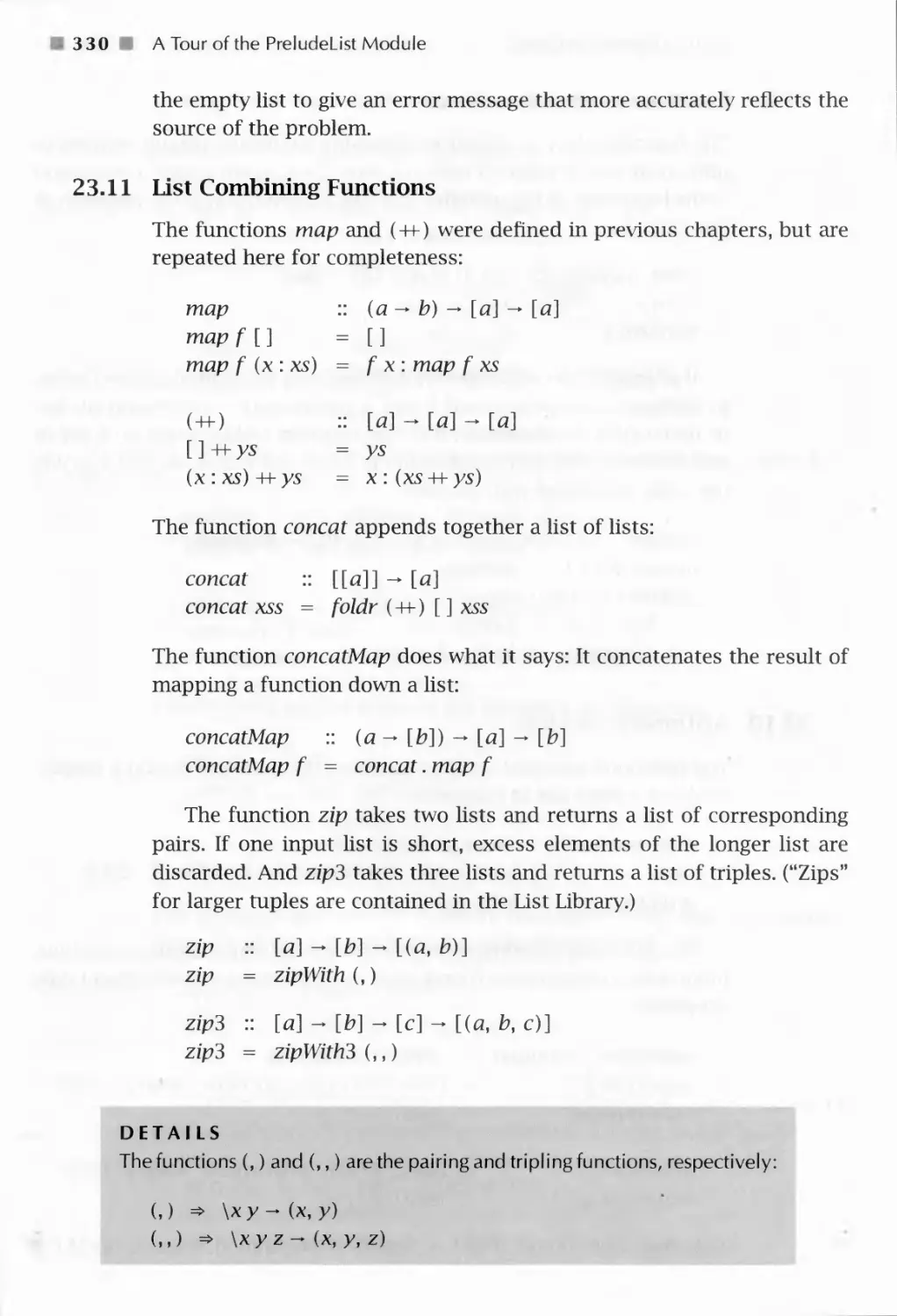
23.11 List Combining Functions
A Tour of Haskell's Standard Type Classes
24.1 The Ordered Class
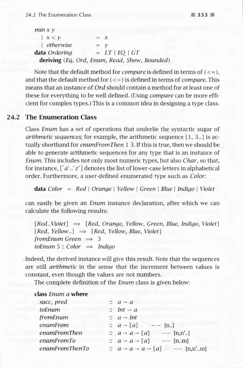
24.2 The Enumeration Class
24.3 The Bounded Class
24.4 The Show Class
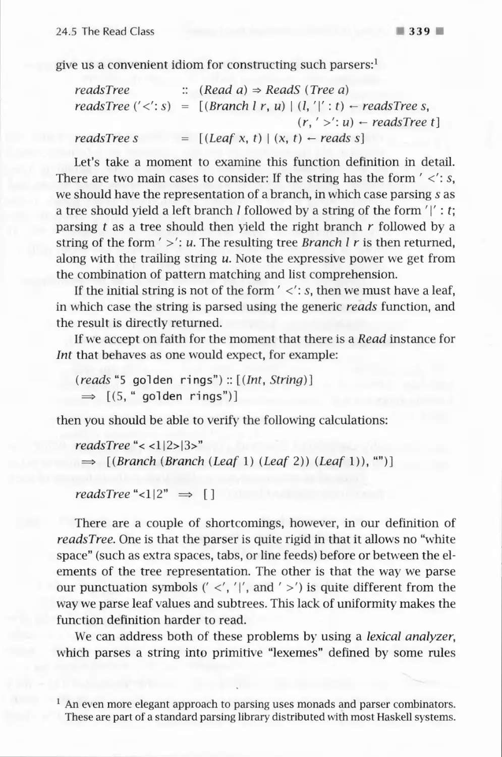
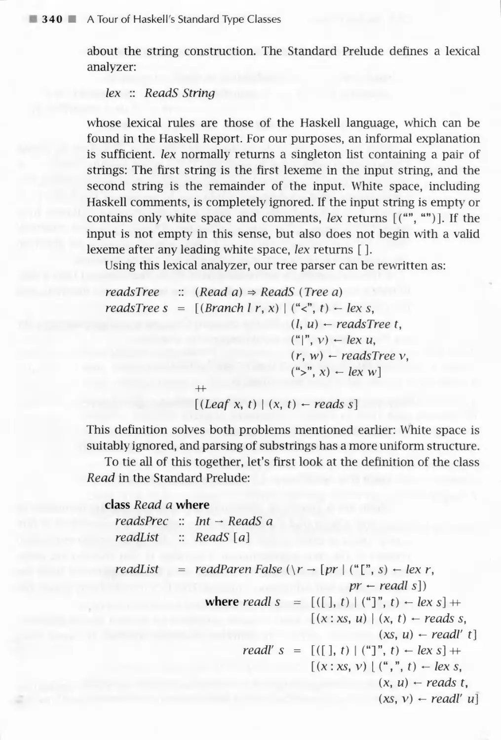
24.5 The Read Class
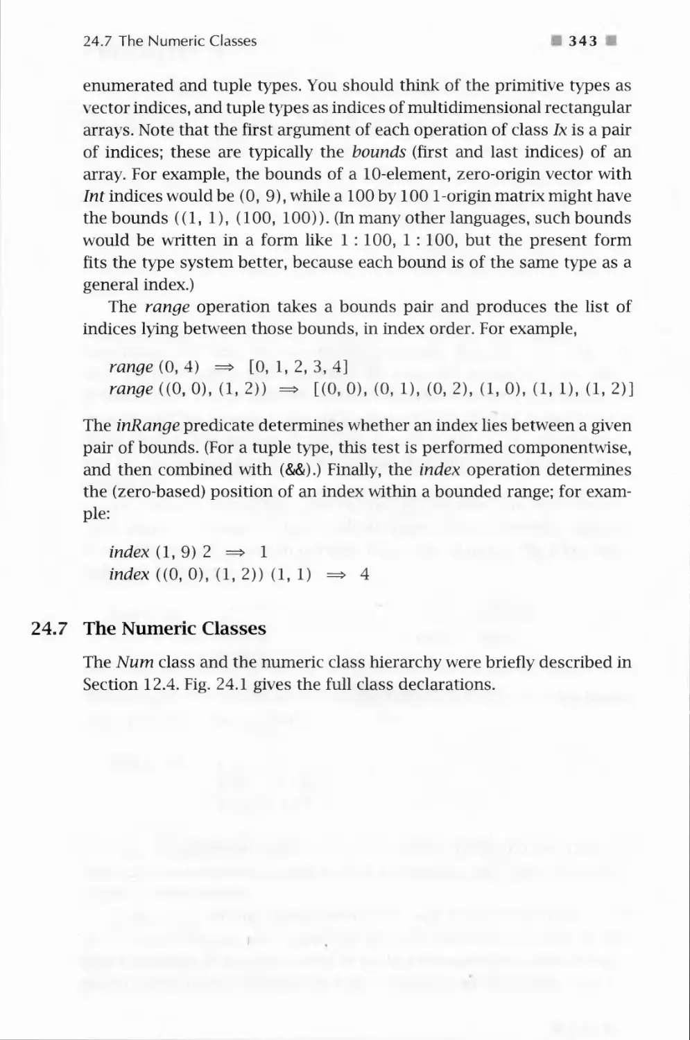
24.6 The Index Class
24.7 The Numeric Classes
Built-in Types Are Not Special
Pattern-Matching Details
Bibliography
327
328
329
329
330
332
332
333
334
334
338
341
343
345
348
353
Index
357

Preface
The first high-level languages developed for general purpose
programming were Fortran (Backus, 1978) and Lisp (McCarthy, 1978), developed
in the late 1950s by John Backus and John McCarthy, respectively. From
Fortran grew many of today's modern imperative languages, most of
which did not improve significantly on the fundamental ideas found in
the language Algol (de Morgan, Hill and Wichmann, 1976), which shortly
followed Fortran. The Lisp family was less fecund, perhaps because it
was so far ahead of its time, but was the seed for the family of functional
languages about which this textbook was written. The most radical in
this class of languages is probably Haskell, originally designed in the late
1980s (Hudak, Wadler, 1988) based on, at that point, a good ten years of
experience designing and implementing similar languages, most notably
a series of languages developed by David Turner in the late 1970s and
early 1980s (Turner, 1976; 1985). Although research continues on the
design of Haskell, the version used in this textbook, Haskell 98 (Augustsson,
et al., 1999), is the latest and most stable version of the language and its
libraries.
Haskell was named after the logician Haskell B. Curry who, along with
Alonzo Church, established the theoretical foundations of functional
programming back when computers themselves were only a gleam in
researchers' eyes. A curious historical fact is that Haskell Curry's father,
Samuel Silas Curry, helped to found and direct a school in Boston called
the School of Expression.1 Because pure functional programming centers
around the notion of an expression, I thought that The Haskell School of
Expression would be a good title for this book.
This school eventually evolved into what is now called Curry College (see
www. curry. edu: 8080/hi story/hi story. html for a brief history of the college).
xiii M

x i v Preface
A Brief Account of Language Success Stories
It's hard to predict just how it is that a language becomes popular.
Fortran became popular because it was the first high-level language and a
welcome alternative to assembly language, and ultimately because it was
a good vehicle for coding numerical algorithms in the domain of
scientific computing. C (Kernighan and Ritchie, 1978) was not revolutionary
by any means, often being described as a high-level assembly language.
But it found a niche in Unix and systems-level programming, and from
there to other operating system platforms. Cobol (Cobol, 1968) was
designed from day one for business applications, and so made its mark.
Java's (Gosling, Joy and Steele, 1996) recent astonishing rise in
popularity is rather perplexing on one hand, yet quite understandable on
another. As a language, it is simple and elegant, but certainly not
revolutionary. Yet it found a niche in its use on the world-wide-web, which at
the time was (and still is) a phenomenon in its own right. Lisp and Scheme
(Rees and dinger, 1986) for AI, Ada (Ada, 79) for real-time applications,
VHDL and Verilog for digital hardware design, and the list goes on.
From this discussion it appears that for a language to become
popular it needs an application - a niche - in which it excels, or in which it
at least was the first to arrive. Curiously, for most language designers,
this is the opposite of what is desired. Most language designers would
like their languages to be truly general purpose, able to solve all of the
world's problems with great succinctness, clarity, and efficiency. As a
result, many excellent languages out there, some with very decent
implementations, will probably forever remain in obscurity because they never
found their niche.
Although the designers of Haskell exhibited no exception to this
ambitious approach to language design, in retrospect I wonder if there might
be a plausible niche for Haskell. These sorts of things are mostly out of
my control, of course, but I thought it would be fun to use multimedia -
graphics, sound, and animation - as an underlying theme, embodied
concretely through many examples and exercises, in this text. Multimedia is
an application area that is certainly current and important, and one in
which Haskell's advantages are highly visible.
In addition, one of the nice things about multimedia programming is
that all of the really interesting (and hard!) problems faced by computer
scientists over the past 30 years are found in the "virtual worlds" that we
create. Nondeterminism, concurrency, state, time, efficiency, decidability,
and others are all issues that must be addressed. Although I don't cover
all of these issues in this text, multimedia programming nevertheless

Preface
xv
provides a good vehicle through which one could teach general topics in
computer science.
1 also hope that this text demonstrates the ease with which one can
embed a domain-specific language in Haskell. In a more general sense,
this might actually be the most profitable niche for Haskell, as there have
been a number of success stories in this area already.
In any case, I hope that you enjoy working through the various
multimedia programs as much as I have enjoyed creating them. At the same
time, I hope that this text might help Haskell to find its niche and thus
avoid the fate of obscurity described earlier. Haskell really is a beautiful
language.
Why I Wrote This Book, and How to Read It
At the time I began writing this book there were not many other books
about programming specifically in Haskell. But that wasn't the main
reason I decided to tackle this task. More importantly, there was a need for
a book that described how to solve problems using a functional language
such as Haskell. As with any major class of languages, there is a
certain mind-set for contemplation, a certain viewpoint of the world, and a
certain approach to problem solving that collectively work best. If you
teach only Haskell language details to a C programmer, she is likely to
write very ugly, incomprehensible functional programs. But if you teach
her how to think differently, how to see problems in a different light,
functional solutions will come easily, and elegant Haskell programs will
result. That, in a nutshell, is my goal in this textbook. As Samuel Silas
Curry once said:
All expression comes from within outward, from the center to the surface,
from a hidden source to outward manifestation. The stud} of expression
as a natural process brings you into contact with cause and makes you
feel the source of reality.
(http: //www.curry.edu:8080/history/history.html)
I encourage the seasoned programmer having experience only with
conventional imperative and/or object-oriented languages to read this
text with an open mind. Many things will be different, and will likely feel
awkward. There will be a tendency to rely on old habits when writing new
programs, and to ignore my suggestions about how to approach things
differently. If you can manage to resist these tendencies, I am confident
that you will have an enjoyable learning experience. Many of those who

xvi Preface
succeed in this process find that many of the things that they learn about
functional programming can be applied to imperative and object-oriented
languages - after all, most of these other languages contain a significant
functional subset - and that their imperative coding style changes for the
better as a result.
I also ask the experienced programmer to be patient while in the
earlier chapters I explain things like "syntax," "operator precedence," and
others because my goal is that this text should be readable by someone
having only modest prior programming experience. With patience the
more advanced ideas will appear soon enough.
If you are a novice programmer, I suggest taking your time with the
book; work through the exercises, and don't rush things. If, however,
you don't fully grasp an idea, feel free to move on, but try to reread
difficult material at a later time when you ha\ e seen more examples of
the concepts in action. For the most part this is a "show by example"
textbook, and you should try to execute as many of the programs in this
text as you can, as well as every program that you wTite. Learn-by-doing
is the corollary to show-by-example.
Finally, although the text begins quite gently, it mo\ es at a fairly rapid
pace, and covers many advanced ideas in functional programming, some
of w7hich are not covered in any other text that I am aware of. So there
is much here even for those who are already familiar with the basics of
functional programming.
Suggestions to Instructors
All of the material in this textbook can be covered in one semester as an
advanced undergraduate course. For lower-level courses, including
possible use in high school, some of the mathematics may cause problems,
but for bright students I suspect most of the material can still be covered.
I strongly encourage sticking to the order of the chapters in the book,
which introduces Haskell language features as they are demanded by the
underlying application themes (generally the chapters alternate between
"concepts" and "applications"). If you are an experienced functional
programmer, you will see instances early in the book where a lambda
expression here, or eta-conversion there, will simplify things, but I have chosen
to delay such simplifications in most cases. Flooding the student with too
many features early on can be overwhelming.
The only exception to following the given chapter order is that
Chapters 20 to 22 provide a somewiiat independent thread on computer music,
and can be covered anytime after Chapter 11. The most difficult chapter

Preface
xvii
is probably Chapter 15, and the most dispensible chapters are probably
Chapters 17 and 22. Also, if you wrant to omit nonmultimedia
applications you might consider skipping Chapter 6, although that chapter
contains the first introduction to infinite lists. Finally, Chapters 23 and 24
are short "tours" of the PreludeList Module and Standard Type Classes,
respecth ely, and could be assigned as auxiliary reading, or covered
piecemeal as related topics are introduced.
The web page http: //haskel 1. org/soe contains a great deal of
useful information related to the text, including libraries, source code for
each chapter, PowerPoint slides, and errata. You can send email to me at
paul. hudak@ya1 e. edu with feedback, questions, corrections, etc.
Haskell Implementations
There are several good implementations of Haskell, all available free on
the internet through the Haskell home page at http://haske11 .org.
One that I especially recommend is the Hugs implementation, a \ery
easy-to-use and easy-to-install Haskell interpreter. Hugs runs on a
variety of platforms, including PC's (Windows 95/NT), various flavors of Unix
(Linux, Solaris, HP), and Mac OS. The Glasgow Haskell Compiler (GHC)
supports the same libraries as Hugs, and has the benefit of being a true
compiler instead of an interpreter.
All of the code in the book is compliant with the Haskell '98 standard,
and has been tested on the Hugs '98 implementation of Haskell.
Unfortunately, the graphics and animation applications rely on a library that
was originally developed only for Windows 95/NT. You should consult
the SOE web page for the latest information regarding compatibility with
other platforms.
Acknowledgments
I learned that writing a textbook is not an easy task, and could not have
been accomplished without the help of many friends and colleagues.
I would especially like to thank Mark Jones, with whom I started this
project, and who first suggested the use of the name School of
Expression. I'd also like to thank John Peterson and Joe Fasel for help in
writing A Gentle Introduction to Haskell (Hudak and Fasel, 1992), from which
some of this text was adapted; Alastair Reid for help with the Hugs
implementation and graphics libraries; Conal Elliott for many helpful
suggestions and inspirations, especially concerning graphics and animation;
Erik Meijer for feedback from using a previous version of this text in his

xviii Preface
class; Mark Tullsen for careful proofreading and tedious index
generation; Tom Makucevich and John Garvin for help with computer music;
Tim Sheard for feedback from using my book in teaching a functional
programming course at Yale, and for creating great PowerPoint slides in
the process; Zhanyong Wan for excellent feedback on the text as a
Teaching Assistant in Tim's course; Sigbjorn Finne for writing the kaleidoscope
program; Valery Trifonov for adapting the kaleidoscope program and
other useful feedback; Linda Joyce for help with the indexing and
excellent administrative support; Martin Sulzmann for help debugging
graphics; Lauren Cowles, my editor, whose patience is extraordinary; and the
many students in various classes at Yale who endured earlier versions of
the text.
I would also like to thank the several United States funding agencies,
most notably NSF and DARPA, who have provided considerable financial
support for functional programming research at Yale and elsewhere.
Most of all, this work could not have been accomplished without the
love and support of my family. Thank you Cathy, Cristina, and Jennifer.
Happy Haskell Hacking!
Paul Hudak
New Haven
June 1999

CHAPTER ONE
Problem Solving, Programming,
and Calculation
Programming, in its broadest sense, is problem solving, [t begins when we
look out into the world and see problems that we want to solve, problems
that we think can and should be solved using a digital computer.
Understanding the problem well is the first - and probably the most important -
step in programming, because without that understanding we may find
ourselves wandering aimlessly down a dead-end alley, or worse, down a
fruitless alley with no end. "Solving the wrong problem" is a phrase often
heard in many contexts, and we certainly don't want to be victims of that
crime. So the first step in programming is answering the question, "What
problem am I trying to solve?"
Once you understand the problem, then you must find a solution. This
may not be easy, of course, and in fact you may discover several solutions,
so we also need a way to measure success. There are various dimensions
in which to do this, including correctness ("Will I get the right answer?")
and efficiency ("Will 1 have enough resources?"). But the distinction of
which solution is better is not always clear, because the number of
dimensions can be large, and programs will often excel in one dimension
and do poorly in others. For example, there may be one solution that
is fastest, one that uses the least amount of memory, and one that is
easiest to understand. Choosing can be difficult and is one of the more
interesting challenges that you will face in programming.
The last measure of success mentioned above - clarity of a program -
is somew7hat elusive, most difficult to measure, and, quite frankly,
sometimes difficult to rationalize. But in large software systems clarity is an
especially important goal, because the most important maxim about such
systems is that they are never really finished! The process of continuing
work on a software system after it is delivered to users is what software
engineers call software maintenance, and is the most expensive phase of
the so-called "software lifecycle." Software maintenance includes fixing
1 m

Problem Solving, Programming, and Calculation
bugs in programs, as well as changing certain functionality and
enhancing the system with new features in response to users' experience.
Therefore, taking the time to write programs that are highly legible -
easy to understand and to reason about - will facilitate the software
maintenance process. It is important to realize that the person performing
software maintenance is usually not the person who wrote the original
program. Therefore, when you write your programs, write them as if you
are writing them for someone else to see, to understand, and ultimately
to pass judgment on!
In this book, I will often solve each example in several different ways
(some of which are dead ends!), taking the time to contrast the style,
efficiency, clarity, and functionality of the results.1 I do this not just for
pedagogical purposes. Such reworking of programs is the norm, and you
are encouraged to get into the habit of doing so. Don't always be satisfied
with your first solution to a problem, and always be prepared to go back
and change parts of your program that you later discover do not satisfy
your actual needs.
Computation by Calculation in Haskell
Discussions of program clarity bring us ultimately to the issue of our
programming language choice. This choice determines how we express
our solutions in such a way that a computer can understand them. Our
programs embody our solutions - and our creativity, eloquence, and
perseverance - for interpretation by the computer.
In this text I will use the programming language Haskell to address
many of the issues discussed in the last section.21 have tried to avoid the
approach of explaining Haskell first and giving examples second. Rather,
I will walk with you, step by step, along the path of understanding an
application, understanding the solution space, and understanding how
to express a particular solution in Haskell. I want you to learn how to
problem solve!
Along this path I will use whatever tools are appropriate for
analyzing a particular problem domain, very often mathematical tools
familiar to the average college student, indeed most to the average high
school student. Concurrently, I will evolve our problems toward a
particular view of computation that is especially useful: that of computation by
1 At times I also explore different methods for proving properties of programs.
2 If this were a text on software engineering, I would address many other issues
as well. The methods that I describe are consistent with the principles of software
engineering, but detailed discussion of those principles is beyond the scope of this
textbook.

1.1 Computation by Calculation in Haskell
■ 3 ■
calculation. You will find that such a viewpoint is not only powerful, it is
also simple (we won't shy away from difficult problems). Haskell supports
well the idea of computation by calculation. Programs in Haskell can be
viewed as functions whose input is that of the problem being solved, and
whose output is our desired result; and the behavior of functions can be
understood easily as computation by calculation.
An example might help to demonstrate these ideas. Suppose we want
to perform an arithmetic calculation such as 3 x (9 + 5). In Haskell we
would write this as 3 * (9 + 5) because most standard computer
keyboards and text editors do not recognize the special symbol x. To
calculate the result, we proceed as follows:
3* (9 + 5)
=> 3 * 14
=> 42
It turns out that this is not the only way to compute the result, as
evidenced by this alternative calculation:3
3* (9 + 5)
=> 3*9 + 3*5
=> 27 + 3*5
=> 27+15
=> 42
Even though this calculation takes two extra steps, it at least gives the
correct answer. Indeed, an important property of each and every program
in this textbook - in fact every program that can be written in the
functional language Haskell - is that it will always yield the same answer when
given the same inputs, regardless of the order in which wre choose to
perform the calculations.4 This is precisely the mathematical definition of a
function: For the same inputs, it always yields the same output.
On the other hand, the first calculation above took fewer steps than
the second, and so we say that it is more efficient. Efficiency in both
space (amount of memory used) and time (number of steps executed)
is important when searching for solutions to problems, but of course if
we get the wrong answer, efficiency is a moot point. In general, we will
search first for any solution to a problem, and later refine it for better
performance.
3 This assumes that multiplication distributes over addition in the number system
being used, a point that I will return to later.
4 As long as we don't choose a nonterminating sequence of calculations, another
issue that we will return to later.

4 ■ Problem Solving, Programming, and Calculation
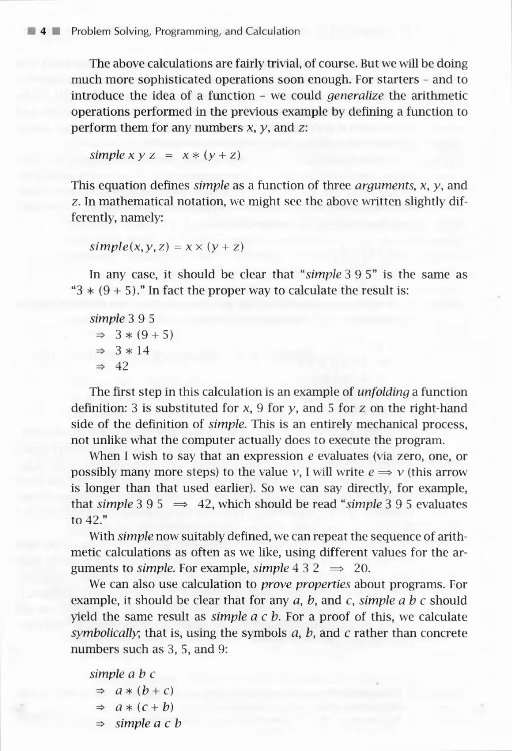
The above calculations are fairly trivial, of course. But we will be doing
much more sophisticated operations soon enough. For starters - and to
introduce the idea of a function - we could generalize the arithmetic
operations performed in the previous example by defining a function to
perform them for any numbers x, y, and z:
simplexy z = x* (y + z)
This equation defines simple as a function of three arguments, x, y, and
z. In mathematical notation, we might see the above written slightly
differently, namely:
simple(x,y,z) = xx (y + z)
In any case, it should be clear that "simple 3 9 5" is the same as
"3 * (9 + 5)." In fact the proper way to calculate the result is:
simple 3 9 5
=> 3* (9 + 5)
=> 3 * 14
=> 42
The first step in this calculation is an example of unfolding a function
definition: 3 is substituted for x, 9 for y, and 5 for z on the right-hand
side of the definition of simple. This is an entirely mechanical process,
not unlike what the computer actually does to execute the program.
When I wish to say that an expression e evaluates (via zero, one, or
possibly many more steps) to the value v, I will write e => v (this arrow
is longer than that used earlier). So we can say directly, for example,
that simple 3 9 5 => 42, which should be read "simple 3 9 5 evaluates
to 42."
With simple now suitably defined, we can repeat the sequence of
arithmetic calculations as often as we like, using different values for the
arguments to simple. For example, simple 4 3 2 => 20.
We can also use calculation to prove properties about programs. For
example, it should be clear that for any a, b, and c, simple ab c should
yield the same result as simple a c b. For a proof of this, we calculate
symbolically, that is, using the symbols a, b, and c rather than concrete
numbers such as 3, 5, and 9:
simple ab c
=> a * (b + c)
=> a * (c + b)
=> simple a c b

1.1 Computation by Calculation in Haskell
5
The same notation will be used for these symbolic steps as for
concrete ones. In particular, the arrow in the notation reflects the direction
of our reasoning, and nothing more. In general, if el => el, then it's also
true that el => el.
I will also refer to these symbolic steps as "calculations," even though
the computer will not typically perform them when executing a program
(although it might perform them before a program is run if it thinks
that it might make the program run faster). The second step in the
calculation above relies on the commutativity of addition (namely that,
for any numbers x and y,x + y = y + x). The third step is the reverse of
an unfold step, and is appropriately called a fold calculation. It w ould be
particularly strange if a computer performed this step while executing a
program, because it does not seem to be headed toward a final answer.
But for proving properties about programs, such "backward reasoning"
is quite important.
When I wish to make the justification for each step clearer, whether
symbolic or concrete, a calculation will be presented with more detail, as
in:
simple a b c
=> { unfold }
a * (b + c)
=> { commutativity }
a * (c + b)
=> {fold}
simple a c b
In most cases, however, this will not be necessary.
Proving properties of programs is another theme that will be repeated
often in this text. As the world relies more and more on computers to
accomplish not just ordinary tasks such as writing term papers and sending
email, but also life-critical tasks such as controlling medical procedures
and guiding spacecraft, then the correctness of programs gains in
importance. Proving complex properties of large, complex programs is not easy,
and is rarely if ever done in practice. However, that should not deter us
from proving simpler properties of the whole system, or complex
properties of parts of the system, because such proofs may uncover errors,
and if not, at least help us to gain confidence in our effort.
If you are already an experienced programmer, the idea of computing
everything by calculation may seem odd at best and naive at worst. How
does one write to a file, draw7 a picture, or respond to mouse clicks? If
you are wondering about these things, have patience reading the early
chapters and find delight reading the later chapters where the full power

6 ■ Problem Solving, Programming, and Calculation
of this approach begins to shine. I will avoid, however, most comparisons
between Haskell and conventional programming languages such as C,
C++, Ada, Java, or even Scheme or ML (two "almost functional" languages),
because for those who have programmed in these other languages the
differences will be obvious, and for those who haven't the comments
would be superfluous.
In many ways this first chapter is the most difficult chapter in the
entire text because it contains the highest density of new concepts. If
you have trouble with some of the ideas here, keep in mind that we will
return to almost every idea at later points in the text. And don't hesitate
to return to this chapter later to reread difficult sections; they will likely
be much easier to grasp at that time.
Exercise 1.1 Write out all of the steps in the calculation of the value of
simple (simple 2 3 4) 5 6
Exercise 1.2 Prove by calculation that simple (a- b) ab => a2 - b2.
DETAILS
In this text the need will often arise to explain some aspect of Haskell in more
detail, without distracting too much from the primary line of discourse. In
those circumstances I will offset the comments and precede them with the
word "Details," such as is done with this paragraph, so that you know the
nature of what is to follow. These details will sometimes concern the syntax
of Haskell (i.e., the notation used to write Haskell programs) or its semantics
(i.e., how to calculate with the language features).
1.2 Expressions, Values, and Types
In this section we will take a much closer look at the idea of computation
by calculation. In Haskell, the objects that we perform calculations on
are called expressions, and the objects that result from a calculation (i.e.,
"the answers") are called values. It is helpful to think of a value just as
an expression on which no more calculation can be carried out.
Examples of expressions include atomic (meaning indivisible)
expressions such as the integer 42 and the character '«,' as well as structured
(meaning made from smaller pieces) expressions such as the list [1, 2, 3]
and the pair ('b,'4) (lists and pairs are different in a subtle way, to be
described later). Each of these examples is also a value, because by
themselves there is no calculation that can be carried out. As another example,

1.2 Expressions, Values and Types 7 H
1 + 2 is an expression, and one step of calculation yields the expression
3, which is a value, because no more calculations can be performed on
it.
Sometimes, however, an expression has only a never-ending sequence
of calculations. For example, if x is defined as:
x = x + 1
then here's what happens when we try to calculate the value of x:
x
=> x + 1
=> (x + l) + l
=> ((x + D + D + l
=> (((x + U + D + D + l
This is clearly a never-ending sequence of steps, in which case we say that
the expression does not terminate, or is nonterminating. In such cases,
the symbol _i_, pronounced "bottom," is used to denote the value of the
expression.
Every expression (and therefore every value) also has an associated
type. You can think of types as sets of expressions (or values) in which
members of the same set have much in common. Examples include the
atomic types Integer (the set of all fixed-precision integers) and Char (the
set of all characters), as well as the structured types [Integer] (the set of
all lists of integers) and (Char, Integer) (the set of all character/integer
pairs). The association of an expression or value with its type is very
important, and there is a special way of expressing it in Haskell. Using
the examples of values and types above, we write:
42 :: Integer
'a' :: Char
[1,2,3] :: [Integer]
('b\ 4) :: (Char, Integer)
DETAILS
Literal characters are written enclosed in single forward quotes, as in 'a',
'A, 'V, ',', '!', ' ' (a space), etc. (There are some exceptions, however; see
the Haskell Report for details.)
The "::" should be read "has type," as in "42 has type Integer."

8 0 Problem Solving, Programming, and Calculation
DETAILS
Note that the names of specific types are capitalized, such as Integer and
Char, but the names of values are not, such as simple and x. This is not just
a convention; it is required when programming in Haskell. In addition, the
case of the other characters matters. For example, test, teSt, and tEST are
all distinct names for values, as are Test, TeST, and TEST for types.
Haskell's type system ensures that Haskell programs are well-typed;
that is, that the programmer has not mismatched types in some way. For
example, it does not make much sense to add together two characters,
so the expression 'a' + 'b' is ill-typed. The best news is that Haskell's type
system will tell you if your program is well-typed before you run it. This
is a big advantage, because most programming errors are manifested as
typing errors.
The idea of dividing the world of values into types should be familiar
to most people. We do it all the time for just about every kind of object.
Take boxes, for example. Just as we have integers and reals, lists and
tuples, etc., we also have large boxes and small boxes, cardboard boxes and
wooden boxes, and so on. And just as we have lists of integers and lists of
characters, we also have boxes of nails and boxes of shoes. And just as we
would not expect to be able to take the square of a list or add two
characters, we would not expect to be able to use a box to pay for our groceries.
Types help us to make sense of the world by organizing it into groups
of common shape, size, functionality, and others. The same is true for
programming, where types help us to organize values into groups of
common shape, size, and functionality, among others. Of course, the kinds
of commonality between values will not be the same as those between
objects in the real world, and in general, we will be more restricted - and
more formal - about just what we can say about types and how we say it.
1.3 Function Types and Type Signatures
What should the type of a function be? It seems that it should at least
convey the fact that a function takes values of one type - Tl, say - as
input and returns values of (possibly) some other type - T2, say - as
output. In Haskell this is written Tl — T2, and we say that such a function
"maps values of type Tl to values of type T2." If there is more than one
argument, the notation is extended with more arrows. For example, if
our intent is that the function simple defined in the previous section has
type Integer — Integer — Integer — Integer, we can declare this fact by

1.3 Function Types and Type Signatures
9 B
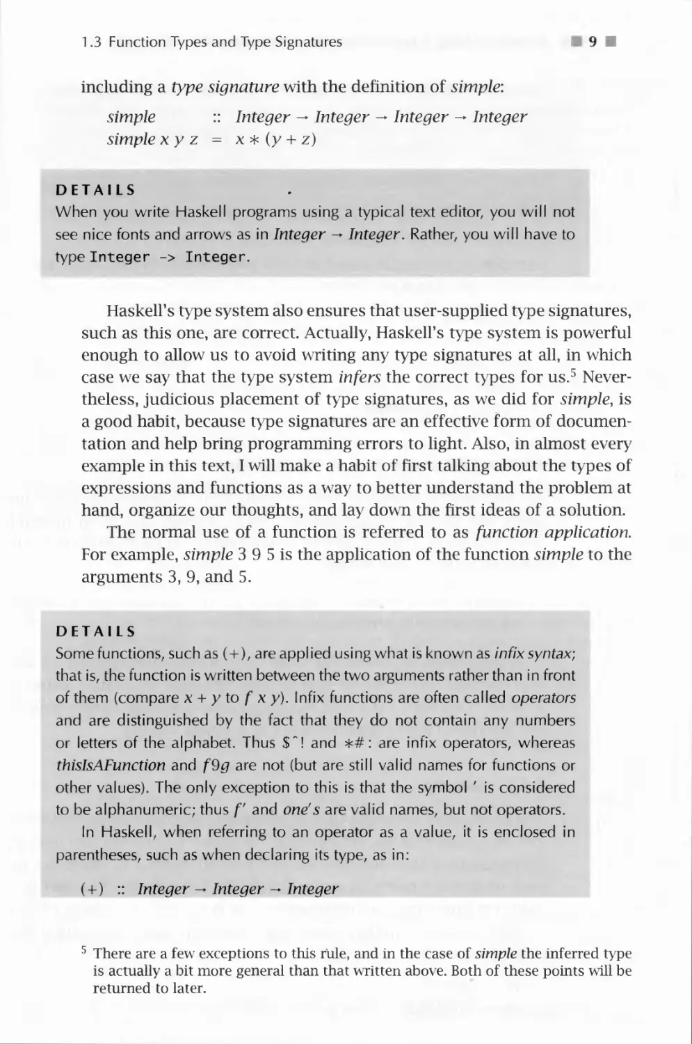
including a type signature with the definition of simple:
simple :: Integer — Integer — Integer — Integer
simplexy z = x* (y + z)
DETAILS
When you write Haskell programs using a typical text editor, you will not
see nice fonts and arrows as in Integer — Integer. Rather, you will have to
type Integer -> Integer.
Haskell's type system also ensures that user-supplied type signatures,
such as this one, are correct. Actually, Haskell's type system is powerful
enough to allow us to avoid writing any type signatures at all, in which
case we say that the type system infers the correct types for us.5
Nevertheless, judicious placement of type signatures, as we did for simple, is
a good habit, because type signatures are an effective form of
documentation and help bring programming errors to light. Also, in almost every
example in this text, I will make a habit of first talking about the types of
expressions and functions as a way to better understand the problem at
hand, organize our thoughts, and lay down the first ideas of a solution.
The normal use of a function is referred to as function application.
For example, simple 3 9 5 is the application of the function simple to the
arguments 3, 9, and 5.
DETAILS
Some functions, such as (+), are applied using what is known as infix syntax;
that is, the function is written between the two arguments rather than in front
of them (compare x + y to f x y). Infix functions are often called operators
and are distinguished by the fact that they do not contain any numbers
or letters of the alphabet. Thus $"! and *#: are infix operators, whereas
thisIsAFunction and f9g are not (but are still valid names for functions or
other values). The only exception to this is that the symbol ' is considered
to be alphanumeric; thus f and one's are valid names, but not operators.
In Haskell when referring to an operator as a value, it is enclosed in
parentheses, such as when declaring its type, as in:
(+) :: Integer — Integer — Integer
5 There are a few exceptions to this rule, and in the case of simple the inferred type
is actually a bit more general than that written above. Both of these points will be
returned to later.

1 0 Problem Solving, Programming, and Calculation
Also, when trying to understand an expression such as f x + g y, there
is a simple rule to remember: Function application always has "higher
precedence" than operator application so that fx + gy is the same as
Despite all of these syntactic differences, however, operators are still just
functions.
Exercise 1.3 Identify the well-typed expressions in the following and,
for each, give its proper type:
[(2, 3), (4, 5)]
[V,42]
(V, -42)
simple'a' 'V 'c'
(simple 12 3, simple)
1.4 Abstraction, Abstraction, Abstraction
The title of this section answers the question: "What are the three most
important ideas in programming?" Well, perhaps this is an
overstatement, but I hope that I've gotten your attention, at least. Webster defines
the verb "abstract" as follows:
abstract, vf (1) remove, separate (2) to consider apart from
application to a particular instance.
In programming we do this when we see a repeating pattern of some
sort and wish to "separate" that pattern from the "particular instances"
in which it appears. Let's refer to this process as the abstraction principle
and see how it might manifest itself in problem solving.
1.4,1 Naming
One of the most basic ideas in programming - for that matter, in everyday
life - is to name things. For example, because it is inconvenient to retype
(or remember) the value of tt beyond a small number of digits, we may
wish to give it a name. In mathematics the Greek letter tt in fact is the
name for this value, but unfortunately we don't have the luxury of using
Greek letters on standard computer keyboards and text editors. So in
Haskell we write:
pi :: Float
pi = 3.14159

1.4 Abstraction, Abstraction, Abstraction
11 H
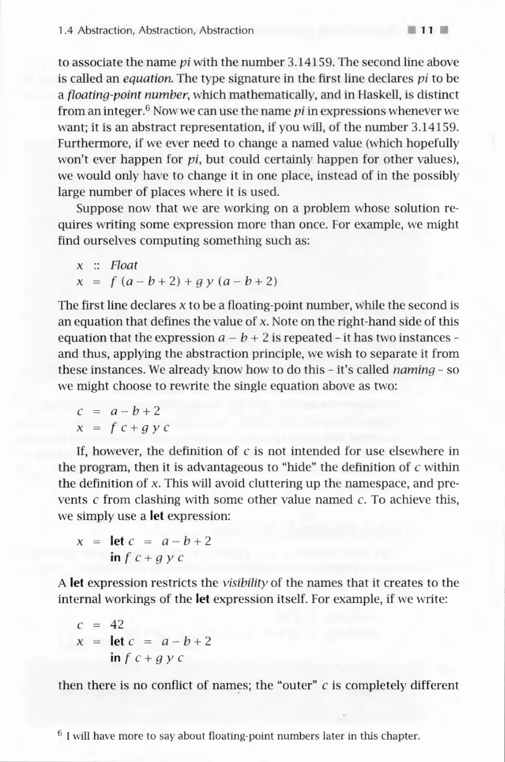
to associate the name pi with the number 3.14159. The second line above
is called an equation. The type signature in the first line declares pi to be
a floating-point number, which mathematically, and in Haskell, is distinct
from an integer.6 Now we can use the name pi in expressions whenever we
want; it is an abstract representation, if you will, of the number 3.14159.
Furthermore, if we ever need to change a named value (which hopefully
won't ever happen for pi, but could certainly happen for other values),
we would only have to change it in one place, instead of in the possibly
large number of places where it is used.
Suppose now that we are working on a problem whose solution
requires writing some expression more than once. For example, we might
find ourselves computing something such as:
x :: Float
x = f {a-b + 2) + gy (a-b + 2)
The first line declares x to be a floating-point number, while the second is
an equation that defines the value of x. Note on the right-hand side of this
equation that the expression a - b + 2 is repeated - it has two instances -
and thus, applying the abstraction principle, we wish to separate it from
these instances. We already know how to do this - it's called naming - so
we might choose to rewrite the single equation above as two:
c = a-b+2
x = f c + gy c
If, however, the definition of c is not intended for use elsewhere in
the program, then it is advantageous to "hide" the definition of c within
the definition of x. This will avoid cluttering up the namespace, and
prevents c from clashing with some other value named c. To achieve this,
we simply use a let expression:
x = let c = a-b + 2
mfc+gyc
A let expression restricts the visibility of the names that it creates to the
internal workings of the let expression itself. For example, if we write:
c = 42
x = letc = a-b + 2
mfc+gyc
then there is no conflict of names; the "outer" c is completely different
6 I will have more to say about floating-point numbers later in this chapter.

112 1 Problem Solving, Programming, and Calculation
from the "inner" one enclosed in the let expression. Think of the inner
c as analogous to the first name of someone in your household. If your
brother's name is "John" he will not be confused with John Thompson
who lives down the street when you say, "John spilled the milk."
DETAILS
An equation such as c = 42 is called a binding. A simple rule to remember
when programming in Haskell is never to give more than one binding for
the same name in a context where the names can be confused, whether at
the top level of your program or nested within a let expression. For example,
this is not allowed:
a = 42
a = 43
nor is this:
a = 42
b = 43
a = 44
So you can see that naming - using either top-level equations or
equations within a let expression - is an example of the abstraction principle
in action. It's often the case, of course, that we anticipate the need for
abstraction; for example, directly writing down the final solution above,
because we knew that we would need to use the expression a - b + 2
more than once.
1.4.2 Functional Abstraction
Let's now consider a more complex example. Suppose we are computing
the sum of the areas of three circles with radii r 1, r2, and r 3, as expressed
by
totalArea :: Float
totalArea = pi * rV2 + pi * r2~2 + pi * r3~2
DETAILS
C) is Haskell's integer exponentiation operator. In mathematics we would
write it x r2 or just rcr2 instead of pi*r~ 2.

1.4 Abstraction, Abstraction, Abstraction
13 m
Although there isn't an obvious repeating expression here as there
was in the last example, there is a repeating pattern of operations, namely,
the operations that square some giv en quantity - in this case the radius -
and then multiply the result by tt. To abstract a sequence of operations
such as this, we use a function, which we will give the name circleArea,
that takes the "given quantity" - the radius - as an argument. There are
three instances of the pattern, each of which we can expect to replace
with a call to circleArea. This leads to:
circleArea :: Float — Float
circleArea r = pi * r~2
totalArea = circleArea r\ + circleArea r2 + circleArea r3
Using the idea of unfolding described earlier, it is easy to verify that this
definition is equivalent to the previous one.
This application of the abstraction principle is sometimes called
functional abstraction, because the sequence of operations is abstracted as a
function, in this case circleArea. Actually, it can be seen as a
generalization of the previous kind of abstraction: naming. That is, circleArea r 1 is
just a name for pi * rY2, circleArea r2 for pi * r2~2, and circleArea r3
for pi * r3~2. In other words, a named quantity, such as c or pi defined
previously, can be thought of as a function with no arguments.
Note that circleArea takes a radius (a floating-point number) as an
argument and returns the area (also a floating-point number) as a result.
This is reflected in its type signature.
The definition of circleArea could also be hidden within totalArea
using a let expression as we did in the previous example:
totalArea = let circleArea r = pi * r~2
in circleArea r\ + circleArea r2 + circleArea r3
On the other hand, it is more likely that computing the area of a circle
will be useful elsewhere in the program, so leaving the definition at the
top level is probably preferable in this case.
1.4.3 Data Abstraction
The value of totalArea is the sum of the areas of three circles. But what
if in another situation we must add the areas of five circles, or in other
situations, even more? In situations where the number of things is not
certain, it is useful to represent them in a list whose length is arbitrary.

1 4 Problem Solving, Programming, and Calculation
So imagine that we are given an entire list of circle areas whose length
isn't known when we write the program. What now?
I will define a function listSum to add the elements of a list. Before
doing so, however, there is a bit more to say about lists.
Lists are an example of a data structure, and when their use is
motivated by the abstraction principle, I will say that we are applying data
abstraction. Earlier we saw the example [1, 2, 3] as a list of integers,
whose type is thus [Integer]. Not surprisingly, a list with no elements is
written [], and pronounced "nil." To add a single element x to the front
of a list xs, we write x : xs. (Note the naming convention used here; xs
is the plural of x, and should be read that way.) In fact, the list [1, 2, 3]
is equivalent to 1 : (2 : (3 : [ ])), which can also be written 1 : 2 : 3 : [ ]
because the infix operator (:) is "right associative."
DETAILS
In mathematics we rarely worry about whether the notation a+ b + c stands
for (a + b) + c (in which case + would be "left associative") or a + (b + c)
(in which case + would "right associative"). This is because in situations
where the parentheses are left out the operator usually is mathematically
associative, meaning that it doesn't matter which interpretation we choose.
If the interpretation does matter, mathematicians will include parentheses
to make it clear. Furthermore, in mathematics there is an implicit
assumption that some operators have higher precedence than others; for example,
2 x a + b is interpreted as (2 x a) + b, not 2x(a + b).
In most programming languages, including Haskell, each operator is
defined as having some precedence level and to be either left or right
associative. For arithmetic operators, mathematical convention is usually followed;
for 2 * a + b is interpreted as (2 * a) + b in Haskell. The predefined list-
forming operator (:) is defined to be right associative. Just as in mathematics,
this associativity can be overridden by using parentheses: thus (a: b) : c is
a valid Haskell expression (assuming that it is well-typed), and is very
different from a : b : c. I will explain later how to specify the associativity and
precedence of new operators that we define.
Examples of predefined functions defined on lists in Haskell include
head and tail, which return the "head" and "tail" of a list, respectively.
That is, head (x : xs) => x and tail {x:xs) => xs (we will define these
two functions formally in Section 5.1). Another example is the function
(-I+), which concatenates, or appends, together its two list arguments. For
example, [1, 2, 3] -H- [4, 5, 6] => [1, 2, 3, 4, 5, 6] ((-H-) will be defined
in Section 11.2).

1.4 Abstraction, Abstraction, Abstraction 1 5
Returning to the problem of defining a function to add the elements
of a list, let's first express what its type should be:
listSum :: [Float] - Float
Now we must define its behavior appropriately. Often in solving
problems such as this, it is helpful to consider, one by one, all possible cases
that could arise. To compute the sum of the elements of a list, what
might the list look like? The list could be empty, in which case the sum
is surely 0. So we write:
listSum [ ] = 0
The other possibility is that the list isn't empty (i.e., it contains at least
one element) in which case the sum is the first number plus the sum of
the remainder of the list. So we write:
listSum (x : xs) = x + listSum xs
Combining these two equations with the type signature brings us to the
complete definition of the function listSum:
listSum :: [Float] — Float
listSum [] = 0
listSum (x: xs) = x + listSum xs
DETAILS
Although intuitive this example highlights an important aspect of Haskell:
pattern matching. The left-hand sides of the equations contain patterns such
as [ ] and x: xs. When a function is applied, these patterns are matched
against the argument values in a fairly intuitive way ([ ] only matches the
empty list, and x: xs will successfully match any list with at least one
element, while naming the first element x and the rest of the list xs). If the
match succeeds, the right-hand side is evaluated and returned as the result
of the application. If it fails, the next equation is tried, and if all equations
fail, an error results. All of the equations that define a particular function
must appear together, one after the other.
Defining functions by pattern matching is quite common in Haskell, and
you should eventually become familiar with the various kinds of patterns
that are allowed; see Appendix B for a concise summary.
This is called a recursive function definition because listSum "refers to
itself" on the right-hand side of the second equation. Recursion is a very

1 6 Problem Solving, Programming, and Calculation
powerful technique that will be used many times in this text. It is also an
example of a general problem-solving technique where a large problem
is broken down into many simpler but similar problems; solving these
simpler problems one by one leads to a solution to the larger problem.
Here is an example of listSum in action:
UstSum [1, 2, 3]
=> listSum (1 : (2: (3: [])))
=> l + listSum(2:(3:[]))
=> 1 + (2 +listSum (3: []))
=> 1 + (2 + (3 + listSum []))
=> l + (2 + (3 + 0))
=> l + (2 + 3)
=> 1 + 5
=> 6
The first step above is not really a calculation, but rather is a rewriting of
the list syntax. The remaining calculations consist of four unfold steps
followed by three integer additions.
Given this definition of listSum we can rewrite the definition of
totalArea as:
totalArea = listSum [circleArea rl, circleArea r2, circleArea r3]
This may not seem like much of an improvement, but if we were
adding many such circle areas in some other context, it would be.
Indeed, lists are arguably the most commonly used structured data type in
Haskell. In the next chapter we will see a more convincing example of the
use of lists; namely, to represent the vertices that make up a polygon.
Because a polygon can have an arbitrary number of vertices, using a data
structure such as a list seems like just the right approach.
In any case, how do we know that this version of totalArea behaves
the same as the original one? By calculation, of course:
listSum [circleArea rl, circleArea r2, circleArea r3]
=> { unfold listSum (four succesive times)}
circleArea rl + circleArea r2 + circleArea r3 + 0
=> { unfold circleArea (three places) }
pi * r 1 ~ 2 + pi * r2 ~ 2 + pi * r3 ~ 2 + 0
=> { simple arithmetic }
pi * rV2 + pi * r2~2 + pi * r3~2

1.5 Code Reuse and Modularity 1 7 ■
1.5 Code Reuse and Modularity
There doesn't seem to be much repetition in our last definition for
totalArea, so perhaps we're done. In fact, let's pause for a moment and
consider how much progress we've made. We started with the definition:
totalArea = pi * r 1 ~ 2 + pi * r2 ~ 2 + pi * r3 ~ 2
and ended with:
totalArea = listSum [circleArea rl, circleArea r2, circleArea r3]
But we have also introduced definitions for the auxiliary functions
circleArea and listSum. In terms of size, our final program is actually
larger than what we began with! So have we actually improved things?
From the standpoint of "removing repeating patterns," we certainly
have, and we could argue that the resulting program is easier to
understand. But there is more. Now that we have defined auxiliary7 functions,
such as circleArea and listSum, we can reuse them in other contexts.
Being able to reuse code is also called modularity, because the reused
components are like little modules, or bricks, that can form the foundation of
many applications.7 We've already talked about reusing circleArea; and
listSum is surely reusable: imagine a list of grocery item prices, or class
sizes, or city populations, for each of which we must compute the total. In
later chapters you will learn other concepts - most notably higher-order
functions and polymorphism - that will substantially increase your
ability to reuse code.
1.6 Beware of Programming with Numbers
In mathematics there are many different kinds of number systems. For
example, there are integers, natural numbers (i.e., non-negative integers),
real numbers, rational numbers, and complex numbers. These number
systems possess many useful properties, such as the fact that
multiplication and addition are commutative, and that multiplication distributes
over addition. You have undoubtedly learned many of these properties in
your studies and have used them often in algebra, geometry7,
trigonometry, and physics, among others.
Unfortunately, each of these number systems places great demands
on computer systems. In particular, a number can in general require an
7 "Code reuse" and "modularity" are important software engineering principles.

■ 1 8 ■ Problem Solving, Programming, and Calculation
arbitrary amount of memory to represent it - e\ en an infinite amount!
Clearly, for example, we cannot represent an irrational number such a^
rr exactly; the best we can do is approximate it, or possibly write a
program that computes it to whatever (finite) precision we need in a given
application. But even integers (and therefore rational numbers) present
problems, because any given integer can be arbitrarily large.
Most programming languages do not deal with these problems very
wrell. In fact, most programming languages do not have exact forms of
an} of these number systems. Haskell does slightly better than most, in
that it has exact forms of integers (the type Integer) as well as rational
numbers (the type Rational, defined in the Ratio Library). But in Haskell
and most other languages, there is no exact form of real numbers, for
example, which are instead approximated by floating-point numbers with
either single-word precision (Float in Haskell) or double-word precision
(Double). What's worse, the behavior of arithmetic operations on
floatingpoint numbers can vary somewhat depending on the CPU being used,
although hardw are standardization in recent years has lessened the degree
of this problem.
The bottom line is that, as simple as numbers seem, great care must be
taken when programming with them. Many computer errors, some quite
serious and renowned, have been rooted in numerical incongruities. The
field of mathematics known as numerical analysis is concerned precisely
with these problems, and programming with floating-point numbers in
sophisticated applications often requires a good understanding of
numerical analysis to devise proper algorithms and wTite correct programs.
As a simple example of this problem, consider the distributiv e law7,
expressed here as a calculation in Haskell and used earlier in this chapter
in calculations involving the function simple:
a* (b + c) => a * £? + a * c
For most floating-point numbers, this law is perfectly valid. For
example, in the Hugs implementation of Haskell, the expressions
pi * (3.52 + 4.75) and pi * 3.52 + pi * 4.75 both yield the same result:
25.981. But funny things can happen when the magnitude of b + c
differs significantly from the magnitude of either b or c. For example, the
following two calculations are from Hugs:
5* (-0.123456 + 0.123457) => 4.99189e-006
5* (-0.123456)+ 5 * (0.123457) => 5.00679^-006
Although the error here is small, its very existence is worrisome, and
in certain situations it could be disastrous. The nature of floating-point

1.6 Beware of Programming with Numbers 1 9 ■
numbers will not be discussed much further in this text, but just
remember that they are approximations to the real numbers. If real-number
accuracy is important to your application, further study of the nature of
floating-point numbers is probably warranted.
On the other hand, the distributive law (and many others) is valid in
Haskell for the exact data types Integer and Ratio Integer (i.e., rational
numbers). However, another problem arises: Although the representation
of an Integer in Haskell is not normally something that we are concerned
about, it should be clear that the representation must be allowed to grow
to an arbitrary size. For example, Haskell has no problem with the
following number:
veryBigNumber :: Integer
veryBigNumber = 43208345720348593219876512372134059
and such numbers can be added, multiplied, etc., without any loss of
accuracy. However, such numbers cannot fit into a single word of
computer memory, most of which are limited to 32 bits. Worse, because the
computer system does not know ahead of time exactly how many words
will be required, it must devise a dynamic scheme to allow just the right
number of words to be used in each case. The overhead of implementing
this idea unfortunately causes programs to run slower.
For this reason, Haskell provides another integer data type called Int,
which has maximum and minimum values that depend on the word size
of the CPU. In other words, every value of type Int fits into one word
of memory, and the primitive machine instructions for integers can be
used to manipulate them very efficiently.8 Unfortunately, this means that
overflow or underflow errors could occur when an Int value exceeds either
the maximum or minumum values. Howev er, most implementations of
Haskell (as well as most other languages) do not even tell you when this
happens. For example, in Hugs, the following Int value:
z:: Int
i = 1234567890
works just fine, but if you multiply it by 2, Hugs returns the value
-1825831516! This is because twice z exceeds the maximum allowed
The Haskell Report requires that every implementation support Ints in the
range -229 to 229 - 1, inclusive. The Hugs implementation running on a Pentium
processor, for example, supports the range -231to231-l.

H 20 H Problem Solving, Programming, and Calculation
value, so the resulting bits become nonsensical9 and are interpreted in
this case as a negative number of the given magnitude.
This is alarming! Indeed, why should anyone ever use Int when Integer
is available? The answer, as mentioned earlier, is efficiency, but clearly,
care should be taken when making this choice. If you are indexing into a
list, for example, and you are confident that you are not performing index
calculations that might result in the above kind of error, then lnt should
work just fine, because a list longer than 231 will not fit into memory
anyway! But if you are calculating the number of microseconds in some
large time interval or counting the number of people living on earth, then
Integer would most likely be a better choice. Choose your number data
types wisely!
In this text the data types Integer, Int, Float, and Rational will be
used for a variety of different applications; for a discussion of the other
number types, consult the Haskell Report. As I use these data types, I will
do so without much discussion; this is not, after all, a book on numerical
analysis. But I will issue a warning whenever reasoning about numbers in
a way that might not be technically sound.
9 Actually, they are perfectly sensible in the following way: The 32-bit
binary representation of I is 01001001100101100000001011010010, and twice
that is 10010011001011000000010110100100. But the latter number is seen
as negative because the 32nd bit (the highest-order bit on the CPU on
which this was run) is a one, which means it is a negative number in
"twos-complement" representation. The twos-complement of this number is in
turn 01101100110100111111101001011100, whose decimal representation is
1825831516.

CHAPTER TWO
A Module of Shapes: Part I
In the previous chapter you learned quite a few techniques for problem
solving via calculation in Haskell. It's time now to apply these ideas to
a larger example, which will require learning even more problem-solving
skills and Haskell language features.
Our job will be to design a simple module of geometric shapes, that
is, a collection of functions and data types for computing with geometric
shapes such as circles, squares, triangles, and others. Users of this
module will be able to create new instances of geometric shapes and compute
their areas. You will learn lots of new things in building this module,
including how to design your own data types. Then in Chapter 4 we will
extend this functionality with the ability to draw geometric shapes, and
in Chapter 6 compute their perimeters.
In the description above I refer to the end product as a module,
through which a user has access to certain well-defined functionalities.
A module can be seen as a way to conveniently wrap up an application
in such a way that only the functionality intended for the end-user is
visible; everything else needed to implement the system is effectively
hidden.
In Haskell we can create a module named Shape in the following way:
module Shape (■ ■ ■) where
...body-of-module...
The "(■ ■ ■)" after the name Shape will ultimately be a list of names of
the functions and data types that the end-user is intended to use, and is
sometimes called the interface to a module. At the end of this chapter
we will fill in the details of the interface once we know what they should
be. The ...body-of-module... is of course where we will place all the code
developed in this chapter.
21 ■

2 2 0 A Module of Shapes: Part I
DETAILS
Module names must always be capitalized (just like type names).
A user of our shape module can later import it into a module that he or
she is constructing, by writing:
import Shape
Indeed, we will do exactly this in later chapters where new modules will
be created in which users will be able to draw shapes, compute their
perimeters, combine them into larger "regions," color them, scale them,
and place them on a "virtual desktop." This desktop will be displayed on
your computer screen, and will be designed in such a way that regions
will rise to the surface of the desktop when they are clicked, just like
windows do in a windows-based user-interface.
2.1 Geometric Shapes
Our first job will be to design a single data type to represent all of the
possible geometric shapes of interest to us. Aside from the fact that this
is intuitively appealing, there are several pragmatic reasons for doing so.
For example, in Section 1.4.2 we saw a function for computing the area
of a circle, and later a function for computing the area of a square. If
we were to define functions for computing the areas of, say, n different
shapes, we would end up with n functions, each with a different name.
Similarly, we would have n functions for drawing shapes and n functions
for computing their perimeters. In contrast, if we had a single data type
that captured all of the geometric shapes, we could (hopefully) define a
single function for each of these tasks.
In Haskell, new data types such as this are defined using a data
declaration:
data Shape = Circle Float
I Square Float
This declaration can be read: "There are two kinds of Shapes: a circle
of the form Circle r where r is a radius of type Float, and a square of
the form Square s where s is the length (also of type Float) of one side."
Because Circle and Square construct new values in this data type, they
are called constructors.

2.1 Geometric Shapes
23
DETAILS
All constructors in a data declaration must be capitalized. In this way they
are syntactically distinguished from ordinary functions. This distinction is
useful because only constructors can be used in the pattern matching that is
part of a function definition, as wrll be described shortly.
Of course, there are more shapes than just circles and squares. And
to complicate matters, squares are really rectangles, rectangles are really
parallelograms, and parallelograms are just quadrilaterals (4-sided
polygons). And, there are (right, equilateral, and isosceles) triangles,
trapezoids, pentagons, hexagons, etc. Do we really want representations for
all of them? If not, which ones do we choose? This is a difficult design
decision that is dependent on the eventual use of the data type, which
may be difficult to predict.
For mostly pedagogical purposes, let's settle on the following
definition:
data Shape = Rectangle Float Float
| Ellipse Float Float
| RtTriangle Float Float
| Polygon [(Float, Float)]
deriving Show
DETAILS
The phrase "deriving Show" is a way to tell the Haskell system that you are
interested in printing out values of the data type that you are defining. Exactly
how this is accomplished will be described in a later chapter.
This declaration defines a new data type called Shape in which:
■ Rectangle si s2 is a rectangle with sides si and s2, both floating-point
numbers.
Ellipse rl r2 is an ellipse with radii rl and r2, both floating-point
numbers.
■ RtTriangle s 1 s2 is a right triangle with sides of length si and s2, both
floating-point numbers.
Polygon [vl, v2, ..., vn] is an n-sided polygon whose vertices are
vl through vn, each vertex being represented by a pair (x,y) of
floating-point coordinates on a Cartesian plane. (Recall that (Float,
Float) is the type of pairs of floating-point numbers; for example
(1.0, pi) :: (Float, Float).)

2 4 0 A Module of Shapes: Part I
One unfortunate aspect of this definition is that floating-point
numbers are used to represent several different quantities, a fact only evident
in the documentation of the code (such as we have written above). One
way to improve on this is to create new names for the various uses of
floating-point numbers, which in Haskell can be achieved using a type
declaration:
data Shape = Rectangle Side Side
I Ellipse Radius Radius
I RtTriangle Side Side
| Polygon [Vertex]
deriving Show
type Radius = Float
type Side = Float
type Vertex = (Float, Float)
DETAILS
Here the Shape declaration is really the same as before, except that we've
used different names for the "constituent types/' and the type declarations
tell us what they really are. It is important to realize that, although a data
declaration creates a completely new data type, a type declaration does not:
it simply creates a new name for an existing type. Indeed, these are called
type synonyms because the new name is just a synonym for the old one.
The result is "self-documenting," and arguably easier to read.
This change can also be seen as another application of the
abstraction principle. Note, for example, that if we decide to represent sides
as double-precision floating-point numbers (which in Haskell have type
Double), we could just change a single line:
type Side = Double
no matter how often we used the name Side. This is a good thing.
Returning to the design issue of deciding which shapes to choose for
this data type, you might object to the fact that to create a square with
side s you must now write something like Rectangle s s. It is easy to
remedy this situation, however, by defining a function square as:
square s = Rectangle s s
Similarly, a circle function can be defined by:
circle r = Ellipse r r

2.2 Areas of Shapes
■ 25 ■
But, you might point out, with the Polygon constructor we can create
polygons with an arbitrary number of sides, each with an arbitrary length,
so why include the special cases of rectangle and right triangle? In other
words, why not just define functions rectangle and rtTriangle in terms
of Polygon? Good question! One answer, as mentioned earlier, is in the
interest of pedagogy: I am trying to illustrate a variety of programming
techniques. Another answer is that the algorithms for computing the
areas of rectangles and right triangles are simpler than the algorithm for
computing the area of a general polygon. A final answer is that there may
be lower-level graphics commands, say, that are more efficient at
drawing rectangles and/or right triangles than general polygons. In any case,
let's proceed with our design and investigate its consequences later.
Exercise 2.1 Define functions rectangle and rtTriangle in terms of
Polygon.
Exercise 2.2 Define a function regularPolygon :: Int-* Side-* Shape
such that regularPolygon n s is a regular polygon with n sides, each of
length s. (Hint: Consider using some of Haskell's trigonometric functions,
such as sin :: Float — Float, cos :: Float-^Float, and tan :: Float — Float.)
2.2 Areas of Shapes
Returning to the problem in Section 1.4.2 of computing areas, we will
define a function:
area :: Shape — Float
by defining its behavior on each of the Shape constructors. We know how
to do this for a rectangle:
area (Rectangle si s2) = si * s2
And the area of a right triangle is just as easy:
area (RtTriangle si s2) = si * s2/2
Before proceeding, note that this way of writing function definitions -
by pattern matching on the arguments - is just like the way we defined
the function listSum in Section 1.4.3. There, listSum was defined by its
behavior on the two constructors in the list data types, [ ] and (:). In
the case of the Shape data type, we happen to have four constructors to
consider instead of two.

■ 2 6 ■ A Module of Shapes: Part I
v4 v4
Vt Vi Vi
Figure 2.1. Computing the Area of a Convex Polygon
Moving on, a standard geometry text tells us that the area of an ellipse
with radii r\ and r2 is just ity^. It is easy to see that this reduces to irr2
for a circle. Translated into Haskell, this becomes:
area (Ellipse r\ r2) = pi * r\ * r2
What about the area of a general polygon? If the polygon is convex
(meaning that all of its interior angles are less than 180°), its area can be
computed fairly simply as follows (the case of concave polygons will be
an exercise):
1. Compute the area of the triangle formed by the first three vertices of
the polygon.
2. Delete the second vertex, forming a new polygon.
3. If there are at least three vertices in the new polygon, repeat this
procedure, returning as the total area the sum of the areas of the individual
triangles.
The intuition for this algorithm is shown pictorially in Fig. 2.1; it is
another example of solving a problem by solving a smaller problem first,
which at least slightly reduces the size of the larger one.
Although we haven't yet decided how to compute the area of a general
triangle, we can write out the above algorithm in Haskell as follows:
area {Polygon (vl : v2 : v3 : vs))
= triArea vl v2 v3 + area (Polygon (vl : v3 : vs))
area (Polygon _)
= 0
DETAILS
The first line above is an example of a nested pattern; that is, J:he pattern
(vl: v2 : v3 : vs) is nested within the pattern Polygon ....

2.2 Areas of Shapes
27 ■
The second equation uses an ''underscore" character "_" as a pattern.
This is called a wildcard pattern, and matches any argument. When more
than one equation is used to define a function, Haskell will try them in the
order that they appear. So in the case of area, an attempt is first made to
match a list containing at least three elements. If that fails, then the
second equation is tried, which of course succeeds immediately, yielding the
value 0.
This version of the algorithm has a more "declarative" feel than the
description given earlier and can be read: "The area of a (convex) polygon
is the area of the triangle formed by its first three vertices, plus the area
of the polygon resulting from deleting the second vertex." In general, we
will try to write declarative definitions such as this directly.
However, note in the recursive call to area that the polygon is
"reconstructed" using the Polygon constructor; so the polygon is taken apart
and then put back together, so to speak, on each recursive call. Also
note that the first vertex never disappears; it is always part of the
reconstruction. We can avoid these slight inefficiencies by defining an auxiliary
function poly Area that computes the area directly from a list of vertices,
as follows:
area (Polygon (vl : vs)) = polyArea vs
where polyArea :: [Vertex] — Float
polyArea (v2 : v3 : vs') = trxArea vl v2 v3
+polyArea (v3 : vs')
polyArea _ =0
DETAILS
Note the use of a where expression. For the most part you can consider
exp where ...equations... to be equivalent to let ...equations... in exp. The
only difference is that a where expression is only allowed at the top level of
a function definition, where its visibility rules are slightly different (see the
Haskell Report for details).
What about triArea? Fortunately, there is a single formula for the
area of an arbitrary triangle with sides of lengths a, b, and c, due to
Heron:
A = ^s{s - a)(s - b)(s- c) where s = \(a + b + c)

2 8 ■ A Module of Shapes: Part I
or, in Haskell:
triArea :: Vertex — Vertex — Vertex — Float
triArea vl v2 v3 = let a = distBetween vl v2
fo = distBetween v2 v3
c = distBetween v3 vl
5 = 0.5 * (a + fo + c)
in sgrf (5 * (5 - fl) * (5 - fc) * (5 - c))
DETAILS
sqrt is Haskell's square root function.
Also, note that more than one equation is allowed in a let (or where)
expression. The first characters of each equation, however, must line up
vertically, and if an equation takes more than one line then the subsequent
lines must be to the right of the first characters. For example, this is legal:
let a = aLongName
+anEvenLongerName
b = 56
in ...
but neither of these is:
let a = aLongName
+anEvenLongerName
b = 56
in ...
let a = aLongName
+anEvenLongerName
b = 56
in ...
(The second line of the first example is too far to the left, as is the third line
in the second example.)
Although this rule, called the layout rule, may seem a bit ad hoc, it avoids
the use of special syntax to denote the end of one equation and the beginning
of the next, thus enhancing readability. In practice, use of layout is rather
intuitive. Just remember two things:
1. The first character following either where or let (and a few other keywords
that we will see later) is what determines the starting column for the set

2.2 Areas of Shapes
29
of equations. Thus, we can begin the equations on the same line as the
keyword, the next line, or whatever.
Be sure that the starting column is further to the right than the starting
column associated with any immediately surrounding clause (otherwise
it would be ambiguous). The "termination" of an equation happens when
something appears at or to the'left of the starting column associated with
that equation.
Here distBetween computes the difference between two vertices - that is,
the length of each side of the triangle - and is defined by:
distBetween :: Vertex -* Vertex -* Float
distBetween (xl, yl) (x2, y2)
= sqrt ((xl -x2)~2 + (yl -
y2)~2)
This definition is easy to see as an application of Pythagorean's theorem,
as shown graphically in Fig. 2.2.
In summary, by collecting the four equations for area, we see that we
have covered each of the constructors in the Shape data type:
area
area {Rectangle si s2)
area (RtTriangle si s2)
area (Ellipse rl r2)
area (Polygon (vl : vs))
where polyArea
poly Area (v2 : v3 : vs')
polyArea _
Shape — Float
si * s2
si *s2/2
pi * rl * r2
polyArea vs
:: [Vertex] — Float
triArea vl v2 v3
+polyArea (v3 : vs')
0
Vl
*2
-
y]{x1-x2f+(y1-y2f
xl
xr
Figure 2.2. Computing the Distance between Two Vertices

30 ■ A Module of Shapes: Part I
We can also pro\e properties about our functions, subject to the
limitations of reasoning with floating-point numbers discussed in Section
1.6. For example, it would be nice if area (circle r) yielded the same
result as circleArea r, where circleArea was defined in Section 1.4.2. We
can do this easily by calculation:
area {circle r)
=> { unfold circle }
area (Ellipse r r)
=> { unfold area }
pi * r * r
=> {foidn }
pi * r~2
=> { fold circleArea }
circleArea r
We can also prove more complex properties, such as:
area (RtTriangle si s2)
=> area (Polygon [(0, 0), (si, 0), (0, s2)])
To prove this particular property it's more natural to start with the
right-hand-side and work backwards:1
area (Polygon [(0, 0), (si, 0), (0, s2)])
=> polyArea [(0, 0), (si, 0), (0, s2)]
=> triArea (0, 0) (si, 0) (0, s2) + polyArea [(0, 0), (0, s2)]
=> triArea (0, 0) (si, 0) (0, s2) + 0
=> let a = distBetween (0, 0) (si, 0)
b = distBetween (si, 0) (0, s2)
c = distBetween (0, s2) (0, 0)
s = 0.5 * (a + b + c)
in sqrt (s * (s - a) * (s - b) * (s - c))
=> let b = sqrt (sl~2 + s2"2)
s = 0.5 * (si + b + s2)
in sqrt (s * (s - si) * (s - b) * (s - s2)) — (1)
From this point on I may skip a few of the more obvious steps in a calculation. If
this is unclear, you should try filling in the missing steps yourself.

2.2 Areas of Shapes
m 3i m
We can simplify this further in two steps. First note:
s * (s - b)
=> 0.5 * (si + b + s2) * (0.5 * (si + b + s2) - b)
=> 0.5 * (si + b + s2) * (0.5 * (si - b + s2))
=> 0.25 * (si + s2 + b) * (si + s2 - b)
=> 0.25* ((si +s2r2-b~2)
=> 0.25* ((Sl+s2)^2-(sr2 + s2^2))
=> 0.25 * (sl~2 + 2 * si * s2 + s2~2 - (sl~2 + s2~2))
=> 0.25* (2 *sl *s2)
=> 0.5 * si * s2
And further note:
(s-sl) * (s-s2)
=> (0.5 * (si + b + s2) - si) * (0.5 * (si + b + s2) - s2)
=> 0.5 * (b-sl+ s2) * (0.5 * (b + sl-s2))
=> 0.25* (b~2- (sl-s2)~2)
=> 0.25* ((sr2 + s2^2)-(sl-s2)^2)
=> 0.25* ((sr2 + s2~2)-(sl~2-2*sl *s2 + s2~2))
=> 0.5 * si * s2
Combining these and continuing from point (1), we get:
sqrt (s ^ (s - si) * (s - b) * (s - s2))
=> sgrf ((0.5 * si * s2) * (0.5 * si * s2))
=> 0.5 * si * s2
=> area (RtTriangle si s2)
and we are done.
That was a lot of work! The primary reason for this is that Heron's
general formula for the area of a triangle is subtle - and powerful. It
is interesting to note, however, that if we were to carry out this proof
in mathematics, we would reason in a very similar way, as follows. By
Heron's formula, the area of a polygon with vertices (0,0), (si,0), and
(0,S2) is given as follows: Let s = \(a + b + c), a = | (0,0),(si,0) |,
b = I (si,0), (0, s2) I, c = | (0,S2),(0,0) | (where | pi,/?2 I is the distance
between vertices p\ and p2). Then the area is given by:
^s(s-a)(s-b)(s-c)

32 A Module of Shapes: Part I
Simplifying a to S\ and c to s2 yields:
^s(s-Sl)(s-b)(s-s2) (2.1)
where b = ^js2 + s2 anc* 5 = \(si + ^ + s2)-
We can simplify this further in two steps. First note:
s(s-b) = \(si + b + s2)(\(si -b + s2))
= \(si +s2 + b)(si +s2-b) = \((si +s2)2 -b2)
= \((Sl + S2)2 - (S2 + S2)) = \(S2 + 2SiS2 + *£ - (5? + *f))
= |(2SiS2) = \siS2
And further note:
(5-5i)(5-52) = \(b-Si +S2){\(.b + Si ~S2))
= \(b2- (Sl - s2)2) = \((s2 + s2) - (Sl - s2)2)
= \((s21+s2)-(s2-2sls2 + st))
= \sxs2
Combining these and continuing from point (1), we get:
yjs(s-si)(s-b)(s-s2)
= ^(\s1s2)(\sis2)
= \sis2
This last formula is just the area of a right triangle with sides s\ and
s2. If you compare this mathematical proof with the corresponding proof
by calculation in Haskell, you will find that they are almost identical,
except for the notation used. So reasoning in Haskell is very often quite the
same as reasoning in mathematics. Because wre often use mathematics
to specify the correct behavior of our programs, a proof by calculation
in Haskell is a proof both about the implementation and about the
specification. This is why Haskell is sometimes referred to as an "executable
specification language."
Unfortunately, as discussed in Section 1.6, care must be taken when
performing this kind of reasoning with floating-point numbers. As is
often the case, numbers that do not approach the limits of floating-point
precision work perfectly well:
area (RtTriangle 3.652 5.126) => 9.36008
area {Polygon [(0, 0), (3.652, 0), (0, 5.126)]) => 9.36008

2.2 Areas of Shapes
33
w7hereas ones that do can yield inconsistent results:
area (RtTriangle 0.0001 5.126) => 0.0002563
area {Polygon [(0, 0), (0.0001, 0), (0, 5.126)]) => 0.000256648
Exercise 2.3 Prove the following property:
area {Rectangles! s2)
=> area {Polygon [(0, 0), (si, 0), (si, s2), (0, s2)])
Exercise 2.4 Define a function convex :: Shape — Bool that determines
whether or not its argument is a convex shape (although we are mainly
interested in the convexity of polygons, you might as well define it for
each kind of shape).
Exercise 2.5 Here is an alternative way to compute the area of a polygon.
Consider a polygon in quadrant 1 of the Cartesian plane (i.e., every vertex
has positive x and y coordinates). Then every7 pair of adjacent vertices
forms a trapeziod with respect to the x-axis. Starting at any vertex and
working clockwise, compute these areas one-by-one, counting the area
as positive if the x-coordinate increases, and negative if it decreases. The
sum of these areas is then the area of the polygon.
It is easy to see that this algorithm is correct for a convex polygon
by just looking at an example, as in Fig. 2.3. But the real beauty in this
algorithm is that it works for concave polygons as well (see figure), and
for a polygon located anywhere in the Cartesian plane. It is also more
efficient than our previous algorithm. (Why?)
Write a Haskell function to compute polygonal areas in this way.
(Note: Polygons can not only be convex or concave, but also self-
crossing. Consider, for example, the four-vertex polygon that outlines a
"bowtie," or the five-vertex polygon that outlines a five-pointed star. What
is the proper notion of area in this case, and do any of the algorithms
discussed here compute it properly?)
areal area2
I
F F
J J
I A B C EHE A B C D. E
areal = AFGB + BGHD + DHIE - CJIE - AFJC
area2 = AFGB + BGHE - CIHE + CIJD - AFJD
Figure 2.3. Using Trapezoids to Compute Area of Polygon

■ A Module of Shapes: Part I
3 Cleaning Up
Recall the discussion at the beginning of this chapter about modules and
the desire to make visible only those named values that are of interest to
the user of a module, thereby hiding irrelevant details of the
implementation. We can now fill in the module declaration details to achieve this
effect:
module Shape (Shape (Rectangle, Ellipse, RtTriangle, Polygon),
Radius, Side, Vertex,
square, circle, distBetween, area
) where
The list of names above are those entities that are intended to be visible,
or exported, from the module. These names come in three flavors:
1. Data types (in this case the data type Shape) that are listed with their
constructors in parentheses.
DETAILS
A data type and its list of constructors may be abbreviated by just listing the
name of the data type followed by (...). For example, the entire Shape data
type may be exported using the form Shape (...). There are many other rules
concerning the import and export of entities to and from modules. Some of
these rules will be used later in the text, but you should consult the Haskell
Report for all of the details.
2. Type synonyms (Radius, Side, and Vertex).
3. Ordinary values (in this case the functions square, circle, distBetween,
and area).
So, for example, the function triArea is not exported from the Shape
module, and thus is not available for use by someone importing the module.
DETAILS
It is sometimes desirable to export everything from a module. A shorthand
way to express this is to simply write:
module Shape where
(i.e., omitting the list of exports is equivalent to exporting everything)

CHAPTER THREE
Simple Graphics
In this chapter simple graphics programming in Haskell will be explained.
Graphics in Haskell is consistent with the notion of computation via
calculation, although it is special enough to warrant the use of special
terminology and notation. In the next chapter we will use the techniques
learned here to draw in a graphics window the geometric shapes defined
in the last chapter. The ideas developed in this chapter will be put into a
module called SimpleGraphics:
module SimpleGraphics where
There are many predefined functions and data types in Haskell, so
many, in fact, that they demand some organization. Entities that are
deemed essential to defining the fundamental nature of Haskell are
contained in what is called the Standard Prelude, a collection of modules
defining various categories of functionality. Entities that are deemed
useful but not essential are contained in one of several Standard Libraries,
also a collection of modules. The entire Standard Prelude is
automatically imported into every program that you write, whereas the Standard
Libraries need to be imported module-by-module.
Unfortunately, there is no standard graphics library for Haskell yet,
although there is one in popular use on Windows machines called Graphics.
The basic graphics functionality that we will use is defined in a library
called SOEGraphics, which is very similar to Graphics but is guaranteed
to work with this textbook, whereas the Graphics library7 may evolve over
time. To use SOEGraphics, it must be imported into the module that is
using it, as follows:
import SOEGraphics
Graphics is a special case of input/output (10) processing in Haskell,
and thus I will begin with a discussion of this more general idea.
m 35 ■

36 0 Simple Graphics
3.1 Basic Input/Output
The Haskell Report defines the result of a program as the value of the
name main in the module Main. On the other hand, the Hugs
implementation of Haskell allows you to type whatever expression you wish to the
Hugs prompt, and it will evaluate it for you. But in either case, the Haskell
system "executes a program" by evaluating an expression, which (for a
well-behaved program) eventually yields a value. The system must then
display that value on your computer screen in some way that makes sense
to you. Most systems will try to display the result in the same way that
you would type it in as part of a program. So an integer is printed as an
integer, a string as a string, a list as a list, and so on. I will refer to the
area of the computer screen where this result is printed as the standard
output area, which may vary from one implementation to another.
But what if a program is intended to write to a file or print a file on
a printer or, the main topic of this chapter, draw a picture in a graphics
window? These are examples of output, and there are related questions
about input. For example, how does a program receive input from a
keyboard or a mouse?
In general, how does Haskell's "expression-oriented" notion of
"computation by calculation" accommodate these various kinds of input and
output?
The answer is fairly simple: In Haskell, there is a special kind of value
called an action. When a Haskell system evaluates an expression that
yields an action, it knows not to try to display the result in the
standard output area, but rather to "take the appropriate action." There are
primitive actions - such as writing a single character to a file or receiving
a single character from the keyboard - as well as compound actions -
such as printing an entire string to a file. Haskell expressions that
evaluate to actions are commonly called commands, because they command
the Haskell system to perform some kind of action. Haskell functions that
yield actions when they are applied are also commonly called commands.
Commands are still just expressions, of course, and some commands
return a value for subsequent use by the program: keyboard input, for
instance. A command that returns a value of type T has type 10 T; if
no useful value is returned the command has type 10 (). The simplest
example of a command is return x, which for a value x :: T immediately
returns x and has type 10 T.
DETAILS
The type () is called the unit type, and has exactly one value, which is
also written (). Thus return () has type 10 (), and is often called a "noop"

3.1 Basic Input/Output
37 H
because it is an operation that does nothing and returns no useful result.
Despite the negative connotation, it is used quite often!
Remember that all expressions in Haskell must be well-typed before
a program is run, so a Haskell system knows ahead of time, by looking
at the type, that it is evaluating a command, and is thus ready to "take
action."
To make these ideas clearer, let's consider a few examples. A very
useful command is the putStr command, which prints a string argument
to the standard output area, and has type String — 10 (). The ()
simply indicates that there is no useful result returned from this action; its
sole purpose is to print its argument to the standard output area. So the
program:
module Main where
main = putStr "Hello World\n"
is the canonical "Hello World" program, which is often the first program
that people write in a new language.
DETAILS
Strings (i.e. sequences of characters) are written between double quotes in
Haskell, as in "Hello World". When typed on your computer, however, it
will look a little different, as in "Hello World" (the double-quote
character is the same at both ends of the string). Strings have type String. The
"\n" at the end of the string above is a "newline" character; that is, if another
string were printed just after this one, it would appear beginning on the next
line, rather than just after "Hello World".
Suppose now that we want to perform two actions, such as first writing
to a file named "testFile.txt", then printing to the standard output
area. Haskell has a special keyword, do, to denote the beginning of a
sequence of commands such as this, and so we can write:
do writeFile "testFile.txt" "Hello File System"
putStr "Hello World\n"
where the file-wTiting function writeFile has type:
writeFile :: FilePath — String — 10 ()
type FilePath = String

I 38 1 Simple Graphics
DETAILS
A do expression allows us to sequence an arbitrary number of commands,
each of type 10 (), using layout to distinguish them (just as in a let or where
expression). When used in this way the result of a do expression also has
type ZO().
So far we have only used actions having type 10 () (i.e., output
actions). But what about input? As above, we will consider input from both
the user and the file system.
To get a line of input from the user (which will be typed in the
standard input area of the computer screen, usually the same as the standard
output area) we can use the function:
getLine :: 10 String
Suppose, for example, that we wish to read a line of input using this
function, and then write that line (a string) to a file. To do this we write
the compound command:
do s — getLine
writeFile "testFi 1 e. txt" s
Note the syntax for binding s to the result of executing the getLine
command; because the type of getLine is 10 String, the type of s is String.
Its value is then used in the next line as an argument to the writeFile
command.
Similarly, we can read the entire contents of a file using the command
readFile :: FilePath — 10 String. For example:
do s - readFile "testFi 1 e. txt"
putStr s
There are many other commands available for file, system, and user
10, some in the Standard Prelude, and some in various libararies (such
as 10, Directory, System, and Time). I will not discuss any of these here;
rather, in the next section I will concentrate on graphics 10.
Before that, however, I want to emphasize that, despite the special do
syntax, Haskell's 10 commands are no different in status from any other
Haskell function or value. For example, it is possible to create a for of
actions, such as:
actionList = [putStr "Hello World\n",
writeFile "testFi 1 e. txt" "Hel 1 o Fi 1 e System",
putStr "File successfully written."]

3.1 Basic Input/Output
39
However, a list of actions is just a list of values; they actually don't do
anything until they are sequenced appropriately using a do expression,
and then returned as the value main of the overall program. Still, it is
often convenient to place actions into a list as above, and the Haskell
Report and Libraries have some useful functions for turning them into
commands. In particular, the function sequence, in the Standard Prelude,
when used with 10, has type:
sequence. :: [10 a] — 10 ()
and can thus be applied to the actionList above to yield the single
command:
main = sequence. actionList
Before I give you a more interesting example of this idea, I will tell
you a secret (more secrets will be revealed later in the text):
DETAILS
Haskell's strings are really lists of characters. In other words, String is a
shorthand - a type synonym - for a list of characters:
type String = [Char]
However, because strings are used so often, Haskell allows you to write
"Hello" instead of ['//', 'e', '/', '/', V]. But keep in mind that this is just
syntax - strings really are just lists of characters, and these two ways of
writing this string are identical from Haskell's perspective.
(Earlier the type synonym FilePath was defined for String. This shows
that type synonyms can be made for other type synonyms.)
Now back to the example. From the function putChar :: Char — 10 (),
which prints a single character to the standard output area, we can define
the function putStr used earlier, which prints an entire string. To do this,
let's first define a function that converts a list of characters (i.e., a string)
into a list of 10 actions:
putCharList :: String - [10 ()]
putCharList [ ] = [ ]
putCharList (c: cs) = putChar c : putCharList cs
With this, putStr is easily defined:
putStr :: String - 10 ()
putStr s = sequence. (putCharList s)

40 ■ Simple Graphics
Note that the expression putCharList s is a list of actions, and sequence-
is used to turn them into a single (compound) command, just as we did
earlier. (The function putStr can also be defined directly as a recursive
function, but I leave this as an exercise.)
10 processing in Haskell is consistent with everything you have
learned about programming with expressions and reasoning through
calculation, although that may not be completely obvious yet. Indeed, it
turns out that a do expression is just syntax for a more primitive way of
combining actions using functions. This secret will be revealed in full in
Chapter 18.
3.2 Graphics Windows
Let's now look at the particulars of graphics 10. Graphics commands are
no different in concept from those discussed earlier. However, there is
no "standard graphics area" on which to draw things. Instead, we must
create a fresh graphics window. Furthermore, because we may wish to
create several such windows, we need a way to distinguish them once
they are created, in order to specify in which window to draw at some
particular point in a program. Haskell accomplishes this by returning a
unique value of type Window at the time we create a window.
To see this concretely, let's look at the type of the openWindow
command that (you guessed it) opens a window:
openWindow :: Title — Size — 10 Window
type Title = String
type Size = (Int, Int)
The Title is a string displayed in the title bar of the new graphics
window, and Size represents the size of the window as a pair of
numbers indicating the width and height in pixel coordinates. A pixel is the
smallest dot that can be displayed on a computer screen; usually 100
or so pixels can be lined up along one inch. The Window that returns
from a call to openWindow is used in subsequent graphics commands
to tell the computer within which window to perform its action. In other
words, every call to openWindow creates a new, unique window, and the
Window value provides a way7 to distinguish between them in the rest of
the program.
Let's write our first graphics program:
mainO
= runGraphics (
do w «- openWindow

3.2 Graphics Windows
141 I
"My First Graphics Program"(300, 300)
drawInWindow w (text (100, 200) "Hel 1 o Craphi cs Worl d")
k «- getKey w
closeWindow w
)
It's not hard to guess what this program does: A 300 x 300-pixel
graphics window is opened, a greeting message is displayed in it, and the
window remains open until the user types a character on the keyboard.
The following five new functions are introduced by this example:
■ runGraphics :: IO () — IO () runs a graphics "action." This is needed
because of special operating system tasks that need to be set up to
perform graphics IO.
■ drawInWindow :: Window — Graphic -* IO () draws a given Graphic
value on a given Window.
m text:: Point — String — Graphic creates a Graphic value consisting
of a String whose lower left-hand corner is at the location specified
by the Point argument, in pixel coodinates:
type Point = (Int, Int)
m getKey :: Window — IO () waits for the user to press (and release) a
key on the keyboard. In the above example getKey is used to prevent
the windowT from closing before the user has a chance to read what's
on the screen.
■ closeWindow :: Window — IO () closes the specified window.
You should know enough about IO at this point that these
descriptions are sufficient to fully understand the sample program given above,
except for one other detail: (0, 0) is the location of the upper left-hand
corner of the graphics window. As the x coordinate increases, the position
moves to the right, and as the y coordinate increases, the position moves
downward. Thus, in the above program, the bottom right-hand corner of
the graphics window is at coordinate (299, 299). I will have more to say
about this in the next chapter.
For convenience, I will define the following command, which also
demonstrates how to write a loop using command sequencing:
spaceClose :: Window -* IO ()
spaceClose w
= do k «- getKey w
if k ==' ' then closeWindow w
else spaceClose w

42 ■ Simple Graphics
DETAILS
An expression if pred then cons else alt is called a conditional expression.
If pred (called the predicate) is true, then cons (called the consequence) is
the result; if pred is false, then alt (called the alternative) is the result. Thus,
the second command in the do context above will either be closeWindow w
or spaceClose w, depending on whether k is a blank space character
Note that spaceClose is defined recursively, and it is precisely the
recursion that achieves the desired looping behavior. This command reads
a keystroke and sees if it is the space character (' ')■ If it is, the window
is closed and the command is finished; if it is not, then the process is
repeated. Because spaceClose w has type JO,(), we can use it in a do
expression like this:
mainl
= runGraphics (
dow- openWindow
"My First Graphics Program"(300, 300)
drawInWindoww (text (100, 200) "Hello Graphics World")
spaceClose w
)
Exercise 3.1 Rewrite the definition of putStr from Section 3.1 so that
it does not use sequence, nor create a list of actions; rather, express
it recursively, using the looping idea mentioned above. Similarly, define
the function getLine (also from Section 3.1) recursively, using the more
primitive function getChar :: IO Char.
Hint: To define these two functions in this way you will need to use the
expressions return () :: IO () and return "" :: IO String (recall the earlier
discussion about return).
3.3 Drawing Graphics Other Than Text
We have seen that the function text returns a Graphic value, and we used
the function draw to turn that into an action. As it turns out, there are
other functions besides text that create Graphic values, in particular ones
for drawing certain kinds of geometric shapes:
ellipse
shearEUipse
line
Point — Point — Graphic
Point — Point -* Point — Graphic
Point — Point — Graphic

3.4 Some Examples
43 ■
polyline :: [Point] — Graphic
polygon :: [Point] — Graphic
polyBezier :: [Point] -* Graphic
Here is a brief description of each of these:
1. ellipse pi p2 draws an ellipse that just fits into the rectangle whose
upper left-hand vertex is at point pi and whose lower right-hand
vertex is at point p2, using the graphics window coordinate system
described earlier.
2. shearEllipse pi p2 p3 draws an ellipse that just fits into the
parallelogram formed by the vertices pi, p2, and p3.
3. line pi p2 draws a straight line between points pi and p2.
4. polygon pts draws a closed polygon with vertices pts. The last point
is connected back to the first, and thus the polygon can be filled with
a color.
5. polyline pts connects each pair of successive points with a straight
line, but does not connect the last point back to the first; thus it cannot
be filled with a color.
6. polyBezier is like polyline, but uses Bezier curves to connect
successive points, rather than straight lines.
If we draw figures and lines using the above primitive functions, the
figures and lines will be white by default. To make the colors more
interesting, we can use the graphics library function:
withColor :: Color — Graphic — Graphic
data Color = Black | Blue \ Green \ Cyan
| Red | Magenta \ Yellow \ White
3.4 Some Examples
As a simple example, here is a program that draws a red ellipse and a
blue outline of a rectangle.
picl = withColor Red
(ellipse (150, 150) (300, 200))
pic2 = withColor Blue
(polyline [(100, 50), (200, 50),
(200, 250), (100, 250), (100, 50)])

Simple Graphics
main2
= runGraphics (
do w «- openWindow
"Some Graphics Figures"(300, 300)
drawInWindow w picl
drawInWindow w picl
spaceClose w
)
For a more interesting example, let's draw a simple fractal image.
A fractal is a mathematical structure that repeats itself infinitely
often in successively finer detail (Barnsle, 1993). Using fractals is a
popular method to simulate natural phenomena like skylines, leaves, and
snowflakes. I am sure you have seen them in many computer-generated
pictures found in calendars, animated movies, among others. A skyline,
for example, has the property that as you "zoom in" on it, it looks
approximately the same at each level of detail. Whereas this detail is somewhat
random for skylines, for crystaline structures such as a snowflake, it is
very regular. Both can be modelled using fractals.
The mathematics of fractals is beyond the scope of this textbook, but
there are some simple fractal images that are pleasing to the eye yet very
easy to describe and draw. One such image is called Sierpinski's Triangle,
which can be described via successive drawings of a triangle (Fig. 3.1). The
first drawing is a single triangle. The second drawing subdivides the first
triangle into three triangles, each one-half the original in both length and
height. The third drawing subdivides each of the triangles in the second
drawing in a similar way. Nowr imagine doing this ad infinitum, and there
you have Sierpinski's Triangle.
Of course, we cannot actually show7 this infinitely-dense triangle in a
graphics window, because we are limited by pixel size (and our eyes would
not be sharp enough to see the details). So to draw Sierpinski's
Triangle we will stop subdividing the triangles when we reach some
predetermined image size, and then just draw each tiny triangle completely at that
point.
Figure 3.1: First Three Constructions of Sierpinski's Triangle

3.4 Some Examples
45
First I will define a function fillTri that draws a blue-filled triangle,
given x and y coordinates and a size (all in pixel coordinates):
fillTri :: Window - Int - Int - Int - 10 ()
fillTri w xy size
= drawInWindqw w (withColor Blue
(polygon [(x, y), (x + s/ze, y), (x, y - s/ze), (x, y)]))
The rest of the algorithm is really very easy (and elegant), and is
presented in one fell swoop:
minSize :: Int
minSize = 8
sierpinskiTri :: Window -* Int -* Int — Int — 10 ()
sierpinskiTri w xy size
= if szze <= minSize
then /z/ZTn w x y s/ze
else let szze2 = szze ldivl 2
in do sierpinskiTri w xy size2
sierpinskiTri w x (y - szze2) szze2
sierpinskiTri w (x + .szze2) y szze2
DETAILS
dzv x y is the integer quotient of x and y. But sometimes it is desirable to
use a function as if it were an infix operator. To do so in Haskell, just enclose
it in backquotes, as in size ldiv' 2 above. The reason for doing this is purely
aesthetic. In the case above, I chose to do so because division is normally
done using an infix operator in mathematics, as in size/2, (The (/) operator in
Haskell is reserved for floating-point and other fractional numbers, a concept
to be explained much later in the text.)
Note the three recursive calls to sierpinskiTri] when the size drops to 8
or less, fillTri is called instead.
Using sierpinskiTri is easy enough; the only trickery is to use a number
that is a power of two for the initial size, to make the subdivisions look
most uniform by avoiding rounding errors.
main3
= runGraphics (
do w — openWindow "Sierpinski 's Triangle" (400, 400)
sierpinskiTri w50300 256
spaceClose w
)
Fig. 3.2 is a snapshot of the actual output of this program.

■ 46 0 Simple Graphics
B Fierp in ski's Tri? igle
71,
SI;..
71, 71,
^71, ^71,
7i, ii, 7i, ii,
*^7I, *Pil, *^7*, *^7I,
-Ox
Figure 3.2: Snapshot of Sierpinski's Triangle
B Snowflake Fractal
■ ■ .. '...:7:.-
*■ y>
m 0
V
tr
f
*•
, " " /
:*!-
*;
,^
*;
A;
.
r
..A.
V
tr
"~
«.
r
»
-□Q
*■■
■r. ■■.'■'
Figure 3.3: A Snowflake Fractal

3.4 Some Examples
47 ■
I have shown this example primarily to illustrate how one can use
the various graphics primitives in interesting ways. But ultimately we are
trying to build higher-level ways to do this, starting with the ability to
draw7 values of type Shape defined in Chapter 2. We will discuss this in
the next chapter.
Exercise 3.2 Draw a snowflake fractal. The idea is to draw an equilateral
triangle, then another of the same size but rotated 180° (thus making a
Star of David). This process is then repeated for each of the six corners,
but now with triangles one-third the size. The process is repeated
infinitely often in the abstract, but in reality is stopped at some suitably
small triangle size, as for the Sierpinski triangle. Fig. 3.3 shows the result
of a program that achieves this to four levels.
Use recursion to write your program, but note that the strategy is a
bit different from that used with the Sierpinski triangle. With Sierpinski,
no triangles are drawn until the very bottom of the recursion, whereas
with the snowflake, triangles are drawn as you recurse, with each set
being of a different size. For aesthetics, try coloring each level of triangles
differently.

CHAPTER FOUR
Shapes II: Drawing Shapes
In Chapter 2 a shape data type and a function for computing the area of
shapes were defined. In the last chapter you learned about basic graphics
programming in Haskell. In this chapter I will define another function of
shapes, namely one that converts a shape into a graphics value that can
then be drawn in a graphics window. Conceptually, this function is no
different from the area function defined in Chapter 2. In both cases, a
shape is turned into some other kind of value; in the case of area, that
value has type Float, and in the case of the function to be defined in this
chapter, that value has type Graphic.
In order to perform graphics 10, we need to import the graphics
library, as discussed in the last chapter. Additionally, we need to import
the Shape module. Calling our new module Draw, we therefore write:
module Draw (inchToPixel, pixelToInch, intToFloat,
xWin, yWin, trans, shapeToGraphic, spaceClose
) where
import Shape
import SOEGraphics
where the list of names contains those functions and values, inchToPixel,
pixelToInch, etc., that we choose to export from the module, and that are
defined in the remainder of this chapter.
4.1 Dealing With Different Coordinate Systems
Before proceeding, let's define a couple of coercion functions that we will
use to convert, or "coerce," the coordinates of a graphics window into
ones that we are more familiar with (and vice versa).
148 1

4.1 Dealing With Different Coordinate Systems 49 ■
In our discussions of shapes, we have always assumed
floatingpoint numbers for all dimensions, presumably in inches or some similar
dimensional units. But the Graphics Library uses pixel coordinates, so
first we need a function to convert from the former to the latter. Let's
assume that the floating-point numbers are in inches, and that there are
100 pixels per inch. Thus.'to convert from inches to pixel coordinates,
we can apply the following function:
inchToPixel :: Float -> Int
inchToPixel x = round (100 * x)
DETAILS
The value round x\sx rounded to the nearest whole number.
Exercise 4,1 Why is inchToPixel x not defined as 100 * round x?
There will also be occasion to coerce in the other direction:
pixelToInch :: Int — Float
pixelToInch n = intToFloat n/100
intToFloat :: Int -> Float
intToFloat n = fromlnteger (tolnteger n)
DETAILS
The function intToFloat converts an integer into a floating-point number, but
to explain it adequately requires an understanding of Haskell's type classes,
which is not covered until Chapter 12. For now, trust that intToFloat works
properly.
Exercise 4.2 Why is pixelToInch n not defined as intToFloat (n/100)?
Also, recall from the previous chapter that the point (0, 0) marks the
upper left-hand corner of a graphics window. If we define some global
names for our window size (in pixel coordinates):
xWin, yWin :: Int
xWin = 600
yWin =500
then the coordinate of the lower right-hand corner is (xWin-1,

50 Shapes II: Drawing Shapes
yWin - 1). Remember that increasing the x coordinate moves the
position to the right, and increasing the y coordinate moves the position
downward.
DETAILS
A type signature may contain more than one name if they all have the same
type.
Unfortunately, this graphics window coordinate system is not the same
as the one most of us are familiar with. Normally, we would expect (0, 0)
to be in the center of the screen, increasing x to move to the right, and
increasing y to move upward. So let's define another coercion function
that translates "our" coordinates into those required by the graphics
window:
trans :: Vertex — Point
trans (x, y) = (xWin2 + inchToPixel x,
yWin2 - inchToPixel y)
xWin2, yWin2 :: Int
xWin2 = xWin 'dzV 2
yWin2 = yWin 'dzV 2
The values xWin2 and yWin2 are defined at the top-level to prevent them
from being recomputed every time trans is called (although a good
compiler may avoid recomputation in any case).
As a sanity check on this function, note that:
trans (0, 0) => (xWin2, yWin2)
as we would expect. Also note, assuming that inchToPixel and
pixelToInch are inverses, that:
trans (pixelToInch xWin2, pixelToInch yWin2)
=> (xWin2 + inchToPixel (pixelToInch xWin2),
yWin2 - inchToPixel (pixelToInch yWin2))
=* (xWin2 + xWin2, yWin2 - yWin2)
=> (xWin, 0)
which, if you think about it, is also correct.

4.2 Converting Shapes to Graphics
51 ■
As a final preliminary task, let us define a function that translates a
list of vertices into the points required by a graphics window:
transList :: [Vertex] — [Point]
transList [] = [ ]
transList (p : ps) = trans p : transList ps
You should convince yourself that this recursive definition achieves the
specified task.
4.2 Converting Shapes to Graphics
Our goal is to define a function:
shapeToGraphic :: Shape -> Graphic
that converts a Shape value into a Graphic value, which can then be drawn
using draw. Let's consider each Shape constructor in turn. The first one,
a rectangle, will be the hardest one to convert, but is nonetheless fairly
straightforward:
shapeToGraphic (Rectangle si s2)
= \eisl2 = sl/2
s22 = s2/2
in polygon (transList
[(-512, -522), (-512, 522), (512, 522), (512, -522)])
Note the use of transList to translate the four coordinates of a
rectangle centered over the origin to the coordinates needed by the graphics
window7.
Com erting an ellipse is even more straightforward:
shapeToGraphic (Ellipse rl r2)
= ellipse (trans (-rl, -r2)) (trans (rl, r2))
A right triangle is handled similarly to a rectangle:
shapeToGraphic (RtTriangle si 52)
= polygon (transList [(0, 0), (si, 0), (0, 52)])
And a polygon simply requires translating the vertices:
shapeToGraphic (Polygon vt$)
= polygon (transList vts)

5 2 ■ Shapes II: Drawing Shapes
Collecting the pieces, we arrive at:
shapeToGraphic :: Shape — Graphic
shapeToGraphic (Rectangle si s2)
= let 512 = sl/2
522 = s2/2
in polygon
(transList [(-sl2, -522), (-512, 522),
(512,522), (512, -522)])
shapeToGraphic (Ellipse rl r2)
= ellipse (trans (-rl, -r2)) (trans (rl, r2))
shapeToGraphic (RtTriangle si 52)
= polygon (transList [(0, 0), (si, 0), (0, 52)])
shapeToGraphic (Polygon vts)
= polygon (transList vts)
4.3 Some Examples
For some examples, let's start by creating a variety of shapes:
5ft 1, sh2, 5ft3, sh4 :: Shape
shl = Rectangle 3 2
sh2 = Ellipse 1 1.5
sh3 = RtTriangle 3 2
5ft4 = Polygon [(-2.5, 2.5), (-1.5, 2.0), (-1.1,0.2),
(-1.7,-1.0), (-3.0, 0)]
We can color and draw shapes one by one by doing something as simple
as:
mainO
= runGraphics (
dow- openWindow "Drawing Shapes" (xWin, yWin)
drawInWindow w (withColor Red (shapeToGraphic shl))
drawInWindow w (withColor Blue (shapeToGraphic sh2))
spaceClose w
)
which draws a red rectangle and a blue ellipse centered on the screen.
To make things more convenient, however, let's define a function that
draws a whole list of color/shape pairs:
type ColoredShapes = [(Color, Shape)]
shs :: ColoredShapes
shs = [(Red, shl), (Blue, sh2), (Yellow, sh3), (Magenta, sh4)]

4.3 Some Examples
53
Such a function is simple to define:
drawShapes :: Window -> ColoredShapes — 10 ()
drawShapes w [ ]
= return ()
drawShapes w ((c, s) : cs)
= do drawInWindow w (withColor c
(shapeToGraphic s))
drawShapes w cs
and can be used like this:
mainl
= runGraphics (
dow- openWindow "Drawing Shapes" (xWin, yWin)
drawShapes w shs
spaceClose w
)
A snapshot of mainl is shown in Fig. 4.1, although the colors have been
B Drawing Shapes - O x
Figure 4.1: Some Colored Shapes (converted to grey tones)

Shapes II: Drawing Shapes
converted to grey tones (as they have been for all of the figures in this
text).
In Retrospect
One might wonder why we bothered to define a function to draw Shape
values in the first place, when using the primitive graphics operations
directly, as described in the previous chapter, seems almost as good. In
particular, it seems that we could easily define new 10 functions for each
of the shapes that we are interested in drawing, and even have these
functions take floating-point values as parameters. In other words, something
like this:
drawRectangle
drawEUipse
drawRtTriangle
drawPolygon
Side - Side - 10 ()
Radius -* Radius -* 10 ()
Side ^ Side ^ 10 ()
[Vertex] - 10 ()
type Radius = Float
type Side = Float
type Vertex = (Float, Float)
Indeed, this is possible, and you may wish to define these functions on
your own as an exercise.
However, there are a couple of good reasons for doing things
"indirectly" using the Shape data type as we have in this chapter. First, Shape
values are "transparent." That is, one can pattern-match against them
to learn what their insides look like. For example, we can determine the
side lengths of a rectangle, the radii of an ellipse, and so on. In contrast, a
value of type 10 () (i.e., an action) is completely "opaque"; the only thing
you can do with it is execute it.
To see the importance of this, suppose I want to do more than one
thing with a shape, such as draw it and also compute its area. Then I am
better off having a transparent value representing it, to which I can apply
a draw function and an area function independently. And if later I decide
to define a new operation on Shapes - such as a function to compute
the perimeter, which we will do in Chapter 6 - then I am in good shape
(pardon the pun). Doing all of this with opaque values would be much
more cumbersome.
A second (and related) advantage of our indirect approach will
become evident in Chapter 8, where we will define a new data type called
Region that captures ways to combine shapes in interesting ways - such

4.4 In Retrospect
55 m
as taking their union and intersection - and ways to transform them as
well - such as scaling and translating them. Having the Region data type
be transparent will be especially useful, not just because we will want to
do more than one thing with them as argued above, but because regions
will be able to share subregions. This is not as easily done with opaque
values.

CHAPTER FIVE
Polymorphic and Higher-Order
Functions
In this chapter I will introduce two new important ideas. The first is
polymorphism, the ability to consider entire families of types as one.
Polymorphic data types are one source of this concept, which is then inherited by
functions defined over these data types. The already familiar list is the
most common example of a polymorphic data type, and it will be
discussed at length in this chapter.
The second concept is the higher-order function, which is a function
that can take one or more functions as arguments or return a function
as a result (functions can also be placed in data structures, making the
data constructors higher-order too). Together, polymorphic and higher-
order functions substantially increase our expressive power and our
ability to reuse code. You will see that both of these new ideas naturally
follow the foundations that we have already built. (A more detailed
discussion of polymorphic functions that operate on lists can be found in
Chapter 23.)
Polymorphic Types
In previous chapters we have seen examples of lists of many different
kinds of elements - integers, floating-point numbers, points, characters,
and even 10 actions. You can well imagine situations requiring lists of
other element types as well. Sometimes, however, we don't wish to be
so particular about the precise type of the elements. For example,
suppose we want to define a function length, which determines the number
of elements in a list. We don't really care whether the list contains
integers, characters, or even other lists. We imagine computing the length in
exactly the same way in each case. The obvious definition is:
length [ ] =0
length {x:xs) = 1 + length xs

5.1 Polymorphic Types
57
This definition is self-explanatory. We can read the equations as saying:
"The length of the empty list is 0, and the length of a list whose first
element is x and remainder is xs, is 1 plus the length of xs."
But what should the type of length be? Intuitively, what we'd like to
say is that, for any type a, the type of length is [a] -* Integer. In Haskell
we write this simply as:
length :: [a] — Integer
DETAILS
Generic names for types, such as a above, are called type variables, and are
uncapitalized to distinguish them from specific types such as Integer.
So length can be applied to a list containing elements of any type. For
example:
length [1, 2, 3] => 3
length ['a', 'V,'c'] => 3
length "def" =* 3
length [[1], [], [2, 3,4]] => 3
Note that the type of the argument to length in the last example is
[[Integer]]] that is, a list of lists of integers.
Here are two other examples of polymorphic list functions, which
happen to be predefined in Haskell:
head :: [a] — a
head (x : _) = x
tail :: [a] — [a]
tail (-:xs) = xs
As discussed briefly in Chapter 1, these two functions take the "head"
and "tail," respectively, of any nonempty list:
head [1, 2, 3] =>
head['a','b','c'] =>
tail [1,2, 3] =>
tail ['a', 'V, 'c'] =>
1
V
[2,3]
['b'.V]
Functions such as length, head, and tail are said to be polymorphic
(poly means many and morphic refers to the structure, or form, of
objects). Polymorphic functions arise naturally when defining functions

Polymorphic and Higher-Order Functions
on lists and other structured data types. In the remainder of this chapter
we will continue studying polymorphic lists, however, in Chapter 7, for
example, we will look at another polymorphic data structure, namely a
tree.
Abstraction Over Recursive Definitions
Recall from Section 4.1, the definition:
transList :: [Vertex] — [Point]
transList [] = [ ]
transList (p'.ps) = trans p : transList ps
and from Section 3.1 the definition:
putCharList :: String - [10 ()]
putCharList [] = []
putCharList (c: cs) = putChar c : putCharList cs
These two functions arose out of completely different contexts: the
former in translating between graphics coordinate systems, and the latter
in performing text 10. Yet surely these two definitions share something
in common; surely there is a repeating pattern of operations here. But
it is not quite like any of the examples that we studied in Section 1.4,
and therefore, it is unclear how to apply the abstraction principle. What
distinguishes this situation is a repeating pattern of recursion.
In discerning the nature of a repeating pattern, it's sometimes helpful
to identify those things that aren't repeating (i.e., those things that are
changing) because these will be the sources of parameterization: those
values that must be passed as arguments to the abstracted function.
In the case above, these changing values are the functions trans and
putChar] let's consider them instances of a new name, f. If we then
simply rewrite either of the above functions as a new function - let's call it
(map f) - which takes an extra argument f, we arrive at:
map f [] = []
map f (x:xs) = f x : map f xs
With this definition of map, we can now redefine transList and
putCharList as:
transList :: [Vertex] — [Point]
transList ps = map trans ps
putCharList :: String - [10 ()]
putCharList cs = map putChar cs

5.2 Abstraction Over Recursive Definitions 5 9
Note that these definitions are nonrecursive; the common pattern of
recursion has been abstracted away and isolated in the definition of map.
They are also very succinct; so much so, that it is often unnecessary to
create new names for these functions at all. For example, in Section 3.1 we
used putCharList to define putStr, whose complete definition was thus:
putStr :: String - 10 ()
putStr s = sequence. {putCharList s)
putCharList :: String - [10 ()]
putCharList [ ] = [ ]
putCharList (c : cs) = putChar c : putCharList cs
With map, however, we can define this much more directly and succinctly:
putStr :: String - 10 ()
putStr s = sequence, (map putChar s)
One of the powers of higher-order functions is that they permit
concise yet easy-to-understand definitions such as this. You will see many
similar examples throughout the remainder of the text.
To prove that the newT versions of these two functions are equivalent
to the old ones can be done via calculation, but requires a proof technique
called induction, because of the recursive nature of the original function
definitions. We will discuss inductive proofs in detail, including these
two examples, in Chapter 11. in reality, induction is a formalization and
generalization of the process above whereby we derived map from two
of its instances.
5.2.1 Map is Polymorphic
What should the type of map be? Let's look first at its use in transList:
it takes the function trans:: Vertex — Point as its first argument, a list
of Vertexs as its second argument, and it returns a list of Points as its
result. So its type must be:
map :: (Vertex -> Point) -> [Vertex] — [Point]
Yet a similar analysis of its use in putCharList reveals that map's type
should be:
map :: (Char - 10 ()) - [Char] - [10 ()]
This apparent anomaly can be resolved by noting that map, like
length, head, and tail, does not really care what its list element types
are, as long as its functional argument can be applied to them. Indeed,

60 Polymorphic and Higher-Order Functions
map is polymorphic, and its most general type is:
map :: {a — b) — [a] — [b]
This can be read: "map is a function that takes a function from any
type a to any type b, and a list of a's, and returns a list of fo's." The
correspondence between the two a's and between the two fo's is important:
A function that converts Int's to Char's, for example, cannot be mapped
over a list of Char's. It is easy to see that in the case of transList, a is
instantiated as Vertex and b as Point, whereas in putCharList, a and b
are instantiated as Char and 10 (), respectively.
DETAILS
It was mentioned in Chapter 1 that every expression in Haskell has an
associated type. But with polymorphism, you might wonder if there is just one
type for every expression. For example, map could have any of these types:
(a - b) - [a] - [b]
(Integer -+ b) — [Integer] — [b]
{a - Float) - [a] - [Float]
(Char - Char) - [Char] - [Char]
and soon, depending on how it will be used. However, notice that the first of
these types is in some fundamental sense more general than the other three.
In fact, every expression in Haskell has a unique type known as its principal
type: the least general type that captures all valid uses of the expression. The
first type above is the principal type of map, because it captures all valid uses
of map, yet is less general than, for example, the type a — b -* c. As another
example, the principal type of head is [a] — a; the types [b] — a, b — a, or
even a are too general, whereas something like [Integer] — Integer is too
specific.1
5.2.2 Using map
Now that we can picture map as a polymorphic function, it is useful
to look back on some of the examples we have worked through to see if
1 The existence of unique principal types is the hallmark feature of the Hindley-
Milner type system (Hindley, 1969; Milner, 1978), which forms the basis of the type
systems of Haskell, ML (Milner et al., 1990), and many other functional languages
(Hudak, 1989).

5.2 Abstraction Over Recursive Definitions
61
there are any situations where map might ha\ e been helpful. For starters,
recall from Section 1.4.3 the definition of totalArea:
totalArea = listSum [circleArea rl, circleArea r2, circleArea r3]
It should be clear that this can be rewritten as:
totalArea = listSum (map circleArea [rl, r2, r3])
A simple calculation is all that is needed to show that these are the
same:
map circleArea [rl, r2, r3]
=> circleArea r\ : map circleArea [r2, r3]
=> circleArea r\ : circleArea r2 : map circleArea [r3]
=> circleArea r\ : circleArea r2 : circleArea r3 : map circleArea [ ]
=> circleArea r\ : circleArea r2 : circleArea r3 : [ ]
=> [circleArea rl, circleArea r2, circleArea r3]
Also recall from Section 4.3 the following function for drawing a list of
colored shapes:
type ColoredShapes = [(Color, Shape)]
drawShapes :: Window — ColoredShapes — 70 ()
drawShapes w [ ]
= return ()
drawShapes w ((c, 5) : C5)
= do draw w (withColor c (shapeToGraphic s))
drawShapes w cs
Using the sequence, function introduced in Section 3.1, this can be
redefined as:
drawShapes w ess
= sequence, (map aux ess)
where aux(c, s) = draww(withColorc(shapeToGraphics))
This example demonstrates that map can be used effectively for 10
tasks. I would argue that this definition is clearer than the earlier one,
because it abstracts away nicely the repeated 10 operation in the function
aux. A suitable reading of the above code might be: "Sequence together
the successive actions of aux on each of the colored shapes." That reading
is less obvious from the earlier recursive definition.

62 Polymorphic and Higher-Order Functions
As a final example of the use of map, let's generate a list of eight
concentric circles:
conCircles = map circle [2.4, 2.1..0.3]
DETAILS
A list [a, b..c] is called an arithmetic sequence, and is special syntax for
the list [a, a + d, a + 2 * d, ..., c] where d = b - a. Thus, [2.4, 2.1..0.3]
is shorthand for the list [2.4, 2.1, 1.8, 1.5, 1.2, 0.9, 0.6, 0.3].
We can pair each of these circles with a color:
coloredCircles =
zip [Black, Blue, Green, Cyan, Red, Magenta, Yellow, White]
conCircles
DETAILS
The PreludeList function zip (see Chapter 23) takes two lists and returns a
list of the pairwise elements. For example:
zip [1, 2, 3] [4, 5, 6] => [(1,4), (2, 5), (3, 6)]
It is defined as:
zip :: (a — b — c) - [a] - [b] - [c]
zip (a : as) (b : bs) = {a, b) : zip as bs
zip-- = []
(Recall that _ is a wildcard pattern, which matches any argument.)
This list of color/circle pairs can then be drawn using drawShapes:
main
= runGraphics (
dow- openWindow "Bull' s Eye" (xWin, yWin)
drawShapes w coloredCircles
spaceClose w
)
Note that coloredCircles is ordered largest circle first; thus draw-
Shapes draws them in order of decreasing size (otherwise the larger
circles would obscure the smaller ones!). A snapshot of main is shown in
Fig. 5.1.

5.3 Append
63
i Bull's Eye -□*
Figure 5.1: A Bull's Eye
In the remainder of the text we will be looking for opportunities to
use map directly rather than after-the-fact. Indeed, there will be many
such opportunities.
5.3 Append
Let's now consider the problem of concatenating or appending two lists
together; that is, creating a third list that consists of all the elements
from the first list followed by all of the elements of the second. Once
again the type of list elements does not matter, so we will define this as
polymorphic infix operator (h+):
(+f) :: [a]^[a]-+[a]
For example, here are two uses of (h+) on different types:
[1, 2, 3]+f[4, 5, 6] => [1,2,3,4,5,6]
"hello"+f "world" =» "hello world"

64 Polymorphic and Higher-Order Functions
As usual, we can approach this problem by considering the various
possibilities that could arise as input. But in the case of (h+) we are given
two inputs - so which do we consider first? In general, this is not an
easy question, but in the case of (+f) we can get a hint about what to
do by noting that the result contains firstly all of the elements from
the first list. So let's consider the first list first: It could be empty, or
nonempty. If it is empty the answer is easy:
[]++ys = ys
and if it is not empty the answer is also straightforward:
(x:?cs)-H-ys = x : (xs -h- ys)
Note the recursive use of (+f). Our full definition is thus:
(-H-) :: [a] - [a] - [a]
[]++ys = ys
(x : xs) -H- ys = x : (xs -h- ys)
If we were to have considered instead the second list first, the first
equation would still be easy:
X5-H- [] = XS
but the second is not so obvious:
xs -h- (y : ys) = ??
So you see, we made the right choice to begin with.
5.3.1 The Efficiency and Fixity of Append
In Chapter 11 we will prove the following simple property about (+f):
(xs -H- ys) -H- zs = xs -H- (ys +f zs)
That is, (+f) is associative.
But what about the efficiency of the left-hand and right-hand sides of
this equation? It is easy to see via calculation that appending two lists
together takes a number of steps proportional to the length of the first

5.4 Fold
65 ■
list (indeed the second list is not evaluated at all). For example:
[1, 2, 3]4f xs
=> 1:([2, 3]+fxs)
=» l:2:([3]-H-xs)
=> 1:2:3: ([]-hhxs) •
=> 1 : 2 : 3 : xs
Therefore, the evaluation of xs h+ (ys +f zs) takes a number of steps
proportional to the length of xs plus the length of ys. But what about
(xs -H- ys) -H- zs? The leftmost append will take a number of steps
proportional to the length of xs, but then the rightmost append will require
a number of steps proportional to the length of xs plus the length of ys,
for a total cost of:
2 * length xs + length ys
Thus, xs -H- (ys ■++■ zs) is more efficient than (xs 4+- ys) +f zs This is why
the Standard Prelude defines the fixity of (-H-) as:
infixr 5 -h-
In other words, if you just write xs -\-\- ys -h- zs, you will get the most
efficient association, namely the right association xs +f (ys +f zs). In the
next section a more dramatic example of this property will be
demonstrated.
5.4 Fold
As another example of applying the abstraction principle to a pair of
recursive definitions (such as we did for map), recall the definition of
HstSum in Section 1.4.3:
listSum :: [Float] - Float
HstSum [ ] =0
listSum (x : xs) = x + listSum xs
Now let's suppose that we need to compute the product of the
elements of a list. For example, suppose the list contains the number of
different colors, sizes, shapes, and so on of boxes that are sold by some
company, and we wish to compute exactly the total number of unique
boxes. This is simply the product of the numbers in the list. And so we

66 ■ Polymorphic and Higher-Order Functions
write:
listProd :: [Float] - Float
listProd [ ] =1
listProd (x: xs) = x * listProd xs
Surely, these two definitions share something in common, as did
transList and putCharList. Using the process that we used to discover
map, let's first identify those things that are changing. There are two
pairs: the 0 and 1 values (for which we'll use the generic name init, for
"initial value"), and the (+) and (*) operators (for which we'll use the
generic name op, for "operator"). If we now rewrite either of the above
functions as a new function - let's call it fold - that takes extra arguments
op and init, we arrive at:2
fold op init [ ] = init
fold op init (x:xs) = x 'op' fold op init xs
DETAILS
I chose infix application for op to reflect better the structure of the repeating
pattern that we are abstracting.
From this it appears that fold's type should be:
fold :: (Float - Float - Float) - Float - [Float] - Float
With this definition of fold we can now rewrite the definitions of listSum
and listProd as:
listSum, listProd :: [Float] — Float
listSum xs = fold ( + ) 0 xs
listProd xs = fold (*) 1 xs
DETAILS
Just as we can turn a function into an operator by enclosing it in backquotes,
we can turn an operator into a function by enclosing it in parentheses. This
is required in order to pass an operator as a value to another function, as
2 The use of the name "fold" for this function is historical, and has little to do with
the use of "fold" and "unfold" to describe steps in a calculation.

5.4 Fold
67 ■
in the examples above. (If we wrote fold + 0 xs instead of fold (+) 0 xs it
would look like we were trying to add fold to 0 xs, which is nonsensical and
ill-typed.)
In Chapter 11 we will use induction to prove that these new definitions
are equivalent to the old ones.
The function fold, like map, is a highly useful, and reusable,
function, as you will see through many examples in this text. Indeed, it too
is polymorphic, for note that it does not depend on the type of the list
elements. Its most general type - somewhat trickier than that for map -
is:
fold :: (a-b-b) - b - [a] - b
This allows us to use fold whenever we need to "collapse" a list of
elements using a binary (i.e., two-argument) operator.
5.4.1 Haskell's Folds
Haskell actually defines two versions of fold in the Standard Prelude. The
first is called foldr ("fold-from-the-right"), which is defined the same as
our fold:
foldr :: (a — b — b) — b — [a] — b
foldr op init [ ] = init
foldr op init (x : xs) = x 'op1 foldr op init xs
A good way to think about foldr is that it replaces all occurrences of the
list operator (:) with its first argument (a function), and replaces [ ] with
its second argument. In other words:
foldr op init (xl : x2 :...: xn : [ ])
=> xl 'op' (x2 'op1 (... (xn 'op' init) ...))
This might help you to understand the type of foldr better, and also
explains its name: the list is "folded from the right." Stated another way,
for any list xs, the following always holds:3
foldr (:) [ ] xs => xs
3 We will formally prove this in Chapter 11.

■ 68 ■ Polymorphic and Higher-Order Functions
Haskell's second \ ersion of fold is called foldl:
foldl :: (b - a-b) - b - [a] ^ b
foldl op init [ ] = init
foldl op init (x: xs) = foldl op (init 'op1 x) xs
A good-way to think about foldl is to imagine "folding the list from the
left":
foldl op init (xl : x2 :...: xn : [ ])
=> (... ((init lopl xl) lopl x2) ...) 'op' xn
5.4.2 Why Two Folds?
Note that if we had used foldl instead of foldr in the definitions given
earlier for listSum and HstProd:
listSum, HstProd :: [Integer] — Integer
listSum xs = foldl (+) 0 xs
HstProd xs = foldl (*) 1 xs
then nothing would have changed; foldr and foldl give the same result.
Indeed, judging from their types, it looks like the only difference between
foldr and foldl is that each takes its arguments in a different order.
So why does Haskell define two versions of foldl It turns out that
there are situations where using one is more efficient, and possibly "more
defined," than the other. (By more defined, I mean that the function
terminates on more values of its input domain.)
Probably the simplest example of this is a generalization of the
associativity of (+f) discussed in the last section. Suppose that we wish
to collapse a list of lists into one list. The Standard Prelude defines the
polymorphic function concat for this purpose:
concat :: [[a]] — [a]
concat xss = foldr (+f) [ ] xss
For example:
concat [[1], [3,4], [], [5,6]]
^ [1,2,3,4,5,6]
More importantly, from the earlier discussion it should be clear that
this property holds:
concat [xsl, xs2, ..., xsn]
=> foldr (-H-) [ ] [xsl, xs2, ..., xsn]
=» xsl -H- (xs2 -H- (... (xn-H-[])) ...)

5.5 A Final Example: Reverse
69
The total cost of this computation is proportional to the sum of the
lengths of all the lists. If each list has the same length len, then this
cost is n * len.
On the other hand, if we had defined concat this way:
slowConcat ?css = foldl-(-\+) [ ] xss
then we have:
slowConcat [xsl, xs2, ..., xsn]
=> foldl (-H-) [ ] [xsl, xs2, ..., ?<sn]
=* (... (([]-h-x1)-h-x2) ...)-H-xn
If each list has the same length len, then the cost of this computation will
be:
len + (len + len) + (len + len + /en) + ... + (n - 1) * len
=> n * (n - 1) * len
which is considerably worse than n * len. Thus, the choice of foldr in the
definition of concat is quite important.
Similar examples can be given to demonstrate that foldl is sometimes
more efficient than foldr. On the other hand, in many cases the choice
does not matter at all (consider, for example, (+)). The moral of all this is
that care must be taken in the choice between foldr and foldl if efficiency
is a concern.
5.5 A Final Example: Reverse
As a final example, consider the problem of creating a list that is the
reverse of a given list, which I will capture in a function called reverse.
For example, reverse [1, 2, 3] is [3, 2, l].Thus, reverse takes a single list
argument, whose possibilities are the normal ones for a list: It is either
empty, or it is not. And so we write:
reverse :: [a] — [a]
reverse [ ] = [ ]
reverse (x:?cs) = reverse xs +h [x]
This, in fact, is a perfectly good definition for reverse. It is certainly
clear, except for one small problem: It is terribly inefficient! To see why,
first note that the number of steps needed to compute xs +f ys is
proportional to the length of xs. Now suppose that the list argument to

70 Polymorphic and Higher-Order Functions
reverse has length n. The recursive call to reverse will return a list of
length n - 1, which is the first argument to (+f). Thus, the cost to
reverse a list of length of n will be proportional to n - 1 plus the cost
to reverse a list of length n - 1. So the total cost is proportional to
(n - 1) + (n - 2) + ■ ■ ■ + 1 = n(n - l)/2, which in turn is proportional to
the square of n. Can we do better than this? Yes we can.
There is another algorithm for reversing a list, which goes something
like this: Take the first element, and put it at the front of an empty
auxiliary list; then take the next element and add it to the front of the auxiliary
list (thus the auxiliary list now consists of the first two elements in the
original list, but in reverse order); then do this again and again until you
reach the end of the original list. At that point the auxiliary list will be
the reverse of the original one.
This algorithm can be expressed recursively, but the auxiliary list
implies that we need a function that takes two arguments - the original
list and the auxiliary one - yet reverse only takes one. So we create an
auxiliary function rev:
reverse xs = rev [ ] xs
where rev ace [ ] = ace
rev ace (x: xs) = rev (x : ace) xs
The auxiliary list is the first argument to rev, and is called ace because it
behaves as an "accumulator" of the intermediate results. Note how it is
returned as the final result once the end of the original list is reached.
A little thought should convince you that this function does not have
the quadratic (n2) behavior of the first algorithm, and indeed can be
shown to execute a number of steps that is directly proportional to the
length of the list, which we can hardly expect to improve upon.
But now, compare the definition of rev with the definition of foldl:
fold! op init [ ] = init
foldl op init (x : xs) = foldl op (init lopl x) xs
They are somewhat similar. In fact, suppose we were to slightly rewrite
rev, yielding:
rev op ace [ ] = ace
rev op ace (x : xs) = rev op (ace 'op1 x) xs
Now rev looks exactly like foldl, and the question becomes whether or
not there is a function that can be substituted for op that would make

5.6 Errors
71
the latter definition of rev equivalent to the former one. Indeed there is:
revOp a b = b : a
For note that:
ace lrevOpl x => revOp ace x => x : ace
So reverse can be rewritten as:
reverse xs = rev revOp [ ] xs
where rev op ace [ ] = ace
rev op ace (x: xs) = rev op (ace lopl x) xs
which is the same as:
reverse xs = foldl revOp [ ] xs
5.6 Errors
Recall the Shape data type from Chapter 2. What if negative side lengths
are used with the Rectangle constructor, or negative radii with the Ellipse?
This may or may not make sense, depending on the application. In
Chapter 8,1 will argue that in some cases it does make sense, but careful
consideration of these potentially anomalous situations is important. If
negative side lengths are used, area may compute a negative area. And
what will happen when such a figure is drawn?
There are many ways to deal with such situations, again depending
on the application, but sometimes we wish to literally stop the program,
signaling to the user that some kind of an error has occurred. In Haskell
this is done with the Standard Prelude function error :: String -* a. Note
that error is polymorphic, meaning that it can be used with any data
type. The value of the expression error s is _l, the completely undefined,
or "bottom" value. As an example of its use, suppose that we wish to
signal an error when the area of a rectangle with negative side lengths is
attempted. We can write:
area (Rectangle si s2)
| si >=0&&s2 >=0 = si *s2
| otherwise = error "area: negative side lengths"
The effect of this change is that if the anomalous situation arises, the
program will terminate immediately, and the string "area: negative
si de 1 engths" will be printed to the standard output area.

72 Polymorphic and Higher-Order Functions
DETAILS
(&&) and (||) are Haskell's Boolean "and" and "or" operators, respectively.
b\ && b2 should be read "b\ and b2"; similarly for (||). They are defined
in the Standard Prelude as:
(&&), (||) :: Bool - Bool - Bool
True && x = x
False && _ = False
True || _ = True
False || x = x
just as we used the constructors in the Shape data type for pattern
matching in previous chapters, here we are pattern matching against the
constructors True and False of the Bool data type.
Exercise 5.1 Rewrite the equation for the area of a polygon given in
Section 2.2 in a higher-order, nonrecursive way, using operators such as
map, fold, and so on.
Exercise 5.2 What is the principal type of each of the following
expressions:
map map
foldl foldl
map foldl
Exercise 5.3 Rewrite the definition of length nonrecursively.
Exercise 5.4 Using higher-order functions that we have now defined, fill
in the two missing functions, fl and f2t in the evaluation below so that
it is valid:
fl (f2 (*) [1,2,3,4]) 5 => [5,10,15,20]
Exercise 5.5 Define a function that behaves as each of the following:
1. Doubles each number in a list. For example:
doubleEach [1, 2, 3] => [2, 4, 6]
2. Pairs each element in a list with that number and one plus that
number. For example:
pairAndOne [1, 2, 3] => [(1, 2), (2, 3), (3, 4)]

5.6 Errors
73
3. Adds together each pair of numbers in a list. For example:
addEachPair [(1, 2), (3, 4), (5, 6)] =^> [3,7,11]
In this exercise and the two that follow, give both recursive and (if
possible) nonrecursive definitions, and be sure to include type signatures.
Exercise 5.6 Define a function maxList that computes the maximum
element of a list. Define minList analogously.
Exercise 5.7 Define a function that adds "pointwise" the elements of a
list of pairs. For example:
addPairsPointwise [(1, 2), (3, 4), (5, 6)] => (9, 12)
Exercise 5.8 Freddie the Frog wants to communicate privately with his
girlfriend Francine by encrypting messages sent to her. Frog brains are
not large, so they agree on this simple strategy: Each character in the text
shall be converted to the character "one greater" than it, based on the
representation described below (with wrap-around from 255 to 0). Define
functions encrypt and decrypt that will allow Freddie and Francine to
communicate using this strategy.
Hint: Characters are often represented inside a computer as some
kind of an integer; in the case of Haskell, a 16-bit Unicode representation
is used. For this exercise, you will want to use two Haskell functions,
toEnum and fromEnum. The first will convert an integer into a character,
the second will convert a character into an integer.
Exercise 5.9 Suppose you are given a nonnegative integer amt
representing a sum of money, and a list of coin denominations [vl, v2,
..., vn], each being a positive integer. Your job is to make change for
amt using the coins in the coin supply. Define a function makeChange
to solve this problem. For example, your function may behave like this:
makeChange 99 [5, 1] => [19,4]
where 99 is the amount and [5, 1] represents the types of coins (say,
nickels and pennies in U.S. currency) that we have. The answer [19, 4]
means that we can make the exact change with 19 five-unit coins and 4
single-unit coins; this is the best (in terms of the total number of coins)
possible solution.
To make things slightly easier, you may assume that the list
representing the coin denominations is given in descending order, and that
the single-unit coin is always one of the coin types.

CHAPTER SIX
Shapes III: Perimeters of Shapes
In this chapter, I will extend the Shape module first introduced in Chapter
2 with the ability to compute the perimeters of geometric shapes. In the
process several techniques involving polymorphic higher-order
functions learned in the last chapter will be used. I will also introduce a new
idea: the infinite list.
Our goal will be to define a new module Perimeter, which imports the
Shape module and exports just one function, perimeter, to be defined
shortly:
module Perimeter (perimeter,
module Shape
) where
import Shape
This module also does something new: It exports the entire Shape
module, as indicated by the phrase "module Shape" in the export list.
The rationale for doing this is that a user of the Perimeter module will
likely want to use the Shape module as well; such a user need only
import Perimeter now instead of both Shape and Perimeter.
DETAILS
To export only a subset of the entities imported from Shape, you can omit
"module Shape" from the export list, and simply name explicitly those
entities from Shape that you want exported.
1 Perimeters of Shapes
Our task is to define a function perimeter to compute the perimeters of
geometric shapes:
perimeter :: Shape — Float

6.1 Perimeters of Shapes
■ 75
Recalling the Shape datatype defined in Section 2.1, it is quite
straightforward to compute the perimeters of two of the shapes:
perimeter (Rectangle si s2) = 2 * (si + s2)
perimeter (RtTriangle si s2) = si + s2 + sqrt (sV2 + s2~2)
Next, consider polygons, for which the algorithm, at least, is clear:
Simply add together the lengths of each side. But first we have to compute
the side lengths. Given the list of vertices of a polygon, we can compute
a list of side lengths by:
sides :: [Vertex] — [Side]
sides [] = []
sides (v : vs) = aux v vs
where aux vl (v2 : vs') = distBetween vl v2 : aux v2 vs'
aux vn[] = distBetween vnv:[]
The auxiliary function aux is defined in a where clause nested within
sides so that it can refer to the first vertex v of the original list when it
gets to the last vertex vn.
This is not the only way to define sides. Using polymorphic higher-
order functions, it's possible to define it without using recursion.
DETAILS
I will use the function zipWith from the PreludeList module, which takes
a function and two lists, and applies the function to successive pairs of
elements from the two lists, returning the results in a list. For example:
zipWith (+) [1, 2, 3] [4, 5, 6] => [5,7,9]
The function zipWith can be seen as a generalization of zip introduced
in the last chapter. Indeed, zip is defined in terms of zipWith (see Chapter
23).
Suppose that the function distBetween is used as the first argument
to zipWith. Then to get a list of side lengths, the two lists that we want
are the original list of vertices vs and the list (tail vs +f [head vs]) (recall
that (h+) concatenates two lists together). In other words:
sides :: [Vertex] — [Side]
sides vs = zipWith distBetween vs (tail vs +f [head vs])

76 ■ Shapes III: Perimeters of Shapes
As a validity check, note that the first element in the result will be
distBetween vl v2, and the last element will be distBetween vn vl.
Deciding which of these definitions of sides is better is a matter of
personal taste, although I encourage you to seek out the higher-order,
nonrecursive solutions because that style of programming takes more
practice than straight recursion, but can lead to very nice results. (Proving
these two recursive definitions equivalent again requires induction, which
we will study in Chapter 11.)
In any case, returning to the problem of computing perimeters, we
can write:
perimeter (Polygon vs) = foldl ( + ) 0 (sides vs)
and we are done with polygons!
But what about the perimeter of an ellipse? This will turn out to be our
greatest challenge. As discussed in Chapter 1, we should first make sure
that we understand the problem well, and so we begin with the
mathematics, which tells us that if we define the eccentricity e of an ellipse
by:
e =
n
where r\ is the larger of the two radii, then the perimeter is given by the
integral:
rO
p = 4ti Vl - e2 cos2 u du
J-T772
In the case of a circle, e = 0, and the above reduces to the
familiar formula 2rcr. But for a general ellipse, the above cannot be
simplified to any elementary formula. Instead, numerical techniques must
be used to approximate it. One might try to directly compute the
integral numerically, but, for reasons beyond the scope of this text, a more
common approach is to rewrite the integral as a mathematical series
of some sort. In the case of the integral above, one such form
suitable for numerical evaluation is given as follows. Define the sequence s
by:
si = \e2
Si = *-i-<™^-e2, i*2 (1)

6.1 Perimeters of Shapes
77
The perimeter is then given by:
oo
p = 2rin (1 - £s/)
z=l
So much for the matliematics. Now how do we compute this in
Haskell? An infinite summation is out of the question, of course, but the
thing to note about the sequence s is that each element is smaller than
one, and the sequence is monotonically decreasing toward zero (i.e., each
St is slightly smaller than the previous value S/_i). On a digital computer
we are limited in our ability to compute with real numbers by the
accuracy of our choice of number representation, in this case floating-point
numbers. At some index j the value of Sj will be smaller than the smallest
value e that we can represent, so there is no use computing elements of
the sequence beyond Sj.
Therefore, we can test to see if each generated element is smaller
than some threshold epsilon, whose value in practice should be several
times the true e. Of course, we can choose epsilon to be even larger;
indeed, this choice provides us with a way to control the accuracy of
the result. Smaller values of epsilon yield greater accuracy, but also
take longer to compute. (Why?) So, depending on the performance
demands and required accuracy of our application, we can adjust epsilon
accordingly.
For now, let's define epsilon as:
epsilon = 0.0001 :: Float
The eccentricity e is easily defined as:
e = sqrt (rV2 -r2"2)/rl
Next, how do we compute the summation? It should be clear that we could
define a recursive function to accumulate elements of the sequence,
returning the sum when the element size becomes less than epsilon. But
instead, let's try to write a nonrecursive version using higher-order
functions. To begin, we define a function nextEl that takes a previous sequence
element and a current index, and generates from it the current sequence
element:
nextEl :: Float — Float — Float — Float
nextEl e si = s * (2 * i - 1)'* (2 * z - 3) * (e~2)/(4 * T2)
This is just the Haskell translation of equation (1).

78 Shapes III: Perimeters of Shapes
Using the polymorphic list function scanl denned in the Standard
Prelude, we will be able to define the sequence s easily.
DETAILS
The function scanl behaves just like foldl except that it returns a list of
intermediate results. For example:
scanl (+)0[1, 2, 3] => [0, 1, 3,6]
It is defined in the Standard Prelude (see Chapter 23) as:
scanl :: (a -* b -* a) — a — [b] — [a]
scanl f q [ ] = q : [ ]
scanl f q {x\xs) = q : scanl f (f qx) xs
With scanl we can express the infinite sequence s as:
s = let aux s i = nextEl e s i
in scanl aux (0.25 * e"2) [2..]
DETAILS
A list [a, b..] is special syntax for the infinite list a:a + d:a + 2*d:
a + 3 * d : ■ ■ ■ where d = b - a. Similarly, [a..] is shorthand for the infinite
list fl:fl+l:fl + 2:fl + 3:---. Thus, [2..] is the infinite list 2 : 3 : 4 : ■ ■ ■.
(Expressions such as these are called arithmetic sequences and are discussed
further in Chapter 24.)
If you have some doubts about this, it may help to unfold the
first few iterations of the recursive definition of scanl. Most
importantly, however, do not be alarmed that this list is infinite! If you tried
to print s on your computer screen, or tried to compute its length,
your program would not terminate. However, nothing will go wrong if
we are interested only in some finite part of the list. Stated another
way, Haskell will only generate the part of the list that other parts of
your program depend on; this is called lazy evaluation. In our case we
are interested in all elements of the list up to the one whose value
is less than epsilon. (Much more will be said about infinite lists in
Chapter 14.)
Using one other polymorphic list function from the Standard Prelude,
our job will be complete.

6.1 Perimeters of Shapes
79 ■
DETAILS
The function takeWhile takes a predicate p and a list xs, and returns the
longest (possibly empty) prefix of xs, all of whose elements satisfy the
predicate p. It is defined in the Standard Prelude (see Chapter 23) as:
takeWhile :: (a - Bool) - [a] - [a]
takeWhile p [] = []
takeWhile p (x : xs)
| p x = x : takeWhile p xs
| otherwise = []
The last two lines above use a guard to place a qualification on the
pattern-matching. Specifically, if the pattern (x : xs) succeeds, then the guard
(p x) is evaluated. If it is true, then its right-hand side is the result; otherwise,
the next guard is tried, which in this case is the keyword otherwise which
always succeeds.
True and False are called Boolean values, and have type Bool, which is
a data type defined in the Standard Prelude as:
data Bool = False I True
Using takeWhile we can express the subsequence of s that we are
interested in as:
let test x = x > epsilon
in takeWhile test s
With this discussion now behind us, let's write out the full definition
for the perimeter of an ellipse:
perimeter (Ellipse r\ r2)
| r\ > r2 = ellipsePerim rl r2
I otherwise = ellipsePerim r2 rl
where ellipsePerim r\r2
= lete = sqrt (rV2 - r2"2)/rl
s = scanl aux (0.25 * e~2) [2..]
aux s i = nextEl e s i
test x = x > epsilon
sSum = foldl ( + ) 0 (takeWMe test s)
in 2 * rl * pi * (1 - sSum)

■ 80 Shapes III: Perimeters of Shapes
DETAILS
The second and third lines above are another example of the use of pattern
guards. If the pattern (Ellipse rl r2) succeeds, then the guard r\ > r2 is
evaluated. If it is true, then its right-hand side is the result; otherwise, the
next guard is tried, which in this case is the otherwise keyword, which always
succeeds.
Remember that our formula for the perimeter only works when rl
is greater than r2. This condition is checked by the guards, so that the
auxiliary function ellipsePerim always receives the radii in the correct
order. Hopefully, you can relate the rest of the code back to the original
formula straightforwardly.

CHAPTER SEVEN
Trees
We have so far only scratched the surface of the many kinds of useful data
types that can be created in Haskell. In this chapter I will introduce the
use of recursive and tree-shaped data types. In the process we will look
at a few motivating examples of trees, but will use them more concretely
in the next chapter when we create a data type of geometric regions.
7.1 A Tree Data Type
In Chapter 2 we defined a data type called Shape:
data Shape = Rectangle Side Side
I Ellipse Radius Radius
| RtTriangle Side Side
I Polygon [Vertex]
deriving Show
type Radius = Float
type Side = Float
type Vertex = (Float, Float)
Note that every value created of this type has the same relative size,
except that the list of vertices in a polygon can be arbitrarily long. In
fact, lists are an example of a data type whose elements can be of any
size, from [ ] to a conceptually infinite list. Lists are built-in to the Haskell
language, but if they weren't, we could easily define a data type that would
behave in the same way:
data List a = Nil | MkList a (List a)
There are two things different about this data type from ones we've
defined earlier. First, it is polymorphic. This is indicated by the fact that
81

82 Trees
the name of the type, List, takes a type as an argument. In other words,
the principal types of the constructors are:
Nil :: List a
MkList :: a — List a — List a
which are in direct correspondence with the types of Haskell's built-in
list constructors:
[] :: [a]
(:) :: a - [a] - [a]
The second important aspect of the List data type definition is that
it is recursive. That is, the type List a is defined in terms of List a. This
recursive structure is what allows lists to be arbitrarily long (or even
infinite), just as a recursh e function may be called an arbitrary number of
times (or even loop forever).
Another thing to note about the recursive structure of List a is that it
is linear, meaning that for each constructor specification there is at most
one occurrence of the recursive type.1 In other words, lists look like linear
sequences of elements.
In contrast, suppose we were to define:
data Tree a = Leaf a | Branch (Tree a) (Tree a)
Here Branch has two references to Tree a, and so we say (as implied by
the name) that this is a tree-shaped data type, because values of this type
look like upside-down trees. This is also why we use Branch for the name
of the constructor that has two branches - also called subtrees - and Leaf
for the name of the constructor at the very end of a branch.
Note also that Tree a is polymorphic, but it doesn't have to be;
consider these alternatives:
data IntegerTree = Leaf Integer \ Branch IntegerTree IntegerTree
data SimpleTree = Leaf | Branch SimpleTree SimpleTree
IntegerTree only allows integers to be stored in the leaves, and
SimpleTree has no internal values at all (it may thus have limited use,
but it is still perfectly valid).
1 For mutually recursive types this definition needs to be generalized somewhat.

7.2 Operations on Trees
83 ■
Note that the polymorphic Tree data type allows us to place elements
in the leaves of the tree, just as we place elements in lists. But the choice
of where to place the elements isn't fixed either; we could choose instead
to place the elements on the internal branches:
data InternalTree a = 'ILeaf
| IBranch a (InternalTree a) (InternalTree a)
Or we could place elements in leaves and branches - in fact, the elements
do not have to be of the same type:
data FancyTree a b = FLeaf a
| FBranch b (FancyTree a b) (FancyTree a b)
Note now that FancyTree is polymorphic in two types, a and b. For
example, FBranch 42 (FLeaf True) (FLeaf False) is a proper value of type
FancyTree Bool Integer.
At this point you should realize that almost anything is possible; it
just depends on your application. In the next chapter we will design a
tree-shaped data type that has more than one branch-like constructor; in
fact it has some linear constructors as well.
In any case, it is helpful to consider the "generic" kinds of trees, such
as defined above, and the kinds of operations that might be used with
them. For the examples in the next section, we will use the Tree data type
that we first defined.
7.2 Operations on Trees
One common operation that we perform on trees is to apply a function to
each of its elements, returning a new tree as a result. From our experience
with map on lists, we can guess that the type that we want is:
mapTree :: (a — b) — Tree a — Tree b
Indeed, the definition of mapTree is not unlike that of map:
mapTree f (Leaf x) = Leaf (f x)
mapTree f (Branch tl t2) = Branch (mapTree f tl)
(mapTree f t2)

8 4 Trees
Another operation is to gather together the leaves of the tree and
return them in a list. We define a function fringe to do this:
fringe :: Tree a — [a]
fringe (Leaf x) = [x]
fringe (Branch f 1 f2) = fringe t\ -h- fringe t2
We may also wish to define a function that computes the size (i.e., the
number of leaves) of a tree:
treeSize :: Tree a -* Integer
treeSize (Leaf x) = 1
treeSize (Branch fl f2) = treeSize fl + treeSize f2
Let's also define a function to measure tree height, where we define a
leaf as having a height of 0:
treeHeight :: Tree a — Integer
treeUeight (Leaf x) = 0
treeHeight (Branch fl r2) = 1 + max (treeHeight fl)
(treeHeight f2)
7.3 Arithmetic Expressions
One common example of a tree-shaped data type is the set of arithmetic
expressions. For example, the arithmetic expression (10 + 8/2) * (7 - 4)
can be seen as the tree shown in Fig. 7.1.
We can capture this idea as a Haskell data type as follows:
data Expr = C Float | Add Expr Expr | Sub Expr Expr
| Mul Expr Expr | Div Expr Expr
Alternatively, we can make this look a little more like an actual arithmetic
Figure 7.1: Tree-shaped Arithmetic Expression

7.3 Arithmetic Expressions
85 ■
expression by using infix constructors, as in:
data Expr = C Float \ Expr :+ Expr \ Expr :- Expr
| Expr :* Expr \ Expr :/ Expr
DETAILS
Infix constructors are just like infix operators in Haskell, but they must
begin with a colon. This distinction exists to make it easier to discern pattern
matching against infix constructors, and is analogous to the distinction
between ordinary names (which must begin with a lower-case character) and
constructor names (which must begin with an upper-case character).
A floating-point constant such as 42 has the form C 42 in this
representation, and the remaining constructors perform addition, subtraction,
multiplication, and division, respectively. For example, the expression
(10 + 8/2) * (7-4) given earlier is represented by:
(C 10 :+ (C 8 :/ C 2)) :* (C 7 :- C 4)
An obvious operation that we would like to perform on an Expr value
is evaluation; that is, the computation of its value. For example, the above
arithmetic expression has the value 42. We can capture this operation in
a function:
evaluate :: Expr — Float
whose definition is quite straightforward:
evaluate (C x) = x
evaluate (el :+ e2) = evaluate el + evaluate e2
evaluate (el :- e2) = evaluate el - evaluate el
evaluate (el :* e2) = evaluate el * evaluate e2
evaluate (el :/ e2) = evaluate el /evaluate e2
The function evaluate is a simple example of an interpreter of a
language. In this case, the language is very simple, the language of
arithmetic expressions. But conceptually, an interprepter for a language such
as Haskell works in just the same way: A Haskell program is represented
internally as a tree data type, and the Haskell interpreter "walks over the
tree" to compute its value. In later chapters we will see other examples
of interpreters.

86 Trees
Exercise 7.1 Look at the definitions of fringe and treeSize. Recall in
Chapter 1 the observation that led to the development of fold. Apply that
idea here by designing a higher-order function that captures the common
pattern of recursion, and then redefine fringe and treeSize in terms of it.
Now do the same for treeHeight. Can you think of other useful functions
that can be defined in terms of your higher-order function?
Exercise 7.2 Using this definition of trees:
data InternalTree a = ILeaf
| IBranch a (InternalTree a) (InternalTree a)
define functions:
takeTree :: Int — InternalTree a — InternalTree a
takeTreeWhile :: (a — Bool) — InternalTree a — InternalTree a
The function takeTree returns the first n levels in a tree. For example, if:
t = let t' = IBranch 1 ILeaf ILeaf
in Branch 2 t' f'
then takeTree 0 t => ILeafand takeTree 1 t => IBranch 2 ILeaf ILeaf.
takeTreeWhile should behave analogously.
Exercise 73 Using the InternalTree data type from the last exercise,
define tree versions of the functions foldr and repeat (there maybe more
than one way to define these).
Exercise 7.4 Using any of the above definitions of trees, define tree
versions of the list functions zip and zipWith.
Exercise 7.5 Enhance the Expr data type with variables and let
expressions, similar in intent to Haskell's variables and let expressions, although
you may assume that the let expression does not allow recursive
definitions. Also enhance the evaluate function to yield the proper value. For
example:
evaluate (Let "x" (C 5) (V "x" :+ V "x"))
=> 10
where Let and V are the new constructors in the Expr data type. Unbound
variables should be treated as errors.

CHAPTER EIGHT
A Module of Regions
In this chapter I will use ideas developed in the last chapter to extend
the functionality of geometric shapes defined in Chapter 2. In particular,
we will consider the problem of combining shapes into larger, possibly
overlapping, regions. We will not be interested in computing the area or
perimeter of these regions (no easy task, by the way, with the shapes
allowed to overlap in arbitrary ways), but rather we will want to know
whether a particular point lies within a region. Regions are thus located
on a two-dimensional (i.e., Cartesian) plane.
The functionality that we develop will be encapsulated in a module
called Region:
module Region (Region (Shape, Translate, Scale, Complement,
Union, Intersect, Empty),
Coordinate,
containsS, containsR,
module Shape
) where
import Shape
Note that this module imports the Shape module, and exports a data type
called Region, functions containsS and containsR, and the entire Shape
module.
8.1 The Region Data Type
Our first task will be to define a data type that captures the various kinds
of regions that interest us:
— A Region is either: .
data Region = Shape Shape — primitive shape
I Translate Vector Region -- translated region
87

88 A Module of Regions
I Scale Vector Region
I Complement Region
I Region 'Union' Region
I Region 'Intersect1 Region
I Empty
deriving Show
type Vector = (Float, Float)
DETAILS
The first line here looks odd: The name Shape appears twice in Shape Shape.
The first occurrence, however, is the name of a new constructor in the Region
data type, whereas the second is the name of an existing data type defined
in Chapter 2. Haskell allows using the same name to define a constructor
and a data type because they can never be confused. The context in which
they are used will always be sufficient to distinguish them.
This example also demonstrates the use of program comments Any text
to the right of"--" until the end of the line is considered to be a comment,
and is effectively ignored by a Haskell implementation. Haskell also permits
nested comments, which have the form {- this is a comment -} and can
appear anywhere in a program.
The comments to the right of the code describe each kind of region
fairly well. Note the use of infix syntax for Union and Intersect (recall
that x 'f y is equivalent to f x y). These two constructors are in fact what
make Region a tree-shaped data type, as discussed in the previous
chapter. Indeed, an important aspect of this data type is that it is recursive,
just like the Tree data types. Thus, regions may be arbitrarily complex,
containing an arbitrary (even infinite!) number of components.
The use of infix for union and intersection is handy, but has one
problem. Expressions such as:
r\ 'Union' r2 'Union' r3
r\ 'Intersect' r2 'Union' r3
are ambiguous, the first because Union has no associativity, the second
because Union and Intersect have equal precedence. We could add
parentheses to disambiguate these expressions, but a better solution is to
provide fixity declarations at the top of the module for each of the
constructors, using mathematical conventions:
infixr 5 'Union'
infixr 6 'Intersect'
-- scaled region
— inverse of region
— - union of regions
— intersection of regions
— empty region

8.1 The Region Data Type
■ 89
This gives both operators right associativity, and gives Intersect higher
precedence than Union. So the above two expressions would be parsed
as:
rl 'Union' (r2 'Union1 r3)
(rl 'Intersect' r2) 'Union' r3
DETAILS
Fixity declarations must appear at the top of a module. The above
declarations establish right associativity; use infixl for left associativity, and infix for
no associativity. The precedence levels must be in the range 0 to 9, inclusive,
with 0 being the weakest, 9 the strongest If no fixity declaration is given for
an operator, it is assumed to have left associativity and highest precedence
(in other words, infixl 9).
Before I present formally what regions really mean, I will first try to
convey intuitively what they mean through a couple of examples. Here is
an example of two squares and a circle:
let circle = Shape (Ellipse 0.5 0.5)
square = Shape (Rectangle 1 1)
in (Scale (2, 2) circle)
'Union' (Translate (1,0) square)
'Union' (Translate (-1,0) square)
This region is shown graphically in Fig. 8.1, where the shaded areas
denote the composite region. Note how the scaling and translation work,
and that there are two instances of the rectangle s.
Figure 8.1: A Sample Region

90 A Module of Regions
As another example, here is an infinite sequence of circles, each with
radius 1, and each placed on the positive x-axis so that the centers are
spaced 2 units apart:
oneCircle = Shape (Ellipse 1 1)
manyCircles = [Translate (x, 0) oneCircle \ x — [0, 2..]]
DETAILS
The list manyCircles demonstrates the use of a list comprehension.
The expression [exp \ x — xs] is just shorthand for the expression
map (\x — exp) xs. It is preferable to the latter, however, because it
resembles more closely set notation in mathematics, namely:
{ exp | x e xs }
Recall that [0, 2..] is the infinite list 0:2:4:6:8 •■•. Therefore,
manyCircles is the infinite list:
[Translate (0, 0) oneCircle,
Translate (2, 0) oneCircle,
Translate (4, 0) oneCircle,
The form x — xs is called a generator, and in general more than one is
allowed, as in:
[(x,y) |x-[0Ill2],y-[VI'fe']]
which evaluates to the list:
[(0, V), (0, '*/), (1, V), (1, '*?'), (2, 'a'), (2, 'b')]
The order here is important; that is, note that the left-most generator changes
least quickly.
There are several other useful features of list comprehensions, but they
are not used in this text. Consult the Haskell Report for details.
We can construct a finite region from this by taking some portion of
it, using the Standard Prelude function take, then folding Union over the
result, as in:
fiveCircles = foldr Union Empty (take 5 manyCircles)
Note the use of Empty as the "init" argument to foldr. This region is
shown graphically in Fig. 8.2.

8.2 The Meaning of Shapes and Regions
91 ■
Figure 8.2: Five Unit Circles
DETAILS
The function take is defined in the Standard Prelude as:
take :: Int — [a] — [a]
takeO. = []
take.[] = []
take n (x : xs) \ n > 0 = x : take (n- I) xs
take _ _ = error
"take: negative argument"
Recall that error :: String — a causes the program to immediately
terminate, and the string argument is printed to the standard output area.
We can also define more complex operations on regions, given the
primitive constructors captured in the Region datatype. For example,
here is the definition of a function that constructs the difference between
two regions:
rl 'difference1 r2 = rl 'Intersect1 (Complement r2)
Exercise 8.1 Define a function that creates five circles (of the same size
and orientation shown in Fig. 8.2) by intersecting a region containing an
infinite sequence of circles with a suitably sized and positioned
rectangle. What are the trade-offs in using this kind of definition compared to
fiveCircles defined above?
8.2 The Meaning of Shapes and Regions
We've now7 seen some graphical examples of shapes and regions, but
examples do not constitute a concrete definition. What, exactly, is a shape
or a region? As we have defined them so far, they are nothing more
than Haskell datatypes. Their meaning relates to what they represent,

92 A Module of Regions
which in turn relates to how we intend to use them. In the next section,
for example, we intend to write a function that determines whether a
point lies within a region or not. But what, exactly, does that mean? We
might choose to simply write the Haskell program for such a function,
and declare that to be the meaning, but somehow that is not entirely
satisfying.
So let's make an attempt to define the meaning of shapes and regions
in some formal sense. This is not too difficult, really, because
mathematicians have already done it for us. Shapes and regions are just sets of points
on some surface, and for our purposes it suffices to consider the surface
to be the Cartesian plane. Indeed, the shaded areas of Figs. 8.1 and 8.2
are simply a way of visualizing these sets of points.
8.2.1 The Meaning of Shapes
To begin, let's consider the meaning of primitive shapes. As an example,
we can define a rectangle of length a and width b as the set:
{ (x,y) | (-- < x < -) a (-- < y < -) } (8.1)
Note that implicit in this definition is the fact that the rectangle is
centered on the origin (0,0).
Similarly, a circle of radius r can be described as the set:
{ (x9y) I x2+y2 < r2 }
More generally, an ellipse with radii r\ (along the x axis) and ^ (along the
y axis), is defined by the set:
{(x'y)l (^)2 + ®^1} (8-2)
Note that the circle and ellipse are also centered over the origin.
What about a polygon? For simplicity we will consider only convex
polygons (the more general case is left as an exercise). The location of a
polygon on the Cartesian plane is obvious from its list of vertices. But to
describe the set of points defined by a polygon requires knowing when
a point is to the left of or to the right of one of its sides. Specifically,
consider a side z (also called a ray) from vertex (xi,yi) to vertex (x2,y2);
does a point (x, y) lie to the left or to the right of z? A bit of mathematics

8.2 The Meaning of Shapes and Regions
93
reveals that it is on or to the left of z just when:
sxv > txu
where (stt) = (x-xuy-yi) (8.3)
(h,v) = (x-x2,y-y2)
Now, it should be clear that a point is contained within a convex
polygon if it is to the left of every side, assuming that the vertices are traversed
in counter-clockwise order. If the vertices are traversed clockwise, the
point is contained if it is to the right of every side.
More formally, the set of points defined by a convex polygon with
vertices V = (xo.yo), (xi.yi). ■ ■ ■. (Xn-i.yn-i) listed in counter-clockwise
order, is given by:
{ (x,y) |5xv>fxu (8.4)
where (s, t) = (x - xh y - yt)
(h,v) = (x-Xjei.y-yiei), 0 < z < (n- 1) }
where e is addition modulo n, whose use here cleverly ensures that the
side from vertex (x„_i,yn_i) back to (xo.yo) is not forgotten.
Finally, what is the meaning of a right triangle? Indeed, where on the
Cartesian plane should it be located? It seems difficult to center it over
the origin, because the notion of "center" is not clear. So somewhat
arbitrarily, let's define the corner opposite the hypotenuse to be located
at the origin. Then we can use a definition similar to the one above to
describe the set of points defined by a right triangle. Better yet, we can
simply say that a right triangle with length a and width b defines the
same set of points as a polygon with vertices { (0,0), (a, 0), (0, b) }.
It is interesting to note that with this definition we can give
meaning to a right triangle with negative side lengths. For example,
RtTriangle (-10) 5 and RtTriangle 10 (-5) define shapes in quadrants
2 and 4, respectively, of the Cartesian plane, as shown in Fig. 8.3. (This
will affect, of course, the behavior of our area and perimeter functions
from previous chapters. Exercise 8.2 is intended to remedy this.)
8.2.2 The Encoding of the Meaning of Shapes
How should we encode the meaning of a shape in Haskell? It would seem
foolhardy to try to build the entire set, or list, of all of its points. (Why?)
But mathematics tells us that every set can be represented by a
characteristic function, which is simply a predicate that tests for a value's

94 A Module of Regions
Figure 8.3: The Result of Negative Side Lengths
membership in the set. Therefore, I will define a function:
containsS :: Shape — Coordinate — Bool
type Coordinate = (Float, Float)
to give meaning to shapes. Thus, the characteristic function, or meaning,
of a shape s is just containsS s, which has the proper type Coordinate —
Bool. However, we will more often use containsS in an infix way:
s 'containsS1 p is True just when the point p is contained in the shape s.
DETAILS
I have chosen the name Coordinate instead of Point to avoid conflicting
with the type Point in the SOEGraphics library. You may recall that the type
synonym Vertex defined in Chapter 2 also refers to (Float, Float), but I
have chosen a new name to more closely reflect the intended use of the
floating-point pairs.
As is usual for the design of a function defined on a data type, we
consider each possible shape that containsS will be applied to. In doing
this, I will use the mathematical meaning of shapes developed in the last
section as a guide.
Starting with a rectangle, whose meaning is given as the set expressed
in formula (8.1), we write:
(Rectangle si s2) 'containsS1 (x, y)
= lettl = sl/2
tl = s2/2
in - fl <= x && x <= tl && - t2 <= y && y <= t2

8.2 The Meaning of Shapes and Regions
■ 95 ■
DETAILS
Recall that (&&) and (||) are Haskell's Boolean "and" and "or" operators,
respectively. In the above, the precedence of (<=) is higher than the
precedence of (&&), and thus, no parentheses are needed.
Note the similarity of this definition to set (8.1). Similarly, we can use
the formal meaning of an ellipse, captured in set (8.2), to guide how the
Haskell function containsS behaves on ellipses:
(Ellipse r\ r2) 'containsS1 (x, y)
= (x/rlV2 + (y/r2V2 <= 1
For the remaining two cases - a right triangle and general polygon - we
need to first solve the simpler problem of determining whether a point is
to the right or left of a directed line, or ray, just as we expressed earlier in
property (8.3). In Haskell terms, consider the ray v from point a to point
b; we want p l isLeftOf1 v to be True just when p is on or to the left of v:
isLeftOf :: Coordinate — Ray — Bool
(px, py) 'isLeftOf1 ((ax, ay), (fox, by))
= let (s, t) = (px - ax, py
(u,v) = (px-bx,py
in5*v>=f*w
type Ray = (Coordinate, Coordinate)
This is just a Haskell rendition of property (8.3).
Now recall the meaning of a polygon as captured in set (8.4). We can
implement this in Haskell as follows:
(Polygon pts) 'containsS1 p
= let leftOfList = map isLeftOfp
(zip pts (tail pts-H- [head pts]))
isLeftOfp p' = isLeftOf p p'
in and leftOfList
Note the care taken to ensure that the side from the last vertex back to
the first is not forgotten. The last line essentially asks if the point is in
fact to the left of each side.
DETAILS
and and or compute the logical "and" and "or," respectively, of all of the
elements in a list of Boolean values. They are defined in the Standard Prelude
ay)
by)

A Module of Regions
and, or :: [Bool] — Bool
and bs = foldr (&&) True bs
or bs = foldr (||) False bs
For a right triangle, we could take an approach that combined the
containment strategies for a rectangle (to handle the two sides) and a
polygon (to handle the hypotenuse), but in the presence of possibly
negative side lengths, it will turn out to be easier to simply treat the right
triangle as a polygon, as was implied in the previous section.
(RtTriangle si s2) lcontainsSl p
= (Polygon [(0, 0), (si, 0), (0, s2)]) 'containsS1 p
This completes the definition of containment within shapes. Our
confidence in its correctness is bolstered by its strong correspondence to the
mathematical specifications developed earlier. Let's now continue with
this same process as we consider containment within regions.
8.2.3 The Meaning of Regions
It is easy to define mathematically the meaning of union and intersection
of regions. Because we are defining the meaning of regions as sets, the
union of regions rx and r2 is just r\ u r2, and the intersection is just r\ n r2\
Also easy is the complement of r, given by:
{p\ Pir} (8.5)
The effect of translation is to move each point in a set a certain distance
along the x and y axes. In particular, given a translation vector (u, v),
every point (x, y) in the original region is transformed to a point (x +
h, y + v) in the new region. So the meaning of the translation of a region
r is given by the set:
{ (x + u,y + v) | (x,y) Er} (8.6)
Similarly, the effect of scaling a region r by a vector (w, v) is to change
each point (x,y) to a point (x * w,y * v):
{ (x* w,y* v) | (x,y) e r} . (8.7)
Finally, the empty region is just the empty set 0.

8.2 The Meaning of Shapes and Regions
97
8.2.4 The Encoding of the Meaning of Regions
We will capture the meaning of regions in a function containsR:
containsR :: Region — Coordinate — Bool
Considering each constructor in turn, the first is easy:
(Shape s) 'containsR' p = s 'containsS' p
Recall that translation moves a point (x,y) to a point (x + w,y + v), as
captured in set (8.6). Thus, to see if a point is in a translated region, all
we have to do is translate the point in the opposite direction (an inverse
translation), and test if the resulting point is in the untranslated region:
(Translate (w, v) r) 'containsR' (x, y)
= r 'containsR' (x - w, y - v)
Similarly, recall that scaling moves a point (x,y) toapoint (x*w,y*v),
as captured in set (8.7). Thus, to see if a point is in a scaled region, we
apply the inverse scaling to the point and see if it is in the unsealed region:
(Scale (w, v) r) 'containsR' (x, y)
= r 'containsR1 (x/w, y/v)
The definition of containment for the Complement and Empty
constructors is easy:
(Complement r) 'containsR' p = not (r 'containsR' p)
Empty 'containsR' p = False
Finally, to see if a point is in the union of two regions, we check to see if
it is in either region; and to see if it is in the intersection, we check to see
if it is in both:
(rl 'Union' r2) 'containsR' p
= rl 'containsR' p || r2 'containsR' p
(rl 'Intersect' r2) 'containsR' p
= rl 'containsR' p && r2 'containsR' p
The complete definitions of containsR and containsS are shown in
Fig. 8.4.
Exercise 8.2 Modify the previous definitions of area and perimeter so
that negative arguments work properly (the area and perimeter should
always be positive).

98 ■ A Module of Regions
containsR
(Shape s) '
:: Region — Coordinate — Bool
containsR' p
= s 'containsS' p
{Translate (u, v) r) 'containsR1 (x, y)
(Scale (u, i
= r 'containsR' (x-u,y-v)
y) r) 'containsR' (x, y)
= r 'containsR' (x/u, y/v)
(Complement r) 'containsR1 p
(r\ 'Union
= not (r 'containsR' p)
r2) 'containsR' p
= r\ 'containsR' p \\ r2 'containsR' p
(r\ 'Intersect1 r2) lcontainsR1 p
= r\ 'containsR' p && r2 'containsR' p
Empty 'containsR1 p
containsS
(Rectangle
(Ellipse r\
= False
:: Shape — Coordinate — Bool
si s2) 'containsS' (x, y)
= lettl = sl/2
f2 = 52/2
in - 11 <= x && x <= f 1 && - f2 <= y && y <= f2
r2) 'containsS' (x, y)
= (x/rir2 + (y/r2r2 <= 1
(Polygon pts) 'containsS' p
(RtTriangl
= let leftOfList = map (isLeftOf p)
(zip pts
(tail pts-H- [head pts]))
in and leftOfList
esl 52) 'containsS' p
= (Polygon [(0, 0), (si, 0), (0, 52)]) 'containsS' p
Figure 8.4: The Complete Definitions of containsR and containsS
Exercise 8.3 Define a function annulus :: Radius — Radius — Region
that creates an annulus, or "donut," whose inner radius is the first
argument, and outer is the second.
Exercise 8.4 The definition of containsS for polygons requires that the
list of vertices be in clockwise order. Redefine it so that the list could be
in either order.

8.3 Algebraic Properties of Regions
99 ■
Exercise 8.5 Add a constructor HalfPlane to the Region data type such
that HalfPlane pi p2 denotes the infinite region, or half plane, to the left
of the line formed by the two points pi and p2. Extend the definition of
containsR to include this constructor.
Exercise 8.6 Assume that there is a HalfPlane constructor as described
in the previous exercise. Assume also that there is no Polygon
constructor. Instead, define a function polygon that realizes convex polygons in
terms of HalfPlane (and possibly other constructors).
Exercise 8.7 Define a function flipX :: Region — Region that flips a
region about the x-axis. Also define a flipY function analogously.
8.3 Algebraic Properties of Regions
Consider the two regions:
ra = rl 'Union1 (r2 'Union' r3)
rb = (rl 'Union' r2) 'Union' r3
As Haskell values, these two regions are not the same. As regions,
however, they share the property that a point is contained in ra if and
only if it is contained in rb. Therefore, let's define a notion of equivalence
of regions:
Definition Two regions rl and r2 are equivalent, written rl = r2, if
and only if:1
(Vp) rl 'containsR' p ^> r2 'containsR' p
The equivalence of regions such as ra and rb can be captured by a set
of axioms that state algebraic properties of regions, such as associativity,
distributhity, commutativity, and so on. For example:
Axiom 1 Union and Intersection are associative. That is, for any rl, r2,
and r3:
rl 'Union' (r2 'Union' r3) = (rl 'Union' rl) 'Union' r3
rl 'Intersect' (r2 'Intersect' r3) = (rl 'Intersect' r2) 'Intersect' r3
1 Recall that, in our notation, the direction of => only reflects the direction of our
calculations; but all calculations are reversible, so the arrow really goes both ways.
In particular, do not confuse this symbol with "implication" as used in
mathematical logic.

1 00 ■ A Module of Regions
We can prove this axiom easily; here is the case for Union (the case for
Intersect is almost identical):
(rl 'Union1 (r2 'Union1 r3)) 'containsR' p
=> (rl 'contains!? p) \\ ((r2 'Union' r3) 'containsR' p)
=> (rl 'containsR' p) || ((r2 'containsR' p) || (r3 'containsR' p))
=> ((rl 'containsR' p) || (r2 'containsR' p)) || (r3 'containsR' p)
=> ((rl 'Union' r2) 'containsR' p) || (r3 'containsR' p)
=> ((rl 'Union' r2) 'Union' r3) 'containsR' p
This axiom relies (in the third step) on the property that (||) is also
associative.
As another example, consider this axiom:
Axiom 2 Union and Intersection are commutative. That is, for any rl
and r2:
rl 'Union' r2 = r2 'Union' rl
rl 'Intersect' r2 = r2 'Intersect' rl
The proof is again simple, shown here for Union (and relying on the
property that (||) is commutative):
(rl 'Union' r2) 'containsR' p
=> (rl 'containsR' p) || (r2 'containsR' p)
=> (r2 'containsR' p) || (rl 'containsR' p)
=> (r2 'Union' rl) 'containsR' p
As you can see, what we are doing is establishing the validity of the
standard algebraic properties of sets, but more importantly, we are
doing so for our implementation of them. With these properties well
established, you can feel confident about performing program transformations
involving equivalent regions.
Below are three other axioms whose proofs are left as an exercise.
Two of them refer to the value univ, or "universe," defined by:
univ = Complement Empty
Axiom 3 Union and Intersection are distributive. That is, for any rl, r2,
and r3:
rl 'Intersect' (r2 'Union' r3)
= (rl 'Intersect' r2) 'Union' (rl 'Intersect' r3)
rl 'Union' (r2 'Intersect' r3)
= (rl 'Union' r2) 'Intersect' (rl 'Union' r3)

8.4 In Retrospect
101
Axiom 4 For any r:
r 'Union' Empty = r
r 'Intersect1 univ = r
Axiom 5 For any r:
r 'Union' Complement r = univ
r 'Intersect' Complement r = Empty
Collectively, these five axioms capture the essence of what is known as a
Boolean algebra (Wiitala, 1987).
Exercise 8.8 Complete the proofs of the five axioms for regions.
Exercise 8.9 The axioms for regions provide a basis from which theorms
can be proved. Prove the following theorems using only the axioms (i.e.,
do not unfold the definition of containsR):
r 'Intersect' r = r
r 'Union' r = r
r 'Union' univ = univ
r 'Intersect' Empty = Empty
rl 'Union' (rl 'Intersect' r2) = rl
rl 'Intersect' (rl 'Union' r2) = rl
Complement (Complement r) = r
Complement Empty = univ
Complement univ = Empty
Complement (rl 'Union' r2)
= Complement rl 'Intersect' Complement r2
Complement (rl 'Intersect' r2)
= Complement rl 'Union' Complement r2
8.4 In Retrospect
The habit of taking the time to really understand the meaning of our
programs, such as the meaning of the shape and region data types just
concluded, is strongly encouraged. This understanding should ideally be
done independently of your programming language, yet achieving it will
reap great benefits when you actually sit down to write your program.

■ 102 A Module of Regions
Before closing this chapter, let's pause for a minute and reflect on a
few other things that we have done. The first is the fact that we have
mentioned a few constraints on our data types that Haskell's type
system is unable to enforce. One is the implicit assumption (made explicit
through our discussion of negative side lengths for a right triangle) that
some floating-point arguments to constructors are expected to be
positive; for example, the radii of an ellipse. What should we do about this?
Haskell does not have a "positive floating-point number" data type,2 so
our choices are as follows:
1. We could ignore the problem. Indeed, if all we are concerned about is
the proper behavior of containsR, then negative side lengths for
rectangles don't matter (because rectangles are centered on the origin),
negative radii don't matter (the radii are always squared), and we
decided that negative side lengths for right triangles are a Good Thing!
2. We could define functions that test for improper values and cause a
run-time error. For example, here is a function that invokes an error
if either side of a rectangle is negative:
rectangle :: Side — Side — Shape
rectangle si s2 =
I sl>=0&&s2>=0 = Rectangle si s2
| otherwise = error "negative side lengths"
Of course, this solution causes the program to terminate prematurely.
3. Alternatively, we could try to take corrective action:
rectangle :: Side — Side — Shape
rectangle si s2 = Rectangle (abs si) (abs s2)
DETAILS
abs is Haskell's absolute value function.
4. Sometimes, however, the fix cannot be done at the point the error is
detected, but must be reported back by propagating an appropriate
error value to some other part of the program. To achieve this, one
could use the Maybe data type, defined in the Standard Prelude as:
data Maybe a = Nothing | Just a
2 Neither does any other mainstream language that I am aware of. Ensuring that such
a property is not violated is not possible at compile-time, for any suitably rich set
of operations on floating-point numbers.

8.4 In Retrospect
103
in which case rectangle could be defined as:
rectangle :: Side — Side — Maybe Shape
rectangle si s2 =
I si >= 0 && s2 > = 0 = Just (Rectangle si s2)
| otherwise # = Nothing
Note that this design is reflected by a change in the type signature,
but now the results of calls to rectangle can be inspected in other
parts of the program; indeed, they can be handled differently in each
case.
5. We could prove that nowhere in our program do we use improper
arguments.
Another constraint that is beyond any conventional type system is
the requirement that the list of vertices to the polygon constructor be
given in counter-clockwise order, and, even more subtle, that it describes
a convex polygon! Our choices in dealing with this are similar to those
above, although ignoring the problem may not be a good idea, because
very wrong behavior of containsR may result. But there is another
option: We could remove the constraint entirely, thus allowing not only
concave polygons, but also ones that have sides that intersect each
another (i.e., "self-crossing," as described in Chapter 2). The meaning of
such a polygon becomes more sophisticated, but it can be made to
work.
While we're at it, let's expand our self-critique to include the entire
design of our shape and region data types and the various operators on
them. As mentioned in a previous chapter, much of this design was driven
by pedagogy: the need to give compelling examples that demonstrated a
variety of ideas in problem solving as well as specific Haskell language
features. But, in reality, if our goal were just to create regions of various
sorts, and to determine point membership within them, there are various
things that we might choose to do differently. For example:
1. There is no need for a right triangle constructor; a general polygon
will do just fine. The same is true for the rectangle.
2. There is no need for side and radius arguments for rectangles and
ellipses, respectively. Instead, we can just have a unit square and unit
circle constructor.
3. In addition to scaling and translating regions, it is also desirable to
rotate them. In fact, all three of these transformations can be
combined into a single one, called an affine transformation, which can be
represented as a single matrix (Foley et al., 1996).

■ 104 A Module of Regions
A design based on these ideas is arguably more elegant, and simplifies
the design of functions such as containsR.
Exercise 8.10 Prove the following facts:
Rectangle si s2 'containsS' p = Rectangle (-si) s2 'containsS' p
Ellipse rl r2 'containsS' p = Ellipse (-rl) r2 'containsS' p
Exercise 8.11 Define a function that checks to see if a list of vertices
describes a convex polygon. You may assume that the vertices are in the
order that defines its sides. Then rewrite the area function so that error
is called if the Shape value is a polygon that is not convex.
Exercise 8.12 Redefine containsS so that it accepts any list of vertices
as an argument to the polygon constructor, again in an order that defines
its sides. (If you wish, you may disallow self-crossing polygons.)
Exercise 8.13 Redefine the Region data type to allow only a unit circle,
polygon, empty region, and affine transformation. Redefine containsR to
work properly with this new design. (The book (Foley et al., 1996) is a
good reference for the mathematics necessary for this exercise.)

CHAPTER NINE
More About Higher-Order Functions
You have now seen several examples where functions are passed as
arguments to other functions, such as with fold and map. In this chapter,
I will show several examples where functions are also returned as values.
This will lead to several techniques for improving definitions that we have
already written - techniques that we will use often in the remainder of
the text.
9.1 Currying
The first improvement relates to the notation we have used to write
function applications, such as simple xy z. Although I have noted the
similarity of this to the mathematical notation simple{x, y, z), in fact, there is an
important difference, namely that simple xy z is actually equivalent to
{{{simple x) y) z). In other words, function application is left associative,
taking one argument at a time.
Let's look at the expression (({simple x) y) z) a bit closer: There is an
application of simple to x, the result of which is applied to y; so {simple x)
must be a function! The result of this application, {{simple x) y), is then
applied to z, so {{simple x) y) must also be a function!
Because each of these intermediate applications yields a function, it
seems perfectly reasonable to define a function such as:
multSumByFive = simple 5
What is simple 5? From the above argument, we know that it must be a
function. And from the definition of simple in Section 1.1, we might guess
that this function takes two arguments, and returns 5 times their sum.
■ 105 ■

106 More About Higher-Order Functions
Indeed, we can calculate this result as follows:
multSumByFive a b
=> (simple 5) a b
=> simple Sab
=> 5 * {a + b)
The intermediate step with parentheses is included just for clarity. This
method of applying functions to one argument at a time, yielding
intermediate functions along the way, is called currying, after the logician
Haskell B. Curry who popularized the idea.1 It is helpful to look at the
types of the intermediate functions as arguments are applied:
simple:: Float — Float — Float — Float
simple 5 :: Float — Float — Float
simple 5 a :: Float — Float
simple 5 a b :: Float
How can we use currying to improve any of the previous examples?
One place is in these defintions of listSum and listProd (in which I have
changed the type to Float's):
listSum, listProd :: [Float] -> Float
listSum xs = foldl (+) 0 xs
listProd xs = foldl (*) 1 xs
which can be slightly simplified to:
listSum, listProd :: [Hoaf] — F/oaf
listSum = foldl (+) 0
fotProd = foldl (*) 1
Similarly, these definitions:
and, or :: [Bool] — Boo/
and xs = foldr (&&) True xs
or xs = /b/dr (||) False xs
can be rewritten as:
and, or :: [5oo/] — Bool
and = foldr (&&) True
or = /b/dr (||) False
It was actuall} Schonfinkel who first called attention to this idea (Schonnnkel,
1924), but the word "schonfinkelling" is rather a mouthful!

9.1 Currying
107 ■
I will refer to this kind of simplification as "currying simplification" or
just "currying," even though it actually has a more technical name, "eta
contraction."
DETAILS
Some care should be taken when using this simplification idea. In
particular, note that the equation f x = g xy x cannot be simplified to f = g x y
because then the x would become undefined!
Here is a more interesting example, in which I will use currying
simplification three times. Recall from Section 5.5 the definition of reverse
using foldh
reverse xs = foldl revOp [ ] xs
where revOp ace x = x : ace
Using the polymorphic function flip, which is defined in the Standard
Prelude as:
flip :: (a — b — c) -> (b — a — c)
flipfxy = fyx
it should be clear that revOp can be rewritten as:
revOp ace x = flip (:) ace x
But now currying simplification can be used twice to reveal that:
revOp = flip (:)
This, along with a third use of currying, allows us to rewrite the definition
of reverse simply as:
reverse = foldl {flip (:)) [ ]
This is in fact the way reverse is defined in the Standard Prelude.
Exercise 9.1 In the last chapter the following portion of the definition
of containsS appeared:

■ 108 More About Higher-Order Functions
(Polygon pts) 'containsS' p
= let leftOfList = map isLeftOfp
(zip pts (tail pts-\-\- [head pts]))
isLeftOfp p' = isLeftOf p p'
in and leftOfList
Rewrite this using currying to simplify.
Exercise 9.2 Show that flip (flip f) is the same as f.
Exercise 9.3 What is the type of ys in:
xs = [1, 2, 3] :: [Float]
ys = map (+) xs
Exercise 9.4 Define a function applyEach that, given a list of functions,
applies each to some given value. For example:
applyEach [simple2 2, (+3)] 5 => [14, 8]
where simple is as defined in Section 1.1.
Exercise 9.5 Define a function apply All that, given a list of functions
[fl, f2, ..., fn] and a value v, returns the result f\ (f2 (... (fnv) ...)).
For example:
applyAll [simple 2 2, (+3)] 5 => 20
Exercise 9.6 Recall the discussion about the efficiency of (-H-) and
concat in Chapter 5. Which of the following functions is more efficient,
and why?
appendr, appendl :: [a] -> [a] — [a]
appendr = foldr (flip (-h-)) [ ]
appendl = foldl (flip (-h-)) [ ]
9.2 Sections
With a bit more syntax, we can also curry applications of infix operators
such as ( + )■ This syntax is called a section, and the idea is that, in an
expression such as (x + y), you can omit either the x or the y, and the result
(with the parentheses still intact) is a function of that missing argument.
If both variables are omitted, it is a function of two arguments. In other
words, the expressions (x+), (+y), and ( + ) are equivalent, respectively,

9.2 Sections
109
to the functions:
fly = x + y
f2x = x + y
f3 x y = x + y
For example, consider this code fragment from Section 6.1:
let test x = x > epsilon
in takeWhile test s
It can be simplified to:
takeWhile (> epsilon) s
The definition for the perimeter of an ellipse that uses this fragment can
likewise be simplified.
For another example, suppose that we need to determine whether
each number in a list is positive. Instead of writing:
poslnts :: [Integer] — [Bool]
poslnts ?ts = map test xs
where test x = x > 0
we can simply write:
poslnts :: [Integer] -* [Bool]
poslnts xs = map (> 0) xs
which can be further simplified using currying:
poslnts :: [Integer] — [Bool]
poslnts = map (> 0)
This is an extremely concise definition.
As you gain experience with higher-order functions, you will not only
be able to start writing such definitions directly, but you will also start
thinking in "higher-order" terms. We will see many examples of this kind
of reasoning throughout the text.
Exercise 9.7 Define a function twice that, given a function /", returns a
function that applies f twice to its argument. For example:
(twice ( + 1)) 2 =* 4
What is the principal type of twice? Describe what twice twice does,
and give an example of its use. How about twice twice twice and
twice [twice twice)!

110 More About Higher-Order Functions
Exercise 9.8 Generalize twice defined in the previous exercise by
defining a function power that takes a function f and an integer n, and
returns a function that applies the function f to its argument n times. For
example:
power (+2) 5 1 => 11
Use power to define something (anything!) useful.
9.3 Anonymous Functions
The final way to define a function in Haskell is in some sense the most
fundamental: it is called an anonymous function.2 As a simple example,
an anonymous function that increments its numeric argument by one
can be written \x — x + 1. Anonymous functions are most useful in
situations where you don't wish to name them, which is why they are called
"anonymous." Anonymity is a property also shared by sections, but
sections can only be derived from a single infix function. As an example, to
add one and then divide by two every element of a list, we could write:
map (\x — (x + l)/2) xs
An even better example is an anonymous function that pattern-matches
its argument, as in:
map (\(at b) — a + b) xs
DETAILS
Anonymous functions can only perform one match against an argument.
That is, you cannot stack together several anonymous functions to define
one function as you can with equations. For example, this is disallowed:
map (\(Rectanglesi s2) — True
(Ellipse rl r2) -* False) shapes
If you have a need to do this, you should instead either define a
function using equations, or use a case expression, which will be introduced in
Chapter 10.
2 Most authors call these lambda expressions, because the concept is drawn directly
from Church's lambda calculus (Church, 1941). Indeed, the "\" in the Haskell
syntax is meant to resemble the lowercase Greek character A.

9.4 Function Composition
111
Anonymous functions are considered most fundamental because
definitions such as that for simple given in Chapter 1:
simple xy z = x* (y + z)
can be written instead as:
simple = \xy z — x * (y + z)
DETAILS
\xy z — exp is shorthand for \x — \y — \z — exp.
We can also use anonymous functions to explain precisely the
behavior of sections. In particular, note that:
(x+) => \y-x + y
(+y) => \x-x + y
(+) => \xy-x + y
Exercise 9.9 Suppose we define a function fix as:
flxf = f (fix f)
What is the principal type of fix? (This is tricky!) Suppose further that we
have a recursive function:
remainder :: Integer — Integer — Integer
remainder a b = if a < b then a
else remainder (a- b) b
Rewrite this function using fix so that it is not recursive. (Also tricky!)
Do you think that this process can be applied to any recursive function?
9.4 Function Composition
An example of polymorphism that has nothing to do with data structures
arises from the desire to take two functions f and g and "glue them
together," yielding another function h that first applies g to its argument,
and then applies f to that result. This is called function composition, and
Haskell predefines a simple infix operator (.) to achieve it, as follows:
(.) :: (b - c) - (a - b) — a - c
(f-g)x = f (g*)

112 More About Higher-Order Functions
fl
f2
y = f2(flx) = (f2.fl)x
Figure 9.1: Gluing Two Functions Together
Note the type of the operator (.); it is completely polymorphic. Note also
that the result of the first function to be applied - some type b - must be
the same as the type of the argument to the second function to be applied.
Pictorially, if you think of a function as a black box that takes input at
one end and returns some output at the other, function composition is
like connecting two boxes together, end to end, as shown in Fig. 9.1.
The ability to compose functions using (.) is extremely useful. For
example, consider this function to compute the sum of the areas of circles
with various radii:
totalCircleArea :: [Float] — Float
totalCircleArea radii = listSum (map circleArea radii)
We can first add parentheses to emphasize the application of interest:
totalCircleArea :: [Float ] — Float
totalCircleArea radii = listSum ((map circleArea) radii)
then rewrite as a function composition:
totalCircleArea :: [Float ] — Float
totalCircleArea radii = (listSum. (map circleArea)) radii
and finally use currying to simplify:
totalCircleArea :: [Float] — Float
totalCircleArea = listSum. map circleArea
Similarly, this definition:
WtalSquareArea :: [Float] — Float
WtalSquareArea sides = listSum (map squareArea sides)
can be rewritten as:
WtalSquareArea :: [Float] — Float
WtalSquareArea = listSum. map squareArea
And from Section 5.2, we wrote this definition for putStr:
putStr :: String - 10 ()
putStr s = sequence, (map putChar s)

9.4 Function Composition
■ 113 ■
which can be simplified to:
putStr :: String -> 10 ()
putStr = sequence., map putChar
But let's also create additional compositions. A function that determines
whether all of the elements in a list are greater than zero, and one that
determines if at least one is greater than zero, can be written:
allOverZero, oneOverZero :: [Integer] — Bool
allOverZero = and. poslnts
oneOverZero = or. poslnts
Note that the auxiliary function poslnts is simple enough that we could
incorporate its definition directly, as in:
allOverZero, oneOverZero :: [Integer] -* Bool
allOverZero = and. map (> 0)
oneOverZero = or .map (> 0)
In the remainder of this text I will not refrain from writing definitions
such as this directly, using a small set of rich polymorphic functions,
such as fold and map, plus a few others drawn from the Prelude and
Standard Libraries.
Exercise 9.10 Rewrite this example:
map (\x — (x + l)/2) xs
using a composition of sections.
Exercise 9.11 Consider the expression:
map f (map g xs)
Rewrite this using function composition and a single call to map. Then
rewrite the earlier example:
map (\x — (x + l)/2) xs
as a "map of a map."
Exercise 9.12 Go back to any exercises prior to this chapter, and
simplify your solutions using ideas learned here.

CHAPTER TEN
Drawing Regions
In Chapters 2 and 8 we defined modules for geometric shapes and
regions, respectively. We will now build a third layer onto this structure:
a module that provides the ability to color regions and to place them
on a "virtual desktop" in a graphics window. These colored regions will
be called pictures. Once placed, you will be able to "click" on a picture
using the mouse, which will cause that picture to rise to the surface of
the desktop (i.e., any objects partially occluding it will be pushed
beneath it). As usual, I will begin the discussion by providing the module
interface:
module Picture {Picture {Region, Over, EmptyPic),
Color {Black, Blue, Green, Cyan,
Red, Magenta, Yellow, White),
regionToGRegion, shapeToGRegion,
drawRegionlnWindow, drawPic, draw, spaceClose,
module Region
) where
import Draw
import Region
import SOEGraphics hiding {Region)
import qualified SOEGraphics as G {Region)
DETAILS
The last two lines above look strange, and arise because both the Region
module and the SOEGraphics module define a data type called Region, so
importing them both into the same module causes a name clash, which
Haskell (quite sensibly) does not allow. In order to use them both, I first
import all of the SOEGraphics module except for Region; that's what
114

10.2 Drawing Pictures
115
the next to the last line does. Then I import SOEGraphics as a
qualified module at the same time renaming it to G, and furthermore I only
import Region from it. All of this is achieved by the last line above.
The end result is that in the Picture module, the Region data type
defined in SOEGraphics has the name G.Region, whereas the one from
module Region is just called Region. (If I had omitted "as G" from
the last line above, then the new Region type would be referred to as
SOEGraphics.Region.)
Note that the Region module is imported and exported; and recall
that the Region module includes the Shape module. So by importing the
Picture module somewhere, we effectively import all three modules; by
importing the Region module, we effectively import it and the Shape
module; and by importing Shape, we get just that module. This reflects
the hierarchical structure of our design.
10.1 The Picture Data Type
Let's first define a Picture data type:
data Picture = Region Color Region
| Picture 'Over1 Picture
| EmptyPic
deriving Show
where the Color type is defined in module SOEGraphics as:
data Color = Black \ Blue | Green \ Cyan
| Red | Magenta \ Yellow \ White
So, for example, Region Red (Shape (Ellipse 10 10)) is a picture of a red
circle with radius 10. Regions will be centered on the origin, which will
be at the center of the graphics window that we will soon create.
10.2 Drawing Pictures
Assume for now that we have a function drawRegionlnWindow that, as
the name suggests, draws regions.
drawRegionlnWindow :: Window ■— Color — Region — IO ()

Drawing Regions
We can then define a drawPic function for pictures as follows:
drawPic :: Window — Picture — 10 ()
drawPic w (Region c r) = drawRegionlnWindow w c r
drawPic w (pi 'Over' p2) = do drawPic w p2\ drawPic w pi
drawPic w EmptyPic = return ()
DETAILS
Although the layout rules are generally used to align commands in a do
expression, several commands may be placed on the same line if they are
separated by a semicolon. This is convenient when the commands are very
short as in the example above. In fact, this same rule may be used to override
the layout rules in a let or where expression, as in:
letx = l;y = 2
in x + y
This is quite straightforward; the only tricky thing is making sure to
draw p2 before pi, because that's what is implied in drawing pi "over"
p2. Drawing one object on top of another essentially occludes the one on
the bottom!
,3 Drawing Regions
To define drawRegionlnWindow will require a bit more thought. In
particular, we need to carefully consider the problem of drawing things such
as intersected and unioned regions. For union, the answer seems easy
enough: Just draw the two regions in either order, and the result on the
screen will appear to be their union. But what about intersection? How
do we draw the intersection of arbitrarily scaled and translated ellipses
and polygons, for example? And what about complement?
Indeed, these are very hard problems! The best general method is to
compute the actual set of pixels to represent each region, and then
compute the intersection or complement of these sets. It turns out that the
Windows 95/NT graphics libraries have routines that do just that (using
arrays to represent the pixel sets for efficiency), and the SOEGraphics
library provides access to them. Unfortunately, the library uses the name
Region to refer to these values, which is the same name that we used in
Chapter 8. So to distinguish these new regions from ours we will call them
graphics regions. Furthermore, because graphics regions are defined in

10.3 Drawing Regions 1 1 7
createRectangle
createEUipse
createPolygon
andRegion
orRegion
xorRegion
diffRegion
drawRegion
: Point — Point — G.Region
: Point -* Point — G.Region
: [Poznf] — G.Region
: G.Region -* G.Region — G.Region
: G.Region — G.Region — G.Region
: G.Region — G.Region — G.Region
: G.Region -* G.Region — G.Region
: G.Region — Graphic
Figure 10.1: Interface for Graphics Regions
the Haskell module SOEGraphics, which is imported under pseudonym
G, the type of graphics regions is actually G.Region in the module we are
currently defining.
Fig. 10.1 summarizes the entities imported from SOEGraphics having
to do with regions. From this figure the correspondence between graphics
regions and our notion of a region should be relatively clear. Indeed, our
primary goal in the remainder of this section will be to define a function:
regionToGRegion :: Region — G.Region
that converts one of our regions into a graphics region. With this function,
the definition of the drawRegionlnWindow function needed in the last
section is straightforward:
drawRegionlnWindow :: Window — Color ■— Region ■— 10 ()
drawRegionlnWindow w c r
= drawInWindow w
(withColor c
(drawRegion (regionToGRegion r)))
The algorithm reflected here is quite simple: Convert a region into a
graphics region, and then draw it with a particular color.
10.3.1 From Regions to Graphics Regions: First Attempt
The main discrepency between regions and graphics regions is that the
latter do not have scale or translation operations. We will have to do this
ourselves, but how?

118 Drawing Regions
As an experiment, suppose that the only constructors in the Region
datatype were Shape and Scale, and the only constructor in the Shape
datatype was Rectangle. Further, suppose that our job is simply to
convert this datatype into another one called NewRegion:
data NewRegion = Rect Side Side
One way to do this is as follows:
regToNReg :: Region — NewRegion
regToNReg (Shape (Rectangle sx sy))
= Rect sx sy
regToNReg (Scale (x, y) r)
= regToNReg (scaleReg (x, y) r)
scaleReg (x, y) (Shape (Rectangle sx sy))
= Shape (Rectangle (x * sx) (y * sy))
scaleReg (x, y) (Scale s r)
= Scale s (scaleReg (x, y) r)
This idea can be easily generalized to the original data types with all of
their constructors, and it does, in fact, perform the translation correctly.
Unfortunately, it is terribly inefficient, even in this simple form! To see
why, suppose we have a region:
(Scale (xl, yl) (Scale (x2, y2) (... (Shape (Rectangle sx sy)))))
where the ... represents an arbitrary number of further scalings. Now
consider the following calculation:
regToNReg (Scale (xl, yl) (Scale (x2, y2)
(... (Shape (Rectangle sx sy)))))
=* regToNReg (Scale (x2, y2)
(... (Shape (Rectangle (xl * sx) (yl * .sy)))))
=> regToNReg (... (Shape (Rectangle (x2 * xl * sx)(y2 * yl * sy))))
Note that the original Region value is traversed completely (by
scaleReg) for every occurrence of Scale. So if there are n nested
occurrences of Scale, and it takes on the order of n steps to make a traversal,
then the total cost of a call to regToNReg is n + (n - 1) + (n - 2) + ■ ■ ■ +
2 + l = n(n + l)/2 steps. This is not satisfactory! Intuitively, at least, it
seems as if we should only have to traverse the data structure once.

10.3 Drawing Regions
119
10.3.2 From Regions to Graphics Regions: Second Attempt
So let's try a different approach: Why not accumulate the scaling
information during a single traversal of the region until we reach the primitive
shapes, which then get scaled exactly once? This is in fact quite easy to
define:
regToNReg :: Region — NewRegion
regToNReg r = rToNR (1, 1) r
rToNR :: (Float, Float) -> Region -> NewRegion
rToNR (xl, yl) {Shape (Rectangle sx sy))
= Rect (xl * sx) (yl * sy)
rToNR (xl, yl) (Scale (x2, y2) r)
= rToNR (xl * x2, yl * y2) r
A little thought should (hopefully) convince you that this only
traverses the data structure once (i.e., a cost on the order of n steps rather
than n(n + l)/2). This is quite a bit of savings, and the code is somewhat
simpler, too! (It is worth noting the similarity of this situation to that of
naively reversing a list in Section 5.5. Both naive algorithms resulted in a
cost proportional to the square of the size of the data structure, and both
inefficiencies were solved by introducing an "accumulator" argument to
keep track of partial results.)
Returning now to our original problem, we can use the same principle
above to define a function RegionToGRegion that converts a Region into
a graphics region (of type G.Region):
regionToGRegion :: Region — G.Region
regionToGRegion r = regToGReg (0, 0) (1, 1) r
Note that the auxilliary function regToGReg takes two extra arguments
instead of one, because we must keep track of not just scaling, but also
translation:
regToGReg :: Vector — Vector — Region — G.Region
type Vector = (Float, Float)
The first argument is for the accumulated translation, and the second for
accumulated scaling.
Assuming a function whose definition we will return to later:
shapeToGRegion :: Vector — Vector — Shape ■— G.Region

120 Drawing Regions
then the treatment of Shape values is easy:
regToGReg loc sea (Shape s)
= shapeToGRegion loc sea s
Given the accumulator arguments, the treatment of scaling is also
straightforward:
regToGReg loc (sx, sy) (Scale (u, v) r)
= regToGReg loc (sx * u, sy * v) r
Translation is slightly more complex, because we have to scale the
translation factors by the accumulated scaling parameters prior to the
translation:
regToGReg (lxt ly) (sx, sy) (Translate (u, v) r)
= regToGReg (lx+ u* sx, ly + v * sy) (sx, sy) r
The graphics library does not have an operator to create an empty
graphics region, so to represent the Empty region, we create a rectangle
with side lengths of zero:
regToGReg loc sea Empty
= createRectangle (0, 0) (0, 0)
Next, let's consider Union:
regToGReg loc sea (rl "Union1 r2)
= let gr\ = regToGReg loc sea rl
gr2 = regToGReg loc sea rl
in orRegion gr\ gr2
It turns out that we will use this sequence of operations - creating two
graphics regions and combining them into a third using some kind of
combining function - several times, so let's apply the abstraction
principle and rewrite the above treatment of union as follows:
regToGReg loc sea (rl 'Union1 rl)
= primGReg loc sea rl rl orRegion
primGReg loc sea rl rl op
= let grl = regToGReg loc sea rl
grl = regToGReg loc sea rl
in op grl grl

10.3 Drawing Regions
m 121 ■
Note the very simple use of the higher-order function op. It is a trivial
matter to calculate that this definition is equivalent to the original one.
With this change, intersection is easily defined:
regToGReg loc sea (rl 'Intersect1 r2)
= primGReg loc sea rl rl andRegion
To complete the definition of regToGReg, there is one other
constructor that we need to define the meaning of: Complement. Unfortunately,
there is no single graphics region function that will do what we want.
Instead, we define a function that creates a region consisting of the entire
graphics window, and then use diffRegion to "subtract out" the argument
to Complement. More precisely:
regToGReg loc sea (Complement r)
= primGReg loc sea winRect r diffRegion
winRect :: Region
winRect = Shape (Rectangle
(pixelToInch xWin) (pixelToInch yWin))
Note that winRect is just a Region that exactly matches the size and
location of the window. diffRegion computes a graphics region that is
equivalent to its first argument minus its second.
10.3.3 Translating Shapes into Graphics Regions
In the last section we assumed the existence of a function:
shapeToGRegion :: Vector — Vector — Shape — G.Region
that translated shapes into graphics regions. Let's now define this
function simply by using the primitive operations that create graphics regions
for rectangles, ellipses, and polygons. For starters, here is the definition
for a rectangle:
shapeToGRegion (lxf ly) (sx, sy) (Rectangle si s2)
= createRectangle(trans(-sl/2, -s2/2))(trans(si/2, s2/2))
where trans (x, y) = (xWin2 + inchToPixel ((x + Ix) * sx)f
yWin2 - inchToPixel ((y + ly) * sy))
xWin2 = xWin ldivl 2
yWin2 = yWin 'div' 2

122 Drawing Regions
The key idea here is the use of the auxiliary function trans to translate
between our coordinates and those of the graphics window. This involves
three critical computations:
1. The scaling and translation of the rectangle's coordinates.
2. The conversion of those coordinates to pixel coordinates.
3. The translation of those pixel coordinates to the center of the screen.
The treatment of an ellipse is similar:
shapeToGRegion (Ix, ly) (sx3 sy) (Ellipse r\ r2)
= createEllipse {trans (-rl, -r2)) {trans (rl, r2))
where trans (x, y) = (xWinl + inchToPixel {{x + Ix) * sx),
yWin2 - inchToPixel ((y + ly) * sy))
The convenience of having trans defined as a separate function becomes
especially handy when dealing with a polygon:
shapeToGRegion (Ix, ly) (sx, sy) {Polygon vs)
= createPolygon (map trans vs)
where trans (x, y) = (xWin2 + inchToPixel ((x + Ix) * sx),
yWin2 - inchToPixel ((y + ly) * sy))
DETAILS
Recall that createPolygon takes a list of points as its argument.
Finally, because there is no graphics operation to directly create a right
triangle, we use createPolygon to make one for us:
shapeToGRegion (Ix, ly) (sx, sy) (RtTriangle si s2)
= createPolygon (map trans [(0, 0), (si, 0), (0, s2)])
where trans (x, y) = (xWin2 + inchToPixel ((x + Ix) * sx)t
yWin2 - inchToPixel ((y + ly) * sy))
DETAILS
Note that the definition of trans is identical in each of the above four
equations. It would be better to have just one definition of trans. One approach
to doing this is to define trans at the top level of the module, but doing so
requires extra arguments (why?), as in:
trans sx sy (x, y) = (xMn2 + inchToPixel ((x + Ix) * sx),
yWml - inchToPixel ((y + ly) * sy))

10.3 Drawing Regions
123
Each call to trans would then have to supply these extra arguments. A better
solution is to use Haskell's case expression, which allows multiple pattern-
matches on an expression without using equations. Using a case expression,
shapeToGRegion can be rewritten as:
shapeToGRegion :: Vector — Vector ■— Shape — G.Region
shapeToGRegion (Ix, ly) (sx, sy) s
= case s of
Rectangle si s2
-* createRectangle (trans (-51/2, -52/2))
{trans {si/2t 52/2))
Ellipse rl r2
— createEllipse (trans (-rl, -r2))
(trans (rl, r2))
Polygon vs
— createPolygon (map trans vs)
RtTriangle si s2
-* createPolygon (map trans [(0, 0), (si, 0), (0, s2)])
where trans :: Vertex -* Point
trans (x, y) = (xWin2 + inchToPixel (Ix + x * sx),
yWin2 - inchToPixel (ly + y * sy))
Now there is only one equation, so only one definition of trans is needed
Furthermore, there is only one set of patterns for shapeToRegionfs first two
arguments.
Note: The same layout rules apply to the vertical alignment of the
patterns in a case expression that are used for the vertical alignment of the
equations in a let or where expression. Also note the use of a nested type
signature.
10.3.4 Examples
A simple function to draw a given picture can be defined as:
draw :: String — Picture - 10 ()
draw s p
= runGraphics $
do w — openWindow s (xWin, yWin)
drawPic w p
spaceClose w

124 Drawing Regions
DETAILS
The operator ($) is defined in the Standard Prelude as:
($) :: (a^b)^a-b
fSx = fx
In other words it is the "apply" operator, and off-hand seems rather useless! It
is convenient, however, in avoiding the use of parentheses, because f (g x)
can be written f$gx. That is the sole reason for using it above, which would
otherwise have to be written as:
draw :: String — Picture -»10 ()
draw s p
= runGraphics (
do w — openWindow "Region Test" (xWin, yWin)
drawPic w p
spaceClose w
)
Other logical relations between regions can be defined. For example,
here is the exclusive union of two regions, analogous to the exclusive or
of boolean values:
xUnion :: Region ■— Region ■— Region
pi 'xUnion1 p2 = (pi 'Intersect1 Complement p2) 'Union1
(p2 'Intersect1 Complement pi)
Using the same shapes as shl through sh4 from module Draw, we
can define four regions:
r\ = Shape (Rectangle 3 2)
r2 = Shape (Ellipse 1 1.5)
r3 = Shape (RtTriangle 3 2)
rA = Shape (Polygon [(-2.5, 2.5), (-3.0,0), (-1.7, -1.0),
(-1.1,0.2), (-1.5,2.0)])
and then combine them into a picture in interesting ways. For example:
regl = r3 'xUnion1 (rl 'Intersect1 Complement r2 'Union1 rA)
picl = Region Blue regl

10.3 Drawing Regions 125
H Region Test - O X
Figure 10.2: Simple Picture Demo
Of course, we can translate and scale things, too. Here is the example
given at the very beginning of Chapter 8:
reg2 = let circle = Shape (Ellipse 0.5 0.5)
square = Shape (Rectangle 1 1)
in (Scale (2, 2) circle)
'Union' (Translate (1,0) square)
'Union1 (Translate (-1, 0) square)
pic2 = Region Yellow (Translate (0, -1) reg2)
Finally, we can also combine pictures:
pic3 = pic2 'Over1 picl
The pictures picl, pic2, and pic3 can be drawn by applying the function
draw to each of them. Fig. 10.2 is a snapshot of pic3.
Exercise 10.1 Use draw to draw each of the above pictures. Also try
drawing the "five circles" example at the beginning of Chapter 8, scaling
the region appropriately to make it fit in the graphics window. Make up
some of your own examples as well.

■ 1 26 ■ Drawing Regions
10.4 User Interaction
Now we can draw pictures in a graphics window. In this section I will
show you how user interaction via the mouse can move regions to the
surface of the desktop.
Suppose we have a list regs of regions in reverse of the order that
they should be drawn in the graphics window" that is, in the order that
they appear top-to-bottom on the virtual desktop. Then if the mouse
is clicked at location p, we can use the containment strategy from
Section 8.2 to determine which region this point might be contained in. If
we search regs from the beginning, the first region r that contains p
must be the one we are looking for, because if any other region contains
p it must be below r and thus further down in the list. This region r
should then be moved to the front of the list (i.e., to the top of the virtual
desktop).
We can create the list of regions from a Picture quite simply as follows:
pictToList :: Picture — [(Color, Region)]
pictToList EmptyPic = [ ]
pictToList (Region c r) = [(c, r)]
pictToList (pi 'Over' p2) = pictToList pi +f pictToList p2
Note the similarity of this function to fringe defined in Section 7.2.
Next we define a function adjust that, given a list of regions regs and a
point p :: Coordinate, returns a pair (hit, rs) where hit is the upper-most
region containing p3 and rs is the same as regs but with hit removed. If
none of the regions contains p we will return Nothing as the first element
and regs as the second (recall from Section 8.4 the discussion about the
Maybe data type).
adjust :: [(Color, Region)] — Coordinate —
(Maybe (Color, Region), [(Color, Region)])
adjust [ ] p
= (Nothing, [])
adjust ((c, r) : regs) p
= if r lcontainsR! p then (Just (c, r), regs)
else let (hit, rs) = adjust regs p
in (hit, (c, r) : rs)
This recursive function looks tricky enough that one might expect
difficulty in finding a nonrecursive solution. But using the break function

10.5 Putting it all Together
127
from the Standard Prelude, we can define adjust as follows:
adjust regs p
= case (break (\(_, r) — r 'containsR p) regs) of
(top, hit: rest) -> (Just hit, top-\+ rest)
(-,[]) . - (Nothing, regs)
DETAILS
The function break takes a list and splits it into two at the first point at which
its predicate argument is True. For example:
break (> 3) [1..6] => ([1, 2, 3], [4, 5, 6])
(See Chapter 23.)
This definition also demonstrates that a case expression can pattern
match against any expression, not just function arguments.
Finally, we need a looping function that draws the list of regions (in
reverse order!), waits for a mouse click, adjusts the list of regions, and
repeats. We will use the simple strategy for now that when the mouse is
clicked on a portion of the virtual desktop not covered by a region, the
entire process terminates.
loop :: Window -* [(Color, Region)] — 10 ()
loop w regs =
do clearWindow w
sequence. [drawRegionlnWindow w c r | (c, r) — reverse regs]
(x, y) - getLBP w
case (adjust regs (pixelToInch (x - xWinl),
pixelToInch (yWin2 -y))) of
(Nothing, _) — closeWindow w
(Just hit, newRegs) ■— loop w (hit: newRegs)
Note how the regs argument to loop serves as the state of the overall
display, and is updated on each recursive call.
10.5 Putting it all Together
Combining user interaction with picture drawing is our final task,
which at this point is very straightforward, and captured in the

128 Drawing Regions
function draw2:
drawl :: String - Picture - 10 ()
drawl s p
= runGraphics $
do w — openWindow s (xWin, yWin)
loop w (pictToList p)
10.5.1 Examples
Using regions rl through rA from Section 10.3.4, we can create four
simple pictures:
pi, pi, p3, p4 :: Picture
pi = Region Red rl
pi = Region Blue rl
p3 = Region Green r3
pA = Region Yellow rA
then combine them into one, and draw them:
pic :: Picture
pic = foldl Over EmptyPic [pi, pi, p3f p4]
main = drawl "Picture Click Test" pic
Fig. 10.3 showTs the initial orientation of the pictures and the result of
clicking on the blue ellipse.
Exercise 10.2 Run the above program, being sure that clicking on each
picture raises it to the top of the graphics window.
Exercise 10.3 Here is a shorter definition of loop, obtained by collapsing
adjust and the old version of loop into a single function:
loop w regs
= do clearWindow w
sequence.
(map (uncurry (drawRegionlnWindow w))
(reverse regs))
(x, y) - getLBP w
let aux (_, r) = r lcontainsR (pixelToInch (x - xWinl),
pixelToInch (yWinl - y))
case (break aux regs) of
(_,[]) — closeWindow w
(top, hit: hot) — loop w (hit '.(topvr hot))
Prove that this version is equivalent to the old.

10.5 Putting it all Together
■ 129 ■
i Picture demo - O * j
H Picture demo lOO
Figure 10.3: Clicking Pictures

130 ■ Drawing Regions
Exercise 10.4 Write a Haskell program that allows you to drag and drop
pictures: When the left mouse button is pressed, the picture under it
should rise to the top, and as long as the left button is held down, the
picture should follow the position of the mouse. Once the button is
released, the picture should remain fixed at its last position. (You will have
to consult Haskell's SOEGraphics library to determine the appropriate
mouse operations to use.)

CHAPTER ELEVEN
Proof by Induction
In this chapter I will introduce a powerful proof technique based on
mathematical induction. With it we will be able to prove complex and
important properties of programs that cannot be accomplished with proof-by-
calculation alone. The inductive proof method is one of the most powerful
and common methods for proving program properties.
11.1 Induction and Recursion
Induction is very closely related to recursion. In fact, in certain
contexts the terms are used interchangeably; in others, one is preferred
over the other primarily for historical reasons. I like to think of them
as being duals of each other: Induction is used to describe things
starting with something very simple, and building up from there, whereas
recursion describes the whole thing first, working backward to the simple
case.
For example, although I have previously used the phrase recursive
data type, in fact data types are often described inductively, such as a
list:
A list is either empty, or it is a pair consisting of a value and another list.
On the other hand, we usually describe functions that manipulate
lists, such as map and foldr, as being recursive. This is because when
you apply a function such as map, you apply it initially to the whole list,
and work backwards toward [ ]. But these differences between induction
and recursion run no deeper: They are really just two sides of the same
coin.
This chapter is about inductive properties of programs (but based on
the above argument could just as rightly be called recursive properties)
that are not usually proven via calculation alone. Proving inductive
ft 131

1 3 2 ■ Proof by Induction
properties usually involves the inductive nature of data types and the
recursive nature of functions defined on the data types.
As an example, suppose that P is an inductive property of a list. In
other words, P(l) for some list / is either true or false (no middle ground
here!). To prove this property inductively, we do so based on the length
of the list: Starting with length 0, we first prove P( []) (using our standard
method of proof-by-calculation).
Now for the key step: Assume for the moment that P(xs) is true for
any list xs whose length is less than or equal to n. Then if we can prove
(via calculation) that P(x : xs) is true for any x (i.e., that P is true for lists
of length n + 1), then the claim is that P is true for lists of any (finite)
length.
Why is this so? Well, from the first step above we know that P is true
for length 0, so the second step tells us that it's also true for length 1. But
if it's true for length 1, then it must also be true for length 2; similarly
for lengths 3, 4, and so on. So P is true for lists of any length!
It it important to realize, however, that a property being true for every
finite list does not necessarily imply that it is true for every infinite list.
The property "the list is finite" is a perfect example of this! I will explain
how to prove properties of infinite lists in Chapter 14.
To summarize, to pro\ e a property P by induction on the length of a
list, we proceed in two steps:
1. Prove P([]) (this is called the base step).
2. Assume that P(xs) is true (this is called the induction hypothesis), and
prove that P(x : xs) is true (this is called the induction step).
11.2 Examples of List Induction
Okay, enough talk. Let's see this idea in action. Recall in Section 5.1 the
following property about foldr:
(Vxs) foldr (:) [ ] xs => xs
We will prove this by induction on the length of xs. Following the ideas
above, we begin with the base step by proving the property for length 0
(i.e., for xs = [ ]):
foldr (:)[][]=>[]
This step is immediate from the definition of foldr. Now for the induction

11.2 Examples of List Induction
133 ■
step: We first assume that the property is true for all lists xs of length
n, and then prove the property for list x: xs. Again, proceeding by
calculation:
foldr (:) [ ] (x : xs)
=> x : foldr (:) [ ] xs
=> x : xs
And we are done; the induction hypothesis is what justifies the second
step.
Now let's do something a bit harder. Suppose we are interested in
pro\ing the following property:
(Vxs, ys) length (xs +f ys) = length xs + length ys
Our first problem is to decide which list to perform the induction over.
A little thought (in particular, a look at how the definitions of length and
(-H-) are structured) should convince you that xs is the right choice. (If
you do not see this, you are encouraged to try the proof by induction
over the length of ys\) Again, following the ideas above, we begin with
the base step by proving the property for length 0 (i.e., for xs = [ ]):
length ([] +fys)
=> length ys
=> 0 + length ys
=> length [ ] + length ys
For the induction step, we first assume that the property is true for all
lists xs of length n, and then prove the property for list x : xs. Again
proceeding by calculation:
length ((x : xs) +f ys)
=> length (x : (xs+f ys))
=> 1 + length (xs +f ys)
=> 1 + {length xs + length ys)
=> (1 + length xs) + length ys
=> length (x: xs) + length ys
And we are done. The transition from the third to the fourth line is where
we used the induction hypothesis.
11.2.1 Proving Function Equivalences
At this point it is a simple matter to return to Chapter 5 and supply the
proofs that functions defined using map and fold are equivalent to the

■ 134 Proof by Induction
recursive versions. In particular, let's prove first that:
transList ps = map trans ps
for any finite list ps, where:
transList [ ] = [ ]
transList (p : ps) = trans p : transList ps
We proceed by induction, starting with the base case ps = [ ]:
transList [ ]
=> []
=> map trans [ ]
Next we assume that transList ps = map trans ps holds, and try to prove
that transList (p : ps) = map trans (p : ps) (note the use of the induction
hypothesis in the second step):
transList (p: ps)
=> trans p : transList ps
=> trans p : map trans ps
=> map trans (p: ps)
The proof that putCharList cs = map putChar cs is equally easy, and is
left as an exercise.
Similarly, we can prove that listSum xs = fold ( + ) 0 xs, where:
listSum [ ] =0
listSum (x:?cs) = x + listSum ?cs
First the base case:
listSum [ ]
^> 0
^> fold(+)0[]
Then the induction step:
listSum (x : xs)
=> x + listSum xs
^> x + fold (+) 0 xs
=> fold(+)0(x\xs)
These proofs were quite easy.

11.2 Examples of List Induction
135 ■
For something much more challenging, consider the definition of
reverse given in Chapter 5:
reversel [ ] = [ ]
reversel (x:xs) = reversel xs +f [x]
and the version defined in Chapter 9:
reversel xs = fold! {flip (:))[] xs
We would like to show that these are the same (i.e., that reversel
xs = reversel xs for all finite lists xs). In carrying out this proof, I will
demonstrate two new ideas, the first being that induction can be used to
prove the equivalence of two programs. The second is the need for an
auxiliary property, which is proved independently of the main result.
The base case is easy, as is often the case:
reversel [ ]
=> []
=> foldl (flip (:))[][]
=> reversel [ ]
Assume now that reversel xs = reversel xs. The induction step proceeds
as follows:
reversel (x: xs)
=> reversel xs +f [x]
=> reversel xs -h- [x]
=* foldl (flip (:)) []xs+f [x]
=> ???
But now wrhat do we do? Intuitively, it seems that the following property,
which I will call property (1), should hold:
foldl (flip (:)) []x5+f [x]
=> foldl (flip (:))[](x:xs)
in which case we could complete the proof as follows:
^> foldl (flip (:)) []xs+f[x]
^ foldl (flip (:))[](x:xs)
=> reversel (x : xs)

136 Proof by Induction
The ability to see that if we could just prove one thing, then perhaps
we could prove another, is a useful skill in conducting proofs. In this case
we have reduced the overall problem to one of proving property (1), which
simplifies the structure of the proof, although not necessarily the
difficulty. These auxiliary properties are often called lemmas in mathematics,
and in many cases their proofs become the most important contributions,
because they are often at the essence of a problem.
In fact, if you try to prove property (1) directly, you will run into a
problem, namely, that it is not general enough. So first I will generalize
property (1) (wThile renaming x to y), as follows:
foldl (flip (:)) ys xs -h- [y]
=* foldl (flip (:)) (ys-H-[y])xs
I will call this property (2). If it is true for any finite xs and ys, then
property (1) is also true, because:
foldl (flip (:))[]xs^-[x]
^ { property (2) }
foldl (flip (:)) ([]-h-[x])xs
=» { unfold (-H-) }
foldl (flip (:)) [x] xs
=> {fold (flip (:)) }
foldl (flip (:)) (flipt) []x)xs
=> { fold foldl }
foldl (flip (:))[](x:xs)
You are encouraged to try proving property (1) directly, and hopefully
you will come to the same conclusion that I did about the need for
generalization. This is not always easy to see, but is sometimes an important
step is constructing a proof, because, despite being somewhat
counterintuitive, it is often the case that making a property more general (and
therefore more powerful) makes it easier to prove.
In any case, how do we prove property (2)? Using induction, of course.
Setting xs to [ ], the base case is easy:
foldl (flip (:))ys[]^-[y]
=» { unfold foldl }
ys 44- [y]
=> { fold foldl }
foldl (flip 0))(ys4f[y])[]

11.3 Useful Properties on Lists
■ 137
and the induction step proceeds as follows:
foldl (flip (:)) ys (x : xs) +f [y]
=» { unfold foldl }
foldl (flip (:)) (flip (0 ys x) xs-h- [y]
^ { unfold flip }
foldl (flip (:)) (x : ys) xs +f [y]
=> {induction hypothesis }
foldl (flip (:)) ((x:ys)-H-[y])xs
=» { unfold (-H-) }
foldl (flip (:)) (x:(ys-H-[y]))xs
=» {fold/WdZ }
foldl (flip (:)) (ys+f [y]) (x:xs)
Useful Properties on Lists
There are many useful properties of functions on lists that require
inductive proofs. Tables 11.1 and 11.2 list a number of them involving
functions used in this text, but I leave their proofs as an exercise for you
(except for one; see below). In any case, you should assume that these
properties are true, and use them freely in proving other properties of
your programs. In fact, some of these properties can be used to simplify
the proof that reverse! and reverse! are the same; see if you can find
them!1
(Note, by the way, that in the first rule for map in Fig. 11.1, the type
of \x — x on the left-hand side is a — bt whereas on the right-hand side
it is [a] — [b]\ i.e. these are really two different functions.)
11.3.1 Function Strictness
Note that the last rule for map in Fig. 11.1 is only valid for strict functions.
A function f is said to be strict if f _i_ = j_. For example, the successor
function ( + 1) is strict, because ( + 1) _i_ = ±+1 = j_. In other words,
if you apply ( + 1) to a nonterminating computation, you end up with a
nonterminating computation.
Not all functions in Haskell are strict, and we have to be careful to
say on which argument a function is strict. For example, ( + ) is strict on
both of its arguments, which is why the section (+1) is also strict. On the
1 More thorough discussions of these properties and their proofs may be found in
(Bird and Wadler, 1988; Bird, 1998).

138 ■ Proof by Induction
Properties of map:
map (\x -* x) = \x -* x
map (f .g) = map f. map g
map f. tail = tail. map f
map f. reverse = reverse. map f
map f. concat = concat. map (map f)
map f (xsvr ys) = map f xs -h- map f ys
For all strict f:
f. head = head. map f
Properties of the fold functions:
(1) If op is associative, and e'op1 x = x and x'op' e =
for all finite xs:
foldr op exs = foldl op exs
(2) If the following are true:
x 'opV (y 'op? z) = (x lopV y) lopT z
x lopV e = e iop2i x
then for all finite xs:
foldr op\ exs = foldl op2 exs
(3) For all finite xs:
foldr op exs = foldl (flip op) e (reversexs)
x for all x, then
Table 11.1: Some Useful Properties of map and fold.
other hand, the constant function:
const xy = x
is strict on its first argument (why?), but not its second, because
const x _i_ = x, for any x.
DETAILS
Understanding strictness requires a careful understanding of Haskell's
pattern-matching rules. For example, consider the definition of (&&) from
the Standard Prelude:
(&&) :: Bool - Bool -> Bool
True && x = x
False && _ = False

11.3 Useful Properties on Lists
139 m
When choosing a pattern to match, Haskell starts with the top, leftmost
pattern, and works to the right and downward. So in the above, (&&) first
evaluates its left argument. If that value is True, then the first equation
succeeds, and the second argument gets evaluated because that is the value that
is returned. But if the first argument is False, the second equation succeeds.
In particular, it does not bother to evaluate the second argument at all, and
simply returns False as the answer. This means that (&&) is strict in its first
argument, but not its second.
A more detailed discussion of pattern matching is found in Appendix B.
Let's now look more closely at the last law for map, which says that
for all strict f:
f. head = head. map f
Let's try to prove this property, starting with the base case, but ignoring
for now the strictness constraint on f:
f(head[])
=> f -L
Properties of (-H-):
For all xs, ys3 and zs:
(xs -H- ys) -H- zs = xs -H- (ys -h- zs)
XS-H- [] = [] -U-XS = XS
Properties of take and drop:
For all finite nonnegative m and n, and finite xs:
take n xs -h- drop nxs = xs
take m. take n = take (min m n)
drop m. drop n = drop (m + ri)
take m. drop n = drop n. take (m + ri)
For all finite nonnegative m and n such that n> m:
drop m. take n = take (n- m). drop m
Properties of reverse:
For all finite xs:
reverse (reverse xs) = xs
head (reverse xs) = last xs •
last (reverse xs) = head xs
Table 11.2: Useful Properties of Other Functions Over Lists

140 Proof by Induction
Base case (n = 0):
fx
=>
=>
=>
0*fx0
1*1
1
f (x * x) 0
Induction step (n + 1):
fx
=>
=>
=>
=>
(n+1) * f x(n +
(x * f x n) * (x *
(x * x) * (f x n *
(x * x) * f (x * x
f (x*x) (n + 1)
1)
fxn)
fx
)n
n)
Figure 11.1: Proof That fxn*fxn = f(x*x)n
The value head [ ] is an error, which you will recall has value J_. So you
can see immediately that the issue of strictness might play a role in the
proof, because without knowing anything about f, there is no further
calculation to be done here. Similarly, if we start with the right-hand side:
head (map f [ ])
=> head [ ]
^> ±
It should be clear that for the base case to be true, it must be that f ± =
_i_ (i.e., f must be strict). Thus, we have essentially "discovered" the
constraint on the theorem through the process of trying to prove it! (This is
not an uncommon phenomenon.)
The induction step is less problematic:
f (head (x : xs))
=> fx
=> head (f x : map f xs)
=> head (map f (x:xs))
and we are done.
Exercise 11.1 From Chapter 5, prove that putCharList cs = map put-
Char cs and that hstProd xs = fold (*) 1 xs, for all finite lists cs and xs.
Exercise 11.2 Prove as many of the properties in Tables 11.1 and 11.2
as you can.

11.4 Induction on Other Data Types
141
Exercise 11.3 Which of the following functions are strict (if the function
takes more than one argument, specify on which arguments it is strict):
reverse, simple, map, tail, area, regionToGRegion, (&&), (True&&),
(False &&), and the following function:
ifFun :: • Bool — a — a — a
ifFun pred cons alt = if pred then cons else alt
11.4 Induction on Other Data Types
Proof by induction is not limited to lists. For example, we can use it to
reason about natural numbers.2 Suppose we define an exponentiation
function as follows:
O :: Integer — Integer — Integer
x~0 = 1
x~n = x * x~(n - 1)
DETAILS
(*) is defined in the Standard Prelude to have precedence level 7, and recall
that if no infix declaration is given for an operator it defaults to precedence
level 9, which means that C) has precedence level 9, which is higher than
that for (*). Therefore, no parentheses are needed to disambiguate the last
line in the definition above, which corresponds nicely to mathematical
convention.
Now suppose that we want to prove that:
(Vx, n > 0, m > 0) x~(n + m) = x~n * x~m
We proceed by induction on n, beginning with n = 0:
x~(0 + m)
=> x"m
=> 1 * (x~m)
=> x~0*x~ra
2 Indeed, one could argue that a proof by induction over finite lists is really an
induction over natural numbers, because it is an induction over the length of the list,
which is a natural number.

142 Proof by Induction
Next we assume that the property is true for numbers less than or
equal to n, and prove it for n + 1:
x~((n + 1) + m)
=> x * x"(n + m)
=> x * (x"n * x~m)
=> (x * x~n) * x~m
=> x~(n + 1) * x~m
and we are done.
Or are we? What if, in the definition of O, x or n is negative?
Because a negative integer is not a natural number, we could
dispense with the problem by saying that these situations fall beyond the
bounds of the property we are trying to prove. But let's look a little
closer. If x is negative, the property we are trying to prove still holds
(why?). But if n is negative, x~n will not terminate (why?). As diligent
programmers we may wish to defend against the latter situation by
writing:
(~) :: Integer — Integer — Integer
x~0 = 1
x~n | n<0 = error "negative exponent"
I otherwise = x*x~(n-l)
If we consider nonterminating computations and ones that produce
an error to both have the same value, namely bottom, then these two
versions of O are equivalent. Pragmatically, however, the latter is clearly
superior.
Note that the above definition will test for n < 0 on every
recursive call, when actually the only call in which it could happen is the
first. Therefore, a slightly more efficient version of this program would
be:
O :: Integer — Integer — Integer
x~n\ n < 0 = error "negative exponent"
I otherwise = f x n
where f x 0 = 1
f x n = x*/?x(n-l)
Proving the property stated earlier for this version of the program is

11.4 Induction on Other Data Types
143
straightforward, with one minor distinction: What we really need to prove
is that the property is true for f\ that is:
(Vx, n > 0, m > 0) fx(n+m) = fxn*fxm
from which the proof for the whole function follows trivially.
11.4.1 A More Efficient Exponentiation Function
However, in fact there is a more serious inefficiency in our
exponentiation function: We are not taking advantage of the fact that, for any even
number n, x" = (x * x)n/2. Using this fact, here is a more clever way to
accomplish the exponentiation task, using the names CO and ff for our
functions to distinguish them from the previous versions:
C!) :: Integer -* Integer -> Integer
x~\n | n < 0 = error "negative exponent"
| otherwise = ff xn
where ff x n | n==0 =1
| even n = ff (x * x) {n'quot1 2)
| otherwise = x*ffx(n-l)
DETAILS
quot is Haskell's quotient operator, which returns the integer quotient of the
first argument divided by the second, rounded toward zero.
You should convince yourself that, intuitively at least, this version of
exponentiation is not only correct, but also more efficient. More precisely,
O executes a number of steps proportional to nt whereas CO executes
a number of steps proportional to the log2 of n. The Standard Prelude
defines C) similarly to the way 1 have defined CO here.
Because intuition is not always reliable, let's prove that this version is
equivalent to the old. That is, we wish to prove that x~n = x~\n for all x
and n.
A quick look at the two definitions reveals that what we really need
to prove is that f xn = ff x nt from which it follows immediately that
x~n = x~\n. We do this by induction on nt beginning with the base case
n = 0:
fxO => 1 ^> ffxO

144 Proof by Induction
so the base step holds trivially. The induction step, however, is
considerably more complicated. We must consider two cases: n + 1 is either even,
or it is odd. If it is odd, we can show that:
f x (n+ 1)
=> x* f x n
=> x* ff x n
=> ffx(n + l)
and we are done (note the use of the induction hypothesis in the second
step).
If n + 1 is even, we might try proceeding in a similar way:
f x(n + l)
=> x * f x n
=> x* ff x n
But now what shall we do? Because n is odd, we might try unfolding the
call to ff:
x* ff x n
=> x * (x * ff x {n - 1))
but this doesn't seem to be getting us anywhere. Furthermore, folding the
call to ff (as we did in the odd case) would involve doubling n and taking
the square root of x, neither of which seems like a good idea!
We could also try going in the other direction:
ffx(n + l)
=> ff (x*x) ((n+1) lquot'2)
^ f (x*x) ((n + 1) 'quot' 2)
The use of the induction hypothesis in the second step needs to be
justified, because the first argument to f has changed from x to x * x.
But recall that the induction hypothesis states that for all values x,
and all natural numbers up to nf f x n is the same as ff x n. So this is
okay.
But even allowing this, we seem to be stuck again! Instead of pushing
this line of reasoning further, let's pursue a different tact based on the
(valid) assumption that if m is even, then:
m = m lquoV 2 + m lquoV 2
Let's use this fact together with the property that we*proved in the last

11.4 Induction on Other Data Types
145 ■
section:
fx (n + 1)
=> fx ((n+ 1) lquot 2 + (n + 1) lquot' 2)
=» fx((n + l) 'guof 2)*fx((«+ 1) 'guof1 2)
Next, as with the proof in the last section involving reverse, let's make an
assumption about a property that will help us along. Specifically, what if
we could prove that f x n * f x n is equal to f (x * x) n? If so, we could
proceed as follows:
fx((n + 1) lquoV 2)*fx((n+ 1) lquoV 2)
=» f (x*x) ((" + D 'flHOf1 2)
=» /jf (x*x) ((n + 1) lquotl2)
=> ffx(n + l)
and we are finally done. Note the use of the induction hypothesis in the
second step, as justified earlier. The proof of the auxiliary property is not
difficult, but also requires induction (see Fig. 11.1).
Aside from improving efficiency, one of the pleasant outcomes of
proving that O and C!) are equivalent is that anything that we prove
about one function will be true for the other. For example, the validity of
the property that we proved earlier:
x~(n + m) = x"n * x~m
immediately implies the validity of:
x~!(n + m) = x"\n * x~\m
Although C!) is more efficient than O, it is also more complicated, so
it makes sense to try proving new properties for O, because the proofs
will likely be easier.
The moral of this story is that you shouldn't throw away old code that
is simpler but less efficient than a newer version. That old code can serve
at least two good purposes. First, if it is simpler, it is likely to be easier
to understand, and thus serves a useful role in documenting your effort.
Second, as we have just discussed, if it is provably equivalent to the new
code, then it can be used to simplify the task of proving properties about
the new code.

146 Proof by Induction
Exercise 11.4 The function C!) can be made more efficient by noting
that in the last line of the definition of fft n is odd, and therefore n - 1
must be even, so the test for n being even on the next recursive call could
be avoided. Redefine ("!) so that it avoids this (minor) inefficiency.
Exercise 11.5 Consider this definition of the factorial function:3
fad :: Integer — Integer
facl 0 = 1
facl n = n * facl (n - 1)
and this alternative definition:
facl :: Integer — Integer
facl n = fac' n 1
where fac' 0 x = x
fac' n x = fac' (n - 1) (n * x)
Prove that facl n = facl n for all nonnegative integers n.
3 The factorial function is defined mathematically as:
_ f 1 if n = 0
factorial n - j n ^ factorial{n _ 1} otherwise

CHAPTER TWELVE
Qualified Types
Recall that a polymorphic type such as (a — a) is really shorthand for
\/(a)a — a, which can be read "for all types a, functions mapping
elements of type a to elements of type a." Note the emphasis on for all.
In practice, however, there are times when we would prefer to limit a
polymorphic type to a smaller number of possibilities. A good example
is a function such as ( + )■ It's probably not a good idea to limit ( + ) to a
single (that is, monomorphic) type such as Integer — Integer — Integer,
because there are other kinds of numbers - such as floating-point and
complex numbers - that we would like to perform addition on. Nor is
it a very good idea to have a different addition function for each type
of number we wish to add, because that would require giving each a
different name, such as addlnteger, addFloat, addComplex, and so on.
And, unfortunately, we can't give ( + ) a type such as a — a — a, because
this would imply that we could add things other than numbers, such
as characters, lists, tuples, and any type that you might define on your
own!
Haskell provides a solution to this problem through the use of
qualified types. Conceptually, you can think of a qualified type just as a
polymorphic type, except that in place of "for all types a" we will be able to
say "for all types a that are members of class C," where the class C can
be thought of as a set of types. For example, suppose there is a class
Num with members Integer, Float, and Complex. Then we could give an
accurate type for ( + ), namely: V(a e Num)a — a — a. But in Haskell,
instead of WTiting \/(a e Num) ■ ■ ■ we will write Num a => ■ ■ ■. So the
proper type signature for ( + ) is:
(+) :: Num a^> a ■— a — a
which should be read: "for all types a that are members of the class Num,
(+) has type a — a — a." Members of a class are also called instances of
m 147 ■

■ Qualified Types
the class, and I will use these two terms interchangeably in the remainder
of the text.
DETAILS
It is important not to confuse Num with a data type or a constructor within
a data type, even though the same syntax ("Num a") is used. Num is a type
class, and the context of its use (namely, to the left of a =>) is always sufficient
to determine this fact.
The ability to qualify polymorphic types is a unique feature of Haskell,
and, as you will soon see, provides great expressiveness, in particular, you
will see that it is possible to define your own type class and its members.
But first, let's look at another example of a predefined qualified type in
Haskell.
1 Equality
Equality between two expressions el and el in Haskell means that the
value of el is the same as the value of el. Another way to view equality
is that you should be able to substitute el for e2 wherever they appear
in a program, without affecting the result of that program.
In general, however, it is not possible for a program to determine
the equality of two expressions; consider, for example, determining the
equality of two infinite lists, or the equality of two functions of type
Integer — Integer. The ability to compute the equality of two values is
called computational equality. Even though by the above simple examples
it is clear that computational equality is strictly weaker than full
equality, it is still an operation that we would like to use in many ordinary
programs.
Haskell's operator for computational equality is ( = = ). Partly because
of the problem mentioned above, there are many types for which we
would like equality defined, but some for which we might not. For
example, we often want to compare two characters, two integers, two
floatingpoint numbers, and so forth. On the other hand, comparing the equality
of functions is difficult, and in general not possible. Thus, Haskell has a
type class called Eq, so that the equality operator ( = = ) can be given the
qualified type:
( ==) :: Eq a => a — a — Bool
In other words, (==) is a function that, for any type a in the class Eq,
tests two values of type a for equality, returning a Boolean (Bool) value*

12.1 Equality
149
as a result. Among Eq's instances are the types Char and Integer, so that
the following calculations hold:
42 == 42 => True
42 == 43 => False
' d ==' d => True
'a' ==' V =» False
Furthermore, the expression 42 == ' d is ill-typed, Haskell is clever
enough to know when qualified types are ill-formed.
One of the nice things about qualified types is that they work in the
presence of ordinary polymorphism. In particular, the type constraints
can be made to propagate through polymorphic data types. For
example, because Integer and Float are members of Eq3 so are the types
(Integer, Char), [Integer], [Float], and so on. Thus:
[42, 43] == [42, 43] =» True
[4.2,4.3] == [4.3,4.2] =» False
(42, 'a') == (42, V) =» True
We will see how this is done is a later section.
Type constraints also propagate through function definitions. For
example, consider this definition of the function elem, which tests for
membership in a list:
x 'elem1 [ ] = False
x 'elem1 (y : ys) = x == y \\ x 'elem1 ys
Note the use of ( = = ) on the right-hand side of the second equation. The
principal type for elem is thus:
elem :: Eq a => a — [a] — Bool
This should be read, "For every type a that is an instance of the class Eq,
elem has type a — [a] — Bool." This is just what we want. It expresses
the fact that elem is not defined on all types, just those for which
computational equality is defined.
The above type for elem is also its principal type, and Haskell will
infer this type if no signature is given. Indeed, if you were to write the
type signature:
elem :: a — [a] — Bool
you would encounter a type error, because this type is fundamentally too
general, and the Haskell type system will complain.

Qualified Types
DETAILS
On the other hand, you could write:
elem :: Integer — [Integer] — Bool
if you expect to use elem only on lists of integers. In other words, using a
type signature to constrain a value to be less general than its principal type
is okay.
As another example of this idea, a function that squares its argument:
square x = x * x
has principal type Num a => a — a, because (*), like ( + ), has type Num
a => a — a — a. Thus:
square 42 => 1764
square 4.2 =» 17.64
I will have much more to say about the Num class shortly.
.2 Defining Your Own Type Classes
Haskell provides a mechanism whereby you can create your own
qualified types, by defining a new type class and specifying which types are
members, or "instances" of it. Indeed, the type classes Num and Eq are
not built-in as primitives in Haskell, but rather are simply predefined in
the Standard Prelude.
To see how this is done, let's take the Eq class as an example. It is
created by the following type class declaration:
class Eq a where
( ==) :: a — a -> Bool
The connection between (= =) and Eq is important: The above declaration
should be read "a type a is an instance of the class Eq only if there is an
operation ( = = ):: a — a — Bool defined on it."
DETAILS
(==) is called an operation in the class Eq, and in general more than one
operation is allowed in a class We will see examples of this shortly.

12.2 Defining Your Own Type Classes 1 51 ■
So far so good. But how do we specify which types are instances of the
class Eq, and the actual behavior of ( = = ) on each of those types? This is
done with an instance declaration. For example:
instance Eq Integer where
x == y = IntegerEq-x y
The definition of ( ==) is called a method. The function IntegerEq
happens to be the primitive function that compares integers for equality,
but in general any valid expression is allowed on the right-hand side,
just as for any other function definition. The overall instance declaration
is essentially saying: "The type Integer is an instance of the class Eq,
and here is the method corresponding to the operation ( = = )." Given this
declaration, we can now compare fixed-precision integers for equality
using ( = = ). Similarly:
instance Eq Float where
x==y = floatEqxy
allows us to compare floating-point numbers using ( = = ).
More importantly, data types that you have defined on your own can
also be made instances of the class Eq. Consider, for example, the
recursive Tree data type defined in Chapter 7, repeated here for convenience:
data Tree a = Leaf a | Branch (Tree a) (Tree a)
Before writing the instance declaration for the Tree data type, let's
ask ourselves a few questions. First, how do we test two branches for
equality? The obvious answer is that we recursively compare for equality
the corresponding pairs of subtrees, and if both pairs are equal, then the
branches that we started with must be equal. Second, how do we test for
the equality of two leaves? The obvious answer here is that we compare
the values stored in the two leaves for equality. But, how do we know that
we are even able to compare these values for equality? That should only
be possible if the type of the values in the leaves is itself an instance of
the class Eq. We need to state this constraint on the values in the leaves,
and so we write:
instance Eq a => Eq (Tree a) where
Leaf a == Leaf b = a == b
Branch 11 rl == Branch 12 r2 = ll == 12 &&rl == r2
.==. = False
Note the constraint Eq a in the first line. This declaration thus says that

■ 152 Qualified Types
we can compare trees of a's for equality as long as we knowT how to
compare a's for equality. If the constraint were omitted from the instance
declaration, a static type error would result.
In reality, the class Eq as defined in Haskell's Standard Prelude is
slightly richer than what wTe have defined above. Here is its exact form:
class Eq a where
( ==), (/=) :: a^ a^ Bool
x/= y = not (x == y)
x == y = not (x /= y)
This is an example of a class with two operations: one for equality, the
other for inequality. It also demonstrates the use of a default method, one
for each operator. If a method for a particular operation is omitted in an
instance declaration, then the default one defined in the class declaration,
if it exists, is used instead. For example, the three instances of Eq defined
earlier will work perfectly well with the above class declaration, yielding
just the right definition of inequality that we want: the logical negation
of equality.
A useful slogan that helps to distinguish type classes from ordinary
polymorphism is as follows: "Polymorphism captures similar structure
over different values, while type classes capture similar operations over
different structures." For example, a sequence of integers, sequence of
characters, and so on, can be captured as a polymorphic List, whereas
equality of integers, equality of trees, and so on, can be captured by a
class such as Eq.
As a final example of this idea, recall in Chapter 8 that we defined two
functions:
containsS :: Shape — Point — Bool
containsR :: Region — Point — Bool
These functions capture a common operation (point containment)
defined over different structures (shapes and regions). Thus, we could
define a type class to capture this idea; let's call it PC for "point
containment:"
class PC t where
contains :: f — Point — Bool
The following two rather trivial instance declarations are all that is
needed to allow us to use the same function, contains, to test for point

12.3 Inheritance
153
membership in either a Shape or Region.
instance PC Shape where
contains = containsS
instance PC Region wh'ere
contains = containsR
For example, both Rectangle 2 3 'contains1 p and (rl 'Union1 r2)
'contains1 p are well-typed Boolean expressions.
12.3 Inheritance
Haskell also supports a notion called inheritance. For example, we may
wish to define a class Ord, which "inherits" all of the operations in Eq, but
in addition has a set of comparison operations and minimum and
maximum functions (a fuller definition of Ord, as taken from the Standard
Prelude, is given in Chapter 24):
class Eq a => Ord a where
(<),(<=),(>=),(>) - a^ a-Bool
max, min :: a — a — a
Note the constraint Eq a => in the class declaration. We say that Eq is a
superclass of Ord (conversely, Ord is a subclass of Eq), and any type that
is an instance of Ord must also be an instance of Eq. The reason that
this extra constraint makes sense is that to perform comparisons such
as a <= b and a >= b implies that we know how to compute a == b.
As an example, we could make Tree an instance of Ord as follows
(note the constraint Ord a => ...):
instance Ord a => Ord (Tree a) where
Leaf _ < Branch _ _ = True
Leaf a < Leaf b = a < b
Branch _ _ < Leaf _ = False
Branch 11 rl < Branch 12 r2 = 11 < 12 && rl < r2
fl <= f2 = fl < t2 || fl == f2
By itself, this instance declaration would cause a type error. But because
we have already made Tree an instance of Eq, everything is fine.

Qualified Types
Another benefit of inheritance is shorter constraints. For example, the
type of a function that uses operations from both the Eq and Ord classes
can use the constraint (Ord a) rather than (Eq a, Ord a), because Ord
"implies" Eq.
As an example of the use of Ord, a generic sort function (such as the
quicksort example from Exercise 12.3) should be able to sort lists of any
type that is an instance of Ord, and thus its most general type should
be:
quicksort :: (Ord a) => [a] -* [a]
This typing for quicksort arises because of the use of the comparison
operators such as < and > = in its definition.
DETAILS
Haskell also permits multiple inheritance, because classes may have more
than one superclass. Name conflicts are avoided by the constraint that a
particular operation can be a member of at most one class in any given
scope. For example, the declaration
class (Eq a, Show a) => C a where
creates a class C which inherits operations from both Eq and Show.
Finally, class methods may have additional class constraints on any type
variable except the one defining the current class. For example, in this class:
class C a where
m :: Eq b => a — b
the method m requires that type b is in class Eq. However, additional class I
constraints on type a are not allowed in the method m; these would instead '
have to be part of the context in the class declaration
A Haskell's Standard Type Classes
The Standard Prelude defines many useful type classes, including Eq and
Ord. They are described in detail in Chapter 24. In addition, the Haskell
Report and the Library Report contain useful examples and discussions
of type classes; you should feel encouraged to read through them.
Here I will briefly describe the Num class, which we have been using
implicitly throughout much of the text. With this explanation a few more
of Haskell's secrets will be revealed.

12.4 Haskell's Standard Type Classes
■ 155 m
As you know, Haskell provides several kinds of numbers, some of
which we have used already: Int, Integer, and Float. What you probably
don't know yet is that these numbers are instances of various type classes
arranged in a rather complicated hierarchy. The reason for this is that
there are many operations, such as ( + ), abst and sint that are common
among some of these number types. For example, we would expect ( + ) to
be defined on every kind of number, whereas sin might only be applicable
to either single precision (Float) or double-precision (Double)
floatingpoint numbers.
Control over what is allowed and what isn't is the purpose of the type
class hierarchy. At the top of the hierarchy, and therefore containing
operations that are valid for all numbers, is the class Num. It is defined
as:
class (Eq a, Show a) => Num a where
(+),(-),(*)
negate
abs, signum
fromlnteger
a — a — a
a -> a
a — a
Integer -* a
Note that (/) is not an operation in this class. The operation negate is the
negation function; abs is the absolute value function; and signum is the
sign function, which returns -1 if its argument is negative, 0 if it is 0,
and 1 if it is positive. The operation fromlnteger converts an Integer into
a value of type Num a^> a, which is useful for certain coercion tasks.
DETAILS
Haskell also has a negation operator, which is Haskell's only prefix operator.
However, it is just shorthand for negate. That is, -e in Haskell is shorthand
for negate e.
The operation fromlnteger also has a special purpose. You might have
wondered how it is that we can write the number 42, say, both in a context
requiring an Int and in one requiring a Float. Somehow Haskell "knows'7
that the 42 is the one that is required in a given context. But, what is the type
of 42 itself? The answer is that it has type Num a => a, for some a to be
determined by its context. (If this seems strange, remember that [ ] by itself
is also somewhat ambiguous; it is a list, but a list of what? The best we can
say about its type is that it is [a] for some a yet to be determined.)
The way this is achieved in Haskell is that 42 is actually shorthand for
fromlnteger 42. Because fromlnteger has type Num a => Integer — a then
fromlnteger 42 has type Num a => a.

156 Qualified Types
Figure 12.1: Numeric Class Hierarchy
The complete hierarchy of numeric classes is shown in Fig. 12.1. Note
that some of the classes are subclasses of certain non-numeric classes,
such as Eq and Show. The comments below each class name refer to the
Standard Prelude types that are instances of that class. See Chapter 24
for more detail.
The Standard Prelude actually defines only the most basic numeric
types: Int, Integer, Float, and Double. Other numeric types, such as
rational numbers {Ratio a) and complex numbers {Complex a), are defined
in libraries. The connection between these types and the numeric classes'

12.5 Derived Instances 157
Numeric Type
Int
Integer
Integral a => Ratio a
Float
Double
RealFloat a => Complex a
Type Class
Integral
Integral
RealFrac
RealFloat
RealFloat
Floating
Description
Fixed-precision integers
Arbitrary-precision integers
Rational numbers
Real floating-point, single precision
Real floating-point, double precision
Complex floating-point
Figure 12.2: Standard Numeric Types
is given in Fig. 12.2. The instance declarations implied by this table can
be found in the Haskell Report.
At this point a function that w7e have used often in this text can finally
be explained. Recall the definition of intToFloat:
intToFloat :: Int -* Float
intToFloat n = fromlnteger (tolnteger n)
The operation fromlnteger was explained above, and the class Integral
has an operation tolnteger :: Integral a^> a — Integer that, as the name
implies, com erts a type that is a member of class Integral into an Integer.
So, to convert an Int into a Float, we first convert it into an Integer using
tolnteger, then into a value of type Num a^> a using fromlnteger. Then
by giving a type signature that essentially declares a to be Float, we are
done!
This may seem like a lot of trickery in order to achieve this simple
task, but the point of it all is generality. Note that there are n{n - 1)
different coercions between pairs of n numeric types. Haskell's numeric
class hierarchy permits us to define these coercion functions as we need
them, using a fixed set of operations such as fromlnteger and tolnteger.
12.5 Derived Instances
Recall the Eq instance for trees in Section 12.1. Such a declaration is
simple - and boring - to produce. We require that the element type in the
leaves be an equality type; then, two leaves are equal if and only if they
contain equal elements, and two branches are equal if and only if their
left and right subtrees are equal, respectively. Any other two trees are
unequal.
In fact, for any data type that we define, the above description can
be adapted quite readily. Because of this, Haskell provides a mechanism
whereby instance declarations for types in the class Eq can be created

158 Qualified Types
automatically. This is done by including a deriving clause in the data
type declaration:
data Tree a = Leaf a | Branch (Tree a) (Tree a)
deriving Eq
Adding the deriving clause implicitly produces an Eq instance declaration
exactly like the one in Section 12.1.
The Ord instance for Tree is slightly more complicated than the Eq
instance, but it too can be derived. The strategy for determining ordering
on the constructors in a data type is to use the same order that they
appear in the data declaration, and the arguments of a constructor are
compared from left to right. With this strategy, we can write:
data Tree a = Leaf a \ Branch (Tree a) (Tree a)
deriving (Eq, Ord)
to derive an instance of Tree for \Eq and Ord.
DETAILS
When instances of more than one class are derived for the same data type,
they appear grouped in parentheses as above. In this case Eq must appear
if Ord does (unless an explicit instance for Eq is given), because Eq is a
superclass of Ord.
In addition, instances of Enum, Bounded, Ix3 Read, and Show (see
Chapter 24) can also be generated by the deriving clause. These type
classes are widely used in Haskell programming, making the deriving
mechanism very useful.
Many of the predefined data types in Haskell have deriving clauses,
even ones with special syntax. For example, if we could write a data type
declaration for lists it would look something like this:
data [a] = [ ]
| a: [a]
deriving (Eq, Ord)
The derived Eq and Ord instances for lists are the usual ones; in
particular, character strings, as lists of characters, are ordered as determined
by the underlying Char type, with an initial substring being less than a
longer string; for example, "cat" < "catalog" is True.
In practice, Eq and Ord instances are almost always derived, rather
than user-defined. In fact, you should provide your own definitions of

12.5 Derived Instances
159 m
equality and ordering predicates only with some trepidation, being
careful to maintain the expected algebraic properties of equivalence relations
and total orders (more on this later). An intransitive ( ==) predicate, for
example, could be disastrous, confusing readers of the program who may
expect ( = = ) to be transitive. Nevertheless, it is sometimes necessary to
provide Eq or Ord instances different from those that would be derived.
Lists also have a Show instance, but it is not derived, because, after
all, it has special syntax. Also, when show is applied to a string such
as "Hello", it should generate a string that, when printed, will look like
"Hello". This means that it must include characters for the quotation
marks themselves, which in Haskell is achieved by prefixing the quotation
mark with the "escape" character \. Given the following data declaration:
data Hello = Hello
deriving Show
it is then instructive to ponder over the following calculations:
show Hello => "Hello"
show (show Hello) => show "Hello" => "\"Hello\""
show (show (show Hello)) => "\"\\\"Hello\\\"\""
DETAILS
To refer to the escape character itself, it must also be escaped; thus "\\"
prints as \.
For further pondering, consider the following program. See if you can
figure out what it does, and why:1
main = putStr (quine q)
quine s = s+\-show s
q = "main = putStr (quineq)\nquine s = s++shows\nq = "
Derived Read (Show) instances are possible for all types whose
component types also have Read (Show) instances. Read and Show instances for
most of the standard types are provided in the Standard Prelude. Some
types, such as the function type ( —), have a Show instance that simply
1 The essence of this idea is due to Willard Van Orman Quine (Quine, 1966), and its
use in a computer program is discussed by Hofstadter (Hofstadter, 1979). It was
adapted to Haskell by Jon Fairbairn.

160 Qualified Types
generates the string "«function»", but not a corresponding Read
instance.
The textual representation defined by a derived Show instance is
consistent with the appearance of constant Haskell expressions of the type
in question. For example, from:
data Color = Red | Orange | Yellow \ Green \ Blue \ Indigo \ Violet
deriving (Eq, Enum, Show)
we can expect that:
show [Red..]
=> "[Red,Orange,Yellow,Green,Blue,Indigo,Violet]"
Further details about derived instances can be found in the Haskell
Report.
12.6 Reasoning With Type Classes
Type classes often imply a set of laws that govern the use of the operators
in the class. For example, for the Eq class, we can expect the following
laws to apply for every instance of the class:
(x/= y) = not (x==y)
(X==y)&&(y==z) => (x==z)
where 3 should be read "implies that."
However, there is no way to guarantee these laws. A user may create
an instance of Eq that violates them, and, in general, Haskell has no way
to enforce them. Nevertheless, it is useful to state the laws that interest
us for a certain class, and to state the expectation that all instances of
the class be "law-abiding." Then as diligent functional programmers, we
should ensure that every instance that we write, whether for our own
class or someone else's, is in fact law-abiding.
As another example, consider the Ord class, whose instances are
intended to be totally ordered, which means that the following laws should
hold, for all a, b, and c:
a <= a
(a <= b) && (b <= c) => (a <= c)
(a <= b) && (b <= a) => (a == b)
(a/= b) ^ (a< b) \\ (b < a)
Similar laws should hold for (>).

12.6 Reasoning With Type Classes ■ 1 61 ■
But alas, our instance of Tree in the class Ord does not satisfy all of
these laws! To see why, consider these two trees:
fl = Branch (Leaf 1) (Leaf 3)
f2 = Branch (Leaf 2) (Leaf 2)
Clearly rl == f2 is false, but the problem is, so are f 1 < f2 and f2 < fl,
thus violating the last law above.
To fix the problem, we need to use a lexicographic ordering on trees,
such as used in a dictionary. For example, "polygon" comes before
"polymorphic," using a left-to-right comparison of the letters. The new
instance declaration looks like this:
instance Ord a => Ord (Tree a) where
Leaf _ < Branch _ _ =
Leaf a < Leaf b =
Branch _ _ < Leaf _ =
Branch 11 rl < Branch 12 r2 \ ll< 12
I /l == /2&&rl <r2 =
I otherwise =
In the equation comparing two branches, the first line is analogous to
saying that "apple" comes before "banana" because 'a' comes before 'b,'
and the second line is analogous to saying that "polygon" comes before
"polymorphic" because "poly" is equal to "poly" and "gon" comes before
"morphic."
This example shows the \ alue of checking to ensure that each instance
obeys the laws of its class. Of course, that check should come in the way
of a proof. This example also highlights the utility of derived instances,
because the derived instance of Tree for the class Ord is equivalent to
that above, yet is done automatically.
Exercise 12.1 Prove that the instance of Tree in the class Eq satisfies
the laws of its class. Also prove that the modified instance of Tree in the
class Ord satisfies the laws of its class.
Exercise 12.2 Write out appropriate instance declarations for the Color
type in the classes Eq, Ord, and Enum.
Exercise 12.3 The problem of sorting a list from lowest value to
highest is one of the most-studied problems in computer science; there are
True
a < b
False
True
True
False

■ 162 ■ Qualified Types
literally dozens of algorithms for doing it. Here is an example of a "divide-
and-conquer" algorithm known as Quicksort. To sort a list of ordered
values, do the following:
1. If the list is empty, it's already sorted.
2. Otherwise, take the first element of the list; call it x.
3. From the rest of the list, create two lists, one containing all of the
elements less than x, the other containing all of the elements greater
than or equal to x.
4. Then sort (using this strategy recursively) the two new lists.
5. Finally, concatenate them together, sticking x in the middle.
Write a polymorphic function quicksort to perform Quicksort on a list
of ordered values (the type signature of this function was given in Section
12.3).
Exercise 12.4 Shapes and regions were defined in previous chapters as
data types, and operations such as area, perimeter, draw, and others, were
later defined on them. Consider now a completely different approach
based on type classes. The idea is to define separate type classes for
"things that have an area," "things that have a perimeter," "things that can
be drawn," and so forth. Then each kind of "thing," such as a rectangle, an
ellipse, a union, and so on is defined as a separate data type that is made
an instance of these classes. Implement and explore the consequences of
this orthogonal design.

CHAPTER THIRTEEN
A Module of Simple Animations
In previous chapters you learned how to draw simple geometric shapes in
a graphics window. Although you also learned how to manipulate these
pictures somewhat using the mouse, they were otherwise static. In this
chapter I will explain how to make these pictures dynamic] that is, how
to program animations. In doing so you will learn several new ideas, such
as how to use timers and how to use polymorphism and type classes in
unique ways.
module Animation where
import Shape
import Draw
import Picture
import SOEGraphics hiding {Region)
import qualified SOEGraphics as G (Region)
import Win32Misc (timeGetTime)
import Word (word32ToInt)
What is an Animation?
An animation is a continuous, time-varying image. However, the
animations that you see in the movies, on TV, or on your computer screen only
seem to be moving continuously. In reality they are created by a sequence
of static images - called frames - that are displayed in such rapid
succession that they appear to be continuous to the human eye. The rate at
which this phenomenon occurs is somewhere between 20 and 30 times
per second, depending on lighting conditions and other factors. I will use
the rate of 30 times per second, or 30 Hertz, abbreviated 30 Hz.
Televisions, computers, and motion pictures all use this fundamental
physiological phenomenon to give the illusion of continuous movement.
VzZ

■ 164 ■ A Module of Simple Animations
So the question is, how do we program an animation? The only
graphics 10 operation that we have discussed so far is drawInWindow, but
note that drawing things using this operation is accumulative. That is,
we never erase anything, nor even do so much as clear the screen. Even
the user interaction given in Chapter 10 does not clear the screen; each
successive rendition of the stack of regions is drawn right over the
previous rendition. This works because each new picture completely hides
the old one.
This will not work, however, if we are drawing a person walking across
the screen, or a ball bouncing in a box. (Unless you like the psychedelic
effect that the resulting "blurred image" will induce!) There are several
standard ways of dealing with this problem:
1. Some graphics systems support a mode of drawing called "XOR
mode," in which a pixel color is computed as the exclusive-or (XOR)
of the desired color and the background color. The nice thing about
this is that if you draw the same thing twice in exactly the same place,
then the screen reverts to the background color, effectively "erasing"
what was just drawn.1
The advantage of this approach is that you don't have to redraw
an entire frame at each time-step; it is only necessary to redraw the
moving part of the scene. However, it is limited in applicability,
because the animation must be drawn over a homogeneous background,
otherwise the image being drawn will change colors at the boundaries
of the underlying colors, according to the algorithm above.
2. Alternatively, we could take a more direct approach, as implied earlier:
Simply clear the screen before drawing each frame. The advantage of
this is generality; it will work regardless of the nature of the animation.
But it has the disadvantage that the entire frame must be redrawn,
and thus if it takes longer than about 33 milliseconds (the period of
one cycle at 30 Hz) to draw a frame, then the animation will begin to
"flicker" somewhat as observed by humans.
3. As a refinement on the more direct approach, many graphics systems
support buffered graphics, which results in smoother animations, for
the following reason.
Every graphics window has its own memory - basically a two-
dimensional array - into which an image is drawn. If one image
is drawn over another, this memory is simply overwritten with the
This is because, mathematically, a® a = 0, and a®0 = a, where © is the exclusive-or
operation on binary numbers. Thus b® a® a = b.

13.2 Representing an Animation
165
representation of the new image. The graphics hardware then reads
from this memory and displays on the screen what is there, but there
is no synchronization between this reading and the above writing.
Thus, there will typically be some overlap between these processes,
which often results in a certain degree of flicker.
To prevent this problem, many graphics systems have a secondary
memory7 - called a buffer - into which a new frame is drawn. Once
this memory is completely written with the new image, the graphics
hardware is told to use this new memory instead of the old. Thus,
the graphics hardware never "sees" the process of writing into the
memory, and the flicker is thus eliminated. The old memory is then
available as the buffer for the next frame.
In this chapter I will explain how to achieve the third approach, using
the SOEGraphics library. First, however, let us consider the issue of how
to represent an animation in Haskell.
13.2 Representing an Animation
Based on the previous discussion, the most obvious way to represent an
animation in Haskell would seem to be a list of frames. We could then
define various operations on animations, such as one to combine
animations similar to the Over constructor in the Picture data type defined in
Chapter 10.
However, animations are not just static pictures, and thus, there may
be other things that we will want to do with/to them. For example, we may
wish to speed them up, or slow them down. Although doubling the speed
of an animation represented as a list is no problem (simply delete every
other frame), changing the speed by a nonintegral factor (such as 2.5), or
slowing an animation down, is problematical. It seems that we would have
to somehow interpolate between images. In general, such an interpolation
will be difficult if not impossible given the primitive operations at our
disposal.
Therefore, I will use a different, more abstract, and ultimately more
accurate, approach: An animation will be represented as a function from
time to an image. And because there may be different kinds of "images"
that are time-varying, we will define a polymorphic animation as follows:
type Animation a = Time — a
type Time = Float .
So, Animation Shape, Animation Region, and Animation Picture are the

166 A Module of Simple Animations
types of animations of shapes, regions, and pictures, respectively, defined
in previous chapters. But in addition, we can even have Animation Int
and Animation Float, which, although are not typically things that we
draw, will nevertheless be useful to us.
This representation of an animation has another important property:
The animation will run at the right speed, regardless of how long it takes
to compute each frame. If computing a frame takes longer than about
33 ms, then the resulting animation may not be as smooth as we would
like, but it will still run at exactly the right speed, and will run at that
speed regardless of how fast the underlying CPU is.
For some examples, here is an animated "pulsating" ball:
rubberBall :: Animation Shape
rubberBall t = Ellipse (sin t) (cos t)
DETAILS
The functions sin and cos are Haskell's sine and cosine functions,
respectively.
By defining one radius as the sine of t, and the other as the cosine of
f, the ball will get very skinny first in one direction, then the other, with a
total cycle time of n seconds (assuming that f is a measure of seconds).
For a slight contrast, here is a fixed-size ball that moves in a revolving,
circular motion (like a planet or moon):
revolvingBall :: Animation Region
revolvingBall t
= let ball = Shape (Ellipse 0.2 0.2)
in Translate (sin r, cos t) ball
Note that this is an animated Region, because we want to use the
Translate constructor. By defining the translation in the x direction as
the sine of f, and in the y direction as the cosine of f, we get a circular
motion about the origin.
We can also create a Picture animation that combines the above two
animations, yielding a yellow ball revolving around a red pulsating ball:
planets :: Animation Picture
planets t
= let pi = Region Red (Shape (rubberBall t))
p2 = Region Yellow (revolvingBall t)
in pi 'Over1 p2

13.3 An Animator
■ 167 ■
Finally, here's a simple animation of a String:
tellTime :: Animation String
tellTimet = "The time is: "-h-show t
13.3 An Animator
The above animations are all well and good, but as usual we now have to
figure out how to draw them! Our goal will be to define a function:
animate :: String -* Animation Graphic — 10 ()
such that animate title anim will open a window with title title and
display the animation anim, which generates Graphic values that are drawn
in the graphics window.
For example, to animate the rubberBall in blue, we would write:
mainl :: 10 ()
mainl = animate "Animated Shape"
(withColor Blue. shapeToGraphic. rubberBall)
DETAILS
Recall that rubberBall has type Animation Shape (i.e., Time — Shape),
shapeToGraphic has type Shape — Graphic, and withColor Blue has
type Graphic — Graphic; thus the composition of the three has type
Time — Graphic (i.e. Animation Graphic).
Or to animate the tellTime text, we just write:
mainl :: 10 ()
mainl = animate "Animated Text" (text (100, 200). tellTime)
DETAILS
Recall that text has type Point — String -* Graphic.
We will return to similar examples that animate revolvingBall (a Region
animation) and planets (a Picture animation) later.
In order to define animate there are a few new graphics operations
that you must learn:

168 A Module of Simple Animations
1. openWindowEx is a version of openWindow, "extended" with
additional functionality. Its type is:
openWindowEx :: String — Maybe Point — Maybe Point —
(Graphic — DrawFun) — Maybe Word32 -*
10 Window
DETAILS
Word32 is the type of binary 32-bit words. A value of this type can be
converted into an Int using word32ToInt:: Word32 — Int.
Executing the command:
w — openWindowEx title (Just (xt y)) (Just (w, h))
drawFun (Just 30)
will create a graphics window w with title title, width w, height hf
and upper left-hand corner at location (x, y). In addition, it will
have a timer (see below) that "ticks" every 30 ms, and the graphics
will be generated using the drawing function drawFun. (Choosing
Nothing for the position or size results in default position or size,
and choosing Nothing for the timer argument results in no timer at
all.)
2. The detailed use of the drawFun function above is beyond the scope
of this text, but normally one of two predefined functions are chosen:
drawGraphic, for nonbuffered graphics, and drawBufferedGraphic,
for buffered graphics. Because we want buffered graphics, we will use
the latter function in this chapter.
3. getWindowTick:: Window — 10 () gets the next tick of the timer.
More precisely, it will not "return" until the next timer tick either
occurs, or has already occurred since the last getWindowTick operation.
4. timeGetTime :: 10 Word32 returns the current time as a 32-bit binary
word in milliseconds. This time may not have any bearing on the
current time of day, or the time since the program was started, or
anything else very predictable. It is just a large, positive number that
increments once every millisecond.
5. setGraphic :: Window — Graphic — 10 () sets the graphic image to be
drawn in a window. It is different from the drawInWindow function
introduced in Chapter 3 in that it is not accumulative. The graphic
argument replaces what was already there, rather than adding to
it.

13.3 An Animator
m 169 ■
DETAILS
An alternative way to achieve this is to first clear the graphic window using
clearWindow, then use drawInWindow to draw the new one* setGraphic
essentially accomplishes this in one step rather than two.
The definition of the animate function is shown in Fig. 13.1. It is fairly
straightforward, except for two things: First, because timeGetTime is
initially a fairly unpredictable number, I have taken the approach of
capturing in tO the time at which the program begins, and subtracting this
from each subsequent time. This has the effect of starting all animations
at time 0.
Second, note the use of the timer, which is set to 30 milliseconds.
You may wonder why I didn't just keep a counter for the current time, to
which 30 is added on each iteration through the loop! The answer is that,
if an animation frame takes longer than 30 ms to generate, I may miss a
timer tick, in which case the current time would become inaccurate.
Of course, you may then wonder why I have a timer at all. Why not
simply run the animation as fast as I can? The answer to this is two-fold:
animate :: String -+ Animation Graphic -+10 ()
animate title anim
= runGraphics {
dow- openWindowEx title {Just (0, 0)) {Just {xWin, yWin))
drawBufferedGraphic {Just 30)'
fO — timeGetTime
let loop =
do f — timeGetTime
let ft = intToFloat {word32ToInt {t - t0))/1000
setGraphic w {anim ft)
getWindowTick w
loop
loop
)
DETAILS
Note the two uses of a let within the do notation These are different from
the normal let expression, in that there is no body, as in let x = 1 in body.
It is simply a convenient way to give names to values while continuing
the flow of control within the do notation.
Figure 13.1: The animate Function

■ 1 70 ■ A Module of Simple Animations
1. There is no sense drawing images faster than every 30 ms, because
the human eye will not be able to tell the difference. Furthermore,
there may be other applications running on your computer that could
be productively using the extra cycles.
2. The setGraphic command does not actually perform any graphics 10;
all it does is set the graphics routine to be used when the graphics 10
is performed by the operating system. Because most implementations
of Haskell are not truly multithreaded, getWindowTick implicitly
relinquishes control back to the operating system, which initiates the
graphics 10.
At the beginning of this section, I showed examples of using animate
for a Shape animation (rubberBall) and a String animation (tellTime):
mainl = animate "Animated Shape"
(withColor Blue. shapeToGraphic. rubberBall)
mainl = animate "Animated Text" (text (100, 200). tellTime)
To animate a Region it is convenient to first define a function to convert
Regions to graphic values:
regionToGraphic :: Region -> Graphic
regionToGraphic = drawRegion. regionToGRegion
Using this function we can now animate the revolving ball (painting it
yellow for aesthetics) given in the previous section:
main3 :: 10 ()
main3 = animate "Animated Region"
(withColor Yellow. regionToGraphic. revolvingBall)
To animate Pictures we have to work a bit harder to come up with a
function to convert Pictures to Graphic values. In particular, we will have
to consider the structure of the Picture data type itself:
picToGraphic :: Picture — Graphic
picToGraphic (Region c r)
= withColor c (regionToGraphic r)
picToGraphic (pi 'Over1 p2)
= picToGraphic pi loverGraphic1 picToGraphic p2
picToGraphic EmptyPic
= emptyGraphic

13.3 An Animator
■ 171 ■
DETAILS
The function overGraphic :: Graphic -* Graphic — Graphic is imported
from the SOEGraphics library, and does what you might expect: It combines
two Graphic values into one, with the first being "on top/' Its similarity to
the Over constructor in our Picture data type should be obvious. The value
emptyGraphic :: Graphic is what the name implies: an empty Graphic
image.
Using picToGraphic we can now easily animate the planets example from
the previous section:
mainA :: 10 ()
main4 = animate "Animated Picture" (picToGraphic.planets)
Nine successive snapshots of this animation, spaced tt/8 seconds apart
and thus completing one cycle of the pulsating ball and one-half cycle of
the revolving ball, are shown in Fig. 13.2 (ordered left-to-right and top-
to-bottom).
H Region Test - O x .
Figure 13.2: The Planets Animation

172 M A Module of Simple Animations
13.4 Fun With Type Classes
13.4.1 Rising to the Level of Animations
For every operation on the underlying static images, it is convenient to
have an analogous operation that works at the level of animations. For
example, concentrating on Picture animations for the moment, we can
first define an empty Picture animation:
emptyA :: Animation Picture
emptyA t = EmptyPic
and a function over A that combines two Picture animations into one:
overA :: Animation Picture — Animation Picture -*
Animation Picture
overA a\ alt = alt 'Over1 al t
With these we can also define a function that collapses a list of animations
into one:
overManyA :: [Animation Picture] — Animation Picture
overManyA = foldr overA emptyA
This general process is often described as "lifting" values from a
domain a, say, to a domain T a. In the examples above, we are lifting from
type Picture to type Animation Picture.
The only problem with this idea is that different names are used for
the analogous operations at each level. In what follows I will show how
lifting can be generalized and combined with type classes to avoid this
problem.
13.4.2 Type Classes to the Rescue
Remember the slogan: "Polymorphism captures similar structure over
different values, while type classes capture similar operations over
different structures." For example, a sequence of integers, sequence of
characters, and so on, can be captured as a polymorphic List, whereas equality
of integers, equality of trees, and so on, can be captured by a class such
as Eq. We have used polymorphism in a number of ways already in
programming graphics and animations; can we also use type classes?
There are in fact two (related) ways that type classes can help us in
organizing our animation operations:
1. We can make pre-existing operations work on animations by making
the Animation type an instance of the appropriate class. For example,

13.4 Fun With Type Classes
173 ■
we can use the arithmetic operators ( + ), (*), and others, on
animations by making Animation an instance of Num.
2. We can capture new operations that are generic to both animations
and the underlying static values by creating a new type class. For
example, as shown earlier, the functions emptyA and overA work
for Animations, and the similar functions (actually constructors)
EmptyPic and Over work for Pictures.
The only real difference between these two approaches is that in one
case there is an existing type class, and in the other case there is not. But
in both cases, the first thing that we need to do is make an animation a
true data type, with its own constructor, rather than a type synonym.
DETAILS
Remember that a type synonym simply renames an existing type For
example, Animation a is just a shorthand for Time -* a. However type synonyms
are not allowed in instance declarations, so we cannot write, for example:
instance Eq (Animation a) where
nor can we write:
instance Eq (Time — a) where
because each argument to the constructor ( —) is required to be a simple
variable. The reasons for these constraints are too technical to discuss here,
but the strategy below is adequate in avoiding them.
I will in fact use a more general name than Animation for this type, to
emphasize that the underlying datatype is not always an image of some
sort:
newtype Behavior a = Beh (Time — a)
DETAILS
A newtype declaration is just like a data declaration, except that it can only
be used to define data types with a single constructor (such as Beh above).
The new data type is different from the analogous one created by a data
declaration, in that there is no computational overhead in having the
constructor; it is as if the data type were defined as a type synonym. You can
think of a newtype declaration as defining a "new type" with exactly the
same structure, behavior, and performance as the underlying type.

174 A Module of Simple Animations
A simple interface to animate yields an animator for picture behaviors:
animateB :: String — Behavior Picture — 10 ()
animateB s (Beh pf) = animate s (picToGraphic. pf)
Fig. 13.3 shows all of the instance declarations required to make Behavior
an instance of the class Floating, which, in turn, requires instances of
Fractional Num, Show, and Eq, because of the subclass constraints.
instance Eq {Behavior a) where
al == a2
= error "Can't compare behaviors."
instance Show (Behavior a) where
showsPrec
nal = error"« Behavior »"
instance Num a => Num {Behavior a) where
(+)
(*)
negate
abs
signum
= nft2(+)
= lift! (*)
= lift! negate
= lift! abs
= lift! signum
fromlnteger = liftO. fromlnteger
instance Fractional a => Fractional {Behavior a) where
(/)
= lifted)
fromRational = liftO. fromRational
instance Floating a => Floating (Behavior a) where
Pi
sqrt
exp =
log
sin =
cos =
tan =
asin =
acos =
atan =
sink =
cosh =
tanh =
asinh =
acosh =
atanh =
liftO pi
liftl sqrt
lift! exp
liftl log
liftl sin
liftl cos
liftl tan
liftl asin
liftl acos
liftl atan
liftl sinh
liftl cosh
liftl tanh
liftl asinh
liftl acosh
liftl atanh
Figure 13.3: Behavior Instances

13.4 Fun With Type Classes
175
These classes contain all of the standard arithmetic operations, such as
(+), (*), (/), and negate, as well as transcendental functions such as sin,
cos, tan, and many others.
Note in these definitions the use of the following handy
polymorphic functions that lift operations on the static values to operations on
Behaviors'.
///TO :: a — Behavior a
liftOx = Beh (\f- x)
liftl :: (a — b) — (Behavior a -> Behavior b)
liftl f {Beh a)
= Beh (\t -> f (a t))
liftl :: {a — b -* c) — {Behavior a — Behavior b -> Behavior c)
lift2 g {Beh a) {Beh b)
= Beh(\t-g(at) {b t))
Uft3 :: (a - fe - c - d) -
{Behavior a — Behavior b — Behavior c — Behavior d)
lift3 g {Beh a) {Beh b) (Beh c)
= Beh(\t-g(at) (b t) (c t))
The end result of all this is that operations that we normally perform
on floating-point numbers, say, can now be done on animated (i.e., time-
varying) floating-point numbers. This idea becomes especially useful if
we define a function:
time :: Behavior Time
time = Beh (\t -* t)
because now, something like time + 5 is really a time-varying function
(i.e., it is equivalent to Beh (\t — r + 5)). To see this, we can reason via
calculation:
time + 5
=> { unfold overloadings for time, (+), and 5 }
(lift2 (+)) (Beh (\t - 0) (Beh (\t - 5))
=» { unfold liftl }
(\(Beh a) (Beh b) -Beh (\f - at + b t)) (Beh (\t - t)) (Beh (\t- 5))
=> { unfold anonymous function }
Beh(\t-(\t-+ t) r+(\t-.5) t)
=> { unfold two anonymous functions }
Beh(\t-* t + S)

176 A Module of Simple Animations
Although you might expect a potentially large overhead in high
degrees of overloading such as this, a good compiler will be able to remove
it almost entirely for many applications.
13.4.3 Defining New Type Classes for Behaviors
The second way that we can use qualified types is to define a new type
class that captures "similar operations over different structures." For
example, as discussed earlier, it is desirable to have operations, such as
empty and over, for both Pictures and Animations. So we can define a
type class:
class Combine a where
empty :: a
over :: a -> a -> a
Class Combine should perhaps more rightly be called Monoid, because
it captures the signature of a monoid in abstract algebra. Other examples
of monoids useful to programming are lists:
instance Combine [a] where
empty = [ ]
over = (44-)
and functions with a common domain and range:
instance Combine (Fun a) where
empty = Fun id
Fun a 'over1 Fun b = Fun (a. b)
newtype Fun a = Fun (a — a)
(Can you think of others?)
Here are instances of Combine for the data types Picture and Behavior;
note the context constraining the latter:
instance Combine Picture where
empty = EmptyPic
over = Over
instance Combine a => Combine (Behavior a) where
empty = liftO empty
over = lift! over

13.5 Lifting to the Limit
■ 177 M
DETAILS
Although these last two equations look recursive, it is important to realize
that, for example, over on the the left-hand side of the last equation has
type:
Combine a => Behavior a -* behavior a -* Behavior a
whereas the occurrence on the right-hand side has type:
Combine a => a -* a — a
That is, they are really two different functions, just overloaded with the same
name.
These instance declarations allow us to write things such as the following
(rather contrived) example:
m :: Behavior Picture
m = let a = liftO (empty 'over' p)
in a 'over1 empty
p :: Picture
p = empty
DETAILS
It is interesting to note that if the two type signatures above are removed,
then the types of the resulting equations are ambiguous; there is not enough
information to determine the types uniquely! To see this, note that p could
be either a Picture or a Behavior Picture, in which case m would either have
type Behavior Picture or Behavior (Behavior Picture), respectively. But in
both cases, the typing makes sense.
With empty and over thus suitably defined, we can also define other
overloaded operations without requiring them to be operations in the
type class itself. The function overMany is a good example of this:
overMany :: Combine a => [a] — a
overMany = foldr over empty
13.5 Lifting to the Limit
It is not unreasonable to lift as many values as possible to the level of
behaviors, and in doing so gain some degree of abstraction over the unlifted

178 ■ A Module of Simple Animations
variants. For example, if we lift these values:
reg = lift! Region
shape = lift I Shape
ell = lift2 Ellipse
red = liftORed
yellow = liftO Yellow
translate (Beh al, Beh al) (Beh r)
= Beh (\t - Translate (al f, al t) (r t))
DETAILS
The names reg and ell were used simply to avoid clashing with the names
region and ellipse imported from elsewhere. Also note that lifting of translate
was not quite as straightforward as the others, because it takes a Point
argument that needs to be lifted specially.
then we can redefine the red revolving ball example as follows:
revolvingBallB :: Behavior Picture
revolvingBallB
= let ball = shape (ell 0.2 0.2)
in reg red (translate (sin time, cos time) ball)
mainS :: 10 ()
mainS = animateB "Revolving Ball Behavior" revolvingBallB
Perhaps a more useful form of lifting involves predicates and
conditionals. For example, we can lift comparison operators such as:
(>*) :: Ord a => Behavior a — Behavior a — Behavior Bool
(>*) = lift2 (>)
DETAILS
Because (>) and similar comparison operators are operators in the class Ord,
you might wonder why we don't just create an instance of Ord for Behaviors,
thus reusing the name (>) and that of other operators in the class. The
problem is that the type of (>) Is a — a -* Bool creating an instance of this for
Behaviors would thus yield a type Behavior a — Behavior a — Bool, which
is not right. We want instead Behavior a — Behavior a — Behavior Bool, as
above.

13.6 Time Transformation
179 m
Lifting the conditional operator is slightly problematical, because of its
special syntax. But if we define:
ifFun :: Bool — a — a — a
ifFun pea = if p then c else a
then it is easy:
cond :: Behavior Bool — Behavior a — Behavior a — Behavior a
cond = lift3 ifFun
Combining the above two liftings allows us to write things such as:
flash :: Behavior Color
flash = cond (sin time >* 0) red yellow
This time-varying color can be used, for example, in place of red in
revolvingBallB to yield a ball that flashes between the colors red and
yellow every tt seconds.
13.6 Time Transformation
Now for something completely different, suppose we want to do time
transformations on behaviors; for example, we may wish to speed up or
slow down an animation. It is straightforward to define a polymorphic
function timeTrans of type:
timeTrans :: Behavior Time — Behavior a — Behavior a
Its definition is:
timeTrans (Beh f) (Beh a) = Beh (\t - a (f t))
or in other words:
timeTrans {Beh f) (Beh a) = Beh (a.f)
So, for example, to double the speed of an animation anim, we simply
do:
timeTrans (2 * time) anim .
Or to display two versions of an animation, one five seconds behind the

& 180 0 A Module of Simple Animations
other, we can do:
timeTrans (5 + time) anim 'over1 anim
We can even make an animation go backwards in time, using:
timeTrans (negate time) anim
Any kind of animation can be time transformed. For example, we can
speed up the rate at which flash (defined in the previous section) changes
color, and use it to control the color of a revolving ball:
flashingBall :: Behavior Picture
flashingBall
= let ball = shape (ell 0.2 0.2)
in reg (timeTrans (8 * time) flash)
(translate (sin time, cos time) ball)
main6 :: 10 ()
main6 = animateB "Flashing Ball" flashingBall
Note that the time transformation is applied to just flash, which increases
the rate of flashing without increasing the speed of the ball.
As a final example, let's define a rotating ring of flashing balls. I will
do this by creating a sequence of eight flashingBall values, each time-
transformed evenly-spaced over 2tt seconds:
revolvingBalls :: Behavior Picture
revolvingBalls
= overMany [timeTrans (liftO (t * pi/4)
+ time) flashingBall \ t - [0..7]]
mainl :: 10 ()
mainl = animateB "Lots of Flashing Balls"
revolvingBalls
13.7 A Final Example: A Kaleidoscope Program
Besides translation and scaling, it is sometimes useful to rotate images.
Because it is conceivable to rotate shapes, regions, pictures, and
animations, we can define a type class to capture the idea of "turnable" data
types:
class Turnable a where
turn :: Float - a-+ a

13.7 A Final Example: A Kaleidoscope Program 181 1
Here are the instance declarations for Behavior and Picture:
instance Turnable Picture where
turn theta {Region c r) = Region c {turn theta r)
turn theta {pi "Over1 p2) = turn theta pi 'Over' turn theta p2
turn theta EmptyPic . = EmptyPic
instance Turnable a => Turnable {Behavior a) where
turn theta {Beh b) = Beh {turn theta.b)
Unfortunately, there is no easy way to rotate an ellipse, except for
certain special cases (such as when the ellipse is a circle, in which case
rotation is trivial). Rotating scaled regions is also problematic. In what
follows I will define rotation just for polygons, leaving other cases as an
exercise.
Rotating polygons requires first defining the rotation of a coordinate
about the origin:
rotate :: Float — Coordinate — Coordinate
rotate theta (x, y)
= (x * c + y * s, y * c - x* s)
where (s, c) = {sin theta, cos theta)
Here theta is assumed to be the turning angle measured in radians.
Given this function, it is straightforward to define rotation for polygons:
instance Turnable Shape where
turn theta {Polygon ps) = Polygon {map {rotate theta) ps)
instance Turnable Region where
turn theta {Shape sh) = Shape {turn theta sh)
Fig. 13.4 shows an interesting use of turn in defining a kaleidoscope,
similar to some screen savers that you have problably seen.2 The function
kaleido is a kaleidoscope generator, and kaleidol and kaleidol
demonstrate two uses of it. The best way to understand the effect of these
programs is to just run them:
mainS :: 10 {)
mainS
= doanimateB "kaleidol (close window for next demo)"
kaleidol
animateB "kaleido2" kaleidol
2 This program was originally written by Sigbjorn Finne, and later adapted to this
textbook by Valery Trif onov.

182 ■ A Module of Simple Animations
slowTime = 0.1 * time
kaleido :: Integer^ (Float — Behavior Coordinate)
— Behavior Picture
kaleido nf =
lift! turn (pi * sin slowTime) $
overMany (zipWith reg (map liftO (cycle spectrum))
(map (flip turn poly) rads))
where
rads = map (((2 * pi I fromlnteger n)*). fromlnteger) [0..n - 1]
poly = polyShapeAnim (map f rads)
kaleidol = kaleido 6 star
where star x = syncPair (2 * cos (v * c + /),
2 * abs (sin (slowTime * s - /)))
where v = liftO x
I = v * (slowTime + 1)
(s, c) = (sin /, cos I)
kaleido2 = kaleido 9 star
where star x = syncPair (2 * abs (sin (v * a + slowTime)),
2 * abs (cos (a + slowTime)))
where v = liftO x
a = v + slowTime * 5/m (v * slowTime)
syncList :: [Behavior a] — Behavior [a]
syncListl = Beh (\t - map (\(Beh f)-» f t) I)
syncPair :: (Behavior a, Behavior b) — Behavior (a, b)
syncPair (Beh x, Beh y) = Beh (\r - (xf,yf))
— Create an animated polygon from a list of point behaviors
polyShapeAnim :: [Behavior Coordinate] — Behavior Region
polyShapeAnim = lift 1 (Shape. Polygon). syncList
— The interesting colors (assuming Black background)
spectrum :: [Co/or]
spectrum = [c | c *- [minltound..], c/= Black]
Figure 13.4: A Kaleidoscope Program

13.7 A Final Example: A Kaleidoscope Program
183
Note the technique here of running two sequential graphics programs;
when the first graphics window is closed, the other one is opened. Fig.
13.5 shows two snapshots of the first kaleidoscope in action. I will say no
more about the operation of these programs, because it is mostly a matter
of aesthetics. As an exercise, see if you can define your own version of a
kaleidoscope.
DETAILS
Note in Fig. 13.4 the definition of spectrum:
spectrum - [c \ c — [minBound..], c/= Black]
The Color data type is defined in the SOEGraphics library as:
data Color
= Black \ Blue \ Green | Cyan | Red \ Magenta \ Yellow | White
deriving (Eq, Ord, Bounded, Enum, Ix, Show, Read)
Therefore, Color is an instance of the class Bounded, which captures data
types that are linearly bounded (i.e., ones that have both a minimum value
called minBound, and a maximum value called maxBound). See
Chapter 24. In the case of Color, the deriving mechanism assigns Black as
the minBound, and White as the maxBound, as you might expect. Thus,
spectrum above is equivalent to:
spectrum = [c \ c +- [Black..], c /= Black]
Why not define it this way in the first place? Or even better:
spectrum = [c | c *- [Blue..]]
The reason is that if the Color data type later changes - for example, the
colors are reordered, or some new color is added that is "less than'' Black -
then the version using minBound will still be correct, whereas the versions
using Black or Blue may not be.
Exercise 13.1 Create instances for Regions and Shapes in the class
Combine. Can you think of a reasonable instance for strings? How about
floating-point numbers?
Exercise 13.2 Make the planets example more realistic by doing the
following:

184 A Module of Simple Animations
1 Kaleidoscope Snapshots HDD
i Kaleidoscope Snapshots -ODl
Figure 13.5: Two Snapshots of Kaleidoscope Program

13.7 A Final Example: A Kaleidoscope Program 1 85 M
1. Create two orbiting systems: one of a moon around a planet, the other
of the planet-moon system itself revolving around a sun.
2. Make the orbits elliptical.
3. Have the orbiting body move behind the other body during one-half
of the cycle, and in front during the other half (this is the trickiest
part).
4. Finally, have the orbiting body get larger as it approaches the observer,
and smaller as it gets farther away.
Exercise 13.3 Build a clock, complete with a face, second hand, minute
hand, and hour hand. Implement the hands as animations.
Exercise 13.4 Using the animation principles developed in this
chapter, design your own variation of a kaleidoscope or other "screen-saver"
program.
Exercise 13.5 In Section 13.7 these instances of the classTurnable were
defined:
instance Turnable Shape where
turn theta (Polygon ps) = Polygon {map {rotate theta) ps)
instance Turnable Region where
turn theta {Shape sh) = Shape {turn theta sh)
Complete these as much as possible for the remaining constructors
in the Shape and Region data types. You will find that most of them are
straightforward. The exceptions are listed below along with suggestions
on how to treat them:
1. Treat rectangles and right triangles as polygons.
2. For an ellipse, test for special cases such as a circle, a radius of zero,
or angles that are multiples of tt/2 (you may wish to test for sin theta
equal to 0 or 1), and give the correct result; signal an error otherwise.
3. For a scaled region, test for special cases such as unit or zero scaling,
or angles that are multiples tt/2, and give the correct result; signal an
error otherwise.
Exercise 13.6 Haskell B. Curry, after whom the language Haskell was
named, was best known for his work on combinatory logic, which was
based on primitive functions called combinators. The three most basic of

186 A Module of Simple Animations
these were called 5", K, and /, and had the following meanings, expressed
in Haskell:
ix = x
kxy = x
sfgx = f x(gx)
It is interesting to then note the following relationships between these
values and the lifting functions defined in Section 13.4:
time = Beh i
liftO x = Beh (K x)
lifti f (Beh bl) ... {Beh hi)
= Beh (s h hi) where Beh h = liftj f bl ... bj
where z >= 1 and j = i - 1.
Prove the last relationship above.

CHAPTER FOURTEEN
Programming With Streams
Recall that in Chapter 6 we used an infinite list to simulate a
mathematical sequence used in the calculation of the perimeter of an ellipse.
When a list is used in a context where it will always be infinite, it is
commonly called a stream. Many problems can be elegantly, concisely,
and efficiently expressed using streams, which we will explore in this
chapter. With the power of streams there are also inherent dangers, which
we will also explore. In the next chapter we will use streams in a
central way in the implementation of a language for expressing reactive
animations.
14.1 Lazy Evaluation
Because streams are never finite, it would seem natural to define a special
polymorphic data type for them, such as:
data Stream a = a :~ Stream a
Although we could certainly do this, it is more convenient to use Haskell
lists to "simulate" streams by just never using the empty list constructor
[ ]. The main advantage of this approach is that we can then reuse many
polymorphic functions already defined on lists rather than redefining
them on a new data type.
In Chapter 6 we used list comprehensions to create the infinite list
[2..], but is there a more fundamental way to create this list? Here is one
way:
twos = 2 : twos
Let's compute this value by calculation:
187 ■

M 188 M Programming With Streams
twos
=> 2 : twos
=> 2:2: twos
=> 2:2:2: twos
There is, of course, no end to this calculation. An important
distinction exists, however, between this calculation and ones that we have
labeled as "infinite loops" and given the value ± in previous chapters: this
calculation is producing useful information, namely the successive
elements of a list. Its value is an infinite list, or stream. A stream contains
an infinte amount of information, whereas ± contains no information
whatsoever.
DETAILS
Try running this example; in Hugs, if you type twos to the evaluation prompt,
it will go into an infinite loop printing 2's.1
Now consider the expression head twos. Recalling the definition of
head in Section 5.1:
head :: [a] — a
head (x : _) = x
one way to compute its value is like this:
head twos
=> head (2 : twos)
=> 2
However, what is to prevent us, or an implementation of Haskell, from
performing the following calculation instead:
head twos
head (2 : twos)
head (2:2: twos)
head (2:2:2: twos)
This calculation is also nonterminating! Of course, if at any time in this
sequence we decide to apply the rule for head, the calculation will
immediately terminate with the same value as above, namely 2. So it seems
In the rest of this chapter I will describe the behavior of Hugs on several different
programs. In each case Hugs was running with its standard heap size on a Windows
NT machine with a 400 MHz processor and 256 MB of RAM.

14.1 Lazy Evaluation
189
that although, as pointed out in Chapter 1, every expression in Haskell
will yield the same value no matter what calculation order is chosen, there
are some calculation orders that might not terminate.
Fortunately, there is a particular calculation order, known as normal
order, that is guaranteed to yield a value if in fact one exists. Normal-
order calculation is more commonly referred to as lazy evaluation, and
the strategy behind it is very simple: If a rule or rules can be applied to
more than one position in an expression, use the rule corresponding to
the outermost position in the expression. For example, starting with the
expression:
head twos
we cannot yet apply the rule for head, so there is only one applicable
rule, the one for twos, yielding:
head (2 : twos)
Now there are two applicable rules, the one for head (...) and the
one for twos. However, twos is contained within head (...), and thus the
latter is outermost. So we apply the rule for head, yielding:
2
Haskell effectively uses normal-order calculation when executing a
program, although it also shares expressions in some ways to be
described shortly. The only subtlety in using normal-order calculation is
the notion of "outermost." For example, consider this function:
ignore :: a — b — b
ignore a b = b
If we evaluate ignore twos 42 using normal-order calculation we
immediately arrive at 42. However, if we wTite it as twos 'ignore1 42, then we
may be tempted to evaluate twos first. Just remember that in any
function application (whether infix or otherwise), the arguments are "within"
the function application, and thus the application itself is outermost.
In a let expression the body is outermost, not any of the bindings.
This is because the bindings just introduce names that are used within
the body. A similar argument holds with respect to a where clause.
Finally, the sole purpose of a case expression is to specify one of
the rules to apply. Its calculation order is driven by the need to match
an expression against a value, moving top-to-bottom and left-to-right, as
discussed in Chapter 1 and detailed in Appendix B.

Programming With Streams
2 Recursive Streams
Many problems are most easily solved using recursive streams. The use of
recursive streams, a very powerful programming idiom, will be explored
in detail in this section. Consider, for example, the Fibonacci sequence:
1, 1, 2, 3, 5, 8, 13, 21, 34, 55, ...
in which the first two numbers are 1, and each subsequent number is the
sum of its two predecessors. The value of the nth Fibonacci number is
defined mathematically as:
f 1 if n = 0 v n = 1
n {n) ~ \ fib(n - 1) + fib(n - 2) if n > 2
From this definition, a Haskell function can be defined straightforwardly
to compute the nth Fibonacci number:
fib :: Integer — Integer
fibO = 1
fib I = 1
fibn = fib(n-l) + fib(n-2)
There is only one problem: This function is horribly inefficient!
DETAILS
Try running this program on successively larger values of n; in Hugs, values
larger than only 20 or so cause a noticeable delay.
To understand the cause of this inefficiency, let's begin the calculation
of, say, fib 8:
fib 8
=> fib 7 + fib 6
=> (fib6 + fib5) + (fib5 + fib4)
=> ((fib5 + fib4) + (fib4 + fib3))
+ ((fib 4 + fib 3) + {fib 3 + fib 2))
=> (((fib 4 + fib 3) + (fib 3 + fib 2))
+ ((fib 3 + fib 2) + (fib 2 + fib 1)))
+ (((fib 3 + fib 2) + (fib 2 + fib D)
+ ((fib 2 + fib 1) + (fib 1 + fib 0)))
It is easy to see that this calculation is blowing up exponentially. That
is, to compute the nth Fibonacci number will require a number of steps

14.2 Recursive Streams
191 H
proportional to 2n. Sadly, many of the computations are being repeated,
but in general we cannot expect a Haskell implementation to realize this
and take advantage of it. So what do we do?
One solution is to construct the Fibonacci sequence directly as an
infinite stream. The key to this construction is noticing that if we add
pointwise the Fibonacci sequence to the tail of the Fibonacci sequence,
we get the tail of the tail of the Fibonacci sequence:
11235 8 1321 Fibonacci sequence
12358 1321 34 tail of Fibonacci sequence
23581321 34 55 tail of tail of Fibonacci sequence
This leads naturally to the following definition of the Fibonacci sequence:
fibs :: [Integer]
fibs = 1:1: zipWith (+) fibs (tail fibs)
Note the concise and naturally recursive nature of this definition.
Evaluating take 10 fibs yields:
[1, 1, 2, 3, 5, 8, 13, 21, 34, 55]
as expected.
DETAILS
Try running take n fibs with successively larger values of n; you will find
that it runs very fast, even though the Fibonacci numbers start getting quite
large. In fact, in Hugs the time is dominated by how long it takes to print the
numbers; try running flbsll 1000 to see how quickly a single value can be
computed and printed.
This program is very efficient. To see why, we can proceed by
calculation. The first step is easy:
fibs
=> 1:1: add fibs (tail fibs)
where, for succinctness, I have written add for zipWith (+).
However, if we now simply substitute the definition of fibs for both of
its occurrences, we find ourselves heading toward the same exponential
blow-up that we saw earlier:
=> 1:1: add (1:1: add fibs (tail fibs))
(1 : add fibs (tail fibs))

192 Programming With Streams
Fortunately, a Haskell implementation will be cleverer than this by
sharing fibs as well as its tail. Starting from the beginning again, this
sharing is noticeable immediately after the first step:
fibs
=> 1:1: add fibs (tail fibs)
at which point we can express the sharing of the tail using a where
clause:
=> l:tf
where tf = 1 : add fibs {tail fibs)
=> l.tf
where tf = 1 : add fibs tf
We can also express the sharing of the tail of the tail in preparation for
unfolding add (I will use tf 2, tf 3, and so forth, for the names of the
successive tails):
=* l:tf
where tf = 1 : tf2
where tf2 = add fibs tf
Finally, we can unfold add to yield:
=* I'.tf
where tf = 1 : tf2
where tf 2 = 2 : add tf tf2
Repeating this process, we introduce even more sharing, and unfold
add again:
=> I'.tf
where tf = 1 : tf2
where tf 2 = 2 : tf 3
where tf 3 = add tf tf2
=* I'.tf
where tf = 1 : tf2
where tf2 = 2: tf 3
where tf 3 = 3 : add tf 2 tf 3
But now note that tf is only used in one place, and thus might as well be
eliminated, yielding:
=* 1 : 1 : tf 2
where tf 2 = 2 : tf 3
where tf 3 = 3 : add tf 2 tf 3

14.3 Stream Diagrams
193
At this point we can begin to repeat the sequence of introducing a new
where clause to capture sharing, unfolding add, and then eliminating the
outermost where binding. This will yield successively longer versions of
the result. Here is one more application of that sequence:
=> 1:1: tf 2
where tf 2 = 2 : tf 3
where tf 3 = 3 : tf 4
where tfA = add tf2 tf 3
=> 1 : 1 : tf2
where tf 2 = 2 : tf 3
where tf3 = 3 : tfA
where tfA = 5 : add tf 3 tfA
=> 1:1:2: if3
where tf 3 = 3 : tf 4
where tf A = 5 : add tf 3 tf 4
The reason that there are always at least two where clauses is that
fibs recurses on itself as well as its tail. The elimination of the where
clause corresponds to the garbage collection of unused memory by an
implementation.
Although this process may seem a bit tedious, it is important only
when wanting to reason about the efficiency (in time and space) of the
calculation. If you are just interested in the resulting values, you can,
of course, use the exponentially expanding calculation, with no fear that
you might get a different answer.
14.3 Stream Diagrams
Another way to reason about both the value and efficiency of fibs involves
thinking of streams as little "wires" along which values flow, and
functions like add as little black boxes that take as input two of these wires
and output a third. With this viewpoint we can draw the equation
describing fibs as shown in Fig. 14.1. Here the constructor (:) is represented as
a circle whose meaning is this: The first value on its output wire is the
single value on its left input wire, and the remaining values are whatever
appears on the right input wire. Finally, any wire that "forks" sends its
values to both destinations.
With this framework in mind, let's now reason about the output wire
of fibs in Fig. 14.1. The first two values are clearly 1. The third value is
the first value on the output wire of add, which is surely 2. This value is
also the second value on the tail of fibs, so now we know that the second
value out of add is 3, which becomes the fourth value of fibs. Continuing

Programming With Streams
fibs = 1,1,2,3,5,8,...
Figure 14.1: Stream Diagram for the Fibonacci Sequence
in this way it is easy to compute as many of the values on the wires as
we want.
Let's try another example. In networking and distributed computing
there is a notion of client-server interactions, where a program known
as a server handles requests from a client program. For example, a web
server might receive requests from a user's web browser; the former is
the server, the latter is the client. The communication is two-way - the
server will typically send data back to the client in response to a request -
and continuous - many requests may be serviced even over a relatively
short period of time.
We can model this using streams as follows. Suppose there is a type
Request of requests, and a type Response of responses. The client and
server types are thus:
client :: [Response] — [Request]
server :: [Request] — [Response]
Their interaction is then neatly captured by these mutually recursive
equations:
reqs = client resps
resps = server reqs
To make this more concrete, let's do something really simple: The
server will receive integers as requests, and will return as responses the

14.4 Lazy Patterns
■ 195 ■
successor to each integer. The client will issue a single integer as the first
request, and then pass on each integer it receives from the server as
subsequent requests. In Haskell:
type Request = Integer
type Response = Integer
client ys = 1 : ys
server xs = map ( + 1) xs
Let's compute the value of reqs by calculation, being careful to
perform outermost calculations first:
reqs
=> client resps
=> 1 : resps
=> 1 : server reqs
Note now that reqs is "chasing its tail," and thus we introduce sharing
and then unfold server:
=> 1 : tr
where tr = server reqs
=> 1 : tr
where tr = 2 : server tr
=> l\tr
where tr = 2: tr2
where tr2 = server tr
=> 1 : tr
where tr = 2 : tr2
where tr2 = 3 : server tr2
=> \\2\tr2
where tr2 = 3 : server tr2
and so on, just as we did for fibs.
We can also draw the equations as a stream diagram, as shown in Fig.
14.2. Note the values on the wires. Indeed, if we evaluate take 10 reqs we
get the expected result:
[1,2,3,4,5,6,7,8,9,10]
14.4 Lazy Patterns
Suppose now that the client program wishes to test the first (and only the
first) response coming back from the server, to be sure that it satisfies

1 96 m Programming With Streams
reqs= 1,2,3,4,5,...
Figure 14.2: Stream Diagram for Client-Server Interactions
some predicate ok. That is:
client (y : ys) = if ok y then 1 : (y : ys)
else error "faulty server"
The nature of ok is unimportant, and so I will make it completely trivial:
oky = True
Now let's see what this seemingly harmless change does to our
calculation:
reqs
=> client resps
=> client {server reqs)
=> client (server {client resps))
=> client (server (client (server reqs)))
This does not terminate! The problem is that client cannot be unfolded
until resps shows its head and tail; but server likewise cannot be unfolded
until reqs shows its head and tail. Deadlock!
DETAILS
Try running this code; in Hugs the error message "ERROR: control stack
overflow'' occurs, which is usually indicative of an infinitely deep nesting of
function calls, such as the calculation above is unfolding into.

14.4 Lazy Patterns
197 m
This problem highlights a subtle aspect of pattern-matching, namely
that it sometimes causes evaluation to be too eager. The problem can
be circumvented in two ways. The most obvious is to rewrite client like
this:
client ys = 1 : if ok (head ys) then ys
else error "faulty server"
Two changes were made here: The pattern-matching was eliminated
by using the explicit selector function head, and the conditional was
pushed inside of the list. You should verify that in fact this allows the
calculation to proceed properly as before. (Of course you will also find
that running the code wil] no longer cause an error.)
An alternative solution is to use a special kind of pattern in Haskell,
called a lazy pattern, which defers the pattern-matching in a way that is
effectively the same as using explicit selector functions. Any pattern p
can be made lazy by preceding it with a tilde, as in ~p. Although we still
need to push the conditional inside of the list, we can use a lazy pattern
to rewrite client like this:
client ~(y :ys) = 1 : if ok y then y : ys
else error "faulty server"
Although this doesn't seem like much of a difference, there are
situations where large numbers of explicit selector functions can be
avoided by using a lazy pattern, and the result is often arguably more
declarative.
Perhaps the easiest way to calculate using lazy patterns is to use
where clauses (once again!) to express the delayed pattern match. For
example, let's calculate reqs with the latest version of client:
reqs
=> client resps
=> 1 : if ok y then y : ys
else error "faulty server"
where y :ys = resps
=> 1 : (y : ys)
where y.ys = resps
=> 1 : resps
At this point we are back at the third step in the original calculation, and
the rest of the calculation proceeds as before.

Programming With Streams
DETAILS
As another example of the use of lazy patterns, consider this alternative
definition of the Fibonacci sequence:
fibs' :: [Integer]
fibs'@ {I: tfibs) = 1:1: zipWith (+) fibs' tfibs
which has the (small) advantage of not using tail on the right-hand side,
because it is available in "destructured" form on the left-hand side as tfib.
This kind of equation is called a pattern binding because it is a top-level
equation in which the entire left-hand side is a pattern (i.e., both fibs' and
tfibs are bound within the scope of the declaration).
Using reasoning similar to that used earlier, you might conclude that this
program will not generate any output. But it does, because in Haskell, pattern
bindings have an implicit ~ in front of them reflecting the most common
behavior expected of pattern bindings. Thus, lazy patterns play an important
role in Haskell, if only implicitly.
Exercise 14,1 Given a list of primes ps, write a recursive stream
representing the infinite sequence of numbers that are divisible by no primes
other than 1 or an element of ps.2 Or, stated inductively:
■ 1 is in the sequence.
if n is in the sequence, so is n * p for each p in ps.
.5 Memoization
1 will now do something rather odd, but otherwise seemingly harmless,
to the program for fibs. I will turn it into a function:
fibsFn :: () - [Integer]
fibsFn x = 1 : 1 : zipWith (+) (fibsFn ()) (tail (fibsFn ()))
DETAILS
Recall that () is the unit data type in Haskell, and it has exactly one value:
() Thus, () denotes both the name of the data type and its value Although
2 This problem is discussed in (Dijkstra, 1976) where it is attributed to
R.W. Hamming.

14.5 Memoization
199 ■
the following is not valid Haskell syntax it captures the intended meaning
of the unit data type:
data() = ()
See Appendix A for further details.
This program unfortunately reverts to the exponential behavior of
our original fib function, and to make matters worse has a huge
(exponential) space leak. A program (whether written in Haskell or some other
language) with a space leak is one that uses memory space so quickly
that it detrimentally affects performance. The leak can be so bad that the
program runs out of memory before computing the desired result. Such
is the case for fibsFn above.
DETAILS
Evaluating take n (fibsFn ()) works using Hugs for values of n up to about
20, but for any larger number the program runs out of memory and halts with
the error message: "ERROR: Garbage collection fails to reclaim sufficient
space."
To understand the source of the space leak, we can again proceed by
calculation. The first two steps are the same as before:
fibsFn ()
=> 1 : 1 : add (fibsFn ()) (tail (fibsFn ()))
* l:tf
where tf = 1 : add (fibsFn ()) (tail (fibsFn ()))
But here is where the problem begins. We cannot expect an
implementation to perform the following step:
=> I'.tf
where tf = 1 : add (fibs ()) tf
because there is no way to know, in general, whether the expression
fibsFn () on the right-hand side is the same as the fibsFn () that we started
with. Therefore, an implementation cannot conclude that tail (fibsFn ())
is the same as tf. You might argue that, because the () data type has only
one value, surely an implementation can deduce that these applications
of fibsFn are the same. But even simple generalizations of this task
become unreasonable. For example, suppose that we use the Integer data

200 Programming With Streams
type instead of (), and apply fibsFn in each case to expressions that
compute the same value, but not obviously so.
The point is that, in general, an implementation cannot be expected
to detect this kind of sharing involving function applications, and thus
the best that we can do for the next step in the calculation above is:
=> l:tf
where tf = 1: add (fibsFn ())
(tail (1:1: add (fibsFn ()) (tail (fibsFn ()))))
Unfortunately, this is clearly headed toward an exponential blowup in
both time and space, as claimed earlier.
Of course, the fix to this particular problem is quite easy: just use
fibs instead of fibsFnl But there are times when such a change is not
possible, or at least not desirable. Indeed, we will run into such a situation
in Chapter 15. What can we do in such circumstances?
One solution is to use a technique called memoization, in which a
primitive function called memo with type:
memo :: (a — b) — (a — b)
is used such that the following relationship holds:
memo f x = f x
In fact this would be a suitable definition of memo (which is really
just the identity function over functions), if memo did not have one other
very important property: A function memo f keeps track of what values
it is applied to, and what the result is in each case. If the function is
ever applied to the same value more than once, it will simply look up the
answer associated with that value rather than recompute it each time.
Memo functions are not part of the Haskell standard, and their
design is beyond the scope of this textbook. One design issue, for
example, is how many previous values a memo function should keep track
of. Sometimes just one value is needed, as will be the case when we use
this technique in Chapter 15. There we will use the function memo!
imported from a nonstandard library called Memo!. This memo function
saves just one previous argument and its value. If the function is applied
to an argument other than the saved one, the new result is computed,
and the new argument/value pair replaces the previous one.
The expression fibsFn can also be memoized using memo!, because
fibsFn is applied to exactly one value, (), ever. The memoization is

14.6 Inductive Properties of Infinite Lists 201 M
achieved as follows:
mfibsFn :: () — [Integer]
mfibsFn x = let mfibs = memol mfibsFn
in 1 :1 : zipWith (+) (mfibs ()) (tail (mfibs ()))
This is somewhat contrived, of course, because as mentioned above
the more obvious solution is to use fibs. But hopefully the example
illustrates well enough the technique; if not, its use in Chapter 15 should be
much more convincing.
14.6 Inductive Properties of Infinite Lists
For something completely different, let's now turn to the problem of
proving inductive properties of streams. In Chapter 11 you learned how
to prove inductive properties over lists. Tables 11.1 and 11.2 provide a
summary of many such properties. The question is, how many of these
properties hold for infinite lists as well as finite lists?
For example, this relationship between take, drop, and (-H-):
take n xs +f drop nxs = xs
is true even if xs is infinite (you should convince yourself intuitively of
this fact). On the other hand, this property of reverse:
reverse (reverse xs) = xs
is clearly not true if xs is infinite, because in that case the left-hand side
will not terminate (i.e., its value is ±).
How can we formally prove such results? Recall that the special value
± denotes both nonterminating and error-producing computations.
Another way to view this value when reasoning about infinite lists is to
think of ± as an approximation to an answer. More specifically, it is the
least approximation (thus the name "bottom") that has absolutely no
content whatsoever.
In Haskell, every data type, whether built-in or user-defined, has a ±
value. For example, every Integer value can be approximated by -integer*
although the subscript is usually omitted if it is obvious from the context
in which the bottom value is being used. We can construct a polymorphic
version of this value as follows:
bot :: a
bot = bot

202 0 Programming With Streams
DETAILS
To evaluate hot at the Hugs prompt you must first specify its type, which
must be in the class Show so that Hugs knows how to print the result. For
example, you can type hot:: Integer. Of course, this information isn't of
much use to Hugs in this case, because the program does not terminate (i.e.,
nothing ever appears on the screen). On the other hand, this is arguably an
excellent interpretation of "bottom."
In the case of lists, the situation is more interesting, because every
tail of a list is also a list, and so could also be approximated by ±. For
example, the following are increasingly more accurate approximations to
the list [1, 2, 3, 4], culminating in the complete list itself:
±
1 :_L
1 :2:_L
1 :2:3:j_
1:2:3:4:_l
1:2:3:4:[]
Most interesting is the case of infinite lists, which are mathematically
the limit of an infinite sequence of increasing approximations. For
example, the limit of this infinite sequence:
_L
1
1
1
1
1
1
1
:±
:2
:2
:2
:2
:2
:2
:_L
:3
:3
:3
:3
:3
:_l
:4
:4
:4
:4
±
5
5
5
:±
:6:±
:6:7:_L
is the infinite list of natural numbers [1, 2..]. ±iist an^i any ^ist whose
tail is ±List is called a partial list. Every infinite list can be described as
the limit of an increasing sequence of partial lists.
Keep in mind that although ± is conceptually a member of every data
type m Haskell, and we can generate that value usmg something like
hot defined earlier, any attempt to test for hot, either through pattern-
matching or an explicit equality test, will lead to nontermination (i.e., it

14.6 Inductive Properties of Infinite Lists
■ 203 M
will lead to _L itself). Pragmatically, you can think of this task as checking
for an error condition or nontermination, which in general is provably
not possible.
Now, the point of all of this is the following. Suppose that we have a
property involving lists, call it P, expressed as an equation in Haskell. If
we can prove that this pro'perty is true for every partial list in a sequence
whose limit is the infinite list xs, then the property P is also true of xs.
How do we prove that the property is true of every partial list? By
induction, of course! But now the base case is different from that used
with finite lists: Instead of the empty list [ ], simply use the least defined
list _l instead.
More precisely, to prove that a property P, expressed as an equation
in Haskell, is true of all infinite lists, we proceed in two steps:
1, Prove P(_l) (the base case).
2. Assume that P(xs) is true (the induction hypothesis), and prove that
P(x : xs) is true (the induction step).
You are probably wondering why the phrase "expressed as an
equation in Haskell" is used to constrain the property of interest. The
problem is that the leap from a property being true for every partial list
in an approximating sequence to the property being true for the
infinite list itself is not justified for all properties. The simplest
counterexample is the property that states "the list is partial." This is trivially
satisfied by every partial list, but is clearly not true of the limit, an
infinite list. Fortunately, there is no way to write this property as an
equation in Haskell, and for reasons that are beyond the scope of this
text, that constraint is enough to guarantee that our proof technique is
sound.
Consider the first example given earlier:
take n xs -h- drop nxs = xs
and recall the definitions of take and (-H-):
take :: Int — [a] — [a]
takeO. = []
take A] = [J
take n (x : xs) \ n > 0 = x : take (n - 1) xs
(-H-) :: [a]^[a]-?[a]
U-u-ys = ys
(x:xs)-\+ys = x:(xs-\+ys)

204 M Programming With Streams
From this we can easily prove the base case as follows:
take n _i_ -h- drop n _i_
=> _L -H- drop n _l
As mentioned earlier, any attempt to pattern-match against ± will lead
to nontermination, or _i_. Because take pattern-matches on its second
argument, and (-H-) on its first, the above two steps are thereby justified.
The proof of the induction step is straightforward (and thus omitted).
This then establishes by induction that the property is true of every
partial list, and therefore of every infinite list as well.
Now consider the second example given earlier:
reverse (reverse xs) = xs
which I claimed was not valid for infinite Usts. Undaunted, however, let's
try to prove its correctness, starting with the base case xs =±:
reverse (reverse ±)
=> reverse ±
=> ±
So the property in fact holds for the base case. Moving on to the induction
step:
reverse (reverse (x:xs))
=> { unfold reverse }
reverse (reverse xs 44- [x])
=> {lemma (see below)}
reverse [x] 44- reverse (reverse xs)
=> { unfold reverse }
[x] 44- reverse (reverse xs)
=> {induction hypothesis }
[x] 44- xs
=> {unfold (44-) }
x: ([]+f xs)
=* { unfold (+f) }
x: xs
So the induction step works as well, implying that the property does in
fact hold for infinite lists! This contradicts our intuition, so what went
wrong?

14.6 Inductive Properties of Infinite Lists
205
The problem is in the implied lemma in the second step of the proof
above, which, generally stated, is:
reverse (xs -h- ys) = reverse ys -h- reverse xs
In order to use this lemm^i in the proof above, it must be true of partial
lists. But it isn't, a fact easily discovered when we try to prove just the
base case. Starting with the left-hand side, we have:
reverse (± -H-ys)
=> reverse j_
whereas the right-hand side yields:
reverse ys +f reverse ±
=> reverse ys-\+ ±
These are clearly not equal (unless ys is also partial, but that is a
special case, and is certainly not true in the context where the lemma
was used in the proof above). On the other hand, the lemma and the
original property both hold for finite lists, which can be proved using the
techniques from Chapter 11.
This example highlights the care that needs to be taken in conducting
formal proofs of program properties. In particular, conditions associated
with the validity of a property need to be observed.
Returning to Tables 11.1 and 11.2, it turns out that every property
listed there that is not qualified with the statement "for all finite lists..."
is valid for infinite lists. The proofs of each of these are left as an exercise.
Exercise 14,2 Prove as many of the properties in Tables 11.1 and 11.2
as you can, for infinite lists.
Exercise 14.3 Prove that fib n = fibs!! n for all n > 0.
Exercise 14,4 Describe each of the following infinite lists, and use take
to evaluate the first 10 elements of each.
xs = 1 : map (*2) xs
ys = [l]:[zipWith(+) (0:q) (q-H-[0]) \ q +-ys]
Exercise 14.5 Show that cycle is the identity function on infinite lists.
In other words, show that for any infinite list 1st, cycle 1st == 1st.

206 Programming With Streams
Exercise 14,6 Consider the problem of symbolically manipulating
polynomials in a single variable, such as:
1 + 2x2 - 4x3 + 3x5
with the assumption that all polynomials contain an infinite number of
terms (ones we normally think of as finite simply have zeros for the
higher-order coefficients). So let's represent such polynomials by an
infinite list of floating-point coefficients:
type Poly = [Float]
For example, the above polynomial can be represented by:
pn :: Poly
pn = 1 :0:2: (-4) :0:3 : repeat 0
DETAILS
The function repeat is defined in the Standard Prelude (see Chapter 23) as:
repeat :: a-* [a]
repeat x = xs where xs = x : xs
There are several things we might wish to do with polynomials. One
is to multiply them by a constant. Here's a function scale that will do just
that:
scale :: Float — Poly — Poly
scale a = map (*a)
Your job is to provide the following additional functions over
polynomials:
1- addPoly :: Poly — Poly — Poly is a function that takes two
polynomials and returns their sum.
2, subPoly :: Poly — Poly — Poly is a function that takes two
polynomials and returns their difference.
3, mulPoly :: Poly — Poly — Poly is a function that takes two
polynomials and returns their product.
4, divPoly :: Poly — Poly — Poly is a function that takes two polynomials
and returns their quotient.
The first two of these - addPoly and subPoly - are easy to define. For
the other two, it might be helpful to review some basic algebra. Consider

14.6 Inductive Properties of Infinite Lists 207
first multiplying two polynomials:
00 00
i=0 i=0 \ z=0 / z'=0
00 00 00
= ao ^biX1 + x ]T flz+ixz ^ fo,xz
z=0 z'=0 z'=0
This derivation should serve as a strong hint for developing a definition
of mulPoly. Similarly, by a derivation similar to the above, we can show
that:
00 00
X aixt X ( fli+l - TTbi+l)xi
i^o _ a0 xi=oK ^ J
~ bo "
X b(x' X btxi
i=0 z=0
which should help you to define divPoly.
Exercise 14,7 Recall from first grade math that:
T = 1 + * + 2x2 + 3x3 + 5x4 + 8x5 + ...
1 - x - xz
Use this result to write the world's most convoluted Fibonacci sequence
generator, and check its correctness by takemg the first 10 elements.
Exercise 14.8 Instead of using special names, such as addPoly, mulPoly,
and so on, for polynomials, create instances of existing type classes to
use names such as ( + ), (*), and others.

CHAPTER FIFTEEN
A Module of Reactive Animations
In Chapter 13 you learned how to progam dynamic, graphical animations
in a highly abstract, declarative manner. But there is one thing missing:
reactivity. That is, the ability of our animations to react to user input or
other external stimuli. In Chapter 10 you learned how user input could
alter a graphics image, so at first blush, doing so for animations would seem
to be just as easy. The problem is, we have lifted our thought processes
and programming style to a level where we are manipulating continuous,
never-ending animations, and the notion of a discrete event, such as a
mouse press, does not fit in so well. For example, try to write a program,
at the level of Behaviors, for a simple ball that changes color from red
to blue when the mouse is pressed. I think that you will find this to be
quite difficult.
In solving this problem I will borrow some ideas from a (nonstandard)
Haskell library called Fran, which is short for functional reactive
animation. Fran, and the version of it that we will develop in this chapter, are
examples of domain specific languages, or DSLs. A DSL is a language that
is designed for a specific application domain, in this case reactive
animations. Haskell is an excellent vehicle for directly implementing DSLs
without having to create a new language from scratch. In this way we say
that the DSL is embedded in Haskell, or that Haskell is the host language
for the DSL. To distinguish our language from Fran, I will call it FAL, for
functional animation language.1
I will begin by describing FAL by example. I will then describe a partial
implementation of FAL based on streams which, because of its simplicity,
1 Fran is described in (Elliott, Hudak, 1997; Elliott, 1997); see also the Haskell home
page for information on the latest release. Related approaches to graphics and
animation programming in functional languages include (Ar/ya, 1986, 1989; Zilles
et al., 1988; Finne, Peyton Jones, 1995; Lucas, Zilles, 1987; Schechter et al., 1994;
Henderson, 1982).
208

15.1 FAL by Example
209 M
can also serve as its specification. Once this foundation is established, I
will describe various extensions to FAL, culminating in a final example, a
twenty-line program to play the game of paddleball Although the actual
rendering of FAL animations is deferred until Chapter 17, you can run
any of the examples in this chapter by using the function:
reactimate :: String — Behavior Graphic — 10 ()
which is similar to the animate function from Chapter 13.
1 FAL by Example
As with animations in Chapter 13, the key data type in FAL is the
polymorphic Behavior of continuous, time-varying values. Constant
behaviors include numbers (such as 1 :: Behavior Float) and colors (such as
red :: Behavior Color). Also as in Chapter 13, time is represented by the
behavior time:: Behavior Float, and most of our animations will have
type Behavior Picture.
On the other hand, in our approach to user interaction in Chapter 10,
pictures were static, and once drawn there was a natural "pause" in
the computation when we could check for and respond to user
input events, such as mouse and key presses. In FAL, however, user
input events are more declarative, much in the way that the
animations themselves are declarative. For example, left button presses are
represented by the value Ibp:: Event () (in constrast to the command
getLBP :: Window — 10 ()), and key presses by key :: Event Char (instead
of getKey :: Window — 10 Char). Furthermore, the declarative reading of
Ibp (and key) is that it is an event stream containing all of the left button
presses (and key presses), not just one.
15.1.1 Basic Reactivity
More concretely, suppose that we wish to generate a color behavior that
starts out as red, and changes to blue when the left mouse button is
pressed. In FAL we would write:
color I :: Behavior Color
colorl = red'untilB' (Ibp -» blue)
DETAILS
The name untilB is used to avoid conflict with the function until defined in
the Standard Prelude.

21 0 & A Module of Reactive Animations
This can be read "behave as red until the left button is pressed, then
change to blue." I can then use colorl to color (or paint) an animation, as
follows:
balll :: Behavior Picture
ball! = paint colorl circ
circ :: Behavior Region
circ = translate (cos time, sin time) (ell 0.2 0.2)
Here ell 0.2 0.2 creates a circle with radius 0.2, and the translation causes
it to revolve about the center of the screen with period 2tt seconds. Thus,
balll is a revolving circle that changes from red to blue when the left
mouse button in pressed.
DETAILS
To run this example or any other of type Behavior Picture, you can type
test balll, where:
test beh = reactimate "FAL Test" {lift! picToGraphic beh)
where picToGraphic is imported from Chapter 13.
As a simple variation of this, suppose that we want the color of the
ball to change from red to blue on the first left button press, back to red
on the second, blue on the third, and so on. This idea is easily captured
through recursion (all of the color examples in this section have type
Behavior Color, and thus the type signatures will be omitted):
color Ir = red luntilBl Ibp ->>
blue "untiW Ibp -»
color Ir
Using color Ir instead of colorl to paint the ball defined above gives the
desired result.
15.1.2 Event Choice
This is all fine for one kind of event, but sometimes it is desirable to
choose between two different behaviors based on different user inputs.
For example, this version of color:
colorl = red luntilBl ((Ibp -» blue) .|. (key ->> yellow))

15.1 FAL by Example
211 m
will start off as red and change to blue if the left mouse button is pressed,
or to yellow if a key is pressed. The (.|.) operator can be read as the "or"
of its event arguments.
As in the previous example, we may also wish for this behavior to
repeat itself; that is, for subsequent mouse and key presses to create a
never-ending choice between blue and yellow. Using recursion, we can
express this desired behavior as:
color2r = red 'untilB1 colorEvent where
colorEvent = (Ibp->> blue 'untilB1 colorEvent) .|.
(key ->> yellow 'untilB' colorEvent)
15.1.3 Recursive Event Processing
As you might imagine, the recursive definition of behaviors and events,
such as found in colorlr and colorlr, arises rather often. It turns out
that, just as we defined higher-order functions like map and fold to
capture common patterns of recursion on lists, it is also useful to define
operators that capture common patterns of recursion on behaviors and
event streams. The most important of these is an operator called switch,
which is just like untilB except that it repeatedly processes its second
argument, the event stream (i.e., it responds to each successive event).
For example, this version of the last example:
color2h = red "switch1 ((Ibp -» blue) .|. (key -» yellow))
looks a lot like colorl, but because switch is used instead of untilB, it
behaves precisely like colorlr, yet is considerably more concise. The key
insight to understanding the difference between switch and untilB is that
events in FAL are really event streams, and untilB responds only to the
first event, whereas switch responds to all of them.
When using switch it also becomes convenient to define other
operators that deal with entire event streams, as demonstrated by this version
of color1:
colorIh = red 'switch1 (Ibp 'withElemJ cycle [blue, red])
which behaves just like colorlr. Here withElem. essentially converts a
stream of left button press events into a stream of color events. Because
switch processes each of them, the resulting color behavior will switch
to each new color event as it occurs.

■ 212 M A Module of Reactive Animations
15.1.4 Events with Data
It is also possible to receive data from certain events, such as the
character from a key press. For example, this version of color:
color3 = white 'switch1 (key =» \c —
case c of R' — red
'V - blue
' Y' — yellow
— white)
will begin as white, then provide a continuous choice (because of the
use of switch) between three colors depending on what key is pressed,
or back to white if none of the three colors is selected. Note the use of
(= > >) instead of (- > >) used previously; the former receives data from
the event, the latter does not.
15.1.5 Snapshot
Suppose now in colore above that the color should remain the same if a
key other than one of the special three is pressed. To do this we need to
somehow take a "snapshot" of the color just before the event, and use
that color instead of white in the last line above. That is:
color A = white "switch1 ((key "snapshot1 color 4) =» \(c, old) —
case c of 'E! — red
'B' - blue
'V -> yellow
- liftOold)
The function snapshot combines an event (in this case key) with a
behavior (in this case coZor4), returning an event whose value is that of
the original event paired with a "snapshot" of the behavior at the time
the event occurs (in this case the pair (c, old)). Here the effect is that a
key-press event returns not just the character c, but the current value of
color A as well. This color, old, is a static color value, not a color behavior,
so to turn it back into a behavior, the constant-lifting function liftO is
applied to it, as we did in Chapter 13.
15.1.6 Boolean Events
Sometimes it is desirable to convert a Boolean behavior b into an event
that occurs as long as b is True. The function while does this. For example,
while (time > * 5) is an event that does not occur until time has exceeded
five seconds, and then starts to occur "infinitely often."

15.1 FAL by Example
213 m
Perhaps more natural than this is the function when that transforms
a Boolean behavior into an event that occurs exactly "when" the Boolean
behavior becomes True (instead of occurring infinitely often "while" it is
true). For example:
colors = red'untilB1 .(when (time >* 5) ->> blue)
defines a color that starts off as red and becomes blue after five seconds.
A nice application of when appears in the bouncing ball example below.
15.1.7 Integration
One of the most useful operations we can add to FAL is integration of
numeric behaviors over time. For example, the physical equations that
describe the position of a mass under the influence of an accelerating
force f can be written as:
s, v :: Behavior Float
s = sO + integral v
v = vO + integral f
where sO and vO are the initial position and velocity, respectively. Note
the similarity of these equations to the mathematical equations
describing the physical system:
s(t) =so + Jorv(t)dt
v(t) = v0 + Jorm)dt
Combining this idea with when we can define a bouncing ball with a
constant horizontal velocity:
ball2 = paint red (translate (x, y) (ell 0.2 0.2))
where g = -4
x = -3 + integral 0.5
y = 1.5 + integral v
v = integral g 'switch1 (hit 'snapshot_' v =>> \v' —
liftO (-v') + integral g)
hit = when (y <* - 1.5)
The parameter g simulates gravity (i.e., the negative accelerating force
exerted on the ball). The detection of a bounce is captured in hit, and
occurs when the ball's y coordinate drops below -1.5. Note how a snapshot
of the velocity is taken, and negated every time a "hit" occurs. One
subtlety is that the second computation of integral g starts from zero after
the hit occurs.

214 A Module of Reactive Animations
B Bouncing Ball - d *
• • •
• • • •
• • • • •
• # •
# # #
Figure 15.1: Demonstration of Reactivity: A Bouncing Ball
This is a very declarative description of a bouncing ball, and similar
techniques will be used at the end of this chapter to define a simple game
of paddleball. Fig. 15.1 shows a visual trace of the ball as it bounces across
the screen.
In this section I have tried to give a representative sample of the many
interesting operators that one might imagine on behaviors and events. We
will return later to several variations and enhancements of these basic
ideas. However, before getting carried away, let's see if we can specify,
via an implementation, the behavior of this new language FAL.
15.2 Implementing FAL
module Fal where
import SOEGraphics hiding (Region, Event)
import qualified SOEGraphics as G (Region, Event)
import Animation (picToGraphic)
import Shape
import Picture
import Memo

15.2 Implementing FAL
m 215 ■
Note that there is only one entity imported from the Animation
module. This is because the design of FAL will require completely new
representations for the underlying behaviors; we are essentially starting from
scratch.
The following fixity declarations will make the writing of FAL
programs less awkward by eliminating the need for many parentheses:
infixr 1 =>>, ->>
infixr 1 'untilB', "switch, 'stepAccum', 'step'
infixl 0 .|.
infixr 4 <*, >*
infixr 3 &&*
infixr 2 11 *
15.2.1 An Implementation Strategy
I will first describe an implementation strategy informally, with
emphasis on the types of behaviors and events. As with nonreactive
animations, there is a base domain Time, which abstractly should be thought
of as real numbers, but in practice is approximated by floating-point
numbers:
type Time = Float
What differentiates FAL from the nonreactive animations in Chapter
13 is the notion of an event such as a mouse or key press. The
SOEGraphics Library defines a data type G.Event as follows:
data G.Event
= Key {char :: Char, isDown :: Bool}
| Button {pt:: Point, isLeft, isDown :: Bool]
I MouseMove {pt:: Point]
I Resize
I Closed
deriving Show
where I have used the name G.Event (recall that the SOEGraphics Library
was imported using pseudonym G), to distinguish it from the Event data
type that I will define later in this chapter. (Of course G.Event is not legal
Haskell syntax in this context.) The field labels give some strong hints
about what the various fields are for, although that does not concern us
at the moment.
Unfortunately, this notion of an event is different from the one that
we want for FAL, and thus I choose to rename G.Event as UserAction:
type UserAction = G.Event

21 6 ■ A Module of Reactive Animations
DETAILS
The above data declaration for G.Event uses Haskell's field label syntax, and
is equivalent to:
data G.Event
= Key Char Bool
I Button Point Bool Bool
| MouseMove Point
| Resize
I Closed
deriving Show
except that the former also defines the field labels char, isDown, pt, and
isLeft, which can be used both to create and select from G.Event values.
For example these two equations:
k = Key 'd True
b = Button (0, 0) True False
are equivalent to these:
k = Key {char = 'a', isDown = True}
b = Button {pt = (0, 0), isLeft = True, isDown = False}
The latter are more descriptive, however, and the order of the fields doesn t
matter; these equations would do just as well:
k = Key {isDown = True, char = 'a'}
b = Button {isLeft = True, isDown = False, pt = (0, 0)}
Field labels can also be used to select from G.Event values:
char k => 'd
char b => error ...
isDown k => True
isDown b => False
They can also be used to selectively update a subset of the fields of an existing
G.Event value:
k {char = 'V\ => Key fV True
and can be used selectively in pattern matching:
incr (Button {pt = (x,y)}) = (x + 1, y + 1)

15.2 Implementing FAL
217 ■
Field labels do not change the basic nature of a data type; they are simply
a convenient syntax for referring to the components of a data structure by
name rather than by position.
Recall that the value of a* nonreactive behavior as described in
Chapter 13 is determined solely by a time t:: Time. Now, however, its value
is determined not only by time, but also by a sequence of user
actions. A reasonable representation for behaviors would therefore seem to
be:
newtype Behaviorl a
= Behaviorl ([(UserAction, Time)] — Time — a)
in which the user actions are time-stamped to indicate when they occur
(in Chapter 171 will explain how this is done). In other words, given a list
of time-stamped user actions uas, the value of a behavior Behaviorl bf
at time t is just bf uas t.
15.2.2 Incremental Sampling
Unfortunately, there is a serious drawback with representing behaviors
in this way. In order to draw an animation in a graphics window we
will have to sample a FAL program at many time values, as we did for
nonreactive animations in Chapter 13. But if Behaviorl is used, we will
have to start at the very beginning of the stream of user actions each time,
working our way down to the point in time that we are interested in. This
is computationally expensive not only in time, but also in space. We will
have to hold onto the entire event stream for the duration of the program,
and this event stream keeps growing as more and more user actions are
received (i.e., a space leak). Our FAL program will eventually either run
out of memory, or become so sluggish in response time that it will be
unusable.
Before describing a solution to this problem, I will describe a solution
to a similar but simpler problem. Suppose that we have a function:
inList :: [Int] - Int - Bool
which determines the membership of an integer in a list whose elements
are ordered from lowest to highest. That is, inList xs x returns True if x
is in the list xs, and false otherwise.

■ 218 A Module of Reactive Animations
The function inList can be defined to take advantage of the fact that its
list argument is ordered, by ceasing the search once it reaches a greater
value than the one being searched for. If the value is not in the list, and
the length of the list is ti, then this function will only have to perform
7i/2 comparisons on average, instead of the n required if the list were
not ordered. However, this is not much of a savings, and is only realized
when the element is not in the list.
Now suppose that we have an ordered list of integers, say ys :: [Int],
each of which we want to test for membership in a list xs. We could
compute the list of Boolean results by:
resultl :: [Bool]
resultl = map (inList xs) ys
For example, given xs = [2, 4, 6, 8, 101 and ys = [3, 6, 91, we would
expect resultl = [False, True, False]. Because inList xs is computed for
each element in ys, the result will take about m * n/2 comparisons on
average, where m and ti are the lengths of ys and xs, respectively.
But surely we can do better. Because both lists are ordered, we could
search for the first element, and once its presence is known, begin the
search for the second element at the point where the search for the first
ended, and so on. This will only require m + n steps in the worst case,
which is considerably better than m * n/2. We can define a function to
do this as follows:
results :: [Bool]
result2 = manylnList xs ys
manylnList :: [Int] — [Int] - [Bool]
manylnList [ ] _ = [ ]
manylnList _ [ 1 = [ ]
manylnList (x : xs) (y : ys) =
if x < y then manylnList xs (y : ys)
else (x == y) : manylnList (x : xs) ys
There is another important advantage of this approach: There is no
space leak. Suppose that xs is very long, perhaps hundreds of thousands
of elements. With the first approach above, xs will grow in size as it is
demanded, until the resultl list is completely released by whatever parts
of the program are using it. In contrast, using manylnList, if the result2
list is consumed one element at a time, the portions of the xs list that have
already been searched will be released for reuse by the garbage collector.
The space leak has gone away.

15.2 Implementing FAL
219
In the case of FAL, the situation is surprisingly similar to this. Given
behavior Behavior I bf, bf has type:
bf :: [(UserAction, Time)] — Time — a
which is analogous to inList:
inList :: [Int] — Int — Bool
What we now want to do is sample these behaviors not just at one
time, but at many monotonically increasing values of time. If we take
the approach used in result 1 above, we will experience the inefficiency
alluded to at the start of this section. Instead, let's choose to represent
behaviors with the type:
newtype Behavior! a
= Behavior! ([(UserAction, Time)] — [Time] — [a])
which is analogous to manylnList:
manylnList :: [Int] — [Int] — [Bool]
This choice avoids the computational expense in both time and space of
the more naive approach implied by Behavior I.
15.2.3 Final Refinements
There are three other refinements to be made to our representation of
behaviors:
1. Note in Behavior! that Time appears twice. If we could conveniently
only ask for a behavior's value at the user action times, then we could
eliminate one of the Time representations. This yields:
newtype Behavior?* a
= Behavior3 ([UserAction] — [Time] — [a])
2. To allow sampling a behavior at times other than user action times, we
could Mt UserAction into a Maybe type, using Nothing \o xepxesenx a
"nonoccurrence:"
newtype Behavior A a
= Behavior A ([Maybe UserAction] — [Time] — [a])
3. Finally, because we will eventually want to memoize (as we did in
Chapter 14) certain functions of this type, it is necessary to uncurry

2 20 ■ A Module of Reactive Animations
the two arguments in this functional form, yielding the following as
our final representation for behaviors:
newtype Behavior a
= Behavior (([Maybe User Action], [Time]) — [a])
I should also point out that in this representation, if two events have
the same timestamp, one will have to appear before the other in the linear
stream. Thus, our implicit approach to dealing with nondeterminism is
to eliminate it by forcing an order between simultaneous events.
15-2.4 Representing Events
By concentrating on the type representation of behaviors, we were able
to do a surprising amount of design without committing to an
implementation, which is not uncommon when programming in Haskell, and
is a process that is encouraged. It is also not uncommon for this design
process to be iterative: A commitment to a particular representation type
turns out to be problematical later, and thus, redesign is called for.
Indeed, in the case of events, my choice of representation type will perhaps
not be as obvious until the implementation of specific events is revealed.
Nevertheless, a nice relationship exists between the event and behavior
types, as described below.
As mentioned earlier, events in FAL are a bit more abstract than the
events imported from the SOEGraphics Library. To motivate the design,
think of an event as just a behavior where, at each time t, the event either
occurs (indicated as Just x for some x), or does not occur (indicated as
Nothing). In other words:
type Event a = Behavior (Maybe a)
However, for type safety, I prefer to represent events using a new data
type:
newtype Event a
= Event (([Maybe User Action], [Time]) — [Maybe a])
15.3 The Implementation
Now that we have suitable types for behaviors and events, we can give
meaning to the various FAL operators. I will begin with the meaning of
some of the behaviors introduced earlier, and return to the meaning of
events shortly.

15.3 The Implementation
221
15.3.1 Behaviors
Time
Consider the simple behavior time. Because time does not depend on user
actions, it ignores that argument. Its sequence of values at time samples
ts is just ts, as you would expect.
time :: Behavior Time
time = Behavior (\(_, ts) — ts)
Lifting Constants
For another simple case, let's define the meaning of constant behaviors,
such as red and blue, used in the earlier examples. To facilitate this we
can first define a function to lift constants to the level of behaviors as we
did in Chapter 13.
constB :: a — Behavior a
constB x = Behavior (\_ — repeat x)
It is then easy to define particular constant behaviors:
red, blue :: Behavior Color
red = constB Red
blue = constB Blue
So, for example, the constant behavior red is represented as an infinite
stream of Red values.
Lifting Functions
I will define a general strategy for lifting functions similar to the concept
introduced in Exercise 13.6. The basic idea is that from the generalized
lifting operator:
($*) :: Behavior (a — b) — Behavior a — Behavior b
Behavior ff $ * Behavior fb
= Behavior (\uts - zipWith ($) (ff uts) {fb uts))
and the constant lifting operator:
Zz/tO :: a — Behavior a
liftO = constB

2 22 A Module of Reactive Animations
all other lifting operators can be defined:
liftl :: (a — b) — (Behavior a - Behavior h)
liftl f b\
= UftOfS* h\
lift2 :: {a — b — c) — (Behavior a — Behavior b — Behavior c)
liftl f b\ b2
= liftl fbl $* b2
Uft3 :: (a - fo - c - d) -
{Behavior a — Behavior b — Behavior c — Behavior d)
lift3 f b\ b2 m
= lift2fbl i?2$* M
and so on.
Fig. 15.2 shows specific liftings used in this chapter, but of course,
there may be many others of interest to you. In addition, there are those
that arise when Behavior is made an instance of the various numeric
classes. However, these liftings turn out to be exactly the same as those
used in Chapter 13, as shown in Fig. 13.3, and thus, are not repeated
here.
Reactivity
The operators untilB and switch represent the juncture of behaviors and
events in FAL, and in that sense are crucial to the semantics of FAL. Their
definitions are relatively concise, but have a couple of subtle aspects
that require some explanation. Let's look first at their types, which are
identical:
untilB, switch :: Behavior a — Event (Behavior a) — Behavior a
Note that the second argument is an event that yields behaviors as its
values. These are the new behaviors that the overall behavior will switch
to as the events occur. Intuitively speaking, we can describe the semantics
of the two operators as follows:
1, b 'untilB' es initially behaves as b, then switches to the first behavior
in the event stream es when it occurs.
2. b 'switch1 es initially behaves as fa, then switches to the first behavior
in the event stream es when it occurs, then to the next one, and so on.

15.3 The Implementation
223 M
pairB ::
pairB =
fstB ::
fstB =
sndB ::
sndB =
paint ::
paint =
Behavior a — Behavior b — Behavior (a, b)
Uft2(,)
Behavior (a, b) -+ Behavior a
liftl fst
Behavior (a, £?)* — Behavior b
liftl snd
Behavior Color — Behavior Region — Behavior Picture
Uft2 Region
red, blue, yellow, green, white, black :: Behavior Color
red
blue
yellow
green
white
black
shape ::
shape =
ell, rec
ell xy
rec x y
translate
= liftORed
= liftOBlue
= liftO Yellow
= liftO Green
= liftO White
= liftO Black
Behavior Shape — Behavior Region
liftl Shape
:: Behavior Float — Behavior Float — Behavior Region
= shape (lift2 Ellipse x y)
= shape (Uft2 Rectangle x y)
:: (Behavior Float, Behavior Float)
— Behavior Region — Behavior Region
translate (Behavior fx, Behavior fy) {Behavior fp)
= Behavior (\uts — zipWith3 aux (fx uts) (fy uts) (fp uts))
where aux xy p = Translate (x, y) p
(>*),(<*) - Ord a => Behavior a — Behavior a — Behavior Bool
(>*)
(<*)
(&&*), (I
(&&*)
(II*)
over ::
over =
= nft2(>)
= Uft2(<)
I*) :: Behavior Bool — Behavior Bool — Behavior Bool
= lift2 (&&)
= Wt2(\\)
Behavior Picture — Behavior Picture — Behavior Picture
lift2 Over
Figure 15.2: Standard Liftings for Reactive Behaviors

A Module of Reactive Animations
i PaddlebaUU
una'
Figure 15.3: Paddleball
We can capture this semantics formally, starting with untilB, as follows
Behavior fb 'untilB1 Event fe =
memoB $ Behavior (\uts@(us, ts) — loop us ts (fe uts) (fb uts))
where loop (_: us) (_: ts) ~ (e: es) (b : bs) =
b : case e of
Nothing — loop us ts es bs
Just (Behavior fb') - fb' (us, ts)
memoB :: Behavior a — Behavior a
memoB (Behavior fb) = Behavior (memol fb)
DETAILS
The second line of this definition contains what is called an "as" pattern.
p@(x, y) matches exactly the same values that (x, y) matches, except that
in addition to providing names (x and y) for the first and second elements
of the pair, it also assigns the name p to the pair itself. This is convenient
whenever there is a need to refer to pieces of a pattern and the whole pattern
itself on the right-hand side of an equation. The idea can be used with any
pattern, even nested ones.

15.3 The Implementation
225 ■
Note that as long as the event stream yields Nothing, the values of the
original behavior fb are placed in the output stream. But once the event
occurs, its associated behavior fb' takes over.
One subtle aspect of this definition is that the change to the new
behavior does not happen until one step afterthe event occurs (as indicated
by the fact that b is always the first value in the result stream). This is
necessary to ensure that recursive behaviors are well defined, as we shall see
later. A related subtlety is the lazy pattern-match on events: Evaluating
them too eagerly can cause recursive behaviors to become "deadlocked."
Finally, note the use of memoization to avoid a potentially exponential
blowup in space, similar to that discussed in Chapter 14.
The definition of switch is quite similar:
Behavior fb 'switch1 Event fe =
memoB $ Behavior (\uts@(us, ts) — loop us ts (fe uts) (fb uts))
where loop (_: us) (_: ts) ~ (e: es) (b: bs) =
b : case e of
Nothing — loop us ts es bs
Just (Behavior fb') — loop us ts es (fb' (us, ts))
The last line is the only one that differs, causing the original event stream
to be further processed via the recursive loop.
15.3.2 Events
Let us turn now to the implementation of events.
Mouse Button Presses
For a simple example of an event, consider Ibp. It must filter through the
user actions, returning a true event only when a left button press occurs.
A user action Button p True True means that the left button was pressed
while at point p, so we have:
Ibp :: Event ()
Ibp = Event (\(uas, _) - map getlbp uas)
where getlbp (Just (Button _ True True)) = Just ()
getlbp _ = Nothing
Event Map
Ibp, of course, returns unit () values, not behaviors. To use it with untilB
and switch there must be a way of turning these values into behaviors.

2 26 M A Module of Reactive Animations
A number of operators could be defined in FAL for doing this, but let's
start with the simplest, (->>), as used in the very first example given
earlier:
color 1 :: Behavior Color
color 1 = red'untilB'Ibp->> blue
DETAILS
Taking advantage of the infix declarations given at the start of this section,
I have dropped the parentheses around Ibp -» blue. I will do similar
simplifications to each of the examples as they are reintroduced in what
follows.
From what has been described thus far, it is clear that in this example
(- > >) should have type:
(->>) :: Event () — Behavior Color — Event (Behavior Color)
But to increase its utility I will give it the polymorphic type:
(->>) :: Event a — b — Event b
In fact, (- > >) is actually a specialized version of a more general operator
(=>>) whose type is:
(=>>) :: Event a — {a — b) — Event b
If you reverse the order of the two arguments to ( = >>) in this
signature, you will see a strong similarity to the type of fmap. Indeed, we
could make Event an instance of the class Functor, although I prefer
using the infix operator (= > >) instead. In any case, its meaning is
straightforward:
Event fe=» f = Event (\uts — map aux (fe uts))
where aux (Just a) = Just (f a)
aux Nothing = Nothing
However, even though I chose not to make Event an instance of
Functor, I can still take advantage of the fact that Maybe is an instance
of Functor, and rewrite the above definition very compactly as:
Event fe=» f = Event {map (fmap f). fe)
Finally, (->>) can now be defined in terms of ( = >>):
e -» v = e=» \_ — v

15.3 The Implementation
m 227 m
Predicate Events
The function while turns a Boolean behavior into an event, and thus has
type:
while :: Behavior Bool — Event ()
It is defined by:
while (Behavior fb)
= Event (\uts - map aux (fb uts))
where aux True = Just ()
aux False = Nothing
In order to define when I will first define a function that removes
duplicate succesive events in an event stream:
unique :: Eq # => Event a — Event a
unique (Event fe) =
Event (\uts - aux (fe uts))
where aux xs = zipWith remdup (Nothing : xs) xs
remdup xy \ x == y = Nothing
I otherwise = y
The function when is then easily defined:
when :: Behavior Bool — Event ()
when = unique. while
Integration
The function integral is defined by:
integral :: Behavior Float — Behavior Float
integral (Behavior fb)
= Behavior (\uts@(us, t: ts) - 0 : loop t 0 ts (fb uts))
where loop tO ace (tl : ts) (a: as)
= let ace' = ace + (tl - tO) * a
in ace': loop t\ ace' ts as
This function simulates the definition of the integral of a function in
calculus (if it exists):
i
j T/At
f(t)dt= lim Y f(At- n) At
except that the At in our case is variable, depending on when a user
action occurs (which, if you will recall from an earlier discussion and will

228 A Modu!e of Reactive Animations
be elaborated on in Chapter 17, includes events corresponding to when
we wish to sample the behavior).
15.3.3 An Example
Before populating FAL with more operators, let's pause briefly and run
a test program. Because behaviors are polymorphic, we don't have to
worry about how to display an animation, and can instead just look at,
for example, the result of a Color behavior such as the one given earlier:
color I :: Behavior Color
colorl = red 'untilB' Ibp ->> blue
Suppose that the user actions and time stamps are:
uas = cycle [Nothing, Just (Button (0, 0) True True), Nothing]
ts = [1, 2..] :: [Time]
where I have used cycle to ensure that the user action list is infinite,
as is required by switch. We can compute the resulting value stream as
follows:
stream! = let Behavior fb = colorl
in take 3 (fb (uas, ts))
The result is [Red, Red, Blue], which hopefully corresponds to your
understanding of FAL, but if not, it is worthwhile to compute this
result by calculation (despite the tedium!). To simplify matters, I will take
the liberty of omitting the Event and Behavior data constructors, thus
writing things like:
Ibp (uas, ts)
instead of
let Event fe = Ibp
in fe (uas, ts)
First I will compute the value of the nested event:
(Ibp ->> blue) (uas, ts)
=> (Ibp =>> \_ — blue) (uas, ts)
=» (map (fmap (\_ — blue)). fe) (uas, ts)
where fe (uas, _) = map getlbp uas
=> map (fmap (\_ — blue)) (fe (uas, ts))
where fe (uas, _) = map getlbp uas
=> map (fmap (\_ — blue)) (Nothing: Just (): Nothing:...)
=> Nothing : Just blue: Nothing ....

15.4 Extensions
229
Using the names:
tuas = tail uas
ttuas = tail (tail uas)
tts = tail ts
ttts = tail (tail ts) •
the overall result is then:
(red 'switch1 (Ibp ->> blue)) (uas, ts)
=> loop uas ts ((Ibp -» blue) (uas, ts)) (red (uas, ts))
=> loop uas ts (Nothing : Just blue: Nothing :...) (red (uas, ts))
=> loop uas ts (Nothing : Just blue: Nothing :...) (repeat Red)
=> loop uas ts (Nothing : Just blue: Nothing :...) [Red..]
=> Red : loop tuas tts (Just blue: Nothing :...) [Red..]
=> ited : ited : loop ttuas ttts (Nothing :...) (blue (ttuas, ttts))
=> Red : Red : loop ttuas ttts (Nothing :...) [Blue..]
=> Red : Red : Blue:...
as expected.
15.4 Extensions
In this section various other FAL operators will be defined, starting with
the remainder of the ones used in the examples given earlier. Be sure that
you understand how and why each of them works the way it does.
The operator withElem^ was used in this example given earlier:
colorlh = red 'switch1 (Ibp lwithElemJ cycle [blue, red])
It is actually an instance of a more general operator, withElem, whose
definition is:
withElem :: Event a — [b] — Event (a, b)
withElem (Event fe) bs = Event (\uts — loop (fe uts) bs)
where loop (Just a : evs) (b'.bs) = Just (a, b) : loop evs bs
loop (Nothing : evs) bs = Nothing : loop evs bs
The definition of withElem- is then easy:
withElem- :: Event a — [b] — Event b
withElem^ ebs = e 'withElem' bs =>> snd

2 30 A Module of Reactive Animations
DETAILS
The use of _ as a suffix to a function is a convention for indicating that the
version of the function with the underbar is the same as the one without,
except that some argument or result is purposely omitted. For example,
looking at the type signatures in this case, the first element in the result pair
of withElem is omitted in withElem-.
The color2 program is an example of the use of an "or" operator (.|.)
on events:
color2 = red 'untilB' (Ibp -» blue .|. key ->> yellow)
which is defined as:
(.|.) :: Event a — Event a — Event a
Event fel .|. Event fe2
= Event (\uts — zipWith aux (fel uts) (fe2 uts))
where aux Nothing Nothing = Nothing
aux (Just x) _ = Just x
aux _ (Just y) = Just y
Note that this function "favors" the left event when two events occur
simultaneously.2
The color2 example also uses a primitive event key, which is defined
by:
key :: Event Char
key = Event (\(uas, _) — map getkey uas)
where getkey (Just (Key ch True)) = Just ch
getkey _ = Nothing
The definition of color3 demonstrates the use of ( = >>), which I have
already defined. The definition of color4, however, also uses the snapshot
operator:
colorA = white 'switch1 (key 'snapshot1 color4 =>> \(c, old) —
case c of 'R — red
'B' - blue
'V - yellow
_ - liftOold)
2 Ideally, we would like for this choice to be made nondeterministically, but to do
so in a deterministic language such as Haskell requires more sophistication than
what I have shown here. (One possibility is to use Haskell's Random Library, but
that requires going through the 10 system.)

15.4 Extensions
231
whose definition is given by:
snapshot :: Event a — Behavior b — Event {a, h)
Event fe 'snapshot' Behavior fb
= Event {\uts — zipWith aux {fe uts) (fb uts))
where-aux (Just x) y = Just (x, y)
aux Nothing _ = Nothing
As was the case with withElem, we can define a version of snapshot
called snapshot- that throws away the first component of the result:
snapshot- :: Event a — Behavior b — Event b
snapshot- eb = e 'snapshot' b =>> snd
By the way, note that color A is recursive, through the use of snapshot.
This common situation is what motivates the need for switch to switch to
its new behavior just after an event occurrence. Consider for a moment
a simplified form of this situation:
b\ = bO 'switch' (e 'snapshot' b\ =>> b2)
Recalling the definition of switch, the first sample in b\ is the first
sample from foO, regardless of switch's second argument. In particular,
the lazy pattern-match on switch's second argument ensures that the
first value does not depend on the event stream at all. If there were such
a dependency, then we would have an infinite loop, because that event
stream depends on b\ (i.e., the stream is chasing its tail!).
15.4.1 Variations on switch
It is convenient to define a couple of variations to the switch operator; in
fact, the two described here are defined in terms of switch. The first is
called step, and has type:
step :: a — Event a — Behavior a
The idea is that a 'step' e starts off as a and switches to the successive
values associated with the events in e. For example, 'A 'step' key starts
off as the character 'A and switches to whatever key is last pressed. That
is, it is equivalent to constB 'A' 'step' key =>> constB. Indeed, step can
be defined in terms of switch as:
a 'step' e = constB a 'switch' e=>> constB

2 32 A Module of Reactive Animations
Another useful operation is the function:
stepAccum :: a — Event (a — a) — Behavior a
Here the function associated with each event is applied to the last value
of the behavior, to yield a new behavior. The operator stepAccum can be
defined in terms of switch and snapshot:
a 'stepAccum1 e = b
where b = a 'step' {e 'snapshot1 b =» uncurry ($))
For example, this behavior:
counter = 0 'stepAccum' Ibp -» ( + 1)
is, as the name implies, a counter: Each time the left button is pressed,
the value of counter increases by one.
As a test of this new operator, note that the value of:
stream! = let Behavior fb = counter
in take 20 (fb (uas, ts))
is [0, 0, 1, 1, 1, 2, 2, 2, 3, 3, 3, 4, 4, 4, 5, 5, 5, 6, 6, 6].
15.4.2 Mouse Motion
As the mouse is moved across a mouse pad, it generates mouse motion
events that we would also like to incorporate into FAL, as follows:
mm :: Event Coordinate
mm = Event {\(uas, _) — map getmm uas)
where getmm (Just (MouseMove pt)) = Just (gPtToPt pt)
getmm _ = Nothing
The function gPtToPt converts a graphics point into a point in our
preferred coordinate system:
gPtToPt :: G.Point - Coordinate
gPtToPt (x, y) = (pixelToInch (x - 300)
, pixelToInch (250 - y))
pixelToInch :: Int — Float
pixelToInch n = intToFloat n/100
Although mm may seem useful, a far more pleasing design is to treat the

15.5 Paddleball in Twenty Lines
■ 233 ■
mouse position as a value mouse with type:
mouse :: (Behavior Float, Behavior Float)
That is, mouse is a pair of behaviors representing the x and y positions
of the mouse. Given mm and step, mouse is very easy to define:
mouse = (fstB m, sndB m)
where m = (0, 0) 'step' mm
For example, recalling that translate has type:
translate :: (Behavior Float, Behavior Float)
— Behavior Region — Behavior Region
we can use mouse to conveniently control the position of a ball, and at
the same time change color based on keyboard input:
ball3 = paint color A circ3
circ3 = translate mouse (ell 0.2 0.2)
Try running this example using the test function mentioned earlier.
The interesting thing about it is that the same source of user actions are
used to create both the color A behavior and the mouse behavior. This
kind of detail is of course hidden at the level of FAL.
Paddleball in Twenty Lines
In this section I will describe a very compact program (actually only 17
lines) that implements a simple version of paddleball, where the user has
a single paddle with which to whack a ball bouncing off of three walls
(i.e., the user acts as the fourth wall). If the user misses, the ball simply
drifts off the screen. The program is an excellent example of the clarity
and brevity afforded by programming at the level of FAL.
Beginning at the top-most level, I will define a function paddleball that
takes a velocity argument representing the approximate speed of the ball
in inches per second.
paddleball vel = walls 'over' paddle 'over' pball vel
A good speed to run the animation is 2, so you can run this program by
typing test (paddleball 2).

A Module of Reactive Animations
The walls are represented as long and narrow blue rectangles:
walls = let upper = paint blue (translate (0, 1.7) (rec 4.4 0.05))
left = paint blue (translate (-2.2, 0) (ra:0.05 3.4))
right = paint blue (translate (2.2, 0) (rec 0.05 3.4))
in upper 'over1 left 'over1 right
The paddle is represented as a short and narrow red rectangle:
paddle = paint red (translate (fst mouse, -1.7) (rec 0.5 0.05))
Finally, of most interest, the ball is represented as a yellow circle
whose position is determined by two sets of recursive, reactive
behaviors. These behaviors simulate movement by integrating a velocity that
alternates between positive and negative values, depending on which wall
the ball last bounced off of.
pball vel =
let xvel = vel 'stepAccum1 xbounce ->> negate
xpos = integral xvel
xbounce = when (xpos >* 2 || * xpos <* - 2)
yvel = vel'stepAccum'ybounce->> negate
ypos = integral yvel
ybounce = when (ypos >* 1.5
|| * ypos 'between' (-2.0, -1.5) &&*
fst mouse'between' (xpos - 0.25, xpos + 0.25))
in paint yellow (translate (xpos, ypos) (ell 0.2 0.2))
x 'between1 (a, b) = x >* a&&* x <* b
Note that if the ball position is within the horizontal boundaries of the
paddle as computed from the x coordinate of the mouse, and is within
0.5 of the bottom of the paddle, then it is considered as a "hit." Fig. 15.3
shows the game in action.
Exercise 15,1 Implement some or all of the following extensions to the
paddleball program:
1- Keep score of how many times the user successfully hits the ball.
Display this score dynamically just above or to one side of the game.
2, Reset the game after the ball drifts off the bottom of the screen. Better
yet, have the game stop at that moment, and require the user to press
a key to restart it.

15.5 Paddleball in Twenty Lines
■ 235 ■
3. Add a way to suspend, or pause, the game, such as by pressing a
certain key.
4. Have the ball begin at some fixed, relatively slow rate, and gradually
increase it over time, thus making the game harder the longer it is
played.
5. Change the game into a two-player game, and go through five rounds
of play, with each player's score being accumulative, and with the
winner being declared at the end of the five rounds.
Exercise 15.2 Simulate a bouncing ball under the influence of gravity
within a four-sided box, and add reciprocity to the ball. That is, when the
ball hits a wall it should lose a bit of its energy, and thus should gradually
slow down until it is sitting at the bottom of the box.
Exercise 15.3 Create a simple arcade game. For example: create a variety
of shapes that drift across the screen from both the right and left, and
use the mouse to "kill" them. Alternatively, create some kind of weapon
at the bottom that shoots missies upwards at the targets.
Exercise 15,4 Write a program that simulates the game of Tetris as
closely as possible. You will want to carefully choose data
representations for the pieces, and devise ways to rotate them under user control.
The speed at which the pieces drift to the bottom should gradually
increase over time, and you may want to include a way for the user to to
drop a piece directly into place.
Exercise 15.5 Time transformation in the presence of reactivity is
somewhat problematical, in that it is not clear what it means to transform user
actions through time. For example, what does it mean to transform user
actions into the future, or to run user actions backward? So let's ignore
the issue of time transformation of user actions, and simply concentrate
on transformation of the dependency on the behavior time. Your job is
to define a function:
timeTrans :: Behavior Time — Behavior a — Behavior a
such that timeTrans tt b causes b to undergo time transformation ft,
while responding to user actions in the current timeframe.
Construct an animation that uses timeTrans in some interesting way.

CHAPTER SIXTEEN
Communicating With the
Outside World
In Chapter 3 you learned enough about 10 programming in Haskell to
handle the graphics tasks encountered in Chapters 4, 10, and 13. In this
chapter we will take a closer look at 10 programming in Haskell,
including more examples of file operations, and several new ideas: file handles,
exceptions, channels, and concurrency. Then in the next chapter I will
show how these ideas can be put to use in defining the reactimate
function introduced in Chapter 15 for rendering reactive animations.
The Standard Prelude contains the most basic 10 commands, with
more advanced ones found in the 10 Library, the SOEGraphics Library
that we have already seen, and several others. The 10 Library contains
quite a few useful operations for file manipulation. Rather than trying to
remember which is in the Standard Prelude and which is in the 10 Library,
it's easier to always import the library if you are doing anything beyond
the most basic 10 tasks.
16,1 Files, Channels, and Handles
The first new idea is the concept of a handle to a file. A file handle is
not unlike the Window value returned from the openWindow command,
where several windows maybe opened simultaneously, using the Window
value to specify in which window subsequent actions are to take place.
File handles work the same way. There may be more than one file that is
open at the same time, and thus we need a way to distinguish among them.
To obtain a handle (of type Handle) to a file there is an operation for
opening the file for use in subsequent 10 operations. There is also an
operation for closing a file via reference to its handle.
openFile :: FilePath — lOMode — 10 Handle
hClose :: Handle - 10 ()
■ 236 ■

16.1 Files, Channels, and Handles 237
data IOMode = ReadMode | WhteMode
I AppendMode | ReadWriteMode
DETAILS
By convention, all IO commands that take a handle argument begin with
the letter h.
The IOMode specifies whether the file is only to be read (ReadMode),
only to be written (WriteMode), only to be appended to (AppendMode), or
to be both read and written (ReadWriteMode).
While a file is open, characters or strings may be written to, read from,
or appended to the file, depending on the mode. For example, operations
such as:
hPutChar :: Handle - Char - IO ()
hPutStr :: Handle - String - IO ()
hPutStrLn :: Handle - String - IO ()
hPrint :: Show a => Handle — a — IO ()
can be used in write mode, and:
hGetChar :: Handle - IO Char
hGetLine :: Handle — IO String
when in read mode.
DETAILS
hPutStrLn and hPrint include a "new line" character at the end of the string
being written.
Haskell also allows the entire contents of a file to be returned as a single
string:
hGetContents :: Handle — String
Pragmatically, it may seem that hGetContents must immediately read
an entire file, resulting in poor space and time performance under
certain conditions. However, this, is not the case. The key point is that
hGetContents returns a "lazy" list of characters, whose elements are read
"by demand" (via normal-order calculation) just like any other list. An

2 3 8 M Communicating With the Outside World
implementation can be expected to implement this demand-driven
behavior by reading one character at a time from the file as they are required
by the computation.
16.1.1 Why Use Handles?
Recall that to write to a file without using handles, the 10 command:
whteFile :: FilePath - String - 10 ()
type FilePath = String
can be used. There is also a similar command for appending to a file:
appendFile :: FilePath — String — 10 ()
You might wonder then why we don't just use these two commands
instead of opening a file and then executing, say, several hPutStr
commands. The reason is efficiency: Everytime a writeFile or appendFile
command is executed, the file is opened, the string is written, and the file is
closed. With one openFile, many hPutStr's, and one hClose, the file is only
opened and closed once.
16.1.2 Channels
Handles are also associated with channels, which are communication
ports not directly attached to files. The most common channels are
the standard input area {stdiri), standard output area (stdout), and
standard error area {stderr).1 Character and string level 10 operations
for channels include the same ones listed above for files. Indeed, the
getChar and putChar commands used previously are in fact defined
as:
getChar = hGetChar stdin
putChar = hPutChar stdout
Even hGetContents can be used with channels, in which case, the end of
the channel contents is signaled by an "end-of-channel" character, which
on most systems is Ctrl-d ("d" typed while holding down the "Control"
key).
In principle, these three "areas" are separate, independent areas of the computer
screen. In practice, they are all the same.

16.2 Exception Handling
239 ■
16.2 Exception Handling
So far, we have avoided the issue of errors during 10 operations. What
would happen, for example, if hGetChar encountered the end of a file?
We certainly don't want the whole program to terminate when this
happens, such as with run-time errors in Haskell. In other words, we would
like a way to recover from such anomalous conditions, which we prefer to
call exceptions rather than errors. Recovering from an exception is called
exception handling. In Haskell no special syntax or semantics is needed
to achieve this; all we need is a few more 10 commands.
Exceptions themselves have type IOError. Among the operations
allowed on this type, there are first of all a collection of predicates that
can be used to test for a particular kind of exception. For example, this
predicate:
isEOFError :: IOError — Bool
determines whether an end-of-file exception has occurred.2
More importantly, there is a function catch, which does the actual
exception handling. The first argument to catch is an 10 action that we
are attempting to execute. The second argument is an exception handler
of type IOError — 10 a.
catch :: 10 a - (IOError - 10 a) - 10 a
The metaphor to grasp here is this: In the command catch command
handler, any exception that occurs in command (which may generate a
long sequence of actions, perhaps even infinite) gets "thrown" outward,
to be "caught" by the exception handler handler. Control is effectively
transferred to the handler by applying it to the IOError that occurred. If
command succeeds, the handler is ignored.
For example, this version of getChar returns a newline character if
any kind of exception is encountered:
getChar' :: 10 Char
getChar' = catch getChar (\e — return f\nf)
2 You might wonder why the Haskell designers did not just define IOError as a data
type that enumerated all possible 10 errors. The main reason is that some
implementations may support different kinds of such errors, and data types in Haskell
are not extensible. Although the predicate approach is more cumbersome to use,
it is easy to add support for a new 10 error by simply including an additional
predicate.

M 240 0 Communicating With the Outside World
However, this is rather crude because it treats all exceptions in the same
manner. If only the end-of-file exception is to be recognized, the lOError
value must be queried:
getChar' :: 10 Char
getChar' = catch getChar (\e^ if isEOFError e then return '\n'
else ioError e)
The ioError function used here "throws" the exception upward to the
next exception handler. In other words, nested calls to catch are
permitted, and produce nested exception handlers. The function ioError maybe
called from within a normal action sequence or from within an exception
handler as in the getChar' example above.
Using getChar' we can redefine getLine to demonstrate the use of
nested handlers:
getLine' :: 10 String
getLine' = catch getLine" (\err — "Error: " +f show err)
where getLine" = do c — getChar'
if c == '\n' then return ""
else do / *- getLine'
return (c: /)
Note how "looping" is achieved simply by a recursive call to getLine'.
Nested exception handlers allow getChar' to catch an end-of-file
exception while any other exception results in a string starting with "Error: "
to be returned from getLine'.
If you do not provide an exception handler for your program, or
fail to catch a particular exception that occurs, Haskell invokes a
default exception handler that prints out the exception and terminates your
program.
Here is a larger example: Suppose that we wish to copy one file to
another, with the file names provided by the user in response to a prompt
from our program. The process of prompting the user, getting the
filename, and opening the file is done twice, so let's first define a function
to capture this process:
module Main where
import 10
getAndOpenFile :: String — IOMode — 10 Handle

16.2 Exception Handling
■ 241 ■
getAndOpenFile prompt mode
= do putStr prompt
name — getLine
catch (do handle *- openFile name mode
return handle)
(\error — do putStrLn ("Cannot open " -h- name)
print error
getAndOpenFile prompt mode)
Note that the error itself is printed to give the user some notion of
the source of the problem (this is possible because IOError is an instance
of the class Show). Once the error is printed, the process is tried again
through the recursive call to getAndOpenFile.
With this task behind us, the rest is relatively simple:
main = do fromHandle *- getAndOpenFile "Copy from: " ReadMode
toHandle — getAndOpenFile "Copy to: " WriteMode
contents — hGetContents fromHandle
hPutStr toHandle contents
hClose fromHandle
hClose toHandle
putStrLn "Done."
By using the lazy hGetContents function, the entire contents of
the file need not be read into memory all at once. If hPutStr chooses to
buffer the output by writing the string in fixed sized blocks of
characters, say, only one block of the input file needs to be in memory at
once.
Exercise 16.1 Write a Haskell program that:
1. Prompts the user for the name of a file by printing something like
"Please type the name of your file:".
2. Prompts the user for a line of input in a similar way.
3. Prints a Haskell list of all of the words in the line of input that was
typed by the user.
4. Writes the line of input to the file.
5. Repeats until the user types the end-of-channel character to end the
session. Remember that the end-of-channel will terminate the input
stream (i.e., you are looking for the end of the stream, not the end-of-
channel character!).

■ 242 ■ Communicating With the Outside World
Feel free to add other frills like the printing of a greeting and/or farewell
message.
16.3 First-Class Channels and Concurrency
There are a number of nonstandard Haskell libraries that define various
kinds of useful communication and concurrency mechanisms.
Unfortunately, they are too numerous to discuss in this text, and their
nonstandard nature means that they are more likely to change compared to the
standard libraries. Nevertheless, I will discuss in this section one such
library, and will use it in the next chapter when building the infrastruture
to render FAL programs in a graphics window.
The module Channel defines a notion of first-class channels through
which Haskell "processes" can communicate asynchronously. These
channels are completely different from the ones just discussed - none of
the operations in the last section apply to them - so I will use the phrase
"first-class channel" to distinguish them.
A first-class channel containing values of type a has type Chan a. The
most important operations defined on this abstract type are:
newChan :: 10 (Chan a)
writeChan :: Chan a - a-+ 10 ()
readChan :: Chan a-+ 10 a
getChanContents :: Chan a — 10 [a]
isEmptyChan :: Chan a — 10 Bool
A first-class channel implements an unbounded queue, which can be
written to and read from asynchronously through 10. A queue is a data
structure such that the first value written to it is the first value read
from it; for this reason it is also known as a FIFO (first-in-first-out) data
structure.
For example, to create a channel and write the characters la' and 'fo'
to it, simply do:
do c *- newChan
writeChan c lal
writeChan c lbl
At any later time the channel can be read, which causes the first element
in it to be removed and returned. For example, continuing from the above,

16.3 First-Class Channels and Concurrency
■ 243 ■
the code-
do...
a «- readChan c
b — readChan c
return [a, b]
returns the string "ab".
Here now is an extended example: The real power of first-class
channels comes when they are combined with concurrency] that is, the
concurrent execution of more than one part of a Haskell program. The
concurrent parts are called processes, which are simply values of type 10 ().
The command:
forklO :: 10 () - 10 ()
module ChannelTest where
import
import
main
main
client
Channel
ConcBase
:: 10 0
= do cl — newChan :: 10 (Chan Int)
cl — newChan :: 10 (Chan Int)
forklO (client cl c2)
forklO (server c2 cl)
:: Chan Int —
client cin cout
server
Chan Int ^ 10 ()
= do writeChan cout 1
loop
where loop
:: Chan Int —
server cin cout
= do loop
where loop
= do c — readChan cin
print c
writeChan cout c
loop
Chan Int - 10 ()
= do c — readChan cin
writeChan cout (c + 1)
. loop
Figure 16.1: A Client-Server Program Using First-Class Channels

■ 244 ■ Communicating With the Outside World
is used to "fork off" a concurrent process. This function and related
concurrency primitives are found in the nonstandard library ConcBase.
DETAILS
The modules ConcBase, Channel, and several other modules involving
concurrency can all be imported together by importing just Concurrent whose
sole purpose is to collect these related modules under one name.
To see how forklO can be used with first-class channels, let's reimplement
the client-server program discussed in Chapter 14. The idea is to:
1- Create two channels - one connecting the output of the client to the
input of the server, the other connecting the output of the server to
the input of the client.
2. Define the client and server as processes with type 10 ().
3. Use forklO to spawn off the client and server concurrently.
Fig. 16.1 shows the complete program, which when executed will print
the numbers 1,2,3,... (i.e., the infinite sequence of natural numbers).
Although this program is much more "heavy-weight" than the elegant
recursive-stream version in Chapter 14, there are situations where the
explicit concurrency is important; in particular, when 10 is involved. An
example of this arises in the next chapter.

CHAPTER SEVENTEEN
Rendering Reactive Animations
The functional animation language FAL was defined in Chapter 15. In this
chapter we will explore a method to render FAL programs in a graphics
window. The fundamental challenge will be interfacing FAL, arguably the
most abstract programming style introduced in this textbook, to the
relatively low-level interface to graphics windows provided by the Graphics
Library.
module Reactimate where
import Fal
import SOEGraphics hiding {Region, Event)
import qualified SOEGraphics as G (Region, Event)
import Draw (xWin, yWin, intToFloat)
import Win32Misc (timeGetTime)
import Word (word32ToInt)
import Channel
17A Preliminaries
Analogous to the function animate in Chapter 13, our goal is to define a
function, which I will call reactimate, having type:
reactimate :: String — Behavior a — {a — 10 Graphic) — 10 ()
Before doing this, however, there is an important secondary task to be
carried out. We need a mechanism to extract a stream of time-stamped
user actions (lifted into the Maybe data type) from the operating system.
We want the stream of user actions to be infinite, and return Just ua if
there is a user action ua present at the time we ask for it, and Nothing if
there is not. The problem is the phrase "at the time we ask for it." How can
we make a stream dependent on the execution time of a program? Surely
■ 245 ■

■ 246 ■ Rendering Reactive Animations
we will need to go through the 10 monad to achieve this dependency,
and, in fact, I will use the Channel abstraction discussed in Chapter 16
to do so. For now, however, let's assume that we have a function:
windowUser :: Window — 10 ({[Maybe UserAction], [Time]), 10 ())
which behaves as follows. Executing the command:
{(us, ts), addEvents) *- windowUser w
in a particular window environment yields a user action stream us and
time stream ts. In addition, it yields an 10 action addEvents that causes
the operating system to update us with whatever user actions happen to
be pending at that time, followed by a Nothing to indicate that there are
no more user actions pending. We can then write our program to process
all user actions in us until we see a Nothing, then execute addEvents, and
repeat.
Indeed, recall from Chapter 15 that these Nothing values, or event
"nonoccurrences," are the ones that we are interested in for the purpose
of sampling the picture values to be drawn in the graphics window. We
can define an Event that captures these sample events as follows:
sample :: Event ()
sample = Event (\(us, _) — map aux us)
where aux Nothing = Just ()
aux (Just _) = Nothing
Curiously, but correctly, sample turns Just into Nothing and Nothing
into Just; this is because the Nothing's in the user action stream are Just
what we want for the sample events.
Finally, for a given FAL program franProg we can describe the picture
values that we want by:
sample 'snapshot.1 franProg
which has type Event Picture.
17.2 Reactimate
We are finally in a position to define the function reactimate, which is
shown complete in Fig. 17.1. Note the initial call to addEvents to ensure
that the user action stream has something in it the first time we look at it.
At the core of reactimate is the function drawPic, which is applied
to each of the picture samples in the event stream generated from the

17.3 WindowUser ■ 247 ■
reactimate
:: String — Behavior a -* (a — 10 Graphic)
reactimate title franProg toGraphic
= runGraphics $
-IO()
do w — openWindowEx title (Just (0, 0)) (Just (xWin, yWin))
drawBufferedGraphic (Just 30)
(user, addEvents) «- windowUser w
addEvents
let drawPic (Just p) =
do g — toGraphic p
setGraphic w g
addEvents
getWindowTick w
drawPic Nothing = return ()
mapM- drawPic
(runEvent (sample ' snapshot-
runEvent (Event fe) u = feu
franProg) user)
Figure 17.1: The reactimate Function
sampled FAL program. This function converts each picture to a Graphic,
sets the graphic window to that graphic, calls addEvents, and then, as
we did in the function animate in Chapter 13, calls getWindowTick to
synchronize control with the operating system.
Window User
All that remains is the definition of windowUser. Recall from Chapter 16
the notion of a channel. I will use it to implement a user action stream
by defining a function:
makeStream :: 10 ([a], a — 10 ())
as follows:
makeStream
= do ch — newChan
contents *- getChanContents ch
return (contents, writeChan ch)
The meaning of this should.be clear: A new channel is created, its
contents are converted into a stream using getChannelContents, and that
stream is returned along with a function to write into the channel.

■ 248 ■ Rendering Reactive Animations
windowUser
:: Window
windowUser w
= do (evs
ro-
- IO (([Maybe User Action], [Time]), 10 0)
addEv) — makeStream
timeGetTime
let loop rt =
do mev — maybeGetWindowEvent w
case mev of
Nothing — return ()
Just e — do addEv (Just e, rt)
loop rt
let addEvents =
do f — timeGetTime
let rt = w32ToTime (t - tO)
Zoop rt
addEv (Nothing, rt)
return ((map fst evs, map snd evs), addEvents)
w32ToTime t
= intToFloat (word32ToInt r)/1000
Figure 17.2: The windowUser Function
With makeStream, the definition of windowUser is straightforward,
if a bit tedious (see Fig. 17.2). The time tO is used to capture the start
time of the program, as we did with the animate function in Chapter 13.
Note that makeStreams is used to generate a stream of user-action/time-
stamp pairs, which is then "unzipped" to return separate user action and
time streams from windowUser.
At the core of windowUser is the function addEvents, which uses a
function maybeGetWindowEvent from the Graphics Library. This
function does what the name implies. If a graphics event e is pending, it will
return Just e; otherwise, it will return Nothing. The loop in addEvents will
add each pending event, with a time stamp, to the user-action stream.
Finally, the last line in addEvents adds a (time-stamped) Nothing event to
signal that no more events are pending, as discussed earlier.

CHAPTER EIGHTEEN
Higher-Order Types
All of the types considered thus far have been first order. For example,
the type constructor Tree has always been paired with an argument, as in
Tree Int (a tree containing Int values) or Tree a (representing the family
of trees containing a values). But Tree by itself is a type constructor:
something that takes a type as an argument and returns a type as a result.
There are no values in Haskell that have this type, but such "higher-order"
types can be used in class declarations in useful ways, as we shall see in
this chapter.
18.1 The Functor Class
To begin, consider the following Functor class defined in the Standard
Prelude:1
class Functor f where
fmap :: {a-+b)-*fa-*fb
DETAILS
Type applications are written in the same manner as function applications,
and are also left associative: The type T a b is equivalent to ((T a) b).
There is something new here. The type variable f is applied to other
types, as in f a and f b. Thus, we would expect f to be a type such as
1 The term functor (as well as the term monad to be introduced shortly) comes from
a branch of abstract mathematics known as category theory (Pierce, 1991). This
reflects the strong mathematical principles that underly Haskell, but otherwise
does not concern us here (i.e., you do not need to know anything about category
theory to understand Haskell's functors and monads).
249 ■

■ 250 B Higher-Order Types
Tree, which can be applied to an argument. Indeed, a suitable instance of
Functor for type Tree would be:
instance Functor Tree where
fmap f {Leaf x) = Leaf (f x)
fmap f {Branch fl f2) = Branch {fmap f fl) {fmap f f2)
Recall that in Section 7.2 we defined a function mapTree that behaved
just as the above fmap method, so we could have instead written:
instance Functor Tree where
fmap = mapTree
Such an instance declaration declares that Tree, rather than Tree a, is an
instance of Functor.
Note that in Haskell we write Tree Int for trees of integers, and we say
that Tree is a type constructor. And we write [Int] for lists of integers.
However, what is the type constructor for lists? Because of Haskell's
special syntax for the list data type, there is also a special syntax for its type
constructor, namely [].
DETAILS
Similarly, for tuples the type constructors are (,), (,,), (,,,), and so on,
and the type constructor for the function type is (—). This means that the
following pairs of types are equivalent: [a] and [ ] a, f — g and (-*) f g,
{a, b) and (,) ah, and so on.
This allows us to create an instance of Functor for lists, as follows:
instance Functor [ ] where
fmap f [ ] = [ ]
fmap f {x:xs) = f x : fmap f xs
Note the use of [ ] here in two ways: as a value in the list data type, and
as a type constructor as described above.
Of course, the above declaration is equivalent to:
instance Functor [ ] where
fmap = map
where map is the familiar function that we have been using since Chapter
5. This instance is in fact predefined in the Standard Prelude.

18.2 The Monad Class
■ 251 ■
The nice thing about the Functor class, of course, is that we can now
use the same name, fmap, for both lists and trees (and any other data type
for which an instance of Functor is declared). This could not have been
done without higher-order type constructors, and here demonstrates the
ability to handle generic "container" types, allowing functions such as
fmap to work uniformly oVer them.
As I mentioned in Section 12.6, type classes often imply a set of laws
that govern the use of the operators in the class. In the case of the Functor
class, the following laws are expected to hold:
fmap id = id
fmap (f .g) = fmap f. fmap g
DETAILS
The function id is the identity function, \x — x. Although id is polymorphic,
note that if its type on the left-hand side of the equation above is a — a, then
its type on the right must be f a — f a for some type constructor f that is an
instance of Functor.
These laws ensure that the shape of the "container type" is unchanged
by fmap, and that the contents of the container are not rearranged by
the mapping function. In the sections that follow, additional laws will be
stated for each new type class as it is introduced.
Exercise 18.1 Verify that the instances of Functor for lists and trees are
law-abiding.
18.2 The Monad Class
There are several classes in Haskell that are related to the notion of a
monad, which can be viewed as a generalization of the principles that
underlie 10. Because of this, although the names of the classes and
methods may seem unusual, these "monadic" operations are rather intuitive
and useful for general programming.2
2 Moggi (Moggi, 1989) was one of the first to point out the value of monads in
describing the semantics of programming languages, and Wadler first popularized their
use in functional programming (Wadler, 1992; Peyton Jones and Wadler, 1993).

Higher-Order Types
There are three classes associated with monads: Functor (which we've
discussed already), Monad (also defined in the Standard Prelude), and
MonadPlus (defined in the Standard Library Monad).
The Monad class defines four basic operators: (>> = ) (often
pronounced "bind"), (>>) (often pronounced "sequence"), return, and fail:
class Monad m where
(>> = ) :: ma-+{a-+mb)-+mb
(>>) :: ma^mb-^mb
return :: a — ma
fail :: String — ma
m>>k = m>>=\_— k
fail s = error s
The default methods for (>>) and fail define behaviors that are
almost always just what is needed. Therefore, most instances of Monad
need only define (>>=) and return.
Before giving examples of particular instances of Monad, I will first
reveal another secret in Haskell, namely that the do syntax is actually
shorthand for use of the monadic operators! The rules for this are a
bit more involved than those for other syntax we've seen, but are still
straightforward. The first rule is this:
do e =» e
So something like do putStr "Hello World" is equivalent to just
putStr "Hello World".
The next rule is:
do el] e2\ ...; en
=> el » do e2\ ...; en
For example, combining this rule with the previous one means that:
do writeFile "testFi 1 e. txt" "Hel 1 o Fi 1 e System"
putStr "Hello World"
is equivalent to:
writeFile "testFile.txt" "Hello File System" >>
putStr "Hello World"
Note now that the sequencing of two commands is just the application
of the function (>>) to two values of type 10 ()■ There is no magic here -
it is all just functional programming!

18.2 The Monad Class
253 ■
DETAILS
What is the type of (>>) above? From the type class declaration we know
that its most general type is:
(>>) :: Monad m => ma — mb — mb
However, in the case above, its two arguments both have type 10 (), so the
type of (>>) must be:
(») :: JO0-/O()-/O()
That is, m = 10, a= (), and b = (). Thus, the type of the result is 10 (), as
expected.
The rule for pattern matching is the most complex, because we must
deal with the situation where the pattern match fails:
do pat — el; e2\ ...; en
=> let ok pat = do e2; ...; en
ok. = fail"..."
in el >>= ok
The right way to think of (>> = ) above is simply this: It "executes"
el, and then applies ok to the result. What happens after that is defined
by ok. If the match succeeds, the rest of the commands are executed,
otherwise the operation fail in the monad class is called, which in most
cases (because of the default method) results in an error.
DETAILS
The string argument to error is a compiler-generated error message,
preferably giving some indication of the location of the pattern-match failure.
A special case of the above rule is the case where the pattern pat is
just a name, in which case the match cannot fail, so the rule simplifies
to:
do x — el; el\ ...; en
=> el »= \x — do el\ ...; en
The final rule deals with the let notation within a do expression:
do let decllist; el\...; en
=> let decllist in do e2\ ...; en

254 ■ Higher-Order Types
DETAILS
Although we have not used this feature, note that a let inside of a do can
take multiple definitions, as implied by the name decllist.
As mentioned earlier, because you already understand Haskell 10, you
should have a fair amount of intuition about what the monadic operators
do. Unf ortuantely, we can't look very closely at the instance of Monad for
the type 10, because it ultimately relies on the state of the underlying
operating system, which we don't have direct access to other than through
primitive operations that communicate with it. Even then, these
operations vary from system to system.
Nevertheless, a proper implementation of 10 in Haskell is obliged to
obey the following monad laws:
return a »= k = k a
m »= return = m
m »= (\x - k x >>= h) = (m>>= k) >>= h
The first of these laws expresses the fact that return simply "sends"
its value to the next action. Likewise, the second law says that if we
immediately return the result of an action, we might as well just let the action
return the value itself. The third law is the most complex, and
essentially expresses an associativity property for the bind operator (>>=). A
special case of this law applies to the sequence operator (>>):
ml >> {ml » m3) = (ml >> ml) » m3
in which case the associativity is more obvious.
There is one other monad law, whose purpose is to connect the Monad
class to the Functor class, and therefore only applies to types that are
instances of both:
fmap f xs = xs »= return. f
We will see an example of this shortly.
Of course, this law can also be expressed in do notation:
fmap f xs = do x — xs; return {f x)
as can the previous ones for do:
do x *- return a; kx = k a
do x *- m; return x = m
do x *- m; y *- k x; h y = do y — (do x — m; k x); h y
do ml; m2; m3 = do (do ml; m2); m3

18.2 The Monad Class
255
So something like this:
do k — getKey w
return k
is just equivalent to getKey w, according to the second law above. As a
final example, the third law-above allows us to transform this:
do k — getKey w
n *- changeKey k
respond n
into this:
let keyStuff = do k — getKey w
changeKey k
in do n — keyStuff
respond n
Exercise 18.2 Verify the associativity law for (>>), starting with the
associativity law for (> >=).
18.2.1 Other Instances of Monad
In addition to 10, the Standard Prelude's Maybe data type is a predefined
instance of Monad:
instance Monad Maybe where
Just x>>= k = kx
Nothing »= k = Nothing
return = Just
fail s = Nothing
DETAILS I
Maybe is also a predefined instance of Functor:
instance Functor Maybe where !
fmap f Nothing = Nothing
fmap f (Just x) = Just (f x)
When used with this instance, the types of the monad operators are:
(>>=):: Maybe a — (a-+ Maybe b) — Maybe b
return :: a — Maybe a

Higher-Order Types
I will leave as an exercise the task of proving that this instance is law-
abiding.
To see how this might be used, consider a computation involving
functions f :: Int — Int, g :: Int — Int, and x :: Int:
g(fx)
Now suppose that each of the calculations using f and g could in
fact be erroneous, and thus the results are encoded using the Maybe
data type. Unfortunately, this can become rather tedious to program,
because each result that might be an error must be checked manually, as
in:
case (f x) of
Nothing — Nothing
Just y — case (g y) of
Nothing — Nothing
Just z — z
Alternatively, you could take advantage of Maybe's membership in the
Monad class, and convert this into monadic form:
f x»= \y-+
gy»= \z-
return z
Or, using the more familiar do notation:
d° y *- f x
z*- gy
return z
Thus, the tedium of the error check is "hidden" within the monad In
this sense, monads are a good example of the abstraction principle in
action (pardon the pun)!
It is also worth noting the following simplification:
fx»= \y -
gy»= \z-
return z
=> { currying simplification }
fx»=\y-+
g y »= return
=> { monad law for return }

18.2 The Monad Class
■ 257 ■
f x»= \y-+
gy
=> { currying simplification }
f x» = g
So we started with g (fm x) and ended with f x>>= g\ this is not too
bad considering the alternative that we started with!
For an even more pleasing result, we can define a monadic
composition operator:
composeM :: Monad m=> (b^mc) -* {a-+ mb)-*{a-+mc)
(g 'composeM' f)x = f x»= g
in which case we started with (g.f)x and ended with
(g 'composeM1 f) x.
DETAILS
Note the type of composeM, It demonstrates that higher-order type
constructors are also useful In type signatures.
Exercise 18.3 Recall in Section 10.4 the use of the Maybe data type in
the function adjust. Rewrite this function using monadic operations.
The list data type in Haskell is also a predefined instance of class
Monad:
instance Monad [ ] where
m»=k = concat (map k m)
return x = [x]
failx = []
DETAILS
Recall that concat takes a list of lists and concatenates them all together It
is defined in the Standard Prelude as:
concat :: [[a]] — [a]
concat xss = foldr (-4+) [ ] xss
The types of the monadic operators in this case are:
(»=):: [a]-* (b - [b])-+[b]
return :: a — [a]

258 ■ Higher-Order Types
The monadic functions in this context can be thought of as dealing
with "multiple values." Monadic binding takes a set (list) of values and
applies a function to each of them, collecting all generated values together.
The return function creates a singleton list, and fail an empty one. For
example,
dox- [1, 2, 3]
y-[4,5,6]
return (x, y)
returns the list:
[(1, 4), (1, 5), (1, 6), (2, 4), (2, 5), (2, 6), (3, 4), (3, 5), (3, 6)]
which happens to be the same list generated by:
[(x,y)|x-[l,2, 3],y-[4, 5, 6]]
So list comprehension syntax is in essence another kind of monad syntax;
indeed, they are not very different! (However, list comprehensions can
only be used with lists.)
Note that if:
do x *- xs; return (f x)
is equivalent to:
[f x\x*-xs]
(which is clearly just map f xs), then at least for the instance of lists in
Monad, the last monad law makes perfect sense:
fmap f xs = do x — xs\ return {f x)
Also note that the Maybe data type in monadic form behaves as a sort
of truncated list in monadic form: Nothing is the same as [ ] and Just x
is the same as [x].)
Exercise 18.4 Verify that all of the instance declarations in this section
are law-abiding.
Exercise 18.5 Consider the identity data type defined by:
data Id a = Id a
Create an instance of Monad for Id, and prove that it is law-abiding.

18.3 The MonadPlus Class B 259 ■
sequence ::
sequence =
sequence.
sequence.
mapM
mapM f as
mapM.
mapM_ f as
(=«)
f =<< x
Monad m => [m a] — m [a]
foldr mcons (return [ ])
where mcons p q = do x — p
xs — q
return (x: xs)
:: Monad m => [m a] — m ()
= /b/dr (>>) (return ())
:: Monad m => (a — m fr) — [a] — m [i>]
= sequence (map f as)
:: Monad m => (a — m b) ^ [a] ^ m ()
= sequence, (map f as)
:: Monad m^(a^mb)^ma^mb
= x»=f
Figure 18.1: Monadic Utility Functions
18.2.2 Other Monadic Operations
The Standard Prelude has several functions specifically designed for use
with monads; they are shown in Fig. 18.1. Indeed, one of these we have
already used: sequence.. Any mystery about how it works should be
gone now; it is a very simple fold of the sequencing operator (>>),
with return () at the end. Note also the definition of sequence, a
generalization of sequence, that returns a list of values of the intermediate
results.
Finally, recall from Section 5.2 that we redefined putStr as:
putStr :: String - 10 ()
putStr s = sequence, {map putChar s)
Using mapM. from Fig. 18.1, this can be rewritten as:
putStr :: String - 10 ()
putStr s = mapM. putChar s
18.3 The MonadPlus Class
The class MonadPlus, defined in the Standard Library Monad, is used for
monads that have a zero element and a plus operator.

260 H igher-Order Types
class Monad m => MonadPlus m where
mzero :: ma
mplus :: ma^ma-+ma
The zero element should obey the following laws:
m >>= (\x — mzero) = mzero
mzero >>= m = mzero
and the plus operator should obey these:
m 'mplus' mzero = m
mzero 'mplus' m = m
By analogy to arithmetic, think of mzero as 0, mplus as addition, and
(>>=) as multiplication. The above laws should then make more sense.
For the Maybe data type, the zero and plus values are:
instance MonadPlus Maybe where
mzero = Nothing
Nothing 'mplus' ys = ys
xs 'mplus' ys = xs
and for lists they are:
instance MonadPlus [ ] where
mzero = [ ]
mplus = (-H-)
So you can see now that the familiar concatentation operation (+f) that
we have been using all along for lists is just a special case of the mplus
operator.
It is worth pointing out that the 10 monad is not an instance of the
MonadPlus class, because it has no zero element. For if it did have a zero
element, then the 10 action putStr "Hello" >> zero should not print the
string "Hel lo", according to the first zero law above. But this is
counterintuitive, or at least is certainly not what the designers of Haskell had in
mind for 10.
The Monad module in the Standard Library also includes several other
useful functions defined in terms of the monadic primitives. You are
encouraged to read these for possible use in your own programs.
Exercise 18.6 Verify that the instances of MonadPlus for the Maybe and
list data types are law-abiding.

18.4 State Monads
■ 261 ■
18.4 State Monads
Monads are commonly used to simulate stateful, or imperative,
computations, in which the details of updating and passing around the state are
hidden within the mechanics of the monad. Generally speaking, a state
monad has a type of the f oj;m:
data SM a = SM (S - (S, a))
where S is some fixed state type, and a is the (possibly polymorphic)
value type. The instance of this type in Monad is given by:
instance Monad SM where
return a
= SM (\s- (s, a))
SM smO »= fsml
= SM$\sO-
let (si, a\) = smO sO
SM sml = fsml a\
(52, a.2) = sml si
in (52, a.2)
The last equation in the let expression could obviously be eliminated, but
I want to stress the symmetry in the treatment of the two commands.
A good example of a state monad, at least abstractly speaking, is
Haskell's 10 type, where the state S is the "state of the world," such as
the contents of the file system, the image on a display, and the output of
a printer.
But what about creating our own state monad? In the next chapter, a
state monad will be used to implement an imperative language for
controlling a simulated robot, but before tackling such a big task let's look
at a much smaller one: updating the leaves of a tree with successive
integers. Given the Tree data type from Chapter 7:
data Tree a = Leaf a \ Branch (Tree a) (Tree a)
deriving Show
I will define a function label:: Tree a — Tree Integer such that, for
example, the value test:
test = let f = Branch(Leaf'a')(Leaf'b')
in label (Branch 11)

Higher-Order Types
evaluates to:
Branch (Branch (Leaf 0) (Leaf 1))
(Branch (Leaf 2) (Leaf 3))
Without knowing anything about monads, this job is relatively easy:
label :: Tree a — Tree Integer
label t = snd (lab t 0)
lab :: Tree a — Integer — (Integer, Tree Integer)
lab (Leaf a) n
= (n+ 1, Leaf n)
lab (Branch tl t2) n
= let (Hi, tl') = lab tl n
(n2, t2') = lab tl Hi
in (h2, Branch tY t2')
Although simple, there is an undeniable tedium in "threading" the
value of h from one call to lab to the next. To solve this problem, note that
lab t has type Integer — (Integer, Tree Integer), which is in the right
form for a state monad. Of course, we need a true data type, and so we
write:
newtype Label a = Label (Integer — (Integer, a))
for which the Monad instance is just like that for SM above:
instance Monad Label where
return a
= Label (\s - (s, a))
Label ItO »= fit I
= Label $\s0 -
let(sl,al) = /t0 50
Label /tl = fltl a\
in /tl si
Now I can write the following monadic version of the labeling function:
mlabel :: Tree a — Tree Integer
mlabel t = let Label It = mlab t
in snd (It 0)

18.5 Type Class Type Errors
263 ■
mlab :: Tree a — Label {Tree Integer)
mlab (Leaf a)
= don- getLabel
return (Leaf n)
mlab (Branch fl f2)
= do tl' «- mlab tl
t2' «- mlab t2
return (Branch tl' f2')
getLabel :: Label Integer
getLabel = Label (\n — (n + 1, n))
Note that the threading of the state has been eliminated from mlab, as
has the incrementing of the state, which has been isolated in the function
getLabel.
For example, this test case:
mtest = let t = Branch (Leaf'a') (Leaf'b')
in mlabel (Branch t t)
generates the same result as the nonmonadic version above.
For this simple example, you may decide that eliminating the
threading of state is not worth it. Indeed, in reality it has just been moved from
the definition of lab to the method declaration for (>> = ), and the new
version of the program is certainly longer than the old! But the capture of
repetitious code into one function is the whole point of the abstraction
principle. Hopefully, you can imagine a context where threading of state
happens more than twice, perhaps hundreds of times, in which case the
abstraction will surely pay off. 10 is one example of this (imagine
threading the state of the world on every 10 command). An example involving
robots will arise in the next chapter.
18.5 Type Class Type Errors
As you know, Haskell's type system detects ill-typed expressions. But
what about errors resulting from malformed types? The value (+) 1 2 3
results in a type error because (+) takes only two arguments. Similarly,
the type Tree Int Int should result in some sort of an error because the
Tree type constructor takes only, a single argument. So, how does Haskell
detect malformed types? The answer is a second type system that ensures
the correctness of types! That is, each type is assigned its own type -

264 Higher-Order Types
which is called its kind - and these kinds are used to ensure that the type
is used correctly.
There are only two kinds that we need to consider:
1- The symbol * represents the kind of type associated with concrete
data objects. That is, if the value v has type f, then the kind of t must
be *.
2. If K\ and k2 are kinds, then K\ — k2 is the kind of type that takes a
type of kind K\ and returns a type of kind k2.
The details of how kinds are used to detect malformed types are
beyond the scope of this text, but it is helpful to walk through a familiar
example: Int has kind *, as does the type Tree Int. The type constructor
Tree, however, has kind * — *. Instances of the Functor class must all
have the kind * — *. Thus, a kind error would result from a declaration
such as:
instance Functor Int where
or
instance Functor (Tree Int) where
Kinds do not appear directly in Haskell programs; the Haskell system
infers them without any need for "kind declarations." Kinds stay in the
background of a Haskell program except when a kind error occurs, in
which case an error message may refer to the kind conflict. Fortunately,
kinds are simple enough that your Haskell system should be able to
provide descriptive error messages in most cases.

CHAPTER NINETEEN
An Imperative Robot Language
It is possible to use a language such as FAL to control things other than
graphics images and animations. In particular, one could use FAL to
control robots, not only in terms of their dynamic movement, but also their
interaction with the real world. This is an interesting declarative approach
to robot control that some researchers have in fact pursued. However,
I will not do so here, for two reasons: First, there are no inexpensive,
standard robots that I could use to make this effort truly worthwhile
(although this may change over the next few years). Second, to
demonstrate this idea using a graphically simulated robot would not make it
significantly different from what I have already done with FAL.
Therefore, in this chapter I will describe a simple imperative language
for robot control, using a simple graphics image to simulate the robot
motion. My purpose is primarily to demonstrate the use of monads to
implement stateful (i.e., imperative) computations. The language, which I
will call IRL (for "imperative robot language"), is much less sophisticated
than FAL, although it still qualifies as an embedded DSL.1
The implementation also uses a new data structure, an array, as part
of the representation of the state of the robot's world. An array is
functionally no different from an indexed list, but is more efficient in access
time.
module Robot where
import Array
import List
import Monad
1 IRL borrows ideas from Logo (Pappert, 1980) and Karel the Robot (PaXtis, 1981). An
approach to using FAL-like ideas to control robots is described in (Peterson, Hudak
and Elliott, 1999; Peterson, Hager and Hudak, 1999).

■ 266 ■ An Imperative Robot Language
import SOEGraphics
import Win32Misc (timeGetTime)
import qualified GraphicsWindows as GW {getEvent)
19.1 IRL by Example
As I did with FAL, I will begin with a brief description of how to program
in IRL, and return to its implementation in the next section. Being an
imperative language, the essence of IRL is a set of commands. These
operations must be sequenced properly to achieve some desired behavior. Not
surprisingly, it is most convenient to use the do syntax to achieve this,
implying that the underlying structure is a monad. All commands in IRL will
have type Robot a for some suitable type a. For example, move :: Robot ()
is the command to move one space forward, and turnRight:: Robot () is
the command to turn 90° to the right (and analogously for turnLeft). A
robot can also draw lines as it moves, and for this purpose, there are
commands penDown :: Robot () and penUp :: Robot (), which lower and
raise the pen (i.e., turn on and off the line drawing, respectively). For
example, this sequence:
drawSquare
= do penDown
move
turnRight
move
turnRight
move
turnRight
move
draws a small square.
It is also possible to tell the robot to face directly in one of four
directions - North, South, East, or West - with the command turnTo::
Direction — Robot (), as in turnTo East. As another example of a
command that takes an argument, setPenColor:: Color — Robot () takes a
Color argument and is used to change the color of the robot's pen, as in
setPenColor Red.
The robot that is controlled by an IRL program lives in a square world
laid out on a grid of fixed size (i.e., it is confined by four walls). There
may be other walls as well (even rooms with small openings for doors),
depending on how we construct the initial grid (more on this later). The
command blocked :: 10 Bool tests to see whether a wall is directly in front

19.1 IRL by Example
267 M
of the robot, which would prohibit forward motion. To make it easy to
use commands like blocked, there is a conditional command cond that
takes three arguments:
cond :: Robot Bool — Robot a — Robot a — Robot a
For example, this use of cond:
evade :: Robot ()
evade = cond blocked
(do turnRight
move)
move
will move the robot one square forward if it isn't blocked, and one square
to the right if it is.
The command condl is similar to cond except that it only takes two
arguments; if the predicate is false, no action is taken. So this version of
evade is equivalent to the one above:
evade :: Robot ()
evade = do condl blocked turnRight
move
IRL has one other control operator, while :: Robot Bool — Robot () —
Robot (), which executes a command (its second argument) repetitively
as long as some predicate (its first argument) is true. For example:
moveToWall :: Robot ()
moveToWall = while (isnt blocked)
move
will move the robot forward until it encounters a wall. Note the use
of the logical operator isnt:: Robot Bool — Robot Bool, which is a lifted
version of Haskell's Boolean not operator. IRL also has lifted binary
Boolean operators, such as (&&*) and (| | *), each of type Robot Bool —
Robot Bool - Robot Bool.
Now, moving around in a world of walls may be fun, but it isn't
productive until we add treasure* Specifically, there may be small gold coins
lying around that the robot may pick up and put in its pocket, carry around,
and possibly drop somewhere else. The command onCoin :: Robot Bool
determines if there is a coin on the current square, pickCoin :: Robot ()
picks up a coin if one is there, and dropCoin :: Robot () drops a coin on

■ 268 ■ An Imperative Robot Language
the current square if the robot has at least one in its pocket. It is a simple
matter to change the moveToWall program to accumulate wealth as it
moves to the wall:
getCoinsToWall :: Robot ()
getCoinsToWall = while (isnt blocked) $
do move
pickCoin
As a final example, I will define a function that, assuming the robot is
initially at the center of the grid, will cause the robot to spiral outwards in
such a way as to cover every square of a wall-less world. The algorithm to
do this is based on the idea that a square spiral can be formed by turning
right, moving n steps in one direction, turning right again, moving n steps
again, and then repeating that process for n + 1. If the robot repeats this
process starting with n = 1 and stopping when it is blocked, it will almost
have completed a spiral. The full program is as follows:
spiral :: Robot ()
spiral = penDown > > loop 1
where loop n =
let twice = do turnRight
moven n
turnRight
moven n
in cond blocked
(twice >> turnRight » moven ri)
(twice » loop (n + 1))
moven :: Int — Robot ()
moven n = mapM. (const move) [l..n]
This example also demonstrates that we can use existing Haskell
functions, such as mapM. and const, to aid in IRL programming.
There are a couple of other operations in IRL that will be explained
later, but the ones described here should be sufficient to motivate the
implementation described in the next section. To get a feel for IRL in
action, Fig. 19.1 shows an initial robot world with a single room containing
lots of gold coins. Fig. 19.2 shows the result of executing a program that
is a variation of the spiral program above. It starts the robot in the
middle of the screen, spirals outward searching for a room, finds the room,
searches for the door, enters the room, and then does an exhaustive

19.1 IRL by Example
B Robot World
Figure 19.1: Initial Robot World
B Robot World - D x
G
Figure 19.2: Actions of a Greedy Robot
■ 269
■on

270 An Imperative Robot Language
sweep to find all the money. Rather than show you the program for
solving this problem, I have left it as Exercise 19.4. Other exercises at the end
of the chapter will allow you to extend IRL in interesting and imaginative
ways.
19.2 Robot is a State Monad
Clearly, from the examples in the last section, an implementation of IRL
must remember many things as it executes a program. Specifically, it
must keep track of:
1. Robot position.
2. Robot orientation.
3. Pen status (up or down).
4. Pen color.
5. Placement of gold coins on the grid.
6. Number of coins in the robot's pocket.
We can capture these six pieces of "robot state" in a data type:
data RobotState
= RobotState
{position:: Position
, facing:: Direction
, pen:: Bool
, color:: Color
, treasure:: [Position]
, pocket:: Int
}
deriving Show
type Position = (Int, Int)
data Direction = North \ East | South \ West
deriving (Eq, Show, Enum)
The Color type is imported from the Graphics Library.
Note that a Position is a pair of integers, which represent the x and y
coordinates on the grid representing the world. The treasure is a list of
coin positions (more than one occurrence of a particular position means
that more than one coin is at that position), and the pocket is simply a
count of the number of coins in the robot's pocket.

19.2 Robot is a State Monad
271
The grid itself does not change, which is why it is not part of the
RobotState. The only operation that we need to worry about for now
involving the grid is at:: Grid — Position — [Direction]. Given a grid g and
a position p, g'aV p is the list of directions in which the robot may move
from that position. The absence of East, for example, means that there
is a wall directly to the east.
We are now ready to talk about the nature of the monad type Robot.
The key insight is the imperative nature of IRL commands: State is taken
in as input, possibly queried in some ways, and possibly modified. Its
potential for modification means that it must be returned as a result, to
be "fed" into the next command. A suitable design would thus seem to be:
type Robotl a = RobotState — Grid — {RobotState, a)
DETAILS
Recall that a monad of type S — {S, a) is commonly called a state monad.
Although Robotl is not exactly of this form, it should still be thought of as a
state monad, with Grid being part of the state that doesn t change (i.e., it is
"read-only").
The only problem with this design is that we also want to model the
robot actions in a graphics window as the program executes. Perhaps the
most obvious solution to this problem is:
type Robot2 a = RobotState — Grid — Window —
{RobotState, a, 10 ())
where I have also added a Window argument to specify in which window
the graphics will appear.
However, this turns out to be an awkward solution in that 10 actions
from nested parts of the program need to be accumulated and then
assembled using monadic sequencing before being returned as part of the
result. A better approach is to include the robot state in the 10 state itself
(recall that 10 is also a state monad), leading to:
type Robot3 a = RobotState - Grid - Window - 10 {RobotState, a)
This basic design is good, except that I will use a true data type instead
of a type synonym, leading to the final design:
newtype Robot a
= Robot {RobotState - Grid - Window - 10 {RobotState, a))

An Imperative Robot Language
The only remaining task is to create an instance of Monad for the type
Robot:
instance Monad Robot where
return a
= Robot (\s _ _ — return (5, a))
Robot sfO»= f
= Robot $ \ 50 g w - do
(si, al) — sfO sO g w
let Robot sfl = f al
(52, a2) - sfl si gw
return (52, a.2)
DETAILS
Note the similarity of this to the instance declaration for the generic state
monad SM given in Section 18.4.
Be sure that you understand every line of this code; it is the essence of
the imperative nature of IRL! In particular, note in the method for (> > =)
how the initial state 50 is modified by the first command to yield a new
state si, which in turn is modifed by the second command to yield the
final state 52.
.3 The Implementation of IRL Commands
Now that the monadic structure is set up, the implementations of the
individual commands are relatively straightforward, the most complex
task being that of getting the graphics right. For this reason, I will start
with commands that do not involve graphics. To make the job easier, it
is convenient to first define a few auxiliary functions (none of which are
intended for use by the IRL programmer), starting with:
right, left :: Direction — Direction
right d = toEnum {succ {fromEnum d) 'mod' 4)
left d = toEnum (pred {fromEnum d) 'mod1 4)
DETAILS
Recall that fromEnum, toEnum, succ, and pred are operations in the class
Enum, of which Direction is a derived instance. The operations succ and
pred here are being applied to the Int value returned by fromEnum, and

19.3 The Implementation of IRL Commands
273 M
the result is then converted back into a Direction. We can't apply succ and
pred directly to the Direction value because we need to account for the
"wrap-around" from the last constructor in the data type (West) to the first
(North). This is what the modulo arithmetic accomplishes (succ West and
pred North generate errors).
It is also convenient to define two auxiliary functions for updating
and querying the state:
updateState :: (RobotState - RobotState) - Robot ()
updateState u = Robot (\s _ _ — return (us, ()))
queryState :: (RobotState — a) — Robot a
queryState q = Robot (\s _ _ — return (s, q s))
19.3.1 Robot Orientation
With these functions, the implementations of the IRL commands turnLeft
and turnRight are easy; all that we need to do is update the robot state:
turnLeft :: Robot ()
turnLeft = updateState (\s -+ s {facing = left (facing s)})
turnRight :: Robot ()
turnRight = updateState (\s — s {facing = right (facing s)})
The command turnTo is even easier:
turnTo :: Direction — Robot ()
turnTo d = updateState (\s — s {facing = d})
IRL also has a command for determining the robot direction:
direction :: Robot Direction
direction = queryState facing
Determining if the robot is blocked amounts to checking to see if the
direction it is facing is missing from the list of valid directions at the
robot's grid position. That is:
blocked :: Robot Bool
blocked = Robot %\s g _ —
return (5, facing s 'notElem* (g 'at position s))

■ 2 74 ■ An Imperative Robot Language
Finally, let's consider what a move entails. If we assume for now the
existence of a command graphicsMove (to be defined in Section 19.5) that
performs the graphics operations associated with a robot move, the task
is fairly straightforward:
move :: Robot ()
move = condl (isnt blocked)
(Robot $ \ s _ w - do
let newPos = movePos {position s) {facing s)
graphicsMove w s newPos
return (s {position = newPos}, ())
)
movePos :: Position -* Direction — Position
movePos (x, y) d
= case d of
North - (x, y+1)
South - (x, y-1)
East - (x + l,y)
West - (x - 1, y)
The graphicsMove command is defined in Section 19.5.
19.3.2 Using the Pen
Implementing the commands for controlling the robot's pen is very easy
(shown at the top of Fig. 19.3).
19.3.3 Playing With Coins
Fig. 19.3 also shows the implementations for the commands that play
with coins. The commands onCoin and coins are very easy, and the only
complication with pickCoin and dropCoin is once again the graphics. The
graphics functions drawCoin and eraseCoin are defined in Section 19.5.
19.3.4 Logic and Control
Fig. 19.4 shows a number of logical operators and control commands.
Note that while is defined in terms of existing commands, and in that
sense is not "primitive." Also note the use of the Monad Library functions
liftM and liftMl to define isnt, (>*), and (<*); thus, no special lifting
functions need to be defined, as w e did for the various kinds of Behaviors
in previous chapters. However, I did not use liftM2 to define (11 *) and

19.3 The Implementation of IRL Commands
■ 275 ■
Using the pen
penUp ::
penUp =
penDown
penDown
Robot ()
updateState (\s -+ s {pen = False})
:: Robot () .
= updateState (\s — s {pen = True})
setPenColor :: Color — Robot ()
setPenColor c = updateState (\s — s {color = c})
Playing with coins:
onCoin ::
onCoin =
coins ::
coins =
pickCoin
pickCoin
dropCoin
dropCoin
Robot Bool
queryState {\s — position s 'elem1 treasure s)
Robot Int
queryState pocket
:: Robot ()
= condl onCoin
(Robot S\s -w -
do eraseCoin w (position s)
return (s {treasure = position s 'delete1 treasure s,
pocket = pocket s + 1}, ())
)
:: Robot ()
= condl (coins >* return 0)
(Robot $ \ s _ w -
do drawCoin w (position s)
return (s {treasure = position s : treasure s,
pocket = pocket s - 1}, ())
)
Figure 19.3: Pens and Coins
(&&*), because to do so would make them unnecessarily strict in their
second arguments.
DETAILS
The functions UftM and liftM2 are defined in the Monad Library as:
UftM :: (Monad m) =» (a - b) — (m a — mb)
UftM f = \a -> do a' - a
return (f a')

276 ■ An Imperative Robot Language
cond
cond p
c a
condl p c -
while
while p
(II*)
bill*
(&&*)
bl&&*
isnt ::
isnt =
(>*),(
(>*)
(<*)
b =
b2
b2
:: Robot Bool — Robot a — itobof a — Robot a
= do pred — p
if pred then c else a
= cond p c (return ())
/tobot Bool - .Robot () - Robot ()
condl p (b >> while p b)
:: Robot £oo7 - .Robot £oo7
= do p — bl
if p then return True
else b2
:: Robot Bool - .Robot Bool
= do p — bl
if p then b2
else return False
Robot Bool - Robot Bool
UftM not
<*)
:: .Robot Int - .Robot Jnt -
= UftMl (>)
= /z/tM2 (<)
- Robot Bool
- Robot Bool
Robot Bool
Figure 19.4: Robot Logic and Control Functions
liftMl :: (Monad m) =» (a— b - c) — (ma— mb - m c)
/zffM2 f = \a b - do a' - a
return (fa' b')
The library also defines functions UftM3, HftMA, and UftMS.
19.4 All the World is a Grid
A value of type Ix a => Array ab in Haskell is an array containing
elements of type fo that are accessed using values of type a as indices
and the access function (!) :: Ix a =» Array ab — a — b. For example, an

19.4 All the World is a Grid
277 M
array arr:: Array Int Color is an array of colors; the color at position
z:: Int is just arr ! z". (Arrays are defined in the Array Library.)
DETAILS
Note the constraint on the index type: It must be an instance of the class Ix,
which contains operations specifically needed for index calculations. Class
Ix is a subclass of Ord and is defined in detail in Chapter 24. The only thing
that you need to know here is that Int as well as pairs of Int are derived
instances of Ix.
Functionally, arrays are very similar to lists that are accessed using the
(!!) operator, defined in the Standard Prelude such that xs!! n returns the
(n + l)th element of the list. However, using (!!) to access the zth element
of a list takes a number of steps proportional to z, whereas using (!) to
access the zth element of an array takes a constant number of steps,
regardless of z. However, this efficiency comes at a cost. Lists can be
arbitrarily long, even infinite, whereas arrays are of fixed size, which must
be defined at the time the array is first created.
Speaking of which, arrays are created using the function:
array :: Ix a^ (a, a) — [(a, b)] — Array a b
The first argument to array is a pair of index bounds, a low bound and
a high bound. The second argument is a list of index/value pairs (which
I will call array entries); these are the initial values that are stored in the
array. For example:
colors :: Array Int Color
colors = array (0, 7) [(0, Black), (1, Blue), (2, Green), (3, Cyan),
(4, Red), (5, Magenta), (6, Yellow), (7, White)]
is an array of eight colors. The value colors ! 3 is Cyan, and so forth.
DETAILS
If Color is as defined in the Graphics Library:
data Color = Black | Blue | Green \ Cyan
| Red | Magenta \ Yellow \ White
deriving (Eq, Ord, Bounded, Enum, Ix, Show, Read)

■ 2 78 An Imperative Robot Language
then colors can be defined more succinctly as:
colors :: Array Int Color
colors = array (0, 7) (zip [0..7] [Black..White])
Arrays can also have more than one dimension; for example, an array
of type Array (Int, Int) Color is a two-dimensional array (i.e., a matrix)
of Color values. This makes arrays ideal for representing the robot grid,
and thus we define:
type Grid = Array Position [Direction]
The access operator at used in the last section is just the indexing
operator (!):
at :: Grid — Position — [Direction]
at = (!)
In constructing the robot grid I will use a coordinate system similar
to that used in the graphics and animation chapters: (0, 0) represents
the center of the grid, (-size, -size) is the lower left-hand corner, and
(size, size) is the upper right-hand corner, where size is whatever we
define it to be:
size :: Int
size = 20
The initial grid, which I will name gO, should have no walls other than
the four surrounding ones. Thus, every interior grid point is represented
by the list:
interior = [North, South, East, West]
whereas the grid points on the "east border," "west border," "northeast
corner," and so forth are represented using the lists eh, wb, nee, and so
forth defined by:
nb
sb
eb
wb
nwc
nee
swe
sec
= [South, East, West]
= [North, East, West]
= [North, South, West]
= [North, South, East]
= [South, East]
= [South, West]
= [North, East]
= [North, West]

19.4 All the World is a Grid
279
Using list comprehensions to enumerate the proper interior and
border points, here then is the definition of gO:
gO :: Grid
gO = array {{-size, -size), {size, size))
([((/, size), rib) | i - r]-h-
[((/, -size), sb) | i «- r] ■++-
[{{size, i), eb) | i — r] -h-
[{{-size, i), wb) \ i «- r] ■++-
[((/, j), interior) \ i «- r, j «- r] ■++■
[((sz'ze, szze), nee), {{size, -size), sec),
{{-size, size), nwc), {{-size, -size), swe)])
where r = [1 - size.size - 1]
To add walls to gO, we can use the Array Library function:
(//) :: Ix a => Array a b - [{a, b)] - Array a b
which derives a new array from an existing one, differing only in the array
entries provided as its second argument. For example:
colors//[{0, White) (7, Black)]
reverses the positions of Black and White in colors defined earlier.
To help make more walls, 1 will define functions:
mkHorWall, mkVerWall :: Int — Int — Int — [{Position, [Direction])]
such that mkHorWall xl x2 y creates a horizontal wall starting just
above grid point (xl, y) and ending just above {x2, y). This implies that
all of the grid points just below the line become "north border points,"
and all points just above become "south border points." The function
mkVerWall behaves analogously, except that the wall is just to the right
of the specified coordinates.
mkHorWall xl x2 y
= [{{x,y),nb) \x+-[xl..x2]]-H-
[((x,y+l)9sb) \x^[xl..x2]]
mkVerWall y\y2x
- [{{x,y), <*)|y-[yl..y2]]-H-
[((x+l,y), wfo)|y-[yl..y2]]

280 An Imperative Robot Language
So, to add a horizontal wall to g0 from (-5, 10) to (5, 10), we can define:
q\ :: Grid
g\ = gO//mkHorWaU (-5) 5 10
Using mkHorWall and mkVerWall I can also define a function to create
the array entries for a box:
mkBox :: Position — Position — [(Position, [Direction])]
mkBox (xl,yl) (x2, y2)
= mkHorWall (xl + 1) x2 yl-h-
mkHorWall (xl + 1) x2 yl -h-
mkVerWall (yl + 1) y2 xl -h-
mkVerWall (yl + 1) y2 x2
However, you will notice that this will create two array entries for each
of the four interior corners. For example, the northeast interior corner will
have one entry as a north border point and one entry as an east border
point. Haskell arrays are designed such that duplicate entries like this
cause the value at that point to be undefined (i.e., _l).
Although 1 am sure that you can imagine ways to fix this problem
involving a more careful generation of the array entries, there is a much
easier fix to this problem. The Array Library function:
accum :: {Ix a) => {b — c — b) — Array ab — [{a, c)] — Array a b
is just like (//), except that if it finds duplicate entries, it uses its first
argument (a function) to combine them into one. What function can we
use for this purpose in the case of mkBox? The answer is intersect, a List
Library function that computes the intersection of two lists. For example,
in the northeast corner, we will have:
[South, East, West] 'intersect' [North, South, West]
=> [South, West]
which is the representation for a northeast corner, as desired.
Thus, to add a box with lower left-hand corner at (-10, 5) and upper
right-hand corner at (-5, 10), we can define:
Ql :: Grid
g2 = accum intersect gO (mkBox (-15, 8) (2, 17))
If we wish to add a "door" to the box, we can use union rather than
intersection to add unconstrained interior points at the appropriate

19.5 Robot Graphics
281
places. For example, to add a door to the middle of the top wall of the
box in ^2, we can define:
g3 :: Grid
g3 = accum union g2 [((-7, 17), interior), ((-7, 18), interior)]
19.5 Robot Graphics
You should know enough about graphics programming in Haskell by now
that I don't have to explain every line of the code that simulates the robot.
Indeed, there is only one new idea introduced in this section, which is the
following.
In all the previous uses of graphics in this text, the goal has been
to draw a particular picture, then change it to something completely
different and draw it again. It was partially for this reason that we used
the drawBufferedGraphics mode when doing animations.
For the robot simulation, however, I want the graphics to be
"incremental." Specifically, I would like to draw all of the walls and coins on
the initial grid, and then show the robot running around (at some
predetermined rate) doing its thing: drawing lines if the pen is down, picking
up coins and thereby making them disappear, and dropping coins and
thereby having them reappear in possibly other locations.
Now, I could do this by redrawing the entire picture after each robot
action, but it turns out to be noticeably inefficient to do this for long
robot runs. Therefore, I will choose a different approach. Instead of using
the command drawInWindow, I will use a new command from the
Graphics Library, drawInWindowNow. The difference between these is that the
former updates the drawing function, but does not do any actual
drawing until a screen refresh occurs (such as is initiated by getWindowTick
and other 10 commands). The command drawInWindowNow, however,
in addition to updating the drawing function for future refreshes, also
draws the new graphics immediately. This will give the incremental
effect that we want. For example, the drawLine function is defined
as:
drawLine :: Window — Color — Point — Point — 10 ()
drawLine w c pi p2
= drawInWindowNow w (withColor c (line pi p2))
The only problem with this approach is that we must carefully ensure
that the graphics actions do not interfere with each other My approach

■ An Imperative Robot Language
to ensuring this is the following:
1- Grid points are 10 pixels apart.
2. Walls are drawn halfway between grid points.
3. The robot pen draws lines directly from one grid point to the next.
4. Coins are drawn as yellow circles just above and to the left of each
grid point.
5. Coins are erased by drawing black circles over the yellow circles that
are already there.
Using this strategy, I first define some top-level constants:
d
d
wc, cc
wc
cc
xWin, yWin
xWin
yWin
=
=
=
=
=
Int
5
Color
Green
Yellow
Int
600
500
- half the distance t
-- color of walls
— color of coins
The remainder of the code is shown in Fig. 19.5. Note the use of
getWindowTick to cause a short delay after each robot move (this is for
aesthetic purposes only, and you may wish to change the tick duration
in the following section to suit your personal taste).
DETAILS
The function bounds :: Ix a => Array ab — (a, a) is from the Array Library,
and does what you might expect: It returns the bounds of its array argument.
.6 Putting it all Together
Using a simple command to wait until the user presses the spacebar:
spaceWait :: Window — IO ()
spaceWait w
= do k — getKey w
if k ==' ' then return ()
else spaceWait w

19.6 Putting it all Together
283 ■
drawGrid :
drawGrid w
drawPos ::
drawPos w (
=
drawCoins
: Window - Grid - 10 ()
wld
- let (low@(xMin, yMiri), hi@(xMax, yMax)) = bounds wld
(xl, yl) = trans low
(x2,y2) = trans hi
in do drawLine w wc (xl - d, yl + d) (xl - d,y2 - d)
drawLine w wc (xl - d, yl + d) (x2 + d, yl + d)
sequence. [drawPos w (trans (x, y)) (wld 'at' (x, y))
I x — [xMin..xMax], y «- [yMin..yMax]]
Window — Point — [Direction] — 10 ()
xf y) ds
do if North 'notElem' ds
then drawLine w wc (x- d,y - d) (x + d, y - d)
else return ()
if East 'notElem1 ds
then drawLine w wc (x + d, y - d) (x + d, y + d)
else return ()
:: Window - RobotState - 10 ()
drawCoins w s = mapM_ (drawCoin w) (treasure s)
drawCoin
drawCoin w
eraseCoin
eraseCoin w
:: Window — Position — 70 ()
p = let (x, y) = trans p
in drawInWindowNow w
(withColor cc (ellipse (x - 5, y - 1) (x - 1, y - 5)))
:: Mndow — Position — 70 ()
p = let (x, y) = trans p
in draw/HW/ndowAfow w
(withColor Black (ellipse (x - 5, y - 1) (x - 1, y - 5)))
graphicsMove :: Window — RobotState — Position -* 10 ()
graphicsMove w s newPos
trans
trans (x, y)
= do if pen s then drawLine w (color s) (trans (position s))
(trans newPos)
else return ()
getWindowTick w
:: Position — Point
= (div xWin 2 -f 2 * d * x, div yWin 2 - 2 * d * y)
Figure 19.5: Robot Graphics

* 284 ■ An Imperative Robot Language
we can now write a top level function that "runs" an IRL program:
runRobot :: Robot () - RobotState - Grid - 10 ()
runRobot (Robot sf) s g
= runGraphics $
do w «- openWindowEx "Robot World" (Just (0, 0))
(Just (xWin, yWin)) drawGraphic (Just 10)
drawGrid w g
drawCoins w s
spaceWait w
sf s g w
spaceClose w
This function opens a window, draws the grid, draws the coins, and
then waits for the user to hit the spacebar. It then runs the robot program
with starting state s and grid g. When execution is complete, it waits for
the user to again hit the spacebar before closing the window.
DETAILS
sf s g w has type 10 (RobotState, ()), but because we don't care about the
result, we can just write it as shown, rather than as (_, ()) — sf s g w.
The grids gO through g3 defined earlier are suitable grids to run
programs with. Here is a suitable starting state:
50 :: RobotState
sO = RobotState {position = (0, 0)
, pen = False
, color = Blue
, facing = North
, treasure = tr
, pocket = 0
}
tr :: [Position]
tr = [(x,y)|x-[-13, -11..1], y-[9, 11..15]]
The treasure here was designed to place all the coins inside the room in
grid g3. For example, to run the spiral example using sO and gO, simply
do:
main = runRobot spiral sO gO

19.6 Putting it all Together
M 285 ■
You should try running some of the other examples given in Section 19 1
as well as some of the ones asked for in the following exercises.
Exercise 19.1 Prove that the instance of Monad for type Robot given in
Section 19.2 obeys the monad laws given in Chapter 18.
Exercise 19.2 Define the following useful commands, not as extensions
to the underlying implementation, but in terms of exsiting IRL
commands:
1. repeat:: Robot Bool — Robot () — Robot () is just like while, except
that it executes its second argument at least once before checking the
conditional.
2. blockedLeft, blockedRight, and blockedBehind, each of type Robot
Bool, that determine if the robot is blocked to the left, to the right,
and behind, respectively.
3. wallFollowLeft and wallFollowRight of type Robot () that cause the
robot to follow a wall that is immediately to the left or right,
respectively. If the robot becomes blocked or the wall disappears, it should
stop at that point.
Exercise 19.3 Implement the following commands as primitives:
1. getPosition :: Robot Point returns the current position of the robot.
2. goToPosition :: Point -* Robot () causes the robot to be "teleported"
immediately to the given position.
3. blockedLeft, blockedRight, and blockedBehind, as described in the
previous exercise.
Exercise 19.4 Write IRL programs for the following tasks:
1. Modify the spiral program given at the beginning of this chapter so
that it picks up coins as it finds them, and then distributes them evenly
along the top of the grid once the spiral is complete. Create a grid with
a number of gold coins scattered about, and test your program on it.
2. Start the robot at the center of the grid again. But now the grid should
have a single rectangular room containing some number of gold coins
and having exactly one dooj (one square wide). The room should be
situated such that the robot is not initially in it. Have the robot spiral
outward again, searching for the room. Once found, it should follow

■ 286 ■ An Imperative Robot Language
the walls of the room, looking for the door, it should then enter the
room and search for and find all gold coins. Figs. 19.1 and 19.2 show
the effect of one solution to this problem.
3. Design a grid with a maze on it, with the starting point at the
southwestern-most corner, and the ending point at the northeastern-
most corner. Write a program to guide the robot through the maze.
4. Write a program to draw interesting and colorful line drawings of your
choosing.
Exercise 19.5 Design and implement some nontrivial extension to the
basic robot world or IRL implementation. For example:
h Allow there to be more than one robot, and allow them to detect each
others' presence, cooperate with each other, or blow each other up if
you prefer.
Observe that our representation of the grid allows for the design of
one-way walls or doors (e.g., a horizontal one-way wall is one that
can be passed through from the south (say), but not from the north).
Add one-way walls to the implementation, and modify the graphics to
adequately differentiate them.
■ Add exceptions and exception handlers to IRL, to allow nonlocal exits
from loops, etc.
Improve the graphics. For example, show the position of the robot
regardless of whether the pen is down, and somehow indicate its
orientation.
Create an instance of Show for RobotState that formats the state in
a nicer way than that given by the derived instance. Use this to print
the initial robot state to standard output when the program begins,
and to print the final state when the program ends.
Exercise 19.6 Prove the following equivalences:
cond p (cl » c) (c2 >> c) => cond p c\ c2 » c
repeat p c => c» while pc
turnTo d » direction => return d
Then use the first of these to prove the equivalence of the twTo versions
of evade described in Section 19.1.

CHAPTER TWENTY
Functional Music Composition
In this chapter I will describe a module for expressing musical
structures in the same high-level, declarative style of functional programming
that we have been using for graphics, animation, and other applications.
These musical structures consist of primitive entities (such as notes and
rests), operations to transform musical structures (such as transpose
and tempo-scaling), and operations to combine musical structures to
form more complex ones (such as concurrent and sequential
composition). From these simple roots, much richer musical ideas can be easily
developed.
For convenience, and in the style of Chapters 15 and 19 (where I
defined the languages FAL and IRL, respectively), I will refer to the ideas
described in this chapter as MDL, for music description language. MDL is
a simplified version of a more complete computer music library called
Haskore. In Chapter 21a module will be developed for interpreting an
MDL program as an abstract performance, and in Chapter 22 these
performances will be converted into MIDI files, which are a standard way
of interchanging electronic music and can be played on any PC with a
standard sound card.1
DETAILS
If you load the Haskell code for Chapter 22 into Hugs you will be able to
play any of the examples presented in this chapter by typing either:
testWin9S m
testNT m
t stLinux m
1 Haskore is described in (Hudak et al., 1996, Hudak, 1996); see also the Haskell
Home Page for information on the latest release. Other approaches to computer
music from a functional programming perspective include (Orlarey et al., 1994,
Dannenberg, Fraley, and Velikanja, 1992).
287 ■

■ Functional Music Composition
depending on what kind of computer you are using This command will
convert m (of type Music, to be defined shortly) into a MIDI file and then
automatically invoke the default MIDI file player on your PC so that you can
hear the result.
module Music where
1 The Music Data Type
I will assume that you are familiar with very basic musical concepts such
as notes, rests, scales, and chords. Nothing more will be needed to
understand what is going on, but of course the richer your musical background,
the more applications of the ideas will be apparent to you.
Perhaps the most basic musical concept in MDL is that of a pitch,
which consists of a pitch class (i.e., one of 12 semitones) and an octave:
type Pitch = (PitchClass, Octave)
data PitchClass = Cf I C | Cs | Df | D \ Ds \ Ef | E \ Es \ Ff \ F
| Fs \ Gf \ G \ Gs \ Af \ A\ As \ Bf \ B \ Bs
deriving (Eq, Show)
type Octave = Int
Cf is read as "C-flat" and normally written as C b, Cs is read "C-sharp"
and normally written as C#; and so on. A Pitch is a pair consisting of a
pitch class and an octave. Octaves are just integers, but I have defined a
separate data type for pitch classes, because distinguishing enharmonics
(that is, pitches that sound the same, such as G# and Ab) may be
important in certain contexts. When tuning instruments or entire orchestras,
there is a notion of "A440", which is the note A at 440 Hz; by convention,
I will designate that pitch as (A, 4) in the above design.
Musical structures are captured in MDL by the Music data type:
data Music = Note Pitch Dur
| Rest Dur
I Music:+: Music
| Music :=: Music
| Tempo (Ratio Int) Music
| Trans Int Music
| Instr IName Music
deriving {Show, Eq)
type Dur = Ratio Int

20.1 The Music Data Type
■ 289 ■
A Note is its pitch paired with its duration (in number of whole notes).
A Rest also has a duration, but of course no pitch. From these two atomic
constructors, we can build more complex musical structures as follows:
■ ml :+: m2 is the "sequential composition" of ml and ml (i.e., ml and
ml are played in sequence).
■ ml :=: ml is the "parallel composition" of ml and ml (i.e., ml and
ml are played simultaneously).
m Tempo a m scales the rate at which m is played (i.e., its tempo) by a
factor of a.
m Trans i m transposes m by interval z (in semitones).
■ Instr iname m declares that m is to be performed using instrument
iname, which is one of 129 names shown in Fig. 20.1. (These odd
names are from the General MIDI Standard, which is explained in more
detail in Chapter 21.)
It is convenient to represent these ideas in Haskell as a recursive data
type because we may wish to not only build musical structures, but also
take them apart, analyze their structure, print them, transform them,
interpret them for performance purposes, and so on. This is the same
kind of argument used to justify Shape, Region, and other data types in
this text.
Note that durations and tempo scalings are represented using
rational numbers:, specifically, as ratios of two Haskell Int values. This is more
accurate than using floating-point numbers, as long as overflow does not
occur, and for musical structures it is often just the right
representation, where many concepts are often expressed as ratios ("quarter-notes,"
"triplets," "dotted-notes," etc.). An alternative to this design is to make
Music polymorphic in the numeric type, but the extra complexity does
not seem to be worth the trouble.
Treating pitches simply as integers is useful in many settings, so let's
also define a notion of absolute pitch:
type AbsPitch = Int
along with some functions for converting between Pitch values and
AbsPitch values:
absPitch :: Pitch - AbsPitch
absPitch (pc, oct) = 12 * oct + pcToInt pc
pitch :: AbsPitch — Pitch
pitch ap = ([C, Cs,D,Ds, E, F, Fs, G, Gs, A, As, B]\\mod ap 11,
quot ap 11)

290 ■ Functional Music Composition
data IName
= AcousticGrandPiano \ BrightAcousticPiano | ElectricGrandPiano
| HonkyTonkPiano \ RhodesPiano | ChorusedPiano
I Harpsichord \ Clavinet \ Celesta \ Glockenspiel \ MusicBox
| Vibraphone \ Marimba \ Xylophone \ TubularBells
| Dulcimer \ HammondOrgan \ PercussiveOrgan
| RockOrgan \ ChurchOrgan \ ReedOrgan
| Accordion \ Harmonica \ Tango Accordion
| AcousticGuitarNylon \ AcousticGuitarSteel \ ElectricGuitarJazz
| ElectricGuitarClean \ ElectricGuitarMuted \ OverdrivenGuitar
I DistortionGuitar \ GuitarHarmonics \ AcousticBass
I ElectricBassFingered \ ElectricBassPicked \ FretlessBass
| SlapBassl \ SlapBassl \ SynthBassl \ SynthBassl
| Violin | Viola \ Cello \ Contrabass \ TremoloStrings
| PizzicatoStrings \ OrchestralHarp \ Timpani
| StringEnsemblel \ StringEnsemble2 \ SynthStringsl
| SynthStringsl \ ChoirAahs \ VoiceOohs \ SynthVoice
| OrchestraHit \ Trumpet \ Trombone \ Tuba
| MutedTrumpet \ FrenchHorn \ BrassSection \ SynthBrassl
| SynthBrass2 \ SopranoSax \ AltoSax \ TenorSax
I BaritoneSax \ Oboe \ Bassoon \ EnglishHorn \ Clarinet
| Piccolo | Flute \ Recorder \ PanFlute \ BlownBottle
| Shakuhachi \ Whistle \ Ocarina \ LeadlSquare
| Lead2Sawtooth \ LeadlCalliope \ LeadAChiff
I LeadsCharang \ Lead6Voice \ LeadlFifths
| LeadSBassLead \ PadlNewAge \ Pad2Warm
| PadlPolysynth \ PadAChoir \ Pad5Bowed
| Pad6Metallic \ PadlHalo \ Pad8Sweep
| FXlTrain \ FX2Soundtrack \ FXICrystal
I FX A Atmosphere \ FX5 Brightness \ FX6 Goblins
| FXlEchoes \ FX8SciFi \ Sitar \ Banjo \ Shamisen
I Koto | Kalimba \ Bagpipe \ Fiddle \ Shanai
| TinkleBell \ Agogo \ SteelDrums \ Woodblock \ TaikoDrum
| MelodicDrum \ SynthDrum \ ReverseCymbal
I GuitarFretNoise \ BreathNoise \ Seashore
| BirdTweet \ TelephoneRing \ Helicopter
| Applause \ Gunshot \ Percussion
deriving {Show, Eq, Ord, Enum)
Figure 20.1: General MIDI Instrument Names

20.1 The Music Data Type
291 ■
pcToInt :
pcToInt pc =
: PitchClass -
= case pc of
Cf
c
Cs
Df
D
Ds
Ef
E
Es
Ff
F
Fs
Gf
G
Gs
Af
A
As
Bf
B
Bs
- -1
- 0
- 1
- 1
- 2
- 3
- 3
- 4
- 5
- 4
- 5
- 6
- 6
- 7
- 8
- 8
- 9
- 10
- 10
- 11
- 12
-- should Cf be 11?
— should Bs be 0?
Should Cf be interpreted as 11 instead of -1, and Bs as 0 instead of
12? I don't know. In most cases it will not matter, but it is an interesting
concern.
DETAILS
(!!) is Haskell's zero-based list-indexing function; listWn returns the
(n + l)th element in list. It is defined in the Prelude as:
infixl
(!!)
(x:_)!!0
(_:xs)!!n|
(.:.)!!_
[]H-
9
=
n>0 =
=
=
i;
[a] — Int — a
X
xsW(n-l)
error"PreludeList.!
error"Pre!udeLi st.!
!: negative index"
! : index too large"
mod and quot are methods in the Integral class, mod x n computes the
value of x modulo n; quot x n computes the integer quotient of x divided
by n.

Functional Music Composition
We can also define a function trans, which transposes pitches
(analogous to Trans, which transposes values of type Music):
trans :: Int — Pitch — Pitch
trans i p = pitch (absPitch p + z)
Finally, for convenience, let's create simple names for familiar notes,
durations, and rests, as shown in Fig. 20.2. Despite the large number of
them, these names are sufficiently arcane that name clashes are unlikely.
Exercise 20.1 Prove that abspitch. pitch = id, and, up to enharmonic
equivalences, pitch. abspitch = id.
cf, c,
cf o
df o
ef o
ffo
df o
af o
bfo
cs, df, d, ds, ef, e, es, ff, f, fs, gf, g, gs, af, a, as, bf, b, bs
Octave — Dur — Music
= Note (Cf, o);co = Note (C, o); cs o = Note (Cs, o)
= Note (Df, o);do = Note (D, o); ds o = Note (Ds, o)
= Note (Ef, o); eo = Note (E, o); es o = Note (Es, o)
= Note (Ff, o); f o = Note (F, o); fs o = Note (Fs, o)
= Note (Gf, o)\ g o = Note (G, o); gs o = Note (Gs, o)
= Note (Af, o); a o = Note (A, o); as o = Note (As, o)
= Note (Bf, o)\b o = Note (B, o); bs o = Note (Bs, o)
wn, hn, qn, en, sn, tn :: Dur
dhn,
wnr,
dhnr
wn
hn
qn
en
sn
tn
dhn
dqn
den
dsn
dqn, den, dsn :: Dur
hnr, qnr, enr, snr, tnr :: Music
, dqnr, denr, dsnr :: Music
= 1; wnr = Rest wn — whole
= 1%2; hnr = Rest hn — half
= 1%4; qnr = Rest qn — quarter
= 1%8; enr = Rest en — eight
= 1%16; snr = Rest sn — sixteenth
= 1%32; tnr = Rest tn — thirty-second
= 3%4; dhnr = Rest dhn — dotted half
= 3%8; dqnr = Rest dqn — dotted quarter
= 39616; denr = Rest den — dotted eighth
= 3%32; dsnr = Rest dsn — dotted sixteenth
Figure 20.2: Convenient Note Names and Pitch Conversion Functions

20.2 Higher-Level Constructions
293 ■
Exercise 20.2 Prove that trans i (trans j p) = trans (i + j) p.
20.2 Higher-Level Constructions
With this modest beginning, we can already express quite a few musical
relationships in MDL simply and effectively.
20.2.1 Lines and Chords
Two common ideas in music are the construction of notes in a horizontal
fashion (a line or melody), and in a vertical fashion (a chord):
line, chord :: [Music] — Music
line = foldr (:+:) {Rest 0)
chord = foldr (:=:) (Rest 0)
For example, from the notes in the C major triad in register 4,1 can
construct a C major arpeggio and chord as well:
cMaj = [n 4 qn\n+-[c, e, g]]
cMajArp = line cMaj
cMajChd = chord cMaj
20.2.2 Delay and Repeat
Suppose that we wish to describe a melody m accompanied by an
identical voice a perfect 5th higher. We can write this very simply as
"m :=: Trans 7 m" (seven semitones is a perfect fifth). Similarly, a
canonlike structure involving m can be expressed as
Mm :=: delay d m," where:
delay :: Dur — Music — Music
delay d m = Rest d:+: m
Of course, Haskell's nonstrict semantics also allows us to define infinite
musical structures. For example, a musical structure may be repeated ad
nauseum using this simple function:
repeatM :: Music — Music
repeatM m = m :+: repeatM m
Thus, an infinite ostinato can be expressed in this way, and then used
in different contexts that extract only the portion that's actually needed.
This will be explained in more detail later.

294 Functional Music Composition
20.2.3 Polyrhythms
For some rhythmical ideas, consider first a simple triplet of eighth notes;
it can be expressed as "Tempo (3%2) m," where mis a line of three eighth
notes. In fact Tempo can be used to create quite complex rhythmical
patterns. For example, consider the "nested polyrhythms" shown in Fig.
20.3. They can be expressed quite naturally as follows (note the use of
the where clause in prl to capture recurring phrases):
prl, prl :: Pitch — Music
prl p = Tempo (5%6)
(Tempo (4%3) (mkLn 1 p qn:+:
Tempo (3%2) (mkLn 3 p en :+:
mkLn 2 p sn :+:
mkLn 1 p qn) :+:
mkLn 1 p qn) :+:
Tempo (3%2) (mkLn 6 p en))
prl p = Tempo (7%6)
(ml :+:
Tempo (5%4) (mkLn 5 p en) :+:
ml:+:
Tempo (3962) ml)
where ml = Tempo (5%4) (Tempo (3%2) m2 :+: m2)
m2 = mkLn 3 p en
mkLn n p d = line (take n (repeat (Note p d)))
5:6
^
^~
r~
. 4:3
_ 3 _
>*
r
3
tJr—€ u
~fm A
\±Y 4
fj
1
1
m
J
i
J
1
|
5S 1—
i i 1
i i
i i
1 1 i i i 1
1 1 1 1 Ml
7:6
"j-j- '"j-j-ji
Figure 20.3: Nested Polyrhythms (top: pr\; bottom: prl)

20.2 Higher-Level Constructions
■ 295 ■
Note that prl and prl have the same duration: one and one-half
beats. (If this is not very obvious, then wait till the function dur, which
computes the duration of Music values, is defined below.) To play these
polyrhythms in parallel using middle C and middle G, respectively, we
could do the following (middle C is in the 5th octave):
pr12 :: Music
prll = prl (C, 5):=: prl (G, 5)
20.2.4 Determining Duration
It is sometimes desirable to compute the duration in beats of a musical
structure; we can do so as follows:
dur
dur {Note _ d)
dur (Rest d)
dur (ml :+: ml)
dur (ml :=: ml)
dur {Tempo a m)
dur (Trans _ m)
dur (Instr _ m)
Music — Dur
d
d
dur ml + dur ml
dur ml 'max' dur ml
dur ml a
dur m
dur m
For example, dur pr\2 is 3%2 (i.e., one and one-half beats).
20.2.5 Reversing Musical Structure
Using dur we can define a function revM that reverses any Music value.
This is straightforward for most Music values:
revM
revM n@(Note _ _)
revM r@(Rest _)
revM (Tempo a m)
revM (Trans i m)
revM (Instr i m)
revM (ml :+: m2)
Music — Music
n
r
Tempo a (revM m)
Trans i (revM m)
Instr i (revM m)
revM ml:+: revM ml
but the treatment of (:=:) is tricky. The problem is that it is not sy-
metrical with respect to time. Even if ml and m2 are single notes, if
they have different durations, then the reverse of ml :=: m2 is not
ml :=: m2; rather, assuming that dur ml = d\ >= dl = dur ml, it is

Functional Music Composition
ml :=: (Rest (dl - dl) :+: m2). With this observation, you can see that
the general case is:
revM (ml :=: m2)
= let dl = dur ml
dl = dur ml
in if dl > d2 then revM ml :=: (Rest (dl - d2) :+: revM m2)
else (itesr (d2 - dl) :+: revM ml) :=: revM ml
20.2.6 Truncating Parallel Composition
Note that the duration of ml :=: m2 is the maximum of the durations
of ml and m2, and thus if one is infinite, so is the result. Sometimes we
would rather have the result be of duration equal to the shorter of the
two. This is not as easy as it sounds, because it may require interrupting
the longer one in the middle of a note (or notes).
I will define a "truncating parallel composition" operator (/=), but
first I will define an auxiliary function cut such that cut d m is the musical
structure m "cut short" to have at most duration d:
cut :: Dur — Music — Music
cut dm\ d <= 0 = Rest 0
cut d (Note x dO) = Note x (min dO d)
cut d (Rest dO) = Rest (min dO d)
cut d (ml :=: ml) = cut d ml :=: cut d ml
cut d (Tempo a m) = Tempo a (cut (d * a) m)
cut d (Trans am) = Trans a (cut d m)
cut d (Instr am) = Instr a (cut d m)
cut d (ml:+: m2) = let ml' = cut d ml
m2' = cut (d- dur ml') ml
in ml' :+: m2'
Note that cut is equipped to handle a Music value of infinite length.
With cut, the definition of (/=:) is now straightforward:
(/=:) :: Music — Music — Music
ml/=: ml = cut (min (dur ml) (dur ml)) (ml :=: m2)
Unfortunately, whereas cut can handle infinite-duration music values,
(/=:) cannot, because computing the minimum of the two durations will
not terminate as written above.
Exercise 20.3 Define a version of (/=:) that shortens correctly when
either one of its arguments is infinite in duration (but not both). (Hint:
First define a function minDur that returns the minimum duration of two

20.2 Higher-Level Constructions
m 297 m
Music values, even if one is infinite.) Harder: Define a version that works
properly even when both arguments are infinite.
Exercise 20.4 Prove that dur (cut d m) <= d, for all d >= 0.
20.2.7 Trills
A trill is an ornament that alternates rapidly between two (usually
adjacent) pitches. The Music value trill i d n will be a trill beginning on the
pitch of note n, with the alternate note being z semitones away, and with
each trill note having duration d. The total duration of trill i d n should
be the same as the duration of n.
trill :: Int — Dur — Music — Music
trill i d n@(Note p nd)
= if d > = nd then n
else Note p d
:+: trill (negate i) d
(Note (trans i p) (nd- d))
trill i d (Tempo am) = Tempo a (trill i (d * a) m)
trill i d (Trans am) = Trans a (trill i d m)
trill i d (Instr am) = Instr a (trill i d m)
trill = error "Tri Hi nput must be a si ngl e note"
It is simple to define a version of this function that starts on the
alternate note rather than the start note:
trill :: Int — Dur — Music — Music
trill' i sDur m = trill (negate i) sDur (Trans i m)
It is also convenient to define a function roll that generates a trill whose
interval is zero. This feature is particularly useful for percussion.
roll :: Dur — Music — Music
roll dur m = trill 0 dur m
Exercise 20.5 Define a function trilln :: Int — Int -* Music — Music that
is just like trill except that its second argument is the number of trill
notes to be generated, rather than the duration of a single trill note. Also
define: (a) trilln'', which is to trilln as trill' is to trill, and (b) rolln, which
is to roll as trilln is to trill.
Here is a simple example of the use of trill and trilln in expressing the
opening flute line in John Philip Sousa's Stars and Stripes Forever:

298 ■ Functional Music Composition
ssfMelody = ml :+: ra2 :+: ra3 :+: ra4
ml = fn7/n 2 5 (fcf 6 en) :+:
/zne [e^ 7 en, ef 6 en, ef 7 en]
m2 = /zne [bf 6 sn, c 7 sn, bf 6 sn, g 6 sn, ef 6 en, frf 5 en]
m3 = /zne [ef 6 sn, f 6 .sn, g 6 sn, af 6 sn, bf 6 en, ef 7 en]
m4 = frz'// 2 tn {bf 6 gn) :+:bf 6 sn :+: denr
ssf = Jnsfr FZizfe (Tempo 2 (ssfMelody))
Exercise 20.6 Prove that dur (trill i d n) = dur n.
20.2.8 Percussion
Speaking of percussion, how do we express that in the MDL framework?
Percussion is a difficult notion to represent in the abstract, because,
in a way, a percussion instrument is just another instrument, so why
should it be treated differently? On the other hand, even common
practice notation treats it specially, even though it has much in common with
nonpercussion notation. The MIDI standard is equally ambiguous about
the treatment of percussion. On one hand, percussion sounds are chosen
by specifying an octave and pitch, just like any other instrument. On the
other hand, these notes have no tonal meaning whatsoever; they are just
a convenient way to select from a large number of percussion sounds.
Indeed, part of the General MIDI Standard is a set of names for commonly
used percussion sounds.
Because MIDI is such a popular platform, we can at least define some
handy functions for using the General MIDI Standard. We start by defining
the data type shown in Fig. 20.4, which borrows its constructor names
from the General MIDI standard. The comments reflecting the "MIDI Key"
numbers will be explained later, but basically a MIDI Key is the equivalent
of an absolute pitch in our terminology. So all we need is a way to convert
these percussion sound names into a Music value (i.e., a Note):
perc :: PercussionSound — Dur — Music
perc ps = Note (pitch (fromEnum ps + 35))
DETAILS
Recall that fromEnum is a method in the Enum class, and has type
(Ord a, Enum a) => a — Int (see Chapter 24).
Because PercussionSound is a (derived) instance of Enum, fromEnum
ps returns (n - 1) if percussion sound ps is the nth constructor in the

20.2 Higher-Level Constructions 299
i PercussionSound
AcousticBassDrum — MIDI Key 35
BassDruml — MIDI Key 36
SideStick — ...
AcousticSnare \ HandClap \ ElectricSnare \ LowFloorTom
ClosedHiHat \ HighFloorTom \ PedalHiHat \ LowTom
OpenHiHat \ LowMidTom \ HiMidTom \ CrashCymball
HighTom \ RideCymball \ ChineseCymbal \ RideBell
Tambourine \ SplashCymbal \ Cowbell \ CrashCymball
Vibraslap \ RideCymball \ HiBongo \ LowBongo
MuteHiConga \ OpenHiConga \ LowConga \ HighTimbale
LowTimbale \ HighAgogo \ LowAgogo \ Cabasa
Maracas \ ShortWhistle \ LongWhistle \ ShortGuiro
LongGuiro \ Cloves \ HiWoodBlock \ LowWoodBlock
MuteCuica \ OpenCuica \ MuteTriangle
OpenTriangle — MIDI Key 82
deriving (Show, Eq, Ord, Ix, Enum)
Figure 20.4: General MIDI Percussion Names
PercussionSound data type. Adding 35 to this yields the correct absolute
pitch for this sound according to the General MIDI standard, and
converting this into a pitch allows us to use the Note constructor.
For example, here are eight bars of a simple rock or "funk groove"
that uses perc and roll:
funkGroove
= let pi = perc LowTom qn
p2 = perc AcousticSnare en
in Tempo 3 {Instr Percussion (cut 8 (repeatM
((pi :+: qnr :+: pi:+: qnr :+: pi:+:
pi :+: pi :+: qnr:+: pi:+: enr)
:=: roll en (perc ClosedHiHat 2))
)))
Exercise 20.7 Find a simple piece of music written by your favorite
composer, and transcribe it into Haskell. In doing so, look for repeating
patterns, transposed phrases, and so on, and reflect this in your code,
thus revealing deeper structural aspects of the music than that found in
common practice notation.
Exercise 20.8 If you are familiar with the terms, define Haskell
functions invert, retro, retrolnvert, and invertRetro to implement the
concepts of inversion, retrograde, retrograde inversion, and inverted

300 Functional Music Composition
retrograde, respectively, as used in twelve-tone music theory. You
may assume that the input to these functions is created by an
application of line above. Prove that "retro, retro" "invert .invert" and
"retrolnvert. invertRetro" are the identity function on values created by
line.
Exercise 20.9 A shortcoming of our current design of musical values
is that there is no representation of dynamics (i.e., loudness, or volume).
There are several ways we could deal with this; the most straightforward
is to add a constructor to the Music data type that expressed volume.
Explore some designs for this, including direct numerical representation
of the volume, as well as more traditional notations such as pianissimo,
piano, mezzo piano, mezzo forte, forte, and fortissimo (often abbreviated
pp, p, mp, mf f and ff, respectively, and for which a Haskell data type
could easily be defined).
Other notions of dynamics include legato, staccato, slurring,
crescendo, and diminuendo. In addition, with respect to tempo, there are
notions of ritardando and accelerando. If these notions are simply
captured in the Music data type, then the most interesting aspect will be
their interpretation in Chapter 22.
Exercise 20.10 Define a data type Mode that enumerates the seven scale
modes: ionian, dorian, phrygian, lydian, mixolydian, aeolian, and locrian.
Then define a function scale that, given a mode and tonic (a start note),
generates a scale in that mode starting on the tonic.
20.3 A Couple of Final Examples
In this section I will briefly explore two ideas for "algorithmic
composition": the idea of writing fairly concise expressions that yield interesting
(hopefully) music.
20.3.1 Cascades
Here is a function that recursively applies transformations f (to elements
in a sequence) and g (to accumulated phrases) a total of n times, playing
everything in unison:
rep :: {Music — Music) — {Music — Music) — Int — Music
— Music
rep f g 0 m = Rest 0
rep f gnm = m:=: g {rep f g {n - 1) {f m))

20.3 A Couple of Final Examples
301 ■
For example, here is a rising arpeggio of perfect fourths beginning on
middle C:
run = rep (Trans 5) (delay tn) 8 (c 4 tn)
Now suppose we use this entire phrase as an argument to rep,
transposing it a major third each time, and delaying each phrase by an eighth
note:
cascade = rep (Trans 4) (delay en) 8 run
Let's do this again, only repeating the phrase once, a few beats later:
cascades = rep id (delay sn) 2 cascade
The result is a "cascade" of sound that has some interesting
properties. All of this was generated from a single starting note. We can create
a final result, a cascade palindrome that I call a "waterfall," played using
a vibraphone as follows:
waterfall = Instr Vibraphone (cascades :+: revM cascades)
Exercise 20.11 Experiment with this idea futher, using other fragments
to start the process, and other transformations.
20.3.2 Self-Similar (Fractal) Music
Fractal images were discussed briefly in Chapter 3. But what does it mean
to have fractal music? There are actually several notions of what fractal
music might be. My notion is as follows. Start with a very simple melody
of n notes. Now duplicate this melody n times, playing each in
succession, but first performing the following transformation: the zth melody
is transposed by an amount proportional to the pitch of the zth note in
the original melody, and is shifted in tempo by a factor proportional to
the duration of the zth note. For example, Fig. 20.5 shows the result of
*g=ji—J -r LiT
m
^^ J • '' A
ft;
Figure 20.5: An Example of Self-Similar Music

■ 302 ■ Functional Music Composition
applying this process once to a four-note melody. Now imagine that this
process is repeated infinitely often, yielding an infinitely dense melody
of infinitesimally shorter notes! To make the result playable, however, we
will stop the process at some predetermined level.
How can this be represented in Haskell? A tree seems to be the logical
choice, which I will call a Cluster:
data Cluster = Cluster SNote [Cluster]
type SNote = (AbsPitch, Dur)
This particular kind of tree happens to be called a rose tree. An SNote is
just a "simple note."
The sequence of SNotes at each level of the cluster is the melodic
fragment for that level. The very top cluster will contain a "dummy" note,
the next level will contain the original melody, the next level will contain
one iteration of the process described earlier (e.g., the melody in Fig.
20.5), and so forth.
To achieve this, I will define a function selfSim, which takes the initial
melody as argument and generates an infinitely deep cluster:
selfSim :: [SNote] - Cluster
self Sim pat = Cluster (0, 0) (map mkCluster pat)
where mkCluster note
= Cluster note (map (mkCluster. addmult note) pat)
addmult (pO, dO) (pi, dl) = (pO + pi, dO * d\)
Note that selfSim itself is not recursive, but mkCluster is.
Next, I define a function to skim off the notes at the nth level, or nth
"fringe," of a cluster:
fringe :: Int — Cluster — [SNote]
fringe 0 (Cluster note els) = [note]
fringe n (Cluster note els) = concat (map (fringe (n - 1)) els)
DETAILS
Recall that concat appends together a list of lists. It is defined in the Standard
Prelude as:
concat :: [[a]] — [a]
concat xss = foldr (-H-) []xss

20.3 A Couple of Final Examples
303 ■
All that is left to do is convert this into a Music value that we can
convert to MIDI:
simToHask :: [SNote] — Music
simToHask ss = let mkNote (p, d) = Note (pitch p) d
in line (map mkNote ss)
Putting it all together, below is a small composition whose seed is the
four-note melody:
pat :: [SNote]
pat = [(3, 0.5), (4, 0.25), (0,0.25), (6, 1.0)]
Note that the flute line and acoustic bass line are the reverse of one
another. The result is rather interesting:
main
= let s = Trans 60
(Tempo 2
(simToHask (fringe 3 (selfSim pat))))
in Instr Flute s
:=: Instr AcousticBass (Trans (-24) (revM s))
Exercise 20.12 Experiment with this idea futher, using other melodic
seeds, exploring different depths of the clusters, and so on.
Exercise 20.13 The function fringe is not very efficient, for the
following reason: The function concat is defined as foldr (-H-) [ ], which means
that it takes a number of steps proportional to the sum of the lengths
of the lists being concatenated. We cannot do any better than this. (If
foldl were used instead, the number of steps would be proportional to
the number of lists times their average length.)
The problem is, concat is being used over and over again, like this:
concat [concat [...], concat [...], concat [...]]
This causes a number of steps proportional to the depth of the tree times
the length of the sublists; clearly not optimal.
Define a version of fringe that is linear in the total length of the final
list.

CHAPTER TWENTY-ONE
Interpreting Functional Music
In Chapter 20 I defined a language called MDL for describing musical
structures. The question now is, how do we actually interpret the
structures; that is, how do we turn them into real music? (This is
analogous to the question of how to draw a Shape or Region value in a
graphics window.) The approach I will take will be to convert a Music
value into a Standard MIDI File, which can then be played on your
computer using any standard media player. I will do this, however, in three
steps:
1- First I will convert a Music value into a value of type Performance,
which is an abstract notion of what the music means.
2. Then I will convert this into a value of type MidiFile, a data type
imported from the Haskore library,1 which represents the structure of
a Standard MIDI File.
3. Finally, I will use the outputMidiFile function, also imported from the
Haskore library, to write this MidiFile value to an actual file.
Dividing the problem into separate steps like this allows us to
separate two concerns: interpreting Music values as music, and the details of
rendering that music as a MIDI file. It also facilitates readability by having
a cleaner structuring of the code, aids debugging by allowing us to look
at each intermediate result, and makes it easier to later add an interface
to some computer music platform other than MIDI (there are several).
In this chapter I will describe only the first step above; steps two and
three are described in the next (Chapter 22). Also in this chapter I will
discuss how the abstract notion of a performance can be used to uncover
See the Preface for instructions on how to obtain this module if it is not installed
on your Haskell system.

21.1 Interpreting Music: A Performance 305
algebraic properties of musical structures.
module Perform where
import Music
21.1 Interpreting Music: A Performance
Our first goal is to interpret a Music value as an abstract performance,
which is a temporally ordered sequence of musical events:
type Performance = [Event]
data Event = Event {eTime :: Time, elnst:: IName,
ePitch :: AbsPitch, eDur :: DurT}
deriving (Eq, Ord, Show)
type Time = Float
type DurT = Float
An event Event s i p d captures the fact that at start time s
instrument z sounds pitch p for a duration d (where now duration and time is
measured in seconds, rather than beats).
To generate a complete performance of (i.e., give an interpretation to)
a musical structure expressed in MDL, we must know the time to begin
the performance, the default instrument to use, and the proper key and
tempo. We can thus model a "performer" as a function perform, which
uses all of this information (called the context) to translate a musical
structure into a performance. It can also be thought of as an interpeter
for an MDL program:
perform :: Context — Music — Performance
data Context = Context {cTime:: Time, clnst:: IName,
cDur :: DurT, cKey :: Key}
deriving Show
type Key = AbsPitch
The cDur:: DurT component of the context is the duration, in
seconds, of one whole note. To make it easier to compute this, we can define
a "metronome" function that, given a standard metronome marking (in
beats per minute) and the note type associated with one beat (quarter

■ 306 Interpreting Functional Music
note, eighth note, and so forth), generates the duration of one whole
note:
metro :: Float — Dur — DurT
metro setting dur = 60/{setting * ratioToFloat dur)
For example, metro 96 qn creates a tempo of 96 quarter notes per
minute.
The function metro uses the following coercion function, which will
also be used several times later:
ratioToFloat :: Ratio Int — Float
ratioToFloat r = intToFloat{numeratorr)/intToFloat(denominatorr)
intToFloat :: Int — Float
intToFloat = fromlnteger. tolnteger
DETAILS
numerator and denominator extract the numerator and denominator
respectively, from a Ratio value.
The definition of perform is relatively straightforward, so I will
present it all at once:
perform c@{Context t i dt k) m =
case m of
Note p d - let d' = ratioToFloat d * dt
in [Event t i {transpose p k i) d'\
Rest d - []
ml :+: m2 — perform c
misperform
{c{cTime = t + ratioToFloat {dur ml) * dt})m2
ml :=: ml — merge {perform c ml) {perform c m2)
Tempo am — perform {c {cDur = dt / ratioToFloat a}) m
Trans p m — perform (c {cKey = k + /?}) m
Jjisfr nm m — perform (c {clnst = nm}) m
where transpose p k Percussion = absPitch p
transpose p k _ = absPitch p + k
A single note is translated into a single-event performance. Note that
the pitch is transposed to correspond to the key, with one catch: No
transposition is done to Percussion, because the note corresponds to
the actual percussion instrument. A rest translates into an empty
performance. Note how the Context is used as the running "state" of the

21.1 Interpreting Music: A Performance
m 307 ■
perform :: Context — Music — Performance
perform cm = fst (perf c m)
perf :: Context — Music — {Performance, DurT)
perf c@{Context t i dt k) m =
case m of
Note p d -+ let d' = ratioToFloat d * dt
in ([£venf f i {transpose p k i) d'], d')
Rest d -*([], ratioToFloat d * dt)
ml :+: ml — let (pfl, dl) = perf c ml
{pf2, dl) = perf (c {cTime = t + dl}) m2
in (pfl-u-pf2, dl + d2)
ml :=: ml — let {pfl, dl) = perf c ml
{pf2,d2) = perf c ml
in {merge pfl pf2, max dl d2)
Tempo am — perf (c {cDur = dt I ratioToFloat a}) m
Trans p m -+ perf (c {cKey = k-\- p}) m
Instr nm m — perf (c {clnst = nm}) m
where transpose p k Percussion = absPitch p
transpose p k _ = absPitch p + k
Figure 21.1: An Efficient perform Function
performance, and gets updated in several different ways. For example,
the interpretation of the Tempo constructor involves scaling dt
appropriately and updating the cDur field of the context.
In the treatment of (:+:), note that the subsequences are appended
together, with the start time of the second argument delayed by the
duration of the first. The function dur (defined in Section 20.2) is used to
compute this duration. Unfortunately, this strategy generates a number
of steps proportional to the square of the size of the Music value. A
more efficient solution is to have perform compute the duration directly,
returning it as part of its result. This version of perform is shown in
Fig. 21.1.
In contrast, the subsequences derived from the arguments to (:=:) are
merged into a time-ordered stream. The definition of merge is:
merge :: Performance — Performance — Performance
merge a@{el : esl) b@{el: es2) =
if el < e2 then el: merge esl b
else e2 : merge a es2
merge [ ] es2 = es2
merge esl [ ] = esl

■ 308 M Interpreting Functional Music
Note that merge compares entire events rather than just start times.
This is to ensure that it is commutative, a desirable condition for some
of the proofs used in Section 21.2. Here is a more efficient version that
will work just as well in practice:
merge a@{el : esl) b@{el : es2) =
if eTime el < eTime el then el : merge esl b
else el: merge a esl
merge [ ] esl = esl
merge esl [] = esl
Exercise 21.1 Prove that the two versions of perform are equivalent.
21.2 An Algebra of Music
A literal performance is a performance in which no aesthetic
interpretation is given to a musical object. The function perform in fact yields a
literal performance for an MDL program.
There are many musical objects whose literal performances we
expect to be equivalent. For example, the following two musical objects are
certainly not equal as data structures, but we would expect their literal
performances to be identical:
(ml :+: ml) :+: m3
ml :+: (ml:+: ra3)
Thus, I will define a formal notion of equivalence:
Definition Two musical objects ml and ml are equivalent, written
ml = ml, if and only if:
(Vc) perform c ml => perform c ml
(Note the similarity of this to the notion of equivalence of regions defined
in Chapter 8.)
One of the most useful things we can do with this notion of
equivalence is establish the validity of certain transformations on musical
objects. A transformation is validif the result of the transformation is
equivalent (in the sense defined above) to the original musical object (i.e., it is
"meaning preserving").
The most basic of these transformations we treat as axioms in an
algebra of music. For example:

21.2 An Algebra of Music
309
Axiom 1 For any rl, r2, and m:
Tempo rl {Tempo rl m) = Tempo (rl * r2) m
We can prove this axiom by calculation. For clarity I will simplify the
context to just df, the tempo duration, and will write rtf as shorthand
for ratioToFloat:
perform dt (Tempo rl (Tempo r2 m))
=> { unfold perform }
perform (dt/rtf rl) (Tempo r2 m)
=> { unfold perform }
perform ((dt/rtf rl)/(rtf r2)) m
=> { arithmetic }
perform (dt/((rtf rl) * (rtf r2))) m
=> {lemma for ratioToFLoat }
perform (dt/(rtf (rl * r2))) m
=> { fold perform }
perform dt (Tempo (rl * r2) m)
Here is another useful transformation and its validity proof (for clarity I
will simplify the context to just (f, dt), the start time and tempo):
Axiom 2 For any r, ml, and m2:
Tempo r (ml :+: m.2) = Tempo r ml :+: Tempo r m.2
In other words, tempo scaling distributes over sequential composition.
Proof:
perform (f, dt) (Tempo r (ml :+: m.2))
=> { unfold perform }
perform (f, dt/rtf r) (ml :+: m2)
=> { unfold perform }
perform (f, dt/rtf r) ml -++■ perform (fl, dt/rtf r) m.2
=> { fold perform }
perform (f, dt) (Tempo r ml) -H- perform (fl, df) (Tempo r m2)
=> { arithmetic }
perform (f, df) (Tempo r ml) -h- perform (f2, df) (Tempo r m.2)
=> { fold dur }
perform (f, df) (Tempo r ml) -h- perform (f3, df) (Tempo r m2)
=> { fold perform }

■ 310 ■ Interpreting Functional Music
perform (f, dt) {Tempo r ml :+: Tempo r m2)
where t1 = f + rff (dur ml) * (dt/rtf r)
t2 = t + rff (dur ml/r) * dr
f3 = t + rff (dur {Tempo r ml)) * df
An even simpler axiom is given by:
Axiom 3 For any m:
Tempo 1 m = m
In other words, unit tempo scaling is the identity function for type Music.
Proof:
perform (f, dt) {Tempo 1 m)
=> { unfold perform }
perform (f, dt/rtf 1) m
=> { arithmetic }
perform (f, dt) m
Note that the above proofs, being used to establish axioms, all involve the
definition of perform. In contrast, we can also establish theorems whose
proofs involve only the axioms. For example, Axioms 1, 2, and 3 are all
needed to prove the following:
Theorem 1 For any r, ml, and m2:
Tempo r ml :+: m2 = Tempo r {ml :+: Tempo (1/r) m2)
Proof:
Tempo r {ml :+: Tempo (1/r) m2)
=> { by Axiom 2 }
Tempo r ml :+: Tempo r {Tempo (1/r) m2)
=> { by Axiom 1 }
Tempo r ml:+: Tempo (r * (1/r)) m2
=> { arithmetic }
Tempo r ml :+: Tempo 1 m2
=> { by Axiom 3 }
Tempo r ml :+: m2
Many other interesting transformations of MDL musical objects can
be stated and proved correct via calculation. I leave as an exercise the

21.2 An Algebra of Music
311
proofs of the axioms listed below (which include the above axioms as
special cases). In general, axioms such as these constitute a set of domain-
specific properties that often capture the essence of the domain under
consideration. Indeed, it is possible to start with these properties as the
specification of the system being designed. This approach is commonly
referred to as algebraic semantics, but I will not pursue the idea here.
Axiom 4 Tempo is multiplicative and Transpose is additive. That is, for
any rl, r2, pi, p2, and m\
Tempo rl {Tempo r2 m) = Tempo (rl * r2) m
Trans pi (Trans p2 m) = Trans (pi + p2) m
Axiom 5 Function composition is commutative with respect to both
tempo scaling and transposition. That is, for any rl, r2, pi and p2:
Tempo rl. Tempo r2 = Tempo r2. Tempo rl
Trans pi. Trans p2 = Trans p2. Trans pi
Tempo rl. Trans pi = Trans pi. Tempo rl
Axiom 6 Tempo scaling and transposition are distributive over both
sequential and parallel composition. That is, for any r, p, ml, and m2:
Tempo r (ml :+: m.2) = Tempo r ml :+: Tempo r m2
Tempo r (ml :=: m.2) = Tempo r ml :=: Tempo r m2
Trans p (ml :+: m2) = Trans p ml :+: Trans p m2
Trans p (ml :=: m2) = Trans p ml :=: Trans p m2
Axiom 7 Sequential and parallel composition are associative. That is,
for any mO, ml, and m2\
mO :+: (ml :+: m2) = (mO :+: ml) :+: m2
mO :=: (ml :=: m2) = (mO :=: ml) :=: m2
Axiom 8 Parallel composition is commutative. That is, for any mO and
ml:
mO :=: ml = ml :=: mO
Axiom 9 Rest 0 is a unit for Tempo and Trans, and a zero for sequential
and parallel composition. That is, for any r, p, and m:
Tempo r (Rest 0) = Rest 0
Trans p (Rest 0) = Rest 0

312 ■ Interpreting Functional Music
m :+: Rest 0 = m = Rest 0 :+: m
m :=: Rest 0 = m = Rest 0 :=: m
Exercise 21.2 Establish the validity of each of the above axioms.
Exercise 21.3 Prove that:
(raO :+: ml) :=: (ra2 :+: ra3) = (mO :=: ml) :+: (ml :=: m3)
if dur mO = dur ml.
Exercise 21.4 Recall the function revM defined in Chapter 20, and note
that, in general, revM (revM m) is not equal to m. However, the following
is true:
revM {revM m) = m
Prove this fact by calculation.

CHAPTER TWENTY-TWO
From Performance to MIDI
MIDI is shorthand for "Musical Instrument Digital Interface," and is a
standard protocol for describing electronic music. In this chapter I will
describe how to convert an abstract performance as defined in Chapter
21 into a MIDI file that can be played on any modern PC with a standard
sound card.
module MDL where
import Music
import Perform
import Haskore {MidiFile (..), MidiChannel, ProgNum, MEvent,
MFType, Velocity, MEvent (..), MidiEvent (..),
MetaEvent (..), Division (..), MTempo,
outputMidiFile)
import List (partition)
import System (system)
As mentioned in Chapter 20, Haskore is a library for computer music
that is more extensive than MDL, and I will borrow much of the basic MIDI
data types defined there, as well as the low-level function outputMidiFile,
to be described later.
22.1 An Introduction to MIDI
MIDI is a standard adopted by most, if not all, manufacturers of
electronic instruments. At its core is a protocol for communicating musical
events (such as note on, note off, key press, pedal press) as well as so-
called meta events (such as select synthesizer patch, change volume).
Beyond the logical protocol, the MIDI standard also specifies electrical
313 ■

314 M From Performance to MIDI
signal characteristics and cabling details. In addition, it specifies what
is known as a Standard MIDI File, which any MIDI-compatible software
package should be able to recognize.
Over the years musicians and manufacturers decided that they also
wanted a standard way to refer to common or general instruments such
as "acoustic grand piano," "electric piano," "violin," and "acoustic bass,"
as well as more exotic ones such as "chorus aahs," "voice oohs," "bird
tweet," and "helicopter." A simple standard known as General MIDI was
developed to fill this role. It is nothing more than an agreed-upon list
of instrument names along with a program patch number for each, a
parameter in the MIDI standard that is used to select a MIDI instrument's
sound. The constructor names in the IName data type (see Fig. 20.1 in
Chapter 20) come directly from this standard.
Most sound cards on conventional PCs know about MIDI and General
MIDI. The sound generated by such modules, even through the typically-
scrawny speakers on most PCs, is pretty good these days. For the best
sound, an outboard keyboard or tone generator, attached to a computer
via a MIDI cable at one end, and to a mce stereo system on the other,
will provide the best sound. It is possible to connect several MIDI
instruments to the same computer, with each assigned a different channel.
Modern keyboards and tone generators are quite amazing little beasts.
Not only is the sound quite good, they are also usually multi-timbral
which means they are able to generate many different sounds
simultaneously, as well as polyphonic, meaning that simultaneous instantiations
of the same sound are possible.
If you decide to use the General MIDI features of your sound card,
you need to know about one other convention, namely that Channel 10
(9 in our 0-based numbering) is dedicated to percussion. I will use this
assumption in this chapter.
22.2 The Conversion Process
Fig. 22.1 is a specification, imported from the Haskore library, that
contains as much of the MidiFile datatype that we will need. The details of
this datatype are unimportant, except for the following points:
1. There are three types of MIDI files; the value of MFType makes the
distinction:
(a) A Format 0 MIDI file stores its information in a single track of
events, and is best used only for monophonic music.

22.2 The Conversion Process
315 ■
data MidiFile =
deriving (Show, Eq)
type MFType =
type Track =
data Division =
deriving (Show, Eq)
data MEvent =
I
I
deriving (Show, Eq)
type ElapsedTime =
— Midi Events
data MidiEvent =
I
I
I
I
deriving (Show, Eq)
type MPitch =
type Velocity =
type ProgNum =
type MidiChannel =
MidiFile MFType Division [Track]
Int
[MEvent]
Ticks Int | SMPTE Int Int
MidiEvent ElapsedTime MidiEvent
MetaEvent ElapsedTime MetaEvent
NoEvent
Int
NoteOff MidiChannel MPitch Velocity
NoteOn MidiChannel MPitch Velocity
ProgChange MidiChannel ProgNum
Int
Int
Int
Int
— Meta Events
data MetaEvent = SetTempo MTempo
i
l
deriving (Show, Eq)
type MTempo = Int
Figure 22.1: Partial Definition of MidiFile Data Type
(b) A Format 1 MIDI file stores its information in multiple tracks that
are played simultaneously, and offers the advantage of being able
to devote each track to one voice in a polyphonic piece.
(c) A Format 2 MIDI file also has multiple tracks, but they are
temporally independent.
In this chapter we will only use Format 1, so the MFType field will
always be 1.

316 N From Performance to MIDI
2. The Division field refers to the "time-code division," or timing
strategy, used by the MIDI file. We will always use 96 time divisions, or
"ticks," per quarter-note, and thus this field will always be Ticks 96.
3. The main body of a MIDI file is a list of Tracks, each of which in
turn is a list of time-stamped (using the ElapsedTime field) MEvents.
There are two kinds of MEvents: MidiEvents and MetaEvents. Fig. 22.1
shows just those instances of these events that we are interested
in:
(a) NoteOn ch pv turns on note (pitch) p with velocity (volume) v on
MIDI channel ch. NoteOff ch p v performs a similar function in
turning the note off. The volume is an integer in the range 0 to
127; we will always use the maximum volume 127.
(b) ProgChange ch pr sets the program number for channel ch to pr.
This is how an instrument is selected.
(c) SetTempo t sets the tempo to t. For Format 1 MIDI files, f is the
time, in microseconds, of one whole note. Using 120 beats per
minute as the norm, or 2 beats per second, works out to 500,000
microseconds per beat, which is the default value that we will
use.
With this structure in mind, our goal is to define a function
performToMidi that converts a Performance into the MidiFile data
type:
performToMidi :: Performance — MidiFile
performToMidi pf =
MidiFile mfType (Ticks division)
(map performToMEvs (splitBylnst pf))
mfType = 1 :: Int
division = 96 :: Int
There are two yet-to-be-defined functions here: performToMEvs and
splitBylnst.
Because we are implementing Type 1 MIDI Files, wre must associate
each instrument with a separate track. That is the purpose of splitBylnst,
which takes a performance pf and returns a list of performances, one
for each unique instrument in pf. As part of this process it also assigns
a unique channel number to each instrument, along with the appropriate

22.2 The Conversion Process
317
program number to select the proper instrument. Thus:
splitBylnst :: Performance-* [(MidiChannel, ProgNum, Performance)]
Remember that channel 9 is reserved for percussion, so a special case
is made for that: The other channels are selected sequentially in the range
0 to 15 (excluding 9). With this strategy, there can be at most 16
instruments (15 if percussion is not used), and thus an error is signaled if this
number is exceeded:
splitBylnst p
= aux 0 p where
aux n[] = [ ]
aux npf = let z = elnst (head pf)
{pfl, pf2) = partition(\e — elnst e== z) pf
n' = if n == 8 then 10 else n + 1
in if z == Percussion
then (9, 0, pfl) : aux npf2
else if n > 15
then error "Too many instruments"
else (m, fromEnum z, pfl) : aux n' pfl
DETAILS
The function partition is imported from the List Standard Library module. It
takes a predicate and a list and returns a pair of lists: those elements of the
argument list that do and do not satisfy the predicate, respectively, partition
is defined by:
partition :: (a — Bool) - [a] - ([a], [a])
partition p xs =
foldr select ([], []) xs
where select x (ts, fs) \ p x = (x : fs, fs)
| otherwise = (fs, x : fs)
Note how partition is used to group into pfl those events that use
the same instrument as the first event in the performance. The rest of
the events are collected into pfl, which is passed recursively to the next
iteration of the aux loop.

318 From Performance to MIDI
The crux of the conversion process is performToMEvs, which converts
a Performance into a stream of MEvents (i.e., a Track).
performToMEvs:: (MidiChannel, ProgNum, Performance) — [MEvent]
performToMEvs (ch, pn, perf)
= let setuplnst = MidiEvent 0 (ProgChange ch pn)
setTempo = MetaEvent 0 {SetTempo tempo)
loop[] = []
loop (e: es) = let (mevl, mev2) = mkMEvents ch e
in mevl : insertMEvent mev2 (loop es)
in setuplnst: setTempo : loop perf
tempo = 500000 :: Int — number of microseconds in one beat
An important source of incompatibilty between our abstract notion
of a performance and that of MIDI is that in a performance a note is
represented as one event with an onset and a duration, while in MIDI
it is represented as two separate events, a note-on event and a note-off
event. Thus, MkMEvents turns an Event into two MEvents, a NoteOn and
a NoteOff.
mkMEvents :: MidiChannel — Event — (MEvent, MEvent)
mkMEvents mChan (Event {eTime = f, ePitch = p, eDur = d})
= (MidiEvent (toDelta t) (NoteOn mChan p 127),
MidiEvent (toDelta (t + d)) (NoteOff mChan p 127))
toDelta t = round (t * 4.0 * intToFloat division)
The time-stamp associated with an event in MIDI is called a delta-time,
and is the time at which the event should occur expressed in time-code
divisions since the beginning of the performance. Because there are 96
time-code divisions per quarter note, there are four times that man) in
a whole note; multiplying that by the time-stamp on one of our Events
gives us the proper delta-time.
In the code for performToMEvs, note that the location of the first
e\ent returned from mkMEvents is obvious; it belongs just where it was
created. Howev er, the second event must be inserted into the proper place
in the rest of the stream of events; there is no way to know of its proper

22.3 Putting It All Together
■ 319 ■
position ahead of time. The function insertMEvent is thus used to insert
an MEvent into an already time-ordered sequence of MEvents.
insertMEvent :: MEvent — [MEvent] — [MEvent]
insertMEvent evl [ ]
= [evl]
insertMEvent evl@{MidiEvent tl _) evs@{ev2@{MidiEvent t2 _) : evs')
= if tl <= t2 then evl: evs
else evl: insertMEvent evl evsf
22.3 Putting It All Together
We are almost done. All that remains is to write the MidiFile value into
a real file. The details of this are surprisingly ugly, however, primarily
because MIDI files were invented at a time when disk space was precious,
and thus a compact bit-level representation was chosen. Fortunately,
there is a function in the Haskore library that solves this problem for
us:
outputMidiFile :: String -* MidiFile — 10 ()
To make this easier to use, let's define a function test, which converts a
Music value using a default Context into a MidiFile value, and then writes
that to a file "test .mid":
test :: Music -> 10 ()
test m = outputMidiFile "test. mi d"
(performToMidi (perform defCon m))
defCon :: Context
defCon = Context {cTime = 0,
clnst = AcousticGrandPiano,
cDur = metro 120 qn,
cKey = 0}
So if you type test m for some Music value m, it will be com erted
to MIDI and written to the file "test.mid", which you can then play
using whatever MIDI-file player is supplied with your computer. If you
are running the Hugs implementation of Haskell on Windows 95/NT
or Linux, you can invoke the standard media player from Haskell by
defining one of the following functions (for these to work you must

■ 320 ■ From Performance to MIDI
also import system from the Hugs module System, via import System
{system)):
testWin95, testNT, testLinux :: Music — 10 ()
testWin9S m = do test m
system "mpl aye r test. mi d"
return ()
testNT m = do test m
system "mpl ay32 test. mi d"
return ()
testLinux m = do tesf m
system "pi aymi di - rf test. mi d"
return ()
For example, typing:
testNT funkGroove
using Hugs on an NT system will write the funkGroove example from
Chapter 20 into a MIDI file and then automatically fire up the media player
so that you can hear the result. Try the above for other examples from
Chapter 20, such as cMajArp, cMajChd, pr!2, waterfall, and main.

CHAPTER TWENTY-THREE
A Tour of the PreludeList Module
The use of lists is particularly common when programming in Haskell,
and thus, not surprisingly, there are many predefined polymorphic
functions for lists. The list data type itself, plus some of the most useful
functions on it, are contained in the Standard Prelude's PreludeList
module, which I will cover in detail in this chapter. There is also a Standard
Library module called List that has additional useful functions. It is a
good idea to become familiar with both modules.
Although this chapter may feel like a long list of "Haskell features,"
the functions described here capture many common patterns of list
usage that have been discovered by functional programmers over many
years of trials and tribulations. In many ways higher-order declarative
programming with lists takes the place of lower-level imperative control
structures in more conventional languages. By becoming familiar with
these list functions you will be able to more quickly and confidently
develop your own applications using lists. Furthermore, if all of us do this,
we will have a common vocabulary with which to understand each others'
programs. Finally, by reading through the code in this module you will
develop a good feel for how to write proper function definitions in Haskell.
It is not necessary for you to understand the details of every function,
but you should try to get a sense for what is available so that you can
return later when your programming needs demand it. In the long run,
you are well-advised to read the rest of the Standard Prelude as well as
the various Standard Libraries, to discover a host of other functions and
data types that you might someday find useful in your own work.
23.1 The PreludeList Module
To get a feel for the PreludeList module, let's first look at its module
declaration:
321 ■

322 ■ A Tour of the PreludeList Module
module PreludeList (
map, (-K-), filter, concat,
head, last, tail, init, null, length, (!!),
foldl, foldll, scanl, scanll, foldr, foldrl, scanr, scanrl,
iterate, repeat, replicate, cycle,
take, drop, splitAt, takeWhile, dropWhile, span, break,
lines, words, unlines, unwords, reverse, and, or,
any, all, elem, notElem, lookup,
sum, product, maximum, minimum, concatMap,
zip, zip3, zipWith, zipWith3, unzip, unzip3)
where
import qualified Char (isSpace)
infixl 9 !!
infixr 5 4+
infix 4 leleml, 'notElem'
I will not cover all of the functions listed above, but will cover most of
them (and some were covered in previous chapters).
23.2 Simple List Selector Functions
The functions head and tail extract the first element and remaining
elements, respectively, from a list, which must be nonempty. The functions
last and init are the dual functions that work from the end of a list, rather
than from the beginning:
head
head (x: _)
head [ ]
last
last [x]
last (_: xs)
last [ ]
tail
tail (_: xs)
tail [ ]
init
init [x]
init {x: xs)
init [ ]
=
=
=
=
=
=
=
=
=
=
[a] — a
X
error "PreludeLi st.
[a] — a
X
last xs
error "PreludeList.
[a] -> [a]
xs
error "PreludeList.
[a] - [a]
[]
x: init xs
error "PreludeList.
.head:
.last:
. tai1:
.init:
empty
empty
empty
empty
list
list
list1
list1

23.3 Index-Based Selector Functions
323 ■
Although head and tail were previously discussed in Section 5.1, the
definitions here include an equation describing their behaviors under
erroneous situations - such as selecting the head of an empty list - in which
case the error function is called. It is a good idea to include such an
equation for any definition in which you have not covered every possible case
in pattern-matching (i.e., if it is possible that the pattern-matching could
"run off the end" of the set of equations). The string argument that you
supply to the error function should be detailed enough that you can
easily track down the precise location of the error in your program.
DETAILS
If such an error equation is omitted, and then during pattern-matching all
equations fail, most Haskell systems will invoke the error function anyway,
but most likely with a string that will be less informative than one you can
supply on your own.
The null function tests to see if a list is empty.
null :: [a] — Bool
null [ ] = True
null (_: _) = False
3 Index-Based Selector Functions
To select the nth element from a list, with the first element being the Oth
element, we can use the indexing function (!!):
(!!) :: [a] - Int -> a
(x:_)!!0 = x
(_:xs)!!n| n>0 = ?cs\\(n-l)
(_:_)!!_ = error "PreludeList.!!: negative index"
[]!!_ = error "PreludeList. !! : index too large"
DETAILS
Note the definition of two error conditions; be sure that you understand
under what conditions these two equations would succeed. In particular,
recall that equations are matched in top-down order: The first to match is
the one that is chosen.
The value take n xs is the prefix of xs of length n, or xs itself if
n > length xs. Similarly, drop n xs is the suffix of xs after the first n
elements, or [ ] if n > length xs. Finally, splitAt n xs is equivalent to

3 2 4 ■ A Tour of the PreludeList Module
{take n xs, drop n xs).
take
take 0 _
take _ [ ]
take n (x:xs) |
take _ _
drop
drop 0 xs
drop _ [ ]
drop n (_: xs) |
drop _ _
splitAt
split At 0 xs
spZ/fAf _ [ ]
splitAt n (x : xs) |
splitAt _ _
length
length [ ]
length (_: /)
For example:
n >
n >
n >
0
0
0
=
=
=
=
=
=
=
=
=
=
=
=
=
=
Jnt - [a] - [a]
[]
[]
x : take (n - 1) xs
error "PreludeList.take:
negative argument"
Jnf - [fl] - [a]
xs
[]
drop {n - 1) xs
em>r "PreludeList.drop:
negative argument"
/nt -[a]- ([a], [a])
aixs)
([],[])
(x: xs', xs")
where (xs', xs") = splitAt {n - 1) xs
error "PreludeList.splitAt:
negative argument"
[fl] - Jnf
0
1 + length I
take3 [0, 1..5] => [0, 1,2]
drop 3 [0, 1..5] =» [3,4, 5]
sp/itAf 3 [0, 1..5] => ([0, 1, 2], [3, 4, 5])
23.4 Predicate-Based Selector Functions
The value takeWhile p xs is the longest (possibly empty) prefix of xs,
all of whose elements satisfy the predicate p. The value dropWhile p xs
is the remaining suffix. Finally, span p xs is equivalent to {takeWhile p
xs, dropWhile p xs), while break p uses the negation of p.
takeWhile :: (a -> Bool) - [a] - [a]
takeWhile p[] = [ ]
takeWhile p (x : xs)
| px = x : takeWhile p xs
| otherwise = []

23.5 Fold-like Functions
■ 325 ■
dropWhile :: (a -* Bool) — [a] — [a]
dropWhile p [ ] = [ ]
dropWhile p xs@(x : xs')
\ p x = dropWhile p xs'
| otherwise = xs
span, break :: {a — Bool) — [a] — ([a], [a])
span*? [] =([],[])
5/7(3/1 p XS@(X '. XS')
\ px = {x : xs', xs") where (xs', xs") = spanpxs
| otherwise = (xs, [])
break p = span (nor. p)
The function /i'Zter removes all elements of a list not satisfying a
predicate:
filter :: {a - Bool) - [a] -> [a]
filter p[] = []
/z'/fer p (x : xs) | p x = x : filter p xs
| otherwise = filter p xs
23.5 Fold-like Functions
The functions foldll and foldr] are variants of foldl and /b/dr that
have no starting value argument, and thus must be applied to nonempty
lists.
foldl
foldl fz[]
foldl f z (x : xs)
foldll
foldll f (x : xs)
foldll - [ ]
foldr
foldr f z [ ]
/b/dr f z (x\xs)
foldrl
foldrl f [x]
/b/drl f {x\xs)
foldrl _ [ ]
=
=
=
=
=
=
=
=
=
(a ^ b ^ a) ^ a ^ [b] -+ a
z
foldl f (f zx)xs
(a ^ a -+ a) ^ [a] ^ a
foldl f x xs
error "PreludeList.foldll: empty list
(a -+ b ^ b) -* b -* [a] ^ b
z
f x (foldr f zxs)
(a -* a ^* a) ^ [a] ^ a
X
f x (foldrl f xs)
error "PreludeList.foldrl: empty list

326 A Tour of the PreludeList Module
The functions foldll and foldrl are best used in cases where an empty
list makes no sense for the application. For example, computing the
maximum or minimum element of a list does not make sense if the list is
empty. Thus, foldll max is a proper function to compute the maximum
element of a list.
The function scanl is similar to foldl, but returns a list of successive
reduced values from the left:
scanl f z [xl, x2, ...]== [z, z 'f xl, (z T xl) T *2, ■ ■ -]
For example:
scanl (+) 0 [1, 2, 3] => [0, 1, 3, 6]
Note that last (scanl f zxs) = foldl f zxs. scanll is similar, but without
the starting element:
scanll f [xl, x2, ...]== [xl, xl lfl x2, ...]
Here are the full definitions:
scanl :: (a — b — a) — a — [fo] — [a]
5c«n/ f g xs = (7 : (case xs of
[] - []
x: xs — scanl f {f q x) xs)
scanll :: {a — a -* a) -* [a] — [a]
scanll f {x:xs) = scanl f xxs
scanll. [] = error "PreludeList. scanll: empty list"
scanr :: (a — b — b) — b — [a] — [fo]
scanr f g0 [ ] = [g0]
scanr f qO (x : xs) = f x q: qs
where qs@(q : _) = samr f qO xs
scanrl :: (a -+ a ^ a) ^ [a] — [a]
scanrl f [x] = [x]
.scanrl f (x : xs) = f x q : qs
where qs@{q : _) = scanrl f xs
scanrl_[] = error"PreludeList.scanrl: empty list"

23.7 String-Based Functions
327
23.6 List Generators
There are some functions that are very useful for generating lists from
scratch in interesting ways. To start, iterate f x returns an infinite list of
repeated applications of f to x. That is:
iterate f x => [x, f x, f (f x), ...]
It is defined by:
iterate :: (a — a) — a — [a]
iterate f x = x : iterate f (f x)
The value repeat x is an infinite list, with x the value of every element
and replicate n x is a list of length n with x the value of every element.
Also, cycle ties a finite list into a circular one, or equivalently, the infinite
repetition of the original list:
repeat :: a — [a]
repeat x = xs where xs = x : xs
replicate :: Int -> a-> [a]
replicate n x = take n {repeat x)
cycle :: [a] — [a]
cycle [] = error "Prelude.cycle: empty list"
cycle xs = xs' where xs' = xs -h- xs'
23.7 String-Based Functions
Recall that strings in Haskell are just fists of characters. Manipulating
strings (i.e., text) is a very common practice, so it makes sense that Haskell
would have a few predefined functions to make this easier for you.
The function lines breaks a string at every newline character (written
as' \ ri in Haskell), thus yielding a list of strings, each of which contains no
newline characters. Similary, words breaks a string up into a list of words,
w7hich were delimited by white space. Finally, unlines and unwords are
the inverse operations: unlines joins lines with terminating newline
characters, and unwords joins words with separating spaces. (Because of the
potential presence of multiple spaces and newline characters, however,

1328 ■ A Tour of the PreludeList Module
these pairs of functions are not true inverses of each other.)
lines :: String — [String]
lines"" = []
lines s = let (/, s') = break ( ==' \n') s
in /: case s' of
[] - []
(_:<>") -> Zincs 5"
words :: String — [String]
words s = case dropWhile Char.isSpace s of
"" - []
s' — \v : words 5"
where (w, s") = break Char.isSpace s'
unlines :: [String] — String
unlines = concatMap (-H-"\n")
unwords :: [String] — String
unwords [ ] = ""
unwords ws = foldrl (\w s -+ w-{+'': s) ws
The function reverse reverses the elements in a finite list:
reverse :: [a] — [a]
reverse = foldl {flip (:)) [ ]
23.8 Boolean List Functions
The elements and and or compute the logical "and" and "or,"
respectively, of all the elements in a list of Boolean values:
and, or :: [Bool] — Bool
and = foldr {&&) True
or = foldr (11) False
Applied to a predicate and a list, any determines if any element of
the list satisfies the predicate. An analogous behavior holds for all:
any, all :: (a — Bool) — [a] — Bool
any p = or. map p
all p = and. map p

23.10 Arithmetic on Lists
329 ■
23.9 List Membership Functions
The function elem is the list membership predicate, usually written in
infix form, e.g., x 'elem' xs (which is why it was given a fixity declaration
at the beginning of the module). The function notElem is the negation of
this function:
elem, notElem :: (Eq a) => a — [a] — Bool
elem x = any (== x)
notElem x = all (/= x)
It is common to store "key/value" pairs in a list, and to access the list
by finding the value associated with a given key (for this reason the list
is often called an association list). The function lookup looks up a key in
an association list, returning Nothing if it is not found, or Just y if y is
the value associated with the key:
lookup :: {Eq a) => a — [{a, b)] — Maybe b
lookup key [ ] = Nothing
lookup key ((x, y) : xys)
| key==x = Just y
| otherwise = lookup key xys
23.10 Arithmetic on Lists
The functions sum and product compute the sum and product,
respectively, of a finite list of numbers:
sum, product :: (Num a) => [a] — a
sum = foldl (+) 0
product = foldl (*) 1
The functions maximum and minimum return the maximum and
minimum value, respectively, from a nonempty, finite list whose element type
is ordered:
maximum, minimum :: (Ord a) => [a] — a
maximum[] = error "Prelude, maximum: empty list"
maximum xs = foldll max xs
minimum [ ] = error "Prelude, mini mum: empty list"
minimum xs = foldll min xs
Note that even though foldll is used in the definition, a test is made for

330 A Tour of the PreludeList Module
the empty list to give an error message that more accurately reflects the
source of the problem.
23.11 List Combining Functions
The functions map and (-H-) were defined in previous chapters, but are
repeated here for completeness:
map :: (a — b) — [a] — [a]
map f [ ] = [ ]
map f (x: xs) = f x : map f xs
(4+) :: [a]^[a]^[a]
U-u-ys = ys
(x:xs)-i+ys = x : (xs -h- ys)
The function concat appends together a list of lists:
concat :: [[a]] — [a]
concat xss = foldr (-H-) [ ] xss
The function concatMap does what it says: It concatenates the result of
mapping a function down a list:
concatMap :: {a — [fo]) — [a] — [b]
concatMap f = concat. map f
The function zip takes two lists and returns a list of corresponding
pairs. If one input list is short, excess elements of the longer list are
discarded. And zip3 takes three lists and returns a list of triples. ("Zips"
for larger tuples are contained in the List Library.)
zip :: [a] - [b] -> [(a, b)]
zip = zipWith (,)
zip3 :: [a] -> [b] -> [c] - [(a, b, c)]
zip3 = zipWith3 (,,)
DETAILS
The functions (,) and (,,) are the pairing and tripling functions, respectively:
(,) => \xy- (x,y)
(,,) => \xyz-*(x,y, z)

23.11 List Combining Functions
331 ■
The zipWith family generalizes the zip and map families (or, in a
sense, combines them) by applying a function (given as the first
argument) to each pair (or triple, etc.) of values. For example, zipWith ( + ) is
applied to two lists to produce the list of corresponding sums:
zipWith :: (a -* b — c) — [a] - [b] - [c]
zipWith z {a : as) {b : bs)
= z a b: zipWith z as bs
zipWith... = []
zipWith3 :: {a - b - c - d) - [a] - [b] - [c] - [d]
zipWith3 z (a : as) (b : bs) (c : cs)
= z a b c: zipWith3 z as bs cs
zipWith3 = [ ]
The following two functions perform the inverse operations of zip
and zip3, respectively:
unzip :: [{a, b)] - ([a], [b])
unzip = foldr (\(a, b) ~(as, bs) -+ (a: as, b: bs)) ([ ], [ ])
unzip3 :: [(a, b, c)] - ([a], [b], [c])
unzip3 = foldr {\(a, b, c) "{as, bs, cs) — {a: as, b: bs, c: cs))
([],[],[])

CHAPTER TWENTY-FOUR
A Tour of Haskell's Standard
Type Classes
In this chapter I will give you a "tour" through the predefined standard
type classes in Haskell, as I did for lists in Chapter 23. These classes
have been simplified somewhat by omitting some of the less interesting
methods. The Haskell Report and Standard Library Report contain more
complete descriptions.
24.1 The Ordered Class
The equality class Eq was defined precisely in Chapter 12, along with a
simplified version of the class Ord. Here is its full specification of class
Ord] note the many default methods:
class {Eq a) => Ord
compare
«),«=),(> = ),
max, min
compare x y
| x ==y
1 x<=y
| otherwise
x <= y
x < y
x>=y
x > y
max xy
\ x>=y
| otherwise
a where
(>)
=
=
=
=
=
=
=
=
=
a — a — Ordering
a — a — Bool
a —> a — a
EQ
LT
GT
compare xy 1= GT
compare xy == LT
compare xy 1= LT
compare xy == GT
X
y
332 ■

24.2 The Enumeration Class 33 3 ■
min x y
| x < y = x
| otherwise = y
data Ordering = LT\EQ_\GT
deriving (Eq, Ord, Enum, Read, Show, Bounded)
Note that the default method for compare is defined in terms of (< =),
and that the default method for (< =) is defined in terms of compare. This
means that an instance of Ord should contain a method for at least one of
these for everything to be well defined. (Using compare can be more
efficient for complex types.) This is a common idea in designing a type class.
24.2 The Enumeration Class
Class Enum has a set of operations that underlie the syntactic sugar of
arithmetic sequences; for example, the arithmetic sequence [1, 3..] is
actually shorthand for enumFromThen 1 3. If this is true, then we should be
able to generate arithmetic sequences for any type that is an instance of
Enum. This includes not only most numeric types, but also Char, so that,
for instance, [ V..'z'] denotes the list of lower-case letters in alphabetical
order. Furthermore, a user-defined enumerated type such as Color:
data Color = Red | Orange | Yellow | Green | Blue \ Indigo \ Violet
can easily be given an Enum instance declaration, after which we can
calculate the following results:
[Red..Violet] => [Red, Orange, Yellow, Green, Blue, Indigo, Violet]
[Red, Yellow..] => [Red, Yellow, Blue, Violet]
fromEnum Green => 3
toEnum 5 :: Color => Indigo
Indeed, the derived instance will give this result. Note that the sequences
are still arithmetic in the sense that the increment between values is
constant, even though the values are not numbers.
The complete definition of the Enum class is given below:
class Enum a where
succ, pred
toEnum
fromEnum
enumFrom
enumFromThen
enumFromTo
enumFromThenTo
a — a
Int — a
a — Int
a-* [a] - - [n..]
.a^ a-> [a] -- [n,n\.]
a-> a^ [a] — [n..m]
a — a — a — [a] -- [n,n'..m]

334 A Tour of Haskell's Standard Type Classes
— Minimal complete definition: toEnum, fromEnum
succ = toEnum. (+1). fromEnum
pred = toEnum. (subtract 1). fromEnum
enumFrom x = map toEnum [fromEnum x..]
enumFromThenxy = map toEnum [fromEnumx, fromEnumy..]
enumFromToxy = map toEnum [fromEnumx..fromEnumy]
enumFromThenTo xy z =
map toEnum [fromEnum x, fromEnum y..fromEnum z]
The six default methods are sufficient for most applications, so when
writing your own instance declaration, it is usually sufficient to only
provide methods for the remaining two operations: toEnum and fromEnum.
In terms of arithmetic sequences, the expressions on the left below
are equivalent to those on the right:
enumFrom n [n..]
enumFromThen n n' [n, n'..]
enumFromTo n m [n..m]
enumFromThenTo n n m [n, n'..m]
24.3 The Bounded Class
The class Bounded captures data types that are linearly bounded in some
way (i.e., they have both a minimum value and a maximum value):
class Bounded a where
minBound :: a
ma?(Bound :: a
24.4 The Show Class
Instances of the class Show are those types that can be converted to
character strings. This is useful, for example, when writing a representation
of a value to the standard output area or to a file. The class Read works in
the other direction: It provides operations for parsing character strings
to obtain the values that they represent. In this section, we will look at
the Show class; in the next we will look at Read.
For efficiency reasons, the primitive operations in these classes are
somewhat esoteric, but they provide good lessons in both algorithm and
software design, so we will look at them in some detail.

24.4 The Show Class
335
First, let's look at one of the higher-level functions that are defined in
terms of the lower-level primitives:
show :: (Show a) => a — String
Naturally enough, show takes a value of any type that is a member
of Show, and returns its representation as a string. For example, show
(2 + 2) yields the string "4", as does show (6 - 2), as well as show applied
to any other expression whose value is 4.
Furthermore, we can construct strings such as:
"The sum of " -h- show x-h- " and " -h- show y -H- " is "
-H- show (x + y) -H-"."
with no difficulty. In particular, because (-H-) is right associative, the
number of steps to construct this string is directly proportional to its
total length, and we can't expect to do any better than that. (Because
(-H-) needs to reconstruct its left argument, if it were left associative
the above expression would repeatedly reconstruct the same substring
on each application of (-H-). If the total string length were n, then in
the worst case, the number of steps needed to do this would be
proportional to n2, instead of proportional to n in the case where (-H-) is right
associative.)
Unfortunately, this strategy breaks down when construction of the
list is nested. A particularly nasty version of this problem arises for tree-
shaped data structures. Consider a function showTree that converts a
value of type Tree into a string, as in:
showTree (Branch (Branch (Leaf 2) (Leaf 3)) (Leaf 4))
=> "«2|3>|4>"
We can define this behavior straightforwardly as follows:
showTree :: (Show a) => Tree a — String
showTree (Leaf x)
i = show x
showTree (Branch I r)
= "<" -H- showTree I -h- " |" -h- showTree r -h- ">"
Each of the recursive calls to showTree introduces more applications
of (-i+), but because they are nested, a large amount of list reconstruction
takes place (similar to the problem that would arise if (-H-) were left
associative). If the tree being converted has size n, then in the worst case,

336 A Tour of Haskell's Standard Type Classes
the number of steps needed to perform this conversion is proportional
to n2. This is no good!
To restore linear complexity, suppose w7e had a function shows:
shows :: (Show a) => a — String — String
which takes a showable value and a string and returns that string with the
value's representation concatenated at the front. For example, we w7ould
expect shows (2 + 2) "hello" to return the string "4hello". The string
argument should be thought of as an "accumulator" for the final result.
Using shows we can define a more efficient version of showTree which,
like shows, has a string accumulator argument. Let's call this function
showsTree:
showsTree :: [Show a) => Tree a — String — String
showsTree (Leaf x) s
= shows x s
showsTree (Branch I r) s
= "<" -H- showsTree I ("|" -h- showsTree r (">" -h- s))
This function requires a number of steps directly proportional to the size
of the tree, thus solving our efficiency problem. To see why this is so,
note that the accumulator argument s is never reconstructed. It is simply
passed as an argument in one recursive call to shows or showsTree, and
is incrementally extended to its left using (-H-).
The function shoMTTree can now be redefined in terms of showsTree
using an empty accumulator:
showTree t = showsTree t""
Exercise 24.1 Prove that this version of showTree is equivalent to the
old.
Although this solves our efficiency problem, the presentation of this
function (and others like it) can be improved somewhat. First, let's create
a type synonym (part of the Standard Prelude):
type ShowS = String — String
Second, we can avoid carrying accumulators around, and also avoid
amassing parentheses at the right end of long sequences of
concatenations, by using functional composition:

24.4 The Show Class
■ 337
showsTree :: (Show a) => Tree a — ShowS
showsTree {Leaf x)
= shows x
showsTree (Branch I r)
= ("<" -H-). showsTree Z. (T 4+) ■ showsTree r. (">" -H-)
DETAILS
This can be simplified slightly more by noting that ("c" -1+) is equivalent to
{'c' :) for any character c.
Something more important than just tidying up the code has come
about by this transformation: We have raised the presentation from an
object level (in this case, strings) to a function level. You can read the
type signature of showsTree as saying that showsTree maps a tree into a
showing function. Functions like ("<" -hh) and ("a stri ng" -hh) are
primitive showing functions, and we build up more complex ones by function
composition.
The actual Show class in Haskell has two additional levels of
complexity (and functionality): (1) the ability to specify the precedence of a string
being generated, which is important when showing a data type that has
infix constructors, because it determines when parentheses are needed,
and (2) a function for showing a list of values of the type under
consideration, because lists have special syntax in Haskell and are so commonly
used that they deserve special treatment. The full definition of the Show
class is given by:
class Show a where
showsPrec :: Int — a — ShowS
showList :: [a] — ShowS
showList [ ]
= showString"U"
showList {x: xs)
= showChar '['. shows x. showl xs
where showl [ ] = showChar ']'
showl {x : xs) = showString ", ". shows x. showl xs
Note the default method for showList, and its "function level" style of
definition.
In addition to this class declaration, the Standard Prelude defines the
following functions, which return us to where we started our journey in

3 38 H A Tour of Haskell's Standard Type Classes
this section:
shows :: {Show a) => a — ShowS
shows = showsPrec 0
show :: (Show a) => a -+ String
show x = shows x ""
Some details about showsPrec can be found in the Haskell Report, but
if you are not displaying constructors in infix notation, the precedence
can be ignored. Furthermore, the default method for showList is perfectly
good for most uses of lists that you will encounter. Thus, for example,
we can finish our Tree example by declaring it to be an instance of the
class Show very simply as:
instance {Show a) => Show {Tree a) where
showsPrec n = showsTree
24.5 The Read Class
Now that we can convert trees into strings, let's turn to the inverse
problem: converting strings into trees. The basic idea is to define a parser
for a type a, which at first glance seems as if it should be a function of
type String — a. However, this simple approach has two problems: (1) it's
possible that the string is ambiguous, leading to more than one way to
interpret it as a value of type a, and (2) it's possible that only a prefix of
the string will parse correctly. Thus, we choose instead to return a list of
{a, String) pairs as the result of a parse. If all goes well, we will always get
a singleton list, such as [(v, "")], as the result of a parse, but we cannot
count on it (in fact, when recursively parsing substrings, we will expect a
singleton list with a nonempty trailing string).
The Standard Prelude provides a ty^e synonym for parsers of the kind
just described:
type ReadS a = String — [{a, String)]
and also defines a function reads that by analogy is similar to shows:
reads :: {Read a) => ReadS a
We will return later to the precise definition of this function, but for
now let's use it to define a parser for the Tree data type, whose string
representation is as described in the previous section. List comprehensions

24.5 The Read Class
339 9
give us a convenient idiom for constructing such parsers:1
readsTree :: (Read a) => Reads (Tree a)
readsTree ('<': s) = [(Branch Z r, h) | (Z, T : f) «- readsTree s,
(r, ' >': u) — readsTree t]
readsTree s = [(Leaf x, r) | (x, r) — reads 5]
Let's take a moment to examine this function definition in detail.
There are two main cases to consider: If the string has the form ' <': s,
we should have the representation of a branch, in which case parsing s as
a tree should yield a left branch Z followed by a string of the form '\' \t\
parsing t as a tree should then yield the right branch r followed by a
string of the form ' >': u. The resulting tree Branch I r is then returned,
along with the trailing string u. Note the expressive power we get from
the combination of pattern matching and list comprehension.
If the initial string is not of the form' <': s, then we must have a leaf,
in which case the string is parsed using the generic reads function, and
the result is directly returned.
If we accept on faith for the moment that there is a Read instance for
Int that behaves as one would expect, for example:
(reads "5 golden rings") :: [(Int, String)]
=> [(5," golden rings")]
then you should be able to verify the following calculations:
readsTree "<<1|2>|3>"
=> [(Branch (Branch (Leaf 1) (Leaf 2)) (Leaf 1)), "")]
readsTree "<1|2" => []
There are a couple of shortcomings, however, in our definition of
readsTree. One is that the parser is quite rigid in that it allows no "white
space" (such as extra spaces, tabs, or line feeds) before or between the
elements of the tree representation. The other is that the way we parse
our punctuation symbols (' <', T, and ' >') is quite different from the
way we parse leaf values and subtrees. This lack of uniformity makes the
function definition harder to read.
We can address both of these problems by using a lexical analyzer,
which parses a string into primitive "lexemes" defined by some rules
An even more elegant approach to parsing uses monads and parser combinators.
These are part of a standard parsing library distributed with most Haskell systems.

340 ■ A Tour of Haskell s Standard Type Classes
about the string construction. The Standard Prelude defines a lexical
analyzer:
lex :: ReadS String
whose lexical rules are those of the Haskell language, which can be
found in the Haskell Report. For our purposes, an informal explanation
is sufficient, lex normally returns a singleton list containing a pair of
strings: The first string is the first lexeme in the input string, and the
second string is the remainder of the input. White space, including
Haskell comments, is completely ignored. If the input string is empty or
contains only white space and comments, lex returns [("", "")]. If the
input is not empty in this sense, but also does not begin with a valid
lexeme after any leading white space, lex returns [ ].
Using this lexical analyzer, our tree parser can be rewritten as:
readsTree :: {Read a) => ReadS (Tree a)
readsTree s = [{Branch I r, x) | ("<", r) — lex s,
(/, u) — readsTree t,
(T, v)-Zexn,
(r, w) +- readsTree v,
(">", x) - lex w]
-H-
[(Leaf x, t) | (x, t) — reads s]
This definition solves both problems mentioned earlier: White space is
suitably ignored, and parsing of substrings has a more uniform structure
To tie all of this together, let's first look at the definition of the class
Read in the Standard Prelude:
class Read a where
readsPrec :: Int — ReadS a
readList :: ReadS [a]
readList = readParen False (\r - [pr | ("[", s) — lex r,
pr — read! s\)
where readl s = [([ ], t) | ("]", t) - lex s] -h-
[(x : xs, u) | (x, t) — reads s,
(xs, u) «- readl' t]
readl' s = [([ ], r) I ("]", f) - lex s] -h-
[(x:xs, v) [(",", t)^lex s,
(x, u) — reads f,
(xs, v) «- readl' u]

24.6 The Index Class
341 ■
readParen :: Bool — Reads a — Reads a
readParen b g = if b then mandatory else optional
where optional r = g r +f mandatory r
mandatory r = [(x, u) | ("(", 5) — lex r,
(x, f)«-optional s,
(")", u) -Zexf]
The default method for readList is rather tedious, but otherwise
straightforward. The function reads can now be defined, along with an
even higher-level function, read:
reads :: (Read a) => ReadS a
reads = readsPrec 0
read :: {Read a) => String — a
read 5 = case [x | (x, t) - reads 5, ("", "") «- /ex f] of
[x] -> x
[] — error "PreludeText.read: no parse"
— error "PreludeText.read: ambiguous parse"
The definition of reads (like shows) should not be surprising. The
definition of read assumes that exactly one parse is expected, and thus
causes a run-time error if there is no unique parse or if the input contains
anything more than a representation of exactly one value of type a (and
possibly comments and white space).
You can test that the Read and Show instances for a particular type
are working correctly by applying {read. show) to a value in that type,
which in most situations should be the identity function.
24.6 The Index Class
The Standard Prelude defines a type class of array indices:
class {Ord a) => Ix a where
range :: {a, a) — [a]
index :: {a, a) — a — Int
inRange :: (a, a) — a — Bool
Arrays are defined elsewhere, but the index class is useful for other things
besides arrays, so I will describe it here.
Instance declarations are provided for Int, Integer, Char, Bool, and
tuples of Ix types; in addition, instances maybe automatically derived for

class (Eq a, Show a) => Num a where
(+), (-), (*) - a- a- a
negate :: a -> a
abs, signum :: a -> a
fromlnteger :: Integer -> a
class (Mz/rz a, Ord a) => itea/ a where
toRational v. a — Rational
class (itea/ «, Ercum a) => Integral a where
quot, rem, div, mod :: a -> a — a
quotRem, divMod :: a — a — (a, a)
tolnteger :: a — Integer
class (Mzm a) => Fractional a where
(/) :: a — a — a
recz'p :: a — a
fromRational :: Rational -> a
class (Fractional a) => Floating a where
pi
exp, /og, sgrf
(**), logBase
sin, cos, tan
asin, acos, atari
sink, cosh, tanh
asinh, acosh, atanh
a
a — a
a — a — a
a — a
a — a
a — a
class (itea/ a, Fractional a) => RealFrac a where
properFraction
truncate, round
ceiling, floor
(Integral h) => a — (b, a)
(Integral h) => a — b
(Integral h) => a — b
class (RealFrac a, Floating a) => RealFloat a where
floatRadix :: a — Integer
floatDigits :: a-^ Int
floatRange :: a -> (Jnf, /nt)
decodeFloat :: a — (Integer, Int)
encodeFloat :: Integer — Int — a
exponent :: a^ Int
significand :: a — a
scaleFloat :: Int ^ a ^ a
isNaN, islnfinite, isDenormalized, isNegativeZero, isIEEE
:: a — Bool
Figure 24.1: Standard Numeric Classes

24.7 The Numeric Classes
343
enumerated and tuple types. You should think of the primitive types as
vector indices, and tuple types as indices of multidimensional rectangular
arrays. Note that the first argument of each operation of class Ix is a pair
of indices; these are typically the bounds (first and last indices) of an
array. For example, the bounds of a 10-element, zero-origin vector with
Int indices would be (0, 9), while a 100 by 100 1-origin matrix might have
the bounds ((1, 1), (100, 100)). (In many other languages, such bounds
would be written in a form like 1 : 100, 1 : 100, but the present form
fits the type system better, because each bound is of the same type as a
general index.)
The range operation takes a bounds pair and produces the list of
indices lying between those bounds, in index order. For example,
ranged A) => [0, 1,2,3,4]
range ((0, 0), (1, 2)) => [(0, 0), (0, 1), (0, 2), (1, 0), (1, 1), (1, 2)]
The inRange predicate determines whether an index lies between a given
pair of bounds. (For a tuple type, this test is performed componentwise,
and then combined with (&&).) Finally, the index operation determines
the (zero-based) position of an index within a bounded range; for
example:
index (1, 9) 2 => 1
index ((0, 0), (1,2)) (1,1) => 4
24.7 The Numeric Classes
The Num class and the numeric class hierarchy were briefly described in
Section 12.4. Fig. 24.1 gives the full class declarations.

APPENDIX A
Built-in Types Are Not Special
Throughout this text we have introduced many "built-in" types such as
lists, tuples, integers, and characters. We have also shown how new user-
defined types can be defined. Aside from special syntax, you might be
wondering if the built-in types are in any way more special than the user-
defined ones. The answer is no. The special syntax is for convenience
and for consistency with historical convention, but has no semantic
consequence.
We can emphasize this point by considering what the type
declarations would look like for these built-in types if in fact we were allowed
to use the special syntax in defining them. For example, the Char type
might be written as:
data Char = ' a' \' V \' c' \ ... - - This is not valid
| 'A I'B'rCI- — Haskell code!
| '1' |'2' |'3' I ...
These constructor names are not syntactically valid; to fix them we would
have to write something like:
data Char = Ca\ Cb\Cc\ ...
I CA | CB | CC | ...
I CI | C2 | C3 | ...
Even though these constructors are actually more concise, they are
quite unconventional for representing characters, and thus, the special
syntax is used instead.
In any case, writing "pseudo-Haskell" code in this way helps us to
see through the special syntax. We see now that Char is just a data
type consisting of a large number of miliary (meaning they take no
arguments) constructors. Thinking of Char in this way makes it clear why, for
345 Wi

346 Built-in Types Are Not Special
example, we can pattern-match against characters (i.e., we would expect
to be able to do so for any of a data type's constructors).
Similarly, using pseudo-Haskell, we could define Int and Integer by:
— more pseudo-code:
data Int = (-2~29) | ... | -1 | 0 | 1 | ... | (2~29 - 1)
data Integer = ...-2|-l|0|l|2...
(Recall that -2~29 to 2~29 - 1 is the minimum range for the Int data type.)
Int is clearly a much larger enumeration than Char, but it's still finite!
In contrast, the pseudo-code for Integer (the type of arbitrary precision
integers) is intended to convey an infinite enumeration (and in that sense
only, the Integer data type is somewhat special).
Haskell has a data type called unit, which has exactly one value: ().
The name of this data type is also written (). This is trivially expressed
in Haskell pseudo-code:
data () = () — more pseudo-code
Tuples are also easy to define playing this game:
data {a, b) = (a, b) — more pseudo-code
data (a, b, c) = (a, b, c)
data (a, b, c, d) = (a, b, c, d)
and so on. Each declaration above defines a tuple type of a particular
length, with parentheses playing a role in both the expression syntax (as
data constructor) and type-expression syntax (as type constructor). By
"and so on" we mean that there are an infinite number of such
declarations, reflecting the fact that tuples of all finite lengths are allowed in
Haskell.
The list data type is also easily handled in pseudo-Haskell, and more
interestingly, it is recursive:
data [a] = [ ] \ a : [a] — more pseudo-code
infixr 5 :
We can nowT see clearly what we described about lists earlier: [ ] is the
empty list, and (:) is the infix list constructor; thusjl, 2, 3] must be
equivalent to the list 1 : 2 : 3 : [ ]. (Note that (:) is right associative.) The
type of [ ] is [a], and the type of (:) is a -> [a] — [a].

Built-in Types Are Not Special
■ 347 ■
DETAILS
The way (:) is defined here is actually legal syntax. Infix constructors are
permitted in data declarations, and are distinguished from infix operators
(for pattern-matching purposes) by the fact that they must begin with a colon
(a property trivially satisfied by ":").
At this point the reader should note carefully the differences between
tuples and lists, which the above definitions make abundantly clear. In
particular, note the recursive nature of the list type whose elements are
homogeneous and of arbitrary length, and the nonrecursive nature of a
(particular) tuple type whose elements are heterogeneous and of fixed
length. The typing rules for tuples and lists should now also be clear: For
(el, e2, ..., en), n > 2, if Ti is the type of ei, then the type of the tuple
is (Tl, T2, ..., Tn). For [el, e2, ..., en], n > 0, each ei must have the
same type T, and the type of the list is [T].

APPENDIX B
Pattern-Matching Details
In this section Haskell's pattern-matching process will be explained in
greater detail. Haskell defines a fixed set of patterns for use in case
expressions and function definitions. Pattern matching is permitted
using the constructors of any type, whether user-defined or predefined
in Haskell. This includes tuples, strings, numbers, characters, and so on.
For example, here's a contrived function that matches against a tuple of
"constants:"
contrived :: ([a], Char, (Int, Float), String, Bool) — Bool
contrived ([], '*?', (1, 2.0), "hi", True)
= False
This example also demonstrates that nesting of patterns is permitted (to
arbitrary depth).
Technically speaking, formal parameters to functions are also
patterns - it's just that they never fail to match a value. As a "side effect" of
a successful match, the formal parameter is bound to the value it is being
matched against. For this reason, patterns in any one equation are not
allowed to have more than one occurrence of the same formal parameter.
A pattern that may fail to match is said to be refutable; for example,
the empty list [ ] is refutable. Patterns such as formal parameters that
never fail to match are said to be irrefutable. There are three other kinds
of irrefutable patterns, which are summarized below.
The first pattern is referred to as an as-pattern. Sometimes it is
convenient to name a pattern for use on the right-hand side of an equation.
For example, a function that duplicates the first element in a list might
be written as:
f (x : xs) = x : x : xs
Note that x : xs appears both as a pattern on the left-hand side, and as
348

Pattern-Matching Semantics
349
an expression on the right-hand side. To improve readability, we might
prefer to write x : xs just once, which we can achieve using an as-pattern
as follows:1
f s@(x : xs) = x : s
Technically speaking, as-patterns always result in a successful match,
although the subpattern (in this case x : xs) could, of course, fail.
The second pattern is known as a wildcard. Another common situation
is matching against a value we really care nothing about. For example, the
functions head and tail can be written as:
head {x : _) = x
tail (_: xs) = xs
in which we have "advertised" the fact that we don't care what a certain
part of the input is. Each wildcard will independently match anything,
but in contrast to a formal parameter, each will bind nothing; for this
reason more than one are allowed in an equation.
The third kind of pattern allowed in Haskell is called a lazy pattern,
and has the form ~pat. Lazy patterns are irrefutable: matching a value v
against ~pat always succeeds, regardless of pat. Operationally speaking,
if an identifier in pat is later "used" on the right-hand side, it will be bound
to that portion of the value that would result if v were to successfully
match pat, and _l otherwise.
Lazy patterns are useful in contexts where infinite data structures are
being defined recursively. For example, infinite lists are an excellent
vehicle for writing simulation programs, and in this context, the infinite lists
are often called streams. Streams were discussed at length in Chapter 14.
Pattern-Matching Semantics
So far we have discussed how individual patterns are matched, how some
are refutable, some are irrefutable, and so forth. But what drives the
overall process? In what order are the matches attempted? What if none
succeed? This section addresses these questions.
Pattern matching can either fail succeed, or diverge. A successful
match binds the formal parameters in the pattern. Divergence occurs
when a value needed by the pattern diverges (i.e., is nonterminating) or
1 Another advantage to doing this is that a naive implementation might otherwise
completely reconstruct x : xs rather than re-use the value being matched against.

350 Pattern-Matching Details
results in an error (_l). The matching process itself occurs "top-down, left-
to-right." Failure of a pattern anywhere in one equation results in failure
of the whole equation, and the next equation is then tried. If all equations
fail, the value of the function application is _l, and results in a run-time
error.
For example, if bot is a divergent or erroneous computation, and if
[1, 2] is matched against [0, hot], then 1 fails to match 0, so the result
is a failed match. But if [1, 2] is matched against [hot, 0], then matching
1 against bot causes divergence (i.e., _l).
The only other twist to this set of rules is that top-level patterns may
also have a boolean guard, as in this definition of a function that forms
an abstract version of a number's sign:
sign x \ x > 0 =1
Ix==0 = 0
| x<0 = -1
Note here that a sequence of guards is given for a single pattern; as with
patterns, these guards are evaluated top-down, and the first that
evaluates to True results in a successful match.
The pattern-matching rules can have subtle effects on the meaning of
functions. For example, consider this definition of take:
takeO. = []
take.[] = []
take n (x: xs) = x : take (n - 1) xs
and this slightly different version (the first two equations have been
reversed):
takel _ [ ] = [ ]
takel 0 _ = [ ]
takel n {x:xs) = x: takel (n - 1) xs
Now note the following:
take Obot => [ ]
takel Obot => ±
take bot [ ] => _l
takel bot[] => []
We see that take is "more defined" with respect to its second argument,
whereas takel is more defined with respect to its first. It is difficult to

Pattern-Matching Semantics
■ 351 ■
say in this case which definition is better. Just remember that in certain
applications, it may make a difference. (The Standard Prelude includes a
definition corresponding to take.)
Case Expressions
Pattern matching provides a way to "dispatch control" based on
structural properties of a value. However, in many circumstances we don't
wish to define a function every time we need to do this. Haskell's case
expression proxldes a way to solve this problem. Indeed, the meaning of
pattern matching in function definitions is specified in the Haskell Report
in terms of case expressions, which are considered more primitive.
In particular, a function definition of the form:
fPn-Pik=ei
fPnl-Pnk = en
where each py is a pattern, is semantically equivalent to:
f xl x2 ... xk = case (xl, ..., xk) of(pnf...,pik) — ei
(Pnl,-,Pnk) — en
where the xi are new identifiers. For example, the definition of take given
earlier is equivalent to:
take mys = case (m, ys) of
(0,-) -[]
(-,[]) -[]
(m, x : xs) — x : take {n - 1) xs
For type correctness, the types of the right-hand sides of a case
expression or set of equations comprising a function definition must all be
the same; more precisely, they must all share a common principal type.
The pattern-matching rules for case expressions are the same as we
have given for function definitions.

Bibliography
Rationale for the design of the Ada programming language, United States
Department of Defense, ACM Sigplan Notices, Vol. 14, No. 6, June
1979.
Arya, K. 1986. A functional approach to animation. Computer Graphics
Forum, 5:297-311.
. 1989. Processes in a functional animation system. In Proceedings of
the Conference on Functional Programming Languages and Computer
Architecture, 382-395. New York: ACM/IFIP.
Augustsson, L., D. Barton, B. Boutel, W. Burton, J. Fasel, K. Hammond,
R. Hinze, P. Hudak, T. Johnsson, M. Jones, J. Launchbury, E. Meijer,
J. Peterson, A. Reid, C. Runciman, P. Walder. 1999. Haskell 98: A non-
strict, purely functional language. Technical Report YALEU/DCS/RR-
1106, Department of Computer Science, J. Hughes and S. Peyton Jones,
(eds.), Yale University.
Backus, J. 1978. The history of FORTRAN I, II, and III. ACM Sigplan Notices,
13(8):165-180.
Barnsley, M. 1993. Fractals Everywhere. New York: Academic Press.
Bird, R. 1998. Introduction to functional programming using Haskell. 2d ed.
London: Prentice Hall.
Bird, R. and P. Wadler. 1988. Introduction to functional programming. New
York: Prentice Hall.
Church, A. 1941. The calculi of lambda conversion. Princeton, NJ: Princeton
University Press.
American National Standard COBOL (ANS X3.23-1968), 1968.
Dannenberg, R.B., C.L. Fraley, and P. Velikonja. 1992. A functional language
for sound synthesis with behavioral abstraction and lazy evaluation.
In Computer generated music, ed. D. Baggi, IEEE Computer Society
Press.
Dijkstra, E.W. 1976. A Discipline of Programming. New York: Prentice-Hall.
de Morgan, R.M., I.D. Hill, and B.A. Wichmann. 1976. Modified report on the
algorithmic language ALGOL 60. Computer Journal 19:364-379.
353

■ 354 ■ Bibliography
Elliott, C. 1997. Modeling interactive 3D and multimedia animation with an
embedded language. In Proceedings of the first conference on Domain-
Specific Languages, 285-296. USENIX.
Elliott, C, and P. Hudak. 1997. Functional reactive animation. In
International Conference on Functional Programming, 163-173.
Finne, S. and S. Peyton Jones. 1995. Pictures: A simple structured graphics
model. In Proceedings of Glasgow Functional Programming Workshop.
Glasgow, Scotland: Glasgow University.
Foley, J.D., A. van Dam, S.K. Feiner, and J.F. Hughes. 1996. Computer
Graphics - Principles and Practice. 2d ed. Reading, MA: Addison-Wesley.
Gosling, J., B. Joy, and G. Steele. 1996. The Java Language Specification.
Reading, MA: Addison-Wesley.
Henderson, P. 1982. Functional geometry. In Proceedings of the 1982 ACM
Symposium on Lisp and Functional Programming, 179-187. New York:
ACM.
Hindley, R., 1969. The principal type scheme of an object in combinatory
logic. Transactions of the American Mathematical Society, 146:29-60.
Hofstadter, D.R. 1979. Godel, Escher, Bach: an Eternal Golden Braid. New
York: Vintage.
Hudak, P. 1989. Conception, evolution, and application of functional
programming languages. ACM Computing Surveys, 21:359-411.
. 1996. Haskore music tutorial. In Second International School on
Advanced Functional Programming, 38-68. Springer Verlag, LNCS 1129.
Hudak, P., and P. Wadler, eds. 1988. Report on the functional programming
language Haskell. Technical Report YALEU/DCS/RR666, Yale
University, Department of Computer Science.
Hudak, P., and J. Fasel. 1992. A gentle introduction to Haskell. ACM
SIGPLANNotices, 27(5): T1-T53.
Hudak, P., T. Makucevich, S. Gadde, and B. Whong. 1996. Haskore music
notation - an algebra of music. Journal of Functional Programming,
6:465-483.
Kernighan, B.W., and Ritchie, D.M. 1978. The C Programming Language.
New York: Prentice Hall.
Lucas, P., and S.N. Zilles. 1987. Graphics in an applicative context. Technical
report, IBM Almaden Research Center.
McCarthy, J. 1978. History of Lisp. ACM Sigplan Notices, 13:217-223.
Milner, R.A. 1978. A theory of type polymorphism in programming. Journal
of Computer and System Sciences, 17:348-375.
Milner, R., M. Tofte, and R. Harper. 1990. The Definition of Standard ML.
Cambridge, MA: The MIT Press.
Moggi, E. 1989. Computational lambda-calculus and monads. In Proceedings
of Symposium on Logic in Computer Science, 14-23. IEEE. Washington
D.C.: Computer Society Press.
Orlarey, O., D. Fober, S. Letz, and M. Bilton. 1994. Lambda calculus and
music calculi. In Proceedings of International Computer Music Conference.
San Francisco: International Computer Music Association.

Bibliography
9 355 ■
Pappert, S. 1980. Mindstorms: Children, computers and powerful ideas. New
York: Basic Books.
Pattis, R.E. 1981. Karel the Robot - A Gentle Introduction to the Art of
Programming with Pascal. New York: John Wiley.
Peterson, J., G. Hager, and P. Hudak. 1999. A language for declarative robotic
programming. In International Conference on Robotics and Automation.
Washington, D.C.: IEEE.
Peterson, J., P. Hudak, and C. Elliott. 1999. Lambda in motion: Controlling
robots with Haskell. In First International Workshop on Practical Aspects
of Declarative Languages. SIGPLAN. New York: ACM.
Peyton Jones, S., and P. Wadler. 1993. Imperative functional programming.
In Proceedings 20th Symposium on Principles of Programming
Languages. NewT York: ACM. 71-84.
Pierce, B. 1991. Basic Category Theory for Computer Scientists. Cambridge,
MA: MIT Press. 1991.
Quine, W.V.O. 1966. The Ways of Paradox, and Other Essays. New York:
Random House.
Rees, J., and W. dinger. 1986. Revised3 report on the algorithmic language
Scheme. SIGPLAN Notices, 21:37-79.
Schechter, G., C. Elliott, R. Yeung, and S. Abi-Ezzi. 1994. Functional 3D
graphics in C++ - with an object-oriented, multiple dispatching
implementation. In Proceedings of the 1994 Eurographics Object-Oriented
Graphics Workshop. Eurographics, Berlin: Springer-Verlag.
Schonfinkel, M., 1924. Ober die bausteine der mathematischen logik. Math-
ematische Annalen, 92:305.
Turner, D.A. 1976. SASL language manual. Technical report, St. Andrews,
Scotland: University of St. Andrews.
. 1985. Miranda: a non-strict functional language with polymorphic
types. In Functional Programming Languages and Computer
Architecture, 1-16. Berlin: Springer-Verlag LNCS 201.
Wadler, P. 1992. The essence of functional programming. In Proceedings
19th Symposium on Principles of Programming Languages, 1-14. New
York: ACM.
Wiitala, S.A. 1987. Discrete Mathematics - A Unified Approach. New York-
McGraw-Hill.
Zilles, S.N., P. Lucas, T.M. Linden, J.B. Lotspiech, and A.R. Harbury. 1998. The
Escher document imaging model. In Proceedings of the ACM Conference
on Document Processing Systems, 159-168. New York: ACM.

Index
(- I -), 230
_l, see bottom
(II), 71
(), 36, 198
(-++), 14,63,330
(,),330
(,,),330
(-) (negation), 155
(- »), 209, 226
(■), HI
(/=),152
(/=:), 296
(:), 14
(<),332
(< = ), 332
( = «), 259
( = = ),148
( = »),212, 226
(>),332
(> = ),332
(»), 252
(>> = ), 252
($), 124
($*), 221
(&&), 71, 138
::, 7
[], 14
_,26
O, 12, 141
T, 166
abs, 155
absPitch, 289
abstraction, 10-16
data, 13-16
functional, 12-13
naming, 10-12
principle, 10
accumulator, 70, 119, 336
action (IO), 36
adjust, 126
afftne transformation, 103
algebraic properties, 99, 308
all, 328
and, 95, 106, 328
animate, 167
animateB, 174
Animation (module), 163
Animation (type synonym), 165
animation, 163-186
reactive, 208-235
any, 328
appendFile, 238
area, 25, 29
arithmetic sequence, 62, 78
arpeggio, 301
array, 276
array, 277
associativity, 14
Behavior (pure animation), 173
Behavior (reactive animation), 220
binding, 12
blocked, 266, 273
Bool, 79
Boolean algebra, 101
Boolean values, 79
357

35 8 ■ Index
bottom, 7, 71, 137, 188, 201
bouncing ball, 213
Bounded, 158, 334
break, 127, 324
buffered graphics, 164
case, 123, 351
case sensitivity, 8
catch, 239
channels, 238
Char, 7, 149, 345
characteristic function, 93
chord, 293
circleArea, 13
class, 147-161
class, 150
deriving, 157
declaration, 150
default method, 152
derived instance, 157
inheritance, 153
instance, 151
laws, 160
method, 151
multiple inheritance, 154
operation, 150
subclass, 153
superclass, 153
client, 194
closeWindow, 41
coins, 275
Color, 43, 115
combinators, 185
combinatory logic, 185
Combine, 176
Command, see action
comments, 88
compare, 332
composeM, 257
computation by calculation, 2
concat, 68, 257, 330
concatenate, see (++)
concatMap, 330
cond, 179, 267
condl, 267
conditional expression, 42
constB, 221
containsR, 97, 152
containsS, 94, 152
Context, 305
Coordinate, 94
cos, 166
Curry, Haskell B., xiii, 106, 185
cut, 296
cycle, 327
data, 22
data structure, 14
delay, 293
denominator, 306
deriving, 23, 157
Direction, 270
direction, 273
distBetween, 29
Division, 316
do, 37, 116,252
domain specific language,
x\,208
Double, 18
Draw, 48
draw, 123
drawInWindow, 41
drawPic, 116
draw'RegionlnWindow, 115, 117
drawShapes, 53
drop, 324
dropCoin, 275
dropWhile, 324
Dur, 288
dur, 295
eccentricity, 76
efficiency, 3, 64, 68, 143, 190
elem, 149, 329
ellipse, 43
empty A, 172
Enum, 158, 333
enumFrom, 333
enumFromThen, 333
enumFromThenTo, 333
enumFromTo, 333
£g, 148, 152
equality, 148
error, 71, 323
errors, 71
evaluate, 85

Index
359
Event, 305
Event (from SOEGraphics), 215
Event (in FAL), 220
exceptions, 239
Expr, 84
expressions, 6
fail, 252
Fal 214
FAL (Functional Animation Lan
208
False, 79
fib, 190
Fibonacci sequence, 190, 207
fibs, 191
field labels, 216
file, 236
FilePath, 37, 238
fillTri, 45
filter, 325
fiveCircles, 90
/zx, 111
fixity declarations, 88
flashingBall, 180
flip, 107
F/oflf, 18
floating-point number, 11
fmap, 249
fold, 65
fold (in a calculation), 5
foldl, 68, 325
foldll, 325
fo/dr, 67, 132, 325
foldrl, 325
/brk/O, 243
fractal music, 301
fractals, 44
fringe, 84
fromEnum, 333
fromlnteger, 155
function
anonymous, 110
application, 9, 105
composition, 111-113
currying, 105-108
lifting, 172
strict, 137
type, 8-10
Functor, 249
funkGroove, 299
generalization, 136
generator, 90
getAndOpenFile, 240
getChanContents, 242
getChar, 238
getKey, 41
getLine, 38
getWindowTick, 168
graphics IO, 40-43
Gn'^, 278
guard, see pattern, guard
Handle, 236
Haskell, xiii
Mose, 236
head, 14, 57, 322
Heron's formula, 27
hGetChar, 237
hGetContents, 237
hGetLine, 237
Hindley-Milner type system, 60
frPrint, 237
hPutChar, 237
hPutStr, 237
hPutStrLn, 237
Hugs, xvii
zd, 251
if then else, 42
z/Fum, 179
ill-typed, 8, 149
imperative language, xiii, 265
import, 21, 35
IName, 290
inchToPixel, 49
zVzdex, 341
induction, 131
infinite list, see list, infinite
infix, 9
infix, 88
Infix constructors, 85, 347
infixl, 88
infixr, 88
init, 322
inRange, 341

■ 360 ■ Index
insertMEvent, 319
instance, see class, instance
Int, 19, 346
Integer, 7, 18, 149, 346
Integral, 157
integral 213,227
intToFloat, 49, 157,306
70,36
ioEOFError, 239
IOError, 239
ioError, 240
JOMcwfe, 236
IRL (Imperative Robot Language),
isEmptyChan, 242
isLeftOf, 95
isnt, 267
zterate, 327
/x, 158, 341
kaleidoscope, 181
key, 209, 230
kinds, 264
last, 322
layout, 116
layout rule, 28
lazy evaluation, 78, 187
Ibp, 209, 225
length, 56, 133, 324
let, 11,28, 116,254
lex, 340
library, see module
lexicographic ordering, 161
liftn, 175
line, 43, 293
lines, 327
List (library), 321
list, 6, 13
indexing, 277, 291, 323
infinite, 78, 132, 187
partial, 202
list comprehension, 90, 258
listProd, 66, 106
listSum, 15,66, 106, 134
lookup, 329
Main, 36
main, 36
makeStream, 247
manyCircles, 90
map, 58, 330
mapM, 259
mapM., 259
mapTree, 83
max, 332
maxBound, 334
maximum, 329
Maybe, 102, 126, 255
MDL (module), 313
MDL (Music Description Language),
265 287
memo, 200
memol, 200
memoization, 198-201
metro, 306
MEvent, 316
MEvents, 318
MFType, 314
MIDI, 298, 304, 313
General, 314
MidiFile, 304, 314
mm, 332
minBound, 334
minbound, 183
minimum, 329
mod, 291
modularity, 17
module, 21
exporting, 34, 74
import, 21, 35
importing, 35, 115
interface, 21
qualified, 114
module, 21
Monad (library), 252
Monad (type class), 252
monad, 251
monad laws, 254
MonadPlus, 259
Monoid, 176
mouse, 233
move, 266, 274
mplus, 259
Muszc (data type), 288
Muszc (module), 288
mzero, 259

Index
361 ■
negate, 155
newChan, 242
newtype, 173
normal order, 189
notElem, 329
NoteOff, 316
NoteOn, 316
null, 323
Num, 147,154,343
number systems, 17-20
numerator, 306
numerical analysis, 18
Octave, 288
onCoin, 275
oneCircle, 90
openFile, 236
openWindow, 40
openWindowEx, 168
operators, 9
or, 95, 106, 328
Od, 153, 332
outputMidiFile, 304, 319
overA, 172
overGraphic, 171
overMany, 177
overAfo/iyA, 172
paddleball, 233
ptf/m, 210
pair, 6
parser, 338
partition, 317
pattern, 15
as-pattern, 348
binding, 198
guard, 79, 350
irrefutable, 348
lazy, 197, 349
matching, 15, 25, 139, 348-i
nested, 26
refutable, 348
wildcard, 26, 349
PC, 152
pcToInt, 289
penDown, 266, 275
penUp, 266, 275
perc, 298
percussion, 298, 314
PercussionSound, 299
Perform, 305
perform, 305, 306
Performance, 304
performToMEvs, 316
performToMidi, 316
Perimeter, 74
perimeter, 74, 79
pi, 11
pickCoin, 275
picToGraphic, 170
picToList, 126
Picture (data type), 115
Picture (module), 114
Pztcfr, 288
pitcfo, 289
PitchClass, 288
pixelToInch, 49
planets, 166
Poznt, 41
poly Area, 27
polyBezier, 43
polygon, 43
polyline, 43
polymorphism, 56-58
polyrhythm, 294
poslnts, 109
Position, 270
precedence, 10, 141
default, 89
PreludeList, 321
primGReg, 120
product, 329
ProgChange, 316
putChar, 238
putCharList, 39, 58
pufStr, 37, 39, 59, 112, 259
quicksort, 154, 162
fluof, 143, 291
range, 341
flatio, 306
Rational, 18
ratioToFloat, 306
flay, 95
Reactimate, 245

Index
reactimate, 209, 245
reactivity, 208
Read, 158,334, 338
read, 341
readChan, 242
readList, 340
readParen, 340
ReadS, 338
reads, 338, 341
readsPrec, 340
recursion, 16, 131
Region (data type), 87
Region (module), 87
regionToGraphic, 170
regionToGRegion, 117, 119
regToGReg, 119
repeat, 206, 327
repeatM, 293
replicate, 327
refum, 36, 252
reverse, 69, 107, 135, 204, 328
revM, 295
revolvingBall, 166
revolvingBalls, 180
itobot, 271
RobotState, 270
ro/7, 297
rotate, 181
rubberBall, 166
round
runGraphics, 41
runRobot, 284
sample, 246
sow/, 78, 326
scan/1, 326
scanr, 326
scanrl, 326
section, 108
self-similar music, 301
seZ/S/m, 302
sequence, 259
sequence., 39, 61, 259
server, 194
setGraphic, 168
setPenColor, 266, 275
SetTempo, 316
Shape (data type), 22
Shape (module), 21
shapeToGraphic, 51
shapeToGRegion, 119, 121, 123
shearEllipse, 43
Show, 23, 158,334
show, 335, 338
showList, 337
ShowS, 336
shows, 336, 338
showsPrec, 337
szdes, 75
Sierpinski's Triangle, 44
sierpinskiTri, 45
signum, 155
simple, 4
SimpleGraphics, 35
szm, 166
snapshot, 212, 230
SOEGraphics, 35
software engineering, 1
space leak, 199
spaceClose, 42
spaceWait, 282
span, 324
spectrum, 183
sp/ztAt, 324
splitBylnst, 316, 317
Standard Libraries, 35
Standard Prelude, 35
state monad, 261-263, 270
step, 231
stepAccum, 232
streams, 187-207
approximation to, 201
diagrams, 193
inductive properties of, 201
limit of, 202
recursive, 190
strict, see function, strict
String, 37
sum, 329
switch, 211, 222
ta/7, 14, 57, 322
take, 91, 203, 324
takeWhile, 79, 324
tellTime, 167
testLinux, 320

Index
testNT, 320
testWin9S, 320
text, 41
Time, 165
time, 175,221
time transformation, 179
timeGetTime, 168
timeTransA, 179
toEnum, 333
totalArea, 12, 16
totalCircleArea, 112
totalSquareArea, 112
Track, 316
frans, 50, 292
translate, 210
transList, 51, 58, 134
Tree, 82
treeHeight, 84
trees, 81-86
treeSize, 84
triArea, 28
trz//, 297
True, 79
tuples, 346
tarn, 180
Turnable, 180
turnLeft, 266, 273
turnRight, 266, 273
tarn To, 266, 273
type, 7, 8, 345
constructor, 22, 249
higher-order, 249
inference, 9
polymorphic, 56-58, 81, 147
principal, 60
qualified, 147-160
recursive, 82, 88
signature, 9, 49
synonym, 173
variable, 57
type, 24
type class, see class
unfold (in a calculation), 4
unit type, 36, 198, 346
unlines, 327
untilB, 209, 222
unwords, 327
unzip, 331
unzip3, 331
UserAction, 215
values, 6
Vector, 87
well-typed, 8
when, 213, 227
where, 27, 116
while, 227
while (command in FAL), 212
while (command in IRL), 267
wildcard, see pattern wildcard
windowUser, 246
withColor, 43
withElem, 211, 229
Word32, 168
words, 327
writeChan, 242
writeFile, 37, 238
zzp, 62, 330
zz'p3, 330
zipWith, 75, 331
zzpW7tfr3, 331

Functional programming is a programming style that emphasizes the
use of functions (in contrast to object-oriented programming, which
emphasizes the use of objects). It has become popular in recent years
because of its simplicity, conciseness, and clarity. This book teaches
functional programming using Haskell, the most popular purely
functional language. The emphasis is on functional programming as a way of
thinking and problem solving, using Haskell as a vehicle for expressing
solutions. Rather than using conventional - arguably boring-examples from
mathematics, which are commonly found in other programming language
books, this tutorial uses examples drawn from multimedia applications,
including graphics, animation, and computer music, thus rewarding the
reader with working programs for inherently more interesting
applications. The author also teaches how to reason about functional programs,
using a very simple process of calculation.
Aimed at both beginning and advanced programmers, this tutorial begins
with a gentle introduction to functional programming, including basic
ideas such as values, types, pattern matching, recursion, higher-order
functions, data structures, polymorphism, abstraction, lazy evaluation,
and proof by calculation. It then moves rapidly on to more advanced
topics, such as infinite data structures, type classes, higher-order types,
10, monads, and inductive proofs. Details about programming in Haskell
are presented in boxes throughout the text for easy reference.
Paul Hudak is Professor of Computer Science at Yale University. He was
instrumental in organizing and chairing the Haskell Committee, an
international group of computer scientists who designed Haskell, a nonstrict,
pure functional programming language. He is a cofounder and editor of
the Journal of Functional Programming. He has published over 100 papers
on the design and application of programming languages.
Hudak believes that programming languages should be pushed further
in the direction of high-level abstractions, in which the programmer says
less about the details of a computation and more about the problem
specification itself. At the same time, he recognizes the need for smart
compilation techniques to make such languages practical. His most recent
interest is in applying these principles to multimedia technology, including
computer music, graphics and animation, and robotics.
Cover art by Mary Valencia
CAMBRIDGE
UNIVERSITY PRESS
www.cambridge.org
ISBN 978-0-521-64408-2
Covers Haskell 98
78052
"6U082">