/


Author: Joseph J.Rotman
Tags: mathematics algebra mathematic methods modern algebra mathematics student book
ISBN: 978-1-4704-1554-9
Year: 2015
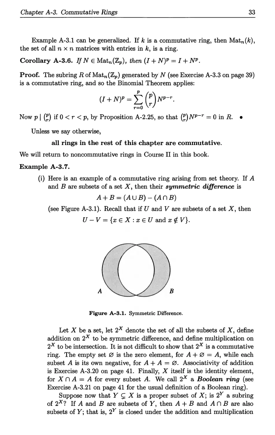
Text
Advanced
Modern Algebra
Third Edition, Part 1
Joseph J. Rotman
Graduate Studies
in Mathematics
Volume 165
I'- HEMJ\ 7"/('
Tf nOI \tH &
'{'J "- .. If>
B American Mathematical Society
'-:
.
Advanced
Modern Algebra
Third Edition, Part 1
Advanced
Modern Algebra
Third Edition, Part 1
Joseph J. Rotman
Graduate Studies
in Mathematics
Volume 165
American Mathematical Society
Providence, Rhode Island
EDITORIAL COMMITTEE
Dan Abramovich
Daniel S. Freed
Rafe Mazzeo (Chair)
G igliola Staffilani
The 2002 edition of this book was previously published by Pearson Education, Inc.
2010 Mathematics Subject Classification. Primary 12-01, 13-01, 14-01, 15-01, 16-01,
18-01, 20-01.
For additional information and updates on this book, visit
www .ams.org/bookpages / gsm-165
Library of Congress Cataloging-in-Publication Data
Rotman, Joseph J., 1934-
Advanced modern algebra / Joseph J. Rotman. - Third edition.
volumes cm. - (Graduate studies in mathematics; volume 165)
Includes bibliographical references and index.
ISBN 978-1-4704-1554-9 (alk. paper: pt. 1)
1. Algebra. I. Title.
QAI54.3.R68 2015
512-dc23
2015019659
Copying and reprinting. Individual readers of this publication, and nonprofit libraries
acting for them, are permitted to make fair use of the material, such as to copy select pages for
use in teaching or research. Permission is granted to quote brief passages from this publication in
reviews, provided the customary acknowledgment of the source is given.
Republication, systematic copying, or multiple reproduction of any material in this publication
is permitted only under license from the American Mathematical Society. Permissions to reuse
portions of AMS publication content are handled by Copyright Clearance Center's RightsLink@
service. For more information, please visit: http://www . ams. org/rightslink.
Send requests for translation rights and licensed reprints to reprint-permission<Dams. org.
Excluded from these provisions is material for which the author holds copyright. In such cases,
requests for permission to reuse or reprint material should be addressed directly to the author ( s) .
Copyright ownership is indicated on the copyright page, or on the lower right-hand corner of the
first page of each article within proceedings volumes.
Third edition @ 2015 by the American Mathematical Society. All rights reserved.
Second edition @ 2010 by the American Mathematical Society. All rights reserved.
First edition @ 2002 by the American Mathematical Society. All right reserved.
The American Mathematical Society retains all rights
except those granted to the United States Government.
Printed in the United States of America.
@ The paper used in this book is acid-free and falls within the guidelines
established to ensure permanence and durability.
Visit the AMS home page at http://www . ams .org/
10 9 8 7 6 5 4 3 2 1
20 19 18 17 16 15
To my wife
Marganit
and our two wonderful kids
Danny and Ella,
whom I love very much
Contents
Preface to Third Edition: Part 1
Acknowledgments
.
Xl
XIV
Part A. Course I
Chapter A-I. Classical Formulas
Cubics
Quartics
3
4
6
9
9
16
19
29
41
47
55
62
74
83
89
97
104
115
116
Chapter A-2. Classical Number Theory
Di visi bili ty
Euclidean Algorithms
Congruence
Chapter A-3. Commutative Rings
Polynomials
Homomorphisms
Quotient Rings
From Arithmetic to Polynomials
Maximal Ideals and Prime Ideals
Finite Fields
Irred uci bility
Euclidean Rings and Principal Ideal Domains
Unique Factorization Domains
Chapter A-4. Groups
Permutations
-
VB
viii
Contents
Even and Odd
Groups
Lagrange's Theorem
Homomorphisms
Quotient Groups
Simple Groups
Chapter A-5. Galois Theory
Insolvability of the Quintic
Classical Formulas and Solvability by Radicals
Translation into Group Theory
Fundamental Theorem of Galois Theory
Calculations of Galois Groups
123
127
139
150
159
173
179
179
187
190
200
223
235
243
247
247
259
Chapter A-6. Appendix: Set Theory
Equivalence Relations
Chapter A-7. Appendix: Linear Algebra
Vector Spaces
Linear Transformations and Matrices
Part B. Course II
Chapter B-1. Modules
Noncommutative Rings
Chain Conditions on Rings
Left and Right Modules
Chain Conditions on Modules
Exact Sequences
273
273
282
288
300
305
313
313
319
323
334
339
345
353
359
359
362
Chapter B-2. Zorn's Lemma
Zorn, Choice, and Well-Ordering
Zorn and Linear Algebra
Zorn and Free Abelian Groups
Semisimple Modules and Rings
Algebraic Closure
Transcendence
Liiroth's Theorem
Chapter B-3. Advanced Linear Algebra
Torsion and Torsion-free
Basis Theorem
Contents
.
IX
Fundamental Theorem
Elementary Divisors
Invariant Factors
From Abelian Groups to Modules
Rational Canonical Forms
Eigenvalues
Jordan Canonical Forms
Smith Normal Forms
Inner Product Spaces
Orthogonal and Symplectic Groups
Hermitian Forms and Unitary Groups
371
371
374
378
383
388
395
402
417
429
436
441
441
461
475
481
492
501
509
522
529
543
543
552
561
566
573
575
591
591
593
599
604
614
623
628
629
Chapter B-4. Categories of Modules
Categories
Functors
Galois Theory for Infinite Extensions
Free and Projective Modules
Injective Modules
Divisible Abelian Groups
Tensor Products
Adjoint Isomorphisms
Flat Modules
Chapter B-5. Multilinear Algebra
Algebras and Graded Algebras
Tensor Algebra
Exterior Algebra
Grassmann Algebras
Exterior Algebra and Differential Forms
Determinants
Chapter B-6. Commutative Algebra II
Old-Fashioned Algebraic Geometry
Affine Varieties and Ideals
Nullstellensatz
Nullstellensatz Redux
Irred uci ble Varieties
Affine Morphisms
Algorithms in k[Xl, . . . , xn]
Monomial Orders
x
Contents
Division Algorithm
Grabner Bases
636
639
651
651
657
659
666
673
678
681
687
693
Chapter B-7. Appendix: Categorical Limits
Inverse Limits
Direct Limits
Directed Index Sets
Adjoint Functors
Chapter B-8. Appendix: Topological Spaces
Topological Groups
Bibliography
Special Notation
Index
Preface to Third Edition:
Part 1
Algebra is used by virtually all mathematicians, be they analysts, combinatorists,
computer scientists, geometers, logicians, number theorists, or topologists. Nowa-
days, everyone agrees that some knowledge of linear algebra, group theory, and
commutative algebra is necessary, and these topics are introduced in undergrad-
uate courses. Since there are many versions of undergraduate algebra courses, I
will often review definitions, examples, and theorems, sometimes sketching proofs
and sometimes giving more details. 1 Part 1 of this third edition can be used as a
text for the first year of graduate algebra, but it is much more than that. It and
the forthcoming Part 2 can also serve more advanced graduate students wishing to
learn topics on their own. While not reaching the frontiers, the books provide a
sense of the successes and methods arising in an area. In addition, they comprise
a reference containing many of the standard theorems and definitions that users of
algebra need to know. Thus, these books are not merely an appetizer, they are a
hearty meal as well.
When I was a student, Birkhoff-Mac Lane, A Survey of Modern Algebra [8], was
the text for my first algebra course, and van der Waerden, Modern Algebra [118],
was the text for my second course. Both are excellent books (I have called this
book Advanced Modern Algebra in homage to them), but times have changed since
their first publication: Birkhoff and Mac Lane's book appeared in 1941; van der
Waerden's book appeared in 1930. There are today major directions that either
did not exist 75 years ago, or were not then recognized as being so important, or
were not so well developed. These new areas involve algebraic geometry, category
1 It is most convenient for me, when reviewing earlier material, to refer to my own text FCAA:
A First Course in Abstract Algebra, 3rd ed. [94], as well as to LMA, the book of A. Cuoco and
myself [23], Learning Modern Algebra from Early Attempts to Prove Fermat's Last Theorem.
-
.
Xl
. .
XlI
Preface to Third Edition: Part 1
theory, 2 computer science, homological algebra, and representation theory. Each
generation should survey algebra to make it serve the present time.
The passage from the second edition to this one involves some significant
changes, the major change being organizational. This can be seen at once, for
the elephantine 1000 page edition is now divided into two volumes. This change
is not merely a result of the previous book being too large; instead, it reflects the
structure of beginning graduate level algebra courses at the University of Illinois
at Urbana-Champaign. This first volume consists of two basic courses: Course I
(Galois theory) followed by Course II (module theory). These two courses serve as
joint prerequisites for the forthcoming Part 2, which will present more advanced
topics in ring theory, group theory, algebraic number theory, homological algebra,
representation theory, and algebraic geometry.
In addition to the change in format, I have also rewritten much of the text.
For example, noncommutative rings are treated earlier. Also, the section on alge-
braic geometry introduces regular functions and rational functions. Two proofs of
the Nullstellensatz (which describes the maximal ideals in k[Xl, . . . , xn] when k is
an algebraically closed field) are given. The first proof, for k = <C (which easily
generalizes to uncountable k), is the same proof as in the previous edition. But the
second proof I had written, which applies to countable algebraically closed fields
as well, was my version of Kaplansky's account [55] of proofs of Goldman and of
Krull. I should have known better! Kaplansky was a master of exposition, and
this edition follows his proof more closely. The reader should look at Kaplansky's
book, Selected Papers and Writings [58], to see wonderful mathematics beautifully
expounded.
I have given up my attempted spelling reform, and I now denote the ring of
integers mod m by Zm instead of by Hm. A star * before an exercise indicates that
it will be cited elsewhere in the book, possibly in a proof.
The first part of this volume is called Course I; it follows a syllabus for an
actual course of lectures. If I were king, this course would be a transcript of my
lectures. But I am not king and, while users of this text may agree with my global
organization, they may not agree with my local choices. Hence, there is too much
material in the Galois theory course (and also in the module theory course), because
there are many different ways an instructor may choose to present this material.
Having lured students into beautiful algebra, we present Course II: module
theory; it not only answers some interesting questions (canonical forms of matrices,
for example) but it also introduces important tools. The content of a sequel algebra
course is not as standard as that for Galois theory. As a consequence, there is much
more material here than in Course I, for there are many more reasonable choices of
material to be presented in class.
To facilitate various choices, I have tried to make the text clear enough so that
students can read many sections independently.
Here is a more detailed description of the two courses making up this volume.
2 A Survey of Modern Algebra was rewritten in 1967, introducing categories, as Mac Lane-
Birkhoff, Algebra [73].
Preface to Third Edition: Part 1
. . .
XIB
Course I
After presenting the cubic and quartic formulas, we review some undergraduate
number theory: division algorithm; Euclidian algorithms (finding d = gcd(a, b)
and expressing it as a linear combination), and congruences. Chapter 3 begins
with a review of commutative rings, but continues with maximal and prime ideals,
finite fields, irreducibility criteria, and euclidean rings, PIDs, and UFD's. The next
chapter, on groups, also begins with a review, but it continues with quotient groups
and simple groups. Chapter 5 treats Galois theory. After introducing Galois groups
of extension fields, we discuss solvability, proving the Jordan-Holder Theorem and
the Schreier Refinement Theorem, and we show that the general quintic is not
solvable by radicals. The Fundamental Theorem of Galois Theory is proved, and
applications of it are given; in particular, we prove the Fundamental Theorem of
Algebra (C is algebraically closed). The chapter ends with computations of Galois
groups of polynomials of small degree.
There are also two appendices: one on set theory and equivalence relations;
the other on linear algebra, reviewing vector spaces, linear transformations, and
matrices.
Course II
As I said earlier, there is no commonly accepted syllabus for a sequel course,
and the text itself is a syllabus that is impossible to cover in one semester. However,
much of what is here is standard, and I hope instructors can design a course from
it that they think includes the most important topics needed for further study. Of
course, students (and others) can also read chapters independently.
Chapter 1 (more precisely, Chapter B-1, for the chapters in Course I are labeled
A-I, A-2, etc.) introduces modules over noncommutative rings. Chain conditions
are treated, both for rings and for modules; in particular, the Hilbert Basis The-
orem is proved. Also, exact sequences and commutative diagrams are discussed.
Chapter 2 covers Zorn's Lemma and many applications of it: maximal ideals; bases
of vector spaces; subgroups of free abelian groups; semisimple modules; existence
and uniqueness of algebraic closures; transcendence degree (along with a proof of
Liiroth's Theorem). The next chapter applies modules to linear algebra, proving
the Fundamental Theorem of Finite Abelian Groups as well as discussing canonical
forms for matrices (including the Smith normal form which enables computation
of invariant factors and elementary divisors). Since we are investigating linear al-
gebra, this chapter continues with bilinear forms and inner product spaces, along
with the appropriate transformation groups: orthogonal, symplectic, and unitary.
Chapter 4 introduces categories and functors, concentrating on module categories.
We study projective and injective modules (paying attention to projective abelian
groups, namely free abelian groups, and injective abelian groups, namely divisible
abelian groups), tensor products of modules, adjoint isomorphisms, and flat mod-
ules (paying attention to flat abelian groups, namely torsion-free abelian groups).
Chapter 5 discusses multilinear algebra, including algebras and graded algebras,
tensor algebra, exterior algebra, Grassmann algebra, and determinants. The last
.
XIV
Preface to Third Edition: Part 1
chapter, Commutative Algebra II, has two main parts. The first part discusses
"old-fashioned algebraic geometry," describing the relation between zero sets of
polynomials (of several variables) and ideals (in contrast to modern algebraic ge-
ometry, which extends this discussion using sheaves and schemes). We prove the
Nullstellensatz (twice!), and introduce the category of affine varieties. The second
part discusses algorithms arising from the division algorithm for polynomials of
several variables, and this leads to Grabner bases of ideals.
There are again two appendices. One discusses categorical limits (inverse limits
and direct limits), again concentrating on these constructions for modules. We also
mention adjoint functors. The second appendix gives the elements of topological
groups. These appendices are used earlier, in Chapter B-4, to extend the Funda-
mental Theorem of Galois Theory from finite separable field extensions to infinite
separable algebraic extensions.
I hope that this new edition presents mathematics in a more natural way,
making it simpler to digest and to use.
I have often been asked whether solutions to exercises are available. I believe
it is a good idea to have some solutions available for undergraduate students, for
they are learning new ways of thinking as well as new material. Not only do
solutions illustrate new techniques, but comparing them to one's own solution also
builds confidence. But I also believe that graduate students are already sufficiently
confident as a result of their previous studies. As Charlie Brown in the comic strip
Peanuts says,
"In the book of life, the answers are not in the back."
Acknowledgments
The following mathematicians made comments and suggestions that greatly im-
proved the first two editions: Vincenzo Acciaro, Robin Chapman, Daniel R. Grayson,
Ilya Kapovich, T.-Y. Lam, David Leep, Nick Loehr, Randy McCarthy, Patrick
Szuta, and Stephen Ullom. I thank them again for their help.
For the present edition, I thank T.-Y. Lam, Bruce Reznick, and Stephen Ullom,
who educated me about several fine points, and who supplied me with needed
references.
I give special thanks to Vincenzo Acciaro for his many comments, both mathe-
matical and pedagogical, which are incorporated throughout the text. He carefully
read the original manuscript of this text, apprising me of the gamut of my errors,
from detecting mistakes, unclear passages, and gaps in proofs, to mere typos. I
rewrote many pages in light of his expert advice. I am grateful for his invaluable
help, and this book has benefited much from him.
Joseph Rotman
Urbana, IL, 2015
Part A
Course I
Chapter A-1
Classical Formulas
As Europe emerged from the Dark Ages, a major open problem in mathematics
was finding roots of polynomials. The Babylonians, four thousand years ago, knew
how to find the roots of a quadratic polynomial. For example, a tablet dating from
1700 BCE poses the problem:
I have subtracted the side of the square from its area, and it is 870. What is
the side of my square?
In modern notation, the text asks for a root of x 2 - x = 870, and the tablet
then gives a series of steps computing the answer. It would be inaccurate to say
that the Babyloni ans knew the quadratic formula (the roots ofax + bx + care
2 (-b::i: v b 2 - 4ac), however, for modern notation and, in particular, formulas, were
unknown to them. 1 The discriminant b 2 - 4ac here is 1 - 4( -870) = 3481 = 59 2 ,
which is a perfect square. Even though finding square roots was not so simple in
those days, this problem was easy to solve; Babylonians wrote numbers in base 60,
so that 59 = 60 - 1 was probably one reason for the choice of 870. The ancients also
considered cubics. Another tablet from about the same time posed the problem of
solving 12x 3 = 3630. Their solution, most likely, used a table of approximations to
cube roots.
1 We must mention that modern notation was not introduced until the late 1500s, but it
was generally agreed upon only after the influential book of Descartes appeared in 1637. To
appreciate the importance of decent notation, consider Roman numerals. Not only are they
clumsy for arithmetic, they are also complicated to write-is 95 denoted by VC or by XCV?
The symbols + and - were introduced by Widman in 1486, the equality sign = was invented
by Recorde in 1557, exponents were invented by Hume in 1585, and letters for variables were
invented by Viete in 1591 (he denoted variables by vowels and constants by consonants). Stevin
introduced decimal notation in Europe in 1585 (it had been used earlier by the Arabs and the
Chinese). In 1637, Descartes used letters at the beginning of the alphabet to denote constants,
and letters at the end of the alphabet to denote variables, so we can say that Descartes invented
"x the unknown." Not all of Descartes' notation was adopted. For example, he used 00 to denote
equality and = for :i::; Recorde's symbol = did not appear in print until 1618 (see Cajori [16]).
-
3
4
Chapter A-i. Classical Formulas
Here is a corollary of the quadratic formula.
Lemma A-1.1. Given any pair of numbers M and N, there are (possibly complex)
numbers g and h with g + h = M and gh = N; moreover, g and h are the roots of
x 2 - M x + N.
Proof. The quadratic formula provides roots g and h of x 2 - Mx + N. Now
x 2 - Mx + N = (x - g) (x - h) = x 2 - (g + h)x + gh,
and so g + h = M and gh = N. .
The Golden Age of ancient mathematics was in Greece from about 600 BCE
to 100 BCE. The first person we know who thought that proofs are necessary was
Thales of Miletus (624 BCE-546 BCE) 2 . The statement of the Pythagorean Theorem
(a right triangle with legs of lengths a, b and hypotenuse of length c satisfies a 2 +b 2 =
c 2 ) was known to the Babylonians; legend has it that Thales' student Pythagorus
(580 BCE-520 BCE) was the first to prove it. Some other important mathematicians
of this time are: Eudoxus (408 BCE-355 BCE), who found the area of a circle;
Euclid (325 BCE-265 BCE), whose great work The Elements consists of six books
on plane geometry, four books on number theory, and three books on solid geometry;
Theatetus (417 BCE-369 BCE), whose study of irrationals is described in Euclid's
Book X, and who is featured in two Platonic dialogues; Eratosthenes (276 BCE-
194 BCE), who found the circumference of a circle and also studied prime numbers;
the geometer Apollonius (262 BCE-190 BCE); Hipparchus (190 BCE-120 BCE), who
introduced trigonometry; Archimedes (287 BCE-212 BCE), who anticipated much of
modern calculus, and is considered one of the greatest mathematicians of all time.
The Romans displaced the Greeks around 100 BCE. They were not at all
theoretical, and mathematics moved away from Europe, first to Alexandria, Egypt,
where the number theorist Diophantus (200 cE-284 CE) and the geometer Pappus
(290 cE-350 CE) lived, then to India around 400 CE, then to the Moslem world
around 800. Mathematics began its return to Europe with translations into Latin,
from Greek, Sanskrit, and Arabic texts, by Adelard of Bath (1075-1160), Gerard
of Cremona (1114-1187), and Leonardo da Pisa (Fibonacci) (1170-1250).
For centuries, the Western World believed that the high point of civilization
occurred during the Greek and Roman eras and the beginnning of Christianity. But
this world view changed dramatically in the Renaissance about five hundred years
ago. The printing press was invented by Gutenberg around 1450, Columbus landed
in North America in 1492, Luther began the Reformation in 1517, and Copernicus
published De Revolutionibus in 1530.
Cubics
Arising from a tradition of public mathematics contests in Venice and Pisa, methods
for finding the roots of cubics and quartics were found in the early 1500s by Scipio
del Ferro (1465-1526), Niccolo Fontana (1500-1554), also called Tartaglia, Lodovici
2 Most of these very early dates are approximate.
Cubics
5
Ferrari (1522-1565), and Giralamo Cardano (1501-1576) (see Tignol [115] for an
excellent account of this early history).
We now derive the cubic formula. The change of variable X = x -1 b transforms
the cubic F(X) = X 3 + bX 2 + cX + d into the simpler polynomial F(x - 1b) =
f(x) = x 3 + qx + r whose roots give the roots of F(X): If u is a root of f(x), then
u -lb is a root of F(X), for
o = f(u) = F(u -lb).
Theorem A-1.2 (Cubic Formula). The roots of f(x) = x 3 + qx + rare
9 + h, wg + w 2 h, and w 2 g + wh,
where g3 = (-r + VR), h = -q/3g, R = r 2 + 2 q3, and w = - + i 1 'tS a
primitive cube root of unity.
Proof. Write a root u of f(x) = x 3 + qx + r as
u = 9 + h,
where 9 and h are to be chosen, and substitute:
o = f ( u) = f (g + h)
= (g + h)3 + q(g + h) + r
= g3 + 3g 2 h + 3gh 2 + h 3 + q(g + h) + r
= g3 + h 3 + 3gh(g + h) + q(g + h) + r
= g3 + h 3 + (3gh + q)u + r.
If 3gh + q = 0, then gh = -lq. Lemma A-1.1 says that there exist numbers g, h
with 9 + h = u and gh = -lq; this choice forces 3gh + q = 0, so that g3 + h 3 = -r.
After cubing both sides of gh = -lq, we obtain the pair of equations
g3 + h 3 = -r,
g 3 h 3 _ _..l.. q 3
- 27 .
By Lemma A-1.1, there is a quadratic equation in g3:
g6 + rg 3 - 2\ q3 = O.
The quadratic formula gives
g3 = (-r + Jr 2 + 2 q3) = (-r + v'R)
(note that h 3 is also a root of this quadratic, so that h 3 = ( -r - VR), and so
g3 - h 3 = VR). There are three cube roots of g3, namely, g, wg, and w 2 g. Because
of the constraint gh = -q/3, each of these has a "mate:" 9 and h = -q/(3g); wg
and w 2 h = -q/(3wg); w 2 g and wh = -q/(3w 2 g) (for w 3 = 1). .
6
Chapter A-l. Classical Formulas
Example A-1.3. If f(x) = x 3 - 15x - 126, then q = -15, r = -126, R = 15376,
and v'R = 124. Hence, g3 = 125, so that 9 = 5. Thus, h = -q/(3g) = 1. Therefore,
the roots of f ( x) are
6, 5w + w 2 = -3 + 2iV3, 5w 2 + w = -3 - 2iV3.
Alternatively, having found one root to be 6, the other two roots can be found as
the roots of the quadratic f(x)/(x - 6) = x 2 + 6x + 21.
Example A-1.4. The cubic formula is not very useful because it often gives roots
in unrecognizable form. For example, let
f(x) = (x - l)(x - 2)(x + 3) = x 3 - 7x + 6;
the roots of f(x) are, obvi ously, 1,2, and - 3, an d the cubic formu la gives
9 + h = V ( -6 + V -: o) + V ( -6 - V -: o ) ·
It is not at all obvious that 9 + h is a real number, let alone an integer.
Another cubic formula, due to Viete, gives the roots in terms of trigonometric
functions instead of radicals (FCAA [94] pp. 360-362).
Before the cubic formula, mathematicians had no difficulty in ignoring negative
numbers or square roots of negative numbers when dealing with quadratic equa-
tions. For example, consider the problem of finding the sides x and y of a rectangle
having area A and perimeter p. The equations xy = A and 2x + 2y = p give the
quadratic 2x2 - px + 2A. The quadratic formula gi ves
x = (P:l:: Vp 2 -16A)
and y = A/x. If p2 - 16A > 0, the problem is solved. If p2 - 16A < 0, they didn't
invent fantastic rectangles whose sides involve square roots of negative numbers;
they merely said that there is no rectangle whose area and perimeter are so related.
But the cubic formula does not allow us to discard "imaginary" roots, for we have
just seen, in Example A-1.4 , that an "hones t" re al and positive ro ot can appear
in terms of such radicals: V ( -6 + V -: o ) + V ( -6 - J -: o ) is an integer!3
Thus, the cubic formula was revolutionary. For the next 100 years, mathematicians
reconsidered the meaning of number, for understanding the cubic formula raises the
questions whether negative numbers and complex numbers are legitimate entities.
Quartics
Consider the quartic F(X) = X 4 + bX 3 + cX 2 + dX + e. The change of variable
X = x - ib yields a simpler polynomial f(x) = x 4 + qx 2 + rx + s whose roots give
the roots of F(X): if u is a root of f(x), then u- ib is a root of F(X). The quartic
3Every cubic with real coefficients has a real root, and mathematicians tried various substi-
tutions to rewrite the cubic formula solely in terms of real numbers. Later we will prove the Casus
lrreducibilis which states that it is impossible to always do so.
Quartics
7
formula was found by Lodovici Ferrari in the 1540s, but we present the version
given by Descartes in 1637. Factor f(x),
f(x) = x 4 + qx 2 + rx + s = (x 2 + jx + f)(x 2 - jx + m),
and determine j, f and m (note that the coefficients of the linear terms in the
quadratic factors are j and -j because f(x) has no cubic term). Expanding and
equating like coefficients gives the equations
/J .2
t. + m - J = q,
j(m - f) = r,
fm = s.
The first two equations give
2m = j2 + q + r / j,
2f=j2+ q - r /j.
Substituting these values for m and f into the third equation yields a cubic in j2,
called the resolvent cubic:
(j2)3 + 2q(j2)2 + (q2 _ 4s )j2 _ r 2 .
The cubic formula gives j2, from which we can determine m and f, and hence the
roots of the quartic. The quartic formula has the same disadvantage as the cubic
formula: even though it gives a correct answer, the values of the roots are usually
unrecognizable.
Note that the quadratic formula can be derived in a way similar to the deriva-
tion of the cubic and quartic formulas. The change of variable X = x - !b re-
places the quadratic polynomial F(X) = X 2 + bX + c with the simpler polynomial
f(x) = x 2 +q whose roots give the roots of F(X): if u is a root of f(x), then u-!b
is a root of F(X). An e xplicit formula for q is c - ib2, so that the ro ots of f (x)
are, obviously, u = :f:! v b 2 - 4c; thus, the roots of F(X) are! ( - b:f: v b 2 - 4c).
It is now very tempting, as it was for our ancestors, to seek the roots of a quintic
F(X) = X5 + bX 4 + cX 3 + dX 2 + eX + f (of course, they wanted to find roots of
polynomials of any degree). Begin by changing variable X = x-!b to eliminate the
X 4 term. It was natural to expect that some further ingenious substitution together
with the formulas for roots of polynomials of lower degree, analogous to the resolvent
cubic, would yield the roots of F(X). For almost 300 years, no such formula was
found. In 1770, Lagrange showed that reasonable substitutions lead to a polynomial
of degree six, not to a polynomial of degree less than 5. Informally, let us say that
a polynomial f(x) is solvable by radicals if there is a formula for its roots which
has the same form as the quadratic, cubic, and quartic formulas; that is, it uses only
arithmetic operations and roots of numbers involving the coefficients of f(x). In
1799, Ruffini claimed that the general quintic formula is not solvable by radicals, but
his contemporaries did not accept his proof; his ideas were, in fact, correct, but his
proof had gaps. In 1815, Cauchy introduced the multiplication of permutations, and
he proved basic properties of the symmetric group Sn; for example, he introduced
the cycle notation and proved unique factorization of permutations into disjoint
cycles. In 1824, Abel gave an acceptable proof that there is no quintic formula; in
8
Chapter A-l. Classical Formulas
his proof, Abel constructed permutations of the roots of a quintic, using certain
rational functions introduced by Lagrange. In 1830, Galois, the young wizard who
was killed before his 21st birthday, modified Lagrange's rational functions but, more
important, he saw that the key to understanding which polynomials of any degree
are solvable by radicals involves what he called groups: subsets of the symmetric
group Sn that are closed under composition-in our language, subgroups of Sn.
To each polynomial f(x), he associated such a group, nowadays called the Galois
group of f(x). He recognized conjugation, normal subgroups, quotient groups, and
simple groups, and he proved, in our language, that a polynomial (over a field of
characteristic 0) is solvable by radicals if and only if its Galois group is a solvable
group (solvability being a property generalizing commutativity). A good case can
be made that Galois was one of the most important founders of modern algebra.
We recommend the book of Tignol [115] for an authoritative account of this history.
Exercises
* A-l.l. The following problem, from an old Chinese text, was solved by Qin Jiushao 4 in
1247. There is a circular castle, whose diameter is unknown; it is provided with four gates,
and two li out of the north gate there is a large tree, which is visible from a point six li
east of the south gate (see Figure A-l.l). What is the length of the diameter?
T
s
6
E
Figure A-l.l. Castle Problem.
Hint. The answer is a root of a cubic polynomial.
A-l.2. (i) Find the complex roots of f(x) = x 3 - 3x + 1.
(ii) Find the complex roots of f(x) = x 4 - 2x 2 + 8x - 3.
A-l.3. Show that the quadratic formula does not hold for f(x) = ax 2 + bx + c if we view
the coefficients a, b, c as lying in Z2, the integers mod 2.
4This standard transliteration into English was adopted in 1982; earlier spelling is Ch'in
Chi u-shao.
Chapter A - 2
Classical Number Theory
Since there is a wide variation in what is taught in undergraduate algebra courses,
we now review definitions and theorems, usually merely sketching proofs and ex-
amples. Even though much of this material is familiar, you should look at it to see
that your notation agrees with mine. For more details, we may cite specific results,
either in my book FCAA [94], A First Course in Abstract Algebra, or in LMA [23],
the book of A. Cuoco and myself, Learning Modern Algebra from Early Attempts
to Prove Fermat's Last Theorem. Of course, these results can be found in many
other introductory abstract algebra texts as well.
Divisibility
Notation. The natural numbers N is the set of all nonnegative integers
N = {O, 1, 2, 3, . . .}.
The set Z of all integers, positive, negative, and zero, is
Z = {:f:n : n EN}.
(This notation arises from Z being the initial letter of Zahlen, the German word for
numbers. )
We assume that N satisfies the Least Integer Axiom (also called the Well-
Ordering Principle): Every nonempty subset C C N contains a smallest element;
that is, there is Co E C with Co < c for all c E C.
Definition. If a, b E Z, then a divides b, denoted by
a I b,
if there is an integer c with b = ac. We also say that a is a divisor of b or that b
is a multiple of a.
Note that every integer a divides 0, but 0 I a if and only if a = o.
-
9
10
Chapter A-2. Classical Number Theory
Lemma A-2.1. If a and b are positive integers and a I b, then a < b.
Proof. Suppose that b = ac. Since 1 is the smallest positive integer, 1 < c and
a < ac = b. .
Theorem A-2.2 (Division Algorithm). If a and b are integers with a # 0, then
there are unique integers q and r, called the quotient and remainder, with
b = qa + rand 0 < r < lal.
Proof. This is just familiar long division. First establish the special case in which
a > 0: r is the smallest natural number of the form b - na with n E Z (see [23]
Theorem 1.15), and then adjust the result for negative a. .
Thus, a I b if and only if the remainder after dividing b by a is O.
Definition. A common divisor of integers a and b is an integer c with c I a and
c I b. The greatest common divisor of a and b, denoted by gcd(a, b), is defined
by
cd(a b) = { o if a = 0 = b,
g, the largest common divisor of a and b otherwise.
This definition extends in the obvious way to give the gcd of integers aI, . . . , an.
We saw, in Lemma A-2.1, that if a and m are positive integers with a I m,
then a < m. It follows that gcd's always exist: there are always positive common
divisors (1 is always a common divisor), and there are only finitely many positive
common divisors < min {a, b}.
Definition. A linear combination of integers a and b is an integer of the form
sa + tb,
where s, t E Z.
The next result is one of the most useful properties of gcd's.
Theorem A-2.3. If a and b are integers, then gcd(a, b) is a linear combination of
a and b.
Proof. We may assume that at least one of a and b is not zero. Consider the set I
of all the linear combinations of a and b:
I = {sa+tb: s,t E Z}.
Both a and b are in I, and the set C of all those positive integers lying in I is
nonempty. By the Least Integer Axiom, C contains a smallest positive integer,
say d, and it turns out that d is the gcd ([23] Theorem 1.19). .
If d = gcd(a, b) and if c is a common divisor of a and b, then c < d, by
Lemma A-2.1. The next corollary shows that more is true: c is a divisor of d; that
is, c I d for every common divisor c.
Divisibility
11
Corollary A-2.4. Let a and b be integers. A nonnegative common divisor d is
their gcd if and only if c I d for every common divisor c of a and b.
Proof. [23], Corollary 1.20. .
Definition. An integer P is prime if P > 2 and its only divisors are :f:1 and :f:p.
If an integer a > 2 is not prime, then it is called composite.
On reason we don't consider 1 to be prime is that some theorems would become
more complicated to state. For example, if we allow 1 to be prime, then the
Fundamental Theorem of Arithmetic (Theorem A-2.13 below: unique factorization
into primes) would be false: we could insert 500 factors equal to 1.
Proposition A-2.5. Every integer a > 2 has a factorization
a = PI . · . Pt,
where PI < . . . < Pt and all Pi are prime.
Proof. The proof is by induction on a > 2. The base step holds because a = 2
is prime. If a > 2 is prime, we are done; if a is composite, then a = uv with
2 < u, v < a, and the inductive hypothesis says each of u, v is a product of primes.
.
We allow products to have only one factor. In particular, we can say that 3 is
a product of primes. Collecting terms gives prime factorizations (it is convenient
to allow exponents in prime factorizations to be 0).
Definition. If a > 2 is an integer, then a prime factorization of a is
el e2 et
a = PI P2 ... Pt ,
where the Pi are distinct primes and ei > 0 for all i.
Corollary A-2.6. There are infinitely many primes.
Proof. If there are only finitely many primes, say, PI, . . . , Pt, then N = 1 + PI . . · Pt
is not a product of primes, for the Division Algorithm says that the remainder after
dividing N by any prime Pi is 1, not O. This contradicts Proposition A-2.5. .
Lemma A-2.7. Ifp is a prime and b is any integer, then
gcd(p, b) = { p if P I b
1 otherw'tse.
Proof. A common divisor c of P and b is, in particular, a divisor of p. But the only
positive divisors of pare 1 and p. .
The next theorem gives one of the most important characterizations of prime
numbers.
12
Chapter A-2. Classical Number Theory
Theorem A-2.8 (Euclid's Lemma). If p is a prime and p 1 ab, for integers a
and b, then pia or p 1 b. More generally, if pial. . . at, then p 1 ai for some i.
Conversely, if m > 2 is an integer such that m 1 ab always implies m 1 a or
m I b, then m is a prime.
Proof. Suppose that p f a. Since gcd(p, a) = 1 (by Lemma A-2.7), there are
integers sand t with 1 = sp + ta (by Theorem A-2.3). Hence,
b = spb + tab.
Now p divides both expressions on the right, and so p 1 b.
Conversely, if m = ab is composite (with a, b < m), then ab is a product
divisible by m with neither factor divisible by m. .
To illustrate: 6 1 12 and 12 = 4 x 3, but 6 f 4 and 6 f 3. Of course, 6 is not
prime. On the other hand, 2 112, 2 f 3, and 2 1 4.
Definition. Call integers a and b relatively prime if their gcd is 1.
Thus, a and b are relatively prime if their only common divisors are :f:1. For
example, 2 and 3 are relatively prime, as are 8 and 15.
Here is a generalization of Euclid's Lemma having the same proof.
Corollary A-2.9. Let a, b, and c be integers. If c and a are relatively prime and
if c I ab, then c lb.
Proof. There are integers sand t with 1 = se + ta, and so b = scb + tab. .
Lemma A-2.10. Let a and b be integers.
(i) Then gcd(a, b) = 1 (that is, a and b are relatively prime) if and only if 1
is a linear combination of a and b.
(ii) If d = gcd(a, b), then the integers aid and bid are relatively prime.
Proof. The first statement follows from Theorem A-2.3; the second is LMA Propo-
sition 1.23 .
Definition. An expression alb for a rational number (where a and b are integers)
is in lowest terms if a and b are relatively prime.
Proposition A-2.11. Every nonzero rational number alb has an expression in
lowest terms.
a a'd a' a
Proof. If d = gcd(a, b), then a = a'd, b = b'd, and b = b'd = b' . But a' = d and
b
b' = d ' so gcd( a', b') = 1 by Lemma A-2.10. .
Proposition A-2.12. There is no rational number alb whose square is 2.
Divisibility
13
Proof. Suppose, on the contrary, that (a/b)2 = 2. We may assume that a/b is in
lowest terms; that is, gcd(a,b) = 1. Since a 2 = 2b 2 , Euclid's Lemma gives 21 a,
and so 2m = a. Hence, 4m 2 = a 2 = 2b 2 , and 2m 2 = b 2 . Euclid's Lemma now gives
2 I b, contradicting gcd(a, b) = 1. .
This last result is significant in the history of mathematics. The ancient Greeks
defined number to mean "positive integer," while rationals were not viewed as
numbers but, rather, as ways of comparing two lengths. They called two segments
of lengths a and b commensurable if there is a third segment of length e with
a = me and b = ne for positive integers m and n. That V2 is irrational was a
shock to the Pythagoreans; given a square with sides of length 1, its diagonal and
side are not commensurable; that is, V2 cannot be defined in terms of numbers
(positive integers) alone. Thus, there is no numerical solution to the equation
x 2 = 2, but there is a geometric solution. By the time of Euclid, this problem
had been resolved by splitting mathematics into two different disciplines: number
theory and geometry.
In ancient Greece, algebra as we know it did not really exist; Greek mathemati-
cians did geometric algebra. For simple ideas, geometry clarifies algebraic formulas.
For example, (a + b)2 = a 2 + 2ab + b 2 or completing the square (x + !b)2 -
(!b)2 + bx + x 2 (adjoining the white square to the shaded area gives a square).
a a 2
ab
.- - - - - - . - -
I
I
I
I
I
I
I
I
!b
2
b ab
b 2
x
a
b
!b
2
x
For more difficult ideas, say, equations of higher degree, the geometric figures in-
volved are very complicated, and geometry is no longer clarifying.
Theorem A-2.13 (Fundamental Theorem of Arithmetic). Every integer
a > 2 has a unique factorization
el et
a = PI ... Pt ,
where PI < . . . < Pt, all Pi are prime, and all ei > o.
Proof. Suppose a = p l · . · p t and a = q{l . . . q[s are prime factorizations. Now
Pt 1 q{l . . . q[s, so that Euclid's Lemma gives Pt I qj for some j. Since qj is prime,
however, Pt = qj. Cancel Pt and qj, and the proof is completed by induction on
max { t, s } . .
The next corollary makes use of our convention that exponents in prime fac-
torizations are allowed to be o.
14
Chapter A-2. Classical Number Theory
Corollary A-2.14. If a = p l . · . p t and b = p{l · . . p{t are prime factorizations,
then a I b if and only if ei < fi for all i.
If g and h are divisors of a, then their product gh need not be a divisor of a.
For example, 6 and 15 are divisors of 60, but 6 x 15 = 90 is not a divisor of 60.
Proposition A-2.15. Let 9 and h be divisors of a. If gcd(g, h) = 1, then gh I a.
Proof. If a = p l p 2 · · . p t is a prime factorization, then 9 = p l · · · p:t and h =
p l . . . p t, where 0 < k i < ei and 0 < f i < ei for all i. Since gcd(g, h) = 1, however,
no prime Pi is a common divisor of them, and so k i > 0 implies f i = 0 and fj > 0
implies k j = O. Hence, 0 < k i + f i < ei for all i, and so
gh - P k l +£1 P kt+£t I P el P et - a .
- 1 ... t 1 ... t - ·
Definition. If a, b are integers, then a common multiple is an integer m with
a I m and b I m. Their least common multiple, denoted by
lcm(a, b),
is their smallest common multiple. This definition extends in the obvious way to
give the lcm of integers aI, . . . , an.
Proposition A-2.16. If a = p l . . . p t and b = p{l . . · p!t are prime factorizations,
then
gcd(a, b) = pr;"l . . . pr;"t and lcm(a, b) = p l . . . p t,
where mi = min{ei, fi} and M i = max{ei, fi} for all i.
Proof. First, pr;"l . . · pr;"t is a common divisor, by Corollary A-2.14. If d=p l . . . p:t
is any common divisor of a and b, then k i < ei and k i < fi; hence, k i < min { ei, fi} =
mi, and d I a and d I b. Thus, pr;"l . . . pr;"t = gcd(a, b), by Corollary A-2.4.
The statement about lcm's is proved similarly. .
Corollary A-2.17. If a and b are integers, then
ab = gcd(a, b) lcm(a, b).
P f If el et d b 11 It th
roo . a = PI ... Pt an = PI ... Pt, en
min{ ei, fi} + max{ ei, fi} = mi + 1\1 i = ei + fi. ·
Exercises
A-2.1. Prove or disprove and salvage if possible. ("Disprove" here means "give a concrete
counterexample." "Salvage" means "add a hypothesis to make it true.")
(i) gcd(O, b) = b,
(ii) gcd(a 2 , b 2 ) = (gcd(a, b))2,
(iii) gcd(a, b) = gcd(a, b + ka) (k E Z),
(iv) gcd(a, a) = a,
Divisibility
15
(v) gcd(a, b) = gcd(b, a),
(vi) gcd(a, 1) = 1,
(vii) gcd(a, b) = - gcd( -a, b).
* A-2.2. If x is a real number, let LxJ denote the largest integer n with n < x. (For
example, 3 = L 1r J and 5 = L 5 J .) Show that the quotient q in the Division Algorithm is
Lb/aJ.
A-2.3. Let Pl,P2,P3,. .. be the list of the primes in ascending order: Pl = 2, P2 = 3,
P3 = 5,. .. Define Ik = PIP2 . . . Pk + 1 for k > 1. Find the smallest k for which Ik is not a
prime.
Hint. 19 I 17, but 7 is not the smallest k.
* A-2.4. If d and d' are nonzero integers, each of which divides the other, prove that
d' = f:d.
* A-2.5. If gcd(r, a) = 1 = gcd(r', a), prove that gcd(rr', a) = 1.
* A-2.6. (i) Prove that if a positive integer n is squarefree (i.e., n is not divisible by the
square of any prime), then .In is irrational.
(ii) Prove that an integer m > 2 is a perfect square if and only if each of its prime
factors occurs an even number of times.
* A-2. 7. Prove that is irrational.
Hint. Assume that can be written as a fraction in lowest terms.
A-2.8. If a > 0, prove that agcd(b, c) = gcd(ab, ac). (We must assume that a > 0 lest
a gcd(b, c) be negative.)
Hint. Show that if k is a common divisor of ab and ac, then k I a gcd(b, c).
* A-2.9. (i) Show that if d is the greatest common divisor of al, a2,. . . , an, then d =
L: tiai, where ti is in Z for 1 < i < n.
(ii) Prove that if c is a common divisor of al, a2,. . . , an, then c I d.
* A-2.10. A Pythagorean triple is an ordered triple (a, b, c) of positive integers for which
a 2 +b 2 = c 2 ;
it is called primitive if there is no d > 1 which divides a, band c.
(i) If q > P are positive integers, prove that
(q2 _ p2, 2qp, q2 + p2)
is a Pythagorean triple (every primitive Pythagorean triple (a, b, c) is of this type).
(ii) Show that the Pythagorean triple (9, 12, 15) is not of the type given in part (i).
(iii) Using a calculator that can find square roots but which displays only 8 digits, prove
that
(19597501,28397460,34503301)
is a Pythagorean triple by finding q and p.
A-2.11. Prove that an integer M > 0 is the smallest common multiple of al, a2, . . . , an
if and only if it is a common multiple of al, a2, . . . , an that divides every other common
multiple.
16
Chapter A-2. Classical Number Theory
* A-2.12. Let al/bl,"', an/b n be rational numbers in lowest terms. If M =lcm{b 1 ,..., b n },
prove that the gcd of M al/bl, . . . , M an/b n is 1.
A-2.13. If a and b are positive integers with gcd(a, b) = 1, and if ab is a square, prove
that both a and b are squares.
* A-2.14. Let [ be a subset of Z such that
(i) 0 E [;
(ii) if a, b E [, then a - b E [;
(Hi) if a E [ and q E Z, then qa E [.
Prove that there is a nonnegative integer d E [ with [ consisting precisely of all the
multiples of d.
A-2.15. Let 2 = Pl < P2 < . . . < Pn < . . . be the list of all the primes. Primes Pi,Pi+l are
called twin primes if Pi+l - Pi = 2. It is conjectured that there are infinitely many twin
primes, but this is still an open problem. In contrast, this exercise shows that consecutive
primes can be far apart.
(i) Find 99 consecutive composite numbers.
(ii) Prove that there exists i so that Pi+ 1 - Pi > 99.
Euclidean Algorithms
Our discussion of gcd's is incomplete. What is gcd(12327, 2409)? To ask the ques-
tion another way, is the expression 2409/12327 in lowest terms? The Euclidean
Algorithm below enables us to compute gcd's efficiently; we begin with another
lemma from Greek times.
Lemma A-2.18.
(i) If b = qa + r, then gcd(a, b) = gcd(r, a).
(ii) If b > a are integers, then gcd(a, b) = gcd(b - a, a).
Proof. [23] Lemma 1.27. .
We will abbreviate gcd(a, b) to (a, b) in the next three paragraphs. If b > a,
then Lemma A-2.18 allows us to consider (b- a, a) instead; indeed, we can continue
reducing the numbers, (b - 2a, a), (b - 3a, a), . . . , (b - qa, a) as long as b - qa > O.
Since the natural numbers b - a, b - 2a, . . . , b - qa are strictly decreasing, the Least
Integer Axiom says that we must reach a smallest such integer: r = b - qa; that is,
r < a. Now (b, a) = (r, a). (Of course, we see the proof of the Division Algorithm
in this discussion.) Remember that the Greeks did not recognize negative numbers.
Since (r, a) = (a, r) and a > r, they could continue shrinking the numbers: (a, r) =
(a - r, r) = (a - 2r, r) = . ... That this process eventually ends yields the Greek
method for computing gcd's, called the Euclidean Algorithm. The Greek term
for this method is antanairesis, a free translation of which is "back and forth
subtraction. "
Euclidean Algorithms
17
Let's use antanairesis to compute gcd(326, 78).
(326,78) = (248,78) = (170,78) = (92, 78) = (14, 78).
So far, we have been subtracting 78 from the other larger numbers. At this point,
we now start subtracting 14 (this is the reciprocal, direction-changing, aspect of
antanairesis), for 78 > 14:
(78,14) = (64,14) = (50,14) = (36, 14) = (22,14) = (8,14).
Again we change direction:
(14,8) = (6,8).
Change direction once again to get (8,6) = (2,6), and change direction one last
time to get
(6,2) = (4,2) = (2,2) = (0,2) = 2.
Thus, gcd (326, 78) = 2.
The Division Algorithm and Lemma A-2.18 give a more efficient way of per-
forming antanairesis. There are four subtractions in the passage from (326, 78) to
(14,78); the Division Algorithm expresses this as
326 = 4 . 78 + 14.
There are then five subtractions in the passage from (78, 14) to (8,14); the Division
Algorithm expresses this as
78 = 5 . 14 + 8.
There is one subtraction in the passage from (14,8) to (6,8):
14 = 1 · 8 + 6.
There is one subtraction in the passage from (8,6) to (2,6):
8 = 1 . 6 + 2,
and there are three subtractions from (6,2) to (0,2) = 2:
6 = 3 . 2.
Theorem A-2.19 (Euclidean Algorithm I). If a and b are positive integers,
there is an algorithm for finding gcd ( a, b) .
Proof. Let us set b = ro and a = rI, so that the equation b = qa + r reads
ro = qIa + r2. Now move a and r2, then r2 and r3, etc., southwest. There are
integers qi and positive integers ri such that
b = ro = qI a + r2, r2 < a,
a = rl = q2 r 2 + r3,
r2 = q3 r 3 + r4,
r3 < r2,
r 4 < r3,
r n -3 = qn-2 r n-2 + rn-I,
r n -2 = qn-lrn-l + r n ,
rn-I = qnrn
rn-I < r n -2,
r n < rn-I,
18
Chapter A-2. Classical Number Theory
(remember that all qj and rj are explicitly known from the Division Algorithm).
There is a last remainder r n : the procedure stops because the remainders form a
strictly decreasing sequence of nonnegative integers (indeed, the number of steps
needed is less than a), and r n is the gcd (LMA [23] Theorem 1.29). .
We rewrite the previous example in the notation of the proof of Theorem A-2.19;
we see that gcd(326, 78) = 2.
(1)
(2)
(3)
(4)
(5)
326 = 4 . 78 + 14,
78 = 5 . 14 + 8,
14 = 1 · 8 + 6,
8 = 1 · 6 + 2,
6 = 3 . 2.
Euclidean Algorithm I combined with Corollary A-2.17 allows us to compute
lcm's, for
ab
lcm(a, b) = gcd(a, b) ·
The Euclidean Algorithm also allows us to compute a pair of integers sand t
expressing the gcd as a linear combination.
Theorem A-2.20 (Euclidean Algorithm II). If a and b are positive integers,
there is an algorithm finding a pair of integers sand t with gcd(a, b) = sa + tb.
Proof. It suffices to show, given equations
b = qa + r,
a = q'r + r' ,
r = q" r' + r" ,
how to write r" as a linear combination of band a. Start at the bottom, and write
r" = r - q" r' .
Now rewrite the middle equation: r' = a - q'r, and substitute:
r" = r - q"r' = r - q" (a - q'r) = (1 - q" q')r - q" a.
Now rewrite the top equation: r = b - qa, and substitute:
r" = (1 - q" q')r - q" a = (1 - q" q')(b - qa) - q" a.
Thus, r" is a linear combination of band a. .
By Exercise A-2.17 below, there are many pairs s, t with gcd(a, b) = sa + tb,
but two people using Euclidean Algorithm II will obtain the same pair.
Congruence
19
We use the equations above to find coefficients sand t expressing 2 as a linear
combination of 326 and 78; work from the bottom up.
2=8-1.6
= 8 - 1 · (14 - 1 · 8)
= 2 . 8 - 1 · 14
= 2 · (78 - 5 . 14) - 1 . 14
= 2 . 78 - 11 · 14
= 2 . 78 - 11 · (326 - 4 . 78)
= 46 .78 - 11 .326.
Thus, s = 46 and t = -11.
by Eq. (4)
by Eq. (3)
by Eq. (2)
by Eq. (1)
Exercises
A-2.16. (i) Find d = gcd(12327, 2409), find integers sand t with d = 12327s + 2409t,
and put the expression 2409/12327 in lowest terms.
(H) Find d = gcd(7563, 526), and express d as a linear combination of 7563 and 526.
(Hi) Find d = gcd(73122, 7404621) and express d as a linear combination of 73122 and
7404621.
* A-2.17. Assume that d = sa + tb is a linear combination of integers a and b. Find
infinitely many pairs of integers (Sk, tk) with
d = Ska + tkb.
Hint. If 2s + 3t = 1, then 2(s + 3) + 3(t - 2) = 1.
A- 2.18. (i) Find gcd (210, 48) using prime' factorizations.
(H) Find gcd(1234, 5678) and Icm(1234, 5678).
* A-2.19. (i) Prove that every positive integer a has a factorization a = 2 k m, where k > 0
and m is odd.
(ii) Prove that .J2 is irrational using (i) instead of Euclid's Lemma.
Congruence
Two integers a and b have the same parity if both are even or both are odd. It
is easy to see that a and b have the same parity if and only if 2 I (a - b); that is,
they have the same remainder after dividing by 2. Around 1750, Euler generalized
parity to congruence.
Definition. Let m > 0 be fixed. Then integers a and b are congruent modulo m,
denoted by
a = b mod m,
if m I (a - b).
20
Chapter A-2. Classical Number Theory
If d is the last digit of a number a, then a = d mod 10; for example, 526 =
6 mod 10.
Proposition A-2.21. If m > 0 is a fixed integer, then for all integers a, b, c:
(i) a = a mod m;
(ii) if a = b mod m, then b = a mod m;
(iii) if a = b mod m and b = c mod m, then a = c mod m.
Proof. [23] Proposition 4.3. .
Remark. Congruence mod m is an equivalence relation: (i) says that congruence
is reflexive; (ii) says it is symmetric; and (iii) says it is transitive.
Here are some elementary properties of congruence.
Proposition A-2.22. Let m > 0 be a fixed integer.
(i) If a = qm + r, then a = r mod m.
(ii) If 0 < r' < r < m, then r r' mod m; that is, rand r' are not congruent
mod m.
(iii) a = b mod m if and only if a and b leave the same remainder after divid-
ing by m.
(iv) Ifm > 2, each a E Z is congruent mod m to exactly one of 0, 1, . . . , m - 1.
Proof. [23] Corollary 4.4. .
Every integer a is congruent to 0 or 1 mod 2; it is even if a = 0 mod 2 and odd
if a = 1 mod 2.
The next result shows that congruence is compatible with addition and multi-
plication.
Proposition A-2.23. Let m > 0 be a fixed integer.
(i) If a = a' mod m and b = b' mod m, then
a + b = a' + b' mod m.
(ii) If a = a' mod m and b = b' mod m, then
ab = a'b' mod m.
(iii) If a = b mod m, then an = b n mod m for all n > 1.
Proof. [23] Proposition 4.5. .
The next example shows how one can use congruences. In each case, the key
idea is to solve a problem by replacing numbers by their remainders.
Congruence
21
Example A-2.24.
(i) If a is in Z, then a 2 = 0, 1, or 4 mod 8.
If a is an integer, then a = r mod 8, where 0 < r < 7; moreover, by
Proposition A-2.23(iii), a 2 = r 2 mod 8, and so it suffices to look at the
squares of the remainders.
r 0 1 2 3 4 5 6 7
r 2 0 1 4 9 16 25 36 49
r 2 mod 8 0 1 4 1 0 1 4 1
Table 1.1. Squares mod 8.
We see in Table 1.1 that only 0, 1, or 4 can be a remainder after dividing
a perfect square by 8.
(ii) n = 1003456789 is not a perfect square.
Since 1000 = 8 .125, we have 1000 = 0 mod 8, and so
n = 1003456789 = 1003456 . 1000 + 789 = 789 mod 8.
Dividing 789 by 8 leaves remainder 5; that is, n = 5 mod 8. Were n a
perfect square, then n = 0,1, or 4 mod 8.
(iii) If m and n are positive integers, are there any perfect squares of the form
3 m + 3 n + I?
Again, let us look at remainders mod 8. Now 3 2 = 9 = 1 mod 8, and
so we can evaluate 3 m mod 8 as follows: If m = 2k, then 3 m = 3 2k =
9 k = 1 mod 8; if m = 2k + 1, then 3 m = 3 2k + I = 9 k .3 = 3 mod 8. Thus,
3 m = { I mod 8 if m is even,
3 mod 8 if m is odd.
Replacing numbers by their remainders after dividing by 8, we have the
following possibilities for the remainder of 3 m + 3 n + 1, depending on the
parities of m and n:
3 + 1 + 1 = 5 mod 8,
3 + 3 + 1 = 7 mod 8,
1 + 1 + 1 = 3 mod 8,
1 + 3 + 1 = 5 mod 8.
In no case is the remainder 0, 1, or 4, and so no number of the form
3 m + 3 n + 1 can be a perfect square, by part (i).
Proposition A-2.25.
(i) If p is prime, then p I ( ) for all r with 0 < r < p, where ( ) is the
binomial coefficient.
(ii) For integers a and b,
(a + b)P = a P + if mod p.
22
Chapter A-2. Classical Number Theory
Proof. Part (i) follows from applying Euclid's Lemma to ( ) = p!/r!(p - r)!, and
part (ii) follows from applying (i) to the Binomial Theorem. .
Theorem A-2.26 (Fermat). Ifp is a prime, then
a P = a mod p
for every a in Z. More generally, for every integer k > 1,
k
a P = a mod p.
Proof. If a = 0 mod p, the result is obvious. If a 0 mod p and a > 0, use induc-
tion on a to show that a P - I = 1 mod p; the inductive step uses Proposition A-2.25
(see LMA [23], Theorem 4.9). Then show that a P - I = 1 mod p for a 0 mod p
and a < O.
The second statement follows by induction on k > 1. .
The next corollary will be used later to construct codes that are extremely
difficult for spies to decode.
Corollary A-2.27. If p is a prime and m = 1 mod (p - 1), then am = a mod p
for all a E Z.
Proof. If a = 0 mod p, then am = 0 mod p, and so am = a mod p. Assume now
that a 0 mod p; that is, p f a. By hypothesis, m -1 = k(p -1) for some integer k,
and so m = 1 + (p - l)k. Therefore,
am = aI+(p-l)k = aa(p-I)k = a(aP-I)k = a modp,
for a P - 1 = 1 mod p, by the proof of Fermat's Theorem. .
We can now explain a well-known divisibility test. The usual decimal notation
for the integer 5754 is an abbreviation of
5 · 10 3 + 7 · 10 2 + 5 . 10 + 4.
Proposition A-2.28. A positive integer a is divisible by 3 (or by 9) if and only if
the sum of its (decimal) digits is divisible by 3 (or by 9).
Proof. 10 = 1 mod 3 and 10 = 1 mod 9. .
There is nothing special about decimal expansions and the number 10.
Example A-2.29. Let's write 12345 in terms of powers of 7. Repeated use of the
Division Algorithm gives
12345 = 1763. 7 + 4,
1763 = 251 .7+ 6,
251 = 35 . 7 + 6,
35 = 5 · 7 + 0,
5 = 0 · 7 + 5.
Congruence
23
Back substituting (Le., working from the bottom up),
o . 7 + 5 = 5,
5 · 7 + 0 = 35,
(0 . 7 + 5) . 7 + 0 = 35,
35 · 7 + 6 = 251,
((0 . 7 + 5) · 7 + 0) . 7 + 6 = 251,
251 .7+ 6 = 1763,
(((0 · 7 + 5) .7+ 0) .7+ 6) · 7 + 6 = 1763,
1763 . 7 + 4 = 12345,
( ( ( (0 · 7 + 5) · 7 + 0) . 7 + 6) . 7 + 6) . 7 + 4 = 12345.
Expanding and collecting terms gives
5 . 7 4 + 0 . 7 3 + 6 · 7 2 + 6 · 7 + 4 = 12005 + 0 + 294 + 42 + 4
= 12345.
We have written 12345 in "base 7:" it is 50664.
This idea works for any integer b > 2.
Proposition A-2.30. If b > 2 is an integer, then every positive integer h has an
expression in base b: there are unique integers d i with 0 < d i < b such that
h = dkbk + dk_Ibk-1 + · · · + do.
Proof. We first prove the existence of such an expression, by induction on h. By
the Division Algorithm, h = qb + r, where 0 < r < b. Since b > 2, we have
h = qb + r > qb > 2q. It follows that q < h; otherwise, q > h, giving the
contradiction h > 2q > 2h. By the inductive hypothesis,
h = qb + r = (d bk + .. . + d )b + r = d bk+I + .. . + d b + r.
We prove uniqueness by induction on h. Suppose that
h = dkbk + · . . + dIb + do = emb m + · . . + elb + eo,
where 0 < ej < b for all j; that is, h = (dkb k - I + ... + dI)b + do and h
(emb m - I + · .. + eI)b + eo. By the uniqueness of quotient and remainder in the
Division Algorithm, we have
dkbk-I + . . . + d l = emb m - I + · · . + el and do = eo.
The inductive hypothesis gives k = m and d i = ei for all i > o. .
Definition. If h = dkbk + dk_Ibk-I + . . . + do, where 0 < d i < b for all i, then the
numbers dk, . . . , do are called the b-adic digits of h.
Example A-2.29 shows that the 7-adic expansion of 12345 is 50664.
24
Chapter A-2. Classical Number Theory
That every positive integer h has a unique expansion in base 2 says that there
is exactly one way to write h as a sum of distinct powers of 2 (for the only binary
digits are 0 and 1).
Example A-2.31. Let's calculate the 13-adic expansion of 441. The only com-
plication here is that we need 13 digits d (for 0 < d < 13), and so we augment 0
through 9 with three new symbols:
t = 10,
e = 11, and w = 12.
Now
441 = 33 · 13 + 12,
33 = 2 . 13 + 7,
2 = 0 · 13 + 2.
So, 441 = 2 · 13 2 + 7 . 13 + 12, and the 13-adic expansion for 441 is
27w.
Note that the expansion for 33 is just 27.
The most popular bases are b = 10 (giving everyday decimal digits), b = 2
(giving binary digits, useful because a computer can interpret 1 as "on" and 0 as
"off"), and b = 16 (hexadecimal, also for computers). The Babylonians preferred
base 60 (giving sexagesimal digits).
Fermat's Theorem enables us to compute n Pk mod p for every prime p and
exponent pk; it says that n Pk = n mod p. We now generalize this result to compute
n h mod p for any exponent h.
Lemma A-2.32. Let p be a prime and let n be a positive integer. If h > 0, then
n h = nE(h) mod p,
where (h) is the sum of the p-adic digits of h.
Proof. Let h = dkpk + · . · + dIP + do be the expression of h in base p. By Fermat's
Theorem, n Pi = n mod p for all i; thus, n dipi = (ndi)pi = n di mod p. Therefore,
n h = ndkpk+...+dlP+do
= ndkpk ndk_lpk-l . . . ndlPndo
_ ( pk ) dk ( pk -1 ) dk -1 ( P ) dl do
- n n ... n n
= ndkndk-l . . . n d1 n do mod p
= n dk +...+ d1 +do mod p
= nE(h) mod p. .
Lemma A-2.32 does generalize Fermat's Theorem, for if h = pk, then (h) = 1.
Congruence
25
Example A-2.33.
(i) Compute the remainder after dividing 10 100 by 7. First, 10 100 =
3 100 mod 7. Second, since 100 = 2.7 2 + 2, the corollary gives 3 100 = 3 4 =
81 mod 7. Since 81 = 11 x 7 + 4, we conclude that the remainder is 4.
(ii) What is the remainder after dividing 312345 by 7? By Example A-2.29, the
7-adic digits of 12345 are 50664. Therefore, 312345 = 3 21 mod 7 (because
5+0+6+6+4 = 21). The 7-adic digits of21 are 30 (because 21 = 3.7+0),
and so 3 21 = 3 3 mod 7 (because 2 + 1 = 3). Hence, 312345 = 3 3 = 27 =
6 mod 7.
Theorem A-2.34. If gcd(a, m) = 1, then, for every integer b, the congruence
ax = b mod m
can be solved for x; in fact, x = sb, where sa = 1 mod m is one solution. Moreover,
any two solutions are congruent mod m.
Proof. If 1 = sa + tm, then b = sab + tmb. Hence, b = a( sb) mod m. If, also, b =
ax mod m, then 0 = a(x - sb) mod m, so that m I a(x - sb). Since gcd(m, a) = 1,
we have m I (x - sb); hence, x = sb mod m, by Corollary A-2.9. .
Theorem A-2.35 (Chinese Remainder Theorem). Ifm and m/ are relatively
prime, then the two congruences
x = b mod m
x = b' mod m/
have a common solution, and any two solutions are congruent mod mm'.
Proof. By Theorem A-2.34, any solution x to the first congruence has the form
x = sb + km for some k E Z. Substitute this into the second congruence and solve
for k. Alternatively, there are integers sand s/ with 1 = sm + s/ m/, and a common
solution is
x = b' ms + bm' s/ .
To prove uniqueness, assume that y = b mod m and y = b' mod m/ . Then
x - y = 0 mod m and x - y = 0 mod m/; that is, both m and m/ divide x - y. The
result now follows from Proposition A-2.15. .
We now generalize the Chinese Remainder Theorem to several congruences.
Notation. Given numbers ml, m2,. . ., m r , define
M i = mlm2 . . . mi . . . m r = ml . . . mi-lmi+l . . . m r ;
that is, M i is the product of all mj other than mi.
26
Chapter A-2. Classical Number Theory
Theorem A-2.36 (Chinese Remainder Theorem Redux). Ifml, m2,..., m r
are pairwise relatively prime integers, then the simultaneous congruences
x = bl mod ml,
x = b 2 mod m2,
x = b r mod m r ,
have an explicit solution, namely,
x = bl (slM 1 ) + b 2 (S2 M 2) +... + b r (srMr),
where
M i = ml m2 . · . mi . . . m r and SiMi = 1 mod mi for 1 < i < r.
Furthermore, any solution to this system is congruent to x mod ml m2 · · . m r .
Proof. We know that M i = 0 mod mj for all j =I i. Hence, for all i,
x = b 1 (slM 1 ) + b 2 (S2 M 2) +... + b r (srMr)
= b i (SiMi) mod mi
= b i mod mi,
because SiMi = 1 mod mi.
Proposition A-2.15 shows that all solutions are congruent mod ml · . . m r . .
Exercises
* A-2.20. Let n = pTm, where p is a prime not dividing an integer m > 1. Prove that
pf (;).
Hint. Assume otherwise, cross multiply, and use Euclid's Lemma.
A-2.21. Let m be a positive integer, and let m' be an integer obtained from m by rear-
ranging its (decimal) digits (e.g., take m = 314159 and m' = 539114). Prove that m - m'
is a multiple of 9.
A-2.22. Prove that a positive integer n is divisible by 11 if and only if the alternating sum
of its digits is divisible by 11 (if the digits of a are dk . .. d2d1dO, then their alternating
sum is do - dl + d2 - · . . ).
Hint. 10 = -1 mod 11.
* A-2.23. (i) Prove that 10q + r is divisible by 7 if and only if q - 2r is divisible by 7.
(ii) Given an integer a with decimal expansion dkdk-l . . . do, define
a' = dkdk-l . . . dl - 2do.
Show that a is divisible by 7 if and only if some one of a', a", a'",. . . is divisible by
7. (For example, if a = 65464, then a' = 6546 - 8 = 6538, a" = 653 - 16 = 637,
and a"' = 63 - 14 = 49; we conclude that 65464 is divisible by 7.)
Congruence
27
* A-2.24. (i) Show that 1000 = -1 mod 7.
(ii) Show that if a = TO + 1000Tl + 1000 2 T2 + . . . , then a is divisible by 7 if and only if
TO - Tl + T2 - . .. is divisible by 7.
Remark. Exercises A-2.23 and A-2.24 combine to give an efficient way to determine
whether large numbers are divisible by 7. If a = 33456789123987, for example, then
a = 0 mod 7 if and only if987-123+789-456+33 = 1230 = 0 mod 7. By Exercise A-2.23,
1230 = 123 = 6 mod 7, and so a is not divisible by 7.
A-2.25. Prove that there are no integers x, y, and z such that x 2 + y2 + z2 = 999.
Hint. See Example A-2.24.
A-2.26. Prove that there is no perfect square a 2 whose last two digits are 35.
Hint. If the last digit of a 2 is 5, then a 2 = 5 mod 10; if the last two digits of a 2 are 35,
then a 2 = 35 mod 100.
A-2.27. If x is an odd number not divisible by 3, prove that x 2 = 1 mod 4.
* A-2.28. Prove that if p is a prime and if a 2 = 1 mod p, then a = ::l: 1 mod p.
Hint. Use Euclid's Lemma.
* A-2.29. If gcd(a, m) = d, prove that ax = b nl0d m has a solution if and only if d 1 b.
A-2.30. Solve the congruence x 2 = 1 mod 21.
Hint. Use Euclid's Lemma with 211 (a + 1)(a - 1).
A-2.31. Solve the simultaneous congruences: (i) x = 2 mod 5 and 3x = 1 mod 8;
(ii) 3x = 2 mod 5 and 2x = 1 mod 3.
A-2.32. (i) Show that (a + b)n = an + b n mod 2 for all a and b and for all n > 1.
Hint. Consider the parity of a and of b.
(ii) Show that (a + b)2 a 2 + b 2 mod 3.
A-2.33. On a desert island, five men and a monkey gather coconuts all day, then sleep.
The first man awakens and decides to take his share. He divides the coconuts into five
equal shares, with one coconut left over. He gives the extra one to the monkey, hides
his share, and goes to sleep. Later, the second man awakens and takes his fifth from the
remaining pile; he, too, finds one extra and gives it to the monkey. Each of the remaining
three men does likewise in turn. Find the minimum number of coconuts originally present.
Hint. Try -4 coconuts.
Chapter A-3
Commutative Rings
We now discuss commutative rings. As in the previous chapter, we begin by re-
viewing mostly familiar material.
Recall that a binary operation on a set R is a function *: R x R ---t R,
denoted by (r, r/) i---+ r * r'. Since * is a function, it is single-valued; that is, the law
of substitution holds: if r = r/ and s = s/, then r * s = r/ * s/.
Definition. A ring 1 R is a set with two binary operations R x R ---t R: addition
( a, b) i---+ a + b and multiplication ( a, b) i---+ ab, such that
(i) R is an abelian group under addition; that is,
(a) a + (b + c) = (a + b) + c for all a, b, c E R;
(b) there is an element 0 E R with 0 + a = a for all a E R;
(c) for each a E R, there is a/ E R with a/ + a = 0;
(d) a + b = b + a.
(ii) Associativit y 2: a(bc) = (ab)c for every a, b, c E R;
(iii) there is t E R with 1a = a = at for every a E R;
(iv) Distributivity: a(b + c) = ab + ac and (b + c) a = ba + ca for every a, b,
c E R.
Read from left to right, distributivity says we may "multiply through by a;"
read from right to left, it says we may "factor out a."
IThis term was probably coined by Hilbert, in 1897, when he wrote Zahlring. One of the
meanings of the word ring, in German as in English, is collection, as in the phrase "a ring of
thieves." (It has also been suggested that Hilbert used this term because, for a ring of algebraic
integers, an appropriate power of each element "cycles back" to being a linear combination of
lower powers.)
2Not all binary operations are associative. For example, subtraction is not associative: if
c # 0, then a - (b - c) # (a - b) - c, and so the notation a - b - c is ambiguous. The cross product
of two vectors in )R3 is another example of a nonassociative operation.
-
29
30
Chapter A-3. Commutative Rings
The element 1 in a ring R has several names; it is called one, the unit of R,
or the identity in R. We do not assume that 1 =I 0, but see Proposition A-3.2(ii).
Given a E R, the element a/ ERin (i) (c) is usually denoted by -a.
Here is a picture of associativity:
*xl
RxRxR > RxR
lX*! !*
RxR
*
R.
The function * xl: R x R x R -t R x R is defined by (a, b, c) (a * b, c), while
1 x *: R x R x R -t R x R is defined by (a, b, c) (a, b * c). Associativity says
that the two composite functions R x R x R -t R are equal.
Notation. We denote the set of all rational numbers by Q:
Q = {ajb : a, b E Z and b =I O}.
The set of all real numbers is denoted by IR, and the set of all complex numbers is
denoted by <C.
Remark. Some authors do not demand, as part of the definition, that rings have 1;
they point to natural examples, such as the even integers or the integrable functions,
where a function f: [0,00) -t IR is integrable if it is bounded and
roo If(x)1 dx = Hrn (t If(x)1 dx < 00.
J o t oo Jo
It is not difficult to see that if f and g are integrable, then so are their pointwise
sum f + g and pointwise product fg. The only candidate for a unit is the constant
function E with E(x) = 1 for all x E [0,00) but, obviously, E is not integrable.
We do not recognize either of these systems as a ring (but see Exercise A-3.2 on
page 39).
The absence of a unit makes many constructions more complicated. For exam-
ple, if R is a "ring without unit," then polynomial rings become strange, for x may
not be a polynomial (see our construction of polynomial rings in the next section).
There are other (more important) reasons for wanting a unit (for example, the
discussion of tensor products would become more complicated), but this example
should suffice to show that not assuming a unit can lead to some awkwardness;
therefore, we insIst that rings do have units.
Example A-3.1.
(i) Denote the set of all n x n matrices [aij] with entries in by
Matn(IR).
Then R = Matn(IR) is a ring with binary operations matrix addition
and matrix multiplication. The unit in Matn( ) is the identity matrix
I = [8 ij ], where
8 ij
is the Kronecker delta: 8 ij = 0 if i =I j, and 8 ii = 1 for all i.
Chapter A-3. Commutative Rings
31
(ii) Let V be a (possibly infinite-dimensional) vector space over a field k.
Then
R = End(V) = {all linear transformations T: V -t V}
is a ring if we define addition by T + S: v T(v) + S(v) for all v E V
and multiplication to be composite: TS: v T(S(v)). When V is n-
dimensional, choosing a basis of V assigns an n x n matrix to each linear
transformation, and the rings Mat n (k) and End(V) are essentially the
same (they are isomorphic).
(iii) If m > 0, the congruence class of an integer a is
[a] = {k E Z : k = a mod m}.
The set of all congruence classes mod m is called the integers mod m,
and we denote it by
Zm
(in the previous editions of this book, we denoted Zm by llm, but our
attempt at spelling reform was not accepted). If we define addition and
multiplication by
[a] + [b] = [a + b],
[a][b] = [ab],
then Zm is a ring, with unit [1] ([94], p. 225). If m > 2, then IZml = m.
It is not unusual to abuse notation and write a instead of [a].
Here are some elementary results.
Proposition A-3.2. Let R be a ring.
(i) o. a = 0 = a · 0 for every a E R.
(ii) If 1 = 0, then R consists of the single element o. In this case, R is called
the zero ring. 3
(iii) If-a is the additive inverse of a, then (-1)(-a) = a = (-a)(-1). In
particular, (-1)( -1) = 1.
(iv) (-1)a = -a = a( -1) for every a E R.
(v) If n E Nand n1 = 0, then na = 0 for all a E R; recall that if a E Rand
n E N, then na = a + a + . . . + a (n summands).4
Proof.
(i) o. a = (0 + O)a = (0 · a) + (0 . a). Now subtract 0 . a from both sides.
(ii) If 1 = 0, then a = 1 . a = 0 . a = 0 for all a E R.
(iii) 0 = O( -a) = (-1 + 1)( -a) = (-1)( -a) + (-a). Now add a to both sides.
(iv) Multiply both sides of (-1)( -a) = a by -1, and use part (iii).
(v) na=a+...+a= (1+...+1)a= (n1)a=0.a=0. .
3The zero ring is not a very interesting ring, but it does arise occasionally.
4Thus, na is the additive version of the multiplicative notation an.
32
Chapter A-3. Commutative Rings
Informally, a subring 8 of a ring R is a ring contained in R such that 8 and R
have the same addition, multiplication, and unit.
Definition. A subset 8 of a ring R is a subring of R if
(i) 1 E 8,5
(ii) if a, b E 8, then a - b E 8,
(iii) if a, b E 8, then ab E 8.
We shall write 8 S; R to denote 8 being a proper subring; that is, 8 C R is a
subring and 8 =I R.
Proposition A-3.3. A subring 8 of a ring R is itself a ring.
Proof. Parts (i) and (ii) in the definition of subring say that addition and multi-
plication are binary operations when restricted to 8. The other statements in the
definition of ring are identities that hold for all elements in R and, hence, hold in
particular for the elements in 8. For example, associativity a(bc) = (ab)c holds for
all a, b, c E R, and so it holds for all a, b, c E 8 C R. .
Of course, one advantage of the notion of subring is that fewer ring axioms
need to be checked to determine whether a subset of a ring is itself a ring.
Example A-3.4. Let n > 3 be an integer; if (n = e 21ri / n = cos(27r In) + i sin(27r In)
is a primitive nth root of unity, define
Z[(n] = {ao + al(n + a2( +... + an_l( -l E C : ai E Z}.
(We assume that n > 3, for (2 = -1 and Z[(2] = Z.) When n = 4, then Z[(4] = Z[i]
is called the ring of Gaussian integers. When n = 3, we write (3 = w =
!( -1 + iV3)), and Z[(3] = Z[w] is called the ring of Eisenstein integers. It
is easy to check that Z[(n] is a subring of C (to prove that Z[(n] is closed under
multiplication, note that if m > n, then m = qn + r, where 0 < r < n, and
( = ( ).
Definition. A ring R is commutative if ab = ba for all a, b E R.
The sets Z, Q, IR, and C are commutative rings with the usual addition and
multiplication (the ring axioms are verified in courses in the foundations of math-
ematics). Also, Zm, the integers mod m, is a commutative ring.
Proposition A-3.5 (B nomial Theorem). Let R be a commutative ring. If
a, b E R, then
(a+b)n = ( )arbn-r.
Proof. The usual inductive proof is valid in this generality if we define aO = 1 for
every element a E R (in particular, 0° = 1). .
5Example A-3.7 below gives a natural example of a subset S of a ring R which is not a subring
even though Sand R have the same addition and the same multiplication; they have different
units.
Chapter A-3. Commutative Rings
33
Example A-3.1 can be generalized. If k is a commutative ring, then Matn(k),
the set of all n x n matrices with entries in k, is a ring.
Corollary A-3.6. If N E Matn(Zp), then (I + N)P = I + NP.
Proof. The subring R of Matn(Zp) generated by. N (see Exercise A-3.3 on page 39)
is a commutative ring, and so the Binomial Theorem applies:
(1 + N)P = ( )NP-r.
Now p I ( ) if 0 < r < p, by Proposition A-2.25, so that ( )NP-r = 0 in R. .
Unless we say otherwise,
all rings in the rest of this chapter are commutative.
We will return to noncommutative rings in Course II in this book.
Example A-3.7.
(i) Here is an example of a commutative ring arising from set theory. If A
and B are subsets of a set X, then their symmetric difference is
A+B = (AU B) - (An B)
(see Figure A-3.1). Recall that if U and V are subsets of a set X, then
U - V = {x EX: x E U and x fj V}.
Figure A-3.1. Symmetric Difference.
Let X be a set, let 2 x denote the set of all the subsets of X, define
addition on 2 x to be symmetric difference, and define multiplication on
2 x to be intersection. It is not difficult to show that 2 x is a commutative
ring. The empty set 0 is the zero element, for A + 0 = A, while each
subset A is its own negative, for A + A = 0. Associativity of addition
is Exercise A-3.20 on page 41. Finally, X itself is the identity element,
for X n A = A for every subset A. We call 2 x a Boolean ring (see
Exercise A-3.21 on page 41 for the usual definition of a Boolean ring).
Suppose now that Y S; X is a proper subset of X; is 2 Y a subring
of 2 x ? If A and B are subsets of Y, then A + B and A n B are also
subsets of Y; that is, 2 Y is closed under the addition and multiplication
34
Chapter A-3. Commutative Rings
on 2 x . However, the identity element in 2 Y is Y, not X, and so 2 Y is
not a subring of 2 x .
(ii) Boolean rings 2 x are quite useful. Proving the de Morgan law
(A U B)C = A C n B C
(where AC is the complement of A) by set-theoretic methods (show each
side is a subset of the other) is not at all satisfying, for it depends too
much on the meaning of the words and, or, and not. The algebraic proof
defines Au B = A + B + AB and AC = 1 + A, and then proves
l+A+B+AB=(l+A)(l+B).
Definition. A domain (often called an integral domain 6 ) is a commutative ring
R that satisfies two extra axioms:
(i) 1 # 0;
(ii) Cancellation Law: For all a, b, c E R, if ca = cb and c # 0, then a = b.
The familiar examples of commutative rings, Z, Q, IR, and C, are domains; the
zero ring is not a domain. The Gaussian integers Z[i] and the Eisenstein integers
Z[w] are commutative rings, and Exercise A-3.8 on page 40 shows that they are
domains.
Proposition A-3.8. A nonzero commutative ring R is a domain if and only if the
product of any two nonzero elements of R is nonzero.
Proof. ab = ac if and only if a(b - c) = o. .
It follows easily that a Boolean ring 2 x is not a domain if X has at least two
elements.
Elements a, b E R are called zero divisors if ab = 0 and a # 0, b # O. Thus,
domains have no zero divisors.
Proposition A-3.9. The commutative ring Zm is a domain if and only if m is
pnme.
Proof. If m is not prime, then m = ab, where 1 < a, b < m; hence, both [a]
and [b] are not zero in Zm, yet [a][b] = [m] = [0]. Conversely, if m is prime and
[a][b] = [ab] = [0], where [a], [b] # [0], then m I ab. Now Euclid's Lemma gives m I a
or m I b; if, say, m I a, then a · md and [a] = [m][d] = [0], a contradiction. .
Example A-3.10.
(i) We denote the set of all functions X -t , where X C , by
F(X);
6The word domain abbreviates the usual English translation integral domain of the German
word Integretatsbereich, a collection of integers.
Chapter A-3. Commutative Rings
35
y t
I
I
I
x
- - -
x
Figure A-3.2. Zero divisors.
it is equipped with the operations of pointwise addition and pointwise
multiplication: given f, 9 E F(X), define f + g, fg E F(X) by
f + g: a .-+ f(a) + g(a) and fg: a .-+ f(a)g(a)
(notice that fg is not their composite). Pointwise operations are the
usual addition and multiplication of functions in calculus.
We claim that F(X) with these operations is a commutative ring.
Verification of the axioms is left to the reader with the following hint:
the zero elerrlent in F(X) is the constant function z with value 0 (that
is, z(a) = 0 for all a E X) and the unit is the constant function e with
e(a) = 1 for all a E X. We now show that F(X) is not a domain if X
has at least two elements. Define f and 9 as drawn in Figure A-3.2:
f(a) = { a if a < 0,
o if a > 0;
g(a)= { O fa < O,
a If a > O.
Clearly, neither f nor 9 is zero (Le., f =1= z and 9 =1= z). On the other
hand, for each a E X, fg: a.-+ f(a)g(a) = 0, because at least one of the
factors f(a) or g(a) is the number zero. Therefore, fg = z, and F(X) is
not a domain.
(ii) If X c (more generally, if X is any topological space), then
C(X)
consists of all continuous functions X --+ . Now C(X) is a subring of
F(X), for constant functions are continuous (in particular, the constant
function identically equal to 1) and the sum and product of continuous
functions are also continuous.
(iii) Recall that a function f: X --+ , where X C , is a Coo -function if it
has an nth derivative f(n) for all n > O. The set of all Coo-functions on
X, denoted by
COO(X),
is a subring of F(X). The identity e is a constant function, hence is Coo,
while the sum and product of Coo-functions are also Coo. This is proved
36
Chapter A-3. Commutative Rings
with the Leibniz formula: 7
(fg)(n)(x) = (;)f(k)(x)g(n-k)(x).
Hence, the COO-functions form a commutative ring.
As we saw in Propositions A-3.231 and A-3.5, some properties of ordinary
arithmetic, that is, properties of the commutative ring Z, hold in more generality.
We now generalize some familiar definitions from Z to arbitrary commutative rings.
Definition. Let a and b be elements of a commutative ring R. Then a divides b
in R (or a is a divisor of b or b is a multiple of a), denoted by
a I b,
if there exists an element c E R with b = ca.
As an extreme example, if 0 I a, then a = 0 · b for some b E R. Since 0 · b = 0,
however, we must have a = O. Thus, 0 I a if and only if a = O.
Notice that whether a divides b depends not only on the elements a and b but
also on the ambient ring R. For example, 3 does divide 2 in Q, for 2 = 3 x and
E Q; on the other hand, 3 does not divide 2 in Z, because there is no integer c
with 3c = 2.
Definition. An element u in a commutative ring R is called a unit if u 11 in R,
that is, if there exists v E R with uv = 1; the element v is called the (multiplicative)
inverse of u and v is usually denoted by u- 1 .
Units are of interest because we can always divide by them: if a E Rand u is
a unit in R (so there is v E R with uv = 1), then
a = u(va)
is a factorization of a in R, for va E R; thus, it is reasonable to define the quotient
aju as va = u-1a. Whether an element u E R is a unit depends on the ambient
ring R (for being a unit means that u 11 in R, and divisibility depends on R). For
example, the number 2 is a unit in Q, for lies in Q and 2 x = 1, but 2 is not a
unit in Z, because there is no integer v with 2v = 1. In fact, the only units in Z
are 1 and -1.
What are the units in Zm?
Proposition A-3.11. If a is an integer, then [a] is a unit in Zm if and only if a
and m are relatively prime. In fact,. if sa + tm = 1, then [a]-l = [s].
Proof. This follows from Theorem A-2.34. .
Corollary A-3.12. If p is prime, then every nonzero [a] in Zp is a unit.
Proof. If 1 < a < p, then gcd(a,p) = 1. .
71t is easy to prove the Leibniz formula by induction on n, but it is not a special case of the
Binomial Theorem.
Chapter A-3. Commutative Rings
37
Definition. If R is a nonzero commutative ring, then the group of units 8 of R
is
U(R) = {all units in R}.
It is easy to check that U(R) is a multiplicative group. (It follows that a unit u
in R has exactly one inverse in R, for each element in a group has a unique inverse.)
There is an obvious difference between Q and Z: every nonzero element of Q
is a unit.
Definition. A field 9 F is a commutative ring in which 1 =1= 0 and every nonzero
element a is a unit; that is, there is a-I E F with a-Ia = 1.
The first examples of fields are Q, , and C.
The definition of field can be restated in terms of the group of units; a com-
mutative ring R is a field if and only if U(R) = R X , the nonzero elements of R. To
say this another way, R is a field if and only if R X is a multiplicative group.
Proposition A-3.13. The commutative ring Zm is a field if and only if m is
pr'tme.
Proof. Corollary A-3.12. .
When p is prime, we usually denote the field Zp by
JF p .
In Exercise A-3.7 on page 39, we will construct a field JF 4 with four elements. Given
a prime p and n > 1, we shall see later that there exist (essentially unique) finite
fields having exactly q = pn elements; we will denote such fields by JF q.
Proposition A-3.14. Every field F is a domain.
Proof. If ab = ae and a =1= 0, then b = a-I (ab) = a-I(ae) = e. .
The converse of this proposition is false, for Z is a domain that is not a field.
Every subring of a domain is itself a domain. Since fields are domains, it follows
that every subring of a field is a domain. The converse is also true, and it is much
more interesting: every domain is a subring of a field.
Given four elements a, b, e, and d in a field F with b =1= 0 and d =1= 0, assume
that ab- 1 = Cd-I. Multiply both sides by bd to obtain ad = be. In other words,
were ab- I written as a/b, then we have just shown that a/b = e/d implies ad = be;
that is, "cross multiplication" is valid. Conversely, if ad = be and both band dare
nonzero, then multiplication by b-Id- I gives ab- I = cd-I, that is, a/b = e/d.
8Since an undergraduate algebra course is a prerequisite for this book, we may assume that
the reader knows the definition of group as well as examples and elementary properties.
9The derivation of the mathematical usage of the English term field (first used by Moore in
1893 in his article classifying the finite fields) as well as the German term Korper and the French
term corps is probably similar to the derivation of the words group and ring: each word denotes
a "realm" or a "collection of things."
38
Chapter A-3. Commutative Rings
The proof of the next theorem is a straightforward generalization of the usual
construction of the field of rational numbers Q from the domain of integers Z.
Theorem A-3.l5. If R is a domain, then there is afield containing R as a subring.
Moreover, sueh a field F can be chosen so that, for each f E F, there are a,
b E R with b =1= 0 and f = ab- 1 .
Proof. Define a relation = on R x R X , where R X is the set of all nonzero elements
in R, by ( a, b) = (e, d) if ad = be. We claim that = is an equivalence relation.
Verifications of reflexivity and symmetry are straightforward; here is the proof of
transitivity. If ( a, b) = (e, d) and (e, d) = (e, f), then ad == be and ef = de. But
ad = be gives adf == b( ef) = bde. Canceling d, which is nonzero, gives af = be; that
is, ( a, b) = (e, f).
Denote the equivalence class of (a, b) by [a, b], define F as the set of all equiv-
alence classes, and equip F with the following addition and multiplication (if we
pretend that [a, b] is the fraction a/b, then these are just the familiar formulas):
[a, b] + [e, d] = [ad + be, bd] and [a, b] [e, d] == [ae, bd]
(since b =1= 0 and d =1= 0, we have bd =1= 0 because R is a domain, and so the formulas
make sense). Let us show that addition is well-defined. If [a, b] == [a', b'] (that
is, ab' = a'b) and [e, d] = [e', d'] (that is, ed' == e'd), then we must show that
[ad + be, bd] = [a'd' + b' e', b' d']. But this is true:
(ad + be)b'd' = ab'dd' + bb' ed' = a'bdd' + bb' e' d = (a'd' + b' e')bd.
A similar argument shows that multiplication is well-defined.
The verification that F is a commutative ring is now routine: the zero element
is [0,1], the unit is [1,1], and the additive inverse of [a, b] is [-a, b]. It is easy to see
that the family R' = {[a, 1] : a E R} is a subring of F, and we identify a E R with
[a, 1] E R'. To see that F is a field, observe that if [a,b] =1= [0,1], then a =1= 0, and
the inverse of [a, b] is [b, a].
Finally, if b =1= 0, then [1, b] = [b, 1]-1, and so [a, b] = [a, l][b, 1]-1. .
Definition. The field F constructed from R in Theorem A-3.15 is called the frac-
tion field of R; we denote it by
Frac(R),
and we denote [a, b] E Frac(R) by a/b; in particular, the elements [a, 1] of Fare
denoted by a/lor, more simply, bya.
The fraction field of Z is Q; that is, ac(Z) = Q.
Definition. A subfield of a field K is a subring k of K that is also a field.
It is easy to see that a subset k of a field K is a su bfield if and only if k is a
subring that is closed under inverses; that is, if a E k and a =1= 0, then a-I E k. It
is also routine to see that any intersection of sub fields of K is itself a subfield of K
(note that the intersection is not equal to {O} because 1 lies in every subfield and
all subfields have the same unit).
Chapter A-3. Commutative Rings
39
Exercises
* A-3.1. Prove that a ring R has a unique 1.
* A-3.2. A ring without unit is a set R equipped with two binary operations which satisfy
all the parts of the definition of ring except (iii): we do not assume that R contains 1.
(i) Prove that every additive abelian group G is a ring without unit if we define ab = 0
for all a, bEG.
(ii) Let R be a ring without unit. As both Z and R are additive abelian groups, so is
their direct product R* = Z x R. Define a multiplication on R* by
(m, r)(n, s) = (mn, ms + nr + rs),
where ms = 0 if m = 0, ms is the sum of s E R with itself m times if m > 0, and
ms is the sum of -s with itself Iml times if m < O. Prove that R* is a ring (its
unit is (1,0». We say that R* arises from R by adjoining a unit. The subset
R' = {(O, r) : r E R} C R* is a subring that may be identified with R (more
precisely, after introducing the term, we will say that R' is isomorphic to R).
* A-3.3. Let R be a (not necessarily commutative) ring.
(i) If (Si)iEI is a family of subrings of R, prove that niEI Si is also a subring of R.
(ii) If X C R is a subset of R, define the 8ubring generated by X, denoted by (X),
to be the intersection of all the su brings of R that contain X. Prove that (X) is
the smallest subring containing X in the following sense: if S is a subring of Rand
X C S, then (X) C S.
A-3.4. (i) Prove that subtraction in Z is not an associative operation.
(ii) Give an example of a commutative ring R in which subtraction is associative.
* A-3.5. (i) If R is a domain and a E R satisfies a 2 = a, prove that either a = 0 or a = 1.
(ii) Show that the commutative ring F(X) in Example A-3.10 contains infinitely many
elements f with f2 = f when X C IR is infinite.
(iii) If f E F(X) is a unit, prove that f(a) # 0 for all a E X.
(iv) Find all the units in F(X).
* A-3.6. Generalize the construction of F(IR): if k is a nonzero commutative ring, let F(k)
be the set of all functions from k to k with pointwise addition f + g: r t-+ f(r) + g(r) and
pointwise multiplication fg: r t-+ f(r)g(r) for r E k.
(i) Show that F(k) is a commutative ring.
(ii) Show that F(k) is not a domain.
(iii) Show that F(JF 2 ) has exactly four elements, and that f + f = 0 for every f E F(JF 2 ).
* A-3.7. (Dean) Define JF 4 to be all 2 x 2 matrices of the form
[: a b] I
where a, b E JF 2 .
40
Chapter A-3. Commutative Rings
(i) Prove that JF 4 is a commutative ring under the usual matrix operations of addition
and multiplication.
(ii) Prove that JF 4 is a field with exactly four elements.
* A-3.8. (i) Prove that the ring of complex numbers C is a field.
(ii) Prove that the rings of Gaussian integers and of Eisenstein integers are domains.
A-3.9. Prove that the only subring of Z is Z itself.
A-3.10. (i) Prove that R = {a + bv'2 : a, b E Z} is a domain.
(ii) Prove that R = { (a + bv'2) : a, b E Z} is not a domain (it's not even a ring).
(iii) Prove that R = {a + ba: : a, b E Z} is a domain, where a: = (1 + V 19).
Hint . Use the fact that a: is a root of x 2 - x + 5.
A-3.11. Show that F = {a + bv'2: a, bE Q} is a field.
A-3.12. (i) Show that F = {a + bi : a, b E Q} is a field.
(ii) Show that F is the fraction field of the Gaussian integers.
A-3.13. Find the units in Zll and compute their multiplicative inverses.
A-3.14. Prove that Q has no proper subfields.
A-3.15. Prove that every domain R with a finite number of elements must be a field.
(Using Proposition A-3.9, this gives a new proof of sufficiency in Proposition A-3.13.)
Hint. If R X denotes the set of nonzero elements of Rand r E R X , apply the Pigeonhole
Principle (If X is a finite set, then the following are equivalent for f: X X: f is an
injection; f is a bijection; f is a surjection) after proving that multiplication by r is an
injection R X R X .
A-3.16. It may seem more natural to define addition in the Boolean ring 2 x as union
rather than symmetric difference. Is 2 x a commutative ring if addition A ffi B is defined
as A U Band AB is defined as A n B?
A-3.17. (i) If X is a finite set with exactly n elements, how many elements are in 2 x ?
(ii) If A and B are subsets of a set X, prove that A C B if and only if A = An B.
(iii) Recall that if A is a subset of a set X, then its complement is
A C = {x EX: x f/. A}.
Prove, in the commutati e ring 2 x , that A C = X + A.
(iv) Let A be a subset of a set X. If S C X, prove that A C = S if and only if AUS = X
and A n S = 0.
(v) If A and B are subsets of a set X, then A - B = {x E A : x f/. B}. Prove that
A - B = An B C . In particular, X - B = B C , the complement of B.
A-3.18. Let A, B, C be subsets of a set X.
(i) Prove that Au (B n C) = (A U B) n (A U C).
(ii) Prove that A n (B U C) = (A n B) U (A n C).
Polynomials
41
* A-3.19. Let A and B be subsets of a set X. Prove the De Morgan laws:
(A U B)C = A C n B C and (A n B)C = A C U B C ,
where A C denotes the complement of A.
* A-3.20. Prove associativity in 2 x by showing that each of A + (B + C) and (A + B) + C
is described by Figure A-3.3.
A
B
Figure A-3.3. Associativity.
* A-3.21. The usual definition of a Boolean ring R is a ring in which 1 # 0 and a 2 = a
for all a E R.
(i) Prove that every Boolean ring (as just defined) is commutative.
(ii) Prove that the ring 2 x in Example A-3.7 is a Boolean ring (as just defined).
(iii) Let X be an infinite set. A subset A C X is cofinite if its complement A C = X - A
is finite. Prove that the family R of all finite subsets and cofinite subsets of 2 x is
a Boolean ring (R is a proper subring of 2 X ).
Polynomials
Even though the reader is familiar with polynomials, we now introduce them care-
fully. The key observation is that one should pay attention to where the coefficients
of polynomials live.
Definition. If R is a commutative ring, then a formal power series over R is a
sequence of elements Si E R for all i > 0, called the coefficients of a:
a= (SO,Sl,S2,...,Si, ...).
To determine when two formal power series are equal, let us use the fact that
a formal power series a is a sequence; that is, a is a function a: 1'1 -+ R, where
1'1 is the set of natural numbers, with a( i) = Si for all i > O. Thus, if T =
( to, t 1 , t2, . . . , ti, . . . ) is a formal power series over R, then a = T if and only if their
coefficients match: a( i) = T( i) for all i > 0; that is, a = T if and only if Si = ti for
all i > o.
42
Chapter A-3. Commutative Rings
Definition. A polynomial over a commutative ring R is a formal power series
a = (so, Sl, . . . , Si, . . .) over R for which there exists some integer n > 0 with Si = 0
for all i > n; that is,
a = (so, S 1, . . . , Sn, 0, 0, . . . ).
A polynomial has only finitely many nonzero coefficients. The zero polyno-
mial, denoted by a = 0, is the sequence a = (0,0,0,. . . ).
Definition. If a = (so, Sl, . . . , Sn, 0, 0, . . .) is a nonzero polynomial, then there is
n > 0 with Sn =1= 0 and Si = 0 for all i > n. We call Sn the leading coefficient
of a, we call n the degree of a, and we denote the degree by
n = deg(a).
If the leading coefficient Sn = 1, then a is called monic.
The zero polynomial 0 does not have a degree because it has no nonzero coef-
ficients. 10
Notation. If R is a commutative ring, then
R[[x]]
denotes the set of all formal power series over R, and
R[x] C R[[x]]
denotes the set of all polynomials over R.
Proposition A-3.16. If R is a commutative 11 ring, then R[[x]] is a commutative
ring that contains R[x] and R' as subrings,12 where R' = {(r, 0,0, . . .) : r E R} C
R[x] .
Proof. Let a = (so, Sl, . . .) and T = (to, tl, . . .) be formal power series over R.
Define addition and multiplication by
a + T = (so + to, Sl + t1, · · . , Sn + tn, . . . )
and
aT = (co, C1 , C2, . . . ),
where Ck = Ei+j=k Sitj = E : 0 sitk-i. Verification of the axioms in the definition
of commutative ring is routine, as is checking that R' and R[x] are subrings of
R[[x]]. (We usually identify R with the subring R' via r .-.t (r, 0, 0,. . .).) .
10S ome authors define deg(O) = -00, where -00 < n for every integer n (this is sometimes
convenient). We choose not to assign a degree to the zero polynomial 0 because it often must be
treated differently than other polynomials.
11 We can define formal power series over noncommutative rings R, but we must be careful
about defining xa and ax for a E R, because these may not be the same. If R is any ring, we
usually write R[x] to denote all polynomials over R in which x commutes with every a E R.
Given a possibly noncommutative ring R and a homomorphism h: R R; that is, for all
a, bE R, we have h(l) = 1, h(a+b) = h(a) +h(b), and h(ab) = h(a)h(b), then the polynomial ring
in which we define ax = xh( a) is a noncommutative ring, called a skew polynomial ring, usually
denoted by R[x, h].
12 R is not a subring of R[[x]]; it is not even a subset of R[[x]].
Polynomials
43
Lemma A-3.17. Let R be a commutative ring and let a,7 E R[x] be nonzero
polynomials.
(i) Either a7 = 0 or deg(a7) < deg(a) + deg(r).
(ii) If R is a domain, then a7 =f. 0 and
deg(a7) = deg(a) + deg(7).
(iii) If R is a domain, a,7 =f. 0, and 7 I a in R[x], then deg(7) < deg(a).
(iv) If R is a domain, then R[x] is a domain.
Proof. Let a = (so, SI , . . . ) and 7 = (to, tl, . . . ) have degrees m and n, respectively.
(i) If k > m + n, then each term in Ei Sitk-i is 0 (for either Si = 0 or
tk-i = 0).
(ii) Each term in Ei Sitm+n-i is 0, with the possible exception of smtn. Since
R is a domain, Sm =f. 0 and t n =f. 0 imply smtn =f. O.
(iii) Immediate from part (ii).
(iv) This follows from part (ii), because the product of two nonzero polyno-
mials is now nonzero. .
Here is the link between this discussion and the usual notation.
Definition. The indeterminate x E R[x] is
x = (0,1,0,0,...).
One reason for our insisting that rings have units is that it enables us to define
indeterminates.
Lemma A-3.1S. The indeterminate x in R[x] has the following properties.
(i) If a = (so, SI, . . . ), then
xa = (O,SO,SI,'..);
that is, multiplying by x shifts each coefficient one step to the right.
(ii) If n > 0, then x n is the polynomial having 0 everywhere except for 1 in
the nth coordinate.
(iii) If r E R, then
(r, 0, 0,.. . )(so, SI,..., Sj,...) = (rso, rSl,.. ., rSj,...).
Proof. Each is a routine computation using the definition of polynomial multipli-
cation. .
If we identify (r, 0, 0,. ..) with r, then Lemma A-3.18(iii) reads
r ( So, S 1 , . . . , Si, . . . ) = (r So, r S 1 , . . . , r Si, . . . ).
We can now recapture the usual notation.
Proposition A-3.19. If a = (so, SI,. .. , Sn, 0, 0,. . .) E R[x] has degree n, then
a = So + SIX + S2X2 +... + sn xn .
44
Chapter A-3. Commutative Rings
Proof.
()' = (SO,SI,... ,sn,O,O,...)
= (so; 0, 0, . . . ) + (0, S 1, 0, . . . ) + . . .. + (0, 0, . . . , Sn, 0, . . . )
= so(l, 0, 0, . . . ) + SI (0, 1,0, . . . ) + . . . + sn(O, 0, . . . , 1,0, . . .)
=SO+SIX+S2X2+...+snxn. .
We shall use this familiar (and standard) notation from now on. As is custom-
ary, we shall write
f(x) = So + SIX + S2X2 +... + sn xn
instead of ()' = (so, SI,'.., Sn, 0, 0,...); in fact, we often write f instead of f(x).
We will denote formal power series by So + SIX + S2x2 + · .. or by - o snxn.
Here is some standard vocabulary associated with polynomials. If f(x) =
So + SIX + S2X2 + · · . + snxn, then So is called its constant term. A constant
polynomial is either the zero polynomial or a polynomial of degree O. Polynomials
of degree 1, namely, a + bx with b =1= 0, are called linear, polynomials of degree 2
are quadratic,13 degree 3's are cubic, then quartics, quintics, sextics and so
on.
Corollary A-3.20. Formal power series (hence polynomials) So + SIX + S2X2 +. . .
and to + tlX + t2x2 + · .. in R[[x]] are equal if and only if Si = ti for all i.
Proof. This is merely a restatement of the definition of equality of sequences,
rephrased in the usual notation for formal power series. .
We can now describe the usual role of X in f(x) as a variable. If R is a
commutative ring, each polynomial f(x) = So + SIX + S2x2 + .. · + snxn E R[x]
defines a polynomial function
f : R --+ R
by evaluation: If a E R, define f (a) = So + Sla+ S2a2 +. . · + snan E R. The reader
should realize that polynomials and polynomial functions are distinct objects. For
example, if R is a finite ring (e.g., R = Zm), then there are only finitely many
functions from R to itself, and so there are only finitely many polynomial functions.
On the other hand, there are infinitely many polynomials; for example, all the
powers 1, X, x 2 , . . . , x n , . .. are distinct, by Corollary A-3.20.
Definition. Let k be a field. The fraction field Frac(k[x]) of k[x], denoted by
k(x),
is called the field of rational functions over k.
Proposition A-3.21. If k is a field, then the elements of k(x) have the form
f(x)/ g(x), where f(x), g(x) E k[x] and g(x) =1= o.
13Quadratic polynomials are so called because the particular quadratic x 2 gives the area
of a square (quadratic comes from the Latin word meaning "four," which is to remind us of the
four-sided figure); similarly, cubic polynomials are so called because x 3 gives the volume of a cube.
Linear polynomials are so called because the graph of a linear polynomial in IR[x] is a line.
Polynomials
45
Proof. Theorem A-3.15. .
Proposition A-3.22. If p is prime, then the field of rational functions lFp(x) is
an infinite field containing IF p as a subfield.
Proof. By Lemma A-3.17(iv), lFp[x] is an infinite domain, because the powers x n ,
for n EN, are distinct. Thus, its fraction field, IF p (x), is an infinite field containing
lFp[x] as a subring. But lFp[x] contains lFp as a subring, by Proposition A-3.16. .
In spite of the difference between polynomials and polynomial functions (we
shall see, in Corollary A-3.56, that these objects essentially coincide when the coef-
ficient ring R is an infinite field), R[x] is usually called the ring of all polynomials
over R in one variable.
If we write A = R[x], then the polynomial ring A[y] is called the ring of all
polynomials over R in two variables x and y, and it is denoted by R[x, y]. For
example, the quadratic polynomial ax 2 + bxy + cy2 + dx + ey + f can be written
cy2 + (bx + e)y + (ax 2 + dx + f), a polynomial in y with coefficients in R[x]. By
induction, we can form the commutative ring R[Xl, X2, . . . , x n ] of all polynomials
in n variables over R,
R[Xl, X2,..., Xn+l] = (R[Xl' X2,..., xn]) [Xn+l]'
Lemma A-3.17(iv) can now be generalized, by induction on n > 1, to say that if
R is a domain, then so is R[Xl, X2, . . . , x n ]. Moreover, when k is a field, we can
describe Frac(k[xl, X2,. . . , x n ]) as all rational functions in n variables
k(Xl, X2,..., x n );
its elements have the form f(xl, X2,..., xn)/g(Xl, X2,..., x n ), where f and g lie in
k [x 1 , X2, . . . , xn] and g is not the zero polynomial.
Each polynomial f(xl,'.. ,x n ) E R[Xl,... ,xn] in several variables gives rise to
a function fb: Rn R, namely, evaluation
fb: (al'...' an) H f (aI, . . . , an).
Exercises
A-3.22. Prove that if R is a commutative ring, then R[x] is never a field.
Hint. If x- 1 exists, what is its degree?
* A-3.23. (i) Let R be a domain. Prove that if a polynomial in R[x] is a unit, then it is
a nonzero constant (the converse is true if R is afield).
(ii) Show that (2x + 1)2 = 1 in Z4[X]. Conclude that 2x + 1 is a unit in Z4[X], and that
the hypothesis in part (i) that R be a domain is necessary.
* A-3.24. Show that the polynomial function fb defined by the polynomial f(x) = x P - x E
JFp[x] is identically zero.
46
Chapter A-3. Commutative Rings
* A-3.25. If R is a commutative ring and f(x) = E =o SiX i E R[x] has degree n > 1, define
its derivative f' (x) E R[x] by
f'(x) = Sl + 2S2X + 3S3X2 + ... + nSnxn-1;
if f(x) is a constant polynomial, define its derivative to be the zero polynomial.
Prove that the usual rules of calculus hold:
(f + g)' = f' + g',
(r f)' = r(f') if r E R,
(fg)' = fg' + f' g,
(fn)' = nfn-l f' for all n > 1.
* A-3.26. Let R be a commutative ring and let f(x) E R[x].
(i) Prove that if (x - a)2 I f(x), then (x - a) I f'(x) in R[x].
(H) Prove that if (x - a) I f(x) and (x - a) I f'(x), then (x - a)2 I f(x).
A-3.27. (i) Prove that the derivative D: R[x] --+ R[x], given by D: f t-+ f', satisfies
D(f + g) = D(f) + D(g).
(H) If f(x) = ax 2p + bx P + C E JFp[x], prove that f'(x) = O.
(Hi) Prove that a polynomial f(x) E JFp[x] has f'(x) = 0 if and only if there is a
polynomial g(x) = E anX n with f(x) = g(x P ); that is, f(x) = E anX np E JFp[x P ].
(iv) If f(x) = ao + a1X + . . . + anx n E Q[x], define
/ 1 2 1 n+ 1 [ ]
f = aox + "2 a1x +... + n + 1 anx E Q x .
Prove that f: Q[x] --+ Q[x] satisfies f f + 9 = f f + f g.
(v) Prove that D f = lQ[x] but that f D =l 1 Q[x]'
* A-3.28. Prove that if R is a domain, then R[[x]] is a domain.
Hint. If u = (so, Sl, . . .) E R[[x]] is nonzero, define the order of u, denoted by ord(u),
to be the smallest n > 0 for which Sn =I O. If R is a domain and u, r E R[[x]] are nonzero,
prove that ur =I 0 and ord(ur) = ord(u) + ord(r).
* A-3.29. (i) If R is a domain and u = E =o x n E R[[x]], prove that u = 1/(1 - x) in
R[[x]]; that is, (1 - x)u = 1.
Hint. A solution of this exercise can use equality of formal power series and
the definition of multiplication, but it cannot use limits (which are not defined in
arbitrary commutative rings).
(H) Let k be a field. Prove that a formal power series u E k[[x]] is a unit if and only if
its constant term is nonzero; that is, ord(u) = O.
Hint. Construct the coefficients of the inverse u of u by induction.
(Hi) Prove that if u E k[[x]] and ord(u) = n, then u = xnu, where u is a unit in k[[x]].
A-3.30. Let R be a commutative ring. Call a sequence (fn(x))n O = (E i aniXi)n O of
formal power series in R[[x]] summable if, for each i, there are only finitely many ani =I O.
(i) If (fn(x))n O is summable, prove that E i (En ani)x i is a formal power series in
R[[x]] .
Homomorphisms
47
(H) If h(x) = Li CiX i E R[[x]] and Co = 0, prove that (hn(x))n O is summable. Con-
clude that if g(x) = Li bix i E R[[x]], then the composite function
(g 0 h)(x) = b o + b 1 h + b2h 2 + .. .
is a power series.
(Hi) Define log(1 + z) = Li>l (_I)i z i Ii E C[[x]] and exp(z) = Ln zn In!. Prove that
the composite exp 0 log - 1.
(iv) Prove the chain rule for summable formal power series 9 and h:
(g 0 h)' = (g' 0 h) . h'.
Homomorphisms
Homomorphisms allow us to compare rings. 14
Definition. If A and R are (not necessarily commutative) rings, a (ring) homo-
morphism is a function <p: A R such that
(i) <p(1) = 1,
(ii) <p(a + a/) = <p(a) + <p(a/) for all a, a/ E A,
(iii) <p( aa/) = <p( a )<p( a/) for all a, a/ E A.
A ring homomorphism that is also a bijection is called an isomorphism. Rings A
and R are called isomorphic, denoted by
A rv R,
if there is an isomorphism <p: A R.
We continue to focus on commutative rings.
Example A-3.23.
(i) Let R be a domain and let F = Frac(R) denote its fraction field. In
Theorem A-3.15 we said that R is a subring of F, but that is not the truth;
R is not even a subset of F. We did find a subring R' of F, however, that
has a very strong resemblance to R, namely, R' = {[a, 1] : a E R} C F.
The function <p: R R', given by <p(a) = [a, 1] = a/I, is an isomorphism.
(ii) In the proof of Proposition A-3.16, we "identified" an element r in a
commutative ring R with the constant polynomial (r, 0, 0, . . .). We saw
that R' = {(r, 0, 0,...) : r E R} is a subring of R[x], but that R is not a
subring because it is not even a subset of R[x]. The function <p: R R',
defined by <p(r) = (r, 0, 0,. . . ), is an isomorphism.
14The word homomorphism comes from the Greek homo meaning "same" and morph mean-
ing "shape" or "form." Thus, a homomorphism carries a ring to another ring (its image) of similar
form. The word isomorphism involves the Greek iso meaning "equal," and isomorphic rings have
identical form.
48 Chapter A-3. Commutative Rings
(Hi) If S is a subring of a commutative ring R, then the inclusion i: S R
is a homomorphism because we have insisted that the identity 1 of R
lies in S. We have seen (in Example A-3.7) that the unit in the Boolean
ring 2 x is X. Thus, if Y is a proper subset of X, then the inclusion
i: 2 Y 2 x is not a homomorphism even though it preserves addition
and multiplication, for i(Y) = Y =1= X. .....
Example A-3.24.
(i) Complex conju gation z = a+ib H z = a-ib is a homomorphism C C,
because I = 1, z + w = z + w , and zw = z w ; it is a bijection because
z = z (so that it is its own inverse), and so it is an isomorphism.
(H) Here is an example of a homomorphism of rings that is not an isomor-
phism. Choose m > 2 and define <p: Z Zm by <p(n) = [n]. Notice that
<p is surjective (but not injective). More generally, if R is a commutative
ring with its unit denoted bye, then the function X: Z R, defined by
X ( n) = ne, is a homomorphism. .....
The next theorem is of fundamental importance, and so we give full details
of its proof. In language to be introduced later, it says that the polynomial ring
R[Xl, . . . , xn] is the free commutative R-algebra generated by the indeterminates.
Theorem A-3.25. Let Rand S be commutative rings, and let <p: R S be a
homomorphism. If Sl,. .. , Sn E S, then there exists a unique homomorphism
: R[Xl,. . . , xn] S
with (Xi) = Si for all i and (r) = <p(r) for all r E R.
Proof. The proof is by induction on n > 1. If n = 1, denote Xl by X and Sl by s.
Define : R[x] S as follows: if f(x) = Ei rixi, then
: ro + rlX + · · . + rnx n H <p(ro) + <p(rl)s + . · . + <p(rn)sn = (f)
( is well-defined because of Corollary A-3.20, uniqueness of coefficients.) This
formula shows that (x) = s and (r) = <p(r) for all r E R.
Let us prove that is a homomorphism. First, (1) = <p(1) = 1, because <p is
a homomorphism. Second, if g(x) = ao + alX +... + amx m , then
(f + g) = (L(ri + ai)x i ) = L <p(ri + ai)si
i i
= L(<p(ri) + <p(ai))si = L<P(ri)si + L<P(ai)si
i i i
= (f) + (g).
Third, let f(x)g(x) =: EkckXk, where Ck = Ei+j=kriaj. Then
(fg) = (LCkXk) = L<P(Ck)sk
k k
= L <p( L riaj)sk = L( L <p(ri)<p(aj))sk.
k i+j=k k i+j=k
Homomorphisms
49
On the other hand,
il!(f)il!(g) = (L:cp(ri)si) (L:cp(aj)sj) = L:( L: cp(ri)cp(aj))sk.
i j k i+j=k
Uniqueness of il! is obvious: if B: R[x] S is a homomorphism with B(x) = sand
B(r) = cp(r) for all r E R, then B(ro+rlx+. . .+rdxd) = cp(ro)+cp(rl)s+. . .+cp(rd)sd.
We have completed the proof of the base step. For the inductive step, define
A = R[Xl, . . . , x n ]; the inductive hypothesis gives a homomorphism 'l/J: A S with
'l/J( Xi) = Si for all i < nand 'l/J( r) = cp( r) for all r E R. The base step gives a
homomorphism W: A[Xn+l] S with W(Xn+l) = Sn+l and w(a) = 'l/J(a) for all
a E A. The result follows because R[Xl, . . . , Xn+l] = A[Xn+l], W(Xi) = 'l/J(Xi) = Si
for all i < n, W(Xn+l) = 'l/J(Xn+l) = Sn+l, and w(r) = 'l/J(r) = cp(r) for all r E R. .
Definition. If R is a commutative ring and a E R, then evaluation at a is the
function e a : R[x] R, defined by ea(f(x)) = f(a); that is, ea(Ei ri xi ) = Ei ri ai .
Recall, given a polynomial f(x) E R[x], that its polynomial function fb: R R
is defined by fb: b H f(b). Hence, ea(f) = fb(a).
Corollary A-3.26. If R is a commutative ring, then evaluation e a : R[x] R is
a homomorphism for every a E R.
Proof. Setting R = S, cp = lR, and il!(x) = a in Theorem A-3.25 gives il! = ea. .
For example, if R is a commutative ring and a E R, then f(x) = q(x)g(x)+r(x)
in R[x] implies, for all a E R, that f(a) = q(a)g(a) + r(a) in R.
Corollary A-3.27. If Rand S are commutative rings and cp: R S is a homo-
morphism, then there is a homomorphism Cp*: R[x] S[x] given by
Cp* : ro + rlX + r2 x2 + . . . H cp(ro) + cp(rl)x + cp(r2)x 2 + . . . .
Moreover, Cp* is an isomorphism if cp is.
Proof. That Cp* is a homomorphism is a special case of Theorem A-3.25. If cp is
an isomorphism, then (cp-l)* is the inverse of Cp*. .
For example, the homomorphism r m : Z Zm, reduction mod m, gives the
homomorphism r m * : Z[x] Zm[x] which reduces all coefficients mod m.
Certain properties of a homomorphism cp: A R follow from its being a
homomorphism between the additive groups A and R. For example, cp(O) = 0,
cp( -a) = -cp(a), and cp(na) = ncp(a) for all n E Z.
Proposition A-3.28. Let cp: A R be a homomorphism.
(i) cp(a n ) = cp(a)n for all n > 0 for all a E A.
(ii) If a E A is a unit, then cp(a) is a unit and cp(a- l ) = cp(a)-l, and so
cp(U(A)) C U(R), where U(A) is the group of units of A. Moreover, if cp
is an isomorphism, then U(A) rv U(R) (as groups).
50
Chapter A-3. Commutative Rings
Proof.
(i) Induction on n > o.
(H) If ab = 1, then 1 = <p(ab) = <p(a)<p(b). .
Definition. If <p: A R is a homomorphism, then its kernel 15 is
ker<p = {a E A with <p(a) = o}
and its image is
im<p = {r E R: r = <p(a) for some a E R}.
Notice that if we forget their multiplications, then the rings A and R are addi-
tive abelian groups and these definitions coincide with the group-theoretic ones.
Let k be a commutative ring, let a E k, and let e a : k[x] k be the evaluation
homomorphism f(x) H f(a). Now e a is always surjective, for if b E k, then
b = ea(f), where f(x) = x - a + b (indeed, b = ea(g), where g is the constant b).
By definition, kere a consists of all those polynomials g(x) for which g(a) = O.
The kernel of a group homomorphism is not merely a subgroup; it is a normal
subgroup; that is, it is also closed under conjugation by any element in the ambient
group. Similarly, if R is not the zero ring, the kernel of a ring homomorphism
<p: A R is never a subring because ker<p does not contain 1: <p(1) = 1 =1= O.
However, we shall see that ker <p is not only closed under multiplication, it is closed
under multiplication by every element in the ambient ring.
Definition. An ideal in a commutative ring R is a subset I of R such that
(i) 0 E I,
(H) if a, b E I, then a + b E I, 16
(Hi) if a E I and r E R, then ra E I.
This is the same notion that arose in the proof that gcd(a, b) is a linear com-
bination of a and b (see Exercise A-2.14 on page 16).
The ring R itself and (0), the subset consisting of 0 alone, are always ideals in
a commutative ring R. An ideal I =1= R is called a proper ideal.
Proposition A-3.29. If <p: A R is a homomorphism, then ker <p is an ideal
in A and im <p is a subring of R. Moreover, if A and R are not zero rings, then
ker <p is a proper ideal.
Proof. ker <p is an additive subgroup of A; moreover, if u E ker <p and a E A, then
<p(au) = <p(a)<p(u) = <p(a) .0 = O. Hence, ker<p is an ideal. If R is not the zero
ring, then 1 =1= 0; hence, ker <p is a proper ideal in A (the identity 1 rt ker <p because
<p(1) = 1 =1= 0). It is routine to check that im <p is a subring of R. .
15 Kernel comes from the German word meaning "grain" or "seed" (corn comes from the
same word). Its usage here indicates an important ingredient of a homomorphism.
161n contrast to the definition of subring, it suffices to assume that a + bEl instead of
a - bEl. If I is an ideal and bEl, then (-1) bEl, and so a - b = a + ( -1) bEl.
Homomorphisms
51
Proposition A-3.30. A homomorphism cp: A R is an injection if and only if
ker cp = (0).
Proof. If cp is an injection, then a =1= 0 implies cp(a) =1= cp(O) = 0, and so a rt kercp;
hence ker cp = (0). Conversely, if cp(a) = cp(b), then cp(a - b) = 0 and a - b E ker cp;
since ker cp = (0), we have a = b and so cp is an injection. .
Example A-3.31.
(i) If an ideal I in a commutative ring R contains 1, then I = R, for now
I contains r = r1 for every r E R. Indeed, if I contains a unit u, then
I = R, for then I contains u-lu = 1.
(ii) It follows from (i) that if R is a field, then the only ideals I in Rare
(0) and R itself: if I =1= (0), it contains some nonzero element, and every
nonzero element in a field is a unit.
Conversely, assume that R is a nonzero commutative ring whose only
ideals are R itself and (0). If a E R and a =1= 0, then (a) = {ra : r E R}
is a nonzero ideal, and so (a) = R; hence, 1 E R = (a). Thus, there is
r E R with 1 = ra; that is, a has an inverse in R, and so R is a field. .....
Corollary A-3.32. If k is a field and cp: k R is a homomorphism, where R is
not the zero ring, then cp is an injection.
Proof. The only proper ideal in k is (0), by Example A-3.31, so that kercp = (0)
and cp is an injection. .
Definition. If b l , b 2 , . . . , b n lie in R, then the set of all linear combinations
I = {rlb l + r2b2 + . . . + rnb n : ri E R for all i}
is an ideal in R. We write I = (b l , b 2 , . . . , b n ) in this case, and we call I the ideal
generated by b l , b 2 , . . . , b n . In particular, if n = 1, then
I = (b) = {rb : r E R}
is an ideal in R. The ideal (b) (often denoted by Rb), consisting of all the multiples
of b, is called the principal ideal generated by b.
Both Rand (0) are principal ideals (note that R = (1)). In Z, the even integers
comprise the principal ideal (2).
Theorem A-3.33. Every ideal I in Z is a principal ideal; that is, there is d E Z
with I = (d).
Proof. By Exercise A-2.14 on page 16. we have I = (d) for some d E I. .
When are principal ideals equal? Here is the answer for arbitrary commutative
rings R; a better answer can be given when R is a domain.
Proposition A-3.34. Let R be a commutative ring and let a, b E R. If a I band
b I a, then (a) = (b).
52
Chapter A-3. Commutative Rings
o
()
3
-1
-I
Figure A-3.4. a(t).
Figure A-3.5. b(t).
Proof. There are v, w E R with b = va and a = wb. If x E (a), then x = ra for
some r E R, and x = ra = rwb E (b); that is, (a) C (b). The reverse inclusion is
proved in the same way, and so (a) = (b). .
Definition. Elements a and b in a commutative ring R are associates if there
exists a unit u E R with b = ua.
For example, in Z, the only units are ::!:1, and so the associates of an integer
mare ::!:m. If k is a field, the only units in k[x] are the nonzero constants, and so
the associates of a polynomial f(x) E k[x] are the polynomials uf(x), where u E k
and u =1= O. The only units in Z[x] are ::!:1, and the only associates of a polynomial
f(x) E Z[x] are ::!:f(x).
Proposition A-3.35. Let R be a domain and let a, b E R.
(i) a I band b I a if and only if a and b are associates.
(ii) The principal ideals (a) and ( b) are equal if and only if a and bare
associates.
Proof.
(i) If a I band b I a, there are r, s E R with b = ra and a = sb, and so
b = ra = rsb. If b = 0, then a = 0 (because b I a); if b =1= 0, then we may
cancel it (R is a domain) to obtain 1 = rs. Hence, rand s are units, and
a and b are associates. The converse is obvious.
(ii) If (a) = (b), then a E (b); hence, a = rb for some r E R, and so b I a.
Similarly, b E (a) implies a I b, and so (i) shows that a and b are associates.
The converse follows from (i) and Proposition A-3.34. .
Example A-3.36 (Kaplansky). We now show the hypothesis in Proposition
A-3.35 that R be a domain is needed. Let X be the interval [0, 3]. We claim that
there are elements a,b E C(X) (see Example A-3.10 (ii)) each of which divides the
Homomorphisms
53
other yet they are not associates. Define
a(t) = 1 - t = b(t) for all t E [0,1],
a(t) = 0 = b(t) for all t E [1,2],
a( t) = t - 2 for all t E [2, 3],
b(t) = -t + 2 for all t E [2,3].
If v E C(X) satisfies v(t) = 1 for all t E [0,1] and v(t) = -1 for all t E [2,3],
then it is easy to see that b = av and a = bv (same v); hence, a and b divide each
other.
Suppose a and b are associates: there is a unit u E C(X) with b = au. As for
v above, u(t) = 1 for all t E [0,1] and u(t) = -1 for all t E [2,3]; in particular,
u(l) = 1 and u(2) = -1. Since u is continuous, the Intermediate Value Theorem of
calculus says that u(t) = 0 for some t E [1,2]. But this contradicts Exercise A-3.5
on page 39 which says that units in C(X) are never O.
The ideals (a) and (b) in C(X) are equal, by Proposition A-3.34, but a and b
are not associates. .....
Exercises
A-3.31. (i) Let A and R be rings, let cp: A -+ R be an isomorphism, and let 'lj;: R -+ A
be its inverse function.
(H) Show that 'lj; is an isomorphism.
(Hi) Show that the composite of two homomorphisms (isomorphisms) is again a homo-
morphism (isomorphism).
(iv) Show that A rv R defines an equivalence relation on any set of commutative rings.
* A-3.32. (i) If R is a nonzero commutative ring, show that R[x, y] =I- R[y, x].
Hint. In R[x, y] = (R[x]) [y], the indeterminate y = (0,1*,0,0,.. .), where 1 * is
the unit in R[x]; that is, 1 * = (1,0,0,.. .), where 1 is the unit in R. In R[y, x] =
(R[y])[x], we have y = (0,1,0,0,.. .).
(H) Prove there is an isomorphism <P: R[x, y] -+ R[y, x] with <p(x) = y, <p(y) = x, and
<P(a) = a for all a E R.
* A-3.33. (i) If (1 j )jEJ is a family of ideals in a commutative ring R, prove that n jEJ 1j
is an ideal in R.
(H) If X is a subset of Rand (1 j ) j E J is the family of all those ideals in R containing X,
then njEJ 1j is called the ideal generated by X.
Prove that if X = {b 1 , . . . , b n }, then n j E J 1j = (b 1 , . . . , b n ).
* A-3.34. If R is a commutative ring and c E R, prove that the function cp: R[x] -+ R[x],
defined by f(x) t-+ f(x+c), is an isomorphism. In more detail, CP(Li Si Xi ) = Li Si(X+C)i.
A-3.35. (i) Prove that any two fields having exactly four elements are isomorphic.
Hint. If F is a field with exactly four elements, first prove that 1 + 1 = 0, and
then show there is a nonzero element a E F with F = {I, a, a 2 , a 3 }.
54
Chapter A-3. Commutative Rings
(H) Prove that the commutative rings Z4 and JF4 (the field with four elements in Exer-
cise A-3.7 on page 39) are not isomorphic.
* A-3.36. (i) Let k be a field that contains lFp as a sub field (e.g., k = JFp(x)). For every
n
positive integer n, show that the function c.pn: k -+ k, given by c.p(a) = a P , is a
homomorphism.
(H) Prove that every element a E JF p has a pth root (Le., there is b E JF p with a = b P ).
A-3.37. If R is a field, show that R rv Frac(R). More precisely, show that the homomor-
phism c.p: R -+ Frac(R), given by c.p: r i---+ [r, 1], is an isomorphism.
* A-3.38. (i) If A and R are domains and c.p: A -+ R is an isomorphism, prove that
[a, b] i---+ [c.p(a), c.p(b)]
is an isomorphism Frac(A) -+ Frac(R).
(H) Prove that if a field k contains an isomorphic copy of Z as a subring, then k must
contain an isomorphic copy of Q.
(Hi) Let R be a domain and let c.p: R -+ k be an injective homomorphism, where k i a
field. Prove that there exists a unique homomorphism <P: Frac(R) -+ k extending
c.p; that is, <P I R = c.p.
* A-3.39. If R is a domain with F = Frac(R), prove that Frac(R[xD rv F(x).
A-3.40. Given integers a1, . . . , an, prove that their gcd is a linear combination of a1 , . . . , an.
* A-3.41. (i) If Rand S are commutative rings, show that their direct product R x S
is also a commutative ring, where addition and multiplication in R x S are defined
coordinatewise:
(r, s) + (r', s') = (r + r', s + s') and (r, s)(r', s') = (rr', ss').
(H) Show that if m and n are relatively prime, then Zmn rv Zm X Zn as rings.
Hint. See Theorem A-4.84.
(Hi) If neither R nor S is the zero ring, show that R x S is not a domain.
(iv) Show that R x (0) is an ideal in R x S.
(v) Show that R x (0) is a ring isomorphic to R, but it is not a subring of R x S.
* A-3.42. (i) Give an example of a commutative ring R with nonzero ideals I and J such
that I n J = (0).
(H) If I and J are nonzero ideals in a domain R, prove that In J =I- (0).
* A-3.43. If Rand S are nonzero commutative rings, prove that
U(R x S) = U(R) x U(S),
where U(R) is the group of units of R.
Hint. Show that (r, s) is a unit in R x S if and only if r is a unit in Rand s is a unit
in S.
Quotient Rings
55
Quotient Rings
We are now going to mimic the construction of the commutative rings Zm.
Definition. Let I be an ideal in a commutative ring R. If a E R, then the coset
a + I is the subset
a + I = {a + i : i E I}.
The coset a + I is often called a mod I. The family of all cosets is denoted by R/ I:
R/I={a+I:aER}.
If I is an ideal in a commutative ring R and a E R, then a E a + I, for 0 E I
and a = a + O.
Example A-3.37. If R = Z, I = (m), and a E Z, we show that the coset
a + I = a + (m) = {a + km : k E Z}
is the congruence class [a] = {n E Z : n = a mod m}. If u E a + (m), then
u = a + km for some k E Z. Hence, u - a = km, m I (u - a), u = a mod m,
and u E [a]. For the reverse inclusion, if v E [a], then v = a mod m, m I (v - a),
v - a =.em for some .e E Z, and v = a +.em E a + (m). Therefore, a + (m) = [a].
According to the notation introduced in the definition above, the family of
all congruence classes mod m should be denoted by Z/(m); indeed, many authors
denote the ideal (m) in Z b:y mZ and write Z/mZ. However, we shall continue to
denote the family of all congruence classes mod m by Zm. .....
Given an ideal I in a commutative ring R, the relation = on R, defined by
a = b if a - b E I,
is called congruence mod I; it is an equivalence relation on R, and its equivalence
classes are the cosets (Exercise A-3.44 on page 61). It follows that the family of
all cosets is a partition of R; that is, cosets are nonempty, R is the union of the
cosets, and distinct cosets are disj oint: if a + I =1= b + I, then (a + I) n (b + I) = 0.
Proposition A-3.38. Let I be an ideal in a commutative ring R. If a, b E R, then
a + I = b + I if and only if a - b E I. In particular, a + I = I if and only if a E I.
Proof. If a + I = b + I, then a E b + I; hence, a == b + i for some i E I, and so
a - b == i E I.
Conversely, assume that a - b E I; say, a - b = i. To see whether a + I C b + I,
we must show that if a + i' E a + I, where i' E I, then a + i' E b + I. But
a + i' == (b + i) + i' = b + (i + i') E b + I (for ideals are closed under addition). The
reverse inclusion, b + I C a + I, is proved similarly. Therefore, a + I = b + I. .
We know that Zm, the family of all congruence classes, is a commutative ring.
We now show that R/ I is a commutative ring for every commutative ring Rand
ideal I in R.
56
Chapter A-3. Commutative Rings
Definition. Let R be a commutative ring and I be an ideal in R. Define addition
a: R/I x R/I -+ R/I by
a: (a + I, b + I) a + b + I,
and multiplication jj: R/ I x R/ I -+ R/ I by
jj: (a + I, b + I) ab + I.
Lemma A-3.39. Addition and multiplication R/ I x R/ I -+ R/ I are well-defined
functions.
Proof. Assume that a + I = a' + I and b + I = b' + I; that is, a - a' E I and
b - b' E I.
To see that addition is well-defined, we must show that a' + b' + I = a + b + I.
But
(a' + b') - (a + b) = (a' - a) + (b' - b) E I,
as desired.
To see that multiplication R/ I x R/ I -+ R/ I is well-defined, we must show
that (a' + I)(b' + I) = a'b' + I = ab + I; that is, ab - a'b' E I. But this is true:
ab - a'b' = ab - a'b + a'b - a'b' = (a - a')b + a'(b - b') E I. .
Theorem A-3.40. If I is an ideal in a commutative ring R, then R/ I is a com-
mutative ring.
Proof. Each of the axioms in the definition of commutative ring must be verified;
all are routine, for they are inherited from the corresponding property in R.
(i) (a + I) + (b + I) = a + b + I = b + a + I = (b + I) + (a + I).
(ii) The zero element is I = 0 + I, for I + (a + I) = 0 + a + I = a + I.
(Hi) The negative of a + I is -a + I, for (a + I) + (-a + I) = 0 + I = I.
(iv) Associativity of addition:
[( a + I) + (b + I)] + (e + I) = (a + b + I) + (e + I)
= [(a + b) + c] + I = [a + (b + c)] + I
= (a + I) + (b + c + I) = (a + I) + [( b + I) + (c + I)].
(v) (a + I) (b + I) = ab + I = ba + I = (b + I) (a + I).
(vi) The unit is 1 + I for (1 + I)(a + I) = la + I = a + I.
(vii) Associativity of multiplication:
[(a + I)(b + I)](c + I) = (ab + I)(c + I)
= [(ab)e] + I = [a(bc)] + I
= (a + I) (be + I) = (a + I)[(b + I)(c + I)].
Quotient Rings
57
(viii) Distributivity:
(a+I)[(b+I)+(c+I)] = (a+I)(b+c+I)
= [a(b + c)] + I = (ab + ac) + I
= (ab + I) + (ac + I)
= (a + I)(b + I) + (a + I)(c + I). .
Definition. The commutative ring Rj I just constructed is called the quotient
ring of R modulo I; it is usually pronounced R mod I.
We claim that the commutative rings Zj(m) and Zm are not merely isomorphic;
they are identical. We have already seen, in Example A-3.37, that they have the
same elements: For every a E Z, both the coset a+ (m) and the congruence class [a]
are subsets of Z, and they are equal. These rings have the same unit, for if 1 is the
number one, then
1 + (m) = [1],
and the operations coincide as well. The additions in each are the same:
(a + (m)) + (b + (m)) = a + b + (m) = [a + b] = [a] + [b];
they have the same multiplication:
(a + (m)) (b + (m)) = ab + (m) = [ab] = [a][b].
Thus, quotient rings truly generalize the integers mod m.
If I = R, then Rj I consists of only one coset, and so Rj I is the zero ring in this
case. Since the zero ring is not very interesting, we usually assume, when forming
quotient rings, that ideals are proper ideals.
Definition. Let I be an ideal in a commutative ring R. The natural map is the
function 7r: R -+ Rj I given by a r-t a + I; that is, 7r(a) = a + I.
Proposition A-3.41. If I is an ideal in a commutative ring R, then the natural
map 7r: R -+ Rj I is a surjective homomorphism and ker 7r = I.
Proof. We know that 7r(1) = 1 + I, the unit in RjI. To see that 7r(a + b)
7r( a) + 7r(b), rewrite the definition of addition ((a + I) + (b + I) = a + b + I) and use
the definition of 7r; since a + I = 7r( a), we have 7r( a) + 7r(b) = 7r( a + b). Similarly,
rewrite (a+I)(b+I) = ab+I to see 7r(a)7r(b) = 7r(ab). Thus, 7r is a homomorphism.
Now 7r is surjective: If a + I E RjI, then a + 1= 7r(a).
Finally, if a E I, then 7r(a) = a + I = I, by Proposition A-3.38; thus, I C ker7r.
For the reverse inclusion, if a E ker7r, then 7r(a) = 0 + I = I. But 7r(a) = a + I;
hence, I = a + I and a E I, by Proposition A-3.38. Therefore, ker 7r C I, and so
ker 7r = I. .
Here is the converse of Proposition A-3.29: Every ideal is the kernel of some
homomorphism.
58
Chapter A-3. Commutative Rings
Corollary A-3.42. Given an ideal I in a commutative ring R, there exists a
commutative ring A and a (surjective) homomorphism cp: R -+ A with I = kercp.
Proof. If we set A = R/ I, then the natural map 7r: R -+ R/ I is a homomorphism
with 1= ker7r. .
We know that isomorphic commutative rings are essentially the same, being
"translations" of each other; that is, if cp: R -+ S is an isomorphism, we may think
of r ERas being in English while cp(r) E S is in French. The next theorem shows
that quotient rings are essentially images of homomorphisms. It also shows how to
modify any homomorphism to make it an isomorphism.
Theorem A-3.43 (First 17 Isomorphism Theorem). Let R and A be commu-
tative rings. If cp: R -+ A is a homomorphism, then ker cp is an ideal in R, im cp is
a subring of A, and
R/ ker cp rv im cp.
In the diagram below, 7r: R -+ R/ I is the natural map, i: im cp -+ A is the
inclusion, and the composite i cp7r = cp:
R
!
R/I
cp =- A
Ii
_ > im cp .
cp
Proof. Let I = ker cp. We have already seen, in Proposition A-3.29, that I is an
ideal in Rand im cp is a subring of A.
Define cp : R/ I -+ im cp by
<p(r + I) = cp(r).
We claim that <p is an isomorphism. First, cp is well-defined: If r + I = s + I, then
r - s E I = kercp, cp(r - s) = 0, and cp(r) = cp(s). Hence
<p(r + I) = cp(r) = cp(s) = <p(s + I).
Now
cp ( (r + I) + (s + I)) = cp (r + s + I)
= cp(r + s) = cp(r) + cp(s)
= cp (r + I) + <p(s + I).
Similarly, cp ((r + I)(s + I)) = <p(r + I) cp (s + I). As <p(1 + I) = cp(l) = 1, we see
that cp a homomorphism.
17There is an analogous result for homomorphisms of groups, as well as second and third
isomorphism theorelns. There are also second and third isomorphism theorems for rings, but they
are not as useful as those for groups (see Exercise A-3.53 on page 62).
Quotient Ring's
59
We show that cp is surjective. If a E im cp, then there is r E R with a = cp( r);
plainly, a = cp(r) = cp (r + I).
Finally, we show that cp is injective. If cp (r + I) = 0, then cp(r) = 0, and
r E ker cp = I. Hence, r + I = I; that is, ker cp = {I} and cp is injective, by
Proposition A-3.30. Therefore, cp is an isomorphism. .
Here's a trivial example. If R is a commutative ring, then (0) is an ideal.
The identity 1R: R -+ R is a surjective homomorphism with ker 1R = (0), so that
the First Isomorphism Theorem gives the isomorphism lR: Rj(O) -+ R; that is,
Rj(O) rv R.
Example A-3.44. Here is a more interesting example. The usual construction of
the complex numbers <C regards the euclidean plane JR2 as a vector space over JR,
views points (a, b) as a + ib, and defines multiplication
(a, b)(e, d) = (ac - bd, ad + be).
Quotient rings give a second construction of <C.
By Theorem A-3.25, there is a homomorphism cp: JR[x] -+ <C with cp(x) = i and
cp( a) = a for all a E JR; that is,
cp: f (x) = ao + al x + a2 x2 + . · · r-t f (i) = ao + al i + a2 i2 + . . .
(cp is almost evaluation at i; in fact, cp is the restriction to JR[x] of evaluation
ei: <C[x] -+ <C). Now cp is surjective, for a + ib = cp(a + bx), and so the First
Isomorphism Theorem gives an isomorphism cp: JR[x]jkercp -+ <C, namely, f(x) +
ker cp r-t f ( i). We claim that ker cp = (x 2 + 1), the principal ideal generated by x 2 + 1.
Since cp(x 2 + 1) = i 2 + 1 = 0, we have x 2 + 1 E ker cp and hence (x 2 + 1) C ker cp.
For the reverse inclusion, if g(x) E JR[x] lies in ker cp, then g(i) = 0; that is, i is a
root of g(x). We will see in Example A-3.85 that the reverse inclusion does hold,
so that JR[x]j(x 2 + 1) rv <C as commutative rings, and so quotient rings give another
proof of the existence of <C. .....
Consider the homomorphism x: Z -+ k, defined by x(n) = nf, where k is a
commutative ring and f denotes the unit in k (if n > 0, then nf is the sum of n
copies of f; if n < 0, then nf is the sum of Inl copies of -f). We are now going to
examine im X when k is a field, for it is intimately related to prime fields.
Definition. If k is a field, the intersection of all the subfields of k is called the
prime field of k.
If X is a subset of a field, define (X), the subfield generated by X, to be
the intersection of all the subfields containing X (recall that every intersection of
subfields is a subfield); (X) is the smallest such subfield in the sense that any
subfield F containing X .must contain (X). In particular, the prime field is the
subfield generated by 1. For example, the prime field of <C is Q, because every
subfield of <C contains Q: in fact, every subring contains Z, and so every subfield
contains 1/n for every nonzero n E Z.
60
Chapter A-3. Commutative Rings
Proposition A-3.45. Let k be a field with unit (!" and let X: Z -+ k be the homo-
morphism X: n I---t n.e.
(i) Either im X rv Z or im X rv JF p for some prime p.
(ii) The prime field of k is isomorphic to Q or to JF p for some prime p.
Proof.
(i) Since every ideal in Z is principal, kerx = (m) for some integer m > o.
If m = 0, then X is an injection, and im X rv Z. If m =I 0, the First
Isomorphism Theorem gives Zm = Zj(m) rv imx C k. Since k is a field,
im X is a domain, and so m is prime (otherwise Zm has zero divisors).
Writing p instead of m, we have imX rv Zp = JF p .
(ii) Suppose that im X rv Z. By Exercise A-3.38 on page 54, there is a field
Q rv Frac(Z) = Q with im X C Q C k. Now Q is the prime field of k, for
it is the subfield generated by .e.
In case im X rv JF p, then im X must be the prime field of k, for it is a
field which is obviously the subfield generated by .e. .
This last result is the first step in classifying different types of fields.
Definition. A field k has characteristic 0 if its prime field is isomorphic to Q; it
has characteristic p if its prime field is isomorphic to JF p for some prime p.
The fields Q, JR, <C, and <C(x) have characteristic 0, as does any subfield of them.
Every finite field has characteristic p for some prime p (after all, Q is infinite); JF p (x),
the field of all rational functions over JF p, is an infinite field of characteristic p.
We have seen finite fields JF p with p elements, for every prime p, and in Exer-
cise A-3.7 on page 39, we saw a field JF 4 with exactly four elements. The next result
shows that the number of elements in a finite field must be a prime power; there is
no field having exactly 15 elements.
It's easy to see that if a commutative ring R contains a subring k which is a
field, then R is a vector space over k: vectors are elements r E R, while scalar
multiplication by a E k is the given multiplication ar of elements in R.
Recall that if K is a vector space over k, its dimension is denoted by dimk(K)
or, more briefly, by dim(K).
Proposition A-3.46. If K is a finite field, then IKI = pn for some prime p and
some n > 1.
Proof. The prime field of K is isomorphic to JF p for some prime p, by Proposi-
tion A-3.45. As we remarked above, K is a vector space over JF p ; as K is finite, it
is obviously finite-dimensional. If dimIF p (K) = n, then IKI = pn. .
We will prove later that, for every prime p and integer n > 1, there exists a
field K having exactly pn elements. Moreover, such fields are essentially unique:
any two fields having exactly pn elements are isomorphic.
Quotient Rings
61
Exercises
* A-3.44. Let I be an ideal in a commutative ring R.
(i) Show that congruence mod I is an equivalence relation on R.
(H) Show that the equivalence classes in part (i) are the cosets mod I.
* A-3.45. (i) If R is a domain, prove that the relation rv on R, defined by a rv b if a and
b are associates, is an equivalence relation.
(H) Prove that there is a bijection between the equivalence classes of rv and the family
of principal ideals in R (assume that R is a domain).
* A-3.46. Prove that if k is a field of characteristic p > 0, then pa = 0 for all a E k.
* A-3.47. For every commutative ring R, prove that R[x]/(x) rv R.
A-3.48. Let R be a commutative ring and let F(R) be the commutative ring of all
functions f: R -t R with pointwise operations.
(i) Show that R is isomorphic to the subring of F(R) consisting of all the constant
functions.
(H) If f(x) E R[x], let fb: R -t R be the polynomial function associated to f; that is,
fb: r t-+ f(r). Show that the function <p: R[x] -t F(R), defined by <p(f) = fb, is a
ring homomorphism.
A-3.49. Let I be an ideal in a commutative ring R. If S is a subring of R and I C S,
prove that S/ I = {r + I : rES} is a subring of R/ I.
* A-3.50. Let Rand R ' be commutative rings, and let I C R and I' C R ' be ideals. If
f: R -t R ' is a homomorphism with f(I) C I', prove that f*: r + I t-+ f(r) + I' is a
well-defined homomorphism f * : R/ I -t R ' / I', which is an isomorphism if f is.
Definition. If <p: X -t Y is a function and S C Y, then the inverse image <p -1 (S) is
the subset of X,
cp-1(S) = {x EX: <p(x) E S}.
* A-3.51. (i) If <p: A -t R is a ring homomorphism, prove that ker <p = <p-1( {O}).
(H) If J is an ideal in R, prove that <p-1 (J) is an ideal in A.
* A-3.52. Let I be an ideal in a commutative ring R. If J is an ideal in R containing I,
define the subset J / I of R/ I by
J / I = {a + I : a E J}.
(i) Prove that 7r- 1 (J /1) = J, where 7r: R -t R/ I is the natural map.
(H) Prove that if J / I is an ideal in R/ I.
(Hi) If I C J C J' are ideals in R, prove that J / I C J' / I. Moreover, if J JI, then
J / I J' /1.
(iv) Let L * and M* be ideals in R/ I. Prove that there exist ideals Land M in R
containing I such that L/ I = L*, M/ I = M*, and (L n M)/ I = L* n M*.
(v) Prove that J t-+ J / I is a bijection from the family of all those ideals in R which
contain I to the family of all ideals in R/ I.
62
Chapter A-3. Commutative Rings
* A-3.53. Prove the Third Isomorphism Theorem: If R is a commutative ring having
ideals I C J, then J / I is an ideal in R/ I and there is an isomorphism (R/ I) / ( J / I) rv R/ J.
Hint. Show that the function cp: R/ I -t R/ J given by a+I i---+ a+J, called enlargement
of coset, is a homomorphism, and apply the First Isomorphism Theorem.
From Arithmetic to Polynomials
We are now going to see, when k is a field, that virtually all the familiar theorems
in Z, as well as their proofs, have polynomial analogs in k[x].
The Division Algorithm for polynomials with coefficients in a field says that
long division is possible.
Theorem A-3.47 (Division Algorithm). If k is a field and f(x),g(x) E k[x]
with f =I 0, then there are unique polynomials q(x), r(x) E k[x] with
g = qf + r,
where either r = 0 or deg(r) < deg(f).
Proof. We prove the existence of such q and r, but let's first dispose of some easy
cases. If g = 0, define q = 0 and r = 0; if f is a nonzero constant so, then it is a
unit (since k is a field and So =I 0, the inverse SOl exists), and we can set q = solg
and r = O. Thus, we may assume that deg(g) is defined and that deg(f) > O. Let
f(x) = sn xn + . . . + So and g(x) = tmx n + . .. + to.
The last normalizing condition: we may assume that deg(g) > deg(f); that is,
m > n; otherwise, we may set q = 0 and r = g.
We prove that q and r exist by induction on m = deg(g) > O. For the base
step m = 0, we have g = to; set q = 0 and r = g. Note that deg(r) = deg(g) = 0 <
deg(f), for f is not constant. For the inductive step, define
h(x) = g(x) - tms:;;lx m - n f(x).
Notice that either h = 0 or deg(h) < deg(g). Now
g = tms;,lx m - n f + h.
If h = 0, we are done. If h =I 0, then deg(h) < deg(g), and the inductive hypothesis
gives q' and r with h = q' f + r, where either r = 0 or deg(r) < deg(f). In the
latter case,
g = (q' + tms:;;lxm-n)f + r.
To prove uniqueness of q and r, assume that g = q' f + r', where deg( r') <
deg(f). Then
(q-q')f=r'-r.
If r' =I r, then each side has a degree. Since k[x] is a domain, deg((q - q')f) =
deg(q - q') +deg(f) > deg(f), while deg(r' - r) < max{ deg(r'), deg(r)} < deg(f), a
contradiction. Hence, r' = rand (q - q')f = o. As f =I 0, it follows that q - q' = 0
and q = q'. .
From Arithmetic to Polynomials
63
Definition. If f(x) and g(x) are polynomials in k[x], where k is a field, then
the polynomials q(x) and r(x) occurring in the Division Algorithm are called the
quotient and the remainder after dividing g by f.
The hypothesis that k is a field is much too strong; the existence of quotient
and remainder holds in R[x] for any commutative ring R as long as the leading
coefficient of f(x) is a unit in R. However, uniqueness of quotient and remainder
may not hold if R is not a domain.
Corollary A-3.48. Let R be a commutative ring, and let f(x) E R[x] be a monic
polynomial. If g(x) E R[x], then there exist q(x), r(x) E R[x] with
g(x) = q(x)f(x) + r(x),
where either r(x) = 0 or deg(r) < deg(f).
Proof. The proof of the Division Algorithm can be repeated here once we observe
that c = tmS:;;l = t m E R (for Sn = 1 because f is monic). .
The importance of the Division Algorithm arises from viewing the remainder
as the obstruction to whether f(x) I g(x); that is, whether g E (f). To see if fig,
first write g = qf + r and then try to show that r = O.
The ideals in k[x] are quite simple when k is a field.
Theorem A-3.49. If k is a field, then every ideal I in k[x] is a principal ideal;
that is, there is dEl with I = (d). Moreover, if I =I (0), then d can be chosen to
be a monic polynomial.
Proof. If I = (0), then I is a principal ideal with generator O. Otherwise, let d
be a polynomial in I of least degree. We may assume that d is lTIonic (if an is the
leading coefficient of d, then an =I 0, and a:;;l E k because k is a field; hence, a:;;ld
is a monic polynomial in I of the same degree as d).
Clearly, (d) C I. For the reverse inclusion, let f E I. By the Division Algo-
rithm, f = qd + r, where either r = 0 or deg(r) < deg(d). But r = f - qd E I;
if r =I 0, then we contradict d being a polynomial in I of minimal degree. Hence,
r = 0, f E (d), and I = (d). .
It is not true that ideals in arbitrary commutative rings are always principal.
Example A-3.50. Let R = Z[x], the commutative ring of all polynomials over Z.
It is easy to see that the set I of all polynomials with even constant term is an ideal
in Z[x]. We show that I is not a principal ideal.
Suppose there is d(x) E Z[x] with I = (d). The constant 2 E I, so that there
is f(x) E Z[x] with 2 = df. Since the degree of a product is the sum of the degrees
of the factors, 0 = deg(2) = deg(d) + deg(f). Since degrees are nonnegative, it
follows that deg(d) = 0 (Le., d(x) is a nonzero constant). As constants here are
integers, the candidates for dare ::1::1 and ::1::2. Suppose d = ::1::2; since x E I, there
is g(x) E Z[x] with x = dg = ::I::2g. But every coefficient on the right side is even,
while the coefficient of x on the left side is 1. This contradiction gives d = ::I:: 1. By
64
Chapter A-3. Commutative Rings
Example A-3.31, I = Z[x], another contradiction. Therefore, no such d(x) exists;
that is, I is not a principal ideal. .....
We now turn our attention to roots of polynomials.
Definition. If f(x) E k[x], where k is a field, then a root of f in k is an element
a E k with f(a) = o.
Remark. The polynomial f(x) = x 2 - 2 has its coefficients in (Q, but we usually
say that J2 is a root of f even though J2 is irrational; that is, J2 fj. (Q. We shall
see later, in Theorem A-3.90, that for every polynomial f(x) E k[x], where k is any
field, there is a larger field E that contains k as a subfield and that contains all the
roots of f. For example, x 2 - 2 E JF 3 [x] has no root in JF 3 , but we shall see that a
version of J2 does exist in some (finite) field containing JF 3. .....
Lemma A-3.51. Let f(x) E k[x], where k is a field, and let u E k. Then there is
q(x) E k[x] with
f(x) = q(x)(x - u) + f(u).
Proof. The Division Algorithm gives
f(x) = q(x)(x - u) + r;
the remainder r is a constant because x - u has degree 1. By Corollary A-3.26,
evaluation at u is a ring homomorphism; hence, f(u) = q(u)(u - u) + r, and so
f(u) = r. .
There is a connection between roots and factoring.
Proposition A-3.52. If f(x) E k[x], where k is a field, then a is a root of f in k
if and only if x - a divides f in k[x].
Proof. If a is a root of f in k, then f(a) = 0 and Lemma A-3.51 gives f(x) =
q(x)(x - a). Conversely, if f(x) = q(x)(x - a), then evaluating at a gives f(a) =
q(a)(a - a) = O. .
Theorem A-3.53. Let k be a field and let f(x) E k[x]. If f has degree n, then f
has at most n roots in k.
Proof. We prove the statement by induction on n > o. If n = 0, then f is a
nonzero constant, and so the number of its roots in k is zero. Now let n > o. If f
has no roots in k, we are done, for 0 < n. Otherwise, we may assume that f has a
root a E k. By Proposition A-3.52,
f(x) = q(x)(x - a);
moreover, q(x) E k[x] has degree n -1. If there is another root of f in k, say b =I a,
then applying the evaluation homomorphism eb gives
o = f(b) = q(b)(b - a).
Since b - a =I 0, we have q(b) = 0 (for k is a field, hence a domain), so that b is a
root of q. Now deg(q) = n - 1, so that the inductive hypothesis says that q has at
most n - 1 roots in k. Therefore, f has at most n roots in k. .
From Arithmetic to Polynomials
65
Example A-3.54. Theorem A-3.53 is not true for polynomials with coefficients
in an arbitrary commutative ring R. For example, if R = Zs, then the quadratic
polynomial X2 - 1 E Zs[x] has four roots in R, namely, [1], [3], [5], and [7]. On the
other hand, Exercise A-3.60 on page 73 says that Theorem A-3.53 remains true if
we assume that the coefficient ring R is a domain.
Corollary A-3.55. Every nth root of unity in C is equal to
e21rik/n = cos(21rk/n) + i sin(21rk/n),
where k = 0, 1, 2, . . . , n - 1.
Proof. Each of the n different complex numbers e21rik/n is an nth root of unity;
that is, each is a root of x n -1. By Theorem A-3.53, there can be no other complex
roots. .
Recall that every polynomial f(x) E k[x] determines the polynomial function
fb: k -t k that sends a into f(a) for all a E k. In Exercise A-3.24 on page 45,
however, we saw that the nonzero polynomial xP-x E Fp[x] determines the constant
function zero. This pathology vanishes when the field k is infinite.
Corollary A-3.56. Let k be an infinite field and let f(x) and g(x) be polynomials
in k[x]. If f and g determine the same polynomial function (that is, f(a) = g(a)
for all a E k), then f = g.
Proof. If f i= g, then the polynomial h(x) = f(x) - g(x) is nonzero, so that it has
some degree, say, n. Now every element of k is a root of h; since k is infinite, h has
more than n roots, and this contradicts the theorem. .
This proof yields a more general result.
Corollary A-3.57. Let k be a (possibly finite) field, let f(x),g(x) E k[x], and let
deg(f) < deg(g) = n. If f(a) = g(a) for n + 1 elements a E k, then f = g.
Proof. If f i= g, then deg(f - g) is defined, deg(f - g) < n, and f - g has too
many roots. .
We now generalize Corollary A-3.56 to polynomials in several variables. Denote
the n-tuple (Xl,. . . , x n ) by X.
Proposition A-3.58. Let f(X),g(X) E k[X] = k[Xl,'.. ,x n ], where k is an infi-
nite field.
(i) If f(X) is nonzero, then there are aI, . . . , an E k with f( aI, . . . , an) i= O.
(ii) If f ( aI, . . . , an) = g ( aI, . . . , an) for all (aI, . . . , an) E k n , then f = g.
Proof.
(i) The proof is by induction on n > 1. If n = 1, then the result is Corol-
lary A-3.56, for if f(a) = 0 for all a E k, then f = O. For the inductive
step, assume that
f(xl,... ,Xn+l) = Bo + Blxn+l + B2X +1 +... + BrX +l'
66
Chapter A-3. Commutative Rings
where B i E k[Xl,..., xn] and Br = Br(Xl,..., x n ) i= o. By induc-
tion, there are al,..., an E k with Br(al,..., an) i= o. Therefore,
f(al,' · ., an, Xn+l) = BO(al,... , an) + · . · + Br(al,' .. , an)X +l i= 0 in
k[xn+d. By the base step, there is a E k with f(al'...' an, a) i= O.
(ii) The proof is by induction on n > 1; the base step is Corollary A-3.56.
For the inductive step, write
f(X,y) = LPi(X)yi and g(X,y) = Lqi(X)yi,
i
i
where X denotes (Xl,.'. ,x n ). Suppose that f(a,{3) = g(a,{3) for every
a E k n and every (3 E k. For fixed a E k n , define Fa(Y) = EiPi(a)yi and
Ga(y) = Ei qi(a)yi. Since both Fa(Y) and Ga(y) are in k[y], the base
step gives Pi (a) = qi (a) for all i and for all a E k n . By the inductive
hypothesis, Pi(X) = qi(X) for all i, and hence
f(X, y) = LPi(X)yi = L qi(X)yi = g(X, y). ·
i
i
Here is a nice application of Theorem A-3.53 to groups.
Theorem A-3.59. Let k be a field. If G is a finite subgroup of the multiplicative
group k X , then G is cyclic. In particular, if k itself is finite (e.g., k = Fp), then k X
is cyclic.
Proof. Let d be a divisor of IGI. If there are two subgroups of G of order d, say,
8 and T, then 18 U TI > d. But each a E 8 U T satisfies ad = 1, by Lagrange's
Theorem, and hence it is a root of xd -1. This contradicts Theorem A-3.53, for this
polynomial now has too many roots in k. Thus, G is cyclic, by Theorem A-4.90 (a
group G of order n is cyclic if and only if, for each divisor d of n, there is at most
one cyclic subgroup of order d). .
Definition. If k is a finite field, a generator of the cyclic group k X is called a
primitive element of k.
Although the multiplicative groups F; are cyclic, no explicit formula giving a
primitive elelnent of Fp for all P, say, [a(p)], is known.
Corollary A-3.60. If P is prime, then the group of units U(Zp) is cyclic.
Proof. We have been writing Fp instead of Zp, and so this follows at once from
Theorem A-3.59. .
The definition of a greatest common divisor of polynomials is essentially the
same as the corresponding definition for integers.
Definition. If f(x) and g(x) are polynomials in k[x], where k is a field, then a
common divisor is a polynomial c(x) E k[x] with c I f and c I g. If f and g in k[x]
are not both 0, define their greatest common divisor, abbreviated gcd, to be the
monic common divisor having largest degree. If f = 0 = g, define gcd(f, g) = o.
We will prove the uniqueness of the gcd in Corollary A-3.62 below.
Froln Arithmetic to Polynomials
67
Theorem A-3.61. If k is a field and f(x), g(x) E k[x], then their gcdd(x) is a
linear combination of f and g; that is, there are s(x), t(x) E k[x] with
d = sf + tg.
Proof. The set (f,g) of all linear combinations of f and g is an ideal in k[x]. The
theorem is true if both f and g are 0, and so we may assume that there is a monic
polynomial d(x) with (f,g) = (d), by Theorem A-3.49. Of course, d lying in (f,g)
must be a linear combination: d = sf + tg. We claim that d is a gcd. Now d is a
common divisor, for f,g E (f,g) = (d). If h is a common divisor of f and g, then
f = flh and g = glh. Hence, d = sf + tg = (sfl + tgl)h and hid. Therefore,
deg( h) < deg( d), and so d is a monic common divisor of largest degree. .
The end of the last proof gives a characterization of gcd's in k[x].
Corollary A-3.62. Let k be a field and let f(x), g(x) E k[x].
(i) A monic common divisor d(x) is the gcd if and only if d is divisible by
every common divisor; that is, if h(x) is a common divisor, then hid.
(ii) f and g have a unique gcd.
Proof.
(i) The end of the proof of Theorem A-3.61 shows that if h is a common
divisor, then hid. Conversely, if hid, then deg(h) < deg(d), and so d is
a common divisor of largest degree.
(ii) If d and d' are gcd's of f and g, then did' and d' I d, by part (i). Since
k[x] is a domain, d and d' are associates; since both d and d' are monic,
we must have d = d'. .
If u is a unit, then every polynomial f(x) is divisible by u and by uf(x). The
analog of a prime number is a polynomial having only divisors of these trivial sorts.
Definition. An element p in a domain R is irreducible if p is neither 0 nor a unit
and, in every factorization p = uv in R, either u or v is a unit.
For example, a prime p E Z is an irreducible element, as is -p (recall that
p i= 1). We now describe irreducible polynomials p(x) E k[x], when k is a field.
Proposition A-3.63. If k is a field, then a polynomial p(x) E k[x] is irreducible
if and only if deg(p) = n > 1 and there is no factorization in k[x] of the form
p(x) = g(x)h(x) in which both factors have degree smaller than n.
Proof. We show first that a polynomial h(x) E k[x] is a unit if and only if
deg(h) = o. If h(x)u(x) = 1, then deg(h) + deg(u) = deg(l) = 0; since degrees are
nonnegative, we have deg(h) = O. Conversely, if deg(h) = 0, then h(x) is a nonzero
constant; that is, h E k; since k is a field, h has a multiplicative inverse.
If p( x) is irreducible, then its only factorizations are of the form p( x) =
g(x)h(x), where g or h is a unit; that is, where either deg(g) = 0 or deg(h) = O.
Hence, p has no factorization in which both factors have smaller degree.
68
Chapter A-3. Commutative Rings
Conversely, if p is not irreducible, it has a factorization p(x) = g(x )h(x) in
which neither g nor h is a unit; that is, since k is a field, neither g nor h has
degree o. Therefore, p is a product of.polynomials of smaller degree. .
As the definition of divisibility depends on the ambient ring, so irreducibility
of a polynomial p(x) E k[x] also depends on the field k. For example, p(x) = x 2 + 1
is irreducible in JR[x], but it factors as (x + i) (x - i) in C[x]. On the other hand, a
linear polynomial f(x) E k[x] must be irreducible.
If k is not a field, however, then this characterization of irreducible polynomials
no longer holds. For example, 2x + 2 = 2(x + 1) is not irreducible in Z[x], but, in
any factorization, one factor must have degree 0 and the other degree 1; but 2 is
not a unit in Z[x].
When k is a field, the units are the nonzero constants, but this is no longer true
for more general rings of coefficients (for example, Exercise A-3.23(ii) on page 45
says that [2]x + [1] is a unit in Z4[X]).
Corollary A-3.64. Let k be a field and let f(x) E k[x] be a quadratic or cubic
polynomial. Then f is irreducible in k[x] if and only if f has no roots in k.
Proof. An irreducible polynomial of degree > 1 has no roots in k, by Propo-
sition A-3.52. Conversely, if f is not irreducible, then f(x) = g(x)h(x), where
neither g nor h is constant; thus, neither g nor h has degree O. Since deg(f) =
deg(g) + deg(h), at least one of the factors has degree 1 and, hence, f has a root.
.
It is easy to see that Corollary A-3.64 can be false if deg(f) > 4. For example,
f(x) = x 4 + 2X2 + 1 = (x 2 + 1)2 factors in JR[x], yet it has no real roots.
Let us now consider polynomials f(x) E Q[x]. If the coefficients of f(x) happen
to be integers, there is a useful lemma of Gauss comparing its factorizations in Z[x]
and in Q[x].
Theorem A-3.65 (Gauss's Lemma).18 Let f(x) E Z[x]. If f(x) = G(x)H(x)
in Q[x], where deg(G), deg(H) < deg(f), then f(x) = g(x)h(x) in Z[x], where
deg(g) = deg(G) and deg(h) = deg(H).
Proof. Clearing denominators, there are positive integers n', n" such that g( x) =
n'G(x) and h(x) = n"H(x). Setting n = n'n", we have
nf(x) = n'G(x)n" H(x) = g(x)h(x) in Z[x].
If p is a prime divisor of n, consider the map Z[x] -t JFp[x], denoted by g r-t g ,
which reduces all coefficients mod p. The equation becomes
o = g (x) h (x).
But JFp[x] is a domain, because JF p is a field, and so at least one of these factors, say
g ( x), is 0; that is, all the coefficients of g( x) are multiples of p. Therefore, we may
18There is a deeper version of Gauss's Lemma for polynomials in several variables.
From Arithmetic to Polynomials
69
write g(x) = pg'(x), where all the coefficients of g'(x) lie in Z. If n = pm, then
pmf(x) = pg' (x )h(x) in Z[x].
Cancel p, and continue canceling primes until we reach a factorization f(x)
g*(x)h*(x) in Z[x] (note that deg(g*) = deg(g) and deg(h*) = deg(h)). .
The contrapositive version of Gauss's Lemma is more convenient to use. If
f(x) E Z[x] has no factorization in Z[x] as a product of two polynomials, each
having degree smaller than deg(f), then f is irreducible in Q[x].
It is easy to see that if p(x) and q(x) are irreducible polynomials, then p I q if
and only if they are associates: there is a unit u with q( x) = up( x). If, in addition,
both p and q are monic, then p I q implies p = q.
Lemma A-3.66. Let k be a field, let p(x), f(x) E k[x], and let d(x) = gcd(p, f).
If p is a monic irreducible polynomial, then
d( x) = {p 1 (X) if p f f,
if p If.
Proof. Since dip, we have d = 1 or d = p. .
Theorem A-3.67 (Euclid's Lemma). Let k be afield and let f(x),g(x) E k[x].
If p(x) is an irreducible polynomial in k[x], and p I fg, then either
p I f or pig.
More generally, if p I fl (x) . . . fn(x), then p I fi for some i.
Proof. Assume that p I fg but that p f f. Since p is irreducible, gcd(p, f) = 1,
and so 1 = sp + tf for some polynomials sand t. Therefore,
g = spg + tfg.
But p I fg, by hypothesis, and so pig. .
Definition. Two polynomials f(x),g(x) E k[x], where k is a field, are called rel-
atively prime if their gcd is 1.
Corollary A-3.68. Let f(x),g(x),h(x) E k[x], where k is afield, and let hand f
be relatively prime. If h I f g, then h I g.
Proof. The proof of Theorem A-3.67 works here: since gcd(h, f) = 1, we have
1 = sh+tf, and so g = shg+tfg. But fg = hh l for some hI, and so g = h(sg+th l ).
.
Definition. If k is a field, then a rational function f(x)/g(x) E k(x) is in lowest
terms if f(x) and g(x) are relatively prime.
Proposition A-3.69. If k is a field, every nonzero f(x)/g(x) E k(x) can be put
in lowest terms.
Proof. If f = df' and g = dg', where d = gcd(f, g), then f' and g' are relatively
prime, and so f' / g' is in lowest terms. .
70
Chapter A-3. Commutative Rings
The next result allows us to compute gcd's.
Theorem A-3.70 (Euclidean Algorithms). If k is a field and f(x), g(x) E k[x],
then there are algorithms for computing gcd(f,g), as well as for finding a pair of
polynomials s(x) and t(x) with
gcd(f, g) = sf + tg.
Proof. The proof is essentially a repetition of the proof of the Euclidean Algorithm
in Z; just iterate the Division Algorithm:
g=qlf+rl,
f = q2 r l + r2,
rl = q3 r 2 + r3,
r n -3 = qn-l r n-2 + rn-l,
r n -2 = qnrn-l + r n ,
rn-l = qn+lrn.
Since the degrees of the remainders are strictly decreasing, this procedure must
stop after a finite number of steps. The claim is that d = r n is the gcd, once it is
made monic. We see that d is a common divisor of f and g by back substitution:
work from the bottom up. To see that d is the gcd, work from the top down to
show that if c is any common divisor of f and g, then c I ri for every i. Finally, to
find sand t with d = sf + tg, again work from the bottom up:
r n = r n -2 - qnrn-l
= r n -2 - qn(r n -3 - qn-l r n-2)
= (1 + qnqn-l)r n -2 - qnrn-3
= sf + tg .
Here is an unexpected bonus from the Euclidean Algorithm. We are going to
see that, even though there are more divisors with complex coefficients, the gcd of
x 3 - 2X2 + x - 2 and x 4 -1 computed in JR[x] is equal to their gcd computed in C[x].
Corollary A-3.71. Let k be a subfield of a field K, so that k[x] is a subring of
K[x]. If f(x), g(x) E k[x], then their gcd in k[x] is equal to their gcd in K[x].
Proof. The Division Algorithm in K[x] gives
g(x) = Q(x)f(x) + R(x),
where Q(x), R(x) E K[x]; since f, g E k[x], the Division Algorithm in k[x] gives
g(x) = q(x)f(x) + r(x),
where q(x), r(x) E k[x]. But the equation g(x) = q(x)f(x) + r(x) also holds in
K[x] because k[x] C K[x], so that the uniqueness of quotient and remainder in
From Arithmetic to Polynomials
71
the Division Algorithm in K[x] gives Q(x) = q(x) E k[x] and R(x) = r(x) E k[x].
Therefore, the list of equations occurring in the Euclidean Algorithm in K[x] is
exactly the same list occurring in the Euclidean Algorithm in the smaller ring k[x],
and so the last r, which is the gcd, is the same in both polynomial rings. .
Corollary A-3.72. If f(x),g(x) E JR[x] have no common root in C, then f,g are
relatively prime in JR[ x] .
Proof. Assume that d(x) = gcd(f,g) i= 1, where d E JR[x]. By the Fundamental
Theorem of Algebra, d has a complex root a. By Corollary A-3.71, d = gcd(f,g)
in C[x]. Since (x - a) I d(x) in C[x], we have (x - a) I f and (x - a) I g; that is, a
is a common root of f and g. .
We shall see that Corollary A-3.72 is true more generally. A theorem of Kro-
necker says that we may replace JR by any field k: For every field k and every
f (x) E k [x], there exists a field K containing k and all the roots of f; that is, there
are a, ai E K with f(x) = a Ili(x - ai) in K[x].
The next result, an analog for polynomials of the Fundamental Theorem of
Arithmetic, shows that irreducible polynomials are "building blocks" of arbitrary
polynomials in the same sense that primes are building blocks of arbitrary integers.
To avoid long sentences, we continue to allow "products" having only one factor.
Theorem A-3.73 (Unique Factorization). Ifk is afield, then every polynomial
f(x) E k[x] of degree > 1 is a product of a nonzero constant and monic irreducibles.
Moreover, if f(x) has two such factorizations,
f (x) = apl (x) . . · Pm (x) and f (x) = bql (x) . . . qn (x),
that is, a and b are nonzero constants and the p's and q's are monic irreducibles,
then a = b, m = n, and the q's may be reindexed so that qi = Pi for all i.
Proof. We prove the existence of a factorization for a polynomial f by induction
on deg(f) > 1. If deg(f) = 1, then f(x) = ax + e, where a i= 0, and f(x) =
a(x + a-Ie). As any linear polynomial, x + a-Ie is irreducible, and so it is a
product of irreducibles (in our present usage of "product"). Assume now that
deg(f) > 1. If the leading coefficient of f is a, write f(x) = a(a- l f(x)). If f is
irreducible, we are done, for a-I f is monic. If f is not irreducible, then f = gh,
where deg(g) < deg(f) and deg(h) < deg(f). By the inductive hypothesis, there are
factorizations g(x) = bPI (x) ... Pm(x) and h(x) = eql(x),., qn(x), where b, e E k
and the p's and q's are monic irreducibles. It follows that
f ( x) = (bc) PI ( x) . . . Pm ( X ) ql (x) . . . qn ( X ) .
To prove uniqueness, suppose that there is an equation
a PI (x) . . . Pm ( x) = bql (x) . . . qn ( X )
in which a and b are nonzero constants and the p's and q's are monic irreducibles.
We prove, by induction on M = max{ m, n} > 1, that a = b, m = n, and the q's may
be reindexed so that qi = Pi for all i. For the base step M = 1, we have apl(x) =
bql (x). Now a is the leading coefficient because PI is monic, while b is the leading
72
Chapter A-3. Commutative Rings
coefficient because ql is monic. Therefore, a = b, and canceling gives PI = ql. For
the inductive step, the given equation shows that Pm I ql . . · qn. By Euclid's Lemma
for polynomials, there is some i with Pm I qi. But qi, being monic irreducible,
has no monic divisors other than 1 and itself, so that qi = Pm. Reindexing, we
may assume that qn = Pm. Canceling this factor, we have apl (x) . · . Pm-l (x) =
bql(X)...qn-l(X). By the inductive hypothesis, a = b, m -1 = n -1 (hence
m = n) and, after reindexing, qi = Pi for all i. .
Unique factorization may not hold when the coefficient ring is not a domain.
For example, in Z8[X], we have 7 = -1,
x 2 - 1 = (x + 1) (x + 7), and x 2 - 1 = (x + 3)(x + 5).
The reader may check that the linear factors are irreducible.
We now collect like factors; as in Z, we allow exponents to be zero.
Definition. Let f(x) E k[x], where k is a fi ld. A prime factorization of f(x)
IS
f ( x) = a PI (x ) e 1 · . · Pm ( x) em ,
where a is a nonzero constant, the Pi are distinct monic irreducible polynomials,
and ei > 0 for all i.
Theorem A-3.73 shows that if deg(f) > 1, then f has prime factorizations;
moreover, if all the exponents ei > 0, then the factors in this prime factorization
are unique. The statement of Proposition A-3.74 below illustrates the convenience
of allowing some ei = O.
Let k be a field, and assume that there are a, rl,. . . , r n E k with
n
f(x) = a II (x - ri);
i=l
we say that f splits over k. If rl, . . . , r s, where s < n, are the distinct roots of
f (x), then a prime factorization of f (x) is
f(x) = a(x - rl)e l (x - r2)e 2 · · . (x - rs)e s .
We call ej the multiplicity of the root rj. As linear polynomials in k[x] are
irreducible, unique factorization shows that multiplicities of roots are well-defined.
Let f(x), g(x) E k[x], where k is a field. As with integers, using zero expo-
nents allows us to assume that the same irreducible factors occur in both prime
factorizations:
f - P al P am
- 1 ... m
and g = p l . . . P':; .
Definition. If f and g are elements in a commutative ring R, then a common
multiple is an element mER with f I m and g I m. If f and g in Rare
not both 0, define their least common multiple, abbreviated lcm(f, g), to be a
common multiple c of them with elm for every common multiple m. If f = 0 = g,
define their lcm = o. If R = k[x], we require lcm's to be monic.
Proposition A-3. 74. If k is a field and f(x), g(x) E k[x] have prime factorizations
f(x) = p l . · . p n and g(x) = p l . . · p n in k[x], then
From Arithmetic to Polynomials
73
(i) fig if and only if ai < b i for all i.
(ii) Ifmi = min{ai,b i } and M i = max{ai,b i }, then
gcd(f, g) = p l . . . p,,::n and lcm(f, g) = pf41 . . . p n.
Proof.
(i) If fig, then g = fh, where h = p l · . · p n and Ci > 0 for all i. Hence,
g(x) - P b l P bn _ (p al P am. ) (p Cl P Cn ) _ P al +Cl P an+c n
- 1... n - 1 ... mI... n - 1 . ... n ·
By uniqueness, ai+ci = b i ; hence, ai < ai+ci = b i . Conversely, if ai < b i ,
then there is Ci > 0 with b i = ai +Ci. It follows that h = p l . · . p n E k[x]
and g = fh.
(ii) Let d(x) = p l · . . p"::n. Now d is a common divisor, for mi < ai, b i .
If D(x) = p l... p n is any other common divisor, then 0 < ei <
min{ai,b i } = mi, and so Did. Therefore, deg(D) < deg(d), and d(x) is
the gcd (for it is monic). The argument for lcm is similar. .
Corollary A-3.75. If k is a field and f(x),g(x) E k[x] are monic polynomials,
then
gcd(f,g)lcm(f,g) = fg.
Proof. The result follows from Proposition A-3.74, for mi + M i = ai + b i . .
Since the Euclidean Algorithm computes the gcd in k[x] when k is a field,
Corollary A-3.75 computes the lcm.
Exercises
A-3.54. Let f(x), g(x) E Q[x] with f monic. Write a pseudocode implementing the
Division Algorithm with input f, 9 and output q(x), r(x), the quotient and remainder.
A-3.55. Prove that cp: k[x] F(k), given by f t-t fb (where fb: k k is the polynomial
function arising from f), is injective if k is an infinite field.
A-3.56. A student claims that x-I is not irreducible because x-I = (VX + 1) (VX - 1)
is a factorization. Explain the error of his ways.
A-3.57. Let f(x) = x 2 + x + 1 E 1F 2 [x]. Prove that f is irreducible and that f has a root
a E 1F4. Use the construction of 1F4 in Exercise A-3.7 on page 39 to display a explicitly.
A-3.58. Find the gcd of x 2 - x - 2 and x 3 - 7x + 6 in 1F 5 [x], and express it as a linear
combination of them.
Hint. The answer is x - 2.
A-3.59. Prove the converse of Euclid's Lemma in k[x], where k is a field: If f(x) E k[x]
is a polynomial of degree > 1 and, whenever f divides a product of two polynomials, it
necessarily divides one of the factors, then f is irreducible.
* A-3.60. Let R be a domain. If f(x) E R[x] has degree n, prove that f has at most n
roots in R.
Hint. Use Frac(R).
74
Chapter A-3. Commutative Rings
* A-3.61. (i) Let I(x), g(x) E R[x], where R is a domain. If the leading coefficient of I
is a unit in R, then the Division Algorithm gives a quotient q( x) and a remainder
r( x) after dividing 9 by I. Prove that q and r are uniquely determined by g and I.
(ii) Give an example of a commutative ring Rand I(x),g(x) E R[x] with I monic such
that the remainder after dividing 9 by I is not un ique.
A-3.62. If k is a field in which 1 + 1 i=- 0, prove that V I - x 2 is not a rational function
over k.
Hint. Mimic the classical proof that J2 is irrational.
* A-3.63. Let I and J be ideals in a commutative ring R.
(i) Prove that I + J = {a + b : a E I and b E J} is the smallest ideal containing I
and J; that is, I C I + J, J C I + J, and if M is an ideal containing both I and J,
then I + J e M.
(ii) Let R = k[x], where k is a field, and let d = gcd(/, g), where I(x), g(x) E k[x].
Prove that (I) + (g) = (d).
(iii) Prove that In J is an ideal. If R = k[x], where K is a field, and h = Icm(/, g),
where I(x), g(x) E k[x], prove that (I) n (g) = (h).
* A-3.64. (i) Let I(x) = (x - a1) . . . (x - an) E k[x], where k is a field. Show that I
has no repeated roots (i.e., all the ai are distinct elements of k) if and only if
gcd(/, I') = 1, where I' is the derivative of I.
Hint. Use Exercise A-3.26 on page 46.
(ii) Prove that if p(x) E Q[x] is an irreducible polynomial, then p has no repeated roots
in C.
Hint. Corollary A-3.71.
(iii) Let k = lF 2 (x). Prove that I(t) = t 2 - x E k[t] is an irreducible polynomial. (There
is a field K containing k and a = VX, and I(t) = (t - a)2 in K[t].)
A-3.65. Prove that I(x) = x p - x-I E lFp[x] is irreducible.
A-3.66. If p is prime, prove that there are exactly (p3 - p) monic irreducible cubic
polynomials in lFp[x]. (A formula for the number of monic irreducible polynomials of
degree n in lFp[x] is given on page 86.)
Maximal Ideals and Prime Ideals
For certain types of ideals I in a commutative ring R, namely maximal ideals and
prime ideals, the quotient rings R/ I are more tractable.
Definition. An ideal I in a commutative ring R is called a maximal ideal if I is
a proper ideal for which there is no proper ideal J with I J.
It is true that maximal ideals in arbitrary commutative rings always exist, but
the proof of this requires Zorn's Lemma. We will discuss this is in Course II, Part B
of this book.
By Example A-3.31, the ideal (0) is a maximal ideal in any field.
Maximal Ideals and Prime Ideals
75
Proposition A-3.76. A proper ideal I in a commutative ring R is a maximal ideal
if and only if R/ I is a field.
Proof. If I is a maximal ideal and a (j: I, then Exercise A-3.52 on page 61 says that
I/ I = (0) is a maximal ideal in R/ I. Therefore, R/ I is a field, by Example A-3.31.
Conversely, if R/ I is a field, then I/ I = (0) is a maximal ideal in R/ I, by
Example A-3.31, and Exercise A-3.52 says that I is a lnaximal ideal in R. .
Example A-3.77.
(i) If p is a prime number, then (p) is a maximal ideal in Z, for Zp is a field.
(ii) If k is a field, then (x) is a maximal ideal in k[x], for k[x]/(x) rv k.
(iii) (x2 + 1) is a maxiInal ideal in IR[x], for we shall see, in Example A-3.85,
that IR[x]/(x2 + 1) rv c.
Proposition A-3.78. If k is a field, then I = (Xl - aI, . . . , X n - an) is a maximal
ideal in k[XI, . . . , xn] whenever aI, . . . , an E k.
Proof. By Theorem A-3.25, there is a homomomorphism
c.p: k[Xl,.'., xn] k[Xl,..., xn]
with c.p(c) = c for all c E k and with c.p(Xi) = Xi + ai for all i. It is easy to see
that c.p is an isomorphism, for its inverse carries Xi to Xi - ai for all i. Now I is a
maximal ideal in k [Xl, . . . , xn] if and only if c.p( I) is. But c.p( I) = (Xl,. . . , x n ), for
c.p(Xi - ai) = c.p(Xi) - c.p(ai) = Xi + ai - ai = Xi. Therefore, c.p(I) is a maximal ideal,
because
k[XI'..' ,xn]/c.p(I) = k[XI,". ,Xn]/(Xl,... ,x n ) rv k,
and k is a field. .
Hilbert's Nullstellensatz, Theorem B-6.14, says that the converse of Proposi-
tion A-3.78 is true when k is algebraically closed.
Prime ideals are related to Euclid's Lemma.
Definition. An ideal I in a commutative ring R is called a prime ideal if I is a
proper ideal such that ab E I implies a E I or b E I.
If p is a prime number, Euclid's Lemma says that (p) is a prime ideal in Z.
If R is a domain, then (0) is a prime ideal, for if a, b E Rand ab E (0), then
ab = 0 and either a = 0 or b = O.
Proposition A-3.79. If I is a proper ideal in a commutative ring R, then I is a
prime ideal if and only if R/ I is a domain.
Proof. If I is a prime ideal, then I is a proper ideal; hence, R/ I is not the zero
ring, and so 1 + I -# 0 + I. If (a + I)(b + I) = 0 + I, then ab E I. Hence, a E I or
b E I; that is, a + I = 0 + I or b + I = 0 + I, which says that R/ I is a domain.
Conversely, if R/ I is a domain, then R/ I is not the zero ring, so that I is a
proper ideal. Moreover, (a + I)(b + I) = 0 + I in R/ I implies that a + I = 0 + I or
b + I = 0 + I; that is, a E I or b E I. Hence, I is a prime ideal. .
76
Chapter A-3. Commutative Rings
Corollary A-3.80. Every maximal ideal is a prime ideal.
Proof. Every field is a domain. .
Note that the ideal (6) in Z is neither prime nor maximal.
Example A-3.81.
(i) (x) is a prime ideal in Z[x], for Z[x]/(x) rv Z. It follows that (x) is not a
maximal ideal in Z[x], for Z[x]/(x) is not a field.
(ii) The ideal (x,2) is a maximal ideal in Z[x], for Z[x]/(x, 2) rv JF 2 .
(iii) If k is a field and R = k[Xl,... ,x n ], then (Xl,..' ,Xi) is a prime ideal for
all i < n, and there is a tower of n prime ideals only the last of which is
maximal:
(Xl) (Xl,X2) ... (Xl".. ,X n ).
Definition. If I and J are ideals in a commutative ring R, then
I J = { all finite sums L aibi: ai E I and bi E J }.
e
It is easy to see that I J is an ideal in R, and Exercise A-3.72 on page 82
says that I J C In J. The next result looks like the definition of prime ideal, but
elements are replaced by ideals.
Proposition A-3.82. Let P be a prime ideal in a commutative ring R. If I and
J are ideals with I J C P, then I C P or J C P.
Proof. If, on the contrary, I P and J P, then there are a E I and b E J with
a, b (j: P. But ab E I J C P, contradicting P being prime. .
Proposition A-3.83. If k is a field and I = (f), where f(x) is a nonzero polyno-
mial in k[x], then the following are equivalent:
(i) f is irreducible;
(ii) k[x]/ I is a field;
(iii) k[x]/ I is a domain.
Proof.
(i) ::::} (ii) Assume that f is irreducible. Since I = (f) is a proper ideal,
the unit in k[x]/ I, namely, 1 + I, is not zero. If g(x) + I E k[x]/ I is
nonzero, then g (j: I: that is, g is not a multiple of f or, to say it another
way, f f g. By Lemma A-3.66, f and 9 are relatively prime, and there
are polynomials 8 and t with 8g + tf = 1. Thus, 89 - 1 E I, so that
1 + I = 89 + I = (8 + I)(g + I). Therefore, every nonzero element of
k[x]/ I has an inverse, and k[x]/ I is a field.
(ii) ::::} (iii) Every field is a domain.
Maximal Ideals and Prime Ideals
77
(iii) ::::} (i) Assume that k[x]j I is a domain. If f is not irreducible, then
f(x) = g(x)h(x) in k[x], where deg(g) < deg(f) and deg(h) < deg(f).
Recall that the zero in k[x]j I is 0 + I = I. Thus, if g + I = I, then
g E I = (f) and fig, contradicting deg(g) < deg(f). Similarly, h+I -I I.
However, the product (g+I)(h+I) = f+I = I is zero in the quotient ring,
which contradicts k[x]j I being a domain. Therefore, f is irreducible. .
The structure of general quotient rings Rj I can be complicated, but we can
give a complete description of k[x]j(p) when k is a field and p(x) is an irreducible
polynomial in k[x].
Proposition A-3.84. Let k be a field, let p(x) be a monic irreducible polynomial
in k[x] of degree d, let K = k[x]j I, where I = (p), and let {3 = x + I E K. Then:
(i) K is a field and k' = {a + I : a E k} is a subfield of K isomorphic to k.
( Hence, if k' is identified with k via a r-t a + I, then k is a subfield of K.)
(ii) (3 is a root of p in K.
(iii) If g(x) E k[x] and {3 is a root of g in K, then pig in k[x].
(iv) p is the unique monic irreducible polynomial in k[x] having {3 as a root.
(v) The list 1, (3, {32, . . . , (3d-l is a basis of K as a vector space 19 over k, and
so dimk(K) = d.
Proof.
(i) The quotient ring K = k[x]j I is a field, by Proposition A-3.83 (since p is
irreducible), and Corollary A-3.32 says that the restriction of the natural
map a r-t a + I is an isomorphism k k'.
(ii) Let p(x) = ao + alX + . .. + ad_lxd-1 + x d , where ai E k for all i. In
K = k[x]j I, we have
p({3) = (ao + I) + (al + I){3 + . . . + (1 + I){3d
= (ao + I) + (al + I)(x + I) + . . . + (1 + I)(x + I)d
= (ao + I) + (alx + I) + . . . + (lx d + I)
= ao + alX + . . . + x d + I
= p(x) + I = I,
because I = (p). But I = 0 + I is the zero element of K = k[x]j I, and
so (3 is a root of p.
(iii) If p f g in k[x], then their gcd is 1 because p is irreducible. Therefore, there
are s(x), t(x) E k[x] with 1 = sp + tg. Since k[x] C K[x], we may regard
this as an equation in K[x]. Evaluating at (3 gives the contradiction
1 = O.
(iv) Let h(x) E k[x] be a monic irreducible polynomial having {3 as .a root.
By part (iii), we have p I h. Since h is irreducible, we have h = cp for
some constant c; since hand p are monic, we have c = 1 and h = p.
19There is an appendix on linear algebra at the end of this course.
78
Chapter A-3. Commutative Rings
(v) Every element of K has the form f+I, where f(x) E k[x]. By the Division
Algorithm, there are polynomials q(x), r(x) E k[x] with f = qp + rand
either r = 0 or deg(r) < d = deg(p). Since f - r = qp E I, it follows that
f+I = r+I. If r(x) = bo+blx+.. .+bd_1x d - 1 , where b i E k for all i, then
we see, as in the proof of part (ii), that r + I = b o + b l {3 +. . . + bd_l{3d-l.
Therefore, 1, {3, {32 , . . . , {3d-l spans K.
By Proposition A-7.9, it suffices to prove uniqueness of the expression
as a linear combination of powers of (3. Suppose that
b o + b l {3 + · · · + bd_l{3n-l = Co + Cl{3 + · · . + cd_l{3d-l.
Define g E k[x] by g(x) = E :-=- (b i - Ci)X i ; if 9 = 0, we are done. If 9 -I 0,
then deg(g) is defined, and deg(g) < d = deg(p). On the other hand, (3
is a root of g, and so part (iii) gives pig; hence, deg(p) < deg(g), and
this is a contradiction. It follows that 1, {3, {32, . . . , (3d-l is a basis of K
as a vector space over k, and this gives dimk(K) = d. .
Definition. If K is a field containing k as a subfield, then K is called an extension
field of k, and we denote 20 an extension field by
K/k.
An extension field K / k is a finite extension if K is a finite-dimensional vector
space over k. The dimension of K, denoted by
[K : k],
is called the degree of K / k.
Proposition A-3.84(v) shows why [K : k] is called the degree of K/k.
Example A-3.85. The polynomial x 2 + 1 E IR[x] is irreducible and so K
IR[x]/(x 2 + 1) is an extension field K/IR of degree 2. If {3 is a root of x 2 + 1
in K, then {32 = -1; moreover, every element of K has a unique expression of the
form a + b{3, where a, b E IR. Clearly, this is another construction of C (which we
have been viewing as the points in the plane equipped with a certain addition and
multiplication) .
There is a homomorphism c.p: IR[x] C with x r-t i and C r-t C for all C E IR,
and the First Isomorphism Theorem gives an isomorphism : IR[x]/ ker c.p C. In
Example A-3.44, we showed that (x 2 + 1) C kerc.p = {f(x) E JR[x] : f(i) = O},
and we can now prove the reverse inclusion. If g(x) E kerc.p, then i is a root of
g and 9 E (x 2 + 1), by Proposition A-3.84(iii). Therefore, kerc.p = (x 2 + 1), and
IR[x]/(x 2 + 1) rv C.
Viewing C as a quotient ring allows us to view its multiplication in a new light:
first treat i as a variable and then impose the condition i 2 = -1; that is, first
multiply in IR[x] and then reduce mod (x 2 + 1). Thus, to compute (a + bi)(c + di),
20This notation should not be confused with the notation for a quotient ring, for a field K
has no interesting ideals; in particular, if k K, then k is not an ideal in K.
Maximal Ideals and Prime Ideals
79
first write ac + (ad + bc)i + bdi 2 , and then observe that i 2 = -1. More generally, if
(3 is a root of an irreducible p(x) E k[x], then the easiest way to multiply
(b o + b l {3 +... + b n _ 1 {3n-l)(co + Cl{3 +... + c n _l{3n-l)
in the quotient ring k[x]/(p) is to regard the factors as polynomials in an indeter-
minate (3, multiply them, and then impose the condition that p({3) = O.
The first step in classifying fields involves their characteristic. Here is the
second step.
Definition. Let K/k be an extension field. An element a E K is algebraic over k
if there is some nonzero polynomial f(x) E k[x] having a as a root; otherwise, a
is transcendental over k. An extension field K / k is algebraic if every a E K is
algebraic over k.
When a real or complex number is called transcendental, it usually means that
it is transcendental over Q. For example, 7r and e are transcendental numbers.
Proposition A-3.86. If K/k is a finite extension field, then K/k is an algebraic
extension.
Proof. By definition, K/k finite means that [K : k] = n < 00; that is, K has
dimension n as a vector space over k. By Corollary A-7.22, every list of n + 1
vectors 1,a,a 2 ,... ,an is dependent: there are CO,Cl,... ,C n E k, not all 0, with
L: Ci ai = O. Thus, the polynomial f(x) = L: Ci xi is not the zero polynomial, and
a is a root of f. Therefore, a is algebraic over k. .
The converse of this last proposition is not true. We shall see that the set A of
all complex numbers that are algebraic over Q is an algebraic extension of Q which
is not a finite extension field.
Definition. If K / k is an extension field and a E K, then
k(a)
is the intersection of all those sub fields of K containing k and a; we call k(a)
the subfield of K obtained by adjoining a to k (instead of calling it the sub field
generated by k and a).
More generally, if A is a (possibly infinite) subset of K, define k(A) to be the
intersection of all the subfields of K containing k U A; we call k(A) the subfield
of K obtained by adjoining A to k. In particular, if A = {Zl,. . . , zn} is a finite
subset, then we may denote k(A) by k(Zl, . . . , zn).
It is clear that k(A) is the smallest sub field of K containing k and A; that is,
if B is any subfield of K containing k and A, then k(A) C B.
We now show that the field k[x]/(p), where p(x) E k[x] is irreducible, is inti-
mately related to adjunction.
80
Chapter A-3. Commutative Rings
Theorem A-3.87.
(i) If ;K/k is an extension field and a E K is algebraic over k, then there
is a unique monic irreducible polynomial p(x) E k[x] having a as a root.
Moreover, if I = (p), then k[x]/ I rv k(a); indeed, there exists an isomor-
phism
<p : k[x]/ I k(a)
with <p(x + I) = a and <p(c + I) = c for all c E k.
(ii) If a' E K is another root of p(x), then there is an isomorphism
() : k ( a) k ( a')
with ()(a) = a' and ()(c) = c for all c E k.
Proof.
(i) Consider the evaluation map <p = eo:: k[x] K, namely <p: f r-t f(a).
Now im <p is the subring of K consisting of all polynomials in a (that
is, all elements of the form f ( a) with f E k [x]), while ker <p is the ideal
in k[x] consisting of all those f E k[x] having a as a root. Since every
ideal in k[x] is a principal ideal, we have ker<p = (p) for some monic
polynomial p(x) E k[x]. But k[x]/(p) rv im<p, which is a domain, and
so p is irreducible, by Proposition A-3.83. This same proposition says
that k[x]/(p) is a field, and so the First Isomorphism Theorem gives
k[x]/(p) rv im <p; that is, im <p is a subfield of K containing k and a.
Since every such subfield of K must contain im<p, we have im<p = k(a).
We have proved everything in the statement except the uniqueness of p;
but this follows from Proposition A-3.84(iv).
(ii) By part (i), there are isomorphisms <p: k[x]/I k(a) and 'ljJ: k[x]/I
k(a') with <p(c + I) = c and 'ljJ(c + I) = c for all c E k; moreover,
<p: x + I r-t a and 'ljJ: x + I r-t a'. The composite () = 'ljJ<p- l is the desired
isomorphism. .
Definition. If K/k is an extension field and a E K is algebraic over k, then the
unique monic irreducible polynomial p(x) E k[x] having a as a root is called the
minimal polynomial of a over k; it is denoted by
irr ( a, k) = p ( x) .
The minimal polynomial irr(a, k) does depend on k. For example, irr(i, IR) =
x 2 + 1, while irr(i, C) = x-i.
The following formula is quite useful, especially when proving a theorem by
induction on degrees.
Theorem A-3.88. Let k C E C K be fields, with E a finite extension field of k
and K a finite extension field of E. Then K is a finite extension field of k and
[K : k] = [K : E][ E : k].
Maximal Ideals and Prime Ideals
81
Proof. If A = aI, . . . , an is a basis of E over k and B = b l , . . . , b m is a basis of K
over E, then it suffices to prove that a list X of all aibj is a basis of Kover k.
To see that X spans K, take U E K. Since B is a basis of Kover E, there are
scalars Aj E E with u = E j Ajb j . Since A is a basis of E over k, there are scalars
J.Lji E k with Aj = Ei J.Ljiai. Therefore, u = Eij J.Ljiaibj, and so X spans Kover k.
To prove that X is linearly independent over k, assume that there are scalars
J.Lji E k with Eij J.Ljiaibj = o. If we define Aj = Ei J.Ljiai, then Aj E E and
E j Ajb j = O. Since B is linearly independent over E, it follows that
o = Aj = L J.Ljiai
i
for all j. Since A is linearly independent over k, it follows that J.Lji = 0 for all j
and i, as desired. .
There are several classical problems in euclidean geometry: trisecting an angle;
duplicating the cube (given a cube with side length 1, construct a cube whose
volume is 2); squaring the circle (given a circle of radius 1, construct a square
whose area is equal to the area of the circle); constructing regular n-gons. In
short, the problems ask whether geometric constructions can be made using only a
straightedge (ruler) and compass according to certain rules. Theorem A-3.88 has a
beautiful application in proving the unsolvability of these classical problems. See a
sketch of the proofs in Kaplansky, [56], pp. 8-9, or see a more detailed account in
[94], pp. 332-344.
Example A-3.89. Let f(x) = x 4 - 10x 2 + 1 E Q[x]. If {3 is a root of f, then the
quadratic formula gives {32 = 5:l: 2V6. But the identity a + 2y(ib + b = (va + Vb) 2
gives {3 = :l: ( V2 + J3). Similarly, 5 - 2V6 = (V2 - J3) 2, so that the roots of fare
v'2 + J3, -v'2 - J3, v'2 - J3, -v'2 + J3.
(By Theorem A-3.101 below, the only possible rational roots of fare :l:1, and so
we have just proved that these roots are irrational.)
We claim that f is irreducible in Q[x]. If g is a quadratic factor of f in Q[x],
then
g(x) = (x - av'2 - bJ3) (x - cv'2 - dJ3),
where a, b, c, d E {I, -I}. Multiplying,
g(x) = x 2 - ((a + c)v'2 + (b + d)/3) x + 2ac + 3bd + (ad + bc)V6.
We check easily that (a + c)V2 + (b + d)J3 is rational if and only if a + c = 0 =
b + d; but these equations force ad + be -# 0, and so the constant term of g is not
rational. Therefore, g (j: Q[x], and so f is irreducible in Q[x]. If (3 = V2 + J3, then
f(x) = irr({3, Q).
Consider the field E = Q({3) = Q ( V2 + J3). There is a tower of fields Q C
E C F, where F = Q( V2, J3), and so
[F : Q] = [F : E][E : Q],
82
Chapter A-3. Commutative Rings
by Theorem A-3.88. Since E = Q(,B) and ,B is a root of an irreducible polynomial
of degree 4, namely, f, we have [E : Q] = 4. On the other hand,
[F: Q] = [F: Q(J2)][Q(J2) : Q].
Now [Q( J2) : Q] = 2, because V2 is a root of the irreducible quadratic x 2 - 2
in Q[x]. We claim that [F : Q( V2)] < 2. The field F arises by adjoining V3 to
Q( V2); either V3 E Q( V2), in which case the degree is 1, or x 2 - 3 is irreducible
in Q( V2) [x], in which case the degree is 2 (in fact, the degree is 2). It follows that
[F : Q] < 4, and so the equation [F : Q] = [F : E][E : Q] gives [F : E] = 1; that is,
F=E.
Let us note that F arises from Q by adjoining all the roots of f, but it also arises
from Q by adjoining all the roots of the reducible polynomial g(x) = (x 2 -2)(x 2 -3).
Exercises
* A-3.67. Let k be a subring of a commutative ring R.
(i) If P is a prime ideal in R, prove that p n k is a prime ideal in k. In particular, if m
is a maximal ideal in R, then m n k is a prime ideal in k.
(H) If m is a maximal ideal in R, prove that m n k need not be a maximal ideal in k.
* A-3.68. (i) Give an example of a homomorphism cp: R -4 A of commutative rings with
P a prime ideal in Rand cp(P) not a prime ideal in A.
(H) Let cp: R -4 A be a homomorphism of commutative rings. If Q is a prime ideal in
A, prove that cp -1 (P) is a prime ideal in R.
(Hi) Prove that if [ C J are ideals in R, prove that J is a maximal ideal in R if and
only if J j [ is a maximal ideal in Rj [.
A-3.69. Let R be a commutative ring, and let p, q be distinct primes.
(i) Prove that R cannot have two subfields A and B with A rv Q and B rv 1Fp.
(H) Prove that R cannot have two subfields A and B with A rv 1Fp and B rv 1Fq.
(Hi) Why doesn't the existence of R = 1Fp x 1Fq contradict part (H)? (Exercise A-3.41
on page 54 defines the direct product of rings.)
A-3.70. Prove that if an ideal (m) in Z is a prime ideal, then m = 0 or Iml is a prime
number.
* A-3.71. Prove that if k is a field and p(x) E k[x] is irreducible, then (p) is a maximal
ideal in k[x].
* A-3.72. Let [ and J be ideals in a commutative ring R.
(i) Prove that [J C [n J, and give an example in which the inclusion is strict.
(ii) If [ = (2) = J is the ideal of even integers in Z, prove that [2 = [J C [n J = [.
(Hi) Let P, Q1, . . . , Qr be ideals in R with P a prime ideal.. Prove that if Q1 n. . . n Qr C
P, then Qi C P for some i.
Finite Fields
83
* A-3.73. Prove that I is a prime ideal in a nonzero commutative ring R if and only if
a fj. I and b fj. I implies ab fj. I; that is, the complement I C = R - I is multiplicatively
closed.
Finite Fields
The Fundamental Theorem of Algebra states that every nonconstant polynomial
in C[x] is a product of linear polynomials in C[x]; that is, C contains all the roots
of every polynomial in C[x]. We are going to prove Kronecker's Theorem, a local
analog of the Fundamental Theorem of Algebra: Given a polynomial f(x) E k[x],
where k is any field, there is SOlne field E containing k that also contains all the
roots of f (we call this a local analog, for even though the larger field E contains
all the roots of the polynomial f, it may not contain roots of other polynomials
in k[x]). We will use Kronecker's Theorem to construct and classify all the finite
fields.
Theorem A-3.90 (Kronecker). If k is a field and f(x) E k[x], there exists an
extension field K/k with f a product of linear polynomials in K[x].
Proof. The proof is by induction on deg(f). If deg(f) = 1, then f is linear and
we can choose K = k. If deg(f) > 1, write f = pg, where p(x), g(x) E k[x] and p is
irreducible. Now Proposition A-3.84(i) provides a field F containing k and a root
z of p. Hence, in F[x], there is h(x) with p = (x - z)h, and so f = (x - z)hg. By
induction, there is a field K containing F (and hence k) so that hg, and hence f,
is a product of linear factors in K [x] . .
For the familiar fields Q, IR, and C, Kronecker's Theorem offers nothing new.
The Fundamental Theorem of Algebra, first proved by Gauss in 1799 (completing
earlier attempts of Euler and of Lagrange), says that every nonconstant f(x) E C[x]
has a root in C; it follows, by induction on deg(f), that all the roots of f lie in C;
that is, f(x) = a(x - rl) . . . (x - r n ), where a E C and rj E C for all j. On the other
hand, if k = JF p or k = C(x) = Frac(C[x]), the Fundamental Theorem does not
apply. But Kronecker's Theorem does apply to tell us, for any given polynomial
in k[x], that there is always an extension field E / k containing all of its roots. For
example, there is some field containing C(x) and JX. We will prove a general
version of the Fundamental Theorem in Course II, part B of this book: Every field
k is a subfield of an algebraically closed field K, that is, there is an extension
field K/k such that every polynomial in K[x] is a product of linear polynomials.
In contrast, Kronecker's Theorem gives roots of only one polynomial at a time.
When we defined the field k(A) obtained from a field k by adjoining a set
A, we assumed there was some extension field K/k containing A; for example, if
f(x) E k[x] and A is the set of roots of f. But what if we don't have K at the
outset? Kronecker's Theorem shows that such a field K exists, and so we may now
speak of the field k (A) obtained by adjoining all the roots A = {Zl, . . . ., zn} of some
f(x) E k[x] without having to assume, a priori, that there is some extension field
K/k containing A. Does k(A) depend on a choice of K/k?
84
Chapter A-3. Commutative Rings
Definition. If K/k is an extension field and f(x) E k[x] is nonconstant, then f
splits over K if f(x) = a(x - Zl) . .. (x - zn), where Zl,. . . , Zn are in K and a E k.
An extension field E / k is called a splitting field of f over k if f splits over E,
but f does not split over any proper sub field of E.
Consider f(x) = x 2 + 1 E Q[x]. The roots of fare ::f:i, and so f splits over C;
that is, f(x) = (x - i)(x + i) is a product of linear polynomials in C[x]. However, C
is not a splitting field of f over Q; there are proper subfields of C containing Q and
all the roots of f. For example, Q( i) is such a subfield; in fact, Q( i) is the splitting
field of f over Q. Note that a splitting field of a polynomial g(x) E k[x] depends
on k as well as on g. The splitting field of x 2 + lover Q is Q(i), while the splitting
field of x 2 + lover IR is IR( i) = C.
In Example A-3.89, we proved that E = Q( V2 + -13) is a splitting field of
f(x) = x 4 - 10x 2 + 1, as well as a splitting field of g(x) = (x 2 - 2)(x 2 - 3).
The existence of splitting fields is an easy consequence of Kronecker's Theorem.
Corollary A-3.91. If k is a field and f(x) E k[x], then a splitting field of f over
k exists.
Proof. By Kronecker's Theorem, there is an extension field K/k such that f splits
in K[x]; say, f(x) = a(x - al) . . . (x - an). The subfield E = k(al, . . . , an) of K is
a splitting field of f over k (a proper subfield of E omits some ai). .
A splitting field of f (x) E k [x] is a smallest extension field E / k containing all
the roots of f. We say "a" splitting field instead of "the" splitting field because it is
not obvious whether any two splitting fields of f over k are isomorphic (they are).
Analysis of this technical point will not only prove uniqueness of splitting fields, it
will enable us to prove that any two finite fields with the same number of elements
are isomorphic.
Example A-3.92. Let k be a field and let E = k(Yl,..., Yn) be the rational
function field in n variables Yl, . . . , Yn over k; that is, E = Frac(k[Yl, . . . , Yn]), the
fraction field of the ring of polynomials in n variables. The general polynomial
of degree n over k is defined to be
f(x) = II (x - Yi) E E[x].
i
The coefficients ai = ai (Yl, . . . , Yn) E E of
f(x) = (x - Yl)(X - Y2)... (x - Yn) = x n + an_lX n - l +... + ao
are called elementary symmetric functions. For example, the general polyno-
mial of degree 2 is
(x - Yl)(X - Y2) = x 2 - (Yl + Y2)X + YlY2,
so that ao = aO(Yl, Y2) = YIY2 and al = al(Yl, Y2) = -(Yl + Y2).
Finite Fields
85
Here are the elementary symmetric functions ai = ai (Yl, . . . , Yn).
an-l = - LYi,
i
a n -2 = L YiYj,
i<j
a n -3 = - L YiYjYk,
i<j<k
ao = (-1) n Yl Y2 . . . Yn.
Observe, in particular, that if f(x) E k[x], then the sum and product of all the
roots of f lie in k (as do all the expressions on the right).
Notice that E is a splitting field of f over the field K = k ( ao, . . . , an-I), for it
arises from K by adjoining all the roots of f, namely, all the Yi.
Example A-3.93. Let f(x) = x n - 1 E k[x] for some field k, and let Elk be a
splitting field. In Theorem A-3.59, we saw that the set of all nth roots of unity in
E is a cyclic group; that is, it consists of all the powers of a generator w, called a
primitive element. It follows that k(w) = E is a splitting field of f.
Here is another application of Kronecker's Theorem.
Proposition A-3.94. Let p be prime, and let k be a field. If f(x) = x P - c E k[x]
and a is a pth root of c (in some splitting field), then either f is irreducible in k [x]
or c has a pth root in k. In either case, if k contains the pth roots of unity, then
k(a) is a splitting field of f.
Proof. By Kronecker's Theorem, there exists an extension field Klk that contains
all the roots of f; that is, K contains all the pth roots of c. If a P = c, then every
such root has the form (a, where ( is a pth root of unity.
If f is not irreducible in k[x], then there is a factorization f = gh in k[x], where
g(x), h(x) are nonconstant polynomials with d = deg(g) < deg(f) = p. Now the
constant term b of g is, up to sign, the product of some of the roots of f:
::l:b = a d (,
where (, which is a product of d pth roots of unity, is itself a pth root of unity. It
follows that
(::l:b)P = (ad()P = a dp = cd.
But p being prime and d < p force gcd(d,p) = 1; hence, there are integers sand t
with 1 = sd + tp. Therefore,
c = c sd + tp = csdc tp = (::l:b)psc tp = [(::l:b)Sct]P,
and c has a pth root in k.
We now assume that k contains the set n of all the pth roots of unity. If a E K
is a pth root of c, then f(x) = TIwEn(x - wa) shows that f splits over K and that
k(a) is a splitting field of f over k. .
86
Chapter A-3. Commutative Rings
We are now going to construct the finite fields. My guess is that Galois knew
that <C can be constructed by adjoining a root of the polynomial x 2 + 1 to JR, and
so it was natural for him to adjoin a root of a polynomial to JF p . Note, however,
that Kronecker's Theorem was not proved until a half century after Galois's death.
Theorem A-3.95 (Galois). If p is prime and n is a positive integer, then there
exists a field having exactly pn elements.
Proof. Write q = pn, and consider the polynomial
g(x) = x q - x E JFp[x].
By Kronecker's Theorem, there is an extension field K JJF p with g a product of linear
factors in K [x]. Define
E = {a E K : g(a) = O};
that is, E is the set of all the roots of g. Since the derivative g'(x) = qx q - l - 1 =
pnxq-l - 1 = -1, we have gcd(g,g') = 1. By Exercise A-3.64 on page 74, all the
roots of g are distinct; that is, E has exactly q = pn elements.
The theorem will follow if E is a subfield of K. Of course, 1 E E. If a,
bEE, then a q = a and b q = b. Therefore, (ab)q = aqb q = ab, and ab E E. By
Exercise A-3.36 on page 54, (a - b)q = a q - b q = a - b, so that a - bEE. Finally,
if a =f:. 0, then the cancellation law applied to a q = a gives a q - l = 1, and so the
inverse of a is a q - 2 (which lies in E because E is closed under multiplication). .
Corollary A-3.96. For every prime p and every integer n > 1, there exists an
irreducible polynomial g(x) E JFp[x] of degree n. In fact, if a is a primitive element
of JFpn, then its minimal polynomial g(x) = irr(a, JF p ) has degree n.
Proof. Let EjJF p be an extension field with pn elements, and let a E E be a
primitive element. Clearly, JFp(a) = E, for it contains every power of a, hence
every nonzero element of E. By Theorem A-3.87(i), g(x) = irr(a,JF p ) E JFp[x] is an
irreducible polynomial having a as a root. If deg(g) = d, then Proposition A-3.84(v)
gives [JFp[x]j(g) : JF p ] = d; but JFp[x]j(g) rv JFp(a) = E, by Theorem A-3.87(i), so
that [E : JF p ] = n. Hence, n = d, and so g is an irreducible polynomial of degree n.
.
This corollary can also be proved by counting. If m = p l . . . p n, define the
Mobius Junction J.L(m) by
J.L(m) =
1
o
(-l)n
if m = 1,
if any ei > 1,
if 1 = el = e2 = . . . = en.
If N n is the number of irreducible polynomials in JFp[x] of degree n, then
1
N n = n LJ.L(d)pn/d,
din
(An elementary proof can be found in Simmons [110].)
Finite Fields
87
Example A-3.97.
(i) In Exercise A-3.7 on page 39, we constructed a field with four elements:
JF 4 = {[ b aib] : a, b E JF 2} ·
On the other hand, we may construct a field of order 4 as the quotient
F = JF 2 [x]/(q), where q(x) E JF 2 [x] is the irreducible polynomial x2+x+1.
By Proposition A-3.84(v), F is a field consisting of all a + b(3, where
(3 = x + (q) is a root of q in F and a, b E JF 2 . Since (32 + (3 + 1 = 0, we
have (32 = - (3 - 1 = (3 + 1; moreover, (33 = (3(32 = (3 ((3 + 1) = (32 + (3 = 1.
It is now easy to see that there is a ring isomorphism cp : JF 4 F with
cp ([b aib]) = a + b(3.
(ii) According to the table in Example A-3.105 on page 91, there are three
monic irreducible quadratics in JF 3 [x], namely,
p(x)=x 2 +1, q(x)=x 2 +x-1, and r(x)=x 2 -x-1;
each gives rise to a field with 9 = 3 2 elements. Let us look at the first two
in more detail. Proposition A-3.84(v) says that E = JF 3 [x]/(p) is given
by
E = {a + ba: where a 2 + 1 = O}.
Similarly, if F = JF 3 [x]/(q), then
F = {a + b (3 : where (32 + (3 - 1 = O}.
These two fields are isomorphic. The map cp: E F (found by trial and
error), defined by cp(a + ba) = a + b(l - (3), is an isomorphism.
Now JF 3 [X]/(X 2 - x-I) is also a field with nine elements, and we
shall soon see that it is isomorphic to both of the two fields E and F just
given (Corollary A-3.100).
(iii) In Example A-3.105, we exhibited eight monic irreducible cubics p(x) E
JF 3 [x]; each of them gives rise to a field JF 3 [x]/(p) having 27 = 3 3 elements.
We are going to solve the isomorphism problem for finite fields.
Lemma A-3.98. Let cp: k k' be an isomorphism of fields, and let Cp*: k[x]
k'[x] be the ring isomorphism of Corollary A-3.27:
Cp*: g(x) = ao + alX +... + anx n H g'(x) = cp(ao) + cp(al)x +... + cp(an)x n .
Let f(x) E k[x] and f'(x) = cp*(f) E k'[x]. If E is a splitting field of f over k
and E' is a splitting field of f' over k', then there is an isomorphism q>: E E'
extending cp:
E- <P E'
k )I k'.
<p
88
Chapter A-3. Commutative Rings
Proof. The proof is by induction on d = [E : k]. If d = 1, then f is a product of
linear polynomials in k[x], and it follows easily that f' is also a product of linear
polynomials in k'[x]. Therefore, E' = k', and we may set q> = cpo
For the inductive step, choose a root z of f in E that is not in k, and let
p(x) = irr(z, k) be the minimal polynomial of z over k. Now deg(p) > 1, because
z k; moreover, [k(z) : k] = deg(p), by Proposition A-3.84(v). Let z' be a root
of p'(x) in E', and let p'(x) = irr(z', k') be the corresponding monic irreducible
polynomial in k' [x] .
The rest of the proof is a straightforward generalization of the proof of Propo-
sition A-3.87(ii). There is an isomorphism cp: k(z) k'(z') extending cp with
cp: z HZ'. We may regard f as a polynomial with coefficients in k( z), for k C k( z)
implies k[x] C k(z) [x]. We claim that E is a splitting field of f over k(z); that is,
E = k(Z)(Zl,. . ., zn),
where Zl, . . . , Zn are the roots of f(x)/(x - z). After all,
E = k ( z, Z 1, . . . , Zn) = k ( Z ) ( Z 1, . . . , Zn).
Similarly, E' is a splitting field of f' over k'(z'). But [E : k(z)] < [E : k], by
Theorem A-3.88, so that the inductive hypothesis gives an isomorphism q>: E E'
that extends cp and, hence, cpo .
Theorem A-3.99. If k is a field and f(x) E k[x], then any two splitting fields of
f over k are isomorphic via an isomorphism that fixes k pointwise.
Proof. Let E and E' be splitting fields of f over k. If cp is the identity, then
Lemma A-3.98 applies at once. .
It is remarkable that the next theorem was not proved until the 1890s, 60 years
after Galois discovered finite fields.
Corollary A-3.100 (Moore). Any two finite fields having exactly pn elements
are isomorphic.
Proof. If E is a field with q = pn elements, then Lagrange's Theorem applied to
the multiplicative group EX shows that a q - l = 1 for every a E EX. It follows that
every element of E is a root of f(x) = x q - x E JFp[x], and so E is a splitting field
of f over JF p . .
Finite fields are often called Galois fields in honor of their discoverer. In light
of Corollary A-3.100, we may speak of the field with q elements, where q = pn is a
power of a prime p, and we denote it by
JF q.
Irreducibility
89
Exercises
A-3.74. Prove that IF3[X]/(X 3 - x 2 + 1) rv IF3[X]/(X 3 - x 2 + x + 1) without using Corol-
lary A-3.100.
A-3.75. Let h(x),p(x) E k[x] be monic polynomials, where k is a field. If p is irreducible
and every root of h (in an appropriate splitting field) is also a root of p, prove that
h(x) = p(x)m for some integer m > 1.
Hint. Use induction on deg(h).
A-3.76. (Chinese Remainder Theorem) (i) Prove that if k is a field and f(x), f'(x) E
k[x] are relatively prime, then given b(x), b'(x) E k[x], there exists c(x) E k[x] with
c - b E (f) and c - b' E (f');
moreover, if d(x) is another common solution, then c - d E (f f').
(ii) Prove that if k is a field and f(x), g(x) E k[x] are relatively prime, then
k[x]/(fg) rv k[x]/(f) x k[x]/(g).
A-3. 77. Write addition and multiplication tables for the field IF a with eight elements using
the irreducible cubic g(x) = x 3 + x + 1 E IF 2 .
A-3.78. Let k C K C E be fields. Prove that if E is a finite extension field of k, then E
is a finite extension field of K and K is a finite extension field of k.
A-3.79. Let k C F C K be a tower of fields, and let z E K. Prove that if k(z)/k is finite,
then [F(z) : F] < [k(z) : k]. In particular, [F(z) : F] is finite.
Hint. Use Proposition A-3.84 to obtain an irreducible polynomial p(x) E k[x]; the poly-
nomial p may factor in K [x] .
A-3.80. (i) Is IF4 a subfield of IFa?
(ii) For any prime p, prove that if IFpn is a subfield of IFpm, then n I m (the converse is
also true, as we shall see later).
Hint. View IFpm as a vector space over IFpn.
A-3.81. Let K/k be an extension field. If A C K and u E k(A), prove that there are
a 1, . . . , an E A with u E k ( a 1, . . . , an).
A-3.82. Let E/k be an extension field. If v E E is algebraic over k, prove that v- 1 is
algebraic over k.
Irreducibility
Although there are some techniques to help decide whether an integer is prime,
the general problem is open and is very difficult. Similarly, it is very difficult to
determine whether a polynomial is irreducible, but there are some useful techniques
that frequently work.
Let k be a field. Proposition A-3.52 shows that if f(x) E k[x] and r is a root
of f in k, then f is not irreducible; there is a factorization f = (x - r)g for some
g(x) E k[x]. We saw, in Corollary A-3.64, that this decides the matter for quadratic
and cubic polynolnials in k[x]: such polynomials are irreducible in k[x] if and only
90
Chapter A-3. Commutative Rings
if they have no roots in k. This is no longer true for polynomials of degree > 4, as
f(x) = (X2 + 1)(x2 + 1) in 1R[x] shows. The next theorem tests for rational roots.
Theorem A-3.101. If f(x) = ao + alX + . .. + anx n E Z[x] C Q[x], then every
rational root of f has the form b/e, where b I ao and e I an. In particular, if f is
monic, then every rational root of f is an integer.
Proof. We may assume that a root b/c is in lowest terms; that is, gcd(b,e) = 1.
Evaluating gives 0 = f (b / e) = ao + al b / e + · . . + anb n / en, and multiplying through
by en gives
o = aoen + albe n - l +... + anb n .
Hence, aoen = b(-alc n - l - ... - anb n - l ), so that b I aoen. Since band e are
relatively prime, it follows that band c n are relatively prime, and so Euclid's Lemma
in Z gives b I ao. Similarly, anb n = e( -an_lb n - l - . . . - aoe n - l ), c I anb n , and
e I an. ·
It follows from the second statement that if an integer a is not the nth power of
an integer, then x n - a has no rational roots; that is, \!Ci is irrational. For exaillple,
J2 is irrational.
The next criterion for irreducibility uses the integers mod p.
Theorem A-3.102. Let f(x) = ao + alX + . .. + an_lX n - l + x n E Z[x] be monic,
and let p be a prime. If f (x) = [aD] + [al]x + . . . + [an_l]x n - l + x n is irreducible in
JFp[x], then f is irreducible in Q[x].
Proof. Reducing coefficients mod p is a special case of Corollary A-3.27, for the
natural map cp: Z JF p gives a ring homomorphism cp*: Z[x] JFp[x], namely,
cp*: f H f . Suppose that f factors in Z[x]; say, f = gh, where deg(g) < deg(f)
and deg(h) < deg(f). Now, deg( g ) < deg(g) and deg( h ) < deg(h)), so that f = gh
(for cp* is a ring homomorphism), and so deg( f ) = deg( g ) + deg( h ). Now f is
monic, because f is, and so deg( f ) = deg(f).2l Thus, both 9 and h have degrees
less than deg( f ), contradicting the irreducibility of f in JFp[x]. Therefore, f is not a
product of polynomials in Z[x] of smaller degree, and so Gauss's Lemma says that
f is irreducible in Q[x]. .
Theorem A-3.102 says that if one can find a prime p with f irreducible in JFp[x],
then f is irreducible in Q[x]. Until now, the finite fields JF p have been oddities; JF p
has appeared only as a curious artificial construct. Now the finiteness of JF p is a
genuine advantage, for there are only a finite number of polynomials in JFp[x] of any
given degree. In principle, then, one can test whether a polynomial of degree n in
JFp[x] is irreducible by just looking at all the possible factorizations of it.
The converse of Theorem A-3.102 is false: x 2 - 2 is irreducible in Q[x], but
it factors mod 2. A lllore spectacular example is x 4 + 1, which is an irreducible
polynomi&.l in Q[x] that factors in JFp[x] for every prime p (see Proposition A-5.10).
2 1 The hypothesis that f(x) be monic can be relaxed; we could assume instead that p does
not divide its leading coefficient.
Irreducibility
91
Example A-3.103. The polynomial f(x) = x 4 + 1 is irreducible 22 in Q[x].
By Gauss's Lemma, it suffices to show that x 4 + 1 does not factor in Z[x]. Now
f has no real roots a, for if a 4 + 1 = 0, then the positive real number a 4 equals
-1. Therefore, if f factors, it must be a product of quadratics in Z[x]:
x 4 + 1 = (x 2 + ax + b)(x 2 - ax + c)
(the coefficients of x are a and -a because x 4 + 1 has no cubic term). Thus,
(x 2 + ax + b)(x 2 - ax + c) = x 4 + (b + c - a 2 )x 2 + a(c - b)x + bc.
We equate coefficients of like powers of x. Now bc = 1; since c - b = 0, we have
b = c = :f:1, because b, c E Z. Hence, 0 = b + c - a 2 = :f:2 - a 2 , so that -2 = a 2
or 2 = a 2 . But -2 = a 2 cannot occur because a 2 > 0, while 2 = a 2 contradicts the
irrationality of V2.
Example A-3.104. We determine the irreducible polynomials in JF 2 [x] of small
degree.
As always, the linear polynomials x and x + 1 are irreducible.
There are four quadratics: x 2 , x 2 + x, x 2 + 1, x 2 + x + 1 (more generally, there
are pf1. lllonic polynomials of degree n in JFp[x], for there are p choices for each of
the n coefficients ao, . . . , an-I). Since each of the first three has a root in JF 2 , there
is only one irreducible quadratic, namely, x 2 + x + 1.
There are eight cubics, of which four are reducible because their constant term
is O. The reillaining polynomials are
x 3 + 1, x 3 + x + 1, x 3 + x 2 + 1, x 3 + x 2 + x + 1.
Now 1 is a root of the first and fourth, and the middle two are the only irreducible
cubics (for they have no roots in JF 2 ).
There are 16 quartics, of which eight are reducible because their constant term
is o. Of the eight with nonzero constant term, those having an even number of
nonzero coefficients have 1 as a root. There are now only four surviving polynomials
f(x), and each of them has no roots in JF 2 ; Le., they have no linear factors. If
f(x) = g(x)h(x), then both g(x) and h(x) must be irreducible quadratics. But there
is only one irreducible quadratic, namely, x2+x+1, and so (x2+x+1)2 = x 4 +x 2 +1
factors while the other three quartics are irreducible.
Irreducible Polynomials of Low Degree over JF 2
x 2 + x + 1.
x 3 + x + 1; x 3 + x 2 + 1.
x 4 +x 3 +1; x 4 +x+1; x 4 +x 3 +x 2 +x+1.
degree 2:
degree 3:
degree 4:
Example A-3.105. Here is a list of the monic irreducible quadratics and cubics
in JF 3 [x]. The reader can verify that the list is correct by first enumerating all such
polynomials; there are 6 monic quadratics having nonzero constant term, and there
are 18 monic cubics having nonzero constant term. It must then be checked which
of these have 1 or -1 as a root (it is more convenient to write -1 instead of 2).
22 Another proof of irreducibility of f is in Exercise A-3.87 on page 97.
92 Chapter A-3. Commutative Rings
Monic Irreducible Quadratics and Cubics over JF 3
degree 2: x 2 + 1; x 2 + x-I; x 2 - x-I.
degree 3:
x 3 - x + 1;
x 3 - x 2 + x + 1;
x 3 + x 2 + x-I;
x 3 + x 2 - x + 1;
x 3 - X - l'
,
3 2 1
x -x -x- .
x 3 - x 2 + 1;
x 3 + x 2 - 1;
Example A-3.106.
(i) We show that f(x) = x 4 - 5x 3 + 2x + 3 is an irreducible polynomial in
Q[x]. By Corollary A-3.101, the only candidates for rational roots of f
are :f:1 and :f:3, and none of these is a root. Since f is a quartic, we
cannot yet conclude that f is irreducible, for it might be a product of
(irreducible) quadratics.
The criterion of Theorem A-3.102 does work. Since f = x 4 +x 3 + 1 in
JF 2 [x] is irreducible, by Example A-3.104, it follows that f is irreducible
in Q[x]. It was _not necessary to check that f has no rational roots;
irreducibility of f is enough to conclude irreducibility of f. However,
checking first for rational roots is a good habit.
(ii) Let 4>5(X) = x 4 +x 3 +x 2 +x+1 E Q[x]. In Example A-3.104, we saw that
4> 5 = x 4 + x 3 + x 2 + x + 1 is irreducible in JF 2 [x], and so 4>5 is irreducible
in Q[x].
Definition. If n > 1 is a positive integer, then an nth root oj unity in a field k
is an element ( E k with (n = 1.
Corollary A-3.55 shows that the numbers e21rik/n = cos(21rk/n) + i sin(21rk/n)
for some k with 0 < k < n - 1 are all the complex nth roots of unity. Just as there
are two square roots of a number a, namely, va and -va, there are n different nth
roots of a, namely, e21rik/n \fa for k = 0, 1, . . . , n - 1.
Every nth root of unity is, of course, a root of the polynomial x n -1. Therefore,
x n - 1 = II (x - ().
<n=l
If ( is an nth root of unity and n is the smallest positive integer for which (n = 1,
we say that ( is a pr'imitive nth root oj unity. For example, i is an 8th root of
unity (for i 8 = 1), but not a primitive 8th root of unity; i is a primitive 4th root of
unity. The nth roots of unity form a multiplicative group, and each primitive nth
roots of unity is a generator, by Theorem A-4.36 in the next chapter. It follows
from Proposition A-4.23 that if ( is a primitive dth root of unity and (n = 1, then
din.
Irred uci bili ty
93
Definition. If d is a positive integer, then the dth cyclotomic polynomial 23 is
defined by
4>d(X) = II (x - (),
where ( ranges over all the primitive dth roots of unity.
For example, since 5 is prime, ( = e 27ri / S , (2 , (3, (4 are all primitive 5th roots
of unity, and
4>S(x) = (x - ()(x - (2)(X - (3)(x _ (4)
x S -1
x-I
= x 4 + x 3 + x 2 + x + 1.
(for x S - 1 = (x - l)4>s(x))
Proposition A-3.107. Let n be a positive integer and regard x n -1 E Z[x]. Then
(i)
x n - 1 = II 4>d(X),
din
where d ranges over all the positive divisors d of n (in particular, 4> 1 (x) =
x-I and 4>n(x) occur).
(ii) 4>n(x) is a monic polynomial in Z[x] and deg(4)n) = 4J(n), the Euler
4J- function.
(iii) For every integer n > 1, we have
n = L 4J(d).
din
Proof.
(i) For each divisor d of n, collect all terms in the equation x n -1 = fI(x-()
with ( a primitive dth root of unity.
(ii) We prove that 4>n(x) E Z[x] by induction on n > 1. The base step
is true, for 4>1 (x) = x-I E Z[x]. For the inductive step, let f(x) =
fIdln,d<n 4>d(X), so that
x n - 1 = f(x)4>n(x).
By induction, each 4>d(X) is a monic polynomial in Z[x], and so f is a
monic polynomial in Z[x]. Since f is monic, Corollary A-3.48 says that
the quotient (x n -1)/ f(x) is a monic polynomial in Z[x]. Exercise A-3.61
on page 74 says that quotients are unique; hence, (x n -1)/ f(x) = 4>n(x),
and so 4>n(x) E Z[x].
23Since Izwl = Izllwl for any complex numbers z and w, it follows that if , is an nth root
of unity, then 1 = I,n 1 = l'ln, so that 1'1 = 1 and' lies on the unit circle. The roots of x n - 1
are the nth roots of unity which divide the unit circle into n equal arcs. This explains the term
cyclotomic, for its Greek origin means "circle splitting."
94
Chapter A-3. Commutative Rings
(iii) Immediate from parts (i) and (ii):
n = deg(xn - 1) = deg(II 4>d) = L deg(4)d) = L 4>(d). ·
d d d
It follows from Proposition A-3.107(i) that if p is prime, then x P -1 = 4>1 (x )4>p(x).
Since 4>1 (x) = x -1, we have
4>p(x) = x p - l + x p - 2 + . .. + x + 1.
The next corollary is used to prove a theorem of Wedderburn that finite division
rings are commutative.
Corollary A-3.108. If q is a positive integer and d is a divisor of an integer n
with d < n, then 4>n(q) is a divisor of both qn - 1 and (qn -l)/(qd - 1).
Proof. We have just seen that x n -1 = 4>n(x)f(x), where f is a monic polynomial
with integer coefficients. Setting x = q gives an equation in integers: qn - 1 =
4>n(q)f(q) E Z; that is, 4>n(q) is a divisor of qn - 1.
If d is a divisor of n and d < n, consider the equation x d - 1 = TI(x - (),
where ( ranges over the dth roots of unity. Notice that each such ( is an nth root
of unity, because d is a divisor of n. Since d < n, collecting terms in the equation
x n - 1 = TI(x - () gives
x n - 1 = 4>n(x)(x d - l)g,
where g(x) is the product of all the cyclotomic polynomials 4>8(X) for all divisors 8
of n with 8 < n and with 8 not a divisor of d. It follo\vs from Proposition A-3.107
that g is a monic polynomial with integer coefficients. Therefore, g(q) E Z and
qn -1
d 1 = 4>n(q)g(q) E Z. ·
q -
If we regard complex numbers as points in the plane, then we may define the
dot product of z = a + ib and w = c + id to be
z . w = ac + bd.
The next result is used in representation theory to investigate character tables.
Proposition A-3.109. If Cl, . . . , Cn are complex roots of unity, where n > 2, then
n n
ILEjl < L IEjl = n.
j=l j=l
Moreover, there is equality if and only if all the C j are equal.
Proof. If u, v are nonzero complex numbers, the Triangle Inequality says that
Iu + vi < Iul + lvi, with equality if and only if u/v is a positive real. The Ex-
tended Triangle Inequality says, for nonzero complex numbers Ul,..., Un, that
IUl + . . . + Un I < lUll + . . . + IU n I, with equality if and only if there is z and positive
real numbers r j with Uj = r j z for all j. Thus, if there is equality and j =f:. k, then
Uj/Uk = rjz/rkz = rj/rk; that is, Uj = (rj/rk)uk. When the Uj = Cj are roots of
Irreduci bility
95
unity, then IEjl = 1 = IEkl, rj/rk = 1, and rj = rk; that is, Ej = Ek and all Ej are
equal. .
As any linear polynomial over a field, the cyclotomic polynomial <P2 (x) = x + 1
is irreducible in Q[x]; <P3(X) = x 2 + x + 1 is irreducible in Q[x] because it has no
rational roots; we saw, in Example A-3.106, that <P5(X) is irreducible in Q[x]. Let us
introduce another irreducibility criterion in order to prove that <pp(x) is irreducible
in Q[x] for all primes p. (In fact, for every (not necessarily prime) d > 1, the
cyclotomic polynomial <Pd(X) is irreducible in Q[x]; see Tignol [115], p. 198.)
Lemma A-3.110. Let g(x) E Z[x]. If there is c E Z with g(x + c) irreducible in
Z[x], then g is irreducible in Q[x].
Proof. By Theorem A-3.25, the function <p: Z[x] Z[x], given by
<p: f H f(x + c),
is an isomorphism (its inverse is f H f(x - c)). If g factors, say g = st, where
s(x),t(x) E Z[x], then <p(g) = <p(s)<p(t); that is, g(x+c) = s(x+c)t(x+c), which is
is a forbidden factorization of g(x+c). Therefore, Gauss's Lemma, Theorem A-3.65,
says that g is irreducible in Q[x]. .
Theorem A-3.111 (Eisenstein Criterion). Let f(x) = ao + alX +. · . + anx n E
Z[x]. If there is a prime p dividing ai for all i < n but with p f an and p2 f ao, then
f is irreducible in Q[x].
Proof. Assume, on the contrary, that
f(x) = (b o + blx + . . . + bmxm)(co + ClX + .. . + Ck xk ),
where m < nand k < n; by Gauss's Lemma, we may assume that both factors lie
in Z[x]. Now p I ao = boco, so that Euclid's Lemma in Z gives p I b o or p I co; since
p2 f ao, only one of them is divisible by p, say, p I Co but P f boo By hypothesis,
the leading coefficient an = bmck is not divisible by p, so that p does not divide
Ck (or b m ). Let C r be the first coefficient not divisible by p (so that p does divide
co, . . . , Cr-l). If r < n, then p I ar, and so bocr = a r - (b l Cr-l + . . . + brco) is also
divisible by p. This contradicts Euclid's Lemma, for p I bocr, but p divides neither
factor. It follows that r = n; hence n > k > r = n, and so k = n, contradicting
k < n. Therefore, f is irreducible in Q[x]. .
R. Singer ([79], p. 78) found the elegant proof of Eisenstein's Criterion below.
Proof. Let r p *: Z[x] JFp[x] be the ring homomorphism that reduces coefficients
modp, and let f denote rp*(f). If f is not irreducible in Q[x], then Gauss's Theorem
gives polynomials g(x), h(x) E Z[x] with f = gh, where g(x) = bo+blx+. . .+bmx m ,
h(x) = Co + CIX + · . . + Ckxk, and m, k > O. There is thus an equation f = gh in
JFp[x].
Since p f an, we have f =1= 0; in fact, f = ux n for some unit u E JF p , because all
of its coefficients aside from its leading coefficient are o. By unique factorization in
JFp[x], we must have 9 = vx m and h = wx k (for units v, w in JF p ), so that each of
9 and h has constant term O. Thus, [b o ] = 0 = [co] in JF p ; equivalently, p I b o and
96
Chapter A-3. Commutative Rings
p I co. But ao = boeo, and so p2 I ao, a contradiction. Therefore, f is irreducible in
Q[x]. .
Theorem A-3.112 (Gauss). For every prime p, the pth cyclotomic polynomial
<pp(x) is irreducible in Q[x].
Proof. Since <pp(x) = (x p - l)/(x - 1), we have
p(x + 1) = [(x + l)P - l]jx = x p - 1 + (i)x P - 2 + ( )XP-3 +... + p.
Since p is prime, we have p I ( ) for all i with 0 < i < p (FCAA, p. 42); hence, Eisen-
stein's Criterion applies, and <pp(x + 1) is irreducible in Q[x]. By Lemma A-3.110,
<pp(x) is irreducible in Q[x]. .
Remark.
(i) We do not say that xn-l + xn-2 + . · . + x + 1 is irreducible when n is not
prime. For example, when n = 4, x 3 + x 2 + x + 1 = (x + 1)(x 2 + 1).
(ii) Gauss needed Theorem A-3.112 in order to prove that every regular 17-
gon can be constructed with ruler and compass. In fact, he proved that
if p is a prime of the form p = 2 2m + 1, where m > 0, then every regular
p-gon can be so constructed (such primes p are called Fermat primes;
the only known such are 3, 5, 17, 257, and 65537). See Tignol [115],
pp. 200-206 or LMA [23], p. 325. ....
Exercises
* A-3.83. Let ( = e 21ri / n be a primitive nth root of unity.
(i) Prove that x n - 1 = (x - 1)(x - ()(x - (2) . . . (x - (n-1) and, if n is odd, that
x n + 1 = (x + 1) (x + ()(x + (2)... (x + (n-1).
(ii) For numbers a and b, prove that an - b n = (a - b) (a - (b) (a - (2b) . . . (a - (n- 1 b)
and, if n is odd, that an + b n = (a + b) (a + (b) (a + (2b) . . . (a + (n- 1 b).
Hint. Set x = a/b if b # O.
* A-3.84. Determine whether the following polynomials are irreducible in Q[x].
(i) f(x) = 3x 2 - 7x - 5.
(ii) f(x) = 2x 3 - X - 6.
(iii) f(x) = 8x 3 - 6x - 1.
(iv) f(x) = x 3 + 6x 2 + 5x + 25.
(v) f(x) = x 4 + 8x + 12.
Hint. In JFs[x], f(x) = (x + l)g(x), where 9 is irreducible.
(vi) f(x) = X S - 4x + 2.
(vii) f (x) = x 4 + x 2 + x + 1.
Hint. Show that f(x) has no roots in JF3 and that a factorization of f as a product
of quadratics would force impossible restrictions on the coefficients.
Euclidean Rings and Principal Ideal Domains
97
(viii) f(x) = x 4 - 10x 2 + 1.
Hint. Show that f has no rational roots and that a factorization of f as a product
of quadratics would force impossible restrictions on the coefficients.
A-3.85. Is x 5 + x + 1 irreducible in JF2[X]?
Hint. Use Example A-3.104.
A-3.86. Let f(x) = (x P - 1)/(x - 1), where p is prime. Using the identity
f(x + 1) = x p - 1 + pq(x),
where q(x) E Z[x] has constant term 1, prove that tPp(x pn ) = xpn(p-1) + . .. + x pn + 1 is
irreducible in Q[x] for all n > O.
* A-3.87. Use the Eisenstein Criterion to prove that if a is a squarefree integer, then xn-a
is irreducible in Q[x] for every n > 1. Conclude that there are irreducible polynomials in
Q[x] of every degree n > 1. In particular, this gives another proof that x 4 + 1 E Q[x] is
irreducible (see Example A-3.103.
A-3.88. Let k be a field, and let f(x) = ao + a1X + .. . + anX n E k[x] have degree nand
nonzero constant term ao. Prove that if f(x) is irreducible, then so is an + a n -1X + . . . +
n
aox .
Euclidean Rings and Principal Ideal Domains
Consider the parallel discussions of divisibility in Z and in k[x], where k is a field. A
glance at proofs of the existence of gcd's, Euclid's Lemma, and unique factorization
suggests that the Division Algorithm is the key property of these rings which yield
these results. We begin by defining a generalization of gcd that makes sense in any
commutative ring.
Definition. If a, b lie in a commutative ring R, then a greatest common divisor
(gcd) of a, b is a common divisor d E R which is divisible by every common divisor;
that is, if c I a and c I b, then c I d.
By Corollary A-3.62, greatest common divisors in k[x], where k is a field, are
still gcd's under this new definition. However, gcd's (when they exist) need not be
unique; for example, it is easy to see that if c is a gcd of f and g, then so is uc for
any unit u E R. In the special case R = Z, we forced uniqueness by requiring the
gcd to be positive; in the case R = k[x], where k is a field, we forced uniqueness
by further requiring the gcd to be monic. Similarly, least common multiples (when
they exist) need not be unique; if c is an lcm of f and g, then so is uc for any unit
u E R.
For an example of a domain in which a pair of elements does not have aged,
see Exercise A-3.94 on page 103.
Example A-3.113. Let R be a domain. If p, a E R with p irreducible, we claim
that aged d of p and a exists. If p I a, then p is a gcd; if p f a, then 1 is aged. ....
Example A-3.114. Even if a gcd of a pair of elements a, b in a domain R exists,
it need not be an R-linear combination of a and b. For example, let R = k[x, y],
where k is a field. It is easy to see that 1 is a gcd of x and y; if there exist
98
Chapter A-3. Commutative Ring's
s = s(x, y), t = t(x, y) E k[x, y] with 1 = xs + yt, then the ideal (x, y) generated by
x and y would not be proper. However, Theorem A-3.25 gives a ring homomorphism
<p: k[x, y] k with <p(x) = 0 = <p(y), so that (x, y) C ker <po But ker <p is a proper
ideal, by Proposition A-3.29, a contradiction. ....
Informally, a euclidean ring is a don1ain having a division algorithm.
Definition. A euclidean ring is a domain R that is equipped with a function
8 : R - {O} 1'1,
called a degree function, such that
(i)24 8(f) < 8(fg) for all f, g E R with f, g =1= 0;
(ii) Division Algorithm: for all f, g E R with f =1= 0, there exist q, r E R
with
9 = qf + r,
where either r = 0 or 8(r) < 8(f).
Example A-3.115.
(i) Let R have a degree function 8 that is identically O. If fER and f =1= 0,
condition (ii) gives an equation 1 = qf + r with r = 0 or 8(r) < 8(f).
This forces r = 0, for 8(r) < 8(f) = 0 is not possible. Therefore, q = f- l
and R is a field.
(ii) The set of integers Z is a euclidean ring with degree function 8(m) = Iml.
Note that 8 is multiplicative:
8(mn) = Imnl = Imllnl = 8(m)8(n).
(iii) When k is a field, the domain k[x] is a euclidean ring with degree function
8(f) = deg(f), the usual degree of a nonzero polynomial f. Note that
deg is additive:
8(fg) = deg(fg) = deg(f) + deg(g) = 8(f) + 8(g). ....
Since 8(mn) = 8(m)8(n) in Z and 8(fg) = 8(f) + 8(g) in k[x], the behavior
of the degree of a product is not determined by the axioms in the definition of a
degree function.
Definition. If a degree function 8 is multiplicative, that is, if 8(f g) = 8(f)8(g),
then 8 is called a norm.
Theorem A-3.116. Let R be a euclidean ring.
(i) Every ideal I in R is a principal ideal.
(ii) Every pair a, b E R has a gcd, say d, that is a linear combination of a
and b; that is, there are s, t E R with
d = sa + tb.
(iii) Euclid's Lemma: If an irreducible element pER divides a product ab,
then either p I a or p I b.
24This axiom is, in a certain sense, redundant (see Exercise A-3.97 on page 104).
Euclidean Rings and Principal Ideal Domains
99
(iv) Unique Factorization: If a E R and a = PI . . . Pm, where the Pi are
irreducible elements, then this factorization is unique in the following
sense: if a = ql . . . qk, where the qj are irreducible elements, then k = m
and the q's can be reindexed so that Pi and qi are associates for all i.
Proof.
(i) If I = (0), then I is the principal ideal generated by 0; therefore, we may
assume that I =1= (0). By the Least Integer Axiom, the set of all degrees
of nonzero elements in I has a smallest element, say, n; choose d E I
with 8( d) = n. Clearly, (d) C I, and so it suffices to prove the reverse
inclusion. If a E I, then there are q, r E R with a = qd + r, where either
r = 0 or 8(r) < 8(d). But r = a - qd E I, and so d having least degree
implies that r = O. Hence, a = qd E (d), and I = (d).
(ii) This proof is essentially the same as that of Theorem A-3.61. We may
assume that at least one of a and b is not zero (otherwise, the gcd is 0 and
the result is obvious). Consider the ideal I of all the linear combinations:
I = {sa + tb : s, t in R}.
Now I is an ideal containing a and b. By part (i), there is d E I with
I = (d). Since a, b E (d), we see that d is a common divisor. Finally, if
c is a common divisor, then a = ca' and b = cb'; hence, c I d, because
d = sa + tb = sca' + tcb' = c(sa' + tb'). Thus, d is a gcd of a and b.
(iii) If P I a, we are done. If P f a, then Example A-3.113 says that 1 is aged
of P and a. Part (ii) gives s, t E R with 1 = sp + ta, and multiplying by
b,
b = spb + ta.b.
Since P I ab, it follows that P I b, as desired.
(iv) This proof is essentially that of Theorem A-3.73. We prove, by induction
on M = max{m, k}, that if PI ... Pm = ap = ql ... qk, where the p's and
q's are irreducible, then m = k and, after reindexing, Pi and qi are asso-
ciates for all i. If M = 1, then PI = a = ql. For the inductive step, the
given equation shows that Pm I ql . . · qk. By part (iii), Euclid's Lemma,
there is some i with Pm I qi. But qi is irreducible, so there is a unit U
with qi = UPm; that is, qi and Pm are associates. Reindexing, we may
assume that qk = UPm; canceling, we have Pl.' 'Prn-l = ql..' (qk-l U ).
Since qk-l U is irreducible, the inductive hypothesis gives m - 1 = k - 1
(hence, m = k) and, after reindexing, Pi and qi are associates for all i. .
Example A-3.117. The Gaussian integers Z[i] form a euclidean ring whose degree
function
8(a + bi) = a 2 + b 2
is a norm. To see that 8 is multiplicative, note first that if a = a + bi, then
8(a) = a a ,
100
Chapter A-3. Commutative Rings
where a = a - bi is the complex conjugate of a. It follows that 8(a{3) = 8(a)8({3)
for all a, (3 E Z[i], because
8(a{3) = a{3 a{3 = a{3 af3 = a a{3{3 = 8(a)8({3);
indeed, this is even true for all a, {3 E Q[i] = {x + yi : x, y E Q}.
We now show that 8 satisfies the first property of a degree function. If {3 =
c + id E Z[i] and (3 =1= 0, then
1 < 8({3),
for 8({3) = c 2 + d 2 is a positive integer; it follows that if a, {3 E Z[i] and (3 =1= 0, then
8(a) < 8(a)8({3) = 8(a{3).
Let us show that 8 also satisfies the Division Algorithm. Given a, {3 E Z[i] with
{3 =1= 0, regard aj {3 as an element of C. Rationalizing the denominator gives aj {3 =
a {3 j (3 {3 = a {3 j 8({3), so that
aj{3 = x + yi,
where x, y E Q. Write x = a + u and y = b + v, where a, b E Z are integers closest
to x and y, respectively; thus, lul, Ivl < . (If x or y has the form m+!, where m is
an integer, then there is a choice of nearest integer: x = m + ! or x = (m + 1) - !;
a similar choice arises if x or y has the form m - !.) It follows that
a = (3(a + bi) + (3(u + vi).
Notice that (3(u + vi) E Z[i], for it is equal to a - (3(a + bi). Finally, we have
8({3( u + vi)) = 8({3)8( u + vi),
and so 8 will be a degree function if 8( u + vi) < 1; this is so, for the inequalities
lul < ! and Ivl < ! give u 2 < and v 2 < , and hence 8(u + vi) = u 2 + v 2 <
+ = ! < 1. Therefore, 8({3(u + vi)) < 8({3), and so Z[i] is a euclidean ring
whose degree function is a norm. .....
We now show that quotients and remainders in Z[i] may not be unique. For
example, let a = 3 + 5i and {3 = 2. Then aj {3 = + i; the possible choices are
a = 1 and u =! or a = 2 and u = -!,
b = 2 and v =! or b = 3 and v = -!.
Hence, there are four quotients and remainders after dividing 3 + 5i by 2 in Z[i],
for each of the remainders (e.g., 1 + i) has degree 2 < 4 = 8(2):
3 + 5i = 2(1 + 2i) + (1 + i),
= 2(1 + 3i) + (1 - i),
= 2(2 + 2i) + (-1 + i),
=2(2+3i)+(-1-i).
Until the middle of the twentieth century, it was believed that the reason for
the parallel behavior of the rings Z and k[x], for k a field, was that they are both
euclidean rings. Nowadays, however, we regard the fact that every ideal in them is
a principal ideal as more significant.
Euclidean Rings and Principal Ideal Domains
101
Definition. A principal ideal domain is a domain R in which every ideal is a
principal ideal. This term is usually abbreviated to PID.
Example A-3.118.
(i) Every field is a PID (Example A-3.31).
(ii) Theorem A-3.116(i) shows that every euclidean ring is a PID. In particu-
lar, if k is a field, then k[x] is a PID, a result we proved in Theorem A-3.49.
(iii) If k is a field, then the ring of formal power series, k[[x]], is a PID (Ex-
ercise A-3.90 on page 103). ....
Theorem A-3.119. The ring Z[i] of Gaussian integers is a principal ideal domain.
Proof. Example A-3.117 says that Z[i] is a euclidean ring, and Theorem A-3.116(i)
says that it is a PID. .
The hypothesis of Theorem A-3.116 can be weakened from R euclidean to R a
PID.
Theorem A-3.120. Let R be a PID.
(i) Every a, b E R has a gcd, say d, that is a linear combination of a and b:
d = sa + tb,
where s, t E R.
(ii) Euclid's Lemma: If an irreducible element pER divides a product ab,
then either P I a or P I b.
(iii) Unique Factorization: If a E R and a = PI .. . Pm, where the Pi are
irreducible elements, then this factorization is unique in the following
sense: if a = ql . · . qk, where the qj are irreducible elements, then k = m
and the q's can be reindexed so that Pi and qi are associates for all i.
Proof. The proof of Theorem A-3.116 is valid here. .
Remark. Prime factorizations in PIDs always exist, but we do not need this fact
now; it is more convenient for us to prove it later. ....
The converse of Example A-3.118(ii) is false: there are PIDs that are not
euclidean rings, as we see in the next example.
Example A-3.121. If a = !(1 + V 19), then it is shown in algebraic number
theory that the ring
Z(a) = {a + ba : a, b E Z}
is a PID (Z(a) is the ring of algebraic integers in the quadratic number field
Q( V 19)). In 1949, Motzkin proved that Z(a) is not a euclidean ring by showing
that it does not have a certain property enjoyed by all euclidean rings.
Definition. An element u in a domain R is a universal side divisor if u is not
a unit and, for every x E R, either u I x or there is a unit z E R with u I (x + z).
102
Chapter A-3. Commutative Rings
Proposition A-3.122. If R is a euclidean ring but not a field, then R has a
universal side divisor.
Proof. Let 8 be the degree function on R, and define
S = {8( v) : v =1= 0 and v is not a unit}.
Since R is not a field, Example A-3.115(i) shows that S is a nonempty subset of the
natural numbers and, hence, S has a smallest element, say, 8(u). We claim that u
is a universal side divisor. If x E R, there are elements q and r with x = qu + r,
where either r = 0 or 8(r) < 8(u). If r = 0, then u I x; if r =1= 0, then r must
be a unit, otherwise its existence contradicts 8(u) being the smallest number in S.
Thus, u divides x - r. We have shown that u is a universal side divisor. .
The proof of Proposition A-3.122 shows that +2 (and -2) are universal side
divisors in Z. Note that 3 (and -3) are universal side divisors as well.
Motzkin showed that Z( a) = {a + ba : a, b E Z} has no universal side divisors,
proving that this PID is not a euclidean ring (see Williams, [121], pp. 176-177).
....
What are the units in the Gaussian integers?
Proposition A-3.123. Let R be a euclidean ring, not a field, whose degree function
8 is a norm.
(i) An element a E R is a unit if and only if 8(a) = 1.
(ii) If a E Rand 8(a) = p, where p is a prime number, then a is irreducible.
(iii) The only units in the ring Z[i] of Gaussian integers are ::1:1 and ::I:i.
Proof.
(i) Since 1 2 = 1, we have 8(1)2 = 8(1), so that 8(1) = 0 or 8(1) = 1.
If 8(1) = 0, then 8(a) = 8(la) = 8(1)8(a) = 0 for all a E R; by
Example A-3.115(i), R is a field, contrary to our hypothesis. We conclude
that 8(1) = 1.
If a E R is a unit, then there is (3 E R with a{3 = 1. Therefore,
8(a)8({3) = 1. Since the values of 8 are nonnegative integers, 8(a) = 1.
For the converse, we begin by showing that there is no nonzero el-
ement (3 E R with 8({3) = o. If such an element existed, the Division
Algorithm would give 1 = q{3 + r, where q,r E R and either r = 0 or
8( r) < 8({3) = O. The inequality cannot occur, and so r = 0; that is, {3
is a unit. But if (3 is a unit, then 8({3) = 1, as we have just proved, and
this contradicts 8({3) = o.
Assume now that 8(a) = 1. The Division Algorithm gives q, r E R
with
a = qa 2 + r,
where r = 0 or 8(r) < 8(a 2 ). As 8(a 2 ) = 8(a)2 = 1, either r = 0 or
8(r) = o. But we have just seen that 8(r) = 0 cannot occur, so that
Euclidean Rings and Principal Ideal Domains
103
r = 0 and a = qa 2 . It follows that 1 = qa, for R is a domain, and so a
is a unit.
(ii) If, on the contrary, a = {3" where neither (3 nor, is a unit, then p =
8(a) = 8({3)8(,). As p is prime, either 8({3) = 1 or 8(,) = 1. By part (i),
either (3 or , is a unit; that is, a is irreducible.
(iii) If a = a + bi E Z[i] is a unit, then 1 = 8(a) = a 2 + b 2 . This can happen
if and only if a 2 = 1 and b 2 = 0 or a 2 = 0 and b 2 = 1; that is, a = ::1:1 or
a = ::I:i. .
If n is an odd number, then either n = 1 mod 4 or n = 3 mod 4; consequently,
the odd prime numbers are divided into two classes. For example, 5, 13, 17 are
congruent to 1 mod 4, while 3, 7, 11 are congruent to 3 mod 4. The Gaussian
integers, viewed as a euclidean ring, can be used to prove the Two Squares Theorem:
An odd prime p is a sum of two squares,
p = a 2 + b 2 ,
where a and b are integers, if and only if p = 1 mod 4 (LMA [23], p. 342). By
Exercise A-3.96 on page 104, the Eisenstein integers is a euclidean ring, and it is
used to prove the case n = 3 of Fermat's Last Theorem: There do not exist positive
integers a, b, c with a 3 + b 3 = c 3 (LMA [23], Section 8.3).
Exercises
A-3.89. Let R be a PID; if a, b E R, prove that their lcm exists.
* A-3.90. (i) Prove that every nonzero ideal in k[[x]] is equal to (x n ) for some n > O.
(ii) If k is a field, prove that the ring of formal power series k[[x]] is a PID.
Hint. Use Exercise A-3.29 on page 46.
* A-3.91. If k is a field, prove that the ideal (x, y) in k[x, y] is not a principal ideal.
A-3.92. For every m > 1, prove that every ideal in Zm is a principal ideal. (If m is
composite, then Zm is not a PID because it is not a domain.)
Definition. Let k be a field. A common divisor of a1 (x), a2(x), ..., an(x) in k[x] is
a polynomial c(x) E k[x] with c(x) I ai(x) for all i; the greatest common divisor is
the monic common divisor of largest degree. We write c( x) = (a1, a2, . . . , an). A least
common multiple of several elements is defined similarly.
A-3.93. Let k be a field, and let polynomials a1(x), a2(x), ..., an(x) in k[x] be given.
(i) Show that the greatest common divisor d(x) of these polynomials has the form
E ti(x)ai(x), where ti(X) E k[x] for 1 < i < n.
(ii) Prove that c I d for every monic common divisor c(x) of the ai(x).
* A-3.94. Prove that there are domains R containing a pair of elements having no gcd
(according to the definition of gcd on page 97).
104
Chapter A-3. Commutative Rings
Hint. Let k be a field and let R be the subring of k[x] consisting of all polynomials having
no linear term; that is, f (x) E R if and only if
f(x) = So + S2X 2 + S3X 3 + . .. .
Show that x 5 and x 6 have no gcd in R.
A-3.95. Prove that R = Z[J2] = {a + bJ2 : a, b E Z} is a euclidean ring if we define
8(a + bJ2) = la 2 - 2b 2 1.
* A-3.96. (i) Prove that the ring Z[w] of Eisenstein integers (see Example A-3.4), where
w = ! ( -1 + iV3), is a euclidean ring if we define
8(a + bw) = a 2 - ab + b 2 .
Hint. This formula arises from the equation w 2 + w + 1 = O.
(ii) Prove that the degree function 8 is a norm.
* A-3.97. (i) Let 8 be the degree function of a euclidean ring R. If m, n E Nand m > 1,
prove that 8' is also a degree function on R, where
8'(x) = m8(x) + n
for all x E R. Conclude that a euclidean ring may have no elements of degree 0 or
degree 1.
(ii) If R is a domain having a function : R - {O} --+ N satisfying axiom (ii) in the
definition of euclidean ring, the Division Algorithm, prove that the function 8,
defined by
8(a) = min (xa)
xER,x#O
equips R with the structure of a euclidean ring.
A-3.98. Let R be a euclidean ring with degree function 8.
(i) Prove that 8(1) < 8(a) for all nonzero a E R.
(ii) Prove that a nonzero u E R is a unit if and only if 8(u) = 8(1).
A-3.99. Let R be a euclidean ring, and assume that b E R is neither zero nor a unit.
Prove, for every i > 0, that 8(b i ) < 8(b i + 1 ).
Hint. There are q, r E R with b i = qb i + 1 + r.
Unique Factorization Domains
In the last section, we proved unique factorization theorems for PIDs; in this section,
we prove another theorem of Gauss: If R has a unique factorization theorem, then
so does R[x]. A corollary is that there is a unique factorization theorem in the ring
k[Xl,. . . , xn] of all polynomials in several variables over a field k, and an immediate
consequence is that any two polynomials in several variables have aged.
Recall that an element p in a domain R is irreducible if it is neither 0 nor a
unit and its only factors are units or associates of p.
Definition. A domain R is a UFD (unique factorization domain or factorial
ring) if
Unique Factorization Domains
105
(i) every r E R, neither 0 nor a unit, is a product of irreducibles;
(ii) if PI · · . Pm = ql . · · qn, where all Pi and qj are irreducible, then m = n
and there is a permutation a E Sn with Pi and qu(i) associates for all i.
We now characterize UFDs.
Proposition A-3.124. Let R be a domain in which every r E R, neither 0 nor a
unit, is a product of irreducibles. Then R is a UFD if and only if (p) is a prime
ideal in R for every irreducible element pER. 25
Proof. Assume that R is a UFD. If a, b E Rand ab E (p), then there is r E R with
ab = rp.
Factor each of a, b, and r into irreducibles; by unique factorization, the left side of
the equation must involve an associate of p. This associate arose as a factor of a or
b, and hence a E (p) or b E (p). Therefore, (p) is a prime ideal.
The proof of the converse is merely an adaptation of the proof of the Funda-
mental Theorem of Arithmetic. Assume that
PI · · · Pm = ql . . . qn,
where Pi and qj are irreducible elements. We prove, by induction on maxi m, n} > 1,
that n = m and the q's can be reindexed so that qi and Pi are associates for all i. If
maxi m, n} = 1, then PI = ql, and the base step is obviously true. For the inductive
step, the given equation shows that PI I ql · · · qn. By hypothesis, (PI) is a prime
ideal (this is the analog of Euclid's Lemma), and so there is some qj with PI I qj.
But qj, being irreducible, has no divisors other than units and associates, so that
qj and PI are associates: qj = UPI for some unit u. Canceling PI from both sides,
we have P2 . . · Pm = Uql . . . q; . . . qn. By the inductive hypothesis, m -1 = n -1 (so
that m = n) and, after possible reindexing, qi and Pi are associates for all i. .
We have been considering uniqueness of prime factorizations; considering exis-
tence involves a new idea: chains of ideals.
Lemma A-3.125.
(i) If R is a commutative ring and
II C 1 2 C . . . C In C I n+ 1 C .. .
is an ascending chain of ideals in R, then J = Un l In is an ideal in R.
(ii) If R is a PID, then it has no infinite strictly ascending chain of ideals
I I C 1 2 C . . . C I C I +1 C.. ·
-,6- -,6- -,6- n -,6- n -,6- .
(iii) If R is a PID and r E R is neither 0 nor a unit, then r is a product of
irreducibles.
25 An element p for which (p) is a nonzero prime ideal is often called a prime element. Such
elements have the property that p I ab implies p I a or p I b; that is, this proposition is a vast
generalization of Euclid's Lemma in Z. Indeed, Corollary A-3.136 below implies that Euclid's
Lemma holds in k [x 1, . . . , Xn] for every field k.
106
Chapter A-3. Commutative Rings
Proof.
(i) We claim that J is an ideal. If a E J, then a E In for some n; if r E R,
then ra E In, because In is an ideal; hence, ra E J. If a, b E J, then
there are ideals In and 1m with a E In and b E 1m; since the chain is
ascending, we may assume that In C 1m, and so a, b E 1m. As 1m is an
ideal, a + b E 1m and, hence, a + b E J. Therefore, J is an ideal.
(ii) If, on the contrary, an infinite strictly ascending chain exists, then define
J = Un>l In. By (i), J is an ideal; since R is a PID, we have J = (d) for
some d E J. Now d got into J by being in In for SOlne n. Hence
J = (d) c In In+l C J,
and this is a contradiction.
(iii) A divisor r of an element a E R is called a proper divisor of a if r is neither
a unit nor an associate of a. If r is a divisor of a, then (a) C (r); if r is
a proper divisor, then (a) (r), for if the inequality is not strict, then
(a) = (r), and this forces a and r to be associates, by Proposition A-3.35.
Call a nonzero non-unit a E R good if it is a product of irreducibles
(recall our convention: we allow products to have only one factor); call it
bad otherwise. We must show that there are no bad elements. If a is bad,
it is not irreducible, and so a = rs, where both rand s are proper divisors.
But the product of good elements is good, and so at least one of the
factors, say r, is bad. The first paragraph shows that (a) (r). It follows,
by induction, that there exists a sequence al = a, a2 = r, aa, . . . , an, . . .
of bad elements with each an+l a proper divisor of an, and this sequence
yields a strictly ascending chain
(al) (a2) ... (an) (an+l) ...,
contradicting part (i) of this lemma. .
Theorem A-3.126. Every PID is a UFD.
Proof. We proved uniqueness of prime factorizations in Theoerem A-3.116(iii),
and existence of prime factorizations is proved in Lemma A-3.125. .
Recall, given a finite number of elements al,.'., an in a domain R, that a
common divisor is an element c E R with c I ai for all i; a greatest common divisor
or gcd is a common divisor d with c I d for every common divisor c. Even in the
familiar examples of Z and k[x], gcd's are not unique unless an extra condition is
imposed. For example, in k[x], where k is a field, we imposed the condition that
nonzero gcd's are monic polynomials. In a general PID, elements may not have
favorite associates. However, there is some uniqueness. If R is a domain, then it is
easy to ses that if d and d' are gcd's of elements aI, . . . , an, then did' and d' I d.
It follows from Proposition A-3.35 that d and d' are associates and, hence, that
(d) = (d'). Thus, gcd's are not unique, but they all generate the same principal
ideal. Nevertheless, we will abuse notation and write gcd(a, b).
Unique Factorization Domains
107
Proposition A-3.127. If R is a UFD, then a gcd(al,. . . , an) of any finite set of
elements aI, . . . , an in R exists.
Proof. We prove first that a gcd of two elen1ents a and b exists. There are distinct
irreducibles PI, . . . , Pt with
e1 e2 et
a = PI P2 ... Pt
and b = p{1p 2 . . · p{t,
where ei > 0 and fi > 0 for all i. It is easy to see that if c I a, then the factorization
of c into irreducibles is c = Wpilp 2 . . . pft, where 0 < gi < ei for all i and w is a
unit. Thus, c is a common divisor of a and b if and only if gi < mi for all i, where
mi = min{ei, fi}.
It is now clear that pr;:lp 2 . . . p"!"t is a gcd of a and b.
M II . f e"1 e"2 e"t h > 0 d . 1 d
ore genera y, I ai = UiPl t P2 t ... Pt t , were eij _ an = ,..., n an Ui
are units, then
d - P J.L1 p J.L2 P J.Lt
- 1 2 ... t
is a gcd of al,..., an, where J.Lj = min{elj, e2j,..., enj}. .
We caution the reader that we have not proved that a gcd of elements aI, . . . , an
is a linear combination of them; indeed, this may not be true (see Exercise A-3.105
on page 113).
Recall that if aI, . . . , an are elements in a commutative ring R, not all zero,
then their least cornmon multiple is a common multiple c with c I m for every
common multiple m. Least common multiples exist in UFDs. Note, as with gcd's,
that lcm's of aI, . . . , an are not unique; however, any two such are associates, and
so they generate the same principal ideal.
Proposition A-3.128. Let R be a UFD, and let al,'.., an in R. An lcm of
aI, . . . , an exists, and
al . . . an = gcd(al,. . . , an) lcm(al,' . . , an).
Proof. We may assume that all ai =1= o. If a, b E R, there are distinct irreducibles
PI, . . . , Pt with
a = p 1p 2 . . . p t and b = p{1p 2 . . . p{t,
where ei > 0 and fi > 0 for all i. The reader may adapt the proof of Proposi-
tion A-3.74 to prove that pt/ 1 pr/ 2 ... p t is an lcm of a and b if M i = max{ei, fi}'
.
Example A-3.129. Let k be a field and let R be the subring of k[x] consisting of all
polynomials f(x) E k[x] having no linear term; that is, f(x) = aO+a2x2+.. .+anx n .
In Exercise A-3.94 on page 103, we showed that x 5 and x 6 have no gcd in R. It
now follows from Proposition A-3.127 that R is not a UFD. ....
Definition. Elements aI, . . . , an in a UFD R are called relatively prime if their
gcd is a unit; that is, if every common divisor of aI, . . . , an is a unit.
108
Chapter A-3. Commutative Rings
We are now going to prove that if R is a UFD, then so is R[x]. Recall Ex-
ercise A-3.23 on page 45: if R is a domain, then the units in R[x] are the units
in R.
Definition. A polynomial f(x) = anx n +... +alx+aO E R[x], where R is a UFD,
is called primitive if its coefficients are relatively prime; that is, the only common
divisors of an, . . . , aI, ao are units.
Of course, every monic polynomial is primitive. Observe that if f(x) is not
primitive, then there exists an irreducible q E R that divides each of its coefficients:
if the gcd is a non-unit d, then take for q any irreducible factor of d.
Example A-3.130. We claim that if R is a UFD, then every irreducible p(x) E
R[x] of positive degree is primitive. Otherwise, there is an irreducible q E R with
p(x) = qg(x); note that deg(q) = 0 because q E R. Since p is irreducible, its only
factors are units and associates; since q is not a unit, it must be an associate of
p. But every unit in R[x] has degree 0 (Le., is a constant), for uv = 1 implies
deg(u) + deg(v) = deg(l) = 0; hence, associates in R[x] have the same degree.
Therefore, q is not an associate of p, for the latter has positive degree, and so p
is primitive. Note that we have shown that 2x + 2 is not irreducible in Z[x], even
though it is linear. ....
We begin with a technical lemma.
Lemma A-3.131 (Gauss). If R is a UFD and f(x), g(x) E R[x] are both primi-
tive, then their product f g is also primitive.
Proof. If f g is not primitive, there is an irreducible pER which divides all its
of coefficients. Let P = (p) and let 1r: R ---t RI P be the natural map a a + P.
Proposition A-3.27 shows that the function 1f: R[x] ---t (RIP) [x], which replaces
each coefficient c of a polynomial by 1r(c), is a homomorphism. Now 1i(fg) = 0 in
(RIP) [x]. Since P is a prime ideal, both RIP and (RIP) [x] are domains. But
neither 1i(f) nor 1i(g) is 0 in (RIP) [x], because f and g are primitive, and this
contradicts (RIP) [x] being a domain. .
Lemma A-3.132. Let R be a UFD, let Q = Frac(R), and let f(x) E Q[x] be
nonzero.
(i) There is a factorization
f(x) = c(f)f*(x),
where c(f) E Q and f* E R[x] is primitive. This factorization is unique
in the sense that if f(x) = qg*(x), where q E Q and g* E R[x] is primi-
tive, then there is a unit w E R with q = wc(f) and f* = wg* .
(ii) If f(x),g(x) E R[x], then c(fg) and c(f)c(g) are associates in Rand
(fg)* and f*g* are associates in R[x].
(iii) Let f(x) E Q[x] have a factorization f = qg*, where q E Q and g*(x) E
R[x] is primitive. Then f E R[x] if and only if q E R.
Unique Factorization Domains
109
(iv) Let g*, f E R[x]. If g* is primitive and g* I bf, where b E Rand b =1= 0,
then g* If.
Proof.
(i) Clearing denominators, there is b E R with bf E R[x]. If d is the gcd of
the coefficients of bf, then f*(x) = (b/d)f E R[x] is a primitive polyno-
mial. If we define c(f) = d/b, then f = c(f)f*.
To prove uniqueness, suppose that c(f)f* = f = qg*, where c(f), q E
Q and f*(x),g*(x) E R[x] are primitive. Exercise A-3.100 on page 113
allows us to write q/ c(f) in lowest terms: q/ c(f) = u/v, where u and v are
relatively prime elements of R. The equation vf*(x) = ug*(x) holds in
R[x]; equating like coefficients, we see that v is a common divisor of all the
coefficients of ug*. Since u and v are relatively prime, Exercise A-3.101
on page 113 says that v is a common divisor of all the coefficients of g*.
But g* is primitive, and so v is a unit. A similar argument shows that
u is a unit. Therefore, q/c(f) = u/v is a unit in R, call it w; we have
q = wc(f) and f* = wg* .
(H) There are two factorizations of f(x)g(x) in R[x]:
fg = c(fg)(fg)*,
f g = c(f) f* c(g )g* = c(f)c(g) f* g* .
Since the product of primitive polynomials is primitive, each of these is a
factorization as in part (i); the uniqueness assertion there says that c(f g)
is an associate of c(f)c(g) and (f g) * is an associate of f* g* .
(Hi) If q E R, then it is obvious that f = qg* E R[x]. Conversely, if f(x) E
R[x], then there is no need to clear denominators, and so c(f) = d E
R, where d is the gcd of the coefficients of f (x). Thus, f = df*. By
uniqueness, there is a unit w E R with q = wd E R.
(iv) Since bf = hg*, we have bc(f)f* = c(h)h*g* = c(h)(hg)*. By uniqueness,
f*, (hg)*, and h* g* are associates, and so g* I f*. But f = c(f)f*, and
so g* If. ·
Definition. Let R be a UFD with Q = Frac(R). If f(x) E Q[x], there is a
factorization f = c(f)f*, where c(f) E Q and f* E R[x] is primitive. We call c(f)
the content of f and f* the associated primitive polynomial.
In light of Lemma A-3.132(i), both c(f) and f* are essentially unique.
We now consider a special case of Lemma A-3.132 which will be used in proving
Liiroth's Theorem.
Corollary A-3.133. Let k be a field, and let
f( ) n gn-l(X) n-l go(x) k ( )[ ]
x,y =y + h n - 1 (x)Y +...+ ho(x) E x y,
110
Chapter A-3. Commutative Rings
where each gi/hi is in lowest terms. If f*(x, y) E k[x][y] is the associated primitive
polynomial of f, then
m x{ deg(gi), deg(h i )} < degx(f*) and n = degy(f*),
where degx(f*) (or degy(f*)) is the highest power of x (or y) occurring in f*.
Proof. As in Lemma A-3.132(i), the content of f is given by c(f) = d/b, where
d = gcd(hn-l'.'.' ho) and b = h n - l ... hOe By Proposition A-3.128,
c(f) = lcm(h n - l , . . . , ho) E k[x].
We abbreviate c(f) to c. The associated primitive polynomial is
f*(x, y) = cf(x, y) = cyn + c n-l yn-l + ... + c h gO E k[x, y].
n-l 0
Since c is the lcm, there are Ui E k[x] with c = Uihi for all i. Hence, each coefficient
C(gi/hi) = Uigi E k[x]. If m = degx(f*), then
m = max{deg(c),deg(c(gi/hi))} = max{deg(c),deg(uigi))}'
for c is a coefficient of f*. Now hi I c for all i, so that deg(h i ) < deg( c) < m.
Also, deg(gi) < deg(uigi) < m. We conclude that maxi{deg(gi),deg(hi)} < m =
degx(f*). ·
Theorem A-3.134 (Gauss). If R is a UFD, then R[x] is also a UFD.
Proof. We show, by induction on deg(f), that every f(x) E R[x], neither zero nor
a unit, is a product of irreducibles. The base step deg(f) = 0 is true, because I is
a constant, hence lies in R, and hence is a product of irreducibles (for R is a UFD).
For the inductive step deg(f) > 0, we have f = c(f)f*, where c(f) E Rand f*(x)
is primitive. Now c(f) is either a unit or a product of irreducibles, by the base
step. If f* is irreducible, we are done. Otherwise, f* = gh, where neither g nor h
is a unit. Since f* is primitive, however, neither g nor h is a constant; therefore,
each of these has degree less than deg(f*) = deg(f), and so each is a product of
irreducibles, by the inductive hypothesis.
Proposition A-3.124 now applies: it suffices to show that if p(x) E R[x] is
irreducible, then (p) is a prime ideal in R[x]; that is, if p I fg, then p I f or pig.
Let us assume that p f f.
(i) Suppose that deg(p) = O. Now f = c(f)f*(x) and g = c(g)g*(x), where
f*, g* are primitive and c(f), c(g) E R, by Lemma A-3.132(iii). Since
p I fg, we have
p I c(f)c(g) f* g* .
Write f* g* = Ei ai xi , where ai E R, so that p I c(f)c(g )ai in R for all i.
Now f*g* is primitive, so there is some i with p f ai in R. Since R is a
UFD, Proposition A-3.124 says that p generates a prime ideal in R; that
is, if s, t E Rand p I st in R, then pis or pit. In particular, p I c(f)c(g)
in R; in fact, p I c(f) or p I c(g). If p I c(f), then p divides c(f) f* = f, a
contradiction. Therefore, p I c(g) and, hence, pig; we have shown that
p generates a prime ideal in R[x].
Unique Factorization Domains
111
(ii) Suppose that deg(p) > O. Let
(p, f) = {s(x)p(x) + t(x)f(x): s(x), t(x) E R[x]};
of course, (p, f) is an ideal in R[x] containing p and f. Choose m(x) E
(p, f) of minimal degree. If Q = Frac(R) is the fraction field of R, then
the division algorithm in Q[x] gives polynomials q'(x), r'(x) E Q[x] with
f = mq' + r' ,
where either r' = 0 or deg(r') < deg(m). Clearing denominators, there
is a constant b E R and polynomials q(x), r(x) E R[x] with
bf = qm+r,
where r = 0 or deg(r) < deg(m). Since m E (p, f), there are polynomials
s(x), t(x) E R[x] with m = sp + tf; hence r = bf - qm E (p, f). Since
m has minimal degree in (p, f), we must have r = 0; that is, bf = mq,
and so bf = c(m)m*q. But m* is primitive, and m* I bf, so that m* I f,
by Lemma A-3.132(iv). A similar argument, replacing f by p (that is,
beginning with an equation b"p = q"m + r" for some constant b"), gives
m * I p. Since p is irreducible, its only factors are units and associates.
If m* were an associate of p, then p I f (because p I m* and m* I f),
contrary to our assumption that p f f. Hence, m* must be a unit; that is,
m = c(m) E R, and so (p, f) contains the nonzero constant c(m). Now
c(m) = sp+tf, and so c(m)g = spg+tfg. Since p I fg, we have p I c(m)g.
But p is primitive, because it is irreducible, by Example A-3.130, and so
Lemma A-3.132(iv) gives pig. .
Corollary A-3.135. If k is a field, then k[Xl, . . . , x n ] is a UFD.
Proof. The proof is by induction on n > 1. We proved, in Theorem A-3.73, that
the polynomial ring k[Xl] in one variable is a UFD. For the inductive step, recall
that k[Xl, . . . , x n , Xn+l] = R[Xn+l], where R = k[Xl, . . . , x n ]. By induction, R is a
UFD and, by Theorem A-3.134, so is R[Xn+l]. .
Corollary A-3.136. If k is a field, then p = P(Xl'.'.' x n ) E k[Xl,..., xn] s
irreducible if and only if p generates a prime ideal in k[Xl, . . . , x n ].
Proof. Proposition A-3.124 applies because k[Xl, . . . , xn] is a UFD. .
Proposition A-3.127 shows that if k is a field, then gcd's exist in k[Xl, . . . , x n ].
Corollary A-3.137 (Gauss's Lemma). Let R be a UFD, let Q = Frac(R), and
let f(x) E R[x]. If f = GH in Q[x], then there is a factorization
f = gh in R[x],
where deg(g) = deg( G) and deg( h) = deg( H); in fact, G is a constant multiple of g
and H is a constant multiple of h. Therefore, if f does not factor into polynomials
of smaller degree in R[x], then f is irreducible in Q[x].
112
Chapter A-3. Commutative Rings
Proof. By Lemma A-3.132(i), the factorization f = GH in Q[x] gives q, q' E Q
with
f = qG*q' H* in Q[x],
where G*, H* E R[x] are primitive. But G* H* is primitive, by Gauss's Lemma
A-3.131. Since f E R[x], Lemma A-3.132(iii) applies to say that the equation
f = qq' (G* H*) forces qq' E R. Therefore, qq' G* E R[x], and a factorization of f in
R[x] is f = (qq'G*)H*. .
The special case R = Z and Q = Q was proved in Theorem A-3.65.
Here is a second proof of Gauss's Lemma, in the style of the proof of Lemma
A-3.131, showing that the product of primitive polynomials is primitive.
Proof. Clearing denominators, we may assume there is r E R with
rf = gh in R[x]
(in more detail, there are r', r" E R with g = r' G and h = r" H; set r = r'r"]. If
p is an irreducible divisor of rand P = (p), consider the map R[x] ---t (RjP) [x]
which reduces all coefficients mod P. The equation becomes
o = g h.
But (RjP)[x] is a domain because RjP is (Proposition A-3.124), and so at least
one of these factors, say, g , is 0; that is, all the coefficients of g are multiples of p.
Therefore, we may write g = pg', where all the coefficients of g' lie in R. If r = ps,
then
psf = pg'h in R[x].
Cancel p, and continue canceling irreducibles until we reach a factorization f = g* h*
in R[x] (note that deg(g*) = deg(g) and deg(h*) = deg(h)). .
Example A-3.138. We claim that f(x, y) = x 2 + y2 - 1 E k[x, y] is irreducible,
where k is a field. Write Q = k(y) = Frac(k[y]), and view f(x, y) E Q[x]. Now
the quadratic g(x) = x 2 + (y2 - 1) is irreducible in Q[x] if and only if it has
no roots in Q = k(y), and this is so, by Exercise A-3.62 on page 74. Moreover,
Proposition A-3.124 shows that (x 2 + y2 - 1) is a prime ideal, for it is generated by
an irreducible polynomial in Q[x] = k[x, y]. ....
Irreducibility of a polynomial in several variables is more difficult to determine
than irreducibility of a polynomial of one variable, but here is one criterion.
Proposition A-3.139. Let k be a field, and view f(xl, . . . , x n ) E k[Xl, . . . , x n ] as
a polynomial in R[x n ] , where R = k[Xl,'.' ,Xn-l]:
f(x n ) = aO(xl,... ,Xn-l) + al(xl,... ,Xn-l)X n +... + am(xl,... ,Xn-l)X .
If f(x n ) is primitive and cannot be factored into two polynomials of lower degree in
R[xn], then f(xl,..., x n ) is irreducible in k[Xl,..., x n ].
Proof. Suppose that f(xn) = g(xn)h(xn) in R[xn]; by hypothesis, the degrees
of g and h in X n cannot both be less than deg(f); say, deg(g) = O. It follows,
because f is primitive, that g is a unit in k[Xl,.'. ,Xn-l]. Therefore, f(xl,... ,x n )
is irreducible in R[xn] = k[Xl, . . . , x n ]. .
Unique Factorization Domains
113
Of course, the proposition applies to any variable Xi, not just to Xn.
Corollary A-3.140. Ifk is afield andg(xl,... ,xn),h(Xl,". ,x n ) E k[Xl,.'. ,xn]
are relatively prime, then f(xl,.'. ,xn,y) = yg(Xl,'.' ,x n ) + h(Xl,'.. ,x n ) is irre-
ducible in k[Xl, . . . , X n , y].
Proof. Let R = k[Xl, . .. , x n ]. Note that f is primitive in R[y], because (g, h) = 1
forces any divisor of its coefficients g, h to be a unit. Since f is linear in y, it is
not the product of two polynomials in R[y] of smaller degree, and hence Proposi-
tion A-3.139 shows that f is irreducible in R[y] = k[Xl,... ,xn,y]. .
For example, xy2 + z is an irreducible polynomial in k[x, y, z] because it is a
primitive polynomial that is linear in x.
Example A-3.141. The polynomials X and y2 + z2 - 1 are relatively prime in
JR[x, y, z], so that f(x, y, z) = x2 + y2 + z2 - 1 is irreducible, by Corollary A-3.140.
Since JR[x, y, z] is a UFD, Corollary A-3.136 gives (f) a prime ideal, hence
JR[x, y, z]j(x 2 + y2 + z2 - 1)
is a domain. ....
Exercises
* A-3.100. Let R be a UFD and let Q = Frac(R) be its fraction field. Prove that each
nonzero a/b E Q has an expression in lowest terms; that is, a and b are relatively prime.
* A-3.101. Let R be a UFD. If a, b, c E R and a and b are relatively prime, prove that
a I bc implies a I c.
* A-3.102. If a, C1,.. ., C n E Rand Ci I a for all i, prove that c I a, where c = Icm(c1,..., Cn).
A-3.103. If R is a domain, prove that the only units in R[X1, . . . , Xn] are units in R. On
the other hand, prove that 2x + 1 is a unit in Z4[X].
A-3.104. Prove that a UFD R is a PID if and only if every nonzero prime ideal is a
maximal ideal.
* A-3.105. (i) Prove that x and yare relatively prime in k[x, y], where k is a field.
(ii) Prove that 1 is not a linear combination of x and y in k [x, y] .
A-3.106. (i) Prove that Z[X1,' . . , Xn] is a UFD for all n > ..1.
(ii) If R is a field, prove that the ring of polynomials in infinitely many variables,
R= k[Xl,X2,...,X n ,...], is also a UFD.
Hint. For the purposes of this exercise, regard R as the union of the ascending
chain of subrings k[X1] k[X1, X2] . . . k[X1, X2, . . . , Xn] . . . .
A-3.107. Let k be a field and let I (Xl, . . . , X n ) E k[X1, . . . , Xn] be a primitive polynomial
in R[x n ], where R = k[xl,. . . , X n -1]. If I is either quadratic or cubic in X n , prove that I
is irreducible in k[X1, . . . , Xn] if and only if I has no roots in k(xl, . . . , X n -1).
* A-3.10S. Let a E C be a root of I(x) E Z[x]. If I is monic, prove that the minimal
polynomial p(x) = irr(o, Q) lies in Z[x].
114
Chapter A-3. Commutative Rings
Hint. Use Lemma A-3.132.
A-3.109. Let R be a UFD with Q = Frac(R). If I(x) E R[x], prove that I is irreducible
in R[x] if and only if I is primitive and I is irreducible in Q[x].
* A-3.110. Let k be a field and let I(x, y) E k[x, y] be irreducible. if F(y) is I(x, y) viewed
as a polynomial in k(x)[y], Prove that F(y) is irreducible in k(x)[y] :) k[x, y], where F(y)
is I(x, y) viewed as a polynomial in the larger ring.
A-3.111. Prove that I(x, y) = xy3 + x 2 y2 - x 5 y + x 2 + 1 is an irreducible polynomial in
JR[x, y].
* A-3.112. Let D = det ([ ]), so that D lies in the polynomial ring Z[x,y,z,w].
(i) Prove that (D) is a prime ideal in Z[x, y, z, w].
Hint. Prove first that D is an irreducible element.
(ii) Prove that Z[x, y, z, w]/(D) is not a UFD. (This is another example of a domain
that is not a UFD. In Example A-3.129, we saw that if k is a field, then the subring
R C k[x] consisting of all polynomials having no linear term is not a UFD.)
Chapter A-4
Groups
We are seeking formulas for roots of polynomials that generalize the quadratic, cu-
bic, and quartic formulas. 1 Naturally, we have been studying polynomial rings k[x].
But, simultaneously, we have also been considering commutative rings, even though
it is anachronistic (rings were not explicitly mentioned until the late 1800s). One
reason for our studying rings, aside from the obvious one that results hold in more
generality, is that they allow us to focus on important issues without distractions.
For example, consider the statement that if f(x),g(x) E k[x] have degrees m and n,
respectively, then deg(fg) = m + n. This is true if k is a field, (even when k is a
domain), but there are examples of commutative rings k for which this is false.
Why should we now study permutations? What have they got to do with
formulas for roots? The key idea is that formulas involving radicals are necessarily
ambiguous. After all, if s is an 11th root of a number r, that is, if sn = r, then ws is
also an nth root of r, where w is any nth root of unity, for (ws)n = wns n = sn = r.
There are two square roots of a number r, namely, f:..jT, and both appear in the
quadratic formula: the roots ofax 2 + bx + care
-b f: Vb 2 - 4ac
2a
Both square roots and cube roots appear in the cubic formula, and we had to choose
cube roots carefully, so each occurs with its "mate." It was well-known that the
coefficients ai of the general polynomial of degree n:
IT (x - Yi) = x n + an_lX n - 1 + . · · + alX + ao
i
x=
(see Example A-3.92) are symmetric; that is, they are unchanged by permuting the
roots Yi. For example, an-l = -(Yl + . · . + Yn) is invariant. In 1770, Lagrange
(and also Vandermonde) recognized the importance of ambiguity of radicals and
1 Aside from intellectual curiosity, a more practical reason arose from calculus. Indefinite
integrals are needed for applications. In particular, Leibniz integrated rational functions using
partial fractions which, in turn, requires us to factor polynomials.
-
115
116
Chapter A-4. Groups
saw connections to permutations; we will give more details later in this chapter.
Lagrange's work inspired Ruffini, who published his proof in 1799 (in a 500 page
book!) that there is no analog of the classical formulas for quintic polynomials.
Alas, Ruffini's proof, while basically correct, had a gap and was not accepted by
his contemporaries. In 1815, Cauchy proved the (nowadays) standard results below
about permutations, leading to Abel's proof, in 1824, of the unsolvability of the
general quintic. In 1830, Galois invented groups and used them to describe precisely
those polynomials of any degree whose roots can be given in terms of radicals. Since
Galois's time, groups have arisen in many areas of mathematics other than the
study of roots of polynomials, for they are the precise way to describe the notion
of symmetry, as we shall see.
Permutations
As in our previous chapters on number theory and commutative rings, we now
review familiar results, here about groups, often merely stating them and giving
references to their proofs.
Definition. A permutation of a set X is a bijection from X to itself.
A permutation of a finite set X can be viewed as a rearrangement; that is,
as a list with no repetitions of all the elements of X. For example, there are six
rearrangements of X = {I, 2, 3}:
123.
,
132; 213;
231.
,
312; 321.
Now let X = {I, 2, . . . , n}. All we can do with such lists is count the number of
them; there are exactly n! rearrangements of the n-element set X.
A rearrangement iI, i 2 , . . . , in of X determines a function a: X ---t X, namely,
a(l) = iI, a(2) = i 2 ,. . . , a(n) = in. For example, the rearrangement 213 deter-
mines the function a with a(l) = 2, a(2) = 1, and a(3) = 3. We use a two-rowed
notation to denote the function corresponding to a rearrangement; if a(j) is the
jth item on the list, then
a = (atl)
2
a(2)
J
a(j)
a(n)) ·
That a list contains all the elements of X says that the corresponding function a
is surjective, for the bottom row is im a; that there are no repetitions on the list
says that distinct points have distinct values; that is, a is injective. Thus, each list
determines a bijection a: X ---t X; that is, each rearrangement determines a permu-
tation. Conversely, every permutation a determines a rearrangement, namely, the
list a(l), a(2), . . . , a(n) displayed as the bottom row. Therefore, rearrangement and
permutation are simply different ways of describing the same thing. The advantage
of viewing permutations as functions, however, is that they can be composed.
Notation. We denote the family of all the permutations of a set X by
Sx,
Permutations
117
but when X = {I, 2,. . ., n}, we denote Sx by
Sn.
The identity permutation Ix is usually denoted by (1).
Composition is a binary operation on S x, for the composite of two permutations
is itself a permutation. Notice that composition in 8 3 is not commutative; it is easy
to find permutations a, (3 of {I, 2, 3} with a(3 =1= (3a. It follows that composition is
not commutative in 8n for any n > 3.
We now introduce some special permutations. Let f: X ---t X be a function. If
x E X, then f fixes x if f(x) = x, and f moves x if f(x) =1= x.
Definition. Let iI, i 2 , . . . , i r be distinct integers in X = {I, 2, . . . , n}. If a E 8n
fixes the other integers in X (if any) and if
a(i l ) = i 2 , a(i 2 ) = i3, . .., a(i r - l ) = ir, a(i r ) = iI,
then a is called an r-cycle. We also say that a is a cycle of length r, and we
denote it by
a = (i l i2 ... i r ).
The term cycle comes from the Greek word for circle. The cycle a = (i l i 2 . . . i r )
can be pictured as a clockwise rotation of the circle, as in Figure A-4.1.
.
11
13
Figure A-4.1. Cycle a = (i1 i2 ... ir)'
The 2-cycle (i l i 2 ) interchanges i l and i 2 and fixes everything else; 2-cycles are
also called transpositions. A I-cycle is the identity, for it fixes every i; thus, all
I-cycles are equal. We extend the cycle notation to I-cycles, writing (i) = (1) for
all i (after all, (i) sends i into i and fixes everything else).
There are r different cycle notations for any r-cycle a, since any ij can be taken
as its "starting point":
a = (i l i 2 ... i r ) = (i 2 i3 ... i r i l ) = · · · = (i r il i 2 ... i r - l ).
Definition. Two permutations a, (3 E 8n are disjoint if every i moved by one is
fixed by the other: if a( i) =1= i, then (3( i) = i, and if (3(j) =1= j, then a(j) = j. A
family (31, . . . , (3t of permutations is disjoint if each pair of them is disjoint.
118
Chapter A-4. Groups
For example, two cycles (i l ... i r ) and (jl... j s) are disjoint if and only if
{ iI, . · . , i r } n {j 1, . . . , j s} = 0.
Proposition A-4.1. Disjoint permutations a, (3 E 8n commute.
Proof. It suffices to prove that if 1 < i < n, then a(3(i) = (3a(i). If (3 moves i,
say, (3( i) = j =1= i, then (3 also moves j (otherwise, (3(j) = j and (3( i) = j contradict
(3's being an injection); since a and (3 are disjoint, a( i) = i and a(j) = j. Hence
(3a( i) = j = a(3( i). The same conclusion holds if a moves i. Finally, it is clear that
a(3(i) = i = (3a(i) if both a and (3 fix i. .
Aside from being cumbersome, there is a major problem with the two-rowed
notation for permutations: it hides the answers to elementary questions such as: Is
a permutation a cycle? or, Is the square of a permutation the identity? We now
introduce an algorithm which remedies this problem by factoring a permutation
into a product of disjoint cycles. Let
( 1 2 3 4 5 6 7 8 9 )
a= 6 4 7 2 5 1 8 9 3 ·
Begin by writing "(I." Now a: 1 I--t 6; write "(1 6." Next, a: 6 I--t 1, and the
parentheses close: a begins "(1 6)." The first number not having appeared is 2,
and we write "(1 6)(2." Now a: 2 I--t 4; write "(1 6)(2 4." Since a: 4 I--t 2, the
parentheses close once again, and we write "(1 6)(2 4)." The smallest remaining
number is 3; now 3 I--t 7, 7 I--t 8, 8 I--t 9, and 9 I--t 3; this gives the 4-cycle (3 7 8 9).
Finally, a(5) = 5; we claim that
a = (1 6)(2 4)(3 789)(5).
Since multiplication in 8n is composition of functions, our claim is that both a and
(1 6)(2 4)(3 7 8 9)(5) assign the same value to each i between 1 and 9 (after all,
two functions f and 9 are equal if and only if they have the same domain, the
same target, and f(i) = g(i) for every i in their domain). The right side is the
value of the composite (3/ , where (3 = (1 6), , = (24), and = (3 789) (we may
ignore the I-cycle (5) when we are evaluating, for it is the identity function). Now
a(l) = 6; let us evaluate the composite on the right when i = 1:
(3, (1) = (3(,( (1)))
= (3(,(1))
= (3(1)
=6
because = (3 7 8 9) fixes 1
because , = (2 4) fixes 1
because (3 = (1 6).
Similarly, we can show that a(i) = (3, (i) for every i, proving the claim.
We multiply permutations from right to left, because multiplication here is
composition of functions; that is, to evaluate a(3(l), we compute a((3(l)).
Here is another example: let us write a = (1 2)(1 342 5)(2 5 1 3) as a product
of disjoint cycles in 8 5 . To find the two-rowed notation for a, evaluate, starting
Permutations
119
with the cycle on the right:
a: 1 r--t 3 r--t 4 r--t 4;
a: 4 r--t 4 r--t 2 r--t 1;
a: 2 r--t 5 r--t 1 r--t 2;
a: 3 r--t 2 r--t 5 r--t 5;
a: 5 r--t 1 r--t 3 r--t 3.
Thus,
a = (1 4)(2)(3 5).
Proposition A-4.2. Every permutation a E Sn is either a cycle or a product of
disjoint cycles.
Proof. The proof is by induction on the number k of points moved bya. The base
step k = 0 is true, for now a is the identity, which is a I-cycle.
If k > 0, let i l be a point moved by a. Define i2 = a(i 1 ), i3 = a(i 2 ),...,
ir+l = a(i r ), where r is the smallest integer for which ir+l E {iI, i2'..., i r } (since
there are only n possible values, the list iI, i 2 , i 3 , . . . , ik, . .. must eventually have a
repetition). We claim that a(i r ) = i l . Otherwise, a(i r ) = ij for some j > 2. But
a( ij -1) = i j ; since r > j - 1, this contradicts the hypothesis that a is an injection.
Let a be the r-cycle (i l i2 i3 ... ir). If r = n, then a = a. If r < n, then a fixes
each point in Y, where Y consists of the remaining n - r points, while a(Y) = Y.
Define a' to be the permutation with a' (i) = a( i) for i E Y that fixes all i Y.
Note that a and a' are disjoint, and
,
a = aa .
The inductive hypothesis gives a' = (31 . . . (3t, where (31, . . . , (3t are disjoint cycles.
Since a and a' are disjoint, a = a (31 . . . (3t is a product of disjoint cycles. .
The inverse of a function f: X -t Y is a function g: Y -t X with 9 f = Ix
and fg = 1y. Recall that f has an inverse if and only if it is a bijection (FCAA
[94], p. 95), and that inverses are unique when they exist. Every permutation is a
bijection; how do we find its inverse? In the pictorial representation on page 117 of a
cycle a as a clockwise rotation of a circle, its inverse a-I is just the counterclockwise
rotation.
Proposition A-4.3.
(i) The inverse of the cycle
a = (i 1 i2 ... i r - l i r )
is the cycle (i r i r -1 ... i 2 i 1 ) :
-1 ( .. . ) -1 ( '. . )
a = Zl Z2 ... Zr = Zr Zr-l . .. Zl .
(ii) If'Y E Sn and'Y = (31 . . . (3k, then
-1 - (3 -1 (3 -1
'Y - k ... 1 .
Proof. FCAA [94], p. 115. .
120
Chapter A-4. Groups
Usually we suppress the I-cycles in the factorization of a permutation in Propo-
sition A-4.2 (for I-cycles equal the identity function). However, a factorization of a
in which we display one I-cycle for each i fixed by a, if any, will arise several times.
Definition. A complete factorization of a permutation a is a factorization of
a into disjoint cycles that contains exactly one I-cycle (i) for every i fixed by a.
For example, a complete factorization of the 3-cycle a = (1 3 5) in 8 5 is
a = (1 3 5)(2)(4).
There is a relation between the notation for an r-cycle (3 = (i 1 i2 ... i r ) and
its powers (3k, where (3k denotes the composite of (3 with itself k times. Note that
i 2 = (3(i l ), i3 = (3(i2) = (3((3(i l )) = (32(i l ), i4 = (3(i 3 ) = (3((32(i l )) = (33(i l ), and,
more generally,
ik+l = (3k(il)'
for all positive k < r.
Theorem A-4.4. Let a E Sn and let a = (31 . . . (3t be a complete factorization into
disjoint cycles. This factorization is unique except for the order in which the cycles
occur.
Proof. Since every complete factorization of a has exactly one I-cycle for each i
fixed by a, it suffices to consider (not complete) factorizations into disjoint cycles
of lengths > 2. Let a = ,I . · .'8 be a second factorization of a into disjoint cycles
of lengths > 2.
The theorem is proved by induction on f, the larger of t and s. The inductive
step begins by noting that if (3t moves iI, then (3f(i l ) = ak(il) for all k > 1. Some
,j must also move il and, since disjoint cycles commute, we may assume that '8
moves i l . It follows that (3t = '8 (Exercise A-4.6 on page 123); right multiplying
by (3;1 gives (31 . . . (3t-l = ,I . . .'8-1, and the inductive hypothesis applies. .
Definition. Two permutations a, (3 E 8n have the same cycle structure if, for
each r > 1, their complete factorizations have the same number of r-cycles.
According to Exercise A-4.3 on page 122, there are
( n( n - 1) · · · (n - r + 1) )
r-cycles in 8n. This formula can be used to count the number of permutations
having any given cycle structure if we are careful about factorizations having several
cycles of the same length. For example, the number of permutations in 8 4 of the
form (a b)(c d) is ! (!(4 x 3)) x (!(2 x 1)) = 3, the "extra" factor! occurring so
that we do not count (a b)(c d) = (c d)(a b) twice.
The types of permutations in 8 4 and in 8 5 are counted in Tables 1 and 2 below.
Here is a computational aid.
Lemma A-4.5. If" a E 8 n , then a,a- 1 has the same cycle structure as,. In
more detail, if the complete factorization of, is
, = (31(32 . · . (i l i2 ...)... (3t,
Permutations
121
Cycle Structure Number
(1) 1
(1 2) 6
(1 2 3) 8
(1 2 3 4) 6
(1 2)(3 4) 3
24
Cycle Structure Number
(1) 1
(1 2) 10
(1 2 3) 20
(1 2 3 4) 30
(1 2 3 4 5) 24
(1 2)(3 4 5) 20
(1 2)(3 4) 15
120
Table 1. Permutations in 84.
Table 2. Permutations in 85.
then a,a- l is the permutation obtained from, by applying a to the symbols in the
cycles of ,.
Remark. For example, if , = (1 3)(2 4 7)(5)(6) and a = (2 5 6)(1 4 3), then
a,a- l = (a1 a3)(a2 a4 a7)(a5)(a6) = (4 1)(5 3 7)(6)(2).
Proof. Observe that
(6) a,a -1 : a( i l ) r-t i l r-t i 2 r-t a( i 2 ).
Let a denote the permutation defined in the statement.
If , fixes i, then a fixes a( i), for the definition of a says that a( i) lives in a
I-cycle in the factorization of a. Assume that, moves a symbol i; say, ,(i) = j, so
that one of the cycles in the complete factorization of , is
(ij ...).
By definition, one of the cycles in the complete factorization of a is
( a ( i) a (j) ...);
that is, a: a(i) r-t a(j). Now Eq. (6) says that a,a- l : a(i) r-t a(j), so that a and
a,a- l agree on all numbers of the form a( i). But every k E X = {I, . . . , n} lies in
im a, because the permutation a is surjective, and so a = a,a- 1 . .
Example A-4.6. We illustrate the converse of Lemma A-4.5; the next theorem will
prove that this converse holds in general. In 8 5 , place the complete factorization
of a 3-cycle (3 over that of a 3-cycle " and define a to be the downward function.
For example, if
(3 = (1 2 3)(4)(5),
, = (5 2 4)(1)(3),
then
( 1 2 3 4 5 )
a= 5 2 4 1 3 '
and the algorithm gives a = (1 534). Now a E 8 5 and
, = (a1 a2 a3),
122
Chapter A-4. Groups
so that, = a(3a- 1 , by Lemma A-4.5. Note that rewriting the cycles of (3, for
example, as (3 = (1 2 3)(5)(4), gives another choice for a.
Theorem A-4.7. Permutations, and a in Sn have the same cycle structure if
and only if there exists a E Sn with a = a,a- l .
Proof. Sufficiency was proved in Lemma A-4.5. For the converse, place one com-
plete factorization over the other so that each cycle below lies under a cycle of the
same length:
, = 8 1 8 2 · . . (i I i 2 . . . ) . . · 8t,
a = 1]1 1]2 · · · (k f ...)... 1]t.
Now define a to be the "downward" function, as in the example; hence, a(i l ) = k,
a(i 2 ) = f, and so forth. Note that a is a permutation, for there are no repetitions
of symbols in the factorization of, (the cycles 1] are disjoint). It now follows from
Lemma A-4.5 that a = a,a- l . .
Exercises
* A-4.1. (Pigeonhole Principle) Let f: X X be a function, where X is a finite set.
(i) Prove equivalence of the following statements: f is an injection; f is a bijection; f
is a surjection.
(H) Prove that no two of the statements in (i) are equivalent when X is an infinite set.
(Hi) Suppose there are 501 pigeons, each sitting in some pigeonhole. If there are only
500 pigeonholes, prove that there is a hole containing more than one pigeon.
* A-4.2. Let Y be a subset of a finite set X, and let f: Y X be an injection. Prove that
there is a permutation a: E Sx with a:IY = f.
* A-4.3. If 1 < r < n, show that there are exactly
(n(n - 1) ... (n - r + 1))
r-cycles in Sn.
Hint. There are exactly r cycle notations for any r-cycle.
* A-4.4. (i) If a: is an r-cycle, show that a: r = (1).
Hint. If a: = (io... i r -1)' show that a:k(io) = ij, where k = qr + j and 0 < j < r.
(H) If a: is an r-cycle, show that r is the smallest positive integer k such that a: k = (1).
* A-4.5. Define f: {O, 1,2,..., 10} {O, 1,2,..., 10} by
f (n) = the remainder after dividing 4n 2 - 3n 7 by 11.
Show that f is a permutation. (If k is a finite field, then a polynomial f(x) with coefficients
in k is called a permutation polynomial if the evaluation function f: k k, defined by
a I---t f(a), is a permutation of k. A theorem of Hermite-Dickson characterizes permutation
polynomials (see [111], p. 40).)
Even and Odd
123
* A-4.6. (i) Let 0: = (38 be a factorization of a permutation 0: into disjoint permutations.
If (3 moves i, prove that o:k(i) = (3k(i) for all k > 1.
(ii) Let (3 and, be cycles both of which move i. If (3k(i) = ,k(i) for all k > 1, prove
that (3 = ,.
A-4. 7. If 0: is an r-cycle and 1 < k < r, is o:k an r-cycle?
* A-4.8. (i) Prove that if 0: and (3 are (not necessarily disjoint) permutations that com-
mute, then (0:(3) k = o:k (3k for all k > 1.
Hint. First show that (3o:k = o:k (3 by induction on k.
(ii) Give an example of two permutations 0: and (3 for which (0:(3)2 i= 0: 2 (32.
* A-4.9. (i) Prove, for all i, that 0: E 8n moves i if and only if 0:- 1 moves i.
(ii) Prove that if 0:, (3 E 8n are disjoint and if 0:(3 = (1), then 0: = (1) and (3 = (1).
A-4.10. Give an example of 0:, (3, , E 8 5 , with 0: i= (1), such that 0:(3 = (30:, 0:, = ,0:,
and (3, i= ,(3.
* A-4.11. If n > 3, prove that if 0: E 8n commutes with every (3 E 8n, then 0: = (1).
A-4.12. If 0: = (31 . . . (3m is a product of disjoint cycles and 8 is disjoint from 0:, show that
(3 1 . . . (3:n m 8 commutes with 0:, where ej > 0 for all j.
Even and Odd
Here is another useful factorization of a permutation.
Proposition A-4.8. If n > 2, then every a E 8n is a transposition or a product
of transpositions.
Proof. In light of Proposition A-4.2, it suffices to factor an r-cycle (3 into a product
of transpositions, and this is done as follows:
(3 = (1 2 ... r) = (1 r) (1 r - 1) . . . (1 3) (1 2). .
Every permutation can thus be realized as a sequence of interchanges, but such
a factorization is not as nice as the factorization into disjoint cycles. First, the trans-
positions occurring need not commute: (1 2 3) = (1 3)(1 2) =1= (1 2)(1 3); second,
neither the factors themselves nor the number of factors are uniquely determined.
For example, here are some factorizations of (1 2 3) in 8 4 :
(1 2 3) = (1 3)(1 2)
= (1 2)(2 3)
= (2 3)(1 3)
= (1 3)(4 2)(1 2)(1 4)
= (1 3)(4 2)(1 2)(1 4)(2 3)(2 3).
Is there any uniqueness at all in such a factorization? We will prove that the parity
of the number of factors is the same for all factorizations of a permutation a; that
124
Chapter A-4. Groups
is, the number of transpositions is always even or always odd (as suggested by the
factorizations of a = (1 2 3) displayed above).
Example A-4.9. The 15-puzzle has a starting position that is a 4 x 4 array
of the numbers between 1 and 15 and a symbol 0, which we interpret as "blank."
For example, consider the following starting position:
12 15 14 8
10 11 1 4
9 5 13 3
6 7 2
A move interchanges the blank with a symbol adjacent to it; for example, there
are two beginning moves for this starting position: either interchange 0 and 2 or
interchange 0 and 3. We win the game if, after a sequence of moves, the starting
position is transformed into the standard array 1, 2, 3, ... , 15, O.
To analyze this game, note that the given array is really a permutation a E 8 16
(if we now call the blank 16 instead of 0). More precisely, if the spaces are labeled
1 through 16, then a( i) is the symbol occupying the ith square. For example, the
given starting position is
( 1 2 3 4 5 6 7 8 9 10 11 12 13 14 15 16 )
12 15 14 8 10 11 1 4 9 5 13 3 6 7 2 16 ·
Each move is a special kind of transposition, namely, one that moves 16 (remember
that the blank 0 = 16). Moreover, performing a move (corresponding to a special
transposition 7) from a given position (corresponding to a permutation (3) yields a
new position corresponding to the permutation 7(3. For example, if a is the position
above and 7 is the transposition interchanging 2 and 0, then 7a(0) = 7(0) = 2
and 7a(15) = 7(2) = 0, while 7a(i) = a(i) for all other i. That is, the new
configuration has all the numbers in their original positions except for 2 and 0
being interchanged. To win the game, we need special transpositions 71, 72, . . . , 7 m
such that
7m · . . 727la = (1).
There are some starting positions a for which the game can be \-von, but there are
others for which it cannot be won, as we shall see in Example A-4.13.
Definition. A permutation a E 8n is even if it is a product of an even number of
transpositions; a is odd if it is not even. The parity of a permutation is whether
it is even or odd.
It is easy to see that (1 2 3) and (1) are even permutations, for there are factor-
izations (1 2 3) = (1 3)(1 2) and (1) = (1 2)(1 2) as products of two transpositions.
On the other hand, we do not yet have any examples of odd permutations! It is
clear that if a is odd, then it is a product of an odd number of transpositions.
The converse is not so obvious: if a permutation is a product of an odd number of
transpositions, it might have another factorization as a product of an even number
of transpositions. After all, the definition of an odd permutation says that there
does not exist a factorization of it as a product of an even number of transpositions.
Even and Odd
125
Proposition A-4.10. Let a, {3 E Sn. If a and {3 have the same parity, then a{3 is
even, while if a and {3 have distinct parity, then a{3 is odd.
Proof. Let a == 71 . . · 7m and {3 == al . . . an, where the 7 and a a.re transpositions,
so that a{3 == 71 . · .7mal . . . an has m + n factors. If a is even, then m is even; if a
is odd, then m is odd. Hence, m + n is even when m, n have the same parity and a{3
is even. Suppose that a is even and {3 is odd. If a{3 were even, then {3 == a-I ( a(3)
is even, being a product of evenly many transpositions, and this is a contradiction.
Therefore, a{3 is odd. Similarly, a{3 is odd when a is odd and {3 is even. .
Definition. If a E Sn and a == {3l . . . (3t is a complete factorization into disjoint
cycles, then signum a is defined by
sgn(a) == (_l)n-t.
Theorem A-4.4 shows that sgn is well-defined, for the number t is uniquely
determined by a. Notice that sgn(e) == 1 for every I-cycle e because t == n. If 7
is a transposition, then it moves two numbers, and it fixes each of the n - 2 other
numbers; therefore, t == (n - 2) + 1 == n - 1, and so sgn(7) == (_l)n-(n-l) == -1.
Theorem A-4.11. For all a, (3 E Sn,
sgn(a{3) == sgn(a) sgn({3).
Proof. We may assume that a is a product of transpositions, say, a == 71 · . .7m.
We prove, by induction on m > 1 that sgn(a{3) == sgn(a) sgn({3) for all {3 E Sn.
For the base step m == 1, let a == (a b) and let {3 == {3l .. . {3t be a complete
factorization of {3. Suppose that both a and b occur in the same cycle {3i; since
disjoint cycles commute, we may assume they occur in {3l. Now
(7) a{3l == ( a b) (a Cl ... Ck b d l ... di) == (a Cl ... Ck) (b d l ... di),
where k, f > 0 and the letters a, b, Ci, d j are all distinct (see FCAA [94], p. 120).
It follows that the complete factorization of a{3 is
"Il"l2{32... {3t,
where "II == (a Cl ... Ck) and "12 = (b d l ... di). Thus, a{3 has one more cycle in
its complete factorization than does (3, so that
sgn( a(3) = - sgn({3) == sgn( a) sgn({3).
Suppose now that a and b occur in different cycles; say, {3l == (a Cl ... Ck) and
{32 == (b d l ... di). Multiplying Eq. (7) on the left by (a b) gives
(a b) (a Cl ... Ck) (b d l ... di) = (a Cl ... Ck b d l ... di).
It follows that a{3 now has one fewer cycle in its complete factorization than does
(3, so that sgn( a(3) == sgn( a) sgn({3) in this case as well.
For the inductive step, note that
a{3 == (71 . · . 7 m) {3 == 71 (72 . . . 7 m(3) .
126
Chapter A-4. Groups
But sgn( 72 . . . 7 m(3) = sgn( 72 . · . 7 m) sgn({3), by the inductive hypothesis, and so
sgn( a(3) = sgn( 71) sgn( 72 . . · 7 m) sgn(,B)
= sgn( 71 7 2 · . · 7m) sgn({3)
= sgn(a) sgn({3). .
Theorem A-4.12.
(i) Let a E 8n; ifsgn(a) = 1, then a is even, and ifsgn(a) = -1, then a is
odd.
(ii) A permutation a is odd if and only if it is a product of an odd number of
transpositions.
Proof.
(i) If a = 71... 7q is a factorization of a into transpositions, then Theo-
rem A-4.11 gives sgn(a) = sgn(7l) . . . sgn(7q) = (-l)q. Thus, if sgn(a) =
1, then q must be even, and if sgn(a) = -1, then q must be odd.
(ii) If a is odd, then it is a product of an odd number of transpositions (for it
is not a product of an even number of such). Conversely, if a = 71 . . .7q,
where the 7i are transpositions and q is odd, then sgn(a) = (-l)q = -1;
hence, q is odd. Therefore, a is not even, by part (i), and so it is odd. .
Example A-4.13. An analysis of the 15-puzzle, as in Example A-4.9, shows that
a game with starting position a E 8 16 can be won if and only if a is an even
permutation that fixes 0 = 16. For a proof of this, we refer the reader to [76],
pp. 229-234 (see Exercise A-4.17 below). The proof in one direction is fairly clear,
however. Now 0 starts in position 16, and each move takes 0 up, down, left, or
right. Thus, the total number m of moves is u + d + l + r, where u is the number
of up moves, and so on. If 0 is to return home, each one of these must be undone:
there must be the same number of up moves as down moves (i.e., u = d) and the
same number of left moves as right moves (i.e., r = l). Thus, the total number of
moves is even: m = 2u + 2r. That is, if 7m. . · 7Ia = (1), then m is even; hence,
a = 71 · · .7m (because 7- 1 = 7 for every transposition 7), and so a is an even
permutation. Armed with this theorem, we see that if the starting position a is
odd, the game starting with a cannot be won. In Example A-4.9,
a = (1 12 3 14 7)(2 15)(4 8)(5 10)(6 11 13)(9)(0).
Now sgn(a) = (_1)16-7 = -1, so that a is an odd permutation. Therefore, it is
impossible to win this game. (The converse, which is proved in McCoy-Janusz [76],
shows that the game can be won if a is even.) .....
Exercises
* A-4.13. Find sgn(a) and a- 1 , where
( 1 2 3 4 5 6 7 8 9 )
a= 9 8 7 6 5 4 3 2 1 .
Groups
127
A-4.14. If a E 8n, prove that sgn(a- 1 ) = sgn(a).
A-4.15. Show that an r-cycle is an even permutation if and only if r is odd.
* A-4.16. Given X = {I, 2,. . ., n}, call a permutation r of X an adjacency if it is a
transposition of the form (i i + 1) for i < n.
(i) Prove that every permutation in 8n, for n > 2, is a product of adjacencies.
(ii) If i < j, prove that (i j) is a product of an odd nUlnber of adjacencies.
Hint. Use induction on j - i.
* A-4.17. (i) Prove, for n > 2, that every a E 8n is a product of transpositions each of
whose factors moves n.
Hint. If i < j < n, then (j n)(i j)(j n) = (i n), by Lemma A-4.5, so that
(i j) = (j n) (i n) (j n).
(ii) Why doesn't part (i) prove that a 15-puzzle with even starting position a which
fixes D can be solved?
A-4.18.
(i) Compute the parity of f in Exercise A-4.5.
(ii) Compute the inverse of f.
* A-4.19. Prove that the number of even permutations in 8n is n!.
Hint. Let r = (1 2). Show that f: An --t On, defined by f: a t-t ra, where An C 8n
is the set of all even permutations and On C 8n is the set of all odd permutations, is a
bijection.
* A-4.20. (i) How many permutations in 8 5 commute with a = (1 2 3), and how many
even permutations in 8 5 commute with a?
Hint. Of the six permutations in 85 commuting with a, only three are even.
(ii) Same questions for (1 2)(3 4).
Hint. Of the eight permutations in 84 commuting with (1 2) (3 4), only four are
even.
* A-4.21. If n > 5, prove that if a E An commutes with every (even) (3 E An, then a = (1).
A-4.22. Prove that if a E 8n, then sgn(a) does not change when a is viewed in 8n+1 by
letting it fix n + 1.
Hint. If the complete factorization of a in 8n is a = {31 . . . {3t, then its complete factor-
ization in 8n+ 1 has one more factor, namely, the I-cycle (n + 1).
Groups
We remind the reader that the essence of a "product" is that two things are com-
bined to form a third thing of the same kind. More precisely, a binary operation is
a function * : G x G -t G which assigns an element * (x, y) in G to each ordered
pair (x, y) of elements in G; it is more natural to write x * y instead of *(x, y). The
examples of the binary operations of composition of permutations and subtraction
of numbers show why we want ordered pairs, for x * y and y * x may be distinct.
128
Chapter A-4. Groups
In constructing a binary operation on a set G, we must check, of course, that if
x, y E G, then x * y E G; we say that G is closed under * when this is so.
As any function, a binary operation is well-defined; when stated explicitly, this
is usually called the Law of Substitution:
If x = x' and y = y', then x * y = x' * y'.
Definition. A group is a set G equipped with a binary operation * such that
(i) the associative law holds: for every x, y, z E G,
x * (y * z) = (x * y) * z;
(ii) there is an element e E G, called the identity, with e * x = x = x * e for
all x E G;
(iii) every x E G has an inverse: there is x' E G with x * x' = e = x' * x.
Some of the equations in the definition of group are redundant. When veri-
fying that a set with a binary operation is actually a group, it is obviously more
economical to check fewer equations. Exercise A-4.27 on page 138 (or see FCAA
[94], p. 127) says that a set G containing an element e and having an associative
binary operation * is a group if and only if e * x = x for all x E G and, for every
x E G, there is x' E G with x' * x = e.
Definition. A group G is called abelian 2 if it satisfies the commutative law:
x*y=y*x
for every x, y E G.
Here are some examples of groups.
Example A-4.14.
(i) The set Sx of all permutations of a set X, with composition as binary
operation and Ix = (1) as the identity, is a group, called the symmetric
group on X. This group is denoted by Sn when X = {I, 2,... ,n}. The
groups Sn, for n > 3, are not abelian because (1 2) and (1 3) are elements
of Sn that do not commute: (1 2)(1 3) = (1 3 2) and (1 3)(1 2) = (1 2 3).
(ii) An n x n matrix A with entries in a field k is called nonsingular if it
has an inverse; that is, there is a matrix B with AB = I = BA, where
I is the n x n identity matrix. Since (AB)-l = B- 1 A-I, the product of
nonsingular matrices is itself nonsingular. The set
GL(n, k)
of all n x n nonsingular matrices over k, with binary operation matrix
multiplication, is a (nonabelian) group, called the general linear group.
The proof of associativity is routine, though tedious; a "clean" proof of
associativity is given in our appendix on linear algebra. .....
2Commutative groups are called abelian because Abel proved (in modern language) that if
the Galois group of a polynomial f(x) is commutative, then f is solvable by radicals.
Groups
129
Example A-4.15.
(i) The set QX of all nonzero rationals is an abelian group, where * is or-
dinary multiplication: the number 1 is the identity, and the inverse of
r E QX is l/r. More generally, if k is a field, then its nonzero elements
k X form an abelian multiplicative group.
Note that the set ZX of all nonzero integers is not a multiplicative
group, for none of its elements (aside from ::1:1) has a multiplicative inverse
in Z x .
(ii) The set Z of all integers is an additive abelian group with a*b = a+b, with
identity 0, and with the inverse of an integer n being -no Similarly, every
ring R is an abelian group under addition (just forget the multiplication
in R). In particular, the integers mod m, Zm, is an abelian group under
addition.
(iii) Let X be a set. The Boolean group B(X) (named after the logician
Boole) is the additive group of the Boolean ring 2 x (see Example A-3.7).
It is the family of all the subsets of X equipped with addition given by
symmetric difference A + B, where
A + B = (A - B) U (B - A).
Recall that the identity is 0, the empty set, and the inverse of A is A
itself, for A + A = 0.
(iv) The circle group,
8 1 = {z E <C : Izl = I},
is the group of all com plex nu mbers of modulus 1 (the modulus of z =
a + ib E <C is Izl = v a 2 + b 2 ) with binary operation multiplication of
complex numbers. The set 8 1 is closed, for if Izl = 1 = Iwl, then Izwl = 1
(because IZlZ21 = IZlllz21 for any complex numbers Zl and Z2). Complex
multiplication is associative, the identity is 1 (which has modulus 1), and
the inverse of any complex number z = a + ib of modulus 1 is its complex
conjugate z = a - ib (which also has modulus 1). Thus, 8 1 is a group.
(v) For any positive integer n, let
r n = {z E <C : zn = I}
be the set of all the nth roots of unity with binary operation multipli-
cation of complex numbers. Now r n is an abelian group: the set r n is
closed (if zn = 1 = w n , then (zw)n = znw n = 1); In = 1; multiplication
is associative and commutative; the inverse of any nth root of unity is its
complex conjugate, which is also an nth root of unity.
(vi) The plane ]R2 is a group with operation vector addition; that is, if Q =
(x, y) and Q' = (x', y'), then Q + Q' = (x + x', y + y'). The identity is the
origin 0 = (0,0), and the inverse of (x, y) is (-x, -y). More generally,
any vector space is an abelian group under addition (just forget scalar
multiplication). .....
130
Chapter A-4. Groups
Lemma A-4.16. Let G be a group.
(i) Cancellation Law: If either x * a = x * b or a * x = b * x, then a = b. 3
(ii) The element e is the unique element in G with e * x = x = x * e for all
x E G.
(iii) Each x E G has a unique inverse: there is only one element x' E G with
x * x' = e = x' * x (henceforth, this element will be denoted by X-I).
(iv) (x- l )-1 = X for all x E G.
Proof.
(i) Choose x' with x' * x = e = x * x'. Then
a = e * a = (x' * x) * a = x' * (x * a)
= x' * (x * b) = (x' * x) * b = e * b = b.
A similar proof works when x is on the right.
(ii) Let eo E G satisfy eo * x = x = x * eo for all x E G. In particular, setting
x = e in the second equation gives e = e * eo; on the other hand, the
defining property of e gives e * eo = eo, so that e = eo.
(iii) Assume that x" E G satisfies x * x" = e = x" * x. Multiply the equation
e = x * x' on the left by x" to obtain
x" = x" * e = x" * (x * x') = (x" * x) * x' = e * x' = x'.
(iv) By definition, (x- l )-1 * X-I = e = X-I * (x- l )-1. But x * X-I = e =
X-I * x, so that (x- l )-1 = x, by (iii). .
From now on, we will usually denote the product x * y in a group by xy, and
we will denote the identity by 1 instead of bye. When a group is abelian, however,
we usually use the additive notation x + y; in this case, the identity is denoted
by 0, and the inverse of an element x is denoted by -x instead of by X-I.
Definition. If G is a group and a E G, define the powers 4 a k , for k > 0, induc-
tively:
a O = 1 and a n + l = aa n .
If k is a positive integer, define
-k ( -l ) k
a = a .
3We cannot cancel x if x * a = b * x. For example, we have (1 2)(1 2 3) = (2 1 3)(1 2) in S3,
but (1 2 3) # (2 1 3). Of course, if x * a = b * x, then b = x * a * x- 1 .
4The terminology x square and x cube for x 2 and x 3 is, of course, geometric in origin. Usage
of the word power in this context arises from a mistranslation of the Greek dunamis (from which
dynamo derives) used by Euclid. Power was the standard European rendition of dunamis; for
example, the first English translation of Euclid, in 1570, by H. Billingsley, renders a sentence of
Euclid as, "The power of a line is the square of the same line." However, contemporaries of Euclid
( e.g., Aristotle and Plato) often used dunamis to mean amplification, and this seems to be a
more appropriate translation, for Euclid was probably thinking of a one-dimensional line segment
sweeping out a two-dimensional square. (I thank Donna Shalev for informing me of the classical
usage of dunamis.)
Groups
131
A binary operation on a set G allows us to multiply two elements of G, but
it is often necessary to multiply more than two elements. Since we are told only
how to multiply two elements, there is a choice when confronted with three factors
a * b * e: first multiply band e, obtaining b * e, and then multiply this new element
with a to get a * (b * c), or first get a * b and then multiply it with e to get (a * b) * e.
Associativity says that either choice yields the same element of G. Thus, there is no
confusion in writing a*b*c without parentheses. Suppose we want to multiply more
than three elements; must we assume more complicated identities? In particular,
consider powers; is it obvious that a 3 a 2 = (a[aa 2 ]) a? The remarkable fact is that
if parentheses are not needed for 3 factors, then they are not needed for n > 3
factors.
Definition. Let G be a set with a binary operation; an expression in G is an
n-tuple (aI, a2, . . . , an) E G X . . . X G which is rewritten as al a2 . . . an; the ai's are
called the factors of the expression.
An expression yields many elements of G by the following procedure. Choose
two adjacent a's, multiply them, and obtain an expression with n - 1 factors: the
new product just formed and n - 2 original factors. In this shorter new expression,
choose two adjacent factors (either an original pair or an original one together with
the new product from the first step) and multiply them. Repeat this procedure
until there is a penultimate expression having only two factors; multiply them and
obtain an element of G which we call an ultimate product. For example, consider
the expression abed. We may first multiply ab, obtaining (ab)ed, an expression with
three factors, namely, ab, c, d. We may now choose either the pair e, d or the
pair ab, e; in either case, multiply these to obtain expressions having two factors:
ab, cd, or (ab)e, d. The two factors in either of these last expressions can now be
multiplied to give two ultimate products from abed, namely (ab)(ed) and ((ab)e)d.
Other ultimate products derived from the expression abcd arise from multiplying
be or cd as the first step. It is not obvious whether the ultimate products from a
given expression are all equal.
Definition. Let G be a set with a binary operation. An expression al a2 . · · an in G
needs no parentheses if all of its ultimate products are equal elements of G.
Theorem A-4.17 (Generalized Associativity I). If G is a group, then every
expression ala2 . . . an in G needs no parentheses.
Proof. The proof is by induction on n > 3. The base step holds because the
operation is associative. For the inductive step, consider two ultimate products U
and V obtained from a given expression al a2 · . · an after two series of choices:
U = (al . . . ai)(ai+l .. . an) and V = (al . . . aj)(aj+l .. . an);
the parentheses indicate the penultimate products displaying the last two factors
that multiply to give U and V, respectively; there are many parentheses inside each
of these shorter expressions. We may assume that i < j. Since each of the four
expressions in parentheses has fewer than n factors, the inductive hypothesis says
that each of thelTI needs no parentheses. It follows that U = V if i = j. If i < j,
132
Chapter A-4. Groups
then the inductive hypothesis allows the first expression to be rewritten as
U = (a 1 . · . ai) ([ ai+ 1 · . . aj ][ a j + 1 · · · an])
and the second to be rewritten as
v = ([al . . . ai][ai+l . · . aj]) (aj+l . · . an),
where each of the expressions al . · · ai, ai+l . · . aj, and aj+l · . . an needs no parenthe-
ses. Thus, these three expressions yield unique elements A, B, and C in G, respec-
tively. The first expression gives U = A(BC) in G, the second gives V = (AB)C
in G, and so U = V in G, by associativity. .
Corollary A-4.18. If G is a group, a E G, and m, n > 1, then
a m + n = am an and (am)n = a mn .
Proof. In the first case, both elements arise from the expression having m + n
factors each equal to a; in the second case, both elements arise from the expression
having mn factors each equal to a. .
It follows that any two powers of an element a in a group commute:
am an = a m + n = a n + m = an am.
Corollary A-4.19.
(i) If aI, a2, . . . , ak-l, ak are elements in a group G, then
( ) -1 -1 -1 -1 -1
ala2.. .ak-lak = a k a k - l .. .a2 a l .
(ii) If a E G and k > 1, then (ak)-l = a- k = (a-l)k.
Proof.
(i) The proof is by induction on k > 2. Using gener.alized associativity,
(ab)(b-la- l ) = [a(bb- l )]a- l = (a1)a- l = aa- l = 1;
a similar argument shows that (b-la- l )(ab) = 1. The base step (ab)-l =
b-la- l now follows from the uniqueness of inverses. The proof of the
inductive step is left to the reader.
(ii) Let every factor in part (i) be equal to a. Note that we have defined
a- k = (a-l)k, and we now see that it coincides with the other worthy
candidate for a - k, namely, (a k) -1 . .
Proposition A-4.20 (Laws of Exponents). Let G be a group, let a, bEG, and
let m and n be (not necessarily positive) integers.
(i) If a and b commute, then (ab)n = anb n .
(ii) (am)n = a mn .
(iii) am an = a m + n .
Proof. The proofs, while routine, are lengthy double inductions. .
Groups
133
The notation an is the natural way to denote a * a * . . · * a, where a appears n
times. However, using additive notation when the operation is +, it is more natural
to denote a + a +. . . + a by na. If G is a group written additively, if a, bEG, and if
m and n are (not necessarily positive) integers, then Proposition A-4.20 is usually
rewritten as
(i) n(a + b) = na + nb.
(ii) m(na) = (mn)a.
(iii) ma + na = (m + n)a.
Theorem A-4.17 and its corollaries hold in much greater generality.
Definition. A semigroup is a set having an associative operation; a monoid is
a semigroup S having a (two-sided) identity element 1; that is, Is = s = sl for all
s E S.
Of course, every group is a monoid.
Example A-4.21.
(i) The set of natural numbers N is a commutative monoid under addition
(it is also a commutative monoid under multiplication). The set of all
even integers under addition is a monoid; it is a semigroup under multi-
plication, but it is not a monoid.
(ii) A direct product of semigroups (or monoids) with coordinatewise oper-
ation is again a semigroup (or monoid). In particular, the set Nn of all
n-tuples of natural numbers is a commutative additive monoid.
(iii) The set of integers Z is a monoid under multiplication, as are all com-
mutative rings (if we forget their addition).
(iv) There are noncommutative monoids; for example, the ring Matn(k) of all
n x n matrices with entries in a commutative ring k, is a multiplicative
monoid. More generally, every noncommutative ring is a monoid (if we
forget its addition). .....
Corollary A-4.22 (Generalized Associativity II). If S is a semigroup and
al , a2, ..., an E S, then the expression al a2 · . · an needs no parentheses.
Proof. The proof of Theorem A-4.17 assumes neither the existence of an identity
element nor the existence of inverses. .
Can two powers of an element a in a group coincide? Can am = an for m =1= n?
If so, then ama- n = a m - n = 1.
Definition. Let G be a group and let a E G. If a k = 1 for some k > 1, then the
smallest such exponent k > 1 is called the order of a; if no such power exists, then
we say that a has infinite order.
In any group G, the identity has order 1, and it is the only element of order 1.
An element has order 2 if and only if it is equal to its own inverse; for example,
(1 2) has order 2 in Sn. In the additive group of integers Z, the number 3 is an
134
Chapter A-4. Groups
element having infinite order (because 3 + 3 + . . . + 3 = 3n =1= 0 if n > 0). In fact,
every nonzero number in Z has infinite order.
The definition of order says that if x has order nand x m = 1 for some positive
integer m, then n < m. The next theorem says that n must be a divisor of m.
Proposition A-4.23. If a EGis an element of order n, then am = 1 if and only
if n I m.
Proof. If m = nk, then am = a nk = (an)k = 1 k = 1. Conversely, assume that
am = 1. The Division Algorithm provides integers q and r with m = nq + r, where
o < r < n. It follows that a r = a m - nq = ama- nq = 1. If r > 0, then we contradict
n being the smallest positive integer with an = 1. Hence, r = 0 and n I m. .
What is the order of a permutation in Sn?
Proposition A-4.24. Let a E Sn.
(i) If a is an r-cycle, then a has order r.
(H) If a = f3l . . . f3t is a product of disjoint ri-cycles f3i, then the order of a
is lcm(rl,..., rt).
(Hi) If p is prime, then a has order p if and only if it is a p-cycle or a product
of disjoint p-cycles.
Proof.
(i) This is Exercise A-4.4 on page 122.
(H) Each f3i has order ri, by (i). Suppose that aM = (1). Since the f3i
commute, (1) = al\t/ = (f3l . . . f3t)M = f3ft/ . . · f3t l . By Exercise A-4.9 on
page 123, disjointness of the f3's implies that f3f1 = (1) for each i, so that
Proposition A-4.23 gives ri I M for all i; that is, M is a common multiple
of rl, . . . , rt. On the other hand, if m = lcm(rl, . . . , rt), then it is easy to
see that am = (1). Therefore, a has order m.
(Hi) Write a as a product of disjoint cycles and use (ii). .
For example, a permutation in Sn has order 2 if and only if it is a product of
disjoint transpositions.
Computing the order of a nonsingular matrix A E GL(n, k) is more interesting.
One uses canonical forms, for A and P AP-l have the same order (we shall do this
later in the book, in Course II).
Example A-4.25. Suppose a deck of cards is shuffled, so that the order of the cards
has changed from 1,2,3,4, . . . ,52 to 2,1,4,3, . . . ,52,51. If we shuffle again in the
same way, then the cards return to their original order. But a similar thing happens
for any permutation a of the 52 cards: if one repeats a sufficiently often, the deck
is eventually restored to its original order. One way to see this uses our knowledge
of permutations. Write a as a product of disjoint cycles, say, a = f3lf32 . . . f3t, where
f3i is an r i-cycle (our original shuffle is a product of disjoint transpositions). By
Groups
135
Proposition A-4.24, a has order k, where k is the least common multiple of the ri.
Therefore, a k = (1).
Here is a more general result with a simpler proof: we show that if G is a finite
group and a E G, then a k = 1 for some k > 1. Consider the list 1, a, a 2 , . . . , an, . . . .
Since G is finite, there must be a repetition occurring on this infinite list: there are
integers m > n with am = an, and hence 1 = ama- n = am-no We have shown that
there is some positive power of a equal to 1. (Our original argument that a k = (1)
for a permutation a of 52 cards is still worthwhile, because it gives an algorithm
computing k.) .....
Let us state formally what was just proved in Example A-4.25.
Proposition A-4.26. If G is a finite group, then every x E G has finite order.
Table 3 for 8s augments Table 2 on page 121.
Cycle Structure Number Order Parity
(1) 1 1 Even
(1 2) 10 2 Odd
(1 2 3) 20 3 Even
(1 2 3 4) 30 4 Odd
(1 2 3 4 5) 24 5 Even
(1 2)(3 4 5) 20 6 Odd
(1 2)(3 4) 15 2 Even
120
Table 3. Permutations in 8s.
Definition. If G is a finite group, then the number of elements in G, denoted by
IGI, is called the order of G.
The word order in group theory has two meanings: the order of an element
a E G; the order IGI of a group G. Proposition A-4.35 in the next section will
explain this by relating the order of a group element a with the order of a group
determined by it.
But first, here are SOlne geometric examples of groups arising from symmetry.
Definition. An isometry is a distance preserving bijectionS <p: )R2 )R2; that
is, if IIv - ull is the distance from v to u, then 1I<p(v) - <p(u) II = IIv - ull. If 7r is a
polygon in the plane, then its symmetry group (7r) consists of all the isometries
<p for which <p(7r) = 7r. The elements of (7r) are called symmetries of 7r.
Example A-4.27. Let 7r4 be a square having vertices {VI, V2, V3, V4} and sides of
length 1; draw 7r 4 in the plane so that its center is at the origin 0 and its sides
are parallel to the axes. It can be shown that every <p E (7r4) permutes the
SIt can be shown that c.p is a linear transformation if c.p(0) = 0 (FCAA [94], Proposition 2.59).
A distance preserving function f: R2 R2 is easily seen to be an injection. It is not so obvious
(though it is true) that f must also be a surjection (FCAA, Corollary 2.60).
136
Chapter A-4. Groups
1n2
V4
V3
Figure A-4.2. Square.
vertices (Exercise A-4.65 on page 159); indeed, a symmetry <p of 7r4 is determined
by {<P(Vi) : 1 < i < 4}, and so there are at most 24 = 4! possible symmetries. Not
every permutation in 8 4 arises from a symmetry of 7r4, however. If Vi and Vj are
adjacent, then Ilvi - Vj II = 1, but IIVI - v311 = V2 = IIv2 - v411; it follows that <p must
preserve adjacency (for isometries preserve distance). The reader may now check
that there are only eight symmetries of 7r4. Aside from the identity and the three
rotations about 0 by 90 0 , 180 0 , and 270 0 , there are four reflections, respectively, in
the lines VI V3, V2V4, the x-axis, and the y-axis (for a generalization to come, note
that the y-axis is Om 1 , where m 1 is the midpoint of VI V2, and the x-axis is Om2,
where m2 is the midpoint of V2V3). The group (7r4) is called the dihedral group6
of order 8, and it is denoted by DB. .....
Example A-4.28. The symmetry group (7rs) of a regular pentagon 7rs with
vertices VI,..., Vs and center 0 (Figure A-4.3) has 10 elements: the rotations
about the origin by (72j)0, where 0 < j < 4, as well as the reflections in the lines
OVk for 1 < k < 5. The symmetry group (7rs) is called the dihedral group of
order 10, and it is denoted by DID. .....
VI
Vs
V2
V 6
V3
"'3
Figure A-4.3. Pentagon.
Figure A-4.4. Hexagon.
6Klein was investigating those finite groups occurring as subgroups of the group of isometries
of R3. Some of these occur as symmetry groups of regular polyhedra (from the Greek poly meaning
"many" and hedron meaning "two-dimensional side"). He invented a degenerate polyhedron that
he called a dihedron, from the Greek di meaning "two" and hedron, which consists of two congruent
regular polygons of zero thickness pasted together. The symmetry group of a dihedron is thus
called a dihedral group. It is more natural for us to describe these groups as in the text.
Groups
137
Definition. If 7r n is a regular polygon with n > 3 vertices VI, V2, . . . , V n and center
0, then the symmetry group E(7r n ) is called the dihedral group of order 2n, and
it is denoted 7 by
D 2n .
We define the dihedral group D4 = V, the four-group, to be the group of order 4
V = {(I), (1 2)(3 4), (1 3)(2 4), (1 4)(2 3)} C 8 4
(see Example A-4.30(i) on page 140).
Remark. Some authors define the dihedral group D 2n as a group of order 2n
generated by elements a, b such that an = 1, b 2 = 1, and bab = a-I. Of course, one
is obliged to prove existence of such a group, and we will do this in Part II. .....
o 13 0 2 3 1 2
3 0 2 2 0 1 1 0 0 0 0 3
o 3 2 1 1 0 3 2
l LSJ 2 3[2]0 2 ITJ 3 0 8 1
Figure A-4.5. Dihedral Group DB.
Figure A-4.5 pictures the elements in DB. The top four squares display the
rotations, while the bottom four squares display the reflections. The vertex labels
describe these as elements of 8 4 ; that is, as permutations of {O, 1, 2, 3}.
More generally, the dihedral group D 2n of order 2n contains the n rotations tJ
about the center by (360jjn)O, where 0 < j < n - 1. The description of the other
n elements depends on the parity of n. If n is odd (as in the case of the pentagon;
see Figure A-4.3), then the other n symmetries are reflections in the distinct lines
OVi, for i = 1,2, . . . , n. If n = 2q is even (the square in Figure A-4.2 or the regular
hexagon in Figure A-4.4), then each line OVi coincides with the line OVq+i, giving
only q such reflections; the remaining q symmetries are reflections in the lines Omi
for i = 1,2, . . . , q, where mi is the midpoint of the edge ViVi+l. For example, the
six lines of symmetry of 7r6 are OVl, OV2, and OV3, and Oml, Om2, and Om3.
Exercises
A-4.23. Let G be a semigroup. Prove directly, without using generalized associativity,
that (ab)(cd) = a[(bc)d] in G.
7 Some authors denote D2n by Dn.
138 Chapter A-4. Groups
A-4.24. (i) Compute the order, inverse, and parity of
a = (1 2)(4 3)(1 3 5 4 2)(1 5)(1 3)(2 3).
(H) What are the respective orders of the permutations in Exercises A-4.13 and A-4.5
on page 122?
A-4.25. (i) How many elements of order 2 are there in 8 5 and in 8 6 ?
(H) Make a table for 86 (as the Table 3 on page 135).
(iii) How many elements of order 2 are there in 8n?
Hint. You may express your answer as a sum.
* A-4.26. If G is a group, prove that the only element 9 E G with 9 2 = 9 is 1.
* A-4.27. This exercise gives a shorter list of axioms defining a group. Let H be a
semigroup containing an element e such that e * x = x for all x E H and, for every x E H,
there is x' E H with x' * x = e.
(i) Prove that if h E H satisfies h * h = h, then h = e.
Hint. If h' * h = e, evaluate h' * h * h in two ways.
(H) For all x E H, prove that x * x' = e.
Hint. Consider (x * X')2.
(Hi) For all x E H, prove that x * e = x.
Hint. Evaluate x * x' * x in two ways.
(iv) Prove that if e ' E H satisfies e ' * x = x for all x E H, then e ' = e.
Hint. Show that (e ' )2 = e ' .
(v) Let x E H. Prove that if x" E H satisfies x" * x = e, then x" = x'.
Hint. Evaluate x' * x * x" in two ways.
(vi) Prove that H is a group.
* A-4.28. Let y be a group element of order n; if n = mt for some divisor m, prove that
yt has order m.
Hint. Clearly, (yt)m = 1. Use Proposition A-4.23 to show that no smaller power of yt is
equal to 1.
* A-4.29. Let G be a group and let a E G have order k. If p is a prime divisor of k and
there is x E G with x P = a, prove that x has order pk.
* A-4.30. Let G = GL(2, Q), let A = [ -l], and let B = [_°1 ].
A = [ -0 1 ] and B = [_°1 ].
Show that A 4 = I = B 6 , but that (AB)n # I for all n > 0, where I = [A ]. Conclude
that AB can have infinite order even though both factors A and B have finite order (of
course, this cannot happen in a finite group).
* A-4.31. If G is a group in which x 2 = 1 for every x E G, prove that G must be abelian.
(The Boolean groups B(X) in Example A-4.15 are such groups.)
A-4.32. Prove that the dihedral group D 2n contains elements a, b such that an = 1,
b 2 = 1, and bab = a -1 .
* A-4.33. If G is a group of even order, prove that the number of elements in G of order 2
is odd. In particular, G must contain an element of order 2.
Hint. Pair each element with its inverse.
Lagrange's Theorem
139
* A-4.34. (i) Use Exercise A-4.11 on page 123 to prove that 8n is center less for all n > 3.
(H) Use Exercise A-4.21 on page 127 to prove that An is centerless for all n > 4.
A-4.35. Let L(n) denote the largest order of an element in 8n. Find L(n) for n =
1, 2, . . . , 10.
The function L(n) is called Landau's junction. No general formula for L(n) is
known, although Landau, in 1903, found its asymptotic behavior:
lim log L(n) = 1.
n-+oo y n log n
See Miller [77], pp. 315-322.
* A-4.36. (i) For any field k, prove that the stochastic group E(2, k), the set of all
nonsingular 2 x 2 matrices with entries in k whose column sums are 1, is a group
under matrix multiplication.
(H) Define the affine group Aff (1, k) to be the set of all f: k -t k of the form f (x) =
ax+b, where a, b E k and a # o. Prove that E(2, k) rv Aff(l, k) (see Exercise A-4.53
on page 157).
(Hi) If k is a finite field with q elements, prove that IE(2, k)1 = q(q - 1).
(iv) Prove that E(2, IF 3 ) rv 83.
Lagrange's Theorem
A subgroup H of a group G is a group contained in G such that h, h' E H implies
that the product hh' in H is the same as the Pl'oduct hh' in G. Note that the
multiplicative group H = {:f:1} is not a subgroup of the additive group Z, for the
product of 1 and -1 in H is -1 while the "product" in Z is their sum, O. The
formal definition of subgroup is more convenient to use.
Definition. A subset H of a group G is a subgroup if
(i) 1 E H,
(ii) H is closed; that is, if x, y E H, then xy E H,
(iii) if x E H, then x-I E H.
Observe that G and {I} are always subgroups of a group G, where {I} denotes
the subset consisting of the single element 1. A subgroup H G is called a proper
subgroup; a subgroup H i- {I} is called a nontrivial subgroup.
Proposition A-4.29. Every subgroup H of a group G is itself a group.
Proof. Property (ii) shows that H is closed, for x, y E H implies xy E H. Asso-
ciativity (xy)z = x(yz) holds for all x, y, z E G, and it holds, in particular, for all
x, y, z E H. Finally, (i) gives the identity, and (iii) gives inverses. .
140
Chapter A-4. Groups
For Galois, groups were subgroups of symmetric groups. Cayley, in 1854, was
the first to define an "abstract" group, mentioning associativity, inverses, and iden-
tity explicitly. He then proved that every abstract group with n elements is iso-
morphic to a subgroup of 8n.
It is easier to check that a subset H of a group G is a subgroup (and hence that
it is a group in its own right) than to verify the group axioms for H: associativity
is inherited from G, and so it need not be verified again.
Example A-4.30.
(i) The set of four permutations,
V = {(I), (1 2)(3 4), (1 3)(2 4), (1 4)(2 3)},
is a subgroup of 8 4 : (1) E V; a 2 = (1) for each a E V, and so a-I = a E
V; the product of any two distinct permutations in V - {(I)} is the third
one. It follows from Proposition A-4.29 that V is a group, called the
four-group (V abbreviates the original German term Vierergruppe).
Consider what verifying associativity a(bc) = (ab)c would involve:
there are four choices for each of a, b, and c, and so there are 4 3 = 64
equations to be checked.
(ii) If we view the plane JR2 as an (additive) abelian group, then any line L
through the origin is a subgroup. The easiest way to see this is to choose
a point (a, b) i- (0,0) on L and then note that L consists of all the scalar
multiples (ra, rb). The reader may now verify that the axioms in the
definition of subgroup do hold for L.
(iii) The circle group 8 1 is a subgroup of the multiplicative group (Cx of
nonzero complex numbers, and the group r n of nth roots of unity (see
Example A-4.15(v)) is a subgroup of 8 1 , but it is not a subgroup of the
plane JR 2 .
(iv) If k is a field, then the special linear group consists of all n x n matrices
over k having determinant 1:
SL(n, k) = {A E GL(n, k) : det(A) = I}.
That SL(n, k) is a subgroup of GL(n, k) follows from the fact that det(AB) =
det(A) det(B). ....
We can shorten the list of items needed to verify that a subset is, in fact, a
subgroup.
Proposition A-4.31. A subset H of a group G is a subgroup if and only if H is
nonempty and xy-l E H whenever x, y E H.
Proof. Necessity is clear. For sufficiency, take x E H (which exists because
H i- 0); by hypothesis, 1 = xx- l E H. If y E H, then y-l = 1y-l E H, and
if x,y E H, then xy = x(y-l)-l E H. .
Note that if the binary operation on G is addition, then the condition in the
proposition is that H is a nonempty subset such that x, y E H implies x - y E H.
Lagrange's Theorem
141
Of course, the simplest way to check that a candidate H for a subgroup is nonempty
is to check whether 1 E H.
Corollary A-4.32. A nonempty subset H of a finite group G is a subgroup if and
only if H is closed; that is, x, y E H implies xy E H.
Proof. Since G is finite, Proposition A-4.26 says that each x E G has finite order.
Hence, if x n = 1, then 1 E H and x-I = x n - l E H. .
This corollary can be false when G is an infinite group. For example, let G be
the additive group Z; the set N = {O, 1,2, . . .} of natural numbers is closed under
addition, but N is not a subgroup of Z.
Example A-4.33. The subset An = {a E Sn : a is even} C Sn is a subgroup, by
Proposition A-4.10, for it is closed under multiplication: even 0 even = even. The
group
An
is called the alternating group8 on n letters. .....
Definition. If G is a group and a E G, then the cyclic subgroup of G generated
by a, denoted by (a), is
(a) = {an: n E Z} = {all powers of a}.
A group G is called cyclic if there exists a E G with G = (a), in which case a is
called a generator of G.
The Laws of Exponents show that (a) is, in fact, a subgroup: 1 = a O E (a);
ana m = a n + m E (a); a-I E (a).
Example A-4.34.
(i) The multiplicative group r n C (Cx of all nth roots of unity (Exam-
ple A-4.15) is a cyclic group; a generator is the primitive nth root of
unity ( = e 21ri / n , for De Moivre's Theorem gives
e21rik/n = (e21r/n)k = (k.
(ii) The (additive) group Z is an infinite cyclic group with generator 1. .....
It is easy to see that Zm is a group; it is a cyclic group, for [1] is a generator.
Note that if m > 1, then Zm has exactly m elements, namely, [0], [1],. . . , [m - 1].
Even though the definition of Zm makes sense for all m > 0, one usually assumes
that m > 2 because the cases m = 0 and m = 1 are not very interesting. If m = 0,
then Zm = Zo = Z, for a = b mod 0 means 0 I (a-b); that is, a = b. Ifm = 1, then
8The alternating group first arose while studying polynomials. If
(x) = (x - U1)(X - U2) .. . (x - Un),
where Ul, . . . , Un are distinct, then the number D = ni<j (Ui -Uj) can change sign when the roots
are permuted: if A-4.33 a: is a permutation of {Ul,U2,... ,un}, then ni<j[a:(Ui) - a:(Uj)) = :f:D.
Thus, the sign of the product alternates as various permutations a: are applied to its factors. The
sign does not change for those a: in the alternating group.
142
Chapter A-4. Groups
Zm = Zl = {[OJ}, for a = b mod 1 means 1 I (a - b); that is, a and b are always
congruent.
The next proposition relates the two usages of the word order in group theory.
Proposition A-4.35. Let G be a group. If a E G, then the order of a is equal to
I ( a) I, the order of the cyclic subgroup generated by a.
Proof. The result is obviously true when a has infinite order, and so we may
assume that a has finite order n. We claim that A = {1, a, a 2 , . . . , an-I} has
exactly n elements; that is, the displayed elements are distinct. If a i = a j for
o < i < j < n - 1, then a j - i = 1; as 0 < j - i < n, this contradicts n being the
smallest positive integer with an = 1.
It suffices to show that A = (a). Clearly, A C (a). For the reverse inclusion,
take a k E (a). By the Division Algorithm, k = qn + r, where 0 < r < n; hence,
a k = a qn + r = aqna T = (an)qa T = aT. Thus, a k = aT E A, and (a) = A. .
A cyclic group can have several different generators; for example, (a) = (a-I).
Definition. If n > 1, then the Euler 4>-function 4>(n) is defined by
4>(n) = I{k E Z : 1 < k < nand gcd(k, n) = 1}1.
Theorem A-4.36.
(i) If G = (a) is a cyclic group of order n, then a k is a generator of G if
and only ifgcd(k,n) = 1.
(ii) If G is a cyclic group of order nand gen( G) = {all generators of G},
then
Igen(G)1 = 4>(n),
where 4>( n) is the Euler 4>-function.
Proof.
(i) If a k generates G, then a E (a k ), so that a = a kt for some t E Z. Hence,
a kt - l = 1; by Proposition A-4.23, n I (kt - 1), so there is v E Z with
nv = kt - 1. Therefore, 1 is a linear combination of k and n, and so
gcd(k, n) = 1.
Conversely, if gcd(k, n) = 1, then ns + kt = 1 for s, t E Z; hence
a = a ns + kt = ansa kt = a kt E (a k ).
Therefore, a, hence every power of a, also lies in (a k ), and so G = (a k ).
(ii) Since G = {I, a, . . . , an-I}, this result follows from Proposition A-4.35.
.
Proposition A-4.37.
(i) The intersection niEI Hi of any family of subgroups of a group G is again
a subgroup of G. In particular, if Hand K are subgroups of G, then HnK
is a subgroup of G.
Lagrange's Theorem
143
(ii) If X is a subset of a group G, then there is a subgroup (X) ofG containing
X that is smallest in the sense that (X) C H for every subgroup H of
G that contains X.
Proof.
(i) This follows easily from the definitions.
(ii) There do exist subgroups of G that contain X; for example, G con-
tains X. Define (X) = nXCH H, the intersection of all the subgroups
H of G containing X. By P oposition A-4.37, (X) is a subgroup of G;
of course, (X) contains X because every H contains X. Finally, if Ho
is any subgroup containing X, then Ho is one of the subgroups whose
intersection is (X); that is, (X) = nH C Ho. .
There is no restriction on the subset X in the last corollary; in particular,
X = 0 is allowed. Since the empty set is a subset of every set, we have (0) C H
for every subgroup H of G. In particular, (0) C {I}, and so (0)= {I}.
Definition. If X is a subset of a group G, then (X) is called the subgroup
generated by X.
Of course, G is cyclic if G = (X) and IXI = 1.
If X is a nonempty subset of a group G, a word 9 on X is an element g E G
of the form g = X l . . . x n, where Xi E X and ei = :f:1 for all i. The inverse of g is
the word x;e n . . . x 1 e1
Proposition A-4.38. If X is a nonempty subset of a group G, then (X) is the
set of all the words on X.
Proof. We claim that W(X), the set of all the words on X, is a subgroup. If X E X,
then 1 = xx- l E W(X); the product of two words on X is also a word on X; the
inverse of a word on X is a word on X. It now follows that (X) C W(X), for
W(X) is a subgroup containing X. The reverse inclusion is clear, for any subgroup
of G containing X must contain every word on X. Therefore, (X) = W(X). .
Definition. If Hand K are subgroups of a group G, then
HV K = (HUK)
is the subgroup generated by Hand K.
It is easy to check that H V K is the smallest subgroup of G that contains both
Hand K.
Corollary A-4.39. If Hand K are subgroups of an abelian group G, then
H V K = H + K = {h + k : h E H, k E K}.
Proof. The words X l . . . x n E (H U K) are written elXl + . . . + enx n in additive
notation, and they can be written in the displayed form because G's being abelian
allows us to collect terms. .
9This term will be modified a bit when we discuss presentations in the next volume, Part 2.
144
Chapter A-4. Groups
Example A-4.40.
(i) If G = (a) is a cyclic group with generator a, then G is generated by the
subset X = {a}.
(ii) Let a and b be integers, and let A = (a) and B = (b) be the cyclic
subgroups of Z they generate. Then An B = (m), where m = lcm(a, b),
and A + B = (d), where d = gcd(a, b).
(iii) The dihedral group D 2n (the symmetry group of a regular n-gon, where
n > 3) is generated by p, a, where p is a rotation by (360jn)O and a
is a reflection. Note that these generators satisfy the equations pn = 1,
a 2 = 1, and apa = p-l. We defined the dihedral group D4 = V, the
four-group, in Example A-4.30(i); note that V is generated by elements
p and a satisfying the equations p2 = 1, a 2 = 1, and apa = p-l = p. .....
Perhaps the most fundamental fact about subgroups H of a finite group G is
that their orders are constrained. Certainly, we have IHI < IGI, but it turns out
that IHI must be a divisor of IGI.
Definition. If H is a subgroup of a group G and a E G, then the coset aH is the
subset aH of G, where
aH = {ah : h E H}.
Each element of a coset aH (e.g., a) is called a representative of it.
The cosets just defined are often called left cosets; there are also right cosets
of H, namely, subsets of the form H a = {ha : h E H}. In general, left cosets and
right cosets may be different, as we shall soon see.
If we use the * notation for the binary operation on a group G, then we denote
the coset aH by a*H, where a*H = {a*h : h E H}. In particular, if the operation
is addition, then this coset is denoted by
a + H = {a + h : h E H}.
Of course, a = a1 E aH. Cosets are usually not subgroups. For example,
if a H, then 1 aH (otherwise 1 = ah for some h E H, and this gives the
contradiction a = h -1 E H).
Example A-4.41.
(i) If [a] is the congruence class of a mod m, then [a] = a + H, where H =
(m) is the cyclic subgroup of Z generated by m.
(ii) Consider the plane JR2 as an (additive) abelian group and let L be a line
through the origin; as in Example A-4.30(ii), the line L is a subgroup of
JR 2 . If {3 E JR 2 , then the coset {3 + L is the line L' containing {3 that is
parallel to L, for if ra E L, then the parallelogram law gives {3 + ra E L'.
(iii) Let A be an m x n matrix with entries in a field k. If the linear system
of equations Ax = b is consistent; that is, the solution set {x E k n :
Ax = b} is nonempty, then there is a column vector s E k n with As = b.
Define the solution space S of the homogeneous system Ax = 0 to be
Lagrange's Theorem
145
Figure A-4.6. The coset {3 + L.
{x E k n : Ax = O}; it is an additive subgroup of k n . The solution set of
the original inhomogeneous system is the coset s + 8.
(iv) Let An be the alternating group, and let r E 8n be a transposition (so
that r 2 = (1)). We claim that 8n = An U rAn. Let a E 8n. If a is
even, then a E An; if a is odd, then a = r(ra) E rAn, for ra, being
the product of two odd permutations, is even. Note that An n rAn = 0,
for no permutation is simultaneously even and odd. (We have proved
Exercise A-4.19 on page 127, IAn I = n!, in a way other than suggested
by the hint there.)
(v) If G = 8 3 and H = «( 1 2)), there are exactly three left cosets of H,
namely
H = {(I), (1 2)} = (12)H,
(1 3)H = {(I 3), (1 2 3)} = (1 23)H,
(2 3)H = {(2 3), (1 3 2)} = (1 32)H,
each of which has size two. Note that these cosets are also "parallel";
that is, distinct cosets are disjoint.
Consider the right cosets of H = «( 1 2)) in 8 3 :
H = {(I), (1 2)} = H(l 2),
H(l 3) = {(I 3), (1 3 2)} = H(l 3 2),
H(2 3) = {(2 3), (1 2 3)} = H(l 2 3).
Again, we see that there are exactly 3 (right) cosets, each of which has
size two. Note that these cosets are "parallel"; that is, distinct (right)
cosets are disjoint.
Finally, observe that the left coset (1 3)H is not a right coset of H;
in particular, (1 3)H =1= H(l 3). .....
Lemma A-4.42. Let H be a subgroup of a group G, and let a, bEG.
(i) aH = bH if and only if b-la E H. In particular, aH = H if and only if
a E H.
(H) If aH n bH =1= 0, then aH = bH.
(Hi) laHI = IHI for all a E G.
Remark. Exercise A-4.37 on page 149 has the version of (i) for right cosets: H a =
Hb if and only if ab- l E H, and hence Ha = H if and only if a E H. .....
146
Chapter A-4. Groups
Proof. The first statement follows from observing that the relation on G, defined
by a = b if b-la E H, is an equivalence relation whose equivalence classes are the left
cosets. Since the equivalence classes of an equivalence relation form a partition, the
left cosets of H partition G (which is the second statement). The third statement
is true because h H ah is a bijection H aH (its inverse is ah H a-l(ah)). .
For example, if H = (m) C Z, then a + H = b + H if and only if a - b E (m);
that is, a = b mod m.
The next theorem is named after Lagrange because he showed, in his 1770
paper, that certain numbers (which we know are orders of subgroups of Sn) are
divisors of n!. The notion of group was invented by Galois 60 years later, and it
was probably Galois who first proved the theorem in full.
Theorem A-4.43 (Lagrange's Theorem). If H is a subgroup of a finite group
G, then IHI is a divisor of IGI.
Proof. Let {alH, . . . , atH} be the family of all the distinct left cosets of H in G.
We claim that
G = alH U a2H U . . . U atH.
If g E G, then g = gl E gH; but gH = aiH for some i, because alH,. . ., atH
is a list of all the left cosets of H. Now Lemma A-4.42(ii) shows that the cosets
partition G into pairwise disjoint subsets, and so
IGI = lalHI + la2 H I +... + latHI.
But laiHI = IHI for all i, by Lenlma A-4.42(iii); hence, IGI = tlHI, as desired. .
Remark. In his 1770 paper, Lagrange defined an action of a permutation a E Sn
on a polynomial in n variables. Given g(Yl, . . . , Yn), the polynomial ag is obtained
from g by letting a permute the variables:
ag(Yl,..., Yn) = g(Yul'...' Yun)'
For example, if g is a symmetric function, then ag = g for all a E Sn. On the
other hand, g(Yl, Y2) = Yl - Y2 is not symmetric; if a is the transposition (12), then
ag(Yl, Y2) = Y2 - Yl = -g. Lagrange called a polynomial g(Yl,. . . , Yn) r-valued,
where 1 < r < n!, if there are exactly r different polynomials of the form ago Thus,
symmetric polynomials g are I-valued. The reader may check that
(Yl, . . . , Yn) = II (Yj - Yi)
i<j
is 2-valued, g(Yl, Y2, Y3) = Yl is 3-valued, and YlY2 - Y2Y3 is 6-valued.
Notation. Given g(Yl,... ,Yn), let
L(g) = {a E Sn : ag = g}.
Lagrange claimed (though his proof is incomplete) that if g(Yl, . . . , Yn) is r-
valued, then
n!
r = IL(g)l.
Lagrange's Theorem
147
In the language of group theory, L(g) is a subgroup of Sn and r = ISnl/IL(g)l.
(When we discuss group actions in Part 2, we will see that the subgroup L(g) is
the stabilizer of g and r is the size of its orbit.) .....
Definition. The index of a subgroup H in G, denoted by
[G : H],
is the number of left 10 cosets of H in G.
The index [G : H] is the number t in the formula IGI = tlHI in the proof of
Lagrange's Theorem, so that
IGI = [G : H]lHI;
this formula shows that the index [G : H] is also a divisor of IGI; moreover,
[G : H] = IGI/IHI.
Example A-4.44.
(i) Here is a third solution of Exercise A-4.19 on page 127. In Exam-
ple A-4.41(iv), we saw that Sn = An U TAn, where T is a transposition.
Thus, there are exactly two cosets of An in Sn; that is, [Sn : An] = 2. It
follows that IAnl = 4n!.
(ii) Recall that the dihedral group D 2n = (7rn), the symmetries of the
regular n-gon 7r n , has order 2n, and it contains the cyclic subgroup (p)
of order n generated by the clockwise rotation p by (360/n)o. Thus,
(p) has index [D 2n : (p)] = 2n/n = 2, and there are only two cosets:
(p) and a(p), where a is any reflection outside of (p). It follows that
D 2n = (p) U a(p); every element a E D 2n has a unique factorization
a = a i , where i = 0, 1 and 0 < j < n. .....
Corollary A-4.45. If G is a finite group and a E G, then the order of a is a
divisor of IGI.
Proof. Immediate fronl Lagrange's Theorem, for the order of a is I (a) I. .
Corollary A-4.46. If G is a finite group, then alGI = 1 for all a E G.
Proof. If a has order d, then IGI = dm for some integer m, by the previous
corollary, and so alGI = a dm = (ad)m = 1. .
Corollary A-4.47. If p is prime, then every group G of order p is cyclic.
Proof. If a E G and a =1= 1, then a has order d > 1, and d is a divisor of p. Since p
is prime, d = p, and so G = (a). .
10Exercise A-4.43 on page 150 shows that the number of left cosets of a subgroup H is equal
to the number of right cosets of H.
148
Chapter A-4. Groups
In Example A-4.41(iii), we saw that the additive group Zm is cyclic of order m.
Now multiplication Zm x Zm Zm, given by
[a][b] = [ab],
is also a binary operation on Zm. However, Zm is not a group under this operation
because inverses may not exist; for example, [0] has no multiplicative inverse.
Proposition A-4.48. The set ll U(Zm), defined by
U(Zm) = {[r] E Zm : gcd(r,m) = I},
is a multiplicative group of order cp( m), where cp is the Euler cp-function. In partic-
ular, if p is prime, then U(Zp) is a multiplicative group of order p - 1.
Remark. Theorem A-3.59 says that U(Zp) is a cyclic group for every prime p. .....
Proof. If gcd(r,m) = 1 = gcd(r',m), then gcd(rr',m) = 1: if sr + tm = 1 and
s'r' + t'm = 1, then
(sr + tm)(s'r' + t'm) = 1 = (ss')rr' + (st'r + ts'r + tt'm)m;
hence U(Zm) is closed under multiplication. We have already mentioned that multi-
plication is associative and that [1] is the identity. If gcd(a, m) = 1, then [a][x] = [1]
can be solved for [x] in Zm. Now gcd(x, m) = 1, because rx + sm = 1 for some
integer s, and so gcd(x, m) = 1. Hence, [x] E U(Zm), and so each [r] E U(Zm)
has an inverse in U(Zm). Therefore, U(Zm) is a group, and the definition of the
Euler cp-function shows that IU(Zm)1 = cp(m). The last statement follows because
cp(p) = p - 1 when p is prime. .
Here is a group-theoretic proof of Fermat's Theorem (Theorem A-2.26).
Corollary A-4.49 (Fermat). If p is prime and a E Z, then
a P = a mod p.
Proof. It suffices to show that raP] = [a] in Zp. If [a] = [0], then raP] = [a]P =
[O]P = [0] = [a]. If [a] =1= [0], then [a] E Z;, the multiplicative group of nonzero
elements in Zp. By Corollary A-4.46 to Lagrange's Theorem, [a]p-l = [1], because
IZ; I = p-1. Multiplying by [a] gives the desired result: raP] = [a]P = [a]. Therefore,
a P = a mod p. .
Theorem A-4.50 (Euler). If gcd(r, m) = 1, then
r (m) = 1 mod m.
Proof. Since IU(Zm)1 = cp(m), Corollary A-4.46 gives [r] (m) = [1] for all [r] E
U(Zm). In congruence notation, if gcd(r, m) = 1, then r (m) = 1 mod m. .
11 This notation is a special case of the notation, introduced on page 36, for the group of
units U (R) of a commutative ring R.
Lagrange's Theorem
149
Example A-4.51. It is easy to see that the square of each element in the group
U(Zs) = {[I], [3], [5], [7]}
is [1] (thus, U(Zs) resembles the four-group V), while
U (ZlO) = {[I], [3], [7], [9]}
is a cyclic group of order 4 with generator [3] (were the term isomorphism available,
we would say that U(Zs) is isomorphic to V and U(ZlO) is isolTIorphic to Z4). See
Example A-4.56. .....
Theorem A-4.52 (Wilson's Theorem). An integer p is prime if and only if
(p-1)! = -1 modp.
Proof. Assume that p is prime. If aI, a2, . . . , an is a list of all the elements of a
finite abelian group G, then the product ala2 . . . an is the same as the product of
all elements a with a 2 = 1, for any other element cancels against its inverse. Since
p is prime, Z; has only one element of order 2, namely, [-1] (if p is prime and
x 2 = 1 modp, then x = [:1:1]). It follows that the product of all the elements in
Z;, namely, [(p - I)!], is equal to [-1]; therefore, (p - I)! = -1 mod p.
Conversely, assume that m is composite: there are integers a and b with m = ab
and 1 < a < b < m. If a < b, then m = ab is a divisor of (m-1)!, and so (m-1)! =
o mod m. If a = b, then m = a 2 . If a = 2, then (a 2 - I)! = 3! = 6 = 2 mod 4 and,
of course, 2 =fi -1 mod 4. If 2 < a, then 2a < a 2 , and so a and 2a are factors of
(a 2 - I)!; therefore, (a 2 - I)! = 0 mod a 2 . Thus, (a 2 - I)! =fi -1 mod a 2 , and the
proof is complete. .
Remark. We can generalize Wilson's Theorem in the same way that Euler's The-
orem generalizes Fermat's Theorem: replace U(Zp) by U(Zm). For example, if
m > 3, we can prove that U(Z2 m ) has exactly 3 elements of order 2, namely,
[-1], [1 + 2m-I], and [-(1 + 2m-I)] (Rotman [97], p. 121). It follows that the
product of all the odd numbers r, where 1 < r < 2 m , is congruent to 1 mod 2 m ,
because
(-1)(1 + 2m-l)( -1- 2m-I) = (1 + 2m-l)2 = 1 + 2 m + 2 2m - 2 = 1 mod 2 m . .....
Exercises
* A-4.37. Let H be a subgroup of a group G.
(i) Prove that right cosets H a and H b are equal if and only if ab -1 E H.
(ii) Prove that the relation a = b if ab- 1 E H is an equivalence relation on G whose
equivalence classes are the right cosets of H.
A-4.38. Prove that GL(2, Q) is a subgroup of GL(2, JR).
* A-4.39. (i) Give an example of two subgroups Hand K of a group G whose union HUK
is not a subgroup of G.
Hint. Let G be the four-group V.
150
Chapter A-4. Groups
(ii) Prove that the union H U K of two subgroups is itself a subgroup if and only if H
is a subset of K or K is a subset of H.
* A-4.40. Let G be a finite group with subgroups Hand K. If H C K C G, prove that
[G : H] = [G : K][ K : H].
A-4.41. If Hand K are subgroups of a group G and IHI and IKI are relatively prime,
prove that H n K = {I}.
Hint. If x E H n K, then x lHI = 1 = xlI<I.
* A-4.42. Let G be a group of order 4. Prove that either G is cyclic or x 2 = 1 for every
x E G. Conclude, using Exercise A-4.31 on page 138, that G must be abelian.
* A-4.43. If H is a subgroup of a group G, prove that the number of left cosets of H in G
is equal to the number of right cosets of H in G.
Hint. The function <p: aH ....-+ H a -1 is a bijection from the family of all left cosets of H
to the family of all right cosets of H.
A-4.44. If p is an odd prime and a1, . . . , a p -1 is a permutation of {I, 2, . . . , p - I}, prove
that there exist i i= j with iai = jaj mod p.
Hint. Use Wilson's Theorem.
* A-4.45. Let Hand K be subgroups of a group G.
(i) Prove that the intersection xH n yK of two cosets is either empty or a coset of
HnK.
(ii) (Poincare) Prove that if Hand K have finite index in G, then H n K also has
finite index.
Hint. By (i), every coset of H n K is an intersection of cosets of H and of K, and
so [G : H n K] < [G : H][G : K].
Homomorphisms
Just as homomorphisms of rings are useful, so too are homomorphisms of groups.
As an example, we have investigated 8 3 , the group of all permutations of {I, 2, 3}.
Now the group 8 y of all the permutations of Y = {a, b, c} is different from 8 3 ,
because permutations of {I, 2, 3} are not permutations of {a, b, c}, but 8 y and
8 3 are isomorphic to each other. A more interesting example is an isomorphism
between 8 3 to D 6 , the symmetries of an equilateral triangle.
Definition. Let (G, *) and (H, 0) be groups (we have displayed the binary opera-
tions on each). A homomorphism is a function satisfying
f(x * y) = f(x) 0 f(y)
for all x, y E G. If f is also a bijection, then f is called an isomorphism. Two
groups G and H are called isomorphic, denoted by G I'V H, if there exists an
isomorphism f : G H between them.
Definition. Let aI, a2, . . . , an be a list with no repetitions of all the elements in a
group G. A multiplication table for G is the n x n matrix whose ij entry is aiaj.
Homomorphisms
151
G al a2 . . . a. . . . an
J
al alaI ala2 . . . alaj . . . alan
a2 a2 a l a2 a 2 . . . a2 a j . . . a2 a n
ai aial ai a 2 aiaj aian
an anal a n a2 . . . anaj . . . ana n
A multiplication table for a group G of order n depends on the listing of the
elements of G, and so G has n! different multiplication tables. Thus, the task of
determining whether a multiplication table for a group G is the same as a mul-
tiplication table for another group H is a daunting one, involving n! comparisons
(the number of pairs of multiplication tables), each of which involves comparing n 2
entries. If aI, a2, . . . , an is a list of all the elements of G with no repetitions, and
if f: G H is a bijection, then f(al), f(a2), . . . , f(a n ) is a list of all the elements
of H with no repetitions, and so this latter list determines a multiplication table
for H. That f is an isomorphism says that if we superimpose the given multipli-
cation table for G (determined by aI, a2, . . . , an) upon the multiplication table for
H (determined by f(al), f(a2),.. . , f(a n )), then the tables match: if aiaj is the ij
entry in the multiplication table of G, then f(aiaj) = f(ai)f(aj) is the ij entry
of the multiplication table for H. In this sense, isomorphic groups have the same
multiplication table. Thus, isomorphic groups are essentially the same, differing
only in the notation for the elements and the binary operations.
Example A-4.53. Let us show that G = 8 3 , the symmetric group permuting
{1,2,3}, and H = 8y, the symmetric group permuting Y = {a,b,c}, are isomor-
phic. First, list G:
(1), (1 2), (1 3), (2 3), (1 2 3), (132).
We define the obvious function f: 8 3 8 y that replaces numbers by letters:
(1), (a b), (a c), (b c), (a b c), (a c b).
Compare the multiplication table for 8 3 arising from this list of its elements with
the multiplication table for 8 y arising from the corresponding list of its elements.
The reader should write out the complete tables of each and superimpose one on
the other to see that they do match. We will check only one entry. The 4, 5 position
in the table for 8 3 is the product (2 3)(1 2 3) = (1 3), while the 4,5 position in the
table for 8 y is the product (b c) (a b c) = (a c).
The same idea shows that 8 3 I'V D 6 , for symmetries of an equilateral trian-
gle correspond to permutations of its vertices. This result is generalized in Exer-
cise A-4.46 on page 157. .....
Lemma A-4.54. Let f: G H be a homomorphism of groups.
(i) f(l) = 1.
(ii) f(x- l ) = f(x)-l.
(Hi) f(x n ) = f(x)n for all n E z.
152
Chapter A-4. Groups
Proof.
(i) 1.1 = 1 implies f(l)f(l) = f(l). Now use Exercise A-4.26 on page 138.
(ii) 1 = X-IX implies 1 = f(l) = f(x- l )f(x).
(iii) Use induction to show that f(x n ) = f(x)n for all n > O. Then observe
that x- n = (x-l)n, and use part (ii). .
Example A-4.55.
(i) If G and H are cyclic groups of the same order m, then G and H are iso-
morphic. Although this is not difficult, it requires a little care. We have
G = {I, a, a 2 ,..., am-I} and H = {I, b, b 2 ,..., b m - l }, and the obvious
choice for an isomorphism is the bijection f: G H given by f ( a i) = b i .
Checking that f is a homomorphism, that is, f ( a i a j ) = b i fj = b i + j, in-
volves two cases: i+ j < m-1, so that aia j = a i + j , and i+ j > m, so that
aia j = a i + j - m . We give a less computational proof in Example A-4.74.
(ii) An action of a group G on a set X is a function a: G x X X, denoted
by a(g, x) = gx, such that
(a) (gh)x = g(hx) for all g, h E G and x E X;
(b) Ix = x for all x E X, where 1 is the identity in G.
For fixed g E G, define a g : X X by a g : x H gx. It is easy to
check that every a g is a permutation of X; that is, a g E 8 x, and that
f: G 8 x given by g H a g is a homomorphism. .....
A property of a group G that is shared by all other groups isomorphic to it
is called an invariant of G. For example, the order IGI is an invariant of G, for
isomorphic groups have the same order. Being abelian is an invariant. In fact, if f
is an isomorphism and a and b commute, then ab = ba and
f(a)f(b) = f(ab) = f(ba) = f(b)f(a);
that is, f(a) and f(b) commute. The groups Z6 and 8 3 have the same order, yet
are not isomorphic (Z6 is abelian and 8 3 is not). See Exercise A-4.49 on page 157
for more examples of invariants.
Example A-4.56. We present two nonisomorphic abelian groups of the same order.
Let V = {(I), (1 2)(3 4), (1 3)(2 4), (1 4)(2 3)} be the four-group, and let
r 4 = (i) = {I, i, -1, -i} be the multiplicative cyclic group of fourth roots of unity,
where i 2 = -1. If there were an isomorphism f: V r 4, then surjectivity of f
would provide some x E V with i = f(x). But x 2 = (1) for all x E V, so that
i 2 = f(x)2 = f(x 2 ) = f((l)) = 1, contradicting i 2 = -1. Therefore, V and r 4 are
not isomorphic.
There are other ways to prove this result. For example, r 4 is cyclic and V is
not; r 4 has an element of order 4 and V does not; r 4 has a unique element of order
2, but V has 3 elements of order 2. At this stage, you should really believe that r 4
and V are not isomorphic! .....
We continue giving the first properties of homomorphisms of groups. Note that
this is essentially the same discussion we gave for homomorphisms of rings.
Homomorphisms
153
Definition. If f: G H is a homomorphism, define
kernel f = {x E G : f (x) = I}
and
image f = {h E H : h = f (x) for some x E G}.
We usually abbreviate kernel f to ker f and image f to im f.
Example A-4.57.
(i) If r 2 is the multiplicative group r 2 = {:l:1}, then sgn: 8n r 2 is a
homomorphism, by Theorem A-4.11. The kernel of sgn is the alternating
group An, the set of all even permutations, and its image is r 2 .
(ii) For a field k, determinant is a surjective homomorphism det: GL( n, k)
k X , the multiplicative group of nonzero elements of k, whose kernel is the
special linear group SL(n, k) of all n x n matrices of determinant 1, and
whose image is k x (det is surjective: if a E k x , then det: [g ] r-t a).
(Hi) Let H = (a) be a cyclic group of order n, and define f: Z H by
f(k) = a k . Then f is a homomorphism with ker f = (n). .....
Proposition A-4.58. Let f: G H be a homomorphism.
(i) ker f is a subgroup of G and im f is a subgroup of H.
(ii) If x E ker f and a E G, then axa- l E ker f.
(Hi) f is an injection if and only if ker f = {I}.
Proof.
(i) Routine.
(ii) f(axa- l ) = f(a)lf(a)-l = 1.
(Hi) f(a) = f(b) if and only if f(b-la) = 1. .
Just as the kernel of a ring homomorphism has extra properties (it is an ideal),
so too is the kernel of a group homomorphism a special kind of subgroup.
Definition. A subgroup K of a group G is called a normal subgroup if k E K
and g E G imply gkg- 1 E K. If K is a normal subgroup of G, we write
K <J G.
Proposition A-4.58(ii) says that the kernel of a homomorphism is always a
normal subgroup (the converse is Corollary A-4.72). If G is an abelian group, then
every subgroup K is normal, for if k E K and g E G, then gkg- l = kgg-l = k E K.
The converse of this last statement is false: in Proposition A-4.66, we shall see that
there is a nonabelian group of order 8 (the quaternions), each of whose subgroups
is normal.
The cyclic subgroup H = (( 1 2)) of 8 3 , consisting of the two elements (1) and
(1 2), is not a normal subgroup of 8 3 : if a = (1 2 3), then
a(l 2)a- l = (1 2 3)(1 2)(3 2 1) = (2 3) H
154
Chapter A-4. Groups
(alternatively, Theorem A-4.7 gives a(l 2)a- l = (a1 a2) = (2 3)). On the other
hand, the cyclic subgroup K = ((1 2 3)) of 8 3 is a normal subgroup, as the reader
should verify.
It follows frOlTI Examples A-4.57(i) and (ii) that An is a normal subgroup of 8n
and SL(n, k) is a normal subgroup of GL(n, k) (it is also easy to prove these facts
directly) .
Definition. Let G be a group. A conjugate of a EGis an element in G of the
form gag- l for some g E G.
It is clear that a subgroup K e Gis a normal subgroup if and only if K contains
all the conjugates of its elements: if k E K, then gkg- l E K for all g E G.
Example A-4.59.
(i) Theorem A-4.7 states that two permutations in 8n are conjugate if and
only if they have the same cycle structure.
(ii) In linear algebra, two matrices A, B E GL(n, JR) are called similar if
they are conjugate; that is, if there is a nonsingular matrix P with B =
P AP- l . In the next course, we shall see that A and B are conjugate if
and only if they have the same rational canonical form. ....
Proposition A-4.60. Let f: G H be a homomorphism and let x E G.
(i) If x has (finite) order k, then f(x) E H has order m, where m I k.
(ii) If f is an isomorphism, then x and f(x) have the same order.
Proof.
(i) Since x has order k, we have f(x)k = f(x k ) = f(l) = 1; hence, f(x) has
finite order, say m. By Proposition A-4.23, we have m I k.
(ii) If x has infinite order, then x n =1= 1 for all n > 1; since f is an isomor-
phisln, it is an injection, and so f(x)n =1= 1 for all n > 1; hence, f(x) has
infini te order.
If k is the order of x and m is the order of f(x), then part (i) gives
m I k. Since f is an isomorphism, so is f-l, and f-l(f(x)) = X. By (i),
kim, and so m = k. .
Definition. If G is a group and g E G, then conjugation by g is the function
Ig: G G defined by
Ig(a) = gag- l
for all a E G.
Proposition A-4.61.
(i) If G is a group and g E G, then conjugation Ig: G G is an isomor-
phism.
(ii) Conjugate elements have the same order.
Homomorphisms
155
Proof.
(i) If g, hE G, then ("'Ig"'lh) (a) = "'Ig(hah- l ) = g(hah- l )g-l = (gh)a(gh)-l =
"'Igh (a); that is,
"'Ig"'lh = "'Igh.
It follows that each "'Ig is a bijection, for "'Ig"'lg-l = "'11 = 1 = "'Ig-l "'Ig. We
now show that "'Ig is an isomorphism: if a, bEG,
"'Ig(ab) = g(ab)g-l = ga(g-lg)bg- l = "'Ig (a)')'g (b).
(ii) If a and b are conjugate, there is g E G with b = gag-I; that is, b = "'Ig(a).
But "'Ig is an isomorphism, and so Proposition A-4.60 shows that a and
b = "'Ig(a) have the same order. .
Example A-4.62. The center of a group G, denoted by Z(G), is
Z(G) = {z E G : zg = gz for all g E G}.
Thus, Z(G) consists of all elements commuting with everything in G.
It is easy to see that Z(G) is a subgroup of G; it is a normal subgroup, for if
z E Z(G) and g E G, then gzg-l = zgg-l = z E Z(G).
A group G is abelian if and only if Z(G) = G. At the other extreme are
groups G with Z(G) = {I}; such groups are called centerless. For example,
Z(8 3 ) = {(I)}; indeed, all large symmetric groups are centerless, for Exercise A-4.11
on page 123 shows that Z(8n) = {(I)} for all n > 3. .....
Example A-4.63. If G is a group, then an automorphism 12 of G is an iso-
morphism f: G ---+- G. For example, every conjugation "'Ig is an automorphislTI of
G; it is called an inner automorphism (its inverse is conjugation by g-l). An
automorphism is called outer if it is not inner. The set
Aut(G)
of all the automorphisms of G is itself a group under COITIposition, called the
automorphism group, and the set of all conjugations,
Inn(G) = {"'Ig : g E G},
is a subgroup of Aut(G). Exercise A-4.71 on page 159 shows that Inn(G) <JAut(G).
.....
Example A-4.64. The four-group V = {(I), (1 2)(3 4), (1 3)(2 4), (1 4)(2 3)}
is a normal subgroup of 8 4 . By Theorem A-4.7, every conjugate of a product of
two transpositions is another such; Table 1 on page 121 shows that only three
permutations in 8 4 have this cycle structure, and so V is a normal subgroup of 8 4 .
.....
Proposition A-4.65. Let H be a subgroup of index 2 in a group G.
(i) g2 E H for every g E G.
(ii) H is a normal subgroup of G.
12The word automorphism is made up of two Greek roots: auto, meaning "self," and morph,
meaning "shape" or "form." Just as an isomorphism carries one group onto a faithful replica, an
automorphism carries a group onto itself.
156
Chapter A-4. Groups
Proof.
(i) Since H has index 2, there are exactly two cosets, namely, Hand aH,
where a H. Thus, G is the disjoint union G = H U aH. Take g E G
with g H, so that g = ah for some h E H. If g2 H, then g2 = ah',
where h' E H. Hence,
g = g-lg2 = h-la-lah' = h-lh' E H,
and this is a contradiction.
(ii) 13 It suffices to prove that if h E H, then the conjugate ghg- l E H for
every g E G. If g E H, then ghg- l E H, because H is a subgroup. If
g H, then g = aho, where ho E H (for G = HUaH). If ghg- l E H, we
are done. Otherwise, ghg- l = ah l for some hI E H. But ah l = ghg- l =
ahohhr;la-l. Cancel a to obtain hI = hohhr;la- l , contradicting a H.
.
Definition. The group of quaternions 14 is the group Q of order 8 consisting of
the following matrices in GL(2, C):
Q = {1,A,A 2 ,A 3 ,B,BA,BA 2 ,BA 3 },
where 1 is the identity matrix, A = [_°1 b], and B = [9 &].
The element A E Q has order 4, so that (A) is a subgroup of order 4 and, hence,
of index 2; the other coset is B(A) = {B, BA, BA 2 , BA3 }. Note that B 2 = A2
and BAB- l = A-I.
Proposition A-4.66. The group Q of quaternions is not abelian, yet every sub-
group of Q is normal.
Proof. By Exercise A-4.67 on page 159, Q is a nonabelian group of order 8 hav-
ing exactly one subgroup of order 2, namely, the center Z(Q) = (-1), which is
normal. Lagrange's Theorem says that the only possible orders of subgroups are 1,
2, 4, or 8. Clearly, the subgroups {1} and Q itself are normal subgroups and, by
Proposition A-4.65(ii), any subgroup of order 4 is normal, for it has index 2. .
A nonabelian finite group is called hamiltonian if every subgroup is normal.
The group Q of quaternions is essentially the only hamiltonian group, for every
hamiltonian group has the form Q x A x B, where A is a necessarily abelian group
with a 2 = 1 for all a E A, and B is an abelian group of odd order (see Robinson
[92], p. 143).
Lagrange's Theorem states that the order of a subgroup of a finite group G
must be a divisor of IGI. This suggests the question, given a divisor d of IGI,
whether G must contain a subgroup of order d. The next result shows that there
need not be such a subgroup.
13 Another proof of this is given in Exercise A-4.57 on page 158.
14Hamilton invented an JR-algebra (a vector space over JR which is also a ring) that he called
quaternions, for it was four-dimensional. The group of quaternions consists of eight special ele-
ments in that system; see Exercise A-4.68 on page 159.
Homomorphisms
157
Proposition A-4.67. The alternating group A4 is a group of order 12 having no
subgroup of order 6.
Proof. First, IA41 = 12, by Example A-4.44(i). If A4 contains a subgroup H
of order 6, then H has index 2, and so a 2 E H for every a E A 4 , by Proposi-
tion A-4.65(i). But if a is a 3-cycle, then a has order 3, so that a = a 4 = (a 2 )2.
Thus, H contains every 3-cycle. This is a contradiction, for there are eight 3-cycles
in A4. .
Exercises
* A-4.46. Show that if there is a bijection f: X Y (that is, if X and Y have the same
number of elements), then there is an isomorphism <p: 8x 8y.
Hint. If a: E 8 x, define <p( a:) = fa: f -1. In particular, show that if I X I = 3, then <p takes
a cycle involving symbols 1, 2, 3 into a cycle involving a, b, c, as in Example A-4.53.
A-4.47. (i) Show that the composite of homomorphisms is itself a homomorphism.
(ii) Show that the inverse of an isomorphism is an isomorphism.
(iii) Show that two groups that are isomorphic to a third group are isomorphic to each
other.
(iv) Prove that isomorphism is an equivalence relation on any set of groups.
A-4.48. Prove that a group G is abelian if and only if the function f: G G, given by
f(a) = a- 1 , is a homomorphism.
* A-4.49. This exercise gives some invariants of a group G. Let f: G H be an isomor-
phism.
(i) Prove that if G has an element of some order nand H does not, then G ';p H.
(ii) Prove that if G rv H, then, for every divisor d of IGI, both G and H have the same
number of elements of order d.
(iii) If a E G, then its conjugacy class is {gag- 1 : 9 E G}. If G and H are isomorphic
groups, prove that they have the same number of conjugacy classes. Indeed, if G
has exactly c conjugacy classes of size s, then so does H.
A-4.50. Prove that A4 and D 1 2 are nonisomorphic groups of order 12.
A-4.51. (i) Find a subgroup H of 84 with H =f. V and H rv V.
(ii) Prove that the subgroup H in part (i) is not a normal subgroup.
A-4.52. Let G = {Xl,. . . , Xn} be a monoid, and let A = [aij] be a multiplication table of
G; that is, aij = aiaj. Prove that G is a group if and only if A is a Latin square, that
is, each row and column of A is a permutation of G.
* A-4.53. Let G = {f: JR JR : f(x) = ax+b, where a =f. O}. Prove that G is a group under
composition that is isomorphic to the subgroup of GL(2, JR) consisting of all matrices of
the form [0 ].
A-4.54. If f: G H is a homomorphism and gcd(IGI, IHI) = 1, prove that f(x) = 1 for
all X E G.
158
Chapter A-4. Groups
A (1 ' ) Prove that [ co . s (} - sin (} ] k = [ C . os k(}
-4.55. SIn (} cos (} SIn k(}
Hint. Use induction on k > 1.
(ii) Prove that the special orthogonal group SO(2, JR), consisting of all 2 x 2 orthog-
onal matrices of determinant 1, is isomorphic to the circle group 8 1 . (Denote the
transpose of a matrix A by AT; if A T = A -1, then A is orthogonal.)
H . C . d [ cos a - sin a ] ( . )
Int. onSI er <p : . J--t cos a, SIn a .
SIn a cos a
- sin k(} ]
cos k(} .
A-4.56. Let G be the additive group of all polynomials in x with coefficients in Z, and
let H be the multiplicative group of all positive rationals. Prove that G rv H.
Hint. List the prime numbers Po = 2, P1 = 3, P2 = 5, . . . , and define
<p(eo + e1X + e2x 2 + . . . + enx n ) = P o .. . p n.
* A-4.57. (i) Show that if H is a subgroup with bH = Hb = {hb : h E H} for every bEG,
then H must be a normal subgroup.
(ii) Use part (i) to give a second proof of Proposition A-4.65(ii): if H C G has index
2, then H <I G.
A-4.58. (i) Prove that if a E 8n, then a and a- 1 are conjugate.
(ii) Give an example of a group G containing an element x for which x and x- 1 are
not conjugate.
* A-4.59. (i) Prove that the intersection of any family of normal subgroups of a group G
is itself a normal subgroup of G.
(ii) If X is a subset of a group G, let N be the intersection of all the normal subgroups
of G containing X. Prove that X C N <I G, and that if 8 is any normal subgroup of
G containing X, then N C 8. We call N the normal subgroup of G generated
by X.
(iii) If X is a subset of a group G and N is the normal subgroup generated by X, prove
that N is the subgroup generated by all the conjugates of elements in X.
* A-4.60. If K <I G and K C H C G, prove that K <I H.
* A-4.61. Define W = «(1 2)(3 4), the cyclic subgroup of 84 generated by (1 2)(3 4).
Show that W is a normal subgroup of V, but that W is not a normal subgroup of 84.
Conclude that normality is not transitive: W <I V and V <I G do not imply W <I G.
* A-4.62. Let G be a finite abelian group written multiplicatively. Prove that if IGI is odd,
then every x E G has a unique square root; that is, there exists exactly one 9 E G with
9 2 = x.
Hint. Show that squaring is an injective function G -+ G.
A-4.63. Give an example of a group G, a subgroup H C G, and an element 9 E G with
[G : H] = 3 and 9 3 H. Compare with Proposition A-4.65(i).
Hint. Take G = 83, H = «(1 2), and 9 = (23).
* A-4.64. Show that the center of GL(2, JR) is the set of all scalar matrices aI with a =f. O.
Hint. Show that if A is a matrix that is not a scalar matrix, then there is some nonsingular
matrix that does not commute with A. (The generalization of this to n x n matrices is
true; see Corollary A-7.41(ii)).
Quotient Groups
159
* A-4.65. Prove that every isometry in the symmetry group E(7r n ) permutes the vertices
{V1, . . . , v n } of 7r n. (See FCAA [94], Theorem 2.65.)
* A-4.66. Define A = [ ( 1 ] and B = [ A I, where C; = e 21fi / n is a primitive nth root of
uni ty.
(i) Prove that A has order nand B has order 2.
(H) Prove that BAB = A -1.
(iH) Prove that the matrices of the form Ai and BA i, for 0 < i < n, form a multiplicative
subgroup G C GL(2, C).
Hint. Consider cases AiAj, AiBAj, BAiAi, and (BAi)(BAj).
(iv) Prove that each matrix in G has a unique expression of the form B i Ai, where
i = 0,1 and 0 < j < n. Conclude that IGI = 2n.
(v) Prove that G rv D2n.
Hint. Define a function G -+ D2n using the unique expression of elements in G in
the form B i Aj .
* A-4.67. Let Q = {1,A,A 2 ,A 3 ,B,BA,BA 2 ,BA 3 }, where A = [ 1 AJ and B = [ ].
(i) Prove that Q is a nonabelian group with binary operation matrix multiplication.
(ii) Prove that A 4 = I,B2 = A 2 , and BAB- 1 = A- 1 .
(iH) Prove that -I is the only element in Q of order 2, and that all other elements
M =f. 1 satisfy M 2 = -I. Conclude that Q has a unique subgroup of order 2,
namely, (-I), and it is the center of Q.
* A-4.68. Prove that the elements of Q can be relabeled as :i:l, :i:i, :i:j, :i:k, where
.2 .2 k 2 1 .. k . k · k . ·
1 = J = = -, IJ = , J = I, 1 = J,
ij = -ji, ik = -ki, jk = -kj.
* A-4.69. Prove that the quaternions Q and the dihedral group DB are nonisomorphic
groups of order 8.
* A-4.70. Prove that A4 is the only subgroup of 84 of order 12.
* A-4.71. (i) For every group G, show that the function r: G -+ Aut(G), given by 9 J--t 19
(where IX is conjugation by g), is a homomorphism.
(H) Prove that kerr = Z(G) and imr = Inn(G); conclude that Inn(G) is a subgroup
of Aut(G).
(Hi) Prove that Inn(G) <I Aut(G).
Quotient Groups
The construction of the additive group of integers modulo m is the prototype of a
more general way of building new groups, called quotient groups, froln given groups.
The homomorphism 7r: Z ---+- Zm, defined by 7r: a f-t [a], is surjective, so that Zm is
equal to im 7r. Thus, every element of Zm has the form 7r(a) for some a E Z, and
7r(a) + 7r(b) = 7r(a + b). This description of the additive group Zm in terms of the
additive group Z can be generalized to arbitrary, not necessarily abelian, groups.
160
Chapter A-4. Groups
Suppose that f: G -t H is a surjective homomorphism between groups G and H.
Since f is surjective, each element of H has the form f(a) for some a E G, and the
operation in H is given by f(a)f(b) = f(ab), where a, bEG. Now ker f is a normal
subgroup of G, and the First Isomorphism Theorem will reconstruct H = im f and
the surjective homomorphism f from G and ker f alone.
We begin by introducing a binary operation on the set
S(G)
of all nonempty subsets of a group G. If X, Y E S(G), define
XY = {xy : x E X and y E Y}.
This multiplication is associative: X(YZ) is the set of all x(yz), where x E X,
Y E Y, and z E Z, (XY)Z is the set of all such (xy)z, and these are the same
because (xy)z = x(yz) for all x, y, z E G. Thus, S(G) is a semigroup; in fact, S(G)
is a monoid, for {l}Y = {I . y : y E Y} = Y = Y{l}.
An instance of this multiplication is the product of a one-point subset {a} and
a subgroup K C G, which is the coset aK.
As a second example, we show that if H is any subgroup of G, then
HH = H.
If h, h' E H, then hh' E H, because subgroups are closed under multiplication,
and so HH C H. For the reverse inclusion, if h E H, then h = hI E HH (because
1 E H), and so H C HH.
It is possible for two subsets X and Y in S(G) to commute even though their
constituent elements do not commute. For example, if H is a nonabelian subgroup
of G, then we have just seen that HH = H. Here is another example: let G = 8 3 ,
let X be the cyclic subgroup generated by (1 2 3), and let Y be the one-point subset
{(I 2)}. Now (1 2) does not commute with (1 23) E X, but (1 2)X = X(l 2). In
fact, here is the converse of Exercise A-4.57 on page 158.
Lemma A-4.68. A subgroup K of a group G is a normal subgroup if and only if
gK = Kg
for every g E G. Thus, every right coset of a normal subgroup is also a left coset.
Proof. Let gk E gK. Since K is normal, gkg- l E K, say gkg- l = k' E K, so
that gk = (gkg-l)g = k'g E Kg, and so gK C Kg. For the reverse inclusion, let
kg E Kg. Since K is normal, (g-l)k(g-l)-l = g-lkg E K, say g-lkg = k" E K.
Hence, kg = g(g-lkg) = gk" E gK and Kg C gK. Therefore, gK = Kg when
K <J G.
Conversely, if gK = Kg for every g E G, then for each k E K, there is k' E K
with gk = k' g; that is, gkg- l E K for all g E G, and so K <J G. .
Quotient Groups
161
A natural question is whether HK is a subgroup when both Hand K are
subgroups. In general, HK need not be a subgroup. For example, let G = 8 3 , let
H = ((1 2)), and let K = ((1 3)). Then
HK = {(I), (1 2), (1 3), (1 32)}
is not a subgroup because it is not closed: (1 3)(1 2) = (1 2 3) H K. Alternatively,
HK cannot be a subgroup because IHKI = 4 is not a divisor of 6 = 18 3 1.
Proposition A-4.69.
(i) If Hand K are subgroups of a group G, at least one of which is normal,
then HK is a subgroup of G; moreover, HK = KH in this case.
(ii) If both Hand K are normal subgroups, then HK is a normal subgroup.
Remark. Exercise A-4.82 on page 172 shows that if Hand K are subgroups of a
group G, then HK is a subgroup if and only if HK = KH. .....
Proof.
(i) Assume first that K <J G. We claim that HK = KH. If hk E HK, then
k' = hkh- l E K, because K <J G, and
hk = hkh-lh = k'h E KH.
Hence, HK C KH. For the reverse inclusion, write kh = hh-lkh = hk" E
HK. (Note that the same argument shows that HK = KH if H <J G.)
We now show that HK is a subgroup. Since 1 E Hand 1 E K, we
have 1 = 1 .1 E HK; if hk E HK, then (hk)-l = k-lh- l E KH = HK; if
hk,hlk l E HK, then hkhlk l E HKHK = HHKK = HK.
(ii) If g E G, then Lemma A-4.68 gives gHK = HgK = HKg, and the same
lemma now gives HK <J G. .
Here is a fundamental construction of a new group from a given group.
Theorem A-4.70. Let G / K denote the family of all the left cosets of a subgroup
K of G. If K is a normal subgroup, then
aKbK = abK
for all a, bEG, and G / K is a group under this operation.
Proof. Generalized associativity holds in S(G), by Corollary A-4.22, because it
is a semigroup. Thus, we may view the product of two cosets (aK) (bK) as the
product {a}K{b}K of four elements in S(G):
(aK)(bK) = a(Kb)K = a(bK)K = abKK = abK;
normality of K gives Kb = bK for all b E K (Lemma A-4.68), while KK = K
(because K is a subgroup). Hence, the product of two cosets of K is again a coset
of K, and so a binary operation on G / K has been defined. As multi plication in S ( G)
is associative, so, in particular, is the'multiplication of cosets in G / K. The identity
is the coset K = 1K, for (lK)(bK) = 1bK = bK = b1K = (bK)(lK), and the
162
Chapter A-4. Groups
inverse of aK is a-lK, for (a-lK)(aK) = a-laK = K = aa-lK = (aK)(a-lK).
Therefore, G / K is a group. .
It is important to remember what we have just proved: the product aKbK =
abK in G / K does not depend on the particular representatives of the cosets. Thus,
the law of substitution holds: if aK = a' K and bK = b' K, then
abK = aKbK = a' Kb' K = a'b' K.
Definition. The group
G/K
is called the quotient group G mod K. When G is finite, its order IG/ KI is the
index [G : K] = IGI/IKI (presumably, this is the reason why quotient groups are so
called) .
Example A-4.71. We show that the quotient group G / K is precisely Zm when
G is the additive group Z and K = (m), the (cyclic) subgroup of all the multiples
of a positive integer m. Since Z is abelian, (m) is necessarily a normal subgroup.
The sets Z/ (m) and Zm coincide because they are comprised of the same elements;
the coset a + (m) is the congruence class [a]:
a+ (rn) = {a+km: k E Z} = [a].
The binary operations also coincide: addition in Z/(m) is given by
(a + (m)) + (b + (m)) = (a + b) + (m);
since a + (m) = [a], this last equation is just [a] + [b] = [a + b], which is the sum
in Zm. Therefore, Zm and the quotient group Z/(m) are equal (and not merely
isomorphic) . .....
There is another way to regard quotient groups. After all, we saw, in the
proof of Lemma A-4.42, that the relation = on G, defined by a = b if b-la E K,
is an equivalence relation whose equivalence classes are the cosets of K. Thus,
we can view the elements of G / K as equivalence classes, with the multiplication
aKbK = abK being independent of the choices of representative.
We remind the reader of Lemma A-4.42(i): two cosets aK and bK of a subgroup
K are equal if and only if b-la E K. In particular, when b = 1, then aK = K if
and only if a E K.
We can now prove the converse of Proposition A-4.58(ii).
Corollary A-4.72. Every normal subgroup K <J G is the kernel of some homo-
morphism.
Proof. Define the natural map 'Tr: G -t G / K by 'Tr( a) = aK. With this notation,
the formula aKbK = abK can be rewritten as 'Tr(a)'Tr(b) = 'Tr(ab); thus, 'Tr is a
(surjective) homomorphism. Since K is the identity element in G/K,
ker'Tr = {a E G : 'Tr(a) = K} = {a E G : aK = K} = K,
by Lemma A-4.42(i). .
Quotient Groups
163
The next theorem shows that every homomorphism gives rise to an isomorphism
and that quotient groups are merely constructions of homomorphic images. Noether
emphasized the fundamental importance of this fact, and this theorem is often
named after her.
Theorem A-4.73 (First Isomorphism Theorem). If f: G -t H is a homo-
morphism, then
ker f <J G and G / ker f rv im f.
In more detail, ifker f = K, then <p: G/K -t imf C H, given by <p: aK I-t f(a),
is an isomorphism.
Remark. The following diagram describes the proof of the First Ison10rphism The-
orem, where 'Tr: G -t G / K is the natural map a I-t aK and i: hn f -t H is the
inclusion:
G
!
G/K
f > H
Ii
> im f .
cp
Proof. We have already seen that K = ker f is a normal subgroup of G. Now
<p is a well-defined function: if aK = bK, then a = bk for some k E K, and so
f(a) = f(bk) = f(b)f(k) = f(b), because f(k) = 1.
Let us now see that <p is a homomorphism. Since f is a homomorphism and
<p(aK) = f(a),
<p(aKbK) = <p(abK) = f(ab) = f(a)f(b) = <p(aK)<p(bK).
It is clear that im <p C im f. For the reverse inclusion, note that if y E im f,
then y = f(a) for some a E G, and so y = f(a) = <p(aK). Thus, <p is surjective.
Finally, we show that <p is injective. If <p(aK) = <p(bK), then f(a) = f(b).
Hence, 1 = f(b)-l f(a) = f(b-la), so that b-la E ker f = K. Therefore, aK = bK
by Lemma A-4.42(i), and so <p is injective. We have proved that <p: G/K -t imf
is an isomorphism. .
Note that i<p'Tr = f, where 'Tr: G -t G / K is the natural map and i: im f -t H
is the inclusion, so that f can be reconstructed from G and K = ker f.
Given any homomorphism f: G -t H, we should immediately ask for its ker-
nel and image; the First Isomorphism Theorem will then provide an isomorphism
G / ker f rv imf. Since there is no significant difference between isomorphic groups,
the First Isomorphism Theorem also says that there is no significant difference
between quotient groups and homomorphic images.
Example A-4.74. Let us revisit Example A-4.55, which showed that any two
cyclic groups of order m are isomorphic. If G = (a) is a cyclic group of order
m, define a function f: Z -t G by f(n) = an for all n E Z. Now f is easily
seen to be a homomorphism; it is surjective (because a is a generator of G), while
ker f = {n E Z : an = I} = (m), by Proposition A-4.23. The First Isomorphism
164
Chapter A-4. Groups
Theorem gives an isomorphism Z/(m) rv G. We have shown that every cyclic
group of order m is isomorphic to Z/(m), and hence that any two cyclic groups
of order m are isomorphic to each other. Of course, Example A-4.71 shows that
Z/(m) = Zm, so that every finite cyclic group of order m is isomorphic to Zm.
The reader should have no difficulty proving that any two infinite cyclic groups
are isomorphic to Z. ....
Example A-4.75. What is the quotient group /Z? Take the real line and identify
integer points, which amounts to taking the unit interval [0,1] and identifying its
endpoints, yielding the circle. Define f: -t 8 1 , where 8 1 is the circle group, by
f: x f-t e 27rix .
Now f is a homomorphism; that is, f(x + y) = f(x)f(y). The map f is surjective,
and ker f consists of all x E for which e 27rix = cos 27rx + i sin 27rx = 1; that is,
cos 27rx = 1 and sin 27rx = o. But cos 27rX = 1 forces x to be an integer; since
1 E ker f, we have ker f = Z. The First Isomorphism Theorem now gives
/Z rv 8 1 . ....
Here is a counting result.
Proposition A-4.76 (Product Formula). If Hand K are subgroups of a finite
group G, then
IHKIIH n KI = IHIIKI.
Remark. The subset H K = {hk : h E Hand k E K} need not be a subgroup
of G; but see Proposition A-4.69 and Exercise A-4.82 on page 172. ....
Proof. Define a function f: H x K -t HK by f: (h, k) f-t hk. Clearly, f is a
surjection. It suffices to show, for every x E HK, that If-l(x)1 = IH n KI, where
f-l(x) = {(h,k) E H x K : hk = x} (because H x K is the disjoint union
UXEHKf-l(x)). We claim that if x = hk, then
f-l(x) = {(hd, d-lk) : d E H n K}.
Each (hd,d- 1 k) E f-l(x), for f(hd,d-lk) = hdd-lk = hk = x. For the reverse
inclusion, let (h', k') E f-l(x), so that h'k' = hk. Then h-lh' = kk,-l E H n K;
call this element d. Then h' = hd and k' = d- l k, and so (h', k') lies in the right side.
Therefore, If-l(x)1 = I{(hd, d-lk) : d E HnK}1 = IHnKI, because d f-t (hd, d-lk)
is a bijection for fixed h E Hand k E K. .
The next two results are consequences of the First Isomorphism Theorem.
Theorem A-4.77 (Second Isomorphism Theorem). If Hand K are subgroups
of a group G with H <J G, then HK is a subgroup, H n K <J K, and
K/(HnK) rv HK/H.
Proof. Since H <J G, Proposition A-4.69 shows that HK is a subgroup. Normality
of H in HK follows from a more general fact: if H c 8 C G and H is normal
in G, then H is normal in 8 (if ghg- l E H for every g E G, then, in particular,
ghg- 1 E H for every g E 8); hence, H <J HK.
Quotient Groups
165
We now show that every coset xH E HKI H has the form kH for some k E K.
Since x E HK = KH (by Proposition A-4.69(ii)), we have x = hk, where h E H
and k E K, so that xH = khH = kH. It follows that the function f: K -+ HKI H,
given by f: k ...-.+ kH, is surjective. Moreover, f is a homomorphism, for it is the
restriction of the natural map 1r: G -+ G I H. Since ker 1r = H, it follows that
ker f = H n K, and so H n K is a normal subgroup of K. The First Isomorphism
Theorem now gives KI(HnK) rv HKIH. .
The Second Isomorphism Theorem gives the product formula in the special case
when one of the subgroups is normal: if KI(HnK) rv HKIH, then IKI(H n K)I =
IHKIHI, and so IHKIIH n KI = IHIIKI. The next result is an analog for groups
of Exercise A-3.52 on page 61.
Theorem A-4.78 (Third Isomorphism Theorem). If Hand K are normal
subgroups of a group G with K C H, then HI K <J G I K and
(GIK)/(HIK) rv GIH.
Proof. Define f: G I K -+ G I H by f: aK ...-.+ aH. Note that f is a (well-defined)
function (called enlargement of coset), for if a' E G and a' K = aK, then
a-la' E K C H, and so aH = a' H. It is easy to see that f is a surjective
homomorphism.
Now ker f = HIK, for aH = H if and only if a E H, and so HIK is a normal
subgroup of G I K. Since f is surjective, the First Isomorphism Theorem gives
(GIK)/(HIK) rv GIH. .
The Third Isomorphism Theorem is easy to remember: the K s can be canceled
in the fraction (GIK)/(HIK). We can better appreciate the First Isomorphism
Theorem after having proved the third one. The quotient group (G I K) I (H I K)
consists of cosets (of HI K) whose representatives are themselves cosets (of K). A
direct proof of the Third Isomorphism Theorem could be nasty.
The next result, which can be regarded as a fourth isomorphism theorem, de-
scribes the subgroups of a quotient group G I K. It says that every subgroup of G I K
is of the form 81K for a unique subgroup 8 C G containing K. The analogous
result for rings is Exercise A-3.53 on page 62.
Theorem A-4.79 (Correspondence Theorem). Let G be a group, let K <J G,
and let 1r: G -+ G I K be the natural map. Then
8...-.+ 1r(8) = 81K
is a bijection between Sub( G; K), the family of all those subgroups 8 of G that
contain K, and Sub(GIK), the family of all the subgroups of GIK. Moreover,
T C 8 C G if and only ifTIK C 81K, in which case [8 : T] = [81K : TIK], and
T <J 8 if and only ifTIK <J 81K, in which case 81T rv (8IK)/(TIK).
166
Chapter A-4. Groups
The following diagram is a way to remember this theorem:
G
GjK
I I
T _____ 8jK
I I
K T K
{I}.
Proof. Define q,: Sub(G;K) -+ Sub(GIK) by q,: 8..-+ 81K (it is routine to check
that if 8 is a subgroup of G containing K, then 81 K is a subgroup of G I K).
To see that q, is injective, we begin by showing that if K c 8 C G, then
11"-111"(8) = 8. As always, 8 C 11"-111"(8). For the reverse inclusion, let a E 11"-111"(8),
so that 1I"(a) = 1I"(s) for some s E 8. It follows that as- l E ker1l" = K, so that a = sk
for some k E K. But K C 8, and so a = sk E 8. Assume now that 11"(8) = 11"(8'),
where 8 and 8' are subgroups of G containing K. Then 11"-111"(8) = 11"-111"(8'), and
so 8 = 8' as we have just proved in the preceding paragraph; hence, q, is injective.
To see that q, is surjective, let U be a subgroup of G I K . Now 11"-1 (U) is a
subgroup of G containing K = 11"-1 ({I}), and 11"(11"-1 (U)) = U.
Now T C 8 C G implies TIK = 1I"(T) C 11"(8) = 81K. Conversely, assume that
TIK C 81K. If t E T, then tK E TIK C 81K and so tK = sK for some s E 8.
Hence, t = sk for some k E K C 8, and so t E 8.
Let us denote 81 K by 8*. When G is finite, we prove that [8 : T] = [8* : T*]
as follows:
[8* : T*] = 18*I/IT*1 = 181KI/ITIKI = (181/1KI) I (ITI/IKI) = 181/1TI = [8: T].
To prove that [8 : T] = [8* : T*] when G is not finite, it suffices to show that
there is a bijection from the family of all cosets of the form sT, where s E 8,
and the family of all cosets of the form s*T*, where s* E 8*, and the reader may
check that sT ..-+ 11"( s )T* is such a bijection. If T <J 8, then T I K <J 81 K and
(8IK)/(TIK) rv 81T, by the Third Isomorphism Theorem; that is, 8*IT* rv 81T.
It remains to show that if T* <J 8*, then T <J 8; that is, if t E T and s E 8,
then sts- l E T. Now 1I"(sts- l ) = 1I"(s)1I"(t)1I"(s)-1 E 1I"(s)T*1I"(S)-1 = T*, so that
sts- l E 11"-1 (T*) = T. .
Example A-4.80. Let G = (a) be a (multiplicative) cyclic group of order 30. If
11": Z -+ G is defined by 1I"(n) = an, then ker1l" = (30). The subgroups (30) C
(10) C (2) C Z correspond to the subgroups
{I} = (a 3D ) C (aID) C (a 2 ) C (a).
Moreover, the quotient groups are
(aID) rv (10) rv
(a3D) = (30) = Z3,
(a 2 ) rv (2) rv
(aID) = (10) = Z5,
(a) rv Z rv
(a2) = (2) = Z2.
.....
Quotient Groups
167
Here are some applications of the Isomorphism Theorems.
Proposition A-4.81. If G is a finite abelian group and d is a divisor of IGI, then
G contains a subgroup of order d.
Remark. We have already seen, in Proposition A-4.67, that this proposition can
be false for nonabelian groups. .....
Proof. We first prove the result, by induction on IGI, for prime divisors p of IGI.
The base step IGI = 1 is true, for there are no prime divisors of 1. For the inductive
step, choose a E G of order k > 1. If p I k, say k = pi, then Exercise A-4.28 on
page 138 says that at has order p. If p f k, consider the cyclic subgroup H = (a).
Now H <J G, because G is abelian, and so the quotient group G I H exists. Note that
IGIHI = IGl/k is divisible by p, and so the inductive hypothesis gives an element
bH E G I H of order p. If b has order m, then Proposition A-4.60 gives p I m. We
have returned to the first case.
Next, let d be any divisor of IGI, and let p be a prime divisor of d. We have just
seen that there is a subgroup S C G of order p. Now S <J G, because G is abelian,
and GIS is a group of order nip. By induction on IGI, GIS has a subgroup H* of
order dip. The Correspondence Theorem gives H* = HIS for some subgroup H of
G containing S, and IHI = IH*IISI = d. .
We now construct a new group from two given groups.
Definition. If Hand K are groups, then their direct product, denoted by
Hx K,
is the set of all ordered pairs (h, k), with h E Hand k E K, equipped with the
operation
(h,k)(h',k') = (hh',kk').
It is easy to check that the direct product H x K is a group (the identity is
(1,1) and (h, k)-l = (h- l , k- l )).
We now apply the First Isomorphism Theorem to direct products.
Proposition A-4.82. Let G and G' be groups, and let K <J G and K' <J G' be
normal subgroups. Then (K x K') <J (G X G'), and there is an isomorphism
(G x G')/(K x K') rv (GIK) X (G'IK').
Proof. Let 7r: G -+ G I K and 7r': G' -+ G' I K' be the natural maps. It is easy to
check that f: G x G' -+ (GIK) x (G'IK'), given by
f: (g, g') (7r(g),7r'(g')) = (gK, g' K'),
is a surjective homomorphism with ker f = K X K'. The First Isomorphism Theo-
rem now gives the desired isomorphism. .
Proposition A-4.83. If G is a group containing normal subgroups Hand K with
H n K = {I} and H K = G, then G rv H x K.
168
Chapter A-4. Groups
Proof. We show first that if g E G, then the factorization g = hk, where h E H
and k E K, is unique. If hk = h'k', then h,-lh = k'k- l E HnK = {I}. Therefore,
h' = hand k' = k. We may now define a function <p: G -+ II x K by <p(g) = (h, k),
where g = hk, h E H, and k E K. To see whether <p is a homomorphism, let
g' = h' k', so that gg' = hkh' k'. Hence, <p(gg') = <p( hkh' k'), which is not in the
proper form for evaluation. If we knew that hk = kh for h E Hand k E K, then
we could continue:
<p(hkh'k') = <p(hh'kk') = (hh', kk') = (h, k)(h', k') = <p(g)<p(g').
Let h E Hand k E K. Since K is a normal subgroup, (hkh-l)k- l E K; since H
is a normal subgroup, h(kh-lk- l ) E H. But HnK = {I}, so that hkh-lk- l = 1
and hk = kh. Finally, we show that the homomorphism <p is an isomorphism. If
(h, k) E H x K, then the element g E G, defined by g = hk, satisfies <p(g) = (h, k);
hence <p is surjective. If <p(g) = (1, 1), then 9 = 1 (by uniqueness of factorization),
so that ker <p = 1 and <p is injective. Therefore, <p is an isomorphism. .
Remark. We must assume that both subgroups Hand K are normal. For example,
8 3 has subgroups H = ((123)) and K = ((12)). Now H <J 8 3 , HnK = {I}, and
HK = 8 3 , but 8 3 H x K (because the direct product is abelian). Of course, K
is not a normal subgroup of 8 3 . .....
Theorem A-4.84. If m and n are relatively prime, then
Zmn rv Zm X Zn.
Proof. If a E Z, denote its congruence class in Zm by [a]m. The reader can show
that the function f: Z -+ Zm X Zn, given by a ..-+ ([a]m, [a]n), is a homomorphism.
We claim that ker f = (mn). Clearly, (mn) C ker f. For the reverse inclusion, if
a E ker f, then [a]m = [O]m and [a]n = [O]n; that is, a = 0 mod m and a = 0 mod n;
that is, m I a and n I a. Since m and n are relatively prime, mn I a (FCAA [94],
Exercise 1.60), and so a E (mn), that is, ker f C (mn) and ker f = (mn). The First
Isomorphism Theorem now gives Zj(mn) rv imf C Zm x Zn. But Zj(mn) rv Zmn
has mn elements, as does Zm x Zn. We conclude that f is surjective. .
For example, it follows that Z6 rv Z2 X Z3. Note that there is no isomorphism
if m and n are not relatively prime. For example, Z4 Z2 X Z2, for Z4 has an
element of order 4 and the direct product (which is isomorphic to the four-group
V) has no such element.
Corollary A-4.85 (Chinese Remainder Theorem). Ifm, n are relatively prime,
then there is a solution to the system
x = b mod m,
x = c mod n.
Proof. In the proof of Theorem A-4.84, we showed that the map f: Z -+ Zm X Zn,
given by a ..-+ ([a]m, [a]n), is surjective. But ([b]m, [c]n) = ([a]m, [a]n) says that
[a]m = [b]m and [a]n = [c]n; that is, a = b mod m and a = C mod n. .
Quotient Groups
169
In light of Proposition A-4.35, we may say that an element a E G has order
n if (a) rv Zn. Theorem A-4.84 can now be interpreted as saying that if a and b
are commuting elements having relatively prime orders m and n, then ab has order
mn. Let us give a direct proof of this result.
Proposition A-4.86. Let G be a group, and let a, bEG be commuting elements
of orders m and n, respectively. If gcd(m, n) = 1, then ab has order mn.
Proof. Since a and b commute, we have (ab)T = aTb T for all r, so that (ab)mn =
amnb mn = 1. It suffices to prove that if (ab)k = 1, then mn I k. If 1 = (ab)k = akb k ,
then a k = b- k . Since a has order m, we have 1 = a mk = b- mk . Since b has order n,
Proposition A-4.23 gives n I mk. As gcd(m, n) = 1, however, we have n I k;
a similar argument gives m I k. Finally, since gcd(m, n) = 1, we have mn I k.
Therefore, mn < k, and mn is the order of ab. .
Corollary A-4.87. If gcd(m, n) = 1, then fjJ(mn) = fjJ(m)fjJ(n) , where fjJ is the
Euler fjJ-function.
Proof. 15 We saw, in the proof of Theorem A-4.84, that f: Zmn --+ Zm X Zn, given
by [a] ..-+ ([a] m, [a] n), is an isomorphism of rings. This corollary will follow if we
prove that f(U(Zmn)) = U(Zm x Zn) = U(Zm) x U(Zn), for then
fjJ(mn) = IU(Zmn)1 = If(U(Zmn))1
= IU(Zm) x U(Zn)1
= IU(Zm)I.IU(Zn)1 = fjJ(m)fjJ(n).
Now f(U(R)) C U(R') for every ring homomorphism f: R --+ R'; in particular,
f(U(Zmn)) C U(Zm) x U(Zn).
For the reverse inclusion, if f([c]) = ([c]m, [c]n) E U(Zm) x U(Zn), then we must
show that [c] E U(Zmn). There is [d]m E Zm with [c]m[d]m = [l]m, and there is
[e]n E Zn with [c]n[e]n = [l]n. Since f is surjective, there is b E Z with ([b]m, [b]n) =
([d]m, [e]n), so that f([l]) = ([l]m, [l]n) = ([c]m[b]m, [c]n[b]n) = f([c][b]). Since f is
an injection, [1] = [c][b] and [c] E U(Zmn). .
Corollary A-4.88.
(i) If p is prime, then <jJ(pe) = pe - pe-1 = pe ( 1 - ).
(ii) If n = p l . . . p t is the prime factorization, where PI, . . . , Pt are distinct
primes, then
<jJ( n) = n ( 1 - :1 ) · · · ( 1 - :t )'
Proof. Part (i) holds because (k, pe) = 1 if and only if P f k, while part (ii) follows
from Corollary A-4.87. .
Lemma A-4.89. Let G = (a) be a cyclic group.
(i) Every subgroup S of G is cyclic.
15S ee Exercise A-3.43 on page 54 for a less cluttered proof.
170
Chapter A-4. Groups
(ii) If IGI = n, then G has a unique subgroup of order d for each divisor d
ofn.
Proof.
(i) We may assume that S =1= {I}. Each element s E S, as every element
of G, is a power of a. If m is the smallest positive integer with am E S, we
claim that S = (am). Clearly, (am) C S. For the reverse inclusion, let
s = a k E S. By the Division Algorithm, k = qm + r, where 0 < r < m.
Hence, s = a k = amqa T = aT. If r > 0, we contradict the minimality
of m. Thus, k = qm and s = a k = (am)q E (am).
(ii) If n = cd, we show that a C has order d (whence (a c ) is a subgroup
of order d). Clearly (ac)d = a cd = an = 1; we claim that d is the
smallest such power. If (ac)m = 1, where m < d, then n I em, by
Proposition A-4.23; hence em = ns = dcs for some integer s, and m =
ds > d, a contradiction.
To prove uniqueness, assume that (x) is a subgroup of order d (every
subgroup is cyclic, by part (i)). Now x = am and 1 = x d = a md ; hence
md = nk for some integer k. Therefore, x = am = (an/d)k = (ac)k, so
that (x) C (a c ). Since both subgroups have the same order d, it follows
that (x) = (a c ). .
The next theorem was used to prove Theorem A-3.59: The multiplicative
group Z; is cyclic if p is prime. Proposition A-3.107(iii) will be used in the next
proof; it says that n = Edln 4>(d) for every integer n > 1.
Theorem A-4.90. A group G of order n is cyclic if and only if, for each divisor
d of n, there is at most one cyclic subgroup of order d.
Proof. If G is cyclic, then the result follows from Lemma A-4.89.
Conversely, define an equivalence relation on a group G by x = y if (x) = (y);
that is, x and yare equivalent if they generate the same cyclic subgroup. Denote
the equivalence class containing an element x by gen(C), where C = (x); thus,
gen( C) consists of all the generators of C. As usual, equivalence classes form a
partition, and so G is the disjoint union
G = U gen(C),
c
where C ranges over all cyclic subgroups of G. In Theorem A-4.36(ii), we proved
that Igen(C)I = 4>(ICI), and so IGI = Ec 4>(ICI).
By hypothesis, for any divisor d of n, the group G has at most one cyclic
subgroup of order d. Therefore,
n = E Igen(C)1 = E 4>(ICI) < E 4>(d) = n,
c c din
the last equality being Proposition A-3.107(iii). Hence, for every divisor d of n, we
must have 4>( d) arising as Igen( C) I for some cyclic subgroup C of G of order d. In
particular, 4>(n) arises; there is a cyclic subgroup of order n, and so G is cyclic. .
Quotient Groups
171
Here is a variation of Theorem A-4.90 (shown to me by D. Leep) which con-
strains the number of cyclic subgroups of prime order in a finite abelian group G.
We remark that we must assume that G is abelian, for the group Q of quaternions
is a nonabelian group of order 8 having exactly one (cyclic) subgroup of order 2.
Theorem A-4.91. If G is an abelian group of order n having at most one cyclic
subgroup of order p for each prime divisor p of n, then G is cyclic.
Proof. The proof is by induction on n = IGI, with the base step n = 1 obviously
true. For the inductive step, note that the hypothesis is inherited by subgroups of
G. We claim that there is some element x in G whose order is a prime divisor p
of IGI. Choose y E G with y =1= 1; its order k is a divisor of IGI, by Lagrange's
Theorem, and so k = pm for some prime p. By Exercise A-4.28 on page 138, the
element x = ym has order p. Define (): G -+ G by () : g ..-+ gP (() is a homomorphism
because G is abelian). Now x E ker(), so that I ker()1 > p. If I ker()1 > p, then
there would be more than p elements 9 E G satisfying gP = 1, and this would force
more than one subgroup of order p in G. Therefore, I ker () I = p. By the First
Isomorphism Theorem, G I ker () rv im () C G. Thus, im () is a subgroup of G of
order nip satisfying the inductive hypothesis, so there is an element z E im () with
im () = (z). Moreover, since z E im (), there is bEG with z = 1JP. There are now
two cases. If p f nip, then xz has order p . nip = n, by Proposition A-4.86, and so
G = (xz). If p I nip, then Exercise A-4.29 on page 138 shows that b has order n,
and G = (b). .
Exercises
* A-4.72. Recall that U(Zm) = {[r] E Zm : gcd(r, m) = I} is a multiplicative group. Prove
that U(Zg) rv Z6 and U(ZlS) rv Z4 X Z2.
A-4.73. (i) Let Hand K be groups. Without using the First Isomorphism Theorem,
prove that H* = {(h, 1) : hE H} and K* = {(I,k) : k E K} are normal subgroups
of H x K with H rv H* and K rv K*, and that f: H -+ (H x K)jK*, defined by
f(h) = (h, I)K*, is an isomorphism.
(ii) Use Proposition A-4.82 to prove that K* <J (H x K) and (H x K)j K* rv H.
Hint. Consider the function f: H x K -+ H defined by f: (h, k) I---t h.
* A-4. 74. Let G and G' be groups, and let H <J G and H' <J G' be normal subgroups.
If f: G -+ G' is a homomorphism with f(H) C H', prove that f*: xH I---t f(x)H' is a
well-defined homomorphism f.: G j H -+ G' j H'; if f is an isomorphism and f(H) = H',
prove that f * is also an isomorphism.
Hint. Compare Exercise A-3.50 on page 61.
A-4.75. (i) Prove that every subgroup of Q x Z2 is normal (see the discussion on
page 156).
(ii) Prove that there exists a nonnormal subgroup of G = Q X Z4. Conclude that G is
not hamiltonian.
172
Chapter A-4. Groups
* A-4.76. If x, yare elements in a group G, then their commutator is xyx- 1 y-1. The
subgroup of G generated by all the commutators is called the commutator subgroup,
and it is denoted by G'. (There are examples of groups in which the product of two
commutators is not a commutator (see Rotman [97], Exercise 2.43), and so the set of all
commutators need not be a subgroup.)
(i) Prove that G' is a normal subgroup of G and that GIG' is abelian.
(H) If H <J G, prove that G I H is abelian if and only if G' C H.
A-4.77. (i) Prove that Aut(V) rv 83 and that Aut(8 3 ) rv 8 3 . Conclude that nonisomor-
phic groups can have isomorphic automorphism groups.
(H) Prove that Aut(Z) rv Z2. Conclude that an infinite group can have a finite auto-
morphism group.
A-4.78. (i) If G is a group for which Aut(G) = {I}, prove that g2 = 1 for all 9 E G.
(H) If G is a group, prove that Aut( G) = {I} if and only if IGI < 2.
Hint. By (i), G is abelian, and it can be viewed as a vector space over 1F 2 . You may
use Corollary B-2.11, which states that GL(V) =I {I} for every, possibly infinite-
dimensional, vector space V.
* A-4.79. Prove that if G is a group for which GIZ(G) is cyclic, where Z(G) denotes the
center of G, then G is abelian; that is, G I Z (G) = {I}.
Hint. If GIZ(G) is cyclic, prove that a generator gives an element outside of Z(G) which
commutes with each element of G.
* A-4.80. (i) Prove that QIZ(Q) rv V, where Q is the group of quaternions and V is the
four-group; conclude that the quotient of a group by its center can be abelian.
(H) Prove that Q has no subgroup isomorphic to V. Conclude that the quotient
QIZ(Q) is not isomorphic to a subgroup of Q.
A-4.81. Let G be a finite group with K <J G. If gcd(IKI, [G : K]) = 1, prove that K is
the unique subgroup of G having order IKI.
Hint. If H C G and IHI = IKI, what happens to elements of H in GIK?
* A-4.82. If Hand K are subgroups of a group G, prove that H K is a subgroup of G if
and only if HK = KH.
Hint. Use the fact that H C H K and K C H K.
* A-4.83. Let G be a group and regard G x G as the direct product of G with itself. If the
multiplication J.t: G x G -+ G is a group homomorphism, prove that G must be abelian.
* A-4.84. Generalize Theorem A-4.84 as follows. Let G be a finite (additive) abelian group
of order mn, where gcd(m, n) = 1. Define
G m = {g E G : order (g) I m} and G n = {h E G : order (h) In}.
(i) Prove that G m and G n are subgroups with G m n G n = {O}.
(H) Prove that G = G m + G n = {g + h : 9 E G m and h E G n }.
(Hi) Prove that G rv G m x G n .
Simple Groups
173
* A-4.85. Let G be a finite group, let p be prime, and let H be a normal subgroup of G.
If both IHI and IG/ HI are powers of p, prove that IGI is a power of p.
A-4.86. If Hand K are normal subgroups of a group G with H K = G, prove that
G/(HnK) rv (G/H) x (G/K).
Hint. If <p: G -+ (G/H) x (G/K) is defined by x t-+ (xH,xK), then ker<p = H n K;
moreover, we have G = H K, so that
UaH = HK = UbK.
a b
Definition. If H 1 , . . . , Hn are groups, then their direct product
H 1 x . . . x Hn
is the set of all n-tuples (h 1 ,. . . , h n ), where hi E Hi for all i, with coordinatewise multi-
plication:
(h1,..., hn)(h ,..., h ) = (h1h ,..., hnh ).
* A-4.87. Let the prime factorization of an integer m be m = p l . . . p n.
(i) Generalize Theorem A-4.84 by proving that
Zm rv Z el X . . . x Z en.
PI Pn
(ii) Generalize Corollary A-4.87 by proving that
U(Zm) rv U(Zp l) X . . . X U(Zp n).
* A-4.88. Define A, B E GL(2, Q) by A = [ -0 1 ] and B = [_°1 ]. The quotient group
M = (A,B)/N, where N = (::1::1), is called the modular group.
(i) Show that a 2 = 1 = b 3 , where a = AN and b = BN in M, and prove that ab has
infinite order. (See Exercise A-4.30 on page 138.)
(ii) Prove that M rv SL(2, Z)/N.
Simple Groups
Abelian groups (and the quaternions) have the property that every subgroup is
normal. At the opposite pole are groups having no normal subgroups other than
the two obvious ones: { I} and G.
Definition. A group G is called simple if G =1= {I} and G has no normal subgroups
other than {I} and G itself.
Proposition A-4.92. An abelian group G is simple if and only if it is finite and
of prime order.
Proof. If G is finite of prime order p, then G has no subgroups H other than
{I} and G, otherwise Lagrange's theorem would show that IHI is a divisor of p.
Therefore, G is simple.
174
Chapter A-4. Groups
Conversely, assume that G is simple. Since G is abelian, every subgroup is
normal, and so G has no subgroups other than {I} and G. If G =1= {I}, choose
x E G with x =1= 1. Since (x) is a subgroup, we have (x) = G. If x has infinite
order, then all the powers of x are distinct, and so (x 2 ) (x) is a forbidden
subgroup of (x), a contradiction. Therefore, every x E G has finite order, say, m.
If m is composite, then m = kf and (xk) is a proper nontrivial subgroup of (x), a
contradiction. Therefore, G = (x) has prime order. .
There do exist infinite nonabelian simple groups.
We are now going to show that As is a nonabelian simple group. Indeed, As is
the smallest such; there is no nonabelian simple group of order less than IAsl = 60.
(Observe that A4 is not simple, for the four-group V is a normal subgroup of A4.)
The next lemma shows that we should focus on the 3-cycles in As.
Lemma A-4.93. Every element in As is a 3-cycle or a product of 3-cycles.
Proof. If a E As, then a is a product of an even number of transpositions: a =
7172 . . . 72k-l 72k. As the transpositions may be grouped in pairs 72i-172i, it suffices
to consider products 77', where 7 and 7' are transpositions. If 7 and 7' are not
disjoint, then 7 = (i j), 7' = (i k), and 77' = (i k j); if 7 and 7' are disjoint, then
77' = (i j) (k f) = (i j) (j k) (j k) (k f) = (i j k) (j k f). .
It is easy to see that Lemma A-4.93 holds for all An with n > 5.
Suppose that an element x E G has k conjugates; that is, define
x G = {gxg- l : 9 E G},
so that IxGI = k. If there is a subgroup H C G with x E H C G, how many
conjugates does x have in H? Since
x H = {hxh- l : h E H} C {gxg- l : g E G} = x G ,
we have IxHI < IxGI. It is possible that there is strict inequality IxHI < IxGI. For
example, take G = 8 3 , X = (1 2), and H = (x). We know that IxGI = 3 (because
all transpositions are conjugate, by Theorem A-4.7: Two permutations in 8n are
conjugate if and only if they have the same cycle structure), whereas IxHI = 1
(because H is abelian).
Consider conjugacy of 3-cycles: any two are conjugate in 8 s ; are they still
conjugate in the subgroup As?
Lemma A-4.94. Let H =1= {I} be a normal subgroup of As.
(i) H contains a 3-cycle.
(ii) All 3-cycles are conjugate in As.
Proof.
(i) As H =1= {(I)}, it contains some a =1= (1). We may assume, after a harmless
relabeling, that either a = (1 2 3), a = (1 2)(3 4), or a = (1 2 3 4 5).
If a = (1 2 3), there is nothing to prove.
Simple Groups
175
If a = (1 2)(3 4) E H, use Lemma A-4.5: conjugate a by {3 = (3 4 5)
to have {3a{3-l = a' = ({31 (32)((33 (34) = (1 2)(4 5) E H (because (3 E A5
and H <] 8 5 ), Hence, aa' = (3 4 5) E H.
If a = (1 234 5) E H, use Lemma A-4.5: conjugate a by , = (1 2 3)
to have ,a,-l = a" = (,I ,2 ,3 ,4 ,5) = (2 3 1 4 5) E H (because
, E As and H <]8s). Hence, a"a- 1 = (2 3 1 4 5)(543 2 1) = (1 24) E H.
(ii) For notational convenience, assume that a = (1 2 3) E H. If {3 is another
3-cycle in A 5 , then they involve at most 5 symbols, and so they cannot
be disjoint; we may assume that {3 = (1 a b). If, = (1 b)(2 a), then
,a,-l = (,1,2,3) = (b a c) E H,
where c = ,(3). If now 8 = (c l)(a b), then
8(b a c)8- 1 = (8b 8a 8c) = (a b 1) = {3.
Thus, (8,)a(8,)-1 = {3 and, therefore, all 3-cycles are conjugate to a =
(1 2 3) in A5' .
Theorem A-4.95. A5 is a simple group.
Proof. We must show that if H is a normal subgroup of A5 and H t= {(I)}, then
H = A5. Since H contains a 3-cycle, normality forces H to contain all of its
conjugates. By Lemma A-4.94, H contains every 3-cycle, and by Lemma A-4.93,
H = A5. Therefore, H = As and A5 is simple. .
We shall see that Theorem A-4.95 is the basic reason why quintic polynomials
are not solvable by radicals.
It turns out that the alternating groups An are simple for all n > 5. We first
show that A6 is simple.
Cycle Structure Number Order Parity
(1) 1 1 Even
(1 2) 15 2 Odd
(1 2 3) 40 3 Even
(1 2 3 4) 90 4 Odd
(1 2 3 4 5) 144 5 Even
(1 2 3 4 5 6) 120 6 Odd
(1 2)(3 4) 45 2 Even
(1 2)(3 4 5) 120 6 Odd
(1 2)(3 4 5 6) 90 4 Even
(1 2)(3 4)(5 6) 15 2 Odd
(1 2 3) (4 5 6) 40 3 Even
720
Table 4. Permutations in 86.
176
Chapter A-4. Groups
Theorem A-4.96. A6 is a simple group.
Proof. We must show that if H is a nontrivial normal subgroup of A 6 , then
H = A6. Since H t= {(I)}, it contains some a t= (1). If a(i) = i for some i
with 1 < i < 6, define
F = {a E A6 : a(i) = i}.
It is easy to check that F is a subgroup of A 6 , and that F rv A 5 ; hence, F is simple.
Since H <] A 6 , the Second Isomorphism Theorem gives H n F <] F. But a E H n F,
so that simplicity of F gives HnF = F; that is, F C H. It follows that H contains
a 3-cycle. The argument in the proof of Theorem A-4.95 can now be repeated,
showing that H = A6.
We may now assume that a E H has no fixed points. Table 4 shows (without
loss of generality) that either a = (1 2)(3 4 5 6) or a = (1 2 3)(4 5 6). In the
first case, a 2 E H is a nontrivial permutation which fixes 1, a contradiction. In the
second case, take {3 = (2 3 4) E A6. Note that (3 does not commute with a, so that
a({3a- 1 (3-1) t= (1). But a({3a- 1 (3-l) E H, because H is normal, and (3 fixes 1, a
contradiction. Therefore, H = A 6 , as we showed in the first paragraph, and so A6
is simple. .
Theorem A-4.97. An is a simple group for all n > 5.
Proof. We must show that H = An if H <] An and H t= {(I)}, and the argument
in Lemma A-4.94 essentially shows that it suffices to prove H contains a 3-cycle. If
a E H is nontrivial, then there exists some i that a moves; say a( i) = j t= i. Choose
a 3-cycle {3 which fixes i and moves j. The permutations a and (3 do not commute:
a{3(i) = a(i) = j, while (3a(i) = (3(j) t= j. It follows that 1 = (3(a{3-1a- 1 ) is a
nontrivial element of H. But a{3-la- 1 is a 3-cycle, by Proposition A-4.7, and so
1 = (3(a{3-1a- 1 ) is a product of two 3-cycles. Hence, 1 moves at most 6 symbols,
say iI, . . . , i6 (if 1 moves fewer than 6 symbols, just adjoin others so we have a list
of 6). Define
F = {a E An : a fixes all i t= iI, . . . , i 6 }.
Since 1 E H n F, we see that H n F is a nontrivial subgroup of F. Now the Second
Isomorphism Theorem says that H n F <] F; but F is simple, being isomorphic to
A 6 , and so H n F = F; that is, F C H. Therefore, H contains a 3-cycle, and so
H = An; the proof is complete. .
In addition to the cyclic groups of prime order and the large alternating groups,
there are several other infinite families of finite simple groups, called the simple
groups of Lie type. The Classification Theorem says that every finite simple
group either lies in one of these families or it is one of 26 sporadic simple groups, the
largest of which is the Monster of order approximately 8 x 10 53 . The classification
theorem was a huge project at the end of the twentieth century, involving many
mathematicians and many articles. The full proof can be found in a series of seven
books, [41] published from 1994 through 2011 and totaling about 2500 pages, with
authors Aschbacher, Gorenstein, Lyons, Smith, and Solomon.
Simple Groups
177
Exercises
A-4.89. Prove that As is a group of order 60 having no subgroup of order 30.
A-4.90. (i) Prove that the only normal subgroups of 84 are {(I)}, V, A 4 , and 84.
(H) If H is a proper normal subgroup of 8n, where n > 5, prove that H n An = {(I)}.
(Hi) If n > 5, prove that the only normal subgroups of 8n are {(I)}, An, and 8n.
A-4.91. Prove that if B is a subgroup of 8n such that B n An = {(I)}, then IBI < 2.
Chapter A-J
Galois Theory
This chapter discusses the interrelation between extension fields and certain groups
associated to them, called Galois groups. This topic is called Galois theory today;
it was originally called Theory of Equations. Informally, \ve say that a polynomial
is solvable by radicals if there is a generalization of the quadratic formula that gives
its roots. Galois theory will enable us to prove the theorem of Abel-Ruffini (there
are polynomials of degree 5 that are not solvable by radicals) as well as Galois's
theorem describing all those polynomials (over a field of characteristic 0) which are
solvable by radicals. Another corollary of this theory is a proof of the. Fundamental
Theorem of Algebra.
Insolvability of the Quintic
Kronecker's Theorem (Theorem A-3.90) says, for each monic f(x) E k[x] (where k
is afield), that there is an extension field K / k and (not necessarily distinct) roots
Z 1, . . . , Zn E K with
f(x) = x n + an_lx n - 1 + ... + alX + ao = (x - Zl).'. (x - zn).
In Example A-3.92, we displayed the coefficients of f in terms of its roots:
(8)
an-l = - LZi,
i
a n -2 = L ZiZj,
i<j
a n -3 = - L ZiZjZk,
i<j<k
ao = (-1) n Z 1 Z2 . . . Zn.
-
179
180
Chapter A-5. Galois Theory
Recall that the elementary symmetric functions of n variables are the
polynomials, for j = 1, . . . , n,
ej (Yl, . . . , Yn) = L Yil. . . Yij .
h<".<ij
Eqs. (8) show that if Zl, . . . , Zn are the roots of f(x) = x n + an_lx n - 1 + · . . + ao,
then
e j ( Z 1 , . . . , Zn) = (-1) j a n - j .
In particular, -an-l is the sum of the roots of f and (-l)n ao is the product of the
roots.
Given the coefficients ao, . . . , an-l of f, can we find its roots? That is, can we
solve the system (8) of n equations in n unknowns? If n = 2, the answer is yes:
the quadratic formula works. If n = 3 or 4, the answer is still yes, for the cubic
and quartic formulas work. But if n > 5, we shall see that no analogous solution
exists. We do not say that no solution of system (8) exists if n > 5. Indeed, there
are ways of finding the roots of a quintic polynomial if we do not limit ourselves
to formulas involving only field operations and extraction of roots. We can find
the roots by Newton's method: If r is a real root of a polynomial f(x) and Xo is a
"good" approximation to r, then r = limn oo x n , where X n is defined recursively
by Xn+l = X n - f(xn)/ f'(xn) for all n > O. There is a method of Hermite finding
roots of quintics using elliptic modular functions, and there are methods for finding
the roots of many polynomials of higher degree using hypergeometric functions (see
King [62]).
Abel proved in 1824 that if n > 5, then there are polynomials of degree n that
are not solvable by radicals (as we said earlier, Ruffini proved the same result in
1799, but his proof was very long, it had a gap, and it was not accepted by his
contemporaries). The key observation is that symmetry is present.
Definition. Let E / k be an extension field. An automorphism of E is an iso-
morphism a: E -t E; an automorphism a of E fixes k if a(a) = a for every a E k.
Note that an extension field E / k is a vector space over k and, if a: E -t E
fixes k, then a is a k-linear transformation (a(ae) = a(a)a(e) = aa(e) for all a E k
and e E E). For example, a splitting field of f(x) = x2 + lover Q is E = Q(i), and
complex conjugation a: a J--t a is an example of an automorphism of E fixing Q.
Proposition A-5.1. Let k be a field, let
f(x) = x n + an_lx n - 1 +... + alX + ao E k[x],
and let E = k(Zl,"., zn) be a splitting field of f over k. If a: E -t E is an
automorphism fixing k, then a permutes the set of roots {Zl, . . . , zn} of f.
Proof. If Z is a root of f, then
o = f(z) = zn + an_lZ n - 1 +... + alZ + ao.
Insolvability of the Quintic
181
Applying a to this equation gives
o = a(z)n + a(an_l)a(z)n-l + · · · + a(al)a(z) + a(ao)
= a(z)n + an_la(z)n-l + ... + ala(z) + ao
= f(a(z)),
because a fixes k. Therefore, a(z) is a root of f. Thus, if n is the set of all the
roots, then aln: n -t n, where aln is the restriction. But aln is injective (because
a is), so that aln is a permutation of n, by the Pigeonhole Principle. .
We now associate a group to any polynomial f(x).
Definition. The Galois group of an extension field E/k, denoted by
Gal(E/k),
is the set of all those automorphisms of E that fix k.
If f(x) E k[x] and E = k(Zl, . . . , zn) is a splitting field of f over k, then the
Galois group of f over k is defined to be Gal(E/k).
It is easy to check that Gal(E/k) is a group with operation composition of
functions. Note that the Galois group Gal(E/k) of a polynomial f is independent of
the choice of splitting field E, for any two splitting fields of f over k are isomorphic.
Given a polynomial f, Galois's definition of its Galois group was given in terms
of certain permutations of its roots (see [115], pp. 295-302). The simpler definition
above is due to E. Artin, around 1930. Both definitions yields isomorphic groups.
Lemma A-5.2. Let a E Gal(E/k), where E = k(Zl,...,Zn). Ifa(zi) = Zi for
all i, then a is the identity 1 E .
Proof. We prove this lemma by induction on n > 1. If n = 1, then each u E E
has the form u = f(Zl)/ g(Zl), where f(x), g(x) E k[x] and g(Zl) t= o. But a fixes
Zl as well as the coefficients of f and of g, so that a fixes all u E E. For the
inductive step, write K = k(Zl, . . . , Zn-l), and note that E = K(zn) (for K(zn) is
the smallest subfield containing k and Zl, . . . , Zn-l, zn). The inductive step is now
just a repetition of the base step with k replaced by K. .
Theorem A-5.3. If f(x) E k[x] has degree n, then its Galois group Gal(E/k) is
isomorphic to a subgroup of Sn.
Proof. Let X = {Zl,...,Zn} be the set of roots of f. If a E Gal(E/k), then
Proposition A-5.1 shows that its restriction alX is a permutation of X. Define
<p: Gal(E/k) -t Sx by <p: a t---t alX. To see that <p is a homomorphism, note
that both <p(ar) and <p(a)<p(r) are functions X -t X that agree on each Zi E X:
<p(ar): Zi t---t (ar)(zi), while <p(a)<p(r): Zi t---t a(r(zi)), and these are the same.
The image of <p is a subgroup of Sx rv Sn. The kernel of <p is the set of all
a E Gal(E/k) with alX = Ix; that is, a fixes each of the roots Zi. As a also fixes k,
by the definition of Galois group, and Lemma A-5.2 gives ker<p = {I}. Therefore,
<p is injective. .
182
Chapter A-5. Galois Theory
We illustrate this result. If I(x) = x 2 + 1 E Q[x], then complex conjugation
a is an automorphism of its splitting field Q(i) (for a interchanges the roots i and
-i); since a fixes Q, we have a E G = Gal(Q(i)/Q). Now G is a subgroup of
the symmetric group 82, which has order 2; it follows that G = (a) rv Z2. The
reader should regard the elements of any Galois group Gal(Elk) as generalizations
of complex conjugation.
In order to compute the order of the Galois group, we must first discuss sepa-
rability.
Lemma A-5.4. If k is a field of characteristic 0, then every irreducible polynomial
p(x) E k[x] has no repeated roots.
Proof. Let I(x) E k[x] be a (not necessarily irreducible) polynomial. In Ex-
ercise A-3.64 on page 74, we saw that I has no repeated roots if and only if
gcd(/, I') = 1, where I' is the derivative of f.
Now consider p(x); we may assume that p is monic of degree d > 1. The highest
coefficient dx d - 1 of the derivative p' is nonzero, because k has characteristic 0, and
so p' t= O. Since p is irreducible, its only divisors are constants and associates; as
p' has smaller degree, it is not an associate of p, and so gcd(p,p') = 1. .
Definition. An irreducible polynomial p(x) is separable if it has no repeated
roots. An arbitrary polynomial f(x) is separable if each of its irreducible factors
has no repeated roots; otherwise, it is inseparable.
Recall Theorem A-3.87(i): If Elk is an extension field and a E E is algebraic
over k, then there is a unique monic irreducible polynomial irr(a, k) E k[x], called
its minimal polynomial, having a as a root.
Definition. Let Elk be an algebraic extension. An element a E E is separable if
either a is transcendental over k or a is algebraic over k and its minimal polynomial
irr( a, k) is separable; that is, irr( a, k) has no repeated roots.
An extension field Elk is separable if each of its elements is separable; we say
that Elk is inseparable if it is not separable.
In Proposition A-5.47, we shall see that a splitting field of a separable polyno-
mial is a separable extension.
Lemma A-5.4 shows that every extension field Elk is separable if k has charac-
teristic O. If E is a finite field with pn elements, then Lagrange's Theorem (for the
multiplicative group EX) shows that every element of E is a root of g(x) = x pn - x.
We saw, in the proof of Theorem A-3.95 (the existence of finite fields with pn
elements), that g has no repeated roots . It follows that if k C E, then Elk is
separable, for if a E E, then irr(a,k) is a divisor of g.
Example A-5.5. Here is an example of an inseparable extension. Let k = JFp(t) =
Frac(JFp[t]), and let E = k(a), where a is a root of f(x) = x P - t; that is, a P = t.
In E[x], we have
f(x) = x P - t = x P - a P = (x - a)P.
Insolvability of the Quintic
183
If we show that a ft k, then f is irreducible (by Proposition A-3.94), hence f =
irr( a, k) is an inseparable polynomial, and so Elk is inseparable. If, on the contrary,
a E k, then there are g(t), h(t) E 1Fp[t] with a = glh. Hence, g = ah and gP =
a P h P = th P , so that
deg(gP) = deg(th P ) = 1 + deg(h P ).
But P I deg(gP) and p I deg( h P ), and this gives a contradiction. .....
Example A-5.6. We now examine roots of unity in fields of different characteris-
tics.
Let n be a positive integer. Theorem A-3.59 says that every finite subgroup of
the multiplicative group of a field E is cyclic; hence, the group f n(E) of all the nth
roots of unity in E is cyclic; any generator of this group, say, w, is called a primitive
nth root of unity. Let f(x) = x n - 1 E k[x], where k is a field. What is the order
of f n (E) if Elk is a splitting field of f? If the characteristic of k is 0, we know that
f has n distinct roots (by Exercise A-3.64 on page 74, for gcd(f, f') = 1). Thus,
If n(E)1 = n and a primitive nth root of unity w has order n. Since every extension
field of characteristic 0 is separable, w is a separable element.
Suppose the characteristic of k is a prime p. Write n = pe m , where gcd(m,p) =
1. If g(x) = x m - 1, then mx m - l t= 0 (because gcd(m,p) = 1) and gcd(g,g') = 1;
hence, g has no repeated roots, and E contains m distinct mth roots of unity. We
claim that If n(E)1 = m; that is, there are no other nth roots of unity in E. If {3
is an nth root of unity, then 1 = {3n = ({3m )p e ; that is, {3m is a root of x pe - 1.
But x pe - 1 = (x - 1 )pe, because k has characteristic p, so that (3m = 1. If w is a
primitive nth root of unity, then irr(w, k) I x m - 1. Hence, the m roots of irr(w, k)
are distinct, and so w is a separable element in this case as well. .....
Separability of Elk allows us to find the order of Gal(Elk).
Theorem A-5.7. Let <p: k -t k' be an isomorphism of fields, and let <p*: k[x] -t
k'[x] be the ring isomorphism of Corollary A-3.27:
<p*: g(x) = ao + . . . + anx n t---t g*(x) = <p(ao) + . . . + <p(an)x n .
(i) Let f(x) E k[x] be separable. If f has splitting field Elk and f*(x) =
<p*(f) E k'[x] has splitting field E* Ik', then there are exactly [E : k]
isomorphisms : E -t E* that extend <p:
E - 4> E*
k > k'.
cp
(ii) If Elk is a splitting field of a separable polynomial f, then
I Gal(Elk) I = [E : k].
184
Chapter A-5. Galois Theory
Proof.
(i) The proof, by induction on [E : k], modifies that of Lemma A-3.98. The
base step [E : k] = 1 gives E = k, and there is only one extension of
<p, namely, <p itself. If [E : k] > 1, let f(x) = p(x)g(x), where p is an
irreducible factor of largest degree, say, d. We may assume that d > 1;
otherwise f splits over k and [E : k] = 1. Choose a root a of p (note that
a E E because E is a splitting field of f = pg). If <p: k( a) -t E* is any
extension of <p, then <p(a) is a root a* of p*(x), by Proposition A-5.1; since
f* is separable, P* has exactly d roots a* E E*. By Lemma A-5.2 and
Theorem A-3.87(ii), there are exactly d isomorphisms rp: k(a) -t k'(a*)
extending <p, one for each a*. Now E is also a splitting field of f over k( a),
because adjoining all the roots of f to k( a) still produces E; similarly,
E* is a splitting field of f*(x) over k'(a*). Now [E : k(a)] < [E : k],
because [E : k(a)] = [E : k]ld, so that induction shows that each of
the d isomorphisms rp has exactly [E : k]1 d extensions : E -t E*.
Thus, we have constructed [E : k] isomorphisms extending <po But there
are no others, because every r extending <p has rlk(a) = rp for some
rp: k( a) -t k' (a*).
(ii) In part (i), take k = k', E = E*, and <p = 1k. .
Example A-5.8. The separability hypothesis in Theorem A-5.7(ii) is necessary. In
Example A-5.5, we saw that if k = JFp(t) and a is a root of xP-t, then E = k(a) is an
inseparable extension. Moreover, x P - t = (x - a)P, so that a is the only root of this
polynomial. Hence, if a E Gal(Elk), then Proposition A-5.1 shows that a(a) = a.
Therefore, Gal(Elk) = {I}, by Lemma A-5.2, and so I Gal(Elk) I = 1 < p = [E : k]
in this case. .....
Corollary A-5.9. Let Elk be a splitting field of a separable polynomial f(x) E k[x]
of degree n. If f is irreducible, then n II Gal(Elk)l.
Proof. By Theorem A-5.7(ii), I Gal(Elk) I = [E : k]. Let a E E be a root of f.
Since f is irreducible, [k(a) : k] = n, by Proposition A-3.84(v), and
[E : k] = [E : k(a)][k(a) : k] = n[E : k(a)]. .
We can now give an example showing that the irreducibility criterion involving
reducing the coefficients of a polynomial in Z[x] mod p may not work.
Proposition A-5.10. The polynomial f(x) = x 4 + 1 is irreducible in Q[x]. yet it
factors in JF P [x] for every prime p.
Proof. We saw, in Example A-3.103 that f is irreducible in Q[x].
We show, for all primes p, that x 4 + 1 factors in JFp[x]. If p = 2, then x 4 + 1 =
(x + 1)4, and so we may assume that p is an odd prime. It is easy to check that
every square in Z is congruent to 0, 1, or 4 mod 8 (see Example A-2.24); since p
is odd, we must have p2 = 1 mod 8, and SOl I (JF p2) X I = p2 - 1 is divisible by 8.
By Theorem A-3.59, (JF p2 ) x is a cyclic group, and so it has a (cyclic) subgroup of
1 Recall that if k is a field, then k x denotes the multiplicative group of its nonzero elements.
Insolvability of the Quintic
185
order 8, by Lemma A-4.89. It follows that JF p 2 contains all the 8th roots of unity; in
particular, JF p2 contains all the roots of x 4 + 1, for x 8 - 1 = (x 4 + 1) (x 4 - 1) ). Hence,
the splitting field Ep of x 4 + 1 over JF p is JF p2, because there is no intermediate field,
and Gal(EpjJF p ) = Gal(JF p 2jJF p ). But [JF p 2 : JF p ] = 2, so that I Gal(EpjJF p ) I = 2.
Now x 4 + 1 is a separable polynomial, by Example A-5.6. Were x 4 + 1 irreducible
in JFp[x], then Corollary A-5.9 would give 4 I I Gal(EpjJF p ) I = 2, a contradiction.
Therefore, x 4 + 1 factors in JFp[x] for every prime p. .
Here are some computations of Galois groups of specific polynomials in Q[x].
Example A-5.11.
(i) Let f(x) = x 3 - 1 E Q[x]. Now f(x) = (x - 1)(x 2 + x + 1), where
x 2 + x + 1 is irreducible (the quadratic formula shows that its roots w
and w do not lie in Q). The splitting field of f is Q(w), for w 2 = w , and
so [Q(w) : Q] = 2. Therefore, I Gal(Q(w)jQ) I = 2, by Theorem A-5.7(ii),
and it is cyclic of order 2. Its nontrivial element is complex conjugation.
(ii) Let f(x) = x 2 - 2 E Q[x]. Now f is irreducible with roots :l::V2, so that
E = Q(V2) is a splitting field. By Theorem A-5.7(ii), I Gal(EjQ) I = 2.
Now every element of E has a unique expression of the form a + bV2,
where a, b E Q (Proposition A-3.84( v)); it is easily seen that a: E ---t E,
defined by a: a + bV2 a - bV2, is an automorphism of E fixing Q.
Therefore, Gal(EjQ) = (a), where a interchanges V2 and -V2.
(iii) Let g(x) = x 3 - 2 E Q[x]. The roots of g are (3, w(3, and w 2 (3, where
(3 = , the real cube root of 2, and w is a primitive cube root of unity.
It is easy to see that the splitting field of g is E = Q((3, w). Note that
[E : Q] = [E : Q((3)][Q((3) : Q] = 3[E : Q((3)],
for g is irreducible over Q (it is a cubic having no rational roots). Now
E # Q((3), for every element in Q((3) is real, while the complex number
w is not real. Therefore, [E : Q] = I Gal(EjQ) I > 3. On the other hand,
we know that Gal(EjQ) is isomorphic to a subgroup of 8 3 , and so we
must have Gal(EjQ) rv 8 3 .
(iv) We examined f(x) = x 4 - 10x 2 + 1 E Q[x] in Example A-3.89, when we
saw that f is irreducible; in fact, f = irr((3, Q), where (3 = V2 + J3.
If E = Q((3), then [E : Q] = 4; moreover, E is a splitting field of f,
where the other roots of fare -V2 - J3, -V2 + J3, and V2 - J3.
It follows from Theorem A-5.7(ii) that if G = Gal(EjQ), then IGI = 4;
hence, either G rv Z4 or G rv v.
We also saw, in Example A-3.89, that E contains V2 and J3. If a
is an automorphism of E fixing Q, then a( V2) = uV2, where u = :l::1,
because a( V2)2 = 2. Therefore, a 2 ( V2) = a(uV2) = ua( V2) = u 2 V2 =
V2; similarly, a 2 (J3) = J3. If a is a root of f, then a = uV2 + vJ3,
where u, v = :l::1. Hence,
a 2 (a) = ua 2 (/2) + va 2 (J3) = u/2 + vJ3 = a.
Lemma A-5.2 gives a 2 = IE for all a E Gal(EjQ), and so Gal(EjQ) rv v.
186
Chapter A-5. Galois TheolY
Here is another way to compute G = Gal(EjQ). We saw in Exam-
ple A-3.89 that E = Q( \1'2 + J3) = Q( \1'2, J3) is also a splitting field of
g(x) = (x 2 - 2)(x 2 - 3) over Q. By Proposition A-3.87(ii), there is an au-
tomorphism <p: Q( \1'2) -t Q( \1'2) taking \1'2 t--t :l::\I'2. But J3 Q( \1'2),
as we noted in Example A-3.89, so that x 2 - 3 is irreducible over Q( \1'2).
Lemma A-3.98 shows that <p extends to an automorphism cI>: E -t E;
of course, cI> E Gal(EjQ). There are two possibilities: cI>( J3) = :l::J3.
Indeed, it is now easy to see that the elements of Gal(E jQ) correspond to
the four-group, consisting of the identity and the permutations (in cycle
notation)
(12, -V2)(J3, J3), (12, -V2)(J3, -J3), (12, V2)(J3, -J3). ....
Here is a pair of more general computations of Galois groups.
Proposition A-5.12. If m is a positive integer, k is a field, and E is a splitting
field ofx m -1 over k, then Gal(Ejk) is abelian. Infact, Gal(Ejk) is isomorphic to a
subgroup of the (multiplicative) group of units U(Zm) = {[i] E Zm : gcd(i, m) = I}.
Proof. By Example A-3.93, E = k(w), where w is a primitive mth root of unity,
and so E = k(w). The group r m of all roots of x m - 1 in E is cyclic (with
generator w) and, if a E Gal(Ejk), then its restriction to r m is an automorphism
of r m. Hence, a(w) = wi must also be a generator of r m; that is, gcd(i, m) = 1,
by Theorem A-4.36(ii). It is easy to see that i is uniquely determined mod m, so
that the function (): Gal(k(w)jk) -t U(Zm), given by (J(a) = [i] if a(w) = wi, is
well-defined. Now (J is a homomorphism, for if r(w) = w j , then
ra(w) = r(w i ) = (wi)j = w ij .
Therefore, Lemma A-5.2 shows that (J is injective. .
Remark. We cannot conclude more from the last proposition, for Theorem B-3.15
on page 368 says that every finite abelian group is isomorphic to a subgroup of
U(Zm) for some integer m. However, ifm = p is prime, then Gal(Ejk) is isomorphic
to a subgroup of U(Zp) which is a cyclic group of order p - 1; hence, Gal(Ejk) is
a cyclic group whose order divides p - 1. ....
Theorem A-5.13. If p is prime, then
Gal(JFpnjJF p ) rv Zn,
and a generator is the Frobenius automorphism
Fr: u t--t up.
Proof. Let q = pn, and let G = Gal(JFqjJF p ). Since JF q has characteristic p, we have
(a + b)P = a P + lJP, and so the Frobenius 14'r is a homomorphism of fields. As any
homomorphism of fields, Fr is injective; as JF q is finite, Fr must be an automorphism,
by the Pigeonhole Principle; that is, Fr E G (Fr fixes JF p , by Fermat's Theorem).
If 1r E JF q is a primi ti ve element, then d( x) = irr ( 1r , JF p) has degree n, by
Corollary A-3.96, and so IGI = n, by Theorem A-5.7(ii). It suffices to prove that
Classical Formulas and Solvability by Radicals
187
the order j of Fr is not less than n. But if Frj = 1IF q for j < n, then u pj = u for all
of the q = pn elements u E JF q , giving too many roots of the polynomial x pj - x. .
The Galois group gives an irreducibility criterion.
Proposition A-5.14. Let k be a field, let f(x) E k[x], and let Elk be a splitting
field of f(x). If f has no repeated roots, then f is irreducible if and only if Gal(Ejk)
acts transitively on the roots of f; that is, given any two roots a, (3 of f, there
exists a E Gal(Ejk) with a(a) = (3.
Proof. Assume that f is irreducible, and let a, (3 E E be roots of f. By Theo-
rem A-3.87(i), there is an isomorphism c.p : k(a) ---t k((3) with c.p(a) = (3 and which
fixes k. Lemma A-3.98 shows that c.p extends to an automorphism cI> of E that fixes
k; that is, cI> E Gal(Ejk). Now cI>(a) = c.p(a) = (3, and so Gal(Ejk) acts transitively
on the roots.
Conversely, assume that Gal(E jk) acts transitively on the roots of f. Let
f = PI . . · Pt be a factorization into irreducibles in k[x], where t > 2. Choose a. root
a E E of PI and a root (3 E E of P2; note that (3 is not a root of PI, because f has
no repeated roots. By hypothesis, there is a E Gal(Ejk) with a(a) = (3. Now a
permutes the roots of PI, by Proposition A-5.1, contradicting (3 not being a root of
Pl. Hence, t = 1 and f is irreducible. .
Classical Formulas and Solvability by Radicals
Here is our basic strategy. First, we will translate the classical formulas (giving the
roots of polynomials of degree at most 4) into terms of subfields of a splitting field E
over k. Second, this translation into the language of fields will further be translated
into the language of groups: If there is a formula for the roots of a polynomial, then
Gal(Ejk) must be a solvable group (which we will soon define). Finally, polynomials
of degree at least 5 can have Galois groups that are not solvable. The conclusion is
that there are polynomials of degree 5 having no formula analogous to the classical
formulas that gives their roots. Without further ado, here is the translation of
the existence of a formula for the roots of a polynomial in terms of subfields of a
splitting field.
Definition. A pure extension of type m is an extension field k(u)jk, where
u m E k for some m > 1.
An extension field K j k is a radical extension if there is a tower of interme-
diate fields
k = /(0 C Kl C . . . C Kt = K
in which each K i + 1 j K i is a pure extension.
If u m = a E k, then k(u) arises from k by adjoining an mth root of a. If
k C <C, there are m different mth roots of a, namely, u, wu, w 2 u, . . . , wm-lu, where
w = e 21ri / m is a primitive mth root of unity. More generally, if k contains the mth
roots of unity, then a pure extension k(u) of type m (that is, u m = a E k) is a
splitting field of x m - a. Not every subfield k of <C contains all the roots of unity;
188
Chapter A-5. Galois Theory
for example, 1 and -1 are the only roots of unity in Q. Since we seek formulas
involving extraction of roots, it will eventually be convenient to assume that k
contains appropriate roots of unity.
When we say that there is a formula for the roots of a polynomial f (x)
analogous to the quadratic formula, we mean that there is an expression giving the
roots of f in terms of its coefficients; this expression may involve field operations,
constants, and extraction of roots, but it should not involve other operations such
as cosine, definite integral, or limit, for example. We maintain that the intuitive
idea of formula just described is captured by the following definition.
Definition. Let f(x) E k[x] have a splitting field E. We say that f is solvable by
radicals if there is a radical extension
k = Ko C Kl C ... C Kt
with E C Kt.
By Exercise A-5.1 on page 199, solvability by radicals does not depend on the
choice of splitting field.
Example A-5.15.
(i) For every field k and every n > 1, we show that f(x) = x n - 1 E k[x]
is solvable by radicals. By Example A-3.93, a splitting field of x n - 1 is
E = k(w), where w is a primitive nth root of unity (if pin, then a pth
power of w does not equal 1). Thus, E / k is a pure extension and, hence,
a radical extension.
(ii) Let p be a prime and let k contain all pth roots of unity (if k has char-
acteristic p, this is automatically true). If k( u) / k is a pure extension of
type p, then we claim that k( u) is a splitting field of f (x) = x P - up. If k
has characteristic p, then x P -uP = (x-u)P, and f splits over k(u); other-
wise, k contains a primitive pth root of unity, w, and f(x) = TIi(x -wiu).
Note that f is separable if characteristic k # p. .....
Let us further illustrate this definition by considering the classical formulas for
polynomials of small degree.
Quadratics
If f(x) = x 2 + bx + e, then the quadr atic for mula gives its roots as
H -b:i: b2 - 4C).
Let k = Q(b, c). Define Kl = k(u), where u = v b 2 - 4e. Then Kl is a radical
extension of k (even a pure extension), for u 2 E k. Moreover, the quadratic formula
implies that K 1 is the splitting field of f, and so f is solvable by radicals.
Cubics
Let f(X) = X 3 + bX 2 + eX + d, and let k = Q(b, c, d). Recall that the change
of variable X = x -lb yields a new polynomial f( x) = x 3 + qx + r E k[x] having
Classical Formulas and Solvability by Radicals
189
the same sp litt ing field E (for if u is a root of f, then u - b is a root of f); it
follows that f is solvable by radicals if and only if f is. The cubic formula gives
the roots of f as
g + h, wg + w 2 h, and w 2 g + wh,
where g3 = ! (-r + VR), h = -q/3g, R = r 2 + 2 q3, and w is a primitive cube root
of unity. Because of the constraint gh = - q, each of these has a "mate," namely,
h = -q/(3g), -q/(3wg) = w 2 h, and -q/(3w 2 g) = who
Let us show that 1 is solvable by radicals. Define Kl = k( VR), where R =
r 2 + 2 q3, and define K2 = Kl(a), where a 3 = !(-r + VR). The cubic formula
shows that K 2 contains the root a + (3 of f, where (3 = -q/3a. Finally, define
K3 = K 2 (w), where w 3 = 1. The other roots of 1 are wa + w 2 (3 and w 2 a + w(3,
both of which lie in K 3 , and so E C K3.
A splitting field E need not equal K3. If g(x) E Q[x] is an irreducible cubic
all of whose roots are real, then E C JR.. As any cubic, g is solvable by radicals,
and so there is a radical extension Kt/Q with E C Kt. The so-called Casus
Irreducibilis (Theorem A-5.73) says that any radical extension Kt/Q containing
E is not contained in JR.. Therefore, E #- Kt. In down-to-earth language, any
formula for the roots of an irreducible cubic in Q[x] having all roots real requires
the presence of complex numbers!
Quartics
Let f(X) = X 4 + bX3 + cX 2 + dX + e, and let k = Q(b, c, d, e). The change
of variable X = x - b yields a new polynomial f( x) = x 4 + qx 2 + rx + s E k[x];
moreover, the splitttng field E of f is equal to the splitting field of f, for if u is a
root of f, then u - b is a root of f. Factor 1 in C[x]:
f( x) = x 4 + qx 2 + rx + s = (x 2 + jx + £)(x 2 - jx + m),
and determine j, £, and m. Now j2 is a root of the resolvent cubic defined on
page 7:
(j2)3 + 2q(j2)2 + (q2 _ 4s )j2 _ r 2 .
The cubic formula gives j2, from which we can determine m and £, and hence the
roots of the quartic.
Define pure extensions
k = Ko C Kl C K 2 C K 3 ,
as in the cubic case, so th at j2 E K3' Define K4 = K3(j) (so that £, m E K 4 ).
Finally, define Ks = K 4 ( y'j 2 - 4£) and K6 = Ks( y'j 2 - 4m) (giving roots of the
quadratic factors x 2 + jx + £ and x 2 - jx + m of f( x)). The quartic formula gives
E C K6.
We have just seen that quadratics, cubics, and quartics in Q[x] are solvable by
radicals. Conversely, let f(x) E k[x] have splitting field E/k. If f(x) is solvable by
190
Chapter A-5. Galois Theory
radicals, we claim that there is a formula which expresses its roots in terms of its
coefficients. Suppose that
k = Ko C Kl C ... C Kt
is a tower of pure extensions with E C Kt. Let Z be a root of f. Now Z E Kt =
Kt-l(U), where u is an mth root of some element a E K t - l ; hence, Z can be
expressed in terms of u and K t - l ; that is, z can be expressed in terms of yIa and
Kt-l. But Kt-l = Kt-2(V), where some power of v lies in Kt-2. Hence, z can
be expressed in terms of u, v, and K t - 2 . Ultimately, z is expressed by a formula
analogous to the classical formulas.
Translation into Group Theory
The second stage of the strategy involves investigating the effect of f(x) being
solvable by radicals on its Galois group.
Suppose that k( u) I k is a pure extension of type 6; that is, u 6 E k. Now k( u 3 ) I k
is a pure extension of type 2, for (u 3 )2 = u 6 E k, and k( u) I k( u 3 ) is obviously a pure
extension of type 3. Thus, k( u) I k can be replaced by a tower of pure extensions
k C k(u 3 ) C k(u) of types 2 and 3. More generally, we may assume, given a tower
of pure extensions, that each field is of prime type over its predecessor: if k C k(u)
is of type m, then factor m = PI . . · Pq, where the p's are (not necessarily distinct)
primes, and replace k C k(u) by
k C k(u m / P1 ) C k(um/PIP2) C .. . C k(u).
Definition. An extension field Elk is called normal if it is the splitting field of
a polynomial in k [x] .
Example A-5.16. If E IQ is the splitting field of x 3 - 2, then E contains a, wa,
and w 2 a, where a = ?12 and w = e 21ri / 3 . The extension field Q(w)/Q is normal
(it is the splitting field of x 3 - 1), but the extension fields Q(a)/Q, Q(wa)/Q and
Q(w 2 a)/Q are not normal. Notice that the subfields Q(a), Q(wa), and Q(w 2 a) of
E are isomorphic; in fact, the automorphism a E Gal(EIQ) with a(a) = wa is an
isomorphism Q( a) Q( wa). .....
Here is a key result allowing us to translate solvability by radicals into the
language of Galois groups (it also shows why normal extension fields are so called).
Theorem A-5.17. Let k C B C E be a tower of fields. If Blk and Elk are
normal extensions, then a(B) = B for all a E Gal(Elk), Gal(EIB) <] Gal(Elk),
and
Gal(Elk)1 Gal(EIB) rv Gal(Blk).
Proof. Since Blk is a normal extension, it is a splitting field of some f(x) in k[x];
that is, B = k(Zl,. . ., Zt) C E, where Zl,. . ., Zt are the roots of f. If a E Gal(Elk),
the restriction of a to B is an automorphism of B, and it thus permutes Zl,. . . , Zt,
by Proposition A-5.1(i) (for a fixes k); hence, a(B) = B. Define p: Gal(Elk)
Gal(Blk) by a aiB. It is easy to see, as in the proof of Theorem A-5.3, that
p is a homomorphism and kerp = Gal(EIB); thus, Gal(EIB) <] Gal(Elk). But p
Translation into Group Theory
191
is surjective: if T E Gal(Blk), then Lemma A-3.98 applies to show that there is
a E Gal(Elk) extending T (i.e., p(a) = alB = T). The First Isomorphism Theorem
completes the proof. .
The next technical result will be needed when we apply Theorem A-5.17.
Lemma A-5.1B.
(i) If B = k( Ul, . . . , Ut) I k is a finite extension field, then there is a normal
extension Elk containing B; that is, E is a splitting field of some f(x) E
k[x]. If each Ui is separable over k, then f is a separable polynomial and,
if G = Gal(Elk), then
E = k(a(ul),.. ., a(ut) : a E G).
(ii) If B I k is a radical extension, then the normal extension Elk is a radical
extension.
Proof.
(i) By Theorem A-3.87(i), there are irreducible polynomials Pi = irr(ui, k) E
k[x], for i = 1,..., t, with Pi( Ui) = O. Define E to be a splitting field
of f(x) = Pl(X)... Pt(x) over k. Since Ui E E for all i, we have B =
k(Ul,. . ., Ut) C E. If each Ui is separable over k, then each Pi is a
separable polynomial, and hence f is a separable polynomial.
For each pair of roots U and u' of any Pi, Theorem A-3.87(ii) gives
an isomorphism ,: k(u) ---t k(u') which fixes k and which takes U u'.
By Lemma A-3.98, each such, extends to an automorphism a E G =
Gal(Elk). Thus, f splits over k(a(ul),..., a(ut) : a E G). But Elk is a
splitting field of f over k and k(a(ul),' . ., a(ut) : a E G) C E. Hence,
E = k(a(ul),. . ., a(ut) : a E G),
because a splitting field is the smallest field over which f splits.
(ii) Assume now that Blk is a radical extension; say, B = k(Vl,.", vs),
where
k C k (VI) C k ( VI , V2) C . . . C k ( VI, . . . , V s) = B
and each k(Vl,..., Vi+l)lk(Vl,. .. , Vi) is a pure extension; of course,
a(B) = k(a(vl),"., a(v s )) is a radical extension of k for every a E G.
We now show that E = k(a(vl),... ,a(v s ) : a E G) is a radical extension
of k. Define
Bl = k(a(vl) : a E G).
Now if G = {I, a, T, . . . }, then the tower
k C k(Vl) C k(vl,a(vl)) C k(vl,a(vl),T(Vl)) C ... C Bl
displays Bl as a radical extension of k. For example, vrlies in k, and
so T(Vl)m = T(Vr) lies in T(k) = k; since k C k(vl,a(vl)), we have
T(Vl)m E k(Vl, a(vl)). Having defined B l , define Bi+l inductively:
Bi+l = Bi(a(vi+l) : a E G).
192
Chapter A-5. Galois Theory
Assume, by induction, that Bi/k is a radical extension and that a(B i ) C
B i for all a E G. Now Bi+l/ B i is a radical extension, for vi+l E B i ,
and so a(vi+l)n E a(B i ) C B i for each a. Thus, every B i is a radical
extension of k and, therefore, E = Bs is a radical extension of k. .
We can now give the heart of the translation we have been seeking: a radical
extension E/k gives rise to a sequence of subgroups of Gal(E/k).
Lemma A-5.19. Let
k = Ko C Kl C K 2 C . . . C Kt
be a tower with each Ki/ K i - l a pure extension of prime type Pi. If Kt/k is a
normal extension and k contains all the pith roots of unity, for i = 1,. . . , t, then
there is a sequence of subgroups
Gal(Kt/ k ) = Go G l G2 . .. G t = {I},
with each G i + l <] G i and Gi/G i + l cyclic of prime order Pi+l or {I}.
Proof. For each i, define Gi = Gal(Kt/ K i ). It is clear that
Gal(Kt/ k ) = Go G l G2 ... G t = {I}
is a sequence of subgroups. Now Kl = k(u), where u Pl E k; since k contains all
the PI th roots of unity, Example A-5.15(ii) says that Kl/k is a splitting field of
the polynomial f(x) = x Pl - u Pl . Theorem A-5.17 now applies: G l = Gal(Kt/ K l )
is a normal subgroup of Go = Gal(Kt/k) and GO/G l rv Gal(Kl/k). Now Ex-
ample A-5.15(ii) also says that if characteristic k # PI, then f is separable. By
Theorem A-5.7(ii), GO/G l rv Zpl. If characteristic k = PI, then Example A-5.8
shows that GO/G l rv Gal(Kl/k) = {I}. This argument can be repeated for each i.
.
We have been led to the following definitions.
Definition. A normal series 2 of a group G is a sequence of subgroups
G = Go G l G2 ... G t = {I}
with each G i + l a normal subgroup of G i ; the factor groups of this series are the
quotient groups
GO/G l , G l /G 2 , ..., Gt-1/G t .
The length of this series is the number of nontrivial factor groups.
A group G is called solvable if it has a normal series each of whose factor
groups is abelian.
In this language, Lemma A-5.19 says that Gal(Kt/k) is a solvable group if Kt/k
is a radical extension and k contains appropriate roots of unity.
2This terminology is not quite standard. We know that normality is not transitive; that is,
if H K are subgroups of a group G, then H <I K and K <I G do not force H <I G. A subgroup
H G is called a subnormal subgroup if there is a chain G = Go 2 G1 2 . . . 2 Gt = H with
Gi <I Gi-1 for all i > 1. Normal series as defined in the text are called subnormal series by
some authors; they reserve the name normal series for those series in which each Gi is a normal
subgroup of the big group G.
Translation into Group Theory
193
Example A-5.20.
(i) Every abelian group is solvable.
(H) Let us see that 8 4 is a solvable group. Consider the chain of subgroups
8 4 A4 V W {I},
where V is the four-group and W is any subgroup of V of order 2. Note,
since V is abelian, that W is a normal subgroup of V. Now I 8 4 /A4 I =
18 4 1/IA 4 1 = 24/12 = 2, IA 4 /VI = IA 4 1/IVI = 12/4 = 3, IV/WI =
IVI/IWI = 4/2 = 2, and IW/{l}1 = IWI = 2. Since each factor group
is a cyclic group (of prime order), hence is abelian, 8 4 is solvable. In
Example A-5.24, we shall see that 8s is not a solvable group.
(Hi) A nonabelian simple group G, for example, G = As, is not solvable, for
its only proper normal subgroup is {I}, and G/{l} rv G is not abelian.
.....
The awkward hypothesis about roots of unity in the next lemma will soon be
removed.
Lemma A-5.21. Let k be a field, let f(x) E k[x] be solvable by radicals, and let
k = Ko C Kl C . . . C Kt be a tower with Ki/ K i - l a pure extension of prime type
Pi for all i. If Kt contains a splitting field E of f and k contains all the Pi th roots
of unity, then the Galois group Gal(E/k) is a quotient of a solvable group.
Proof. By Lemma A-5.18, we may assume that Kt is a normal extension of k.
The hypothesis on k allows us to apply Lemma A-5.19 to see that Gal(Kt/k) is a
solvable group. Since E and Kt are splitting fields over k, Theorem A-5.17 shows
that Gal(Kt/E) <] Gal(Kt/k) and Gal(Kt/ k )/ Gal(Kt/ E ) rv Gal(E/k), as desired.
.
Proposition A-5.22. Every quotient of a solvable group G is itself a solvable
group.
Proof. Let G = Go G l G 2 · · . G t = {I} be a sequence of subgroups as
in the definition of solvable group. If N <] G, we must show that G/N is solvable.
Now GiN is a subgroup of G for all i, and so there is a sequence of subgroups
G = GoN GIN ... GtN = N {I}.
To see that this is a normal series, we claim, with obvious notation, that
(gin)Gi+lN(gin)-l C giGi+l N g;l = giGi+lg;l N C Gi+lN.
The first inclusion holds because n(G i + 1 N)n- l C NGi+lN C (Gi+lN)(Gi+lN) =
Gi+lN (for Gi+lN is a subgroup). The equality holds because N g;l = g;l N (for
N <] G, and so its right cosets coincide with its left cosets). The last inclusion
holds because G i + l <] G i .
The Second Isomorphism Theorem gives
G i Gi(Gi+lN) GiN
- ,
G i n (Gi+lN) Gi+lN Gi+lN
194
Chapter A-5. Galois Theory
the last equation holding because GiG i + l = G i . Since G i + l <J G i n Gi+lN, the
Third Isomorphism Theorem gives a surjection Gi/G i + l --* Gi/[G i n Gi+lN], and
so the composite is a surjection Gi/G i + l --* GiN /G i + 1 N. As Gi/G i + l is abelian,
its image is also abelian. Therefore, G / N is a solvable group. .
Proposition A-5.23. Every subgroup H of a solvable group G is solvable.
Proof. Since G is solvable, there is a sequence of subgroups
G = Go G l ... G t = {I}
with G i normal in G i - l and Gi-l/G i abelian for all i. Consider the sequence of
subgroups
H = H n Go H n G l ... H n G t = {I}.
This is a normal series: if hi+l E H n G i + l and gi E H n Gi, then gihi+lg;l E H,
for gi, hi+l E H; also, gihi+lg;l E G i + l because G i + 1 is normal in G i . Therefore,
gihi+lg;l E HnGi+l, and so HnG i + l <JHnG i . Finally, the Second Isomorphism
Theorem gives
(H n Gi)/(H n G i + l ) = (H n Gi)/[(H n G i ) n G i + l ]
rv Gi+l(H n G i )/G i + 1 .
But the last quotient group is a subgroup of Gi/G i + l . Since every subgroup of an
abelian group C is abelian, it follows that the factor groups (H n Gi)/(H n G i + l )
are also abelian. Therefore, H is a solvable group. .
Example A-5.24. In Example A-5.20(ii), we showed that 8 4 is a solvable group.
On the other hand, if n > 5, then the symmetric group 8n is not solvable. Oth-
erwise, each of its subgroups would also be solvable. But As C 8s C 8n, and the
simple group As is not solvable, by Example A-5.20(iii). .....
Proposition A-5.25. If H <J G and both Hand G / H are solvable groups, then G
is solvable.
Proof. Since G / H is solvable, there is a normal series,
G/H K; K ... K:n = {I},
having abelian factor groups. By the Correspondence Theorem for Groups, there
are subgroups K i of G,
G Kl K 2 . . . Km = H,
with Ki/ H = Ki and Ki+l <J K i for all i. By the Third Isomorphism Theorem,
Ki / Ki+l rv Ki/ Ki+l
for all i, and so Ki/ Ki+l is abelian for all i.
Since H is solvable, there is a normal series
H = Ho HI ... Hq = {I}
having abelian factor groups. Splice these two series together,
G Kl ... Km = Ho HI ... Hq = {I},
Tra11slation into Group TheolY
195
to obtain a normal series of G having abelian factor groups (note that H <JG implies
Ho = H = Km). .
Corollary A-5.26. If Hand K are solvable groups, then H x K is solvable.
Proof. The result follows from Proposition A-5.25 because (H x K)/H rv K. .
There is a subtle point; when is a group G not solvable? By definition, G is
solvable if it has a normal series with abelian factor groups; hence, G is not solvable
if it has no such nornlal series. It is not enough to display one normal series having
a nonabelian factor group; perhaps another normal series does have all its factor
groups abelian. But we have to be a bit more careful. After all, 8 3 is a solvable
group, for the factor groups of the normal series
8 3 :) A3 :) {I}
are Z2, Z3. On the other hand, 8 3 :) {I} is another normal series whose factor
group(s) is not abelian. This suggests that we look at the longest normal series.
Definition. A composition series of a group is a normal series all of whose non-
trivial factor groups are simple. The list of nontrivial factor groups of a composition
series is called the list of composition factors of G. The length of a composition
series is the number of nontrivial factor groups.
A finite group G is solvable if it has a normal series with abelian factor groups
(many define a finite group to be solvable if it has a normal series with all factor
groups cyclic). Exercise A-5.9 on page 200 says that G is solvable if and only if it
has a normal series all of whose factor groups are cyclic of prime order. As groups
of prime order are simple groups, this normal series is a composition series and the
cyclic groups are its composition factors.
A group need not have a composition series; for example, the abelian group Z
has no composition series.
Proposition A-5.27. Every finite group G has a composition series.
Proof. Let G be a least criminal; that is, assume that G is a finite group of smallest
order that does not have a composition series. Now G is not simple, otherwise
G ;2 {I} is a composition series. Hence, G has a proper normal subgroup H.
Since G is finite, we may assume that H is a maximal normal subgroup, so that
G/H is a simple group. But IHI < IGI, so that H has a composition series: say,
H = Ho ;2 HI ;2 ... ;2 {I}. Hence, G ;2 Ho ;2 HI ;2 ... ;2 {I} is a composition
series for G, a contradiction. .
We begin with a technical result that generalizes the Second Isomorphism The-
orem; it is useful when comparing different normal series of a group.
Lemma A-5.28 (Zassenhaus Lemma). Given four subgroups A<JA* and B<JB*
of a group G, then A(A* n B) <J A(A* n B*), B(B* n A) <J B(B* n A*), and there
is an isomorphism
A(A* n B*) B(B* n A*)
A(A* nB) - B(B* nA) .
196
Chapter A-5. Galois Theory
Remark. The isomorphism is symmetric in the sense that the right side is obtained
from the left by interchanging the symbols A and B.
The Zassenhaus Lemma is sometimes called the Butterfly Lemma because of
the following picture. I confess that I have never liked this picture; it doesn't remind
me of a butterfly, and it doesn't help me understand or remember the proof:
A(A* n B*) B(A* n B*)
------ A* n B* ------
A(A* n B) B(A n B*)
I -------- -------- I
A D=(A*nB)(AnB*) B
I _________ ______ I
A n B* A * n B . .....
Proof. We claim that (AnB*) <J (A* nB*): that is, if c E AnB* and x E A* nB*,
then xcx- l E A n B*. Now xcx- l E A because c E A, x E A*, and A <J A*;
but also xcx- l E B*, because c,x E B*. Hence, (AnB*) <J (A* nB*); similarly,
(A* n B) <J (A* n B*). Therefore, the subset D, defined by D = (A n B*)(A* n B),
is a normal subgroup of A * n B*, because it is generated by two normal subgroups.
Using the symmetry in the remark, it suffices to show that there is an isomor-
phism
A(A* n B*) A* n B*
A(A* n B) D .
Define <p : A(A* n B*) (A* n B*)ID by <p : ax H xD, where a E A and
x E A* n B*. Now <p is well-defined: if ax = a'x', where a' E A and x' E A* n B*,
then (a')-la = x'x- l E An(A*nB*) = AnB* C D; hence, xD = x'D. Also, <p is a
homomorphism: axa'x' = a"xx', where a" = a(xa'x-l) E A (because A<JA*), and
so <p(axa'x') = <p(a"xx') = xx'D = <p(ax)<p(a'x'). It is routine to check that <p is
surjective and that ker<p = A(A* nB). The First Isomorphism Theorem completes
the proof. .
The Zassenhaus Lemma implies the Second Isomorphism Theorem: if 8 and
T are subgroups of a group G with T <J G, then T81T rv 81(8 n T); set A* = G,
A = T, B* = 8, and B = 8 n T.
Here are two composition series of G = (a), a cyclic group of order 30 (note
that normality of subgroups is automatic because G is abelian). The first is
G = (a) :> (a 2 ) :> (aID) :> {I};
the factor groups of this series are (a) 1 (a 2 ) rv Z2, (a 2 ) 1 (aID) rv Zs, and (aID) 1 {I} rv
(aID) rv Z3 (see Example A-4.80 on page 166). Another nornlal series is
G = (a) :> (as) :> (a lS ) :> {I};
the factor groups of this series are (a)/(aS) rv Z s , (a s )/(a lS ) rv Z 3 , and (a lS )/{l} rv
(a lS ) rv Z2. Notice that the same factor groups arise, although the order in which
they arise is different. We will see that this phenomenon always occurs: different
Translation into Group Theory
197
composition series of the same group have the same factor groups. This is the
Jordan-Holder Theorem, and the next definition makes its statement more precise.
Definition. Two normal series of a group G are equivalent if there is a bijection
between the lists of nontrivial factor groups of each so that corresponding factor
groups are isomorphic.
The Jordan-Holder Theorem says that any two composition series of a group
are equivalent. It is more efficient to prove a more general theorem, due to Schreier.
Definition. A refinement of a normal series of a group G is a normal series
G = No ::> . · . ::> Nk = {I} having the original series as a subseries.
In other words, a refinement of a normal series is a normal series obtained from
the original one by inserting more subgroups.
Notice that a composition series admits only insignificant refinements; one can
merely repeat terms (if Gi/G i + l is simple, then it has no proper nontrivial normal
subgroups and, hence, there is no intermediate subgroup L with G i ;2 L ;2 G i + l
and L <J G i ). Therefore, any refinement of a composition series is equivalent to the
original composition series.
Theorem A-5.29 (Schreier Refinement Theorem). Any two normal series
G= Go ::> G l ::> ... ::> G n = {I}
and
G= No ::> N l ::> ... ::> Nk = {I}
of a group G have equivalent refinements.
Proof. We insert a copy of the second series between each pair of adjacent terms
in the first series. In more detail, for each i > 0, define
G ij = Gi+l(G i n N j )
(this is a subgroup, by Proposition A-4.69(i), because G i + l <J G i ). Since No = G,
we have
G iO = Gi+l(G i n No) = Gi+lG i = G i ,
and since Nk = {I}, we have
Gik = Gi+l(G i n Nk) = G i + l .
Therefore, the series of G i is a subsequence of the series of G ij :
. . . ::> G, = G ' 0 ::> G' l ::> G ' 2 ::> . · · ::> G ' k = G ' +1 ::> · .. .
- - - - - -
Similarly, the second series of N j is a subsequence of the series
N ji = Nj+l(N j n G i ).
Both doubly indexed sequences have nk terms. For each i,j, the Zassenhaus
Lemma, for the four subgroups G i + 1 <J G i and N j + l <J N j , says both subsequences
are normal series, hence are refinements, and there is an isomorphism
Gi+l(G i n N j ) Nj+l(N j n G i ) .
Gi+l(G i n N j + l ) - Nj+l(N j n G i + l )'
198
Chapter A-5. Galois Theory
that is,
Gi,j / Gi,j+l rv Nj,i/ N j ,i+l.
The association Gi,j/Gi,j+l H Nj,i/Nj,i+l is a bijection showing that the two
refinements are equivalent. .
Theorem A-5.30 (Jordan-Holder Theorem 3 ). Any two composition series of
a group G are equivalent. In particular, the length of a composition series, if one
exists, is an invariant of G.
Proof. As we remarked earlier, any refinement of a composition series is equivalent
to the original composition series. It now follows from Schreier's Theorem that any
two composition series are equivalent. .
We have resolved the subtle point: if a finite group G has one composition series
with a factor group not of prime order, then G is not solvable, for the Jordan-Holder
Theorem say that every composition series of G has such a factor group.
The importance of the Jordan-Holder Theorem, for group theory as well as for
other branches of mathematics, is that it shows that valuable information about
a group (or a topological space or a ring, for example) can be retrieved from an
analog of a normal series. In light of the next proof, the theorem can be viewed
as a kind of unique factorization result; here is a new proof of the Fundamental
Theorem of Arithmetic.
Corollary A-5.31. Every integer n > 2 has a factorization into primes, and the
prime factors and their multiplicities are uniquely determined by n.
Proof. Since the group Zn is finite, it has a composition series; let 8 1 , . . . , 8t be
the factor groups. Now an abelian group is simple if and only if it is of prime order,
by Proposition A-4.92; since n = IZnl is the product of the orders of the factor
groups (Exercise A-5.7 on page 199), we have proved that n is a product of primes.
Moreover, the Jordan-Holder Theorem gives the uniqueness of the (prime) orders
of the factor groups and their multiplicities. .
Example A-5.32.
(i) Nonisomorphic groups can have the same composition factors. For ex-
ample, both Z4 and V have composition series whose factor groups are
Z2, Z2.
(ii) Let G = GL(2, JF 4) be the general linear group of all 2 x 2 nonsingular
matrices with entries in the field JF 4 with four elements. Now det: G --t
(JF 4) x, where (JF 4) x rv Z3 is the multiplicative group of nonzero elements
of JF 4 . Since kerdet = SL(2, JF 4 ), the special linear group consisting of
those matrices of determinant 1, there is a normal series
G = GL(2, JF 4 ) :> SL(2, JF 4 ) :> {I}.
31n 1868, Jordan proved that the orders of the factor groups of a composition series depend
only on G and not on the composition series; in 1889, Holder proved that the factor groups
themselves, up to isomorphism, do not depend on the composition series.
Translation into Group Theory
199
The factor groups of this normal series are Z3 and SL(2,JF4). It is true
that SL(2, JF 4 ) is a nonabelian simple group (in fact, SL(2, JF 4 ) rv As), and
so this series is a composition series. We cannot yet conclude that G is
not solvable, for the definition of solvability requires that there be some
composition series, not necessarily this one, having factor groups of prime
order. However, the Jordan-Holder Theorem says that if one composition
series of G has all its factor groups of prime order, then so does every
other composition series. We may now conclude that GL(2, JF 4) is not a
solvable group. .....
Exercises
* A-5.1. Prove that solvability by radicals does not depend on the choice of splitting field:
if Ejk and E' jk are splitting fields of f(x) E k[x] and there is a radical extension Ktjk
with E C Kt, prove that there is a radical extension K;jk with E' C K;.
* A-5.2. Let f(x) E E[x] be monic, where E is a field, and let 0': E E be an auto-
morphism. If f splits and 0' fixes every root of f(x), prove that 0' fixes every coefficient
of f.
* A-5.3. (Accessory Irrationalities) Let Ejk be a splitting field of f(x) E k[x] with
Galois group G = Gal(Ejk). Prove that if k* jk is an extension field and E* is a splitting
field of f over k*, then 0' I-t O'IE is an injective homomorphism Gal(E* jk*) Gal(Ejk).
Hint. If 0' E Gal(E* jk*), then 0' permutes the roots of f, so that O'IE E Gal(Ejk).
A-5.4. (i) Let Kjk be an extension field, and let f(x) E k[x] be a separable polynomial.
Prove that f is a separable polynomial when viewed as a polynomial in K[x].
(ii) Let k be a field, and let f(x), g(x) E k[x]. Prove that if both f and 9 are separable
polynomials, then their product f 9 is also a separable polynomial.
A-5.5. Let k be a field and let f(x) E k[x] be a separable polynomial. If Ejk is a splitting
field of f, prove that every root of f in E is a separable element over k.
A-5.6. (i) Let Kjk be an extension field that is a splitting field of a polynomial f(x) E
k[x]. If p(x) E k[x] is a monic irreducible polynomial with no repeated roots and
p(x) = g1 (x) .. . gr(X) in K[x],
where the gi are monic irreducible polynomials in K[x], prove that all the gi have
the same degree. Conclude that deg(p) = r deg(gi).
Hint. In some splitting field Ej K of pf, let a be a root of gi and (3 be a root of
gj, where i =1= j. There is an isomorphism cp: k(a) k({3) with cp(a) = (3, which
fixes k and which admits an extension to <l>: E E. Show that <l>IK induces an
automorphism of K[x] taking gi to gj.
(ii) Let Elk be a finite extension field. Prove that Elk is a normal extension if and
only if every irreducible p(x) E k[x] having a root in E splits in E[x]. (Compare
with Theorem A-5.42 which uses a separability hypothesis.)
Hint. Use part (i).
* A-5. 7. Let G be a finite group with normal series
G = Go ::> G1 ::> .. . ::> G n = {I}.
200
Chapter A-5. Galois Theory
Prove that IGI = ni IGi-11/IGil; that is, the order of G is the product of the orders of
the factor groups.
A-5.S. (i) Give an example of a group G having a subnormal subgroup that is not a
normal subgroup.
(H) Give an example of a group G having a subgroup that is not a subnormal subgroup.
* A-5.9. (i) Prove that a finite solvable group G =1= {I} has a normal subgroup of index p
for some prime p.
(H) Prove that a finite group is solvable if and only if it has a normal series all of whose
factor groups are cyclic of prime order.
A-5.10. Prove that the following statements are equivalent for f(x) = ax 2 +bx+c E Q[x].
(i) f is irredu cible in Q[x].
(H) y b 2 - 4a c is not rational.
(Hi) Gal(Q( y b 2 - 4ac)/Q) has order 2.
* A-5.11. Let k be a field, let f(x) E k[x] be a polynomial of degree p, where p is prime,
and let Elk be a splitting field of f. Prove that if Gal(Elk) rv /lp, then f is irreducible.
Hint. Show that f has no repeated roots, and use Proposition A-5.14.
* A-5.12. Generalize Theorem A-5.13: prove that if E is a finite field and k C E is a
subfield, then Gal( Elk) is cyclic.
Fundamental Theorem of Galois Theory
We return to fields, for we can now give the main criterion that a polynomial be
solvable by radicals.
Theorem A-5.33 (Galois). Let f(x) E k[x], where k is a field, and let E be a
splitting field of f over k. If f is solvable by radicals, then its Galois group Gal( E / k)
is a solvable group.
Remark. The converse of this theorem is false if k has characteristic P > 0 (The-
orem A-5.66), but it is true when k has characteristic 0 (Corollary A-5.63). .....
Proof. Let PI, . . . , Pt be the types of the pure extensions occurring in the radical
extension arising from f being solvable by radicals. Define m to be the product
of all these Pi, define E* to be a splitting field of x m - lover E, and define
k* = k(f2), where f2 is the set of all mth roots of unity in E*. Now E* /k* is
a normal extension, for it is a splitting field of f over k*, and so Gal( E* / k*) is
solvable, by Lemma A-5.21. Consider the tower k C k* C E*:
E*
E/ I
I k*
k/
Fundamental Theorem of Galois Theory
201
since k* /k is normal, Theorem A-5.17 gives Gal(E* /k*) <J Gal(E* /k) and
Gal(E* /k)/ Gal(E* /k*) rv Gal(k* /k).
Now Gal(E* /k*) is solvable, while Gal(k* /k) is abelian, hence solvable; there-
fore, Gal(E* /k) is solvable, by Proposition A-5.25. Finally, we may use Theo-
rem A-5.17 once again, for the tower k C E C E* satisfies the hypothesis that
both E and E* are normal (E* is a splitting field of (x m - l)f(x)). It follows
that Gal(E*/k)/Gal(E*/E) rv Gal(E/k), and so Gal(E/k), being a quotient of a
solvable group, is solvable. .
Recall that if k is a field and E = k(Yl, . . . , Yn) = Frac(k[Yl, . . . , Yn]) is the field
of rational functions, then the general polynomial of degree n over k is
(x - Yl)(X - Y2) · · . (x - Yn)'
Galois's Theorem is strong enough to prove that there is no generalization of the
quadratic formula for the general quintic polynomial.
Theorem A-5.34 (Abel-Ruffini). If n > 5, the general polynomial
f (x) = (x - Yl) (x - Y2) . . . (x - Yn)
over a field k is not solvable by radicals.
Proof. In Example A-3.92, we saw that if E = k(Yl, . . . , Yn) is the field of all ratio-
nal functions in n variables with coefficients in a field k, and if F = k(ao, . . . , an-I),
where the ai are the coefficients of f(x), then E is the splitting field of f over F.
We claim that Gal(E/F) rv Sn. Recall Exercise A-3.38 on page 54: If A and
R are domains and <p: A --t R is an isomorphism, then a/b H <p(a)/<p(b) is an
isomorphism Frac(A) --t Frac(R). Now if a E Sn, then Theorem A-3.25 gives an
automorphism a of k[Yl, . . . , Yn], defined by a: f(Yl,.'., Yn) H f(YUl,..., Yun);
that is, a just permutes the variables. Thus, a extends to an automorphism a* of
E = Frac(k[Yl,... ,Yn]), and Eqs. (8) on page 179 show that a* fixes F; hence, a* E
Gal(E / F). Using Lemma A-5.2, it is easy to see that a H a* is an injection Sn --t
Gal(E/F), so that ISnl < I Gal(E/F) I. On the other hand, Theorem A-5.3 shows
that Gal(E/F) can be imbedded in Sn, giving the reverse inequality I Gal(E/F) I <
ISnl. Therefore, Gal(E / F) rv Sn. But Sn is not a solvable group if n > 5, by
Example A-5.24, and so Theorem A-5.33 shows that f is not solvable by radicals.
.
Some quintics in Q[x] are solvable by radicals; for example, Example A-5.15
says that x 5 - 1 is solvable by radicals. Here is an explicit example of a quintic
polynomial in Q[x] which is not solvable by radicals.
Corollary A-5.35. f(x) = x 5 - 4x + 2 E Q[x] is not solvable by radicals.
Proof. By Eisenstein's criterion (Theorem A-3.111), f is irreducible over Q. We
now use some calculus. There are exactly two real roots of the derivative f'(x) =
5x 4 -4, namely, :f: \f415 rv :f: .946, and so f has two critical points. Now f( \f415) <
o and f( - \f415) > 0, so that f has one relative maximum and one relative mini-
mum. It follows easily that f has exactly three real roots.
202
Chapter A-5. Galois Tl1eolY
6
4
2
----l
-2
-I
2
-2
-4
-6 .
Figure A-5.1. f(x) = x 5 - 4x + 2.
Let E IQ be the splitting field of f contained in <C. The restriction of complex
conjugation to E, call it 7, interchanges the two complex roots while it fixes the
three real roots. Thus, if X is the set of five roots of f(x), then 7 is a transposition
in 8x. The Galois group Gal(EIQ) of f is isomorphic to a subgroup G C 8x.
Corollary A-5.9 gives IGI = [E : Q] divisible by 5, so that G contains an element
a of order 5, by Cauchy's Theorem (FCAA [94], p. 200). (If G is a finite group
whose order is divisible by a prime p, then G contains an element of order p.) Now
a must be a 5-cycle, for the only elements of order 5 in 8x rv 8 5 are 5-cycles. But
Exercise A-5.13 on page 221 says that 8 5 is generated by any transposition and any
5-cycle. Since G ::> (a,7), we have G = 8x. By Example A-5.24, Gal(EIQ) rv 8 5
is not a solvable group, and Theorem A-5.33 says that f is not solvable by radicals.
.
Let E be a field and let Aut(E) be the group of all (field) automorphisms
of E (see Exercise A-5.16 on page 222). If k is any subfield of E, then the Galois
group Gal(Elk) is a subgroup of Aut(E), and so it acts on E. We have already seen
several theorems about Galois groups whose hypothesis involves a normal extension
Elk. It turns out that the way to understand normal extensions Elk is to examine
them in the context of this action of Gal(Elk) on E and separability.
What elements of E are fixed by every a in some subset H of Aut(E)?
Definition. If E is a field and H is a subset 4 of Aut(E), then the fixed field of
H is defined by
E H = {a E E : a(a) = a for all a E H}.
4The most important instance of a fixed field EH arises when H is a subgroup of Aut(E),
but we will meet cases in which it is merely a subset; for example, H = {(1}.
Fundamental Theorem of Galois Theory
203
It is easy to see that if a E Aut(E), then EU = {a E E : a(a) = a} is a subfield
of E; in fact, EU = E(u) It follows that E H is a subfield of E, for
E H = n E U .
uEH
Example A-5.36. If k is a subfield of E and G = Gal(E jk), then k C EG, but this
inclusion can be strict. For exalnple, let E = Q(.v2) C JR. If a E G = Gal(E jQ),
then a must fix Q, and so it permutes the roots of f(x) = x 3 - 2. But the other
two roots of f are not real, so that a( .v2) = .v2. Lemma A-5.2 gives a = 1G; that
is, EG = E. Note that E is not a splitting field of f. .....
The proof of the following proposition is ahnost obvious.
Proposition A-5.37. If E is a field, then the function from subsets of Aut(E) to
subfields of E, given by H H E H , is order-reversing: if H C L C Aut(E), then
E L C E H .
Proof. If a E E L , then a( a) = a for all a E L. Since H C L, it follows, In
particular, that a( a) = a for all a E H. Hence, E L C E H . .
Our immediate goal is to determine the degree [E : E G ], where G C Aut(E).
To this end, we introduce the notion of characters.
Definition. A characterS of a group G in a field E is a (group) honlomorphism
a: G --t EX , where EX denotes the multiplicative group of nonzero elements of the
field E.
If a E Aut(E), then its restriction alEx: EX --t EX is a character in E. In
particular, if k is a subfield of E, then every a E Gal(Ejk) gives a character in E.
Definition. Let E be a field and let G be a group. A list aI, .. . , an of characters
of G in E is independent if, whenever Ei Ciai(X) = 0, for Cl,'.', C n E E and all
x E G, then all the Ci = O.
In Example A-7.14(iii), we saw that the set V of all the functions from a set X
to a field E is a vector space over E: addition of functions is defined by
O"+r: xHa(x)+r(x),
and scalar multiplication is defined, for C E E, by
ca: x H ca(x).
Independence of characters, as just defined, is linear independence in the vector
space V when X is the group G.
5This definition gives a special case of character in representation theory: if (1: G GL(n, E)
is a homomorphism, then its character Xu: G E is defined, for x E G, by
Xu(x) = tr((1(x)),
where the trace, tr( A), of an n x n matrix A is the sum of its diagonal entries. If n = 1, then
G L( 1, E) = E x and Xu (x) = (1( x) is called a linear character.
204
Chapter A-5. Galois Theory
Proposition A-5.38 (Dedekind). Every list 0"1,.. . ,O"n of distinct characters of
a group G in a field E is independent.
Proof. The proof is by induction on n > 1. The base step n = 1 is true, for if
cO"(x) = 0 for all x E G, then either C = 0 or O"(x) = 0; but O"(x) =I- 0, because
imO" C EX = E - {O}. .
Assume that n > 1; if the characters are not independent, there are Ci E E,
not all zero, with
(9)
ClO"l(X) + ... + Cn-lO"n-l(X) + cnO"n(x) = 0
for all x E G. We may assume that all Ci =I- 0, for if some Ci = 0, then the inductive
hypothesis can be invoked to reach a contradiction. Multiplying by c l if necessary,
we may assume that C n = 1. Since O"n =I- 0"1, there exists Y E G with O"l(Y) =I- O"n(Y).
In Eq. (9), replace x by yx to obtain
ClO"l(Y)O"l(X) + ... + Cn-lO"n-l(Y)O"n-l(X) + O"n(Y)O"n(x) = 0,
for O"i(YX) = O"i(Y)O"i(X). Now multiply this equation by O"n(y)-l to obtain the
equation
ClO"n(y)-lO"l (Y)O"l (x) + . . . + Cn-lO"n(y)-lO"n-l (Y)O"n-l (x) + O"n(x) = o.
Subtract this last equation from Eq. (9) to obtain a sum of n - 1 terms:
Cl [1 - 0" n (y ) -10"1 (y) ] 0"1 (X) + C2 [1 - 0" n (y) -10"2 (y ) ] 0"2 ( X) + . . . = O.
By induction, each of the coefficients ci[l - O"n(y)-lO"i(Y)] = O. Now Ci =I- 0, and
so O"n(y)-lO"i(Y) = 1 for all i < n. In particular, O"n(Y) = O"l(Y), contradicting the
definition of y. .
Lemma A-5.39. If G = {O"l,...' O"n} is a set of n distinct automorphisms of a
field E, then
[E : E G ] > n.
Proof. Suppose, on the contrary, that [E : EG] = r < n, and let al,. .., a r be a
basis of E / E G . Consider the homogeneous linear system over E of r equations in
n unknowns:
O"l(al)Xl +. .. + O"n(al)Xn = 0,
0"1 (a2)Xl +... + O"n(a2)X n = 0,
O"l(ar)Xl + ... + O"n(ar)Xn = O.
Since r < n, there are more unknowns than equations, and Corollary A-7.12 gives
a nontrivial solution (Cl, . . . , c n ) in En.
We are now going to show that 0"1 ({3)Cl + . . . + O"n({3)C n = 0 for every {3 E EX,
which will contradict the independence of the characters O"lIE x ,. . . , O"nlEx. Since
aI, . . . , a r is a basis of E over E G , each {3 E E can be written
{3 = L biai,
Fundamental Theorem of Galois Theory
205
where b i E EG. Multiply the ith row of the system by 0"1 (b i ) to obtain the system
with ith row
0"1 (bi)O"l (ai)Cl + · . . + 0"1 (bi)O"n( ai)C n = o.
But 0"1 (b i ) = b i = O"j(b i ) for all i,j, because b i E EG. Thus, the system has ith row
0"1 (biai)Cl + . . . + O"n(biai)Cn = o.
Adding all the rows gives
0"1 (,8)Cl + . . · + O"n(,8)C n = 0,
contradicting the independence of the characters. .
Proposition A-5.40. If G = {O"l, . . . ,O"n} is a subgroup of Aut(E), then
[E : E G ] = IGI.
Proof. In light of Lemma A-5.39, it suffices to prove that [E : EG] < IGI. If,
on the contrary, [E : EG] > n, there is a linearly independent list WI, . . . , Wn+l of
vectors in E over EG. Consider the system of n equations in n + 1 unknowns:
0"1 (Wl)Xl + . . . + 0"1 (Wn+l)Xn+l = 0,
O"n(Wl)Xl + . · . + O"n(Wn+l)Xn+l = O.
Corollary A-7.12 gives nontrivial solutions over E, which we proceed to normalize.
Choose a nontrivial solution (,81,. . . , ,8r, 0, . . . ,0) having the smallest number r of
nonzero components (by reindexing the Wi, we may assume that all nonzero com-
ponents come first). Note that r =1= 1, lest 0"1 (Wl),8l = 0 imply ,81 = 0, contradicting
(,81,0, . . . ,0) being nontrivial. Multiplying by its inverse if necessary, we may as-
sume that ,8r = 1. Not all ,8i E E G , lest the row corresponding to 0" = 1 E violate
the linear independence of WI , . . . , W n + 1. Our last assumption is that ,81 does not lie
in EG (this, too, can be accomplished by reindexing the Wi); thus, there is some O"k
with O"k(,8l) =1= ,81. Since,8r = 1, the original system has jth row (after renumbering
the rows)
(10) O"j (Wl),8l + . . . + O"j (W r -l),8r-l + O"j (w r ) = o.
Apply O"k to this system to obtain
O"kO"j (Wl)O"k(,8l) + · · . + O"kO"j (W r -l)O"k(,8r-l) + O"kO"j (w r ) = O.
Since G is a group, O"kO"l,..., O"kO"n is just a permutation of 0"1, . . . ,O"n. Setting
O"kO"j = O"i, the system has ith row
O"i(Wl)O"k(,8l) +... + O"i(W r -l)O"k(,8r-l) + O"i(W r ) = o.
Subtract this from the ith row of Eq. (10) to obtain a new system with ith row
O"i(Wl) [,81 - O"k(,8l)] + .. · + O"i(Wr-l) [,8r-l - O"k(,8r-l)] = O.
Since ,81 - O"k (,81) =1= 0, we have found a nontrivial solution of the original system
having fewer than r nonzero components, a contradiction. .
These ideas give a result needed in the proof of the Fundamental Theorem of
Galois Theory.
206
Chapter A-5. Galois Theory
Theorem A-5.41. If G and H are finite subgroups of Aut(E) with EG = E H ,
..
then G = H.
Proof. We first show that a E Aut(E) fixes EG if and only if a E G. Clearly, a
fixes EG if a E G. Suppose, conversely, that a fixes EG but a G. If IGI = n,
then
n = IGI = [E : E G ],
by Proposition A-5.40. Since a fixes E G , we have EG C EGu{a}. But the reverse
inequality always holds, by Proposition A-5.37, so that EG = EGu{a}. Hence,
n = [E: E G ] = [E: EGu{a}] > IGU {a}1 = n+ 1,
by Lemma A-5.39, a contradiction.
If a E H, then a fixes E H = E G , and hence a E G; that is, H C G; the reverse
inclusion is proved the same way, and so H = G. .
Here is the characterization we have been seeking. Recall that a normal exten-
sion is a splitting field of some polynomial; we now characterize splitting fields of
separable polynomials.
Theorem A-5.42. If Elk is a finite extension field with Galois group G=Gal(Elk),
then the following statements are equivalent.
(i) E is a splitting field of some separable polynomial f ( x) E k [x] .
(ii) k = EG.
(iii) If a monic irreducible p(x) E k[x] has a root in E, then it is separable
and splits in E[x].
Proof.
(i) =} (ii) By Theorem A-5.7(ii), IGI = [E : k]. But Proposition A-5.40 gives
IGI = [E : EG]; hence,
[E : k] = [E : E G ].
Since k C EG, we have [E : k] = [E : EG][EG : k], so that [EG : k] = 1
and k = EG.
(ii) =} (iii) Let p(x) E k[x] be a monic irreducible polynomial having a root a
in E, and let the distinct elements of the set {a ( a): a E G} be aI, . . . , an.
Define g(x) E E[x] by
g(x) = II(x - ai)'
Now each a E G permutes the ai, so that each a fixes each of the coef-
ficients of g (for they are elementary symmetric functions of the roots);
that is, the coefficients of g lie in EG = k. Hence, g is a polynomial in
k[x] which, by construction, has no repeated roots. Now p and g have a
common root in E, and so their gcd in E[x] is not 1, by Corollary A-3.72.
Since p is irreducible, it must divide g. Therefore, p has no repeated roots;
that is, p is separable. Finally, g = p, for they are monic polynomials of
the same degree having the same roots. Hence, p splits in E[x].
Fundamental Theorem of Galois Theory
207
(iii) =} (i) Choose al E E with al k. Since Elk is a finite extension
field, al must be algebraic over k; let PI (x) = irr(al, k) E k[x] be its
minimal polynomial. By hypothesis, PI is a separable polynomial that
splits over E; let Kl C E be its splitting field. If Kl = E, we are done.
Otherwise, choose a2 E E with a2 Kl. By hypothesis, there is a
separable irreducible P2(X) E k[x] having a2 as a root that splits in E[x].
Let K 2 C E be the splitting field of PlP2, a separable polynomial in k[x].
If K 2 = E, we are done; otherwise, repeat this construction. This process
must end with Km = E for some m because Elk is finite. Thus, E is a
splitting field of the separable polynomial PI . . . Pm E k[x]. .
Definition. A finite extension field Elk is a Galois extension 6 if it satisfies any
of the equivalent conditions in Theorem A-5.42.
Example A-5.43. If B I k is a finite separable extension and E IBis the radical
extension of B constructed in Lemn1a A-5.18, then Theorem A-5.42(i) shows that
Elk is a Galois extension. ....
Corollary A-5.44. If Elk is a finite Galois extension and B is an intermediate
field (that is, a subfield B with k C B C E), then E IBis a Galois extension.
Proof. We know that E is a splitting field of some separable polynomial f (x) E
k[x]; that is, E = k(al,...,a n ), where al,...,a n are the roots of f. Since k C
B C E, we have E = B(al,'.. ,an), and f E B[x]. .
We do not say that if Elk is a finite Galois extension and B I k is an inter-
mediate field, then B I k is a Galois extension, for this may not be true. In Exam-
ple A-5.11(iii), we saw that E = Q( , w) is a splitting field of x 3 - 2 over Q, where
w is a primitive cube root of unity, and so it is a Galois extension. However, the
intermediate field B = Q( ) is not a Galois extension, for x 3 - 2 is an irreducible
polynomial having a root in B, yet it does not split in B[x].
The next proposition determines when an intermediate field B is a Galois ex-
tension.
Definition. Let Elk be a Galois extension and let B be an intermediate field. A
conjugate of B is an intermediate field of the form
O'(B) = {O'(b) : b E B}
for some a E Gal(Elk).
Proposition A-5.45. If Elk is a finite Galois extension, then an intermediate
field B is a Galois extension of k if and only if B has no conjugates other than B
itself.
Proof. Assume that O'(B) = B for all a E G, where G = Gal(Elk). Let p(x) E k[x]
be an irreducible polynomial having a root (3 in B. Since B C E and Elk is Galois,
p(x) is a separable polynomial and it splits in E[x]. If (3' E E is another root of
p(x), there exists an isomorphism a E G with 0'((3) = (3' (for G acts transitively
61nfinite extension fields may be Galois extensions; we shall define them in Course II.
208
Chapter A-5. Galois Theory
on the roots of an irreducible polynomial, by Proposition A-5.14). Therefore, (3' =
0'((3) E O'(B) = B, so that p(x) splits in B[x]. Therefore, Blk is a Galois extension.
The converse follows from Theorem A-5.17: since B Ik is a splitting field of
some (separable') polynomial f(x) over k, it is a normal extension. .
We have looked at symmetric polynomials of several variables; we now consider
rational functions in several variables. In Example A-3.92, we considered E =
k(Yl, . . . , Yn), the rational function field in n variables with coefficients in a field k,
and its subfield K = k(ao, . . . , an-I), where
f(x) = (x - Yl)(X - Y2)... (x - Yn) = ao + alX +... + an_lx n - l + x n
is the general polynomial of degree n over k. We saw that E is a splitting field
of f over K, for it arises from K by adjoining to it all the roots of f, namely,
Y = {Yl, . . . , Yn}. Since every permutation of Y extends to an automorphism of E,
by Theorem A-3.25, we may regard Sn as a subgroup of Aut(E). The elements of
K are called the symmetric functions in n variables over k.
Definition. A rational function g(Yl'...' Yn)lh(Yl,'.', Yn) E k(Yl,..., Yn) is a
symmetric Junction if it is unchanged by permuting its variables: for every
a E Sn, we have g(Yal,... ,Yan)lh(Yal,... ,Yan) = g(Yl,... ,Yn)lh(Yl,... ,Yn).
The elementary symmetric functions are the polynomials, for j = 1, . . . , n:
ej (Yl, . . . , Yn) = L Yil. . . Yij.
il <".<ij
We have seen that if aj is the jth coefficient of the general polynomial of degree n,
then aj = (-l)je n -j(Yl,.'. , Yn). We now prove that K = k(el,. .., en) = ESn.
Theorem A-5.46 (Fundamental Theorem of Symmetric Functions). If k
is a field, every symmetric function in k(Yl, . . . , Yn) is a rational function in the
elementary symmetric functions el, . . . , en.
Proof. Let K = k(el,.'. ,en) C E = k(Yl,... ,Yn). As we saw in Example A-3.92,
E is the splitting field of the general polynomial f(x) of degree n:
n
f(x) = II (x - Yi).
i=l
As f is a separable polynomial, ElK is a Galois extension. We saw, in the proof
of the Abel-Ruffini Theorem, that Gal(EI K) rv 8n. Therefore, ESn = K, by The-
orem A-5.42. But g(Yl,'.. ,Yn)lh(Yl,... ,Yn) E ESn if and only if it is unchanged
by permuting its variables; that is, it is a symmetric function. .
There is a useful variation of Theorem A-5.46. The Fundamental Theo-
rem oj Symmetric Polynomials says that every symmetric polynomial f E
k[Xl,." ,x n ] lies in k[el,... ,en]; that is, f is a polynomial (not merely a rational
function) in the elementary symmetric functions. There is a proof of this in van
der Waerden [118], pp. 78-81, but we think it is more natural to prove it using the
Division Algorithm for polynomials in several variables (in Course II).
Fundamental Theorem of Galois Theory
209
Definition. If A and Bare subfields of a field E, then their compositum, denoted
by
A V B,
is the intersection of all the subfields of E containing Au B.
It is easy to see that A V B is the smallest subfield of E containing both A and B.
For example, if Elk is an extension field with intermediate fields A = k( aI, . . . , an)
and B = k({3l,. . . , (3m), then their compositum is
k (aI, . · . , an) V k ({3l , . . . , (3m) = k ( aI, . · · , an, (3l , . . · , (3m).
Proposition A-5.47.
(i) Every finite Galois extension is separable.
(H) If Elk is a (not necessarily finite) algebraic extension and S C E is a
(possibly infinite) set of separable elements, then k(S)lk is separable.
(iH) Let Elk be a (not necessarily finite) algebraic extension, where k is a
field, and let A and B be intermediate fields. If both AI k and B I k are
separable, then their compositum A V B is also a separable extension of k.
Proof.
(i) If (3 E E, then p(x) = irr({3, k) E k[x] is an irreducible polynomial in k[x]
having a root in E. By Theorem A-5.42(Hi), p is a separable polynomial
(which splits in E[x]). Therefore, (3 is separable over k, and Elk is
separable.
(H) Let us first consider the case when S is finite; that is, B = k(al, . . . , at)
is a finite extension field, where each ai is separable over k. By Lemma
A-5.18(i), there is an extension field EI B that is a splitting field of some
separable polynomial f(x) E k[x]; hence, Elk is a Galois extension, by
Theorem A-5.42(i). By part (i), Elk is separable; that is, for all a E E,
the polynomial irr( a, k) has no repeated roots. In particular, irr( a, k)
has no repeated roots for all a E B, and so B I k is separable.
We now consider the general case. If a E k(S), then Exercise A-3.81
on page 89 says that there are finitely many elements al,..., an E S
with a E B = k( aI, . . . , an). As we have just seen, B Ik is separable, and
so a is separable over k. As a is an arbitrary element of k(S), it follows
that k(S)lk is separable.
(Hi) Apply part (H) to the subset S = Au B, for A V B = k(A U B). .
We are now going to show, when Elk is a finite Galois extension, that the
intermediate fields are classified by the subgroups of Gal(Elk).
We begin with some general definitions.
Definition. A set X is a partially ordered set if it has a binary relation x -< y
defined on it that satisfies, for all x, y, z EX,
(i) Reflexivity: x -< x;
(H) Antisymmetry: if x -< y, and y -< x, then x = y;
(Hi) Transitivity: if x -< y and y -< z, then x -< z.
210
Chapter A-5. Galois TheolY
An element c in a partially ordered set X is an upper bound of a pair a, b E X
if a -< c and b -< c; an element d E X is a least upper bound of a, b if d is an upper
bound and d -< c for every upper bound c of a and b. Lower bounds and greatest
lower bounds are defined similarly, everywhere reversing the inequalities.
We shall return to"partially ordered sets in Course II when we discuss Zorn's
Lemma, inverse limits, and direct limits. Here, we are more interested in special
partially ordered sets called lattices.
Definition. A lattice is a partially ordered set .c in which every pair of elements
a, b E .c has a greatest lower bound a /\ b and a least upper bound a V b.
Example A-5.48.
(i) If U is a set, define .c to be the family of all the subsets of U, and define a
partial order A -< B by A C B. Then.c is a lattice, where A/\B = AnB
and A V B = A U B.
(ii) If G is a group, define .c = Sub(G) to be the falnily of all the subgroups
of G, and define A -< B to mean A C B; that is, A is a subgroup of B.
Then .c is a lattice, V\There A /\ B = A n B and A V B is the subgroup
generated by A U B.
(iii) If Elk is an extension field, define .c = Int(Elk) to be the family of all
the intermediate fields, and define K -< B to mean K C B; that is, K is
a subfield of B. Then.c is a lattice, where A /\ B = An B and A V B is
the compositum of A and B.
(iv) If n is a positive integer, define Div(n) to be the set of all the positive
divisors of n. Then Div(n) is a partially ordered set if one defines d -< d'
to mean did'. Here, d /\ d' = gcd( d, d') and d V d' = lcm( d, d'). ....
Definition. Let.c and .c' be partially ordered sets. A function f: .c .c' is called
order-reversing if a -< b in .c implies f (b) -< f (a) in .c'.
Example A-5.49. There exist lattices .c and .c' and an order-reversing bijection
cp: .c .c' whose inverse cp-l: .c' .c is not order-reversing. For example, consider
the lattices
a 4
b/ I
.c= and .c'= 3
/c I
d 2
I
1
The bijection cp: .c .c', defined by
cp(a) = 1, cp(b) = 2, cp(c) =3, cp(d) = 4,
is an order-reversing bijection, but its inverse cp-l: .c' .c is not order-reversing,
because 2 -< 3 but c = cp-l (3) cp-l (2) = b. ....
Fundamental Theorem of Galois Theory
211
The De Morgan laws say that if A and B are subsets of a set X, then
(AnB)'=A'UB' and (AUB)'=A'nB',
where A' denotes the complement of A. These identities are generalized in the next
lemma.
Lemma A-5.50. Let [, and [,' be lattices, and let <p: [, [,' be a bijection such
that both <p and <p -1 are order-reversing. Then
<p(a /\ b) = <p(a) V <p(b) and <p(a V b) = <p(a) /\ <p(b).
Proof. Since a, b -< a V b, we have <p(a V b) -< <p(a), <p(b); that is, <p(a V b) is a lower
bound of <p(a), <p(b). It follows that <p(a V b) -< <p(a) /\ <p(b).
For the reverse inequality, surjectivity of <p gives c E [, with <p( a) /\ <p( b) = <p( c).
Now <p(c) = <p(a) /\ <p(b) -< <p(a), <p(b). Applying <p-l, which is also order-reversing,
we have a, b -< c. Hence, c is an upper bound of a, b, so that a V b -< c. Therefore,
<p(a V b) >- <p(c) = <p(a) /\ <p(b). A shnilar argument proves the other half of the
statement. .
Recall Example A-5.48: if G is a group, then Sub(G) is the lattice of all its
subgroups and, if E j k is an extension field, then Int( E j k) is the lattice of all the
interlnediate fields.
Theorem A-5.51 (Fundamental Theorem of Galois Theory). Let Ejk be a
finite 7 Galois extension with Galois group. G = Gal( E j k).
(i) The function,: Sub(Gal(Ejk)) Int(Ejk), defined by
,: H E H , .
is an order-reversing bijection whose inverse,
c5: Int(Ejk) Sub(Gal(Ejk)),
is the order-reversing bijection
c5: B Gal(EjB).
(ii) For every B E Int(Ejk) and H E Sub(Gal(Ejk)),
EGa1(E/B) = Band Gal(EjE H ) = H.
(iii) For evenJ H, K E Sub(Gal(Ejk)) and A, B E Int(Ejk),
E HVK = E H n E K ,
E HnK = E H V E 1 <,
Gal(Ej(A V B)) = Gal(EjA) n Gal(EjB),
Gal(Ej(An B)) = Gal(EjA) V Gal(EjB).
(iv) For every B E Int(Ejk) and H E Sub(Gal(Ejk)),
[B: k] = [G: Gal(EjB)] and [G: H] = [E H : k].
7 There is a generalization to infinite Galois extensions in Course II.
212
Chapter A-5. Galois Theory
(v) If B E Int(Elk), then Blk is a Galois extension if and only if Gal(EI B)
is a normal subgroup of G.
Proof.
(i) Proposition A-5.37 proves that, is order-reversing, and it is also easy to
prove that 8 is order-reversing. Now injectivity of , is proved in Theo-
rem A-5.41, so that i suffices to prove that ,8: Int(Elk) Int(Elk) is
the identity;8 it will follow that, is a bijection with inverse 8. If B is an
intermediate field, then 8,: B EGal(Ej B). But E I E B is a Galois ex-
tension, by Corollary A-5.44, and so EGal(Ej B) = B, by Theorem A-5.42.
(ii) This is just the statement that ,8 and 8, are identity functions.
(iii) These statements follow from Lemma A-5.50.
(iv) By Theorem A-5.7(ii) and the fact that EIB is a Galois extension,
[B : k] = [E: k]/[E: B] = IGI/I Gal(EIB) I = [G: Gal(EIB)].
Thus, the degree of B I k is the index of its Galois group in G. The
second equation follows from this one; take B = E H , noting that (ii)
gives Gal(EIE H ) = H:
[E H : k] = [G: Gal(EIE H )] = [G: H].
(v) It follows from Theorem A-5.17 that Gal(EIB) <JG when Blk is a Galois
extension (both B I k and Elk are normal extensions). For the converse,
let H = Gal(EIB), and assume that H <JG. Now E H = EGal(EjB) = B,
by (ii), and so it suffices to prove that O'(E H ) = E H for every a E G, by
Proposition A-5.45. Suppose now that a E EH; that is, 1](a) = a for all
1] E H. If a E G, then we must show that 1](O'(a)) = O'(a) for all 1] E H;
that is, O'(a) E E H . Now H <J G says that if 1] E H and a E G, then there
is 1]' E H with 1]0' = 0'1]' (of course, 1]' = 0'-11]0'). But
1]0' ( a) = 0'1]' ( a) = 0'( a ) ,
because 1]'(a) = a, as desired. Therefore, Blk = E H Ik is Galois. .
Example A-5.52. We use our discussion of f(x) = x 3 - 2 E Q[x] in Exam-
ple A-5.16 to illustrate the Fundamental Theorem. The roots of f(x) are al = (3,
a2 = w(3, and a3 = w 2 (3, where (3 = and w is a primitive cube root of unity. By
Example A-5.11(iii), the splitting field is E = Q((3,w) and Gal(EIQ) rv 8 3 .
Figure A-5.2 shows the lattice of subgroups of Gal(EIQ): O'ij denotes the
automorphism that interchanges ai, aj, where i,j E {1,2,3}, and fixes the other
root; T denotes the automorphism sending al a2, a2 a3, and a3 al.
Figure A-5.3 shows the lattice of intermediate fields (without the Fundamental
Theorem, it would not be obvious that these are the only such).
We compute fixed fields. If a = 0'12, what is E(a)? Now
O'(al) = 0'((3) = w(3 and 0'(a2) = O'(w(3) = (3.
81f I: X --+ Y and g: Y --+ X, then gl = Ix implies that 9 is surjective and 1 is injective.
Fundamental Theorem of Galois Theory
213
Gal(E/Q) = 8 3
(a12) (a13) (a23) (r)
p
{I}
Figure A-5.2. Sub(Gal(E/Q)).
Q
Q(a3) Q(a2) Q(al) Q(w)
E=Q({3,w)
Figure A-5.3. Sub(Gal(E/Q)) and Int(E/Q).
Hence,
a(a2/ a l) = a(w{3/{3) = a(w).
On the other hand,
a(a2/al) = a(a2)/a(al) = (3/w{3 = w 2 .
Therefore, a(w) = w 2 , so that w E(a). Since the only candidates for E(a) are
Q(a3), Q(a2), Q(al), and Q(w), we conclude that E(a) = Q(a3).
What is E(T)? We note that it contains no root ai, for r moves each of them.
On the other hand,
a(w) = a(a2/al) = a(a2)/a(al) = w 2 {3/w{3 = w,
so that w E E(T). Thus, E(T) = Q(w), for it is not any of the other intermediate
fields. Note, as the Fundamental Theorem predicts, that Q(w)/Q is a normal
extension, for it corresponds to the normal subgroup (r) of Gal(E/Q); that is,
A3 <] 8 3 (of course, Q(w)/Q is the splitting field of x 3 - 1). ....
Here are some corollaries.
Theorem A-5.53. If E/k is a finite Galois extension whose Galois group is
abelian, then every intermediate field is a Galois extension.
Proof. Every subgroup of an abelian group is a normal subgroup. .
Corollary A-5.54. A finite Galois extension E / k has only finitely many inter-
mediate fields.
214
Chapter A-5. Galois Theory
Proof. The finite group Gal(Elk) has only finitely many subgroups. .
Definition. An extension field Elk is a simple extension if there is u E E with
E = k(u).
The following theorem characterizes simple extensions.
Theorem A-5.55 (Steinitz). A finite extension field Elk is simple if and only
if it has only finitely many intermediate fields.
Proof. Assume that Elk is a simple extension, so that E = k(u); let p(x) -
irr(u, k) E k[x] be its minimal polynomial. If B is any intermediate field, let
q(x) = irr(u, B) = b o + blx + . . . + bn_1x n - l + x n E B[x]
be the minimal polynomial of u over B, and define
B' = k(b o , . . . , b n - l ) C B.
Note that q is an irreducible polynomial over the smaller field B'. Now
E = k(u) C B'(u) C B(u) C E,
so that B'(u) = E = B(u). Hence, [E : B] = [B(u) : B] and [E : B'] = [B'(u) : B'].
But each of these is equal to deg(q), by Proposition A-3.84(v), so that [E : B] =
deg(q) = [E : B']. Since B' C B, it follows that [B : B'] = 1; that is,
B = B' = k(b o , . . . , b n - l ).
We have characterized B in terms of the coefficients of q, a monic divisor of p(x) =
irr(u, k) in E[x]. But p has only finitely many monic divisors, and hence there are
only finitely many intermediate fields.
Conversely, assume that Elk has only finitely many intermediate fields. If k is
a finite field, then we know that Elk is a simple extension (take u to be a primitive
element); therefore, we may assume that k is infinite. Since Elk is a finite extension
field, there are elements Ul,. .. , Un with E = k(Ul,. .., un). By induction on n > 1,
it suffices to prove that E = k( u, v) is a simple extension. Now there are infinitely
many elements c E E of the form c = u + tv, where t E k, for k is now infinite.
Since there are only finitely many intermediate fields, there are, in particular, only
finitely many fields of the form k(c). By the Pigeonhole Principle, there exist
distinct t, t' E k with k(c) = k(c'), where c' = u + t'v. Clearly, k(c) C k(u, v).
For the reverse inclusion, the field k(c) = k(c') contains c - c' = (t - t')v, so that
v E k(c) (because t - t' E k and t - t' =1= 0). Hence, u = c - tv E k(c), and so
k(c) = k(u,v). .
An immediate consequence is that every Galois extension is simple; in fact,
even more is true.
Theorem A-5.56 (Theorem of the Primitive Element). If B I k is a finite
separable extension, then there is u E B with B = k ( u) .
In particular, if k has characteristic 0, then every finite extension field B I k is
a simple extension.
Fundamental Theorem of Galois Theory
215
Proof. By Example A-5.43, the radical extension E /k constructed in Lemma A-5.18
is a Galois extension having B as an intermediate field, so that Corollary A-5.54
says that the extension field E / k has only finitely many intermediate fields. It
follows at once that the extension field B / k has only finitely many intermediate
fields, and so Steinitz's Theorem says that B /k has a primitive element. .
The Theorem of the Primitive Element was known to Lagrange, and Galois
used a modification of it to construct the original version of the Galois group.
We now turn to finite fields.
Theorem A-5.57. The finite field JF q , where q = pn, has exactly one subfield of
order pd for every divisor d of n, and no others.
Proof. First, JFq/JF p is a Galois extension, for it is a splitting field of the separable
polynomial x q - x (all the roots of x q - x are distinct). Now G = Gal(JFq/JF p ) is
cyclic of order n, by Theorem A-5.13. Since a cyclic group of order n has exactly
one subgroup of order d for every divisor d of n, by Lemma A-4.89, it follows that G
has exactly one subgroup H of index n/d. Therefore, there is only one intermediate
field, namely, E H , with [EH: JF p ] = [G: H] = n/d, and E H = JFpn/d. .
The Fundamental Theorem of Algebra was first proved by Gauss in 1799. Here
is an algebraic proof which uses the Fundamental Theorem of Galois Theory as well
as a two group theoretic results we will prove in Part 2: If pk is the largest power
of a prime p dividing the order of a finite group G, then G contains a subgroup of
order pk (this is one of the Sylow Theorems); Every group of order pk contains a
subgroup of order pd for every d < k.
We assume only that JR satisfies a weak form of the Intermediate Value Theo-
rem: If f(x) E JR[x] and there exist a, b E JR such that f(a) > 0 and f(b) < 0, then
f has a real root.
(i) Every.positive real number r has a real square root.
If f(x) = x 2 - r, then f(l + r) = (1 + r)2 - r = 1 + r + r 2 > 0, and
f(O) = -r < O.
(ii) Every quadratic g(x) E C[x] has a complex root.
First, every complex number z has a complex square root: when z
is written in polar form z = re i8 , where r > 0, then /Z = VTe i8 /2. The
quadratic formula gives the (complex) roots of g.
(iii) The field C has no extension fields of degree 2.
Such an extension field would contain an element whose minimal
polynomial is an irreducible quadratic in C[x]; but item (ii) shows that
no such polynomial exists.
(iv) Every f(x) E JR[x] having odd degree has a real root.
Let f(x) = aO+alx+.. .+an_IXn-I+X n E JR[x]. Define t = 1+ E lail.
Now lail < t - 1 for all i and, if h(x) = f(x) - x n , then Ih(t)1 < t n :
Ih(t)1 = lao + alt + . · · + an-l t n - l I
< (t - 1) (1 + t + . . . + tn-I) = t n - 1 < tn.
216
Chapter A-5. Galois Theory
Therefore, -t n < -lh(t)1 < h(t) and 0 = -t n + t n < h(t) + t n = f(t). A
similar argument shows that Ih( -t)1 < tn, so that
f( -t) = h( -t) + (-t)n < t n + (-t)n.
When n is odd, (-t)n = -tn, and so f( -t) < t n - t n = o. Therefore,
the Intermediate Value Theorem provides a real number r E (-t, t) with
f(r) = 0; that is, f has a real root.
(v) There is no extension field E jJR of odd degree > 1.
If u E E, then its minimal polynomial irr( u, JR) must have even de-
gree, by item (iv), so that [JR( u) : JR] is even. Hence [E : JR] = [E :
JR(u)][JR(u) : JR] is even.
Theorem A-5.58 (Fundamental Theorem of Algebra). Every nonconstant
f(x) in C[x] has a complex root.
Proof. If g(x) = Eaixi E C[x], define g (x) = E a ixi, where a i is the complex
conjugate of ai. Now g g = ECkXk, where Ck = Ei+j=kai aj ; hence, Ck = Ck and
g g E JR[x]. We claim that if g g has a (complex) root, say z, then 9 must have a
root. Since g(z) g (z) = 0, either g(z) = 0 and z is a root of g, or g (z) = O. In the
latter case, z is a root of g , and so z is a root of g. In either event, 9 has a root.
It now suffices to prove that every nonconstant monic polynomial f(x) with
real coefficients has a complex root. Let EjJR be a splitting field of (x 2 + l)f(x);
of course, C is an intermediate field. Since JR has characteristic 0, E jJR is a Galois
extension; let G = Gal(EIJR) be its Galois group. Now IGI = 2 m [, where m > 0
and [ is odd. By the Sylow Theorem quoted above, G has a subgroup H of order
2 m ; let B = E H be the corresponding intermediate field. By the Fundamental
Theorem of Galois Theory, the degree [B : JR] is equal to the index [G : H] = [.
But we have seen, in item (v), that JR has no extension field of odd degree greater
than 1; hence [ = 1 and G is a 2-group (that is, IGI is a power of 2). Now EIC
is also a Galois extension, and Gal(EjC) e Gis also a 2-group. If this group is
nontrivial, then it has a subgroup K of index 2. By the Fundamental Theorem once
again, the intermediate field E K is an extension field of C of degree 2, contradicting
item (iii). We conclude that [E : C] = 1; that is, E = C. But E is a splitting field
of f over C, and so f has a complex root. .
We now prove the converse of Galois's Theorem (which holds only in character-
istic 0): if the Galois group of a polynomial f(x) is solvable, then f(x) is solvable
by radicals. In order to prove that certain extension fields are pure extensions, we
will use the norm.
Definition. If Elk is a Galois extension and u E EX, the nonzero elements of E,
define the norm N; EX EX by
N(u) = II a(u).
aEGal(E/k)
For example, if E = Q(i), then Gal(EjQ) = \r), where r: z r-t z is complex
conjugation, and N(u) = z z .
Fundamental Theorem of Galois Theory
217
Here are some preliminary properties of the norm, whose simple proofs are left
to the reader.
(i) If u E EX, then N(u) E k X (because N(u) E EG = k).
(ii) N(uv) = N(u)N(v), so that N: EX k X is a homomorphism.
(iii) If a E k X C EX, then N(a) = an, where n = [E: k].
(iv) If a E G and u E EX, then N(a(u)) = N(u).
Given a homomorphism, we always ask about its kernel and image. The image
of the norm is not easy to compute; the next result (which was the ninetieth theorem
in Hilbert's 1897 exposition of algebraic number theory) computes the kernel of the
norm in a special case.
Theorem A-5.59 (Hilbert's Theorem 90). Let Elk be a Galois extension
whose Galois group G = Gal(Elk) is cyclic of order n, say, with generator a.
If u E EX, then N(u) = 1 if and only if there exists v E EX with u = va(v)-l.
Proof. If u = va( v) -1, then
N(u) = N(va(v)-l) = N(v)N(a(v)-l) = N(v)N(a( v))-l = N(v)N(v)-l = 1.
Conversely, let N ( u) = 1. Define "partial norms" in EX:
0'0 = u,
0' 1 = ua ( u ) ,
0'2 = ua( u )a 2 (u),
O'n-l = ua( u) . . . a n - 1 (u).
Note that O'n-l = N(u) = 1. It is easy to see that
(11) ua(O'i) = O'i+l for all 0 < i < n - 2.
By independence of the characters 1, a, a 2 , . . . , an-I, there exists y E E with
O'oy + 0'1 a(y) + . . . + O'n_2an-2 (y) + a n - 1 (y) =1= 0;
call this sum v . Using Eq. (11), we easily check that
a(v) = a(O'o)a(y) + a(0'1)a 2 (y) +... + a(O'n_2)a n - 1 (y) + an(y)
= u- 1 0'1a(y) + u- 1 0'2a 2 (y) + . . . + U- 1 0'n_la n - l (y) + Y
= u- 1 (Ola(y) + 02a2(y) + ... + On_lan-1(y)) + u-1ooy
-1
= U v.
Hence, a(v) = u- 1 v and u = vla(v). .
Corollary A-5.60. Let Elk be a Galois extension of prime degree p. If k contains
a primitive pth root of unity w, then E = k(z), where zP E k, and so Elk is a pure
extension of type p.
218
Chapter A-5. Galois Theory
Proof. The Galois group G = Gal(Elk) has order p, hence is cyclic; let a be a
generator. Observe that N(w) = w P = 1, because w E k. By Hilbert's Theorem 90,
we have w = za(z)-I for some z E E. Hence a(z) = w-Iz. Thus, a(zP) =
(w- I z)P = zP, and so zP E EG, because a generates G; since Elk is Galois,
however, we have EG = k, so that zP E k. Note that z (j. k, lest w = 1, so that
k(z) =1= k is an intermediate field. Therefore E = k(z), because [E : k] = p is prime,
and hence E has no proper intermediate fields. .
We confess that we have presented Hilbert's Theorem 90 not only because of
its corollary, which will be used to prove Galois's theorem below, but also because
it is a well-known result that is an early instance of homological algebra.
Here is an elegant proof of Corollary A-5.60 which does not use Hilbert's The-
orem 90.
Proposition A-5.61 (= Corollary A-5.60). Let Elk be a Galois extension of
prime degree p. If k contains a primitive pth root of unity w, then E = k(z), where
zP E k, and so Elk is a pure extension of type p.
Proof (Houston). Since Elk is a Galois extension of degree p, its Galois group
G = Gal(Elk) has order p, and hence it is cyclic: G = \a). We view a: E E as
a linear transformation. Now a satisfies the polynomial x P - 1, because a P = 1 E,
by Lagrange's Theorem. But a satisfies no polynomial of smaller degree, lest we
contradict independence of the characters 1, a, a 2 , . . . , a P - I . Therefore, x P -1 is the
minimal polynomial of a, and so every pth root of unity is an eigenvalue of a. Since
w- l E E, by hypothesis, there is some eigenvector z E E of a with a(z) = w- l z
(note that z k because it is not fixed by a). Hence, a(zP) = (a(z))P = (w- I )PzP =
zP, from which it follows that zP E EG = k. Now p = [E : k] = [E : k(z)][k(z) : k];
since p is prime and [k(z) : k] =1= 1, we have [E : k(z)] = 1; that is, E = k(z), and
so Elk is a pure extension. .
Theorem A-5.62 (Galois).. Let k be a field of characteristic 0, let Elk be a Galois
extension, and let G = Gal(Elk) be a solvable group. Then E can be imbedded in
a radical extension of k.
Proof. Since G is solvable, Exercise A-5.9 on page 200 says that it has a normal
subgroup H of prime index, say, p. Let w be a primitive pth root of unity, which
exists in SOlne extension field because k has characteristic O.
Case (i): w E k. We prove the statement by induction on [E : k]. The base
step is obviously true, for k = E is a radical extension of itself. For the inductive
step, consider the intermediate field EH. Now E I E H is a Galois extension, by
Corollary A-5.44, and H = Gal(E I EH) is solvable, being a subgroup of the solvable
group G. Since [E : EH] < [E : k], the inductive hypothesis gives a radical tower
E H C Rl C ... C Rt, where E C Rt. Now E H Ik is a Galois extension, for
H <] G, and its index [G : H] = p = [EH : k], by the Fundamental Theorem.
Corollary A-5.60 now applies to give EH = k(z), where zP E k; that is, E H Ik is
a pure extension. Hence, the radical tower above can be lengthened by adding the
prefix k C EH, thus displaying Rt I k as a radical extension containing E.
Fundamental T11eorem of Galois TheolY
219
Case (ii): General case. Let k* = k(w), and define E* = E(w). We claim that
E* I k is a Galois extension. Since Elk is a Galois extension, it is the splitting field
of some separable f(x) E k[x], and so E* is a splitting field over k of f(x)(x P - 1).
But x P - 1 is separable, because k has characteristic 0, and so E* Ik is a Galois
extension. Therefore, E* Ik* is also a Galois extension, by Corollary A-5.44. Let
G* = Gal(E* Ik*). By Exercise A-5.3 on page 199 (Accessory Irrationalities), there
is an injection 'l/J: G* -t G = Gal( Elk), so that G* is solvable, being isomorphic
to a subgroup of a solvable group. Since w E k*, the first case says that there is a
radical tower k* C Ri C .. . C R:n with E C E* C R:n. But k* = k(w) is a pure
extension, so that this last radical tower can be lengthened by adding the prefix
k C k*, thus displaying R:nl k as a radical extension containing E. .
Corollary A-5.63 (Galois). If k is a field of characteristic 0 and f(x) E k[x],
then f is solvable by radicals if and only if the Galois group of f is a solvable group.
Remark. A counterexample in characteristic p is given in Theorem A-5.66.
Proof. Let Elk be a splitting field of f and let G = Gal(Elk). Since G is solvable,
Theorem A-5.62 says that there is a radical extension Rlk with E C R; that is, f
is solvable by radicals. The converse is Theorem A-5.33. .
We now have another proof of the existence of the classical formulas.
Corollary A-5.64. Let f(x) E k[x], where k has characteristic o. If deg(f) < 4,
then f is solvable by radicals.
Proof. If G is the Galois group of f, then G is isomorphic to a subgroup of 8 4 .
But 8 4 is a solvable group, and so every subgroup of 8 4 is also solvable. By
Corollary A-5.63, f is solvable by radicals. .
Suppose we know the Galois group G of a polynomial f(x) E Q[x] and that
G is solvable. Can we use this information to find the roots of f? The answer is
affirmative; we suggest the reader look at the book by Gaal [40] to see how this is
done.
In 1827, Abel proved that if the Galois group of a polynomial f(x) is con1mu-
tative, then f is solvable by radicals (of course, Galois groups had not yet been
defined). This result was superseded by Galois's Theorem, proved in 1830 (for
abelian groups are solvable), but it is the reason why abelian groups are so called.
A deep theorem of Feit and Thompson (1963) says that every group of odd
order is solvable. It follows that if k is a field of characteristic 0 and f(x) E k[x]
is a polynomial whose Galois group has odd order or, equivalently, whose splitting
field has odd degree over k, then f is solvable by radicals.
The next theorem gives an example showing that the converse of Galois's The-
orem is false in prime characteristic.
Lemma A-5.65. The polynomial f(x) = x P - x - t E JFp[t] has no roots in JFp(t),
the field of rational functions over JF p .
220
Chapter A-5. Galois Theory
Proof. If there is a root a of f(x) lying in JFp(t), then there are g(t), h(t) E JFp[t]
with a = gjh; we may assume that gcd(g, h) = 1. Since a is a root of f, we have
(gjh)P - (gjh) = t; clearing denominators, there is an equation
gP - hP-1g = thP
in JFp[t]. Hence, g I th P . Since gcd(g, h) = 1, we have g I t, so that g(t) = at
or g(t) is a constant, say, g(t) = b,. where a, b E JF p . Transposing hP-lg in the
displayed equation shows that h I gP; but gcd(g, h) = 1 forces h to be a constant.
We conclude that if a = gjh, then a = at or a = b. In the first case,
O=aP-a-t
= (at)P - (at) - t
= aPt P - at - t
= atP - at - t (by Fermat's Theorem)
= t(at p - 1 - a - 1).
Hence, at p - l -a-1 = O. But a =1= 0, and this contradicts t being transcendental over
JF p . In the second case, a = b E JF p . But b is not a root of f, for f(b) = bP-b-t = -t,
by Fermat's Theorem. Thus, no root a of f can lie in JFp(t). .
Theorem A-5.66. Let k = JFp(t), where p is prime. The Galois group of f(x) =
x P - x - t over k is cyclic of order p, but f is not solvable by radicals over k.
Proof. Let a be a root of f. It is easy to see that the roots of f are a + i, where
o < i < p, for Fermat's Theorem gives i P = i in JF p , and so
f(a + i) = (a + i)P - (a + i) - t = a P + i P - a - i - t = a P - a - t = O.
It follows that f is a separable polynomial and that k(a) is a splitting field of f
over k. We claim that f is irreducible in k[x]. Suppose that f = gh, where
g(x) = x d + Cd_lXd-1 +... + Co E k[x]
and 0 < d < deg(f) = p; then g is a product of d factors of the form x - (a + i).
Now -Cd-l E k is the sum of the roots: -Cd-l = da + j, where j E JF p , and so
da E k. Since 0 < d < p, however, d =1= 0 in k, and this forces a E k, contradicting
Lemma A-5.65. Therefore, f is an irreducible polynomial in k[x]. Since deg(f) = p,
we have [k(a) : k] = p and, since f is separable, I Gal(k(a)jk)1 = [k(a) : k] = p.
Therefore, Gal(k(a)jk) rv Zp.
It will be convenient to have certain roots of unity available. Define
o = {w : w q = 1, where q is a prime and q < p}.
We claim that a k(O). On the one hand, if n = IIq<p q, then 0 is contained in
the splitting field of x n - 1, and so [k(O) : k] I n!, by Theorem A-5.3. It follows
that p f [k(O) : k]. On the other hand, if a E k(O), then k(a) C k(O) and
[k(O) : k] = [k(O) : k(a)][k(a) : k] = p[k(O) : k(a)]. Hence, p I [k(O) : k], and this
is a contradiction.
If f were solvable by radicals over k(O), there would be a radical extension
k(O) = Bo C Bl C . . . C Br
Fundamental Theorem of Galois Theory
221
with k(O, a) C Br. We may assume, for each i > 1, that Bij B i - 1 is of prime type;
that is, B i = Bi-1(Ui), where Ufi E B i - 1 and qi is prime. There is some j > 1 with
a E Bj but a B j - 1 . Simplifying notation, we set Uj = U, qj = q, B j - 1 = B, and
Bj = B'. Thus, B' = B(u), u q = b E B, a E B', and a, u B. We claim that
f(x) = x P - x - t, which we know to be irreducible in k[x], is also irreducible in
B[x]. By Accessory Irrationalities (Exercise A-5.3 on page 199), restriction gives
an injection Gal(B(a)jB) --+ Gal(k(a)jk) rv Zp. If Gal(B(a)jB) = {I}, then
B(a) = B and a E B, a contradiction. Therefore, Gal(B(a)jB) rv Zp, and f is
irreducible in B[x], by Exercise A-5.11 on page 200.
Since u B' and B contains all the qth roots of unity, Proposition A-3.94 shows
that x q - b is irreducible in B[x], for it does not split in B[x]. Now B' = B(u) is a
splitting field of x q - b, and so [B' : B] = q. We have B B(a) C B', and
q = [B' : B] = [B' : B(a)][B(a) : B].
Since q is prime, [B' : B(a)] = 1; that is, B' = B(a), and so q = [B(a) : B].
As a is a root of the irreducible polynomial f(x) = x P - x - t E B[x], we have
[B(a) : B] = p; therefore, q = p. Now B(u) = B' = B(a) is a separable extension,
by Proposition A-5.47, for a is a separable element. It follows that u E B' is also
a separable element, contradicting irr(u, B) = x q - b = x P - b = (x - u)P having
repeated roots.
We have shown that f is not solvable by radicals over k(O). It follows that f
is not solvable by radicals over k, for if there were a radical extension k = Ro C
Rl C ... C Rt with k(a) C Rt, then k(O) = Ro(O) C Rl(O) C ... C Rt(O) would
show that f is solvable by radicals over k(O), a contradiction. .
Exercises
* A-5.13. (i) Let a, 'T E 8 5 , where a is a 5-cycle and 'T is a transposition. Prove that
8 5 = (a, 'T); that is, 8 5 is generated by a, 'T.
(ii) Show that 86 contains a 6-cycle a and a transposition 'T which generate a proper
subgroup of 86.
* A-5.14. Let k be a field, let f(x) E k[x] be a separable polynomial, and let Ejk be
a splitting field of f. Assume further that there is a factorization f(x) = g(x)h(x) in
k[x], and that B j k and C j k are intermediate fields that are splitting fields of 9 and h,
respecti vely.
(i) Prove that Gal(Ej B), Gal(EjC) are normal subgroups of Gal(Ejk).
(ii) Prove that Gal(EjB) n Gal(EjC) = {I}.
(iii) If B n C = k, prove that Gal(Ej B) Gal(EjC) = Gal(Ejk).
Hint. Use the Fundamental Theorem of Galois Theory, along with Proposi-
tion A-4.83 and Theorem A-5.17, to show, in this case, that
Gal(Ejk) rv Gal(Bjk) x Gal(Cjk).
(Note that Gal(Bjk) is not a subgroup of Gal(Ejk).)
222
Chapter A-5. Galois Theory
,
(iv) Use (iii) to give another proof that Gal(E/Q) rv V, where E = Q( V2 + \1'3) (see
Example A-3.89 on page 81).
(v) Let f(x) = (x 3 - 2)(x 3 - 3) E Q[x). If B/Q and G/Q are the splitting fields of
x 3 - 2 and x 3 - 3 inside <C, prove that Gal(E/Q) Gal(B/Q) x Gal(G/Q), where
E is the splitting field of f contained in <C.
A-5.15. Let k be a field of characteristic 0, and let f(x) E k[x) be a polynomial of degree
5 with splitting field E/k. Prove that f is solvable by radicals if and only if [E : k) < 60.
* A-5.16. Let E be a field and let Aut(E) be the group of 'all (field) automorphisms of E.
Prove that Aut(E) = Gal(E/k), where k is the prime field of E.
A-5.17. Let E/k be a Galois extension with Gal(E/k) cyclic of order n. If cp: Int(E/k) --+
Div(n) is defined by cp(L) = [L : k), prove that cp is an order-preserving lattice isomorphism
(see Example A-5.48(iv)).
A-5.IB. Use Theorem A-5.57 to prove that 1F pm is a subfield of 1F pn if and only if min.
A-5.19. Find all finite fields k whose subfields form a chain; that is, if k' and k" are
subfields of k, then either k' C k" or k" C k'.
A-5.20. (i) Let k be an infinite field, let f(x) E k[x) be a separable polynomial, and let
E = k(a1,' . . , an), where a1,... , an are the roots of f. Prove that there are Ci E k
so that E = k({3), where (3 = C1a1 + . . . + cna n .
Hint. Use the proof of Steinitz's Theorem.
(ii) (Janusz) Let k be a finite field and let k(a, (3)/k be finite. If k(a)nk({3) = k, prove
that E = k(a + (3). (This result is false in general. For example, N. Boston used
the computer algebra system MAGMA to show that there are primitive elements
a of 1F 26 and {3 of 1F 210 such that 1F 2 (a, (3) = JF 230 while IF 2 (a + (3) = 1F 215.)
Hint. Use Proposition A-3.74(ii).
A-5.21. Let E/k be a finite Galois extension with Galois group G = Gal(E/k). Define
the trace T: E --+ E by
T(u) = L O"(u).
uEG
(i) Prove that im T C k and that T(u + v) = T(u) + T(v) for all u, v E E.
(ii) Use independence of characters to prove that T is not identically zero.
A-5.22. Let E/k be a Galois extension with [E : k) = n and with cyclic Galois group
G = Gal(E/k), say, G = (0"). Define'T = 0" - IE, and prove that im'T = kerT, where
T: E --+ E is the trace. Conclude, in this case, that the Trace Theorem is true:
kerT = {a E E : a = O"(u) - u for some u E E}.
Hint. Show that ker'T = k, so that dim(im'T) = n - 1 = dim(kerT).
A-5.23. Let k be a field of characteristic p > 0, and let E/k be a Galois extension having
a cyclic Galois group G = (0") of order p. Using the Trace Theorem, prove that there is
an element u E E with O"(u) - u = 1. Prove that E = k(u) and that there is c E k with
irr(u, k) = x P - x-c. (This is an additive version of Hilbert's Theorem 90.)
Hint. If u is a root of g(x) = x P - x - c, then so is u + i for 0 < i < p - 1. But
irr(u, k) = TIr x - (u + i).
Calculations of Galois Groups
223
Calculations of Galois Groups
We now show how to compute Galois groups of polynomials of low degree. The
discriminant of a polynomial will be useful, as will some group-theoretic theorems
we will cite when appropriate.
If f(x) E k[x] is a monic polynomial having a splitting field Elk, then there is
a factorization in E [x] :
f(x) = II (x - ai),
i
where aI, . . . , an is a list of the roots of f (with repetitions if f has repeated roots).
Definition. Define
L1 = L1(f) = II(ai - aj),
i<j
and define the discriminant to be
D = D(f) = L1 2 = II (ai - aj)2.
i<j
The product L1 = IIi<j (ai - aj) has one factor ai - aj for each distinct pair of
indices (i,j) (the inequality i < j prevents a pair of indices from occurring twice).
It is clear that f has repeated roots if and only if its discriminant D(f) = O.
Each a E Gal( Elk) permutes the roots, and so a perlTIutes all the distinct pairs.
However, it may happen that i < j while the subscripts involved in a(ai) - a(aj)
are in reverse order. For exalTIple, suppose the roots of a cubic are al,a2, and a3.
If there is a E G with a(al) = a2, a(a2) = aI, and a(a3) = a3 (that is, a is a
transposition), then
a(L1) = (a(al) - a(a2)) (a(al) - a(a3)) (a(a2) - a(a3))
= (a2 - al)(a2 - a3)(al - a3) = -(al - a2)(a2 - a3)(al - a3) = -L1.
Each term ai - aj occurs in a(L1), but with a possible sign change. We conclude,
for all a E Gal(Elk), that a(L1) = :i:L1. It is natural to consider L1 2 rather than L1,
for L1 depends not only on the roots of f(x), but also on the order in which they
are listed, whereas D = L1 2 does not depend on the ordering. For a connection
between discriminants and the alternating group An, see the footnote on page 141.
In fact, a( L1) = sgn( a )L1.
Proposition A-5.67. If f(x) E k[x] is a separable polynomial, then its discrimi-
nant D(f) lies in k.
Proof. Let Elk be a splitting field of f; since f is separable, Theorem A-5.42
applies to show that Elk is a Galois extension. Each a E Gal(Elk) permutes the
roots aI, . . . , an of f, and a( L1) = :i:L1, as we have just seen. Therefore,
a(D) = a(L12) = a(L1)2 = (:i:L1)2 = D,
so that D E EG. But Elk is a Galois extension, so that E G = k and D E k. .
224
Chapter A-5. Galois Theory
If f(x) = x 2 + bx + c E k[x], where k is a field of characteristic =1= 2, then the
quadratic formula gives the roots o f f:
a= (-b+ v b2-4c) and (3= (-b- v b2-4c).
It follows that
D = l:1 2 = (a - (3)2 = b 2 - 4c.
If f is a cubic with roots a, (3, "(, then
D = l:1 2 = (a - (3)2(a - "()2((3 - "()2;
it is not obvious how to compute the discriminant D from the coefficients of f (see
Theorem A-5.68(ii) below).
Recall our discussion of the classical formulas for cubics and quartics. For each
f(x) = x n + C n _l Xn - 1 + ... + Co E k[x], the change of variable x to x - Cn-l
produces a reduced polynomial 1; that is, one with no x n - 1 term. This change
of variable is always possible if k has characteristic 0; it is also possible if the
characteristic is p and p f n.
If f(x) = x n + C n _lX n - 1 +... + Co E k[x] and (3 E k is a root of J, then
o = f( (3) = f((3 - Cn-l).
Hence, (3 is a root of f if and only if (3 - C n -l is a root of f.
Theorem A-5.68. Let k be a field of characteristic O.
---
(i) A polynomial f(x) E k[x] nd its reduced polynomial f(x) have the same
discriminant: D(f) = D(f).
(ii) The discriminant of a reduced cubic f(x) = x 3 + qx + r is
D = D(f) = -4 q 3 - 27r 2 .
Proof.
(i) If the roots of f = E Ci xi are aI, . . . , an, then the roots of fare (31, . . . , (3n,
where (3i = ai + Cn-l. Therefore, (3i - (3j = ai - aj for all i, j,
l:1(f) = II (ai - aj) = II ((3i - (3j) = l:1(f),
i<j i<j
and so the discriminants, which are the squares of these, are equal.
---
(ii) The cubic formula gives the roots of f as
a = 9 + h, (3 = wg + w 2 h, and "( = w 2 9 + wh,
where 9 = [ ( -r + /R)] 1/3, h = -q/3g, R = r 2 + 2 q3, and w is a cube
root of unity. Because w 3 = 1, we have
a - (3 = (g + h) - (wg + w 2 h)
= (g - w 2 h) - (wg - h)
= (g - w 2 h) - (g - w 2 h)w
= (g - w 2 h)(1 - w).
Calculations of Galois Groups
225
Similar calculations give
Q - f = (g + h) - (W 2 g + wh) = (g - wh)(l - W 2 )
and
/3 - f = (wg + w 2 h) - (W 2 g + wh) = (g - h)w(l - w).
It follows that
Ll = (g - h)(g - wh)(g - w 2 h)w(1 - w 2 )(1 - w)2.
By Exercise A-5.24 on page 232, we have w(l - w 2 )(1 - w)2 = 3iJ3;
moreover, the identity
x 3 - 1 = (x - 1) (x - w) (x - w 2 ),
with x = gjh, gives
(g - h)(g - wh)(g - w 2 h) = g3 - h 3 = VR
(we saw that g3 - h 3 = VR on page 5). Therefore, Ll = 3iJ3JR, and
D = Ll 2 = -27R = -27r 2 - 4 q 3. .
Remark. Let k be a field, and let f(x) = amx m + am_lX m - l + . . . + alx + ao and
g(x) = bnx n + bn_lx n - l + .. · + blx + b o E k[x] have degrees m > 1 and n > 1,
respectively. Their resultant is defined as
Res(f,g) = det(M),
where M = M(f, g) is the (m + n) x (m + n) matrix
am am-l al ao
am am-l al ao
am am-l al ao
M= b n b n - l b l b o
b n b n - l b l b o
b n b n - l b l b o
there are n rows for the coefficients ai of f and m rows for the coefficients b j of
g; all the entries other than those shown are assumed to be O. It can be proved
that Res(f, g) = 0 if and only if f and 9 have a nonconstant common divisor
(Jacobson [51], p. 309). We mention the resultant here because the discriminant
can be computed in terms of it:
D(f) = (-1)n(n-l)/2Res(f, f'),
where f'(x) is the derivative of f (see van der Waerden [118], pp. 83-88, or
Dummit-Foote [28], pp. 600-602). .....
Here is a way to use the discriminant in computing Galois groups.
226
Chapter A-5. Galois Theory
Proposition A-5.69. Let k be a field of characteristic =I 2, let f(x) E k[x] be a
polynomial of degree n with no repeated roots, and let D = Ll 2 be its discriminant.
Let E / k be a splitting field of f, and let G = Gal( E / k) be regarded as a subgroup
of 8n (as in Theorem A-5.3).
(i) If H = An n G, then E H = k(Ll).
(ii) G is a subgroup of An if and only if Ll = VJ5 E k.
Proof.
(i) The Second Isomorphism Theorem gives H = (G n An) <J G and
[G : H] = [G : An n G] = [AnG : An] < [8n : An] = 2.
By the Fundamental Theorem of Galois Theory (which applies because
f has no repeated roots, hence is separable), [E H : k] = [G : H], so
that [E H : k] = [G : H] < 2. By Exercise A-5.28 on page 232, we have
k(Ll) C EAn, and so k(Ll) C EH, for H is contained in An. Therefore,
[E H : k] = [E H : k(Ll)][k(Ll) : k] < 2.
There are two cases. If [E H : k] = 1, then each factor in the dis-
played equation is 1; in particular, [E H : k(Ll)] = 1 and E H = k(Ll).
If [E H : k] = 2, then [G : H] = 2 and there exists a E G, a (j. An'
so that a(Ll) = -Ll. Now Ll =I 0, because f has no repeated roots,
and -Ll =I Ll, because k does not have characteristic 2. Hence, Ll (j.
EG = k and [k(Ll) : k] > 1. It follows from the displayed inequality that
[E H : k(Ll)] = 1 and E H = k( ).
(ii) The following are equivalent: G C An; H = GnA n = G; E H = EG = k.
Since E H = k(Ll), by part (i), E H = k is equivalent to k(Ll) = k; that
is, Ll = VJ5 E k. .
We can now show how to compute Galois groups of polynomials over Q of low
degree.
If f(x) E Q[x] is quadratic, then its Galois group has order either 1 or 2 (because
the symmetric group 8 2 has order 2). The Galois group has order 1 if f splits; it
has order 2 if f does not split; that is, if f is irreducible.
If f(x) E Q[x] is a cubic having a rational root, then its Galois group G is the
same as that of its quadratic factor. Otherwise f is irreducible; since IGI is now a
multiple of 3, by Corollary A-5.9, and G C 8 3 , it follows that either G rv A3 rv Z3
or G rv 8 3 .
Proposition A-5.70. Let f(x) E Q[x] be an irreducible cubic with Galois group
G and discriminant D.
(i) f has exactly one real root if and only if D < 0, in which case G rv 8 3 .
(ii) f has three real roots if and only if D > O. In this case, either VJ5 E Q
and G rv Z3 or VJ5 (j. Q and G rv 8 3 .
Calculations of Galois Groups
227
Proof. Note first that D =I 0, for irreducible polynomials over Q have no repeated
roots because Q has characteristic O. Let E /Q be the splitting field of f.
(i) Suppose that f has one real root a and two complex roots: /3 = u + iv
and /3 = u - iv, where u, v E JR. Sin ce /3 - /3 = 2iv and a = a , we have
Ll = (a - (3)(a - (3 )(/3 - (3 ) = (a - (3) (a - (3)(/3 - (3 ) = 2ivla - /31 2 ,
and so D = Ll 2 = -4v 2 1a - /31 4 < O. Now E =I Q(a), because /3 E E is
not real, so that [E : Q] = 6 and G rv 8 3 .
(ii) If f has three real roots, then Ll is real (by definition), D = Ll 2 > 0, and
/D is real. By Proposition A-5.69(ii), G rv A3 rv Z3 if and only if /D
is rational, and G rv 8 3 if /D is irrational. .
Example A-5.71. The polynomial f(x) = x 3 - 2 E Q[x] is irreducible, by Eisen-
stein's Criterion. Its discriminant is D = -108, and so its Galois group is 8 3 , by
part (i) of the proposition.
The polynomial x 3 - 4x + 2 E Q[x] is irreducible, by Eisenstein's Criterion;
its discriminant is D = 148, and so it has three real roots. Since v148 = 2V37 is
irrational, the Galois group is 8 3 .
The polynomial f(x) = x 3 -48x+64 E Q[x] is irreducible, by Theorem A-3.101
(it has no rational roots); the discriminant is D = 2 12 3 4 , and so f has three real
roots. Since /D = 2 6 3 2 is rational, the Galois group is A3 rv Z3. .....
The following corollary can sometimes be used to compute a splitting field of
a polynomial even when we do not know all of its roots.
Corollary A-5.72. Let f(x) = x 3 + qx + r E C[x] have discriminant D and roots
u, v and w. If F = Q(q, r), then F(u, /D) is a splitting field of f over F.
Proof. Let E = F(u, v, w) be a splitting field of f, and let K = F(u, /D). Now
K C E, for the definition of discriminant gives /D = ::f: ( u - v) ( u - w) (v - w) E E.
For the reverse inclusion, it suffices to prove that v E K and w E K. Since u E K
is a root of f, there is a factorization
f(x) = (x - u)g(x) in K[x].
Now the roots of the quadratic 9 are v and w, so that
g(x) = (x - v)(x - w) = x 2 - (v + w)x + vw.
Since 9 has its coefficients in K and u E K, we have
g(u) = (u - v)(u - w) E K.
Therefore,
v - w = (u - v)(u - w)(v - w)/(u - v)(u - w)
= ::f: VD/(u - v)(u - w) E K.
On the other hand, v + w E K, because it is a coefficient of 9 and g(x) E K[x].
But we have just seen that v - w E K; hence, v, w E K and E = F(u, v, w) C K =
F(u, /D). Therefore, F(u, v, w) = F(u, /D). .
228
Chapter A-5. Galois Theory
In Example A-1.4 on page 6, we observed that the cubic formula giving the
roots of f(x) = x 3 + qx + r involves VR, where R = r 2 + 4q3/27. Thus, when
R is negative, every root of f involves complex numbers. Since every cubic f has
at least one real root, this phenomenon disturbed mathematicians of the sixteenth
century, and they spent much time trying to rewrite specific formulas to eliminate
complex numbers. The next theorem shows why such attempts were doomed to
fail. On the other hand, these attempts ultimately led to a greater understanding
of numbers in general and of complex numbers in particular.
Theorem A-5.73 (Casus Irreducibilis). If f(x) = x 3 + qx + r E Q[x] is an
irreducible cubic having three real roots u, v, and w, then any radical extension
Kt/Q containing the splitting field of f is not real; that is, if Kt C C, then Kt JR.
Proof. Let F = Q(q,r), let E = F(u,v,w) be a splitting field of f, and let
F = Ko C Kl C . . . C Kt
be a radical tower with E C Kt.
Since all the roots u, v and ware real,
D= ((u-v)(u-w)(v-w)r > O,
and so /D is real. There is no loss in generality in assuming that /D has been
adjoined first:
Kl = F(/D).
We claim that f remains irreducible in Kl[x]. If not, then Kl contains a root of
f, say, u. Now w E Kl(V), because x - w = f(x)/(x - u)(x - v) E Kl(v)[x],
and hence E C Kl(V). The reverse inclusion holds, for E contains v and /D =
(u-v)(u-w)(v-w); thus, E = Kl(V). Now [E: K l ] < 2 and [Kl : F] < 2, so that
[E : F] = [E : Kl][Kl : F] is a divisor of 4. By Theorem A-3.88, the irreducibility
of f over F gives 3 I [E : F]. This contradiction shows that f is irreducible in
Kl [x].
We may assume that each pure extension Ki+l/ K i in the radical tower is of
prime type. As f is irreducible in Kl[X] and splits in Kt[x] (because E C Kt),
there is a first pure extension Kj+l/ Kj with f irreducible in Kj [x] and factoring in
Kj+l[X]. By hypothesis, Kj+l = Kj(a), where a is a root of x P - c for some prime
p and some c E Kj. By Proposition A-3.94, either x P - c is irreducible over Kj or c
is a pth power in Kj. In the latter case, we have Kj+l = Kj, contradicting f being
irreducible over Kj but not over Kj+l' Therefore, x P - c is irreducible over Kj, so
that
[Kj+l : Kj] = p.
Since f factors over K j + l , there is a root of f lying in it, say,
u E K j + l ;
hence, Kj C Kj(u) C Kj+l. But f is an irreducible cubic over Kj, so that
3 I [Kj+l : Kj] = p, by Theorem A-3.88. It follows that p = 3 and
Kj+l = Kj(u).
Calculations of Galois Groups
229
Now Kj+l contains u and v'D, so that Kj C E = F(u, v'D) C K j + l , by
Corollary A-5.72. Since [Kj+l : Kj] has no proper intermediate subfields (Corol-
lary A-5.9 again), we have Kj+l = E. Thus, Kj+l is a splitting field of f over Kj,
and hence Kj+l is a Galois extension of Kj. The polynomial x 3 - c (remember
that p = 3) has a root, namely Q, in K j + l , so that Theorem A-5.42 says that Kj+l
contains the other roots WQ and W 2 Q as well, where W is a primitive cube root of
unity. But this gives W = (WQ)/Q E K j + l , which is a contradiction because W is
not real while Kj+l C Kt C JR. .
Before examining quartics, we cite a property of 8 4 which is proved using a
group-theoretic theorem of Sylow: If d is a divisor of 18 4 1 = 24, then 8 4 has a
subgroup of order d; moreover, V and Z4 are nonisomorphic subgroups of order 4,
but any two subgroups of order d =I 4 are isomorphic. We conclude that the Galois
group G of a quartic is determined, up to isomorphism, by its order unless IGI = 4.
Consider a (reduced) quartic f(x) = x 4 + qx 2 + rx + s E Q[x]; let E/Q be its
splitting field and let G = Gal(E /Q) be its Galois group (by Exercise A-5.25(ii) on
page 232, a polynomial and its reduced polynomial have the same Galois group).
If f has a rational root Q, then f(x) = (x - Q)c(x), and its Galois group is the
same as that of the cubic factor c; but Galois groups of cubics have already been
discussed. Suppose that f = h.e is the product of two irreducible quadratics; let Q be
a root of h and let (3 be a root of .e. If Q(Q) n Q((3) = Q, then Exercise A-5.14(iii)
on page 221 shows that G rv V, the four-group; otherwise, Q E Q((3), so that
Q((3) = Q( Q, (3) = E, and G has order 2.
We are left with the case of f irreducible. The basic idea now is to compare G
with the four-group V, namely, the normal subgroup of 8 4 ,
V = {(I), (1 2)(3 4), (1 3)(2 4), (1 4)(2 3)},
so that we can identify the fixed field of V n G. If the four roots of fare Ql, Q2, Q3,
Q4 (Proposition A-5.75(ii) shows that these are distinct), consider the numbers:
u = (Ql + Q2)(Q3 + Q4),
v = (Ql + Q3)(Q2 + Q4),
W = (Ql + Q4)(Q2 + Q3)'
(12)
It is clear that if a E V n G, then a fixes u, v, and w. Conversely, if a E 8 4 fixes
u = (Ql + Q2)(Q3 + Q4), then
a E V U {(I 2), (3 4), (1 3 2 4), (1 4 2 3)}.
However, none of the last four permutations fixes both v and w, and so a E G fixes
each of u, v, w if and only if a E V n G. Therefore,
E vnG = Q(u,v,w).
Definition. The resolvent cubic of f(x) = x 4 + qx 2 + rx + s is
g(x) = (x - u)(x - v)(x - w),
where u, v, ware the numbers defined in Eqs. (12).
230
Chapter A-5. Galois Theory
Proposition A-5.74. The resolvent cubic of f(x) = x 4 + qx 2 + rx + s is
g(x) = x 3 - 2qx 2 + (q2 - 4s)x + r 2 .
Proof. If f(x) = (x 2 + jx + .e)(x 2 - jx + m), then we saw, in our discussion of the
quartic formula on page 7, that j2 is a root of
h(x) = x 3 + 2qx 2 + (q2 - 4s)x - r 2 ,
a polynomial differing from the claimed expression for 9 only in the sign of its
quadratic and constant terms. Thus, a number /3 is a root of h if and only if -/3 is
a root of g.
Let the four roots Ql, Q2, Q3, Q4 of f be indexed so that Ql, Q2 are the roots of
x 2 + jx +.e and Q3, Q4 are the roots of x 2 - jx + m. Then j = -(Ql + (2) and
-j = -(Q3 + (4); therefore,
u = (Ql + (2)(Q3 + (4) = _j2
and -u is a root of h since h(j2) = o.
Now factor f into two quadratics, say,
f(x) = (x 2 + JX + f)(x 2 - jx + in),
where Ql, Q3 are the roots of the first factor and Q2, Q4 are the roots of the second.
The same argument as before now shows that
-2
v = (Ql +(3)(Q2 +(4) = -j ;
hence -v is a root of h. Similarly, -w = -(Ql + (4)(Q2 + (3) is a root of h.
Therefore,
h(x) = (x + u)(x + v)(x + w),
and so
g(x) = (x - u)(x - v)(x - w)
is obtained from h by changing the sign of the quadratic and constant terms. .
Proposition A-5.75. Let f(x) E Q[x] be a quartic polynomial.
(i) The discriminant D(f) is equal to the discriminant D(g) of its resolvent
cubic g.
(ii) If f is irreducible, then 9 has no repeated roots.
Proof.
(i) One checks easily that
u - v = QlQ3 + Q2 Q 4 - QlQ2 - Q3 Q 4 = -(Ql - (4)(Q2 - (3).
Similar ly,
u - w = -(Ql - (3)(Q2 - (4) and v - w = (Ql - (2)(Q3 - (4).
We conclude that
D(g) = [(u-v)(u-w)(v-wW = [- II(ai-aj)r =D(f).
i<j
Calculations of Galois Groups
231
(ii) If f is irreducible, then it has no repeated roots (it is separable because
Q has characteristic 0), and so D(f) =I O. But D(g) = D(f) =I 0, and so
9 has no repeated roots. .
In the notation of Eqs. (12) on page 229, if f is an irreducible quartic, then, by
(ii) above, u,v,w are distinct, and our discussion there gives E vnG = Q(u,v,w),
where G = Gal(E/Q) is the Galois group of f. We can almost compute G; there
is one ambiguous case. The resolvent cubic contains much information about the
Galois group of the irreducible quartic from which it comes.
Proposition A-5.76. Let f(x) E Q[x] be an irreducible quartic. Let G be its
Galois group, D its discriminant, g(x) its resolvent cubic, and m the order of the
Galois group of g.
(i) Ifm = 6, then G rv 8 4 . In this case, 9 is irreducible and v'D is irrational.
(ii) If m = 3, then G rv A4. In this case, 9 is irreducible and v'D is rational.
(iii) If m = 1, then G rv V. In this case, 9 splits in Q[x].
(iv) If m = 2, then G rv DB or G rv Z4. In this case, 9 has an irreducible
quadratic factor.
Proof. We have seen that EvnG = Q(u, v, w). By the Fundamental Theorem of
Galois Theory,
[G : V n G] = [E vnG : Q] = [Q(u, v, w) : Q] = I Gal(Q(u, v, w)/Q)I = m.
Since f is irreducible, IGI is divisible by 4, by Corollary A-5.9, and the group-
theoretic statements follow from Exercise A-5.31 on page 233. Finally, in the first
two cases, IGI is divisible by 12, and Proposition A-5.69(ii) shows whether G rv 8 4
or G rv A4. The conditions on 9 in the last two cases are easy to see. .
Example A-5.77.
(i) Let f(x) = x 4 - 4x + 2 E Q[x]; f is irreducible, by Eisenstein's cri-
terion. (Alternatively, we can see that f has no rational roots, using
Theorem A-3.101, and then show that f has no irreducible quadratic
factors by examining conditions imposed on its coefficients.) By Propo-
sition A-5.74, the resolvent cubic is
g(x) = x 3 - 8x + 16.
Now 9 is irreducible (for g(x) = x 3 + 2x + 1 in JFs[x], and the latter
polynomial is irreducible because it has no roots in JF s ). The discriminant
of 9 is -4864, so that Theorem A-5.70(i) says that the Galois group of 9
is 8 3 , hence has order 6. Theorem A-5.76(i) now shows that G rv 8 4 .
(ii) Let f(x) = x 4 - 10x 2 + 1 E Q[x]; f is irreducible, by Example A-3.89.
By Proposition A-5.74, the resolvent cubic is
x 3 + 20x 2 + 96x = x(x + 8)(x + 12).
In this case, Q(u,v,w) = Q and m = 1. Therefore, G rv V. (This should
not be a surprise once we recall Example A-3.89, for f is the irreducible
polynomial of a = J2 + J3, where Q(a) = Q(J2, J3).) .....
232
Chapter A-5. Galois Theory
An interesting open question is the inverse Galois problem: Which finite
abstract groups G are isomorphic to Gal(E/Q), where E/Q is a Galois extension?
Hilbert proved that the symmetric groups Sn are such Galois groups, and Sha-
farevich proved that every solvable group is a Galois group (see Neukirk-Schmidt-
Wingberg [84], Chapter IX 96). After the classification of the finite simple groups,
it was shown that most simple groups are Galois groups. For more information,
the reader is referred to Malle-Matzat [74] and Serre [107].
Exercises
* A-5.24. Prove that w(1 - w 2 )(1 - W)2 = 3i¥3, where w = e 21ri / 3 .
* A-5.25. (i) Prove that if a i= 0, then f(x) and af(x) have the same discriminant and
the same Galois group. Conclude that it is no loss in generality to restrict our
attention to monic polynomials when computing Galois groups.
(ii) Let k be a field of c aracteristic O. Prove that a polynomial f(x) E k[x] and its
reduced polynomial f(x) have the same Galois group.
A-5.26. (i) Let k be a field of characteristic O. If f(x) = x 3 + ax 2 + bx + c E k[x], then
its reduced polynomial is x 3 + qx + r, where
b 12 d 23 1 b
q = - 3 a an r = 27 a - 3a + c.
(ii) Show that the discriminant of f is
D = a 2 b 2 - 4b 3 - 4a 3 c - 27c 2 + 18abc.
A-5.27. Find the Galois group of the cubic polynomial arising from the castle problem
in Exercise A -1.1 on page 8.
* A-5.28. If a E 8n and f(X1, . . . , x n ) E k[X1, . . . , x n ], where k is a field, define
(a f) (Xl, ..., x n ) = f(X u 1,..., X un ).
(i) Prove that (a, f(X1, . . . , x n )) 1---7 a f is an action of 8n on k[X1, . . . , x n ] (see Exam-
ple A-4.55(ii) on page 152).
(ii) Let = (X1,'.' ,x n ) = TIi<j(Xi - Xj) (on page 223, we saw that a =:I: for
all a E 8n). If a E 8n, prove that a E An if and only if a = .
Hint. Define cp: 8n G, where G is the multiplicative group {I, -I}, by
{ I if a = ,
cp( a) =
-1 if a = - .
Prove that cp is a homomorphism, and that ker cp = An.
A-5.29. Prove that if f(x) E Q[x] is an irreducible quartic whose discriminant has a
rational square root, then the Galois group of f has order 4 or 12.
A-5.30. Let f(x) = X4 + rx + S E Q[x] have Galois group G.
(i) Prove that the discriminant of f is -27r 4 + 256s3.
(ii) Prove that if s < 0, then G is not isomorphic to a subgroup of A4.
(iii) Prove that f(x) = x 4 + x + 1 is irreducible and that G rv 84.
Calculations of Galois Groups
233
* A-5.31. Let G be a subgroup of 8 4 with IGI a multiple of 4; define m = IG/(G n V)I.
(i) Prove that m is a divisor of 6.
(ii) If m = 6, then G = 84; if m = 3, then G = A 4 ; if m = 1, then G = V; if m = 2,
then G rv DB, G rv Z4, or G rv V.
* A-5.32. Let G be a subgroup of 8 4 , and let G act transitively on X = {I, 2, 3, 4}. If
IG/(V n G)I = 2, prove that G rv DB or G rv Z4. (If we merely assume that G acts
transitively on X, then IGI is a multiple of 4 (Corollary A-5.9). The added hypothesis
IG/(V n G)I = 2 removes the possibility G rv V when m = 2.)
A-5.33. Compute the Galois group over Q of x 4 + x 2 - 6.
A-5.34. Compute the Galois group over Q of f(x) = x 4 + x 2 + x + 1.
Hint. Use Example A-3.105 to prove irreducibility of f, and prove irreducibility of the
resolvent cubic by reducing mod 2.
A-5.35. Compute the Galois group over Q of f(x) = 4x 4 + 12x + 9.
Hint. Prove that f is irreducible in two steps: first show that it has no rational roots,
and then use Descartes's method (on page 3) to show that f is not the product of two
quadratics over Q.
Chapter A - 6
Appendix: Set Theory
Pick up any calculus book; somewhere near the beginning is a definition of function
which reads something like this: A function I: A --t B is a rule that assigns to
each elen1ent a in a set A exactly one element, called I(a), in a set B. Actually,
this isn't too bad. The spirit is right: 1 is dynamic; it is like a machine, whose
input consists of the elements of A and whose output consists of certain elements
of B. The sets A and B may be made up of numbers, but they don't have to be.
One problem we have with this calculus definition of function lies in the word
rule. To see why this causes problems, we ask when two functions are equal. If
1 is the function I(x) = x 2 + 2x + 1 and 9 is the function g(x) = (x + 1)2, is
1 = g? We usually think of a rule as a recipe, a set of directions. With this
understanding, 1 and 9 are surely different: 1(5) = 25 + 10 + 1 and g(5) = 6 2 .
These are different recipes; note, however, that both recipes cook the same dish:
for example, 1(5) = 36 = g(5).
A second problem with the calculus definition is what a rule is. For example,
is f: IR --t IR, defined by
f(x) = { I if x is rational,
o if x is irrational,
a function? Is the description of f a rule?
The simplest way to deal with these problems is to avoid the imprecise word
rule. We begin with a little set theory.
Definition. If AI, A 2 , . . . , An are sets, their cartesian product is
Al X A 2 X . . . x An = {( aI, a2, . . . , an) : ai E Ai for all i}.
In particular, an ordered pair is an element (aI, a2) E Al X A 2 .
Two n-tuples (aI, a2, . . . , an) and (a , a , . . . , a ) are defined to be equal if
ai = a for all subscripts i.
-
235
236
Chapter A-6. Appendix: Set Theory
Informally, a function is what we usually call its graph.
Definition. Let A and B be sets. A function I: A --t B is a subset 1 C A x B
such that, for each a E A, there is a unique b E B with (a, b) E I. The set A is
called its domain, and the set B is called its target.
If 1 is a function and (a, b) E I, then we write I(a) = b and we call b the value
of 1 at a. Define the image (or range) of I, denoted by im f, to be the subset of
the target B consisting of all the values of I.
The second problem above - is I: 1R --t JR, given by I(x) = 1 if x is rational
and I(x) = 0 if x is irrational, a function? - can now be resolved; 1 is a function.
f = {(x, 1) : x is rational} U {(x, 0) : x is irrational} C JR x JR.
Before resolving the first problem arising from the imprecise term rule, let's see
some more examples.
Example A-6.1.
(i) Consider squaring I: JR --t JR, given by I(a) = a 2 . By definition, f is
the parabola consisting of all points in the plane JR x JR of the form (a, a 2 ).
(ii) If A and B are sets and b o E B, then the constant function at b o is the
function I: A --t B defined by I(a) = b o for all a E A (when A = JR = B,
then the graph of a constant function is a horizontal line).
(iii) For any set A, the identity function
1A: A --t A
is the function consisting of the diagonal, all (a, a) E A x A, and 1A (a) =
a for all a E A.
To maintain the spirit of a function being dynamic, we often use the notation
I: a r-+ b,
pronounced "I sends a to b," instead of f(a) = b. For example, we may write the
squaring function as I: a r-+ a 2 instead of f ( a) = a 2 .
Let's return to our first complaint about rules: when are two functions equal?
Since functions I: A --t B are subsets of A x B, let's review equality of subsets.
Two subsets U and V of a set X are equal if they are comprised of exactly
the same elements: If x E X, then x E U if and only if x E V. Now U is a subset
of V, denoted by U C V if, for all U E U, we have U E V. Thus, U = V if and
only if U C V and V C U. This obvious remark is important because many proofs
of equality break into two parts, each showing that one subset is contained in the
other. For example, let
U = {x E JR : x > O} and V = {x E JR : there exists y E 1R with x = y2}.
Now U C V because x = (VX)2 E V, while V C U because y2 > 0 for every real
number y (if y < 0, then y = -a for a > 0 and y2 = a 2 ). Hence, U = V.
Proposition A-6.2. Let f: A --t Band g: A --t B be functions. Then f = g if
and only if I(a) = g(a) for every a E A.
Chapter A-6. Appendix: Set Theory
237
Pro3f. Assume that f = g. Functions are subsets of A x B, and so f = g means
that each of f and 9 is a subset of the other. If a E A, then (a, f(a)) E f; since
f = g, we have (a, f(a)) E g. But there is only one ordered pair in 9 with first
coordinate a, namely, (a, g( a)) (because the definition of function says that 9 gives
a unique value to a). Therefore, (a, f(a)) = (a, g(a)), and equality of ordered pairs
gives f(a) = g(a), as desired.
Conversely, assume that f(a) = g(a) for every a E A. To see that f = g, it
suffices to show that f C 9 and 9 C f. Each element of f has the form (a, f(a)).
Since f(a) = g(a), we have (a, f(a)) = (a, g(a)), and hence (a, f(a)) E g. Therefore,
f C g. The reverse inclusion 9 C f is proved similarly. Therefore, f = g. .
This proposition resolves the first problem raised by the imprecise term rule.
If f, g: IR --t IR are given by f(x) = x 2 + 2x + 1 and g(x) = (x + 1)2, then f = 9
because f(a) = g(a) for every number a.
Let us clarify a point. Can functions f: A --t Band g: A' --t B' be equal?
Here is the commonly accepted usage.
Definition. Functions f: A --t Band g: A' --t B' are equal if A = A', B = B',
and f(a) = g(a) for all a E A.
A function f: A --t B has three ingredients - its domain A, its target B, and
its graph - and we are saying that two functions are equal if and only if they have
the same domains, the same targets, and the same graphs. It is plain that the
domain and the graph are essential parts of a function; why should we care about
the target? Example A-7.24(iv) illustrates why the target is a necessary ingredient.
If A is a subset of a set B, the inclusion i: A --t B is the function given by
i(a) = a for all a E A; that is, i is the subset of A x B consisting of all (a, a) with
a E A. If S is a proper subset of a set A (that is, S C A and S =1= A, which we
denote by S A), then the inclusion i: S --t A is not the identity function Is
because its target is A, not S; it is not the identity function 1A because its domain
is S, not A.
Instead of saying that the values of a function f are unique, we sometimes
says that f is single-valued or that it is well-defined. For example, if IR
denotes the set of nonnegative reals, then J: 1R --t IR is a function because we
agree that va > 0 for every positive number a. On the other hand, g(a) = :i:va
is not single-valued, and hence it is not a function. The simplest way to verify
whether an alleged function f is single-valued is to phrase uniqueness of values as
an implication:
if a = a', then f(a) = f(a').
For example, consider the addition function a: Q x Q --t Q. To say that a is
well-defined is to say that if (a/b, c/ d) = (a' /b', c' / d') in Q x Q, then a( a/b, c/ d) =
a(a' /b', c' /d'); that is, a/b + c/d = a' /b' + c' /d'. This is usually called the Law of
Substitution.
There is a name for functions whose image is equal to the whole target.
238
Chapter A-6. Appendix: Set Theory
Definition. A function f: A --t B is surjective (or onto) if
im f = B.
..'
Thus, f is surjective if, for each b E B, there is some a E A (depending on b)
with b = f(a).
Example A-6.3.
(i) The identity function 1A: A --t A is a surjection.
(ii) The sine function JR --t JR is not surjective, for its image is [-1, 1], a
proper subset of its target JR.
(iii) The functions x 2 : JR --t JR and eX: JR --t JR have target JR. Now im x 2
consists of the nonnegative reals and im eX consists of the positive reals,
so that neither x 2 nor eX is surjective.
(iv) Let f: JR --t JR be defined by
f(a)=6a+4.
To see whether f is a surjection, we ask whether every b E JR has the
form b = f(a) for some a; that is, given b, can we find a so that
6a + 4 = b?
Since a = !(b - 4), this equation can always be solved for a, and so f is
a surjection.
(v) Let f: JR - { } --t JR be defined by
f(a) = 6a+4 .
2a- 3
To see whether f is a surjection, we seek, given b, a solution a: can we
solve
b = f(a) = : : ?
This leads to the equation a(6 - 2b) = -3b - 4, which can be solved for
a if 6 - 2b =1= 0 (note that (-3b - 4)/(6 - 2b) =1= 3/2). On the other hand,
it suggests that there is no solution when b = 3 and, indeed, there is
not: if (6a + 4)/(2a - 3) = 3, cross multiplying gives the false equation
6a + 4 = 6a - 9. Thus, 3 im f, and f is not a surjection (in fact,
im f = JR - {3}).
The following definition gives another important property a function may have.
Definition. A function f: A --t B is injective (or one-to-one) if, whenever a and
a' are distinct elements of A, then f ( a) =1= f (a'). Equivalently, (the contrapositive
states that) f is injective if, for every pair a, a' E A, we have
f(a) = f(a') implies a = a'.
The reader should note that being injective is the converse of being single-
valued: f is single-valued if a = a' implies f(a) = f(a'); f is injective if f(a) = f(a')
implies a = a'.
Chapter A-6. Appendix: Set Theory
239
Example A-6.4.
(i) The identity function 1A: A -t A is injective.
(ii) If A C B, then the inclusion i: A -t B is an injection.
(iii) Let f: IR - {!} -t IR be defined by
f(a) = 6a+4 .
2a- 3
To check whether f is injective, suppose that f(a) = f(b):
6a + 4 6b + 4
2a - 3 2b - 3 .
Cross multiplying yields
12ab + 8b - 18a - 12 = 12ab + 8a - 18b - 12,
which simplifies to 26a = 26b and hence a = b. We conclude that f is
inj ecti ve.
(iv) Consider f: IR -t IR given by f(x) = x 2 - 2x - 3. If we try to check
whether f is an injection by looking at the consequences of f(a) = f(b),
as in part (ii), we arrive at the equation a 2 -2a = b 2 -2b; it is not instantly
clear whether this forces a = b. Instead, we seek the roots of f, which
are 3 and -1. It follows that f is not injective, for f(3) = 0 = f( -1);
that is, there are two distinct numbers having the same value.
Sometimes there is a way of combining two functions to form another function,
their composite.
Definition. If f: A -t Band g: B -t C are functions (the target of f is the
domain of g), then their composite, denoted by 9 0 f, is the function A -t C given
by
gof: a g(f(a));
that is, first evaluate f on a and then evaluate 9 on f(a).
Composition is thus a two-step process: a f(a) g(f(a)). For example,
the function h: IR -t IR, defined by h( x) = e COS x, is the composite 9 0 f, where
f(x) = cosx and g(x) = eX. This factorization is plain as soon as one tries to
evaluate, say, h(1£'); one must first evaluate f(1£') = COS1£' = -1 and then evaluate:
h(1£') = g(f(1£')) = g( -1) = e- l .
The chain rule in calculus is a formula for computing the derivative (go f)' in terms
of g' and f':
(g 0 f)'(x) = g'(f(x)) . f'(x).
If f: A -t B is a function, and if 8 is a subset of A, then the restriction of f
to 8 is the function fl8
fI8:8-tB,
defined by (fI8)(s) = f(s) for all s E 8. It is easy to see that if i: 8 -t A is the
inclusion, then fl8 = f 0 i.
240
Chapter A-6. Appendix: Set Theory
If I: N --t Nand g: N --t IR are functions, then 9 0 f: N --t IR is defined, but
fog is not defined (for target(g) = 1R =1= N = domain(f)). Even when I: A --t B
and g: B --t A, so that both composites go 1 and log are defined, these composites
need not be equal. For example, define I, g: N --t N by I: n I--t n 2 and g: n I--t 3n;
then go I: 2 I--t g(4) = 12 and fog: 2 I--t f(6) = 36. Hence, go 1 =1= log.
Given a set A, let
A A = {all functions A --t A}.
The composite 9 0 1 of two functions I, 9 E AA is always defined, and 9 0 f E AA;
that is, 9 0 I: A --t A. As we have just seen, composition is not commutative;
that is, log and 9 0 1 need not be equal. Let us now show that composition is
always associative.
Proposition A-6.5. Composition is associative: If I: A --t B, g: B --t C, and
h: C --t D are functions, then
h 0 (g 0 I) = (h 0 g) 0 f.
Proof. We show that the value of either composite on an element a E A is just
h(g(/(a))). If a E A, then
h 0 (g 0 I): a I--t (g 0 I)(a) = g(f(a)) I--t h(g(/(a)))
and
(h 0 g) 0 I: a I--t f(a) I--t (h 0 g)(/(a)) = h(g(f(a))).
Since both are functions A --t D, it follows from Proposition A-6.2 that the com-
posites are equal. .
In light of this proposition, we need not write parentheses: the notation hog 0 f
is unambiguous.
Suppose that I: A --t Band g: C --t D are functions. If B C C, then some
authors define the composite h: A --t D by h(a) = g(/(a)). We do not allow
composition if B =1= C. However, we can define h as the composite h = 9 0 i 0 I,
where i: B --t C is the inclusion.
In the text, we usually abbreviate the notation for composites, writing gl
instead of 9 0 I.
The next result shows that the identity function 1A behaves for composition
just as the number one does for multiplication of numbers.
Proposition A-6.6. If I: A --t B, then 1B 0 1 = 1 = 1 0 1A.
Proof. If a E A, then
1B 0 I: a I--t I(a) I--t I(a)
and
1 0 1A: a I--t a I--t I(a). .
Are there "reciprocals" in AA; that is, are there any functions I: A --t A for
which there is 9 E AA with log = 1A and go 1 = 1A? The following discussion
will allow us to answer this question.
Chapter A-6. Appendix: Set Theory
241
Definition. A function I: A --t B is bijective (or is a one-to-one correspondence)
if it is both injective and surjective.
Example A-6.7.
(i) Identity functions are always bijections.
(ii) Let X = {1,2,3} and define I: X --t X by
1(1) = 2, 1(2) = 3, 1(3) = 1.
It is easy to see that f is a bijection.
We can draw a picture of a function I: X --t Y in the special case when X and
Yare finite sets (see Figure A-6.1). Let X = {I, 2, 3,4, 5}, let Y = {a, b, c, d, e},
and define f: X --t Y by
1(1) = b,
1(2) = e,
1(3) = a,
f(4) = b,
1(5) = c.
Now 1 is not injective, because 1(1) = b = 1(4), and 1 is not surjective, because
there is no x E X with I(x) = d. Can we reverse the arrows to get a function
g: Y --t X? There are two reasons why we can't. First, there is no arrow going
to d, and so g(d) is not defined. Second, what is g(b)? Is it 1 or is it 4? The
first problem is that the domain of 9 is not all of Y, and it arises because 1 is not
surjective; the second problem is that 9 is not single-valued, and it arises because
1 is not injective (this reflects the fact that being single-valued is the converse of
being injective). Neither problem arises when 1 is a bijection.
1 a
2 b
X 3 c Y
4 d
5 e
Figure A-B.l. Picture of a function.
Definition. A function I: X --t Y is invertible if there is a function g: Y --t X,
called its inverse, with both composites 9 oland log being identity functions.
We do not say that every function 1 is invertible; on the contrary, we have
just given two reasons why a function may not have an inverse. Notice that if
an inverse function 9 does exist, then it "reverses the arrows" in Figure A-6.1. If
I(a) = y, then there is an arrow from a to y. Now 9 0 f being the identity says
that a = (g 0 I) (a) = g(1 (a)) = g(y); therefore g: y .-t a, and so the picture of g is
obtained from the picture of 1 by reversing arrows. If 1 twists something, then its
inverse 9 untwists it.
242
Chapter A-6. Appendix: Set Theory
Lemma A-6.8. If f: X --t Y and g: Y --t X are functions such that 9 0 f = lx,
then f is injective and 9 is surjective.
Proof. Suppose that f(a) = f(a ' ); apply 9 to obta.in g(f(a)) = g(f(a ' )); that is,
a = a ' (because go f = Ix), and so f is injective. If x E X, then x = g(f(x)), so
that x E im g; hence 9 is surjective. .
Proposition A-6.9. A function f: X --t Y has an inverse g: Y --t X if and only
if it is a bijection.
Proof. If f has an inverse g, then Lemma A-6.8 shows that f is injective and
surjective, for both composites 9 0 f and fog are identities.
Assume that f is a bijection. Let y E Y. Since f is surjective, there is some
a E X with f(a) = y; since f is injective, this element a is unique. Defining g(y) = a
thus gives a (single-valued) function whose domain is Y (g merely "reverses arrows:"
since f ( a) = y, there is an arrow from a to y, and the reversed arrow goes from y
to a). It is plain that 9 is the inverse of f; that is, f(g(y)) = f(a) = y for all y E Y
and g(f(a)) = g(y) = a for all a E X. .
The inverse of a bijection f is denoted by f-l; this is the same notation used for
inverse trigonometric functions in calculus; for example, sin -I x = arcsin x satisfies
sin(arcsin(x)) = x and arcsin(sin(x)) = x.
Example A-6.10. Here is an example of two functions f, g: N --t N with one
composite gf the identity, but with the other composite fg not the identity; thus,
f and 9 are not inverse functions.
Define f, g: N --t N as follows:
f(n) = n + 1,
{ 0 if n = 0,
g(n) =
n - 1 if n > 1.
The composite gf = IN, for g(f(n)) = g(n + 1) = n (because n + 1 > 1). On the
other hand, fg =1= IN because f(g(O)) = f(O) = 1 =1= o.
The next theorem summarizes some results of this section. If X is a nonempty
set, define the symmetric group
Sx = {bijections a: X --t X}.
Theorem A-6.11. If X is a nonempty set, then composition (f, g) r-+ 9 0 f is a
function S x x S X --t S x satisfying the following properties:
(i) (f 0 g) 0 h = f 0 (g 0 h) for all f, g, h E Sx;
(ii) there is Ix E Sx with Ix 0 f = f = f 0 Ix for all f E Sx;
(iii) for all f E Sx, there is f' E Sx with f' 0 f = Ix = f 0 f'.
Chapter A-6. Appendix: Set TheolY
243
Equivalence Relations
When fractions are first discussed in grammar school, students are told that
! = because 1 x 6 = 3 x 2; cross-multiplying makes it so! Don't believe your eyes
that 1 =1= 2 and 3 =1= 6. Doesn't everyone see that 1 x 6 = 6 = 3 x 2? Of course, a
good teacher wouldn't just say this. Further explanation is required, and here it is.
We begin with the general notion of relation.
Definition. Let X and Y be sets. A relation from X to Y is a subset R of
X x Y (if X = Y, then we say that R is a relation on X). We usually write xRy
instead of (x, y) E R.
Here is a concrete example. Certainly < should be a relation on JR; to see that
it is, define the subset
R = {(x, y) E JR x JR : (x, y) lies on or above the line y = x}.
You should check that (x, y) E R if the second coordinate is bigger than the first.
Thus, xRy here coincides with the usual meaning x < y.
Example A-6.12.
(i) Every function f: X --t Y is a relation from X to Y.
(ii) Equality is a relation on any set X.
(iii) For every natural number m, congruence mod m is a relation on Z.
(iv) If X = {(a, b) E Z x Z : b =1= O}, then cross multiplication defines a
relation = on X by (a, b) = (c, d) if ad = be.
Definition. A relation x = y on a set X is
(i) reflexive if x = x for all x EX;
(ii) symmetric if x = y implies y = x for all x, y E X;
(iii) transitive if x = y and y = z imply x = z for all x, y, z E X.
If = has all three properties. then it is called an equivalence relation on X.
Example A-6.13.
(i) Ordinary equality is an equivalence relation on any set.
(ii) If m > 0, then x = y mod m is an equivalence relation on X = Z.
(iii) In calculus, equivalence relations are implicit in the discussion of vectors.
An arrow from a point P to a point Q can be denoted by the ordered
pair (P, Q); call P its foot and Q its head. An equivalence relation on
arrows can be defined by saying that (P, Q) = (PI, Q') if these arrows
have the same length and the same direction. More precisely, (P, Q) =
(PI, Q') if the quadrilateral obtained by joining P to P' and Q to Q' is
a parallelogram (this definition is incomplete, for one must also relate
collinear arrows as well as "degenerate" arrows (P P) ). Note that the
direction of an arrow from P to Q is important; if P =1= Q, then (P, Q)
(Q,P).
244
Chapter A-6. Appendix: Set Theory
An equivalence relation on a set X yields a family of subsets of X.
Definition. Let = be an equivalence relation on a set X. If a EX, the equivalence
class of a, denoted by [a], is defined by
[a] = {x EX: x = a} C X.
We now display the equivalence classes arising from the equivalence relations
in Example A-6.13.
Example A-6.14.
(i) If = is equality on a set X and a E X, then [a] = {a}, the subset having
only one element, namely, a. After all, if x = a, then x and a are equal!
(ii) Consider the relation = mod m on Z. The congruence class of a E Z
is defined by
{x E Z : x = a + km where k E Z}.
On the other hand, the equivalence class of a is, by definition,
{x E Z : x = a mod m}.
Since x = a mod m if and only if x = a + km for some k E Z, these two
subsets coincide; that is, the equivalence class [a] is the congruence class.
(iii) The equivalence class of ( a, b) under cross multiplication, where a, b E Z
and b =1= 0, is
(iv)
[ ( a , b)] = {( e, d) : ad = be}.
If we denote [(a, b)] by a/b, then this equivalence class is precisely the
fraction usually denoted by a/b. After all, it is plain that (1,3) =1= (2,6),
but [(1,3)] = [(2, 6)]; that is, 1/3 = 2/6.
An equivalence class [(P, Q)] of arrows, as in Example A-6.13, is called a
vector; we denote it by [(P, Q)] = PQ.
The next lemma says that we can replace equivalence by honest equality at the
cost of replacing elements by their equivalence classes.
Lemma A-6.15. If = is an equivalence relation on a set X, then x = y if and
only if [x] = [y].
Proof. Assume that x = y. If z E [x], then z = x, and so transitivity gives z = y;
hence [x] C [y]. By symmetry, y = x, and this gives the reverse inclusion [y] C [x].
Thus, [x] = [y].
Conversely, if [x] = [y], then x E [x], by reflexivity, and so x E [x] = [y].
Therefore, x = y. .
Here is a set-theoretic idea, partitions, that we'll see is intimately involved with
equivalence relations.
Chapter A-6. Appendix: Set Theory
245
Definition. Subsets A and B of a set X are disjoint if An B = 0; that is, no
x E X lies in both A and B. A family P of subsets of a set X is called pairwise
disjoint if, for all A, B E P, either A = B or An B = 0.
A partition of a set X is a family of nonempty pairwise disjoint subsets, called
blocks, whose union is all of X.
We are now going to prove that equivalence relations and partitions are merely
different ways of viewing the same thing.
Proposition A-6.16. If = is an equivalence relation on a set X, then the equiva-
lence classes form a partition of X. Conversely, given a partition P of X, there is
an equivalence relation on X whose equivalence classes are the blocks in P.
Proof. Assume that an equivalence relation = on X is given. Each x E X lies
in the equivalence class [x] because = is reflexive; it follows that the equivalence
classes are nonempty subsets whose union is X. To prove pairwise disjointness,
assume that a E [x] n [y], so that a = x and a = y. By symmetry, x = a, and
so transitivity gives x = y. Therefore, [x] = [y], by Lemma A-6.15, and so the
equivalence classes form a partition of X.
Conversely, let P be a partition of X. If x, y EX, define x = y if there is
A E P with x E A and YEA. It is plain that = is reflexive and symmetric. To see
that = is transitive, assume that x = y and y = z; that is, there are A, B E P with
x, yEA and y, z E B. Since yEA n B, pairwise disjointness gives A = B and so
x, z E A; that is, x = z. We have shown that = is an equivalence relation.
It remains to show that the equivalence classes are the blocks in P. If x E X,
then x E A for some A E P. By definition of = , if YEA, then y = x and y E [x];
hence, A C [x]. For the reverse inclusion, let z E [x], so that z = x. There is some
B with x E Band z E B; thus, x E A n B. By pairwise disjointness, A = B, so
that z E A, and [x] C A. Hence, [x] = A. .
Corollary A-6.17. If = is an equivalence relation on a set X and a, b EX, then
[a] n [b] =1= 0 implies [a] = [b].
Example A-6.18.
(i) If = is the identity relation on a set X, then the blocks are the one-point
subsets of X.
(ii) Let X = [0, 27r], and define the partition of X whose blocks are {O, 27r}
and the singletons {x}, where 0 < x < 27r. This partition identifies the
endpoints of the interval (and nothing else), and so we may regard this
as a construction of the unit circle. .....
Exercises
* A-6.1. Let A and B be sets, and let a E A and b E B. Define their ordered pair as
follows:
( a, b) = {a, {a, b} }.
246
Chapter A-6. Appendix: Set Theory
If a' E A and b' E B, prove that (a', b') = (a, b) if and only if a' = a and b' = b.
Hint. One of the axioms constraining the E relation is that the statement
aExEa
is always false.
A-6.2. If I: X --t Y has an inverse g, show that 9 is a bijection.
* A-6.3. Show that if I: X --t Y is a bijection, then it has exactly one inverse.
A-6.4. Show that I: JR --t JR, defined by 1 (x) = 3x + 5, is a bijection, and find its inverse.
A-6.5. Determine whether I: Q x Q --t Q, given by
I(a/b, c/d) = (a + c)/(b + d)
is a function.
* A-6.6. Let X = {Xl,..., x m } and Y = {Yl,..., Yn} be finite sets, where the Xi are
distinct and the Yj are distinct. Show that there is a bijection I: X --t Y if and only if
IXI = IYI; that is, m = n.
Hint. If 1 is a bijection, there are m distinct elements I(X1),.. ., I(x m ) in Y, and so
m < n; using the bijection 1- 1 in place of 1 gives the reverse inequality n < m.
* A-6. 7. Let I: X --t Y and g: Y --t Z be functions.
(i) If both 1 and 9 are injective, prove that go 1 is injective.
(H) If both f and 9 are surjective, prove that 9 0 1 is surjective.
(Hi) If both f and 9 are bijective, prove that 9 0 1 is bijective.
(iv) If 9 0 1 is a bijection, prove that 1 is an injection and 9 is a surjection.
A-6.S. Let I: X --t Y be a function. Define a relation on X by X = x' if I(x) = I(x').
Prove that = is an equivalence relation. If x E X and I(x) = y, the equivalence class [x]
is denoted by 1- 1 (y); it is called the fiber over y.
A-6.9. (i) Find the error in the following argument which claims to prove that a sym-
metric and transitive relation R on a set X must be reflexive; that is, R is an
equivalence relation on X. If x E X and xRy, then symmetry gives yRx and
transitivity gives xRx.
(H) Give an example of a symmetric and transitive relation on the closed unit interval
X = [0, 1] which is not reflexive.
Chapter A-7
Appendix: Linear Algebra
Linear algebra is the study of vector spaces and their homomorphisms (linear trans-
formations) with applications to systems of linear equations. Aside from its intrinsic
value, it is a necessary tool in further investigation of groups and rings. Most read-
ers have probably had some course involving matrices, perhaps only with real or
complex entries. Here, we do not emphasize computational aspects of the subject,
such as Gaussian elimination, finding inverses, determinants, and eigenvalues. In-
stead, we discuss more theoretical properties of vector spaces with scalars in any
field. Readers should skim this section if they feel they are already comfortable
with its results.
Vector Spaces
Dimension is a rather subtle idea. We think of a curve in the plane, that is,
the image of a continuous function f: JR ---* JR2, as a one-dimensional subset of a
two-dimensional ambient space. Imagine the confusion at the end of the nineteenth
century when a "space-filling curve" was discovered: there exists a continuous func-
tion f: JR ---* JR2 with image the whole plane! We are going to describe a way of
defining dimension that works for analogs of euclidean space (there are topological
ways of defining dimension of more general spaces).
Definition. If k is a field, then a vector space over k is an additive abelian
group V equipped with a function k x V ---* V, denoted by (a, v) r-t av and called
scalar multiplication, such that, for all a, b, 1 E k and all u, v E V,
(i) a(u+v)=au+av,
(ii) (a + b)v = av + bv,
(iii) (ab)v = a(bv),
(iv) Iv = v.
-
247
248
Chapter A-7. Appendix: Linear Algebra
The elements of V are called vectors and the elements of k are called scalars. 1
Example A-7.1.
(i) Euclidean space V = JRn is a vector space over JR. Vectors are n-tuples
(aI, . . . , an), where ai E JR for all i. Picture a vector v as an arrow from
the origin to the point having coordinates (al,' . . , an). Addition is given
by
(aI, . . . , an) + (b l , . . . , b n ) = (al + b l , . . . , an + b n );
geometrically, the sum of two vectors is described by the parallelogram
law.
Scalar multiplication is given by
av = a(al,... ,an) = (aal,'.' ,aa n ).
Scalar multiplication v H av "stretches" v by a factor lal, reversing its
direction when a is negative (we put quotes around stretches because av
is shorter than v when lal < 1).
(ii) We generalize part (i). If k is any field, define V = k n , the set of all
n- tuples v = (aI, . . . , an), where ai E k for all i. Addition is given by
(aI, . . . , an) + (b l , . · . , b n ) = (al + b l , . . . , an + b n ),
and scalar multiplication is given by
a v = a ( aI, . . . , an) = (aa 1, . . . , aa n ).
We regard vectors in k n as n x 1 column vectors. Thus, we may write
such a vector as c T = (al,'.., an)T, where c = (al,..., an) and ai E k
for all i. 2
(iii) If R is a commutative ring having a field k as a subring, then R is a vector
space over k. Regard the elements of R as vectors and the elements of k
as scalars; define scalar multiplication av, where a E k and v E R, to be
the given product of two elements in R. Notice that the axioms in the
definition of vector space are just particular cases of some of the axioms
of a ring.
For example, if k is a field, then the polynomial ring R = k[x] is a
vector space over k. Vectors are polynomials f(x), scalars are elements
a E k, and scalar multiplication gives the polynomial af(x); that is, if
f(x) = bnx n + . . . + blx + b o ,
then
af(x) = abnx n + ... + ablx + ab o .
1 The word vector comes from the Latin word meaning "to carry;" vectors in euclidean space
carry the data of length and direction. The word scalar comes from regarding v ....-+ av as a change
of scale. The terms scale and scalar come from the Latin word meaning "ladder," for the rungs
of a ladder are evenly spaced.
21f A = [aij] is an m x n matrix, then its transpose is the n x m matrix AT = [aji]' Thus,
c = (a1,. . . , an) is a 1 x n row vector and its transpose c T = (at, . . . , an) T is an n x 1 column
vector.
Vector Spaces
249
Here is another example: if E is a field and k is a subfield, then E is a
vector space over k. .....
Informally, a subspace of a vector space V is a subset of V that is a vector space
under the addition and scalar multiplication in V.
Definition. If V is a vector space over a field k, then a subspace of V is a subset
U of V such that
(i) 0 E U,
(ii) u, u' E U imply u + u' E U,
(iii) u E U and a E k imply au E U.
It is easy to see that every subspace is itself a vector space.
Example A-7.2.
(i) The extreme cases U = V and U = {O} (where {O} denotes the subset
consisting of the zero vector alone) are always subspaces of a vector space
V. A subspace U C V with U =1= V is called a proper subspace of V;
we may denote U being a proper subspace by U V.
(ii) If k is a field, then a linear system over k of m equations in n unknowns
is a set of equations
allXl + . . . + alnX n = b l ,
a2l X l + · · . + a2n X n = b 2 ,
amlXl + · · · + amnX n = b m ,
where aij, b i E k. A solution of this system is a vector c T = (Cl, . . . , c n ) T E
k n (vectors in k n are n x 1 columns), where E j aijCj = b i for all i. A
linear system is homogeneous if all b i = O. A solution C T of a homoge-
neous linear system is nontrivial if some Cj =1= O. The set of all solutions
of a homogeneous linear system is a subspace of k n , called the solution
space (or nullspace) of the system. The m x n matrix A = [aij] is called
the coefficient matrix of the system, and the system can be written
compactly as Ax = b.
In particular, we can solve systems of linear equations over 1Fp, where
p is prime. This says that we can treat a system of congruences mod p
just as we treat an ordinary system of equations. For example, the system
of congruences
3x - 2y + z = 1 mod 7,
x + y - 2z = 0 mod 7,
-x + 2y + z = 4 mod 7,
can be regarded as a system of equations over the field JF 7. This system
can be solved just as in high school, for inverses mod 7 are now known:
[2][4] = [1]; [3][5] = [1]; [6][6] = [1]. The solution is
(x, y, z) = ([5], [4], [1]). .....
250
Cllapter A-7. Appendix: Linear Algebra
Definition. A list in a vector space V is an ordered set X = VI, . . . , V n of vectors
in V.
More precisely, a list X is a function <p: {I, 2, . . . , n} ---* V, for some n > 1,
with <p(i) = Vi for all i, and we denote this list by X = <p(1), . . . , <p(n). Thus, X is
ordered in the sense that there is a first vector VI, a second vector V2, and so forth. 3
A vector may appear several times on a list; that is, <p need not be injective.
Definition. Let V be a vector space over a field k. A k-linear combination of
a list X = VI, . . . , V n in V is a vector V of the form
V = al VI + . . · + an V n ,
where ai E k for all i.
Definition. If X = VI,. . . , V m is a list in a vector space V, then the subspace
spanned by X,
< VI, . . . , v m ),
is the set of all the k-linear combinations of VI, . . . , V m . We also say that VI, . . . , V m
spans <VI,..., V m ). (We will consider infinite spanning sets in Course II.)
Lemma A-7.3. Let V be a vector space over a field k.
(i) Every intersection of subspaces of V is itself a subspace.
(ii) If X = VI,..., v m is a list in V, then the intersection of all the sub-
spaces of V containing the subset {VI, . . . , v m } is <VI, . . . , v m ), the sub-
space spanned by VI, . . . , V m . Thus, <VI,..., v m ) is the smallest sub-
space of V containing {VI, · . . , V m }.
Proof. Part (i) is routine. For (ii), let S denote the family of all the subspaces of
V containing {VI, . . . , v m }; clearly, V is a subspace in S. We claim that
n s = < VI , . . . , v m ) .
8E8
The inclusion C is clear, because <VI, . . . , V m ) E S. For the reverse inclusion, note
that if S E S, then S contains VI, . . . , V m , and so it contains the set of all linear
combinations of VI, . . . , V m , namely, <VI, . . . , V m ). .
It follows from the second part of the lemma that the subspace spanned by a
list X = VI,. . . , V m does not depend on the ordering of the vectors, but only on
the set of vectors themselves; that is, all the n! lists arising from a set of n vectors
span the same subspace. Were all terminology in algebra consistent, we would call
< VI, . . . , v m ) the subspace generated by X. The reason for the different names is
that the theories of rings, groups, and vector spaces developed independently of
each other.
3For the purists, a similar notational trick defines an n-tuple; it is a function we choose to
write using parentheses and commas: (at,..., an). Thus, a list is an n-tuple.
Vector Spaces
251
Example A-7.4.
(i) If X = o, then (X) = nsEs S, where S is the family of all the subspaces
of V, for every subspace contains o. Thus, (0) = {O}.
(ii) Let V = JR2, let el = (1,0), and let e2 = (0,1). Now V = (el, e2), for if
v = ( a, b) E V, then
v = (a,O) + (0, b)
= a(l, 0) + b(O, 1)
= ael + be2 E (el, e2).
(iii) If k is a field and V = k n , define ei as the n-tuple having 1 in the ith
coordinate and O's elsewhere. The reader may adapt the argument in (ii)
to show that el, . . . , en spans k n .
(iv) A vector space V need not be spanned by a finite list. For example, let
V = k[x], and suppose that X = fl (x),.. . , fm(x) is a finite list in V.
If d is the largest degree of any of the fi, then every (nonzero) k-linear
combination of fl'.'.' fm has degree at most d. Thus, xd+l is not a
k-linear combination of vectors in X, and so X does not span k [x] . .....
The following definition makes sense even though the term dimension has not
yet been defined.
Definition. A vector space V is called finite-dimensional if it is spanned by a
finite list; otherwise, V is called infinite-dimensional.
Example A-7.4(iii) shows that k n is finite-dimensional, while Example A-7.4(iv)
shows that k[x] is infinite-dimensional. By Example A-7.1(iii), JR and C are vector
spaces over Q; both of them are infinite-dimensional.
Proposition A-7.5. If V is a vector space, then the following conditions on a list
X = VI, . . . , V m spanning V are equivalent.
(i) X is not a shortest spanning list.
(ii) Some Vi is in the subspace spanned by the others; that is,
Vi E (VI, . . . , Vi, . . . , V m )
(if VI, . . . , V m is a list, then VI, . . . , Vi . . . , V m is the shorter list with Vi
deleted) .
(iii) There are scalars aI, . . . , am, not all zero, with
m
L afVf = O.
f=l
Proof. (i) (ii). If X is not a shortest spanning list, then one of the vectors
in X, say Vi, can be thrown out, and the shorter list still spans. Thus, Vi is a linear
combination of the others.
(ii) =} (iii). If Vi = Ej=/=i CjVj, then define ai = -1 =1= 0 and aj = Cj for all j =1= i.
252
Chapter A-7. Appendix: Linear Algebra
(iii) =} (i). The given equation implies that one of the vectors, say, Vi, is a linear
combination of the others. Deleting Vi gives a shorter list, which still spans: if V E V
is a linear combination of all the Vj (including Vi), just substitute the expression
for Vi as a linear combination of the other Vj and collect terms. .
Definition. A list X = VI, . . . , V m in a vector space V is linearly dependent if
there are scalars aI, . . . , am, not all zero, with E 1 af,Vf, = 0; otherwise, X is called
linearly independent.
The empty set 0 is defined to be linearly independent (we may interpret 0 as
a list of length 0).
Note that linear dependence or linear independence of a list X = VI, . . . , V m
does not depend on the ordering of the vectors, but only on the set of vectors
themselves.
Example A-7.6.
(i) Any list X = VI, . . . , V m containing the zero vector is linearly dependent.
(ii) A list VI of length 1 is linearly dependent if and only if VI = 0; hence, a
list VI of length 1 is linearly independent if and only if VI =1= o.
(iii) A list VI, V2 is linearly dependent if and only if one of the vectors is a
scalar multiple of the other.
(iv) If there is a repetition on the list VI, . . . , V m (that is, if Vi = Vj for some
i =1= j), then VI,... , V m is linearly dependent: define Ci = 1, Cj = -1, and
all other c = o. Therefore, if VI, . . . , V m is linearly independent, all the
vectors Vi are distinct. .....
The contrapositive of Proposition A-7.5 is worth stating.
Corollary A-7.7. If X = VI,..., v m is a list spanning a vector space V, then X
is a shortest spanning list if and only if X is linearly independent.
Linear independence has been defined indirectly, as not being linearly depen-
dent. Because of the importance of linear independence, let us define it directly. A
list X = VI, . . . , V m is linearly independent if, whenever a k-linear combination
E 1 af,Vf, = 0, then every ai = O. It follows that every sub list of a linearly inde-
pendent list is itself linearly independent (this is one reason for decreeing that 0
be linearly independent).
We have arrived at the notion we have been seeking.
Definition. A basis of a vector space V is a linearly independent list that spans V.
Thus, bases are shortest spanning lists. Of course, all the vectors in a linearly
independent list VI,..., V n are distinct, by Example A-7.6(iv). Note that a list
X = VI, . . . , V m being a basis does not depend on the ordering of the vectors, but
only on the set of vectors themselves, for neither spanning nor linear independence
depends on the ordering.
Vector Spaces
253
Example A-7.8. In Example A-7.4(iii), we saw that X = el,...,e n spans k n ,
where ei is the n-tuple having 1 in the ith coordinate and O's elsewhere. It is easy
to see that X is linearly independent: E 1 aiei = (al,. . . , an), and (al,.. . , an) =
(0, . . . ,0) if and only if all ai = O. Hence, the list el, . . . , en is a basis; it is called
the standard basis of k n .
Proposition A-7.9. Let X = VI,. . . , V n be a list in a vector space V over a field k.
Then X is a basis if and only if each vector in V has a unique expression as a k-
linear combination of vectors in X.
Proof. If a vector V = E aiVi = E biVi, then E(ai-bi)vi = 0, and so independence
gives ai = b i for all i; that is, the expression is unique.
Conversely, existence of an expression shows that the list of Vi spans. Moreover,
if 0 = E CiVi with not all Ci = 0, then the vector 0 does not have a unique expression
as a linear combination of the Vi. .
Definition. If X = VI, . . . , V n is a basis of a vector space V and V E V, then there
are unique scalars al,. . ., an with v = E - l aiVi. The n-tuple (al,. . ., an) is called
the coordinate list of a vector v E V relative to the basis X.
Observe that if VI, . . . , V n is the standard basis of V = k n , then this coordinate
list coincides with the usual coordinate list.
Coordinates are the reason we have defined bases as lists and not as subsets. If
VI, . . . , V n is a basis of a vector space V over a field k, then each vector V E V has
a unique expression
v = alVl + a2 V 2 +... + anv n ,
where ai E k for all i. Since there is a first vector VI, a second vector V2, and
so forth, the coefficients in this k-linear combination determine a unique n-tuple
(aI, a2, . . . , an). Were a basis merely a subset of V and not a list (i.e., an ordered
subset), then there would be n! coordinate lists for every vector.
We are going to define the dimension of a vector space V to be the number of
vectors in a basis. Two questions arise at once.
(i) Does every vector space have a basis?
(ii) Do all bases of a vector space have the same number of elements?
The first question is easy to answer; the second needs some thought.
Theorem A-7.10. Every finite-dimensional 4 vector space V has a basis.
Proof. A finite spanning list X exists, since V is finite-dimensional. If it is linearly
independent, it is a basis; if not, X can be shortened to a spanning sub list X', by
Proposition A-7.5. If X' is linearly independent, it is a basis; if not, X' can be
shortened to a spanning sub list X". Eventually, we arrive at a shortest spanning
sublist, which is independent, by Corollary A-7.7, and hence it is a basis. .
4The definitions of spanning and linear independence can be extended to infinite-dimensional
vector spaces, and we will see, in Course II, that bases always exist. It turns out that a basis of
k [x] is 1, x, x 2 , . . . , X n , . . . .
254
Chapter A-7. Appendix: Linear Algebra
We now prove Invariance of Dimension, one of the most important results about
vector spaces.
Lemma A-7.11. Let Ul, . . . , Un and VI, . . . , V m be lists in a vector space V, and
let VI,..., V m E (Ul'.'. , Un). If m > n, then VI,..., v m is linearly dependent.
Proof. The proof is by induction on n > 1.
If n = 1, then there are at least two vectors VI, V2 and VI = al Ul and V2 = a2Ul.
If Ul = 0, then VI = 0 and the list of V's is linearly dependent. Suppose Ul =1= o.
We may assume that VI =1= 0, or we are done; hence, al =1= O. Therefore, VI, V2 is
linearly dependent, for V2 - a2allvl = 0, and hence the larger list VI,... , V m is
linearly dependent.
Let us prove the inductive step by assuming the assertion true for n -1. There
are equations, for i = 1, . . . , m,
Vi = ail Ul + . . . + ain Un.
We may assume that some ail =1= 0; otherwise VI, . . . , V m E (U2'...' Un), and the
inductive hypothesis applies. Changing notation if necessary (that is, by reordering
the v's), we may assume that all =1= O. For each i > 2, define
v = Vi - ail a ll lv l E (U2, . . . , Un)
(if we write v as a linear combination of the u's, then ail - (ail alII )all = 0 is the
coefficient of Ul). Clearly, v ,..., v:n E (U2,..., Un). Since m - 1 > n - 1, the
inductive hypothesis gives scalars b 2 , . . . , b m , not all 0, with
b2V + . . . + b m v:n = O.
Rewrite this equation using the definition of v :
( - 2: biailaii )Vl + b 2 v2 + ... + bmv m = Q.
i 2
Not all the coefficients are 0, and so VI, . . . , V m is linearly dependent. .
The following familiar fact illustrates the intimate relation between linear al-
gebra and systems of linear equations.
Corollary A-7.12. A homogeneous system of linear equations over a field k with
more unknowns than equations has a nontrivial solution.
Proof. An n-tuple (b l , . . . , b n ) T E k n is a solution of a system
allXl + . . · + alnX n = 0
amlxl + . . . + amnX n = 0
if ail b l + . · . + ainbn = 0 for all i. Thus, if 1'1, . . . , In E k m are the columns of the
coefficient matrix [aij], then
bIll + . . . + b n In = O.
Vector Spaces
255
Now k m can be spanned by m vectors (the standard basis, for example). Since
n> m, by hypothesis, Lemma A-7.11 shows that the list l'l,... ,l'n is linearly de-
pendent; there are scalars Cl,..., Cn, not all zero, with Cl l'l + · . . + Cnl'n = O.
Therefore, c T = (Cl, . . . , cn) T is a nontrivial solution of the system. .
Theorem A-7.13 (Invariance of Dimension). If X = Xl,..., x n and Y -
Yl, . . . , Ym are bases of a vector space V, then m = n.
Proof. Suppose that m =1= n. If n < m, then Yl, . . . , Ym E (Xl' . . . , x n ), because X
spans V, and Lemma A-7.11 gives Y linearly dependent, a contradiction. A similar
contradiction arises if m < n, and so m = n. .
It is now permissible to make the following definition.
Definition. The dimension of a finite-dimensional vector space V over a field k,
denoted by
dimk(V) or dim(V),
is the number of elements in a basis of V.
Example A-7.14.
(i) Example A-7.8 shows that k n has dimension n, which agrees with our
intuition when k = JR. Thus, the plane JR x JR is two-dimensional!
(ii) If V = {O}, then dim(V) = 0, for there are no elements in its basis 0.
(This is a good reason for defining 0 to be linearly independent.)
(iii) Let X = {Xl, . . . , xn} be a finite set. Define
k X = {functions f: X k}.
Now k X is a vector space if we define addition k X x k X k X by
(f,g) f + g: X f(x) + g(x)
and scalar multiplication k x k X k X by
(a, f) af: X af(x).
It is easy to check that the set of n functions of the form f x, where X EX,
defined by
fx(Y) = { I fy = x,
o If Y =1= x,
form a basis, and so dim(k X ) = n = IXI.
This is not a new example: since an n-tuple (al,'.., an) is really
a function f: {I,..., n} k with f( i) = ai for all i, the functions fx
comprise the standard basis.
Here is a second proof of Invariance of Dimension; it will be used in Course II
to adapt the notion of dimension to the notion of transcendence degree. We begin
with a modification of the proof of Proposition A-7.5.
256
Chapter A-7. Appendix: Linear Algebra
Lemma A-7.15. If X = VI,..., v n is a linearly dependent list of vectors in a
vector space V, then there exists V r with r > 1 with V r E (VI, V2, . . . , Vr-l) (when
r = 1, we interpret (VI, . . . , Vr-l) to mean {O}).
Remark. Let us compare Proposition A-7.5 with this one. The earlier result says
that if VI, V2, V3 is linearly dependent, then either VI E (V2, V3)' V2 E (VI, V3)' or
V3 E (VI, V2). This lemma says that either VI E {O}, V2 E (VI)' or V3 E (VI, V2).
Proof. Let r be the largest integer for which VI, . . . , Vr-l is linearly independent.
If VI = 0, then r = 1, that is, VI E {O}, and we are done. If VI =1= 0, then r > 2;
since VI, V2, . . . , V n is, by hypothesis, linearly dependent, we have r - 1 < n. As
r - 1 is largest, the list VI, V2, . . . , V r is linearly dependent. There are thus scalars
aI, . . . , a r , not all zero, with al VI + . . · + a r v r = O. In this expression, we must have
a r =1= 0, lest VI, . . . , Vr-l be linearly dependent. Therefore,
r-l
V r = L (-a;l)aivi E (VI'.'.' Vr-l). ·
i=l
Lemma A-7.16 (Exchange Lemma). If X = Xl,'.' ,x m is a basis of a vector
space V and Yl, . . . , Yn is a linearly independent list in V, then n < m.
Proof. We begin by showing that one of the x's in X can be replaced by Yn so
that the new list still spans V. Now Yn E (X), since X spans V, so that the list
Yn,XI,.."X m
is linearly dependent, by Proposition A-7.5. Since the list YI,..., Yn is linearly
independent, Yn fj. (0). By Lemma A-7.15, there is some i with Xi = aYn +
Ej<i ajxj. Throwing out Xi and replacing it by Yn gives a spanning list of the
same length,
X I .-
= Yn, Xl, · · . , Xi, . . . , X m
(if V = ET=l bjxj then, as in the proof of Proposition A-7.5, replace Xi by its
expression as a k-linear combination of the other x's and Yn, and then collect
terms) .
Now repeat this argument for the spanning list Yn-l, Yn, Xl, . . . , Xi, . . . , Xm.
The options offered by Lemma A-7.15 for this linearly dependent list are Yn E
(Yn-l)' Xl E (Yn-I,Yn), X2 E (Yn-I,Yn,XI), and so forth. Since Y is linearly
independent, so is its sublist Yn-l, Yn, and the first option Yn E (Yn-l) is not
feasible. It follows that the disposable vector (provided by Lemma A-7.15) must be
one of the remaining x's, say Xi. After throwing out Xi, we have a new spanning list
X" of the same length. Repeat this construction of spanning lists; each time a new Y
is adjoined as the first vector, an X is thrown out, for the option Yi E (Yi+l, · . . , Yn)
is not feasible. If n > m, that is, if there are more Y's than x's, then this procedure
ends with a spanning list consisting of my's (one for each of the m x's thrown out)
and no x's. Thus a proper sublist YI, . . . , Ym of Y spans V, contradicting the linear
independence of Y. Therefore, n < m. .
Theorem A-7.17 (Invariance of Dimension again). If X = Xl, . . . , X m and
Y = YI, . . · , Yn are bases of a vector space V, then m = n.
Vector Spaces
257
Proof. By Lemma A-7.16, viewing X as a basis with m elements and Y as a
linearly independent list with n elements gives the inequality n < m; viewing Y
as a basis and X as a linearly independent list gives the reverse inequality m < n.
Therefore, m = n, as desired. .
We have constructed bases as shortest spanning lists; we are now going to
construct them as longest linearly independent lists.
Definition. A maximal (or longest) linearly independent list UI,..., Urn in a
vector space V is a linearly independent list for which there is no vector v E V with
UI, . . . , Urn, V linearly independent.
Lemma A-7.18. Let X = UI,..., Urn be a linearly independent list in a vector
space V. If X does not span V, then there exists v E V such that the list X' =
U I, . . . , Urn, V is linearly independent.
Proof. Since X does not span V, there exists v E V with v fj. (UI'.'.' Urn)' By
Proposition A - 7.5 (ii), the longer list X I is linearly independent. .
Proposition A-7.19. Let V be a finite-dimensional vector space; say, dim(V) = n.
(i) There exist maximal linearly independent lists in V.
(ii) Every maximal linearly independent list X is a basis of v.
Proof.
(i) If a linearly independent list X = Xl, . . . , X r is not a basis, then it does
not span: there is w E V with w fj. (Xl'...' x r ). By Lemma A-7.18,
the longer list X' = Xl,..., X r , W is linearly independent. If X' is a
basis, we are done; otherwise, repeat and construct a longer list. If this
process does not stop, then there is a linearly independent list having
n + 1 elements. Comparing this list with a basis of V, we contradict the
inequality in the Exchange Lemma.
(ii) If a maximal linearly independent list X is not a basis, then Lemma A-7.18
constructs a larger linearly independent list, contradicting the maximal-
ity of X. .
Corollary A-7.20. Let V be a vector space with dim(V) = n.
(i) Any list of n vectors that spans V must be linearly independent.
(ii) Any linearly independent list of n vectors must span v.
Proof.
(i) Were a list linearly dependent, it could be shortened to give a basis; this
basis is too small.
(ii) If a list does not span, it could be lengthened to give a basis; this basis
is too big. .
258
Chapter A-7. Appendix: Linear Algebra
Proposition A-7.21. Let V be a finite-dimensional vector space. If Z = Ul, . . . , Urn
is a linearly independent list in V, then Z can be extended to a basis: there are
vectors V rn + 1, . . . , V n such that U 1, . . . , Urn, V rn + 1, . . . , V n is a basis of V .
Proof. Iterated use of Lemma A-7.18 (as in the proof of Proposition A-7.19(i))
shows that Z can be extended to a maximal linearly independent set X in V. But
Proposition A-7.19(ii) says that X is a basis. .
Corollary A-7.22. If dim(V) = n, then any list of n + 1 or more vectors is linearly
dependent.
Proof. Otherwise, such a list could be extended to a basis having too many ele-
ments. .
Corollary A-7.23. Let U be a subspace of a vector space V, where dim(V) = n.
(i) U is finite-dimensional and dim(U) < dim(V).
(ii) If dim(U) = dim(V), then U = V.
Proof.
(i) Any linearly independent list in U is also a linearly independent list in V.
Hence, there exists a maximal linearly independent list X = Ul, . . . , Urn
in U. By Proposition A-7.19, X is a basis of U; hence, U is finite-
dimensional and dim(U) = m < n.
(ii) If dim(U) = dim(V), then a basis of U is already a basis of V (otherwise
it could be extended to a basis of V that would be too large). .
Exercises
A-7.1. Prove that dim(V) < 1 if and only if the only subspaces of a vector space V are
{O} and V itself.
A-7.2. Prove, in the presence of all the other axioms in the definition of vector space,
that the commutative law for vector addition is redundant; that is, if V satisfies all the
other axioms, then u + v = v + u for all u, v E V.
Hint. If u, v E V, evaluate -[( -v) + (-u)] in two ways.
A-7.3. If V is a vector space over 1F 2 and V1 V2 are nonzero vectors in V, prove that
V1, V2 is linearly independent. Is this true for vector spaces over any other field?
A-7.4. Prove that the columns of an m x n Inatrix A over a field k are linearly dependent
in k m if and only if the homogeneous linear system Ax = 0 has a nontrivial solution.
A-7.5. If U is a subspace of a vector space V over a field k, define a scalar multiplication
on the (additive) quotient group V/U by
a( v + U) = QV + U,
where Q E k and v E V. Prove that this is a well-defined function that makes V/U into a
vector space over k (V / U is called a quotient space).
Linear TI:ansformations and Matrices
259
A-7.6. Let Ax = b be a linear system over a field k with m equations in n unknowns,
and assume that c T E k n is a solution. Prove that if U C k n is the solution space of
the homogeneous system Ax = 0, then the set of all solutions of Ax = b is the coset
c T + U C k n .
A-7.7. If V is a finite-dimensional vector space and U is a subspace, prove that
dim(U) + dim(VjU) = dim(V).
Hint. Prove that if V1 + U, . . . , V r + U is a basis of V jU, then the list V1, . . . , V r is linearly
independent.
* A-7.8. Prove that every finite-dimensional vector space over a countable field is countable.
Definition. If U and Ware subspaces of a vector space V, define
U + W = {u + w : u E U and w E W}.
* A-7.9. (i) Prove that U + W is a subspace of V.
(ii) If U and U' are subspaces of a finite-dimensional vector space V, prove that
dim(U) + dim(U') = dim(U n U') + dim(U + U').
Hint. Take a basis of U n U' and extend it to bases of U and of U'.
Definition. Let V be a vector space having subspaces U and W. Then V is the direct
sum, V = U ffi W, if Un W = {O} and V = U + W.
* A-7.10. If U and "' are finite-dimensional vector spaces over a field k, prove that
dim(U ffi W) = dim(U) + dim(W).
A-7.11. Let U be a subspace of a finite-dimensional vector space V. Prove that there
exists a subspace W of V with V = U ffi W.
Hint. Extend a basis X of U to a basis X' of V, and define W = (X' - X).
Linear Transformations and Matrices
Homomorphisms between vector spaces are called linear transformations.
Definition. If V and Ware vector spaces over a field k, then a linear transfor-
mation is a function T: V -t W such that, for all vectors u, v E V and all scalars
a E k,
(i) T(u + v) == T(u) + T(v),
(ii) T(av) == aT(v).
We say that a linear transformation T: V -t W is an isomorphism (or is non-
singular) if it is a bijection. Two vector spaces V and W over k are isomorphic,
denoted by V rv W, if there exists an isomorphism T: V -t W.
If "ve forget the scalar multiplication, then a vector space is an (additive) abelian
group and a linear transformation T is a group homomorphism; thus, T(O) == O. It
is easy to see that T preserves all k-linear combinations:
T(alvl +... + amv m ) == a1T(vl) +... + amT(v m ).
260
Chapter A-7. Appendix: Linear Algebra
Example A-7.24.
(i) The identity function 1 v: V -t V on any vector space V is a nonsingular
linear transformation.
(ii) If () is an angle, then rotation about the origin by () is a linear transforma-
tion R8: ]R2 -t ]R2. The function R8 preserves addition because it takes
parallelograms to parallelograms, and it preserves scalar multiplication
because it preserves the lengths of arrows (see Example A-7.1(i)). Every
rotation is nonsingular: the inverse of R8 is R-8.
(iii) If V and Ware vector spaces over a field k, write Homk(V, W) for the
set of all linear transformations V -t W. Define addition S + T by v I-t
S(v) + T(v) for all v E V, and define scalar multiplication aT: V -t W,
where a E k, by v I-t a[T(v)] for all v E V. Both S+T and aT are linear
transformations, and Homk(V, W) is a vector space over k.
(iv) A special case of part (iii) is given by the dual space V* of a vector
space V over a field k:
V* = Homk(V, k)
(the field k can be viewed as a I-dimensional vector space over itself).
If f: V -t W is a linear transformation, then the function
f*: W* -t V*,
defined by f*: T I-t T f, is a linear transformation.
This example illustrates why the target B of a function g: A -t B
is a necessary ingredient in the definition of function. Everyone agrees
that the domain A is a necessary part. Now we see that the target W of
f: V -t W determines the domain of f*: W* -t V*.
(v) Regard elements of k n as n x 1 column vectors. If A is an m x n matrix
with entries in k, then T: k n -t k m , given by v I-t Av (where Av is
the m x 1 column vector given by matrix multiplication), is a linear
transformation.
Definition. If V is a vector space over a field k, then the general linear group,
denoted by GL(V), is the set of all nonsingular linear transformations V -t V.
The composite ST of linear transformations Sand T is again a linear transfor-
mation, and ST is an isomorphism if both Sand T are; moreover, the inverse of
an isomorphism is again a linear transformation. It follows that GL(V) is a group
with composition as operation, for composition of functions is always associative.
Kernels and images of linear transformations are defined just as they are for
group homomorphisms and ring homomorphisms.
Definition. If T: V -t W is a linear transformation, then the kernel (or null
space) of T is
kerT = {v E V : T(v) = O},
and the image (or range) of T is
im T = {w E W : w = T ( v) for some v E V}.
Linear Transformations and Matrices
261
As in Example A-7.24(v), an m x n matrix A with entries in a field k determines
a linear transformation k n k m , namely, y t-t Ay, where y is an n x 1 column
vector. The kernel of this linear transformation is usually called the solution space
of A (see Example A-7.2(ii)).
The proof of the next proposition is straightforward.
Proposition A-7.25. Let T: V W be a linear transformation.
(i) kerT is a subspace of V and imT is a subspace ofW.
(ii) T is injective if and only if ker T = {O}.
We can now interpret the fact that a homogeneous linear system over a field
k with m equations in n unknowns has a nontrivial solution if m < n. If A is the
m x n coefficient matrix of the system, then T: x t-t Ax is a linear transformation
k n k m . If there is only the trivial solution, then kerT = {O}, so that k n is
isomorphic to a subspace of k m , contradicting Corollary A-7.23(i): if U C V, then
dim(U) < dim(V).
Lemma A-7.26. Let T: V W be a linear transformation.
(i) If T is an isomorphism, then for every basis X = VI, V2, . . . , V n of V, the
list T(X) = T( VI), T( V2), . . . , T( V n ) is a basis of W.
(ii) Conversely, if there exists some basis X = VI, V2, . . . , V n of V for which
T(X) = T(VI),T(V2),...,T(v n ) is a basis ofW, then T is an isomor-
phism.
Proof.
(i) Let T be an isomorphism. If E CiT(Vi) = 0, then T(E CiVi) = 0, and
so E CiVi E ker T = (0). Hence each Ci = 0, because X is linearly
independent, and so T(X) is linearly independent. If W E W, then the
surjectivity of T provides V E V with W = T(v). But V = E aivi, and so
W = T(v) = T(Eaivi) = EaiT(Vi). Therefore, T(X) spans W, and so
it is a basis of W.
(ii) Let W E W. Since T(Vl),"., T(v n ) is a basis of W, we have w =
ECiT(Vi) = T(EciVi), and so T is surjective. If ECiVi E kerT, then
E CiT(Vi) = 0, and so linear independence gives all Ci = 0; hence,
E CiVi = 0 and ker T = (0). Therefore, T is an isomorphism. .
Recall Exercise A-4.1 on page 122, the Pigeonhole Principle: If X is a finite
set, then a function f: X X is an injection if and only if it is a surjection. Here
is the linear algebra version.
Proposition A-7.27 (Pigeonhole Principle). Let V be a finite-dimensional
vector space with dim(V) = n, and let T: V V be a linear transformation. The
following statements are equivalent:
(i) T is nonsingular;
(ii) T is surjective;
(iii) T is injective.
262
Chapter A-7. Appendix: Linear Algebra
Proof.
(i) => (ii) This implication is obvious.
(ii) => (iii) Let VI, . . . , V n be a basis of V. Since T is surjective, there are
vectors UI, . . . , Un with TUi = Vi for all i. We claim that UI, . . . , Un is
linearly independent. If there are scalars CI,. . . , C n , not all zero, with
E CiUi = 0, then after applying T, we obtain a dependency relation 0 =
E Ci T ( Ui) = E CiVi, a contradiction. By Corollary A-7 .20(ii), Ul, . . . , Un
is a basis of V. To show that T is injective, it suffices to show that
kerT = (0). Suppose that T(u) = O. Now U = E CiUi, and so 0 =
T E CiUi = E CiVi; hence, linear independence of VI, . . . , V n gives all
Ci = 0, and so U = o. Therefore, T is injective.
(iii) => (i) Let VI,..' ,v n be a basis of V. If Cl,... ,C n are scalars, not all 0,
then E CiVi =1= 0, for a basis is linearly independent. Since T is injective,
it follows that E CiTvi =1= 0, and so TVI, . . . , TV n is linearly independent.
Therefore, Corollary A-7.20(ii) shows that T is nonsingular. .
We now show how to construct linear transformations T: V W, where V
and Ware vector spaces over a field k. The next theorem says that there is a
linear transformation that can do anything to a basis; moreover, such a linear
transformation is unique.
Theorem A-7.28. Let V and W be vector spaces over a field k.
(i) If VI, ..., V n is a basis of V and UI,..., Un is a list in W, then there exists
a unique linear transformation T: V W with T(Vi) = Ui for all i.
(ii) If linear transformations S, T: V W agree on a basis, then S = T.
Proof. By Theorem A-7.9, each V E V has a unique expression of the form V =
Eiaivi, and so T: V W, given by T(v) = Eaiui, is a (well-defined) function.
It is now a routine verification to check that T is a linear transformation.
To prove uniqueness of T, assume that S: V W is a linear transformation
with S(Vi) = Ui = T(Vi) for all i. If V E V, then V = E aivi and
S(v) = S(Laivi) = LS(aivi) = LaiS(Vi) = LaiT(Vi) = T(v).
Since V is arbitrary, S = T. .
The statement of Theorem A-7.28 can be pictured. The list UI, . . . , Un in W
gives the function f: X = {VI,..., V n } W defined by f( Vi) = Ui for all i; the
vertical arrow j: X V is the inclusion; the dotted arrow is the unique linear
transformation which extends f:
V
" , "" T
J "
X =- W.
f
Linear Transformations and Matrices
263
Theorem A-7.29. If V is an n-dimensional vector space over a field k, then V is
isomorphic to k n .
Proof. Choose a basis VI, . . . , V n of V. If el, . . . , en is the standard basis of k n ,
then Theorem A-7.28(i) says that there is a linear transformation T: V -t k n with
T( Vi) = ei for all i; by Lemma A-7.26, T is an isomorphism. .
Theorem A-7.29 does more than say that every finite-dimensional vector space
is essentially the familiar vector space of all n-tuples. It says that a choice of basis
in V is tantamount to choosing coordinate lists for every vector in V. The freedom
to change coordinates is important because the usual coordinates may not be the
most convenient ones for a given problem, as the reader has seen (in a calculus
course) when rotating axes to simplify the equation of a conic section.
Corollary A-7.30. Two finite-dimensional vector spaces V and W over a field k
are isomorphic if and only if dim(V) = dim(W).
Proof. Assume that there is an isomorphism T: V -t W. If X = VI,..., v n
is a basis of V, then Lemma A-7.26 says that T(VI),..', T(v n ) is a basis of W.
Therefore, dim(W) = n = dim(V).
If n = dim(V) = dim(W), there are isomorphisms T: V -t k n and S: W -t k n ,
by Theorem A-7.29, and the composite S-IT: V -t W is an isomorphism. .
Linear transformations defined on k n are easy to describe.
Theorem A-7.31. 1fT: k n -t k m is a linear transformation, then there exists a
unique m x n matrix A such that
T(y) = Ay
for all y E k n (here, y is an n x 1 column matrix and Ay is matrix multiplication).
Proof. If el, . . . , en is the standard basis of k n and e , . . . , e is the standard basis
of k m , define A = [aij] to be the matrix whose jth column is the coordinate list of
T(ej). If S: k n -t k m is defined by S(y) = Ay, then S = T because both agree on a
basis: T(ej) = Ei aijei = Aej. Uniqueness of A follows fronl Theorem A-7.28(ii):
if T(y) = By for all y, then Bej = T(ej) = Aej for all j; that is, the columns of A
and B are the same. .
Theorem A-7.31 establishes the connection between linear transformations and
matrices, and the definition of matrix multiplication arises from applying this con-
struction to the composite of two linear transformations.
Definition. Let X = VI, . . . , V n be a basis of V and let Y = WI, . . . , W m be a basis
of W. If T : V -t W is a linear transformation, then the matrix of T is the m x n
matrix A = [aij] whose jth column alj, a2j,..., amj is the coordinate list of T(vj)
determined by the w's: T(vj) = E I aijWi.
264
Chapter A-7. Appendix: Linear Algebra
Since the matrix A depends on the choice of bases X and Y, we will write
A = y[T]x
when it is necessary to display them.
Remark. Consider the linear transformation T: k n -t k m in Example A-7.24(v)
given by T(y) = Ay, where A is an m x n matrix and y is an n x 1 column vector.
If el, . . . , en and e , . . . , e are the standard bases of k n and k m , respectively, then
the definition of matrix multiplication says that T( ej) = Aej is the jth column
of A. But
A " ,
ej = alj e l + a2je2 + . . . + amje m ;
that is, the coordinates of T( ej) = Aej with respect to the basis e ,... , e are
(alj, . . . , amj). Therefore, the matrix associated to T is the original matrix A.
In case V = W, we often let the bases X = VI,.. . , V n and Y = WI,. . . , W m
coincide. If 1 v: V -t V, given by v t-t v, is the identity linear transformation,
then x[lv]x is the n x n identity matrix In (usually, the subscript n is omitted),
defined by
I = [8 ij ],
where 8 ij is the Kronecker delta:
{ 0 if j =1= i,
8 ij =
1 if j = i.
Thus, I has l's on the diagonal and O's elsewhere else. On the other hand, if
X and Yare different bases, then y [1 v]x is not the identity matrix. The ma-
trix y [1 v]x is called the transition matrix from X to Y; its columns are the
coordinate lists of the v's with respect to the w's.
In Theorem A-7.34, we shall prove that matrix multiplication arises from com-
position of linear transformations. If T: V -t W has matrix A and S: W -t U has
matrix B, then the linear transformation ST: V -t U has matrix BA.
Example A-7.32.
(i) Let X = Cl, C2 be the standard basis of1R 2 , where Cl = (1,0), C2 = (0,1).
If T: JR2 -t JR2 is rotation by 90°, then T: Cl t-t C2 and C2 t-t -Cl. Hence,
the matrix of T relative to X is
[ 0 -1 ]
x [T]x = 1 0 :
T(cl) = C2 = (0,1), the first column of x[T]x, and T(c2) = -Cl =
(-1,0), which gives the second column.
If we reorder X to obtain the new basis Y = 'fJl, 'fJ2, where 'fJl = C2 a.nd
'fJ2 = Cl, then T('fJl) = T(c2) = -Cl = -'fJ2 and T('fJ2) = T(cl) = C2 = 'fJl.
The matrix of T relative to Y is
y[71y = [_ ].
Linear Transformations and Matrices
265
(ii) Let k be a field, let T: V -+ V be a linear transformation on a two-
din1ensional vector space, and assume that there is some vector v E V
with T(v) not a scalar multiple of v. The assumption on v says that
the list X = v, T( v) is linearly independent, by Example A-7.6(iii), and
hence it is a basis of V (because dim(V) = 2). Write VI = v and V2 = Tv.
We compute x[T]x:
T(Vl) = V2 and T(V2) = aVl + bV2
for some a, b E k. We conclude that
x[T]x = [ ].
The next proposition is a paraphrase of Theorem A-7.28(i).
Proposition A-7.33. Let V and W be vector spaces over a field k, and let X =
VI, . . . , V n and Y = WI, . . . , W m be bases of V and W, respectively. If Homk (V, TV)
denotes the set of all linear transformations T: V -+ W, and Mat m x n (k) denotes
the set of all m x n matrices with entries in k, then the function T y[T]x is a
bijection F: Homk(V, W) -+ Matmxn(k).
Proof. Given a matrix A, its columns define vectors in W; in more detail, if the
jth column of A is (alj,..., amj), define Zj = E 1 aijWi. By Theorem A-7.28(i),
there exists a linear transformation T: V -+ W with T(vj) = Zj and y[T]x = A.
Therefore, F is surjective.
To see that F is injective, suppose that y[T]x = A = y[S]x. Since the columns
of A determine T(vj) and S(Vj) for all j, Theorem A-7.28(ii) gives S = T. .
The next theorem shows where the definition of matrix multiplication comes
from: the product of two matrices is the matrix of a composite.
Theorem A-7.34. Let T: V -+ Wand S: W -+ U be linear transformations.
Choose bases X = Xl, . . . , X n of V, Y = Yl, . . . , Ym of W, and Z = Zl, . . · , Zf. of U.
Then
z [S 0 T] x = (z [ S] y ) (y [T] x ) ,
where the product on the right is matrix multiplication.
Proof. Let y[T]x = [aij], so that T(xj) = EpapjYp, and let z[S]y = [b qp ], so that
S(Yp) = E q bqpz q . Then
ST(xj) = S(T(xj)) = S(LapjYp)
p
= LapjS(yp) = LLapjbqpzq = LCqjZq,
p p q q
where Cqj = E p bqpapj. Therefore,
z[ST]x = [cqj] = (z[S]y) (y[T]x). .
266
Chapter A-7. Appendix: Linear Algebra
Corollary A-7.35. If X is a basis of an n-dimensional vector space V over a
field k, then F: Homk(V, V) -+ Matn(k), given by T x[T]x, is an isomorphism
of rings.
Proof. The function F is a bijection, by Proposition A-7.33. It is easy to see that
F(lv) == I and F(T + 8) == F(T) + F(8), while F(T8) == F(T)F(8) follows from
Theorem A-7.34. Therefore, F is an isomorphism of rings. .
Corollary A-7.36. Matrix multiplication is associative.
Proof. Let A be an m x n matrix, let B be an n x p matrix, and let C be a p x q
matrix. By Theorem A-7.28(i), there are linear transformations,
k q k P k n k m
,
with C == [T], B == [8], and A == [R].
Then
[R 0 (80 T)] == [R][8 0 T] == [R]([8][T]) == A(BC).
On the other hand,
[(R 08) 0 T] == [R 0 8][T] == ([R][8])[T] == (AB)C.
Since composition of functions is associative, R 0 (8 0 T) == (R 0 8) 0 T, and so
A(BC) == [R 0 (8 0 T)] == [(R 0 8) 0 T] == (AB)C. .
The connection with composition of linear transformations is the real reason
why matrix multiplication is associative.
Recall that an n x n matrix P is called nonsingular if there is an n x n
matrix Q with PQ == I == QP. If such a matrix Q exists, it is unique, and it is
denoted by P- l .
Corollary A-7.37. Let T: V -+ W be a linear transformation of vector spaces V
and W over afield k, and let X and Y be bases of V and W, respectively. 1fT is
an isomorphism, then the matrix of T-l is the inverse of the matrix of T :
x [T- 1 ] Y == (y [T] x ) -1 .
Proof. We have 1== y[lw]y == (y[T]x) (x[T-l]y), and so Theorem A-7.34 gives
I == x[lv]x == (x[T- 1 ]y) (y[T]x). .
The next corollary determines all the matrices arising from the same linear
transformation as we vary bases.
Corollary A-7.38. Let T: V -+ V be a linear transformation on a vector space
V over a field k. If X and Yare bases of V, then there is a nonsingular matrix P
(namely, the transition matrix P == y[lv]x) with entries in k so that
y[T]y == P(x[T]X)p-l.
Conversely, if B == P AP- l , where B, A, and Pare n x n matrices with P nonsin-
gular, then there is a linear transfomtation T: k n -+ k n and bases X and Y of k n
such that B == y[T]y and A == x[T]x.
Linear Transformations and Matrices
267
Proof. The first statement follows from Theorem A-7.34 and associativity:
y[T]y == y[lv T1 v]y == (y[lv]x )(x[T]x )(x[lv]y).
Set p == y[lv]x and note that Corollary A-7.37 gives p-l == x[lv]y.
For the converse, let E = el,..., en be the standard basis of k n , and define
T: k n ---t k n by T(ej) = Aej (remember that vectors in k n are column vectors, so
that Aej is matrix multiplication; indeed, Aej is the jth column of A). It follows
that A = E[T]E. Now define a basis Y = Yl,...,Yn by Yj = p-lej; that is,
the vectors in Yare the columns of p-l. Note that Y is a basis because p-l is
nonsingular. It suffices to prove that B = y[T]y; that is, T(Yj) = Ei bijYi, where
B = [b ij ]:
T(Yj) = AYj = Ap-lej = p-l Bej
= p-l L bijei = L bijp-lei == L bijYi. ·
i
i
i
Definition. Two n x n matrices B and A with entries in a field k are similar if
there is a nonsingular matrix P with entries in k such that B == PAP-I.
Corollary A-7.38 says that two matrices arise from the same linear transforma-
tion on a vector space V (from different choices of bases) if and only if they are
similar. In Course II, we will see how to determine whether two given matrices are
similar.
The next corollary shows that "one-sided inverses" are enough.
Corollary A-7.39. If A and Bare n x n matrices with AB = I, then BA == I.
Therefore, A is nonsingular with inverse B.
Proof. There are linear transformations T, 8: k n ---t k n with [T] == A and [8] == B,
and AB = I gives
[T 8] == [T][8] == [lk n ].
Since T [T] is a bijection, by Proposition A-7.33, it follows that T 8 = 1k n . By
Set Theory, T is a surjection and 8 is an injection. But the Pigeonhole Principle,
Proposition A-7.27, says that both T and 8 are nonsingular, so that 8 == T- l and
T8 == lk n = 8T. Therefore, I == [8T] = [8][T] = BA, as desired. .
Definition. The set of all nonsingular n x n matrices with entries in k is denoted
by GL(n,k).
Now that we have proven associativity, it is easy to prove that GL(n, k) is a
group under matrix multiplication.
A choice of basis gives an isomorphism between the general linear group and
the group of nonsingular matrices.
Proposition A-7.40. If V is an n-dimensional vector space over a field k and X
is a basis of V, then f: GL(V) ---t GL(n,k), given by f(T) = x[T]x, is a group
isomorphism.
268
Chapter A-7. Appendix: Linear Algebra
Proof. By Corollary A-7.35, the function F: T x[T]x is a ring isomorphism
Homk(V, V) -+ Matn(k), and so Proposition A-3.28(ii) says that the restriction
of F gives an isomorphism U(Homk(V, V)) rv U(Matn(k)) between the groups of
units of these rings. Now T: V -+ V is a unit if and only if it is nonsingular, while
Corollary A-7.37 shows that F(T) = f(T) is a nonsingular matrix. .
The center of the general linear group is easily identified; we now generalize
Exercise A-4.64 on page 158.
Definition. A linear transformation T: V -+ V is a scalar transformation if
there is c E k with T(v) = cv for all v E V; that is, T = c1v. An n x n matrix A
is a scalar matrix if A = cI, where c E k and I is the identity matrix.
A scalar transformation T = cl v is nonsingular if and only if c i= 0 (its inverse
is c -11 v ) .
Corollary A-7.41.
(i) The center of the group GL(V) consists of all the nonsingular scalar
transformations.
(ii) The center of the group GL(n, k) consists of all the nonsingular scalar
matrices.
Proof.
(i) If T E GL(V) is not scalar, then Example A-7.32(ii) shows that there
exists v E V with v, T(v) linearly independent. By Proposition A-7.19,
there is a basis v, T ( v ) , U3, . . . , Un of V. I t is easy to see that v, v +
T ( v), U3, . . . , Un is also a basis of V, and so there is a nonsingular linear
transformation S with S(v) = v, S(T(v)) = v + T(v), and S(Ui) = Ui
for all i. Now Sand T do not commute, for ST(v) = v + T(v) while
TS(v) = T(v). Therefore, T is not in the center of GL(V).
(ii) If f: G -+ H is any group isomorphism between groups G and H, then
f(Z(G)) = Z(H). In particular, if T = c1v is a nonsingular scalar
transformation, then [T] is in the center of GL(n, k). But [T] = cI is a
scalar matrix: if X = VI, . . . , V n is a basis of V, then T( Vi) = CVi for all i.
.
Exercises
A-7.12. If U and Ware vector spaces over a field k, define their (external) direct sum
U E9 W = {( u, w) : u E U and w E W}
with addition (u, w) + (u', w') = (u + u', w + w') and scalar multiplication a(u, w) =
(au, aw) for all a E k. (Compare this definition with that on page 259.)
Let V be a vector space with subspaces U and W such that U n W = {O} and
U + W = {u + w : u E U and w E W} = V. Prove that V rv U E9 W.
Linear Transformations and Matrices
269
* A-7.13. Recall Example A-7.24(Hi): if V and Ware vector spaces over a field k, then
Homk(V, W) is a vector space over k.
(i) If V and Ware finite-dimensional, prove that
dim(Homk (V, W)) = dim(V) dim(W).
(H) The dual space V* of a vector space V over k is defined by
V* = Homk(V, k).
If dim(V) = n, prove that dim(V*) = n, and hence that V* rv V.
(Hi) If X = V1, . . . , V n is a basis of V, define 8 1 , . . . ,8n E V* by
8 i (vj) = { 0 1 if j i= i,
if j = i.
Prove that 8 1 "." 8n is a basis of V* (it is called the dual basis arising from
V1, . . . , v n ).
A-7.14. If A = [ ], define det(A) = ad-be. If V is a vector space with basis X = V1, V2,
define T: V --t V by T(V1) = aV1 +bv2 and T(V2) = CV1 +dv2. Prove that Tis nonsingular
if and only if det(x [T] x) i= O.
Hint. You may assume the following (easily proved) fact of linear algebra: given a system
of linear equations with coefficients in a field,
ax + by = p,
ex + dy = q,
there exists a unique solution if and only if ad - be i= O.
A-7.15. Let U be a subspace of a vector space V.
(i) Prove that the natural map 7r: V --t V / U, given by v I---t v + U, is a linear
transformation with kernel U. (Quotient spaces were defined in Exercise A-7.5 on
page 258.)
(H) (First Isomorphism Theorem for Vector Spaces) Prove that if T: V --t W
is a linear transformation, then ker T is a subspace of V and <p: V / ker T --t im T,
given by <p: v + kerT I---t T(v), is an isomorphism.
* A-7.16. Let V be a finite-dimensional vector space over a field k, and let B denote the
family of all the bases of V. Prove that B is a transitive GL(V)-set.
Hint. Use Theorem A-7.28(i).
* A-7.17. An n x n matrix N with entries in a field k is strictly upper triangular if all
entries of N above and on its diagonal are O.
(i) Prove that the sum and product of strictly upper triangular matrices is again
strictly upper triangular. .
(H) Prove that if N is strictly upper triangular, then N n = O.
Hint. Let el,.. . , en be the standard basis of k n (regarded as column vectors),
and define T: k n --t k n by T(ei) = Nei. Show that Ti(ej) = 0 for all j < i and
T(ei+1) E (e1,. . ., ei), and conclude that Tn(ei) = 0 for all i.
A-7.18. Define the rank of a linear transformation T: V --t W between vector spaces
over a field k by
rank(T) = dimk(im T).
270
Chapter A-7. Appendix: Linear Algebra
(i) Regard the columns of an m x n matrix A as m-tuples, and define the column
space of A to be the subspace of k m spanned by the columns; define the rank
of A, denoted by rank ( A), to be the dimension of the column space. If T: k n --t k m
is the linear transformation defined by T(X) = AX, where X is an n x 1 vector,
prove that
rank(A) = rank(T).
(H) If A is an m x n matrix and B is a p x m matrix, prove that
rank(BA) < rank(A).
(Hi) Prove that similar n x n matrices have the same rank.
Part B
Course II
Chapter B-1
Mod ules
This course studies not necessarily commutative rings R from the viewpoint of
R-modules, which are representations of R as operators on abelian groups. Equiv-
alently, modules may be viewed as generalized vector spaces whose scalars lie in
a ring instead of in a field. Investigating modules, especially when conditions are
imposed on the ring, leads to many applications. For example, we shall see, when
R is a PID, that the classification of finitely generated R-modules simultaneously
classifies all finitely generated abelian groups as well as all square matrices over
a field via canonical forms. Other important topics will arise: noetherian rings
and the Hilbert Basis Theorem; Zorn's Lemma with applications to linear algebra
and existence and uniqueness of algebraic closures of fields; categories and func-
tors, which not only provide a unifying context, but which also lay the groundwork
for homological algebra (projectives, injectives, tensor product, flats); direct and
inverse limits. We shall also discuss multilinear algebra, some algebraic geometry,
and Grabner bases.
N oncommutative Rings
We have concentrated on commutative rings in Course I; we now consider noncom-
mutative rings. Recall the definition.
Definition. A ring R is a set with two binary operations, addition and multipli-
cation, such that
(i) R is an abelian group under addition,
(ii) a(bc) = (ab)c for every a, b, c E R,
(iii) there is an element 1 E R with 1a = a = al for every a E R,
(iv) a(b + c) = ab + ac and (b + c) a = ba + ca for every a, b, c E R.
A ring R is commutative if ab = ba for all a, b E R.
-
273
274
Chapter B-1. Modules
Here are some examples of noncommutative rings.
Example B-1.1.
(i) If k is any nonzero commutative ring, then Matn(k), all n x n matri-
ces with entries in k, is a ring under matrix multiplication and matrix
addition; Matn(k) is commutative if and only if n = 1.
(ii) Matrices over any, not necessarily commutative, ring k also form a ring.
If A = [aip] is an m x f. matrix and B = [b pj ] is an f. x n matrix, then
their product AB is defined to be the m x n matrix whose ij entry has
the usual formula: (AB)ij = E p aipb pj ; just make sure that entries aip
in A always appear on the left and that entries b pj of B always appear
on the right. Thus, Matn(k) is a ring, even if k is not commutative.
(iii) If G is a finite group (whose binary operation is written multiplicatively)
and k is a field, we define the group algebra kG as follows. Its additive
group is the vector space over k having a basis labeled by the elements
of G; thus, each element has a unique expression of the form E9EG agg,
where a g E k for all g E G. If g and h are basis elements, that is, if
g, h E G, define their product in kG to be their product gh in G, while
ag = ga whenever a E k and g E G. The product of any two elements of
kG is defined by extending by linearity:
(2: a g g ) (2: bhh) = 2:(2: a9bh)z,
gEG hEG zEG gh=z
The group algebra kG is commutative if and only if the group G is abelian.
(iv) Part (Hi) can be generalized to rings kG where G is any, not necessarily
finite, group and k is any commutative ring. In particular, we can define
group rings 'LG. If G is a group and k is a commutative ring, define
kG = {<p: G --+ k : <p(g) = 0 for almost all g E G} 1 .
Equip kG with pointwise addition and a binary operation called convo-
lution: If <p, 1j; E kG, then <p1j; is defined by
<p1j;: g J-+ 2: <p ( x ) 1j; ( X-I g) .
xEG
It is easy to see that kG is a ring. Exercise B-l.18 on page 282 says,
when k is a field and G is finite, that this version of kG is isomorphic to
that in part (iii).
(v) An endomorphism of an abelia.n group A is a homomorphism f: A --+ A.
The endomorphism ring of A, denoted by End(A), is the set of all
endomorphisms with operation pointwise addition,
f + g: a H f(a) + g(a),
1 The phrase "<p(g) = 0 for almost all 9 E Gn means that there can be only finitely many 9
with <p(g) # O.
Noncommutative Rings
275
and composition as multiplication. It is easy to check that End(A) is
always a ring. Simple examples show that End(A) may not be com-
mutative; for example, there are endomorphisms of Z E9 Z which do not
commute (in fact, End(Z E9 Z) rv Mat2(Z)).
(vi) Here is a variation of End(A). Recall Example A-7.24(iii): If V and W
are vector spaces over a field k, then
Homk(V, W) = {all linear transformations T: V -+ W}
is also a vector space over k. If T, S E Homk(V, W), then their sum is
defined by T+S: v r-t T(v)+S(v), and if a E k, then scalar multiplication
is defined by aT: v r-t aT(v). Write
Endk(V) = Homk(V, V)
when V = W. If we define multiplication as composite, then Endk (V) is
a ring (whose identity is Iv).
(vii) A polynomial ring k[x] can be defined when k is any, not necessarily
commutative, ring if we insist that the indeterminate x commutes with
constants in k.
(viii) Let k be a ring, and let a: k -+ k be a ring homomorphism. Define a
new multiplication on polynomials k[x] = {Ei aixi : ai E k} satisfying
xa = a(a)x for all a E k.
Thus, multiplication of two polynomials is now given by
(L i ai xi ) (L j bjxi) = Lr crx r ,
where C r = Ei+j=r aiai(bj). It is a routine exercise to show that k[x]
equipped with this new multiplication is a not necessarily commutative
ring. This ring is denoted by k[x; a], and it is called a ring of skew
polynomials.
(ix) If R 1, . . . , Rt are rings, then their direct product
R = Rl X . . . x Rt
is the cartesian product with operations coordinatewise addition and mul-
tiplication: If (rl, . . . , r t) is abbreviated to (r i), then
(ri) + (r ) = (ri + r ) and (ri)(r ) = (rir ).
It is easy to see that R is a ring. Identify ri E R i with the t-tuple whose
ith coordinate is ri and whose other coordinates are 0; then rirj = 0 if
i=l=j.
(x) A division ring D (or skew field) is a "noncommutative field;" that
is, D is a ring in which 1 =1= 0 and every nonzero element a E D has a
multiplicative inverse: there exists a' E D with aa' = 1 = a' a. Equiva-
lently, a ring D is a division ring if the set D X of its nonzero elements
is a multiplicative group. Of course, fields are division rings; here is a
noncommutative example.
276
Chapter B-1. Modules
Let ]HI be a four-dimensional vector space over JR, and label a basis
1, i, j, k. Thus, a typical element h in ]HI is
h = a + bi + cj + dk,
where a, b, c, d E JR. Define multiplication of basis elements as follows:
i 2 = j2 = k 2 = -1,
ij = k = -ji; jk = i = -kj; ki = j = -ik;
we insist that every a E JR commutes with 1, i, j, k and 1h = h = hI for
all h E ]HI, where 1 is a basis element in]HI. Finally, define multiplication
of arbitrary elements by extending by linearity. It is straightforward to
check that ]HI is a ring; it is called the (real) quaternions. 2 To see that]HI
is a division ring, it suffices to find inverses of nonzero elements. Define
the conjugate u of u = a + bi + cj + dk E ]HI by
u = a - bi - cj - dk;
we see easily that
uu = a 2 + b 2 + c 2 + d 2 .
Hence, uu =1= 0 when u =1= 0, and so
-1 u U
U =-- .
uu a 2 + b 2 + c 2 + d 2
It is not difficult to prove that conjugation is an additive isomorphism
satisfying
uw = w u .
As the Gaussian integers can be used to prove Fermat's Two-Squares The-
orem, an odd prime p is a sum of two squares if and only if p = 1 mod 4,
the quaternions can be used to prove Lagrange's Theorem that every
positive integer is the sum of four squares (Samuel, Algebraic Theory of
Numbers, pp. 82-85). Of course, the quaternions have other applications
besides this result.
The only property of the field IR we have used in constructing ]HI is
that a sum of nonzero squares is nonzero; C does not have this property,
but any subfield of JR does. Thus, there is a division ring of rational
quaternions, for example. We shall construct other examples of division
rings when we discuss crossed product algebras and the Brauer group in
Part 2.
Here are some elementary properties of rings; the proofs are the same as for
commutative rings (see Proposition A-3.2).
2The quaternions were discovered in 1843 by W. R. Hamilton when he was seeking a gener-
alization of the complex numbers to model some physical phenomena. He had hoped to construct
a three-dimensional algebra for this purpose, but he succeeded only when he saw that dimen-
sion 3 should be replaced by dimension 4. This is why Hamilton called ]HI the quaternions, and
this division ring is denoted by ]HI to honor Hamilton. The reader may check that the subset
{::I: 1, ::I:i, ::I:j, ::I:k} is a multiplicative group isomorphic to the group Q of quaternions (see Exer-
cise B-1.14 on page 281).
Noncommutative Rings
277
Proposition B-l.2. Let R be a ring.
(i) o. a = 0 = a . 0 for every a E R.
(ii) If -a is the additive inverse of a, then (-1)( -a) = a = (-1)( -a). In
particular, (-1)( -1) = 1.
(iii) (-l)a = -a = a( -1) for every a E R.
Informally, a subring S of a ring R is a ring contained in R such that Sand R
have the same addition, multiplication, and unit. Recall the formal definition.
Definition. A subring S of a ring R is a subset of R such that
(i) 1 E S;
(ii) if a, b E S, then a - b E S;
(iii) if a, b E S, then ab E S.
Subrings are rings in their own right.
Definition. The center of a ring R, denoted by Z(R), is the set of all those
elements z E R commuting with everything:
Z(R) = {z E R : zr = rz for all r E R}.
It is easy to see that Z(R) is a subring of R.
Example B-1.3.
(i) If k is a commutative ring and G is a group, then k rv {a1 : a E k} c
Z ( kG) .
(ii) Exercise B-1.8 on page 281 asks you to prove, for any ring R, that the
center of a matrix ring Matn(R) is the set of all scalar matrices aI,
where a E Z(R) and I is the n x n identity matrix.
(iii) Exercise B-1.11 on page 281 says that Z(JHI) = {a1 : a E JR} rv JR.
(iv) If D is a division ring, then its center, Z(D), is a field.
Here are two nonexamples.
Example B-1.4.
(i) Define S = {a + ib : a, b E Z} C C. Define addition in S to coincide with
addition in C, but define multiplication in S by
(a + bi)(c + di) = ac + (ad + bc)i
(thus, i 2 = 0 in S, whereas i 2 =1= 0 in C). It is easy to check that S is a
ring that is a subset of C, but it is not a subring of C.
(ii) If R = Z x Z. is the direct product, then its unit is (1,1). Let
S = {(n,O) E Z x Z: n E Z}.
It is easily checked that S is closed under addition and multiplication;
indeed, S is a ring, for (1,0) is the unit in S. However, S is not a subring
of R because S does not contain the unit (1,1) of R.
278
Chapter B-1. Modules
An immediate complication arising from noncommutativity is that the notion
of ideal splinters into three notions. There are now left ideals, right ideals, and
two-sided ideals.
Definition. Let R be a ring, and let I be an additive subgroup of R. Then I is a
left ideal if a E I and r E R implies ra E I, while I is a right ideal if ar E I. We
say that I is a two-sided ideal if it is both a left ideal and a right ideal.
Both {O} and R are two-sided ideals in R. Any ideal (left, right, or two-sided)
distinct from R is called proper.
Example B-1.5. In Mat2(IR), the equation
[: ] [: ] = [: ]
shows that the "first columns" (that is, the matrices that are 0 off the first column),
form a left ideal (the "second columns" also form a left ideal); neither of these left
ideals is a right ideal. The equation
[ ] [: :] = [ ]
shows that the "first rows" (that is, the matrices that are 0 off the first row) form a
right ideal (the "second rows" also form a right ideal); neither of these right ideals
is a left ideal. The only two-sided ideals are {O} and Mat2 (IR) itself, as the reader
may check.
This example generalizes, in the obvious way, to give examples of one-sided
ideals in Matn(k) for all n > 2 and every commutative ring k. It is true, when k is
a field, that Matn(k) has no two-sided ideals other than {O} and Matn(k).
Example B-1.6. In a direct product of rings, R = Rl X ... x Rt, each Rj is
identified with
Rj = {( 0, . . . , 0, r j, 0, . . . , 0) : r j E Rj } ,
where rj occurs in the jth coordinate. It is easy to see that each such Rj is a
two-sided ideal in R (for if j =1= i, then r j r i = 0 = r i r j ). Moreover, any left or right
ideal in Rj is also a left or right ideal in R. Exercise B-1.8 on page 281 says that
Z(R) = Z(R l ) x.. · x Z(Rt).
We can form the quotient ring R/ I when I is a two-sided ideal, if we define
multiplication on the abelian group R/ I by
(r + I) (s + I) = r s + I.
This operation is well-defined: If r+ I = r' + I and s+ I = s' + I, then r s+ I = r' s' + I;
that is, if r - r' E I and 8 - s' E I, then rs - r's' E I. To see this, note that
r s - r's' = r 8 - r s' + r s' - r's' = r (s - 8') + (r - r') s' E I,
for both s - 8' and r - r' lie in I, and each term on the right side also lies in I
because I is a two-sided ideal.
Noncommutative Rings
279
Example B-1.7. Here is an example in which R/I is not a ring when I is not
a two-sided ideal. Let R = Mat2(IR) and let I be the left ideal of first columns
(see Example B-1.5). Set A = [g I], A' = [8 I], B = [I A], and B' = [8 A]. Note
that A - A' E I and B - B' E I. However, AB = [A g] and A' B' = [8 ], so that
AB - A' B' fj. I. Thus, the law of substitution does not hold: A + I = A' + I and
B + I = B' + I, but AB + I =1= A' B' + I.
Two-sided ideals arise from homomorphisms; we recall the definition.
Definition. If Rand S are rings, then a ring homomorphism (or ring map) is
a function <p: R S such that, for all r, r' E R,
(i) <p(r + r') = <p(r) + <p(r');
(ii) <p( rr') = <p( r )<p( r');
(iii) <p(1) = 1.
A ring isomorphism is a ring homomorphism that is also a bijection.
It is easy to see that the natural map 1r: R R/I, defined (as usual) by
r I---t r + I, is a ring map.
Some properties of a ring homomorphism f: A R (between noncommutative
rings) follow from f being a homomorphism between the additive groups of A and
of R. For example, f(O) = 0, f( -a) = - f(a), and f(na) = nf(a) for all n E Z.
Definition. If f: A R is a ring homomorphism, then its kernel is
ker f = {a E A with f(a) = O}
and its image is
im f = {r E R : r = f ( a) for some a E R}.
The proofs of the First Isomorphism Theorem and of the Correspondence The-
orem for commutative rings are easily modified to prove their analogs for general,
not necessarily commutative, rings.
Theorem B-1.8 (First Isomomorphism Theorem). Let f: R A be a ring
homomorphism. Then ker f a two-sided ideal in R, im f is a subring of A, and
there is a ring isomorphism f: R/ ker f im f given by
-
f: r + ker f I---t f ( r ) .
Theorem B-1.9 (Correspondence Theorem). Let R be a ring, let I be a two-
sided ideal in R, and let 1r: R R/ I be the natural map. Then
J I---t 1r(J) = J /1
is an order-preserving bijection between f Id(R, I), the family of all those left ideals
J of R containing I, and fId(R/ I), the family of all the left ideals of R/ I; that is,
I C J C J' C R if and only if J /1 C J' /1 C R/ I.
Similarly, J I---t 1r( J) = J / I is an order-preserving bijection between r Id( R, I),
the family of all those right ideals J of R containing I, and rId(R/I), the family
of all the right ideals of R/ I.
280
Chapter B-1. Modules
If I is an ideal in a commutative ring R, the Correspondence Theorem gives
a bijection between the family of all the ideals in R/ I and all the "intermediate"
ideals J in R containing I. In particular, if I is a maximal ideal in R, then R/ I has
no proper nontrivial ideals, and Example A-3.31 shows that R/ I is a field. If R is a
noncommutative ring and I is a maximal two-sided ideal in R, then Theorem B-1.9
shows that R/ I has no proper nonzero two-sided ideals (we assume I is a two-sided
ideal so that R/ I is a ring). But R/ I need not be a division ring; the analog of
Example A-3.31 no longer holds. For example, Exercise B-1.17 on page 282 shows,
when k is a field, that Mat2 (k ), has no proper nonzero two-sided ideals. Of course,
Mat2 (k) is not a division ring.
Call a ring R simple if it is not the zero ring and it has no proper nonzero
two-sided ideals. It is a theorem of Wedderburn, when is a division ring, that
Mat n ( ) is a simple ring for all n > 1.
Exercises
* B-1.l. Prove that every ring R has a unique 1.
B-l.2. (i) Let <p: A R be a ring isomorphism, and let 1/J: R A be its inverse
function. Show that 1/J is a ring isomorphism.
(H) Show that the composite of two ring homomorphisms (or isomorphisms) is again a
ring homomorphism (or isomorphism).
(Hi) Show that A rv R defines an equivalence relation on any set of rings.
B-1.3. Prove that every two-sided ideal I in any ring R is a kernel; that is, there is a ring
A and a homomorphism f: R A with I = ker f.
B-l.4. Let R be a ring. (i) If (Si)iEI is a family of subrings of R, prove that niEI Si is
also a subring of R.
(H) If X C R is a subset of R, define the 8ubring generated by X, denoted by (X),
to be the intersection of all the subrings of R that contain X. Prove that (X) is
the smallest subring containing X in the following sense: If S is. a subring of Rand
X C S, then (X) C S.
(Hi) If (I j )jEJ is a family of (left, right, or two-sided) ideals in R, prove that njEJ Ij is
also a (left, right, or two-sided) ideal in R.
(iv) If X C R is a subset of R, define the left ideal generated by X, denoted by (X),
to be the intersection of all the left ideals in R that contain X. Prove that (X) is
the smallest left ideal containing X in the following sense: If S is a left ideal in R
and X C S, then (X) C S. Similarly, we can define the right ideal or the two-sided
ideal generated by X.
B-l.5. Let R be a ring. (i) Define the circle operation R x R R by
a 0 b = a + b - ab.
Prove that the circle operation is associative and that 0 0 a = a for all a E R.
(H) Prove that R is a field if and only if {a E R : a i= I} is an abelian group under the
circle operation.
Noncommutative Rings
281
Hint. If a i= 1, then 1 - a i= 0 and division by 1 - a is allowed.
* B-l.6. (i) Show that if Rand S are rings, then R x (0) is a two-sided ideal in R x S.
(ii) Show that R x (0) is a ring isomorphic to R, but it is not a subring of R x S.
* B-l.7. (i) If k is a commutative ring and G is a cyclic group of finite order n, prove that
kG rv k[x]/(x n - 1).
(ii) If k is a domain,3 define the ring of Laurent polynomials as the subring of k(x)
consisting of all rational functions of the form f(x)/x n for f(x) E k[x] and n E Z. If
G is infinite cyclic, prove that kG is isomorphic to the ring of Laurent polynomials.
* B-l.8. (i) If R is a possibly noncommutative ring, prove that Matn(R) is a ring.
(ii) Prove that the center of a matrix ring Matn(R) is the set of all scalar matrices aI,
where a E Z (R) and I is the identity matrix.
* B-l.9. Let R = R1 X . . . x Rt be a direct product of rings.
(i) Prove that Z(R) = Z(R1) x .. . X Z(R t ).
(ii) If k is a field and
R = Mat n1 (k) x . . . x Mat nt (k),
prove that dimk(R) = E n and dimk(Z(R)) = t.
B-1.1 o. Let R be a four-dimensional vector space over C with basis 1, i, j, k. Define a
multiplication on R so that these basis elements satisfy the same identities satisfied in the
quaternions]HI (see Example B-l.l(x)). Prove that R is not a division ring.
* B-l.ll. Prove that Z(]HI) = {al : a E JR}.
* B-l.12. Let t:J. be a division ring.
(i) Prove that the center Z(t:J.) is a field.
(ii) If t:J. x is the multiplicative group of nonzero elements of t:J., prove that Z(t:J. X) =
Z(t:J.) x; that is, the center of the multiplicative group t:J. x consists of the nonzero
elements of Z ( t:J.) .
* B-1.13. Let R be the set of all complex matrices of the form [ b :], where a denotes
the complex conjugate of a. Prove that R is a subring of Mat2(C) and that R rv ]HI, where
]HI is the division ring of quaternions.
* B-l.14. Write the elements of the group Q of quaternions as
1, I, i, , j, j, k, k,
and define a linear transformation <p : JRQ ]HI, where JRQ is the group algebra, by
<p(x) = x and <p( x ) = -x for x = 1, i,j, k.
Prove that <p is a surjective ring map, and conclude that there is an isomorphism of rings
JRQ/ ker <p rv JHI.
B-l.15. (i) If R is a ring, r E R, and k C Z(R) is a subring, prove that the subring
generated by rand k is commutative.
3Laurent series over an arbitrary commutative ring k can be defined using localization at the
multiplicative subset {x n : n O}.
282
Chapter B-1. Modules
(ii) If t:J. is a division ring, r E t:J., and k c Z(t:J.) is a subring, prove that the sub-division
ring generated by rand k is a (commutative) field.
B-l.16. If R is a ring in which x 2 = x for every x E R, prove that R is commutative. (A
Boolean ring is an example of such a ring.)
Remark. There are vast generalizations of this result. Here are two such. (i) If R is a
ring for which there exists an integer n > 1 such that x n - x E Z (R) for all x E R, then
R is commutative. (ii) If R is a ring such that, for all x, y E R, there exists n = n(x, y)
with (xy - yx)n = xy - yx, then R is commutative. (See Herstein [48] Chapter 3.) .....
* B-l.17. Prove. when k is a field, that the only two-sided ideals in Mat2(k) are {O} and
Mat2 (k ). What if k is a division ring?
* B-l.18. In Example B-l.l(iv), we defined the ring kG, where G is a group and k is a
commutative ring, as the set of all those functions <p: G k with <p( x) = 0 for almost all
x E G, equipped with operations pointwise addition and convolution:
(<p'ljJ)(g) = L <p(x)'ljJ(x- 1 g).
xEG
If u E G, define <pu E kG by <Pu(g) = 0 for 9 i= u while <Pu(u) = 1. When k is a field and
G is a finite group, prove that the ring kG constructed in Example B-l.l(iii) is isomorphic
to that constructed in Example B-l.l(iv) via the map 4> given by 4>: u I---t <pu.
B-l.19. (Kaplansky) An element a in a ring R has a left inverse if there is u E R with
ua = 1, and it has a right inverse if there is v E R with av = 1.
(i) Prove that if a E R has both a left inverse u and a right inverse v, then u = v.
(ii) Let k be a field and view k[x] as an infinite-dimensional vector space over k. If
b E k, define a linear transformation Ab: k[x] k[x] by Ab: I I---t b + xl. Prove
that U: k[x] k[x], defined by
U n n-1
: ao + a 1 x + . . . + anx I---t a1 + a2 x + . . . + an x ,
is a left inverse of Ab in Endk(k[x]); that is, U Ab = l k [x]' Find a linear transfor-
mation U': k[x] k[x] with U' i= U and U' Ab = l k [x].
(iii) Let R be a ring and let a, u, v E R satisfy ua = 1 = va. If v i= u, prove that a
has infinitely many left inverses. Conclude that each element in a finite ring has at
most one left inverse.
Hint. Generalize the construction in (ii); you must show that the left inverses you
construct are all distinct.
Chain Conditions on Rings
When k is a field, Hilbert's Basis Theorem states one of the most important prop-
erties of k[Xl, . . . , xn]: every ideal can be generated by a finite number of elements.
This finiteness property is intimately related to chains of ideals.
Definition. A ring R satisfies left ACC (left ascending chain condition) if
every ascending chain of left ideals
II C 1 2 C .. . C In C .. ·
Chain Conditions on Rings
283
stops; that is, the sequence is constant from some point on: there is an integer N
with IN = IN+l = IN+2 = . . .. Similarly, we can define ACC on right ideals or on
two-sided ideals.
Lemma A-3.125 shows that every PID satisfies ACC (the adjectives left and
right modifying ACC are not necessary for commutative rings).
Definition. If U is a subset of a ring R, then the left ideal generated by U is
the set of all finite linear combinations
(U) = { L TiUi: Ti E Rand Ui E U}.
finite
We say that a left ideal I is finitely generated if there is a finite set U with
I = (U); if U = {Ul, . . . , un}, we abbreviate I = (U) = ({ Ul , . . . , un}) to
I = (U 1 , . . . , Un),
and we say that the left ideal I is generated by Ul, . . . , Un.
A set of generators Ul, . . . , Un of an ideal I is sometimes called a basis of I
(this is a weaker notion than that of a basis of a vector space, for we do not assume
that the coefficients ri in c = E riUi are uniquely determined by c).
Of course, every ideal I in a PID is finitely generated, for it can be generated
by one element.
Proposition B-1.10. The following conditions are equivalent for a ring R.
(i) R satisfies the left ACC.
(ii) R satisfies the left maximum condition: every nonempty family F of
left ideals in R has a maximal element; that is, there is some M E F for
which there is no I E F with 1\11 I.
(iii) Every left ideal in R is finitely generated.
Proof. (i) * (ii) Let 1-£ be a nonempty family of left ideals in R, and assume that
1-£ has no maximal element. Choose II E 1-£. Since II is not a maximal element,
there is 1 2 E 1-£ with II 1 2 . Now 1 2 is not a maximal element in 1-£, and so there
is 13 E 1-£ with 1 2 13. Continuing in this way constructs an ascending chain of
ideals in R that does not stop, contradicting left ACC.
(ii) * (iii) Let I be a left ideal in R, and define Q to be the family of all the
finitely generated left ideals contained in I; of course, Q =1= 0, for (0) E Q. By
hypothesis, there exists a maximal element !vI E Q. Now M C I because M E Q.
If M I, then there is a E I with a M. The left ideal
J = {m + ra: m E M and r E R} C I
is finitely generated, and so J E F; but M J, contradicting the maximality of M.
Therefore, M = I, and I is finitely generated.
(iii) * (i) Assume that every left ideal in R is finitely generated, and let
II C 1 2 C .. . C In C . . .
284
Chapter B-1. Modules
be an ascending chain of left ideals in R. By Lemma A-3.125(i), the ascending
union J = Un l In is a left ideal. By hypothesis, there are elements ai E J with
J = (al,' . . , a q ). Now ai got into J by being in I ni for some ni. If N is the largest
ni, then I ni C IN for all i; hence, ai E IN for all i, and so
J = (aI, . . . , a q ) C IN C J.
It follows that if n > N, then J = IN C In C J, so that In = J; therefore, the
chain stops, and R has left ACC. .
We now give a name to a ring that satisfies any of the three equivalent conditions
in the proposition.
Definition. A ring R is called left noetherian 4 if every left ideal in R is finitely
generated. The term right noetherian is defined similarly.
Exercise B-1.28 on page 288 gives an example of a left noetherian ring that is
not right noetherian.
We shall soon see that k[Xl, . . . , xn] is noetherian whenever k is a field. On the
other hand, here is an example of a commutative ring that is not noetherian.
Example B-1.11. Let R = F(IR) be the ring of all real-valued functions on the
reals under pointwise operations (see Example A-3.10). For every positive integer n,
In = {f: IR -+ IR : f(x) = 0 for all x > n}
is an ideal and In In+l for all n. Therefore, R does not satisfy ACC, and so R
is not noetherian. Note that In is finitely generated; however, Exercise B-1.23 on
page 287 asks you to prove that the family {In: n > I} does not have a maximal
element, and that I = Un In is not finitely generated.
Definition. If k is a commutative 5 subring of a ring A, then we call A a k-algebra
if scalars in k commute with everything:
( o:u ) V = 0:( uv) = U ( o:v )
for all 0: E k and u, v E A. Thus, k C Z(A).
For example, matrix rings Matn(k), group algebras kG, endomorphism rings
Endk(V) (see Example B-1.1(vi)), and polynomial rings k[x] are k-algebras.
Proposition B-1.12. If k is a field, then every finite-dimensional k-algebra A is
left and right noetherian.
Proof. It is easy to see that A is a vector space over k and that a left or right ideal
of A is a subspace of A. Hence, if dimk(A) = n, then there are at most n strict
inclusions in any ascending chain of left ideals or of right ideals. .
Here is an application of the maximum condition.
4This name honors Emmy Noether (1882-1935), who introduced chain conditions in 1921.
51f A is a k-algebra, then the subring k must be commutative: in the displayed equations,
take v = 1 and u E k.
Chain Conditions on Rings
285
Corollary B-1.13. If I is a proper ideal in a left noetherian ring R, then there
exists a maximal left ideal M in R containing I. In particular, every left noetherian
ring has maximal left ideals. 6
Proof. Let F be the family of all those proper left ideals in R which contain I;
note that F i= 0 because I E F. Since R is left noetherian, the maximum condition
gives a maximal element M in F. We must still show that M is a maximal left
ideal in R (that is, that M is a maximal element in the larger family F' consisting
of all the proper left ideals in R). This is clear: if there is a proper left ideal J with
M C J, then I C J, and J E F. Hence, maximality of M gives M = J, and so M
is a maximal left ideal in R. .
The next result constructs a new noetherian ring from an old one.
Corollary B-1.14. If R is a left noetherian ring and I is a two-sided ideal in R,
then R/ I is also left noetherian.
Proof. If A is a left ideal in R/ I, then the Correspondence Theorem for Rings
provides a left ideal J in R with J /1 = A. Since R is left noetherian, the left
ideal J is finitely generated, say, J = (b l ,. . . , b n ), and so A = J /1 is also finitely
generated (by the cosets b l + I, . . . , b n + I). Therefore, R/ I is left noetherian. .
The following anecdote is well known. Around 1890, Hilbert proved the famous
Hilbert Basis Theorem, showing that every ideal in <C[Xl, . . . , xn] is finitely gener-
ated. As we will see, the proof is nonconstructive in the sense that it does not give
an explicit set of generators of an ideal. It is reported that when P. Gordan, one of
the leading algebraists of the time, first saw Hilbert's proof, he said, "This is not
Mathematics, but theology!" On the other hand, Gordan said, in 1899 when he
published a simplified proof of Hilbert's Theorem, "I have convinced myself that
theology also has its advantages."
Lemma B-1.15. A ring R is left noetherian if and only if, for every sequence
al , . . · , an, . . . of elements in R, there exist m > 1 and rl , . . . , r mER with a m + 1 =
rIal + . · · + rma m .
Proof. Assume that R is left noetherian and that aI, . . . , an, . .. is a sequence of
elements in R. If In is the left ideal generated by al,..., an, then there is an
ascending chain of left ideals, II C 1 2 C .... By left ACC, there exists m > 1
with 1m = Im+l' Therefore, am+l E Im+l = 1m, and so there are ri E R with
am+l = rIal + . . . + rma m .
Conversely, suppose that R satisfies the condition on sequences of elements. If
R is not left noetherian, then there is an ascending chain of left ideals II C 1 2 C . . .
that does not stop. Deleting any repetitions if necessary, we may assume that In
In+l for all n. For each n, choose an+l E In+l with an+l In. By hypothesis, there
exist m and ri E R for i < m with am+l = Ei<m riai E 1m. This contradiction
implies that R is left noetherian. . -
6This corollary is true without assuming that R is noetherian, but the proof of the general
result needs Zorn's Lemma (see Theorem B-2.3).
286
Chapter B-1. Modules
Theorem B-1.16 (Hilbert Basis Theorem). If R is a left noetherian ring, then
R[x]7 is also left noetherian.
Proof (Sarges). Assume that I is a left ideal in R[x] that is not finitely generated;
of course, I i= (0). Define fo(x) to be a polynomial in I of minimal degree and
define, inductively, fn+l (x) to be a polynomial of minimal degree in 1- (fo, · · · , fn).
Note that fn(x) exists for all n > 0: if I - (fo, . . . , fn) were empty, then I would
be finitely generated. It is clear that
deg(fo) < deg(fl) < deg(f2) < . . . ·
Let an denote the leading coefficient of fn. Lemma B-1.15 gives an integer m with
am+l E (ao,... , am); there are ri E R with am+l = roao + · .. + rma m . Define
m
f*(x) = fm+l(X) - Lxdm+l-dirifi(x),
i=O
where d i = deg(fi). Now f* E I - (fo, · . · , fm), for otherwise, fm+l E (fo, · · . , fm).
We claim that deg(f*) < deg(fm+l)' If fi(X) = aixdi + lower terms, then
m
f*(x) = fm+l(x) - Lxdm+l-dirifi(x)
i=O
m
= (am+lx dm + 1 + lower terms) - Lxdm+l-diri(aixdi + lower terms).
i=O
The leading term being subtracted is thus E 0 riaixdm+l = am+lX dm + 1 . We
have contradicted fm+l having minimal degree among polynomials in I not in
(fo,... ,fm). ·
Corollary B-1.17.
(i) If k is a field, then k[Xl, . . . , x n ] is noetherian.
(ii) The ring Z[Xl, . . . , x n ] is noetherian.
(iii) For any ideal I in k[Xl, . . . , x n ], where k = Z or k is a field, the quotient
ring k[Xl, . . . , x n ]/ I is noetherian.
Proof. The proofs of the first two items are by induction on n > 1, using the
theorem, while the proof of (iii) follows from Corollary B-1.14. .
Here is another chain condition.
Definition. A ring R is left artinian if it has left DCC: every descending
chain of left ideals II :J 1 2 :J 13 :J ... stops; that is, there is some t > 1 with
It = It+l = It+2 = . . . .
Proposition B-1.18. The following conditions are equivalent for a ring R.
(i) R satisfies left DCC.
7This is the polynomial ring in which the indeterminate x commutes with each constant in R.
Chain Conditions on Rings
287
(ii) R satisfies the left minimum condition: every nonempty family F of
left ideals in R has a minimal element; that is, there is some M E F for
which there is no I E F with M ;2 I.
Proof. Adapt the proof of Proposition B-1.10, replacing C by :J . .
Definition. A left ideal L in a ring R is a minimal left ideal if L i= (0) and
there is no left ideal J with (0) J L.
Note that a ring need not contain minimal left ideals. For example, Z has no
minimal ideals: every nonzero ideal I in Z has the form I = (n) for some nonzero
integer n, and I = (n) ;2 (2n) i= (0).
We define right artinian rings similarly, and there are examples of left artinian
rings that are not right artinian (Exercise B-1.30 on page 288). If k is a field,
then every finite-dimensional k-algebra A is both left and right artinian, for if
dimk(A) = n, then there are at most n strict inclusions in any descending chain of
left ideals or of right ideals. In particular, if G is a finite group and k is a field,
then kG is finite-dimensional, and so it is left and right artinian. We conclude that
kG has both chain conditions (on the left and on the right) when k is a field and
G is a finite group.
The ring Z is left noetherian, but it is not left artinian, because the chain
Z :J (2) :J (2 2 ) :J (2 3 ) :J · . .
does not stop. The Hopkins-Levitzki Theorem, which we will prove later, says that
every left artinian ring must be left noetherian.
Exercises
B-1.20. (i) Give an example of a noetherian ring R containing a subring that is not
noetherian.
(ii) Give an example of a commutative ring R containing proper ideals I J R with
J finitely generated but with I not finitely generated.
B-1.21. Let R be a (commutative) noetherian domain such that every a,b E R has a
gcd that is an R-linear combination of a and b. Prove that R is a PID. (The noetherian
hypothesis is necessary, for there exist non-noetherian domains, called Bezout rings, in
which every finitely generated ideal is principal.)
Hint . Use induction on the number of generators of an ideal.
B-1.22. Give a proof not using Proposition B-l.10 that every nonempty family F of ideals
in a PID R has a maximal element.
* B-1.23. Example B-l.ll shows that R = F(JR), the ring of all functions on JR under
pointwise operations, does not satisfy ACC.
(i) Show that the family of ideals (In)n l in that example does not have a maximal
element.
(ii) Prove that I = Un l In is an ideal that is not finitely generated.
288
Chapter B-1. Modules
B-1.24. If R is a commutative ring, define the ring of formal power series in several
variables inductively:
R[[X1, . . . , X n +1]] = A[[X n +1]],
where A = R[[X1,"', x n ]]. Prove that if R is a noetherian ring, then R[[X1, . . . , Xn]] is
also a noetherian ring.
Hint. If n = 1, use Exercise A -3.90 on page 1 03; when n > 1, use the proof of the Hilbert
Basis Theorem, but replace the degree of a polynomial by the order of a formal power
series (the order of a nonzero formal power series E CiX i is defined to be n, where n is the
smallest i with Ci i= 0; see Exercise A-3.28 on page 46).
B-1.25. Let
8 2 = {(x, y, z) E R3: X2 + y2 + Z2 = I}
be the 2-sphere in R 3 . Prove that
I = {f(x, y, z) E R[x, y, z]: f(a, b, c) = 0 for all (a, b, c) E 8 2 }
is a finitely generated ideal in R[x, y, z].
B-1.26. If Rand 8 are noetherian, prove that their direct product Rx8 is also noetherian.
B-1.27. Let {An: n > I} be a family of (nonzero) rings and let R = TIn>l An. Prove
that R is not noetherian. -
* B-1.28. (Small) Prove that the ring of all matrices of the form [: ], where a E Z
and b, C E Q, is left noetherian but not right noetherian.
* B-1.29. Recall that a ring R has zero-divisors if there exist nonzero a, b E R with ab = O.
More precisely, an element a in a ring R is called a left zero-divisor if a i= 0 and there
exists a nonzero b E R with ab = 0; the element b is called a right zero-divisor. Prove
that a left artinian ring R having no left zero-divisors must be a division ring.
* B-1.30. Let R be the ring of all 2 x 2 upper triangular matrices [ ], where a E Q
and b, C E R. Prove that R is right artinian but not left artinian.
Hint. The ring R is not left artinian because, for every V C R that is a vector space
over Q, e.g., V = Q[vI2],
[ ] = {[ ]: v E V}
is a left ideal.
Left and Right Modules
We now introduce R-modules, where R is a ring. Informally, modules are "vector
spaces over R;" that is, scalars in the definition of vector space are allowed to be
in the ring R instead of in a field.
Definition. Let R be a ring. A left R-module is an additive abelian group M
equipped with a scalar multiplication R x M -t M, denoted by
(r, m) I---t rm,
such that the following axioms hold for all m, m' E M and all r, r', 1 E R:
(i) r(m + m') = rm + rm'.
Left and Right Modules
289
(ii) (r + r')m = rm + r'm.
(iii) (rr')m = r(r'm).
(iv) 1m = m.
A right R-module is an additive abelian group M equipped with a scalar multi-
plication M x R -t M, denoted by
(m, r) I---t mr,
such that the following axioms hold for all m, m' E M and r, r', 1 E R:
(i) (m + m')r = mr + m'r.
(ii) m(r + r') = mr + mr'.
(iii) m(rr') = (mr)r'.
(iv) m1 = m.
Notation. A left R-module is often denoted by RM, and a right R-module M is
often denoted by MR.
Of course, there is nothing to prevent us from denoting the scalar multiplication
in a right R-module by (m, r) I---t rm. If we do so, then we see that only axiom (iii)
differs from the axioms for a left R-module; the right version now reads
(rr')m = r'(rm).
If R is commutative, however, this distinction vanishes, for (rr')m = (r'r)m =
r'(rm). Thus, when R is commutative, we will omit the adjective left or right and
merely say that an abelian group M equipped with scalars in R is an R-module.
Here are some examples of modules over commutative rings.
Example B-1.19.
(i) Every vector space over a field k is a k-module.
(ii) The Laws of Exponents (Proposition A-4.20) say that every abelian group
is a Z-module.
(iii) Every commutative ring R is a module over itself: define scalar multipli-
cation R x R -t R to be the given multiplication of elements of R.
More generally, every ideal I in R is an R-module, for if i E I and
r E R, then ri E I.
(iv) Let T: V -t V be a linear transformation on a finite-dimensional vector
space V over a field k. The vector space V can be made into a k[x]-
module by defining scalar multiplication k[x] x V -t V as follows. If
f(x) = E o Ci xi lies in k[x], then
m m
Iv = (I>iXi) v = I>iTi(v),
i=O i=O
where TO is the identity map lv, T l = T, and T i is the composite of T
with itself i times if i > 2. We denote V viewed as a k[x]-module by V T .
290
Chapter B-1. Modules
Here is a special case of this construction. Let A be an n x n ma-
trix with entries in k, and let T: k n -t k n be the linear transformation
T(w) = Aw, where w is an nx 1 column vector and Aw is matrix multipli-
cation. Now the vector space k n becomes a k[x]-module by defining scalar
multiplication k[x] x k n -t k n as follows: if f(x) = E ;n ° Cixi E k[x], then
m m
fw = C ::>iXi)W = : ::>iAiW,
i=O i=O
where AO = I is the identity matrix, Al = A, and Ai is the ith power
of A if i > 2. We now show that (kn)T = (kn)A. Both modules are
comprised of the same elements (namely, all n x 1 column vectors), and
the scalar multiplications coincide: in (kn)T, we have xw = T(w); in
(kn)A, we have xw = Aw; these are the saIne because T(w) = Aw.
(v) The construction in part (iv) can be generalized. Let k be a commutative
ring, M a k-module, and 'P: !vI -t M a k-map. Then M becomes a k[x]-
module, denoted by M<P, if we define
m m
C2:>ixi)m = :2:>icpi(m),
i=O i=O
m .
where f(x) = Ei=O CiX E k[x] and m E M.
Here are some examples of modules over noncommutative rings.
Example B-1.20.
(i) Left ideals in a ring R are left R-modules, while right ideals in Rare
right R-modules. Thus, we see that left R-modules and right R-modules
are distinct entities.
(ii) If S is a subring of a ring R, then R is a left and a right S-module, where
scalar multiplication is just the given multiplication of elements of R. For
example, if S = k is a (not necessarily commutative) ring, then R = k[X]
is a left k-module; thus, if k is a field, then k[X] is a vector space over k.
(iii) If A is an abelian group, then A is a left End(A)-module, where scalar
multiplication End(A) x A -t A is defined by evaluation: (f, a) H f(a).
We check associativity axiom (iii) in the definition of module using extra-
fussy notation: write fog to denote the composite (which is the product
of f and g in End(A)), and write f * a to denote the action of f on a (so
that f * a = f(a)). Now
(fg) * a = (f 0 g) * a = (f 0 g)(a) = f(g(a)),
while
f * (g * a) = f * (g(a)) = f(g(a)).
Thus, (fg) * a = f * (g * a); in the usual notation, (fg)a = f(ga).
Left and Right Modules
291
(iv) Let Elk be an extension field with Galois group G = Gal(Elk). Then E
is a left kG-module: if e E E, then
(2: ao-<T) (e) = 2: ao-<T(e).
CTEG CTEG
(v) Let G be a group, let k be a commutative ring, and let A be a left
kG-module. Define a new action of G on A, denoted by g * a, by
g * a = g-la,
where a E A and g E G. For an arbitrary element of kG, define
(2: mgg) * a = 2: m g g- 1 a.
gEG gEG
It is easy to see that A is a right kG-module under this new action; that
is, if u E kG and a E A, the function A x kG -t A, given by (a, u) H u*a,
satisfies the axioms in the definition of right module (in particular, check
axiom (iii)). Of course, we usually write au instead of u * a. Thus, a
kG-module can be viewed as either a left or a right kG-module.
Here is the appropriate notion of homomorphism of modules.
Definition. If R is a ring and M and N are both left R-modules (or both right
R-modules), then a function f: M -t N is an R-homomorphism (or R-map) if
(i) f(m + m') = f(m) + f(m');
(ii) f(rm) = rf(m) (or f(mr) = f(m)r)
for all m,m' E M and all r E R.
If an R-homomorphism is a bijection, then it is called an R-isomorphism;
we call R-modules M and N isomorphic, denoted by M rv N, if there is some
R- isomorphism f: M -t N.
Note that the composite of R-homomorphisms is an R-homomorphism and, if
f is an R-isomorphism, then its inverse function f- l is also an R-isomorphism.
Example B-1.21.
(i) If R is a field, then R-modules are vector spaces and R-maps are linear
transformations. Isomorphisms here are nonsingular linear transforma-
tions.
(ii) By Example B-1.19(ii), Z-modules are just abelian groups, and Lemma
A-4.54 shows that every homomorphism of (abelian) groups is a Z-map.
(iii) If M is a left R-module and r E Z(R), then multiplication by r (or
homothety by r) is the function J-Lr: M -t M given by J-Lr: m H rm.
The functions J-Lr are R-maps because r lies in the center Z(R): if
a E Rand m E M, then J-Lr(am) = ram while aJ-Lr(m) = arm = ram.
Hence, if R is commutative, then J-Lr is an R-map for all r E R.
We are now going to show that ring elements can be regarded as operators
(that is, as endomorphisms) on an abelian group.
292
Chapter B-1. Modules
Definition. A representation of a ring R is a ring homomorphism
a: R -4 End(M),
where M is an abelian group.
Representations of rings can be translated into the language of modules.
Proposition B-1.22. Every representation a: R -4 End(M), where M 1,S an
abelian group, equips M with the structure of a left R-module. Conversely, every
left R-module M determines a representation a: R -4 End( M) .
Proof. Given a homomorphism a: R -4 End(M), denote a(r): M -4 M bya r ,
and define scalar multiplication R x M -4 M by
rm = ar(m),
where m E M. A routine calculation shows that M, equipped with this scalar
multiplication, is a left R-module.
Conversely, assume that M is a left R-module. If r E R, then m I---t rm
defines an endomorphism Tr: M -4 M. It is easily checked that the function
a: R -4 End(M), given by a: r I---t Tr, is a representation. .
Definition. A left R-module is called faithful if, for r E R, whenever rm = 0 for
all m E M, we have r = O.
Of course, M being faithful merely says that the representation a: R -4 End( M)
(given in Proposition B-1.22) is an injection. Exercise B-1.36 on page 299 says, when
R = Z, that an abelian group M is a faithful Z-module if and only if there is no
positive integer n with nM = {O}.
Instead of stating definitions and results for all all left R-modules and then
saying that similar statements hold for right R-modules, let us now show that it
suffices to consider left modules only.
Definition. Let R be a ring with multiplication J-L: R x R -4 R. Define the
opposite ring to be the ring ROP whose additive group is the same as the additive
group of R, but whose multiplication J-L 0P : R x R -4 R is defined by J-L0P(r, s) =
J-L ( s, r) = sr.
Thus, we have merely reversed the order of multiplication. It is straightforward
to check that ROP is a ring, that (ROP)OP = R, and that R = ROP if and only if R
is commutative.
Proposition B-1.23.
(i) Every right R-module M is a left ROP-module, and every left R-module is
a right ROP -module.
(ii) Any theorem about all left R-modules, as R varies over all rings, is also
a theorem about all right R-modules.
Left and Right Modules
293
Proof.
(i) We will again be ultra-fussy. To say that M is a right R-module is to
say that there is a function a: M x R -t M, denoted by 0'( m, r) = mr.
If J-L: R x R -t R is the given multiplication in R, then axiom (iii) in the
definition of right R-module says that
O'(m,J-L(r,r')) = O'(O'(m,r),r').
To obtain a left ROP-module, define a': ROP x M -t M by O"(r, m) =
O'(m, r). To see that M is a left ROP-module, it is only a question of
checking axiom (iii), which reads, in the fussy notation,
O"(J-L0P(r,r'),m) = O"(r,O"(r',m)).
But
O"(J-L0P(r, r'), m) = O'(m, J-L0P(r, r')) = O'(m, J-L(r', r)) = m(r'r),
while the right side is
O"(r, O"(r', m)) = O'(O"(r', m), r) = O'(O'(m, r'), r) = (mr')r.
Thus, the two sides are equal because M is a right R-module.
The second half of the proposition now follows because a right ROP_
module M is a left (ROP)OP-module; that is, M is a left R-module, for
(ROP)OP = R.
(ii) As R varies over all rings, so does ROP. Hence, a theorem about all left
R-modules is necessarily a theorem about all left ROP-modules; but, by
part (i), it is also a theorem about all right R-modules. .
As a consequence of Proposition B-1.23(ii), we no longer have to say "Similarly,
this theorem also holds for all right R-modules."
Opposite rings are more than an expository device; they do occur in nature.
Definition. An anti-isomorphism c.p: R -t A, where R and A are rings, is an
additive bijection such that
c.p(rs) = c.p(s)c.p(r).
We need not say that c.p(1) = 1, for this follows from the definition: if c.p: R -t A
is an ant i- isomorphism and r E R, then
c.p(r) = c.p(r .1) = c.p(l)c.p(r).
That c.p(1) = 1 now follows from the uniqueness of the identity element in a ring.
We claim, for any ring R, that the identity 1R: r H r is an anti-isomorphism
c.p: R -t ROP: c.p(rs) = rs = J-L(r,s), but in ROP, we have rs = J-L0P(s,r); therefore,
c.p(rs) = c.p(s)c.p(r), the product on the right being multiplication in ROP.
If k is a commutative ring, then transposing, A HAT, is an anti-isomorphism
of Matn(k) to itself. We saw, in Example B-1.1(x), that conjugation JH[ -t JH[ is an
anti- isomorphism of the quaternions JH[ with itself.
294
Chapter B-1. Modules
It is easy to see that rings R and A are anti-isomorphic if and only if R rv AOP.
We conclude that Matn(k) rv Matn(k)OP and JH[ rv JH[0P. (There do exist rings R
which are not isomorphic to ROP; in fact, there are division rings with oP.)
In Example B-1.1(v), we defined End(A), where A is an abelian group, as
the set of all homomorphisms A -t A; it is a ring under pointwise addition and
composition as multiplication. We generalize this construction.
Definition. If M is a left R-module, an R-endomorphism of M is an R-map
f:M-tM.
The set EndR(M) = HomR(M, M) of all R-endomorphisms of M is an additive
abelian group; EndR(M) is a ring, called the endomorphism ring of M, if we
define multiplication to be composition: If f,g: M -t M, then fg: m H f(g(m)).
If M is regarded as an abelian group, then we may write Endz(M) for the
endomorphism ring End(M) (with no subscript) defined in Example B-1.1(v). Note
that EndR(M) is a subring of Endz(M).
It was shown, in Example B-1.20(iii), that an abelian group A is always a left
End(A)-module. The argument there generalizes to show that if R is any ring and
M is a left R-module, then M is a left EndR(M)-module.
Proposition B-1.24. If a ring R is regarded as a left module over itself, then there
is an isomorphism of rings
EndR(R) rv ROP.
Proof. Define c.p: EndR(R) -t R by c.p(f) = f(l); it is routine to check that c.p
is an isomorphism of additive abelian groups. Now c.p(f)c.p(g) = f(l)g(l). On the
other hand, c.p(fg) = (f 0 g)(l) = f(g(l)). But if we write r = g(l), then f(g(l)) =
f(r) = f(r .1) = r f(l), because f is an R-map, and so f(g(l)) = r f(l) = g(l)f(l).
Therefore,
c.p(fg) = c.p(g)c.p(f).
We have shown that c.p: EndR(R) -t R is an additive bijection that reverses mul-
tiplication. Composing c.p with the anti-isomorphism 1R: R -t ROP gives a ring
isomorphism EndR(R) -t ROP. .
If k is a commutative ring, then transposition, A HAT, is an anti-isomorphism
Matn(k) -t Matn(k), because (AB)T = B T AT; hence, Matn(k) rv (Matn(k)fP.
However, when k is not commutative, the formula (AB)T = B T AT no longer holds.
For example,
while
([: :] [ ;]) T = [:: :: :]T,
[ ;]T [ :]T = [: :] [: ]
has pa + rb =I ap + br as its 1,1 entry.
Left and Right Modules
295
Proposition B-l.25. If R is any ring, then
(Matn(R)) op rv Matn(ROP).
Proof. We claim that transposing, A I---t AT, is an isomorphism of rings,
(Matn(R) fP -7 Matn(ROP).
First, it follows from (AT) T = A that A I---t AT is a bijection. Let us set notation.
If M = [mij] is a matrix, its ij entry mij may also be denoted by (M)ij. Denote
the multiplication in ROP by a * b, where a * b = ba, and denote the multiplication
in (Matn(R))OP by A * B, where A * B = BA, that is, (A * B)ij = (BA)ij =
L,k bikakj E R. We must show that A * B (in Matn(R)OP) maps to AT B T (in
Matn(ROP)). In (Matn(R))OP, we have
(A * B) = (BA) = (BA)ji = L bjkaki.
k
In Matn(ROP), we have
(AT BT)ij = L(AT)ik * (BT)kj = L(A)ki * (B)jk = L aki * bjk = L bjkaki.
k k k k
Therefore, (A * B)T = AT B T in Matn(ROP), as desired. .
Many constructions made for abelian groups and for vector spaces can also be
made for modules. Informally, a submodule S is an R-module contained in a larger
R-module M such that if s, s' E Sand r E R, then s + s' and rs have the same
meaning in S as in M.
Definition. If M is a left R-module, then a submodule N of M, denoted by
N C M, is an additive subgroup N of M closed under scalar multiplication: rn E N
whenever n E Nand r E R.
Example B-l.26.
(i) Both {O} and M are submodules of a left R-module M. A proper sub-
module of M is a submodule N C M with N =f. M. In this case, we
may write N M.
(ii) If a ring R is viewed as a left module over itself, then a submodule of R
is a left ideal; I is a proper submodule when it is a proper ideal.
(iii) A submodule of a Z-module (i.e., of an abelian group) is a subgroup.
(iv) A submodule of a vector space is a subspace.
(v) A submodule W of VT, where T: V ---t V is a linear transformation, is
a subspace W of V with T(W) C W (it is clear that a submodule has
this property; the converse is left as an exercise for the reader). Such a
subspace is called an invariant subspace.
(vi) If M is a left R-module over a ring Rand r E Z(R), then
rM = {rm : m E M}
296
Chapter B-1. Modules
is a submodule of M. If r is an element of R not in the center of R, let
J = Rr = {sr : s E R} (J is the left ideal generated by r). Now
J M = {am: a E J and m E M}
is a submodule. We illustrate these constructions. Let R = Mat2(k),
where k is a field, let r = [A g] (r f/. Z(R)), and let M = RR (that is, R
viewed as a left R-module). Now rM = {[o oJ}, which is not a left ideal;
hence, rM is not a submodule of M. On the other hand, if J = Rr, then
J M = {[: g]} = J is a left ideal and hence a submodule of M.
More generally, if J is any left ideal in Rand M is a left R-module,
then
JM = {: :::>imi: ji E J and mi EM}
i
is a submodule of M.
(vii) If (Si)iEI is a family of submodules of a left R-module M, then niEI Si
is a submodule of M.
(viii) If X is a subset of a left R-module M, then
(X) = { L riXi: ri E R and Xi EX},
finite
the set of all R-linear combinations of elements in X, is called the
submodule generated by X (see Exercise B-1.33 on page 299 for a
characterization of (X)). A left R-module M is finitely generated
if M is generated by a finite set; that is, there is a finite subset X =
{ Xl, . . . , Xn} C M with M = (X). For example, a vector space is finitely
generated if and only if it is finite-dimensional.
(ix) If X = {x} is a single element, then (x) = Rx is called the cyclic
submodule generated by x.
(x) If Sand Tare submodules of a left R-module M, then
S + T = {s + t: s E Sand t E T}
is a submodule of M which contains Sand T. Indeed, it is the submodule
generated by S u T.
(xi) Recall Example B-1.20(iv): a (finite) extension field Elk with Galois
group G = Gal( Elk) is a left kG-module. We say that Elk has a normal
basis if E is a cyclic left kG-module. We will see later that every Galois
extension Elk has a normal basis. .....
We continue extending definitions from abelian groups and vector spaces to
modules.
Definition. If f: M ---t N is an R-map between left R-modules, then its kernel is
ker f = {m E M: f(m) = O}
and its image is
imf = {n E N: there exists m E M with n = f(m)}.
Left and Right Modules
297
It is routine to check that ker f is a submodule of M and that im f is a submod-
ule of N. Suppose that M = (X); that is, M is generated by a subset X. Suppose
further that N is a module and that f, g: M ---t N are R-homomorphisms. If f and
g agree on X (that is, if f(x) = g(x) for all x E X), then f = g. The reason is that
f - g: M ---t N, defined by f - g: m r-+ f(m) - g(m), is an R-homomorphism with
X C ker(f - g). Therefore, M = (X) C ker(f - g), and so f - g is identically zero;
that is, f = g.
Definition. If N is a submodule of a left R-module M, then the quotient module
is the quotient group M/N (remember that M is an abelian group and N is a
subgroup) equipped with scalar multiplication
r( m + N) = rm + N.
The natural map 7r: M ---t M / N, given by m r-+ m + N, is easily seen to be an
R-map.
Scalar multiplication in the definition of quotient module is well-defined: if
m + N = m' + N, then m - m' E N, hence r(m - m') E N (because N is a
subn10dule), and so rm - rm' E Nand rm + N = rm' + N.
Definition. If f: M ---t N is a map, its cokernel is
A f M N ... t .col\ rf d Nl I i f /' k . f {O} d f .. t . . f
map: ---t IS InJec lve It an on y I er = , an IS surJec lve I
and only if coker f = {O}. The next theorem says that if f: M ---t N is an R-map
and i: ker f ---t M is the inclusion, then coker i rv im f.
Theorem B-l.27 (First Isomorphism Theorem). If f: M ---t N is an R-map
of left R-modules, then there is an R-isomorphism
<p: M / ker f ---t im f
given by
<p: m + ker f r-+ f(m).
Proof. If we view M and N only as abelian groups, then the First Isomorphism
Theorem for Groups says that <p: M / ker f ---t im f is an isomorphism of abelian
M
w!
M / ker f cp
f
:. N
line
:. imf
groups. But <p is an R-map: <p(r(m + ker f)) = <p(rm + ker f) = f(rm); since f is
an R-map, however, f(rm) = r f(m) = r<p(m + ker f), as desired. .
The Second and Third Isomorphism Theorems are corollaries of the first one.
Theorem B-l.28 (Second Isomorphism Theorem). If 8 and Tare submod-
ules of a left R-module M, then there is an R-isomorphism
8/(8 n T) ---t (8 + T)/T.
298
Chapter B-1. Modules
Proof. Let 1f: M ---t M/T be the natural map, so that ker1f = T; define h = n18,
so that h: 8 ---t M/T. Now ker h = 8nT and im h = (8+T)/T (for im h = {s+T :
s E 8} = (8 + T) /T; that is, im h consists of all those cosets in M /T having a
representative in 8). The First Isomorphism Theorem now applies. .
Theorem B-l.29 (Third Isomorphism Theorem). If T c 8 C M is a tower
of submodules, then 8/T is a submodule of M/T and there is an R-isomorphism
(M/T)/(8/T) ---t M/8.
Proof. Define the map g: M /T ---t M /8 to be enlargement of coset; that is,
g: m + T r-+ m + 8.
Now g is well-defined: if m+T = m' +T, then m-m' E T C 8 and m+8 = m' +8.
Moreover, ker g = 8/T and im g = M /8. Again, the First Isomorphism Theorem
completes the proof. .
If f: M ---t N is a map of modules and 8 e N, then the reader may check that
1-1(8) = {m E M: f(m) E 8}
is a submodule of M containing ker f.
Theorem B-l.30 (Correspondence Theorem). If T is a submodule of a left
R-module M, then
<p: {intermediate submodules T C 8 c M} ---t {submodules of M/T},
given by <p: 8 r-+ 8/T, is a bijection. Moreover, 8 C 8' in M if and only if
8/T c 8' /T in M/T:
M
I
8' M /T
I I
8 '-....... 8' IT
I I
T 8/T
I
{O}.
Proof. Since every module is an additive abelian group, every submodule is a sub-
group, and so the Correspondence Theorem for Groups, Theorem A-4.79, shows
that <p is an injection that preserves inclusions: 8 C 8' in M if and only if
8/T c 8' /T in lvI/To The remainder of this proof is an adaptation of the proof
of Proposition B-1.9; we need check only that additive homomorphisms here are
R-maps, and this is straightforward. .
Proposition B-l.31. If R is a ring, then a left R-module M is cyclic if and only
if M rv R/ I for some left ideal I.
Left and Right Modules
299
Proof. If M is cyclic, then M = (m) for some m EM. Define f: R ---t M by
f(r) = rm. Now f is an R-map, since f(ar) = arm = af(r); f is surjective, since
M is cyclic, and its kernel is some left ideal I. The First Isomorphism Theorem
gives R/ I rv M.
Conversely, R/ I is cyclic with generator 1 + I, and any module isomorphic to
a cyclic module is itself cyclic. .
Definition. A left R-module M is simple (or irreducible) if M =f. {O} and M has
no proper nonzero submodules; that is, the only submodules of Mare {O} and M.
Example B-1.32. By Proposition A-4.92, an abelian group G is simple if and only
if G rv Zp for some prime p. .....
Corollary B-1.33. A left R-module M is simple if and only if M rv R/I, where
I is a maximal left ideal.
Proof. This follows from the Correspondence TheorelTI and the fact that simple
modules are cyclic. .
Thus, the existence of maximal left ideals guarantees the existence of simple
left R-modules.
Exercises
* B-l.31. Prove that a division ring Ll is a simple left Ll-module.
B-l.32. Let R be a ring. Call an (additive) abelian group M an almost left R-module
if there is a function R x M -+ M satisfying all the axioms of a left R-module except
axiom (iv): we do not assume that 1m = m for all m E M. Prove that M = M1 ffi Mo,
where M1 = {m EM: 1m = m} and Mo = {m EM: rm = 0 for all r E R} are subgroups
of M that are almost left R-modules; in fact, M1 is a left R-module.
* B-l.33. (i) If X is a subset of a module M, prove that (X), the submodule of M
generated by X (as defined in Example B-l.26(viii)), is equal to n 8, where the
intersection ranges over all those su bmod ules 8 C M containing X.
(ii) Prove that (X) is the smallest submodule containing X: if 8 is any submodule
of M with X C 8, then (X) C 8.
(iii) If 8 and Tare su bmod ules of a module M, define
8 + T = {s + t : s E 8 and t E T}.
Prove that (8 U T) = 8 + T.
B-l.34. Prove that if f: M -+ N is an R-map and K is a submodule of M with K C ker f,
then f induces an R-map f : M/ K -+ N by f : m + K J-+ f(m).
* B-l.35. Let I be a two-sided ideal in a ring R. Prove that an abelian group M is a left
(R/ I)-module if and only if it is a left R-module that is annihilated by I.
* B-l.36. Prove that an abelian group M is faithful if and only if there is no positive
integer n with nM = {O}.
300
Chapter B-1. Modules
* B-l.37. Let R be a commutative ring and let J be an ideal in R. Recall that if M is an
R-module, then JM = {Eijimi: ji E J and mi E M} is a submodule of M. Prove that
MIJM is an (RIJ)-module if we define scalar multiplication
(r + J)(m+ JM) = rm+ JM.
Conclude that if J M = {O}, then M itself is an (RI J)-module; in particular, if J is a
maximal ideal in Rand J M = {O}, then M is a vector space over RI J.
* B-l.38. If Ll is a division ring, prove that Ll op is also a division ring.
B-l.39. Give an example of a ring R for which ROP ';p R.
B-l.40. (i) For k a field and G a finite group, prove that (kG)OP rv kG.
(ii) Prove that 1HI op rv 1HI, where 1HI is the division ring of real quaternions.
B-l.41. Let M be a nonzero R-module over a commutative ring R. If m E M, define its
order ideal by
ord(m) = {r E R : rm = O}.
(i) Prove that ord( m) is an ideal.
(ii) Prove that every maximal element in X = {ord(m) : m E M and m f:. O} is a prime
ideal.
* B-l.42. Let M and M' be R-modules, and let 8 C M and 8' C M' be submodules.
If f: M -+ M' is an R-map with f(8) C 8', prove that f*: MI8 -7 M'18', given by
f*: m + 8 M f(m) + 8', is a well-defined R-map . Prove that if f is an isomorphism and
f(8) = 8', then f* is also an isomorphism. (Compare Exercise A-4.74 on page 171.)
* B-l.43. (Modular Law) Let A, B, and A' be submodules of a module M. If A' C A,
prove that An (B + A') = (A n B) + A'.
* B-l.44. (Bass) Recall that a family (Ai)iEI of left R-modules is a chain if, for each
i,j E I, either Ai C A j or A j C Ai. Prove that a left R-module M is finitely generated
if and only if the union of every ascending chain of proper su bmod ules of M is a proper
submodule.
* B-l.45. Let A be a submodule of a module B. If both A and BIA are finitely generated,
prove that B is finitely generated.
Chain Conditions on Modules
We have already considered chain conditions on rings and ideals; we now consider
chain conditions on modules and submodules. There is no logical reason for first
treating rings and then repeating things for modules; after all, every ring is a module
over itself and its submodules are ideals. However, we think it is easier for readers
to digest these results if we discuss them in two stages.
Definition. A left R-module M over a ring R has ACC (ascending chain con-
dition) if every ascending chain of submodules stops; that is, if
8 1 c 8 2 C 8 3 C . · .
is a chain of submodules, then there is some t > 1 with
8t = 8t+ 1 = 8t+2 = . .. .
Chain Conditions on Modules
301
A left R-module M over a ring R has DCC (descending chain condition)
if every descending chain of submodules stops; that is, if
8 1 :::) 8 2 :::) 83 :::) · . .
is a chain of submodules, then there is some t > 1 with
8t = 8 t + l = 8t+2 = . .. .
Specializing the first definition to the ring R considered as a left R-module over
itself gives left noetherian rings; specializing the second definition gives left artinian
rIngs.
The next result generalizes Proposition B-1.10 from rings to modules; the proof
is essentially the one given for rings.
Proposition B-l.34. Let R be a ring. The following conditions on a left R-module
M are equivalent.
(i) M has ACC on submodules.
(ii) Every nonempty family of submodules of M contains a maximal element.
(iii) Every submodule of M is finitely generated.
The next result extends the Hilbert Basis Theorem from rings to modules.
Theorem B-l.35. A ring R is left noetherian if and only if every submodule of a
finitely generated left R-module M is itself finitely generated.
Proof. Assume that every submodule of a finitely generated left R-module is
finitely generated. In particular, every submodule of R, which is a cyclic left
R-module and hence is finitely generated, is finitely generated. But submodules
of R are left ideals, and so every left ideal is finitely generated; that is, R is left
noetherian.
We prove the converse by induction on n > 1, where M = (Xl'...' X n ). If
n = 1, then M is cyclic, and Proposition B-1.31 gives M rv RI I for some left
ideal I. If 8 is a submodule of M, then the Correspondence Theorem gives a left
ideal J with I C J C Rand 8 rv J I I. But R is left noetherian, so that J, and
hence 8 rv J I I, is finitely generated.
If n > 1 and M = (Xl,...,Xn,Xn+l)' let M' = (Xl,...,Xn), let i: M' ---t M
be the inclusion, and let p: M ---t M I M' be the natural map. Note that M I M' is
cyclic, being generated by x n + 1 + M'. If 8 C M is a submodule, then 8 n M' C 8.
Now 8 n M' C M', and hence it is finitely generated, by the inductive hypothesis.
Furthermore, 81(8 n M') rv (8 + M')IM' C MIM', so that 81(8 n M') is finitely
generated, by the base step. Using Exercise B-1.45 on page 300, we conclude that
8 is finitely generated .
We have already proved the Jordan-Holder Theorem for groups (Theorem
A-5.30); here is the version of this theorem for modules. Both of these versions
are special cases of a theorem about operator groups; see Robinson [92], p. 65.
302
Chapter B-1. Modules
Theorem B-l.36 (Zassenhaus Lemma). Given four submodules A C A* and
B C B* of a left R-module M over a ring R, then A + (A* n B) C A + (A* n B*),
B + (B* n A) C B + (B* n A*), and there is an isomorphism
A+(A*nB*) B+(B*nA*)
A + (A* n B) - B + (B* n A) .
Proof. A straightforward adaptation of the proof of Lemma A-5.28. .
The Zassenhaus Lemma implies the Second Isomorphism Theorem: If Sand T
are submodules of a module M, then (T+S)/T rv S/(SnT)); set A* = M, A = T,
B* = S, and B = S n T.
Definition. A filtration (or series) of a left R-module M over a ring R is a
sequence of submodules, M = Mo, M l , . . . , M n = {O}, such that
M = Mo :) M l :) . . . :) M n = {O}.
The quotients Mo/Ml' Ml/M2'. .. , Mn-l/M n = M n - l are called the factor mod-
ules of this filtration, and the number of strict inclusions is called the length of
the filtration; equivalently, the length is the number of nonzero factor modules.
A refinement of a filtration is a filtration M = M , M{, . . . , Mf = {O} having
the original filtration as a subsequence. Two filtrations of a module M are equiv-
alent if there is a bijection between the lists of nonzero factor modules of each so
that corresponding factor modules are isomorphic.
Theorem B-l.37 (Schreier Refinement Theorem). Any two filtrations
M = Mo :) M l :) . . . :) M n = {O} and M = No :) N l :) · . . :) Nt = {O}
of a left R-module M have equivalent refinements.
Proof. A straightforward adaptation, using the Zassenhaus Lemma, of the proof
of Theorem A-5.29. .
Recall that a left R-module M is simple (or irreducible) if M =f. {O} and M has
no submodules other than {O} and M itself. The Correspondence Theorem shows
that a submodule N of a left R-module M is a maximal submodule if and only if
lv//N is simple; indeed, the proof of Corollary B-1.33 (a left R-module M is cyclic
if and only if M rv R/ I for some left ideal I) can be adapted to show that a left
R-module is simple if and only if it is isomorphic to R/ I for some maximal left
ideal I.
Definition. A composition series of a module is a filtration all of whose nonzero
factor modules are simple.
A module need not have a composition series; for example, the abelian group Z,
considered as a Z-module, has no composition series (Proposition B-1.41). Notice
that a composition series admits only insignificant refinements; we can only repeat
terms (if Mi/Mi+l is simple, then it has no proper nonzero submodules and, hence,
there is no submodule L with M i ;2 L ;2 M i + l ). More precisely, any refinement of
a composition series is equivalent to the original composition series.
Chain Conditions on Modules
303
Theorem B-l.38 (Jordan-Holder Theorem). Any two composition series of
a left R-module M over a ring R are equivalent. In particular, the length of a
composition series, if one exists, is an invariant of 1\1, called the length of M.
Proof. As we have just remarked, any refinement of a composition series is equiva-
lent to the original composition series. It now follows from the Schreier Refinement
Theorem that any two composition series are equivalent; in particular, they have
the same length. .
Corollary B-l.39. If a left R-module M has length n, then every ascending or
descending chain of submodules of !vI has length < n.
Proof. There is a refinement of the given chain that is a composition series, and
so the length of the given chain is at most n. .
The Jordan-Holder Theorem can be regarded as a kind of unique factorization
theorem; for example, we used it in Corollary A-5.31, to prove the Fundamental
Theorem of Arithmetic. Here is another proof of Invariance of Dimension. If V is
an n-dimensional vector space over a field k, then V has length n: if VI, . . . , V n is a
basis of V, then a composition series for V is
V = (VI, . . . , v n ) ;2 (V2, . . . , v n ) ;2 . . . ;2 (V n ) ;2 {O}
(the factor modules are I-dimensional, hence they are simple k-modules).
If 6. is a division ring, then a left 6.-module V is called a left vector space
over 6.. We now use the Jordan-Holder Theorem to prove Invariance of Dimension
for left vector spaces over division rings.
Definition. Let V be a left vector space over a division ring 6.. A list X =
Xl, . . . , X m in V is linearly dependent if
Xi E (Xl' . . . , Xi, . . . , X m )
for some i; otherwise, X is called linearly independent.
A basis of V is a linearly independent list that generates V.
As for vector spaces over fields, linear independence of Xl, . . . , X m implies that
(Xl' . . . , x m ) = (Xl) E9 . . . E9 (Xm).
The proper attitude is that theorems about vector spaces over fields have true
analogs for left vector spaces over division rings, but the reader should not merely
accept the word of a gentleman and scholar that this is so. Here is a proof of
Invariance of Dimension for left vector spaces.
Proposition B-l.40. Let V be a finitely generated left vector space over a division
ring 6..
(i) V is a direct sum of copies of 6.; that is, every finitely generated left
vector space over 6. has a basis.
(ii) Any two bases of V have the same number of elements.
304
Chapter B-1. Modules
Proof.
(i) Let V = (VI,'..' v n ), and consider the series
V = (VI, . . . , V n ) :) (V2, . . . , V n ) :) (V3,. . . , V n ) :) . . . :) (v n ) :) {o}.
Denote (Vi+l'...' v n ) by U i , so that (Vi'...' V n ) = (Vi) + U i . By the
Second Isomorphism Theorem,
( Vi, . . . , V n ) / ( Vi+ 1, . · . , V n ) = ((Vi) + U i ) / U i rv (Vi) / ( ( Vi) n U i ).
Therefore, the ith factor module is isomorphic to a quotient of (Vi) rv 6.
if Vi =f. O. Since 6. is a division ring, its only quotients are 6. and {O}.
After throwing away those Vi corresponding to trivial factor modules {O},
we claim that the remaining v's, denote them by VI, . . . , V m , form a basis.
(ii) As in the proof above for vector spaces over a field, a basis VI, V2, . . . , V n
of V gives a filtration
V = (VI, V2, . . . , V n ) ;2 (V2, · · . , V n ) ;2 · · . ;2 (v n ) ;2 {O}.
This is a composition series, for every factor module is isomorphic to 6.
and, hence, is simple, by Exercise B-1.31 on page 299. By the Jordan-
Holder Theorem, the composition series arising from any other basis of
V must have the same length. .
It now follows that every finitely generated left vector space V over a division
ring 6. has a left dimension; it will be denoted by dim (V).
If an abelian group V is a left vector space and a right vector space over a
division ring 6., must its left dimension equal its right dimension? There is an
example (Jacobson [54], p. 158) of a division ring 6. and an abelian group V, which
is a vector space over 6. on both sides, with left dimension 2 and right dimension 3.
Not every group has a composition series, but every finite group does. When
does a module have a composition series?
Proposition B-l.41. A left R-module M over a ring R has a composition series
if and only if M has both chain conditions on submodules.
Proof. If M has a composition series of length n, then no sequence of submodules
can have length> n, lest we violate the Schreier Refinement Theorem (refining a
filtration cannot shorten it). Therefore, M has both chain conditions.
Conversely, let Fl be the family of all the proper submodules of M. By Propo-
sition B-1.18, the maximum condition gives a maximal submodule M l E Fl. Let
F 2 be the family of all proper sub modules of M l , and let M 2 be the maximal
submodule of F2. Iterating, we have a descending sequence
M ;2 M l ;2 M 2 ;2 . . . .
If M n occurs in this sequence, the only obstruction to constructing Mn+l is if
M n = {O}. Since M has both chain conditions, this chain must stop, and so
Mt = {O} for some t. This chain is a composition series of M, for each M i is a
maximal submodule of its predecessor. .
Exact Sequences
305
Exact Sequences
We begin this section with a useful but very formal definition.
Definition. A directed graph consists of a set V, called vertices and, for some
ordered pairs (u, v) E V x V, an arrow from u to v. A diagram is a directed
graph whose vertices are modules (or groups or rings or ...) and whose arrows are
maps.
For example, here are two diagrams:
x
f!
Y > Z
9
A
g' !
c
I > B
!g
> D
I'
If we think of an arrow as a "one-way street," then a path in a diagram is a
"walk" from one vertex to another taking care never to walk the wrong way. A
path in a diagram may be regarded as a composite of maps.
Definition. A diagram commutes if, for each pair of vertices A and B, any two
paths from A to B are equal; that is, the composites are the same.
For example, the triangular diagram above commutes if g f = h and the square
diagram above commutes if g f = f' g'. The term commutes in this context arises
from the latter example.
The following terminology, coined by the algebraic topologist Hurewicz, comes
from advanced calculus, where a differential form w is called closed if dw = 0 and
it is called exact if w = dh for some function h (any discussion of the de Rham
complex contains more details; for example, see Bott-Tu [11]). It is interesting
to look at the book Hurewicz-Wallman [49], Chapter VIII, which was written just
before this coinage. Many results there would have been much simpler to state and
to digest had the term exact been available.
Definition. A sequence of R-maps and left R-modules
M In+l M In M
. . . -4 n+l n n-l -4 · . .
is called an exact sequence if im fn+l = ker fn for all n E Z.
Observe that there is no need to label an arrow {O} l.t A or B 4 {O} for, in
either case, such maps are unique: either f: 0 0 or g is the zero map g(b) = 0
for all b E B.
Here are some simple consequences of a sequence of homomorphisms being
exact.
306
Chapter B-1. Modules
Proposition B-1.42.
(i) A sequence 0 A -4 B is exact if and only if f is injective. 8
(ii) A sequence B 4 C 0 is exact if and only if g is surjective.
(iii) A sequence 0 A B 0 is exact if and only if h is an isomorphism.
Proof.
(i) The image of 0 A is {O}, so that exactness gives ker f = {O}, and so
f is injective. Conversely, given f: A B, there is an exact sequence
ker f A -4 B. If f is injective, then ker f = {O}.
(ii) The kernel of C 0 is C, so that exactness of B 4 C 0 gives
im g = C, and so g is surjective. Conversely, given g: B C, there is an
exact sequence B -4 C C / im g (Exercise B-l.49). If g is surjective,
then C = img and cokerg = C/img = {O}.
(iii) Part (i) shows that h is injective if and only if 0 A B is exact, while
part (ii) shows that h is surjective if and only if A B 0 is exact.
Hence, h is an isomorphism if and only if the sequence 0 A B 0
is exact. .
Some people denote an injective map A B by A>--+ B and a surjective map
A B by A-»B.
Definition. A short exact sequence is an exact sequence of the form
o A -4 B 4 C o.
We also call this short exact sequence an extension of A by C (some authors call
it an extension of C by A).
An extension is a short exact sequence, but we often call its middle module B
an extension of A by C as well (so do most people). The Isomorphism Theorems
can be restated in the language of exact sequences.
Proposition B-1.43.
(i) If 0 A -4 B 4 C 0 is a short exact sequence, then
A rv imf and B/imf rv C.
(ii) If Sand Tare submodules of a module M, then the following diagram
is commutative, the rows are short exact sequences, the two left vertical
arrows are inclusions, and there exists a third vertical arrow which is an
isomorphism:
o
SnT---+S
1 1
> Sj(SnT)
I
I
't'
(S+T)jT
> 0
o
> T S+T
> o.
BIn displays, we usually write 0 instead of {O}.
Exact Sequences
307
(iii) 1fT c 8 C M is a tower of submodules, then there is an exact sequence
o 8 IT -4 M IT M I 8 o.
Proof.
(i) Since f is injective, it is an isomorphism A im f. The First Isomor-
phism Theorem gives Biker g rv im g. By exactness, however, ker g =
imf and img = C; therefore, Blimf rv C.
(ii) The Second Isomorphism Theorem says the map 81(8nT) (8+T)IT,
given by s + 8 n T s + T, is an isomorphism.
(iii) Define f: 81T MIT to be the inclusion, and define g: MIT MI8
to be "enlargement of coset" g: m + T m + 8. As in the proof of the
Third Isomorphism Theorem, g is surjective, and ker 9 = 8 IT = im f. .
In the special case when A is a submodule of Band f: A B is the inclusion,
exactness of 0 A -4 B C 0 gives BIA rv C.
Definition. A short exact sequence
O A B-4C O
is split if there exists a map j: C B with pj = Ie.
Proposition B-1.44. If an exact sequence
O A B-4C O
is split, then B rv A E9 C.
Proof. We show that B = im i E9 im j, where j: C B satisfies pj = Ie. If b E B,
then pb E C and b - jpb E kerp, for p(b - jpb) = pb - pj(pb) = 0 because pj = Ie.
By exactness, there is a E A with ia = b - jpb. It follows that B = im i + im j. It
remains to prove that im in imj = {O}. If ia = x = jc, then px = pia = 0, because
pi = 0, whereas px = pjc = c, because pj = Ie. Therefore, x = jc = 0, and so
B rv A E9 C. .
Exercise B-l.55 below says that a short exact sequence 0 A B -4 C 0
splits if and only if there exists q: B A with qi = lA.
Example B-l.45. The converse of the last proposition is not true: there exist
exact sequences 0 A B C 0 with B rv A E9 C which are not split. Let
A = (a), B = (b), and C = (c) be cyclic groups of orders 2, 4, and 2, respectively.
If i: A B is defined by i(a) = 2b and p: B C is defined by p(b) = c, then
o A B -4 C 0 is an exact sequence that is not split: im i = (2b) is not a
direct summand of B (why?). By Exercise B-l.48 below, for any abelian group M,
there is an exact sequence
./ /
o A B E9 M C E9 M 0,
where i'(a) = (2b,0) and p'(b, m) = (c, m), and this sequence does not split either.
If we choose M = Z4 [x] E9 Z2 [x] (the direct summands are the polynomial rings over
308
Chapter B-1. Modules
Z4 and Z2, respectively), then A E9 (C E9 M) rv B E9 M. (For readers familiar with
infinite direct sums, M is the direct sum of infinitely many copies of Z4 E9 Z2. ) ....
Here is a useful proposition combining commutative diagrams and exact se-
quences.
Proposition B-1.46. Given a commutative diagram with exact rows in which f
is a surjection and g is an isomorphism,
A' i > A p > A"
I! 1 9 I
Ih
f
B' > B > B"
j q
> 0
> 0
there exists a unique isomorphism h: A" -4 B" making the augmented diagram
commute.
Proof. If a" E A", then there is a E A with p( a) = a" because p is surjective.
Define h(a") = qg(a). Of course, we must show that h is well-defined; that is,
if u E A satisfies p(u) = a", then qg(u) = qg(a). Since p(a) = p(u), we have
p( a - u) = 0, so that a - u E ker p = im i, by exactness. Hence, a - u = i( a'), for
some a' E A'. Thus, qg(a - u) = qgi(a') = qjf(a') = 0, because qj = o. Therefore,
h is well-defined.
To prove uniqueness of h, suppose that h': A" -4 B" satisfies h'p = qg. If
a" E A", choose a E A with pa = a"; then h' a" = h' pa = qga = ha".
To see that h is an injection, suppose that h(a") = O. Now 0 = ha" = qga,
where pa = a"; hence, ga E kerq = imj, and so ga = jb' for some b' E B'. Since
f is surjective, there is a' E A' with fa' = b'. Commutativity of the first square
gives gia' = j fa' = j b' = ga. Since g is an injective, we have ia' = a. Therefore,
o = pia' = pa = a" and h is injective.
To see that h is a surjection, let b" E B". Since q is surjective, there is b E B
with qb = b"; since g is surjective, there is a E A with qa = b. Commutativity of
the second square gives h(pa) = qga = qb = b". .
The proof of the last proposition is an example of diagram chasing. Such
proofs appear long, but they are, in truth, quite mechanical. We choose an element
and, at each step, there are only two possible things to do with it: either push it
along an arrow or lift it (i.e., choose an inverse image) back along another arrow.
The next proposition is also proved in this way.
Proposition B-1.47. Given a commutative diagram with exact rows,
o
> A' i > A p A"
I 9 h
if
> B' > B > B"
j q ,
o
there exists a unique map f: A' -4 B' making the augmented diagram commute.
Moreover, f is an isomorphism if g and h are isomorphisms.
Exact Sequences 309
Proof. A diagram chase. .
Who would think that a lemma about 10 modules and 13 homomorphisms
could be of any interest?
Proposition B-1.48 (Five Lemma). Consider a commutative diagram with ex-
act rows:
Al
hI!
Bl
=- A 2
h 2 !
A4
! h4
A3
! ha
As
! h5
B 2
B3
B4
=- Bs.
(i) If h 2 and h4 are surjective and hs is injective, then h3 is surjective.
(ii) If h 2 and h4 are injective and hI is surjective, then h3 is injective.
(iii) If hI, h 2 , h 4 , and hs are isomorphisms, then h3 is an isomorphism.
Proof. A diagram chase. .
Exercise B-1.60 below asks for an example of a diagram in which all the data
of part (iii) of the Five Lemma hold except the existence of a middle map h3.
Exercises
B-1.46. Let A -4 B 4 C be a sequence of module maps. Prove that gf = 0 if and only
if im f C ker g. Give an example of such a sequence that is not exact.
B-1.47. If 0 M 0 is an exact sequence, prove that M = {O}.
* B-1.48. Let 0 A B C 0 be a short exact sequence of modules. If M is any
module, prove that there are exact sequences
O AffiM BffiM C O
and
o A B ffi M C ffi M O.
* B-1.49. If f: M N is a map, prove that there is an exact sequence
o ker f M -4 N co kerf o.
B-1.50. If A -4 B C D is an exact sequence, prove that f is surjective if and only
if h is injective.
B-1.51. If A B C D E is exact, prove that there is an exact sequence
o coker f C ker k 0,
where a: b + im f I--t gb and (3: e I--t he.
* B-1.52. (i) Let An+1 d n +)l An d n ) An-1 be an exact sequence, and let imd n + 1 =
Kn = ker d n for all n. Prove that
. d '
K 1.n A n K
o n n n-1 0
310
Chapter B-1. Modules
is an exact sequence for all n, where in is the inclusion and d is obtained from d n
by changing its target. We say that the original sequence has been factored into
these short exact sequences.
(ii) Let A 1 Ao K 0 and 0 K Bo B1 be exact sequences.
Prove that
A 1 Ao 90fy Bo B1
is an exact sequence. We say that the original two sequences have been spliced to
form the new exact sequence.
* B-1.53. Let 0 A B 4 e 0 be a short exact sequence of modules.
(i) Assume that A = (X) and e = (Y). For each y E Y, choose y' E B withp(y') = y.
Prove that
B = (i( X) U {y': y E Y} ).
(ii) Prove that if both A and e are finitely generated, then B is finitely generated.
More precisely, prove that if A can be generated by m elements and e can be
generated by n elements, then B can be generated by m + n elements.
B-1.54. Prove that every short exact sequence of vector spaces is split.
* B-1.55. Prove that a short exact sequence 0 A B 4 e 0 splits if and only if
there exists q: B A with qi = lA.
Hint. Take q to be a retraction.
* B-1.56. Let 0 A B e 0 be an exact sequence of left R-modules, for some
ring R.
(i) Prove that if both A and e have DCC, then B has DCC. Conclude, in this case,
that A ffi e has DCC.
(ii) Prove that if both A and G have ACC, then B has ACC. Conclude, in this case,
that A ffi e has ACC.
(iii) Prove that every ring R that is a direct sum of minimal left ideals is left artinian.
* B-1.57. Assume that the following diagram commutes, and that the vertical arrows are
isomorphisms:
> A
o B' B B" O.
Prove that the bottom row is exact if and only if the top row is exact.
o
> A'
A"
> 0
* B-1.58. (3 x 3 Lemma) Consider the following commutative diagram of R-modules and
R-maps having exact columns:
0 0 0
f f
0 A' A A" 0
t
0 B' B B" 0
t
0 e' e e" 0
t t t
0 0 0
Exact Sequences
311
If the bottom two rows are exact, prove that the top row is exact; if the top two rows are
exact, prove that the bottom row is exact.
* B-1.59. Consider the following commutative diagram of R-modules and R-maps having
exact rows and columns:
A' A A" 0
f t f
B' B B" 0
f t f
e' e e" 0
t t t
0 0 0
If A" B" and B' B are injections, prove that e' e is an injection. Similarly, if
e' e and A B are injections, then A" B" is an injection. Conclude that if the
last column and the second row are short exact sequences, then the third row is a short
exact sequence and, similarly, if the bottom row and the second column are short exact
sequences, then the third column is a short exact sequence.
* B-1.60. Give an example of a commutative diagram with exact rows and vertical maps
h 1 , h2, h4, hs isomorphisms
A 1
hl
B1
A 2
h2
B2
As
h5
Bs
A3
A4
h4
B4
B3
for which there does not exist a map h3: A3 B3 making the diagram commute.
Hint. Let the rows be 0 Zp Zp2 Zp 0 and 0 Zp Zp ffi Zp Zp O.
Chapter B-2
Zorn's Lemma
Dealing with infinite sets often requires appropriate tools of set theory. We now
discuss Zorn's Lemma, the most useful such tool; we will then apply it to linear
algebra, to free abelian groups, to algebraic closures of fields, and to the structure
of fields.
Zorn, Choice, and Well-Ordering
We begin with the formal definition of cartesian product of sets. Recall that a set
X is nonempty if there exists an element x EX.
Definition. Given a family (Xa)aEA of nonempty sets, indexed by a possibly infi-
nite set A, their cartesian product IIaEA Xa is the set of all functions:
II Xa = {,B: A U Xa with ,B(a) E Xa for all a E A}.
aEA aEA
Such functions ,B are called choice functions.
Informally, IIaEA Xa consists of all "vectors" (xa) with Xa E Xa (of course,
Xa = ,B(a)). The reason ,B is called a choice function is that it "simultaneously
chooses" an element from each Xa.
If the index set A is finite, say with n elements, then it is easy to prove, by
induction on n, that cartesian products of n nonempty sets are always nonempty.
Definition. The Axiom of Choice states that every family of nonempty sets
(Xa)aEA indexed by a nonempty set A has a choice function.
Informally, the Axiom of Choice is a harmless looking statement; it asserts that
any cartesian product IIaEA Xa contains some choice function ,B = (xa); that is,
a cartesian product of nonempty sets is itself nonempty. The inductive argument
above shows that the Axiom of Choice is only needed if the index set A is infinite.
-
313
314
Chapter B-2. Zorn '8 Lemma
The Axiom of Choice, one of the standard axioms of set theory, is easy to
accept, but it is not convenient to use as it stands. There are various equivalent
forms of it that are more useful, and we now discuss the most popular of them,
Zorn's Lemma, which we will state after giving several preliminary definitions.
Definition. A set X is partially ordered if there is a relation x -< y defined on X
which is
(i) reflexive: x -< x for all x EX;
(ii) anti-symmetric: if x -< y and y -< x, then x = y;
(iii) transitive: if x -< y and y -< z, then x -< z.
We often abbreviate "partially ordered set" to poset.
An element m in a partially ordered set X is a maximal element if there is
no x E X for which m -< x; that is,
if m -< x, then m = x.
Example B-2.1.
(i) A poset may have no maximal elements. For example, IR, with its usual
ordering, has no maximal elements.
(ii) A poset may have many maximal elements. For example, if A is a
nonempty set and X = P*(A) is the family of all the proper subsets 1
of A partially ordered by inclusion, then a subset S C A is a maximal
element of X if and only if S = A - {a} for some a E A; that is, S is the
complement of a point.
(iii) If X is the family of all the proper ideals in a commutative ring R,
partially ordered by inclusion, then a maximal element in X is a maximal
ideal. ....
Zorn's Lemma gives a condition that guarantees the existence of maximal ele-
ments.
Definition. A poset X is a chain (or is simply ordered or is totally ordered)
if, for all x, y E X, either x -< y or y -< x.
The set of real numbers IR with its usual ordering is a chain.
Recall that an upper bound of a nonempty subset Y of a poset X is an element
Xo EX, not necessarily in Y, with y -< Xo for every y E Y.
Zorn's Lemma. If X is a nonempty poset in which every chain has an upper bound
in X, then X has a maximal element.
The next lemma is frequently used in verifying that the hypothesis of Zorn's
Lemma does hold.
Lemma B-2.2. If C is a chain in a poset X and S = {Cl, . . . , c n } is a finite subset
of C, then there exists some Ci with Cj -< Ci for all Cj E s.
1 We denote the family of all, not necessarily proper, subsets of a set A by P(A) or by 2 A .
Zorn, Choice, and Well-Ordering
315
Proof. The proof is by induction on n > 1. The base step is trivially true. Let
8 = {Cl,..., C n + I}. The inductive hypothesis provides Ci, for 1 < i < n, with
Cj -< Ci for all Cj E 8 - {Cn+l}. Since C is a chain, either Ci -< Cn+l or Cn+l -< Ci.
Either case provides a largest element of 8. .
Let us illustrate how Zorn's Lemma is used. We have already proved the next
result for noetherian rings using the maximal condition holding there.
Theorem B-2.3. If R is a nonzero commutative ring, then R has a maximal ideal.
Indeed, every proper ideal U in R is contained in a maximal ideal.
Proof. The second statement implies the first, for if R is a nonzero ring, then the
ideal (0) is a proper ideal, and so there exists a maximal ideal in R containing it.
Let's prove the first statement.
Let X be the family of all the proper ideals containing U, partially ordered
by inclusion (note that X t= 0 because U E X). A maximal element of X, if one
exists, is a maximal ideal in R, for there is no proper ideal strictly containing it.
Let C be a chain in X; thus, given I, J E C, either I C J or J C I. We claim
that 1* = UIEC I is an upper bound of C. Clearly, I C 1* for all I E C, so that it
remains to prove that 1* is a proper ideal. Lemma A-3.125(i) shows that 1* is an
ideal; let us show that 1* is a proper ideal. If 1* = R, then 1 E 1*; now 1 got into
1* because 1 E I for some I E C, and this contradicts I being a proper ideal.
We have verified that every chain in X has an upper bound. Hence, Zorn's
Lemma provides a maximal element in X, as desired. .
Remark.
(i) Commutativity of multiplication is not used in the proof of Theorem
B-2.3. Thus, every left (or right) ideal in a ring is contained in a maximal
left (or right) ideal.
(ii) Theorem B-2.3 would be false if the definition of ring R did not insist on
R containing 1. An example of such a "ring without unit" is any additive
abelian group G with multiplication defined by ab = 0 for all a, bEG.
The usual definition of ideal makes sense, and it is easy to see that a
subset 8 e Gis an ideal if and only if it is a subgroup. Thus, a maximal
ideal 8 is just a maximal subgroup; that is, G j 8 has no proper subgroups,
which says that G j 8 is a simple abelian group. But an abelian group
is simple if and only if it is a finite group of prime order, so that 8 is a
maximal ideal in G if and only if IG j 81 = p for some prime p.
Now choose G = Q, the additive abelian group of all rationals, and
suppose 8 C Q is a maximal subgroup with IQj 81 = p; by Lagrange's
Theorem, p(Qj8) = {O}. But if a + 8 E Qj8 is nonzero, where a E Q,
then there is b E Q with a = pb. Hence, 0 t= a + 8 = pb + 8 E p(Qj 8) =
{O}, a contradiction. Thus, Q has no maximal subgroups and, therefore,
the "ring without unit" Q has no maximal ideals.
We emphasize the necessity of checking, when applying Zorn's Lemma to a
poset X, that X be nonempty; after all, the conclusion of Zorn's Lemma is that
316
Chapter B-2. Zorn's Lemma
there exists a certain kind of element in X. For example, a careless person might
claim that Zorn's Lemma can be used to prove that there is a maximal uncountable
subset of Z. Define X to be the set of all the uncountable subsets of Z, and
partially order X by inclusion. If C is a chain in X, then it is clear that the
uncountable subset S* = Usee S is an upper bound of C, for S C S* for every
SEC. Therefore, Zorn's Lemma provides a maximal element in X, which must be
a maximal uncountable subset of Z. The flaw, of course, is that X = 0 (for every
subset of a countable set is itself countable).
The following definitions enable us to state the Well-Ordering Principle, another
statement equivalent to the Axiom of Choice. Well-ordering will also be involved
in a generalization of induction on page 346 called transfinite induction.
Definition. A poset X is well-ordered if every nonempty subset S of X contains
a smallest element; that is, there is 80 E S with
80 -< s for all s E S.
The set of natural numbers N is well-ordered (this is precisely what the Least
Integer Axiom in Course 1 states), but the set Z of all integers is not well-ordered
because the negative integers form a nonempty subset with no smallest element.
Remark. Every well-ordered set X is a chain: if x, y E X, then the nonempty
subset {x, y} has a least element, say, x, and so x -< y.
Well-Ordering Principle. Every set X has some well-ordering of its elements.
If X happens to be a poset, then a well-ordering, whose existence is asserted
by the Well-Ordering Principle, may have nothing to do with the original partial
ordering. For example, Z is not well-ordered in the usual ordering, but it can be
well-ordered as follows:
o -< 1 -< -1 -< 2 -< -2 -< . .. .
Theorem B-2.4. The following statements are equivalent.
(i) Zorn's Lemma.
(H) The Well-Ordering Principle.
(iii) The Axiom of Choice.
Proof. We merely sketch the proof; only the implication (Hi) =* (i) is tricky.
(i) =* (H) Let X be a non empty set and let X be the family of all subsets
S e x, each equipped with every possible well-ordering of it; if a subset S
cannot be well-ordered, then it does not belong to X. Note that X t= 0,
for every singleton set lies in it. Call a subset T of a well-ordered set S
an initial segment if either T = S or there is s E S with T = {x EX:
x < s} or there is s E S with T = {x EX: x < 8}.
If A, B EX, define A -< B if A is an initial segment of B. Then X
is a partially ordered set in which chains C = {Aa:} have upper bounds.
In more detail, let A * = Ua: Aa: equipped with the following ordering: if
a, b E A*, then a, b E Aa: for some a, and a < bin A* if a < bin Aa:. (Note
Zorn, Choice, and Well-Ordering
317
that this construction does not produce well-ordered sets in general: for
every n E N, the set An = {m E Z : m > -n} is well-ordered, but
Un An = Z is not well-ordered). By Zorn, there is a maximal element
M E X. If M = X, we are done. If M X, then there is some Xo E X
with Xo M. Define M* = M U {xo}, and make it into a well-ordered
set with m < Xo for every m E M (so M is an initial segment of lvI*).
Clearly, M -< M*, contradicting the maximality of M. Thus, M = X,
and X can be well-ordered.
(ii) =* (iii) Let (Xa)aEA be a family of nonempty sets. Well-order each Xa.
If Za is the smallest element in Xa, then (za) is a choice function.
(iii) =* (i) See Kaplansky [60] Section 3.3. .
Henceforth, we shall assume, unashamedly, that all these statements are true,
and we will use any of them whenever convenient.
The next application characterizes noetherian rings in terms of their prime
ideals.
Lemma B-2.5. Let R be a commutative ring and let :F be the family of all those
ideals in R that are not finitely generated. If:F t= 0, then:F has a maximal element.
Proof. Partially order :F by inclusion. It suffices, by Zorn's Lemma, to prove that
if C is a chain in :F, then 1* = UIEC I is not finitely generated, for then 1* is an
upper bound of C. If, on the contrary, 1* = (al,..', an), then aj E Ij for some
Ij E C. But C is a chain, and so one of the ideals II,.. . , In, call it 1 0 , contains
the others, by Lemma B-2.2. It follows that 1* = (al,. . . , an) C 10. The reverse
inclusion is clear, for I C 1* for all I E C. Therefore, 10 = 1* is finitely generated,
contradicting 10 E:F. .
Theorem B-2.6 (I. S. Cohen). A commutative ring R is noetherian if and only
if every prime ideal in R is finitely generated.
Proof. Only sufficiency needs proof. Assume that every prime ideal is finitely
generated, and let :F be the family of all those ideals in R that are not finitely
generated. If F t= 0, then the lemma provides an ideal I that is not finitely
generated and is maximal in the set :F. We will show that I is a prime ideal. With
the hypothesis that every prime ideal is finitely generated, this contradiction will
show that :F = 0 and, hence, that R is noetherian.
Suppose that ab E I but a I and b I. Since a I, the ideal I + Ra is
strictly larger than I, and so I + Ra is finitely generated; indeed, we may assume
that
I + Ra = (i 1 + rl a, . . . , in + r n a) ,
where ik E I and rk E R for all k. Consider J = (I : a) = {x E R : xa E I}.
Now I + Rb C J; since b I, we have I J, and so J is finitely generated. We
claim that I = (i l ,. . . , in, Ja). Clearly, (i l ,..., in, Ja) C I, for every ik E I and
Ja C I. For the reverse inclusion, if Z E I C I + Ra, there are Uk E R with Z =
Lk uk(ik+rk a ). Then (Lk ukrk)a = z- Lk Ukik E I, so that Lk Ukrk E J. Hence,
318
Chapter B-2. Zorn's Lemma
Z = Lk ukik + (Lk UkTk)a E (il,... , in, Ja). It follows that 1 = (i l ,. . ., in, Ja) is
finitely generated, a contradiction, and so 1 is a prime ideal. .
A theorem of Krull says that noetherian rings have DCC (descending chain
condition) on prime ideals: every descending series of ideals
II :) 1 2 :) · . . :) In :) . . ·
is constant from some point on.
Exercises
* B-2.1. Prove that every non-unit in a commutative ring lies in some maximal ideal.
* B-2.2. Let R be a nonzero ring, and let a E R not have a left inverse; that is, there is no
b E R with ba = 1. Prove that there is a maximal left ideal in R containing a.
* B-2.3. Recall that if S is a subset of a partially ordered set X, then the least upper
bound of S (should it exist) is an upper bound m of S such that m u for every upper
bound u of S. If X is the following partially ordered set:
a b
X
c d
(in which d a is indicated by a line joining a and d with a higher than d), prove that
the subset S = {c, d} has an upper bound but no least upper bound.
* B-2.4. Let G be an abelian group and let S C G be a subgroup. Prove that there exists
a subgroup H of G maximal with the property that H n S = {O}. Is this true if G is not
abelian?
* B-2.5. Call a subset C of a partially ordered set X co final if, for each x E X, there
exists c E C with x c.
(i) Prove that Q and Z are cofinal subsets of JR.
(ii) Prove that every chain X contains a well-ordered cofinal subset.
Hint. Use Zorn's Lemma on the family of all the well-ordered subsets of X.
(iii) Prove that every well-ordered subset in X has an upper bound if and only if every
chain in X has an upper bound.
B-2.6. Prove that every commutative ring R has a minimal prime ideal, that is, a
prime ideal [ for which there is no prime ideal P with P [.
Hint. Partially order the set of all prime ideals by reverse inclusion: P Q means
P -::> Q.
* B-2.7. A subset S of a commutative ring R is multiplicative (many say multiplicatively
closed instead of multiplicative) if 0 f/:. S, 1 E S, and s, s' E S implies ss' E S. For
example, the (set-theoretic) complement R - P of a prime ideal P is multiplicative.
(i) Given a multiplicative set S C R, prove that there exists an ideal J which is
maximal with respect to the property J n S = 0, and that any such ideal is a
prime ideal.
Zorn and Linear Algebra
319
(ii) Let R be a commutative ring and let x E R not be nilpotent; that is, x n i= 0 for
all n > O. Prove that there exists a prime ideal P C R with x f/:. P.
Hint. Take S = {I, x, x 2 , . . .}.
Zorn and Linear Algebra
We begin by generalizing the usual definition of a basis of a vector space so that
it applies to all, not necessarily finite-dimensional, vector spaces. All the results in
this section are valid for left vector spaces over division rings, but we present them
in the more familiar context of vector spaces over fields.
Definition. Let V be a vector space over a field k, and let Y C V be a (possibly
infinite) subset. 2
(i) Y is linearly independent if every finite subset of Y is linearly inde-
pendent.
(ii) Y spans V if each v E V is a linear combination of finitely3 many
elements of Y. We write V = (Y) if V is spanned by Y.
(iii) A basis of a vector space V is a linearly independent subset that spans V.
We say that almost all elements of a set Y have a certain property if there
are at most finitely many Y E Y which do not enjoy this property; that is, there are
only finitely many (perhaps no) exceptions. For example, let Y = {Yi : i E I} be a
subset of a vector space. To say that E aiYi = 0 for almost all ai = 0 means that
only finitely many ai can be nonzero. Thus, Y is linearly independent if, whenever
E aiYi = 0, where almost all ai = 0, then all ai = O.
Example B-2.7. Let k be a field, and regard V = k[x] as a vector space over k.
We claim that
Y = {I, x, x 2 , . . . , x n , . . . }
is a basis of V. Now Y spans V, for every polynomial of degree d > 0 is a k-linear
combination of 1, x, x 2 , . . . , x d . Also, Y is linearly independent. Otherwise, there is
m > 0 with 1, x, x 2 , . . . , x m linearly dependent; that is, there are ao, aI, . . . , am E k,
not all 0, with aO+alx+. · .+amx m the zero polynomial, a contradiction. Therefore,
Y is a basis of V.
Theorem B-2.8. Every vector space V over a field k has a basis. Indeed, every
linearly independent subset B of V is contained in a basis of V; that is, there is a
subset B' so that B u B' is a basis of V.
Proof. Note that the first statement follows from the second, for B
linearly independent subset contained in any basis.
o IS a
2When dealing with infinite bases, it is more convenient to work with subsets instead of with
lists, that is, ordered subsets. We have noted that whether a finite list Xl, . . . , X n of vectors is a
basis depends only on the subset {Xl, . . . , Xn} and not upon its ordering.
30 n l y finite sums of elements in V are allowed. Without limits, convergence of infinite series
does not make sense, and so a sum with infinitely many nonzero terms is not defined.
320
Chapter B-2. Zorn's Lemma
Let X be the family of all the linearly independent subsets of V containing B.
The family X is nonempty, for B EX. Partially order X by inclusion. We use
Zorn's Lemma to prove the existence of a maximal element in X. Let B = (Bj)jEJ
be a chain of X. Thus, each Bj is a linearly independent subset containing B
and, for all i,j E J, either Bj C B i or B i C Bj. Proposition B-2.2 says that if
B j1 , . . . , Bjn is any finite family of Bj's, then one contains all of the others.
Let B* = UjEJ Bj. Clearly, B* contains Band Bj C B* for all j E J. Thus,
B* is an upper bound of B if it belongs to X, that is, if B* is a linearly independent
subset of V. If B* is not linearly independent, then it has a finite subset Yil' · . . , Yi m
that is linearly dependent. How did Yik get into B*? Answer: Yik E Bjk for some
index jk. Since there are only finitely many Yik' Proposition B-2.2 applies again:
there exists Bjo containing all the B ik ; that is, Yil'...' Yi m E Bjo. But Bjo is
linearly independent, by hypothesis, and this is a contradiction. Therefore, B* is
an upper bound of the chain B. Thus, every chain in X has an upper bound and,
hence, Zorn's Lemma applies to say that there exists a maximal element in X.
Let M be a maximal element in X. Since M is linearly independent, it suffices
to show that it spans V (for then M is a basis of V containing B). If M does not
span V, then there is Vo E V with Vo (M), the subspace spanned by M. By
Lemma A-7.18, the subset M* = M U {va} is linearly independent, contradicting
the maximality of M. Therefore, M spans V, and so it is a basis of V. The last
statement follows if we define B ' = M - B. .
Recall that a subspace W of a vector space V is a direct summand if there is a
subspace W' of V with {O} = W n W' and V = W + W' (i.e., each v E V can be
written as v = w + w', where w E Wand w' E W'). We say that V is the direct
sum of Wand W', and we write V = W E9 W'.
Corollary B-2.9. Every subspace W of a vector space V is a direct summand.
Proof. Let B be a basis of W. By the theorem, there is a subset B ' with B U B ' a
basis of V. It is straightforward to check that V = W E9 (B'), where (B') denotes
the subspace spanned by B ' . .
The proof of Theorem B-2.8 is typical of proofs using Zorn's Lemma. After
obtaining a maximal element, the argument is completed indirectly: if the desired
result were false, then a maximal element could be enlarged.
We can now generalize Theorem A-7.28 to infinite-dimensional vector spaces.
Theorem B-2.10. Let V and W be vector spaces over a field k. If X is a basis
of V and f: X -t W is a function, then there exists a unique linear transformation
T: V -t W with T(x) = f(x) for all x EX.
Proof. As in the proof of Proposition A-7.9, each v E V has a unique expression
of the form v = Eiaixi, where Xl,.."X n E X and ai E k, and so T: V -t W,
given by T(v) = Eaif(xi), is a (well-defined) function. It is routine to check that
T is a linear transformation and that it is the unique such extending f. .
Zorn and Linear Algebra
321
Corollary B-2.11. If V is an infinite-dimensional vector space over afield k, then
GL(V) t= {I}.
Proof. Let X be a basis of V, and choose distinct elements y, z EX. By Theo-
rem B-2.10, there exists a linear transformation T: V -t V with T(y) = z, T(z) = y,
and T(x) = x for all x E X - {y,z}. Now T is nonsingular, because T 2 = Iv. .
Example B-2.12.
(i) The field of real numbers JR is a vector space over Q, and a basis H C JR
is called a Hamel basis; every real number r has a unique expression
as a finite linear combination r = qlh l + . . . + qmhm, where qi E Q
and hi E H for all i. Hamel bases can be used to construct analytic
counterexamples. For example, we may use a Hamel basis to prove the
existence of an everywhere discontinuous function f: JR -t JR such that
f(x + y) = f(x) + f(y).
Here is a sketch of a proof, using infinite cardinal numbers, that such
discontinuous functions f exist. By Theorem B-2.10, if B is a (possibly
infinite) basis of a vector space V, then any function f: B -t V extends
to a linear transformation F: V -t V; namely, F(E ribi) = E rif(b i ). A
Hamel basis has cardinal c = IJRI, and so there are C C = 2 C > c functions
f: JR -t JR satisfying f (x + y) = f (x) + f (y), for every linear transforma-
tion is additive. On the other hand, every continuous function JR -t JR is
determined by its values on Q, which is countable. It follows that there
are only N o = c continuous functions JR -t JR. Therefore, there exists an
additive function f: JR -t JR and a real number u with f discontinuous
at u: there is some € > 0 such that, for every > 0, there is v E JR
with Iv - ul < and If(v) - f(u)1 > €. We now show that f is discon-
tinuous at every w E JR. The identity v - u = (v + w - u) - w gives
I(v +w - u) - wi < , and the identity f(v + w - u) - f(w) = f(v) - f(u)
gives If(v + w - u) - f(w)1 > €.
(ii) A Hamel basis H can be used to construct a nonmeasurable subset of JR
(in the sense of Lebesgue): if H' is obtained from H by removing one
element, then the subspace over Q spanned by H' is nonmeasurable
(Kharazishvili [61], p. 35).
(iii) A Hamel basis H of JR (viewed as a vector space over Q) can be used
to give a positive definite inner product on JR all of whose values are
rational.
Definition. An inner product on a vector space V over a field k is a
function V x V -t k, whose values are denoted by (v, w), such that
( a) (v + v' , w) = (v, w) + (v', w) for all v, v' , w E V;
(b) (av,w) = a(v,w) for all v,w E V and a E k;
( c) (v, w) = (w, v) for all v, w E V.
An inner product is positive definite if (v, v) > 0 for all v E V and
(v, v) t= 0 whenever v t= o.
322
Chapter B-2. Zorn's Lemma
Using zero coefficients if necessary, for each v, w E JR, there are
hi E H and rationals ai and b i with v = E aihi and w = E bih i (the
nonzero ai and nonzero b i are uniquely determined by v and w, respec-
tively). Define
(v, w) = L aibi;
note that the sum has only finitely many nonzero terms. It is routine
to check that we have defined a positive definite inner product all of
whose values are rational. (Fixing a value of the first coordinate, say,
(5, ): JR -t Q, given by u ..-..+ (5, u), is another example of an additive
function on JR that is not continuous.)
There is a notion of dimension for infinite-dimensional vector spaces; of course,
dimension will now be an infinite cardinal number. In the following proof, we
shall cite and use several facts about cardinals. Recall that we denote the cardinal
number of a set X by IXI.
Theorem B-2.13. Let k be a field and let V be a vector space over k.
(i) Any two bases of V have the same number of elements (that is, they have
the same cardinal number); this cardinal, called the dimension of V, is
denoted by dim(V).
(ii) Vector spaces V and V' over k are isomorphic if and only if dim(V) =
dim(V') .
Proof.
(i) Let Band B' be bases of V. If B is finite, then V is finite-dimensional,
and hence B' is also finite (Corollary A-7.23); moreover, Invariance of
Dimension, Theorem A-7.17, says that IBI = IB'I. Therefore, we may
assume that both Band B' are infinite.
Each v E V has a unique expression of the form v = EbEB abb, where
ab E k and almost all ab = O. Define the support of v (with respect
to B) by SUPPB(V) = {b E B : ab t= O}; thus, SUPPB(V) is a finite subset
of B for every v E V. Define f: B' -t Fin( B), the family of all finite
subsets of B, by f(b') = sUPPB(b'). Note that if sUPPB(b') = {b l ,.. . , b n },
then b' E (b l ,..., b n ) = (suPPB(b'), the subspace spanned by sUPPB(b').
Since (suPPB(b') has dimension n, it contains at most n elements of B',
because B' is independent (Corollary A-7.22). Therefore, f-l(T) is finite
for every finite subset T C B (of course, f-l(T) = 0 is possible). Now
IB'I < IFin(B)1 = IBI.4 Interchanging the roles of Band B' gives the
reverse inequality IBI < IB'I, and so IBI = IB'I. 5
(ii) Adapt the proof of the finite-dimensional version, Corollary A-7.30. .
4We use two facts about cardinal numbers: (i) if X is infinite and f: X Y is a function
which is finite-to-one (that is, f-1(y) is finite for all y E Y), then IXI < IYINo ::; IYI; (ii) if Y is
infinite, then IFin(Y)1 = IYI.
51f X and Yare sets with IXI ::; IYI and IYI ::; lXI, then IXI = IYI. This is usually called
the Schroeder-Bernstein Theorem; see Birkhoff-Mac Lane [8], p. 387.
Zorn and Free Abelian Groups
323
Exercises
B-2.8. (i) If S is a subspace of a vector space V, prove that there exists a subspace W
of V maximal with the property that W n S = {O}.
(H) Prove that V = W €a S.
(Hi) Is part (ii) true for IE-modules?
Hint. Consider subgroups of 1E4.
B-2.9. Regard JR as a vector space over Q. If P is the set of primes in IE, prove that
{ vP : pEP} is linearly independent.
B-2.10. If k is a countable field and V is a vector space over k of countable dimension,
prove that V is countable. Conclude that dimQ(JR) is uncountable.
Zorn and Free Abelian Groups
The notion of direct sum, already discussed for vector spaces and for groups, extends
to modules.
Definition. Let R be a ring and let (Ai)iEI be an indexed family of left R-modules.
The (external) direct product IliEI Ai is the cartesian product (i.e., the set of
all I -tuples (ai) whose ith coordinate ai lies in Ai for every i) with coordinatewise
addition and scalar multiplication:
(ai) + (b i ) = (ai + b i ),
r( ai) = (rai),
where r E R and ai, b i E Ai for all i.
If a = (ai) E IliEI Ai, then the support of a is
supp(a) = {i E I : ai t= O}.
The (external) direct sum, denoted by ffiiEI Ai (or by LiE I Ai), is the sub-
module of IliEI Ai consisting of all (ai) with finite support; that is, (ai) has only
finitely many nonzero coordinates.
Note that if the index set I is finite, then IliEI Ai = ffiiEI Ai. On the other
hand, when I is infinite and infinitely many Ai t= 0, then the direct sum is a proper
submodule of the direct product (and they are almost never isomorphic).
There is another way to describe a finite direct sum; that is, the index set I is
finite. The easiest version, given above, is their external direct sum whose elements
are all n-tuples; we temporarily denote it by 8 1 x... X 8n. However, the most
useful version, isomorphic to 8 1 x . . . X 8n, is sometimes called their internal direct
sum; it is the additive version of the statement of Proposition A-4.83 (about the
analogous construction for nonabelian groups) involving submodules 8 i of a given
mod ule 1\1.
324
Chapter B-2. Zorn's Lemma
Recall Exercise B-l.33 on page 299: the submodule of a module M generated
by submodules 8 and T is denoted by 8 + T:
8 + T = {8 + t : 8 E 8 and t E T}.
Definition. If 8 and T are left R-modules over a ring R, then their (external)
direct sum, denoted by 8 x T, is the cartesian product 8 x T with coordinatewise
operations:
(8, t) + (8', t') = (8 + 8', t + t'),
r( s, t) = (r 8, rt),
where s, s' E 8, t, t' E T, and r E R.
If E = 8 x T, then there are injective R-maps i: 8 -t E and j: T -t E, namely
i: 8 t-+ (s,O) and j: t t-+ (0, t); thus, im i = 8 x {O} and imj = {O} x T. There
are also surjective R-maps p: E -t 8 and q: E -t T, namely p: (8, t) t-+ 8 and
q: (s, t) t-+ t. Note that (8 x {O}) + ({O} x T) = E, (S x {O}) n ({O} x T) = {O}, and
each e = (8, t) E E has a unique expression e = (s, 0) + (0, t), where (8,0) E 8 x {O}
and (0, t) E {O} x T. These maps have the following properties:
pi = Is, qj = IT, pj = 0, qi = 0, and ip + jq = IE.
Here is a second version of direct sum.
Definition. Let M be a left R-module M, and let 8 and T be submodules of M.
Then M is the (internal) direct sum, denoted by
M = 8 fIJ T,
if every m E M has a unique expression of the form m = 8 + t for 8 E 8 and t E T.
For example, if V is a two-dimensional vector space over a field k with basis
x, y, then V = (x) fIJ (y), for every vector v E V has a unique expression as a
linear combination of x and y; that is, there are scalars a, b E k with v = ax + by,
ax E (x) and by E (y).
Exercise B-l.33 on page 299 shows that M = 8 fIJ T if and only if 8 + T = M
and 8 n T = {O}.
In light of the next proposition, we will omit the adjectives external and internal
when speaking of direct sums of two modules, but our viewpoint is almost always
internal.
Proposition B-2.14.
(i) If a left R-module M is an internal direct sum, M = 8 fIJ T, then
8xT rv 8fIJT
via (8, t) t-+ 8 + t.
(ii) Conversely, every external direct sum is an internal direct sum: given left
R-modules 8 and T, then
8 x T = S' fIJ T' ,
where 8' = {(8,0) : 8 E 8} rv 8 and T' = {(O,t) : t E T} rv T.
Zorn and Free Abelian Groups
325
Proof.
(i) Define f: 8 x T -+ 8EBT by f: (s, t) s+t. Now f is a homomorphism:
f: (s, t) + (s', t') = (s + s', t + t') s + s' + t + t'; on the other hand,
f(s, t) + f(s', t') = s + t + s' + t'. These are equal because t + s' = s' + t
in 8 EB T. Finally, f is an isomorphism, for its inverse s + t (s, t) is
well-defined because of uniqueness of expression.
(ii) The submodule 8' C 8 x T is isomorphic to 8 via (s, 0) s; similarly,
T' rv T via (O,t) t. Now 8' +T' = 8 x T, for (s,t) = (s,O) + (O,t) E
8' + T'. Clearly, 8' nT' = {(O, O)}, and so 8 x T = 8' EB T'. .
Definition. A submodule 8 of a left R-module M is a direct summand of M if
there exists a submodule T of M, called a complement of 8, with M = 8 EB T.
Complements of a submodule 8, if they exist, may not be unique. For example,
if V is a two-dimensional vector space with basis x, y, then V = (x) EB (y). But
x,x + Y is also a basis, and V = (x) EB (x + y); hence, both (y) and (x + y) are
complements of (x). On the other hand, if a module M = 8 EB T, then any two
complements of 8 are isomorphic: if M = 8 EB T', then T' rv M / 8 rv T.
The next corollary will connect direct summands with a special type of homo-
morphism.
Definition. Let 8 be a submodule of a left R-module M. Then 8 is a retract
of M if there exists an R-homomorphism p: M -+ 8, called a retraction, with
p(s) = s for all s E 8.
We can rephrase this definition: If i: 8 -+ M is the inclusion, then p: M -+ 8
is a retraction if and only if pi = 1 s .
Corollary B-2.15. A submodule 8 of a left R-module M is a direct summand if
and only if there exists a retraction p: M -+ 8, in which case M = S EB ker p; that
is, ker p is a complement of 8.
Proof. If i: 8 -+ M is the inclusion and p: M -+ 8 is a retraction, we show that
M = 8 EB T, where T = ker p. If m E M, then m = (m - pm) + pm. Plainly,
pm E imp = 8. On the other hand, p(m - pm) = pm - ppm = 0, because pm E 8
and so p(pm) = pm. Therefore, M = 8 + T.
If m E 8, then pm = m; if mET = ker p, then pm = O. Hence, if m E 8 n T,
then m = o. Therefore, 8 n T = {O}, and M = 8 EB T.
For the converse, if M = 8 EB T, then each m E M has a unique expression of
the form m = s + t, where s E 8 and t E T, and it is easy to check that p: M -+ 8,
defined by p: s + t s, is a retraction M -+ 8. .
Corollary B-2.16. If M = S EB T and 8 C A C M, then A = 8 EB (A n T).
Proof. Let p: M -+ 8 be the retraction s + t s; note that ker p = T. Since
S C A, the restriction piA: A -+ 8 is a retraction with ker(pIA) = AnT. Thus,
AnT is a complement of 8. .
326
Chapter B-2. Zorn's Lemma
We now extend the direct sum construction to finitely many modules. Again
there are external and internal versions.
Definition. Let 8 1 ,.. . ,8 n be left R-modules. Define the external direct sum
8 1 x.. . X 8n
to be the left R-module whose underlying set is the cartesian product 8 1 x . . . X 8n
and whose operations are
(Sl, . . . , sn) + (s , . . . , s ) = (Sl + s , . . . , Sn + s ),
r(sl,...,Sn) = (rsl,...,rsn).
Let M be a left R-module, and let 8 1 ,... ,8 n be submodules of M. Then M
is the internal direct sum, denoted by
M = 8 1 €a . · . €a 8n,
if each m E M has a unique expression of the form m = Sl +. . · + Sn, where Si E 8 i
for all i = 1, . . . , n. We may denote 8 1 €a . . . €a 8n by
n
EB 8 i .
i=l
For example, if V is an n-dimensional vector space over a field k and VI, . . . , V n
is a basis, then
V = (VI) €a · . . €a (v n ),
where (Vi) is the subspace of V generated by Vi. We let the reader prove that the
internal and external versions, when the former is defined, are isomorphic.
If 8 1 , . . . , 8n are submodules of a module M, when is (8 1 "." 8n), the sub-
module generated by the 8 i , equal to their direct sum? A common mistake is to
say that it is enough to assume that 8 i n 8j = {O} for all i =I j, but this is not
enough (see Example B-2.18 below).
Proposition B-2.17. Let M = 8 1 +. .. + 8n, where the 8 i are submodules of M,
and let ji: 8 i -+ M be inclusions. The following conditions are equivalent.
(i) M = 8 1 €a . . · €a 8n; that is, every m E M has a unique expression of the
form m = Sl + . . · + Sn, where Si E Si for all i.
(ii) For each i,
-
8 i n (8 1 + . . . + 8 i + . · · + 8n) = {O},
-
where 8 1 , . . . , 8 i , . . . , Sn is the list with 8 i deleted.
(iii) There are homomorphisms Pi: M -+ 8 i for all i such that
Piji = ls i , Pkji = 0 for k =I i, and jlPl + ... + jnPn = 1M.
Proof.
-
(i) => (ii) If, for some i, there is Si E 8 i n (8 1 +. . . + 8 i +. . . + 8n) with Si =I 0,
then Si has two expressions: Si and Sl + · . . + Si-l + Si+l + · . . + Sn.
Zorn and Free Abelian Groups
327
(ii) =} (iii) Uniqueness of expression says, for each i, that the functions
Pi: M -+ Si, given by Pi: m = Sl + . . . + Sn Si, are well-defined.
Verification of the displayed equations is routine.
(iii) =} (i) If m = Sl + . · . + Sn, where Si E Si for all i, then the identities
show that each Si = Pim, so that Si is uniquely determined by m. .
Example B-2.18. Let x, y be a basis of a two-dimensional vector space V over a
field k, and view Vasa k-module. It is easy to see that the intersection of any two
of the one-dimensional subs paces (x), (y), and (x + y) is {a}. On the other hand,
V =I (x) €a (y) €a (x + y) lest V be three-dimensional.
The next result constructs homomorphisms from direct sums. Informally, it
says that a family of maps Si -+ M can be assembled to give a map E9 Si -+ M.
Definition. Let R be a ring, let D = E9iEI Si be a direct sum of R-modules
indexed by a set I, and for each Si E Si, let ji(Si) be the element of D whose
ith coordinate is Si and whose other coordinates are O. The maps ji: Si -+ D
are called injections, and the maps Pi: D -+ Si, defined by (Si) Si, are called
projections.
The equations Piji = ls i show that the injections ji must be injective and the
projections Pi must be surjective.
Proposition B-2.19. Let R be a ring. Given a direct sum D = E9iEI Si of left R-
modules, a left R-module M, and a family of R-maps {fi: Si -+ M}iEI' there exists
a unique R-map (): D -+ M making the following diagram commute for each i:
Si
y
D------ M.
8
Proof. Define (): D -+ M by () ( ( Si)) = Ei fi ( Si) (this makes sense, for only finitely
many Si are nonzero). The diagram commutes: if Si E Si, then ()ji(Si) = fi(si). The
map () is unique: If 1/;: D -+ M also makes the diagram commute, then 1/;( (Si)) =
Ei fi(si). Since 1/; is a homomorphism, we have
1/J((Si)) = 1/J(L:ji(Si)) = L: 1/Jji(Si) = L: /i(Si) = O((Si))'
i i i
Therefore,1/;= (). ·
Here is a useful consequence.
Proposition B-2.20. Let R be a ring. If {Mi}iEI is a family of left R-modules
and {Si C Mi}iEI is a family of submodules, then
.
E9i i 'V E9 ( i ) .
E9i S iEI S
328
Chapter B-2. Zorn's Lemma
In particular, if the index set I is finite, then
1 Ef) · · · Ef) n rv (Md 8 1 ) Ef) . . . Ef) (M n /8n).
lEB...EB n
Proof. We apply Proposition B-2.19. Consider the diagram
M i
;/
ffi. M. - - - - - - ffi . ( M. / S. )
'17 (J '17
in which ji: M i -+ E9i M i is an injection into the direct sum, while fi is the compos-
ite of the natural map 1ri: M i -+ Mi/S i with the injection Mi/S i -+ E9 i (M i /S i ).
An explicit formula is 0: (mi) (mi + Si), and we see that 0 is surjective and
kerO = E9 i Si. Now apply the First Isomorphism Theorem. .
Direct sums of copies of Z arise often enough to have their own name.
Definition. An abelian group F is free abelian if it is isomorphic to the direct
sum
F = EB (Xi),
iEI
where {(Xi) }iEI is a (possibly infinite) family of infinite cyclic groups. Call X =
{Xi : i E I} a basis of F.
In particular, a finitely generated free abelian group F looks like
(Xl) EB . · · EB (Xn),
and a basis is X = Xl, . . . , Xn. Of course, a free abelian group has many bases.
Note that F is isomorphic to zn via alXl + . . . + anx n aIel + . . . + ane n ,
where el, . . . , en is the standard basis of zn; that is, ei is the n-tuple having 1 in
the ith place and D's elsewhere. We may denote F by zn.
If G is an abelian group and m is an integer, let us write
mG = {ma: a E G}.
It is easy to see that mG is a subgroup of G.
Proposition B-2.21. If G is an abelian group and p is prime, then G /pG is a
vector space over JF p.
Proof. If [r] E JF p = Zp and a E G, define scalar multiplication on G/pG by
[r](a + pG) = ra + pG.
This formula is well-defined: if r' = r mod p, then r' = r + pm for some integer m,
and so
r' a + pG = ra + pma + pG = ra + pG,
because pma E pG. Hence, [r'] (a + pG) = [r](a + pG). It is routine to check that
the axioms for a vector space do hold (see Exercise B-1.35 on page 299). .
Proposition B-2.22. zm rv zn if and only if m = n.
Zorn and Free Abelian Groups
329
Proof. Only necessity needs proof. Note first that if an abelian group G is a
direct sum, G = G l EB · . · EB G n , then 2G = 2G l EB . . . EB 2G n . It follows from
Proposition B-2.20 that
G/2G rv (G l /2G l ) EB . . . EB (G n /2G n ).
In particular, if G = zn, then IG /2GI = 2 n . Finally, if zn rv zm, then zn /2zn rv
zm /2zm and 2 n = 2 m . We conclude that n = m. .
Corollary B-2.23. If F is a free abelian group, then any two (finite) bases of F
have the same number of elements.
Proof. If Xl, . . . , X n is a basis of F, then F rv zn, and if Yl, . . . , Ym is another basis
of F, then F rv zm. By Proposition B-2.22, m = n. .
Definition. If F is a free abelian group with basis Xl, . . . , X n , then n is called the
rank of F, and we write
rank(F) = n.
Corollary B-2.23 says that rank(F) is well-defined; that is, it does not depend
on the choice of basis. The proof actually applies to free abelian groups F of infinite
rank as well, for it is only a question of whether dim(F/pF) is well-defined, which
it is. In this language, Proposition B-2.22 says that two free abelian groups are
isomorphic if and only if they have the same rank. Thus, the rank of a free abelian
group plays the same role as the dimension of a vector space.
We have been treating abelian groups, that is Z-modules, in this section. Since
every result about abelian groups proved so far generalizes to R-modules when R
is a PID, we continue our discussion in a more general context.
Definition. If R is a ring, then a free left R-module F is a direct sum of copies
of R, where each summand R is viewed as a left R-module.
If F = E9iEI(Xi), where (Xi) rv R for all i, then X = {Xi}iEI is called a basis
of F. In particular, if F is a direct sum of n copies of R, then
F = (Xl) EB . . . EB (Xn),
and we may denote F by Rn.
Remark. If R is a ring, a natural question is whether rank is always well-defined;
if Rm rv Rn, is m = n? The answer is yes if R is commutative, but there are
noncommutative rings for which the answer is no. For example, if R = Endk(V),
where V is an infinite-dimensional vector space over a field k, then R rv REBR as left
R-modules. If R is commutative, it has a maximal ideal m, and the rank of a finitely
generated free R-module F' is well-defined because the proof of Proposition B-2.22
can be generalized by replacing the vector space F/pF over Zp by the vector space
Rn /mRn over the field R/m.6 There do exist noncommutative rings R for which
the rank of finitely generated free left R-modules is well-defined; for example, left
noetherian rings are such (Rotman [96], Theorem 3.24).
6This proof may not apply to noncommutative rings R, for if m is a maximal two-sided ideal,
the quotient ring Rim is a simple ring; that is, a ring with no nontrivial two-sided ideals, but it
need not be a field or a division ring; it may be a ring of matrices, for example.
330
Chapter B-2. Zorn's Lemma
Recall Theorem A - 7 .28: Let VI,. . . , V n be a basis of a vector space V. If W
is a vector space and Ul,. . . , Un is a list in W, then there exists a unique linear
transformation T: V -+ W with T( Vi) = Ui for all i.
We rewrite this in terms of diagrams. Denote the basis of V by X = VI, . . . , V n ,
and define,: X -+ W by ,(Vi) = Ui; then there exists a unique linear transforma-
tion T: V -+ W with T(Vi) = ,(Vi) = Ui for all i and j: X -+ V is the inclusion
V
. f "" T
J "
"'
X > W.
'Y
Theorem B-2.24 (Freeness Property). Let R be a ring and let F be a free left
R-module with basis X. If M is any left R-module and,: X -+ M is any function,
then there exists a unique R-map h: F -+ M making the diagram commute, where
i: X -+ F is the inclusion; that is, h(x) = ,(x) for all x E x:
F
- f "" h
"
"'
X > M.
'Y
Proof. For each x E X, there is an R-map fx: (x) -+ M given by rx r,(x). By
Proposition B-2.19, these maps can be assembled to give an R-map h: F -+ M. .
Proposition B-2.25. For any ring R, every left R-module M is a quotient of a
free left R-module F . Moreover, M is finitely generated if and only if F can be
chosen to be finitely generated.
Proof. Let F be the direct sum of IMI copies of R (so F is a big free left R-module),
and let (Xm)mEM be a basis of F. By the Freeness Property, Theorem B-2.24, there
is an R-map g: F -+ M with g(xm) = m for all m E M. Obviously, g is a surjection,
and so FI ker g rv M.
If M is finitely generated, then M = (ml'...' m n ). If we choose F to be
the free left R-module with basis {Xl,..., X n }, then the map g: F -+ M with
g(Xi) = mi is a surjection, for
img = (g(Xl)".. ,g(x n )) = (ml'..' ,m n ) = M.
The converse is obvious, for any image of a finitely generated module is itself finitely
generated .
Here is another nice application of the freeness property.
Proposition B-2.26. If R is a ring, B a submodule of a left R-module A, and
AI B is free, then B has a complement: A = B €a C, where C is a submodule of A
with C rv 41 B. In other words, the exact sequence
o -+ B -+ A -+ AI B -+ 0
splits.
Zorn and Free Abelian Groups
331
Proof. Let {ak + B : k E K} be a basis of AI B. By Theorem B-2.24, there is a
homomorphism h: AI B -+ A with h( ak + B) = ak for all k E K. The result now
follows from Proposition B-1.44. .
The following proposition characterizes free abelian groups.
Proposition B-2.27. Let X be a subset of an abelian group A, and suppose that A
have the freeness property: for every abelian group G and every function,: X -+ G,
there exists a unique homomorphism g: A -+ G with g(x) = ,(x) for all x E X.
Then A is a free abelian group of rank n with basis X.
Proof. We set up notation. Let Y be a set for which there is a bijection q: X -+ Y;
let p: Y -+ X be its inverse. There is a free abelian group F with basis Y, namely
F = E9 yE Y (y). Finally, let j: X -+ A and k: Y -+ F be the inclusions.
Consider the diagram
9
A-- F
jl h -Ik
q
X > Y.
I(
p
By the freeness property, there is a map g: A -+ F with g j = kq (for kq: X -+ F).
Since F is a free abelian group with basis Y, it has the freeness property, by
Theorem B-2.24; there is a map h: F -+ A with hk = jp.
To see that g: A -+ F is an isomorphism, consider the diagram
A
" I "" hg
J "
"'
o > X > A.
j
Now hgj == hkq = jpq = j. Since A has the freeness property, hg is the unique such
homomorphism. But 1A is another such, and so hg = 1A. A similar diagram shows
that the other composite gh = IF, and so g and h are isomorphisms. Finally, that
F is free with basis Y implies that A is free with basis X = h(Y). .
The next proof uses well-ordering instead of Zorn's Lemma. 'Ve quote Kaplan-
sky:
On page 50 of Lefschetz's Algebraic Topology, (American Math.
Society Colloquium Publ. no. 27, 1942), it is asserted that for this
theorem well-ordering gives a shorter, more intuitive proof than
Zorn's lemma. I agree, although on page 44 of my Infinite Abelian
Groups (Rev. ed., Univ. of Mich. Press, 1960) I have stubbornly
given a Zorn style proof.
Theorem B-2.28. If R is a PID, then every submodule H of a free R-module F
is free and rank(H) < rank(F).
332
Chapter B-2. Zorn's Lemma
Proof. We are going to use the statement, equivalent to the Axiom of Choice and
to Zorn's Lemma, that every set can be well-ordered. In particular, we may assume
that {Xk : k E K} is a basis of F having a well-ordered index set K.
For each k E K, define
F = (Xj : j -< k) and Fk = (Xj : j -< k) = F €a (Xk);
note that F = Uk Fk. Define
H =HnF and Hk=HnF k .
Now H = Hn F = Hk n F , so that
Hk/H = Hk/(Hk n F ) rv (H k + F )/F c Fk/F rv R.
Thus, either Hk/ H = {O}, in which case Hk = H , or Hk/ H is isomorphic to a
nonzero submodule of R; that is, a nonzero ideal. Since R is a PID, every ideal
(a) in R is isomorphic as an R-module to R via the R-map ra r, the second
case gives Hk/H rv R, and Proposition B-2.26 says Hk = H €a (hk), where
h k E Hk C Hand (h k ) rv R. We claim that H is a free R-module with basis the
set of all h k . It will then follow that rank(H) < rank(F) (of course, these ranks
may be infinite cardinals).
Since F = U Fk, each f E F lies in some Fk. Since K is well-ordered, there is
a smallest index k E K with f E Fk, and we denote this smallest index by jj(f). In
particular, if h E H, then
jj(h) = smallest index k with h E Fk.
Note that if h E H C F , then jj(h) -< k. Let H* be the submodule of H generated
by all the hk.
Suppose that H* is a proper submodule of H. Let j be the smallest index in
{jj(h) : h E Hand h t/.: H*},
and choose h' E H to be such an element having index j; that is, h' t/.: H* and
jj(h ' ) = j. Now h' E H n Fj, because jj(h ' ) = j, and so there is a unique expression
h' = a + rh j , where a E Hj and r E R.
Thus, a = h' - rh j E Hj and a t/.: H*; otherwise h' E H* (because h j E H*). Since
jj( a) -< j, we have contradicted j being the smallest index of an element of H not
in H*. We conclude that H* = H; that is, every h E H is a linear combination of
hk's.
It remains to prove that an expression of any h E H as a linear combination of
hk's is unique. By subtracting two such expressions, it suffices to prove that if
0= rlhk 1 + r2 h k2 +... + rnhkn,
then all the coefficients ri = o. Arrange the terms so that k l -< k 2 -< · · . -< k n . If
r n =I 0, then rnhk n E (hk n ) n H n = {O}, a contradiction. Therefore, all ri = 0,
and so H is a free module with basis {hk : k E K}. .
Zorn and Free Abelian Groups
333
Alas, it is not true, for all rings R, that submodules of free left R-modules must
also be free. For example, let R = k[x, y] where k is a field. Now R is a free module
over itself (with basis {I}), and its submodules are its ideals. The ideal M = (x, y)
is not principal; were it free, its rank would be > 2, and hence there would be
nonzero ideals I and J with M = I €a J. But if a E I and b E J are nonzero, then
ab E In J = {O}, contradicting R being a domain. Therefore, M is not free.
Exercises
* B-2.11. (i) Given an abelian group G, prove that there is a free abelian group F and a
surjective homomorphism g: F -+ G.
(ii) If G is an abelian group for which every exact sequence 0 -+ A -4 B .!4 G -+ 0
splits, prove that G is free abelian.
* B-2.12. Let J be a maximal ideal in a commutative ring R, and let F be a free R-
mod ule. If B is a basis of F, prove that the set of co sets (b + J F) bE B is a basis of the
vector space F/JF over the field R/J. See Exercise B-l.37 on page 300.
B-2.13. (i) Prove that Z6 rv Z2 ffiZ3. Conclude that a finite cyclic group may be a direct
sum of two nonzero subgroups.
(ii) Prove that a finite cyclic group of prime power order is not a direct sum of two
nonzero subgroups.
B-2.14. Let M be a left R-module, let A, B be submodules of M, and let A x B be their
external direct sum: A x B = {(a, b) : a E A, b E B}. Prove that the following sequence
is exact:
o -+ A n B -4 A x B .!4 A + B -+ 0,
where An B and A + Bare submodules of M, f: x (x, x), and g: (a, b) a-b.
B-2.15. (i) Prove that Q, the additive group of rationals, is not a direct sum of two
nonzero subgroups. (A module M is called indecomposable if M i= {O} and there
do not exist nonzero submodules 8 and T with M = 8 ffi T.)
(ii) Prove that every nonzero subgroup of Q is indecomposable.
Hint. Describe the intersection of two distinct nonzero subgroups.
B-2.16. There is an example of Pontrjagin, (see [35], p. 151), of an indecomposable group
G with Z ffi Z C G C Q ffi Q, such that every subgroup 8 of rank 1 (8 does not contain a
basis of Q ffi Q) is isomorphic to Z. Use Pontrjagin's example to show that G i= H ffi 8 in
Exercise B-2.4 on page 318.
B-2.17. An idempotent in a ring A is an element e E A with e i= 0 and e 2 = e. If M
is a left R-module over a ring R, prove that every direct summand 8 C M determines an
idempotent in EndR(M).
Hint. See Corollary B-2.15.
* B-2.18. Prove that a free abelian group E9iEI(Xi) is finitely generated if and only if the
index set I is finite.
Hint. Use Propositions B-2.25 and B-2.26.
334
Chapter B-2. Zorn's Lemma
Semisimple Modules and Rings
We now study an important class of rings, semisimple rings, which contains most
group algebras kG, but we first consider semisimple modules over any ring.
Definition. A left R-module M over a ring R is simple (or irreducible) if
M =I {O} and M has no proper nonzero submodules; we say that M is semisimple
(or completely reducible) if it is a direct sum of (possibly infinitely many) simple
modules.
We saw in Theorem B-1.33 that a left R-module M is simple if and only if
M rv R/ I for some maximal left ideal I.
The zero module is not simple, but it is semisimple, for {O} = E9iE0 Si. Let
S be a simple submodule of a module M. If T is another submodule of M, then
S n T, being a submodule of S, is either {O} or S. In the latter case, S n T = S, so
that S C T; that is, either Sand T are disjoint or S is contained in T.
Proposition B-2.29. A left R-module M over a ring R is semisimple if and only
if every submodule of M is a direct summand.
Proof. Suppose that !vI is semisimple; hence, M = E9 jE J Sj, where each Sj is
simple. For any subset I C J, define
S[ = EBSj.
jE[
If B is a submodule of M, Zorn's Lemma provides a subset K C J maximal
with the property that S K n B = {O}. We claim that M = B €a S K. We must show
that M = B + SK, for their intersection is {O} by hypothesis; it suffices to prove
that Sj C B + SK for all j E J. If j E K, then Sj C SK C B + SK. If j K, then
maximality gives (SK + Sj) n B =I {o}. Thus,
SK + Sj = b =I 0,
where SK E SK, Sj E Sj, and b E B. Note that Sj i= 0, lest SK = b E SKnB = {O}.
Hence,
Sj = b - SK E Sj n (B + SK),
so that Sj n (B + SK) =I {O}. But Sj is simple, so that Sj = Sj n (B + SK) and
Sj C B + SK, as desired. Therefore, M = B €a SK.
Conversely, assume that every submodule of M is a direct summand.
(i) Every nonzero submodule B contains a simple summand.
Let b E B be nonzero. By Zorn's Lemma, there exists a submodule
C of B maximal with b C. Now C is a submodule of M as well, hence
a direct summand of M; by Corollary B-2.16, C is a direct summand of
B: there is some submodule D with B = C €a D. We claim that D is
simple. If D is not simple, we may repeat the argument just given to
show that D = D' €a D" for nonzero submodules D' and D". Thus,
B = C €a D = C €a D' €a D" .
Semisimple Modules and Rings
335
We claim that at least one of C EB D' or C EB D" does not contain the
original element b. Otherwise, b = e' + d' = e" + d", where e', e" E C,
d' ED', and d" ED". But e' - e" = d" - d' E C n D = {O} gives
d' = d" E D' n D" = {O}. Hence, d' = d" = 0, and so b = e' E C,
contradicting the definition of C. If, say, b tJ. CEBD', then this contradicts
the maximality of C. Hence, B = C EB D.
(ii) M is semisimple.
By Zorn's Lemma, there is a family (Sj )jEI of simple submodules
of M maximal such that the submodule U they generate is their direct
sum: U = E9 jE I Sj. By hypothesis, U is a direct summand: M = U EB V
for some submodule V of M. If V = {O}, we are done. Otherwise,
by part (i), there is some simple submodule S contained in V that is a
summand: V = S EB V' for some V' C V. The family is} U (Sj)jEI
violates the maximality of the first family of simple submodules, for this
larger family also generates its direct sum. Therefore, V = {O} and M is
left semisimple. .
Corollary B-2.30. Every submodule and every quotient module of a semisimple
left R-module M is itself a semisimple module.
Proof. Let B be a submodule of M. Every submodule C of B is, clearly, a sub-
module of M. Since M is semisimple, C is a direct summand of M and so, by
Corollary B-2.16, C is a direct summand of B. Hence, B is semisimple, by Propo-
sition B-2.29.
Let M / H be a quotient of M. Now H is a direct summand of 1\11, so that
M = H EB H' for some submodule H' of M. But H' is semisimple, by the first
paragraph, and M / H rv H'. .
Suppose a ring R is left semisimple when viewed as a left module over itself.
Of course, submodules of R are just its left ideals. Now a simple submodule is
a minimal left ideal, for it is a nonzero ideal containing no proper nonzero left
ideals. (Such ideals may not exist; for example, Z has no minimal left ideals.)
Definition. A ring R is left semisimple if it is a direct sum of minimal left ideals.
Although a semisimple module can be a direct sum of infinitely many simple
modules, a semisimple ring can have only finitely many summands.
Lemma B-2.31. If a ring R is a direct sum of left ideals, say, R = E9iEI L i , then
only finitely many L i are nonzero.
Proof. Each element in a direct sum has finite support; in particular, the unit
element 1 E R = E9iEI L i can be written as 1 = el + . . · + en, where ei ELi. If
a E Lj for some j i= 1, . . . , n, then
a = a1 = ael + . · . + ae n E Lj n (L l EB . . . EB Ln) = {O}.
Therefore, Lj = {O}, and R = Ll EB . . · EB Ln. .
336
Chapter B-2. Zorn's Lemma
Corollary B-2.32. The direct product R = RI X . · · x Rm of left semisimple rings
R I , . . . , Rm is also a left semisimple ring.
Proof. Since each R i is left semisimple, it is a direct sum of minimal left ideals,
say, R i = J il EB · . . EB J i t(i). Each Jik is a left ideal in R, not merely in R i , as we
saw in Example B-1.6. It follows that Jik is a minimal left ideal in R. Hence, R is
a direct sum of minimal left ideals, and so it is a left semisimple ring. .
Corollary B-2.33. A ring R which is a finite direct product of division rings is
semisimple. In particular, a finite direct product of fields is a commutative semisim-
ple ring.
Proof. Division rings are simple. .
It follows from the Chinese Remainder Theorem that if n is a squarefree integer,
then Zn is semisimple. Moreover, let k be a field and let PI (X), ... ,Pn(X) E k[x]
be distinct irreducible polynomials. If f(x) = PI (X) .. . Pn(x), then k[x]/(f) is a
semisimple ring.
Corollary B-2.34.
(i) If R is a left semisimple ring, then every left R-module M is a semisimple
module.
(ii) If I is a two-sided ideal in a left semisimple ring R, then the quotient
ring R/ I is also a semisimple ring.
Proof.
(i) There is a free left R-module F and a surjective R-map cp: F -t M. Now
R is a semisimple R-module over itself (this is the definition of semisimple
ring), and so F is a semisimple R-module (for F is a direct sum of copies
of R). Thus, M is a quotient of the semisimple module F, and so it is
itself semisimple, by Corollary B-2.30.
(ii) First, R/ I is a ring, because I is a two-sided ideal. The left R-module
R/I is semisimple, by (i), and so it is a direct sum R/I rv EBSj, where
the Sj are simple left R-modules annihilated by I. Hence, each Sj is an
R/ I-module as well. But each Sj is also simple as a left (R/ I)-module,
for any (R/ I)-submodule of Sj is also an R-submodule of Sj. Therefore,
R/ I is semisimple. .
In Part 2, we will prove the Wedderburn-Artin Theorem, which says that every
left semisimple ring R is (isomorphic to) a finite direct product of matrix rings:
R rv Mat n1 ( l) x.. · x Mat nt ( t),
where the i are division rings (division rings arise here as endomorphism rings of
simple modules). Moreover, the division rings i and the integers t, nl, . . . , nt are
a complete set of invariants of R.
Here are some consequences of this classification of left semisimple rings. A
partial converse of Corollary B-2.33 holds: A commutatative ring is semisimple
Semisimple Modules and Rings
337
if and only if it is a finite direct product of fields (for a matrix ring Matn(Dt.) is
commutative if and only if n = 1 and the division ring Dt. is a field). Using opposite
rings, we can see that every left semisimple ring is also right semisimple; thus,
these rings are called semisimple, dropping the adjective left or right. Moreover,
semisimple rings are left and right noetherian.
The next theorem gives the most important example of a semisimple ring, for
it is the starting point of representation theory.
Theorem B-2.35 (Maschke's Theorem). If G is a finite group and k is a field
whose characteristic p does not divide IGI, then kG is a left semisimple ring.
Remark. The hypothesis holds if k has characteristic O. ....
Proof. By Proposition B-2.29, it suffices to prove that every left ideal I of kG is a
direct summand. Since k is a field, kG is a vector space over k and I is a subspace.
By Corollary B-2.9, I is a (vector space) direct summand: there is a subspace V
(which may not be a left ideal in kG) with kG = I EB V. Each u E kG has a unique
expression of the form u = b + v, where b E I and v E V, and d(u) = b; hence, the
projection map d: kG -t I is a k-linear transformation with d(b) = b for all b E I
and with ker d = V. Were d a kG-map, not merely a k-map, then we would be
done, by the criterion of Corollary B-2.15 (I is a summand of kG if and only if it
is a retract: there is a kG-map D: kG -t I with D(u) = u for all u E I). We now
force d to be a kG-map by an "averaging process;" that is, we construct a kG-map
D from d with D(u) = u for all u E I.
Define D : kG -t kG by
1 -1
D(u) = jGf L..J xd(x u)
xEG
for all u E kG. Note that IGI i= 0 in k, by the hypothesis on the characteristic of
k, and so l/IGI is defined. It is obvious that D is a k-map.
(i) imD C I.
If u E kG and x E G, then d(x-lu) E I (because imd C I), and
xd(x-lu) E I because I is a left ideal. Therefore, D(u) E I, for each
term in the sum defining D ( u) lies in I.
(ii) If b E I, then D(b) = b.
Since b E I, so is x-lb, and so d(x-lb) = x-lb. Hence, xd(x-lb) =
xx-lb = b. Therefore, L:xEG xd(x-lb) = IGlb, and so D(b) = b.
(iii) D is a kG-map.
It suffices to prove that D(gu) = gD(u) for all g E G and all u E kG:
1 1
gD(u) = jGf L gxd(x- 1 u) = jGf L gxd(x- 1 g- 1 gU)
xEG xEG
1
= jGf L yd(y-lgU) = D(gu)
y=gxEG
(as x ranges over all of G, so does y = gx). .
338
Chapter B-2. Zorn's Lemma
The converse of lVlaschke's Theorem is true: if G is a finite group and k is a
field whose characteristic p divides IGI, then kG is not left semisimple.
The description of kG simplifies when the field k is algebraically closed. A
theorem of Molien (which we will prove in Part 2) states that if G is a finite group
and k is an algebraically closed field whose characteristic does not divide IGI, then
kG rv Mat n1 (k) x . . . x Mat nt (k).
In particular,
CG rv Mat n1 (C) x . . . x lVlat nt (C).
Here is a glimpse how information about a finite group G can be obtained from
CG. Since CG has dimension IGI, we have IGI = n + n + ... + n , for the ith
summand Mat ni (C) has dimension n . It can be shown that the ni are divisors of
IGI. The number t of summands in CG also has a group-theoretic interpretation:
it is the number of conjugacy classes in G.
On the other hand, there are nonisomorphic finite groups G and H having
isomorphic complex group algebras. If G is an abelian group of order n, then CG,
being a commutative ring, is a direct product of fields; here, it is a direct product of
n copies of C. It follows that if H is any abelian group of order n, then CG rv CH.
In particular, Z4 and Z2 EB Z2 are nonisomorphic groups with CG rv CH as rings.
Exercises
* B-2.19. Let G be a finite group, and let k be a commutative ring. Define e: kG k by
e(La g g ) = Lag
gEG gEG
(this map is called the augmentation, and its kernel, denoted by Q, is called the aug-
mentation ideal).
(i) Prove that e is a kG-map; prove that kG/Q rv k as rings. Conclude that Q is a
two-sided ideal in kG.
(H) Prove that kG/Q rv Vo(k), where Vo(k) is k viewed as a trivial kG-module; that is,
ga = a for all 9 E G and a E k.
Hint. Q is a two-sided ideal generated by all xu - u = (x - l)u.
(Hi) Use part (H) to prove that if kG = Q ffi V, then V = (v), where v = E gEG g.
(iv) Show that e(v) = IGI.
(v) Prove that Q is a proper ideal of kG.
(vi) Assume that k is a field whose characteristic p does divide IGI. Prove that kG is
not left semisimple.
Hint. If kG = Q ffi V, then e(u) = 0 for all u E kG.
* B-2.20. Let M be a left R-module over a semisimple ring R. Prove that M is indecom-
posable if and only if M is simple. (A left S-module M over any ring S is indecomposable
if there do not exist nonzero submodules A and B with M = A ffi B.)
Algebraic Closure
339
B-2.21. If 6. is a division ring, prove that every two minimal left ideals in Mat n (6.) are
isomorphic.
B-2.22. Let T: V V be a linear transformation, where V is a vector space over a field
k, and let k[T] be defined by
k[T] = k[x]j(m(x)),
where m(x) is the minimum polynomial of T.
(i) If m(x) = n p p(x)e p , where the p(x) E k[x] are distinct irreducible polynomials
and e p > 1, prove that k[T] rv n p k[x]j(p(x)e p ).
(ii) Prove that k[T] is a semisimple ring if and only if m(x) is a product of distinct
linear factors. (In linear algebra, this last condition is equivalent to T being di-
agonalizable; that is, any matrix of T (arising from some choice of basis of T) is
similar to a diagonal matrix.)
Algebraic Closure
Our next application involves algebraic closures of fields. Recall that an extension
field K/k is algebraic if every a E K is a root of some nonzero polynomial f(x) E
k[x]; that is, K/k is an algebraic extension if every element a E K is algebraic
over k.
We have already discussed algebraic extensions in Proposition A-3.84, and the
following proposition adds a bit more.
Proposition B-2.36. Let K / k be an extension field.
(i) If Z E K, then Z is algebraic over k if and only if k (z ) / k is finite.
(H) If Zl, Z2, . . . , Zn E K are algebraic over k, then k(Zl, Z2, . . . , zn) / k is finite.
(Hi) If y, Z E K are algebraic over k, then y + z, yz, and y-l (if y i= 0) are
also algebraic over k.
(iv) Define
(K/k)alg = {z E K : Z is algebraic over k}.
Then (K/k)alg is a subfield of K.
Proof.
(i) If k(z)/k is finite, then Proposition A-3.84(i) shows that Z is algebraic
over k. Conversely, if z is algebraic over k, then Proposition A-3.84( v)
shows that k(z)/k is finite.
(H) We prove this by induction on n > 1; the base step is part (i). For the
inductive step, there is a tower of fields
k C k(Zl) C k(Zl, Z2) c ... C k(Zl,..., zn) C k(Zl,..., Zn+l).
Now [k(Zn+l) : k] is finite (by Theorem A-3.87); say, [k(Zn+l) : k] = d,
where d is the degree of the :monic irreducible polynomial in k[x] having
340
Chapter B-2. Zorn's Lemma
Zn+l as a root. Since Zn+l satisfies a polynomial of degree d over k, it sat-
isfies a polynomial of degree d' < d over the larger field F = k (Zl, . . . , zn):
d' = [k(Zl,..., Zn+l) : k(Zl,... , zn)] = [F(Zn+l) : F] < [k(Zn+l) : k] = d.
Therefore,
[k(Zl, . . . , Zn+l) : k] = [F(Zn+l) : k] = [F(Zn+l) : F][F : k] < d[F : k] < 00,
because [F : k] = [k(Zl, . . . , zn) : k] is finite, by the inductive hypothesis.
(Hi) Now k(y, z)lk is finite, by part (H). Therefore, k(y + z) C k(y, z) and
k(yz) C k(y, z) are also finite, for any subspace of a finite-dimensional
vector space is itself finite-dimensional (Corollary A-7.23). By part (i),
y + z, yz, and y-l are algebraic over k.
(iv) This follows at once from part (Hi). .
Definition. Given the extension <C/Q, define the algebraic numbers by
A = (<C/Q) alg.
Thus, A consists of all those complex numbers which are roots of nonzero
polynomials in Q[x], and the proposition shows that A is a subfield of <C that is
algebraic over Q.
Example B-2.37. We claim that A/Q is an algebraic extension that is not finite.
Suppose, on the contrary, that [A : Q] = n for some integer n. There exist irre-
ducible polynomials in Q[x] of degree n + 1; for example, p(x) = xn+l - 2. If a is
a root of p(x), then a E A, and so Q(a) C A. Thus,
n = [A: Q] = [A: Q(a)][Q(a): Q] > n+ 1,
a contradiction. .....
Lemma B-2.38.
(i) If k C K C E is a tower of fields with ElK and Klk algebraic, then
Elk is also algebraic.
(H) Let
Ko C Kl C . . . C Kn C Kn+l C . . ·
be an ascending tower of fields. If Kn+ll Kn is algebraic for all n > 0,
then K* = Un O Kn is a field algebraic over Ko.
(Hi) Let K = k(A); that is, K is obtained from k by adjoining the elements
in a (possibly infinite) set A. If each element a E A is algebraic over k,
then K I k is an algebraic extension.
Proof.
(i) Let e E E; since ElK is algebraic, there is some f(x) = L: =o aixi E K[x]
having e as a root. If F = k(ao, . . . , an), then e is algebraic over F, and
so k(ao,. . . , an, e) = F(e) is a finite extension of F; that is, [F(e) : F] is
finite. Since K I k is an algebraic extension, each ai is algebraic over k,
Algebraic Closure
341
and Proposition B-2.36(ii) shows that the intermediate field F is finite-
dimensional over k; that is, [F : k] is finite,
[k ( ao, . . . , an, e) : k] = [F ( e) : k] = [F ( e) : F][ F : k] < 00,
and so e is algebraic over k, by Proposition B-2.36(i). Hence Elk is
algebraic.
(ii) If y, z E K*, then they are there because y E Km and z E Kn; we may
assume that m < n, so that both y, z E Kn C K*. Since Kn is a field, it
contains y + z, yz, and y-l if y i= o. Therefore, K* is a field.
If z E K*, then z must lie in Kn for some n. But Knl Ko is algebraic,
by an obvious inductive generalization of part (i), and so z is algebraic
over Ko. Since every element of K* is algebraic over Ko, the extension
K* I Ko is algebraic.
(iii) Let z E k(A); by Exercise A-3.81 on page 89, there is an expression for
z involving k and finitely many elements of A; say, al,..., am. Hence,
z E k(al,. . . , am)' By Proposition B-2.36(ii), k(z)lk is finite and hence
z is algebraic over k. .
Definition. A field K is algebraically closed if every nonconstant f(x) E K[x]
has a root in K. An algebraic closure of a field k is an algebraic extension k of
k that is algebraically closed.
The algebraic closure of Q turns out to be the algebraic numbers: Q = A (it is
not C, which is not algebraic over Q).
The Fundamental Theorem of Algebra says that C is algebraically closed; more-
over, C is an algebraic closure of JR. We have already proved this in Theorem A-5.58,
but the simplest proof of the Fundamental Theorem is probably that using Liou-
ville's Theorem in complex variables: every bounded entire function is constant. If
f(x) E C[x] had no roots, then II f(x) would be a bounded entire function that is
not constant.
There are two main results here. First, every field has an algebraic closure;
second, any two algebraic closures of a field are isomorphic. Our proof of existence
will make use of "big" polynomial rings (see Proposition B-5.24): we assume that
if k is a field and T is an infinite set, then there is a polynomial ring k[T] having
one indeterminate for each t E T. We have already constructed k[T] when T is
finite, and the infinite case is essentially a union of k[U], where U ranges over all
the finite subsets of T.
Lemma B-2.39. Let k be a field, and let k[T] be the polynomial ring in a set T of
indeterminates. 1ftl,'.., t n E T are distinct, where n > 2, and fi(ti) E k[ti] C k[T]
are nonconstant polynomials, then the ideal I = (fl (tl), . . . , fn(t n )) in k[T] is a
proper ideal.
Remark. If n = 2, then fl(tl) and f2(t2) are relatively prime, and this lemma
says that 1 is not a linear combination of them. In contrast, k[tl] is a PID, and
relatively prime polynomials of a single variable do generate k[t l ]. ....
342
Chapter B-2. Zorn's Lemma
Proof. If I is not a proper ideal in k[T], then there exist hi(T) E k[T] with
1 = hI (T)fl (tl) + · . . + hn(T)fn(t n ).
Consider the extension field k( aI, . . . , an), where ai is a root of fi (ti) for i
1, . . . , n (the fi are not constant). Denote the variables involved in the hi(T)
other than tl,. . . , tn, if any, by tn+l,.. . , t m . Evaluating when ti = ai if i < n
and ti = 0 if i > n + 1 (by Corollary A-3.26, evaluation is a ring homomorphism
k[T] -t k( aI, . . . , an)), the right side is 0, and we have the contradiction 1 = O. .
Theorem B-2.40. Given a field k, there exists an algebraic closure k of k.
Proof. Let T be a set in bijective correspondence with the family of nonconstant
polynomials in k[x]. Let R = k[T] be the big polynomial ring, and let I be the
ideal in R generated by all elements of the form f(tf), where tf E T; that is, if
f(x) = x n + an_lx n - l +... + ao,
where ai E k, then
f(tf) = (tf)n + an-l(tf )n-l + ... + ao.
We claim that the ideal I is proper; if not, 1 E I, and there are distinct
tl, . . . , t n E T and polynomials hI (T), . . . , hn(T) E k[T] with 1 = hI (T)fl (tl) +
· · . + hn(T)fn(t n ), contradicting Lemma B-2.39. Therefore, there is a maximal
ideal M in R containing I, by Theorem B-2.3. Define K = RIM. The proof is now
completed in a series of steps.
(i) K I k is an extension field.
We know that K = RIM is a field because M is a maximal ideal.
Let i: k -t k[T] be the ring map taking a E k to the constant polynomial
a, and let () be the composite k k[T] = R RIM = K. Now () is
injective, by Corollary A-3.32, because k is a field. We identify k with
im() C K.
(ii) Every nonconstant f(x) E k[x] splits in K[x].
By definition, for each t f E T, we have f (t f) E I e M, and so the
coset tf + M E RIM = K is a root of f(x). (It now follows by induction
on degree that f(x) splits over K.)
(iii) The extension K I k is algebraic.
By Lemma B-2.38(iii), it suffices to show that each tf+M is algebraic
over k (for K = k(all tf + M)); but this is obvious, for tf is a root of
f(x) E k[x].
We complete the proof as follows. Let k l = K and construct kn+l from k n
in the same way K is constructed from k. There is a tower of fields k = ko C
k l C ... C k n C kn+l C ... with each extension kn+l/kn algebraic and with every
nonconstant polynomial in kn[x] having a root in kn+l. By Lemma B-2.38(ii),
E = Un k n is an algebraic extension of k. We claim that E is algebraically closed.
If g(x) = L: o eixi E E[x] is a nonconstant polynomial, then it has only finitely
many coefficients eo,.. . , em, and so there is some kq that contains them all. It
Algebraic Closure
343
follows that g(x) E kq[x] and so g(x) has a root in kq+l C E, as desired. Therefore,
E is an algebraic closure of k. .
Remark. It turns out that K = k l is algebraically closed (i.e., we can stop after
the first step), but a proof is tricky. See Isaacs [50]. ....
Corollary B-2.41. If k is a countable field, then it has a countable algebraic
closure. In particular, the algebraic closures of the prime fields Q and IF pare
countable.
Proof. If k is countable, then the set T of all nonconstant polynomials is countable,
say, T = {tl, t2,...}' because k[x] is countable. Hence, k[T] = Ui>l k[tl,..., ti] is
countable, as is its quotient k l (our notation is that in the proof of Theorem B-2.40;
thus, Un>l k n is an algebraic closure of k). It follows, by induction on n > 1, that
every k n IS countable. Finally, a countable union of countable sets is itself countable,
so that an algebraic closure of k is countable. .
We are now going to prove uniqueness of an algebraic closure.
Definition. If F/k and K/k are extension fields, then a k-map is a ring homo-
morphism cp : F -t K that fixes k pointwise.
Recall Proposition A-5.1: if K/k is an extension field, cp : K -t K is a k-map,
and f(x) E k[x], then cp permutes all the roots of f(x) that lie in K.
Lemma B-2.42. If K/k is an algebraic extension, then every k-map cp: K -t K
is an automorphism of K.
Proof. By Corollary A-3.32, the k-map cp is injective. To see that cp is surjective,
let a E K. Since K/k is algebraic, there is an irreducible polynomial p(x) E k[x]
having a as a root. As we have just remarked, the k-map cp permutes the set A of
all those roots of p ( x) that lie in K. Therefore, a E cp (A) C im cp. .
The next lemma will use Zorn's Lemma by partially ordering a family of func-
tions. Since a function is essentially a set (its graph), it is reasonable to take a
union of functions in order to obtain an upper bound; we give details below.
Lemma B-2.43. Let k be a field and let k /k be an algebraic closure. If F/k is an
algebraic extension, then there is an injective k-map 'l/J : F -t k.
Proof. If E is an intermediate field, k C E C F, let us call an ordered pair (E, f)
an approximation if f : E -t k is a k-map. In the following diagram, all arrows
other than f are inclusions:
k
il
k > E > F.
344
Chapter B-2. Zorn's Lemma
Define X = {approximations (E, f) : k C E C F}. Note that X i= 0 because
(k, i) E X. Partially order X by
(E, f) -< (E', f') if E C E' and f'IE = f.
That the restriction f'IE is f means that f' extends f; that is, the two functions
agree whenever possible: f'(u) = f(u) for all u E E.
It is easy to see that an upper bound of a chain
S = {(Ej,fj): j E J}
is given by (UEj,Ufj). That UEj is an intermediate field is, by now, a routine
argument. We can take the union of the graphs of the fj, but here is a more
down-to-earth description of q) = U fj: if u E U Ej, then u E Ejo for some jo,
and q): u H fjo(u). Note that q) is well-defined: if u E E j1 , we may assume,
for notation, that Ejo C E j1 , and then fjl (u) = fjo (u) because fjl extends fjo'
Observe that q) is a k-map because all the fj are.
By Zorn's Lemma, there exists a maximal element (Eo, fo) in X. We claim
that Eo = F, and this will complete the proof (take 'l/J = fo). If Eo F, then there
is a E F with a tJ. Eo. Since F / k is algebraic, we have F / Eo algebraic, and there
is an irreducible p(x) E Eo[x] having a as a root. Since k /k is algebraic and k is
algebraically closed, we have a factorization in k [x]:
n
fo(p(x)) = II (x - b i ),
i=l
where fa: Eo[x] -t k [x] is the map fa: eo + .. · + enx n H fo(eo) + · .. + fo(en)x n .
If all the b i lie in fo(Eo) C k , then fr;l(b i ) E Eo C F for some i, and there is
a factorization of p(x) in F[x], namely, p(x) = rr =l[x - fr;l(b i )]. But a tJ. Eo
implies a i= fr;l(b i ) for any i. Thus, x - a is another factor of p(x) in F[x],
contrary to unique factorization. We conclude that there is some b i tJ. fo(Eo). By
Theorem A-3.87(i), we may define fl: Eo(a) -t k by
Co + CIa + C2 a2 + · · · H fo(co) + fo(cl)b i + fo(c2)b + . .. .
A straightforward check shows that fl is a (well-defined) k-map extending fo.
Hence, (Eo, fo) -< (Eo(a), fl), contradicting the maximality of (Eo, fo). This com-
pletes the proof. .
Theorem B-2.44. Any two algebraic closures of a field k are isomorphic via a
k-map.
Proof. Let K and L be two algebraic closures of a field k. By Lemma B-2.43,
there are injective k-maps 'l/J: K -t Land 0: L -t K. By Lemma B-2.42, both
composites O'l/J: K -t K and 'l/JO: L -t L are automorphisms. It follows that 'l/J (and
0) is a k- isomorphism. .
It is now permissible to speak of the algebraic closure of a field.
Transcendence
345
Exercises
B-2.23. Prove that every algebraically closed field is infinite.
B-2.24. Prove that the algebraic closures of the prime fields Q and JF p are countable.
Transcendence
We investigate further the structure of arbitrary fields.
Definition. Let Elk be an extension field. A subset U of E is algebraically
dependent over k if there exists a finite subset {Ul,.'., un} C U and a nonzero
polynomial f(Xl, . . . , x n ) E k[Xl, . . . , xn] with f( Ul, . . . , un) = o. A subset B of E
is algebraically independent if it is not algebraically dependent.
An extension field Elk is purely transcendental if either E = k or E contains
an algebraically independent subset Band E = k(B).
Since algebraically dependent subsets are necessarily nonempty, it follows that
the empty subset 0 is algebraically independent. A singleton {u} C E is alge-
braically dependent if U is algebraic over k; that is, U is a root of a nonconstant
polynomial over k. If { u} is algebraically independent, then U is transcendental over
k, in which case k(x) rv k(u), for the surjective map k[x] --+ k[u] with x U has
kernel {O}. By Exercise A-3.38 on page 54, this maps extends to an isomorphism
of fraction fields k(x) --+ k(u).
Lemma B-2.45. Let Elk be a purely transcendental extension with E = k(B),
where B = {Ul, . . . , un} is a finite algebraically independent subset. If k(Xl, . . . , x n )
is the function field with indeterminates Xl, . . . , X n , then there is an isomorphism
c.p: k(Xl,. . . , x n ) --+ E with c.p: Xi ..-t Ui for all i.
Proof. The bijection X = {Xl,.." Xn} --+ B given by Xi ..-t Ui extends to an
isomorphism c.p: k[Xl'. . . , xn] --+ k[Ul, . . . , un], by Theorem A-3.25, which in turn
k( Xl, . . . , X n )
t
k[Xl, . . . , Xn]
<p
=- Frac(E) = E
t
<p
=- E
extends to an isomorphism of fraction fields k(Xl, . . . , X n ) --+ k( Ul, . . . , un). .
We eliminate the finiteness hypothesis on B by introducing a generalization of
mathematical induction: transfinite induction.
Given a family of statements {Sn : n EN}, ordinary induction proves that all
Sn are true in two steps: the base step proves that So is true; the inductive step
proves that the implication Sn * Sn+l is true. Transfinite induction replaces the
index set N by a well-ordered set A, and our aim is to prove that all the statements
346
Chapter B-2. Zorn's Lemma
{Sa : a E A} are true. We first prove the base step So is true, where 0 is the smallest
index in A, but the inductive step is modified. To understand this, consider the
well-ordered subset A of the reals
A = {I - : n > I} U {2 - : n > I} = {O, !, i, £, · . · ; 1, , , i, . . .}.
Now there are two types of elements a E A: the first type is exemplified by 2 - !,
which is the next 7 index after 2 - !; we call a a successor. The second type of
element is a = 2 - t = 1, which is not a successor; we call a a limit. The inductive
step is: If S{3 is true for all (3 < a, then Sa is true. Verifying this inductive step for
Sa usually has two cases: a is a successor; a is a limit.
Proposition B-2.46 (Transfinite Induction). Let A be a well-ordered set and
let {Sa : a E A} be a family of statements. If
(i) Base step: So is true (where 0 is the smallest element in A);
(ii) Inductive step: If S"'( is true for all 0 < , < (3, then S{3 is true,
then Sa is true for all a E A.
Proof. Suppose, on the contrary, that not all the statements are true; that is, the
subset F = {, E A : S"'( is false} is not empty. Since A is well-ordered, there is a
smallest element (3 E F. Now 0 < (3 because the base step says that So is true, so
that (3 has predecessors. But since (3 is the smallest index in F, all the statements
S"'( are true for, < (3. The inductive step says that S{3 is true, contradicting (3 E F.
Therefore, F = 0 and all the statements Sa are true. .
We can now improve Lemma B-2.45 by removing the finiteness hypothesis.
Proposition B-2.4 7. Let E / k be a purely transcendental extension; that is, E =
k(B), where B is an algebraically independent subset. Then E rv k(X), the function
field with indeterminates X, where IXI = IBI, via an isomorphism c.p: k(X) --+ E
with c.p( x) E B for all x EX.
Proof. 8 By the Well-Ordering Principle, we may assume that B is well-ordered.
Now let X be a set equipped with a bijection h: X --+ B; we may assume that X
is well-ordered by defining x < x' to mean h(x) < h(x'). If y E X, define
Xy = {x EX: x < y} and By = {h(x) E B : x < y}.
We prove by transfinite induction that there are isomorphisms c.py: k(X y ) --+ k(By)
with c.py(x) = h(x) for all x < y and with c.py' extending c.py whenever y < y'. This
will suffice, for k(X) = UyEx k(X y ) and E = k(B) = UyEx k(By).
The base step was proved in Lemma B-2.45 with E = k(By) = k(y), where y
is the smallest element in B.
The inductive step wants an isomorphism c.pz: k(Xz) --+ k(Bz) with y ..-t h(y)
for all y < z. If z is a successor, say z is the next index after y, then k (X y) (z) =
7 If you want to be fussy, the next element after (3 (in any well-ordered set) is the smallest
element of the subset {'Y E A : (3 < 'Y}'
8We are being ultra-fussy here, but such arguments are really routine and usually much less
detailed.
Transcendence
347
k(Xz), and the base step in Lemma B-2.45 gives an isomorphism k(Xy)(z) --+
k(By)(h(z)).
If z is a limit, observe that the family of subfields k(X y ) for all y < z is an
increasing chain, and so K* = Uy<z k(X y ) is a field; similarly, E* = Uy<z k(By) is a
field. If y < y' < z, then the isomorphism C{Jy': k(Xy') --+ k(By') extends C{Jy, so that
Uy<z C{Jy is a (well-defined) isomorphism K* = Uy<z k(X y ) --+ Uy<z k(By) = E*.
As every rational function in k(Xz) involves only finitely many indeterminates, say
Yl < · .. < Ym < z, the Lemma says the isomorphism C{JYm can be extended to an
isomorphism k(X ym ) --+ k(BYm). As these isomorphisms agree whenever possible,
they can be assembled to an isomorphism C{Jz: k(Xz) --+ k(Bz). .
Remark. In 1882, Lindemann proved that if U =1= 0 is algebraic over Q, then e U is
transcendental over Q. Applying this for U = 1 shows that e is transcendental. It
also shows that 1f is transcendental: assume, on the contrary, that 1f is algebraic.
Since 2i is also algebraic, so is 21fi. But e 27ri = 1 and 1 is not transcendental,
contradicting Lindemann's Theorem. In 1885, Weierstrass generalized Lindemann's
Theorem: the Lindemann- Weierstrass Theorem says that if aI, . . . , an are
algebraic numbers linearly independent over Q, then eat, . . . , e an are algebraically
independent over Q.
A related result is the Gelfond-Schneider Theorem: If a and (3 are algebraic
numbers with a =1= 0,1 and (3 irrational, then a!3 is transcendental. 9
Proposition A - 7.5 says that if V is a vector space and X = VI, . . . , V m is a list
in V, then X is linearly dependent if and only if some Vi is in the subspace spanned
by the others. Here is an analog of this for algebraic dependence.
Proposition B-2.48. Let Elk be an extension field. Then U C E is algebraically
dependent over k if and only if there is v E U with v algebraic over k(U - {v} ).
Proof. If U is algebraically dependent over k, then there is a finite algebraically
dependent subset {Ul'..', Un} C U; thus, we may assume that U is finite. We
prove, by induction on n > 1, that some Ui is algebraic over k(U - {Ui}). If n = 1,
then there is some nonzero f(x) E k[x] with f(Ul) = 0; that is, Ul is algebraic over k.
But U - {Ul} = 0, and so Ul is algebraic over k(U - {Ul}) = k(0) = k. For the
inductive step, let U = {Ul, . . . , Un+l} be algebraically dependent. We may assume
that {Ul, . . . , un} is algebraically independent; otherwise, the inductive hypothesis
gives some Uj, for 1 < j < n, which is algebraic over k( Ul, . . . , Uj, . . . , un) and,
hence, algebraic over k(U - {Uj}). Since U is algebraically dependent, there is
a nonzero f(X, y) E k[Xl'..., X n , y] with f(ul,..', Un, Un+l) = 0, where X =
(Xl,.'. ,x n ) and y is a new variable. We may write f(X,y) = Eigi(X)yi, where
gi(X) E k[X] (because k[X, y] = k[X][y]). Since f(X, y) =1= 0, some gi(X) =1= 0, and
it follows from the algebraic independence of {Ul, . . . , un} that gi (Ul, . . . , un) =1= o.
Therefore, h(y) = Eigi(Ul,...,un)yi E k(U)[y] is not the zero polynomial. But
o = f(ul,.'., Un, Un+l) = h(Un+l), so that Un+l is algebraic over k(Ul,. .., un)'
gIn 1900, Hilbert posed 23 open problems that he believed mathematicians should investigate
in the new century. The Gelfond-Schneider Theorem solved one of them.
348
Chapter B-2. Zorn'8 Lemma
For the converse, assume that v is algebraic over k(U - {v}). We may as-
sume that U - {v} is finite, say, U - {v} = {Ul,... ,un}, vlhere n > 0 (if n = 0,
we mean that U - {v} = 0). We prove, by induction on n > 0, that U is al-
gebraically dependent. If n = 0, then v is algebraic over k, and so {v} is al-
gebraically dependent. For the inductive step, let U - {Un+l} = {Ul'.'" un}.
We may assume that U - {Un+l} = {Ul, . . . , un} is algebraically independent, for
otherwise U - {Un+l}, and hence its superset U, is algebraically dependent. By
hypothesis, there is a nonzero polynomial f(y) = Ei ciyi E k( Ul, . . . , un) [y] with
f(un+l) = o. As f(y) =1= 0, we may assume that at least one of its coefficients is
nonzero. For all i, the coefficient Ci E k( Ul, . . . , un), so there are rational functions
Ci(Xl,.. ., X n ) with Ci(Ul,. . . , un) = Ci (because k(Ul,.. . , un) rv k(Xl,. . . , x n ), the
function field in n variables). Since f(un+l) = 0, we may clear denominators and
assume that each Ci (Xl, . . . , x n ) is a polynomial in k[Xl,. . . , x n ]. Moreover, that
some Ci(Ul,. .. , un) =1= 0 implies Ci(Xl,... , x n ) =1= O. Hence,
C(Xl,... , X n , y) = L Ci(Xl,. .. , Xn)yi E k[Xl,. .. , xn][Y]
i
is nonzero and vanishes on (Ul,... ,Un+l); therefore, {Ul,... ,Un+l} is algebraically
dependent. .
There is a strong parallel between linear dependence in a vector space and
algebraic dependence in a field. The analog of a basis in a vector space is a tran-
scendence basis in a field; the analog of dimension is transcendence degree. In
fact, both discussions are special cases of theorems about dependence relations (see
Jacobson, [53], p. 153)
Notation. Let Elk be an extension field. If U E E and 8 C E, then U is depen-
dent on 8, denoted by
U -< 8,
if U is algebraic over k(8), the subfield of E generated by k and 8.
Theorem B-2.49. Let Elk be an extension field, let U E E, and let 8 C E.
(i) Ifu E 8, then U -< 8.
(ii) If U -< 8, then there exists a finite subset 8' C 8 with U -< 8'.
(iii) (Transitivity) Let T C E; if U -< 8 and each element of 8 is dependent
on T, then U is dependent on T.
(iv) (Exchange Property) Ifu is dependent on 8 = {V,Sl,...,Sn} but
not on {Sl'...' sn}, then v is dependent on {u, 81,..., sn} but not on
{Sl,...,Sn}.
Proof. It is easy to check (i) and (ii).
We now verify (iii). If U -< 8, then U is algebraic over k(8); that is, U E
(Elk(8))alg = {e E E : e is algebraic over k(8)}. Suppose there is some T C E
with s -< T for every s E 8; that is, 8 C (E Ik(T))alg' It follows from Lemma B-2.38
that U is algebraic over k(T); that is, U is dependent on T.
Transcendence
349
Let us verify (iv). The Exchange Property assumes that u -< 8 (that is, u is
algebraic over k( 8)) and u is transcendental over k( 8 - {v}) (that is, u 8 - {v} ).
Note that v E 8, by hypothesis, and u 8 (lest u be algebraic over k( 8 - { v} )). Let
us apply Proposition B-2.48 to the subsets U' = {u, v} and 8' = 8 - {v} of E and
the subfield k' = k(8'). With this notation, k'(U'-{u}) = k'(v) = k(S',v) = k(8),
so that u algebraic over k(8) can be restated as u algebraic over k'(U' - {u}).
Thus, Proposition B-2.48 says that U' = {u, v} is algebraically dependent over
k' = k(8'): there is a nonzero polynomial f(x, y) E k(8')[x, y] with f(u, v) = o.
In more detail, f(x,y) = go(x) + gl(X)Y +... + gn(x)yn, where gi(X) E k(8')[x];
that is, the coefficients of all gi (x) do not involve u, v. Define h(y) = f ( u, y) =
Eigi(U)yi E k(8',u)[y]. Now h(y) is not the zero polynomial: some gi(U) =1= 0
because u is transcendental over k(8 - {v}) = k(8'). But h(v) = f(u,v) = O.
Therefore, v is algebraic over k(8 - {v},u); that is, v -< (8 - {v}) U {u}. .
Let us extend the -< notation to vector spaces. If V is a vector space over a
field k and if 8 c V, then we can say that v E V depends on 8, denoted by
v -< 8, if v is a linear combination of vectors in 8. We can now rephrase the notion
of linear dependence in a vector space using -< : a subset 8 is linearly dependent if
s -< 8 - {s} for some s E 8.
Returning to extension fields Elk, a nonempty subset 8 C E is algebraically
independent if and only if s 8 - is} for all s E 8. It follows that every subset of
an algebraically independent set is itself algebraically independent.
Definition. If Elk is an extension field, then a subset 8 C E generates E (in
the sense of a dependency relation and not to be confused with k(8) = E) if x -< 8
for all x E E.
A basis of E is an algebraically independent subset that generates E.
Lemma B-2.50. Let Elk be an extension field. If T C E is algebraically indepen-
dent over k and z E E is transcendental over k(T), then T U {z} is algebraically
independent.
Proof. Since z T, TheorelTI B-2.49(i) gives z T, and so T TU {z}; it follows
that (T U {z}) - {z} = T. If T U {z} is algebraically dependent, then there exists
t E T U {z} with t -< (T U {z}) - it}. If t = z, then z -< T U {z} - {z} = T,
contradicting z T. Therefore, t E T. Since T is algebraically independent,
t T - it}. If we set 8 = (T U {z}) - it}, t = x, and y = z in the Exchange
Property, we conclude that z -< (T U {z} - {t}) - {z} U {t} = T, contradicting the
hypothesis z T. Therefore, T U {z} is algebraically independent. .
Definition. If Elk is an extension field, then a transcendence basis is a maximal
algebraically independent subset of E over k.
Theorem B-2.51. If Elk is an extension field, then E has a transcendence basis.
In fact, every algebraically independent subset is part of a transcendence basis.
Proof. Let B be an algebraically independent subset of E. We use Zorn's Lemma
to prove the existence of maximal algebraically independent subsets of E containing
B. Let X be the family of all algebraically independent subsets of E containing B,
350
Chapter B-2. Zorn'8 Lemma
partially ordered by inclusion. Note that X is nonempty, for B EX. Suppose
that B = (Bj )jEJ is a chain in X. It is clear that B* = UjEJ Bj is an upper
bound of B if it lies in X, that is, if B* is algebraically independent. If, on the
contrary, B* is algebraically dependent, then there is Y E B* with Y -< B* - {y}.
By Theorem B-2.49(ii), there is a finite subset {Xl,.. ., Xn} C B* - {y} with Y -<
{Xl,...,X n }. Now there is Bjo E B with Y E Bjo, and, for each i with 1 <
i < n, there is B ji E B with Xi E B ji . Since B is a chain, one of these, call
it B', contains all the others, and the algebraically dependent set {y, Xl, . . . , xn} is
contained in B'. But since B' is algebraically independent, so are its subsets, and
this is a contradiction. Zorn's Lemma now provides a maximal element M of X;
that is, M is a maximal algebraically independent subset of E containing B. If M is
not a basis, then there exists X E E with X M. By Lemma B-2.50, M U {x} is an
algebraically independent set strictly larger than M, contradicting the maximality
of M. .
Theorem B-2.52. If B is a transcendence basis, then k(B)lk is purely transcen-
dental and Elk(B) is algebraic.
Proof. By Theorem B-2.51, it suffices to show that if B is a transcendence basis,
then E I k( B) is algebraic. If not, then there exists u E E with u transcendental over
k(B). By Lemma B-2.50, BU{u} is algebraically independent, and this contradicts
the maximality of B. .
We now generalize the proof of Lemma A-7.16, the Exchange Lemma, and its
application to Invariance of Dimension, Theorem A-7.17.
Theorem B-2.53. If Band C are transcendence bases of an extension field Elk,
then IBI = ICI.
Proof. If B = 0, we claim that C = 0. Otherwise, there exists Y E C and, since
C is algebraically independent, Y C - {y}. But Y -< B = 0 since B generates E
and 0 C C - {y}, so that Transitivity (Theorem B-2.49(iii)) gives y -< C - {y}, a
contradiction. Therefore, we may assume that both Band Care nonempty.
Now assume that B is finite; say, B = {Xl,... ,X n }. We prove, by induction on
k > 0, that there exists {Yl, . . . , Yk-l} C C with
Bk = {Yl,... ,Yk-l,Xk,.'. ,xn}
a basis; that is, the elements Xl . . . , Xk-l in B can be exchanged with elements
Yl,... ,Yk-l E C so that Bk is a basis. We define Bo = B, and we interpret the
base step to mean that if none of the elements of B are exchanged, then B = Bo is
a basis; this is obviously true.
For the inductive step, assume that Bk = {Yl, . . . , Yk-l, Xk, . . . , xn} is a basis.
We 'claim that there is Y E C with Y Bk - {Xk}' Otherwise, Y -< Bk - {Xk} for
all Y E C. But Xk -< C, because C is a basis, and so Theorem B-2.49(iii) gives
Xk -< Bk - {Xk}, contradicting the independence of Bk. Hence, we may choose
Yk E C with Yk Bk - {Xk}. By Lemma B-2.50, the set B k + l , defined by
Bk+l = (B k - {Xk}) U {Yk} = {Yl,... ,Yk,Xk+l,... ,x n },
Transcendence
351
is independent. To see that Bk+l is a basis, it suffices to show that it generates E.
Now Yk -< Bk (because Bk is a basis), and Yk Bk - {Xk} by the argument above;
the Exchange Property, Theorem B-2.49(iv), gives Xk -< (Bk - {Xk}) U{Yk} = Bk+l.
By Theorem B-2.49(i), all the other elements of Bk are dependent on Bk+l. Now
each element of E is dependent on B k, and each element of B k is dependent on
B k + l . By Theorem B-2.49(iii), Bk+l generates E.
If IGI > n = IBI, that is, if there are more Y's than x's, then Bn G. Thus a
proper subset of G generates E, contradicting the independence of G. Therefore,
IGI < IBI. It follows that G is finite, and so the preceding argument can be
repeated, interchanging the roles of Band G. Hence, IBI < IGI, and we conclude
that IBI = IGI if E has a finite basis.
When B is infinite, the reader may complete the proof by adapting the proof of
Theorem B-2.13. In particular, replace supp(u) in that proof by the smallest finite
subset satisfying Theorem B-2.49(ii). .
Theorem B-2.53 shows that the following analog of dimension is well-defined.
Definition. The transcendence degree of an extension field Elk is defined by
trdeg(Elk) = IBI,
where B is a transcendence basis of Elk.
Example B-2.54.
(i) If Elk is an extension field, then trdeg(Elk) = 0 if and only if Elk is
algebraic.
(ii) If E = k(Xl, . . . , x n ) is the function field in n variables over a field k, then
trdeg(Elk) = n, because {Xl,. . . , xn} is a transcendence basis of E.
Here is a small application of transcendence degree.
Proposition B-2.55. There are nonisomorphic fields each of which is isomorphic
to a subfield of the other.
Proof. Clearly, C is isomorphic to a subfield of C(x). However, we claim that C(x)
is isomorphic to a subfield of C. Let B be a transcendence basis of Cover Q, and
discard one of its elements, say, b. The algebraic closure F of Q( B - {b}) is a proper
subfield of C, for b F; in fact, b is transcendental over F, by Proposition B-2.48.
Hence, F rv C, by Exercise B-2.34 on page 352, and so F(b) rv C(x). Therefore,
each of C and C(x) is isomorphic to a subfield of the other. On the other hand,
C(x) qp C, because C(x) is not algebraically closed. .
Schanuel's conjecture is an interesting unsolved problem which would imply
both the Lindemann-Weierstrass Theorem and the Gelfond-Schneider Theorem; it
states, given any n complex numbers Zl,. .. , Zn algebraically independent over Q,
that
trdeg(Q(Zl,...,Zn,e z1 ,. ..,eZn)/Q) > n.
352
Chapter B-2. Zorn'8 Lemma
If proved, Schanuel's conjecture, would show that e and 'If are algebraically inde-
pendent: just set Zl = 1 and Z2 = 'lfi, for then Q(l, 'lfi, e, e1l"i) = Q('lfi, e), because
e 1I"i + 1 = o.
Exercises
B-2.25. Prove that log(a) is transcendental for any real algebraic number a ;/= 0,1.
Hint. Assume that log(a) is algebraic and use the Lindemann-Weierstrass Theorem.
B-2.26. (i) Prove that if a is a nonzero algebraic number, then the set {eO, e Q } = {I, e Q }
is linearly independent over the algebraic numbers.
(ii) Prove that if a is a nonzero algebraic number, then eO/. is transcendental.
B-2.27. Prove that e + 7r is transcendental if Schanuel's conjecture is true.
B-2.28. Prove that the set A of all algebraic numbers is the algebraic closure of Q.
B-2.29. Consider the tower Q C Q(x) C Q(x,x + V2) = E. Prove that {x, x + V2} is
algebraically independent over Q and trdeg(EIQ) = 2.
B-2.30. Prove that there is no intermediate field K with Q C K C with CI K purely
transcendental. Conclude that an extension field Elk may not have an intermediate field
K with Klk algebraic and ElK purely transcendental.
B-2.31. If E = k(X) is an extension of a field k and every pair u, v E X is algebraically
dependent, prove that trdeg(Elk) < 1. Conclude that if
k C k 1 C k 2 C . . .
is a tower of fields with trdeg(knlk) = 1 for all n > 1, then trdeg(k* Ik) - 1, where
k* = Un;:::1 k n .
* B-2.32. (i) If k C F C E is a tower of fields, prove that
trdeg(Elk) = trdeg(EI F) + trdeg(Flk).
Hint. Prove that if X is a transcendence basis of Flk and Y is a transcendence
basis of ElF, then X U Y is a transcendence basis for Elk.
(ii) Let Elk be an extension field, and let K and L be intermediate fields. Prove that
trdeg(K V L) + trdeg(K n L) = trdeg(K) + trdeg(L),
where K V L is the compositum.
Hint. Extend a transcendence basis of K n L to a transcendence basis of K and
to a transcendence basis of L.
B- 2.33. Prove that if k is the prime field of a field E and trdeg( Elk) < No, then E is
countable.
* B-2.34. (i) Prove that two algebraically closed fields of the same characteristic are iso-
morphic if and only if they have the same transcendence degree over their prime
fields.
Hint. Use Lemma B-2.43.
(ii) Prove that trdeg(C/Q) = c, where c = IJRI.
Liiroth'8 Theorem
353
(iii) Prove that a field F is isomorphic to C if and only if F has characteristic 0, it is
algebraically closed, and trdeg(F/Q) = c.
Liiroth's Theorem
We now investigate the structure of simple transcendental extensions k(x),
where k is a field and x is transcendental over k; that is, we examine the function
field k(x).
Definition. If cp E k(x) is in lowest terms, then cp = g(x)/h(x), where g(x), h(x) E
k[x] and gcd(g, h) = 1. Define the height of cp by
height(cp) = max{deg(g),deg(h)}.
A rational function cp E k( x) is called a linear fractional transformation
if
ax+b
cp= cx+d'
where a, b, c, d E k and ad - bc =1= O. Let
LF(k)
denote the set of all linear fractional transformations in k(x). Define a binary
operation composition LF(k) xLF(k) --+ LF(k) as follows: If cp: x (ax+b)/(cx+d)
and 'l/J: x (rx + s) / (tx + u), then
1/J rcp(x) + s (ra + sc)x + (rb + sd)
cp: x tcp(x)+u = (ta+ud)x+(tb+ud)'
The reader can easily verify that LF(k) is a group under composition.
Now cp E k(x) has height 0 if and only if cp is a constant (that is, cp E k), while
Exercise B-2.36 on page 358 says that cp E k(x) has height 1 if and only if cp is a
linear fractional transformation.
Proposition B-2.56. Let k be a field, let cp = g/h E k(x) be nonconstant, where
g(x) = Eaixi, h(x) = Ebix i E k[x], and gcd(g,h) = 1. Then
(i) cp is transcendental over k;
(ii) k ( x) is a finite extension of k ( cp ) ;
(iii) the minimal polynomial irr(x, k(cp)) of x over k(cp) is 8(y), where
8(y) = g(y) - cph(y) E k(cp)[y]
and
[k(x) : k( cp)] = height ( cp).
354
Chapter B-2. Zorn'8 Lemma
Proof. Let us describe 8(y) in more detail (we allow some coefficients of g and h
to be zero, so that even though we use the same index i of summation, we are not
assuming that g and h have the same degree).
8(y) = g(y) - cph(y)
= Laiyi - cp Lbiyi
i i
= L(ai - cpbi)yi.
i
If 8(y) is the zero polynomial, then all its coefficients are o. But h is not the zero
polynomial (being the denominator of cp = g/h), so h has some nonzero coefficient,
say b i . But if the ith coefficient ai - cpb i of 8 is 0, then cp = ai/bi, contradicting cp
not being a constant. Thus, 8 =1= 0; we compute deg( 8):
deg(8) = deg(g(y) - cph(y)) = max{deg(g),deg(h)} = height(cp).
Now x is a root of 8, for 8(x) = g(x) - cph(x) = 0 because cp = g/h; therefore, x is
algebraic over k(cp). Hence, k(x)/k(cp) is a finite extension field.
Were cp algebraic over k, then k( cp) / k would be finite, giving [k( x ) : k] =
[k(x) : k(cp)][k(cp) : k] finite, a contradiction. Therefore, cp is transcendental over k.
We have verifed statements (i) and (ii).
We claim that 8(y) is an irreducible polynomial in k(cp) [y]. If not, then 8(y)
factors in k[cp][y], by Gauss's Lemma (Corollary A-3.137). But 8(y) = g(y) -
cph(y) is linear in cp, and so Corollary A-3.140 shows that 8(y) is irreducible since
gcd(g, h) = 1. Finally, since deg(8) = height(cp), we have [k(x) : k(cp)] = height(cp).
We have verified (iii), for the degree of any extension field k(a)/k is deg(irr(a, k)).
.
Corollary B- 2.57. Let cp E k ( x ), where k ( x) is the field of rational functions over
a field k. Then k(cp) = k(x) if and only if cp is a linear fractional transformation.
Proof. By Proposition B-2.56, k( cp) = k(x) if and only if height ( cp) = 1; that is, cp
is a linear fractional transformation. .
Define a map (: GL(2, k) --+ LF(k) by [ ] ..--t (ax + b)/(cx + d). It is easily
checked that ( is a homomorphism of groups. In Exercise B-2.37 on page 358,
the reader will prove that ker ( = Z (2, k), the center of G L (2, k) consisting of all
nonzero 2 x 2 scalar matrices. Hence, if
PGL(2, k) = GL(2, k)/Z(2, k),
then LF(k) rv PGL(2, k).
Corollary B-2.58. If k(x) is the field of rational functions over a field k, then
Gal(k(x)/k) rv LF(k) rv PGL(2, k).
Proof. Let a: k(x) --+ k(x) be an automorphism of k(x) fixing k. Since k(a(x)) =
k(x), Corollary B-2.57 says that a(x) is a linear fractional transformation. Define
,: Gal(k(x)/k) --+ LF(k) by,: a ..--t a(x). Now, is a homomorphism: ,(a7) =
,(a),(7), because (a7)(x) = a(x)7(x) (remember that the binary operation in
Liiroth's Theorem
355
LF(k) is composition). Finally, , is an isomorphism: ,-1 is the function assigning,
to any linear fractional transformation <p = (ax + b) / ( ex + d), the automorphism of
k(x) that sends x to <po .
We now prove Liiroth's Theorem which classifies all the intermediate fields
k B C k(x), where x is transcendental over k; the proof is essentially a converse
of that of Proposition B-2.56. We will use the following result from the section on
unique factorization domains.
Corollary A-3.133: Let k be a field, and let
l(x, y) = yn + 9n-l (x) yn-l + . . . + 90(X) E k(x)[yJ,
h n - l ( x) ho ( x)
where each gi / hi is in lowest terms. If I* ( x, y) E k [x] [y] is the associated primitive
polynomial of I, then
m x{height(gi/hi)} < degx(I*) and n = degy(I*),
where deg x (I*) (or deg y (I*)) is the highest power of x (or y) occurring in I* .
Theorem B-2.59 (Liiroth's Theorem). If k(x) is a simple transcendental ex-
tension, then every intermediate field B with k B C k(x) is also a simple tran-
scendental extension of k: there is <p E B with B = k ( <p) .
Remark. Liiroth's Theorem can be rephrased: If k(x) is a simple transcendental
extension of k, then every intermediate field B =1= k is isomorphic to it. .....
Proof. If {3 E B is not constant, then Proposition B-2.56 says that (3 is transcen-
dental over k, k(x)/k({3) is algebraic, and [k(x) : k({3)] is finite. As k({3) C B C k(x),
we have [k(x) : k({3)] = [k(x) : B][B : k({3)], so that k(x)/B is a finite extension
field. Let
I(x, y) = irr(x, B) E B[y]
be the minimal polynomial of x over B:
I(x, y) = yn + bn_lyn-l + . . . + b o E B[y];
of course, this says that
[k(x) : B] = n.
Each coefficient b i of I (x, y) is a rational function lying in B, say, b i = gi ( x) / hi( x) ,
where gi, hi E k[x] and gcd(gi, hi) = 1. Thus,
(13) l(x,y) = yn + 9n-l(X) yn-l +... + 90(X) E B[yJ.
hn-l ( x ) ho ( x)
We may assume that x B (otherwise B = k(x) and the theorem is obviously
true). It follows that not all the coefficients b i = gi/hi of I(x, y) lie in k, lest x be
algebraic over k. If b j = gj/h j k, we simplify notation by omitting the subscript j
and defining <p = b j , g(x) = gj(x), and h(x) = hj(x); thus,
<p = g(x)/h(x) E Band <p k.
356
Chapter B-2. Zorn's Lemma
Define
(14)
8(x,y) = g(y) - cph(y) E k(cp)[y].
As in Proposition B-2.56, deg y (8) = m = height ( cp), and [k(x) : k( cp] = height ( cp).
Since k(cp) C B C k(x), we have
m = [k(x) : k(cp] = [k(x) : B][B : k(cp)] = n[B : k(cp)].
Therefore, if we show that m = n, then [B : k(cp)] = 1 and B = k(cp).
Having reduced the problem to showing equality of two degrees, it is no loss
in generality to forget cp and rewrite equations in terms of x and y; indeed, we
can even forget B and the fact that I(x, y) = irr(x, B). However, we do remember
that I(x, y) E k(x)[y] is a monic irreducible polynomial having x as a root, so that
I(x, y) is the minimal polynomial of x in k(x)[y]. As x is a root of 8(y), we have I
is a divisor of 8 in k( x) [y]: there is a( x, y) E k( x) [y] with
(15)
8(x, y) = a(x, y)I(x, y).
We are in the setting of Gauss's treatment of UFDs, and we now factor each poly-
nomial as the product of its content and its associated primitive polynomial. By
Lemma A-3.132, we have c(8) = l/h(x) and 8 = c(8)8*, where
8*(x,y) = h(x)g(y) - g(x)h(y) E k[x][y].
Reversing the roles of x and y, there is an anti-symmetry:
8*(y,x) = -8*(x,y);
thus,
deg x (8*) = deg y (8*).
Taking associated primitive polynomials, Eq. (15) becomes
(16)
8 * ( x, y) = a * ( x, y) 1* ( x, y).
Since a polynomial and its associated primitive polynomial have the same degree,
m = deg x (8) = deg x (8*) = degx(a* 1*) = degx(a*) + degx(I*).
By Corollary A-3.133, we have degx(I*) > deg x (8*) = m, so that m > degx(a*)+m.
We conclude that degx(a*) = 0; that is, a* is a function of y alone. The anti-
symmetry of 8* says that 8* is primitive as a polynomial in x. But 8* = a* 1*, and
so a* divides all the coefficients. Therefore, we must have degy(a*) = 0; that is, a*
is a constant. Now take y-degrees in Eq. (16):
deg y (8*) = degy(a*) + degy(I*) = 0 + n.
By anti-symmetry, deg y (8*) = deg x (8*) = m. Therefore, m = n, and the theorem
is proved. .
Liiroth's Theorem
357
For an old-fashioned geometric interpretation of Liiroth's Theorem, we quote
van der Waerden [118], p. 199.
The significance of Liiroth's Theorem in geometry is as follows:
A plane (irreducible) algebraic curve F( , 'fJ) = 0 is called ratio-
nal if its points, except a finite number of them, can be represented
in terms of rational parametric equations:
= f(t),
'fJ = g(t).
It may happen that every point of the curve (perhaps with a
finite number of exceptions) belongs to several values of t. (Exam-
ple: If we put
= t 2 ,
'fJ = t 2 + 1,
the same point belongs to t and -t.) But by means of Liiroth's
theorem this can always be avoided by a suitable choice of the
parameter. For let be a field containing the coefficients of the
functions f, g, and let t, for the present, be an indeterminate. E =
(f, g) is a subfield of (t). If t' is a primitive element of E, we
have, for example,
f(t) = fl (t') (rational),
g(t) = gl (t') (rational),
t' = cp(f,g) = cp( ,'fJ),
and we can verify easily that the new parametrization
= fl(t'),
'fJ = gl(t')
represents the same curve, while the denominator of the function
cp(x, y) vanishes only at a finite number of points of the curve so
that to all points of the curve (apart from a finite number of them)
there belongs only one t'-value.
Here is this geometric interpretation of Liiroth's Theorem stated in more mod-
ern language (which we will not elaborate upon here, but see Proposition B-6.54):
Every affine algebraic curve over a given field k is birationally equivalent to a pro-
jective curve over k.
The generalization of Liiroth's Theorem to several variables is best posed geo-
metrically: Can the term curve in van der Waerden's account be replaced by surface
or higher-dimensional variety? A theorem of Castelnuovo gives a positive answer
for certain surfaces, but there are negative examples in all dimensions > 2.
358
Chapter B-2. Zorn's Lemma
Exercises
B-2.35. Let k be a field.
(i) What is trdeg(K), where K = k(x, y'X)? Is K rv k(x)?
(ii) What is trdeg(K), where K = k(x, v I + x 2 )? Is K rv k(x)?
* B-2.36. Prove that <p E k(x) has height 1 if and only if <p is a linear fractional transfor-
mation.
* B-2.37. For any field k, define a map (: GL(2, k) --t LF(k) by
(: [ ] (ax + b)/(cx + d).
(i) Prove that ( is a surjective group homomorphism.
(ii) Prove that ker ( = Z(2, k), the subgroup of GL(2, k) consisting of all nonzero scalar
matrices and Z(2, k) is its center.
Chapter B-3
Advanced Linear Algebra
We are going to classify finitely generated R-modules when R is a PID. The Basis
Theorem says that every such module is a direct sum of cyclic R-modules; the
Fundamental Theorem states uniqueness conditions. When R = Z, we will have
classified all finitely generated abelian groups. When R = k[x], where k is a field,
we will have shown that square matrices over k are similar if and only if they have
the same canonical forms. Logically, the proof for R-modules should be given first,
followed by its special cases R = Z and R = k[x]. However, we think it is clearer
to begin with abelian groups (Z-modules), then promote these results to modules
over PIDs, and finally to apply the module results to linear algebra.
Torsion and Torsion-free
Here is an important subgroup.
Definition. The torsionlsubgroup tG of an abelian group G is
tG = {x E G : x has finite order}.
We say that G is torsion if tG = G, while G is torsion-free if tG = {O}.
It is plain that tG is a subgroup when G is abelian (it need not be a subgroup
when G is not abelian). We now consider the short exact sequence
o --t tG --t G --t G ItG --t O.
Proposition B-3.1. Let G and H be abelian groups.
(i) G ItG is torsion-free.
(ii) If G rv H, then tG rv tH and GltG rv HltH.
1 This terminology comes from algebraic topology. To each space X, a sequence of abelian
groups is assigned, called homology groups, and if X is "twisted," then there are elements of finite
order in some of these groups.
-
359
360
Chapter B-3. Advanced Linear Algebra
Proof.
(i) Assume that x + tG =1= 0 in GjtG; that is, x tG so that x has infinite
order. If x + tG has finite order, then there is some n > 0 such that
0+ tG = n(x + tG) = nx + tG; that is, nx E tG. Thus, there is m > 0
with 0 = m(nx) = (mn)x, contradicting x having infinite order.
(ii) If <p: G -t H is a homomorphism and x E tG, then nx = 0 for some
n > 0 and n<p(x) = <p(nx) = 0; thus, <p(x) E tH and <p(tG) C tHo If <p is
an isomorphism, then the reverse inclusion tH C <p(tG) holds as well, for
if h E tH, then h = <p(g) for some g E tG (since isomorphisms preserve
orders of elements), and so h = <p(g) E <p(tG). Therefore, <p(tG) = tHo
For the second statement, Exercise B-1.42 on page 300, which applies
because <p(tG) = tH, says that the map <p*: GjtG -t HjtH, defined by
<p*: x + tG.-t <p(x) + tH, is an isomorphism. .
Torsion-free abelian groups can be very complicated, but finitely generated
torsion-free abelian groups are easy to describe.
Theorem B-3.2.
(i) Every finitely generated torsion-free abelian group G is free abelian.
(ii) Every subgroup S of a finitely generated free abelian group F is itself free,
and rank( S) < rank( F) . 2
Proof.
(i) The proof is by induction on n > 1, where G = (VI, . . . , v n ). If n = 1,
then G is cyclic. Since G is torsion-free, G rv Z and G is free abelian.
For the inductive step, let G = (VI, . . . , Vn+l)' and define
U = {x E G : there is a nonzero m E Z with mx E (Vn+l)}.
It is easy to check that U is a subgroup of G and that U =1= {O} (for
Vn+l E U). We show that GjU is torsion-free. If g E G, g U, and
k(g + U) = 0, then kg E U; hence, there is k' > 0 with k'kg E (Vn+l)'
contradicting g U.
Plainly, G jU can be generated by the n elements VI + U, . . . , V n + U,
and so GjU is free abelian, by the inductive hypothesis. Now Proposi-
tion B-2.26 gives
G rv U fB (GjU),
so that it suffices to prove that U rv zr for some r.
If x E U, then there is some nonzero r E Z with rx E (Vn+l); that is,
there is a E Z with rx = aVn+l. Define <p: U -t Q by <p: x .-t ajr. Now
<p is well-defined: if rx = aVn+l and sx = bVn+l, then savn+l = rbvn+l;
since Vn+l has infinite order, we have sa = rb and ajr = bj S. It is
a straightforward calculation, left to the reader, that <p is an injective
homomorphism. Now im <p rv U is finitely generated, for U is a direct
summand, hence an image, of G.
2This second statement is true without the finitely generated hypothesis; see Theorem B-2.28.
Torsion and Torsion-free
361
The proof will be complete if we prove that every finitely generated
subgroup D of Q (e.g., D = im <p) is cyclic in which case U is isomorphic
to Z. Now
D = (bl/Cl,. . . , bm/c m ),
where b i , Ci E Z. Let c = IIi ci, and define f: D -t Z by f: d .-t cd for all
d E D (it is plain that f has values in Z, for multiplication by c clears all
denominators). Since D is torsion-free, f is an injective homomorphism,
and so D is isomorphic to a subgroup of Z; that is, D is isomorphic to
an ideal. But, every nonzero ideal in Z is principal, hence isomorphic to
Z, and so U rv im <p = D rv Z or U = {O}.
(ii) If n = 1, then F is cyclic and, since F is torsion-free, F rv Z. A subgroup
8 of F is an ideal and, since Z is a PID, either 8 = {O} or 8 rv Z.
For the inductive step, let G = (VI,..., V n + 1) . There is an exact
sequence
o -t 8 n (VI, . . . , V n ) -t 8 -t 8/(8 n (VI, . . . , V n )) -t O.
The inductive hypothesis says that the first term can be generated by n
or fewer elements, while the Second Isomorphism Theorem gives
8 rv 8 + (VI, . . . , V n ) ( VI , . . . , V n + 1 )
S n (VI, . . . , V n ) = (V!, . . . , V n ) C (V!, . . . , V n ) ·
But 8/ (8 n (VI, . . . , v n )) is isomorphic to a subgroup of the cyclic group
generated by Vn+l + (VI, . . . , v n ) and, hence, can be generated by one
element; the result now follows from Exercise B-1.53 on page 310. .
Corollary B-3.3. If an abelian group G can be generated by n elements, then every
subgroup 8 C G can be generated by n or fewer elements.
Proof. Let G = (gl, . . . , gn). If F is the free abelian group with basis Xl, . . . , X n ,
then there is a surjective homomorphism <p: F -t G with <p : Xi .-t gi for all i. By
the Correspondence Theorem, there is a subgroup F ' with ker <p C F ' C F such that
F'/ ker <p rv 8. By Theorem B-3.2, F ' is free abelian and rank(F ' ) < rank(F) = n,
so that 8 can be generated by n or fewer elements. .
Remark. It is not difficult to generalize Theorem B-3.2 and its Corollary B-3.3
to R-modules, where R is a PID. However, they may not be true for modules over
more general commutative rings. For example, if R is not noetherian, it has an
ideal that is not finitely generated. But R, viewed as a module over itself, is finitely
generated; it is even cyclic (with generator 1). Thus, it is possible that a submodule
of a finitely generated module may not be finitely generated.
Corollary B-3.3 may be false for noetherian rings. For example, if R = k[x, y],
then the ideal (x, y) is a finitely generated submodule of the cyclic R-module R
which cannot be generated by only one element. ...
Both statements in the next corollary do require the finitely generated hypoth-
esis, for there exist abelian groups G whose torsion subgroup tG is not a direct
362
Chapter B-3. Advanced Linear Algebra
summand of G. For example (see Exercise B-4.61 on page 507), G = II p Zp, where
p varies over all the primes, then tG = E9 p Zp and it is not a direct summand of G.
Corollary B-3.4.
(i) Every finitely generated abelian group G is a direct sum,
G = tG E9 F,
where F is a finitely generated free abelian group.
(ii) If G and H are finitely generated abelian groups, then G rv H if and only
iftG rv tH and rank(GltG) = rank(HltH).
Proof.
(i) The quotient group GltG is finitely generated, because G is, and it is
torsion-free, by Proposition B-3.1. Therefore, GltG is free abelian, by
Theorem B-3.2, and so G rv tG E9 (GltG), by Proposition B-2.26.
(ii) By Proposition B-3.1, if G rv H, then tG rv tH and GltG rv HltH. Since
GltG is finitely generated torsion-free, it is free abelian, as is HltH, and
these are isomorphic if they have the same rank.
Conversely, since G rv tG E9 (GltG) and H rv tH E9 (HltH), we
can assemble the isomorphisms on each summand into an isomorphism
G -t H. .
Basis Theorem
In light of Corollary B-3.4, we can now focus on the structure of torsion groups.
It is convenient to analyze torsion groups locally; that is, one prime at a time. A
not necessarily abelian group G is called a p-group if each a E G has order some
power of p. When working wholly in the context of abelian groups, p-groups are
usually called p-primary groups.
Definition. Let p be a prime. An abelian group G is p-primary if, for each a E G,
there is k > 1 with pka = O. If we do not want to specify the prime p, we merely
say that G is primary (instead of p-primary).
If G is any abelian group, then its p-primary component is
G p = {a E G : pk a = 0 for some k > I}.
The reader may check that each G p is a subgroup of G.
The first result implies that it suffices to study p-primary groups.
Theorem B-3.5 (Primary Decomposition). Let G and H be torsion abelian
groups.
(i) G is the direct sum of its p-primary components:
G = Ef1G p .
p
(ii) G and H are isomorphic if and only if G p rv Hp for every prime p.
Basis Theorem
363
Proof.
(i) Let x E G have order d > 1, and let the prime factorization of d be
d - 11 It
- PI ... Pt .
Define ri = d/p{i, so that p{i ri = d. It follows that rix E G pi for each i
(because dx = 0). But the gcd of rl, . . . , rt is 1 (the only possible prime
divisors of d are PI, . . . , Pt, and no Pi is a common divisor because Pi f r i).
Hence, there are integers 81, . . . , St with 1 = Ei 8iri. Therefore,
x = L Siri X E G p1 + . . . + G pt .
i
""
Write Ai = G p1 + . · . + G pi + · · . + G pt . By Proposition B-2.17(iii),
it suffices to prove, for all i, that
G pi n Ai = {O}.
If x E G pi n Ai, then P x = 0 for some I!. > 0 (since x E G pi ) and
ux = 0 for some u = IIj#i p j (since x E Ai, we have x = Ej#i Yj and
p j Yj = 0). But P and u are relatively prime, so there exist integers 8
and t with 1 = sp + tu. Therefore,
x = (8pf + tu)x = spfx + tux = O.
(ii) If <p: G -t H is a homomorphism, then <p(G p ) C Hp for every prime P,
for if ptx = 0, then 0 = <p(pt x ) = pt<p(x). If <p is also an isomorphism,
then <p-l: H -t G is an isomorphism (so that <p-l(Hp) C G p for all p).
It follows that each restriction <pIG p : G p -t Hp is an isomorphism, with
inverse <p-lIHp.
Conversely, given isomorphisms 1/Jp: G p -t Hp for all p, there is an
isomorphislTI W: E9 p G p -t E9 p H p given by Epa p H E p 1/J p (a p ). .
Generators of a direct sum of cyclic groups enjoy a special type of independence,
not to be confused with linear independence in a vector space.
Proposition B-3.6. If G = (Yl,. . . , Yt), then E i miYi = 0 in G implies miYi = 0
for all i 3 if and only if
G = (Yl) EB . . . EB (Yt).
Proof. We use Proposition B-2.17(iii) to show that G is a direct sum. If
g E (Yi) n (Yl, . . . , Yi, . . . , Yt) ,
there are mi, mj E Z with miYi = g = Ej#i mjYj, and so -miYi + Ej#i mjYj = O.
By hypothesis, each summand is 0; in particular, g = miYi = 0, as desired.
Conversely, suppose that G = (Yl)EB. . 'EB(Yt). If E i rniYi = 0, then uniqueness
of expression gives miYi = 0 for each i. .
31n a vector space, linear independence would have all mi = 0 instead of all miYi = O.
364
Chapter B-3. Advanced Linear Algebra
Example B-3. 7. Linear independence in a vector space is intimately related to
direct sums of subspaces. View an n-dimensional vector space V over a field k
merely as an additive abelian group by forgetting its scalar multiplication. If X =
VI, . . . , V n is a linearly independent list in V, we claim that
V = (VI) EB . · · EB (v n ),
where (Vi) = {rVi : r E k} is the one-dimensional subspace spanned by Vi. Each
V E V has a unique expression of the form v = al VI + . . . + an V n , where aivi E (Vi).
Thus, V is a direct sum, by Proposition B-2.17(ii).
Conversely, if X = VI, . . . , V n is a list in a vector space V over a field k and the
subspace it generates is a direct sum of one-dimensional subspaces, (VI) EB. · · EB ( V n ),
then X is linearly independent. By uniqueness of expression, Ei aivi = 0 in V
implies aiVi = 0 for each i, where ai E k. But aivi = 0 holds in a vector space,
where ai E k and V E V, if and only if ai = 0 or Vi = O. Therefore, X = VI,. .., V n
is a linearly independent list. .....
Proposition B-3.8. Two torsion abelian groups G and G' are isomorphic if and
only if G p rv G for every prime p.
Proof. If f: G -t G' is a homomorphism, then f(G p ) C G for every prime p,
for if pix = 0, then 0 = I(pi x ) = pi f(x). If I is an isomorphism, then so is
1-1: G' -t G. It follows that each restriction flG p : G p -t G is an isomorphism,
with inverse f-lIG .
Conversely, if there are isomorphisms I p : G p -t G for all p, then there is an
isomorphism <p: E9 p G p -t E9pG given by Epxp.-t Epfp(x p ). .
We now focus on p-primary abelian groups. The next type of subgroup will
play an important role.
Definition. Let p be prime and let G be a p-primary abelian group. A subgroup
S e Gis a pure 8ubgroup4 if, for all n > 0,
S npnG = pnS. 5
The inclusion S n pnG pns is true for every subgroup S C G, and so it is
only the reverse inclusion S n pnG C pn S that is significant. It says that if s E S
satisfies an equation s = pna for some a E G, then there exists s' E S with s = pns'.
Example B-3.9. Let G be a p-primary abelian group.
(i) Every direct summand S of G is a pure subgroup. Let G = S EB T and
s E S. If s = pn(u + v) for U E S and VET, thenpn v = s-pnu E SnT =
{O}, and s = pnu. The converse, every pure subgroup S of a group G
4Recall that pure extensions k(u)/k arose in our discussion of solvability by radicals on
page 187; in such an extension, the adjoined element u satisfies the equation un = a for some
a E k. Pure subgroups are defined in terms of similar equations (written additively), and they are
probably so called because of this.
51f G is not a primary group, then a pure subgroup S G is defined to be a subgroup that
satisfies S n mG = mS for all m E Z (see Exercises B-3.3 and B-3.14 on page 371).
Basis Theorem
365
is a (direct) summand, is true when G is finite (see Exercise B-3.4 on
page 370), but it may be false when G is infinite (see Exercise B-3.14).
In fact, the torsion subgroup tG of an abelian group G is always pure;
it is a direct summand when G is finitely generated, but it may not be
summand otherwise. (It is a theorem of Priifer that tG is a summand
if it has bounded order; that is, there is a positive integer m with
m(tG) = {O}.)
(ii) If G = (a) is a cyclic group of order p2, where p is prime, then S = (pa) is
not a pure subgroup of G, for s = pa E S, but there is no element s' E S
with s = ps' (because s' = mpa, for m E Z, and so ps' = mp 2 a = 0).
Lemma B-3.10. If p is prime and G is a finite p-primary abelian group, then G
has a nonzero pure cyclic subgroup. Indeed, if y is an element of largest order in
G, then (y) is a pure cyclic subgroup.
Proof. Since G is finite, there exists y E G of largest order, say, pf.. We claim that
S = (y) is a pure subgroup of G.
If s E S, then s = mpt y , where t > 0 and p f m. Suppose that
s = pn a
for some a E G; an element s' E S with s = pn s' must be found. We may assume
that n <.e: otherwise, s = pna = 0 (since y has largest order pf., we have pf.g = 0
for all g E G), and we may choose s' = O.
We claim that t > n. If t < n, then
pf.a = pf.-npna = pf.-ns = pf.-nmpt y = mpf.-n+t y .
But p f m and .e - n + t < .e, because -n + t < 0, and so pf.a =I- 0, contradicting y
having largest order. Thus, t > n, and we can define s' = mpt-ny. Now s' E Sand
pns' = pnmpt-ny = mpt y = s,
so that S is a pure subgroup. .
Definition. If p is prime and G is a finite p-primary abelian group, then G/pG is
a vector space over JF p and
<5(G) = dimIFp(G/pG).
Observe that <5 is additive over direct sums,
<5(G E9 H) = <5(G) + <5(H),
for Proposition A-4.82 gives
(G E9 H)/p(G E9 H) = (G E9 H)/(pG E9 pH) rv (G/pG) E9 (H/pH).
The dimension of the left side is <5 ( G E9 H) and the dimension of the right side is
<5(G) + <5(H), for the union of a basis of G/pG and a basis of H/pH is a basis of
(G/pG) E9 (H/pH).
Exercise B-3.2 on page 369 shows that if G is a finite p-primary abelian group,
then <5(G) = 0 if and only if G = {O}. There are nonzero p-primary abelian groups
366
Chapter B-3. Advanced Linear Algebra
H with 6(H) = 0: for example, if H is the Prii,fer group Z(pOO), the subgroup of
the multiplicative group of nonzero complex numbers defined as follows:
Z(pOO) = (e21ri/pj : j > 0),
then H = pH; that is, 6(H) = O.
Finite p-primary abelian groups G with 6(G) = 1 are easily characterized.
Lemma B-3.11. If G is a finite p-primary abelian group, then 6(G) = 1 if and
only if G is a nonzero cyclic group.
Proof. If G is a nonzero cyclic group, then so is any nonzero quotient of G; in
particular, GjpG is cyclic. Now GjpG =I- {O}, by Exercise B-3.2 on page 369, and
so dim(GjpG) = 1; that is, gjpG rv Zp.
Conversely, if 6(G) = 1, then GjpG rv Zp; hence GjpG is cyclic, say, GjpG =
(z + pG). Of course, G =I- {O}, and we are done if G = (z). Assume, on the
contrary, that (z) is a proper subgroup of G. The Correspondence Theorem says
that pG is a maximal subgroup of G (for Zp is a simple group). We claim that
pG is the only maximal subgroup of G. If L e Gis any maximal subgroup, then
G j L rv Zp, for G j L is a simple abelian p-group and, hence, has order p. It follows
that if a E G, then p(a + L) = 0 in GjL, and so pa E L; that is, pG C L.
But here pG is a maximal subgroup, so that pG = L. As every proper subgroup
is contained in a maximal subgroup, every proper subgroup of G is contained in
pG. In particular, (z) C pG, so that the generator z + pG of G j pG is zero, a
contradiction. Therefore, G = (z) is a nonzero cyclic group. .
We need one more lemma before proving the Basis Theorem.
Lemma B-3.12. Let 8 be a subgroup of a finite p-primary abelian group G.
(i) If 8 C G, then 6 ( G j 8) < 6 ( G) .
(ii) If S is a pure subgroup of G, then 6(G) = 6(8) + 6(Gj8).
Proof.
(i) By the Correspondence Theorem, p(Gj8) = (pG + 8)j8, so that
Gj8 Gj8 G
p(Gj8) (pG + 8)j8 - pG + 8
by the Third Isomorphism Theorem. Since pG C pG + 8, there is a
surjective homomorphism (of vector spaces over JF p ),
GjpG --+ Gj(pG + 8),
namely, 9 + pG r-t 9 + (pG + 8). Hence,
6(G) = dim(GjpG) > dim(Gj(pG + 8)) = 6(Gj8).
(ii) We now analyze (pG + 8)jpG, the kernel of GjpG --+ Gj(pG + 8), which
is isomorphic to (Gj8)jp(Gj8). By the Second Isomorphism Theorem,
(pG + 8)jpG rv 8j(8 npG).
Basis Theorem
367
Since S is a pure subgroup, S n pG = pS; therefore,
(pG + S)lpG rv SipS,
and so dim[(pG + S)lpG] = (S). But if W is a subspace of a finite-
dimensional vector space V, then dim(V) = dim(W) + dim(VIW), by
Exercise A-7.7 on page 259. Hence, for V = GlpG and W = (pG+S)lpG,
we have (G) = (S) + (GIS). .
Theorem B-3.13. Every finite abelian group G is the direct sum of primary cyclic
groups.
Proof. By the Primary Decomposition, we may assume that G is p-primary for
some prime p. We prove that G is a direct sum of cyclic groups by induction on
(G) > 1. The base step is Lemma B-3.11, which shows that G must be cyclic in
this case.
For the inductive step, Lemma B-3.10 says that there exists a nonzero pure
cyclic subgroup S C G, and Lemma B-3.12 says that
(GIS) = (G) - (S) = (G) - 1 < (G).
By induction, GIS is a direct sum of q cyclic groups, say,
q
GIS = ffi( X i),
i=l
where Xi = Xi + S.
Let 9 E G and let g = 9 + S in GIS have order pl!.. We claim that there is a
lifting Z E G (that is, Z + S = g = g + S) such that
order Z = order g .
Now g has order pn, where n > f. But pl!.(g + S) = pl!. g = 0 in GIS, so there is
some s E S with pl!.g = s. By purity, there is s' E S with pl!.g = pl!.s'. If we define
Z = g - s', then pI!. Z = 0 and Z + S = 9 + S = g . If Z has order pm, then m > f
because z I--t g ; since pI!. z = 0, the order of z is equal to pl!..
For each i, choose a lifting Zi E G with order Zi = order X i, and define T by
T = (Zl, . . . , Zq ) .
Now S + T = G, because G is generated by S and the Zi. To see that G = S E9 T,
it suffices to prove that S n T = {O}. If yES n T, then y = Ei miZi, where
mi E Z. Now YES, and so Ei mi x i = 0 in GIS. Since GIS is the direct sum
( X l) E9. . . E9 ( xn ), Proposition B-3.6 says that each mi xi = o. Therefore, using the
fact that Zi and Xi have the same order, miZi = 0 for all i, and hence y = O.
Finally, G = SE9T implies (G) = (S)+ (T) = l+ (T), so that (T) < (G).
By induction, T is a direct sum of cyclic groups, and this completes the proof. .
Theorem B-3.14 (Basis Theorem 6 ). Every finitely generated abelian group G
is a direct sum of primary cyclic and infinite cyclic groups.
6The Basis Theorem was proved by Schering in 1868 and, independently, by Kronecker in
1870.
368
Chapter B-3. Advanced Linear Algebra
Proof. By Corollary B-3.4, G = tG E9 F, where F is free abelian of finite rank.
The Primary Decomposition shows that tG is a direct sum of primary groups, and
Theoerem B-3.13 shows that each primary component is a direct sum of cyclics. .
Here is a nice application of the Basis Theorem. The proof uses Dirichlet's
Theorem on primes in arithmetic progressions: If gcd(a, d) = 1, then there are
infinitely many primes of the form a + nd (Borevich-Shafarevich [10], p. 339).
Recall that the group of units in Zm is
U(Zm) = {[k] E Zm : gcd(k, m) = I}.
Theorem B-3.15. If G is a finite abelian group, then there exists an integer m 7
such that G is isomorphic to a subgroup of U(Zm).
Proof. Consider the special case when G is a cyclic group of order d. By Dirichlet's
Theorem, there is a prime P of the form 1 +nd, and so d I (p-1). Now the group of
units U(Zp) is a cyclic group of order p-1, by Corollary A-3.60, and so it contains a
cyclic subgroup of order d, by Lemma A-4.89. Thus, G is isomorphic to a subgroup
of U(Zp) in this case.
By the Basis Theorem, G rv EB : 1 C i , where C i is a cyclic group of order d i , say.
By Dirichlet's Theorem, for each i < k, there exists a prime Pi with Pi = 1 mod d i .
Moreover, since there are infinitely many such primes for each i, we may assume
that the primes PI, . . . , Pk are distinct. By Theorem A-4.84 (essentially, the Chinese
Remainder Theorem), Zm rv ZPl E9 . . . E9 ZPk' where m = PI . . . Pk, and so
U(Zm) rv U(Zpl) E9 . . . E9 U(Zpk).
Since C i is isomorphic to a subgroup of U(Zpi) for all i, we have G EBi C i
isomorphic to a subgroup of EBi U(Zpi) rv U(Zm). .
There are shorter proofs of the Basis Theorem; here is one of them (one reason
we have given the longer proof above is that it fits well with the upcoming proof of
the Fundamental Theorem).
Lemma B-3.16. A finite p-primary abelian group G is cyclic if and only if it has
a unique subgroup of order p.
Proof. Recall Theorem A-4.90: if G is an abelian group of order n having at most
one cyclic subgroup of order P for every prime divisor P of n, then G is cyclic. This
lemma follows at once when n is a power of p. The converse is Lemma A-4.89. .
We cannot remove the hypothesis that G be abelian, for the group Q of quater-
nions is a 2-group having a unique subgroup of order 2. However, if G is a (possibly
nonabelian) finite p-group having a unique subgroup of order P, then G is either
cyclic or generalized quaternion. The finiteness hypothesis cannot be removed, for
the Priifer group Z(p OO ) is an infinite abelian p-primary group having a unique
subgroup of order p.
7The proof shows that m can be chosen to be squarefree.
Basis Theorem
369
The next lemma follows easily from the Basis Theorem and the fact (proved
in Lemma B-3.10) that A is a pure subgroup. However, we want this alternative
proof of the Basis Theorem to be self-contained.
Lemma B-3.17. Let G be a finite p-primary abelian group. If a is an element of
largest order in G, then A = (a) is a direct summand of G.
Proof. The proof is by induction on IGI > 1; the base step IGI = 1 is trivially true.
We may assume that G is not cyclic, for any group is a direct summand of itself (with
complementary summand {O}). Now A = (a) has a unique subgroup of order p; call
it G. By Lemma B-3.16, G contains another subgroup of order p, say G'. Of course,
AnG' = {O}. By the Second Isomorphism Theorem, (A+G')jG' rv Aj(AnG') rv A
is a cyclic subgroup of GjG'. But no homomorphic image of G can have a cyclic
subgroup of order greater than IAI (for no element of an image can have order larger
than the order of a). Therefore, (A + G')jG' is a cyclic subgroup of GjG' of largest
order and, by the inductive hypothesis, it is a direct summand; the Correspondence
Theorem gives a subgroup B j G', with G' C B C G, such that
GjG' = ((A + G')jG') E9 (BjG').
We claim that G = A E9 B. Clearly, G = A + G' + B = A + B (for G' C B), while
An B c An ((A + G') n B) c An G' = {O}. .
Theorem B-3.18 (Basis Theorem Again). Every finitely generated abelian
group G is a direct sum of primary and infinite cyclic groups.
Proof. As before, Corollary B-3.4 and the Primary Decomposition reduce the prob-
lem, allowing us to assume G is p-primary. The proof is by induction on IGI > 1,
and the base step is obviously true. To prove the inductive step, let p be a prime
divisor of IGI. Now G = G p E9 H, where p f IHI (either we can invoke the Primary
Decomposition or reprove this special case of it). By induction, H is a direct sum of
primary cyclic groups. If G p is cyclic, we are done. Otherwise, Lemma B-3.17 ap-
plies to write G p = A E9 B, where A is primary cyclic. By the inductive hypothesis,
B is a direct sum of primary cyclic groups, and the theorem is proved. .
The shortest proof of the Basis Theorem that I know is due to Navarro [83].
Another short proof is due to Rado [91].
Exercises
* B-3.1. (i) Show that GL(2, Z), the multiplicative group of all 2 x 2 matrices A over Z
with det(A) = :1:1, contains elements A, B of finite order such that AB has infinite
order. Conclude that the set of all elements of finite order in a nonabelian group
need not be a subgroup.
(ii) Give an example of a nonabelian group G for which G p , the subset of all the
elements in G having order some power of a prime p, is not a subgroup.
* B-3.2. Let G be a p-primary abelian group. If G = pG, prove that either G = {O} or G
is infinite.
370
Chapter B-3. Advanced Linear Algebra
* B-3.3. Let G be an abelian group, not necessarily primary. Define a subgroup 8 C G to
be a pure subgroup if, for all m E Z,
8nmG = m8.
Prove that if G is a p-primary abelian group, then a subgroup 8 e Gis pure as just
defined if and only if 8 n pn G = pn 8 for all n > 0 (the definition on page 364).
* B-3.4. Prove that a subgroup of a finite abelian group is a direct summand if and only
if it is a pure subgroup.
Hint. Modify the proof of the Basis Theorem.
B-3.5. If G is a torsion-free abelian group, prove that a subgroup 8 e Gis pure if and
only if G /8 is torsion-free.
B-3.6. Let R be a PID, and let M be an R-module, not necessarily primary. Define a
submodule 8 C M to be a pure submodule if 8 n rM = r8 for all r E R.
(i) Prove that if M is a (p)-primary module, where (p) is a nonzero prime ideal in R,
then a submodule 8 C M is pure as just defined if and only if 8 n pn M = pn 8 for
all n > o.
(ii) Prove that every direct summand of M is a pure submodule.
(iii) Prove that the torsion submodule tM is a pure submodule of M.
(iv) Prove that if M /8 is torsion-free, then S is a pure submodule of M.
(v) Prove that if S is a family of pure submodules of a module M that is a chain under
inclusion (that is, if 8,8' E S, then either 8 C 8' or 8' C 8), then USES 8 is a
pure submodule of M.
(vi) Give an example of a pure submodule that is not a direct summand.
B-3.7. (i) If F is a finitely generated free R-module, where R is a PID, prove that every
pure submodule of F is a direct summand.
(ii) Let R be a PID and let M be a finitely generated R-module. Prove that a sub-
module 8 C M is a pure submodule of M if and only if 8 is a direct summand of
M.
B-3.8. (i) Give an example of an abelian group G having pure subgroups A and B such
that An B is not a pure subgroup of G.
Hint. Let G = Z4 E9 Z4.
(ii) Give an example of an abelian group G having direct summands A and B such
that A n B is not a direct summand of G.
* B-3.9. Let G be a torsion-free abelian group.
(i) Prove that the intersection of any family of pure subgroups of G is also a pure
subgroup of G.
(ii) If X e Gis any subset of G, define (X)*' the pure subgroup generated by X,
to be the intersection of all the pure subgroups of G containing X. Prove that
(X) * = {g E G : mg E (X) for some m > O}.
(In the proof of Theorem B-3.2, the subgroup U is the pure subgroup generated by
V n +1. )
Fundamental Theorem
371
* B-3.10. Let G be the Priifer group Z(pOO), the multiplicative group of all pSth complex
roots of unity for all natural numbers s.
(i) Prove that G = pG.
(ii) Prove that G has a unique subgroup of order p.
(iii) Prove that the torsion subgroup of JR/Z is Q/Z.
(iv) Prove that G is the p-primary component of Q/Z. Conclude that
Q/Z rv E9 Zpoo .
p
* B-3.11. Let p be prime and let q be relatively prime to p. Prove that if G is a p-primary
group and 9 E G, then there exists x E G with qx = g.
B-3.12. The proof of Theorem B-3.13 contains the following result: if S is a pure subgroup
of a p-primary abelian group G, then every 9 + S E GIS has a lifting 9 E G with 9 and
9 + S having the same order. Prove the converse: if S is a subgroup of G such that every
element of GIS has a lifting of the same order, then S is a pure subgroup.
* B-3.13. If G is a finite abelian group (not necessarily primary) and x E G has maximal
order (that is, no element in G has larger order), prove that (x) is a direct summand of G.
* B-3.14. Let G be a possibly infinite abelian group. Prove that tG is a pure subgroup
of G. (There exist abelian groups G whose torsion subgroup tG is not a direct summand,
so that a pure subgroup need not be a direct summand.)
Fundamental Theorem
When are two finitely generated abelian groups G and H isomorphic? By the Basis
Theorem, these groups are direct sums of cyclic groups, and so our first guess is
that G rv H if they have the same number of cyclic summands of each type. Now
we know that the number of infinite cyclic summands depends only on G (for it
is equal to rank(GjtG)). Perhaps G and H have the same number of finite cyclic
summands? This hope is dashed by Theorem A-4.84, which says that if m and
n are relatively prime, then Zmn rv Zm E9 Zn; for example, Z6 rv Z2 E9 Z3' Thus,
we retreat and try to count primary cyclic summands. But can we do this? Why
should two decompositions of a finite p-primary group have the same number of
summands of order p2 or p17? We are asking whether there is a unique factorization
theorem here, analogous to the Fundamental Theorem of Arithmetic.
Elementary Divisors
Before stating the next lemma, recall that G j pG is a vector space over JF p and
that we have defined
<5(G) = dimIFp(GjpG).
In particular, <5(pG) = dim(pG jp 2 G) and, more generally,
<5(p n G) = dim(pnGjpn+lG).
Let us denote a cyclic group of order pn by
C (pn).
372
Chapter B-3. Advanced Linear Algebra
Lemma B-3.19. Let G be a finite p-primary abelian group, let G = EB j OJ, where
each OJ is cyclic, and let pt be the largest order of any of the cyclic summands OJ.
If b n > 0 is the number of summands OJ isomorphic to O(pn), then
6(p n G) = b n + l + b n + 2 + · . . + b t .
Proof. Let Bn be the direct sum of all OJ isomorphic to O(pn), if any. Since G is
finite, there is some t with
G = Bl E9 B 2 E9 . · . E9 Bt.
Now
pnG = pn Bn+l E9 . · . E9 pn Bt,
because pn Bj = {O} for all j < n. Similarly,
pn+lG = pn+l Bn+2 E9 · · · E9 pn+l Bt.
By Proposition B-2.20, pnG /pn+lG is isomorphic to
(pn Bn+l/pn+l B n + l ) E9 (pn Bn+2/pn+l B n + 2 ) E9 · . . E9 (pn Bt/pn+l Bt)
(note that the first summand is just pn Bn+l because pn+l Bn+l = {O}). By Exer-
cise B-3.17 on page 377, 6(pn Bm/pn+l Bm) = 6(pn Bm) = b m for all n < m; since 6
is additive over direct sums, we have 6(pnG) = bn+l + b n + 2 + · · · + b t . .
The numbers b n can now be described in terms of G.
Definition. Let G be a finite p-primary abelian group, where p is prime. For
n > 0, defines
U(n, G) = 6(p n G) - 6(pn+lG).
Lemma B-3.19 shows that 6(pnG) = b n + l + · .. + b t and 6(pn+lG) = b n + 2 +
. . . + b t , so that U(n, G) = bn+l.
Theorem B-3.20. If p is prime, any two decompositions of a finite p-primary
abelian group G into direct sums of cyclic groups have the same number of cyclic
summands of each type. More precisely, for each n > 0, the number of cyclic
summands having order pn+l is U(n, G).
Proof. By the Basis Theorem, there exist cyclic subgroups OJ with G = EB j OJ.
Lemma B-3.19 shows, for each n > 0, that the number of OJ having order pn+l is
U(n, G), a number that is defined without any mention of the given decomposition
of G into a direct sum of cyclics. Thus, if G = EBk Dk is another decomposition
of G, where each Dk is cyclic, then the number of Dk having order pn+l is also
U(n, G), as desired. .
Corollary B-3.21. If G and H are finite p-primary abelian groups, then G rv H
if and only if U(n, G) = U(n, H) for all n > O.
8 A theorem of Ulm [57] classifies all countable p-primary abelian groups, using Ulm invariants
which generalize Un(n, G). Our proof of the Fundamental Theorem is an adaptation of the proof
of Ulm's Theorem given in Kaplansky [57], p. 27.
Fundamental Theorem
373
Proof. If <p : G -+ H is an isomorphism, then <p(pnG) = pn H for all n > 0, and
so <p induces isomorphisms, for all n > 0, of the JFp-vector spaces pnG/pn+lG rv
pn H/pn+l H by png + pn+lG r-t pn<p(g) + pn+l H. Thus, their dimensions are the
same; hence,
U(n, G) = dim(pnG/pn+lG) - dim(pn+lG/pn+2G)
= dim(pn H/pn+l H) - dim(pn+l H/pn+2 H)
= U(n, H).
Conversely, assume that U(n, G) = U(n, H) for all n > o. If G = EBi C i and
H = EB j Cj, where the C i and Cj are cyclic, then Lemma B-3.19 shows that the
number of summands of each type is the same, and so it is a simple matter to
construct an isomorphism G -+ H. .
Definition. If G is a p-primary abelian group, then its elementary divisors are
the numbers in the sequence
U(O, G), U(l, G), ..., U(t - 1, G),
where pt is the largest order of a cyclic summand of G.
If the elementary divisors of a finite p-primary abelian group G are U(O, G),
U(l, G),. . . , U(t - 1, G), then G is the direct sum of U(O, G) cyclic groups isomor-
phic to C(p), U(l, G) cyclic groups isomorphic to C(p2), . . ., and U(t - 1, G) cyclic
groups isomorphic to C(pt). For example,
G = C(p) E9 C(p) E9 C(p) E9 C(p2) E9 C(p4) E9 C(p4)
is a p-group G with U(O, G) = 3, U(l, G) = 1, U(2, G) = 0, and U(3, G) = 2. We
also describe G by the string
( 2 4 4 )
p, p, p, p , p , p .
Notice that the product of all the numbers in the string is IGI.
We now extend the definition of elementary divisors to groups which may not
be primary.
D finition. If G is a finite (not necessarily primary) abelian group, then its el-
ementary divisors are the elementary divisors of its primary components G p ,
which we denote by
Up(n, G).
If G is a finite abelian group G of order
IGI = p lpe2 . . . p':n m ,
then Upi(n,G) is the number of summands isomorphic to C(p +l). For example, a
group
G = C(2) E9 C(2) E9 C(4) E9 C(9) E9 C(27) E9 C(27) E9 C(81)
has elementary divisors U 2 (0, G) = 2, U2(1, G) = 1, U 3 (0, G) = 0, U 3 (1, G) = 2,
U 3 (2, G) = 1, U 3 (3, G) = 1. We may also describe G as
(2,2,2 2 ; 3 2 , 3 3 , 3 3 , 34)
(a semicolon separates prime powers corresponding to different primes).
374
Chapter B-3. Advanced Linear Algebra
We can now classify all, not necessariy primary, finite abelian groups.
Theorem B-3.22 (Fundamental Theorem of Finite Abelian Groups). Two
finite abelian groups G and H are isomorphic if and only if, for each prime p, they
have the same elementary divisors; that is, any two decompositions of G and H
into direct sums of primary cyclic groups have the same number of such summands
of each order.
Proof. 9 By the Primary Decomposition, G rv H if and only if G p rv Hp for every
prime p. The result now follows from Corollary B-3.21. .
Assemble the previous results.
Theorem B-3.23 (Fundamental Theorem of Finitely Generated Abelian
Groups). Two finitely generated abelian groups G and H are isomorphic if and
only if they have the same number of infinite cyclic summands and their torsion
subgroups have the same elementary divisors; that is, any two decompositions of G
and H into direct sums of primary and infinite cyclic groups have the same number
of such summands of each order.
Example B-3.24. How many abelian groups are there of order 72? Now 72 = 2 3 3 2 ,
so that any abelian group of order 72 is the direct sum of a 2-group of order 8 and a
3-group of order 9. Up to isomorphism, there are three groups of order 8: PI, P 2 , P 3 ,
described by the strings
(2,2,2), (2,4), or (8)
(the groups have elementary divisors U 2 (O, PI) = 3 and U 2 (n, PI) = 0 for all n > 1;
U 2 (O, P 2 ) = 1, U 2 (1, P 2 ) = 1, U 2 (n, P 2 ) = 0 for all n > 2; or U 2 (2, P 3 ) = 1,
U 2 (n, P 3 ) = 0 for all n =I- 2), and two groups Ql, Q2 of order 9:
(3,3) or (9)
(with elementary divisors U 3 (O, Ql) = 2 and U 3 (n, Ql) = 0 for all n > 1; or
U 3 (1, Q2) = 1, and U 2 (n, Q2) = 0 for all n =I- 1). Therefore, there are six abelian
groups of order 72.
Invariant Factors
Here is a second type of decomposition of a finite abelian group into a direct
sum of cyclics, which does not mention primary groups.
Proposition B-3.25. Every finite (not necessarily primary) abelian group G is a
direct sum of cyclic groups,
G = C ( d l ) E9 C ( d2) E9 · · . E9 C ( d r ) ,
where r > 1, C(d j ) is a cyclic group of order d j , and
d 1 I d 2 I .. · I dr.
9The Fundamental Theorem was first proved by Frobenius and Stickelberger in 1878.
Fundamental Theorem
375
Proof. Since the strings for different primary components of G may have different
lengths, insert "dummy" powers p? = 1 at the front, if necessary, so that all the
strings have the same length, say r. Make an m x r matrix:
e(ll) e(lr)
PI PI
e(2l) e(2r)
P2 P2
Elem( G) =
e(ml) e(mr)
m pm
where the ith row lists the elementary divisors of G pi and 0 < e(i1) < e(i2) < · .. <
e( ir) for all i.
Define d j , for 1 < j < r, to be the product of all the entries in the jth column
of Elem( G):
d . - e(lj) e(2j) e(mj)
.1 - PI P2 . . . Pm
Note that d j 1 d j + l , for
d e(lj) e(2j) e(mj) 1 e(lj+l) e(2j+l) e(mj+l) - d
j = PI P2 · . · Pm PI P2 · · . Pm - j+l,
because e(ij) < e(ij + 1) for all i,j.
Finally, define
C(d j ) = C(p (lj») EB C(p (2j») EB... EB C(p mj»).
Theorem A-4.84 says that each C(d j ) is cyclic of order d j . .
Corollary B-3.26. Every noncyclic finite abelian group G has a subgroup isomor-
phic to C(k) EB C(k) for some k > 1.
Proof. By Proposition B-3.25, G rv C(d l ) EB C(d 2 ) EB . .. EB C(d r ), where r > 2,
because G is not cyclic. Since d l 1 d 2 , the cyclic group C(d 2 ) contains a subgroup
isomorphic to C(d l ), and so G has a subgroup isomorphic to C(d l ) EB C(d l ). .
Example B-3.27. We illustrate the construction of three of the six groups in
Example B-3.24. The group with strings (2, 2, 2) and (3, 3) has matrix
[ ].
The invariant factors are 2 I 6 1 6.
The group with strings (2,4) and (3,3) has matrix
[ i].
The invariant factors are 6 112.
The group with strings (2, 2, 2) and (9) has matrix
[ ].
The invariant factors are 2 1 2 118.
376
Chapter B-3. Advanced Linear Algebra
Definition. If G is a finite abelian group and
G = C ( d l ) EB C ( d 2 ) EB . . . EB C ( d r ) ,
where r > 1, C(d j ) is a cyclic group of order d j > 1, and d l I d 2 I ... I dr, then
d l , d 2 , . . . , d r are called the invariant factors of G.
Note that IGI = d l d 2 · · · dr. We will soon see that invariant factors really are
invariant.
There is a nice interpretation of the last invariant factor.
Definition. If G is a finite abelian group,lO then its exponent is the smallest
positive integer e for which eG = {O}; that is, eg = 0 for all g E G.
Corollary B-3.28. If G = C(d l ) EB C(d 2 ) EB... EB C(d r ) is a finite abelian group,
where C( d j ) is a cyclic group of order d j and d l I d 2 I ... I dr, then d r is the
exponent of G.
Proof. Since d j I d r for all j, we have drC(d j ) = {O} for all j, and so drG = {O}.
On the other hand, there is no number e with 1 < e < d r with eC(d r ) = {O}, and
so d r is the smallest positive integer annihilating G. .
We now show that finite abelian groups are classified by invariant factors.
Theorem B-3.29 (Fundamental Theorem II). Two finite abelian groups are
isomorphic if and only they have the same invariant factors.
Proof. Let IGI = Ipi l . . . P¥;:. It suffices to construct the elementary divisors of a
finite abelian group G from the invariant factors d j = p (lj) p (2j) . . . p mj). For all
j with 1 < j < r, we have
d e(lj+l) e(2j+l) e(mj+l)
j+l _ PI P2 . · · Pm e(lj+l)-e(lj) e ( mj+l ) -e ( m J O )
- d ° e(l j) e(2j) e(mj) = PI . · . Pm
J PI P2 . · . pm
By the Fundamental Theorem of Arithmetic, we know the exponents for fixed i:
e(ir) - e(ir -1), e(ir -1) - e(ir - 2), ..., e(i2) - e(i 1).
Adding, we have telescoping sums for all j > 1; hence,
(17)
e(ij) - e(i 1)
for all i, j.
Since the product of the entries in the ith row is IG pi I = pfi, the product of all the
entries in Elem( G) is IGI; hence, IGI = d l d 2 . · · d r = pi l . . . p¥nm. Finally,
IGI pi l p 2 . . . p¥nm _ 9l- e (11)... 9m -e(m 1)
d l - e(ll) e(2l) e(m 1) - PI Pm .
PI P2 · · · Pm
Thus, we can calculate the exponents gi - e(i 1), and all e(i 1) can be computed;
using Eq. (17), we can compute e(ij) for all ij and, hence, Elem(G). .
10This definition applies to nonabelian groups G as well; it is the smallest positive integer e
with x e = 1 for all x E G.
Fundamental Theorem
377
Assembling previous results yields the following version of the Fundamental
Theorem.
Theorem B-3.30 (Finitely Generated Abelian Groups). Two finitely gen-
erated abelian groups G and H are isomorphic if and only if they have the same
number of infinite cyclic summands and their torsion subgroups have the same in-
variant factors.
Example B-3.31. Let us now start with invariant factors and compute elementary
divisors. Consider the group G with invariant factors
d l I d 2 I d 3 = 2 I 6 I 6.
Now IGI = 72 = 2 . 6 · 6 = 2 3 3 2 . Factoring, d l = 2, d 2 = 2 · 3, and d 3 = 2 . 3. As in
the proof of Theorem B-3.29, we can compute the exponents e(ij), and
Elem(G) = [ ]. ...
The Basis Theorem is no longer true for abelian groups that are not finitely
generated; for example, the additive group Q of rational numbers is not a direct
sum of cyclic groups.
Exercises
* B-3.15. Let G = (a) be a cyclic group of finite order m. Prove that GlnG is a cyclic
group of order d, where d = gcd(m, n).
Hint. First show that nG is generated by na and compute its order.
* B-3.16. For an abelian group G and a positive integer n, define
G[n] = {g E G : ng = O}.
(i) Prove that G[n] is a subgroup of G.
(ii) If G = (a) has order m, prove that G[n] = «(mld)a), where d = (m, n), and
conclude that G[n] '" Zd.
* B-3.17. Prove that if B = Bm = (Xl) EB . . . EB (Xb m ) is a direct sum of b m cyclic groups
of order pm, then for n < m, the co sets pn Xi + pn+1 B for 1 < i < b m form a basis for
pn B I pn+1 B. Conclude that 8 (pn Bm) = b m when n < m. (Recall that if G is a finite
abelian group, then G/pG is a vector space over JF p and 8(G) = dim(GlpG).)
* B-3.18. (i) If G and H are finite abelian groups, prove, for all primes p and all n > 0,
that Up(n, G EB H) = Up(n, G) + Up(n, H).
(ii) If A, B, and G are finite abelian groups, prove that AEBB '" AEBG implies B '" G.
(iii) If A and B are finite abelian groups, prove that A EB A '" B EB B implies A '" B.
B-3.19. If n is a positive integer, then a partition of n is a sequence of positive integers
i1 < i2 < ... < i r with i1 + i2 + . . . + i r = n. If p is prime, prove that the number of
nonisomorphic abelian groups of order pn is equal to the number of partitions of n.
B-3.20. Prove that there are, up to isomorphism, exactly 14 abelian groups of order 288.
378
Chapter B-3. Advanced Linear Algebra
B-3.21. Prove the uniqueness assertion in the Fundamental Theorem of Arithmetic by
applying the Fundamental Theorem of Finite Abelian Groups to G = :In.
B-3.22. (i) If G is a finite abelian group, define
Vk(G) = the number of elements in G of order k.
Prove that two finite abelian groups G and H are isomorphic if and only if Vk (G) =
Vk (H) for all integers k.
Hint. If B is a direct sum of k copies of a cyclic group of order pn, then how many
elements of order pn are in B?
(ii) Give an example of two nonisomorphic not necessarily abelian finite groups G and
H for which Vk (G) = Vk (H) for all integers k.
Hint. Take G of order p3.
B-3.23. Let G be an abelian group with G = HI EB H 2 EB . . . EB Ht, where the Hi are
subgroups of G.
(i) Prove that G(p) = H 1 (P) EB H 2 (P) EB . . . EB Ht (P), where G(p) = {g E G : pg = O}.
(ii) Using the notation of Lemma B-3.19, prove, for all n > 0, that
pnG n G(p) = (pnG n B1 (P)) EB (pnG n B2 (P]) EB . . . EB (pnG n Bt (P])
= (pn B1 n B 1 (P]) EB (pn B2 n B 2 (P)) EB... EB (pnBt n Bt(P)).
(Hi) If G is a finite p-primary abelian group, prove, for all n > 0, that
. ( pnG n G(p) )
Up(n, G) = dIm pnHG n G(p] ·
* B-3.24. Let M be a (p)-primary R-module, where R is a PID and (p) is a prime ideal.
Define, for all n > 0,
V(p)(n, M) = dim ((pn M n M(p))/(pn+1 M n M(P))) ,
where M(P) = {m EM: pm = O}.
(i) Prove that V(p) (n, M) = U(p) (n, M) when M is finitely generated. (The invariant
V(p) (n, M) is introduced because we cannot subtract infinite cardinal numbers.)
(H) Let M = E9iEI C i be a direct sum of cyclic modules C i , where I is any index set,
possibly infinite. Prove that the number of summands C i having order ideal (pn)
is V(p) (n, M), and hence it is an invariant of M.
(Hi) Let M and M' be torsion modules that are direct sums of cyclic modules. Prove
that M rv M' if and only if V(p)(n, M) = V(p)(n, M') for all n > 0 and all prime
ideals (p).
From Abelian Groups to Modules
The two versions of the Fundamental Theorem of Finite Abelian Groups, using
elementary divisors or invariant factors, can be generalized to finitely generated
modules ever PIDs. This is not mere generalization for its own sake. When applied
to k[x]-modules, where k is a field, the module versions will yield canonical forms
for matrices: invariant factors yield rational canonical forms; elementary divisors
yield Jordan canonical forms. Not only do the theorems generalize, their proofs
From Abelian Groups to Modules
379
generalize as well. After presenting a dictionary translating group terms into the
language of modules, we will prove the module version of the primary decomposition
in detail. This example should suffice to persuade readers that there is no difficulty
in upgrading the group theorems in the previous section to their module versions.
Even though some things we say are valid for more general rings, the reader
may assume that R is a PID for the rest of this section.
Definition. Let R be a commutative ring, and let !\II be an R-module. If m E M,
then its order ideal (or annihilator) is
ann(m) = {r E R : rm = O}.
We say that m has finite order (or is a torsion element) if ann(m) # (0); other-
wise, m has infinite order.
When a commutative ring R is regarded as a module over itself, its identity
element 1 has infinite order, for ann( 1) = (0).
Let us see that order ideals generalize the group-theoretic notion of the order
of an element.
Proposition B-3.32. Let G be an abelian group. If g E G has finite order d, then
the principal ideal (d) in Z is equal to ann(g) when G is viewed as a Z-module.
Proof. If k E ann(g), then kg = 0; thus, d I k, by Proposition A-4.23, and so
k E (d). For the reverse inclusion, if n E (d), then n = ad for some a E Z; hence,
ng = adg = 0, and so n E ann(g). .
If an element g in an abelian group G has order d, then the cyclic subgroup
(g) is isomorphic to Z/(d). A similar result holds for cyclic R-modules !\II = (m).
Define <p: R -+ M by r .-+ rm. Then <p is surjective, ker <p = ann ( m), and the First
Isomorphism Theorem gives
(18)
M = (m) rv R/ ann(m).
Definition. If 1\11 is an R-module, where R is a domain, then its torsion sub-
module tM is defined by
t!\lI = {m EM: m has finite order}.
Proposition B-3.33. If R is a domain and M is an R-module, then tM 1,S a
submodule of M.
Proof. If m, m' E t!\lI, then there are nonzero elements r, r' E R with rm = 0
and r'm' = O. Clearly, rr'(m + m') = O. Since R is a domain, rr' # 0, and so
ann(m + m') # (0); therefore, m + m' E tM.
Let m E tlVI and r E ann(m), where r # O. If s E R, then sm E tM, because
r(sm) = s(rm) = O. .
Proposition B-3.33 may be false if R is not a domain. For example, let R = Z6.
Viewing Z6 as a module over itself, both [3] and [4] have finite order: [2] E ann([3])
380
Chapter B-3. Advanced Linear Algebra
and [3] E ann([4]). But [3] + [4] = [1] has infinite order because ann(l) = (0) in any
commutative ring.
Definition. Let R be a domain and let M be an R-module. Then M is a torsion
module if tM = M, while M is torsion-free if tM = {O}.
Proposition B-3.34. Let M and N be R-modules, where R is a domain. 11
(i) M/tM is torsion-free.
(ii) If M rv N, then tM rv tN and M/tM rv N/tN.
Proof.
(i) Assume that m + tM # 0 in M/tM; that is, m tM so that m has
infinite order. If m + tM has finite order, then there is some r E R with
r # 0 such that 0 = r(m + tM) = rm + tM; that is, rm E tM. Thus,
there is s E R with s # 0 and with 0 = s(rm) = (sr)m. But sr # 0, since
R is a domain, and so ann(m) # (0); this contradicts m having infinite
order.
(ii) If <p: M M' is an isomorphism, then <p( tM) c tM', for if rm = 0 with
r # 0, then r<p(m) = <p(rm) = 0 (this is true for any R-homomorphism).
Hence, <pltM: tM tM' is an isomorphism (with inverse <p-lltM').
For the second statement, the map <p*: M/tM M' /tM', defined by
<p* : m + tM t-7 <p( m) + tM', is easily seen to be an isomorphism. .
Thus, when R is a domain, every R-module M is an extension of a torsion
module by a torsion-free module; there is an exact sequence
O tM M M/tM O.
Much of our discussion of the Basis Theorem and the Fundamental Theorem
for abelian groups considered finite abelian groups, but finite does not have an
obvious translation into the language of modules. But we can characterize finite
abelian groups.
Proposition B-3.35. An abelian group G is finite if and only if it is finitely
generated torsion.
Proof. If G is finite, it surely is finitely generated. By Corollary A-4.46 to La-
grange's Theorem, each g E G has finite order; hence, G is torsion.
Conversely, assume that G = (gl, . . . , gt) is torsion, so there are positive inte-
gers d i with dig i = 0 for all i. Let F be the free abelian group with basis Xl, . . . , Xt,
and define h: F G by h: Xi t-7 gi. Now h is surjective, for im h contains a
set of generators of G. Since dF C ker h, where d = Il d i , there is a surjection
F/dF F/ ker h, namely, enlargement of coset u + dF t-7 u + ker h, where u E F.
But F/dF is finite (for IF/dFI = t d ), and so its image F/kerh rv G is also finite.
.
11 There is a generalization of the torsion submodule, called the singular submodule, which
is defined for left R-modules over any not necessarily commutative ring. See Dauns [24], pp. 231-
238.
From Abelian Groups to Modules
381
One more term needs translation.
Definition. If M is an R-module, then its annihilator is
ann(M) = {r E R: rM = {O}}.
It is easy to see that ann(M) is an ideal, and if R is a PID, then ann(M) = (a); it
is called the exponent of M.
Here is our dictionary.
abelian group G
finite order d
cyclic group C(d) of order d
Zp = Z/(p) = JF p for prime p
finite group
exponent of group G
R-module M
order ideal (d)
cyclic module C(d) rv R/(d)
R/ (p) for irreducible p
finitely generated torsion module
ann(M) of module M
Having completed the dictionary, we now illustrate upgrading a theorem about
abelian groups to one about modules over a PID.
Recall that every PID R is a UFD, so that every nonzero prime ideal in R has
the form (p) for some irreducible element pER; moreover, two irreducible elements
generate the same (prime) ideal if and only if they are associates.
Theorem B-3.36. Every finitely generated torsion-free module over a PID is a
free module.
Proof. See the proof of Theorem B-3.2. .
Definition. Let R be a PID and M be an R-module. If (p) is a nonzero prime ideal
in R, then M is (p)-primary if, for each m E M, there is n > 1 with pnm = O.
If M is any R-module, then its (p)-primary component is
M(p) = {m EM: pnm = 0 for some n > I}.
Every nonzero prime ideal (p) in a PID R is a maximal ideal, and so the quotient
ring R/(p) is a field; it is the analog of Zp. It is clear that (p)-primary components
are submodules. If we do not want to specify the prime (p), we will say that a
module is primary (instead of (p)-primary).
Proposition B-3.37. Two torsion modules M and M' over a PID are isomorphic
if and only if M(p) rv M(p) for every nonzero prime ideal (p).
Proof. See the proof of Proposition B-3.8. .
The translation from abelian groups to modules is straightforward, but let us
see this explicitly by generalizing the primary decomposition for torsion abelian
groups, Theorem B-3.5, to modules over PIDs.
382
Chapter B-3. Advanced Linear Algebra
Theorem B-3.38 (Primary Decomposition). If R is a PID, then every torsion
R-module M is the direct sum of its (p)-primary components:
M = E9M(p).
(p)
Proof. If m E M is nonzero, its order ideal ann ( m) = (d), for some nonzero d E R.
By unique factorization, there are irreducible elements PI, . . . ,Pn, no two of which
are associates, and positive exponents el, . . . , en with
d el en
= PI ... Pn .
By Proposition A-3.124, (Pi) is a prime ideal for each i. Define ri = d/p i, so
that p iri = d. It follows that rim E M(pi) for each i. But the gcd of the elements
rl,. . . , r n is 1, and so there are elements Sl,. .. , Sn E R with 1 = Ei Siri. Therefore,
m = LSiri m E (UM(p»).
i (p)
For each prime (p), write H(p) = (U(q) (p) M(q»). To prove that lYI is a direct
sum, we use Exercise B- 7 .11 on page 671: it suffices to prove that if
m E M(p) n H(p)
for all P, then m = O. Since m E M(p), we have pim = 0 for some £ > 0; since
m E H(p), we have um = 0, where u is divisible only by the prime divisors of d
not equal to p. But pi and u are relatively prime, so there exist s, t E R with
1 = spi + tu. Therefore,
m = (spi + tu)m = spi m + tum = O. .
We can now state the module versions of the Basis Theorem and Fundamental
Theorem of Finite Abelian Groups.
Theorem B-3.39. Every finitely generated torsion R-module M, where R is a
PID, is a direct sum of cyclic (p)-primary cyclic modules.
Theorem B-3.40. Let R be a PID, and let M and N be finitely generated torsion
R-modules. Then lYI rv N if and only if they have the same elementary divisors;
that is, any two decompositions of M and N into direct sums of primary cyclic
modules have the same number of such summands of each order.
If M is an R-module, then
M = C(d l ) EB C(d 2 ) EB · .. EB C(d r ),
where r > 1, C(d j ) is a cyclic module of order (d j ), and (d l ) :> (d 2 ) :> ... :> (d r );
that is, d l I d 2 I ... I dr. The ideals (d l ) :> (d 2 ) :> ... :> (d r ) are called the
invariant factors of M.
Theorem B-3.41. Let R be a PID, and let M and N be finitely generated torsion
R-modules. Then M rv N if and only they have the same invariant factors.
Rational Canonical Forms
383
Corollary B-3.42. Let R be a PID, and let M be a finitely generated torsion R-
module. If the invariant factors of Mare (d l ) :> (d 2 ) :> ... :> (d r ), then (d r ) =
ann( M); that is, (d r ) is the module analog of the exponent of a finite abelian group.
Proof. Corollary B-3.28 says that the exponent of a finite abelian group is the
largest invariant factor. .
Rational Canonical Forms
In Appendix A-7, we saw that if T: V V is a linear transformation and X =
VI, . . . , V n is a basis of V, then T determines the n x n matrix A = x [T] x = [aij]
whose jth column alj, a2j, . . . , amj is the coordinate list of T( Vj) determined by X:
T(vj) = E 1 aijVi. If Y is another basis of V, then the matrix B = y[T]y may
be different from A, but Corollary A-7.38 says that A and B are similar; that is,
there exists a nonsingular matrix P with B = PAP-I.
Corollary A-7.38. Let T: V V be a linear transformation on a vector space
V over a field k. If X and Yare bases of V, then there is a nonsingular matrix P
with entries in k, namely, P = y[lv]x, so that
y[T]y = p(x[T]X)p-l.
Conversely, if B = P AP- l , where B, A, and Pare n x n matrices with entries
in k and P is nonsingular, then there is a linear transformation T: k n k n and
bases X and Y of k n such that B = y[T]y and A = x[T]x.
We now consider how to determine when two given matrices are similar. Recall
Example B-1.19(iv): If T: V V is a linear transformation, where V is a vector
space over a field k, then V is a k[x]-module: it admits a scalar multiplication by
polynomials f(x) E k[x]:
m m
f(x)v = (LCiXi)V = LCiTi(v),
i=O i=O
where TO is the identity map 1 v, and T i is the composite of T with itself i times
if i > 1. We denote this k[x]-module by V T .
We now show that if V is n-dimensional, then V T is a finitely generated torsion
k[x]-module. To see that V T is finitely generated, note that if X = VI, . . . , V n is
a basis of V over k, then X generates V T over k[x]; that is, V T = (VI,... ,v n ).12
To see that V T is torsion, note that Corollary A-7.22 says, for each V E V, that
the list v, T(v), T2(v),. .. , Tn(v) must be linearly dependent (for it contains n + 1
vectors) . Therefore, there are Ci E k, not all 0, with E 0 Ci T i ( v) = 0, and this
says that g(x) = E =o Cixi lies in the order ideal ann(v).
An important special case of the construction of the k[x]-module V T arises
from an n x n matrix A with entries in k. Define T: k n k n by T(v) = Av (the
1 2 Most likely, yT can be generated by a proper sub list of X, since to say that X generates
y is to say, for each v E y, that v = Ei aiVi for ai E k, while X generates V T says that
v = Ei fi(X)Vi for fi(X) E k[x).
384
Chapter B-3. Advanced Linear Algebra
elements of k n are n x 1 column vectors v and Av is matrix multiplication). This
k[x]-module (kn)T is denoted by (kn)A; explicitly, the action is given by
m m
Iv = (I>iXi)V = L CiAiv.
i=O i=O
It is shown in Example B-1.19(iv) that V T rv (kn)A as k[x]-modules.
We now interpret the results in the previous section (about finitely generated
modules over general PIDs) for the special k[x]-modules V T and (kn)A. IfT: V V
is a linear transformation, then a submodule W of V T is called an invariant
subspace; in other words, f(T)W C W for all f E k[x]. We have shown that
W is a subspace of V with T(W) C W, and so the restriction TIW is a linear
transformation on W; that is, TIW: W W.
Definition. If A is an r x r matrix and B is an s x s matrix, then their direct
sum A EB B is the (r + s) x (r + s) matrix
A6jB=[ ].
Lemma B-3.43. If V T = W EB W', where Wand W' are submodules, then
BUB,[T]BUB' = B[TIW]B EB B,[TIW']B',
where B = WI, . . . , W r is a basis of Wand B ' = wi, . . . , w is a basis of W'.
Proof. Since Wand W' are submodules, we have T(W) C Wand T(W ' ) C W';
that is, the restrictions TIW and TIW ' are linear transformations on Wand W',
respectively. Since V = W EB W', the union B U B ' is a basis of V. Finally, the
matrix BUB,[T]BUB' is a direct sum: T(Wi) E W, so that it is a linear combination
of WI, . . . , W r , and hence it requires no nonzero coordinates from the wj; similarly,
T(wj) E W', and so it requires no nonzero coordinates from the Wi. .
When we studied permutations, we saw that the cycle notation allowed us
to recognize important properties that are masked by the conventional functional
notation. We now ask whether there is an analogous notation for matrices; for
example, if V T is a cyclic k[x]-module, can we find a basis B of V so that the
corresponding matrix B [T] B displays the order ideal of T?
Lemma B-3.44. Let T: V V be a linear transformation on a vector space V
over a field k, and let W be a submodule of V T . Then W is cyclic with generator v
of finite order if and only if there is an integer s > 1 such that
T T 2 T s-l
v, v, v,. . . , v
is a (vector space) basis of W. If (T S + E:==- ciTi)v = 0, then ann( v) = (g), where
g(x) = X S + Cs_lX s - l +... + ClX + co, and
W rv k[x]/(g)
as k[x]-modules.
Rational Canonical Forms
385
Proof. Since the cyclic module W = (v) = {.ev : .e E k[x]} has finite order,
there is a nonzero polynomial f(x) E k[x] with fv = O. If g(x) is the monic
polynomial of least degree with gv = 0, then Eq. (18) gives (g) = ann(v) and
W rv k[x]/(g); let deg(g) = s. We claim that the list v, Tv, T 2 v, . . . , TS-lv is
linearly independent; otherwise, a nontrivial linear combination of them being zero
would give a polynomial h(x) with hv = 0 and deg(h) < deg(g), contradicting the
minimality of s. This list spans W: If w E W, then W = (v) says that w = fv
for some f(x) E k[x]. The Division Algorithm gives q, r E k[x] with f = qg + r
and either deg(r) < s or r = O. Now w = fv = qgv + rv = rv, since gv = 0,
so that w = rv. But rv does lie in the subspace spanned by v, Tv, T 2 v, . . . , TS-lv
(or we would again contradict the minimality of s, because deg(r) < deg(g) = s).
Therefore, this list is a vector space basis of W.
To prove the converse, assume that there is a vector v E Wand an integer s > 1
such that the list v, Tv, T 2 v, . . . , TS-lv is a (vector space) basis of W. It suffices to
show that W = (v) and that v has finite order. Now (v) C W, for W is a submodule
of V T containing v. For the reverse inclusion, each w E W is a linear combination
of the basis: there are Ci E k with w = Li ciTiv. Hence, if f(x) = Li Cixi, then
w = f v E (v). Therefore, W = (v). Finally, v has finite order. Adjoining the
vector TSv E W to the basis v, Tv, T 2 v, . . . , TS-lv gives a linearly dependent list,
and a nontrivial k-linear combination gives a nonzero polynomial in ann(v). .
Definition. If g(x) = x+co, then its companion matrix C(g) is the 1 x 1 matrix
[-co]; if s > 2 and g(x) = X S + Cs_lX s - l + ... + ClX + co, then its companion
matrix C(g) is the s x s matrix
000
100
010
C(g) = 0 0 1
o -co
o -Cl
o -C2
o -C3
000
1 -Cs-l
Obviously, we can recapture the polynomial g from the last column of the
companion matrix C(g). This notation is consistent with that in our dictionary on
page 379.
Lemma B-3.45. Let T: V --t V be a linear transformation on a vector space V
over a field k, and let V T be a cyclic k[x]-module with generator v. If ann(v) = (g),
where g(x) = X S + Cs_lX s - l + · . . + ClX + co, then B = v, Tv, T 2 v, . . . , TS-lv is a
basis of V and the matrix B [T]B is the companion matrix C(g).
Proof. Let A = B[T]B. By definition, the first column of A consists of the coor-
dinate list of T(v), the second column, the coordinate list of T(Tv) = T 2 v, and,
more generally, for i < s - 1, we have T(Tiv) = Ti+lv; that is, T sends each basis
vector into the next one. However, for the last basis vector, T(TS-lv) = TSv =
- L :-; ci Tiv , where g(x) = X S + L :-; Ci xi . Thus, B[T]B is the companion matrix
C (g) . .
386
Chapter B-3. Advanced Linear Algebra
We now invoke the Fundamental Theorem, invariant factor version.
Theorem B-3.46.
(i) Let A be an n x n matrix with entries in a field k. If
(kn)A = WI EB . . . EB W r ,
where each Wi is a cyclic module, say, with order ideal (gi), then A is
similar to a direct sum of companion matrices
C (gl) EB . . . EB C (gr ) .
(ii) Every n x n matrix A over a field k is similar to a direct sum of companion
matrices
C(gl) EB . . · EB C(gr)
in which the gi (x) are monic polynomials and
gl I g2 I · . . I gr.
Proof. Define V = k n and define T: V --t V by T(y) = Ay, where y is a column
vector.
(i) By Lemma B-3.45, each Wi has a basis B i such that the matrix of TIW i
with respect to B i is C(gi), the companion matrix of gi. Now BlU.. .UB r
is a basis of V, and Proposition B-3.43 shows that T has the desired
matrix with respect to this basis. By Corollary A-7.38, A is similar to
C (gl) EB · · · EB C (gr ) .
(ii) As we discussed on page 384, the k[x]-module V T is a finitely gener-
ated torsion module, and so the module version of the Basis Theorem,
Theorem B-3.39, gives
(kn)A = WI Ee W2 EB · · · EB W r ,
where each Wi is a cyclic module, say, with generator Vi having order
ideal (gi), and gl I g2 I · . . I gr' The statement now follows from part (i).
.
Definition. A rational canonical form 13 is a matrix R that is a direct sum of
companion matrices,
R = C (gl) EB · . . EB C (gr ) ,
where the gi are monic polynomials with gl I g2 I . . . I gr.
If a matrix A is similar to a rational canonical form C (gl) EB . . . EB C (gr ), where
gl I g2 I · . . I gr, then its invariant factors are gl, g2, . . . , gr.
13The usage of the adjective rational in rational canonical form arises as follows. If E / k is
an extension field, then we call the elements of the ground field k rational (so that every e E E
not in k is irrational; this generalizes our calling numbers in 1R not in Q irrational). Now all the
entries of a rational canonical form lie in the field k and not in some extension of it. In contrast,
the Jordan canonical form, to be discussed in the next section, involves the eigenvalues of a matrix
which may not lie in k.
The adjective canonical originally meant something dictated by ecclesiastical law , as canon-
ical hours being those times devoted to prayers. The meaning broadened to mean things of
excellence, leading to the mathematical meaning of something given by a general rule or formula.
Rational Canonical Forms
387
We have just proved that every n x n matrix over a field is similar to a rational
canonical form, and so it has invariant factors. Can a matrix A have more than
one list of invariant factors?
Theorem B-3.47. Let k be a field.
(i) Two n x n matrices A and B with entries in k are similar if and only if
they have the same invariant factors.
(ii) An n x n matrix A over k is similar to exactly one rational canonical
form.
Proof.
(i) By Corollary A-7.38, A and B are similar if and only if (kn)A rv (kn)B.
By Theorem B-3.41, (kn)A rv (kn)B if and only if their invariant factors
are the same.
(ii) If C(gl)EB.. 'EBC(gr) and C(hl)Ee'. .EBC(h t ) are rational canonical forms
of A, then part (i) says that the k[x]-modules k[X]/(gl) EB . · . EB k[x]/(gr)
and k[x]/(h l ) EB . . . EB k[x]/(h t ) are isomorphic. Theorem B-3.41 gives
t = rand gi = hi for all i. .
Recall Corollary A-3.71: if k is a subfield of a field K and f, g E k[x], then
their gcd in k[x] is equal to their gcd in K[x]. Here is an analog of this result.
Corollary B-3.48.
(i) Let k be a subfield of a field K, and let A and B be n x n matrices with
entries in k. If A and B are similar over K, then they are similar over
k (that is, if there is a nonsingular matrix P having entries in K with
B = P AP- l , then there is a nonsingular matrix Q having entries in k
with B = QAQ-l).
(ii) If k is the algebraic closure of a field k, then two n x n matrices A and B
with entries in k are similar over k if and only if they are similar over k .
Proof.
(i) Suppose that gl, . . . , gr are the invariant factors of A regarded as a matrix
over k, while G l ,..., G r are the invariant factors of A regarded as a
matrix over K. By Theorem B-3.47(ii), the two lists of polynomials
coincide, for both are invariant factors for A as a matrix over K. Now
B has the same invariant factors as A, for they are similar over K; since
these invariant factors lie in k, however, A and B are similar over k.
(ii) Ilnmediate from part (i). .
For example, suppose that A and B are matrices with real entries that are
similar over the complexes; that is, if there is a nonsingular complex matrix P
such that B = P AP- l , then there exists a nonsingular real matrix Q such that
B = QAQ-l.
388
Chapter B-3. Advanced Linear Algebra
Eigenvalues
Does a linear transformation T on a finite-dimensional vector space V over a field k
leave anyone-dimensional subspaces of V invariant; that is, is there a nonzero
vector v E V with T( v) = av for some a E k? We ask this question for square
matrices as well. Is there a column vector v with Av = av?
Definition. Let V be a vector space over a field k and let T: V --t V be a linear
transformation. If T(v) = av, where a E k and v E V is nonzero, then a is called
an eigenvalue of T and v is called an eigenvector 14 of T for a
Let A be an n x n matrix over a field k. If Av = av, where a E k and
v E k n is a nonzero column, then a is called an eigenvalue of A and v is called an
eigenvector of A for a.
Rotation by 90° has no (real) eigenvalues: If T: JR2 --t JR2 is rotation by 90 0 ,
then its matrix A with respect to the standard basis is [ c/]: T: (1,0) r-t (0,1)
and (0,1) r-t (-1,0). Now
T: [ ] M [ 1] [ ] [-;] .
If v = [ ] is a nonzero vector and T( v) = av for some a E JR, then ax = -y and
ay = x; it follows that (a 2 + l)x = 0 and (a 2 + l)y = O. Since v =I- 0, a 2 + 1 = 0
and a JR. Thus, T has no one-dimensional invariant subspaces. Note that [ 0 1 ]
is the companion matrix of x 2 + 1. Eigenvalues of a matrix A over a field k may not
lie in k, as in this example of rotation, and it is convenient to extend the definition
so that they may lie in some extension field K / k. We may regard A as a matrix
over K, and a E K is an eigenvalue if there is a nonzero column v (whose entries
may lie in K) with Av = avo
Eigenvalues first arose in applications. Euler studied rotational motion of a
rigid body and discovered the importance of principal axes, and Lagrange realized
that principal axes are the eigenvectors of the "inertia matrix." In the early 19th
century, Cauchy saw how eigenvalues could be used to classify quadric surfaces.
Cauchy also coined the term racine caracteristique (characteristic root) for what is
now called eigenvalue; his language survives in the term characteristic polynomial
we will soon define.
Similarity of matrices is intimately bound to eigenvalues and to determinants.
Courses introducing linear algebra usually discuss determinants of square matrices
with entries in JR and, often, with entries in C. It should not be surprising that
properties of determinants established there hold when entries lie in any field. In-
deed, most properties actually hold for matrices with entries in any commutative
ring, and this is necessary because a discussion of the characteristic polynomial,
for example, requires entries lying in polynomial rings. We are going to use some
properties of determinants now, usually without proof. In a later chapter, we will
develop determinants more thoroughly, giving complete proofs.
1 4 This standard English translation of the German Eigenwert is curious, for it is a hybrid of
the German eigen and the English value. Other renditions, but less common, are characteristic
value and proper value.
Eigenvalues
389
Definition. Let R be a commutative ring and let B = [b ij ] be an n x n matrix
over R; that is, the entries of B lie in R. The determinant of B is defined by
det(B) = L sgn(o-)bu(l) lb u (2) 2..' bu(n)n,
uES n
where sgn(o-) = ::1:1 depending on whether a permutation 0- of {I, 2,.. . , n} is even
or odd.
Each term bu(l) 1 b u (2) 2 . . . bu(n) n has exactly one factor from each column in B
because all the second subscripts j are distinct; similarly, each term has exactly one
factor from each row in B because all the first subscripts o-(j) are distinct. This
definition of det(B) (there are other equivalent ones) is usually called the complete
expans'ton.
It is plain that det(B) makes sense when entries of B lie in any commutative
ring R, and that det(B) E R.
Determinants can be used to check nonsingularity.
Proposition B-3.49. Let P be an n x n matrix over a field k.
(i) P is nonsingular if and only if det(P) =I- O.
(H) If P is nonsingular, then det(p- l ) = det(p)-l.
(Hi) If A and B are similar, then det(A) = det(B).
Proof.
(i) It is known that det(AB) = det(A) det(B) for all n x n matrices A
and B. Hence, pp- l = I gives 1 = det(pp-l) = det(P)det(p-l), and
so det(P) =I- O.
(H) As in (i), 1 = det(P) det(p- l ), so that det(p- l ) = det(p)-l.
(iii) There is a nonsingular P with B = P AP- l , and so
det(B) = det(P AP- l ) = det(P) det(A) det(p)-l = det(A). .
Theorem B-3.50. Let A be an n x n matrix with entries in a field k, and let
K/k be an extension field. An element a E K is an eigenvalue of A if and only if
det(aI - A) = o.
Proof. If a is an eigenvalue of A, then Av = av for v nonzero. Thus, v is a
nontrivial solution of the homogeneous system (A - aI)v = 0; that is, aI - A is a
singular matrix. Hence, det(xI - A) = O.
Conversely, if det(xI - A) = 0, then aI - A is a singular matrix, and so the
homogeneous system Ax - ax = 0 has a nonzero solution v. Hence, Av = av and
a is an eigenvalue of A. .
How do we find the eigenvalues of a matrix A?
Lemma B-3.51. Let A = [aij] be an n x n matrix with entries in a commutative
ring k. Then det(xI - A) is a monic polynomial in k[x] of degree n whose coefficient
of x n - l is -(all + · . . + ann).
390
Chapter B-3. Advanced Linear Algebra
Proof. First, the entries of xl - A lie in k[x], so that det(xI - A) is a polynomial
in k[x]. For the moment, write xl - A = B so that the ij entry of xl - A is denoted
by b ij ; thus, only the diagonal entries b ii = x - aii involve x. Can there be a term
sgn(a)bu(l)l · · · bu(n)n in the formula for det(B) having at least n - 1 factors bU(i)i
which involve x? Since the indeterminate x occurs only on the diagonal in xl - A,
any such factor bU(i)i must have a(i) = i. Thus, a E Sn fixes n - 1 numbers in
{I, 2, . . . , n}, and so it must fix the remaining number as well; that is, a is the
identity permutation. Since sgn(a) = +1 when a E Sn is the identity, the only
term in det(xI - A) involving x n and xn-l is
b ll · . . b n n = (x - all) . · . (x - ann).
This last polynomial is monic of degree n, while Example A-3.92 shows that the
coefficient of xn-l is as advertised. .
We give a name to det(xI - A).
Definition. The characteristic polynomial of an n x n matrix A over a field k
is
'l/JA(X) = det(xI - A) E k[x].
Corollary B-3.52. Let A be an n x n matrix with entries in a field k, and let k /k
be the algebraic closure of k. An element a E k is an eigenvalue of A if and only if
it is a root of the characteristic polynomial 'l/J A.
Proof. This follows at once from Theorem B-3.50. .
Corollary B-3.53. An n x n matrix A over a field has at most n eigenvalues
in k. 15
Proof. A polynomial f(x) E k[x] of degree n, where k is a field, has at most n
roots in k. .
Recall that the trace of an n x n matrix A = [aij] is
n
tr(A) = E aii.
i=l
Proposition B-3.54. If A = [aij] is an n x n matrix over a field k having eigen-
values (with multiplicities) al,..., an, then
tr(A) = - E ai and det(A) = II ai.
i
i
15 In functional analysis, a linear operator T on an infinite-dimensional complex vector space
V can have eigenvalues: they are complex numbers a for which T - al V is not invertible. The set
of all eigenvalues is called the spectrum of T, and it may be infinite. In the infinite-dimensional
case, no analog of determinant is known that computes eigenvalues.
Eigenvalues
391
Proof. We know that
'l/JA(X) = (x - al) . . . (x - an).
On the other hand, we saw in the proof of Lemma B-3.51 that
'l/JA(X) = x n - (all + · . · + ann)x n - l + g(x),
where g = 0 or deg(g) < n - 2; that is,
'l/JA (x) = x n - tr(A)x n - l + g(x).
For any polynomial f E k[x], if
f(x) = x n + Cn_lX n - l +... + ClX + Co = (x - al)... (x - an),
then Cn-l = - Li ai and Co = (-l)n IIi ai. In particular, 'l/JA = II 1 (x - ai), so
that Cn-l = - Li ai = - tr(A). Now the constant term of any polynomial f is just
f(O); setting x = 0 in 'l/JA = det(xI - A) gives 'l/JA(O) = det( -A) = (-l)n det(A).
Hence, det(A) = IIi ai. ·
The next result generalizes Proposition B-3.54.
Proposition B-3.55. Similar matrices A and B have the same characteristic poly-
nomial: 'l/J A = 'l/J B ·
Proof. If B = P AP- l , then xl commutes with every matrix, and so
'l/JB(X) = det(xI - B)
= det(xI - PAP-I)
= det(PxIp- l - PAP-I)
= det(P(xI - A)p-l)
= det(P) det(xI - A) det(p- l )
= det(xI - A) = 'l/JA(X). .
Here is another formula for determinant; it is most convenient when proving
results about determinants of n x n matrices by induction on n.
Notation. Let A = [aij] be an n x n matrix over a commutative ring R. For fixed
i and j, let A ij denote the (n -1) x (n - 1) matrix obtained from A by deleting its
ith row and jth column.
Proposition B-3.56. If R is a commutative ring and A = [aij] is an n x n matrix
over R, then for each fixed i,
(19) det(A) = E( -l)i+ j aij det(A ij ).
j
Eq. (19) is called Laplace expansion across the ith row. We will prove that
det(AT) = det(A), where AT is the transpose of A. Since transposing interchanges
rows and columns, we can compute det(A) by Laplace expansion down the jth
column.
Here are two more results about determinants (which we will prove later).
392
Chapter B-3. Advanced Linear Algebra
Fact 1. If A = [aij] is a lower triangular n x n matrix; that is, aij = 0 for all
i < j, then det(A) = II 1 aii.
Fact 2. If AI, . . . , At are ni x ni matrices, then the determinant of their direct
sum is
t
det(A l EB . . . EB At) = II det(A i ).
i=l
We return to rational canonical forms.
Lemma B-3.57. If C(g) is the companion matrix of g(x) E k[x], then
det(xI - C(g)) = g.
Proof. If g(x) = x + co, then C(g) is the 1 x 1 matrix [-co], and det(xI - C(g)) =
x + Co = g. If deg(g) = s > 2, then
x 0 0
-1 x 0
1/JC(g) = xl - C(g) = 0 -1 x
0 0 0
o Co
o Cl
o C2
-1 X+Cs-l
and Laplace expansion across the first row gives
det(xI - C(g)) = xdet(L) + (-l)l+sc o det(M),
where L is the matrix obtained by erasing the top row and first column, and M is
the matrix obtained by erasing the top row and last column. Now M is a triangular
(s-l) x (s-l) matrix having -l's on the diagonal, while L = xl -C((g(x)-co)/x).
By induction, det(L) = (g(x) - co)/x, while det(M) = (_l)S-l. Therefore,
det(xI - C(g)) = x[(g(x) - co)/x] + (_l)(l+S)+(S-l)CO = g(x). .
Proposition B-3.58. If A is an n x n matrix over a field k, then its characteristic
polynomial is the product of its invariant factors: If R = C (gl) EB · · · EB C (gr) is a
rational can nical form for A, then
r
1/JA(X) = II gi(X).
i=l
Proof. Now xl - R = [xl - C(gl)] EB . . . EB [xl - C(gr)]. Using Fact 2 above,
Lemma B-3.57 gives 1/JR(X) = II ; l1/JC(gd(x) = II ; 1 gi(X). But Proposition B-3.55
says that 1/J A = 1/J R. ·
In light of our observation on page 376, the characteristic polynomial of an
n x n matrix A over a field k is the analog for (kn)A of the order of a finite abelian
group.
Theorem B-3.59 (Cayley-Hamilton). If A is an n x n matrix with character-
istic polynomial1/JA(x) = x n + bn_lx n - l + · · · + blx + b o , then 1/JA(A) = 0; that
'ts,
An + bn_lAn-l + . · . + blA + boI = O.
Eigenvalues
393
Proof. We may assume that A = C (gl) EB . . . Ee C (gr) is a rational canonical form,
by Proposition B-3.55, where 1/JA = gl . . . gr. If we regard k n as the k[x]-module
(kn)A, then Corollary B-3.42 says that gr(A)y = 0 for all y E k n . Thus, gr(A) = o.
As gr I1/JA, however, we have 1/JA(A) = O. .
There are proofs of the Cayley-Hamilton Theorem without rational canonical
forms; for example, see Birkhoff-Mac Lane [8], p. 341.
The Cayley-Hamilton Theorem is the analog of Corollary A-4.46 to Lagrange's
Theorem: if G is a finite group, then alGI = 1 for all a E G; in additive notation,
IGla = 0 for all a E G. If M = (kn)A is the k[x]-module corresponding to an n x n
matrix A, then, as we mentioned above, the characteristic polynomial corresponds
to the order of M.
Definition. The minimal polynomial mA(x) of an n x n matrix A is the monic
polynomial f(x) of least degree with the property that f(A) = O.
Recall that if M is an R-module, then
ann(M) = {r E R: rm = 0 for all m EM}.
In particular, given an n x n matrix A, let M = (kn)A be its corresponding k[x]-
module. Since k[x] is a PID, the ideal ann(M) is principal, and mA is its monic
generator. The minimal polynomial is the analog for matrices of the exponent of a
finite abelian group.
Proposition B-3.60. The minimal polynomial mA is a divisor of the characteristic
polynomial1/JA, and every eigenvalue of A is a root ofmA.
Proof. By the Cayley-Hamilton Theorem, 1/JA E ann((kn)A). But ann((kn)A) =
(mA), so that mA I1/JA.
Corollary B-3.42 implies that gr is the minimal polynomial of A, where gr(x)
is the invariant factor of A of highest degree. It follows from the fact that
1/J A = gl · · . gr,
where gl I g2 I ... I gr, that mA = gr is a polynomial having every eigenvalue
of A as a root (of course, the multiplicity of a root of mA may be less than its
multiplicity as a root of the characteristic polynomial1/J A). .
Corollary B-3.61. If all the eigenvalues of an n x n matrix A are distinct, then
mA = 1/JA; that is, the minimal polynomial coincides with the characteristic polyno-
mial.
Proof. This is true because every root of 1/JA is a root of mA. .
Corollary B-3.62.
(i) A finite abelian group G is cyclic if and only if its exponent equals its
order.
(ii) An n x n matrix A is similar to a companion matrix if and only if
mA = 1/JA.
394
Chapter B-3. Advanced Linear Algebra
Remark. An n x n matrix A whose minimum polynomial is equal to its charac-
teristic polynomial is called nonderogatory. .....
Proof.
(i) A cyclic group of order n has only one invariant factor, namely, n; but
Corollary B-3.42 identifies the exponent as the last invariant factor.
If the exponent of G is equal to its order IGI, then G has only one
invariant factor, namely, IGI. Hence, G and ZIGI have the same invariant
factors, and so they are isomorphic.
(ii) A companion matrix C(g) has only one invariant factor, namely, g; but
Corollary B-3.42 identifies the minimal polynomial as the last invariant
factor.
If mA = 1/JA, then A has only one invariant factor, namely, 1/JA.
Hence, A and C(1/JA) have the same invariant factors, and so they are
similar. .
Exercises
B-3.25. (i) How many 10 x 10 matrices A over 1R are there, up to similarity, with A 2 = 1?
(ii) How many 10 x 10 matrices A over 1Fp are there, up to similarity, with A 2 = 1?
Hint. The answer depends on the parity of p.
B-3.26. Find the rational canonical forms of
A = [ ], B = [ ], and C = [ ].
* B-3.27. If A is similar to A' and B is similar to B ' , prove that A ffi B is similar to A' ffi B ' .
B-3.28. Let k be a field, and let f(x) and g(x) lie in k[x]. If 9 I f and every root of f
is a root of g, show that there exists a matrix A having minimal polynomial mA = 9 and
characteristic polynomial 't/J A = f.
B-3.29. (i) Give an example of two nonisomorphic finite abelian groups having the same
order and the same exponent.
(ii) Give an example of two nonsimilar matrices having the same characteristic poly-
nomial and the same minimal polynomial.
B-3.30. Prove that two 2 x 2 matrices over a field k are similar if and only if they have
the same trace and the same determinant.
B-3.31. Prove that if a is an eigenvalue of an n x n matrix A, then am is an eigenvalue
of Am for all m > O.
* B-3.32. A matrix over a field is diagonalizable if it is similar to a diagonal matrix
diag(a1,. . . , an). Let A be an n x n matrix over a field k.
(i) If A is similar to diag( a1, . . . , an), prove that every ai is an eigenvalue of A.
(ii) Prove that A is diagonalizable if and only if k n has a basis of eigenvectors of A.
Jordan Canonical Forms
395
(iii) Prove that A is diagonalizable if and only if its minimum polynomial mA(x) has
no multiple roots; that is, mA (x) is a product of distinct linear factors.
(iv) Prove that if A has n distinct eigenvalues, then A is diagonalizable.
We remark that every symmetric matrix A over IR (that is, AT = A) is diagonalizable.
Jordan Canonical Forms
The multiplicative group GL(n, k) of all nonsingular n x n matrices over k is a
finite group when k is finite, and so every element in it has finite order. Consider
the group-theoretic question: What is the order of A = [ 8 ] in GL(3,JF 7 ), the
013
multiplicative group of all nonsingular n x n matrices over JF 7? Of course, we can
compute the powers A 2 , A 3 , . . . , and Lagrange's Theorem guarantees that there is
some m > 1 with Am = I; but this procedure for finding the order of A is tedious.
We recognize A as the companion matrix of
(20) g(x) = x 3 - 3x 2 - 4x - 1 = x 3 - 3x 2 + 3x - 1 = (x - 1)3
(remember that g(x) E JF 7 [x]). Now A and P AP- l are conjugates in the group
GL(3, JF 7 ) and, hence, they have the same order. But the powers of a companion
matrix are complicated (e.g., the square of a companion matrix is not a companion
matrix). We now give a second canonical form whose powers are easily calculated,
and we shall use it to compute the order of A later in this section.
Definition. Let k be a field and let a E k. A 1 x 1 Jordan block is a matrix
J(a, 1) = [a] and, if s > 2, an s x s Jordan block is a matrix J(a, s) of the form
a 0 0 0 0
1 a 0 0 0
0 1 a 0 0
J(a, s) =
0 0 0 a 0
0 0 0 1 a
Here is a lTIOre compact description of a Jordan block when s > 2. Let L denote
the s x s lTIatrix having all entries 0 except for l's on the sub diagonal just below
the main diagonal. With this notation, a Jordan block J(a, s) can be written as
J(a,s)=aI+L.
Let us regard L as a linear transformation on k S . If el, . . . , e s is the standard basis,
then Lei = ei+l if i < s while Le s = O. It follows easily that the matrix L 2 is all
O's except for l's on the second subdiagonal below the main diagonal; L 3 is all O's
except for l's on the third subdiagonal; Ls- l has 1 in the s,l position, with O's
everywhere else, and LS = O. Thus, L is nilpotent.
396
Chapter B-3. Advanced Linear Algebra
Lemma B-3.63. If J = J(a, s) = aI + L is an s x s Jordan block, then for all
m > 1,
s-l ( )
Jm = amI +?= 7 am-iL i ,
=l
Proof. Since Land aI commute (the scalar matrix a1 commutes with every ma-
trix), the subring of Mats(k) generated over k by a1 and L is commutative, and
the Binomial Theorem applies. Finally, note that all terms involving L i for i > s
are 0 because LS = O. .
Example B-3.64. Different powers of L are "disjoint"; that is, if m i- n and the
i, j entry of Ln is nonzero, then the i, j entry of Lm is zero. For example,
[ a 0
1 a
o 1
[ ] m [ ]
a 0 am 0
1 a - ma m - l am
0 ] m [ am
o = ma m - l
a (r;) a m - 2
o 0 ]
am O.
ma m - l am
.....
and
Lemma B-3.65. If g(x) = (x - a)S, then the companion matrix O(g) is similar
to the s x s Jordan block J(a, s).
Proof. If T: k S k S is defined by Z H O(g)z, then the proof of Lemma B-3.45
gives a basis of k S of the form v, Tv, T 2 v, . . . , Ts-lv. Another basis of k S is given
by the list Y = Yo, . . . , Ys-l, where
Yo = v, Yl = (T - a1)v, ..., Ys-l = (T - a1)S-lv.
It is easy to see that Y spans V, because Tiv E (Yo,. . . , Yi) for all 0 < i < s - 1.
Since there are s elements in Y, Proposition A-7.19 shows that Y is a basis.
We now compute J = y[T]y, the matrix of T with respect to Y. If j + 1 < s,
..
then
TYj = T(T - a1)jv
= (T - a1)jTv
= (T - a1)j[a1 + (T - a1)]v
= a(T - a1)jv + (T - a1)j+lv.
Thus, if j + 1 < s, then
TYj = aYj + Yj+l.
If j + 1 = s, then (T - a1)j+lv = (T - a1)Sv = 0, by the Cayley-Hamilton Theorem
(for 1/JC(g) (x) = (x - a)S here); hence,
TYs-l = aYs-l.
Therefore, J is the Jordan block J(a,s). By Corollary A-7.38, O(g) and J(a,s)
are similar. .
Jordan Canonical Forms
397
It follows that Jordan blocks correspond to polynomials (just as companion
matrices do); in particular, the characteristic polynomial of J ( a, 8) is the same as
that of C((x - a)S):
1/JJ(o:,S)(x) = (x - a)s.
Theorem B-3.66. Let A be an n x n matrix with entries in a field k. If k contains
all the eigenvalues of A (in particular, if k is algebraically closed), then A i8 similar
to a direct sum of Jordan blocks.
Proof. Instead of using the invariant factors 91 I 92 I ... I 9r, we are now going
to use the elementary divisors fi (x) occurring in the Basis Theorem itself; that is,
each fi is a power of an irreducible polynomial in k[x]. By Theorem B-3.46(i), a
decomposition of (kn)A into a direct sum of cyclic k[x]-modules Wi yields a direct
sum of companion matrices
U = C(fl) E9 · . . E9 C(ft)
(where (fi) is the order ideal of the k[x]-module Wi) and U is similar to A. However,
the hypothesis on k says that each fi = (x - ai)Si for some 8i > 1, where ai is
an eigenvalue of A. By Lemma B-3.65, C(fi) is similar to a Jordan block and, by
Exercise B-3.27 on page 394, A is similar to a direct sum of Jordan blocks. .
Definition. A Jordan canonical form is a direct sum of Jordan blocks.
If a matrix A is similar to the Jordan canonical form
J(al, 81) E9... E9 J(a r , 8 r ),
then we say that A has elementary divisors (x - al) SI , . . . , (x - a r ) Sr .
Theorem B-3.66 says that every square matrix A having entries in a field con-
taining all the eigenvalues of A is similar to a Jordan canonical form. Can a matrix
be similar to several Jordan canonical forms? The answer is yes, but not really.
Example B-3.67. Let Ir be the r x r identity matrix, and let Is be the 8 x 8
identity matrix. Then interchanging blocks in a direct sum yields a similar matrix:
[ B 0 ] = [ 0 Ir ] [ A 0 ] [ 0 Is ]
o A Is 0 0 B Ir 0 .
Since every permutation is a product of transpositions, it follows that permuting
the blocks of a matrix of the form Al E9 A 2 E9 . . . E9 At yields a matrix similar to the
original one. ....
Theorem B-3.68.
(i) If A and Bare n x n matrices over a field k containing all their eigen-
values, then A and B are similar if and only if they have the same ele-
mentary divisors.
(ii) If a matrix A is similar to two Jordan canonical forms, say, H and H',
then H and H' have the same Jordan blocks (i. e., H' arises from H by
permuting its Jordan blocks).
398
Chapter B-3. Advanced Linear Algebra
Remark. The hypothesis that all the eigenvalues of A and B lie in k is not a serious
problem. Recall that Corollary B-3.48(ii) says that if K/k is an extension field and
A and B are similar over K, then they are similar over k. Thus, if A and Bare
matrices over k, define K = k(al,..., at), where al,. .., at are their eigenvalues.
Use Jordan canonical forms to determine whether A and B are similar over K, and
then invoke Corollary B-3.48(ii) to conclude that they are similar over k. .....
Proof.
(i) By Corollary A-7.38, A and B are similar if and only if (kn)A rv (kn)B.
By Theorem B-3.41, (kn)A rv (kn)B if and only if their elementary divi-
sors are the same.
(ii) In contrast to the invariant factors, which are given in a specific order
(each dividing the next), A determines only a set of elementary divisors,
hence only a set of Jordan blocks. By Example B-3.67, the different
Jordan canonical forms obtained from a given Jordan canonical form by
permuting its Jordan blocks are all similar. .
Here are more applications of canonical forms.
Proposition B-3.69. If A is an n x n matrix with entries in a field k, then A is
similar to its transpose AT.
Proof. First, Corollary B-3.48(ii) allows us to assume that k contains all the eigen-
values of A. Now if B = P AP-l, then B T = (pT)-l AT pT; that is, if B is similar
to A, then B T is similar to AT. Thus, it suffices to prove that H is similar to H T
for a Jordan canonical form H; by Exercise B-3.27 on page 394, it is enough to
show that a Jordan block J = J( a, s) is similar to JT.
We illustrate the idea for J(a,3). Let Q be the matrix having l's on the
"wrong" diagonal and O's everywhere else; notice that Q = Q-l:
[ 0 0 1 ] [ a 0 0 ] [ 0 0 1 ] [ a 1 0 ]
010 1aO 010=Oa1.
100 01a 100 OOa
A proof can be given using the following idea: let VI, . . . , V s be a basis of a vector
space W, define Q: W -t W by Q: Vi H Vs-i+l, and define J: W -t W by
J: Vi H aVi + Vi+l for i < sand J: V S H av s . The reader can now prove that
Q = Q-l and QJ(a,s)Q-l = J(a,s)T. .
Since similar matrices have the same characteristic polynomial, it follows that
for all square matrices A, we have det(A T) = det(A); we will give a more elementary
proof of this later.
Example B-3.70. At the beginning of this section, we asked for the order of the
matrix
[ 0 0 1 ]
A= 1 0 4
013
Jordan Canonical Forms
399
in the group GL(3,JF 7 ). Now A is the companion matrix of (x -1)3 (see Eq. (20));
since 1/JA is a power of x-I, the eigenvalues of A are all equal to 1 and, hence, lie
in JF 7 . By Lemma B-3.65, A is similar to the Jordan block
[ 1 0 0 ]
J= 1 1 0 .
011
By Example B-3.64,
Jm= [ ] ,
(r;) m 1
and it follows that J7 = I because, in JF 7 , we have [7] = [0] and [(;)] = [21] = [0].
Hence, A has order 7 in GL(3, JF 7 ). .....
Exponentiating a matrix is used to find solutions to systems of linear differential
equations; it is also very useful in setting up the relation between a Lie group and
its corresponding Lie algebra. An n x n complex matrix B consists of n 2 entries,
and so B may be regarded as a point in C n 2 . This allows us to define convergence
of a sequence of n x n complex matrices: B l , B 2 , . . . , Bk, . .. converges to a matrix
M if, for each i, j, the sequence of i, j entries converges. As in calculus, convergence
of a series means convergence of the sequence of its partial sums.
Definition. If A is an n x n complex matrix, then
00
A 1 A k I A l A 2 1 A 3 1 A n
e = L...J k! = + + 2" + 6 + . . . + n! + · .. .
k=O
This series converges for every matrix A (see Exercise B-3.39 on page 402), and
the function A H e A is continuous; that is, if limk--+oo Ak = !vI, then
lim e Ak = eM.
k --+ 00
Since the Jordan canonical form of A allows us to deal with powers of matrices,
it allows us to compute eA.
Proposition B-3.71. Let A = [aij] be an n x n complex matrix.
(i) If P is nonsingular, then PeAp-l = e PAP - l .
(ii) If AB = BA, then eAe B = e A + B .
(iii) For every matrix A, the matrix e A is nonsingular; indeed,
( A ) -l -A
e = e .
(iv) If L is the n x n matrix having 1 's just below the main diagonal and 0 's
elsewhere, then e L is a lower triangular matrix with 1 's on the diagonal.
( v) If D is a diagonal matrix, say, D = diag( aI, a2, . . . , an), then
e D = diag( eal , e a2 , . . . , e an ).
(vi) If al , . . . , an are the eigenvalues of A (with multiplicities), then eal , . . . ,
e an are the eigenvalues of e A (with multiplicities).
400
Chapter B-3. Advanced Linear Algebra
(vii) We can compute eA.
(viii) Iftr(A) = 0, then det(e A ) = 1.
Proof.
(i) We use the continuity of matrix exponentiation:
n
PeA p- l = P ( lim " Ak ) p-l
n-+oo k!
k=O
n
= lim L k \ (PAkp-l)
n-+oo .
k=O
n
= Hrn " (PAP-l)k
n-+oo k!
k=O
PAP- 1
=e .
(ii) The coefficient of the kth term of the power series for e A + B is
1 k
k! (A + B) ,
while the kth term of eAe B is
k k
" .!.Ai.!.Bj = " 1 AiB k - i = " ( k ) AiBk-i.
i! j! i!(k - i)! k! i
i+j=k i=O i=O
Since A and B commute, the Binomial Theorem shows that both kth
coefficients are equal. (See Exercise B-3.41 on page 402 for an example
where this is false if A and B do not commute.)
(iii) This follows immediately from part (ii), for -A and A commute and
eO = I, where 0 denotes the zero matrix.
(iv) The equation
eL=I+L+ L2+...+ 1 L8-l
2 (8 - I)!
holds because L8 = O. For example, when 8 = 5,
e L =
1
1
1
2
1
6
1
24
o
1
1
1
2
1
6
o 0 0
o 0 0
100
110
1 1
1
2
(v) This is clear from the definition:
e D = I + D + ! D 2 + D 3 + . .. ,
for D k = diag( a , a , . . . , a ).
Jordan Canonical Forms
401
(vi) Since C is algebraically closed, A is similar to its Jordan canonical form J:
there is a nonsingular matrix P with P AP- l = J. Now A and J have
the same characteristic polynomial and, hence, the same eigenvalues with
multiplicities. But J is a lower triangular matrix with the eigenvalues
aI, . . . , an of A on the diagonal, and so the definition of matrix expo-
nentiation gives e J lower triangular with e 01 ,. . . , eOn on the diagonal.
Since e A = e P - 1Jp = p-le J P, it follows that the eigenvalues of e A are
as claimed.
(vii) Since A is similar to a direct sum of Jordan blocks, it follows that A is
similar to + L, where is a diagonal matrix, L n = 0, and L = L .
Hence,
PeA p- l = e P AP- 1 = e +L = e eL.
But e is computed in part (v) and e L is computed in part (iv). Hence,
e A = p-le eL P is computable.
(viii) By Proposition B-3.54, - tr(A) is the sum of its eigenvalues, while det(A)
is the product of the eigenvalues. By (vi), the eigenvalues of e A are
e 01 , . . . , eOn, we have
det(e A ) = IT e Oi = e EiOi = e-tr(A).
i
Hence, tr(A) = 0 implies det( e A ) = 1. .
Exercises
B-3.33. Find all n x n matrices A over a field k for which A and A 2 are similar.
* B-3.34. (Jordan Decomposition) Prove that every nxn matrix A over an algebraically
closed field k can be written as
A = D + N,
where D is diagonalizable (i.e., D is similar to a diagonal matrix), N is nilpotent (i.e.,
N m = 0 for some m > 1), and DN = N D. We remark that the Jordan decomposition
of a matrix is unique if k is a perfect field; that is, either k has characteristic 0 or k has
characteristic p and every a E k is a pth power (a = b P for some b E k).
B-3.35. Give an example of an n x n complex matrix that is not diagonalizable. (It is
known that every hermitian matrix A is diagonalizable (A is hermitian if A = A*, where
the i,j entry of A* is aji ), the complex conjugate of aji. In particular, the eigenvalues of
a real symmetric matrix B = [b ij ] (that is, b ji = b ij ; equivalently, B T = B) are real.)
Hint. A rotation (not the identity) about the origin in}R2 sends no line through the origin
into itself.
B-3.36. (i) Prove that all the eigenvalues of a nilpotent matrix are O.
(ii) Use the Jordan form to prove the converse: if all the eigenvalues of a matrix A
are 0, then A is nilpotent. (This result also follows from the Cayley-Hamilton
Theorem. )
B-3.37. How many similarity classes of 6 x 6 nilpotent matrices are there over a field k?,
402
Chapter B-3. Advanced Linear Algebra
B-3.38. If A and B are similar and A is nonsingular, prove that B is nonsingular and
that A -1 is similar to B- 1 .
* B-3.39. Let A = [aij] be an n x n complex matrix.
(i) If M = maXij laij I, prove that no entry of AS has absolute value greater than (nM)s.
(H) Prove that the series defining e A converges.
(Hi) Prove that A r-t e A is a continuous function: C n2 C n2 .
* B-3.40. (i) Prove that every nilpotent matrix N is similar to a strictly lower triangular
matrix (i.e., all entries on and above the diagonal are 0).
(H) If N is a nilpotent matrix, prove that I + N is nonsingular.
* B-3.41. Let A = [ 8] and B = [8 ]. Prove that eAe B # eBe A and eAe B # e A + B .
B-3.42. How many conjugacy classes are there in the group GL(3, JF 7 )?
B-3.43. (Schottenfels, 1900). The projective unimodular group over a field k is
defined as
PSL(n, k) = SL(n, k)jSZ(n, k),
where SL(n, k) is the multiplicative group of all n x n matrices A over k with det(A) = 1
and SZ(n, k) is the subgroup of all scalar matrices aI with an = 1. It is known ([97],
Theorem 8.23)), for all n > 3 and all fields k, that PSL( n, k) is a simple group. Moreover,
if k = JF q , then
I PSL ( n JF )1 = (qn - 1)(qn - q) .. . (qn - qn-1)
, q d( q - 1) ,
where d = gcd(n, q - 1). Thus, PSL(3, JF 4 ) is a siInple group of order 20160 = 8!.
Now As contains an element of order 15, namely, (1 2 3 4 5)(6 7 8). Prove that
PSL(3, JF 4 ) has no element of order 15, and conclude that PSL(3, JF 4 ) As. Conclude
further that there exist nonisomorphic finite simple groups of the same order.
Hint. Use Corollary B-3.48 to replace JF4 by a larger field containing any needed eigen-
values of a matrix. Compute the order (in the group PSL(3, JF4)) of the possible Jordan
canonical forms
A = [ ], B = [ ], and C = [ ].
Smith Normal Forms
There is a defect in our account of canonical forms: how do we find the invariant
factors or the elementary divisors of a given matrix? This section will give an
algorithm for computing them; in particular, it will enable us to compute minimal
polynomials.
Our discussion of canonical forms to this point began by translating n x n
matrices A over a field k into the language of modules by defining k[x]-modules
VA, where V is an n-dimensional vector space over k. The key idea now is to
describe V A in terms of generators and relations. Indeed, the next proposition
describes R-modules over any ring R.
Smith Normal Forms
403
Proposition B-3.72 (= Propostion B-2.25). For any ring R, every left R-
module M is a quotient of a free left R-module F . Moreover, M is finitely generated
if and only if F can be chosen to be finitely generated.
Proof. Let F be the direct sum of IMI copies of R (so F is a free left R-module),
and let {Xm}mEM be a basis of F. By the Freeness Property, Theorem B-2.24,
there is an R-map g: F -t M with g(xm) = m for all m E M. Obviously, 9 is a
surjection, and so F / ker g rv !vI.
If !vI is finitely generated, then M = \ ml, . . . , m n ). If we choose F to be
the free left R-module with basis {Xl,...,X n }, then the map g: F -t M with
g(Xi) = mi is a surjection, for
im g = \g ( Xl), . . . , 9 ( X n )) = \ m 1, . . . , m n ) = M.
The converse is obvious, for any image of a finitely generated module is itself finitely
generated .
Let's rewrite Proposition B-3.72.
Corollary B-3.73. Let R be a ring. Given a left R-module Ai, there is an exact
sequence
F ' l::t F 4 M -t 0
,
where F ' and F are free left R-modules.
Proof. By Theorem B-2.24, there exists a free left R-module F and a surjective
R-map g: F -t M. Apply this proposition again: there is a free left R-module F '
and a surjective R-map h: F -t kerg. Since imh = kerg, we can assemble this
data into the desired exact sequence. .
Definition. Given a ring R, a left R-module Ai, and an exact sequence
F ' l::t F 4 M -t 0
,
where F ' and F are free left R-modules, then a: presentation of M is an ordered
paIr
(X I Y),
where X is a basis of F, Y generates im h C F, and F / (Y) rv !vI. We call X
generators 16 and (Y) relations of M.
The reason we had to apply Theorem B-2.24 twice in proving Corollary B-3.73
is that ker g may not be a free left R-module. But things are better if R is a PID.
Corollary B-3.74. Let R be a PID. Given a R-module M, there is an exact
sequence
o -t F ' F 4 Ai -t 0,
where F ' and F are free R-modules.
Proof. Since R is a PID, every submodule of a free R-module is itself free. .
16This usage of generators differs from our previous usage, for X is a subset of F, not of M.
404
Chapter B-3. Advanced Linear Algebra
The last proposition can give descriptions of modules. For example, consider
the abelian group G = (a) of order 6 and the homomophism a: F -t G defined
by a(x) = a, where F is a free abelian group with basis x (so that F rv Z).
Now kera = (6x). If we define F ' = (6x) and h: F ' -t F to be the inclusion,
then (x I 6x) is a presentation of G. The homomorphism 0/: F -t G defined by
a'(x) = -a gives a different presentation: (x I -6x).
Here is a another presentation of G. Now let F be the free abelian group with
basis x, y. Define {3: F -t G by (3 (x) = 3a and (3 (y) = 2a. The reader may check
that ker (3 = (2x,3y) which gives the presentation (x, y I 2x,3y) for G.
Yet another presentation arises from letting F be the free abelian group with
basis x, y, z. Define "(: F -t G by "((x) = 3a, "((y) = 2a, and "((z) = 6a. The
corresponding presentation is (x, y, z I 2x, 3y, 6z).
In each of these examples, we began with an abelian group G and found pre-
sentations of it. Two important questions arise. Given G (more generally, given a
module), find presentations of it. And, of all these presentations, is there a "best"
one that helps us understand G? The Smith normal form gives complete answers to
these questions for finitely generated k[x]-modules. In particular, it will provide an
explicit algorithm to compute the best presentation. At the end of this section, we
will use the Smith normal form to show that if an abelian group G has presentation
(x, y, z I 7x + 5y + 2z, 3x + 3y, 13x + 11y + 2z),
then G rv Z6 E9 Z.
Remark. We can also use presentations (that is, homomorphisms between free
modules) to construct new modules. We contrast this viewpoint with our examples
above. Rather than starting with a known module M, we now want to show that
modules having certain properties exist.
The abelian group Q contains a nonzero element a satisfying the equations a =
n!x n for all n > 1 (indeed, these equations can be solved for every nonzero a E Q; let
X n = a/n!). Thus, a E nn>l n!Q, where n!Q = {q E Q : q = n!q' for some q' E Q};
in fact, n!Q = Q for all n :> 1, so that nn l n!Q = Q.
Is there an abelian group G containing a nonzero a satisfying the equations
a = n!x n with X n E G for all n > 1 and with nn>l n!G = (a)? Contrast the
presentation of Q, -
(a,b n for n > 11 a = b l , b n + l = (n+ l)b n for n > 1),17
with the following presentation defining an abelian group G:
(a, b n for n > 1 I a = b l , a = nb n for n > 1).
How can we prove that a i- 0 in this last group G? We can solve equations.
Let F be the free abelian group with basis x, Yn for n > 1 and let F ' C F be the
subgroup generated by x - Yl, X - nYn for n > 1. To see that a i- 0 in G, we
must show that x t/:. F'. If, on the contrary, x E F ' , then x would be a finite linear
combination x = m(x - Yl) + Ei mi(x - iYi). Multiply and collect terms, and use
17We often write a = b1, for example, instead of a - b1. After all, the relations in a presen-
tation correspond are all equal to 0 in the module.
Smith Normal Forms
405
uniqueness of coordinates to prove the result. This method can be used to prove
that (a) = nn l n!G = (a). ....
We are now going to give a practical formula for the map i : F' ---7 F in
Corollary B-3.73
Recall that a linear transformation T: V ---7 W between finite-dimensional
vector spaces determines a matrix z[T]y once bases Y of V and Z of Ware chosen.
This construction can be generalized. If R is a commutative ring, then an R-map
cp: R t ---7 Rn between free R-modules R t and Rn determines a matrix z[cp]y = [aij]
once bases Y of R t and Z of Rn are chosen. As usual, the elements of R t are t x 1
column vectors.
Definition. Let R be a commutative ring and let cp: R t ---7 R n be an R-map, where
R t and Rn are free R-modules. If Y = Yl, . . . , Yt is a basis of R t and Z = Zl,. . . , Zn
is a basis of R n , then z[cp]y is the n x t matrix over R whose ith column, for each
i, is the coordinate list CP(Yi)
n
CP(Yi) = L ajiZj
j=l
The matrix z[cp]y is called a presentation matrix for M rv cokercp = Rn/imcp.
Suppose an R-module M has an n x t presentation matrix for some n, t. We
are now going to compare two such matrices arising from different choices of bases
in R t and in R n (one could try to compare presentation matrices of different sizes,
but we shall not).
Proposition B-3.75. Let cp: R t ---7 Rn be an R-map between free R-modules,
where R is a commutative ring. Choose bases Y and Y' of R t and Z and Z' of Rn.
There exist invertible 18 matrices P and Q (where P is t x t and Q is n x n), with
r' = Qr p- l ,
where r' = Z' [cp]y, and r = z [cp]y are the corresponding presentation matrices.
Conversely, if rand r' are n x t matrices with r' = Qr p-l for some invertible
matrices P and Q, then there is an R-map cp: R t ---7 Rn, bases Y and Y' of R t ,
and bases Z and Z' of Rn, respectively, such that r = z[cp]y and r' = z'[cp]y'.
Proof. This is the same calculation we did in Corollary A-7.38 when we applied
the formula
(z[S]y) (y[T]x) = z[ST]x,
where T: V ---7 V' and S: V' ---7 V" and X, Y, and Z are bases of V, V', and
V", respectively. Note that the original proof never used the inverse of any matrix
entry, so that the earlier hypothesis that the entries lie in a field can be relaxed to
allow entries to lie in any commutative ring. .
18 A matrix P is invertible if it is square and there exists a matrix pI with P pI = I and
pI p = I.
406
Chapter B-3. Advanced Linear Algebra
Definition. Two n x t matrices rand r' with entries in a commutative ring Rare
R-equivalent if there are invertible matrices 19 P and Q with entries in R with
r' = Qrp.
Of course, equivalence as just defined is an equivalence relation on the set of
all (rectangular) n x t matrices over R. Thus, Proposition B-3.75 says that any two
n x t presentation matrices of an R-module M rv Rn / im cp are R-equivalent. The
following corollary proves that the converse is true as well.
The following corollary shows that the converse is also true.
Corollary B-3.76. Let M and M' be R-modules over a commutative ring R.
Assume that there are exact sequences
t A 1r t A' 1r'
R -7 R n -7 M -7 0 and R -7 R n -7 M' -7 0,
and that bases Y, Y' of R t and Z, Z' of Rn are chosen. If r = z[A]y and r' =
z' [A']y' are R-equivalent, then M rv M'.
Proof. Since rand r' are R-equivalent, there are invertible matrices P and Q with
r' = Qr p-l. Now Q determines an R-isomorphism (): R n -7 Rn, and P determines
an R-isomorphism cp: R t -7 R t . The equation r' = Qrp-l gives commutativity of
the diagram
R t A > Rn 1r > M
! !9 I
Iv
'f
R t > Rn > M'
A' 1r'
> 0
> o.
Define an R-map 1/: M -7 M' as follows. If m E M then surjectivity of 1r gives an
element u E R n with 1r(u) = m; set 1/(m) = 1r'(}(u). Proposition B-1.46 (diagram-
chasing) shows that 1/ is a well-defined isomorphism. .
If V is a vector space over a field k, then we saw, in Example B-1.19(iv), how
to construct an k[x]-module V T from a linear transformation T: V -7 V. For
each f(x) = E Ci Xi E k[x] and v E V, define fv = Ei CiTi(v). In particular, if
V = k n and A is an n x n matrix over k, then T: V -7 V defined by T( v) = Av
is a linear transformation and the k[x]-module V T is denoted by VA. Thus, scalar
multiplication fv in VA, where f(x) = E CiXi and v E V, is given by
fv = L Ci AiV .
i
We are now going to give a nice presentation of the k[x]-module VA. (The theorem's
hypothesis that k is a field is much too strong; we could assume that k is any
commutative ring and V is a free k-module. However, when we get serious and
apply the theorem, we will want k[x] to be a euclidean ring.)
Part (i) of the next theorem is just a restatement of Corollary B-3.73, since R
is a PID. The long proof here will allow us to compute the maps A and 1r explicitly.
191n light of Proposition B-3.75, it would have been more natural to define R-equivalence of
rand r' if r' = Qr p-1. But these relations are the same because P is assumed invertible,
Smith Normal Forms
407
Theorem B-3.77 (Characteristic Sequence). Let V be an n-dimensional vector
space over a field k and let A = [aij] be an n x n matrix over k.
(i) Then there is an exact sequence of k[x]-modules
(21) 0 --7 k[x]n k[x]n VA --7 O.
(ii) The presentation matrix E[A]E of the exact sequence (21) with respect to
the standard basis E of k[x]n is xl - A.
Proof.
(i) This proof is elementary, but it is long because there are many items to
check.
Let Y = Yl,. . . , Yn be a basis of V. The standard basis E = el, . . . , en
of F = k[x]n consists of n-tuples having 1 in the ith spot and O's else-
where. Each element w in the direct sum
(22)
F = k[x]n
has a unique expression of the form w = fl(x)el + ... + fn(x)e n , where
fi(x) = CiO + Cil X + Ci2 X2 + . .. E k[x]. Expand this, collecting terms
involving x j :
w = Uo + XU 1 + X 2 U2 + . . . ,
where each Uj is a k-linear combination of el , . . . , en; that is, each Uj E k n .
Let U C F be the subset of all k-linear combinations of el, . . . , en; that
is, U is a vector space over k that is a replica of V via ei ..-+ Yi. Thus,
Eq. (22) allows us to regard elements w E F as polynomials E j XjUj in
x with coefficients in U.
(a) Define 1r: F --7 VA by
1r(x j u) = Ajv,
where U = Clel + ... + cne n E U and v IS the column vector
( Cl, · .. , c n ) T .
(b) 1r is a k[x]-map:
1r(x(x j u)) = 1r(x j + l u) = Aj+lV = xAjv = X1r(x j u).
(c) 1r1 U: U --7 V is an isomorphism:
if U E U, then U = Clel + ... + cne n and 1r: U ..-+ AOv - v -
Cl Yl + . · · + CnYn.
( d) 1r is surjective:
This follows from (c), for VA and V are equal as sets.
(e) Define A: F --7 F by
A(XjU) = xj+lU - x j Au
(if U = Cl el + . . . + cne n , view the coordinate list (Cl,..., c n ) as a
column vector C E k n ; now the notation Au means c el +. . . + c en,
where the column (c ,. . . , c ) T = Ac).
408
Chapter B-3. Advanced Linear Algebra
(f) A is a k[x]-map:
A(X(XjU)) = A(xj+lU) = x j + 2 u - x j + l Au
= x(xj+lu - x j Au) = XA(XjU).
(g) im A C ker 1r:
1r A(XjU) = 1r(x j + l u - x j Au) = Aj+lV - Aj Av = O.
(h) ker 1r C im A:
If w E ker1r, then w = E "; oXjUj, where E "; o Ajvj = 0; by (c),
m .
Ej=o AJuj = O. Now
m m
W = W - LAjUj = L (xjUj - Ajuj).
j=O j=O
Since xOuo - AOuo = Uo - Uo = 0, we may assume j > 1:
m
W = L ( x j Uj - Aj Uj ) ·
j=l
But, for each j > 1, XjUj - Ajuj is the telescoping sum:
j-l
XjUj - Ajuj = L (xj-iAiuj - xj-i-lAi+lUj)
i=O
. . 1 . 1 . 2
= (xJUj - x J - AUj) + (x J - AUj - x J A Uj) +... .
As each term x j - i Aiuj - x j - i - l Ai+lUj obviously lies in im A, we
have w E imA.
(i) A is injective:
m .
Suppose that w' = Ei=l XJUj E ker A; that is, A(W ' ) = O. We may
assume that xmu m =1= 0, and so U m E k n is nonzero. Now k[x] is a
k-module; indeed, it is a free k-module with basis {I, x, x 2 , . . .}. It
follows that xm+lu m =1= O. Now
m
o = A(W ' ) = L(xj+lUj - x j AUj),
j=O
so that
m-l
xm+lu m = -x m AU m - L (xj+lUj - x j AUj).
j=O
Hence, viewing k[x] as a free k-module with basis {Xi: i > O},
m
o =1= Xm+lU m E (xm+l) n E9(x j ) = {O},
j=O
a contradiction. Therefore, all Uj = 0, w' = 0, and A is injective.
Smith Normal Forms
409
(ii) The ith column of E[A]E arises from writing A(ei) in terms of E. Recall
that the n x n identity matrix I = [Oij], where Oji is the Kronecker delta.
Now
A(ei) = xei - Aei
= xei - L ajiej
j
= L XOijej - L ajiej
j j
= L (XOij - aji)ej.
j
Therefore, the presentation matrix EAE = xl - A. .
Corollary B-3.78. Two n x n matrices A and B over a field k are similar if and
only if the matrices r = xl - A and r' = xl - Bare k[x]-equivalent.
Proof. If A is similar to B, there is a nonsingular matrix P with entries in k such
that B = PAP-I. But
P(xI - A)P- l = xl - P AP- l = xl - B,
because the scalar matrix xl commutes with P (it commutes with every matrix).
Thus, xl - A and xl - Bare k[x]-equivalent.
Conversely, suppose that the matrices xl -A and xl -B are k[x]-equivalent. By
Theorem B-3.77, (k[x]n)A and (k[x]n)B are finitely generated k[x]-modules having
presentation matrices xl -A and xl -B, respectively. Now Corollary B-3.76 shows
that (kn)A rv (kn)B as k[x]-modules, and so Theorem B-3.47 gives A and B similar.
.
As we remarked earlier, Corollary B-3.76 is a criterion for two finitely presented
R-modules to be isomorphic, but it is virtually useless because, for most commuta-
tive rings R, there is no way to determine whether matrices rand r' with entries
in Rare R-equivalent.
However, Corollary B-3.78 reduces the question of similarity of matrices over
a field k to a problem of equivalence of matrices over k[x]. Fortunately, we shall
see that Gaussian elimination, a method for solving systems of linear equations
whose coefficients lie in a field k, can be used when R = k[x] (indeed, when R is
any euclidean ring) to find a computable normal form of a matrix.
In what follows, we denote the ith row of a matrix A by ROW ( i) and the jth
column by COL(j).
Definition. There are three elementary row operations on an n x t matrix A
with entries in a commutative ring R:
I. Multiply ROW(j) by a unit u E R.
II. Replace ROW ( i) by ROW ( i) + c ROW(j), where j =1= i and c E R; that is,
add CROW(j) to Row(i).
III. Interchange Row(i) and ROW(j).
410
Chapter B-3. Advanced Linear Algebra
There are three analogous elementary column operations.
Notice that an operation of type III (an interchange) can be accomplished by
operations of the other two types. We indicate this schematically:
[ : :] -7 [a c b d d] -7 [a a c b d] -7 [ c d] -7 [ :].
Definition. An elementary matrix is an n x n matrix obtained from the n x n
identity matrix I by applying an elementary row 20 operation to it.
Thus, there are three types of elementary matrix. Performing an elementary
row operation is the same as multiplying on the left by an elementary matrix. For
example, given a 2 x 3 matrix A = [1 _ ], consider elementary matrices
E I = [ ] j En = [ ] j Em = [ ],
where U is a unit in R. The product EIA is A with its first row multiplied by U; the
product EllA is A after adding c times its first row to its second row; the product
EIIIA is A with its first and second rows interchanged.
E I A = [ u 2u 3U ] . E ll A - [ 1 2 3 ] . EII I A = [ 4 1 5 2 6 3] .
4 5 6' - c + 4 2c + 5 3c + 6 '
Similarly, applying an elementary column operation to A gives the matrix AE,
where E is the corresponding 3 x 3 elementary Inatrix.
In general, given an m x n matrix A, applying an elementary row operation to A
gives the matrix EA obtained by multiplying A on the left by a suitable elementary
matrix E, while applying an elementary column operation to A gives the matrix
AE obtained by multiplying A on the right by a suitable elementary matrix E.
It is easy to see that every elementary matrix is invertible, and its inverse is
elementary of the same type. It follows that every product of elementary matrices
is invertible.
Definition. Let R be a commutative ring. Then an n x t matrix r' is Gaussian
equivalent to an n x t matrix r if there is a sequence of elementary row and column
operations
r = r 0 ---7 r 1 ---7 . . . ---7 r r = r'.
Gaussian equivalence is an equivalence relation on the family of all n x t matrices
over R. It follows that if r' is Gaussian equivalent to r, then there are matrices Q
and P (where Q is n x nand P is t x t), each a product of elementary matrices, with
r' = Qr P. Recall that two n x t matrices r' and rare R-equivalent if there are
invertible matrices Q and P with r' = Qr P. Hence, if r' is Gaussian equivalent
to r, then r' and rare R-equivalent, for the inverse of an elementary matrix is
elementary. We shall see that the converse is true when R is euclidean.
20 Applying elementary column operations to I gives the same collection of elementary
matrices.
Smith Normal Forms
411
Theorem B-3.79 (Smith Normal Form 2l ). Every nonzero n x t matrix r with
entries in a euclidean ring R is Gaussian equivalent to a matrix of the form
[ ],
where = diag( 0"1, . . . , 0" q) and 0"1 1 0"2 1 ... 1 0" q are nonzero (the lower blocks of
O's or the blocks of O's on the right may not be present).
Proof. If 0" E R is nonzero, let 8(0") denote its degree in the euclidean ring R.
Among all the nonzero entries of all those matrices Gaussian equivalent to r, let
0"1 have the smallest degree, and let be a matrix Gaussian equivalent to r that
has 0"1 as an entry, say, in position k,f. 22 We claim that 0"1 11}kj for alll}kj in
Row(k) of . Otherwise, there is j =1= f and an equation l}kj = KO"l + p, where
8(p) < 8(0"1)' Adding (-K)COL(f) to COL(j) gives a matrix ' having p as an
entry. But ' is Gaussian equivalent to r, and it has an entry p whose degree
is smaller than 8(0"1), a contradiction. The same argument shows that 0"1 divides
every entry in its column. Let us return to , a matrix Gaussian equivalent to r
that contains 0"1 as an entry. We claim that 0"1 divides every entry of , not merely
those entries in O"l'S row and column; let a be such an entry. Schematically, we are
focusing on a submatrix [ :1]' where b = UO"l and c = VO"l. Now replace Row(l)
by Row(l)+(l - u)Row(2) = [a + (1 - u)c, 0"1]. Since the new matrix is Gaussian
equivalent to , we have 0"1 dividing a + (1 - u)c; since 0"1 1 c, we have 0"1 1 a. We
conclude that we may assume that 0"1 is an entry of r which divides every entry
of r.
Let us normalize r further. By interchanges, there is a matrix that is Gaussian
equivalent to r and that has 0"1 in the 1, 1 position. If 1}1j is another entry in the
first row, then 1}1j = KjO"l, and adding (-Kj)cOL(l) to COL(j) gives a new matrix
whose 1,j entry is O. Thus, we may also assume that r has 0"1 in the 1,1 position
and with O's in the rest of the first row.
Having normalized r, we now complete the proof by induction on the number
n > 1 of its rows. If n = 1, we have just seen that a nonzero 1 x t matrix is Gaussian
equivalent to [0"1 0 ... 0]. For the inductive step, we may assume that 0"1 is in the
1,1 position and that all other entries in the first row are O. Since 0"1 divides all
entries in the first column, r is Gaussian equivalent to a matrix having all O's in
the rest of the first column as well. Thus, r is Gaussian equivalent to a matrix of
the form [ 1 g]. By induction, the matrix n is Gaussian equivalent to a matrix
[ /g], where ' = diag(0"2,...,O"q) and 0"2 10"31...1 O"q. Hence, r is Gaussian
equivalent to [ 1 I ] , and so 0"1 divides every entry of this matrix. In particular,
o 0 0
0"1 I 0"2. ·
Definition. The n x t matrix [ g] in the statement of the theorem is called a
Smith normal form of r.
21This theorem and the corresponding uniqueness result, soon to be proved, were found by
H. J. S. Smith in 1861.
221t is amusing that this nonconstructive existence proof will soon be used to explicitly
compute elementary divisors.
412
Chapter B-3. Advanced Linear Algebra
Thus, Theorem B-3.79 states that every nonzero (rectangular) matrix with
entries in a euclidean ring R is Gaussian equivalent to a Smith normal form.
Theorem B-3.80. Let R be a euclidean ring.
(i) Every invertible n x n matrix r with entries in R is a product of elemen-
tary matrices.
(ii) Two matrices rand r' over Rare R-equivalent if and only if they are
Gaussian equivalent.
Proof.
(i) We now know that r is Gaussian equivalent to a Smith normal form [ g],
where is diagonal. Since r is a (square) invertible matrix, there can be
no blocks of O's, and so r is Gaussian equivalent to ; that is, there are
matrices Q and P that are products of elementary matrices such that
Qrp = = diag(O"l,... ,O"n).
Hence, r = Q-l p-l. Now the inverse of an elementary matrix is again
elementary, so that Q-l and p-l are products of elementary matrices.
Since is invertible, det( ) = 0"1 . . . O"n is a unit in R. It follows that
each O"i is a unit, and so is a product of n elementary matrices (arising
from the elementary operations of multiplying Row(i) by the unit O"i).
(ii) It is always true that if r' and r are Gaussian equivalent, then they are
R-equivalent, for if r' = Qr P, where P and Q are products of elementary
matrices, then P and Q are invertible. Conversely, if r' is R-equivalent
to r, then r' = Qrp, where P and Q are invertible, and part (i) shows
that r' and r are Gaussian equivalent. .
There are examples showing that Theorem B-3.79 may be false for PID's that
are not euclidean. 23 Investigating this phenomenon was important in the beginnings
of algebraic K - theory (see Milnor [78]).
Theorem B-3.81 (Simultaneous Bases). Let R be a euclidean ring, let F be a
finitely generated free R-module, and let S be a submodule of F. Then there exists
a basis Zl,.. . , Zn of F and nonzero 0"1,. .., O"q in R, where 0 < q < n, such that
0"1 1...1 O"q and O"lZl,..' ,00qZq is a basis of s.
Proof. If M = FIS, then Theorem B-3.2 shows that S is free of rank < n, and so
0-7S F-7M-70
is a presentation of M, where .A is the inclusion. Now any choice of bases of S
and F associates a (possibly rectangular) presentation matrix r to.A. According
to Proposition B-3.75, there are new bases X of Sand Y of F relative to which
r = y[.A]x is R-equivalent to a Smith normal form; these new bases are as described
in the theorem. .
23There is a version for general PID's obtained by augmenting the collection of elementary
matrices by secondary matrices; see Exercise B-3.47 on page 416.
Smith Normal Forms
413
Corollary B-3.82. Let R be a euclidean ring, let r be the n x t presentation
matrix associated to an R-map A: R t ---7 Rn relative to some choice of bases, and
let M = coker A.
(i) If r is R-equivalent to a Smith normal form diag(O"l, . . . ,O"q) E9 0, then
those 0"1, . . . , 0" q that are not units are the invariant factors of M.
(ii) If diag(1Jl,.. ., 1Js) E90 is another Smith normal form ofr, then s = q and
there are units Ui with 1Ji = UiO" i for all i; that is, the diagonal entries
are associates.
Proof.
(i) If diag( 0"1, . . . , 0" q) E9 0 is a Smith normal form of r, then there are bases
Yl,..., Yt of R t and Zl,..., Zn of R n with A(Yl) = O"lZl,..., A(Yq) = O"qZq
and A(Yj) = 0 for all Yj with j > q, if any. Now R/(O) rv Rand
R/(u) = {O} if U is a unit. If o"s is the first O"i that is not a unit, then
M rv R nq R R
= - E9-E9'.'E9-,
(O"s) (O"q)
a direct sum of cyclic modules for which o"s 1 . · · I O"q. The Fundamental
Theorem of Finitely Generated R-Modules identifies o"s,... ,O"q as the
invariant factors of M.
(ii) Part (i) proves the essential uniqueness of the Smith normal form, for the
invariant factors, being generators of order ideals in a domain, are only
determined up to associates. .
With a slight abuse of language, we may now speak of the Smith normal form
of a matrix r.
Theorem B-3.83. Two n x n matrices A and B over a field k are similar if and
only if xl - A and xl - B have the same Smith normal form over k[x].
Proof. By Theorem B-3.78, A and B are similar if and only if xl - A is k[x]-
equivalent to xl - B, and, since k[x] is euclidean, Corollary B-3.82 shows that
xl - A and xl - Bare k[x]-equivalent if and only if they have the same Smith
normal form. .
Corollary B-3.84. Let F be a finitely generated free abelian group, and let S be a
subgroup of F having finite index. Let Yl, . . . , Yn be a basis of F, let Zl, . . . , Zn be a
basis of S, and let A = [aij] be the n x n matrix with Zi = E j ajiYj. Then
[F : S] = I det(A) I.
Proof. Changing bases of S and of F replaces A by a matrix B that is Z-equivalent
to it:
B = Q AP,
where Q and P are invertible matrices with entries in Z. Since the only units in
Z are 1 and -1, we have I det(B) 1 = I det(A)I. In particular, if we choose B to be
a Smith normal form, then B = diag(gl,. . . , gn), and so I det(B) I = gl ... gn. But
414
Chapter B-3. Advanced Linear Algebra
gl, . . . , gn are the invariant factors of F j B; by Corollary B-3.28, their product is
the order of FjB, which is the index [F : B]. .
We have not yet kept our promise to give an algorithm computing the invariant
factors of a matrix with entries in a field k. Of course, the most interesting euclidean
ring R for us in the next theorem is the polynomial ring k[x].
Theorem B-3.85. Let = diag( 0"1, . . . , 0" q) be the diagonal block in the Smith nor-
mal form of a matrix r with entries in a euclidean ring R. Define d i (r) inductively:
do(r) = 1 and, for i > 0,
d i (r) = gcd( all i x i minors of r).
Then, for all i > 1,
O"i = di(r)jdi-l(r).
Proof. Write a rv b to denote a and b being associates in R.
We are going to show that if rand r' are R-equivalent, then
di(r) rv di(r')
for all i. This will suffice to prove the theorem, for if r' is the Smith normal form
of r whose diagonal block is diag(O"l,..., O"q), then di(r') = 0"10"2.. · O"i' Hence,
O"i(X) = di(r')jdi-l(r') rv di(r)jdi-l(r).
By Theorem B-3.80, it suffices to prove that
d i (r) rv d i (Lr) and d i (r) rv d i (r L )
for every elementary matrix L. Indeed, it suffices to prove that d i (r L) rv d i (r),
because di(rL) = di([rL]T) = di(LTr T ) (the i x i submatrices of r T are the
transposes of the i x i submatrices of r; now use the facts that L T is elementary
and that, for every square matrix M, we have det(M T ) = det(M)).
As a final simplification, it suffices to consider only elementary operations of
types I and II, for we have seen on page 410 that an operation of type III, inter-
changing two rows, can be accomplished using the other two types.
L is of type I: If we multiply Row(f) of r by a unit u, then an i xi submatrix
either remains unchanged or one of its rows is multiplied by u. In the first case,
the minor, namely, its determinant, is unchanged; in the second case, the minor is
multiplied by the unit u. Therefore, every i x i minor of Lr is an associate of the
corresponding i x i minor of r, and so di(Lr) rv di(r).
L is of type II: If L replaces Row(f) by Row(f) +rRow(j), then only Row(f)
of r is changed. Thus, an i x i submatrix of r either does not involve this row
or it does. In the first case, the corresponding minor of Lr is unchanged. The
second case has two subcases: the i x i submatrix involves ROW(j) or it does not.
If it does involve ROW(j), the minors (that is, the determinants of the submatrices)
are equal. If the submatrix does not involve ROW(j), then the new minor has the
form m + rm', where m and m' are i x i minors of r (for det is a multilinear
function of the rows of a matrix). It follows that di(r) I di(Lr), for di(r) I m and
di(r) I m'. Since L -1 is also an elementary matrix of type II, this argument shows
Smith Normal Forms
415
that di(Lr) I di(L-l(Lr)). Of course, L-l(Lr) = r, so that di(r) and di(Lr)
divide each other. As R is a domain, we have di(Lr) rv di(r). .
Theorem B-3.86. There is an algorithm to compute the elementary divisors of
any square matrix A with entries in a field k.
Proof. By Theorem B-3.83, it suffices to find a Smith normal form for r = xl - A
over the ring k[x]; by Corollary B-3.82, the invariant factors of A are those nonzero
diagonal entries that are not units.
Here are two algorithms.
(i) Compute di(xI - A) for all i (of course, this is not a very efficient algo-
rithm for large matrices).
(ii) Put xl - A into Smith normal form using Gaussian elimination over k[x].
The reader should now have no difficulty in writing a program to compute the
elementary divisors. .
Example B-3.87. Find the invariant factors over Q of
A= [ ] .
o 0 -4
We are going to use a combination of the two modes of attack: Gaussian elimination
and gcd's of minors. Now
[ X-2 -3 -1 ]
xl - A = -1 x - 2 -1 .
o 0 x+4
It is plain that gl = 1, for it is the gcd of all the entries of A, some of which are
nonzero constants. Interchange Row(l) and Row(2), and then change sign in the
top row to obtain
[ 1 -x + 2
x - 2 -3
o 0
Add -(x - 2)ROW(1) to Row(2) to obtain
[ X2 -X4 1 _x1+ 1 ] [ X2 - X + 1
o 0 x+4 0 0
1 ]
-1
x+4
-Xo+ 1 ] .
x+4
The gcd of the entries in the 2 x 2 submatrix
[X 2 - X + 1
-x + 1 ]
x+4
is 1, for -x+1 and x+4 are distinct irreducibles, and so g2 = 1. We have shown that
there is only one invariant factor of A, namely, (x 2 -4x+1)(x+4) = x 3 -15x+4, and
it must be the characteristic polynomial of A. It follows that the characteristic and
416
Chapter B-3. Advanced Linear Algebra
minimal polynomials of A coincide, and Corollary B-3.62 shows that the rational
canonical form of A is
[ 0 0 -4 ]
1 0 15 .
010
.....
Example B-3.88. Find the abelian group G having generators a, b, c and relations
7 a + 5b + 2c = 0,
3a + 3b = 0,
13a + lIb + 2c = o.
Using elementary operations over Z, we find the Smith normal form of the matrix
of relations:
[ 7 5 2 ] [ 1 0 0 ]
330-+060.
13 11 2 0 0 0
It follows that G rv (Z/lZ) EB (Z/6Z) EB (Z/OZ). Simplifying, G rv Z6 EB Z. .....
Exercises
B-3.44. Let G be the abelian group G constructed in the Remark on page 404.
(i) Prove that a EGis nonzero.
(ii) Prove that nn l n!G = (a).
B-3.45. Find the invariant factors over Q of the matrix
[ -4 6 3 ]
-3 5 4 .
4 -5 3
B-3.46. Find the invariant factors over Q of the matrix
-6 2
2 0
-2 1
3 -1
-5 -19
1 5
o -5 .
2 9
* B-3.47. Let R be a PID, and let a, b E R.
(i) If d is the gcd of a and b, prove that there is a 2 x 2 matrix Q = [:,:,] with
det(Q) = 1 so that
Q [: :] = [; :],
where did'.
Hint. If d = xa + yb, define x' = bid and y' = -ald.
Inner Product Spaces
417
(ii) Call an n x n matrix U secondary if it can be partitioned
u = [ ],
where Q is a 2 x 2 matrix of determinant 1. Prove that every n x n matrix A with
entries in a PID can be transformed into a Smith canonical form by a sequence of
elementary and secondary matrices.
Inner Product Spaces
In this section, V will be a vector space over a field k, usually finite-dimensional,
equipped with more structure. In the next section, we will see the impact on those
linear transformations that preserve this extra structure.
We begin by generalizing the usual dot product }Rn x }Rn --+ }R to any finite-
dimensional vector space over a field k.
Definition. If V is a vector space over a field k, then a function f: V x V --+ k is
bilinear if, for all v, v', w, w' E V and a E k, we have
f (v + v' , w) = f ( v, w) + f ( v' , w),
f(v, w + w') = f(v, w) + f(v, w'),
f(av,w) = af(v,w) = f(v,aw).
A bilinear form (or inner product) on a finite-dimensional vector space V
over a field k is a bilinear function
f: V x V --+ k.
The ordered pair (V, f) is called an inner product space over k.
Of course, (k n , f) is an inner product space if f is the familiar dot product
f(u, v) = L UiVi,
i
where u = (Ul,. . . , un) T and v = (VI,..., v n ) T (the superscript T denotes trans-
pose; remember that the elements of k n are n x 1 column vectors). In terms of
matrix multiplication, we have
f(u,v)=uTv
(if u = (Ul,'.., un) T, then u T = (Ul,..., Un) is a 1 x n row matrix while V
(VI,.. . , v n ) T is an n x 1 column matrix; thus, u T v is 1 x 1; that is, u T V E k).
Two types of bilinear forms are of special interest.
Definition. A bilinear form f: V x V --+ k is symmetric if
f(u, v) = f(v, u)
for all u, v E V; we call an inner product space (V, f) a symmetric space when f
is symmetric.
418
Chapter B-3. Advanced Linear Algebra
A bilinear form f: V x V --+ k is alternating if
f( v, v) = 0
for all v E V; we call an inner product space (V, f) an alternating space when f
is alternating.
Example B-3.89.
(i) Dot product k n x k n --+ k is an example of a symmetric bilinear form.
(ii) If we view the elements of V = k 2 as column vectors, then we lnay identify
Mat2(k) with V x V. The function f: V x V --+ k, given by
f: ([ ], [ ]) M det [ ] = ad - be,
is an alternating bilinear form, for if two columns of A are equal, then
det(A) = O. This example will be generalized to determinants of n x n
matrices. .....
Every bilinear form over a field of characteristic not 2 can be expressed in terms
of symmetric and alternating bilinear forms.
Proposition B-3.90. Let k be a field of characteristic not 2, and let f be a bilinear
form defined on a vector space V over k. Then there are unique bilinear forms fs
and fa, where fs is symmetric and fa is alternating, such that f = fs + fa.
Proof. By hypothesis, E k, and so we may define
fs(u,v) = (f(u,v) + f(v,u))
and
"-
fa(u,v) = (f(u,v) - f(v,u)).
It is clear that f = fs + fa, that fs is symmetric, and that fa is alternating. Let us
prove uniqueness. If f = f + f , where f is symmetric and f is alternating, then
fs + fa = f + f , so that fs - f = f - fa. If we define g to be the common value,
fs - f = 9 = f - fa, then 9 is both symmetric and alternating. By Exercise B-3.51
on page 439, we have g = 0, and so fs = f and fa = f . .
Definition. A bilinear form 9 on a vector space V is called skew (or skew-
symmetric) if
g(v, u) = -g(u, v)
for all u, v E V.
Proposition B-3.91. If k is a field of characteristic not 2, then 9 is alternating
if and only if 9 is skew.
Proof. If 9 is any bilinear form, we have
g(u + v, u + v) = g(u, u) + g(u, v) + g(v, u) + g(v, v).
Therefore, if 9 is alternating, then 0 = g(u, v) + g(v, u), so that 9 is skew. (This
implication does not assume that k has characteristic not 2.)
Inner Product Spaces
419
Conversely, if 9 is skew, then set u = v in the equation g(u, v) = -g(v, u) to
get g(u, u) = -g(u, u); that is, 2g(u, u) = O. Since k does not have characteristic 2,
g(u, u) = 0, and 9 is alternating. (When k has characteristic 2, then 9 is alternating
if and only if g(u, u) = 0 for all u.) .
Definition. Let (V, f) be an inner product space over k. If E = el,. . . , en is a
basis of V, then the inner product matrix of f relative to E is
[f ( ei, ej )].
Suppose that (V, f) is an inner product space, E = el, . . . , en is a basis of V,
and A = [f(ei,ej)] is the inner product matrix of f relative to E. If b = Ebiei
and c = E Ciei are vectors in V, then
f(b, c) = f(L biei, L Ciei) = L bif(ei, ej)cj.
i,j
If b = (b l ,..., b n ) T and c = (Cl,..., c n ) T are column vectors, then the displayed
equation can be rewritten in matrix form:
(23)
f(b, c) = b T Ac.
Thus, an inner product matrix determines f completely.
Proposition B-3.92. Let V be an n-dimensional vector space over a field k.
(i) Every n x n matrix A over a field k is the inner product matrix of some
bilinear form f defined on V.
(H) If f is symmetric, then its inner product matrix A relative to any basis
of V is a symmetric matrix (i.e., AT = A).
(Hi) If f is alternating and k has characteristic not 2, then the inner product
matrix of f relative to any basis of V is a skew-symmetric matrix
(i.e., AT = -A). If k has characteristic 2, then every skew-symmetric
matrix is symmetric with O's on the diagonal.
(iv) Given n x n matrices A and A', if b T Ac = b T A' c for all column vectors
b andc, thenA=A'.
( v) Let A and A' be inner product matrices of bilinear forms f and f' on V
relative to bases E and E', respectively. Then f = f' if and only if A
and A' are congruent; that is, there exists a nonsingular matrix P with
A' = P TAP.
In fact, P is the transition matrix E 1 E' .
Proof.
(i) For any matrix A, the function f: k n x k n k, defined by f(b, c) = b T Ac,
is easily seen to be a bilinear form, and A is its inner product matrix
relative to the standard basis el, . . . , en. The reader may easily transfer
this construction to any vector space V once a basis of V is chosen.
(H) If f is symmetric, then so is its inner product matrix A = [aij], for
aij = f ( ei, ej) = f ( e j , ei) = aj i.
420
Chapter B-3. Advanced Linear Algebra
(Hi) Assume that f is alternating. If k does not have characteristic 2, then f
is skew: aij = f(ei, ej) = - f(ej, ei) = -aji, and so A is skew-symmetric.
If k has characteristic 2, then f( ei, ej) = - f( ej, ei) = f( ej, ei), while
f( ei, ei) = 0 for all i; that is, A is symmetric with O's on the diagonal.
(iv) If b = Li biei and c = Li Ciei, then we have seen that f(b, c) = b T Ac,
where band c are the column vectors of the coordinate lists of band c
with respect to E. In particular, if b = ei and c = ej, then f (ei, ej) = aij
is the i, j entry of A.
( v) Let the coordinate lists of band c with respect to the basis E' be b'
and c/, respectively, so that f'(b, c) = (b')T A'c', where A' = [f(e , ej)].
If P is the transition matrix E[l]EI, then b = Pb' and c = Pc/. Hence,
f(b, c) = b T Ac = (Pb') T A(Pc') = (b') T (pT AP)d. By part (iv), we must
have pT AP = A'.
For the converse, the given matrix equation A' = pT AP yields equa-
tions:
[f'(e ,ej)] = A' = pT AP = [LPuf(ei,eq)pqj]
i,q
= [f(Lpuei, LPqje q )] = [f(e , ej)].
i q
Hence, f'(e , ej) = f(e , ej) for all i,j, from which it follows that
f'(b, c) = f(b, c) for all b, c E V. Therefore, f = f'. .
Corollary B-3.93. If (V, f) is an inner product space and A and A' are inner
product matrices of f relative to different bases of V, then there exists a nonzero
d E k with
det(A') = d 2 det(A).
Consequently, A' is nonsingular if and only if A is nonsingular.
Proof. This follows from the familiar facts: det(pT) = det(P) and det(AB) =
det(A) det(B). Thus,
det(A') = det(p T AP) = det(p)2 det(A). .
The most important bilinear forms are the nondegenerate ones.
Definition. A bilinear form f is nondegenerate if it has a nonsingular inner
product matrix.
For example, the dot product on k n is nondegenerate, for its inner product
matrix relative to the standard basis is the identity matrix I.
The discriminant of a bilinear form is essentially the determinant of its inner
product matrix. However, since the inner product matrix depends on a choice of
basis, we must complicate the definition a bit.
Definition. If k is a field, then its multiplicative group of nonzero elements is
denoted by k X . Define (k X )2 = {a 2 : a E k X }. The discriminant of a bilinear
Inner Product Spaces
421
form f is either 0 or
det ( A) ( k x ) 2 E k x / ( k x ) 2 ,
where A is an inner product matrix of f.
It follows from Corollary B-3.93 that the discriminant of f is well-defined.
Quite often, however, we are less careful and say that det(A) is the discriminant of
f, where A is some inner product matrix of f.
The next (technical) definition will be used in characterizing nondegeneracy.
Definition. If (V, f) is an inner product space and W C V is a subspace of V,
then the left orthogonal complement of W is
W..L L = {b E V: f(b,w) = 0 for all w E W};
the right orthogonal complement of W is
W..LR = {c E V: f(w,c) = 0 for all wE W}.
It is easy to see that both W..L L and W..LR are subspaces of V. Moreover,
W..L L = W..LR if f is either symmetric or alternating, in which case we write
W..L.
Let (V, f) be an inner product space, and let A be the inner product matrix
of f relative to a basis el, . . . , en of V. We claim that b E V..L L if and only if b is
a solution of the homogeneous system AT x = o. If b E V..L L . then f(b, ej) = 0 for
all j. Writing b = Li biei, we see that 0 = f(b, ej) = f(Li biei, ej) = Li bif(ei, ej).
In matrix terms, b = (b l ,..., b n ) T and b T A = 0; transposing, b is a solution
of the homogeneous system AT x = O. The proof of the converse is left to the
reader. A similar argument shows that c E V..LR if and only if c is a solution of the
homogeneous system Ax = O.
Theorem B-3.94. Let (V, f) be an inner product space. Then f is nondegenerate
if and only if V..L L = {O} = V..LR; that is, if f(b, c) = 0 for all c E V, then b = 0,
and if f(b, c) = 0 for all b E V, then c = o.
Proof. Our remarks above show that b E V..L L if and only if b is a solution of the
homogeneous system AT x = o. Therefore, V..L L =I {O} if and only if there is a
nontrivial solution b, and Exercise A-7.4 on page 258 shows that this holds if and
only if det(AT) = O. Since det(A T ) = det(A), we have f degenerate. A similar
argument shows that V..LR =I {O} if and only if there is a nontrivial solution to
Ax = O. .
Remark. If X, Y, Z are sets, then every function of two variables, f: X x Y Z,
gives rise to two (one-parameter families of) functions of one variable. If Xo EX,
then
f(xo, ): Y Z sends y f(xo, y),
and if Yo E Y, then
f( , Yo): X Z sends x f(x, Yo).
422
Chapter B-3. Advanced Linear Algebra
Here is another characterization of nondegeneracy, in terms of the dual space.
This is quite natural, for if f is a bilinear form on a vector space V over a field k,
then the function f( , u): V --+ k is a linear functional for any fixed u E V.
Theorem B-3.95. Let (V, f) be an inner product space, and let el,. .. , en be a
basis of V. Then f is nondegenerate if and only if the list f ( , e 1), . . · , f ( , en)
is a basis of the dual space V* .
Proof. Assume that f is nondegenerate. Since dim(V*) = n, it suffices to prove
linear independence. If there are scalars Cl, . . . , C n with Li cif( , ei) = 0, then
L cif(v, ei) = 0 for all v E v:
i
If we define u = Li Ciei, then f(v, u) = 0 for all v, so that nondegeneracy gives
u = O. But el,..', en is a linearly independent list, so that all Ci = 0; hence,
f( , el), ... , f( , en) is also linearly independent, and hence it is a basis of V*.
Conversely, assume that the given linear functionals are a basis of V*. If
f(v, u) = 0 for all v E V, where u = Li Ciei, then Li cif( , ei) = O. Since these
linear functionals are linearly independent, all Ci = 0, and so u = 0; that is, f is
nondegenerate. .
We call the list f( , el), . . . , f( , en) the dual basis of V with respect to f.
Corollary B-3.96. If (V, f) is an inner product space with f nondegenerate, then
every linear functional 9 E V* has the form
9 = f( , u)
for a unique u E V.
Proof. Let el,. . ., en be a basis of V, and let f( , el),.. . , f( , en) be its dual
basis. Since 9 E V*, there are scalars Ci with 9 = Li cif( , ei). If we define
u = Li Ciei, then g( v) = f( v, u).
To prove uniqueness, suppose that f( , u) = f( , u/). Then f(v, u - u/) = 0
for all v E V, and so nondegeneracy of f gives u - u/ = O. .
Remark. There is an analog of this corollary in functional analysis, called the
Reisz Representation Theorem. If (V, f) is an inner product space, where V
is a vector space over IR and f is nondegenerate, then we can define a norm on V
by
/lv/l = V f(v, v).
Norms should be viewed as generalizations of absolute value; the norm makes V
into a metric space, and the completion of V is called a real Hilbert space.
For example, if ][ = [0,1] is the closed unit interval, then the set V of all
continuous real-valued functions f: ][ --+ IR is an inner product space with
(I, g) = 1 1 f(x)g(x) dx.
Inner Product Spaces
423
The completion H is a Hilbert space, usually denoted by L 2 (ll). The Reisz Repre-
sentation Theorem says, for every linear functional <p on H, there is f E H with
cp(g) = 1 1 f(x)g(x) dx. ....
Corollary B-3.97. Let (V, f) be an inner product space with f nondegenerate. If
el, . . . , en is a basis of V, then there exists a basis b l , . . . , b n of V with
f ( ei, b j ) = 8 ij .
Proof. Since f is nondegenerate, the function V --+ V*, given by v f ( , v), is
an isomorphism. Hence, the following diagram commutes:
f
V x V k,
!
V x V*
where ev is evaluation (x, g) g(x) and <p: (x, y) (x, f( , y)). For each i,
let gi E V* be the ith coordinate function: if v E V and v = Lj cjej, then
gi(V) = Ci. By Corollary B-3.96, there are b l ,... ,b n E V with gi = f( ,b i ) for all
i. Commutativity of the diagram gives
f(ei,b j ) = ev(ei,gj) = 8 ij . .
Example B-3.98. Let (V, f) be an inner product space, and let W C V be a
subspace. It is possible that f is nondegenerate, while its restriction f/(W x W)
is degenerate. For example, let V = k 2 , and let f have the inner product matrix
A = [ 6] relative to the standard basis el, e2. It is clear that A is nonsingular, so
that f is nondegenerate. On the other han,d, if W = (el)' then fl(W x W) = 0,
and hence it is degenerate. .....
Proposition B-3.99. Let (V, f) be either a symmetric or an alternating space,
and let W be a subspace of V. If fl(W x W) is nondegenerate, then
V = WEB W..L.
Remark. We do not assume that f itself is nondegenerate; even if we did, it would
not force fl(W x W) to be nondegenerate, as we have seen in Example B-3.98. .....
Proof. If U E W n W..L, then f(w,u) = 0 for all w E W. Since f/(W x W) is
nondegenerate and u E W, we have u = 0; hence, W n W..L = {O}. If v E V,
then f( ,v)/W is a linear functional on W; that is, f( ,v)IW E W*. By
Corollary B-3.96, there is Wo E W with f(w, v) = f(w, wo) for all w E W; i.e.,
f(w, v - wo) = 0 for all w E W). Hence, v = Wo + (v - wo), where Wo E W and
v - Wo E W..L. .
There is a name for direct sum decompositions as in the proposition.
Definition. Let (V, f) be an inner product space. Then a direct sum
V = WI EB . · · EB W r
424
Chapter B-3. Advanced Linear Algebra
is an orthogonal direct sum if, for all i =I j, we have f( Wi, Wj) = 0 for all Wi E Wi
and Wj E W j . (Some authors denote orthogonal direct sum by V = Wl..l. . . ..lW r .)
We are now going to look more carefully at special bilinear forms; first we
examine alternating forms, then symmetric ones.
We begin by constructing all alternating bilinear forms f on a two-dimensional
vector space V over a field k. As always, f = 0 is an example. Otherwise, there
exist two vectors el, e2 E V with f( el, e2) =I 0; say, f( el, e2) = c. If we replace el
by e = C-lel, then f(e ,e2) = 1. Since f is alternating, the inner product matrix
A of f relative to the basis e , e2 is A = [ l 6]. This is even true when k has
characteristic 2; in this case, A = [ 6].
Definition. A hyperbolic plane over a field k is a two-dimensional vector space
over k equipped with a nonzero alternating bilinear form.
We have just seen that every two-dimensional alternating space (V, f) in which
f is not identically zero has an inner product matrix A = [ l 6].
Theorem B-3.100. Let (V, f) be an alternating space, where V is a vector space
over any field k. If f is nondegenerate, then there is an orthogonal direct sum
V = HI EB . . · EB Hm,
where each Hi is a hyperbolic plane.
Proof. The proof is by induction on dim(V) > 1. For the base step, note that
dim(V) > 2, because an alternating form on a one-dimensional space must be 0,
hence degenerate. If dim(V) = 2, then we saw that V is a hyperbolic plane. For the
inductive step, note that there are vectors el, e2 E V with f( el, e2) =I 0 (because f
is nondegenerate, hence, nonzero), and we may normalize so that f(el, e2) = 1: if
f(el, e2) = d, replace e2 by d- le 2. The subspace HI = (el, e2) is a hyperbolic plane,
and the restriction f/(H l x HI) is nondegenerate. Thus, Proposition B-3.99 gives
V = HI EBH t. Since the restriction of f to H t is nondegenerate, by Exercise B-3.53
on page 439, the inductive hypothesis applies. .
Corollary B-3.101. Let (V, f) be an alternating space, where V is a vector space
over a field k. If f is nondegenerate, then dim(V) is even.
Proof. By the theorem, V is a direct sum of two-dimensional subspaces. .
Definition. Let (V, f) be an alternating space with f nondegenerate. A symplec-
tic basis 24 is a basis Xl, Yl,. . . , X m , Ym such that f(xi, Yi) = 1, f(Yi, Xi) = -1 for
all i, and all other f(xi, Xj), f(Yi, Yj), f(xi, Yj), and f(Yj, Xi) are O.
24The term symplectic was coined by Weyl [120], p. 165; he wrote, "The name 'complex
group' formerly advocated by me in allusion to line complexes, as these are defined by the vanishing
of antisymmetric bilinear forms, has become more and more embarrassing through collision with
the word 'complex' in the connotation of complex number. I therefore propose to replace it by the
corresponding Greek adjective 'symplectic.' Dickson calls the group the 'Abelian linear group' in
homage to Abel who first studied it."
Inner Product Spaces
425
Corollary B-3.102. Let (V, f) be an alternating space with f nondegenerate, and
let A be an inner product matrix for f (relative to some basis of V).
(i) There exists a symplectic basis Xl, Yl, . . . , X m , Ym for V, and A is a 2m x
2m matrix for some m > 1.
(H) If k has characteristic not 2, then A is congruent to a matrix direct sum
of blocks of the form [ l 6], and the latter is congruent to [ I b], where
I is the m x m identity matrix. 25 If k has characteristic 2, then remove
the minus signs, for -1 = 1.
(Hi) Every nonsingular skew-symmetric matrix A over a field k of character-
istic not 2 is congruent to a direct sum of 2 x 2 blocks [ l 6]' If k has
characteristic 2, then remove the minus signs.
Proof.
(i) By Theorem B-3.100, a symplectic basis exists, and so V is even dimen-
sional.
(H) The matrix A is congruent to the inner product matrix relative to a
symplectic basis arising from a symplectic basis Xl, Yl, . . . , X m , Ym. The
second inner product matrix arises from a reordered symplectic basis
Xl, . . . , X m , Yl, . . . , Ym.
(iH) A routine calculation. .
We now consider symmetric bilinear forms.
Definition. Let (V, f) be a symmetric space, and let E = el,..., en be a basis
of V. Then E is an orthogonal basis if f ( ei, e j) = 0 for all i i= j, and E is an
orthonormal basis if f(ei,ej) = 8 ij , where 8 ij is the Kronecker delta.
If el,. . . , en is an orthogonal basis of a symmetric space (V, f), then V -
( el) EB . . . EB (en) is an orthogonal direct sum. In Corollary B-3. 97, we saw that
if (V, f) is a symmetric space with f nondegenerate and e 1, . . . , en is a basis of V,
then there exists a basis b l , . . . , b n of V with f ( ei, b j ) = 8 ij . If E is an orthonormal
basis, then we can set b i = ei for all i.
Theorem B-3.103. Let (V, f) be a symmetric space, where V is a vector space
over a field k of characteristic not 2.
(i) V has an orthogonal basis, and so every symmetric matrix A with entries
in k is congruent to a diagonal matrix.
(H) IfC = diag[c dl,... ,c dn]' then C is congruent to D = diag[d l ,... ,d n ].
(Hi) If f is nondegenerate and every element in k has a square root in k, then
V has an orthonormal basis. Every nonsingular symmetric matrix A with
entries in k is congruent to I.
251f the form f is degenerate, then A is congruent to a direct sum of 2 x 2 blocks [ 1 A] and
a block of O's.
426
Chapter B-3. Advanced Linear Algebra
Proof.
(i) If f = 0, then every basis is an orthogonal basis. We may now assume
that f i= O. By Exercise B-3.51 on page 439, which applies because k does
not have characteristic 2, there is some v E V with f( v, v) i= 0 (otherwise,
f is both symmetric and alternating). If W = (v), then fl(W x W) is
nondegenerate, so that Proposition B-3.99 gives V = W EB W.l. The
proof is now completed by induction on dim(W).
If A is a symmetric n x n matrix, then Proposition B-3.92(i) shows
that there is a symmetric bilinear form f and a basis U = Ul,. .. , Un,
so that A is the inner product matrix of f relative to U. We have just
seen that there exists an orthogonal basis VI,..., V n , so that Proposi-
tion B-3.92(v) shows A is congruent to the diagonal matrix diag[f(vi, Vi)].
(H) If an orthogonal basis consists of vectors Vi with f(vi, Vi) = c;d i , then
replacing each Vi by v = c:;lVi gives an orthogonal basis with f(v ,v ) =
d i . It follows that the inner product matrix of f relative to the basis
vi, . . . , v is D = diag[d l , . . . , d n ].
(Hi) This follows from parts (i) and (H) by letting d i = 1 for each i. .
Notice that Theorem B-3.103 does not say that any two diagonal matrices over
a field k of characteristic not 2 are congruent; this depends on k. For example, if
k = C, then all (nonsingular) diagonal matrices are congruent to I, but we now
show that this is false if k = JR.
Definition. A symmetric bilinear form f on a vector space V over JR is positive
definite if f(v,v) > 0 for all nonzero v E V, while f is negative definite if
f(v, v) < 0 for all nonzero v E V.
The next result, and its matrix corollary, was proved by Sylvester. When n = 2,
it classifies the conic sections, and when n = 3, it classifies the quadric surfaces.
Lemma B-3.104. If f is a symmetric bilinear form on a vector space V over JR
of dimension m, then there is an orthogonal direct sum
V = W + EB W - EB Wo,
where flW+ is positive definite, flW- is negative definite, and flW o is identically O.
Moreover, the dimensions of these three subspaces are uniquely determined by f.
Proof. By Theorem B-3.103, there is an orthogonal basis VI,. . ., V m of V. Denote
f(vi,vi) by d i . As any real number, each d i is either positive, negative, or 0, and
we rearrange the basis vectors so that VI,.. . , v p have positive d i , Vp+l,.'., v p + r
have negative d i , and the last vectors have d i = O. It follows easily that V is the
orthogonal direct sum
V = (VI, . · . , V p ) EB (v p + 1, . . . , V p + r ) EB (v p + r + 1, · · · , v m ),
and that the restrictions of f to each summand are positive definite, negative defi-
nite, and zero.
Inner Product Spaces
427
Now W o = V.l depends only on f, and hence its dimension depends only on
f as well. To prove uniqueness of the other two dimensions, suppose that there
is a second orthogonal direct sum V = W EB W EB W o . If T: V -t W + is the
projection, then kerT = W_ EB Woo It follows that if <p = TIW , then
ker<p = W n kerT = W n (W_ EB W o ).
However, if v E W , then f(v,v) > 0, while if v E W_ EB W o , then f(v,v) < 0;
hence, if v E ker <p, then f( v, v) = O. But flW is positive definite, for this is one of
the defining properties of W , so that f(v, v) = 0 implies v = O. We conclude that
ker<p = {OJ, and <p: W -t W+ is an injection; therefore, dim(W ) < dim(W+).
The reverse inequality is proved similarly, so that dim(W ) = dim(W+). Finally,
the formula dim(W_) = dim(V) - dim(W+) - dim(W o ) and its primed version
dim(W ) = dim(V) - dim(W ) - dim(Wo) give dim(W ) = dim(W_). .
Theorem B-3.105 (Law of Inertia). Every symmetric n x n matrix A over IR
is congruent to a matrix of the form
o 0 ]
-Ir 0 .
o 0
Moreover, the signature s of f, defined by s = p - r, is well-defined, and two
symmetric real n x n matrices are congruent if and only if they have the same rank
and the same signature.
[g
Proof. By Theorem B-3.103, A is congruent to a diagonal matrix diag[d l , . . . , d n ],
where d l ,. . . , d p are positive, d p + l ,..., d p + r are negative, and d p + r + l , . . . , d n are
o. But every positive real is a square, while every negative real is the negative of
a square; it now follows from Theorem B-3.103(ii) that A is congruent to a matrix
as in the statement of the theoren1.
It is clear that congruent n x n matrices have the same rank and the same
signature. Conversely, let A and A' have the same rank and the same signature.
Now A is congruent to the matrix direct sum Ip EB -Ir EB 0 and A' is congruent
to Ip' EB -I r , EB O. Since rank(A) = rank(A ' ), we have p' + r ' = p + r; since the
signatures are the same, we have p' - r' = p - r. It follows that p' = p and r ' = r,
so that both A and A' are congruent to the same diagonal matrix of 1 's, -1 's, and
O's, and hence they are congruent to each other. .
It would be simplest if a symmetric space (V, f) with f nondegenerate always
had an orthonormal basis; that is, if every symmetric matrix were congruent to the
identity matrix. This need not be so: the real 2 x 2 matrix - I is not congruent to I
because their signatures are different (I has signature 2 and -I has signature -2).
Closely related to a bilinear form f is a quadratic form Q. giv en by Q(v) =
f(v, v). Recall that the length of a vector v = (Xl" .., X n ) E IRn is V x + ... + x .
Thus, if f is the dot product on IR n , then
IIv1l 2 = ( J x +...+x r =f(v,v)=Q(v).
428
Chapter B-3.. Advanced Linear Algebra
Definition. Let V be a vector space over a field k. A quadratic form is a function
Q: V -t k such that
(i) Q(cv) = c 2 Q(v) for all v E V and c E k;
(H) the function f: V x V -t k, defined by
f(u, v) = Q(u + v) - Q(u) - Q(v),
is a bilinear form. We call f the associated bilinear form.
If Q is a quadratic form, it is clear that its associated bilinear form f is sym-
metric: f( u, v) = f( v, u).
Example B-3.106.
(i) If g is a bilinear form on a vector space V over a field k, we claim that Q,
defined by Q(v) = g(v, v), is a quadratic form. Now Q(cv) = g(cv, cv) =
c 2 g( v, v) = c 2 Q( v), giving the first axiom in the definition. If u, v E V,
then
Q(u + v) = g(u + v, u + v)
= g(u, u) + g(u, v) + g(v, u) + g(v, v)
= Q(u) + Q(v) + f(u,v),
where
f(u, v) = g(u, v) + g(v, u).
It is easy to check that f is a symmetric bilinear form.
(H) We have just seen that every bilinear form g determines a quadratic form
Q; the converse is true if g is symmetric and k does not have character-
istic 2. In this case, Q determines g; in fact, the formula from part (i),
f ( u, v) = g ( u, v) + 9 ( v, u) = 2g ( u, v), gives
g(u, v) -. !f(u, v).
In other words, given a symmetric bilinear form f over a field k of char-
acteristic not 2, we can construct the quadratic form Q (as in part (i))
associated to ! f .
(Hi) If f is the usual dot product defined on jRn, then the corresponding
quadratic form is Q ( v) = II V 11 2 , where II v II is the length of the vector v.
(iv) If f is a bilinear form on a vector space V with inner product matrix
A = [aij] relative to some basis el, . . . , en, and u = L: Ciei is a column
vector, then Q(u) = u TT Au; that is,
Q(u) = LaijCiCj.
If n = 2, for example, we have i,j
Q(u) = allc + (a12 + a2l)clc2 + a22c .
Thus, quadratic forms are really homogeneous quadratic polynomials in
a finite number of indeterminants.
Orthogonal and Symplectic Groups
429
We have just observed, in Example B-3.106(ii), that if a field k does not have
characteristic 2, then symmetric bilinear forms and quadratic forms are merely two
different ways of viewing the same thing, for each determines the other. Thus,
we have classified quadratic forms Q over C (Theorem B-3.103(iii)) and over IR
(Theorem B-3.1 05) . The classification over the prime fields (even over JF 2) is also
known, as is the classification over the finite fields.
Call two quadratic forms equivalent if their associated bilinear forms have
congruent inner product matrices, and call a quadratic form nondegenerate if its
bilinear form f is nondegenerate.
We now state (without proof) the results when Q is nondegenerate. If k is
a finite field of odd characteristic, then two nondegenerate quadratic forms over
k are equivalent if and only if they have the same discriminant (Kaplansky [59],
pp. 14-15 or Lam [64]). If k is a finite field of characteristic 2, the theory is a bit
more complicated. In this case, the associated symmetric bilinear form
f(x, y) = Q(x + y) + Q(x) + Q(y)
must also be alternating, for f(x, x) = Q(2x) + 2Q(x) = o. Therefore, V has a
symplectic basis Xl, Yl, . . . , x m , Ym. The A rf invariant of Q is defined by
m
Arf(Q) = L Q(Xi)Q(Yi)
i=l
(it is not at all obvious that the Arf invariant is an invariant, i.e., that Arf( Q) does
not depend on the choice of symplectic basis; see Dye [29] for an elegant proof). If
k is a finite field of characteristic 2, then two nondegenerate quadratic forms over
k are equivalent if and only if they have the same discriminant and the same Arf
invariant ([59], pp. 27-33). The classification of quadratic forms over Q is much
deeper. Just as IR can be obtained from Q by completing it with respect to the
usual metric d(a,b) = la - bl, so, too, can we complete Z, for every prime p, with
respect to the p-adic metric; the completion Zp is called the p-adic integers. The
p-adic metric on Z can be extended to Q, and its completion Qp (which turns out to
be Frac(Zp)) is called the p-adic numbers. The Hasse-Minkowski Theorem
([10], pp. 61) says that two quadratic forms over Q are equivalent if and only if
they are equivalent over IR and over Qp for all primes p.
Orthogonal and Symplectic Groups
The first theorems of linear algebra consider the structure of vector spaces in or-
der to pave the way for a discussion of linear transformations. Similarly, the first
theorems of inner product spaces enable us to discuss appropriate linear transfor-
mations.
Definition. If (V, f) is an inner product space with f nondegenerate, then an
isometry is a linear transformation <p: V ---t V such that, for all u, v E V,
f ( u, v) = f ( <pu, <pv).
430
Chapter B-3. Advanced Linear Algebra
For example, if f is the dot product on }Rn and v = (Xl,. . ., x n ), then we saw
in Example B-3.106(iii) that IIvll 2 = f(v, v). If <p: }Rn -t}Rn is an isometry, then
II <p ( v ) 11 2 = f ( <pv, <pv) = f ( v, v) = II V 11 2 ,
so that 1I<p( v) II = IIvll. Since the distance between two points u, v E }Rn is lIu - vII,
every isometry <p preserves distance; it follows that isometries are continuous.
Definition. Let (V, f) be an inner product space with f nondegenerate. Then
Isom(V, f) = {all isometries V -t V}.
Proposition B-3.107. If (V, f) is an inner product space with f nondegenerate,
then Isom(V, f) is a subgroup of GL(V).
Proof. Let us see that every isometry <p: V -t V is nonsingular. If u E V and <pu =
0, then, for all v E V, we have 0 = f(<pu,<pv) = f(u,v). Since f is nondegenerate,
u = 0 and so <p is an injection. Hence, dim(im<p) = dim(V), so that im<p = V, by
Corollary A-7.23(ii). Thus, <p E GL(V), and Isom(V,f) C GL(V).
We now show that Isom(V, f) is a subgroup. Of course, 1 v is an isometry. The
inverse of an isometry <p is also an isometry: for all u, v E V,
f ( <p -1 U, <p -1 v) = f ( <p<p -1 U, <p<p -1 v) = f ( u, v).
Finally, the composite of two isometries <p and 8 is also an isometry:
f ( u, v) = f ( <pu, <pv) = f ( 8<pu, 8<pv) · .
Proposition B-3.108. Let (V, f) be an inner product space with f nondegenerate,
let E = el, . . . , en be a basis of V, and let A be the inner product matrix relative to
E. Then <p E GL(V) is an isometry if and only if its matrix M = E[<p]E satisfies
the equation M T AM = A.
Proof. Recall Equation (1) on page 419:
f(b,c)=bTAc,
where b, c E V (elements of k n are n x 1 column vectors). If el, . . . , en is the
standard basis of k n , then
<p(ei) = Mei
for all i, because M ei is the i th column of M (which is the coordinate list of <p ( ei) ) .
Therefore,
f(<pei,<pej) = (Mei)T A(Mej) = eJ(M T AM)ej.
If <p is an isometry, then
f(<pei,<pej) = f(ei,ej) = eJ Aej,
so that f(ei, ej) =eJ Aej =eJ (M T AM)ej for all i,j. Hence, Proposition B-3.92(iv)
gives M T AM = A.
Conversely, if M T AM = A, then
f(<pei, <pej) = eJ (M T AM)ej = eJ Aej = f(ei, ej),
and <p is an isometry. .
Orthogonal and Symplectic Groups
431
Computing the inverse of a general nonsingular matrix is quite time-consuming,
but it is easier for isometries. For example, if a matrix A is the identity matrix I,
then the equation M T AM = A in Proposition B-3.108 simplifies to M T 1M = I;
that is, M T = M- l .
We introduce the adjoint of a linear transformation to aid us.
Definition. Let (V, f) be an inner product space with f nondegenerate. The
adjoint of a linear transformation T: V ---t V is a linear transformation T*: V ---t V
such that, for all u, v E V,
f(Tu, v) = f(u, T*v).
Let us see that adjoints exist.
Proposition B-3.109. If (V, f) is an inner product space with f nondegenerate,
then every linear transformation T: V ---t V has an adjoint.
Proof. Let el, . . . , en be a basis of V. For each j, the function <Pj: V ---t k, defined
by
<pj(v) = f(Tv, ej),
is easily seen to be a linear functional. By Corollary B-3.96, there exists Uj E V
with <pj(v) = f(v,uj) for all v E V. Define T*: V ---t V by T*(ej) = Uj, and note
that
f(Tei, ej) = <Pj (ei) = f( ei, Uj) = f( ei, T* ej). .
Proposition B-3.110. Let (V, f) be an inner product space with f nondegenerate.
If T: V ---t V is a linear transformation, then T is an isometry if and only if
T*T = 1 v, in which case T* = T- l .
Proof. If T*T = 1 v, then, for all u, v E V, we have
f(Tu, Tv) = f(u, T*Tv) = f(u, v),
so that T is an isometry.
Conversely, assume that T is an isometry. Choose v E V; for all U E V, we
have
f(u, T*Tv - v) = f(u, T*Tv) - f(u, v) = f(Tu, Tv) - f(u, v) = o.
Since f is nondegenerate, T*Tv - v = 0; that is, T*Tv = v. As this is true for all
v E V, we have T*T = Iv. .
Definition. Let (V, f) be an inner product space with f nondegenerate.
(i) If f is alternating, then Isom(V, f) is called the symplectic group, and
it is denoted by Sp(V, f).
(ii) If f is symmetric, then Isom(V, f) is called the orthogonal 26 group, and
it is denoted by O(V, f).
26Symplectic groups turn out not to depend on the nondegenerate bilinear form, but orthog-
onal groups do; there are different orthogonal groups.
432
Chapter B-3. Advanced Linear Algebra
As always, a choice of basis E of an n-dimensional vector space V over a
field k gives an isomorphism J.L: GL(V) -t GL( n, k), the group of all nonsingular
n x n matrices over k. In particular, let (V, f) be an alternating space with f
nondegenerate, and let E = Xl, Yl,.. ., X m , Ym be a symplectic basis of V (which
exists, by Corollary B-3.102); recall that n = dim(V) is even; say, n = 2m. Denote
the image of Sp(V, f) by Sp(2m, k). Similarly, if (V, f) is a symmetric space with
f nondegenerate and E is an orthogonal basis (which exists when k does not have
characteristic 2, by Theorem B-3.103), denote the image of O(V, f) by O(n, f). The
description of orthogonal groups when k has characteristic 2 is more complicated;
see our discussion on page 435.
Let (V, f) be an inner product space with f nondegenerate. We find adjoints,
first when f is symmetric, then when f is alternating. This will enable us to
recognize orthogonal matrices and symplectic matrices.
Proposition B-3.111. Let (V, f) be a symmetric space with f nondegenerate, let
T: V -t V be a linear transformation, let E = el, . . . , en be a basis of V, and let
B = [b ij ] = ET E. Let B* denote the matrix of the adjoint T* of T.
(i) If E is an orthogonal basis, then B* is the "weighted" transpose B* =
[c;lcjb ji ], where f(ei, ei) = Ci for all i.
(ii) If E is an orthonormal basis, then B* = B T . Moreover, B is orthogonal
if and only if B T B = I.
Proof. We have
J(Bei,ej) = J(I)iiei,ej) = L.buJ(ei,ej) = bjicj.
f. f.
If B* = [bij]' then a similar calculation gives
f( ei, B* ej) = L. bljf( ei, ef.) = Cib;j.
f.
Since f(Bei,ej) = f(ei,B*ej), we have bjicj = cibij for all i,j. Since f is nonde-
generate, all Ci i= 0, and so
b * -1 b
.. = c. C J . J .,j
J r.'
because B is the matrix of the map T. Statement (ii) follows from Proposi-
tion B-3.110, for Ci = 1 for all i when E is orthonormal. .
How can we recognize symplectic matrices?
Proposition B-3.112. Let (V, f) be an alternating space with f nondegenerate,
where V is a 2m-dimensional vector space. If B = [ ] is a 2m x 2m matrix
partitioned into m x m blocks, then the adjoint of B is
[ TT
B* = -ST
QT ]
pT ,
and B is symplectic if and only if B* B = I.
Orthogonal and Symplectic Groups
433
Proof. Let E be a symplectic basis ordered as Xl, . . . , X m , Yl, . . . , Ym, and assume
that the partition of B respects E; that is,
f(Bxi, Xj) = f(LPliXl + SliYl, Xj) = LPlif(Xl, Xj) + L Slif(Yl, Xj) = -Sji
£ £ £
[the definition of symplectic basis says that f(x£, Xj) == 0 and f(y£, Xj) == -8£j for
all i, j]. Partition the adjoint B* into m x m blocks:
B* = [ ] .
Hence,
f(Xi, B*xj) = f( Xi, L 'TrljXl + CTljYl) = L 'Trljf(Xi, Xl) + L CTljf(Xi, Yl) = CTij
£ £ £
[for f(xi, Xi) == 0 and f(xi, Y£) == 8 i £]. Since f(Bxi, Xj) == f(xi, B*xj), we have
O'ij == -Sji. Hence, E == -ST. Computation of the other blocks of B* is similar,
and is left to the reader. The last statement follows from Proposition B-3.110. .
The next question is whether Isom(V, f) depends on the choice of nondegenerate
bilinear form f. We shall see that it does not depend on f when f is alternating,
and so there is only one symplectic group Sp(V) (however, when f is symmetric,
then Isom(V, f) does depend on f and there are several types of orthogonal groups).
Definition. Let V and W be finite-dimensional vector spaces over a field k, and let
f: V x V -t k and g: W x W -t k be bilinear forms. Then f and g are equivalent
if there is an isometry <p: V -t W; that is, f (u, v) == g( <pu, <pv) for all u, v E V.
Lemma B-3.113. If f, g are bilinear forms on a finite-dimensional vector space V,
then the following statements are equivalent.
(i) f and g are equivalent.
(ii) If E == el,. . . , en is a basis of V, then the inner product matrices of f
and g with respect to E are congruent.
(iii) There is <p E GL(V) with 9 == fCP.
Proof.
(i) * (ii) If <p: V -t V is an isometry, then g(<p(b), <p(c)) == f(b, c) for all
b, c E V. If E == el,.. ., en is a basis of V, then E' == <p(el),..., <p(e n )
is also a basis, because isometries are isomorphisms. Thus, for all i, j,
we have g(<p(ei), <p(ej)) == f(ei, ej). Now the inner product matrix A'
of g with respect to the basis E' is A' == [g( <pei, <pej)], while the inner
product matrix A of f with respect to the basis E is A == [f(ei,ej)]. By
Proposition B-3.92(v), the inner product matrix of g with respect to E
is congruent to A.
(ii) * (iii) If A == [f( ei, ej)] and A' == [g( ei, ej)], then there exists a nonsingu-
lar matrix Q == [qij] with A' == QT AQ, by hypothesis. Define (): V -t V
434
Chapter B-3. Advanced Linear Algebra
to be the linear transformation with 8( ej) = Ev qvje v . Finally, g = f9-1:
[g(ei, ej)] = A' = QT AQ = [f(L qviev. L q,Xje>..)]
v A
9- 1
= [f(8(ei), 8(ej))] = [f (ei, ej)].
Now let <p = 8- 1 .
(Hi) ::::} (i) It is obvious from the definition that <p-l: (V, g) -t (V, f) is an
isometry:
g(b, c) = fCP (b, c) = f (<p-l b, <p-lC).
Hence, <p is an isometry, and 9 is equivalent to f. .
Remark. The next lemma, which implies that equivalent bilinear forms have iso-
morphic isometry groups, uses some elementary results about group actions, stabi-
lizers, and orbits. The reader may accept the lemma (it is used here only in the
proof of Theorem B-3.115) or read the appropriate bit of group theory (for example,
in Part 2).
In more detail, observe that GL(V) acts on k Vxv : if <p E GL(V) and
f: V x V -t k, define <pf = fCP, where
fCP(b, c) = f(<p-lb, <p-lc).
This.formula does yield an action: if 8 E GL(V), then (<p8)f = fCP9, where
(<p8)f(b, c) = fCP9(b, c) = f((<p8)-lb, (<p8)-lC) = f(8- l <p-lb, 8- l <p-lc).
On the other hand, <p( 8 f) is defined by
(f9)CP(b, c) = f9 (<p-lb, <p-lC) = f(8- l <p-lb, 8- l <p-lC),
so that (<p8)f = <p(8f).
Lemma B-3.114.
(i) Let (V, f) be an inner product space with f non degenerate. The stabilizer
GL(V)j of f under the action on k VxV is Isom(V, f).
(H) If a bilinear form g: V x V -t k lies in the same orbit as f, then
Isom(V, f) and Isom(V, g) are isomorphic; in fact, they are conjugate
subgroups of GL(V).
Proof.
(i) By definition of stabilizer, <p E GL(V)j if and only if fCP = f; that is, for
all b, c E V, we have f( <p-lb, <p-lC) = f(b, c). Thus, <p-l, and hence <p, is
an isometry.
(H) Since two points in the same orbit have conjugate stabilizers, we have
GL(V)g = 7(GL(V)j )7- 1 for some 7 E GL(V); that is, Isom(V, g) =
7Isom(V, f)7- l . .
We can now show that the symplectic group is, up to isomorphism, independent
of the choice of nondegenerate alternating form.
Orthogonal and Symplectic Groups
435
Theorem B-3.115. If (V, .f) and (V, g) are alternating spaces with f and g non-
degenerate, then f and g are equivalent and
Sp(V, f) rv Sp(V, g).
Proof. By Corollary B-3.102(ii), the inner product matrix of any nondegenerate
alternating bilinear form is congruent to [ I 6], where I is the identity matrix.
The result now follows from Lemma B-3.113. .
When k is a finite field, say, k = JF q for some prime power q, the matrix
group GL(n, k) is often denoted by GL(n, q). A similar notation is used for other
groups arising from GL(n, k). For example, if V is a 2m-dimensional space over JF q
equipped with a nondegenerate alternating form g, then Sp(V, f) may be denoted
by Sp(2m, q) (we have just seen that this group does not depend on f).
Symplectic and orthogonal groups give rise to simple groups. We summarize the
main facts below; a full discussion can be found in the following books: E. Artin [3];
Carter [18], as well as the article by Carter in Kostrikin-Shafarevich [63]; Conway
et al. [21]; Dieudonne [26]; Suzuki [114].
Symplectic groups yield the following simple groups. If k is a field, define
PSp(2m, k) = Sp(2m, k)jZ(2m, k),
where Z(2m, k) is the subgroup of all scalar matrices in Sp(2m, k). The groups
PSp(2m, k) are simple for all m > 1 and all fields k with only three exceptions:
PSp(2, JF 2 ) rv 8 3 , PSp(2, JF 3 ) rv A 4 , and PSp(4, JF 2 ) rv 8 a .
The orthogonal groups, that is, isometry groups of a symmetric space (V, f)
when f is nondegenerate, also give rise to simple groups. In contrast to symplectic
groups, however, they depend on properties of the field k. We restrict our attention
to finite fields k.
Assume that k has odd characteristic p.
There is only one orthogonal group, O(n,pm), when n is odd, but when n is
even, there are two groups, 0+ (n, pm) and 0- (n, pm). Simple groups are defined
from these groups as follows: first form 80€ (n, pm) (where € = + or € = -) as
all orthogonal matrices having determinant 1; next, form P80€(n,pm) by dividing
by all scalar matrices in 80€(n,pm). Finally, we define a subgroup {1€(n,pm) of
P80€(n,pm) (essentially the commutator subgroup), and these groups are simple
with only a finite number of exceptions (which can be explicitly listed).
Assume that k has characteristic 2.
We usually begin with a quadratic forn1 instead of a symn1etric bilinear form.
In this case, there is also only one orthogonal group 0(n,2 m ) when n is odd, but
there are two, which are also denoted by 0+ (n, 2 m ) and 0- (n, 2 m ), when n is
even. If n is odd, say, n = 2£ + 1, then 0(2£ + 1, 2 m ) rv Sp(2£,2 m ), so that we
consider only orthogonal groups 0€(2£, 2 m ) arising from symmetric spaces of even
dhnension. Each of these groups gives rise to a simple group in a manner analogous
to the odd characteristic case.
436
Chapter B-3. Advanced Linear Algebra
Quadratic forms are of great importance in number theory. For an introduction
to this aspect of the subject, see Hahn [43], Lam [64], and O'Meara [88].
Hermitian Forms and Unitary Groups
Definition. Let (V, f) be an inner product space with f nondegenerate. A linear
transformation T: V --+ V is self-adjoint if T = T* .
For example, if f is symmetric, then Proposition B-3.111(ii) shows that the
matrix B of a self-adjoint linear transformation T relative to an orthonormal basis
of V is symmetric since B* = TT. We shall see that a matrix being self-adjoint
influences its eigenvalues.
There is a variant of the dot product that is useful for complex vector spaces.
Definition. If V is a finite-dimensional vector space over C, define the comple
inner product h: V x V --+ C by
n
h(u, v) = L Uj Vj ,
j=l
where u = (Ul, . . . , un), v = (VI, . . . , V n ) E V, and z denotes the complex conjugate
of a complex number z.
Here are some elementary properties of h.
Proposition B-3.116. Let V be a finite-dimensional vector space over C equipped
with a complex inner product h.
(i) h( U + u ' , v) = h( u, v) + h( u ' , v) and h( u, v + v') = h( u, v) + h( u, v') for
all u, u ' , v, v' E V.
(ii) h(cu,v) = ch(u, v) and h(u,cv) = ch(u,v) for all c E C and u,v E V.
(iii) h(v, u) = h(u, v) for all u, v E V,
(iv) h(u,u) = 0 if and only ifu = o.
(v) The standard basis el, . . . , en is an orthonormal basis; that is, h( ei, ej) =
8 ij .
( vi) Q ( v) = h( v, v) is a real-valued quadratic form.
Remark. It follows from (ii) that h is not bilinear, for it does not preserve scalar
multiplication in the second variable. However, it is often called sesquilinear
(from the Latin meaning one and a half). .....
Proof. All verifications are routine; nevertheless, we check nondegeneracy. If
h(u,u) = 0, then
n n
o = L Uj Uj = L IUjI2.
j=l j=l
Since IUjl2 is a nonnegative real, each Uj = 0 and u = O. This last computation
also shows that Q is real-valued. .
Hermitian Forms and Unitary Groups
437
Definition. Let V be a finite-dimensional complex vector space equipped with a
complex inner product h. An isometry T: V --+ V (that is, h(Tu, Tv) = h( u, v) for
all u, v E V) is called unitary.
The matrix A of a unitary transformation T relative to the standard basis is
called a unitary matri .
It is easy to see, as in the proof of Proposition B-3.107, that all unitary matrices
form a subgroup of GL(n, C).
Definition. The unitary group U(n, C) is the set of all n x n unitary linear ma-
trices. The special unitary group SU(n, C) is the subgroup of U(n, C) consisting
of all unitary matrices having determinant 1.
Even though the complex inner product h is not bilinear, its resemblance to
"honest" inner products allows us to define the adjoint of a linear transformation
T: V --+ Vasa linear transformation T*: V --+ V such that, for all u, v E V,
h(Tu, v) = h(u, T*v).
Proposition B-3.117. Let V be a finite-dimensional complex vector space equipped
with a complex inner product h, and let T: V --+ V be a linear transformation.
(i) T is a unitary transformation if and only ifT*T = Iv.
(ii) If A = [aij] is the matrix of T relative to the standard basis E, then the
matrix A* = [a;j] of T* relative to E is its conjugate transpose: for
all i, j ,
* -
aij = aji.
Proof. Adapt the proofs of Propositions B-3.110 and B-3.111. .
We are now going to see that self-adjoint matrices are useful.
Definition. A complex n x n matrix A is called hermitian if A = A * .
Thus, A = [aij] is hermitian if and only if aji = aij for all i, j and its diagonal
entries are real; a real matrix is hermitian if and only if it is symmetric.
What are the eigenvalues of a real symmetric 2 x 2 matrix A? If A = [ ],
then its characteristic polynomial is
d et(XI-A)=det ([ x- p -q ]) =(x-p)(x-r)-q2=x2-(p+r)x-q2,
-q x - r
and its eigenvalues are given by the quad ratic formula:
( - (p + r) :i: V (p + r) 2 + 4q2) .
The eigenvalues are real because the discriminant (p + r)2 + 4q2, being a sum of
squares, is nonnegative. Therefore, the eigenvalues of a real symmetric 2 x 2 matrix
are real.
One needs great courage to extend this method to prove that the eigenvalues
of a real symmetric 3 x 3 matrix are real, even if one assumes the characteristic
polynomial is a reduced cubic and uses the cubic formula.
438
Chapter B-3. Advanced Linear Algebra
The next result is half of the Principal Axis Theorem.
Theorem B-3.118. The eigenvalues of a hermitian n x n matrix A are real. In
particular, the eigenvalues of a symmetric real n x n matrix are real.
Proof. The second statement follows from the first, for real hermitian matrices are
symmetric.
Since C is algebraically closed, all the eigenvalues of A lie in C. If c is an
eigenvalue, then Au = cu for some nonzero vector u. Now h(Au, u) = h(cu, u) =
ch(u, u). On the other hand, since A is hermitian, we have A* = A and h(Au, u) =
h(u,A*u) = h(u,Au) = h(u,cu) = ch(u,u). Therefore, (c - c)h(u,u) = O. But
h( u, u) i= 0, and so c = c; that is, c is real. .
The other half of the Principal Axis Theorem says that if A is a hermitian
matrix, then there is an unitary matrix U with U AU- l = U AU* diagonal; if A is
a real symmetric matrix, then there is a real orthogonal matrix 0 with OAO-l =
OAO T diagonal.
The definition of the complex inner product h can be extended to vector spaces
over any field k that has an automorphism u of order 2 (in place of complex con-
jugation on C); for example, if k is a finite field with Ikl = q2 = p2n elements, then
u: a I---t aU = a q is an automorphism of order 2. If V is a finite-dimensional vector
space over such a field k, call a function g: V x V --+ k hermitian it satisfies the
first four properties of h in Proposition B-3.116.
(i) g(u + u ' , v) = g(u, v) + g(u ' , v) and g(u, v + v') = g(u, v) + g(u, v') for all
I I E V
u,u ,v, v .
(ii) g(au, v) = ag(u, v) and g(u, av) = aU g(u, v) for all a E k and u, v E V.
(iii) g( v, u) = g( u, v)U for all u, v E V,
(iv) g(u, u) = 0 if and only if u = O.
If A = [aij] E GL(n, k), define A* = [aji]. Call A unitary if AA* = I, and
define the unitary group U(n, k) to be the family of all unitary n x n matrices
over k; it is a subgroup of GL(n, k). The special unitary group SU(n, k) is the
subgroup of U(n, k) consisting of all unitary matrices having determinant 1. The
projective unitary group PSU(n, k) = SU(n, k)jZ(n, k), where Z(n, k) is the
center of SU(n, k) consisting of all scalar matrices aI with aa u = 1. When k is a
finite field of order q2, then every PSU(n,k) is a simple group except PSU(2,JF 4 ),
PSU(2, JF g ), and PSU(3, JF 4 ).
Exercises
B-3.48. It is shown in analytic geometry that if £1 and £2 are lines with slopes m1 and
m2, respectively, then £1 and £2 are perpendicular if and only if m1 m2 = -1. If
£i = {QVi + Ui : Q E IR},
Hermitian Forms and Unitary Groups
439
for i = 1,2, prove that m1m2 = -1 if and only if the dot product V1 . V2 = O. (Since both
lines have slopes, neither of them is vertical.)
Hint. The slope of a vector v = (a, b) is m = b/a.
B-3.49. (i) In calculus, a line in space passing through a point u is defined as
{u + ow : 0 E }R} C }R3,
where w is a fixed nonzero vector. Show that every line through the origin is a
one-dimensional subspace of }R3 .
(ii) In calculus, a plane in space passing through a point u is defined as the subset
{v E }R3 : (v - u) . n = O} C }R3 ,
where n i= 0 is a fixed normal vector. Prove that a plane through the origin is a
two-dimensional subspace of }R3 .
Hint. To determine the dimension of a plane through the origin, find an orthogonal
basis of}R3 containing n.
B-3.50. If k is a field of characteristic not 2, prove that for every n x n matrix A with
entries in k, there are unique matrices Band C with B symmetric, C skew-symmetric
(i.e., C T = -0), and A = B + C.
* B-3.51. Let (V, f) be an inner product space, where V is a vector space over a field k of
characteristic not 2. Prove that if f is both symmetric and alternating, then f = O.
B-3.52. If (V, f) is an inner product space, define u 1. v to mean f(u, v) = O. Prove that
1. is a symmetric relation if and only if f is either symmetric or alternating.
* B-3.53. Let (V, f) be an inner product space with f nondegenerate. If W is a proper
subspace and V = WEB Wl., prove that fl(Wl. x Wl.) is nondegenerate.
B-3.54. (i) Let (V, f) be an inner product space, where V is a vector space over a field k
of characteristic not 2. Prove that if f is symmetric, then there is a basis e1, . . . , en
of V and scalars C1, . . . , C n such that f(x, y) = Ei CiXiYi, where x = E Xiei and
Y = E Yi ei. Moreover, if f is nondegenerate and k has square roots, then the basis
e1,.. ., en can be chosen so that f(x, y) = E i XiYi.
(ii) If k is a field of characteristic not 2, then every symmetric matrix A with entries
in k is congruent to a diagonal matrix. Moreover, if A is nonsingular and k has
square roots, then A = pT P for some nonsingular matrix P.
B-3.55. Give an example of two real symmetric m x m matrices having the same rank
and the same discriminant but that are not congruent.
B-3.56. For every field k, prove that Sp(2, k) = SL(2, k).
Hint. By Corollary B-3.102(ii), we know that if P E Sp(2m, k), then det(P) = ::f::l.
However, Proposition B-3.111 shows that det(P) = 1 for P E Sp(2, k) (it is true, for all
m > 1, that Sp(2m, k) C SL(2m, k)).
B-3.57. If A is an m x m matrix with AT A = I, prove that [ ] is a symplectic matrix.
Conclude, if k is a finite field of odd characteristic, that O(m, k) C Sp(2m, k).
B-3.58. Let (V, f) be an alternating space with f nondegenerate. Prove that T E GL(V)
is an isometry [i.e., T E Sp(V, f)] if and only if, whenever E = Xl, Y1 , . . . , X m , Ym is a
symplectic basis of V, then T( E) = TX1, TY1, . . . , TXm, TYm is also a symplectic basis
of V.
440
Chapter B-3. Advanced Linear Algebra
B-3.59. Prove that the group Q of quaternions is isomorphic to a subgroup of the special
unitary group SU(2, C).
Hint. Recall that Q = (A, B) C GL(2,C), where A = [ 1 6] and B = [ &].
Chapter B-4
Categories of Modules
This chapter introduces the language of categories and functors. The categories
of left or right R-modules for various rings R, as well as Hom functors and ten-
sor product functors will be considered, after which we will investigate projective,
injective, and flat modules.
Eilenberg and Mac Lane invented categories and functors in the 1940s by dis-
tilling ideas that had arisen in algebraic topology, where topological spaces and con-
tinuous maps are studied by means of various algebraic systems (homology groups,
cohomology rings, homotopy groups) associated to them. Categorical notions have
proven to be valuable in purely algebraic contexts as well; indeed, it is fair to say
that the recent great strides in algebraic geometry and arithmetic geometry, pi-
oneered by Grothendieck and Serre (for example, Wiles' proof of Fermat's Last
Theorem could not have occurred outside a categorical setting).
Categorie
Imagine a set theory whose primitive terms, instead of set and element, are set
and function. 1 How could we define bijection, cartesian product, union, and inter-
section? Category theory will force us to think in this way. Now categories are
the context for discussing general properties of systems such as groups, rings, vec-
tor spaces, modules, sets, and topological spaces, in tandem with their respective
transformations: homomorphisms, functions, or continuous maps. Here are two
basic reasons for studying categories: the first is that they are needed to define
functors and natural transformations; the other is that categories will force us to
regard a module, for example, not in isolation, but in a context serving to relate
it to all other modules (for example, we will define certain modules as solutions to
universal mapping problems). The essence of the development of abstract algebra in
1 Actually, the term element does not occur explicitly in the commonly accepted axioms of
set theory; "elements" of sets are certain other sets but, informally, we can discuss elements by
using various circumlocutions.
-
441
442
Chapter B-4. Categories of Modules
the nineteenth century was an emphasis on the structure of sets of solutions rather
than only finding all solutions. For exalnple, the solution set of a homogeneous
system of linear equations has a structure - it is a vector space, and the dimension
of this space is important in describing and understanding the original system. The
twentieth century viewpoint also involves a change in viewpoint: a passage from
algebraic systems - groups, rings, modules - to categories.
The heart of an indirect proof is the Law of the E cluded Middle: given
a statement 8, either it or its negation -8 is true. F9r example, if P is the set
of all prime numbers, either P is finite or P is infinite. Having shown that P is
not finite, we concluded that there are infinitely many primes. What do we do if
neither 8 nor -8 is true? We have a "paradox:" there must be something wrong
with the statement 8. One such paradox shows that contradictions arise if we
are not careful about how the undefined terms set or E are used. For example,
Russell's parado gives a contradiction arising from regarding every collection
as a set. Define a Russell set to be a set C that is not a member of itself; that is,
C C, and define R to be the collection of all Russell sets. Is R itself a Russell set?
The short answer is that if it is, it isn't, and if it isn't, it is. In more detail, if R is
in R, that is, if R E R, then R is a Russell set (for R is comprised only of Russell
sets); but the definition of Russell set says R fj. R, and this is a contradiction. On
the other hand, the negation "R is not in R," in symbols R R, is also false; in
this case, R isn't a Russell set, for R contains all the Russell sets; thus, R E R,
which says that R is a Russell set, another contradiction. 2 Poor R has no home.
We conclude that some conditions are needed to determine which collections are
allowed to be sets; such conditions are given in the Zermelo-Fraenkel a ioms
for set theory, specifically, by the A iom of Comprehension. The collection
R is not a set, and this is one way to resolve the Russell paradox. Some other
resolutions involve restricting the E relation: some declare that x E x is not a
well-formed formula; others allow x E x to be well-formed, but insist it is always
false.
Let us give a bit more detail. The Zermelo-Fraenkel axioms (usually called
ZFC, the C standing for the Axiom of Choice) have primitive terms class and E
and rules for constructing classes, as well as for constructing certain special classes,
called sets. For example, finite classes and the natural numbers N are assumed to
be sets. A class is called small if it has a cardinal number, and it is a theorem
that a class is a set if and only if it is small. A class that is not a set is called
a proper class. For example, N, Z, and Q, are sets of cardinal No, IR and Care
sets of cardinal c, the collection of all sets is a proper class, and the collection
R of all Russell classes is not even a class. For a more complete discussion, see
Mac Lane [71], pp. 21-24 and Herrlich-Strecker [46], Chapter II and its Appendix.
We quote [46], p. 331.
2Compare this argument with the proof that 12 x I > IXI for a set X. If, on the contrary,
12 x I = lXI, there is a bijection cp: 2 x -+ X, and then each x E X has the form cp(S) for a unique
subset S X. Considering whether cp(S*) E S*, where S* = {x = cp(S) : cp(S) rt S}, gives a
contradiction.
Categories
443
There are two important points (in different approaches to Cat-
egory Theory). ... First, there is no such thing as the category
Sets of all sets. If one approaches Set Theory from a naive
standpoint, inconsistencies will arise, and approaching it from
any other standpoint requires an axiom scheme, so that the
properties of Sets will depend upon the foundation chosen. ...
The second point is that (there is) a foundation that allows us
to perform all of the categorical-theoretical constructions that
at the moment seem desirable. If at some later time different
constructions that cannot be performed within this system are
needed, then the foundation should be expanded to accommo-
date them, or perhaps should be replaced entirely. After all,
the purpose of foundations is not to arbitrarily restrict inquiry,
but to provide a framework wherein one can legitimately per-
form those constructions and operations that are n1athemati-
cally interesting and useful, so long as they are not inconsistent
within themselves.
We will be rather relaxed about set theory. As a practical matter, when an alleged
class arises, there are three possibilities: it is a set; it is a proper class; it is not a
class at all. In this book, we will not worry about the third possibility.
Definition. A category C consists of three ingredients: a class obj(C) of objects,
a set of morphisms (or arrows) Hom(A,B) for every ordered pair (A, B) of
objects, and composition Hom(A, B) x Hom(B, C) --+ Hom(A, C), denoted by
(f,g) gf,
for every ordered triple (A, B, C) of objects. We often write f: A --+ B or A -4 B
to denote f E Hom(A, B). These ingredients are subject to the following axioms.
(i) Hom sets are pairwise disjoint;3 that is, each morphisn1 f E Hom(A, B)
has a unique domain A and a unique target B.
(ii) For each object A, there is an identity morphism 1A E Hom(A, A)
such that
f1A = f and 1Bf = f for all f: A --+ B.
(iii) Composition is asso iative: given morphisms
A-4B4C D
,
we have
h(gf) = (hg)f.
The important notion in this circle of ideas is not category but functor, which
will be introduced in the next section; categories are necessary because they are an
3 In the unlikely event that some particular candidate for a category does not have dis-
joint Hom sets, we can force pairwise disjointness: redefine Hom(A, B) as Hom(A, B) -
{A} x Hom(A, B) x {B}, so that each morphism f E Hom(A, B) is relabeled as (A, f, B). If
(A, B) ;j; (A',B'), then Hom(A,B) and Hom(A',B') are disjoint.
444
Chapter B-4. Categories of Modules
essential ingredient in the definition of functor. A similar situation occurs in linear
algebra: linear transformation is the important notion, but we must first consider
vector spaces in order to define it.
The following examples explain certain fine points in the definition of category.
Example B-4.1.
(i) C = Sets. The 0 b j ects in this category are sets (not proper classes),
morphisms are functions, and composition is the usual composition of
functions.
A standard result of set theory is that Hom(A, B), the class of all
functions from a set A to a set B, is a set. That Hom sets are pairwise
disjoint is just the reflection of the definition of equality of functions given
in Course I: in order that two functions be equal, they must, first, have
the same domain and the same target (and, of course, they must have
the same graph).
(ii) C = Groups. Objects are groups, morphisms are homomorphisms, and
composition is the usual composition (homomorphisms are functions).
(Hi) C = Ab. Objects are abelian groups, morphisms are homomorphisms,
and composition is the usual composition.
(iv) C = Rings. Objects are rings, morphisms are (ring) homomorphisms,
and composition is the usual composition of functions.
(v) C = ComRings. Objects are commutative rings, morphisms are ring
homomorphisms, and composition is the usual composition.
(vi) C = RMod. The objects in this category are left R-modules over a
ring R, morphisms are R-homomorphisms, and composition is the usual
composition. We denote the sets Hom(A, B) in RMod by
HomR(A, B).
If R = /l, then zMod = Ab, for /l-modules are just abelian groups.
(vii) C = ModR. The objects in this category are right R-modules over a
ring R, morphisms are R-homomorphisms, and composition is the usual
composition. The Hom sets in ModR are also denoted by
HomR(A, B).
(viii) C = PO(X). Regard a partially ordered set (X, -< ) as a category whose
objects are the elements of X, whose Hom sets are either empty or have
only one element:
Hom(x, y) = { 7K }
if x y,
if x -< y
(the symbol K denotes the unique element in the Hom set when x -< y),
and whose composition is given by
y x _ x
Kz Ky - Kz.
Categorjes
445
Note that Ix = K;, by reflexivity, while composition makes sense because
-< is transitive. 4
We insisted, in the definition of category, that Hom(A, B) be a set,
but we left open the possibility that it be empty. The category PO(X)
is an example in which this possibility occurs. Not every Hom set in a
category C can be empty, for Hom(A, A) i- 0 for every object A E C
because it contains the identity morphism 1A.
(ix) C = C(G). If G is a group, then the following description defines a
category C(G): there is only one object, denoted by *, Hom(*, *) = G,
and composition
Hom( *, *) x Hom( *, *) ---t Hom( *, *);
that is, G x G ---t G, is the given multiplication in G. We leave verification
of the axioms to the reader. 5 The category C (G) can be visualized as a
multigraph having one vertex, namely *, and IGI edges joining * to itself
labeled by the elements of G.
The category C (G) has an unusual property. Since * is merely an
object, not a set, there are no functions * ---t * defined on it; morphisms
here are not functions! Another curious property of this category is
also a consequence of there being only one object: there are no proper
"subobjects" here.
(x) There are many interesting nonalgebraic examples of categories. For
example, C = Top, the category with objects all topological spaces, mor-
phisms all continuous functions, and usual composition. One step in ver-
ifying that Top is a category is showing that the composite of continuous
functions is continuous.
(xi) Another example is the homotopy category hTop whose objects are
topological spaces but whose morphisms are homotopy classes of continu-
ous functions. In more detail, two continous functions f: X ---t Yare ho-
motopic, denoted by I rv g, if there is a continuous F: X x I ---t Y, where
I is the closed unit interval [0,1], with F(x, 0) = f(x) and F(x, 1) = g(x)
for all x EX. Homotopy is an equivalence relation, and the equivalence
class of f, denoted by [f], is called its homotopy class. It turns out that
if continuous maps h, k: Y ---t Z are homotopic, then [hf] = [kg], and so
we can define the composite [h] [f] of two homotopy classes as [hi]. .....
Here is how to translate isomorphism into categorical language.
Definition. A morphism f: A ---t B in a category C is an isomorphism if there
exists a morphism g: B ---t A in C with
gf = 1A and fg = lB.
The morphism g is called the inverse of f.
4 A nonempty set X is called quasiordered if it has a relation x --< y that is reflexive and
transitive (if, in addition, this relation is anti-symmetric, then X is partially ordered). PO(X) is
a category for every quasiordered set X.
5That every element in G have an inverse is not needed to prove that C(G) is a category, and
C (G) is a category for every monoid G.
446
Chapter B-4. Categorjes of Modules
It is easy to see that an inverse of an isomorphism is unique.
Identity morphisms in a category are always isomorphisms. If C = PO(X),
where X is a partially ordered set, then the only isomorphisms are identities; if
C = C(G), where G is a group (see Example B-4.1(ix)), then every morphism is an
isomorphism. If C = Sets, then isomorphisms are bijections; if C = Groups, Ab,
RMod, ModR, Rings, or ComRings, then isomorphisms are isomorphisms in
the usual sense; if C = Top, then isomorphisms are homeomorphisms; in hTop,
isomorphisms are called homotopy equivalences.
Let us give a name to a feature of the categories RMod and Mod R that is not
shared by more general categories: homomorphisms can be added.
Definition. A category C is pre-additive if every Hom(A, B) is equipped with a
binary operation making it an (additive) abelian group for which the distributive
laws hold: for all f, g E Hom(A, B),
(i) if p: B -t B', then
p(f + g) = pf + pg E Hom(A, B');
(ii) if q: A' -t A, then
(f + g)q = fq + gq E Hom(A', B).
In Exercise B-4.3 on page 457, it is shown that Groups does not have the
structure of a pre-additive category.
Definition. A subcategory S of a category C is a category with obj(S) C obj(C),
morphisms Homs(A, B) C Home (A, B) for every ordered pair (A, B) of objects in
S, such that 1A E Homs(A, A) for all A E obj(S), and composition is the restriction
of composition in C.
Example B-4.2.
(i) Every category is a subcategory of itself.
(ii) Ab is a subcategory of Groups.
(iii) ComRings is a subcategory of Rings.
(iv) hTop is not a subcategory of Top. .....
We now try to describe various constructions in Sets or in RMod in such a
way that they make sense in arbitrary categories. At this stage, it is probably best
to read the text "lightly," just to get the flavor of it; proper digestion will occur
naturally as the constructions are used later in this course.
We gave the following characterization of direct sum of modules M = A E9 B
in Chapter B-2: there are homomorphisms p: M -t A, q: M -t B, i: A -t M, and
j: B -t !vI such that
pi=lA, qj=lB, pj=O, qi=O, and ip+jq=llVI.
Categorjes
447
Even though this description of direct sum is phrased in terms of arrows, it is
not general enough to make sense in every category; morphisms can be added
because RMod is pre-additive, but they cannot be added in Sets, for example. In
Corollary B-2.15, we gave another description of direct sum in terms of arrows: if
S C M is a submodule, then there is a map p: lYI -t S with ps = s; moreover,
ker p = im j, im p = im i, and p( s) = s for every s E im p. This description
(M = imp E9 ker p) does not make sense in arbitrary categories because image and
kernel of a morphism may fail to be defined. For example, the morphisms in C( G)
are elements in Hom( *, *) = G, not functions, and so the image of a morphism
has no obvious meaning. Thus, we have to think a bit more in order to find
the appropriate categorical description. On the other hand, we can define direct
summand categorically using retracts: recall that an object S is (isomorphic to) a
retract of an object M if there exist morphisms i: S -t lYI and p: M -t S with
pi = Is.
One of the nice aspects of thinking in a categorical way is that it enables us to
see analogies we might not have recognized before. For example, we shall soon see
that "direct sum" in RMod is the same notion as "disjoint union" in Sets.
If A and B are subsets of a set S, then their intersection is defined:
An B = {s E S : sEA and s E B}.
If two sets are not given as subsets, then their intersection may surprise us: for
example, if Q is defined as all equivalence classes of ordered pairs (m, n) of integers
with n i- 0, then Z n Q = 0.
We can force two overlapping subsets A and B to be disjoint by "disjointifying"
them. Consider the cartesian product (AU B) x {I, 2} and its subsets A' = A x {I}
and B' = B x {2}. It is plain that A' n B' = 0, for a point in the intersection
would have coordinates (a, 1) = (b, 2); this cannot be, for their second coordinates
are not equal. We call A' U B' the disjoint union of A and B. Let us take note of
the functions a: A -t A' and (3: B -t B', given by a: a r-+ (a, 1) and (3: b r-+ (b, 2).
We denote the disjoint union A' U B' by A u B.
If there are functions f: A -t X and g: B -t X, for some set X, then there is a
unique function 8: AuB -t X with 8a = f and 8(3 = g, defined by 8((a, 1)) = f(a)
and 8((b, 2)) = g(b); the function 8 is well-defined because A' and B' are disjoint.
Here is a way to describe this construction categorically (i.e., with diagrams).
Definition. If A and B are objects in a category C, then their coproduct, denoted
by A u B, is an object C in obj (C) together with injections 6 a: A -t A U Band
(3: B -t Au B, such that, for every object X in C and every pair of morphisms
f: A -t X and g: B -t X, there exists a unique morphism 8: A U B -t X making
6The name injection here is merely a name, harking back to the familiar example of coproduct
in RMod (which is C = A E9 B, as is proved in Proposition B-4.3 below); the maps A -t C and
B -t C were called "injections," and they turn out to be one-one functions. We have yet to discuss
whether a version of one-one function can be defined in a general category.
448
Chapter B-4. Categorjes of Modules
the following diagram commute (i.e., 8a = f and 8(3 = g):
A
/
(J
AuB------:;.-X
B.
Here is a formal proof that the set A u B = A' U B' C (A U B) x {1,2} just
constructed is a coproduct in Sets. If X is any set and f: A -t X and g: B -t X
are any given functions, then we have already defined a function 8: A U B -t X
that extends both f and g. It remains to show that 8 is the unique such function.
If 1/J: A U B -t X satisfies 1/Ja = f and 1/J (3 = g, then
1/J(a(a)) = 1/J((a, 1)) = f(a) = 8((a, 1))
and, similarly,
1/J( (b, 2)) = g(b).
Therefore, 1/J agrees with 8 on A' U B' = Au B, and so 1/J = 8.
We do not assert that coproducts always exist; in fact, it is easy to construct
examples of categories in which a pair of objects does not have a coproduct (see
Exercise B-4.2 on page 457). The formal proof just given, however, shows that
coproducts do exist in Sets, where they are disjoint unions. Coproducts exist in
Groups; they are called free products. Free groups turn out to be free products of
infinite cyclic groups (analogous to free abelian groups being direct sums of infinite
cyclic groups; see Rotman [97], p. 388). A theorem of Kurosh states that every
subgroup of a free product is itself a free product ([97], p. 392).
Proposition B-4.3. If A and Bare R-modules, then a coproduct in RMod exists,
and it is the (externaQ direct sum C = A E9 B.
Proof. The statement of the proposition is not complete, for a coproduct requires
injection morphisms a and (3. The underlying set of the external direct sum C is
the cartesian product A x B, so that we may define a: A -t C by a: a (a, 0)
and (3: B -t C by (3: b (0, b).
Now let X be a module, and let f: A -t X and g: B -t X be homomorphisms.
Define 8: C -t X by 8: (a, b) f(a)+g(b). First, the diagram commutes: if a E A,
then 8a(a) = 8((a, 0)) = f(a) and, similarly, if b E B, then 8(3(b) = 8((0, b)) = g(b).
Finally, 8 is unique. If 1/J: C -t X makes the diagram commute, then 1/J( (a, 0)) =
f(a) for all a E A and 1/J((0, b)) = g(b) for all b E B. Since 1/J is a homomorphism,
we have
1/J((a, b)) = 1/J((a, 0) + (0, b)) = 1/J((a, 0)) + 1/J((0, b)) = f(a) + g(b).
Therefore, 1/J = 8. .
A similar proof shows that coproducts exist in Mod R .
Categorjes
449
We can give an explicit formula for the map 8 in the proof of Proposition B-4.3.
If f: A -t X and g: B -t X are R-maps, then 8: A E9 B -t X is given by
8: (a, b) r-+ f(a) + g(b).
Proposition B-4.4. If C is a category and A and B are objects in C, then any two
coproducts of A and B, should they exist, are isomorphic:
A
;/
(J
C------ D
B
A
;/
1/J
D------ C
B
Proof. Suppose that C and Dare coproducts of A and B. In more detail, assume
that a: A -t C, (3: B -t C, "'I: A -t D, and 8: B -t D are injection morphisms. If,
in the defining diagram for C, we take X = D, then there is a morphism 8: C -t D
making the left diagram commute. Similarly, if, in the defining diagram for D, we
take X = C, we obtain a morphism 1/;: D -t C making the right diagram commute.
Consider now the following diagram, which arises from the juxtaposition of the
two diagrams above:
A
;/ 9
C ---> D C
;:
B.
This diagram commutes because 1/;8a = 1/;"'1 = a and 1/;8(3 = 1/;8 = (3. But plainly,
the identity morphism Ie: C -t C also makes this diagram commute. By the
uniqueness of the dashed arrow in the defining diagram for coproduct, 1/;8 = Ie.
The same argument, mutatis mutandis, shows that 81/; = 1D. We conclude that
8: C -t D is an isomorphism. .
Informally, an object S in a category C is called a solution to a univer-
sal mapping problem if S is defined by a diagram which shows, whenever we
vary an object X and various morphisms, that there exists a unique morphism
making some subdiagrams commute. For example, Proposition B-2.27 proves the
universal mapping property for free abelian groups. The "metatheorem" is that
solutions, if they exist, are unique up to unique isomorphism. The proof just
given is a prototype for proving the metatheorem 7 (if we wax categorical, then the
statement of the metatheorem can be made precise, and we can then prove it; see
Mac Lane [71] Chapter III for appropriate definitions, statement, and proof). The
strategy of such a proof involves two steps. First, if C and C' are solutions, get
7 Another prototype is given in Exercise B-4.11 on page 459.
450
Chapter B-4. Categorjes of Modules
morphisms 8: C -t C' and 1/J: C' -t C by setting X = C' in the diagram showing
that C is a solution, and by setting X = C in the corresponding diagram showing
that C' is a solution. Second, set X = C in the diagram for C and show that
both 1/J8 and Ie are "dashed" morphisms making the diagram commute; as such a
dashed morphism is unique, conclude that 1/J8 = Ie. Similarly, the other composite
81/J = Ie', and so 8 is an isomorphism.
Here is a construction "dual" to coproduct.
Definition. If A and B are objects in a category C, then their product, denoted
by A n B, is an object P E obj(C) and projections p: P -t A and q: P -t B, such
that, for every object X E C and every pair of morphisms f: X -t A and g: X -t B,
there exists a unique morphism 8: X -t P making the following diagram commute:
A
;/'Z
(J
AnB ------X
B.
The cartesian product P = A x B of two sets A and B is the categorical
product in Sets: define p: A x B -t A by p: (a, b) a and define q: A x B -t B
by q: (a, b) b. If X is a set and f: X -t A and g: X -t B are functions, then
the reader may show that 8: X -t A x B, defined by 8: x (f(x),g(x)) E A x B,
satisfies the necessary conditions.
Proposition B-4.5. If A and B are objects in a category C, then any two products
of A and B, should they exist, are isomorphic.
Proof. Adapt the proof of the prototype, Proposition B-4.4. .
Reversing the arrows in the defining diagram for coproduct gives the defining
diagram for product. A similar reversal of arrows can be seen in Exercise B-4.47 on
page 491: the diagram characterizing surjections in RMod is obtained by reversing
all the arrows in the diagram characterizing injections. If S is a solution to a
universal mapping problem posed by a commutative diagram V, let V' be the
commutative diagram obtained from V by reversing all its arrows. If S' is a solution
to the universal mapping problem posed by V', then we call Sand S' duals. There
are examples of categories in which an object and its dual object both exist, and
there are examples in which an object exists but its dual does not.
What is the product of two modules?
Proposition B-4.6. If R is a ring and A and B are left R-modules, then their
(categoricaQ product An B exists in R Mod; in fact,
An B I'V A E9 B I'V Au B.
Categorjes
451
Remark. Thus, the product and coproduct of two objects, though distinct in Sets,
coincide in RMod. .....
Proof. In Proposition B-4.3, we characterized the direct sum M = A E9 B by
. q
the existence of projection and injection morphisms A M +=: B satisfying the
P J
equations
pi = lA, qj = 1B, pj = 0, qi = 0, and ip+jq = 11\1/.
If X is a module and f: X -t A and g: X -t B are homomorphisms, define
8: X -t Au B by 8(x) = if(x) + jg(x). The product diagram
A
;/'Z
(J
AUB ------X
B
commutes because p8(x) = pif(x) + pjg(x) = pif(x) = f(x) for all x E X (using
the given equations) and, similarly, q8(x) = g(x). To prove uniqueness of 8, note
that pre-additivity and the equation ip + jq = 1AUB give
1/J = ip1/J + jq1/J = if + jg = 8.
Thus, the coproduct A U B in RMod is also a solution to the universal mapping
problem for product, so uniqueness of solutions gives A n B rv A U B in RMod. .
Here is an explicit formula for the map 8 in the proof of Proposition B-4.6. If
f: A -t X and g: B -t X are R-maps, then 8: X -t A E9 B is given by
8: (a) r--+ f(a) + g(a).
Exercise B-4.4 on page 457 shows that products in Groups are direct products,
so that, in contrast to RMod, products and coproducts of two objects can be
different.
Recall that there are (at least) two ways to extend the notion of direct sum of
modules from two summands to an indexed family of summands.
Definition. Let R be a ring and let (Ai)iEI be an indexed family of left R-modules.
The direct product I1 iE I Ai is the cartesian product (i.e., the set of all I-tuples 8
(ai) whose ith coordinate ai lies in Ai for every i) with coordinatewise addition and
scalar multiplication:
( ai) + (b i ) = (ai + b i ),
r ( ai) = (r ai) ,
where r E R and ai, b i E Ai for all i.
The direct sum, denoted by E9iEI Ai (or by EiEI Ai), is the submodule of
I1 iE I Ai consisting of all (ai) having only finitely many nonzero coordinates.
8 An I -tuple is a function f: I --+ U i Ai with f(i) E Ai for all i E I.
452
Chapter B-4. Categorjes of Modules
Given a family (Aj)jEI of left R-modules, define injections Cti: Ai -t E9 j Aj
by setting Cti(ai) to be the I-tuple whose ith coordinate is ai and whose other
coordinates are O. Each m E E9iEI Ai has a unique expression of the form
m = LCti(ai),
iEI
where ai E Ai and almost all ai = 0; that is, only finitely many ai can be nonzero.
Note that if the index set I is finite, then I1iEI Ai = E9iEI Ai. On the other
hand, when I is infinite and infinitely many Ai i- 0, then the direct sum is a proper
submodule of the direct product (they are almost never isomorphic).
We now extend the definitions of coproduct and product to a family of objects.
Definition. Let C be a category, and let (Ai)iEI be a family of objects in C indexed
by a set I. A coproduct is an ordered pair (C, {Cti: Ai -t C}), consisting of an
object C and a family (Cti: Ai -t C)iEI of injections, that satisfies the following
property. For every object X equipped with morphisms fi: Ai -t X, there exists a
unique morphism (J: C -t X making the following diagram commute for each i:
Ai
7
C------ X.
(J
A coproduct, should it exist, is denoted by UiEI Ai; it is unique up to isomor-
phism.
We sketch the existence of the disjoint union of sets (Ai)iEI. First form the set
B = (UiEI Ai) X I, and then define
A = {( ai, i) E B : ai E Ai}.
Then the disjoint union is UiEI Ai = UiEI A (of course, the disjoint union of
two sets is a special case of this construction). The reader may show that Ui Ai
together with the functions Cti: Ai -t U i Ai, given by Cti: ai r-+ (ai, i) E Ui Ai
(where ai E Ai), comprise the coproduct in Sets; that is, we have described a
solution to the universal mapping problem.
Proposition B-2.19 shows that the direct sum C = E9iEI Ai, equipped with
injections ji: Ai -t C (where jiai, for ai E Ai, is the I-tuple having ith coordinate
ai and all other coordinates 0), is the coproduct in RMod.
Here is the dual notion.
Definition. Let C be a category, and let (Ai)iEI be a family of objects in C indexed
by a set I. A product is an ordered pair (C,{Pi: C -t Ai}), consisting of an
object C and a family (Pi: C -t Ai)iEI of projections, that satisfies the following
condition. For every object X equipped with morphisms fi: X -t Ai, there exists
Categorjes
453
a unique morphism 8: X -t C making the following diagram commute for each i:
Ai
;/'Z
C ------X.
(J
Should it exist, a product is denoted by niE1A i , and it is unique up to isomor-
phism.
We let the reader prove that cartesian product is the product in Sets.
Proposition B-4.7. If (Ai)iEI is a family of left R-modules, then the direct product
C = I1iEI Ai is their product in RMod.
Proof. The statement of the proposition is not complete, for a product requires
projections. For each j E I, define Pj: C -t Aj by Pj: (ai) r-+ aj E Aj.
Now let X be a module and, for each i E I, let Ii: X -t Ai be a homomorphism.
Define 8: X -t C by 8: x r-+ (fi(x)). First, the diagram commutes: if x E X, then
Pi8( x) = fi (x). Finally, 8 is unique. If 1f;: X -t C makes the diagram commute,
then Pi1f;(X) = fi(x) for all i; that is, for each i, the ith coordinate of 1f;(x) is fi(x),
which is also the ith coordinate of 8(x). Therefore, 1f;(x) = 8(x) for all x E X, and
so 1f; = 8. .
An explicit formula for the map 8: X -t I1iEI Ai is 8: x r-+ (fi (x) ).
The categorical viewpoint makes the proof of the next theorem straightforward.
Theorem B-4.8. Let R be a ring.
(i) For every left R-module A and every family (Bi)iEI of left R-modules,
HomR(A,IIB i ) rv IIHomR(A,B i ),
iEI iEI
via the Z-isomorphism 9 <p: f r-+ (pif) (Pi are the projections of the prod-
uct I1iEI B i ).
(ii) For every left R-module B and every family (Ai)iEI of R-modules,
HomR (EB Ai, B) rv IIHomR(Ai,B),
iEI iEI
via the Z-isomorphism f r-+ (fai) (ai are the injections of the sum
E9iEI Ai).
(iii) If A, A', B, and B' are left R-modules. then there are Z-isomorphisms
HomR(A, B E9 B') rv HomR(A, B) E9 HomR(A, B')
and
HomR(A E9 A', B) rv HomR(A, B) E9 HomR(A', B).
9There are certain cases when the abelian group HomR (A, B) is a module; in these cases,
the Z-isomorphisms in parts (i), (ii), and (iii) are R-module isomorphisms (see Theorem B-4.28).
454
Chapter B-4. Categorjes of Modules
Proof.
(i) It is easy to see that <p is additive; let us see that <p is surjective. If
(fi) E IIi HomR(A, B i ), then fi: A -t B i for every i:
B i
;/'Z
II B i - - 8 - - - A .
By Proposition B-4.7, II B i is the product in RMod, and so there is a
unique R-map 8: A -t II B i with Pi8 = Ii for all i. Thus, (fi) = <p( 8)
and <p is surjective.
To see that <p is injective, suppose that f E ker <p; that is, 0 = <p(f) =
(Pif). Thus, Pif = 0 for every i. Hence, the following diagram containing
I commutes:
B i
;/
II B i I( A .
f
But the zero homomorphism also makes this diagram commute, and so
the uniqueness of the arrow A -t II B i gives I = O.
(ii) This proof, similar to that of part (i), is left to the reader.
(iii) When the index set is finite, direct sum and direct product of modules
are equal. .
Exercise B-4.7 on page 458 shows that HomR(A, E9i B i ) '1- E9i HomR(A, B i )
and HomR(IIi Ai, B) '1- IIi HomR(A i , B).
Remark. Let II = IIn l (en), where each (en) is infinite cyclic. Call a torsion-free
abelian group S slender if, for every homomorphism f: II -t S, we have I(e n ) = 0
for large n. S iada [103] proved that a countable torsion-free abelian group G is
slender if and only if it is reduced (that is, Hom(Q, G) = {O}), and Fuchs proved
that any direct sum of slender groups is slender (see Fuchs [37], pp. 159-160). Here
is a remarkable theorem of Los ([37], p. 162). If S is slender and (Ai)iEI is a family
of torsion-free abelian groups, where I is not a measurable cardinal,lo then there
is an isomorphism
<p: Hom(IT Ai, S) -t EB Hom(Ai, S).
iEI iEI
In fact, if f: IIiEI Ai -t S, then there is a finite subset Ail' . . . , Ai n with <p(f) =
f I (Ail E9 . . . E9 Ai n ). In particular,
Homz(IT Zi, Z) rv EB Zi and Homz(EB Zi, Z) rv IT Zi. ....
iEN iEN iEN iEN
10 A cardinal number d is measurable if d is uncountable and every set of cardinal d has a
countably additive measure whose only values are 0 and 1. It is unknown whether measurable
cardinals exist.
Categories
455
We now present two dual constructions, pullbacks and pushouts, that are very
useful. We shall see, in Sets, that intersections are pullbacks and unions are
pushouts.
Definition. Given two morphisms f: B A and g: C A in a category C, a
solution is an ordered triple (D, a, {3) making the left-hand diagram in Figure B-4.1
commute. A pullback (or fibered product) is a solution (D, a, {3) that is "best" in
the following sense: for every solution (X, a', {3'), there exists a unique morphism
(): X D making the right-hand diagram in Figure B-4.1 commute.
D
1
B
a C
:;.
1 9
:;. A
f
:;. C
1 9
:;. A
f
Figure B-4.1. Pullback diagram.
Example B-4.9. We show that kernel is a pullback. More precisely, if f: B A is
a homomorphism in R Mod, then the pullback of the first diagram in Figure B-4.2
is (ker f, 0, i), where i: ker f B is the inclusion. Let i': X B be a map with
fi' = 0; then fi'x = 0 for all x E X, and so i'x E ker f. If we define (): X ker f
to be the map obtained from i' by changing its target, then the diagram commutes:
i(} = i'. To prove uniqueness of the map (), suppose that ()': X ker f satisfies
i(}' = i'. Since i is the inclusion, ()' x = i' x = (}x for all x EX, and so ()' = (). Thus,
(ker f, 0, i) is a pullback. .....
f
=- A
=- 0
!o
ker f
t i
B
o =- 0
!o
f
:;. A
Figure B-4.2. Kernel as pullback.
Pullbacks, when they exist, are unique up to isomorphism; the proof is in the
same style as the proof of Proposition B-4.4 that coproducts are unique.
Proposition B-4.10. The pullback of two maps f: B A and g: C A in
RMod exists.
456
Chapter B-4. Categories of Modules
Proof. Define
D = {(b,c) E B EB 0: f(b) = g(c)},
define a: D 0 to be the restriction of the projection (b, c) r-t c, and define
{3: D B to be the restriction of the projection (b, c) r-t b. It is easy to see that
(D, a, {3) is a solution.
If (X,a',{3') is another solution, define (): X D by (): x r-t ({3'(x),a'(x)).
The values of () do lie in D, for f{3'(x) = ga'(x) because X is a solution. We let
the reader prove that the diagram commutes and that () is unique. .
Example B-4.11. That Band 0 are subsets of a set A can be restated as saying
that there are inclusion maps i: B A and j: 0 A. The reader will enjoy
proving that the pullback D exists in Sets, and that D = B n O. .....
Here is the dual construction.
Definition. Given two morphisms f: A Band g: A 0 in a category C, a
solution is an ordered triple (D, a, {3) making the left-hand diagram commute.
A pushout (or fibered sum) is a solution (D, a, {3) that is "best" in the following
sense: for every solution (X, a', {3'), there exists a unique morphism (): D X
making the right-hand diagram in Figure B-4.3 commute.
9
9> 0 A > 0
!p I! p!
B > D 9 {3'
a "
"
"
X
A
I!
B
a
> D
Figure B-4.3. Pushout diagram.
Example B-4.12. We show that cokernel is a pushout in RMod. More precisely,
if f: A B is an R-map, then the pushout of the first diagram in Figure B-4.4
is (coker f, 1T, 0), where 1T: B coker f is the natural map. The verification that
cokernel is a pushout is similar to that in Example B-4.9. .....
o
o
> 0
!o
> coker f
7r
A
I!
B
A
I!
B
Figure B-4.4. Cokernel as pushout.
Again, pushouts are unique up to isomorphism when they exist.
Categories
457
Proposition B-4.13. The pushout of two maps f: A Band g: A G n
RMod exists.
Proof. It is easy to see that
s= {(f(a),-g(a)) E BuG: a E A}
is a submodule of BuG. Define D = (B u G) / S, define a: B D by b r-t (b, 0) + S,
and define {3: G D by c r-t (0, c) + S. It is easy to see that (D, a, {3) is a solution.
Given another solution (X, a', {3'), define the map (): D X by (): (b, c) + S r-t
a'(b) + {3'(c). Again, we let the reader prove commutativity of the diagram and
uniqueness of (). .
Pushouts in Groups are quite interesting; the pushout of two injective homo-
morphisms is called a free product with amalgamation [97], pp. 401-406.
Example B-4.14. If Band G are subsets of a set A, then there are inclusion maps
i: B n G Band j: B n G B. The reader will enjoy proving that the pushout
D exists in Sets, and that D is their union BuG. .....
Exercises
B-4.1. (i) Prove, in every category C, that each object A E C has a unique identity
morphism.
(ii) If f is an isomorphism in a category, prove that its inverse is unique.
* B-4.2. (i) Let X be a partially ordered set, and let a, b EX. Show, in PO(X) (defined
in Example B-4.1(viii)), that the coproduct aU b is the least upper bound of a and
b, and that the product a n b is the greatest lower bound.
(ii) Let Y be a set, let 2 Y denote the family of all its subsets, and regard 2 Y as a partially
ordered set under inclusion. If A and B are subsets of Y, show, in PO(2 Y ), that
the coproduct A U B = A u B and that the product A n B = A n B.
(iii) Give an example of a category in which there are two objects whose coproduct does
not exist.
Hint. See Exercise B-2.3 on page 318.
* B-4.3. (i) Prove that Groups is not a pre-additive category.
Hint. If G is not abelian and f,g: G --+ G are homomorphisms, show that the
function x t--t f(x)g(x) may not be a homomorphism.
(ii) Prove that Rings and ComRings are not pre-additive categories.
* B-4.4. If A and B are (not necessarily abelian) groups, prove that An B = A x B (direct
product) in Groups.
B-4.5. If G is a finite abelian group, prove that Homz(<Q, G) = O.
458
Chapter B-4. Categories of Modules
B-4.6. Generalize Proposition B-2.20 for infinite index sets. Let (Mi)iEI be a family of
modules and, for each i, let N i be a submodule of Mi. Prove that
(ffiM i )/( ffiN i ) ru ffi(Mi/Ni).
i i i
* B-4.7. (i) Prove, for every abelian group A, that n Hom(A, Zn) = {O}; that is, nf = 0
for every homomorphism f: A --+ Zn.
(ii) Let A = E9n>2 Zn. Prove that Hom(A, E9n Zn) E9n Hom(A, Zn).
Hint. The right-hand side is a torsion group, but the element lA on the left-hand
side has infinite order.
* B-4.8. Given a map 0': I1 B i --+ I1 OJ, find a map u making the following diagram
commute:
Hom(A,I1B i ) q:;. Hom(A,I10j)
T ! ! T'
I1 Hom(A, Bi) - -= I1 Hom(A, OJ)
q
where rand r' are the isomorphisms of Theorem B-4.8(i).
Hint. If f E Hom(A, I1 B i ), define u: (fi) (PjO' f); that is, the jth coordinate of U(fi)
is the jth coordinate of O'(f) E I1 OJ.
* B-4.9. (i) Given a pushout diagram in RMod,
A g"> 0
11 1p
B 0::;' D,
prove that 9 injective implies a injective, and that 9 surjective implies a surjective.
Thus, parallel arrows have the same properties.
(ii) Given a pullback diagram in RMod,
D 0::;. 0
p1 1 9
B :;. A,
f
prove that f injective implies a injective, and that f surjective implies a surjective.
Thus, parallel arrows have the same properties.
* B-4.10. Let u: A --+ B be a map in R Mod.
(i) Prove that the inclusion i: ker u --+ A solves the following universal mapping prob-
lem: ui = 0 and, for every X and g: X --+ A with ug = 0, there exists a unique
8: X --+ ker u with i8 = g:
X
8: o
'f g
ker u :;. A
i U
Hint. Use Proposition B-l.47.
Categories
459
(ii) Prove that the natural map 7r: B --+ coker u solves the following universal mapping
problem: 7rU = 0 and, for every Y and h: B --+ Y with hu = 0, there exists a
unique (J: coker u --+ Y with (J7r = h:
A
u
Hint. Use Proposition B-l.46.
Definition. An object A in a category C is called an initial object if, for every object
o in C, there exists a unique morphism A --+ O.
An object n in a category C is called a terminal object if, for every object 0 in C,
there exists a unique morphism 0 --+ n.
* B-4.11. (i) Prove the uniqueness of initial and terminal objects, if they exist. Give
an example of a category which contains no initial object. Give an example of a
category that contains no terminal object.
(ii) If n is a terminal object in a category C, prove, for any G E obj(C), that the
projections A: G n n --+ G and p: n n G --+ G are isomorphisms.
(iii) Let A and B be objects in a category C. Define a new category C' whose objects are
diagrams A 0 B, where 0 is an object in C and a and {3 are morphisms
in C. Define a morphism in C' to be a morphism (J in C that makes the following
diagram commute:
A 0.> 0 < {3 B
lA ! ! 8 ! IB
A > 0' I( B .
0.' {3'
There is an obvious candidate for composition. Prove that C' is a category.
(iv) Prove that an initial object in C' is a coproduct in C, and use this to give another
proof of Proposition B-4.4, the uniqueness of coproduct (should it exist).
(v) Give an analogous construction showing that product is a terminal object in a
suitable category, and give another proof of Proposition B-4.5.
* B-4.12. A zero object in a category C is an object Z that is both an initial object and
a terminal object.
(i) Prove that {O} is a zero object in RMod.
(ii) Prove that 0 is an initial object in Sets.
(iii) Prove that anyone-point set is a terminal object in Sets.
(iv) Prove that a zero object does not exist in Sets.
B-4.13. (i) Assuming that coproducts exist, prove associativity:
Au (B U 0) rv (A U B) U O.
(ii) Assuming that products exist, prove associativity:
A n (B n 0) rv (A n B) n O.
460
Chapter B-4. Categories of Modules
B-4.14. Let C1, C2, Dl, D2 be objects in a category C.
(i) If there are morphisms Ii: C i --+ Di, for i = 1,2, and C1 n C2 and D1 n D2 exist,
prove that there exists a unique morphism 11 n 12 making the following diagram
commute:
C1 n C2 11 n I; D1 n D2
Pi ! ! qi
Ci
Ii
Di.
where Pi and qi are projections.
(ii) If there are morphisms 9i: X --+ C i , where X is an object in C and i = 1,2, prove
that there is a unique morphism (91,92) making the following diagram commute:
X
91/ 1 92
/' (91 J92)
C1 I( C1 n C2 C2.
P1 P2
where the Pi are projections.
Hint. First define an analog of the diagonal x: X --+ X x X in Sets, given by
x t--t (x, x), and then define (91, 92) = (91 n 92) x .
B-4.15. Let C be a category having finite products and a terminal object n. A group
object in C is a quadruple (G, j.j, "1, f), where G is an object in C, J.£: GnG --+ G, "1: G --+ G,
and €: n --+ G are morphisms, so that the following diagrams commute:
Associativity:
1n
GnGnG GnG
m ! !
GnG
> G.
Identity:
G n n 1 n E G n G / n 1 n n G
! /
G
where A and p are the isomorphisms in Exercise B-4.11 on page 459.
Inverse:
(1,7]) G n G (7],1)
I(
!
G
lw
n
G
w!
n
E
> G I(
E
where w: G --+ n is the unique morphism to the terminal object.
(i) Prove that a group object in Sets is a group.
(ii) Prove that a group object in Groups is an abelian group.
Hint. Use Exercise A-4.83 on page 172.
Functors
461
(iii) Prove that a group object in TOP2, the category of all Hausdorff topological spaces,
is a topological group (a group G is a topological group if G is a topological space
such that multiplication G x G --+ G taking (gl, g2) t--t glg2 and inversion G --+ G
taking 9 t--t g-l are both continuous. It is usually, but not always, assumed that G
is a Hausdorff space.)
(iv) Define cogroup objects, the dual of groups. (In topology, the n-sphere sn, for
n > 1, turns out to be a cogroup object in hTop; in algebra, cogroup objects arise
in H opf algebras.)
Functors
Functors 1l are homomorphisms of categories.
Definition. If C and V are categories, then a functor T: C V is a function
such that
(i) if A E obj(C), then T(A) E obj(V);
(H) if f: A A' in C, then T(f): T(A) T(A') in V;
(Hi) if A A' -4 A" in C, then T(A) T(f} T(A') T(g T(A") in V and
T(gf) = T(g)T(f);
(iv) for every A E obj(C),
T(lA) = 1 T (A).
There are two types of functors: those which preserve the direction of arrows;
those which reverse the direction of arrows. The former, as in the definition just
given, are called covariant; the latter, to be introduced soon, are called con-
travariant.
Example B-4.15.
(i) If C is a category, then the identity functor Ie: C C is defined by
Ie (A) = A for all objects A
and
Ie (f) = f for all morphisms f.
(H) If C is a category and A E obj(C), then the Horn functor TA: C Sets
is defined by
TA(B) = Hom(A, B) for all B E obj(C),
and if f: B B' in C, then TA(f): Hom(A,B) Hom(A,B') is given
by
TA(f): h fh.
We call T A (f) the induced map, and we denote it by f*:
f*: h fh.
11The term functor was coined by the philosopher R. Carnap, and S. Mac Lane thought it
was the appropriate term in this context.
462
Chapter B-4. Categories of Modules
Because of the importance of this example, we verify each part of
the definition in detail. First, the very definition of category says that
Hom(A, B) is a set. Note that the composite fh makes sense:
fh
A -- :;. B --r- B'.
h f
Suppose now that g: B' ---t B". Let us compare the functions
(gf)* and g*f*: Hom(A, B) ---t Hom(A, B").
If h E Hom(A, B), i.e., if h: A ---t B, then
(gf)*: h r-t (gf)h;
on the other hand,
g*f* : h r-t fh r-t g(fh),
and these are equal by associativity. Finally, if f is the identity map
1B: B ---t B, then
(lB)*: h r-t 1 B h = h
for all h E Hom(A, B), so that (lB)* = 1 Hom (A,B).
We usually denote T A by
Hom(A, ).
Theorem B-4.8(i) says that T A preserves products in RMod; that is,
TA(IliBi) rv IliTA(B i ). In the usual notation, we write
Hom(A, IT B i ) rv IT Hom(A, Bi).
i i
(iii) Let C be a category, and let A E obj(C). Define T: C ---t C by T(C) = A
for every C E obj(C), and T(f) = 1A for every morphism f in C. Then
T is a functor, called the constant functor at A.
(iv) If C = Groups, define the forgetful functor U: Groups ---t Sets
as follows: U(G) is the "underlying" set of a group G and U(f) is a
homomorphism f regarded as a mere function. A group is really an
ordered triple (G, J.l, L), where G is its (underlying) set, J.l: G x G ---t G is
its operation, and L: G ---t G is inversion x r-t x-I. Thus, the functor U
"forgets" the operation and inversion, and remembers only the underlying
set G.
There are many variants. For example, an R-module is an ordered
triple (M, a, a), where M is a set, a: M x M ---t M is addition, and
a: R x M ---t M is scalar multiplication. There are forgetful functors
U': RMod ---t Ab with U'((M,a,a)) = (M,a), and U": RMod ---t Sets
with U"((M, a, a)) = M, for example.
(v) Let Top*, the category of pointed spaces, have objects (X, xo), where
X is a topological space with basepoint Xo EX, and morphisms pointed
maps, f: (X, xo) ---t (Y, Yo), where f: X ---t Y is a continuous function
Functors
463
with f (xo) = Yo. For example, the unit circle 8 1 = {e 27rix : x E H = [0, I]}
can be viewed as the pointed space (8 1 ,1), where 1 = e 27rix for x = o.
If g, h: (8 1 , 1) (X, xo) are pointed maps, then a relative homo-
topy F: g h is a continuous function F: 8 1 x H X such that
F( e 27rix , 0) = g( e 27rix ) for all x E H,
F( e 27rix , 1) = h( e 27rix ) for all x E H,
F(l, t) = Xo for all t E H.
It can be shown that this is an equivalence relation; the equivalence class
of g is denoted by [g]. The fundamental group 11"l(X,XO) is defined as
follows: its elements are classes [g], where g: (8 1 , 1) (X, xo), and the
binary operation is [g][h] = [g * h], where
. {g( e27ri2X ) if 0 < x < 1
h ( 27r X ) - - 2'
9 * e = h(e2'11"i(2x-l) if < x < 1.
It can be shown (Rotman [98], Chapter 3) that this operation is well-
defined, that 11"1 (X, xo) is a group (the inverse of [g] is [g'], defined by
g'(e 27rix ) = g(e 27ri {1-X})), and that 11"1: Top* Group is a functor (if
f: (X, xo) (Y, Yo), then 11"1 (f): 11"1 (X, xo) 11"1 (Y, Yo) is defined by
[g] r-t [fg] - if g: (8 1 , 1) (X, xo), then fg: (8 1 , 1) (Y, Yo)). We
remark that the fundamental group is the first of the sequence of homo-
topy groups 1I"n: Top* Group; its elements are relative homotopy
classes of pointed maps 8 n X. If n > 2, then it turns out that 11"n
takes values in Ab.
The fundamental group functor illustrates why, when defining func-
tions, we have to be so fussy about targets. Suppose that f is the identity
(8 1 , 1) (8 1 , 1) and that j: (8 1 , 1) (]R2, 1) is the inclusion; thus, the
morphisms f and j f differ only in their target. Now f induces the identity
11"1(8 1 , 1) 11"1(8 1 ,1), while jf induces 1I"1(jf): 11"1(8 1 , 1) 11"1 (]R2, 1).
But 11"1 (8 1 ,1) rv Z while 11"1 (]R2, 1) = {O}, so that f induces the identity
on Z while j f induces 11"1 (j f) = 11"1 (j)11"l (f) = 0 [98]. It follows that
f =1= j f. Similarly, we must also be fussy about domains of functions. .....
The following result is important, even though it is very easy to prove.
Proposition B-4.16. If T: C V is a functor and f: A B is an isomorphism
in C, then T(f) is an isomorphism in V.
Proof. If g is the inverse of f, apply T to the equations
gf = 1A and fg = lB. ·
This proposition illustrates, admittedly at a low level, the reason why it is useful
to give categorical definitions: functors can recognize definitions phrased solely in
terms of objects, morphisms, and diagrams. How could we prove this result in Ab
if we only regard an isomorphism as a homomorphism that is an injection and a
surjection?
464
Chapter B-4. Categories of Modules
A second type of functor reverses the direction of arrows.
Definition. If C and V are categories, then a contravariant functor T: C V
is a function such that
(i) if C E obj(C), then T( C) E obj(V);
(ii) if f: C C' in C, then T(f): T(C') T(C) in V;
(iii) if C -4 c' -4 C" in C, then T(C") T(g T(C') T(I} T(C) in V and
T(gf) = T(f)T(g);
(iv) for every A E obj(C),
T(lA) = 1 T (A).
Example B-4.17.
(i) If C is a category and B E obj(C), then the contravariant Hom func-
tor T B : C Sets is defined, for all C E obj(C), by
TB(C) = Hom(C,B)
and, if f: C C' in C, then T B (f): Hom( C', B) Hom( C, B) is given
by
TB(f): h hf.
We call T B (f) the induced map, and we denote it by f*:
f*: h hf.
We usually denote T B by
Hom( , B).
Because of the importance of this example, we verify the axioms, showing
that T B is a (contravariant) functor. Note that the composite hf makes
sense:
hi
C ---,. C' B.
I h
Given homomorphisms
C -4 c' C"
,
let us compare the functions
(g f) * and f* g*: Hom( C", B) Hom( C, B).
If h E Hom( C", B) (i.e., if h: C" B), then
(gf)*: h h(gf);
on the other hand,
f*g*: h hg (hg)f,
and these are equal by associativity. Finally, if f is the identity map
Ie: C C, then
(le)*: h hIe = h
Functors
465
for all h E Hom(O, B), so that (lc)* = 1 Hom (c,B).
We usually denote T B by
Hom( , B).
Theorem B-4.8(ii) says that the contravariant functor T B converts sums
to products in RMod: TB (E9i Ai) rv TIi T B (Ai). In the usual notation,
we write
Hom(EB Ai, B) rv II Hom(A i , B). ....
i
i
It is easy to see, as in Proposition B-4.16, that contravariant functors preserve
isomorphisms; that is, if T: C -t V is a contravariant functor and f: 0 -t 0' is an
isomorphism in C, then T(f): T(O') -t T(O) is an isomorphism in V.
The following construction plays the same role for categories and functors as
opposite rings play for left and right modules.
Definition. If C is a category, its opposite category cop has objects obj(COP) =
obj(C), morphisms Homcop(A, B) = Homc(B, A) (we may write morphisms in cop
as fOP, where f is the corresponding morphism in C), and composition the reverse
of that in C; that is, fOPgop = (gf)OP when A B 0 in C.
It is routine to check that cop is a category. We illustrate composition in coP:
gOP fOP f 9
a diagram 0 -=---t B -=----+ A in cop corresponds to A --=---t B --=--t 0 in C. Opposi te
categories are hard to visualize. If C = Sets, for example, the set HomSetsOP (X, 0)
for any set X has exactly one element, namely, i OP , where i is the inclusion 0 -t X
in Sets. But i OP : X -t 0 cannot be a function, for there are no functions from a
nonempty set X to 0.
If T: C -t V is a functor, define TOP: cop -t Vop by TOP(O) = T(O) for all
o E obj(C) and TOP(f OP ) = T(f)OP for all morphisms f in C. It is easy to show
that TOP is a functor cop -t vop having the same variance as T. For example, if T
is covariant, then
TOP(fOPgOP) = TOP([gf]OP) = T(gf)OP
= [TgTf]OP = [Tf]OP[Tg]OP = TOP(fOP)TOP(gOP).
If a category has extra structure, then a functor preserving the structure gains
an adjective.
Definition. If C and V are pre-additive categories, then a functor T: C -t V,
of either variance, is called an additive functor if, for every pair of morphisms
f,g: A -t B, we have
T(f + g) = T(f) + T(g).
Horn functors RMod -t Ab of either variance are additive functors.
Every covariant functor T: C -t V gives rise to functions
TAB: Hom(A,B) -t Hom(TA,TB),
466
Chapter B-4. Categories of Modules
for every A and B, defined by h H T(h). If T is an additive functor between
pre-additive categories, then each TAB is a homomorphism of abelian groups; the
analogous statement for contravariant functors is also true.
Here is a modest generalization of Theorem B-4.8.
Proposition B-4.18. 1fT: RMod Ab is an additive functor of either variance,
then T preserves finite direct sums:
T(AI EB . . · EB An) rv T(A l ) EB . . . EB T(An).
Proof. By induction, it suffices to prove that T(A EB B) rv T(A) EB T(B). Proposi-
tion B-4.3 characterizes M = A EB B by maps p: !vI A, q: M B, i: A M,
and j: B M such that pi = lA, qj = 1B, pj = 0, qi = 0, and ip + jq = 1M.
Since T is an additive functor, Exercise B-4.18 on page 474 gives T(O) = 0, and so
T preserves these equations. .
We have just seen that additive functors T: RMod Ab preserve the direct
sum of two modules:
T(A EB C) = T(A) EB T(C).
If we regard such a direct sum as a split short exact sequence, then we may rephrase
this by saying that if
O A B C O
is a split short exact sequence, then so is
o T(A) T(B) T(C) O.
This leads us to a more general question: If
O A B C O
is any, not necessarily split, short exact sequence, is
O T(A) T(B) T(C) o
also an exact sequence? Here is the answer for covariant Horn functors (there is no
misprint in the statement of the theorem: " O" should not appear at the end of
both sequences, and we shall discuss this point after the proof).
Theorem B-4.19. If 0 A B C is an exact sequence of R-modules and X
is an R-module, then there is an exact sequence
o HomR(X, A) HomR(X, B) 4 HomR(X, C).
Proof.
(i) ker i* = {O}.
If f E keri*, then f: X A and i*(f) = 0; that is,
if (x) = 0 for all x E X.
Since i is injective, f(x) = 0 for all x E X, and so f = o.
Functors
467
(ii) im i* C ker p*.
If g E imi*, then g: X Band g = i*(f) = if for some f: X A.
But p*(g) = pg = pif = 0, because exactness of the original sequence,
namely, im i = ker p, implies pi = O.
(iii) ker p* C im i*.
If g E kerp*, then g: X Band p*(g) = pg = O. Hence, pg(x) = 0
for all x E X, so that g(x) E kerp = imi. Thus, g(x) = i(a) for some
a E A; since i is injective, this element a is unique. Hence, the function
f: X A, given by f(x) = a if g(x) = i(a), is well-defined. It is easy to
check that f E HomR(X, A); that is, f is an R-homomorphism. Since
g(x + x') = g(x) + g(x') = i(a) + i(a') = i(a + a'),
we have
f(x + x') = a + a' = f(x) + f(x').
A similar argument shows that f(rx) = rf(x) for all r E R. But i*(f) =
if and if(x) = i(a) = g(x) for all x E X; that is, i*(f) = g, and so
g E im i* . .
Example B-4.20. Even if the map p: B C in the original exact sequence is
assumed to be surjective, the functored sequence need not end with " 0;" that is,
p*: HomR(X, B) HomR(X, C) may fail to be surjective.
The abelian group QjZ consists of co sets q + Z for q E Q, and it is easy to see
that its element + Z has order 2. It follows that Homz(Z2, QjZ) =1= {O}, for it
contains the nonzero homomorphism [1] + Z.
Apply the functor Homz(Z2, ) to
o Z Q 4 QjZ 0,
where i is the inclusion and p is the natural map. We have just seen that
Homz(Z2, QjZ) =1= {O};
on the other hand, Homz(Z2, Q) = {O} because Q has no (nonzero) elements of
finite order. Therefore, the induced map p*: Homz(Z2, Q) Homz(Z2, QjZ)
cannot be surjective. ....
Definition. A covariant functor T: RMod Ab is called left exact if exactness
of
0 A B4C
implies exactness of
o T(A) T(B) T(C).
Thus, Theorem B-4.19 shows that covariant Horn functors HomR(X, ) are
left exact functors. Investigation of the cokernel of T(p) is done in homological
algebra; it is related to a functor called Extk(X, ).
There is an analogous result for contravariant Horn functors.
468
Chapter B-4. Categories of Modules
Theorem B-4.21. If A B 4 C 0 is an exact sequence of R-modules and Y
is an R-module, then there is an exact sequence in Ab
* .*
o HomR(C, Y) HomR(B, Y) HomR(A, Y).
Proof.
(i) ker p* = {o}.
If hE kerp*, then h: C Y and 0 =p*(h) = hp. Thus, h(p(b)) = 0
for all b E B, so that h( c) = 0 for all c E im p. Since p is surjective,
imp = C, and so h = o.
(ii) imp* C ker i*.
If g E HomR(C, Y), then i*p*(g) = (pi)*(g) = 0, because exactness
of the original sequence, namely, im i = ker p, implies pi = O.
(iii) ker i* C im p*.
If g E keri*, then g: B Y and i*(g) = gi = o. If c E C, then
c = p(b) for some b E B, because p is surjective. Define f: C Y by
f(c) = g(b) if c = p(b). Note that f is well-defined: if p(b) = p(b'), then
b - b' E kerp = im i, so that b - b' = i(a) for some a E A. Hence,
g(b) - g(b') = g(b - b') = gi(a) = 0,
because gi = O. The reader may check that f is an R-map. Finally,
p*(f) = fp = g,
for c = p(b) implies g(b) = f(c) = f(p(b)). Therefore, g E imp*. .
Example B-4.22. Even if the map i: A B in the original exact sequence is
assumed to be injective, the functored sequence need not end with " 0;" that is,
i*: HomR(B, Y) HomR(A, Y) may fail to be surjective.
We claim that Homz(Q, Z) = {O}. Suppose that f: Q Z and f(a/b) =1= 0 for
some a/b E Q. If f(a/b) = m, then, for all n > 0,
nf(a/nb) = f(na/nb) = f(a/b) = m.
Thus, m is divisible by every positive integer n. Therefore, m = 0, lest we contradict
the Fundamental Theorem of Arithmetic, and so f = o.
If we apply the functor Homz( , Z) to the short exact sequence
o Z Q 4 Q/Z 0,
where i is the inclusion and p is the natural map, then the induced map
i*: Homz(Q, Z) Homz(Z, Z)
cannot be surjective, for Homz(Q, Z) = {O} while Homz(Z, Z) =1= {O}, because it
contains 1z. ....
Definition. A contravariant functor T: RMod Ab is called left exact if ex-
actness of
A B4C 0
Functors
469
implies exactness of
o T(C) T(B) T(A).
Thus, Theorem B-4.21 shows that contravariant Horn functors HomR( , Y) are
left exact functors. 12 Investigation of the cokernel of T( i) is done in homological
algebra; it is related to a contravariant functor called Extk( , Y).
Here is a converse of Theorem B-4.21; a dual statement holds for covariant
Horn functors.
Proposition B-4.23. Let i: B' Band p: B B" be R-maps, where R is a
ring. If
* .*
o HomR(B", M) HomR(B, M) HomR(B', M)
is an exact sequence in Ab for every R-module M, then so is
B' B B" o.
Proof.
(i) p is surjective.
Let M = B" / im p and let f: B" M be the natural map, so that
f E Hom(B", M). Then p*(f) = fp = 0, so that f = 0, because p* is
injective. Therefore, B" / im p = 0, and p is surjective.
(ii) im i C ker p.
Since i*p* = 0, we have 0 = (pi) * . Hence, if M = B" and g = 1B",
so that g E Hom(B", M), then 0 = (pi)*g = gpi = pi, and so imi C kerp.
(iii) ker p C im i.
Now choose M = B / im i and let h: B M be the natural map, so
that h E Hom(B, M). Clearly, i*h = hi = 0, so that exactness of the Horn
sequence gives an element h' E HomR(B", M) with p*(h') = h'p = h. We
have im i C ker p, by part (ii); hence, if im i =1= ker p, there is an element
b E B with b fj. im i and b E ker p. Thus, hb =1= 0 and pb = 0, which gives
the contradiction 0 =1= hb = h' pb = o. .
Definition. A covariant functor T: RMod Ab is an exact functor if exactness
of
O A B C O
implies exactness of
o T(A) T(B) T(C) O.
An exact contravariant functor is defined similarly.
In the next chapter, we will see that covariant Horn functors are exact functors
for certain choices of modules, namely projective modules, while contravariant Horn
functors are exact for injective modules.
1 2 These functors are called left exact because the functored sequences have 0 ---+- on the left.
470
Chapter B-4. Categories of Modules
Recall that if A and B are left R-modules, then HomR(A, B) is an abelian
group. However, if R is a commutative ring, then it turns out that HomR(A, B) is
also an R-module. We now show, for any ring R, that HomR(A, B) is a module if
A or B has extra structure.
Definition. Let Rand S be rings and let M be an abelian group. Then M is an
(R, S)-bimodule, denoted by
RMS,
if M is a left R-module, a right S-module, and the two scalar multiplications are
related by an associative law:
r(ms) = (rm)s
for all r E R, m EM, and s E S.
If M is an (R, S)-bimodule, it is permissible to write rms with no parentheses,
for the definition of bimodule says that the two possible associations agree.
Example B-4.24.
(i) Every ring R is an (R, R)-bimodule; the extra identity is just the asso-
ciativity of multiplication in R.
(ii) Every two-sided ideal in a ring R is an (R, R)-bimodule.
(iii) If M is a left R-module (i.e., if M = RM), then M is an (R, Z)-bimodule;
that is, M = RMz. Similarly, a right R-module N is a bimodule ZNR.
(iv) If R is commutative, then every left (or right) R-module is an (R, R)-
bimodule. In more detail, if M = RM, define a new scalar multiplication
M x R M by (m, r) rm; that is, simply define mr to equal rm.
To see that M is a right R-module, we must show that m(rr') = (mr)r',
that is, (rr')m = r'(rm), and this is so because rr' = r'r. Finally, M is
an (R, R)-bimodule because both r(mr') and (rm)r' are equal to (rr')m.
(v) In Example B-1.20(v), we made any left kG-module M into a right kG-
module by defining mg = g-lm for every m E M and every g in the group
G. Even though M is both a left and right kG-module, it is usually not
a (kG, kG)-bimodule because the required associativity formula may not
hold. For example, let G be a nonabelian group, and let g, h E G be
noncommuting elements. If m E M, then g(mh) = g(h-lm) = (gh- l )m;
on the other hand, (gm)h = h-l(gm) = (h-lg)m. In particular, if
M = kG and m = 1, then g(lh) = gh- l , while (gl)h = h-lg. Therefore,
g(lh) =1= (gl)h, and kG is not a (kG, kG)-bimodule. ....
We now show that HomR(A, B) is a module when one of the modules A and
B is also a bimodule. The reader should bookmark this page, for the following
technical result will be used often.
Proposition B-4.25. Let Rand S be rings.
(i) Let RAS be a bimodule and RB be a left R-module. Then
HomR(A, ): RMod sMod
Functors
471
is a covariant functor; that is, HomR(A, B) is a left S -module and
sf: a f(as) is an S-map.
(ii) Let RAS be a bimodule and Bs be a right S -module. Then
Homs(A, ): Mods Mod R
is a covariant functor; that is, Homs(A, B) is a right R-module and
fr: a f(ra) is an R-map.
(Hi) Let SBR be a bimodule and A R be a right R-module. Then
HomR( ,B): Mod R sMod
is a contravariant functor; that is, HomR(A, B) is a left S-module and
sf: a sf(a) is an S-map.
(iv) Let SBR be a bimodule and sA be a left S-module. Then
Homs(A, ): sMod Mod R
is a contravariant functor; that is, Homs(A, B) is a right R-module and
fr: a f(a)r is an R-map.
Proof. We only prove (i); the proofs of the other parts are left to the reader. First,
as makes sense because A is a right S-module, and so f(as) is defined. To see that
HomR(A, B) is a left S-module, we compare (ss')f and s(s' f), where s, s' E Sand
f: A B. Now (ss')f: a f(a(ss')), while s(s' f): a (s' f) (as) = f((as)s').
But a(ss') = (as)s' because A is an (R, S)-bimodule.
To see that the functor HomR(A, ) takes values in s Mod, we must show
that if g: B B' is an R-map, then g*: HomR(A,B) HomR(A,B'), given by
f gf, is an S-map; that is, g*(sf) = s(g*f) for all s E Sand f: A B. Now
g*(sf): a g((sf)a) = g(f(as)), and s(g*f): a (g*f)(as) = gf(as) = g(f(as)),
as desired. .
For example, every ring R is a (Z, R)-bimodule. Hence, for any abelian group D,
Proposition B-4.25(i) shows that Homz(R, D) is a left R-module.
Remark. Suppose f: A B is an R-map and we write the function symbol f on
the side opposite the scalar action; that is, write fa if A is a right R-module and
write af when A is a left R-module. With this notation, each of the four parts of
Proposition B-4.25 (which makes Hom(A, B) into a module when either A or B is
a bimodule) is an associative law. For example, in part (i) with both A and B left
R-modules, writing sf for s E S, we have a(sf) = (as)f. Similarly, in part (ii), we
define fr, for r E R so that (fr)a = f(ra). .....
Corollary B-4.26. Let R be a commutative ring and A, B be R-modules. Then
HomR(A,B) is an R-module if we define rf: a f(ra). In this case,
HomR(A, ): RMod RMod and HomR( , B): RMod RMod
are functors.
Proof. When R is commutative, Example B-4.24(iv) shows that R-modules are
(R, R)-bimodules. .
472
Chapter B-4. Categories of Modules
We have shown, when R is commutative, that HomR(A, ) is a functor with
values in RMod; similarly, when R is commutative, HomR( , B) takes values in
RMod. In particular, if R is a field, then the HomR's are vector spaces and the
induced maps are linear transformations
Corollary B-4.27. If R is a ring and M is a left R-module, then HomR(R, M) is
a left R-module and
<PM: HomR(R, M) M,
given by <PM: f f(l), is an R-isomorphism.
Proof. Note that R is an (R, R)-bimodule, so that Proposition B-4.25(i) says
that HomR(R, M) is a left R-module if scalar multiplication R x HomR(R, M)
HomR(R, M) is defined by (r, f) fr, where fr(a) = f(ar) for all a E R.
It is easy to check that <PM is an additive function. To see that <PM is an
R-homomorphism, note that
<PM(r f) = (r f)(l) = f(lr) = f(r) = r[f(l)] = r<pM(f),
because f is an R-map. Consider the function M HomR(R, M) defined as
follows: if m E M, then fm: R M is given by fm(r) = rm; it is easy to see that
fm is an R-homomorphism, and that m fm is the inverse of <PM. .
In the presence of bimodules, the group isomorphisms in Theorem B-4.8 are
module isomorphisms.
Theorem B-4.28.
(i) If RAS is a bimodule and (Bi)iEI is a family of left R-modules, then the
Z-isomorphism
<p: HomR(A,II B i ) rv II HomR(A, B i ),
iEI iEI
given by <p: f (pif) (Pi are the projections of the product TIiEI B i ), is
an S -isomorphism.
(ii) Given a bimodule RAS and left R-modules B, B', the Z-isomorphism
HomR(A, B EB B') rv HomR(A, B) EB HomR(A, B')
is an S -isomorphism.
(iii) If R is commutative, A is an R-module, and (Bi)iEI is a family of R-
modules, then
<p: HomR ( A, II B i ) rv II HomR(A, B i )
iEI iEI
is an R-isomorphism.
(iv) If R is commutative and A, B, B' are R-modules, then the Z-isomorphism
HomR(A, B EB B') rv HomR(A, B) EB HomR(A, B')
is an R-isomorphism.
Functors
473
Remark. There is a similar result involving the isomorphism
cp: HomR(EBAi,B) rv IIHomR(Ai,B). ....
iEI iEI
Proof. To prove (i), we must show that cp(sf) = scp(f) for all s E Sand f: A
IT B i . Now cp(sf) = (pi(sf)), the I-tuple whose ith coordinate is Pi(sf). On the
other hand, since S acts coordinatewise on an I-tuple (gi) by S(gi) = (sgi), we have
scp(f) = (s(Pif)). Thus, we must show that Pi(sf) = s(pif) for all i. Note that
both of these are maps A B i . If a E A, then Pi(sf): a Pi[(sf)(a)] = Pi(f(as)),
and s(Pif): a (Pif)(as) = Pi(f(as)), as desired.
Part (ii) is a special case of (i): when the index set if finite, direct sum and
direct product of modules are equal. Parts (iii) and (iv) are special cases of (i) and
(ii), for all R-modules are (R, R)-bimodules when R is commutative. .
Example B-4.29.
(i) A linear functional on a vector space V over a field k is a linear
transformation cp: V k (after all, k is a (one-dimensional) vector space
over itself). For example, if
V = {continuous f: [0, 1] JR},
then integration, f Jo l f(t) dt, is a linear functional on V. Recall that
if V is a vector space over a field k, then its dual space is
V* = Homk(V, k).
By Corollary B-4.26, V* is also a k-module; that is, V* is a vector space
over k.
If dim(V) = n < 00, then we know that V = VI EB · .. EB V n , where
each Vi is one-dimensional; that is, Vi rv k. By the previous remark,
V* rv E9i Homk(Vi, k) is a direct sum of n one-dimensional spaces (for
Corollary B-4.27 gives Homk(k, k) rv k), and so dim(V*) = dim(V) = n.
Therefore, a finite-dimensional vector space and its dual space are isomor-
phic. It follows that the double dual, V**, defined as (V*)*, is isomorphic
to V as well when V is finite-dimensional. However, the isomorphism
V rv V**, called natural, is more important (it will be one of the first
examples we will see of natural transformation, which compare functors
of the same variance).
(ii) There are variations of dual spaces. In functional analysis, one encoun-
ters topological real vector spaces V, so that it makes sense to speak of
continuous linear functionals. The topological dual V* consists of all the
continuous linear functionals, and it is important to know whether V is
reflexive; that is, whether an analog of the natural isomorphism V V**
for finite-dimensional spaces is a homeomorphism for such a space. For
example, the fact that Hilbert space is reflexive is one of its important
properties. ....
474
Chapter B-4. Categories of Modules
Exercises
* B-4.16. If M is a finitely generated abelian group, prove that the additive group of the
ring End(M) is a finitely generated abelian group.
Hint. There is a finitely generated free abelian group F mapping onto M; apply
Hom( , M) to F --t M --t 0 to obtain an injection 0 --t Hom(M, M) --t Hom(F, M).
But F is a direct sum of finitely many copies of Z, and so Hom(F, M) is a finite direct
sum of copies of M.
* B-4.1 7. Let V1, . . . , V n be a basis of a vector space V over a field k, so that every v E V
has a unique expression v = a1 V1 + . . . + anv n , where ai E k for i = 1,..., n. Recall
Exercise A-7.13 on page 269. For each i, the function vi: V --t k, defined by vi: v t---+ ai,
lies in the dual space V*, and the list vi , . . . , v is a basis of V* (called the dual basis of
V1,...,V n ).
If f: V --t V is a linear transformation, let A be the matrix of f with respect to a
basis V1, . . . , V n of V; that is, the i th column of A consists of the coordinate list of f ( Vi)
with respect to the given basis. Prove that the matrix of the induced map f*: V* --t V*
with respect to the dual basis is AT, the transpose of A.
* B-4.18. Let T: RMod --t Ab be an additive functor of either variance.
(i) Prove that T(O) = 0, where 0 is a zero morphism.
(ii) Prove that T( {O}) = {O}, where {O} is a zero module.
* B-4.19. Give an example of a covariant functor that does not preserve coproducts.
B-4.20. Let A B C be functors. Prove that the composite A C is a functor
that is covariant if the variances of Sand T are the same, and contravariant if the variances
of Sand T are different.
B-4.21. Define F: ComRings --t ComRings on objects by F(R) = R[x], and on ring
homomorphisms <p: R --t S by F(<p): E i aix i t---+ E i <p(ai)x i . Prove that F is a functor.
B-4.22. Prove that there is a functor Groups --t Ab taking each group G to G/G',
where G' is its commutator subgroup.
Hint. A commutator in a group G is an element of the form xyx- 1 y-1, and the com-
mutator subgroup G' is the subgroup of G generated by all the commutators (see Exer-
cise A-4.76 on page 172).
* B-4.23. (i) If X is a set and k is a field, define the vector space k X to be the set of
all functions X --t k under pointwise operations. Prove that there is a functor
F: Sets --t kMod with F(X) = k X .
(ii) If X is a set, define F(X) to be the free group with basis X. Prove that there is a
functor F: Sets --t Groups with F: X t---+ F(X).
B-4.24. Let R be a ring, and let M, N be right R-modules. If f E HomR(M, N) and
r E R, define r f: M --t N by r f: m t---+ f(mr).
(i) Prove that if r, s E R, then (rs)f = r(sf) for all f E HomR(M, N).
(ii) Show that HomR(M, N) need not be a left R-module.
Galois Theory for Infinite Extensions
475
* B-4.25. (Change of Rings). Let k, k* be commutative rings, let cp: k -+ k* be a ring
homomorphism, and let M* be a left k* -module.
(i) Prove that M* is a k-module, denoted by tpM* and called an induced module, if
we define rm* = cp(r)m* for all r E k and m* E M*.
(H) Prove that every k* -map f*: M* -+ N* induces a k-map tpM* -+ tpN*.
(Hi) Use parts (i) and (H) to prove that cp induces an additive exact functor
<I>: k* Mod -+ k Mod
with <I>: M* I--t tpM*. We call <I> a change of rings functor.
* B-4.26. Let Elk be a finite Galois extension with Galois group Gal(Elk).
(i) Prove that F(Ejk) is a category whose objects are the intermediate fields Blk
with B C E and whose morphisms are inclusions.
(H) Prove that Q(Ejk) is a category whose objects are the subgroups of Gal(Ejk) and
whose morphisms are inclusions.
(iH) Prove that Gal: B I--t Gal(Ej B) is a contravariant functor F(Ejk) -+ Q(Ejk).
(iv) Prove that H I--t E H is a contravariant functor Q(Ejk) -+ F(Ejk).
Galois Theory for Infinite Extensions
We have investigated Galois theory for finite extensions Elk, but there is also a
theory for infinite algebraic extensions. In short, the Galois group Gal(Elk) will be
made into a topological group, and there is a bijection between all the intermediate
fields of Elk and all the closed subgroups of Gal(Elk).
Definition. A extension field Elk is a Galois extension if it is algebraic and
EG = k, where G = Gal(Elk). If Elk is an extension field, then its Galois group,
Gal(Elk), is the set of all those automorphisms of E that fix k.
Theorem A-5.42 shows that if Elk is a finite extension, then this definition
coincides with our earlier definition on page 206. Many properties of finite Galois
extensions hold in the general case.
Lemma B-4.30. If Elk is a Galois extension and (Kilk)iEI is the family of all
finite Galois extensions k C K i C E, then E = UiEI K i .
Proof. It suffices to prove that every a E E is contained in a finite Galois exten-
sion Klk. Now irr(a, k) is a separable polynomial in k[x] having a root in E, by
Theorem A-5.42 (the finiteness hypothesis is not needed in proving this implica-
tion), and its splitting field Kover k is a finite Galois extension contained in E.
Therefore, a E K C E. .
Proposition B-4.31. Let k C B C E be a tower of fields, where Elk and Blk
are both Galois extensions.
(i) If 7 E Gal(Elk), then 7(B) = B.
(ii) If a E Gal(Blk), then there is a E Gal(Elk) with alB = a.
476
Chapter B-4. Categories of Modules
(iii) The map p: Gal(Ejk) --t Gal(Bjk), given by a t-+ alB, is surjective, its
kernel is Gal(EjB), and Gal(Ejk)jGal(EjB) rv Gal(Bjk).
(iv) If H C Gal(Ejk) and E H C B, then E H = EP(H).
Proof.
(i) By Lemma B-4.30, we have B = UjEJ Fj, where (Fjjk)jEJ is the family
of all finite Galois extensions in B. But r(Fj) = Fj, by Theorem A-5.17.
(ii) Consider the family X of all ordered pairs (K, <p), where B C K C E and
<p: K --t E is a field map extending a. Partially order X by (K, <p) -<
(K', <p') if K C K' and <p'IK = <p. By Zorn's Lemma, there is a maximal
element (Ko, <Po) in X. The proof of Lemma A-3.98, which proves this
result for finite extensions, shows that Ko = E.
(iii) The proof of Theorem A-5.17 assumes that Ejk is a finite extension.
However, parts (i) and (ii) show that this assumption is not necessary.
(iv) If a E E, then a(a) = a for all a E H if and only if (aIB)(a) = a for all
alB E p(H). .
By Lemma B-4.30, E is a (set-theoretic) union of the finite Galois extensions
Kijk. If K i C Kj, there are inclusion maps A : K i --t Kj which show how these
subfields of E fit together to form E (more precisely, AtA = A if K i C Kj C Kr).
There is a universal mapping problem, discussed in the appendix on limits, whose
solution iEI K i , called a direct limit,13 recaptures E from these data. In the
diagram below, X is any extension field of k, E = iEI K i , and the maps K i --t E
and Kj --t E are inclusions:
It is easy to generalize the spirit of Exercise B-4.26 on page 475 to infinite
Galois extensions; regard Gal: B t-+ Gal(E j B) as a contravariant functor C(E jk) --t
Q(Ejk), where C(Ejk) is the category of all finite Galois extensions Kijk with
K i C E, and Q(Ejk) consists of the subgroups of Gal(Ejk). Since contravariant
functors reverse arrows, Gal converts the universal mapping problem above to the
dual universal mapping problem (which is also discussed in the appendix on limits)
13Direct limit generalizes coproduct, pushout, and ascending union.
Galois Theory for Infinite Extensions
477
described by the diagram below in which G is any group:
11m G. ....e - - 8_ - - - - G
FiE! ;;1
G i
+.
1/J
I
G j .
Q"
3
The solution m iEI G i to this problem, called an inverse limit,14 suggests that
Gal(Ejk) = m iEI G i . Indeed, this is true: we proceed in two steps: the inverse
limit exists; it is the Galois group. (One great bonus of phrasing things in terms of
categories and functors is that we can often guess the value of a functor on certain
objects-of course, our guess might be wrong.) There is another important example
of inverse limit: the completion of a metric space, and this suggests that Gal(Ejk)
might have a topology. Inverse limits of finite groups, as here, are called profinite
groups. 15
At this point, let's be more precise about the data. We assume that the ho-
momorphisms 1/;1: G j --t G i , defined whenever K i C Kj, satisfy 1/;[ = 1/;11/;'; if
K i C Kj C Kr. These conditions do, in fact, hold in our situation above.
We now specialize the existence theorem for general inverse limits, Proposi-
tion B-7.2, to our present case.
Proposition B-4.32. There is a subgroup L C I1iEI G i which solves the universal
mapping problem described by the diagram above, and so L rv m iEI G i .
Proof. Call an element (Xi) E I1iEI G i a thread if Xi = 1/;l(xj) whenever i < j,
and define L C I1iEI G i to be the subset of all the threads. It is easy to check that
L is a subgroup of I1iEI G i , and we now show that L solves the universal mapping
problem whose solution is m iEI G i (see Proposition B-7.2); it will then follow that
L rv m iEI G i , for it is a general fact that any two solutions are isomorphic.
Define ai: L --t G i to be the restriction of the projection (Xi) Xi. It is clear
that 1/;1 aj = ai. Assume that G is a group having homomorphisms hi: G --t G i
satisfying 1/;1 h j = hi for all i < j. Define e: G --t I1iEI G i by
e ( z) = (hi ( Z ) )
for z E G. That im e C L follows from the given equation 1/;1 h j = hi for all i < j.
Also, e makes the diagram commute: aie: z (hi(z)) hi(z). Finally, e is
the unique such map G --t L (making the diagram commute for all i < j). If
c.p: G --t L is another such map, then c.p(z) = (Xi) and aic.p(z) = Xi for all z E G.
Thus, if c.p satisfies aic.p(z) = hi(z) for all i, then Xi = hi(z), and so c.p = e. Since
141nverse limit generalizes product, pullback, and nested intersection.
15When inverse limits were first studied, they were sometimes called projective limits-
nowadays, some call direct limits co limits and inverse limits merely limits).
478
Chapter B-4. Categories of Modules
solutions to universal mapping problems are unique to isomorphism, we conclude
that L rv m iEI G i . .
We can now see that our guess that Gal(E/k) is an inverse limit is correct.
Proposition B-4.33. Let E/k be a Galois extension, let (Ki/k)iEI be the family
of all finite Galois extensions k C K i C E, and let G i = Gal(Ki/k). Then
Gal(E/k) rv Gal(Ki/k).
iEI
Proof. If K i C Kj, then Proposition B-4.31(iii) shows that 1/;1: Gal(Kj/k) -t
Gal(Ki/k), given by a t-+ alKi, is well-defined and 1/;i = 1/;11/;; if K i C Kj C Kr.
By Theorem A-5.17, the restriction fi: a t-+ alKi is a homomorphism Gal(E/k) -t
Gal(Ki/k) making the following diagram commute:
Gal(Kdk)"", - - _(J_ - - - -Gal(E/k)
Gal(Ki/k)
.pft
Gal(Kj/k) .
The universal property of inverse limit gives a map 8: Gal(E/k) -t m Gal(Ki/k)
which we claim is an isomorphism.
(i) 8 is injective: Take a E Gal(E/k) with a =1= 1. There is a E E with
a(a) =1= a. By Lemma B-4.30, there is a finite Galois extension K i with a E K i , and
alKi E Gal(Ki/ k ). Now (aIKi)(a) = a(a) =1= a, so that alKi =1= 1. Thus, fi a =1= 1,
hence, Cki8(a) =1= 1, and so 8 is injective (since the Cki are merely projections).
(ii) 8 is surjective: Take'T = ('Ti) E m iEI Gal(Ki/k). If a E E, then a E K i
for some i, by Lemma B-4.30. Define a: E -t E by a(a) = 'Ti(a). This definition
does not depend on i because of the coherence conditions holding for ('Ti) E L C
I1iE Gal( Ki/ k): if i < j, then 'Ti (a) = 'Tj (a). The reader may check that a lies in
Gal(E/k) and that 8(a) = 'T. .
At the moment, the Galois group Gal(E/k) of a Galois extension has no topol-
ogy; we will topologize it using the next proposition.
A topological group is a group G which is also a Hausdorff topological space
for which multiplication G x G -t G and inversion G -t G are continuous. Recall
that a product P = I1iEI Xi is a topological space with the product topology: a
cylinder is a subset of P of the form I1iEI Vi, where Vi is an open subset of Xi
and almost all Vi = Xi, and a subset U C P is open if and only if it is a union
of cylinders. The product of Hausdorff spaces is Hausdorff (Lemma B-8.3), and
the product of topological groups is a topological group (Proposition B-8.7(i)). In
particular, if finite groups are given the discrete topology, then they are topological
groups, and every profinite group, that is, every inverse limit of finite groups, is a
topological group, by Proposition B-8.7(ii). We can say more.
Galois Theory for Infinite Extensions
479
Proposition B-4.34. If Ejk is a Galois extension, then Gal(Ejk) is a compact
topological group.
Proof. Each G i is compact, for it is finite, and the Tychonoff Theorem says that
I1iEI G i is compact. Now Lemma B-8.4 shows that I1iEI G i is a compact Haus-
dorff space, and Proposition B-8.6 shows that the inverse limit is a closed sub-
set of I1iEI G i , and so it is compact. Now use the isomorphism (}: Gal(Ejk) -t
Gal(Kijk) in Proposition B-4.33 to induce a topology on Gal(Ejk) .
Product spaces are related to function spaces. Given sets X and Y, the function
space y x is the set of all f: X -t Y. Since elements of a product space I1 iE I Xi are
functions f: I -t UiEI Xi with f (i) E Xi for all i, we can imbed Y x into I1xEX Zx
(where Zx = Y for all x) via f t-+ (f(x)).
Definition. If X and Y are spaces, then the finite topology on the function space
Y x has a subbase of open sets consisting of all sets
U(f;xl,'.. ,x n ) = {g E yX : g(Xi) = f(xi) for 1 < i < n},
where f: X -t Y, n > 1, and Xl,... ,X n E X.
In Proposition B-8.8, we show that if Y is discrete, then the finite topology
on Y x coincides with the topology induced by its being a subspace of I1xEX Zx
(where Zx = Y for all x EX).
We have used the fact that closed subsets of compact (Hausdorff) spaces are
compact. We use compactness below, for compact subspaces of Hausdorff spaces
must be closed.
The generalization to infinite Galois extensions of Theorem A-5.51, the Funda-
mental Theorem of Galois Theory, is due to Krull. Let E j k be a Galois extension,
let
Sub(Gal(Ejk))
denote the family of all closed subgroups of Gal(Ejk), and let Int(Ejk) denote the
family of all intermediate fields k C B C E.
Theorem B-4.35 (Fundamental Theorem of Galois Theory II). Let Ejk
be a Galois extension. The function,: Sub(Gal(Ejk)) -t Int(Ejk), defined by
,: H t-+ E H ,
is an order-reversing bijection whose inverse, : Int(Ejk) -t Sub(Gal(Ejk)), is the
order-reversing bijection
: B t-+ Gal(EjB).
Moreover, an intermediate field B jk is a Galois extension if and only if Gal(E j B)
is a normal subgroup ofG, in which case Gal(Ejk)jGal(EjB) rv Gal(Bjk).
Proof. Proposition A-5.37 proves that, is order-reversing: if H C L, then E L C
E H . If B is an intermediate field, then Gal(E j B) is a compact subgroup of
Gal(Ejk). Since Gal(Ejk) is Hausdorff, every compact subset of it is closed; there-
fore, (B) = Gal(EjB) is closed and, hence, it lies in Sub(Gal(Ejk)). It is easy to
prove that is order-reversing: if B C C, then Gal(EjC) C Gal(EjB).
480
Chapter B-4. Categories of Modules
To see that ,8 == 1 Int (Efk), we must show that if B is an intermediate field,
then EGal(EfB) == B. Of course, B C EGal(EfB), for Gal(E/B) fixes B. For the
reverse inclusion, let a E E with a B. By Lemma B-4.30, there is a finite Galois
extension K/B with a E K. By finite Galois Theory, B == KGal(KfB), so there
is a E Gal(K/B) with a(a) =1= a. Now Proposition B-4.31 says that a extends to
a E Gal(E/ B); thus, a(a) == a(a) =1= a, and so a EGa1(EfB).
To see that 8, == 1 Sub (Gal(Efk», we must show that if H is a closed sub-
group of Gal(E/k), then Gal(E/E H ) == H. Of course, H C Gal(E/E H ), for
if a E H, then a E Gal( E / k) and a fixes E H . For the reverse inclusion, let
'T E Gal(E/E H ), and assume that 'T H. Since H is closed, its complement is
open. Hence, there exists an open neighborhood U of 'T disjoint from H; we may
assume that U is a cylinder: U == U('T; aI, . . . , an), where al,. . . , an E E - E H .
But since the product topology coincides here with the finite topology, we have
U == {g E yX : g(ai) == 'T(ai) for 1 < i < n}. If K/EH(al'.'. ,an) is a fi-
nite Galois extension (where E H C K C E), then Proposition B-4.31(iii) says
that restriction p: a alK is a surjection Gal(E/E H ) -t Gal(K/EH). Now
p('T) == 'TIK E Gal(K/E H ), by Proposition B-4.31(i); we claim that 'TIK p(H);
that is, p(H) is a proper subgroup of Gal(K/E H ). Otherwise, 'TIK == alK for
some a E Gal(E/ E H ), contradicting U('T; al,.. . , an) n H == 0 (which says, for
all a E Gal(E/E H ), that there is some ai with 'T(ai) =1= a(ai)). But finite Ga-
lois Theory says that p(H) == Gal(K/EP(H») == Gal(K/E H ) (for EP(H) == E H , by
Proposition B-4.31(iv)), another contradiction. It follows that both, and 8 are
bijections. The last statement is just Proposition B-4.31(iii). .
The lattice-theoretic statements in the original Fundamental Theorem of Galois
Theory, e.g., Gal(E/B) n Gal(E/C) == Gal(E/B V C), are valid in the general
case as well, for their proof in Lemma A-5.50 does not assume finiteness (and the
intersection of two closed sets is closed!).
Definition. The absolute Galois group of a field k is Gal( k s/k), where k s is the
separable algebraic closure of k; that is, k s is the maximal separable extension 16
of k in k .
Chapter IX of Neukirch-Schmidt-Wingberg [84] is entitled "The Absolute Ga-
lois Group of a Global Field." It begins by raising the question of "the determi-
nation of all extensions of a fixed base field k (where the most important case is
k == Q), which means exploring how these extensions are built up over each other,
how they are related, and how they can be classified. In other words, we want to
study the structure of the absolute Galois group as a profinite group."
We mention that there is a Galois Theory of commutative ring extensions; see
Chase- Harrison-Rosenberg [20].
16S ee Exercise B-4.34 below.
Free and Projective Modules
481
Exercises
B-4.27. If G is a group, H is a discrete group, and H G has the product topology, prove
that Hom(G, H) C H G is a closed subset.
B-4.28. (i) Prove that a topological group G is Hausdorff if and only if {I} is closed.
(ii) Prove that if N is a closed normal subgroup of a topological group G, then the
quotient group G I H is Hausdorff.
B-4.29. Give an example of a subgroup of the p-adic integers Z; that is not closed.
Hint. Since Z; is compact, look for a subgroup which is not compact.
B-4.30. (i) A topological space is totally disconnected if its components are its points.
Prove that a compact topological group G is totally disconnected if and only if
n J ttj = {I}, where (ttj)jEJ is the family of all the compact open neighborhoods
of 1.
(ii) Prove that a topological group G is profinite if and only if it is compact and totally
disconnected.
Hint. See the article by Gruenberg in Cassels-Frohlich [19].
B-4.31. Prove that every Galois extension Elk is separable.
Hint. Use Proposition A-5.47(iii).
B-4.32. Prove, for every prime p, that the absolute Galois group of JF p is an uncountable
torsion-free group.
B-4.33. If G is a profinite group, prove that G rv \im J G IUi, where (Ui)iEJ is the family
of all open normal subgroups of G.
* B-4.34. If Elk is an algebraic extension, prove that
S = {a: E E : a: is separable over k}
is an intermediate field that is the unique maximal separable extension of k contained
in E.
Hint. Use Proposition A-5.47.
Free and Projective Modules
The simplest modules are free modules and, as for abelian groups, every module is
a quotient of a free module; that is, every module has a presentation by generators
and relations. Projective modules are generalizations of free modules, and they,
too, turn out to be useful.
Recall that a left R-module F is called a free left R-module if F is isomorphic
to a direct sum of copies of R: that is, there is a (possibly infinite) index set I with
F = E9R i ,
iEI
where R i = (b i ) rv R for all i. We call B = (bi)iEI a basis of F.
482
Chapter B-4. Categories of Modules
A free Z-module is just a free abelian group. Every ring R, when considered as
a left module over itself, is a free left R-module (with basis the one-point set {I}).
From our discussion of direct sums, we know that each m E F has a unique
expression of the form
m = L ribi,
iEI
where ri E R and almost all ri = o. A basis of a free module has a strong reSelTI-
blance to a basis of a vector space. Indeed, it is easy to see that a vector space V
over a field k is a free k-module and that the two notions of basis coincide in this
case.
Here is a generalization of Theorem A-7.28 from finite-dimensional vector spaces
to arbitrary free modules (in particular, to infinite-dimensional vector spaces).
Proposition B-4.36. Let F be a free left R-module with basis B, and let i: B -t F
be the inclusion. For every left R-module !vI and every function,: B -t M, there
exists a unique R-map g: F -t M with gi(b) = ,(b) for all b E B.
F
" r "" 9
"
"'
B > M.
'Y
Remark. The map g is said to arise from, by extending by linearity.
Proof. Every element v E F has a unique expression of the form v = EbEB rbb,
where rb E R and almost all rb = O. Define g: F -t M by g(v) = EbEB rb,(b). It
is easy to check that g is an R-map making the diagram above commute. To prove
uniqueness, suppose that 8: F -t M is an R-map with 8(b) = ,(b) for all b E B.
Thus, the maps 8 and g agree on a generating set B, and so 8 = g. .
The following two results, while true for all commutative rings, are false in
general, as we shall soon see.
Proposition B-4.37. If R is a nonzero commutative ring, then any two bases of
a free R-module F have the same cardinality.
Proof. Choose a maximal ideal J in R (which exists, by Theorem B-2.3). If B is
a basis of the free R-module F, then Exercise B-2.12 on page 333 says that the set
of cosets (b + J F) bE B is a basis of the vector space F / J F over the field R / J. If Y
is another basis of F, then the same argument gives (y + J F)YEY, a basis of F / J F.
But any two bases of a vector space have the same size (which is the dimension of
the space), and so IBI = IYI, by Theorem B-2.13. .
Definition. If F is a free k-module, where k is a commutative ring, then the
number of elements in a basis is called the rank of F.
Proposition B-4.37 shows that the rank of free modules over commutative rings
is well-defined. Of course, rank is the analog of dimension.
Free and Projective Modules
483
Corollary B-4.38. If R is a nonzero commutative ring, then free R-modules F
and F' are isomorphic if and only ifrank(F) = rank(F').
Proof. Suppose that <p: F -t F' is an isomorphism. If B is a basis of F, then it
is easy to see that <p(B) is a basis of F'. But any two bases of the free module F'
have the same size, namely, rank(F'), by Proposition B-4.37. Hence, rank(F') =
rank(F).
Conversely, let B be a basis of F, let B' be a basis of F', and let ,: B -t B'
be a bijection. Composing, with the inclusion B' -t F', we may assume that
,: B -t F'. By Proposition B-4.36, there is a unique R-map <p: F -t F' extending
,. Similarly, we may regard ,-1: B' -t B as a function B' -t F, and there
is a unique 'l/J: F' -t F extending ,-I. Finally, both 'l/J<p and IF extend 1B, so
that 'l/J<p = IF. Similarly, the other composite is IF', and so <p: F -t F' is an
isomorphism. (The astute reader will notice a strong resemblance of this proof to
that of the uniqueness of a solution to a universal mapping problem (see the proof
of Proposition B-4.4, for example.)) .
Definition. We say that a ring R has IBN (invariant basis number) if
Rm rv R n implies m = n for all m, n E N.
Thus, every commutative ring has IBN. It can be shown, [96], p. 58, that rank
is well-defined for free left R-modules when R is left noetherian; that is, if every
left ideal in R is finitely generated (Rotman [96], p. 113). However, there do exist
noncommutative rings R such that R rv R EB R as left R-modules (for example, if
V is an infinite-dimensional vector space over a field k, then R = Endk (V) is such
a ring), and so the notion of rank is not always defined. The reason the proof of
Proposition B-4.37(i) fails for noncommutative rings R is that R/ I need not be a
division ring if I is a maximal two-sided ideal (Exercise B-4.37 on page 490).
Let us now focus on the key property of bases, Lemma B-4.36 (which holds
for free modules as well as for vector spaces) in order to get a theorem about free
modules that does not mention bases.
Theorem B-4.39. If R is a ring and F is a free left R-module, then for every sur-
jection p: A -t A" and each h: F -t A", there exists a homomorphism g: F -t A
making the following diagram commute:
F
9 / / !
/ h
po
A > A" > o.
p
Proof. Let B = (bi)iEI be a basis of F. Since p is surjective, there is ai E A with
p(ai) = h(b i ) for all i. There is an R-map g: F -t A with g(b i ) = ai for all i, by
Proposition B-4.36. Now pg(b i ) = p(ai) = h(b i ), so that pg agrees with h on the
basis B; it follows that pg = h on (B) = F; that is, pg = h. .
Definition. We call a map g: F -t A with pg = h (in the diagram in Theo-
rem B-4.39) a lifting of h.
484
Chapter B-4. Categories of Modules
If F is any, not necessarily free, module, then a lifting g of h, should one exist,
need not be unique. Since pi = 0, where i: ker p -t A is the inclusion, other
liftings are g + if for any f E HomR(F, kerp), because p(g + if) = pg + pif = pg.
Alternatively, this follows from exactness of the sequence
o -t Hom(F,kerp) Hom(F,A) Hom(F,A").
Any two liftings of h differ by a map in kerp* = imi* C Hom(F,A).
We now promote the (basis-free) property of free modules in Theorem B-4.39
to a definition.
Definition. A left R-module P is projective if, whenever p: A -t A" is surjective
and h: P -t A" is any map, there exists a lifting g: P -t A; that is, there exists a
map g making the following diagram commute:
P
9 / / !
/ h
po
A =- A" o.
p
Remark. The definition of projective module can be generalized to define a pro-
jective object in more general categories if we can translate surjection into the
language of categories. For example, if we define surjections in Groups to be the
usual surjections, then we can define projectives there. Exercise B-4.35 on page 490
says that a group G is projective in Groups if and only if it is a free group.
We know that every free left R-module is projective; is the converse true? Is
every projective R-module free? We shall see that the answer depends on the
ring R. Note that if projective left R-modules happen to be free, then free modules
are characterized without having to refer to a basis.
Let us now see that projective modules arise in a natural way. We know that
the Hom functors are left exact; that is, for any module P, applying HomR(P, )
to an exact sequence
o -t A' A A"
gives an exact sequence
o -t HomR(P, A') HomR(P, A) HomR(P, A").
Proposition B-4.40. A left R-module P is projective if and only if HomR(P, )
is an exact functor.
Remark. Since HomR(P, ) is a left exact functor, the thrust of the proposition
is that p* is surjective whenever p is surjective.
Proof. If P is projective, then given a surjection h: P -t A", there exists a lifting
g: P -t A with pg = h. Thus, if h E HomR(P, A"), then h = pg = p*(g) E imp*,
and so p* is surjective. Hence, Hom(P, ) is an exact functor.
For the converse, assume that Hom(P, ) is an exact functor and that p* is
surjective: if h E HomR(P, A"), there exists g E HomR(P, A) with h = p*(g) = pg.
Free and Projective Modules
485
This says that given p and h, there exists a lifting g making the diagram commute;
that is, P is projective. .
Proposition B-4.41. A left R-module P is projective if and only if every short
exact sequence 0 A B 4 P 0 is split.
Proof. Assume that every short exact sequence ending with P splits. Consider
the left-hand diagram below with p surjective:
P
1/
B > C
p
> 0
D G:==- p
p1 j -1/
B ==- c
p
> o.
Now form the pullback. By Exercise B-4.9 on page 458, surjectivity of p in the
pullback diagram gives surjectivity of a. By hypothesis, there is a (retraction) map
j: P D with aj = 1p. Define g: P B by g = (3j. We check: pg = p(3j =
faj = f1p = f. Therefore, P is projective.
Conversely, if P is projective, then there exists j: P B making the following
diagram commute; that is, pj = 1p:
P
. / I
J/ / t Ip
B ==- P
> O.
p
Corollary B-2.15 now gives the result, for P is a retract of B, and so the sequence
splits. .
We restate one half of Proposition B-4.41 without mentioning the word exact.
Proposition B-4.42. Let A be a submodule of a module B. If B/A is projective,
then A has a complement: there is a submodule C of B with C rv B / A and
B = A EB C.
Proposition B-4.43.
(i) If (Pi)iEI is a family of projective left R-modules, then their direct sum
EBiEI Pi is also projective.
(ii) Every direct summand S of a projective module P is projective.
Proof.
(i) Consider the left-hand diagram below. If aj: Pj EB Pi is an injection
of the direct sum, then haj is a map Pj C, and so projectivity of Pj
gives a map gj: Pj B with pgj = haj. Since EB Pi is a coproduct, there
is a map (): EB Pi B with ()aj = gj for all j. Hence, p()aj = pgj = haj
for all j, and so p() = h. Therefore, EB Pi is projective.
486
Chapter B-4. Categories of Modules
EBiEI Pi Pj.
!h 9; / / ! hOt.
/ 3
B C 0 B C 0
p p
(ii) Suppose that S is a direct summand of a projective module P, so there
are maps q: P Sand i: S P with qi = Is. Now consider the
diagram
q
P < S
I i .... 1
hi.......... f
f p:.' 9
B c o
p
where p is surjective. The composite fq is a map P C; since P is
projective, there is a map h: P B with ph = fq. Define g: S B by
g = hi. It remains to prove that pg = f. But pg = phi = fqi = f 1 s = f.
.
Theorem B-4.44. A left R-module P is projective if and only if it is a direct
summand of a free left R-module.
Proof. Sufficiency follows from Proposition B-4.43, for free modules are projective,
and every direct summand of a projective is itself projective.
Conversely, assume that P is projective. By Proposition B-3.72, every module is
a quotient of a free module. Thus, there is a free module F and a surjection g: F
P, and so there is an exact sequence 0 ker g F P O. Proposition B-4.41
now shows that this sequence splits, so that P is a direct summand of F. .
Theorem B-4.44 gives another proof of Proposition B-4.43. To prove (i), note
that if Pi is projective, then there are Qi with Pi EB Qi = F i , where F i is free. Thus,
EB(P i EB Qi) = EB Pi EB EB Qi = EB F i .
i i i i
But, obviously, a direct sum of free modules is free. To prove (ii), note that if P is
projective, then there is a module Q with PEBQ = F, where F is free. If SEBT = P,
then S EB (T EB Q) = P EB Q = F.
We can now give an example of a (commutative) ring R and a projective R-
module that is not free.
Example B-4.45. The ring R = Z6 is the direct sum of two ideals:
Z6 = J EB I,
where J = Z3 X {O} rv Z3 and I = {O} X Z2 rv Z2. Now Z6 is a free module
over itself, and so J and I, being direct summands of a free module, are projective
Z6-modules. Neither J nor I can be free, however. After all, a (finitely generated)
free Z6-module F is a direct sum of, say, n copies of Z6, and so F has 6 n elements.
Free and Projective Modules
487
Therefore, J and I are too small to be free, for each of them has fewer than six
elements. ....
Describing projective R-modules is a problem very much dependent on the
ring R. In Theorem B-2.28, we proved that if R is a PID, then every submodule
of a free module is itself free; it follows from Theorem B-4.44 that every projective
R-module is free in this case. A much harder result is that if R = k[Xl, . . . , x n ] is
the polynomial ring in n variables over a field k, then every projective R-module
is also free; this theorem, implicitly conjectured 17 by Serre, was proved, indepen-
dently, by Quillen and by Suslin in 1976 (Lam [67] or Rotman [96], pp. 203-
211). Another proof of the Quillen-Suslin Theorem, using Grabner bases, is due to
Fitchas-Galligo [32].
There are domains having projective modules that are not free. For example,
if R is the ring of all the algebraic integers in an algebraic number field E (that
is, E /Q is an extension field of finite degree), then every ideal in R is a projective
R-module. There are such rings R that are not PIDs, and any ideal in R that is not
principal is a projective module that is not free (we will see this when we discuss
Dedekind rings in Part 2).
Here is another characterization of projective modules. Note that if A is a
free left R-module with basis (ai)iEI, then each x E A has a unique expression
x = EiEI riai, and so there are coordinate maps, namely, the R-maps 'Pi: A ---* R,
given by 'Pi: x I--t r i.
Proposition B-4.46. A left R-module A is projective if and only if there exist
elements (ai)iEI in A and R-maps ('Pi: A ---* R)iEI such that
(i) for each x E A, almost all 'Pi(X) = 0;
(ii) for each x E A, we have x = EiEI('Pix)ai.
Moreover, A is generated by (ai)iEI in this case.
Proof. If A is projective, there is a free left R-module F and a surjective R-map
1/J: F ---* A. Since A is projective, there is an R-map 'P: A ---* F with 1/J'P = lA,
by Proposition B-4.41. Let (ei)iEI be a basis of F, and define ai = 1/J(ei). Now if
x E A, then there is a unique expression 'P(x) = E i riei, where ri E R and almost
all r i = O. Define 'Pi: A ---* R by 'Pi (x) = r i. Of course, given x, we have 'Pi (x) = 0
for almost all i. Since 1/J is surjective, A is generated by (ai = 1/J( ei)) iEI. Finally,
x = 1/J'P(x) = 1/J(L riei) = L ri1/J(ei) = L('Pi x )1/J(ei) = L('Pix)ai.
Conversely, given (ai)iEI C A and a family of R-maps ('Pi: A ---* R)iEI as in
the statement, define F to be the free left R-module with basis (ei)iEI, and define
an R-map 1/J: F ---* A by 1/J: ei I--t ai. It suffices to find an R-map 'P: A ---* F with
1/J'P = lA, for then A is (isomorphic to) a retract (i.e., A is a direct summand of
F), and hence A is projective. Define 'P by 'P(x) = Ei('Pix)ei, for x E A. The sum
170n page 243 of [106], Serre writes "... on ignore s'il existe des A-modules projectifs de
type fini qui ne soient pas libres." Here, A = k[xl,. . . ,xn].
488
Chapter B-4. Categories of Modules
is finite, by condition (i), and so cP is well-defined. By condition (ii),
1/Jcp(x) = 1/J L(CPix)ei = L(CPi x )1/J(ei) = L(CPix)ai = x;
that is, 1/JcP = 1A. .
Definition. If A is a left R-module, then a subset (ai)iEI of A and a family of
R-maps (CPi: A R)iEI satisfying the conditions in Proposition B-4.46 is called a
projective basis.
An interesting application of projective bases is a proof of a result of Bkouche.
Let X be a locally compact Hausdorff space, let C(X) be the ring of all continuous
real-valued functions on X, and let J be the ideal in C(X) consisting of all such
functions having compact support. Then X is a paracompact space if and only if
J is a projective C(X)-module (Finney-Rotman [31]).
Recall, for any ring R, that every left R-module M is a quotient of a free left
R-module F. Moreover, M is finitely generated if and only if F can be chosen to
be finitely generated. Thus, every module has a presentation.
Definition. A left R-module M is finitely presented if it has a presentation
(X I Y) in which both X and Yare finite.
The fundamental group 7rl (K, xo) of a simplicial complex K is finitely presented
if and only if K is finite (Rotman [98], p. 172).
If a left R-module M is finitely presented, there is a short exact sequence
o K F M 0,
where F is free and both K and F are finitely generated. Equivalently, M is finitely
presented if there is an exact sequence
F' F M 0,
where both F' and F are finitely generated free modules (just map a finitely gener-
ated free module F' onto K). Note that the second exact sequence does not begin
with "0 ."
Proposition B-4.47. If R is a left noetherian ring, then every finitely generated
left R-module M is finitely presented.
Proof. There is a surjection cp: F M, where F is a finitely generated free left R-
module. Since R is left noetherian, Proposition B-1.35 says that every submodule
of F is finitely generated. In particular, ker cP is finitely generated, and so M is
finitely presented. .
Every finitely presented left R-module is finitely generated, but we will soon
see that the converse may be false. We begin by comparing two presentations of a
module (we generalize a bit by replacing free modules with projectives); compare
this with the proof of Corollary B-3.76.
Free and Projective Modules
489
Proposition B-4.48 (Schanuel's Lemma). Given exact sequences of left R-
modules
i 11"
O K P M O
and
., ,
o K' P' M 0,
where P and P' are projective, there is an R-isomorphism
K EB P' rv K' EB P.
Proof. Consider the diagram with exact rows:
o
:. K i > P 11" > M
I 1 ! 1M
al 1,8
f f
> K' :. P' :. M
i' 11"'
> 0
o
> o.
Since P is projective, there is a map {3: P P' with 1r' {3 = 1r; that is, the right
square in the diagram commutes. We now show that there is a map a: K K'
making the other square commute. If x E K, then 1r' {3ix = 1rix = 0, because 1ri = O.
Hence, {3ix E ker 1r' = im i'; thus, there is x' E K' with i' x' = {3ix; moreover, x'
is unique because i' is injective. Therefore, a: x r-t x' is a well-defined function
a: K K' that makes the first square commute. The reader can show that a is
an R-map. Consider the sequence
o K P EB K' P' 0,
where (}: x r-t (ix, ax) and 1/;: (u, x') r-t {3u - i'x', for x E K, u E P, and x' E K'.
This sequence is exact; the straightforward calculation, using commutativity of the
diagram and exactness of its rows, is left to the reader. But this sequence splits,
because P' is projective, so that P EB K' rv K EB P'. .
Corollary B-4.49. If M is a finitely presented left R-module and
O K F M O
is an exact sequence, where F is a finitely generated free left R-module, then K is
finitely generated.
Proof. Since M is finitely presented, there is an exact sequence
o K' F' M 0
with F' free and with both F' and K' finitely generated. By Schanuel's Lemma,
K EB F' rv K' EB F. Now K' EB F is finitely generated because both summands are,
so that the left side is also finitely generated. But K, being a summand, is also a
homomorphic image of K EB F', and hence it is finitely generated. .
We can now give an example of a finitely generated module that is not finitely
presented.
490
Chapter B-4. Categories of Modules
Example B-4.50. Let R be a commutative ring that is not noetherian; that is, R
contains an ideal I that is not finitely generated (Example B-1.11). We claim that
the R-module M = R/ I is finitely generated but not finitely presented. Of course,
M is finitely generated; it is even cyclic. If M were finitely presented, then there
would be an exact sequence 0 K F M 0 with F free and both K and F
finitely generated. Comparing this with the exact sequence 0 I R M 0,
as in Corollary B-4.49, gives I finitely generated, a contradiction. Therefore, M is
not finitely presented. ....
Exercises
* B-4.35. Prove that a group G is projective in Groups if and only if G is a free group.
Hint. Free groups are defined by the diagram in Proposition B-4.36 (surjections in
Groups are the usual surjections.), and they are generated by special subsets (also called
bases). You may use the Nielsen-Schreier Theorem, Rotman [97], p. 383, that every
subgroup of a free group is itself a free group.
* B-4.36. Let R be a ring and let S be a nonzero submodule of a free right R-module.
Prove that if a E R is not a right zero-divisor (i.e., there is no nonzero b E R with ba = 0),
then Sa f:. {O}.
* B-4.37. (i) If k is a field, prove that the only two-sided ideals in Mat2(k) are (0) and
the whole ring.
(ii) Let p be a prime and let <p: Mat2(Z) -+ Mat2(JFp) be the ring homomorphism which
reduces entries mod p. Prove that ker <p is a maximal two-sided ideal in Mat2(Z)
and that im <p is not a division ring.
* B-4.38. (i) Prove that if a ring R has IBN, then so does R/ I for every proper two-sided
ideal I.
(ii) If Foo is the free abelian group with basis (Xj)j2:o, prove that End(Foo) is isomorphic
to the ring of all column-finite (almost all the entries in every column are zero)
No x No matrices with entries in Z.
(iii) Prove that End(Foo) does not have IBN.
Hint. Actually, Endk (V) does not have IBN, where V is an infinite-dimensional
vector space over a field k.
B-4.39. Let M be a free R-module, where R is a domain. Prove that if rm = 0, where
r E Rand m E M, then either r = 0 or m = O. (This is false if R is not a domain.)
B-4.40. Prove that Homz(Zn, G) rv G[n] for any abelian group G, where G[n] = {g E G :
ng = O}.
Hint. Use left exactness of Hom( , G) and the exact sequence 0 -+ Z -+ Z -+ Zn -+ O.
* B-4.41. If R is a domain but not a field and Q = Frac(R), prove that HomR(Q, R) = {O}.
B-4.42. Prove that every left exact covariant functor T: RMod -+ Ab preserves pull-
backs. Conclude that if Band Care submodules of a module A, then for every module
M, we have
HomR(M, B n C) = HomR(M, B) n HomR(M, C).
Free and Projective Modules
491
B-4.43. Given a set X, prove that there exists a free R-module F with a basis B for
which there is a bijection <p: B -+ X.
* B-4.44. (i) Prove that every vector space V over a field k is a free k-module.
(ii) Prove that a subset B of V is a basis of V considered as a vector space (B is a
linearly independent spanning set) if and only if B is a basis of V considered as a free
k-module (functions with domain B extend to homomorphisms with domain V).
* B-4.45. Define G to be the abelian group having the presentation (X I Y), where
X = {a, b1, b2,.. . , b n ,. . .} and Y = {2a, a - 2 n b n , n > I}.
Thus, G = F/K, where F is the free abelian group with basis X and K = (Y).
(i) Prove that a + KEG is nonzero.
(ii) Prove that z = a + K satisfies equations z = 2 n Yn, where Yn E G and n > 1, and
that z is the unique such element of G.
(iii) Prove that there is an exact sequence 0 -+ (a) -+ G -+ E9n2:1 Z2 n -+ O.
(iv) Prove that Homz(Q, G) = {O} by applying Homz(Q, ) to the exact sequence in
part (iii).
B-4.46. (i) If R is a domain and I and J are nonzero ideals in R, prove that In J ¥- (0).
(ii) Let R be a domain and let I be an ideal in R that is a free R-module; prove that
I is a principal ideal.
* B-4.47. Let <p: B -+ C be an R-map of left R-modules.
(i) Prove that <p is injective if and only if <p can be canceled from the left; that is, for
all modules A and all maps I,g: A -+ B, we have <pI = <pg implies 1= g:
A b B 4 c.
9
(ii) Prove that <p is surjective if and only if <p can be canceled from the right; that is,
for all R-modules D and all R-maps h, k: C -+ D, we have h<p = k<p implies h = k:
B 4 C D.
k
* B-4.48. (Eilenberg-Moore) Let G be a (possibly nonabelian) group.
(i) If H is a proper subgroup of a group G, prove that there exists a group Land
distinct homomorphisms I, g: G -+ L with IIH = giH.
Hint. Define L = Sx, where X denotes the family of all the left cosets of H in G
together with an additional element, denoted 00. If a E G, define I(a) = la E Sx
by la( 00) = 00 and la(bH) = abH. Define g: G -+ Sx by 9 = 'Y 0 I, where 'Y E Sx
is conjugation by the transposition (H,oo).
(ii) If A and G are groups, prove that a homomorphism <p: A -+ G is surjective if and
only if <p can be canceled from the right; that is, for all groups L and all maps
I, g: G -+ L, we have l<p = g<p implies I = g:
B 4 G b L.
9
492
Chapter B-4. Categories of Modules
Injective Modules
There is another type of module, injective module, that is interesting. Even though
there are some nice examples in this section and the next, the basic reason for
studying injective modules will not be seen until we discuss homological algebra in
Part 2.
Definition. A left R-module E is injective if HomR( , E) is an exact functor.
We will give examples of injective modules after we establish some of their
properties. Of course, E = {O} is injective.
Injective modules are duals of projective modules in that these modules are
characterized by commutative diagrams, and the diagram for injectivity is obtained
from the diagram for projectivity by reversing all arrows. For example, a surjective
homomorphism p: B ---* C can be characterized by exactness of B 4 C ---* 0,
while an injective homomorphism i: A ---* B can be characterized by exactness of
o ---* A B.
The next proposition is the dual of Proposition B-4.40.
Proposition B-4.51. A left R-module E is injective if and only if, given any map
f: A ---* E and an injection i: A ---* B, there exists g: B ---* E making the following
diagram commute:
E
fl ' ,
o " A " B.
i
Remark. In words, homomorphisms from a submodule into E can always be ex-
tended to homomorphisms from the big module into E. ....
Proof. Since the contravariant functor HomR( , E) is left exact for any module E,
the thrust of the proposition is that i* is surjective whenever i is an injection; that
. ..
is, exactness of 0 ---* A B gives exactness of HomR(B, E) HomR(A, E) ---* o.
If E is an injective left R-module, then HomR( , E) is an exact functor, so
that i* is surjective. Therefore, if f E HomR(A, E), there exists g E HomR(B, E)
with f = i* (g) = gi; that is, the diagram commutes.
For the converse, if E satisfies the diagram condition, then given f: A ---* E,
there exists g: B ---* E with gi = f. Thus, if f E HomR(A, E), then f = gi =
i* (g) E im i*, and so i* is surjective. Hence, Hom( , E) is an exact functor, and
so E is injective. .
The next result is the dual of Proposition B-4.41.
Proposition B-4.52. A left R-module E is injective if and only if every short
exact sequence 0 ---* E B 4 C ---* 0 splits.
Injective Modules
493
Proof. If E is injective, then there exists q: B E making the following diagram
commute; that is, qi = IE:
E
lE I " , ,
> E > B.
i
o
Thus, q is a retraction and the result follows.
Conversely, assume every exact sequence beginning with E splits. The pushout
of the left-hand diagram below is the right-hand diagram:
E
11
E cr. > D
11 "';, I
> A > B.
i
o
> A > B
i
o
By Exercise B-4.9 on page 458, the map a is an injection, so that 0 E D
coker a 0 splits; that is, there is q: D E with qa = IE. If we define g: B E
by g = q(3, then the original diagram commutes: gi = q(3i = qaf = 1Ef = f.
Therefore, E is injective. .
Necessity of this proposition can be restated without mentioning the word exact.
Corollary B-4.53. If an injective left R-module E is a submodule of a left R-
module M, then E is a direct summand of M: there is a submodule S of M with
M = E ff) S.
Proposition B-4.54. Every direct summand of an injective module E is injective.
Proof. Suppose that S is a direct summand of an injective module E, so there are
maps q: E Sand i: S E with qi = Is. Now consider the diagram
i
S < > E
I q !
f......... I h
g...... I
> A > B
j
o
where j is injective. The composite if is a map A E; since E is injective, there
is a map h: B E with hj = if. Define g: B S by g = qh. It remains to prove
that gj = f. But gj = qhj = qif = 1sf = f. ·
Proposition B-4.55. Let (Ei)iEI be a family of left R-modules. Then IliEI E i is
injective if and only if each E i is injective.
494
Chapter B-4. Categories of Modules
Proof. Consider the diagram
E
II
:;. A '> B
o
K,
where E = IT E i and /'i,: A B is an injection. Let Pi: E E i be the ith
projection. Since E i is injective, there is gi: B E i with gi/'i, = Pif. By the
universal property of products, there is a map g: B E given by g: b (gi(b)),
and g clearly extends f.
The converse follows from Proposition B-4.54, for ITkEI Ek = E i EB ITj#i Ej. .
Corollary B-4.56. A finite 18 direct sum of injective left R-modules is injective.
Proof. The direct sum of finitely many modules is their direct product. .
The following theorem is very useful.
Theorem B-4.57 (Baer Criterion). A left R-module E is injective if and only
if every R-map f: I E, where I is a left ideal in R, can be extended to R:
E
II ' ,
o '> I :;. R.
i
Proof. Necessity is clear: since left ideals I are submodules of R, the existence of
extensions g of f is just a special case of the definition of injectivity of E.
For sufficiency, consider the diagram with exact row:
E
II
:;. A
o
i
:;. B.
For notational convenience, let us assume that i is the inclusion (this assumption
amounts to permitting us to write a instead of i(a) whenever a E A). As in the
proof of Lemma B-2.43, we are going to use Zorn's Lemma on approximations to
an extension of f. More precisely, let X be the set of all ordered pairs (A', g'),
where A C A' C Band g': A' E extends f; that is, g'lA = f. Note that X i- 0
because (A, f) E X. Partially order X by defining
(A', g') -< (A", g")
to mean A' C A" and g" extends g'. The reader may supply the argument that
Zorn's Lemma applies, and so there exists a maximal element (Ao, go) in X. If
Ao = B, we are done, and so we may assume that there is some b E B with b Ao.
18 A direct sum of infinitely many injective left R-modules need not be injective; it depends
on the ring R (see Proposition B-4.66).
Injective Modules
495
Define
I = {r E R: rb E Ao}.
It is easy to see that I is an ideal in R. Define h: I ---t E by
h(r) = go(rb)
(the map h makes sense because rb E Ao if rEI). By hypothesis, there is a map
h*: R ---t E extending h. Now define Al = Ao + (b) and gl: Al ---t E by
gl (ao + rb) = go ( ao) + r h * (1) ,
where ao E Ao and r E R.
"Let us show that gl is well-defined. If ao + rb = ab + r'b, then (r - r')b =
ab - ao E Ao; it follows that r - r' E I. Therefore, go((r - r')b) and h(r - r') are
defined, and we have
go (a - ao) = go ( (r - r') b) = h( r - r') = h * (r - r') = (r - r') h * (1) .
Thus, go(ab) - go(ao) = rh*(l) - r'h*(l) and go(ab) + r'h*(l) = go(ao) + rh*(l),
as desired. Clearly, gl(ao) = go(ao) for all ao E Ao, so that the map gl extends
go. We conclude that (Ao, go) -< (AI, gl), contradicting the maximality of (Ao, go).
Therefore, Ao = B, the map go is a lifting of f, and E is injective. .
We have not yet presented any nonzero examples of injective modules (Theo-
rem B-4.64 will show there are plenty of them), but here are some.
Proposition B-4.58. Let R be a domain and let Q = Frac(R).
(i) If f: I ---t Q is an R-map, where I is an ideal in R, then there is c E Q
with f(a) = ca for all a E I.
(ii) Q is an injective R-module.
(iii) If g: Q ---t Q is an R-map, there is c E Q with g( x) = cx for all x E Q.
Proof.
(i) If a, bEl are nonzero, then f(ab) is defined (because I is an ideal) and
af(b) = f(ab) = bf(a) (because f is an R-map). Hence,
f(a)/a = f(b)/b.
If c E Q denotes their common value, then f(a)/a = c and f(a) = ca for
all a E I.
(ii) By the Baer Criterion, it suffices to extend an R-map f: I ---t Q, where
I is an ideal in R, to all of R. By (i), there is c E Q with f(a) = ca for
all a E I; define g: R ---t Q by
g(r) = cr
for all r E R. It is obvious that g is an R-map extending f, and so Q is
an injective R-module.
(iii) Let g: Q ---t Q be an R-map, and let f = glR: R ---t Q. By (i) with
I = R, there is c E Q with f(a) = g(a) = ca for all a E R. Now if
x E Q, then x = a/b for a, b E R. Hence, bx = a and g(bx) = g(a). But
g(bx) = bg(x), because g is an R-map. Therefore, g(x) = ca/b = cx. .
496
Chapter B-4. Categories of Modules
Definition. Let R be a domain. Then an R-module D is divisible if, for each
d E D and nonzero r E R, there exists d' E D with d = rd'.
Example B-4.59. Let R be a domain.
(i) Frac(R) is a divisible R-module. In particular, Q is divisible.
(ii) Every direct sum of divisible R-modules is divisible. Hence, every vector
space over Frac(R) is a divisible R-module.
(iii) Every quotient of a divisible R-module is divisible. .....
Lemma B-4.60. If R is a domain, then every injective R-module E is divisible.
Proof. Assume that E is injective. Let e E E and let ro E R be nonzero; we
must find x E E with e = rox. Define f: (ro) ---t E by f(rro) = re (note that f is
well-defined: since R is a domain, rro = r'ro implies r = r'). Since E is injective,
there exists h: R ---t E extending f. In particular,
e = f(ro) = h(ro) = r o h(l),
so that x = h(l) is the element in E required by the definition of divisible. .
We now prove the converse of Lemma B-4.60 for PIDs.
Corollary B-4.61. If R is a PID, then an R-module E is injective if and only if
it is divisible.
Proof. Assume that E is divisible. By the Baer Criterion, Theorem B-4.57, it
suffices to extend any map f: I ---t E to all of R. Since R is a PID, I is principal;
say, I = (ro) for some ro E I. Since E is divisible, there exists e E E with
roe = f(ro), and so f(rro) = rroe. Define h: R ---t E by h(r) = reo It is easy to see
that h is an R-map extending f, and so E is injective. .
Remark. Corollary B-4.61 may be false for more general rings R, but it is true for
Dedekind rings, domains arising in algebraic number theory; for example, rings of
integers in algebraic number fields are Dedekind rings. Indeed, one characterization
of them is that a domain R is a Dedekind ring if and only if every divisible R-module
is injective. Hence, if R is a domain that is not Dedekind, then there exist divisible
R-modules that are not injective. .....
Example B-4.62. In light of Example B-4.59, the following abelian groups are
injective Z-modules:
Q, IR, <C, Q/Z, IR/Z, 8 1 ,
where 8 1 is the circle group; that is, the multiplicative group of all complex numbers
z with Izl = 1. .....
Proposition B-3.72 says, for any ring R, that every left R-module is a quotient
of a projective left R-module (actually, it is a stronger result: every module is a
quotient of a free left R-module).
Corollary B-4.63. Every abelian group M can be imbedded as a subgroup of some
injective abelian group.
Injective Modules
497
Proof. By Proposition B-3.72, there is a free abelian group F = EB i Zi with M =
F/K for some K C F. Now
M = P/K = (E9Zi)/K c (E9Qi)/K,
i i
where we have merely imbedded each copy Zi of Z into a copy Q i of Q. But
Example B-4.59 gives divisibility of EBiQi and of the quotient (EBiQi)/K. By
Corollary B-4.61, (EBi Qi)/ K is injective. .
Writing an abelian group M as a quotient of a free abelian group F (exactness
of F ---t M ---t 0) is the essence of describing it by generators and relations. Thus,
we may think of Corollary B-4.63, imbedding M as a subgroup of an injective
abelian group E (exactness of 0 ---t M ---t E) as dualizing this idea. The next
theorem generalizes this corollary to left R-modules for any ring R, but its proof
uses Proposition B-4.102: if R is a ring and D is a divisible abelian group, then
Homz(R, D) is an injective left R-module.
Theorem B-4.64. For every ring R, every left R-module M can be imbedded as
a submodule of some injective left R-module.
Proof. If we regard M as an abelian group, then Corollary B-4.63 says that there
is a divisible abelian group D and an injective Z-map j: M ---t D. For a fixed
m E M, the function fm: r j(rm) lies in Homz(R, D), and it is easy to see that
cp: m fm is an injective R-map M ---t Homz(R,D) (recall that Homz(R,D) is
a left R-module with scalar multiplication defined by sf: R ---t D, where sf: r
f(rs)). This completes the proof, for Homz(R, D) is an injective left R-module, by
Proposition B-4.102. .
This last theorem can be improved, for there is a smallest injective module
containing any given module, called its injective envelope (Rotman [96], p. 127).
If k is a field, then k-modules are vector spaces. It follows that all k-modules are
projective (even free, for every vector space has a basis). Indeed, every k-module
is injective. We now show that semisimple rings form the precise class of all those
rings for which this is true.
Proposition B-4.65. The following conditions on a ring R are equivalent.
(i) R is semisimple.
(ii) Every left (or right) R-module M is a semisimple module.
(iii) Every left (or right) R-module M is injective.
(iv) Every short exact sequence of left (or right) R-modules splits.
(v) Every left (or right) R-module M is projective.
Proof.
(i) => (ii). Since R is semisimple, it is semisimple as a module over itself;
hence, every free left R-module is a semisimple module. Now M is a
quotient of a free module, by Theorem B-3.72, and so Corollary B-2.30
gives M semisimple.
498
Chapter B-4. Categories of Modules
(ii) => (iii). If M is a left R-module, then Proposition B-4.52 says that M
is injective if every exact sequence 0 ---t M ---t B ---t C ---t 0 splits. By
hypothesis, M is a semisimple module, and so Proposition B-2.29 implies
that the sequence splits; thus, M is injective.
(Hi) => (iv). If 0 ---t A ---t B ---t C ---t 0 is an exact sequence, then it must split
because, as every module, A is injective (see Corollary B-4.53).
(iv) => (v). Given a module M, there is an exact sequence
o ---t p' ---t P ---t M ---t 0,
where P is free. By hypothesis, this sequence splits and P rv M E9 P'.
Therefore, M is a direct summand of a free module, and hence it is
projective, by Theorem B-4.44.
(v) => (i). If I is a left ideal of R, then
o ---t I ---t R ---t R / I ---t 0
is an exact sequence. By hypothesis, R/ I is projective, and so this se-
quence splits, by Proposition B-4.41; that is, I is a direct summand of
R. By Proposition B-2.29, R is a semis imp Ie left R-module. Therefore,
R is a left semisimple ring. .
Semisimple rings are so nice that there is a notion in homological algebra of
global dimension of a ring R which measures how far R is from being semisimple.
Left noetherian rings can be characterized in terms of their injective modules.
Proposition B-4.66.
(i) If R is a left noetherian ring and (Ei)iEI is a family of injective R-
modules, then EBiEI E i is an injective R-module.
(ii) (Bass-Papp) If R is a ring for which every direct sum of injective left
R-modules is injective, then R is left noetherian.
Proof.
(i) By the Baer Criterion, Theorem B-4.57, it suffices to complete the dia-
gram
EBiEI E i
II
0 > J > R
K,
where J is an ideal in R. Since R is noetherian, J is finitely generated,
say, J = (al,...,a n ). For k = 1,...,n, f(ak) E EBiEIEi has only
finitely many nonzero coordinates, occurring, say, at indices in some set
S(ak) C I. Thus, S = U =l S(ak) is a finite set, and so im f C EB iES E i ;
by Corollary B-4.56, this finite sum is injective. Hence, there is an R-
map g': R ---t EBiES E i extending f. Composing g' with the inclusion of
EBiES E i into EBiEI E i completes the given diagram.
Injective Modules
499
(ii) We show that if R is not left noetherian, then there is a left ideal I and
an R-map to a sum of injectives that cannot be extended to R. Since
R is not left noetherian, there is a strictly ascending chain of left ideals
II 1 2 . . · ; let I = U In. By Theorem B-4.64, we may imbed I I In in
an injective left R-module En; we claim that E = EBn En is not injective.
Let 7r n : I ---t I I In be the natural map. For each a E I, note that
7r n (a) = 0 for large n (because a E In for some n), and so the R-map
f: I ---t I1 ( I I In), defined by
f: a .-t (7r n (a)),
actually has its image in EBn(IIIn); that is, for each a E I, almost
all the coordinates of f(a) are o. We note that II In =I {O} for all n.
Composing with the inclusion EB(I I In) ---t EB En = E, we may regard f
as a map I ---t E. If there is an R-map g: R ---t E extending f, then
g(l) is defined; say, g(l) = (xn). Choose an index m and choose a E I
with a r/:. 1m; since a r/:. 1m, we have 7r m (a) =I 0, and so g(a) = f(a) has
nonzero mth coordinate 7r m (a). But g(a) = ag(l) = a(xn) = (axn), so
that 7r m (a) = aXm. It follows that X n =I 0 for all n, and this contradicts
g(l) lying in the direct sum E = EB En. .
The next result gives a curious example of an injective module; we use it to
give another proof of the Basis Theorem for Finite Abelian Groups.
Proposition B-4.67. Let R be a PID, let a E R be neither zero nor a unit, and
let J = (a). Then RI J is an injective RI J -module.
Proof. By the Correspondence Theorem, every ideal in RI J has the form I I J for
some ideal I in R containing J. Now I = (b) for some bEl, so that I I J is cyclic
with generator x = b + J. Since (a) C (b), we have a = rb for some r E R. We are
going to use the Baer Criterion, Theorem B-4.57, to prove that RI J is an injective
RI J-module.
Assume that f: IIJ ---t RIJ is an RIJ-map, and write f(b+J) = s+J for some
s E R. Since r(b+J) = rb+J = a+J = 0, we have r f(b+J) = r(s+J) = rs+J = 0,
and so r s E J = (a). Hence, there is some r' E R with r s = r' a = r' br; canceling r
gives s = r'b. Thus,
f (b + J) = s + J = r' b + J.
Define h: RI J ---t RI J to be multiplication by r'; that is, h: u + J .-t r' u + J. The
displayed equation gives h(b + J) = f(b + J), so that h does extend f. Therefore,
RI J is injective. .
For example, if m > 2, then Zm is self-injective; that is, Zm is an injective
mod ule over itself.
Corollary B-4.68 (Basis Theorem). Every finite abelian group G is a direct
sum of cyclic groups.
Proof. By the Primary Decomposition, we may assume that G is a p-primary
group for some prime p. If pn is the largest order of elements in G, then png = 0 for
500
Chapter B-4. Categories of Modules
all g E G, and so G is a Zpn-module. If x E G has order pn, then S = (x) rv Zpn.
Hence, S is self-injective, by the previous remark. But injective submodules S are
always direct summands in exact sequences 0 ---t S ---t G, and so G = S E9 T for
some Zpn-module T. 19 By induction on IGI, the complement T is a direct sum of
cyclic groups. .
Exercises
* B-4.49. Prove that the following conditions are equivalent for an abelian group A.
(i) A is torsion-free and divisible;
(ii) A a vector space over Q;
(iii) for every positive integer n, the multiplication map J.Ln: A -+ A, given by a ...-.+ na,
is an isomorphism.
* B-4.50. (i) Prove that a left R-module E is injective if and only if, for every left ideal
I in R, every short exact sequence 0 -+ E -+ B -+ I -+ 0 of left R-modules splits.
(ii) If R is a domain, prove that torsion-free divisible R-modules are injective.
B-4.51. Prove the dual of Schanuel's Lemma. Given exact sequences
. ., ,
0-+ M 4 E Q -+ 0 and 0 -+ M E' Q' -+ 0,
where E and E' are injective, then there is an isomorphism Q E9 E' rv Q' E9 E.
B-4.52. (i) Prove that every vector space over a field k is an injective k-module.
(ii) Prove that if 0 -+ U -+ V -+ W -+ 0 is an exact sequence of vector spaces, then
the corresponding sequence of dual spaces 0 -+ W* -+ V* -+ U* -+ 0 is also exact.
B-4.53. (i) Prove that if a domain R is self-injective, that is, R is an injective R-
module, then R is a field.
(ii) Prove that Z6 is simultaneously an injective and a projective module over itself.
(iii) Let R be a domain that is not a field, and let M be an R-module that is both
injective and projective. Prove that M = {O}.
* B-4.54. Prove that every torsion-free abelian group A can be imbedded as a subgroup of
a vector space over <Q.
Hint. Imbed A in a divisible abelian group D, and show that A n tD = {O}, where
tD = {d ED: d has finite order}.
* B-4.55. Let A and B be abelian groups and let J.L: A -+ A be the multiplication map
a ...-.+ na.
(i) Prove that the induced maps
J.L*: Homz(A, B) -+ Homz(A, B) and J.L*: Homz(B, A) -+ Homz(B, A)
are also multiplication by n.
(ii) Prove that Homz(<Q, A) and Homz(A, <Q) are vector spaces over <Q.
19Lemma B-3.17 gives another proof of this fact.
Divisible Abelian Groups
501
B-4.56. Give an example of two injective submodules of a module whose intersection is
not injective.
Hint. Define abelian groups A rv Z(pOO) rv A':
A = (an,n > Olpao = 0,pa n +1 = an) and A' = (a ,n > Olpa = O,pa +l = a ).
In A E9 A', define E = A E9 {O} and E ' = ({(a n +1, a ) : n > O}).
* B-4.57. (Pontrjagin Duality) If G is an abelian group, its Pontrjagin dual is the
group
G* = Homz(G, Q/Z).
(Pontrjagin duality extends to locally compact abelian topological groups G, and the
dual G* consists of all continuous homomorphisms G JR/Z. However, G ...-.+ G* is not
an exact functor: if JRd is the additive group of reals in the discrete topology, then the
"identity" f: JR JRd is a continuous injective homomorphism, but f*: (JR d )* JR* is
not surjective.)
(i) Prove that if G is an abelian group and a EGis nonzero, then there is a homo-
morphism f: G Q/Z with f(a) i= O.
(ii) Prove that Q/Z is an injective abelian group.
(iii) Prove that if 0 A G B 0 is an exact sequence of abelian groups, then
so is 0 B* G* A* O.
(iv) If G rv Zn, prove that G* rv G.
(v) If G is a finite abelian group, prove that G* rv G.
(vi) Prove that if G is a finite abelian group and G/ H is a quotient group of G, then
G/H is isomorphic to a subgroup of G. (The analogous statement for nonabelian
groups is false: if Q is the group of quaternions, then Q/Z(Q) rv V, where V is
the four-group; but Q has only one element of order 2 while V has three elements
of order 2. This exercise is also false for infinite abelian groups: since Z has no
element of order 2, it has no subgroup isomorphic to Z/2Z rv Z2.)
Divisible Abelian Groups
Injective Z-modules (that is, injective abelian groups) turn out to be quite familiar.
Recall that an abelian group D is divisible if, for each d E D and each positive
integer n, there exists d' E D with d = nd'. Every quotient of a divisible group is
divisible, as is every direct sum of divisible groups.
The statement of the following proposition is in Exercise B-4.49, but the proof
here is different from that outlined in the exercise.
Proposition B-4.69. A torsion-free abelian group D is divisible if and only if it
is a vector space over Q.
Proof. If D is a vector space over Q, then it is a direct sum of copies of Q, for
every vector space has a basis. But Q is a divisible group, and any direct sum of
divisible groups is itself a divisible group.
Let D be torsion-free and divisible; we must show that D admits scalar mul-
tiplication by rational numbers. Suppose that d E D and n is a positive integer.
502
Chapter B-4. Categories of Modules
Since D is divisible, there exists d' E D with nd' = d (of course, d' is a candidate
for (l/n)d). Note, since D is torsion-free, that d' is the unique such element: if
also nd" = d, then n(d' - d") = 0, so that d' - d" has finite order, and hence is
O. If m/n E Q, define (m/n)d = md', where nd' = d. The reader can prove that
this scalar multiplication is well-defined (if m/n = a/b, then (m/n)d = (a/b) d) and
that the various axioms in the definition of vector space hold. .
Definition. If G is an abelian group, then dG is the subgroup generated by all the
divisible subgroups of G.
Proposition B-4.70.
(i) For any abelian group G, the subgroup dG is the unique maximal divisible
subgroup of G.
(ii) Every abelian group G is a direct sum
G = dG GJ R,
where dR = {O}. Hence, R rv G/dG has no nonzero divisible subgroups.
Proof.
(i) It suffices to prove that dG is divisible, for then it is obviously the largest
such. If x E dG, then x = Xl + · . . + Xt, where Xi E D i and the D i are
divisible subgroups of G. If n is a positive integer, then there are Yi E D i
with Xi = nYi, because D i is divisible. Hence, Y = Yl + · . · + Yt E dG and
X = ny, so that dG is divisible.
(ii) Since dG is divisible, Proposition B-4.52 and Corollary B-4.53 give
G = dG GJ R,
where R is a subgroup of G. If R has a nonzero divisible subgroup D,
then R = D GJ S for some subgroup S, by Corollary B-4.53. But dG GJ D
is a divisible subgroup of G properly containing dG, contradicting (i). .
Definition. An abelian group G is reduced if dG = {O}; that is, G has no nonzero
divisible subgroups.
Exercise B-4.60 on page 507 says that an abelian group G is reduced if and
only if Hom(Q, G) = {O}.
We have just shown that G / dG is always reduced. The reader should compare
the roles of the maximal divisible subgroup dG of a group G with that of tG, its
torsion subgroup: G is torsion if tG = G, and it is torsion-free if tG = {O}; G is
divisible if dG = G, and it is reduced if dG = {O}. There are exact sequences
o -t dG -t G -t G/dG -t 0
and
o -t tG -t G -t G /tG -t 0;
the first sequence always splits, but we will see, in Exercise B-4.61 on page 507,
that the second sequence may not split.
Divisible Abelian Groups
503
If p is a prime and n > 1, let us denote the primitive pnth root of unity by
Z - e 2 -rri/pn
n - .
Of course, every complex pnth root of unity is a power of Zn.
Definition. The Prii,fer group Z (or the quasicyclic p_ group 20) is the sub-
group of the multiplicative group <C x :
Z(pOO) = (zn : n > 1) = (e 2 -rri/pn : n > 1).
Note, for every integer n > 1, that the subgroup (Zn) is the unique subgroup
of Z(pOO) of order pn, for the polynomial x pn - 1 E <C[x] has exactly pn complex
roots.
Proposition B-4.71. Let p be a prime.
(i) Z(pOO) is isomorphic to the p-primary component of Q/Z. Hence
Q/Z rv E9 Z(pOO).
p
(ii) Z(pOO) is a divisible p-primary abelian group.
(iii) The subgroups of Z(pOO) are
{I} (Zl) (Z2) . . . (Zn) (Zn+l) . . . Z(pOO),
and so they are well-ordered by inclusion.
(iv) Z(pOO) has DCC on subgroups but not ACC. 21
Proof.
(i) Define cp: EB p Z(pOO) ---t Q/Z by cp: (e2-rriCp/pnp) E p cp/pn p +Z, where
c p E Z. It is easy to see that cp is an injective homomorphism. To see
that cp is surjective, let a/b + Z E Q/Z and write b = TIp pn p . Since
the numbers b/pnp are relatively prime, there are integers mp with 1 =
E p mp(b/pnp). Therefore, a/b = E p amp/pn p = cp((ea2-rrimp/pnp)).
(ii) Since a direct summand is always a homomorphic image, Z(pOO) is a
homomorphic image of the divisible group Q/Z; but every quotient of a
divisible group is itself divisible.
(iii) Let S be a proper subgroup of Z(pOO). Since {zn : n > I} generates
Z(pOO), we may assume that Zm r/:. S for some (large) m. It follows that
f-m
Zf. r/:. S for all f, > m; otherwise Zm = z: E S. If S =I {O}, we claim
that S contains some Zn; indeed, we show that S contains Zl. Now S
must contain some element x of order p, by Cauchy's Theorem (proved in
Part 2): If G is a finite group whose order is divisible by a prime p, then
G contains an element of order p. Thus, (x) contains all the elements
of order p in Z(pOO) (there are only p of them), and so Zl E (x). Let d
20The group Z(pOO) is called quasicyclic because every proper subgroup of it is cyclic (Propo-
sition B-4. 71 (Hi)) .
21 We will prove the Hopkins-Levitzki Theorem in Part 2: A ring with DCC must also have
ACC. Proposition B-4.71(iv) shows that the analogous result for abelian groups is false.
504 Chapter B-4. Categories of Modules
be the largest integer with Zd E S. Clearly, (Zd) C S. For the reverse
inclusion, let s E S. If s has order pn > pd, then (s) contains Zn, because
(zn) contains all the elements of order pn in Z(pOO). But this contradicts
our observation that Zf. r/:. S for all f, > d. Hence, s has order < pd, and
so s E (Zd); therefore, S = (Zd).
As the only proper nonzero subgroups of Z(pOO) are the groups (Zn),
it follows that the subgroups are well-ordered by inclusion.
(iv) First, Z(pOO) does not have ACC, as the chain of subgroups
{I} (Zl) (Z2) . . .
illustrates. Now every strictly decreasing sequence in a well-ordered set
is finite (if Xl >- X2 >- X3 >- ... is infinite, the subset (Xn)n>l has no
smallest element). It follows that Z(pOO) has DCC on subgroups. .
Notation. If G is an abelian group and n is a positive integer, then
G[n] = {g E G : ng = O}.
It is easy to see that G[n] is a subgroup of G. Note that if p is prime, then G[p]
is a vector space over JF p.
Lemma B-4.72. If G and H are divisible p-primary abelian groups, then G rv H
if and only ifG[P] rv H[P].
Proof. If there is an isomorphism f: G ---t H, then it is easy to see that its restric-
tion fIG[P] is an isomorphism G[p] ---t H[P] .
For sufficiency, assume that f: G[p] ---t H[P] is an isomorphism. Composing
with the inclusion H[P] ---t H, we may assume that f: G[p] ---t H. Since H is
divisible, f extends to a homomorphism F: G ---t H; we claim that any such F is
an isomorphism.
(i) F is an injection.
If g E G has order p, then g E G[p] and, since f is an isomorphism,
F(g) = f(g) =I O. Suppose that g has order pn for n > 2. If F(g) = 0,
then F(pn-lg) = 0 as well, and this contradicts the hypothesis, because
pn-lg has order p. Therefore, F is an injection.
(ii) F is a surjection.
We show, by induction on n > 1, that if h E H has order pn, then
h E imF. If n = 1, then h E H[P] = imf C imF. For the inductive
step, assume that h E H has order pn+l. Now pnh E H[p], so there exists
g E G with F(g) = f(g) = pnh. Since G is divisible, there is g' E G with
png' = g; thus, F(png') = F(g), which implies that pnF(g') = pnh, and
so pn(h-F(g')) = o. By induction, there is X E G with F(x) = h-F(g').
Therefore, F(x + g') = h, as desired. .
The next theorem classifies all divisible abelian groups. Recall Exercise B-4.49
on page 500: every torsion-free divisible abelian group is a vector space over Q.
Divisible Abelian Groups
505
Definition. If D is a divisible abelian group, define
8 oo (D) = dimQ(DjtD)
(for D /tD is torsion-free and divisible) and, for all primes p, define
8 p (D) = dimIF p (D[P]).
Of course, dimensions may be infinite cardinals.
Theorem B-4.73.
(i) Every divisible abelian group is isomorphic to a direct sum of copies of
Q and of copies of Z(pOO) for various primes p.
(ii) Let D and D' be divisible abelian groups. Then D rv D' if and only if
8oo(D) = 8 oo (D') and 8 p (D) = 8 p (D') for all primes p.
Proof.
(i) If xED has finite order, n is a positive integer, and x = ny for some
y ED, then y has finite order. It follows that if D is divisible, then its
torsion subgroup tD is also divisible, and hence, by Corollary B-4.53,
D = tD E9 V,
where V is torsion-free. Since every quotient of a divisible group is di-
visible, V is torsion-free and divisible, and hence it is a vector space over
Q, by Proposition B-4.69.
Now tD is the direct sum of its primary components: tD = ffi p Tp,
each of which is p-primary and divisible, and so it suffices to prove that
each Tp is a direct sum of copies of Z(pOO). If dim(Tp[p]) = r (r may
be infinite), define W to be a direct sum of r copies of Z(pOO), so that
dim(W[p]) = r. Lemma B-4.72 now shows that Tp rv W.
(ii) By Proposition B-3.34, if D rv D', then D /tD rv D' /tD' and tD rv tD';
hence, the p-primary components (tD)p rv (tD')p for all p. But D/tD
and D' /tD' are isomorphic vector spaces over Q, and hence have the
same dimension; moreover, the vector spaces (tD)p[p] and (tD')p[P] are
also isomorphic, so they, too, have the same dimension over 1F p.
For the converse, write D = V E9 ffi p Tp and D' = V/ E9 ffi p T ,
where V and V/ are torsion-free divisible, and Tp and T are p-primary
divisible. By Lemma B-4.72, 8 p (D) = 8 p (D') implies Tp rv T , while
8oo(D) = 8 oo (D') implies that the vector spaces V and V/ are isomorphic.
Now imbed each summand of D into D', and use Proposition B-2.19 to
assemble these imbeddings into an isomorphism D rv D'. .
We can now describe some familiar groups. The additive group of a field K is
easy to describe: it is a vector space over its prime field k, and so the only question
is computing its degree [K : k] = dimk(K). In particular, if K = k is the algebraic
closure of k = 1Fp or of k = Q, then [k : k] = No.
Recall our notation: if F is a field, then F X denotes the multiplicative group
of its nonzero elements.
506
Chapter B-4. Categories of Modules
Corollary B-4. 74.
(i) If K is an algebraically closed field with prime field k, then
K X rv t( k x)E9V,
where V is a vector space over Q.
(ii) t( Q x) rv Q/Z rv ffi p Z(poo) , where Q is the algebraic closure of Q.
(iii) t( IF; ) rv ffiq#p Z(qoo), where IFp is the algebraic closure ofIF p .
Proof.
(i) Since K is algebraically closed, the polynomials x n - a have roots in K
whenever a E K; this says that every a has an nth root in K, which is
the multiplicative way of saying that K X is a divisible abelian group. An
element a E K has finite order if and only if an = 1 for some positive
integer n; that is, a is an nth root of unity. It is easy to see that the torsion
subgroup T = t(K X ) is divisible and, hence, it is a direct summand:
K X = T E9 V, by Lemma B-4.70. The complementary summand V is
a vector space over Q, for V is torsion-free divisible. Finally, we claim
that T = t( k x), for all roots of unity in K x are already present in the
alge braic closure k of the prime field k.
(ii) If K = Q is the algebraic closure of Q, there is no loss in generality in
assuming that K C C. Now the torsion subgroup T of K consists of
all the roots of unity e 27rir , where r E Q. It follows easily that the map
r t-t e 27rir is a surjection Q T having kernel Z, so that T rv Q/Z.
(iii) Let us examine the primary components oft( IF; ). If q =I p is a prime, then
the polynomial f(x) = x q -1 has no repeated roots (for gcd(f(x), f'(x)) =
1), and so there is some qth root of unity other than 1. Thus, the q-
primary component is nontrivial, and there is at least one summand iso-
morphic to Z( qoo) (since t( IF; ) is a torsion divisible abelian group, it is a
direct sum of copies of Prufer groups, by Theorem B-4.73(i)). Were there
more than one such summand, there would be more than q elements of
order q, and this would provide too many roots for x q - 1 in IFp . Finally,
there is no summand isomorphic to Z(poo), for x P -1 = (x -l)P in IFp [x],
and so 1 is the only pth root of unity. .
Corollary B-4.75. The following abelian groups G are isomorphic:
C X ; (Q/Z) 1R; 1R/Z; IT Z(poo); 8 1
P
(8 1 is the circle group; that is, the multiplicative group of all complex numbers z
with Izl = 1).
Proof. All the groups G on the list are divisible. Theorem B-4.73(iii) shows they
are isomorphic, since 8 p (G) = 1 for all primes p and 8 00 (G) = c (the cardinal of the
continuum). .
Divisible Abelian Groups
507
Exercises
* B-4.58. If M is an R-module, where R is a domain, and r E R, let r: M -+ M be
multiplication by r; that is, r: m I--t rm (see Example B-l.21).
(i) Prove that r is an injection for every r i= a if and only if M is torsion-free.
(ii) Prove that r is a surjection for every r i= a if and only if M is divisible.
(iii) Prove that M is a vector space over Q if and only if, for every r i= 0, the map
r: M -+ M is an isomorphism.
* B-4.59. Let R be a domain with Q = Frac(R), and let M be an R-module.
(i) Prove that M is a vector space over Q if and only if it is torsion-free and divisible.
(This generalizes Exercise B-4.49 on page 500.)
(ii) Let r: M -+ M be multiplication by r, where r E R. For every R-module A,
prove that the induced maps
( r)*: HomR(A, M) -+ HomR(A, M) and ( r)*: HomR(M, A) -+ HomR(M, A)
are also multiplication by r.
(iii) Prove that both HomR(Q, M) and HomR(M, Q) are vector spaces over Q.
* B-4.60. Prove that an abelian group G is reduced if and only if Homz(Q, G) = {a}.
* B-4.61. Let G = TIp(a p ), where p varies over all the primes, and (a p ) rv Zp.
(i) Prove that tG = EB p (a p ).
Hint. Use Exercise B-3.11 on page 371.
(ii) Prove that G ItG is a divisible group.
(iii) Prove that tG is not a direct summand of G.
Hint. Use Exercise B-4.60: show that Hom(Q, G) = {a} but that Hom(Q, GltG) i=
{a}. Conclude that G tG EB GltG.
B-4.62. Prove that if R is a domain that is not a field, then an R-module M that is both
projective and injective must be {a}.
Hint. Use Exercise B-4.41 on page 490.
B-4.63. If M is a torsion R-module, where R is a PID, prove that
HomR(M, M) II HomR(M(p), M(p»),
(p)
where M(p) is the (p)-primary component of M.
* B-4.64. (i) If G is a torsion abelian group with p-primary components {G p : pEP},
where P is the set of all primes, prove that G = t(TIpEP G p ).
(ii) Prove that (TIpEP G p ) I (EBpEP G p ) is torsion-free and divisible.
Hint. Use Exercise B-3.11 on page 371.
B-4.65. (i) If p is a prime and G = t(TIk>l (ak»), where (ak) is a cyclic group of order
pk, prove that G is an uncountable p-primary abelian group with Vp(n, G) = 1 for
all n > O.
508
Chapter B-4. Categories of Modules
(ii) Use Exercise B-3.24 to prove that the primary group G in part (i) is not a direct
sum of cyclic groups.
B-4.66. Prove that there is an additive functor d: Ab ---? Ab that assigns to each group
G its maximal divisible subgroup dG.
B-4.67. (i) Prove that Z(pOO) has no maximal subgroups.
(ii) Prove that Z(pOO) = UnZpn.
(iii) Prove that a presentation of Z(pOO) is
(an, n > 1 I pal = O,pa n +1 = an for n > 1).
B-4.68. If 0 ---? A ---? B ---? C ---? 0 is exact and both A and C are reduced, prove that B
is reduced.
Hint . Use left exactness of Homz (Q, ).
B-4.69. If {D i : i E I} is a family of divisible abelian groups, prove that TIiEI D i is
isomorphic to a direct sum EBjEJ Ej, where each Ej is divisible.
B-4.70. Prove that the multiplicative group of nonzero rationals, QX, is isomorphic to
Z2 EB F, where F is a free abelian group of infinite rank.
B-4.71. Prove that JR x rv Z2 EB JR.
Hint. Use eX.
B-4.72. (i) Prove, for every group homomorphism f: Q ---? Q, that there exists r E Q
with f(x) = rx for all x E Q.
(ii) Prove that Homz(Q, Q) rv Q.
(iii) Prove that Endz(Q) rv Q as rings.
B-4.73. Prove that if G is a nonzero abelian group, then Homz( G, QjZ) i= {O}.
B-4. 74. Prove that an abelian group G is injective if and only if every nonzero quotient
group is infinite.
B-4.75. Prove that if G is an infinite abelian group all of whose proper subgroups are
finite, then G rv Z(pOO) for some prime p.22
B-4.76. (i) Let D = EB =l D i , where each D i rv Z(pi) for some prime Pi. Prove that
every subgroup of D has DCC.
(ii) Prove, conversely, that if an abelian group G has DCC, then G is isomorphic to a
subgroup of a direct sum of a finite number of copies of Z(pi).
B-4.77. If G = TIpEP Z(pOO), where P is the set of all primes, prove that
tG = ffi Z(pOO) and G/tG rv JR.
pEP
22There exist infinite nonabelian groups all of whose proper subgroups are finite. Indeed,
Ol'shanskii proved that there exist infinite groups, called Tarski monsters, all of whose proper
subgroups have prime order.
Tensor Products
509
Tensor Products
One of the most compelling reasons to study tensor products comes from algebraic
topology. We assign to every topological space X a sequence of homology groups,
Hn(X) for n > 0, that are of basic importance. The Kunneth Formula computes
the homology groups of the cartesian product X x Y of two topological spaces in
terms of the tensor product of the homology groups of the factors X and Y.
Tensor products are also useful in many areas of algebra. For example, they are
involved in bilinear forms, the Adjoint Isomorphism, free algebras, exterior algebra,
and determinants. They are especially interesting in representation theory (as we
shall see in Part 2), which glean information about a group G by looking at its
homomorphisms into familiar groups; such homomorphisms lead to modules over
group rings kG for fields k. Now induced representations, which extend represen-
tations of subgroups H (that is, kH-modules M) to representations of the whole
groups G), are most easily constructed as kG (i)kH M, which turn out to be much
simpler to define and to use than their original computational definition.
Consider the following more general problem: if S is a subring of a ring R, can
we construct an R-module from an S-module M? Here is a naive approach. If M
is generated as an S-module by a set X, each m E M has an expression of the form
m = Ei SiXi, where Si E S and Xi E X. Perhaps we can construct an R-module
containing M by taking all expressions of the form Ei rixi, where ri E R. This
simple idea is doomed to failure. For example, a cyclic group G = (g) of finite
order n is a Z-module; can we make it into a Q-module? A Q-module V is a vector
space over Q, and it is easy to see, when v E V and q E Q, that qv = 0 if and
only if q = 0 or v = O. If we could create a rational vector space V containing G
in the naive way just described, then ng = 0 would imply g = 0 in V! Our idea of
adjoining scalars to obtain a module over a larger ring still has merit but, plainly,
we cannot be so cavalier about its construction. The proper way to deal with such
matters is to use tensor products. In notation to be introduced later in this section,
an S-module M will be replaced by the R-module R (i)s M.
Definition. Let R be a ring, let A R be a right R-module, let RB be a left R-
module, and let G be an (additive) abelian group. A function f: A x B G is
called R-biadditive if, for all a, a/ E A, b, b' E B, and r E R, we have
f(a + a',b) = f(a,b) + f(a',b),
f(a, b + b') = f(a, b) + f(a, b'),
f(ar,b) = f(a,rb).
Let R be commutative and let A, B, and M be R-modules. Then a biadditive
function f: A x B M is called R-bilinear if
f(ar, b) = f(a, rb) = r f(a, b).
Example B-4.76.
(i) If R is a ring, then its multiplication J.L: R x R R is R-biadditive; the
first two axioms are the right and left distributive laws, while the third
510
Chapter B-4. Categories of Modules
axiom is associativity:
J-L(ar,b) = (ar)b = a(rb) = J-L(a,rb).
If R is a commutative ring, then J-L is R-bilinear, for (ar)b = a(rb) = r(ab).
(ii) If RM is a left R-module, then its scalar multiplication u: R x M M
is R-biadditive; if R is a commutative ring, then u is R-bilinear.
(Hi) If M R is a right R-module and RN R is an (R, R)-bimodule, then Propo-
sition B-4.25(iii) shows that HomR(M, N) is a left R-module: if f E
HomR(M, N) and r E R, define r f: M N by
r f: m H r[f(m)].
We can now see that evaluation e: M x HomR(M,N) N, given by
(m, f) H f(m), is R-biadditive.
The dual space V* of a vector space V over a field k gives a special
case of this construction: evaluation V x V* k is k-bilinear.
(iv) If G* = Homz(G, Q/Z) is the Pontrjagin dual of an abelian group G,
then evaluation G x G* Q/Z is Z-bilinear (see Exercise B-4.57 on
page 501).
The coming definition may appear unusual. Instead of saying that a tensor
product is an abelian group and describing its elements, we draw a diagram one of
whose vertices is labeled tensor product. Even though we defined projective and
injective modules in this way, this definition seems to say how tensor products are
used rather than what they are.
This is not so weird. Suppose we were defining sucrose, ordinary table sugar.
We could say what it is: sucrose consists of a six member ring of glucose and a five
member ring of fructose, joined by an acetal oxygen bridge in the alpha-Ion the
glucose and beta-2 on the fructose orientation. Its formula is C12H2201l. But we
could also say that sucrose is used to sweeten food. The coming definition says that
tensor products convert biadditive functions to linear ones; that is, it is an abelian
group used to replace biadditive functions by homomorphisms.
Definition. Given a ring R and modules A R and RB, their tensor product is an
abelian group A Q9R B and an R-biadditive function 23
h: A x B A Q9R B
such that, for every abelian group q, and every R-biadditive f: A x B G, there
exists a unique Z-homomorphism f: A Q9R B G making the following diagram
commute:
AxB
G.
h
> A Q9R B
./
./
./
./ -
f
23Strictly speaking, a tensor product is an ordered pair (A @R B, h), but we usually don't
mention the biadditive function h explicitly.
Tensor Products
511
If a tensor product of A and B exists, then it is unique up to isomorphism, for
it has been defined as a solution to a universal mapping problem (see the proof of
Proposition B-4.4 on page 449).
Quite often, A Q9R B is denoted by A Q9 B when R = Z.
Proposition B-4.77. If R is a ring and A R and RB are modules, then their tensor
product exists.
Proof. Let F be the free abelian group with basis A x B; that is, F is free on all
ordered pairs (a, b), where a E A and b E B. Define S to be the subgroup of F
generated by all elements of the following types:
(a, b + b') - (a, b) - (a, b'),
(a + a/ , b) - (a, b) - (a/ , b),
(ar,b) - (a,rb).
Define A Q9 R B = F IS, denote the coset (a, b) + S by a Q9 b, and define
h: A x B A Q9R B by h: (a, b) H a Q9 b
(thus, h is the restriction to the basis A x B of the natural map F F IS). It is
easy to see that the following identities hold in A Q9R B:
a Q9 (b + b') = a Q9 b + a Q9 b',
(a + a/) Q9 b = a Q9 b + a/ Q9 b,
ar Q9 b = a Q9 rb.
It is now obvious that his R-biadditive. For example, the first equality aQ9(b+b') =
a Q9 b + a Q9 b' is just a rewriting of (a, b + b') + S = ( a, b) + S + (a, b') + S.
Consider the following diagram, where G is an abelian group and f is R-
biadditive:
A x B h:. A Q9R B
/1/
f F II-
I I f
I<PI
'f
G
where i: A x B F is the inclusion. Since F is free abelian with basis A x B,
there exists a homomorphism cp: F G with cp((a,b)) = f((a,b» for all (a, b);
now S C kercp because f is R-biadditive, and so cp induces a map f: A Q9R B G
(because A Q9R B = FIS) by
,...., ,....,
f(a Q9 b) = f((a, b) + S) = cp((a, b)) = f((a, b)).
,....,
!his equation may be rewritten as fh = f; that is, the diagram commutes. Finally,
f is unique because A Q9R B is generated by the set of all a Q9 b's. .
512
Chapter B-4. Categories of Modules
,....,
Here is an explicit formula for f: the abelian group A Q9R B is generated by all
a Q9 b, and
f(aQ9 b) = f((a,b)) for all (a, b) E A x B.
Since A Q9 RBis generated by the elements of the form a Q9 b, every u E A Q9 R B
has the form
U = L ai Q9 b i
i
(there is no need to write a Z-linear combination Ei ci(ai Q9 b i ) for Ci E Z, for
Ci (ai Q9 b i ) = (Ci ai) Q9 b i ) and Ci ai E A).
This expression for u is not unique; there are many ways to express u = 0, for
example:
o = a Q9 (b + b') - a Q9 b - a Q9 b',
= (a + a/) Q9 b - a Q9 b - a/ Q9 b,
= ar Q9 b - a Q9 rb.
Therefore, given some abelian group G, we must be suspicious of a definition of a
map g: A Q9 R B G that is given by specifying g on the generators a Q9 b; such a
"function" g may not be well-defined because elements have many expressions in
terms of these generators. In essence, g is only defined on F (the free abelian group
with basis A x B), and we must still show that g(S) = {O}, because AQ9 R B = FIS.
The simplest (and safest!) procedure is to define an R-biadditive function on A x B,
and it will yield a (well-defined) homomorphism with domain AQ9 R B. We illustrate
this procedure in the next proofs.
Proposition B-4.78. Let f: A R Ak and g: RB RB' be maps of right R-
modules and left R-modules, respectively. Then there is a unique Z-homomorphism,
denoted by f Q9 g: A Q9 R B A' Q9 R B', with
f Q9 g: a Q9 b H f(a) Q9 g(b).
Proof. The function cp: A x B A' Q9 R B', given by (a, b) H f (a) Q9 g(b), is easily
seen to be an R-biadditive function. For example,
cp: (ar, b) H f(ar) Q9 g(b) = f(a)r Q9 g(b)
and
cp: (a,r) H f(a) Q9g(rb) = f(a) Q9rg(b);
these are equal because of the identity a/ r Q9 b' = a/ Q9rb' in A' Q9 R B'. The biadditive
function cp yields a unique homomorphism A Q9 R B A' Q9 R B' taking
a Q9 b H f(a) Q9 g(b). .
Corollary B-4.79. Given maps of right R-modules, A -4 A' 4 A", and maps of
9 g'
left R-modules, B B' -=-+ B", we have
(f' Q9 g')(f Q9 g) = f' f Q9 g/ g.
Proof. Both maps take a Q9 b H f / f ( a) Q9 g/ g (b ), and so the uniqueness of such a
homomorphism gives the desired equation. .
Tensor Products
513
Theorem B-4.80. Given AR, there is an additive functor FA: RMod Ab,
defined by
FA(B) = A Q!JR Band FA(g) = 1A Q!J g,
where g: B B' is a map of left R-modules.
Proof. First, note that FA preserves identities: FA(lB) = 1A Q!J 1B is the identity
1A@B, because it fixes every generator a Q!J b. Second, FA preserves composition:
FA(g' g) = 1A Q!J g/ g = (lA Q!J g')(lA Q!J g) = FA(g')FA(g),
by Corollary B-4.79. Therefore, FA is a functor.
To see that FA is additive, we must show that FA(g + h) = FA(g) + FA(h),
where g, h: B B'; that is, 1A Q!J (g + h) = 1A Q!J g + 1A Q!J h. This is also easy, for
both these maps send a Q!J b H a Q!J g(b) + a Q!J h(b). .
We denote the functor FA: RMod Ab by
A Q!JR -.
Of course, there is a similar result if we fix a left R-module B: there is an additive
functor
- Q!JR B: Mod R Ab.
Corollary B-4.81. If f: M M' and g: N N' are, respectively, isomorphisms
of right and left R-modules, then f Q!J g: M Q!J R N M' Q!J R N' is an isomorphism
of abelian groups.
Proof. Now fQ!J1N' is the value of the functor FN' on the isomorphism f, and hence
fQ!J1N' is an isomorphism; similarly, 1MQ!Jg is an isomorphism. By Corollary B-4.79,
we have f Q!J g = (f Q!J IN' )(lM Q!J g). Therefore, f Q!J g is an isomorphism, being the
composite of isomorphisms. .
In general, the tensor product of two modules is only an abelian group; is it
ever a module? In Proposition B-4.25, we saw that HomR(M, N) has a module
structure when one of the variables is a bimodule. Here is the analogous result for
tensor product.
Proposition B-4.82.
(i) Given a bimodule SAR and a left module RB, the tensor product AQ!JRB
is a left S-module, where s(a Q!J b) = (sa) Q!J b.
(ii) Given A R and RBS, the tensor product A Q!JR B is a right S-module,
where (a Q!J b) s = a Q!J (bs).
Proof. For fixed s E S, the multiplication J.Ls: A A, defined by a H sa, is an
R-map, for A being a bimodule gives
J.Ls(ar) = s(ar) = (sa)r = J.Ls(a)r.
If F = - Q!JR B: Mod R Ab, then F(J.Ls): A Q!JR B A Q!JR B is a (well-defined)
Z-homomorphism. Thus, F(J.Ls) = J.Ls Q!J 1B: a Q!J b H (sa) Q!J b, and so the formula in
514
Chapter B-4. Categories of Modules
the statement of the lemma makes sense. It is now straightforward to check that
the module axioms do hold for A Q9R B. .
For example, if V and IV are vector spaces over a field k, then their tensor
product V Q9k W is also a vector space over k.
Corollary B-4.83.
(i) Given a bimodule SAR, then the functor A Q9R -: RMod Ab actually
takes values in sMod.
(ii) If R is a commutative ring, then A Q9R B is an R-module, where
r(a Q9 b) = (ra) Q9 b = a Q9 rb
for all r E R, a E A, and b E B.
(iii) If R is a commutative ring, r E R, and tLr: B B is multiplication by r,
then 1A Q9 tLr: A Q9 R B A Q9 RBis also multiplication by r.
Proof.
(i) We know, by Proposition B-4.82, that A Q9R B is a left S-module, where
s( a Q9 b) = (sa) Q9 b, and so it suffices to show that if g: B B' is a map
of left R-modules, then the induced map 1A Q9 g is an S-map. But
(lA Q9 g)[s(a Q9 b)] = (lA Q9 g)[(sa) Q9 b]
= (sa) Q9 gb
= s( a Q9 gb) by Proposition B-4.82
= s(lA Q9 g)(a Q9 b).
(ii) Since R is commutative, we may regard A as an (R, R)-bimodule by
defining ar = ra. Proposition B-4.82 now gives
r(a Q9 b) = (ra) Q9 b = (ar) Q9 b = a Q9 rb.
(iii) This statement merely sees the last equation a Q9 rb = r(a Q9 b) from a
different viewpoint:
(lA Q9 tLr)(a Q9 b) = a Q9 rb = r(a Q9 b). .
Recall Corollary B-4.27: if M is a left R-module, then HomR(R, M) is also a
left R-module, and there is an R-isomorphism <PAtI: HomR(R, M) M. Here is
the analogous result for tensor product.
Proposition B-4.84. For every left R-module M, there is an R-isomorphism
8 M : RQ9RM M
given by 8 Af : r Q9 m H rm.
Proof. The function R x M M, given by (r,m) H rm, is R-biadditive, and so
there is an R-homomorphism 8: RQ9 R M M with rQ9m H rm (we are using the
fact that R is an (R, R)-bimodule). To see that 8 is an R-isomorphism, it suffices
to find a Z-homomorphism f: M RQ9R M with Of and f8 identity maps (for it
Tensor Products
515
is now only a question of whether the function (J is a bijection). Such a Z-map is
given by f: m r-t 1 Q9 m. .
After a while, we see that proving properties of tensor products is just a matter
of showing that the obvious maps are, indeed, well-defined functions.
We have now proved the assertion made at the beginning of this section: if
S is a subring of a ring Rand M is a left S-module, then R Q9s M is a left
R-module. We have created a left R-module from M by extending scalars;
that is, Proposition B-4.82 shows that R Q9s M is a left R-module, for R is an
(R, S)-bimodule. The following special case of extending scalars is important in
representation theory. If H is a subgroup of a group G and V is a left kH-module,
where kH is the group ring (see Example B-1.1(iv)), then the induced module
V G = kG Q9kH V is a left kG-module, by Proposition B-4.82. Note that kG is a
right kH-module (it is even a right kG-module), and so the tensor product kGQ9kH V
makes sense.
We have defined R-biadditive functions for arbitrary, possibly noncommutative,
rings R, whereas we have defined R-bilinear functions only for commutative rings.
Tensor product was defined as the solution of a certain universal mapping problem
involving R-biadditive functions; we now consider the analogous problem for R-
bilinear functions when R is commutative.
Here is a provisional definition, soon to be seen unnecessary.
Definition. If R is a commutative ring, then an R-bilinear product is an R-
module X and an R-bilinear function h: A x B -t X such that, for every R-
module M and every R-bilinear function g: A x B -t M, there exists a unique
R-homomorphism g: X -t M making the following diagram commute:
AxB
M.
h
X
/
/
/-
9
Of course, when R is commutative, R-bilinear functions are R-biadditive. The
next result shows that R-bilinear products exist, but they are nothing new.
Proposition B-4.85. If R is a commutative ring and A and Bare R-modules,
then the R-module AQ9 R B and the biadditive function h form an R-bilinear product.
Proof. We show that X = AQ9 R B provides the solution if we define h(a, b) = aQ9b;
note that h is also R-bilinear, thanks to Corollary B-4.83(ii). Since 9 is R-bilinear,
it is R-biadditive, and so there does exist a Z-homomorphism g: AQ9 R B -t M with
g(a Q9 b) = g(a, b) for all (a, b) E A x B. We need only show that 9 is an R-map. If
516
Chapter B-4. Categories of Modules
u E k, then
g(u(a b)) = g((ua) b)
=g(ua,b)
= ug(a, b) for 9 is R-bilinear
=ug(a b). .
As a consequence of the proposition, the term bilinear product is unnecessary,
and we shall call it the tensor product instead.
The next theorem says that tensor product preserves arbitrary direct sums.
Theorem B-4.86. Given a right module A R and left R-modules {RBi : i E I},
there is a Z-isomorphism
<p: A R (E9B i ) -+ E9(A R B i )
iEI iEI
with c.p: a (b i ) r-t (a b i ). Moreover, if R is commutative, then c.p is an R-
isomorphism.
Proof. Since the function f: A x (E9 i B i ) -t E9 i (A R B i ), given by f: (a, (b i )) r-t
(a b i ), is R-biadditive, there exists a Z-homomorphism
<p: A R (E9B i ) -+E9(A RBi)
i i
with c.p: a (b i ) r-t (a b i ). If R is commutative, then A R (E9iEI B i ) and
E9iEI (A R B i ) are R-modules and c.p is an R-map (for c.p is the function given by
the universal mapping problem in Proposition B-4.85).
To see that c.p is an isomorphism, we give its inverse. Denote the injection
Bj -t E9 i B i by Aj (where Aj(b j ) E E9i B i has jth coordinate b j and all other
coordinates 0), so that 1A Aj: A R Bj -t A R (E9 i B i ) is a Z-map (that is
not necessarily an injection). That direct sum is the coproduct in RMod gives a
homomorphism (J: E9 i (A R B i ) -t A R (E9i B i ) with (}: (a b i ) r-t a E i Ai(b i ).
It is now routine to check that (J is the inverse of c.p, so that c.p is an isomorphism.
.
Example B-4.87. Let k be a field and let V and W be k-modules; that is, V
and Ware vector spaces over k. Now W is a free k-module; say, W = E9iEI(Wi),
where (Wi)iEI is a basis of W. Therefore, V k W rv E9 iE I V k (Wi). Similarly,
V = E9 jE J( Vj), where (Vj )jEJ is a basis of V and V k (Wi) rv E9 jE J( Vj) k (Wi)
for each i. But the one-dimensional vector spaces (Vj) and (Wi) are isomorphic to
k, and Proposition B-4.84 gives (Vj) k (Wi) rv (Vj Wi). Hence, V k W is a
vector space over k having (Vj Wi)(j,i)EJXI as a basis. In case both V and Ware
finite-dimensional, we have
dim(V k W) = dim(V) dim(W). ....
Example B-4.88. We now show that there may exist elements in a tensor product
V k V that cannot be written in the form u W for u, W E V.
Tensor Products
517
Let VI, V2 be a basis of a two-dimensional vector space V over a field k. As in
Example B-4.87, a basis for V Q9k V is
VI Q9 VI, VI Q9 V2, V2 Q9 VI, V2 Q9 V2.
We claim that there do not exist u, w E V with VI Q9V2 +V2 Q9Vl = UQ9W. Otherwise,
write U and w in terms of VI and V2:
VI Q9 V2 + V2 Q9 VI = U Q9 W
= (aVl + bV2) Q9 (CVl + dV2)
= aeVl Q9 VI + adVl Q9 V2 + bCV2 Q9 VI + bdv2 Q9 V2.
By linear independence of the basis,
ac = 0 = bd and ad = 1 = be.
The first equation gives a = 0 or C = 0, and either possibility, when substituted
into the second equation, gives 0 = 1. .....
As a consequence of Theorem B-4.86, if
o -t B' B B" -t 0
is a split short exact sequence of left R-modules, then, for every right R-module A,
o -t A Q9R B' i A Q9R B lA@r A Q9R B" -t 0
is also a split short exact sequence. What if the exact sequence is not split?
Theorem B-4.89 (Right Exactness). Let A be a right R-module, and let
B' B B" -t 0
be an exact sequence of left R-modules. Then
A Q9R B' i A Q9R B lA@r A Q9R B" -t 0
is an exact sequence of abelian groups.
Remark.
(i) The absence of 0 -t at the beginning of the sequence will be discussed
after this proof.
(ii) We will give a nicer proof of this theorem, in Proposition B-4.100, once
we prove the Adjoint Isomorphism. .....
Proof. There are three things to check.
(i) im(l Q9 i) C ker(l Q9p).
It suffices to prove that the composite is 0; but
(1 Q9 p) (1 Q9 i) = 1 Q9 pi = 1 Q9 0 = O.
(ii) ker (1 Q9 p) C im (1 Q9 i).
Let E = im(l Q9 i). By part (i), E C ker(l Q9 p), and so 1 Q9 p induces
a map p : (A Q9 B)j E -t A Q9 B" with
p : a Q9 b + E r-t a Q9 pb,
518
Chapter B-4. Categories of Modules
where a E A and b E B. Now if 1r: A B -t (A B)j E is the natural
map, then
p1r = 1 p,
for both send a b r-t a pb:
A RB
7r
> (A RB)jE
/
A B" .
Suppose we show that p is an isomorphism. Then
ker(l p) = ker p1r = ker1r = E = im(l i),
and we are done. To see that p is, indeed, an isomorphism, we construct
its inverse A B" -t (A B)j E. Define
f: A x B" -t (A B)jE
as follows. If b" E B", there is b E B with pb = b", because p is surjective;
let
f: (a, b") r-t a b + E.
Now f is well-defined: if pb l = b", then p( b - b l ) = 0 and b - b l E ker p =
im i. Thus, there is b' E B' with ib' = b - b l ; hence a (b - b l ) =
a ib' E im(l i) = E. Thus, a b + E = a b l + E. Clearly, f is R-
biadditive, and so the definition of tensor product gives a homomorphism
1: A B" -t (A B)j E with f( a b") = a b + E. The reader may
check that f is the inverse of p, as desired.
(iii) 1 p is surjective.
If E ai b ' E A B", then there exist b i E B with pb i = b ' for all
i, for p is surjective. But
1 p : L ai b i r-t L ai pb i = L ai b ' . ·
A similar statement holds for the functor - R B. If B is a left R-module and
A' A A" -t 0
is a short exact sequence of right R-modules, then the following sequence is exact:
A' R B i@lf A R B p@lr A" R B -t O.
Definition. A (covariant) functor T: RMod -t Ab is called right exact if ex-
actness of a sequence of left R-modules
B' B B"-tO
implies exactness of the sequence
T(B') T(B) T(B") -t o.
There is a similar definition for covariant functors Mod R -t Ab.
Tensor Products
519
In this terminology, the functors A R - and - R B are right exact functors.
The next example illustrates the absence of "0 ---t" in Theorem B-4.89.
Example B-4.90. Consider the exact sequence of abelian groups
o ---t Z Q ---t Q/Z ---t 0,
where i is the inclusion. For every prime p, right exactness gives an exact sequence
Zp Z l@ Zp Q ---t Zp (Q/Z) ---t 0
(we have abbreviated z to ). Now Zp Z rv Zp, by Proposition B-4.84. On the
other hand, if a q is a generator of Zp Q, then
a q = a (pq/p) = pa (q/p) = 0 (q/p) = o.
Therefore, Zp Q = {O}, and so 1 i cannot be an injection. ....
We have seen that if B' is a submodule of a left R-module B, then A R B'
may not be a submodule of A R B (the coming discussion of fiat modules A will
investigate the question when A R - preserves injections). Clearly, this is related
to our initial problem of imbedding an abelian group G in a vector space over Q. In
Part 2, we shall consider ker(A R B' l4 i A R B), where i: B' ---t B is inclusion,
using the functor Tor (A, ) of homological algebra.
The next proposition helps one compute tensor products (at last we look at
sucrose itself).
Proposition B-4.91. For every abelian group B and every n > 2, we have
Zn z B rv B/nB.
Proof. There is an exact sequence
o ---t Z J.Ln) Z Zn ---t 0,
where J.Ln is multiplication by n. Tensoring by B gives exactness of
Z z B J.L n@ B Z z B p@lr Zn z B ---t O.
Consider the diagram
Z z B J.Ln@l: Z z B
8! !8
B > B
J.Ln
p@lB r']J 10\ B
> n 'O'z
> 0
7r > B/nB
> 0
where (J: Z zB ---t B is the isomorphism of Proposition B-4.84, namely, (J: m b r-t
mb, where m E Z and b E B. This diagram commutes, for both composites take
m b to nmb. Proposition B-1.46, diagram-chasing, constructs an isomorphism
Zn z B rv B/nB. .
A tensor product of two nonzero modules can be zero. The following proposition
generalizes the computation in Example B-4.90.
520
Chapter B-4. Categories of Modules
Proposition B-4.92. If D is a divisible abelian group and T is a torsion abelian
group, then D z T = {O}.
Proof. It suffices to show that each generator d t, where d E D and t E T, is
equal to 0 in D z T. As t has finite order, there is a nonzero integer n with nt = O.
Since D is divisible, there exists d' E D with d = nd'. Hence,
d t = nd' t = d' nt = d' 0 = O. .
We now understand why we cannot make a finite cyclic group G into a Q-
module. Even though 0 -t Z -t Q is exact, the sequence 0 -t Z z G -t Q z G is
not exact; since Z z G = G and Q z G = {O}, the group G cannot be imbedded
into Q z G.
Corollary B-4.93. If D is a nonzero divisible abelian group with every element of
finite order (e.g., D = QjZ), then there is no multiplication D x D -t D making
D a ring.
Proof. Assume, on the contrary, that there is a multiplication J.l: D x D -t D
making D a ring. If 1 is the identity, we have 1 =1= 0, lest D be the zero ring. Since
multiplication in a ring is Z-bilinear, there is a homomorphism J.l : D z D -t D
with J.l ( d d') = J.l( d, d') for all d, d' ED. In particular, if d =1= 0, then J.l ( d 1) =
J.l(d,l) = d =1= o. But D z D = {O}, by Proposition B-4.92, so that Ji(d 1) = O.
This contradiction shows that no multiplication J.l on D exists. .
Exercises
B-4.78. Let V and W be finite-dimensional vector spaces over a field k, say, and let
V1, . . . , V m and W1, . . . , W n be bases of V and W, respectively. Let S: V --t V be a linear
transformation having matrix A = [aij], and let T: W --t W be a linear transformation
having matrix B = [bki]. Show that the matrix of S@T: V@k W --t V@k W, with respect
to a suitable listing of the vectors Vi @ Wj, is their Kronecker product: the nm x nm
matrix which we write in block form:
a11 B a12B
a21 B a22B
a1m B
a2m B
A@B=
a m1 B a m 2B
ammB
B-4.79. Let R be a domain with Q = Frac(R). If A is an R-module, prove that every
element in Q @R A has the form q @ a for q E Q and a E A (instead of Li qi @ ai).
(Compare this result with Example B-4.88.)
* B-4.80. Let m and n be positive integers, and let d = gcd( m, n). Prove that there is an
isomorphism of abelian groups
Zm @ Zn rv Zd.
Hint. See Proposition B-4.91.
* B-4.81. (i) Let k be a commutative ring, and let P and Q be projective k-modules.
Prove that P @k Q is a projective k-module.
Tensor Products
521
(ii) Let cp: R --t R' be a ring homomorphism. Prove that R' is an (R', R)-bimodule
if we define r'r = r' cp( r) for all r E Rand r' E R'. Conclude that if P is a left
R-module, then R' @R P is a left R'-module.
(Hi) Let cp: R --t R' be a ring homomorphism. Prove that if P is a projective left
R-module, then R' @R P is a projective left R' -module. Moreover, if P is finitely
generated, so is R' @R P.
* B-4.82. Call a subset X of an abelian group A independent if, whenever Li miXi = 0,
where mi E Z and almost all mi = 0, then mi = 0 for all i. Define rank(A) to be the
number of elements in a maximal independent subset of A.
(i) If X is independent, prove that (X) = E9xEX(x) is a free abelian group with
basis X.
(ii) If A is torsion, prove that rank(A) = O.
(Hi) If A is free abelian, prove that the two notions of rank coincide (the earlier notion
defined rank( A) as the number of elements in a basis of A).
(iv) Prove that rank(A) = dim(Q @z A), and conclude that every two maximal in-
dependent subsets of A have the same number of elements; that is, rank(A) is
well-defined.
(v) If 0 --t A --t B --t C --t 0 is an exact sequence of abelian groups, prove that
rank(B) = rank(A) + rank(C).
B-4.83. (Kulikov) Call a subset X of an abelian p-group G pure-independent if X is
independent (Exercise B-4.82) and (X) is a pure subgroup.
(i) Prove that G has a maximal pure-independent subset.
(H) If X is a maximal pure-independent subset of G, the subgroup B = (X) is called
a basic subgroup of G. Prove that if B is a basic subgroup of G, then G / B is
divisible. (See Fuchs [36] Chapter VI, for more about basic subgroups.)
B-4.84. Prove that if G and H are torsion abelian groups, then G @z H is a direct sum
of cyclic groups.
Hint. Use an exact sequence 0 --t B --t G --t G / B --t 0, where B is a basic subgroup,
along with the following theorem: if 0 --t A' A --t A" --t 0 is an exact sequence of
abelian groups and i(A') is a pure subgroup of A, then
o --t A' @z B --t A @z B --t A" @z B --t 0
is exact for every abelian group B (Rotman [96], p. 150).
B-4.85. Let A, B, and C be categories. A functor of two variables (or bifunctor) is
a function T: A x B --t C that assigns to each ordered pair of objects (A, B) an object
T(A, B) E obj(C), and to each ordered pair of morphisms f: A --t A' and g: B --t B' a
morphism T(f, g): T(A, B) --t T(A', B'), such that:
(a) Fixing either variable is a functor; that is, for all A E obj(A) and B E obj(B),
TA = T(A, ): B --t C and TB = T( , B): A --t C
are functors, where TA(B) = T(A, B) and TA(g) = T(IA,g).
522
Chapter B-4. Categories of Modules
(b) The following diagram commutes:
T(A, B) T(l A ,g) T(A, B')
T(f.lB)! !T(f'lB,)
T(A', B) =- T(A', B') .
T(l A' ,g)
(i) Prove that tensor ModR x RMod --t Ab, given by (A, B) i--+ A @R B, is a functor
of two variables.
(H) Prove that direct sum R Mod x R Mod --t R Mod, given by (A, B) i--+ A ffi B, is a
functor of two variables (if f: A --t A' and g: B --t B', then f ffi g: A ffi B --t A' ffi B'
is defined by (a, b) i--+ (fa, gb)).
(Hi) Modify the definition of a functor of two variables to allow contravariance in a
variable, and prove that HomR( , ): R Mod x R Mod --t Ab is a functor of two
variables.
* B-4.86. Let A be a category with finite products, let A, B E obj(A), and let i, j: A --t
AffiA and i', j': B --t BffiB be injections. If f, g: A --t B, prove that fffig: AffiA --t BffiB
is the unique map completing the coproduct diagram
A
/
A ffi A f(J)g B ffi B
A.
B-4.87. Let 0 --t A --t B --t 0 --t 0 and 0 --t A' --t B' --t 0' --t 0 be, respectively, exact
sequences of right R-modules and left R-modules. Prove that the following diagram is
commutative and all its rows and columns are exact:
A@RA' B@RA' O@RA'----+O
t t t
A@R B' ----+ B@R B' O@R B' 0
t t t
A @R 0' ----+ B @R 0' ----+ 0 @R 0' ----+ 0
t
000
Adjoint Isomorphisms
There is a remarkable relationship between Horn and : the Adjoint Isomorphisms.
We begin by introducing a way of comparing two functors. The reader has
probably noticed that some homomorphisms are easier to construct than others.
For example, if W, U are vector spaces over a field k and c.p: W ---t U is a linear
transformation, then c.p*: Homk (V, W) ---t Homk (V, U), given by f r-t f c.p, is a
Adjoint Isomorphisms
523
linear transformation. On the other hand, if dim(V) = nand dim(W) = m,
then Matm,n(k), the vector space of all m x n matrices over k, is isomorphic to
Homk( W); to construct an isomorphism Ow, we usually choose bases of V and
of W (see the proof of Proposition A-7.40). We think of the first homomorphism as
simpler, more natural, than the second one; the second depends on making choices,
while the first does not. The next definition arose from trying to recognize this
difference and to describe it precisely.
Definition. Let F, G: C ---t V be covariant functors. A natural transformation
is a family of morphisms T = (TC: FC ---t GC)CEobj(C), such that the following
diagram commutes for all f: C ---t C' in C:
)I GC'.
Gf
If each TC is an isomorphism, then T is called a natural isomorphism and F and
G are called naturally isomorphic.
There is a similar definition of natural transformation between contravariant
functors.
FC
Te!
GC
Ff )I FC'
! Te'
When V = k, the induced maps C{J*: Homk(V, W) ---t Homk(V, U) in our pre-
amble play the role of the maps F f above in the natural transformation
Homk(k, ) ---t 1 k Mod (this is a special case of Proposition B-4.95 below). How-
ever, the isomorphisms Ow: Homk(V, W) ---t Matm,n(k), which assign spaces of
linear transformations to spaces of matrices, do not form a natural transformation;
in fact, the assignment isn't even a functor!
Example B-4.94.
(i) If P = {p} is a one-point set, we claim that Hom(P, ): Sets ---t Sets is
naturally isomorphic to the identity functor lSets. If X is a set, define
TX: Hom(P, X) ---t lSets(X) = X by f r-t f(p).
Each TX is a bijection, as is easily seen, and we now show that T is a
natural transformation. Let X and Y be sets, and let h: X ---t Y; we
must show that the following diagram commutes:
Hom(P,X)
TX !
lSets(X)
h.)I Hom(P, Y)
!TY
)I ls ets (Y)
h
where h*: f r-t hf. Going clockwise, f r-t hf r-t (hf)(p) = h(f(p)), while
going counterclockwise, f r-t f (p) r-t h(f (p)).
(ii) If k is a field and V is a vector space over k, then its dual space V* is the
vector space Homk(V, k) of all linear functionals on V. If we fix v E V,
524
Chapter B-4. Categories of Modules
then the evaluation map e v : f r-t f(v) is a linear functional on V*; that
is, e v : V* ---t k and so e v E (V*) * = V**. Define TV: V ---t V** by
TV: v r-t e v .
The reader may check that T is a natural transformation from the identity
functor 1 k Mod to the double dual functor; its restriction to the subcate-
gory of finite-dimensional vector spaces is a natural isomorphism. .....
From now on, we will abbreviate notation like lSets(X) to X.
Proposition B-4.95. The isomorphisms <PM of Corollary B-4.27 form a natural
isomorphism HomR(R, ) ---t 1 R Mod, the identity functor on R Mod.
Proof. 24 The isomorphism <PM: HomR(R, M) ---t M is given by f r-t f(l). To see
that these isomorphisms <PM form a natural isomorphism, it suffices to show, for
any module homomorphism h: M ---t N, that the following diagram commutes:
HomR(R, M)
M !
M
h. :. HomR(R, N)
! N
h
:. N
where h*: f r-t hf. Let f: R ---t M. Going clockwise, f r-t hf r-t (hf)(l) = h(f(l)),
while going counterclockwise, f r-t f(l) r-t h(f(l)). .
Proposition B-4.96. The isomorphisms OM of Corollary B-4.84 form a natural
isomorphism Rfl)R - ---t 1 R Mod, the identity functor on RMod.
Proof. The isomorphism OM: R x R M ---t M is given by r fl) m r-t rm. To see that
these isomorphisms OM form a natural isomorphism, we must show, for any module
homomorphism h: M ---t N, that the following diagram commutes:
R fl)R M l@h:. R fl)R N
8M ! ! 8N
M :. N.
h
It suffices to look at a generator rfl)m (sometimes called a pure tensor) of Rfl)RM.
Going clockwise, rfl)m r-t rfl)h(m) r-t rh(m), while going counterclockwise, rfl)m r-t
rm r-t h(rm). These agree, for h is an R-map, so that h(rm) = rh(m). .
Example B-4.97.
(i) We are now going to construct functor categories. Given categories A
and C, we construct the category CA whose objects are (covariant) func-
tors F: A ---t C, whose morphisms are natural transformations T: F ---t G,
and whose composition is the only reasonable candidate: if
F G H
24Note the similarity of this proof and the next with the argument in Example B-4.94(i).
Adjoint Isomorphisms
525
are natural transformations, define aT: F -t H by (aT)A = aATA for
every A E obj(A).
Recall that a category consists of a class of objects, sets of morphisms,
and composition. It would be routine to check that C A is a category
if each Hom(F, G) = {all natural transformations F -t G} were a set.
But if obj(A) is a proper class, then so is any natural transformation
T: F -t G, for T is a family of morphisms, one for each object in A. In
the usual set theory, however, a proper class is forbidden to be an element
of a class: hence, T Hom(F, G). A definition saves us.
Definition. A category A is a small category if obj(A) is a set.
The functor category C A actually is a category when A is a small category.
If F, G: A -t C are functors, then Homc.A (F, G) is a bona fide set; it is
often denoted by Nat(F, G).
(ii) Let V be a category with objects A, B. In Exercise B-4.11 on page 459,
we constructed a category C whose objects are sequences A X ? B,
where A, B are two chosen objectis in V, and whose morphisms are triples
(lA, 0, 1B) making the following diagram commute:
A
IA!
A
OI. C < (3
!o
B
!IB
B.
;) C' <
01.' (3'
We saw that a coproduct of A and B in C is an initial object in this new
category, and we used this fact to prove uniqueness of coproduct. If A
is the (small) category with obj(A) = {1,2,3} and Hom(1,2) = {i} and
Hom(3,2) = {j}, then a functor F: A -t C sends
1 2?3
to the sequence
A-tCf-B
(note that A and B are fixed). A commutative diagram is just a natural
transformation. Hence, the category that arose in the exercise is just the
functor category CA.
(iii) Consider Z as a partially ordered set in which we reverse the usual in-
equalities. As in Example B-4.1(viii), we consider the (small) category
PO(Z) whose objects are integers and whose morphisms are identities
n -t n and composites of arrows n -t n - 1. Given a category C, a
covariant functor F: PO(Z) -t C is a sequence
. · . -t F n+ 1 -t F n -t F n-l -t . . ·
526
Chapter B-4. Categories of Modules
and a natural transformation is just a sequence (r n)nEZ making the fol-
lowing diagram commute:
> Fn+l f > Fn 9 > Fn-l
Tn+ll ! Tn 1 Tn-l
> F +l > F ' , > F -l
f' n
9
=- ...
)I ...
Thus, the functor category cPO(Z) can be viewed as a category whose
objects are sequences and whose morphisms are commutative diagrams.
....
The key idea behind the Adjoint Isomorphisms is that a function of two vari-
ables, say, f: A x B -t C, can be viewed as a one-parameter family (fa)aEA of
functions of the first variable: fix a E A and define fa: B -t C by fa: b ..-+ f (a, b).
Recall Proposition B-4.82: if Rand S are rings, A R is a module, and RBS is a
bimodule, then A@RB is a right S-module, where (a@b)s = a@(bs). Furthermore,
if Cs is a module, then Proposition B-4.25 shows that Homs(B, C) is a right R-
module, where (fr)(b) = f(rb). Thus, HomR(A, Homs(B, C)) makes sense, for
it consists of R-maps between right R-modules. Finally, if F: A -t Homs(B, C),
that is, F E HomR(A, Homs(B, C)), then F is a one-parameter family of functions
(Fa: B -t C)aEA, where Fa: b ..-+ F(a)(b).
Theorem B-4.98 (Adjoint Isomorphism). Given modules AR' RBS, and Cs,
where Rand S are rings, there is an isomorphism of abelian groups
rA,B,C: Homs(A@RB,C) -tHomR(A,Homs(B,C));
namely, for f: A @R B -t C, a E A, and b E B,
rA,B,c: f ..-+ f* = (f:: B -t C)aEA, where f:: b..-+ f(a @ b).
Indeed, fixing any two of A, B, C, the maps r A,B,C constitute natural isomorphisms
Homs( - @R B, C) -t HomR( , Homs(B, C)),
Homs(A@R -,C) -t HomR(A,Homs( ,C)),
and
Homs(A @R B, ) -t HomR(A, Homs(B, )).
Proof. To prove that r = rA,B,c is a Z-homomorphism, let f,g: A @R B -t C.
The definition of f + g gives, for all a E A,
r(f + g)a: b ..-+ (f + g) (a @ b) = f(a @ b) + g(a @ b) = r(f)a(b) + r(g)a(b).
Therefore, r(f + g) = r(f) + r(g).
Next, r is injective. If r(f) = 0, then r(f)a = 0 for all a E A, so that
o = r(f)a(b) = f(a @ b) for all a E A and b E B. Therefore, f = 0 because it
vanishes on every generator of A @ R B.
Adjoint Isomorphisms
527
We now show that T is surjective. If F: A -t Homs(B,C) is an R-map, define
<p: A x B -t C by <p(a, b) = Fa(b). Now consider the diagram:
A x B h =- A @R B
"; // /
cp Je. cp
C.
It is straightforward to check that <p is R-biadditive, and so there exists a Z-
homomorphism <p : A @R B -t C with <p (a @ b) = <p(a,b) = Fa(b) for all a E A
and b E B. Therefore, F = T( (ji), so that T is surjective.
We let the reader prove that the indicated maps form natural transformations
by supplying diagrams and verifying that they commute. .
We merely state a variation of the Adjoint Isomorphism. The key idea now
is to view a function f: A x B -t C of two variables as a one-parameter family
(fb)bEB of functions of the second variable: fix b E B and define fb: A -t C by
fb: a t-+ f(a, b).
Theorem B-4.99 (Adjoint Isomorphism II). Given modules RA, SBR, and
sC, where Rand S are rings, there is an isomorphism of abelian groups
T Be: Homs(B @R A, C) -t HomR(A, Homs(B, C));
, ,
namely, for f: B @R A -t C, a E A, and b E B,
T ,B,C: f t-+ f* = (f: : B -t C)aEA, where f: : b t-+ f(b @ a).
Moreover, T ,B,C is a natural isomorphism in each variable.
As promised earlier, here is a less computational proof of Theorem B-4.89, the
right exactness of tensor product.
Proposition B-4.100. If A is a right R-module, then A @R - is a right exact
functor; that is, if
B' B B" -t 0
is an exact sequence of left R-modules, then
A R B' l4 i A @R B lA@)P A @R B" -t 0
is an exact sequence of abelian groups.
Proof. Regard a left R-module B as an (R, Z)-bimodule, and note, for anyabelian
group C, that Homz(B, C) is a right R-module, by Proposition B-4.25(iv). In light
of Proposition B-4.23, it suffices to prove that the top row of the following diagram
is exact for every C:
o Homz (A @R B" , C) Homz (A @R B, C) Homz( A @R B', C)
T1,c! ! TA,C ! T .C
o > HomR(A, H") > HomR(A, H) > HomR(A, H')
528
Chapter B-4. Categories of Modules
where H" = Homz(B",C), H = Homz(B,C), and H' = Homz(B',C). By the
Adjoint Isomorphism, the vertical maps are isomorphisms and the diagram com-
mutes. The bottom row is exact, for it arises from the given exact sequence
B' -t B -t B" -t 0 by first applying the left exact (contravariant) functor
Homz( , C), and then applying the left exact (covariant) functor HomR(A, ).
Exactness of the top row now follows from Exercise B-1.57 on page 310. .
Exercises
B-4.88. Let F, G: R Mod --t Ab be additive functors of the same variance. If F and G
are naturally isomorphic, prove that the following properties of F are also enjoyed by G:
left exact; right exact; exact.
B-4.89. A functor T: RMod --t Ab is called representable if it is naturally isomorphic
to HomR(A, ) for some R-module A. Prove that if HomR(A, ) rv HomR(B, ), then
A rv B. Conclude that if T is naturally isomorphic to HomR(A, ), then T determines A
up to isomorphism.
Hint. Use Yoneda's Lemma (Rotman [96], p. 25). Let C be a category, let A E obj(C),
and let G: C --t Sets be a covariant functor. Then there is a bijection
y: Nat(Homc(A, ), G) --t G(A)
given by y: T TA(IA).
B-4.90. If k V is the category of all finite-dimensional vector spaces over a field k, prove
that the double dual, V V**, is naturally isomorphic to the identity functor.
B-4.91. Prove that there is a category, Cat, whose objects are small categories and whose
morphisms are (covariant) functors.
B-4.92. Define a category Groups2 whose objects are ordered pairs (G, N), where N
is a normal subgroup of G, whose morphisms (G, N) --t (H, M) are homomorphisms
f: G --t H with f(N) C M, and with the obvious composition.
(i) Prove that Groups2 is a category.
(H) Prove that Q: Groups2 --t Groups2 is a functor, where Q is defined on objects
by Q(G, N) = (GIN, {I}) and on morphisms by Q(f): (GIN, {I}) --t (HIM, {I}),
where Q(f): x + N f(x) + M.
(Hi) Prove that the family of natural maps 1(": G --t GIN form a natural transformation
1(": IGroups2 --t Q; that is, the following diagrams commute:
(G,N)
1r(G,N) !
(GIN, {I})
f
> (H, M)
! 1r(H,M)
(HIM, {I}).
:>
Qf
Thus, the natural maps are natural!
Flat Modules
529
Flat Modules
Flat modules arise from tensor products in the same way that projective and injec-
tive modules arise from Horn.
Definition. Let R be a ring. A right R-module A is flat 25 if A Q9R - is an exact
functor. A left R-module B is flat if - Q9R B is an exact functor.
Since AQ9R - is a right exact functor for every right R-module A, we see that A
is flat if and only if 1 A Q9 i: A Q9 R B' -t A Q9 RBis an inj ection whenever i: B' -t B is
an injection. Investigation of the kernel of AQ9 R B' -t AQ9 R B is done in homological
algebra; it is intimately related to a functor called Torf(A, ). Similarly, a left
R-module B is flat if and only if j Q91B: A' Q9 R B -t AQ9 R B is an injection whenever
j: A' -t A is an injection, and investigation of the kernel of A' Q9R B -t A Q9R B is
related to a functor called Torf( , B).
We will see, in Corollary B-4.105, that abelian groups are flat Z-modules if
and only if they are torsion-free. In particular, Z, Q, JR, and C are flat Z-modules.
However, finite fields 1Fq are not flat when viewed as Z-modules.
Here are some examples of flat modules over more general rings.
Lemma B-4.101. Let R be an arbitrary ring.
(i) The right R-module R is a flat right R-module, and the left R-module R
is a flat left R-module.
(ii) A direct sum EB j M j of right R-modules is flat if and only each M j 'ts
flat.
(iii) Every projective right R-module F is flat.
Proof.
(i) Consider the commutative diagram
A
u!
RQ9 R A
i
=- B
!T
=- R Q9R B
lR@i
where i: A -t B is an injection, a: a I--t 1 Q9 a, and r: b I--t 1 Q9 b. Now
both a and r are natural isomorphisms, by Proposition B-4.84, and so
1 R Q9 i = ria -1 is an inj ection. Therefore, R is a flat module over itself.
(ii) Any family of R-maps (fj: U j -t Yj)jEJ can be assembled into an R-map
<p: EB j U j -t EB j Yj, where <p: (Uj) I--t (fj (Uj)), and it is easy to check
that <p is an injection if and only if each fj is an injection (compose fj
with the imbedding of Yj into EB Vi, and then apply Proposition B-2.19).
25 This term arose as the translation into algebra of a geometric property of varieties.
530
Chapter B-4. Categories of Modules
Let i: A -t B be an injection. There is a commutative diagram
(E9 j M j ) @R A
!
E9j(M j @R A)
l@i
> (E9 j M j ) @R B
!
V' > E9j(M j @R B)
where <p: (mj @ a) ..-+ (mj @ ia), (in the previous paragraph, take U j =
M j @R A and Vj = M j @R B), 1 is the identity map on E9 j M j , and the
downward maps are the isomorphisms of Proposition B-4.86.
By our initial observation, 1 @ i is an injection if and only if each
1M; @ i is an injection; this says that E9 j M j is flat if and only if each
M j is flat.
(Hi) A free right R-module, being a direct sum of copies of R, must be flat,
by (i) and (H). But a module is projective if and only if it is a direct
summand of a free module, so that (H) shows that projective modules
are flat. .
This lemma cannot be improved without further assumptions on the ring, for
there exist rings R for which right R-modules are flat if and only if they are pro-
jective.
We can now prove a result that we used earlier, in the proof of Theorem B-4.64:
Every left R-module can be imbedded as a submodule of an injective left R-module.
Proposition B-4.102. If B is a flat right R-module and D is a divisible abelian
group, then Homz(B, D) is an injective left R-module. In particular, Homz(R, D)
is an injective left R-module.
Proof. Since B is a (Z, R)-bimodule, Proposition B-4.25(i) shows that Homz(B, D)
is a left R-module. It suffices to prove that HomR( , Homz(B, D)) is an exact func-
tor. For any left R-module A, Adjoint Isomorphism II gives natural isomorphisms
TA: Homz(B @R A, D) -t HomR(A, Homz(B, D));
that is, the functors Homz(B@R , D) and HomR( , Homz(B, D)) are isomorphic.
Now Homz(B@R , D) is just the composite A ..-+ B @R A ..-+ Homz(B @R A, D).
The first functor B @R - is exact because B R is flat, and the second functor
Homz( , D) is exact because D is divisible (hence Z-injective). Since the composite
of exact functors is exact, we have Homz(B, D) injective. .
Proposition B-4.103. If every finitely generated submodule of a right R-module
M is flat, then M is fiat.
Proof. Let f: A -t B be an injective R-map between left R-modules. If u E
M R A lies in ker(lM @ f), then u = Ei mi @ ai, where mi E M and ai E A, and
n
(1M @ f)(u) = L mi @ fai = 0 in M @R B.
i=l
Flat Modules
531
As in the construction of the tensor product in the proof of Proposition B-4.77, we
have M @R B rv FIS, where F is the free abelian group with basis M x Band S
is the subgroup generated by all elements in F of the form
(m, b + b') - (m, b) - (m, b'),
(m+m',b) - (m,b) - (m',b),
(mr, b) - (m, rb).
Since E i mi @ fai = 0, we must have Ei(mi, fai) E S, and hence it is a sum of
finitely many relators (i.e., generators of S); let D denote the finite set consisting
of the first coordinates in this expression. Define N to be the submodule of M
generated by {ml,. . ., m n } n D. Of course, N is a finitely generated submodule of
M; let j: N -t M be the inclusion. Consider the element
v = L mi @ ai E N @R A.
i
Note that j @ 1A: N @R A -t M @R A, and
(j@lA)(v) = Lmi@ai =u.
i
Now v lies in ker(lN @ f), for we have taken care that all the relations making
(l!\tf @ f)(u) = 0 in M @R B are still present in N @R B:
M@RA lM@! M@RB
j01A I I j01B
N@RA > N@RB.
IN@f
Since N is flat, by hypothesis, we have v = O. But (j @ 1A)(v) = U, so that u = 0
and hence M is flat. .
Proposition B-4.104. If R is a domain, then every flat R-module A is torsion-
free.
Proof. Since A is flat, the functor A@R- is exact. Hence, exactness of 0 -t R -t Q,
where Q = FracR, gives exactness of 0 -t R @R A -t Q @R A. Now R@R A rv A
and Q @R A is torsion-free, for it is a vector space over Q. As any submodule of a
torsion-free R-module, A is torsion-free. .
Corollary B-4.105. If R is a PID, then an R-module A is flat if and only if it is
torsion-free.
Proof. Necessity if Proposition B-4.104. For sufficiency, assume that A is torsion-
free. By Proposition B-4.103, it suffices to prove that every finitely generated
submodule S of A is flat. But the Basis Theorem says that S is free, since A is
torsion-free, and so S is flat. .
Remark. Proposition B-4.103 will be generalized in the appendix on limits. Given
a family of modules (Aj)jEJ indexed by a poset J, and a family of maps relating
the Aj, there is a construction of a module jEJ Aj, called their direct limit,
532
Chapter B-4. Categories of Modules
which generalizes direct sum, pushout, and union (if the index set J has an extra
property-J is directed-then jEJ Aj behaves "nicely"). We shall see that every
direct limit (with directed index set) of flat modules is flat. This does generalize
Proposition B-4.103 because every module is a direct limit (with directed index
set) of its finitely generated submodules. If R is a domain, then Frac(R) is a direct
limit of cyclic modules, and this will generalize the next corollary. ....
Corollary B-4.106. If R is a PID with Q = Frac(R), then Q is a flat R-module.
Remark. As we have just remarked, this corollary is true for every domain R. ....
Proof. By Proposition B-4.103, it suffices to prove that every finitely generated
submodule N = (Xl,...,Xn) C Q is flat. Now each Xi = ri/si, where ri,Si E R
and Si =1= O. If s = Sl . . . Sn, then N C (1/ s) rv R. Now N is torsion-free, being a
submodule of a torsion-free module, and so it is flat, by Corollary B-4.105. .
We are now going to give a connection between flat modules and injective
modules (Proposition B-4.108).
Definition. If B is a right R-module, its character group B* is the left R-module
B* = Homz(B, Q/Z).
Recall that B* is a left R-module if we define r f (for r E Rand f: B -t Q/Z)
by
rf: b H- f(br).
The next lemma improves Proposition B-4.23.
Lemma B-4.107. A sequence of right R-modules
O-tA B C-tO
is exact if and only if the sequence of character groups
o -t C* B* A * -t 0
is exact.
Proof. Since divisible abelian groups are injective Z-modules, by Corollary B-4.61,
Q/Z is injective. Hence, Homz( , Q/Z) is an exact contravariant functor, and ex-
actness of the original sequence gives exactness of the sequence of character groups.
For the converse, it suffices to prove that ker,8 = im a without assuming that
either a* is surjective or ,8* is injective.
ima C ker,8: If x E A and ax ker,8, then ,8a(x) =1= O. Now there is a map
f: C -t Q/Z with f,8a(x) =1= 0, by Exercise B-4.57(i) on page on page 501. Thus,
f E C* and f,8a =1= 0, which contradicts the hypothesis that a*,8* = O.
ker,8 C im a: If y E ker,8 and y im a, then y + im a is a nonzero element
of B/ima. Thus, there is a map g: B/ima -t Q/Z with g(y + ima) =1= 0, by
Exercise B-4.57(i). If v: B -t B/ima is the natural map, define g' = gv E B*;
note that g'(y) =1= 0, for g'(y) = gv(y) = g(y + ima). Now g'(ima) = {O}, so that
0= g'a = a*(g') and g' E kera* = im,8*. Thus, g' = ,8* (h) for some h E C*; that
Flat Modules
533
is, g' = h{3. Hence, g'(y) = h{3(y), which is a contradiction, for g'(y) =1= 0, while
h{3(y) = 0, because y E ker {3. .
Proposition B-4.108 (Lambek). A right R-module B is flat if and only if its
character group B* is an injective left R-module.
Proof. If B is flat, then Proposition B-4.102 shows that the left R-module B* =
Homz(B, QjZ) is an injective left R-module (for QjZ is divisible).
Conversely, let B* be an injective left R-module and let A' -t A be an injection
between left R-modules A' and A. Since HomR(A, B*) = HomR(A, Homz(B, QjZ)),
the Adjoint Isomorphism gives a commutative diagram in which the vertical maps
are isomorphisms:
=- HomR(A', B*)
1
=- Homz(B@A',QjZ)
1=
=- (B @R A')*
)I 0
HomR(A, B*)
1
Homz(B @R A, QjZ)
=1
(B @R A)*
=- 0
)I o.
Since B* is injective, the top row is exact, which gives exactness of the bottom row.
By Lemma B-4.107, the sequence 0 -t B @R A' -t B @R A is exact, and this gives
B flat. .
Corollary B-4.109. A right R-module B is flat if and only if 0 -t B @R I -t
B @ R R is exact for every finitely generated left ideal I.
Proof. If B is flat, then the sequence 0 -t B @R I -t B @R R is exact for every
left R-module I; in particular, this sequence is exact when I is a finitely generated
left ideal.
Conversely, Proposition B-4.103 shows that every (not necessarily finitely gen-
erated) left ideal I is flat (for every finitely generated ideal contained in I is flat).
There is an exact sequence (B @R R)* -t (B @R 1)* -t 0 that, by the Adjoint Iso-
morphism, gives exactness of HomR(R, B*) -t HomR(I, B*) -t O. This says that
every map from a left ideal I to B* extends to a map R -t B*; thus, B* satisfies the
Baer Criterion, Theorem B-4.57, and so B* is injective. By Proposition B-4.108,
B is flat. .
We now seek further connections between flat modules and projectives.
Lemma B-4.110. Given modules (RX, RYS, Zs), where Rand S are rings, there
is a natural transformation,
TX,Y,Z: Homs(Y, Z) @R X -t Homs(HomR(X, Y), Z),
given by
TX,Y,z(f @ x): g f(g(x))
(where f E Homs(Y, Z) and x E X), which is an isomorphism whenever X is a
finitely generated free left R-module.
534
Chapter B-4. Categories of Modules
Proof. Note that both Homs( Z) and HomR(X, Y) make sense, for Y is a bi-
module. It is straightforward to check that TX,Y,Z is a homomorphism natural in
X, Y, Z, that TR,Y,Z is an isomorphism, and, by induction on the size of a basis,
that TX,Y,Z is an isomorphism when X is finitely generated and free. .
Theorem B-4.111. A finitely presented left R-module B over any ring R is flat
if and only if it is projective.
Remark. See Rotman [96], p. 142, for a different proof of this theorem. ....
Proof. All projective modules are flat, by Lemma B-4.101, and so only the converse
is significant. Since B is finitely presented, there is an exact sequence
F ' -t F -t B -t 0,
where both F ' and F are finitely generated free left R-modules. We begin by show-
ing, for every left R-module Y (which is necessarily an (R, Z)-bimodule), that the
map TB = TB,Y,Q/Z: Y* @R B -t HomR(B, Y)* of Lemma B-4.110 is an isomor-
phism.
Consider the following diagram:
Y* @R F '
TF ' !
HomR(F ' , Y)*
=- Y* @R F
!TF
=- Y* @R B
!TB
=- 0
=- HomR(F, Y)*
=- HomR(B, Y)*
=- O.
By Lemma B-4.110, this diagram commutes (for Y* @R F = Homz(Y, QjZ) @R F
and HomR(F, Y)* = Homz(HomR(F, Y),QjZ)) and the first two vertical maps
are isomorphisms. The top row is exact, because Y* @R - is right exact. The
bottom row is exact because HomR( , Y)* is left exact: it is the composite of the
contravariant left exact functor HomR( , Y) and the contravariant exact functor
* = Homz( , QjZ). Proposition B-1.46 now shows that the third vertical arrow,
TB: Y* @R B -t HomR(B, Y)*, is an isomorphism.
To prove that B is projective, it suffices to prove that Hom(B, ) preserves
surjections: that is, if A -t A" -t 0 is exact, then Hom(B, A) -t Hom(B, A") -t 0
is exact. By Lemma B-4.107, it suffice to show that 0 -t Hom(B, A")* -t
Hom(B, A)* is exact. Consider the diagram:
o
=- A" * @R B
T!
=- Hom(B, A")*
=- A* @R B
!T
> Hom(B, A)* .
o
Naturality of T gives commutativity, and the vertical maps T are isomorphisms,
by Lemma B-4.110, because B is finitely presented. Since A -t A" -t 0 is exact,
o -t A"* -t A * is exact, and so the top row is exact, because B is flat. It follows
that the bottom row is also exact; that is, 0 -t Hom(B, A")* -t Hom(B, A")* is
exact, which is what we were to show. Therefore, B is projective. .
Flat Modules
535
Corollary B-4.112. If R is left noetherian, then a finitely generated left R-module
B is flat if and only if it is projective.
Proof. This follows from the theorem once we recall Proposition B-4.47: every
finitely generated left module over a noetherian ring is finitely presented. .
We have seen that if R is a PID, then an R-module is flat if and only if it is
torsion-free; it follows that every submodule of a flat R-module is itself flat. If R
is not a PID, are submodules of flat R-modules always flat? We choose to consider
this question in the context of algebraic number theory.
Definition. A ring R is left hereditary if every left ideal is a projective left R-
module. A ring R is right hereditary if every right ideal is a projective right
R-module.
A Dedekind ring is a domain R that is (left and right) hereditary; that is,
every ideal is a projective R-module.
Every PID R is a Dedekind ring, for every ideal I is principal. Hence, either
I = (0) (which is projective) or I = (a) for a f= 0, in which case r r-t ra is an
isomorphism, R rv I; thus, I is free and, hence, is projective.
A more interesting example of a Dedekind ring is the ring of integers in an
algebraic number field, which we will discuss in Part 2.
There is an interesting noncommutative example of a left hereditary ring due
to Small :
R={[ ] :aEZandb,cEQ}.
We have already seen, in Exercise B-1.28 on page 288, that R is left noetherian but
not right noetherian. It turns out that R is left hereditary but not right hereditary.
The following theorem, well-known for modules over PIDs (where every nonzero
ideal is isomorphic to R-see Theorem B-2.28) and more generally over Dedekind
rings, was generalized by Kaplansky for left hereditary rings.
Theorem B-4.113 (Kaplansky). If R is left hereditary, then every submodule A
of a free left R-module F is isomorphic to a direct sum of left ideals.
Proof. Let {Xk : k E K} be a basis of F; by the Axiom of Choice, we may assume
that the index set K is well-ordered. Define Fo = {O}, where 0 is the smallest index
in K and, for each k E K, define
Fk = ffi RXi and
i<k
F k = ffi RXi = Fk E9 RXk.
i k
It follows that Fo = Rxo. Each element a E A n F k has a unique expression
a = b + rXk, where b E Fk and r E R, so that C{Jk: An F k ---t R, given by a r-t r, is
well-defined. There is an exact sequence of R-modules
o ---t An Fk ---t A n F k ---t im CPk ---t o.
536
Chapter B-4. Categories of Modules
Since im <Pk is a left ideal, it is projective, and so this sequence splits:
An F k = (A n Fk) E9 Ck,
where Ck rv im C{Jk. We claim that A = EBkEK Ck, which will complete the proof.
(i) A = (UkEK Ck): Since F = UkEK F k, each a E A (as any element of F) lies in
some F k; let J.L(a) be the smallest index k with a E F k' Define C = (UkEK Ck) C A.
If C S;; A, then J = {J.L(a) : a E A - C} =I 0. Let j be the smallest element in
J, and let yEA - C have J.L(Y) = j. Now yEA n Fj = (A n Fj) E9 Cj, so that
y = b + c, where b E An Fj and c E Cj. Hence, b = y - c E A, b C (lest y E C),
and J.L(b) < j, a contradiction. Therefore, A = C = (UkEK Ck).
(ii) Uniqueness of expression: Suppose that Cl + . . . + C n = 0, where Ci E C ki ,
k l < . . . < k n , and k n is minimal (among all such equations). Then
Cl + .. . + Cn-l = -C n E (A n Fk n ) n C kn = {O}.
It follows that C n = 0, contradicting the minimality of k n . .
Corollary B-4.114. If R is a left hereditary ring, then every submodule S of a
projective left R-module P is projective.
Proof. Since P is projective, it is a submodule, even a direct summand, of a free
module, by Theorem B-4.44. Therefore, S is a submodule of a free module, and
so S is a direct sum of ideals, by Theorem B-4.113, each of which is projective.
Therefore, S is projective, by Corollary B-4.43. .
Here is another proof for PIDs.
Corollary B-4.115. If R is a PID, then every submodule A of a free R-module F
is a free R-module.
Proof. In the notation of Theorem B-4.113, if F has a basis {Xk : k E K}, then
A = EBkEK Ck, where Ck is isomorphic to an ideal in R. Since R is a PID, every
nonzero ideal is isomorphic to R: either Ck = {O} or Ck rv R. Therefore, A is free
and rank(A) < IKI = rank(F). .
Let A be a submodule of a free R-module F. While rank(A) < rank(F) holds
when R is a PID, this inequality need not hold for more general domains R. First,
if R is a domain that is not noetherian, then it has an ideal I that is not finitely
generated; that is, I is a submodule of a cyclic module that is not finitely generated.
Second, if B can be generated by n elements and B' C B is finitely generated,
B' still may require more than n generators. For example, if k is a field and
R = k[x, y], then R is not a PID, and so there is some ideal I that is not principal
(e.g., I = (x, y)); that is, R is generated by one element and its submodule I cannot
be generated by one element.
Corollary B-4.116. If R is a PID, then every projective R-module is free.
Proof. This follows at once from Corollary B-4.115(i), for every projective module
is a submodule (even a summand) of a free module. .
Flat Modules
537
If R is a Dedekind ring, then we have just shown, in Theorem B-4.113, that
every finitely generated projective R-module P, being a submodule of a free module,
is (isomorphic to) a direct sum of ideals: P rv II E9 . . . E9 In. This decomposition
is not unique: P rv F E9 J, where F is free and J is an ideal (in fact, J is the
prod uct ideal II . · . In). Steinitz proved that this latter decomposition is unique to
isomorphism (we shall prove this in Part 2).
Let us show that a direct product of projectives need not be projective.
Theorem B-4.117 (Baer)c The direct product ZN of infinitely many copies of Z
is not free (and, hence, it is not projective).
Remark. It is easy to see that the standard "basis" B = {en : n > I}, where en
has nth coordinate 1 and all other coordinates 0, is not a basis here, for (B) is
countable while ZN is uncountable. .....
Proof. Let us write the elements of ZN as sequences (m n ), where m n E Z. It
suffices, by Corollary B-4.115, to exhibit a subgroup S c ZN that is not free.
Choose a prime p, and define S by
S = {(m n ) E ZN : for each k > 1, we have pk I m n for almost all n }26.
Thus, p divides almost all m n , p2 divides almost all m n , and so forth. For example,
s = (1, p, p2, p3, . . .) E S. It is easy to check that S is a subgroup of ZN. We claim
that if s = (m n ) E Sand s = ps* for some s* E ZN, then s* E S. If s* = (d n ), then
pd n = m n for all n; since pk+l I m n for almost all n, we have pk I d n for almost
all n.
If (m n ) E S, then so is (Enm n ), where En = ::1::1, so that S is uncountable. Were
S a free abelian group, then SipS would be uncountable, for S = EBjEJ C j implies
SipS rv EBjEJ(CjlpC j ). We complete the proof by showing that dim(Slp.S) is
countable, contradicting SipS being countable. Let en = (0, . . . ,0,1,0, . . .), where
1 is in the nth spot; note that en E S. We claim that the countable family of cosets
{en + pS : n E N} spans SipS. If s = (m n ) E S, then almost all m n are divisible
by p. Hence, there is an integer N so that s - E 0 mne n = ps*, and s* lies in S.
Thus, in SipS, the coset s + pS is a finite linear combination of cosets of en, and
so dim(SlpS) is countable. .
We have just seen that ZN, the direct product of countably many copies of
Z, is not free abelian, but it is true that every countable subgroup of ZN is a free
abelian group. A theorem of Specker-Nobeling (see Fuchs [37], p. 175) shows that
the subgroup B of all bounded sequences,
B = {(m n ) E ZN : there exists N with Imnl < N for all n},
is a free abelian group (in fact, this is true for ZI for any index set I).
We are going to show that Corollary B-4.114 characterizes left hereditary rings,
but we begin with a lemma.
26 For readers familiar with the p-adic topology, S consists of null-sequences.
538
Chapter B-4. Categories of Modules
Lemma B-4.118. A left R-module P is projective if and only if every diagram
with exact row and with Q injective can be completed to a commutative diagram;
that is, every map f: P -t Q" can be lifted:
P
/' /' /' f
po
Q > Q" > o.
Proof. If P is projective, then the diagram can always be completed, with no
hypothesis on Q.
For the converse, we must find a map P -t A making the following diagram
commute:
P
/' /' /' t f
po
> A > A"
i T
> o.
o
> A'
By Theorem B-4.64, there are an injective module Q and an imbedding a: A -t Q.
Enlarge the diagram to obtain
P
...............t f
iT: II
> A ....> A
.... I
U ! .:.....'Y I p
Ii' 'f
ui > Q v > Q"
> 0
o
> A'
I!
o
> A'
> 0,
where Q" = coker ai and v is the natural map. By Proposition B-1.46, there exists
a map p: A" -t Q" making the diagram commute. By hypothesis, the map pf can
be lifted: there exists ,: P -t Q with v, = pf. We claim that im, C ima, which
will complete the proof (because ima rv A). If x E P, choose a E A with ra = fx.
Then v,x = pfx = pra = vaa, so that ,x - aa E kerv = imai. Hence, there is
a ' E A' with,x - aa = aia ' , and so ,x = a(a + ia ' ) E ima. .
Theorem B-4.119 (Cartan-Eilenberg). The following statements are equiva-
lent for a ring R.
(i) R is left hereditary.
(ii) Every submodule of a projective module is projective.
(Hi) Every quotient of an injective module is injective.
Proof.
(i) =} (H) Corollary B-4.114.
(ii) =} (i) R is a free R-module, and so it is projective. Therefore, its sub-
modules, the left ideals, are projective, and R is left hereditary.
Flat Modules
539
(Hi) =} (H) Consider the diagram with exact rows
p <j P ' < 0
I' .... 1
k 1 h >.(/ 9 f
f;:: "'
Q ...... Q " 0
7' :> ,
r
where P is projective and Q is injective. By Lemma B-4.118, it suffices to
find a map g: P' - Q with rg = f. Now Q" is injective, by hypothesis, so
that there exists a map h: P -t Q" giving commutativity: hj = f. Since
P is projective, there is a map k: P -t Q with rk = h. The composite
9 = kj: P' -t P -t Q is the desired map, for rg = r(kj) = hj = f.
(ii) =} (Hi) Dualize the proof just given, using the dual of Lemma B-4.118. .
We can characterize noetherian hereditary rings in terms of flatness.
Proposition B-4.120. If R is a left noetherian ring, then every left ideal is flat
if and only if R is left hereditary.
Proof. Since R is left noetherian, every left ideal I is finitely presented, and so I
flat implies that it is projective, by Corollary B-4.112. Hence, R is left hereditary.
Conversely, if R is left hereditary, then every left ideal is projective, and so every
left ideal is flat, by Proposition B-4.101. .
Let us now show that our definition of Dedekind ring coincides with more
classical definitions.
Definition. Let R be a domain with Q = Frac(R). An ideal I is invertible if
there are elements aI, . . . , an E I and elements ql, . . . , qn E Q with
(i) qiI C R for all i = 1, . . . , n,
(H) 1 = Ei : l qiai.
For example, eyery nonzero principal ideal Ra is invertible: define al = a and
ql = 1/ a. Note that if I is invertible, then I =I (0). We show that I = (aI, . . . , an).
Clearly, (al,'.., an) C I. For the reverse inclusion, let b E I. Now b = bl =
E(bqi)ai; since bqi E qiI C R, we have I C (aI, . . . , an)'
Remark. If R is a domain and Q = Frac(R), then a fractional ideal is a finitely
generated nonzero R-submodule of Q. All the fractional ideals in Q form a commu-
tative monoid under the following multiplication: if I, J are fractional ideals, their
product is
IJ = {2:Ctk'Yk : Ctk E I and 'Yk E J}.
k
The unit in this monoid is R. If I is an invertible ideal and I-I is the R-submodule
of Q generated by ql, . . . , qn, then I-I is a fractional ideal and
/1- 1 = R = I-II.
540
Chapter B-4. Categories of Modules
We will soon see that every nonzero ideal in a Dedekind ring R is invertible, so that
the monoid of all fractional ideals is an abelian group (which turns out to be free
with basis all nonzero prime ideals). The class group of R is defined to be the
quotient group of this group by the subgroup of all nonzero principal ideals. 27 ....
Proposition B-4.121. If R is a domain, then a nonzero ideal I is projective if
and only if it is invertible.
Proof. If I is projective, then Proposition B-4.46 says that I has a projective basis:
there are (ak E I)kEK and R-maps (<fJk: I -t R)kEK such that, (i) for each b E I,
almost all <fJk(b) = 0, (ii) for each b E I, we have b = EkEK(<fJkb)ak.
Let Q = Frac(R). If b E I and b =I 0, define qk E Q by
qk = <fJk(b)/b.
Note that qk does not depend on the choice of nonzero b: if b' E I is nonzero, then
b''Pk(b) = <fJk(b'b) = b<fJk(b'), so that 'Pk(b')/b' = <fJk(b)/b. It follows that qkI C R
for all k: if b E I, then qkb = ['Pk(b)/b]b = <fJk(b) E R. By condition (i), if b E I,
then almost all 'Pk(b) = O. Since qk = 'Pk(b)/b whenever b =I 0, there are only
finitely many (nonzero) qk. Discard all ak for which qk = O. Condition (ii) gives,
for b E I,
b = )cpkb)ak = )qkb)ak = b(Lqkak)'
Cancel b from both sides to obtain 1 = E qkak. Thus, I is invertible.
Conversely, if I is invertible, there are elements aI, . . . , an E I and ql, . . . , qn E
Q, as in the definition. Define 'Pk: I -t R by b r-t qkb (note that qkb E qkI C R). If
b E I, then
L('Pkb)ak = Lqkbak = b Lqkak = b.
Therefore, I has a projective basis and, hence, I is a projective module. .
Corollary B-4.122. A domain R is a Dedekind ring if and only if every nonzero
ideal in R is invertible.
Proof. This follows at once from Proposition B-4.121. .
Corollary B-4.123. Every Dedekind ring is noetherian.
Proof. Invertible ideals are finitely generated. .
We can now generalize Corollary B-4.61 from PIDs to Dedekind rings.
Theorem B-4.124. A domain R is a Dedekind ring if and only if every divisible
R-module is injective.
27 Alternatively, two fractional ideals I and J of R are isomorphic as R-modules if and only
if there is a nonzero a E Q with I = aJ, and the class group consists of the isomorphism classes
of fractional ideals.
Flat Modules
541
Proof. Assume that every divisible R-module is injective. If E is an injective R-
module, then E is divisible, by Lemma B-4.60. Since every quotient of a divisible
module is divisible, every quotient E" of E is divisible, and so E" is injective, by
hypothesis. Therefore, R is a Dedekind ring, by Theorem B-4.119.
Conversely, assume that R is Dedekind and that E is a divisible R-module. By
the Baer Criterion, it suffices to complete the diagram
E
it " "- "-
o > I .> R,
IDC
where I is an ideal and inc is the inclusion. Of course, we may assume that I is
nonzero, so that I is invertible: there are elements aI, . . . , an E I and ql, . . . , qn E
Frac(R) with qiI C Rand 1 =. Ei qiai. Since E is divisible, there are elements
ei E E with f(ai) = aiei. Note, for every b E I, that
f(b) = f(L qiai b ) = L(qib)f(ai) = L(qib)aiei = b L(qiai)ei.
i i i i
Hence, if we define e = Ei(qiai)ei, then e E E and f(b) = be for all b E I. Now
define g: R -t E by g( r) = re; since 9 extends f, the module E is injective. .
Lemma B-4.125. If R is a unique factorization domain, then a nonzero ideal I
is projective if and only if it is principal.
Proof. Every nonzero principal ideal I = (b) in a domain R is isomorphic to R
via r I----t rb. Thus, I is free and, hence, projective. Conversely, suppose that R is a
UFD. If I is a projective ideal, then it is invertible, by Proposition B-4.121. There
are elements ai,.. ., an E I and ql,. . . , qn E Q with 1 = Ei qiai and qiI C R for
all i. Write qi = bifci and assume, by unique factorization, that b i and Ci have no
non-unit factors in common. Since (bif ci)aj E R for j = 1,. . . , n, we have Ci I aj
for all i,j. We claim that I = (c), where C = lcm{cl,..., c n }. Note that c E I,
for c = cEbiaifci = E(bicfci)ai E I, for (bicfci) E R. Hence, (c) C I. For the
reverse inclusion, Ci I aj for all i, j implies C I aj for all j, and so aj E (c) for all j.
Hence, I C (c). .
Theorem B-4.126. A Dedekind ring R is a unique factorization domain if and
only if it is a PID.
Proof. Every PID is a UFD. Conversely, if R is a Dedekind ring, then every nonzero
ideal I is projective. Since R is a UFD, I is principal, by Lemma B-4.125, and so
R is a PID. .
Example B-4.127. If k is a field, then R = k[x, y] is not a Dedekind ring, for it
is not a PID (for example, we know that I = (x, y) is not a principal ideal). For
noetherian domains, we have shown that the following conditions are equivalent
for an ideal I: projective; flat; invertible; principal. Therefore, I = (x, y) is a
submodule of a flat module, namely R, but it is not flat.
Another proof of this fact is given in Exercise B-4.96 below. ....
542
Chapter B-4. Categories of Modules
Exercises
* B-4.93. Let k be a commutative ring, and let P and Q be flat k-modules. Prove that
P @k Q is a flat k-module.
B-4.94. Prove that if G and H are torsion abelian groups, then G @z H is a direct sum
of cyclic groups.
Hint. Use an exact sequence 0 --+ B --+ G --+ Gj B --+ 0, where B is a basic subgroup,
along with the following theorem: if 0 --+ A' -4 A --+ A" --+ 0 is an exact sequence of
abelian groups and i(A ' ) is a pure subgroup of A, then
o --+ A' @z B --+ A @z B --+ A" @z B --+ 0
is exact for every abelian group B (Rotman [96], p. 150).
* B-4.95. Generalize Proposition B-4.92 as follows: if R is a domain, D is a divisible R-
module, and T is a torsion R-module, then D @R T = {O}.
* B-4.96. Let R = k[x, y] be the polynomial ring in two variables over a field k, and let
1=(x,y).
(i) Prove that x @ y - y @ x # 0 in 1 @R 1.
Hint. Show that this element has a nonzero image in (1 j 12) @R (1 j 1 2 ).
(ii) Prove that x @ y - y @ x is a torsion element in 1 @R 1, and conclude that the
tensor product of torsion-free modules need not be torsion-free. Conclude, in light
of Exercise B-4.93, that 1 is not a flat R-module.
B-4.97. For every positive integer n, prove that Zn is not a flat Z-module.
B-4.98. Use the Basis Theorem to prove that if A is a finite abelian group, then A rv
A* = Homz(A, QjZ).
* B-4.99. Let R be a domain with Q = Frac(R).
(i) If E is an injective R-module, prove that EjtE is a vector space over Q, where tE
is the torsion submodule of E.
(ii) Prove that every torsion-free R-module M can be imbedded as a submodule of a
vector space over Q.
Hint. Imbed M in an injective R-module E, show that MntE = {O}, and conclude
that M is imbedded in EjtE.
Chapter B-5
Multilinear Algebra
We are now going to use tensor products of several modules in order to construct
some useful rings, such as tensor algebras (which are free noncommutative rings),
exterior algebra, and determinants. Alas, this material is rather dry, and so it
should be skimmed now to see what's in it. When you need it (and you will need
it), you will find it very interesting.
Throughout this chapter, k denotes a commutative ring.
Algebras and Graded Algebras
Algebras are rings having an extra structure.
Definition. If k is a commutative l ring, then a ring R is a k-algebra if R is a
k-module and scalars in k commute with everything:
a(rs) = (ar)s = r(as)
for all a E k and r, s E R.
If Rand S are k-algebras, then a ring homomorphism f: R -t S is called a
k-algebra map if
f(ar) = af(r)
for all a E k and r E R; that is, f is also a map of k-modules.
For example, if k is a field, then the polynomial ring k[x] is a k-algebra; it is a
ring and a vector space.
1The hypothesis that k be commutative is essentially redundant: in the important special
case when k is a subring of A, the displayed equations in the definition, with s = 1 and r E k,
give ar = ra; that is, k must be commutative.
-
543
544
Chapter B-5. Multilinear Algebra
Example B-5.1.
(i) Every ring R is a Z-algebra, and every ring homomorphism is a Z-algebra
map. This example shows why, in the definition of R-algebra, we do not
demand that k be a subring of R: the ring Z2 is a Z-algebra even though
Z is not a subring of Z2.
(H) The polynomial ring A = C[x] is a C-algebra and cp: A -t A, defined by
cp: E j Cj x j r-t E j Cj (x - l)j, is a C-algebra map. On the other hand,
the function B: A -t A, defined by B: E j CjX j r-t E j Cj(x - l)j (where
C is the complex conjugate of c), is a ring map but it is not a C-algebra
map. For example, B(ix) = -i(x - 1) while iB(x) = i(x - 1). Now C[x]
is also an JR-algebra, and B is an JR-algebra map.
(Hi) If k is a subring contained in the center of R, then R is a k-algebra.
(iv) If k is a commutative ring, then Matn(k) is a k-algebra.
(v) If k is a commutative ring and G is a group, then the group ring kG is a
k-algebra. ....
We are now going to use tensor product to construct k-algebras; if A and B
are k-algebras, then we shall make A Q9k B into a k-algebra.
In contrast to the Horn functors, the tensor functors obey certain commutativity
and associativity laws.
Proposition B-5.2 (Commutativity). If M and N are k-modules, then there
is a k-isomorphism
7: M Q9k N -t N Q9k M
with 7: m Q9 n r-t n Q9 m.
Proof. First, Corollary B-4.83 shows that both MQ9kN and NQ9kM are k-modules.
Consider the diagram
MxN
h
)I M Q9k N
/'
/'
/'
/' T
N Q9k M ,
where f(m, n) = n Q9 m. It is easy to see that f is k-bilinear, and so there is a
unique k-map 7: M Q9k N -t N Q9k M with 7: m Q9 n r-t n Q9 m. Similarly, there is a
k-map 7': N Q9k M -t M Q9k N with 7': n Q9 m r-t m Q9 n. Clearly, 7' is the inverse
of 7; that is, 7 is a k-isomorphism. .
Proposition B-5.3 (Associativity). Given A R , RBS, and sC, there is an iso-
morphism of Z-modules
B: A Q9R (B Q9s C) rv (A Q9R B) Q9s C
given by
a Q9 (b Q9 c) r-t (a Q9 b) Q9 c.
Algebras and Graded Algebras
545
Proof. Define a triadditive function f: A x B x C --+ G, where G is an abelian
group, to be a function that is additive in each of the three variables (when we fix
the other two), such that
f(ar, b, e) = f(a, rb, e) and f(a, bs, e) = f(a, b, se)
for all r E Rand s E S. Consider the universal mapping problem described by the
diagram
h
A x B x C =- T(A, B, C)
//i/
G.
-
where G is an abelian group, hand fare triadditive, and f is a Z-homomorphism.
As for biadditive functions and tensor products of two modules, define T(A, B, C) =
FIN, where F is the free abelian group on all ordered triples (a, b, e) E A x B x C,
and N is the obvious subgroup of relations. Define h: A x B x C --+ T(A, B, C) by
h: (a, b, e) (a, b, e) + N,
and denote (a, b, e) + N by a @ b @ e. A routine check shows that this construction
does give a solution to the universal mapping problem for triadditive functions.
We now show that A@R (B@sC) is another solution to this universal problem.
Define a triadditive function 1}: A x B x C --+ A @R (B @s C) by
1}: (a, b, e) a @ (b @ e);
- -
we must find a Z-homomorphism f: A @R (B @s C) --+ G with f1} = f. For each
a E A, the S-biadditive function fa: B x C --+ G, defined by (b, e) f(a, b, e),
gives a unique Z omomorphism fa: B @s C --+ G taking b @ e f(a, b, ). If
a, a' E A, then fa+a' (b @ e) = f(a + a', b, e) = f(a, b, e) + f(a', b, e) = fa(b @
e) + fa,(b @ e) . It follows that the function c.p: A x (B @s C) --+ G, defined by
c.p(a, b@ e) = fa(b@ e) , is additive in both variables. It is R- biadditive, for if r E R,
then c.p(ar, b@ e) = far(b @ e) = f(ar, b, e) = f(a, rb, e) = fa(rb @ e) = c.p(a, r(b@ e))
(note that rb makes sense because B is a left R-module, and r(b @ e) makes sense
be cause C is also a left R-module). Therefore, there is a unique Z-homomorphism
f: A @R (B @s C) --+ G with a @ (b @ e) c.p(a, b @ e) = f(a, b, e); that is,
f1} = f. Uniqueness of solutions to universal mapping problems shows there is
an isomorphism T(A, B, C) --+ A @R (B @s C) with a @ b @ e a @ (b @ e).
Similarly, T(A, B, C) rv (A @R B) @s C via a @ b @ e (a @ b) @ e, and so
A @R (B @s C) rv (A@R B) @s C via a @ (b @ e) (a @ b) @ e. .
We have proved that (A @k B) @k C rv A @k (B @k C), and we are tempted to
invoke Corollary A-4.22: generalized associativity holds in any semigroup. However,
this corollary does not apply; it needs equality (A @ B) @ C = A @ (B @ C), not
the weaker relation of isomorphism. We will return to this on page 553, but here
is a special case of associativity that we need now.
546
Chapter B-5. Multilinear Algebra
Proposition B-5.4 (4-Associativity). If A, B, C, Dare k-modules, then there
is a k-isomorphism
(): (A @k B) @k (C @k D) -+ [A @k (B @k C)] @k D
given by
(a @ b) @ (c @ d) [a @ (b @ c)] @ d.
Proof. The proof is a straightforward modification of the proof of Proposition
B-5.3, using 4-additive functions A x B x C x D -+ M, for a k-module M, in place
of triadditive functions. We leave the details to the reader; note, however, that the
proof is a bit less fussy because all modules here are k-modules. .
Proposition B-5.5. If A and Bare k-algebras, then their tensor product A @k B
is a k-algebra if we define (a @ b) (a' @ b') = aa' @ bb' .
Proof. First, A @k B is a k-module, by Corollary B-4.83. Let J.L: A x A -+ A and
v: B x B -+ B be the given multiplications on the algebras A and B, respectively.
We must show that there is a multiplication on A @k B as in the statement; that
is, there is a well-defined k-bilinear function A: (A @k B) x (A @k B) -+ A @k B
with A: (a @ b, a' @ b') aa' @ bb'. Indeed, A is the composite
(A @ B) x (A @ B) (A @ B) @ (A @ B) [A @ (B @ A)] @ B
(l l [A @ (A @ B)] @ B (A @ A) @ (B @ B) A @ B
(the map () is 4-Associativity); on generators, these maps are
(a @ b, a' @ b') (a @ b) @ (a' @ b') [a @ (b @ a')] @ b'
[a @ (a' @ b)] @ b' (a @ a') @ (b @ b') (aa') @ (bb').
It is now routine to check that the k-module A @k B is a k-algebra. .
Example B-5.6. Exercise B-4.80 on page 520 shows that there is an isomor-
phism of abelian groups: Zm @ Zn rv Zd, where d = gcd(m, n). It follows that if
gcd(m, n) = 1, then Zm @Zn = {O}. Of course, this tensor product is still {O} if we
regard Zm and Zn as Z-algebras. Thus, in this case, the tensor product is the zero
ring. Had we insisted, in the definition of ring, that 1 =1= 0, then the tensor product
of rings would not always be defined. But any rings A and Bare Z-algebras, and
the Z-algebra A @z B always exists. .....
We now show that the tensor product of algebras is an "honest" construction;
it really occurs in nature.
Proposition B-5.7. If A and B are commutative k-algebras, then A @k B is the
coproduct in the category of commutative k-algebras.
Algebras and Graded Algebras
547
Proof. Define p: A --+ A @k B by p: a ..--t a @ 1, and define a: B --+ A @k B by
a: b ..--t 1 @ b. Let R be a commutative k-algebra, and consider the diagram
A
/
A @k B - - _8 - - - R
B,
where f and g are k-algebra maps. The function c.p: A x B --+ R, given by (a, b) ..--t
f(a)g(b), is easily seen to be k-bilinear, and so there is a unique map of k-modules
8: A @k B --+ R with 8(a @ b) = f(a)g(b). It remains to prove that 8 is also a k-
algebra map, for which it suffices to prove that 8((a@b)(a'@b')) = 8(a@b)8(a'@b').
Now
8( (a @ b)(a' @ b')) = 8(aa' @ bb') = f(a)f(a')g(b )g(b').
On the other hand, 8(a@b)8(a' @b') = f(a)g(b)f(a')g(b'). Since R is commutative,
8 does preserve multiplication. .
Proposition B-5.8.
(i) If A is a commutative k-algebra, there is a k-algebra isomorphism
8: A @k k[x] --+ A[x]
such that, for all i > 0, u E A, and r E k,
8: u @ rx i urx i .
(ii) If k is a field and L = k(a) is a simple field extension, where p(x) E k[x]
is irrreducible and a is a root of p, then there is a k-algebra isomorphism
c.p: L @k L rv L[x]j(p)
where (p) is the principal ideal in L [x] generated by p.
Proof.
(i) This is a special case of the proof of Proposition B-5.7: take B = k[x],
p: a a @ 1 for a E A, f: a ..--t a (that is, f(a) is the constant polyno-
mial), a: h 1 @ h (where h(x) E k[x]), and g: h eh, where e is the
unit element in A.
(ii) There is an exact sequence of k-modules
o --+ I k[x] L --+ 0,
where I is the principal ideal in k[x] generated by p, i is the inclusion, and
v is the k-algebra map with v: x a. Since k is a field, the vector space
L is a free k-module, and hence it is flat. Thus, the following sequence
is exact:
o --+ L @k I 1@ L @k k[x] l@) L @k L --+ O.
548
Chapter B-5. Multilinear Algebra
By (i), the map 1L@v is a k-algebra homomorphism, hence a ring homo-
morphism, so that its image is an ideal in L@k k[x]. Let (J: L@k k[x]--+
L[x] be the isomorphism in part (i), and let A: L @k I --+ (f) be the
restriction of (J. Now the following diagram commutes and its rows are
exact:
o
> L @k I
Al
> (f)
l@i
> L @k k[x]
!8
> L[x]
l@v L L
=- @k
I
l<p
f
=- L[x]/(f)
=- 0
o
> O.
There is a k-homomorphism <p: L@kL --+ L[x]/(f), by Proposition B-1.46
(diagram chasing), which is a k-isomorphism, by the Five Lemma. Using
an explicit formula for <p. the reader may check that <p is also a k-algebra
isomorphism. .
A consequence of the construction of the tensor product of two algebras is that
bimodules can be viewed as left modules over a suitable ring.
Proposition B-5.9. If Rand S are k-algebras, then every (R, S)-bimodule M is
a left R @k SOP-module, where sop is the opposite ring and (r @ s)m = rms.
Proof. The function R x sop x M --+ M, given by (r, s, m) rms, is k-trilinear,
and this can be used to prove that (r @ s)m = rms is well-defined. Let us write
s * s' for the product in SOP; that is, s * s' = s's. The only axiom that is not obvious
is axiom (iii) in the definition of module: if a, a' E R@k SOP, then (aa')m = a(a'm),
and it is enough to check that this is true for generators a = r @ s and a' = r' @ s'
of R@k soP. But
[(r @ s)(r' @ s')]m = [rr' @ s * s']m = (rr')m(s * s') = (rr')m(s's) = r(r'ms')s.
On the other hand,
(r @ s)[(r' @ s')m] = (r @ s)[r'(ms')] = r(r'ms')s. .
Definition. If A is a k-algebra, then its enveloping algebra is
Ae=A@k AoP .
Corollary B-5.10. If A is a k-algebra, then A is a left Ae-module whose submod-
ules are the two-sided ideals.
Proof. Since a k-algebra A is an (A, A)-bimodule, it is a left Ae-module. .
Enveloping algebras let us recapture the center of a ring.
Proposition B-5.11. If A is a k-algebra, then
EndAe(A) rv Z(A).
Proof. If f: A --+ A is an Ae- map , then it is a map of A viewed only as a left A-
module. Proposition B-1.24 applies to say that f is determined by z = f(l), because
f(a) = f(a1) = af(l) = az for all a E A. On the other hand, since f is also a map
Algebras and Graded Algebras
549
of A viewed as a right A-module, we have f(a) = f(la) = f(l)a = za. Therefore,
z = f(l) E Z(A); that is, the map <p: f f(l) is a map EndAe(A) -+ Z(A). The
map <p is surjective, for if z E Z(A), then f(a) = za is an Ae-endomorphism with
<p(f) = z; the map <p is injective, for if f E EndAe(A) and f(l) = 0, then f = O. .
Separability of a finite extension field will now be described using enveloping
algebras. If L is a commutative k-algebra, then its enveloping algebra is Le = L@kL,
for LOP = L. Recall that multiplication in Le is given by
(a @ b)(a' @ b') = aa' @ bb'.
Theorem B-5.12. If Land k are fields and L is a finite separable extension of k,
then L is a projective Le-module.
Proof. Since L is an (L, L)-bimodule, it is an Le-module. It suffices to prove
that Le = L @k L is a direct product of fields, for then it is a semisimple ring
(Corollary B-2.33) and every module over a semisimple ring is projective (Proposi-
tion B-4.65).
Since L is a finite separable extension of k, Theorem A-5.56, the Theorem of
the Primitive Element, gives a E L with L = k(a). If p(x) E k[x] is the irreducible
polynomial of a, then there is an exact sequence of k-modules
o -+ (p) k[x] L -+ 0,
where (f) is the principal ideal generated by f, i is the inclusion, and v is the
k-algebra map with v: x a. Since k is a field, the k-algebra L, viewed as a
vector space, is a free k-module and, hence, it is flat. Thus, the following sequence
is exact:
o -+ L @k (f) l@ L @k k[x] l@) L @k L -+ O.
By Proposition B-5.8(i), this exact sequence can be rewritten as
o -+ (f) -+ L[x] -+ L[x]/(f) -+ 0,
for Proposition B-5.8(ii) gives a k-algebra isomorphism <p: L@kL = Le -+ L[x]/(f).
Now p, though irreducible in k[x], may factor in L[x], and separability says it has
no repeated factors:
p(x) = II qi(X),
i
where the qi are distinct irreducible polynomials in L[x]. The ideals (qi) are thus
distinct maximal ideals in L[x], and the Chinese Remainder Theorem gives a k-
algebra isomorphism
L e rv L[x]/(p) rv II L[X]/(qi).
i
Since each L[X]/(qi) is a field, Le is a semisimple ring. .
The converse of Theorem B-5.12 is true (see De Meyer-Ingraham [25], p. 49),
and generalizations of Galois theory to commutative k-algebras R (where k is a
commutative ring) define R to be separable over k if R is a projective Re-module
(Chase-Harrison-Rosenberg [20]).
We now consider algebras equipped with an extra structure.
550
Chapter B-5. Multilinear Algebra
Definition. A k-algebra A is a graded k-algebra if there are k-submodules AP,
for p > 0, such that
(i) A = E9p o AP;
(ii) for all p, q > 0, if x E AP and y E Aq, then xy E Ap+q; that is,
AP Aq C Ap+q.
An element x E AP is called homogeneous of degree p.
Notice that 0 is homogeneous of any degree, but that most elements in a graded
ring are not homogeneous and, hence, have no degree. Note also that (ii) implies
that any product of homogeneous elements is itself homogeneous.
Just as the degree of a polynomial is often useful, so, too, is the degree of a
homogeneous element in a graded algebra.
Example B-5.13.
(i) The polynomial ring A = k[x] is a graded k-algebra if we define
AP = {rx P : r E k}.
The homogeneous elements are the monomials and, in contrast to ordi-
nary usage, only monomials (including 0) have degrees. On the other
hand, x P has degree p in both usages of the term degree.
(ii) The polynomial ring A = k[Xl, X2, . . . , x n ] is a graded k-algebra if we
define
AP = {rx l X 2 · · · x;n : r E k and L ei = P };
that is, AP consists of all monomials of total degree p.
(iii) In algebraic topology, we assign a sequence of (abelian) cohomology groups
HP(X, k) to a space X, where k is a commutative ring and p > 0, and we
define a multiplication on E9p o HP(X, k), called cup product, making it
a graded k-algebra (called the cohomology ring).
If A is a graded k-algebra and u E Ar, then multiplication by u
gives k-maps AP ---t AP+r for all p. This elementary observation arises in
applications of the cohomology ring of a space. .....
Definition. If A and B are graded k-algebras and d E Z, then a graded map of
degree d is a k-algebra map f: A ---t B such that f(AP) C BP+d for all p > 0. 2
If A is a graded k-algebra, then a graded ideal (or homogeneous ideal) is a
two-sided ideal I in A with I = E9p o IP, where IP = I n AP.
Example B-5.14. In k[x], where k is a commutative ring, take
I = (x n ) = {x n f(x) : f(x) E k[x]}.
Clearly, I = E9p n IP, where IP = {rx P : r E k}. .....
Here are some first properties of graded algebras.
2S ome authors assume graded maps f: A B always have degree 0; that is, f(AP) BP.
Algebras and Graded Algebras
551
Proposition B-5.15. Let A, B, and C be graded k-algebras.
(i) If f: A --+ B is a graded map of degree d and g: B --+ C is a graded
map of degree d', then their composite 9 f: A --+ C is a graded map of
degree d + d' .
(ii) If f: A --+ B is a graded map, then ker f is a graded ideal.
(iH) Let I be a graded ideal in A. Then AI I is a graded k-algebra if we define
(AII)P = (AP + I)II.
Moreover, AI I = E9 p (AII)P rv E9 p (AP lIP).
(iv) A two-sided ideal I in A is graded if and only if it is generated by homo-
geneous elements.
(v) The identity element 1 in A is homogeneous of degree o.
Proof.
(i) Routine
(H) This is also routine.
(Hi) Since I is a graded ideal, the Second Isomorphism Theorem gives
(AII)P = (AP + I)I I rv AP 1(1 nAP) = AP lIP.
(iv) If I is graded, then I = E9 p IP, so that I is generated by Up IP. But
Up IP consists of homogeneous elements because IP = I n AP C AP for
all p.
Conversely, suppose that I is generated by a set X of homogeneous
elements. We must show that I = E9 p (I nAP), and it is only necessary
to prove I C E9 p (I nAP), for the reverse inclusion always holds. Since
I is the two-sided ideal generated by X, a typical element in I has the
form Ei aixibi, where ai, b i E A and Xi E X. It suffices to show that
each aixibi lies in E9 p (I nAP), and so we drop the subscript i. Since
a = E aj and b = E bi (where each aj and bi is homogeneous), we have
axb = Ej,i ajXbi. But each ajXbi lies in I (because I is generated by
X), and it is homogeneous, being the product of homogeneous elements.
(v) Write 1 = eo + el +... + et, where ei E Ai. If a p E AP, then
a p - eoa p = ela p + . . . + etap E AP n (AP+l E9 . . . E9 AP+t) = {O}.
It follows that a p = eoa p for all homogeneous elements a p , and so a =
E a p = eo E a p = eoa for all a E A. A similar argument, examining
a p = a p 1 instead of a p = lap, shows that a = aeo for all a E A; that is,
eo is also a right identity. Therefore, 1 = eo, by the uniqueness of the
identity element in a ring. .
Example B-5.16. The quotient k[x]/(x 13 ) is a graded k-algebra. Now (x 13 ) =
E9p 13IP, where IP = {rx P : r E k}. Thus k[x]/(x 13 ) rv E9 p (APIIP) rv E9 p <13 AP ,
where AP = {rx P : r E k}. However, there is no obvious grading on the algebra
k[x]/(x 13 + 1). After all, what degree should be assigned to the coset of x 13 , which
is the same as the coset of -I? .....
552
Chapter B-5. Multilinear Algebra
Tensor Algebra
We continue the discussion of associativity of tensor product.
Definition. Let M l ,. . . , Mp be k-modules. A function f: M l x .. · x Mp --+ N,
where N is a k-module, is k-multilinear if it is additive in each of the p variables
(when we fix the other p - 1 variables) and, if 1 < i < p, then
f ( m 1, · . · , rmi, . . . , mp) = r f ( m 1, · . . , mi, . . . , m p ),
where r E k and mi E M i for all i.
If p = 2, then multilinear is just bilinear.
Proposition B-5.17. Let M l , . . . , Mp be k-modules.
(i) There exists a k-module U[M l , . . . , Mp] that is a solution to the universal
mapping problem posed by multilinearity:
h
M l x . . . x Mp > U[M l ,..., Mp]
//1//
N;
that is, there is a k-multilinear h such t ha t, whenever f is k-multilinear,
there exists a unique k-homomorphism f making the diagram commute.
(ii) If fi: M i --+ MI are k-maps, then there is a unique k-map
u[fl, . . . , f p ]: U[Ml'. . . , Mp] --+ U[M , . . . , M;]
with h(ml,.. ., mp) h'(fl(ml),.. ., fp(m p )), where
h': M x . . . x M; --+ U[M , . . . , M;].
Proof.
(i) This is a straightforward generalization of Theorem B-4.77, the existence
of tensor products, using multilinear functions instead of bilinear ones.
Let Fp be the free k-module with basis M l x . . . x Mp, and let S be the
submodule of Fp generated by all elements of the following two types:
(A, mi + m , B) - (A, mi, B) - (A, m , B),
(A, rmi, B) - r(A, mi, B),
where A = ml,...,mi-l, B = mi+l,...,mp, r E k, mi,m E M i , and
1 < i < p (of course, A is empty if i = 1 and B is empty if i = p). Define
U[M l ,..., Mp] = FpjS,
and define h: M l x ... x Mp --+ U[M l ,... ,Mp] by
h: (m 1, . . . , mp) (m 1, . . . , mp) + S.
The reader should check that h is k-multilinear. The remainder of the
proof is merely an adaptation of the proof of Proposition B-4.77, and it
is also left to the reader.
Tensor Algebra
553
(ii) The function M l x.. . x Mp -+ U[M{, . . . , M;], given by
( m 1, · . . , mp) h' (f 1 ( m 1 ), · . . , f p ( mp ) ) ,
is easily seen to be k-multilinear; by universality, there exists a unique
k-homomorphism as described in the statement. .
Observe that no parentheses are needed in the argument of the generator
h(ml, . . . , mp); that is,
h ( m 1, . . . , mp) = (m 1, . . . , mp) + S
depends only on the p-tuple (ml,. . . , mp) and not on any association of its coordi-
nates. The next proposition relates this construction to iterated tensor products.
Once this is done, we will change the notation U[M l , . . . , Mp] to M l @. . . @ Mp and
(ml, . . . , mp) + S to ml @ · · · @ mp.
Proposition B-5.18 (Generalized Associativity). If M l @k . .. @k Mp is a
tensor product of k-modules M l ,. . . , Mp in some association, then there is a k-
isomorphism
U[M l ,. . . , Mp] -+ M l @k . · . @k Mp
taking h(ml,... ,mp) ml @... @mp.
Remark. As we remarked earlier, associativity of tensor product for three fac-
tors does not imply associativity for many factors, because we proved the as-
sociative law for three factors only to isomorphism; we did not prove equality
A @k (B @k C) = (A @k B) @k C. There is an extra condition, due, independently,
to Mac Lane and Stasheff: if the associative law holds up to isomorphism and a
certain "pentagonal" diagram commutes, then generalized associativity holds up to
isomorphism (Mac Lane [71], pp. 157-161). .....
Proof. The proof is by induction on p > 2. The base step is true, for U[M l , M 2 ] =
M l @k M 2 . For the inductive step, let us assume that
M l @k... @k Mp = U[M l ,... ,M i ] @k U[Mi+l'... , M p ].3
We are going to prove that U[M l ,. . ., Mp] rv M l @k @. . · @k Mp.
By induction, there are multilinear functions
h': M l x . . . X M i -+ M l @k · · . @k M i
and
h": Mi+l x . · · x Mp -+ M i + l @k . . . @k Mp
.with h'(ml'..' ,mi) = ml @... @ mi associated as in M l @k ... @k M i , and with
h"(mi+l,.. . , mp) = mi+l @. · . @m p associated as in M i + l @k. . . @k Mp. Induction
also gives isomorphisms
<p': U[Ml'. . . , M i ] -+ M l @k . . . @k M i
3We have indicated the final factors in the given association; for example,
((M1 @k M2) @k M3) @k (M4 @k Ms) = U[M1, M2, M3] @k U[M4, Ms].
554
Chapter B-5. Multilinear Algebra
and
<p": U[Mi+l'. · · , Mp] --+ Mi+l Q9k · . . Q9k Mp
with <p' h' = hi (M l x. . . X M i ) and <p" h" = hi (Mi+l x. . · x M p ). By Corollary B-4.81,
<p' Q9 <p" is an isomorphism U[M l , . . . , M i ] Q9k U[M i + l , . · · , Mp] --+ M l Q9k . . . Q9k Mp.
We now show that U[M l , . . . , M i ] Q9k U[M i + l , . . . , Mp] is a solution to the uni-
versal problem for multilinear functions. Consider the diagram
M l x... x Mp
---
N,
1'/=h' @h"
=- U[M l ,... ,M i ] Q9k U[Mi+l'... ,Mp]
......
......
......
......
...... -
f
where 17(ml,..., mp) = h'(ml'. .., mi) Q9h"(mi+l,. . ., m p ), is a k-module, and f
is a given multilinear map. We must find a homomorphism f making the diagram
commute.
If (ml'...' mi) E M l x... xM i , the function f(ml,...,mi): Mi+l x... xM p --+ N,
defined by (mi+l'...' mp) ..--t f(ml',:, .. , mi, mi+l,... , m p )), is multilinear;
hence, there is a unique homomorphism f(ml,...,mi): U[Mi+l'...' Mp] --+ N with
f( ml,...,mi): h"(mi+l,... , mp) ..--t f(ml,. . ., m p ).
If r E k and 1 < j < i, then
f( ml,...,rmj,...,mi) (h"(mi+l, .. ., mp)) = f(ml,..., rmj,.. ., mp)
= r f (ml, · . . , mj, . . . , mi)
= rl(ml,...,md(h"(mi+l,... ,m p )).
Similarly, if mj, mj E M j , where 1 < j < i, then
f(ml,...,mj+mj,...,md = f(ml,...,mj,...,mi) + f(ml,...,mj,...,mi).
The function of i + 1 vari ables M l x... X M i X U[Mi+l'. .. , Mp] --+ N, defined
by (ml,...,mi,u")..--t f(ml,...,mi) (u"), is multilinear, and so it gives a bilinear
function U [Ml ,...,M i ] x U[Mi+l,...,Mp] --+ N. Thus, ther is a unique homo-
morphism f: U[M l ,..., M i ] Q9k U[Mi+l' ... , Mp] --+ N with f17 = f. Therefore,
U[M l , . . . , M i ] Q9k U[Mi+l' . . . , Mp] is a solution to the universal mapping prob-
lem. By uniqueness of such solutions, there is an isomorphism 8: U[M l , . . . , Mp] --+
U[M l , . . . , M i ] Q9k U[Mi+l' . . . , Mp] with
8 h ( m 1, . . . , mp) = h' ( m 1, . . . , mi) Q9 h" ( mi+ 1, · · · , mp) = 17 ( ml, . . . , m p ).
Therefore, (<p' Q9<P") 8 : U[M l , . . . , Mp] rv M l Q9k. · .Q9kMp is the desired isomorphism.
.
Notation. Abandon the notation in Proposition B-5.17; from now on, we write
U[M l , . · · , Mp] = M l Q9k · · · Q9k Mp,
h ( m 1, . . . , mp) = m 1 Q9 · · · Q9 mp,
u[fl, · · · , f p ] = fl Q9 · · · Q9 fp.
Tensor Algebra
555
This notation is simplified when all M i = M, where M is a k-module; write
o
Q9 M = k,
1
Q9 M = M,
Q9P M = M @k · · · @k M (p times) if p > 2.
Thus, when p > 2, the k-module @P M is generated by symbols ml · . · mp
in which no parentheses occur.
We now construct tensor algebras. In contrast to A k B (a k-algebra with
multiplication (a b)(a' b') = aa' bb'), we now begin with a k-module M
instead of with k-algebras A and B.
Definition. If M is a k-module, define
T(M) =EB(Q9P M ) =kE9ME9(M@kM)E9(M@kM@kM)E9....
p O
Define a scalar multiplication on T(M) by
r(Yl . . · Yp) = (rYl) Y2 . . . YP
if r E k and Yl . · . YP E @PM, and multiplication J.L: @PM x @qM -t @p+qM,
for p, q > 1 by
J.L: (Xl .. · XP' Yl .. . Yq) r-t Xl . . . X p Yl . . . Yq.
Proposition B-5.19. If M is a k-module, then T(M) is a graded k-algebra with
the scalar multiplication and multiplication just defined.
Proof. Since scalars are allowed to slide across the tensor sign, we have
r((xl ... x p ) (Yl ... Yq)) =r(xl ... x p ) (Yl ... Yq)
=(rxl . . . x p ) (Yl . . . Yq)
=Xl · · . rx p Yl . . . Yq
=Xl · · . x p rYl . . . Yq
=(Xl ... xp) r(Yl ... Yq).
Thus, scalars commute with everything in T(M). Now define the product of two ho-
mogeneous elements by the formula in the definition. It follows that multiplication
J.L: T(M) x T(M) -t T(M) is
J1.: ( mp, m ) t-t mp@m ,
p q p,q
where mp E @P M and m E @q M. Multiplication is associative because no
parentheses are needed in describing generators Xl . . · x p of @P M; the dis-
tributive laws hold because multiplication is k-bilinear. Finally, 1 E k = @o M
is the identity, each element of k commutes with every element of T(M), and
(@PM)(@qM) C @p+qM, so that T(M) is a graded k-algebra. .
556
Chapter B-5. Multilinear Algebra
For example, if u = Xl . . . x p in T(M), then
u 2 = Xl . . . X p Xl . . . xp.
The reader may check that if M = k, then T(M) rv k[x], the polynomial ring.
Associativity holds in T(M), for example, (u v) w = u (v w), because both
are equal to u v w. Remember, in the definition of @P M, that a homogeneous
element Xl . . · x p is equal to the coset (Xl'...' X p ) + S in Fp/ S, where Fp is
the free k-module with basis M x . . . x M (p factors); this definition depends only
on the p-tuple and not on any grouping of its coordinates. Finally, if X, y, Z E M,
what is (xy) z, where xy E M and Z E M? This really isn't a problem, because
xy E M doesn't make sense. After all, M is only a k-module, not a k-algebra, and
so xy isn't defined (even if M were a k-algebra, the construction ofT(M) uses only
the module structure of M; any additional structure M may have is forgotten).
For every commutative ring k, we are going to construct a functor T: k Mod ---t
GrkA1g, the category of all graded k-algebras and graded maps of degree o. In
particular, if V is the free k-module with basis X, then T(V) consists of polynomials
in noncommuting variables X.
Definition. If M is a k-module, then T(M) is called the tensor algebra on M.
Proposition B-5.20. Tensor algebra defines a functor T: kMod ---t GrkAlg that
preserves surjections.
Proof. We have already defined T on every k-module M: it is the tensor algebra
T( M). If f: M ---t N is a k-homomorphism, then Proposition B-5.17 provides maps
f @ · · · @ f: (if/ M -t (if/ N,
for each p, which give a graded k-algebra map T(M) ---t T(N) of degree o. It is a
simple matter to check that T preserves identity maps and composites.
Assume that f: M ---t N is a surjective k-map. If nl · . · np E @P N, then
surjectivity of f provides mi E M, for all i, with f(mi) = ni, and so
T (f) : ml . . . mp r-t nl · · . np. .
We now generalize the notion of free module to free algebra.
Definition. Let X be a subset of a k-algebra F. Then F is a free k-algebra
with basis X if, for every k-algebra A and every function cp: X ---t A, there exists
a unique k-algebra map cp with cp (x) = cp(x) for all X E X. In other words, the
following diagram commutes, where i: X ---t F is the inclusion:
F
I " --
" cp
i "
"
X > A.
cp
In the special case when V is a free k-module with basis X, T(V) is called the ring
of poly omials over k in noncommuting variables X, and it is denoted by
k(X).
Tensor Algebra
557
If V is the free k-module with basis X = {Xi : i E I}, then any expression of the
form rilxil ri2xi2 .. . ripxip can be written as rilri2.. · rip (Xii Xi2.. . Xip)'
so that each element u in k(X) = T(V) has a unique expression
u - r. . ( X' ... x. )
- L..J l ,..., p l p ,
p o
i},... , ip
where ril,...,ip = ril ri2 . . . rip E k and Xij EX. We obtain the usual notation
for such a polynomial by erasing the tensor product symbols. For example, if
X = {x, y}, then
2 2
u = ro + rlX + r2Y + r3 X + r4Y + r5 X Y + r6YX + . . . .
We must remember, when multiplying two monomials in k(X), that the indeter-
minates in X do not commute.
Proposition B-5.21. If V is a free k-module with basis X, then k(X) = T(V) is
a free k-algebra with basis X.
Proof. Consider the diagram
T(V)
. f "" T(ip)
J "
V T(A)
it '"rP, ....11£
X A,
cp
where i: X -t V and j: V -t T(V) are inclusions, and A is a k-algebra. Viewing
A only as a k-module gives a k-module map cp : V -t A, for V is a free k-module
with basis X. Applying the functor T gives a k-algebra map T( cp ): T(V) -t T(A).
For existence of a k-algebra map T(V) -t A, it suffices to define a k-algebra map
J.L: T(A) -t A such that the composite J.L 0 T( cp ) is a k-algebra map extending cpo
For each p, consider the diagram
hp p
Ax...xA @ A
:JLP
mp
'f
A,
where hp: (al'.'.' a p ) I---t al . . . a p and mp: (al'.'.' a p ) I---t al . .. a p , the latter
being the product of the elements aI, . . . , a p in the k-algebra A. Of course, mp is
k-multilinear, and so it induces a k-map J.Lp making the diagram commute. Now
define J.L: T( A) = E9 p (@P A) -t A by J.L = E p J.Lp. To see that J.L is multiplicative,
it suffices to show that
J.Lp+q ( (al . . . a p ) (a . . . a )) = J.Lp (al . · . a p ) J.Lq (a . . . a ).
But this equation follows from the associative law in A:
(al'. .ap)(a .' .a ) = al.' .apa .. .a .
558
Chapter B-5. Multilinear Algebra
Finally, uniqueness of this k-algebra map follows from V generating T(V) as a k-
algebra (after all, every homogeneous element in T(V) is a product of elements of
degree 1). .
Corollary B-5.22.
(i) If A is a k-algebra, then there is a surjective k-algebra map T(A) -t A.
(ii) Every k-algebra A is a quotient of a free k-algebra.
Proof.
(i) The map T(A) -t A, constructed in the proof of Proposition B-5.21, is
surjective because A has a unit 1, and it is easily seen to be a map of
k-algebras; that is, it preserves multiplication.
(ii) Let V be a free k-module for which there exists a surjective k-map
cp : V -t A. By Proposition B-5.20, the induced map T(CP): T(V) -t
T(A) is surjective. Now T(V) is a free k-algebra, and if we compose
T( cp ) with the surjection T(A) -t A, then A is a quotient of T(V). .
Example B-5.23. Just as for modules, we can now construct rings (Z-algebras)
by generators and relations. The first example of a ring that is left noetherian but
not right noetherian was given by Dieudonne (see Cartan-Eilenberg [17], p. 16);
it is the ring R generated by elements x and y satisfying the relations yx = 0 and
y2 = O. Proving that such a ring R exists is now easy: let V be the free abelian
group with basis U,v, let R = T(V)jI, where I is the two-sided ideal generated by
vu and v 2 , and set x = u + I and y = v + I . Note that since the ideal I is generated
by homogeneous elements of degree 2, we have @lV = V n I = {O}, and so x # 0
and y # o. ....
We can now give a precise definition of a k-algebra being finitely generated.
Definition. A k-algebra A can be generated by n elements if A is a homomor-
phic image of a free k-algebra T(V), where V is a free k-module of rank n.
If A is a k-algebra that can be generated by n elements, then there is a set
X = {Xl,.. . , xn} and every a E A has a (not necessarily unique) expression of the
form
a- r. . x. ...X.
- L..J b''' p l p'
p O
h ,. .. ip
where ril,...ip E k and Xij EX.
For example, given two matrices M, N E Matn(k), where k is a commutative
ring, we can construct the k-subalgebra they generate: it is the set of all finite sums
of products involving M and N having coefficents in k.
We now construct polynomial rings in any (possibly infinite) set of commuting
variables. The existence of polynomial rings k[X] in infinitely many variables X
was assumed in Lemma B-2.39 in constructing the algebraic closure of a field.
Definition. Let X be a subset of a commutative k-algebra F. Then F is a free
commutative k-algebra with basis X if, for every commutative k-algebra A and
Tensor Algebra
559
every function cp: X -t A, there exists a unique k-algebra map cp with cp (x) = cp(x)
for all x EX. In other words, the following diagram commutes, where i: X -t F
is the inclusion:
F
I " --
" cp
i "
"
X > A.
cp
Proposition B-5.24. Given any set X, there exists a free commutative k-algebra
having X as a basis; it is given by T(V)j I, where V is the free k-module with basis
X and I is the two-sided ideal generated by all v v' - v' v for v, v' E V.
Proof. The reader may show that I is a graded ideal, so that T(V) j I is a graded
k-algebra.
Define X' = {x+I : x E X}, and note that v: x r-t x+I is a bijection X -t X'.
It follows from X generating V that X' generates T(V)j I. Consider the diagram
T(V)
"
1r
> T(V)j I
A
I /
9 /
/
/
" j&.
A
X > X'.
"
9 "
A'
v
Here A is an arbitrary commutative k-algebra, A and A' are inclusions, 1r is the
natural map, v: x r-t x + I, and,: X' -t A is a function. Let g: T(V) -t A
be the unique homomorphism with gA = ,v, which exists because T(V) is a free
k-algebra, and define g': T(V) j I -t A by w + I r-t g( w) (g' is well-defined because
A commutative implies g( v v') = g( v )g( v') = g( v')g( v) = g( v' v) - recall that
that multiplication in T(V) is tensor), and so I C ker g). Now g' A' =" for
glA'v = g'1rA = gA = ,v;
since v is a surjection, it follows that g' A' = ,. Finally, g' is the unique such map,
for if g" satisfies gliA' = " then g' and g" agree on the generating set X', hence
they are equal. .
Definition. Let V be the free k-module with basis X, and let I be the two-sided
ideal in T(V) generated by all V V' -v' v, where v, v' E V. Then T(V)j I is called
the ring of polynomials over k in commuting variables X, and it is denoted by
k[X].4
4This construction is a special case of the symmetric algebra S(M) of a k-module M, which
is defined as T( M) I I, where I is the two-sided ideal generated by all m m' - m' m, where
m,m' EM.
560
Chapter B-5. Multilinear Algebra
As usual, solutions to universal mapping problems are unique up to isomor-
phism. If X = {Xl,..., Xn} is finite, then Theorem A-3.25 shows that the usual
polynomial ring k[Xl, . . . , xn] is the free commutative k-algebra on X. As we said
earlier, the existence of big polynomial rings k[X] was used to construct algebraic
closures of fields. We now know how to construct k[X]; it is just a quotient of the
tensor algebra T(M), where M is the free k-module with basis X.
Our earlier definition of k[x, y] as A[y], where A = k[x], was careless. For
example, it does not imply that k[x, y] = k[y, x], although these two rings are
isomorphic (Exercise A-3.32 on page 53). However, if V is the free k-module with
basis x, y, then y, X is also a basis of the k-module V, and so k[x, y] rv k[y, x] via
an isomorphism interchanging x and y.
We now mention a class of rings generalizing commutative rings. A polynomial
identity on a k-algebra A is an element f(X) E k(X) (the ring of polynomials
over k in noncommuting variables X) all of whose substitutions in A give O. For
example, when f(x, y) = xy - yx E k(x, y), we have f a polynomial identity on a
k-algebra A if ab - ba = 0 for all a, b E A; that is, A is a commutative k-algebra.
Definition. A k-algebra A is a PI-algebra if A satisfies some polynomial identity
at least one of whose coefficients is 1.
The standard polynomial 8m E k(X) is defined by
8m(Xl,' . . , x m ) = L sgn(u)xu(l)... xu(m)'
uES m
For example, a commutative k-algebra satisfies 82(Xl, X2). We can prove that
the matrix algebra Matm(k) satisfies the standard polynomial 8m2+l (see Exer-
cise B-5.3 on page 572), and Amitsur and Levitzki proved that Matm(k) satisfies
82m; moreover, 2m is the lowest possible degree of such a polynomial identity. There
is a short proof of this due to Rosset [93].
Definition. A central polynomial identity on a k-algebra A is a polynomial
f(X) E k(X) on A all of whose values f(al, a2,...) (as the ai vary over all elements
of A) lie in Z(A).
It was proved, independently, by Formanek [33] and Razmyslov [90] that
Mat m (k) satisfies central polynomial identities.
There are theorems showing, in several respects, that PI-algebras behave like
commutative algebras. For example, a ring R is called primitive if it has a faithful
simple left R-module; commutative primitive rings are fields (Lam [65], p. 184).
Kaplansky proved that every primitive quotient of a PI-algebra is simple and finite-
dimensional over its center. The reader is referred to Procesi [89].
Another interesting area of current research involves noncommutative algebraic
geometry. In essence, this involves the study of varieties now defined as zeros of
ideals in k(Xl' . . . , x n ) (the free k-algebra in n noncommuting variables) instead of
in k [Xl, . . . , X n] .
Exterior Algebra
561
Exterior Algebra
In calculus, the differential df of a differentiable function f(x, y) at a point P =
(xo, Yo) is defined by
8f l 8f l
djlp = ax p(x - xo) + ay p(y - Yo).
If (x, y) is a point near P, then dflp linearly approximates the difference between
the true value f(x, y) and f(xo, Yo). The quantity df is considered "small," and so
its square, a second-order approximation, is regarded as negligible. For the moment,
let's take being negligible seriously; write (df)2 0, but let's pretend (df)2 were
actually equal to zero for all differentials df. There is a curious consequence: if du
and dv are differentials, then so is du + dv = d(u + v). But (du + dv)2 0 gives
o (du + dv)2 (du)2 + du dv + dv du + (dv)2 du dv + dv du,
and so du and dv anticommute:
dv du -du dv.
Now consider a double integral IID f(x, y)dx dy, where D is some region in the
plane. Equations
x=F(u,v),
y=G(u,v),
lead to the change of variables formula,
1L j(x,y)dxdy = 1L j(F(u,v),G(u,v))J(u,v)dudv,
where is some new region and J ( u, v) is the Jacobian: J ( u, v) = I det [ : :] I .
A key idea in proving this formula is that the graph of a differentiable function
f (x, y) in ]R3 looks, locally, like a real vector space-its tangent plane. Consider
a basis of the tangent plane at a point comprised of two vectors we name dx, dy.
If du, dv is another basis of this tangent plane, then the chain rule defines a linear
transformation by the following system of linear equations:
dx = Fudu + Fvdv
dy = Gudu + Gvdv.
The Jacobian J now arises in a natural way if we treat all these quantities as mere
symbols (this is an algebra text!) stripped of their meaning in calculus:
dx dy = (Fudu + Fvdv) (Gudu + Gvdv)
= FuduGudu + FuduGvdv + FvdvGudu + FvdvGvdv
= FuGu(du)2 + FuGvdudv + FvGudv du + FvGv(dv)2
FuGvdudv + FvGudvdu
(FuGv - FvGu)du dv
= det [ Fu Fv ] dudv.
G u G v
Analytic considerations, involving orientation, force us to use the absolute value of
the determinant when proving the change of variables formula.
562
Chapter B-5. Multilinear Algebra
In the preceding equations, we used the distributive and associative laws, to-
gether with anticommutativity; that is, we assumed that the differentials form a ring
in which all squares are O. The following construction puts this kind of reasoning
on a firm basis.
Definition. If M is a k-module, then its exterior algebraS is AM = T(M)jJ,
pronounced wedge M, where J is the two-sided ideal in the tensor algebra T(M)
generated by all m m with m E M; that is,
J = {a m m b: a,b E T(M) and m EM}.
The coset ml . .. mp + J in AM, denoted by
m 1 /\ · . · /\ mp,
is called a wedge of p factors.
Notice that J is generated by homogeneous elements (of degree 2). Moreover,
Proposition B-5.15 says that J is a graded ideal in T(M) and AM = T(M)j J is a
graded k-algebra:
2 3
/\M = k (f) M (f) /\ M (f) /\ M (f) · · · ,
where, for p > 2, we have APM = (@PM)jJP and JP = In @PM. Finally, AM
is generated, as a k-algebra, by A I M = M.
Definition. We call A P M the pth exterior power of a k-module M.
Lemma B-5.25. Let M be a k-module.
(i) If m, m' E M, then m /\ m' = -m' /\ m in A 2 1 \11.
(ii) Ifp > 2 and mi = mj for some i # j, then ml/\.../\ mp = 0 in APM.
Proof.
(i) Recall that A 2 M (M k M)j J2, where J2 = J n (M k M). If
m, m' E M, then
(m+m') (m+m') = m m+m m' +m' m+m' m'.
Therefore, m m' + J2 = -m' m+ J2, because J2 contains the elements
(m + m') (m + m'), m m, and m' m'. It follows, for all m, m' E 1\11,
that
m /\ m' = -m' /\ m.
(ii) As we saw in the proof of Proposition B-5.15, A P M = (@P M)/ JP, where
JP = In@p M consists of all elements of degree p in the ideal J generated
by all elements in @2 M of the form m m. In more detail, JP consists
of all sums of homogeneous elements a m m {3, where m E M,
a E @qM, {3 E @TlvI, and q+r+2 = p; it follows that ml/\. . ./\m p = 0 if
there are two equal adjacent factors, say, mi = mi+l. Since multiplication
5 The original adjective in this context-the German aufler, meaning "outer" -was intro-
duced by Grassmann in 1844. Grassmann used it in contrast to inner product. The first usage
of the translation exterior can be found in work of Cartan in 1945, who wrote that he was using
terminology of Kaehler. The wedge notation seems to have been introduced by Bourbaki.
Exterior Algebra
563
in /\M is associative, however, we can (anti)commute a factor mi of
ml /\ . . · /\ mp several steps away at the possible cost of a change in sign,
and so we can force any pair of factors to be adjacent. .
One of our goals is to give a "basis-free" construction of determinants, and the
idea is to focus on some properties that such a function has. If we regard an n x n
matrix A as consisting of its n columns, then its determinant, det(A), is a function
of n variables (each ranging over n-tuples). One property of determinants is that
det(A) = 0 if two columns of A are equal, and another property is that it is mul-
tilinear. Corollary B-5.44 will show that these two properties almost characterize
the determinant.
Definition. If M and N are k-modules, a k-multilinear function f: x P M -t N
(where x P M is the cartesian product of M with itself p times) is alternating if
f ( ml, . . . , mp) = 0
whenever mi = mj for some i # j.
An alternating JR-bilinear function arises naturally when considering (signed)
areas in the plane JR2. Informally, if VI, V2 E JR2, let A( VI, V2) denote the area of
the parallelogram having sides VI and V2. It is clear that
A(rVl, SV2) = rsA(vl, V2)
for all r, s E JR (but we must say what this means when these numbers are negative),
and a geometric argument can be given to show that
A(WI + VI, V2) = A(Wl, V2) + A(Vl, V2);
that is, A is JR-bilinear. Now A is alternating, for A(Vl,Vl) = 0 because the de-
generate "parallelogram" having sides VI and VI has zero area. A similar argument
shows that volume is an alternating JR-multilinear function on JR3, as we see in
vector calculus using the cross product.
Theorem B-5.26. For all p > 0 and all k-modules M, the pth exterior power /\P M
solves the universal mapping problem posed by alternating multilinear functions:
xPM h > /\PM
;./1/
N.
If 11,: x P M -t /\P M is defined by h(ml,..', mp) = ml/\ .../\ mp, then fo r every
alternating multilinear function f, there exists a unique k-homomorphism f making
the diagram commute.
564
Chapter B-5. Multilinear Algebra
Proof. Consider the diagram
xPM
h
where h'(ml,.. . , mp) = ml . · . mp and v(ml ... mp) = ml . .. mp + J =
mll\.. .I\m p . Since f is multilinear, there is a k-map f': @PM -t N with f'h' = f;
since f is alternating, J n @P M C ker f', and so f' can be factored through f\ PM;
that is, f' induces a map
- P ( @PM )
f: 0 In@PM --*N
with fv = f'. Hence,
fh = fv h' = f'h' = f.
But @P M / (J n @P M) = f\ PM, as desired. Finally, 1 is the unique such map
because im h generates f\ PM. .
Proposition B-5.27. For each p > 0, the pth exterior power is a functor
/\P: k Mod --* k Mod .
Proof. Now f\P M has been defined on modules; it remains to define it on mor-
phisms. Suppose that g: M -t M' is a k-homomorphism. Consider the diagram
xPM
h
:. f\P M
/
/
/
j&. / I\P(g)
f\P M' ,
where f(ml, . . . , mp) = gml 1\ . . · 1\ gmp. It is easy to see that f is an alternating
multilinear function, and so universality yields a unique map
/\P (g): /\P M --* /\P M'
with ml 1\ · . . 1\ mp I---t gml 1\ . . . 1\ gmp.
If g is the identity map on a module M, then f\P(g) is also the identity map,
for it fixes a set of generators. Finally, suppose that g': M' -t Mil is a k-map. It
is routine to check that both f\P(g'g) and f\P(g')f\P(g) make the following diagram
commute:
xPM
h
:. f\P M
/
/
/
/
j&.
f\P Mil ,
Exterior Algebra
565
where F (ml, . . . , mp) = (g' gml) /\ · · . /\ (g' gm p ). Uniqueness of such a dashed arrow
gives f\P(g' g) = f\P(g')f\P(g), as desired. ·
We will soon see that f\P is not as nice as Hom or tensor, for it is not an additive
functor.
Theorem B-5.28 (Anticommutativity). If M is a k-module, x E f\P M, and
Y E f\ q M, then
x /\ Y = (-1 )pq Y /\ x.
Remark. This identity holds only for products of homogeneous elements. .....
Proof. If x E f\ 0 M = k, then f\M being a k-algebra implies that x /\ Y = Y /\ x for
all Y E f\M, and so the identity holds, in particular, when Y E f\ q M for any q. A
similar argument holds if Y is homogeneous of degree o. Therefore, we may assume
that p, q > 1; we do a double induction.
Base Step: p = 1 and q = 1. Suppose that x, Y E f\ 1 M = M. Now
o = (x + y) /\ (x + y)
=x/\x+x/\y+y/\x+y/\y
= x /\ y + Y /\ x.
It follows that x /\ y = -y /\ x, as desired.
Inductive Step: (p, 1) (p + 1, 1). The inductive hypothesis gives
(Xl /\... /\x p ) /\y = (-l)P y /\ (Xl /\... /\ X p ).
Using associativity, we have
(Xl /\ . . . /\ Xp+l) /\ y = Xl /\ [(X2 /\ · . . /\ Xp+l) /\ y]
= Xl /\ [( -l)P y /\ (X2 /\ . . . /\ Xp+l)]
= [Xl /\ (-l)Py] /\ (X2 /\ . . . /\ Xp+l)
= (-1) p+ 1 (y /\ Xl) /\ (X2 /\ · · · /\ X p + 1 ) ·
Inductive Step: (p, q) (p, q + 1). Assume that
(Xl /\... /\ X p ) /\ (Yl /\... /\Yq) = (-l)Pq(Yl /\... /\ Yq) /\ (Xl /\... /\X p ).
We let the reader prove, using associativity, that
(Xl /\ · · . /\ X p ) /\ (Yl /\ . . . /\ Yq+ 1)
= (-l)P(q+l)(Yl /\... /\ Yq+l) /\ (Xl /\... /\ X p ). .
Definition. Let n be a positive integer and let 1 < p < n. An increasing p < n
list of integers is a list
H = iI, . . . , ip
for which 1 < i l < i 2 < . . · < ip < n.
566
Chapter B-5. Multilinear Algebra
If H = iI, . . . , ip is an increasing p < n list, we write
e H = ei 1 /\ ei2 /\ · . . /\ ei p .
Of course, the number of increasing p < n lists is the same as the number of
p-subsets of a set with n elements, namely, (;).
Proposition B-5.29. Let M be finitely generated, say, M = (el'...' en). If
p > 1, then the k-module /\P M is generated by all elements of the form eH, where
H = iI, . . . , ip is an increasing p < n list.
Proof. Every element of M has some expression of the form E aiei, where ai E k.
We prove the proposition by induction on p > 1. Let ml /\ . . . /\ mp+l be a typical
generator of /\P+l M. By induction, each generator of the k-module /\P M can be
written
ml/\.../\m p = LaHeH,
H
where aH E k and H is an increasing p < n list. If mp+l = E bjej, then
ml /\ · · · /\ m p +1 = (L aHe H ) /\ (L bjej ).
H j
Each ej in E bjej can be moved to any position in each eH = eil /\ · · · /\ ei p (with
a possible change in sign) by (anti)commuting it from right to left. Of course, if
ej = ei i for any f, then this term is 0, and so we can assume that all the factors in
surviving wedges are distinct and are arranged with indices in ascending order. .
Corollary B-5.30. If M can be generated by n elements, then /\P M = {O} for all
p> n.
Proof. Any wedge of p factors must be 0, for it must contain a repetition of one
of the generators. .
Grassmann Algebras
Grassmann algebras are graded algebras we shall use to prove the Binomial Theo-
rem, which computes the wedge of direct sums.
Definition. If V is a free k-module of rank n, then a Grassmann algebra on V
is a k-algebra G(V) with identity element, denoted by eo, such that
(a) G(V) contains (eo) ffi Vasa submodule, where (eo) rv k;
(b) G(V) is generated, as a k-algebra, by the set (eo) Ee V;
( c ) v 2 = 0 for all v E V;
(d) G(V) is a free k-module of rank 2 n .
The computation on page 561 shows that the condition v 2 = 0 for all v E V
implies vu = -uv for all u, v E V. A candidate for G(V) is /\ V but, at this stage,
it is not clear how to show that /\ V is free and of the desired rank.
Grassmann Algebras
567
Grassmann algebras carry a generalization of complex conjugation, and this
fact is the key to proving their existence. If A is a k-algebra, then an algebra
automorphism is a k-algebra isomorphism of A with itself.
The notation eH = eh /\ · . . /\ ei p in /\PV can be extended to eH = eh . · · ei p in
GP(V).
Theorem B-5.31. Let V be a free k-module with basis el,... , en, where n > 1.
(i) A Grassmann algebra G(V) exists; moreover, it has a k-algebra automor-
phism u u , called conjugation, such that
u = u,
eo = eo,
v = -v for all v E V.
(ii) The Grassmann algebra G(V) is a graded k-algebra
G(V) = EB GP(V),
P
where GP(V) = (eH : H is an increasing p < n list). Moreover, GP(V) is
a free k-module with
rank(GP(V)) = (;).
Proof.
(i) The proof is by induction on n > 1. The base step is clear: if V = (el) rv
k, set G(V) = (eo) Ee (el); note that G(V) is a free k-module of rank 2.
Define a multiplication on G(V) by
eoeo = eo; eOel = el = eleO; elel = o.
It is routine to check that G(V) is a k-algebra that satisfies the axioms of
a Grassmann algebra. There is no choice in defining the automorphism;
we must have
aeo + bel = aeo + bel = aeo - bel.
Finally, it is easy to see that u u is the automorphism we seek.
For the inductive step, let V be a free k-module of rank n + 1 and
let el,..., en+l be a basis of V. If W = (el'.. ., en), then the inductive
hypothesis provides a Grassmann algebra G(W), free of rank 2 n , and an
automorphism u u for all u E G(W). Define G(V) = G(W) Ee G(W),
so that G(V) is a free module of rank 2 n + 2 n = 2n+l. We make G(V)
into a k-algebra by defining
(Xl, X2)(Yl, Y2) = (XlYl, X2 Y l + XlY2).
Note that G(W) is a subalgebra of G(V), for (Xl, O)(Yl, 0) = (XlYl, 0).
We now verify the four parts in the definition of Grassmann algebra.
568
Chapter B-5. Multilinear Algebra
(a) At the moment, V is not a submodule of G(V). Each v E V has a
unique expression of the form v = w + aen+l, where w E Wand a E k.
The k-map V G(V), given by
v = w + aen+l I--t (w, aeo),
is an isomorphism of k-modules since (eo) rv k, and we identify V with
its image in G(V). In particular, en+l is identified with (0, eo). Note
that the identity element eo E G(W) in G(W) has been identified with
(eo, 0) in G(V), and that the definition of multiplication in G(V) shows
that (eo,O) is the identity in G(V).
(b) By induction, we know that the elements of (eo) Ee W generate G (W)
as a k-algebra; that is, all (Xl,O) E G(W) C G(V) arising from elements
of W. Next, by our identification, e n + 1 = (0, eo),
(Xl,O)en+l = (Xl, 0)(0, eo) = (0, Xl),
and so the elements of V generate all pairs of the form (0, X2). Since
addition is coordinatewise, all (Xl, X2) = (Xl,O) + (0, X2) arise from V
using algebra operations.
(c) If v E V, then v = w + aen+l, where w E W, and v is identified with
(w,aeo) in G(V). Hence,
v 2 = (w, aeo)(w, aeo) = (w 2 , aeo w + aeow).
Now w 2 = 0, and w = -w, so that v 2 = O.
(d) rank G(V) = 2n+l because G(V) = G(W) Ee G(W).
We have shown that G(V) is a Grassmann algebra. Finally, define
conjugation by
(Xl, X2) = ( X l, - X 2).
The reader may check that this defines a function with the desired prop-
erties.
(ii) We prove, by induction on n > 1, that
GP (V) = (e H : H is an increasing p < n list)
is a free k-module with the displayed products as a basis. The base step
is obvious: if rank(V) = 1, say, with basis el, then G (V) = (eo, el);
moreover, both GO(V) and Gl(V) are free of rank 1.
For the inductive step, assume that V is free with basis el, . . . , en+l.
As in the proof of part (i), let W = (el'.. ., en). By induction, GP(W)
is a free k-module of rank (;) with basis all eH, where H is an in-
creasing p < n list. Here are two types of element of GP(V): ele-
ments eH E G(W), where H is an increasing p < n list; elements
eK = eh . .. eip_l en+l, where K is an increasing p < (n + 1) list that
involves en+l. We know that the elements of the first type comprise
a basis of G(W). The definition of multiplication in G(V) gives eK =
eh . · . eip_l en+l = (eh... eip_l' 0) (0, eo) = (0, ei 1 · · . ei p _ 1 ). Thus, the
number of such products is (P l). As G(V) = G(W) Ee G(W), we see
Grassmann Algebras
569
that the union of these two types of products form a basis for GP(V),
and so rank(GP(V)) = (;) + (P l) = (n l).
It remains to prove that GP(V)Gq(V) C Gp+q(V). Consider a prod-
uct eh · · · ei p ejl . . . ejq. If some subscript i r equals a subscript j s, then
the product is 0, because it has a repeated factor; if all the subscripts are
distinct, then the product lies in Gp+q(V), as desired. Therefore, G(V)
is a graded k-algebra whose graded part of degree p is a free k-module of
rank (;). .
Theorem B-5.32 (Binomial Theorem). If V is a free k-module of rank n, then
there is an isomorphism of graded k-algebras,
/\ V rv G(V).
Thus, /\PV is a free k-module, for all p > 1, with basis all increasing p < n lists,
and hence
rank(/\P V ) = (;).
Proof. For any p > 2, consider the diagram
xPV h =- /\PV
// /
GP(V) ,
where h( VI, . . . , V p ) = VI /\ . . . /\ v p and gp( VI, . . . , V p ) = VI . · . v p . Since v 2 = 0 in
GP(V) for all V E V, the function gp is alternating multilinear. By the universal
property of exterior power, there is a unique k-homomorphism gp: /\PV GP(V)
making the diagram commute; that is,
gp (VI /\ . . . /\ V p ) = VI . · · v p .
If el,. . . , en is a basis of V, then we have just seen that GP(V) is a free k-module
with basis all eh . . . ei p ' and so gp is surjective. Now /\PV is generated by all
eh /\ . .. /\ ei p ' by Proposition B-5.29. If some k-linear combination EH aHeH lies
in kerg p , then EaHgp(eH) = 0 in GP(V). But the list of images gp(eH) forms a
basis of the free k-module GP(V), so that all the coefficients aH = o. Therefore,
kerg p = {O}, and so gp is a k-isomorphism.
Define ,: /\V G(V) by ,(E ; oU p ) = E ;_ ogp(u p ), so that ,(/\PV) C
GP(V). We are done if we can show that, is an algebra map: ,(u/\v) = ,(u),(v).
But this is clear for homogeneous elements of /\ V, and hence it is true for all
elements. .
Corollary B-5.33. If V is a free k-module with basis el, . . . , en, then
n
/\ V = (e 1 /\ · . . /\ en) rv k.
Proof. By Proposition B-5.29, we know that /\ nV is a cyclic module generated by
el /\ · . . /\ en (there is only one nonzero wedge of with n factors that arises from an
increasing p < n list!), but we cannot conclude from this proposition whether or
570
Chapter B-5. Multilinear Algebra
not this element is zero. However, the Binomial Theorem not only says that this
element is nonzero; it also says that it generates a cyclic module isomorphic to k.
.
Proposition B-4.18 says that if T: kMod --t kMod is an additive functor, then
T(V Ee V') rv T(V) EeT(V'). It follows, for p > 2, that /\P is not an additive functor:
if V is a free k-module of rank n, then /\P(V Ee V) is free of rank ( ), whereas
/\PV Ee /\PV is free of rank 2 (;) .
An astute reader will have noticed that our construction of a Grassmann alge-
bra G(V) depends not only on the free k-module V but also on a choice of basis
of V. Had we chosen a second basis of V, would the second Grassmann algebra be
isomorphic to the first one?
Corollary B-5.34. Let V be a free k-module, and let Band B' be bases of V.
If G(V) is the Grassmann algebra defined using Band G'(V) is the Grassmann
algebra defined using B', then G(V) rv G' (V) as graded k-algebras.
Proof. Both G(V) and G'(V) are isomorphic to /\ V, and the latter has been
defined without any choice of basis. .
A second proof of the Binomial Theorem follows from the next result.
Theorem B-5.35. For all p > 0 and all k-modules A and B,
P. .
/\P (A (J) B) rv EB (/\ A (i!)k /\P- B).
i=O
Proof. We sketch a proof. Let A be the category of all alternating anticommutative
graded k-algebras R = E9p o RP (these algebras satisfy r 2 = 0 for all r E R
homogeneous of odd degree, and rs = (-l) pQ sr, where r E RP and s E sq);
by Theorem B-5.28, the exterior algebra /\A E obj(A) for every k-module A. If
R, S E obj(A), then one verifies that Rfl}k S = E9p o (E9 f- o R i fl}k SP-i) E obj(A);
using ant icommut ativity, a modest generalization of Proposition B-5.7 shows that
A has coproducts.
We claim that (/\, D) is an adjoint pair of functors, where /\: kMod --t A
sends A /\A, and D: A --t kMod sends Ep o RP R l , the terms of degree 1.
If R = E9 p RP, then there is a map 1r R: /\R l --t R; define T A,R: HomA (/\A, R) --t
Homk(A,R 1 ) by cp 1rR(cpIA). It follows from Theorem B-7.20 that /\ preserves
coproducts: A(A(J) B) rv AA(i!)kAB and AP(A (J) B) rv E9 f 0 (AiA(i!)kAP-iB) for
allp. .
Here is an explicit formula for an isomorphism. In /\ 3(A Ee B), we have
(al + b l ) /\ (a2 + b 2 ) /\ (a3 + b 3 ) = al /\ a2 /\ a3 + al /\ b 2 /\ a3
+ b l /\ a2 /\ a3 + b l /\ b 2 /\ a3 + al /\ a2 /\ b 3
+ a 1 /\ b 2 /\ b 3 + b l /\ a2 /\ b 3 + b l /\ b 2 /\ b 3 .
Grassmann Algebras
571
By anticommutativity, this can be rewritten so that each a precedes all the b's:
(al + b l ) /\ (a2 + b 2 ) /\ (a3 + b 3 ) = al /\ a2 /\ a3 - al /\ a3 /\ b 2
+ a2 /\ a3 /\ b l + a3 /\ b l /\ b 2 + al /\ a2 /\ b 3
+ al /\ b 2 /\ b 3 - a2 /\ b l /\ b 3 + b l /\ b 2 /\ b 3 .
An i-shuffle is a partition of {I, 2, . . . , p} into two disjoint subsets J.Ll < . . . < J.Li
and VI < ... < Vp-i; it gives the permutation a E Sp with a(j) = J.Lj for j < i
and a( i +.e) = Vi for j = i + .e > i. (This term arises from shuffling cards: a deck
of cards is divided into two piles which are then reunited with the ordering of the
cards in each pile unchanged; for example, if the ace of hearts comes before the ten
of spades in the first pile, then the ace still comes before the ten in the reunited
deck, but there may be cards of the second pile between them). Each "mixed" term
in (al + b l ) /\ (a2 + b 2 ) /\ (a3 + b 3 ) defines a shuffle, with the a's giving the J.L and
the b's giving the V; for example, al /\ b 2 /\ a3 is a 2-shuffle and b l /\ a2 /\ b 3 is a
I-shuffle. We define the signature e(a) of a to be the total number of leftward
moves of a's so that they precede all the b's, and the reader may check that the
signs in the rewritten expansion are sgn(a) = (_l)c(u).
The isomorphism f: /\P (A ffi B) --t EB f 0 (/\ i A k /\p-i B) of Theorem B-5.35
is given by
p
f((al +b 1 ) /\. .. /\ (a p + b p )) = L ( L sgn(a)aILl /\. .. /\ a ILi @b V1 /\.. · /\ b VP _ i )'
i=O i-shuffles u
Corollary B-5.36 (Binomial Theorem Again). If V is a free k-module of
rank n, then /\PV is a free k-module of rank (;).
Proof. Write V = k ffi B and use induction on rank(V). .
Here is a nice result when k is a field and, hence, k-modules are vector spaces.
Proposition B-5.37. Let k be a field, let V be a vector space over k, and let
VI, . . . , v p be vectors in V. Then VI /\ . . . /\ V p = 0 in /\ V if and only if VI, . . . , v p is
a linearly dependent list.
Proof. Since k is a field, a linearly independent list VI, . . . , V p can be extended to a
basis VI, . . . , V p , . . . , V n of V. By Corollary B-5.33, VI /\. . . /\ V n =f. O. But VI /\. . . /\ v p
is a factor of VI /\ . · . /\ V n , so that VI /\ . . . /\ V p =f. O.
Conversely, if VI, . . . , v p is linearly dependent, there is an i with Vi = Ej i ajvj,
where aj E k. Hence,
VI /\ . . . /\ Vi /\ · . . /\ V p = VI /\ · . . /\ L ajVj /\ . . . /\ V p
j i
= L ajVl /\ . . . /\ Vj /\ . . . /\ V p .
j i
After expanding, each term has a repeated factor Vj, and so this is O. .
572
Chapter B-5. Multilinear Algebra
Exercises
B-5.1. Prove that the ring R in Example B-5.23 is left noetherian but not right noether-
ian.
B-5.2. Let G be a group. Then a k-algebra A is called G-graded if there are k-submodules
A9, for all 9 E G, such that
(i) A = E9 9E G A9;
(ii) for all g, h E G, A9 A h C A9 h .
An Z2-graded algebra is called a superalgebra. If A is a G-graded algebra and e is the
identity element of G, prove that 1 E A e .
* B-5.3. (i) If A is a k-algebra generated by n elements, prove that A satisfies a standard
polynomial defined on page 560. (This is not so easy.)
(ii) Prove that Matm(k) satisfies the standard polynomial 8m2+1 (Xl, .. . , Xm2+1) de-
fined on page 560.
Hint. Use Corollary B-5.30.
B-5.4. Let G(V) be the Grassmann algebra of a free k-module V, and let U = L: p Up E
G(V), where Up E GP(V) is homogeneous of degree p. If U is the conjugate of u in
Theorem B-5.31, prove that u = L: p ( -1)Pu p .
B-5.5. (i) Let p be a prime. Show that /\ 2 (Zp EB Zp) # 0, where Zp EB Zp is viewed as a
Z-module (i.e., as an abelian group).
(ii) Let D = Q/Z EB Q/Z. Prove that /\ 2 D = 0, and conclude that if i: Zp EB Zp -+ D
is an inclusion, then /\ 2 (i) is not an injection.
B-5.6. (i) If k is a commutative ring and N is a direct summand of a k-module M, prove
that /\P N is a direct summand of /\P M for all p > O.
Hint. Use Corollary B-2.15 on page 325.
(ii) If k is a field and i: W -+ V is an injection of vector spaces over k, prove that
/\P (i) is an injection for all p > O.
B-5.7. Prove, for all p, that the functor /\P preserves surjections.
B-5.8. If P is a projective k-module, where k is a commutative ring, prove that /\ q P is
a projective k-module for all q.
B-5.9. Let k be a field, and let V be a vector space over k. Prove that two linearly
independent lists U1,. . . , Up and V1,. . . , V p span the same subspace of V if and only if
there is a nonzero c E k with UI 1\ . . .1\ up = CV1 1\ . . . 1\ v p .
* B-5.10. If U and V are k-modules over a commutative ring k and U' C U and V' C V
are submodules, prove that
(U/U') @k (V/V') rv (U @k V)/(U' @k V + U @k V').
Hint. Compute the kernel and image of cp: U @k V -+ (U/U') @k (V/V') defined by
cp: U @ v t-+ (u + U') @ v + U @ (v + V').
B-5.11. Let V be a finite-dimensional vector space over a field k, and let q: V -+ k be
a quadratic form on V. Define the Clifford algebra C(V, q) as the quotient C(V, q) =
Exterior Algebra and Differential Forms
573
T(V)/ J, where J is the two-sided ideal generated by all elements of the form v@v - q(v)1
(note that J is not a graded ideal). For v E V, denote the coset v + J by [v], and define
h: V -+ C(V, q) by h(v) = [v].
(i) Prove that C(V, q) is a solution to the following universal problem:
V h> C(V, q)
I ! / :. /
/ I
A,
where A is a k-algebra and f: V -+ A is a k-module map with f(V)2 = q(v) for all
v E V.
(H) If q is the zero quadratic form, prove that C(V, q) = G(V).
(Hi) If k = JR, q is nondegenerate, and n = 2, prove that the Clifford algebra has
dimension 4 and C(V, q) rv ]H[, the division ring of quaternions.
Clifford algebras are used in the study of quadratic forms, hence of orthogonal groups; see
Jacobson [52], pp. 228-245.
Exterior Algebra and Differential Forms
We introduced exterior algebra by looking at Jacobians; we now use exterior algebra
to introduce differential forms. Let X be a connected open 6 subset of JRn. A
function f: X --t JR is called a COO-function if, for all p > 1, the pth partials
8 P f / 8xf H exist for all i = 1, . . . , n, as do all the mixed partials.
Definition. If X is a connected open subset of JRn, define
A(X) = {f: X --t JR: f is a COO-function}.
The condition that X be a connected open subset of JRn is present so that
COO-functions are defined. It is easy to see that A(X) is a commutative ring under
pointwise operations:
f + g: x i--t f(x) + g(x);
fg: x i--t f(x)g(x).
In the free A(X)-module A(x)n of all n-tuples, rename the standard basis
dXl, . . . , dx n .
The Binomial Theorem says that a basis for /\P A(x)n consists of all elements
of the form dXh /\ · · · /\ dXip' where il'...' ip is an increasing p < n list. But
Proposition B-5.19 says that if M is a k-module, then scalar multiplication by
r E k is given by r(ml . · · mp) = (rml) . . . mp. It follows that each
w E /\P A(x)n has a unique expression
w= E (fh,...,ipdxh)/\.../\dxip'
il,...,i p
6 A topological space X is connected if it has no proper nonempty subset that is simultane-
ously closed and open, while X is path connected if any pair of points in X can be joined by a
path lying wholly in X. An open subset in ]Rn is connected if and only if it is path connected.
574
Chapter B-5. Multilinear Algebra
where fh ,...,i p E A(X) is a COO-function on X and iI, . . . , ip is an increasing p < n
list. We write
QP(X) = I\P A(x)n,
and we call its elements differential p-forms on X.
Definition. The exterior derivative d P : {1P(X) --t {1p+l (X) is defined as follows:
(i) if f E {10(X) = A(X), then dO f = E ; 1 l!;dXj;
(ii) if p > 1 and W E {1P(X), then w = Eh...i p fh...ipdxh A .. . A dXip' and
d P w = "'" dO (f . . ) A dx. A... A dx. .
l"' p 1 p
i 1 .. . ip
If X is a connected open subset of JRn, exterior derivatives give a sequence of
A(X)-maps, called the de Rham complex:
o --t {1o(X) {1l(X) {12(X) --t .. . --t {1n-l(x) {1n(X) --t o.
Proposition B-5.38. If X is a connected open subset of JRn, then
dp+ld P : {1P(X) --t {1p+2(X)
is the zero map for all p > O.
Proof. It suffices to prove that ddw = 0, where w = fdx] (we are using an earlier
abbreviation: dx] = dXh A . . . A dXip' where I = iI, . . . , ip is an increasing p < n
list). Now
ddw = d(dOfAx])
= d ( 2; :!i dXi A dx[ )
a 2 f
= L 8 .8 . dXj A dXi A dx[.
.. X xJ
,J
Compare the i, j and j, i terms in this double sum: the first is
a 2 f
a a dXj A dXi A dx/,
Xi Xj
the second is
a 2 f
a a dXi A dXj A dx/,
Xj Xi
and these cancel each other because the mixed second partials are equal and
dXi A dXj = -dxj A dXi. .
Example B-5.39. Consider the special case of the de Rham complex for n = 3:
o --t {1o(X) {1l(X) {12(X) {13(X) --t o.
Determinants
575
If w E nO(X), then w = f(x, y, z) E A(X), and
° 8f 8f 8f
d f = ax dx + ay dy + az dz,
a I-form resembling grad(f).
If w E nl(X), then w = fdx + gdy + hdz, and a simple calculation gives
dlw = ( 8 9 _ 8 f ) dx /\ dy + ( 8h _ 8 9 ) dy /\ dz + ( 8 f _ 8h ) dz /\ dx,
8x 8y 8y 8z 8z 8x
a 2-form resembling curl(w).
If w E n 2 (X), then w = Fdy /\ dz + adz /\ dx + Hdx /\ dy. Now
d 2 _ 8F 8a 8H
w - 8x + 8y + 8z'
a 3-form resembling div(w).
These are not mere resemblances. Since nl(X) is a free A(X)-module with
basis dx, dy, dz, we see that dOw is grad(w) when w is a O-form. Now n 2 (X) is a
free A(X)-module, but we choose a basis dx /\ dy, dy /\ dz, dz /\ dx instead of the
usual basis dx /\ dy, dx /\ dz, dy /\ dz; it follows that dlw is curl(w) in this case.
Finally, n 3 (X) has a basis dx /\ dy /\ dz, and so d 3 w is div(w) when w is a 2-form.
We have shown that the de Rham complex is
o --t nO (X) gra nl(x) n 2 (x) n 3 (x) --t O.
Proposition B-5.38 now gives the familiar identities from Advanced Calculus:
curl. grad = 0 and div. curl = O.
We call a I-form w closed if dw = 0, and we call it exact if w = gradf for
some COO-function f. More generally, call a p-form w closed if dPw = 0, and call
it exact if w = dP-lw ' for some (p - I)-form w'. Thus, w E np(X) is closed if and
only if w E ker d P , and w is exact if and only if w E im d P - l . Therefore, the de Rham
complex is an exact sequence of A(X)-modules if and only if every closed form is
exact; indeed, this is the etymology of the adjective exact in "exact sequence." It
can be proved that the de Rham complex is an exact sequence whenever X is a
simply connected open subset of Rn. For any (not necessarily simply connected)
space X, we have imgrad C kercurl and imcurl C kerdiv, and the R-vector spaces
ker curl/ im grad and ker div / im curl are called the cohomology groups of X (Bott-
1\1 [11] Chapter I). ....
Determinants
We have been using familiar properties of determinants, even though the reader
may have seen their verifications only over fields and not over general commutative
rings. Since determinants of matrices whose values lie in a commutative ring k are
of interest, the time has come to establish these properties in general, for exterior
algebra is now available to help us.
576
Chapter B-5. Multilinear Algebra
We claim that every k-module map f: k -t k is just multiplication by some
d E k: if f(l) = d, then
f(a) = f(a1) = af(l) = ad = da
for all a E k. Here is a slight generalization: if V = (v) rv k, then every k-map
f: V -t V has the form f: av H dav, where f(v) = dv. Suppose now that V is
a free k-module with basis el, . . . , en; Corollary B-5.33 shows that /\ nV is free of
rank 1 with generator e 1 /\ · · · /\ en . It follows that every k- map f: /\ n V -t /\ n V has
the form f(a(el /\. . ./\e n )) = d(a(el /\. . . /\e n )). In particular, /\ n: kMod -t kMod
is a functor, by Proposition B-5.27, and /\ n (f): el /\ . . . /\ en H d( el /\ · · . /\ en) for
some d E k; we call d the determinant of f.
Definition. If V is a free k-module with basis el,. . . , en and f: V -t V is a k-
homomorphism, then the determinant of f, denoted by det(f), is the element
det(f) E k for which
/\ n (f): e 1 /\ · · · /\ en f-7 f ( e 1) /\ · · · /\ f( en) = det (f)( e 1 /\ · · · /\ en)'
If A is an n x n matrix over k, define det(A) = det(f), where f: k n -t k n is given
by f(x) = Ax.
We restate the definition of determinant of a matrix in down-to-earth language.
Proposition B-5.40. If A is an n x n matrix over k, then
det(A)( el /\ . . · /\ en) = Ael /\ . . . /\ Ae n .
Proof. An n x n matrix A with entries in k defines the k-map f: k n -t k n with
f (x) = Ax, where x E k n is a column vector. If el, . . . , en is the standard basis of
k n , then the ith column of A is Aei. By definition,
Ael /\ ... /\ Ae n = det(A)(el /\ ... /\ en).
Thus, the wedge of the columns of A in /\ n k n is a constant multiple of el /\ · · · /\ en,
and det(A) is that constant. .
Example B-5.41. If A = [b d], then the wedge of the columns of A is
(ael + be2) /\ (eel + de2) = aeel /\ el + adel /\ e2 + bee2 /\ el + bde2 /\ e2
= adel /\ e2 + bee2 /\ el
= adel /\ e2 - beel /\ e2
= (ad - be) ( el /\ e2).
Therefore, det ( A) = ad - be. ....
The reader has probably noticed that this calculation is a repetition of the
calculation on page 561 where we computed the Jacobian of a change of variables
in a double integral. The next example considers triple integrals.
Determinants
577
Example B-5.42. Let us change variables in fffD f(x, y, z) dxdydz using equa-
tions:
x = F(u, v, w),
y = G(u,v,w),
z = H(u,v,w).
Denote a basis of the tangent space Tanp of f(x, y, z) at a point P E ]R3 by dx,
dy, dz. If du, dv, dw is another basis of Tanp, then the chain rule defines a linear
transformation on Tanp by the equations:
dx = Fudu + Fvdv + Fwdw,
dy = Gudu + Gvdv + Gwdw,
dz = Hudu + Hvdv + Hwdw.
If we write the differential dxdydz in the integrand as dx /\ dy /\ dz, then the change
of variables gives the new differential
dx A dy A dz = det ([ £:
Fv
G v
Hv
£:]) duAdvAdw.
Expand
(Fudu + Fvdv + Fwdw) /\ (Gudu + Gvdv + Gwdw) /\ (Hudu + Hvdv + Hw dw )
to obtain nine terms, three of which involve (dU)2, (dV)2, or (dw)2, and hence are o.
Of the remaining six terms, three have a minus sign, and it is now easy to see that
this sum is the determinant. ....
Proposition' B-5.43.
(i) If I is the identity matrix, then det(I) = 1.
(ii) If A and Bare n x n matrices with entries in k, then
det(AB) = det(A) det(B).
Proof. Both results follow from Proposition B-5.27: /\ n: kMod -t kMod is a
functor!
(i) If A is the identity matrix, its linear transformation is f = 1k n : v H v.
Since every functor takes identities to identities we have /\ n (f) = 1/\ n (kn) ;
that is, /\ n(f)(el /\ .. . /\ en) = f(el) /\ . .. /\ f(e n ) = el /\ . . . /\ en. Since
/\n(f)(el/\.. ./\e n ) = det(f)(el/\.. ./\e n ), we have det(A) = det(f) = 1.
(ii) If f and g are the linear transformations on k n arising from A and B,
respectively, then f g is the linear transformation arising from AB. If we
578
Chapter B-5. Multilinear Algebra
denote el /\ . . . /\ en by eN, then
det(fg)eN = /\n(f9)(eN)
= /\ n(f)(/\ n(g)(e N ))
= /\ n (f) (det(g)eN )
= det(g) /\ n (f) (eN )
= det(g) det(f)eN
= det(f) det(g)eN.
The next to last equation uses the fact that /\ n(f) is a k-map. The last
equation follows because det(f) and det(g) lie in k. Therefore,
det(AB) = det(fg) = det(f) det(g) = det(A) det(B). .
Corollary B-5.44. det: Mat n (k) -t k is the unique alternating multilinear func-
tion with det (I) = 1.
Proof. The definition of determinant as the wedge of the columns shows that
it is an alternating multilinear function det: x n V -t k, where V = k n , and
Proposition B-5.43 shows that det(I) = 1.
The uniqueness of such a function follows from the universal property of /\ n:
xnv h > /\nV
/ /
k.
If det' is another multilinear map, then there exists a unique k-map f: /\ nV -t k
with 8h = det'. Moreover, det'(el,..., en) = 1 implies 8(el /\ ... /\ en) = 1. Since
/\nV rv k, every k-map 8: /\nV -t k is determined by 8(el /\... /\ en). Thus, the
map 8 is the same for det' as it is for det, a.nd so det' = 8h = det. .
We now show that the determinant just defined coincides with the familiar-:
determinant function.
Lemma B-5.45. Let el, . . . , en be a basis of a free k-module. If a is a permutation
of 1, 2, . . . , n, then
eq(l) /\... /\ eq(n) = sgn(a)(el /\... /\ en) = sgn(a)eN,
where eN = e 1 /\ · . . /\ en.
Proof. Since m /\ m' = -m' /\ m, it follows that interchanging adjacent factors in
the product eN = el /\ · . · /\ en gives
e 1 /\ · . · /\ ei /\ ei+ 1 /\ . . · /\ en = - e 1 /\ · . . /\ ei+ 1 /\ ei /\ . · · /\ en.
More generally, if i < j, then we can interchange ei and ej by a sequence of inter-
changes of adjacent factors, each of which causes a sign change. By Exercise A-4.16
Determinants
579
on page 127, this can be accomplished with an odd number of interchanges of
adjacent factors. Hence, for any transposition T E Sn, we have
e r ( 1) /\ · · · /\ e r ( n ) = e 1 /\ · . . /\ e j /\ · · · /\ ei /\ . . . /\ en
= - [ e 1 /\ · . . /\ ei /\ . . . /\ e j /\ · . · /\ en]
= sgn(T)(el /\ . . · /\ en) = sgn(T)eN.
We prove the general statement by induction on m, where a is a product of m
transpositions. The base step having just been proven, we proceed to the inductive
step. Write a = TlT2..'Tm+l, and denote T2...Tm+l by a'. By the inductive
hypothesis,
eql(l) /\ . . · /\ eql(n) = sgn( a')eN,
and so
eq(l) /\ · · · /\ eq(n) = er1ql(1) /\ . . . /\ er1ql(n)
= -eql(l) /\ . · · /\ eql(n)
= - sgn(a')eN
= sgn(Tl) sgn(a')eN
= sgn(a)eN. .
Remark. Here is another proof of this lemma in the special case when k is a field.
If k has characteristic 2, then Lemma B-5.45 is obviously true, and so we may
assume that the characteristic of k is not 2. Let e 1, . . . , en be the standard basis of
k n . If a E Sn, define a linear transformation <{Jq: k n -t k n by <(Jq: ei H e q ( i). Since
<{Jqr = <(Jq<{Jr, as is easily verified, there is a group homomorphism d: Sn -t k X given
by d: a H det(<{Jq). If a is a transposition, then a 2 = (1) and d(a)2 = 1 in k X .
Since k is a field, d( a) = :f: 1. As every permutation is a product of transpositions,
it follows that d(a) = :f:1 for every permutation a, and so im(d) C {:f:1}. Now
there are only two homomorphisms Sn -t {:f:1}: the trivial homomorphism with
kernel Sn and sgn. To show that d = sgn, it suffices to show that d((l 2)) i- 1.
But d((l 2)) = det(cp(12)); that is, by the very definition of determinant,
det( CP(12) )eN = det( «J(12)) (el /\ · . · /\ en)
= <{J (1 2) ( e 1) /\ · . . /\ <{J (1 2) ( en)
= e2 /\ el /\ e3 /\ . · . /\ en
= - ( e 1 /\ · . . /\ en) = - eN.
(base step)
(inductive step)
Therefore, d((l 2)) = -1 i- 1, because k does not have characteristic 2, and so, for
all a E Sn, d(a) = det(cpq) = sgn(a); that is, eq(l) /\... /\ eq(n) = sgn(a)eN. ....
We return to our notation that k be a commutative ring, not necessarily a field.
Proposition B-5.46 (Complete Expansion). If A = [aij] is an n x n matrix
with entries in k, then
det(A) = E sgn(a)a q (1),la q (2),2... aq(n),n.
qESn
580
Chapter B-5. Multilinear Algebra
Proof. The jth column Xj = Li aijei, where el,. . ., en is a basis of a free module.
Since it is hazardous to use the same symbol to mean different things in a single
equation, we denote the jqth column by Xjq = Li q aiqjqeiq, where 1 < q < n.
Expand the wedge of the columns of A:
Xl /\ . · . /\ X n = E ailleh /\ E ai2 2e i2 /\ . . . /\ E ainnei n
il i2 in
E ah 1 eh /\ ai22ei2 /\ . · · /\ ai n nei n .
h ,i2,...,i n
Any summand in which ei p = ei q for p i=- q must be 0 because it has a repeated
factor, and so we may assume, in any surviving term, that iI, i2, . . . , in are all
distinct; that is, for each summand, there is a permutation a E Sn with iq = a(q)
for all 1 < q < n. The original product now has the form
E (au(l)l a u (2)2 . . . au(n)n) eu(l) /\ e u (2) /\ · · · /\ eu(n).
uES n
By Lemma B-5.45, eu(l) /\ e u (2) /\ . · . /\ eu(n) = sgn(a)eN. Therefore, the wedge of
the columns is equal to (LUESn sgn(a)a U (1)la U (2)2 .. . au(n)n)eN, and this completes
the proof. .
Quite often, the complete expansion is taken as the definition of the determi-
nant, but proofs are then more complicated.
Corollary B-5.47. Let A be an n x n matrix with entries in k. The characteristic
polynomial 'l/JA(X) = det(xI - A) E k[x] is a monic polynomial of degree n, and the
coefficient of xn-l in 'l/J A (x) is - tr(A).
Proof. Let A = [aij] and let B = [b ij ], where b ij = x8 ij - aij (where 8 ij is the
Kronecker delta). By Proposition B-5.46, the Complete Expansion,
det(B) = E sgn(a)b u (1),lb u (2),2... bu(n),n.
uES n
If a = (1), then the corresponding term in the complete expansion is
b ll b 22 . .. b nn = IT (x - aii) = g(x),
i
where g(x) = Ili(x-aii) is a monic polynomial in k[x] of degree n. If a i=- (1), then
the ath term in the complete expansion cannot have exactly n - 1 factors from the
diagonal of xl - A, for if a fixes n - 1 indices, then a = (1). Therefore, the sum of
the terms over all a i=- (1) is either 0 or a polynomial in k [x] of degree at most n - 2.
It follows that deg('l/JA) = n and the coefficient of x n - l is - Li aii = - tr(A). .
Let f(x) E k[x], where k is a field. If f(x) = (x - al) · .. (x - an) = x n +
an_lX n - l + ... + ao, then an-l = -(al + ... + an); that is, -an-l is the sum
of the roots of f (x). In particular, since - tr( A) is the coefficient of xn-l in the
characteristic polynomial of an n x n matrix A, we see that tr(A) is the sum (with
multiplicities) of the eigenvalues of A.
Determinants
581
Proposition B-5.48. If A is an n x n matrix, then
det(A T ) = det(A),
where AT is the transpose of A.
Proof. If A = [aij], write the complete expansion of det(A) more compactly:
det(A) = E sgn(a) IT aq(i),i'
qE Sn i
For any permutation 7 E Sn, we have i = 7(j) for all i, and so
IT aq(i),i = IT aq(r(j)),r(j),
i j
for this merely rearranges the factors in the product. Choosing 7 = a-I gives
IT aq(r(j)),r(j) = IT aj,q-l(j).
j j
Therefore,
det(A) = E sgn(a) IT aj,q-l(j).
qES n j
Now sgn(a) = sgn(a- l ) (if a = 7l...7q, where the 7 are transpositions, then
a-I = 7q . . · 71); moreover, as a varies over Sn, so does a-I. Hence, writing a-I = p
gives
det(A) = E sgn(p) IT aj,p(j).
pES n j
Now write AT = [b ij ], where b ij = aji. Then
det(A T ) = E sgn(p) IT bp(j),j = E sgn(p) IT aj,p(j) = det(A). ·
pES n j pES n j
We now prepare for a proof that determinants can be computed by Laplace
expanS'l,ons.
Definition. Let A be an n x n matrix with entries in a commutative ring k. If
H = i l ,... ,ip and L = jl,... ,jp are increasing p < n lists (that is, 1 < il < i 2 <
· · · < ip < nand 1 < jl < j2 < . . · < jp < n), then AH,L is the p x p 8ubmatrix
fast], where (s, t) E H x L. A minor of order p is the determinant of a p x p
submatrix.
The submatrix AH,L is obtained from A by deleting all ith rows for i not in
H and all jth columns for j not in L. For example, every entry aij is a minor
of A = [aij] (for it is the determinant of the 1 x 1 submatrix obtained from A by
deleting all rows except the ith and all columns except the jth). If
A = [ : : ] ,
a3l a32 a33
582
Chapter B-5. Multilinear Algebra
then some minors of order 2 are
det [ all a12 ]
a2l a22
and
det [ a 12
a32
a 13 ] .
a33
If 1 < i < n, let i' denote the increasing n - 1 < n list in which i is omitted; thus,
an (n - 1) x (n - 1) submatrix has the form Ai' ,j', and its determinant is a minor
of order n - 1. Note that Ai',j' is the submatrix obtained from A by deleting its
ith row and jth column.
Lemma B-5.49. Let el, . . . , en be the standard basis of k n , let A = [aij] be an n x n
matrix over k, and let L = jl , . . . , jp be an increasing p < n list. If x jl , . . . , x jp are
the corresponding columns of A, then
Xjl /\ · . . /\ Xjp = E det(AH,L)eH,
H
where H varies over all increasing p < n lists iI, . . . , ip and eH = eil /\ . . . /\ ei p .
Proof. The proof is quite similar to the proof of Proposition B-5.46, the Complete
Expansion. For q = 1, 2, . . . , p, write Xjq = Lt q atqjq et q , so that
Xjl /\... /\ Xjp = E ailjl eiI /\ . .. /\ E aipjpei p = E ailjl... aipjpeil /\ ... /\ ei p .
il ip il,...,ip
All terms involving a repeated index are 0, so that we may assume that the sum
is over all i l ,. . . , ip having no repetitions; that is, for each summand, there is a
permutation a E Sp with i l = iq(l)'...' ip = iq(p). With this notation,
aiIjl . . . aipjp eiI /\ · · · /\ ei p = aiq(l)jl · · · aiq(p)jp eiO'(l) /\ . . . /\ eiO'(p)
= sgn( a )aiq(l)jl · . . aiq(p)jp eH.
Summing over all H gives the desired formula
'" a. . ... a. . e. /\... /\ e. = '" det ( A H L ) e H . .
L-i lJl pJp l p L-i '
H H
Multiplication in the algebra /\ V is determined by the products eH /\ eK of
pairs of basis elements. Let us introduce the following notation: if H = tl, . . . , t p
and K = £1, . . . , £q are disjoint increasing lists, then define
TH,K
to be the permutation that rearranges the list tl, . . . , t p , £1, . . . , £q into an increasing
list, denoted by H * K. Define
PH,K = sgn(TH,K).
With this notation, Lemma B-5.45 says that
{ 0
eH /\ eK =
PH,KeH*K
if HnK 1= 0,
ifHnK=0.
Determinants
583
Example B-5.50. The lists H = 1,3,4 and K = 2,6 are increasing:
H * K = 1, 2, 3, 4, 6
and
( 1 3 4 2 6 )
TH,K = 1 2 3 4 6 = (243).
Therefore,
PH,K = sgnTH,K = +1
and
eH A eK = (el A e3 A e4) A (e2 A e6) = el A e2 A e3 A e4 A e6 = eH*K. .....
Proposition B-5.51. Let A = [aij] be an n x n matrix with entries in k.
(i) If I = iI, . . . , ip is an increasing p < n list and XiI' . . . , Xi p are the corre-
sponding columns of A, then denote xh A. . · A Xi p by XI. If J = jl, . . . , jq
is an increasing q < n list, then
xIAxJ = LPH,Kdet(AH,I)det(AK,J)eH*K,
H,K
where the sum is taken over all those p < n lists Hand q < n lists K
such that H n K = 0.
(ii) Laplace expansion down the jth column: For each fixed j,
det(A) = (_l)l+j alj det(Al'j') + .. . + (-l)n+ j anj det(An'j'),
where Ai',j' is the (n-1) x (n-1) submatrix obtained from A by deleting
its ith row and jth column.
(iii) Laplace expansion across the ith row: For each fixed i,
det(A) = (-l)i+lail det(Ai',l') + . . . + (-l)i+n ain det(Ai',n').
Proof.
(i) By Lemma B-5.49,
XI A XJ = L det(AH,I )eH A L det(AK,J )eK
H K
= L det(AH,I )eH A det(AK,J )eK
H,K
= L det(AH,I) det(AK,J )eH A eK
H,K
= L PH,K det(AH,I) det(AK,J )eH*K.
H,K
........
(ii) If I = j has only one element and J = j' = 1, . . . , j, . . . , n is its comple-
ment, then
........
Xj A Xj' = Xj A Xl A . . . A Xj A.. · A X n
. 1
= (-1)3- Xl A . . · A X n
. 1
= (-1)3- det(A)el A.. · A en,
584
Chapter B-5. Multilinear Algebra
........
because j, 1, . . . , j, . . . , n can be put in increasing order by j - 1 transpo-
sitions. On the other hand, we can evaluate Xj /\ Xj' using part (i):
Xj /\ Xj' = E PH,K det(AH,j) det(AK,j' )eH*K.
H,K
In this sum, H has just one element, say, H = i, while K has n - 1
elements; thus, K = i' for some element i. Since eh /\ e£, = 0 if {i} n i' i-
0, we may assume that i tJ. i'; that is, we may assume that i' = i'. Now,
det(Ai,j) = aij (this is a 1 x 1 minor), while det(AK,j') = det(Ai',j'); that
is, Ai' ,j' is the submatrix obtained from A by deleting its jth column and
its ith row. Hence, if eN = el /\ . . . /\ en,
Xj /\ Xj' = E PH,K det(AH,j) det(AK,j' )eH*K
H,K
= '"' P - -, d et ( A - - ) d et ( A -, -, ) e N
L-i , J ,J
i
= E( -l)i-l aij det(Ai',j' )eN.
i
Therefore, equating both values for Xj /\ Xj' gives
det ( A) = E ( -1 ) i+ j aij det ( Ai' ,j' ) .
i
(Hi) Laplace expansion across the ith row of A is Laplace expansion down the
ith column of AT, and the result follows because det(A T) = det(A). .
The determinant is independent of the row or column used in Laplace expan-
sion.
Corollary B-5.52. Given any n x n matrix A, Laplace expansion across any row
or down any column always has the same value.
Proof. All expansions equal det(A). .
The Laplace expansions resemble the sums arising in matrix multiplication,
and the following matrix was invented to make this resemblance a reality.
Definition. If A = [aij] is an n x n matrix with entries in a commutative ring k,
then the adjoint 7 of A is the matrix
adj(A) = [C ij ],
where
C ij = (-l)i+ j det(Aj'i').
The reversing of indices is deliberate. In words, adj (A) is the transpose of the
matrix whose i,j entry is (-l)i+ j det(Ai'j'). We call C ij the ij-cofactor of A.
Corollary B-5.53. If A is an n x n matrix, then
A adj(A) = det(A)I = adj(A)A.
7 There is no connection between the adjoint of a matrix as just defined and the adjoint of a
matrix with respect to an inner product defined on page 431_
Determinants
585
Proof. Denote the ij entry of Aadj(A) by b ij . The definition of matrix multipli-
cation gives
n n
b ij = L aipC pj = L aip( -l)j+p det(Ajlpl).
p=l p=l
If j = i, Proposition B-5.51 gives
b ii = det(A).
If j =1= i, consider the matrix M obtained from A by replacing row j with row
i. Of course, det(M) = 0, for it has two identical rows. On the other hand, we
may compute det(M) using Laplace expansion across its "new" row j. All the
submatrices Mjlpl = Ajlpl, and so all the corresponding cofactors of M and A are
equal. The matrix entries of the new row j are aip, so that
o = det(M) = (-l)i+lail det(Aj/l/) + . . · + (-l)i+n ain det(Ajlnl).
We have shown that A adj(A) is a diagonal matrix having each diagonal entry equal
to det(A). The similar proof that det(A)I = adj(A)A is left to the reader. .
Definition. An n x n matrix A is invertible over k if there is a matrix B with
entries in k such that
AB = I = BA.
If k is a field, then invertible matrices are usually called nonsingular, and they
are characterized by having a nonzero determinant. Consider the matrix with
entries in Z:
A = [ ].
Now det(A) = 2 =1= 0, but it is not invertible over Z. Suppose
[ ] [ ] = [3::: 3 c C::],
If this product is I, then
3a + b = 1 = c + d,
3c + d = 0 = a + b.
Hence, b = -a and 1 = 3a + b = 2a; as there is no solution to 1 = 2a in Z, the
matrix A is not invertible over Z. Of course, A is invertible over Q.
Theorem B-5.54. Let A E Matn(k). Then A is invertible if and only if det(A) is
a unit in k.
Proof. If A is invertible, then there is a matrix B with AB = I. Hence,
1 = det(I) = det(AB) = det(A) det(B);
this says that det(A) is a unit in k.
Conversely, assume that det(A) is a unit in k, so there is an element u E k with
u det(A) = 1. Define
B = uadj(A).
586
Chapter B-5. Multilinear Algebra
By Corollary B-5.53,
AB = Auadj(A) = udet(A)I = I = uadj(A)A = BA.
Thus, A is invertible. .
The next result generalizes Corollary A-7.39 from matrices over fields to ma-
trices over commutative rings.
Corollary B-5.55. Let A and B be n x n matrices; if AB = I, then BA = I.
Proof. If AB = I, then det(A) det(B) = 1; that is, det(A) is a unit in k. Therefore,
A is invertible, by Theorem B-5.54; that is, AB = I = BA. .
Corollary B-5.56 (Cramer's Rule). If A is an invertible n x n matrix and
B = [b i ] is an n x 1 column matrix, then the solution of the linear system AX = B
is X = (Xl, . . . , X n ) T, where Xj = det(M j ) det(A)-l and M j is obtained from A by
replacing its j th column by B.
Proof. Multiply AX = B by adj(A) to obtain
det(A)X = adj(A)B.
Now if C ij is the ij cofactor of A, then
n
(adj(A)B)j = L Cjib i
i=l
n
= L b i ( _l)i+ j det(Ai'jl)
i=l
= det(M j ). .
Here is a proof by exterior algebra of the computation of the determinant of a
matrix in block form.
Proposition B-5.57. Let k be a commutative ring, and let
X = [ ]
be an (m + n) x (m + n) matrix with entries in k, where A is an m x m submatrix,
and B is an n x n submatrix. Then
det(X) = det(A) det(B).
Proof. Let el,..., e m + n be the standard basis of k m + n , let al,..., am be the
columns of A (which are also the first m columns of X), and write the (m + i)th
column of X as Ii +{3i, where Ii stands for the C-part and {3i stands for the B-part.
Now "Ii E (el'...' em), SO that Ii = E ";" 1 Cjiej. Therefore, if H = 1,2,..., m,
then
m
eH /\ Ii = eH /\ L Cjiej = 0,
j=l
Determinants
587
because each term has a repeated ej. Using associativity, we see that
eH /\ ('I + ,81) /\ (,2 + ,82) /\ . . . /\ (,n + ,8n)
= eH /\,81 /\ (,2 + ,82) /\ . . · /\ (,n + ,8n)
= e H /\ ,81 /\ ,82 /\ . · . /\ (,n + ,8n)
= e H /\ ,81 /\ ,82 /\ . . · /\ ,8n.
Hence, if J = m + 1, m + 2, . . . , m + n,
det(X)eH /\ eJ = al /\ · . . /\ am /\ ('I + ,81) /\ . . · /\ (,n + ,8n)
= det (A) e H /\ (,1 + ,81) /\ . · . /\ (,n + ,8n)
= det(A)eH /\ ,81 /\ . · · /\ ,8n
= det(A)eH /\ det(B)eJ
= det(A) det(B)eH /\ eJ.
Therefore, det(X) = det(A) det(B). .
Corollary B-5.58. If A = [aij] is a triangular n x n matrix, that is, aij = 0 for
all i < j (lower triangular) or aij = 0 for all i > j (upper triangular), then
n
det(A) = II aii;
i=l
that is, det(A) is the product of the diagonal entries.
Proof. An easy induction on n > 1, using Laplace expansion down the first column
(for upper triangular matrices) and the proposition for the inductive step. .
Although the definition of determinant of a matrix A in terms of the wedge of
its columns gives an obvious algorithm for computing it, there is a more efficient
means of calculating det(A). Using Gaussian elimination, there are elementary row
operations changing A into an upper triangular matrix T:
A Al · · · Ar = T.
Keep a record of the operations used. For example, if A Al is an operation
of Type I, which multiplies a row by a unit c, then cdet(A) = det(A l ) and so
det(A) = c- l det(Al); if A -t Al is an operation of Type II, which adds a multiple
of some row to another one, then det(A) = det(Al); if A -t Al is an operation of
Type III, which interchanges two rows, then det(A) = - det(A l ). Thus, the record
allows us, eventually, to write det(A) in terms of det(T). But since T is upper
triangular, det(T) is the product of its diagonal entries.
Another application of exterior algebra constructs the tra.ce of a map.
Definition. A derivation of a k-algebra A is a homomorphism d: A A of k-
modules for which
d(ab) = (da)b + a(db).
In words, a derivation acts like ordinary differentiation in calculus, for we are
saying that the product rule, (f g)' = f' g + f g', holds.
588
Chapter B-5. Multilinear Algebra
Lemma B-5.59. Let M be a k-module.
(i) Given a k-map <p: M M, there exists a unique derivation
DVJ: T(M) T(M),
where T(M) is the tensor algebra on M, which is a graded map of degree 0
with DVJIM = <p; that is, for all p > 0,
D",(&lM) c 0PM.
(ii) Given a k-map <p: M M, there exists a unique derivation
dVJ: I\M I\M
which is a graded map of degree 0 with dVJIM = <p; that is, for all p > 0,
d", (I\P M) c I\P M.
Proof.
(i) Define DVJlk = 1k (recall that @o M = k), and define DVJI@lM = <p
(recall that @lM = M). If p > 2, define D : @P M @P M by
P
D (ml Q9 . . . Q9 mp) = L ml Q9 . . . Q9 <p( mi) Q9 . . . Q9 mp.
i=l
For each i, the ith summand in the sum is well-defined, because it arises
from the k-multilinear function (ml, . . . , mp) ml Q9 . . · Q9 <p( mi) Q9 . . . Q9
m p ; it follows that DVJ is well-defined.
It is clear that DVJ is a map of k-modules. To check that DVJ is
a derivation, it suffices to consider its action on homogeneous elements
u = Ul Q9 . . . Q9 up and v = VI Q9 . . . Q9 v q :
D VJ ( Uv) = D VJ (Ul Q9 . · · Q9 up Q9 VI Q9 . . . Q9 V q )
p
= L u 1 Q9 . . . Q9 <p ( Ui) Q9 · · . Q9 up Q9 V
i=l
q
+ L U Q9 VI Q9 · · . Q9 <p( Vj) Q9 · · · Q9 V q
;=1
= DVJ(u)v + uDVJ(V).
We leave the proof of uniqueness to the reader.
(ii) Define dVJ: AM AM using the same formula as that for DVJ after
replacing Q9 by /\. To see that this is well-defined, we must show that
DVJ(J) C J, where J is the two-sided ideal generated by all elements
of the form m Q9 m. It suffices to prove, by induction on p > 2, that
DVJ(JP) C JP, where JP = J n @P M. The base step p = 2 follows from
the identity, for a, b EM,
a Q9 b + b Q9 a = (a + b) Q9 (a + b) - a Q9 a - b Q9 b E J2.
Determinants
589
To prove the inductive step DVJ(JP+l) C JP+l, note that JP+l is
generated by all a Q9 b Q9 c, where a, C E M and b E JP-l. Since DVJ is a
derivation, we have DVJ(a Q9 b Q9 c) = DVJ(a Q9 b) Q9 C + a Q9 b Q9 DVJ(c). Now
DVJ(aQ9b) E JP, by induction, for aQ9b E JP, so that DVJ(aQ9b)Q9c E JP+l;
since aQ9b E JP and DVJ(c) E J, we have aQ9bQ9DVJ(c) E JP+l; therefore,
the whole sum lies in JP+l. .
Proposition B-5.60. Let <p: M M be a k-map, where M is the free k-module
with basis e 1, . . . , en, and let dVJ: /\ M /\ M be the derivation it determines; then
d<pl/\ n M = tr(cp)eN,
where eN = e 1 /\ . . . /\ en.
Proof. By Lemma B-5.59(ii), we have dVJ: /\nM /\nM. Since M is a free k-
module of rank n, the Binomial Theorem gives /\nM rv k. Hence, dVJ(eN) = ceN
for some C E k; we show that C = tr(<p). Now <p(ei) = "L,ajiej, and
dVJ ( eN) = LeI /\ . · · /\ <p ( e r ) /\ . . · /\ en
r
= LeI /\ · . · /\ L aj r e j /\ . . . /\ en
r
= LeI /\ . . . /\ arr e r /\ · · · /\ en
r
= L arreN
r
= tr(<p)eN. .
Exercises
B-5.12. Let V and W be free k-modules of ranks m and n, respectively.
(i) If J: V --t V is a k-map, prove that det(J 1 w) = (det(J)]n.
(H) If J: V --t V and g: W --t Ware k-maps, prove det(J g) = (det(J)]n(det(g)]m.
* B-5.13. (i) Consider the Vandermonde matrix with entries in a commutative ring k:
1 1 1
Zl Z2 Zn
V (Zl , . . . , Zn) = z z z
n-1 n-1 n-1
Zl Z2 Zn
Prove that det(V(zl,. . ., Zn)) = ni<j(Zj - Zi).
(H) If J(x) = ni(x - Zi) has discriminant D, prove that D = det(V(zl,... , Zn)).
(Hi) Prove that if Zl,..., Zn are distinct elements of a field k, then V (Zl , . . . , Zn) is
nonsingular.
590
Chapter B-5. Multilinear Algebra
B-5.14. Define a tridiagonal matrix to be an n x n matrix of the form
Xl 1 0 0 0 0 0 0
-1 X2 1 0 0 0 0 0
0 -1 X3 1 0 0 0 0
0 0 -1 X4 0 0 0 0
T[X1, . . . , Xn] =
0 0 0 0 X n -3 1 0 0
0 0 0 0 -1 X n -2 1 0
0 0 0 0 0 -1 X n -1 1
0 0 0 0 0 0 -1 X n
(i) If Dn = det(T[x1,. . ., x n ]), prove that D1 = Xl, D2 = X1X2 + 1, and, for all n > 2,
Dn = XnDn-1 + Dn-2.
(ii) Prove that if all Xi = 1, then Dn = F n +1, the nth Fibonacci number. (Recall that
Fa = 0, F 1 = 1, and Fn = Fn-1 + Fn-2 for all n > 2.)
B-5.15. If a matrix A is a direct sum of square blocks,
A=B1EB".EBB t ,
prove that det(A) = ni det(B i ).
B-5.16. If A and Bare n x n matrices with entries in a commutative ring k, prove that
AB and BA have the same characteristic polynomial.
Hint. (Goodwillie)
[ 1 B ] [ 0 0 ] [ 1 -B ] = [ BA 0 ]
01AABO 1 AO.
Chapter B-6
Commutative Algebra II
This chapter is divided into two parts, both of which focus on polynomial rings in
several variables. The first part deals with studying the relation between such rings
and geometry which began with Descartes, while the second part deals with the
algorithmic study of such rings using modern computers.
Old-Fashioned Algebraic Geometry
Linear algebra is the study of solutions of systems of linear equations:
fl(Xl,..., X n ) = allxl +... + alnX n = b l ,
fm(xl,. . ., X n ) = amlxl + .. . + amnX n = b m ,
where the coefficients aij and the b i lie in a commutative ring k. A solution is
an element (Cl,..., cn) T E k n such that fi (Cl, . . . , cn) = b i for all i. There is
a geometric aspect in describing the set S of all the solutions when this system is
homogeneous; that is, when all b i = o. If k is a field, then S is a vector space over k,
and its dimension is an important invariant. More generally, for any commutative
ring k, the totality of all solutions forms a submodule S of k n which has a geometric
structure that can be used in describing it.
Algebraic geometry is the study of solutions of systems of equations in which
the polynomials fi need not be linear. Descartes recognized that a solution has
a geometric interpretation (at least when k = JR and n < 3) by introducing co-
ordinates of points, thereby identifying algebraic solutions with geometric points.
Thus, analytic geometry gives pictures of equations. For example, we picture a
function f: JR JR as its graph, which consists of all the ordered pairs (a, f (a)) in
the plane; that is, f is the set of all the solutions (a, b) E JR2 of
g(X,y) = y - f(x) = o.
-
591
592
Chapter B-6. Commutative Algebra II
We can also picture equations that are not graphs of functions. For example, the
set of all the zeros of the polynomial
h(x, y) = x 2 + y2 - 1
is the unit circle. Simultaneous solutions in ]R2 of several polynomials of two vari-
ables can also be pictured; indeed, simultaneous solutions of several polynomials of
n variables can be pictured in ]Rn.
It is no surprise that graphs are useful in studying functions f: ]R ]R; indeed,
functions g: ]Rm ]Rn benefit from geometric intuition. Why should we care about
polynomials with coefficients in other fields? One obvious reason is that there may
be complex solutions and no real solutions. For example,
h(x, y) = x 2 + y2 + 1 = 0
has no real solutions but lots of complex ones. Why should we care about other
fields, say, finite fields? Number theory studies systems of equations involving poly-
nomials with coefficients in Z (usually called Diophantine equations). For exam-
ple, Fermat's Last Theorem involves looking for solutions of f(x, y, z) = 0, where
f(x, y, z) = x n + yn - zn E Z[x, y, z]. A fruitful approach in investigating solu-
tions is to reduce coefficients mod p, replacing Z[x, y, z] by JFp[x, y, z]. Sometimes
solutions mod pm, which involve coefficients in Z/(pm), can lead (using Hensel's
Lemma) to solutions in p-adic integers Z; and then to solutions over its fraction
field Frac (Z;) = Q;, the p-adic numbers. In short, it makes sense to study systems
of polynomial equations whose coefficients lie not only in various fields but also in
fairly general commutative rings; however, here we will focus on polynomial rings
over fields
A second generalization involves the definition of solution; if the polynomials
in the system lie in k[Xl, . . . , x n ], must their solutions lie in k n ? Most likely your
first algebra course involved quadratic polynomials f(x) E ]R[x], and finding their
roots (that is, solutions of f(x) = 0), leads outside of]R to C. Thus, we may want
to consider solutions in Kn instead of in k n , where K is some extension field of k.
But even this may not be enough. Consider the system
y2 _ x 2 - 1 = 0,
y - x = 0,
where the polynomials lie in ]R[x, y]. The graph of the first polynomial is a curve in
the plane ]R2, the graph of the second is a line, and the solutions are the points of
intersection of the curve and the line. Now this intersection is empty, but if you draw
the picture, you will see that the curve is asymptotic to the line. This suggests that
there is a "point at infinity" which may reasonably be regarded as a solution; this
line of thought suggests looking inside of projective space. As a practical matter, the
suggestion is necessary in stating and proving Bezout's Theorem which describes
how solution sets intersect.
We call this study old-fashioned algebraic geometry (perhaps we should call it
classical algebraic geometry), for this is how solutions were studied from Descartes'
time, the early 1600s, until the 1950s. Many beautiful results and conjectures
were made, but the subject was revolutionized by Grothendieck and Serre who
Affine Varieties and Ideals
593
introduced schemes and sheaves as their proper context. There is a deep analogy
between differentiable manifolds and varieties. An n-manifold is a Hausdorff space
M each of whose points has an open neighborhood homeomorphic to ]Rn; that is, it
is a union of open replicas of euclidean space glued together in a coherent way; M is
differentiable if it has a tangent space at each of its points. For example, a torus
T (i.e., a doughnut) is a differentiable manifold. A variety V can be identified with
its coordinate ring k[V], and neighborhoods of its points can be described "locally",
using what is called a sheaf of local rings. If we "glue" sheaves together along open
subsets, we obtain a scheme, and schemes are the modern way to treat varieties.
We shall say a bit more about modern algebraic geometry in Part 2, but the
power of these new ideas can be seen in their providing the viewpoint that led to
the proof of Fermat's Last Theorem in 1995 by Wiles.
Affine Varieties and Ideals
Let k be a field and let k n denote the set of all n-tuples:
k n = {a = (aI, . . . , an): ai E k for all i}.
We use the abbreviation
x = (x 1, . . . , x n ),
so that the polynomial ring k[Xl,. . . , xn] in several variables may be denoted by
k[X] and a polynomial f(xl,. . ., x n ) in k[X] may be abbreviated by f(X).
Polynomials f(X) E k[X] determine polynomial functions k n k.
Definition. If f(X) E k[X], its associated polynomial function fb: k n k is
defined by evaluation:
fb: (al'...' an) f (aI, . . . , an)'
In Proposition A-3.58(ii), we proved that if k is an infinite field and fb = gb,
then f(X) = g(X). Recall that algebraically closed fields are infinite (every finite
field is isomorphic to JF q for some q, and there are irreducible polynomials in JFq[x]
of any degree).
For the remainder of this section, we assume that all fields are infinite.
Consequently, we drop the fb notation and identify polynomials with their associ-
ated polynomial functions.
Definition. If f(X) E k[X] = k[Xl,... ,xn] and f(a) = 0, where a E k n , then a is
called a zero of f(X). If f(x) is a polynomial in one variable, then a zero of f is
usually called a root l of f.
Proposition B-6.1. If k is an algebraically closed field and f(X) E k[X] is not a
constant, then f(X) has a zero.
1The etymology of root is discussed in FCAA, pp. 33-34.
594
Chapter B-6. Commutative Algebra II
Proof. We prove the result by induction on n > 1, where X = (Xl,... ,x n ). The
base step follows at once from our assuming that k l = k is algebraically closed. As
in the proof of Proposition A-3.58(ii), write
f(X,y) = Egi(X)yi.
i
For each a E k n , define fa(Y) = Eigi(a)yi. If f(X,y) has no zeros, then for each
a E k n , the polynomial fa(Y) E k[y] has no zeros, and the base step says that fa(Y)
is a nonzero constant for all a E k n . Thus, gi (a) = 0 for all i > 0 and all a E k n . By
Proposition A-3.58(ii), which applies because algebraically closed fields are infinite,
gi(X) = 0 for all i > 0, and so f(X, y) = go(X)yO = go(X). By the inductive
hypothesis, go(X) is a nonzero constant, and the proof is complete. .
Here are some general definitions describing solution sets of polynomials.
Definition. If F is a subset of k[X] = k[Xl' . . . , xn], then the affine variety 2,3
defined by F is
Var(F) = {a E k n : f(a) = 0 for every f(X) E F};
thus, Var(F) consists of all those a E k n which are zeros of every f(X) E F.
The projective plane arose from the plane ]R2 by adjoining a "line at infinity,"
which is a precise way of describing the horizon. The plane is called affine, for it is
the finite part of the projective plane.
We shall abbreviate affine variety to variety until we reach the section on
irred uci bili ty.
Example B-6.2.
(i) Assume that k is algebraically closed; Proposition B-6.1 now says that if
f(X) E k[X] is not constant, then Var(f) =1= 0.
(ii) Here are some varieties defined by two equations:
Var(x,y) = {(a, b) E k 2 : X = 0 and y = O} = {(O,O)}
and
Var(xy) = x-axis U y-axis.
(iii) Here is an example in higher-dimensional space. Let A be an m x n
matrix with entries in k. A system of m equations in n unknowns,
AX = B,
where B is an n x 1 column matrix, defines a variety, Var(AX = B),
which is a subset of k n . Of course, AX = B is really a shorthand for
a set of m linear equations in n variables, and Var(AX = B) is usually
called the solution set of the system AX = B. When this system is
2There is some disagreement about the usage of this term. Many insist that varieties should
be irreducible, which we will define later in this chapter. In modern terminology, affine varieties
correspond to sheaves and varieties correspond to schemes.
3The term variety arose in 1869 as E. Beltrami's translation of the German term M annig-
faltigkeit used by Riemann; nowadays, this term is usually translated as manifold.
Affine Varieties and Ideals
595
homogeneous, that is, when B = 0, then Var(AX = 0) is a subspace of
k n , called the solution space of the system. .....
The next result shows, as far as varieties are concerned, that we may just as
well assume that the subsets F of k[X] are ideals of k[X].
Proposition B-6.3. Let k be a field, and let F and G be subsets of k[X].
(i) If F C G C k[X], then Var(G) C Var(F).
(ii) If F C k[X] and I = (F) is the ideal generated by F, then
Var(F) = Var(I).
Proof.
(i) If a E Var(G), then g(a) = 0 for all g(X) E G; since F C G, it follows,
in particular, that J(a) = 0 for all f(X) E F.
(ii) Since F C (F) = I, we have Var(I) C Var(F), by part (i). For the
reverse inclusion, let a E Var(F), so that J(a) = 0 for every J(X) E f.
If g(X) E I, then g(X) = Ei ri(X)Ji(X), where ri(X) E k[X] and
fi(X) E F; hence, g(a) = Ei ri(a)fi(a) = 0 and a E Var(I). .
It follows that not every subset of k n is a variety. For example, if n = 1, then
k[x] is a PID. Hence, if F is a subset of k[x], then (F) = (g) for some g(x) E k[x],
and so
Var(F) = Var((F)) = Var((g)) = Var(g).
But if g =1= 0, then it has only a finite number of roots, and so Var(F) is finite.
Thus, for infinite fields k, most subsets of k l = k are not varieties.
In spite of our wanting to draw pictures in the plane, there is a major defect
with k = JR: some polynomials have no zeros. For example, f (x) = x 2 + 1 has no
real roots, and so Var(x 2 + 1) = 0. More generally, g(Xl, . . . , x n ) = x +. · · +x + 1
has no zeros in JRn, and so Var(g) = 0. It is natural to want the simplest varieties,
those defined by a single nonconstant polynomial, to be nonempty. For polynomials
in one variable over a field k, this amounts to saying that k is algebraically closed.
In light of Proposition B-6.1, we know that Var(J) =1= 0 for every nonconstant
f(X) in several variables over an algebraically closed field. Of course, varieties are
of interest for all fields k, but it makes more sense to consider the simplest case
before trying to understand more complicated problems. On the other hand, many
of the first results are valid for any field k. Thus, even though we may state weaker
hypotheses, the reader may always assume (the most important case here) that k
is algebraically closed.
Here are some elementary properties of Var.
Proposition B-6.4. Let k be a field.
(i) Var(l) = 0 and Var(O) = k n , where 0 is the zero polynomial.
596
Chapter B-6. Commutative Algebra II
(H) If I and J are ideals in k [X], then
Var(I J) = Var(I n J) = Var(I) U Var(J),
where I J = {E i fi(X)gi(X): fi(X) E I and gi(X) E J}.
(Hi) If (Ii)iEL is a family of ideals in k[X], then Var (Ei Ii) = n i Var(I i ),
where Ei Ii is the set of all finite sums of the form E i ri with ri Eli.
Proof.
(i) That Var(l) = 0 is clear, for the constant polynomial 1 has no zeros.
That Var(O) = k n is clear, for every point a is a zero of the zero polyno-
mial.
(H) Since I J C In J, it follows that Var(I J) :J Var(I n J); since I J C I, it
follows that Var( I J) :J Var( I). Similarly, Var( I J) :J Var( J). Hence,
Var(I J) :J Var(I n J) :J Var(I) U Var(J).
To complete the proof, it suffices to show that Var( I) UVar( J) :J Var( I J).
If a Var(I) U Var(J), then there exist f(X) E I and g(X) E J with
f(a) =1= 0 and g(a) =1= o. But f(X)g(X) E I J and (fg)(a) = f(a)g(a) =1= 0,
because fields are domains. Therefore, a Var( I J), as desired.
(Hi) For each .e, the inclusion Ii C Ei Ii gives Var(Ei Ii) C Var(Ii), and so
Var(I:Ii) c nVar(Ii).
i i
For the reverse inclusion, if g(X) E Ei Ii, then there are finitely many .e
with g(X) = E i fi, where fi(X) E Ii. Therefore, if a E ni Var(Ii), then
fi(a) = 0 for all .e, and so g(a) = 0; that is, a E Var(Ei Ii). .
Corollary B-6.5. If k is a field, then k n is a topological space whose closed sets
are the varieties.
Proof. The different parts of Proposition B-6.4 verify the axioms for closed sets
that define a topology. .
Definition. The Zariski topology on k n is the topology whose closed sets are
the varieties.
The usual way of regarding JR = JR 1 as a topological space has many closed
sets; for example, every closed interval is a closed set. In contrast, the only Zariski
closed sets in JR, aside from JR itself, are the finite sets. The Zariski open sets are,
of course, complements of Zariski closed sets. A subset U of a set X is cofinite
if its complement UC = X - U is finite. In particular, the Zariski open sets in k
are the cofinite sets. Since we are assuming that k is infinite, it follows that any
two nonempty Zariski open sets intersect nontrivially, and so k is not a Hausdorff
space.
Definition. A hypersurface in k n is a subset of the form Var(f) for some non-
constant f(X) E k[X].
Affine Varieties and Ideals
597
Corollary B-6.6. Every variety Var(I) in k n is the intersection of finitely many
hypersurfaces.
Proof. By the Hilbert Basis Theorem, the ideal I is finitely generated: there are
fl'...' It E k[X] with I = (fl,..., ft) = 'Ei(fi). By Proposition B-6.4(iii), we
have Var(I) = ni Var(/i). .
Given an ideal I in k[X], we have just defined its variety Var(I) C k n . We now
reverse direction: given a subset A C k n , we assign an ideal Id(A) in k[X] to it; in
particular, we assign an ideal to every variety.
Definition. If A C k n is an affine variety, then
Id(A) = {g(X) E k[X] : g(a) = 0 for all a E A}.
It is easy to see that Id(A) is an ideal in k[X], and the Hilbert Basis Theorem
says that Id(A) is a finitely generated ideal.
When do polynomials g, h E k[X] agree on A?
Definition. If A C k n , its coordinate ring k[A] is defined by
k[A] = {g: A --+ k; g = GIA for some G E k[X]}.
Note that k[A] is a commutative ring under pointwise operations: if g, h E k[A]
and a = (aI, . . . , an), then
g + h: a J--t g(a) + h(a),
gh: a J--t g(a)h(a).
We assume that k is a subring of k[A] by identifying each c E k with the constant
function at c. Thus, we may regard k[A] as a k-algebra.
Proposition B-6. 7. If A C k n , there is an isomorphism
k[X]j Id(A) rv k[A].
Proof. The restriction map res: k[X] --+ k[A] is a surjection with kernel Id(A), and
so the result follows from the First Isomorphism Theorem. Thus, if two polynomials
f and g agree on A, then f - g E Id(A). .
Although the definition of Var(F) makes sense for any subset F of k[X], it is
most interesting when F is an ideal. Similarly, although the definition of Id(A)
makes sense for any subset A of k n , it is most interesting when A is a variety. After
all, varieties are comprised of solutions of (polynomial) equations, which is what
we care about.
Proposition B-6.8. Let k be an infinite field.
(i) Id(0) = k[X] and Id(k n ) = (0).
(ii) If A C B are subsets of k n , then Id(B) C Id(A).
(Hi) If (A)i)iEL is a family of subsets of k n , then Id(Ui Ai) = n i Id(Ai)'
598
Chapter B-6. Commutative Algebra II
Proof.
(i) If A = 0, every f(X) E k[X] must lie in Id(0), for there are no elements
a E 0. Therefore, Id(0) = k[X].
If f(X) E Id(k n ), then fb = Ob, and so f(X) = 0, by Proposi-
tion A-3.58(ii).
(ii) If f(X) E Id(B), then f(b) = 0 for all b E B; in particular, f(a) = 0 for
all a E A, because A C B, and so f(X) E Id(A).
(iii) Since Ai C Ui Ai, we have Id(Ai) :J Id(Ui Ai) for all f E L; hence,
ni Id(A i ) :J Id(Ui Ai). For the reverse inclusion, suppose that f(X) E
ni Id(Ai); that is, f(ai) = 0 for all f and all ai E Ai. If b E Ui Ai, then
bE Ai for some f, and hence f(b) = 0; therefore, f(X) E Id(UiAi). .
We would like to have a formula for Id(A n B). Certainly, it is not true that
Id(A n B) = Id(A) U Id(B), for the union of two ideals is almost never an ideal.
Once we prove the Nullstellensatz, we will see that varieties A and A' in k[X]
are equal if and only if their coordinate rings k[A] and k[A'] are isomorphic via
f + Id(A) .--t f + Id(A'). (See Corollary B-6.16(iii))
The next idea arises in characterizing those ideals of the form Id(V) when V is
a variety.
Definition. If I is an ideal in a commutative ring R, then its radical is
radical(I) = Vi = {r E R: r m E I for some integer m > I}.
An ideal I is called a radical ideal 4 if v'l = I.
Exercise B-6.13 on page 622 asks you to prove that v'l is an ideal. It is easy
to see that I C v'l, and so an ideal I is a radical ideal if and only if v'l C I. For
example, every prime ideal P is a radical ideal, for if fn E P, then f E P. It is
easy to give an example of an ideal that is not radical: I = (x 2 ) is not a radical
ideal because x 2 E I and x I.
Definition. An element a in a ring R is called nilpotent if a =1= 0 and there is
some n > 1 with an = O.
Note that I is a radical ideal in a commutative ring R if and only if R/ I has
no nilpotent elements. A commutative ring having no nilpotent elements is called
reduced.
Proposition B-6.9. If an ideal I = Id(A) for some A C k n , then it is a radical
ideal. Hence, the coordinate ring k [A] has no nilpotent elements.
Proof. Since I C v'l is always true, it suffices to check the reverse inclusion. By
hypothesis, I = Id(A) for some A C k n ; hence, if f E v'l, then fm E I = Id(A);
that is, f(a)m = 0 for all a E A. But the values of f(a)m lie in the field k, so that
f(a)m = 0 implies f(a) = 0; that is, f E Id(A) = I. .
4This term is appropriate, for if r m E I, then its mth root r also lies in I.
Nullstellensatz
599
Proposition B-6.10.
(i) If I and J are ideals, then v I n J == VI n VJ.
(ii) If I and J are radical ideals, then I n J is a radical ideal.
Proof.
(i) If f E v I n J, then fm E I n J for some m > 1. Hence, fm E I and
fm E J, and so f E VI and f E VJ; that is, f E VI n VJ.
For the reverse inclusion, assume that f E VI n VJ, so that fm E I
and f q E J . We may assume that m > q, and so fm E In J; that is,
f E v InJ.
(ii) If I and J are radica l idea ls, then I == VI and J == VJ; by part (i),
InJ Cv InJ==V!nv'J==InJ. .
Nullstellensatz
We are now going to prove Hilbert's Nullstellensatz 5 for <C[X]. Actually, we will give
two proofs. The first proof easily generalizes to k[X], where k is any uncountable
algebraically closed field. The second proof applies to k[X] for all algebraically
closed fields k so that, in particular, the Nullstellensatz is true for the algebraic
closures of the prime fields (which are countable).
Lemma B-6.11. If k is a field and <p: k[X] --+ k is a surjective ring homomorphism
which fixes k pointwise, then <p is an evaluation map. Hence, if J == ker <p, then
Var( J) =1= 0.
Proof. Let <p(Xi) == ai E k and let a == (al'.." an) E k n . If
f(X) == L cO:l,...,O:n xr 1 . . . x n E k[X],
0:1,...,O:n
then
<p(f(X)) == L c0: 1 ,...,O:n <p(Xl)0:1 . . . <p(xn)O:n
0:1,... ,O:n
== L C0: 1 ,...,O:n ar 1 . · · a n == f(al, · . . , an) == f(a).
0:1,...,O:n
This shows that <p is an evaluation map: f == ea. Hence, if f(X) E J == ker<p, then
f(a) == 0, and so a E Var(J). .
As you read this proof of the Nullstellensatz, Theorem B-6.13, note that the
only properties of <C used are that it is an uncountable algebraically closed field.
Theorem B-6.12 (Weak Nullstellensatz over <C). If fl(X)".., ft(X) E <C[X],
then I == (fl, . . . , ft) is a proper ideal in <C[X] if and only if the fi have a common
zero; i.e., if and only ifVar(I) =1= 0.
5The German word Nullstelle means root or zero, and so Nullstellensatz means the theorem
of zeros.
600
Chapter B-6. Commutative Algebra II
Proof. If Var(I) =1= 0, then I is a proper ideal, because Var(<C[X]) = 0.
For the converse, suppose that I is a proper ideal. By Corollary B-1.13, there
is a maximal ideal M containing I, and so K = <C[X]/M is a field. It is plain
that the natural map <p: <C[X] --+ <C[X]/M = K carries <C to itself, so that K/<C
is an extension field; it follows that K is a vector space over <C. Now <C[X] has
countable dimension, as a <C-space, for a basis consists of all the monic monomials
1, x, x 2 , x 3 , . . .. Therefore, dimc(K) is countable (possibly finite), for it is a quotient
of <C[X].
Suppose that K is a proper extension of <C; that is, there is some t E K with
t <C. Since <C is algebraically closed, t cannot be algebraic over <C, and so it is
transcendental. Consider the subset B of K,
B = {l/(t - c): c E <C}
(note that t - C =1= 0 because t <C). The set B is uncountable, for it is indexed
by the uncountable set <C. We claim that B is linearly independent over <C; if so,
then the fact that dimc(K) is countable is contradicted, and we will conclude that
K = <C. If B is linearly dependent, there are nonzero aI, . . . , a r E <C and distinct
Cl,. · ., C r E <C with E 1 ai/(t - Ci) = O. Clearing denominators, we have shown
that t is a root of h(x), where
-----
h( x) = L ai (x - Cl) . · . (x - Ci) . . . (x - c r ).
i
Now h(Cl) = al(cl - C2)... (Cl - c r ) =1= 0, so that h(x) is not the zero polynomial.
But this contradicts t being transcendental; therefore, K = <C. Thus, <p: <C[x] --+ <C
is a surjective ring homomorphism with kernel M. Lemma B-6.11 now applies to
show that Var(M) =1= 0. But Var(M) C Var(I), and this completes the proof. .
Consider the special case of this theorem for I = (f) C <C[x], where f(x) E <C[x]
is not constant. To say that Var(f) C <C is nonempty is to say that f has a complex
root. Thus, the Weak Nullstellensatz is a generalization to several variables of the
Fundamental Theorem of Algebra.
This proof of Hilbert's Nullstellensatz uses the Rabinowitz trick 6 of imbedding
a polynomial ring in n variables into a polynomial ring in n + 1 variables.
Theorem B-6.13 (Nullstellensatz). If I is an ideal in <C[X], then
Id(Var(I)) = Vi.
Thus, f vanishes on Var(I) if and only if fm E I for some m > 1.
Proof. The inclusion Id(Var(I)) :J Vi is obviously true. In fact, if f E Vi, then
fm E I for some m > o. If a is a common root of all the polynomials in I, that is,
6S earc hing publications of mathematicians named Rabinowitz, say from 1915 through 1930,
turns up no articles containing the Rabinowitz trick. Here is an anecdote, perhaps apocryphal,
that may explain this. Professor R (many versions of this story identify Professor R as G. Y.
Rainich), who came to the United States in the 1920s from Russia, had Americanized his name,
as did many emigres. In the middle of one of his first lectures in his new country, a mathematician
in the audience interrupted him and angrily said, "How dare you say these are your theorems! I
happen to know that they were proved by Rabinowitz." Professor R replied, "I am Rabinowitz."
Nullstellensatz
601
if a E Var(I), then, in particular, Im(a) = O. Since <C is a field, hence a domain, it
follows that f(a) = 0, and so I E Id(Var(I)).
For the converse, assume that h E Id(Var(I)), where I = (fl,... , ft); that is,
if fi(a) = 0 for all i, where a E <c n , then h(a) = O. We must show that some power
of h lies in I. Of course, we may assume that h is not the zero polynomial. Let us
regard
<C[Xl,..., xn] C <C[Xl,..., X n , y];
thus, every fi(xl,.. . , x n ) is regarded as a polynomial in n + 1 variables that does
not depend on the last variable y. We claim that the polynomials
11, ..., It, 1 - yh
in <C[Xl,. . . , X n , y] have no common zeros. If (al,.. . , an, b) E <c n + l is a common
zero, then a = (al,.. ., an) E <c n is a common zero of fl,. . ., ft, and so h(a) = o.
But now 1- bh(a) = 1 =1= O. The weak Nullstellensatz now applies to show that the
ideal (11,. . . , ft, 1 - yh) in <C[Xl, . . . , X n , y] is not a proper ideal. Therefore, there
are gl,..., gt+l E <C[Xl,.'. ,xn,y] with
1 = Ilgl + · · . + ftgt + (1 - yh)gt+l.
Let d i be the degree in y of gi(Xl, . . . , X n , y). Make the substitution y = 1/h, so
that the last term involving gt+l vanishes. Rewriting, gi(X,y) = E ;i oUj(X)yj,
and so gi(X, h- l ) = E ;i 0 uj(X)h- j . It follows that, if r > d i , then
h r gi(X, h- l ) E <C[X].
Therefore, if m = maxi d l , . . . , d t }, then
h m = (hmgl)fl + . . . + (hmgt)ft E I. .
We remark that some call Theorem B-6.13 the Nullstellensatz, while others call
the next theorem the Nullstellensatz; the theorems are equivalent.
Theorem B-6.14. Every maximal ideal M in <C[Xl,... ,xn] has the form
M = (Xl - al,. . . , X n - an) = Id(a)
for some a = (aI, . . . , an) E <c n .
Proof. By Proposition A-3.78, the ideal (Xl - al,. .. , X n - an) is a maximal ideal.
Conversely, if M is maximal, then by Theorem B-6.13, Id(Var(M)) = VM =
M, because M is a prime, hence radical, ideal. Since M is a proper ideal, we
have Var(M) =1= 0, by Theorem B-6.12; that is, there is a = (al,..., an) E <c n
with f(a) = 0 for all f E M. Hence, a E Var(M), and Proposition B-6.8(ii) gives
M = Id(Var(M)) C Id(a). Since Id(a) does not contain any nonzero constant, it is a
proper ideal, and so maximality of M gives M = Id(a) = {/(X) E <C[X] : f(a) = O}.
If fi(X) = Xi - ai, then fi(a) = 0, so that (11,. . . , fn) = (Xl - al,. . ., X n - an) C
Id(a). But (Xl -al,.'., X n -an) is a maximal ideal, so that (Xl -al,..., X n -an) =
M. .
602
Chapter B-6. Commutative Algebra II
We may now identify <en with the family of maximal ideals in <e[Xl,.. . , xn] via
the bijection (al,. . . , an) I--t (Xl - al,. . ., X n - an).
As we said earlier, the proofs we have just given for <e[X] easily generalize
to k[X], where k is any uncountable algebraically closed field. Before giving a
second proof of the Nullstellensatz which holds for all algebraically closed fields,
we continue the study of the operators Var and Id. Using the Nullstellensatz,
we will prove Corollary B-6.16(ii): If II and 1 2 are radical ideals in <e[X] with
Var(Il) = Var(I 2 ), then II = 1 2 .
Proposition B-6.15. Let k be any field.
(i) For every subset F C k n ,
Var(Id(F)) :) F.
(ii) For every ideal I C k[X],
Id(Var(I)) :) I.
(iii) If V is a variety of k n , then Var(Id(V)) = V.
(iv) If F C k n , then Var(Id(F)) = F , the Zariski closure of F, that is, the
intersection of all those varieties containing F.
(v) If V C V* C k n are varieties, then
V* = V u V* - V,
the Zariski closure of V* - v.
Proof.
(i) This result is almost a tautology. If a E F, then g(a) = 0 for all g(X) E
Id(F). Hence, the set Var(Id(F)) of common roots of Id(F) contains a.
Therefore, Var(Id(F)) :) F.
(ii) Again, we merely look at the definitions. If f(X) E I, then f(a) = 0 for
all a E Var(I); hence, f(X) is surely one of the polynomials annihilating
Var(I).
(iii) If V is a variety, then V = Var(J) for some ideal J in k[X]. Now
Var(Id(Var( J))) :) Var( J),
by part (i). Also, part (ii) gives Id(Var(J)) :) J, and applying Proposi-
tion B-6.3(i) gives the reverse inclusion
Var(Id(Var(J))) C Var(J).
Therefore, Var(Id(Var(J))) = Var(J); that is, Var(Id(V)) = V.
(iv) By Proposition B-6.4(iii), F = nV2F V is a variety containing F. Since
Var(Id(F)) is a variety containing F, it follows that F C Var(Id(F)).
For the reverse inclusion, it suffices to prove that if V is any variety
containing F, then V :) Var(Id(F)). If V :) F, then Id(V) C Id(F), and
V = Var(Id(V)) :) Var(Id(F)).
Nullstellensatz
603
(v) Since V*- V V*, we have V* - V c V* = V*. By hypothesis, V C V*,
and so V U V* - V C V*. For the reverse inclusion, there is an equation
of subsets, V* = V U (V* - V). Ta king clo sures,
V* = V* C V U V* - V = V U V* - V
- ,
because V = V. .
Corollary B-6.16.
(i) If VI and V 2 are varieties over any field k and Id(V l ) = Id(V2), then
VI = V2.
(ii) If II and 1 2 are radical ideals in C[x] and Var(Il) = Var(I 2 ), then II = 1 2 .
(Hi) The function V Id(V) is a bijection from varieties in cn to radical
ideals in C[x].
Proof.
(i) If Id(V l ) = Id(V2), then Var(Id(V l )) = Var(Id(V2)); it now follows from
Proposition B-6.15(iii) that VI = V2.
(ii) If Var(Il) = Var(I 2 ), then Id(Var(I l )) = Id(Var(I 2 )). By the Nullstel-
lensatz, VI; = vr;; since II and 1 2 are radical ideals, we have II = 1 2 .
(iii) The inverse function is I Var(I). .
Definition. Let R be a commutative ring, I an ideal in R, and S a subset of R.
Then the colon ideal (or ideal quotient) is
(I : S) = {r E R : rs E I for all s E S}.
It is easy to check that (I : S) is an ideal in R. Other properties of colon ideals
can be found in the exercises below.
We can now give a geometric interpretation of colon ideals.
Proposition B-6.17. Let I be a radica l ideal in C[X]. Then, for every ideal J,
Var((I: J)) = Var(I) - Var(J).
Proof. We first show that Var((I : J)) :J Var(I) - Var(J). If f E (I : J), then
!g E I for all g E J. Hence, if x E Var(I), then f(x)g(x) = 0 for all g E J. However,
if x Var(J), then there is some g E J with g(x) =1= O. Since C[X] is a domain, we
have f(x) = 0 for all x E Var(I) - Var(J); that is, ! E Id(Var(I) - Var(J)). Thus,
(I : J) C Id(Var(I) - Var(J)), and so
Var((I: J)) :J Var(Id(Var(I) - Var(J))) = Var(I) - Var(J),
by Proposition B-6.15(iv).
Conversely, suppose now that h E Id(Var(I) - Var(J)). If g E J, then hg van-
ishes on Var( J) (because g does); on the other hand, hg vanishes on Var( I) - Var( J)
(because h does). It follows that hg vanishes on Var(J)U(Var(I)- Var(J)) = Var(I);
hence, hg E Vi = I for all g E J, because I is a radi cal ideal, and so h E (I : J).
Therefore, Var((I : J)) C Var(Id(Var(I) - Var(J))) = Var(I) - Var(J). .
604
Chapter B-6. Commutative Algebra II
Nullstellensatz Redux
We now prove the Nullstellensatz for arbitrary, possibly countable, algebraically
closed fields (in particular, for the algebraic closures of prime fields, which are all
countable). There are several different proofs of this result, and we present the
proof of Goldman as expounded by Kaplansky [55], pp. 12-20.
More precisely, we are going to prove the Weak Nullstellensatz: If k is an
algebraically closed field, then every maximal ideal m in k[Xl, . . . , xn] has the form
m = (Xl - aI, . . . , X n - an) for aI, . . . , an E k. As before, this result implies the
Nullstellensatz: For every ideal I in k[Xl, . . . , xn], we have Id(Var(I)) = Vi. The
idea is to prove the theorem by induction on n > 1. The base step is easy. Since
k[x] is a PID, every maximal ideal m is equal to (f) for some irreducible f(x) E k[x];
since k is algebraically closed, f(x) = X - a for some a E k.
The inductive step is not straightforward. Let m in k[Xl, . . . , Xn+l] be a maxi-
mal ideal; the obvious candidate for a maximal ideal in k[Xl, . . . , xn] is the contrac-
tion I = m n k[Xl, . . . , x n ]. Recall Exercise A-3.67 on page 82: If S is a subring of
a commutative ring Rand p is a prime ideal in R, then I = P n S is a prime ideal
in S. The proof is easy. Suppose a, b E S, a I, and b I. If ab E I = P n S,
then ab E p, contradicting p being prime. In particular, if m is a maximal ideal
in k[Xl,..., Xn+l], then I = m n k[Xl,..., xn] is a prime ideal in k[Xl,..., xn];
unfortunately, it may not be maximal. Thus, we must use the hypothesis that
R = k[Xl, . . . , Xn+l] here.
Let's begin.
Definition. If A is a subring of a commutative ring R, then R is a finitely gen-
erated A-algebra if there is a surjective A-algebra map <p: A [Xl, . . . , Xn] --+ R. If
<p(Xi) = ai, then we write
R = A [a 1, . . . , an].
The notion of integrality is fundamental in algebraic number theory, but we will
use it here only in a technical way. We will discuss it more thoroughly in Part 2 in
its proper context.
Definition. Let A be a subring of a commutative ring R. An element u E R is
integral over A if it is a root of a monic polynomial in A[x]: there are ai E A with
un + an-l u n - l + · · . + al u + ao = O.
Let OR/A be the set of all u E R that are integral over A; OR/A is called the
integral closure of A in R.
Here is a characterization of integrality. Recall that if M is an A-module, where
A is a commutative ring, then
annA(M) = {a E A : am = 0 for all m EM}.
Recall that an A-module M is faithful if annA(M) = (0).
Proposition B-6.18. Let A be a subring of a commutative ring R and let u E R.
Nullstellensatz
605
(i) The element u is integral over A if and only if there is a finitely generated
faithful A-submodule M of R with uM C M.
(ii) OR/A is a ring containing A as a subring.
Proof.
(i) If u is integral over A, then un + an-l u n - l + · . . + al u + ao = 0, where
ai E A for all i. Define M to be the A-submodule of R generated by
1, u, . . . un-I. It is plain that M is finitely generated and that uM C M.
Moreover, if r E annR(M), then rm = 0 for all m E M; since 1 E M, we
must have r = O. Thus, M is faithful.
Conversely, suppose that u E R and there is a finitely generated A-
module N, say N = (b l ,. . . , b t ) C R, with annR(N) = (0) and uN C N.
If we pretend that b l , . . . , b n are indeterminates, then there is a system of
n equations Ubi = E ; 1 Cij b j with all coefficients Cij E A. If C = [Cij] and
X = (b l ,..., bn)T is an n x 1 column vector, then the n x n system can
be rewritten in matrix notation: (uI - C)X = o. By Corollary B-5.53,
o = (adj(uI - C))(uI - C) = dX, where d = det(uI - C). Since dX = 0,
we have db i = 0 for all i, and so dN = {OJ. Hence, d E annR(N) = (0),
by hypothesis, and d = o. On the other hand, Corollary B-5.47 says that
d = 1/;c(u), where 1/;c(x) E A[x] is a monic polynomial of degree n. Thus,
u is integral over A.
(ii) Clearly, each a E A is integral over A, for it is a root of x-a; in particular,
1 is integral, and so 1 E OR/A. Suppose u, u' E R are integral over A. By
(i), there are finitely generated A-submodules of R, say N = (b l , . . . , b p )
and N' = (bi,.. . , b ), with annR(N) = (0) = annR(N'), uN C N, and
u' N' C N'. Define
NN' = (bibj : 1 < i < p, 1 < j < q).
Note that the products bibj make sense because Nand N' are contained
in R. But (u+u')NN' C NN' and (uu')NN' C NN', and so both u+u'
and uu' are integral over A. Therefore, OR/A is a subring of R. .
For the rest of this section, k will denote a domain with F = Frac( k) .
Lemma B-6.19. Let k be a domain with F = Frac(k). Then F is a finitely
generated k-algebra if and only if there is u E k with F = k[u- l ].
Proof. Sufficiency is obvious; we prove necessity. If F = k[al/b l , . . . , an/b n ], define
u = IIi b i . We claim that F = k[u- l ]. Clearly, F :> k[u- l ]. For the reverse
"'"
inclusion, note that ai/bi = aiui/u E k[u- l ], where Ui = b l . . . b i . . . b n . .
Proposition B-6.20. Let k be a domain which is a subring of a domain R. If R
is integral over k, then R is a field if and only if k is a field.
Proof. Assume that R is a field. If u E k is nonzero, then u- l E R, and so u- l is
integral over k. Therefore, there is an equation (u- l )n+an_l (u- l )n-l+. · .+ao = 0,
606
Chapter B-6. Commutative Algebra II
where all ai E k. Multiplying by (u-l)n-l gives u- l = -(an-l + ... +rou n - l ).
Therefore, u- l E k and k is a field.
Conversely, assume that k is a field. If a E R is nonzero, then there is a monic
f(x) E k[x] with f(a) = O. Thus, a is algebraic over k, so we may assume that
f(x) = irr(a, k); that is, f is irreducible. If f(x) = E 0 ai xi , where ai E k, then
a(a n - l + an_la n - l +... + al) = -ao.
Irreducibility of f gives ao =1= 0; hence, a-I = -a;;-l(an-l+an_lan-l+.. .+al) E R;
thus, R is a field. .
Definition. A domain k is a G-domain if F = Frac(k) is a finitely generated
k-algebra.
Obviously, every field is a G-domain. Corollary B-6.24 below says that Z is not
a G-domain. More important, we shall see that k[x] is never a G-domain.
We now seek an "internal" characterization of G-domains, phrased solely in
terms of k, with no mention of Frac(k).
Proposition B-6.21. Let k be a domain with F = Frac(k). The following condi-
tions are equivalent, where u E k is nonzero.
(i) u lies in every nonzero prime ideal of k.
(ii) for every nonzero ideal I in k, there is an integer n = n(I) with un E I.
(iii) k is a G-domain; that is, F = k[u- l ].
Proof.
(i) => (ii). Suppose there is a nonzero ideal I for which un I for all n > o.
If S = {un: n > OJ, then InS = 0. By Zorn's Lemma, there is an ideal
p maximal with I C P and p n S = 0. Now P is a prime ideal, and this
contradicts u lying in every prime ideal.
(ii) => (iii). If b E k and b =1= 0, then un E (b) for some n > 1, by hypothesis.
Hence, un = rb for some r E k, and so b- l = ru- n E k[u- l ]. Since b is
arbitrary, it follows that F = k[u- l ].
(iii) => (i). Let p be a nonzero prime ideal in k. If b E P is nonzero, then
b- l = E =Oriu-i, where ri E k, because F = k[u- l ]. Hence un =
b(E i riu n - i ) lies in p, because b E P and Ei riun-i E k. Since p is a
prime ideal, u E p. .
Corollary B-6.22. If k is a G-domain and k C R C F = Frac(k). then R is a
G-domain.
Proof. There is u E F with F = k[u- l ], and so F = R[u- l ]. Hence R is a
G-domain, by Proposition B-6.21. .
Corollary B-6.23. A domain k is a G-domain if and only if n p prime P =1= (0).
p#O
Proof. By Proposition B-6.21, k is a G-domain if and only if it has a nonzero
element u lying in every nonzero prime ideal. .
Nullstellensatz
607
Corollary B-6.24. If k is a PID, then k is a G-domain if and only if k has only
finitely many prime ideals.
Proof. If k is a G-domain, then I = n P =1= (0), where p ranges over all nonzero
prime ideals. Suppose that k has infinitely many prime ideals, say, (PI), (P2), . . . .
If a E I, then Pi I a for all i. But a = p l . · . p n, where the Pj are distinct prime
elements, contradicting unique factorization in the PID k.
Conversely, if k has only finitely many nonzero prime ideals, say, (PI), . . . , (Pm),
then the product PI . · · Pm is a nonzero element lying in ni (Pi). Therefore, k is a
G-domain. .
It follows, for example, that the ring Z(p) in Exercise B-6.6 on page 613 is a
G-domain.
On the other hand, we show that k[x] is never a G-domain. If Frac(k) = F
and k[x] is a G-domain, then F[x] would also be a G-domain, by Corollary B-6.22.
Now F[x], being a PID, is a G-domain if and only if it has only finitely many prime
ideals, by Corollary B-6.24. But we know, for every field K, that K[x] has infinitely
many different monic irreducible polynomials, hence infinitely many prime ideals.
Proposition B-6.25. Let E be a domain having a domain k as a subring. If E
is a finitely generated k-algebra and each a E E is algebraic over k (that is, a is a
root of a nonzero polynomial in k[x]), then k is a G-domain if and only if E is a
G-domain.
Proof. Let k be a G-domain, so that F = Frac(k) = k[u- l ] for some nonzero
U E k, by Lemma B-6.19. Now E[u- l ] C Frac(E), because u E k C E,. But
E[u- l ] is a domain algebraic over the field F = k[u- l ], so that E[u- l ] is a field, by
Exercise B-6.5 on page 613. Since Frac(E) is the smallest field containing E, we
have E[u- l ] = Frac(E), and so E is a G-domain.
If E is a G-domain, then there is v E E with Frac(E) = E[v- l ]. By hypothesis,
E = k[b l ,... ,b n ], where b i is algebraic over k and hence over F = Frac(k) for all i.
Now v E E, so that v algebraic over k implies v-I is algebraic over F. Thus, there
are monic polynomials fo(x),fi(x) E F[x] with fo(v- l ) = 0 and fi(b i ) = 0 for all
i > 1. Clearing denominators, we obtain equations (3ifi(b i ) = 0, for i > 0, with
coefficients in k:
{3o ( v-I) do + . . . = 0,
{3i bfi + . . . = O.
Define k* = k[{3ol, {31 l , . . . , {3;1]. Each b i is integral over k*, for we can multiply the
ith equation by {3;1 since each {3i is a unit in k*. The same holds for v-I. Since each
(3i- l E Frac(k) and E[v- l ] is a field, E[v- l ] = k*[v-l,bl,...,b n ]. Thus, the field
E[v- l ] is integral over k*, by Proposition B-6.18 (since E[v- l ] = k* [v-I, b l , . . . , b n ]
and each of the displayed generators is integral over k*), and this forces k* to be
a field, by Proposition B-6.20. But k* = k[{3ol, {31 l ,. . . , {3;1] C F, because {3i E k
for all i, so that k* = F. Therefore, F = k[{3ol, {31 l , . . . , {3;1] is a finitely generated
k-algebra; that is, k is a G-domain. .
608
Chapter B-6. Commutative Algebra II
Proposition B-6.26. Let k C R be domains, and let u E R. If k[u] is a G-domain,
then u is algebraic over k and k is a G-domain.
Proof. Set E = k[u] in Proposition B-6.25. Now u must be algebraic over k
because the polynomial ring k[x] is not a G-domain. .
The discussion so far arose because proving the Weak Nullensatz by induction
on the number of variables in k[Xl,..., x n ] hit a snag: we could not guarantee
that the contraction of a maximal ideal is maximal. We can now make explicit the
relation between ideals in k[Xl,..', xn] and those in k[Xl,..., Xn-l].
Theorem B-6.27. A domain k is a G-domain if and only if the polynomial ring
k[x] has a maximal ideal m such that m n k = (0).
Proof. If k is a G-domain, then F = Frac( k) = k [u -1]. There is a k-algebra map
cp: k[x] ---t F with cp: x t-t u- l . Now cp is surjective, since F = k[u- l , and so its
kernel m is a maximal ideal in k[x]. But cplk is an injection, so that m n k = (0).
Conversely, suppose that there is a maximal ideal m in k[x] with m n k = (0).
If v = v(x). where v: k[x] ---t k[x]/m is the natural map, then k[v] = im v is a field.
Now Proposition B-6.26 says that k is a G-domain. .
Definition. An ideal I in a commutative ring R is a G-ideal 7 if it is prime and
R/ I is a G-domain.
Obviously, every field is a G-domain, and so every maximal ideal in a commu-
tative ring is a G-ideal. However, Corollary B-6.24 says that Z is not a G-domain.
Hence, the ideal (x) in Z[x] is a prime ideal which is not a G-ideal, for Z[x]/(x) rv Z.
Definition. If k is a commutative ring, then its nilradical is
nil(k) = {r E k : r is nilpotent}.
We note that nil(k) is an ideal. If r, s E k are nilpotent, then r n = 0 = sm, for
positive integers m and n. Hence,
m+n-l ( )
(r + s)m+n-l = L m + - 1 rism+n-l-i,
. 0 2
1,=
If i > n, then r i = 0 and the ith term in the sum is 0; if i < n, then m+n-i-l > m,
sm+n-l-i = 0, and the ith term in the sum is 0 in this case as well. Thus,
(r + s)m+n-l = 0 and r + s is nilpotent. Finally, rs is nilpotent, for (rs)mn =
r mn sms = o.
Given a prime ideal p, it is easy to prove that every n lpotent element u must
lie in p: if u m = 0, use induction on m > 1. Therefore, every nilpotent element lies
in the intersection of all the prime ideals; that is, nil(k) C n p p, where p varies over
all prime ideals in k.
The next theorem is a modest improvement of a theorem of Krull which char-
acterizes the nilradical as the intersection of all the prime ideals.
7 G-domains and G-ideals are named after O. Goldman.
Nullstellensatz
609
Theorem B-6.28 (Krull). If k is a commutative ring, then
nil(k) = n p = n p.
p=prime
ideal
p=G-ideal
Remark. If k is a domain, then (0) is a prime ideal, and so nil(k) = (0) (there
are no nonzero nilpotent elements in a domain). However, the intersection of all
the nonzero prime ideals in a commutative ring k may be larger than nil( k); this
happens, for example, when k = Z(p), the ring in Exercise B-6.6 on page 613. .....
Proof. There are inclusions nil(k) c np=prime ideal p C np=G-ideal p: just before
stating the theorem, we observed that the first inclusion holds, and the second one
holds because every G- ideal is a prime ideal.
For the reverse inclusion, we show that n p = G-ideal p C nil ( k). Suppose that
un =1= 0 for all n =1= 1 Now the subset S = {un : n > I} is multiplicative, By
Exercise B-2.7 on page 318, there exists an ideal q, maximal with q n S = 0, which
is necessarily a prime ideal, and so kjq is a domain. We claim that q is a G-ideal,
which will give u np=G-ideal p. If there is a nonzero prime ideal p* in kjq not
containing u + q, then there is an ideal p ;2 q in k with p* = pjq (for p* =1= (0))
not containing u, contradicting the maximality of q. Therefore, u + q lies in every
nonzero prime ideal in kjq. By Corollary B-6.23, kjq is a G-domain, and so q is a
G- ideal. .
The next corollary follows easily from Krull's Theorem.
Corollary B-6.29. If I is an ideal in a commutative ring k, then Vi is the inter-
section of all the G -ideals containing I.
Proof. By definition, Vi = {r E k : r n E I for some n > I}. Therefore, Vi j I =
nil(kj I) = np*=G-ideal p*. For each p*, there is an ideal p containing I with p* =
pjl, and Vi = np/I=G-ideal p. Finally, every p involved in the intersection is a
G-ideal, because (kjI)jp* is a G-domain, and kjp rv (kjl)j(pjl) = (kjl)jp*. .
We can now characterize G-ideals.
Proposition B-6.30. An ideal I in a commutative ring k is a G-ideal if and only
if I is the contraction of a maximal ideal m in k[x]; that is, I = m n k.
Proof. If I is a G-ideal in k, then I is prime and kj I is a G-domain. By Propo-
sition B-6.27, there is a maximal ideal m' in (kjl)[x] with m' n (kjl) = (0). By
Exercise A-3.52(iv) on page 61, there is an ideal m in k[x], necessarily maximal,
with mjl = m', and m n k = I.
Conversely, assume that m is a maximal ideal in k[x] and m n k = I. As we
noted above, I is a prime ideal in k (so kj I is a domain), and it suffices to show that
kj I is a G-domain. Again we use Proposition B-6.27: there is a maximal ideal m' in
(kjl)[x] with m' nkjl = (0). Now lift this equation to k[x], using Exercise A-3.52.
If cp: k[x] (kj I) [x] reduces coefficients mod I, then let m = cp-l(m'). .
610
Chapter B-6. Commutative Algebra II
Notation. If I is an ideal in a commutative ring k and f(x) E k[x], then f (x)
denotes the polynomial in (k/I) [x] obtained from f by reducing its coefficients
mod I; that is, if f(x) = Ei aixi, for some ai E k, then
f (x) = f(x) + I = L(ai + I)x i .
i
Corollary B-6.31. Let k be a commutative ring, and let m be a maximal ideal in
k[x]. If the contraction m' = m n k is a maximal ideal in k, then m = (m', f(x)) for
some f(x) E k[x] with f (x) E (k/m')[x] irreducible. If kim' is algebraically closed,
then m = (m',x - a) for some a E k.
Proof. First, Proposition B-6.30 says that m' = m n k is a G-ideal in k. Consider
the map cp: k[x] (k/m') [x] which reduces coefficients mod m'. Since cp is a
surjection, the ideal cp(m) is a maximal ideal; since kim' is a field, it follows that
cp(m) = (g), where g(x) E (k/m') [x] is irreducible. Therefore, m = (m', f(x)), where
cp(f) = g; that is, f (x) = g(x). .
Maximal ideals are always G-ideals, and G-ideals are always prime ideals. The
next definition gives a class of rings in which the converse holds.
Definition. A commutative ring k is a Jacobson ringS if every G-ideal is a
maximal ideal.
Example B-6.32.
(i) Every field is a Jacobson ring.
(ii) By Corollary B-6.24, a PID k is a G-domain if and only if it has only
finitely many prime ideals. Such a G-domain cannot be a Jacobson ring,
for (0) is a G-ideal which is not maximal (k/(O) rv k is a G-domain).
On the other hand, if k has infinitely many prime ideals, then k is not a
G-domain and (0) is not a G-ideal. The G-ideals, which are now nonzero
prime ideals, must be maximal. Therefore, a PID is a Jacobson ring if
and only if it has infinitely many prime ideals.
(iii) We note that if k is a Jacobson ring, then so is any quotient k* = k/ I. If
p* is a G-ideal in k*, then k* /p* is a G-domain. Now p* = p/ I for some
ideal p in k, and kip rv (k/ I)/(p/ I) = k* /p*. Thus, P is a G-ideal in k.
Since k is a Jacobson ring, p is a maximal ideal, and kip rv k* /p* is a
field. Therefore, p* is a maximal ideal, and so k* is also a Jacobson ring.
(iv) By Corollary B-6.29, every radical ideal in a commutative ring k is the
intersection of all the G-ideals containing it. Therefore, if k is a Jacobson
ring, then every radical ideal is an intersection of some maximal ideals.
.....
Example B-6.32(iv) suggests the following result.
8These rings are called Hilbert rings by some authors. In 1951, Krull and Goldman, in-
dependently, published proofs of the Nullstellensatz using the techniques in this section. Krull
introduced the term Jacobson ring in his paper.
Nullstellensatz
611
Proposition B-6.33. A commutative ring k is a Jacobson ring if and only if every
prime ideal in k is an intersection of maximal ideals.
Proof. By Corollary B-6.29, every radical ideal, hence, every prime ideal, is the
intersection of all the G-ideals containing I. But in a Jacobson ring, every G-ideal
is maximal.
Conversely, assume that every prime ideal in k is an intersection of maximal
ideals. We let the reader check that this property is inherited by quotient rings.
Let p be a G-ideal in k, so that kjp is a G-domain. Thus, there is u =1= 0 in kjp
with Frac(kjp) = (kjp)[u- l ]. By Proposition B-6.21, u lies in every nonzero prime
ideal of kjp, and so u lies in every nonzero maximal ideal. Now every prime ideal
in kjp is an intersection of maximal ideals; in particular, since kjp is a domain,
there are maximal ideals mo: with (0) = no: mo:. If all these mo: are nonzero, then
u E no: mo: = (0), a contradiction. We conclude that (0) is a maximal ideal.
Therefore, kjp is a field, the G-ideal p is maximal, and k is a Jacobson ring. .
Proposition B-6.34. A commutative ring k is a Jacobson ring if and only if
nil(kj I) = (0)
for every ideal I.
Proof. Let k be a Jacobson ring. If I is an ideal in k, then Vi = n m, where m is
a maximal ideal containing I. Now nil(kj I) consists of all the nilpotent elements in
kj I. But 0 = (f + I)n = fn + I holds if and only if fn E I; that is, f E Vi. To prove
the converse, note that hypothesis says that every radical ideal in k is an intersection
of maximal ideals. In particular, every prime ideal is such an intersection, and so
k is a Jacobson ring. .
The next result can be used to give many examples of Jacobson rings.
Theorem B-6.35. A commutative ring k is a Jacobson ring if and only if k[x] is
a Jacobson ring.
Proof. We have seen that every quotient of a Jacobson ring is a Jacobson ring.
Hence, if k[x] is a Jacobson ring, then k rv k[x]j(x) is also a Jacobson ring.
Conversely, suppose that k is a Jacobson ring. If q is a G-ideal in k[x], then we
may assume that q n k = (0), by Exercise B-6.7 on page 614. If v: k[x] k[x]jq
is the natural map, then k[x]jq = k[u], where u = v(x). Now k[u] is a G-domain,
because q is a G-ideal; hence, if K = Frac(k[u]), then there is v E K with K =
k[u][v- l ]. If Frac(k) = F, then
K = k[u] [v-I] C F[u] [v-I] C K,
so that F[u][v- l ] = K; that is, F[u] is a G-domain. But F[u] is not a G-domain
if u is transcendental over F, by Corollary B-6.24, for F[x] rv F[u] has infinitely
many prime ideals. Thus, u is algebraic over F, and hence u is algebraic over k.
Since k[u] is a G-domain, Proposition B-6.25 says that k is a G-domain. Now k is
a Jacobson ring, and so k is a field, by Exercise B-6.4 on page 613. But if k is a
612
Chapter B-6. Commutative Algebra II
field, so is kk[u], for u is algebraic over k. Therefore, k[u] = k[x]/q is a field, so
that q is a maximal ideal, and k[x] is a Jacobson ring. .
We have now found the property of k[Xl, . . . , xn] that can be used to do the
inductive step we need to prove the Weak Nullstellensatz.
Corollary B-6.36. If k is a field, then k[Xl, . . . , xn] is a Jacobson ring.
Proof. The proof is by induction on n > 1. For the base step, k[x] is a PID having
infinitely many prime ideals, by Exercise B-6.11 on page 614, and so it is a Jacobson
ring, by Example B-6.32(ii). For the inductive step, the inductive hypothesis gives
R = k[Xl, . . . , Xn-l] a Jacobson ring, and Theorem B-6.35 applies. .
Theorem B-6.37. If m is a maximal ideal in k[Xl,. .. , xn], where k is an alge-
braically closed field, then there are aI, . . . , an E k such that
m = (x 1 - aI, . . . , X n - an).
Proof. The proof is by induction on n > 1. If n = 1, then m = (p(x)), where
p(x) E k[x] is irreducible. Since k is algebraically closed, p(x) is linear. For the
inductive step, let R = k[Xl, . . . , Xn-l]. Corollary B-6.36 says that R is a Jacobson
ring, and so m n R is a G-ideal in R, by Proposition B-6.30. Since R is a Jacobson
ring, m' is a maximal ideal. Corollary B-6.31 now applies to give m = (m', f(xn)),
where f(xn) E R[xn] and f (xn) E (Rlm')[xn] is irreducible. As k is algebraically
closed and Rim' is a field which is a finitely generated k-algebra, Rim' rv k, and
we may assume that f(xn) is linear; there is an E k with fn(x) = X n - an. By the
inductive hypothesis, m' = (Xl - aI, . . . , Xn-l - an-I) for aI, . . . , an-l E k, and this
completes the proof. .
We now use Theorem B-6.37 to prove the Weak Nullstellensatz for every al-
gebraically closed field; Theorem B-6.12, the special case of the Nullstellensatz for
k = C, was proved earlier.
Theorem B-6.38 (Weak Nullstellensatz). Let fl(X),..., ft(X) E k[X], where
k is an algebraically closed field. Then I = (fl,. . . , ft) is a proper ideal in k[X] if
and only if Var(fl, . . . , ft) =1= 0.
Proof. If I is a proper ideal, then there is a maximal ideal m containing it. By
Theorem B-6.12, there is a = (al,... ,an) E k n with m = (Xl - al,..' ,X n - an).
Now I C m implies Var(m) C Var(I). But a E Var(m), and so Var(I) =1= 0. .
We could now repeat the proof of the Nullstellensatz over C, Theorem B-6.13, to
obtain the Nullstellensatz over any algebraically closed field. However, the following
proof is easier.
Theorem B-6.39 (Nullstellensatz). Let k be an algebraically closed field. If I
is an ideal in k[Xl,.'. ,x n ], then Id(Var(I)) = Vi.
Proof. The inclusion Id(Var(I)) :> Vi is easy to see. If f E Vi, so that fn(a) = 0
for all a E Var(I), then f(a) = 0 for all a E Var(I), because the values of f lie in
the field k. Hence, f E Id(Var(I)).
Nullstellensatz
613
For the reverse inclusion, note first that k[Xl,..., xn] is a Jacobson ring, by
Corollary B-6.36; hence, Example B-6.32(iv) shows that Vi is an intersection of
maximal ideals. Let g E Id(Var(I)). If m is a maximal ideal containing I, then
Var(m) C Var(I), and so Id(Var(I)) C Id(Var(m)). But Id(Var(m)) = m; in fact,
Id(Var(I)) :> vm = m, because m is a maximal, hence prime ideal. Therefore,
g E nm;21 m = Vi, as desired. .
Another proof of the Nullstellnsatz is due to Munshi. The key result there is
the following (compare this with Proposition B-6.30).
Theorem B-6.40 (Munshi). Let R be a domain such that the intersection of
all its nonzero prime ideals is (0). If m is a maximal ideal in R[Xl, . . . , x n ], then
m n R # (0).
Proof. See [75]. .
Exercises
* B-6.1. Let f(X) E k[X] be an irreducible polynomial, where k is an algebraically closed
field, and let V = Var(1), where 1 = (f). Prove that Id(V) = (f).
B-6.2. Let R be a commutative ring, 1 an ideal in R, and 8 a subset of R,
(i) If J = (8) is the ideal generated by 8, prove that (1 : 8) = (1 : J).
(ii) Let R be a domain and a, b E R, where b 1= O. If 1 = (ab) and J = (b), prove
that (1 : J) = (a) (this is the reason colon ideals (also called ideal quotients) are
so called).
* B-6.3. Let 1 and J be ideals in a commutative ring R.
(i) Prove that 1 C (1 : J) and J(1 : J) C 1.
(ii) If 1 = Q1 n . . . n Qr, where the Qs are ideals, prove that
(1 : J) = (Q 1 : J) n .. . n (Q r : J).
(iii) If 1 = J 1 + . . . + I n is a sum of ideals, prove that
(1 : J) = (1 : J 1) n . . . n (1 : J n) .
* B-6.4. Prove that a commutative ring R is a field if and only if R is both a Jacobson ring
and a G-domain.
* B-6.5. Let E be a domain containing a subring R which is a field.
I
(i) Let bEE be algebraic over R. Prove that there exists an equation
b n + Tn-1 b n - 1 + . . . + T1 b + TO = 0,
where Ti E R for all i and TO 1= O.
(ii) If E = R[b1, . . . , b m ], where each b j is algebraic over R, prove that E is a field.
* B-6.6. Let p be a prime, and define
Z(p) = {a/b E Q : gcd(b,p) = I}.
Prove that Z(p) is a domain having a unique nonzero prime ideal.
614
Chapter B-6. Commutative Algebra II
* B-6.7. Let R be a Jacobson ring, and assume that (R/q')[x] is a Jacobson ring for every
G-ideal q in R[x], where q' = q n R. Prove that R[x] is a Jacobson ring.
B-6.8. (i) Prove that m = (x 2 - y, y2 - 2) is a maximal ideal in Q[x, y].
(ii) Prove that there do not exist f(x) E Q[x] and g(y) E Q[y] with m = (f(x),g(y)).
B-6.9. Let k be a field and let m be a maximal ideal in k[X1, . . . , x n ]. Prove that there
are polynomials fi such that
m = (f1 (Xl), f2 (Xl, X2), . . . , f n-1 (Xl, . . . , X n -1), f n (Xl, . . . , X n )) .
Hint. Use Corollary B-6.31.
* B-6.10. . Recall that if I is an ideal, then
In = {L a1 . . . an : ai E I}.
i
We say that I is nilpotent if there is n > 1 with In = (0). Prove that if R is noetherian,
then nil(R) is a nilpotent ideal
* B-6.11. If k is a field, prove that k[x] has infinitely many prime ideals.
Irreducible Varieties
Can a variety be decomposed into simpler subvarieties? In this section, we let k
denote a field and k its algebraic closure.
Definition. A variety V over a field k is irreducible if it is not a union of distinct
proper subvarieties; that is, V =1= W' u W", where both W' and W" are nonempty.
Proposition B-6.41. Let k be any field. Every variety V in k n is a union of
finitely many irreducible subvarieties:
V = VI U V 2 U ... U V m .
Proof. Call a variety W E k n good if it is irreducible or a union of finitely many
irreducible subvarieties; otherwise, call W bad. We must show that there are no
bad varieties. If W is bad, it is not irreducible, and so W = W' U W", where both
W' and W" are proper subvarieties. But a union of good varieties is good, and so
at least one of W' and W" is bad; say, W' is bad, and rename it W' = WI. Repeat
this construction for WI to get a bad subvariety W 2 . It follows by induction that
there exists a strictly descending sequence
W:>W l :>...:> W :>...
...,.... ...,.... ...,.... n...,....
of bad subvarieties. Since the operator Id reverses inclusions, there is a strictly
increasing chain of ideals (the inclusions are strict because of Corollary B-6.16(i))
Id(W) Id(W l ) · · . Id(W n ) . .. ,
contradicting the Hilbert Basis Theorem. Therefore, every variety is good. .
Irreducible varieties over infinite fields have a nice characterization.
Irreducible Varieties
615
Proposition B-6.42. Let k be an infinite field. A variety V in k n is irreducible
if and only if Id(V) is a prime ideal in k[X].
Hence, the coordinate ring k[V] of an irreducible variety V is a domain.
Proof. Assume that V is an irreducible variety. It suffices to show that if fl(X),
f2(X) Id(V), then fl (X)f2(X) Id(V). Define, for i = 1,2,
Wi = V n Var(fi(X)).
Note that each Wi is a subvariety of V, for it is the intersection of two varieties;
moreover, since fi(X) Id(V), there is some ai E V with fi(ai) # 0, and so Wi is a
proper subvariety of V. Since V is irreducible, we cannot have V = WI UW 2 . Thus,
there is some b E V that is not in WI U W 2 ; that is, fl(b) # 0 # f2(b). Therefore,
fl(b)f2(b) # 0, hence fl(X)f2(X) Id(V), and so Id(V) is a prime ideal.
Conversely, assume that Id(V) is a prime ideal. Suppose that V = VI U V 2 ,
where VI and V2 are subvarieties. If V 2 V, then we must show that V = VI. Now
Id(V) = Id(V l ) n Id(V 2 ) :) Id(V l ) Id(V 2 );
the equality is given by Proposition B-6.8, and the inequality :) is given by Ex-
ercise A-3.72 on page 82. Since Id(V) is a prime ideal, Proposition A-3.82 says
that Id(V l ) C Id(V) or Id(V2) C Id(V). But V 2 V implies Id(V2) Id(V),
and we conclude that Id(V l ) C Id(V). Now the reverse inclusion Id(V l ) :) Id(V)
holds as well, because VI C V, and so Id(Vl) = Id(V). Therefore, VI = V, by
Corollary B-6.16, and so V is irreducible. .
In particular, Proposition B-6.42 holds for all algebraically closed fields because
they are all infinite.
Remark. Proposition B-6.42 shows the significance of prime ideals, for most people
assume that affine varieties V are irreducible. 9
We have already equipped affine space k n with the Zariski topology: the closed
sets are all the subsets of the form V = Var(I), where I is an ideal in k[Xl,. . ., x n ].
Definition. The set of all the prime ideals in a commutative ring R is denoted by
Spec(R).
Proposition B-6.42 shows that the restriction of V Id(V) to irreducible
varieties is a bijection to Spec( k [X]). This construction can be extended to arbitrary
commutative rings R.
The Zariski topology on Spec(R) defines the closure of X C Spec(R) to be
X = {all the prime ideals in R containing X}
(after all, the Zariski closed subvarieties of a variety Var(I) have the form Var(J),
where J :) I).
9 As we mentioned earlier, the term affine variety is ambiguous; most assume V is irreducible,
but we have not. However, both usages are covered if we say (Zariski) closed set instead of variety.
616
Chapter B-6. Commutative Algebra II
Alternatively, we can prove that Spec( R) is a topological space directly, without
using V Id(V), by showing:
(i) (0) = Spec(R).
(ii) R = 0.
(iii) Ei Ii = ni Ii .
(iv) In J = I U J .
Note that a point p in Spec(R) is a closed set if and only if it is a maximal ideal;
hence, Spec( R) is not Hausdorff.
Exercise B-6.18 on page 622 says that Spec: ComRings -t Top is a con-
travariant functor.
We now consider whether the irreducible subvarieties in the decomposition of
a variety over an arbitrary field k into a union of irreducible varieties are uniquely
determined. There is one obvious way to arrange nonuniqueness: if in a decompo-
sition V = VI U . .. U V m , some Vi C Vj, leave out Vi.
Definition. A decomposition V = VI U . . . U V m is an irredundant union if no
Vi can be omitted; that is, for all i,
........
V # VI U . . . U Vi U · . . U V m .
Proposition B-6.43. Every variety V over an arbitrary field k is an irredundant
union of irreducible subvarieties
V = VI U . . . U V m ;
moreover, the irreducible subvarieties Vi are uniquely determined by V.
Proof. By Proposition B-6.41, V is a union of finitely many irreducible subvari-
eties; say, V = VI U . . . U V m . If m is chosen minimal, then this union must be
irredundant.
We now prove uniqueness. Suppose that V = WI U · . . U W s is another ir-
redundant union of irreducible subvarieties. Let X = {VI,..., V m } and let Y =
{WI,.. . , W s }; we shall show that X = Y. If Vi E X, we have
Vi = Vi n V = U (Vi n Wj).
j
Now Vi n W j # 0 for some j; since Vi is irreducible, there is only one such Wj.
Therefore, Vi = Vi n W j , and so Vi C W j . The same argument applied to W j shows
that there is exactly one Vi with W j C Vi. Hence,
Vi C W j C Vi.
Since the union VI U . . · U V m is irredundant, we must have Vi = Vi, and so Vi =
W j = Vi; that is, Vi E Y and X C Y. The reverse inclusion is proved in the same
way. .
Definition. An intersection I = J l n . . . n J m is irredundant if no J i can be
omitted; that is, for all i,
........
I # J 1 n · · . n J i n . . . n J m .
Irreducible Varieties
617
Corollary B-6.44. Every radical ideal J in k [X] is an irredundant intersection of
prime ideals:
J = PI n . . . n Pm.
Moreover, the prime ideals Pi are uniquely determined by J.
Remark. This corollary is generalized in Exercise B-6.21 on page 623: an ideal in
an arbitrary commutative noetherian ring is a radical ideal if and only if it is an
intersection of finitely many prime ideals.
Proof. Since J is a radical ideal, there is a variety V with J = Id(V) (by Corol-
lary B-6.16(iii)). Now V is an irredundant union of irreducible subvarieties,
V = VI U · · · U V m ,
so that
J = Id(V) = Id(V l ) n . . · n Id(V m ).
By Proposition B-6.42, Vi irreducible implies Id(Vi) is prime, and so J is an inter-
section of prime ideals. This is an irredundant intersection, for if there is f with
J = Id(V) = n j #£ Id(Vj), then
V = Var(Id(V)) = U Var(Id(Vj)) = U Vj,
j#£ j#£
contradicting the given irredundancy of the union.
Uniqueness is proved similarly. If J admits another decomposition, say,
Id(W l ) n · · · n Id(W s ), where each Id(W i ) is a prime ideal (hence is a radical ideal),
then each Wi is an irreducible variety. Applying Var expresses V = Var(Id(V)) =
Var( J) as an irredundant union of irreducible subvarieties, and the uniqueness of
this decomposition gives the uniqueness of the prime ideals in the intersection. .
Given an ideal I in k [X], how can we find the irreducible components C i of
Var(I)? To ask the question another way, what are the prime ideals Pi with C i =
Var(Pi)? The first guess is that I = PI n . . . n Pr, but this is easily seen to be
incorrect: an ideal need not be an intersection of prime ideals. For example, in
C[x], the ideal ((x - 1)2) is not an intersection of prime ideals. In light of the
Nullstellensatz, we can replace the prime ideals Pi by ideals Qi with VlJi = Pi, for
Var(Pi) = Var(Qi). We are led to the notion of primary ideal, defined soon, and the
Primary Decomposition Theorem, which states that every ideal in a commutative
noetherian ring, not merely in k [X], is an intersection of primary ideals.
We now leave the realm of (algebraic) geometry and return to commutative
algebra.
Definition. An ideal Q in a commutative ring R is primary if it is a proper ideal
such that ab E Q (where a, b E R) and b Q implies an E Q for some n > 1.
It is clear that every prime ideal is primary. Moreover, in Z, the ideal (pe),
where p is prime and e > 2, is a primary ideal that is not a prime ideal. Exam-
ple B-6.49 below shows that this example is, alas, misleading: there are primary
ideals that are not powers of prime ideals; there are powers of prime ideals that are
not primary ideals.
618
Chapter B-6. Commutative Algebra II
Proposition B-6.45. If Q is a primary ideal in a commutative ring, then its
radical P = VQ is a prime ideal. Moreover, if Q is primary, then ab E Q and
a Q implies b E P.
Proof. Assume that ab E VQ, so that (ab)m = amb m E Q for some m > 1. If
a VQ, then am Q. Since Q is primary, it follows that some power of b m ,
say, b mn E Q; that is, b E VQ. We have proved that VQ is prime. The second
statement is almost a tautology. .
Definition. If Q is primary and P = VQ, then we often call Q a P-primary
ideal, and we say that Q and P belong to each other.
We now prove that the properties in Proposition B-6.45 characterize primary
ideals.
Proposition B-6.46. Let J and T be ideals in a commutative ring. If
(i) J C T,
(ii) t E T implies there is some m > 1 with t m E J,
(iii) if ab E J and a J, then bET,
then J is a primary ideal with radical T.
Proof. Now J is a primary ideal, for if ab E J and a J, then item (iii) gives bET,
and item (ii) gives b m E J. It remains to prove that T = YJ. Now item (ii) gives
T C YJ. For the reverse inclusion, if r E YJ, then r m E J; choose m minimal. If
m = 1, then item (i) gives r E J C T, as desired. If m > 1, then rr m - l E J; since,
by the minimality of m, r m - l J, item (iii) gives r E T. Therefore, T = YJ. .
Let R be a commutative ring, and let M be an R-module. Multiplication
by an element a E R defines an R-map alvI: Iv! ---t M by alvI: m I---t am (recall
that if Q is an ideal in R, then R/Q is an R-module with scalar multiplication
r(a + Q) = ra + Q).
Lemma B-6.47. Let Q be an ideal in a commutative ring R. Then Q is a primary
ideal if and only if, for each a E R, the map aR/Q: R/Q ---t R/Q, given by r + Q I---t
ar + Q, is either an injection or is nilpotent [(aR/Q)n = 0 for some n > 1].
Proof. Assume that Q is primary. If a E Rand aR/Q is not an injection, then
there is b E R with b Q and aR/Q(b+Q) = ab+Q = Q; that is, ab E Q. We must
prove that aR/Q is nilpotent. Since Q is primary, there is n > 1 with an E Q; hence,
anr E Q for all r E R, because Q is an ideal. Thus, (aR/Q)n(r+Q) = anr+Q = Q
for all r E R, and (aR/Q)n = 0; that is, aR/Q is nilpotent.
Conversely, assume that every aR/Q is either injective or nilpotent. Suppose
that aR/Q is not injective, so that a + Q E keraR/Q' By hypothesis, (aR/Q)n = 0
for some 1 > 1; that is, anr E Q for all r E R. Setting r = 1 gives an E Q, and so
Q is primary. .
The next result gives a way of constructing primary ideals.
Irreducible Varieties
619
Proposition B-6.48. If P is a maximal ideal in a commutative ring Rand Q
is an ideal with pe C Q C P for some e > 0, then Q is a P -primary ideal. In
particular, every power of a maximal ideal is primary.
Proof. We show, for each a E R, that aR/Q is either nilpotent or injective. Suppose
first that a E P. In this case, a e E pe C Q; hence, aeb E Q for all b E R, and
so (aR/Q)e = 0; that is, aR/Q is nilpotent. Now assume that a P; we are going
to show that a + Q is a unit in R/Q, which implies that aR/Q is injective, by
Lemma B-6.47. Since P is a maximal ideal, the ring R/ P is a field; since a P,
the element a + P is a unit in R/ P: there are a' E Rand z E P with aa' = 1 - z.
Now z + Q is a nilpotent element of R/Q, for ze E pe C Q. Thus, 1 - z + Q is a
unit in R/Q (its inverse is 1 + z + · · · + ze-l + Q). It follows that a + Q is a unit
in R/Q, because (a + Q)(a' + Q) = aa' + Q = 1 - z + Q. Finally, Q belongs to P,
for P = -{Pi C VQ C vP = P, and so the radical of Q equals P. .
Example B-6.49.
(i) We now show that a power of a prime ideal need not be primary. Suppose
that R is a commutative ring containing elements a, b, c such that ab = c 2 ,
P = (a, c) is a prime ideal, a p2, and b P. Now ab = c 2 E p2; were
p2 primary, then a p2 would imply that b E VP2 = P, and this is not
so. We construct such a ring R as follows. Let k be a field, and define
R = k[x, y, z]/(xy - z2) (note that R is noetherian). Define a, b, c E R to
be the cosets of x, y, z, respectively. Now P = (a, c) is a prime ideal, for
the Third Isomorphism Theorem for Rings, Exercise A-3.53 on page 62,
gives
R/( ) - k[x, y, z]/ (xy - z2) k[x, y, z] k[ ]
a, c - - - y,
(x,z)/(xy- z2) (x,z)
which is a domain. The equation ab = c 2 obviously holds in R. Now
p2 = (a 2 ,c 2 ,ac), i.e., it is the set of elements of the form fx 2 + gxz +
+hz 2 + .e(xy - z2). Were a E p2, then it would yield an equation
x = f(x, y, z)x 2 + g(x, y, z)xz + h(x, y, z)z2 + .e(x, y, z)(xy - z2).
Setting y = 0 = z (i.e., using the evaluation homomorphism k[x, y, z] -t
k[x]) gives the equation x = f(x, 0, 0)x 2 in k[x], a contradiction. A
similar argument shows that b P.
(ii) We use Proposition B-6.48 to show that there are primary ideals Q that
are not powers of prime ideals. Let R = k[x, y], where k is a field. The
ideal P = (x,y) is ma.ximal, hence prime (for R/P rv k); moreover,
p2 (x 2 , y) (x, y) = P
[the strict inequalities follow from x (x 2 , y) and y p 2 ]. Thus, Q =
(x 2 , y) is not a power of P; indeed, we show that Q # L e , where L is a
prime ideal. If Q = L e , then p2 C L e C P, hence VP2 C & C vP,
and so P C L C P, a contradiction.
620
Chapter B-6. Commutative Algebra II
We now generalize Corollary B-6.44 by proving that every ideal in a noetherian
ring, in particular, in k[X] for k a field, is an intersection of primary ideals. This
result, along with uniqueness properties, was first proved by E. Lasker lO ; his proof
was later simplified by E. Noether. Note that we will be working in arbitrary
noetherian rings, not merely in k[X].
Definition. A primary decomposition of an ideal I in a commutative ring R is
a finite family of primary ideals Ql, . . . , Qr with
I = Ql n Q2 n · . · n Qr.
Theorem B-6.50 (Lasker-Noether I). If R is a commutative noetherian ring,
then every proper ideal I in R has a primary decomposition.
Proof. Let F be the family of all those proper ideals in R that do not have a
primary decomposition; we must show that F is empty. Since R is noetherian, if
F # 0, then it has a maximal element, say, J. Of course, J is not primary, and
so there exists a E R with aR/ J: R/ J -t R/ J neither injective nor nilpotent. The
ascending chain of ideals of R/ J,
ker aR/J C ker (aR/J)2 C ker (aR/J)3 C ... ,
must stop (because aR/Q is not injective, and so R/ J, being a quotient of the
noetherian ring R, is itself noetherian); there is m > 1 with ker( a / J) = ker( ay:/ J)
for all f > m. Denote (aR/ J)m by cp, so that ker( cp2) = ker cpo Note that ker cp # (0),
because (0) keraR/J C ker(aR/J)m = kercp, and that imcp = im(aR/J)m # (0),
because aR/J is not nilpotent.
We claim that kercpnimcp = (0). Therefore, if x E kercpnimcp, then cp(x) = 0
and x = cp(y) for some y E R/J. But cp(x) = cp(cp(y)) = cp2(y), so that y E
ker( cp2) = ker cp and x = cp(y) = O.
If 11": R -t R/J is the natural map, then A = 1I"-1(kercp) and A' = 1I"-1(imcp)
are ideals of R with A n A' = J. It is obvious that A is a proper ideal; we claim
that A' is also proper. Otherwise, A' = R, so that A n A' = A; but A n A' = J, as
we saw above, and A # J, a contradiction. Since A and A' are strictly larger than
J, neither of them lies in F: there are primary decompositions A = Ql n . . . n Qm
and A' = Q n · . . n Q . Therefore,
J = A n A' = Ql n . . . n Qm n Q n . . . n Q ,
contradicting J not having a primary decomposition (for J E F). .
Definition. A primary decomposition I = Ql n . . . n Qr is irredundant if no Qi
can be omitted; for all i,
........
I # Ql n . . . n Qi n . . . n Qr.
The prime ideals PI = J7J1,..., Pr = vq; are called the associated prime
ideals of the irredundant primary decomposition.
It is clear that any primary decomposition can be made irredundant by throwing
away, one at a time, any primary ideals that contain the intersection of the others.
10Emanuel Lasker was also the world chess champion 1894-1910.
Irreducible Varieties
621
Theorem B-6.51 (Lasker-Noether II). If 1 is an ideal in a noetherian ring R,
then any two irredundant primary decompositions of 1 have the same set of as-
sociated prime ideals. Hence, the associated prime ideals are uniquely determined
by 1.
Proof. Let 1 = Ql n . · . n Qr be an irredundant primary decomposition, and let
Pi = Y7Ji be the associated primes. We are going to prove that a prime ideal P
in R is equal to an associated prime if and only if there is c 1 with (1 : c) a
P-primary ideal. This will suffice, for the colon ideal (1 : c) is defined solely in
terms of 1 and not in terms of any primary decomposition.
Given Pi, there exists c E nj=li Qj with c Qi, because of irredundancy; we
show that (1 : c) is Pi-primary. Proposition B-6.46 says that the following three
conditions:
(i) (1 : c) C Pi;
(H) b E Pi implies there is some m > 1 with b m E (1 : c);
(Hi) if ab E (1 : c) and a (1 : c), imply that b E Pi and (1 : c) is Pi-primary.
To see (i), take u E (1 : c); then uc E 1 C Pi. As c Qi, we have u E Pi,
by Proposition B-6.45. To prove (H), we first show that Qi C (1 : c). If a E Qi,
then ca E Qi, since Qi is an ideal. If j # i, then c E Qj, and so ca E Qj.
Therefore, ca E Ql n · . . n Qr = 1, and so a E (1 : c). If, now, b E Pi, then
b m E Qi C (1 : c). Finally, we establish (Hi) by proving its contrapositive: if
xy E (1 : c) and x Pi, then y E (1 : c). Thus, assume that xyc E 1; since 1 C Qi
and x Pi = Y7Ji, we have yc E Qi. But yc E Qj for all j # i, for c E Qj.
Therefore, yc E Ql n · . . n Qr = 1, and so y E (1 : c). We conclude that (1 : c) is
P i - primary.
Conversely, assume that there is an element c 1 and a prime ideal P such that
(1 : c) is P-primary. We must show that P = Pi for some i. Exercise B-6.3(H) on
page 613 gives (1 : c) = (Q l : c) n... n (Qr : c). There fore, by Proposition B-6.10,
p = y (1 : c) = y (Ql : c) n . . . n y (Qr : c).
If c E Qi, then (Qi : c) = R; if c Qi, then, as we saw in the first part of this proof,
with Qi playing the ro le of 1, ( Qi : c) is Pi-prima ry. Thus, there is s < r with
P = Y ( Q il : c) n . . . n y ( Q is : c) = Ph n · . . n Pis ·
Of course, P C P ij for all j. On the other hand, Exercise A-3.72(Hi) on page 82
gives P ij C P for some j, and so P = P ij , as desired. .
Example B-6.52.
(i) Let R = Z, let (n) be a nonzero proper ideal, and let n = p l . . . p:t be
the prime factorization. Then
( n) = (p l) n . . . n (p t)
is an irredundant primary decomposition.
(H) Let R = k[x, y], where k is a field. Define Ql = (x) and Q2 = (x, y)2.
Note that Ql is prime, and hence Ql is PI-primary for every prime P
is P-primary. Also, P 2 = (x, y) is a maximal ideal, and so Q2 = pi is
622
Chapter B-6. Commutative Algebra II
P 2 -primary, by Proposition B-6.48. Define I = Ql n Q2. This primary
decomposition of I is irredundant. The associated primes of I are thus
{ PI , P 2 }.
Exercises
B-6.12. Prove that if an element a in a commutative ring R is nilpotent, then 1 + a is a
unit.
Hint. Consider the formal power series for 1/ (1 + a).
* B-6.13. Prove that the radical v7 of an ideal I in a commutative ring R is an ideal.
Hint. If I r E I and g8 E I, prove that (I + g)r+8 E I.
B-6.14. If R is a commutative ring, then its nilradical nil(R) is defined to be the in-
tersection of all the prime ideals in R. Prove that nil(R) coincides with the set of all the
nilpotent elements in R:
nil(R) = {r E R: r m = 0 for some m > I}.
Hint. If r E R is not nilpotent, show that there is some prime ideal not containing r.
B-6.15. (i) Show that x 2 + y2 is irreducible in JR[x, y], and conclude that (x 2 + y2) is a
prime, hence radical, ideal in JR[x, y].
(H) Prove that Var(x 2 + y2) = {(O, O)}.
(Hi) Prove that Id(Var(x 2 +y2)) ;2 (X 2 +y2), and conclude that the radical ideal (x 2 + y2)
in JR[x, y] is not of the form Id(V) for some variety V. Conclude that the Nullstel-
lensatz may fail in k[X] if k is not algebraically closed.
(iv) Prove that (x 2 + y2) = (x + iy) n (x - iy) in C[x, y].
(v) Prove that Id(Var(x 2 + y2)) = (x 2 + y2) in C[x, y].
B-6.16. Let 11(X),..., It (X) E C[X]. Prove that Var(!l,..., It) = 0 if and only if there
are h 1 , . . . , ht E C[X] such that
t
1 = L hi(X)/i(X).
i=l
* B-6.17. Let I = (/1 (X),. .. , It(X)) C C[X]. For every g(X) E C[X], prove that 9 E
v7 C C[X] if and only if (/1,. . . , It, 1 - yg) is not a proper ideal in C[X, y].
Hint. Use the Rabinowitz trick.
* B-6.18. (i) Let!: R A be a ring homomorphism, and define 1*: Spec(A) Spec(R)
by 1* (p) = 1- 1 (p), where p is any prime ideal in A. Prove that 1* is a continuous
function. (Recall that 1- 1 (p) is a prime ideal.)
(H) Prove that Spec: ComRings Top is a contravariant functor.
B-6.19. Prove that the function cp: k n Spec(k[x1,'" ,x n ]), given by
cp: (a 1, . . . , an) (x 1 - a 1, . . . , X n - an),
is a continuous injection [where k = C or k is an (uncountable) algebraically closed field
and both k n and Spec(k[x1,. .. , x n ]) are equipped with the Zariski topology].
Affine Morphisms
623
B-6.20. Prove that any descending chain
F 1 ::> F2 ::> . . . ::> Fm ::> Fm+1 ::> . . .
of Zariski closed sets in k n (where k is a field) stops; there is some t with Ft = Ft+1 = . . . .
* B-6.21. If R is a commutative noetherian ring, prove that an ideal I in R is a radical
ideal if and only if I = P 1 n . . . n Pr, where the Pi are prime ideals.
B-6.22. Give an example of a commutative ring R containing an ideal I that is not
primary and whose radical VI is prime.
Hint. Take R = k[x, y], where k is a field, and I = (x 2 , xy).
B-6.23. Let R = k[x, y], where k is a field, and let I = (x 2 , y). For each a E k, prove
that I = (x) n (y + ax, x 2 ) is an irredundant primary decomposition. Conclude that the
primary ideals in an irredundant primary decomposition of an ideal need not be unique.
Affine Morphisms
We are going to define morphisms between affine varieties over an algebraically
closed field k, thereby defining a category Aff(k). Our aim is a modest one: to see
how these definitions arise. It is clearest if we first consider algebraic curves and
their morphisms.
When we first learned the Pythagorean Theorem, we were pleased to see right
triangles, all of whose sides were integers: 3, 4, 5 and 5, 12, 13. So were the
Babylonians: a cuneiform tablet from 1800 BCE (now called Plimpton 322) has a
list of such, one of which has sides 12709, 13500, 18541. Most likely, such triplets
were used in creating exercises involving a 2 + b 2 = c 2 , for computing square roots
was tedious in those days.
Definition. A Pythagorean triple is a triplet (a, b, c) of positive integers such
that a 2 + b 2 = c 2 .
Around 250 CE, Diophantus found all Pythagorean triples. In modern language,
he saw that ( )2 + ( )2 = 1, which led him to the equation x 2 + y2 = 1 and its
curve, the unit circle. Thus, the problem of finding all Pythagorean triples is the
same as finding all (x, y) on the circle and in the first quadrant that are rational
points; that is, points both of whose coordinates lie in (Q. Even though Diophantus
lived about 1500 years before the invention of analytic geometry, we see that his
solution is geometric. Choose the point A = (-1,0) on the circle, and parametrize
all the points of the circle by seeing where lines f through A, which have equation
y = t(x + 1), intersect it (see Figure B-6.1). The usual formula for the slope of f,
namely t = (y - O)j(x - (-1)), coupled with x 2 + y2 = 1 gives
1 - t 2 2t
x = 1 + t2 and y = 1 + t 2 .
Now,
( 1 - t 2 2t )
( x, y) = 1 + t 2 ' 1 + t 2
624
Chapter B-6. Commutative Algebra II
is a rational point if and only if t is rational, solving the problem. (This method of
Diophantus can be found in many places; in particular, it is in LMA [23], pp. 11-
13.)
(-1,0) = A
Figure B-6.1. Tangent half-angle.
Here is an interesting application of this parametrization of the unit circle (well,
the point A = (-1, 0) is left out). The usual parametrization involves trigonometry
and a parameter 0:
( x, y) = (cos 0, sin 0) .
The equation
. ( 1 - t 2 2t )
( cos 0, SIn 0) = 1 + t2 ' 1 + t 2 '
leads to the tangent half-angle formula, a substitution useful in integration.
The line f through A intersecting the circle in B = (cos 0, sin 0) joins the points
(-1,0) and (cos 0, sin 0), and it has slope
sint
t= l+cost "
In Figure B-6.1, we see that t = tan , so that
dO = 2dt .
1 + t 2
In most calculus courses, the indefinite integral J see 0 dO = log I see 0 + tan 0 I
is found by some unmotivated trick, but this integration is quite natural when we
use the method of Diophantus:
J see 0 dO = J = J 1 + t 2 . 2 dt = J 2 dt
cos 0 1 - t 2 1 + t 2 1 - t 2 .
(24)
o = 2 arctan t and
Since
2 1 1
1 - t 2 = 1 + t + 1 - t '
we have
J 2 dt J dt J dt
2 = 1 + 1 = log 11 + tl-Iog 11 - tl.
1-t +t -t
Affine Morphisms
625
The hard work is done; log 11 + tl-Iog 11- tl = log 1 1 + t I , and it is merely cosmetic
1-t
to continue, using Eq. (24),
l+t (1+t)2 1+2t+t 2 1+t 2 2t
- - - 1 _ t2 + 1 _ t 2 = see 0 + tan o.
1 - t 1 - t 2 1 - t 2
Let's extend this example to more general curves.
Definition. Let k be a field, f(x, y) E k[x, y], and V C k 2 be the curve consisting
of all points (a, b) for which f(a, b) = O. Then V is a rational curve if there are
rational functions cp,1/J E k(t), not both constant, such that
f ( cp ( t), 1/J ( t)) = 0 in k ( t) .
Saying that f(cp(t),1/J(t)) = 0 in k(t) means that f(cp(a),1/J(a)) = 0 for almost
all a E k: there are finitely many exceptions, namely, the roots of the denominators
of the rational functions cp(t) and of 1/J(t).
Now some curves are rational and some are not. We have just seen that the
unit circle is a rational curve when k = Q. On the other hand, the curve arising
from f(x, y) = x 3 + y3 - 1 E Q[x] is not rational. Were it rational, there would be
nonzero integers a, b, c with a 3 + b 3 = c 3 , contradicting Euler's proof that Fermat's
Last Theorem is true for n = 3 (see LMA [23] Section 8.3).
Let a curve V be defined by f(x, y) = 0, where f E k[x, y]. If f factors in k[x, y],
say f = gh, then V is the union of the curves of g and of h. If f is an irreducible
polynomial; that is, it has no such factorization, then its curve V irreducible as
defined in the previous section. How can we see whether an irreducible curve V is
rational?
By Proposition B-6.42, the coordinate ring k[V] = k[x, y]/ Id(V) of any irre-
ducible affine variety V is a domain, and hence we can consider its fraction field.
Definition. If V is an irreducible affine variety, then its coordinate field is
k(V) = Frac(k[V]).
A rational function u E k(V) is defined on V if u(x,y) = p(x,y)/q(x,y), where
q # 0 in k [V] .
We are going to show that every irreducible affine curve is rational.
Lemma B-6.53. If k is a field and gcd(f, q) = 1, where f(x, y), q(x, y) E k[x, y],
then Var(f) n Var(q) is finite.
Proof. That f, q have no common divisor in k[x, y] = k[x][y] implies, by Gauss's
Lemma, Corollary A-3.137, that they have no common divisor in k(x)[y]. Now
k(x)[y] is a PID (for k(x) is a field), so there are u,v E k(x)[y] with
(25) 1 = uf + vq.
Clearing denominators, there is c(x) E k[x] with cu, cv in k[x, y]; hence, multiplying
Eq. (25) by c gives c = (cu)f + (cv)g. If (a, b) E Var(f) n Var(q), then c(a) = O.
But the polynomial c(x) has only finitely many zeros; that is, there are only finitely
626
Chapter B-6. Commutative Algebra II
many different first coordinates of points in Var(f) n Var(q). Similarly, there are
only finitely many second coordinates, and so Var(f) n Var(q) is finite. .
Theorem B-6.54. Let k be an algebraically closed field. If V is an irreducible
curve defined by f ( x, y) = 0, where f E k [x, y] is irreducible, then V is a rational
curve if and only if its coordinate field k(V) is isomorphic to k(t).
Proof. If V is rational, there are <p,1/J E k(t), not both constant, such that
f(<p(t),1/J(t)) = O. Note that Id(V) = (f), by Exercise B-6.1 on page 613. If
u(x, y) = p(x, y)/q(x, y), define A: k(V) = Frac(k[V]/(f)) -+ k(t) by
A: u + (f) M p(cp(t), 'IjJ{t)) E k(t).
q(<p(t),1/J(t))
We claim that q(<p(t), 1/J(t)) is not the zero polynomial in k[t]. If q(<p, 1/J) + (f)) = 0
in k(t), then almost all a E k satisfy q(<p(a), 1/J(a)) = O. On the other hand, almost
all a E k satisfy f(<p(a), 1/J(a)) = o. Therefore, since k is infinite, f and q agree on
infinitely many a E k; that is, Var(f) n Var(q) is infinite. But q fj: (f), so that f
irreducible says that f and q have no COmlTIOn factor; that is, gcd(f, q) = 1. By
Lemma B-6.53, Var(f) n Var(q) is finite, a contradiction. Thus, A is a well-defined
function.
It is easy to check that A is a homomorphism; it is injective because its domain
is a field. Now im A =I- k, because not both <p and 1/J are constant. Therefore,
Liiroth's Theorem applies, giving im A rv k(t); that is, k(V) rv k(t).
Conversely, if A: k(V) -+ k(t) is an isomorphism, let A(x + (f)) = <p(t) and
A(y + (f)) = 1/J(t). Since f(x, y) = 0 in k(V), we have
0= A(f(x,y)) = f(A(x),A(y)) = f(<p(t),1/J(t)).
Therefore, f is a rational curve. .
The following definition should now be natural.
Definition. Let V = Var(I) C k n and W = Var(J) C k m be irreducible affine
varieties. A rational map F: V -+ W is a sequence
F = (<PI,. . . , <Pm), where all <Pi E k(Xl, . . . , x n ),
such that for all a = (al,. . . , an) E V = Var(I); we have
F ( a) = F ( aI, . . . , an) = (<PI ( aI, . . · , an), . . . , <Pm ( aI, . . . , an)) E W = Var ( J) ;
that is,
g( <PI (aI, . . · , an), · . · , <Pm (aI, . . · , an)) = 0 for all g E J.
A regular map F: k n -+ k m is a rational map such that all <Pi are polynomials
in k [Xl, . . . , X n] .
For example, that a curve V C k 2 , given by f(x, y) = 0, is a rational curve
(that is, V can be parametrized by rational functions <p(t),1/J(t) E k(t)), can be
phrased in terms of rational maps. If we define X C k l = k to be k itself, then
F = (<p,1/J) is a rational map X -+ V because f(<p(t), 1/J(t)) = o.
Affine MOlphisms
627
Note that a rational map F = (<p(t), 1/;(t)) need not be defined for all values of
the parameter t. As we have seen, the denominators of the rational functions have
roots in k, for k is algebraically closed, and so there may be finitely many points
a E k for which F is not defined.
Definition. Given an algebraically closed field k, the class of all affine varieties
with morphisms rational maps is a category if composition is defined as follows: if
F = (<PI,... ,<Pm), where all <Pi E k(Xl,... ,x n ) and G = (1/;1,... ,1/;r), where all
1/;; E k(Xl,... ,x m ) then
G F = (1/;1 (<PI, . . . , <Pm), . . . , 1/;r (<PI, . . . , <Pm)).
We denote this category by
Aff(k).
The reader may easily verify that Aff(k) is a category. Isomorphisms in Aff(k)
are called birational maps. A regular morphism is called biregular if it has a
regular inverse.
As usual, morphisms are used to compare different objects as well as to detect
invariants of them. Just as canonical forms replace matrices by simpler ones with
the same invariants, indeed, just as rotations and translations replace conic sections
in the plane by conics with simpler equations, so too are varieties replaced with
simpler ones. We merely mention an interesting result.
Theorem B-6.55. Let V and V' be irreducible affine varieties over an algebraically
closed field k.
(i) There is a biregular morphism V -+ V' if and only if their coordinate
rings are isomorphic; that is, k[V] rv k[V ' ] as k-algebras.
(ii) There is a birational morphism V -+ V' if and only if their their coordi-
nate fields are isomorphic; that is, k(V) rv k(V ' ).
Proof. For (i), see Shafarevich [109], p. 20, and for (ii), see Fulton [38], p. 155. .
There is one more general construction before geometers get serious: projective
varieties. Informally, there are affine curves in k 2 that ought to intersect but don't;
they might be asymptotic, for example. The projective plane adjoins the "horizon"
to k 2 (it is called the line at infinity), and asymptotic curves intersect there. In
fact, even in euclidean geometry, theorems about lines often need separate cases
dealing with parallel lines (the projective plane is constructed so that parallel lines
intersect on the line at infinity). More generally, affine space k n is imbedded in
projective n-space, and this is the reason affine space is so-called: it is the finite
part of projective space.
This is really the beginning of classical algebraic geometry, but we are ending
this introduction just as it starts to get interesting. One way the reader may
continue is to read more about curves and projective space in Fulton [38] and
then read Harris [45] for a discussion of higher dimensional varieties. After these,
Macdonald [70] and Atiyah-Macdonald [5] discuss the transition from classical
628
Chapter B-6. Commutative Algebra II
algebraic geometry to the modern version. Along the way, consult Shafarevich
[109], which covers the gamut from classical to modern, and Mumford [80].
Exercises
B-6.24. (i) Prove that the parabola y2 = x has a parametrization
1 1
x = t 2 ' y = t'
and conclude that it is a rational curve.
(ii) Prove that every conic section in ? is a rational curve.
B-6.25. If cI>(x, y) E JR(x, y), prove that J cI>(cos 0, sin 0) dO can be integrated explicitly.
Hint. Use the tangent half-angle substitution.
B-6.26. Prove that y2 = x 2 + x 3 = 0 gives a rational curve in the plane JR2.
B-6.27. If V is a line in k 2 , where k is an infinite field, prove that its coordinate field
k(V) is isomorphic to k(t).
Hint. First prove this in an easy case, say, f (x, y) = y.
Algorithms in k[Xl, . . . , Xn]
Computer programs and efficient algorithms are useful, if for no other reason than to
provide data from which we might conjecture theorems. But algorithms can do more
than provide data in particular cases. For example, the Euclidean Algorithm is used
in an essential way in proving that if K/k is an extension field and f(x), g(x) E k[x],
then their gcd in K[x] is equal to their gcd in k[x].
Given two polynomials f(x), g(x) E k[x] with g(x) =I- 0, where k is a field,
when is g(x) a divisor of f(x)? The Division Algorithm gives unique polynomials
q(x), r(x) E k[x] with
f(x) = q(x)g(x) + r(x),
where r = 0 or deg(r) < deg(g), and g I f if and only if the remainder r = O.
Let us look at this formula from a different point of view. To say that g I f is to
say that f E (g), the principal ideal generated by g(x). Thus, the remainder r is
the obstruction to f lying in this ideal; that is, f E (g) if and only if r = O. Now
consider the membership problem. Given polynomials
f(x), gl (x), . . . , gm(x) E k[x],
where k is a field, when is f E I = (gl, . . . , gm)? The Euclidean Algorithm finds
d = gcd {gl, . . . , gm}, 11 and I = (d). Thus, the two classical algorithms combine to
give an algorithm determining whether f E I = (gl, . · . , gm) = (d).
11 Use induction on m > 2 to find d' = gcd{gl,. . . , gm-1}; then d = gcd{d', gm}.
Monomial Orders
629
We now ask whether there is an algorithm in k[Xl,. . ., Xn] = k[X] to determine,
given f(X), gl(X),.. ., gm(X) E k[X], whether f E (gl,..., gm). A generalized
Division Algorithm in k[X] should be an algorithm yielding
r(X), al (X), . . . , am(X) E k[X],
with r(X) unique, such that
f = algI + · . · + amg m + r
and f E (gl, . . . , gm) if and only if r = O. Since (gl, . . . , gm) consists of all the linear
combinations of the g's, such an algorithm would say that the remainder r is the
obstruction to f lying in (gl, . . · , gm) .
We are going to show that both the Division Algorithm and the Euclidean Al-
gorithm can be extended to polynomials in several variables. Even though these
results are elementary, they were discovered only recently, in 1965, by B. Buch-
berger. Algebra has always dealt with algorithms, but the power and beauty of
the axiomatic method has dominated the subject ever since Cayley and Dedekind
in the second half of the nineteenth century. After the invention of the transistor
in 1948, high-speed calculation became a reality, and old complicated algorithms,
as well as new ones, could be implemented; a higher order of computing had en-
tered algebra. Most likely, the development of computer science is a major reason
why generalizations of the classical algorithms, from polynomials in one variable to
polynomials in several variables, are only now being discovered. This is a dramatic
illustration of the impact of external ideas on mathematics.
Monomial Orders
The most important feature of the Division Algorithm in k[x], where k is a field, is
that the remainder r(x) has small degree. Without the inequality deg(r) < deg(g),
the result would be virtually useless; after all, given any Q(x) E k[x], there is an
equation
f(x) = Q(x)g(x) + [f(x) - Q(x)g(x)].
When dividing f(x) by g(x) in k[x], one usually arranges the monomials in
f(x) in descending order, according to degree:
f(x) = Cnx n + Cn_lX n - l + ... + C2 x2 + ClX + Co.
Consider a polynomial in several variables:
f(X) = f(xl,... ,x n ) = LC{a:l,...,a:n)X l.. .x n,
where C{a:l,...,a: n ) E k and ai > 0 for all i. We will abbreviate (aI, . . . , an) to a and
X l · · · x n to Xa:, so that f(X) can be written more compactly as
f(X) = L ca:Xa:.
a:
Our aim is to arrange the monomials involved in f(X) in a reasonable way.
630
Chapter B-6. Commutative Algebra II
Definition. The degree of a nonzero monomial cxr 1 · . . x n = cX a E k[X] -
k[Xl,..., x n ] is the n-tuple a = (al'...' an) E Nn. We write
DEG(CX a ) = a.
The weight lal of cxa is the sum lal = al + .. . + an E N.
The set N n, consisting of all the n-tuples a = (aI, . . . , an) of natural numbers,
is a commutative monoid, where addition is coordinatewise:
( aI, . · . , an) + ((31, . . . , (3n) = (al + (31, . . . , an + (3n).
We now return to well-ordered sets.
Proposition B-6.56. Let n be a well-ordered set.
(i) n is a chain; that is, if x, YEn, then either x -< y or y -< x.
(ii) Every strictly decreasing sequence in n is finite.
Proof.
(i) The subset {x, y} has a smallest element, which must be either x or y.
In the first case, x -< y; in the second case, y -< x.
(ii) Assume that there is an infinite strictly decreasing sequence, say,
Xl >- X2 >- x3 >- · .. .
Since n is well-ordered, the subset consisting of all the Xi has a smallest
element, say, X n . But Xn+l -< X n , a contradiction. .
The second property of well-ordered sets will be used in showing that an al-
gorithm eventually stops. Given f(x),g(x) E k[x], the Division Algorithm yielding
q, r E k[x] with f = qg + r and either r = 0 or deg(r) < deg(g) proceeds by low-
ering the degree of f at each step; the Euclidean Algorithm proceeds by lowering
the degree of certain remainders. If the algorithm yielding the gcd does not stop at
a given step, then the natural number associated to the next step-the degree of
an associated polynomial-is strictly smaller. Since the set N of natural numbers,
equipped with the usual inequality < , is well-ordered, any strictly decreasing se-
quence of natural numbers must be finite; that is, the algorithm stops after a finite
number of steps.
We are interested in orderings of degrees that are compatible with addition in
the monoid N n .
Definition. A monomial order is a well-ordering of N n such that
a -< (3 implies a + l' -< (3 + l'
for all a, (3, l' E N n .
A monomial order on Nn gives a well-ordering of monomials in k[Xl, . . ., x n ]:
define
x a -< X{3
Monomial Orders
631
if a -< (3. Thus, monomials are ordered according to their degrees: xo. -< X/3 if
DEG(Xo.) -< DEG(X/3). We now extend this definition of degree from monomials to
polynomials.
Definition. If Nn is equipped with a monomial order, then every f(X) E k[X] =
k[Xl, . . . , xn] can be written with its largest monomial first, followed by its other,
smaller, monomials in descending order: f(X) = Co.Xo. + lower monomials. Define
its leading monomial 12 to be
LM(f) = Co.Xo.
and its degree to be
DEG(f) = a = DEG(Co.Xo.) = DEG(LM(f)).
Call f(X) monic if LM(f) = Xo.; that is, if Co. = 1.
There are many examples of monomial orders, but we shall give only the two
most popular ones. Here is the first example.
Definition. The lexicographic order on N n is defined by a -< lex (3 if either a = (3
or the first nonzero coordinate in (3 - a is positive.1 3
In other words, if a -<lex (3, their first i-I coordinates agree for some i > 1
(that is, al = (31,. · · , ai-l = (3i-l) and there is strict inequality ai < (3i.
The term lexicographic refers to the standard ordering in a dictionary. For
example, the following 8-letter German words are increasing in lexicographic order
(the letters are ordered a < b < C < . . . < z):
ausgehen
ausladen
auslagen
auslegen
bedeuten
Proposition B-6.57. The lexicographic order on Nn is a monomial order.
Proof. First, we show that the lexicographic order is a partial order. The relation
-< lex is reflexive, for its definition shows that a -< lex a. To prove antisymmetry,
assume that a -< lex (3 and (3 -< lex a. If a =1= (3, there is a first coordinate, say the
ith, where they disagree. For notation, we may assume that ai < (3i. But this
contradicts (3 -< lex a. To prove transitivity, suppose that a -<lex (3 and (3 -<lex 1 (it
suffices to consider strict inequality). Now al = (31, . · . , ai-l = (3i-l and ai < (3i.
Let 1P be the first coordinate with (3p < 1p. If p < i, then
11 = (31 = aI, · . · "P-l = (3p-l = ap-l, a p = (3p < 1P;
if p > i, then
11 = (31 = aI, . · · , 1i-l = (3i-l = ai-I, ai < (3i = 1i.
12The leading monomial if often called the leading term; it is then denoted by LT.
13The difference {3 - a may not lie in N n, but it does lie in zn.
632
Chapter B-6. Commutative Algebra II
In either case, the first nonzero coordinate of , - a is positive; that is, a -<lex,.
Next, we show that the lexicographic order is a well-order. If S is a nonempty
subset of N n, define
C l = {all first coordinates of n-tuples in S},
and define 6 1 to be the smallest number in C l (note that C l is a nonempty subset
of the well-ordered set N). Inductively, for all i < n, define C i + l as all the (i + l)th
coordinates of those n-tuples in S whose first i coordinates are (6 1 ,6 2 ",., 6 i ),
and define 6 i + l to be the smallest number in C i + l (note that C i + l cannot be
empty). By construction, the n-tuple 6 = (6 1 ,6 2 ,..., 6n) lies in S; moreover, if
a = (aI, a2, . . . , an) E S, then
a - 6 = (al - 6 1 , a2 - 6 2 , · . · , an - 6n)
has all nonnegative coordinates. Hence, if a =I- 6, then its first nonzero coordinate
is positive, and so 6 -<lex a. Therefore, the lexicographic order is a well-order.
Assume that a -< lex (3; we claim that
a + , -< lex (3 + ,
for all , EN. If a = (3, then a + , = (3 + ,. If a -<lex (3, then the first nonzero
coordinate of (3 - a is positive. But
((3 +,) - (a +,) = (3 - a,
and so a +, -<lex (3 +,. Therefore, -< lex is a monomial order. .
Remark. If 0 is any well-ordered set with order -< , then the lexicographic order on
on can be defined by a = (aI, . . . , an) -< lex b = (b l ,. . . , b n ) if either a = b or they
first disagree in the ith coordinate and ai -< b i . It is straightforward to generalize
Proposition B-6.57 by replacing Nn with on.
If -< is a monomial order on Nn, then monomials in k[X] are well-ordered by
Xo. -< X/3 if a -< (3. In particular, Xl >- X2 >- X3 >- · .. in the lexicographic order,
for
(1,0,...,0) >- (0,1,0,...,0) >- ... >- (0,0,...,1).
Permutations of the variables Xu(l), . . . , xu(n) can arise from different lexicographic
orders on N n .
Given a well-ordered set 0, we define a monoid
W+(O)
as the set of all words on 0; that is, all finite sequences XlX2 . . · x p with all Xi E O.
Its binary operation is juxtaposition, and its identity is 1, the empty word (p = 0).
In contrast to Nn, in which all words have length n, the monoid W+(O) has words
of different lengths.
Corollary B-6.58. If 0 is a well-ordered set, then the monoid W+(O) is well-
ordered in the lexicographic order (which we also denote by -< lex).
Monomial Orders
633
Proof. We will only give a careful definition of the lexicographic order here; the
proof that it is a well-order is left to the reader. First, define the empty word
1 -< lex W for all w E W+(O). Next, given words u = Xl .. · x p and v = Yl . · · Yq
in W+(O), make them the same length by adjoining l's at the end of the shorter
word, and rename them u' and v' in W+(O). If m = max{p, q}, we may regard
u' , v', E om, and we define u -< lex V if u' -< lex V' in om. (This is the word order
commonly used in dictionaries, where a blank precedes any letter: for example,
muse precedes museum.) .
Definition. Given a monomial order on Nn, each polynomial f(X) = Eo: co:XO: E
k[X] = k[Xl, . . . , xn] can be written with the degrees of its monomials in descending
order: al >- a2 >- . · . >- a p . Define
word(f) = al ... a p E W+(N n ).
In light of Corollary B-6.58, for g another polynomial, it makes sense to write
word(f) -< lex word(g).
Consider, for example, the polynomial
f(x, y) = x3 + 4xy 2 - 2xy + y - 5.
We use the lexicographic order on Nn. The exponents of fare
al = (3,0), a2 = (1,2), a3 = (1,1), a4 = (0,1), as = (0,0).
The terms of f are in descending order: for al - a2 = (2, -2), so 4 xy 2 -< x3;
a2 - a3 = (0,1), so -2xy -< 4 xy 2, and so forth.
The next lemma considers the change in word(f) after replacing a monomial
C/3X/3 in f(X), not necessarily the leading monomial, by a polynomial h with
DEG(h) -< (3.
Lemma B-6.59. Given a monomial order on Nn, let f(X), h(X) E k[X], let C/3X/3
be a nonzero monomial in f(X), and let DEG(h) -< (3.
(i) word(f(X) - C/3X/3 + h(X)) -<lex word(f) in W+(Nn).
(ii) Any sequence of steps of the form
f(X) -+ f(X) - C/3x/3 + h(X),
where C/3X/3 is a nonzero monomial in f(X) and DEG(h) -< (3, must be
finite.
Proof.
(i) The result is clearly true if C/3X/3 = LM(f), and so we may assume that
/3 -< DEG(f). Write f(X) = f'(X) + C/3X/3 + f"(X), where f'(X) is
the sum of all monomials in f(X) with DEG >- (3 and f"(X) is the sum
of all monomials in f(X) with DEG -< (3. The sum of the monomials
in f(X) - C/3X/3 + h(X) having DEG >- (3 is f'(X), and the sum of the
lower monomials is f"(X) + h(X). Now DEG(f" + h) = 1 -< (3, by
Exercise B-6.32 on page 636. Therefore, the leading monomials of f(X)
and f(X) - C{3X/3 + h(X) of DEG > (3 agree, while the next monomial in
634
Chapter B-6. Commutative Algebra II
f(X) - C/3X/3 + h(X) has DEG , -< (3. The definition of the lexicographic
order on W+(Nn) now gives f(X) >-lex f(X) - C/3X/3 + h(X), for the
first disagreement occurs in the (3th position: word(f) = al . . . ai(3. . .
and word(f(X) - C/3X/3 + g(X)) = al . . . ai,. . . , where (3 >- ,.
(ii) By part (i), word(f) >-lex word(f(X) - C/3X/3 + h(X)). Since W+(Nn)
is well-ordered, it follows from Proposition B-6.56 that any sequence of
steps of the form f(X) -+ f(X) - C/3X/3 + h(X) must be finite. .
The classical Division Algorithm is a sequence of steps in which the leading
monomial of a polynomial is replaced by a polynomial of smaller degree. The
Division Algorithm for polynomials in several variables is also a sequence of steps,
but a step may involve replacing a monomial, not necessarily the leading monomial,
by a polynomial of smaller degree. This is the reason we have introduced W+(Nn),
for an induction on DEG is not strong enough to prove that a sequence of such
replacements must stop.
Here is a second monomial order. Recall that if a = (al,. . . , an) E N n , then
its weight is lal = al + · · · + an.
Definition. The degree-lexicographic order on N n is defined by a -< dlex (3 if
either a = (3, or lal < 1(31, or lal = 1(31 and the first nonzero coordinate in (3 - a is
positive.
It would be more natural for us to call this the weight-lexicographic order. In
other words, given (al,..., an) = a =I- (3 = ((31,..., (3n), first check weights: if
I a I < 1(31, then a -< dlex (3; if there is a tie, that is, if a and (3 have the same weight,
then order them lexicographically. For example, (1, 2, 3, 0) -<dlex (0, 2, 5, 0) and
(1, 2, 3, 4) -<dlex (1, 2, 5, 2).
Proposition B-6.60. The degree-lexicographic order -< dlex is a monomial order
on N n .
Proof. It is routine to show that -< dlex is a partial order on N n. To see that it
is a well-order, let S be a nonempty subset of N n. The weights of elements in S
form a nonempty subset of N, and so there is a smallest such weight, say, t. The
nonempty subset of all a E S having weight t has a smallest element, because the
degree-lexicographic order -< dlex coincides with the lexicographic order -< lex on this
subset. Hence, there is a smallest element in S in the degree-lexicographic order.
Assume that a -< dlex (3 and, E Nn. Now la +,1 = lal + 1,1, so that lal = 1(31
implies la +,1 = 1(3 +,1 and lal < 1(31 implies la +,1 < 1(3 + ,I; in the former case,
Proposition B-6.57 shows that a +, -< dlex (3 +,. .
The next proposition shows, with respect to any monomial order, that polyno-
mials in several variables behave like polynomials in a single variable.
Proposition B-6.61. Let -< be a monomial order on Nn, and let f(X),g(X),
h(X) E k[X] = k[Xl, . . . , xn], where k is a field.
(i) If DEG(f) = DEG(g), then LM(g) I LM(f).
Monomial Orders
635
(ii) LM(hg) = LM(h)LM(g).
(iii) IfDEG(f) = DEG(hg), then LM(g) I LM(f).
Proof.
(i) If DEG(f) = a = DEG(g), then LM(f) = cXO: and LM(g) = dXO:. Since
k is a field, LM(g) I LM(f) (and also LM(f) I LM(g)).
(ii) Let DEG(g) = "I, so that g(X) = bX'Y + lower monomials; let DEG(h) =
(3, so that h(X) = cX{3 + lower monomials; thus, LM(g) = bX{3 and
LM(h) = cX'Y. Clearly, cbX'Y+{3 is a nonzero monomial in h(X)g(X).
To see that it is the leading monomial, let cJ.LXJ.L be a monomial in h(X)
with J.L -< "I, and let bvXv be a monomial in g(X) with v -< (3. Now
DEG( cJ.LXJ.LbvXV) = J.L + v; since -< is a monomial order, we have J.L + v -<
"I + v -< "I + (3. Thus, cbX'Y+{3 is the monomial in h(X)g(X) with largest
degree.
(iii) Since DEG(f) = DEG(hg), part (i) gives LM(hg) I LM(f) and part (ii)
gives LM(h)LM(g) = LM(hg); hence, LM(g) I LIvI(f). .
Exercises
B-6.28. Give an example of a well-ordered set X containing an element u having infinitely
many predecessors.
B-6.29. Every subset X C IR is a chain. Prove that X is countable if it is well-ordered.
Hint. There is a rational number between any two real numbers.
B-6.30. (i) Write the first 10 monic monomials in k[x, y] in lexicographic order and in
degree-lexicographic order.
(ii) Write all the monic monomials in k[x, y, z] of weight at most 2 in lexicographic
order and in degree-lexicographic order.
* B-6.31. (i) Let (X, -< ) and (Y, -< ') be well-ordered sets, where X and Yare disjoint.
Define a binary relation < on X U Y by
Xl < X2
Y1 < Y2
x < y
if Xl, X2 E X and Xl -< X2,
if Y1 , Y2 E Y and Y1 -< ' Y2,
if X E X and y E Y.
Prove that (X U Y, < ) is a well-ordered set.
(ii) If r < n, we may regard N r as the subset of N n consisting of all n-tuples of the
form (n1,"" n r , 0, . . . ,0), where ni E N for all i < r. Prove that there exists a
monomial order on N n in which a -< b whenever a E N r and {3 E N n - N r .
Hint. Consider the lex order on k[X1, . . . , Xn] in which Xl -< X2 -< . . . -< Xn.
636
Chapter B-6. Commutative Algebra II
* B-6.32. Let -< be a monomial order on N n , and let f(X), g(X) E k[X] = k[X1, . . . , Xn]
be nonzero polynomials. Prove that if f + 9 i= 0, then
DEG(f + g) -< max{DEG(f), DEG(g)},
and that strict inequality can occur only if DEG(f) = DEG(g).
Division Algorithm
We are now going to use monomial orders to give a Division Algorithm for polyno-
mials in several variables.
Definition. Let -< be a monomial order on Nn and let f(X),g(X) E k[X] =
k[Xl,..., x n ]. If there is a nonzero monomial C{3X{3 in f(X) with LM(g) I C{3X{3,
then reduction
f(X) f'(X) = f(X) - :) g(X)
is the replacement of f(X) by f'(X).
Reduction uses 9 to eliminate a monomial of degree (3 from f. Now g(X) =
bX'Y + lower terms, so LM(g) = bX'Y. Then LM(g) I C{3X{3 implies 'Y -< (3. Hence,
C{3X{3 C{3X{3-'Y
(26) LM(g) g(X) = b (bX'Y + lower terms) = C{3X{3 - h(X),
where DEG(h) -< (3. Thus,
C{3X{3
f'(X) = f(X) - LM(g) g(X) = f(X) - C{3X{3 + h(X).
When (3 = DEG(f), it replaces the leading monomial LM(f); when (3 -< DEG(f),
reduction is a replacement as in Lemma B-6.59.
Proposition B-6.62. Let -< be a monomial order on N n , let f(X), g(X) E k[X] =
k[Xl,. . ., xn], and let C{3X{3 be a nonzero monomial in f(X) with LM(g) I C{3X{3;
define f'(X) = f(X) - :) g(X).
(i) If (3 = DEG(f), then either f' (X) = 0 or DEG(f') -< DEG(f).
(ii) If (3 -< DEG(f), then DEG(f') = DEG(f).
In either case,
DEG( :) g(X)) -< DEG(f).
Proof. We have seen, in Eq. (26), that reduction replaces a monomial of degree
(3 either with 0 or with a polynomial h(X) having DEG(h) -< (3. In case (i), (3 =
DEG(f), then DEG(f') -< DEG(f); in case (ii), (3 -< DEG(f), we have DEG(f') =
DEG(f). It is now easy to see that the last stated inequality holds. .
Definition. Let {gl,. . . , gm} be a set of polynomials in k[X]. A polynomial r(X)
is reduced mod {gl, . . . , gm} if either r(X) = 0 or no LM(gi) divides any nonzero
monomial in r(X).
Division Algorithm
637
Here is the Division Algorithm for polynomials in several variables. Because
the algorithm requires the "divisor polynomials" {gl'...' gm} to be used in a spe-
cific order (after all, an algorithm must give explicit directions), we will be using
an m-tuple of polynomials instead of a subset of polynomials. We use the nota-
tion [gl, . . . , gm] for the m-tuple whose ith entry is gi, because the usual notation
(gl, · · · , gm) would be confused with the notation for the ideal (gl, . . . , gm) gener-
ated by the gi.
Theorem B-6.63 (Division Algorithm in k[Xl,...,X n ]). Let -< be a mono-
mial order on Nn, and let k[X] = k[Xl,...,X n ]. If f(X) E k[X] and G =
[gl (X), . . . , gm(X)] is an m-tuple of polynomials in k[X], then there is an algo-
rithm giving polynomials r(X), al (X), . . . , am (X) E k[X] with
f = algI + · · . + amg m + r,
where r is reduced mod {gl, . . . , gm}, and aigi = 0 or DEG( aigi) -< DEG(f) for all i.
Proof. Once a monomial order is chosen, so that leading monomials and degrees
are defined, the algorithm is a straightforward generalization of the Division Al-
gorithm in one variable. Starting with a polynomial f, first apply reductions of
the form h h' as many times as possible, then apply reductions of the form
h !!:# h', then h 4 h' again, etc. Here is a pseudocode describing the algorithm
more precisely:
Input: f(X) = E,B C,BX,B, [gl, · . . , gm]
Output: r, al,.. ., am
r := f; ai:= 0
WHILE r is not reduced mod {gl, . . . , gm} DO
select the smallest i such that LM(gi) I C,BX,B with (3 maximal among the C,BX,B
In r
f - [C,Bx,B /LM(gi)]gi := f
ai + [C,Bx,B /LM(gi)] := ai
END WHILE
g.
At each step h j hj+l of the algorithm,
word(h j ) >-lex word(h j + l ) in W+(N n ),
by Lemma B-6.59, and so the algorithm does stop, because -< lex is a well-order on
W+(Nn). Obviously, the output r(X) is reduced mod {gl,. . ., gm}, for if r(X) has
a monomial divisible by some LM(gi), then one further reduction is possible.
Finally, each monomial in ai(X) has the form C,BX,B /LM(gi) for some interme-
diate output h(X) (as one sees in the pseudocode). It now follows from Proposi-
tion B-6.62 that either aigi = 0 or DEG( aigi) -< DEG(f). .
Definition. Given a monomial order on Nn, a polynomial f(X) E k[X], and an
m-tuple G = [gl,..., gm], we call the output r(X) of the Division Algorithm the
remainder of f mod G.
The remainder r of f mod G is reduced mod {gl,.'. ,gm}, and f - rEI =
(gl,... ,gm). The Division Algorithm requires that G be an m-tuple, because of
the command,
select smallest i with LM(gi) I C,BX,B for some (3,
638
Chapter B-6. Commutative Algebra II
specifying the order of reductions. The next example shows that the remainder may
depend not only on the set of polynomials {9l, . . . ,9m} but also on the ordering of
the coordinates in the m-tuple G = [91, . . . ,9m]. That is, if a E 8m is a permutation
and G q = [9q(1)'... ,9q(m)], then the remainder r q of f mod G q may not be the
same as the remainder r of f mod G. Even worse, it is possible that r =1= 0 and
r q = 0, so that the remainder mod G is not the obstruction to f being in the ideal
(91,... ,9m). We illustrate this phenomenon in the next example, and we will deal
with it in the next section.
Example B-6.64. Let f(x, y, z) = x 2 y2 + xy, and let G = [91,92,93], where
2 2
91 = Y + z ,
2
92 = X Y + yz,
93 = z3 + xy.
We use the degree-lexicographic order on N 3 . Now y2 = LM(9l) I LM(f) = x 2 y2,
and so f 4 h, where h = f - x;t (y2 + z2) = _X 2 z 2 + xy. The polynomial
-x 2 z2 + xy is reduced mod G, because neither -x 2 z2 nor xy is divisible by any of
the leading monomials LM(9l) = y2, LM(92) = x 2 y, or LM(93) = z3.
On the other hand, let us apply the Division Algorithm using the 3-tuple G ' =
[92,91,93]. The first reduction gives f h', where
x 2 y2
h' = f - (X2y + yz) = _y2z + xy.
x y
Now h' is not reduced, and reducing mod 91 gives
_y2z
h' - 2 (y2 + z2) = z3 + xy.
y
But z3 + xy = 93, and so z3 + xy -4 o.
Thus, the remainder depends on the ordering of the divisor polynomials 9i in
the m-tuple.
For a simpler example of different remainders (but with neither remainder 0);
see Exercise B-6.33. .....
Exercises
* B-6.33. Let G = [x - y, x - z] and G' = [x - z, x - y]. Show that the remainder of x
mod G (degree-lexicographic order) is distinct from the remainder of x mod G'.
Grobner Bases
639
B-6.34. Use the degree-lexicographic order in this exercise.
(i) Find the remainder of x7y2 + x 3 y2 - y + 1 mod [xy2 - X,X _ y3].
(ii) Find the remainder of x 7 y2 + x 3 y2 - y + 1 mod [x - y3, xy2 - x].
B-6.35. Use the degree-lexicographic order in this exercise.
(i) Find the remainder of x 2 y + xy2 + y2 mod [y2 - 1, xy - 1].
(ii) Find the remainder of x 2 y + xy2 + y2 mod [xy - 1, y2 - 1].
* B-6.36. Let XO: be a monomial, and let f(X), g(X) E k[X] be polynomials none of whose
monomials is divisible by XO:. Prove that none of the monomials in f(X) -g(X) is divisible
by XO:.
B-6.37. Let f(X) = Eo: co:XO: E k[X], where k is a field and X = (Xl,..., x n ), be
symmetric; that is, for all permutations CT E Sn,
f(x u 1,..., x un ) = f(X1,..., x n ).
If a monomial Co:X 1 . .. x n in f(X) occurs with nonzero coefficient Co:, prove that every
monomial x t . . . x ;;;, where CT E Sn, also occurs in f(X) with nonzero coefficient.
* B-6.38. Let N n be equipped with the degree-lexicographic order, let X = (Xl,. .. , x n ),
and let k(X) = k[X1, . . . , x n ], where k is a field.
(i) If f(X) = Eo: co:XO: E k[X] is symmetric and DEG(f) = {3 = ({31,.. . , (3n), prove
that {31 > {32 > . . . > (3n.
(ii) If e1, . . . , en are the elementary symmetric polynomials, prove that
DEG(ei) = (1,...,1,0,... ,0),
where there are iI's.
(iii) Let (, 1 , .. . , In) = ({31 - {32, {32 - {33, .. . , {3n-1 - (3n, (3n). Prove that if g(X1, .. . , X n ) =
xII.. . x n, then g(e1,.. . , en) is symmetric and DEG(g) = {3.
(iv) (Fundamental Theorem of Symmetric Polynomials) Prove that if k is a field,
then every symmetric polynomial f(X) E k[X] is a polynomial in the elementary
symmetric functions e1, . . . , en (compare with Theorem A-5.46).
Hint. Prove that h(X) = f(X) - C/3g(e1,..., en) is symmetric and DEG(h) < {3.
Grobner Bases
We will assume in this section that Nn is equipped with some monomial order (the
reader may use the degree-lexicographic order), so that degrees are defined and the
Division Algorithm makes sense.
We have seen that the remainder of f mod [gl,.'., gm] obtained from the
Division Algorithm depends upon the order in which the gi are listed. Informally,
a Grobner basis {gl, . . . , gm} of the ideal I = (gl, . . . , gm) is a generating set such
that, for any of the m-tuples G formed from the gi, the remainder of f mod G
is always the obstruction to whether f lies in I. We define Grabner bases using a
property that is more easily checked, and we then show, in Proposition B-6.65, that
they are characterized by the more interesting obstruction property just mentioned.
640
Chapter B-6. Commutative Algebra II
Definition. A set of polynomials {gl, . . . , gm} is a Grabner basis 14 of the ideal
I = (gl, . . . , gm) if, for each nonzero f E I, there is some gi with LM(gi) I LM(f).
Note that a Grabner basis is a set of polynomials, not an m-tuple of polyno-
mials. Example B-6.64 shows that
{y2 + Z2, x 2 y + yz, z3 + xy}
is not a Grabner basis of the ideal I = (y2 + z2, x 2 y + yz, z3 + xy).
Proposition B-6.65. A set {gl'...' gm} of polynomials is a Grobner basis of
I = (gl,... ,gm) if and only if, for each m-tuple G q = [gq(l)".. ,gq(m)], where
a E 8 m , every f E I has remainder 0 mod GO'.
Proof. Assume that {gl, . . . , gm} is a Grabner basis, and there is some permutation
a E 8m and some f E I whose remainder mod G q is not o. Among all such
polynomials, choose f of minimal degree. Since {gl,... , gm} is a Grabner basis,
LM(gi) I LM(f) for some i; select the smallest a( i). thus, we have a reduction f g )
h; the reader can check that h E I. Since DEG(h) -< DEG(f), by Proposition B-6.62,
the Division Algorithm gives a sequence of reductions h = ho hI h 2 · · .
hp = O. But the Division Algorithm for f adjoins f h at the front, showing that
o is the remainder of f mod G q, a contradiction.
Conversely, if {gl,. .. , gm} is not a Grabner basis of I = (gl,. .. , gm), then there
is a nonzero f E I with LM(gi) f LM(f) for every i. Thus, in any reduction f -4 h,
we have LM( h) = LM(f). Hence, if G = [gl,..., gm], the Division Algorithm
mod G gives reductions f hI h 2 . . . hp = r in which LM(r) = LM(f).
Therefore, r =1= o. .
Corollary B-6.66. Let I = (gl, . . . , gm) be an ideal, let {gl, . . . , gm} be a Grobner
basis of I, and let G = [gl,. . . , gm] be any m-tuple formed from the gi. If f(X) E
k[X], then there is a unique r(X) E k[X], which is reduced mod G, such that
f - rEI; in fact, r is the remainder of f mod G.
Proof. The Division Algorithm gives polynomials aI, . . . , am and a polynomial r
reduced mod G with f = algI +. . .+amg m +r; clearly, f -r = algI +. . .+amg m E I.
To prove uniqueness, suppose that rand r' are reduced mod G and that f - r
and f - r' lie in I, so that (f - r') - (f - r) = r - r' E I. Since rand r' are
reduced mod G, none of their monomials is divisible by any LM(gi)' If r - r' =1= 0,
then Exercise B-6.36 on page 639 says that no monomial in r - r' is divisible by
any LM(gi); in particular, LM(r - r') is not divisible by any LM(gi), and this
contradicts the definition of a Grabner basis. Therefore, r = r'. .
The next corollary shows that Grabner bases resolve the problem of differ-
ent remainders in the Division Algorithm arising from different permutations of
gl, · . . , gm.
141t was B. Buchberger who, in his dissertation, defined Grobner bases and proved their main
properties. He named these bases to honor his thesis advisor, W. Grabner.
Grobner Bases
641
Corollary B-6.67. Let I = (gl, . . . , gm) be an ideal, let {gl, . . . , gm} be a Grobner
basis of I, and let G be the m-tuple G = [gl, · · . , gm].
(i) If f(X) E k[X] and G q = [gq(l)'... ,gq(m)], where a E 8m is a permu-
tation, then the remainder of f mod G is equal to the remainder of f
mod G q.
(ii) A polynomial f E 1 if and only if f has remainder 0 mod G.
Proof.
(i) If r is the remainder of f mod G, then Corollary B-6.66 says that r is
the unique polynomial, reduced mod G, with f - rEI; similarly, the
remainder r q of 1 mod G q is the unique polynomial, reduced mod G q ,
with f - r q E I. The uniqueness assertion in Corollary B-6.66 gives
r = r q .
(ii) Proposition B-6.65 shows that if f E I, then its remainder is O. For the
converse, if r is the remainder of f mod G, then f = q + r, where q E I.
Hence, if r = 0, then f E I. .
There are several obvious questions. Do Grabner bases exist and, if they do,
are they unique? Given an ideal 1 in k[X], is there an algorithm to find a Grabner
basis of I?
The notion of 8 -polynomial will allow us to recognize a Grabner basis, but we
first introduce some notation.
Definition. If a = (aI, . . . , an) and (3 = ((31, . . . , (3n) are in N n, define
a V (3 = J.L,
where J.L = (J.Ll, · . · , J.Ln) is given by J.Li = max{ ai, (3i}.
Note that Xo. v {3 is the least common multiple of the monomials Xo. and X{3.
Definition. Let f(X), g(X) E k[X]. If LM(f) = ao.Xo. and LM(g) = b{3X{3, define
L(f, g) = xo. v {3.
The 8-polynomial 8(f,g) is defined by
L(/, g) L(f, g)
B(f, g) = LM(f) f - LM(g) g.
Note that 8(f, g) = -S(g, f).
Here's an example. Consider the polynomials
f(x, y) = x 3 + 4 xy 2 - 2xy + y - 5,
g(x, y) = 7x 2 y + 5 y 2.
642
Chapter B-6. Commutative Algebra II
Now LM(/) = x 3 and a = (3,0); LM(g) = 7x 2 y and (3 = (2,1); hence, aV (3 = (3,1)
and L(f, g) = x 3 y. Therefore,
x 3 y x 3 y
S(f,g) = f - _ 7 2 9
X xy
x
= yl - -g
7
x
= y(x 3 + 4 xy 2 - 2xy + Y - 5) - 7 (7x2y + 5y2)
19
= 4 xy 3 - 7 xy2 + y2 - 5y.
We claim that either S(f,g) = 0 or DEG(S(f,g)) -< max{DEG(f),DEG(g)}.
Let f(X) = ao:XO: + f'(X) and g(X) = b{3X{3 + g'(X), where DEG(f') -< a and
DEG(g') -< (3. If (3 -< a, then
8(1 ) = L(I,g) 1 _ L(I,g)
,g LM(f) LM(g)g
= a l X(o:v{3)-o: I - bpI X(o:v{3)-{3 9
= [Xo: v {3 + a l X(o:v{3)-o: f'] - [Xo: v {3 + bpI X(o:v{3)-{3 g']
= a l X(o:v{3)-o: I' - bpI X(o:v{3)-{3 g'
_ L(I,g) /,_ L(I,g) ,
- LM(f) LM(g) 9 ·
Example B-6.68. We show that if f = XO: and 9 = X{3 are monomials, then
S(f, g) = O. Since I and 9 are monomials, we have LM(/) = f and LM(g) = g.
Hence,
L(f, g) L(/, g) Xo:v{3 Xo:v{3
8(1, g) = LM(I/ - LM(g) g= 1 1- 9 g=O.
.....
The following technical lemma indicates why S-polynomials are relevant. It
gives a condition when a polynomial can be rewritten as a linear combination of
S-polynomials with monomial coefficients.
Lemma B-6.69. Let gl (X), . . . , g£(X) E k[X] = k[Xl,. . . , x n ]. Given monomials
cjXO:(j), where a(j) E Nn, let h(X) = E =l cjXo:(j)gj(X).
Let 0 E Nn. If DEG(h) -< 0 and DEG(CjXo:(j)gj(X)) = 0 for all j < f, then
there are d j E k with
h(X) = L d j X 8 -J.t(j) S(gj, gj+l),
j<f.
where J.L(j) = DEG(gj) V DEG(gj+l), and for all j < f,
DEG(X 8 -J.t(j)S(gj,gj+l)) -< o.
Proof. Let LM(gj) = b j X{3(j), so that LM(cjXo:(j)gj(X)) = C j b j X8. The coeffi-
cient of X8 in h(X) is thus E j cjb j . Since DEG(h) -< 0, we must have E j cjb j = O.
Grobner Bases
643
Define monic polynomials
Uj(X) = bjl Xo:(j)gj(X).
There is a telescoping sum
f. f.
h(X) = LcjXo:(j)gj(X) = Lcjbjuj
j=l j=l
= clbl(Ul - U2) + (clb l + C2 b 2)(U2 - U3) + ...
+ (clb l +... + Cf.-lbf.-l) (Uf.-l - Ul)
+ (clb l +... + Cf.bf.)Ul.
Now the last monomial (clb l + ... + cf.bf.)uf. = 0 because 2: j cjb j = o. We have
a(j) + f3(j) = 0, since DEG(CjXo:(j)gj(X)) = 0, so that X{3(j) I X6 for all j. Hence,
for all j < f, we have Icm{X{3(j), X{3(j+l)} = X{3(j)V{3(j+l) I X6; that is, if we write
J.L(j) = f3(j) V f3(j + 1), then 0 - J.L(j) E Nn. But
6 ( . ) 6 ( . ) ( X J.L (j) X J.L (j) )
X -J.£ 3 8(9j,9j+1) = X -J.£ 3 LM(9j) 9j (X) - LM(9j+1) 9j+l(X)
X6 X 6
LM(9j) 9j(X) - LM(9j+l) 9j+l(X)
- b -l X O:(j) g . _ b - l X O:(j+l) g .
- j 3 j+l 3+ 1
= Uj - Uj+l.
Substituting this equation into the telescoping sum gives a sum of the desired form,
where d j = clb l + . . . + cjb j :
h(X) = c l b l X 6 -J.L(1)S(gl,g2) + (clb l + C2b2)X6-J.L(2)S(g2,g3) +...
+ (clb l + ... + Cf._l b f._l)X 6 -J.L(l-1)S(gf._l, gf.).
Finally, since both Uj and Uj+l are monic with leading monomial of DEG 0, we
have DEG(Uj -Uj+l) -< o. But we have shown that Uj -Uj+l = X6-J.L(j)S(gj,gj+l),
and so DEG(X 6 -J.L(j)S(gj, gj+l)) -< 0, as desired. .
Let I = (gl,... ,gm). By Proposition B-6.65, {gl,... ,gm} is a Grabner basis of
the ideal I if every f E I has remainder 0 mod G (where G is any m-tuple formed
by ordering the gi). The importance of the next theorem lies in its showing that it
is necessary to compute the remainders of only finitely many polynomials, namely,
the S-polynomials S(gp,gq), to determine whether {gl,... ,gm} is a Grabner basis.
Theorem B-6.70 (Buchberger). A set {gl,... ,gm} is a Grobner basis of I =
(gl,. .. , gm) if and only if S(gp, gq) has remainder 0 mod G for all p, q, where G =
[gl, . . . , gm] .
Proof. Clearly, S(gp,gq), being a linear combination of gp and gq, lies in I. Hence,
if G = {gl, . . . , gm} is a Grabner basis, then S(gp, gq) has remainder 0 mod G, by
Proposition B-6.65.
Conversely, assume that S(gp, gq) has remainder 0 mod G for all p, q; we must
show that every f E I has remainder 0 mod G. By definition, it suffices to show
644
Chapter B-6. Commutative Algebra II
that if f E I, then LM(9i) I LM(f) for some i. Suppose there is f E I for which
this is false. Since f E I = (91, . . . , 9m), we may write f = Ei h i 9i, and so
DEG(f) -< m { DEG( h i 9i) }.
If DEG(f) = DEG(h i 9i) for some i, then Proposition B-6.61 gives LM(9i) I LM(f), a
contradiction. Hence, we may assume strict inequality: DEG(f) -< maxi {DEG( h i 9i)}.
The polynomial f may be written as a linear combination of the 9i in many
ways. Of all the expressions of the form f = Ei h i 9i, choose one in which 0 =
maxi{DEG(hi9i)} is minimal (which is possible because -< is a well-order). We are
done if DEG(f) = 0, as we have seen above; therefore, we may assume that there is
strict inequality: DEG(f) -< o. Write
(27)
f=
L h j 9j +
j, DEG(h j 9j )=6
L hf.9f..
f., DEG(ht9t)-<6
If DEG(E j h j 9j) = 0, then DEG(f) = 0, a contradiction; hence, DEG(E j h j 9j) -< o.
But the coefficient of X6 in this sum is obtained from its leading monomials, so
that
DEG(LLM(h j )9j) -< o.
j
Now E j LM(h j )9j is a polynomial satisfying the hypotheses of Lemma B-6.69, and
so there are constants d j and degrees J.L(j) so that
(28)
LLM(h j )9j = L d j X 6 -J.I,(j)8(9j,9j+l),
j j
where DEG(X6-J.I,(j)8(9j,9j+l)) -< 0. 15
Since each 8(9j,9j+l) has remainder 0 mod G, the Division Algorithm gives
aji(X) E k[X] with
8(9j,9j+l) = Laji9i,
i
where DEG(aji9i) -< DEG(8(9j, 9j+l)) for all j, i. It follows that
X 6 -J.I,(j) 8(9j, 9j+l) = L X 6 -J.I,(j)aji9i'
i
Therefore, Lemma B-6.69 gives
(29)
DEG(XcS-J.I,(j)aji) -< DEG(X 6 -J.I,(j)8(gj, 9j+l)) -< o.
15The reader may wonder why we consider all S-polynomials S(9p, 9q) instead of only those
of the form S(9i, 9i+1). The answer is that the remainder condition is applied only to those hj9j
for which DEG(hj9j) = d, and so the indices viewed as i's need not be consecutive. .
Grobner Bases
645
Substituting into Eq. (28), we have
LLM(hj)gj = Ld j X 8 -J.t(j)S(gj,gj+l)
j
j
= L d j (L X 6 -P.(j)aji9i)
j i
= L(Ld j X 6 -P.(j)aji)9i'
i j
If we denote E j d j X8-J.t(j)aji by h , then
(30)
LLM(hj)gj = Lh 9i'
j i
where, by Eq. (29), DEG(h gi) -< 0 for all i.
Finally, we substitute the expression in Eq. (30) into Eq. (27):
f = L hjg j
j
DEG( h j gj ) =8
+ L htgt
t
DEG(hege) 8
L LM(hj)gj
j
DEG(h j gj )=8
L h gi +
+
L [h j - LM(hj)]gj
j
DEG(hjg j )=8
+
L htgt
t
DEG(hege) 8
i
L [h j - LM(hj)]gj
j
DEG(hjg j )=8
+
L htgt.
t
DEG(hege) 8
We have rewritten f as a linear combination of the gi in which each monomial has
DEG strictly smaller than 0, contradicting the minimality of o. This completes the
proof. .
Definition. A monomial ideal in k[X] = k[Xl'... ,xn] is an ideal I that is
generated by monomials; that is, I = (XO:(l),..., Xo:(q»), where a(j) E Nn for
j=l,...,q.
Lemma B-6.71. Let I = (XO:(l), . . . , Xo:(q») be a monomial ideal.
(i) Let f(X) = E,8 C,8X,8. Then f(X) E I if and only if, for each nonzero
C,8X,8, there is j with XO:(j) I X,8.
(ii) If G = [gl,..', gm] and r is reduced mod G, then r does not lie in the
monomial ideal (LM (gl ), . . . , LM (gm) ) .
Proof.
(i) If each monomial in f is divisible by some Xo:(i), then just collect terms
(for each i) to see that f E I.
Conversely, if f E I, then f = Eiai(X)Xo:(i), where ai(X) E k[X].
Expand this expression to see that every monomial in f is divisible by
some Xo:( i) .
646
Chapter B-6. Commutative Algebra II
(ii) The definition of being reduced mod G says that no monomial in r(X) is
divisible by any LM(gi)' Hence, r (LM(gl),. . . , LM(gm)), by part (i).
.
Corollary B-6.72. If I = (fl'. . . , fs) is a monomial ideal in k[X], that is, each
fi is a monomial, then {fl, . . . , fs} is a Grobner basis of I.
Proof. By Example B-6.68, the 8-polynomial of any pair of monomials is O. .
Here is the main result.
Theorem B-6.73 (Buchberger's Algorithm). Every ideal I = (fl,..., fs) in
k[X] has a Grobner basis 16 which can be computed by an algorithm.
Proof. Here is a pseudocode for an algorithm.
Input: B = {fl, . . . , fs} G = [fl, . . . , fs]
Output: a Grabner basis B = {gl, · · . , gm} containing {fl, . . . , fs}
B:= {fl,... ,fs}; G:= [fl,... ,is]
REPEAT
B' := B; G' := G
FOR each pair g, g' with 9 =1= g' DO
r := remainder of 8(g, g') mod G'
IF r =1= 0 THEN
B:= B U {r}; G' := [gl,... ,gm,r]
END IF
END FOR
UNTIL B = B'
Now each loop of the algorithm enlarges a subset B C I by adjoining the remainder
mod G of one of its 8-polynomials 8(g, g'). As g, g' E I, the remainder r of 8(g, g')
lies in I, and so the larger set B U {r} is contained in I.
The only obstruction to the algorithm stopping at some point is if some 8(g, g')
does not have remainder 0 mod G'. Thus, if the algorithm stops, then Theo-
rem B-6.70 shows that B' is a Grabner basis.
To see that the algorithm does stop, suppose a loop of the FOR cycle starts
with B' and ends with B. Since B' C B, we have an inclusion of monomial ideals
(LM(g'): g' E B') C (LM(g): 9 E B) .
We claim that if B' B, then there is also a strict inclusion of ideals. Suppose that
r is a nonzero remainder of some 8-polynomial mod B', and that B = B' U {r }. By
definition, the remainder r is reduced mod G', and so no monomial in r is divisible
by LM(g') for any g' E B'; in particular, LM(r) is not divisible by any LM(g').
Hence, LM(r) (LM(g'): g' E B'), by Lemma B-6.71. On the other hand, we do
have LM(r) E (LM(g): 9 E B). Therefore, if the algorithm does not stop, there is
16 A nonconstructive proof of the existence of a Grobner basis can be given using the proof of
the Hilbert Basis Theorem; for example, see Section 2.5 of the book by Cox, Little, and O'Shea [22]
(they give a constructive proof in Section 2.7).
Grobner Bases
647
an infinite strictly ascending chain of ideals in k[X], which contradicts the Hilbert
Basis Theorem, for k[X] has ACC. .
Example B-6. 74. The reader may show that B' = {y2 + z2, x 2 y + yz, z3 + xy}
is not a Grabner basis because S(y2 + z2,x 2 y + yz) = X 2 z 2 - y2z does not have
remainder 0 mod G'. However, adjoining x 2 z 2 - y2z does give a Grabner basis B
because all S-polynomials in B have remainder 0 mod B'.
Theoretically, Buchberger's algorithm computes a Grabner basis, but the ques-
tion arises how practical it is. In very many cases, it does compute in a reasonable
amount of time; on the other hand, there are examples in which it takes a very long
time to produce its output. The efficiency of Buchberger's Algorithm is discussed
in Cox-Little-O'Shea [22], Section 2.9.
Corollary B-6.75.
(i) If I = (fl,..., ft) is an ideal in k[X], then there is an algorithm to
determine whether a polynomial h(X) E k[X] lies in I.
(ii) If I = (fl,. . . , ft) and I' = (ff, . . . , f ) are ideals in k[X], then there is
an algorithm to determine whether I = I'.
Proof.
(i) Use Buchberger's algorithm to find a Grabner basis B of I, and then use
the Division Algorithm to compute the remainder of h mod G (where G
is any m-tuple arising from ordering the polynomials in B). By Corol-
lary B-6.67(ii), h E I if and only if r = O.
(ii) Use Buchberger's algorithm to find Grabner bases {gl, . . . , gm} of I and
{g , . . . , g } of I'. By part (i), there is an algorithm to determine whether
each gj E I, and hence I' C I if each gj E I. Similarly, there is an
algorithm to determine the reverse inclusion, and so there is an algorithm
to determine whether I = I'. .
One must be careful here. Corollary B-6.75 does not begin by saying "If I
is an ideal in k[X]"; instead, it specifies a generating set: I = (fl,..., ft). The
reason, of course, is that Buchberger's Algorithm requires a generating set as input.
For example, the algorithm cannot be used directly to check whether a polynomial
f(X) lies in the radical v7, for we do not have a generating set of v7. The book of
Becker-Weispfenning [7], p. 393, gives an algorithm computing a basis of v7 when
the field k of coefficients satisfies certain conditions.
No algorithm is known that computes the associated primes of an ideal, al-
though there are algorithms to do some special cases of this general problem. We
have seen that if an ideal I has a pri mary d ecomposition I = Ql n. . · n Qr, then the
associated prime Pi has the form y (I : Ci) for any Ci E nj;j:i Qj and Ci Qi. Now
there is an algorithm computing a basis of colon ideals (see Becker- Weispfenning [7],
p. 266); thus, we could compute Pi if there were an algorithm finding the required
elements Ci. A survey of applications of Grabner bases to various parts of mathe-
matics can be found in Buchberger-Winkler [14].
648
Chapter B-6. Commutative Algebra II
A Grabner basis B = {9l,..., 9m} can be too large. For example, it follows
from Proposition B-6.65 that if f E I, then B U if} is also a Grabner basis of I;
thus, we seek Grabner bases that are, in some sense, minimal.
Definition. A basis {9l, . . . , 9m} of an ideal I is reduced if
(i) each 9i is monic;
(ii) each 9i is reduced mod {9l, . . . , 9i, . . . ,9m}.
Exercise B-6.43 on page 650 gives an algorithm for computing a reduced basis
for every ideal (fl,. . ., ft). When combined with the algorithm in Exercise B-6.44
on page 650, it shrinks a Grabner basis to a reduced Grabner basis. It can be
proved (Becker-Weispfenning [7], p. 209) that a reduced Grabner basis of an ideal
is unique.
In the special case when each fi(X) is linear, that is,
fi(X) = ailXl + . . . + ainXn,
the common zeros Var(fl,' .. , ft) are the solutions of a homogeneous system of t
equations in n unknowns. If A = [aij] is the t x n matrix of coefficients, then it can
be shown that the reduced Grabner basis corresponds to the row reduced echelon
form for the matrix A ([7], Section 10.5).
Another special case occurs when fl,. . . , ft are polynomials in one variable.
The reduced Grabner basis obtained from {fl,. . . , ft} turns out to be their gcd,
and so the Euclidean Algorithm has been generalized to polynomials in several
variables ([7], p. 217, last paragraph).
We end this chapter by showing how to find a basis of an intersection of ideals.
There is a family of results called elimination theory whose starting point is the
next proposition. Given a system of polynomial equations in several variables, one
way to find solutions is to eliminate variables (van der Waerden [118], Chapter XI
and Eisenbud [30], Chapters 14 and 15). Given an ideal I C k[X], we are led to
an ideal in a subset of the indeterminates, which is essentially the intersection of
Var(I) with a lower-dimensional space.
Definition. Let k be a field and let I C k[X, Y] be an ideal, where k[X, Y] is the
polynomial ring in two disjoint sets of variables X and Y. The elimination ideal
Ix is defined by Ix = In k[X].
For example, if I = (X2, xy), then a Grabner basis is {X2, xy} (by Corol-
lary B-6.72, because its generators are monomials), and Ix = (X2) C k[x], while
Iy = (0).
Proposition B-6.76. Let k be a field and let k[X] = k[Xl' . . . , xn] have a monomial
order for which Xl >- X2 >- . . . >- X n (for example, the lexicographic order) and, for a
fixed p > 1, let Y = xp,. . . , Xn. If I C k[X] has a Grobner basis G = {9l,.. ., 9m},
then G n I y is a Grobner basis for the elimination ideally = In k[x p , . . . , x n ].
Proof. Recall that {9l,. . . , 9m} being a G ro bner basis of I = (91, . . . , 9m) means
that for each nonzero f E I, there is gi with LM(9i) I LM(f). Let f(x p , . . . , x n ) E Iy
Grobner Bases
649
be nonzero. Since I y C I, there is some gi(X) with LM(gi) I LM(f); hence, LM(gi)
involves only the "later" variables xP' . . . , Xn. Let DEG(LM(gi)) = /3. If gi has a
monomial co:XO: involving "early" variables Xi with i < p, then a >- /3, because
Xl >- · · · >- X p >- . · · >- Xn. This is a contradiction, for /3, the degree of the leading
monomial of gi, is greater than the degree of any other monomial in gi. It follows
that gi E k[x p ,. . . , x n ]. Exercise B-6.42 on page 650 shows that G n k[x p , . . . , xn]
is a Grabner basis for Iy = I n k[x p , . . . , x n ]. .
We can now give Grabner bases of intersections of ideals.
Proposition B-6.77. Let k be a field, and let II, . . . , It be ideals in k[X], where
X = Xl, . . . , X n ; let Y = Yl, . . . , Yt .
(i) Consider the polynomial ring k[X, Y] in n + t indeterminates. If J is the
ideal in k[X, Y] generated by 1 - (Yl + . . . + Yt) and by all the YjIj, then
nJ=lI j = Jx.
(ii) Given Grobner bases of II, . . . , It, a Grobner basis of nJ=l Ij can be
computed.
Proof.
(i) If f = f(X) E Jx = J n k[X], then f E J, and so there is an equation
f(X) = g(X, Y)(l - L Yj) + L hj(X, )Yjqj(X),
j
where g, h j E k[X, Y] and qj E Ij. Since the polynomial f does not
depend on the indeterminates Yi, we can assign any value to them, leaving
f unchanged. Therefore, if Yj = 1 and Y£ = 0 for f =1= j, then f =
hj(X, 0,...,1,..., O)qj(X). Note that hj(X, 0,...,1,...,0) E k[X], and
so f E Ij. As j was arbitrary, we have f E nIj, and so Jx C nIj. For
the reverse inclusion, fEn Ij implies f E J x, for f = f (1 - E Yj) +
EjYjf E Jnk[X] = Jx.
(ii) This follows from part (i) and Proposition B-6.76 if we use a monomial
order in which all the variables in X precede the variables in Y. .
Example B-6.78. Consider the ideal I = (x) n (X2,xy,y2) C k[x,y], where k is a
field. Even though it is not difficult to find a basis of I by hand, we shall use Grabner
bases to illustrate Proposition B-6.77. Let u and v be new variables, and define
J = (1- u - v, ux, vx 2 , vxy, vy2) C k[x, Y, u, v]. The first step is to find a Grabner
basis of J; we use the lexicographic monomial order with x -< Y -< u -< v. Since
the S-polynomial of two monomials is 0 (Example B-6.68), Buchberger's algorithm
quickly gives a Grabner basis 17 G of J:
G= {v+u-1,x 2 ,yx,ux,uy2 _y2}.
It follows from Proposition B-6.76 that a Grabner basis of I is Gnk[x,y]: all those
elements of G that do not involve the variables u and v. Thus,
I = (x) n (x 2 , xy, y2) = (x 2 , xy).
17This is actually the reduced Grobner basis given by Exercise B-6.44 on page 650.
650
Chapter B-6. Commutative Algebra II
Exercises
Use the degree-lexicographic monomial order in the following exercises.
B-6.39. Let 1 = (y - x 2 , Z - x 3 ).
(i) Order x -< y -< z, and let -< lex be the corresponding monomial order on N 3 . Prove
that [y - x 2 , Z - x 3 ] is not a Grabner basis of 1.
(ii) Order y -< z -< x, and let -< lex be the corresponding monomial order on N 3 . Prove
that [y - x 2 , Z - x 3 ] is a Grabner basis of 1.
B-6.40. Find a Grabner basis of 1 = (x 2 -1, xy2 -x) and of J = (x 2 +y, x 4 +2x 2 y+y2+3).
B-6.41. (i) Find a Grabner basis of 1 = (xz, xy - z, yz - x). Does x 3 + x + 1 lie in 1?
(ii) Find a Grabner basis of 1 = (x 2 - y, y2 - x, x 2 y2 - xy). Does x 4 + x + 1 lie in 1?
* B-6.42. Let 1 be an ideal in k[X], where k is a field and k[X] has a monomial order.
Prove that if a set of polynomials {gl, . . . , gm} C 1 has the property that, for each nonzero
I E 1, there is some gi with LM(gi) I LM(/), then 1 = (gl,..., gm). Conclude, in the
definition of Grabner basis, that one need not assume that 1 is generated by gl, . . . , gm.
* B-6.43. Show that the following pseudocode gives a reduced basis Q of an ideal 1 =
(/1,...,lt):
Input: P = [/1,. . ., It]
Output: Q = [q1, . .. , qs]
Q :=P
WHILE there is q E Q which is not reduced mod Q - {q} DO
select q E Q which is not reduced mod Q - {q}
Q:=Q-{q}
h := the remainder of q mod Q
IF h =1= 0 THEN
Q:=QU{h}
END IF
END WHILE
make all q E Q monic
B-6.44. Show that the following pseudocode replaces a Grabner basis G with a reduced
Grabner basis H:
Input: G = {gl, . . . , gm}
Output: H
H := 0; F:= G
WHILE F =1= 0 DO
select I' from F
F := F - {I'}
IF LM(/) f LM(I') for all I E F AND
LM(h) f LM(I') for all h E H THEN
H := H U {I'}
END IF
END WI-IILE
apply the algorithm in Exercise B-6.43 to H
Chapter B-7
Appendix: Categorical
Limits
Many of the categorical constructions we have given are special cases of inverse
limits or direct limits. For example, given a family of modules (Aj)jEJ indexed
by a poset J and a family of maps relating the Aj, their inverse limit, \im jEJ Aj,
generalizes direct product, pullback, kernel, and intersection, while their direct
limit, jEJ Aj, generalizes direct sum, pushout, cokernel, and union. The main
advantage of recognizing these constructions as limits is that we can often see how
to evaluate functors on them, but another advantage is that they may suggest
stronger versions of theorems. Thus, we shall generalize Proposition B-4.103 by
proving that direct limits of flat modules are flat.
Inverse Limits
The data needed to define inverse limit form an inverse system.
Definition. An inverse system in a category C consists of an ordered pair
{M i ,1/Jf}, where (Mi)iEI is a family of objects in C indexed by a partially ordered
set (I, -< ) and (,tPf: Alj -t Mi)i j in IxI is a family of morphisms, such that the
following diagram commutes whenever i -< j -< k:
1/J
Mk )I !vIi
M j .
In Example B-4.1(viii), we saw that a partially ordered set I defines a category
PO(I) whose objects are the elements of I and whose morphisms are
Hom(i,j) = { { }
if i -< j,
otherwise,
-
651
652
Chapter B-7. Appendix: Categorical Limits
where is a symbol denoting the unique morphism i -t j. Define F( i) = M i and
F ( ) = 1/Jl. It is now easy to see that {M i , 1/Jl} is an inverse system in C if and
only if F: PO(I) -t C is a contravariant functor.
Example B-7.1.
(i) If I = {I, 2, 3} is the partially ordered set in which 1 -< 2 and 1 -< 3, then
an inverse system over I is a diagram of the form
A
1 9
B c.
f
(ii) A family I of submodules of a module A can be partially ordered by
reverse inclusion: M -< M' in case M :J M'. If M -< M', then the
inclusion map M' -t M is defined, and it is easy to see that the family
of all M E I with inclusion maps is an inverse system.
(iii) Let a set I be equipped with the discrete partial order; that is, i -< j
if and only if i = j. There is only one morphism 1/Jl : M j -t M i , namely,
1/J1 = 1Mi' and {M i , 1M i } an inverse system over I. This inverse system
is just an indexed family of modules.
(iv) If N is the natural numbers with the usual partial order, then an inverse
system over N is a diagram
Mo M l M 2 . .. .
(v) If J is an ideal in a commutative ring R, then its nth power is defined by
In = {L al · · . an : ai E J}.
Each In is an ideal and there is a decreasing sequence
R :J J :J J2 :J J3 :J · .. .
If A is an R-module, there is a sequence of submodules
A :J J A :J J2 A :J J3 A :J · . . .
If m > n, define 1/J'!;': AI Jm A -t AI In A by
1/;:-: a + Jm A r-t a + In A.
These maps are well-defined, for m > n implies Jm A C In A; in fact,
they are enlargement of coset maps, because 1/J'!;' is the inclusion. It is
easy to see that
{AI In A, 1/J:-}
is an inverse system over N.
(vi) Let G be a group and let N be the family of all the normal subgroups N
of G having finite index partially ordered by reverse inclusion. If N -< N'
in N, then N' < N; define 1/JIJ.' : GIN' -t GIN by gN' H gN. It is easy
to see that the family of all such quotients together with the maps 1/JIJ.'
form an inverse system over N.
Chapter B-7. Appendix: Categorical Limits
653
When we extended Galois theory to infinite algebraic extensions, we introduced
profinite groups as certain closed subgroups of cartesian products of discrete groups.
Profinite groups enjoy a certain universal mapping property, and inverse limits
generalize this construction.
Definition. Let I be a partially ordered set, and let {M i , 1/;1} be an inverse system
over I in a category C. The inverse limit (also called projective limit or limit)
is an object \im Mi and a family of morphisms (ai : \im Mi -t Mi)iEI, such that
(i)
(ii)
II/' a. = a. whenever i -< J ..
0/1, J 1, - ,
for every object X having morphisms fi: X -t M i satisfying 1/;1 fj = fi
for all i -< j, there exists a unique morphism (): X -t \im M i making the
following diagram commute:
M j .
The notation \im M i for an inverse limit is deficient in that it does not display
the morphisms of the inverse system (and \im M i does depend on them). However,
this is standard practice.
As with any object defined as a solution to a universal mapping problem, the
inverse limit of an inverse system is unique (up to isomorphism) if it exists.
Proposition B-7.2. The inverse limit of any inverse system {M i ,1/;1} of left R-
modules over a partially ordered index set I exists.
Proof. Define
L = {(m i ) E II M i : mi = "pf(mj) whenever i -< j}; 1
it is easy to check that L is a submodule of IIi Mi. If Pi is the projection of the
product to M i , define ai: L -t M i to be the restriction PilL. It is clear that
II/,j r\1. - r\1.
0/ i \,..{, J - \,..{,1, .
Assume that X is a module having maps fi: X -t M i satisfying 1/;1 fj = fi for
all i -< j. Define (): X -t II M i by
()( x) = (fi (x)).
That im () C L follows from the given equation 1/;1 fj = fi for all i -< j. Also, ()
makes the diagram commute: ai(): x H (fi(x)) H fi(x). Finally, () is the unique
map X -t L making the diagram commute for all i -< j. If <p: X -t L, then
1 An element (mi) E f1 Mi is called a thread if mi = 1/Jl for all i j. Thus, L is the set of
all threads.
654
Chapter B-7. Appendix: Categorical Limits
<p(X) = (mi) and ai<P(x) = mi. Thus, if <P satisfies ai<P(x) = fi(x) for all i and all
x, then mi = fi(x), and so <P = O. We conclude that L rv \im Mi. .
Inverse limits in categories other than module categories may exist; for example,
inverse limits of commutative algebras exist, as do inverse limits of groups or of
topological spaces. However, it is not difficult to construct categories in which
inverse limits do not exist.
The reader should verify the following assertions in which we describe the in-
verse limit of each of the inverse systems in Example B- 7 .1.
Example B-7.3.
(i) If I is the partially ordered set {I, 2, 3} with 1 -< 2 and 1 -< 3, then an
inverse system is a diagram
A
!9
B > 0
f
and the inverse limit is the pullback.
(ii) Recall Example B-4.9(i): kernels of R-maps are pullbacks. Thus, ker-
nels are inverse limits. Therefore, if an additive contravariant functor
F: RMod -t sMod preserves inverse limits, it preserves kernels in par-
ticular, and so it is left exact.
(iii) We have seen that the intersection of two submodules of a module is a
special case of pullback. Suppose now that I is a family of submodules of
a module A, so that I and inclusion maps form an inverse system, as in
Example B-7.1(ii). The inverse limit of this inverse system is nMEI M.
(iv) If I is a discrete index set, then the only morphisms are identities 1Mi.
Thus, there are no morphisms M j -t M i for i =1= j in the diagram defining
inverse limit. Indeed, this is just the diagrammatic definition of product,
so that the inverse limit is the product TIi 1\l i .
(v) If J is an ideal in a commutative ring Rand M is an R-module, then the
inverse limit of the inverse system {lvI/J n M,1//f;:} in Example B-7.1(v)
-
is usually called the J -adic completion of M; let us denote it by M.
Recall that a sequence (xn) in a metric space X with metric d con-
verges to a limit y E X if, for every € > 0, there is an integer N so that
d(xn, y) < € whenever n > N; we denote (xn) converging to y by
X n -t y.
A sequence (xn) is a Cauchy sequence if, for every € > 0, there is
N so that d(xm, x n ) < € whenever m, n > N (far out terms are close
together). The virtue of this condition on a sequence is that it involves
only the terms of the sequence and not its limit. In general metric spaces,
we can prove that convergent sequences are Cauchy sequences, but the
Chapter B-7. Appendix: Categorical Limits
655
converse may be false. A metric space X is complete if every Cauchy
sequence in X converges to a limit in X.
Definition. A completion of a metric space (X, d) is an ordered pair
(X, cp: X X) such that:
(a) (X, d:) is a complete metric space;
(b) cp is an isometry; that is, d(cp(x), cp(y)) = d(x, y) for all x, y E X;
(c) cp(X) is a dense subspace of X; that is, for every x E X, there is a
sequence (x n ) in X with cp(x n ) x.
It can be proved that completions exist (Kaplansky [60], p. 92) and
that any two completions of a metric space X are isometric: if (X, cp)
and (Y, 1/;) are completions of X, then there exists a unique bijective
isometry (): X Y with1/;= ()cp. Indeed, a completion of X is just a
solution to the obvious universal mapping problem (density of im cp gives
the required uniqueness of ()). One way to prove existence of a completion
is to define its elements as equivalence classes of Cauchy sequences (x n )
in X, where we define (x n ) = (Yn) if d(x n , Yn) o.
Let us return to the inverse system {M / In M, 1/;-:::}. A sequence
(al + JM, a2 + J2 M, a3 + J3 M,...) E (M/Jn M)
satisfies the condition 1/;-::: (am + Jm M) = am + In!VI for all m > n, so
that
am - an E In M whenever m > n.
This suggests the following metric on M in the (most important) special
case when n : 1 In M = {o}. If x E M and x f= 0, then there is i
with x E JiM and x Ji+l M; define IIxll = 2- i ; define 11011 = O. It
is a routine calculation to see that d( x, y) = II x - y II is a metric on
M (without the intersection condition, IIxll would not be defined for a
nonzero x E n : 1 In M). Define cp( a), for a EM, to be the sequence
(a + JM, a + J2 M, a + J3 M,...,). If a sequence (an) in M is a Cauchy
sequence, then it is easy to construct an element (b n +J M) E \im M / In M
that is a limit of (cp(a n )) (just let b n = an for all n). In particular, when
M = Z and J = (p), where p is prime, then the completion Z; is called
the ring of p-adic integers. It turns out that Z; is a domain, and
Q; = Frac(Z;) is called the field of p-adic numbers.
As in Example B-7.1(v), 1/;1 is just coset enlargement; that is, if i < j,
then 1/;1 : x + Z t-+ x + piZ, where x = ao + alP + a2p2 + . · . + aj
and ak E Z. We may think of p-adic integers as infinite series Ek akpk;
of course, this series does not converge in the usual topology, but it does
converge in the p-adic topology.
(vi) We have seen, in Example B-7.1(vi), that the family N of all normal
subgroups of finite index in a group G forms an inverse system; the inverse
limit of this system, ¥m GIN, denoted by G, is called the projinite
completion of G. There is a map G -t G, namely, 9 t-+ (gN), and it is
656
Chapter B-7. Appendix: Categorical Limits
an injection if and only if G is residually finite; that is, nNEN N = {I}.
We will prove in Part 2 that every free group is residually finite.
There are some lovely results obtained making use of profinite com-
pletions. A group G is said to have rank r > 1 if every subgroup of
G can be generated by r or fewer elements. If G is a residually finite
p-group (every element in G has order a power of p) of rank r, then G is
isomorphic to a subgroup of GL(n, Zp) for some n (not every residually
finite group admits such a linear imbedding). See Dixon-du Sautoy-
Mann-Segal [27], p. 172. .....
The next result, generalizing Theorem B-4.8(i), says that HomR(A, ) pre-
serves inverse limits.
Proposition B-7.4. If {M i , 'l/;f} is an inverse system of left R-modules, then
HomR(A, Mi) rv HomR(A,Mi)
for every left R-module A.
Proof. Note that Exercise B-7.2 on page 670 shows that {HomR(A, M i ), (cp )*} is
an inverse system, so that \im HomR(A, M i ) makes sense.
This statement follows from inverse limit being the solution of a universal map-
ping problem. In more detail, consider the diagram
Hom(A,Mi) -E - - - _9_ - - - -Hom(A, Mi)
Hom(A, M i )
.pl. t
Hom(A, M j ) ,
where the (3i are the maps given in the definition of inverse limit.
To see that (): Hom(A, \im M i ) ---t \im Hom(A,Mi) is injective, suppose that
f: A ---t \im M i and ()(f) = O. Then 0 = (3i() f = O!.if for all i, and so the following
diagram commutes:
\im M i <
f
But the zero map in place of f also makes the diagram commute, and so the
uniqueness of such a map gives f = 0; that is, () is injective.
Chapter B-7. Appendix: Categorical Limits
657
To see that () is s rjective, take 9 E \im Hom(A, M i ). For each i, there is a map
(3ig: A M i with 'l/Jf (3ig = (3j g:
g'
M i --E - - - - - - - A
M i
.pft
M j .
The definition of \im M i provides a map g': A \im M i with O!.ig' = (3ig for all i.
It follows that 9 = ()(g'); that is, () is surjective. .
Here is another proof of Theorem B-4.8(i).
Corollary B-7.5. For every left R-module A over a ring R and every family
(Mi)iEI of left R-modules,
HomR ( A, II M i ) rv II HomR(A, M i ).
iEI iEI
Direct Limits
We now consider the dual construction.
Definition. A direct system in a category C consists of an ordered pair {M i , cp },
where (Mi)iEI is a family of objects in C indexed by a partially ordered set (I, -< )
and (cp : M i M j )i:5j in IxI is a family of morphisms, such that the following
diagram commutes whenever i -< j -< k:
cp
M i =- Mk
M j .
In Example B-4.1(viii), we viewed I as a category, PO(I). Define F(i) = M i
and F( ) = cp . It is easy to see that {Mi'cp } is a direct system if and only if
F: PO (I) C is a covariant functor.
Example B-7.6.
(i) If I = {I, 2, 3} is the partially ordered set in which 1 -< 2 and 1 -< 3, then
a direct system over I is a diagram of the form
A g., B
1!
c.
(ii) If I is a family of submodules of a module A, then it can be partially
ordered by inclusion; that is, M -< M' in case M C M'. For M -< M',
658 Chapter B-7. Appendix: Categorical Limits
the inclusion map M ---t M' is defined, and it is easy to see that the
family of all M E I with inclusion maps is a direct system.
(iii) If N is the natural numbers with the usual partial order, then a direct
system over N is a diagram
Mo ---t M l ---t M 2 ---t · . . .
(iv) If I is equipped with the discrete partial order, then a direct system over
I is just a family of modules indexed by I. ....
Definition. Let I be a partially ordered set, and let {M i , cpJ} be a direct system
over I in a category C. The direct limit (also called colimit or injective limit)
is an object M i and a family of morphisms (ai : M i ---t Mi)iEI, such that
(i) ajcpJ = ai whenever i -< j;
(ii) for every module X having maps fi: M i ---t X satisfying fjcpJ = fi for all
i -< j, there exists a unique map (): M i ---t X making the following
diagram commute:
The notation M i for a direct limit is deficient in that it does not display the
morphisms of the corresponding direct system (and Mi does depend on them).
However, this is standard practice.
As with any object defined as a solution to a universal mapping problem, the
direct limit of a direct system is unique (to isomorphism) if it exists.
Proposition B-7.7. The direct limit of any direct system {Mi,cpJ} of left R-
modules over a partially ordered index set I exists.
Proof. For each i E I, let Ai be the injection of M i into the sum EB i Mi. Define
D = (E9 M i ) / S,
i
where S is the submodule of EB M i generated by all elements AjcpJmi - Aimi with
mi E M i and i -< j. Now define ai: M i ---t D by ai: mi H Ai(mi) + S. It is routine
to check that D rv Mi. For example, if mj = cpJmi' then ai(mi) = Aimi + S
and aj(mj) = Ajmj + S; these are equal, for Aimi - Ajmj E S. .
Thus, each element of M i has a representative of the form E Aimi + S.
The argument in Proposition B- 7.7 can be modified to prove that direct limits
in other categories exist; for example, direct limits of commutative rings, of groups,
or of topological spaces exist. However, it is not difficult to construct categories in
which direct limits do not exist.
Chapter B-7. Appendix: Categorical Limits
659
The reader should verify the following assertions, in which we describe the
direct limit of two of the direct systems in Example B-7.6.
Example B-7.8.
(i) If I is the partially ordered set {I, 2, 3} with 1 -< 2 and 1 -< 3, then a
direct system is a diagram
A g., B
11
c
and the direct limit is the pushout.
(ii) Recall Example B-4.12(i): cokernels of R-maps are pushouts. Thus,
cokernels are direct limits. Therefore, if an additive covariant functor
F: RMod ---t sMod preserves direct limits, it preserves cokernels in
particular, and so it is right exact.
(iii) If I is a discrete index set, then the direct system is just the indexed family
{M i , 1N/ i }, and the direct limit is the direct sum: 1\II i rv EBi M i , for
the submod ule S in the construction of M i is {O}. Alternatively, this
is just the diagrammatic definition of a coproduct. ....
The next result says that the contravariant functor Hom( , B) converts direct
limits to inverse limits.
Theorem B-7.9. If {M i , cp } is a direct system of left R-modules, then
HomR( 1vli,B) rv HomR(Mi,B)
for every left R-module B.
Proof. This statement follows from direct limit being the solution of a universal
mapping problem. The proof is dual to that of Proposition B-7.4, and it is left to
the reader. .
We have generalized Theorem B-4.8(ii).
Corollary B-7.10. For every left R-module B over a ring R and every family
(Mi)iEI of R-modules,
Hom R (E9M i ,B) rv fIHomR(Mi,B),
iEI iEI
Directed Index Sets
There is a special kind of partially ordered index set that is useful for direct
limits.
Definition. A directed set is a partially ordered set I such that, for every i,j E I,
there is k E I with i -< k and j -< k.
660
Chapter B-7. Appendix: Categorical Limits
Example B-7.11.
(i) Let I be a chain of submodules of a module A; that is, if M, M' E I, then
either M C M' or M' C M. As in Example B-7.6(ii), I is a partially
ordered set; in fact, it is a directed set.
(ii) If I is the partially ordered set {I, 2, 3} with 1 -< 2 and 1 -< 3, then I is
not a directed set.
(iii) If {M i : i E I} is some family of modules and I is a discrete partially
ordered index set, then I is not directed. However, if we consider the
family F of all finite partial sums
M. l':D... l':D M.
l I;J7 I;J7 n ,
where n > 1, then F is a directed set under inclusion.
(iv) If A is a module, then the family Fin(A) of all the finitely generated
submodules of A is partially ordered by inclusion, as in Example B-7.6(ii),
and it is a directed set.
(v) If R is a domain and Q = Frac(R), then the family of all cyclic R-
submodules of Q of the form (l/r), where r E Rand r f= 0, is a partially
ordered set, as in Example B-7.6(ii); it is a directed set under inclusion,
for given (l/r) and (l/s), then each is contained in (l/rs).
(vi) Let U be the family of all the open intervals in JR containing O. Partially
order U by reverse inclusion:
U -< V if V C U.
Notice that U is directed: given U, V E U, then unv E U, and it is clear
that U -< U n V and V -< U n V.
For each U E U, define
F(U) = {f: U ---t JR : f is continuous},
and, if U -< V, that is, V C U, define p : F(U) ---t F(V) to be the
restriction map f H fiV. Then {F(U), p } is a direct system. ....
There are two reasons to consider direct systems with directed index sets. The
first is that a simpler description of the elements in the direct limit can be given;
the second is that then preserves short exact sequences.
Proposition B-7.12. Let {M i , cp } be a direct system of left R-modules over a
directed index set I, and let Ai: M i ---t EB M i be the i th injection, so that M i =
( EB M i ) / S, where
S = (Ajcp mi - Aimi : mi E M i and i -< j).
(i) Each element of M i has a representative of the form Aimi +S (instead
of E i Aimi + S).
(ii) Aimi + S = 0 if and only if cp (mi) = 0 for some t >- i.
Chapter B-7. Appendix: Categorical Limits
661
Proof.
(i) As in the proof of the existence of direct limits, Mi = (EB M i )/ S, and
so a typical element x E M i has the form x = E Ai mi + S. Since I is
directed, there is an index j with j >- i for all i occurring in the (finite)
sum for x. For each such i, define b i = cpJmi E M j , so that the element
b, defined by b = Ei b i , lies in M j . It follows that
L Aimi - Ajb = L(Aimi - Ajb i )
= L(Aimi - Ajcp;mi) E S.
Therefore, x = E Aimi + S = Ajb + S, as desired.
(ii) If cp mi = 0 for some t >- i, then
Aimi + S = Aimi + (AtCP mi - Aimi) + S = S.
Conversely, if Aimi+S = 0, then Aimi E S, and there is an expression
Aimi = Laj(AkCP{mj - Ajmj) E S,
j
where aj E R. We are going to normalize this expression. First, we
introduce the following notation for relators: if j -< k, define
r(j, k, mj) = AkCP{mj - Ajmj.
Since ajr(j, k, mj) = r(j, k, ajmj), we may assume that the notation has
been adjusted so that
Aimi = L r(j, k, mj).
j
As I is directed, we may choose an index tEl larger than any of the
indices i, j, k occurring in the last equation. Now
AtCP mi = (AtCP mi - Aimi) + Aimi
= r(i, t, mi) + Aimi
= r(i, t, mi) + L r(j, k, mj).
j
Next,
r(j, k, mj) = AkCP{mj - Ajmj
. k' .
= (Atcptmj - Ajmj) + [At CPt (-cp1 m j) - Ak(-cp1 m j)]
= r(j, t, mj) + r(k, t, -cp{mj),
because cp cp = cp , by definition of direct system. Hence,
AtCP mi = L r(.e, t, Xtt)'
t
where for each .e each term Xtt belongs to Mt. But it is easily checked,
for .e -< t, that
r(.e, t, mt) + r(.e, t, m ) = r(.e, t, mt + m ).
662
Chapter B-7. Appendix: Categorical Limits
Therefore, we may amalgamate all relators with the same smaller index
f and write
AtCP mi = L r(f, t, Xi)
i
= L(Atcpfxi - AiXi)
i
= At (L CPfXi) - L AiXi,
i i
where Xi E Mi and all the indices f are distinct. The unique expression
of an element in a direct sum allows us to conclude, if f f= t, that AiXi =
0; that is, Xi = 0, for Ai is an injection. The right side simplifies to
AtCP mt - Atmt = 0, because cp is the identity. Thus, the right side is 0
and AtCP mi = O. Since At is an injection, we have cp mi = 0, as desired.
.
Remark. Our original construction of M i involved a quotient of EB M i ; that
is, Mi is a quotient of a coproduct. In the category Sets, coproduct is disjoint
union Ui Mi. We may regard a "quotient" of a set X as an orbit space, that is, as
the family of equivalence classes of some equivalence relation on X. This categorical
analogy suggests that we might be able to give a second construction of M i using
an equivalence relation on Ui Mi. When the index set is directed, this can actually
be done (Exercise B- 7.1 on page 670). ....
Example B-7.13.
(i) Let I be a chain of submodules of a module A; that is, if M, M' E I,
then either M C M' or M' C M. Then I is a directed set, and Mi rv
Ui Mi.
(ii) If {M i : i E f} is some family of modules, then F, the family of all finite
partial sums, is a directed set under inclusion, and Mi rv EB i Mi.
(iii) If A is a module, then the family Fin(A) of all the finitely generated
submodules of A is a directed set and M i rv A.
(iv) If R is a domain and Q = Frac(R), then the family of all cyclic R-
submodules of Q of the form (l/r), where r E Rand r f= 0, forms a
directed set under inclusion, and M i rv Q; that is, Q is a direct limit
of its cyclic modules. ....
Definition. Let {Ai, a } and {B i , f3}} be direct systems over the same index set f.
A transformation 2 r: {Ai,a } ---t {B i ,f3}} is an indexed family of homomor-
phisms
r = {ri: Ai ---t B i }
21£ we recall that a direct system of R-modules over I can be regarded as a covariant functor
PO (I) ---+ R Mod, then transformations are natural transformations. Similarly, we can define
transformations of inverse systems over an index set I.
Chapter B-7. Appendix: Categorical Limits
663
that makes the following diagram commute for all i -< j:
Ai ri > B i
Q ! !p;
A. > Bj.
J r.
3
A transformation r: {Ai, a } ---t {B i , f3J} determines a homomorphism
f: Ai ---t Bi
by
f: L Aiai + S H L JLiriai + T,
where S C EB Ai and T C EB B i are the relation submodules in the construction
of Ai and B i , respectively, and Ai and JLi are the injections of Ai and B i
into the direct sums. The reader should check that r being a transformation of
direct systems implies that f is independent of the choice of coset representative,
and hence it is a well-defined function.
Proposition B-7.14. Let I be a directed set, and let {Ai,a }, {Bi,f3J}, and
{Ci,)'J} be direct systems over I. If r: {Ai, a}} ---t {B i , f3J} and s: {B i , f3J} ---t
{ C i , ,J} are transformations and
o ---t Ai B i C i ---t 0
is exact for each i E I, then there is an exact sequence
o --+ Ai Bi Ci --+ O.
Remark. The hypothesis that I be directed enters the proof only in showing that
f is an injection. ....
Proof. We prove only that f is an injection, for the proof of exactness of the
rest is routine. Suppose that f(x) = 0, where x E Ai. Since I is directed,
Proposition B-7.12(i) allows us to write x = Aiai + S (where S C EB Ai is the
relation submodule and Ai is the injection of Ai into the direct sum). By definition,
f(x + S) = JLiriai + T (where T C EB B i is the relation submodule and J.Li is
the injection of B i into the direct sum). Now Proposition B-7.12(ii) shows that
JLiriai +T = 0 in Bi implies that there is an index k >- i with f3 riai = O. Since
r is a transformation of direct systems, we have
o = f3 riai = rka ai.
Finally, since rk is an injection, we have a ai = 0 and, hence, using Proposi-
tion B-7.12(ii) again, x = Aiai + S = o. Therefore, f is an injection. .
An analysis of the proof of Proposition B-7.4 shows that it can be generalized
by replacing Hom(A, ) by any (covariant) left exact functor F: RMod ---t Ab
that preserves products. However, this added generality is only illusory, for it is
a theorem of Watts, given such a functor F, that there exists a module A with
F naturally isomorphic to HomR(A, ). Another theorem of Watts characterizes
664
Chapter B-7. Appendix: Categorical Limits
contravariant Horn functors: if G: RMod ---t Ab is a contravariant left exact func-
tor that converts sums to products, then there exists a module B with G naturally
isomorphic to HomR( , B). Watts also characterized tensor functors as right ex-
act additive functors which preserve direct sums. Proofs of these theorems can be
found in Rotman [96], pp. 261-266.
In Theorem B-7.4, we proved that Hom(A, ) preserves inverse limits; we now
prove that A Q9 - preserves direct limits. Both of these results will follow from
Theorem B-7.20. However, we now give a proof based on the construction of direct
limits.
Theorem B-7.15. If A is a right R-module and {B i , cp } is a direct system of left
R-modules (over any, not necessarily directed, index set I), then
A Q9R Bi rv (A Q9R B i ).
Proof. Note that Exercise B-7.2 on page 670 shows that {A Q9R B i , 1 Q9 cp } is a
direct system, so that (A Q9R B i ) makes sense.
We begin by constructing B i as the cokernel of a certain map between sums.
For each pair i,j E I with i -< j in the partially ordered index set I, define B ij
to be a module isomorphic to B i by a bijective map b i H b ij , where b i E B i , and
define a: EBij B ij ---t EB i B i by
a: b ij H Aj cp; b i - Aibi,
where Ai is the injection of B i into the sum. Note that im a = S, the submod-
ule arising in the construction of Bi in Proposition B-7.7. Thus, coker a =
(EBBi)/S rv Bi' and there is an exact sequence
EB B ij -4 EB B i ---t B i ---t O.
Right exactness of A Q9 R - gives exactness of
A i8)R (EB B ij ) 1@ A i8)R (EB B i ) -+ A i8)R ( Bi) -+ O.
By Theorem B-4.86, the map T: A i8)R ( EB i B i ) -+ EBi(A i8)R B i ), given by
7: a Q9 (b i ) H (a Q9 b i ),
is an isomorphism, and so there is a commutative diagram
A Q9 EB B ij
rl
EB(A Q9 B ij )
1@0' A B
> Q9Q] i
1 r'
0' > EB(A Q9 B i )
=- A Q9 B i
I
I
V
> (A Q9 B i )
> 0
> 0,
where 7' is another instance of the isomorphism of Theorem B-4.86, and
u: a Q9 b ij H (1 Q9 Aj)(a Q9 cp;b i ) - (1 Q9 Ai)(a Q9 b i ).
There is an isomorphism A Q9R Bi ---t cokeru rv (A Q9R B i ), by Proposi-
tion B-1.46. .
Chapter B-7. Appendix: Categorical Limits
665
The reader has probably observed that we have actually proved a stronger
result: any right exact functor that preserves direct sums must preserve all direct
limits. Let us record this observation.
Proposition B-7.16. If T: R Mod ---t Ab is a right exact functor that preserves
all direct sums, then T preserves all direct limits.
Proof. This result is contained in the proof of Theorem B-7.15. .
The dual result also holds, and it has a similar proof; every left exact functor
that preserves products must preserve all inverse limits.
The next result generalizes Proposition B-4.103.
Corollary B-7.17. If {F i , <p } is a direct system of fiat right R-modules over a
directed index set I, then F i is also fiat.
Proof. Let 0 ---t A B be an exact sequence of left R-modules. Since each F i is
flat, the sequence
o ---t F i R A li f F i R B
is exact for every i, where Ii abbreviates 1Pi. Consider the commutative diagram
k
=- (Fi B)
l
l k ( Fi) B,
o
=- (Fi A)
l
=- ( Fi) A
o
where the vertical maps <p and 'tjJ are the isomorphisms of Theorem B-7.15, the
-
map k is induced from the transformation of direct systems {Ii k}, and 1 is the
identity map on !4¥ F i . Since each F i is flat, the maps Ii k are injections; since
the index set I is dIrected, the top row is exact, by Proposition B-7.14. Therefore,
1 k: ( Fi) A ---t ( Fi) B is an injection, for it is the composite of injections
-
'tjJk<p-l. Therefore, F i is flat. .
Here are new proofs of Proposition B-4.103 and Corollary B-4.106.
Corollary B-7.18.
(i) If every finitely generated submodule of a right R-module M is fiat, then
M is fiat.
(ii) If R is a domain with Q = Frac(R), then Q is a fiat R-module.
Proof.
(i) In Example B-7.13(iii), we saw that M is a direct limit, over a directed
index set, of its finitely generated submodules. Since every finitely gen-
erated submodule is flat, by hypothesis, the result follows from Corol-
lary B- 7.1 7.
666
Chapter B-7. Appendix: Categorical Limits
(ii) In Example B-7.11(v), we saw that Q is a direct limit, over a directed
index set, of cyclic submodules, each of which is isomorphic to R. Since
R is flat, the result follows from Corollary B-7.17. .
A remarkable theorem of Lazard states that a left R-module over any ring R is
flat if and only if it is a direct limit (over a directed index set) of finitely generated
free left R-modules (Rotman [96], p. 253).
Adjoint Functors
The Adjoint Isomorphisms, Theorem B-4.98, give natural isomorphisms
T: Homs(A R B, C) HomR(A, Homs(B, C)),
where Rand S are rings and A R , RBS, and Cs are modules. Rewrite this by
keeping B fixed; that is, by setting F = - R Band G = Homs(B, ), so that
F: ModR ---t Mods and G: Mods ---t ModR:
T: Homs(F A, C) ---t HomR(A, GC).
If we pretend that HOln( , ) is an inner product, then we are reminded of ad-
joints in linear algebra (we discuss them on page 431): if T: V ---t W is a linear
transformation, then its adjoint is the linear transformation T*: W V such that
(Tv, w) = (v, T*w)
for all v E V and w E W.
Definition. Given categories C and V, an ordered pair (F, G) of functors,
F: C ---t V and G: V ---t C
is an adjoint pair if, for each pair of objects C E C and D E V, there are bijections
TC,D: Homv(FC, D) ---t Homc(C, GD)
that are natural transformations in C and in D.
In more detail, the following two diagrams commute for every f: C' C in C
and g: D ---t D' in V:
(F f).
=- Homv(FC', D)
1 TC',D
f.=- Home (C', GD) ,
Homv(FC, D)
TC,D 1
Homc(C, GD)
Homv(FC, D)
TC,D 1
Homc(C,GD)
g. =- Homv(FC, D')
1 TC,D'
=- Home(C, GD') .
(Gg).
Example B-7.19.
(i) Recall Example B-4.15(iv): let U: Groups Sets be the forgetful func-
tor that assigns to each group G its underlying set and views each homo-
morphism as a mere function, and let F: Sets Groups be the free
functor that assigns to each set X the free group F X having basis X.
That FX is free with basis X says, for every group H, that every func-
tion cp: X ---t H corresponds to a unique homomorphism <p: F X ---t H.
Chapter B-7. Appendix: Categorical Limits
667
Define F on morphisms by Fcp = cp o The reader should realize that the
function 7X,H: f H fiX is a bijection (whose inverse is cp H cp )
7X,H: HomGroups(F X, H) ---t Homsets(X, U H).
Indeed, 7X,H is a natural bijection, showing that (F, U) is an adjoint pair
of functors.
This example can be generalized by replacing Groups with other
categories having free objects; for example, RMod for any ring R.
(ii) Adjointness is a property of an ordered pair of functors. In (i), we saw
that (F, U) is an adjoint pair, where F is a free functor and U is the
forgetful functor. Were (U, F) an adjoint pair, then there would be a
natural bijection Homsets(UH, Y) rv HomGroups(H,FY), where H is a
group and Y is a set. This is false in general; if H = Z2 and Y is a
set with more than one element, then I Homsets(UH, Y)I = IYI 2 , while
I HomGroups(H, FY)I = 1 (the free group FY has no elements of order 2).
Therefore, (U, F) is not an adjoint pair.
(iii) Theorem B-4.98 shows that if Rand S are rings and B is an (R, S)-
bimodule, then
(- Q9R B, Homs(B, ))
is an adjoint pair of functors.
For many more examples of adjoint pairs of functors, see Mac Lane [71], Chap-
ter 4, especially pp. 85-86, and Herrlich-Strecker [46], pp. 197-199.
Let (F, G) be an adjoint pair of functors, where F: C ---t V and G: V ---t C.
If C E obj (C), then setting D = FC gives a bijection 7: Homv (FC, FC) ---t
Home ( C, G FC), so that 1Jc, defined by
1Jc = 7(lpc),
is a morphism C ---t GFC. Exercise B-7.12 on page 671 shows that 1J: Ie ---t GF is
a natural transformation; it is called the unit of the adjoint pair.
Theorem B-7.20. Let (F, G) be an adjoint pair of functors, where F: C ---t V and
G: V ---t C. Then F preserves all direct limits and G preserves all inverse limits.
Remark.
(i) There is no restriction on the index sets of the limits; in particular, they
need not be directed.
(ii) A more precise statement is that if C i exists in C, then FC i exists
in V, and FC i rv F( C i ). Moreover, if ¥m D i exists in V, then
GDi exists in C, and GDi rv G( Di)
Proof. Let I be a partially ordered set, and let {C i , cp } be a direct system in C
over I. It is easy to see that {FC i , Fcp } is a direct system in V over I. Consider
the following diagram in V:
FC; ,
where ai: C i ---t C i are the maps in the definition of direct limit. We must
show that there exists a unique morphism,: F( C i ) ---t D making the diagram
commute. The idea is to apply G to this diagram, and to use the unit 1}: Ie ---t G F
to replace GF( Ci) and GFC i by Ci and C i , respectively. In more detail,
there are morphisms 1} and 1}i, by Exercise B-7.12 on page 671, making the following
diagram commute:
T/
> GF( Ci)
G POI; f
=- GFCti.
T/i II
Ci
i Oli
C i
Composing this with G applied to the original diagram gives commutativity of
Q"
3
By definition of direct limit, there exists a unique /3: C i ---t GD making the
diagram commute; that is, (3 E Home( C i , GD). Since (F, G) is an adjoint pair,
there exists a natural bijection
' Ci,D: Homv(F( Ci)' D) ---t Home( Ci' GD).
We will omit the indices on , in the rest of the proof; the context will still be clear.
Define
, = ,-1((3) E Homv(F( Ci),D).
We claim that ,: F( C i ) ---t D makes the first diagram commute. The first
commutative square in the definition of adjointness gives commutativity of
Home( Ci' GD)
r- 1 !
Q
> Home (C i , GD)
! r- 1
Homv(F(limCi),D) > Homv(FCi,D).
---t (FQi)*
Chapter B-7. Appendix: Categorical Limits
669
Hence, ,-lai = (Fai)*,-l. Evaluating both functions on (3, we have
( Fa i)*,-l((3) = (Fai)*' = ,Fai.
On the other hand, since (3ai = (Gfi)1}i, we have
,-la;((3) = ,-1 ((3ai) = ,-1 ((Gfi)1}i).
Therefore,
,Fai = ,-I (( G fi)1}i).
The second commutative square in the definition of adjointness gives commutativity
of
( ) (Ii). ( )
Homv FC i , FC i :. Homv FC i , D
rl lr
Home (C i , GFC i ) :. Home (C i , GD),
(Gli).
that is,
,(fi)* = (Gfi)*'.
Evaluating at 1FC i , we have ,(fi)*(l) = (Gfi)*,(l), and so the definition of 1}i
gives, fi = (G fi)1}i. Therefore,
,Fai = ,-I (( G fi)'TJi) = ,-I, fi = fi,
so that , makes the original diagram commute.
We leave the proof of the uniqueness of , as an exercise for the reader, with
the hint to use the uniqueness of (3.
The dual proof shows that G preserves inverse limits. .
There is a necessary and sufficient condition, called the Adjoint Functor
Theorem, that a functor F: C ---t V be part of an adjoint pair; see Mac Lane [71],
p. 117. We state the special case of this theorem when C, V are categories of modules
and F is covariant.
Theorem B-7.21. If F: ModR ---t Ab is an additive functor, then the following
statements are equivalent.
(i) F preserves direct limits.
(ii) F is right exact and preserves direct sums.
(iii) F rv - R B for some left R-module B.
(iv) F has a right adjoint: there is a functor G: Ab ---t ModR so that (F, G)
is an adjoint pair.
Proof. Rotman [96], p. 267. .
Theorem B-7.22. If G: R Mod ---t Ab is an additive functor, then the following
statements are equivalent.
(i) G preserves inverse limits.
(ii) G is left exact and preserves direct products.
670
Chapter B-7. Appendix: Categorical Limits
(iii) G is representable; i.e., G rv HomR(B, ) for some left R-module B.
(iv) G has a left adjoint: there is a functor F: Ab R Mod so that (F, G)
is an adjoint pair.
Proof. Rotman [96], p. 267. .
Exercises
* B-7.1. Let {M i , <p;} be a direct system of left R-modules with index set I, and let U i M i
be the disjoint union. Define mi rv mj on U i M i , where mi E M i and mj E M j , if there
exists an index k with k >- i and k >- j such that <p mi = <p{ mj.
(i) Prove that rv is an equivalence relation on U i Mi.
(ii) Denote the equivalence class of mi by [mi], and let L denote the family of all such
equivalence classes. Prove that the following definitions give L the structure of an
R-module:
r[mi] = [rmi] if r E R;
[mi] + [mj] = [<p mi + <p{mj], where k >- i and k >- j.
(iii) Prove that L rv !!!¥ Mi.
Hint. Use ProposItion B-7.12.
* B-7.2. Let {M i , <p;} be a direct system of left R-modules, and let F: RMod -+ C be
a functor to some category C. Prove that {F M i , F<p;} is a direct system in C if F is
covariant, while it is an inverse system if F is contravariant.
B-7.3. Give an example of a direct system of modules, {Ai, a;}, over some directed index
set I, for which Ai f= {OJ for all i and Ai = {O}.
B-7.4. (i) Let K be a cofinal subset of a directed index set I (that is, for each i E I,
there is k E K with i -< k), let {M i , <p;} be a direct system over I, and let {M i , <p; }
be the subdirect system whose indices lie in K. Prove that the direct limit over I
is isomorphic to the direct limit over K.
(ii) A partially ordered set I has a top element if there exists 00 E I with i -< 00 for
all i E I. If {M i , <p;} is a direct system over I, prove that
Mi rv Moo.
(iii) Show that part (i) may not be true if the index set is not directed.
Hint. Pushout.
B-7.5. Prove that a ring R is left noetherian if and only if every direct limit (with directed
index set) of injective left R-modules is itself injective.
Hint. See Proposition B-4.66.
B-7.6. Consider the ideal (x) in k[x], where k is a commutative ring. Prove that the
completion of the polynomial ring k[x] in the (x)-adic topology (see Example B-7.1(v)) is
k[[x]], the ring of formal power series.
B-7.7. Let r: {Ai, a;} -+ {Bi,,sJ} and s: {Bi,,sj} -+ {C i ,1'J} be transformations of
inverse systems over an index set I. If
r. s.
o -+ Ai -4 B i -4 C i
Chapter B-7. Appendix: Categorical Limits
671
is exact for each i E I, prove that there is an exact sequence
o -+ Ai Bi Ci'
* B-7.8. A commutative k-algebra F is a free commutative k-algebra with basis X,
where X is a subset of F, if for every commutative k-algebra A and every function
cp: X -+ A, there exists a unique k-algebra map with cp ( x) = cp( x) for all x EX:
F
. 1 "" cp
t "
"
X > A.
cp
(i) Let Fin(X) be the family of all finite subsets of a set X, partially ordered by
inclusion. Prove that {k[Y], cp }, where the morphisms cp : k[Y] -+ k[Z] are the
k-algebra maps induced by inclusions Y -+ Z, is a direct system of commutative
k-algebras over Fin(X).
(ii) Denote k[Y] by k[X], and prove that k[X] is the free commutative k-algebra
with basis X. (Another construction of k[X] is given on page 559.)
B-7.9. If I is a partially ordered set and C is a category, then a presheaJ over I in C is
a contravariant functor F: PO(I) -+ C (see Example B-4.1(viii)).
(i) If I is the family of all open intervals U in JR containing 0, show that F in Exam-
ple B-7.11(vi) is a presheaf of abelian groups.
(ii) Let X be a topological space, and let I be the partially ordered set whose elements
are the open sets in X. Define a sequence of presheaves F' -+ F -+ F" over I to
Ab to be exact if
F' (U) -+ F(U) -+ F" (U)
is an exact sequence for every U E I. If F is a presheaf on I, define Fx, the stalk at
x EX, by Fx = U3x F(U). If F' -+ F -+ F" is an exact sequence of presheaves,
prove, for every x EX, that there is an exact sequence of stalks
F -+ Fx -+ F::.
B-7.10. Prove that if T: RMod -+ Ab is an additive left exact functor preserving prod-
ucts, then T preserves inverse limits.
* B-7.11. Generalize Proposition B-2.17 to allow infinitely many summands. Let (Si)iEI
be a family of submodules of an R-module M, where R is a commutative ring. If M =
<UiEI Si), then the following conditions are equivalent.
(i) M = E9iEI Si.
(ii) Every a E M has a unique expression of the form a = Sil +. . .+Si n , where Sij E Sij.
(iii) For each i E I,
Si n <U Sj) = {OJ.
j i
* B-7 .12. Let (F, G) be an adjoint pair of functors, where F: C -+ V and G: V -+ C, and
let
(31)
TC,D: Hom(FC, D) -+ Hom(C, GD)
be the natural bijection.
672
Chapter B-7. Appendix: Categorical Limits
(i) If D = FC in Eq. (31), there is a natural bijection
TC,FC: Hom(FC, FC) --+ Hom(C, GFC)
with T (1 FC) = ".,c E Hom( C, G FC). Prove that ".,: Ie --+ G F is a natural transfor-
mation.
(ii) If C = GD in Eq. (31), there is a natural bijection
TGb,D: Hom(GD,GD) --+ Hom(FGD,D)
with T- 1 (ID) = cD E Hom(FGD, D). Prove that c: FG --+ Iv is a natural
transformation. (We call c the counit of the adjoint pair.)
B-7.13. (i) Let F: Groups --+ Ab be the functor with F(G) = G/G', where G' is the
commutator subgroup of a group G, and let U: Ab --+ Groups be the functor
taking every abelian group A into itself (that is, U A regards A as an object in
Groups). Prove that (F, U) is an adjoint pair of functors.
(ii) Prove that the unit of the adjoint pair (F, U) is the natural map G --+ G /G'.
B-7.14. Let cp: k --+ k* be a ring homomorphism.
(i) Prove that if F = Homk(k*, ): kMod --+ k* Mod, then both (cpO, F) and (F, cpO)
are adjoint pairs of functors, where cpO is the change of rings functor (see Exer-
cise B-4.25 on page 475).
(ii) Using Theorem B-7.20, conclude that both cpO and F preserve all direct limits and
all inverse limits.
Chapter B-8
Appendix: Topological
Spaces
We begin by reviewing some point-set topology. A metric space is a set in which it
makes sense to speak of the distance between points.
Definition. A set X is a metric space if there exists a function d: X x X ---t JR,
called a metric (or a distance junction) such that, for all x,y,z E X,
(i) d(x, y) > 0 and d(x, y) = 0 if and only if x = y;
(ii) d(x, y) = d(y, x);
(iii) (Triangle Inequality) d(x, y) < d(x, z) + d(z, y).
We will denote a metric space X by (X, d) if we wish to display its metric d.
Euclidean space JRn is a metric spa ce with the usu al metric: if x = (Xl, . . . , x n )
and y = (Yl,.. . , Yn), then d(x, y) = VE = l (Xi - Yi)2. In particular, when n = 1,
d is absolute value, for d(x, y) = V (x - y)2 = Ix - yl.
Here is a more exotic example. Given a prime p and nonzero a E Z, let pk be
the highest power of p dividing a; that is, a = pkm, where gcd(p, m) = 1. Define
the p-adic norm lIall to be 0 if a = 0 and 1
lIali = e- k
if a =t O. Define the p-adic metric on Z by
d(a,b) = lIa- bll.
It is easy to check that the p-adic norm on Z behaves much like the usual absolute
value on JR, and that the p-adic metric on Z is, in fact, a metric. In fact, there is
a stronger version of the Triangle Inequality (in this case, the metric is called an
ultrametric): lIa - bll < max{lIa - ell, IIc - bll}.
1 Any real number > 1 could be used instead of e.
-
673
674
Chapter B-8. Appendix: Topological Spaces
As in elementary analysis, define the limit of a sequence {xn} in a metric
space X by limn-too X n = L if, for every € > 0, there is N such that d(xn, L) < €
for all n > N (we also say that {xn} converges to L, and we may write X n ---t L).
A metric space X is compact if every sequence {xn} in X has a convergent sub-
sequence X n1 , x n2 , X n3 , . . .; that is, there is LEX with lin1i-too x ni = L.
If X and Yare metric spaces, a function f: X --t Y is continuous if whenever
X n ---t L in X, then f(xn) ---t f(L) in Y.
A Cauchy sequence is a sequence {xn} such that, for every € > 0, there is M
such that d(xn, x m ) < € for all m, n > M. Every convergent sequence is Cauchy,
but the converse may not be true (if X is the closed interval X = [0,1], then
the sequence {l/n} converges, for limn-too l/n = 0; but if X is the open interval
X = (0,1), then the Cauchy sequence {l/n} does not converge, for its limit is no
longer there).
Definition. A metric space X is complete if every Cauchy sequence {xn} in X
converges; that is, there is L in X with limn-too X n = L.
The completion of a metric space (X, d) is a complete metric space (X*, d*)
with X C X*, with d*(x,y) = d(x,y) for all x,y E X, and such that, for each
x* E X*, there exists a sequence {xn} E X with limn-too X n = x* (we say that X
is dense in X* if the last property holds).
Every metric space (X, d) has a completion (X*, d*) which is unique in the
following sense: if (Xi, di) is another completion, then there is a homeomorphism 2
h: X* ---t Xi with h(x) = x for all x E X. Moreover, h is an isometry; that is,
d*(x*, y*) = di(h(x*), h(y*)) for all x*, y* E X*. For example, the completion of
the open interval (0, 1) is [0, 1].
The completion of Z with respect to the p-adic metric is called the p-adic
integers, and it is denoted by3
Z;.
The p-adic integers form a comlnutative ring: if a*, b* E Z;, there are sequences
{an} and {b n } in Z with an ---t a* and b n ---t b*, and we define binary operations
a* + b* = lim (an + b n ) and a*b* = lim (anb n ).
n-+oo n-too
Addition and multiplication are well-defined, and Z; is a domain; the fraction field
Q; = Frac(Z;) is called the field of p-adic numbers.
The important result for us is to recall a construction of the completion. Each
sequence {xn} in X can be viewed as the "vector" (xn) in the cartesian product
o = ITn>l X n (where all X n = X). We can equip 0 with a metric, and X* is
essentially the subset of 0 consisting of Cauchy sequences in X (more precisely, X*
consists of all equivalence classes of sequences (xn) in 0 where we identify (xn) and
(Yn) if d(xn, Yn) ---t 0 in JR).
2 A homeomorphism is a continuous bijection whose inverse is also continuous. If IRd is the
real numbers with d(x, y) = 1 whenever x # y, then the "identity" f: IRd ---t IR, given by f(x) = x,
is a continuous bijection which in not a homeomorphism because its inverse is not continuous.
3S ome denote the ring of p-adic integers by Zp, which is our notation for the integers mod p.
Be careful!
Chapter B-8. Appendix: Topological Spaces
675
Topological spaces are generalizations of metric spaces. Recall that a topology
on a set X is a family U of subsets of X, whose elements are called open sets,
which is closed under finite intersections and (possibly infinite) unions; in particular,
X itself and the empty set 0 are open. A subset C of X is called closed if its
complement X - C is open. A topological space is an ordered pair (X,U), where
X is a set and U is a topology on X; we usually simplify notation and say that X
(instead of (X,U)) is a (topological) space. Topologies allow us to define continuity:
a function f: X ---t Y is continuous if the inverse image f- l (V) of each open V
in Y is an open set in X.
A set X can have different topologies. For example, X is discrete if every
subset is open. We say that a topology U l on a set X is stronger that another
topology U2 on X if U 2 C U l ; that is, U l has more open sets. As the intersection
of any family of topologies on a set X is also a topology on X, it makes sense to
speak of the strongest topology on X having a given property. Here is one way this
topology can be described explicitly. Given a family S = (UaJa:EA of subsets of X,
the topology generated by S is the set of all unions of finite intersections of U's
in S. A subbase of a topology U is a family B C U of open sets that generates
U; that is, every open V is a union of subsets of the form Bl n . . . n Bn, where all
B i E B. A base S of U is a family of open subsets with every open V a union of
sets in S (thus, all finite intersections of sets in S form a base of U).
The reader is, of course, familiar with the topology of euclidean space JRn (more
generally, the topology of any metric space (X, d)), which has a base consisting of
all open balls
Br(x) = {y EX: d(x,y) < r},
for x E X and r > O.
Here are two useful algebraic constructions.
Definition. If G is an (additive) abelian group and p is a prime, then the p-adic
topology is the family having a base consisting of all the cosets of pnG, where
n > O.
The p-adic topology on Z arises from the p-adic metric.
Definition. The finite index topology on a (possibly nonabelian) group G is the
topology having a base consisting of all cosets of subgroups N having finite index.
Lemma B-8.1.
(i) The p-adic topology on an abelian group G is a topology.
(ii) The finite index topology on a group G is a topology.
Proof.
(i) It suffices to show that all the cosets form a base: that is, a finite inter-
section of cosets can be written as a union of cosets. But Exercise A-4.45
on page 150 says that (a+pmG) n (b+pnG) is either empty or a coset of
pmG n pnG; of course, if m < n, then pnG n pmG = pnG. Thus, a finite
676 Chapter B-8. Appendix: Topological Spaces
intersection of cosets ai + pniG is either empty or a coset of pmG, where
m = maxi{ni}.
(ii) This proof is similar to that in (i), using Exercise A-4.45(ii): if Nand M
are subgroups of finite index, then so is N n M. .
Here are some similar constructions. The Priifer topology on an abelian
group G has a base consisting of all the cosets of n!G for all n > O. If R is a
commutative ring, m is an ideal in R, and M is an R-module, then the m-adic
topology on M has a base consisting of all the cosets of m n M for n > O.
Definition. A topological space X is Hausdorff if distinct points in X have
disjoint neighborhoods; that is, if x, y E X and x i= y, then there exist disjoint
open sets U, V with x E U and v E V.
Although there are some interesting spaces that are not Hausdorff, the most
interesting spaces are Hausdorff.
If G is an abelian group, then the p-adic topology on G is Hausdorff if and only
if nn>opnG = {O}. Define the p-adic norm of x E G by IIxll = e- n if x E pnG
but x - pn+lG; then G is a metric space with d(x, y) = IIx - yll if and only if G is
Hausdorff. Similarly, the m-adic topology on an R-module M is Hausdorff if and
only if nn>l mnM = {O}, and a metric can be defined on M if and only if M is
Hausdorff. -
Here is a second way to construct a topology on a set X (other than generating
it from a family of subsets of X).
Definition. Given families (Xi)iEI of topological spaces and (<Pi: X ---t Xi)iEI, the
induced topology on X is the strongest topology on X making all <Pi continuous.
In particular, if X is a subset of a topological space Y and if the family has only
one member, the inclusion <p: X ---t Y, then X is called a subspace if it has the
induced topology, and a subset A is open in X if and only if A = <p-l (U) = X n U
for some open U in Y. Every subspace of a Hausdorff space is Hausdorff.
The product topology on a cartesian product X = TIiEI Xi of topological
spaces is induced by the projections Pi: X ---t Xi, so that all the projections are
continuous. If U j is an open subset of X j , then Pjl(U j ) = TI Vi, where Vj = U j
and Vi = Xi for all i i= j. A cylinder is a finite intersection of such sets; it is a
subset of the form TIiEI Vi, where Vi is an open set in Xi and almost all Vi = Xi.
The family of all cylinders is a base of the product topology: every open set in X
is a union of cylinders.
Here is a characterization of Hausdorff spaces, preceded by a set-theoretic ob-
servation.
Lemma B-8.2. If U and V are subsets of a set X, then U and V are disjoint if
and only if D.x n (U x V) = 0, where D.x is the diagonal:
D.x = {(x, x) E X x X: x EX}.
Chapter B-8. Appendix: Topological Spaces
677
Proof. The following statements are equivalent: UnV =1= 0; there exists x E Unv;
(x, x) E D.x n (U x V); D.x n (U x V) =1= 0. .
Proposition B-8.3. A topological space X is Hausdorff if and only if the diagonal
D.x is a closed subset of X x X.
Proof. Let x, Y be distinct points in X, so that (x, y) D.x. If X is Hausdorff,
there are disjoint open sets U and V with x E U and Y E V. By the Lemma,
D.x n (U x V) = 0; that is, U x V C D. x , the complement of D.x. Since U x V is
an open subset of X x X, we have D. x open, and so D.x is closed.
Conversely, suppose that D.x is closed, so that D.x is open. Now (x, y) E D. x ,
so there exists an open set W containing (x, y) with W n D.x = 0. Since the
cylinders comprise a base of the product topology of X x X, there are open sets U
and V with (x, y) E U x V C W. But D.x n (U x V) = 0, for D.x n W = 0, and
so U and V are disjoint, by the lemma. Therefore, X is Hausdorff. .
Lemma B-8.4. Let X = TIiEI Xi be a product, and let Pi: X ---t Xi be the ith
projection.
(i) If all Xi are Hausdorff, then X is Hausdorff.
(ii) If Y is a topological space, then a function f: Y ---t X is continuous if
and only if pif: Y ---t Xi is continuous for all i.
(iii) Given families (Yi)iEI of topological spaces and (gi: Yi ---t Xi)iEI of con-
tinuous maps, the function g: TI Yi ---t TI Xi defined by g: (Yi) (gi(Yi))
is continuous.
Proof.
(i) If a = (ai) and b = (b i ) are distinct points in X, then aj =1= b j for some j.
Since X j is Hausdorff, there are disjoint open sets U j and Vj in X j with
aj E U j and b j E Vj. It follows that the cylinders U j x TIi=lj Xi and
Vj x TIi=lj Xi are disjoint neighborhoods of a and b, respectively.
(ii) If f is continuous, then so are all the Pif, because the composite of
continuous functions is continuous.
Conversely, if V C X is in the subbase, then V = p:;l(UI), where ul
is an open set in Xi. Therefore,
f-l(V) = f- l (p:;l(UI)) = f-lp:;l(UI) = (pif)-l(UI)
is open (for the Pif are continuous), and so f is continuous.
(iii) If qj: TI Yi ---t Yj is the jth projection, then there is a commutative
diagram
TIYi 9 > TI Xi
qj ! !Pj
y. > X j .
J 9j
678
Chapter B-8. Appendix: Topological Spaces
Thus, Pjg = gjqj is continuous, being the composite of the continuous
functions gj and qj. It now follows from part (ii) (with Y = TIi Yi) that
g is continuous. .
Here are two special types of topologies. A space X is discrete if every subset
of X is open; that is, its topology U is the family of all the subsets of X.
Compactness can be generalized from metric spaces to topological spaces: a
space (X,U) is compact if, whenever X = Ui U i , where all U i are open, then there
are finitely many of them with X = U i1 U . . . U U in (in words, every open cover
of X has a finite subcover). It turns out that the p-adic integers Z; is compact.
Every closed subspace of a compact space is itself compact. The Tychonoff The-
orem (whose proof uses Zorn's Lemma) says that products of compact spaces are
compact.
Topological Groups
Definition. A group G is a topological group if it is a Hausdorff topological
space 4 such that inversion t: G ---t G (given by t: g g-l) and multiplication
J.L: G x G ---t G (given by J.L: (g, h) gh) are continuous.
Of course, if a space G is equipped with the discrete topology and Y is any
topological space, then every function f: G ---t Y is continuous: since every subset
of G is open, f- l (V) is open for every open V C Y. In particular, every discrete
group is a topological group, for G discrete implies that G x G is also discrete.
Here are some elementary properties of topological groups.
Proposition B-8.5. Let G be a topological group.
(i) If a E G, then translation Ta: x ax and x xa are homeomor-
phisms.
(ii) If U is open in G, then so is every translate aU and Ua. In particular,
if a subgroup N of G is open, then so is every coset of N.
(Hi) If N is an open subgroup of G, then N is also a closed subset of G.
(iv) If H is a topological group and f: G ---t H is a homomorphism continuous
at 1, then f is continuous at every x E G.
Proof.
(i) Every translation x ax is a bijection, for its inverse is x a-Ix. It is
continuous because multiplication is continuous; it is a homeomorphism
for its inverse is continuous, again because multiplication is continuous.
(ii) Every homeomorphism preserves open sets.
(iii) The group G is the union of the cosets of N. Since different cosets of N
are disjoint, the complement G - N is a union of cosets, each of which is
open. Hence, G - N is open, and so its complement N is closed.
4 Some people do not require G to be Hausdorff.
Topological Groups
679
(iv) By hypothesis, if V is an open set in H containing f(l), then f-l(V) is
open in G. Now take x E G, and let W be an open set in H containing
f(x). Then f(x)W is an open set containing f(l), so that f-l(f(x)W)
is open in G. Now translate by x. .
Proposition B-8.6. If all the G i are discrete, then \im iEI G i is a closed subset of
TIiEI G i .
Proof. Let L = \im I G i ; if x = (Xi) is in the closure of L, then every open neigh-
borhood U of x meets L. Choose p < q in I, and let U = {x p } x {x q } x TIi=Fp,q Vi
be such a neighborhood, where Vi = G i for all i =1= p, q. Note that U is a cylinder:
since G p and G q are discrete, {x p } and {x q } are open. There is (gi) E L with
x p = gp and x q = gq; hence, <p (Xq) = xp. The argument above is true for all index
pairs p, q with p -< q; hence, x = (Xi) E L, and so L is closed. .
Proposition B-8. 7.
(i) If (Gi)iEI is a family of topological groups, then TIiEI G i is a topological
group.
(ii) If {G i , 'lj;f} is an inverse system of topological groups, then \im J G i is a
topological group.
Proof.
(i) By Lemma B-8.4(i), the product TIiEI G i is Hausdorff. Now inversion
t: TI G i ---t TI G i is given by t: (Xi) (xiI); since each Xi xiI is con-
tinuous, so is t, by Lemma B-8.4(iii). Finally, if we view TIi G i x TIi G i
as TIi (G i X G i ), then multiplication J.L: TIi G i x TIi G i ---t TIi G i is continu-
ous, by Lemma B-8.4(iii), because each multiplication
G i x G i ---t G i is continuous.
(ii) View \im G i as a subgroup of TI G i ; every subgroup of a topological group
is a topological group. .
Product spaces are related to function spaces. Given sets X and Y, the function
space Y x is the set of all f: X ---t Y. Since elements of a product space TIiEI Xi are
functions f: I ---t UiEI Xi with f (i) E Xi for all i, we can imbed Y x into TIxEX Zx
(where Zx = Y for all x) via f (f(x)).
Definition. If X and Y are spaces, then the finite topology on the function space
Y x has a subbase of open sets consisting of all sets
U(f;xl,." ,x n ) = {g E yX : g(Xi) = f(xi) for 1 < i < n},
where f: X ---t Y, n > 1, and Xl,... ,X n E X.
Proposition B-8.8. If Y is discrete, then the finite topology on Y x coincides
with the topology induced by its being a subspace of TIxEX Zx (where Zx = Y for
all x E X).
680
Chapter B-8. Appendix: Topological Spaces
Proof. When Y is discrete, a cartesian product TIiEI Vi, where Vi = X for almost
all i and the other Vi = {Xi} for some Xi E X, is a cylinder. But these cylinders
are precisely the subsets comprising the subbase of the finite topology. .
Definition. A profinite group G is an inverse limit of finite groups.
Clearly, each finite group is a topological group if we equip its underlying set
with the discrete topology. By Proposition B-8.7, if G = \im G i with each G i finite,
then G is a topological group. Since each finite group is compact, any product
of finite groups is compact, by Tychonoff's Theorem, and so profinite groups are
compact. For example, the p-adic integers Z; = \im n Z/pnz is a profinite group, so
that it is compact, as are Galois groups of separable algebraic extensions. On the
other hand, the p-adic numbers Q; is not compact.
Bibliography
1. Albert, A. A., editor, Studies in Modern Algebra, MAA Studies in Mathematics, Vol. 2,
Mathematical Association of America, Washington, 1963.
2. Anderson, F. W., and Fuller, K. R., Rings and Categories of Modules, 2nd ed., Springer-
Verlag, Berlin, 1992.
3. Artin, E., Galois Theory, 2nd ed., Notre Dame, 1955; Dover reprint, Mineola, 1998.
4. Aschbacher, M., Lyons, R., Smith, S. D., Solomon, R., The classification of finite simple
groups. Groups of characteristic 2 type, Mathematical Surveys and Monographs, 172. Amer-
ican Mathematical Society, Providence, 2011..
5. Atiyah, M., and Macdonald, I. G., Introduction to Commutative Algebra, Addison-Wesley,
Reading, 1969.
6. Baker, A., Transcendental Number Theory, Cambridge University Press, Cambridge, 1975.
7. Becker, T., and Weispfenning, V., Grobner Bases: A Computational Approach to Commu-
tative Algebra, Springer-Verlag, New York, 1993.
8. Birkhoff, G., and Mac Lane, S., A Survey of Modern Algebra, 4th ed., Macmillan, New York,
1977.
9. Blyth, T. S., Module Theory; An Approach to Linear Algebra, Oxford University Press, 1990.
10. Borevich, Z. I., and Shafarevich, I. R., Number Theory, Academic Press, Orlando, 1966.
11. Bott, R., and '1\1, L. W., Differential Forms in Algebraic Topology, Springer-Verlag, New
York, 1982.
12. Bourbaki, N., Elements of Mathematics; Algebra I; Chapters 1-3, Springer-Verlag, New
York, 1989.
13. , Elements of Mathematics; Commutative Algebra, Addison-Wesley, Reading, 1972.
14. Buchberger, B., and Winkler, F., editors, Grobner Bases and Applications, LMS Lecture
Note Series 251, Cambridge University Press, 1998.
15. Burnside, W., The Theory of Groups of Finite Order, 2nd ed., Cambridge University Press,
1911; Dover reprint, Mineola, 1955.
16. Cajori, F., A History of Mathematical Notation, Open Court, 1928; Dover reprint, Mineola,
1993.
17. Cartan, H., and Eilenberg, S., Homological Algebra, Princeton University Press, Princeton,
1956.
18. Carter, R., Simple Groups of Lie Type, Cambridge University Press, Cambridge, 1972.
-
681
682
Bibliography
19. Cassels, J. W. S., and Frohlich, A., Algebraic Number Theory, Thompson Book Co., Wash-
ington, D.C., 1967.
20. Chase, S. U., Harrison, D. K., and Rosenberg, A., Galois Theory and Cohomology of Com-
mutative Rings, Mem. Amer. Math. Soc. No. 52, Providence, 1965, pp. 15-33.
21. Conway, J. H., Curtis, R. T., Norton, S. P., Parker, R. A., and Wilson, R. A., ATLAS of
Finite Groups, Oxford University Press, 1985.
22. Cox, D., Little, J., and O'Shea, D., Ideals, Varieties, and Algorithms, 2nd ed., Springer-
Verlag, New York, 1997.
23. Cuoco, A.A., and Rotman, J. J., Learning Modern Algebra from Early Attempts to Prove
Fermat's Last Theorem, MAA Textbooks, Mathematical Association of America, Washing-
ton D. C., 2013.
24. Dauns, J., Modules and Rings, Cambridge University Press, 1994.
25. De Meyer, F.,and Ingraham, E., Separable Algebras over Commutative Rings, Lecture Notes
in Mathematics, Vol. 181, Springer-Verlag, New York, 1971.
26. Dieudonne, J., La Geometrie des Groupes Classiques, Springer-Verlag, Berlin, 1971.
27. Dixon, J. D., du Sautoy, M. P. F., Mann, A., and Segal, D., Analytic Pro-p Groups, 2nd ed.,
Cambridge University Press, 1999.
28. Dummit, D. S., and Foote, R. M., Abstract Algebra, 2nd ed., Prentice Hall, Upper Saddle
River, 1999.
29. Dye, R. L. , On the Arf Invariant, Journal of Algebra 53 (1978), pp. 36-39.
30. Eisenbud, D., Commutative Algebra with a View Toward Algebraic Geometry, Springer-
Verlag, New York, 1994.
31. Finney Jr., R. L., and Rotman, J. J., Paracompactness of locally compact Hausdorff spaces,
Michigan Math. J. 17 (1970),359-361.
32. Fitchas, N., and Galligo, A., Nullstellensatz effectif et conjecture de Serre (theoreme de
Quillen-Suslin) pour Ie calcul formel, Math. Nachr. 149 (1990), 231-253.
33. Formanek, E., Central polynomials for matrix rings, J. Algebra 23 (1972), 129-132.
34. Frohlich, A., and Taylor, M. J., Algebraic Number Theory, Cambridge Studies in Advanced
Mathematics 27, Cambridge University Press, 1991.
35. Fuchs, L., Abelian Groups, Publishing House of the Hungarian Academy of Science, Bu-
dapest, 1958.
36. Fuchs, L., Infinite Abelian Groups I, Academic Press, Orlando, 1970.
37. , Infinite Abelian Groups II, Academic Press, Orlando, 1973.
38. Fulton, W., Algebraic Curves, Benjamin, New York, 1969.
39. , Algebraic Topology; A First Course, Springer-Verlag, New York, 1995.
40. Gaal, L., Classical Galois Theory with Examples, 4th ed., Chelsea, American Mathematical
Society, Providence, 1998.
41. Gorenstein, D., Lyons, R. and Solomon, R., The Classification of the Finite Simple Groups,
Math. Surveys and Monographs, Vol. 40, American Mathematical Society, Providence, 1994.
42. Hadlock, C., Field Theory and Its Classical Problems, Carus Mathematical Monographs,
No. 19, Mathematical Association of America, Washington, 1978.
43. Hahn, A. J., Quadratic Algebras, Clifford Algebras, and Arithmetic Witt Groups, Universi-
text, Springer-Verlag, New York, 1994.
44. Hardy, G. H., and Wright, E. M., An Introduction to the Theory of Numbers, 4th ed., Oxford
University Press, 1960.
45. Harris, J., Algebraic Geometry; A First Course, Springer-Verlag, New York, 1992.
46. Herrlich, H., and Strecker, G. E., Category Theory. An Introduction, Allyn & Bacon, Boston,
1973.
47. Herstein, I. N., Topics in Algebra, 2nd ed., Wiley, New York, 1975.
Bibliography
683
48. , Noncommutative Rings, Carus Mathematical Monographs, No. 15, Mathematical
Association of America, Washington, 1968.
49. Hurewicz, W., and Wallman, H., Dimension Theory, Princeton University Press, Princeton,
1948.
50. Isaacs, I. M., Roots of Polynomials in Algebraic Extensions of Fields, American Mathematical
Monthly 87 (1980), 543-544.
51. Jacobson, N., Basic Algebra I, Freeman, San Francisco, 1974.
52. , Basic Algebra II, Freeman, San Francisco, 1980.
53. , Lectures in Abstract Algebra III, Springer-Verlag, 1975.
54. , Structure of Rings, Colloquium Publications, 37, American Mathematical Society,
Providence, 1956.
55. Kaplansky, I., Commutative Rings, University of Chicago Press, 1974.
56. , Fields and Rings, 2nd ed., University of Chicago Press, 1972.
57. , Infinite Abelian Groups, 2nd ed., University of Michigan Press, Ann Arbor, 1969.
58. , Selected Papers and Writings, Springer-Verlag, New York, 1995.
59. , Linear Algebra and Geometry; a Second Course, Allyn & Bacon, Boston, 1969.
60. , Set Theory and Metric Spaces, Chelsea, American Mathematical Society, Provi-
dence, 1977.
61. Kharazishvili, Nonmeasurable Sets and FUnctions, North Holland Mathematics Studies 195,
Elsevier, Amsterdam, 2004.
62. King, R. B., Beyond the Quartic Equation, Birkhauser, Boston, 1996.
63. Kostrikin, A. I., and Shafarevich, I. R. ( editors), Algebra IX. Finite Groups of Lie
Type; Finite-Dimensional Division Algebras, Encyclopaedia of Mathematical Sciences, 77,
Springer- Verlag, New York, 1996.
64. Lam, T. Y., The Algebraic Theory of Quadratic Forms, Benjamin, Reading, 1973, 2nd revised
printing, 1980.
65. , A First Course in Noncommutative Rings, Springer-Verlag, New York, 1991.
66. , Lectures on Modules and Rings, Springer-Verlag, New York, 1999.
67. , Lam, T. Y., Serre's problem on projective modules, Springer Monographs in Math-
ematics. Springer-Verlag, Berlin, 2006.
68. Lang, S., Algebra, Addison-Wesley, Reading, 1965.
69. Lyndon, R. C., and Schupp, P. E., Combinatorial Group Theory, Springer-Verlag, New York,
1977.
70. Macdonald, I. G., Algebraic Geometry; Introduction to Schemes, Benjamin, New York, 1968.
71. Mac Lane, S., Categories for the Working Mathematician, Springer-Verlag, New York, 1971.
72. , Homology, Springer-Verlag, New York, 3rd corrected printing, 1975.
73. Mac Lane, S., and Birkhoff, G., Algebra, MacMillan, New York, 1967.
74. Malle, G., and Matzat, B., Inverse Galois Theory, Springer-Verlag, New York, 1999.
75. May, J. P., IVlunshi's proof of the Nullstellensatz, Amer. Math. Monthly 110 (2003), 133-140.
76. McCoy, N. H., and Janusz, G. J., Introduction to Modern Algebra, 5th ed., W. C. Brown
Publishers, Dubuque, Iowa, 1992.
77. Miller, W., The Maximal Order of an Element of a Finite Symmetric Group, A mer. Math.
l\tfonthly 94 (1987), 315-322.
78. Milnor, J., Introduction to Algebraic K -Theory, Annals of Mathematical Studies, No. 72,
Princeton University Press, 1971.
79. Montgomery, S., and Ralston, E. W., Selected Papers on Algebra, Raymond W. Brink Se-
lected Mathematical Papers, Vol. 3, Mathematical Association of America, Washington,
1977.
684 Bibliography
80. Mumford, D., The Red Book of Varieties and Schemes. Lecture Notes in Mathematics 1358,
Springer-Verlag, Berlin, 1988.
81. Munkres, J. R., Topology, A First Course, Prentice Hall, Upper Saddle River, 1975.
82. , Elements of Algebraic Topology, Addison-Wesley, Reading, 1984.
83. Navarro, G., On the fundamental theorem of finite abelian groups, Amer. Math. Monthly 110
(2003), pp. 153-154.
84. Neukirch, J., Schmidt, A., and Wingberg, K., Cohomology of Number Fields, Grundlehren
der mathematischen Wissenschaften, Vol. 323, Springer-Verlag, New York, 2000.
85. Niven, I., and Zuckerman, H. S., An Introduction to the Theory of Numbers, Wiley, New
York, 1972.
86. Northcott, D. G., Ideal Theory, Cambridge University Press, 1953.
87. Ol'shanskii, A. Y., Geometry of Defining Relations in Groups, Kluwer Academic Publishers,
Dordrecht, 1991.
88. O'Meara, O. T., Introduction to Quadratic Forms, Springer-Verlag, New York, 1971.
89. Procesi, C., Rings with Polynomial Identities, Marcel Dekker, New York, 1973.
90. Razmyslov, Ju. P., A certain problem of Kaplansky (Russian), Izv. Akad. Nauk SSSR Ser.
Mat. 37 (1973), 483-501.
91. Rado, R., A proof of the basis theorem for finitely generated Abelian groups, J. London
Math. Soc. 26 (1951), pp. 75-76, erratum, 160.
92. Robinson, D. J. S., A Course in the Theory of Groups, 2nd ed., Springer-Verlag, New York,
1996.
93. Rosset, S., A New Proof of the Amitsur-Levitski Identity, Israel Journal of Mathematics 23,
1976, pp. 187-188.
94. Rotman, J. J., A First Course in Abstract Algebra, 3rd ed., Prentice Hall, Upper Saddle
River, N J, 2006.
95. , Galois Theory, 2nd ed., Springer-Verlag, New York, 1998.
96. , An Introduction to Homological Algebra, 2nd ed., Springer, New York, 2009.
97. , An Introduction to the Theory of Groups, 4th ed., Springer-Verlag, New York, 1995.
98. , Covering complexes with applications to algebra, Rocky Mountain J. of Math. 3
(1973), 641-674.
99. , An Introduction to Algebraic Topology, Springer-Verlag, New York, 1988.
100. , Journey into Mathematics, Prentice Hall, Upper Saddle River, 1998, Dover reprint,
Mineola, 2007.
101. Rowen, L. H., Polynomial Identities in Ring Theory, Academic Press, New York, 1980.
102. , Ring Theory, Vols. I, II, Academic Press, Boston, 1988.
103. S iada, E. Proof that every countable and reduced torsion-free abelian group is slender,
Bull. Acad. Polon. Sci. 7, (1959), 143-144.
104. Serre, J.-P., Algebre Locale: Multiplicites, Lecture Notes in Mathematics 11, 3rd ed.,
Springer- Verlag, New York, 1975; English transl., Local Algebra, Springer Monographs in
Mathematics, Springer-Verlag, 2000.
105. , Corps Locaux, Hermann, Paris, 1968; English transl., Local Fields, Graduate Texts
in Mathematics, 67, Springer-Verlag, 1979.
106. , Faisceaux algebriques coherents, Annals Math. 61 (1955), 197-278.
107. , Topics in Galois Theory, Jones and Bartlett, Boston, 1992.
108. Shafarevich, I. R., Algebra I. Basic Notions of Algebra, Encyclopaedia of Mathematical
Sciences, 11, Springer-Verlag, Berlin, 1990.
109. , Basic Algebraic Geometry, Springer-Verlag, New York, 1974.
110. Simmons, G. J., The Number of Irreducible Polynomials of Degree n over GF(p), Amer.
Math. Monthly 77 (1970), pp. 743-745.
Bibliography
685
111. Small, C., Arithmetic of Finite Fields, Monographs and Textbooks in Pure and Applied
Mathematics 148, Marcel Dekker, Inc., New York, 1991.
112. Stewart, I., Galois Theory, 3rd ed., Chapman & Hall/CRC, Boca Raton, 2004.
113. Stillwell, J., Mathematics and Its History, Springer-Verlag, New York, 1989.
114. Suzuki, M., Group Theory I, Springer-Verlag, New York, 1982.
115. Tignol, J.-P., Galois' Theory of Algebraic Equations, World Scientific Publishing Co., Inc.,
River Edge, 2001.
116. van der Waerden, B. L., Geometry and Algebra in Ancient Civilizations, Springer-Verlag,
New York, 1983.
117. , A History of Algebra, Springer-Verlag, New York, 1985.
118. , Modem Algebra, Vols. I, II, 4th ed., Ungar, New York, 1966.
119. , Science Awakening, Wiley, New York, 1963.
120. Weyl, H., The Classical Groups; Their Invariants and Representations, Princeton, 1946.
121. Williams, K. S., Note Qn Non-Euclidean Principal Ideal Domains, Math. Mag., 48 (1975),
pp. 176-177.
122. Zariski, 0., and Samuel, P., Commutative Algebra I, van Nostrand, Princeton, 1958.
123. , Commutative Algebra II, van Nostrand, Princeton, 1960.
Special Notation
IXI
N
1R
Ix
( )
cardinal number of set X
natural numbers
real numbers
identity function on set X
binomial coefficient '( n ) ,
r. n r.
<C complex numbers
Q rational numbers
Z integers
A T transpose of matrix A
Zm integers mod m
Course I
w: cube root of unity: w = -! + i -4 ....................................... 5
a I b: a is a divisor of b . . . . . . . . . . . . . . . . . . . . . . . . . . . . . . . . . . . . . . . . . . . . . . . . . . . . .. 9
gcd( a, b): greatest common divisor ......................................... 10
a = b mod m: a and b congruent mod m ................................... 19
Mat n (lR): n x n matrices, real entries ...................................... 30
Oij: Kronecker delta: Oij = 0 if i i= j and Oii = 1 ........................... 30
End(V): endomorphism ring . . . . . . . . . . . . . . . . . . . . . . . . . . . . . . . . . . . . . . . . . . . . . .. 31
Zm: integers mod m ....................................................... 31
Z[i]: Gaussian integers . . . . . . . . . . . . . . . . . . . . . . . . . . . . . . . . . . . . . . . . . . . . . . . . . . . .. 32
Z [w]: Eisenstein integers ................................................... 32
2 x : Boolean ring of all subsets of X ....................................... 33
F( X): real- valued functions on X ......................................... 34
C(X): all continuous real-valued functions on a space X ................... 35
Coo (X): all f: X -+ 1R having all nth derivatives . . . . . . . . . . . . . . . . . . . . . . . . . .. 35
U (R): group of units of commutative ring R ............................... 37
JF p: finite field with p elements; another name for Zp ....................... 37
Frac( R): fraction field of domain R ........................................ 38
-
687
688
Special Notation
A C: set-theoretic complement of subset A .................................. 40
deg(f): degree of a polynomial f (x) ....................................... 42
R[x]: polynomial ring over a commutative ring R .......................... 42
R[[x]]: formal power series ring over a commutative ring R . . . . . . . . . . . . . . . .. 42
x: indeterminate............... . . . . . . . . . . . . . . . . . . . . . . . . . . . . . . . . . . . . . . . . . . .. 43
fb: polynomial function R -t R of f(x) E R[x] ............................. 44
k( x): field of rational functions of field k ................................... 44
A rv R: isomorphism of rings A and R ..................................... 47
e a : R[x] -t R: evaluation at a E R . . . . . . . . . . . . . . . . . . . . . . . . . . . . . . . . . . . . . . . .. 49
(b l , . . . , b n ): ideal generated by b l , . . . , b n .................................. 51
( b) : principal ideal generated by b . . . . . . . . . . . . . . . . . . . . . . . . . . . . . . . . . . . . . . . . .. 51
R x S: direct product of rings Rand S .................................... 54
a + I: coset of ideal I with representative a E R ........................... 55
R/ I: quotient ring of ring R mod ideal I .................................. 55
<p -1 (S): inverse image of S C Y if <p: X -t Y .............................. 61
lcm(f, g): least common multiple of f and g ............................... 72
K / k: K is an extension field of a field k ................................... 78
[K : k]: degree of extension field K / k ...................................... 78
k( a): field obtained from k by adjoining a ................................. 79
irr( a, k): minimal polynomial of a over field k ............................. 80
J-L ( m) : Mobius function .................................................... 86
JF q: finite field with q = pn elements . . . . . . . . . . . . . . . . . . . . . . . . . . . . . . . . . . . . . . .. 88
d (x): cyclotomic polynomial .... . . . . . . . . . . . . . . . . . . . . . . . . . . . . . . . . . . . . . . . . .. 93
8: degree function of euclidean ring ........................................ 98
PID: principal ideal domain .............................................. 101
UFD: unique factorization domain . . . . . . . . . . . . . . . . . . . . . . . . . . . . . . . . . . . . . . .. 104
S x: symmetric group on set X ........................................... 116
Sn: symmetric group on n letters ......................................... 11 7
( iI, i2 . . . , i r ): r-cycle.................... . . . . . . . . . . . . . . . . . . . . . . . . . . . . . . . .. 11 7
sgn( a): signum of permutation a ......................................... 125
GL( n, k): general linear group over commutative ring k ................... 128
B (X): Boolean group on set X ........................................... 129
S 1 : circle gro up .......................................................... 129
r n: group of nth roots of unity ........................................... 129
I GI: order of group G ......... . . . . . . . . . . . . . . . . . . . . . . . . . . . . . . . . . . . . . . . . . . .. 135
D 2n : dihedral group of order 2n .......................................... 137
V: four-group... . . . . . . . . . . . . . . . . . . . . . . . . . . . . . . . . . . . . . . . . . . . . . . . . . . . . . . . .. 137
Special Notation 689
An: alternating group .................................................... 141
< a): cyclic subgroup generated by a ...................................... 141
<p( n): Euler <p- function . . . . . . . . . . . . . . . . . . . . . . . . . . . . . . . . . . . . . . . .. . . . . . . . . . .. 142
H V K: subgroup generated by subgroups Hand K ...................... 143
aH: (multiplicative) left coset of subgroup H ............................. 144
[G : H]: index of subgroup H C G ........................................ 147
K <J G: K is a normal subgroup of G ..................................... 153
'Y g: G -+ G: conj ugation by g E G ........................................ 154
Z (G): center of group G .. . . . . . . . . . . . . . . . . . . . . . . . . . . . . . . . . . . . . . . . . . . . . . . .. 155
Aut( G): automorphism group of group G ................................. 155
Inn( G): inner automorphism group of group G . . . . . . . . . . . . . . . . . . . . . . . . . . .. 155
Q: quaternion group of order 8 ........................................... 156
G j K: quotient group G by normal subgroup K ........................... 161
H x K: direct product of groups Hand K ............................... 167
G': commutator subgroup of group G .... . . . . . . . . . . . . . . . . . . . . . . . . . . . . . . . .. 172
Gal(Ejk): GaloisgroupofextensionfieldEjk ............................ 181
Fr: k -+ k: Frobenius automorphism of field k of characteristic p .......... 186
EH: fixed field of H C Gal( E j k) ......................................... 202
A VB: compositum of subfields A and B ................................. 209
x -< y: x precedes y in a partial order ..................................... 209
dimk(V), dim(V): dimension of vector space V over k .................... 255
Homk(V, W): all k-linear transformations V -+ W ........................ 260
V*: dual space of vector space V ......................................... 260
GL(V): general linear group of vector space V ............................ 260
y[T]x: matrix of transformation T with respect to bases Y and X ........ 264
I, In: identity matrix, n x n identity matrix .............................. 264
Course II
kG: group algebra: G group, k commutative ring .........................
ZG: group ring of group G ...............................................
Endk (M): endomorphism ring of k- module ...............................
Z (R): center of ring R . . . . . . . . . . . . . . . . . . . . . . . . . . . . . . . . . . . . . . . . . . . . . . . . . . . .
RlvI: M is a left R- mod ule ...............................................
M R : M is a right R-module ..............................................
j.jr: multiplication by r ...................................................
R op . t .
: OppOSI e rIng . . . . . . . . . . . . . . . . . . . . . . . . . . . . . . . . . . . . . . . . . . . . . . . . . . . . . . . .
(x): cyclic module with generator x . . . . . . . . . . . . . . . . . . . . . . . . . . . . . . . . . . . . . . .
coker <p: cokernel of map <p . . . . . . . . . . . . . . . . . . . . . . . . . . . . . . . . . . . . . . . . . . . . . . . .
274
274
275
277
289
289
291
292
296
297
690
Special Notation
supp( v): support of element v with respect to basis ....................... 322
ITiEI Ai: direct product .................................................. 323
ffiiEI Ai: direct sum .... . . . . . . . . . . . . . . . . . . . . . . . . . . . . . . . . . . . . . . . . . . . . . . . . .. 323
g: augmentation ideal of group G ........................................ 338
A: all algebraic numbers . . . . . . . . . . . . . . . . . . . . . . . . . . . . . . . . . . . . . . . . . . . . . . . . .. 340
k : algebraic closure of field k ............................................. 341
trdeg( E / k): transcendence degree ........................................ 351
height ( <p): height of rational function <p ................................... 353
tG: torsion subgroup of G ................................................ 359
G p : p-primary component ................................................ 362
ann( m): order ideal of element m . . . . . . . . . . . . . . . . . . . . . . . . . . . . . . . . . . . . . . . .. 379
ann ( M): annihilator of module M ........................................ 381
C (g) : companion matrix of polynomial g ................................. 385
det( A): determinant of matrix A ......................................... 389
'l/J A (x): characteristic polynomial of matrix A ............................. 390
tr( A): trace of matrix A .................................................. 390
J ( a, s): Jordan block .......................................... . . . . . . . . . .. 395
PSL( n, k): projective unimodular group .................................. 402
(X I Y): presentation........ . . . . . . . . . . . . . . . . . . . . . . . . . . . . . . . . . . . . . . . . . . . .. 403
(V, f): inner product space ............................................... 41 7
W.l: orthogonal complement ............................................. 421
Wl..i W 2 : orthogonal direct sum . . . . . . . . . . . . . . . . . . . . . . . . . . . . . . . . . . . . . . . . . .. 424
Sp(V, f): symplectic group . . . . . . . . . . . . . . . . . . . . . . . . . . . . . . . . . . . . . . . . . . . . . . .. 431
O(V, f): orthogonal group................................................ 431
obj (C): class of objects in category C ..................................... 443
Hom( A, B): set of morphisms . . . . . . . . . . . . . . . . . . . . . . . . . . . . . . . . . . . . . . . . . . . .. 443
1 A: identity morphism ... . . . . . . . . . . . . . . . . . . . . . . . . . . . . . . . . . . . . . . . . . . . . . . . .. 443
Sets: category of sets .................................................... 444
Groups: category of groups .............................................. 444
Ab: category of abelian groups ........................................... 444
Rings: category of rings . . . . . . . . . . . . . . . . . . . . . . . . . . . . . . . . . . . . . . . . . . . . . . . . .. 444
ComRings: category of commutative rings . . . . . . . . . . . . . . . . . . . . . . . . . . . . . .. 444
RMod: category of left R- modules ....................................... 444
Mod R : category of right R-modules ...................................... 444
PO (X): category of partially ordered set ................................. 444
C (G): category of group G ............... . . . . . . . . . . . . . . . . . . . . . . . . . . . . . . . .. 445
hTop: homotopy category . . . . . . . . . . . . . . . . . . . . . . . . . . . . . . . . . . . . . . . . . . . . . . .. 445
Special Notation 691
A U B: coprod uct . . . . . . . . . . . . . . . . . . . . . . . . . . . . . . . . . . . . . . . . . . . . . . . . . . . . . . . .. 447
A n B: categorical product ............................................... 450
lIorn(A, ): covariant horn functor ....................................... 462
Top*: category of pointed spaces ......................................... 463
coP: opposite category . . . . . . . . . . . . . . . . . . . . . . . . . . . . . . . . . . . . . . . . . . . . . . . . . . .. 465
RMS: (R,S)-bimodule .................................................... 470
IBN: invariant basis number .............................................. 483
dG: maximal divisible subgroup of G ..................................... 502
Z : Prufer group. . . . . . . . . . . . . . . . . . . . . . . . . . . . . . . . . . . . . . . . . . . . . . . . . . . . . . .. 503
ooo(D): dimQ(D), where D is divisible abelian group. . . . . . . . . . . . . . . . . . . . .. 505
A @ k B: tensor product of k- mod ules ..................................... 510
f @ g: map A @k B -+ A' @k B' ........................................... 512
A @k B: tensor product of k-algebras ..................................... 546
A e: enveloping algebra ................................................... 548
p M: tensor product of module M with itself p times ................... 555
T(M): tensor algebra on module M ...................................... 555
GrkA1g: category of graded k-algebras ................................... 556
/\ M: exterior algebra on k-module M .................................... 562
m /\ m': wedge product in /\ M of m, m' EM. . . . . . . . . . . . . . . . . . . . . . . . . . . .. 562
/\P M: pth exterior power of k-module M ................................. 562
e H: eil /\ . · . /\ ei p for H = 1 < i 1 < · · · < ip < n .......................... 566
G(V): Grassmann algebra on free k-module V ............................ 566
det(f): determinant of f: M -+ M, ....................................... 576
det(A): determinant of matrix A .........................................576
A H L: submatrix. . . . . . . . . . . . . . . . . . . . . . . . . . . . . . . . . . . . . . . . . . . . . . . . . . . . . . . .. 581
,
Ai' j': matrix with row i and column j deleted ............................ 584
adj ( A): adj oint matrix . . . . . . . . . . . . . . . . . . . . . . . . . . . . . . . . . . . . . . . . . . . . . . . . . . .. 584
C ij : cofactor.... . . . . . . . . . . . . . . . . . . . . . . . . . . . . . . . . . . . . . . . . . . . . . . . . . . . . . . . .. 584
f(X): f(xl, . . . , x n ) ...................................................... 593
fb: associated polynomial function . . . . . . . . . . . . . . . . . . . . . . . . . . . . . . . . . . . . . . .. 593
Var(I): affine variety of ideal I ........................................... 594
Id(V): ideal of variety .................................................... 597
k [A]: coordinate ring of A C k n ........................................... 597
Vi: radical of ideal I ..................................................... 598
(I : S): colon ideal . . . . . . . . . . . . . . . . . . . . . . . . . . . . . . . . . . . . . . . . . . . . . . . . . . . . . . .. 603
k [aI, . . . , an]: finitely generated k-algebra ................................. 604
o R/ k: integral elements in k-algebra R ................................... 604
692
Special Notation
nil ( k): nilradical of commutative ring k ................................... 608
Spec(k): set of prime ideals in commutative ring k ........................ 615
aR/Q: R/Q -+ R/Q: map r + Q t-t ar + Q if Q is ideal in R .............. 618
k(V): coordinate field k(V) = Frac(k[V]) if V is irreducible. . . . . . . . . . . . . .. 625
Aff (k): category of affine varieties over k ................................. 627
cXO:: monomial in several variables ....................................... 630
DEG: degree of monomial ................................................. 630
I ad: weight of monomial .................................................. 630
LM(f): leading monomial ................................................ 631
w+ (n): monoid of words on well-ordered set n ........................... 632
S (f, g): S - polynomial . . . . . . . . . . . . . . . . . . . . . . . . . . . . . . . . . . . . . . . . . . . . . . . . . . . .. 641
{ M i , "pf}: inverse system ................................................. 651
m j M i : inverse limit ..................................................... 653
Z;: p-adic integers . . . . . . . . . . . . . . . . . . . . . . . . . . . . . . . . . . . . . . . . . . . . . . . . . . . . . . .. 655
{ M i , <I';}: direct system . . . . . . . . . . . . . . . . . . . . . . . . . . . . . . . . . . . . . . . . . . . . . . . . . .. 657
j M i : direct limit ...................................................... 658
Index
Abel, N. H., 7, 219
abelian group, 128
divisible, 496
free, 328
primary, 362
reduced, 502
torsion, 380
torsion-free, 380
absolute Galois group, 480
ACC, 282, 300
Accessory Irrationalities, 199
action of group, 152
transitive, 187
additive functor, 465
additive notation, 130
Adelard of Bath, 4
adjacency, 127
adjoining a unit, 39
adjoining to field, 79
adjoint
functors, 666
linear transformation, 431, 437
matrix, 584
Adjoint Isomorphism, 526, 527
affine group, 139
affine variety, 594
algebra, 284, 543
enveloping, 548
finitely generated, 604
generated by n elements, 558
graded, 550
algebra map, 543
algebraic
closure, 341
element, 79
extension, 79
numbers, 340
algebraically
closed, 341
dependent, 345
algorithm
Buchberger, 646
Euclidean, 1 7
into disjoint cycles, 118
almost all, 319
alternating
bilinear form, 418
group, 141
multilinear, 563
space, 418
alternating sum, 26
Amitsur, S. A., 560
annihilator
element, 379
module, 381
antanairesis, 16
anti-isomorphism, 293
Apollonius, 4
Archimedes, 4
Arf invariant, 429
Arf, C., 429
artinian ring, 286
ascending chain condition, 282
associated polynomial function, 593
associated prime ideal, 620
associates, 52
associativity, 29, 128
generalized, 131, 553
augmentation, 338
augmentation ideal, 338
automorphism
field, 180
-
693
694
Index
group, 155
inner, outer, 155
automorphism group, 155
Axiom of Choice, 313
Carnap, R., 461
Cartan, H., 538
Cartan-Eilenberg Theorem, 538
cartesian product, 235
castle problem, 8
Casus Irreducibilis, 189
category, 443
composition, 443
morphism, 443
objects, 443
opposite, 465
pre-additive, 446
small, 525
Cauchy sequence, 654
Cauchy, A.-L., 7
Cayley, A., 140
Cayley-Hamilton Theorem, 392
center
group, 155
matrix ring, 268, 281
ring, 277
centerless, 155
chain, 314
change of rings, 475
character, 203
character group, 532
characteristic of field, 60
characteristic polynomial, 390
Ch'in Chiu-shao, 8
Chinese Remainder Theorem
Z,25
k[x], 89
circle operation, 280
circle group, 129
class group, 540
Classification Theorem of Finite Simple
Groups, 176
Clifford algebra, 572
Clifford, W. K., 572
coefficients, 41
cofactor, 584
cofinal subset, 318
cofinite, 41, 596
Cohen, I. S., 31 7
cokernel, 297
co limit (see direct limit), 658
colon ideal, 603
Columbus, 4
column space of matrix, 270
commensurable, 13
common divisor, 10
in Z, 10
several polynomials, 103
two polynomials, 66
commutative, 128
commutative diagram, 305
commutative ring, 32
b-adic digits, 23
Baer Theorem, 537
Baer, R., 494
base b, 23
base of topology, 675
basepoint, 463
basic subgroup, 521
basis
dependence, 349
free abelian group, 328
free algebra, 556
free module, 329, 481
ideal, 283
standard, 253
vector space
finite-dimensional, 252
infinite-dimensional, 319
Basis Theorem
finite abelian groups, 367, 499
Hilbert, 286
Bass, H., 300, 498
Beltrami, E., 594
biadditive, 509
bifunctor, 521
bijection, 241
bilinear form, 417
alternating, 418
nondegenerate, 420
skew, 418
symmetric, 417
negative definite, 426
positive definite, 426
bilinear function, 417, 509
bimodule, 470
binary operation, 29
Binomial Theorem
commutative ring, 32
exterior algebra, 569
birational map, 627
Bkouche, R., 488
Boole, G., 129
Boolean group, 129
Boolean ring, 33, 41
Buchberger's algorithm, 646
Buchberger's Theorem, 643
Buchberger, B., 629, 640
COO -function, 35
cancellation law
domain, 34
group, 130
Cardano, G., 5
Index
695
domain, 34
euclidean ring, 98
factorial, 104
field, 37
Jacobson, 610
PID, 101
polynomial ring, 42
several variables, 45
reduced, 598
UFD, 105
compact, 674
companion matrix, 385
complement, 40, 325
complete factorization, 120
completion, 655
complex
de Rham, 574
modulus, 129
composite integer, 11
composite of functions, 239
composition factors, 195
composition series, 195, 302
length, 195
composition, category, 443
compositum, 209
congruence mod 1,55
congruence class, 244
congruent mod m, 19
congruent matrices, 419
conjugacy class, 157
conjugate
group elements, 154
intermediate fields, 207
conjugation
Grassmann algebra, 567
groups, 154
quaternions, 276
constant function, 236
constant functor, 462
constant polynomial, 44
constant term, 44
content, 109
continuous, 675
contravariant functor, 464
convolution, 274, 282
coordinate field, 625
coordinate list, 253
coordinate ring, 597
Copernicus, 4
coproduct
family of objects, 452
two objects, 447
Correspondence Theorem
groups, 165
modules, 298
rings, 279
coset
ideal, 55
subgroup, 144
covariant functor, 461
Cramer's Rule, 586
Cubic Formula, 5
cubic polynomial, 44, 188
cycle
permutation, 117
cycle structure, 120
cyclic
group, 141
module, 296
cyclotomic polynomial, 93
DCC, 286, 301
De Morgan laws, 41
De Morgan, A., 41
de Rham complex, 574
de Rham, G., 574
Dean, R. A., 39
Dedekind ring, 535
Dedekind Theorem, 204
Dedekind, R., 204
degree
euclidean ring, 98
extension field, 78
graded map, 550
homogeneous element, 550
polynomial, 42
several variables, 631
several variables, 630
degree-lexicographic order, 634
derivation, 587
derivative, 46
Descartes, R., 3, 7
determinant, 576
diagonalizable, 394, 401
diagram, 305
commutative, 305
diagram chasing, 308
Dickson, L. E., 122
Dieudonne, J., 558
differential form, 574
dihedral group, 136
dimension, 255, 322
Diophantus, 4
direct limit, 658
direct product
commutative rings, 54
groups, 167
modules, 323, 451
rings, 275
direct sum
matrices, 384
modules, 323, 324, 451
external, 324, 326
internal, 326
696
Index
vector spaces, 259, 268
direct summand, 325
direct system, 657
transformation, 662
directed set, 659
Dirichlet, J. P. G. L., 368
discrete, 678
discriminant, 223
bilinear form, 420
of cubic, 224
of quartic, 230
disjoint permutations, 117
disjoint union, 452
distributivity, 29
divides
commutative ring, 36
in Z, 9
divisible module, 496
Division Algorithm
k[x], 62
k[Xl, . . . ,xn], 637
in Z, 10
division ring, 275
divisor
in Z, 9
domain
commutative ring, 34
morphism, 443
of function, 236
PID, 101
UFD, 105
dual basis, 269
dual space, 260, 269
duals in category, 450
Dye, R. L., 429
equivalent
filtration, 302
matrices, 406
normal series, 197
series, groups, 197
Eratosthenes, 4
etymology
abelian, 219
adjoint functors, 666
affine, 594
affine space, 627
alternating group, 141
automorphism, 155
canonical form, 386
commutative diagram, 305
cubic, 44
cycle, 117
dihedral group, 136
domain, 34
exact sequence, 575
exterior algebra, 562
field, 37
flat, 529
functor, 461
homomorphism, 47
isomorphism, 47
kernel, 50
left exact, 469
polyhedron, 136
power, 130
profinite, 477
pure subgroup, 364
quadratic, 44
quasicyclic, 503
quaternions, 276
quotient group, 162
radical, 598
rational canonical form, 386
ring, 29
symplectic, 424
torsion subgroup, 359
variety, 594
vector, 248
Euclid, 4
Euclid's Lemma, 69, 98, 101
integers, 12
Euclidean Algorithm I
integers, 17
Euclidean Algorithm II
integers, 18
Euclidean Algorithm, k[x], 70
euclidean ring, 98
Eudoxus, 4
Euler <l>-function, 142
Euler Theorem, 148
Euler, L., 19
evaluation homomorphism, 49
eigenvalue, 388
eigenvector, 388
Eilenberg, S., 441, 491, 538
Eisenstein Criterion, 95
Eisenstein integers, 32
Eisenstein, G., 95
elementary divisors
finite abelian group, 373
matrix, 397
elementary matrix, 410
elimination ideal, 648
endomorphism
abelian group, 274
module, 294
ring, 274
enlargement of coset, 62, 165, 298
enveloping algebra, 548
equal subsets, 236
equality of functions, 118
equivalence class, 244
equivalence relation, 243
Index
697
even permutation, 124
exact
functor, 469
left, 467
right, 517
sequence, 305
factored, 310
short, 306
splice, 310
Exchange Lemma, 256
exponent
group, 376
module, 381
extension
modules, 306
extension field, 78
algebraic, 79
degree, 78
finite, 78
Galois, 207, 475
inseparable, 182
normal, 190
pure, 187
purely transcendental, 345
radical, 187
separable, 182
simple, 214
exterior algebra, 562
exterior derivative, 574
exterior power, 562
fini te
extension, 78
order (module), 379
topology, 479, 679
finite index topology, 675
finite-dimensional, 251
finitely generated
algebra, 604
ideal, 283
module, 296
finitely presented module, 488
Finney, Jr., R. L., 488
First Isomorphism Theorem
commutative rings, 58
groups, 163
modules, 297
vector spaces, 269
Five Lemma, 309
fixed field, 202
fixes, 117, 180
flat module, 529
forgetful functor, 462
formal power series
one variable, 41
Formanek, E., 560
four-group, 137
fraction field, 38
fractional ideal, 539
Fraenkel, A. A. H., 442
free
abelian group, 328
algebra, 556
commutative algebra, 558, 671
module, 329, 481
freeness property, 330
Frobenius
automorphism, 186
Frobenius, G., 374
function, 236
bijection, 241
constant, 236
identity, 236
inclusion, 237
injective, 238
polynomial, 44
rational, 45
restriction, 239
surjective, 238
functor
additive, 465
constant, 462
contravariant, 464
contravariant Hom, 464
covariant, 461
covariant Hom, 461
exact, 469
forgetful, 462
factor groups, 192
factor modules, 302
factorial ring (see UFD), 104
faithful module, 292
Feit, W., 219
Feit-Thompson Theorem, 219
Fermat Little Theorem, 22
Fermat prime, 96
Fermat's Theorem, 148
Ferrari, Lodovici, 5
Fibonacci, 4, 590
field, 37
algebraic closure, 341
algebraically closed, 341
finite, 186
fraction, 38
Galois, 88
perfect, 401
prime, 59
rational functions, 44
15-puzzle, 124, 126
filtration, 302
length, 302
refinement, 302
filtrations
equivalent, 302
698
Index
identity, 461
left exact, 467, 468
representable, 528
right exact, 517
two variables, 521
fundamental group, 463
Fundamental Theorem
Arithmetic, 198
finite abelian groups
elementary divisors, 374
invariant factors, 376
finitely generated abelian groups
elementary divisors, 374
invariant factors, 377
Galois Theory, 211, 479
modules
elementary divisors, 382
invariant factors, 382
symmetric functions, 208
symmetric polynomials, 208, 639
Grassmann algebra, 566
Grassmann, H. G., 566
greatest common divisor
domain, 97
in Z, 10
several polynomials, 103
two polynomials, 66
Grobner, W., 640
Grobner basis, 640
Grothendieck, A., 441, 592
group
abelian, 128
additive notation, 130
affine, 139
algebra, 274
alternating, 141
axioms, 128, 138
Boolean, 129
circle group, 129
conjugacy class, 157
cyclic, 141
dihedral, 136
four-group, 137
free abelian, 328
Galois, 181
general linear , 128
hamiltonian, 156
modular, 173
Priifer, 503
quasicyclic, 503
quaternions, 156
quotient, 162
simple, 173
solvable, 192
special linear, 140
special unitary, 437
stochastic, 139
symmetric, 117, 128
topological, 461, 678
torsion, 359
torsion-free, 359
unitary, 437
group algebra, 274
group object, 460
group of units, 37
Gruenberg, K. A., 481
Gutenberg, 4
G-domain, 606
G-ideal, 608
Galligo, A., 487
Galois extension, 207, 475
Galois field, 88
Galois group, 181, 475
absolute, 480
Galois Theorem, 86
Galois, E., 8, 146
Gauss Theorem
R[x] UFD, 110
cyclotomic polynomial, 96
Gauss's Lemma, 111
Gauss, C. F., 215
Gaussian elimination, 409
Gaussian equivalent, 410
Gaussian integers, 32
gcd, 10
Gelfond, A., 347
Gelfond-Schneider Theorem, 347
general linear group, 128
general polynomial, 84
Generalized Associativity, 131
generalized associativity, 553
generate
dependence, 349
generator
cyclic group, 141
generators and relations, 403
algebra, 556
Gerard of Cremona, 4
Goldman, 0., 604
Goodwillie, T. G., 590
Gordan, P., 285
graded algebra, 550
graded map, 550
Hamel basis, 321
Hamel, G. K. W., 321
Hamilton, W. R., 156, 276, 392
hamiltonian, 156
Hasse, H., 429
Hasse-Minkowski Theorem, 429
Hausdorff, 676
Hausdorff, F., 676
height (rational function), 353
Index
699
Hermite, C., 122
hermitian, 437
Hilbert, D., 29, 232, 285
Basis Theorem, 286
Nullstellensatz, 600, 612
Theorem 90, 217
Hipparchus, 4
Holder, 0., 198
Hom functor
contravariant, 464
covariant, 461
homogeneous element, 550
homogeneous ideal, 550
homomorphism
R-homomorphism, 291
algebra, 543
commutative ring, 47
graded algebra, 550
group, 150
conjugation, 154
natural map, 162
ring, 279
Houston, E., 218
Hume, J., 3
Hurewicz, W., 305
hyperbolic plane, 424
hypersurface, 596
group element, 128
morphism, 443
image.
function, 236
linear transformation, 260
module homomorphism, 296
inclusion, 237
increasing p < n list, 565
indecomposable, 333
Independence of Characters, 203
independent list, 252
maximal, 257
indeterminate, 43
index of subgroup, 147
induced map, 461, 464
induced topology, 676
induction (transfinite), 345
infinite order, 133, 379
infinite-dimensional, 251
initial object, 459
injections
coproduct, 447, 452
direct sum of modules, 327
injective, 238
limit (see direct limit), 658
module, 492
inner automorphism, 155
inner product, 417
matrix, 419
space, 417
inseparable
extension, 182
polynomial, 182
integers, 9
integers mod m, 31
integral closure, 604
integral domain (see domain), 34
intermediate field, 207
Invariance of Dimension, 255, 256
invariant (of group), 152
invariant basis number, 483
invariant factors
finite abelian group, 376
matrix, 386
invariant subspace, 295
inverse
commutative ring, 36
function, 241
Galois problem, 232
group element, 128
image, 61
limit, 653
right, 282
system, 651
invertible ideal, 539
invertible matrix, 585
irreducible
IBN, 483
ideal, 50, 278
augmentation, 338
basis of, 283
colon, 603
commutative ring, 50
elimination, 648
finitely generated, 283
fractional, 539
generated by subset, 53
homogeneous, 550
invertible, 539
left, 278
maximal, 74
minimal left, .287
monomial, 645
nilpotent, 614
order, 379
primary, 61 7
prime, 75
principal, 51
proper, 50
radical, 598
right, 278
two-sided, 278
ideal generated by X, 280
identity
function, 236
functor, 461
700
Index
element, 67
module (see simple module), 299
variety, 614
irredundant, 620
union, 616
Isaacs, I. M., 343
isometry, 135, 429
isomorphic
commutative rings, 47
groups, 150
modules, 291
isomorphism
R-isomorphism, 291
category, 445
groups, 150
modules, 291
rings, 47
vector spaces, 259
Laurent, P. A., 281
law of inertia, 427
Law of Substitution, 128, 237
laws of exponents, 132
Lazard, M., 666
leading coefficient, 42
least common multiple
commutative ring, 72
in Z, 14
Least Integer Axiom, 9
left exact functor, 467
left hereditary ring, 535
left noetherian ring, 284
length
composition series, 195
cycle, 117
filtration, 302
module, 303
normal series, 192
Leonardo da Pisa (Fibonacci), 4
Levitzki, J., 560
lexicographic order, 631
lifting, 483
limit (see inverse limit), 653
Lindemann, F., 347
linear
fractional transformation, 353
functional, 473
polynomial, 44
transformation, 259
nonsingular, 259
linear combination
in Z, 10
module, 296
vector space, 250
linearly dependent list, 252
linearly independent infinite set, 319
linearly independent list, 252
list, 250
coordinate, 253
increasing p < n, 565
linearly dependent, 252
linearly independent, 252
Lodovici Ferrari, 7
Los, J., 454
lowest terms
in Q, 12
in k[x], 69
Liiroth, J., 355
Liiroth's Theorem, 355
Luther, M., 4
Jacobson ring, 610
Jacobson, N., 610
Janusz, G. J., 222
Jordan canonical form, 397
Jordan, C., 198
Jordan-Holder Theorem
groups, 198
modules, 303
k-algebra, 543
k-linear combination, 250
k-map, 343
Kaplansky Theorem, 535
Kaplansky, I., 52, 282, 560
kernel
group homomorphism, 153
linear transformation, 260
module homomorphism, 296
ring homomorphism, 50, 279
Kronecker delta, 30
Kronecker product, 520
Kronecker Theorem, 83
Kronecker, L., 374
Krull Theorem, 609
Krull, W., 318, 479
Kulikov, L. Yu., 521
Kurosh, A. G., 448
Lagrange Theorem, 146
Lagrange, J.-L., 7, 146
Lambek, J., 533
Landau, E., 139
Laplace expansion, 583
Laplace, P.-S., 583
Lasker, E., 620
Latin square, 157
lattice, 210
Laurent polynomials, 281
m-adic topology, 676
Mac Lane, S., 441, 461, 553
mapping problem, universal, 449
Maschke's Theorem, 337
Maschke, H., 337
Index
701
matrix
elementary, 410
linear transformation, 263
nilpotent, 401
nonsingular, 128
scalar, 158, 268
strictly triangular, 269
maximal element
poset, 314
maximal ideal, 74
maximal independent list, 257
maximum condition, 283
metric space, 673
minimal
left ideal, 287
polynomial
matrix, 393
prime ideal, 318
minimal polynomial
algebraic element, 80
minimum condition, 287
Minkowski, H., 429
minor, 581
Mobius, A. F., 86
modular group, 173
modular law, 300
module, 288
bimodule, 470
cyclic, 296
divisible, 496
faithful, 292
finitely generated, 296
finitely presented, 488
flat, 529
free, 329, 481
injective, 492
left, 288
primary, 381
projective, 484
quotient, 297
right, 289
simple, 299
torsion, 380
torsion-free, 359, 380
modulus, 129
Molien, T., 338
monic polynomial, 42
several variables, 631
monkey, 27
monoid, 133
W+(O),632
monomial ideal, 645
monomial order, 630
degree-lexicographic order, 634
lexicographic order, 631
Moore Theorem, 88
Moore, E. H., 88
Moore, J., 491
morphism, 443
identity, 443
Motzkin, T. S., 101
moves, 117
multilinear function, 552
alternating, 563
multiplication by r, 291
multiplication table, 150
multiplicity, 72
Munshi, R., 613
natural
isomorphism, 523
transformation, 523
natural map, 57
groups, 162
modules, 297
rings, 279
vector spaces, 269
natural numbers, 9, 141
Navarro, G., 369
Niccolo Fontana (Tartaglia), 4
nilpotent
element, 598
matrix, 401
nilpotent ideal, 614
nilradical, 608
Nobeling, G., 537
Noether, E., 163, 284, 620
noetherian, 284, 301
nondegenerate, 420
quadratic form, 429
nonderogatory, 394
nonsingular
linear transformation, 259
matrix, 128
nontrivial subgroup, 139
norm, 216
euclidean ring, 98
normal
extension, 190
series, 192
factor groups, 192
length, 192
refinement, 197
subgroup, 153
generated by X, 158
Nullstellensatz, 600, 612
weak, 599, 612
objects of category, 443
odd permutation, 124, 126
Ol'shanskii, A. Yu., 508
one- to-one
(injective function), 238
one- to-one correspondence
702
Index
(bijection), 241
onto function
(surjective function), 238
opposite category, 465
opposite ring, 292
order
group, 135
group element, 133
power series, 46
order ideal, 300, 379
order-reversing, 210
ordered pair, 235
orthogonal
basis, 425
complement, 421
direct sum, 424
group, 431
matrix, 158
orthonormal basis, 425
outer automorphism, 155
n variables, 45
commuting variables, 559
cyclotomic, 93
function, 593
general, 84
irreducible, 67
monic, 42
noncommuting variables, 556
reduced, 224
separable, 182
skew, 275
zero, 42
polynomial function, 44, 593
polynomial identity, 560
Pontrjagin duality, 501
Pontrjagin, L. S., 333
poset, 209, 314
positive definite, 426
power series, 41
powers, 130
Priifer, H., 365
pre-additive category, 446
presheaf, 671
primary component, 362, 381
Primary Decomposition
commutative rings, 620
irredundant, 620
primary decomposition, 362
primary ideal, 617
belongs to prime ideal, 618
prime element, 105
prime factorization
in Z, 11
polynomial, 72
prime field, 59
prime ideal, 75
associated, 620
belongs to primary ideal, 618
minimal, 318
primitive
element, 66
theorem, 214
polynomial, 108
associated, 109
root of unity, 92
primitive element, 85
principal
ideal, 51
ideal domain, 101
product
categorical
family of objects, 452
two objects, 450
direct
groups, 167
modules, 323, 451
rings, 275
p-adic topology, 675
p-adic integers, 655
p-adic numbers, 655
p-primary abelian group, 362
(p )-primary module, 381
pairwise disjoint, 245
Papp, Z., 498
Pappus, 4
parallelogram law, 248
parity, 19, 124
partially ordered set, 209
chain, 314
directed set, 659
discrete, 652
well-ordered, 316
partition, 55, 245
partition of n, 377
perfect field, 401
permutation, 116
adjacency, 127
complete factorization, 120
cycle, 117
disjoint, 117
even, 124
odd, 124, 126
parity, 124
signum, 125
transposition, 117
<l>-function, 142
PI-algebra, 560
PID, 101
Pigeonhole Principle, 261
Poincare, H., 150
pointed spaces, 463
pointwise operations, 35
polynomial, 42
Index
703
product topology, 678
profinite completion, 656
profinite group, 680
projections
direct sum of modules, 327
product, 450, 452
projective
limit (see inverse limit), 653
module, 484
projective unimodular group, 402
proper
class, 442
divisor, 106
ideal, 50
subgroup, 139
submodule, 295
subring, 32
subset, 237
subspace, 249
Prufer, H., 503
Prufer group, 503
Prufer topology, 676
pullback, 455
pure
extension, 187
subgroup, 364
submodule, 370
purely transcendental, 345
pushout, 456
Pythagorean triple, 15, 623
primitive, 15
Pythagorus, 4
R-homomorphism, 291
R-isomorphism, 291
R-linear combination, 296
R-map, 291
R-module, 288
Rabinowitz trick, 600
radical extension, 187
radical ideal, 598
Rado, R., 369
rank
free abelian group, 329
free module, 482
linear transformation, 269
matrix, 270
rational canonical form, 386
rational curve, 625
rational functions, 44
rational map, 626
Razmyslov, Yu. P., 560
Recorde, R., 3
reduced
abelian group, 502
basis, 648
commutative ring, 598
mod {gl,. . . ,gm}, 636
polynomial, 224
reduction, 636
refinement, 197, 302
reflexive relation, 243
regular map, 626
Reisz Representation Theorem, 422
Reisz, M., 422
relation, 243
relatively prime
k[x], 69
in Z, 12
integers, 12
UFD, 107
remainder, 10
k[x], 63
k[xl, . . . ,xn], 637
mod G, 637
repeated roots, 74
representable functor, 528
representation of ring, 292
representative of coset, 144
resolvent cubic, 7, 229
restriction, 239
resultant, 225
retract, 325
retraction, 325
right R-module, 289
right exact functor, 518
ring, 29, 273
artinian, 286
Boolean, 33, 41
commutative, 32
Qin Jiushao, 8
quadratic form, 428
equivalence, 429
nondegenerate, 429
quadratic polynomial, 44
Quartic Formula, 7
quartic polynomial, 44, 189
resolvent cubic, 7
quasicyclic group, 503
quasiordered set, 445
quaternions, 156
division ring, 276
Quillen, D., 487
quintic polynomial, 44
quotient
(Division Algorithm)
k[x], 63
(Division Algorithm) in Z, 10
group, 162
module, 297
space, 258
quotient ring, 57, 278
r-cycle, 117
704
Index
Dedekind, 535
division ring, 275
quaternions, 276
endomorphism ring, 274
group algebra, 274
Jacobson, 610
left hereditary, 535
left noetherian, 284
opposite, 292
polynomial, 42
self-injective, 499
semisimple, 335
skew polynomial, 42
unique factorization domain, 541
zero, 31
root
multiplicity, 72
polynomial, 64
root of unity, 92, 129
primitive, 92
Rosset, S., 560
Rotman, J. J., 488
Ruffini, P., 7
Russell paradox, 442
Russell, B. A. W., 442
composition, 302
factor modules, 302
Serre, J.-P., 441, 487, 592
sesquilinear, 436
set, 442
sgn, 125
Shafarevich, I., 232
short exact sequence, 306
split, 307
shuffle, 571
signature, 427
signum, 125
similar matrices, 154, 267
Simmons, G. J., 86
simple
extension, 214
group, 173
module, 299, 334
transcendental extension, 353
Singer, R., 95
single-valued, 237
skew field, 275
skew polynomial ring, 42
skew polynomials, 275
slender, 454
small category, 525
small class (= set), 442
Small, L., 288, 535
smallest
element in partially ordered set, 316
subspace, 250
Smith normal form, 411
Smith, H. J. S., 411
solution
linear system, 249
universal mapping problem, 449
solution space, 144, 249
solvable
by radicals, 188
group, 192
spans, 250
infinite-dimensional space, 319
Spec( R)
topological space, 615
special linear group, 140
special unitary group, 437
Specker, E., 537
splice, 310
split short exact sequence, 307
splits
polynomial, 72, 84
splitting field
polynomial, 84
S-polynomial, 641
square free integer, 15
stalk, 671
standard basis, 253
Sarges, H., 286
S iada, E., 454
scalar
matrix, 158, 268
multiplication, 247
module, 288
transformation, 268
Schanuel's Lemma, 489
dual, 500
Schanuel, S., 351
Schering, E., 374
Schneider, T., 347
Schottenfels, I. M., 402
Schreier Refinement Theorem
groups, 197
modules, 302
Scipio del Ferro, 4
Second Isomorphism Theorem
groups, 164
modules, 297
secondary matrices, 417
self-adjoint, 436
self-injective, 499
semigroup, 133
semisimple module, 334
semisimple ring, 335
separable
element, 182
extension, 182
polynomial, 182
series
Index
705
standard polynomial, 560
Stasheff, J., 553
Steinitz Theorem, 214
Steinitz, E., 214
Stevin, S., 3
Stickelberger, L., 374
string, 373
subbase of topology, 675
subcategory, 446
subfield, 38
generated by X, 59
prime field, 59
subgroup, 139
basic, 521
center, 155
cyclic, 141
generated by X, 143
index, 147
nontrivial, 139
normal, 153
generated by X, 158
proper, 139
pure, 364
subnormal, 192
torsion, 359
submatrix, 581
submodule, 295
cyclic, 296
generated by X, 296
proper, 295
torsion, 379
subnormal subgroup, 192
subring, 32, 277
subring generated by X, 280
subspace, 249
invariant, 295
proper, 249
smallest, 250
spanned by X, 250
superalgebra, 572
support, 323
surjective, 238
Suslin, A. A., 487
Sylvester, J. J., 426
symmetric
algebra, 559
bilinear form, 417
function, 208
group, 117
space, 417
symmetric difference, 33, 129
symmetric functions
elementary, 84, 180
symmetric group, 128, 242
symmetric relation, 243
symmetry, 135
sym plectic
basis, 424
group, 431
tangent half-angle formula, 624
target, 236, 443, 463
Tarski monsters, 508
Tarski, A., 508
Tartaglia, 4
tensor algebra, 556
tensor product, 510
terminal object, 459
Thales of Miletus, 4
Theatetus, 4
Third Isomorphism Theorem
groups, 165
modules, 298
Thompson, J. G., 219
top element, 670
topological group, 678
topological group, 461
topological space
metric space, 673
topology, 675
p-adic, 675
base, 675
compact, 674
discrete, 678
finite index, 675
generated by S, 675
Hausdorff, 676
induced, 676
Priifer, 676
product, 678
subbase, 675
torsion
group, 359
module, 380
subgroup, 359
submodule, 379
torsion-free, 359, 380
trace, 222
Trace Theorem, 222
transcendence basis, 349
transcendence degree, 351
transcendental element, 79
transcendental extension, 353
transfinite induction, 345
transformation of direct system, 662
transition matrix, 264
transitive relation, 243
transpose, 248
transposition, 117
twin primes, 16
type (pure extension field), 187
UFD, 105
Ulm, H., 372
706
Index
unique factorization domain, 105
unique factorization, k[x], 71
unit, 36
unitary
group, 437
matrix, 437
transformation, 437
universal mapping problem, 449
solution, 449
upper bound, 210, 314
Vandermonde matrix, 589
Vandermonde, A.-T., 589
variety, 594
affine, 594
irreducible, 614
vector space, 247
Viete, F., 3, 6
Watts, C. E., 663
wedge of p factors, 562
Weierstrass, K., 347
weight, 630
well-defined, 237
well-ordered, 316
Widman, J., 3
Wiles, A. J., 441, 593
Williams, K. S., 102
Wilson's Theorem, 149
Wilson, J., 149
Yoneda, N., 528
Zariski
closure, 602
topology
on k n , 596
on Spec(R), 615
Zariski, 0., 596
Zassenhaus Lemma, 195
modules, 302
Zassenhaus, H., 195
Zermelo, E. E. F., 442
zero divisor, 34
zero object, 459
zero of polynomial, 593
zero polynomial, 42
zero ring, 31
zero-divisor, 288
ZFC, 442
Zorn's Lemma, 314
Zorn, M., 314
This new edition, now in two parts, has been significantly reor-
ganized and many sections have been rewritten. This first part,
designed for a first year of graduate algebra, consists of two courses:
Galois theory and Module theory.Topics covered in the first course
are classical formulas for solutions of cubic and quartic equations,
classical number theory, commutative algebra, groups, and Galois
theory. Topics in the second course are Zorn's lemma, canonical forms, inner product
spaces, categories and limits, tensor products, projective, injective, and flat modules,
multilinear algebra, affine varieties, and Grebner bases.
..
ISBN 978-1-4704-1554-9
_ For additional information
!!!!!! and updates on this book, visit
www.ams.org/bookpages/gsm-165
9
GSM/165
AMS on the Web
www.ams.org