/





ISBN: 978-1801819312




Text
OM H
FR ATC
R
SC
BUILD A
Sebastian Raschka
MANNING
Fine-tunes the pretrained
LLM to create a
classification model
STAGE 1
1) Data
preparation
& sampling
2) Attention
mechanism
STAGE 2
5) Training
loop
3) LLM
architecture
6) Model
evaluation
STAGE 3
7) Load
pretrained
weights
Dataset with class labels
8) Fine-tuning
Classifier
4) Pretraining
Building an LLM
Foundation model
Personal assistant
Implements the data sampling and
understand the basic mechanism
Pretrains the LLM on unlabeled
data to obtain a foundation
model for further fine-tuning
9) Fine-tuning
Instruction dataset
Fine-tunes the pretrained
LLM to create a personal
assistant or chat model
The three main stages of coding a large language model (LLM) are implementing the LLM architecture and data
preparation process (stage 1), pretraining an LLM to create a foundation model (stage 2), and fine-tuning the
foundation model to become a personal assistant or text classifier (stage 3). Each of these stages is explored
and implemented in this book.
Build a Large Language Model (From Scratch)
Build a Large
Language Model
(From Scratch)
SEBASTIAN RASCHKA
MANNING
SHELTER ISLAND
For online information and ordering of this and other Manning books, please visit
www.manning.com. The publisher offers discounts on this book when ordered in quantity.
For more information, please contact
Special Sales Department
Manning Publications Co.
20 Baldwin Road
PO Box 761
Shelter Island, NY 11964
Email: orders@manning.com
©2025 by Manning Publications Co. All rights reserved.
No part of this publication may be reproduced, stored in a retrieval system, or transmitted, in
any form or by means electronic, mechanical, photocopying, or otherwise, without prior written
permission of the publisher.
Many of the designations used by manufacturers and sellers to distinguish their products are
claimed as trademarks. Where those designations appear in the book, and Manning Publications
was aware of a trademark claim, the designations have been printed in initial caps or all caps.
Recognizing the importance of preserving what has been written, it is Manning’s policy to have
the books we publish printed on acid-free paper, and we exert our best efforts to that end.
Recognizing also our responsibility to conserve the resources of our planet, Manning books
are printed on paper that is at least 15 percent recycled and processed without the use of
elemental chlorine.
The authors and publisher have made every effort to ensure that the information in this book
was correct at press time. The authors and publisher do not assume and hereby disclaim any
liability to any party for any loss, damage, or disruption caused by errors or omissions, whether
such errors or omissions result from negligence, accident, or any other cause, or from any usage
of the information herein.
Manning Publications Co.
20 Baldwin Road
PO Box 761
Shelter Island, NY 11964
ISBN: 9781633437166
Printed in the United States of America
Development editor:
Technical editor:
Review editor:
Production editor:
Copy editors:
Proofreader:
Technical proofreader:
Typesetter:
Cover designer:
Dustin Archibald
David Caswell
Kishor Rit
Aleksandar Dragosavljević
Kari Lucke and Alisa Larson
Mike Beady
Jerry Kuch
Dennis Dalinnik
Marija Tudor
brief contents
1
■
Understanding large language models
2
■
Working with text data
3
■
Coding attention mechanisms
4
■
Implementing a GPT model from scratch to
generate text 92
5
■
Pretraining on unlabeled data
6
■
Fine-tuning for classification
7
■
Fine-tuning to follow instructions
A
■
Introduction to PyTorch
B
■
References and further reading 289
C
■
Exercise solutions
D
■
Adding bells and whistles to the training loop 313
E
■
Parameter-efficient fine-tuning with LoRA
v
1
17
50
128
169
204
251
300
322
contents
preface xi
acknowledgments xiii
about this book xv
about the author xix
about the cover illustration
xx
1
Understanding large language models
2
Working with text data
1.1
1.2
1.3
1.4
1.5
1.6
1.7
2.1
2.2
2.3
2.4
1
What is an LLM? 2
Applications of LLMs 4
Stages of building and using LLMs 5
Introducing the transformer architecture 7
Utilizing large datasets 10
A closer look at the GPT architecture 12
Building a large language model 14
17
Understanding word embeddings 18
Tokenizing text 21
Converting tokens into token IDs 24
Adding special context tokens 29
vii
CONTENTS
viii
2.5
2.6
2.7
2.8
3
Byte pair encoding 33
Data sampling with a sliding window 35
Creating token embeddings 41
Encoding word positions 43
Coding attention mechanisms
3.1
3.2
3.3
3.4
50
The problem with modeling long sequences 52
Capturing data dependencies with attention
mechanisms 54
Attending to different parts of the input with
self-attention 55
A simple self-attention mechanism without trainable weights
Computing attention weights for all input tokens 61
56
Implementing self-attention with trainable weights
64
Computing the attention weights step by step
compact self-attention Python class 70
3.5
65
■
Hiding future words with causal attention
Implementing a
74
Applying a causal attention mask 75 Masking additional
attention weights with dropout 78 Implementing a compact
causal attention class 80
■
■
3.6
Extending single-head attention to multi-head
attention 82
Stacking multiple single-head attention layers
multi-head attention with weight splits 86
4
82
■
Implementing
Implementing a GPT model from scratch to generate text
4.1
4.2
4.3
4.4
4.5
4.6
4.7
Coding an LLM architecture 93
Normalizing activations with layer normalization 99
Implementing a feed forward network with GELU
activations 105
Adding shortcut connections 109
Connecting attention and linear layers in a transformer
block 113
Coding the GPT model 117
Generating text 122
92
CONTENTS
5
ix
Pretraining on unlabeled data
5.1
128
Evaluating generative text models
129
Using GPT to generate text 130 Calculating the text
generation loss 132 Calculating the training and validation
set losses 140
■
■
5.2
5.3
Training an LLM 146
Decoding strategies to control randomness
Temperature scaling 152 Top-k sampling
Modifying the text generation function 157
■
5.4
5.5
Loading and saving model weights in PyTorch 159
Loading pretrained weights from OpenAI 160
6
Fine-tuning for classification
7
Fine-tuning to follow instructions
6.1
6.2
6.3
6.4
6.5
6.6
6.7
6.8
7.1
7.2
7.3
7.4
7.5
7.6
7.7
7.8
7.9
151
155
169
Different categories of fine-tuning 170
Preparing the dataset 172
Creating data loaders 175
Initializing a model with pretrained weights 181
Adding a classification head 183
Calculating the classification loss and accuracy 190
Fine-tuning the model on supervised data 195
Using the LLM as a spam classifier 200
204
Introduction to instruction fine-tuning 205
Preparing a dataset for supervised instruction
fine-tuning 207
Organizing data into training batches 211
Creating data loaders for an instruction dataset
Loading a pretrained LLM 226
Fine-tuning the LLM on instruction data 229
Extracting and saving responses 233
Evaluating the fine-tuned LLM 238
Conclusions 247
223
What’s next? 247 Staying up to date in a fast-moving
field 248 Final words 248
■
■
CONTENTS
x
appendix A
appendix B
appendix C
appendix D
appendix E
Introduction to PyTorch 251
References and further reading 289
Exercise solutions 300
Adding bells and whistles to the training loop 313
Parameter-efficient fine-tuning with LoRA 322
index
337
preface
I’ve always been fascinated with language models. More than a decade ago, my journey into AI began with a statistical pattern classification class, which led to my first
independent project: developing a model and web application to detect the mood of
a song based on its lyrics.
Fast forward to 2022, with the release of ChatGPT, large language models (LLMs)
have taken the world by storm and have revolutionized how many of us work. These
models are incredibly versatile, aiding in tasks such as checking grammar, composing
emails, summarizing lengthy documents, and much more. This is owed to their ability
to parse and generate human-like text, which is important in various fields, from customer service to content creation, and even in more technical domains like coding
and data analysis.
As their name implies, a hallmark of LLMs is that they are “large”—very large—
encompassing millions to billions of parameters. (For comparison, using more traditional machine learning or statistical methods, the Iris flower dataset can be classified
with more than 90% accuracy using a small model with only two parameters.) However, despite the large size of LLMs compared to more traditional methods, LLMs
don’t have to be a black box.
In this book, you will learn how to build an LLM one step at a time. By the end,
you will have a solid understanding of how an LLM, like the ones used in ChatGPT,
works on a fundamental level. I believe that developing confidence with each part of
the fundamental concepts and underlying code is crucial for success. This not only
xi
xii
PREFACE
helps in fixing bugs and improving performance but also enables experimentation
with new ideas.
Several years ago, when I started working with LLMs, I had to learn how to implement them the hard way, sifting through many research papers and incomplete code
repositories to develop a general understanding. With this book, I hope to make
LLMs more accessible by developing and sharing a step-by-step implementation tutorial detailing all the major components and development phases of an LLM.
I strongly believe that the best way to understand LLMs is to code one from
scratch—and you’ll see that this can be fun too!
Happy reading and coding!
acknowledgments
Writing a book is a significant undertaking, and I would like to express my sincere
gratitude to my wife, Liza, for her patience and support throughout this process. Her
unconditional love and constant encouragement have been absolutely essential.
I am incredibly grateful to Daniel Kleine, whose invaluable feedback on the inprogress chapters and code went above and beyond. With his keen eye for detail and
insightful suggestions, Daniel’s contributions have undoubtedly made this book a
smoother and more enjoyable reading experience.
I would also like to thank the wonderful staff at Manning Publications, including
Michael Stephens, for the many productive discussions that helped shape the direction of this book, and Dustin Archibald, whose constructive feedback and guidance in
adhering to the Manning guidelines have been crucial. I also appreciate your flexibility in accommodating the unique requirements of this unconventional from-scratch
approach. A special thanks to Aleksandar Dragosavljević, Kari Lucke, and Mike Beady
for their work on the professional layouts and to Susan Honeywell and her team for
refining and polishing the graphics.
I want to express my heartfelt gratitude to Robin Campbell and her outstanding
marketing team for their invaluable support throughout the writing process.
Finally, I extend my thanks to the reviewers: Anandaganesh Balakrishnan, Anto
Aravinth, Ayush Bihani, Bassam Ismail, Benjamin Muskalla, Bruno Sonnino, Christian
Prokopp, Daniel Kleine, David Curran, Dibyendu Roy Chowdhury, Gary Pass, Georg
Sommer, Giovanni Alzetta, Guillermo Alcántara, Jonathan Reeves, Kunal Ghosh,
Nicolas Modrzyk, Paul Silisteanu, Raul Ciotescu, Scott Ling, Sriram Macharla, Sumit
xiii
xiv
ACKNOWLEDGMENTS
Pal, Vahid Mirjalili, Vaijanath Rao, and Walter Reade for their thorough feedback on
the drafts. Your keen eyes and insightful comments have been essential in improving
the quality of this book.
To everyone who has contributed to this journey, I am sincerely grateful. Your support, expertise, and dedication have been instrumental in bringing this book to fruition. Thank you!
about this book
Build a Large Language Model (From Scratch) was written to help you understand and
create your own GPT-like large language models (LLMs) from the ground up. It
begins by focusing on the fundamentals of working with text data and coding attention mechanisms and then guides you through implementing a complete GPT
model from scratch. The book then covers the pretraining mechanism as well as
fine-tuning for specific tasks such as text classification and following instructions. By
the end of this book, you’ll have a deep understanding of how LLMs work and the
skills to build your own models. While the models you’ll create are smaller in scale
compared to the large foundational models, they use the same concepts and serve
as powerful educational tools to grasp the core mechanisms and techniques used in
building state-of-the-art LLMs.
Who should read this book
Build a Large Language Model (From Scratch) is for machine learning enthusiasts, engineers, researchers, students, and practitioners who want to gain a deep understanding of how LLMs work and learn to build their own models from scratch. Both
beginners and experienced developers will be able to use their existing skills and
knowledge to grasp the concepts and techniques used in creating LLMs.
What sets this book apart is its comprehensive coverage of the entire process of
building LLMs, from working with datasets to implementing the model architecture,
pretraining on unlabeled data, and fine-tuning for specific tasks. As of this writing, no
xv
xvi
ABOUT THIS BOOK
other resource provides such a complete and hands-on approach to building LLMs
from the ground up.
To understand the code examples in this book, you should have a solid grasp of
Python programming. While some familiarity with machine learning, deep learning,
and artificial intelligence can be beneficial, an extensive background in these areas is
not required. LLMs are a unique subset of AI, so even if you’re relatively new to the
field, you’ll be able to follow along.
If you have some experience with deep neural networks, you may find certain concepts more familiar, as LLMs are built upon these architectures. However, proficiency
in PyTorch is not a prerequisite. Appendix A provides a concise introduction to
PyTorch, equipping you with the necessary skills to comprehend the code examples
throughout the book.
A high school–level understanding of mathematics, particularly working with vectors and matrices, can be helpful as we explore the inner workings of LLMs. However,
advanced mathematical knowledge is not necessary to grasp the key concepts and
ideas presented in this book.
The most important prerequisite is a strong foundation in Python programming.
With this knowledge, you’ll be well prepared to explore the fascinating world of LLMs
and understand the concepts and code examples presented in this book.
How this book is organized: A roadmap
This book is designed to be read sequentially, as each chapter builds upon the concepts and techniques introduced in the previous ones. The book is divided into seven
chapters that cover the essential aspects of LLMs and their implementation.
Chapter 1 provides a high-level introduction to the fundamental concepts behind
LLMs. It explores the transformer architecture, which forms the basis for LLMs such
as those used on the ChatGPT platform.
Chapter 2 lays out a plan for building an LLM from scratch. It covers the process of
preparing text for LLM training, including splitting text into word and subword
tokens, using byte pair encoding for advanced tokenization, sampling training examples with a sliding window approach, and converting tokens into vectors that feed into
the LLM.
Chapter 3 focuses on the attention mechanisms used in LLMs. It introduces a basic
self-attention framework and progresses to an enhanced self-attention mechanism.
The chapter also covers the implementation of a causal attention module that enables
LLMs to generate one token at a time, masking randomly selected attention weights
with dropout to reduce overfitting and stacking multiple causal attention modules
into a multihead attention module.
Chapter 4 focuses on coding a GPT-like LLM that can be trained to generate
human-like text. It covers techniques such as normalizing layer activations to stabilize
neural network training, adding shortcut connections in deep neural networks to
train models more effectively, implementing transformer blocks to create GPT models
ABOUT THIS BOOK
xvii
of various sizes, and computing the number of parameters and storage requirements
of GPT models.
Chapter 5 implements the pretraining process of LLMs. It covers computing the
training and validation set losses to assess the quality of LLM-generated text, implementing a training function and pretraining the LLM, saving and loading model
weights to continue training an LLM, and loading pretrained weights from OpenAI.
Chapter 6 introduces different LLM fine-tuning approaches. It covers preparing a
dataset for text classification, modifying a pretrained LLM for fine-tuning, fine-tuning
an LLM to identify spam messages, and evaluating the accuracy of a fine-tuned LLM
classifier.
Chapter 7 explores the instruction fine-tuning process of LLMs. It covers preparing a dataset for supervised instruction fine-tuning, organizing instruction data in
training batches, loading a pretrained LLM and fine-tuning it to follow human
instructions, extracting LLM-generated instruction responses for evaluation, and evaluating an instruction-fine-tuned LLM.
About the code
To make it as easy as possible to follow along, all code examples in this book are conveniently available on the Manning website at https://www.manning.com/books/
build-a-large-language-model-from-scratch, as well as in Jupyter notebook format on
GitHub at https://github.com/rasbt/LLMs-from-scratch. And don’t worry about getting stuck—solutions to all the code exercises can be found in appendix C.
This book contains many examples of source code both in numbered listings and
in line with normal text. In both cases, source code is formatted in a fixed-width
font like this to separate it from ordinary text.
In many cases, the original source code has been reformatted; we’ve added line
breaks and reworked indentation to accommodate the available page space in the
book. In rare cases, even this was not enough, and listings include line-continuation
markers (➥). Additionally, comments in the source code have often been removed
from the listings when the code is described in the text. Code annotations accompany
many of the listings, highlighting important concepts.
One of the key goals of this book is accessibility, so the code examples have been
carefully designed to run efficiently on a regular laptop, without the need for any special hardware. But if you do have access to a GPU, certain sections provide helpful tips
on scaling up the datasets and models to take advantage of that extra power.
Throughout the book, we’ll be using PyTorch as our go-to tensor and a deep learning library to implement LLMs from the ground up. If PyTorch is new to you, I recommend you start with appendix A, which provides an in-depth introduction, complete
with setup recommendations.
ABOUT THIS BOOK
xviii
liveBook discussion forum
Purchase of Build a Large Language Model (From Scratch) includes free access to liveBook, Manning’s online reading platform. Using liveBook’s exclusive discussion features, you can attach comments to the book globally or to specific sections or
paragraphs. It’s a snap to make notes for yourself, ask and answer technical questions,
and receive help from the author and other users. To access the forum, go to https://
livebook.manning.com/book/build-a-large-language-model-from-scratch/discussion.
You can also learn more about Manning’s forums and the rules of conduct at https://
livebook.manning.com/discussion.
Manning’s commitment to readers is to provide a venue where a meaningful dialogue between individual readers and between readers and the author can take place.
It is not a commitment to any specific amount of participation on the part of the
author, whose contribution to the forum remains voluntary (and unpaid). We suggest
you try asking the author some challenging questions lest his interest stray! The forum
and the archives of previous discussions will be accessible from the publisher’s website
as long as the book is in print.
Other online resources
Interested in the latest AI and LLM research trends?
Check out my blog at https://magazine.sebastianraschka.com, where I regularly
discusses the latest AI research with a focus on LLMs.
Need help getting up to speed with deep learning and PyTorch?
I offer several free courses on my website at https://sebastianraschka.com/
teaching. These resources can help you quickly get up to speed with the latest
techniques.
Looking for bonus materials related to the book?
Visit the book’s GitHub repository at https://github.com/rasbt/LLMs-from
-scratch to find additional resources and examples to supplement your learning.
about the author
SEBASTIAN RASCHKA, PhD, has been working in machine learning and AI for more than a decade. In addition to being a
researcher, Sebastian has a strong passion for education. He is
known for his bestselling books on machine learning with
Python and his contributions to open source.
Sebastian is a staff research engineer at Lightning AI, focusing on implementing and training LLMs. Before his industry
experience, Sebastian was an assistant professor in the Department of Statistics at the University of Wisconsin-Madison, where
he focused on deep learning research. You can learn more about Sebastian at https://
sebastianraschka.com.
xix
about the cover illustration
The figure on the cover of Build a Large Language Model (From Scratch), titled “Le duchesse,” or “The duchess,” is taken from a book by Louis Curmer published in 1841.
Each illustration is finely drawn and colored by hand.
In those days, it was easy to identify where people lived and what their trade or station in life was just by their dress. Manning celebrates the inventiveness and initiative
of the computer business with book covers based on the rich diversity of regional culture centuries ago, brought back to life by pictures from collections such as this one.
xx
Understanding large
language models
This chapter covers
High-level explanations of the fundamental
concepts behind large language models (LLMs)
Insights into the transformer architecture from
which LLMs are derived
A plan for building an LLM from scratch
Large language models (LLMs), such as those offered in OpenAI’s ChatGPT, are
deep neural network models that have been developed over the past few years.
They ushered in a new era for natural language processing (NLP). Before the
advent of LLMs, traditional methods excelled at categorization tasks such as email
spam classification and straightforward pattern recognition that could be captured
with handcrafted rules or simpler models. However, they typically underperformed
in language tasks that demanded complex understanding and generation abilities,
such as parsing detailed instructions, conducting contextual analysis, and creating
coherent and contextually appropriate original text. For example, previous generations of language models could not write an email from a list of keywords—a task
that is trivial for contemporary LLMs.
1
2
CHAPTER 1
Understanding large language models
LLMs have remarkable capabilities to understand, generate, and interpret human
language. However, it’s important to clarify that when we say language models “understand,” we mean that they can process and generate text in ways that appear coherent and contextually relevant, not that they possess human-like consciousness or
comprehension.
Enabled by advancements in deep learning, which is a subset of machine learning and artificial intelligence (AI) focused on neural networks, LLMs are trained on
vast quantities of text data. This large-scale training allows LLMs to capture deeper
contextual information and subtleties of human language compared to previous
approaches. As a result, LLMs have significantly improved performance in a wide
range of NLP tasks, including text translation, sentiment analysis, question answering, and many more.
Another important distinction between contemporary LLMs and earlier NLP models is that earlier NLP models were typically designed for specific tasks, such as text
categorization, language translation, etc. While those earlier NLP models excelled in
their narrow applications, LLMs demonstrate a broader proficiency across a wide
range of NLP tasks.
The success behind LLMs can be attributed to the transformer architecture that
underpins many LLMs and the vast amounts of data on which LLMs are trained,
allowing them to capture a wide variety of linguistic nuances, contexts, and patterns
that would be challenging to encode manually.
This shift toward implementing models based on the transformer architecture and
using large training datasets to train LLMs has fundamentally transformed NLP, providing more capable tools for understanding and interacting with human language.
The following discussion sets a foundation to accomplish the primary objective of
this book: understanding LLMs by implementing a ChatGPT-like LLM based on the
transformer architecture step by step in code.
1.1
What is an LLM?
An LLM is a neural network designed to understand, generate, and respond to humanlike text. These models are deep neural networks trained on massive amounts of text
data, sometimes encompassing large portions of the entire publicly available text on
the internet.
The “large” in “large language model” refers to both the model’s size in terms of
parameters and the immense dataset on which it’s trained. Models like this often have
tens or even hundreds of billions of parameters, which are the adjustable weights in
the network that are optimized during training to predict the next word in a sequence.
Next-word prediction is sensible because it harnesses the inherent sequential nature
of language to train models on understanding context, structure, and relationships
within text. Yet, it is a very simple task, and so it is surprising to many researchers that
it can produce such capable models. In later chapters, we will discuss and implement
the next-word training procedure step by step.
1.1
What is an LLM?
3
LLMs utilize an architecture called the transformer, which allows them to pay selective attention to different parts of the input when making predictions, making them
especially adept at handling the nuances and complexities of human language.
Since LLMs are capable of generating text, LLMs are also often referred to as a form
of generative artificial intelligence, often abbreviated as generative AI or GenAI. As illustrated in figure 1.1, AI encompasses the broader field of creating machines that can
perform tasks requiring human-like intelligence, including understanding language, recognizing patterns, and making decisions, and includes subfields like machine
learning and deep learning.
Deep neural network for
parsing and generating
human-like text
Machine learning with
neural networks consisting
of many layers
GenAI involves the use of
deep neural networks to
create new content, such
as text, images, or various
forms of media
Large language models
GenAI
Deep learning
Algorithms that learn rules
automatically from data
Machine learning
Artificial intelligence
Systems with
human-like intelligence
Figure 1.1 As this hierarchical depiction of the relationship between the different fields suggests, LLMs
represent a specific application of deep learning techniques, using their ability to process and generate humanlike text. Deep learning is a specialized branch of machine learning that focuses on using multilayer neural
networks. Machine learning and deep learning are fields aimed at implementing algorithms that enable computers
to learn from data and perform tasks that typically require human intelligence.
The algorithms used to implement AI are the focus of the field of machine learning.
Specifically, machine learning involves the development of algorithms that can learn
from and make predictions or decisions based on data without being explicitly programmed. To illustrate this, imagine a spam filter as a practical application of
machine learning. Instead of manually writing rules to identify spam emails, a
machine learning algorithm is fed examples of emails labeled as spam and legitimate
emails. By minimizing the error in its predictions on a training dataset, the model
then learns to recognize patterns and characteristics indicative of spam, enabling it to
classify new emails as either spam or not spam.
As illustrated in figure 1.1, deep learning is a subset of machine learning that focuses
on utilizing neural networks with three or more layers (also called deep neural networks) to model complex patterns and abstractions in data. In contrast to deep learning, traditional machine learning requires manual feature extraction. This means that
human experts need to identify and select the most relevant features for the model.
4
CHAPTER 1
Understanding large language models
While the field of AI is now dominated by machine learning and deep learning, it
also includes other approaches—for example, using rule-based systems, genetic algorithms, expert systems, fuzzy logic, or symbolic reasoning.
Returning to the spam classification example, in traditional machine learning,
human experts might manually extract features from email text such as the frequency of certain trigger words (for example, “prize,” “win,” “free”), the number of
exclamation marks, use of all uppercase words, or the presence of suspicious links.
This dataset, created based on these expert-defined features, would then be used to
train the model. In contrast to traditional machine learning, deep learning does not
require manual feature extraction. This means that human experts do not need to
identify and select the most relevant features for a deep learning model. (However,
both traditional machine learning and deep learning for spam classification still
require the collection of labels, such as spam or non-spam, which need to be gathered either by an expert or users.)
Let’s look at some of the problems LLMs can solve today, the challenges that LLMs
address, and the general LLM architecture we will implement later.
1.2
Applications of LLMs
Owing to their advanced capabilities to parse and understand unstructured text data,
LLMs have a broad range of applications across various domains. Today, LLMs are
employed for machine translation, generation of novel texts (see figure 1.2), sentiment analysis, text summarization, and many other tasks. LLMs have recently been
used for content creation, such as writing fiction, articles, and even computer code.
LLMs can also power sophisticated chatbots and virtual assistants, such as OpenAI’s
ChatGPT or Google’s Gemini (formerly called Bard), which can answer user queries
and augment traditional search engines such as Google Search or Microsoft Bing.
Moreover, LLMs may be used for effective knowledge retrieval from vast volumes
of text in specialized areas such as medicine or law. This includes sifting through documents, summarizing lengthy passages, and answering technical questions.
In short, LLMs are invaluable for automating almost any task that involves parsing
and generating text. Their applications are virtually endless, and as we continue to
innovate and explore new ways to use these models, it’s clear that LLMs have the
potential to redefine our relationship with technology, making it more conversational,
intuitive, and accessible.
We will focus on understanding how LLMs work from the ground up, coding an
LLM that can generate texts. You will also learn about techniques that allow LLMs to
carry out queries, ranging from answering questions to summarizing text, translating
text into different languages, and more. In other words, you will learn how complex
LLM assistants such as ChatGPT work by building one step by step.
1.3 Stages of building and using LLMs
5
User input
(instructions)
Model output
Figure 1.2 LLM interfaces enable natural language communication between users and AI systems. This
screenshot shows ChatGPT writing a poem according to a user’s specifications.
1.3
Stages of building and using LLMs
Why should we build our own LLMs? Coding an LLM from the ground up is an excellent exercise to understand its mechanics and limitations. Also, it equips us with the
required knowledge for pretraining or fine-tuning existing open source LLM architectures to our own domain-specific datasets or tasks.
NOTE Most LLMs today are implemented using the PyTorch deep learning
library, which is what we will use. Readers can find a comprehensive introduction to PyTorch in appendix A.
Research has shown that when it comes to modeling performance, custom-built
LLMs—those tailored for specific tasks or domains—can outperform general-purpose
LLMs, such as those provided by ChatGPT, which are designed for a wide array of
applications. Examples of these include BloombergGPT (specialized for finance) and
LLMs tailored for medical question answering (see appendix B for more details).
Using custom-built LLMs offers several advantages, particularly regarding data privacy. For instance, companies may prefer not to share sensitive data with third-party
LLM providers like OpenAI due to confidentiality concerns. Additionally, developing
smaller custom LLMs enables deployment directly on customer devices, such as laptops
and smartphones, which is something companies like Apple are currently exploring.
6
CHAPTER 1
Understanding large language models
This local implementation can significantly decrease latency and reduce server-related
costs. Furthermore, custom LLMs grant developers complete autonomy, allowing
them to control updates and modifications to the model as needed.
The general process of creating an LLM includes pretraining and fine-tuning. The
“pre” in “pretraining” refers to the initial phase where a model like an LLM is trained
on a large, diverse dataset to develop a broad understanding of language. This pretrained model then serves as a foundational resource that can be further refined
through fine-tuning, a process where the model is specifically trained on a narrower
dataset that is more specific to particular tasks or domains. This two-stage training
approach consisting of pretraining and fine-tuning is depicted in figure 1.3.
An LLM is pretrained
on unlabeled text data.
• Internet texts
• Books
• Wikipedia
• Research articles
Raw, unlabeled text
(trillions of words)
Train
• Text completion
• Few-shot capabilities
Train
Pretrained LLM
(foundation model)
The LLM has a few
basic capabilities
after pretraining.
• Classification
• Summarization
• Translation
• Personal assistant
•…
Fine-tuned LLM
A pretrained LLM can be
further trained on a labeled
dataset to obtain a fine-tuned
LLM for specific tasks.
Labeled dataset
Figure 1.3 Pretraining an LLM involves next-word prediction on large text datasets. A pretrained LLM
can then be fine-tuned using a smaller labeled dataset.
The first step in creating an LLM is to train it on a large corpus of text data, sometimes
referred to as raw text. Here, “raw” refers to the fact that this data is just regular text
without any labeling information. (Filtering may be applied, such as removing formatting characters or documents in unknown languages.)
NOTE Readers with a background in machine learning may note that labeling information is typically required for traditional machine learning models
and deep neural networks trained via the conventional supervised learning
paradigm. However, this is not the case for the pretraining stage of LLMs. In
this phase, LLMs use self-supervised learning, where the model generates its
own labels from the input data.
1.4 Introducing the transformer architecture
7
This first training stage of an LLM is also known as pretraining, creating an initial pretrained LLM, often called a base or foundation model. A typical example of such a model
is the GPT-3 model (the precursor of the original model offered in ChatGPT). This
model is capable of text completion—that is, finishing a half-written sentence provided by a user. It also has limited few-shot capabilities, which means it can learn to
perform new tasks based on only a few examples instead of needing extensive training data.
After obtaining a pretrained LLM from training on large text datasets, where the
LLM is trained to predict the next word in the text, we can further train the LLM on
labeled data, also known as fine-tuning.
The two most popular categories of fine-tuning LLMs are instruction fine-tuning and
classification fine-tuning. In instruction fine-tuning, the labeled dataset consists of
instruction and answer pairs, such as a query to translate a text accompanied by the
correctly translated text. In classification fine-tuning, the labeled dataset consists of
texts and associated class labels—for example, emails associated with “spam” and “not
spam” labels.
We will cover code implementations for pretraining and fine-tuning an LLM, and
we will delve deeper into the specifics of both instruction and classification fine-tuning
after pretraining a base LLM.
1.4
Introducing the transformer architecture
Most modern LLMs rely on the transformer architecture, which is a deep neural network architecture introduced in the 2017 paper “Attention Is All You Need” (https://
arxiv.org/abs/1706.03762). To understand LLMs, we must understand the original
transformer, which was developed for machine translation, translating English texts to
German and French. A simplified version of the transformer architecture is depicted
in figure 1.4.
The transformer architecture consists of two submodules: an encoder and a
decoder. The encoder module processes the input text and encodes it into a series of
numerical representations or vectors that capture the contextual information of the
input. Then, the decoder module takes these encoded vectors and generates the output text. In a translation task, for example, the encoder would encode the text from
the source language into vectors, and the decoder would decode these vectors to generate text in the target language. Both the encoder and decoder consist of many layers
connected by a so-called self-attention mechanism. You may have many questions
regarding how the inputs are preprocessed and encoded. These will be addressed in a
step-by-step implementation in subsequent chapters.
A key component of transformers and LLMs is the self-attention mechanism (not
shown), which allows the model to weigh the importance of different words or tokens
in a sequence relative to each other. This mechanism enables the model to capture
long-range dependencies and contextual relationships within the input data, enhancing its ability to generate coherent and contextually relevant output. However, due to
8
CHAPTER 1
Understanding large language models
8. The complete output
(translation)
4. The encoder returns
embedding vectors as
input to the decoder.
Embeddings
3. The encoder has
access to the
complete input
text to produce
text encodings
used by the
decoder.
2. The input text is
prepared for the
encoder.
1. The input text to
be translated.
Output layers
Encoder
Decoder
Preprocessing steps
Preprocessing steps
Input text
Input text
7. The decoder
generates the
translated text
one word at a
time.
6. The input text is
prepared for the
decoder.
5. A partial output
text: the model
completes the
translation one
word at a time.
Figure 1.4 A simplified depiction of the original transformer architecture, which is a deep learning model for
language translation. The transformer consists of two parts: (a) an encoder that processes the input text and
produces an embedding representation (a numerical representation that captures many different factors in
different dimensions) of the text that the (b) decoder can use to generate the translated text one word at a time.
This figure shows the final stage of the translation process where the decoder has to generate only the final word
(“Beispiel”), given the original input text (“This is an example”) and a partially translated sentence (“Das ist
ein”), to complete the translation.
its complexity, we will defer further explanation to chapter 3, where we will discuss
and implement it step by step.
Later variants of the transformer architecture, such as BERT (short for bidirectional
encoder representations from transformers) and the various GPT models (short for generative pretrained transformers), built on this concept to adapt this architecture for different
tasks. If interested, refer to appendix B for further reading suggestions.
BERT, which is built upon the original transformer’s encoder submodule, differs
in its training approach from GPT. While GPT is designed for generative tasks, BERT
and its variants specialize in masked word prediction, where the model predicts masked
1.4 Introducing the transformer architecture
9
or hidden words in a given sentence, as shown in figure 1.5. This unique training strategy
equips BERT with strengths in text classification tasks, including sentiment prediction
and document categorization. As an application of its capabilities, as of this writing, X
(formerly Twitter) uses BERT to detect toxic content.
BERT
Fills in the
missing
words to
generate
the original
sentence
GPT
This is an example of how concise I can be
This is an example of how concise I can be
Encoder
Decoder
Preprocessing steps
Preprocessing steps
Input text
Input text
This is an __ of how concise I __ be
This is an example of how concise I can
Receives inputs where words
are randomly masked during
training
Learns to
generate one
word at a
time
Receives incomplete texts
Figure 1.5 A visual representation of the transformer’s encoder and decoder submodules. On the left, the
encoder segment exemplifies BERT-like LLMs, which focus on masked word prediction and are primarily used for
tasks like text classification. On the right, the decoder segment showcases GPT-like LLMs, designed for
generative tasks and producing coherent text sequences.
GPT, on the other hand, focuses on the decoder portion of the original transformer
architecture and is designed for tasks that require generating texts. This includes
machine translation, text summarization, fiction writing, writing computer code,
and more.
GPT models, primarily designed and trained to perform text completion tasks,
also show remarkable versatility in their capabilities. These models are adept at executing both zero-shot and few-shot learning tasks. Zero-shot learning refers to the ability to generalize to completely unseen tasks without any prior specific examples. On
the other hand, few-shot learning involves learning from a minimal number of examples the user provides as input, as shown in figure 1.6.
10
CHAPTER 1
Understanding large language models
Creates plausible text
given a partial input text
Input
TEXT COMPLETION
ZERO-SHOT
FEW-SHOT
Breakfast is the
Output
most important meal of the day.
Translate English to German:
breakfast =>
gaot => goat
sheo => shoe
pohne =>
phone
Completes a
task without an
explicit example
Completes a task given a
few examples of the task
Figure 1.6 In addition to text completion, GPT-like LLMs can solve various tasks based on their inputs without
needing retraining, fine-tuning, or task-specific model architecture changes. Sometimes it is helpful to provide
examples of the target within the input, which is known as a few-shot setting. However, GPT-like LLMs are also
capable of carrying out tasks without a specific example, which is called zero-shot setting.
Transformers vs. LLMs
Today’s LLMs are based on the transformer architecture. Hence, transformers and
LLMs are terms that are often used synonymously in the literature. However, note
that not all transformers are LLMs since transformers can also be used for computer vision. Also, not all LLMs are transformers, as there are LLMs based on recurrent and convolutional architectures. The main motivation behind these alternative
approaches is to improve the computational efficiency of LLMs. Whether these alternative LLM architectures can compete with the capabilities of transformer-based
LLMs and whether they are going to be adopted in practice remains to be seen. For
simplicity, I use the term “LLM” to refer to transformer-based LLMs similar to GPT.
(Interested readers can find literature references describing these architectures in
appendix B.)
1.5
Utilizing large datasets
The large training datasets for popular GPT- and BERT-like models represent diverse
and comprehensive text corpora encompassing billions of words, which include a vast
array of topics and natural and computer languages. To provide a concrete example,
table 1.1 summarizes the dataset used for pretraining GPT-3, which served as the base
model for the first version of ChatGPT.
1.5
Table 1.1
Utilizing large datasets
11
The pretraining dataset of the popular GPT-3 LLM
Dataset name
Dataset description
Number of tokens
Proportion
in training data
CommonCrawl (filtered)
Web crawl data
410 billion
60%
WebText2
Web crawl data
19 billion
22%
Books1
Internet-based book corpus
12 billion
8%
Books2
Internet-based book corpus
55 billion
8%
Wikipedia
High-quality text
3 billion
3%
Table 1.1 reports the number of tokens, where a token is a unit of text that a model
reads and the number of tokens in a dataset is roughly equivalent to the number of
words and punctuation characters in the text. Chapter 2 addresses tokenization, the
process of converting text into tokens.
The main takeaway is that the scale and diversity of this training dataset allow these
models to perform well on diverse tasks, including language syntax, semantics, and
context—even some requiring general knowledge.
GPT-3 dataset details
Table 1.1 displays the dataset used for GPT-3. The proportions column in the table
sums up to 100% of the sampled data, adjusted for rounding errors. Although the
subsets in the Number of Tokens column total 499 billion, the model was trained on
only 300 billion tokens. The authors of the GPT-3 paper did not specify why the model
was not trained on all 499 billion tokens.
For context, consider the size of the CommonCrawl dataset, which alone consists of
410 billion tokens and requires about 570 GB of storage. In comparison, later iterations of models like GPT-3, such as Meta’s LLaMA, have expanded their training
scope to include additional data sources like Arxiv research papers (92 GB) and
StackExchange’s code-related Q&As (78 GB).
The authors of the GPT-3 paper did not share the training dataset, but a comparable
dataset that is publicly available is Dolma: An Open Corpus of Three Trillion Tokens for
LLM Pretraining Research by Soldaini et al. 2024 (https://arxiv.org/abs/2402.00159).
However, the collection may contain copyrighted works, and the exact usage terms
may depend on the intended use case and country.
The pretrained nature of these models makes them incredibly versatile for further
fine-tuning on downstream tasks, which is why they are also known as base or foundation models. Pretraining LLMs requires access to significant resources and is very
expensive. For example, the GPT-3 pretraining cost is estimated to be $4.6 million in
terms of cloud computing credits (https://mng.bz/VxEW).
12
CHAPTER 1
Understanding large language models
The good news is that many pretrained LLMs, available as open source models,
can be used as general-purpose tools to write, extract, and edit texts that were not
part of the training data. Also, LLMs can be fine-tuned on specific tasks with relatively smaller datasets, reducing the computational resources needed and improving
performance.
We will implement the code for pretraining and use it to pretrain an LLM for educational purposes. All computations are executable on consumer hardware. After implementing the pretraining code, we will learn how to reuse openly available model weights
and load them into the architecture we will implement, allowing us to skip the expensive pretraining stage when we fine-tune our LLM.
1.6
A closer look at the GPT architecture
GPT was originally introduced in the paper “Improving Language Understanding by
Generative Pre-Training” (https://mng.bz/x2qg) by Radford et al. from OpenAI.
GPT-3 is a scaled-up version of this model that has more parameters and was trained
on a larger dataset. In addition, the original model offered in ChatGPT was created by
fine-tuning GPT-3 on a large instruction dataset using a method from OpenAI’s
InstructGPT paper (https://arxiv.org/abs/2203.02155). As figure 1.6 shows, these
models are competent text completion models and can carry out other tasks such as
spelling correction, classification, or language translation. This is actually very remarkable given that GPT models are pretrained on a relatively simple next-word prediction
task, as depicted in figure 1.7.
The model is simply trained to
predict the next word
Figure 1.7 In the next-word prediction pretraining task for GPT
models, the system learns to predict the upcoming word in a
sentence by looking at the words that have come before it. This
approach helps the model understand how words and phrases
typically fit together in language, forming a foundation that can
be applied to various other tasks.
The next-word prediction task is a form of self-supervised learning, which is a form of
self-labeling. This means that we don’t need to collect labels for the training data
explicitly but can use the structure of the data itself: we can use the next word in a sentence or document as the label that the model is supposed to predict. Since this nextword prediction task allows us to create labels “on the fly,” it is possible to use massive
unlabeled text datasets to train LLMs.
Compared to the original transformer architecture we covered in section 1.4, the
general GPT architecture is relatively simple. Essentially, it’s just the decoder part
without the encoder (figure 1.8). Since decoder-style models like GPT generate text
by predicting text one word at a time, they are considered a type of autoregressive
model. Autoregressive models incorporate their previous outputs as inputs for future
1.6
A closer look at the GPT architecture
13
predictions. Consequently, in GPT, each new word is chosen based on the sequence
that precedes it, which improves the coherence of the resulting text.
Architectures such as GPT-3 are also significantly larger than the original transformer
model. For instance, the original transformer repeated the encoder and decoder blocks
six times. GPT-3 has 96 transformer layers and 175 billion parameters in total.
Creates the next
word based on
the input text
Iteration 1
Iteration 2
Iteration 3
Output layers
Output layers
Output layers
Decoder
Decoder
Decoder
Preprocessing steps
Preprocessing steps
Preprocessing steps
Input text
Input text
Input text
The output of the
previous round
serves as input to
the next round.
Figure 1.8 The GPT architecture employs only the decoder portion of the original transformer. It is designed for
unidirectional, left-to-right processing, making it well suited for text generation and next-word prediction tasks to
generate text in an iterative fashion, one word at a time.
GPT-3 was introduced in 2020, which, by the standards of deep learning and large language model development, is considered a long time ago. However, more recent architectures, such as Meta’s Llama models, are still based on the same underlying concepts,
introducing only minor modifications. Hence, understanding GPT remains as relevant
as ever, so I focus on implementing the prominent architecture behind GPT while providing pointers to specific tweaks employed by alternative LLMs.
Although the original transformer model, consisting of encoder and decoder blocks,
was explicitly designed for language translation, GPT models—despite their larger yet
14
CHAPTER 1
Understanding large language models
simpler decoder-only architecture aimed at next-word prediction—are also capable of
performing translation tasks. This capability was initially unexpected to researchers, as
it emerged from a model primarily trained on a next-word prediction task, which is a
task that did not specifically target translation.
The ability to perform tasks that the model wasn’t explicitly trained to perform is
called an emergent behavior. This capability isn’t explicitly taught during training but
emerges as a natural consequence of the model’s exposure to vast quantities of multilingual data in diverse contexts. The fact that GPT models can “learn” the translation
patterns between languages and perform translation tasks even though they weren’t
specifically trained for it demonstrates the benefits and capabilities of these largescale, generative language models. We can perform diverse tasks without using diverse
models for each.
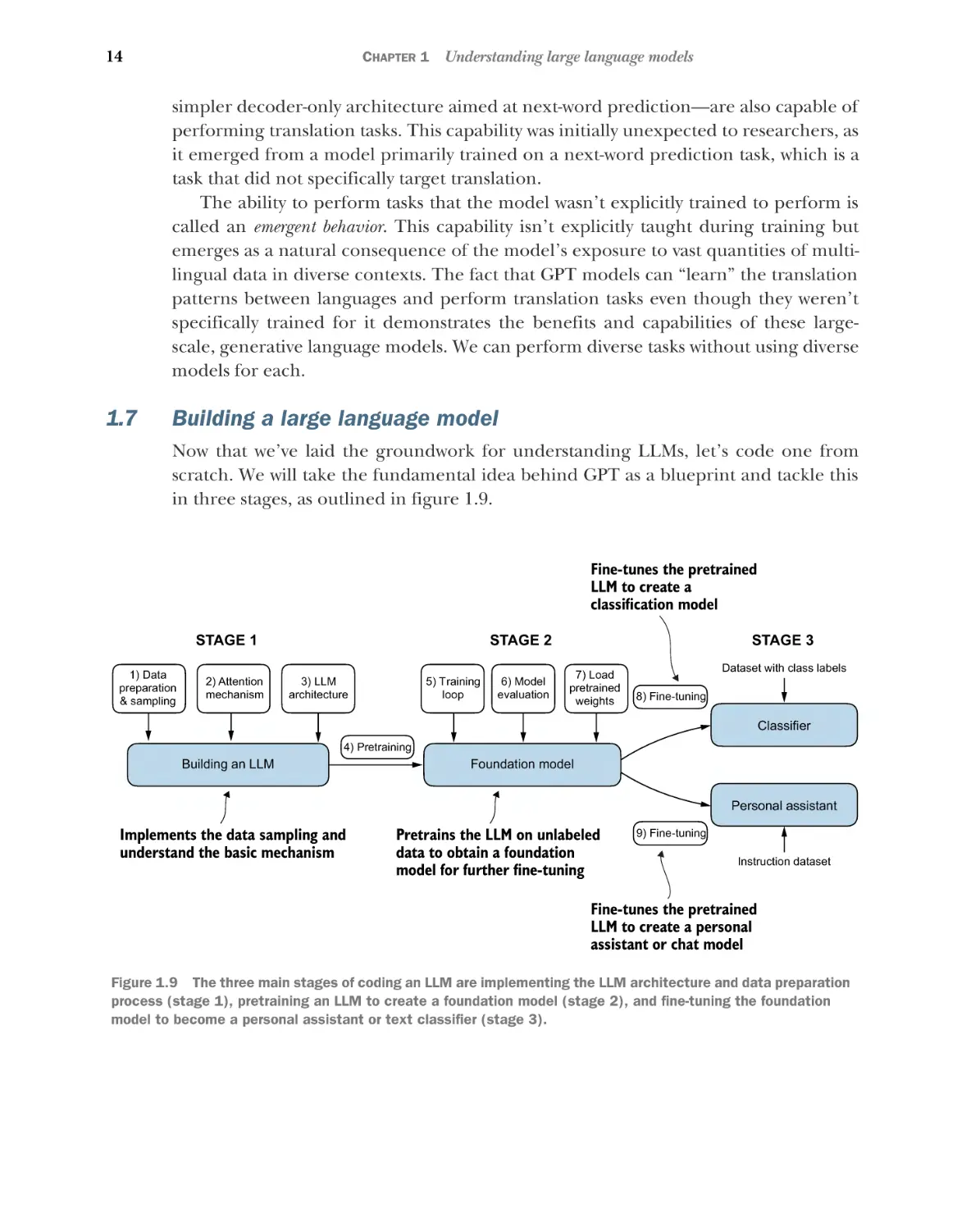
1.7
Building a large language model
Now that we’ve laid the groundwork for understanding LLMs, let’s code one from
scratch. We will take the fundamental idea behind GPT as a blueprint and tackle this
in three stages, as outlined in figure 1.9.
Fine-tunes the pretrained
LLM to create a
classification model
STAGE 1
1) Data
preparation
& sampling
2) Attention
mechanism
STAGE 3
STAGE 2
5) Training
loop
3) LLM
architecture
6) Model
evaluation
7) Load
pretrained
weights
Dataset with class labels
8) Fine-tuning
Classifier
4) Pretraining
Building an LLM
Foundation model
Personal assistant
Implements the data sampling and
understand the basic mechanism
Pretrains the LLM on unlabeled
data to obtain a foundation
model for further fine-tuning
9) Fine-tuning
Instruction dataset
Fine-tunes the pretrained
LLM to create a personal
assistant or chat model
Figure 1.9 The three main stages of coding an LLM are implementing the LLM architecture and data preparation
process (stage 1), pretraining an LLM to create a foundation model (stage 2), and fine-tuning the foundation
model to become a personal assistant or text classifier (stage 3).
Summary
15
In stage 1, we will learn about the fundamental data preprocessing steps and code the
attention mechanism at the heart of every LLM. Next, in stage 2, we will learn how to
code and pretrain a GPT-like LLM capable of generating new texts. We will also go
over the fundamentals of evaluating LLMs, which is essential for developing capable
NLP systems.
Pretraining an LLM from scratch is a significant endeavor, demanding thousands
to millions of dollars in computing costs for GPT-like models. Therefore, the focus of
stage 2 is on implementing training for educational purposes using a small dataset. In
addition, I also provide code examples for loading openly available model weights.
Finally, in stage 3, we will take a pretrained LLM and fine-tune it to follow instructions such as answering queries or classifying texts—the most common tasks in many
real-world applications and research.
I hope you are looking forward to embarking on this exciting journey!
Summary
LLMs have transformed the field of natural language processing, which previ-
ously mostly relied on explicit rule-based systems and simpler statistical methods. The advent of LLMs introduced new deep learning-driven approaches
that led to advancements in understanding, generating, and translating human
language.
Modern LLMs are trained in two main steps:
– First, they are pretrained on a large corpus of unlabeled text by using the
prediction of the next word in a sentence as a label.
– Then, they are fine-tuned on a smaller, labeled target dataset to follow
instructions or perform classification tasks.
LLMs are based on the transformer architecture. The key idea of the transformer architecture is an attention mechanism that gives the LLM selective
access to the whole input sequence when generating the output one word at
a time.
The original transformer architecture consists of an encoder for parsing text
and a decoder for generating text.
LLMs for generating text and following instructions, such as GPT-3 and
ChatGPT, only implement decoder modules, simplifying the architecture.
Large datasets consisting of billions of words are essential for pretraining
LLMs.
While the general pretraining task for GPT-like models is to predict the next
word in a sentence, these LLMs exhibit emergent properties, such as capabilities to classify, translate, or summarize texts.
16
CHAPTER 1
Understanding large language models
Once an LLM is pretrained, the resulting foundation model can be fine-tuned
more efficiently for various downstream tasks.
LLMs fine-tuned on custom datasets can outperform general LLMs on specific
tasks.
Working with text data
This chapter covers
Preparing text for large language model training
Splitting text into word and subword tokens
Byte pair encoding as a more advanced way of
tokenizing text
Sampling training examples with a sliding window
approach
Converting tokens into vectors that feed into a
large language model
So far, we’ve covered the general structure of large language models (LLMs) and
learned that they are pretrained on vast amounts of text. Specifically, our focus was on
decoder-only LLMs based on the transformer architecture, which underlies the models used in ChatGPT and other popular GPT-like LLMs.
During the pretraining stage, LLMs process text one word at a time. Training
LLMs with millions to billions of parameters using a next-word prediction task
yields models with impressive capabilities. These models can then be further finetuned to follow general instructions or perform specific target tasks. But before we
can implement and train LLMs, we need to prepare the training dataset, as illustrated in figure 2.1.
17
18
CHAPTER 2
Working with text data
Fine-tunes the pretrained
LLM to create a
classification model
Implements the data
sampling pipeline
STAGE 1
1) Data
preparation
& sampling
2) Attention
mechanism
STAGE 2
5) Training
loop
3) LLM
architecture
6) Model
evaluation
STAGE 3
7) Load
pretrained
weights
Dataset with class labels
8) Fine-tuning
Classifier
4) Pretraining
Building an LLM
Foundation model
Personal assistant
Implements the data sampling and
understand the basic mechanism
Pretrains the LLM on unlabeled
data to obtain a foundation
model for further finetuning
9) Fine-tuning
Instruction dataset
Fine-tunes the pretrained
LLM to create a personal
assistant or chat model
Figure 2.1 The three main stages of coding an LLM. This chapter focuses on step 1 of stage 1: implementing the
data sample pipeline.
You’ll learn how to prepare input text for training LLMs. This involves splitting text
into individual word and subword tokens, which can then be encoded into vector representations for the LLM. You’ll also learn about advanced tokenization schemes like
byte pair encoding, which is utilized in popular LLMs like GPT. Lastly, we’ll implement a sampling and data-loading strategy to produce the input-output pairs necessary for training LLMs.
2.1
Understanding word embeddings
Deep neural network models, including LLMs, cannot process raw text directly. Since
text is categorical, it isn’t compatible with the mathematical operations used to implement and train neural networks. Therefore, we need a way to represent words as
continuous-valued vectors.
NOTE Readers unfamiliar with vectors and tensors in a computational context can learn more in appendix A, section A.2.2.
The concept of converting data into a vector format is often referred to as embedding.
Using a specific neural network layer or another pretrained neural network model, we
can embed different data types—for example, video, audio, and text, as illustrated in
figure 2.2. However, it’s important to note that different data formats require distinct
embedding models. For example, an embedding model designed for text would not
be suitable for embedding audio or video data.
2.1
Understanding word embeddings
Video embedding model
Video
sample
Audio
sample
Unlabeled
input data
Video embedding vector
1.23
Audio embedding model
Text
sample
0.89
0.45
2.11
Text embedding vector
1.78
Embedding model converts raw
input into a vector representation
-0.31
Audio embedding vector
-0.15
Text embedding model
19
0.18 -2.10
Vector representation
of the input
Figure 2.2 Deep learning models cannot process data formats like video, audio, and text in their raw
form. Thus, we use an embedding model to transform this raw data into a dense vector representation
that deep learning architectures can easily understand and process. Specifically, this figure illustrates
the process of converting raw data into a three-dimensional numerical vector.
At its core, an embedding is a mapping from discrete objects, such as words, images,
or even entire documents, to points in a continuous vector space—the primary purpose of embeddings is to convert nonnumeric data into a format that neural networks
can process.
While word embeddings are the most common form of text embedding, there are
also embeddings for sentences, paragraphs, or whole documents. Sentence or paragraph embeddings are popular choices for retrieval-augmented generation. Retrievalaugmented generation combines generation (like producing text) with retrieval (like
searching an external knowledge base) to pull relevant information when generating
text, which is a technique that is beyond the scope of this book. Since our goal is to
train GPT-like LLMs, which learn to generate text one word at a time, we will focus on
word embeddings.
Several algorithms and frameworks have been developed to generate word embeddings. One of the earlier and most popular examples is the Word2Vec approach.
Word2Vec trained neural network architecture to generate word embeddings by predicting the context of a word given the target word or vice versa. The main idea
behind Word2Vec is that words that appear in similar contexts tend to have similar
meanings. Consequently, when projected into two-dimensional word embeddings for
visualization purposes, similar terms are clustered together, as shown in figure 2.3.
Word embeddings can have varying dimensions, from one to thousands. A higher
dimensionality might capture more nuanced relationships but at the cost of computational efficiency.
20
CHAPTER 2
Working with text data
Vector embeddings of
different types of birds
Vector embedding of
the word squirrel
duck
eagle
squirrel
goose
Second
dimension
Germany
England
Berlin
longer
long
longest
London
First dimension
Figure 2.3 If word embeddings are two-dimensional, we can plot them in a twodimensional scatterplot for visualization purposes as shown here. When using word
embedding techniques, such as Word2Vec, words corresponding to similar concepts
often appear close to each other in the embedding space. For instance, different types
of birds appear closer to each other in the embedding space than in countries and cities.
While we can use pretrained models such as Word2Vec to generate embeddings for
machine learning models, LLMs commonly produce their own embeddings that are
part of the input layer and are updated during training. The advantage of optimizing
the embeddings as part of the LLM training instead of using Word2Vec is that the
embeddings are optimized to the specific task and data at hand. We will implement
such embedding layers later in this chapter. (LLMs can also create contextualized output embeddings, as we discuss in chapter 3.)
Unfortunately, high-dimensional embeddings present a challenge for visualization because our sensory perception and common graphical representations are
inherently limited to three dimensions or fewer, which is why figure 2.3 shows twodimensional embeddings in a two-dimensional scatterplot. However, when working
with LLMs, we typically use embeddings with a much higher dimensionality. For
both GPT-2 and GPT-3, the embedding size (often referred to as the dimensionality
of the model’s hidden states) varies based on the specific model variant and size. It
is a tradeoff between performance and efficiency. The smallest GPT-2 models (117M
and 125M parameters) use an embedding size of 768 dimensions to provide concrete examples. The largest GPT-3 model (175B parameters) uses an embedding
size of 12,288 dimensions.
Next, we will walk through the required steps for preparing the embeddings used
by an LLM, which include splitting text into words, converting words into tokens, and
turning tokens into embedding vectors.
2.2 Tokenizing text
2.2
21
Tokenizing text
Let’s discuss how we split input text into individual tokens, a required preprocessing
step for creating embeddings for an LLM. These tokens are either individual words or
special characters, including punctuation characters, as shown in figure 2.4.
Output text
Postprocessing steps
GPT-like
decoder-only
transformer
Token embeddings:
Token IDs:
Tokenized text:
This section covers the
concept of splitting
text into tokens
Input text:
40134
This
2052
133
is
an
389
example
12
.
This is an example.
Figure 2.4 A view of the text processing steps in the context of an LLM. Here, we split an
input text into individual tokens, which are either words or special characters, such as
punctuation characters.
The text we will tokenize for LLM training is “The Verdict,” a short story by Edith
Wharton, which has been released into the public domain and is thus permitted to be
used for LLM training tasks. The text is available on Wikisource at https://en.wikisource
.org/wiki/The_Verdict, and you can copy and paste it into a text file, which I copied
into a text file "the-verdict.txt".
Alternatively, you can find this "the-verdict.txt" file in this book’s GitHub
repository at https://mng.bz/Adng. You can download the file with the following
Python code:
22
CHAPTER 2
Working with text data
import urllib.request
url = ("https://raw.githubusercontent.com/rasbt/"
"LLMs-from-scratch/main/ch02/01_main-chapter-code/"
"the-verdict.txt")
file_path = "the-verdict.txt"
urllib.request.urlretrieve(url, file_path)
Next, we can load the the-verdict.txt file using Python’s standard file reading utilities.
Listing 2.1
Reading in a short story as text sample into Python
with open("the-verdict.txt", "r", encoding="utf-8") as f:
raw_text = f.read()
print("Total number of character:", len(raw_text))
print(raw_text[:99])
The print command prints the total number of characters followed by the first 100
characters of this file for illustration purposes:
Total number of character: 20479
I HAD always thought Jack Gisburn rather a cheap genius--though a good fellow
enough--so it was no
Our goal is to tokenize this 20,479-character short story into individual words and special characters that we can then turn into embeddings for LLM training.
NOTE It’s common to process millions of articles and hundreds of thousands
of books—many gigabytes of text—when working with LLMs. However, for
educational purposes, it’s sufficient to work with smaller text samples like a
single book to illustrate the main ideas behind the text processing steps and
to make it possible to run it in a reasonable time on consumer hardware.
How can we best split this text to obtain a list of tokens? For this, we go on a small
excursion and use Python’s regular expression library re for illustration purposes.
(You don’t have to learn or memorize any regular expression syntax since we will later
transition to a prebuilt tokenizer.)
Using some simple example text, we can use the re.split command with the following syntax to split a text on whitespace characters:
import re
text = "Hello, world. This, is a test."
result = re.split(r'(\s)', text)
print(result)
The result is a list of individual words, whitespaces, and punctuation characters:
['Hello,', ' ', 'world.', ' ', 'This,', ' ', 'is', ' ', 'a', ' ', 'test.']
2.2 Tokenizing text
23
This simple tokenization scheme mostly works for separating the example text into
individual words; however, some words are still connected to punctuation characters
that we want to have as separate list entries. We also refrain from making all text lowercase because capitalization helps LLMs distinguish between proper nouns and common nouns, understand sentence structure, and learn to generate text with proper
capitalization.
Let’s modify the regular expression splits on whitespaces (\s), commas, and periods ([,.]):
result = re.split(r'([,.]|\s)', text)
print(result)
We can see that the words and punctuation characters are now separate list entries just
as we wanted:
['Hello', ',', '', ' ', 'world', '.', '', ' ', 'This', ',', '', ' ', 'is',
' ', 'a', ' ', 'test', '.', '']
A small remaining problem is that the list still includes whitespace characters. Optionally, we can remove these redundant characters safely as follows:
result = [item for item in result if item.strip()]
print(result)
The resulting whitespace-free output looks like as follows:
['Hello', ',', 'world', '.', 'This', ',', 'is', 'a', 'test', '.']
NOTE When developing a simple tokenizer, whether we should encode
whitespaces as separate characters or just remove them depends on our application and its requirements. Removing whitespaces reduces the memory and
computing requirements. However, keeping whitespaces can be useful if we
train models that are sensitive to the exact structure of the text (for example,
Python code, which is sensitive to indentation and spacing). Here, we remove
whitespaces for simplicity and brevity of the tokenized outputs. Later, we will
switch to a tokenization scheme that includes whitespaces.
The tokenization scheme we devised here works well on the simple sample text. Let’s
modify it a bit further so that it can also handle other types of punctuation, such as question marks, quotation marks, and the double-dashes we have seen earlier in the first 100
characters of Edith Wharton’s short story, along with additional special characters:
text = "Hello, world. Is this-- a test?"
result = re.split(r'([,.:;?_!"()\']|--|\s)', text)
result = [item.strip() for item in result if item.strip()]
print(result)
24
CHAPTER 2
Working with text data
The resulting output is:
['Hello', ',', 'world', '.', 'Is', 'this', '--', 'a', 'test', '?']
As we can see based on the results summarized in figure 2.5, our tokenization scheme
can now handle the various special characters in the text successfully.
Input text
Tokenized text
Hello
Hello, world. Is this-- a test?
,
world
.
Is
this
--
a
test
?
Figure 2.5 The tokenization scheme we implemented so far splits
text into individual words and punctuation characters. In this specific
example, the sample text gets split into 10 individual tokens.
Now that we have a basic tokenizer working, let’s apply it to Edith Wharton’s entire
short story:
preprocessed = re.split(r'([,.:;?_!"()\']|--|\s)', raw_text)
preprocessed = [item.strip() for item in preprocessed if item.strip()]
print(len(preprocessed))
This print statement outputs 4690, which is the number of tokens in this text (without
whitespaces). Let’s print the first 30 tokens for a quick visual check:
print(preprocessed[:30])
The resulting output shows that our tokenizer appears to be handling the text well
since all words and special characters are neatly separated:
['I', 'HAD', 'always', 'thought', 'Jack', 'Gisburn', 'rather', 'a',
'cheap', 'genius', '--', 'though', 'a', 'good', 'fellow', 'enough',
'--', 'so', 'it', 'was', 'no', 'great', 'surprise', 'to', 'me', 'to',
'hear', 'that', ',', 'in']
2.3
Converting tokens into token IDs
Next, let’s convert these tokens from a Python string to an integer representation to
produce the token IDs. This conversion is an intermediate step before converting the
token IDs into embedding vectors.
To map the previously generated tokens into token IDs, we have to build a vocabulary first. This vocabulary defines how we map each unique word and special character
to a unique integer, as shown in figure 2.6.
2.3
Converting tokens into token IDs
2. Each unique token is
added to the vocabulary
in alphabetical order.
1. Tokenization breaks
down the input text
into individual tokens.
Complete training dataset
Input text
The training set consists
of only one sentence for
illustration purposes.
Vocabulary
Tokenized training dataset
The
The quick brown fox jumps
over the lazy dog
25
brown
brown
0
The vocabulary
contains all unique
tokens in the training
set and is usually
sorted alphabetically.
dog
1
fox
2
jumps
3
lazy
4
over
5
quick
6
the
7
quick
Each unique token is
mapped to a unique
integer called token ID.
Unique tokens
Token IDs
Figure 2.6 We build a vocabulary by tokenizing the entire text in a training dataset into individual
tokens. These individual tokens are then sorted alphabetically, and duplicate tokens are removed.
The unique tokens are then aggregated into a vocabulary that defines a mapping from each unique
token to a unique integer value. The depicted vocabulary is purposefully small and contains no
punctuation or special characters for simplicity.
Now that we have tokenized Edith Wharton’s short story and assigned it to a Python
variable called preprocessed, let’s create a list of all unique tokens and sort them
alphabetically to determine the vocabulary size:
all_words = sorted(set(preprocessed))
vocab_size = len(all_words)
print(vocab_size)
After determining that the vocabulary size is 1,130 via this code, we create the vocabulary and print its first 51 entries for illustration purposes.
Listing 2.2
Creating a vocabulary
vocab = {token:integer for integer,token in enumerate(all_words)}
for i, item in enumerate(vocab.items()):
print(item)
if i >= 50:
break
26
CHAPTER 2
Working with text data
The output is
('!', 0)
('"', 1)
("'", 2)
...
('Her', 49)
('Hermia', 50)
As we can see, the dictionary contains individual tokens associated with unique integer labels. Our next goal is to apply this vocabulary to convert new text into token IDs
(figure 2.7).
Tokenization breaks down the
training set into individual tokens.
New tokenized sample
text is mapped to
token IDs using an
existing vocabulary.
Figure 2.7 Starting with a new text sample, we tokenize the text and use the vocabulary to convert
the text tokens into token IDs. The vocabulary is built from the entire training set and can be applied
to the training set itself and any new text samples. The depicted vocabulary contains no punctuation
or special characters for simplicity.
When we want to convert the outputs of an LLM from numbers back into text, we need a
way to turn token IDs into text. For this, we can create an inverse version of the vocabulary that maps token IDs back to the corresponding text tokens.
2.3
Converting tokens into token IDs
27
Let’s implement a complete tokenizer class in Python with an encode method that
splits text into tokens and carries out the string-to-integer mapping to produce token
IDs via the vocabulary. In addition, we’ll implement a decode method that carries out
the reverse integer-to-string mapping to convert the token IDs back into text. The following listing shows the code for this tokenizer implementation.
Listing 2.3
Implementing a simple text tokenizer
Stores the vocabulary as a class attribute for
access in the encode and decode methods
Creates an inverse
vocabulary that maps
token IDs back to the
original text tokens
class SimpleTokenizerV1:
def __init__(self, vocab):
self.str_to_int = vocab
self.int_to_str = {i:s for s,i in vocab.items()}
def encode(self, text):
preprocessed = re.split(r'([,.?_!"()\']|--|\s)', text)
preprocessed = [
item.strip() for item in preprocessed if item.strip()
]
ids = [self.str_to_int[s] for s in preprocessed]
return ids
def decode(self, ids):
text = " ".join([self.int_to_str[i] for i in ids])
text = re.sub(r'\s+([,.?!"()\'])', r'\1', text)
return text
Processes
input text
into token
IDs
Converts token IDs
back into text
Removes spaces
before the specified
punctuation
Using the SimpleTokenizerV1 Python class, we can now instantiate new tokenizer
objects via an existing vocabulary, which we can then use to encode and decode text,
as illustrated in figure 2.8.
Let’s instantiate a new tokenizer object from the SimpleTokenizerV1 class and
tokenize a passage from Edith Wharton’s short story to try it out in practice:
tokenizer = SimpleTokenizerV1(vocab)
text = """"It's the last he painted, you know,"
Mrs. Gisburn said with pardonable pride."""
ids = tokenizer.encode(text)
print(ids)
The preceding code prints the following token IDs:
[1, 56, 2, 850, 988, 602, 533, 746, 5, 1126, 596, 5, 1, 67, 7, 38, 851, 1108,
754, 793, 7]
Next, let’s see whether we can turn these token IDs back into text using the decode
method:
print(tokenizer.decode(ids))
28
CHAPTER 2
Working with text data
Calling tokenizer.encode(text) on sample text
Sample text
The brown dog
playfully chased
the swift fox
Tokenized sample text
The
0
dog
7
0
1
Vocabulary
Tokenized sample text
Token IDs
7
brown
Token IDs
1
The
brown
dog
Inverse
vocabulary
Sample text
The brown dog
playfully chased
the swift fox
Calling tokenizer.decode(ids) on token IDs
Figure 2.8 Tokenizer implementations share two common methods: an encode method and a decode
method. The encode method takes in the sample text, splits it into individual tokens, and converts the
tokens into token IDs via the vocabulary. The decode method takes in token IDs, converts them back
into text tokens, and concatenates the text tokens into natural text.
This outputs:
'" It\' s the last he painted, you know," Mrs. Gisburn said with
pardonable pride.'
Based on this output, we can see that the decode method successfully converted the
token IDs back into the original text.
So far, so good. We implemented a tokenizer capable of tokenizing and detokenizing text based on a snippet from the training set. Let’s now apply it to a new text sample not contained in the training set:
text = "Hello, do you like tea?"
print(tokenizer.encode(text))
Executing this code will result in the following error:
KeyError: 'Hello'
The problem is that the word “Hello” was not used in the “The Verdict” short story.
Hence, it is not contained in the vocabulary. This highlights the need to consider
large and diverse training sets to extend the vocabulary when working on LLMs.
2.4
Adding special context tokens
29
Next, we will test the tokenizer further on text that contains unknown words and
discuss additional special tokens that can be used to provide further context for an
LLM during training.
2.4
Adding special context tokens
We need to modify the tokenizer to handle unknown words. We also need to address
the usage and addition of special context tokens that can enhance a model’s understanding of context or other relevant information in the text. These special tokens
can include markers for unknown words and document boundaries, for example. In
particular, we will modify the vocabulary and tokenizer, SimpleTokenizerV2, to support two new tokens, <|unk|> and <|endoftext|>, as illustrated in figure 2.9.
Sample text
The brown dog
playfully chased
the swift fox
Tokenized sample text
The
brown
dog
playfully
Existing vocabulary
Token IDs
brown
0
dog
1
fox
2
<|unk|>
783
<|endoftext|>
784
7
Extend vocabulary
with additional
special tokens
0
1
783
Figure 2.9 We add special tokens to a vocabulary to deal with certain contexts. For instance,
we add an <|unk|> token to represent new and unknown words that were not part of the training
data and thus not part of the existing vocabulary. Furthermore, we add an <|endoftext|>
token that we can use to separate two unrelated text sources.
We can modify the tokenizer to use an <|unk|> token if it encounters a word that is
not part of the vocabulary. Furthermore, we add a token between unrelated texts.
For example, when training GPT-like LLMs on multiple independent documents or
books, it is common to insert a token before each document or book that follows a
previous text source, as illustrated in figure 2.10. This helps the LLM understand
that although these text sources are concatenated for training, they are, in fact,
unrelated.
30
CHAPTER 2
Independent text source
“… the underdog
team finally clinched
the championship in
a thrilling overtime
victory.”
“<|endoftext|> …
Elara and Finn lived
with kindness and
wisdom, enjoying
their days happily
ever after.”
Working with text data
The <|endoftext|> tokens are
prepended to each subsequent text
source.
“<|endoftext|> …
The Dow Jones
Industrial Average
closed up 250 points
today, marking its
highest gain in the
past three months.”
“<|endoftext|> …
Amelia smiled,
knowing her journey
had forever changed
her heart.”
Text concatenated from all
independent sources
“… in a thrilling overtime victory. <|endoftext|> … days happily ever after. <|endoftext|>
… marking its highest gain in the past three months. <|endoftext|> … journey had forever
changed her heart.”
Figure 2.10 When working with multiple independent text source, we add <|endoftext|>
tokens between these texts. These <|endoftext|> tokens act as markers, signaling the
start or end of a particular segment, allowing for more effective processing and understanding
by the LLM.
Let’s now modify the vocabulary to include these two special tokens, <unk> and
<|endoftext|>, by adding them to our list of all unique words:
all_tokens = sorted(list(set(preprocessed)))
all_tokens.extend(["<|endoftext|>", "<|unk|>"])
vocab = {token:integer for integer,token in enumerate(all_tokens)}
print(len(vocab.items()))
Based on the output of this print statement, the new vocabulary size is 1,132 (the previous vocabulary size was 1,130).
As an additional quick check, let’s print the last five entries of the updated vocabulary:
for i, item in enumerate(list(vocab.items())[-5:]):
print(item)
The code prints
('younger', 1127)
('your', 1128)
('yourself', 1129)
('<|endoftext|>', 1130)
('<|unk|>', 1131)
2.4
Adding special context tokens
31
Based on the code output, we can confirm that the two new special tokens were
indeed successfully incorporated into the vocabulary. Next, we adjust the tokenizer
from code listing 2.3 accordingly as shown in the following listing.
Listing 2.4
A simple text tokenizer that handles unknown words
class SimpleTokenizerV2:
def __init__(self, vocab):
self.str_to_int = vocab
self.int_to_str = { i:s for s,i in vocab.items()}
Replaces
def encode(self, text):
unknown words
preprocessed = re.split(r'([,.:;?_!"()\']|--|\s)', text)
by <|unk|>
preprocessed = [
tokens
item.strip() for item in preprocessed if item.strip()
]
preprocessed = [item if item in self.str_to_int
else "<|unk|>" for item in preprocessed]
ids = [self.str_to_int[s] for s in preprocessed]
return ids
def decode(self, ids):
text = " ".join([self.int_to_str[i] for i in ids])
text = re.sub(r'\s+([,.:;?!"()\'])', r'\1', text)
return text
Replaces spaces
before the specified
punctuations
Compared to the SimpleTokenizerV1 we implemented in listing 2.3, the new SimpleTokenizerV2 replaces unknown words with <|unk|> tokens.
Let’s now try this new tokenizer out in practice. For this, we will use a simple text
sample that we concatenate from two independent and unrelated sentences:
text1 = "Hello, do you like tea?"
text2 = "In the sunlit terraces of the palace."
text = " <|endoftext|> ".join((text1, text2))
print(text)
The output is
Hello, do you like tea? <|endoftext|> In the sunlit terraces of
the palace.
Next, let’s tokenize the sample text using the SimpleTokenizerV2 on the vocab we
previously created in listing 2.2:
tokenizer = SimpleTokenizerV2(vocab)
print(tokenizer.encode(text))
32
CHAPTER 2
Working with text data
This prints the following token IDs:
[1131, 5, 355, 1126, 628, 975, 10, 1130, 55, 988, 956, 984, 722, 988, 1131, 7]
We can see that the list of token IDs contains 1130 for the <|endoftext|> separator
token as well as two 1131 tokens, which are used for unknown words.
Let’s detokenize the text for a quick sanity check:
print(tokenizer.decode(tokenizer.encode(text)))
The output is
<|unk|>, do you like tea? <|endoftext|> In the sunlit terraces of
the <|unk|>.
Based on comparing this detokenized text with the original input text, we know that
the training dataset, Edith Wharton’s short story “The Verdict,” does not contain the
words “Hello” and “palace.”
Depending on the LLM, some researchers also consider additional special tokens
such as the following:
[BOS] (beginning of sequence)—This token marks the start of a text. It signifies to
the LLM where a piece of content begins.
[EOS] (end of sequence)—This token is positioned at the end of a text and
is especially useful when concatenating multiple unrelated texts, similar to
<|endoftext|>. For instance, when combining two different Wikipedia articles or books, the [EOS] token indicates where one ends and the next begins.
[PAD] (padding)—When training LLMs with batch sizes larger than one, the
batch might contain texts of varying lengths. To ensure all texts have the same
length, the shorter texts are extended or “padded” using the [PAD] token, up to
the length of the longest text in the batch.
The tokenizer used for GPT models does not need any of these tokens; it only uses an
<|endoftext|> token for simplicity. <|endoftext|> is analogous to the [EOS] token.
<|endoftext|> is also used for padding. However, as we’ll explore in subsequent
chapters, when training on batched inputs, we typically use a mask, meaning we don’t
attend to padded tokens. Thus, the specific token chosen for padding becomes inconsequential.
Moreover, the tokenizer used for GPT models also doesn’t use an <|unk|> token
for out-of-vocabulary words. Instead, GPT models use a byte pair encoding tokenizer,
which breaks words down into subword units, which we will discuss next.
2.5 Byte pair encoding
2.5
33
Byte pair encoding
Let’s look at a more sophisticated tokenization scheme based on a concept called byte
pair encoding (BPE). The BPE tokenizer was used to train LLMs such as GPT-2, GPT-3,
and the original model used in ChatGPT.
Since implementing BPE can be relatively complicated, we will use an existing
Python open source library called tiktoken (https://github.com/openai/tiktoken), which
implements the BPE algorithm very efficiently based on source code in Rust. Similar
to other Python libraries, we can install the tiktoken library via Python’s pip installer
from the terminal:
pip install tiktoken
The code we will use is based on tiktoken 0.7.0. You can use the following code to
check the version you currently have installed:
from importlib.metadata import version
import tiktoken
print("tiktoken version:", version("tiktoken"))
Once installed, we can instantiate the BPE tokenizer from tiktoken as follows:
tokenizer = tiktoken.get_encoding("gpt2")
The usage of this tokenizer is similar to the SimpleTokenizerV2 we implemented previously via an encode method:
text = (
"Hello, do you like tea? <|endoftext|> In the sunlit terraces"
"of someunknownPlace."
)
integers = tokenizer.encode(text, allowed_special={"<|endoftext|>"})
print(integers)
The code prints the following token IDs:
[15496, 11, 466, 345, 588, 8887, 30, 220, 50256, 554, 262, 4252, 18250,
8812, 2114, 286, 617, 34680, 27271, 13]
We can then convert the token IDs back into text using the decode method, similar to
our SimpleTokenizerV2:
strings = tokenizer.decode(integers)
print(strings)
The code prints
Hello, do you like tea? <|endoftext|> In the sunlit terraces of
someunknownPlace.
34
CHAPTER 2
Working with text data
We can make two noteworthy observations based on the token IDs and decoded text.
First, the <|endoftext|> token is assigned a relatively large token ID, namely, 50256.
In fact, the BPE tokenizer, which was used to train models such as GPT-2, GPT-3, and
the original model used in ChatGPT, has a total vocabulary size of 50,257, with
<|endoftext|> being assigned the largest token ID.
Second, the BPE tokenizer encodes and decodes unknown words, such as
someunknownPlace, correctly. The BPE tokenizer can handle any unknown word. How
does it achieve this without using <|unk|> tokens?
The algorithm underlying BPE breaks down words that aren’t in its predefined
vocabulary into smaller subword units or even individual characters, enabling it to
handle out-of-vocabulary words. So, thanks to the BPE algorithm, if the tokenizer
encounters an unfamiliar word during tokenization, it can represent it as a sequence
of subword tokens or characters, as illustrated in figure 2.11.
Text sample with
unknown words
Unknown words are
tokenized into individual
characters or subwords.
Tokens:
"A k w i r w i e r "
"Ak"
Token IDs: 33901
"w"
"ir"
"w"
""
"ier"
86
343
86
220
959
Figure 2.11 BPE tokenizers
break down unknown words
into subwords and individual
characters. This way, a BPE
tokenizer can parse any word
and doesn’t need to replace
unknown words with special
tokens, such as <|unk|>.
The ability to break down unknown words into individual characters ensures that
the tokenizer and, consequently, the LLM that is trained with it can process any text,
even if it contains words that were not present in its training data.
Exercise 2.1 Byte pair encoding of unknown words
Try the BPE tokenizer from the tiktoken library on the unknown words “Akwirw ier” and
print the individual token IDs. Then, call the decode function on each of the resulting
integers in this list to reproduce the mapping shown in figure 2.11. Lastly, call the
decode method on the token IDs to check whether it can reconstruct the original
input, “Akwirw ier.”
A detailed discussion and implementation of BPE is out of the scope of this book, but
in short, it builds its vocabulary by iteratively merging frequent characters into subwords and frequent subwords into words. For example, BPE starts with adding all individual single characters to its vocabulary (“a,” “b,” etc.). In the next stage, it merges
character combinations that frequently occur together into subwords. For example,
“d” and “e” may be merged into the subword “de,” which is common in many English
2.6
Data sampling with a sliding window
35
words like “define,” “depend,” “made,” and “hidden.” The merges are determined by
a frequency cutoff.
2.6
Data sampling with a sliding window
The next step in creating the embeddings for the LLM is to generate the input–target
pairs required for training an LLM. What do these input–target pairs look like? As we
already learned, LLMs are pretrained by predicting the next word in a text, as depicted
in figure 2.12.
Text
sample:
LLMs learn to predict one word at a time
LLMs learn to predict one word at a time
LLMs learn to predict one word at a time
The LLM can’t
access words past
the target.
LLMs learn to predict one word at a time
LLMs learn to predict one word at a time
Input the
LLM receives
LLMs learn to predict one word at a time
LLMs learn to predict one word at a time
Target to
predict
LLMs learn to predict one word at a time
Figure 2.12 Given a text sample, extract input blocks as subsamples that serve as
input to the LLM, and the LLM’s prediction task during training is to predict the next
word that follows the input block. During training, we mask out all words that are past
the target. Note that the text shown in this figure must undergo tokenization before
the LLM can process it; however, this figure omits the tokenization step for clarity.
Let’s implement a data loader that fetches the input–target pairs in figure 2.12 from
the training dataset using a sliding window approach. To get started, we will tokenize
the whole “The Verdict” short story using the BPE tokenizer:
with open("the-verdict.txt", "r", encoding="utf-8") as f:
raw_text = f.read()
enc_text = tokenizer.encode(raw_text)
print(len(enc_text))
Executing this code will return 5145, the total number of tokens in the training set,
after applying the BPE tokenizer.
Next, we remove the first 50 tokens from the dataset for demonstration purposes,
as it results in a slightly more interesting text passage in the next steps:
enc_sample = enc_text[50:]
36
CHAPTER 2
Working with text data
One of the easiest and most intuitive ways to create the input–target pairs for the nextword prediction task is to create two variables, x and y, where x contains the input
tokens and y contains the targets, which are the inputs shifted by 1:
context_size = 4
x = enc_sample[:context_size]
y = enc_sample[1:context_size+1]
print(f"x: {x}")
print(f"y:
{y}")
The context size determines
how many tokens are included
in the input.
Running the previous code prints the following output:
x: [290, 4920, 2241, 287]
y:
[4920, 2241, 287, 257]
By processing the inputs along with the targets, which are the inputs shifted by one
position, we can create the next-word prediction tasks (see figure 2.12), as follows:
for i in range(1, context_size+1):
context = enc_sample[:i]
desired = enc_sample[i]
print(context, "---->", desired)
The code prints
[290]
[290,
[290,
[290,
---->
4920]
4920,
4920,
4920
----> 2241
2241] ----> 287
2241, 287] ----> 257
Everything left of the arrow (---->) refers to the input an LLM would receive, and
the token ID on the right side of the arrow represents the target token ID that the
LLM is supposed to predict. Let’s repeat the previous code but convert the token IDs
into text:
for i in range(1, context_size+1):
context = enc_sample[:i]
desired = enc_sample[i]
print(tokenizer.decode(context), "---->", tokenizer.decode([desired]))
The following outputs show how the input and outputs look in text format:
and
and
and
and
----> established
established ----> himself
established himself ----> in
established himself in ----> a
We’ve now created the input–target pairs that we can use for LLM training.
There’s only one more task before we can turn the tokens into embeddings: implementing an efficient data loader that iterates over the input dataset and returns the
2.6
Data sampling with a sliding window
37
inputs and targets as PyTorch tensors, which can be thought of as multidimensional
arrays. In particular, we are interested in returning two tensors: an input tensor containing the text that the LLM sees and a target tensor that includes the targets for the
LLM to predict, as depicted in figure 2.13. While the figure shows the tokens in string
format for illustration purposes, the code implementation will operate on token IDs
directly since the encode method of the BPE tokenizer performs both tokenization
and conversion into token IDs as a single step.
Sample text
"In the heart of the city stood the old library, a relic from a bygone era. Its
stone walls bore the marks of time, and ivy clung tightly to its facade …"
Tensor
containing
the inputs
x = tensor([[ "In",
[ "the" ,
[ "old",
[ …
"the",
"heart",
"city",
"stood",
"library", ",",
Tensor
containing
the targets
y = tensor([[ "the",
"heart",
[ "city",
"stood",
[ "library", “,",
[ …
"of",
"the",
“a",
"of"
"the"
"a"
],
],
],
]])
"the" ],
"old" ],
“relic"],
]])
Figure 2.13 To implement efficient data loaders, we collect the inputs in a tensor, x, where each row
represents one input context. A second tensor, y, contains the corresponding prediction targets (next
words), which are created by shifting the input by one position.
NOTE For the efficient data loader implementation, we will use PyTorch’s
built-in Dataset and DataLoader classes. For additional information and
guidance on installing PyTorch, please see section A.2.1.3 in appendix A.
The code for the dataset class is shown in the following listing.
Listing 2.5
A dataset for batched inputs and targets
import torch
from torch.utils.data import Dataset, DataLoader
class GPTDatasetV1(Dataset):
def __init__(self, txt, tokenizer, max_length, stride):
self.input_ids = []
self.target_ids = []
token_ids = tokenizer.encode(txt)
Tokenizes the
entire text
38
CHAPTER 2
Working with text data
for i in range(0, len(token_ids) - max_length, stride):
input_chunk = token_ids[i:i + max_length]
target_chunk = token_ids[i + 1: i + max_length + 1]
self.input_ids.append(torch.tensor(input_chunk))
self.target_ids.append(torch.tensor(target_chunk))
def __len__(self):
return len(self.input_ids)
def __getitem__(self, idx):
return self.input_ids[idx], self.target_ids[idx]
Returns a single row
from the dataset
Uses a sliding window to chunk
the book into overlapping
sequences of max_length
Returns the total number
of rows in the dataset
The GPTDatasetV1 class is based on the PyTorch Dataset class and defines how individual rows are fetched from the dataset, where each row consists of a number of
token IDs (based on a max_length) assigned to an input_chunk tensor. The target_
chunk tensor contains the corresponding targets. I recommend reading on to see what
the data returned from this dataset looks like when we combine the dataset with a
PyTorch DataLoader—this will bring additional intuition and clarity.
If you are new to the structure of PyTorch Dataset classes, such as
shown in listing 2.5, refer to section A.6 in appendix A, which explains the
general structure and usage of PyTorch Dataset and DataLoader classes.
NOTE
The following code uses the GPTDatasetV1 to load the inputs in batches via a PyTorch
DataLoader.
Listing 2.6
A data loader to generate batches with input-with pairs
def create_dataloader_v1(txt, batch_size=4, max_length=256,
stride=128, shuffle=True, drop_last=True,
num_workers=0):
tokenizer = tiktoken.get_encoding("gpt2")
dataset = GPTDatasetV1(txt, tokenizer, max_length, stride)
dataloader = DataLoader(
dataset,
batch_size=batch_size,
shuffle=shuffle,
drop_last=drop_last,
drop_last=True drops the last
num_workers=num_workers
batch if it is shorter than the
)
specified batch_size to prevent
loss spikes during training.
return dataloader
The number of CPU processes
to use for preprocessing
Initializes the
tokenizer
Creates
dataset
2.6
Data sampling with a sliding window
39
Let’s test the dataloader with a batch size of 1 for an LLM with a context size of 4 to
develop an intuition of how the GPTDatasetV1 class from listing 2.5 and the create_
dataloader_v1 function from listing 2.6 work together:
with open("the-verdict.txt", "r", encoding="utf-8") as f:
raw_text = f.read()
dataloader = create_dataloader_v1(
raw_text, batch_size=1, max_length=4, stride=1, shuffle=False)
data_iter = iter(dataloader)
Converts dataloader into a Python
first_batch = next(data_iter)
iterator to fetch the next entry via
print(first_batch)
Python’s built-in next() function
Executing the preceding code prints the following:
[tensor([[
40,
367, 2885, 1464]]), tensor([[ 367, 2885, 1464, 1807]])]
The first_batch variable contains two tensors: the first tensor stores the input token
IDs, and the second tensor stores the target token IDs. Since the max_length is set to
4, each of the two tensors contains four token IDs. Note that an input size of 4 is quite
small and only chosen for simplicity. It is common to train LLMs with input sizes of at
least 256.
To understand the meaning of stride=1, let’s fetch another batch from this dataset:
second_batch = next(data_iter)
print(second_batch)
The second batch has the following contents:
[tensor([[ 367, 2885, 1464, 1807]]), tensor([[2885, 1464, 1807, 3619]])]
If we compare the first and second batches, we can see that the second batch’s token
IDs are shifted by one position (for example, the second ID in the first batch’s input is
367, which is the first ID of the second batch’s input). The stride setting dictates the
number of positions the inputs shift across batches, emulating a sliding window
approach, as demonstrated in figure 2.14.
Exercise 2.2 Data loaders with different strides and context sizes
To develop more intuition for how the data loader works, try to run it with different
settings such as max_length=2 and stride=2, and max_length=8 and stride=2.
Batch sizes of 1, such as we have sampled from the data loader so far, are useful for
illustration purposes. If you have previous experience with deep learning, you may
know that small batch sizes require less memory during training but lead to more
40
CHAPTER 2
Working with text data
A stride of 1 moves the input field by 1 position
Sample text
"In the heart of the city stood the old library, a relic from a bygone era. Its
stone walls bore the marks of time, and ivy clung tightly to its facade …"
Inputs of batch 1:
"In the heart of"
Inputs of batch 2:
"the heart of the"
A stride of 4 moves the input field by 4 positions
"In the heart of the city stood the old library, a relic from a bygone era. Its
stone walls bore the marks of time, and ivy clung tightly to its facade …"
Inputs of batch 1:
"In the heart of"
Inputs of batch 2:
“the city stood the"
Figure 2.14 When creating multiple batches from the input dataset, we slide an
input window across the text. If the stride is set to 1, we shift the input window by
one position when creating the next batch. If we set the stride equal to the input
window size, we can prevent overlaps between the batches.
noisy model updates. Just like in regular deep learning, the batch size is a tradeoff and
a hyperparameter to experiment with when training LLMs.
Let’s look briefly at how we can use the data loader to sample with a batch size
greater than 1:
dataloader = create_dataloader_v1(
raw_text, batch_size=8, max_length=4, stride=4,
shuffle=False
)
data_iter = iter(dataloader)
inputs, targets = next(data_iter)
print("Inputs:\n", inputs)
print("\nTargets:\n", targets)
This prints
Inputs:
tensor([[
40,
367, 2885, 1464],
[ 1807, 3619,
402,
271],
[10899, 2138,
257, 7026],
[15632,
438, 2016,
257],
[ 922, 5891, 1576,
438],
[ 568,
340,
373,
645],
2.7
[ 1049,
[ 284,
5975,
3285,
Creating token embeddings
284,
326,
41
502],
11]])
Targets:
tensor([[ 367, 2885, 1464, 1807],
[ 3619,
402,
271, 10899],
[ 2138,
257, 7026, 15632],
[ 438, 2016,
257,
922],
[ 5891, 1576,
438,
568],
[ 340,
373,
645, 1049],
[ 5975,
284,
502,
284],
[ 3285,
326,
11,
287]])
Note that we increase the stride to 4 to utilize the data set fully (we don’t skip a single
word). This avoids any overlap between the batches since more overlap could lead to
increased overfitting.
2.7
Creating token embeddings
The last step in preparing the input text for LLM training is to convert the token IDs
into embedding vectors, as shown in figure 2.15. As a preliminary step, we must initialize
Output text
Postprocessing steps
GPT-like
decoder-only
transformer
Creating input
token embeddings
Token embeddings:
Token IDs:
Tokenized text:
Input text:
40134
This
2052
133
is
an
389
12
example
.
This is an example.
Figure 2.15 Preparation involves tokenizing text, converting text tokens to token IDs, and
converting token IDs into embedding vectors. Here, we consider the previously created token
IDs to create the token embedding vectors.
42
CHAPTER 2
Working with text data
these embedding weights with random values. This initialization serves as the starting
point for the LLM’s learning process. In chapter 5, we will optimize the embedding
weights as part of the LLM training.
A continuous vector representation, or embedding, is necessary since GPT-like
LLMs are deep neural networks trained with the backpropagation algorithm.
NOTE If you are unfamiliar with how neural networks are trained with backpropagation, please read section B.4 in appendix A.
Let’s see how the token ID to embedding vector conversion works with a hands-on
example. Suppose we have the following four input tokens with IDs 2, 3, 5, and 1:
input_ids = torch.tensor([2, 3, 5, 1])
For the sake of simplicity, suppose we have a small vocabulary of only 6 words (instead
of the 50,257 words in the BPE tokenizer vocabulary), and we want to create embeddings of size 3 (in GPT-3, the embedding size is 12,288 dimensions):
vocab_size = 6
output_dim = 3
Using the vocab_size and output_dim, we can instantiate an embedding layer in
PyTorch, setting the random seed to 123 for reproducibility purposes:
torch.manual_seed(123)
embedding_layer = torch.nn.Embedding(vocab_size, output_dim)
print(embedding_layer.weight)
The print statement prints the embedding layer’s underlying weight matrix:
Parameter containing:
tensor([[ 0.3374, -0.1778,
[ 0.9178, 1.5810,
[ 1.2753, -0.2010,
[-0.4015, 0.9666,
[-1.1589, 0.3255,
[-2.8400, -0.7849,
-0.1690],
1.3010],
-0.1606],
-1.1481],
-0.6315],
-1.4096]], requires_grad=True)
The weight matrix of the embedding layer contains small, random values. These values are optimized during LLM training as part of the LLM optimization itself. Moreover, we can see that the weight matrix has six rows and three columns. There is one row
for each of the six possible tokens in the vocabulary, and there is one column for each of
the three embedding dimensions.
Now, let’s apply it to a token ID to obtain the embedding vector:
print(embedding_layer(torch.tensor([3])))
2.8
Encoding word positions
43
The returned embedding vector is
tensor([[-0.4015,
0.9666, -1.1481]], grad_fn=<EmbeddingBackward0>)
If we compare the embedding vector for token ID 3 to the previous embedding
matrix, we see that it is identical to the fourth row (Python starts with a zero index, so
it’s the row corresponding to index 3). In other words, the embedding layer is essentially a lookup operation that retrieves rows from the embedding layer’s weight matrix
via a token ID.
NOTE For those who are familiar with one-hot encoding, the embedding
layer approach described here is essentially just a more efficient way of implementing one-hot encoding followed by matrix multiplication in a fully connected layer, which is illustrated in the supplementary code on GitHub at
https://mng.bz/ZEB5. Because the embedding layer is just a more efficient
implementation equivalent to the one-hot encoding and matrix-multiplication approach, it can be seen as a neural network layer that can be optimized
via backpropagation.
We’ve seen how to convert a single token ID into a three-dimensional embedding vector. Let’s now apply that to all four input IDs (torch.tensor([2, 3, 5, 1])):
print(embedding_layer(input_ids))
The print output reveals that this results in a 4 × 3 matrix:
tensor([[ 1.2753, -0.2010, -0.1606],
[-0.4015, 0.9666, -1.1481],
[-2.8400, -0.7849, -1.4096],
[ 0.9178, 1.5810, 1.3010]], grad_fn=<EmbeddingBackward0>)
Each row in this output matrix is obtained via a lookup operation from the embedding weight matrix, as illustrated in figure 2.16.
Having now created embedding vectors from token IDs, next we’ll add a small
modification to these embedding vectors to encode positional information about a
token within a text.
2.8
Encoding word positions
In principle, token embeddings are a suitable input for an LLM. However, a minor
shortcoming of LLMs is that their self-attention mechanism (see chapter 3) doesn’t
have a notion of position or order for the tokens within a sequence. The way the previously introduced embedding layer works is that the same token ID always gets
mapped to the same vector representation, regardless of where the token ID is positioned in the input sequence, as shown in figure 2.17.
44
CHAPTER 2
Weight matrix of the
embedding layer
0.3374 −0.1778
0.9178
1.5810
1.2753 − 0.2010
− 0.4015 0.9666
− 1.1589 0.3255
− 2.8400 − 0.7849
Token IDs to embed
Working with text data
− 0.1690
1.3010
− 0.1606
− 1.1481
− 0.6315
− 1.4096
Input text
2
3
5
1
fox
jumps
over
dog
Embedding vector of
the first token ID
1.2753 − 0.2010 − 0.1606
− 0.4015 0.9666 − 1.1481
− 2.8400 − 0.7849 − 1.4096
0.9178
1.5810
1.3010
Embedded token IDs
2
3
5
1
fox
jumps
over
dog
Embedding vector of
the third token ID
Figure 2.16 Embedding layers perform a lookup operation, retrieving the embedding
vector corresponding to the token ID from the embedding layer’s weight matrix. For
instance, the embedding vector of the token ID 5 is the sixth row of the embedding
layer weight matrix (it is the sixth instead of the fifth row because Python starts
counting at 0). We assume that the token IDs were produced by the small vocabulary
from section 2.3.
Weight matrix of the
embedding layer
0.3374 − 0.1778 − 0.1690
0.9178
1.5810
1.3010
1.2753 − 0.2010 − 0.1606
− 0.4015 0.9666 − 1.1481
− 1.1589 0.3255 − 0.6315
− 2.8400 − 0.7849 − 1.4096
Token IDs to embed
fox
jumps
over
fox
The same token IDs
result in the same
embedding vectors
2
3
5
2
2
3
5
2
fox
jumps
over
fox
1.2753 − 0.2010 − 0.1606
− 0.4015 0.9666 − 1.1481
− 2.8400 − 0.7849 − 1.4096
1.2753 − 0.2010 − 0.1606
Figure 2.17 The embedding layer converts a token ID into the same vector
representation regardless of where it is located in the input sequence. For
example, the token ID 5, whether it’s in the first or fourth position in the
token ID input vector, will result in the same embedding vector.
2.8
Encoding word positions
45
In principle, the deterministic, position-independent embedding of the token ID is
good for reproducibility purposes. However, since the self-attention mechanism of
LLMs itself is also position-agnostic, it is helpful to inject additional position information into the LLM.
To achieve this, we can use two broad categories of position-aware embeddings: relative positional embeddings and absolute positional embeddings. Absolute positional
embeddings are directly associated with specific positions in a sequence. For each position in the input sequence, a unique embedding is added to the token’s embedding to
convey its exact location. For instance, the first token will have a specific positional
embedding, the second token another distinct embedding, and so on, as illustrated in
figure 2.18.
Input embeddings:
2.1
2.2
2.3
3.1
3.2
3.3
4.1
4.2
4.3
5.1
5.2
5.3
Positional embeddings:
1.1
1.2
1.3
2.1
2.2
2.3
3.1
3.2
3.3
4.1
4.2
4.3
Token embeddings:
1
1
1
1
1
1
1
+
1
+
Embedding of the first token
1
+
1
+
1
1
Embedding of the third token
Figure 2.18 Positional embeddings are added to the token embedding vector to create the
input embeddings for an LLM. The positional vectors have the same dimension as the original
token embeddings. The token embeddings are shown with value 1 for simplicity.
Instead of focusing on the absolute position of a token, the emphasis of relative positional embeddings is on the relative position or distance between tokens. This means
the model learns the relationships in terms of “how far apart” rather than “at which
exact position.” The advantage here is that the model can generalize better to sequences
of varying lengths, even if it hasn’t seen such lengths during training.
Both types of positional embeddings aim to augment the capacity of LLMs to
understand the order and relationships between tokens, ensuring more accurate and
context-aware predictions. The choice between them often depends on the specific
application and the nature of the data being processed.
OpenAI’s GPT models use absolute positional embeddings that are optimized
during the training process rather than being fixed or predefined like the positional
encodings in the original transformer model. This optimization process is part of the
model training itself. For now, let’s create the initial positional embeddings to create the
LLM inputs.
46
CHAPTER 2
Working with text data
Previously, we focused on very small embedding sizes for simplicity. Now, let’s consider more realistic and useful embedding sizes and encode the input tokens into a
256-dimensional vector representation, which is smaller than what the original GPT-3
model used (in GPT-3, the embedding size is 12,288 dimensions) but still reasonable
for experimentation. Furthermore, we assume that the token IDs were created by the
BPE tokenizer we implemented earlier, which has a vocabulary size of 50,257:
vocab_size = 50257
output_dim = 256
token_embedding_layer = torch.nn.Embedding(vocab_size, output_dim)
Using the previous token_embedding_layer, if we sample data from the data loader,
we embed each token in each batch into a 256-dimensional vector. If we have a batch
size of 8 with four tokens each, the result will be an 8 × 4 × 256 tensor.
Let’s instantiate the data loader (see section 2.6) first:
max_length = 4
dataloader = create_dataloader_v1(
raw_text, batch_size=8, max_length=max_length,
stride=max_length, shuffle=False
)
data_iter = iter(dataloader)
inputs, targets = next(data_iter)
print("Token IDs:\n", inputs)
print("\nInputs shape:\n", inputs.shape)
This code prints
Token IDs:
tensor([[
40,
[ 1807,
[10899,
[15632,
[ 922,
[ 568,
[ 1049,
[ 284,
367, 2885, 1464],
3619,
402,
271],
2138,
257, 7026],
438, 2016,
257],
5891, 1576,
438],
340,
373,
645],
5975,
284,
502],
3285,
326,
11]])
Inputs shape:
torch.Size([8, 4])
As we can see, the token ID tensor is 8 × 4 dimensional, meaning that the data batch
consists of eight text samples with four tokens each.
Let’s now use the embedding layer to embed these token IDs into 256-dimensional
vectors:
token_embeddings = token_embedding_layer(inputs)
print(token_embeddings.shape)
2.8
Encoding word positions
47
The print function call returns
torch.Size([8, 4, 256])
The 8 × 4 × 256–dimensional tensor output shows that each token ID is now embedded as a 256-dimensional vector.
For a GPT model’s absolute embedding approach, we just need to create another
embedding layer that has the same embedding dimension as the token_embedding_
layer:
context_length = max_length
pos_embedding_layer = torch.nn.Embedding(context_length, output_dim)
pos_embeddings = pos_embedding_layer(torch.arange(context_length))
print(pos_embeddings.shape)
The input to the pos_embeddings is usually a placeholder vector torch.arange(context_length), which contains a sequence of numbers 0, 1, ..., up to the maximum
input length –1. The context_length is a variable that represents the supported input
size of the LLM. Here, we choose it similar to the maximum length of the input text.
In practice, input text can be longer than the supported context length, in which case
we have to truncate the text.
The output of the print statement is
torch.Size([4, 256])
As we can see, the positional embedding tensor consists of four 256-dimensional vectors. We can now add these directly to the token embeddings, where PyTorch will add
the 4 × 256–dimensional pos_embeddings tensor to each 4 × 256–dimensional token
embedding tensor in each of the eight batches:
input_embeddings = token_embeddings + pos_embeddings
print(input_embeddings.shape)
The print output is
torch.Size([8, 4, 256])
The input_embeddings we created, as summarized in figure 2.19, are the embedded
input examples that can now be processed by the main LLM modules, which we will
begin implementing in the next chapter.
48
CHAPTER 2
Working with text data
Output text
Postprocessing steps
GPT-like
decoder-only
transformer
The input embedding pipeline
Input embeddings:
Positional embeddings:
+
Token embeddings:
Token IDs:
Tokenized text:
Input text:
40134
This
2052
133
is
an
389
example
12
.
This is an example.
Figure 2.19 As part of the input processing pipeline, input text is first broken
up into individual tokens. These tokens are then converted into token IDs using a
vocabulary. The token IDs are converted into embedding vectors to which positional
embeddings of a similar size are added, resulting in input embeddings that are used
as input for the main LLM layers.
Summary
LLMs require textual data to be converted into numerical vectors, known as
embeddings, since they can’t process raw text. Embeddings transform discrete
data (like words or images) into continuous vector spaces, making them compatible with neural network operations.
As the first step, raw text is broken into tokens, which can be words or characters.
Then, the tokens are converted into integer representations, termed token IDs.
Special tokens, such as <|unk|> and <|endoftext|>, can be added to enhance
the model’s understanding and handle various contexts, such as unknown
words or marking the boundary between unrelated texts.
Summary
49
The byte pair encoding (BPE) tokenizer used for LLMs like GPT-2 and GPT-3
can efficiently handle unknown words by breaking them down into subword
units or individual characters.
We use a sliding window approach on tokenized data to generate input–target
pairs for LLM training.
Embedding layers in PyTorch function as a lookup operation, retrieving vectors
corresponding to token IDs. The resulting embedding vectors provide continuous representations of tokens, which is crucial for training deep learning models like LLMs.
While token embeddings provide consistent vector representations for each
token, they lack a sense of the token’s position in a sequence. To rectify this,
two main types of positional embeddings exist: absolute and relative. OpenAI’s
GPT models utilize absolute positional embeddings, which are added to the token
embedding vectors and are optimized during the model training.
Coding attention
mechanisms
This chapter covers
The reasons for using attention mechanisms in
neural networks
A basic self-attention framework, progressing to
an enhanced self-attention mechanism
A causal attention module that allows LLMs to
generate one token at a time
Masking randomly selected attention weights with
dropout to reduce overfitting
Stacking multiple causal attention modules into a
multi-head attention module
At this point, you know how to prepare the input text for training LLMs by splitting
text into individual word and subword tokens, which can be encoded into vector representations, embeddings, for the LLM.
Now, we will look at an integral part of the LLM architecture itself, attention
mechanisms, as illustrated in figure 3.1. We will largely look at attention mechanisms
in isolation and focus on them at a mechanistic level. Then we will code the remaining
50
51
This chapter implements the
attention mechanism, an important
building block of GPT-like LLMs
STAGE 1
1) Data
preparation
& sampling
STAGE 2
2) Attention
mechanism
3) LLM
architecture
5) Training
loop
6) Model
evaluation
STAGE 3
7) Load
pretrained
weights
Dataset with class labels
8) Fine-tuning
Classifier
4) Pretraining
Building an LLM
Foundation model
Personal assistant
9) Fine-tuning
Instruction dataset
Figure 3.1 The three main stages of coding an LLM. This chapter focuses on step 2 of stage 1: implementing
attention mechanisms, which are an integral part of the LLM architecture.
parts of the LLM surrounding the self-attention mechanism to see it in action and to
create a model to generate text.
We will implement four different variants of attention mechanisms, as illustrated in
figure 3.2. These different attention variants build on each other, and the goal is to
A type of self-attention used in LLMs
that allows a model to consider only
previous and current inputs in a
sequence, ensuring temporal order
during the text generation
A simplified self-attention
technique to introduce the
broader idea
1) Simplified
self-attention
2) Self-attention
Self-attention with trainable
weights that forms the basis of
the mechanism used in LLMs
3) Causal attention
4) Multi-head
attention
An extension of self-attention and
causal attention that enables the
model to simultaneously attend
to information from different
representation subspaces
Figure 3.2 The figure depicts different attention mechanisms we will code in this chapter, starting
with a simplified version of self-attention before adding the trainable weights. The causal attention
mechanism adds a mask to self-attention that allows the LLM to generate one word at a time. Finally,
multi-head attention organizes the attention mechanism into multiple heads, allowing the model to
capture various aspects of the input data in parallel.
52
Coding attention mechanisms
CHAPTER 3
arrive at a compact and efficient implementation of multi-head attention that we can
then plug into the LLM architecture we will code in the next chapter.
3.1
The problem with modeling long sequences
Before we dive into the self-attention mechanism at the heart of LLMs, let’s consider
the problem with pre-LLM architectures that do not include attention mechanisms.
Suppose we want to develop a language translation model that translates text from
one language into another. As shown in figure 3.3, we can’t simply translate a text word
by word due to the grammatical structures in the source and target language.
German input sentence to translate
Kannst
du
mir
helfen
diesen
Satz
zu
uebersetzen
Can
you
me
help
this
sentence
to
translate
The word-by-word translation results
in a grammatically incorrect sentence
Kannst
du
mir
helfen
diesen
Satz
zu
uebersetzen
Can
you
help
me
to
translate
this
sentence
The correct translation
Certain words in the generated translation
require access to words that appear earlier
or later in the original sentence.
Figure 3.3 When translating text from one language to another, such as German to English, it’s not
possible to merely translate word by word. Instead, the translation process requires contextual
understanding and grammatical alignment.
To address this problem, it is common to use a deep neural network with two submodules, an encoder and a decoder. The job of the encoder is to first read in and process the
entire text, and the decoder then produces the translated text.
Before the advent of transformers, recurrent neural networks (RNNs) were the most
popular encoder–decoder architecture for language translation. An RNN is a type of
neural network where outputs from previous steps are fed as inputs to the current
3.1 The problem with modeling long sequences
53
step, making them well-suited for sequential data like text. If you are unfamiliar with
RNNs, don’t worry—you don’t need to know the detailed workings of RNNs to follow this discussion; our focus here is more on the general concept of the encoder–
decoder setup.
In an encoder–decoder RNN, the input text is fed into the encoder, which processes it sequentially. The encoder updates its hidden state (the internal values at the
hidden layers) at each step, trying to capture the entire meaning of the input sentence in the final hidden state, as illustrated in figure 3.4. The decoder then takes this
final hidden state to start generating the translated sentence, one word at a time. It
also updates its hidden state at each step, which is supposed to carry the context necessary for the next-word prediction.
The translated English sentence
Decoder
Outputs
Hidden states of a
neural network
Can
you
help
Hidden states
Encoder
A memory cell (hidden state)
memorizing entire input
Inputs
Kannst
du
mir
German input sentence to translate
Figure 3.4 Before the advent of transformer models, encoder–decoder RNNs were a popular choice
for machine translation. The encoder takes a sequence of tokens from the source language as input,
where a hidden state (an intermediate neural network layer) of the encoder encodes a compressed
representation of the entire input sequence. Then, the decoder uses its current hidden state to begin
the translation, token by token.
While we don’t need to know the inner workings of these encoder–decoder RNNs,
the key idea here is that the encoder part processes the entire input text into a hidden state (memory cell). The decoder then takes in this hidden state to produce the
output. You can think of this hidden state as an embedding vector, a concept we discussed in chapter 2.
The big limitation of encoder–decoder RNNs is that the RNN can’t directly access
earlier hidden states from the encoder during the decoding phase. Consequently, it
relies solely on the current hidden state, which encapsulates all relevant information.
This can lead to a loss of context, especially in complex sentences where dependencies might span long distances.
54
CHAPTER 3
Coding attention mechanisms
Fortunately, it is not essential to understand RNNs to build an LLM. Just remember that encoder–decoder RNNs had a shortcoming that motivated the design of
attention mechanisms.
3.2
Capturing data dependencies with attention
mechanisms
Although RNNs work fine for translating short sentences, they don’t work well for longer texts as they don’t have direct access to previous words in the input. One major
shortcoming in this approach is that the RNN must remember the entire encoded
input in a single hidden state before passing it to the decoder (figure 3.4).
Hence, researchers developed the Bahdanau attention mechanism for RNNs in
2014 (named after the first author of the respective paper; for more information, see
appendix B), which modifies the encoder–decoder RNN such that the decoder can
selectively access different parts of the input sequence at each decoding step as illustrated in figure 3.5.
We are focusing on
generating the second
output token.
Outputs
Can
you
help
Hidden states
Inputs
Kannst
du
mir
When generating an output
token, the model has a way
to access to all input tokens.
The dotted line width is proportional
to how important the input token is
for the respective output token.
Figure 3.5 Using an attention mechanism, the text-generating decoder part of the network can
access all input tokens selectively. This means that some input tokens are more important than others
for generating a given output token. The importance is determined by the attention weights, which we
will compute later. Note that this figure shows the general idea behind attention and does not depict
the exact implementation of the Bahdanau mechanism, which is an RNN method outside this book’s
scope.
Interestingly, only three years later, researchers found that RNN architectures are
not required for building deep neural networks for natural language processing and
3.3
Attending to different parts of the input with self-attention
55
proposed the original transformer architecture (discussed in chapter 1) including a
self-attention mechanism inspired by the Bahdanau attention mechanism.
Self-attention is a mechanism that allows each position in the input sequence to
consider the relevancy of, or “attend to,” all other positions in the same sequence
when computing the representation of a sequence. Self-attention is a key component
of contemporary LLMs based on the transformer architecture, such as the GPT series.
This chapter focuses on coding and understanding this self-attention mechanism
used in GPT-like models, as illustrated in figure 3.6. In the next chapter, we will code
the remaining parts of the LLM.
Output text
Postprocessing steps
The remaining parts of the
LLM architecture are the
topic of the next chapter
Self-attention module
GPT-like
decoder-only
transformer
Topic of the
current
chapter
Topic of the
previous
chapter
Preprocessing steps
Input text
Figure 3.6 Self-attention is a mechanism in transformers used to compute
more efficient input representations by allowing each position in a sequence to
interact with and weigh the importance of all other positions within the same
sequence. In this chapter, we will code this self-attention mechanism from the
ground up before we code the remaining parts of the GPT-like LLM in the
following chapter.
3.3
Attending to different parts of the input
with self-attention
We’ll now cover the inner workings of the self-attention mechanism and learn how to
code it from the ground up. Self-attention serves as the cornerstone of every LLM
based on the transformer architecture. This topic may require a lot of focus and attention (no pun intended), but once you grasp its fundamentals, you will have conquered one of the toughest aspects of this book and LLM implementation in general.
56
CHAPTER 3
Coding attention mechanisms
The “self” in self-attention
In self-attention, the “self” refers to the mechanism’s ability to compute attention
weights by relating different positions within a single input sequence. It assesses and
learns the relationships and dependencies between various parts of the input itself,
such as words in a sentence or pixels in an image.
This is in contrast to traditional attention mechanisms, where the focus is on the relationships between elements of two different sequences, such as in sequence-tosequence models where the attention might be between an input sequence and an
output sequence, such as the example depicted in figure 3.5.
Since self-attention can appear complex, especially if you are encountering it for the
first time, we will begin by examining a simplified version of it. Then we will implement the self-attention mechanism with trainable weights used in LLMs.
3.3.1
A simple self-attention mechanism without trainable weights
Let’s begin by implementing a simplified variant of self-attention, free from any trainable weights, as summarized in figure 3.7. The goal is to illustrate a few key concepts
in self-attention before adding trainable weights.
Input vector
(token embedding)
corresponding to
the first token
0.4 0.1 0.8
0.5 0.8 0.6
0.5 0.8 0.6
0.0 0.8 0.5
Attention weight to
weigh the importance
of input x(1)
0.4 0.6 0.5
(2)
The context vector z is
computed as a combination of
all input vectors weighted with
respect to input element x(2)
Figure 3.7 The goal of self-attention is to compute a context vector for each input
element that combines information from all other input elements. In this example,
we compute the context vector z(2). The importance or contribution of each input
element for computing z(2) is determined by the attention weights 21 to 2T. When
computing z(2), the attention weights are calculated with respect to input element
x(2) and all other inputs.
3.3
Attending to different parts of the input with self-attention
57
Figure 3.7 shows an input sequence, denoted as x, consisting of T elements represented as x(1) to x(T). This sequence typically represents text, such as a sentence, that
has already been transformed into token embeddings.
For example, consider an input text like “Your journey starts with one step.” In this
case, each element of the sequence, such as x(1), corresponds to a d-dimensional
embedding vector representing a specific token, like “Your.” Figure 3.7 shows these
input vectors as three-dimensional embeddings.
In self-attention, our goal is to calculate context vectors z(i) for each element x(i)
in the input sequence. A context vector can be interpreted as an enriched embedding
vector.
To illustrate this concept, let’s focus on the embedding vector of the second input
element, x(2) (which corresponds to the token “journey”), and the corresponding context vector, z(2), shown at the bottom of figure 3.7. This enhanced context vector, z(2),
is an embedding that contains information about x(2) and all other input elements,
x(1) to x(T).
Context vectors play a crucial role in self-attention. Their purpose is to create
enriched representations of each element in an input sequence (like a sentence)
by incorporating information from all other elements in the sequence (figure 3.7).
This is essential in LLMs, which need to understand the relationship and relevance
of words in a sentence to each other. Later, we will add trainable weights that help
an LLM learn to construct these context vectors so that they are relevant for the
LLM to generate the next token. But first, let’s implement a simplified self-attention mechanism to compute these weights and the resulting context vector one
step at a time.
Consider the following input sentence, which has already been embedded into
three-dimensional vectors (see chapter 2). I’ve chosen a small embedding dimension
to ensure it fits on the page without line breaks:
import torch
inputs = torch.tensor(
[[0.43, 0.15, 0.89],
[0.55, 0.87, 0.66],
[0.57, 0.85, 0.64],
[0.22, 0.58, 0.33],
[0.77, 0.25, 0.10],
[0.05, 0.80, 0.55]]
)
#
#
#
#
#
#
Your
journey
starts
with
one
step
(x^1)
(x^2)
(x^3)
(x^4)
(x^5)
(x^6)
The first step of implementing self-attention is to compute the intermediate values ω,
referred to as attention scores, as illustrated in figure 3.8. Due to spatial constraints,
the figure displays the values of the preceding inputs tensor in a truncated version;
for example, 0.87 is truncated to 0.8. In this truncated version, the embeddings of the
words “journey” and “starts” may appear similar by random chance.
58
CHAPTER 3
The embedded query
token is one of the
embedded input tokens
(here, the query is the
second token).
Coding attention mechanisms
Inputs:
0.5 0.8 0.6
0.4 0.1 0.8
0.5 0.8 0.6
0.5 0.8 0.6
0.0 0.8 0.5
0.9
1.4
1.4
1.0
Embedded query token:
Attention score between
input x(1) and query x(2)
Attention score between
input x(3) and query x(2)
Figure 3.8 The overall goal is to illustrate the computation of the context vector z(2) using the
second input element, x(2) as a query. This figure shows the first intermediate step, computing the
attention scores between the query x(2) and all other input elements as a dot product. (Note that
the numbers are truncated to one digit after the decimal point to reduce visual clutter.)
Figure 3.8 illustrates how we calculate the intermediate attention scores between the
query token and each input token. We determine these scores by computing the dot
product of the query, x(2), with every other input token:
query = inputs[1]
attn_scores_2 = torch.empty(inputs.shape[0])
for i, x_i in enumerate(inputs):
attn_scores_2[i] = torch.dot(x_i, query)
print(attn_scores_2)
The second input
token serves as
the query.
The computed attention scores are
tensor([0.9544, 1.4950, 1.4754, 0.8434, 0.7070, 1.0865])
Understanding dot products
A dot product is essentially a concise way of multiplying two vectors element-wise and
then summing the products, which can be demonstrated as follows:
res = 0.
for idx, element in enumerate(inputs[0]):
res += inputs[0][idx] * query[idx]
print(res)
print(torch.dot(inputs[0], query))
The output confirms that the sum of the element-wise multiplication gives the same
results as the dot product:
tensor(0.9544)
tensor(0.9544)
3.3
Attending to different parts of the input with self-attention
59
Beyond viewing the dot product operation as a mathematical tool that combines
two vectors to yield a scalar value, the dot product is a measure of similarity
because it quantifies how closely two vectors are aligned: a higher dot product indicates a greater degree of alignment or similarity between the vectors. In the context of self-attention mechanisms, the dot product determines the extent to which
each element in a sequence focuses on, or “attends to,” any other element: the
higher the dot product, the higher the similarity and attention score between two
elements.
In the next step, as shown in figure 3.9, we normalize each of the attention scores we
computed previously. The main goal behind the normalization is to obtain attention
weights that sum up to 1. This normalization is a convention that is useful for interpretation and maintaining training stability in an LLM. Here’s a straightforward method
for achieving this normalization step:
attn_weights_2_tmp = attn_scores_2 / attn_scores_2.sum()
print("Attention weights:", attn_weights_2_tmp)
print("Sum:", attn_weights_2_tmp.sum())
0.4 0.1 0.8
0.5 0.8 0.6
0.5 0.8 0.6
0.0 0.8 0.5
We computed these attention
scores in the previous step.
0.5 0.8 0.6
Attention weights:
0.9
0.1
1.4
0.2
1.4
0.2
1.0
0.1
We now normalize the
attention scores ω to obtain
the attention weights α
Figure 3.9 After computing the attention scores 21 to 2T with respect to the input query x(2), the next
step is to obtain the attention weights 21 to 2T by normalizing the attention scores.
As the output shows, the attention weights now sum to 1:
Attention weights: tensor([0.1455, 0.2278, 0.2249, 0.1285, 0.1077, 0.1656])
Sum: tensor(1.0000)
In practice, it’s more common and advisable to use the softmax function for normalization. This approach is better at managing extreme values and offers more favorable
60
CHAPTER 3
Coding attention mechanisms
gradient properties during training. The following is a basic implementation of the
softmax function for normalizing the attention scores:
def softmax_naive(x):
return torch.exp(x) / torch.exp(x).sum(dim=0)
attn_weights_2_naive = softmax_naive(attn_scores_2)
print("Attention weights:", attn_weights_2_naive)
print("Sum:", attn_weights_2_naive.sum())
As the output shows, the softmax function also meets the objective and normalizes the
attention weights such that they sum to 1:
Attention weights: tensor([0.1385, 0.2379, 0.2333, 0.1240, 0.1082, 0.1581])
Sum: tensor(1.)
In addition, the softmax function ensures that the attention weights are always positive. This makes the output interpretable as probabilities or relative importance,
where higher weights indicate greater importance.
Note that this naive softmax implementation (softmax_naive) may encounter
numerical instability problems, such as overflow and underflow, when dealing with
large or small input values. Therefore, in practice, it’s advisable to use the PyTorch
implementation of softmax, which has been extensively optimized for performance:
attn_weights_2 = torch.softmax(attn_scores_2, dim=0)
print("Attention weights:", attn_weights_2)
print("Sum:", attn_weights_2.sum())
In this case, it yields the same results as our previous softmax_naive function:
Attention weights: tensor([0.1385, 0.2379, 0.2333, 0.1240, 0.1082, 0.1581])
Sum: tensor(1.)
Now that we have computed the normalized attention weights, we are ready for the
final step, as shown in figure 3.10: calculating the context vector z(2) by multiplying the
embedded input tokens, x(i), with the corresponding attention weights and then summing the resulting vectors. Thus, context vector z(2) is the weighted sum of all input vectors, obtained by multiplying each input vector by its corresponding attention weight:
query = inputs[1]
context_vec_2 = torch.zeros(query.shape)
for i,x_i in enumerate(inputs):
context_vec_2 += attn_weights_2[i]*x_i
print(context_vec_2)
The results of this computation are
tensor([0.4419, 0.6515, 0.5683])
The second input
token is the query.
3.3
Attending to different parts of the input with self-attention
Inputs:
0.4 0.1 0.8
×
Attention weights: 0.1
Multiply each input vector
with the corresponding
attention weight.
0.5 0.8 0.6
0.2
×
0.5 0.8 0.6
0.2
+
Context vector:
0.4 0.6 0.5
61
0.0 0.8 0.5
×
0.1
×
This is the second context vector because
the attention weights were computed
with respect to the second input vector
in the previous steps.
Figure 3.10 The final step, after calculating and normalizing the attention scores to obtain the
attention weights for query x(2), is to compute the context vector z(2). This context vector is a
combination of all input vectors x(1) to x(T) weighted by the attention weights.
Next, we will generalize this procedure for computing context vectors to calculate all
context vectors simultaneously.
Computing attention weights for all input tokens
step
one
with
starts
journey
So far, we have computed attention weights and the context vector for input 2, as
shown in the highlighted row in figure 3.11. Now let’s extend this computation to calculate attention weights and context vectors for all inputs.
Your
3.3.2
Your 0.20 0.20 0.19 0.12 0.12 0.14
journey 0.13 0.23 0.23 0.12 0.10 0.15
starts 0.13 0.23 0.23 0.12 0.11 0.15
This row contains the attention
weights (normalized attention
scores) computed previously
with 0.14 0.20 0.20 0.14 0.12 0.17
one 0.15 0.19 0.19 0.13 0.18 0.12
step 0.13 0.21 0.21 0.14 0.09 0.18
Figure 3.11 The highlighted row shows the attention weights for the second
input element as a query. Now we will generalize the computation to obtain
all other attention weights. (Please note that the numbers in this figure are
truncated to two digits after the decimal point to reduce visual clutter. The
values in each row should add up to 1.0 or 100%.)
62
CHAPTER 3
Coding attention mechanisms
We follow the same three steps as before (see figure 3.12), except that we make a few
modifications in the code to compute all context vectors instead of only the second
one, z(2):
attn_scores = torch.empty(6, 6)
for i, x_i in enumerate(inputs):
for j, x_j in enumerate(inputs):
attn_scores[i, j] = torch.dot(x_i, x_j)
print(attn_scores)
1) Compute attention scores
Compute the attention scores as
dot products between the inputs.
2) Compute attention weights
The attention weights are a normalized
version of the attention scores.
3) Compute context vectors
The context vectors are computed as
a weighted sum over the inputs.
Figure 3.12 In step 1, we add an additional for loop to compute the dot
products for all pairs of inputs.
The resulting attention scores are as follows:
tensor([[0.9995,
[0.9544,
[0.9422,
[0.4753,
[0.4576,
[0.6310,
0.9544,
1.4950,
1.4754,
0.8434,
0.7070,
1.0865,
0.9422,
1.4754,
1.4570,
0.8296,
0.7154,
1.0605,
0.4753,
0.8434,
0.8296,
0.4937,
0.3474,
0.6565,
0.4576,
0.7070,
0.7154,
0.3474,
0.6654,
0.2935,
0.6310],
1.0865],
1.0605],
0.6565],
0.2935],
0.9450]])
Each element in the tensor represents an attention score between each pair of inputs,
as we saw in figure 3.11. Note that the values in that figure are normalized, which is
why they differ from the unnormalized attention scores in the preceding tensor. We
will take care of the normalization later.
When computing the preceding attention score tensor, we used for loops in
Python. However, for loops are generally slow, and we can achieve the same results
using matrix multiplication:
attn_scores = inputs @ inputs.T
print(attn_scores)
We can visually confirm that the results are the same as before:
tensor([[0.9995,
[0.9544,
[0.9422,
[0.4753,
0.9544,
1.4950,
1.4754,
0.8434,
0.9422,
1.4754,
1.4570,
0.8296,
0.4753,
0.8434,
0.8296,
0.4937,
0.4576,
0.7070,
0.7154,
0.3474,
0.6310],
1.0865],
1.0605],
0.6565],
3.3
Attending to different parts of the input with self-attention
63
[0.4576, 0.7070, 0.7154, 0.3474, 0.6654, 0.2935],
[0.6310, 1.0865, 1.0605, 0.6565, 0.2935, 0.9450]])
In step 2 of figure 3.12, we normalize each row so that the values in each row sum to 1:
attn_weights = torch.softmax(attn_scores, dim=-1)
print(attn_weights)
This returns the following attention weight tensor that matches the values shown in
figure 3.10:
tensor([[0.2098,
[0.1385,
[0.1390,
[0.1435,
[0.1526,
[0.1385,
0.2006,
0.2379,
0.2369,
0.2074,
0.1958,
0.2184,
0.1981,
0.2333,
0.2326,
0.2046,
0.1975,
0.2128,
0.1242,
0.1240,
0.1242,
0.1462,
0.1367,
0.1420,
0.1220,
0.1082,
0.1108,
0.1263,
0.1879,
0.0988,
0.1452],
0.1581],
0.1565],
0.1720],
0.1295],
0.1896]])
In the context of using PyTorch, the dim parameter in functions like torch.softmax
specifies the dimension of the input tensor along which the function will be computed. By setting dim=-1, we are instructing the softmax function to apply the normalization along the last dimension of the attn_scores tensor. If attn_scores is a
two-dimensional tensor (for example, with a shape of [rows, columns]), it will normalize across the columns so that the values in each row (summing over the column
dimension) sum up to 1.
We can verify that the rows indeed all sum to 1:
row_2_sum = sum([0.1385, 0.2379, 0.2333, 0.1240, 0.1082, 0.1581])
print("Row 2 sum:", row_2_sum)
print("All row sums:", attn_weights.sum(dim=-1))
The result is
Row 2 sum: 1.0
All row sums: tensor([1.0000, 1.0000, 1.0000, 1.0000, 1.0000, 1.0000])
In the third and final step of figure 3.12, we use these attention weights to compute all
context vectors via matrix multiplication:
all_context_vecs = attn_weights @ inputs
print(all_context_vecs)
In the resulting output tensor, each row contains a three-dimensional context vector:
tensor([[0.4421,
[0.4419,
[0.4431,
[0.4304,
[0.4671,
[0.4177,
0.5931,
0.6515,
0.6496,
0.6298,
0.5910,
0.6503,
0.5790],
0.5683],
0.5671],
0.5510],
0.5266],
0.5645]])
64
CHAPTER 3
Coding attention mechanisms
We can double-check that the code is correct by comparing the second row with the
context vector z(2) that we computed in section 3.3.1:
print("Previous 2nd context vector:", context_vec_2)
Based on the result, we can see that the previously calculated context_vec_2 matches
the second row in the previous tensor exactly:
Previous 2nd context vector: tensor([0.4419, 0.6515, 0.5683])
This concludes the code walkthrough of a simple self-attention mechanism. Next, we
will add trainable weights, enabling the LLM to learn from data and improve its performance on specific tasks.
3.4
Implementing self-attention with trainable weights
Our next step will be to implement the self-attention mechanism used in the original transformer architecture, the GPT models, and most other popular LLMs. This
self-attention mechanism is also called scaled dot-product attention. Figure 3.13 shows
how this self-attention mechanism fits into the broader context of implementing
an LLM.
We already implemented
a simplified attention
mechanism.
We will now extend the
self-attention mechanism
with trainable weights.
1) Simplified
self-attention
1) Data
preparation
& sampling
2) Attention
mechanism
2) Self-attention
3) LLM
architecture
3) Causal attention
5) Training
loop
6) Model
evaluation
7) Load
pretrained
weights
4) Multi-head
attention
Dataset with class labels
8) Fine-tuning
Classifier
4) Pretraining
Building an LLM
Foundation model
Personal assistant
9) Fine-tuning
Instruction dataset
Figure 3.13 Previously, we coded a simplified attention mechanism to understand the basic mechanism behind
attention mechanisms. Now, we add trainable weights to this attention mechanism. Later, we will extend this
self-attention mechanism by adding a causal mask and multiple heads.
3.4
Implementing self-attention with trainable weights
65
As illustrated in figure 3.13, the self-attention mechanism with trainable weights builds
on the previous concepts: we want to compute context vectors as weighted sums over
the input vectors specific to a certain input element. As you will see, there are only slight
differences compared to the basic self-attention mechanism we coded earlier.
The most notable difference is the introduction of weight matrices that are
updated during model training. These trainable weight matrices are crucial so that
the model (specifically, the attention module inside the model) can learn to produce
“good” context vectors. (We will train the LLM in chapter 5.)
We will tackle this self-attention mechanism in the two subsections. First, we will code
it step by step as before. Second, we will organize the code into a compact Python class
that can be imported into the LLM architecture.
3.4.1
Computing the attention weights step by step
We will implement the self-attention mechanism step by step by introducing the
three trainable weight matrices Wq, Wk, and Wv. These three matrices are used to
project the embedded input tokens, x(i), into query, key, and value vectors, respectively, as illustrated in figure 3.14.
The second input token serves as the
current input vector to create the query
0.4 0.1 0.8
0.3 0.7
key
0.5 0.8 0.6
0.1 0.8
0.4 1.4
0.4 1.1
0.0 0.8 0.5
0.3 1.0
0.3 0.9
0.3 0.7
value
This is the value vector corresponding to the first input token obtained via
matrix multiplication between the weight matrix
and input token
Figure 3.14 In the first step of the self-attention mechanism with trainable weight matrices, we compute query
(q), key (k), and value (v) vectors for input elements x. Similar to previous sections, we designate the second
input, x(2), as the query input. The query vector q(2) is obtained via matrix multiplication between the input x(2) and
the weight matrix Wq. Similarly, we obtain the key and value vectors via matrix multiplication involving the weight
matrices Wk and Wv.
Earlier, we defined the second input element x(2) as the query when we computed the
simplified attention weights to compute the context vector z(2). Then we generalized
this to compute all context vectors z(1) ... z(T) for the six-word input sentence “Your
journey starts with one step.”
66
CHAPTER 3
Coding attention mechanisms
Similarly, we start here by computing only one context vector, z(2), for illustration
purposes. We will then modify this code to calculate all context vectors.
Let’s begin by defining a few variables:
The second
input element
x_2 = inputs[1]
d_in = inputs.shape[1]
d_out = 2
The input embedding
size, d=3
The output embedding
size, d_out=2
Note that in GPT-like models, the input and output dimensions are usually the same,
but to better follow the computation, we’ll use different input ( d_in=3) and output
(d_out=2) dimensions here.
Next, we initialize the three weight matrices Wq, Wk, and Wv shown in figure 3.14:
torch.manual_seed(123)
W_query = torch.nn.Parameter(torch.rand(d_in, d_out), requires_grad=False)
W_key
= torch.nn.Parameter(torch.rand(d_in, d_out), requires_grad=False)
W_value = torch.nn.Parameter(torch.rand(d_in, d_out), requires_grad=False)
We set requires_grad=False to reduce clutter in the outputs, but if we were to use
the weight matrices for model training, we would set requires_grad=True to update
these matrices during model training.
Next, we compute the query, key, and value vectors:
query_2 = x_2 @ W_query
key_2 = x_2 @ W_key
value_2 = x_2 @ W_value
print(query_2)
The output for the query results in a two-dimensional vector since we set the number
of columns of the corresponding weight matrix, via d_out, to 2:
tensor([0.4306, 1.4551])
Weight parameters vs. attention weights
In the weight matrices W, the term “weight” is short for “weight parameters,” the values of a neural network that are optimized during training. This is not to be confused
with the attention weights. As we already saw, attention weights determine the extent
to which a context vector depends on the different parts of the input (i.e., to what
extent the network focuses on different parts of the input).
In summary, weight parameters are the fundamental, learned coefficients that define
the network’s connections, while attention weights are dynamic, context-specific values.
3.4
Implementing self-attention with trainable weights
67
Even though our temporary goal is only to compute the one context vector, z(2), we still
require the key and value vectors for all input elements as they are involved in computing the attention weights with respect to the query q (2) (see figure 3.14).
We can obtain all keys and values via matrix multiplication:
keys = inputs @ W_key
values = inputs @ W_value
print("keys.shape:", keys.shape)
print("values.shape:", values.shape)
As we can tell from the outputs, we successfully projected the six input tokens from a
three-dimensional onto a two-dimensional embedding space:
keys.shape: torch.Size([6, 2])
values.shape: torch.Size([6, 2])
The second step is to compute the attention scores, as shown in figure 3.15.
0.4 0.1 0.8
0.3 0.7
key
0.5 0.8 0.6
0.1 0.8
0.4 1.4
0.4 1.1
0.3 1.0
0.3 0.9
0.3 0.7
value
0.4 1.4
query
0.0 0.8 0.5
0.4 1.4
1.2
Attention
score
1.8
The unscaled attention score is computed
as a dot product between the query and
the key vectors.
1.5
Since we want to compute the context vector
for the second input token, the query is derived
from that second input token.
Figure 3.15 The attention score computation is a dot-product computation similar to what we used in the
simplified self-attention mechanism in section 3.3. The new aspect here is that we are not directly computing the
dot-product between the input elements but using the query and key obtained by transforming the inputs via the
respective weight matrices.
First, let’s compute the attention score ω22:
keys_2 = keys[1]
attn_score_22 = query_2.dot(keys_2)
print(attn_score_22)
Remember that Python
starts indexing at 0.
68
CHAPTER 3
Coding attention mechanisms
The result for the unnormalized attention score is
tensor(1.8524)
Again, we can generalize this computation to all attention scores via matrix
multiplication:
attn_scores_2 = query_2 @ keys.T
print(attn_scores_2)
All attention scores
for given query
As we can see, as a quick check, the second element in the output matches the
attn_score_22 we computed previously:
tensor([1.2705, 1.8524, 1.8111, 1.0795, 0.5577, 1.5440])
Now, we want to go from the attention scores to the attention weights, as illustrated in
figure 3.16. We compute the attention weights by scaling the attention scores and
using the softmax function. However, now we scale the attention scores by dividing
them by the square root of the embedding dimension of the keys (taking the square
root is mathematically the same as exponentiating by 0.5):
d_k = keys.shape[-1]
attn_weights_2 = torch.softmax(attn_scores_2 / d_k**0.5, dim=-1)
print(attn_weights_2)
0.4 0.1 0.8
0.3 0.7
key
0.5 0.8 0.6
0.1 0.8
0.4 1.4
0.4 1.1
0.3 1.0
0.3 0.9
0.3 0.7
value
0.4 1.4
query q
0.0 0.8 0.5
0.4 1.4
(2)
1.2
0.1
Attention
score
Attention
weight
1.8
q (2)
0.2
The unscaled attention
score from the previous
step.
1.5
0.1
The attention weights
are computed using the
softmax function.
Figure 3.16 After computing the attention scores , the next step is to normalize these scores using the
softmax function to obtain the attention weights .
3.4
Implementing self-attention with trainable weights
69
The resulting attention weights are
tensor([0.1500, 0.2264, 0.2199, 0.1311, 0.0906, 0.1820])
The rationale behind scaled-dot product attention
The reason for the normalization by the embedding dimension size is to improve the
training performance by avoiding small gradients. For instance, when scaling up the
embedding dimension, which is typically greater than 1,000 for GPT-like LLMs, large
dot products can result in very small gradients during backpropagation due to the
softmax function applied to them. As dot products increase, the softmax function
behaves more like a step function, resulting in gradients nearing zero. These small
gradients can drastically slow down learning or cause training to stagnate.
The scaling by the square root of the embedding dimension is the reason why this
self-attention mechanism is also called scaled-dot product attention.
Now, the final step is to compute the context vectors, as illustrated in figure 3.17.
0.4 0.1 0.8
0 .3 0 . 7
key
(
0.5 0.8 0.6
0.1 0.8
0.4 1.4
0.4 1.1
0.3 0.9
0.3 1.0
0.3 0.7
value
0.4 1.4
query
0.0 0.8 0.5
0.4 1.4
1.2
1.8
1.5
T
Attention
weight
0 .1
0.2
0.1
T
0 . 3 0 .8
Context
vector
The last step is multiplying each
value vector with its respective
attention weight and then summing
them to obtain the context vector
Figure 3.17 In the final step of the self-attention computation, we compute the context vector by combining all
value vectors via the attention weights.
Similar to when we computed the context vector as a weighted sum over the input vectors (see section 3.3), we now compute the context vector as a weighted sum over the
value vectors. Here, the attention weights serve as a weighting factor that weighs
70
CHAPTER 3
Coding attention mechanisms
the respective importance of each value vector. Also as before, we can use matrix multiplication to obtain the output in one step:
context_vec_2 = attn_weights_2 @ values
print(context_vec_2)
The contents of the resulting vector are as follows:
tensor([0.3061, 0.8210])
So far, we’ve only computed a single context vector, z(2). Next, we will generalize the
code to compute all context vectors in the input sequence, z(1) to z(T).
Why query, key, and value?
The terms “key,” “query,” and “value” in the context of attention mechanisms are
borrowed from the domain of information retrieval and databases, where similar concepts are used to store, search, and retrieve information.
A query is analogous to a search query in a database. It represents the current item
(e.g., a word or token in a sentence) the model focuses on or tries to understand.
The query is used to probe the other parts of the input sequence to determine how
much attention to pay to them.
The key is like a database key used for indexing and searching. In the attention mechanism, each item in the input sequence (e.g., each word in a sentence) has an associated key. These keys are used to match the query.
The value in this context is similar to the value in a key-value pair in a database. It
represents the actual content or representation of the input items. Once the model
determines which keys (and thus which parts of the input) are most relevant to the
query (the current focus item), it retrieves the corresponding values.
3.4.2
Implementing a compact self-attention Python class
At this point, we have gone through a lot of steps to compute the self-attention outputs. We did so mainly for illustration purposes so we could go through one step at a
time. In practice, with the LLM implementation in the next chapter in mind, it is
helpful to organize this code into a Python class, as shown in the following listing.
Listing 3.1
A compact self-attention class
import torch.nn as nn
class SelfAttention_v1(nn.Module):
def __init__(self, d_in, d_out):
super().__init__()
self.W_query = nn.Parameter(torch.rand(d_in, d_out))
self.W_key
= nn.Parameter(torch.rand(d_in, d_out))
self.W_value = nn.Parameter(torch.rand(d_in, d_out))
3.4
Implementing self-attention with trainable weights
71
def forward(self, x):
keys = x @ self.W_key
queries = x @ self.W_query
values = x @ self.W_value
attn_scores = queries @ keys.T # omega
attn_weights = torch.softmax(
attn_scores / keys.shape[-1]**0.5, dim=-1
)
context_vec = attn_weights @ values
return context_vec
In this PyTorch code, SelfAttention_v1 is a class derived from nn.Module, which is a
fundamental building block of PyTorch models that provides necessary functionalities
for model layer creation and management.
The __init__ method initializes trainable weight matrices (W_query, W_key, and
W_value) for queries, keys, and values, each transforming the input dimension d_in to
an output dimension d_out.
During the forward pass, using the forward method, we compute the attention
scores (attn_scores) by multiplying queries and keys, normalizing these scores using
softmax. Finally, we create a context vector by weighting the values with these normalized attention scores.
We can use this class as follows:
torch.manual_seed(123)
sa_v1 = SelfAttention_v1(d_in, d_out)
print(sa_v1(inputs))
Since inputs contains six embedding vectors, this results in a matrix storing the six
context vectors:
tensor([[0.2996,
[0.3061,
[0.3058,
[0.2948,
[0.2927,
[0.2990,
0.8053],
0.8210],
0.8203],
0.7939],
0.7891],
0.8040]], grad_fn=<MmBackward0>)
As a quick check, notice that the second row ([0.3061, 0.8210]) matches the contents of context_vec_2 in the previous section. Figure 3.18 summarizes the self-attention mechanism we just implemented.
Self-attention involves the trainable weight matrices Wq, Wk, and Wv. These matrices
transform input data into queries, keys, and values, respectively, which are crucial components of the attention mechanism. As the model is exposed to more data during
training, it adjusts these trainable weights, as we will see in upcoming chapters.
We can improve the SelfAttention_v1 implementation further by utilizing
PyTorch’s nn.Linear layers, which effectively perform matrix multiplication when
the bias units are disabled. Additionally, a significant advantage of using nn.Linear
72
CHAPTER 3
The embedding
vector x(2) of the
second input token
Coding attention mechanisms
Weight
matrix
Weight
matrix
0.4 1.4
0.4 1.1
0.3 1.0
Queries
Keys
Values
Weight
matrix
0.4 0.1 0.8
one
with
starts
Your
Attention weight matrix
containing the attention
scores for each pair of
inputs
journey
Embedded queries, where the
second row is the query
vector q(2) corresponding to
the second input token x(2)
step
Inputs
We multiply the inputs X
with weight matrix Wv to
get the value matrix V.
Your 0.19 0.16 0.16 0.15 0.17 0.15
journey 0.20 0.16 0.16 0.14 0.16 0.14
starts 0.20 0.16 0.16 0.14 0.16 0.14
0.3 0.8
with 0.18 0.16 0.16 0.15 0.16 0.15
Context
vectors
Context vector
corresponding to
the second input
token
one 0.18 0.16 0.16 0.15 0.16 0.15
step 0.19 0.16 0.16 0.15 0.16 0.15
Figure 3.18 In self-attention, we transform the input vectors in the input matrix X with the three weight
matrices, Wq, Wk, and Wv. The new compute the attention weight matrix based on the resulting queries (Q) and
keys (K). Using the attention weights and values (V), we then compute the context vectors (Z). For visual clarity,
we focus on a single input text with n tokens, not a batch of multiple inputs. Consequently, the three-dimensional
input tensor is simplified to a two-dimensional matrix in this context. This approach allows for a more straightforward
visualization and understanding of the processes involved. For consistency with later figures, the values in the
attention matrix do not depict the real attention weights. (The numbers in this figure are truncated to two digits
after the decimal point to reduce visual clutter. The values in each row should add up to 1.0 or 100%.)
instead of manually implementing nn.Parameter(torch.rand(...)) is that nn.Linear
has an optimized weight initialization scheme, contributing to more stable and
effective model training.
Listing 3.2
A self-attention class using PyTorch’s Linear layers
class SelfAttention_v2(nn.Module):
def __init__(self, d_in, d_out, qkv_bias=False):
3.4
Implementing self-attention with trainable weights
73
super().__init__()
self.W_query = nn.Linear(d_in, d_out, bias=qkv_bias)
self.W_key
= nn.Linear(d_in, d_out, bias=qkv_bias)
self.W_value = nn.Linear(d_in, d_out, bias=qkv_bias)
def forward(self, x):
keys = self.W_key(x)
queries = self.W_query(x)
values = self.W_value(x)
attn_scores = queries @ keys.T
attn_weights = torch.softmax(
attn_scores / keys.shape[-1]**0.5, dim=-1
)
context_vec = attn_weights @ values
return context_vec
You can use the SelfAttention_v2 similar to SelfAttention_v1:
torch.manual_seed(789)
sa_v2 = SelfAttention_v2(d_in, d_out)
print(sa_v2(inputs))
The output is
tensor([[-0.0739,
[-0.0748,
[-0.0749,
[-0.0760,
[-0.0763,
[-0.0754,
0.0713],
0.0703],
0.0702],
0.0685],
0.0679],
0.0693]], grad_fn=<MmBackward0>)
Note that SelfAttention_v1 and SelfAttention_v2 give different outputs because
they use different initial weights for the weight matrices since nn.Linear uses a more
sophisticated weight initialization scheme.
Exercise 3.1 Comparing SelfAttention_v1 and SelfAttention_v2
Note that nn.Linear in SelfAttention_v2 uses a different weight initialization
scheme as nn.Parameter(torch.rand(d_in, d_out)) used in SelfAttention_v1,
which causes both mechanisms to produce different results. To check that both
implementations, SelfAttention_v1 and SelfAttention_v2, are otherwise similar, we can transfer the weight matrices from a SelfAttention_v2 object to a SelfAttention_v1, such that both objects then produce the same results.
Your task is to correctly assign the weights from an instance of SelfAttention_v2
to an instance of SelfAttention_v1. To do this, you need to understand the relationship between the weights in both versions. (Hint: nn.Linear stores the weight
matrix in a transposed form.) After the assignment, you should observe that both
instances produce the same outputs.
74
CHAPTER 3
Coding attention mechanisms
Next, we will make enhancements to the self-attention mechanism, focusing specifically
on incorporating causal and multi-head elements. The causal aspect involves modifying the attention mechanism to prevent the model from accessing future information
in the sequence, which is crucial for tasks like language modeling, where each word
prediction should only depend on previous words.
The multi-head component involves splitting the attention mechanism into multiple “heads.” Each head learns different aspects of the data, allowing the model to
simultaneously attend to information from different representation subspaces at different positions. This improves the model’s performance in complex tasks.
Hiding future words with causal attention
Your 0.19 0.16 0.16 0.15 0.17 0.15
journey 0.20 0.16 0.16 0.14 0.16 0.14
starts 0.20 0.16 0.16 0.14 0.16 0.14
Your
step
one
with
starts
journey
Your
step
one
with
starts
journey
For many LLM tasks, you will want the self-attention mechanism to consider only the
tokens that appear prior to the current position when predicting the next token in a
sequence. Causal attention, also known as masked attention, is a specialized form of selfattention. It restricts a model to only consider previous and current inputs in a sequence
when processing any given token when computing attention scores. This is in contrast
to the standard self-attention mechanism, which allows access to the entire input
sequence at once.
Now, we will modify the standard self-attention mechanism to create a causal
attention mechanism, which is essential for developing an LLM in the subsequent
chapters. To achieve this in GPT-like LLMs, for each token processed, we mask out
the future tokens, which come after the current token in the input text, as illustrated in figure 3.19. We mask out the attention weights above the diagonal, and we
Your
3.5
1.0
journey 0.55 0.44
Masked out
future tokens
for the “Your”
token
starts 0.38 0.30 0.31
with 0.18 0.16 0.16 0.15 0.16 0.15
with 0.27 0.24 0.24 0.23
one 0.18 0.16 0.16 0.15 0.16 0.15
one 0.21 0.19 0.19 0.18 0.19
step 0.19 0.16 0.16 0.15 0.16 0.15
step 0.19 0.16 0.16 0.15 0.16 0.15
Attention weight for input tokens
corresponding to “step” and “Your”
Figure 3.19 In causal attention, we mask out the attention weights above the diagonal such that for
a given input, the LLM can’t access future tokens when computing the context vectors using the
attention weights. For example, for the word “journey” in the second row, we only keep the attention
weights for the words before (“Your”) and in the current position (“journey”).
3.5 Hiding future words with causal attention
75
normalize the nonmasked attention weights such that the attention weights sum to 1 in
each row. Later, we will implement this masking and normalization procedure in code.
3.5.1
Applying a causal attention mask
Our next step is to implement the causal attention mask in code. To implement the
steps to apply a causal attention mask to obtain the masked attention weights, as summarized in figure 3.20, let’s work with the attention scores and weights from the previous section to code the causal attention mechanism.
1) Apply
softmax
3) Normalize
rows
2) Mask with 0’s
above diagonal
Attention scores
Attention weights
Masked attention scores
Masked attention weights
(unnormalized)
(normalized)
(unnormalized)
(normalized)
“Normalized” means that the
values in each row sum to 1
Figure 3.20 One way to obtain the masked attention weight matrix in causal attention is to apply the
softmax function to the attention scores, zeroing out the elements above the diagonal and normalizing
the resulting matrix.
In the first step, we compute the attention weights using the softmax function as we
have done previously:
Reuses the query and key weight matrices
queries = sa_v2.W_query(inputs)
of the SelfAttention_v2 object from the
keys = sa_v2.W_key(inputs)
previous section for convenience
attn_scores = queries @ keys.T
attn_weights = torch.softmax(attn_scores / keys.shape[-1]**0.5, dim=-1)
print(attn_weights)
This results in the following attention weights:
tensor([[0.1921, 0.1646, 0.1652, 0.1550,
[0.2041, 0.1659, 0.1662, 0.1496,
[0.2036, 0.1659, 0.1662, 0.1498,
[0.1869, 0.1667, 0.1668, 0.1571,
[0.1830, 0.1669, 0.1670, 0.1588,
[0.1935, 0.1663, 0.1666, 0.1542,
grad_fn=<SoftmaxBackward0>)
0.1721,
0.1665,
0.1664,
0.1661,
0.1658,
0.1666,
0.1510],
0.1477],
0.1480],
0.1564],
0.1585],
0.1529]],
We can implement the second step using PyTorch’s tril function to create a mask
where the values above the diagonal are zero:
context_length = attn_scores.shape[0]
mask_simple = torch.tril(torch.ones(context_length, context_length))
print(mask_simple)
76
CHAPTER 3
Coding attention mechanisms
The resulting mask is
tensor([[1.,
[1.,
[1.,
[1.,
[1.,
[1.,
0.,
1.,
1.,
1.,
1.,
1.,
0.,
0.,
1.,
1.,
1.,
1.,
0.,
0.,
0.,
1.,
1.,
1.,
0.,
0.,
0.,
0.,
1.,
1.,
0.],
0.],
0.],
0.],
0.],
1.]])
Now, we can multiply this mask with the attention weights to zero-out the values above
the diagonal:
masked_simple = attn_weights*mask_simple
print(masked_simple)
As we can see, the elements above the diagonal are successfully zeroed out:
tensor([[0.1921, 0.0000, 0.0000,
[0.2041, 0.1659, 0.0000,
[0.2036, 0.1659, 0.1662,
[0.1869, 0.1667, 0.1668,
[0.1830, 0.1669, 0.1670,
[0.1935, 0.1663, 0.1666,
grad_fn=<MulBackward0>)
0.0000,
0.0000,
0.0000,
0.1571,
0.1588,
0.1542,
0.0000,
0.0000,
0.0000,
0.0000,
0.1658,
0.1666,
0.0000],
0.0000],
0.0000],
0.0000],
0.0000],
0.1529]],
The third step is to renormalize the attention weights to sum up to 1 again in each
row. We can achieve this by dividing each element in each row by the sum in each row:
row_sums = masked_simple.sum(dim=-1, keepdim=True)
masked_simple_norm = masked_simple / row_sums
print(masked_simple_norm)
The result is an attention weight matrix where the attention weights above the diagonal are zeroed-out, and the rows sum to 1:
tensor([[1.0000, 0.0000, 0.0000,
[0.5517, 0.4483, 0.0000,
[0.3800, 0.3097, 0.3103,
[0.2758, 0.2460, 0.2462,
[0.2175, 0.1983, 0.1984,
[0.1935, 0.1663, 0.1666,
grad_fn=<DivBackward0>)
0.0000,
0.0000,
0.0000,
0.2319,
0.1888,
0.1542,
0.0000,
0.0000,
0.0000,
0.0000,
0.1971,
0.1666,
0.0000],
0.0000],
0.0000],
0.0000],
0.0000],
0.1529]],
Information leakage
When we apply a mask and then renormalize the attention weights, it might initially
appear that information from future tokens (which we intend to mask) could still influence the current token because their values are part of the softmax calculation. However, the key insight is that when we renormalize the attention weights after masking,
3.5 Hiding future words with causal attention
77
what we’re essentially doing is recalculating the softmax over a smaller subset (since
masked positions don’t contribute to the softmax value).
The mathematical elegance of softmax is that despite initially including all positions
in the denominator, after masking and renormalizing, the effect of the masked positions is nullified—they don’t contribute to the softmax score in any meaningful way.
In simpler terms, after masking and renormalization, the distribution of attention
weights is as if it was calculated only among the unmasked positions to begin with.
This ensures there’s no information leakage from future (or otherwise masked)
tokens as we intended.
While we could wrap up our implementation of causal attention at this point, we can
still improve it. Let’s take a mathematical property of the softmax function and implement the computation of the masked attention weights more efficiently in fewer steps,
as shown in figure 3.21.
1) Mask with −∞
above diagonal
2) Apply
softmax
Attention scores
Masked attention scores
Masked attention weights
(unnormalized)
(unnormalized)
(normalized)
Figure 3.21 A more efficient way to obtain the masked attention weight matrix in
causal attention is to mask the attention scores with negative infinity values before
applying the softmax function.
The softmax function converts its inputs into a probability distribution. When negative infinity values (-∞) are present in a row, the softmax function treats them as zero
probability. (Mathematically, this is because e –∞ approaches 0.)
We can implement this more efficient masking “trick” by creating a mask with 1s
above the diagonal and then replacing these 1s with negative infinity (-inf) values:
mask = torch.triu(torch.ones(context_length, context_length), diagonal=1)
masked = attn_scores.masked_fill(mask.bool(), -torch.inf)
print(masked)
This results in the following mask:
tensor([[0.2899,
-inf,
-inf,
-inf,
-inf,
-inf],
[0.4656, 0.1723,
-inf,
-inf,
-inf,
-inf],
[0.4594, 0.1703, 0.1731,
-inf,
-inf,
-inf],
[0.2642, 0.1024, 0.1036, 0.0186,
-inf,
-inf],
[0.2183, 0.0874, 0.0882, 0.0177, 0.0786,
-inf],
[0.3408, 0.1270, 0.1290, 0.0198, 0.1290, 0.0078]],
grad_fn=<MaskedFillBackward0>)
78
CHAPTER 3
Coding attention mechanisms
Now all we need to do is apply the softmax function to these masked results, and we
are done:
attn_weights = torch.softmax(masked / keys.shape[-1]**0.5, dim=1)
print(attn_weights)
As we can see based on the output, the values in each row sum to 1, and no further
normalization is necessary:
tensor([[1.0000, 0.0000, 0.0000, 0.0000,
[0.5517, 0.4483, 0.0000, 0.0000,
[0.3800, 0.3097, 0.3103, 0.0000,
[0.2758, 0.2460, 0.2462, 0.2319,
[0.2175, 0.1983, 0.1984, 0.1888,
[0.1935, 0.1663, 0.1666, 0.1542,
grad_fn=<SoftmaxBackward0>)
0.0000,
0.0000,
0.0000,
0.0000,
0.1971,
0.1666,
0.0000],
0.0000],
0.0000],
0.0000],
0.0000],
0.1529]],
We could now use the modified attention weights to compute the context vectors via
context_vec = attn_weights @ values, as in section 3.4. However, we will first cover
another minor tweak to the causal attention mechanism that is useful for reducing
overfitting when training LLMs.
3.5.2
Masking additional attention weights with dropout
Dropout in deep learning is a technique where randomly selected hidden layer units
are ignored during training, effectively “dropping” them out. This method helps prevent overfitting by ensuring that a model does not become overly reliant on any specific set of hidden layer units. It’s important to emphasize that dropout is only used
during training and is disabled afterward.
In the transformer architecture, including models like GPT, dropout in the attention mechanism is typically applied at two specific times: after calculating the attention weights or after applying the attention weights to the value vectors. Here we will
apply the dropout mask after computing the attention weights, as illustrated in figure 3.22, because it’s the more common variant in practice.
In the following code example, we use a dropout rate of 50%, which means masking out half of the attention weights. (When we train the GPT model in later chapters,
we will use a lower dropout rate, such as 0.1 or 0.2.) We apply PyTorch’s dropout
implementation first to a 6 × 6 tensor consisting of 1s for simplicity:
torch.manual_seed(123)
dropout = torch.nn.Dropout(0.5)
example = torch.ones(6, 6)
print(dropout(example))
We choose a
dropout rate of 50%.
Here, we create a
matrix of 1s.
Your
79
step
one
with
starts
journey
Your
3.5 Hiding future words with causal attention
1.0
journey 0.55 0.44
starts 0.38 0.30 0.31
with 0.27 0.24 0.24 0.23
one 0.21 0.19 0.19 0.18 0.19
Your
step
one
with
starts
Your
Attention weight for input
tokens corresponding to
“step” and “Your”
journey
step 0.19 0.16 0.16 0.15 0.16 0.15
Dropout mask
with random
positions to be
dropped
1.0
journey
starts 0.38 0.30 0.31
with
0.24 0.24
one
0.19
step
0.16 0.16 0.15 0.16
0.18
The dropout mask
applied to the
attention scores will
zero out certain
attention scores
Figure 3.22 Using the causal attention mask (upper left), we apply an additional
dropout mask (upper right) to zero out additional attention weights to reduce overfitting
during training.
As we can see, approximately half of the values are zeroed out:
tensor([[2.,
[0.,
[2.,
[0.,
[0.,
[0.,
2.,
0.,
2.,
2.,
2.,
2.,
0.,
0.,
2.,
2.,
0.,
2.,
2.,
2.,
2.,
0.,
2.,
2.,
2.,
0.,
0.,
0.,
0.,
2.,
0.],
2.],
2.],
2.],
2.],
0.]])
When applying dropout to an attention weight matrix with a rate of 50%, half of the
elements in the matrix are randomly set to zero. To compensate for the reduction in
active elements, the values of the remaining elements in the matrix are scaled up by a
factor of 1/0.5 = 2. This scaling is crucial to maintain the overall balance of the atten-
80
CHAPTER 3
Coding attention mechanisms
tion weights, ensuring that the average influence of the attention mechanism remains
consistent during both the training and inference phases.
Now let’s apply dropout to the attention weight matrix itself:
torch.manual_seed(123)
print(dropout(attn_weights))
The resulting attention weight matrix now has additional elements zeroed out and the
remaining 1s rescaled:
tensor([[2.0000, 0.0000, 0 .0000, 0.0000, 0.0000, 0.0000],
[0.0000, 0.0000, 0.0000, 0.0000, 0.0000, 0.0000],
[0.7599, 0.6194, 0.6206, 0.0000, 0.0000, 0.0000],
[0.0000, 0.4921, 0.4925, 0.0000, 0.0000, 0.0000],
[0.0000, 0.3966, 0.0000, 0.3775, 0.0000, 0.0000],
[0.0000, 0.3327, 0.3331, 0.3084, 0.3331, 0.0000]],
grad_fn=<MulBackward0>
Note that the resulting dropout outputs may look different depending on your operating system; you can read more about this inconsistency here on the PyTorch issue
tracker at https://github.com/pytorch/pytorch/issues/121595.
Having gained an understanding of causal attention and dropout masking, we can
now develop a concise Python class. This class is designed to facilitate the efficient
application of these two techniques.
3.5.3
Implementing a compact causal attention class
We will now incorporate the causal attention and dropout modifications into the
SelfAttention Python class we developed in section 3.4. This class will then serve as a
template for developing multi-head attention, which is the final attention class we will
implement.
But before we begin, let’s ensure that the code can handle batches consisting of
more than one input so that the CausalAttention class supports the batch outputs
produced by the data loader we implemented in chapter 2.
For simplicity, to simulate such batch inputs, we duplicate the input text example:
batch = torch.stack((inputs, inputs), dim=0)
print(batch.shape)
Two inputs with six tokens each; each
token has embedding dimension 3.
This results in a three-dimensional tensor consisting of two input texts with six tokens
each, where each token is a three-dimensional embedding vector:
torch.Size([2, 6, 3])
The following CausalAttention class is similar to the SelfAttention class we implemented earlier, except that we added the dropout and causal mask components.
3.5 Hiding future words with causal attention
Listing 3.3
81
A compact causal attention class
class CausalAttention(nn.Module):
def __init__(self, d_in, d_out, context_length,
dropout, qkv_bias=False):
super().__init__()
Compared
self.d_out = d_out
to the previous
self.W_query = nn.Linear(d_in, d_out, bias=qkv_bias)
SelfAttention_v1
self.W_key
= nn.Linear(d_in, d_out, bias=qkv_bias)
class, we added a
self.W_value = nn.Linear(d_in, d_out, bias=qkv_bias)
dropout layer.
self.dropout = nn.Dropout(dropout)
self.register_buffer(
'mask',
torch.triu(torch.ones(context_length, context_length),
diagonal=1)
The register_buffer call is also a new addition
)
(more information is provided in the following text).
def forward(self, x):
b, num_tokens, d_in = x.shape
keys = self.W_key(x)
queries = self.W_query(x)
values = self.W_value(x)
We transpose
dimensions 1 and 2,
keeping the batch
dimension at the first
position (0).
attn_scores = queries @ keys.transpose(1, 2)
attn_scores.masked_fill_(
self.mask.bool()[:num_tokens, :num_tokens], -torch.inf)
attn_weights = torch.softmax(
In PyTorch, operations
attn_scores / keys.shape[-1]**0.5, dim=-1
with a trailing underscore
)
are performed in-place,
attn_weights = self.dropout(attn_weights)
context_vec = attn_weights @ values
return context_vec
avoiding unnecessary
memory copies.
While all added code lines should be familiar at this point, we now added a self
.register_buffer() call in the __init__ method. The use of register_buffer in
PyTorch is not strictly necessary for all use cases but offers several advantages here. For
instance, when we use the CausalAttention class in our LLM, buffers are automatically moved to the appropriate device (CPU or GPU) along with our model, which will
be relevant when training our LLM. This means we don’t need to manually ensure
these tensors are on the same device as your model parameters, avoiding device mismatch errors.
We can use the CausalAttention class as follows, similar to SelfAttention
previously:
torch.manual_seed(123)
context_length = batch.shape[1]
ca = CausalAttention(d_in, d_out, context_length, 0.0)
context_vecs = ca(batch)
print("context_vecs.shape:", context_vecs.shape)
82
CHAPTER 3
Coding attention mechanisms
The resulting context vector is a three-dimensional tensor where each token is now
represented by a two-dimensional embedding:
context_vecs.shape: torch.Size([2, 6, 2])
Figure 3.23 summarizes what we have accomplished so far. We have focused on the
concept and implementation of causal attention in neural networks. Next, we will
expand on this concept and implement a multi-head attention module that implements several causal attention mechanisms in parallel.
In the previous section,
we implemented a
self-attention mechanism
with trainable weights.
1) Simplified
self-attention
2) Self-attention
In this section, we extended
the self-attention mechanism
with a causal mask and
dropout mask.
3) Causal attention
In the next section, we
extend causal attention
to multi-head attention.
4) Multi-head
attention
Figure 3.23 Here’s what we’ve done so far. We began with a simplified attention mechanism, added trainable
weights, and then added a causal attention mask. Next, we will extend the causal attention mechanism and code
multi-head attention, which we will use in our LLM.
3.6
Extending single-head attention to multi-head
attention
Our final step will be to extend the previously implemented causal attention class over
multiple heads. This is also called multi-head attention.
The term “multi-head” refers to dividing the attention mechanism into multiple
“heads,” each operating independently. In this context, a single causal attention module can be considered single-head attention, where there is only one set of attention
weights processing the input sequentially.
We will tackle this expansion from causal attention to multi-head attention. First,
we will intuitively build a multi-head attention module by stacking multiple CausalAttention modules. Then we will then implement the same multi-head attention
module in a more complicated but more computationally efficient way.
3.6.1
Stacking multiple single-head attention layers
In practical terms, implementing multi-head attention involves creating multiple
instances of the self-attention mechanism (see figure 3.18), each with its own weights,
and then combining their outputs. Using multiple instances of the self-attention
mechanism can be computationally intensive, but it’s crucial for the kind of complex
pattern recognition that models like transformer-based LLMs are known for.
3.6
Extending single-head attention to multi-head attention
83
Figure 3.24 illustrates the structure of a multi-head attention module, which consists of multiple single-head attention modules, as previously depicted in figure 3.18,
stacked on top of each other.
The embedded input tokens
remain unchanged.
Weight
matrix
Weight
matrix
Weight
matrix
Instead of one value weight
matrix Wv in single-head
attention, use two matrices
Wv1 and Wv2.
Inputs
0.7 0.2 0.1
The values of the 5th row (input)
are shown as an example.
Queries
Keys
Values
Instead of one query matrix Q, we
have two query matrices Q1 and Q2.
We now have two sets of
context vectors, Z1 and Z2.
Context
vectors
For multi-head attention with
two heads, we obtain two
attention weight matrices,
including causal and dropout
masks.
-0.7 -0.1
Combined
context
vectors Z
-0.7 -0.1 0.7 0.4
0.7 0.4
The context vector in Z2
corresponding to the fifth
input that was highlighted
in the inputs X.
Figure 3.24 The multi-head attention module includes two single-head attention modules stacked on top of
each other. So, instead of using a single matrix Wv for computing the value matrices, in a multi-head attention
module with two heads, we now have two value weight matrices: Wv1 and Wv2. The same applies to the other
weight matrices, WQ and Wk. We obtain two sets of context vectors Z1 and Z2 that we can combine into a single
context vector matrix Z.
As mentioned before, the main idea behind multi-head attention is to run the attention
mechanism multiple times (in parallel) with different, learned linear projections—the
results of multiplying the input data (like the query, key, and value vectors in attention
mechanisms) by a weight matrix. In code, we can achieve this by implementing a simple MultiHeadAttentionWrapper class that stacks multiple instances of our previously
implemented CausalAttention module.
84
CHAPTER 3
Listing 3.4
Coding attention mechanisms
A wrapper class to implement multi-head attention
class MultiHeadAttentionWrapper(nn.Module):
def __init__(self, d_in, d_out, context_length,
dropout, num_heads, qkv_bias=False):
super().__init__()
self.heads = nn.ModuleList(
[CausalAttention(
d_in, d_out, context_length, dropout, qkv_bias
)
for _ in range(num_heads)]
)
def forward(self, x):
return torch.cat([head(x) for head in self.heads], dim=-1)
For example, if we use this MultiHeadAttentionWrapper class with two attention heads
(via num_heads=2) and CausalAttention output dimension d_out=2, we get a fourdimensional context vector (d_out*num_heads=4), as depicted in figure 3.25.
Context
vector
matrices
Inputs
Multi-head attention
Concatenated
context vector
matrices
Z1
Z
X
d_in = 3
Two attention heads produces a
tensor stacking two matrices that
represent the context vectors.
Z2
Z1 Z2
d_out = 2
d_out = 4
Choosing an embedding dimension of 2 (d_out = 2)
for the context vectors results in a final embedding
dimension of 4 (d_out × num_heads).
Figure 3.25 Using the MultiHeadAttentionWrapper, we specified the number of
attention heads (num_heads). If we set num_heads=2, as in this example, we obtain
a tensor with two sets of context vector matrices. In each context vector matrix, the
rows represent the context vectors corresponding to the tokens, and the columns
correspond to the embedding dimension specified via d_out=4. We concatenate these
context vector matrices along the column dimension. Since we have two attention
heads and an embedding dimension of 2, the final embedding dimension is 2 × 2 = 4.
To illustrate this further with a concrete example, we can use the MultiHeadAttentionWrapper class similar to the CausalAttention class before:
torch.manual_seed(123)
context_length = batch.shape[1] # This is the number of tokens
d_in, d_out = 3, 2
3.6
Extending single-head attention to multi-head attention
85
mha = MultiHeadAttentionWrapper(
d_in, d_out, context_length, 0.0, num_heads=2
)
context_vecs = mha(batch)
print(context_vecs)
print("context_vecs.shape:", context_vecs.shape)
This results in the following tensor representing the context vectors:
tensor([[[-0.4519,
[-0.5874,
[-0.6300,
[-0.5675,
[-0.5526,
[-0.5299,
0.2216,
0.0058,
-0.0632,
-0.0843,
-0.0981,
-0.1081,
0.4772,
0.5891,
0.6202,
0.5478,
0.5321,
0.5077,
[[-0.4519, 0.2216, 0.4772,
[-0.5874, 0.0058, 0.5891,
[-0.6300, -0.0632, 0.6202,
[-0.5675, -0.0843, 0.5478,
[-0.5526, -0.0981, 0.5321,
[-0.5299, -0.1081, 0.5077,
context_vecs.shape: torch.Size([2, 6,
0.1063],
0.3257],
0.3860],
0.3589],
0.3428],
0.3493]],
0.1063],
0.3257],
0.3860],
0.3589],
0.3428],
0.3493]]], grad_fn=<CatBackward0>)
4])
The first dimension of the resulting context_vecs tensor is 2 since we have two input
texts (the input texts are duplicated, which is why the context vectors are exactly the
same for those). The second dimension refers to the 6 tokens in each input. The third
dimension refers to the four-dimensional embedding of each token.
Exercise 3.2 Returning two-dimensional embedding vectors
Change the input arguments for the MultiHeadAttentionWrapper(..., num_
heads=2) call such that the output context vectors are two-dimensional instead of
four dimensional while keeping the setting num_heads=2. Hint: You don’t have to
modify the class implementation; you just have to change one of the other input
arguments.
Up to this point, we have implemented a MultiHeadAttentionWrapper that combined
multiple single-head attention modules. However, these are processed sequentially via
[head(x) for head in self.heads] in the forward method. We can improve this
implementation by processing the heads in parallel. One way to achieve this is by computing the outputs for all attention heads simultaneously via matrix multiplication.
86
3.6.2
CHAPTER 3
Coding attention mechanisms
Implementing multi-head attention with weight splits
So far, we have created a MultiHeadAttentionWrapper to implement multi-head
attention by stacking multiple single-head attention modules. This was done by instantiating and combining several CausalAttention objects.
Instead of maintaining two separate classes, MultiHeadAttentionWrapper and
CausalAttention, we can combine these concepts into a single MultiHeadAttention
class. Also, in addition to merging the MultiHeadAttentionWrapper with the CausalAttention code, we will make some other modifications to implement multi-head
attention more efficiently.
In the MultiHeadAttentionWrapper, multiple heads are implemented by creating
a list of CausalAttention objects (self.heads), each representing a separate attention head. The CausalAttention class independently performs the attention mechanism, and the results from each head are concatenated. In contrast, the following
MultiHeadAttention class integrates the multi-head functionality within a single class.
It splits the input into multiple heads by reshaping the projected query, key, and value
tensors and then combines the results from these heads after computing attention.
Let’s take a look at the MultiHeadAttention class before we discuss it further.
Listing 3.5
An efficient multi-head attention class
class MultiHeadAttention(nn.Module):
def __init__(self, d_in, d_out,
context_length, dropout, num_heads, qkv_bias=False):
super().__init__()
assert (d_out % num_heads == 0), \
"d_out must be divisible by num_heads"
Reduces the projection
self.d_out = d_out
dim to match the
self.num_heads = num_heads
desired output dim
self.head_dim = d_out // num_heads
self.W_query = nn.Linear(d_in, d_out, bias=qkv_bias)
self.W_key = nn.Linear(d_in, d_out, bias=qkv_bias)
self.W_value = nn.Linear(d_in, d_out, bias=qkv_bias)
self.out_proj = nn.Linear(d_out, d_out)
Uses a Linear
self.dropout = nn.Dropout(dropout)
layer to combine
self.register_buffer(
head outputs
"mask",
torch.triu(torch.ones(context_length, context_length),
diagonal=1)
)
def forward(self, x):
b, num_tokens, d_in = x.shape
keys = self.W_key(x)
queries = self.W_query(x)
values = self.W_value(x)
Tensor shape: (b,
num_tokens, d_out)
3.6
We implicitly
split the matrix
by adding a
num_heads
dimension. Then
we unroll the
last dim: (b,
num_tokens,
d_out) -> (b,
num_tokens,
num_heads,
head_dim).
Computes
dot product
for each head
Extending single-head attention to multi-head attention
87
keys = keys.view(b, num_tokens, self.num_heads, self.head_dim)
values = values.view(b, num_tokens, self.num_heads, self.head_dim)
queries = queries.view(
b, num_tokens, self.num_heads, self.head_dim
)
keys = keys.transpose(1, 2)
queries = queries.transpose(1, 2)
values = values.transpose(1, 2)
Transposes from shape (b, num_tokens,
num_heads, head_dim) to (b, num_heads,
num_tokens, head_dim)
attn_scores = queries @ keys.transpose(2, 3)
mask_bool = self.mask.bool()[:num_tokens, :num_tokens]
Masks
truncated to
the number
of tokens
attn_scores.masked_fill_(mask_bool, -torch.inf)
attn_weights = torch.softmax(
attn_scores / keys.shape[-1]**0.5, dim=-1)
attn_weights = self.dropout(attn_weights)
Uses the
mask to fill
attention
scores
context_vec = (attn_weights @ values).transpose(1, 2)
context_vec = context_vec.contiguous().view(
b, num_tokens, self.d_out
)
context_vec = self.out_proj(context_vec)
return context_vec
Combines heads, where self.d_out
= self.num_heads * self.head_dim
Tensor shape:
(b, num_tokens,
n_heads,
head_dim)
Adds an optional
linear projection
Even though the reshaping (.view) and transposing (.transpose) of tensors inside
the MultiHeadAttention class looks very mathematically complicated, the MultiHeadAttention class implements the same concept as the MultiHeadAttentionWrapper earlier.
On a big-picture level, in the previous MultiHeadAttentionWrapper, we stacked
multiple single-head attention layers that we combined into a multi-head attention
layer. The MultiHeadAttention class takes an integrated approach. It starts with a
multi-head layer and then internally splits this layer into individual attention heads, as
illustrated in figure 3.26.
The splitting of the query, key, and value tensors is achieved through tensor reshaping and transposing operations using PyTorch’s .view and .transpose methods. The
input is first transformed (via linear layers for queries, keys, and values) and then
reshaped to represent multiple heads.
The key operation is to split the d_out dimension into num_heads and head_dim,
where head_dim = d_out / num_heads. This splitting is then achieved using the .view
method: a tensor of dimensions (b, num_tokens, d_out) is reshaped to dimension
(b, num_tokens, num_heads, head_dim).
88
CHAPTER 3
Coding attention mechanisms
Weight
matrix
Queries
Inputs X
Weight
matrix
Queries
Perform two matrix multiplications to obtain
the two query matrices, Q1 and Q2.
Inputs
Weight
matrix
Queries
Obtain queries Q with only one
matrix multiplication.
Queries
Queries
Then split queries Q into
Q1 and Q2.
Figure 3.26 In the MultiHeadAttentionWrapper class with two attention heads,
we initialized two weight matrices, Wq1 and Wq2, and computed two query matrices, Q1
and Q2 (top). In the MultiheadAttention class, we initialize one larger weight matrix
Wq, only perform one matrix multiplication with the inputs to obtain a query matrix Q, and
then split the query matrix into Q1 and Q2 (bottom). We do the same for the keys and
values, which are not shown to reduce visual clutter.
The tensors are then transposed to bring the num_heads dimension before the num_
tokens dimension, resulting in a shape of (b, num_heads, num_tokens, head_dim). This
transposition is crucial for correctly aligning the queries, keys, and values across the
different heads and performing batched matrix multiplications efficiently.
To illustrate this batched matrix multiplication, suppose we have the following
tensor:
a = torch.tensor([[[[0.2745, 0.6584, 0.2775, 0.8573],
[0.8993, 0.0390, 0.9268, 0.7388],
[0.7179, 0.7058, 0.9156, 0.4340]],
[[0.0772, 0.3565, 0.1479, 0.5331],
[0.4066, 0.2318, 0.4545, 0.9737],
[0.4606, 0.5159, 0.4220, 0.5786]]]])
The shape of this
tensor is (b, num_heads,
num_tokens, head_dim)
= (1, 2, 3, 4).
3.6
Extending single-head attention to multi-head attention
89
Now we perform a batched matrix multiplication between the tensor itself and a view
of the tensor where we transposed the last two dimensions, num_tokens and head_dim:
print(a @ a.transpose(2, 3))
The result is
tensor([[[[1.3208, 1.1631, 1.2879],
[1.1631, 2.2150, 1.8424],
[1.2879, 1.8424, 2.0402]],
[[0.4391, 0.7003, 0.5903],
[0.7003, 1.3737, 1.0620],
[0.5903, 1.0620, 0.9912]]]])
In this case, the matrix multiplication implementation in PyTorch handles the fourdimensional input tensor so that the matrix multiplication is carried out between the two
last dimensions (num_tokens, head_dim) and then repeated for the individual heads.
For instance, the preceding becomes a more compact way to compute the matrix
multiplication for each head separately:
first_head = a[0, 0, :, :]
first_res = first_head @ first_head.T
print("First head:\n", first_res)
second_head = a[0, 1, :, :]
second_res = second_head @ second_head.T
print("\nSecond head:\n", second_res)
The results are exactly the same results as those we obtained when using the batched
matrix multiplication print(a @ a.transpose(2, 3)):
First head:
tensor([[1.3208, 1.1631, 1.2879],
[1.1631, 2.2150, 1.8424],
[1.2879, 1.8424, 2.0402]])
Second head:
tensor([[0.4391, 0.7003, 0.5903],
[0.7003, 1.3737, 1.0620],
[0.5903, 1.0620, 0.9912]])
Continuing with MultiHeadAttention, after computing the attention weights and context vectors, the context vectors from all heads are transposed back to the shape (b,
num_tokens, num_heads, head_dim). These vectors are then reshaped (flattened) into
the shape (b, num_tokens, d_out), effectively combining the outputs from all heads.
Additionally, we added an output projection layer (self.out_proj) to MultiHeadAttention after combining the heads, which is not present in the CausalAttention class. This output projection layer is not strictly necessary (see appendix B for
90
CHAPTER 3
Coding attention mechanisms
more details), but it is commonly used in many LLM architectures, which is why I
added it here for completeness.
Even though the MultiHeadAttention class looks more complicated than the
MultiHeadAttentionWrapper due to the additional reshaping and transposition of
tensors, it is more efficient. The reason is that we only need one matrix multiplication
to compute the keys, for instance, keys = self.W_key(x) (the same is true for the queries and values). In the MultiHeadAttentionWrapper, we needed to repeat this matrix
multiplication, which is computationally one of the most expensive steps, for each
attention head.
The MultiHeadAttention class can be used similar to the SelfAttention and
CausalAttention classes we implemented earlier:
torch.manual_seed(123)
batch_size, context_length, d_in = batch.shape
d_out = 2
mha = MultiHeadAttention(d_in, d_out, context_length, 0.0, num_heads=2)
context_vecs = mha(batch)
print(context_vecs)
print("context_vecs.shape:", context_vecs.shape)
The results show that the output dimension is directly controlled by the d_out
argument:
tensor([[[0.3190,
[0.2943,
[0.2856,
[0.2693,
[0.2639,
[0.2575,
0.4858],
0.3897],
0.3593],
0.3873],
0.3928],
0.4028]],
[[0.3190, 0.4858],
[0.2943, 0.3897],
[0.2856, 0.3593],
[0.2693, 0.3873],
[0.2639, 0.3928],
[0.2575, 0.4028]]], grad_fn=<ViewBackward0>)
context_vecs.shape: torch.Size([2, 6, 2])
We have now implemented the MultiHeadAttention class that we will use when we
implement and train the LLM. Note that while the code is fully functional, I used
relatively small embedding sizes and numbers of attention heads to keep the outputs
readable.
For comparison, the smallest GPT-2 model (117 million parameters) has 12 attention heads and a context vector embedding size of 768. The largest GPT-2 model (1.5
billion parameters) has 25 attention heads and a context vector embedding size of
1,600. The embedding sizes of the token inputs and context embeddings are the same
in GPT models (d_in = d_out).
Summary
91
Exercise 3.3 Initializing GPT-2 size attention modules
Using the MultiHeadAttention class, initialize a multi-head attention module that
has the same number of attention heads as the smallest GPT-2 model (12 attention
heads). Also ensure that you use the respective input and output embedding sizes
similar to GPT-2 (768 dimensions). Note that the smallest GPT-2 model supports a
context length of 1,024 tokens.
Summary
Attention mechanisms transform input elements into enhanced context vector
representations that incorporate information about all inputs.
A self-attention mechanism computes the context vector representation as a
weighted sum over the inputs.
In a simplified attention mechanism, the attention weights are computed via
dot products.
A dot product is a concise way of multiplying two vectors element-wise and then
summing the products.
Matrix multiplications, while not strictly required, help us implement computations more efficiently and compactly by replacing nested for loops.
In self-attention mechanisms used in LLMs, also called scaled-dot product
attention, we include trainable weight matrices to compute intermediate transformations of the inputs: queries, values, and keys.
When working with LLMs that read and generate text from left to right, we add
a causal attention mask to prevent the LLM from accessing future tokens.
In addition to causal attention masks to zero-out attention weights, we can add
a dropout mask to reduce overfitting in LLMs.
The attention modules in transformer-based LLMs involve multiple instances of
causal attention, which is called multi-head attention.
We can create a multi-head attention module by stacking multiple instances of
causal attention modules.
A more efficient way of creating multi-head attention modules involves batched
matrix multiplications.
Implementing
a GPT model from
scratch to generate text
This chapter covers
Coding a GPT-like large language model (LLM)
that can be trained to generate human-like text
Normalizing layer activations to stabilize neural
network training
Adding shortcut connections in deep neural
networks
Implementing transformer blocks to create GPT
models of various sizes
Computing the number of parameters and
storage requirements of GPT models
You’ve already learned and coded the multi-head attention mechanism, one of the
core components of LLMs. Now, we will code the other building blocks of an LLM
and assemble them into a GPT-like model that we will train in the next chapter to
generate human-like text.
The LLM architecture referenced in figure 4.1, consists of several building
blocks. We will begin with a top-down view of the model architecture before covering the individual components in more detail.
92
4.1
A building block of an LLM
that we previously implemented
in the previous chapter
Coding an LLM architecture
In this chapter, we will
now implement the
other parts of the LLM
STAGE 1
1) Data
preparation
& sampling
93
In the next chapter, we
add the training loop
and pretrain the LLM
STAGE 2
2) Attention
mechanism
3) LLM
architecture
5) Training
loop
6) Model
evaluation
STAGE 3
7) Load
pretrained
weights
Dataset with class labels
8) Fine-tuning
Classifier
4) Pretraining
Building an LLM
Foundation model
Personal assistant
9) Fine-tuning
Instruction dataset
Figure 4.1 The three main stages of coding an LLM. This chapter focuses on step 3 of stage 1: implementing the
LLM architecture.
4.1
Coding an LLM architecture
LLMs, such as GPT (which stands for generative pretrained transformer), are large deep
neural network architectures designed to generate new text one word (or token) at a
time. However, despite their size, the model architecture is less complicated than you
might think, since many of its components are repeated, as we will see later. Figure 4.2
provides a top-down view of a GPT-like LLM, with its main components highlighted.
We have already covered several aspects of the LLM architecture, such as input
tokenization and embedding and the masked multi-head attention module. Now, we
will implement the core structure of the GPT model, including its transformer blocks,
which we will later train to generate human-like text.
Previously, we used smaller embedding dimensions for simplicity, ensuring that the
concepts and examples could comfortably fit on a single page. Now, we are scaling up
to the size of a small GPT-2 model, specifically the smallest version with 124 million
parameters, as described in “Language Models Are Unsupervised Multitask Learners,”
by Radford et al. (https://mng.bz/yoBq). Note that while the original report mentions 117 million parameters, this was later corrected. In chapter 6, we will focus on
loading pretrained weights into our implementation and adapting it for larger GPT-2
models with 345, 762, and 1,542 million parameters.
In the context of deep learning and LLMs like GPT, the term “parameters” refers
to the trainable weights of the model. These weights are essentially the internal variables of the model that are adjusted and optimized during the training process to
minimize a specific loss function. This optimization allows the model to learn from
the training data.
94
CHAPTER 4
Implementing a GPT model from scratch to generate text
“Every effort moves you forward”
GPT
model
Output layers
The goal is to generate new
text one word at a time.
In this chapter, we
implement a GPT model
including all of its
subcomponents.
Transformer block
We implemented the
attention module in
the previous chapter.
Transformer blocks are
a key component of
GPT-like LLMs.
Masked multi-head
attention
Embedding layers
Embedding layers and
tokenization were
covered in chapter 2.
Tokenized text
“Every effort moves you”
Figure 4.2 A GPT model. In addition to the embedding layers, it consists of one or more
transformer blocks containing the masked multi-head attention module we previously
implemented.
For example, in a neural network layer that is represented by a 2,048 × 2,048–dimensional
matrix (or tensor) of weights, each element of this matrix is a parameter. Since there
are 2,048 rows and 2,048 columns, the total number of parameters in this layer is 2,048
multiplied by 2,048, which equals 4,194,304 parameters.
GPT-2 vs. GPT-3
Note that we are focusing on GPT-2 because OpenAI has made the weights of the
pretrained model publicly available, which we will load into our implementation in
chapter 6. GPT-3 is fundamentally the same in terms of model architecture, except
that it is scaled up from 1.5 billion parameters in GPT-2 to 175 billion parameters
in GPT-3, and it is trained on more data. As of this writing, the weights for GPT-3
are not publicly available. GPT-2 is also a better choice for learning how to implement LLMs, as it can be run on a single laptop computer, whereas GPT-3 requires a
GPU cluster for training and inference. According to Lambda Labs (https://lambdalabs
.com/), it would take 355 years to train GPT-3 on a single V100 datacenter GPU
and 665 years on a consumer RTX 8000 GPU.
4.1
Coding an LLM architecture
95
We specify the configuration of the small GPT-2 model via the following Python dictionary, which we will use in the code examples later:
GPT_CONFIG_124M = {
"vocab_size": 50257,
"context_length": 1024,
"emb_dim": 768,
"n_heads": 12,
"n_layers": 12,
"drop_rate": 0.1,
"qkv_bias": False
}
#
#
#
#
#
#
#
Vocabulary size
Context length
Embedding dimension
Number of attention heads
Number of layers
Dropout rate
Query-Key-Value bias
In the GPT_CONFIG_124M dictionary, we use concise variable names for clarity and to
prevent long lines of code:
vocab_size refers to a vocabulary of 50,257 words, as used by the BPE tokenizer
(see chapter 2).
context_length denotes the maximum number of input tokens the model can
handle via the positional embeddings (see chapter 2).
emb_dim represents the embedding size, transforming each token into a 768dimensional vector.
n_heads indicates the count of attention heads in the multi-head attention
mechanism (see chapter 3).
n_layers specifies the number of transformer blocks in the model, which we
will cover in the upcoming discussion.
drop_rate indicates the intensity of the dropout mechanism (0.1 implies a 10%
random drop out of hidden units) to prevent overfitting (see chapter 3).
qkv_bias determines whether to include a bias vector in the Linear layers of
the multi-head attention for query, key, and value computations. We will initially
disable this, following the norms of modern LLMs, but we will revisit it in chapter 6 when we load pretrained GPT-2 weights from OpenAI into our model (see
chapter 6).
Using this configuration, we will implement a GPT placeholder architecture (DummyGPTModel), as shown in figure 4.3. This will provide us with a big-picture view of how
everything fits together and what other components we need to code to assemble the
full GPT model architecture.
The numbered boxes in figure 4.3 illustrate the order in which we tackle the individual concepts required to code the final GPT architecture. We will start with step 1,
a placeholder GPT backbone we will call DummyGPTModel.
96
Implementing a GPT model from scratch to generate text
CHAPTER 4
Finally, we will use multiple
transformer blocks to
implement the untrained
GPT model.
7) Final GPT
architecture
6) Transformer
block
2) Layer
normalization
Next, we will
implement building
blocks 2–5.
3) GELU
activation
Then we will combine building
blocks 2–5, including the
multi-head attention
module from chapter 3,
into a transformer block.
4) Feed forward
network
1) GPT
backbone
5) Shortcut
connections
We developed a GPT
placeholder model to see
the overall structure of
the model.
Figure 4.3 The order in which we code the GPT architecture. We start with the GPT
backbone, a placeholder architecture, before getting to the individual core pieces and
eventually assembling them in a transformer block for the final GPT architecture.
Listing 4.1
A placeholder GPT model architecture class
import torch
import torch.nn as nn
class DummyGPTModel(nn.Module):
def __init__(self, cfg):
super().__init__()
self.tok_emb = nn.Embedding(cfg["vocab_size"], cfg["emb_dim"])
self.pos_emb = nn.Embedding(cfg["context_length"], cfg["emb_dim"])
self.drop_emb = nn.Dropout(cfg["drop_rate"])
self.trf_blocks = nn.Sequential(
*[DummyTransformerBlock(cfg)
Uses a placeholder
for _ in range(cfg["n_layers"])]
for TransformerBlock
)
self.final_norm = DummyLayerNorm(cfg["emb_dim"])
Uses a
self.out_head = nn.Linear(
placeholder for
cfg["emb_dim"], cfg["vocab_size"], bias=False
LayerNorm
)
def forward(self, in_idx):
batch_size, seq_len = in_idx.shape
tok_embeds = self.tok_emb(in_idx)
pos_embeds = self.pos_emb(
torch.arange(seq_len, device=in_idx.device)
)
x = tok_embeds + pos_embeds
x = self.drop_emb(x)
x = self.trf_blocks(x)
x = self.final_norm(x)
logits = self.out_head(x)
return logits
4.1
Coding an LLM architecture
class DummyTransformerBlock(nn.Module):
def __init__(self, cfg):
super().__init__()
def forward(self, x):
return x
97
A simple placeholder class that will be
replaced by a real TransformerBlock later
This block does nothing and
just returns its input.
A simple placeholder class that will be
replaced by a real LayerNorm later
class DummyLayerNorm(nn.Module):
def __init__(self, normalized_shape, eps=1e-5):
The parameters here
super().__init__()
are just to mimic the
def forward(self, x):
return x
LayerNorm interface.
The DummyGPTModel class in this code defines a simplified version of a GPT-like
model using PyTorch’s neural network module (nn.Module). The model architecture
in the DummyGPTModel class consists of token and positional embeddings, dropout,
a series of transformer blocks (DummyTransformerBlock), a final layer normalization
(DummyLayerNorm), and a linear output layer (out_head). The configuration is
passed in via a Python dictionary, for instance, the GPT_CONFIG_124M dictionary we
created earlier.
The forward method describes the data flow through the model: it computes token
and positional embeddings for the input indices, applies dropout, processes the data
through the transformer blocks, applies normalization, and finally produces logits
with the linear output layer.
The code in listing 4.1 is already functional. However, for now, note that we use
placeholders (DummyLayerNorm and DummyTransformerBlock) for the transformer block
and layer normalization, which we will develop later.
Next, we will prepare the input data and initialize a new GPT model to illustrate
its usage. Building on our coding of the tokenizer (see chapter 2), let’s now consider a high-level overview of how data flows in and out of a GPT model, as shown in
figure 4.4.
To implement these steps, we tokenize a batch consisting of two text inputs for the
GPT model using the tiktoken tokenizer from chapter 2:
import tiktoken
tokenizer = tiktoken.get_encoding("gpt2")
batch = []
txt1 = "Every effort moves you"
txt2 = "Every day holds a"
batch.append(torch.tensor(tokenizer.encode(txt1)))
batch.append(torch.tensor(tokenizer.encode(txt2)))
batch = torch.stack(batch, dim=0)
print(batch)
98
CHAPTER 4
Implementing a GPT model from scratch to generate text
The goal is to generate
the next word, “forward.”
effort moves you forward
The number of input tokens matches
the number of output tokens; hence,
the first token (“Every”) will not be
contained in the output.
Outputs:
-1.2 0.3
Output text
The LLM returns one 768dimensional output vector
for each 768-dimensional
input token embedding.
Postprocessing steps
-0.1 0.4
0.5 1.6
0.0 1.6
For the smallest GPT-2 model,
each embedding vector consists
of 768 dimensions (only the first
2 dimensions are shown).
GPT model
Token embeddings:
2.4 2.4
-2.6 -1.3
2.0 1.8
-1.6 2.1
Token IDs:
6109
3626
6100
345
Tokenized text:
Every
effort
moves
you
Input text:
We tokenize the input
text and convert it into
token embeddings.
Every effort moves you
Figure 4.4 A big-picture overview showing how the input data is tokenized, embedded, and fed to the GPT model.
Note that in our DummyGPTClass coded earlier, the token embedding is handled inside the GPT model. In LLMs,
the embedded input token dimension typically matches the output dimension. The output embeddings here
represent the context vectors (see chapter 3).
The resulting token IDs for the two texts are as follows:
tensor([[6109,
[6109,
3626,
1110,
6100,
6622,
345],
257]])
The first row corresponds to the first text, and
the second row corresponds to the second text.
Next, we initialize a new 124-million-parameter DummyGPTModel instance and feed it
the tokenized batch:
torch.manual_seed(123)
model = DummyGPTModel(GPT_CONFIG_124M)
logits = model(batch)
print("Output shape:", logits.shape)
print(logits)
4.2
Normalizing activations with layer normalization
99
The model outputs, which are commonly referred to as logits, are as follows:
Output shape: torch.Size([2, 4, 50257])
tensor([[[-1.2034, 0.3201, -0.7130, ..., -1.5548, -0.2390, -0.4667],
[-0.1192, 0.4539, -0.4432, ..., 0.2392, 1.3469, 1.2430],
[ 0.5307, 1.6720, -0.4695, ..., 1.1966, 0.0111, 0.5835],
[ 0.0139, 1.6755, -0.3388, ..., 1.1586, -0.0435, -1.0400]],
[[-1.0908, 0.1798, -0.9484,
[-0.7860, 0.5581, -0.0610,
[ 0.3567, 1.2698, -0.6398,
[-0.2407, -0.7349, -0.5102,
grad_fn=<UnsafeViewBackward0>)
..., -1.6047, 0.2439, -0.4530],
..., 0.4835, -0.0077, 1.6621],
..., -0.0162, -0.1296, 0.3717],
..., 2.0057, -0.3694, 0.1814]]],
The output tensor has two rows corresponding to the two text samples. Each text sample consists of four tokens; each token is a 50,257-dimensional vector, which matches
the size of the tokenizer’s vocabulary.
The embedding has 50,257 dimensions because each of these dimensions refers to
a unique token in the vocabulary. When we implement the postprocessing code, we
will convert these 50,257-dimensional vectors back into token IDs, which we can then
decode into words.
Now that we have taken a top-down look at the GPT architecture and its inputs and
outputs, we will code the individual placeholders, starting with the real layer normalization class that will replace the DummyLayerNorm in the previous code.
4.2
Normalizing activations with layer normalization
Training deep neural networks with many layers can sometimes prove challenging
due to problems like vanishing or exploding gradients. These problems lead to unstable training dynamics and make it difficult for the network to effectively adjust its
weights, which means the learning process struggles to find a set of parameters
(weights) for the neural network that minimizes the loss function. In other words, the
network has difficulty learning the underlying patterns in the data to a degree that
would allow it to make accurate predictions or decisions.
NOTE If you are new to neural network training and the concepts of gradients, a brief introduction to these concepts can be found in section A.4 in
appendix A. However, a deep mathematical understanding of gradients is not
required to follow the contents of this book.
Let’s now implement layer normalization to improve the stability and efficiency of neural network training. The main idea behind layer normalization is to adjust the activations (outputs) of a neural network layer to have a mean of 0 and a variance of 1, also
known as unit variance. This adjustment speeds up the convergence to effective
weights and ensures consistent, reliable training. In GPT-2 and modern transformer
architectures, layer normalization is typically applied before and after the multi-head
attention module, and, as we have seen with the DummyLayerNorm placeholder, before
100
Implementing a GPT model from scratch to generate text
CHAPTER 4
the final output layer. Figure 4.5 provides a visual overview of how layer normalization
functions.
0.61
1.41
-0.87
0.58
-0.87
-0.87
Mean = 0.00
Variance = 1.00
Apply layer normalization
0.22
0.34
0.00
0.22
0.00
0.00
Mean = 0.13
Variance = 0.39
Zero-centered
mean and unit
variance after
normalization
Layer
outputs
Layer inputs, where
the five values represent
a single training example
-0.11
0.12
-0.36
-0.24
-1.19
Figure 4.5 An illustration of layer normalization where the six outputs of the layer, also
called activations, are normalized such that they have a 0 mean and a variance of 1.
We can recreate the example shown in figure 4.5 via the following code, where we
implement a neural network layer with five inputs and six outputs that we apply to two
input examples:
torch.manual_seed(123)
batch_example = torch.randn(2, 5)
layer = nn.Sequential(nn.Linear(5, 6), nn.ReLU())
out = layer(batch_example)
print(out)
Creates two training
examples with five
dimensions (features) each
This prints the following tensor, where the first row lists the layer outputs for the first
input and the second row lists the layer outputs for the second row:
tensor([[0.2260, 0.3470, 0.0000, 0.2216, 0.0000, 0.0000],
[0.2133, 0.2394, 0.0000, 0.5198, 0.3297, 0.0000]],
grad_fn=<ReluBackward0>)
The neural network layer we have coded consists of a Linear layer followed by a nonlinear activation function, ReLU (short for rectified linear unit), which is a standard
activation function in neural networks. If you are unfamiliar with ReLU, it simply
thresholds negative inputs to 0, ensuring that a layer outputs only positive values,
which explains why the resulting layer output does not contain any negative values.
Later, we will use another, more sophisticated activation function in GPT.
4.2
Normalizing activations with layer normalization
101
Before we apply layer normalization to these outputs, let’s examine the mean and
variance:
mean = out.mean(dim=-1, keepdim=True)
var = out.var(dim=-1, keepdim=True)
print("Mean:\n", mean)
print("Variance:\n", var)
The output is
Mean:
tensor([[0.1324],
[0.2170]], grad_fn=<MeanBackward1>)
Variance:
tensor([[0.0231],
[0.0398]], grad_fn=<VarBackward0>)
The first row in the mean tensor here contains the mean value for the first input row,
and the second output row contains the mean for the second input row.
Using keepdim=True in operations like mean or variance calculation ensures that the
output tensor retains the same number of dimensions as the input tensor, even though
the operation reduces the tensor along the dimension specified via dim. For instance,
without keepdim=True, the returned mean tensor would be a two-dimensional vector
[0.1324, 0.2170] instead of a 2 × 1–dimensional matrix [[0.1324], [0.2170]].
The dim parameter specifies the dimension along which the calculation of the statistic (here, mean or variance) should be performed in a tensor. As figure 4.6 explains, for
dim=1 or dim=-1 calculates mean across the
column dimension to obtain one mean per row
Mean
Input 1 0.22 0.34 0.00 0.22 0.00 0.00
Input 2 0.21 0.23 0.00 0.51 0.32 0.00
0.13
0.21
dim=0 calculates mean across the row
dimension to obtain one mean per column
Input 1 0.22 0.34 0.00 0.22 0.00 0.00
Input 2 0.21 0.23 0.00 0.51 0.32 0.00
Mean 0.21 0.29 0.00 0.37 0.16 0.00
Figure 4.6 An illustration of the dim parameter when calculating the mean
of a tensor. For instance, if we have a two-dimensional tensor (matrix) with
dimensions [rows, columns], using dim=0 will perform the operation
across rows (vertically, as shown at the bottom), resulting in an output that
aggregates the data for each column. Using dim=1 or dim=-1 will perform
the operation across columns (horizontally, as shown at the top), resulting in
an output aggregating the data for each row.
102
CHAPTER 4
Implementing a GPT model from scratch to generate text
a two-dimensional tensor (like a matrix), using dim=-1 for operations such as mean or
variance calculation is the same as using dim=1. This is because -1 refers to the tensor’s
last dimension, which corresponds to the columns in a two-dimensional tensor. Later,
when adding layer normalization to the GPT model, which produces three-dimensional
tensors with the shape [batch_size, num_tokens, embedding_size], we can still use
dim=-1 for normalization across the last dimension, avoiding a change from dim=1 to
dim=2.
Next, let’s apply layer normalization to the layer outputs we obtained earlier. The
operation consists of subtracting the mean and dividing by the square root of the variance (also known as the standard deviation):
out_norm = (out - mean) / torch.sqrt(var)
mean = out_norm.mean(dim=-1, keepdim=True)
var = out_norm.var(dim=-1, keepdim=True)
print("Normalized layer outputs:\n", out_norm)
print("Mean:\n", mean)
print("Variance:\n", var)
As we can see based on the results, the normalized layer outputs, which now also contain negative values, have 0 mean and a variance of 1:
Normalized layer outputs:
tensor([[ 0.6159, 1.4126, -0.8719, 0.5872, -0.8719, -0.8719],
[-0.0189, 0.1121, -1.0876, 1.5173, 0.5647, -1.0876]],
grad_fn=<DivBackward0>)
Mean:
tensor([[-5.9605e-08],
[1.9868e-08]], grad_fn=<MeanBackward1>)
Variance:
tensor([[1.],
[1.]], grad_fn=<VarBackward0>)
Note that the value –5.9605e-08 in the output tensor is the scientific notation for
–5.9605 × 10⁻⁸, which is –0.000000059605 in decimal form. This value is very close to 0,
but it is not exactly 0 due to small numerical errors that can accumulate because of
the finite precision with which computers represent numbers.
To improve readability, we can also turn off the scientific notation when printing
tensor values by setting sci_mode to False:
torch.set_printoptions(sci_mode=False)
print("Mean:\n", mean)
print("Variance:\n", var)
The output is
Mean:
tensor([[
[
0.0000],
0.0000]], grad_fn=<MeanBackward1>)
4.2
Normalizing activations with layer normalization
103
Variance:
tensor([[1.],
[1.]], grad_fn=<VarBackward0>)
So far, we have coded and applied layer normalization in a step-by-step process. Let’s
now encapsulate this process in a PyTorch module that we can use in the GPT model
later.
Listing 4.2
A layer normalization class
class LayerNorm(nn.Module):
def __init__(self, emb_dim):
super().__init__()
self.eps = 1e-5
self.scale = nn.Parameter(torch.ones(emb_dim))
self.shift = nn.Parameter(torch.zeros(emb_dim))
def forward(self, x):
mean = x.mean(dim=-1, keepdim=True)
var = x.var(dim=-1, keepdim=True, unbiased=False)
norm_x = (x - mean) / torch.sqrt(var + self.eps)
return self.scale * norm_x + self.shift
This specific implementation of layer normalization operates on the last dimension of
the input tensor x, which represents the embedding dimension (emb_dim). The variable eps is a small constant (epsilon) added to the variance to prevent division by zero
during normalization. The scale and shift are two trainable parameters (of the
same dimension as the input) that the LLM automatically adjusts during training if it
is determined that doing so would improve the model’s performance on its training
task. This allows the model to learn appropriate scaling and shifting that best suit the
data it is processing.
Biased variance
In our variance calculation method, we use an implementation detail by setting
unbiased=False. For those curious about what this means, in the variance calculation, we divide by the number of inputs n in the variance formula. This approach does
not apply Bessel’s correction, which typically uses n – 1 instead of n in the denominator to adjust for bias in sample variance estimation. This decision results in a socalled biased estimate of the variance. For LLMs, where the embedding dimension n
is significantly large, the difference between using n and n – 1 is practically negligible.
I chose this approach to ensure compatibility with the GPT-2 model’s normalization
layers and because it reflects TensorFlow’s default behavior, which was used to
implement the original GPT-2 model. Using a similar setting ensures our method is
compatible with the pretrained weights we will load in chapter 6.
Let’s now try the LayerNorm module in practice and apply it to the batch input:
104
CHAPTER 4
Implementing a GPT model from scratch to generate text
ln = LayerNorm(emb_dim=5)
out_ln = ln(batch_example)
mean = out_ln.mean(dim=-1, keepdim=True)
var = out_ln.var(dim=-1, unbiased=False, keepdim=True)
print("Mean:\n", mean)
print("Variance:\n", var)
The results show that the layer normalization code works as expected and normalizes
the values of each of the two inputs such that they have a mean of 0 and a variance of 1:
Mean:
tensor([[
-0.0000],
[
0.0000]], grad_fn=<MeanBackward1>)
Variance:
tensor([[1.0000],
[1.0000]], grad_fn=<VarBackward0>)
We have now covered two of the building blocks we will need to implement the GPT
architecture, as shown in figure 4.7. Next, we will look at the GELU activation function, which is one of the activation functions used in LLMs, instead of the traditional
ReLU function we used previously.
7) Final GPT
architecture
We implemented
layer normalization.
2) Layer
normalization
We implemented a GPT
placeholder model to see
the overall structure of
the model.
6) Transformer
block
3) GELU
activation
4) Feed forward
network
5) Shortcut
connections
1) GPT
backbone
Next, we will implement
components 3 and 4.
Figure 4.7 The building blocks necessary to build the GPT architecture. So far, we
have completed the GPT backbone and layer normalization. Next, we will focus on
GELU activation and the feed forward network.
Layer normalization vs. batch normalization
If you are familiar with batch normalization, a common and traditional normalization
method for neural networks, you may wonder how it compares to layer normalization.
Unlike batch normalization, which normalizes across the batch dimension, layer normalization normalizes across the feature dimension. LLMs often require significant
4.3
Implementing a feed forward network with GELU activations
105
computational resources, and the available hardware or the specific use case can
dictate the batch size during training or inference. Since layer normalization normalizes each input independently of the batch size, it offers more flexibility and stability
in these scenarios. This is particularly beneficial for distributed training or when
deploying models in environments where resources are constrained.
4.3
Implementing a feed forward network
with GELU activations
Next, we will implement a small neural network submodule used as part of the transformer block in LLMs. We begin by implementing the GELU activation function,
which plays a crucial role in this neural network submodule.
NOTE For additional information on implementing neural networks in
PyTorch, see section A.5 in appendix A.
Historically, the ReLU activation function has been commonly used in deep learning
due to its simplicity and effectiveness across various neural network architectures.
However, in LLMs, several other activation functions are employed beyond the traditional ReLU. Two notable examples are GELU (Gaussian error linear unit) and SwiGLU
(Swish-gated linear unit).
GELU and SwiGLU are more complex and smooth activation functions incorporating Gaussian and sigmoid-gated linear units, respectively. They offer improved performance for deep learning models, unlike the simpler ReLU.
The GELU activation function can be implemented in several ways; the exact version is defined as GELU(x) = x⋅Φ(x), where Φ(x) is the cumulative distribution function of the standard Gaussian distribution. In practice, however, it’s common to
implement a computationally cheaper approximation (the original GPT-2 model was
also trained with this approximation, which was found via curve fitting):
In code, we can implement this function as a PyTorch module.
Listing 4.3
An implementation of the GELU activation function
class GELU(nn.Module):
def __init__(self):
super().__init__()
def forward(self, x):
return 0.5 * x * (1 + torch.tanh(
torch.sqrt(torch.tensor(2.0 / torch.pi)) *
(x + 0.044715 * torch.pow(x, 3))
))
106
CHAPTER 4
Implementing a GPT model from scratch to generate text
Next, to get an idea of what this GELU function looks like and how it compares to the
ReLU function, let’s plot these functions side by side:
import matplotlib.pyplot as plt
gelu, relu = GELU(), nn.ReLU()
Creates 100 sample
data points in the
range –3 to 3
x = torch.linspace(-3, 3, 100)
y_gelu, y_relu = gelu(x), relu(x)
plt.figure(figsize=(8, 3))
for i, (y, label) in enumerate(zip([y_gelu, y_relu], ["GELU", "ReLU"]), 1):
plt.subplot(1, 2, i)
plt.plot(x, y)
plt.title(f"{label} activation function")
plt.xlabel("x")
plt.ylabel(f"{label}(x)")
plt.grid(True)
plt.tight_layout()
plt.show()
As we can see in the resulting plot in figure 4.8, ReLU (right) is a piecewise linear
function that outputs the input directly if it is positive; otherwise, it outputs zero.
GELU (left) is a smooth, nonlinear function that approximates ReLU but with a nonzero gradient for almost all negative values (except at approximately x = –0.75).
Figure 4.8 The output of the GELU and ReLU plots using matplotlib. The x-axis shows the function
inputs and the y-axis shows the function outputs.
The smoothness of GELU can lead to better optimization properties during training,
as it allows for more nuanced adjustments to the model’s parameters. In contrast,
ReLU has a sharp corner at zero (figure 4.18, right), which can sometimes make optimization harder, especially in networks that are very deep or have complex architectures. Moreover, unlike ReLU, which outputs zero for any negative input, GELU
allows for a small, non-zero output for negative values. This characteristic means that
during the training process, neurons that receive negative input can still contribute to
the learning process, albeit to a lesser extent than positive inputs.
4.3
Implementing a feed forward network with GELU activations
107
Next, let’s use the GELU function to implement the small neural network module,
FeedForward, that we will be using in the LLM’s transformer block later.
Listing 4.4
A feed forward neural network module
class FeedForward(nn.Module):
def __init__(self, cfg):
super().__init__()
self.layers = nn.Sequential(
nn.Linear(cfg["emb_dim"], 4 * cfg["emb_dim"]),
GELU(),
nn.Linear(4 * cfg["emb_dim"], cfg["emb_dim"]),
)
def forward(self, x):
return self.layers(x)
As we can see, the FeedForward module is a small neural network consisting of two
Linear layers and a GELU activation function. In the 124-million-parameter GPT
model, it receives the input batches with tokens that have an embedding size of 768
each via the GPT_CONFIG_124M dictionary where GPT_CONFIG_ 124M["emb_dim"] = 768.
Figure 4.9 shows how the embedding size is manipulated inside this small feed forward neural network when we pass it some inputs.
Output tensor with
shape (2, 3, 768)
Linear layer
Input: (2, 3, 3072)
Output: (2, 3, 768)
GELU activation
Input: (2, 3, 3072)
Output: (2, 3, 3072)
Linear layer
Input: (2, 3, 768)
Output: (2, 3, 3072)
Input tensor with
shape (2, 3, 768)
The second linear layer
decreases the embedding
dimension by a factor of 4.
The first linear layer
increases the embedding
dimension by a factor of 4.
The three values represent
the batch size (2), number
of tokens (3), and embedding
size (768).
Figure 4.9 An overview of the connections between the layers of the
feed forward neural network. This neural network can accommodate
variable batch sizes and numbers of tokens in the input. However, the
embedding size for each token is determined and fixed when initializing
the weights.
108
CHAPTER 4
Implementing a GPT model from scratch to generate text
Following the example in figure 4.9, let’s initialize a new FeedForward module with a
token embedding size of 768 and feed it a batch input with two samples and three
tokens each:
ffn = FeedForward(GPT_CONFIG_124M)
x = torch.rand(2, 3, 768)
out = ffn(x)
print(out.shape)
Creates sample input
with batch dimension 2
As we can see, the shape of the output tensor is the same as that of the input tensor:
torch.Size([2, 3, 768])
Outputs
.
..
The FeedForward module plays a crucial role in enhancing the model’s ability to learn
from and generalize the data. Although the input and output dimensions of this
module are the same, it internally expands the embedding dimension into a higherdimensional space through the first linear layer, as illustrated in figure 4.10. This expansion is followed by a nonlinear GELU activation and then a contraction back to the original dimension with the second linear transformation. Such a design allows for the
exploration of a richer representation space.
The second linear layer shrinks the
outputs by a factor of 4, so that they
match the original input dimensions.
.
..
Linear layer 2
The inputs are projected into
a four-times larger space via
the first linear layer.
Inputs
.
..
Linear layer 1
Figure 4.10 An illustration of the expansion and contraction of the layer outputs in the feed
forward neural network. First, the inputs expand by a factor of 4 from 768 to 3,072 values. Then,
the second layer compresses the 3,072 values back into a 768-dimensional representation.
Moreover, the uniformity in input and output dimensions simplifies the architecture
by enabling the stacking of multiple layers, as we will do later, without the need to
adjust dimensions between them, thus making the model more scalable.
4.4
Adding shortcut connections
109
As figure 4.11 shows, we have now implemented most of the LLM’s building blocks.
Next, we will go over the concept of shortcut connections that we insert between different layers of a neural network, which are important for improving the training
performance in deep neural network architectures.
7) Final GPT
architecture
6) Transformer
block
2) Layer
normalization
We implemented building
blocks 2-4, which we need for
implementing a GPT model.
3) GELU
activation
4) Feed forward
network
1) GPT
backbone
5) Shortcut
connections
Next, we implement shortcut
connections so that we can
assemble the transformer block.
Figure 4.11 The building blocks necessary to build the GPT architecture. The black checkmarks
indicating those we have already covered.
4.4
Adding shortcut connections
Let’s discuss the concept behind shortcut connections, also known as skip or residual
connections. Originally, shortcut connections were proposed for deep networks in
computer vision (specifically, in residual networks) to mitigate the challenge of vanishing gradients. The vanishing gradient problem refers to the issue where gradients
(which guide weight updates during training) become progressively smaller as they
propagate backward through the layers, making it difficult to effectively train earlier
layers.
Figure 4.12 shows that a shortcut connection creates an alternative, shorter path
for the gradient to flow through the network by skipping one or more layers, which is
achieved by adding the output of one layer to the output of a later layer. This is why
these connections are also known as skip connections. They play a crucial role in preserving the flow of gradients during the backward pass in training.
In the following list, we implement the neural network in figure 4.12 to see how
we can add shortcut connections in the forward method.
110
CHAPTER 4
Implementing a GPT model from scratch to generate text
Deep neural network
GELU
Layer 5
Gradient: 0.0050
GELU
GELU
Gradient: 0.0007
Linear
GELU
Layer 4
Gradient: 0.26
Linear
Layer 3
GELU
Layer 5
Gradient: 1.32
Linear
Layer 4
Gradient: 0.0013
Deep neural network with
shortcut connections
Linear
GELU
Layer 3
Gradient: 0.32
Linear
Linear
GELU
Layer 2
Gradient: 0.0001
Linear
Gradient: 0.0002
Layer 1
Gradient: 0.22
Linear
[1.0,
0.0,
In very deep networks, the
gradient values in early layers
become vanishingly small
Linear
Shortcut connection
adds input values to
the outputs of layer 1
GELU
GELU
Layer 1
GELU
Layer 2
Gradient: 0.20
-1.0]
Linear
[1.0,
0.0,
-1.0]
The shortcut connections
help with maintaining
relatively large gradient
values even in early layers
Figure 4.12 A comparison between a deep neural network consisting of five layers without (left) and with
shortcut connections (right). Shortcut connections involve adding the inputs of a layer to its outputs, effectively
creating an alternate path that bypasses certain layers. The gradients denote the mean absolute gradient at each
layer, which we compute in listing 4.5.
Listing 4.5
A neural network to illustrate shortcut connections
class ExampleDeepNeuralNetwork(nn.Module):
def __init__(self, layer_sizes, use_shortcut):
super().__init__()
self.use_shortcut = use_shortcut
Implements
self.layers = nn.ModuleList([
five layers
4.4
Adding shortcut connections
111
nn.Sequential(nn.Linear(layer_sizes[0],
GELU()),
nn.Sequential(nn.Linear(layer_sizes[1],
GELU()),
nn.Sequential(nn.Linear(layer_sizes[2],
GELU()),
nn.Sequential(nn.Linear(layer_sizes[3],
GELU()),
nn.Sequential(nn.Linear(layer_sizes[4],
GELU())
layer_sizes[1]),
layer_sizes[2]),
layer_sizes[3]),
layer_sizes[4]),
layer_sizes[5]),
])
Compute the
Check if
def forward(self, x):
output of the
shortcut can
for layer in self.layers:
current layer
be applied
layer_output = layer(x)
if self.use_shortcut and x.shape == layer_output.shape:
x = x + layer_output
else:
x = layer_output
return x
The code implements a deep neural network with five layers, each consisting of a
Linear layer and a GELU activation function. In the forward pass, we iteratively pass the
input through the layers and optionally add the shortcut connections if the self.use_
shortcut attribute is set to True.
Let’s use this code to initialize a neural network without shortcut connections.
Each layer will be initialized such that it accepts an example with three input values
and returns three output values. The last layer returns a single output value:
layer_sizes = [3, 3, 3, 3, 3, 1]
sample_input = torch.tensor([[1., 0., -1.]])
torch.manual_seed(123)
model_without_shortcut = ExampleDeepNeuralNetwork(
layer_sizes, use_shortcut=False
)
Specifies random seed
for the initial weights
for reproducibility
Next, we implement a function that computes the gradients in the model’s backward pass:
def print_gradients(model, x):
output = model(x)
target = torch.tensor([[0.]])
loss = nn.MSELoss()
loss = loss(output, target)
loss.backward()
Forward pass
Calculates loss based
on how close the target
and output are
Backward pass to
calculate the gradients
112
CHAPTER 4
Implementing a GPT model from scratch to generate text
for name, param in model.named_parameters():
if 'weight' in name:
print(f"{name} has gradient mean of {param.grad.abs().mean().item()}")
This code specifies a loss function that computes how close the model output and a
user-specified target (here, for simplicity, the value 0) are. Then, when calling
loss.backward(), PyTorch computes the loss gradient for each layer in the model. We
can iterate through the weight parameters via model.named_parameters(). Suppose we
have a 3 × 3 weight parameter matrix for a given layer. In that case, this layer will have
3 × 3 gradient values, and we print the mean absolute gradient of these 3 × 3 gradient
values to obtain a single gradient value per layer to compare the gradients between
layers more easily.
In short, the .backward() method is a convenient method in PyTorch that computes loss gradients, which are required during model training, without implementing the math for the gradient calculation ourselves, thereby making working with
deep neural networks much more accessible.
NOTE If you are unfamiliar with the concept of gradients and neural network
training, I recommend reading sections A.4 and A.7 in appendix A.
Let’s now use the print_gradients function and apply it to the model without skip
connections:
print_gradients(model_without_shortcut, sample_input)
The output is
layers.0.0.weight
layers.1.0.weight
layers.2.0.weight
layers.3.0.weight
layers.4.0.weight
has
has
has
has
has
gradient
gradient
gradient
gradient
gradient
mean
mean
mean
mean
mean
of
of
of
of
of
0.00020173587836325169
0.0001201116101583466
0.0007152041653171182
0.001398873864673078
0.005049646366387606
The output of the print_gradients function shows, the gradients become smaller
as we progress from the last layer (layers.4) to the first layer (layers.0), which is
a phenomenon called the vanishing gradient problem.
Let’s now instantiate a model with skip connections and see how it compares:
torch.manual_seed(123)
model_with_shortcut = ExampleDeepNeuralNetwork(
layer_sizes, use_shortcut=True
)
print_gradients(model_with_shortcut, sample_input)
The output is
4.5
Connecting attention and linear layers in a transformer block
layers.0.0.weight
layers.1.0.weight
layers.2.0.weight
layers.3.0.weight
layers.4.0.weight
has
has
has
has
has
gradient
gradient
gradient
gradient
gradient
mean
mean
mean
mean
mean
of
of
of
of
of
113
0.22169792652130127
0.20694105327129364
0.32896995544433594
0.2665732502937317
1.3258541822433472
The last layer (layers.4) still has a larger gradient than the other layers. However,
the gradient value stabilizes as we progress toward the first layer (layers.0) and
doesn’t shrink to a vanishingly small value.
In conclusion, shortcut connections are important for overcoming the limitations
posed by the vanishing gradient problem in deep neural networks. Shortcut connections are a core building block of very large models such as LLMs, and they will help
facilitate more effective training by ensuring consistent gradient flow across layers
when we train the GPT model in the next chapter.
Next, we’ll connect all of the previously covered concepts (layer normalization,
GELU activations, feed forward module, and shortcut connections) in a transformer
block, which is the final building block we need to code the GPT architecture.
4.5
Connecting attention and linear layers
in a transformer block
Now, let’s implement the transformer block, a fundamental building block of GPT and
other LLM architectures. This block, which is repeated a dozen times in the 124-millionparameter GPT-2 architecture, combines several concepts we have previously covered:
multi-head attention, layer normalization, dropout, feed forward layers, and GELU
activations. Later, we will connect this transformer block to the remaining parts of the
GPT architecture.
Figure 4.13 shows a transformer block that combines several components, including the masked multi-head attention module (see chapter 3) and the FeedForward
module we previously implemented (see section 4.3). When a transformer block processes an input sequence, each element in the sequence (for example, a word or subword token) is represented by a fixed-size vector (in this case, 768 dimensions). The
operations within the transformer block, including multi-head attention and feed forward layers, are designed to transform these vectors in a way that preserves their
dimensionality.
The idea is that the self-attention mechanism in the multi-head attention block identifies and analyzes relationships between elements in the input sequence. In contrast,
the feed forward network modifies the data individually at each position. This combination not only enables a more nuanced understanding and processing of the input but
also enhances the model’s overall capacity for handling complex data patterns.
114
CHAPTER 4
Implementing a GPT model from scratch to generate text
[[-0.0256, ...,
0.6890],
[-0.0178, ...,
0.7431],
[ 0.4558, ...,
0.7814],
[ 0.0702, ...,
0.7134]]
Outputs have the same
form and dimensions
as the inputs.
Linear layer
Dropout
The transformer
block
Feed forward
GELU activation
LayerNorm 2
Linear layer
Dropout
Masked multi-head
attention
The input tokens to be
embedded
A view into the “feed
forward” block
LayerNorm 1
Shortcut connection
Every
effort
[[0.2961, ..., 0.4604],
moves
[0.6945, ..., 0.5963],
you
[0.0890, ..., 0.5833]]
[0.2238, ..., 0.7598],
This tensor represents an
embedded text sample
that serves as input to the
transformer block.
Each row is a 768-dimensional
vector representing an embedded
input token.
Figure 4.13 An illustration of a transformer block. Input tokens have been embedded into 768dimensional vectors. Each row corresponds to one token’s vector representation. The outputs of the
transformer block are vectors of the same dimension as the input, which can then be fed into
subsequent layers in an LLM.
4.5
Connecting attention and linear layers in a transformer block
115
We can create the TransformerBlock in code.
Listing 4.6
The transformer block component of GPT
from chapter03 import MultiHeadAttention
class TransformerBlock(nn.Module):
def __init__(self, cfg):
super().__init__()
self.att = MultiHeadAttention(
d_in=cfg["emb_dim"],
d_out=cfg["emb_dim"],
context_length=cfg["context_length"],
num_heads=cfg["n_heads"],
dropout=cfg["drop_rate"],
qkv_bias=cfg["qkv_bias"])
self.ff = FeedForward(cfg)
self.norm1 = LayerNorm(cfg["emb_dim"])
self.norm2 = LayerNorm(cfg["emb_dim"])
self.drop_shortcut = nn.Dropout(cfg["drop_rate"])
def forward(self, x):
shortcut = x
x = self.norm1(x)
x = self.att(x)
x = self.drop_shortcut(x)
x = x + shortcut
Shortcut connection
for attention block
Add the original
input back
Shortcut connection
shortcut = x
for feed forward block
x = self.norm2(x)
x = self.ff(x)
x = self.drop_shortcut(x)
x = x + shortcut
Adds the original
return x
input back
The given code defines a TransformerBlock class in PyTorch that includes a multi-head
attention mechanism (MultiHeadAttention) and a feed forward network (FeedForward), both configured based on a provided configuration dictionary (cfg), such
as GPT_CONFIG_124M.
Layer normalization (LayerNorm) is applied before each of these two components,
and dropout is applied after them to regularize the model and prevent overfitting. This
is also known as Pre-LayerNorm. Older architectures, such as the original transformer
model, applied layer normalization after the self-attention and feed forward networks
instead, known as Post-LayerNorm, which often leads to worse training dynamics.
116
CHAPTER 4
Implementing a GPT model from scratch to generate text
The class also implements the forward pass, where each component is followed by
a shortcut connection that adds the input of the block to its output. This critical feature helps gradients flow through the network during training and improves the
learning of deep models (see section 4.4).
Using the GPT_CONFIG_124M dictionary we defined earlier, let’s instantiate a transformer block and feed it some sample data:
torch.manual_seed(123)
x = torch.rand(2, 4, 768)
block = TransformerBlock(GPT_CONFIG_124M)
output = block(x)
Creates sample input of shape
[batch_size, num_tokens, emb_dim]
print("Input shape:", x.shape)
print("Output shape:", output.shape)
The output is
Input shape: torch.Size([2, 4, 768])
Output shape: torch.Size([2, 4, 768])
As we can see, the transformer block maintains the input dimensions in its output, indicating that the transformer architecture processes sequences of data without altering
their shape throughout the network.
The preservation of shape throughout the transformer block architecture is not
incidental but a crucial aspect of its design. This design enables its effective application across a wide range of sequence-to-sequence tasks, where each output vector
directly corresponds to an input vector, maintaining a one-to-one relationship. However, the output is a context vector that encapsulates information from the entire
input sequence (see chapter 3). This means that while the physical dimensions of the
sequence (length and feature size) remain unchanged as it passes through the transformer block, the content of each output vector is re-encoded to integrate contextual
information from across the entire input sequence.
With the transformer block implemented, we now have all the building blocks
needed to implement the GPT architecture. As illustrated in figure 4.14, the transformer block combines layer normalization, the feed forward network, GELU activations, and shortcut connections. As we will eventually see, this transformer block will
make up the main component of the GPT architecture.
4.6
Coding the GPT model
7) Final GPT
architecture
117
Next, we will assemble
these building blocks to
create a GPT model.
6) Transformer
block
2) Layer
normalization
3) GELU
activation
We have completed building
blocks 1–6, which we need to
implement a GPT model.
4) Feed forward
network
5) Shortcut
connections
1) GPT
backbone
Figure 4.14 The building blocks necessary to build the GPT architecture. The black
checks indicate the blocks we have completed.
4.6
Coding the GPT model
We started this chapter with a big-picture overview of a GPT architecture that we
called DummyGPTModel. In this DummyGPTModel code implementation, we showed the
input and outputs to the GPT model, but its building blocks remained a black box
using a DummyTransformerBlock and DummyLayerNorm class as placeholders.
Let’s now replace the DummyTransformerBlock and DummyLayerNorm placeholders
with the real TransformerBlock and LayerNorm classes we coded previously to assemble a fully working version of the original 124-million-parameter version of GPT-2. In
chapter 5, we will pretrain a GPT-2 model, and in chapter 6, we will load in the pretrained weights from OpenAI.
Before we assemble the GPT-2 model in code, let’s look at its overall structure, as
shown in figure 4.15, which includes all the concepts we have covered so far. As we can
see, the transformer block is repeated many times throughout a GPT model architecture. In the case of the 124-million-parameter GPT-2 model, it’s repeated 12 times,
which we specify via the n_layers entry in the GPT_CONFIG_124M dictionary. This
transform block is repeated 48 times in the largest GPT-2 model with 1,542 million
parameters.
The output from the final transformer block then goes through a final layer normalization step before reaching the linear output layer. This layer maps the transformer’s
output to a high-dimensional space (in this case, 50,257 dimensions, corresponding to
the model’s vocabulary size) to predict the next token in the sequence.
Let’s now code the architecture in figure 4.15.
118
CHAPTER 4
Implementing a GPT model from scratch to generate text
[[-0.0055,
[ 0.2663,
[ 1.1146,
[-0.8239,
A 4 × 50,257–dimensional
tensor
GPT
model
..., -0.4747],
..., -0.4224],
..., 0.0276],
..., -0.3993]]
Linear output layer
Final LayerNorm
The goal is for these embeddings to
be converted back into text such
that the last row represents the
word the model is supposed to
generate (here, the word “forward”).
The last linear layer embeds
each token vector into a 50,257dimensional embedding, where
50,257 is the size of the
vocabulary.
Dropout
Feed forward
LayerNorm 2
Dropout
Masked multi-head
attention
The transformer block
is repeated 12 times.
LayerNorm 1
12
Dropout
The GPT code implementation
includes a token embedding
and positional embedding layer
(see chapter 2).
Positional embedding layer
Token embedding layer
T okenized text
Every effort moves you
Figure 4.15 An overview of the GPT model architecture showing the flow of data through the GPT model.
Starting from the bottom, tokenized text is first converted into token embeddings, which are then augmented
with positional embeddings. This combined information forms a tensor that is passed through a series of
transformer blocks shown in the center (each containing multi-head attention and feed forward neural network
layers with dropout and layer normalization), which are stacked on top of each other and repeated 12 times.
4.6
Listing 4.7
Coding the GPT model
119
The GPT model architecture implementation
class GPTModel(nn.Module):
def __init__(self, cfg):
super().__init__()
self.tok_emb = nn.Embedding(cfg["vocab_size"], cfg["emb_dim"])
self.pos_emb = nn.Embedding(cfg["context_length"], cfg["emb_dim"])
self.drop_emb = nn.Dropout(cfg["drop_rate"])
self.trf_blocks = nn.Sequential(
*[TransformerBlock(cfg) for _ in range(cfg["n_layers"])])
self.final_norm = LayerNorm(cfg["emb_dim"])
self.out_head = nn.Linear(
cfg["emb_dim"], cfg["vocab_size"], bias=False
)
def forward(self, in_idx):
batch_size, seq_len = in_idx.shape
tok_embeds = self.tok_emb(in_idx)
The device setting will allow
us to train the model on a CPU
or GPU, depending on which
device the input data sits on.
pos_embeds = self.pos_emb(
torch.arange(seq_len, device=in_idx.device)
)
x = tok_embeds + pos_embeds
x = self.drop_emb(x)
x = self.trf_blocks(x)
x = self.final_norm(x)
logits = self.out_head(x)
return logits
Thanks to the TransformerBlock class, the GPTModel class is relatively small and
compact.
The __init__ constructor of this GPTModel class initializes the token and positional embedding layers using the configurations passed in via a Python dictionary,
cfg. These embedding layers are responsible for converting input token indices into
dense vectors and adding positional information (see chapter 2).
Next, the __init__ method creates a sequential stack of TransformerBlock modules equal to the number of layers specified in cfg. Following the transformer blocks,
a LayerNorm layer is applied, standardizing the outputs from the transformer blocks to
stabilize the learning process. Finally, a linear output head without bias is defined,
which projects the transformer’s output into the vocabulary space of the tokenizer to
generate logits for each token in the vocabulary.
The forward method takes a batch of input token indices, computes their embeddings, applies the positional embeddings, passes the sequence through the transformer
blocks, normalizes the final output, and then computes the logits, representing the next
token’s unnormalized probabilities. We will convert these logits into tokens and text
outputs in the next section.
120
CHAPTER 4
Implementing a GPT model from scratch to generate text
Let’s now initialize the 124-million-parameter GPT model using the GPT_CONFIG_
124M dictionary we pass into the cfg parameter and feed it with the batch text input
we previously created:
torch.manual_seed(123)
model = GPTModel(GPT_CONFIG_124M)
out = model(batch)
print("Input batch:\n", batch)
print("\nOutput shape:", out.shape)
print(out)
This code prints the contents of the input batch followed by the output tensor:
Input batch:
tensor([[6109,
[6109,
3626,
1110,
6100,
6622,
Token IDs of text 1
345],
257]])
Token IDs of text 2
Output shape: torch.Size([2, 4, 50257])
tensor([[[ 0.3613, 0.4222, -0.0711, ...,
[-0.1792, -0.5660, -0.9485, ...,
[ 0.7120, 0.0332, 0.1085, ...,
[-1.0076, 0.3418, -0.1190, ...,
[[-0.2564, 0.0900, 0.0335,
[ 0.1230, 0.3653, -0.2074,
[ 1.0558, 1.0318, -0.2800,
[-0.1565, 0.3926, 0.3288,
grad_fn=<UnsafeViewBackward0>)
...,
...,
...,
...,
0.3483, 0.4661, -0.2838],
0.0477, 0.5181, -0.3168],
0.1018, -0.4327, -0.2553],
0.7195, 0.4023, 0.0532]],
0.2659, 0.4454, -0.6806],
0.7705, 0.2710, 0.2246],
0.6936, 0.3205, -0.3178],
1.2630, -0.1858, 0.0388]]],
As we can see, the output tensor has the shape [2, 4, 50257], since we passed in two
input texts with four tokens each. The last dimension, 50257, corresponds to the
vocabulary size of the tokenizer. Later, we will see how to convert each of these 50,257dimensional output vectors back into tokens.
Before we move on to coding the function that converts the model outputs into
text, let’s spend a bit more time with the model architecture itself and analyze its size.
Using the numel() method, short for “number of elements,” we can collect the total
number of parameters in the model’s parameter tensors:
total_params = sum(p.numel() for p in model.parameters())
print(f"Total number of parameters: {total_params:,}")
The result is
Total number of parameters: 163,009,536
Now, a curious reader might notice a discrepancy. Earlier, we spoke of initializing
a 124-million-parameter GPT model, so why is the actual number of parameters
163 million?
4.6
Coding the GPT model
121
The reason is a concept called weight tying, which was used in the original GPT-2
architecture. It means that the original GPT-2 architecture reuses the weights from
the token embedding layer in its output layer. To understand better, let’s take a look at
the shapes of the token embedding layer and linear output layer that we initialized on
the model via the GPTModel earlier:
print("Token embedding layer shape:", model.tok_emb.weight.shape)
print("Output layer shape:", model.out_head.weight.shape)
As we can see from the print outputs, the weight tensors for both these layers have the
same shape:
Token embedding layer shape: torch.Size([50257, 768])
Output layer shape: torch.Size([50257, 768])
The token embedding and output layers are very large due to the number of rows for
the 50,257 in the tokenizer’s vocabulary. Let’s remove the output layer parameter
count from the total GPT-2 model count according to the weight tying:
total_params_gpt2 = (
total_params - sum(p.numel()
for p in model.out_head.parameters())
)
print(f"Number of trainable parameters "
f"considering weight tying: {total_params_gpt2:,}"
)
The output is
Number of trainable parameters considering weight tying: 124,412,160
As we can see, the model is now only 124 million parameters large, matching the original size of the GPT-2 model.
Weight tying reduces the overall memory footprint and computational complexity
of the model. However, in my experience, using separate token embedding and output layers results in better training and model performance; hence, we use separate
layers in our GPTModel implementation. The same is true for modern LLMs. However,
we will revisit and implement the weight tying concept later in chapter 6 when we load
the pretrained weights from OpenAI.
Exercise 4.1 Number of parameters in feed forward and attention modules
Calculate and compare the number of parameters that are contained in the feed forward module and those that are contained in the multi-head attention module.
122
CHAPTER 4
Implementing a GPT model from scratch to generate text
Lastly, let’s compute the memory requirements of the 163 million parameters in our
GPTModel object:
Calculates the total size in
bytes (assuming float32, 4
bytes per parameter)
total_size_bytes = total_params * 4
total_size_mb = total_size_bytes / (1024 * 1024)
print(f"Total size of the model: {total_size_mb:.2f} MB")
Converts to
megabytes
The result is
Total size of the model: 621.83 MB
In conclusion, by calculating the memory requirements for the 163 million parameters in our GPTModel object and assuming each parameter is a 32-bit float taking up 4
bytes, we find that the total size of the model amounts to 621.83 MB, illustrating the
relatively large storage capacity required to accommodate even relatively small LLMs.
Now that we’ve implemented the GPTModel architecture and saw that it outputs
numeric tensors of shape [batch_size, num_tokens, vocab_size], let’s write the code
to convert these output tensors into text.
Exercise 4.2 Initializing larger GPT models
We initialized a 124-million-parameter GPT model, which is known as “GPT-2 small.”
Without making any code modifications besides updating the configuration file, use
the GPTModel class to implement GPT-2 medium (using 1,024-dimensional embeddings, 24 transformer blocks, 16 multi-head attention heads), GPT-2 large (1,280dimensional embeddings, 36 transformer blocks, 20 multi-head attention heads),
and GPT-2 XL (1,600-dimensional embeddings, 48 transformer blocks, 25 multi-head
attention heads). As a bonus, calculate the total number of parameters in each GPT
model.
4.7
Generating text
We will now implement the code that converts the tensor outputs of the GPT model
back into text. Before we get started, let’s briefly review how a generative model like
an LLM generates text one word (or token) at a time.
Figure 4.16 illustrates the step-by-step process by which a GPT model generates
text given an input context, such as “Hello, I am.” With each iteration, the input context grows, allowing the model to generate coherent and contextually appropriate
text. By the sixth iteration, the model has constructed a complete sentence: “Hello, I
am a model ready to help.” We’ve seen that our current GPTModel implementation
outputs tensors with shape [batch_size, num_token, vocab_size]. Now the question
is: How does a GPT model go from these output tensors to the generated text?
The process by which a GPT model goes from output tensors to generated text
involves several steps, as illustrated in figure 4.17. These steps include decoding the
4.7
Generating text
The input context
for the model
123
The next generated
token
The token generated in
the previous round is
appended to the input for
the next iteration
1st iteration:
Hello , I am a
2nd iteration:
Hello , I am a model
3rd iteration:
Hello , I am a model ready
6th iteration:
Hello , I am a model ready to help .
The input context
grows in each
iteration
Figure 4.16 The step-by-step process by which an LLM generates text, one
token at a time. Starting with an initial input context (“Hello, I am”), the
model predicts a subsequent token during each iteration, appending it to the
input context for the next round of prediction. As shown, the first iteration
adds “a,” the second “model,” and the third “ready,” progressively building
the sentence.
output tensors, selecting tokens based on a probability distribution, and converting
these tokens into human-readable text.
The next-token generation process detailed in figure 4.17 illustrates a single step
where the GPT model generates the next token given its input. In each step, the model
outputs a matrix with vectors representing potential next tokens. The vector corresponding to the next token is extracted and converted into a probability distribution via
the softmax function. Within the vector containing the resulting probability scores, the
index of the highest value is located, which translates to the token ID. This token ID is
then decoded back into text, producing the next token in the sequence. Finally, this
token is appended to the previous inputs, forming a new input sequence for the subsequent iteration. This step-by-step process enables the model to generate text sequentially, building coherent phrases and sentences from the initial input context.
In practice, we repeat this process over many iterations, such as shown in figure 4.16,
until we reach a user-specified number of generated tokens. In code, we can implement the token-generation process as shown in the following listing.
124
CHAPTER 4
2. The GPT model returns a matrix consisting
of four vectors (rows), where each vector
has 50257 dimensions (columns).
1. Encodes text input
into four token IDs
"Hello"
[15496,
","
11,
"I"
314,
"am"
716]
"a"
257
Implementing a GPT model from scratch to generate text
3. Extracts the last vector,
which corresponds to
the next token that the
GPT model is supposed
to generate
[[-0.2949, ..., -0.8141],
[ 1.2199, ..., -0.3599],
GPT
[ 1.0446, ...,
0.0020],
[-0.4929, ..., -0.6093]]
Logits: [-0.4929, ..., 2.4812, ..., -0.6093]]
Softmax
Probabilities: [ 0.0001, ..., 0.0200, ...,
0
257
0.0001]]
50257
6. Appends token to the previous
inputs for the next round
"a"
Token ID decoded
into text
4. Converts logits
into probability
distribution
using the softmax
function
5. Indentifies the index
position of the
largest value, which
also represents the
token ID
If the largest element
is at position 257, we
obtain token ID 257.
Figure 4.17 The mechanics of text generation in a GPT model by showing a single iteration in the token
generation process. The process begins by encoding the input text into token IDs, which are then fed into the
GPT model. The outputs of the model are then converted back into text and appended to the original input text.
Listing 4.8
A function for the GPT model to generate text
Crops current context if it exceeds the supported context size,
e.g., if LLM supports only 5 tokens, and the context size is 10,
then only the last 5 tokens are used as context
idx is a (batch, n_tokens)
array of indices in the
current context.
def generate_text_simple(model, idx,
max_new_tokens, context_size):
for _ in range(max_new_tokens):
idx_cond = idx[:, -context_size:]
with torch.no_grad():
Focuses only on the last time step,
logits = model(idx_cond)
so that (batch, n_token, vocab_size)
becomes (batch, vocab_size)
logits = logits[:, -1, :]
probas = torch.softmax(logits, dim=-1)
idx_next = torch.argmax(probas, dim=-1, keepdim=True)
idx = torch.cat((idx, idx_next), dim=1)
return idx
idx_next has
shape (batch, 1).
Appends sampled index to the
running sequence, where idx has
shape (batch, n_tokens+1)
probas has
shape (batch,
vocab_size).
4.7
Generating text
125
This code demonstrates a simple implementation of a generative loop for a language model using PyTorch. It iterates for a specified number of new tokens to be
generated, crops the current context to fit the model’s maximum context size, computes predictions, and then selects the next token based on the highest probability
prediction.
To code the generate_text_simple function, we use a softmax function to convert the logits into a probability distribution from which we identify the position with
the highest value via torch.argmax. The softmax function is monotonic, meaning it
preserves the order of its inputs when transformed into outputs. So, in practice, the
softmax step is redundant since the position with the highest score in the softmax output tensor is the same position in the logit tensor. In other words, we could apply the
torch.argmax function to the logits tensor directly and get identical results. However,
I provide the code for the conversion to illustrate the full process of transforming logits to probabilities, which can add additional intuition so that the model generates the
most likely next token, which is known as greedy decoding.
When we implement the GPT training code in the next chapter, we will use additional sampling techniques to modify the softmax outputs such that the model doesn’t
always select the most likely token. This introduces variability and creativity in the generated text.
This process of generating one token ID at a time and appending it to the context
using the generate_text_simple function is further illustrated in figure 4.18. (The
token ID generation process for each iteration is detailed in figure 4.17.) We generate
the token IDs in an iterative fashion. For instance, in iteration 1, the model is provided with the tokens corresponding to “Hello, I am,” predicts the next token (with
ID 257, which is “a”), and appends it to the input. This process is repeated until the
model produces the complete sentence “Hello, I am a model ready to help” after six
iterations.
Let’s now try out the generate_text_simple function with the "Hello, I am" context as model input. First, we encode the input context into token IDs:
start_context = "Hello, I am"
encoded = tokenizer.encode(start_context)
print("encoded:", encoded)
encoded_tensor = torch.tensor(encoded).unsqueeze(0)
print("encoded_tensor.shape:", encoded_tensor.shape)
The encoded IDs are
encoded: [15496, 11, 314, 716]
encoded_tensor.shape: torch.Size([1, 4])
Adds batch
dimension
126
Implementing a GPT model from scratch to generate text
CHAPTER 4
The predicted token
ID is appended to the
context for the next round.
The initial tokens (context)
provided as input to the LLM
Iteration
[15496, 11, 314, 716]
,
I
am
[257]
a
Ap
pe
Hello
nd
1
The token IDs converted
into a text representation
for illustration purposes
ID
Predict
2
[15496, 11, 314, 716, 257]
Hello
3
,
am
a
model
[15496, 11, 314, 716, 257, 2746]
Hello
,
...
6
I
[2746]
I
am
a
model
[3492]
ready
...
[15496, ..., 3492, 284, 1037, 13]
The output tokens
after six iterations
(max_new_tokens=6)
Hello, I am a model ready to help.
Figure 4.18 The six iterations of a token prediction cycle, where the model takes a sequence of initial token IDs
as input, predicts the next token, and appends this token to the input sequence for the next iteration. (The token
IDs are also translated into their corresponding text for better understanding.)
Next, we put the model into .eval() mode. This disables random components like
dropout, which are only used during training, and use the generate_text_simple
function on the encoded input tensor:
model.eval()
Disables dropout since
out = generate_text_simple(
we are not training
model=model,
the model
idx=encoded_tensor,
max_new_tokens=6,
context_size=GPT_CONFIG_124M["context_length"]
)
print("Output:", out)
print("Output length:", len(out[0]))
The resulting output token IDs are
Output: tensor([[15496,
30961, 42348, 7267]])
Output length: 10
11,
314,
716, 27018, 24086, 47843,
Summary
127
Using the .decode method of the tokenizer, we can convert the IDs back into text:
decoded_text = tokenizer.decode(out.squeeze(0).tolist())
print(decoded_text)
The model output in text format is
Hello, I am Featureiman Byeswickattribute argue
As we can see, the model generated gibberish, which is not at all like the coherent text
Hello, I am a model ready to help. What happened? The reason the model is unable to
produce coherent text is that we haven’t trained it yet. So far, we have only implemented
the GPT architecture and initialized a GPT model instance with initial random weights.
Model training is a large topic in itself, and we will tackle it in the next chapter.
Exercise 4.3 Using separate dropout parameters
At the beginning of this chapter, we defined a global drop_rate setting in the GPT_
CONFIG_124M dictionary to set the dropout rate in various places throughout the
GPTModel architecture. Change the code to specify a separate dropout value for the
various dropout layers throughout the model architecture. (Hint: there are three distinct places where we used dropout layers: the embedding layer, shortcut layer, and
multi-head attention module.)
Summary
Layer normalization stabilizes training by ensuring that each layer’s outputs
have a consistent mean and variance.
Shortcut connections are connections that skip one or more layers by feeding
the output of one layer directly to a deeper layer, which helps mitigate the vanishing gradient problem when training deep neural networks, such as LLMs.
Transformer blocks are a core structural component of GPT models, combining masked multi-head attention modules with fully connected feed forward
networks that use the GELU activation function.
GPT models are LLMs with many repeated transformer blocks that have millions to billions of parameters.
GPT models come in various sizes, for example, 124, 345, 762, and 1,542 million parameters, which we can implement with the same GPTModel Python class.
The text-generation capability of a GPT-like LLM involves decoding output tensors into human-readable text by sequentially predicting one token at a time
based on a given input context.
Without training, a GPT model generates incoherent text, which underscores
the importance of model training for coherent text generation.
Pretraining
on unlabeled data
This chapter covers
Computing the training and validation set losses
to assess the quality of LLM-generated text
during training
Implementing a training function and pretraining
the LLM
Saving and loading model weights to continue
training an LLM
Loading pretrained weights from OpenAI
Thus far, we have implemented the data sampling and attention mechanism and
coded the LLM architecture. It is now time to implement a training function and
pretrain the LLM. We will learn about basic model evaluation techniques to measure the quality of the generated text, which is a requirement for optimizing the
LLM during the training process. Moreover, we will discuss how to load pretrained
weights, giving our LLM a solid starting point for fine-tuning. Figure 5.1 lays out
our overall plan, highlighting what we will discuss in this chapter.
128
5.1
Evaluating generative text models
In the previous chapter, we
implemented a GPT-like
LLM architecture.
For the pretraining, we will
implement the training
loop along with model
evaluation metrics.
129
Finally, we load openly
available pretrained
weights into the
model.
STAGE 1
1) Data
preparation
& sampling
STAGE 3
2) Attention
mechanism
3) LLM
architecture
5) Training
loop
6) Model
evaluation
7) Load
pretrained
weights
Dataset with class labels
8) Fine-tuning
Classifier
4) Pretraining
Building an LLM
Foundation model
Personal assistant
STAGE 2
9) Fine-tuning
In this chapter, we will
pretrain the LLM model.
Instruction dataset
Figure 5.1 The three main stages of coding an LLM. This chapter focuses on stage 2: pretraining the LLM (step
4), which includes implementing the training code (step 5), evaluating the performance (step 6), and saving and
loading model weights (step 7).
Weight parameters
In the context of LLMs and other deep learning models, weights refer to the trainable
parameters that the learning process adjusts. These weights are also known as
weight parameters or simply parameters. In frameworks like PyTorch, these weights
are stored in linear layers; we used these to implement the multi-head attention module in chapter 3 and the GPTModel in chapter 4. After initializing a layer (new_layer
= torch.nn.Linear(...)), we can access its weights through the .weight attribute, new_layer.weight. Additionally, for convenience, PyTorch allows direct
access to all a model’s trainable parameters, including weights and biases, through
the method model.parameters(), which we will use later when implementing the
model training.
5.1
Evaluating generative text models
After briefly recapping the text generation from chapter 4, we will set up our LLM for
text generation and then discuss basic ways to evaluate the quality of the generated text.
We will then calculate the training and validation losses. Figure 5.2 shows the topics
covered in this chapter, with these first three steps highlighted.
130
CHAPTER 5
Implement additional LLM text
generation strategies to reduce
training data memorization
1) Text
generation
2) Text
evaluation
Pretraining on unlabeled data
4) LLM training
function
3) Training
& validation
losses
5) Text generation
strategies
Train the model
to generate
human-like text
Implement functions to save and
load the LLM weights to use or
continue training the LLM later
6) Weight saving &
loading
7) Pretrained weights
from OpenAI
Load pretrained weights from
OpenAI into our LLM model
Evaluate how well
the model performs
Figure 5.2 An overview of the topics covered in this chapter. We begin by recapping text generation
(step 1) before moving on to discuss basic model evaluation techniques (step 2) and training and
validation losses (step 3).
5.1.1
Using GPT to generate text
Let’s set up the LLM and briefly recap the text generation process we implemented in
chapter 4. We begin by initializing the GPT model that we will later evaluate and train
using the GPTModel class and GPT_CONFIG_124M dictionary (see chapter 4):
import torch
from chapter04 import GPTModel
We shorten the
GPT_CONFIG_124M = {
context length from
"vocab_size": 50257,
1,024 to 256 tokens.
"context_length": 256,
"emb_dim": 768,
"n_heads": 12,
"n_layers": 12,
It’s possible and common
"drop_rate": 0.1,
to set dropout to 0.
"qkv_bias": False
}
torch.manual_seed(123)
model = GPTModel(GPT_CONFIG_124M)
model.eval()
Considering the GPT_CONFIG_124M dictionary, the only adjustment we have made compared to the previous chapter is that we have reduced the context length (context_
length) to 256 tokens. This modification reduces the computational demands of
training the model, making it possible to carry out the training on a standard laptop
computer.
Originally, the GPT-2 model with 124 million parameters was configured to handle
up to 1,024 tokens. After the training process, we will update the context size setting
5.1
Evaluating generative text models
131
and load pretrained weights to work with a model configured for a 1,024-token context length.
Using the GPTModel instance, we adopt the generate_text_simple function from
chapter 4 and introduce two handy functions: text_to_token_ ids and token_ids_
to_text. These functions facilitate the conversion between text and token representations, a technique we will utilize throughout this chapter.
1. Use the tokenizer to encode input
text into a token ID representation.
text_to_token_ids()
tensor([[ 6109, 3626, 6100, 345 ]])
Every effort moves you
T okenizer
GPTModel
tensor([[[-0.2968,
[-1.3747,
[ 1.8251,
[-0.0922,
3. After converting the logits to
token IDs, we use the tokenizer
to decode these IDs back into
a text representation.
..., -0.1714],
token_ids_to_text()
..., 0.3993],
effort moves you forward
..., -0.9297],
..., -0.6768]]])
T okenizer
2. Given four input token IDs, the model
produces 4 logit vectors (rows) where
each vector has 50,257 elements
(columns) equal to the vocabulary size.
Figure 5.3 Generating text involves encoding text into token IDs that the LLM processes into logit vectors. The
logit vectors are then converted back into token IDs, detokenized into a text representation.
Figure 5.3 illustrates a three-step text generation process using a GPT model. First,
the tokenizer converts input text into a series of token IDs (see chapter 2). Second,
the model receives these token IDs and generates corresponding logits, which are vectors representing the probability distribution for each token in the vocabulary (see
chapter 4). Third, these logits are converted back into token IDs, which the tokenizer
decodes into human-readable text, completing the cycle from textual input to textual output.
We can implement the text generation process, as shown in the following listing.
Listing 5.1
Utility functions for text to token ID conversion
import tiktoken
from chapter04 import generate_text_simple
def text_to_token_ids(text, tokenizer):
encoded = tokenizer.encode(text, allowed_special={'<|endoftext|>'})
132
CHAPTER 5
Pretraining on unlabeled data
encoded_tensor = torch.tensor(encoded).unsqueeze(0)
return encoded_tensor
def token_ids_to_text(token_ids, tokenizer):
flat = token_ids.squeeze(0)
return tokenizer.decode(flat.tolist())
.unsqueeze(0)
adds the batch
dimension
Removes batch
dimension
start_context = "Every effort moves you"
tokenizer = tiktoken.get_encoding("gpt2")
token_ids = generate_text_simple(
model=model,
idx=text_to_token_ids(start_context, tokenizer),
max_new_tokens=10,
context_size=GPT_CONFIG_124M["context_length"]
)
print("Output text:\n", token_ids_to_text(token_ids, tokenizer))
Using this code, the model generates the following text:
Output text:
Every effort moves you rentingetic wasn? refres RexMeCHicular stren
Clearly, the model isn’t yet producing coherent text because it hasn’t undergone
training. To define what makes text “coherent” or “high quality,” we have to implement a numerical method to evaluate the generated content. This approach will
enable us to monitor and enhance the model’s performance throughout its training
process.
Next, we will calculate a loss metric for the generated outputs. This loss serves as a
progress and success indicator of the training progress. Furthermore, in later chapters, when we fine-tune our LLM, we will review additional methodologies for assessing model quality.
5.1.2
Calculating the text generation loss
Next, let’s explore techniques for numerically assessing text quality generated
during training by calculating a text generation loss. We will go over this topic step by
step with a practical example to make the concepts clear and applicable, beginning
with a short recap of how the data is loaded and how the text is generated via the
generate_text_simple function.
Figure 5.4 illustrates the overall flow from input text to LLM-generated text using a
five-step procedure. This text-generation process shows what the generate_text_simple
function does internally. We need to perform these same initial steps before we can
compute a loss that measures the generated text quality later in this section.
Figure 5.4 outlines the text generation process with a small seven-token vocabulary
to fit this image on a single page. However, our GPTModel works with a much larger
5.1
vocabulary
"a":
"effort":
"every":
"forward":
"moves":
"you":
"zoo":
}
= {
0,
1,
2,
3,
4,
5,
6
Evaluating generative text models
133
inverse_vocabulary = {
0: "a",
1: "effort",
2: "every",
3: "forward",
4: "moves",
5: "you",
5. Map index
6: "zoo"
positions back
}
3. Locate the index position
with the highest probability
value in each row vector, which
is done via the argmax function.
1. Use vocabulary
to map the input
text to token IDs.
every
[2,
[0.10, 0.60, 0.20, 0.05, 0.00, 0.02, 0.01]
1 ,
[ 1,
effort
1,
[0.06, 0.07, 0.01, 0.26, 0.35, 0.13, 0.12]
4 ,
moves
4]
[0.01, 0.10, 0.10, 0.20, 0.12, 0.34, 0.13]
5
Index position:
0
1
2
3
44
55
effort
into text via
the inverse
vocabulary.
moves
]
you
6
Input text
2. Obtain seven-dimensional
probability row vector
for each input token via
the softmax function.
4. Obtain all predicted
token IDs as the index
positions with the
highest probabilities.
The output text
generated by
the LLM
Figure 5.4 For each of the three input tokens, shown on the left, we compute a vector containing probability
scores corresponding to each token in the vocabulary. The index position of the highest probability score in each
vector represents the most likely next token ID. These token IDs associated with the highest probability scores
are selected and mapped back into a text that represents the text generated by the model.
vocabulary consisting of 50,257 words; hence, the token IDs in the following code will
range from 0 to 50,256 rather than 0 to 6.
Also, figure 5.4 only shows a single text example ("every effort moves") for simplicity. In the following hands-on code example that implements the steps in the figure, we will work with two input examples for the GPT model ("every effort moves"
and "I really like").
Consider these two input examples, which have already been mapped to token IDs
(figure 5.4, step 1):
inputs = torch.tensor([[16833, 3626, 6100],
[40,
1107, 588]])
# ["every effort moves",
# "I really like"]
Matching these inputs, the targets contain the token IDs we want the model to
produce:
targets = torch.tensor([[3626, 6100, 345 ],
[1107, 588, 11311]])
# [" effort moves you",
# " really like chocolate"]
Note that the targets are the inputs but shifted one position forward, a concept we
covered in chapter 2 during the implementation of the data loader. This shifting strategy is crucial for teaching the model to predict the next token in a sequence.
134
CHAPTER 5
Pretraining on unlabeled data
Now we feed the inputs into the model to calculate logits vectors for the two input
examples, each comprising three tokens. Then we apply the softmax function to
transform these logits into probability scores (probas; figure 5.4, step 2):
Disables gradient tracking
with torch.no_grad():
since we are not training yet
logits = model(inputs)
probas = torch.softmax(logits, dim=-1)
Probability of each
print(probas.shape)
token in vocabulary
The resulting tensor dimension of the probability score (probas) tensor is
torch.Size([2, 3, 50257])
The first number, 2, corresponds to the two examples (rows) in the inputs, also known
as batch size. The second number, 3, corresponds to the number of tokens in each
input (row). Finally, the last number corresponds to the embedding dimensionality,
which is determined by the vocabulary size. Following the conversion from logits to
probabilities via the softmax function, the generate_text_simple function then converts the resulting probability scores back into text (figure 5.4, steps 3–5).
We can complete steps 3 and 4 by applying the argmax function to the probability
scores to obtain the corresponding token IDs:
token_ids = torch.argmax(probas, dim=-1, keepdim=True)
print("Token IDs:\n", token_ids)
Given that we have two input batches, each containing three tokens, applying the
argmax function to the probability scores (figure 5.4, step 3) yields two sets of outputs,
each with three predicted token IDs:
Token IDs:
tensor([[[16657],
[ 339],
[42826]],
[[49906],
[29669],
[41751]]])
First batch
Second batch
Finally, step 5 converts the token IDs back into text:
print(f"Targets batch 1: {token_ids_to_text(targets[0], tokenizer)}")
print(f"Outputs batch 1:"
f" {token_ids_to_text(token_ids[0].flatten(), tokenizer)}")
When we decode these tokens, we find that these output tokens are quite different
from the target tokens we want the model to generate:
Targets batch 1:
Outputs batch 1:
effort moves you
Armed heNetflix
5.1
Evaluating generative text models
135
The model produces random text that is different from the target text because it has
not been trained yet. We now want to evaluate the performance of the model’s generated text numerically via a loss (figure 5.5). Not only is this useful for measuring
the quality of the generated text, but it’s also a building block for implementing the
training function, which we will use to update the model’s weight to improve the
generated text.
1) Text
generation
Implement
the loss
computation
to evaluate how
well the model
performs.
2) Text
evaluation
3) Training
& validation
losses
Implement additional LLM text
generation strategies to reduce
training data memorization
4) LLM training
function
5) Text generation
strategies
Train the model
to generate
human-like text
Implement functions to save and
load the LLM weights to use or
continue training the LLM later
6) Weight saving &
loading
7) Pretrained weights
from OpenAI
Load pretrained weights from
OpenAI into our LLM model
Apply the loss to the entire dataset,
which we split into a training and
validation portion
Figure 5.5 An overview of the topics covered in this chapter. We have completed step 1. We are now ready to
implement the text evaluation function (step 2).
Part of the text evaluation process that we implement, as shown in figure 5.5, is to measure “how far” the generated tokens are from the correct predictions (targets). The
training function we implement later will use this information to adjust the model
weights to generate text that is more similar to (or, ideally, matches) the target text.
The model training aims to increase the softmax probability in the index positions
corresponding to the correct target token IDs, as illustrated in figure 5.6. This softmax
probability is also used in the evaluation metric we will implement next to numerically
assess the model’s generated outputs: the higher the probability in the correct positions, the better.
Remember that figure 5.6 displays the softmax probabilities for a compact seventoken vocabulary to fit everything into a single figure. This implies that the starting
random values will hover around 1/7, which equals approximately 0.14. However, the
vocabulary we are using for our GPT-2 model has 50,257 tokens, so most of the initial
probabilities will hover around 0.00002 (1/50,257).
136
CHAPTER 5
Pretraining on unlabeled data
3. An untrained model
produces random
vectors for each token.
Inputs:
Targets:
[0.15, 0.13, 0.13,
3, 0.16, 0.14, 0.15, 0.14]
moves
4 ,
moves
4]
[0.13, 0.14, 0.15,
5, 0.16, 0.15, 0.13, 0.14]
you
1. The model receives
three input tokens and
generates three vectors.
0
"a"
Index position:
11
2
3
44
55
6
"zoo"
1,
"you"
effort
"moves"
1 ,
[ 1,
"forward"
effort
"every"
[2, [0.14, 0.14, 0.1
0.13, 0.17, 0.15, 0.13, 0.14]
"effort"
every
5
]
4. In model training, the goal is
to maximize the values that
correspond to the index of
the token in the target vector.
2. Each vector index position
in the model-generated
tensors corresponds to a
word in the vocabulary.
Figure 5.6 Before training, the model produces random next-token probability vectors. The goal of model
training is to ensure that the probability values corresponding to the highlighted target token IDs are maximized.
For each of the two input texts, we can print the initial softmax probability scores corresponding to the target tokens using the following code:
text_idx = 0
target_probas_1 = probas[text_idx, [0, 1, 2], targets[text_idx]]
print("Text 1:", target_probas_1)
text_idx = 1
target_probas_2 = probas[text_idx, [0, 1, 2], targets[text_idx]]
print("Text 2:", target_probas_2)
The three target token ID probabilities for each batch are
Text 1: tensor([7.4541e-05, 3.1061e-05, 1.1563e-05])
Text 2: tensor([1.0337e-05, 5.6776e-05, 4.7559e-06])
The goal of training an LLM is to maximize the likelihood of the correct token, which
involves increasing its probability relative to other tokens. This way, we ensure the
LLM consistently picks the target token—essentially the next word in the sentence—
as the next token it generates.
5.1
Evaluating generative text models
137
Backpropagation
How do we maximize the softmax probability values corresponding to the target
tokens? The big picture is that we update the model weights so that the model outputs
higher values for the respective token IDs we want to generate. The weight update is
done via a process called backpropagation, a standard technique for training deep
neural networks (see sections A.3 to A.7 in appendix A for more details about backpropagation and model training).
Backpropagation requires a loss function, which calculates the difference between
the model’s predicted output (here, the probabilities corresponding to the target
token IDs) and the actual desired output. This loss function measures how far off the
model’s predictions are from the target values.
Next, we will calculate the loss for the probability scores of the two example batches,
target_probas_1 and target_probas_2. The main steps are illustrated in figure 5.7.
Since we already applied steps 1 to 3 to obtain target_probas_1 and target_
probas_2, we proceed with step 4, applying the logarithm to the probability scores:
log_probas = torch.log(torch.cat((target_probas_1, target_probas_2)))
print(log_probas)
= [[[ 0.1113, -0.1057, -0.3666,
..., ]]]
1
Logits
2
Probabilities
= [[[1.8849e-05, 1.5172e-05, 1.1687e-05,
3
T arget
probabilities
= [7.4541e-05, 3.1061e-05, 1.1563e-05, ..., ]
4
Log probabilities
5
Average
log probability
6
Negative average
log probability
..., ]]]
= [-9.5042, -10.3796, -11.3677, ..., ]
= -10.7940
= 10.7940
The negative average
log probability is the
loss we want to
compute
Figure 5.7 Calculating the loss involves several steps. Steps 1 to 3, which we have already
completed, calculate the token probabilities corresponding to the target tensors. These
probabilities are then transformed via a logarithm and averaged in steps 4 to 6.
This results in the following values:
tensor([ -9.5042, -10.3796, -11.3677, -11.4798,
-9.7764, -12.2561])
138
CHAPTER 5
Pretraining on unlabeled data
Working with logarithms of probability scores is more manageable in mathematical
optimization than handling the scores directly. This topic is outside the scope of this
book, but I’ve detailed it further in a lecture, which can be found in appendix B.
Next, we combine these log probabilities into a single score by computing the average (step 5 in figure 5.7):
avg_log_probas = torch.mean(log_probas)
print(avg_log_probas)
The resulting average log probability score is
tensor(-10.7940)
The goal is to get the average log probability as close to 0 as possible by updating the
model’s weights as part of the training process. However, in deep learning, the common practice isn’t to push the average log probability up to 0 but rather to bring the
negative average log probability down to 0. The negative average log probability is
simply the average log probability multiplied by –1, which corresponds to step 6 in
figure 5.7:
neg_avg_log_probas = avg_log_probas * -1
print(neg_avg_log_probas)
This prints tensor(10.7940). In deep learning, the term for turning this negative
value, –10.7940, into 10.7940, is known as the cross entropy loss. PyTorch comes in
handy here, as it already has a built-in cross_entropy function that takes care of all
these six steps in figure 5.7 for us.
Cross entropy loss
At its core, the cross entropy loss is a popular measure in machine learning and deep
learning that measures the difference between two probability distributions—typically, the true distribution of labels (here, tokens in a dataset) and the predicted distribution from a model (for instance, the token probabilities generated by an LLM).
In the context of machine learning and specifically in frameworks like PyTorch, the
cross_entropy function computes this measure for discrete outcomes, which is
similar to the negative average log probability of the target tokens given the model’s
generated token probabilities, making the terms “cross entropy” and “negative average log probability” related and often used interchangeably in practice.
Before we apply the cross_entropy function, let’s briefly recall the shape of the logits
and target tensors:
print("Logits shape:", logits.shape)
print("Targets shape:", targets.shape)
5.1
Evaluating generative text models
139
The resulting shapes are
Logits shape: torch.Size([2, 3, 50257])
Targets shape: torch.Size([2, 3])
As we can see, the logits tensor has three dimensions: batch size, number of tokens,
and vocabulary size. The targets tensor has two dimensions: batch size and number
of tokens.
For the cross_entropy loss function in PyTorch, we want to flatten these tensors
by combining them over the batch dimension:
logits_flat = logits.flatten(0, 1)
targets_flat = targets.flatten()
print("Flattened logits:", logits_flat.shape)
print("Flattened targets:", targets_flat.shape)
The resulting tensor dimensions are
Flattened logits: torch.Size([6, 50257])
Flattened targets: torch.Size([6])
Remember that the targets are the token IDs we want the LLM to generate, and the
logits contain the unscaled model outputs before they enter the softmax function to
obtain the probability scores.
Previously, we applied the softmax function, selected the probability scores corresponding to the target IDs, and computed the negative average log probabilities.
PyTorch’s cross_entropy function will take care of all these steps for us:
loss = torch.nn.functional.cross_entropy(logits_flat, targets_flat)
print(loss)
The resulting loss is the same that we obtained previously when applying the individual steps in figure 5.7 manually:
tensor(10.7940)
Perplexity
Perplexity is a measure often used alongside cross entropy loss to evaluate the performance of models in tasks like language modeling. It can provide a more interpretable way to understand the uncertainty of a model in predicting the next token in a
sequence.
Perplexity measures how well the probability distribution predicted by the model
matches the actual distribution of the words in the dataset. Similar to the loss, a lower
perplexity indicates that the model predictions are closer to the actual distribution.
140
CHAPTER 5
Pretraining on unlabeled data
(continued)
Perplexity can be calculated as perplexity = torch.exp(loss), which returns
tensor(48725.8203) when applied to the previously calculated loss.
Perplexity is often considered more interpretable than the raw loss value because it signifies the effective vocabulary size about which the model is uncertain at each step. In
the given example, this would translate to the model being unsure about which among
48,725 tokens in the vocabulary to generate as the next token.
We have now calculated the loss for two small text inputs for illustration purposes.
Next, we will apply the loss computation to the entire training and validation sets.
5.1.3
Calculating the training and validation set losses
We must first prepare the training and validation datasets that we will use to train the
LLM. Then, as highlighted in figure 5.8, we will calculate the cross entropy for the
training and validation sets, which is an important component of the model training
process.
1) Text
generation
Implement
the loss
computation to
evaluate how
well the model
performs.
2) Text
evaluation
3) Training
& validation
losses
Implement additional LLM text
generation strategies to reduce
training data memorization.
4) LLM training
function
5) Text generation
strategies
Train the model
to generate
human-like text.
Implement functions to save and
load the LLM weights to use or
continue training the LLM later.
6) Weight saving &
loading
7) Pretrained weights
from OpenAI
Load pretrained weights from
OpenAI into our LLM model.
Apply the loss to the entire dataset,
which we split into a training and
validation portion.
Figure 5.8 Having completed steps 1 and 2, including computing the cross entropy loss, we can now apply this
loss computation to the entire text dataset that we will use for model training.
To compute the loss on the training and validation datasets, we use a very small text
dataset, the “The Verdict” short story by Edith Wharton, which we have already
worked with in chapter 2. By selecting a text from the public domain, we circumvent
any concerns related to usage rights. Additionally, using such a small dataset allows
for the execution of code examples on a standard laptop computer in a matter of
5.1
Evaluating generative text models
141
minutes, even without a high-end GPU, which is particularly advantageous for educational purposes.
NOTE Interested readers can also use the supplementary code for this book
to prepare a larger-scale dataset consisting of more than 60,000 public domain
books from Project Gutenberg and train an LLM on these (see appendix D
for details).
The cost of pretraining LLMs
To put the scale of our project into perspective, consider the training of the 7 billion
parameter Llama 2 model, a relatively popular openly available LLM. This model
required 184,320 GPU hours on expensive A100 GPUs, processing 2 trillion tokens.
At the time of writing, running an 8 × A100 cloud server on AWS costs around $30
per hour. A rough estimate puts the total training cost of such an LLM at around
$690,000 (calculated as 184,320 hours divided by 8, then multiplied by $30).
The following code loads the “The Verdict” short story:
file_path = "the-verdict.txt"
with open(file_path, "r", encoding="utf-8") as file:
text_data = file.read()
After loading the dataset, we can check the number of characters and tokens in the
dataset:
total_characters = len(text_data)
total_tokens = len(tokenizer.encode(text_data))
print("Characters:", total_characters)
print("Tokens:", total_tokens)
The output is
Characters: 20479
Tokens: 5145
With just 5,145 tokens, the text might seem too small to train an LLM, but as mentioned earlier, it’s for educational purposes so that we can run the code in minutes
instead of weeks. Plus, later we will load pretrained weights from OpenAI into our
GPTModel code.
Next, we divide the dataset into a training and a validation set and use the data
loaders from chapter 2 to prepare the batches for LLM training. This process is visualized in figure 5.9. Due to spatial constraints, we use a max_length=6. However, for the
actual data loaders, we set the max_length equal to the 256-token context length that
the LLM supports so that the LLM sees longer texts during training.
142
CHAPTER 5
Pretraining on unlabeled data
The first sample
in the tokenized
dataset of length 6
The second sample in the
tokenized dataset when
the stride is set to 6
[ 818, 262, 13360, 286, 5874, 33543, 11, 810,
2695, 13580, 82, 17700, 11, 612, 7160, 257,
We use a large portion of
the input text dataset for
model training.
1) Input text dataset
To
2) Tokenized
training dataset
46944, 25451, 1900, 355, 8474, 13829, 4696, 13,
3423, 11, 31095, 262, 10296, 20009, 286, 1486,
4847, 11, 2456, 502, 4066, 1231, 2081, 4007, 11,
r
e
niz
ke
1865, 351, 257, 45960, 286, 3616, 13, 770, 2420,
11, 6159, 1165, 3144, 39438, 4249, 1165, 34377,
11, 9179, 355, 257, 34538, 329, 2951, 326, 9367,
11, 6095, 262, 19657, 9136, 326, 481, 6070, 262,
In the realm of visual compositions, where content reigns
7951, 13, 1081, 262, 4252, 3350 ]
supreme, there exists a tranquil harbor known as
Process the dataset
with a max length
of 6
Placeholder Bay. Here, amidst the gentle sway of design
elements, words meander without true purpose, yet with a
[[
818,
286,
5874, 33543 ],
[
11,
810,
262, 13360,
2695, 13580,
82, 17700 ],
semblance of meaning. This text, neither too captivating nor
[
11,
612,
7160,
too bland, serves as a beacon for eyes that scan, seeking
[
1900,
355,
8474, 13829,
[
3423,
the eventual substance that will fill the void. As the sun casts
...
[
11, 31095,
3) Training datasets
in chunks of length 6
257, 46944, 25451 ],
4696,
13 ],
262, 10296, 20009 ],
7850,
11,
2456, 42462,
Batch 1
[[[ 1900,
[
11,
355,
810,
8474, 13829,
2695, 13580,
Batch 2
[[ 7850,
[ 3423,
588,
9813 ]]
its golden hues over Placeholder Bay, sentences flow like a
The second sample
in the tokenized
dataset
gentle river, words ripple like waves against the shore.
We use a small portion of the data
to construct the validation set.
4696,
13 ],
82, 17700 ]],
11, 2456, 42462,
588, 9813 ],
11, 31095,
262, 10296, 20009 ]],
...
Last batch
[[
[
11,
818,
4) Training datasets
in batches
612, 7160,
262, 13360,
257, 46944, 25451 ],
286, 5874, 33543 ]]]
Organize dataset
into batches; here
with batch size 2
and shuffling
enabled.
Figure 5.9 When preparing the data loaders, we split the input text into training and validation set portions. Then
we tokenize the text (only shown for the training set portion for simplicity) and divide the tokenized text into
chunks of a user-specified length (here, 6). Finally, we shuffle the rows and organize the chunked text into batches
(here, batch size 2), which we can use for model training.
NOTE We are training the model with training data presented in similarly
sized chunks for simplicity and efficiency. However, in practice, it can also be
beneficial to train an LLM with variable-length inputs to help the LLM to better generalize across different types of inputs when it is being used.
To implement the data splitting and loading, we first define a train_ratio to use 90%
of the data for training and the remaining 10% as validation data for model evaluation during training:
train_ratio = 0.90
split_idx = int(train_ratio * len(text_data))
train_data = text_data[:split_idx]
val_data = text_data[split_idx:]
5.1
Evaluating generative text models
143
Using the train_data and val_data subsets, we can now create the respective data
loader reusing the create_dataloader_v1 code from chapter 2:
from chapter02 import create_dataloader_v1
torch.manual_seed(123)
train_loader = create_dataloader_v1(
train_data,
batch_size=2,
max_length=GPT_CONFIG_124M["context_length"],
stride=GPT_CONFIG_124M["context_length"],
drop_last=True,
shuffle=True,
num_workers=0
)
val_loader = create_dataloader_v1(
val_data,
batch_size=2,
max_length=GPT_CONFIG_124M["context_length"],
stride=GPT_CONFIG_124M["context_length"],
drop_last=False,
shuffle=False,
num_workers=0
)
We used a relatively small batch size to reduce the computational resource demand
because we were working with a very small dataset. In practice, training LLMs with
batch sizes of 1,024 or larger is not uncommon.
As an optional check, we can iterate through the data loaders to ensure that they
were created correctly:
print("Train loader:")
for x, y in train_loader:
print(x.shape, y.shape)
print("\nValidation loader:")
for x, y in val_loader:
print(x.shape, y.shape)
We should see the following outputs:
Train loader:
torch.Size([2,
torch.Size([2,
torch.Size([2,
torch.Size([2,
torch.Size([2,
torch.Size([2,
torch.Size([2,
torch.Size([2,
torch.Size([2,
256])
256])
256])
256])
256])
256])
256])
256])
256])
torch.Size([2,
torch.Size([2,
torch.Size([2,
torch.Size([2,
torch.Size([2,
torch.Size([2,
torch.Size([2,
torch.Size([2,
torch.Size([2,
256])
256])
256])
256])
256])
256])
256])
256])
256])
144
CHAPTER 5
Pretraining on unlabeled data
Validation loader:
torch.Size([2, 256]) torch.Size([2, 256])
Based on the preceding code output, we have nine training set batches with two samples and 256 tokens each. Since we allocated only 10% of the data for validation, there
is only one validation batch consisting of two input examples. As expected, the input
data (x) and target data (y) have the same shape (the batch size times the number of
tokens in each batch) since the targets are the inputs shifted by one position, as discussed in chapter 2.
Next, we implement a utility function to calculate the cross entropy loss of a given
batch returned via the training and validation loader:
def calc_loss_batch(input_batch, target_batch, model, device):
input_batch = input_batch.to(device)
The transfer to a
target_batch = target_batch.to(device)
given device allows
logits = model(input_batch)
us to transfer the
loss = torch.nn.functional.cross_entropy(
data to a GPU.
logits.flatten(0, 1), target_batch.flatten()
)
return loss
We can now use this calc_loss_batch utility function, which computes the loss for a
single batch, to implement the following calc_loss_loader function that computes
the loss over all the batches sampled by a given data loader.
Listing 5.2
Function to compute the training and validation loss
def calc_loss_loader(data_loader, model, device, num_batches=None):
total_loss = 0.
if len(data_loader) == 0:
Iteratives over all
return float("nan")
batches if no fixed
elif num_batches is None:
num_batches is specified
num_batches = len(data_loader)
else:
num_batches = min(num_batches, len(data_loader))
for i, (input_batch, target_batch) in enumerate(data_loader):
if i < num_batches:
loss = calc_loss_batch(
Reduces the number
input_batch, target_batch, model, device
of batches to match
)
the total number of
total_loss += loss.item()
batches in the data
Sums loss
loader if num_batches
else:
for each
exceeds the number
break
batch
of batches in the
return total_loss / num_batches
data loader
Averages the loss over all batches
By default, the calc_loss_loader function iterates over all batches in a given data
loader, accumulates the loss in the total_loss variable, and then computes and
5.1
Evaluating generative text models
145
averages the loss over the total number of batches. Alternatively, we can specify a
smaller number of batches via num_batches to speed up the evaluation during model
training.
Let’s now see this calc_loss_loader function in action, applying it to the training
and validation set loaders:
If you have a machine with a
CUDA-supported GPU, the LLM
will train on the GPU without
making any changes to the code.
Disables gradient tracking
for efficiency because we
are not training yet
device = torch.device("cuda" if torch.cuda.is_available() else "cpu")
model.to(device)
with torch.no_grad():
train_loss = calc_loss_loader(train_loader, model, device)
val_loss = calc_loss_loader(val_loader, model, device)
print("Training loss:", train_loss)
Via the “device” setting,
print("Validation loss:", val_loss)
we ensure the data is loaded onto
the same device as the LLM model.
The resulting loss values are
Training loss: 10.98758347829183
Validation loss: 10.98110580444336
The loss values are relatively high because the model has not yet been trained. For
comparison, the loss approaches 0 if the model learns to generate the next tokens as
they appear in the training and validation sets.
Now that we have a way to measure the quality of the generated text, we will train
the LLM to reduce this loss so that it becomes better at generating text, as illustrated
in figure 5.10.
1) Text
generation
2) Text
evaluation
3) Training
& validation
losses
Implement additional LLM text
generation strategies to reduce
training data memorization.
4) LLM training
function
5) Text generation
strategies
Train the model
to generate
human-like text.
Implement functions to save and
load the LLM weights to use or
continue training the LLM later.
6) Weight saving &
loading
7) Pretrained weights
from OpenAI
Load pretrained weights from
OpenAI into our LLM model.
Figure 5.10 We have recapped the text generation process (step 1) and implemented basic model
evaluation techniques (step 2) to compute the training and validation set losses (step 3). Next, we
will go to the training functions and pretrain the LLM (step 4).
146
CHAPTER 5
Pretraining on unlabeled data
Next, we will focus on pretraining the LLM. After model training, we will implement
alternative text generation strategies and save and load pretrained model weights.
5.2
Training an LLM
It is finally time to implement the code for pretraining the LLM, our GPTModel. For this,
we focus on a straightforward training loop to keep the code concise and readable.
NOTE Interested readers can learn about more advanced techniques, including learning rate warmup, cosine annealing, and gradient clipping, in appendix D.
1) Iterate over training epochs
One epoch is one complete
pass over a training set.
2) Iterate over batches in
each training epoch
The number of batches is
determined by the training
set size divided by the size
of each batch.
3) Reset loss gradients from
previous batch iteration
4) Calculate loss on
current batch
5) Backward pass to
calculate loss gradients
These are the usual steps
used for training deep
neural networks in PyTorch.
6) Update model weights
using loss gradients
7) Print training and
validation set losses
Optional steps for tracking
the training progress.
8) Generate sample text
for visual inspection
Figure 5.11 A typical training loop for training deep neural networks in
PyTorch consists of numerous steps, iterating over the batches in the training
set for several epochs. In each loop, we calculate the loss for each training
set batch to determine loss gradients, which we use to update the model
weights so that the training set loss is minimized.
The flowchart in figure 5.11 depicts a typical PyTorch neural network training workflow, which we use for training an LLM. It outlines eight steps, starting with iterating
over each epoch, processing batches, resetting gradients, calculating the loss and new
5.2 Training an LLM
147
gradients, and updating weights and concluding with monitoring steps like printing
losses and generating text samples.
NOTE If you are relatively new to training deep neural networks with PyTorch
and any of these steps are unfamiliar, consider reading sections A.5 to A.8 in
appendix A.
We can implement this training flow via the train_model_simple function in code.
Listing 5.3
The main function for pretraining LLMs
def train_model_simple(model, train_loader, val_loader,
optimizer, device, num_epochs,
eval_freq, eval_iter, start_context, tokenizer):
train_losses, val_losses, track_tokens_seen = [], [], []
tokens_seen, global_step = 0, -1
Initializes lists to
Starts the main
track losses and
for epoch in range(num_epochs):
training loop
tokens seen
model.train()
for input_batch, target_batch in train_loader:
optimizer.zero_grad()
Resets loss gradients
loss = calc_loss_batch(
from the previous
input_batch, target_batch, model, device
batch iteration
)
loss.backward()
Calculates loss gradients
optimizer.step()
Updates model weights
tokens_seen += input_batch.numel()
using loss gradients
global_step += 1
if global_step % eval_freq == 0:
Optional evaluation step
train_loss, val_loss = evaluate_model(
model, train_loader, val_loader, device, eval_iter)
train_losses.append(train_loss)
val_losses.append(val_loss)
track_tokens_seen.append(tokens_seen)
print(f"Ep {epoch+1} (Step {global_step:06d}): "
f"Train loss {train_loss:.3f}, "
f"Val loss {val_loss:.3f}"
)
generate_and_print_sample(
model, tokenizer, device, start_context
)
return train_losses, val_losses, track_tokens_seen
Prints a sample text
after each epoch
Note that the train_model_simple function we just created uses two functions we
have not defined yet: evaluate_model and generate_and_print_sample.
The evaluate_model function corresponds to step 7 in figure 5.11. It prints the
training and validation set losses after each model update so we can evaluate whether
the training improves the model. More specifically, the evaluate_model function calculates the loss over the training and validation set while ensuring the model is in eval-
148
CHAPTER 5
Pretraining on unlabeled data
uation mode with gradient tracking and dropout disabled when calculating the loss
over the training and validation sets:
Dropout is disabled during
evaluation for stable,
reproducible results.
Disables gradient tracking, which is not
required during evaluation, to reduce
the computational overhead
def evaluate_model(model, train_loader, val_loader, device, eval_iter):
model.eval()
with torch.no_grad():
train_loss = calc_loss_loader(
train_loader, model, device, num_batches=eval_iter
)
val_loss = calc_loss_loader(
val_loader, model, device, num_batches=eval_iter
)
model.train()
return train_loss, val_loss
Similar to evaluate_model, the generate_and_print_sample function is a convenience
function that we use to track whether the model improves during the training. In particular, the generate_and_print_sample function takes a text snippet (start_context) as
input, converts it into token IDs, and feeds it to the LLM to generate a text sample
using the generate_text_simple function we used earlier:
def generate_and_print_sample(model, tokenizer, device, start_context):
model.eval()
context_size = model.pos_emb.weight.shape[0]
encoded = text_to_token_ids(start_context, tokenizer).to(device)
with torch.no_grad():
token_ids = generate_text_simple(
model=model, idx=encoded,
max_new_tokens=50, context_size=context_size
)
Compact
decoded_text = token_ids_to_text(token_ids, tokenizer)
print format
print(decoded_text.replace("\n", " "))
model.train()
While the evaluate_model function gives us a numeric estimate of the model’s training progress, this generate_and_print_sample text function provides a concrete text
example generated by the model to judge its capabilities during training.
AdamW
Adam optimizers are a popular choice for training deep neural networks. However, in
our training loop, we opt for the AdamW optimizer. AdamW is a variant of Adam that
improves the weight decay approach, which aims to minimize model complexity and
prevent overfitting by penalizing larger weights. This adjustment allows AdamW to
achieve more effective regularization and better generalization; thus, AdamW is frequently used in the training of LLMs.
5.2 Training an LLM
149
Let’s see this all in action by training a GPTModel instance for 10 epochs using an
AdamW optimizer and the train_model_simple function we defined earlier:
torch.manual_seed(123)
model = GPTModel(GPT_CONFIG_124M)
The .parameters() method
model.to(device)
returns all trainable weight
optimizer = torch.optim.AdamW(
parameters of the model.
model.parameters(),
lr=0.0004, weight_decay=0.1
)
num_epochs = 10
train_losses, val_losses, tokens_seen = train_model_simple(
model, train_loader, val_loader, optimizer, device,
num_epochs=num_epochs, eval_freq=5, eval_iter=5,
start_context="Every effort moves you", tokenizer=tokenizer
)
Executing the train_model_simple function starts the training process, which takes
about 5 minutes to complete on a MacBook Air or a similar laptop. The output
printed during this execution is as follows:
Ep 1 (Step 000000): Train loss 9.781, Val loss 9.933
Ep 1 (Step 000005): Train loss 8.111, Val loss 8.339
Intermediate
Every effort moves you,,,,,,,,,,,,.
results removed
Ep 2 (Step 000010): Train loss 6.661, Val loss 7.048
to save space
Ep 2 (Step 000015): Train loss 5.961, Val loss 6.616
Every effort moves you, and, and, and, and, and, and, and, and, and, and,
and, and, and, and, and, and, and, and, and, and, and, and,, and, and,
[...]
Ep 9 (Step 000080): Train loss 0.541, Val loss 6.393
Every effort moves you?" "Yes--quite insensible to the irony. She wanted
him vindicated--and by me!" He laughed again, and threw back the
window-curtains, I had the donkey. "There were days when I
Ep 10 (Step 000085): Train loss 0.391, Val loss 6.452
Every effort moves you know," was one of the axioms he laid down across the
Sevres and silver of an exquisitely appointed luncheon-table, when, on a
later day, I had again run over from Monte Carlo; and Mrs. Gis
As we can see, the training loss improves drastically, starting with a value of 9.781
and converging to 0.391. The language skills of the model have improved quite a
lot. In the beginning, the model is only able to append commas to the start context
(Every effort moves you,,,,,,,,,,,,) or repeat the word and. At the end of the
training, it can generate grammatically correct text.
Similar to the training set loss, we can see that the validation loss starts high
(9.933) and decreases during the training. However, it never becomes as small as the
training set loss and remains at 6.452 after the 10th epoch.
Before discussing the validation loss in more detail, let’s create a simple plot that
shows the training and validation set losses side by side:
150
CHAPTER 5
Pretraining on unlabeled data
import matplotlib.pyplot as plt
from matplotlib.ticker import MaxNLocator
def plot_losses(epochs_seen, tokens_seen, train_losses, val_losses):
fig, ax1 = plt.subplots(figsize=(5, 3))
ax1.plot(epochs_seen, train_losses, label="Training loss")
ax1.plot(
epochs_seen, val_losses, linestyle="-.", label="Validation loss"
)
ax1.set_xlabel("Epochs")
ax1.set_ylabel("Loss")
Creates a second
ax1.legend(loc="upper right")
x-axis that shares
ax1.xaxis.set_major_locator(MaxNLocator(integer=True))
the same y-axis
ax2 = ax1.twiny()
ax2.plot(tokens_seen, train_losses, alpha=0)
Invisible plot for
ax2.set_xlabel("Tokens seen")
aligning ticks
fig.tight_layout()
plt.show()
epochs_tensor = torch.linspace(0, num_epochs, len(train_losses))
plot_losses(epochs_tensor, tokens_seen, train_losses, val_losses)
The resulting training and validation loss plot is shown in figure 5.12. As we can see,
both the training and validation losses start to improve for the first epoch. However,
the losses start to diverge past the second epoch. This divergence and the fact that the
validation loss is much larger than the training loss indicate that the model is overfitting to the training data. We can confirm that the model memorizes the training data
verbatim by searching for the generated text snippets, such as quite insensible to
the irony in the “The Verdict” text file.
Figure 5.12 At the beginning of the training, both the training and validation
set losses sharply decrease, which is a sign that the model is learning. However,
the training set loss continues to decrease past the second epoch, whereas the
validation loss stagnates. This is a sign that the model is still learning, but it’s
overfitting to the training set past epoch 2.
5.3 Decoding strategies to control randomness
151
This memorization is expected since we are working with a very, very small training
dataset and training the model for multiple epochs. Usually, it’s common to train a
model on a much larger dataset for only one epoch.
NOTE As mentioned earlier, interested readers can try to train the model on
60,000 public domain books from Project Gutenberg, where this overfitting
does not occur; see appendix B for details.
Implement additional LLM text
generation strategies to reduce
training data memorization.
1) Text
generation
2) Text
evaluation
4) LLM training
function
3) Training
& validation
losses
5) Text generation
strategies
Implement functions to save and
load the LLM weights to use or
continue training the LLM later.
6) Weight saving &
loading
Train the model
to generate
human-like text.
7) Pretrained weights
from OpenAI
At the end of this chapter,
load pretrained weights from
OpenAI into our LLM model.
Figure 5.13 Our model can generate coherent text after implementing the training function.
However, it often memorizes passages from the training set verbatim. Next, we will discuss
strategies to generate more diverse output texts.
As illustrated in figure 5.13, we have completed four of our objectives for this chaper.
Next, we will cover text generation strategies for LLMs to reduce training data memorization and increase the originality of the LLM-generated text before we cover weight
loading and saving and loading pretrained weights from OpenAI’s GPT model.
5.3
Decoding strategies to control randomness
Let’s look at text generation strategies (also called decoding strategies) to generate
more original text. First, we will briefly revisit the generate_text_simple function that
we used inside generate_and_print_sample earlier. Then we will cover two techniques,
temperature scaling and top-k sampling, to improve this function.
We begin by transferring the model back from the GPU to the CPU since inference with a relatively small model does not require a GPU. Also, after training, we put
the model into evaluation mode to turn off random components such as dropout:
model.to("cpu")
model.eval()
Next, we plug the GPTModel instance (model) into the generate_text_simple function, which uses the LLM to generate one token at a time:
152
CHAPTER 5
Pretraining on unlabeled data
tokenizer = tiktoken.get_encoding("gpt2")
token_ids = generate_text_simple(
model=model,
idx=text_to_token_ids("Every effort moves you", tokenizer),
max_new_tokens=25,
context_size=GPT_CONFIG_124M["context_length"]
)
print("Output text:\n", token_ids_to_text(token_ids, tokenizer))
The generated text is
Output text:
Every effort moves you know," was one of the axioms he laid down across the
Sevres and silver of an exquisitely appointed lun
As explained earlier, the generated token is selected at each generation step corresponding to the largest probability score among all tokens in the vocabulary. This
means that the LLM will always generate the same outputs even if we run the preceding generate_text_simple function multiple times on the same start context (Every
effort moves you).
5.3.1
Temperature scaling
Let’s now look at temperature scaling, a technique that adds a probabilistic selection
process to the next-token generation task. Previously, inside the generate_text_simple
function, we always sampled the token with the highest probability as the next token
using torch.argmax, also known as greedy decoding. To generate text with more variety,
we can replace argmax with a function that samples from a probability distribution
(here, the probability scores the LLM generates for each vocabulary entry at each
token generation step).
To illustrate the probabilistic sampling with a concrete example, let’s briefly discuss the next-token generation process using a very small vocabulary for illustration
purposes:
vocab = {
"closer": 0,
"every": 1,
"effort": 2,
"forward": 3,
"inches": 4,
"moves": 5,
"pizza": 6,
"toward": 7,
"you": 8,
}
inverse_vocab = {v: k for k, v in vocab.items()}
5.3 Decoding strategies to control randomness
153
Next, assume the LLM is given the start context "every effort moves you" and generates the following next-token logits:
next_token_logits = torch.tensor(
[4.51, 0.89, -1.90, 6.75, 1.63, -1.62, -1.89, 6.28, 1.79]
)
As discussed in chapter 4, inside generate_text_simple, we convert the logits into
probabilities via the softmax function and obtain the token ID corresponding to the
generated token via the argmax function, which we can then map back into text via
the inverse vocabulary:
probas = torch.softmax(next_token_logits, dim=0)
next_token_id = torch.argmax(probas).item()
print(inverse_vocab[next_token_id])
Since the largest logit value and, correspondingly, the largest softmax probability
score are in the fourth position (index position 3 since Python uses 0 indexing), the
generated word is "forward".
To implement a probabilistic sampling process, we can now replace argmax with
the multinomial function in PyTorch:
torch.manual_seed(123)
next_token_id = torch.multinomial(probas, num_samples=1).item()
print(inverse_vocab[next_token_id])
The printed output is "forward" just like before. What happened? The multinomial
function samples the next token proportional to its probability score. In other words,
"forward" is still the most likely token and will be selected by multinomial most of
the time but not all the time. To illustrate this, let’s implement a function that repeats
this sampling 1,000 times:
def print_sampled_tokens(probas):
torch.manual_seed(123)
sample = [torch.multinomial(probas, num_samples=1).item()
for i in range(1_000)]
sampled_ids = torch.bincount(torch.tensor(sample))
for i, freq in enumerate(sampled_ids):
print(f"{freq} x {inverse_vocab[i]}")
print_sampled_tokens(probas)
The sampling output is
73 x closer
0 x every
0 x effort
582 x forward
2 x inches
154
CHAPTER 5
Pretraining on unlabeled data
0 x moves
0 x pizza
343 x toward
As we can see, the word forward is sampled most of the time (582 out of 1,000 times),
but other tokens such as closer, inches, and toward will also be sampled some of
the time. This means that if we replaced the argmax function with the multinomial
function inside the generate_and_print_sample function, the LLM would sometimes generate texts such as every effort moves you toward, every effort moves
you inches, and every effort moves you closer instead of every effort moves you
forward.
We can further control the distribution and selection process via a concept called
temperature scaling. Temperature scaling is just a fancy description for dividing the logits
by a number greater than 0:
def softmax_with_temperature(logits, temperature):
scaled_logits = logits / temperature
return torch.softmax(scaled_logits, dim=0)
Temperatures greater than 1 result in more uniformly distributed token probabilities,
and temperatures smaller than 1 will result in more confident (sharper or more peaky)
distributions. Let’s illustrate this by plotting the original probabilities alongside probabilities scaled with different temperature values:
temperatures = [1, 0.1, 5]
scaled_probas = [softmax_with_temperature(next_token_logits, T)
for T in temperatures]
x = torch.arange(len(vocab))
bar_width = 0.15
fig, ax = plt.subplots(figsize=(5, 3))
for i, T in enumerate(temperatures):
rects = ax.bar(x + i * bar_width, scaled_probas[i],
bar_width, label=f'Temperature = {T}')
ax.set_ylabel('Probability')
ax.set_xticks(x)
ax.set_xticklabels(vocab.keys(), rotation=90)
ax.legend()
plt.tight_layout()
plt.show()
Original, lower,
and higher
confidence
The resulting plot is shown in figure 5.14.
A temperature of 1 divides the logits by 1 before passing them to the softmax function to compute the probability scores. In other words, using a temperature of 1 is the
same as not using any temperature scaling. In this case, the tokens are selected with a
probability equal to the original softmax probability scores via the multinomial sampling function in PyTorch. For example, for the temperature setting 1, the token corresponding to “forward” would be selected about 60% of the time, as we can see in
figure 5.14.
5.3 Decoding strategies to control randomness
155
Figure 5.14 A temperature of 1 represents the unscaled probability
scores for each token in the vocabulary. Decreasing the temperature to
0.1 sharpens the distribution, so the most likely token (here, “forward”)
will have an even higher probability score. Likewise, increasing the
temperature to 5 makes the distribution more uniform.
Also, as we can see in figure 5.14, applying very small temperatures, such as 0.1, will
result in sharper distributions such that the behavior of the multinomial function
selects the most likely token (here, "forward") almost 100% of the time, approaching
the behavior of the argmax function. Likewise, a temperature of 5 results in a more
uniform distribution where other tokens are selected more often. This can add more
variety to the generated texts but also more often results in nonsensical text. For
example, using the temperature of 5 results in texts such as every effort moves you
pizza about 4% of the time.
Exercise 5.1
Use the print_sampled_tokens function to print the sampling frequencies of the
softmax probabilities scaled with the temperatures shown in figure 5.14. How often
is the word pizza sampled in each case? Can you think of a faster and more accurate
way to determine how often the word pizza is sampled?
5.3.2
Top-k sampling
We’ve now implemented a probabilistic sampling approach coupled with temperature
scaling to increase the diversity of the outputs. We saw that higher temperature values
result in more uniformly distributed next-token probabilities, which result in more
diverse outputs as it reduces the likelihood of the model repeatedly selecting the most
probable token. This method allows for the exploring of less likely but potentially
more interesting and creative paths in the generation process. However, one downside of this approach is that it sometimes leads to grammatically incorrect or completely nonsensical outputs such as every effort moves you pizza.
156
CHAPTER 5
Pretraining on unlabeled data
"effort"
"forward"
"inches"
"moves"
"pizza"
"toward"
"you"
Index position:
"every"
Vocabulary:
"closer"
Top-k sampling, when combined with probabilistic sampling and temperature scaling, can improve the text generation results. In top-k sampling, we can restrict the
sampled tokens to the top-k most likely tokens and exclude all other tokens from the
selection process by masking their probability scores, as illustrated in figure 5.15.
0
1
2
3
4
5
6
7
8
Logits
= [ 4.51,
0.89, -1.90,
6.75,
1.63, -1.62, -1.89,
6.28,
1.79 ]
Top-k (k = 3)
= [ 4.51,
0.89, -1.90,
,
6.75,
1.63, -1.62, -1.89,
6.28,
1.79 ]
-inf mask
= [ 4.51,
-inf, -inf,
6.75,
-inf,
-inf,
-inf,
6.28,
-inf ]
Softmax
= [ 0.06,
0.00,
0.57,
0.00,
0.00,
0.00,
0.36,
0.00 ]
,
0.00,
By assigning zero probabilities to the
non-top-k positions, we ensure that
the next token is always sampled
from a top-k position.
Figure 5.15 Using top-k sampling with k = 3, we focus on the three tokens associated with the highest logits
and mask out all other tokens with negative infinity (–inf) before applying the softmax function. This results
in a probability distribution with a probability value 0 assigned to all non-top-k tokens. (The numbers in this figure
are truncated to two digits after the decimal point to reduce visual clutter. The values in the “Softmax” row
should add up to 1.0.)
The top-k approach replaces all nonselected logits with negative infinity value (-inf),
such that when computing the softmax values, the probability scores of the non-top-k
tokens are 0, and the remaining probabilities sum up to 1. (Careful readers may
remember this masking trick from the causal attention module we implemented in
chapter 3, section 3.5.1.)
In code, we can implement the top-k procedure in figure 5.15 as follows, starting
with the selection of the tokens with the largest logit values:
top_k = 3
top_logits, top_pos = torch.topk(next_token_logits, top_k)
print("Top logits:", top_logits)
print("Top positions:", top_pos)
5.3 Decoding strategies to control randomness
157
The logits values and token IDs of the top three tokens, in descending order, are
Top logits: tensor([6.7500, 6.2800, 4.5100])
Top positions: tensor([3, 7, 0])
Subsequently, we apply PyTorch’s where function to set the logit values of tokens that are
below the lowest logit value within our top-three selection to negative infinity (-inf):
Identifies logits less than
new_logits = torch.where(
the minimum in the top 3
condition=next_token_logits < top_logits[-1],
input=torch.tensor(float('-inf')),
Assigns –inf to these lower logits
other=next_token_logits
)
Retains the original logits
print(new_logits)
for all other tokens
The resulting logits for the next token in the nine-token vocabulary are
tensor([4.5100,
-inf])
-inf,
-inf, 6.7500,
-inf,
-inf,
-inf, 6.2800,
Lastly, let’s apply the softmax function to turn these into next-token probabilities:
topk_probas = torch.softmax(new_logits, dim=0)
print(topk_probas)
As we can see, the result of this top-three approach are three non-zero probability
scores:
tensor([0.0615, 0.0000, 0.0000, 0.5775, 0.0000, 0.0000, 0.0000, 0.3610,
0.0000])
We can now apply the temperature scaling and multinomial function for probabilistic
sampling to select the next token among these three non-zero probability scores to
generate the next token. We do this next by modifying the text generation function.
5.3.3
Modifying the text generation function
Now, let’s combine temperature sampling and top-k sampling to modify the generate_
text_simple function we used to generate text via the LLM earlier, creating a new
generate function.
Listing 5.4
A modified text generation function with more diversity
def generate(model, idx, max_new_tokens, context_size,
temperature=0.0, top_k=None, eos_id=None):
for _ in range(max_new_tokens):
idx_cond = idx[:, -context_size:]
with torch.no_grad():
logits = model(idx_cond)
logits = logits[:, -1, :]
The for loop is the same
as before: gets logits
and only focuses on the
last time step.
158
CHAPTER 5
Pretraining on unlabeled data
if top_k is not None:
Filters logits with
top_logits, _ = torch.topk(logits, top_k)
top_k sampling
min_val = top_logits[:, -1]
logits = torch.where(
logits < min_val,
torch.tensor(float('-inf')).to(logits.device),
Carries out
logits
greedy next)
Applies
token selection
temperature
if temperature > 0.0:
as before when
scaling
logits = logits / temperature
temperature
probs = torch.softmax(logits, dim=-1)
scaling is
idx_next = torch.multinomial(probs, num_samples=1)
disabled
else:
idx_next = torch.argmax(logits, dim=-1, keepdim=True)
if idx_next == eos_id:
Stops generating early
break
if end-of-sequence
idx = torch.cat((idx, idx_next), dim=1)
token is encountered
return idx
Let’s now see this new generate function in action:
torch.manual_seed(123)
token_ids = generate(
model=model,
idx=text_to_token_ids("Every effort moves you", tokenizer),
max_new_tokens=15,
context_size=GPT_CONFIG_124M["context_length"],
top_k=25,
temperature=1.4
)
print("Output text:\n", token_ids_to_text(token_ids, tokenizer))
The generated text is
Output text:
Every effort moves you stand to work on surprise, a one of us had gone
with random-
As we can see, the generated text is very different from the one we previously generated via the generate_simple function in section 5.3 ("Every effort moves you know,"
was one of the axioms he laid...! ), which was a memorized passage from the training set.
Exercise 5.2
Play around with different temperatures and top-k settings. Based on your observations, can you think of applications where lower temperature and top-k settings are
desired? Likewise, can you think of applications where higher temperature and top-k
settings are preferred? (It’s recommended to also revisit this exercise at the end of
the chapter after loading the pretrained weights from OpenAI.)
5.4
Loading and saving model weights in PyTorch
159
Exercise 5.3
What are the different combinations of settings for the generate function to force
deterministic behavior, that is, disabling the random sampling such that it always produces the same outputs similar to the generate_simple function?
5.4
Loading and saving model weights in PyTorch
Thus far, we have discussed how to numerically evaluate the training progress and pretrain an LLM from scratch. Even though both the LLM and dataset were relatively
small, this exercise showed that pretraining LLMs is computationally expensive. Thus,
it is important to be able to save the LLM so that we don’t have to rerun the training
every time we want to use it in a new session.
So, let’s discuss how to save and load a pretrained model, as highlighted in figure 5.16. Later, we will load a more capable pretrained GPT model from OpenAI into
our GPTModel instance.
1) Text
generation
2) Text
evaluation
3) Training
& validation
losses
Implement additional LLM text
generation strategies to reduce
training data memorization
4) LLM training
function
5) Text generation
strategies
Implement functions to save and
load the LLM weights to use or
continue training the LLM later
6) Weight saving &
loading
Train the model
to generate
human-like text
7) Pretrained weights
from OpenAI
At the end of this chapter,
load pretrained weights from
OpenAI into our LLM model
Figure 5.16 After training and inspecting the model, it is often helpful to save the model so that
we can use or continue training it later (step 6).
Fortunately, saving a PyTorch model is relatively straightforward. The recommended
way is to save a model’s state_dict, a dictionary mapping each layer to its parameters,
using the torch.save function:
torch.save(model.state_dict(), "model.pth")
"model.pth" is the filename where the state_dict is saved. The .pth extension is a
convention for PyTorch files, though we could technically use any file extension.
Then, after saving the model weights via the state_dict, we can load the model
weights into a new GPTModel model instance:
160
CHAPTER 5
Pretraining on unlabeled data
model = GPTModel(GPT_CONFIG_124M)
model.load_state_dict(torch.load("model.pth", map_location=device))
model.eval()
As discussed in chapter 4, dropout helps prevent the model from overfitting to the
training data by randomly “dropping out” of a layer’s neurons during training. However, during inference, we don’t want to randomly drop out any of the information
the network has learned. Using model.eval() switches the model to evaluation mode
for inference, disabling the dropout layers of the model. If we plan to continue pretraining a model later—for example, using the train_model_simple function we
defined earlier in this chapter—saving the optimizer state is also recommended.
Adaptive optimizers such as AdamW store additional parameters for each model
weight. AdamW uses historical data to adjust learning rates for each model parameter
dynamically. Without it, the optimizer resets, and the model may learn suboptimally
or even fail to converge properly, which means it will lose the ability to generate coherent text. Using torch.save, we can save both the model and optimizer state_dict
contents:
torch.save({
"model_state_dict": model.state_dict(),
"optimizer_state_dict": optimizer.state_dict(),
},
"model_and_optimizer.pth"
)
Then we can restore the model and optimizer states by first loading the saved data via
torch.load and then using the load_state_dict method:
checkpoint = torch.load("model_and_optimizer.pth", map_location=device)
model = GPTModel(GPT_CONFIG_124M)
model.load_state_dict(checkpoint["model_state_dict"])
optimizer = torch.optim.AdamW(model.parameters(), lr=5e-4, weight_decay=0.1)
optimizer.load_state_dict(checkpoint["optimizer_state_dict"])
model.train();
Exercise 5.4
After saving the weights, load the model and optimizer in a new Python session or
Jupyter notebook file and continue pretraining it for one more epoch using the
train_model_simple function.
5.5
Loading pretrained weights from OpenAI
Previously, we trained a small GPT-2 model using a limited dataset comprising a shortstory book. This approach allowed us to focus on the fundamentals without the need
for extensive time and computational resources.
5.5 Loading pretrained weights from OpenAI
161
Fortunately, OpenAI openly shared the weights of their GPT-2 models, thus eliminating the need to invest tens to hundreds of thousands of dollars in retraining the
model on a large corpus ourselves. So, let’s load these weights into our GPTModel class
and use the model for text generation. Here, weights refer to the weight parameters
stored in the .weight attributes of PyTorch’s Linear and Embedding layers, for example. We accessed them earlier via model.parameters() when training the model. In
chapter 6, will reuse these pretrained weights to fine-tune the model for a text classification task and follow instructions similar to ChatGPT.
Note that OpenAI originally saved the GPT-2 weights via TensorFlow, which we
have to install to load the weights in Python. The following code will use a progress
bar tool called tqdm to track the download process, which we also have to install.
You can install these libraries by executing the following command in your terminal:
pip install tensorflow>=2.15.0
tqdm>=4.66
The download code is relatively long, mostly boilerplate, and not very interesting.
Hence, instead of devoting precious space to discussing Python code for fetching files
from the internet, we download the gpt_download.py Python module directly from
this chapter’s online repository:
import urllib.request
url = (
"https://raw.githubusercontent.com/rasbt/"
"LLMs-from-scratch/main/ch05/"
"01_main-chapter-code/gpt_download.py"
)
filename = url.split('/')[-1]
urllib.request.urlretrieve(url, filename)
Next, after downloading this file to the local directory of your Python session, you
should briefly inspect the contents of this file to ensure that it was saved correctly and
contains valid Python code.
We can now import the download_and_load_gpt2 function from the gpt_download
.py file as follows, which will load the GPT-2 architecture settings (settings) and
weight parameters (params) into our Python session:
from gpt_download import download_and_load_gpt2
settings, params = download_and_load_gpt2(
model_size="124M", models_dir="gpt2"
)
Executing this code downloads the following seven files associated with the 124M
parameter GPT-2 model:
checkpoint: 100%|███████████████████████████| 77.0/77.0 [00:00<00:00,
63.9kiB/s]
encoder.json: 100%|█████████████████████████| 1.04M/1.04M [00:00<00:00,
2.20MiB/s]
162
CHAPTER 5
Pretraining on unlabeled data
hprams.json: 100%|██████████████████████████| 90.0/90.0 [00:00<00:00,
78.3kiB/s]
model.ckpt.data-00000-of-00001: 100%|███████| 498M/498M [01:09<00:00,
7.16MiB/s]
model.ckpt.index: 100%|█████████████████████| 5.21k/5.21k [00:00<00:00,
3.24MiB/s]
model.ckpt.meta: 100%|██████████████████████| 471k/471k [00:00<00:00,
2.46MiB/s]
vocab.bpe: 100%|████████████████████████████| 456k/456k [00:00<00:00,
1.70MiB/s]
NOTE If the download code does not work for you, it could be due to intermittent internet connection, server problems, or changes in how OpenAI
shares the weights of the open-source GPT-2 model. In this case, please visit
this chapter’s online code repository at https://github.com/rasbt/LLMsfrom-scratch for alternative and updated instructions, and reach out via the
Manning Forum for further questions.
Assuming the execution of the previous code has completed, let’s inspect the contents
of settings and params:
print("Settings:", settings)
print("Parameter dictionary keys:", params.keys())
The contents are
Settings: {'n_vocab': 50257, 'n_ctx': 1024, 'n_embd': 768, 'n_head': 12,
'n_layer': 12}
Parameter dictionary keys: dict_keys(['blocks', 'b', 'g', 'wpe', 'wte'])
Both settings and params are Python dictionaries. The settings dictionary stores the
LLM architecture settings similarly to our manually defined GPT_CONFIG_124M settings.
The params dictionary contains the actual weight tensors. Note that we only printed
the dictionary keys because printing the weight contents would take up too much
screen space; however, we can inspect these weight tensors by printing the whole dictionary via print(params) or by selecting individual tensors via the respective dictionary keys, for example, the embedding layer weights:
print(params["wte"])
print("Token embedding weight tensor dimensions:", params["wte"].shape)
The weights of the token embedding layer are
[[-0.11010301
[ 0.04034033
[-0.12746179
...
[-0.04453601
[ 0.1860082
... -0.1363697
0.01506208
0.04531523]
... 0.08605453 0.00253983
0.04318958]
... 0.08991534 -0.12972379 -0.08785918]
...
...
0.10435229
-0.09625227
0.09783269 -0.06952604]
0.07847701 -0.02245961]
5.5 Loading pretrained weights from OpenAI
163
[ 0.05135201 ...
0.00704835 0.15519823 0.12067825]]
Token embedding weight tensor dimensions: (50257, 768)
We downloaded and loaded the weights of the smallest GPT-2 model via the download_
and_load_gpt2(model_size="124M", ...) setting. OpenAI also shares the weights of
larger models: 355M, 774M, and 1558M. The overall architecture of these differently
sized GPT models is the same, as illustrated in figure 5.17, except that different
GPT
model
Total number of parameters:
• 124 M in “gpt2-small”
• 355 M in “gpt2-medium”
• 774 M in “gpt2-large”
• 1558 M in “gpt2-xl”
Linear output layer
Final LayerNorm
Dropout
Feed forward
LayerNorm 2
Dropout
Masked multi-head
attention
Repeat this transformer block:
• 12 × in “gpt2-small”
• 24 × in “gpt2-medium”
• 36 × in “gpt2-large”
• 48 × in “gpt2-xl”
Number of heads in
multi-head attention:
• 12 in “gpt2-small”
• 16 in “gpt2-medium”
• 20 in “gpt2-large”
• 25 in “gpt2-xl”
LayerNorm 1
N
Dropout
Positional embedding layer
Token embedding layer
Embedding dimensions:
• 768 in “gpt2-small”
• 1,024 in “gpt2-medium”
• 1,280 in “gpt2-large”
• 1,600 in “gpt2-xl”
T okenized text
Every effort moves you
Figure 5.17 GPT-2 LLMs come in several different model sizes, ranging from 124 million to 1,558 million
parameters. The core architecture is the same, with the only difference being the embedding sizes and the number
of times individual components like the attention heads and transformer blocks are repeated.
164
CHAPTER 5
Pretraining on unlabeled data
architectural elements are repeated different numbers of times and the embedding
size differs. The remaining code in this chapter is also compatible with these larger
models.
After loading the GPT-2 model weights into Python, we still need to transfer them
from the settings and params dictionaries into our GPTModel instance. First, we create a dictionary that lists the differences between the different GPT model sizes in
figure 5.17:
model_configs = {
"gpt2-small (124M)": {"emb_dim": 768, "n_layers": 12, "n_heads": 12},
"gpt2-medium (355M)": {"emb_dim": 1024, "n_layers": 24, "n_heads": 16},
"gpt2-large (774M)": {"emb_dim": 1280, "n_layers": 36, "n_heads": 20},
"gpt2-xl (1558M)": {"emb_dim": 1600, "n_layers": 48, "n_heads": 25},
}
Suppose we are interested in loading the smallest model, "gpt2-small (124M)". We can
use the corresponding settings from the model_configs table to update our full-length
GPT_CONFIG_124M we defined and used earlier:
model_name = "gpt2-small (124M)"
NEW_CONFIG = GPT_CONFIG_124M.copy()
NEW_CONFIG.update(model_configs[model_name])
Careful readers may remember that we used a 256-token length earlier, but the original GPT-2 models from OpenAI were trained with a 1,024-token length, so we have to
update the NEW_CONFIG accordingly:
NEW_CONFIG.update({"context_length": 1024})
Also, OpenAI used bias vectors in the multi-head attention module’s linear layers to
implement the query, key, and value matrix computations. Bias vectors are not commonly used in LLMs anymore as they don’t improve the modeling performance and
are thus unnecessary. However, since we are working with pretrained weights, we need
to match the settings for consistency and enable these bias vectors:
NEW_CONFIG.update({"qkv_bias": True})
We can now use the updated NEW_CONFIG dictionary to initialize a new GPTModel
instance:
gpt = GPTModel(NEW_CONFIG)
gpt.eval()
5.5 Loading pretrained weights from OpenAI
165
By default, the GPTModel instance is initialized with random weights for pretraining.
The last step to using OpenAI’s model weights is to override these random weights
with the weights we loaded into the params dictionary. For this, we will first define a
small assign utility function that checks whether two tensors or arrays (left and
right) have the same dimensions or shape and returns the right tensor as trainable
PyTorch parameters:
def assign(left, right):
if left.shape != right.shape:
raise ValueError(f"Shape mismatch. Left: {left.shape}, "
"Right: {right.shape}"
)
return torch.nn.Parameter(torch.tensor(right))
Next, we define a load_weights_into_gpt function that loads the weights from the
params dictionary into a GPTModel instance gpt.
Listing 5.5
Loading OpenAI weights into our GPT model code
import numpy as np
Sets the model’s positional
and token embedding weights
to those specified in params.
def load_weights_into_gpt(gpt, params):
gpt.pos_emb.weight = assign(gpt.pos_emb.weight, params['wpe'])
gpt.tok_emb.weight = assign(gpt.tok_emb.weight, params['wte'])
for b in range(len(params["blocks"])):
q_w, k_w, v_w = np.split(
(params["blocks"][b]["attn"]["c_attn"])["w"], 3, axis=-1)
gpt.trf_blocks[b].att.W_query.weight = assign(
gpt.trf_blocks[b].att.W_query.weight, q_w.T)
gpt.trf_blocks[b].att.W_key.weight = assign(
gpt.trf_blocks[b].att.W_key.weight, k_w.T)
gpt.trf_blocks[b].att.W_value.weight = assign(
gpt.trf_blocks[b].att.W_value.weight, v_w.T)
q_b, k_b, v_b = np.split(
(params["blocks"][b]["attn"]["c_attn"])["b"], 3, axis=-1)
gpt.trf_blocks[b].att.W_query.bias = assign(
gpt.trf_blocks[b].att.W_query.bias, q_b)
gpt.trf_blocks[b].att.W_key.bias = assign(
gpt.trf_blocks[b].att.W_key.bias, k_b)
gpt.trf_blocks[b].att.W_value.bias = assign(
gpt.trf_blocks[b].att.W_value.bias, v_b)
gpt.trf_blocks[b].att.out_proj.weight = assign(
gpt.trf_blocks[b].att.out_proj.weight,
params["blocks"][b]["attn"]["c_proj"]["w"].T)
The np.split function is used to divide the attention and bias weights
into three equal parts for the query, key, and value components.
Iterates over each transformer block in the model
166
CHAPTER 5
Pretraining on unlabeled data
gpt.trf_blocks[b].att.out_proj.bias = assign(
gpt.trf_blocks[b].att.out_proj.bias,
params["blocks"][b]["attn"]["c_proj"]["b"])
gpt.trf_blocks[b].ff.layers[0].weight = assign(
gpt.trf_blocks[b].ff.layers[0].weight,
params["blocks"][b]["mlp"]["c_fc"]["w"].T)
gpt.trf_blocks[b].ff.layers[0].bias = assign(
gpt.trf_blocks[b].ff.layers[0].bias,
params["blocks"][b]["mlp"]["c_fc"]["b"])
gpt.trf_blocks[b].ff.layers[2].weight = assign(
gpt.trf_blocks[b].ff.layers[2].weight,
params["blocks"][b]["mlp"]["c_proj"]["w"].T)
gpt.trf_blocks[b].ff.layers[2].bias = assign(
gpt.trf_blocks[b].ff.layers[2].bias,
params["blocks"][b]["mlp"]["c_proj"]["b"])
gpt.trf_blocks[b].norm1.scale = assign(
gpt.trf_blocks[b].norm1.scale,
params["blocks"][b]["ln_1"]["g"])
gpt.trf_blocks[b].norm1.shift = assign(
gpt.trf_blocks[b].norm1.shift,
params["blocks"][b]["ln_1"]["b"])
gpt.trf_blocks[b].norm2.scale = assign(
gpt.trf_blocks[b].norm2.scale,
params["blocks"][b]["ln_2"]["g"])
gpt.trf_blocks[b].norm2.shift = assign(
gpt.trf_blocks[b].norm2.shift,
params["blocks"][b]["ln_2"]["b"])
The original GPT-2 model
by OpenAI reused the token
embedding weights in the
output layer to reduce the
total number of parameters,
which is a concept known as
weight tying.
gpt.final_norm.scale = assign(gpt.final_norm.scale, params["g"])
gpt.final_norm.shift = assign(gpt.final_norm.shift, params["b"])
gpt.out_head.weight = assign(gpt.out_head.weight, params["wte"])
In the load_weights_into_gpt function, we carefully match the weights from
OpenAI’s implementation with our GPTModel implementation. To pick a specific
example, OpenAI stored the weight tensor for the output projection layer for the
first transformer block as params["blocks"][0]["attn"]["c_proj"]["w"]. In our
implementation, this weight tensor corresponds to gpt.trf_blocks[b].att.out_proj
.weight, where gpt is a GPTModel instance.
Developing the load_weights_into_gpt function took a lot of guesswork since
OpenAI used a slightly different naming convention from ours. However, the assign
function would alert us if we try to match two tensors with different dimensions. Also,
if we made a mistake in this function, we would notice this, as the resulting GPT
model would be unable to produce coherent text.
Let’s now try the load_weights_into_gpt out in practice and load the OpenAI
model weights into our GPTModel instance gpt:
load_weights_into_gpt(gpt, params)
gpt.to(device)
Summary
167
If the model is loaded correctly, we can now use it to generate new text using our previous generate function:
torch.manual_seed(123)
token_ids = generate(
model=gpt,
idx=text_to_token_ids("Every effort moves you", tokenizer).to(device),
max_new_tokens=25,
context_size=NEW_CONFIG["context_length"],
top_k=50,
temperature=1.5
)
print("Output text:\n", token_ids_to_text(token_ids, tokenizer))
The resulting text is as follows:
Output text:
Every effort moves you toward finding an ideal new way to practice
something!
What makes us want to be on top of that?
We can be confident that we loaded the model weights correctly because the model can
produce coherent text. A tiny mistake in this process would cause the model to fail. In
the following chapters, we will work further with this pretrained model and fine-tune it
to classify text and follow instructions.
Exercise 5.5
Calculate the training and validation set losses of the GPTModel with the pretrained
weights from OpenAI on the “The Verdict” dataset.
Exercise 5.6
Experiment with GPT-2 models of different sizes—for example, the largest 1,558 million parameter model—and compare the generated text to the 124 million model.
Summary
When LLMs generate text, they output one token at a time.
By default, the next token is generated by converting the model outputs into
probability scores and selecting the token from the vocabulary that corresponds
to the highest probability score, which is known as “greedy decoding.”
Using probabilistic sampling and temperature scaling, we can influence the
diversity and coherence of the generated text.
Training and validation set losses can be used to gauge the quality of text generated by LLM during training.
168
CHAPTER 5
Pretraining on unlabeled data
Pretraining an LLM involves changing its weights to minimize the training loss.
The training loop for LLMs itself is a standard procedure in deep learning,
using a conventional cross entropy loss and AdamW optimizer.
Pretraining an LLM on a large text corpus is time- and resource-intensive, so we
can load openly available weights as an alternative to pretraining the model on
a large dataset ourselves.
Fine-tuning
for classification
This chapter covers
Introducing different LLM fine-tuning approaches
Preparing a dataset for text classification
Modifying a pretrained LLM for fine-tuning
Fine-tuning an LLM to identify spam messages
Evaluating the accuracy of a fine-tuned LLM
classifier
Using a fine-tuned LLM to classify new data
So far, we have coded the LLM architecture, pretrained it, and learned how to
import pretrained weights from an external source, such as OpenAI, into our
model. Now we will reap the fruits of our labor by fine-tuning the LLM on a specific
target task, such as classifying text. The concrete example we examine is classifying
text messages as “spam” or “not spam.” Figure 6.1 highlights the two main ways of
fine-tuning an LLM: fine-tuning for classification (step 8) and fine-tuning to follow
instructions (step 9).
169
170
CHAPTER 6
In chapter 4, we
implemented a GPT-like
LLM architecture
Fine-tuning for classification
In this chapter, we will
fine-tune the pretrained
LLM to classify texts
In chapter 5, we also loaded
pretrained model weights
into the LLM architecture
STAGE 1
1) Data
preparation
& sampling
STAGE 3
2) Attention
mechanism
3) LLM
architecture
5) Training
loop
6) Model
evaluation
7) Load
pretrained
weights
Dataset with class labels
8) Fine-tuning
Classifier
4) Pretraining
Building an LLM
Foundation model
Personal assistant
STAGE 2
9) Fine-tuning
In chapter 5, we
pretrained an LLM
Instruction dataset
Figure 6.1 The three main stages of coding an LLM. This chapter focus on stage 3 (step 8): fine-tuning a
pretrained LLM as a classifier.
6.1
Different categories of fine-tuning
The most common ways to fine-tune language models are instruction fine-tuning and
classification fine-tuning. Instruction fine-tuning involves training a language model on
a set of tasks using specific instructions to improve its ability to understand and execute tasks described in natural language prompts, as illustrated in figure 6.2.
Is the following text ‘spam’?
Add instructions
for the model
“You are a winner you have been
specially selected to receive $1000
cash or a $2000 award.”
LLM
Yes.
Answer with 'yes' or 'no'.
Model input
Translate into German:
“The quick brown fox
jumps over the lazy dog.”
LLM
Model output
"Der schnelle braune
Fuchs springt über den
faulen Hund."
Figure 6.2 Two different instruction fine-tuning scenarios. At the top, the model is tasked with determining
whether a given text is spam. At the bottom, the model is given an instruction on how to translate an English
sentence into German.
In classification fine-tuning, a concept you might already be acquainted with if you
have a background in machine learning, the model is trained to recognize a specific
6.1
Different categories of fine-tuning
171
set of class labels, such as “spam” and “not spam.” Examples of classification tasks extend
beyond LLMs and email filtering: they include identifying different species of plants
from images; categorizing news articles into topics like sports, politics, and technology;
and distinguishing between benign and malignant tumors in medical imaging.
The key point is that a classification fine-tuned model is restricted to predicting
classes it has encountered during its training. For instance, it can determine whether
something is “spam” or “not spam,” as illustrated in figure 6.3, but it can’t say anything
else about the input text.
“You are a winner you have been
specially selected to receive $1000
cash or a $2000 award.”
Spam
LLM
Model can only output
two types of responses:
“Spam” and “Not spam.”
Model input without
instructions
“Hey, just wanted to check if
we're still on for dinner tonight?
Let me know!”
LLM
Not
spam
Figure 6.3 A text classification scenario using an LLM. A model fine-tuned for spam
classification does not require further instruction alongside the input. In contrast to
an instruction fine-tuned model, it can only respond with “spam” or “not spam.”
In contrast to the classification fine-tuned model depicted in figure 6.3, an instruction
fine-tuned model typically can undertake a broader range of tasks. We can view a classification fine-tuned model as highly specialized, and generally, it is easier to develop a
specialized model than a generalist model that works well across various tasks.
Choosing the right approach
Instruction fine-tuning improves a model’s ability to understand and generate responses
based on specific user instructions. Instruction fine-tuning is best suited for models
that need to handle a variety of tasks based on complex user instructions, improving
flexibility and interaction quality. Classification fine-tuning is ideal for projects requiring precise categorization of data into predefined classes, such as sentiment analysis or spam detection.
While instruction fine-tuning is more versatile, it demands larger datasets and greater
computational resources to develop models proficient in various tasks. In contrast,
classification fine-tuning requires less data and compute power, but its use is confined to the specific classes on which the model has been trained.
172
6.2
CHAPTER 6
Fine-tuning for classification
Preparing the dataset
We will modify and classification fine-tune the GPT model we previously implemented
and pretrained. We begin by downloading and preparing the dataset, as highlighted
in figure 6.4. To provide an intuitive and useful example of classification fine-tuning,
we will work with a text message dataset that consists of spam and non-spam messages.
Stage 1:
Dataset preparation
We start with downloading,
inspecting, and preparing the
dataset that we will use to
fine-tune the model.
Stage 2:
Model setup
Stage 3:
Model fine-tuning
and usage
4) Initialize
model
1) Download
the dataset
8) Fine-tune
model
5) Load pretrained
weights
2) Preprocess
dataset
9) Evaluate
fine-tuned model
6) Modify model
for fine-tuning
3) Create data
loaders
10) Use model
on new data
7) Implement
evaluation utilities
Figure 6.4 The three-stage process for classification fine-tuning an LLM. Stage 1 involves dataset
preparation. Stage 2 focuses on model setup. Stage 3 covers fine-tuning and evaluating the model.
NOTE Text messages typically sent via phone, not email. However, the same
steps also apply to email classification, and interested readers can find links to
email spam classification datasets in appendix B.
The first step is to download the dataset.
Listing 6.1
Downloading and unzipping the dataset
import urllib.request
import zipfile
import os
from pathlib import Path
url = "https://archive.ics.uci.edu/static/public/228/sms+spam+collection.zip"
zip_path = "sms_spam_collection.zip"
extracted_path = "sms_spam_collection"
data_file_path = Path(extracted_path) / "SMSSpamCollection.tsv"
def download_and_unzip_spam_data(
url, zip_path, extracted_path, data_file_path):
if data_file_path.exists():
6.2 Preparing the dataset
173
print(f"{data_file_path} already exists. Skipping download "
"and extraction."
)
return
with urllib.request.urlopen(url) as response:
with open(zip_path, "wb") as out_file:
out_file.write(response.read())
with zipfile.ZipFile(zip_path, "r") as zip_ref:
zip_ref.extractall(extracted_path)
Downloads
the file
Unzips the file
original_file_path = Path(extracted_path) / "SMSSpamCollection"
os.rename(original_file_path, data_file_path)
print(f"File downloaded and saved as {data_file_path}")
Adds a .tsv
file extension
download_and_unzip_spam_data(url, zip_path, extracted_path, data_file_path)
After executing the preceding code, the dataset is saved as a tab-separated text file,
SMSSpamCollection.tsv, in the sms_spam_collection folder. We can load it into a
pandas DataFrame as follows:
import pandas as pd
df = pd.read_csv(
data_file_path, sep="\t", header=None, names=["Label", "Text"]
)
df
Renders the data frame in a Jupyter
notebook. Alternatively, use print(df).
Figure 6.5 shows the resulting data frame of the spam dataset.
Figure 6.5 Preview of the
SMSSpamCollection dataset
in a pandas DataFrame, showing
class labels (“ham” or “spam”) and
corresponding text messages. The
dataset consists of 5,572 rows
(text messages and labels).
Let’s examine the class label distribution:
print(df["Label"].value_counts())
174
CHAPTER 6
Fine-tuning for classification
Executing the previous code, we find that the data contains “ham” (i.e., not spam) far
more frequently than “spam”:
Label
ham
4825
spam
747
Name: count, dtype: int64
For simplicity, and because we prefer a small dataset (which will facilitate faster finetuning of the LLM), we choose to undersample the dataset to include 747 instances
from each class.
NOTE There are several other methods to handle class imbalances, but these
are beyond the scope of this book. Readers interested in exploring methods for
dealing with imbalanced data can find additional information in appendix B.
We can use the code in the following listing to undersample and create a balanced
dataset.
Listing 6.2
Creating a balanced dataset
def create_balanced_dataset(df):
num_spam = df[df["Label"] == "spam"].shape[0]
Counts the instances
ham_subset = df[df["Label"] == "ham"].sample(
of “spam”
num_spam, random_state=123
)
Randomly samples “ham”
balanced_df = pd.concat([
instances to match the number
ham_subset, df[df["Label"] == "spam"]
of “spam” instances
])
return balanced_df
balanced_df = create_balanced_dataset(df)
print(balanced_df["Label"].value_counts())
Combines ham
subset with “spam”
After executing the previous code to balance the dataset, we can see that we now have
equal amounts of spam and non-spam messages:
Label
ham
747
spam
747
Name: count, dtype: int64
Next, we convert the “string” class labels "ham" and "spam" into integer class labels 0
and 1, respectively:
balanced_df["Label"] = balanced_df["Label"].map({"ham": 0, "spam": 1})
This process is similar to converting text into token IDs. However, instead of using the
GPT vocabulary, which consists of more than 50,000 words, we are dealing with just
two token IDs: 0 and 1.
6.3 Creating data loaders
175
Next, we create a random_split function to split the dataset into three parts: 70%
for training, 10% for validation, and 20% for testing. (These ratios are common in
machine learning to train, adjust, and evaluate models.)
Listing 6.3
Splitting the dataset
def random_split(df, train_frac, validation_frac):
Shuffles the entire
DataFrame
df = df.sample(
frac=1, random_state=123
Calculates
).reset_index(drop=True)
split indices
train_end = int(len(df) * train_frac)
validation_end = train_end + int(len(df) * validation_frac)
Splits the DataFrame
train_df = df[:train_end]
validation_df = df[train_end:validation_end]
test_df = df[validation_end:]
return train_df, validation_df, test_df
train_df, validation_df, test_df = random_split(
balanced_df, 0.7, 0.1)
Test size is implied
to be 0.2 as the
remainder.
Let’s save the dataset as CSV (comma-separated value) files so we can reuse it later:
train_df.to_csv("train.csv", index=None)
validation_df.to_csv("validation.csv", index=None)
test_df.to_csv("test.csv", index=None)
Thus far, we have downloaded the dataset, balanced it, and split it into training and
evaluation subsets. Now we will set up the PyTorch data loaders that will be used to
train the model.
6.3
Creating data loaders
We will develop PyTorch data loaders conceptually similar to those we implemented
while working with text data. Previously, we utilized a sliding window technique to
generate uniformly sized text chunks, which we then grouped into batches for more
efficient model training. Each chunk functioned as an individual training instance.
However, we are now working with a spam dataset that contains text messages of varying lengths. To batch these messages as we did with the text chunks, we have two primary options:
Truncate all messages to the length of the shortest message in the dataset or batch.
Pad all messages to the length of the longest message in the dataset or batch.
The first option is computationally cheaper, but it may result in significant information loss if shorter messages are much smaller than the average or longest messages,
176
CHAPTER 6
Fine-tuning for classification
potentially reducing model performance. So, we opt for the second option, which
preserves the entire content of all messages.
To implement batching, where all messages are padded to the length of the longest message in the dataset, we add padding tokens to all shorter messages. For this
purpose, we use "<|endoftext|>" as a padding token.
However, instead of appending the string "<|endoftext|>" to each of the text
messages directly, we can add the token ID corresponding to "<|endoftext|>" to the
encoded text messages, as illustrated in figure 6.6. 50256 is the token ID of the padding
token "<|endoftext|>". We can double-check whether the token ID is correct by
encoding the "<|endoftext|>" using the GPT-2 tokenizer from the tiktoken package
that we used previously:
import tiktoken
tokenizer = tiktoken.get_encoding("gpt2")
print(tokenizer.encode("<|endoftext|>", allowed_special={"<|endoftext|>"}))
Input text
message
1. Tokenize
texts
This is the first text
message
2. Pad to longest
sequence
1212, 318, 262, 717,
2420, 3275
Padded
token IDs
1212, 318, 262, 717,
2420, 3275, 50256, 50256,
50256, 50256, 50256
We use 50256 as
a padding token.
Token IDs
This is another text
message
1212, 318, 1194,
2420, 3275
1212, 318, 1194, 2420,
3275, 50256, 50256, 50256,
50256, 50256, 50256
This is the third text
message, which is
very long
1212, 318, 262, 2368,
2420, 3275, 11, 543, 318,
845, 890
1212, 318, 262, 2368,
2420, 3275, 11, 543,
318, 845, 890
No padding in this last
example because it is
the longest message
Figure 6.6 The input text preparation process. First, each input text message is converted into a sequence of
token IDs. Then, to ensure uniform sequence lengths, shorter sequences are padded with a padding token (in this
case, token ID 50256) to match the length of the longest sequence.
Indeed, executing the preceding code returns [50256].
We first need to implement a PyTorch Dataset, which specifies how the data is
loaded and processed before we can instantiate the data loaders. For this purpose,
we define the SpamDataset class, which implements the concepts in figure 6.6. This
SpamDataset class handles several key tasks: it identifies the longest sequence in the
training dataset, encodes the text messages, and ensures that all other sequences are
padded with a padding token to match the length of the longest sequence.
6.3 Creating data loaders
Listing 6.4
177
Setting up a Pytorch Dataset class
import torch
from torch.utils.data import Dataset
class SpamDataset(Dataset):
def __init__(self, csv_file, tokenizer, max_length=None,
pad_token_id=50256):
self.data = pd.read_csv(csv_file)
Pretokenizes texts
self.encoded_texts = [
tokenizer.encode(text) for text in self.data["Text"]
]
if max_length is None:
self.max_length = self._longest_encoded_length()
else:
self.max_length = max_length
Truncates sequences if they
are longer than max_length
self.encoded_texts = [
encoded_text[:self.max_length]
for encoded_text in self.encoded_texts
]
Pads sequences to
the longest sequence
self.encoded_texts = [
encoded_text + [pad_token_id] *
(self.max_length - len(encoded_text))
for encoded_text in self.encoded_texts
]
def __getitem__(self, index):
encoded = self.encoded_texts[index]
label = self.data.iloc[index]["Label"]
return (
torch.tensor(encoded, dtype=torch.long),
torch.tensor(label, dtype=torch.long)
)
def __len__(self):
return len(self.data)
def _longest_encoded_length(self):
max_length = 0
for encoded_text in self.encoded_texts:
encoded_length = len(encoded_text)
if encoded_length > max_length:
max_length = encoded_length
return max_length
178
CHAPTER 6
Fine-tuning for classification
The SpamDataset class loads data from the CSV files we created earlier, tokenizes
the text using the GPT-2 tokenizer from tiktoken, and allows us to pad or truncate
the sequences to a uniform length determined by either the longest sequence or a
predefined maximum length. This ensures each input tensor is of the same size,
which is necessary to create the batches in the training data loader we implement
next:
train_dataset = SpamDataset(
csv_file="train.csv",
max_length=None,
tokenizer=tokenizer
)
The longest sequence length is stored in the dataset’s max_length attribute. If you are
curious to see the number of tokens in the longest sequence, you can use the following code:
print(train_dataset.max_length)
The code outputs 120, showing that the longest sequence contains no more than
120 tokens, a common length for text messages. The model can handle sequences
of up to 1,024 tokens, given its context length limit. If your dataset includes longer
texts, you can pass max_length=1024 when creating the training dataset in the preceding code to ensure that the data does not exceed the model’s supported input
(context) length.
Next, we pad the validation and test sets to match the length of the longest training sequence. Importantly, any validation and test set samples exceeding the length of
the longest training example are truncated using encoded_text[:self.max_length]
in the SpamDataset code we defined earlier. This truncation is optional; you can set
max_length=None for both validation and test sets, provided there are no sequences
exceeding 1,024 tokens in these sets:
val_dataset = SpamDataset(
csv_file="validation.csv",
max_length=train_dataset.max_length,
tokenizer=tokenizer
)
test_dataset = SpamDataset(
csv_file="test.csv",
max_length=train_dataset.max_length,
tokenizer=tokenizer
)
6.3 Creating data loaders
179
Exercise 6.1 Increasing the context length
Pad the inputs to the maximum number of tokens the model supports and observe
how it affects the predictive performance.
Using the datasets as inputs, we can instantiate the data loaders similarly to when we
were working with text data. However, in this case, the targets represent class labels
rather than the next tokens in the text. For instance, if we choose a batch size of 8,
each batch will consist of eight training examples of length 120 and the corresponding class label of each example, as illustrated in figure 6.7.
Each text message is
padded to 120 tokens.
Original message text
1
1
At what time are
you ...
2
XMAS Prize
draws! ...
3
Dear voucher
holder ...
8
K. I will sent it
again ...
Each batch consists of
eight training examples.
2
3
Class label array, where 1
stands for “spam” and 0
for “ham” (not spam)
120
640, ..., 50256
0
55, 31180, 15895, ..., 50256
1
20266, 40621, 15762, ..., 50256
1
2953,
42,
644,
13,
314, ..., 50256
Each entry (row) represents
the token IDs corresponding
to the original message text
0
The class label of the
eighth training example
Figure 6.7 A single training batch consisting of eight text messages represented as token IDs. Each
text message consists of 120 token IDs. A class label array stores the eight class labels corresponding
to the text messages, which can be either 0 (“not spam”) or 1 (“spam”).
180
CHAPTER 6
Fine-tuning for classification
The code in the following listing creates the training, validation, and test set data loaders that load the text messages and labels in batches of size 8.
Listing 6.5
Creating PyTorch data loaders
from torch.utils.data import DataLoader
num_workers = 0
batch_size = 8
torch.manual_seed(123)
This setting ensures compatibility
with most computers.
train_loader = DataLoader(
dataset=train_dataset,
batch_size=batch_size,
shuffle=True,
num_workers=num_workers,
drop_last=True,
)
val_loader = DataLoader(
dataset=val_dataset,
batch_size=batch_size,
num_workers=num_workers,
drop_last=False,
)
test_loader = DataLoader(
dataset=test_dataset,
batch_size=batch_size,
num_workers=num_workers,
drop_last=False,
)
To ensure that the data loaders are working and are, indeed, returning batches of the
expected size, we iterate over the training loader and then print the tensor dimensions of the last batch:
for input_batch, target_batch in train_loader:
pass
print("Input batch dimensions:", input_batch.shape)
print("Label batch dimensions", target_batch.shape)
The output is
Input batch dimensions: torch.Size([8, 120])
Label batch dimensions torch.Size([8])
As we can see, the input batches consist of eight training examples with 120 tokens
each, as expected. The label tensor stores the class labels corresponding to the eight
training examples.
Lastly, to get an idea of the dataset size, let’s print the total number of batches in
each dataset:
6.4 Initializing a model with pretrained weights
181
print(f"{len(train_loader)} training batches")
print(f"{len(val_loader)} validation batches")
print(f"{len(test_loader)} test batches")
The number of batches in each dataset are
130 training batches
19 validation batches
38 test batches
Now that we’ve prepared the data, we need to prepare the model for fine-tuning.
6.4
Initializing a model with pretrained weights
We must prepare the model for classification fine-tuning to identify spam messages.
We start by initializing our pretrained model, as highlighted in figure 6.8.
In this section, we initialize the
pretrained model from the previous
chapter that we will fine-tune.
Stage 1:
Dataset preparation
Stage 2:
Model setup
Stage 3:
Model fine-tuning
and usage
4) Initialize
model
In the previous section,
we prepared the SPAM
prediction dataset for
classification fine-tuning.
1) Download
the dataset
8) Fine-tune
model
5) Load pretrained
weights
2) Preprocess
dataset
9) Evaluate
fine-tuned model
6) Modify model
for fine-tuning
3) Create data
loaders
10) Use model
on new data
7) Implement
evaluation utilities
Figure 6.8 The three-stage process for classification fine-tuning the LLM. Having completed stage 1,
preparing the dataset, we now must initialize the LLM, which we will then fine-tune to classify spam
messages.
To begin the model preparation process, we employ the same configurations we used
to pretrain unlabeled data:
CHOOSE_MODEL = "gpt2-small (124M)"
INPUT_PROMPT = "Every effort moves"
182
CHAPTER 6
Fine-tuning for classification
BASE_CONFIG = {
Vocabulary size
"vocab_size": 50257,
Context length
"context_length": 1024,
"drop_rate": 0.0,
Dropout rate
"qkv_bias": True
Query-key-value bias
}
model_configs = {
"gpt2-small (124M)": {"emb_dim": 768, "n_layers": 12, "n_heads": 12},
"gpt2-medium (355M)": {"emb_dim": 1024, "n_layers": 24, "n_heads": 16},
"gpt2-large (774M)": {"emb_dim": 1280, "n_layers": 36, "n_heads": 20},
"gpt2-xl (1558M)": {"emb_dim": 1600, "n_layers": 48, "n_heads": 25},
}
BASE_CONFIG.update(model_configs[CHOOSE_MODEL])
Next, we import the download_and_load_gpt2 function from the gpt_download.py
file and reuse the GPTModel class and load_weights_into_gpt function from pretraining (see chapter 5) to load the downloaded weights into the GPT model.
Listing 6.6
Loading a pretrained GPT model
from gpt_download import download_and_load_gpt2
from chapter05 import GPTModel, load_weights_into_gpt
model_size = CHOOSE_MODEL.split(" ")[-1].lstrip("(").rstrip(")")
settings, params = download_and_load_gpt2(
model_size=model_size, models_dir="gpt2"
)
model = GPTModel(BASE_CONFIG)
load_weights_into_gpt(model, params)
model.eval()
After loading the model weights into the GPTModel, we reuse the text generation utility function from chapters 4 and 5 to ensure that the model generates coherent text:
from chapter04 import generate_text_simple
from chapter05 import text_to_token_ids, token_ids_to_text
text_1 = "Every effort moves you"
token_ids = generate_text_simple(
model=model,
idx=text_to_token_ids(text_1, tokenizer),
max_new_tokens=15,
context_size=BASE_CONFIG["context_length"]
)
print(token_ids_to_text(token_ids, tokenizer))
The following output shows the model generates coherent text, which is indicates that
the model weights have been loaded correctly:
Every effort moves you forward.
The first step is to understand the importance of your work
6.5 Adding a classification head
183
Before we start fine-tuning the model as a spam classifier, let’s see whether the model
already classifies spam messages by prompting it with instructions:
text_2 = (
"Is the following text 'spam'? Answer with 'yes' or 'no':"
" 'You are a winner you have been specially"
" selected to receive $1000 cash or a $2000 award.'"
)
token_ids = generate_text_simple(
model=model,
idx=text_to_token_ids(text_2, tokenizer),
max_new_tokens=23,
context_size=BASE_CONFIG["context_length"]
)
print(token_ids_to_text(token_ids, tokenizer))
The model output is
Is the following text 'spam'? Answer with 'yes' or 'no': 'You are a winner
you have been specially selected to receive $1000 cash
or a $2000 award.'
The following text 'spam'? Answer with 'yes' or 'no': 'You are a winner
Based on the output, it’s apparent that the model is struggling to follow instructions.
This result is expected, as it has only undergone pretraining and lacks instruction
fine-tuning. So, let’s prepare the model for classification fine-tuning.
6.5
Adding a classification head
We must modify the pretrained LLM to prepare it for classification fine-tuning. To do
so, we replace the original output layer, which maps the hidden representation to a
vocabulary of 50,257, with a smaller output layer that maps to two classes: 0 (“not
spam”) and 1 (“spam”), as shown in figure 6.9. We use the same model as before, except
we replace the output layer.
Output layer nodes
We could technically use a single output node since we are dealing with a binary classification task. However, it would require modifying the loss function, as I discuss in
“Losses Learned—Optimizing Negative Log-Likelihood and Cross-Entropy in PyTorch”
(https://mng.bz/NRZ2). Therefore, we choose a more general approach, where the
number of output nodes matches the number of classes. For example, for a threeclass problem, such as classifying news articles as “Technology,” “Sports,” or “Politics,” we would use three output nodes, and so forth.
184
CHAPTER 6
Fine-tuning for classification
The GPT model we implemented
in chapter 5 and loaded in the
previous section
Outputs
GPT
model
Linear output layer
1
50,257
Final LayerNorm
Dropout
Feed forward
1
768
The original linear output layer mapped 768
hidden units to 50,257 units (the number of
tokens in the vocabulary).
LayerNorm 2
1
Dropout
2
Masked multihead
attention
LayerNorm 1
1
768
12
Dropout
Positional embedding layer
We replace the original linear output layer above
with a layer that maps from 768 hidden units to
only 2 units, where the 2 units represent the two
classes ("spam" and "not spam").
Token embedding layer
T okenized text
Inputs
Figure 6.9 Adapting a GPT model for spam classification by altering its architecture. Initially, the model’s linear
output layer mapped 768 hidden units to a vocabulary of 50,257 tokens. To detect spam, we replace this layer
with a new output layer that maps the same 768 hidden units to just two classes, representing “spam” and “not
spam.”
6.5 Adding a classification head
185
Before we attempt the modification shown in figure 6.9, let’s print the model architecture via print(model):
GPTModel(
(tok_emb): Embedding(50257, 768)
(pos_emb): Embedding(1024, 768)
(drop_emb): Dropout(p=0.0, inplace=False)
(trf_blocks): Sequential(
...
(11): TransformerBlock(
(att): MultiHeadAttention(
(W_query): Linear(in_features=768, out_features=768, bias=True)
(W_key): Linear(in_features=768, out_features=768, bias=True)
(W_value): Linear(in_features=768, out_features=768, bias=True)
(out_proj): Linear(in_features=768, out_features=768, bias=True)
(dropout): Dropout(p=0.0, inplace=False)
)
(ff): FeedForward(
(layers): Sequential(
(0): Linear(in_features=768, out_features=3072, bias=True)
(1): GELU()
(2): Linear(in_features=3072, out_features=768, bias=True)
)
)
(norm1): LayerNorm()
(norm2): LayerNorm()
(drop_resid): Dropout(p=0.0, inplace=False)
)
)
(final_norm): LayerNorm()
(out_head): Linear(in_features=768, out_features=50257, bias=False)
)
This output neatly lays out the architecture we laid out in chapter 4. As previously discussed, the GPTModel consists of embedding layers followed by 12 identical transformer
blocks (only the last block is shown for brevity), followed by a final LayerNorm and the
output layer, out_head.
Next, we replace the out_head with a new output layer (see figure 6.9) that we will
fine-tune.
Fine-tuning selected layers vs. all layers
Since we start with a pretrained model, it’s not necessary to fine-tune all model layers.
In neural network-based language models, the lower layers generally capture basic language structures and semantics applicable across a wide range of tasks and datasets.
So, fine-tuning only the last layers (i.e., layers near the output), which are more specific
to nuanced linguistic patterns and task-specific features, is often sufficient to adapt the
model to new tasks. A nice side effect is that it is computationally more efficient to finetune only a small number of layers. Interested readers can find more information,
including experiments, on which layers to fine-tune in appendix B.
186
CHAPTER 6
Fine-tuning for classification
To get the model ready for classification fine-tuning, we first freeze the model, meaning
that we make all layers nontrainable:
for param in model.parameters():
param.requires_grad = False
Then, we replace the output layer (model.out_head), which originally maps the layer
inputs to 50,257 dimensions, the size of the vocabulary (see figure 6.9).
Listing 6.7
Adding a classification layer
torch.manual_seed(123)
num_classes = 2
model.out_head = torch.nn.Linear(
in_features=BASE_CONFIG["emb_dim"],
out_features=num_classes
)
To keep the code more general, we use BASE_CONFIG["emb_dim"], which is equal to
768 in the "gpt2-small (124M)" model. Thus, we can also use the same code to work
with the larger GPT-2 model variants.
This new model.out_head output layer has its requires_grad attribute set to
True by default, which means that it’s the only layer in the model that will be
updated during training. Technically, training the output layer we just added is sufficient. However, as I found in experiments, fine-tuning additional layers can noticeably improve the predictive performance of the model. (For more details, refer to
appendix B.) We also configure the last transformer block and the final LayerNorm
module, which connects this block to the output layer, to be trainable, as depicted
in figure 6.10.
To make the final LayerNorm and last transformer block trainable, we set their
respective requires_grad to True:
for param in model.trf_blocks[-1].parameters():
param.requires_grad = True
for param in model.final_norm.parameters():
param.requires_grad = True
Exercise 6.2 Fine-tuning the whole model
Instead of fine-tuning just the final transformer block, fine-tune the entire model and
assess the effect on predictive performance.
Even though we added a new output layer and marked certain layers as trainable or
nontrainable, we can still use this model similarly to how we have previously. For
6.5 Adding a classification head
187
Outputs
GPT
model
Linear output layer
Final LayerNorm
The GPT model we
implemented in chapter 5
and loaded in the previous
section
Transformer
block
We make the output layer,
final LayerNorm, and the last
transformer block trainable
Dropout
Feed forward
LayerNorm 2
Dropout
As we saw in chapter 5,
this transformer block
is repeated 12x in the
124M-parameter GPT-2
model
Masked multihead
attention
LayerNorm 1
12
Dropout
Positional embedding layer
Token embedding layer
T okenized text
Inputs
Figure 6.10 The GPT model includes 12 repeated transformer blocks. Alongside the output layer, we set the final
LayerNorm and the last transformer block as trainable. The remaining 11 transformer blocks and the embedding
layers are kept nontrainable.
instance, we can feed it an example text identical to our previously used example
text:
inputs = tokenizer.encode("Do you have time")
inputs = torch.tensor(inputs).unsqueeze(0)
print("Inputs:", inputs)
print("Inputs dimensions:", inputs.shape)
shape: (batch_size,
num_tokens)
188
CHAPTER 6
Fine-tuning for classification
The print output shows that the preceding code encodes the inputs into a tensor consisting of four input tokens:
Inputs: tensor([[5211, 345, 423, 640]])
Inputs dimensions: torch.Size([1, 4])
Then, we can pass the encoded token IDs to the model as usual:
with torch.no_grad():
outputs = model(inputs)
print("Outputs:\n", outputs)
print("Outputs dimensions:", outputs.shape)
The output tensor looks like the following:
Outputs:
tensor([[[-1.5854, 0.9904],
[-3.7235, 7.4548],
[-2.2661, 6.6049],
[-3.5983, 3.9902]]])
Outputs dimensions: torch.Size([1, 4, 2])
A similar input would have previously produced an output tensor of [1, 4, 50257],
where 50257 represents the vocabulary size. The number of output rows corresponds
to the number of input tokens (in this case, four). However, each output’s embedding
dimension (the number of columns) is now 2 instead of 50,257 since we replaced the
output layer of the model.
Remember that we are interested in fine-tuning this model to return a class label
indicating whether a model input is “spam” or “not spam.” We don’t need to finetune all four output rows; instead, we can focus on a single output token. In particular, we will focus on the last row corresponding to the last output token, as shown in
figure 6.11.
To extract the last output token from the output tensor, we use the following code:
print("Last output token:", outputs[:, -1, :])
This prints
Last output token: tensor([[-3.5983,
3.9902]])
We still need to convert the values into a class-label prediction. But first, let’s understand why we are particularly interested in the last output token only.
We have already explored the attention mechanism, which establishes a relationship
between each input token and every other input token, and the concept of a causal
attention mask, commonly used in GPT-like models (see chapter 3). This mask restricts a
6.5 Adding a classification head
189
A 4 × 2–dimensional tensor
The number of rows corresponds
to the number of input tokens,
as discussed in chapter 4.
GPT
model
[[-1.5854,
0.9904],
[-3.7235,
7.4548],
[-2.2661,
6.6049],
[-3.5983,
3.9902]]
The last row corresponds
to the last token.
Linear output layer
Final LayerNorm
The GPT model we
implemented in chapter 5
and loaded in the previous
section
Dropout
Feed forward
LayerNorm 2
Dropout
This transformer block
is repeated 12x in the
124M-parameter GPT-2
model.
Masked multihead
attention
LayerNorm 1
12
Dropout
Positional embedding layer
Token embedding layer
T okenized text
Do you have time
Figure 6.11 The GPT model with a four-token example input and output. The output tensor consists of
two columns due to the modified output layer. We are only interested in the last row corresponding to
the last token when fine-tuning the model for spam classification.
190
CHAPTER 6
Fine-tuning for classification
time
have
you
Do
token’s focus to its current position and the those before it, ensuring that each token
can only be influenced by itself and the preceding tokens, as illustrated in figure 6.12.
Tokens masked out via
the causal attention mask.
Do 1.0
you 0.55 0.45
have 0.38 0.30 0.32
time 0.27 0.24 0.24 0.25
The last token is the only
token with an attention
score to all other tokens.
Figure 6.12 The causal attention
mechanism, where the attention scores
between input tokens are displayed in a
matrix format. The empty cells indicate
masked positions due to the causal attention
mask, preventing tokens from attending to
future tokens. The values in the cells
represent attention scores; the last token,
time, is the only one that computes
attention scores for all preceding tokens.
Given the causal attention mask setup in figure 6.12, the last token in a sequence accumulates the most information since it is the only token with access to data from all the
previous tokens. Therefore, in our spam classification task, we focus on this last token
during the fine-tuning process.
We are now ready to transform the last token into class label predictions and calculate the model’s initial prediction accuracy. Subsequently, we will fine-tune the model
for the spam classification task.
Exercise 6.3 Fine-tuning the first vs. last token
Try fine-tuning the first output token. Notice the changes in predictive performance
compared to fine-tuning the last output token.
6.6
Calculating the classification loss and accuracy
Only one small task remains before we fine-tune the model: we must implement the
model evaluation functions used during fine-tuning, as illustrated in figure 6.13.
Before implementing the evaluation utilities, let’s briefly discuss how we convert
the model outputs into class label predictions. We previously computed the token ID
of the next token generated by the LLM by converting the 50,257 outputs into probabilities via the softmax function and then returning the position of the highest probability via the argmax function. We take the same approach here to calculate whether
the model outputs a “spam” or “not spam” prediction for a given input, as shown in
figure 6.14. The only difference is that we work with 2-dimensional instead of 50,257dimensional outputs.
6.6
Stage 1:
Dataset preparation
Calculating the classification loss and accuracy
Stage 2:
Model setup
191
Stage 3:
Model fine-tuning
and usage
4) Initialize
model
8) Fine-tune
model
1) Download
the dataset
5) Load pretrained
weights
2) Preprocess
dataset
9) Evaluate
fine-tuned model
6) Modify model
for fine-tuning
10) Use model
on new data
3) Create data
loaders
7) Implement
evaluation utilities
Implement the utility
function to calculate the
classification loss and
accuracy of the model.
Figure 6.13 The three-stage process for classification fine-tuning the LLM.
We've completed the first six steps. We are now ready to undertake the last step
of stage 2: implementing the functions to evaluate the model’s performance to
classify spam messages before, during, and after the fine-tuning.
Input text
message
Outputs corresponding
to the last row (token)
1. Convert outputs to
softmax probabilities.
The predicted
labels
You won the lottery
LLM
[ 3.5983,
-3.9902 ]
[ 0.99,
0.01 ]
0
1
(not spam)
Do you have time
LLM
[ -3.9846,
5.2940 ]
[ 0.01,
0.99 ]
1
(spam)
Index position:
0
1
(not spam)
(spam)
2. Locate the index position with
the highest probability value in
each row vector, which is done
via the argmax function.
Figure 6.14 The model outputs corresponding to the last token are converted into probability scores for each
input text. The class labels are obtained by looking up the index position of the highest probability score. The
model predicts the spam labels incorrectly because it has not yet been trained.
192
CHAPTER 6
Fine-tuning for classification
Let’s consider the last token output using a concrete example:
print("Last output token:", outputs[:, -1, :])
The values of the tensor corresponding to the last token are
Last output token: tensor([[-3.5983,
3.9902]])
We can obtain the class label:
probas = torch.softmax(outputs[:, -1, :], dim=-1)
label = torch.argmax(probas)
print("Class label:", label.item())
In this case, the code returns 1, meaning the model predicts that the input text is
“spam.” Using the softmax function here is optional because the largest outputs
directly correspond to the highest probability scores. Hence, we can simplify the code
without using softmax:
logits = outputs[:, -1, :]
label = torch.argmax(logits)
print("Class label:", label.item())
This concept can be used to compute the classification accuracy, which measures the
percentage of correct predictions across a dataset.
To determine the classification accuracy, we apply the argmax-based prediction
code to all examples in the dataset and calculate the proportion of correct predictions
by defining a calc_accuracy_loader function.
Listing 6.8
Calculating the classification accuracy
def calc_accuracy_loader(data_loader, model, device, num_batches=None):
model.eval()
correct_predictions, num_examples = 0, 0
if num_batches is None:
num_batches = len(data_loader)
else:
num_batches = min(num_batches, len(data_loader))
for i, (input_batch, target_batch) in enumerate(data_loader):
if i < num_batches:
input_batch = input_batch.to(device)
target_batch = target_batch.to(device)
with torch.no_grad():
logits = model(input_batch)[:, -1, :]
predicted_labels = torch.argmax(logits, dim=-1)
num_examples += predicted_labels.shape[0]
correct_predictions += (
Logits of last
output token
6.6
Calculating the classification loss and accuracy
193
(predicted_labels == target_batch).sum().item()
)
else:
break
return correct_predictions / num_examples
Let’s use the function to determine the classification accuracies across various datasets
estimated from 10 batches for efficiency:
device = torch.device("cuda" if torch.cuda.is_available() else "cpu")
model.to(device)
torch.manual_seed(123)
train_accuracy = calc_accuracy_loader(
train_loader, model, device, num_batches=10
)
val_accuracy = calc_accuracy_loader(
val_loader, model, device, num_batches=10
)
test_accuracy = calc_accuracy_loader(
test_loader, model, device, num_batches=10
)
print(f"Training accuracy: {train_accuracy*100:.2f}%")
print(f"Validation accuracy: {val_accuracy*100:.2f}%")
print(f"Test accuracy: {test_accuracy*100:.2f}%")
Via the device setting, the model automatically runs on a GPU if a GPU with Nvidia
CUDA support is available and otherwise runs on a CPU. The output is
Training accuracy: 46.25%
Validation accuracy: 45.00%
Test accuracy: 48.75%
As we can see, the prediction accuracies are near a random prediction, which would be
50% in this case. To improve the prediction accuracies, we need to fine-tune the model.
However, before we begin fine-tuning the model, we must define the loss function
we will optimize during training. Our objective is to maximize the spam classification
accuracy of the model, which means that the preceding code should output the correct class labels: 0 for non-spam and 1 for spam.
Because classification accuracy is not a differentiable function, we use crossentropy loss as a proxy to maximize accuracy. Accordingly, the calc_loss_batch function remains the same, with one adjustment: we focus on optimizing only the last
token, model(input_batch)[:, -1, :], rather than all tokens, model(input_batch):
def calc_loss_batch(input_batch, target_batch, model, device):
input_batch = input_batch.to(device)
Logits of last
target_batch = target_batch.to(device)
output token
logits = model(input_batch)[:, -1, :]
194
CHAPTER 6
Fine-tuning for classification
loss = torch.nn.functional.cross_entropy(logits, target_batch)
return loss
We use the calc_loss_batch function to compute the loss for a single batch obtained
from the previously defined data loaders. To calculate the loss for all batches in a data
loader, we define the calc_loss_loader function as before.
Listing 6.9
Calculating the classification loss
def calc_loss_loader(data_loader, model, device, num_batches=None):
total_loss = 0.
if len(data_loader) == 0:
return float("nan")
Ensures number of
elif num_batches is None:
batches doesn’t exceed
num_batches = len(data_loader)
batches in data loader
else:
num_batches = min(num_batches, len(data_loader))
for i, (input_batch, target_batch) in enumerate(data_loader):
if i < num_batches:
loss = calc_loss_batch(
input_batch, target_batch, model, device
)
total_loss += loss.item()
else:
break
return total_loss / num_batches
Similar to calculating the training accuracy, we now compute the initial loss for each
data set:
with torch.no_grad():
Disables gradient tracking
train_loss = calc_loss_loader(
for efficiency because we
train_loader, model, device, num_batches=5
are not training yet
)
val_loss = calc_loss_loader(val_loader, model, device, num_batches=5)
test_loss = calc_loss_loader(test_loader, model, device, num_batches=5)
print(f"Training loss: {train_loss:.3f}")
print(f"Validation loss: {val_loss:.3f}")
print(f"Test loss: {test_loss:.3f}")
The initial loss values are
Training loss: 2.453
Validation loss: 2.583
Test loss: 2.322
Next, we will implement a training function to fine-tune the model, which means
adjusting the model to minimize the training set loss. Minimizing the training set loss
will help increase the classification accuracy, which is our overall goal.
6.7
6.7
Fine-tuning the model on supervised data
195
Fine-tuning the model on supervised data
We must define and use the training function to fine-tune the pretrained LLM and
improve its spam classification accuracy. The training loop, illustrated in figure 6.15,
is the same overall training loop we used for pretraining; the only difference is that
we calculate the classification accuracy instead of generating a sample text to evaluate the model.
One epoch is one complete
pass over a training set.
1) For each training epoch
2) For each batch in training set
The number of batches is
determined by the training
set size divided by the size
of each batch.
3) Reset loss gradients from
the previous batch iteration
4) Calculate loss on
current batch
5) Backward pass to
calculate loss gradients
These are the usual steps
used for training deep
neural networks in PyTorch.
6) Update model weights
using loss gradients
7) Print training and
validation set losses
Optional steps for tracking
the training progress
8) Generate sample text
for visual inspection
Figure 6.15 A typical training loop for training deep neural networks in
PyTorch consists of several steps, iterating over the batches in the training
set for several epochs. In each loop, we calculate the loss for each training
set batch to determine loss gradients, which we use to update the model
weights to minimize the training set loss.
The training function implementing the concepts shown in figure 6.15 also closely mirrors the train_model_simple function used for pretraining the model. The only two distinctions are that we now track the number of training examples seen (examples_seen)
instead of the number of tokens, and we calculate the accuracy after each epoch instead
of printing a sample text.
196
CHAPTER 6
Listing 6.10
Fine-tuning for classification
Fine-tuning the model to classify spam
Initialize lists to
def train_classifier_simple(
track losses and
model, train_loader, val_loader, optimizer, device,
examples seen
num_epochs, eval_freq, eval_iter):
train_losses, val_losses, train_accs, val_accs = [], [], [], []
examples_seen, global_step = 0, -1
Main training loop
for epoch in range(num_epochs):
model.train()
Sets model to training mode
for input_batch, target_batch in train_loader:
optimizer.zero_grad()
loss = calc_loss_batch(
input_batch, target_batch, model, device
)
loss.backward()
optimizer.step()
examples_seen += input_batch.shape[0]
global_step += 1
Optional
evaluation
step
Resets loss gradients
from the previous
batch iteration
Calculates loss
gradients
Updates model
weights using
loss gradients
New: tracks examples
if global_step % eval_freq == 0:
instead of tokens
train_loss, val_loss = evaluate_model(
model, train_loader, val_loader, device, eval_iter)
train_losses.append(train_loss)
val_losses.append(val_loss)
print(f"Ep {epoch+1} (Step {global_step:06d}): "
f"Train loss {train_loss:.3f}, "
f"Val loss {val_loss:.3f}"
)
Calculates accuracy
after each epoch
train_accuracy = calc_accuracy_loader(
train_loader, model, device, num_batches=eval_iter
)
val_accuracy = calc_accuracy_loader(
val_loader, model, device, num_batches=eval_iter
)
print(f"Training accuracy: {train_accuracy*100:.2f}% | ", end="")
print(f"Validation accuracy: {val_accuracy*100:.2f}%")
train_accs.append(train_accuracy)
val_accs.append(val_accuracy)
return train_losses, val_losses, train_accs, val_accs, examples_seen
The evaluate_model function is identical to the one we used for pretraining:
def evaluate_model(model, train_loader, val_loader, device, eval_iter):
model.eval()
with torch.no_grad():
6.7
Fine-tuning the model on supervised data
197
train_loss = calc_loss_loader(
train_loader, model, device, num_batches=eval_iter
)
val_loss = calc_loss_loader(
val_loader, model, device, num_batches=eval_iter
)
model.train()
return train_loss, val_loss
Next, we initialize the optimizer, set the number of training epochs, and initiate the
training using the train_classifier_simple function. The training takes about 6
minutes on an M3 MacBook Air laptop computer and less than half a minute on a
V100 or A100 GPU:
import time
start_time = time.time()
torch.manual_seed(123)
optimizer = torch.optim.AdamW(model.parameters(), lr=5e-5, weight_decay=0.1)
num_epochs = 5
train_losses, val_losses, train_accs, val_accs, examples_seen = \
train_classifier_simple(
model, train_loader, val_loader, optimizer, device,
num_epochs=num_epochs, eval_freq=50,
eval_iter=5
)
end_time = time.time()
execution_time_minutes = (end_time - start_time) / 60
print(f"Training completed in {execution_time_minutes:.2f} minutes.")
The output we see during the training is as follows:
Ep 1 (Step 000000): Train loss 2.153, Val loss 2.392
Ep 1 (Step 000050): Train loss 0.617, Val loss 0.637
Ep 1 (Step 000100): Train loss 0.523, Val loss 0.557
Training accuracy: 70.00% | Validation accuracy: 72.50%
Ep 2 (Step 000150): Train loss 0.561, Val loss 0.489
Ep 2 (Step 000200): Train loss 0.419, Val loss 0.397
Ep 2 (Step 000250): Train loss 0.409, Val loss 0.353
Training accuracy: 82.50% | Validation accuracy: 85.00%
Ep 3 (Step 000300): Train loss 0.333, Val loss 0.320
Ep 3 (Step 000350): Train loss 0.340, Val loss 0.306
Training accuracy: 90.00% | Validation accuracy: 90.00%
Ep 4 (Step 000400): Train loss 0.136, Val loss 0.200
Ep 4 (Step 000450): Train loss 0.153, Val loss 0.132
Ep 4 (Step 000500): Train loss 0.222, Val loss 0.137
Training accuracy: 100.00% | Validation accuracy: 97.50%
Ep 5 (Step 000550): Train loss 0.207, Val loss 0.143
Ep 5 (Step 000600): Train loss 0.083, Val loss 0.074
Training accuracy: 100.00% | Validation accuracy: 97.50%
Training completed in 5.65 minutes.
198
CHAPTER 6
Fine-tuning for classification
We then use Matplotlib to plot the loss function for the training and validation set.
Listing 6.11
Plotting the classification loss
import matplotlib.pyplot as plt
def plot_values(
epochs_seen, examples_seen, train_values, val_values,
label="loss"):
Plots training
fig, ax1 = plt.subplots(figsize=(5, 3))
and validation loss
against epochs
ax1.plot(epochs_seen, train_values, label=f"Training {label}")
ax1.plot(
epochs_seen, val_values, linestyle="-.",
label=f"Validation {label}"
)
ax1.set_xlabel("Epochs")
ax1.set_ylabel(label.capitalize())
Creates a
ax1.legend()
second x-axis for
examples seen
ax2 = ax1.twiny()
ax2.plot(examples_seen, train_values, alpha=0)
ax2.set_xlabel("Examples seen")
fig.tight_layout()
plt.savefig(f"{label}-plot.pdf")
plt.show()
Invisible plot for
aligning ticks
Adjusts layout
to make room
epochs_tensor = torch.linspace(0, num_epochs, len(train_losses))
examples_seen_tensor = torch.linspace(0, examples_seen, len(train_losses))
plot_values(epochs_tensor, examples_seen_tensor, train_losses, val_losses)
Figure 6.16 plots the resulting loss curves.
Figure 6.16 The model’s training and
validation loss over the five training
epochs. Both the training loss,
represented by the solid line, and the
validation loss, represented by the
dashed line, sharply decline in the first
epoch and gradually stabilize toward the
fifth epoch. This pattern indicates good
learning progress and suggests that the
model learned from the training data
while generalizing well to the unseen
validation data.
6.7
Fine-tuning the model on supervised data
199
As we can see based on the sharp downward slope in figure 6.16, the model is learning
well from the training data, and there is little to no indication of overfitting; that is,
there is no noticeable gap between the training and validation set losses.
Choosing the number of epochs
Earlier, when we initiated the training, we set the number of epochs to five. The number of epochs depends on the dataset and the task’s difficulty, and there is no universal solution or recommendation, although an epoch number of five is usually a
good starting point. If the model overfits after the first few epochs as a loss plot (see
figure 6.16), you may need to reduce the number of epochs. Conversely, if the trendline suggests that the validation loss could improve with further training, you should
increase the number of epochs. In this concrete case, five epochs is a reasonable
number as there are no signs of early overfitting, and the validation loss is close to 0.
Using the same plot_values function, let’s now plot the classification accuracies:
epochs_tensor = torch.linspace(0, num_epochs, len(train_accs))
examples_seen_tensor = torch.linspace(0, examples_seen, len(train_accs))
plot_values(
epochs_tensor, examples_seen_tensor, train_accs, val_accs,
label="accuracy"
)
Figure 6.17 graphs the resulting accuracy. The model achieves a relatively high training
and validation accuracy after epochs 4 and 5. Importantly, we previously set eval_iter=5
Figure 6.17 Both the training accuracy (solid line) and the validation
accuracy (dashed line) increase substantially in the early epochs and
then plateau, achieving almost perfect accuracy scores of 1.0. The
close proximity of the two lines throughout the epochs suggests that
the model does not overfit the training data very much.
200
CHAPTER 6
Fine-tuning for classification
when using the train_classifier_simple function, which means our estimations of
training and validation performance are based on only five batches for efficiency
during training.
Now we must calculate the performance metrics for the training, validation, and
test sets across the entire dataset by running the following code, this time without
defining the eval_iter value:
train_accuracy = calc_accuracy_loader(train_loader, model, device)
val_accuracy = calc_accuracy_loader(val_loader, model, device)
test_accuracy = calc_accuracy_loader(test_loader, model, device)
print(f"Training accuracy: {train_accuracy*100:.2f}%")
print(f"Validation accuracy: {val_accuracy*100:.2f}%")
print(f"Test accuracy: {test_accuracy*100:.2f}%")
The resulting accuracy values are
Training accuracy: 97.21%
Validation accuracy: 97.32%
Test accuracy: 95.67%
The training and test set performances are almost identical. The slight discrepancy
between the training and test set accuracies suggests minimal overfitting of the training data. Typically, the validation set accuracy is somewhat higher than the test set
accuracy because the model development often involves tuning hyperparameters to
perform well on the validation set, which might not generalize as effectively to the test
set. This situation is common, but the gap could potentially be minimized by adjusting
the model’s settings, such as increasing the dropout rate (drop_rate) or the weight_
decay parameter in the optimizer configuration.
6.8
Using the LLM as a spam classifier
Having fine-tuned and evaluated the model, we are now ready to classify spam messages (see figure 6.18). Let’s use our fine-tuned GPT-based spam classification model.
The following classify_review function follows data preprocessing steps similar
to those we used in the SpamDataset implemented earlier. Then, after processing
text into token IDs, the function uses the model to predict an integer class label,
similar to what we implemented in section 6.6, and then returns the corresponding
class name.
6.8
Stage 1:
Dataset preparation
Using the LLM as a spam classifier
Stage 2:
Model setup
201
Stage 3:
Model fine-tuning
and usage
4) Initialize
model
1) Download
the dataset
8) Fine-tune
model
5) Load pretrained
weights
2) Preprocess
dataset
9) Evaluate
fine-tuned model
6) Modify model
for fine-tuning
3) Create data
loaders
10) Use model
on new data
7) Implement
evaluation utilities
We are ready to try the model
on new text messages.
Figure 6.18 The three-stage process for classification fine-tuning our LLM. Step
10 is the final step of stage 3—using the fine-tuned model to classify new spam
messages.
Listing 6.12
Using the model to classify new texts
def classify_review(
text, model, tokenizer, device, max_length=None,
pad_token_id=50256):
model.eval()
Prepares inputs
to the model
input_ids = tokenizer.encode(text)
supported_context_length = model.pos_emb.weight.shape[1]
Truncates sequences if
they are too long
input_ids = input_ids[:min(
max_length, supported_context_length
)]
input_ids += [pad_token_id] * (max_length - len(input_ids))
input_tensor = torch.tensor(
input_ids, device=device
).unsqueeze(0)
Adds batch
dimension
with torch.no_grad():
logits = model(input_tensor)[:, -1, :]
predicted_label = torch.argmax(logits, dim=-1).item()
Pads sequences
to the longest
sequence
Models inference
without gradient
tracking
return "spam" if predicted_label == 1 else "not spam"
Logits of the last output token
Returns the classified result
202
CHAPTER 6
Fine-tuning for classification
Let’s try this classify_review function on an example text:
text_1 = (
"You are a winner you have been specially"
" selected to receive $1000 cash or a $2000 award."
)
print(classify_review(
text_1, model, tokenizer, device, max_length=train_dataset.max_length
))
The resulting model correctly predicts "spam". Let’s try another example:
text_2 = (
"Hey, just wanted to check if we're still on"
" for dinner tonight? Let me know!"
)
print(classify_review(
text_2, model, tokenizer, device, max_length=train_dataset.max_length
))
The model again makes a correct prediction and returns a “not spam” label.
Finally, let’s save the model in case we want to reuse the model later without having
to train it again. We can use the torch.save method:
torch.save(model.state_dict(), "review_classifier.pth")
Once saved, the model can be loaded:
model_state_dict = torch.load("review_classifier.pth, map_location=device")
model.load_state_dict(model_state_dict)
Summary
There are different strategies for fine-tuning LLMs, including classification
fine-tuning and instruction fine-tuning.
Classification fine-tuning involves replacing the output layer of an LLM via a
small classification layer.
In the case of classifying text messages as “spam” or “not spam,” the new classification layer consists of only two output nodes. Previously, we used the number
of output nodes equal to the number of unique tokens in the vocabulary
(i.e., 50,256).
Instead of predicting the next token in the text as in pretraining, classification
fine-tuning trains the model to output a correct class label—for example,
“spam” or “not spam.”
The model input for fine-tuning is text converted into token IDs, similar to
pretraining.
Summary
203
Before fine-tuning an LLM, we load the pretrained model as a base model.
Evaluating a classification model involves calculating the classification accuracy
(the fraction or percentage of correct predictions).
Fine-tuning a classification model uses the same cross entropy loss function as
when pretraining the LLM.
Fine-tuning to follow
instructions
This chapter covers
The instruction fine-tuning process of LLMs
Preparing a dataset for supervised instruction
fine-tuning
Organizing instruction data in training batches
Loading a pretrained LLM and fine-tuning it to
follow human instructions
Extracting LLM-generated instruction responses
for evaluation
Evaluating an instruction-fine-tuned LLM
Previously, we implemented the LLM architecture, carried out pretraining, and
imported pretrained weights from external sources into our model. Then, we
focused on fine-tuning our LLM for a specific classification task: distinguishing
between spam and non-spam text messages. Now we’ll implement the process for
fine-tuning an LLM to follow human instructions, as illustrated in figure 7.1.
Instruction fine-tuning is one of the main techniques behind developing LLMs for
chatbot applications, personal assistants, and other conversational tasks.
204
7.1
Introduction to instruction fine-tuning
In chapter 4, we
implemented a GPT-like
LLM architecture.
In chapter 5, we also loaded
pretrained model weights
into the LLM architecture.
205
In the previous chapter,
we fine-tuned the pretrained
LLM to classify texts.
STAGE 1
1) Data
preparation
and sampling
STAGE 3
2) Attention
mechanism
3) LLM
architecture
5) Training
loop
6) Model
evaluation
7) Load
pretrained
weights
Dataset with class labels
8) Fine-tuning
Classifier
4) Pretraining
Building an LLM
Foundation model
Personal assistant
STAGE 2
9) Fine-tuning
In chapter 5, we
pretrained an LLM.
Instruction dataset
In this chapter, we
fine-tune the pretrained
LLM to follow instructions.
Figure 7.1 The three main stages of coding an LLM. This chapter focuses on step 9 of stage 3: fine-tuning a
pretrained LLM to follow human instructions.
Figure 7.1 shows two main ways of fine-tuning an LLM: fine-tuning for classification
(step 8) and fine-tuning an LLM to follow instructions (step 9). We implemented step
8 in chapter 6. Now we will fine-tune an LLM using an instruction dataset.
7.1
Introduction to instruction fine-tuning
We now know that pretraining an LLM involves a training procedure where it learns
to generate one word at a time. The resulting pretrained LLM is capable of text completion, meaning it can finish sentences or write text paragraphs given a fragment as
input. However, pretrained LLMs often struggle with specific instructions, such as “Fix
the grammar in this text” or “Convert this text into passive voice.” Later, we will examine a concrete example where we load the pretrained LLM as the basis for instruction
fine-tuning, also known as supervised instruction fine-tuning.
Here, we focus on improving the LLM’s ability to follow such instructions and generate a desired response, as illustrated in figure 7.2. Preparing the dataset is a key
aspect of instruction fine-tuning. Then we’ll complete all the steps in the three stages
of the instruction fine-tuning process, beginning with the dataset preparation, as
shown in figure 7.3.
206
CHAPTER 7
Fine-tuning to follow instructions
The goal for the
LLM is to generate
a desired response.
The instructions serve
as inputs for the LLM.
Instruction
Desired response
Convert 45 kilometers to meters.
45 kilometers is 45000 meters.
Provide a synonym for “bright.”
A synonym for “bright” is “radiant.”
Edit the following sentence to
remove all passive voice: “The
song was composed by the artist.”
The artist composed the song.
Figure 7.2 Examples of instructions that are processed by an LLM to
generate desired responses
We start with downloading,
inspecting, and preparing
the dataset that we will use
to fine-tune the model.
Stage 1:
Preparing the dataset
1) Dataset
download and
formatting
2) Batching the
dataset
3) Creating
data loaders
Stage 2:
Fine-tuning the LLM
4) Loading a
pretrained LLM
5) Instruction
fine-tuning the
LLM
6) Inspecting
the modeling
loss
Stage 3:
Evaluating the LLM
7) Extracting
responses
8) Qualitative
evaluation
9) Scoring the
responses
Figure 7.3 The three-stage process for instruction fine-tuning an LLM. Stage 1 involves
dataset preparation, stage 2 focuses on model setup and fine-tuning, and stage 3 covers
the evaluation of the model. We will begin with step 1 of stage 1: downloading and
formatting the dataset.
7.2
7.2
Preparing a dataset for supervised instruction fine-tuning
207
Preparing a dataset for supervised instruction
fine-tuning
Let’s download and format the instruction dataset for instruction fine-tuning a pretrained LLM. The dataset consists of 1,100 instruction–response pairs similar to those in
figure 7.2. This dataset was created specifically for this book, but interested readers
can find alternative, publicly available instruction datasets in appendix B.
The following code implements and executes a function to download this dataset,
which is a relatively small file (only 204 KB) in JSON format. JSON, or JavaScript Object
Notation, mirrors the structure of Python dictionaries, providing a simple structure
for data interchange that is both human readable and machine friendly.
Listing 7.1
Downloading the dataset
import json
import os
import urllib
def download_and_load_file(file_path, url):
if not os.path.exists(file_path):
with urllib.request.urlopen(url) as response:
text_data = response.read().decode("utf-8")
with open(file_path, "w", encoding="utf-8") as file:
file.write(text_data)
else:
with open(file_path, "r", encoding="utf-8") as file:
text_data = file.read()
with open(file_path, "r") as file:
data = json.load(file)
return data
Skips download if
file was already
downloaded
file_path = "instruction-data.json"
url = (
"https://raw.githubusercontent.com/rasbt/LLMs-from-scratch"
"/main/ch07/01_main-chapter-code/instruction-data.json"
)
data = download_and_load_file(file_path, url)
print("Number of entries:", len(data))
The output of executing the preceding code is
Number of entries: 1100
The data list that we loaded from the JSON file contains the 1,100 entries of the
instruction dataset. Let’s print one of the entries to see how each entry is structured:
print("Example entry:\n", data[50])
208
CHAPTER 7
Fine-tuning to follow instructions
The content of the example entry is
Example entry:
{'instruction': 'Identify the correct spelling of the following word.',
'input': 'Ocassion', 'output': "The correct spelling is 'Occasion.'"}
As we can see, the example entries are Python dictionary objects containing an
'instruction', 'input', and 'output'. Let’s take a look at another example:
print("Another example entry:\n", data[999])
Based on the contents of this entry, the 'input' field may occasionally be empty:
Another example entry:
{'instruction': "What is an antonym of 'complicated'?",
'input': '',
'output': "An antonym of 'complicated' is 'simple'."}
Instruction fine-tuning involves training a model on a dataset where the input-output
pairs, like those we extracted from the JSON file, are explicitly provided. There are
various methods to format these entries for LLMs. Figure 7.4 illustrates two different
An entry in the
instruction dataset
{
"instruction": "Identify the correct spelling of the following word.",
"input": "Ocassion",
"output": "The correct spelling is 'Occasion.'"
},
One way to format
the data entry to
train the LLM
Apply Alpaca prompt style template.
Below is an instruction that
describes a task. Write a response
that appropriately completes the
request.
### Instruction:
Identify the correct spelling of the
following word.
Apply Phi-3 prompt style template.
<|user|>
Identify the correct spelling of the
following word: 'Ocassion'
<|assistant|>
The correct spelling is 'Occasion'.
### Input:
Ocassion
### Response:
The correct spelling is 'Occasion'.
Figure 7.4 Comparison of prompt styles for instruction fine-tuning in LLMs. The Alpaca style (left) uses a
structured format with defined sections for instruction, input, and response, while the Phi-3 style (right) employs
a simpler format with designated <|user|> and <|assistant|> tokens.
7.2
Preparing a dataset for supervised instruction fine-tuning
209
example formats, often referred to as prompt styles, used in the training of notable
LLMs such as Alpaca and Phi-3.
Alpaca was one of the early LLMs to publicly detail its instruction fine-tuning process. Phi-3, developed by Microsoft, is included to demonstrate the diversity in prompt
styles. The rest of this chapter uses the Alpaca prompt style since it is one of the most
popular ones, largely because it helped define the original approach to fine-tuning.
Exercise 7.1 Changing prompt styles
After fine-tuning the model with the Alpaca prompt style, try the Phi-3 prompt style
shown in figure 7.4 and observe whether it affects the response quality of the model.
Let’s define a format_input function that we can use to convert the entries in the
data list into the Alpaca-style input format.
Listing 7.2
Implementing the prompt formatting function
def format_input(entry):
instruction_text = (
f"Below is an instruction that describes a task. "
f"Write a response that appropriately completes the request."
f"\n\n### Instruction:\n{entry['instruction']}"
)
input_text = (
f"\n\n### Input:\n{entry['input']}" if entry["input"] else ""
)
return instruction_text + input_text
This format_input function takes a dictionary entry as input and constructs a formatted string. Let’s test it to dataset entry data[50], which we looked at earlier:
model_input = format_input(data[50])
desired_response = f"\n\n### Response:\n{data[50]['output']}"
print(model_input + desired_response)
The formatted input looks like as follows:
Below is an instruction that describes a task. Write a response that
appropriately completes the request.
### Instruction:
Identify the correct spelling of the following word.
### Input:
Ocassion
### Response:
The correct spelling is 'Occasion.'
210
CHAPTER 7
Fine-tuning to follow instructions
Note that the format_input skips the optional ### Input: section if the 'input' field
is empty, which we can test out by applying the format_input function to entry
data[999] that we inspected earlier:
model_input = format_input(data[999])
desired_response = f"\n\n### Response:\n{data[999]['output']}"
print(model_input + desired_response)
The output shows that entries with an empty 'input' field don’t contain an ###
Input: section in the formatted input:
Below is an instruction that describes a task. Write a response that
appropriately completes the request.
### Instruction:
What is an antonym of 'complicated'?
### Response:
An antonym of 'complicated' is 'simple'.
Before we move on to setting up the PyTorch data loaders in the next section, let’s
divide the dataset into training, validation, and test sets analogous to what we have
done with the spam classification dataset in the previous chapter. The following listing
shows how we calculate the portions.
Listing 7.3
Partitioning the dataset
Use 85% of the data for training
train_portion = int(len(data) * 0.85)
test_portion = int(len(data) * 0.1)
val_portion = len(data) - train_portion - test_portion
Use 10% for
testing
train_data = data[:train_portion]
test_data = data[train_portion:train_portion + test_portion]
val_data = data[train_portion + test_portion:]
print("Training set length:", len(train_data))
print("Validation set length:", len(val_data))
print("Test set length:", len(test_data))
This partitioning results in the following dataset sizes:
Training set length: 935
Validation set length: 55
Test set length: 110
Use remaining
5% for validation
7.3
Organizing data into training batches
211
Having successfully downloaded and partitioned the dataset and gained a clear understanding of the dataset prompt formatting, we are now ready for the core implementation of the instruction fine-tuning process. Next, we focus on developing the method
for constructing the training batches for fine-tuning the LLM.
7.3
Organizing data into training batches
As we progress into the implementation phase of our instruction fine-tuning process,
the next step, illustrated in figure 7.5, focuses on constructing the training batches
effectively. This involves defining a method that will ensure our model receives the
formatted training data during the fine-tuning process.
In this section, we learn how to efficiently
pad the data samples to equal lengths
so we can assemble multiple instruction
examples in a batch.
Then, we create the PyTorch
data loaders we will use for
fine-tuning the LLM.
Stage 1:
Preparing the dataset
1) Dataset
download and
formatting
2) Batching the
dataset
3) Creating
data loaders
Stage 2:
Fine-tuning the LLM
4) Loading a
pretrained LLM
5) Instruction
fine-tuning the
LLM
6) Inspecting
the modeling
loss
Stage 3:
Evaluating the LLM
7) Extracting
responses
8) Qualitative
evaluation
9) Scoring the
responses
Figure 7.5 The three-stage process for instruction fine-tuning an LLM. Next, we look at step 2 of stage
1: assembling the training batches.
In the previous chapter, the training batches were created automatically by the PyTorch
DataLoader class, which employs a default collate function to combine lists of samples
into batches. A collate function is responsible for taking a list of individual data samples and merging them into a single batch that can be processed efficiently by the
model during training.
However, the batching process for instruction fine-tuning is a bit more involved
and requires us to create our own custom collate function that we will later plug into
212
CHAPTER 7
Fine-tuning to follow instructions
the DataLoader. We implement this custom collate function to handle the specific
requirements and formatting of our instruction fine-tuning dataset.
Let’s tackle the batching process in several steps, including coding the custom collate function, as illustrated in figure 7.6. First, to implement steps 2.1 and 2.2, we
code an InstructionDataset class that applies format_input and pretokenizes all
inputs in the dataset, similar to the SpamDataset in chapter 6. This two-step process,
detailed in figure 7.7, is implemented in the __init__ constructor method of the
InstructionDataset.
2.1) Format data
using prompt
template.
Below is an instruction that describes a task. Write a
response that appropriately completes the request.
### Instruction: …
### Response: …
Format input into an instructionresponse template.
2.2) T okenize
formatted data.
[21106, 318, 281, 12064, 326,
8477, 257, 4876, 13, ...,]
Convert instruction-response
entry into token IDs.
2.3) Adjust to the
same length with
padding tokens.
[21106, 318, 281, 12064, 326,
8477, 257, 4876, 13, ...,
50256, 50256, 50256]
Add end-of-text tokens (50256)
to pad data samples to the same
length.
2.4) Create target
token IDs for
training.
[21106, 318, 281, 12064, 326,
8477, 257, 4876, 13, ...,
50256, 50256, 50256]
[318, 281, 12064, 326, 8477,
257, 4876, 13, ...,
50256, 50256, 50256, 50256]
2.5) Replace
padding tokens
with placeholders.
[21106, 318, 281, 12064, 326,
8477, 257, 4876, 13, ...,
50256, 50256, 50256]
[318, 281, 12064, 326, 8477,
257, 4876, 13, ...,
50256, -100, -100, -100]
Create a list of target token IDs
for the model to learn (these are
the inputs shifted by 1, plus an
additional padding token).
Replace certain padding tokens
by -100 to exclude them from
the training loss.
Figure 7.6 The five substeps involved in implementing the batching process: (2.1) applying the
prompt template, (2.2) using tokenization from previous chapters, (2.3) adding padding tokens,
(2.4) creating target token IDs, and (2.5) replacing -100 placeholder tokens to mask padding
tokens in the loss function.
7.3
Organizing data into training batches
The input entry is formatted
using the prompt template.
2.1) Format
dataset entry.
{
"instruction": "Identify the correct
spelling of the following word.",
"input": "Ocassion",
"output": "The correct
spelling is 'Occasion.'"
Below is an instruction that
describes a task. Write a response
that appropriately completes the
request.
### Instruction:
Identify the correct spelling of the
following word.
213
The token IDs that the
LLM will receive as input.
2.2) T okenize
formatted entry.
[21106, 318, 281, 12064,
326, 8477, 257, 4876, 13,
19430, ..., 29223, 4247,
4458]
### Input:
Ocassion
}
### Response:
The correct spelling is 'Occasion'.
Below is an instruction that
describes a task. Write a response
that appropriately completes the
request.
{
"instruction": "Convert 45 kilometers
to meters.",
"input": "Ocassion",
"output": "45 kilometers is 45000
meters.'"
}
### Instruction:
Convert 45 kilometers to meters.
[21106, 318, 281, 12064,
326, 8477, 257, 4876, 13,
19430, ... , 830, 10700,
13]
### Response:
45 kilometers is 45000 meters.
Figure 7.7 The first two steps involved in implementing the batching process. Entries are first formatted using
a specific prompt template (2.1) and then tokenized (2.2), resulting in a sequence of token IDs that the model
can process.
Listing 7.4
Implementing an instruction dataset class
import torch
from torch.utils.data import Dataset
class InstructionDataset(Dataset):
def __init__(self, data, tokenizer):
self.data = data
Pretokenizes
self.encoded_texts = []
texts
for entry in data:
instruction_plus_input = format_input(entry)
response_text = f"\n\n### Response:\n{entry['output']}"
full_text = instruction_plus_input + response_text
self.encoded_texts.append(
tokenizer.encode(full_text)
)
def __getitem__(self, index):
return self.encoded_texts[index]
def __len__(self):
return len(self.data)
214
CHAPTER 7
Fine-tuning to follow instructions
Similar to the approach used for classification fine-tuning, we want to accelerate training by collecting multiple training examples in a batch, which necessitates padding all
inputs to a similar length. As with classification fine-tuning, we use the <|endoftext|>
token as a padding token.
Instead of appending the <|endoftext|> tokens to the text inputs, we can append
the token ID corresponding to <|endoftext|> to the pretokenized inputs directly. We
can use the tokenizer’s .encode method on an <|endoftext|> token to remind us
which token ID we should use:
import tiktoken
tokenizer = tiktoken.get_encoding("gpt2")
print(tokenizer.encode("<|endoftext|>", allowed_special={"<|endoftext|>"}))
The resulting token ID is 50256.
Moving on to step 2.3 of the process (see figure 7.6), we adopt a more sophisticated approach by developing a custom collate function that we can pass to the data
loader. This custom collate function pads the training examples in each batch to the
same length while allowing different batches to have different lengths, as demonstrated in figure 7.8. This approach minimizes unnecessary padding by only extending
sequences to match the longest one in each batch, not the whole dataset.
Token IDs corresponding to
the first training example
The first
batch
Input 1
[ 0,
1,
Input 2
[ 5,
6]
Input 3
[7,
8,
Pad all training examples in a batch
so that they have the same length.
2,
3,
9]
4]
[
0,
1,
2,
3,
4]
[
5,
6, 50256, 50256, 50256]
[
7,
8,
9, 50256, 50256]
Token ID 50256 is used
as the padding token.
The
second
batch
Input 4
[ 8,
1]
Input 5
[10,
3,
11,
Input 6
[ 5,
22,
13,
[
8,
1, 50256, 50256]
6]
[
10,
3,
11,
6]
13]
[
5,
22,
13,
13]
Figure 7.8 The padding of training examples in batches using token ID 50256 to ensure uniform length within
each batch. Each batch may have different lengths, as shown by the first and second.
7.3
Organizing data into training batches
215
We can implement the padding process with a custom collate function:
def custom_collate_draft_1(
batch,
pad_token_id=50256,
device="cpu"
):
batch_max_length = max(len(item)+1 for item in batch)
inputs_lst = []
for item in batch:
new_item = item.copy()
new_item += [pad_token_id]
Finds the longest
sequence in the
batch
Pads and
prepares inputs
padded = (
new_item + [pad_token_id] *
(batch_max_length - len(new_item))
)
inputs = torch.tensor(padded[:-1])
inputs_lst.append(inputs)
Removes extra
padded token
added earlier
inputs_tensor = torch.stack(inputs_lst).to(device)
return inputs_tensor
Converts the list of
inputs to a tensor
and transfers it to
the target device
The custom_collate_draft_1 we implemented is designed to be integrated into a
PyTorch DataLoader, but it can also function as a standalone tool. Here, we use it
independently to test and verify that it operates as intended. Let’s try it on three different inputs that we want to assemble into a batch, where each example gets padded
to the same length:
inputs_1 = [0, 1, 2, 3, 4]
inputs_2 = [5, 6]
inputs_3 = [7, 8, 9]
batch = (
inputs_1,
inputs_2,
inputs_3
)
print(custom_collate_draft_1(batch))
The resulting batch looks like the following:
tensor([[
[
[
0,
5,
7,
1,
2,
3,
4],
6, 50256, 50256, 50256],
8,
9, 50256, 50256]])
This output shows all inputs have been padded to the length of the longest input list,
inputs_1, containing five token IDs.
216
CHAPTER 7
Fine-tuning to follow instructions
We have just implemented our first custom collate function to create batches from
lists of inputs. However, as we previously learned, we also need to create batches with
the target token IDs corresponding to the batch of input IDs. These target IDs, as
shown in figure 7.9, are crucial because they represent what we want the model to
generate and what we need during training to calculate the loss for the weight
updates. That is, we modify our custom collate function to return the target token IDs
in addition to the input token IDs.
2.1) Format data
using prompt
template.
Below is an instruction that describes a task. Write a
response that appropriately completes the request.
### Instruction: …
### Response: …
Format input into an instructionresponse template.
2.2) T okenize
formatted data.
[21106, 318, 281, 12064, 326,
8477, 257, 4876, 13, ...,]
Convert instruction-response
entry into token IDs.
2.3) Adjust to the
same length with
padding tokens.
[21106, 318, 281, 12064, 326,
8477, 257, 4876, 13, ...,
50256, 50256, 50256]
Add end-of-text tokens (50256)
to pad data samples to the same
length.
2.4) Create target
token IDs for
training.
[21106, 318, 281, 12064, 326,
8477, 257, 4876, 13, ...,
50256, 50256, 50256]
[318, 281, 12064, 326, 8477,
257, 4876, 13, ...,
50256, 50256, 50256, 50256]
2.5) Replace
padding tokens
with placeholders.
[21106, 318, 281, 12064, 326,
8477, 257, 4876, 13, ...,
50256, 50256, 50256]
[318, 281, 12064, 326, 8477,
257, 4876, 13, ...,
50256, -100, -100, -100]
Create a list of target token IDs
for the model to learn (these are
the inputs shifted by 1, plus an
additional padding token).
Replace certain padding tokens
by -100 to exclude them from
the training loss.
Figure 7.9 The five substeps involved in implementing the batching process. We are now focusing on
step 2.4, the creation of target token IDs. This step is essential as it enables the model to learn and
predict the tokens it needs to generate.
Similar to the process we used to pretrain an LLM, the target token IDs match the
input token IDs but are shifted one position to the right. This setup, as shown in figure 7.10, allows the LLM to learn how to predict the next token in a sequence.
7.3
Organizing data into training batches
217
The target vector does not
contain the first input ID.
Input 1
[
0,
1,
2,
3,
Target 1
[
1,
2,
3,
4,
The token IDs in the target
are similar to the input IDs
but shifted by 1 position.
4
]
50256
]
We add an end-of-text
(padding) token.
Input 2
[
5,
6, 50256, 50256, 50256
]
Target 2
[
6, 50256, 50256, 50256, 50256
]
We always add an end-of-text
(padding) token to the target.
Figure 7.10 The input and target token alignment used in the instruction
fine-tuning process of an LLM. For each input sequence, the corresponding
target sequence is created by shifting the token IDs one position to the right,
omitting the first token of the input, and appending an end-of-text token.
The following updated collate function generates the target token IDs from the input
token IDs:
def custom_collate_draft_2(
batch,
pad_token_id=50256,
device="cpu"
):
batch_max_length = max(len(item)+1 for item in batch)
inputs_lst, targets_lst = [], []
for item in batch:
new_item = item.copy()
new_item += [pad_token_id]
218
CHAPTER 7
Fine-tuning to follow instructions
padded = (
new_item + [pad_token_id] *
(batch_max_length - len(new_item))
)
inputs = torch.tensor(padded[:-1])
targets = torch.tensor(padded[1:])
inputs_lst.append(inputs)
targets_lst.append(targets)
Truncates the
last token for
inputs
Shifts +1 to the
right for targets
inputs_tensor = torch.stack(inputs_lst).to(device)
targets_tensor = torch.stack(targets_lst).to(device)
return inputs_tensor, targets_tensor
inputs, targets = custom_collate_draft_2(batch)
print(inputs)
print(targets)
Applied to the example batch consisting of three input lists we defined earlier, the
new custom_collate_draft_2 function now returns the input and the target batch:
tensor([[
[
[
tensor([[
[
[
0,
1,
2,
5,
6, 50256,
7,
8,
9,
1,
2,
3,
6, 50256, 50256,
8,
9, 50256,
3,
50256,
50256,
4,
50256,
50256,
4],
50256],
50256]])
50256],
50256],
50256]])
The first tensor
represents inputs.
The second tensor
represents the targets.
In the next step, we assign a -100 placeholder value to all padding tokens, as highlighted in figure 7.11. This special value allows us to exclude these padding tokens
from contributing to the training loss calculation, ensuring that only meaningful data
influences model learning. We will discuss this process in more detail after we implement this modification. (When fine-tuning for classification, we did not have to worry
about this since we only trained the model based on the last output token.)
However, note that we retain one end-of-text token, ID 50256, in the target list, as
depicted in figure 7.12. Retaining it allows the LLM to learn when to generate an endof-text token in response to instructions, which we use as an indicator that the generated response is complete.
In the following listing, we modify our custom collate function to replace tokens
with ID 50256 with -100 in the target lists. Additionally, we introduce an allowed_
max_length parameter to optionally limit the length of the samples. This adjustment
will be useful if you plan to work with your own datasets that exceed the 1,024-token
context size supported by the GPT-2 model.
7.3
Organizing data into training batches
2.1) Format data
using prompt
template.
219
Below is an instruction that describes a task. Write a
response that appropriately completes the request.
### Instruction: …
### Response: …
Format input into an instructionresponse template.
2.2) T okenize
formatted data.
[21106, 318, 281, 12064, 326,
8477, 257, 4876, 13, ...,]
Convert instruction-response
entry into token IDs.
2.3) Adjust to the
same length with
padding tokens.
[21106, 318, 281, 12064, 326,
8477, 257, 4876, 13, ...,
50256, 50256, 50256]
Add end-of-text tokens (50256)
to pad data samples to the same
length.
2.4) Create target
token IDs for
training.
[21106, 318, 281, 12064, 326,
8477, 257, 4876, 13, ...,
50256, 50256, 50256]
[318, 281, 12064, 326, 8477,
257, 4876, 13, ...,
50256, 50256, 50256, 50256]
2.5) Replace
padding tokens
with placeholders.
[21106, 318, 281, 12064, 326,
8477, 257, 4876, 13, ...,
50256, 50256, 50256]
[318, 281, 12064, 326, 8477,
257, 4876, 13, ...,
50256, -100, -100, -100]
Create a list of target token IDs
for the model to learn (these are
the inputs shifted by 1, plus an
additional padding token).
Replace certain padding tokens
by -100 to exclude them from
the training loss.
Figure 7.11 The five substeps involved in implementing the batching process. After creating the
target sequence by shifting token IDs one position to the right and appending an end-of-text token, in
step 2.5, we replace the end-of-text padding tokens with a placeholder value ( -100).
Target 1 [
1,
4, 50256
]
[
1,
2,
3,
Target 2 [
6, 50256, 50256, 50256, 50256
]
[
6, 50256,
-100,
-100,
-100
]
Target 3 [
8,
]
[
8,
9, 50256,
-100,
-100
]
2,
3,
9, 50256, 50256, 50256
We don’t modify the first
instance of the end-of-text
(padding) token.
4, 50256
]
We replace all but the first
instance of the end-of-text
(padding) token with -100.
Figure 7.12 Step 2.4 in the token replacement process in the target batch for the training data preparation. We
replace all but the first instance of the end-of-text token, which we use as padding, with the placeholder value
-100, while keeping the initial end-of-text token in each target sequence.
220
CHAPTER 7
Listing 7.5
Fine-tuning to follow instructions
Implementing a custom batch collate function
def custom_collate_fn(
batch,
pad_token_id=50256,
ignore_index=-100,
allowed_max_length=None,
device="cpu"
):
batch_max_length = max(len(item)+1 for item in batch)
inputs_lst, targets_lst = [], []
for item in batch:
new_item = item.copy()
new_item += [pad_token_id]
padded = (
new_item + [pad_token_id] *
(batch_max_length - len(new_item))
)
inputs = torch.tensor(padded[:-1])
targets = torch.tensor(padded[1:])
mask = targets == pad_token_id
indices = torch.nonzero(mask).squeeze()
if indices.numel() > 1:
targets[indices[1:]] = ignore_index
Pads sequences
to max_length
Truncates the last token for inputs
Shifts +1 to the right for targets
Replaces all but the first
padding tokens in targets
by ignore_index
if allowed_max_length is not None:
inputs = inputs[:allowed_max_length]
targets = targets[:allowed_max_length]
Optionally truncates to the
maximum sequence length
inputs_lst.append(inputs)
targets_lst.append(targets)
inputs_tensor = torch.stack(inputs_lst).to(device)
targets_tensor = torch.stack(targets_lst).to(device)
return inputs_tensor, targets_tensor
Again, let’s try the collate function on the sample batch that we created earlier to
check that it works as intended:
inputs, targets = custom_collate_fn(batch)
print(inputs)
print(targets)
The results are as follows, where the first tensor represents the inputs and the second
tensor represents the targets:
tensor([[
[
[
0,
5,
7,
1,
2,
3,
4],
6, 50256, 50256, 50256],
8,
9, 50256, 50256]])
7.3
tensor([[
[
[
Organizing data into training batches
1,
2,
3,
6, 50256, -100,
8,
9, 50256,
221
4, 50256],
-100, -100],
-100, -100]])
The modified collate function works as expected, altering the target list by inserting
the token ID -100. What is the logic behind this adjustment? Let’s explore the underlying purpose of this modification.
For demonstration purposes, consider the following simple and self-contained
example where each output logit corresponds to a potential token from the model’s
vocabulary. Here’s how we might calculate the cross entropy loss (introduced in chapter 5) during training when the model predicts a sequence of tokens, which is similar
to what we did when we pretrained the model and fine-tuned it for classification:
logits_1 = torch.tensor(
predictions for 1st token
[[-1.0, 1.0],
predictions for 2nd token
[-0.5, 1.5]]
)
targets_1 = torch.tensor([0, 1]) # Correct token indices to generate
loss_1 = torch.nn.functional.cross_entropy(logits_1, targets_1)
print(loss_1)
The loss value calculated by the previous code is 1.1269:
tensor(1.1269)
As we would expect, adding an additional token ID affects the loss calculation:
logits_2 = torch.tensor(
[[-1.0, 1.0],
New third token
[-0.5, 1.5],
ID prediction
[-0.5, 1.5]]
)
targets_2 = torch.tensor([0, 1, 1])
loss_2 = torch.nn.functional.cross_entropy(logits_2, targets_2)
print(loss_2)
After adding the third token, the loss value is 0.7936.
So far, we have carried out some more or less obvious example calculations using
the cross entropy loss function in PyTorch, the same loss function we used in the
training functions for pretraining and fine-tuning for classification. Now let’s get to
the interesting part and see what happens if we replace the third target token ID
with -100:
targets_3 = torch.tensor([0, 1, -100])
loss_3 = torch.nn.functional.cross_entropy(logits_2, targets_3)
print(loss_3)
print("loss_1 == loss_3:", loss_1 == loss_3)
222
CHAPTER 7
Fine-tuning to follow instructions
The resulting output is
tensor(1.1269)
loss_1 == loss_3: tensor(True)
The resulting loss on these three training examples is identical to the loss we calculated from the two training examples earlier. In other words, the cross entropy loss
function ignored the third entry in the targets_3 vector, the token ID corresponding
to -100. (Interested readers can try to replace the -100 value with another token ID
that is not 0 or 1; it will result in an error.)
So what’s so special about -100 that it’s ignored by the cross entropy loss? The
default setting of the cross entropy function in PyTorch is cross_entropy(...,
ignore_index=-100). This means that it ignores targets labeled with -100. We take
advantage of this ignore_index to ignore the additional end-of-text (padding) tokens
that we used to pad the training examples to have the same length in each batch.
However, we want to keep one 50256 (end-of-text) token ID in the targets because it
helps the LLM to learn to generate end-of-text tokens, which we can use as an indicator that a response is complete.
In addition to masking out padding tokens, it is also common to mask out the target token IDs that correspond to the instruction, as illustrated in figure 7.13. By masking out the LLM’s target token IDs corresponding to the instruction, the cross
entropy loss is only computed for the generated response target IDs. Thus, the model
is trained to focus on generating accurate responses rather than memorizing instructions, which can help reduce overfitting.
Mask out the instruction
when calculating the loss.
Input text:
Target text:
Below is an instruction that describes a task. Write a
response that appropriately completes the request.
is an instruction that describes a task. Write a response
that appropriately completes the request.
### Instruction:
Rewrite the following sentence using passive voice.
### Instruction:
Rewrite the following sentence using passive voice.
### Input:
The team achieved great results.
### Input:
The team achieved great results.
### Response:
Great results were achieved by the team.
### Response:
Great results were achieved by the team.<|endoftext|>
Tokenize
Tokenize
[21106, 318, 281, 12064, 326, ..., 13]
[-100, -100, -100, -100, -100, ..., 13, 50256]
The token IDs corresponding
to the input text
The instruction tokens
are replaced by -100.
Figure 7.13 Left: The formatted input text we tokenize and then feed to the LLM during training. Right: The
target text we prepare for the LLM where we can optionally mask out the instruction section, which means
replacing the corresponding token IDs with the -100 ignore_index value.
7.4
Creating data loaders for an instruction dataset
223
As of this writing, researchers are divided on whether masking the instructions is universally beneficial during instruction fine-tuning. For instance, the 2024 paper by Shi
et al., “Instruction Tuning With Loss Over Instructions” (https://arxiv.org/abs/
2405.14394), demonstrated that not masking the instructions benefits the LLM performance (see appendix B for more details). Here, we will not apply masking and
leave it as an optional exercise for interested readers.
Exercise 7.2 Instruction and input masking
After completing the chapter and fine-tuning the model with InstructionDataset,
replace the instruction and input tokens with the -100 mask to use the instruction
masking method illustrated in figure 7.13. Then evaluate whether this has a positive
effect on model performance.
7.4
Creating data loaders for an instruction dataset
We have completed several stages to implement an InstructionDataset class and a
custom_collate_fn function for the instruction dataset. As shown in figure 7.14, we
are ready to reap the fruits of our labor by simply plugging both InstructionDataset
objects and the custom_collate_fn function into PyTorch data loaders. These loaders
In the previous section, we
assembled multiple instruction
examples in a batch.
Now, we create the PyTorch
data loaders we will use for
fine-tuning the LLM.
Stage 1:
Preparing the dataset
1) Dataset
download and
formatting
2) Batching the
dataset
3) Creating
data loaders
Stage 2:
Fine-tuning the LLM
4) Loading a
pretrained LLM
5) Instruction
fine-tuning the
LLM
6) Inspecting
the modeling
loss
Stage 3:
Evaluating the LLM
7) Extracting
responses
8) Qualitative
evaluation
9) Scoring the
responses
Figure 7.14 The three-stage process for instruction fine-tuning an LLM. Thus far, we have prepared the
dataset and implemented a custom collate function to batch the instruction dataset. Now, we can
create and apply the data loaders to the training, validation, and test sets needed for the LLM
instruction fine-tuning and evaluation.
224
CHAPTER 7
Fine-tuning to follow instructions
will automatically shuffle and organize the batches for the LLM instruction fine-tuning process.
Before we implement the data loader creation step, we have to briefly talk about
the device setting of the custom_collate_fn. The custom_collate_fn includes code
to move the input and target tensors (for example, torch.stack(inputs_lst).to
(device)) to a specified device, which can be either "cpu" or "cuda" (for NVIDIA
GPUs) or, optionally, "mps" for Macs with Apple Silicon chips.
Using an "mps" device may result in numerical differences compared
to the contents of this chapter, as Apple Silicon support in PyTorch is still
experimental.
NOTE
Previously, we moved the data onto the target device (for example, the GPU memory
when device="cuda") in the main training loop. Having this as part of the collate
function offers the advantage of performing this device transfer process as a background process outside the training loop, preventing it from blocking the GPU
during model training.
The following code initializes the device variable:
device = torch.device("cuda" if torch.cuda.is_available() else "cpu")
# if torch.backends.mps.is_available():
Uncomments these two
#
device = torch.device("mps")"
lines to use the GPU on
print("Device:", device)
an Apple Silicon chip
This will either print "Device: cpu" or "Device: cuda", depending on your machine.
Next, to reuse the chosen device setting in custom_collate_fn when we plug it
into the PyTorch DataLoader class, we use the partial function from Python’s
functools standard library to create a new version of the function with the device
argument prefilled. Additionally, we set the allowed_max_length to 1024, which truncates the data to the maximum context length supported by the GPT-2 model, which
we will fine-tune later:
from functools import partial
customized_collate_fn = partial(
custom_collate_fn,
device=device,
allowed_max_length=1024
)
Next, we can set up the data loaders as we did previously, but this time, we will use our
custom collate function for the batching process.
7.4
Listing 7.6
Creating data loaders for an instruction dataset
225
Initializing the data loaders
from torch.utils.data import DataLoader
num_workers = 0
batch_size = 8
torch.manual_seed(123)
You can try to increase this number if
parallel Python processes are supported
by your operating system.
train_dataset = InstructionDataset(train_data, tokenizer)
train_loader = DataLoader(
train_dataset,
batch_size=batch_size,
collate_fn=customized_collate_fn,
shuffle=True,
drop_last=True,
num_workers=num_workers
)
val_dataset = InstructionDataset(val_data, tokenizer)
val_loader = DataLoader(
val_dataset,
batch_size=batch_size,
collate_fn=customized_collate_fn,
shuffle=False,
drop_last=False,
num_workers=num_workers
)
test_dataset = InstructionDataset(test_data, tokenizer)
test_loader = DataLoader(
test_dataset,
batch_size=batch_size,
collate_fn=customized_collate_fn,
shuffle=False,
drop_last=False,
num_workers=num_workers
)
Let’s examine the dimensions of the input and target batches generated by the training loader:
print("Train loader:")
for inputs, targets in train_loader:
print(inputs.shape, targets.shape)
The output is as follows (truncated to conserve space):
Train loader:
torch.Size([8, 61]) torch.Size([8, 61])
torch.Size([8, 76]) torch.Size([8, 76])
torch.Size([8, 73]) torch.Size([8, 73])
...
226
CHAPTER 7
Fine-tuning to follow instructions
torch.Size([8, 74]) torch.Size([8, 74])
torch.Size([8, 69]) torch.Size([8, 69])
This output shows that the first input and target batch have dimensions 8 × 61, where
8 represents the batch size and 61 is the number of tokens in each training example in
this batch. The second input and target batch have a different number of tokens—for
instance, 76. Thanks to our custom collate function, the data loader is able to create
batches of different lengths. In the next section, we load a pretrained LLM that we
can then fine-tune with this data loader.
7.5
Loading a pretrained LLM
We have spent a lot of time preparing the dataset for instruction fine-tuning, which is
a key aspect of the supervised fine-tuning process. Many other aspects are the same as
in pretraining, allowing us to reuse much of the code from earlier chapters.
Before beginning instruction fine-tuning, we must first load a pretrained GPT
model that we want to fine-tune (see figure 7.15), a process we have undertaken previously. However, instead of using the smallest 124-million-parameter model as before,
we load the medium-sized model with 355 million parameters. The reason for this
choice is that the 124-million-parameter model is too limited in capacity to achieve
Now, we create the PyTorch
data loaders we will use for
fine-tuning the LLM.
1) Dataset
download and
formatting
2) Batching the
dataset
3) Creating
data loaders
Stage 2:
Fine-tuning the LLM
4) Loading a
pretrained LLM
5) Instruction
fine-tuning the
LLM
6) Inspecting
the modeling
loss
Stage 3:
Evaluating the LLM
7) Extracting
responses
8) Qualitative
evaluation
9) Scoring the
responses
Stage 1:
Preparing the dataset
Now, we are loading
the LLM for fine-tuning.
Figure 7.15 The three-stage process for instruction fine-tuning an LLM. After the dataset
preparation, the process of fine-tuning an LLM for instruction-following begins with loading
a pretrained LLM, which serves as the foundation for subsequent training.
7.5
Loading a pretrained LLM
227
satisfactory results via instruction fine-tuning. Specifically, smaller models lack the
necessary capacity to learn and retain the intricate patterns and nuanced behaviors
required for high-quality instruction-following tasks.
Loading our pretrained models requires the same code as when we pretrained the
data (section 5.5) and fine-tuned it for classification (section 6.4), except that we now
specify "gpt2-medium (355M)" instead of "gpt2-small (124M)".
NOTE Executing this code will initiate the download of the medium-sized
GPT model, which has a storage requirement of approximately 1.42 gigabytes. This is roughly three times larger than the storage space needed for the
small model.
Listing 7.7
Loading the pretrained model
from gpt_download import download_and_load_gpt2
from chapter04 import GPTModel
from chapter05 import load_weights_into_gpt
BASE_CONFIG = {
"vocab_size": 50257,
"context_length": 1024,
"drop_rate": 0.0,
"qkv_bias": True
}
#
#
#
#
Vocabulary size
Context length
Dropout rate
Query-key-value bias
model_configs = {
"gpt2-small (124M)": {"emb_dim": 768, "n_layers": 12, "n_heads": 12},
"gpt2-medium (355M)": {"emb_dim": 1024, "n_layers": 24, "n_heads": 16},
"gpt2-large (774M)": {"emb_dim": 1280, "n_layers": 36, "n_heads": 20},
"gpt2-xl (1558M)": {"emb_dim": 1600, "n_layers": 48, "n_heads": 25},
}
CHOOSE_MODEL = "gpt2-medium (355M)"
BASE_CONFIG.update(model_configs[CHOOSE_MODEL])
model_size = CHOOSE_MODEL.split(" ")[-1].lstrip("(").rstrip(")")
settings, params = download_and_load_gpt2(
model_size=model_size,
models_dir="gpt2"
)
model = GPTModel(BASE_CONFIG)
load_weights_into_gpt(model, params)
model.eval();
After executing the code, several files will be downloaded:
checkpoint: 100%|██████████| 77.0/77.0 [00:00<00:00, 156kiB/s]
encoder.json: 100%|██████████| 1.04M/1.04M [00:02<00:00, 467kiB/s]
hparams.json: 100%|██████████| 91.0/91.0 [00:00<00:00, 198kiB/s]
model.ckpt.data-00000-of-00001: 100%|██████████| 1.42G/1.42G
228
CHAPTER 7
Fine-tuning to follow instructions
[05:50<00:00, 4.05MiB/s]
model.ckpt.index: 100%|██████████| 10.4k/10.4k [00:00<00:00, 18.1MiB/s]
model.ckpt.meta: 100%|██████████| 927k/927k [00:02<00:00, 454kiB/s]
vocab.bpe: 100%|██████████| 456k/456k [00:01<00:00, 283kiB/s]
Now, let’s take a moment to assess the pretrained LLM’s performance on one of the
validation tasks by comparing its output to the expected response. This will give us a
baseline understanding of how well the model performs on an instruction-following
task right out of the box, prior to fine-tuning, and will help us appreciate the effect
of fine-tuning later on. We will use the first example from the validation set for this
assessment:
torch.manual_seed(123)
input_text = format_input(val_data[0])
print(input_text)
The content of the instruction is as follows:
Below is an instruction that describes a task. Write a response that
appropriately completes the request.
### Instruction:
Convert the active sentence to passive: 'The chef cooks the meal every day.'
Next we generate the model’s response using the same generate function we used to
pretrain the model in chapter 5:
from chapter05 import generate, text_to_token_ids, token_ids_to_text
token_ids = generate(
model=model,
idx=text_to_token_ids(input_text, tokenizer),
max_new_tokens=35,
context_size=BASE_CONFIG["context_length"],
eos_id=50256,
)
generated_text = token_ids_to_text(token_ids, tokenizer)
The generate function returns the combined input and output text. This behavior was
previously convenient since pretrained LLMs are primarily designed as text-completion
models, where the input and output are concatenated to create coherent and legible
text. However, when evaluating the model’s performance on a specific task, we often
want to focus solely on the model’s generated response.
To isolate the model’s response text, we need to subtract the length of the input
instruction from the start of the generated_text:
response_text = generated_text[len(input_text):].strip()
print(response_text)
7.6
Fine-tuning the LLM on instruction data
229
This code removes the input text from the beginning of the generated_text, leaving
us with only the model’s generated response. The strip() function is then applied to
remove any leading or trailing whitespace characters. The output is
### Response:
The chef cooks the meal every day.
### Instruction:
Convert the active sentence to passive: 'The chef cooks the
This output shows that the pretrained model is not yet capable of correctly following
the given instruction. While it does create a Response section, it simply repeats the
original input sentence and part of the instruction, failing to convert the active sentence to passive voice as requested. So, let’s now implement the fine-tuning process
to improve the model’s ability to comprehend and appropriately respond to such
requests.
7.6
Fine-tuning the LLM on instruction data
It’s time to fine-tune the LLM for instructions (figure 7.16). We will take the loaded
pretrained model in the previous section and further train it using the previously prepared instruction dataset prepared earlier in this chapter. We already did all the hard
work when we implemented the instruction dataset processing at the beginning of
Stage 1:
Preparing the dataset
1) Dataset
download and
formatting
2) Batching the
dataset
3) Creating
data loaders
Stage 2:
Fine-tuning the LLM
4) Loading a
pretrained LLM
5) Instruction
fine-tuning the
LLM
6) Inspecting
the modeling
loss
Stage 3:
Evaluating the LLM
7) Extracting
responses
8) Qualitative
evaluation
9) Scoring the
responses
After preparing the
dataset and loading a
pretrained model, we
now fine-tune the model
on the instruction data.
Figure 7.16 The three-stage process for instruction fine-tuning an LLM. In step 5, we train the pretrained model
we previously loaded on the instruction dataset we prepared earlier.
230
CHAPTER 7
Fine-tuning to follow instructions
this chapter. For the fine-tuning process itself, we can reuse the loss calculation and
training functions implemented in chapter 5:
from chapter05 import (
calc_loss_loader,
train_model_simple
)
Before we begin training, let’s calculate the initial loss for the training and validation sets:
model.to(device)
torch.manual_seed(123)
with torch.no_grad():
train_loss = calc_loss_loader(
train_loader, model, device, num_batches=5
)
val_loss = calc_loss_loader(
val_loader, model, device, num_batches=5
)
print("Training loss:", train_loss)
print("Validation loss:", val_loss)
The initial loss values are as follows; as previously, our goal is to minimize the loss:
Training loss: 3.825908660888672
Validation loss: 3.7619335651397705
Dealing with hardware limitations
Using and training a larger model like GPT-2 medium (355 million parameters) is more
computationally intensive than the smaller GPT-2 model (124 million parameters). If
you encounter problems due to hardware limitations, you can switch to the smaller
model by changing CHOOSE_MODEL = "gpt2-medium (355M)" to CHOOSE_MODEL =
"gpt2-small (124M)" (see section 7.5). Alternatively, to speed up the model training,
consider using a GPU. The following supplementary section in this book’s code repository lists several options for using cloud GPUs: https://mng.bz/EOEq.
The following table provides reference run times for training each model on various
devices, including CPUs and GPUs, for GPT-2. Running this code on a compatible GPU
requires no code changes and can significantly speed up training. For the results
shown in this chapter, I used the GPT-2 medium model and trained it on an A100
GPU.
7.6
Fine-tuning the LLM on instruction data
Model name
231
Device
Run time for two epochs
gpt2-medium (355M)
CPU (M3 MacBook Air)
15.78 minutes
gpt2-medium (355M)
GPU (NVIDIA L4)
1.83 minutes
gpt2-medium (355M)
GPU (NVIDIA A100)
0.86 minutes
gpt2-small (124M)
CPU (M3 MacBook Air)
5.74 minutes
gpt2-small (124M)
GPU (NVIDIA L4)
0.69 minutes
gpt2-small (124M)
GPU (NVIDIA A100)
0.39 minutes
With the model and data loaders prepared, we can now proceed to train the model.
The code in listing 7.8 sets up the training process, including initializing the optimizer, setting the number of epochs, and defining the evaluation frequency and starting context to evaluate generated LLM responses during training based on the first
validation set instruction (val_data[0]) we looked at in section 7.5.
Listing 7.8
Instruction fine-tuning the pretrained LLM
import time
start_time = time.time()
torch.manual_seed(123)
optimizer = torch.optim.AdamW(
model.parameters(), lr=0.00005, weight_decay=0.1
)
num_epochs = 2
train_losses, val_losses, tokens_seen = train_model_simple(
model, train_loader, val_loader, optimizer, device,
num_epochs=num_epochs, eval_freq=5, eval_iter=5,
start_context=format_input(val_data[0]), tokenizer=tokenizer
)
end_time = time.time()
execution_time_minutes = (end_time - start_time) / 60
print(f"Training completed in {execution_time_minutes:.2f} minutes.")
The following output displays the training progress over two epochs, where a steady
decrease in losses indicates improving ability to follow instructions and generate
appropriate responses:
Ep 1
Ep 1
Ep 1
Ep 1
...
(Step
(Step
(Step
(Step
000000):
000005):
000010):
000015):
Train
Train
Train
Train
loss
loss
loss
loss
2.637,
1.174,
0.872,
0.857,
Val
Val
Val
Val
loss
loss
loss
loss
2.626
1.103
0.944
0.906
232
CHAPTER 7
Fine-tuning to follow instructions
Ep 1 (Step 000115): Train loss 0.520, Val loss 0.665
Below is an instruction that describes a task. Write a response that
appropriately completes the request. ### Instruction: Convert the
active sentence to passive: 'The chef cooks the meal every day.'
### Response: The meal is prepared every day by the chef.<|endoftext|>
The following is an instruction that describes a task.
Write a response that appropriately completes the request.
### Instruction: Convert the active sentence to passive:
Ep 2 (Step 000120): Train loss 0.438, Val loss 0.670
Ep 2 (Step 000125): Train loss 0.453, Val loss 0.685
Ep 2 (Step 000130): Train loss 0.448, Val loss 0.681
Ep 2 (Step 000135): Train loss 0.408, Val loss 0.677
...
Ep 2 (Step 000230): Train loss 0.300, Val loss 0.657
Below is an instruction that describes a task. Write a response
that appropriately completes the request. ### Instruction:
Convert the active sentence to passive: 'The chef cooks the meal
every day.' ### Response: The meal is cooked every day by the
chef.<|endoftext|>The following is an instruction that describes
a task. Write a response that appropriately completes the request.
### Instruction: What is the capital of the United Kingdom
Training completed in 0.87 minutes.
The training output shows that the model is learning effectively, as we can tell based
on the consistently decreasing training and validation loss values over the two epochs.
This result suggests that the model is gradually improving its ability to understand and
follow the provided instructions. (Since the model demonstrated effective learning
within these two epochs, extending the training to a third epoch or more is not essential and may even be counterproductive as it could lead to increased overfitting.)
Moreover, the generated responses at the end of each epoch let us inspect the
model’s progress in correctly executing the given task in the validation set example. In
this case, the model successfully converts the active sentence "The chef cooks the
meal every day." into its passive voice counterpart: "The meal is cooked every day by
the chef."
We will revisit and evaluate the response quality of the model in more detail later.
For now, let’s examine the training and validation loss curves to gain additional
insights into the model’s learning process. For this, we use the same plot_losses
function we used for pretraining:
from chapter05 import plot_losses
epochs_tensor = torch.linspace(0, num_epochs, len(train_losses))
plot_losses(epochs_tensor, tokens_seen, train_losses, val_losses)
From the loss plot shown in figure 7.17, we can see that the model’s performance on
both the training and validation sets improves substantially over the course of training. The rapid decrease in losses during the initial phase indicates that the model
quickly learns meaningful patterns and representations from the data. Then, as training progresses to the second epoch, the losses continue to decrease but at a slower
7.7
Extracting and saving responses
233
rate, suggesting that the model is fine-tuning its learned representations and converging to a stable solution.
Figure 7.17 The training and validation loss trends over two
epochs. The solid line represents the training loss, showing a
sharp decrease before stabilizing, while the dotted line
represents the validation loss, which follows a similar pattern.
While the loss plot in figure 7.17 indicates that the model is training effectively, the
most crucial aspect is its performance in terms of response quality and correctness.
So, next, let’s extract the responses and store them in a format that allows us to evaluate and quantify the response quality.
Exercise 7.3 Fine-tuning on the original Alpaca dataset
The Alpaca dataset, by researchers at Stanford, is one of the earliest and most popular openly shared instruction datasets, consisting of 52,002 entries. As an alternative to the instruction-data.json file we use here, consider fine-tuning an LLM on
this dataset. The dataset is available at https://mng.bz/NBnE.
This dataset contains 52,002 entries, which is approximately 50 times more than
those we used here, and most entries are longer. Thus, I highly recommend using a
GPU to conduct the training, which will accelerate the fine-tuning process. If you
encounter out-of-memory errors, consider reducing the batch_size from 8 to 4, 2,
or even 1. Lowering the allowed_max_length from 1,024 to 512 or 256 can also
help manage memory problems.
7.7
Extracting and saving responses
Having fine-tuned the LLM on the training portion of the instruction dataset, we are
now ready to evaluate its performance on the held-out test set. First, we extract the
model-generated responses for each input in the test dataset and collect them for
manual analysis, and then we evaluate the LLM to quantify the quality of the
responses, as highlighted in figure 7.18.
234
CHAPTER 7
Fine-tuning to follow instructions
Stage 1:
Preparing the dataset
1) Dataset
download and
formatting
2) Batching the
dataset
3) Creating
data loaders
Stage 2:
Fine-tuning the LLM
4) Loading a
pretrained LLM
5) Instruction
fine-tuning the
LLM
6) Inspecting
the modeling
loss
Stage 3:
Evaluating the LLM
7) Extracting
responses
8) Qualitative
evaluation
9) Scoring the
responses
In this section, we extract
the responses from our
fine-tuned LLM.
Then, we compare the model’s
responses with the correct
responses in the test set.
Figure 7.18 The three-stage process for instruction fine-tuning the LLM. In the first
two steps of stage 3, we extract and collect the model responses on the held-out test
dataset for further analysis and then evaluate the model to quantify the performance of
the instruction-fine-tuned LLM.
To complete the response instruction step, we use the generate function. We then
print the model responses alongside the expected test set answers for the first three
test set entries, presenting them side by side for comparison:
torch.manual_seed(123)
Iterates over the
first three test set
samples
for entry in test_data[:3]:
input_text = format_input(entry)
Uses the generate function
token_ids = generate(
imported in section 7.5
model=model,
idx=text_to_token_ids(input_text, tokenizer).to(device),
max_new_tokens=256,
context_size=BASE_CONFIG["context_length"],
eos_id=50256
)
generated_text = token_ids_to_text(token_ids, tokenizer)
response_text = (
generated_text[len(input_text):]
.replace("### Response:", "")
.strip()
)
7.7
Extracting and saving responses
235
print(input_text)
print(f"\nCorrect response:\n>> {entry['output']}")
print(f"\nModel response:\n>> {response_text.strip()}")
print("-------------------------------------")
As mentioned earlier, the generate function returns the combined input and output
text, so we use slicing and the .replace() method on the generated_text contents to
extract the model’s response. The instructions, followed by the given test set response
and model response, are shown next.
Below is an instruction that describes a task. Write a response that appropriately
completes the request.
### Instruction:
Rewrite the sentence using a simile.
### Input:
The car is very fast.
Correct response:
>> The car is as fast as lightning.
Model response:
>> The car is as fast as a bullet.
Below is an instruction that describes a task. Write a response that appropriately
completes the request.
### Instruction:
What type of cloud is typically associated with thunderstorms?
Correct response:
>> The type of cloud typically associated with thunderstorms is cumulonimbus.
Model response:
>> The type of cloud associated with thunderstorms is a cumulus cloud.
Below is an instruction that describes a task. Write a response that appropriately
completes the request.
236
CHAPTER 7
Fine-tuning to follow instructions
### Instruction:
Name the author of ‘Pride and Prejudice.’
Correct response:
>> Jane Austen.
Model response:
>> The author of ‘Pride and Prejudice’ is Jane Austen.
As we can see based on the test set instructions, given responses, and the model’s
responses, the model performs relatively well. The answers to the first and last instructions are clearly correct, while the second answer is close but not entirely accurate.
The model answers with “cumulus cloud” instead of “cumulonimbus,” although it’s
worth noting that cumulus clouds can develop into cumulonimbus clouds, which are
capable of producing thunderstorms.
Most importantly, model evaluation is not as straightforward as it is for completion
fine-tuning, where we simply calculate the percentage of correct spam/non-spam class
labels to obtain the classification’s accuracy. In practice, instruction-fine-tuned LLMs
such as chatbots are evaluated via multiple approaches:
Short-answer and multiple-choice benchmarks, such as Measuring Massive Mul-
titask Language Understanding (MMLU; https://arxiv.org/abs/2009.03300),
which test the general knowledge of a model.
Human preference comparison to other LLMs, such as LMSYS chatbot arena
(https://arena.lmsys.org).
Automated conversational benchmarks, where another LLM like GPT-4 is
used to evaluate the responses, such as AlpacaEval (https://tatsu-lab.github.io/
alpaca_eval/).
In practice, it can be useful to consider all three types of evaluation methods: multiplechoice question answering, human evaluation, and automated metrics that measure
conversational performance. However, since we are primarily interested in assessing conversational performance rather than just the ability to answer multiple-choice questions, human evaluation and automated metrics may be more relevant.
Conversational performance
Conversational performance of LLMs refers to their ability to engage in human-like
communication by understanding context, nuance, and intent. It encompasses skills
such as providing relevant and coherent responses, maintaining consistency, and
adapting to different topics and styles of interaction.
7.7
Extracting and saving responses
237
Human evaluation, while providing valuable insights, can be relatively laborious and
time-consuming, especially when dealing with a large number of responses. For
instance, reading and assigning ratings to all 1,100 responses would require a significant amount of effort.
So, considering the scale of the task at hand, we will implement an approach similar to automated conversational benchmarks, which involves evaluating the responses
automatically using another LLM. This method will allow us to efficiently assess the
quality of the generated responses without the need for extensive human involvement, thereby saving time and resources while still obtaining meaningful performance indicators.
Let’s employ an approach inspired by AlpacaEval, using another LLM to evaluate
our fine-tuned model’s responses. However, instead of relying on a publicly available
benchmark dataset, we use our own custom test set. This customization allows for a
more targeted and relevant assessment of the model’s performance within the context
of our intended use cases, represented in our instruction dataset.
To prepare the responses for this evaluation process, we append the generated
model responses to the test_set dictionary and save the updated data as an
"instruction-data-with-response.json" file for record keeping. Additionally, by
saving this file, we can easily load and analyze the responses in separate Python sessions later on if needed.
The following code listing uses the generate method in the same manner as
before; however, we now iterate over the entire test_set. Also, instead of printing the
model responses, we add them to the test_set dictionary.
Listing 7.9
Generating test set responses
from tqdm import tqdm
for i, entry in tqdm(enumerate(test_data), total=len(test_data)):
input_text = format_input(entry)
token_ids = generate(
model=model,
idx=text_to_token_ids(input_text, tokenizer).to(device),
max_new_tokens=256,
context_size=BASE_CONFIG["context_length"],
eos_id=50256
)
generated_text = token_ids_to_text(token_ids, tokenizer)
response_text = (
generated_text[len(input_text):]
.replace("### Response:", "")
.strip()
)
test_data[i]["model_response"] = response_text
with open("instruction-data-with-response.json", "w") as file:
json.dump(test_data, file, indent=4)
indent for
pretty-printing
238
CHAPTER 7
Fine-tuning to follow instructions
Processing the dataset takes about 1 minute on an A100 GPU and 6 minutes on an M3
MacBook Air:
100%|██████████| 110/110 [01:05<00:00,
1.68it/s]
Let’s verify that the responses have been correctly added to the test_set dictionary
by examining one of the entries:
print(test_data[0])
The output shows that the model_response has been added correctly:
{'instruction': 'Rewrite the sentence using a simile.',
'input': 'The car is very fast.',
'output': 'The car is as fast as lightning.',
'model_response': 'The car is as fast as a bullet.'}
Finally, we save the model as gpt2-medium355M-sft.pth file to be able to reuse it in
future projects:
import re
Removes white spaces
and parentheses
from file name
file_name = f"{re.sub(r'[ ()]', '', CHOOSE_MODEL) }-sft.pth"
torch.save(model.state_dict(), file_name)
print(f"Model saved as {file_name}")
The saved model can then be loaded via model.load_state_dict(torch.load("gpt2
-medium355M-sft.pth")).
7.8
Evaluating the fine-tuned LLM
Previously, we judged the performance of an instruction-fine-tuned model by looking
at its responses on three examples of the test set. While this gives us a rough idea of
how well the model performs, this method does not scale well to larger amounts of
responses. So, we implement a method to automate the response evaluation of the
fine-tuned LLM using another, larger LLM, as highlighted in figure 7.19.
To evaluate test set responses in an automated fashion, we utilize an existing
instruction-fine-tuned 8-billion-parameter Llama 3 model developed by Meta AI. This
model can be run locally using the open source Ollama application (https://ollama
.com).
NOTE Ollama is an efficient application for running LLMs on a laptop. It
serves as a wrapper around the open source llama.cpp library (https://github
.com/ggerganov/llama.cpp), which implements LLMs in pure C/C++ to
maximize efficiency. However, Ollama is only a tool for generating text using
LLMs (inference) and does not support training or fine-tuning LLMs.
7.8 Evaluating the fine-tuned LLM
239
Stage 1:
Preparing the dataset
1) Dataset
download and
formatting
2) Batching the
dataset
3) Creating
data loaders
Stage 2:
Fine-tuning the LLM
4) Loading a
pretrained LLM
5) Instruction
fine-tuning the
LLM
6) Inspecting
the modeling
loss
Stage 3:
Evaluating the LLM
7) Extracting
responses
8) Qualitative
evaluation
9) Scoring the
responses
After extracting the responses by our
fine-tuned LLM, we use another LLM to
automatically evaluate these responses.
Figure 7.19 The three-stage process for instruction fine-tuning the LLM. In this last
step of the instruction-fine-tuning pipeline, we implement a method to quantify the
performance of the fine-tuned model by scoring the responses it generated for the test.
Using larger LLMs via web APIs
The 8-billion-parameter Llama 3 model is a very capable LLM that runs locally. However, it’s not as capable as large proprietary LLMs such as GPT-4 offered by OpenAI.
For readers interested in exploring how to utilize GPT-4 through the OpenAI API to
assess generated model responses, an optional code notebook is available within
the supplementary materials accompanying this book at https://mng.bz/BgEv.
To execute the following code, install Ollama by visiting https://ollama.com and follow the provided instructions for your operating system:
For macOS and Windows users—Open the downloaded Ollama application. If
prompted to install command-line usage, select Yes.
For Linux users—Use the installation command available on the Ollama website.
Before implementing the model evaluation code, let’s first download the Llama 3
model and verify that Ollama is functioning correctly by using it from the commandline terminal. To use Ollama from the command line, you must either start the Ollama
application or run ollama serve in a separate terminal, as shown in figure 7.20.
240
CHAPTER 7
Fine-tuning to follow instructions
First option: make sure to start ollama in a separate
terminal via the ollama serve command.
Second option: if you are using macOS, you
can also start the ollama application and
make sure it is running in the background
instead of running ollama serve.
Then run ollama run llama3 to download
and use the 8-billion-parameter Llama 3 model.
Figure 7.20 Two options for running Ollama. The left panel illustrates starting Ollama using ollama serve.
The right panel shows a second option in macOS, running the Ollama application in the background instead of
using the ollama serve command to start the application.
With the Ollama application or ollama serve running in a different terminal, execute
the following command on the command line (not in a Python session) to try out the
8-billion-parameter Llama 3 model:
ollama run llama3
The first time you execute this command, this model, which takes up 4.7 GB of storage space, will be automatically downloaded. The output looks like the following:
pulling manifest
pulling 6a0746a1ec1a... 100%
pulling 4fa551d4f938... 100%
pulling 8ab4849b038c... 100%
pulling 577073ffcc6c... 100%
pulling 3f8eb4da87fa... 100%
verifying sha256 digest
writing manifest
removing any unused layers
success
|████████████████| 4.7 GB
|████████████████| 12 KB
|████████████████| 254 B
|████████████████| 110 B
|████████████████| 485 B
7.8 Evaluating the fine-tuned LLM
241
Alternative Ollama models
The llama3 in the ollama run llama3 command refers to the instruction-fine-tuned
8-billion-parameter Llama 3 model. Using Ollama with the llama3 model requires
approximately 16 GB of RAM. If your machine does not have sufficient RAM, you can
try using a smaller model, such as the 3.8-billion-parameter phi3 model via ollama
run llama3, which only requires around 8 GB of RAM.
For more powerful computers, you can also use the larger 70-billion-parameter Llama
3 model by replacing llama3 with llama3:70b. However, this model requires significantly more computational resources.
Once the model download is complete, we are presented with a command-line interface that allows us to interact with the model. For example, try asking the model,
“What do llamas eat?”
>>> What do llamas eat?
Llamas are ruminant animals, which means they have a four-chambered
stomach and eat plants that are high in fiber. In the wild,
llamas typically feed on:
1. Grasses: They love to graze on various types of grasses, including tall
grasses, wheat, oats, and barley.
Note that the response you see might differ since Ollama is not deterministic as of this
writing.
You can end this ollama run llama3 session using the input /bye. However, make
sure to keep the ollama serve command or the Ollama application running for the
remainder of this chapter.
The following code verifies that the Ollama session is running properly before we
use Ollama to evaluate the test set responses:
import psutil
def check_if_running(process_name):
running = False
for proc in psutil.process_iter(["name"]):
if process_name in proc.info["name"]:
running = True
break
return running
ollama_running = check_if_running("ollama")
if not ollama_running:
raise RuntimeError(
"Ollama not running. Launch ollama before proceeding."
)
print("Ollama running:", check_if_running("ollama"))
242
CHAPTER 7
Fine-tuning to follow instructions
Ensure that the output from executing the previous code displays Ollama running:
True. If it shows False, verify that the ollama serve command or the Ollama application is actively running.
Running the code in a new Python session
If you already closed your Python session or if you prefer to execute the remaining
code in a different Python session, use the following code, which loads the instruction
and response data file we previously created and redefines the format_input function we used earlier (the tqdm progress bar utility is used later):
import json
from tqdm import tqdm
file_path = "instruction-data-with-response.json"
with open(file_path, "r") as file:
test_data = json.load(file)
def format_input(entry):
instruction_text = (
f"Below is an instruction that describes a task. "
f"Write a response that appropriately completes the request."
f"\n\n### Instruction:\n{entry['instruction']}"
)
input_text = (
f"\n\n### Input:\n{entry['input']}" if entry["input"] else ""
)
return instruction_text + input_text
An alternative to the ollama run command for interacting with the model is through
its REST API using Python. The query_model function shown in the following listing
demonstrates how to use the API.
Listing 7.10
Querying a local Ollama model
import urllib.request
def query_model(
prompt,
model="llama3",
url="http://localhost:11434/api/chat"
):
data = {
Creates the data
"model": model,
payload as a dictionary
"messages": [
{"role": "user", "content": prompt}
],
"options": {
Settings for deterministic
"seed": 123,
responses
7.8 Evaluating the fine-tuned LLM
"temperature": 0,
"num_ctx": 2048
}
}
243
Converts the
dictionary to a JSONformatted string and
encodes it to bytes
payload = json.dumps(data).encode("utf-8")
request = urllib.request.Request(
url,
data=payload,
method="POST"
)
Creates a request
object, setting the
method to POST and
adding necessary
headers
request.add_header("Content-Type", "application/json")
response_data = ""
with urllib.request.urlopen(request) as response:
Sends the
while True:
request and
line = response.readline().decode("utf-8")
captures the
if not line:
response
break
response_json = json.loads(line)
response_data += response_json["message"]["content"]
return response_data
Before running the subsequent code cells in this notebook, ensure that Ollama is still
running. The previous code cells should print "Ollama running: True" to confirm
that the model is active and ready to receive requests.
The following is an example of how to use the query_model function we just
implemented:
model = "llama3"
result = query_model("What do Llamas eat?", model)
print(result)
The resulting response is as follows:
Llamas are ruminant animals, which means they have a four-chambered
stomach that allows them to digest plant-based foods. Their diet
typically consists of:
1. Grasses: Llamas love to graze on grasses, including tall grasses,
short grasses, and even weeds.
...
Using the query_model function defined earlier, we can evaluate the responses generated by our fine-tuned model that prompts the Llama 3 model to rate our finetuned model’s responses on a scale from 0 to 100 based on the given test set
response as reference.
244
CHAPTER 7
Fine-tuning to follow instructions
First, we apply this approach to the first three examples from the test set that we
previously examined:
for entry in test_data[:3]:
prompt = (
f"Given the input `{format_input(entry)}` "
f"and correct output `{entry['output']}`, "
f"score the model response `{entry['model_response']}`"
f" on a scale from 0 to 100, where 100 is the best score. "
)
print("\nDataset response:")
print(">>", entry['output'])
print("\nModel response:")
print(">>", entry["model_response"])
print("\nScore:")
print(">>", query_model(prompt))
print("\n-------------------------")
This code prints outputs similar to the following (as of this writing, Ollama is not fully
deterministic, so the generated texts may vary):
Dataset response:
>> The car is as fast as lightning.
Model response:
>> The car is as fast as a bullet.
Score:
>> I’d rate the model response “The car is as fast as a bullet.” an 85 out of 100.
Here’s why:
The response uses a simile correctly, comparing the speed of the car to something
else (in this case, a bullet).
The comparison is relevant and makes sense, as bullets are known for their high
velocity.
The phrase “as fast as” is used correctly to introduce the simile.
The only reason I wouldn’t give it a perfect score is that some people might find the
comparison slightly less vivid or evocative than others. For example, comparing
something to lightning (as in the original response) can be more dramatic and attention grabbing. However, “as fast as a bullet” is still a strong and effective simile that
effectively conveys the idea of the car’s speed.
Overall, I think the model did a great job!
7.8 Evaluating the fine-tuned LLM
245
Dataset response:
>> The type of cloud typically associated with thunderstorms is cumulonimbus.
Model response:
>> The type of cloud associated with thunderstorms is a cumulus cloud.
Score:
>> I’d score this model response as 40 out of 100.
Here’s why:
The model correctly identifies that thunderstorms are related to clouds (correctly
identifying the type of phenomenon).
However, it incorrectly specifies the type of cloud associated with thunderstorms.
Cumulus clouds are not typically associated with thunderstorms; cumulonimbus
clouds are.
The response lacks precision and accuracy in its description.
Overall, while the model attempts to address the instruction, it provides an incorrect
answer, which is a significant error.
Dataset response:
>> Jane Austen.
Model response:
>> The author of ‘Pride and Prejudice’ is Jane Austen.
Score:
>> I’d rate my own response as 95 out of 100. Here’s why:
The response accurately answers the question by naming the author of Pride and Prejudice as Jane Austen.
The response is concise and clear, making it easy to understand.
There are no grammatical errors or ambiguities that could lead to confusion.
The only reason I wouldn’t give myself a perfect score is that the response is slightly
redundant—it’s not necessary to rephrase the question in the answer. A more concise response would be simply “Jane Austen.”
246
CHAPTER 7
Fine-tuning to follow instructions
The generated responses show that the Llama 3 model provides reasonable evaluations and is capable of assigning partial points when a model’s answer is not entirely
correct. For instance, if we consider the evaluation of the “cumulus cloud” answer, the
model acknowledges the partial correctness of the response.
The previous prompt returns highly detailed evaluations in addition to the score.
We can modify the prompt to just generate integer scores ranging from 0 to 100,
where 100 represents the best possible score. This modification allows us to calculate
an average score for our model, which serves as a more concise and quantitative
assessment of its performance. The generate_model_scores function shown in the
following listing uses a modified prompt telling the model to "Respond with the
integer number only."
Listing 7.11
Evaluating the instruction fine-tuning LLM
def generate_model_scores(json_data, json_key, model="llama3"):
scores = []
for entry in tqdm(json_data, desc="Scoring entries"):
prompt = (
f"Given the input `{format_input(entry)}` "
f"and correct output `{entry['output']}`, "
f"score the model response `{entry[json_key]}`"
f" on a scale from 0 to 100, where 100 is the best score. "
f"Respond with the integer number only."
Modified
)
instruction line
score = query_model(prompt, model)
to only return
try:
the score
scores.append(int(score))
except ValueError:
print(f"Could not convert score: {score}")
continue
return scores
Let’s now apply the generate_model_scores function to the entire test_data set,
which takes about 1 minute on a M3 Macbook Air:
scores = generate_model_scores(test_data, "model_response")
print(f"Number of scores: {len(scores)} of {len(test_data)}")
print(f"Average score: {sum(scores)/len(scores):.2f}\n")
The results are as follows:
Scoring entries: 100%|████████████████████████| 110/110
[01:10<00:00, 1.56it/s]
Number of scores: 110 of 110
Average score: 50.32
The evaluation output shows that our fine-tuned model achieves an average score
above 50, which provides a useful benchmark for comparison against other models
7.9
Conclusions
247
or for experimenting with different training configurations to improve the model’s
performance.
It’s worth noting that Ollama is not entirely deterministic across operating systems
at the time of this writing, which means that the scores you obtain might vary slightly
from the previous scores. To obtain more robust results, you can repeat the evaluation
multiple times and average the resulting scores.
To further improve our model’s performance, we can explore various strategies,
such as
Adjusting the hyperparameters during fine-tuning, such as the learning rate,
batch size, or number of epochs
Increasing the size of the training dataset or diversifying the examples to cover
a broader range of topics and styles
Experimenting with different prompts or instruction formats to guide the
model’s responses more effectively
Using a larger pretrained model, which may have greater capacity to capture
complex patterns and generate more accurate responses
NOTE For reference, when using the methodology described herein, the
Llama 3 8B base model, without any fine-tuning, achieves an average score of
58.51 on the test set. The Llama 3 8B instruct model, which has been finetuned on a general instruction-following dataset, achieves an impressive average score of 82.6.
Exercise 7.4 Parameter-efficient fine-tuning with LoRA
To instruction fine-tune an LLM more efficiently, modify the code in this chapter to
use the low-rank adaptation method (LoRA) from appendix E. Compare the training
run time and model performance before and after the modification.
7.9
Conclusions
This chapter marks the conclusion of our journey through the LLM development
cycle. We have covered all the essential steps, including implementing an LLM architecture, pretraining an LLM, and fine-tuning it for specific tasks, as summarized in figure 7.21. Let’s discuss some ideas for what to look into next.
7.9.1
What’s next?
While we covered the most essential steps, there is an optional step that can be performed after instruction fine-tuning: preference fine-tuning. Preference fine-tuning is
particularly useful for customizing a model to better align with specific user preferences. If you are interested in exploring this further, see the 04_preference-tuningwith-dpo folder in this book’s supplementary GitHub repository at https://mng
.bz/dZwD.
248
CHAPTER 7
In chapter 4, we
implemented a GPT-like
LLM architecture.
Fine-tuning to follow instructions
In chapter 5, we also loaded
pretrained model weights
into the LLM architecture.
In the previous chapter,
we fine-tuned the pretrained
LLM to classify texts.
STAGE 1
STAGE 3
1) Data
preparation
and sampling
3) LLM
architecture
2) Attention
mechanism
5) Training
loop
6) Model
evaluation
7) Load
pretrained
weights
Dataset with class labels
8) Fine-tuning
Classifier
4) Pretraining
Building an LLM
Foundation model
Personal assistant
STAGE 2
9) Fine-tuning
In chapter 5, we
pretrained an LLM.
Instruction dataset
In this chapter, we
fine-tune the pretrained
LLM to follow instructions.
Figure 7.21
The three main stages of coding an LLM.
In addition to the main content covered in this book, the GitHub repository also contains a large selection of bonus material that you may find valuable. To learn more
about these additional resources, visit the Bonus Material section on the repository’s
README page: https://mng.bz/r12g.
7.9.2
Staying up to date in a fast-moving field
The fields of AI and LLM research are evolving at a rapid (and, depending on who
you ask, exciting) pace. One way to keep up with the latest advancements is to explore
recent research papers on arXiv at https://arxiv.org/list/cs.LG/recent. Additionally,
many researchers and practitioners are very active in sharing and discussing the latest
developments on social media platforms like X (formerly Twitter) and Reddit. The
subreddit r/LocalLLaMA, in particular, is a good resource for connecting with the
community and staying informed about the latest tools and trends. I also regularly
share insights and write about the latest in LLM research on my blog, available at
https://magazine.sebastianraschka.com and https://sebastianraschka.com/blog/.
7.9.3
Final words
I hope you have enjoyed this journey of implementing an LLM from the ground up
and coding the pretraining and fine-tuning functions from scratch. In my opinion,
building an LLM from scratch is the most effective way to gain a deep understanding
of how LLMs work. I hope that this hands-on approach has provided you with valuable
insights and a solid foundation in LLM development.
Summary
249
While the primary purpose of this book is educational, you may be interested in
utilizing different and more powerful LLMs for real-world applications. For this, I recommend exploring popular tools such as Axolotl (https://github.com/OpenAccess
-AI-Collective/axolotl) or LitGPT (https://github.com/Lightning-AI/litgpt), which I
am actively involved in developing.
Thank you for joining me on this learning journey, and I wish you all the best in
your future endeavors in the exciting field of LLMs and AI!
Summary
The instruction-fine-tuning process adapts a pretrained LLM to follow human
instructions and generate desired responses.
Preparing the dataset involves downloading an instruction-response dataset,
formatting the entries, and splitting it into train, validation, and test sets.
Training batches are constructed using a custom collate function that pads
sequences, creates target token IDs, and masks padding tokens.
We load a pretrained GPT-2 medium model with 355 million parameters to
serve as the starting point for instruction fine-tuning.
The pretrained model is fine-tuned on the instruction dataset using a training
loop similar to pretraining.
Evaluation involves extracting model responses on a test set and scoring them
(for example, using another LLM).
The Ollama application with an 8-billion-parameter Llama model can be used
to automatically score the fine-tuned model’s responses on the test set, providing an average score to quantify performance.
appendix A
Introduction to PyTorch
This appendix is designed to equip you with the necessary skills and knowledge to
put deep learning into practice and implement large language models (LLMs)
from scratch. PyTorch, a popular Python-based deep learning library, will be our
primary tool for this book. I will guide you through setting up a deep learning
workspace armed with PyTorch and GPU support.
Then you’ll learn about the essential concept of tensors and their usage in
PyTorch. We will also delve into PyTorch’s automatic differentiation engine, a feature that enables us to conveniently and efficiently use backpropagation, which is a
crucial aspect of neural network training.
This appendix is meant as a primer for those new to deep learning in PyTorch.
While it explains PyTorch from the ground up, it’s not meant to be an exhaustive
coverage of the PyTorch library. Instead, we’ll focus on the PyTorch fundamentals
we will use to implement LLMs. If you are already familiar with deep learning, you
may skip this appendix and directly move on to chapter 2.
A.1
What is PyTorch?
PyTorch (https://pytorch.org/) is an open source Python-based deep learning
library. According to Papers With Code (https://paperswithcode.com/trends), a platform that tracks and analyzes research papers, PyTorch has been the most widely
used deep learning library for research since 2019 by a wide margin. And, according to the Kaggle Data Science and Machine Learning Survey 2022 (https://www.kaggle
.com/c/kaggle-survey-2022), the number of respondents using PyTorch is approximately 40%, which grows every year.
One of the reasons PyTorch is so popular is its user-friendly interface and efficiency. Despite its accessibility, it doesn’t compromise on flexibility, allowing
advanced users to tweak lower-level aspects of their models for customization and
251
252
APPENDIX
A
Introduction to PyTorch
optimization. In short, for many practitioners and researchers, PyTorch offers just the
right balance between usability and features.
A.1.1
The three core components of PyTorch
PyTorch is a relatively comprehensive library, and one way to approach it is to focus on
its three broad components, summarized in figure A.1.
PyTorch implements a
tensor (array) library for
efficient computing.
2
Automatic
differentiation engine
Tensor library
3
PyTorch includes utilities to
differentiate computations
automatically
Deep learning
library
PyTorch’s deep learning
utilities make use of its
tensor library and automatic
differentiation engine.
Figure A.1 PyTorch’s three main components include a tensor library as
a fundamental building block for computing, automatic differentiation for
model optimization, and deep learning utility functions, making it easier to
implement and train deep neural network models.
First, PyTorch is a tensor library that extends the concept of the array-oriented programming library NumPy with the additional feature that accelerates computation on
GPUs, thus providing a seamless switch between CPUs and GPUs. Second, PyTorch is
an automatic differentiation engine, also known as autograd, that enables the automatic
computation of gradients for tensor operations, simplifying backpropagation and
model optimization. Finally, PyTorch is a deep learning library. It offers modular, flexible, and efficient building blocks, including pretrained models, loss functions, and
optimizers, for designing and training a wide range of deep learning models, catering
to both researchers and developers.
A.1.2
Defining deep learning
In the news, LLMs are often referred to as AI models. However, LLMs are also a type
of deep neural network, and PyTorch is a deep learning library. Sound confusing?
Let’s take a brief moment and summarize the relationship between these terms before
we proceed.
AI is fundamentally about creating computer systems capable of performing tasks
that usually require human intelligence. These tasks include understanding natural
language, recognizing patterns, and making decisions. (Despite significant progress,
AI is still far from achieving this level of general intelligence.)
A.1 What is PyTorch?
253
Machine learning represents a subfield of AI, as illustrated in figure A.2, that focuses
on developing and improving learning algorithms. The key idea behind machine
learning is to enable computers to learn from data and make predictions or decisions
without being explicitly programmed to perform the task. This involves developing
algorithms that can identify patterns, learn from historical data, and improve their
performance over time with more data and feedback.
Artificial intelligence (AI)
Machine learning
Deep learning
Deep learning is machine
learning with neural networks
that have many layers.
Figure A.2 Deep learning is a
subcategory of machine learning
focused on implementing deep neural
networks. Machine learning is a
subcategory of AI that is concerned
with algorithms that learn from data. AI
is the broader concept of machines
being able to perform tasks that
typically require human intelligence.
Machine learning has been integral in the evolution of AI, powering many of the
advancements we see today, including LLMs. Machine learning is also behind technologies like recommendation systems used by online retailers and streaming services,
email spam filtering, voice recognition in virtual assistants, and even self-driving cars.
The introduction and advancement of machine learning have significantly enhanced
AI’s capabilities, enabling it to move beyond strict rule-based systems and adapt to new
inputs or changing environments.
Deep learning is a subcategory of machine learning that focuses on the training and
application of deep neural networks. These deep neural networks were originally
inspired by how the human brain works, particularly the interconnection between
many neurons. The “deep” in deep learning refers to the multiple hidden layers of
artificial neurons or nodes that allow them to model complex, nonlinear relationships
in the data. Unlike traditional machine learning techniques that excel at simple pattern recognition, deep learning is particularly good at handling unstructured data
like images, audio, or text, so it is particularly well suited for LLMs.
The typical predictive modeling workflow (also referred to as supervised learning) in
machine learning and deep learning is summarized in figure A.3.
Using a learning algorithm, a model is trained on a training dataset consisting of
examples and corresponding labels. In the case of an email spam classifier, for example, the training dataset consists of emails and their “spam” and “not spam” labels that
a human identified. Then the trained model can be used on new observations (i.e.,
new emails) to predict their unknown label (“spam” or “not spam”). Of course, we
also want to add a model evaluation between the training and inference stages to
254
APPENDIX
A
Introduction to PyTorch
TRAINING
Training dataset
Examples
Labels
New observations
Model and
learning algorithm
Trained model
In supervised learning,
we train a model on a
labeled dataset.
Predicted labels
INFERENCE
Once a model is trained,
we can use it to predict
the labels of new data.
Figure A.3 The supervised learning workflow for predictive modeling
consists of a training stage where a model is trained on labeled examples
in a training dataset. The trained model can then be used to predict the
labels of new observations.
ensure that the model satisfies our performance criteria before using it in a real-world
application.
If we train LLMs to classify texts, the workflow for training and using LLMs is similar to that depicted in figure A.3. If we are interested in training LLMs to generate
texts, which is our main focus, figure A.3 still applies. In this case, the labels during
pretraining can be derived from the text itself (the next-word prediction task introduced in chapter 1). The LLM will generate entirely new text (instead of predicting
labels), given an input prompt during inference.
A.1.3
Installing PyTorch
PyTorch can be installed just like any other Python library or package. However, since
PyTorch is a comprehensive library featuring CPU- and GPU-compatible codes, the
installation may require additional explanation.
Python version
Many scientific computing libraries do not immediately support the newest version of
Python. Therefore, when installing PyTorch, it’s advisable to use a version of Python
that is one or two releases older. For instance, if the latest version of Python is 3.13,
using Python 3.11 or 3.12 is recommended.
A.1 What is PyTorch?
255
For instance, there are two versions of PyTorch: a leaner version that only supports CPU
computing and a full version that supports both CPU and GPU computing. If your
machine has a CUDA-compatible GPU that can be used for deep learning (ideally, an
NVIDIA T4, RTX 2080 Ti, or newer), I recommend installing the GPU version. Regardless, the default command for installing PyTorch in a code terminal is:
pip install torch
Suppose your computer supports a CUDA-compatible GPU. In that case, it will automatically install the PyTorch version that supports GPU acceleration via CUDA,
assuming the Python environment you’re working on has the necessary dependencies
(like pip) installed.
NOTE As of this writing, PyTorch has also added experimental support for
AMD GPUs via ROCm. See https://pytorch.org for additional instructions.
To explicitly install the CUDA-compatible version of PyTorch, it’s often better to specify the CUDA you want PyTorch to be compatible with. PyTorch’s official website
(https://pytorch.org) provides the commands to install PyTorch with CUDA support
for different operating systems. Figure A.4 shows a command that will also install
PyTorch, as well as the torchvision and torchaudio libraries, which are optional for
this book.
Select the latest stable version.
Select a CUDA version that is compatible
with your graphics card.
If you don’t have an Nvidia graphics card that supports
CUDA, select the CPU version.
Figure A.4 Access the PyTorch installation recommendation on https://pytorch.org to customize and select the
installation command for your system.
256
APPENDIX
A
Introduction to PyTorch
I use PyTorch 2.4.0 for the examples, so I recommend that you use the following command to install the exact version to guarantee compatibility with this book:
pip install torch==2.4.0
However, as mentioned earlier, given your operating system, the installation command might differ slightly from the one shown here. Thus, I recommend that you
visit https://pytorch.org and use the installation menu (see figure A.4) to select the
installation command for your operating system. Remember to replace torch with
torch==2.4.0 in the command.
To check the version of PyTorch, execute the following code in PyTorch:
import torch
torch.__version__
This prints
'2.4.0'
PyTorch and Torch
The Python library is named PyTorch primarily because it’s a continuation of the Torch
library but adapted for Python (hence, “PyTorch”). “Torch” acknowledges the library’s
roots in Torch, a scientific computing framework with wide support for machine learning algorithms, which was initially created using the Lua programming language.
If you are looking for additional recommendations and instructions for setting up
your Python environment or installing the other libraries used in this book, visit
the supplementary GitHub repository of this book at https://github.com/rasbt/
LLMs-from-scratch.
After installing PyTorch, you can check whether your installation recognizes your
built-in NVIDIA GPU by running the following code in Python:
import torch
torch.cuda.is_available()
This returns
True
If the command returns True, you are all set. If the command returns False, your
computer may not have a compatible GPU, or PyTorch does not recognize it. While
GPUs are not required for the initial chapters in this book, which are focused on
implementing LLMs for educational purposes, they can significantly speed up deep
learning–related computations.
A.1 What is PyTorch?
257
If you don’t have access to a GPU, there are several cloud computing providers
where users can run GPU computations against an hourly cost. A popular Jupyter
notebook–like environment is Google Colab (https://colab.research.google.com),
which provides time-limited access to GPUs as of this writing. Using the Runtime
menu, it is possible to select a GPU, as shown in the screenshot in figure A.5.
Access this menu by clicking Change
runtime type in the Runtime tab.
Select GPU instead of TPU or CPU
If an A100 GPU is not available,
it’s ok to choose a different GPU.
Figure A.5
Select a GPU device for Google Colab under the Runtime/Change Runtime Type menu.
PyTorch on Apple Silicon
If you have an Apple Mac with an Apple Silicon chip (like the M1, M2, M3, or newer
models), you can use its capabilities to accelerate PyTorch code execution. To use
your Apple Silicon chip for PyTorch, you first need to install PyTorch as you normally
would. Then, to check whether your Mac supports PyTorch acceleration with its Apple
Silicon chip, you can run a simple code snippet in Python:
print(torch.backends.mps.is_available())
If it returns True, it means that your Mac has an Apple Silicon chip that can be used
to accelerate PyTorch code.
Exercise A.1
Install and set up PyTorch on your computer
Exercise A.2
Run the supplementary code at https://mng.bz/o05v that checks whether your environment is set up correctly.
258
A.2
APPENDIX
A
Introduction to PyTorch
Understanding tensors
Tensors represent a mathematical concept that generalizes vectors and matrices to
potentially higher dimensions. In other words, tensors are mathematical objects that
can be characterized by their order (or rank), which provides the number of dimensions. For example, a scalar (just a number) is a tensor of rank 0, a vector is a tensor of
rank 1, and a matrix is a tensor of rank 2, as illustrated in figure A.6.
A scalar is just a
single number.
An example of a 3D
vector that consists
of 3 entries
A matrix with 3 rows
and 4 columns
2
3
1
3
Scalar
Vector
Matrix
1D tensor
2D tensor
0D tensor
3 5 1 2
1 7 2 3
3 3 4 9
Figure A.6 Tensors with different
ranks. Here 0D corresponds to
rank 0, 1D to rank 1, and 2D to
rank 2. A three-dimensional
vector, which consists of three
elements, is still a rank 1 tensor.
From a computational perspective, tensors serve as data containers. For instance, they
hold multidimensional data, where each dimension represents a different feature.
Tensor libraries like PyTorch can create, manipulate, and compute with these arrays
efficiently. In this context, a tensor library functions as an array library.
PyTorch tensors are similar to NumPy arrays but have several additional features
that are important for deep learning. For example, PyTorch adds an automatic differentiation engine, simplifying computing gradients (see section A.4). PyTorch tensors
also support GPU computations to speed up deep neural network training (see section A.8).
PyTorch with a NumPy-like API
PyTorch adopts most of the NumPy array API and syntax for its tensor operations. If
you are new to NumPy, you can get a brief overview of the most relevant concepts via
my article “Scientific Computing in Python: Introduction to NumPy and Matplotlib” at
https://sebastianraschka.com/blog/2020/numpy-intro.html.
A.2.1
Scalars, vectors, matrices, and tensors
As mentioned earlier, PyTorch tensors are data containers for array-like structures. A
scalar is a zero-dimensional tensor (for instance, just a number), a vector is a onedimensional tensor, and a matrix is a two-dimensional tensor. There is no specific
term for higher-dimensional tensors, so we typically refer to a three-dimensional tensor as just a 3D tensor, and so forth. We can create objects of PyTorch’s Tensor class
using the torch.tensor function as shown in the following listing.
A.2
Listing A.1
Creating PyTorch tensors
import torch
tensor0d = torch.tensor(1)
Creates a zero-dimensional tensor
(scalar) from a Python integer
tensor1d = torch.tensor([1, 2, 3])
tensor2d = torch.tensor([[1, 2],
[3, 4]])
tensor3d = torch.tensor([[[1, 2], [3, 4]],
[[5, 6], [7, 8]]])
A.2.2
259
Understanding tensors
Creates a one-dimensional tensor
(vector) from a Python list
Creates a two-dimensional tensor
from a nested Python list
Creates a three-dimensional
tensor from a nested Python list
Tensor data types
PyTorch adopts the default 64-bit integer data type from Python. We can access the
data type of a tensor via the .dtype attribute of a tensor:
tensor1d = torch.tensor([1, 2, 3])
print(tensor1d.dtype)
This prints
torch.int64
If we create tensors from Python floats, PyTorch creates tensors with a 32-bit precision
by default:
floatvec = torch.tensor([1.0, 2.0, 3.0])
print(floatvec.dtype)
The output is
torch.float32
This choice is primarily due to the balance between precision and computational efficiency. A 32-bit floating-point number offers sufficient precision for most deep learning
tasks while consuming less memory and computational resources than a 64-bit floatingpoint number. Moreover, GPU architectures are optimized for 32-bit computations, and
using this data type can significantly speed up model training and inference.
Moreover, it is possible to change the precision using a tensor’s .to method. The
following code demonstrates this by changing a 64-bit integer tensor into a 32-bit
float tensor:
floatvec = tensor1d.to(torch.float32)
print(floatvec.dtype)
This returns
torch.float32
260
APPENDIX
A
Introduction to PyTorch
For more information about different tensor data types available in PyTorch, check
the official documentation at https://pytorch.org/docs/stable/tensors.html.
A.2.3
Common PyTorch tensor operations
Comprehensive coverage of all the different PyTorch tensor operations and commands is outside the scope of this book. However, I will briefly describe relevant operations as we introduce them throughout the book.
We have already introduced the torch.tensor() function to create new tensors:
tensor2d = torch.tensor([[1, 2, 3],
[4, 5, 6]])
print(tensor2d)
This prints
tensor([[1, 2, 3],
[4, 5, 6]])
In addition, the .shape attribute allows us to access the shape of a tensor:
print(tensor2d.shape)
The output is
torch.Size([2, 3])
As you can see, .shape returns [2, 3], meaning the tensor has two rows and three columns. To reshape the tensor into a 3 × 2 tensor, we can use the .reshape method:
print(tensor2d.reshape(3, 2))
This prints
tensor([[1, 2],
[3, 4],
[5, 6]])
However, note that the more common command for reshaping tensors in PyTorch is
.view():
print(tensor2d.view(3, 2))
The output is
tensor([[1, 2],
[3, 4],
[5, 6]])
Similar to .reshape and .view, in several cases, PyTorch offers multiple syntax options
for executing the same computation. PyTorch initially followed the original Lua
A.3 Seeing models as computation graphs
261
Torch syntax convention but then, by popular request, added syntax to make it similar
to NumPy. (The subtle difference between .view() and .reshape() in PyTorch lies in
their handling of memory layout: .view() requires the original data to be contiguous
and will fail if it isn’t, whereas .reshape() will work regardless, copying the data if necessary to ensure the desired shape.)
Next, we can use .T to transpose a tensor, which means flipping it across its diagonal. Note that this is similar to reshaping a tensor, as you can see based on the following result:
print(tensor2d.T)
The output is
tensor([[1, 4],
[2, 5],
[3, 6]])
Lastly, the common way to multiply two matrices in PyTorch is the .matmul method:
print(tensor2d.matmul(tensor2d.T))
The output is
tensor([[14, 32],
[32, 77]])
However, we can also adopt the @ operator, which accomplishes the same thing more
compactly:
print(tensor2d @ tensor2d.T)
This prints
tensor([[14, 32],
[32, 77]])
As mentioned earlier, I introduce additional operations when needed. For readers
who’d like to browse through all the different tensor operations available in PyTorch
(we won’t need most of these), I recommend checking out the official documentation
at https://pytorch.org/docs/stable/tensors.html.
A.3
Seeing models as computation graphs
Now let’s look at PyTorch’s automatic differentiation engine, also known as autograd.
PyTorch’s autograd system provides functions to compute gradients in dynamic computational graphs automatically.
A computational graph is a directed graph that allows us to express and visualize
mathematical expressions. In the context of deep learning, a computation graph lays
262
APPENDIX
A
Introduction to PyTorch
out the sequence of calculations needed to compute the output of a neural network—
we will need this to compute the required gradients for backpropagation, the main
training algorithm for neural networks.
Let’s look at a concrete example to illustrate the concept of a computation graph.
The code in the following listing implements the forward pass (prediction step) of a
simple logistic regression classifier, which can be seen as a single-layer neural network.
It returns a score between 0 and 1, which is compared to the true class label (0 or 1)
when computing the loss.
Listing A.2
A logistic regression forward pass
This import statement is a common convention
in PyTorch to prevent long lines of code.
import torch.nn.functional as F
y = torch.tensor([1.0])
x1 = torch.tensor([1.1])
w1 = torch.tensor([2.2])
b = torch.tensor([0.0])
z = x1 * w1 + b
a = torch.sigmoid(z)
loss = F.binary_cross_entropy(a, y)
True label
Input feature
Weight parameter
Bias unit
Net input
Activation and output
If not all components in the preceding code make sense to you, don’t worry. The
point of this example is not to implement a logistic regression classifier but rather to
illustrate how we can think of a sequence of computations as a computation graph, as
shown in figure A.7.
A trainable weight
parameter
The input data
A trainable bias unit
The target label
An intermediate result in
the computation graph
Figure A.7 A logistic regression forward pass as a computation graph. The input feature
x1 is multiplied by a model weight w1 and passed through an activation function σ after
adding the bias. The loss is computed by comparing the model output a with a given label y.
In fact, PyTorch builds such a computation graph in the background, and we can use
this to calculate gradients of a loss function with respect to the model parameters
(here w1 and b) to train the model.
A.4
A.4
Automatic differentiation made easy
263
Automatic differentiation made easy
If we carry out computations in PyTorch, it will build a computational graph internally
by default if one of its terminal nodes has the requires_grad attribute set to True.
This is useful if we want to compute gradients. Gradients are required when training
neural networks via the popular backpropagation algorithm, which can be considered
an implementation of the chain rule from calculus for neural networks, illustrated in
figure A.8.
The partial derivative of
the intermediate result z
with respect to the bias unit
The partial derivative of the
loss with respect to its input
We can obtain the partial derivative of
the loss with respect to the trainable
weight by chaining the individual partial
derivative in the graph.
Similar to above, we can compute the
partial derivative of the trainable
derivative by applying the chain rule.
Figure A.8 The most common way of computing the loss gradients in a
computation graph involves applying the chain rule from right to left, also called
reverse-model automatic differentiation or backpropagation. We start from the
output layer (or the loss itself) and work backward through the network to the input
layer. We do this to compute the gradient of the loss with respect to each parameter
(weights and biases) in the network, which informs how we update these
parameters during training.
PARTIAL
DERIVATIVES AND GRADIENTS
Figure A.8 shows partial derivatives, which measure the rate at which a function
changes with respect to one of its variables. A gradient is a vector containing all of the
partial derivatives of a multivariate function, a function with more than one variable
as input.
If you are not familiar with or don’t remember the partial derivatives, gradients, or
chain rule from calculus, don’t worry. On a high level, all you need to know for this book
is that the chain rule is a way to compute gradients of a loss function given the model’s
parameters in a computation graph. This provides the information needed to update
each parameter to minimize the loss function, which serves as a proxy for measuring the
264
APPENDIX
A
Introduction to PyTorch
model’s performance using a method such as gradient descent. We will revisit the computational implementation of this training loop in PyTorch in section A.7.
How is this all related to the automatic differentiation (autograd) engine, the second component of the PyTorch library mentioned earlier? PyTorch’s autograd engine
constructs a computational graph in the background by tracking every operation performed on tensors. Then, calling the grad function, we can compute the gradient of the
loss concerning the model parameter w1, as shown in the following listing.
Listing A.3
Computing gradients via autograd
import torch.nn.functional as F
from torch.autograd import grad
y = torch.tensor([1.0])
x1 = torch.tensor([1.1])
w1 = torch.tensor([2.2], requires_grad=True)
b = torch.tensor([0.0], requires_grad=True)
z = x1 * w1 + b
a = torch.sigmoid(z)
loss = F.binary_cross_entropy(a, y)
grad_L_w1 = grad(loss, w1, retain_graph=True)
grad_L_b = grad(loss, b, retain_graph=True)
By default, PyTorch destroys
the computation graph after
calculating the gradients to
free memory. However, since
we will reuse this
computation graph shortly,
we set retain_graph=True
so that it stays in memory.
The resulting values of the loss given the model’s parameters are
print(grad_L_w1)
print(grad_L_b)
This prints
(tensor([-0.0898]),)
(tensor([-0.0817]),)
Here, we have been using the grad function manually, which can be useful for experimentation, debugging, and demonstrating concepts. But, in practice, PyTorch provides even more high-level tools to automate this process. For instance, we can call
.backward on the loss, and PyTorch will compute the gradients of all the leaf nodes in
the graph, which will be stored via the tensors’ .grad attributes:
loss.backward()
print(w1.grad)
print(b.grad)
The outputs are
(tensor([-0.0898]),)
(tensor([-0.0817]),)
A.5 Implementing multilayer neural networks
265
I’ve provided you with a lot of information, and you may be overwhelmed by the calculus concepts, but don’t worry. While this calculus jargon is a means to explain
PyTorch’s autograd component, all you need to take away is that PyTorch takes care of
the calculus for us via the .backward method—we won’t need to compute any derivatives or gradients by hand.
A.5
Implementing multilayer neural networks
Next, we focus on PyTorch as a library for implementing deep neural networks. To
provide a concrete example, let’s look at a multilayer perceptron, a fully connected
neural network, as illustrated in figure A.9.
This network has
10 input units.
Input layer
The 1st hidden layer has
six nodes and one bias unit.
1st hidden layer
This node represents the
bias unit in this layer.
2nd hidden layer
The edges represent
weight connections.
The 2nd hidden layer has
four nodes and a node
representing the bias units.
There are three output units.
Output layer
Figure A.9 A multilayer perceptron with two hidden layers. Each node represents
a unit in the respective layer. For illustration purposes, each layer has a very small
number of nodes.
When implementing a neural network in PyTorch, we can subclass the torch.nn.Module
class to define our own custom network architecture. This Module base class provides a
lot of functionality, making it easier to build and train models. For instance, it allows us to
encapsulate layers and operations and keep track of the model’s parameters.
Within this subclass, we define the network layers in the __init__ constructor and
specify how the layers interact in the forward method. The forward method describes
how the input data passes through the network and comes together as a computation
graph. In contrast, the backward method, which we typically do not need to implement ourselves, is used during training to compute gradients of the loss function given
the model parameters (see section A.7). The code in the following listing implements a
266
APPENDIX
A
Introduction to PyTorch
classic multilayer perceptron with two hidden layers to illustrate a typical usage of the
Module class.
Listing A.4
A multilayer perceptron with two hidden layers
Coding the number of
inputs and outputs as
variables allows us to reuse
the same code for datasets
with different numbers of
features and classes
class NeuralNetwork(torch.nn.Module):
def __init__(self, num_inputs, num_outputs):
super().__init__()
self.layers = torch.nn.Sequential(
# 1st hidden layer
torch.nn.Linear(num_inputs, 30),
torch.nn.ReLU(),
# 2nd hidden layer
torch.nn.Linear(30, 20),
torch.nn.ReLU(),
Nonlinear activation functions are
placed between the hidden layers.
# output layer
torch.nn.Linear(20, num_outputs),
)
def forward(self, x):
logits = self.layers(x)
return logits
The Linear layer takes the
number of input and output
nodes as arguments.
The number of output nodes of one
hidden layer has to match the number
of inputs of the next layer.
The outputs of the last
layer are called logits.
We can then instantiate a new neural network object as follows:
model = NeuralNetwork(50, 3)
Before using this new model object, we can call print on the model to see a summary
of its structure:
print(model)
This prints
NeuralNetwork(
(layers): Sequential(
(0): Linear(in_features=50, out_features=30, bias=True)
(1): ReLU()
(2): Linear(in_features=30, out_features=20, bias=True)
(3): ReLU()
(4): Linear(in_features=20, out_features=3, bias=True)
)
)
Note that we use the Sequential class when we implement the NeuralNetwork class.
Sequential is not required, but it can make our life easier if we have a series of layers we want to execute in a specific order, as is the case here. This way, after instantiating self.layers = Sequential(...) in the __init__ constructor, we just have to
A.5 Implementing multilayer neural networks
267
call the self.layers instead of calling each layer individually in the NeuralNetwork’s
forward method.
Next, let’s check the total number of trainable parameters of this model:
num_params = sum(p.numel() for p in model.parameters() if p.requires_grad)
print("Total number of trainable model parameters:", num_params)
This prints
Total number of trainable model parameters: 2213
Each parameter for which requires_grad=True counts as a trainable parameter and
will be updated during training (see section A.7).
In the case of our neural network model with the preceding two hidden layers,
these trainable parameters are contained in the torch.nn.Linear layers. A Linear
layer multiplies the inputs with a weight matrix and adds a bias vector. This is sometimes referred to as a feedforward or fully connected layer.
Based on the print(model) call we executed here, we can see that the first Linear
layer is at index position 0 in the layers attribute. We can access the corresponding
weight parameter matrix as follows:
print(model.layers[0].weight)
This prints
Parameter containing:
tensor([[ 0.1174, -0.1350,
[-0.0169, 0.1265,
[-0.0973, -0.0974,
...,
[-0.0681, 0.1058,
[-0.0159, 0.0587,
[-0.1019, 0.1345,
requires_grad=True)
-0.1227,
0.0255,
-0.0739,
..., 0.0275, -0.0520, -0.0192],
..., -0.1247, 0.1191, -0.0698],
..., -0.0068, -0.0892, 0.1070],
-0.0315,
-0.0916,
-0.0176,
..., -0.1081, -0.0290, -0.1374],
..., -0.1153, 0.0700, 0.0770],
..., 0.0114, -0.0559, -0.0088]],
Since this large matrix is not shown in its entirety, let’s use the .shape attribute to
show its dimensions:
print(model.layers[0].weight.shape)
The result is
torch.Size([30, 50])
(Similarly, you could access the bias vector via model.layers[0].bias.)
The weight matrix here is a 30 × 50 matrix, and we can see that requires_grad is
set to True, which means its entries are trainable—this is the default setting for
weights and biases in torch.nn.Linear.
268
APPENDIX
A
Introduction to PyTorch
If you execute the preceding code on your computer, the numbers in the weight
matrix will likely differ from those shown. The model weights are initialized with small
random numbers, which differ each time we instantiate the network. In deep learning, initializing model weights with small random numbers is desired to break symmetry during training. Otherwise, the nodes would be performing the same operations
and updates during backpropagation, which would not allow the network to learn
complex mappings from inputs to outputs.
However, while we want to keep using small random numbers as initial values for
our layer weights, we can make the random number initialization reproducible by
seeding PyTorch’s random number generator via manual_seed:
torch.manual_seed(123)
model = NeuralNetwork(50, 3)
print(model.layers[0].weight)
The result is
Parameter containing:
tensor([[-0.0577, 0.0047, -0.0702,
[ 0.0502, 0.0307, 0.0333,
[ 0.1077, -0.1108, 0.0122,
...,
[-0.0787, 0.1259, 0.0803,
[ 0.1359, 0.0175, -0.0673,
[ 0.0790, 0.1343, -0.0293,
requires_grad=True)
...,
...,
...,
0.0222, 0.1260, 0.0865],
0.0951, 0.1134, -0.0297],
0.0108, -0.1049, -0.1063],
...,
...,
...,
0.1218, 0.1303, -0.1351],
0.0674, 0.0676, 0.1058],
0.0344, -0.0971, -0.0509]],
Now that we have spent some time inspecting the NeuralNetwork instance, let’s briefly
see how it’s used via the forward pass:
torch.manual_seed(123)
X = torch.rand((1, 50))
out = model(X)
print(out)
The result is
tensor([[-0.1262,
0.1080, -0.1792]], grad_fn=<AddmmBackward0>)
In the preceding code, we generated a single random training example X as a toy
input (note that our network expects 50-dimensional feature vectors) and fed it to the
model, returning three scores. When we call model(x), it will automatically execute
the forward pass of the model.
The forward pass refers to calculating output tensors from input tensors. This
involves passing the input data through all the neural network layers, starting from
the input layer, through hidden layers, and finally to the output layer.
These three numbers returned here correspond to a score assigned to each of the
three output nodes. Notice that the output tensor also includes a grad_fn value.
A.5 Implementing multilayer neural networks
269
Here, grad_fn=<AddmmBackward0> represents the last-used function to compute a
variable in the computational graph. In particular, grad_fn=<AddmmBackward0> means
that the tensor we are inspecting was created via a matrix multiplication and addition
operation. PyTorch will use this information when it computes gradients during backpropagation. The <AddmmBackward0> part of grad_fn=<AddmmBackward0> specifies the
operation performed. In this case, it is an Addmm operation. Addmm stands for matrix
multiplication (mm) followed by an addition (Add).
If we just want to use a network without training or backpropagation—for example, if we use it for prediction after training—constructing this computational graph
for backpropagation can be wasteful as it performs unnecessary computations and consumes additional memory. So, when we use a model for inference (for instance, making
predictions) rather than training, the best practice is to use the torch.no_grad() context manager. This tells PyTorch that it doesn’t need to keep track of the gradients,
which can result in significant savings in memory and computation:
with torch.no_grad():
out = model(X)
print(out)
The result is
tensor([[-0.1262,
0.1080, -0.1792]])
In PyTorch, it’s common practice to code models such that they return the outputs of
the last layer (logits) without passing them to a nonlinear activation function. That’s
because PyTorch’s commonly used loss functions combine the softmax (or sigmoid
for binary classification) operation with the negative log-likelihood loss in a single
class. The reason for this is numerical efficiency and stability. So, if we want to compute class-membership probabilities for our predictions, we have to call the softmax
function explicitly:
with torch.no_grad():
out = torch.softmax(model(X), dim=1)
print(out)
This prints
tensor([[0.3113, 0.3934, 0.2952]]))
The values can now be interpreted as class-membership probabilities that sum up to 1.
The values are roughly equal for this random input, which is expected for a randomly
initialized model without training.
270
A.6
APPENDIX
A
Introduction to PyTorch
Setting up efficient data loaders
Before we can train our model, we have to briefly discuss creating efficient data loaders in PyTorch, which we will iterate over during training. The overall idea behind
data loading in PyTorch is illustrated in figure A.10.
Custom
DataLoader class
Dataset class
We create a custom
class that defines
how individual data
records are loaded.
Instantiate
Instantiate
Training dataset
Using the Dataset
class, we create
different Dataset
objects.
Training dataloader
T est dataset
Each DataLoader
object handles
dataset shuffling,
assembling the
data records into
batches, and more
T est dataloader
Each Dataset object is
fed to a data loader.
Figure A.10 PyTorch implements a Dataset and a DataLoader class. The Dataset class is used to
instantiate objects that define how each data record is loaded. The DataLoader handles how the data is shuffled
and assembled into batches.
Following figure A.10, we will implement a custom Dataset class, which we will use to
create a training and a test dataset that we’ll then use to create the data loaders. Let’s
start by creating a simple toy dataset of five training examples with two features each.
Accompanying the training examples, we also create a tensor containing the corresponding class labels: three examples belong to class 0, and two examples belong to
class 1. In addition, we make a test set consisting of two entries. The code to create this
dataset is shown in the following listing.
Listing A.5
Creating a small toy dataset
X_train = torch.tensor([
[-1.2, 3.1],
[-0.9, 2.9],
[-0.5, 2.6],
[2.3, -1.1],
[2.7, -1.5]
])
y_train = torch.tensor([0, 0, 0, 1, 1])
X_test = torch.tensor([
[-0.8, 2.8],
[2.6, -1.6],
])
y_test = torch.tensor([0, 1])
A.6
Setting up efficient data loaders
271
NOTE PyTorch requires that class labels start with label 0, and the largest
class label value should not exceed the number of output nodes minus 1
(since Python index counting starts at zero). So, if we have class labels 0, 1, 2,
3, and 4, the neural network output layer should consist of five nodes.
Next, we create a custom dataset class, ToyDataset, by subclassing from PyTorch’s
Dataset parent class, as shown in the following listing.
Listing A.6
Defining a custom Dataset class
from torch.utils.data import Dataset
class ToyDataset(Dataset):
def __init__(self, X, y):
self.features = X
self.labels = y
def __getitem__(self, index):
one_x = self.features[index]
one_y = self.labels[index]
return one_x, one_y
def __len__(self):
return self.labels.shape[0]
train_ds = ToyDataset(X_train, y_train)
test_ds = ToyDataset(X_test, y_test)
Instructions for retrieving
exactly one data record and
the corresponding label
Instructions for
returning the total
length of the dataset
The purpose of this custom ToyDataset class is to instantiate a PyTorch DataLoader.
But before we get to this step, let’s briefly go over the general structure of the
ToyDataset code.
In PyTorch, the three main components of a custom Dataset class are the
__init__ constructor, the __getitem__ method, and the __len__ method (see listing A.6). In the __init__ method, we set up attributes that we can access later in the
__getitem__ and __len__ methods. These could be file paths, file objects, database
connectors, and so on. Since we created a tensor dataset that sits in memory, we
simply assign X and y to these attributes, which are placeholders for our tensor
objects.
In the __getitem__ method, we define instructions for returning exactly one item
from the dataset via an index. This refers to the features and the class label corresponding to a single training example or test instance. (The data loader will provide
this index, which we will cover shortly.)
Finally, the __len__ method contains instructions for retrieving the length of the
dataset. Here, we use the .shape attribute of a tensor to return the number of rows in
the feature array. In the case of the training dataset, we have five rows, which we can
double-check:
print(len(train_ds))
272
APPENDIX
A
Introduction to PyTorch
The result is
5
Now that we’ve defined a PyTorch Dataset class we can use for our toy dataset, we can
use PyTorch’s DataLoader class to sample from it, as shown in the following listing.
Listing A.7
Instantiating data loaders
from torch.utils.data import DataLoader
torch.manual_seed(123)
train_loader = DataLoader(
dataset=train_ds,
batch_size=2,
shuffle=True,
num_workers=0
)
test_loader = DataLoader(
dataset=test_ds,
batch_size=2,
shuffle=False,
num_workers=0
)
The ToyDataset instance
created earlier serves as
input to the data loader.
Whether or not to
shuffle the data
The number of
background processes
It is not necessary to
shuffle a test dataset.
After instantiating the training data loader, we can iterate over it. The iteration over
the test_loader works similarly but is omitted for brevity:
for idx, (x, y) in enumerate(train_loader):
print(f"Batch {idx+1}:", x, y)
The result is
Batch 1: tensor([[-1.2000, 3.1000],
[-0.5000, 2.6000]]) tensor([0, 0])
Batch 2: tensor([[ 2.3000, -1.1000],
[-0.9000, 2.9000]]) tensor([1, 0])
Batch 3: tensor([[ 2.7000, -1.5000]]) tensor([1])
As we can see based on the preceding output, the train_loader iterates over the training dataset, visiting each training example exactly once. This is known as a training
epoch. Since we seeded the random number generator using torch.manual_seed(123)
here, you should get the exact same shuffling order of training examples. However, if
you iterate over the dataset a second time, you will see that the shuffling order will
change. This is desired to prevent deep neural networks from getting caught in repetitive update cycles during training.
We specified a batch size of 2 here, but the third batch only contains a single example. That’s because we have five training examples, and 5 is not evenly divisible by 2.
A.6
Setting up efficient data loaders
273
In practice, having a substantially smaller batch as the last batch in a training epoch
can disturb the convergence during training. To prevent this, set drop_last=True,
which will drop the last batch in each epoch, as shown in the following listing.
Listing A.8
A training loader that drops the last batch
train_loader = DataLoader(
dataset=train_ds,
batch_size=2,
shuffle=True,
num_workers=0,
drop_last=True
)
Now, iterating over the training loader, we can see that the last batch is omitted:
for idx, (x, y) in enumerate(train_loader):
print(f"Batch {idx+1}:", x, y)
The result is
Batch 1: tensor([[-0.9000, 2.9000],
[ 2.3000, -1.1000]]) tensor([0, 1])
Batch 2: tensor([[ 2.7000, -1.5000],
[-0.5000, 2.6000]]) tensor([1, 0])
Lastly, let’s discuss the setting num_workers=0 in the DataLoader. This parameter in
PyTorch’s DataLoader function is crucial for parallelizing data loading and preprocessing. When num_workers is set to 0, the data loading will be done in the main process and not in separate worker processes. This might seem unproblematic, but it can
lead to significant slowdowns during model training when we train larger networks on
a GPU. Instead of focusing solely on the processing of the deep learning model, the
CPU must also take time to load and preprocess the data. As a result, the GPU can sit
idle while waiting for the CPU to finish these tasks. In contrast, when num_workers is
set to a number greater than 0, multiple worker processes are launched to load data in
parallel, freeing the main process to focus on training your model and better utilizing
your system’s resources (figure A.11).
However, if we are working with very small datasets, setting num_workers to 1 or
larger may not be necessary since the total training time takes only fractions of a second anyway. So, if you are working with tiny datasets or interactive environments such
as Jupyter notebooks, increasing num_workers may not provide any noticeable speedup.
It may, in fact, lead to some problems. One potential problem is the overhead of spinning up multiple worker processes, which could take longer than the actual data loading when your dataset is small.
Furthermore, for Jupyter notebooks, setting num_workers to greater than 0 can
sometimes lead to problems related to the sharing of resources between different processes, resulting in errors or notebook crashes. Therefore, it’s essential to understand
274
APPENDIX
A
Introduction to PyTorch
Data loading without multiple workers
For each epoch:
The next batch is taken
from the loaded batches
the data loader already
queued up in the
background.
Data loading with multiple workers
For each epoch:
For each batch:
For each batch:
Load data
Continue with
the next batch
Load data
x, y
A bottleneck
where the
model waits
for the next
batch to be
loaded
Model training loop
iteration
x, y
x, y
x, y
Model training loop
iteration
Model predicts the labels,
the loss is computed, and the
model weights are updated.
x, y
With multiple workers
enabled, the data loader
can prepare the next data
batches in the background.
Figure A.11 Loading data without multiple workers (setting num_workers=0) will create a data loading
bottleneck where the model sits idle until the next batch is loaded (left). If multiple workers are enabled, the data
loader can queue up the next batch in the background (right).
the tradeoff and make a calculated decision on setting the num_workers parameter.
When used correctly, it can be a beneficial tool but should be adapted to your specific
dataset size and computational environment for optimal results.
In my experience, setting num_workers=4 usually leads to optimal performance on
many real-world datasets, but optimal settings depend on your hardware and the code
used for loading a training example defined in the Dataset class.
A.7
A typical training loop
Let’s now train a neural network on the toy dataset. The following listing shows the
training code.
Listing A.9
Neural network training in PyTorch
import torch.nn.functional as F
torch.manual_seed(123)
model = NeuralNetwork(num_inputs=2, num_outputs=2)
optimizer = torch.optim.SGD(
model.parameters(), lr=0.5
)
num_epochs = 3
for epoch in range(num_epochs):
model.train()
The optimizer needs to
know which parameters
to optimize.
The dataset has two
features and two
classes.
A.7
275
A typical training loop
for batch_idx, (features, labels) in enumerate(train_loader):
logits = model(features)
loss = F.cross_entropy(logits, labels)
optimizer.zero_grad()
loss.backward()
optimizer.step()
Sets the gradients from the previous
round to 0 to prevent unintended
gradient accumulation
The optimizer uses the gradients
to update the model parameters.
### LOGGING
print(f"Epoch: {epoch+1:03d}/{num_epochs:03d}"
f" | Batch {batch_idx:03d}/{len(train_loader):03d}"
f" | Train Loss: {loss:.2f}")
Computes
the gradients
of the loss
given the
model
parameters
model.eval()
# Insert optional model evaluation code
Running this code yields the following outputs:
Epoch:
Epoch:
Epoch:
Epoch:
Epoch:
Epoch:
001/003
001/003
002/003
002/003
003/003
003/003
|
|
|
|
|
|
Batch
Batch
Batch
Batch
Batch
Batch
000/002
001/002
000/002
001/002
000/002
001/002
|
|
|
|
|
|
Train Loss: 0.75
Train Loss: 0.65
Train Loss: 0.44
Trainl Loss: 0.13
Train Loss: 0.03
Train Loss: 0.00
As we can see, the loss reaches 0 after three epochs, a sign that the model converged
on the training set. Here, we initialize a model with two inputs and two outputs
because our toy dataset has two input features and two class labels to predict. We used
a stochastic gradient descent (SGD) optimizer with a learning rate (lr) of 0.5. The
learning rate is a hyperparameter, meaning it’s a tunable setting that we must experiment with based on observing the loss. Ideally, we want to choose a learning rate such
that the loss converges after a certain number of epochs—the number of epochs is
another hyperparameter to choose.
Exercise A.3
How many parameters does the neural network introduced in listing A.9 have?
In practice, we often use a third dataset, a so-called validation dataset, to find the optimal hyperparameter settings. A validation dataset is similar to a test set. However,
while we only want to use a test set precisely once to avoid biasing the evaluation, we
usually use the validation set multiple times to tweak the model settings.
We also introduced new settings called model.train() and model.eval(). As these
names imply, these settings are used to put the model into a training and an evaluation mode. This is necessary for components that behave differently during training
and inference, such as dropout or batch normalization layers. Since we don’t have dropout
276
APPENDIX
A
Introduction to PyTorch
or other components in our NeuralNetwork class that are affected by these settings,
using model.train() and model.eval() is redundant in our preceding code. However, it’s best practice to include them anyway to avoid unexpected behaviors when we
change the model architecture or reuse the code to train a different model.
As discussed earlier, we pass the logits directly into the cross_entropy loss function, which will apply the softmax function internally for efficiency and numerical
stability reasons. Then, calling loss.backward() will calculate the gradients in the computation graph that PyTorch constructed in the background. The optimizer.step()
method will use the gradients to update the model parameters to minimize the loss.
In the case of the SGD optimizer, this means multiplying the gradients with the learning rate and adding the scaled negative gradient to the parameters.
NOTE To prevent undesired gradient accumulation, it is important to include
an optimizer.zero_grad() call in each update round to reset the gradients to
0. Otherwise, the gradients will accumulate, which may be undesired.
After we have trained the model, we can use it to make predictions:
model.eval()
with torch.no_grad():
outputs = model(X_train)
print(outputs)
The results are
tensor([[ 2.8569, -4.1618],
[ 2.5382, -3.7548],
[ 2.0944, -3.1820],
[-1.4814, 1.4816],
[-1.7176, 1.7342]])
To obtain the class membership probabilities, we can then use PyTorch’s softmax
function:
torch.set_printoptions(sci_mode=False)
probas = torch.softmax(outputs, dim=1)
print(probas)
This outputs
tensor([[
[
[
[
[
0.9991,
0.9982,
0.9949,
0.0491,
0.0307,
0.0009],
0.0018],
0.0051],
0.9509],
0.9693]])
Let’s consider the first row in the preceding code output. Here, the first value (column) means that the training example has a 99.91% probability of belonging to class
A.7
A typical training loop
277
0 and a 0.09% probability of belonging to class 1. (The set_printoptions call is used
here to make the outputs more legible.)
We can convert these values into class label predictions using PyTorch’s argmax
function, which returns the index position of the highest value in each row if we set
dim=1 (setting dim=0 would return the highest value in each column instead):
predictions = torch.argmax(probas, dim=1)
print(predictions)
This prints
tensor([0, 0, 0, 1, 1])
Note that it is unnecessary to compute softmax probabilities to obtain the class labels.
We could also apply the argmax function to the logits (outputs) directly:
predictions = torch.argmax(outputs, dim=1)
print(predictions)
The output is
tensor([0, 0, 0, 1, 1])
Here, we computed the predicted labels for the training dataset. Since the training
dataset is relatively small, we could compare it to the true training labels by eye and
see that the model is 100% correct. We can double-check this using the == comparison
operator:
predictions == y_train
The results are
tensor([True, True, True, True, True])
Using torch.sum, we can count the number of correct predictions:
torch.sum(predictions == y_train)
The output is
5
Since the dataset consists of five training examples, we have five out of five predictions
that are correct, which has 5/5 × 100% = 100% prediction accuracy.
To generalize the computation of the prediction accuracy, let’s implement a
compute_accuracy function, as shown in the following listing.
278
APPENDIX
Listing A.10
A
Introduction to PyTorch
A function to compute the prediction accuracy
def compute_accuracy(model, dataloader):
model = model.eval()
correct = 0.0
total_examples = 0
for idx, (features, labels) in enumerate(dataloader):
with torch.no_grad():
logits = model(features)
predictions = torch.argmax(logits, dim=1)
compare = labels == predictions
correct += torch.sum(compare)
total_examples += len(compare)
return (correct / total_examples).item()
Returns a tensor of True/
False values depending on
whether the labels match
The sum operation counts
the number of True values.
The fraction of correct prediction,
a value between 0 and 1. .item()
returns the value of the tensor as
a Python float.
The code iterates over a data loader to compute the number and fraction of the correct predictions. When we work with large datasets, we typically can only call the model
on a small part of the dataset due to memory limitations. The compute_accuracy function here is a general method that scales to datasets of arbitrary size since, in each iteration, the dataset chunk that the model receives is the same size as the batch size seen
during training. The internals of the compute_accuracy function are similar to what
we used before when we converted the logits to the class labels.
We can then apply the function to the training:
print(compute_accuracy(model, train_loader))
The result is
1.0
Similarly, we can apply the function to the test set:
print(compute_accuracy(model, test_loader))
This prints
1.0
A.8
Saving and loading models
Now that we’ve trained our model, let’s see how to save it so we can reuse it later.
Here’s the recommended way how we can save and load models in PyTorch:
torch.save(model.state_dict(), "model.pth")
A.9 Optimizing training performance with GPUs
279
The model’s state_dict is a Python dictionary object that maps each layer in the
model to its trainable parameters (weights and biases). "model.pth" is an arbitrary
filename for the model file saved to disk. We can give it any name and file ending we
like; however, .pth and .pt are the most common conventions.
Once we saved the model, we can restore it from disk:
model = NeuralNetwork(2, 2)
model.load_state_dict(torch.load("model.pth"))
The torch.load("model.pth") function reads the file "model.pth" and reconstructs the Python dictionary object containing the model’s parameters while
model.load_state_dict() applies these parameters to the model, effectively restoring its learned state from when we saved it.
The line model = NeuralNetwork(2, 2) is not strictly necessary if you execute this
code in the same session where you saved a model. However, I included it here to
illustrate that we need an instance of the model in memory to apply the saved
parameters. Here, the NeuralNetwork(2, 2) architecture needs to match the original saved model exactly.
A.9
Optimizing training performance with GPUs
Next, let’s examine how to utilize GPUs, which accelerate deep neural network training compared to regular CPUs. First, we’ll look at the main concepts behind GPU
computing in PyTorch. Then we will train a model on a single GPU. Finally, we’ll look
at distributed training using multiple GPUs.
A.9.1
PyTorch computations on GPU devices
Modifying the training loop to run optionally on a GPU is relatively simple and only
requires changing three lines of code (see section A.7). Before we make the modifications, it’s crucial to understand the main concept behind GPU computations within
PyTorch. In PyTorch, a device is where computations occur and data resides. The CPU
and the GPU are examples of devices. A PyTorch tensor resides in a device, and its
operations are executed on the same device.
Let’s see how this works in action. Assuming that you installed a GPU-compatible
version of PyTorch (see section A.1.3), we can double-check that our runtime indeed
supports GPU computing via the following code:
print(torch.cuda.is_available())
The result is
True
Now, suppose we have two tensors that we can add; this computation will be carried
out on the CPU by default:
280
APPENDIX
A
Introduction to PyTorch
tensor_1 = torch.tensor([1., 2., 3.])
tensor_2 = torch.tensor([4., 5., 6.])
print(tensor_1 + tensor_2)
This outputs
tensor([5., 7., 9.])
We can now use the .to() method. This method is the same as the one we use to
change a tensor’s datatype (see 2.2.2) to transfer these tensors onto a GPU and perform the addition there:
tensor_1 = tensor_1.to("cuda")
tensor_2 = tensor_2.to("cuda")
print(tensor_1 + tensor_2)
The output is
tensor([5., 7., 9.], device='cuda:0')
The resulting tensor now includes the device information, device='cuda:0', which
means that the tensors reside on the first GPU. If your machine hosts multiple GPUs,
you can specify which GPU you’d like to transfer the tensors to. You do so by indicating the device ID in the transfer command. For instance, you can use .to("cuda:0"),
.to("cuda:1"), and so on.
However, all tensors must be on the same device. Otherwise, the computation will
fail, where one tensor resides on the CPU and the other on the GPU:
tensor_1 = tensor_1.to("cpu")
print(tensor_1 + tensor_2)
The results are
RuntimeError
Traceback (most recent call last)
<ipython-input-7-4ff3c4d20fc3> in <cell line: 2>()
1 tensor_1 = tensor_1.to("cpu")
----> 2 print(tensor_1 + tensor_2)
RuntimeError: Expected all tensors to be on the same device, but found at
least two devices, cuda:0 and cpu!
In sum, we only need to transfer the tensors onto the same GPU device, and PyTorch
will handle the rest.
A.9.2
Single-GPU training
Now that we are familiar with transferring tensors to the GPU, we can modify the
training loop to run on a GPU. This step requires only changing three lines of code,
as shown in the following listing.
281
A.9 Optimizing training performance with GPUs
Listing A.11
A training loop on a GPU
torch.manual_seed(123)
model = NeuralNetwork(num_inputs=2, num_outputs=2)
device = torch.device("cuda")
model = model.to(device)
Defines a device variable
that defaults to a GPU
optimizer = torch.optim.SGD(model.parameters(), lr=0.5)
Transfers the model
onto the GPU
num_epochs = 3
Transfers the data
onto the GPU
for epoch in range(num_epochs):
model.train()
for batch_idx, (features, labels) in enumerate(train_loader):
features, labels = features.to(device), labels.to(device)
logits = model(features)
loss = F.cross_entropy(logits, labels) # Loss function
optimizer.zero_grad()
loss.backward()
optimizer.step()
### LOGGING
print(f"Epoch: {epoch+1:03d}/{num_epochs:03d}"
f" | Batch {batch_idx:03d}/{len(train_loader):03d}"
f" | Train/Val Loss: {loss:.2f}")
model.eval()
# Insert optional model evaluation code
Running the preceding code will output the following, similar to the results obtained
on the CPU (section A.7):
Epoch:
Epoch:
Epoch:
Epoch:
Epoch:
Epoch:
001/003
001/003
002/003
002/003
003/003
003/003
|
|
|
|
|
|
Batch
Batch
Batch
Batch
Batch
Batch
000/002
001/002
000/002
001/002
000/002
001/002
|
|
|
|
|
|
Train/Val
Train/Val
Train/Val
Train/Val
Train/Val
Train/Val
Loss:
Loss:
Loss:
Loss:
Loss:
Loss:
0.75
0.65
0.44
0.13
0.03
0.00
We can use .to("cuda") instead of device = torch.device("cuda"). Transferring a
tensor to "cuda" instead of torch.device("cuda") works as well and is shorter (see
section A.9.1). We can also modify the statement, which will make the same code executable on a CPU if a GPU is not available. This is considered best practice when sharing PyTorch code:
device = torch.device("cuda" if torch.cuda.is_available() else "cpu")
In the case of the modified training loop here, we probably won’t see a speedup due
to the memory transfer cost from CPU to GPU. However, we can expect a significant
speedup when training deep neural networks, especially LLMs.
282
APPENDIX
A
Introduction to PyTorch
PyTorch on macOS
On an Apple Mac with an Apple Silicon chip (like the M1, M2, M3, or newer models)
instead of a computer with an Nvidia GPU, you can change
device = torch.device("cuda" if torch.cuda.is_available() else "cpu")
to
device = torch.device(
"mps" if torch.backends.mps.is_available() else "cpu"
)
to take advantage of this chip.
Exercise A.4
Compare the run time of matrix multiplication on a CPU to a GPU. At what matrix size
do you begin to see the matrix multiplication on the GPU being faster than on the
CPU? Hint: use the %timeit command in Jupyter to compare the run time. For example, given matrices a and b, run the command %timeit a @ b in a new notebook cell.
A.9.3
Training with multiple GPUs
Distributed training is the concept of dividing the model training across multiple
GPUs and machines. Why do we need this? Even when it is possible to train a model
on a single GPU or machine, the process could be exceedingly time-consuming. The
training time can be significantly reduced by distributing the training process across
multiple machines, each with potentially multiple GPUs. This is particularly crucial in
the experimental stages of model development, where numerous training iterations
might be necessary to fine-tune the model parameters and architecture.
NOTE For this book, access to or use of multiple GPUs is not required. This
section is included for those interested in how multi-GPU computing works in
PyTorch.
Let’s begin with the most basic case of distributed training: PyTorch’s DistributedDataParallel (DDP) strategy. DDP enables parallelism by splitting the input data
across the available devices and processing these data subsets simultaneously.
How does this work? PyTorch launches a separate process on each GPU, and each
process receives and keeps a copy of the model; these copies will be synchronized
during training. To illustrate this, suppose we have two GPUs that we want to use to
train a neural network, as shown in figure A.12.
Each of the two GPUs will receive a copy of the model. Then, in every training iteration, each model will receive a minibatch (or just “batch”) from the data loader. We
283
A.9 Optimizing training performance with GPUs
The model is initialized
on the CPU.
The model is initialized
on the CPU.
The first minibatch
Figure A.12 The model and data transfer in DDP involves two key steps. First, we create a
copy of the model on each of the GPUs. Then we divide the input data into unique
minibatches that we pass on to each model copy.
can use a DistributedSampler to ensure that each GPU will receive a different, nonoverlapping batch when using DDP.
Since each model copy will see a different sample of the training data, the model
copies will return different logits as outputs and compute different gradients during
the backward pass. These gradients are then averaged and synchronized during training to update the models. This way, we ensure that the models don’t diverge, as illustrated in figure A.13.
Each GPU computes
the outputs (logits)
independently.
The gradients are
synced across the
GPUs to compute
the weight updates
for each GPU.
Figure A.13 The forward and backward passes in DDP are executed independently on each GPU with
its corresponding data subset. Once the forward and backward passes are completed, gradients from
each model replica (on each GPU) are synchronized across all GPUs. This ensures that every model
replica has the same updated weights.
The benefit of using DDP is the enhanced speed it offers for processing the dataset compared to a single GPU. Barring a minor communication overhead between devices that
284
APPENDIX
A
Introduction to PyTorch
comes with DDP use, it can theoretically process a training epoch in half the time with
two GPUs compared to just one. The time efficiency scales up with the number of GPUs,
allowing us to process an epoch eight times faster if we have eight GPUs, and so on.
NOTE DDP does not function properly within interactive Python environments like Jupyter notebooks, which don’t handle multiprocessing in the same
way a standalone Python script does. Therefore, the following code should be
executed as a script, not within a notebook interface like Jupyter. DDP needs
to spawn multiple processes, and each process should have its own Python
interpreter instance.
Let’s now see how this works in practice. For brevity, I focus on the core parts of the
code that need to be adjusted for DDP training. However, readers who want to run the
code on their own multi-GPU machine or a cloud instance of their choice should use
the standalone script provided in this book’s GitHub repository at https://github
.com/rasbt/LLMs-from-scratch.
First, we import a few additional submodules, classes, and functions for distributed
training PyTorch, as shown in the following listing.
Listing A.12
PyTorch utilities for distributed training
import torch.multiprocessing as mp
from torch.utils.data.distributed import DistributedSampler
from torch.nn.parallel import DistributedDataParallel as DDP
from torch.distributed import init_process_group, destroy_process_group
Before we dive deeper into the changes to make the training compatible with DDP,
let’s briefly go over the rationale and usage for these newly imported utilities that we
need alongside the DistributedDataParallel class.
PyTorch’s multiprocessing submodule contains functions such as multiprocessing
.spawn, which we will use to spawn multiple processes and apply a function to multiple inputs in parallel. We will use it to spawn one training process per GPU. If we
spawn multiple processes for training, we will need a way to divide the dataset among
these different processes. For this, we will use the DistributedSampler.
init_process_group and destroy_process_group are used to initialize and quit
the distributed training mods. The init_process_group function should be called
at the beginning of the training script to initialize a process group for each process in
the distributed setup, and destroy_process_group should be called at the end of the
training script to destroy a given process group and release its resources. The code in
the following listing illustrates how these new components are used to implement
DDP training for the NeuralNetwork model we implemented earlier.
Listing A.13
Model training with the DistributedDataParallel strategy
def ddp_setup(rank, world_size):
os.environ["MASTER_ADDR"] = "localhost"
Address of the
main node
285
A.9 Optimizing training performance with GPUs
world_size
is the
number of
GPUs to
use.
os.environ["MASTER_PORT"] = "12345"
init_process_group(
backend="nccl",
rank=rank,
world_size=world_size
)
torch.cuda.set_device(rank)
Any free port
on the machine
nccl stands for NVIDIA Collective
Communication Library.
rank refers to the index of
the GPU we want to use.
def prepare_dataset():
# insert dataset preparation code
Sets the current GPU device on
train_loader = DataLoader(
which tensors will be allocated and
dataset=train_ds,
Distibutedoperations will be performed
batch_size=2,
Sampler
shuffle=False,
takes care of
Enables faster memory transfer
the shuffling
pin_memory=True,
when training on GPU
now.
drop_last=True,
sampler=DistributedSampler(train_ds)
Splits the dataset into distinct,
)
non-overlapping subsets for
return train_loader, test_loader
each process (GPU)
def main(rank, world_size, num_epochs):
The main function
ddp_setup(rank, world_size)
running the model
train_loader, test_loader = prepare_dataset()
training
model = NeuralNetwork(num_inputs=2, num_outputs=2)
model.to(rank)
optimizer = torch.optim.SGD(model.parameters(), lr=0.5)
model = DDP(model, device_ids=[rank])
rank is the
for epoch in range(num_epochs):
GPU ID
for features, labels in train_loader:
features, labels = features.to(rank), labels.to(rank)
# insert model prediction and backpropagation code
print(f"[GPU{rank}] Epoch: {epoch+1:03d}/{num_epochs:03d}"
f" | Batchsize {labels.shape[0]:03d}"
f" | Train/Val Loss: {loss:.2f}")
model.eval()
train_acc = compute_accuracy(model, train_loader, device=rank)
print(f"[GPU{rank}] Training accuracy", train_acc)
test_acc = compute_accuracy(model, test_loader, device=rank)
print(f"[GPU{rank}] Test accuracy", test_acc)
destroy_process_group()
Cleans up resource
allocation
if __name__ == "__main__":
print("Number of GPUs available:", torch.cuda.device_count())
torch.manual_seed(123)
num_epochs = 3
world_size = torch.cuda.device_count()
mp.spawn(main, args=(world_size, num_epochs), nprocs=world_size)
Launches the main function using multiple processes, where
nprocs=world_size means one process per GPU.
Before we run this code, let’s summarize how it works in addition to the preceding
annotations. We have a __name__ == "__main__" clause at the bottom containing code
executed when we run the code as a Python script instead of importing it as a module.
286
APPENDIX
A
Introduction to PyTorch
This code first prints the number of available GPUs using torch.cuda.device_count(),
sets a random seed for reproducibility, and then spawns new processes using PyTorch’s
multiprocessesing.spawn function. Here, the spawn function launches one process per
GPU setting nproces=world_size, where the world size is the number of available GPUs.
This spawn function launches the code in the main function we define in the same script
with some additional arguments provided via args. Note that the main function has a
rank argument that we don’t include in the mp.spawn() call. That’s because the rank,
which refers to the process ID we use as the GPU ID, is already passed automatically.
The main function sets up the distributed environment via ddp_setup—another
function we defined—loads the training and test sets, sets up the model, and carries
out the training. Compared to the single-GPU training (section A.9.2), we now transfer the model and data to the target device via .to(rank), which we use to refer to the
GPU device ID. Also, we wrap the model via DDP, which enables the synchronization of
the gradients between the different GPUs during training. After the training finishes
and we evaluate the models, we use destroy_process_group() to cleanly exit the distributed training and free up the allocated resources.
Earlier I mentioned that each GPU will receive a different subsample of the training data. To ensure this, we set sampler=DistributedSampler(train_ds) in the training loader.
The last function to discuss is ddp_setup. It sets the main node’s address and port
to allow for communication between the different processes, initializes the process
group with the NCCL backend (designed for GPU-to-GPU communication), and sets
the rank (process identifier) and world size (total number of processes). Finally, it
specifies the GPU device corresponding to the current model training process rank.
SELECTING
AVAILABLE GPUS ON A MULTI-GPU MACHINE
If you wish to restrict the number of GPUs used for training on a multi-GPU machine,
the simplest way is to use the CUDA_VISIBLE_DEVICES environment variable. To illustrate this, suppose your machine has multiple GPUs, and you only want to use one
GPU—for example, the GPU with index 0. Instead of python some_script.py, you can
run the following code from the terminal:
CUDA_VISIBLE_DEVICES=0 python some_script.py
Or, if your machine has four GPUs and you only want to use the first and third GPU,
you can use
CUDA_VISIBLE_DEVICES=0,2 python some_script.py
Setting CUDA_VISIBLE_DEVICES in this way is a simple and effective way to manage
GPU allocation without modifying your PyTorch scripts.
Let’s now run this code and see how it works in practice by launching the code as a
script from the terminal:
python ch02-DDP-script.py
287
A.9 Optimizing training performance with GPUs
Note that it should work on both single and multi-GPU machines. If we run this code
on a single GPU, we should see the following output:
PyTorch version: 2.2.1+cu117
CUDA available: True
Number of GPUs available: 1
[GPU0] Epoch: 001/003 | Batchsize
[GPU0] Epoch: 001/003 | Batchsize
[GPU0] Epoch: 002/003 | Batchsize
[GPU0] Epoch: 002/003 | Batchsize
[GPU0] Epoch: 003/003 | Batchsize
[GPU0] Epoch: 003/003 | Batchsize
[GPU0] Training accuracy 1.0
[GPU0] Test accuracy 1.0
002
002
002
002
002
002
|
|
|
|
|
|
Train/Val
Train/Val
Train/Val
Train/Val
Train/Val
Train/Val
Loss:
Loss:
Loss:
Loss:
Loss:
Loss:
0.62
0.32
0.11
0.07
0.02
0.03
The code output looks similar to that using a single GPU (section A.9.2), which is a
good sanity check.
Now, if we run the same command and code on a machine with two GPUs, we
should see the following:
PyTorch version: 2.2.1+cu117
CUDA available: True
Number of GPUs available: 2
[GPU1] Epoch: 001/003 | Batchsize
[GPU0] Epoch: 001/003 | Batchsize
[GPU0] Epoch: 002/003 | Batchsize
[GPU1] Epoch: 002/003 | Batchsize
[GPU0] Epoch: 003/003 | Batchsize
[GPU1] Epoch: 003/003 | Batchsize
[GPU1] Training accuracy 1.0
[GPU0] Training accuracy 1.0
[GPU1] Test accuracy 1.0
[GPU0] Test accuracy 1.0
002
002
002
002
002
002
|
|
|
|
|
|
Train/Val
Train/Val
Train/Val
Train/Val
Train/Val
Train/Val
Loss:
Loss:
Loss:
Loss:
Loss:
Loss:
0.60
0.59
0.16
0.17
0.05
0.05
As expected, we can see that some batches are processed on the first GPU (GPU0) and
others on the second (GPU1). However, we see duplicated output lines when printing
the training and test accuracies. Each process (in other words, each GPU) prints the
test accuracy independently. Since DDP replicates the model onto each GPU and
each process runs independently, if you have a print statement inside your testing
loop, each process will execute it, leading to repeated output lines. If this bothers you,
you can fix it using the rank of each process to control your print statements:
if rank == 0:
print("Test accuracy: ", accuracy)
Only print in the
first process
This is, in a nutshell, how distributed training via DDP works. If you are interested in
additional details, I recommend checking the official API documentation at https://
mng.bz/9dPr.
288
APPENDIX
A
Introduction to PyTorch
Alternative PyTorch APIs for multi-GPU training
If you prefer a more straightforward way to use multiple GPUs in PyTorch, you can consider add-on APIs like the open-source Fabric library. I wrote about it in “Accelerating
PyTorch Model Training: Using Mixed-Precision and Fully Sharded Data Parallelism”
(https://mng.bz/jXle).
Summary
PyTorch is an open source library with three core components: a tensor library,
automatic differentiation functions, and deep learning utilities.
PyTorch’s tensor library is similar to array libraries like NumPy.
In the context of PyTorch, tensors are array-like data structures representing
scalars, vectors, matrices, and higher-dimensional arrays.
PyTorch tensors can be executed on the CPU, but one major advantage of
PyTorch’s tensor format is its GPU support to accelerate computations.
The automatic differentiation (autograd) capabilities in PyTorch allow us to
conveniently train neural networks using backpropagation without manually
deriving gradients.
The deep learning utilities in PyTorch provide building blocks for creating custom deep neural networks.
PyTorch includes Dataset and DataLoader classes to set up efficient data-loading pipelines.
It’s easiest to train models on a CPU or single GPU.
Using DistributedDataParallel is the simplest way in PyTorch to accelerate
the training if multiple GPUs are available.
appendix B
References and
further reading
Chapter 1
Custom-built LLMs are able to outperform general-purpose LLMs as a team at
Bloomberg showed via a version of GPT pretrained on finance data from scratch.
The custom LLM outperformed ChatGPT on financial tasks while maintaining
good performance on general LLM benchmarks:
“BloombergGPT: A Large Language Model for Finance” (2023) by Wu et al.,
https://arxiv.org/abs/2303.17564
Existing LLMs can be adapted and fine-tuned to outperform general LLMs as well,
which teams from Google Research and Google DeepMind showed in a medical
context:
“Towards Expert-Level Medical Question Answering with Large Language
Models” (2023) by Singhal et al., https://arxiv.org/abs/2305.09617
The following paper proposed the original transformer architecture:
“Attention Is All You Need” (2017) by Vaswani et al., https://arxiv.org/abs/
1706.03762
On the original encoder-style transformer, called BERT, see
“BERT: Pre-training of Deep Bidirectional Transformers for Language Under-
standing” (2018) by Devlin et al., https://arxiv.org/abs/1810.04805
The paper describing the decoder-style GPT-3 model, which inspired modern LLMs
and will be used as a template for implementing an LLM from scratch in this book, is
289
290
APPENDIX
B
References and further reading
“Language Models are Few-Shot Learners” (2020) by Brown et al., https://
arxiv.org/abs/2005.14165
The following covers the original vision transformer for classifying images, which illustrates that transformer architectures are not only restricted to text inputs:
“An Image is Worth 16x16 Words: Transformers for Image Recognition at
Scale” (2020) by Dosovitskiy et al., https://arxiv.org/abs/2010.11929
The following experimental (but less popular) LLM architectures serve as examples
that not all LLMs need to be based on the transformer architecture:
“RWKV: Reinventing RNNs for the Transformer Era” (2023) by Peng et al.,
https://arxiv.org/abs/2305.13048
“Hyena Hierarchy: Towards Larger Convolutional Language Models” (2023) by
Poli et al., https://arxiv.org/abs/2302.10866
“Mamba: Linear-Time Sequence Modeling with Selective State Spaces” (2023)
by Gu and Dao, https://arxiv.org/abs/2312.00752
Meta AI’s model is a popular implementation of a GPT-like model that is openly available in contrast to GPT-3 and ChatGPT:
“Llama 2: Open Foundation and Fine-Tuned Chat Models” (2023) by Touvron
et al., https://arxiv.org/abs/2307.092881
For readers interested in additional details about the dataset references in section 1.5,
this paper describes the publicly available The Pile dataset curated by Eleuther AI:
“The Pile: An 800GB Dataset of Diverse Text for Language Modeling” (2020) by
Gao et al., https://arxiv.org/abs/2101.00027
The following paper provides the reference for InstructGPT for fine-tuning GPT-3,
which was mentioned in section 1.6 and will be discussed in more detail in chapter 7:
“Training Language Models to Follow Instructions with Human Feedback”
(2022) by Ouyang et al., https://arxiv.org/abs/2203.02155
Chapter 2
Readers who are interested in discussion and comparison of embedding spaces with
latent spaces and the general notion of vector representations can find more information in the first chapter of my book:
Machine Learning Q and AI (2023) by Sebastian Raschka, https://leanpub.com/
machine-learning-q-and-ai
The following paper provides more in-depth discussions of how byte pair encoding is
used as a tokenization method:
“Neural Machine Translation of Rare Words with Subword Units” (2015) by
Sennrich et al., https://arxiv.org/abs/1508.07909
Chapter 3
291
The code for the byte pair encoding tokenizer used to train GPT-2 was open-sourced
by OpenAI:
https://github.com/openai/gpt-2/blob/master/src/encoder.py
OpenAI provides an interactive web UI to illustrate how the byte pair tokenizer in
GPT models works:
https://platform.openai.com/tokenizer
For readers interested in coding and training a BPE tokenizer from the ground
up, Andrej Karpathy’s GitHub repository minbpe offers a minimal and readable
implementation:
“A Minimal Implementation of a BPE Tokenizer,” https://github.com/karpa-
thy/minbpe
Readers who are interested in studying alternative tokenization schemes that are used
by some other popular LLMs can find more information in the SentencePiece and
WordPiece papers:
“SentencePiece: A Simple and Language Independent Subword Tokenizer and
Detokenizer for Neural Text Processing” (2018) by Kudo and Richardson,
https://aclanthology.org/D18-2012/
“Fast WordPiece Tokenization” (2020) by Song et al., https://arxiv.org/abs/
2012.15524
Chapter 3
Readers interested in learning more about Bahdanau attention for RNN and language translation can find detailed insights in the following paper:
“Neural Machine Translation by Jointly Learning to Align and Translate”
(2014) by Bahdanau, Cho, and Bengio, https://arxiv.org/abs/1409.0473
The concept of self-attention as scaled dot-product attention was introduced in the
original transformer paper:
“Attention Is All You Need” (2017) by Vaswani et al., https://arxiv.org/abs/
1706.03762
FlashAttention is a highly efficient implementation of a self-attention mechanism,
which accelerates the computation process by optimizing memory access patterns.
FlashAttention is mathematically the same as the standard self-attention mechanism
but optimizes the computational process for efficiency:
“FlashAttention: Fast and Memory-Efficient Exact Attention with IO-Awareness”
(2022) by Dao et al., https://arxiv.org/abs/2205.14135
“FlashAttention-2: Faster Attention with Better Parallelism and Work Partitioning” (2023) by Dao, https://arxiv.org/abs/2307.08691
292
APPENDIX
B
References and further reading
PyTorch implements a function for self-attention and causal attention that supports
FlashAttention for efficiency. This function is beta and subject to change:
scaled_dot_product_attention documentation: https://mng.bz/NRJd
PyTorch also implements an efficient MultiHeadAttention class based on the scaled_
dot_product function:
MultiHeadAttention documentation: https://mng.bz/DdJV
Dropout is a regularization technique used in neural networks to prevent overfitting
by randomly dropping units (along with their connections) from the neural network
during training:
“Dropout: A Simple Way to Prevent Neural Networks from Overfitting” (2014)
by Srivastava et al., https://jmlr.org/papers/v15/srivastava14a.html
While using the multi-head attention based on scaled-dot product attention remains
the most common variant of self-attention in practice, authors have found that it’s
possible to also achieve good performance without the value weight matrix and projection layer:
“Simplifying Transformer Blocks” (2023) by He and Hofmann, https://arxiv
.org/abs/2311.01906
Chapter 4
The following paper introduces a technique that stabilizes the hidden state dynamics
neural networks by normalizing the summed inputs to the neurons within a hidden
layer, significantly reducing training time compared to previously published methods:
“Layer Normalization” (2016) by Ba, Kiros, and Hinton, https://arxiv.org/abs/
1607.06450
Post-LayerNorm, used in the original transformer model, applies layer normalization
after the self-attention and feed forward networks. In contrast, Pre-LayerNorm, as
adopted in models like GPT-2 and newer LLMs, applies layer normalization before
these components, which can lead to more stable training dynamics and has been
shown to improve performance in some cases, as discussed in the following papers:
“On Layer Normalization in the Transformer Architecture” (2020) by Xiong et
al., https://arxiv.org/abs/2002.04745
“ResiDual: Transformer with Dual Residual Connections” (2023) by Tie et al.,
https://arxiv.org/abs/2304.14802
A popular variant of LayerNorm used in modern LLMs is RMSNorm due to its
improved computing efficiency. This variant simplifies the normalization process by
normalizing the inputs using only the root mean square of the inputs, without subtracting the mean before squaring. This means it does not center the data before computing the scale. RMSNorm is described in more detail in
Chapter 5
293
“Root Mean Square Layer Normalization” (2019) by Zhang and Sennrich,
https://arxiv.org/abs/1910.07467
The Gaussian Error Linear Unit (GELU) activation function combines the properties
of both the classic ReLU activation function and the normal distribution’s cumulative
distribution function to model layer outputs, allowing for stochastic regularization
and nonlinearities in deep learning models:
“Gaussian Error Linear Units (GELUs)” (2016) by Hendricks and Gimpel,
https://arxiv.org/abs/1606.08415
The GPT-2 paper introduced a series of transformer-based LLMs with varying sizes—
124 million, 355 million, 774 million, and 1.5 billion parameters:
“Language Models Are Unsupervised Multitask Learners” (2019) by Radford et
al., https://mng.bz/lMgo
OpenAI’s GPT-3 uses fundamentally the same architecture as GPT-2, except that the
largest version (175 billion) is 100x larger than the largest GPT-2 model and has been
trained on much more data. Interested readers can refer to the official GPT-3 paper
by OpenAI and the technical overview by Lambda Labs, which calculates that training
GPT-3 on a single RTX 8000 consumer GPU would take 665 years:
“Language Models are Few-Shot Learners” (2023) by Brown et al., https://
arxiv.org/abs/2005.14165
“OpenAI’s GPT-3 Language Model: A Technical Overview,” https://lambdalabs
.com/blog/demystifying-gpt-3
NanoGPT is a code repository with a minimalist yet efficient implementation of a
GPT-2 model, similar to the model implemented in this book. While the code in this
book is different from nanoGPT, this repository inspired the reorganization of a large
GPT Python parent class implementation into smaller submodules:
“NanoGPT, a Repository for Training Medium-Sized GPTs, https://github.com/
karpathy/nanoGPT
An informative blog post showing that most of the computation in LLMs is spent in
the feed forward layers rather than attention layers when the context size is smaller
than 32,000 tokens is:
“In the Long (Context) Run” by Harm de Vries, https://www.harmdevries.com/
post/context-length/
Chapter 5
For information on detailing the loss function and applying a log transformation to
make it easier to handle for mathematical optimization, see my lecture video:
L8.2 Logistic Regression Loss Function, https://www.youtube.com/watch?v=
GxJe0DZvydM
294
APPENDIX
B
References and further reading
The following lecture and code example by the author explain how PyTorch’s crossentropy functions works under the hood:
L8.7.1 OneHot Encoding and Multi-category Cross Entropy, https://www
.youtube.com/watch?v=4n71-tZ94yk
Understanding Onehot Encoding and Cross Entropy in PyTorch, https://
mng.bz/o05v
The following two papers detail the dataset, hyperparameter, and architecture details
used for pretraining LLMs:
“Pythia: A Suite for Analyzing Large Language Models Across Training and
Scaling” (2023) by Biderman et al., https://arxiv.org/abs/2304.01373
“OLMo: Accelerating the Science of Language Models” (2024) by Groeneveld
et al., https://arxiv.org/abs/2402.00838
The following supplementary code available for this book contains instructions for
preparing 60,000 public domain books from Project Gutenberg for LLM training:
Pretraining GPT on the Project Gutenberg Dataset, https://mng.bz/Bdw2
Chapter 5 discusses the pretraining of LLMs, and appendix D covers more advanced
training functions, such as linear warmup and cosine annealing. The following paper
finds that similar techniques can be successfully applied to continue pretraining
already pretrained LLMs, along with additional tips and insights:
“Simple and Scalable Strategies to Continually Pre-train Large Language Mod-
els” (2024) by Ibrahim et al., https://arxiv.org/abs/2403.08763
BloombergGPT is an example of a domain-specific LLM created by training on both
general and domain-specific text corpora, specifically in the field of finance:
“BloombergGPT: A Large Language Model for Finance” (2023) by Wu et al.,
https://arxiv.org/abs/2303.17564
GaLore is a recent research project that aims to make LLM pretraining more efficient.
The required code change boils down to just replacing PyTorch’s AdamW optimizer in
the training function with the GaLoreAdamW optimizer provided by the galore-torch
Python package:
“GaLore: Memory-Efficient LLM Training by Gradient Low-Rank Projection”
(2024) by Zhao et al., https://arxiv.org/abs/2403.03507
GaLore code repository, https://github.com/jiaweizzhao/GaLore
The following papers and resources share openly available, large-scale pretraining
datasets for LLMs that consist of hundreds of gigabytes to terabytes of text data:
“Dolma: An Open Corpus of Three Trillion Tokens for LLM Pretraining
Research” (2024) by Soldaini et al., https://arxiv.org/abs/2402.00159
Chapter 6
295
“The Pile: An 800GB Dataset of Diverse Text for Language Modeling” (2020) by
Gao et al., https://arxiv.org/abs/2101.00027
“The RefinedWeb Dataset for Falcon LLM: Outperforming Curated Corpora
with Web Data, and Web Data Only,” (2023) by Penedo et al., https://arxiv.org/
abs/2306.01116
“RedPajama,” by Together AI, https://mng.bz/d6nw
The FineWeb Dataset, which includes more than 15 trillion tokens of cleaned
and deduplicated English web data sourced from CommonCrawl, https://
mng.bz/rVzy
The paper that originally introduced top-k sampling is
“Hierarchical Neural Story Generation” (2018) by Fan et al., https://arxiv.org/
abs/1805.04833
An alternative to top-k sampling is top-p sampling (not covered in chapter 5), which
selects from the smallest set of top tokens whose cumulative probability exceeds a
threshold p, while top-k sampling picks from the top k tokens by probability:
Top-p sampling, https://en.wikipedia.org/wiki/Top-p_sampling
Beam search (not covered in chapter 5) is an alternative decoding algorithm that generates output sequences by keeping only the top-scoring partial sequences at each step
to balance efficiency and quality:
“Diverse Beam Search: Decoding Diverse Solutions from Neural Sequence
Models” (2016) by Vijayakumar et al., https://arxiv.org/abs/1610.02424
Chapter 6
Additional resources that discuss the different types of fine-tuning are
“Using and Finetuning Pretrained Transformers,” https://mng.bz/VxJG
“Finetuning Large Language Models,” https://mng.bz/x28X
Additional experiments, including a comparison of fine-tuning the first output token
versus the last output token, can be found in the supplementary code material on
GitHub:
Additional spam classification experiments, https://mng.bz/AdJx
For a binary classification task, such as spam classification, it is technically possible
to use only a single output node instead of two output nodes, as I discuss in the following article:
“Losses Learned—Optimizing Negative Log-Likelihood and Cross-Entropy in
PyTorch,” https://mng.bz/ZEJA
296
APPENDIX
B
References and further reading
You can find additional experiments on fine-tuning different layers of an LLM in the
following article, which shows that fine-tuning the last transformer block, in addition
to the output layer, improves the predictive performance substantially:
“Finetuning Large Language Models,” https://mng.bz/RZJv
Readers can find additional resources and information for dealing with imbalanced
classification datasets in the imbalanced-learn documentation:
“Imbalanced-Learn User Guide,” https://mng.bz/2KNa
For readers interested in classifying spam emails rather than spam text messages, the
following resource provides a large email spam classification dataset in a convenient
CSV format similar to the dataset format used in chapter 6:
Email Spam Classification Dataset, https://mng.bz/1GEq
GPT-2 is a model based on the decoder module of the transformer architecture, and
its primary purpose is to generate new text. As an alternative, encoder-based models
such as BERT and RoBERTa can be effective for classification tasks:
“BERT: Pre-training of Deep Bidirectional Transformers for Language Under-
standing” (2018) by Devlin et al., https://arxiv.org/abs/1810.04805
“RoBERTa: A Robustly Optimized BERT Pretraining Approach” (2019) by Liu
et al., https://arxiv.org/abs/1907.11692
“Additional Experiments Classifying the Sentiment of 50k IMDB Movie Reviews,”
https://mng.bz/PZJR
Recent papers are showing that the classification performance can be further
improved by removing the causal mask during classification fine-tuning alongside
other modifications:
“Label Supervised LLaMA Finetuning” (2023) by Li et al., https://arxiv.org/
abs/2310.01208
“LLM2Vec: Large Language Models Are Secretly Powerful Text Encoders”
(2024) by BehnamGhader et al., https://arxiv.org/abs/2404.05961
Chapter 7
The Alpaca dataset for instruction fine-tuning contains 52,000 instruction–response
pairs and is one of the first and most popular publicly available datasets for instruction
fine-tuning:
“Stanford Alpaca: An Instruction-Following Llama Model,” https://github
.com/tatsu-lab/stanford_alpaca
Additional publicly accessible datasets suitable for instruction fine-tuning include
LIMA, https://huggingface.co/datasets/GAIR/lima
– For more information, see “LIMA: Less Is More for Alignment,” Zhou et al.,
https://arxiv.org/abs/2305.11206
Chapter 7
297
UltraChat, https://huggingface.co/datasets/openchat/ultrachat-sharegpt
– A large-scale dataset consisting of 805,000 instruction–response pairs; for
more information, see “Enhancing Chat Language Models by Scaling Highquality Instructional Conversations,” by Ding et al., https://arxiv.org/abs/
2305.14233
Alpaca GPT4, https://mng.bz/Aa0p
– An Alpaca-like dataset with 52,000 instruction–response pairs generated with
GPT-4 instead of GPT-3.5
Phi-3 is a 3.8-billion-parameter model with an instruction-fine-tuned variant that is
reported to be comparable to much larger proprietary models, such as GPT-3.5:
“Phi-3 Technical Report: A Highly Capable Language Model Locally on Your
Phone” (2024) by Abdin et al., https://arxiv.org/abs/2404.14219
Researchers propose a synthetic instruction data generation method that generates
300,000 high-quality instruction-response pairs from an instruction fine-tuned Llama3 model. A pretrained Llama 3 base model fine-tuned on these instruction examples
performs comparably to the original instruction fine-tuned Llama-3 model:
“Magpie: Alignment Data Synthesis from Scratch by Prompting Aligned LLMs
with Nothing” (2024) by Xu et al., https://arxiv.org/abs/2406.08464
Research has shown that not masking the instructions and inputs in instruction finetuning effectively improves performance on various NLP tasks and open-ended generation benchmarks, particularly when trained on datasets with lengthy instructions and
brief outputs or when using a small number of training examples:
“Instruction Tuning with Loss Over Instructions” (2024) by Shi, https://
arxiv.org/abs/2405.14394
Prometheus and PHUDGE are openly available LLMs that match GPT-4 in evaluating
long-form responses with customizable criteria. We don’t use these because at the
time of this writing, they are not supported by Ollama and thus cannot be executed
efficiently on a laptop:
“Prometheus: Inducing Finegrained Evaluation Capability in Language Mod-
els” (2023) by Kim et al., https://arxiv.org/abs/2310.08491
“PHUDGE: Phi-3 as Scalable Judge” (2024) by Deshwal and Chawla, “https://
arxiv.org/abs/2405.08029
“Prometheus 2: An Open Source Language Model Specialized in Evaluating
Other Language Models” (2024), by Kim et al., https://arxiv.org/abs/2405
.01535
The results in the following report support the view that large language models primarily acquire factual knowledge during pretraining and that fine-tuning mainly
enhances their efficiency in using this knowledge. Furthermore, this study explores
298
APPENDIX
B
References and further reading
how fine-tuning large language models with new factual information affects their ability to use preexisting knowledge, revealing that models learn new facts more slowly
and their introduction during fine-tuning increases the model’s tendency to generate
incorrect information:
“Does Fine-Tuning LLMs on New Knowledge Encourage Hallucinations?” (2024)
by Gekhman, https://arxiv.org/abs/2405.05904
Preference fine-tuning is an optional step after instruction fine-tuning to align the
LLM more closely with human preferences. The following articles by the author provide more information about this process:
“LLM Training: RLHF and Its Alternatives,” https://mng.bz/ZVPm
“Tips for LLM Pretraining and Evaluating Reward Models,” https://mng.bz/
RNXj
Appendix A
While appendix A should be sufficient to get you up to speed, if you are looking for
more comprehensive introductions to deep learning, I recommend the following
books:
Machine Learning with PyTorch and Scikit-Learn (2022) by Sebastian Raschka,
Hayden Liu, and Vahid Mirjalili. ISBN 978-1801819312
Deep Learning with PyTorch (2021) by Eli Stevens, Luca Antiga, and Thomas Viehmann. ISBN 978-1617295263
For a more thorough introduction to the concepts of tensors, readers can find a 15minute video tutorial that I recorded:
“Lecture 4.1: Tensors in Deep Learning,” https://www.youtube.com/watch?v=
JXfDlgrfOBY
If you want to learn more about model evaluation in machine learning, I recommend
my article
“Model Evaluation, Model Selection, and Algorithm Selection in Machine
Learning” (2018) by Sebastian Raschka, https://arxiv.org/abs/1811.12808
For readers who are interested in a refresher or gentle introduction to calculus, I’ve
written a chapter on calculus that is freely available on my website:
“Introduction to Calculus,” by Sebastian Raschka, https://mng.bz/WEyW
Why does PyTorch not call optimizer.zero_grad() automatically for us in the background? In some instances, it may be desirable to accumulate the gradients, and
PyTorch will leave this as an option for us. If you want to learn more about gradient
accumulation, please see the following article:
“Finetuning Large Language Models on a Single GPU Using Gradient Accumu-
lation” by Sebastian Raschka, https://mng.bz/8wPD
Appendix A
299
This appendix covers DDP, which is a popular approach for training deep learning
models across multiple GPUs. For more advanced use cases where a single model
doesn’t fit onto the GPU, you may also consider PyTorch’s Fully Sharded Data Parallel
(FSDP) method, which performs distributed data parallelism and distributes large layers across different GPUs. For more information, see this overview with further links
to the API documentation:
“Introducing PyTorch Fully Sharded Data Parallel (FSDP) API,” https://mng
.bz/EZJR
appendix C
Exercise solutions
The complete code examples for the exercises’ answers can be found in the supplementary GitHub repository at https://github.com/rasbt/LLMs-from-scratch.
Chapter 2
Exercise 2.1
You can obtain the individual token IDs by prompting the encoder with one string
at a time:
print(tokenizer.encode("Ak"))
print(tokenizer.encode("w"))
# ...
This prints
[33901]
[86]
# ...
You can then use the following code to assemble the original string:
print(tokenizer.decode([33901, 86, 343, 86, 220, 959]))
This returns
'Akwirw ier'
300
301
Chapter 3
Exercise 2.2
The code for the data loader with max_length=2 and stride=2:
dataloader = create_dataloader(
raw_text, batch_size=4, max_length=2, stride=2
)
It produces batches of the following format:
tensor([[ 40, 367],
[2885, 1464],
[1807, 3619],
[ 402, 271]])
The code of the second data loader with max_length=8 and stride=2:
dataloader = create_dataloader(
raw_text, batch_size=4, max_length=8, stride=2
)
An example batch looks like
tensor([[
40,
[ 2885,
[ 1807,
[ 402,
367, 2885,
1464, 1807,
3619,
402,
271, 10899,
1464, 1807,
3619,
402,
271, 10899,
2138,
257,
3619,
402,
271, 10899,
2138,
257,
7026, 15632,
271],
2138],
7026],
438]])
Chapter 3
Exercise 3.1
The correct weight assignment is
sa_v1.W_query = torch.nn.Parameter(sa_v2.W_query.weight.T)
sa_v1.W_key = torch.nn.Parameter(sa_v2.W_key.weight.T)
sa_v1.W_value = torch.nn.Parameter(sa_v2.W_value.weight.T)
Exercise 3.2
To achieve an output dimension of 2, similar to what we had in single-head attention,
we need to change the projection dimension d_out to 1.
d_out = 1
mha = MultiHeadAttentionWrapper(d_in, d_out, block_size, 0.0, num_heads=2)
Exercise 3.3
The initialization for the smallest GPT-2 model is
block_size = 1024
d_in, d_out = 768, 768
num_heads = 12
mha = MultiHeadAttention(d_in, d_out, block_size, 0.0, num_heads)
302
APPENDIX
C
Exercise solutions
Chapter 4
Exercise 4.1
We can calculate the number of parameters in the feed forward and attention modules as follows:
block = TransformerBlock(GPT_CONFIG_124M)
total_params = sum(p.numel() for p in block.ff.parameters())
print(f"Total number of parameters in feed forward module: {total_params:,}")
total_params = sum(p.numel() for p in block.att.parameters())
print(f"Total number of parameters in attention module: {total_params:,}")
As we can see, the feed forward module contains approximately twice as many parameters as the attention module:
Total number of parameters in feed forward module: 4,722,432
Total number of parameters in attention module: 2,360,064
Exercise 4.2
To instantiate the other GPT model sizes, we can modify the configuration dictionary
as follows (here shown for GPT-2 XL):
GPT_CONFIG = GPT_CONFIG_124M.copy()
GPT_CONFIG["emb_dim"] = 1600
GPT_CONFIG["n_layers"] = 48
GPT_CONFIG["n_heads"] = 25
model = GPTModel(GPT_CONFIG)
Then, reusing the code from section 4.6 to calculate the number of parameters and
RAM requirements, we find
gpt2-xl:
Total number of parameters: 1,637,792,000
Number of trainable parameters considering weight tying: 1,557,380,800
Total size of the model: 6247.68 MB
Exercise 4.3
There are three distinct places in chapter 4 where we used dropout layers: the embedding layer, shortcut layer, and multi-head attention module. We can control the dropout rates for each of the layers by coding them separately in the config file and then
modifying the code implementation accordingly.
The modified configuration is as follows:
GPT_CONFIG_124M = {
"vocab_size": 50257,
"context_length": 1024,
"emb_dim": 768,
303
Chapter 4
"n_heads": 12,
"n_layers": 12,
"drop_rate_attn": 0.1,
"drop_rate_shortcut": 0.1,
"drop_rate_emb": 0.1,
"qkv_bias": False
}
Dropout for multihead attention
Dropout for shortcut
connections
Dropout for
embedding layer
The modified TransformerBlock and GPTModel look like
class TransformerBlock(nn.Module):
def __init__(self, cfg):
super().__init__()
self.att = MultiHeadAttention(
d_in=cfg["emb_dim"],
d_out=cfg["emb_dim"],
context_length=cfg["context_length"],
num_heads=cfg["n_heads"],
Dropout for multidropout=cfg["drop_rate_attn"],
head attention
qkv_bias=cfg["qkv_bias"])
self.ff = FeedForward(cfg)
self.norm1 = LayerNorm(cfg["emb_dim"])
self.norm2 = LayerNorm(cfg["emb_dim"])
self.drop_shortcut = nn.Dropout(
Dropout for shortcut
cfg["drop_rate_shortcut"]
connections
)
def forward(self, x):
shortcut = x
x = self.norm1(x)
x = self.att(x)
x = self.drop_shortcut(x)
x = x + shortcut
shortcut = x
x = self.norm2(x)
x = self.ff(x)
x = self.drop_shortcut(x)
x = x + shortcut
return x
class GPTModel(nn.Module):
def __init__(self, cfg):
super().__init__()
self.tok_emb = nn.Embedding(
cfg["vocab_size"], cfg["emb_dim"]
)
self.pos_emb = nn.Embedding(
cfg["context_length"], cfg["emb_dim"]
)
self.drop_emb = nn.Dropout(cfg["drop_rate_emb"])
Dropout for
embedding
layer
304
APPENDIX
C
Exercise solutions
self.trf_blocks = nn.Sequential(
*[TransformerBlock(cfg) for _ in range(cfg["n_layers"])])
self.final_norm = LayerNorm(cfg["emb_dim"])
self.out_head = nn.Linear(
cfg["emb_dim"], cfg["vocab_size"], bias=False
)
def forward(self, in_idx):
batch_size, seq_len = in_idx.shape
tok_embeds = self.tok_emb(in_idx)
pos_embeds = self.pos_emb(
torch.arange(seq_len, device=in_idx.device)
)
x = tok_embeds + pos_embeds
x = self.drop_emb(x)
x = self.trf_blocks(x)
x = self.final_norm(x)
logits = self.out_head(x)
return logitss
Chapter 5
Exercise 5.1
We can print the number of times the token (or word) “pizza” is sampled using the
print_sampled_tokens function we defined in this section. Let’s start with the code
we defined in section 5.3.1.
The “pizza” token is sampled 0x if the temperature is 0 or 0.1, and it is sampled 32× if
the temperature is scaled up to 5. The estimated probability is 32/1000 × 100% = 3.2%.
The actual probability is 4.3% and is contained in the rescaled softmax probability
tensor (scaled_probas[2][6]).
Exercise 5.2
Top-k sampling and temperature scaling are settings that have to be adjusted based on
the LLM and the desired degree of diversity and randomness in the output.
When using relatively small top-k values (e.g., smaller than 10) and when the temperature is set below 1, the model’s output becomes less random and more deterministic. This setting is useful when we need the generated text to be more predictable,
coherent, and closer to the most likely outcomes based on the training data.
Applications for such low k and temperature settings include generating formal
documents or reports where clarity and accuracy are most important. Other examples
of applications include technical analysis or code-generation tasks, where precision is
crucial. Also, question answering and educational content require accurate answers
where a temperature below 1 is helpful.
On the other hand, larger top-k values (e.g., values in the range of 20 to 40) and
temperature values above 1 are useful when using LLMs for brainstorming or generating creative content, such as fiction.
Chapter 5
305
Exercise 5.3
There are multiple ways to force deterministic behavior with the generate function:
1
2
Setting to top_k=None and applying no temperature scaling
Setting top_k=1
Exercise 5.4
In essence, we have to load the model and optimizer that we saved in the main chapter:
checkpoint = torch.load("model_and_optimizer.pth")
model = GPTModel(GPT_CONFIG_124M)
model.load_state_dict(checkpoint["model_state_dict"])
optimizer = torch.optim.AdamW(model.parameters(), lr=5e-4, weight_decay=0.1)
optimizer.load_state_dict(checkpoint["optimizer_state_dict"])
Then, call the train_simple_function with num_epochs=1 to train the model for
another epoch.
Exercise 5.5
We can use the following code to calculate the training and validation set losses of the
GPT model:
train_loss = calc_loss_loader(train_loader, gpt, device)
val_loss = calc_loss_loader(val_loader, gpt, device)
The resulting losses for the 124-million parameter are as follows:
Training loss: 3.754748503367106
Validation loss: 3.559617757797241
The main observation is that the training and validation set performances are in the
same ballpark. This can have multiple explanations:
1
2
“The Verdict” was not part of the pretraining dataset when OpenAI trained
GPT-2. Hence, the model is not explicitly overfitting to the training set and performs similarly well on the training and validation set portions of “The Verdict.”
(The validation set loss is slightly lower than the training set loss, which is
unusual in deep learning. However, it’s likely due to random noise since the
dataset is relatively small. In practice, if there is no overfitting, the training and
validation set performances are expected to be roughly identical).
“The Verdict” was part of GPT-2’s training dataset. In this case, we can’t tell
whether the model is overfitting the training data because the validation set
would have been used for training as well. To evaluate the degree of overfitting,
we’d need a new dataset generated after OpenAI finished training GPT-2 to
make sure that it couldn’t have been part of the pretraining.
306
APPENDIX
C
Exercise solutions
Exercise 5.6
In the main chapter, we experimented with the smallest GPT-2 model, which has only
124-million parameters. The reason was to keep the resource requirements as low as
possible. However, you can easily experiment with larger models with minimal code
changes. For example, instead of loading the 1,558 million instead of 124 million
model weights in chapter 5, the only two lines of code that we have to change are the
following:
hparams, params = download_and_load_gpt2(model_size="124M", models_dir="gpt2")
model_name = "gpt2-small (124M)"
The updated code is
hparams, params = download_and_load_gpt2(model_size="1558M", models_dir="gpt2")
model_name = "gpt2-xl (1558M)"
Chapter 6
Exercise 6.1
We can pad the inputs to the maximum number of tokens the model supports by setting the max length to max_length = 1024 when initializing the datasets:
train_dataset = SpamDataset(..., max_length=1024, ...)
val_dataset = SpamDataset(..., max_length=1024, ...)
test_dataset = SpamDataset(..., max_length=1024, ...)
However, the additional padding results in a substantially worse test accuracy of
78.33% (vs. the 95.67% in the main chapter).
Exercise 6.2
Instead of fine-tuning just the final transformer block, we can fine-tune the entire
model by removing the following lines from the code:
for param in model.parameters():
param.requires_grad = False
This modification results in a 1% improved test accuracy of 96.67% (vs. the 95.67% in
the main chapter).
Exercise 6.3
Rather than fine-tuning the last output token, we can fine-tune the first output token
by changing model(input_batch)[:, -1, :] to model(input_batch)[:, 0, :] everywhere in the code.
As expected, since the first token contains less information than the last token, this
change results in a substantially worse test accuracy of 75.00% (vs. the 95.67% in the
main chapter).
Chapter 7
307
Chapter 7
Exercise 7.1
The Phi-3 prompt format, which is shown in figure 7.4, looks like the following for a
given example input:
<user>
Identify the correct spelling of the following word: 'Occasion'
<assistant>
The correct spelling is 'Occasion'.
To use this template, we can modify the format_input function as follows:
def format_input(entry):
instruction_text = (
f"<|user|>\n{entry['instruction']}"
)
input_text = f"\n{entry['input']}" if entry["input"] else ""
return instruction_text + input_text
Lastly, we also have to update the way we extract the generated response when we collect the test set responses:
for i, entry in tqdm(enumerate(test_data), total=len(test_data)):
input_text = format_input(entry)
tokenizer=tokenizer
token_ids = generate(
model=model,
idx=text_to_token_ids(input_text, tokenizer).to(device),
max_new_tokens=256,
context_size=BASE_CONFIG["context_length"],
eos_id=50256
)
generated_text = token_ids_to_text(token_ids, tokenizer)
response_text = (
New: Adjust
generated_text[len(input_text):]
###Response to
.replace("<|assistant|>:", "")
<|assistant|>
.strip()
)
test_data[i]["model_response"] = response_text
Fine-tuning the model with the Phi-3 template is approximately 17% faster since it
results in shorter model inputs. The score is close to 50, which is in the same ballpark
as the score we previously achieved with the Alpaca-style prompts.
Exercise 7.2
To mask out the instructions as shown in figure 7.13, we need to make slight modifications to the InstructionDataset class and custom_collate_fn function. We can
modify the InstructionDataset class to collect the lengths of the instructions, which
308
APPENDIX
C
Exercise solutions
we will use in the collate function to locate the instruction content positions in the targets when we code the collate function, as follows:
class InstructionDataset(Dataset):
def __init__(self, data, tokenizer):
self.data = data
self.instruction_lengths = []
self.encoded_texts = []
Separate list
for instruction
lengths
for entry in data:
instruction_plus_input = format_input(entry)
response_text = f"\n\n### Response:\n{entry['output']}"
full_text = instruction_plus_input + response_text
self.encoded_texts.append(
tokenizer.encode(full_text)
)
instruction_length = (
len(tokenizer.encode(instruction_plus_input)
)
self.instruction_lengths.append(instruction_length)
Collects
instruction
lengths
def __getitem__(self, index):
return self.instruction_lengths[index], self.encoded_texts[index]
def __len__(self):
return len(self.data)
Returns both instruction
lengths and texts separately
Next, we update the custom_collate_fn where each batch is now a tuple containing (instruction_length, item) instead of just item due to the changes in the
InstructionDataset dataset. In addition, we now mask the corresponding instruction tokens in the target ID list:
def custom_collate_fn(
batch,
pad_token_id=50256,
ignore_index=-100,
allowed_max_length=None,
device="cpu"
):
batch_max_length = max(len(item)+1 for instruction_length, item in batch)
inputs_lst, targets_lst = [], []
batch is now
a tuple.
for instruction_length, item in batch:
new_item = item.copy()
new_item += [pad_token_id]
padded = (
new_item + [pad_token_id] * (batch_max_length - len(new_item)
)
inputs = torch.tensor(padded[:-1])
targets = torch.tensor(padded[1:])
mask = targets == pad_token_id
309
Chapter 7
indices = torch.nonzero(mask).squeeze()
if indices.numel() > 1:
targets[indices[1:]] = ignore_index
targets[:instruction_length-1] = -100
Masks all input and
instruction tokens
in the targets
if allowed_max_length is not None:
inputs = inputs[:allowed_max_length]
targets = targets[:allowed_max_length]
inputs_lst.append(inputs)
targets_lst.append(targets)
inputs_tensor = torch.stack(inputs_lst).to(device)
targets_tensor = torch.stack(targets_lst).to(device)
return inputs_tensor, targets_tensor
When evaluating a model fine-tuned with this instruction masking method, it performs slightly worse (approximately 4 points using the Ollama Llama 3 method from
chapter 7). This is consistent with observations in the “Instruction Tuning With Loss
Over Instructions” paper (https://arxiv.org/abs/2405.14394).
Exercise 7.3
To fine-tune the model on the original Stanford Alpaca dataset (https://github.com/
tatsu-lab/stanford_alpaca), we just have to change the file URL from
url = "https://raw.githubusercontent.com/rasbt/LLMs-from-scratch/main/ch07/
01_main-chapter-code/instruction-data.json"
to
url = "https://raw.githubusercontent.com/tatsu-lab/stanford_alpaca/main/
alpaca_data.json"
Note that the dataset contains 52,000 entries (50x more than in chapter 7), and the
entries are longer than the ones we worked with in chapter 7.
Thus, it’s highly recommended that the training be run on a GPU.
If you encounter out-of-memory errors, consider reducing the batch size from 8 to
4, 2, or 1. In addition to lowering the batch size, you may also want to consider lowering the allowed_max_length from 1024 to 512 or 256.
Below are a few examples from the Alpaca dataset, including the generated model
responses:
Exercise 7.4
To instruction fine-tune the model using LoRA, use the relevant classes and functions
from appendix E:
from appendix_E import LoRALayer, LinearWithLoRA, replace_linear_with_lora
310
APPENDIX
C
Exercise solutions
Next, add the following lines of code below the model loading code in section 7.5:
total_params = sum(p.numel() for p in model.parameters() if p.requires_grad)
print(f"Total trainable parameters before: {total_params:,}")
for param in model.parameters():
param.requires_grad = False
total_params = sum(p.numel() for p in model.parameters() if p.requires_grad)
print(f"Total trainable parameters after: {total_params:,}")
replace_linear_with_lora(model, rank=16, alpha=16)
total_params = sum(p.numel() for p in model.parameters() if p.requires_grad)
print(f"Total trainable LoRA parameters: {total_params:,}")
model.to(device)
Note that, on an Nvidia L4 GPU, the fine-tuning with LoRA takes 1.30 min to run on
an L4. On the same GPU, the original code takes 1.80 minutes to run. So, LoRA is
approximately 28% faster in this case. The score, evaluated with the Ollama Llama 3
method from chapter 7, is around 50, which is in the same ballpark as the original
model.
Appendix A
Exercise A.1
The network has two inputs and two outputs. In addition, there are two hidden layers
with 30 and 20 nodes, respectively. Programmatically, we can calculate the number of
parameters as follows:
model = NeuralNetwork(2, 2)
num_params = sum(p.numel() for p in model.parameters() if p.requires_grad)
print("Total number of trainable model parameters:", num_params)
This returns
752
We can also calculate this manually:
First hidden layer—2 inputs times 30 hidden units plus 30 bias units
Second hidden layer—30 incoming units times 20 nodes plus 20 bias units
Output layer—20 incoming nodes times 2 output nodes plus 2 bias units
Then, adding all the parameters in each layer results in 2 × 30 + 30 + 30 × 20 + 20 + 20
× 2 + 2 = 752.
Appendix A
311
Exercise A.2
The exact run-time results will be specific to the hardware used for this experiment. In
my experiments, I observed significant speedups even for small matrix multiplications
as the following one when using a Google Colab instance connected to a V100 GPU:
a = torch.rand(100, 200)
b = torch.rand(200, 300)
%timeit a@b
On the CPU, this resulted in
63.8 μs ± 8.7 μs per loop
When executed on a GPU,
a, b = a.to("cuda"), b.to("cuda")
%timeit a @ b
the result was
13.8 μs ± 425 ns per loop
In this case, on a V100, the computation was approximately four times faster.
Exercise A.3
The network has two inputs and two outputs. In addition, there are 2 hidden layers
with 30 and 20 nodes, respectively. Programmatically, we can calculate the number of
parameters as follows:
model = NeuralNetwork(2, 2)
num_params = sum(p.numel() for p in model.parameters() if p.requires_grad)
print("Total number of trainable model parameters:", num_params)
This returns
752
We can also calculate this manually as follows:
First hidden layer: 2 inputs times 30 hidden units plus 30 bias units
Second hidden layer: 30 incoming units times 20 nodes plus 20 bias units
Output layer: 20 incoming nodes times 2 output nodes plus 2 bias units
Then, adding all the parameters in each layer results in 2×30+30 + 30×20+20 +
20×2+2 = 752.
312
APPENDIX
C
Exercise solutions
Exercise A.4
The exact run-time results will be specific to the hardware used for this experiment. In
my experiments, I observed significant speed-ups even for small matrix multiplications
when using a Google Colab instance connected to a V100 GPU:
a = torch.rand(100, 200)
b = torch.rand(200, 300)
%timeit a@b
On the CPU this resulted in
63.8 μs ± 8.7 μs per loop
When executed on a GPU
a, b = a.to("cuda"), b.to("cuda")
%timeit a @ b
The result was
13.8 μs ± 425 ns per loop
In this case, on a V100, the computation was approximately four times faster.
appendix D
Adding bells and whistles
to the training loop
In this appendix, we enhance the training function for the pretraining and finetuning processes covered in chapters 5 to 7. In particular, it covers learning rate warmup, cosine decay, and gradient clipping. We then incorporate these techniques into
the training function and pretrain an LLM.
To make the code self-contained, we reinitialize the model we trained in
chapter 5:
import torch
from chapter04 import GPTModel
Vocabulary size
Shortened context
length (orig: 1024)
GPT_CONFIG_124M = {
"vocab_size": 50257,
Embedding dimension
Number of attention heads
"context_length": 256,
"emb_dim": 768,
"n_heads": 12,
"n_layers": 12,
"drop_rate": 0.1,
"qkv_bias": False
Number of layers
Dropout rate
Query-key-value bias
}
device = torch.device("cuda" if torch.cuda.is_available() else "cpu")
torch.manual_seed(123)
model = GPTModel(GPT_CONFIG_124M)
model.to(device)
model.eval()
After initializing the model, we need to initialize the data loaders. First, we load the
“The Verdict” short story:
313
314
APPENDIX
D
Adding bells and whistles to the training loop
import os
import urllib.request
file_path = "the-verdict.txt"
url = (
"https://raw.githubusercontent.com/rasbt/LLMs-from-scratch/"
"main/ch02/01_main-chapter-code/the-verdict.txt"
)
if not os.path.exists(file_path):
with urllib.request.urlopen(url) as response:
text_data = response.read().decode('utf-8')
with open(file_path, "w", encoding="utf-8") as file:
file.write(text_data)
else:
with open(file_path, "r", encoding="utf-8") as file:
text_data = file.read()
Next, we load the text_data into the data loaders:
from previous_chapters import create_dataloader_v1
train_ratio = 0.90
split_idx = int(train_ratio * len(text_data))
torch.manual_seed(123)
train_loader = create_dataloader_v1(
text_data[:split_idx],
batch_size=2,
max_length=GPT_CONFIG_124M["context_length"],
stride=GPT_CONFIG_124M["context_length"],
drop_last=True,
shuffle=True,
num_workers=0
)
val_loader = create_dataloader_v1(
text_data[split_idx:],
batch_size=2,
max_length=GPT_CONFIG_124M["context_length"],
stride=GPT_CONFIG_124M["context_length"],
drop_last=False,
shuffle=False,
num_workers=0
)
D.1
Learning rate warmup
Implementing a learning rate warmup can stabilize the training of complex models
such as LLMs. This process involves gradually increasing the learning rate from a very
low initial value (initial_lr) to a maximum value specified by the user (peak_lr).
Starting the training with smaller weight updates decreases the risk of the model
encountering large, destabilizing updates during its training phase.
D.1
315
Learning rate warmup
Suppose we plan to train an LLM for 15 epochs, starting with an initial learning
rate of 0.0001 and increasing it to a maximum learning rate of 0.01:
n_epochs = 15
initial_lr = 0.0001
peak_lr = 0.01
warmup_steps = 20
The number of warmup steps is usually set between 0.1% and 20% of the total number of steps, which we can calculate as follows:
total_steps = len(train_loader) * n_epochs
warmup_steps = int(0.2 * total_steps)
print(warmup_steps)
20% warmup
This prints 27, meaning that we have 20 warmup steps to increase the initial learning
rate from 0.0001 to 0.01 in the first 27 training steps.
Next, we implement a simple training loop template to illustrate this warmup process:
optimizer = torch.optim.AdamW(model.parameters(), weight_decay=0.1)
lr_increment = (peak_lr - initial_lr) / warmup_steps
This increment is
determined by how
much we increase the
inital_lr in each of the
20 warmup steps.
global_step = -1
track_lrs = []
for epoch in range(n_epochs):
for input_batch, target_batch in train_loader:
optimizer.zero_grad()
global_step += 1
Applies the
calculated
learning
rate to the
optimizer
if global_step < warmup_steps:
lr = initial_lr + global_step * lr_increment
else:
lr = peak_lr
for param_group in optimizer.param_groups:
param_group["lr"] = lr
track_lrs.append(optimizer.param_groups[0]["lr"])
Executes a typical
training loop iterating
over the batches in the
training loader in each
epoch
Updates the learning
rate if we are still in
the warmup phase
In a complete training loop, the loss and the model updates
would be calculated, which are omitted here for simplicity.
After running the preceding code, we visualize how the learning rate was changed by
the training loop to verify that the learning rate warmup works as intended:
import matplotlib.pyplot as plt
plt.ylabel("Learning rate")
plt.xlabel("Step")
total_training_steps = len(train_loader) * n_epochs
plt.plot(range(total_training_steps), track_lrs);
plt.show()
316
APPENDIX
D
Adding bells and whistles to the training loop
The resulting plot shows that the learning rate starts with a low value and increases for
20 steps until it reaches the maximum value after 20 steps (figure D.1).
Figure D.1 The learning rate warmup
increases the learning rate for the first
20 training steps. After 20 steps, the
learning rate reaches the peak of 0.01
and remains constant for the rest of
the training.
Next, we will modify the learning rate further so that it decreases after reaching the
maximum learning rate, which further helps improve the model training.
D.2
Cosine decay
Another widely adopted technique for training complex deep neural networks and
LLMs is cosine decay. This method modulates the learning rate throughout the training
epochs, making it follow a cosine curve after the warmup stage.
In its popular variant, cosine decay reduces (or decays) the learning rate to nearly
zero, mimicking the trajectory of a half-cosine cycle. The gradual learning decrease in
cosine decay aims to decelerate the pace at which the model updates its weights. This
is particularly important because it helps minimize the risk of overshooting the loss
minima during the training process, which is essential for ensuring the stability of the
training during its later phases.
We can modify the training loop template by adding cosine decay:
import math
min_lr = 0.1 * initial_lr
track_lrs = []
lr_increment = (peak_lr - initial_lr) / warmup_steps
global_step = -1
for epoch in range(n_epochs):
for input_batch, target_batch in train_loader:
optimizer.zero_grad()
global_step += 1
if global_step < warmup_steps:
lr = initial_lr + global_step * lr_increment
else:
progress = ((global_step - warmup_steps) /
(total_training_steps - warmup_steps))
Applies linear
warmup
Uses cosine
annealing
after warmup
D.3
317
Gradient clipping
lr = min_lr + (peak_lr - min_lr) * 0.5 * (
1 + math.cos(math.pi * progress)
)
for param_group in optimizer.param_groups:
param_group["lr"] = lr
track_lrs.append(optimizer.param_groups[0]["lr"])
Again, to verify that the learning rate has changed as intended, we plot the learning rate:
plt.ylabel("Learning rate")
plt.xlabel("Step")
plt.plot(range(total_training_steps), track_lrs)
plt.show()
The resulting learning rate plot shows that the learning rate starts with a linear warmup
phase, which increases for 20 steps until it reaches the maximum value after 20 steps.
After the 20 steps of linear warmup, cosine decay kicks in, reducing the learning rate
gradually until it reaches its minimum (figure D.2).
Figure D.2 The first 20 steps of
linear learning rate warmup are
followed by a cosine decay, which
reduces the learning rate in a halfcosine cycle until it reaches its
minimum point at the end of training.
D.3
Gradient clipping
Gradient clipping is another important technique for enhancing stability during LLM
training. This method involves setting a threshold above which gradients are downscaled to a predetermined maximum magnitude. This process ensures that the updates
to the model’s parameters during backpropagation stay within a manageable range.
For example, applying the max_norm=1.0 setting within PyTorch’s clip_grad_
norm_ function ensures that the norm of the gradients does not surpass 1.0. Here, the
term “norm” signifies the measure of the gradient vector’s length, or magnitude,
within the model’s parameter space, specifically referring to the L2 norm, also known
as the Euclidean norm.
In mathematical terms, for a vector v composed of components v = [v1, v2, ..., vn],
the L2 norm is
318
APPENDIX
D
Adding bells and whistles to the training loop
This calculation method is also applied to matrices. For instance, consider a gradient
matrix given by
If we want to clip these gradients to a max_norm of 1, we first compute the L2 norm of
these gradients, which is
Given that |G|2 = 5 exceeds our max_norm of 1, we scale down the gradients to ensure
their norm equals exactly 1. This is achieved through a scaling factor, calculated as
max_norm/|G|2 = 1/5. Consequently, the adjusted gradient matrix G' becomes
To illustrate this gradient clipping process, we begin by initializing a new model and
calculating the loss for a training batch, similar to the procedure in a standard training loop:
from chapter05 import calc_loss_batch
torch.manual_seed(123)
model = GPTModel(GPT_CONFIG_124M)
model.to(device)
loss = calc_loss_batch(input_batch, target_batch, model, device)
loss.backward()
Upon calling the .backward() method, PyTorch calculates the loss gradients and
stores them in a .grad attribute for each model weight (parameter) tensor.
To clarify the point, we can define the following find_highest_gradient utility
function to identify the highest gradient value by scanning all the .grad attributes of
the model’s weight tensors after calling .backward():
def find_highest_gradient(model):
max_grad = None
for param in model.parameters():
if param.grad is not None:
grad_values = param.grad.data.flatten()
max_grad_param = grad_values.max()
if max_grad is None or max_grad_param > max_grad:
max_grad = max_grad_param
return max_grad
print(find_highest_gradient(model))
319
D.4 The modified training function
The largest gradient value identified by the preceding code is
tensor(0.0411)
Let’s now apply gradient clipping and see how this affects the largest gradient value:
torch.nn.utils.clip_grad_norm_(model.parameters(), max_norm=1.0)
print(find_highest_gradient(model))
The largest gradient value after applying the gradient clipping with the max norm of 1
is substantially smaller than before:
tensor(0.0185)
D.4
The modified training function
Finally, we improve the train_model_simple training function (see chapter 5) by adding the three concepts introduced herein: linear warmup, cosine decay, and gradient
clipping. Together, these methods help stabilize LLM training.
The code, with the changes compared to the train_model_simple annotated, is as
follows:
Retrieves the initial learning rate from the optimizer,
assuming we use it as the peak learning rate
from chapter05 import evaluate_model, generate_and_print_sample
def train_model(model, train_loader, val_loader, optimizer, device,
n_epochs, eval_freq, eval_iter, start_context, tokenizer,
warmup_steps, initial_lr=3e-05, min_lr=1e-6):
train_losses, val_losses, track_tokens_seen, track_lrs = [], [], [], []
tokens_seen, global_step = 0, -1
peak_lr = optimizer.param_groups[0]["lr"]
total_training_steps = len(train_loader) * n_epochs
lr_increment = (peak_lr - initial_lr) / warmup_steps
for epoch in range(n_epochs):
model.train()
for input_batch, target_batch in train_loader:
optimizer.zero_grad()
global_step += 1
Calculates the
total number of
iterations in the
training process
Calculates the learning
rate increment during
the warmup phase
if global_step < warmup_steps:
lr = initial_lr + global_step * lr_increment
else:
progress = ((global_step - warmup_steps) /
(total_training_steps - warmup_steps))
lr = min_lr + (peak_lr - min_lr) * 0.5 * (
1 + math.cos(math.pi * progress))
Adjusts the
learning rate
based on the
current phase
(warmup or
cosine
annealing)
320
APPENDIX
D
Adding bells and whistles to the training loop
for param_group in optimizer.param_groups:
Applies the calculated
param_group["lr"] = lr
learning rate to the optimizer
track_lrs.append(lr)
loss = calc_loss_batch(input_batch, target_batch, model, device)
loss.backward()
if global_step > warmup_steps:
torch.nn.utils.clip_grad_norm_(
model.parameters(), max_norm=1.0
)
optimizer.step()
tokens_seen += input_batch.numel()
Applies gradient clipping
after the warmup phase
to avoid exploding
gradients
Everything below here
remains unchanged
compared to the
train_model_simple
function used in
chapter 5.
if global_step % eval_freq == 0:
train_loss, val_loss = evaluate_model(
model, train_loader, val_loader,
device, eval_iter
)
train_losses.append(train_loss)
val_losses.append(val_loss)
track_tokens_seen.append(tokens_seen)
print(f"Ep {epoch+1} (Iter {global_step:06d}): "
f"Train loss {train_loss:.3f}, "
f"Val loss {val_loss:.3f}"
)
generate_and_print_sample(
model, tokenizer, device, start_context
)
return train_losses, val_losses, track_tokens_seen, track_lrs
After defining the train_model function, we can use it in a similar fashion to train the
model compared to the train_model_simple method we used for pretraining:
import tiktoken
torch.manual_seed(123)
model = GPTModel(GPT_CONFIG_124M)
model.to(device)
peak_lr = 5e-4
optimizer = torch.optim.AdamW(model.parameters(), weight_decay=0.1)
tokenizer = tiktoken.get_encoding("gpt2")
n_epochs = 15
train_losses, val_losses, tokens_seen, lrs = train_model(
model, train_loader, val_loader, optimizer, device, n_epochs=n_epochs,
eval_freq=5, eval_iter=1, start_context="Every effort moves you",
tokenizer=tokenizer, warmup_steps=warmup_steps,
initial_lr=1e-5, min_lr=1e-5
)
D.4 The modified training function
321
The training will take about 5 minutes to complete on a MacBook Air or similar laptop and prints the following outputs:
Ep 1 (Iter 000000): Train loss 10.934, Val loss 10.939
Ep 1 (Iter 000005): Train loss 9.151, Val loss 9.461
Every effort moves you,,,,,,,,,,,,,,,,,,,,,,,,,,,,,,,,,,,,,,,,,,,,,,,,,,
Ep 2 (Iter 000010): Train loss 7.949, Val loss 8.184
Ep 2 (Iter 000015): Train loss 6.362, Val loss 6.876
Every effort moves you,,,,,,,,,,,,,,,,,,, the,,,,,,,,, the,,,,,,,,,,,
the,,,,,,,,
...
Ep 15 (Iter 000130): Train loss 0.041, Val loss 6.915
Every effort moves you?" "Yes--quite insensible to the irony. She wanted him
vindicated--and by me!" He laughed again, and threw back his head to look up
at the sketch of the donkey. "There were days when I
Like pretraining, the model begins to overfit after a few epochs since it is a very small
dataset, and we iterate over it multiple times. Nonetheless, we can see that the function is working since it minimizes the training set loss.
Readers are encouraged to train the model on a larger text dataset and compare
the results obtained with this more sophisticated training function to the results that
can be obtained with the train_model_simple function.
appendix E
Parameter-efficient
fine-tuning with LoRA
Low-rank adaptation (LoRA) is one of the most widely used techniques for parameterefficient fine-tuning. The following discussion is based on the spam classification finetuning example given in chapter 6. However, LoRA fine-tuning is also applicable to
the supervised instruction fine-tuning discussed in chapter 7.
E.1
Introduction to LoRA
LoRA is a technique that adapts a pretrained model to better suit a specific, often
smaller dataset by adjusting only a small subset of the model’s weight parameters.
The “low-rank” aspect refers to the mathematical concept of limiting model adjustments to a smaller dimensional subspace of the total weight parameter space. This
effectively captures the most influential directions of the weight parameter changes
during training. The LoRA method is useful and popular because it enables efficient fine-tuning of large models on task-specific data, significantly cutting down
on the computational costs and resources usually required for fine-tuning.
Suppose a large weight matrix W is associated with a specific layer. LoRA can be
applied to all linear layers in an LLM. However, we focus on a single layer for illustration purposes.
When training deep neural networks, during backpropagation, we learn a ΔW
matrix, which contains information on how much we want to update the original
weight parameters to minimize the loss function during training. Hereafter, I use
the term “weight” as shorthand for the model’s weight parameters.
In regular training and fine-tuning, the weight update is defined as follows:
322
E.1
Introduction to LoRA
323
The LoRA method, proposed by Hu et al. (https://arxiv.org/abs/2106.09685), offers
a more efficient alternative to computing the weight updates ΔW by learning an
approximation of it:
where A and B are two matrices much smaller than W, and AB represents the matrix
multiplication product between A and B.
Using LoRA, we can then reformulate the weight update we defined earlier:
Figure E.1 illustrates the weight update formulas for full fine-tuning and LoRA side
by side.
Weight update in regular fine-tuning
The weight
parameters in any
of the neural
network layers
Weight update in LoRA
Outputs
Outputs
Weight
update
ΔW
Pretrained
weights
W
Pretrained
weights
W
LoRA matrices A and B
approximate the weight
update matrix ΔW.
The inner dimension r
is a hyperparameter.
d
Inputs
The values by which the
weights are updated
during training
Inputs
Figure E.1 A comparison between weight update methods: regular fine-tuning and LoRA. Regular fine-tuning
involves updating the pretrained weight matrix W directly with ΔW (left). LoRA uses two smaller matrices, A and
B, to approximate ΔW, where the product AB is added to W, and r denotes the inner dimension, a tunable
hyperparameter (right).
If you paid close attention, you might have noticed that the visual representations of
full fine-tuning and LoRA in figure E.1 differ slightly from the earlier presented formulas. This variation is attributed to the distributive law of matrix multiplication,
which allows us to separate the original and updated weights rather than combine
them. For example, in the case of regular fine-tuning with x as the input data, we can
express the computation as
324
APPENDIX
E
Parameter-efficient fine-tuning with LoRA
Similarly, we can write the following for LoRA:
Besides reducing the number of weights to update during training, the ability to keep
the LoRA weight matrices separate from the original model weights makes LoRA even
more useful in practice. Practically, this allows for the pretrained model weights to
remain unchanged, with the LoRA matrices being applied dynamically after training
when using the model.
Keeping the LoRA weights separate is very useful in practice because it enables
model customization without needing to store multiple complete versions of an LLM.
This reduces storage requirements and improves scalability, as only the smaller LoRA
matrices need to be adjusted and saved when we customize LLMs for each specific customer or application.
Next, let’s see how LoRA can be used to fine-tune an LLM for spam classification,
similar to the fine-tuning example in chapter 6.
E.2
Preparing the dataset
Before applying LoRA to the spam classification example, we must load the dataset
and pretrained model we will work with. The code here repeats the data preparation
from chapter 6. (Instead of repeating the code, we could open and run the chapter 6
notebook and insert the LoRA code from section E.4 there.)
First, we download the dataset and save it as CSV files.
Listing E.1
Downloading and preparing the dataset
from pathlib import Path
import pandas as pd
from ch06 import (
download_and_unzip_spam_data,
create_balanced_dataset,
random_split
)
url = \
"https://archive.ics.uci.edu/static/public/228/sms+spam+collection.zip"
zip_path = "sms_spam_collection.zip"
extracted_path = "sms_spam_collection"
data_file_path = Path(extracted_path) / "SMSSpamCollection.tsv"
download_and_unzip_spam_data(url, zip_path, extracted_path, data_file_path)
df = pd.read_csv(
data_file_path, sep="\t", header=None, names=["Label", "Text"]
)
balanced_df = create_balanced_dataset(df)
balanced_df["Label"] = balanced_df["Label"].map({"ham": 0, "spam": 1})
train_df, validation_df, test_df = random_split(balanced_df, 0.7, 0.1)
train_df.to_csv("train.csv", index=None)
E.2
Preparing the dataset
validation_df.to_csv("validation.csv", index=None)
test_df.to_csv("test.csv", index=None)
Next, we create the SpamDataset instances.
Listing E.2
Instantiating PyTorch datasets
import torch
from torch.utils.data import Dataset
import tiktoken
from chapter06 import SpamDataset
tokenizer = tiktoken.get_encoding("gpt2")
train_dataset = SpamDataset("train.csv", max_length=None,
tokenizer=tokenizer
)
val_dataset = SpamDataset("validation.csv",
max_length=train_dataset.max_length, tokenizer=tokenizer
)
test_dataset = SpamDataset(
"test.csv", max_length=train_dataset.max_length, tokenizer=tokenizer
)
After creating the PyTorch dataset objects, we instantiate the data loaders.
Listing E.3
Creating PyTorch data loaders
from torch.utils.data import DataLoader
num_workers = 0
batch_size = 8
torch.manual_seed(123)
train_loader = DataLoader(
dataset=train_dataset,
batch_size=batch_size,
shuffle=True,
num_workers=num_workers,
drop_last=True,
)
val_loader = DataLoader(
dataset=val_dataset,
batch_size=batch_size,
num_workers=num_workers,
drop_last=False,
)
test_loader = DataLoader(
dataset=test_dataset,
batch_size=batch_size,
num_workers=num_workers,
drop_last=False,
)
325
326
APPENDIX
E
Parameter-efficient fine-tuning with LoRA
As a verification step, we iterate through the data loaders and check that the batches
contain eight training examples each, where each training example consists of 120
tokens:
print("Train loader:")
for input_batch, target_batch in train_loader:
pass
print("Input batch dimensions:", input_batch.shape)
print("Label batch dimensions", target_batch.shape)
The output is
Train loader:
Input batch dimensions: torch.Size([8, 120])
Label batch dimensions torch.Size([8])
Lastly, we print the total number of batches in each dataset:
print(f"{len(train_loader)} training batches")
print(f"{len(val_loader)} validation batches")
print(f"{len(test_loader)} test batches")
In this case, we have the following number of batches per dataset:
130 training batches
19 validation batches
38 test batches
E.3
Initializing the model
We repeat the code from chapter 6 to load and prepare the pretrained GPT model.
We begin by downloading the model weights and loading them into the GPTModel
class.
Listing E.4
Loading a pretrained GPT model
from gpt_download import download_and_load_gpt2
from chapter04 import GPTModel
from chapter05 import load_weights_into_gpt
CHOOSE_MODEL = "gpt2-small (124M)"
INPUT_PROMPT = "Every effort moves"
Vocabulary size
BASE_CONFIG = {
"vocab_size": 50257,
"context_length": 1024,
"drop_rate": 0.0,
"qkv_bias": True
}
Context length
Dropout rate
Query-key-value bias
E.3
Initializing the model
327
model_configs = {
"gpt2-small (124M)": {"emb_dim": 768, "n_layers": 12, "n_heads": 12},
"gpt2-medium (355M)": {"emb_dim": 1024, "n_layers": 24, "n_heads": 16},
"gpt2-large (774M)": {"emb_dim": 1280, "n_layers": 36, "n_heads": 20},
"gpt2-xl (1558M)": {"emb_dim": 1600, "n_layers": 48, "n_heads": 25},
}
BASE_CONFIG.update(model_configs[CHOOSE_MODEL])
model_size = CHOOSE_MODEL.split(" ")[-1].lstrip("(").rstrip(")")
settings, params = download_and_load_gpt2(
model_size=model_size, models_dir="gpt2"
)
model = GPTModel(BASE_CONFIG)
load_weights_into_gpt(model, params)
model.eval()
To ensure that the model was loaded corrected, let’s double-check that it generates
coherent text:
from chapter04 import generate_text_simple
from chapter05 import text_to_token_ids, token_ids_to_text
text_1 = "Every effort moves you"
token_ids = generate_text_simple(
model=model,
idx=text_to_token_ids(text_1, tokenizer),
max_new_tokens=15,
context_size=BASE_CONFIG["context_length"]
)
print(token_ids_to_text(token_ids, tokenizer))
The following output shows that the model generates coherent text, which is an indicator that the model weights are loaded correctly:
Every effort moves you forward.
The first step is to understand the importance of your work
Next, we prepare the model for classification fine-tuning, similar to chapter 6, where
we replace the output layer:
torch.manual_seed(123)
num_classes = 2
model.out_head = torch.nn.Linear(in_features=768, out_features=num_classes)
device = torch.device("cuda" if torch.cuda.is_available() else "cpu")
model.to(device)
Lastly, we calculate the initial classification accuracy of the not-fine-tuned model (we
expect this to be around 50%, which means that the model is not able to distinguish
between spam and nonspam messages yet reliably):
328
APPENDIX
E
Parameter-efficient fine-tuning with LoRA
from chapter06 import calc_accuracy_loader
torch.manual_seed(123)
train_accuracy = calc_accuracy_loader(
train_loader, model, device, num_batches=10
)
val_accuracy = calc_accuracy_loader(
val_loader, model, device, num_batches=10
)
test_accuracy = calc_accuracy_loader(
test_loader, model, device, num_batches=10
)
print(f"Training accuracy: {train_accuracy*100:.2f}%")
print(f"Validation accuracy: {val_accuracy*100:.2f}%")
print(f"Test accuracy: {test_accuracy*100:.2f}%")
The initial prediction accuracies are
Training accuracy: 46.25%
Validation accuracy: 45.00%
Test accuracy: 48.75%
E.4
Parameter-efficient fine-tuning with LoRA
Next, we modify and fine-tune the LLM using LoRA. We begin by initializing a LoRALayer that creates the matrices A and B, along with the alpha scaling factor and the
rank (r) setting. This layer can accept an input and compute the corresponding output, as illustrated in figure E.2.
Outputs
Initialize LoRA matrices
A and B, which approximate
the weight update matrix ΔW.
The inner dimension r
is a hyperparameter.
Inputs
Figure E.2 The LoRA matrices A and B are
applied to the layer inputs and are involved in
computing the model outputs. The inner
dimension r of these matrices serves as a
setting that adjusts the number of trainable
parameters by varying the sizes of A and B.
In code, this LoRA layer can be implemented as follows.
E.4
Listing E.5
329
Parameter-efficient fine-tuning with LoRA
Implementing a LoRA layer
import math
class LoRALayer(torch.nn.Module):
def __init__(self, in_dim, out_dim, rank, alpha):
super().__init__()
self.A = torch.nn.Parameter(torch.empty(in_dim, rank))
torch.nn.init.kaiming_uniform_(self.A, a=math.sqrt(5))
self.B = torch.nn.Parameter(torch.zeros(rank, out_dim))
self.alpha = alpha
def forward(self, x):
x = self.alpha * (x @ self.A @ self.B)
return x
The same initialization
used for Linear layers
in PyTorch
The rank governs the inner dimension of matrices A and B. Essentially, this setting
determines the number of extra parameters introduced by LoRA, which creates balance between the adaptability of the model and its efficiency via the number of
parameters used.
The other important setting, alpha, functions as a scaling factor for the output
from the low-rank adaptation. It primarily dictates the degree to which the output
from the adapted layer can affect the original layer’s output. This can be seen as a way
to regulate the effect of the low-rank adaptation on the layer’s output. The LoRALayer
class we have implemented so far enables us to transform the inputs of a layer.
In LoRA, the typical goal is to substitute existing Linear layers, allowing weight
updates to be applied directly to the pre-existing pretrained weights, as illustrated in
figure E.3.
Computing the outputs involves
both the original weights and
the LoRA weights
Outputs
The original weights
in a given layer of
a model
LoRA matrices A and B, which
approximate the weight
update matrix ΔW
Pretrained
weights
W
Inputs
Figure E.3 The integration of LoRA into a model layer. The original pretrained weights (W)
of a layer are combined with the outputs from LoRA matrices (A and B), which approximate
the weight update matrix (ΔW). The final output is calculated by adding the output of the
adapted layer (using LoRA weights) to the original output.
330
APPENDIX
E
Parameter-efficient fine-tuning with LoRA
To integrate the original Linear layer weights, we now create a LinearWithLoRA layer.
This layer utilizes the previously implemented LoRALayer and is designed to replace
existing Linear layers within a neural network, such as the self-attention modules or
feed-forward modules in the GPTModel.
Listing E.6
Replacing a LinearWithLora layer with Linear layers
class LinearWithLoRA(torch.nn.Module):
def __init__(self, linear, rank, alpha):
super().__init__()
self.linear = linear
self.lora = LoRALayer(
linear.in_features, linear.out_features, rank, alpha
)
def forward(self, x):
return self.linear(x) + self.lora(x)
This code combines a standard Linear layer with the LoRALayer. The forward method
computes the output by adding the results from the original linear layer and the
LoRA layer.
Since the weight matrix B (self.B in LoRALayer) is initialized with zero values, the
product of matrices A and B results in a zero matrix. This ensures that the multiplication does not alter the original weights, as adding zero does not change them.
To apply LoRA to the earlier defined GPTModel, we introduce a replace_linear_
with_lora function. This function will swap all existing Linear layers in the model
with the newly created LinearWithLoRA layers:
def replace_linear_with_lora(model, rank, alpha):
Replaces the Linear layer
for name, module in model.named_children():
with LinearWithLoRA
if isinstance(module, torch.nn.Linear):
setattr(model, name, LinearWithLoRA(module, rank, alpha))
else:
replace_linear_with_lora(module, rank, alpha)
Recursively applies the same
function to child modules
We have now implemented all the necessary code to replace the Linear layers in the
GPTModel with the newly developed LinearWithLoRA layers for parameter-efficient
fine-tuning. Next, we will apply the LinearWithLoRA upgrade to all Linear layers
found in the multihead attention, feed-forward modules, and the output layer of the
GPTModel, as shown in figure E.4.
E.4
GPT
model
The GPT model we
implemented and
used in previous
chapters.
331
Parameter-efficient fine-tuning with LoRA
Linear output layer
Final LayerNorm
Transformer
block
Dropout
Feed forward
We update the Linear layers
with LinearWithLoRA layers.
LayerNorm 2
Dropout
Masked multihead
attention
LayerNorm 1
12
Dropout
Positional embedding layer
Token embedding layer
T okenized text
Every effort moves you
Figure E.4 The architecture of the GPT model. It highlights the parts of the model where Linear layers are
upgraded to LinearWithLoRA layers for parameter-efficient fine-tuning.
Before we apply the LinearWithLoRA layer upgrades, we first freeze the original model
parameters:
total_params = sum(p.numel() for p in model.parameters() if p.requires_grad)
print(f"Total trainable parameters before: {total_params:,}")
for param in model.parameters():
param.requires_grad = False
332
APPENDIX
E
Parameter-efficient fine-tuning with LoRA
total_params = sum(p.numel() for p in model.parameters() if p.requires_grad)
print(f"Total trainable parameters after: {total_params:,}")
Now, we can see that none of the 124 million model parameters are trainable:
Total trainable parameters before: 124,441,346
Total trainable parameters after: 0
Next, we use the replace_linear_with_lora to replace the Linear layers:
replace_linear_with_lora(model, rank=16, alpha=16)
total_params = sum(p.numel() for p in model.parameters() if p.requires_grad)
print(f"Total trainable LoRA parameters: {total_params:,}")
After adding the LoRA layers, the number of trainable parameters is as follows:
Total trainable LoRA parameters: 2,666,528
As we can see, we reduced the number of trainable parameters by almost 50× when
using LoRA. A rank and alpha of 16 are good default choices, but it is also common to
increase the rank parameter, which in turn increases the number of trainable parameters. Alpha is usually chosen to be half, double, or equal to the rank.
Let’s verify that the layers have been modified as intended by printing the model
architecture:
device = torch.device("cuda" if torch.cuda.is_available() else "cpu")
model.to(device)
print(model)
The output is
GPTModel(
(tok_emb): Embedding(50257, 768)
(pos_emb): Embedding(1024, 768)
(drop_emb): Dropout(p=0.0, inplace=False)
(trf_blocks): Sequential(
...
(11): TransformerBlock(
(att): MultiHeadAttention(
(W_query): LinearWithLoRA(
(linear): Linear(in_features=768, out_features=768, bias=True)
(lora): LoRALayer()
)
(W_key): LinearWithLoRA(
(linear): Linear(in_features=768, out_features=768, bias=True)
(lora): LoRALayer()
)
(W_value): LinearWithLoRA(
(linear): Linear(in_features=768, out_features=768, bias=True)
(lora): LoRALayer()
)
E.4
Parameter-efficient fine-tuning with LoRA
333
(out_proj): LinearWithLoRA(
(linear): Linear(in_features=768, out_features=768, bias=True)
(lora): LoRALayer()
)
(dropout): Dropout(p=0.0, inplace=False)
)
(ff): FeedForward(
(layers): Sequential(
(0): LinearWithLoRA(
(linear): Linear(in_features=768, out_features=3072, bias=True)
(lora): LoRALayer()
)
(1): GELU()
(2): LinearWithLoRA(
(linear): Linear(in_features=3072, out_features=768, bias=True)
(lora): LoRALayer()
)
)
)
(norm1): LayerNorm()
(norm2): LayerNorm()
(drop_resid): Dropout(p=0.0, inplace=False)
)
)
(final_norm): LayerNorm()
(out_head): LinearWithLoRA(
(linear): Linear(in_features=768, out_features=2, bias=True)
(lora): LoRALayer()
)
)
The model now includes the new LinearWithLoRA layers, which themselves consist of
the original Linear layers, set to nontrainable, and the new LoRA layers, which we will
fine-tune.
Before we begin fine-tuning the model, let’s calculate the initial classification
accuracy:
torch.manual_seed(123)
train_accuracy = calc_accuracy_loader(
train_loader, model, device, num_batches=10
)
val_accuracy = calc_accuracy_loader(
val_loader, model, device, num_batches=10
)
test_accuracy = calc_accuracy_loader(
test_loader, model, device, num_batches=10
)
print(f"Training accuracy: {train_accuracy*100:.2f}%")
print(f"Validation accuracy: {val_accuracy*100:.2f}%")
print(f"Test accuracy: {test_accuracy*100:.2f}%")
334
APPENDIX
E
Parameter-efficient fine-tuning with LoRA
The resulting accuracy values are
Training accuracy: 46.25%
Validation accuracy: 45.00%
Test accuracy: 48.75%
These accuracy values are identical to the values from chapter 6. This result occurs
because we initialized the LoRA matrix B with zeros. Consequently, the product of
matrices AB results in a zero matrix. This ensures that the multiplication does not
alter the original weights since adding zero does not change them.
Now let’s move on to the exciting part—fine-tuning the model using the training
function from chapter 6. The training takes about 15 minutes on an M3 MacBook Air
laptop and less than half a minute on a V100 or A100 GPU.
Listing E.7
Fine-tuning a model with LoRA layers
import time
from chapter06 import train_classifier_simple
start_time = time.time()
torch.manual_seed(123)
optimizer = torch.optim.AdamW(model.parameters(), lr=5e-5, weight_decay=0.1)
num_epochs = 5
train_losses, val_losses, train_accs, val_accs, examples_seen = \
train_classifier_simple(
model, train_loader, val_loader, optimizer, device,
num_epochs=num_epochs, eval_freq=50, eval_iter=5,
tokenizer=tokenizer
)
end_time = time.time()
execution_time_minutes = (end_time - start_time) / 60
print(f"Training completed in {execution_time_minutes:.2f} minutes.")
The output we see during the training is
Ep 1 (Step 000000): Train loss 3.820, Val loss 3.462
Ep 1 (Step 000050): Train loss 0.396, Val loss 0.364
Ep 1 (Step 000100): Train loss 0.111, Val loss 0.229
Training accuracy: 97.50% | Validation accuracy: 95.00%
Ep 2 (Step 000150): Train loss 0.135, Val loss 0.073
Ep 2 (Step 000200): Train loss 0.008, Val loss 0.052
Ep 2 (Step 000250): Train loss 0.021, Val loss 0.179
Training accuracy: 97.50% | Validation accuracy: 97.50%
Ep 3 (Step 000300): Train loss 0.096, Val loss 0.080
Ep 3 (Step 000350): Train loss 0.010, Val loss 0.116
Training accuracy: 97.50% | Validation accuracy: 95.00%
Ep 4 (Step 000400): Train loss 0.003, Val loss 0.151
Ep 4 (Step 000450): Train loss 0.008, Val loss 0.077
Ep 4 (Step 000500): Train loss 0.001, Val loss 0.147
Training accuracy: 100.00% | Validation accuracy: 97.50%
E.4
Parameter-efficient fine-tuning with LoRA
335
Ep 5 (Step 000550): Train loss 0.007, Val loss 0.094
Ep 5 (Step 000600): Train loss 0.000, Val loss 0.056
Training accuracy: 100.00% | Validation accuracy: 97.50%
Training completed in 12.10 minutes.
Training the model with LoRA took longer than training it without LoRA (see chapter 6) because the LoRA layers introduce an additional computation during the forward pass. However, for larger models, where backpropagation becomes more costly,
models typically train faster with LoRA than without it.
As we can see, the model received perfect training and very high validation accuracy.
Let’s also visualize the loss curves to better see whether the training has converged:
from chapter06 import plot_values
epochs_tensor = torch.linspace(0, num_epochs, len(train_losses))
examples_seen_tensor = torch.linspace(0, examples_seen, len(train_losses))
plot_values(
epochs_tensor, examples_seen_tensor,
train_losses, val_losses, label="loss"
)
Figure E.5 plots the results.
Figure E.5 The training and
validation loss curves over six epochs
for a machine learning model.
Initially, both training and validation
loss decrease sharply and then they
level off, indicating the model is
converging, which means that it is
not expected to improve noticeably
with further training.
In addition to evaluating the model based on the loss curves, let’s also calculate the
accuracies on the full training, validation, and test set (during the training, we
approximated the training and validation set accuracies from five batches via the
eval_iter=5 setting):
train_accuracy = calc_accuracy_loader(train_loader, model, device)
val_accuracy = calc_accuracy_loader(val_loader, model, device)
test_accuracy = calc_accuracy_loader(test_loader, model, device)
print(f"Training accuracy: {train_accuracy*100:.2f}%")
print(f"Validation accuracy: {val_accuracy*100:.2f}%")
print(f"Test accuracy: {test_accuracy*100:.2f}%")
336
APPENDIX
E
Parameter-efficient fine-tuning with LoRA
The resulting accuracy values are
Training accuracy: 100.00%
Validation accuracy: 96.64%
Test accuracy: 98.00%
These results show that the model performs well across training, validation, and test
datasets. With a training accuracy of 100%, the model has perfectly learned the training data. However, the slightly lower validation and test accuracies (96.64% and
97.33%, respectively) suggest a small degree of overfitting, as the model does not generalize quite as well on unseen data compared to the training set. Overall, the results
are very impressive, considering we fine-tuned only a relatively small number of model
weights (2.7 million LoRA weights instead of the original 124 million model weights).
index
Symbols
[BOS] (beginning of sequence) token 32
[EOS] (end of sequence) token 32
[PAD] (padding) token 32
@ operator 261
%timeit command 282
<|endoftext|> token 34
<|unk|> tokens 29–31, 34
== comparison operator 277
Numerics
04_preference-tuning-with-dpo folder 247
124M parameter 161
355M parameter 227
A
AdamW optimizer 148, 294
AI (artificial intelligence) 252
allowed_max_length 224, 233, 309
Alpaca dataset 233, 296
alpha scaling factor 328
architectures, transformer 7–10
argmax function 134, 152–155, 190, 277
arXiv 248
assign utility function 165
attention mechanisms
causal 74–82
coding 50, 54
implementing self-attention with trainable
weights 64–74
multi-head attention 82–91
problem with modeling long sequences 52
self-attention mechanism 55–64
attention scores 57
attention weights, computing step by step
65–70
attn_scores 71
autograd engine 264
automatic differentiation 263–265
engine 252
partial derivatives and gradients 263
autoregressive model 13
Axolotl 249
B
backpropagation 137
.backward() method 112, 318
Bahdanau attention mechanism 54
base model 7
batch normalization layers 276
batch_size 233
BERT (bidirectional encoder representations from
transformers) 8
BPE (byte pair encoding) 32–35
C
calc_accuracy_loader function 192
calc_loss_batch function 145, 193–194
calc_loss_loader function 144, 194
calculating, training and validation 140, 142
CausalAttention class 80–81, 86, 90
module 83–84
object 86
337
338
INDEX
causal attention mask 190
causal attention mechanism 74–82
cfg dictionary 115, 119
classification
fine-tuning
categories of 170
preparing dataset 172–175
fine-tuning for
adding classification head 183–190
calculating classification loss and
accuracy 190–194
supervised data 195–200
using LLM as spam classifier 200
tasks 7
classify_review function 200
clip_grad_norm_ function 317
clipping, gradient 317
code for data loaders 301
coding
attention mechanisms 54
GPT model 117–122
collate function 211
computation graphs 261
compute_accuracy function 277–278
computing gradients 258
connections, shortcut 109–113
context, adding special tokens 29–32
context_length 47, 95
context vectors 57, 64, 85
conversational performance 236
converting tokens into token IDs 24–29
cosine decay 313, 316
create_dataloader_v1 function 39
cross_entropy function 138–139
CUDA_VISIBLE_DEVICES environment
variable 286
custom_collate_draft_1 215
custom_collate_draft_2 218
custom_collate_fn function 224, 308
datasets
downloading 207
preparing 324
utilizing large 10
DDP (DistributedDataParallel) strategy 282
ddp_setup function 286
decode method 27, 33–34
decoder 52
decoding strategies to control randomness
151–159
modifying text generation function 157
temperature scaling 152–155
top-k sampling 155
deep learning 253
library 252
destroy_process_group function 284
device variable 224
dim parameter 101–102
DistributedDataParallel class 284
DistributedSampler 283–284
Dolma: An Open Corpus of Three Trillion Tokens
for LLM Pretraining Research (Soldaini
et al.) 11
dot products 58
d_out argument 90, 301
download_and_load_gpt2 function 161, 163, 182
drop_last parameter 273
dropout
defined 78
layers 276
drop_rate 95
.dtype attribute 259
DummyGPTClass 98
DummyGPTModel 95, 97–98, 117
DummyLayerNorm 97, 99, 117
placeholder 100
DummyTransformerBlock 97, 117
D
emb_dim 95
Embedding layer 161
embedding size 46
emergent behavior 14
encode method 27, 33, 37
encoder 52
encoding word positions 43–47
entry dictionary 209
eps variable 103
.eval() mode 126
eval_iter value 200
evaluate_model function 147–148, 196
data, sampling with sliding window 35–41
DataFrame 173
data list 207, 209
DataLoader class 38, 211, 224, 270–272
data loaders 175–181
code for 301
creating for instruction dataset
224–226
efficient 270–274
Dataset class 38, 177, 270–272, 274
E
INDEX
F
feedforward layer 267
FeedForward module 107–108, 113
feed forward network, implementing with GELU
activations 105–109
find_highest_gradient function 318
fine-tuning
categories of 170
creating data loaders for instruction
dataset 224–226
evaluating fine-tuned LLMs 238–247
extracting and saving responses 233–238
for classification 169
adding classification head 183–190
calculating classification loss and
accuracy 190–194
data loaders 175–181
fine-tuning model on supervised data
195–200
initializing model with pretrained
weights 181
preparing dataset 172–175
using LLM as spam classifier 200
instruction data 230–233
instruction fine-tuning, overview 205
LLMs, to follow instructions 204
organizing data into training batches 211–223
supervised instruction fine-tuning, preparing
dataset for 207–211
FineWeb Dataset 295
first_batch variable 39
format_input function 209–210, 242, 307
forward method 97, 109, 267, 330
foundation model 7
fully connected layer 267
functools standard library 224
339
__getitem__ method 271
Google Colab 257
GPT-2 94
model 230
tokenizer 176
gpt2-medium355M-sft.pth file 238
GPT-3 11, 94
GPT-4 239
GPT_CONFIG_124M dictionary 95, 97, 107,
116–117, 120, 127, 130
GPTDatasetV1 class 38–39
gpt_download.py Python module 161
GPT (Generative Pre-trained Transformer) 8,
18, 93
architecture 12–14
coding 117–122
coding architecture 93–99
implementing feed forward network with GELU
activations 105–109
implementing from scratch, shortcut
connections 109–113
implementing from scratch to generate text
92, 122
implementing model from scratch 99–105,
113–116
GPTModel 119, 121–122, 133, 146, 182, 330
class 122, 130, 182, 326
code 141
implementation 166
instance 131, 159, 164–167
GPUs (graphics processing units), optimizing
training performance with 279–288
.grad attribute 318
grad_fn value 268
grad function 264
gradient clipping 313, 317
gradients 263
greedy decoding 125, 152
G
I
GELU (Gaussian error linear unit) 105, 107, 293
activation function 104, 111
GenAI (generative AI) 3
generate_and_print_sample function 147–148,
151, 154
generate function 157, 159, 167, 228, 234–235,
237, 305
generate_model_scores function 246
generate_simple function 157, 159
generate_text_simple function 125–126, 131–132,
134, 148, 151–153
generative text models, evaluating 129
information leakage 76
__init__ constructor 71, 81, 119, 266–267, 271
initializing model 326
initial_lr 314
init_process_group function 284
input_chunk tensor 38
input_embeddings 47
'input' object 208
instruction data, fine-tuning LLMs on 230–233
instruction dataset 205
InstructionDataset class 212, 224, 308
340
INDEX
instruction fine-tuning 7, 170, 322
instruction following, creating data loaders for
instruction dataset 224–226
'instruction' object 208
instruction–response pairs 207
loading pretrained LLMs 226–229
overview 205
LoRALayer class 329–330
LoRA (low-rank adaptation) 247, 322
parameter-efficient fine-tuning 324, 326
loss.backward() function 112
losses 140, 142
loss metric 132
lr (learning rate) 275
K
M
keepdim parameter 101
machine learning 253
Machine Learning Q and AI (Raschka) 290
macOS 282
main function 286
masked attention 74
.matmul method 261
matrices 258–261
max_length 38, 141, 178, 306
minbpe repository 291
model_configs table 164
model.eval() function 160
model.named_parameters() function 112
model.parameters() method 129
model_response 238
model.train() setting 276
model weights, loading and saving in PyTorch
159
Module base class 265
mps device 224
mp.spawn() call 286
multi-head attention 80, 82–91
implementing with weight splits 86–91
stacking multiple single-head attention
layers 82–85
MultiHeadAttention class 86–87, 90–91, 292
MultiHeadAttentionWrapper class 83–87, 90
multilayer neural networks, implementing
265–269
multinomial function 153–155
multiprocessing.spawn function 284
multiprocessing submodule 284
L
LayerNorm 103, 115, 117, 119
layer normalization 99–105
learning rate warmup 313–314
__len__ method 271
LIMA dataset 296
Linear layers 95, 107, 329–330, 332–333
Linear layer weights 330
LinearWithLoRA layer 330–331, 333
LitGPT 249
LLama 2 model 141
Llama 3 model 238
llama.cpp library 238
LLMs (large language models) 17–18
applications of 4
building and using 5–7, 14
coding architecture 93–99
coding attention mechanisms, causal attention
mechanism 74–82
fine-tuning 230–233, 238–247, 295
fine-tuning for classification 183–194, 200
implementing GPT model, implementing feed
forward network with GELU
activations 105–109
instruction fine-tuning, loading pretrained
LLMs 226–229
overview of 1–4
pretraining 132, 140, 142, 146–151, 159
training function 313, 319–321
training loop, gradient clipping 317
transformer architecture 7–10
utilizing large datasets 10
working with text data, word embeddings 18–20
loading, pretrained weights from OpenAI
160–167
load_state_dict method 160
load_weights_into_gpt function 165–166, 182
logistic regression loss function 293
logits tensor 139
N
NeuralNetwork model 284
neural networks
implementing feed forward network with
GELU activations 105–109
implementing multilayer neural networks
265–269
NEW_CONFIG dictionary 164
n_heads 95
INDEX
nn.Linear layers 72
nn.Module 71, 97
numel() method 120
num_heads dimension 88
num_tokens dimension 88
O
Ollama application 238, 241
Ollama Llama 3 method 309
ollama run command 242
ollama run llama3 command 240–241
ollama serve command 239–242
OLMo 294
one-dimensional tensor (vector) 259
OpenAI, loading pretrained weights from
160–167
OpenAI’s GPT-3 Language Model: A Technical
Overview 293
optimizer.step() method 276
optimizer.zero_grad() method 276
out_head 97
output layer nodes 183
'output' object 208
P
parameter-efficient fine-tuning 322
LoRA (low-rank adaptation) 322
preparing dataset 324
parameters 129
calculating 302
params dictionary 162, 164–165
partial derivatives 263
partial function 224
peak_lr 314
perplexity 139
Phi-3 model 297
PHUDGE model 297
pip installer 33
plot_losses function 232
plot_values function 199
pos_embeddings 47
Post-LayerNorm 115
preference fine-tuning 298
Pre-LayerNorm 115
pretokenizes 212
pretrained weights, initializing model with 181
pretraining 7
calculating text generation loss 132
calculating training and validation set losses
140, 142
decoding strategies to control randomness
151–159
loading and saving model weights in
PyTorch 159
loading pretrained weights from OpenAI
160–167
on unlabeled data 128
training LLMs 146–151
using GPT to generate text 130
print_gradients function 112
print_sampled_tokens function 155, 304
print statement 24
Prometheus model 297
prompt styles 209
.pth extension 159
Python version 254
PyTorch
and Torch 256
automatic differentiation 263–265
computation graphs 261
data loaders 210
dataset objects 325
efficient data loaders 270–274
implementing multilayer neural networks
265–269
installing 254–257
loading and saving model weights in 159
optimizing training performance with
GPUs 279–288
overview 251–257
saving and loading models 278
training loops 274–278
understanding tensors 258–261
with a NumPy-like API 258
Q
qkv_bias 95
Q query matrix 88
query_llama function 243
query_model function 242–243
R
random_split function 175
rank argument 286
raw text 6
register_buffer 81
re library 22
ReLU (rectified linear unit) 100, 105
.replace() method 235
replace_linear_with_lora function 330, 332
341
342
.reshape method 260–261
re.split command 22
responses, extracting and saving 233–238
retrieval-augmented generation 19
r/LocalLLaMA subreddit 248
RMSNorm 292
RNNs (recurrent neural networks) 52
S
saving and loading models 278
scalars 258–261
scaled dot-product attention 64
scaled_dot_product function 292
scale parameter 103
sci_mode parameter 102
SelfAttention class 90
self-attention mechanism 55–64
computing attention weights for all input
tokens 61–64
implementing with trainable weights 64–74
without trainable weights 56–61
SelfAttention_v1 class 71, 73
SelfAttention_v2 class 73
self.out_proj layer 90
self.register_buffer() call 81
self.use_shortcut attribute 111
Sequential class 267
set_printoptions method 277
settings dictionary 162, 164
SGD (stochastic gradient descent) 275
.shape attribute 260, 271
shift parameter 103
shortcut connections 109–113
SimpleTokenizerV1 class 27
SimpleTokenizerV2 class 29, 31, 33
single-head attention, stacking multiple layers
82–85
sliding window 35–41
softmax function 269, 276
softmax_naive function 60
SpamDataset class 176, 178
spawn function 286
special context tokens 29–32
state_dict 160, 279
stride setting 39
strip() function 229
supervised data, fine-tuning model on 195–200
supervised instruction fine-tuning 205
preparing dataset for 207–211
supervised learning 253
SwiGLU (Swish-gated linear unit) 105
INDEX
T
target_chunk tensor 38
targets tensor 139
temperature scaling 151–152, 154–155
tensor2d 259
tensor3d 259
Tensor class 258
tensor library 252
tensors 258–261
common tensor operations 260
scalars, vectors, matrices, and tensors 258–261
tensor data types 259
three-dimensional tensor 259
two-dimensional tensor 259
test_data set 246
test_loader 272
test_set dictionary 237–238
text completion 205
text data 17
adding special context tokens 29–32
converting tokens into token IDs 24–29
creating token embeddings 42–43
encoding word positions 43–47
sliding window 35–41
tokenization, byte pair encoding 33–35
word embeddings 18–20
text_data 314
text generation 122
using GPT to generate text 130
text generation function, modifying 157
text generation loss 132
text_to_token_ids function 131
tiktoken package 176, 178
.T method 261
.to() method 259, 280
token_embedding_layer 46–47
token embeddings 42–43
token IDs 24–29
token_ids_to_text function 131
tokenization, byte pair encoding 33–35
tokenizing text 21–24
top-k sampling 151, 155–156
torch.argmax function 125
torchaudio library 255
torch.manual_seed(123) 272
torch.nn.Linear layers 267
torch.no_grad() context manager 269
torch.save function 159
torch.sum method 277
torch.tensor function 258
torchvision library 255
INDEX
total_loss variable 145
ToyDataset class 271
tqdm progress bar utility 242
train_classifier_simple function 197, 200
train_data subset 143
training, optimizing performance with GPUs
279–288
PyTorch computations on GPU devices 279
selecting available GPUs on multi-GPU
machine 286–288
single-GPU training 280
training with multiple GPUs 282–288
training batches, organizing data into 211–223
training function 319–321
enhancing 313
modified 319–321
training loops 274–278
cosine decay 316
gradient clipping 317
learning rate warmup 314
train_loader 272
train_model_simple function 147, 149, 160, 195
train_ratio 142
train_simple_function 305
transformer architecture 3, 7–10, 55
TransformerBlock class 115
transformer blocks 93, 185
connecting attention and linear layers in
113–116
.transpose method 87
tril function 75
U
UltraChat dataset 297
unbiased parameter 103
343
unlabeled data, decoding strategies to control
randomness 151–159
V
val_data subset 143
variable-length inputs 142
vectors 258–261
.view method 87
vocab_size 95
v vector 317
W
.weight attribute 129, 161
weight_decay parameter 200
weight parameters 66, 129
weights
initializing model with pretrained weights 181
loading pretrained weights from OpenAI
160–167
weight splits 86–91
Wk matrix 65, 71
Word2Vec 19
word embeddings 18–20
word positions, encoding 43–47
Wq matrix 65, 71, 88
Wv matrix 65, 71
X
X training example 268
Z
zero-dimensional tensor (scalar) 259
RELATED MANNING TITLES
Deep Learning with Python, Second Edition
by Francois Chollet
ISBN 9781617296864
504 pages, $59.99
October 2021
Generative AI in Action
by Amit Bahree
ISBN 9781633436947
469 pages (estimated), $59.99
October 2024 (estimated)
Machine Learning Algorithms in Depth
by Vadim Smolyakov
ISBN 9781633439214
328 pages, $79.99
July 2024
For ordering information, go to www.manning.com
RELATED MANNING TITLES
Inside Deep Learning
by Edward Raff
Foreword by Kirk Borne
ISBN 9781617298639
600 pages, $59.99
April 2022
Math and Architectures of Deep Learning
by Krishnendu Chaudhury
with Ananya H. Ashok, Sujay Narumanchi,
Devashish Shankar
Foreword by Prith Banerjee
ISBN 9781617296482
552 pages, $69.99
April 2024
Transformers in Action
by Nicole Koenigstein
ISBN 9781633437883
393 pages (estimated), $59.99
February 2025 (estimated)
For ordering information, go to www.manning.com
Hands-on projects for learning your way
liveProjects are an exciting way to develop your skills that’s just like learning on the job.
In a Manning liveProject, you tackle a real-world IT challenge and work out your own
solutions. To make sure you succeed, you’ll get 90 days of full and unlimited access to a
hand-picked list of Manning book and video resources.
Here’s how liveProject works:
• Achievable milestones. Each project is broken down into steps and sections so
you can keep track of your progress.
• Collaboration and advice. Work with other liveProject participants through
chat, working groups, and peer project reviews.
• C
ompare your results. See how your work shapes up against an expert
implementation by the liveProject’s creator.
• Everything you need to succeed. Datasets and carefully selected learning
resources come bundled with every liveProject.
• Build your portfolio. All liveProjects teach skills that are in demand from
industry. When you’re finished, you’ll have the satisfaction that comes with
success and a real project to add to your portfolio.
Explore dozens of data, development, and cloud engineering
liveProjects at www.manning.com!
Output text
Postprocessing steps
GPT-like
decoder-only
transformer
Token embeddings:
Token IDs:
Tokenized text:
This section covers the
concept of splitting
text into tokens
Input text:
40134
This
2052
is
133
389
an
example
12
.
This is an example.
A view of the text processing steps in the context of an LLM. The process starts with input
text, which is broken down into tokens and then converted into numerical token IDs. These IDs
are linked to token embeddings that serve as the input for the GPT model. The model processes
these embeddings and generates output text. Finally, the output undergoes postprocessing
steps to produce the final text. This flow illustrates the basic operations of tokenization,
embedding, transformation, and postprocessing in a GPT model that is implemented from
the ground up in this book.
AI
BUILD A
Large Language Model (FROM SCRATCH)
Sebastian Raschka
hysicist Richard P. Feynman reportedly said, “I don’t
understand anything I can’t build.” Based on this same
powerful principle, bestselling author Sebastian
Raschka guides you step by step as you build a GPT-style
LLM that you can run on your laptop. This is an engaging
book that covers each stage of the process, from planning
and coding to training and fine-tuning.
P
Build a Large Language Model (From Scratch) is a practical and
eminently-satisfying hands-on journey into the foundations
of generative AI. Without relying on any existing LLM
libraries, you’ll code a base model, evolve it into a text classifier, and ultimately create a chatbot that can follow your
conversational instructions. And you’ll really understand it
because you built it yourself!
What’s Inside
●
●
●
●
●
Plan and code an LLM comparable to GPT-2
Load pretrained weights
Construct a complete training pipeline
Fine-tune your LLM for text classification
Develop LLMs that follow human instructions
Readers need intermediate Python skills and some knowledge of machine learning. The LLM you create will run on
any modern laptop and can optionally utilize GPUs.
Truly inspirational! It
“
motivates you to put your
new skills into action.
”
—Benjamin Muskalla
Senior Engineer, GitHub
e most understandable
“andThcomprehensive
explanation of language models yet!
Its unique and practical
teaching style achieves a level
of understanding you can’t
get any other way.
”
—Cameron Wolfe
Senior Scientist, Netflix
Sebastian combines deep
“knowledge
with practical
engineering skills and a knack
for making complex ideas
simple. This is the guide
you need!
”
—Chip Huyen, author of
Designing Machine Learning Systems
and AI Engineering
nitive, up-to-date cover“age.DefiHighly
recommended!
”
—Dr. Vahid Mirjalili, Senior Data
Scientist, FM Global
Sebastian Raschka is a Staff Research Engineer at Lightning
AI, where he works on LLM research and develops opensource software.
The technical editor on this book was David Caswell.
For print book owners, all ebook formats are free:
https://www.manning.com/freebook
MANNING
See first page
ISBN-13: 978-1-63343-716-6