/


Author: Hanna Rowland J.H.
Tags: mathematics informatics higher mathematics john wiley and sons wiley-interscience publication boundary value problems
ISBN: 0079-8185
Year: 1990


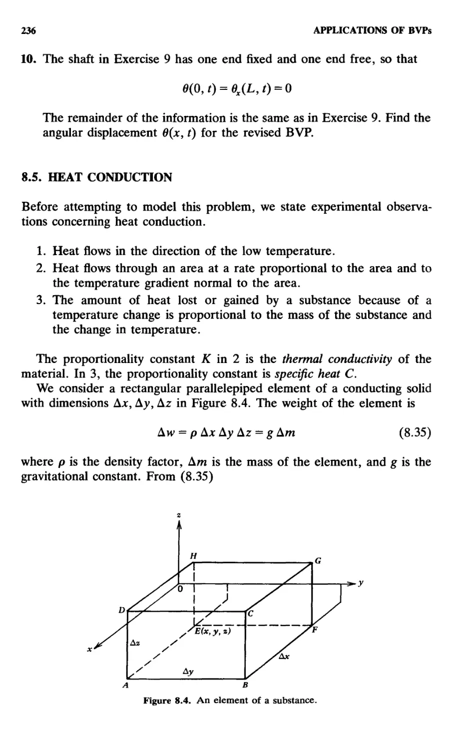
Text
FOURIER SERIES,
TRANSFORMS, AND
BOUNDARY VALUE
PROBLEMS
Second Edition
J. RAY HANNA
Professor Emeritus
University of Wyoming
Laramie, Wyoming
JOHN H. ROWLAND
Department of Mathematics
and Department of Computer Science
University of Wyoming
Laramie, Wyoming
A Wiley-Interscience Publication
John Wiley & Sons, Inc.
New York / Chichester / Brisbane / Toronto / Singapore
PURE AND APPLIED MATHEMATICS
A Wiley-Interscience Series of Texts, Monographs, and Tracts
Founded by RICHARD COURANT
Editors: LIPMAN BERS, PETER HILTON, HARRY HOCHSTADT, PETER LAX,
JOHN TOLAND
ADAMEK, HERRLICH, and STRECKER—Abstract and Concrete Categories
*ARTIN—Geometric Algebra
BERMAN, NEUMANN, and STERN—Nonnegative Matrices in Dynamic Systems
¦CARTER—Finite Groups of Lie Type
CLARK—Mathematical Bioeconomics: The Optimal Management of Renewable
Resources, 2nd Edition
"CURTIS and REINER—Representation Theory of Finite Groups and Associative Algebras
¦CURTIS and REINER—Methods of Representation Theory: With Applications to Finite
Groups and Orders, Vol. I
CURTIS and REINER—Methods of Representation Theory: With Applications to Finite
Groups and Orders, Vol. II
¦DUNFORD and SCHWARTZ—Linear Operators
Part 1—General Theory
Part 2—Spectral Theory, Self Adjoint Operators in
Hilbert Space
Part 3—Spectral Operators
FOLLAND—Real Analysis: Modern Techniques and Their Applications
FRIEDMAN—Variational Principles and Free-Boundary Problems
FROLICHER and KRIEGL—Linear Spaces and Differentiation Theory
GARDINER—Teichmiiller Theory and Quadratic Differentials
GRIFFITHS and HARRIS—Principles of Algebraic Geometry
HANNA and ROWLAND—Fourier Series, Transforms, and Boundary Value Problems,
2nd Edition
HARRIS—A Grammar of English on Mathematical Principles
*HENRICI—Applied and Computational Complex Analysis
*Vol. 1, Power Series—Integration—Conformal Mapping—Location of Zeros
Vol. 2, Special Functions—Integral Transforms—Asymptotics—Continued
Fractions
Vol. 3, Discrete Fourier Analysis, Cauchy Integrals, Construction of
Conformal Maps, Univalent Functions
¦HILTON and WU—A Course in Modern Algebra
*HOCHSTADT—Integral Equations
KOBAYASHI and NOMIZU—Foundations of Differential Geometry, Vol. I
KOBAYASHI and NOMIZU—Foundations of Differential Geometry, Vol. II
KRANTZ—Function Theory of Several Complex Variables
LAMB—Elements of Soliton Theory
LAY—Convex Sets and Their Applications
McCONNELL and ROBSON—Noncommutative Noetherian Rings
NAYFEH—Perturbation Methods
NAYFEH and MOOK—Nonlinear Oscillations
TRENTER—Splines and Variational Methods
RAO—Measure Theory and Integration
RENELT—Elliptic Systems and Quasiconformal Mappings
RICHTMYER and MORTON—Difference Methods for Initial-Value Problems,
2nd Edition
RIVLIN—Chebyshev Polynomials: From Approximation Theory to Algebra and Number
Theory, 2nd Edition
ROCKAFELLAR—Network Flows and Monotropic Optimization
ROITMAN—Introduction to Modern Set Theory
*RUDIN—Fourier Analysis on Groups
SCHUMAKER—Spline Functions: Basic Theory
SENDOV and POPOV—The Averaged Moduli of Smoothness
*SIEGEL—Topics in Complex Function Theory
Volume 1—Elliptic Functions and Uniformization Theory
Volume 2—Automorphic Functions and Abelian Integrals
Volume 3—Abelian Functions and Modular Functions of Several Variables
STAKGOLD—Green's Functions and Boundary Value Problems
¦STOKER—Differential Geometry
STOKER—Nonlinear Vibrations in Mechanical and Electrical Systems
TURAN—On a New Method of Analysis and Its Applications
WHITHAM—Linear and Nonlinear Waves
ZAUDERER—Partial Differential Equations of Applied Mathematics, 2nd Edition
*Now available in a lower priced paperback edition in the Wiley Classics
Library.
Copyright © 1990 by John Wiley & Sons, Inc.
All rights reserved. Published simultaneously in Canada.
Reproduction or translation of any part of this work
beyond that permitted by Section 107 or 108 of the
1976 United States Copyright Act without the permission
of the copyright owner is unlawful. Requests for
permission or further information should be addressed to
the Permissions Department, John Wiley & Sons, Inc.
Library of Congress Catagloging in Publication Data:
Hanna, J. Ray.
Fourier series, transforms, and boundary value problems. -- 2nd
ed. / J. Ray Hanna and John H. Rowland.
p. cm. -- (Pure and applied mathematics, ISSN 0079-8185)
Rev. ed. of: Fourier series and integrals of boundary value
problems. cl982.
"A Wiley-Interscience publication."
Includes bibliographical references (p.
ISBN 0-471-61983-3
1. Boundary value problems. 2. Fourier series. I. Rowland, John
H. II. Hanna, J. Ray. Fourier series and integrals of boundary
value problems. III. Title. IV. Series: Pure and applied
mathematics (John Wiley & Sons)
QA379.H36 1990
515\36--dc20 89-25089
CIP
Printed in the United States of America
10 987654321
PREFACE
The basic philosophy remains the same as in the first edition. The primary
changes consist of the addition of new material on integral transforms,
discrete and fast Fourier transforms, series solutions, harmonic analysis,
spherical harmonics, and a glance at some of the numerical techniques for
the solution of boundary value problems. The order of presentation of some
of the material from the first edition has been rearranged to provide more
flexibility in arranging courses based on this text.
The book contains more than enough material for a one semester course.
For this reason we have attempted to keep the later chapters relatively
self-contained. The first three chapters contain basic material which would
ordinarily be covered in a course of this nature. These could be followed by
any combination of Chapters 4, 5, 6, and 8, except that Sections 8.11-8.13
depend on Chapter 5 and Sections 8.14 and 8.15 depend on Chapter 6.
Chapter 7 depends somewhat on the theory presented in Chapter 4 and the
Hankel and Legendre transforms depend on Chapters 5 and 6, respectively.
Chapter 9, taken in its entirety, is dependent on all of the preceding
chapters. However, instructors who prefer to interweave applications with
the development of tools will find that it is possible to select pertinent topics
from Chapters 8 and 9 as the necessary mathematics is developed.
A one-semester course given at the University of Wyoming covers
substantial portions of Chapters 1, 2, 3, 4, 7, and 8. This course has upper
class and graduate students from fields such as geophysics, physics, en-
engineering, computer science, and mathematics.
We are indebted to Maria Taylor and Bob Hilbert for valuable editorial
assistance and to many students for catching errors and suggesting improve-
improvements. Finally, we express our special appreciation to Janet Netzel and
Mitzi Stephens for their skillful typing.
J. Ray Hanna
Aurora, Colorado
John H. Rowland
Laramie, Wyoming
May, 1990
PREFACE TO THE FIRST
EDITION
This book is a result of the development of a set of notes for a course in
boundary value problems, using Fourier series and integrals. Its primary
objective is to acquaint students with the solutions of boundary value
problems associated with natural phenomena. It is therefore necessary for
the reader to understand basic concepts and manipulations of elementary
calculus. Although some mathematical ideas from advanced calculus are
beneficial, many of the concepts are contained in this book. A minimal
background in physics will aid one in understanding the modeling of a few
problems concerning heat, wave, and potential theory.
This book refers to the main process for solving boundary value problems
as the Fourier method. To understand the details of this procedure, topics of
orthogonality, Fourier series, and integrals precede the discussion of the
Fourier method. Of necessity such topics as convergence, existence, and
uniqueness are included. Emphasis is placed clearly on the use of basic
concepts and techniques rather than the details of developing the theory.
There are many completely solved examples. These are followed by exer-
exercises that allow the reader ample opportunity to test his/her understanding
of the material. Most exercises are accompanied with answers. Some
answers are implied in the problems, while others are given in an answer
section. The abbreviations used are listed in the index.
Content similar to that of this book has been used in a course of three
semester hours with several classes. If a prerequisite of ordinary differential
equations is prescribed, much of Chapter 1 may be omitted. To shorten the
course chapters on either Bessel functions or Legendre polynomials may be
deleted. Work with operators may be reduced, or other sections may be
omitted without seriously affecting the continuity of the course. The prefer-
preference of the instructor, the background and interests of the students, and the
intensity of the course should govern the choice of subject matter.
Numerous colleagues and students have influenced the form of this book.
It is my pleasure to thank everyone who has offered suggestions for its
improvement. I am particularly indebted to my department head, Joseph
viii PREFACE TO THE FIRST EDITION
Martin, for his faithful support of the project, and to Daniel Katz, a former
student, for his helpful ideas and his solutions for many of the problems. To
Beatrice Shube for valuable editorial assistance, and to all of the Wiley
publication staff, I am deeply grateful. Finally, I express a special apprecia-
appreciation for the skillful typing of the manuscript by Laureda Dolan, Paula
Melcher, and Pat Twitchell.
Humbly I acknowledge the volumes of literature, extending from a time
before J. Fourier to the present, which have influenced the composition of
this book. It would be an endless task to mention each one. A list of
references, by no means exhaustive, is included to aid the reader.
In spite of careful proofreading, some errors are elusive and not discov-
discovered. I encourage readers to inform me of mistakes and to offer suggestions
for the improvement of the book.
J. Ray Hanna
Laramie, Wyoming
January 1982
CONTENTS
1. Linear Differential Equations
1.1. Linear Operators, 1
1.2. Ordinary Differential Equations, 2
1.3. Homogeneous Linear ODE with Constant Coefficients, 5
1.4. Euler's ODE, 7
1.5. Series Solutions, 8
1.6. Frobenius Method, 13
1.7. Numerical Solutions, 19
1.8. Linear PDEs, 23
1.9. Classification of a Linear PDE of Second Order, 23
1.10. Boundary Value Problems with PDEs, 24
1.11. Second Order Linear PDEs with Constant Coefficients, 26
1.12. Separation of Variables, 35
2. Orthogonal Sets of Functions 40
2.1. Orthogonality and Vectors, 40
2.2. Orthogonal Functions, 42
2.3. Complex Functions, 46
2.4. Additional Concepts of Orthogonality, 47
2.5. The Sturm-Liouville Boundary Value Problem, 50
2.6. Uniform Convergence of Series, 58
2.7. Series of Orthogonal Functions, 61
2.8. Approximation by Least Squares, 64
2.9. Completeness of Sets, 65
3. Fourier Series 68
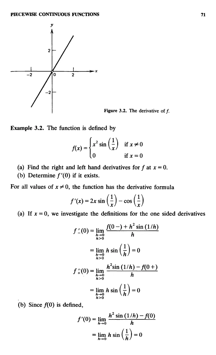
3.1. Piecewise Continuous Functions, 68
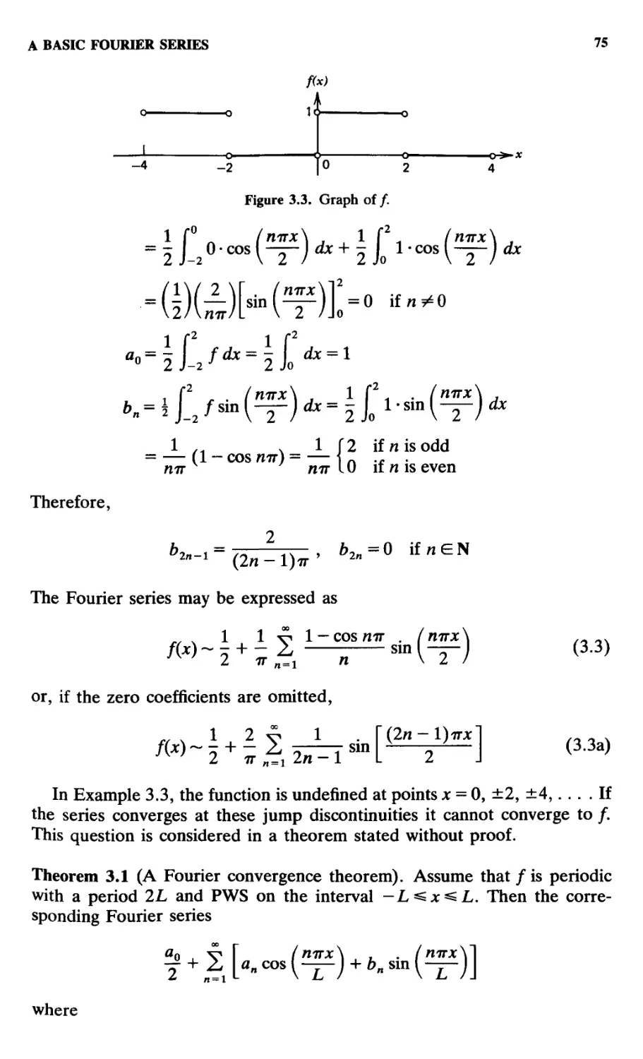
3.2. A Basic Fourier Series, 72
3.3. Even and Odd Functions, 76
ix
x CONTENTS
3.4. Fourier Sine and Cosine Series, 77
3.5. Complex Fourier Series, 80
3.6. Harmonic Analysis, 82
3.7. Uniform Convergence of Fourier Series, 89
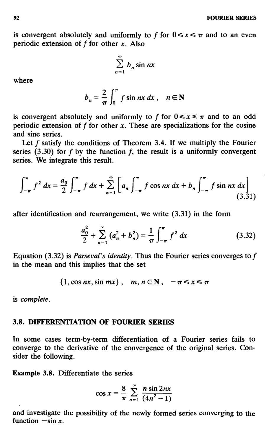
3.8. Differentiation of Fourier Series, 92
3.9. Integration of Fourier Series, 94
3.10. Double Fourier Series, 97
4. Fourier Integrals 102
4.1. Uniform Convergence of Integrals, 102
4.2. A Generalization of the Fourier Series, 107
4.3. Fourier Sine and Cosine Integrals, 109
4.4. The Exponential Fourier Integral, 112
5. Bessel Functions 117
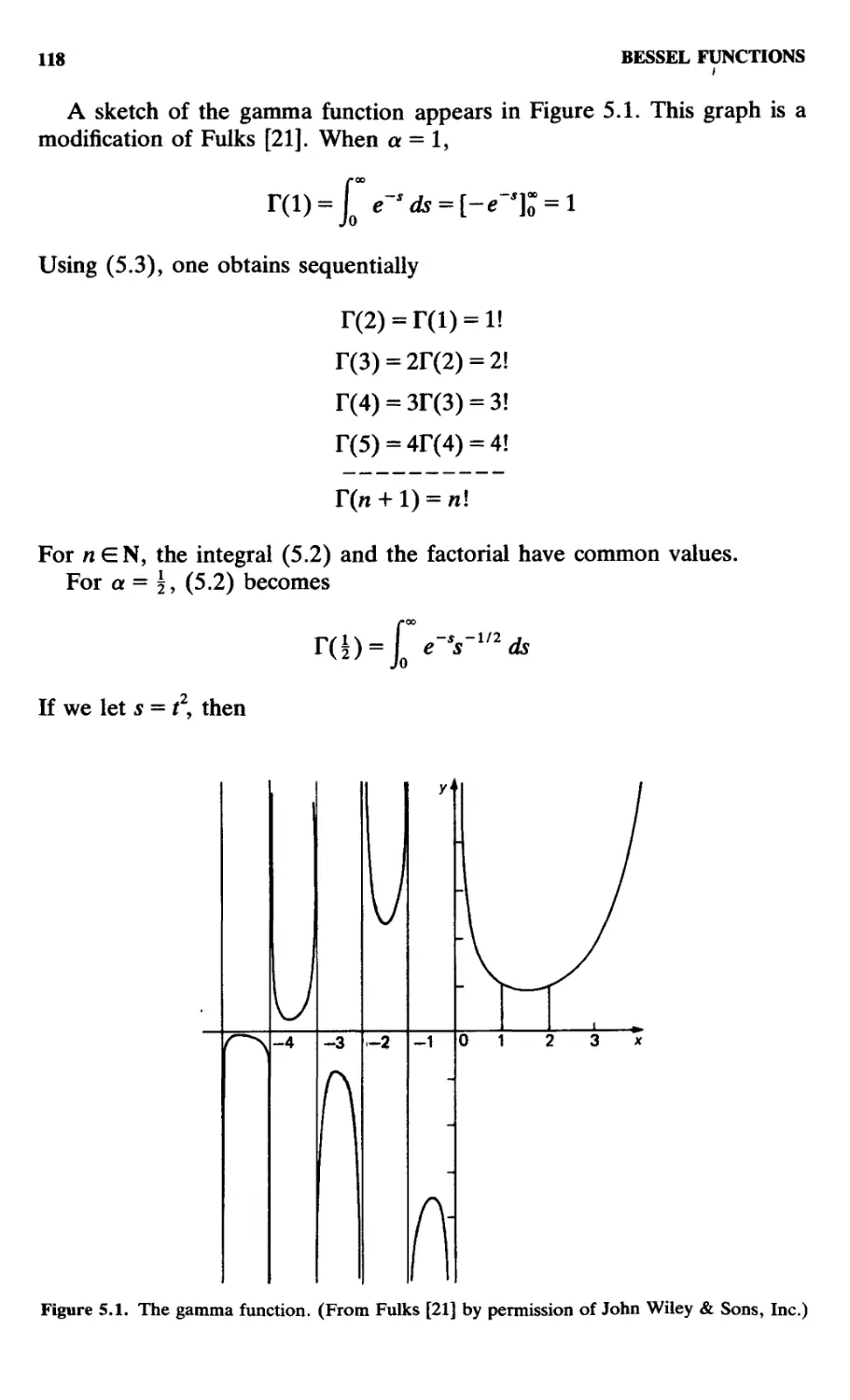
5.1. The Gamma Function and the Bessel Function, 117
5.2. Additional Bessel Functions, 120
5.3. Differential Equations Solvable with Bessel Functions, 122
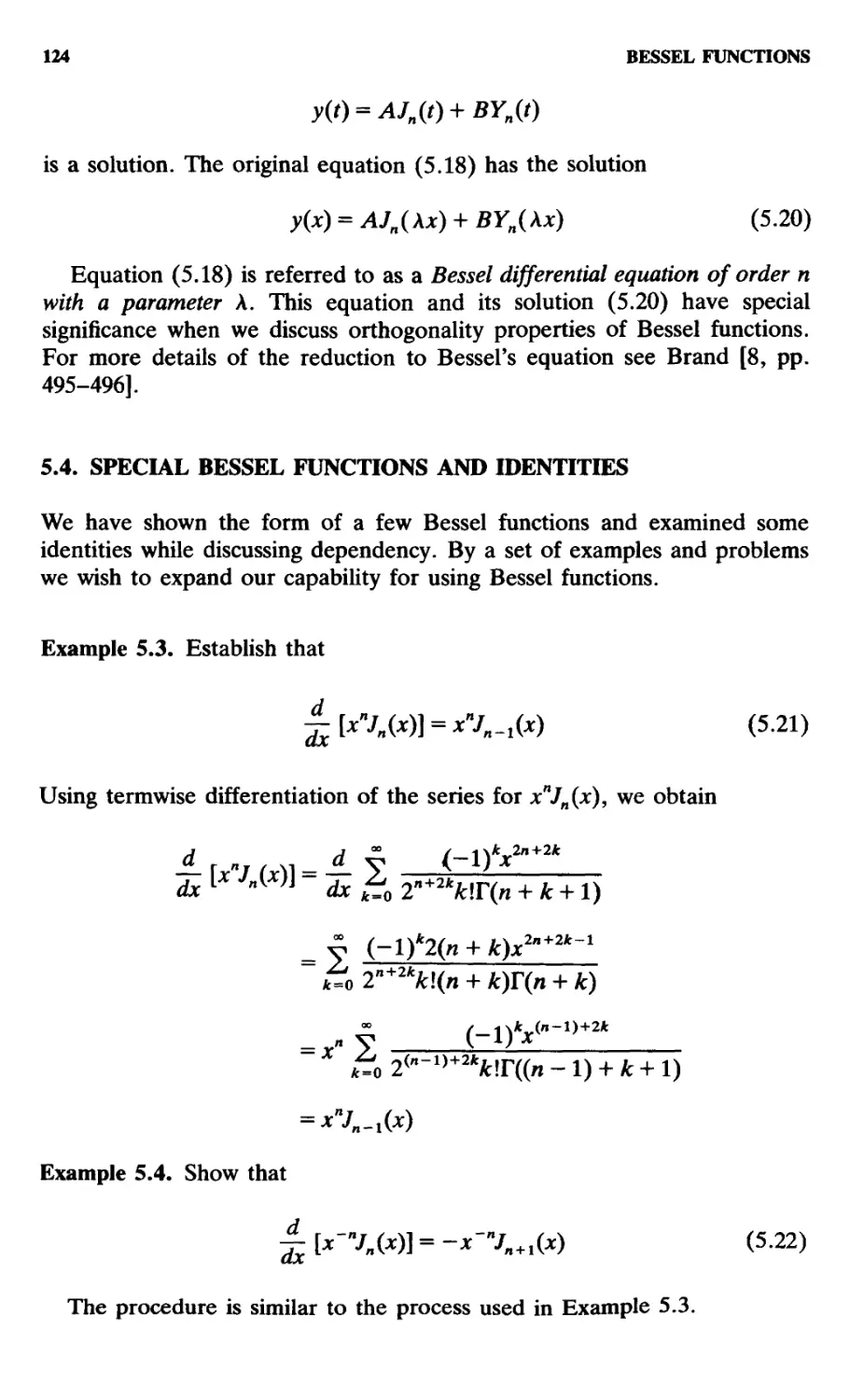
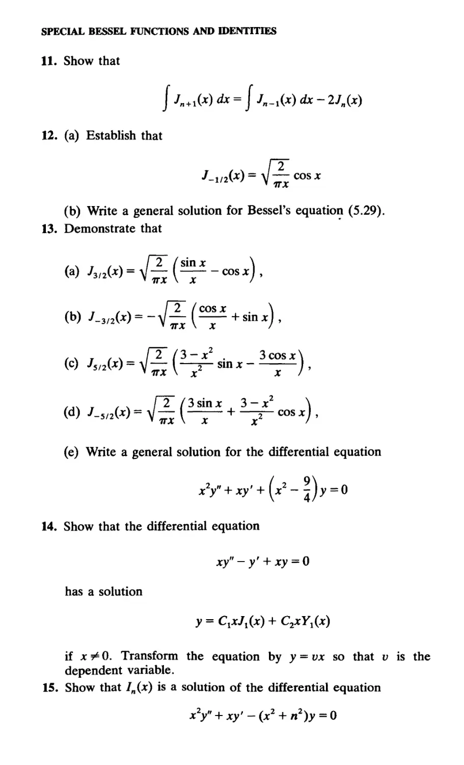
5.4. Special Bessel Functions and Identities, 124
5.5. An Integral Form for Jn(x), 130
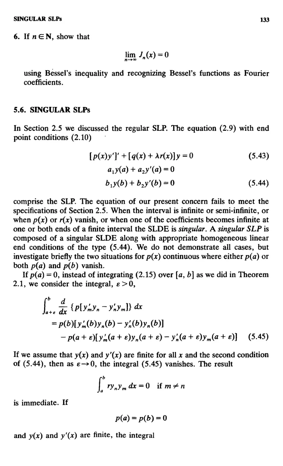
5.6. Singular SLPs, 133
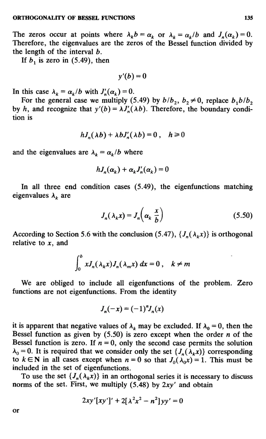
5.7. Orthogonality of Bessel Functions, 134
5.8. Orthogonal Series of Bessel Functions, 137
5.9. Bessel Functions and Cylindrical Geometry, 140
6. Legendre Polynomials 142
6.1. Solutions to the Legendre Equation, 142
6.2. Rodrigues' Formula for Legendre Polynomials, 146
6.3. A Generating Function for Pn(x), 149
6.4. The Legendre Polynomial Pn(cos 0), 151
6.5. Orthogonality and Norms of Pn(x), 152
6.6. Legendre Series, 154
6.7. Legendre Polynomials and Spherical Geometry, 158
6.8. Spherical Harmonics, 161
6.9. The Generalized Legendre Equation, 162
7. Integral Transforms 168
7.1. Laplace Transforms, 168
7.2. Existence of the Transform, 169
7.3. The Gamma Function and Laplace Transforms, 170
7.4. Transforms of Derivatives, 172
7.5. Derivatives of Transforms, 172
7.6. The Inverse Laplace Transform, 173
CONTENTS xi
7.7. Solutions of ODEs and IVPs, 173
7.8. Partial Fractions, 174
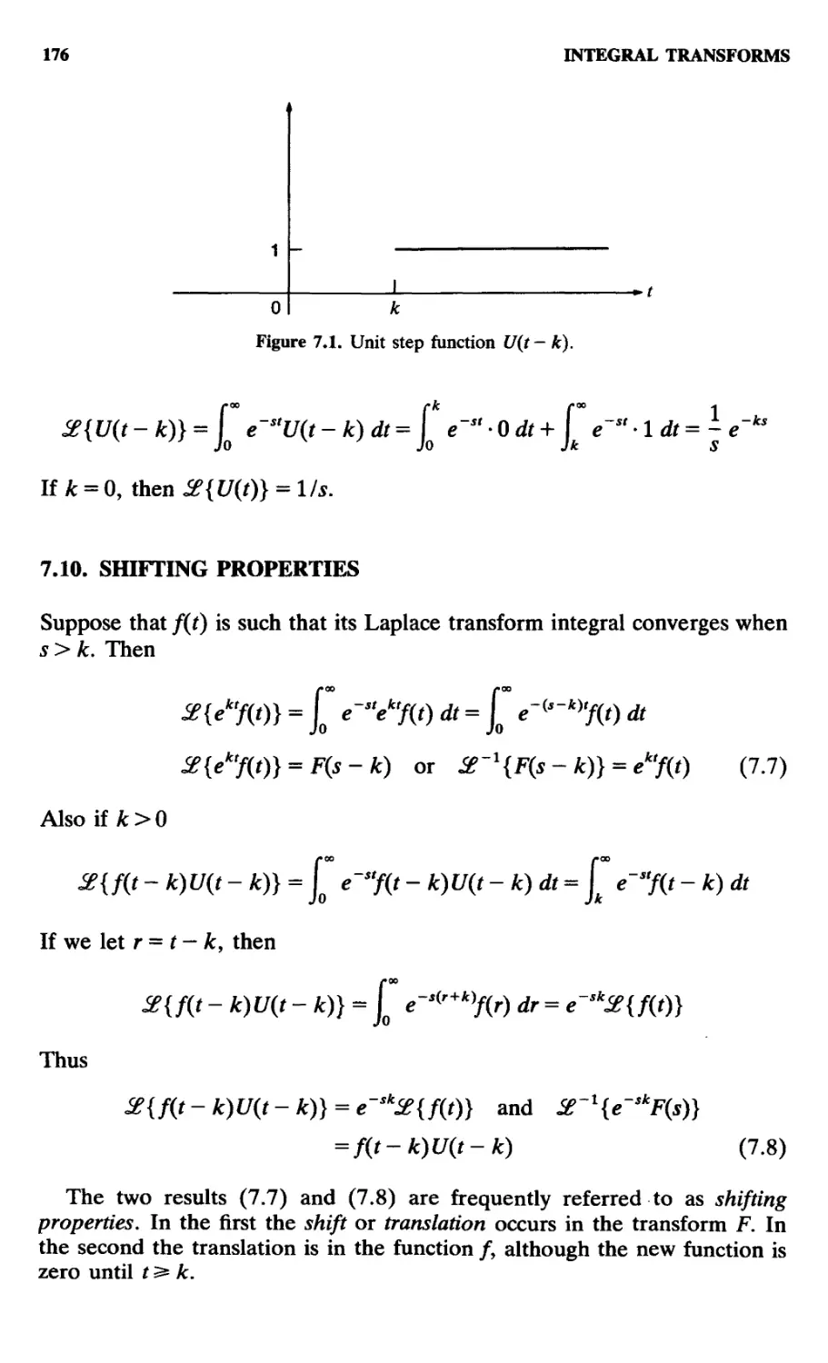
7.9. The Unit Step Function, 175
7.10. Shifting Properties, 176
7.11. The Dirac Delta Function, 177
7.12. Convolution, 180
7.13. Laplace Transform Method for PDEs, 186
7.14. Finite Fourier Transforms, 189
7.15. Fourier Transforms, 191
7.16. The Discrete Fourier Transform, 197
7.17. The Fast Fourier Transform, 203
7.18. Fourier Transforms of Functions of Two Variables, 208
7.19. Hankel Transforms, 209
7.20. Legendre Transform, 214
7.21. Mellin Transform, 215
8. Application of BVPs 219
8.1. The Vibrating String, 219
8.2. Verification and Uniqueness of the Solution of the
Vibrating String Problem, 225
8.3. The Vibrating String with Two Nonhomogeneous
Conditions, 228
8.4. Longitudinal Vibrations along an Elastic Rod, 230
8.5. Heat Conduction, 236
8.6. Numerical Solution of the Heat Equation, 241
8.7. Verification and Uniqueness of the Solution for the
Heat Problem, 242
8.8. Gravitational Potential, 246
8.9. Laplace's Equation, 247
8.10. Numerical Solution of the Laplace Equation, 251
8.11. Temperature in a Circular Disk with Insulated Faces, 254
8.12. Steady State Temperature in a Right Semicircular Cylinder, 256
8.13. Harmonic Interior of a Right Circular Cylinder, 260
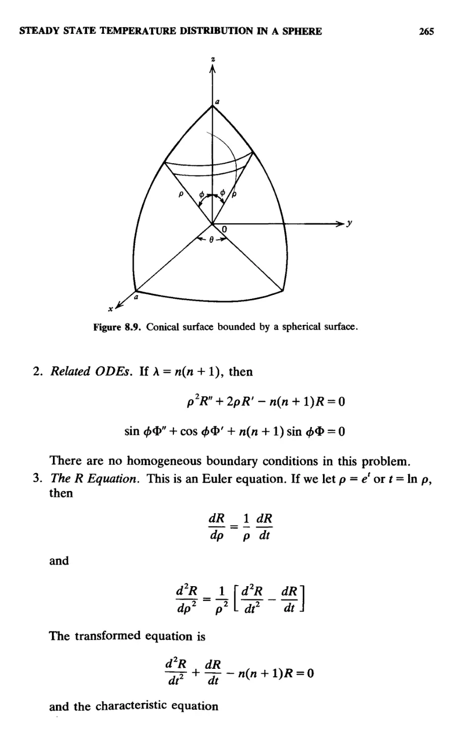
8.14. Steady State Temperature Distribution in a Sphere, 264
8.15. Potential for a Sphere, 267
9. Additional Applications 270
9.1. Mechanical and Electrical Oscillations, 270
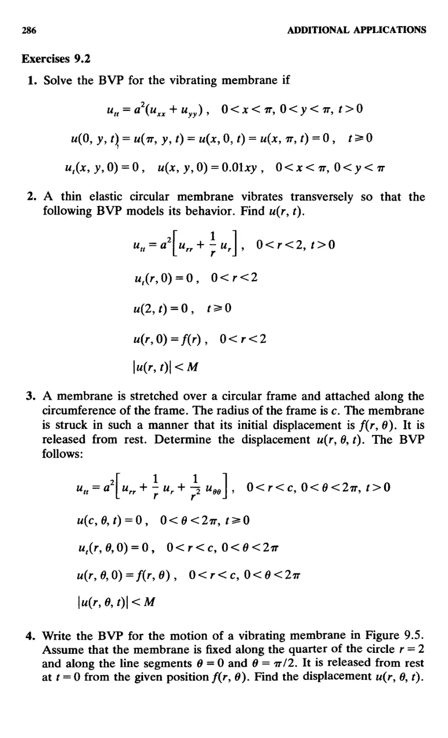
9.2. The Vibrating Membrane, 273
9.3. Vibrations of a Circular Membrane Dependent on Distance
from Center, 280
9.4. The Vibrating String with an External Force, 283
9.5. Nonhomogeneous End Temperatures in a Rod, 289
9.6. A Rod with Insulated Ends, 291
xii CONTENTS
9.7. A Semi-Infinite Bar, 295
9.8. An Infinite Bar, 297
9.9. Discrete Fourier Transform Solutions, 305
9.10. A Semi-Infinite String, 307
9.11. A Semi-Infinite String with Initial Velocity, 310
References 315
Answers to Exercises 317
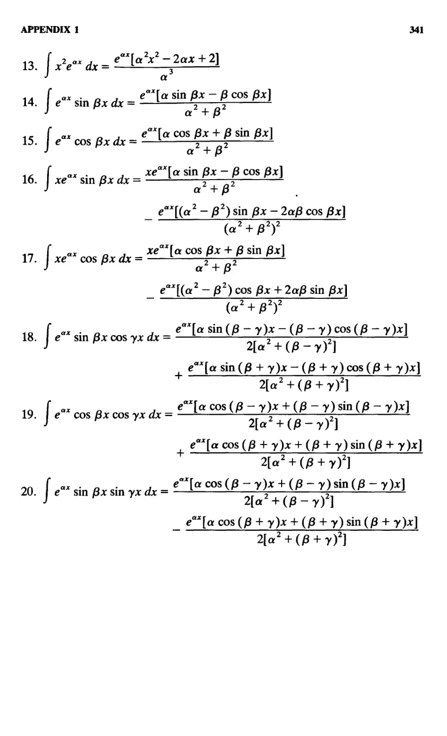
Appendix 1 Selected Integrals 340
Appendix 2 Table of Laplace Transforms 342
Appendix 3 Tables of Finite Fourier Transforms 344
Appendix 4 Tables of Fourier Transforms 346
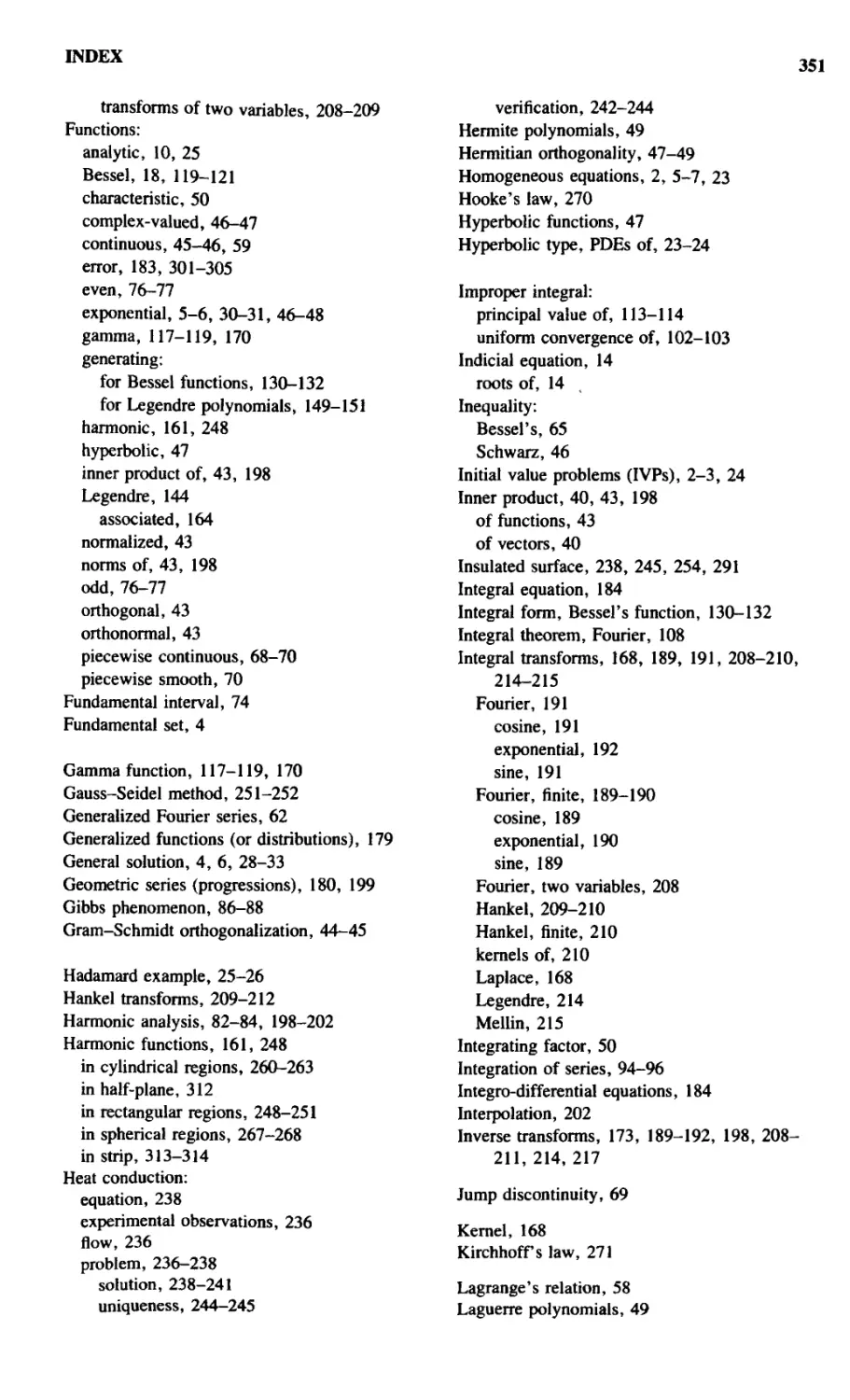
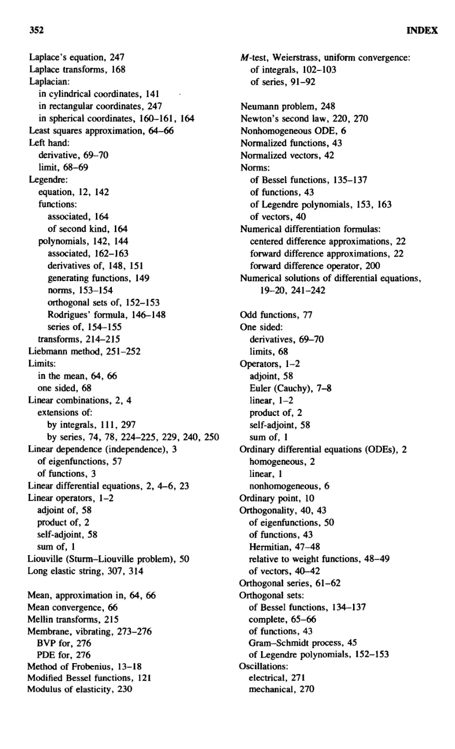
Index 349
FOURIER SERIES,
TRANSFORMS, AND
BOUNDARY VALUE
PROBLEMS
1
LINEAR DIFFERENTIAL
EQUATIONS
The primary objective of this book is to develop procedures for obtaining
solutions to boundary value problems (abbreviated BVPs) containing partial
differential equations (abbreviated PDEs). One of the principal solution
procedures for PDEs requires some knowledge of ordinary differential
equations (abbreviated ODEs) and their solutions. This chapter begins with
a review of basic concepts for solving ODEs. The topics considered will
include the superposition principle, characteristic equations, power series
solutions, the Frobenius method, and numerical solutions. The remainder of
the chapter will involve definitions, classifications, and solutions of PDEs.
1.1. LINEAR OPERATORS
An operator is a mathematical transformation applied to a function to
produce another function. If Q is an operator, the notation Qy means that
Q acts upon the function у to produce a new function Qy. For Qy = y2, Q is
a squaring operator. The new function is y2. When Qy — Dy, Q is a
derivative operator D and the transformed function is the derivative of y.
A linear operator L changes each function so that for two functions yx and
y2 of a class
ДС1У1 + c2y2) = cxLyx + c2Ly2 A.1)
if cx and c2 are constants. One finds by using A.1) that the differential
operator D is linear but the squaring operator is not linear.
The sum of two linear operators L and M is defined by
(L + M)y = Ly
2 LINEAR DIFFERENTIAL EQUATIONS
A product of two linear operators LM is the linear operator M acting upon у
and sequentially L operating on My. This is expressed by
LMy = L(My)
In A.1), c1yl + c2y2 is called a linear combination ofy1 and y2. The linear
operator acting upon the linear combination of yx and y2 is the linear
combination of Lyx and Ly2. A linear combination of a set of n functions is
defined by
ckyk
1.2. ORDINARY DIFFERENTIAL EQUATIONS
For a linear differential operator
L = D* + a^D"'1 + ¦ • ¦ + o^WD + an (x)
and a function f(x)
Ly=f A.2)
is a //near ODE of order n. If/=0, the equation
Ly-0 A.3)
is a linear homogeneous ODE of order n.
An initial value problem (abbreviated IVP) is composed of a differential
equation A.2) or A.3) and set of n restrictions at a single point. These
restrictions, called initial conditions, have the form
У(*о) = Уо , ?(x0) = yj,. . . , yb-^xo) - y?-» A.4)
where yQ9 yf0,. . . , y^'^ are constants.
A boundary value problem (abbreviated BVP) contains a differential
equation and a set of n constants called boundary conditions. These
conditions are given at two or more points. At this time definitions for both
the IVP and the BVP are relative to ODEs.
The equation y" + 4y == 0 with restrictions y@) = y'@) = 1 is an IVP. The
ODE y" + Ay = 0 accompanied by y@) = 1, у(тг/4) = О is a BVP.
Although our main emphasis is the determination of solutions, questions
of existence and uniqueness of solutions for differential equations with
constraints are important. If one succeeds in finding a solution for an IVP or
ORDINARY DIFFERENTIAL EQUATIONS 3
a BVP then a solution exists. To ascertain whether other solutions exist for
the same problem may be as necessary as knowing a solution. We state
without proof an existence-uniqueness theorem for an IVP.
Theorem 1.1. Let x0E(a,b) and аг(х), а2(*), • • ¦ , «„(*), and f(x) be
continuous on (a, b) for the IVP composed of A.2) with initial conditions
A.4). Then there exists a unique solution y{x) for the problem.
A set of functions
A.5)
defined on (a, b) is linearly independent if the linear combination for the set
Wi + сгУг + • • • + cnyn = 0 A.6)
implies that for all x on the interval the only с solution is
If some constants ck #0 exist in A.6) then the set is linearly dependent.
Example 1.1. Are the functions ex and e x linearly dependent?
Examine the equation
cxex + c2e~x = 0
If both sides of A.7) are multiplied by ex
A.7)
2x
The two members are identical for all x only if
The Wronskian of the set of functions A.5), assumed differentiable n - 1
times, is denned by
У г ¦¦¦ Уп
У'г ¦•• У'п
It can be shown that if W(ytJ y2,. . . , yn) is not zero for any x G (a, b),
4 LINEAR DIFFERENTIAL EQUATIONS
then A.5) is linearly independent. If A.5) is a solution set for A.3) the
linear combination of A.5)
У = cxyx + С2У2 + • • • + cnyn A.8)
is a solution of A.3). This idea is referred to as the superposition principle.
The n solutions of A.3) form a fundamental solution set if every solution of
A.3) can be formed as a linear combination of A.5) as shown in A.8).
ЩУг> Уг-> • • • з Уп) f°r toe solution set A.5) can be shown either to vanish
identically or else never be zero. The following theorem describes conditions
for a fundamental solution set and defines a general solution.
Theorem 1.2. Let ax(x), <*2(х),. . . , an(x) be continuous on (a, b), let A.5)
be the solution set of the linear homogeneous ODE A.3), and let
ЩУп Уп • • • > >O^0 f°r one point on (a, b). Then it is possible to form
any solution of A.3) as a linear combination of A.5). The solution set is a
fundamental set. The linear combination A.8) is called the general solution.
Exercises 1.1
1. Show that the two conditions L(yx + y2) — Lyv + Ly2 and L(cy) = cLy
taken together imply linearity.
2. Show that the sum of two linear operators L and M is linear.
3. If both L and M are linear operators, is LM linear?
4. Assume that L and M are linear operators. Show by contradiction that
LM and ML are not always the same.
5. (a) Verify that yx = l/(x + 1) and y2 = l/(x + 2) are both solutions of
y' + y2=0.
(b) Compute the Wronskian W(yls y2). Is the set {y1? y2} linearly
independent?
(c) Is there a c1 so that c1y1 is a solution?
(d) Is there a c2 so that c2y2 is a solution?
(e) If nonzero values of cx and c2 are used from (c) and (d) then is
cxyx + c2y2 a solution of the differential equation? Do your results
violate Theorem 1.2? Explain.
6. (a) If уг and y2 are solutions of the differential equation y" + x2y = 0, is
у = c^j + c2y2 a solution? Why?
(b) If yx and y2 are solutions of y" + y = x\ is у = c1y1 + c2y2 a
solution?
7. (a) Assume that y1 and y2 satisfy the differential equation y" + sin у =
0. Is у = c1y1 + c2y2 a solution?
(b) If yx and >>2 are solutions of y" + sin л; = 0, is у = cxyx + c2y2 a
solution? Explain basic differences in the differential equations of
(a) and (b).
HOMOGENEOUS LINEAR ODE WITH CONSTANT COEFFICIENTS 5
8. (a) Is the set of functions {ex, e2x} linearly independent?
(b) Test the set {ex, e2x, xe2x) for linear independence.
(c) For the differential equation ym-5y* + 8y' -Ay =0 verify that ex
and e2x are solutions.
(d) Is cxex + c2e2x a solution of the ODE in (c)? Is it a general solution?
Why?
(e) Is xe2x a solution of the ODE in (c)? Is cxex + c2e2x + c3xe2x a
general solution? Explain.
9. (a) Verify that the equation y" + 4y = 0 is satisfied by the two solutions
yx = 2 cos2* - 1 and y2 = 1 - 2 sin2*.
(b) Determine the Wronskian WBcos2*- 1,1 - 2 sin2*). Is the set
{yl7 y2} of (a) linearly independent?
(c) Is c1y1 + c2y2 a general solution for y" + Ay = 0?
10. The differential equation y" + Ay = 4 has two solutions уг = cos 2* + 1
and y2 = sin2jt +1. Is c^ + c2y2 a solution of the ODE? Is Theorem
1.2 violated?
The ODE
y"+a2y =
and its general solution
y = cl cos a* + c2 sin a*
play a prominent role in our study of BVPs of PDEs. Usually our linear
ODEs will be homogeneous of order no greater than 2. Since the discussion
of the nth order case is as easy basically as the second, the nth order
equation is our choice.
1.3. HOMOGENEOUS LINEAR ODE WITH CONSTANT
COEFFICIENTS
The equation described under this heading has the form
Ly = (Dn + axDnl + - • • + an^D + an)y = 0 A.9)
where a1?. . . , an are real constants. Let у = етх be a proposed solution for
A.9). Actual substitution of emx in A.9) implies that
mn
ап_гт + an = 0 A.10)
This polynomial equation is called the auxiliary or characteristic equation for
A.9). Of the n roots of A.10) (a) all may be real and distinct, (b) some may
be imaginary, or (c) some may be multiple roots.
LINEAR DIFFERENTIAL EQUATIONS
1. Real and Distinct Roots. If roots of A.10) are m%9 m2,... , mn, then
the fundamental solution set is emiX, e™2*,. .. , emnX, and by superpo-
superposition
у = cxemi* + сгетг* + • • • + cnem»x
is the general solution.
2. Imaginary Roots. If a1? a2,. .. , an are all real and a + ib (a and 6
real numbers) is,a root of A.10), then a — ib is also a root. A solution
corresponding to the conjugate pair of roots a±ib, b т^О, is
У к ~ e<lX(c\ cos bx + c2 sin бд:)
3. Multiple Roots. If one root of the characteristic equation mk is
repeated r times, then the solution corresponding to the multiple root
is
If the ODE has the differential operator of A.9) but the form
Ly=f A.11)
then the equation is nonhomogeneous if/^0. To solve A.11) one first finds
a general solution yc for the equation Ly = 0. Next find a function yp that
satisfies A.11). The general solution for A.11) is y = yc + yp- We refrain
from discussing procedures for determining yp. For readers having a need
for this information see Boyce and DiPrima [6, pp. 143-162 and 270-278].
Example 1.2. Find the general solution for the ODE y" - 4y' + 13y = 0.
The characteristic equation is
m2 - Am + 13 = 0
with roots 2 ± 3i. The general solution is written
у = e2x(cl cos 3x + c2 sin 3x)
Example 1.3. Determine the solution for the BVP
The ODE has a characteristic equation
EULER'S ODE 7
m3 -6m2 + 12m -8-0 A.12)
or
(w - 2K = 0
A root 2 of multiplicity 3 is the solution of A.12). The general solution of
the ODE is expressed by the linear combination
у = (cl + c2x + сгх2)е2х
If y@) = 0, then cx = 0. If y{\) = 0,c2 + c3 = 0. Note that
yf = 2(c2jc + c3*2)e2* + (c2 + 2с3д:)е2л
If /@) = 1, c2 = 1. Therefore, c3 = -1. The BVP has the solution
y = (x-x2)e2x
1.4. EULER'S ODE
The operator of the Euler (or Cauchy) ODE is the operator of A.9) with an
added factor xn inserted in each coefficient, where n is the order of the
derivative. For the ODE
Ly - (xnDn + axxn-lDn-1 + ¦ • - + an_xxD + an)y =/ A.13)
a transformation jc = e' is employed to change the independent variable x to
t. This transformation converts A.13) to a new ODE with constant coef-
coefficients.
Example 1.4. Solve the differential equation
x2y" + 7xy' + 9y = 0 A.14)
Let x = e* and t = In jc. Then
4у_1<(У . d2y ±\d2y dy]
dx~xli and ^7-*2U2 AJ
The new ODE with the independent variable t is
8 LINEAR DIFFERENTIAL EQUATIONS
The characteristic equation
rn + 6m + 9 = 0
has a double root —3. Equation A.15) has a general solution
Using the transformation again, one obtains
y(x) = (cx + c2 In x)x~3 A.15a)
Euler equations appear in solutions of BVPs involving spherical geometry.
Exercises 1.2
1. Determine a general solution for the equation y" + 5y' + 6y = 0.
2. Find a general solution for the equation y" - Ay' + Ay — 0.
3. Solve the differential equation y" + 2/ + 2y = 0.
4. Show that the characteristic equation for ym - 2yf - Ay = 0 has a root of
2. Then solve the differential equation.
5. Solve the boundary value problem ytf - у = 0, y@) = 0, у'{тг) — 1.
6. Find a general solution for yD) - у = 0.
7. Solve the differential equation /" - 5/' + 6/ = 0.
8. Determine a general solution for the equation x2y" - Ъху' + Ъу = 0.
9. Solve the BVP x2y" - 3xyr + Ay = 0, y(l) = 0, y(e) = e\
10. Find a general solution for л;2/' -xy' + 5y = Q.
11. Find a solution for the BVP x2y" + xyf + у = 0, y(l) = 0, у(е7Г/2) = тг.
1.5. SERIES SOLUTIONS
In Section 1.3 we have seen how to determine solutions for linear ODEs
with constant coefficients. These closed form solutions are expressed by
elementary functions. If the coefficients of A.9) or A.11) are not constants,
then with a few exceptions such as the Euler equation it is not possible to
find closed form solutions for second and higher order equations. For these
situations we introduce the power series and numerical methods for solving
differential equations. It is assumed that the reader has an acquaintance
SERIES SOLUTIONS 9
with the elementary theory of power series such as that described in Boyce
and DiPrima [6, Section 4.1].
If a function is represented by a power series on the interior of its interval
of convergence, then termwise differentiation of that series produces a
power series which converges on that same interval to the derivative of the
function. Frequently, the ratio test is useful for determining the radius of
convergence. The foregoing fact along with the usual algebraic operations
are necessary when a series is substituted into a differential equation. To
illustrate the mechanics of this method, we consider a simple example.
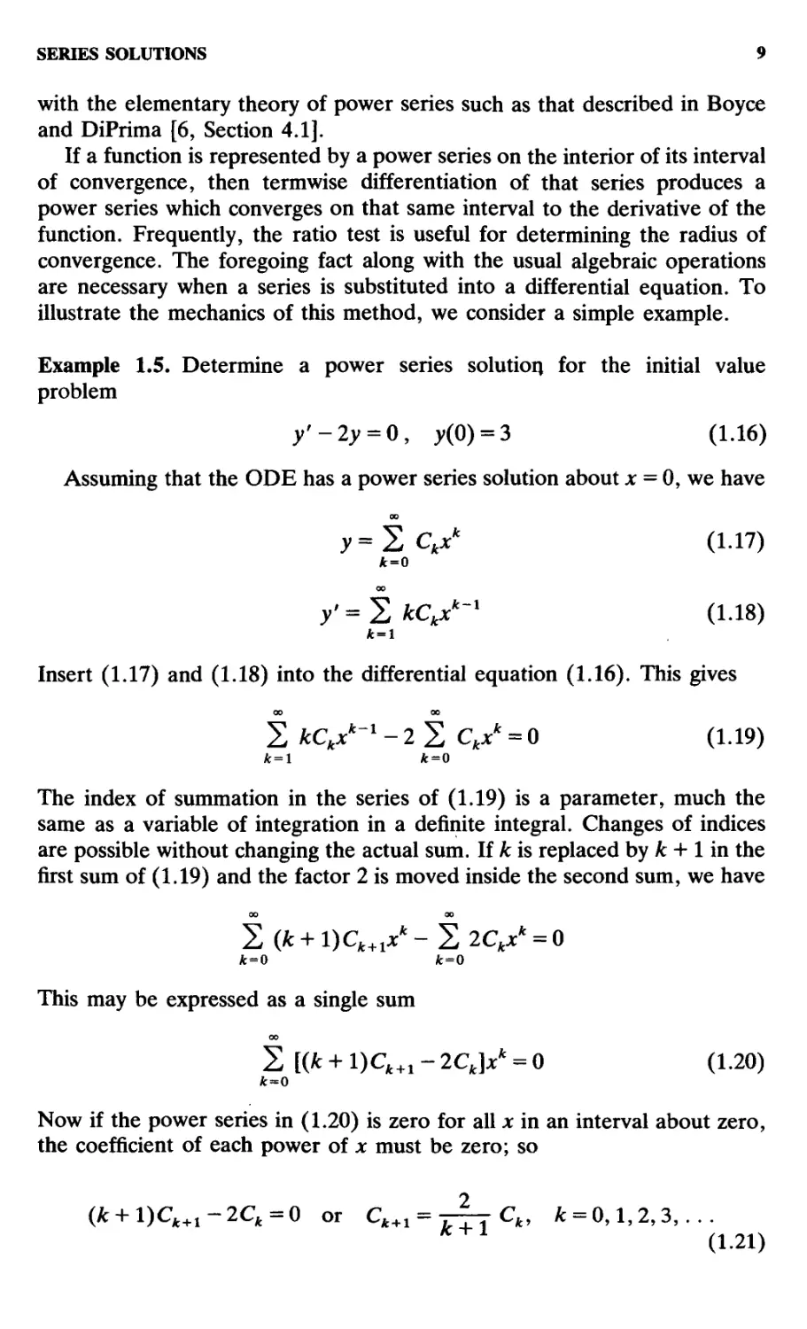
Example 1.5. Determine a power series solution for the initial value
problem
y'-2y = 0, K0) = 3 A.16)
Assuming that the ODE has a power series solution about x = 0, we have
00
PSC/ A.17)
Jt=O
00
/= 2 kCkxk"x A.18)
k=\
Insert A.17) and A.18) into the differential equation A.16). This gives
00 00
2 кСкхк'1 - 2 2 Ckxk = 0 A.19)
The index of summation in the series of A.19) is a parameter, much the
same as a variable of integration in a definite integral. Changes of indices
are possible without changing the actual sum. If к is replaced by к + 1 in the
first sum of A.19) and the factor 2 is moved inside the second sum, we have
00 00
2 (k + l)Ck+lxk - 2 2Ckxk = 0
Jt = O Jfc=0
This may be expressed as a single sum
00
2 [(k + l)Ct+1 - 2Ck)xk = 0 A.20)
Now if the power series in A.20) is zero for all x in an interval about zero,
the coefficient of each power of x must be zero; so
= 0 or Ck+l = -r^-rCk, k = 0,l,2,3,...
K + 1 A.21)
10 LINEAR DIFFERENTIAL EQUATIONS
Successively substituting к = 0,1,2, 3,... , in the recursion formula A.21),
we obtain
2 22 2 23
Q = 2C0 , C2 = - Q = ~ Co , C3 = ^ Q = з[ ^o? * * •
The solution у is given by
2Cx +
22 23
у = Co + 2Cox + - Cx2 + Cx3
or
But >^@) = 3; so
3 = C0(l + 2) jg) and Co = 3 A.22)
It follows from A.22) that the solution is
y = 3Z -^p =3e A.23)
This solution is the same as we obtain using the procedure of Section 1.3.
The series in A.23) converges for all values of x.
A function fix) is analytic at jc0 if it can be represented by a power series
of the form E?=o Ck(x ~ xo)k with positive radius of convergence. Consider
the second order homogeneous differential equation
y" + p(x)y' + q(x)y = 0 A.24)
When both p(x) and q(x) are analytic at x = xQ, then jc0 is an ordinary point
of the differential equation. If either or both p{x) and q(x) fail to be analytic
at x = jc0, then x0 is a singular point.
If x = jt0 is an ordinary point of A.24), then each solution can be
expressed as a power series
which converges on the interval (x0 — R, xo + R). Here Я is the smaller of
the radii of convergence of the power series (in powers of x - x0) represent-
representing p{x) and q(x).
SERIES SOLUTIONS 11
Example 1.6. Determine a power series solution for the ODE
y" + xy = 0 A.25)
The differential equation A.25) has an ordinary point at jc = O, and we
may assume a power series solution of the type A.17). Substituting the
series for у and y" into A.25), we obtain
00 00
2 Kk - \)Ckxk~2 + x 2 Ckxk = 0
Replacing к by к + 2 in the first series, A; by /г - 1 in the second, and
multiplying inside the second series termwise by x, we obtain
At this point it is desirable to have the indices of the sums begin with the
same number; this can be accomplished by displaying the first term of the
first sum separately. Then the sume can be combined to yield
00
2C2+ 2 [(k + 2)(k + 1)Сл+2 + Ск_г]хк = 0
Therefore,
C2 = 0 and (/г + 2)(/:4-1)Сл+2 + СЬ1=0
or
С = — Ir = 1 9 4
W + 2 /k _|_ 2V& + 1^ ' * " "
This implies that
С С С 2
Сз"^2 = -зГ' С4==" 4Л = " 4! Clf
Similarly, we obtain
С —О Г — ° г* — г1
5 ' 6~ 6! ' 7~ 7! x
where Co and Cx are arbitrary. Therefore,
12 LINEAR DIFFERENTIAL EQUATIONS
The solution A.26) is a linear combination of two series which can each be
shown to be convergent for all jc.
The equation
A - jc2)/ - 2xy' + n{n + \)y = 0 A.27)
is known as the Legendre differential equation of degree n. Since jc = 0 is an
ordinary point of the equation, we can use a power series to solve the
equation. Let
У = 2o Ckxk
be inserted in A.27). After several summation simplifications, the result
may be written
00
2 {{k + 2){k + l)CA+2 4- [{n - k)(n + к + l)]Ck}xk = 0 A.28)
Since A.28) is an identity with zero,
4+2 (* + 2)(* + l) C* l 'Щ
Two arbitrary constants, Co and Clf appear in the series solution. If к = n
in A.29) the coefficient Ск+2 - О and all successive coefficients Ck+2m will be
zeros also. Therefore, if n is a positive integer the series truncates and
becomes a polynomial. We include the results of A.29) for Co and Ct for a
few values of the index fc.
n(n + l) (nl)(n+2)
~" 2! °' 3 3! l
_(n-2)(n+3)n(n + l) ^ (n-3)(/i + 4)(n-!)(» +2)
J ьc -
S\ l
(n - 4)(/t + 5)(n - 2)(n + 3)(n)(n + 1)
6 ~ 6! °'
_ (n - 5)(/i + 6)(n - 3)(n + 4)(n - l)(n + 2)
FROBENIUS METHOD 13
If yo(x) represents the part of the solution associated with Co and уг(х)
associated with Cx, then
A.30)
where
v M _ т <n + 1) 2 n(n + !)(« - 2)(n + 3) 4
and
Ух (х) = х - хъ + л:5
(n - 1)(я + 2)(я - 3)(я + 4)(я - 5)(и -h 6) 7 +
?! A.32)
Legendre's series and polynomial functions will be studied in more detail in
Chapter 6.
1.6. FROBENIUS METHOD
Example 1.7. Solve the ODE
x2y" + Ixy' + 9y = 0 A-33)
We rewrite A.33) in the form A.24) so that the coefficient of y" is 1
It is apparent that x = 0 is a singular point for A.34). When one attempts to
find a series solution of the form A.17) using the method illustrated by
Examples 1.5 and 1.6, one obtains the trivial solution у = 0 (see Problem 4
of Exercises 1.3). However, A.33) is the ODE of Example 1.4, which has a
solution
у = {Cx + C2 In х)х~ъ
obtained by the procedure of Section 1.4. We will now show how to modify
the series technique to handle regular singular points.
14 LINEAR DIFFERENTIAL EQUATIONS
In the ODE A.24), assume that x = x0 is a singular point. It is a regular
singular point if (л: - xo)p(x) and (x - xoJtf(*) are each analytic. A singular
point which fails to be regular is an irregular singular point. We have noted
that the power series method fails to give a suitable solution for the ODE
A.33). As a modification to the power series method, let us assume that
A.33) has a solution of the type
y = /Sc/=Ec/+r, C0 = l, x>0 A.35)
This is the basic series for the Frobenius method. Note that if x = x0 is a
regular singular point, substitution of t = x - jc0 will change the power series
in (*-jc0) into a power series of the form A.35). Using A.35) and its
derivatives in A.33), we have
OO 00
x2 2 (k + r)(k + r - l)Ckxk+r-2 + 7x2, (k + r)^***'
*=0 *=0
00
+ 9? Ckxk+r = 0
This reduces to
00
2 [(k + r)(k + г - 1) + 7(k + r) + 9]Qx*+r = 0 A.36)
If к = 0, then [r(r - 1) + 7r + 9]C0 = 0. But Co # 0, ¦ and hence [r(r - 1) +
Ir + 9] = 0, or r2 + 6r + 9 = 0. This is called the indicial equation and its
roots, -3 and -3, the indicial roots or the exponents of the differential
equation. If r = -3, then from A.36), [(Jfc - 3)(* - 4) + l(k - 3) + 9]Ck = 0
and [k2 - 9 + 9]Ck = 0. Therefore, Ck = 0 for all A: > 1. The solution
Ar=O
is then equivalent to
У1 = х~3 A.37)
Since —3 is a double root of the indicial equation only one solution will be
obtained by direct substitution in A.35). A second solution may be obtained
by using the method commonly called the variation of parameters. The
method is based on the assumption that a solution y2 = и^ (м a function of
x) is a second solution of the differential equation. The assumption is
equivalent to y2 = ux~3. Substituting y2 and its derivatives into A.33), one
obtains
FROBENIUS METHOD 15
x2(l2x~5u - 6jT V + Jt~ V) + 7x(~3x~4u + лГ V) + 9x~3w = О
This reduces to
Integrating both sides and deferring the constants of integration until the
end, we obtain
In u' = -lnjc = x
and
u = lnx
Then
у2 = лГ31пх A.38)
The linear combination of yx and y2 in A.37) and A.38) can be written
y = (Kx + K2lnx)x-3
This is equivalent to A.15a).
Suppose that x = 0 is a regular singular point of the ODE A.24). Assume
that rx and r2 are the indicial roots of the equation found from the
substitution of у = xr Ll=0 Ckxk, C0 = l, in A.24). Then A.24) has two
linearly independent solutions уг and y2 on the interval 0<\x\<R if the
power series for xp(x) and x2q(x), in powers of x, are valid for |*|<Д.
Three cases follow:
(a) If rx - r2 differs from an integer, then
Уг = |x|ri S akxk , ao = l
k-0
00
^ = W'!S ькхк, bo = i
To avoid using x>0, absolute value signs are used.
16 LINEAR DIFFERENTIAL EQUATIONS
(b) If rx — r2 = r, then
00
Уг = Wr S akxk , a0 = 1
* = 0
00
У2 = \х\Г 2 V* + ^ In |x| , bo = l
*-0
(c) К rx - r2 is a positive integer, then
Jt = O
00
J2 = Wr2S Ькхк + ВУ1\п\х\, 60 = l
where 5 is a constant which may be zero.
Treatment of irregular singular points and situations involving complex
functions are omitted. For further information see a differential equation
text such as Boyce and DiPrima [6, Chapter 4].
We close our discussion of the Frobenius method by obtaining a solution
to BesseVs equation. This equation, which is very important in applied
mathematics, is given by
x2y" + xy' + (jc2 - n2)y = 0 A.39)
Consider the Frobenius series solution for x > 0. We let
к
and substitute this series and its derivatives into A.39). After simplification
we obtain
(r2 - n2)Coxr + [A + rf - n2]clX'+1 + ? {[(к + rf - п2]ск + ск_2}хк+г = О
*=2
A.40)
The condition that A.40) is an identity implies that the coefficient of each
xk+r is zero. The coefficient of xr is (r2 - n2)c0, which leads to the indicial
equation
r2-n2 = 0 A.41)
Thus the indicial roots for Bessel's equation are r~ ±n.
FROBENIUS METHOD 17
First, we consider the case where r = n. If r = n, the factor [A + nJ —
n2] ^ 0 and this implies that ct = 0. All remaining coefficients must be zeros,
or
Solving for ck, we have
If к is odd, we observe that ck = 0, since c, = 0. Using A.42) we can write
one solution for the Bessel differential equation A.39) in the form
у =
x4
x
242!(n + l)(n + 2)
,6
263!(и + l)(n + 2)(n + 3)
If r= -n, we replace n with —n in A.43) and write
xA
!A - n) 242!A - и)B - n)
- + _ . . . (\ ЛЛ\
263!A - n)B - n)C - и) J K ' '
Let Л^ represent the natural numbers and let No = N U {0}. If n = 0, both
A.43) and A.44) are the same, but if n GN A.44) fails to exist. If n^N0
the two solutions A.43) and A.44) can be shown to be linearly independent
and
У
263!(n + l)(/i + 2)(и + 3)
2 x*
221!A - n) 242!A - n)B - n)
, 1
263!A - n)B - n)C - n) J
is a general solution. For the present we investigate the first solution A.43)
and assume that n?N0.
18 LINEAR DIFFERENTIAL EQUATIONS
The solution A.43) has the arbitrary constant factor c0. It is customary to
assign
^° п\гп
so that A.43) becomes
A.45)
where Jn(x) is a Bessel function of the first kind of order n. Naturally, it is a
solution of the Bessel differential equation A.39). According to the ratio
test A.45) is convergent for all real x.
Bessel functions will be discussed more thoroughly in Chapter 5.
Exercises 1.3
1. Find the power series solutions for the following differential equations
about a suitable point x = a (which is given for some problems).
(a) ? = x-y.
(b) y' = xy, y@) = 3.
(c) xy"+ >> = (), o = l.
(e) yr — x + ex (use a power series for e*).
(f) y" - xy = 0 (Airy's equation). Use a = 0, then a = 1.
(g) ? + ху'-у = 09№ = 1>?@) = 0.
2. There is a solution obtained by what is known as the Taylor series
method. A power series solution about an ordinary point is determined
by successive differentiation of the differential equation. The resulting
coefficients are placed in the Taylor series
For example, ify' = y-x-l, let y@) = c. Then
/ = /-1, /" = /', /4) = /
Evaluation of these expressions at x = 0 gives
Therefore
NUMERICAL SOLUTIONS 19
Solve the following by the Taylor series method:
(a) / =
(b) /' +
(c) *У
(d) / + */ + 2у = 0.
3, For each of the following differential equations, determine the regular
singular points (if they exist), the indicial equation and indicial roots.
Then for each of the equations (d)-(h) obtain a solution (if one exists)
using the Frobenius method.
(a) 4x2y" - 8x2y' + {Ax2 + \)y = 0.
(b) xy"-y'-xy = 0.
(c) 2x2y" + xy' - (x + l)y = 0.
(d)
(e)
(f)
(g)
(h) *У + ху'-4у = 0.
4. Show that the method described in Examples 1.5 and 1.6 only leads to
the trivial solution y = 0 when applied to equation A.33).
1.7. NUMERICAL SOLUTIONS
In addition to the series approach described in the previous section there are
a number of numerical techniques for approximating solutions to ordinary
and partial differential equations. We will describe here the classical fourth
order Runge-Kutta formula, which represents one of the popular numerical
methods for solving differential equations, along with several numerical
differentiation formulas which are used to generate approximate solutions
for partial differential equations.
Consider an initial value problem of the form
and suppose a solution*is desired on the interval [a, b] with x0 = a. We will
subdivide the interval [a, b] with a uniform step size A, so that a = x0 < x1 <
* • • < xn = b and h = xi+1 — xr The symbol yt will represent the approxima-
approximation to y(xt), i = 0,1,... , n. The approximations y. are computed by the
recursion formula
yi+i = Уг+ g (wi + 2w2 + 2w3 + m4) A.46)
where
20 LINEAR DIFFERENTIAL EQUATIONS
„ ч J h h\
™i =/(*i> У,) , «2я/^| + 2 ' Vi l 2/
/A h\
\ 2' 2/
Example 1.8. Consider the initial value problem
With x0 = 0, y0 = 1, and A = 0.1, we obtain
mx =/@,1) = 1, m2 -/@.05,1.05) = 1.10
w3 =/@.05,1.055) = 1.105 , m4 =/@.1,1.1105) = 1.2105
Then A.46) gives
y@.1) = у(хг) = уг = 1.11034167 (actual solution 1.11034184)
In a similar manner we obtain for the next step,
m1 = 1.21034167 , m2 - 1.32085875
m3 = 1.32638460 , m4 = 1.44298013
and
y@.2) = y(x2) = y2 - 1.24280514 (actual solution 1.24280552)
One can easily check that the function у defined by
у - 2ex - x - 1
is the solution to this IVP. The actual solution values listed above were
obtained by evaluating this function to eight decimal places.
The Runge-Kutta formula A.46) can be applied to systems of first order
ODEs if y, y0, ml, m2J /n3, m4, and/are interpreted as vectors. Consider
the initial value problem
Ух = fi(*> Уг>Уг>"-> У к) , УЫ = Уох
У г =Л(^ УиУ2>---> У к) у УгМ = У02
y'k=fk(x> У и Уг* • • ¦ > У к) »
This can be written in vector form as
NUMERICAL SOLUTIONS 21
/=/(*, У) , У(*о)=Уо
where У=(у1,У2,---,Ук)> Уо = <Уо1» Уо2> • * * > Уок)> and / =
(Л> /г» • • •» Л)- Tte vector Runge-Kutta formula becomes
fm4] A.47)
where
-« ч -A ^h ^h \
mi -JKxi> Уи 9 mi ~J\xi + 2 ' '* *2 Wv
Example 1.9. Consider the system of two equations
Let us apply the Runge-Kutta formula with h = 0.2, x0 = 0, ,y0 = A0,20),
and/=(/1(/2), where
From the vector formulas given above we obtain
Уо + I mi = (io, 20) + 0.1A10,70) = B1,27)
m2 - Д0.1,21, 27) - A56,132)
Уо+\тг= A0,20) + 0.1A56,132) = B5.6,33.2)
m3 -/@.1,25.6,33.2) - A91.6,161.2)
y0 + hm3 = A0, 20) + 0.2A91.6,161.2) = D8.32,52.24)
m4 = Д0.2,48.32, 52.24) - C09.52,293.84)
Substituting these in A.47) we have
yx - A0,20) +0.033333A114.72,950.24) = D7.157333,51.674667)
22 LINEAR DIFFERENTIAL EQUATIONS
One can easily check that the solution to this initial value problem is given
by
For * = 0.2 this gives D7.555109,52.048399) for the actual solution to six
decimals.
In theory, one can improve the approximations by decreasing the step
size; in practice there will be a point of diminishing returns where the
round-off error begins to dominate the approximation error. Further discus-
discussion of this and other numerical methods for solving ODEs can be found in
Conte and de Boor [16] or Szidarovszky and Yakowitz [46].
One technique used to obtain numerical solutions to partial differential
equations is to approximate some or all of the derivatives by so-called finite
difference formulas. This leads in some cases to a linear system of algebraic
equations and in other cases to a system of first order ODEs involving the
values of the solution at grid points in the domain. We list without
derivation the following numerical differentiation formulas:
»** ,1.48)
>-*-*> (L49)
In these formulas h represents a small positive increment. The formula
A.48) is called a. forward difference approximation, while A.49) and A.50)
are referred to as centered difference approximations. Derivations and
further discussion of these formulas are given in Conte and de Boor [16] or
Szidarovszky and Yakowitz [46].
Exercises 1.4
1. Approximate yA.4) and yA.8) using the Runge-Kutta formula with step
size h = 0.4 if
2. Consider the system of equations
Approximate ^@.1) and y2@.1) using the Runge-Kutta formula for
systems with step size h = 0.1.
CLASSIFICATION OF A LINEAR PDE OF SECOND ORDER 23
3. Let f(x) - In x and h = 0.1. Approximate
(a) /'C) using (i) A.48) and (ii) A.49),
(b) /"C) using A.50),
(c) repeat (a) and (b) using h - 0.01.
In each case compare your approximation to the actual value.
1.8. LINEAR PDEs
A PDE is called linear if L is a linear partial differential operator so that
Lu=f A.51)
The variable и is dependent and /is a function of the independent variables
alone. If the equation is not linear it is described as nonlinear. Equation
A.51) is homogeneous if/^0; otherwise it is referred to as nonhomoge-
neous. A solution for the equation is a function of independent variables
which satisfies A.51). The order of a PDE is the order of its highest order
derivative. The following are examples of PDEs.
Lu = ux + uy = x{x + 2y) A.52)
Lu = uxy + uyy = Q A.53)
Lu = uyuyy + uux = 0 A-54)
Equation A.52) is linear, nonhomogeneous of order 1 with a solution
и = х2у. The second equation A.53) is linear, homogeneous of order 2. One
can verify that и = sin x, и — еу~х, и = g(x) and и = h(y — x) are all solu-
solutions of A.53). The functions g and h are arbitrary. The last equation A.54)
is nonlinear, homogeneous of order 2. It has a solution и = sin {x + y).
For ODEs of nth order, general solutions are families of functions with n
arbitrary constants. Instead of arbitrary constants, general solutions for
PDEs are arbitrary functions of definite functions. The last two solutions
mentioned for A.53) were arbitrary functions g{x) and h(y - x). This
implies that functions ex, cosjc, sin(_y-jc), (y - jcJ, \n(y~x), and all
others that are appropriately differentiable functions of x alone or у - x are
solutions of A.53). Finding a particular solution from a general solution
satisfying a constraint may be a difficult task. It may be preferable to find a
particular solution satisfying specified conditions directly.
1.9. CLASSIFICATION OF A LINEAR PDE OF SECOND ORDER
A second order linear PDE with two independent variables has the form
Auxx + Buxy + Cuyy + Dux + Euy + Fu=G A.55)
24 LINEAR DIFFERENTIAL EQUATIONS
where coefficients A,... , G are functions of x and у alone. The equation is
hyperbolic, elliptic, or parabolic at a specific point in a domain as
B2-4AC A.56)
is positive, negative, or zero. The classification is analogous to the analytic
geometry classification of conic sections. It can be shown by proper coordi-
coordinate transformation that the nature of A.55) is invariant and the sign of
A.56) is unaltered. Equation A.55) can be classified different at different
points. Should the coefficients A,. .. , G be constants, then the equation is
a single type for all points of the domain. For details of the classification,
and information on canonical forms and characteristic equations, the reader
may refer to Sommerfeld [44, pp. 36-43]. Illustrations of the classification
follow:
(a) uxx - uyy = 0 is hyperbolic with B2 - 4AC = 4.
(b) uxx + uyy + u = xy is elliptic with B2 - 4AC = -4.
(c) uxx 4- ux - uy + и = 0 is parabolic with B2 - A AC = 0.
(d) uxx + xuyy ~ 0 is elliptic, parabolic, or hyperbolic as x > 0, x = 0, or
x < 0 since B2 - 4AC = -4л\
1.10. BOUNDARY VALUE PROBLEMS WITH PDEs
A mathematical problem composed of a PDE and certain constraints on the
boundary of the domain is called a boundary value problem. If и is the
dependent variable of the PDE it must satisfy the PDE in a domain of its
independent variables and also constraint equations involving и and appro-
appropriate partial derivatives of м.
Problems involving time t as one of the independent variables of the PDE
may have a condition given at one specified time, frequently when f = 0.
Such a constraint is referred to as an initial condition. If all the supplemen-
supplementary conditions are initial conditions then the problem is an initial value
problem. A problem that has both initial and boundary conditions is
properly called an initial-boundary value problem. In the literature one often
finds the use of the terminology boundary value problem to include the
initial-boundary value problem or mixed problem. In the problem
ut(x, t) = a2uxx(x,t), @<x<l,t>0) A.57)
и@,0 = иA,0 = 0, (r>0) A.58)
Ф,0) =/(*), (O^x^l) A.59)
BOUNDARY VALUE PROBLEMS WITH PDEs 25
the condition A.59) is an initial condition, while A.58) are boundary
conditions. The problem A.57)-A.59) is an initial-boundary value problem
or simply a boundary value problem depending on one's preference.
Existence and uniqueness are important topics for boundary or initial
value problems of PDEs. At this time we indicate only a Cauchy-Kowalew-
sky theorem for the second order PDE with initial conditions. For details
see Zachmanoglou and Thoe [55, pp. 100-109].
Theorem.* Let
utt = F(ty xy un ux, utx, uxx) A.60)
be the PDE with initial conditions
M@, *)=/(*), «,«),*) = «(*) A.61)
Functions f(x) and g(x) are defined on an interval of the x axis containing
the origin. Assume that f(x) and g(x) are analytic in a neighborhood of the
origin and F is analytic in a neighborhood of the point
@,0, /@), g@), /'@), g'@), /"@)). Then the problem A.60), A.61) has a
unique analytic solution u(x, t) in a neighborhood of the origin.
The Cauchy-Kowalewsky theorem serves as an example of an existence-
uniqueness theorem for an IVP with a PDE. At a later time we Avill
investigate properties of existence and uniqueness for a few problems of
mathematical physics.
A mathematical problem is well posed if it has a unique solution that
depends continuously on initial or boundary data. The last requirement
implied above is sometimes referred to as stability. For a mathematical
model to describe a specified phenomenon, a small modification in the
original data should result only in a small variation of the solution. Even
though most of our problems are well posed, it is important to know that
there are problems that fail to meet these conditions. From a family of
examples attributed to Hadamard [23, pp. 33-34] the elliptic equation
ихх + иуу=0, -оо<л:<оо, y>0
with the initial conditions on the x axis
m(jc,0) = 0, -oo<jc<oo
uy(x, 0) = e"^ sin nx , -» < x < oo
has the solution
•From Zachmanoglou and Thoe [55], by permission of Williams & Wilkins Co.
26 LINEAR DIFFERENTIAL EQUATIONS
e
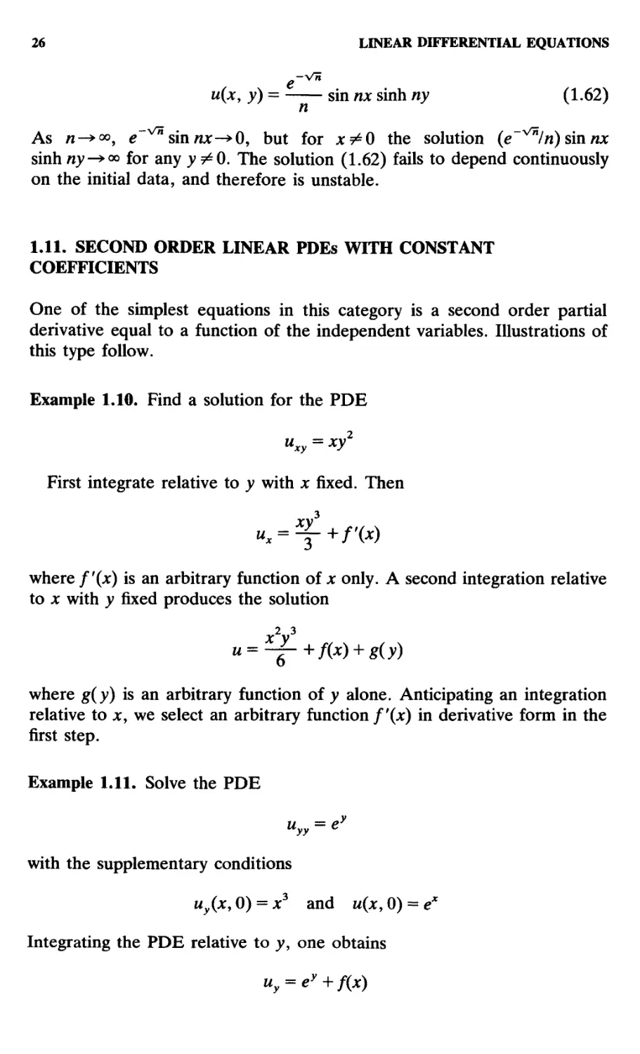
u(x, y) = sin nx sinh ny A.62)
n
As n—>°°, €-v" sin ш:—»0, but for я: т*0 the solution (e'^/n) sin wjc
sinh лу-><» for any у 7*0. The solution A.62) fails to depend continuously
on the initial data, and therefore is unstable.
1.11. SECOND ORDER LINEAR PDEs WITH CONSTANT
COEFFICIENTS
One of the simplest equations in this category is a second order partial
derivative equal to a function of the independent variables. Illustrations of
this type follow.
Example 1.10. Find a solution for the PDE
uxy = xy2
First integrate relative to у with x fixed. Then
where /'(*) is an arbitrary function of x only. A second integration relative
to x with у fixed produces the solution
where g(y) is an arbitrary function of у alone. Anticipating an integration
relative to x, we select an arbitrary function f'(x) in derivative form in the
first step.
Example 1.11. Solve the PDE
uyy = ey
with the supplementary conditions
uy{x, 0) = x3 and u(x, 0) = ex
Integrating the PDE relative to y, one obtains
и =ey+f(x)
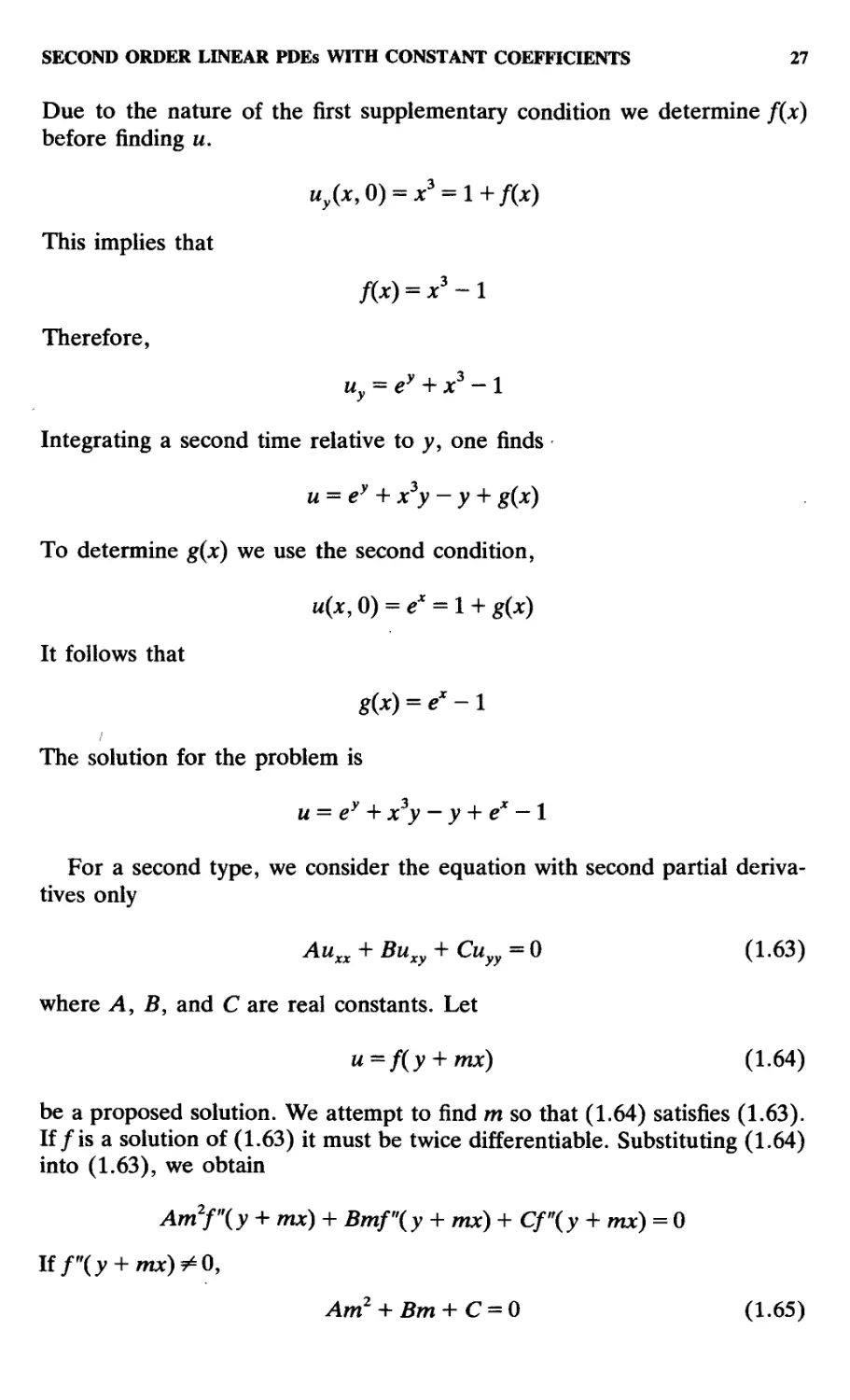
SECOND ORDER LINEAR PDEs WITH CONSTANT COEFFICIENTS 27
Due to the nature of the first supplementary condition we determine f(x)
before finding w.
This implies that
Therefore,
Uy =
Integrating a second time relative to y, one finds
и = ey + x3y - у + g(x)
To determine g(x) we use the second condition,
u(x,0) = ex = l + g(x)
It follows that
g« = e*-l
The solution for the problem is
и = ey + x3y - у + ex - 1
For a second type, we consider the equation with second partial deriva-
derivatives only
Auxx + Buxy + Cuyy = 0 A.63)
where A, B, and С are real constants. Let
1Я*) A.64)
be a proposed solution. We attempt to find m so that A.64) satisfies A.63).
If/is a solution of A.63) it must be twice differentiable. Substituting A.64)
into A.63), we obtain
Am2f"(y + mx) + Bmf\y + mx)+ Cf"{y + mx) = 0
A.65)
28 LINEAR DIFFERENTIAL EQUATIONS
The polynomial equation A.65) is a characteristic equation. If it has distinct
roots /n = m1 and m = m2 then и = f(y + mxx) and и = g(y + m2x) are
solutions of A.63). The linear combination
u=f{y + тгх) + g{y + m2x) A.66)
is a general solution of A.63).
If mx and m2 are distinct and new variables
r — y + mxx and 5 = ^ + ^12^ A*67)
are introduced in A.63), the new equation is (see Hildebrand [25, Chapter
8])
A[m\urr + 2mxm2urs + m\uss] + B[mxurr + (тг + т2)м„ + m2uj
+ C[iiFr + 2«fI + «J = 0 A.68)
assuming urs = usr. Equation A.68) can be simplified so that the coefficients
of urr and uss are both zero, and
«„=0 A.69)
Equation A.69) is a special type solvable by integration. It has the solution
Replacing r and s as given in A.67) one obtains the solution A.66).
The d'Alembert solution of the wave equation
un = c2uxx, c>0 A.70)
is a good illustration of the transformation described in A.67). Equation
A.70) is hyperbolic. The auxiliary equation is
m2-c2 = 0 A.71)
The transformation A.67) becomes
r = * + cf and s = x~-ct A.72)
Using A.72) as described above, we obtain
u=f(x + ct) + g(x-ct)
for the solution of the wave equation.
SECOND ORDER LINEAR PDEs WITH CONSTANT COEFFICIENTS 29
The solutions of the characteristic equation A.65) may be (a) real and
distinct, (b) double, or (c) conjugate (imaginary part nonzero) complex
numbers. The discriminant for the quadratic equation A.65), is the same as
the discriminant for A.63). Therefore, a hyperbolic PDE A.63) is matched
by real and distinct roots in A.65); an elliptic equation A.63) is paired with
conjugate complex roots in A.65); and a parabolic equation A.63) is
associated with a double root in A.65).
If mx = m2 in A.65), then B2 -4AC = 0. The two roots are mx - -Bl
2A. A second solution for A.63) is
This result can be verified if mx = m2 = -B/2A is employed. In this case
"=/(>> + mxx) + xg{y + mxx) A.73)
is a general solution for A.63). One can show that
u =f(y + mlX) + yg(y + miX) A.74)
is a general solution of A.63) also.
Example 1.12. Find a general solution for uxx + Auxy + Auyy = 0.
This equation is parabolic. The characteristic equation has a double root
-2. A general solution using A.73) is
If A.74) is used
is a general solution.
Example 1.13. Determine a solution for uxx + 4uyy = 0.
The discriminant B2-4AC<0. Therefore, the equation is elliptic. The
characteristic equation has roots ±2/. The general solution is written in the
same form as A.66). For this PDE
u=f(y-2ix) + g(y + 2ix)
is a general solution.
By comparison with an ODE one may suspect the existence of an
exponential solution for the homogeneous PDE
30 LINEAR DIFFERENTIAL EQUATIONS
Auxx + Buxy + Cuyy + Dux + Euy + Fu = 0 A.75)
where the coefficients Л,.. ., F are real constants. Let
u~eax+fiy A.76)
where a and p are real, be a proposed solution. Substituting A.76) in
A.75), one obtains the condition
Aa2 + Ba& + Cp2 + Da + ?0 + F = 0 A.77)
In the quadratic equation A.77), one may solve for /3 as a function of a or a
as a function of j8. Assume that we solve for p and obtain Px(a) and /32(a)-
A particular solution
is the result.
Example 1.14. Determine a solution for the PDE
uxx ~uyy-2ux + u = 0 A.78)
Substitute the exponential function
и = eax+^y
in A.78). The characteristic equation
a2 -p2 -2a + 1 = 0
has solutions
j3 = a-l and j3 = -a + l
Using superposition of the two solutions one finds the particular solution
и = Kxe^ia-1)y + K2eaxH~a+1)y
This solution may be written
и - Кге-уеа^у) + tf2eV"(*-»
We may conjecture that a general solution has the form
и - e~yf{x + y) + eyg(x - y) A.79)
SECOND ORDER LINEAR PDEs WITH CONSTANT COEFFICIENTS 31
where / and g are twice differentiable arbitrary functions. By substituting
A.79) into A.78), we confirm that A.79) is a solution.
When the left member of A.77) has distinct linear factors, the type of
simplification discussed is possible. The case of a repeated linear factor may
be considered by using a result comparable to A.73) or A.74).
Example 1.15. Examine
for a general solution.
Let м = eax+^y and obtain a characteristic equation
a2 - lap + j32 - 2/3 + 2a + 1 = 0
The double root is
An exponential form of a solution is
A general solution
u = ey[f(x + y) + xg{x + y)]
can be verified.
Certain cases may arise in A.77) where linear factors with imaginary
elements appear.
Example 1.16. Investigate a solution for the equation
uxx + uyy-2uy + u = 0 A.80)
Let
и = eax+fiy
be a proposed solution. The characteristic equation
a2 + 02-20 + l = O
has two linear factors with imaginary elements for which
32 LINEAR DIFFERENTIAL EQUATIONS
K = 1 ± ia
An exponential solution is
u~ey[ea{x+iy) + ea(x~iy)] A.81)
A general solution for A.80) is suggested by A.81)
u = ey[f(x + iy) + g(x-iy)] A.82)
It is easy to verify that A.82) is a solution of A.80).
In some situations the exponential procedure may produce a set of useful
particular solutions, but fail to suggest a general solution.
Example 1.17. Determine a solution for the equation
uxx + uyy + 4м = О
One obtains a characteristic equation
a2 + ?2 + 4 = 0
with
/3 = ±/Va2 + 4
If the exponential substitution is followed then
и = eax[K1elV°J+*y + К2
This solution can be expressed
и = eax[Mx cos Va2 + 4 у + M2 sin Va2
if ?x and ?2 are properly related to Mx and M2 using Euler's identity.
Equation A.75) can be solved almost like an ODE if only partial
derivatives with respect to one variable appear. Arbitrary constants of the
ODE solution become arbitrary functions of the remaining variable.
Example 1.18. Solve the PDE
uyy — Auy + Зм = О
The dependent variable м is a function of x and y, but the only derivatives
involved are relative to у alone. The corresponding ODE, with м as a
function of y,
SECOND ORDER LINEAR PDEs WITH CONSTANT COEFFICIENTS 33
has a solution
d2u
dy2
и
du
dy
Arbitrary constants cx and c2 are replaced by arbitrary functions of x alone.
The general solution becomes
Other PDEs may be solved by using comparable solutions of ODEs.
Example 1.19. Find a solution for the PDE
xuxy + 2uy = y2
We observe that the equation may be written
By integrating, we obtain
Dividing by x, with у fixed, one recognizes a linear differential equation of
first order
The integrating factor is x2. This equation may be displayed
Integrating the most recent equation, we obtain
An explicit form of the solution is
34 LINEAR DIFFERENTIAL EQUATIONS
For more information regarding Section 1.11 the reader may consult
Hildebrand [25, Chapter 8].
Exercises 1.5
1. Solve the boundary value problem
2. Find the solution for
uyx = x2y , uy@, y) = y2 , u(x, 1) = cos x
3. Determine a solution for ихд. = cos x if
m@, y) = y2 and м(тг, y) = 7r sin у
4. Classify the following PDEs as hyperbolic, parabolic or elliptic:
(a) yuxx + ям^ = О;
(b) x2uxx + 2лумху + y2uyy + мл + иу = 0;
(c) му^
(d) Иях-2ижу + 11уу=0;
(e) и„ + в2иуу = О,в>О;
(f) ив»2иху + 2иуу = 0.
Solve the equations (c)-(f).
5. The d'Alembert solution of the wave equation A.70) is
и =Дх+сО+ *(*-<*)
Solve the wave equation if m(jc, 0) = 0 and мг(х, 0) = ф(х).
6. (a) Determine a general solution for (c) in Exercise 4 by using the
transformations s = y -3x, r~y + x.
(b) If m@, y) = 0 and ux@, y) = <Ky) in (a), show that
7. Determine a solution for мхд. + 2млу + иуу + м^ + му = 0 by letting м =
eax+Py. After finding jS as a function of a, propose a general solution.
Verify the general solution.
8. Using the substitution и = eax+fiy
(a) find an exponential solution for 4uxx — uyy — 4ux + 2uy = 0;
(b) propose and verify a general solution for the equation.
SEPARATION OF VARIABLES 35
9. Solve the PDE xuxy + Ъиу = у3.
10. If Auxx + Buxy + Cwy>, = F(x, y), A, B, and С are constants, then the
equation has a general solution
и = wc(x, у) + up(x, y)
where wc(jc, y) is a general solution of Auxx + Bw^ + Cuyy = 0 and
иДх, y) is a particular solution of the original equation. Find a general
solution for the following equations:
(a) uxx-2uxy-3uyy = ex;
(b) uxx - uxy - 2uyy = sin y.
1.12. SEPARATION OF VARIABLES
It is assumed in this method that the solution of a PDE can be expressed in
the form of a product of functions of single independent variables. Using
this procedure we produce an equation with one member a function of a
single variable and the other member a function of the remaining variables.
Each member can be a constant but not a function of all the original
independent variables. This process is illustrated in the following examples.
Example 1.20. Find a solution for the PDE
ut = 4uxx A.83)
using the separation of variables.
We assume that the solution of A.83) has the form
u(x,t) = X(x)T(t) A.84)
where X is a function of x alone and Г is a function of t alone. Inserting
A.84) into A.83) we obtain
XT'=4X"T
After dividing by 4XT, one has the variables separated in the form
4f = -X <L85>
If A.85) is differentiated partially relative to t, one attains the result
36 LINEAR DIFFERENTIAL EQUATIONS
Assuming ф is an arbitrary function of x alone, the solution of A.86) is
T'
This violates the condition that Г is a function of t alone unless ф(х) is a
constant. A similar partial differentiation of A.85) relative to x leads to a
PDE which has a solution
valid only if ij/(t) is constant. Therefore both members of A.85) must be
equal to the same constant, say a2 or — a2.
If a2 is used A.85) becomes
4T = Jt=a A87)
Result A.87) is equivalent to two ODEs
Г'-4а2Г = 0, X"-a2X=0 A.88)
The solutions of the two ODEs of A.88) are respectively,
Г= Ae4', X= Вгеах + B2e~ax A.89)
Inserting the solutions of A.89) in A.84) we find a solution
where Cx = ABX and C2 = AB2.
If —a2 is used instead of a2 in A.87) the two ODEs are
7" + 4а2Г- 0 , X" + a2X=0 A.90)
The solutions of A.90) are
T= A*e~4a2t , X=B\ cos a* + B*2 sin ajc A.91)
Using the solutions of A.91) in A.84) we have
и = ea\C\ cos ax + C* sin ад;]
In most of our BVPs a bounded solution will be necessary. The constants a2
or —a2 must be selected to satisfy this requirement.
SEPARATION OF VARIABLES 37
Example 1.21. Determine a solution for
ut = a\uxx + uyy) A.92)
Since three independent variables appear in A.92), we let
u(x,y,t)=T(t)X(x)Y(y) A.93)
Equation A.92) has the form
T'XY=a2(TX"Y + TXY"). A.94)
after substituting A.93) in the PDE. Equation A.94) has another form
Partially differentiating A.95) relative to x, then y, and finally t, we have
respectively
Solutions of the three PDEs of A.96) are
2 02
A.97)
In order that A.95) be satisfied we select -(a2 + /32) as the constant in the
solution of the T equation.
The three associated ODEs
X"+a2X = 0
have solutions
X = Bx cos ax + 52 sin ax
Y = Cx cos 0y + C2 sin /3y
Therefore,
и = exp [-(a2 + p2)a2i\[B\ cos ax + Я^ sin ax][Ca cos /3y + C2 sin
38 LINEAR DIFFERENTIAL EQUATIONS
is a solution of A.92). Other forms for the solution are available. The one
displayed is a bounded solution.
The method of separation of variables is valuable for solving a number of
important problems of mathematical physics, yet it fails for many PDEs and
BVPs. Myint-U [35, pp. 128-129] shows that the second order PDE* with
variable coefficients in x and у
A(x, y)uxx + C(x, y)uyy + D(x, y)ux + E(x, y)uy + F(x, y)u = 0
A.98)
is separable when a functional multiplier 1/[ф(х, у)] converts the new
equation
A(x, y)X"Y + C(x, y)XY" + D(x, y)X' Y + E(x, y)XY' + F(x, y)XY = 0
into the form
Ax(x)X"Y + Bx{y)XYn^ A2(x)X'Y + B2(y)XY' + [A3(x)
Explicit rules for the workability of this method are a bit elusive. Types
of differential equations, kinds of coordinate systems, and forms of boun-
boundary conditions are all important items for the success of the procedure.
Exercises 1.6
1. Test the following PDEs for the method of separation of variables. If the
method is successful, solve the PDE.
(a) uxy-u = 0.
(b) utt-uxx = 0.
(c) uxx-uyy-2uy = 0.
(d) uxx - uyy + 2ux - 2uy + и = 0.
(e) t2utt-x2uxx=0.
(f) (t2 + x2)utt + uxx=0.
(g) uxx - y\y - yuy = 0.
(h) uxy = 0.
(i) и„ - иху + и,„ = 2x.
(j) «**-"yy-My=0-
"The example that follows is from Myint-U [35], by permission of Elsevier/North-Holland, Inc.
SEPARATION OF VARIABLES 39
2. Find a solution for the boundary (or initial) value problems:
(a) ип-ихх = 0, и(х,0) = и@,0 = 0;
(b) uxx - uyy - 2uy = 0, их@, y) = u(xy 0) = 0;
(c) ut = uxx, их@,/) = 0.
3- (a) Show that the equation with constant coefficients
A uxx + Buxy + Cuyy = 0
is separable if the coefficients meet proper conditions. Determine
appropriate conditions. Note: Let u(x, y) = X(x)Y(y) and show that
a result
is obtained from
X * A X Y + A Y
Finally, show that
У"+АУ = 0 and X"-k^X' + k2^-X = 0
A A
are related ODEs.
b) Find a solution for uxx - uxy + uyy = 0 by separating variables.
2
ORTHOGONAL SETS OF
FUNCTIONS
The Jirst concept of orthogonality for many of us is associated with perpen-
perpendicularity in geometry. Here our first reference to orthogonality and ortho-
normality pertains to right angle relations with vectors. Later we define
orthogonal and orthonormal functions. We describe several types of ortho-
orthogonality. Finally we consider a BVP that has a solution set of special
orthogonal functions. The formation of a series based upon a set of
orthogonal functions is fundamental for our development of Fourier series.
2.1. ORTHOGONALITY AND VECTORS
Vectors furnish good examples of orthogonal sets. Using the component
form, i = A,0,0), j = @,1,0), and к = @,0,1). Then the set {i, j, k} is an
orthogonal set of unit position vectors. This means that i, j, and к are
mutually perpendicular. If vector A= (au a2, a3), then its length or norm
||A|| = (a\ + a\ + a*I'2. If a second vector В = (Ьг, b2, b3), then the inner
product of A and В is defined by
A • В = (A, B) = ||A|| ||B|| cos в = a1b1 + a2b2 + a3b3 B.1)
where в is the angle between the two vectors. See Figure 2.1.
Consider a set of orthogonal vectors {el9e2Je3}. Since the set is ortho-
orthogonal, the definition B.1) implies that
(e1?e2) = (e1? e3) = (e2, e3) =0 B.2)
Let vector V= (u1? v2, v3) be related to {er}, r = 1,2, 3 by
V= vxtx + v2e2 + v3e3 = 2 vrer B.3)
r=l
ORTHOGONALITY AND VECTORS
41
Figure 2.1. Two position vectors in a three di-
dimensional rectangular coordinate system.
This implies that V is referenced to a coordinate system having axes along
which vectors el9e2,e3 lie as position vectors. If V= Mxi+ uj + w3k =
(ul9 u2, м3)Цк then V is related to i,j,k referenced to the x, y, z axes.
Therefore,
ux\
u3k
v2e2
Using B.1), and assuming that {el9e29^} is related to {i,j,k},
Then
B.4)
Example 2.1. If the reference set of vectors {e1>e2,e3} is given by ex =
A,1,0), e2= (-1,1,0), and e3 = @,0,1), find Vyk = A,2, 3) related to
Using B.1), we observe that
and the set {e1,e2,e3} is orthogonal. If we let
i + 2j + 3k = vxet + u2e2 + u3
then
42 ORTHOGONAL SETS OF FUNCTIONS
1,2,3).<-1,1,O) = ||<-1,1,0I14
Completing the computation, we have vx = \, ьг-\, v3 = 3. The vector
V.ie2.3=|e1+|e2 + 3e3.
If in addition to the conditions B.2) we have
then the set {er}, r = 1, 2, 3, is composed of vectors having norms of 1. In
this case
0 when
1 when r = s
and the set {er}, r = 1,2,3, is referred to as an orthonormal set of vectors.
The set {i, j, k} is an orthonormal set of vectors. The set in Example 2.1 is
orthogonal, but not orthonormal. If the set of orthonormal vectors {er},
r = 1, 2, 3, is used as a basis or reference set for B.3) then B.4) becomes
v2=(u19u2,u3)-e2
The idea we have expressed can be generalized so that the vectors have n
components and an orthogonal basis {er}, r = 1,2,. .. , n. Assume a vector
V= (u19u2,.. . ,Oaia2 ....„ where a1 = (l,0,... ,0), a2 =
<0,l,...,0),...,an = @,0,...,l>. The set {ar}, r = l,2,...,n, is
orthonormal. If the set {er}, r = l,2, ...,n is related to {ar}, r =
1,2,... , n, then
and one obtains
2.2. ORTHOGONAL FUNCTIONS
It is possible to consider a function A(x)9 a^x^b, analogous to a vector
having an infinity of components, each component specified by the value of
ORTHOGONAL FUNCTIONS 43
A(x) at a particular value of x G (a, b). Instead of using a sum in this case
we use a limit of a sum or an integral.
The norm of A(x) is defined by
and the inner product of two functions A(x) and B(x), a =? x =s b, by
(A,B)=\ A(x)B(x)dx
Ja
For the analogy to be extended, the condition that A(x) and B(x) are
orthogonal is defined by
(A, B) = f A(x)B(x) dx = 0 B.5)
Ja
As a special case, the inner product
(A,A) = \\A\\2
Although we have suggested some analogies with functions and vectors,
we hasten to add that our geometrical significance is gone. The concept of
orthogonality as defined by B.5) bears fruit when a study of Fourier series is
undertaken.
If we consider an orthogonal set of functions {fn(x)}, n E N (N the set of
natural numbers), a^x^b, then
(/„, /J = l ШШ dx = 0 when n * m
If the set {gn(x)}, nGN, a ^ x ^ b, is orthonormal, then
v 8n > Sm ) 1 i
when пФт
when n = m
A set {/„(*)} which is orthogonal, but not orthonormal, can be transformed
into an orthonormal set by dividing each function of the set by its norm
||/J|. Naturally this process of normalization is possible only if all norms are
nonzero.
Example 2.2. Show that the set of functions {sin nx}, O^x^tt, n€N, is
orthogonal. Find a normalizing factor and display the corresponding ortho-
normal set.
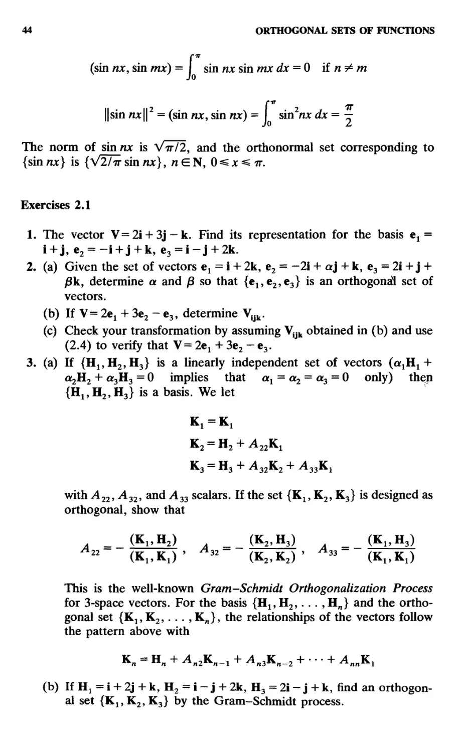
44 ORTHOGONAL SETS OF FUNCTIONS
m
(sin nx, sin mx) = I sin nx sin mx dx = 0 if n Ф
||sin njc||2 = (sin nx, sin nx) = I sin2n;c dx = —
jo ^
The norm of sin/zx is Vtt/2, and the orthonormal set corresponding to
{sin л*} is {V2hrsinш:}, n6N, 0*?jc *? тт.
Exercises 2.1
1. The vector V=2i + 3j-k. Find its representation for the basis ex =
i-hj, e2 = -i + j + k, e3=i-j + 2k.
2. (a) Given the set of vectors ex = i + 2k, e2 = -2i + aj + k, e3 = 2i 4- j +
Kk, determine a and K so that {е^ез^ез} is an orthogonal set of
vectors.
(b) If V= 2ex + 3e2 - e3, determine VUk.
(c) Check your transformation by assuming Vjjk obtained in (b) and use
B.4) to verify that V= 2ex + 3e2 - e3.
3. (a) If {HjjH^HJ is a linearly independent set of vectors (^H
a2H2 + a3H3 = 0 implies that аг = a2 = a3 = 0 only)
{Нг, Н2, H3} is a basis. We let
with Л22, А32, and A33 scalars. If the set {K1? K2, K3} is designed as
orthogonal, show that
л - (K"H*> л А
(K^K,)' Лз2 (К2,К2)' Лз3 (K^KJ
This is the well-known Gram-Schmidt Orthogonalization Process
for 3-space vectors. For the basis {Hlf H2,.. ., Hn} and the ortho-
orthogonal set {K1? K2,. . . , Кл}, the relationships of the vectors follow
the pattern above with
К„ = Hn + An2Kn_x + An3Kn_2 + • • • + AnnK2
(b) If Ha = i + 2j + k, H2 = i - j + 2k, H3 = 2i - j + k, find an orthogon-
orthogonal set {К19К2,Кз} by the Gram-Schmidt process.
ORTHOGONAL FUNCTIONS 45
4. (a) Show that the set of functions {sinnvx}, -Kjc<1, w6N, is
orthogonal,
(b) Is the set in part (a) orthonormal?
5. (a) Find a so that {1, jc, 1 + ax2} on (-1,1) is orthogonal.
(b) Normalize the set obtained in (a).
6. (a) Show that the set {1, cos (nirx/L), sin (mvx/L)}, n, m E N, -L <
x<L, is orthogonal but not orthonormal.
(b) Normalize the set of (a).
7. (a) Is the set {cos(/ittjc/2)}, nGN0 (No is the set of natural numbers
plus 0), 0<jc<2, orthonormal?
(b) If it fails to be orthonormal, write the corresponding orthonormal
set.
8. Given the set of nontrivial orthogonal functions {/„(*)}> a^x^b,
«GN0, show that the set is linearly independent.
9. The set of continuous functions {gn(x)}, a^x^b, nEN, is linearly
independent. A new set {/„(*)}> a^x^b, «GN, designed to be
orthogonal, has the relationships with the first set:
fn = En + Л2Л-1 + ^пз/п-2 + ' ' * + Knh
where A22, A32, ^зз> • • • > Anl, An3,. . . , Ann are constants. As with
vectors, this is the Gram-Schmidt orthogonalization process for func-
functions. Show that for the set {gl9 g2, g3} on [a, ft], the orthogonal set
given by the Gram-Schmidt process is
f2~82 TKJdfl
f = „ (/2» S3) f (/1.83)
h 8э (//)/a (//)
10. The set {I,x9x29x3}9 -1=^x^1, is linearly independent and continu-
continuous. By the Gram-Schmidt process of Exercise 9, find the correspond-
corresponding orthogonal set.
46 ORTHOGONAL SETS OF FUNCTIONS
11. The integral J* J* [ f(x)g(y) - /( y)g(x)]2 dxdy^O. Show that
\la^[f^)g{y)-f{y)g{x)]Uxdy^\\f\ng\\2-{f,gJ and prove
the Schwarz inequality: (/, g)^ \\f\\ \\g\\.
12. If/and g are continuous functions on (a, b) and one function has a zero
norm, then the inner product (/, g) = 0. Show this statement is true.
Use Exercise 11.
2.3. COMPLEX FUNCTIONS
Before discussing an orthogonality concept involving complex functions, we
state a few definitions and operations on these functions. A complex
function of a real variable is defined by
w(x) = u(x) + iv(x)
where и (real part of w) and v (imaginary part of w) are both real functions
of the real variable jc. If v(x) is identically zero, then w(x) is a real function.
The complex conjugate of w, denoted by w, is defined by
w(x) = u(x) - iv(x)
The absolute value of w, written \w\, is
For h>(jc)
wr(x)^ut(x) + ivr(x)
and
I >v(jc) dx = m(jc) dx + i I v(x) dx
Ja Ja Ja
We define a complex function of a complex variable z by
w(z) = u(x, y) + iv(x, y)
where z = x + iy with и and v real functions of the real variables x and y.
The exponential function exp z or ez is expressed by
exp z = e*(cos у + i sin y)
Other definitions of elementary functions follow:
ADDITIONAL CONCEPTS OF ORTHOGONALITY 47
sinhz = « (eZ~
The derivatives of these elementary complex functions follow forms of
the derivatives of the corresponding real elementary functions. For example,
d /. ч
— (sm z) = cos z
dz
-7- (cos z) - -sin z
If z(s) = jc(s) + o>(s), then
ds y ' ds
-7- (sin z) = cos z —
~j- (COS Z) = -Sin 2 -j-
tfa v ' ds
The integral
2.4. ADDITIONAL CONCEPTS OF ORTHOGONALITY
/Л(х) = mw(jc) + /ип(дс), then the set of complex functions {/„(*)}, л ^ jc ^
b, is orthogonal in the Hermitian sense if
The square of the norm in this case is
II/.toll' = l ШШ dx = [ [u2n(x) + v2a(x)] dx
48 ORTHOGONAL SETS OF FUNCTIONS
Example 2.3. Show that the set of functions {exp[2ri7rix/(b — a)]}, a ^ x ^
b, n E Z (Z is the set of all integers), is orthogonal in the Hermitian sense.
To show Hermitian orthogonality we must demonstrate that the integral
/:
B6)
is zero when пФт> It can be shown that
2ттг1х\ (-2mirix\
Integral B.6) may be rewritten
f" B{n-m)irix\ . b-a Г B(п-т)тт1
I eXp V b-a ) ** = 2(я-m)« LeXP V b-a
m)«
b-a {2(n-m)iria\\ B(n - m)<jri(b - a)
eXp( ЯеХР( —
= 0 И
The set satisfies the definition for Hermitian orthogonality.
The definition given in Section 2.2 for orthogonality of a set of functions
{fn(x)}> n G N, a ^ x ^ b, is a special case of a concept we consider at this
time. We say that the set is orthogonal with respect to a weight function
ь
r(*)fn (X)L (x)dx = 0 when m Ф п
The square of the norm is written
H2 = f r(x)fl(x)dx
One observes that the ordinary type of orthogonality occurs when r(x) = 1.
Orthogonality with respect to a weight function r(x) reduces to ordinary
orthogonality if the set {Vr(x)fn(x)} replaces the set {/„(*)} in our new
definition. The importance of orthogonality with respect to weight functions
will become apparent when we consider orthogonality of eigenfunctions of
Strum-Liouville problems.
Example 2.4. Functions Tn(x) = cos (n arccos x) are called Tchebycheff
polynomials of the first kind. Show that the set { Tn(x)}, -1 ^ x *? 1, n e No,
is orthogonal with respect to the weight function A - #2)~1/2.
ADDITIONAL CONCEPTS OF ORTHOGONALITY 49
In compliance with the definition, we must test the integral
\\{\-x2yinTn{x)Tm{x)dx B.7)
To evaluate the integral, let в = arccos x or x = cos 0. Then B.7) may be
written
Jcos пв cos mO dd
о
= - sin(n + т)в + sin(n - mH = О ИпФт
2\-n + m v л - m 'Jo
Thus the set {Tn(x)} is orthogonal with respect to the weight function given.
Exercises 2.2
1. Show that elniri = 1 and e{2n+1)vi = -1, n € No.
2. (a) Show that the set {ехр(шх)}, -тг^х^тг, wEZ, is orthogonal in
the Hermitian sense,
(b) Determine the norm for the set in (a).
3. (a) Is the set Fn(x) = sin[(w + 1) arccos x] on (-1,1), n E No, orthogonal
with respect to the weight function A - x2I/2
(b) Tchebycheff polynomials of the second kind are defined by Un(x) =
A-х )/2sin[(w + l)arccosx]. Show that the set {?/„(*)}, -1^
x =? 1 is orthogonal relative to the weight function A - jc2I/2.
4. (a) The set of functions {Ln(x)} satisfies the Laguerre differential equa-
equation xy" + (l-x)y' + «j> = 0. Ln(x) is generated so that Lo(x) = l
and Ьп(х)-(ех1п\)йп1<1хп{хпе~х), wEN. Compute Ln{x) for w =
1,2, and show that {Lo, Ll9 L2} satisfy the differential equation.
(b) By direct integration show that {Lo, L19 L2} form an orthogonal set
on the real axis @, o°) with respect to the weight function e~x.
(c) The set {#„(*)} satisfies the Hermite differential equation y"-
2xyr + 2ny - 0. 2 Hn{x) has properties Я0(х) = 1 and
Hn(x) = (-l)nex\dnfdxn)(e~x2), n E N. Determine Hn(x) for n = 1,2
and show that {Яо, Нг,Н2} satisfy the differential equation.
(d) Using the appropriate definition show that {#0, Я1? Н2} is an ortho-
orthogonal set with respect to the weight function e~x2 for -oo<*<oo.
Definitions for Ln(x) and Hn(x) appear in Brand [8, pp. 475 and
478]. Appropriate weight functions and definitions for Tn(x) and
Un(x) are found in Abramowitz and Stegun [1, pp. 774-776].
50 ORTHOGONAL SETS OF FUNCTIONS
2.5. THE STURM-LIOUVILLE BOUNDARY VALUE PROBLEM
In the discussion of the method of separation of variables in Chapter 1,
equations of the type y"+a2y = 0 were discovered. These equations are
special forms of
cMf + сг(х)у' + [c2(x) + A]y = 0 B.8)
For the first two terms of B.8) to be written [p(x)yr]' we multiply the
equation by an integrating factor p(x) = exp[J (сх(х)/с0(х)) dx]. If in addi-
addition we let q(x)-[c2(x)/c0(x)]p(x) and r{x) = p{x) /co(x) then B.8) be-
becomes
[p(x)y'Y + lq(x) + kr{x)]y^0 B.9)
which is called a Sturm-Liouville differential equation (SLDE). It is regular
in [a, b) if p{x) and r(x) are positive in the interval. For a given Л two
linearly independent solutions of a regular SLDE exist in [a, b].
The boundary value problem containing the SLDE, a^x^b, along with
the separated end conditions,
а1У(а) + а2у'(а) = 0, Ь,у(Ь) + Ь2у'(Ь) = 0 B.10)
forms a Sturm-Liouville problem (SLP). If the coefficients al9 a2 and bl9 b2
are real constants such that a\ + al^O and b\ + b\ Ф 0 and the SLDE is
regular, then the problem is a regular SLP. The trivial solution у — 0 satisfies
the SLP for any value of the parameter A. Nontrivial solutions are called
eigenfunctions or characteristic functions of the SLP. The corresponding
values of Л for which these nontrivial solutions exist are known as eigen-
eigenvalues or characteristic values.
Theorem 2.1. Assume that the functions p(jc), q(x), and r(x) of the regular
SLP B.9) and B.10) are real and continuous in [a, b]. If yn(x) and ym{x)
are continuously differentiable eigenfunctions of the matching distinct eigen-
eigenvalues An and Am, respectively, then yn{x) and ym{x) are orthogonal in the
interval with respect to the weight function r(x).
Since yn and ym are solutions corresponding to An and Am
' + [« + Аяг]У||«0 B.11)
+ [* + Ажг]уж-0 B.12)
By multiplying B.11) by ym and B.12) by yn and then subtracting
B.12)-B.11) we obtain
ГНЕ STURM-LIOUVILLE BOUNDARY VALUE PROBLEM
[рУшУУп - \рУп\Ут + (Am - K)rynym = о
However,
fa {[РУ'тЪп - [РУпЬт) = [РУтУУп "
Using B.14), equation B.13) may be written
•fa {р[УтУп ~ У>т]} = (K - Ат)гу
Integrating B.15) over [a, b]
rb
п-УпУт)]а=(К-Ю\ ГУп
Ja
51
B.13)
B.14)
B.15)
B.16)
We observe that yn and ym must satisfy the conditions of B.10).
Therefore
and
The condition that B.10a) has a solution other than al = a2 = 0 is
Similarly if B.10b) has a nontrivial solution then
Conditions B.17) and B.18) permit us to restate B.16) as
(Л„-Лт)[ rynymdx = 0
Since А„-Ат#0, then
Ja гУпУтЖс^в if n#m
This concludes the proof.
B.10a)
B.10b)
B.17)
B.18)
B.19)
52 ORTHOGONAL SETS OF FUNCTIONS
Example 2.5. Find all the eigenvalues and eigenfunctions for the SLP:
In this problem p{x) = 1, q{x) = 0, r{x) = 1, and A = A when the ODE is
compared to the SLDE B.9). We check the cases when A<0, A = 0, and
A > 0. First, if A = -a2, a a real constant, the ODE has the form
y"-a2y =
and the general solution is
г**
у = Kie«* + Кг€
y' = aKxeax - aK2e~a
Applying the two boundary conditions, we have
Klea + K2e-° = 0 B.20)
The only solution for B.20) is Кг = K2 = 0. Therefore у = 0, the forbidden
trivial solution, is the only solution if A < 0. If A = 0, then
/' = 0, y = KlX + K2
After using the two boundary conditions, Kx = K2 = 0, and у = 0 is the only
solution. If A = a2, a a real constant, then
and
у = cx cos ax + c2 sin ax
yf = —acx sin ax + ac2 cos ax
In this case
and c2 = 0, since a
y{\) = Cj cos a = 0
If cx ^ 0, then cos a = 0. If cos a = 0, then a = Bл - 1)тг/2.
THE STURM-LIOUVILLE BOUNDARY VALUE PROBLEM 53
2 Bn - 1)V
is the set of eigenvalues.
yM.m[ea^is.], „eN
is the set of eigenfunctions. We have stated the set using cx = 1. The set
{cos[Bw - 1)тгх/2]}, «6N, O^jc^I, is orthogonal with weight function
r(*) = l.
The SLP composed of the SLDE B.9) with p(a) = p(b)>0 and the
periodic end constraints
y'(a) = y'{b) B.21)
is a periodic SLP. If f(x + P)=f(x), f(x) is periodic with a period P.
Theorem 2.2. Let yn{x) and ym(x) be continuously differentiable eigenfunc-
tions matching distinct kn and km, respectively, for a periodic SLP. Then
yn(x) and ym(x) are orthogonal relative to the weight function r{x) in [a, b].
Since the solutions yn and ym must satisfy B.21), it follows that
уМ = Уп(Ъ) and y'n(a) = y'n{b)
УМ-УЛЬ) and y^a) = y^b) B.21a)
If the end constraints B.21a) are used in B.16), then
[p(b) -p(a)][y^a)yn(a) - y'n(a)ym(a)] = (Л„ - Am) f* rynym dx
Ja B.22)
From the hypothesis of the theorem it is implied that p{b) - p{a) = 0.
Therefore B.22) becomes
rynymdx = 0
Since Л„ and Am are distinct, А„ ?^ A and
\a гУпУтйх^О МтФп
The final statement implies orthogonality.
54 ORTHOGONAL SETS OF FUNCTIONS
Example 2.6* Determine the eigenvalues and eigenfunctions for the periodic
SLP: y" + \y = 0; y(-L) = y(L); y'(-L) = y'{L).
If A <0, the only solution is trivial. If Л - 0, then
When y{-L) = y(L), Kx = 0. If y'(-L) = y\L), there is no restriction on
K2. Therefore y0 = 1 is a solution matching A = 0. When A = a2
and
= cx cos ajc + c2 sin ax
y' = — acr sin ax 4- ac2 cos ax
The two boundary conditions in this case permit us to write
cx sin ah = 0 and c2 sin ah = 0
If cx Ф 0 and c2 t^ 0, then sin ah = 0 so that ah — птг. Therefore, a = nir/L
and
for the set of eigenvalues. The set of eigenfunctions is displayed by
n,/n?N, -L<x<L B.23)
The set B.23) is orthogonal in the ordinary sense. That is r(x) — 1.
A SLDE can be associated with unbounded intervals such as @, <*>) or
(-oo5 go) as well as finite intervals. When the interval is unbounded, when the
interval is finite with p(x) or r(x) zero at one or both endpoints, or when
q{x) is discontinuous at these points, the SLDE is described as singular. We
avoid discussing the corresponding singular SLP here, but refer the reader
to Birkhoff and Rota [2, pp. 263-265].
In addition to orthogonality other properties of the eigenvalues and
eigenfunctions are important in the study of the SLP.
Theorem 2.3. For a regular SLP with p(x) > 0 all the eigenvalues are real if
p(x), q(x), and r(x) are real functions and the eigenfunctions are differenti-
able and continuous.
THE STURM-LIOUVILLE BOUNDARY VALUE PROBLEM 55
Let y(x) be an eigenfunction corresponding to an eigenvalue у + i8 where
у and 8 are real numbers. We assume у has the form и + iv where и and v
are real functions of x. Substitution of the complex form of у and Л in the
SLDE B.9) results in
[p(ur + w')]' + к + (y + i8)r][u + w] - 0 B.24)
Equating the real and imaginary parts to zero in B.24) one writes
(puj + (q + yr)w - 8rv = 0 B.25)
' + (* + 7r)y + Sru = ° B.26)
If we multiply B.25) by v and B.26) by м and subtract the results, we find
that
u(pv')' - u(pu')' + 8r(u2 + у2) = О B.27)
Using a procedure similar to B.14) we obtain for B.27)
Integrating over [a, b] one finds that
rb
-8 \ r(u2 + v2)dx = [p(uv'-vu')]ba B.28)
If the complex form is inserted in B.10) we have
fliMfl) + *v(a)] + a2[u\a) + iv'(a)] ~ 0
0 B.29)
The two zero complex constraints of B.29) imply that
«!«(«) + a2u\a) = 0
а1У(а) + а2у'(о)-0 B.30)
and
ЬМЬ) + Ь2и'(Ь) = 0 B.31)
The conditions a] + a^#0 and Ь\ + Ь\ф§ imply that not both ax and a2 are
zero, and fej and 62 are not both zero. Therefore
56
ORTHOGONAL SETS OF FUNCTIONS
and
u(a) u'(a)
v(a) v\a)
u(b) u\b)
v(b) v\b)
= u(a)v'(a)-u'(a)v(a) =
= u(b)v'(b)-u'(b)v(b) =
B.32)
B.33)
Using B.32) and B.33) in the evaluation of the right member of B.28) we
obtain
fb
-8 r(u2 + v2
B.34)
If r(x)>0, the integral of B.34) is positive. Therefore 5=0. Since 5 = 0,
then A = y. This implies that the eigenvalues are real.
Theorem 2.4. Let yn(x) and ym(x) be any two solutions of the SLDE B.9)
on [a, b] for a given A. We assume that yn{x) and ym{x) are continuous and
differentiable. If W(yn, ym) is the Wronskian of the solutions, then
Р(*)ЩУп> Ут) is a constant.
Since yn and ym are solutions of B.9) then
=0 B.35)
0 B.36)
Multiplying B.35) by ym and B.36) by yn and then subtracting, one obtains
[рУ»]'Уп-[РУп]'Ут=0 B-37)
If we use the relation B.14), then B.37) becomes
-^{р(У»Уп-У'пУт)} = 0 B-38)
By integrating B.38) over the interval a to *, a *? x *? b, we find that
p(x)W(yn(x), ym(x)) = p(a)[y^(a)yn(a) - у'МуЛ")] B-39)
The left member of B.39) is a constant C. Therefore
p(x)W(yn(x),ym(x)) = C
THE STURM-LIOUVILLE BOUNDARY VALUE PROBLEM 57
Theorem 2.5. Two eigenfunctions yn(x) and ym(x) matching a single A of a
regular SLP are linearly dependent. We assume the eigenfunctions are
differentiable and continuous.
We let yn(x) and ym{x) be eigenfunctions for a single eigenvalue A. By
Theorem 2.4 we know that
p(x)W(yn(x),ym(x)) = C
with p{x) > 0. According to the discussion of the Wronskian, Section 1.2, if
Щуп(х)> Ут(х)) vanishes at a point in [a, b] it must vanish at every point in
the interval.
The eigenfunctions yn(x) and ym(x) satisfy the end constraints at x = a, so
that
Recall that a^ + a* ^ 0» so that
в) yi(«) =n
This determinant is W(yn(a), ym{p)) after a row-column interchange. There-
Therefore W(yn(a), ym(a)) = 0. It is a sufficient condition that yn(x) and )>w(x)
matching a single A are dependent. This implies that one eigenfunction yn(x)
is a constant times ym(x). Another way of stating the result is to say that for
a single A in the regular SLP the matching eigenfunction is unique except for a
constant factor.
Theorem 2.6.* A regular SLP has an infinite sequence of real eigenvalues
Ao < Ax < A2 < • • •, with limw_0O Ал = <*>. Every eigenfunction yn(x) matching
the eigenvalue Ал has exactly n zeros in (a, b). The eigenfunction is unique
except for a constant factor.
The last sentence of the theorem comes as a result of Theorem 2.5. The
remainder of Theorem 2.6 is established by a sequence of ideas terminating
with the statement in Birkhoff and Rota [2, p. 273].
Exercises 2.3
1. Find all the eigenvalues and eigenfunctions for the following regular
SLPs:
* Adapted from Birkhoff and Rota [2], by permission of John Wiley & Sons, Inc.
58 ORTHOGONAL SETS OF FUNCTIONS
(a) y" + Ay = 0,y(O) =
(b) y" + Ay = 0,y@) = y'B)=0;
(c) y" + Ay = 0,y'@) = y'(ir/2) = 0;
(d) y" + Ay = 0, y@) = 0, y(l) + y'(l) = 0.
2. For the periodic SLPs, determine the set of eigenvalues and the set of
eigenfunctions:
(a) y" + Ay = 0, y(- v) = y(ff), у'(-тг) = /К);
(b) y" + Ay = 0, y@) = y(l), y'@) = /A);
(c) y" + Ay = O,y(-l) = y(l),y'(-l) = y'(l)-
3. Determine the eigenvalues and eigenfunctions for the SLPs:
(a) x5y" + 5jc4y' + Ajc3y = 0, y(l) = y(e) = 0,
(b) [C + xJyT + Ay
(c) [xy']' + [A/jc]y =
4. If the linear operator L is defined by
Ly = cQ(x)y"(x) + сДд:)^'^) + c2(x)y(x)
and the linear operator L* defined so that
L*y = [со(х)у(х)Г - [^(xMx)]' + c2(x)y(x)
then we say that L* is the adjoint of L. If L and L* are identical then
operator L is self-adjoint.
(a) Show that if
Ly = p(x)y"(x) + p'(*)/(*) + [q(x) + Ar(x)]y(x)
then L is self-adjoint.
(b) For L defined in (a) show that
zLy-yLz = [p{zy'-z'y)]'
is satisfied if all derivatives exits. This relation is credited to Lag-
range. It is a form of B.14).
(c) If Ly = A - x2)y" - 2xy' + n(w + l)y is L self-adjoint?
(d) If x2y" + xy' + (л:2 - w2)y = 0, can the left member of the equation
be transformed into an equivalent self-adjoint form?
2.6. UNIFORM CONVERGENCE OF SERIES
Assume that {un(x)}, n eN, is a set of functions on [a, b]. The nth partial
sum is defined by
UNIFORM CONVERGENCE OF SERIES 59
The series
00
2 un{x) B.40)
и = 1
is convergent in [a, b] if
Urn Sn(x) = S(x) B.40a)
and S(x) is called the sum of the series. We say that B.40) converges to S(x)
if for e > 0 and x G [a, b] we can find M > 0 so that
\Sn(x) ~ S(x)\ <e for all n > M B.41)
In this case M(x, e) is a function of x and e and we refer to the condition as
pointwise convergence. If M(e) is dependent on e alone and not x, then the
series is uniformly convergent.
The Weierstrass M-test for uniform convergence is stated as follows.
Suppose that a sequence of positive constants {Mn} can be found such that
in some interval
(а)к(х)|«М„
and
oo
Ф) 2 мп
n = l
converges. Then the series B.40) is uniformly and absolutely convergent in
the interval.
If all un(x) are continuous functions on [a, b] and the series B.40) is
uniformly convergent, then S(x) in B.40a) is a continuous function. Under
these conditions the series can be integrated termwise over [a, b] and the
result is the integral of 5(x) over [a, b]. When un and urn are continuous and
B.40) converges and the series E^ u'n is uniformly convergent, then B.40)
is termwise differentiable and equal to S'(x).
Example 2.7. Test the series H~=1 (l/n2)cosn;c for uniform convergence.
Since
к?)
1
cos nx
— = Mn
and
60 ORTHOGONAL SETS OF FUNCTIONS
converges, then by the Weierstrass M-test the series is uniformly convergent
for all real x.
Example 2,8. Investigate the uniform convergence of the series
00
2xn-\l-x), *?[-§,§]
11=1
The nth partial sum is
Sn(x) = 1 - x + x - x2 + x2 - + л" + xn-г - xn = 1 - xn
From B.40a)
when - § «? x =? \.
Therefore,
In
,,.
п1п(|)<1п?, n
'(I)
and
lne
(?) in(!)
M does not depend on x in the interval. This result satisfies the definition for
uniform convergence.
Example 2.9. Assume that
S(x) = 2 ("~з 1
COS ПХ , — 7Г =? X =? 7Г
(a) Is 5(x) continuous when - тг =^ x ^ тг?
(b) If J^'2 5(x) dx exists, compute it.
(c) Find S'(tt/2) if it exists.
SERIES OF ORTHOGONAL FUNCTIONS 61
Since |A/w3) cosnx| ^ 1/n3 we see from the M-test that the series is
uniformly convergent for all real x,
(a) Since the series is uniformly convergent for all real x, it is uniformly
convergent for xG[-tt, 7t], and {(l/n3)cosnx} contains only con-
continuous functions for n E N on the interval, then S(x) is continuous on
[-7Г, 7Г].
(b) The series satisfies the condition for termwise integration. Therefore
we compute
Г1г/2 /чг/2 °° / 1 \ °° C*12 / 1 \
-i (?)*(?)-2 (-«-[jj^.
„=1 \n / \ Z / n=i IB/1-1)
(c) The series of derivatives
—ч Ism nx
is uniformly convergent as we can verify by the M-test. The original
series is convergent since it is uniformly convergent. Therefore, the
series is termwise differentiable. We compute
2.7. SERIES OF ORTHOGONAL FUNCTIONS
Finding a Taylor series expansion for a specified function / is an experience
encountered early in the study of elementary calculus. Here we examine an
analogous venture of representing a given function with an infinite linear
combination or series of orthogonal functions. Consider the set {gn(x)},
nGN, a^x^b, orthogonal relative to a weight function r(x). We assume
that the given function / can be represented by a uniformly convergent
series—a sufficient condition on the series to permit the procedure that
follows. Let
ОС
Л*)=2с.&(х) B.42)
62 ORTHOGONAL SETS OF FUNCTIONS
To find the constants Cn, we multiply both sides of B.42) by r(x)gm(x) and
integrate termwise over the interval [a, b]. This results in
f r(x)f(x)gm(x) dx=J:Cnf r(x)gn(x)gm(x) dx B.43)
Ja n = \ Ja
Because of the orthogonality property, all terms in the series are zeros
except when n = w. Then B.43) becomes
Kx)f(x)gn(x) dx = Cn [ r(x)g2n(x) dx
Solving for Cn one finds
с^пШ^г{х)ЯхШх)ах B44)
where ||gM(x)||2 is the square of the norm J* r(x)gl(x) dx.
When the set {gn(x)} is orthogonal in the ordinary sense with r(x) = 1,
then B.44) becomes
?Лх)л(х)Л B44a)
If the set {gn(x)} is orthonormal relative to the weight function r(x), then
B.44) has the form
[
r(x)f(x)gn(x)dx B.44b)
The representation B.42) for / is called an orthonormal series or a general-
generalized Fourier series. The coefficients Cn are the Fourier coefficients. If
||gw(x)|| = l, then we say the expansion is an orthonormal series. When
{gn(x)} is a set of eigenfunctions for a SLP, the terminology Sturm-
Liouville series or eigenfunction series describes the expansion.
The series B.42), with coefficients B.44), B.44a), or B.44b), is assumed
to be uniformly convergent. This limitation is more severe than we wish in
certain situations. To avoid asserting that the series converges to / we may
use a correspondence notation ~. Then B.42) is written
with coefficients Cn given by B.44), B.44a), or B.44b).
Example 2.10. Determine the expansion for /(jc) = 1,0<дс<тг, in a series
of eigenfunctions of the SLP
SERIES OF ORTHOGONAL FUNCTIONS 63
y"+\y = 0, y@) = y(n) = 0
First, we determine the solution of the SLP. If A = a\ then
y"+a2y = 0
у = Q cos ax + C2 sin ax
у(тг) = C2 sin атг = О
If C2 Ф 0, sin атг = 0, and атг = птг. Therefore a = n and the set of eigen-
eigenvalues includes kn = a2n — n2. IfA<0orA = 0 the solutions are trivial. Thus
the eigenvalues are
The matching set of eigenfunctions is
{sinnx}, n?N, 0<д:<7г
Next, we write the series representing the function
CO
/(x) -2 Q sin nx
л = 1
where
1 Г
Cn = ТГ* n2 1 ' sin nx dx
n ||sm/ix|| Jo
ii • n2 I • 2 j ^
sinnx = sin nxdx= —
11 " Jo 2
Therefore
2 Г17 / 2 \
= — I sin nx tir = I — 1A - cos
7Г Jo \/l7T/V
_ 2 f 0 if n is
nirXl if /z is
even
odd
If we avoid writing the zero coefficients then
C
C2"-X = B/1 " 1O7"
and
64 ORTHOGONAL SETS OF FUNCTIONS
2.8. APPROXIMATION BY LEAST SQUARES
We define the function / to be square integrable (SI) if / and /2 are both
integrable.
The set {gn(x)}, n6N, a^x^b, is assumed orthogonal relative to a
weight function r(x) > 0. The set and / are SI. The idea is to approximate /
with a linear combination of these orthogonal functions
k=\
so that the error
E = [rix)[f(x)-Qn(x)]2dx B.45)
is as small as possible. This procedure is referred to as an approximation by
least squares, total square error, or best approximation in the mean. We wish
to determine the coefficients ak of Qn so that E is a minimum. If the Fourier
coefficients B.44) are written
^ (/> gn)
r =
n llft.ll2
where the inner products
(/.&) = /. r(x)f(x)gn(x)dx
then
= f Kx)/2(x) ^ + ? a2,(gfc, &) - 2 t at(/, gt)
+ (zero inner products)
*x)f\x) dx + ± ai||fc||2-2 S akCk\\gk\\2
k=l k=\
E = fr(x)f\x)dx+ ± (ak-CkJ\\gk\\2- 2 C2k\\gk\\2 B.46)
Ja к=1 к = 1
Since E 3s 0 in B.45) and E is smallest in B.46) when ak = Ск, к = 1,. . . , n
we see that the error is least when
n
Qn(x) = 2
A:=l
Our work can be stated as a theorem.
COMPLETENESS OF SETS 65
Theorem 2.7. Let the set {gn(x}}, л EN, a ^x ^ b, be orthogonal relative
to a weight function r(x) >0. Assume that the set and/are SI. If Qn(x) is a
linear combination of the set, and if/is approximated by Qn(x) in the sense
of least square errors, then the error
E=fr(x)[f(x)-Qn(x)]2dx
Ja
is least when the coefficients of Qn(x) are the Fourier coefficients Cn given
by B.44).
2.9. COMPLETENESS OF SETS
One may recall the necessity that all terms be included in a Taylor series
representation of a function. As an example, if the constant term 1 is
omitted in the expansion of ex, then
e**%^ B-47)
but
ex = 1 + Ё ^y B.48)
The differentiable set upon which the Taylor series is based in B.48) is
complete, but not with the term 1 missing as in B.47). In this section we
pursue the idea of completeness for sets of orthogonal functions. Our main
concern is related to complete sets upon which we build series.
We return to the material of the preceding section. From B.46), the
minimum value of E allows us to write
Therefore
i C2k\\gk\\2^fr(x)f2(x)dx B.49)
This result is known as BesseVs inequality. Since J* r(x)/2(x) dx is indepen-
independent of w, in B.49) E?=1 C?||gJ2 is bounded. The series
ic2||gj|2 B.50)
is bounded also. Therefore it is convergent. Since B.50) converges
66 ORTHOGONAL SETS OF FUNCTIONS
If the set {gn(x)} is orthonormal as assumed for B.44b) then the series
converges, and
lim Cn=0 B.51)
When Qn(x) contains the Fourier coefficients, and
r(x)[f(x)-Qn(x)]2dx = 0
we say that the sequence Qn(x) converges in the mean to f(x) relative to the
weight function r(x). If the series Qn(x) converges in the mean to/(jc), then
lim [ r(x)[f(x) - 1; Ckgk(x)]2 dx = 0
Instead of obtaining Bessel's inequality, we have
SI Cw2||gJ|2 = ja r(x)f(x) dx B.52)
This is referred to as ParsevaVs identity or the completeness relation. The
condition that the set {gn(x)} of orthogonal SI functions be complete is that
the generalized Fourier series for any SI function / converges to f in the
mean. This implies that if the set is complete then Parseval's identity B.52)
is satisfied. For a class of SI functions on [a, b] it is known that the set of
eigenfunctions of the SLP B.9) and B.10) is complete. It can be shown that
a generalized Fourier series converges in the mean to a single function only
(except possibly at a finite set of points). Mean convergence fails to assure
ordinary or pointwise convergence, Parseval's identity is not equivalent to
Tolstov [47, pp. 54-60] defines completeness differently than we have here,
but a number of additional properties are included in his discussion.
Exercises 2.4
1. Is the series ?~=1 (l/n4)sin nx convergent? What domain is appro-
appropriate?
COMPLETENESS OF SETS 67
2. Show that A -x)'1 = E*^ x" converges uniformly on the interval
xE[-a, a] where 0<a<l.
3. (a) If the interval in Example 2.8 is changed to 0 ^ x ^ 3, what could be
said about uniform convergence of the series?
(b) For the interval — К x < 1, is the series in Example 2.8 uniformly
convergent?
4. Test the series S~=1 e~nx for uniform convergence if x 5* a >0.
5. Compute Al9 A2, and A3 so that the function
. . 7ГХ A . 27ГХ . 37ГХ
Лг sm — + A2 sin —— + Аъ sm —r-
is the best approximation in the sense of least squares best fit to the
function /(x) = 1 over the interval @,2).
6. If /(x) - |x| for — 7Г < x < it, find the coefficients of the approximating
function
ее*
Q(x) = — + аг cos x + /Зг sin x + a2 cos 2x + /32 sin 2x
so that the square error is least.
7. Assume that
8 v 1 Bn-l)irx л
(a) Is termwise integration justified? If it is justified find the integral
from 0 to x.
(b) Using Parseval's identity show that
96 ?B/1-IL
8. Find the expansion of /(x) = x, 0<x<l, formally, in a series of
eigenfunctions of the SLP
9. Expand the function /(x) - 1, 0 < x < ir9 formally, in a series of eigen-
eigenfunctions of the SLP
10. Compute the limit if n e N
[See B.44b) and B.51).]
3
FOURIER SERIES
In this chapter we are concerned with the series based on orthogonal sets of
functions, primarily orthogonal sets of trigonometric functions. This series is
named after the French mathematical physicist Joseph Fourier A768-1830).
Although Fourier's work generally failed to consider the validity of the
series representation, it did much to create interest in the trigonometric
series. Cajori [12, pp. 269-271] offers a short summary on the life of
Fourier. Lanczos [31, p. 1] gives in a few brief paragraphs some hint of the
early debates on the series. Langer [32, Chapter 5] indicates some of the
controversy existing among d'Alembert, Euler and Bernoulli. The entire
Langer paper is helpful for understanding the development of the theory.
Our ultimate goal is to use the Fourier series effectively in the solution of
BVPs. This chapter will introduce the mathematical background necessary
to understand and utilize Fourier series in applied problems.
3.1. PIECEWISE CONTINUOUS FUNCTIONS
A function / is sectionally continuous or piecewise continuous (PWC) in
[a, b] if it is continuous at all points on the interval except at most at a finite
number of points where finite jump discontinuities may exist. We assume/is
a real valued function of ^ single variable x. The left hand limit of / at x0,
represented by f(x0 —), is the limit of / as x-^jc0 from the left of x0.
Symbolically if h > 0
f(xo) timf(xoh)
A>0
The right hand limit is defined similarly so that as Jt-»jt0 from the right of
jc0, the limit of/is
/(хо)/(о
Л>0
If/ a PWC function, has discontinuities at
PIECEWISE CONTINUOUS FUNCTIONS 69
a < xx < x2 < • • • < xn_x < b
then
must all exist and be finite. The function / is continuous at jc0 if
If f(x0 -) and f(x0 + ) are unequal but both exist we say there is a jump
discontinuity at x0 and the jump is defined as/(x0 +) - f(x0 -). The negative
of f(xQ +) -f(x0 -) is sometimes given as the jump in the function.
A PWC function on a closed interval is bounded and integrable on the
interval. If / is PWC, then
f f(x)dx=P f(x)dx+P f(x)dx + ---+[ f(x)dx
Ja Ja Jx1 Jxn~l
with at most finite discontinuities at
d, X^y Xjy • • • 9 Xn-\9 О
If ft and/2 are PWC functions on [a, b], then there is a way of subdividing
the interval so that the product /х/2, the linear combination cxfx + c2f2 and
the square f\ are all PWC. Therefore, the integrals of these combinations
over the interval must exist.
If a PWC function has a jump discontinuity at x0, then the derivative fails
to exist at that point. We define one sided derivatives for these situations.
Assume that/is a function whose limit from the left of jc0 exists. If h >0 the
left hand derivative at jc0 is defined by
л>о
In a similar way, if f(x0 +) exists, the right hand derivative at x0 is
Д(дс„) - hm
Л>0
70
FOURIER SERIES
Right and left hand derivatives are sometimes defined for continuous
functions only so that f(x0 -) and f(x0 +) are replaced with f(x0). The
definitions given here are more useful for some of our applications with
certain PWC functions.
The function /is said to be smooth on the interval [a, b] if it possesses a
continuous derivative on the interval. Geometrically this means that the
graph of a smooth function has a continuous curve that has a tangent which
turns continuously as the tangent goes along the curve. There are no points
where right and left hand derivatives differ. The function is piecewise
smooth (PWS) on [a, b] if it is PWC and has a PWC derivative on the
interval. The graph of a PWS function is either a continuous curve or one
that can have a finite number of points where the function or its derivative
may have jump discontinuities.
Example 3.1. Given
-1 if*<0
+ 1 ifjc>0
discuss continuity and smoothness for the function. Compute jumps if they
exist.
The function / is PWC with a jump discontinuity at x — 0. The jump
/@ +) —/@ —) is 2. The derivative of / exists for all x except x — 0. Since
/@) is not defined, the definition of/' at x - 0 is not satisfied at this point,
even though
/;(O)=/:(o)=o
The jump at x = 0 for the derivative function is zero. The function/is PWS.
See Figures 3.1 and 3.2.
Figure 3.1. The PWC function /.
PIECEWISE CONTINUOUS FUNCTIONS
У
A
71
Figure 3.2. The derivative of/.
Example 3.2. The function is defined by
/« = <
x2sin(-j i
0
ifx =
ifjt = O
(a) Find the right and left hand derivatives for / at x = 0.
(b) Determine /'@) if it exists.
For all values of x Ф 0, the function has the derivative formula
(a) If x = 0, we investigate the definitions for the one sided derivatives
J "v ' л
Л>0
lim h sin
A->0
A>0
7 =0
A>0
= lim h sin ( т ) = \
A>0
(b) Since /@) is defined,
/40) «Ii
Л
lim h sin I 7-1 = 0
a-^o \ h /
72 FOURIER SERIES
Exercises 3.1
L Graph the function
Г x if x < 0
/(*)= 1 if* = 0
U2 ifx>o
Determine whether the function is PWC, continuous, PWS, and smooth.
2. (a) If fix) = |jc|, is f(x) continuous at x = 0?
(b) Determine/;@) and/1@).
(c) Is /(*) differentiable at x = 0?
3. Suppose
(
0 ifx=-l
хъ iix>-l
Draw a graph of the function and compute the jump in the function at
Jt=-1.
4. Consider the function
(a) Find/;(O) and/'(O+).
(b) Determine /:@) and /'@ -).
(c) Compute /'@) if it exists.
5. Assume that
f( )- (*3sin(l/;c) if x
Д } lO if jc = 0
(a) Compute f'(x) for all values of x where the derivative exists.
(b) Is f'(x) differentiable at x = 0?
3.2. A BASIC FOURIER SERIES
In Example 2.6, the set
-?-j,cos^——)], /1,/nGN, -L<x<L
is orthogonal. Using the procedure of Section 2.7, we construct the series
A BASIC FOURIER SERIES 73
и \ ao л , V Г (п7тх\ . /mrx\~\
fix) ~ - ¦ 1 4- 2 [an cos (—j + fen Sln (—j J
Employing B.44a) we write the coefficients
"n ||sin(n^/L)||2J-z.y ^
For the squares of the norms,
Hill2 = Г l2dx = 2L
\\cos\
—)\\=Lcos[-ir)dx=
As a result
and
Therefore, the series may be written
я \ a° -l V Г (п7тх\ . (птгх\\ ^ л.
fix) ~ у + 2, [«. cos (—J + bn im (-r jj C.1)
where
74 FOURIER SERIES
x, nEN C.2)
We refer to the series C.1) with the coefficients C.2) as a basic Fourier
series or Fourier trigonometric expansion corresponding to the function /. By
writing the constant ao/2 instead of a0, no separate formula is needed in
C.2).
Each term of the series is periodic with a period 2L. As a result when the
series converges to/on the fundamental interval (-L, L), it converges to a
periodic function with a period 2L, a function that agrees with / on the
fundamental interval. In this case we say that the series represents the
periodic extension of / for all x.
A popular form of the Fourier series is obtained when L = тг in C.1) and
C.2). With this substitution we have
/(*) ~ "T + 2 (an cos nx + bn sin nx), - тг < x < тг C.1a)
where
1 Г
an = — / cos nx dx , n G No
7Г J~ir
l Г
*>„=- /sinnxdx, n?N C.2a)
ТГ J-ir
The formulas for an and ftn in C.2) or C.2a) are known as in the Euler
formulas for the series.
Example 3.3
(a) Draw a graph of the function
f( \ = l° if-2<;c<0
^x) ll if 0<*<2
where the period of the function is 4.
(b) Determine the Fourier coefficients and write the Fourier series
corresponding to the function in (a).
The graph for this function is shown in Figure 3.3. For this function
Л BASIC FOURIER SERIES 75
fix)
-2 |0 2
Figure 3.3. Graph of/.
-o->-#
1 f2
= J_n-cosw7r)= — B ifwisodd
птг COS W ятг lO if n is even
Therefore,
&2n-i=2 i4 > *2n=0 ifnGN
The Fourier series may be expressed as
1 1 y 1~coswtt . / птгх\
2 7г n=i /i \ 2 /
or, if the zero coefficients are omitted,
fWJ 2y _J_ ГBи-1)*х1
2 7Г „ = i z/i — 1 L Z J
In Example 3.3, the function is undefined at points x = 0, ±2, ±4,.... If
the series converges at these jump discontinuities it cannot converge to /.
This question is considered in a theorem stated without proof.
Theorem 3.1 (A Fourier convergence theorem). Assume that /is periodic
with a period 2L and PWS on the interval -L^x^L. Then the corre-
corresponding Fourier series
where
76 FOURIER SERIES
If (n<rrx\
an — T I 7 COS I —;— I ax ,
n L )-lj \ L I
1 fL , , (птгх\ ,
/ J J — i^ \ iv '
converges to the average
/(*+)+/(*-) C4)
A proof of the theorem when L = тг is given by Young [54, pp. 179-186].
The function/in Example 3.3 satisfies the hypothesis of Theorem 3.1. At
points x = 0, ±2, ±4,... , the convergence given by C.4) is 1/2. It should
be emphasized that the Fourier series representing /, as defined in Theorem
3.1, may or may not converge to the function. At any point where
and the hypothesis of the theorem is met, the Fourier series converges to /.
At other points where the function is not defined or the function is defined
differently than the arithmetic mean of /(*+) and /(*—), the series
converges to
/(*+)+/(*-)
2
The conditions of the theorem are sufficient conditions only. Surprisingly,
continuity of / alone is not adequate to establish convergence of the
corresponding Fourier series. Illustrations of this situation are difficult to
construct and are of a rather "abnormal" structure.
The convergence theorem provides us with a reason for the practical
importance of the Fourier series. Functions with finite jump discontinuities
can be expanded in Fourier series, but they would fail to meet the
differentiability requirement of a Taylor series expansion. In physics and
engineering a significant class of problems involves periodic finite jumps.
Consequently, the Fourier series is a vital tool for studying these processes.
3.3. EVEN AND ODD FUNCTIONS
A function / having the property that
is an even function, and a function satisfying the condition that
FOURIER SINE AND COSINE SERIES 77
is an odd function.
Example 3.4. Test the functions for even or odd properties using the
definitions x2, cos x, sin *, лс3, ex, ex + e~x, ex - e~x, x3 + x\ 1, and 0.
The functions x\ cos x, ex + e~x, and 1 are all even functions. Functions
sin x, x3, ex - e~x are all odd functions. The polynomial x3 + x2 and ex are
neither even nor odd, but 0 satisfies the definitions of both even and odd
functions. Polynomials having only odd degree terms are odd, and those
containing only even degree terms are even.
If/and g are both even functions, then the product fg is even. If /is even
and g odd, the product is odd. For / and g both odd, the product is even.
Conclusions involving other operations are easy to formulate from the
definitions. We are especially interested in even and odd functions over
symmetric intervals of the type (—L, L). The graph of an even function is
symmetric relative to the functional axis, and the graph of an odd function is
symmetric with respect to the origin. Two properties associated with integr-
integrals of even and odd functions over symmetric intervals are essential for our
current discussion. We observe that if /is an even function, then
„„ fdx C-5)
and if /is odd,
jLfdx = 0 C.6)
We assume in C.5) and C.6) that/is integrable.
3.4. FOURIER SINE AND COSINE SERIES
Fourier sine and cosine series frequently are referred to as half range series
since only half of a symmetric interval is employed in the integrals defining
the coefficients. To obtain these series one assumes that the function/is an
even or an odd function.
We observe that if / is even, then / cos {mrxIL) is also even. The
coefficient an in C.2) has an even integrand on (-L, L). Using the property
C.5) we write twice the integral over half the interval and obtain
78 FOURIER SERIES
Since /%т(пттх1Ь) is odd and bn has an odd integrand over a symmetric
interval, by employing C.6) in C.2), we obtain
With / even, we write C.1) in its new form
(^) C.7)
where
C-8)
The interval in this case is @, L), but the even periodic extension of /
presumes a period of 2L. This series is called the Fourier cosine series or the
half range Fourier cosine series.
If /is an odd function, then/ sin (птгх/L) is an even function. In this case
2f\. (nirx\
The product /cos (птгх/L) is odd, and
я„=0
As a result we may write
¦F( \ ^O t * / "•* I Уу^ Q\
n = 1 -*-^
where
n = r /sin I—— J dx C.10)
Again the interval is @, L) and a period of 2L is assumed when the odd
periodic extension of/is considered. This is a Fourier sine series. Specialized
theorems are stated for the convergence of series C.7) and C.9).
Theorem 3-2 (A Fourier convergence theorem for the cosine series). As-
Assume that / is an even periodic function and PWS on the interval @, L).
Then the corresponding Fourier series
where
FOURIER SINE AND COSINE SERIES
79
converges to
Theorem 3,3 (A Fourier convergence theorem for the sine series). Assume
that /is an odd periodic function and PWS on the interval @, L). Then the
corresponding Fourier series
ntrx
-i
where
converges to
Example 3.5. (a) Find the Fourier series for the function
'W I cosjc ifO<*<77
(b) Find the convergence at all jump discontinuities.
(a) Although a graph is not requested in this example, a picture of the
function is helpful. See Figure 3.4.
Since / is odd we can construct a sine series representation for the
function. In this case L - тт.
fix)
0 т
-1
Figure 3.4. Graph of /.
2 Г
= —
7Г Jo
80 FOURIER SERIES
cos x sin nx dx
=(*)(!) T[sinA+n)jc "sinA"n)x] dx
l Г -l l "Г
= — т-— cos A + п)х + cos A - n)x
<nll + n v ' 1-й v Mo
2n 1@ if n is odd
2 — 1O7Jl2 if n is even
8n
2 Г
л ~ — I
1 7Г Jo
cos x sin x dx = 0
Therefore, the series is
У и s^n 2w^c
(b) A jump discontinuity in the function exists at x = 0. If the odd
periodic extension is considered for /, then jump discontinuities exist at
x - /от, n?Z. At each discontinuity the convergence is zero.
3.5. COMPLEX FOURIER SERIES
In Example 2.3 we determined that the set of exponential functions
{ехр[2птги:/(Ь — a)]}, «6Z, a<x<b, is orthogonal in the Hermitian
sense. If adequate convergence conditions are assumed and we write a series
for / based on this set, then
^ Bmrix
where cn may be determined by multiplying by ехр[-2ттг/х/F — a)] and
then integrating over (a, b). Only when n = m will we obtain a nonzwero
term in the series, and then
° 1
Therefore,
COMPLEX FOURIER SERIES 81
If/. / —2nrrix
Proceeding as we did earlier with relaxed conditions, we write the corre-
correspondence
where
This is a complex form of the Fourier series. It also may be called the
exponential form of the series. Convergence follows the pattern of previous
series.
If a = -тг and b = тг, the series C.11) has the form
Л*)~ i V"* C.13)
where
c--s?/->""* C14)
Example 3.6. Determine the Fourier complex series for the function f(x) =
e2x, - тг < x < тг.
Series C.13) with coefficients C.14) fit this problem exactly.
where
с„ =
2тгB-ш) L J-"
= 2тгB-ш) [е
_ ("~1)"B + ш) sinh 2тг
тгD + п2)
Therefore the series is
82 FOURIER SERIES
j_ у (-1)"B+ in) wuilir einx
7Г n=-<» 4 + n2
By inserting C.12) in the series C.11), employing Euler's identity,
displaying the series as an isolated term plus two series, changing an index,
and finally combining the two series again, one obtains
3.6, HARMONIC ANALYSIS
Included in the topic of Harmonic Analysis is the problem of approximating
a function, assumed to be periodic, by a linear combination of orthogonal
functions. If a periodic function is to be approximated over a complete
period or more than one period, it is appropriate to use an approximating
function which has the same period as f(x). Although there are other ways
to determine an approximation, the procedure we propose here follows
Theorem 2.7.
We assume that the linear combination of orthogonal functions Qn(x) of
the theorem is composed of sines and cosines. The approximation for f(x)
has the form
и
f(x) ~ -? + 2 (ak cos kx + bk sin kx) C.16)
where the coefficients ak and bk are to be found so that the integrated square
error is least. We restrict our investigation to the interval @,2?r) and assume
that the function f(x) has a period of 2тг, so that f(x + 2тг) =/(*). The
requirement of the theorem specifies that
[? 2 ] dx
f
o
ksinkx)]
-¦
is smallest when the coefficients of C.16) are the Fourier coefficients.
Therefore,
1 f27r 1 f27r
ak = ~~ I f(x) coskxdx 9 bk- — I f(x) sin kx dx , к E No
W j° *J° C.17)
Typical of the least squares approximation by orthogonal functions is that
each coefficient is computed independently of the others. Each coefficient
HARMONIC ANALYSIS 83
has a value not depending on the number of harmonics to be included in the
approximation.
Example 3.7. Let
Use C.16) and C.17) to determine the least squares approximation.
Let f(x) be represented by the linear combination
n
f(x) ~ tt + 2 (ak cos he + fcA sin fee)
For the "best fit" by least squares
flo = - f(x)dx=- I x dx + - 0 <?t = -
1 f2" ./ ч , , If" , J ft 1 /cos tar-1\
flt = "~ /(*) cos fcc rfx = — x cos A:jc dx + 0 = — I -5 I
fc TtJo A/ 7Г Jo 7Г \ к2 /
1 f2* ч . , . 1 Г . , j л cos Ьг
fet = — I /(jc) sin kx dx = —I x sin kx dx + 0 = :—
k 7Г Jo J v y 7Г Jo A:
If we choose n = 10 in C.16), f{x) is represented by
/(x) = — cos x + sin x - - sin 2x - ^— cos 3x + - sin 3x - - sin 4x
7 4 7Г 2 9тг 3 4
cos 5x + - sin 5x - 7 sin 6x - т;;— cos 7x + - sin Ix
12 11
- - sin 8x - 31— cos 9x + - sin 9x - — sin Юх
о olTT у 1U
A comparison of the given function / and its truncated series approximation
7 at selected points is shown in Figure 3.5. The asterisks represent the values
of/for x = 0, тг/10, 2tt/10, . . . , 2тг. Notice the jump discontinuity at x = тг.
From Theorem 3.1 the Fourier series converges to
/(*+)+/(*-) ^тг
2 2
at this discontinuity. Note also the slight overshoot of the approximation to
the left of the discontinuity; this is evidence of Gibbs's phenomenon which
will be discussed presently.
There are other important problems associated with harmonic analysis.
The determination of an approximating formula from a discrete set of
84
FOURIER SERIES
тг/2
ir/2 тг * Зтг/2
Figure 3.5. Graph of/and/.
2тг
periodic data has many applications. Here we assume that the values of the
function are known for certain equally spaced points. The problem is then to
approximate the data with a truncated trigonometric series, either in the
least squares sense or by interpolation. It will be shown in Chapter 7 that
this problem can be solved by means of the discrete Fourier transform.
Exercises 3.2
For Exercises 1-5 (a) sketch the graph of/, (b) determine the Fourier series
corresponding to/, and (c) indicate the convergence at the given points. It is
assumed that the functions are periodic and one period is given.
-2 if-2<jt<0
2 if 0<*<2
Find the convergence at x - 0.
Г0 if»2<x<-l
2. /(x) = J2 if-l<x< 1
10 if 1<jc< 2
Find the convergence at x = — 1.
3. f(x) = x, -1<х<1. Find the convergence at x = 1.
0
4 \2 +
-х if
0 if Kx< 2
Find the convergence at x = 1 and x = 2,
HARMONIC ANALYSIS 85
5. /(jc) = e~*, -1 < jc < 1. Find the convergence at jc = — 1 and jc = 1.
6. Prove that the sum of two odd functions is odd.
7* Show that if/is odd, then |/| and/2 are even functions.
8. Show that if / is defined for all jc, then
(a) g(x) = [/(*) + /(-*)]/2 is even,
(b) h{x) = [/(*) - /(-*)]/2 is odd.
9. If
when - тг/2 <x< it 12
when tj72<*<3tj72
with a period 2тг, (a) find the Fourier series for /, and (b) show that
4 ~ 2«-l
10. (a) Find the Fourier series for /(jc) = |sin x\, -ir<x<ir
(b) Show that
- = E 1
(c) Show that
1 «r_y (-1)"
11. Write (a) the Fourier cosine series and (b) the Fourier sine series for
/(jc) = cos jc, 0 < x < тт.
12. Write the Fourier cosine series for the function
л, ч Г cos x when 0 < jc ^ тг/2
13. If /(jc) = jc for -7Г < x < 7Г, find the Fourier series for the function. If
the series represents /(jc) on the given interval show graphically the
function represented by the series for all jc.
14. Write the Fourier cosine series for /(jc) = jc, O^jc^tt. If the series
represents /(jc) on the given interval, show graphically the function
represented by the series for all jc. What differences do you notice in the
extensions of the functions of Exercises 13 and 14?
15. If /(jc) = jc2, 0 < jc < 7Г, find the Fourier sine series and draw a graph of
the function with its periodic extension.
16. If/(jc)-jc2 -L<x< L, write the Fourier series corresponding to /.
17. Find the complex form of the Fourier series for the function
*, ч _ Г —1 when - 7Г < jc < 0
^X* I 1 when 0 < jc < 7Г
+ 2тг) =/(*).
86 FOURIER SERIES
18. From C.2a) and (ЗЛ4),
(a) Express cn and cn in terms of an and Ь„.
(b) Find an and bn in terms of cn and с„.
(c) Determine c_n and c_n in terms of an and bn.
(d) How are с_„ and cn related?
19. Determine the Fourier complex series for the function f(x) = e3x, - тг <
x < тг, and f(x + 2тг) = /(*).
20. Derive the form of the Fourier series indicated in C.15).
21. Compute Exercise 9(a) using the formula derived in Exercise 20.
22. Using C.15), find the Fourier series for/(*) = e~x, 0<x< 1.
23. Determine the complex form of the Fourier series for f(x) = cosh x,
24. In Exercise 17, the function is odd. The sine expansion for the function
is
The graph of the function (Figure 3.6) is compared for one period with
graphs of the partial sums S2n_l(x) for n = 1,2,3 and a larger number.
When / has a finite jump discontinuity, as this one does, the Fourier
series for the function cannot converge uniformly to / on an interval
containing the discontinuity. While successive graphs of 52„_г(х) appar-
apparently fit the function better and better, well inside the subintervals
between jumps, the approximation is poor for values of x near discon-
discontinuities. For example, the distance from the minimum nearest x = 0 to
the maximum nearest x = 0 is considerably greater than the actual jump
in the function. This excess prevails for all S2n_1(jc). The condition is
characteristic for partial sums of Fourier series near points of discon-
discontinuity. The behavior of the approximating Fourier curves for the
function with discontinuities resembles that of a diver as he goes
through his preliminary motions before jumping from the spring board.
The greatest oscillation takes place immediately before the "jump." At
jump discontinuities the "overshooting" or "undershooting" is known
as Gibb's phenomenon. The demonstration function used here is re-
referred to as the square wave function.
To compute the extent of this condition we follow the procedure
frequently employed by many investigators. The sum of the first n terms
of the Fourier sine series of the function of Exercise 17 is
2k-
HARMONIC ANALYSIS
87
S*(x)
fix)
S3(x)
fix)
X
\
-1
fix)
1
1.
Figure 3.6. Graphical comparison of the square-wave function and S2n_1(x). (Reproduced in
modified form from Carslaw [13, p. 300], by permission of Dover Publications, Inc.)
(8 FOURIER SERIES
(a) Show that
S\(x) = - S cos Bk - l)x = - ^^ C.19)
n W 7Г j^l 7Г SinX
The identity
2 sin x cos Bk - 1)дг = sin 2kx - sin B* - 2)x C.20)
will be useful to form a telescoping series in C.19).
(b) Find extrema points from Srn(x) = 0, and show that the extremum at
jc = 7r/2n is a maximum.
(c) From C.19) show that
„ , ч 2 Г sin2nf , 2 Г . _ , VI sin Л .
5m(jc) dt = - sin 2nt(tcsc t)[ 5~ I Л
77 Jo ' *"Jo V f r C 21)
f^ C.22)
(d) Let <^(r) = rcsc^ for r#0 and ф@) = 1. Show that ф is continuous
and increasing on [0, тг/2]. Thus max \<f>(t)\ = тг/2 for 0^ t^ тг/2.
(e) By changing variables in the first integral of C.21) and observing
that 0 < tl3\ - r75! + • • • < f/3! when 0 < t ^ тг/2, verify that
л/ ч 2 Г2ид: sin a J If , 1 2
SJx) da <-T7 I tat— — x
nv тг Jo a 3! Jo 12
(f) Finally show that
Л A.852) = 1.179
7Г
) Л
2n/ 7Г Jo а 7Г
approximately.
Instead of a maximum 1, we obtained 1.179 approximately. If the
overshoot is compared to the jump in the function it is about 9%. For a
more general statement of the process for determining the approximate
maximum deviation of the partial sum of the function near a finite jump
in the function, see Bocher [4, pp. 131-132].
25. The function fix) = \x\9 - тг «? x ^ тг, f(x + 2тг) =/(*) is called the saw-
sawtooth function. It is an even function and has a cosine series
tt_4 у cosBA:-1)a:
2 тгл=а B*-IJ
UNIFORM CONVERGENCE OF FOURIER SERIES 89
(a) Are there any discontinuities in /?
(b) Write S0(x) and S2n^(x), n = 1,2,3.
(c) Graph and compare S0(x), S^x), and S3(*) with \x\ over one
period. We see by Theorem 3.4 that this series is uniformly con-
convergent.
(d) If a computer is available, write a program to compute S2n_x(x),
x = 0, ±0.1 я-, ±0.2тг,.. ., ±тг for n = 1,3,8. Graph these partial
(by hand or computer) and compare with |x|.
3.7. UNIFORM CONVERGENCE OF FOURIER SERIES
As a matter of simplifying notation we investigate the special series C.1a)
when L = 7Г in this section. We assume that/is a PWS function on (- тг, тг)
and Д-ir) = Дя*). The derivative function /' is a PWC function, since / is
PWS. The coefficients of the derivative series are
a'n = - \ f cos nx dx , w6N0 C.23)
7Г J-тг
l Г
K=- }_w f sin nx dx , nEN C.24)
Since Д-7г)=/(тг),
0j=^ ?/'& = <> C.25)
Integrating by parts C.23) and C.24)
1 n (*
a'n — "[f cos nx]^ + —I / sin nx dx
7T 7Г J-tr
= nbn C.26)
1 n (™
К = - [/ sin /ur]!w - - ]_^ / cos nx dx
= -nan C.27)
From C.26) and C.27)
We observe that
90 FOURIER SERIES
a'n\--\ 2=0
or
л n
Thus
n n2 ~" n
Similarly, we find that
v n/ nL n
Therefore,
2 2 2l>1 ri
and
Using Bessel's inequality for/' and C.25), we have
The corresponding series in C.28)
is convergent. The series
also converges. Then
UNIFORM CONVERGENCE OF FOURIER SERIES 91
ilkl + IM] C-29)
л = 1
converges. We see that
\an cos nx + bn sin nx\ ^ \an cos nx\ + \bn sin nx\
«kl + IM
Using the Weierstrass M-test, knowing that C.29) converges, we have
00
— + 2j (#n cos nx + bn sin nx)
converges absolutely and uniformly for -ir^x^ir. Young [54, pp. 190-
192] gives the proof. We state the results as a theorem.
Theorem 3.4.* Assume that /is a continuous PWS function of period 2тг on
- 7Г =? x ^ 7Г with /(- тг) = /(я-). Then the Fourier series corresponding to /
00
-? + 2 («„ cos wjc + bn sin их) C.30)
2 л = 1
where
1 f7"
an = —I / cos «jcdic, wEN0
l Г
^л = ""I / s*n nx dx , n?N
is convergent absolutely and uniformly to / for —
The periodic extension of / is continuous and PWS. Conditions of the
theorem assure absolute and uniform convergence on any interval to the
periodic extension of the function.
If / is continuous PWS on 0 ^ x ^ тг, ДО) = /(тг), then
-? + 2u an cos nx
where
2 Г
an — ~ /cos nxdx ,
7Г JO
*From Young [54], by permission of the author.
92 FOURIER SERIES
is convergent absolutely and uniformly to / for 0 *? x *? тг and to an even
periodic extension of / for other x. Also
2j bn sin nx
where
2 Г
sin nx dx , w?N
2 Г
— I f si
7Г JO
is convergent absolutely and uniformly to / for 0 *? x ^ тг and to an odd
periodic extension of / for other x. These are specializations for the cosine
and sine series.
Let / satisfy the conditions of Theorem 3.4. If we multiply the Fourier
series C.30) for / by the function /, the result is a uniformly convergent
series. We integrate this result.
\ f2dx=^ Г fdx+ 2) \an I fcosnxdx + bn I fsinnxdx]
J-rr 2 J — 1T и_1 L J-ТГ J-7T J
C.31)
after identification and rearrangement, we write C.31) in the form
f+ 2 («* + **) = M" fdx
I 7Г Jrr
fM f C.32)
I n = 1 7Г J-rr
Equation C.32) is ParsevaVs identity. Thus the Fourier series converges to/
in the mean and this implies that the set
{1,coswjc, sin mx} , m,n?N, —тг^х^тг
is complete.
3.8. DIFFERENTIATION OF FOURIER SERIES
In some cases term-by-term differentiation of a Fourier series fails to
converge to the derivative of the convergence of the original series. Con-
Consider the following.
Example 3.8. Differentiate the series
8 v
and investigate the possibility of the newly formed series converging to the
function — sinjc.
DIFFERENTIATION OF FOURIER SERIES 93
By termwise differentiation we have the series
16 у n2 cos 2nx
H ?i 4n2-l
presumably the representation for the function -sin л:. Upon investigating
the limit of A6/тг)(л2/Dл2 - l))cos nx as n—><», we find it is not zero.
Thereforethe new series is divergent and cannot be the convergence of
-sin xt
If the function/is replaced by /' in Theorem 3.1 with L = тг, then we are
assured that the series corresponding to/' converges. If/' is periodic with a
period 2тг and PWS on -тг ^x*s тг, then the corresponding Fourier series
¦y + 2 ia'n cos nx + b'n sin nx)
where
1 Г
a'n = — /' cos nx dx , wEN0
ТГ J-TT
1 Г
b'n=-)_ f sinnxdx, w6N
converges to
If we add that /(-тг) =/(тг) and make / a continuous function with /'
PWS, then both /' and / are PWC. Coefficients
a'0 = 0, a'n = nba, b'n = -nan
have been determined. The derivative/' is continuous where/" exists. For
the values of x where /" exists.
/'(*)=/'(*+)=/'(*-)
and
or
00
fix) = 2 (nbn cos njc - nan sin /uc)
n = l
The following theorem contains the results.
94 FOURIER SERIES
Theorem 3.5. Assume that / is a continuous function of period 2тг on the
interval — ir «? x *s >n with /(-тт) = /(тг). Let /', also a periodic function of
period 2тг, be PWC on the interval. Then at every point where /" exists, /is
termwise differentiable and the series converges to /'. The series
has the derivative
/'(*) = 2 (л?>„ cos w* - /ш„ sin их)
where
l Г
an = — I / cos nxdx
1 Г
Ь„— — \ /sin пдсdx
When/" fails to exist but/"(x) and/"(x) exists, differentiation is valid
in the sense that the series for/' converges to
2
For other types of Fourier series, Theorem 3.5 applies if the natural
modifications are made in the theorem. If/is continuous and/' is PWC on
L, then where /" exists the Fourier series for / is differentiable.
3.9. INTEGRATION OF FOURIER SERIES
We let / be PWC on [-тг, <тг] so that
The derivative
/(*)" у
Therefore h is continuous everywhere that / exists. Even at discontinuous
points it can be shown that
\h(x) - A(xo)| < e for all 0 < \x - xQ\ < 8
INTEGRATION OF FOURIER SERIES 95
if x is to the right or left of the discontinuous point x0. Thus A is a
continuous function. We compute
Since ^we have shown that h is periodic with period 2тг, then
Summarizing properties for A, we find that A is a continuous PWS function
of period 2тг, -тг^х^я-, with Л(-тг) = А('тг). Therefore, according to
Theorem 3.4, h can be represented by a uniformly and absolutely con-
convergent Fourier series
A °°
A(x) = -^ + 2 (An cos nx + Bn sin nx) C.33)
with coefficients
1 Г
i = ~ I h cos nxdx, wEN
'TT J-7T
l Г
= —I A sin nx rfx , w E N
Integrating by parts, we obtain
1 \\h%mn
1 Г1 Г" а {* 1
— __ f sjn nx fa - -A sin nx rfx
n Lit J-» ^ 2тг J-тг J
AH=-^9 «EN C.34)
Using a similar procedure, we find that
Bn = ^, n6N C.35)
After substituting coefficients C.34) and C.35) in C.33) and observing that
we have
96 FOURIER SERIES
Г fdt = (^o\(x^a\+ V r^n(sin^~sinnfl) _ bn(cosnx-cos no)!
Ja \ 2 / я = 1 L П П Л
C.36)
Formula C.36) is exactly what one finds by termwise integration of the
Fourier series. We are able at this time to state the result as a theorem.
Theorem 3.6. Assume that / is PWC and periodic with period 2тг on
- 7Г ^ x ^ тг. Then whether or not the Fourier series for /,
00
~? + 2 (flrt cos nx + bn sin nx)
is convergent, the series can be integrated termwise over any interval with
the result C.36).
Example 3.9. Show that the Fourier series for
2 тг2 л^ (—l)ncosnx
лг= —+4Z1——г > -тг<л:<7г
3 n=\ n
can be integrated from 0 to x when — тг *? x ^ тг and obtain a converging
series
з 2г_19 у (-1)яапуцс
JC ~ ТГ ДС — 1Z ^ 3
n = \ П
The function x2 satisfies the hypothesis of Theorem 3.6 so that termwise
integration is permitted.
Jr-JC 2 ГХ
•j-w 7+42, -3
J J „=1 П
or
^-Л = 12ЁЬ1?™« C.37)
The series for the polynomial converges to the polynomial. If F(x) =
x3 - тг2*, then F(— тг) = Дтг) and all other conditions of the hypothesis of
Theorem 3.4 are satisfied. Therefore the series of C.37) is uniformly and
absolutely convergent to F(x) for — тг ^ jc ^ тг.
DOUBLE FOURIER SERIES 97
3.10. DOUBLE FOURIER SERIES
Fourier series for functions of two variables are similar to expansions that
we considered in Section 2.7. As in our earlier work we assume that
adequate convergence conditions exist and /(*, y) is defined so that all
suggested operations are permissible. Myint-U and Debnath [36, pp. 125-
126] gives adequate conditions for a problem similar to the one we consider
here. Assume that f(x, y) is smooth in the domain — K<x< K, —L<y<
L, and let the series be uniformly convergent. Then if у is held constant
?i ч ao(y) , v Г / ч (ттгх\ . (тттх\\
/(*> У) = ~\- + 2, [am(y) cos (-?-) + bm(y) sin [~^-)\
w=1 C.38)
The coefficients, functions of y, are
-? \_K /(*> У) cos (pYJ d*' meNo
\ fix, У) sin \pjr-) dx, m E N
Coefficients am(y) and bm(y) are smooth, so we expand them in uniformly
convergent series
- c-f
The coefficients of the last two series are
i J-l Ь J-,/(л' ^cos Ьг)
cos {—) *dy
= kl L L
l [L Г л \ (m-nx\ . (niry\
™ = kl L L *x>y) TOS [it) sin Kir) **dy
- = kl U J-ж
1 fL f^
™ = ^L J-l J-
sin l^i ^ It iл dy
By substituting am and bm into C.38) we obtain
98 FOURIER SERIES
* »-*+§?[«
.?,[¦¦
1 V Г
2 h I
mirx\ . (гмгх\\
J+c-sin hr Л
е-cos l^r J+c-sin
J+c-sin hr Л
V v[ (mir\ (у (
к h г- Ш8 vnr)т {—)+ ъ™ т \пг)sln
mirx\ (птгу\ (ттгх\ . (мгу
nr)т {—)+ ъ™ т \пг)sln \~г
+ Cmn Sin У^) COS Yl) + dmn Sin \Ё) ЙП \^I/J
C.39)
Result C.39) is referred to as a double Fourier series.
Conditions of symmetry in z = /(x, y) relative to coordinate planes allow
simplifications in the double series C.39). If f(—x, у) =/(х, у) and
fix, —y) = f(x, y), amn is the only nonzero set of coefficients. The double
series becomes a cosine series
/(*' У) = а + о ^ flon cos "Т^ + ^ Z am0 cos —гг-
Ч Z и=1 lu L т = 1 Л
^ ^ ттгх птгу
+ 2j 2j amn cos —— cos ——
tn — 1 и = 1 -Л- *-*
л /*L ГА
flm« = ~777 I I /(^j У) cos —7Г~ COS —;^— dx dy
Kb Jo Jo K L
If /(—jc, y)~ fix, y) and fix, —у) = —/(я, у), the only nonzero coefficients
are
f(x, у) - 2 2 bOn sm {-j-) 4- 22 2 bmn cos ^ j sin (—
b™=KL)o Jo /(^^)cos^Jsm(—)dxdy
lff(-x, y) = -Дл:, -у) and/(*, ™y) =/(x, у), стп is the only nonzero set of
coefficients.
)=2 ^ c-°sin l~H+ix .tic-sin \~ir)cos
™=KL)o Jo Ax9y)mn(-r)co,
If /(-x, y) = -f{x, y) and /(jc, -y) = -f{x, y), dmn is the only nonzero set
of coefficients. The double series is a sine series in this case.
DOUBLE FOURIER SERIES 99
00 00 / \ / \
/(*, y)=Z 2, d^smy—^jsmy-j^j
4 [L [K
mn ~ KL Jo Jo ^Xy У' Sm
I I
\ L /
L [к
Example 3.10. If /(jc, _y) = *>>, 0<х<1, 0<>?<2, determine the double
series representation.
The function f(x, y) satisfies the condition
/(-*, У) = -xy = -f(x, y)
f(x, -y) - -xy = -f(x, y)
Therefore, we adopt the sine series representation
f(x, y) = Z, 2j dmn sm I —j— I sin I—=—J
m=ln-1 \ 1 / \ L I
where
<*"" = Щ /о /о ХУ Sin (W^ Sin (^F) Л ^
л Г2 Г sin ттглс лс cos ттглс V I птгу \ ,
~ 2 I г^ у sm ( —r^-1 dy
Jo L m 7г inn jo \ 2 / J
тптг
dmn~
mri7r2
Exercises 3.3
1. In No. 12 of Exercises 3.2
_ f cos jc when 0 ^ jc ^ тг/2
I 0 when /2
and
ЧП + 1
11 ^ 2 v (-l)"+1cos2^
(a) Show directly from the Fourier series for / that the series converges
uniformly for all x.
100 FOURIER SERIES
(b) Investigate the conditions imposed upon / in Theorem 3.4. Is the
hypothesis satisfied?
(c) Is the series termwise differentiable except for isolated points? What
are these points?
2. If /(jt) = jc, 0 < x < 7Г, No. 14 of Exercises 3.2, differentiate the Fourier
series for / to obtain the expansion for f'(x) = lon the interval. Does
the derived series converge to 1?
3. If f(x) = jc, - 7Г < x < 7Г, No. 13 of Exercises 3.2, the Fourier series for x
can be expressed
Differentiate the series and x. Does the derived series here converge to
1? Do you see basic differences in Exercises 2 and 3?
4. If f(x) = x, —тг<х<7г, Exercise 3, integrate the series. Is termwise
integration valid 0 to jc?
5. (a) Write the Fourier sine series for the function
f(x) = 1 , 0 < X < 7Г
(b) Integrate the series obtained in (a). Does this new series converge
to x?
(c) Differentiate the series determined in (a). Does this derived series
converge to 0?
6. Assume that / and g are PWC functions, both with — тг^ лс ^ тг, and
both periodic with a period 2тг. The Fourier coefficients for /are an,bn,
and for g they are An, Bn. Determine ParsevaVs identity for the inner
product:
7. Assume that the Fourier coefficients an and bn are in the series for / in
Theorem 3.5. Show that
(a) nan->0 as n-»°o.
(b) nbn—>0 as я-*».
8. Write a theorem similar to Theorem 3.4 on uniform convergence if
9. Write a theorem similar to Theorem 3.5 on differentiation if the
function has a period 2L.
10. Write a theorem on integration similar to Theorem 3.6 if/has a period
2L.
DOUBLE FOURIER SERIES 101
11, Determine the double Fourier sine series for
f(x,y) = l, 0<x<a, 0<y<b
12. Find the double Fourier series if
К*, У) = Xy2 , ~1Г<Х<7Г, -7Г<у<7Г
13* Write^the double Fourier series if
/(*» У) = x2y2 9 -тг<х<1т , -ir<y<7T
14. Expand as a double Fourier series,
fix, y) = xcos у , -
15. The Fourier series for x2, —тг^х^тг, is given in Example 3.9. The
integral of the series from 0 to jc is computed,
(a) show that
(-i)
71 + 1
32 „^Bи-1K
(b) Using Parseval's identity, show that
6 °° 1
7Г V* 1
945
1
6
4
FOURIER INTEGRALS
In the field of function representations, Fourier series are extremely useful
for periodic functions. When the functions that we wish to represent are not
periodic, Fourier integrals serve a similar special need. We seek a repre-
representation analogous to a Fourier series on (~L,L) with an infinite L.
Before investigating these Fourier integrals, we include some of the basic
mathematics to study improper integrals.
4.1. UNIFORM CONVERGENCE OF INTEGRALS
The improper integral JJ m(jc, /) dt has a strong analogy with the infinite
series E*=1 un{x). Essentially the variable of integration t replaces the index
n. When the series and integral are each convergent, we say they define a
function 5(дг). Definitions and discussions parallel closely the ideas concern-
concerning series.
We define the improper integral
u(x, i) dt
to be uniformly convergent to S(x) for a domain of x, if for e >0, a number
P can be found so that
4 u(x,t)dt-S(x)
<e for all tf >P D.1)
where P(e) is dependent on s alone. If the inequalities of D.1) require
P(x, e) dependent on both x and e, then the integral is simply convergent.
An M-test for improper integrals similar to the one for series is stated.
We let M(t) be continuous for a**t<<x>, and w(x, t) be continuous as a
function of t for a «? t < <» for each x in a domain D. If
UNIFORM CONVERGENCE OF INTEGRALS 103
for x in D and
I M(t)dt
Ja
converges, then
f u(x,t)dt
Ja
converges uniformly and absolutely for x in D.
Suppose u(x, i) is continuous for a «? t < <», b ^ x ^ c, and
I u(x7t)dt
Ja
is uniformly convergent to S(x) on b^x^c; then S(x) is continuous on
[b,c], and
JO /-00
u(x, t)dt= lim u(x, i) dt
a Ja x~*x0
Under the assumptions stated at the beginning of this paragraph, the
improper integral and its convergence S(x) may be integrated over any two
points, b ^ xb ^ x ^ xc ^ c, and the order of integration interchanged.
\C S(x)dx=\ | u(x,t)dtdx={ \u(x9t)dxdt
Jxb Jxb Ja Ja Jxb
Now suppose that и(лг, t) and its partial derivative ux are continuous in t
and ;cfora^^<ooj b^x^c and the integral
[ u(x,t)dt
Ja
converges, while
ja ux(x,t)dt
converges uniformly for b «? x «? c. Then for any x on the interval
104
FOURIER INTEGRALS
Example 4.1. Show that the integral
f °° sin xt .
—2- dt
h t
converges uniformly for all real jc.
For any real x,
smxf
The integral
h 7 Л=Ч" tit *=^> I fJi
From the result of the M-test, the given integral converges uniformly.
Example 4.2. Investigate the uniform convergence of
[
= [xe~txdt
for 0 < a ^ jc, and show that S(x) = 1.
The convergence
S{x) = lim |o xe~tx dt = Urn [- e~tx]^0 - 1
if x>0.
Using the idea expressed in the definition for uniform convergence, if
s > 0 we can find a P which is dependent on e but not x, so that
fq
- xe~txdt
Jo
for all q>(\la) ln(l/e). Therefore uniform convergence follows. We
should point out that as a—> 0, P increases without limit and the integral fails
to converge uniformly for x >0.
Example 4.3. Evaluate the integral
Jo
o t
J
dt
First, we show that if
with x > 0. then
UNIFORM CONVERGENCE OF INTEGRALS
105
e xtsint
The integral
Ге~"Л
Jo
converges on any interval 0<a^Jt<°°. Therefore, by the M-test
converges uniformly for x ^ a. Thus the derivative may be computed
S'(x) = -jQ e~xt sin tdt D.3)
If 0 < a *? x < oo, then
and
Г
Jo
converges. Therefore D.3) converges uniformly on
the improper integral D.3) one obtains
Therefore,
Now from D.2)
e xtsint
-
x
. Integrating
D.4)
for any x > 0. As x-> «>, S(x)-> 0. In D.4) as x->
С = тг/2. Formula D.4) may be written
S(x) = — arctan x + у
-тг/2+ С, and
D.5)
It can be shown (see Fulks [21, p. 598]) that the integral of D.2) is
Uniformly convergent for x 5* 0, hence
106 FOURIER INTEGRALS
г с/ ч Г i- fe~xt$mt\ , Г sin/
hm S(x) = hm ) dt = —— Л D.6)
^o+ Jo „0+ V f / Jo t
Finally, as jc->0+ in D.5), S(x)-^> тг/2. Therefore,
1*-! <4-7)
Exercises 4.1
1. Show that
"" cosxt
f00 cosxt
Jo IT?
converges uniformly for all x.
2. Verify that
Jo
cos д* Л
is uniformly convergent for all x.
3. (a) If 0 < a < by show that J*^ e~*' dt is uniformly convergent on [a, b],
and then evaluate the given integral.
(b) Integrate the result found in (a) relative to x over [a, b] and show
that
b pe-«'-g-*
In - = Л
a Jo f
4. (a) The evaluation of the integral in Exercise 3(a) is
i-Г.-*
x Jo
for x >0. Differentiation of the integral is permissible. Why?
(b) Show that
5. (a) Show that if the integral in Exercise 2 converges to S(x), then
1
(b) Establish the result
J"°° e~l smxt .
at = arctan x
о t
A GENERALIZATION OF THE FOURIER SERIES 107
4,2, A GENERALIZATION OF THE FOURIER SERIES
If the series C.1) converges to/and the coefficients C.2) replace an and bn
in the series, then
1 V Г [L *, J n7rt П7ГХ , • n7Tt . П7ГХ
+1 „t-, u-l Щт -Tcm~r+sm~rnn-r
If lim^^ JfL \f(t)\ dt exists, then lim^*, 1/2L JfL|/(Ol dt becomes zero.
We say that / is absolutely integrable (AI) on -oo < x < » when J"^ | Дг)| Л
converges. The remainder of D.8) is
00 1 fL nTr(t-x)
f(x) = Hm 2 ? J ^ /@ cos ^ ; Л D.9)
If we allow an = wn7L, then Дап = ал+1 - an = тг/L. Now the series D.9) is
f(x) = lim S - [ [ /@ cos an(t - x) dt] Aan D.10)
or
00
where
FL(an, x) = ^ j_L f{t) cos anit - x) dt D.12)
The sum in D.11) is analogous to a definite integral. The limit as L—» oo may
suggest an improper integral in D.12). It is at least suggestive that the series
D.10) as Aan—>0 and L^oo resembles an improper integral of the form
i I [J- m °°s a('"x) dt]
da D13)
The result given in D.13) is a Fourier integral formula or Fourier integral
representation for /. Our analogy developed from a few manipulations
preceding D.10) does not provide a mathematical justification that the
integral converges to /.
If we write D.13) in the form
108 FOURIER INTEGRALS
1 Г (ТГ 1 Г Г 11
/(*) = - 1 Л0 cos at dt cos ax + \\ f(t) sin atdt sin ax\ da
7Г JO ILJ-» J LJ-°° J У
then we can express the Fourier integral
f(x) - I [A(a) cos ax + B(a) sin ax] da , -oo < д: < oo D.14)
where
1 f00
A(a)= - f(t) cos atdt
7Г J—°°
sin a* A D.15)
7Г J-
Convergence of the integral to /has been assumed up to this point in this
section. Even though the integral may converge, conditions may exist so
that the integral fails to converge to the function. In some situations the
correspondence notation may be appropriate in place of the equal sign. We
state a theorem, without proof, that supplies conditions for convergence.
Theorem 4.1 (A Fourier integral convergence theorem). Assume that / is
PWS on every finite interval on the jc axis and let /be AI for all real лг. Then
for every x on the entire axis
i Г Г f(t) cos «(/ - x) dt da = Я«+>+Л*-) D.16)
7Г JO J-oo 2,
As with the Fourier series, if / is continuous and all of the other conditions
of the hypothesis of the theorem are satisfied, the Fourier integral converges
to /. If / is defined so that it matches [f(x +) +/(x -)]/2 and all other
conditions are satisfied, the Fourier integral converges to /.
Example 4.4. (a) Draw a graph for the function
@ when x < 0
x whenO<jc<l
0 when x > 1
(b) Find the Fourier integral representing / of part (a).
(c) Determine the convergence of the integral at x = 1.
(a) See Figure 4.1.
(b) The integral representation of / is
Г
/О) - I [A(a) cos ax + B(a) sin a*] da D.17)
where
FOURIER SINE AND COSINE INTEGRALS
fix)
109
Figure 4.1. Graph of/.
tcos atdt+ 0-cos atdt
1 Г
А(а)= - ДО cos at dt
7Г J-°°
If0 If1 Г
= —I 0 • cos at dt+—\ t cos at dt+ I
7Г J-« 7Г JO J\
1 Г 1 1 . I1 1 Г cos a + a sin a-11
= — —2 cos at + — sin an = — =
ir la ol Jo 7Г L a J
If" If1
B(a)=— f(t) sin at dt =— I ^sina^d^
7 7Г J-» ^ 7Г Jo
1 Г 1 . ^ I1 1 Г sin a - a cos a 1
= ™" "^5 sin а* cos at\ = — ^
it la ol Jo 7Г L a J
Replacing A(a) and 5(a) in D.17) by their computed values, we have
I
da
cos ax
sin a — a cos a
1 f °° Г cos a + a sin a — 1
7Г Jo L a2 a
- L Г cos a(l - x) + a sin q(l - jc) - cos ax
it Jo a2
sin ax
da
(c) At jc = 1, the integral fails to converge to the function. In fact, the
function is not defined at this point. The convergence at x = 1 is
2 2 2
4.3. FOURIER SINE AND COSINE INTEGRALS
Even and odd functions play a simplifying role for Fourier integral repre-
representations. In D.14) if/ is even, the integral in D.15) for A(a) has an
integrand which is even. Therefore,
2 f°°
A(a) = — /(/) cos at dt
тт Jo
Since the integrand of B(a) in D.15) is odd
110 FOURIER INTEGRALS
B(a) = 0
Rewriting D.14) and D.15), we have
f(x) ~ Jo A(a) cos ax da , 0 <*<<*> D.18)
where
A(a)=~jQ fit) cos at dt D.19)
If / is odd in D.14), then /(/) cos at is odd and
A(a) = 0
and
2 Г
B(e*)= - I f(t) sin at dt
It follows that if / is odd
fix) ~ Jo #(a) sin ax da , 0 < jc < » D.20)
where
B(«)=H f(t) sin at dt D.21)
A convergence theorem can be altered to fit the even and odd functions
and their integrals.
Theorem 4.2 (A Fourier sine and cosine integral convergence theorem).
Assume that/is PWS on every finite interval on the positive x axis and let/
be AI for all real x > 0. Then / may be represented by either:
(a) Fourier sine integral
I B(a) sin ax da , 0 < x < oo D.20a)
where
lL D.21a)
FOURIER SINE AND COSINE INTEGRALS Ш
(b) Fourier cosine integral
I A(a) cos ax da , 0 < x < oo D.18a)
where
2 Г
A(<x) = - /@ cos at dt D.19a)
7Г JO
Each integral D.18) and D.20) converges to
> D.22,
The odd extension of / in (a) when represented by a sine integral will be
an odd function over the entire real axis. Similarly, the even extension of/
represented in (b) by a cosine integral will be even over the entire real axis.
Extensions here are not periodic as we discussed with Fourier series.
Example 4.5. (a) Draw a graph of the function
0 when -oo < x < - 7Г
—1 when— тг<х<0
1 when 0 < x < 7Г
. 0 when 7Г < x < oo
(b) Determine the Fourier integral for the function described in (a).
(c) To what number does the integral found in (b) converge at x = - тг?
(a) See Figure 4.2.
(b) Since / is an odd function and AI and PWS, we use D.20) with the
coefficients D.21) for its representation.
f(x)~\Q B(a) sin ax dx
where
fix)
0 n
> -1 Figure 4.2. Graph of /.
112 FOURIER INTEGRALS
B(a) = — /@ sin at dt = —I 1 • sin а* Л + —I 0 • sin atdt
2 Г cosaf"T 2 /л ч
= — = — A - cos air)
7Г L a Jo тга
Therefore,
2 PVl-costtTr^ .
/(x) I I sin ax da
(c) According to the convergence theorem and D.22) we conclude that
the integral converges to - \ at x - - тт.
4.4. THE EXPONENTIAL FOURIER INTEGRAL
The Fourier integral for / can be expressed
fix) = \ I /_ Л0 cos a(x - i) dt da D.23)
Since cos a(x - t) = cos a(t - x), this representation agrees with D.13).
From Euler's relation
€ia(x-t) + e-ia(x"t)
cos a(x ~t) = r D.24)
Inserting D.24) in D.23), we have
1 Г00 Г00 ^««Of-0 + ~ia(x-t)
/W = » Jo j- Л0 2 *d" D25)
The representation D.25) is equivalent to
*»> - s f /-"- Л'»"'*"" * *+ h f L «'>e""""" * * „
D.26)
If a is replaced with -a in the second integral of D.26)
*•> - h Г Г. да*—* * *+s Г ? №)eW""" * % 27)
We express D.27) in the form
THE EXPONENTIAL FOURIER INTEGRAL 113
**»" h Г L ло^-° **¦+ ? Г. ?. я"*1"""" * *
D.25)
Combining the integrals of D.28) we have
f(x) = Ьг L J- Я0^(х"Г) 4Л, "«>< * < oo D.29)
But D.29) is the same as
/w=h J-- f- /(')e~la v" л d?i D*30)
Therefore, we write D.30) in the form
f(x)~ f C(a)eiaxda, -»<x<» D.31)
J —oo
where
С(а)=^|_оо/(Ое-^Л D.32)
Either D.29) or D.31) with coefficients D.32) are exponential forms of
the Fourier integral. The reader should be aware that some references are
made to a slightly different basic integral than D.29). Some require the
Cauchy principal value of an integral. The Cauchy principal value of
I*» f{x) dx is defined by
\ J{x)dx = \mi\5 J(x)dx
This differs from the usual definition of the improper integral
f f(x)dx= hm \" f(x)dx
a—» — oo
The Cauchy principal value of the integral may exist even though the regular
improper integral fails to converge. As a simple example, note that
lim xdx
exists and is zero, while
I xdx
Ja
114 FOURIER INTEGRALS
fails to converge as a->~oo and 6-»oo. if the regular improper integral
exists, then so does the Cauchy principal value and the two integrals have
the same value. In this context we agree to use the Cauchy principal value of
the integral.
Exercises 4.2
1. Find the Fourier integral representation for the function
Г0 ifx<-2andjc>2
2. Determine the Fourier integral representing
,, v /si
3. (a) Assume that
sin x when — тг < x < it
when x < — тг and x > тг
whenO<x<2
when x < 0 and x > 2
Show that
„ ч 1 f°° sin \aB — x)] + sin ax
/00 — —— <
J тг Jo a
(b) When x = 1, show that
Г °° sin a f тг
rfa = -
Jo a 2
4. (a) The function
0 if
COSJC
Show that
^^ ^ тг Jo l - a2 ^Sln a^ X) Sm aX*
(b) If the result of part (a) is valid, show that
Ja sin атг тг
(c) How can one define /@) and /(тг) so that the integral converges t
fix) for all real xl
THE EXPONENTIAL FOURIER INTEGRAL 115
5. (a) Show that for f(x) - e~x, 0<x<°°, the Fourier cosine integral is
2 f " cos ax
= —I
7Г Jo 1 + a2
(b) For the function of (a), show that the Fourier sine integral is
__ 2 fa sin ax
(с) Determine the Fourier integral for
Vх whenO<;c
) when x < 0
and show that
"" cos ax + a sin ax
(d) If the results of (a) and (b) are added what result does one obtain
for e'xl Is this compatible with the result in (c)? Show graphically
the actual functions and extensions of functions involved if we
consider the entire real axis.
(e) If /is defined as in part (c), show that the exponential form of the
Fourier integral is
1 - ia iax
ITC da
To what number do you believe the integral converges if x = 0?
6. Let
f( ) = { \x\ when ~2 < x < 2
*^X' 10 when x < -2 and x > 2
(a) Show that
cos 2a + 2a sin 2a - 1
a2
cos ax da
(b) Find the convergence of the integral in (a) when x = 2.
7. (a) Assume that
0 ifl<x<oo
and determine the Fourier sine integral
ff*\ 2 f °° a - sin a .
f(x) ^ sin ax da
тг Jo a
116 FOURIER INTEGRALS
(b) Show that
Z _ f °° (tt ~ sina) sin (a/2)
4 Jo a2
8. Let /0) = e~x cos *, 0 < л; < oo.
(a) Show that the Fourier sine integral is
-, 2 Г а ? sin ax
(b) Determine that the Fourier cosine integral is
" + 2) cos ал:
2 f (az + 2
- L
7Г Jo a
+ 4
da
9, Show that if f(x) = 1 on the positive real axis then the Fourier cosine
integral fails to exist.
10. Show that an exponential form of the Fourier integral may be written
f{x) = I Ci<x) e~iax da, -oo < x < oo D.33)
where
Cia)=±j Jit)eiatdt D.34)
if D.23) is written in an equivalent form
№ = \ I [j_ fit) cos a(* - x) dt] da
11. Write an appropriate convergence theorem for the exponential Fourier
integral.
5
BESSEL FUNCTIONS
Most of our geometrical discussions up to this point have been concerned
with rectangular coordinates. Certain models or physical systems have
geometrical properties that fit cylindrical coordinates better than rectangular
coordinates. It is for these problems that we are especially concerned with
the Bessel differential equation and its solution set the Bessel functions. In
Chapter 1 we considered the Frobenius series solution of the Bessel equation
x2y" + xy' + (x2-n2)y = Q, x>0 E.1)
In addition to differential forms of cylindrical and polar coordinates, we
discuss orthogonality of Bessel functions and the resulting Fourier-Bessel
series. We begin this chapter with a brief sketch of the gamma function.
5.1. THE GAMMA FUNCTION AND THE BESSEL FUNCTION
The gamma function is defined by
-'s^ds, a>0 E.2)
It can be demonstrated using integration by parts that the recurrence
formula
Г(а + 1) = аГ(а) E.3)
is valid. If E.3) is written in the form
Г()^Ш, а „o.-l, -2,...
()
then T(a) is a real valued function defined for all nonintegral negative a and
117
118
BESSEL FUNCTIONS
A sketch of the gamma function appears in Figure 5.1. This graph is a
modification of Fulks [21]. When a = 1,
Using E.3), one obtains sequentially
ГB) =
ГC) = 2ГB) = 2!
ГD) = ЗГC) = 3!
ГE) = 4ГD) = 4!
Г(л + 1) = л!
For л EN, the integral E.2) and the factorial have common values.
For a = \, E.2) becomes
If we let s = t2y then
Figure 5.1. The gamma function. (From Fulks [21] by permission of John Wiley & Sons, Inc.)
THE GAMMA FUNCTION AND THE BESSEL FUNCTION 119
e~t2dt E.4)
When b = 1 in (9.67), the integral for n>@) agrees with the integral of E.4).
Therefore,
By replacing (n + k)\ by Г(п + к +1) in A.45), we now define the flesse/
function of the first kind of order n without the restriction that nGN0
<5-5>
In E.5) we need only restrict n + кФ-\, -2,.... Since tGN0 in E.5),
the definition is adequate for all n Ф -1, -2,....
If x is replaced by —jc in E.5) it is easy to see that
/„(-*) = (-iR(*) E.6)
In E.6) one finds that Jn(x) is an odd function if n is an odd number, and
Jn(x) is an even function of n is an even number.
We observe that if n is replaced by —n in E.5), then
Д>*!Г(-/1 + * + 1) \2>
-П + 2Л
V ttf M
А=„ А:!Г(-и + к + 1) \2/
As Л->0,1,..., и — 1, Г(-и + к + 1) either increases or decreases without
bound when n G N. Thus the first of the two sums for /_„(*) goes to zero. If
we let к = n + q in the second sum, then
, w= у (-1)я+« /х
nW n+t=n(n + 9)!r(« + l) V2/
= (-l)"/B(x) E.7)
when n6N. It is apparent in E.7) that /_„(*) and /„(*) are linearly
dependent. When n>0 and n^N, J_n(x) has no bound and Jn(x)-^0 as
120 BESSEL FUNCTIONS
x—>0. In this case the two functions /_„(*) and Jn(x) are linearly indepen-
independent. Therefore, for n>0 and az
адм E-8)
is a general solution of E.1).
5.2. ADDITIONAL BESSEL FUNCTIONS
If the conditions of E.8) are not met, we need to find a second independent
solution for Bessel's differential equation. By introducing
y2 = v(x)Jn{x)
in E.1) we find a second solution
<59>
for E.1) which is linearly independent.
As another approach to the problem, we define
v f
If n is not an integer, then Yn(x) is a solution of E.1), since it is a linear
combination of Jn(x) and /_„(*)• И п is an integer, E.10) is undefined and
we consider
nV y r—n Sill Г1Г
Details are omitted, but the limit of E.11) exists and can be written
/,(x)(in 2+r)
"^? [Л
where
и -u
2
A* = l+;
and
у = ton (l + i + • • • + ? - In Jfc) = 0.577215 . ..
ADDITIONAL BESSEL FUNCTIONS 121
is the Euler or Mascheroni constant. The function Yn(x) is the Bessel
function of the second kind of order n. The reader may consult Watson [50,
pp. 57-73] for additional information on a second solution of Bessel's
equation.
We mention two other Bessel functions. The modified Bessel function of
the first kind of order n is defined by
In{x) = rnJn(ix) E.12)
The modified Bessel function of the second kind of order n is given by
КЛХ)~ 2 skT^
if n?N0, and
Кя(х)-1ш'-М-Ш E.13)
nV ' 2 r-+n sm rir v '
if «GN0. The limit indicated in E.13) exists. In E.12) the definition for
ln{x) is a real function. ln{x) and Kn(x) are solutions of the modified Bessel
differential equation
jc2/ + xy' - (jc2 + n2)y = 0 E.14)
If n G Z, then
and these Bessel functions are dependent. In(x) and /_n(jc) are linearly
independent functions, and
is a general solution of E.14) if n^Z. If n is an integer, then In(x) and
Kn(x) are linearly independent and
у^ам + сдм E.15)
is a general solution. If n is not an integer, Kn(x) is not dependent on In(x)
and E.15) is still a solution of E.14). Figure 5.2 is an adaptation from
Abramowitz and Stegun [1, pp. 359 and 374]. Resembling a bit the cosine
and sine functions, Jn(x) and Yn(x) oscillate about zero with a decreasing
amplitude. In(x) and Kn(x) fail to be oscillatory functions. Their behavior is
somewhat like exponential functions. The series for Jn(x) converges for all
values of x if n ^ 0. Jn(x) = 0 has infinitely many real roots. It can be shown
that the difference between successive roots for Jn(x) = 0 approaches тг as
the roots increase. Yn(x) is not defined for jc = 0. Roots for Jn(x) = 0 are
between those for /rt_iC0 = 0 and Jn+1(x) = 0. In our applications we use
/m(jc) and Yn(x) primarily.
122
BESSEL FUNCTIONS
к
J
4
3
2
1
0
х)
\
-
Is
>>
А
II
/А(х)
i i ^
2 3 "
Figure 5.2. Bessel functions.^*) First kind; (b) second kind; (c) modified first kind; (d)
modified second kind. (Adapted from Abramowitz and Stegun [1], by permission of the
author.)
5.3. DIFFERENTIAL EQUATIONS SOLVABLE WITH BESSEL
FUNCTIONS
There are numerous ODEs which can be transformed into Bessel equations.
After writing the solution of the Bessel equation, we employ the transforma-
transformation again and obtain the solution of the original equation.
DIFFERENTIAL EQUATIONS SOLVABLE WITH BESSEL FUNCTIONS 123
Example 5.1. Given the equation
4(xA~n2)y = 0 E.16)
with the transformation x2 = t. Find y{x).
Using the transformation we change the given equation with y(x) to a
new equation with y(t). Derivative transformations follow:
dy _9г^У _9J/2 ^У
dx~lX dt~Lt dt
dx2 4tdt2+2dt
The differential equation E.16) becomes after substitution and simplifi-
simplification
The solution of the new equation E.17) is
Since x2 = t,
is the solution of E.16).
Example 5.2. Show that the differential equation
*У + xyr + (A V - n2)y = 0 E.18)
can be transformed into a Bessel differential equation if \x = t.
Using the transformation to change independent variables, we write
dy = xdl d2y _ 2d2y
dx A dt' dx2 A dt2
Equation E.18) becomes
'2§ + 'f +«*-»a)>-0 E-19)
Since E.19) is a Bessel differential equation
124 BESSEL FUNCTIONS
is a solution. The original equation E.18) has the solution
\x) E.20)
Equation E.18) is referred to as a Bessel differential equation of order n
with a parameter A. This equation and its solution E.20) have special
significance when we discuss orthogonality properties of Bessel functions.
For more details of the reduction to Bessel's equation see Brand [8, pp.
495-496].
5.4. SPECIAL BESSEL FUNCTIONS AND IDENTITIES
We have shown the form of a few Bessel functions and examined some
identities while discussing dependency. By a set of examples and problems
we wish to expand our capability for using Bessel functions.
Example 5.3. Establish that
^[xnJn(x)] = xnJn.1(x) E.21)
Using termwise differentiation of the series for xnJn(x), we obtain
dx [X JnWi dx ?0 2n+2kkW(n
2n+2kk\(n + к)Г(п + к)
Example 5.4. Show that
-?[x-nJa(x)] = -x-"Jn+l(x) E.22)
The procedure is similar to the process used in Example 5.3.
SPECIAL BESSEL FUNCTIONS AND IDENnTIES 125
Example 5.5. Find /^(ж) in terms of /„-Л*) and /n+l(*).
From E.21) and E.22),
± [x"Jn(x)] = x"/;(*) + пх"-%(х) = X7...W E.23)
and
? [*-V.(x)] = x-V.(x) - nx-(n+1\(x) = -x"V.+l(x) E.24)
In E.23) we find that
=/«-!(*)-¦¦'.(*) E-25)
and from E.24)
Adding E.25) and E.26), we find that
or
/;(*) = /-l(*)~/"+l(*) E.27)
Example 5.6. Find an identity involving 7n_x(jc), Jn(x), and /rt+1(x).
If one subtracts E.26) from E.25), derivative terms vanish and
W^ + J.-iW-T7»**) E>28)
126 BESSEL FUNCTIONS
Example 5.7. Show that
i
Substituting n = 1/2 in E.5), one finds that
(\)уЛт \2/ l!(i)(|)V7r \2
3! 5!
1/2
smjc
7ГХ
Is it safe to conclude that the differential equation
jc2/ + xy* + (jc2 - J jy = 0 E.29)
has a solution
Bessel functions of the order ±(n + |), nGN0, are often referred to as
half order Bessel functions or spherical Bessel functions. From the recurrence
relation E.28), we are able to write sequentially J(n+i/2)(x)
Substituting n = \ and then n = - \ in E.28), we obtain
1
3/2V ^ -im у ^ 1/2V ^
and
1
SPECIAL BESSEL FUNCTIONS AND IDENTITIES 127
Once we have J1/2(x) and /_1/2(*)> we can compute /3/2W an<i -^-з/гОО*
Substituting n = | and then w = -§ in E.28), we obtain
3
and
/_1/2(x) + /_5/2W = - " '-3/2W
These spherical Bessel functions are elementary functions.
Example 5.8. Determine J xtlJn_1(x) dx.
From E.21)
Example 5.9. Find J02 jcV3(jc)
Employing E.30),
E.30)
Example 5.10. Show that if n is not an integer
?[*"Гя(*)] = *"П-1(*) E.31)
According to the definition of Yn(x) and E.21) and E.22)
dx L nV л di
= я,яГ ^-i W ^ ^ + ^»+i W1
L sin ятг J
= ^„r Jn-iW(-cos (n - 1)тг) + J.(w.1)(x) 1
L — SHI (я — 1OГ J
_ я.пГ 7п-1 (*) COS (П - 1)Д" " 7-(n-l)W 1
L — sin(n — 1)тг J
The result E.31) may be established also when n is an integer by using the
limits in the definition.
28 BESSEL FUNCTIONS
Exercises 5.1
1. Show that J^(x) = -J&).
2. Show that
3. Show that
4. Demonstrate that
5. Show that
6. Establish that
7. Determine that
8. Demonstrate that
9. Observing that дГ1 = x~2x and integrating by parts, show that
J *"/,<*) dx = -Л(х) + J /0(x) dx
0. Establish that
SPECIAL BESSEL FUNCTIONS AND IDENTITIES
11. Show that
/ /B+i(x) dx = | /„.,(.) cix - 2Jn(x)
12. (a) Establish that
J-i/2(*)=\ —«и*
(b) Write a general solution for BessePs equation E.29).
13. Demonstrate that
/ \ r / \ /~2~ /sin* \
(a) /3/2(*) = у — ^—j— - cosxj ,
/2 /cosjc . \
= ~y— (-^- +sin*J >
3-Jc2 . 3cosjc
Sin
^47 / 4 Г^ /3sin* . 3-JC2 \
(d) /.5/2(x) = y— ^—— + ^^ cos xj ,
(e) Write a general solution for the differential equation
x2y + лгу' + (*2 - т jy = 0
14. Show that the differential equation
xyn-y' + xy = Q
has a solution
if д: Ф 0. Transform the equation by y = vx so that и is the
dependent variable.
15. Show that In(x) is a solution of the differential equation
130 BESSEL FUNCTIONS
L6. Show that
ia cos f>dp=
E.32)
Suggestions:
(a) Let A(a) = J027r cos (a cos K) ^3.
(b) By employing the power series for cos (a cos j8), show that
2тг °° / 2 \ и
E.33)
(c) Compare the series E.33) with the series for /0(a) and show that
(d) Show that B(a) = J027r sin (a cos B)dB = 0.
(e) Notice that A(a) + iB(a) = J2ir eia cos p dp.
(f) Then J2ir eia cos" dB = 2т7/0(а).
5.5. AN INTEGRAL FORM FOR Jn(x)
The exponential function exp[x(t-l/t)/2] is called a generating function
and is employed to obtain an integral form for Jn(x). We observe that
exp L 2 J = eXp \2) CXP Г 2~t)
?02гг\Ч1?0 ft!
= 2 2 У^г I"' E.34)
r=O5=o 2 rlj!
by multiplying two absolutely convergent series. If we let r = n + s or
n = r-s and «6Z, then E.34) becomes
AN INTEGRAL FORM FOR J,(x) 131
exp [ -—^-J = Jj^ [Z 2"+2^!(n + j)!jr
= 2 /„(*)'"
n=-oo
00 00
E.35)
If we let f = ew, then
1 / 1 \ ei$~ e~ie
- U I = = i sin в
and
exp [ *^~17^ J == ^IJC sin 9 = cos (jc sin в) + i sin (jc sin 0) E.36)
If n is even, say n = 2k, then
f + ^~- = t2k + 4k = e'2** + e~l2^ - 2 cos 2A:0 E.37)
If n is odd, say n - 2k - 1, then
^ H — = t 2k-\ "" e ~ 6 — Zi Sin ^Z/C — Ija
E.38)
From E.35) and E.36) along with E.37) and E.38) we have
oo
cos (jc sin 0) = /0(jc) + 2 2 J2k(x)cos 2ke E-39)
and
oo
sin (jc sin 0) = 2 S /2*-i(*) sin Bfc " *)* E.40)
by equating real and imaginary parts. Equation E.39) indicates that 2J2k(x)
are the Fourier cosine coefficients of cos (jc sin в) considered as a function of
ft Therefore for 0 =? в *s тг,
132 BESSEL FUNCTIONS
2 Г
2J2k(x) = - J cos (jc sin 0) cos 2кв de
or
1 Г
J2k(X) = - COS (* Sin *) COS 2кв de
IT JO
Similarly with E.40)
1 Г
J2k-x(x) = — I sin (jc sin 0) sin Bk - 1H dO
We see that
J/ • лч ,л ГтгЛОс) if «is even
cos w0cos(jcsin0)d0 = I n и -r . ..
о v ' 10 if w is odd
and
fw . ... v , „f^nW if w is odd
j^ sin w sin (x in ; ~ \ 0 if n is even
Therefore,
/л(х) = — I [cos пв cos (x sin 0) + sin пв sin (jc sin 0)] de
or
1 Г
Jn(x) = - Jo cos («0 - jc sin 0) <# E.41)
If we differentiate E.41) m times we obtain
/j,m)(jc) - - I sinm0 cos (пв - x sin в + ^) dfl E.42)
7Г JO \ Z /
Exercises 5.2
1
1 P
. Show that /'(jc) = - sin (пв - x sin в) sin в de.
7Г JO
2. Verify E.42).
3. Demonstrate that Jn(x) is a bounded function, so that |У„(х)|«1.
4. Show that |/<т)(*)|«1-
5. Using E.39) and E.40) show that
(a) cos x = /0(*) - 2J2(x) + 2J4(x) -¦¦¦,
(b) sin x = 2J,(x) - 2J3(x) + 2J5(x) ,
(c) 1 = /„(*) + 2J2(x) + 2JA(x) + ¦¦¦.
SINGULAR SLPs Ш
6. If n E N, show that
using Bessel's inequality and recognizing Bessel's functions as Fourier
coefficients.
5.6. SINGULAR SLPs
In Section 2.5 we discussed the regular SLP. The equation B.9) with end
point conditions B.10)
[pW/Г + [«(*) + АК*)]У = 0 E.43)
b) = 0 E.44)
comprise the SLP. The equation of our present concern fails to meet the
specifications of Section 2.5. When the interval is infinite or semi-infinite, or
when p(x) or r(x) vanish, or when one of the coefficients becomes infinite at
one or both ends of a finite interval the SLDE is singular. A singular SLP is
composed of a singular SLDE along with appropriate homogeneous linear
end conditions of the type E.44). We do not demonstrate all cases, but
investigate briefly the two situations for p(x) continuous where either p(a) or
both p(a) and p(b) vanish.
If p(a) = 0, instead of integrating B.15) over [a, b] as we did in Theorem
2.1, we consider the integral, e>0,
If we assume that y(x) and y'(x) are finite for all x and the second condition
of E.44), then as e-*0, the integral E.45) vanishes. The result
L
is immediate. If
and y(x) and y'(x) are finite, the integral
134 BESSEL FUNCTIONS
rb-e j
- ш)[у'т{Ь - е)уп(Ь - e) - y'n(b - e)ym(b - a)]
As ?->0, the integral E.46) vanishes and
fb
}агУпУт<1х = 0 \1пФт E.47)
For the singular case discussed first we used one end condition, the
second of E.44), to establish orthogonality. In the second singular case, we
employed no boundary conditions to accompany the differential equation to
show orthogonality. Eigenfunctions matching distinct eigenvalues of a singu-
singular SLP are orthogonal relative to r(x) if the eigenfunctions are SI. The
reader may wish to see Birkhoff and Rota [2, pp. 263-265] for added
information on the singular SLP.
5.7. ORTHOGONALITY OF BESSEL FUNCTIONS
The differential equation E.18) may be written in the form
= 0 E.48)
The equation is a SLDE given in E.43) where p{x) - r(x) = jc, q{x) = -и2/
jc, and A2 replaces A. As we observe from Example 5.2
is a solution of E.18) and therefore a solution of E.48). On the interval
[0, b] the SLP composed of E.48) and an end condition
biyip) + b2y'(b) — 0 E.49)
is singular, since p@) = 0 and q(x) increases without bound as jc->0. At
jc = 0, Y@) is undefined and we take B = 0. Therefore, the solution we
consider is /„(Ajc). There are three principal cases for discussion considering
E.49).
If fc2 = 0in E.49), then
y(b) = 0
is given and the eigenvalues A are obtained from the roots of Jn(\kb) = 0.
ORTHOGONALITY OF BESSEL FUNCTIONS 135
The zeros occur at points where \kb = ak or \k = ajb and Jn(ak) = 0.
Therefore, the eigenvalues are the zeros of the Bessel function divided by
the length of the interval b.
If bx is zero in E.49), then
In this case \k - ajb with J'n(ak) = 0.
For the general case we multiply E.49) by b/b2, b2?>0, replace b1blb2
by A, and recognize that y'{b) = XJ'n(Xb). Therefore, the boundary condi-
condition is
and the eigenvalues are \k = aklb where
In all three end condition cases E.49), the eigenfunctions matching
eigenvalues \k are
E.50)
According to Section 5.6 with the conclusion E.47), {7„( \кх)} is orthogonal
relative to jc, and
ь
xJn{\kx)Jn{\mx) dx = 0 , к Ф m
We are obliged to include all eigenfunctions of the problem. Zero
functions are not eigenfunctions. From the identity
it is apparent that negative values of Xk may be excluded. If Ao = 0, then the
Bessel function as given by E.50) is zero except when the order n of the
Bessel function is zero. If n = 0, only the second case permits the solution
Ao = 0. It is required that we consider only the set {Jn(Xkx)} corresponding
to A:EN in all cases except when n = 0 so that /o(Aox) = 1. This must be
included in the set of eigenfunctions.
To use the set {Jn(Xkx)} in an orthogonal series it is necessary to discuss
norms of the set. First, we multiply E.48) by 2xyf and obtain
2xy'[xyf]r + 2[AV - n2]yyf = 0
or
136 BESSEL FUNCTIONS
2x2y'y" + 2jc(/J + 2[A V - n2]yy' = 0 E.51)
We observe that
[(xy'J]' = 2(xy')(xy" + y') = 2x2y'y" + 2x(y'J
Hence E.51) may be written
[fcy'J]'+ [A V-nW-O E.51a)
Integrating E.51a) over @, b) we have
f0 [(xy'f)' dx + X2 fQ x2[y2V dx-n2 [ [y2]' dx = 0 E.52)
In the second integral of E.52) we integrate by parts and find that
К*з021о* + A W]$ - 2A2 С xy2 dx - n2[yX = 0
Therefore,
2 / xy2 dx = [(xy'J + (AV - «2)>-2]fc
2A2 /o xy2 dx = [(xy'J + (AV - «2)>-2]0fc
If y(x) = Jn(\x) is the solution of E.48), then y'(x) = Wn(\x) and y'(b) =
\Jn(Xb). Therefore,
2A2 fQ xJ2n(Xx) dx = [{(^A)/;(A^)}2 + (AV - n2)/2(Ax)]J
= A2b2[J'n(\b)]2 + [AV - n2]/2(AZ>) E.53)
If the boundary condition is
with kk = aklb and ak the positive roots of Jn(<xk) = 0, then
\l xJ2n{kkx) dx = ? [J'n(Xkb)f E-54
According to E.26), we may write
\кЪГп(\кЪ) = nJn(\kb) - kkbJn+l{kkb)
With our boundary condition,
ORTHOGONAL SERIES OF BESSEL FUNCTIONS 137
Therefore, E.54) becomes
or
b2
is the square of the norm.
If the boundary condition is
E.55)
and кк — ak/b with ak the positive roots of
then
From E.53) and the boundary condition,
2]l E.56)
The remaining condition is J'0(Xb) = 0. Suppose Ao = 0, then Jo(Xqx) = 1
and
From E.56) with n = h = 0,
|2=
5.8. ORTHOGONAL SERIES OF BESSEL FUNCTIONS
We use the procedure of Section 2.7 to construct series based on the
orthogonal set {/„( ААл:)}, 0 < x < by relative to a weight function x. In each
138 BESSEL FUNCTIONS
case the set is accompanied by an appropriate boundary condition. The
representation for f(x) follows:
kn, 0<x<b E.57)
Jfc=l
If the construction of Section 2.7 is used, the coefficients B.44) become
<5-58)
if the end condition Jn(\b) = 0 is given. Since the norm of E.55) accom-
accompanies this end condition,
E>59)
If Xk are the eigenvalues from the end condition
hJn(\b) + Ш'п(кЪ) = 0, h 5*0
then the norm of E.56) accompanies the end condition and
E.60)
If the boundary condition is J'0(Xb) = 0, then we write the series
00
f(x)~A0+ E AkJ0(\kx), 0<x<b E.61)
where
A0=~f xf(x)dx E.62)
b Jo
and
, кen E.63)
No special case needs to be discussed for the coefficients if J'n(\b) =
and л #0. In this situation coefficients come from E.60) when h = 0.
ORTHOGONAL SERIES OF BESSEL FUNCTIONS 139
For the series E.57) the coefficients E.59) and E.60) are certain
determinations of E.58). The special case E.61) when /q(A&) = 0 has a
constant term Ao given by E.62) and the remaining coefficients E.63) are
special cases of E.60). These series are referred to as Fourier-Bessel series.
The convergence theorem for the /Fourier-Bessel series representing a
function/is established by Watson [50, pp. 591-592]. We include a similar
theorem without proof.
Theorem 5.1. If /is sectionally smooth on the interval @, ft), then the
Fourier-Bessel series E.57) or its special case E.61) with appropriate
coefficients converges to
&±ШЬ=1 E.64)
Example 5.11. Expand f(x) = 2 over the interval @,2) if /„BЛ) = 0.
00
2-2 AkJn(Xkx), 0<x<2
k = l
where
or
Example 5.12. Find the representation for /(jc) = 2, 0<jc<3 if the end
condition is
/;CA) = 0, h>0
00
2- 2 AkJ3(Akx),
jt=i
where
2A2
A = V
Г3
) Jo
140 BESSEL FUNCTIONS
Exercises 5.3
1. Expand f(x) = 1 over the interval @,2) in terms of Bessel functions of
the first kind order 0 which satisfy the end condition /0BA) = 0.
2. If
B when 0 < x < 2
0 when2<jc<4
1 when x = 2
find the Fourier-Bessel series representation for f(x) on 0 < x < 4 given
the condition /0DA) = 0.
3. Show that if A/0BA) + BA)/^BA) = 0, h>0, and f(x) = l, 0<jc<2,
then
4. If /(x) = l, 0<x<3, and JqC\) = 0, find the Fourier-Bessel series
representation.
5. Show that the Fourier-Bessel series in Jx{Xkx) for f(x) = x, 0<jc<2,
where /гBА) = 0, is
X = <
5.9. BESSEL FUNCTIONS AND CYLINDMCAL GEOMETRY
The formulas relating cylindrical and rectangular coordinates are given by
(see Figure 5.3)
x = r cos в , у = r sin в , z = z E.65)
In the xy plane the formulas are those of the rectangular-polar coordinate
relations. The z coordinate remains the same in both rectangular and
cylindrical coordinates.
In rectangular coordinates the Laplacian is
V2m = uxx + uyy + uzz
To find V2m in cylindrical coordinates we must determine uxx and uyy in polar
coordinates. The term uzz will remain unchanged in cylindrical coordinate
representation. From E.65)
, z = z E.66)
Using the chain rule,
BESSEL FUNCTIONS AND CYLINDRICAL GEOMETRY
141
. (x,y, *)
(г, в, z)
Figure 5.3. Rectangular and cylindrical coor-
coordinates for a point.
их = игх + и.вх = иЛх2 + У2ГШ-ив
= ur cos в - ue
sin 0
[sin 01 Г л sin
ur cos в - щ \rx + \ur cos 0 - ив —
sin 0 cos 0 sin 0 л sm 0 cos 0 sm 0
r r г в г ее 2
Employing E.66) and the chain rule again,
cos 0
= ur sin 0 + ue
mvv = wrr sin 0 + 2иг
yy
sin 0 cos 0 cos 0 ^ sin 0 cos 0 cos 0
+ Wr 2мв г + Мвв 2~
r r г в r r
Therefore,
_2 ,* гл. 2пл_^ /sin2g + cos2(?\ , /sinVhcos^X
V и = wrr(sin 0 + cos 6) + мД ) + ивв[ p j + uz
or
In the xy or polar plane E.67) becomes
E.67)
Other specializations are considered in BVPs.
6
LEGENDRE
POLYNOMIALS
Just as in Chapter 5, nonrectangular coordinates will motivate our discussion
in this chapter. Some models of physical systems have geometrical prop-
properties that are spherical in nature. Legendre polynomials are solutions for
Legendre differential equations, and associated Legendre polynomials are
solutions of associated Legendre differential equations. All lend themselves
to spherical geometry. We consider spherical coordinates and differential
forms related to spherical coordinates, as well as properties of the polyno-
polynomials and differential equations.
6.1. SOLUTIONS TO THE LEGENDRE EQUATION
In Chapter 1, we used a power series to express the solution of the Legendre
differential equation of degree n
A - x2)y" - 2xy' + n{n + \)y = 0 F.1)
The solution of the equation is repeated for our immediate use
У(х) = СоУо(х) + С1У1(х) F.2)
where
vM,_ n(n + 1) 2 л(я + 1)(л-2)(л + 3) 4
W 4!
2! 4!
+ 1)(л-2)(и + 3)(п-4)(и
and
142
^
SOLUTIONS TO THE LEGENDRE EQUATION 143
v M _ r (» - *)(* + 2) з | (* ~ !)(« + 2)(n - 3)(n + 4) 5
3* 51
(n + 2)(n - 3)(n 4- 4)(я - 5)(л + 6)
{
If и = О, Co = 1, and Cx = 0, then 1 is a solution of Legendre's equation.
If n = 1, Co = 0, and Q = 1, then jc is a solution of the equation. If n = 2,
1 —3jc2 is a solution, and if я = 3, # — 5хъ1Ъ is a solution. While these
polynomials are solutions of F.1), they are not all Legendre polynomials.
Co and Cx are assigned so that the coefficients of the highest power of x have
the value
F-5)
2>!J
The recurrence relation A.29) may be written
* in - k)(n + к
U к is replaced by n - 2, then
In -1) "
Continuing the use of F.6), we may write
_ (-l)*n(n - l)(n - 2) ... (n - 2k + 2)(n - 2k +1)
"~2k ~ 2kk\Bn - l)Bn - 3)... Bn - 2k + 1)
Replacing Cn with F.5), employing some factorial arithmetic and a few
simplifications, we obtain
F.7)
Using the coefficients F.7), we define the solution as the Legendre polyno-
polynomial of degree n as follows:
where M = n/2 or Af = (n-l)/2, whichever makes M an integer. We
observe that Pn(x) is even or odd as n is an even or odd number. The
solution of F.1) involves no new form for the equation if n is replaced by
~(n + 1). Therefore, it is adequate to consider only nonnegative integers in
144 LEGENDRE POLYNOMIALS
the Legendre equation. A few of the polynomials represented by F.8) are
listed as follows:
5л:3 - Зл:
P*W 2
_ , ч 35л:4 - 30л:2 + 3 п/ . 63л:5 - 70л:3 + 15л:
Рл(х) = , Р5(х) =
We observe that a general solution F.2) of F.1) is composed of a linear
combination of a series F.3) with even powers of x and a series F.4) with
odd powers of x. When n is an even number the series yo(x) terminates with
xn and yo(x) is a polynomial, while y^x) is an infinite series. If n is an odd
number then the series y^{x) terminates with xn but yo(x) is an infinite
series.
A general solution F.2) contains a polynomial Pn(x) and an infinite series
that we shall denote as Qn(x). The definition
n rvx _ 1УоО)Ух W when n is even
QnW~{-y1(l)y0(x) when n is odd
for |jc| < 1, is the Legendre function of the second kind. It can be shown that
Qn(x) for |jc| < 1 converges, and Qn(x) and Pn(x) are linearly independent.
Therefore,
is a general solution for F.1).
If |jc| > 1, then F.8a) fails to converge. An alternate definition for Qn(x)
in this case is given by Pipes and Harvill [39, p. 802], but it is neglected in
our discussion. In fact, the polynomial Pn(x) is more important for our
immediate work than is Qn(x). However, we shall include the following Qn
functions:
+
3x2 -1 ( ** дс5. \ 3^ (Ъх2-\\л (l + x\ 3x
Figure 6.1 is a graphical display of a few of the Legendre polynomials and
functions adapted from Brand [8, p. 464] and Jahnke and Emde [28, p. 110].
A,1)
-0.5 -
-1
Figure 6.1. Legendre polynomials and functions, (a) Legendre polynomials Pn(x); (b) Legen-
Legendre functions Qn(x). (Adapted from Brand [8] and Jahnke and Emde [28], by permission of
John Wiley & Sons, Inc., and Dover Publications, Inc.)
145
146 LEGENDRE POLYNOMIALS
Exercises 6.1
1. Show that
(a) P3(-x) = -P3(x),
(b) P,(-x) = P4(x).
2. Determine from F.8)
(a) P0(x),
(b) P6(x).
3. From the definition of a Legendre polynomial show that
(b)
4. By first differentiating the Legendre polynomial P?n(x), show that
*?.(o) = o.
5. (a) Determine the polynomial solution CPn(x) of the differential
equation
w = (x2 - 1)"
(b) If the positive value is chosen for n in (a) and y@) = 2, what is the
solution of the resulting IVP assuming that the solution is a valid one
when x = 1?
6. Extend the graph for P0(x), Рг(х), Р2(х)9 P3(x), and P4(x) in Figure
6.1(a) for -
6.2. RODRIGUES' FORMULA FOR LEGENDRE POLYNOMIALS
To develop this formula we let
(l-x2)y"-2xy'
Differentiating, we have
This we multiply by x2 - 1, so that
(l-x2)^+2nxw = 0 F.9)
Differentiating F.9), one obtains
Continuing the differentiation, we see that
RODRIGUEZ FORMULA FOR LEGENDRE POLYNOMIALS 147
and
Differentiating к + 1 times, we find that
"* F.10)
where
If we let Jfc = n in F.10), then
2 ^ ^
^ ^ n + l)i^) - 0 F.11)
From F.11) we see that Kw{n) is a solution for the Legendre differential
equation. Assuming that the Legendre polynomials form a unique polyno-
polynomial solution set for F.1) except for multiplicative constants,
Pe(x) = tfJ^(*2-l)" F.12)
We investigate the highest power of x for each member of F.12). We recall
that Cn is
2>!J
and
n!
Therefore,
2"(n!J = * ~^Г
and
148 LEGENDRE POLYNOMIALS
As a result,
РЛх)==тЬ ?*(х2~1)П (блз)
Equation F.13) is known as Rodrigues' formula for generating Legendre
polynomials.
Example 6.1. Show that
Bn + l)Pn(x) = P'n+1(x)-P'n_1(x)
From F.13) we obtain
= ш h=*[Bи)*2(*2 ~ 1)П~2+(*2 -1)(х2" 1)П]
dx"
1
2 л \/ 2 i\n-2i
Replacing n with n + 1 in F.14), we write
^ S + 1)jt2 )(^2 " 1Г 1] F15)
From F.13),
1 d"'1 2 t
-lW " г-^и -1)! ^t" (д: ~ }
The derivative of Pn^(x) is
The difference F.15) - F.16) is
- P:_x(x) = 2^7 ^? КBи + l)x2 - 1)(*2 -1)-1 - 2n(*2 - I)"]
2n + l dn
2
1}
~ 2"n! dxn{x 1}
= Bn + \)Pn (x)
or
(in + !)/»„(*) = р;+1(х) - p;_,w F.17)
A GENERATING FUNCTION FOR Ря(х) 149
6.3. A GENERATING FUNCTION FOR Pn(x)
It can be shown that the coefficient of tn in the expansion of
[l-2xt+t2]~in
is the Legendre polynomial Pn(x). We write a few terms of the expansion
[1 - K2x -1)]" - 1 + | «Ix - I) + i^ ,\2x - ,f
The term f appears in the term tnBx - t)n and in preceding terms. The
coefficient of f is a finite series which we display:
K '
1-3...Bи-1) „„,„ _ 1-3...B/1-3) п - 1 /ллл_2
2"~4(n -1)!
(и-2Х/1-3) „,_,„_
2"-2(/i-2)! 2! v~'
чп-6
3!
+
By appropriate factorial arithmetic and other simplifications this series has
the form:
Bn)! B/1-2)! 2 Bn-4)!
2"/i!/i! 2> - 1)!(и - 2)! 2!(/i - 2)!(/i - 4)!
- 6)!
x"'6 + ¦•• F.18)
However, F.18) represents the first few terms of Pn(x) in F.8). It is
suggestive that
00
[1 - 2xt + t2y1/2 = 2 Pn(x)tn F.19)
The expression
[l-2xt+t2r1/2
is referred to as a generating function for the Legendre polynomial Prt(jc).
150 LEGENDRE POLYNOMIALS
Example 6.2. Show that
Bn + l)xPn(x) = (n + l)Pn+1 (*) + "?„_,(*)
Differentiating F.19) relative to t, we have
(x - 0A - 2xr + ;2Г3/2 = 2 «^(x)^ F.20)
n=0
If we multiply F.20) by 1 - 2xt + t\ then
00 00
2(x~ t)Pn(x)t" =2(l
rt=0 rt=0
or
n=0 n=0
If we equate coefficients of tny then
xPn(x) - Pn^(x) = (n + l)Pn+l(x) - 2nxPn{x) + (n-
Collecting coefficients of Pn(x) and Рп_г(х), one obtains
pn(x) = (л + l)Prt+iW + пРп_г(х) F.21)
Example 6.3. Show that Р„A) = 1.
From F.19), if x = 1, then
n=0
00
(i-0=2
and
Thus, for all coefficients of Л
THE LEGENDRE POLYNOMIAL P»(cos 0) 151
The coefficients F.5) were assigned so that РиA) = 1. It can be shown
that for -
6.4. THE LEGENDRE POLYNOMIAL Pn(cos 0)
If we replace the independent variable x with 0 in F.1) using the substi-
substitution
X-COS0
then we obtain
dy л dy
-f = - esc 0 -?
dx dO
and
d2y _ 2Й Г d*y_ _ cos^ ?<
The new equation becomes
sin 0 —3 + cos в -jj- + n(n + 1) sin в у = 0 F.22)
Equation F.22) has a solution
y = Pn(cos6) F.23)
The form of the Legendre differential equation F.22) with the solution
F.23) is frequently useful for solving BVPs.
Exercises 6.2
1. Solve for Pn+l(x) in F.21) and then determine
(a) P2(x)f (b) P3(x), (c) P4(x).
2. Using Rodrigues' formula, verify P0(x), Рг(х), and P2(x).
3. Show that
4. Establish the formula
152 LEGENDRE POLYNOMIALS
5. Show that
6. Determine that
3 COS 20 + 1
(a) P2(cos0) =
(b) P3(cosi
4
5 cos 30 + 3 cos в
' 8
7. Find the coefficients so that
x2 = B0P0(x) + ВгРг (x) + 52P2(x) + Я3Р3(х) + • ¦ ¦
8. Represent x3 as a linear combination of Legendre polynomials.
9. Show that
10. Find
(a)
11. Show that
S.5. ORTHOGONALITY AND NORMS OF Pn{x)
Hie Legendre differential equation F.1) may be restated in the form
[(l-*V]' + Ay = 0 F.24)
ivhere Л = n(n + 1). Comparing F.24) with B.9) one observes that p(x) -
L — x2y q(x) = 0, and r(jc) = l. The A has already been assigned n(n + l).
Iberefore, F.24) is a SLDE. The differential equation is singular at x = ±1.
[f we consider an interval [-1,1], then the SLP is the type discussed in
Section 5.6 where p(-l) =p(l) = 0. In this type no end condition needs to
iccompany the differential equation to show orthogonality. Since a solution
set of F.24) is {Pn(x)} it is an orthogonal set relative to the weight function
*(x) = 1. As a result ordinary orthogonality is implied, and
ORTHOGONALITY AND NORMS OF Pn(x)
153
F.25)
To find the norm of Pn(x), we employ the generating function of Section
6.3. We begin by squaring both members of F.19), so that
«=o
F.26)
By integrating both members of F.26) relative to x, we obtain
„=o
+
Pt(x)dx
V 2и I „?, ч ,
= 2 f2" Pfr) ^ F.27)
n=0 -*
lh
\-t
Equating coefficients of ^2" in F.27) one finds that
F.28)
From F.28), the norm of />„(*) is
II^WII
Exercises 6.3
1. Determine
In
(a) J t xP6(x) dx ,
(b)
2. Show that
dx .
f [AP0(x)
J —1
dx = 0, if n = 2,3,4,
154 LEGENDRE POLYNOMIALS
3. Show that
Pn(x)dx = O, if «EN
4* establish that
5. Show that
J x x2Pn(x) dx = Q, if л = 3,4,5,.
J sin 0Pn (cos 0)Pm(cos 0)^0 = 0, if
6. Demonstrate that
||Pn(cos 0||2 = JT sin 0P2(cos fl) dO =
6.6. LEGENDRE SERIES
Since we have shown that the set of functions {Pn(x)}, -
is orthogonal, we may construct a series based on the set in the same
manner used in Section 2.7. Following the pattern of the previous section,
Pn(x) replaces gn(x), and
дх)~2с,ад, -i<*<i F.29)
where
According to F.28), we may write
Cn = ^L+A Г /(х)Р„(х) d^ F.30)
Thus F.29) is the Legendre series representation for a function/, and F.30)
is the formula for the coefficients of the series.
A convergence theorem for the Legendre series is discussed by Jackson
[27, pp. 65-68]. A similar theorem is included here without proof.
LEGENDRE SERIES 155
Theorem 6.1. If / is sectionally smooth on the interval (-1,1) the series
F.29) with its appropriate coefficients F.30) converges to
Example 6.4. (a) Find the Legendre series for
1 when -]
0 when О < x < 1
(b) Determine the convergence of the series when x = 0.
In part (a), the coefficients are
= —^- J_t 1 • Pn(x) dx + —j— Jq 0- ?„(*) dx
Therefore,
Cn = -^— jt Pn{x) dx
and we compute several coefficients which follow:
Q = ! J_, sC5x4 - 30x2 + 3) dx = 0
C5 = ? I t iF3*5 - 70л;3 + 15дг) die = -
Using the computed coefficients, we display a few terms of the Legendre
series
+ • • • F-32)
156 LEGENDRE POLYNOMIALS
In part (b), according to Theorem 6.1, the series converges to the average
of the right and left hand limits at 0. Thus, the convergence is \9
Example 6.5. If f(x) = x2, find the series so that
n=0
According to F.30),
Therefore,
Using the result of No. 4, Exercises 6.3
ri
J i x2Pn(x) dx = 0, if л = 3,4.5,...
Thus the series is written
x2 = \P0{x)+\P2{x)
and all other coefficients are zeros.
In this example the function is a polynomial on the interval -
and the representation is a truncated series of Legendre polynomials. We
observe that x2 is an even function on the symmetric interval. Only even
functions P0(x) and P2(x) appear in the expansion. More general ideas
concerning even and odd functions follow later in No. 6 of Exercises 6.4.
Exercises 6.4
1. Obtain the Legendre series for f(x) = 1 when -Kx < 1. Is the expan-
expansion valid for all real xl
2. If f{x) = \x\, -1<jc<1, determine the first three nonzero terms of the
Legendre series.
3. Determine the Legendre series for x3.
LEGENDRE SERIES 157
4. Find the Legendre expansion for
1 when-l<x<0
x when 0 < x < 1
Express the first three nonzero terms of the series.
5. Write the first three nonzero terms for the Legendre series representing
2 when-l<x<0
1 when 0 < x < 1
6. (a) If / on @,1) has an even extension, then show that the Legendre
series for / may be expressed
oo
fix)-I, C2nP2n(x), 0<*<l
n=0
where
f(x)P2n(x)dx
(b) When/on @,1) has an odd extension, show that the Legendre series
representing / may be written
f(x)~2 С2п+1Р2п+л(х) , 0<х<1
n=0
where
Kx)P2n+1{x) dx
7. Determine the Legendre series for the function
-1 when-l<x<0
1 when 0 < x < 1
using exercise 6. Also employ in the problem
f
dt =
when x is 0 and n is replaced by In + 1. Show that
2n+1 " 2w + 2 22"(w!J
8. Using Exercise 6(a), write the first three nonzero terms of the Legendre
series if f(x) = x, 0<x<l. What function is represented by the same
series on -l<x<0?
158
LEGENDRE POLYNOMIALS
6Л. LEGENDRE POLYNOMIALS AND SPHERICAL GEOMETRY
Rectangular, cylindrical, and spherical coordinates of a point P are shown in
Figure 6.2. In Section 5.9, we considered cylindrical-rectangular coordinate
relations. Formulas relating spherical-rectangular coordinates follow:
x = p sin ф cos в , у = p sin ф sin в , z = p cos ф
Spherical-cylindrical coordinates are related by
r = p sin ф , в = в , 2 = p cos
F.33)
Even though rectangular coordinates seem the most common and fun-
fundamental of the three systems, we shall develop the Laplacian in spherical
coordinates from spherical-cylindrical coordinate relations. The в coordinate
is unchanged in both cylindrical and spherical systems. In cylindrical coordi-
coordinates
и - ur
1
7 м-
«в» + U22
F.34)
as listed in E.67). To determine V2w in spherical coordinates we must find
игУ urr, and uzz. The term uee will remain unchanged in the spherical system.
From F.33),
P2 = z2 + r2, tan ф = - , в = в
If ф is a function of r and z, then
Figure 6.2. Cylindrical and spherical coordinates
related to a rectangular system.
LEGENDRE POLYNOMIALS AND SPHERICAL GEOMETRY 159
-
соъ2ф cos ф
=
If p is a function of r and z, then
2PPr = 2r
and
pr = - = sin ф
P
Therefore,
(cos d>\
-) F.35)
sin ф + иф —^-\pPr + ["P «n ф
up sin ф + и \P + [" «n ф + »(
. 2. „ cos ф sin A _
= upp sin2* + 2ирф <Рр - 2иф
cos ф sin A _ cos <6 sin
<Р 2 ^
Next,
However,
2ppz = 2z
and
Now,
and
p cos ф
pz = = cos ф
*ес2ффж == - p
160 LEGENDRE POLYNOMIALS
т 2 sm ф
ф — — —2 cos ф == —
z 9
Therefore,
uz - up cos ф + иД- ^)
uzz = м cos ф + и,( ) pz + м cos ф + м.
LK v\ p/Jp LK
2, _ sin ф cos ф sin ф cos ф
пф sinV
у + ифф —з- F.37)
Adding F.36) and F.37), we obtain
«rr + «« = ^ + Js + i^ F38)
P p
According to F.35) and basic relations,
1 If., cos^l 1 согф , ^лч
- иг = —г—г ио sin ф + и< = - ио + —^- и, F.39)
Г р Sin ф \- И ф р J р И п
\ ин = 2 1 2 «ее F.40)
From F.38), F.39), and F.40),
V2m = мрр + - ир + 2 1 а мвв + Л "ф* + ^^ "* F-41)
If V2m depends on p alone, then
From F.41), the Laplace differential equation in spherical coordinates may
be expressed as
u~ + lu> + -?u** + s^u*+yhi Ue°=0 F42)
SPHERICAL HARMONICS 161
As an exercise it is left for the reader to show the equivalence of F.42) and
"+ йЬ(sin фЫф)ф + ~^фивв = 0 F43)
or
F-44)
6.8. SPHERICAL HARMONICS
If f(rx, ry, rz) = rnf(x, y, z) where г is a constant, then/(jc, y, z) is homoge-
homogeneous of degree n. Harmonics are the solutions of the Laplace differential
equation. A function Vn(x, y, z) is referred to as a solid spherical harmonic
of degree n if V2Vn = 0 and Vn(x, y, z) is homogeneous of degree n. If Vn is a
solid spherical harmonic of degree n, then there is another function Sn,
referred to as a spherical surface harmonic, such that
Vn = P"Sn F.45)
If F.45) is substituted into F.43) and the result divided by pn, one obtains
the differential equation for 5n, a function of ф and в alone. Thus
sin2<? дв2 ' sin ф д
A solid zonal harmonic is a spherical harmonic which is expressed as a
function of p and z. A surface zonal harmonic of degree n is a solid zonal
harmonic of degree w divided by prt. If Zn is a surface zonal harmonic in
spherical coordinates it does not contain в and F.46) becomes
1 д I dZ \
^—r — sin<?—f +/z(w + l)Z =0 F.47)
sin ф дф \ ^ Эф ) v f n v y
F'48)
^—r — sin<?—f
sin ф дф \ ^ Эф
If л; = cos ф, then F.47) may be expressed as an ODE
This transformation is considered in the exercises. In F.48) Zn is the
Legendre polynomial Pn(x).
162 LEGENDRE POLYNOMIALS
Exercises 6.5
1. Find the degree of homogeneity for
(a) ax + by + cz,
(b) xyz,
(c) x2 + y2 + z\
2. After multiplying F.42) by p2 and recognizing certain partial derivative
forms, show that the Laplace differential equation may be expressed as
F.43) or F.44).
3. If Vn is a solution for F.43) show that the differentiation of F.45) with
respect to p becomes
p(pVn)pp = n(n + l)p"Sn F.49)
4. Show that the differential equation for Sn is F.46).
5. Show that if x = cos ф, F.47) becomes F.48) which is a Legendre
differential equation with a solution Pn(x).
6.9. THE GENERALIZED LEGENDRE EQUATION
By differentiating the equation
A - x2)y\x) - 2xy'(x) + n(n + l)y(x) = 0 F.50)
m times relative to x and then replacing y(m)(x) with a new variable м, one
obtains
A - x2)u"(x) - 2x(m + 1)и'(х) + (л - m){n + m + l)u(x) = 0
F.51)
Apparently,
dx
2)m/2
satisfies F.51). Letting v = w(l - x2)m/2, we find that F.51) becomes
A - x2)v"(x) ~ 2xv'(x) + [n(n + 1) - Y^]v(x) = 0 F.52)
This equation F.52) is called the associated Legendre differential equation.
Its solution may be written
THE GENERALIZED LEGENDRE EQUATION 163
which is known as an associated Legendre polynomial and is designated by
P™(x). If m > n, then
If m = 0, then the differential equation F.52) becomes F.50) again. The
functions P™(x) are said to be of degree n and order /л.
It is possible to match the equation F.52) with the SLDE since it can be
written
[A - x Vl' + [n(n + 1) - ТГ?]*> = О F.53)
with p(x) -1-х2, q(x) = rnl{\ - Jt2), r(x) =Л, and Л - n(n + 1). We ob-
observe that F.53) has singular points at x - ±1 and p(l) ~p(~l) - 0. The
SLP is the type discussed in Section 5.6. No end condition is required to
show orthogonality. Consequently,
\dx = 0, \in*k F.54)
The norm squared is
\^ = -\-^Щ F.55)
2n + l {n-m)\
as shown in Whitaker and Watson [53, pp. 324-325].
Relations F.54) and F.55) allow us to write expansions for certain
functions/. If
:, -Kx<l
л = 0
then
f f(x)P™(x) dx=Cnl [P"(x)f dx = ^-r in + mjl Cn
j_j /v j n \ j "J-il "WJ 2n + 1 (n - m)\ n
Therefore,
_ Bn + 1Хя - m)\ Г
Without asserting conditions for convergence, we express the represen-
representation,
164 LEGENDRE POLYNOMIALS
00
fix)-2 спр:(х), -k*<i
where
The associated Legendre functions can be generated from the Legendre
functions Pn(x) and Qn{x). We state two relations:
where Q"(x) is called the associated Legendre function of the second kind.
Example 6.6. Determine the associated Legendre function P\{x).
From Section 6.1,
Ръ(х)=\{5хъ-Ъх)
P\{x) = A - x2J12 ?2 P3(x) = A - x2) ± [\ (Ш2 - 3)]
Example 6.7. Determine Рл2(х).
According to Section 6.1,
Р2{х)=\(Ъх2-\)
P\{X) = A - x2L'2 ? P2(x) = A - x2J ?, [\{Ъх2 - 1)] = 0
This result could have been written immediately from the statement that if
Example 6.8. Investigate a solution for the Laplace equation in spherical
form
О Л 1
V2U = иоо + - uo + —г—. Г (w<6 sin Ф)<ь + ~2 2" uoe = 0
pp p p p2sin<t>K ф ^}ф р2вт2ф вв
ГНЕ GENERALIZED LEGENDRE EQUATION 165
1. Separation of Variables. Let м(р, 0, ф) = Л(р)в@)Ф(ф). Then
ДФ + - Д'@Ф + -^4 (Л@Ф; sin ф)ф + 2 * . Д0"Ф = 0
р р sm<? ф р втф
Multiplying by (p2 ьт2ф)№®Ф, we obtain
Р 2.2, (Ф'sinф)'sin ф 0"
Р sm Ф + ^ = ~ -^Г
л р — v • ф ©
and assign
0" 2
="а
Then,
0" + а2© = О
and
P2R" + 2pR' . 2а (Ф' sin ф)' sin ф 2
sin ф + = а
If we let
then
Finally,
(Ф' sin <f>)' sin ф 2
^ ^ = a2
and
(Ф' sin ФУ sin ф + [n(n + 1) sin2<? - а2]Ф = О
2.
f -n(n
sin ф(Ф' sin фу + [n(n + 1) sinV - «2]Ф == 0
166 LEGENDRE POLYNOMIALS
3. The @ Equation, The solution of
@"+a2© = 0
is
в@) = Ax cos ав + A2 sin ав
For 0@) to be a periodic function we need
or
Ax cos а(в + 2тг) + vl2 sin a@ + 2тг) = Ax cos a0 + A2 sin «0
This condition is true if
A t cos (ав + 2тга) = Л t cos a0
Л2 sin (a0 + 2тга) = Л2 sin a0 F.56)
The statements of F.56) are valid if a = m and qj2 = w2, mEN0.
Therefore,
®m@) = A1cosme + A2sinm6 , wEN0 F.57)
4. Гйе /? Equation. The solution of
will be given in (8.85). We duplicate it for reference here:
i F.58)
5. 77ie Ф Equation. In the equation with constants inserted,
sin ф(Ф' sin ф)' + [n(n + 1) sinV - т2]Ф = О F.59)
We let у = cos ф, so that F.59) becomes
A ~ y2) Ту
or
F.60)
Equation F.60) is Legendre's associated differential equation
THE GENERALIZED LEGENDRE EQUATION 167
A-/H-2y^ + [,K» + l)-T^i>-O F.61)
A solution for F.61) is
or
Ф(ф) = СхРГ(совф) F.62)
Therefore a solution of V2u = 0 may be expressed as
where according to F.57), F.58), and F.62)
0@) = Ax cos тв + Л2 sin m0
Exercises 6.6
1. Find the associated Legendre functions
(a) P\(x), (b) Pfo), (c) CS(x)f (d) /*(*).
2. Determine a series for the function x(l - x2)in in the form
е:.0Ся/?М where m = l.
3. If we let jc = cos ф, so that <?*/<?<? = -sin ф, show that the differential
equation for Sn9 F.46) can be transformed into the equation
2 T + T
1-х2 дв2 д
4. Using separation of variables to solve F.63) if 5n(jc, в) - Х(х)®F) and
©70= -m\ then the ODEs become
= 0 and [A - x2)X']' + [n(n
Notice that the second ODE is the equivalent of F.52).
5. Show that
(a) JT(cos ф) = CP™(cos ф).
(b) Бп(ф, 6) = (A cos m6 + В$ттв)Р™(со$ф) is the solution for the
spherical surface harmonics.
(c) Vn(p, ф, 0) = pn(A cos тв + В sin md)P™(cos ф) is the solution for
the corresponding solid spherical harmonics of degree n.
7
INTEGRAL TRANSFORMS
We have encountered the idea of an operator or a transformation applied to
a function to produce another function in Section 1.1. The introduction of
integral transforms can sometimes simplify manipulations. For example,
certain linear differential equations can be converted to algebraic equations
by means of transforms. An integral transformation is defined by
T{№} = [ K(s, 0/@ dt = F(s) G.1)
A function / is transformed into another function F by this integral. The
definition of a particular integral transformation is determined once the
kernel К and the limits of integration are given. For example, if the kernel is
e~st with limits a = 0 and b = <» then F(s) is the Laplace transformation of
f(i) which we will discuss in a moment. Usually the function being trans-
transformed is represented by a lower case letter and the transformed function by
the same capital letter or by an operator symbol such as «Sf{ } which is used
for the Laplace transform. The transformations defined by G.1) satisfy the
condition A.1) for a linear operator. That is,
T{cJ(t) + c2g(t)} - cxT{ДО} + c2T{g(t)} G.2)
This property is sometimes convenient for termwise operations with trans-
transforms.
7.1. LAPLACE TRANSFORMS
The Laplace transform is defined by the equation
t = F(s) G.3)
EXISTENCE OF THE TRANSFORM 169
Example 7.1. Determine F(s) if ДО = ek\ Substituting into the definition
G.3), we have
e~stekt dt = e~is~k)t dt = -j—
Jo k-
-k)t
—L—, ifs-k>0
s- к
Although the improper integral G.3) converges for the example above,
this is not always the case. Consider the following.
Example 7.2. Attempt to find <?{l/t2}.
\}= e—dt= e—dt+ e—dt
t2) Jo t Jo t h t
When 0 *= t *= 1, e~st ^ e~s if 5 > 0. Therefore,
Г-J/ У-1 —J У-00 -J/
But Jo lit1 dt diverges and hence ?{l/t2} fails to converge. As a result lit2
fails to have a Laplace transform.
7.2. EXISTENCE OF THE TRANSFORM
PWC functions are discussed at the beginning of Chapter 3. A function f(t)
is of exponential order as t—> °° if nonnegative constants k, M, and T exist so
that |/@l ^ Mekt for all 12* Г. Another way of expressing this condition is to
saY/@ ^ of the order ek\ written ДО = О(е*'). The Laplace transform exists
if ДО is PWC when t ^ 0 and ДО = O(ekt). To show this is true, we observe
that if ДО is PWC, then e~stf(t) is integrable over the interval [0, T] for any
Г>0, and
jT
Me~ns~k)
e ste dt =—
s-k
When s>k, the last expression approaches zero as *-»<». Therefore
5t k~'7@l * is convergent if 5 > к and hence «S?{ Д0} exists.
If a constant к exists so that the limit of e~*'|/@| exists as *->=», then
Д0 = O(ekt). If this limit is infinite, then Д0 is not of exponential order. All
bounded functions are of exponential order with к = 0. However e'2 is not of
exponential order.
We emphasize that the existence statement is one of sufficiency and not
one of necessity. Consider the following.
170 INTEGRAL TRANSFORMS
Example 7.3. Is the function f(t) = t~xn PWC? Determine %{Ги2} if the
transform exists.
This function is not PWC for all t^O since Г1'2-»» as f->0+. Inves-
Investigate
Let us make the change of variable t = y2 followed by a second change
Vsy - x. Then
2{С1П) = 2 [ e~sy2 dy = 2s-V2 [ e'* dx
Using (9.67) with b = 1, we obtain J^ e"'2 dx = |Vlf. Therefore,
Even though the condition of PWC is violated, the Laplace transform of
Г1'2 exists
transform.
t xn exists. Thus PWC is not a necessary condition for existence of the
7.3. THE GAMMA FUNCTION AND LAPLACE TRANSFORMS
Using the definition for the gamma function E.2), we have
If p = stys> 0, then
f 00 /•»
T/ _I_ 1 4 -^ I —'' Ot + ljCK J^ m^ Ot +1 I ~~St*Ot I,
Therefore if a > -1 and s > 0,
and
THE GAMMA FUNCTION AND LAPLACE TRANSFORMS 171
In Section 5.1, it is pointed out that the integral E.2) and the factorial have
common values when a EN. It follows that
for n G N and s >0.
Exercises 7.1
1. As f->oo test ДО for O(ekt) if (а) ДО = t\ (b) ДО - е'\
2. Find <?{!}.
3. Determine ?в{sin kt} using result A4) in the Selected Integrals in
Appendix 1.
4. Obtain cS?{sin kt} using the complex variable definition given in Section
2.3.
5. Determine J?{cos kt} using result A5) in the Selected Integrals in
Appendix 1.
6. Obtain (a) i?{sinh kt}, (b) j?{cosh kt}. Use the exponential definitions
for sinh kt and cosh kt.
7. (a) Without using the gamma function, show that if s>0, then
(b) Find
8. Compute (a) Se{t112}, (b) 2{t312}, (c) 2{t512}. See E.3).
9. (a) Assume that F(s) = ?{f(t)} exists for s>k. Show that if k>0,
then
(b) Show that F(as) = - iff/(-)).
a L \ct/)
(c) Find i?{sin ?].
10. Does ?{l/t3} exist? From the definition of a Laplace transform,
attempt to resolve the problem.
11, Using the properties for integrals, establish that a Laplace transform is a
linear operator. That is,
<?{cj(t) + c2g(t)} =
172 INTEGRAL TRANSFORMS
7.4. TRANSFORMS OF DERIVATIVES
If a function f(t) is PWC and of exponential order, there is no assurance that
/'@ will meet the two conditions. When we seek if {/'@} we shall specify
that /'@ be PWC and f'(t) = O(ekt), as well as f(t) continuous and
= O(ekt). Using integration by parts,
e-"f(t)dt
2{f'(t)} = &№)}-№ G-4)
If f"(t) is now restricted as/'@ was in G.4) with/'@ and/(f) continuous
and of exponential order, then
= sSB{f\t)} -fW = s[s<e{f(t)}-f@)] -/'@)
s22{f(t)} - s№ -/'@) G.5)
Assume f(i), f'(t),..., /(nl)@ are continuous when t>0 and of exponen-
exponential order as t-*<*>. Also assume that fin\t) is PWC and of exponential
order. Repeated use of the above process allows us to state,
- *"~V@) - s"-2f'@) /(n-x)@)
G.6)
Example 7.4. Use G.6) to find {}
Let f(t) = t\ f'(t) = 3t2, f"{t) = 6t, f'(t) = 6, and apply G.6) to obtain
#{6} = s*2{t3} - s2 • 0 - s • 0 - 0
3\_
.4
7.5. DERIVATIVES OF TRANSFORMS
If F(s) = J^ e~stf(i) dt and differentiation under the integral is permissible,
then
F'(s) = [ (*~7@ dt = [ e-st[~tf(t)} dt
Therefore,
SOLUTIONS OF ODEs AND IVPs 173
2{-№) = П') and 2
Continuing this process, we have
Example 7.5. Obtain i?{fV'}.
^ J ~dsl E-3JJ~ (s-3K
7.6. THE INVERSE LAPLACE TRANSFORM
For certain procedures it is desirable to find/(f) when F(s) is known. This is
known as the inversion problem for the Laplace transform. If ??{f(t)} =
F(s), we indicate that f(t) is an inverse Laplace transform of F(s) by the
notation
The complex integral,
is an inverse of F(s). For those wishing to use this representation, see
Churchill [14, pp. 193-195].
A transform does not in general have a unique inverse, since, for
example, functions which differ at only one point will have the same
transform. However, any transform can have at most one continuous
inverse, and in general inverses of the same transform can differ only at
their points of discontinuity (see Churchill [14, pp. 201-202]). For our
purposes an effective method for determining inverse transforms is to use a
table of transforms such as Appendix 2.
7.7. SOLUTIONS OF ODEs AND IVPs
Linear ODEs with constant coefficients and their corresponding IVPs can be
converted into algebraic equations by taking the Laplace transform of both
sides of the differential equation. Since transforms of derivatives involve
initial values of the original function and its derivatives, the procedure is a
natural one for solving IVPs. The inverse transform of the solution of the
algebraic equation is the solution of the ODE or IVP. We illustrate the
process with the following example.
174 INTEGRAL TRANSFORMS
Example 7.6. Find the solution for the initial value problem
y"{t) + y>{t)-6y{t) = et withy@) = l, y'@)-0
Using Laplace transforms of both sides of the equation, we have
s2Y(s) - s + sY(s) - 1 - 6 Y(s) = j^-j-
w (s - l)(s - 2)(s + 3) s-1 5-2 5 + 3
Using partial fraction expansions, one obtains
-1 4 9
(S) 4E - 1) 5E - 2) 20E + 3)
Using the table of Laplace transforms from Appendix 2, we have
We assumed initially that the solution has a Laplace transform. Once we
find what we believe is the solution our assumption should be justified by
inserting it in the differential equation and the initial conditions. This is left
as an exercise.
7.8. PARTIAL FRACTIONS
In our brief exposure to solving an ODE using Laplace transforms we have
seen the need to find the inverse transformation of a rational fraction
F(s)/G(s). The numerator of the rational fraction contains a polynomial of
degree smaller that the degree of the polynomial denominator. The fraction
has the partial fraction expansion as used in calculus. We are able to replace
a complicated expression in the transform with a sum of simpler transforms
and then use the linearity of the inverse. These simpler transforms may have
inverses that are recognizable. Formulas are available for partial fraction
expansions of rational fractions. Except for the exercises below we will not
discuss any other formulas.
Exercises 7.2
1. Find (a) &{tcosh3t}, (b) &{t2sin3t}.
2. Determine i?{cos kt) using G.5).
THE UNIT STEP FUNCTION 175
3. Obtain (a) %{t2e3'}, (b) %{t2sinht}.
4. Find
Using Laplace transforms solve the following ODEs and IVPs.
5. /'(') + 3/@ + 2y(t) = 0, y@) = 0, /@) = 1.
6. y"(t) - y'{t) - 6y(t) = 0. For a general solution, let y@) = A, /@) = B.
7. /'@ + y(t) = sin *, y@) = 0, y'@) = 1.
8. y"(t) - 3/@ + 2y(t) = e~' (see Exercise 6).
9. yD)@ - y@ = 0, y@) = 1, /@) = 0, /@) = 0, /"@) = 1.
10. /@ - /@ + Ы0 = 0' уФ) = i. /@) = i.
11. y'"@ + 3/(/) + 3/@ + y(t) = 1, y@) = 1, /@) = 0, /@) = -2.
12. /@ + y{t) = 0, y(*-/2) = 2, ><@) = 0 (let /@) = с and find c).
13. Suppose F(s) and G{s) are polynomials in s with no common factors,
the degree of F(s) is less than the degree of G(s), and G(s) has distinct
zeros ru r2,..., rn. Prove the Heaviside expansion formula
?Г G\rk)
Hint: Expand F(s)/G(s) in partial fractions and multiply both sides of
the corresponding equation by s - rk. Then use FHospitaFs rule to show
that
Hence
ад
Use this to determine the coefficients of the partial fraction of F(s)/
G(s).
7.9. THE UNIT STEP FUNCTION
The function U defined by U(t - k) = 0 if t <k and U(t - k) = 1 if t ^ к is
referred to as the unit step function of Heaviside (Figure 7.1). The function
is PWC and bounded. Therefore, it has a Laplace transform.
176
INTEGRAL TRANSFORMS
1
I
О к
Figure 7.1. Unit step function U(t-k).
If Jfc = 0, then
e~stU(t-k)dt =
= Us.
dt = ~ e~ks
7.10. SHIFTING PROPERTIES
Suppose that f(t) is such that its Laplace transform integral converges when
s > k. Then
2{ek%t)} = [ e~stekt№ dt = [ e'^k)tf(t) dt
or
G.7)
Also if к > 0
= jk e~stf(t-k)dt
If we let r = t - A:, then
Thus
and
f(t-k)U(t-k)
G.8)
The two results G.7) and G.8) are frequently referred to as shifting
properties. In the first the shift or translation occurs in the transform F. In
the second the translation is in the function /, although the new function is
zero until 12= k.
THE DIRAC DELTA FUNCTION 177
Example 7.7. (a) Find .ST1 {*<*)} if F(s) = \l(/ + 2s + 5).
Rearrange the fraction in F(s) by completing the square:
F(s) =
ДО =- sin It
(s + lf + 22
We recognize this as a form F*(s + 1) = l/((s + IJ + 22), where
Therefore
(b) Determine i?{cos(f- ir)U(t- тт)}.
?{cos(t - ir)U(t - n)} = e""i?{cos t) = Ц—
7.11. THE DIRAC DELTA FUNCTION
The unit impulse function or Dirac delta function S(t - k) is defined so that
8(t-k) = 0 when t?= к G.9)
f S(t-k)dt = l G.10)
/.oo Л'Ж'- *) *=/(*) G.11)
Although other definitions are possible, for any e>0, we define
ifk-e<t<k+e
and observe that 8e(t~k) has properties which approximate properties
G.9)-G.11) of the Dirac delta function (or symbol, as some prefer) (Figure
7.2). Also note that 8e(t - k) is PWC. To obtain the infinite spike or surge,
we define
e-*0
No ordinary function has all the conditions of G.9)-G.11).
178
INTEGRAL TRANSFORMS
1/2e
I
0 k-e к Jfc+e
Figure 7.2. The function d,(t~ k)
The delta function fails to satisfy the sufficient conditions for existence of
the Laplace transform (given earlier). Since we have defined 8(t- k) as a
limit of 8e(t - k) as e->0, we define %{8(t - k)} as a similar limit, so that
2{8(t - *)} = Urn if {8e(t - k)}
First, we determine
2^ Jfc-e 2e5
se
Therefore,
iP{S(/ - k)} = lim e~J* ^^ = е-* lira s ^^ = *"'* G.12)
se
It is possible to define the integral of the product of the delta function
and any continuous function f{t) in a similar fashion. That is, define
f
J—
s,(t-k)f(t)dt
Using the mean value theorem for integrals, we see that
THE DIRAC DELTA FUNCTION 179
where к - s < t* < к + e. But as e->0, **-»*;. Therefore,
\_J{t-k)f(t)dt = f{k) G.13)
The delta function is a useful tool to deal with applications involving
impulsive phenomena such as voltages or forces of extreme magnitude
acting for an instant of time. We have carried out formal operations using
limits and integrals as though the delta function is mathematically legiti-
legitimate. To justify these procedures rigorous mathematics exists, but it is
beyond the scope of our discussion. These "functions" are sometimes
referred to as generalized functions or distributions. (See Danese [17, Vol. 2,
Chapter 24].)
Exercises 7.3
1. Find (a) 2{teTu}9 (b) ?{e2tcos3t}.
2. Determine (a) ?{U(t - 3) sinh (t - 3)}, (b) 2{U(t - 2) cosh (t - 2)}.
3. Sketch the graphs of the functions and find their Laplace transforms:
(a) f(t) = U(t - 1) + U(t - 2) - 2U(t - 3);
(с)
(d)
4. Obtain <?{U(t-2)e'~2}.
5. Determine
(a)
6. If f(t + p)=f(t), then f(t) is periodic. Show that if f(t) is periodic of
period p, then
Hint: Begin by observing that
180 INTEGRAL TRANSFORMS
/•да oo r
JO m=0J
Then let f = mp + r and notice that the integral is over a single period of
/. Therefore, the sum becomes
m=0
The sum
is a geometric series converging to 1/A - e sp) under suitable conditions.
7. Use the result of Exercise 6 to determine the Laplace transforms of
(с) Лг) = в' if 0«г*<1,Дг + 1)
8. Solve the following initial value problems:
(a) /@ + M = U(t - tt), y@) = 0, v'@) = 1;
(b) /'@ + 3/@ + 2y(t) = U(t - 2), y@) = у'@) = 0;
(c) y\t) ~ 3/@ + 2^@ = tf('" 2), j<0) = 1, y'@) = 0;
(d) v"@ + У@ = f/(f - тг) sin (t - w), y@) = y'@) = 0.
9. Solve the IVPs:
(a) y'(t) + 2y(t) = 18(t-l),y@) = l;
(b) /@ + 4Я0 = S(t - тг), y@) = 1, /@) - 0;
(c) f{t) + 2/@ + 2y(t) = 4S(t - 1), y@) = 1, f@) = 0;
(d) v"@ + Я0 = S(t - it) cos t, y@) = 1, /@) = 0.
7.12. CONVOLUTION
There are situations where we recognize a Laplace transform as the product
of two other transforms. It is our problem to determine the nature of this
product of two Laplace transforms and the inverse of this product.
We define the convolution h of two functions / and g by the equation
CONVOLUTION 181
The convolution is often denoted by f*g. Let us assume that we have
sufficient conditions on/and g for the existence of the Laplace transforms of
f,g, and h=f*g. Then
H(s) = jo e-"h(t)dt = \o e-"[j'of(t-r)g(r)dr\dt
= [ [e-"f(t-r)g(r)drdt
Assuming that the order of integration can be changed we have
г G.14)
Let z = t - т in the inner integral of G.14) to obtain
H(s) = [ g(r)[[ <T'(*+T)/(z) dz] dr
= [ g(r)e-!T[[e-"f(z)dz]dr
We have shown that if h =/*g, then
H(s) = F(s)G(s)
or
2-l{F(s)G(s)} = Kt) = [ fit ~ r)g(r) dr
Let us also note that the convolution satisfies the commutative law so that
f*g = g*f. The proof is left to the reader.
Exercises 7.4
1. Find the Laplace transform of f(t) if
(a)
(b) ДО = Jo e~(r~T) cos т dr
INTEGRAL TRANSFORMS
Using the convolution method, determine
(a) Using the convolution of 1 and f(t), show that
(b) Find iP|J cost dr].
(c) Find j?{jo eT dr}.
(d) Determine
(e) Obtain
s(s-2)
(a) Show that
(b) Obtain
(c) Using (a) check Exercise 2(c).
CONVOLUTION 182
5. (a) Showthatif^{/@} = FE)andif/@/^O(^)and/(r)/H
then the integral of the transform /* F(a) da is given by
Hint: Observe that
F(a)da=\ e'a'f(t) dt da
s Js JO
Change the order of integration and compute the inside integral.
Then
JT F(a) da = [ J[" e-%) da dt = [ е~*< f~f dt
(b) Show that
eJ sin kt\ 7Г s к
Щ i = _. _ arctan -r = arctan - , s > 0
(c) Find
2 Г - г
6. The error function, erf (г) is defined by erf(f) = —p= I e a da.
Show that
2Vt
Hint: Let a = V7 in the integral. Then we have ^"| 77=7~~n J
e'erfVf.
7. (a) Show that
(b) Show that
* er = er + -^= + er erf Vt
VWt
V5-U VTT/ Vi77 VWt
184 INTEGRAL TRANSFORMS
8. Solve the IVPs:
(a) y"(t) + 4y(t) = e',y@) = y-@) = 0;
(b) y\t) - 2/@ + y(t) = ДО, y@) = /@) = 0;
(c) /"@ + /@ = ДО, У@) = у'@) = /(О) = 0.
9. An equation of the type
[T)dT G.15)
in which the unknown function appears inside the integral is referred to
as an integral equation. The example given here is called a Volterra
integral equation. Since the integral is a convolution integral, we can
express its Laplace transform under suitable conditions.
(a) Solve for y{i) and check your solution if
y{i) - sin 1+ I y{t - r) sin r dr
(b) Solve the integral equation and verify the solution
(c) Solve for v@ in the integro-differential equation and check the
solution
\oy{r)dr-y\t) = \,
(d) Solve the integral equation
(e) Find the Laplace transforms for G.15) and solve for Y(s).
10. The Taylor series for
t2 t*
+
Assuming that the Laplace transform of this series can be computed
termwise, show that
Hint: Find a geometric series.
11. Use the Taylor series method to show that i?{sin t] = l/(s2 + 1).
CONVOLUTION 185
12. From A.45) if n = 0,
lk
Assuming that the Laplace transform of this Taylor series can be
computed term wise, show that
13. In A.39) if the index n = 0, the Bessel differential equation is expressed
as
t2y"{i) + ty'(t) + t2y{t) - 0
If )>@) = 1, the transformed equation is
or
From this we obtain
H y@) = 1, then С = 1. But y(t) = J0(t). Therefore,
14. The Laplace transform method is useful when applied to certain systems
of differential equations. Find a solution for each of the systems given
below.
x'(t) = y@ + z(t)]
(b) y\t) = *(') + У@ \, x@) = 0, y@) = 1, z@) = 0
186 INTEGRAL TRANSFORMS
7.13. LAPLACE TRANSFORM METHOD FOR PDEs
The Laplace transform method is useful for certain BVPs which contain
linear PDEs with constant coefficients. The process involves transforming
the PDE relative to one of the independent variables and reducing the
equation to an ODE or one with a smaller number of independent variables.
So far as the Laplace transform is concerned the remaining independent
variables are treated as constants. The transformed equation must be solved
considering boundary conditions, and the inverse transform of this result is
the required solution. One should be aware that there are problems for
which the Laplace transform method is not advised. Instead of attempting a
lengthy discussion of the process, we consider the solution of an example
accompanied by a complete verification that the solution is a proper one
which satisfies the conditions of the BVP.
Example 7.8. Solve the BVP
= 0, jc>0 G.17)
= -l, x>0 G.18)
,t) = t9 x>0 G.19)
lim y(x, t) exists for a fixed t>0 G.20)
Some of the features of this BVP, which suggest that the Laplace
transform method may be desirable, follow. The PDE is linear with constant
coefficients. One independent variable (at least) has a range @, oo). Initial
conditions (f = 0) involving the independent variable are assumed. The
independent variable x also has a range @, <*>), but only G.19) has a
condition at (jc = 0). For this equation two conditions are necessary for the
transformation of a second order derivative. We use the Laplace transform
relative to t first, so that
2{y(x91)} = Y(x, s) = [ e'ay(x9 t) dt G.21)
and x is treated as a constant in the transform. The PDE G.16) will be
transformed into an ODE with the independent variable x and the parame-
parameter s. Applying G.21) to G.16) we have
G-22)
LAPLACE TRANSFORM METHOD FOR PDEs 187
Notice that in G.22) we have exchanged the operation of transforming and
differentiating. This interchange may not be valid, but if the process
produces a solution to the problem, we will offer no further explanation of
its validity. Thus, it is essential to verify the result when this process is used.
Proceeding with G.22) along with G.17) and G.18), one obtains
d2Y d2Y
—2-=4(s2y+l) or —Т-452У = 4 G.23)
It would be possible to solve G.23) using the Laplace transform method, but
for this ODE we select the process described in Section 1.3. The solution of
G.23) may be expressed
Y(x, s) = еде" + C2(s)e2sx - ~ G.24)
With another note of caution concerning G.20), we write
<T"[lim y(x, t)] dt = lim е~3'у(х, t) dt = lim Y(x, s) G.25)
It follows from G.25) that limMee Y(x, s) must exist. Therefore C2(s) must
be zero, and
Y{x,s) = Cl{s)e-2sx-j2
From G.19) using G.21), the transform of >>@, t) is
2{y@, 0} = ПО, 5) = /o e~"t dt=j2 G.26)
Therefore,
1_ = j_ CM--
1 s2 s2 1 s2
and
9 1
У(х, s) = 4 *"te ~ 4 G.27)
The solution is the inverse transform of G.27),
у(лг, 0 = -f + 2{t - 2x)U(t - 2x) G.28)
To see that G.28) is indeed a solution of the original BVP, we check each
of the conditions G.16)-G.20) beginning with G.17). Note that у(л:,О) =
188 INTEGRAL TRANSFORMS
0 + 2(-2x)U(-2x). But U(-2x) = 0; so y{x, 0) = 0 for all x>0. Next let us
compute y,. For ж > 0, t > 0 and f ^ 2ж,
There is a discontinuity in the derivative along t — 2xin the first quadrant of
an xt plane. The solution G.28) does not satisfy G.16) along the line t - 2x
since the second order derivative fails to exist there. Substituting t = 0, we
obtain for x > 0
Checking G.19) we see that for f>0
y@, t) = -t + 2tU(t) = -t + 2t = t
For the final boundary condition note that
lim y(x, t) = -t + 21mi(t- 2x)U(t - 2x)
For a fixed t, t — 2x is negative for all adequately large x, and U(t — 2x) = 0.
Therefore,
and G.20) is satisfied. The verification is complete except for the PDE
G.16). We have discussed the difficulty along t = 2x. The derivative yt{x, i)
has been computed, and
ytt(x,t) = 0 forx>0, t>0, гФ2х
^(д:,0 = 0 + 2(-2)С/(г-2д:) = -4[/(г-2д:), д:>0, t>0, 1Ф2х
yxx(x,t) = 0 forx>0, t>0, 1Ф2х
Therefore, yxx = 4ytt is satisfied in the xt region for x > 0, t > 0, t Ф 2x, and
the verification is complete.
Exercises 7.5
Solve the following BVPs and check each solution completely.
1. yx + 2yt=-At9 f>0, x>0; y(x,0) = 0, x>0; y@, t) = t\ t>0.
2. Solve Exercise 1 with the condition y(x, 0) = x, x > 0, replacing y(x, 0) =
0.
FINITE FOURIER TRANSFORMS 189
3. yn=4y ?
x > 0; lim^*, y(x, t) exists for a fixed t > 0.
4. yxx = 16у„, * > 0, x > 0; Яле, 0) = 0, x > 0; >>,(*, 0) = -2, x > 0; y@, f) =
t2 - t, t > 0; linr^ y(x, 0 exists for a fixed * > 0.
Of all the integral transforms it seems that the Laplace transform is the
most important. Although there certainly are examples where other integral
transforms have definite advantages, the Laplace transform is perhaps the
most powerful for its use with IVPs generally. In our work we will introduce
other integral transforms, but not with the same intensity as we have
devoted to the Laplace transform. Even our discussion of the Laplace
transform has been brief, with emphasis on the development of tools for
solving IVPs and BVPs. For a more extensive coverage see such references
as Churchill [14].
7.14. FINITE FOURIER TRANSFORMS
Finite sine and cosine transforms are defined from corresponding sine and
cosine Fourier series. Assume that / is a PWC function on an interval
@, L). Then we define the finite Fourier sine transform by
= [ fit) sin (^)dt=Fs(n), n?N G.29)
The inverse of the transform is the Fourier series with the factor 2/L.
G-30)
The finite Fourier cosine transform is defined in a similar way by
Cnif} = \L0 Kt) cos (^)dt = Fc(n), «6N0 G.31)
where the inverse is
*> - ^f-+1 „lx адcos (t9 G32)
The factor 21L may be associated with either the transform or the inverse
of the transform or the factor V2/L may be associated with both the
transform and the inverse. We have elected to associate 21L with the inverse
of the transform in this discussion, even though 21L is the factor in the
190 INTEGRAL TRANSFORMS
Fourier sine series coefficients. The two types of notation employed to
represent the transforms are both useful. Sn{f} specifies the actual function
being transformed, while Fs(n) indicates the index of the accompanying
series. Both notations contain an 5, indicating the "sine" transform.
If we choose the exponential representation for the Fourier series C.13)
and the coefficients C.14), then our definition for the finite Fourier exponen-
exponential transform may be written
En{/} = Г fe~int dt = Fe(n) , n G Z G.33)
and the inverse is
=^~ E Fe(n)eint, -7г<*<тг G.34)
Example 7.9. If/' is continuous and /" is PWC on [0, L] show that
To show this relation, we replace /in G.29) by/" and integrate by parts
two times.
= x w») - (-№)] - ^ ад
Exercises 7.6
1. If/' is continuous and /" PWC on [0, L] show that
СЛП - (-1)№) -/'@) - ^ F
2. Show that if/' is continuous on [0, L] then
(a) Sn{/'} = -^Fc(n),
(b) Cn{/'} = ( - 1)"/(L) -/@) + —¦ Fs(n).
FOURIER TRANSFORMS 191
3. Find
(a) $.{!>,
(b) Sn{t},
(c) C.{1},
(d) СЛ0.
(e) С„{е*'},
@ $,{«"},
(g) ?„{0,
(h) En{sint}.
4. If/' is continuous and /" PWC on [0, it] show that
?„{/"} = [/'(*) -/'(-^](-i)n + и[Л*) -Л-я-Ж-i)" - h2f,(")
5. If/' is continuous show that
ЕЛП = №) -Л-1ГЖ-1)" + mF»
7.15. FOURIER TRANSFORMS
Just as finite Fourier transforms are related to Fourier series and coeffici-
coefficients, the Fourier transforms follow from Fourier integrals and correspond-
corresponding coefficients. Using the pattern of D.18) with coefficients D.19), we
define the Fourier cosine transform Ca{f} of the function / as
= /0 f(t)cos atdt=Fc(a), a >0 G.36)
The inverse of the transform Fc is given by the Fourier cosine integral as
=ljo pc(a) cos atda, t>0 G.37)
The factor 2/тг found in G.37) is sometimes split into two factors л/2/тг and
associated with both the Fc integral and the / integral. The situation is the
same as we discussed concerning finite Fourier transforms. The user of
Fourier transforms needs to be familiar with the definitions assumed.
We define the Fourier sine transform Sa{f} of the function / by
sin atdt =F», a>0 G.38)
The inverse of Fs is defined by
Л0 = \ I F,(a) sin atda, t > 0 G.39)
192 INTEGRAL TRANSFORMS
From the definition of the Fourier cosine transform G.36), we write the
transform of /" and integrate by parts twice to obtain an operational
formula. We assume that / and its first and second order derivatives are
continuous and AI on @, °o).
АО cos at dt = [f'(t) cos at]; + a J[ f'(t) sin at dt
If /'@-*° as f-*oo, then
САП = "/'(О) + a{[f(t) sin at]; - a jQ f(t) cos at dt}
lff(t)-*O as *->oo, then
2 G.40)
For a Fourier exponential transform, we investigate the form of the
Fourier integral D.31) and its coefficients D.32). We let
jj(t)e-iatdt=Fe(a)9 -~<a
be the definition of the transform. The inverse of the transform of Fe is
defined by
Assume that / and /' are continuous and AI on (—oo, o°),
e~iat dt = [ЛОе""] + ш / f(t)e~iat
Ea {П = \[m fV)e~iat dt = [ЛОе""]-.. + ш /_ f(t)e~iat dt
*0 as M-»°°, then
G.41)
Other operational formulas will be found in the exercises.
We assume that the two functions / and g are each PWC and AI on the
real axis. In the context of Fourier transforms, the convolution <?//and g
defined by
f*g
"f_wA*-r)g(r)dT G.42)
To formally compute the Fourier transform of the convolution G.42), we
note that
FOURIER TRANSFORMS 193
?(т)<Г'"т J". /(' - т)е-"<'-
If we let z = t - т in the inner integral, then
Ea{f*8) = ? *W«"taT[?. f(z)e-iaz~dz] dr
= ?a{/} /_e «(т)е^ dr = ?a{/} • Ea{g}
Thus
?.{/*«) = Яв{/}-^Ы G.43)
Formula G.43) is the conclusion of the convolution theorem.
Example 7.10. (a) Find the Fourier sine transform for the function f(t) =
e~k\ k>0, from the definition.
(b) Find the Fourier cosine transform for f(t) = e~k\ к > 0, using the
operational formula G.40).
e~kt sin at dt = -^ 2 (~k sin at-a cos at)
0 L /c + a -1°
, k>0
(b) Ca{e~*'} is to be determined by the formula
If
f' = -ke-", fW = -k
Са{к2е-"'} = -(-к) - oL2Ca{e-k>) G.44)
Ca{f} is a linear operator. Therefore,
194 INTEGRAL TRANSFORMS
We can write G.44) as
and
Example 7.11. Solve the integral equation
Jrc° r/ ч . f 1 when 0 < a < 7Г
/(f)cosafdf=in u ^ .
о у v y 10 when 7Г < a < oo
An equation of the form
J f(t) cos at dt = g(a)
is an integral equation. To solve the equation one needs to determine /.
Therefore,
2 Г
ДО = — g(a) cos a^ da
7Г JO
In our problem,
2 Г 2 Г1 I17
ДО = — 1' cos at da = — - sin at\
'W7rJo TTLf JO
/@= — sinTrr
Example 7.12. Show that
if с is a real constant.
If z = t — c or t=z +с, then
FOURIER TRANSFORMS 195
= e~iac \ f(z)e-'" dz = e-*
Hence
Ea{f(t-c)} = e-""Ea{f(t)} G.45)
This result is sometimes referred to as shifting or translating.
Example 7.13. Determine a solution for the integral* equation
J{t)h{x-t)dt
\_
We assume that the Fourier transforms of /, g, and h exist and are
represented by Fe(a), Ge(a), and He(a), respectively. If we write the
transforms of the equation, using the convolution theorem, we have
Fe(a) = G» + Fe(a) • He(a) G.46)
From G.46) we obtain
or
If Fe(a) has an inverse, then
Exercises 7.7
1. If
A when 0 < x < L
0 when L < x < oo
\ when x = L
show that
96 INTEGRAL TRANSFORMS
2. Find the Fourier sine transform for
3. Determine the Fourier cosine transform for
f(t) = e~* cos f,
and show that
_, 2 Г (а2 + 2) cos at J
cos f = - - t1 da , O
7Г Jo a +4
4. Even though f(t) = sin Ms continuous and has continuous derivatives,
explain why it fails to have a Fourier sine transform.
5. Show that Ca{f} is a linear transform.
6. Show that
This is a scaling formula.
7. (a) For appropriate conditions on /, show that
State sufficient conditions on /.
(b) Derive the formula
Do the conditions on / in (a) need to be altered for this derivation?
(c) Generalize (b) and show that
8. Solve the integral equation
Г r/,\ • * j+ \~a when 0< a < 1
/@ sin at dt = i n u 1 - .
h 10 when К a < oo
9. Determine / in the integral equation
[ f{t) sin at dt = e~a
THE DISCRETE FOURIER TRANSFORM 197
10. Show that
(a) f*g = g*f,
(b) f*(g + h)=f*g+f*h.
11. Verify the convolution theorem if f(t) and g(t) are both defined as
when -Kt<l
' when t< -1 or t>\
12. Show that Ea{f(-t)} - Fe(-a)
13. Find Ea {eictf(t)}.
14. Determine Ea{e~ul}.
15. Show that
E(e-c'U(t)} = —-Ц, c>0
16. e{
17. Show that:
(a)
(b)
(с)
(e) i
(f) я^
18. Solve the differential equation, /'@ + #'@ + У@= 0- Use Fourier
transforms.
19. Using Fourier transforms, solve the differential equation, y"(t) +
#'@ + 0>@ = 0. Check the solution.
7.16. THE DISCRETE FOURIER TRANSFORM
The discrete Fourier transform is convenient for the harmonic analysis of
discrete data such as those obtained from experimental measurements or by
sampling a function at a finite set of points. The utility of the discrete
transform has been markedly increased by the development of an algorithm,
known as the fast Fourier transform, which permits rapid computer evalua-
evaluation of the transform at a large number of points. We will first discuss the
198 INTEGRAL TRANSFORMS
discrete transform and then we will outline the steps in the fast Fourier
transform algorithm.
Let T= {t0, tl9.. ., tn_r} be a finite set of uniformly spaced real numbers
and let f{t) and g(t) be complex-valued functions defined on Г. We will
define a discrete norm and inner product for such functions by the equations
\Ш\\2-2\№\г <7-47)
(/,*)=* 2Л',Й$) G-48)
where g(fy) represents the complex conjugate of g(tj). The norm defined by
G.47) is sometimes called a pseudo-norm because in the context of an
interval [a, b] which contains T9 it fails to have the property that ||/|| =0
implies f(t) is identically zero.
For notational simplicity in defining the discrete transform we will take
t. = j, j = 0,1,..., n — 1. (One can always convert the problem to this form
by a linear change of variable when the points are uniformly spaced.) The
discrete Fourier transform (DFT) is defined by
G.49)
The inverse transform is defined by
G.50)
where <Oj = 2тту7п. The inverse transform agrees with the original function
f(t) at points of T but not necessarily at all points of [a, b] if Г С [a, b].
We would now like to develop some properties of the DFT and point out
its connection to the discrete least squares approximation. First, let us show
that the inverse transform defined by G.50) actually agrees with the original
function at points in Г.
Theorem 7.1. For к = 0,1,. . . , n - 1,
ЕЧкУ"''* =/('*) G.51)
/=o
To avoid confusion replace the dummy variable j by v in G.49). Then
replace Fd(a)j) by the middle member of G.49) to obtain
THE DISCRETE FOURIER TRANSFORM 199
j = 0 /=0 " i/=0
SV^ G.52)
=4 2 AOS
Now let us examine the inner sum in G.52). Recall that a>j = Inj/n and let
z = ei2<tk~tv)ln. Note that z = 1 if к = v. Since 0 ^ k, v < n, it follows that
z t^ 1 when к Ф v. Note that zn = 1 in either case. Using the formula for the
sum of a geometric progression we obtain for z Ф1,
2 *' = 7zt=0 G*53)
Obviously the left member of G.53) is n when z = 1. It follows that
n~l n~l ( 'f [г—
^Q f?0 lO otherwise
Thus the inner sum in G.52) is zero except when v — к and the result
follows.
The following corollary will facilitate the comparison of discrete and
continuous least squares approximations.
Corollary 7.2. Let M be any set of n consecutive integers. Then for
y
/ел/
The proof is essentially the same as that for Theorem 7.1.
Next, we note without proof that the DFT is a linear operator.
Theorem 7.3. Let the DFTs of ДО, g(t), and h{i) be Fd{a>), Gd(a))9 and
Hd(a>), respectively. If h(t) = cj(t) + c2g(t), then Hd(a>) = с^ы) +
Next, let us show that the DFT is a periodic function with period 2тг.
Theorem 7.4. If Fd(a>) is the DFT of /(*), then
(i) Fd(a> + 27r) = Fd(a>),
(ii) FdB7r-6>) = Frf(-o>).
Substitute o> + 2тг for w in G.49) to obtain
200
INTEGRAL TRANSFORMS
Fd(<»
But fy. = 7; so
- ?
П
"
? 2 №е-ш'е-°1
« 0
*'/ = Cos 2тг/ - 1 sin 2тг/ = 1
and (i) follows.
Part (ii) is obtained from (i) by replacing a> in (i) by -w.
We will define a forward difference operator Д by the equations
The following theorem lists some periodicity and shifting properties for the
DFT along with formulas analogous to those given for continuous trans-
transforms which relate the transform of the derivative to the transform of the
function and so forth.
Theorem 7.5. Suppose /(/) is periodic with period n. Then
(i) /д/Ю = (е^-1)//Ю,
(ii) Щщ) = /,(»fc), where g(t) - (е~^ - l)f(t)
Substituting in G.49) we obtain
y=o
Next,
/ +1 in the right sum in G.54) to obtain
G.54)
Now /(n)=/@) because f{i) is periodic, and е~Шк'п = e'i2nk = 1 because
Г„ = п and <ол = 2тгА://г. Thus Дгя)е~'"л =/(^0)^"Шл/°- It follows that
v = 0
G.55)
Part (i) now follows from G.54) and G.55).
To prove (ii), note that
THE DISCRETE FOURIER TRANSFORM 201
*'/(»*) = //(»»«) - //Ю = ? 2 /(',Ж1Ш*+1'' - *"**] (У-56)
n 7 = 0
Now o>k+1 — 2(k + lOr/n = <ок + a^; hence
Substituting this in G.56) we have
This completes the proof of Theorem 7.5.
Let us now show the connection between the DFT and the discrete least
squares approximation. This connection comes about because the complex
exponential functions ela>kt are orthogonal with respect to the discrete inner
product defined by G.48). Define the sequence {фА@} by the equation
Theorem 7.6. The functions {ф*@} are orthogonal with respect to the
discrete inner product G.48).
Note that
Letting z = e1^*""^ = e*2<k-»v»9 we proceed as in the proof of Theorem 7.1
to conclude:
(**,*,)-2,* ={0 otherwis
and the proof is complete.
Now consider the problem of approximating the function f(t) on the set T
by a linear combination of the complex exponential functions {<^}™=0,
m ^ n - 1. The least squares criterion requires that the sum of the squares
of the deviations be minimized. That is, ao,au...,am should be chosen so
that
7=0 L ' j=o
is minimized. It can be shown that the discrete analog of Theorem 2.7 holds;
so that 5 is minimized when
202 INTEGRAL TRANSFORMS
/t-l л л-1
^ - \
Theorem 7.1 shows that when m = n - 1, the function
7-0
approximates f(t) exactly on T. In this case the function Ф(/) is said to
interpolate f(t) on the set Г.
Example 7.14. Let Г= {0,1,... , 20} and let Gd(a>) be the DFT of g(t),
where
Г0
g(t) = \ir(t-lO)/lO
Itt/2
Then
л 20 1 19
CM - i 2 ЛЯ.- -1 A +.—) ¦ i 2,5 W -
Now let v = у - 10 to obtain
<?-(«) - f A + e-—) + 2I0 2
Let z = e"IU> and use the result of Problem 2, Exercises 7.8 to obtain
-lOito 9
o^)-i(i + .—) + 2L5-2«-
-10@
or
-lliw
G.57)
THE FAST FOURIER TRANSFORM 203
Further details on discrete Fourier transforms are given by Weaver [51],
Bloomfield [3], and Brigham [9]. Applications of DFTs to PDEs are
discussed by Weaver [51], Vichnevetsky and Bowles [49], and Pickering
[38].
Exercises 7.8
1. Let f(t) = t2 and T = {0,1,2. 3,4}. Write out the terms for the DFT.
Then separate this expression into real and imaginary parts.
2. Derive a formula for T,"Zl ]zK Hint: Differentiate both sides of the
formula for the sum of a geometric progression.
3. Let Gd(a)) be given by G.57) and define
20
7 = 0
Write a computer program to compute Ф(*) for t = 0,0.5,1.0,... ,20.
Then compare the graphs of g{t) and Ф(*).
7.17. THE FAST FOURIER TRANSFORM
The fast Fourier transform (FFT) is an efficient algorithm for computing the
discrete Fourier transform. This algorithm requires roughly 2n \og2n arith-
arithmetic operations to compute the complete DFT for the Fourier frequencies
(Oj = 2 irj In, / = 0,1,...,/j — 1, associated with n data points. This contrasts
with the roughly 2n2 operations which would be required for an algorithm
based directly on G.49). Our intention here is to present the key idea
behind this algorithm, but not to discuss the details involved in a computer
implementation of the FFT. These details (including a program listing) are
discussed by Bloomfield [3]. Other references on the FFT include Weaver
[51] and Brigham [9].
The central idea behind the FFT is to exploit the periodicity of the terms
e~lOikti in G.49) which results in a duplication of terms in the expressions for
Fd(a>k). The FFT algorithm saves these duplicate terms so that they need
only be computed once. Let z = е~Шх - e~i2^^ jjjen z js a so_caned roO( of
unity because zn = e'2* = 1. Note that
and so forth. This illustrates the fact that the integral powers of z are
periodic with period n. In fact,
*'" = ** if к =j (mod n) G.58)
204 INTEGRAL TRANSFORMS
To see how the FFT works, let us examine the computation of Fd(<ok),
к — 0,1,.. ., 7 associated with 8 data points y^ = /(*,-), / = 0,1,.. . , 7. As
before assume that x}= /. Note that e~ito^ = zkK Then G.49) becomes
f>*)=s2vw, * = 0,l,...,7 G.59)
We will split this sum into two parts, one involving terms with even indices
and the other involving terms with odd indices. For к = 0,1, 2,3 let
, So(k) = t yv+12w+1)* G.60)
It is understood in G.60) that the exponents of z are reduced to numbers
between 0 and 7 by means of G.58). Note, for example, that
8Fd(«o) = Уо + Ух + ''' + Уп = 5Д0) + 5o@)
while
SFd(wA) = yo + yxz4 + y2z* + ¦¦¦ + 2*
? У г + Уъ2* + У*
Having saved 5^@) and 5o@) from the calculation of Fd(<o0) we use fewer
additions and multiplications in the calculation of Fd(a>4) than would be
required by direct application of G.59). This is the crux of the FFT. In a
similar manner one can цве the fact that z4 = elir — -1 to show that
8F>fc) = S.(*) + Se(fc), к = 0,1,2,3
G.61)
8FdK) = Se(A:-4)-5o(A:-4)! * = 4,5,6,7
Now let us do a careful count of the number of arithmetic operations
required to compute
using G.61) and compare that to the number required for a direct applica-
application of G.59). Such operation counts actually depend on the exact details of
the computer program used to perform the calculations. However, in order
to simplify the analysis, we envision a program based directly on the
formulas which, for example, does not take into account of the fact that the
term yoz° would not actually require a multiplication.
THE FAST FOURIER TRANSFORM 205
For both methods let us assume that z°, z\. .. , z1 are computed and
stored in a table. This requires 7 multiplications. Note that G.60) requires 3
additions and 4 multiplications to compute each term Se(k) or So(k), for a
subtotal of 24 additions and 32 multiplications. The transforms Fd(a>k),
к — 0,1,2,.. ., 7 computed from G.61) each require one addition and one
division for a second subtotal of 8 additions and 8 divisions. Adding the
subtotals and the 7 multiplications required for the powers of z we obtain
the results shown in the second row of Table 7.1. A similar analysis applied
to G.59) was used to obtain the first row in this table. The savings obtained
by storing Se(k) and So(k), к = 0,1,2,3 for later use amounted to 24
additions and 32 multiplications.
A further saving can be effected by applying the same type of reasoning
to each of the terms Se(k) and So(k). Let
, fc-0,1 G.62)
Then
Se(k) = See{k)-Seo(k), So(k) = Soe(k)-Soo(k), к = 2,3
G.63)
Now S€(k) and So(k), к = 0,1, 2,3 can be computed by means of G.62)
and G.63) with a total of 16 additions and 16 multiplications for an
additional saving of 8 additions and 16 multiplications. The totals for this
approach are shown on the third line of Table 7.1.
The fast Fourier transform algorithm proceeds along the lines illustrated
in the above example. This is an example of the divide and conquer strategy
which has wide application in computer science. The original sums required
for the DFT are split into two sums, one involving terms with even index
and the other involving terms with odd index. These new sums form two
new DFT computations, each with half as many data points. The new DFT
computations can be split in two again, and so on until the sums only have
two terms. The next theorem shows that when n is a power of 2, the DFT
calculations G.59) can be accomplished with only n log2n multiplications
and additions.
TABLE 7.1. Operation Counts for
Formula G.59)
Formula G.61)
Formula G.63)
Additions
56
32
24
Formulas G.59),
Multiplications
71
39
23
G.61), and G.63)
Divisions
00 00 00
206 INTEGRAL TRANSFORMS
Theorem 7.7. Suppose that n = 2m for some integer m s* 1, z = e'2lTi/n, and
y0, yx,. .., yn_x are complex numbers. The sums
n-l
ОД=1)'/, k = 0,1,. . . ,n-l G.64)
can be evaluated using at most n log2n each of additions and multiplications.
This theorem will be proved using induction on m. When m = 1 (n = 2)
we have
These sums can be evaluated with at most 2 additions and 2 multiplications.
Thus the theorem holds when m - 1 because in that case n \o%2n = 2.
For the inductive step suppose the theorem holds for some /л>1. Let
n = 2m+1 and suppose z - e2in/". Define
л/2-l
л/2-l
1= 2 y2y+i22(/+1)* , к = 0,1,..., /i -1 G.65)
/-o
For Л 3= (n/2), let A = к - (n/2). Then
= Y y2iz"'z^ = S.(A) = Se(k - \
/=0 x **
/=0
л; = (zn)'
because 2л; = (zn)' =* 1. Similarly
n/2-l n/2-1
У V r(«/2+A)By + l) _ V
- У V r(«/2+A)By + l) _ V (и/2)Bу + 1)
because zBi+1)al2 = 2n/2n/2 = e" = -1. Thus
*-f,...,n-l G.66)
Now let us determine the number of operations required to evaluate
Se(k) and So(k), к = 0,1,. . . , nil - 1. Let v - n/2, w = z\ u{ = y2>, and
Vj = y2i+\- Substituting these in G.65) and simplifying, we obtain
THE FAST FOURIER TRANSFORM 207
v-l
G.67)
„1
z~kSo(k)=2,vJwkj, к = 0,1,.-., v-l G.68)
Note that h>" = z" = 1; so one can infer that G.67) and G.68) are both
problems of the form G.65) with n replaced by v = n/2. The inductive
hypothesis then implies that G.67) and G.68) can each be evaluated with
i>log2j> additions and multiplications. As before, we will assume that
z°, z1,.. . , zv~l are computed and stored. This leads to the following
breakdown for the operations required to compute the S(k)'s, as shown in
Table 7.2. The totals follow from the fact that n = 2v and the equation
n + n log2- = n + n[log2n - 1] = n log2n
This completes the inductive step and the proof is complete.
Corollary 7.8. Suppose that n = 2m for some integer m ^ 1, <uy = 2тг//л, and
у09.. • , у„_1 are complex numbers. The discrete Fourier transform Fd can
be evaluated at <o0,.. . , <on_1 using at most n divisions, and n log2n each of
additions and multiplications.
This corollary follows from Theorem 7.7 and G.49).
The fast Fourier transform can be used to approximate Fourier series and
transforms, and to speed up the process of approximating solutions to
PDEs. These applications are discussed by Weaver [51], Pickering [38],
Vichnevetsky and Bowles [49], and Brigham [9].
Exercises 7.9
1. (a) Write out expressions for the sums S(k) in G.64) for n = 6.
(b) Write out expressions for So(k) and Se(k) in G.65) for n = 6.
TABLE 7.2. Operation Counts for Fast Fourier Transform
Additions Multiplications
Compute S(k) by G.66) n
Compute Se(k) by G.67) Hog^ I'logi*'
Compute z'fcSo(k) by G.68) v\o%%v v\o%2v
Compute 2°,... , zv v
Multiply z~kSo{k) by zk v
Total n\og2n n\og2n
208 INTEGRAL TRANSFORMS
(c) Show that the formulas G.66) are valid for this example.
(d) Determine the number of operations required for calculating Fd(<ok),
k = 0,1,.. . ,5 using G.49) and compare with those required for
G.66) for n = 6.
7.18. FOURIER TRANSFORMS OF FUNCTIONS OF TWO VARIABLES
Fourier transforms may be extended to functions of two or more variables.
We consider the case for functions of two variables primarily to understand
an origin for a Hankel transform. If /(jc, y) is a function of two independent
variables x and y, let us consider/as a function of x alone. Then the Fourier
exponential transform is
(x,y)e-iaxdx G.69)
Considering Да, у) as a function of y9 we have
f(«,0)=f K">y)*~mdy G.70)
J-00
Combining G.69) and G.70),
or
F(a, /8) = Г f" fix, y)e-*"+M dx dy G.71)
J-00 J-00
This is the exponential Fourier transform off(x, y).
To consider the inversion of F(a, 0), we begin by considering
fix, y) = ^ ? /(«, y)eiax da G.72)
In a similar manner,
f(a, y)=± ? F(a, fi)e»> dC G.73)
From G.72) and G.73), we obtain
or
HANKEL TRANSFORMS 209
'y)=~(?п? Г. Г-F(a' пеК"
Thus G.71) and G.74) may be considered an exponential Fourier transform
pair. From this pair we may obtain a new pair by transforming coordinates.
7.19. HANKEL TRANSFORMS
In G.71) we introduce the polar coordinate substitutions,
x — rcos в , у = rsind , a = p cos ф , {$ = p sin
ax + 0j> = rp cos @ - <?) ,
da df$ = p dp d<f)
Then,
F(a, j8) - Г Г A\/7T?)e-Kmx+M dx dy
J—QO J-00
and this becomes,
-фг cos •
e-ipr cos [в-ф) jq
Due to the periodic nature of the integrand,
rltr г2тг
I ^-ipr cos @-ф) jQ _ I e~lPri
Jo Jo
From Problem 16 of Exercises 5.1,
and
From E.6), J0{-pr) = /0(p0- Therefore,
or
210 INTEGRAL TRANSFORMS
F(P) = 2ttJo rf(r)J0(pr)dr G.75)
The inverse
becomes
Then
It follows that
/(r)^Jo Pp(p)Jo(pr) dp G.76)
The constant factors preceding the integrals of G.75) and G.76) come from
the Fourier integral representation and could have been assigned differently
(or neglected completely). It is important to know the exact statement of the
transform pair when tabular entries are used. Except for the notation, Miles
[34, p. 85] defines the Hankel transform or Bessel transform with the nth
order Bessel function kernel by
HP) = i rf(r)Jn(pr) dr = Bn{f(r)} G.77)
and the inverse
/(r)-JQ pF(p)Jn(pr)dp G.78)
In these definitions the transform and its inverse have identical integrals.
The other transforms we consider, involving Bessel functions are as-
associated with the orthogonal series of Bessel functions. From E.57) and
E.58) we define the Finite Hankel transform and its inverse, if the end
condition /n(kb) = 0 is given.
#„{/«} = [ xf(x)Jn(\kx) dx = FHn(K) G.79)
and
HANKEL TRANSFORMS 211
/(*) = 72 2 Ял 2 G.80)
If kk are the eigenvalues from the end condition
then
#„{/(*)} = /0 */(*R(A**) dx = Fffe(Afc) , t?N G.82)
and
/W 2 2* f,2 , ,, ,ч2 И21Г2/, М
jt=1 [А +(АЛ6) -п ]/и(АлЬ
The case where the boundary condition is /q(A&) = 0 is left for the prob-
problems. No special case is made for J^(A&) = 0 if n^O. In this situation
transforms come from G.82) and G.83) with A = 0.
Example 7.15. Find the finite Hankel transform of f'(x) if Jn{kkb) = 0.
»„{/'(*)} = J[ xfWn(Kx)dx = [xf(x)Jn(Kx)]o-l f(x)[xJn(\kx)]'dx
From E.28)
'-(A**) = ^ K-i(A^) + /я+1(А,х)] G.84)
and from E.27)
А^/;( Aftx) = ^ [Jn-tiK*) ~ Jn+i(h*)] G.85)
Hn{ f'(x)} = bf(b)Jn(\kb) - 0 - ? /(*)[/„(A,*)
But Jn(kkb) = 0 since kk is an eigenvalue. Therefore,
In
cb
= /0 ^/W ^ K" - VJn+i
and
212 INTEGRAL TRANSFORMS
where Hn+1 and Hn_1 show (in the subscripts) the orders of the Bessel
functions used in the transforms.
Example 7.16. If Jn(kkb) = 0, the Finite Hankel transform of f(x)/x is
or
Exercises 7.10
1. If J'o(kb) = 0, show that the finite Bessel transform pair is
rb
H0{f(x)}=\xf(x)dx = FHO@)9 ifAo = O, fc-0,
Jo */(*)/„( Akx) ^c = FTO( At) , if jfe e N ,
and
2. Show that if Jn(Xkb) = 0,
where Hn_1 and Ял+1 show the order of the Bessel functions of the
transforms.
3. (a) Using integration by parts show that
Hn{nx) + \ /'(*)} - -A, I
tiANKEL TRANSFORMS 213
(b) Determine the transform of f"(x) + A/*)/'(*) - (n2/x2)f(x). Show
that it can be expressed by
Hn\f"{x) + \ /'(*) - ^ /(
if/n(V>) = o.
4. Show that if /,( \kb) = 0,
Hl{f'(x)}
5. (a) If Jo(Xkb) = 0, show that
H0{f"(x) + ?&} = \к
(b) lff(b) = O, then
H0{f"(x) + ffl} = -\2kHo{f(x)}
6. Show that Jo xn+xJn{\kx) dx = {bn+xl\k)Jn+l(kkb) and that Яп{х"}
= (Ья+1/АА)Уя+1(А^Ь). For the following exercises use the transform
pair G.77) and G.78).
7. Show that
8. Show that
9. Assuming that rf(r)->0 as r->0 and r->», obtain the transform
Bn{f'(r)} = ^ [(« - 1)*B+1{/(r)} - (n + l)^.^ Дг)}]
10. Assuming that rf'(r)^^0 as r—>0 and r^<», show that
11. (a) Suppose rf'(r)^>0 as r^-0 and r-юо. Using integration by parts,
determine that
214 INTEGRAL TRANSFORMS
(b) If r/(r)-»0 as r->0 and r->°°, show that
Bn{f'V) + i /'(r)} = p JT /(r) | [гУ;(рг)] rfr
(c) Obtain the integral relationship
Г '\Пг) + 7 /Ч
(d) Finally, by employing the fact that Jn(pr) satisfies the Bessel
differential equation
X
show that the following operational property holds:
в\г(т)+\пг)-? /(/¦)} = -/
7.20. LEGENDRE TRANSFORM
Finite Fourier transforms were defined from an observation of Fourier series
and their coefficients. In much the same way, the finite Hankel transform
was defined. Similar definitions are used here with the Legendre series from
F.29) and F.30). The Legendre transform off(x) is defined by the following
equation:
fif(x)Pn(x)dx = FL(n) G.88)
and its inverse
fix) = \ i Bл + l)FL(n)Pn(x) G.89)
* л=О
Using F.24),
MK1 - x2)f'(x)]'} = L{-n(n
or we can express the differentiation property
MELLIN TRANSFORM 215
M[(l - *2)/'(*)]'} = "«(я + l)FL(n) G.90)
Equation F.22) can be written in the form,
Therefore,
and
7.21. MELLIN TRANSFORM
We define the Mellin transform by selecting in the integral transform G.1)
the kernel K(s, x) = xs~l, a = 0, and b — ^. Therefore, the transform is
displayed by
f(x)xs-ldx = FM(s) G.92)
From definition G.92) we begin our discussion by finding a transform for
\o xf\x)xs-ldx
Integrating by parts, we have
If we assume that/(*)**->0 as *-*•<», then
Ms{xf'(x)} = -sFu(s) G.93)
By using the same procedure again,
Ms{x(xf'(x))'} = -sMs{xf'(x)} = s2FM(s), G.94)
assuming that both f(x)xs-^>0 and xf'(x)xs->0 as д:^0. The function
x(xf'(x)y = x2f'\x) + xf'(x), so that
216 INTEGRAL TRANSFORMS
MAx2f\x) + xf'(x)} = s2FM(s) G.95)
From G.93) and G.95), one obtains
Ms{x2f"(x)} = (s2 + s)FM(s) G.96)
Using the definition G.92) again, we determine a transform for /'(*)•
Using integration by parts,
MAf'W = [f(x)xs~X -1 f(x)(s - l)x'-2 dx
If f(x)xs~'-*•() as x^>°°, then
Ms{f'(x)} = -(s- l)FM(s-l) G.97)
Continuing with transforms of derivatives of functions fM(x), we have
*-1]; - JT f(n-l\
- \)x°-2 dx
In our use of integration by parts, we assume that/is such that the content
of the square brackets [ ]q vanishes. Therefore
Ms{fl"\x)} = - [ fl"-l)(xXs ~ l)x'~2 dx
f(n-2)(x)(s-2)xs-3dx
= (s- 2)(s - 1)(-1) [ fin-3)(x)(s - 3K dx
= -(* - 3)(* - 2)(s - 1) I fb-*\x)x-< dx
Continuing this process we find that
- n)(s - (n - 1)) ... (s - 2)(* - 1)FM(S - n)
G.98)
MELLIN TRANSFORM 217
This gives the Mellin transfonn of f^n\x) in terms of the Mellin transform of
the function with s replaced by s — n in the transform.
Other transforms follow:
Ms{f(ax)} = jo f(ax)xs-1dx
In this integral, let и = ax, so that
МЛКах)} = JT f(u) ? Ц = 1 /; f(u)u°-i du
Therefore,
Ms{f{ax)) = a-sFM(s), a>0 G.99)
Also
Ms{f(xh)} = JT /(*V~' dx = JT f(u)u^'k ^
if и = xA, d« = Ajc* dx and * = и1/А. Then
f(u)uKs!h)~l du
Hence
Л*Д/(*Л)} = т/Цг) > Л>0 G.100)
The inversion formula, involving complex variables, may be stated as
follows. Assume that f(x) is PWS when 0^x<» and f(x) = 0(eCoX), x^O,
co ^=0. If FM(s) is the transform of f(x), then
There is a convolution relation for the Mellin transform. Assume FM(s) is
the transform of f(x) when a1<s<bl and GM(s) is the transform of g(x)
when a2 <s< b2. If max(al9 a2) <s <min (ftx, b2), then
Fm(s)Gm(s) = Ms{[ f(u)g( J) ^} G.102)
The Mellin transform becomes the two-sided or bilateral Laplace transform
or a combination of the Laplace transform if the variable is changed so that
x = e~'9 dx=~e~'dt
Then
218 INTEGRAL TRANSFORMS
and
Fm(s) = f_J(e-')e~" dt G.103)
Assuming s = p + iq,2i complex variable, then the Mellin transform may be
expressed as an exponential Fourier transform. We assume also that the
variable x is changed by the substitution x = e~\ Then the Mellin transform
becomes
FM(P + iq) = JT fc-')e-*>+«-l\-e- dt)
dt
Then let x become the integration variable. This gives
FM(P + iq) = ? [/(e->-"K'«* dx G.104)
It is possible to obtain Mellin transforms from the bilateral Laplace trans-
transforms and the exponential Fourier transform tables. Erdelyi [19] has exten-
extensive tables for the Mellin transform and its inverse. Some applications of the
Mellin transform are given by Tranter [48]. Problems involving such forms
as xf\x) and x2f"(x) are likely candidates for the use of the Mellin
transform. However, the conditions under which the transform exists are
somewhat restrictive and this tends to limit its practical use.
Exercises 7.11
1. (a) Show that Ms{f(l/x)} = FM(-s).
(b) Determine the Mellin transform for xaf(x).
(c) Find Ms{f(x~h)} if A>0.
(d) Show that Ms{xaf(bx)} = b~s'aFM(s + a), a>0.
(e) Demonstrate that Ms{e~x) =
(f) Find Л#,{*~"}.
(g) Show that M,{sin x} = T(s) sin
(h) Determine Ms{cos x}.
8
APPLICATIONS OF BVPs
In this chapter we are concerned with the actual formulations and solutions
of BVPs. Although some problems are stated without specific reference to
physical situations, most of our models are related to "real world" physical
or geometric concepts. Our idea of modeling is a process that progresses
from a physical or ideological notion to a mathematical description of the
concept in terms of IVPs, SLPs, BVPs, and so forth. Our primary objective
is to bring together all of the ingredients of the Fourier Method for solving
BVPs. This procedure involves (a) separation of variables, (b) SLPs, and (c)
superposition for the homogeneous part of the problem. After superposition
comes (d) evaluation of nonhomogeneous initial conditions. Proper se-
sequencing of the various parts of the solution is very important. The methods
discussed here are primarily suited for linear PDEs with homogeneous
boundary conditions and one or more nonhomogeneous initial conditions.
Most of the necessary mathematical tools have been discussed in previous
chapters.
Although our main emphasis is centered on the systematic solution of
BVPs, we have included several examples of existence and uniqueness
demonstrations for BVPs. Numerical methods are illustrated by applying
difference techniques to the heat and Laplace equations.
8.1. THE VIBRATING STRING
A vibrating string stretched between two points is our subject for modeling.
Figure 8.1 is a representation of a small section or element of the string. We
investigate displacements if the string satisfies the following characteristics:
1. Motion is entirely in the xy plane. Equilibrium points are positions
along the x axis.
2. The string is completely flexible. Tensile forces T(x) exerted on an
element are tangent to the string midline at points of action (x, y) and
(* + Ax, y + Ay).
220
APPLICATIONS OF BVPs
T(x)
T(x + Ax)
x x + Ax
Figure 8.1. The element of a string.
3. Displacements y(x, t) are small compared to the length of the string.
A point moves only in the у direction.
4. Slopes yx(x, t) are small. Horizontal components Th of T(x) have
equal magnitudes.
5. The string is a uniform substance which has a constant density p.
Equating forces in the vertical direction, we have
- T(x) sin a + T(x + Ax) sin p-mg = mytt{x, t)
(8.1)
since Newton's second law describes the force as myfr(x, t). The force
mg = p Ax for the element.
According to assumption 4,
- T(x) cos a + T(x + Ax) cos 0 = 0
and
T(x) cos a = Г(д: + Дх) cos 0 =
Solving for 7Xx) and Дх + Ax) in (8.2) we find
T(x).
T(x + Ax) =
cos a ' ' cos P
The results of (8.3) in (8.1) allow us to write
-Th tan a + Th tan /3 - p Axg = p Axytt(x, t)
The slopes at the ends (jc, y) and (jc + Ax, у + Aj) are
yx(x, t) = tan a , ул(х + Ax, 0 = tan /3
The results of (8.5) in (8.4) permit us to state that
- Thyx(xy t) + Thyx(x + Ax, 0 - pg Ax = pytt(x, t) Ax
Dividing by Ax, we have
(8.2)
(8.3)
(8.4)
(8.5)
THE VIBRATING STRING
221
A*, 0-
-p8 = py«
If Ajc->0, then
This may be written
h
« = — yxx-g
If the weight of the string is neglected in (8.6), then *
У и = <*2УХХ
(8.6)
(8.7)
where a2 = Thlp. Equation (8.7) is the wave equation. If in place of mg in
(8.1) we insert a damping force per unit length Ax proportional to the
velocity yn we obtain
Уtt = <*2УХХ ~ кУ(
where к includes the original proportionality constant and another factor.
From the description of the problem, we state an appropriate set of
constraints
The string is fastened at x = 0 and x~L. Displacement is zero at each end
point.
The string is at rest when we begin the experiment. Initial velocity is zero.
y(x,0)=f(x)
Initially the string follows the curve у = f(x) as suggested in Figure 8.2.
\y(x9t)\<M
\
Figure 8.2. Initial position of a string.
222 APPLICATIONS OF BVPs
For all x and t in the domain, the displacement is bounded. We request a
bounded solution to our problems generally, even though we may omit this
restrictive notation. The formal statement of the BVP follows:
ytt(x, t) = a2yxx(x, i), 0<x<L,t>0
\y(x,t)\<M9 O^x^L.t^O (8.8)
To solve the BVP we proceed with the Fourier method.
1. Separation of Variables. Let y(x, t) = X(x)T(t). We write the PDE of
(8.8) in the form
XT* = a2X"T
and dividing by a2XT, one obtains
The ratios of (8.9) cannot be positive, since a bounded solution is
required. Therefore
JT_ = X^ = _ 2
a2T~ X " a
As a result we obtain two ODEs.
2. Related ODEs
X"+a2X = 0, T"+a2a2T=0
To solve the PDE with its boundary conditions, we actually solve
the related ODEs with their constraints. Therefore, we want boun-
boundary conditions associated with ODEs. We investigate the homoge-
homogeneous constraints.
3. Homogeneous Boundary Conditions. Using the separation substitu-
substitution of 1, we write
y@,0 = *@) 7X0 = 0
Since the product X@)T(t) is zero, at least one factor is zero. If
T(f) = 0, then the trivial solution follows, since T(i) is a factor of
y(x, t). If T(t)^09 then
THE VIBRATING STRING 223
In a similar argument with
y(L,t) = X(L)T(t) = O
if T(t)^O, then
X(L) = O
The last homogeneous condition is
у,(х,0) = ВДГ@) = 0
If X(x)^0, then
Г'@) = 0 (8.10)
From our related ODEs and newly discovered boundary conditions
we write the following.
4. A Related SLP
Xй + a2X = 0 , X@) = X(L) = 0
The SLDE has a general solution
X = Cx cos ax + C2 sin ax
Using the first boundary condition of the SLP, we have
X@) = Сг + 0 = 0
The second condition along with Cx = 0 permits us to write
If C2 and Cx are both zero, then X = 0 is a trivial solution of the SLP.
This implies that y(x, t) = 0. If C2^0, then sin aL = 0. This means
that aL = rnr or a = wtt/L. Then
a" = ^Z7"' weN (8Л1)
is a set of eigenvalues for the SLP. Testing for a = 0, we find only a
trivial solution. Therefore, (8.11) is the complete set of eigenvalues.
The matching eigenfunctions are
S24 APPLICATIONS OF BVPs
*„(;<:) = sin ^ , nSN (8.12)
In (8.12) we wrote the solution set with C2 = 1. The general constant
factor C2 could have been included in (8.12). Because of the
homogeneity of the linear problem, (8.12) is an adequate solution set
or set of eigenfunctions. This is the only complete SLP, but we must
solve the T equation with a2 and the constraint (8.10) known.
5. The New T Equation. Now we have the equation and condition
j7Ta
The general solution is
m л ntrat л . mtat
T = Bx cos —— + B2 sm ——
Since the constraint involves the derivative, we write
This implies that B2 = 0. The Г solution is
r.@-oo.^ (8.13)
We have employed all homogeneous conditions available in the
problem. Now we write the following.
6. Solution Set for Homogeneous Conditions. Using the separation
substitution along with the solutions (8.12) and (8.13) we write a
solution set
^^ (8.14)
Since (8.14) is a solution set of a linear homogeneous differential
equation accompanied by linear homogeneous boundary conditions,
a linear combination of the set is also a solution. This is the
superposition principle mentioned in Section 1.2. If the set is infinite,
as it is here, the linear combination is an infinite series. Superposition
of the solution set is still a solution if the series can be differentiated
termwise enough times to account for all derivatives of the BVP and
all the series are uniformly convergent.
VERIFICATION AND UNIQUENESS OF THE SOLUTION 225
7. Superposition. If we write the infinite linear combination of the
solution set (8.14), then
y(x, 0=1, Ся sin — cos —— (8.15)
Finally, we attempt to determine the coefficients of (8.15) by using
the remaining steps.
8. Nonhomogeneous Initial Condition. From the statement of the BVP
(8.8) and (8.15), we observe that
00
y(x,0)=f(x)=2 Cnsin^, 0<x<L (8.16)
is the Fourier sine series for /. The coefficients are
[L . П7ГХ
9. Solution for the Original BVP
v1 л . nitx птгш Ул ._ч
y(x, 0=LCn sin — cos —— (8.17)
„ = 1 L» Ь
where
Details of the formal solution are emphasized in items 1-9. The proper
sequence of these items in the solution is important. For example, if one
uses the nonhomogeneous condition y(x, 0) = f(x) prematurely before
superposition, f(x) cannot be an arbitrary function. The items of the
solution will vary in problems, but a logical outline of the procedure is
recommended.
8,2. VERIFICATION AND UNIQUENESS OF THE SOLUTION OF THE
VIBRATING STRING PROBLEM
If У =/(*) is the initial pattern of the string, it is reasonable to assume that/
is continuous. Since the string is fixed at x = 0 and x = L, /@) = f(L) = 0.
For convenience we assume that/is a smooth function. By a specialization
of Theorem 3.4, the sine series of (8.16) converges to / absolutely and
uniformly on 0 ^ x ^ L.
Employing the identity
APPLICATIONS OF BVPs
. птгх nirat 1 Г . птг . t ч . мг "I
sin —у— cos —-— = - sm — (x + at) + sin — (jc - at)
the solution (8.17) becomes
1 Г °° и °° n Л
y(x, t) = - 2 sin — (x + ar) + 2 sin — (x - af)
We define
00
F(x) =SC sin
for all real x. Then F is the odd periodic extension of /. F must satisfy the
conditions
F(x)=f(x) fc
F(-x) = -F(x) for all x
F(x + 2L) = F(x) for all x
Since
F(x + aO = S Cn sin ^ (x + at
we have
(8.18)
To show the verification, we must check that boundary conditions of
(8.8) are satisfied by (8.18). Since Fis odd,
= \[F(L + at) + F(-L - at)] = 0
Next, we investigate the nonhomogeneous condition
= F(x) = f(x),
VERIFICATION AND UNIQUENESS OF THE SOLUTION 227
The derivative /jon 0 ^ x ^ L is continuous, since /is smooth. Therefore
our new function F' is continuous for all real x. Now we check
y,(x, t) = \[aF'(x + at) - аГ(х - at)}
yt(x,0)=i[aF'(x)-aF'(x)] = 0
To check the PDE of the problem, we assume that, on O^x *? L, /" is
continuous and /"@) ~f\L) = 0. As a result F" is continuous for all x, and
utt = |[a2F V + at) + a2F"(x - at)]
uxx=\[F»(x + at) + F\x-at)]
This is adequate to show that
Since all conditions and the PDE are satisfied, we have shown that, under
the conditions asserted, a solution exists.
To establish uniqueness for the solution, we let y(x, t) and z(x, t) be two
solutions for the BVP (8.8). If w(x, t) - y(x, i) - z(x, t), then w(x, t) satis-
satisfies the BVP
wtt(x,t) = a2wxx(x,t), 0<x<L,t>0
(8.19)
We need to show that w(x, t) = 0 throughout (O^x^L, ^^0). Phys-
Physically, it seems that this is the case, since a string satisfying (8.19) is neither
displaced initially nor dislodged from its rest position. The string is subject-
subjected to no external force except the tensile force. Certainly, our intuition
would be that no displacement takes place in w(x, t). To show this analyti-
analytically we note from Section 1.11 that the PDE wtt = a2wxx has the general
solution
w(x, 0 = F{x + at) + G(x - at) (8.20)
where F and G are arbitrary (twice differentiable) functions. Thus
wt(x, t) = a[F\x + at) - G\x - at)] (8.21)
The initial condition 0 = wt(x, 0) then becomes
0 = a[F'(x)-G'(x)]
228 APPLICATIONS OF BVPs
It follows that G(jc) = F(x) + с for some constant с The initial condition
w(x, 0) = 0 can now be expressed as
0 = F(x) + G(x) = 2F(x) + с (8.22)
from which it follows that F(x) = -c/2 and G(x) = c/2. Thus
w(x,t) = F(x + at)+G(x-at) = -^ + ^0 (8.23)
Then w is identically zero and the solution to (8.8) is unique.
8.3. THE VIBRATING STRING WITH TWO NONHOMOGENEOUS
CONDITIONS
This BVP is that of Section 8.1 with an arbitrary initial velocity. The
problem follows.
ytt(x,t) = a2yxx(xyt), 0<x<L,t>0
0) = g(x)9 y(x90)=f(x)9 O^x^L (8.24)
\y(x9t)\<M ,
Since the differential equation and the two linear homogeneous boundary
conditions are the same as those in (8.8), the steps will coincide with those
of Section 8.1 through result (8.12). The new T equation is the same as the
one of Section 8.1, but there is no accompanying homogeneous boundary
condition.
5. The New T Equation. The equation
ж ' L2 '""
has the general solution
rn@ = BlCos^ + B2sin^ (8.25)
Lt JL/
At this point the procedure must be altered. We have exhausted all
of the homogeneous boundary conditions.
6. Solution Set for Homogeneous Conditions. In this case the solution set
from (8.12) and (8.25) is
THE VIBRATING STRING WITH TWO NONHOMOGENEOUS CONDITIONS 229
, ч '. П7гх Г _ nirat . птгагЛ
уп(х, 0 =sin -j— Bx cos —г- + В2sin —— , n?N
L L L L J (8.26)
after considering all homogeneous conditions.
7. Superposition. The infinite linear combination
>>(*, 0=2, sin — \Kn cos -^-- + Mn sin —^— J
where the constants Kn and Mn absorb Bx and J?2 of (8.26). Two
nonhomogeneous conditions remain.
8. Nonhomogeneous Initial Conditions. The initial condition
П7ТХ
is the same as (8.16) and therefore
2 fL . wttjc
Assuming that termwise differentiation is permitted, we write
• П7ГХ \птта ( . nirat ,.
sn [ ^ЛГ s + Mn cos
/ v V • П7ГХ \птта ( . nira
yt(x, t) = 2. sin — [-j- ^—ЛГЛ sm -^
The initial velocity condition
y?x9 0) = g(x) = Z, -j- Mn sin —
gives us another sine series with
,, 2 fL . wtta:
Mn = g(x) sin —=— dx
n птга Jo ov ' L
9. Solution for the Original BVP
, v v • n7rJC Г ^ птга^ _ _ . nirat 1
>(л:, 0=2, sin — [ЛГИ cos -^- + Mn sin -^—J
л = 1
where
. п-тгх
230 APPLICATIONS OF BVPs
8.4. LONGITUDINAL VIBRATIONS ALONG AN ELASTIC ROD
Assume that a rod has a natural length L and an axis is placed along its
length as in Figure 8.3. We include several idealizations in our definition of
the problem. First we assume that motion takes place only in a linear
direction parallel to the x axis. Longitudinal displacements along the rod at
any two positions x and x + Ax and a common time t are given by y{x, t) and
y(x + Д*, t), respectively. The element of length Ax is stretched by an
amount y(x + Ax, i) — y(x, i). From elementary physics, the modulus of
elasticity E is the ratio of tensile stress to tensile strain. Stress in this case is
the force per unit area or FIA, The strain is elongation per unit length or
y(x + Ax, t) - y(x, t)
Ax
Formalizing, we have
y(* + bx?-y(x>t) (8.27)
As Ajc-^O in (8.27) the instantaneous force F becomes
F=AEyx(x,t)
where A is a constant cross sectional area.
If p is the density factor, according to Newton's second law of motion, the
force for the element of length Ajc is
pA Axytt(x, t)
Equating forces for the element we have
pA Axytt(x, i) - AEyx{x + A*, t) - AEyx(x, t)
Solving for ytt(x, t) one obtains
y(x, t) _ y(x + Ax,t)
x x + Ax
Figure 8.3. An element of an elastic rod.
LONGITUDINAL VIBRATIONS ALONG AN ELASTIC ROD 231
As Ax-^0 in (8.28),
ytt(x, t) - a2yxx(x, t)
if a2 = E/p. This is the wave equation which we determined originally with
the vibrating string.
For our discussion, we are concerned with the case where both ends of
the rod are free. We assume that the rate of change of longitudinal
displacement relative to x is zero at both ends of the rod. The rod is initially
at rest and f(x) is the initial displacement for each x on 0<*<L. The
boundary value problem is described as follows:
ytt(x, t) = a2yxx(x, t) , 0<x<L, t>0
yx(o,t) = yx(L,t) = o, t>o
yt(x,0) = 0, 0<x<L
y(x,0)=f(x), 0<x<L
Details of the Fourier method accompany sequentially the BVP.
1. Separation of Variables. Let y(x, t) = X(x)T(t). The PDE becomes
from which we obtain
T* X"
a T A
2. Related ODEs
X"+a2X = 0, T"+a2a2T
3. Homogeneous Boundary Conditions
yx@,t) = X
If T(t)^0, then
X'@) = 0
yx(L,t) = X
If T\t)^O, then
APPLICATIONS OF BVPs
If ВД^О, then
Г@) = 0
A Related SLP
X"+a2X=Q, X'@) = X'(L) = 0
The general solution for the SLDE is
X - Cx cos ax + C2 sin ax
Differentiating, we have
X' = — aCx sin ax + aC2 cos ax
Either a = 0 or C2 = 0. If a ^ 0, C2 = 0.
sin
If а Ф 0, Ct Ф 0, then sin aL = 0. This implies that ah = rnr, and
2_HV
a" L2
If n = 0, a = 0, and
JT» = 0 , A'' = Kt (8.30)
From the condition X'@) = 0, we find Kt = 0.
is the general solution of (8.30). We have found Kx = 0, but K2 is
arbitrary. Therefore,
X0(x) = l
and
*„(*) = cos ^, nGN0 (8.31)
LONGITUDINAL VIBRATIONS ALONG AN ELASTIC ROD 233
5. The New T Equation. We do not have a complete SLP in T(t), but
T"+—^-T = 0, 7"@) = 0
Lt
_ _ nirat . mrat
T=BX cos —— + B2 sm —=—
M-i Lt
is the general solution. Differentiating, we obtain
„,, —nita _ . mrat nira _
Г' = —=— Bx sin —— + —— B2 cos
L L L
Therefore, B2 = 0, and
7n@ = cos^, n?N0 (8.32)
6. Solution Set for Homogeneous Conditions. Employing the separation
substitution and the functions (8.31) and (8.32), we have
yn(x, t) = cos ^ cos ?jr- , n?N0 (8.33)
7. Superposition. The infinite linear combination of (8.33) is the series
Ao тг\ A niTX nvat yn ллч
y(jc, 0 - -^ + Z An cos -у- cos —— (8.34)
We observe that Ao/2 is the coefficient of X0T0 = 1 in (8.34).
8. Nonohomogeneous Boundary Condition
/ r\\ x/ \ ^0 , V а П7ГХ
y(x, 0) = /(*) = y+ZAncos —
contains a Fourier cosine series.
9. Solution for the Original BVP
У\х> 0 = - + 2, An cos ^— cos
where
234 APPLICATIONS OF BVPs
Even though we omitted | y(x, t)\ < M in the BVP, we assume that a
bounded solution is in order.
Exercises 8.1
1. A string is fastened at the end points @,0) and B,0), and initially has a
velocity g(x). It has an equilibrium position у = 0. Show that the BVP
associated with these conditions is
yn{x91) = a2yxx(x, t) , 0<*<2,
y(x, 0) = 0, yt(x, 0) = g(x) , 0 < jc < 2
Solve the BVP.
2. Determine the solution for the BVP
ytt(x, t) = a2yxx(x, i) , 0 < jc < 7Г, ^ > 0
yx@, t) = ^(тг, i) - 0 , Г > 0
yX*, 0) = 0, y(x, 0) = fot, 0<jc<tt, A: constant
3. A string is stretched between the points @,0) and (L,0). The initial
contour of the string is
f0.02jc ifO*?jt^L/2
y(x,0) = Io.O2(L -x) itLll^x^L
The string is released from rest. Write an appropriate BVP for the string
and solve it. This may be referred to as the plucked string problem.
4. A string is stretched between @. 0) and B,0) and given an initial
velocity
ifO<JC<l
o.O5B-x) ifl<jc<2
Initially the string is in an equilibrium position along у = 0. Construct a
BVP matching the given conditions and solve the problem. This may be
called the struck string problem.
5. Find the deflection for a string of length L if the two ends are attached
at @,0) and (L,0) and the initial deflection is 0.05 sin Dttx/L).
Initially the string is at rest.
LONGITUDINAL VIBRATIONS ALONG AN ELASTIC ROD 235
6. Solve the BVP
*„ = 4у„, 0<x<5,t>0
y(x, 0) = 0, >>,(*, 0) = sin 2 ttjc, 0<jc<5
7. Verify that
**, 0=5 №+«o+я* - «oi+^
is a solution of the BVP (8.24) if F and G are the odd periodic
extensions of / and g, respectively.
8. If the rod described in (8.29) has a fixed end at x = 0 and a free end at
x = L, show that the BVP describing longitudinal displacement is
ytt(x,t) = a2yxx(x,t), 0<x<L,t>0
if all other information in the problem is unchanged. Solve the BVP.
9. It can be shown that if в is the angular displacement in a torsionally
vibrating shaft of length L, the wave equation
*« = e4* > 0<x<L, t>0
under suitable conditions describes the angular vibratory motion. We
assume that the ends of the shaft are fixed, so that
0@, 0 = 0(L, 0 = 0
The shaft is twisted initially so that each cross section rotates through an
angle proportional to *, or
6(x,O) = /cjc, O^x^L, к constant
Finally, the shaft is released from rest in this position, and
6t(x, 0) = 0,
Solve the BVP for 6(x, t).
236 APPLICATIONS OF BVPs
10* The shaft in Exercise 9 has one end fixed and one end free, so that
The remainder of the information is the same as in Exercise 9. Find the
angular displacement 6(x, i) for the revised BVP.
8.5. HEAT CONDUCTION
Before attempting to model this problem, we state experimental observa-
observations concerning heat conduction.
1. Heat flows in the direction of the low temperature.
2. Heat flows through an area at a rate proportional to the area and to
the temperature gradient normal to the area.
3. The amount of heat lost or gained by a substance because of a
temperature change is proportional to the mass of the substance and
the change in temperature.
The proportionality constant К in 2 is the thermal conductivity of the
material. In 3, the proportionality constant is specific heat С
We consider a rectangular parallelepiped element of a conducting solid
with dimensions Ax, Ay, Az in Figure 8.4. The weight of the element is
Aw = p Ax Ay Az = g Am
(8.35)
where p is the density factor, Am is the mass of the element, and g is the
gravitational constant. From (8.35)
А В
Figure 8.4. An element of a substance.
HEAT CONDUCTION 237
p Ax Ay Az /ft „^4
Am = L (8.36)
о
If the temperature change is Aw for a time interval At, the amount of heat
AQ stored in the element according to 3 is
= CAmAu (8.37)
Inserting (8.36) in (8.37), one obtains
Co
AQ = — Ax Ay Az Аи (8.38)
о
Dividing (8.38) by At, we have
?-2 4,4,4, ? (8.39)
According to 2 if heat flows into the element the rate of flow is
-KAAux (8.40)
where A A is the area of a face and ux is the gradient. If the flow is out of the
element the sign in (8.40) is reversed. For the element, AA is Ay Az for the
faces ABCD and EFGH; AA is Д* Az for BCGF and ADHE; and for
ABFE and CDHG the area AA is Д* Ду.
Heat that causes the temperature change Ди comes from within the
substance or the transfer of the heat through faces of the element. We let
q(x, y, z, t) represent the amount of heat change internally per unit volume.
The net rate of change of heat entering and leaving the element through
faces EFGH and ABCD is
We assume in this problem that ux\x+Ax indicates the partial derivative
relative to x evaluated at x + Ax at the centroid of the face (yc, zc).
Equating the rate in (8.39) with the contribution in (8.40) for the total
AA from the six faces of the element, we obtain
Ц Ax Ay Az % = K[Ay Az(ux\x+Ax - ux\x) + A* Az(uy\y+^ » uy\y)
+ Ax Ay(uz\z+bZ - uz\z)] + Ax Ay Azq(x, y, z, t)
Dividing by (Cp/g) Ax Ay Az and allowing Ax, Ay, Azy and At to go to zero,
we have
238 APPLICATIONS OF BVPs
", = *\uxx + uyy + uzz) + ^ q(x, y, z, 0
where a2 = Kg/Cp. This is the ЛеаГ equation for three dimensional conduc-
conduction. Ifiheat is neither generated nor lost within the substance, q(x, y, z, t)
is zero. Usually this will be our assumption.
If ut = 0, and all changes relative to time have ceased, we have the steady
state condition
The one dimensional heat equation is
ut = a2uxx
In this equation one assumes a heat transfer along a single jc-axis. The case
is illustrated by the temperature in a long rod or bar of homogeneous cross
section with the material insulated laterally parallel to the Jt-axis. The
equation
ut = a2V2u
is also the diffusion equation if a2 is the coefficient of diffusion.
As an example of a heat conduction problem in one dimension, let us
consider the temperature и at any point x and time tin a rod whose ends at
x — 0 and x = L are kept at zero temperature. The initial temperature in the
bar is /(*). The lateral surface of the rod is insulated.
Appropriate constraints follow.
и@, *) = и(Ь, 0 = 0
The ends of the rod of length L are kept at zero temperature.
The initial temperature in the rod is dependent only on the location along
the jc-axis.
A formal statement of the BVP follows:
ut(x, 0 = a2uxx(x, t) , 0<x<L,t>0
m@, t) = u(L, t) = 0 , t^O (8.41)
м(л;,0) =/(*), 0<*<L
HEAT CONDUCTION 239
1. Separation of Variables. Let u(x, t) = X(x)T(t). The PDE displayed in
(8.41) becomes
Dividing by агХТ and recognizing the constant ratios, we obtain
7" X"
if a bounded solution is demanded. We obtain two related ODEs.
2. Related ODEs
X" + a2X = 0 , T' + «Vr= 0 (8.42)
From the BVP (8.41), we investigate the homogeneous boundary
conditions.
3. Homogeneous Boundary Conditions. Using the separation substitu-
substitution of 1, we have
If Г@^0, then
X@) = 0 (8.43)
In a similar manner
If T(t)^0, then
J*T(L) = O (8.44)
From (8.42), (8.43), and (8.44) we have a related SLP.
4. A Related SLP
X" + a2X = 0 , X@) = X(L) = 0
The SLDE has a general solution
X — Cx cos ax + C2 sin a *
Employing the first boundary condition of the SLP, we have
240 APPLICATIONS OF BVPs
Using the second condition with Cx = 0, we write
X(L) = 0 = C2 sin aL
If C2 7^0, then sin aL = 0. This implies that aL - птт or a = птг/L.
Then
(8.45)
is a set of eigenvalues for the SLP. If n = 0 and a = 0, we find a trivial
solution. The complete set of eigenvalues is included in (8.45). The
corresponding eigenfunctions are
There are no other SLPs to be found in the data.
5. The New T Equation. We have obtained a2, but there are not T
constraints.
* r L2
is the new T equation. The solution is
2 2 2.
(8.47)
All of the homogeneous boundary conditions have been employed at
this point. We display a solution set for homogeneous conditions.
6. Solution Set for Homogeneous Conditions. From the separation sub-
substitution along with (8.46) and (8.47) we write a solution set
un(x, t) = exp ( p— j sin — , nEN (8.48)
7. Superposition. The infinite linear combination of (8.48) is
u{x, t)=2*An exp I -?—) sin — (8.49)
In order that we may compute the coefficients An of (8.49) we
consider the following.
NUMERICAL SOLUTION OF THE HEAT EQUATION 241
8. Nonhomogeneous Boundary Condition, From the last boundary con-
condition
w(x,0) = /(*)= 2 Artsin^^ , 0<x<L
The coefficients of the sine series are
An=l? f(x)sin™dx (8.50)
9. Solution of the Original BVP
U{X> t)=L „?x U. /(*> 8Ю "Г * J
nWt\ . П1ГХ
)
or
Ф, 0 = z 1 J ДО exp (- -JT-) sm -^ sm — d(
n=1 (8.51)
In (8.51) we need to identify the variable of integration separate from the
variables of the function. Other forms of the solution are possible. The
series (8.49) with coefficients (8.50) comprise a simple form of the solution.
8.6. NUMERICAL SOLUTION OF THE HEAT EQUATION
We will use the one dimensional heat equation to illustrate the fundamental
concepts of finite difference methods for obtaining numerical solutions to
BVPs. These methods are based on finite difference approximations to
derivatives such as those given by A.48)-A.50).
Consider the following nonhomogeneous BVP
= a2uxx
Let us subdivide the x, t plane into a grid; that is, let
Xi = ih9 i = 0,1,. . . , m , tj=jk9 jr = 0,1,. . . , n
where h and к are (small) positive numbers known as step sizes. Our
objective will be to approximate the solution и at each of the grid points
242 APPLICATIONS OF BVPs
(*,-, 0. For brevity let us use the notation u,j for the approximate value of
u(xt, tj). The derivatives in the PDE u, = a2uxx will be approximated using
the formulas A.48) and A.50) to give
",(*,->',)
The PDE is approximated by the equation
»U+1 ~ Щ.1 2 Ui-lJ-2ui,J+Ui+l,J
* ~й л5
~й л5 (8'52)
Let A = a2klh2. Solving (8.52) for ulJ+1, we obtain
uu+i = *(«,-w + «i+w) + A" 2А)м,,у (8.53)
The initial and boundary values can be written as
Mi\o =/(*;)> i = l,2,.. . ,»i-l
iiOf/ - ф(^), Mmty = »A@), J = 0,1,. .., n
The approximate solution can then be stepped along in time by using (8.53)
with (a) ; = 0 to compute utl, i = 1,2,. . . , m - 1, (b) / = 1 to compute ui2,
i = 1,2,... , m - 1, and so forth. The method is stable only when A < 1/2;
so the step sizes must be selected with care. This technique is referred to as
the forward difference method.
8.7. VERIFICATION AND UNIQUENESS OF THE SOLUTION FOR
THE HEAT PROBLEM
We assume that (8.49) with coefficients (8.50) is the formal solution of the
BVP (8.41). By using Bessel's inequality and a bit of the theory of infinite
series, we can show that ^4rt->0 as n—>«>. For all n EN, An is bounded or
|Л„| < A if A is some positive constant. For t0 >0,
nirx
»VA
when tz* r0. Using the ratio test one finds that the series of constant terms
exp (-п2тг2а\/L2) converges. According to the Weierstrass M-test, series
(8.49) converges uniformly relative to x and t when O^x^L, t^t0. The
series is made up of terms that are continuous functions. Series (8.49)
VERIFICATION AND UNIQUENESS OF THE SOLUTION 243
converges to a continuous function u(x, i) when tz*to>O. In particular
u(x, t) is continuous at x — 0 and x = L. As a result if x = 0 and x = L in
(8.49), then
when
By termwise differentiation relative to /, we have
V л (п2тт2а2\ ( n2iT2a2t\ . птгх ,л слх
ut- - Z, A A 2—j exP [ 2—J sm ~~T~ (8.54)
By testing the series for ut of (8.54) using a procedure similar to the one just
employed, we find that the series converges uniformly in0^x=sL,?Ss?o>
0. In the same way one can differentiate (8.49) twice relative to x and obtain
/„2~2\ / *Лг2/72Л H^V
V4 / П 7Г \ / П 7Г и I \ , П7ГХ , ч
uxx = ~ 2j AA—г" I exp I г—) sm ~~Г~ (8.55)
This series is uniformly convergent also. If the series of (8.55) for uxx is
multiplied by a2 one has the series for wf. As a result,
is satisfied by the solution (8.49).
We still need to show that м(х, i) satisfies the nonhomogeneous condition
M(x,0)=/(jt), O^x^L
The reader should see Churchill and Brown [15, pp. 268-271] for a
discussion of Abel's test for uniform convergence. If/is continuous on [0, L]
and ДО) = f(L) - 0, and / is PWS on @, L), then
By employing Abel's test, the series resulting from the product of the terms
of the uniformly convergent series of (8.56) and the bounded monotone
members of exp (—п2тг2а t/L2) converges uniformly relative to f. Therefore,
oo / 2 2 2ч
/ *\ V a I n тг at\ . птгх
u(x, t)= Z, An exp ^ -j—J sm -j—
converges uniformly when 0<x^L,^0. The function u(xy t) is continu-
continuous when O^jc^L, rssO. Certainly и is continuous in t when
Therefore,
244 APPLICATIONS OF BVPs
Since w(x, 0) -f(x), the initial nonhomogeneous condition is satisfied. The
solution (8.49) is verified and a solution exists.
To show uniqueness, we assume that the BVP (8.41) has two solutions
w(x, t) and v(x, t), and w(x, i) = u(xy i) - v(x, f). Then w(x, t) satisfies the
BVP
wt = a2wxx , 0 < x < L, t > 0
w@,0=w(L,0 = 0, ^0 (8.57)
w(x, 0) = 0,
To show that w(x, t)^0 we follow an idea* used by Myint-U [35, pp.
147-148]. An integral function
\x,t)dx (8.58)
is introduced. Differentiating (8.58) relative to t, one obtains
a
after employing the PDE of (8.57). After integrating by parts, one finds that
H'(t) = w(L9 t)wx(L, t) - w@, t)wx@, 0 - Jo w2x(x, t) dx (8.59)
From (8.57),
so that (8.59) becomes
Н'@ = ~ I wldx*zO (8.60)
Since и>(х,0) = 0, we have Я@) = 0. From this result and (8.60) we
conclude that H(t) is a nonincreasing function. Therefore,
(8.61)
and from (8.58)
*From [35, pp. 147-148], by permission of Elsevier/North-Holland.
VERIFICATION AND UNIQUENESS OF THE SOLUTION 245
H(t)^0 (8.62)
To satisfy bo)h (8.61) and (8.62)
Since w(x, i) is continuous and H(t) = 0, we conclude from (8.58) that
w(x,t) = 0
for 0 *? x ^ L, t** 0. Hence u(x, *) = u(x, 0 and the solution is unique.
For uniqueness of a more elaborate heat problem see Sagan [42, pp.
79-81].
Exercises 8.2
1. Both faces of a bar of length L are insulated. The lateral surface of the
4 bar is also insulated. The initial temperature in the bar is cosCttx/L).
Find the lateral temperature at any point x and time t for the bar. The
BVP is
ut(x,t) = a2uxx(x,t), 0<x<L,t>0
ux(Q,t)=ux(L,t) = 0, *»0
u(x, 0) = cos ~^~ , 0 < x < L
2. One face of a rod at x = 0 is kept at zero temperature and the face at
x= L is insulated. The initial temperature distribution is given by /(x).
Show that the related BVP is
Find m(jc,
3. Consider
')•
the
t XX
u(Q t\ = ы (L
m(x,0) = /(x),
BVP
Ut = Uxx >
м(д
, 0<x<L, t^
0<x<L
0^x=e4, t^O
mD, t) = 100 - :
;, 0) = 25x
246 APPLICATIONS OF BVPs
(a) Find a function v satisfying the PDE and the boundary conditions but
not the initial condition. Hint: Let v(x, t)-(ax-\- b)t + g(x) and
determine a, b, and g.
(b) Find a function w satisfying the PDE, homogeneous boundary
conditions, and the initial condition w(x, 0) = 25x - u(x, 0).
(c) Show that и - v + w is a solution to the BVP.
(d) Approximate wC,1) by adding three terms in the series for w to v.
(e) Use the forward difference method with h = 1 and к = 0.25 to
approximate мC,1).
4. Face x = L of a rod is kept at zero temperature and face x = 0 is
insulated. Initially the temperature distribution is cos5ttx/2L. Write the
related BVP and determine its solution.
5. Solve the BVP
ut = 2uxx , 0<x<4, f>0
m@, f) = wD, t) = 0, t^O
, m Г x ifO<x<2
u\x^) \4~x if2^x^4
6. Solve the BVP
ut=uxx, 0<x<2, t>0
when 0 < x < 1
when К x < 2
8.8. GRAVITATIONAL POTENTIAL
Gravitational potential may be defined by the function
u(x, y, z) = °-
where с = GMm. G is the gravitational constant, M is the mass of a particle
at a fixed point (X, У, Z), and m is the mass of a particle at (x, >>, г). The
distance r between the two points satisfies
If A is a particle of mass M and В a particle of mass m, then Л attracts В
with a gravitational force that is the gradient of the function c/r.
LAPLACE'S EQUATION 247
To extend the idea, we let u(x, y, z) be the potential и of a continuous
body at a point (x, y, z) outside the body. Then the potential и is defined by
u(x,y,z) = k] J J
where p is the density of a mass at (X, Y, Z) and к is a positive constant. In
the remarks that follow, we assume that the resulting derived functions are
continuous. Then
(8.63)
(864)
(8.65)
V
Adding (8.63), (8.64), and (8.65), one finds that
V2M = uxx + uyy + uzz = 0 (8.66)
This is Laplace's equation in 3 space referenced to rectangular coordinates.
In much the same way as with gravitational potential, и of equation
(8.66) may represent electric or magnetic potential functions at points not
filled with electric charges or magnetic poles. Laplace's equation is as-
associated with incompressible fluid flow problems. As we mentioned previ-
previously, the steady state heat problem involves V2w = 0.
8.9. LAPLACE'S EQUATION
In this section we are concerned with BVPs associated with Laplace's
equation (8.66). The same notation V2u is used to represent uxx + uyy and
equivalent forms relative to other coordinate systems.
The first type BVP, the Dirichlet problem, has the form
V2m = 0, u=f on В
where В is the boundary of the domain D of the problem.
248 APPLICATIONS OF BVPs
The second type BVP, the Neumann problem, has the form
an
The duldn is the outward normal derivative of u.
The thrid type BVP concerns
V2M = 0, — + hu = p onB
on
This is sometimes referred to as the Robin or Churhcill problem. It is a
mixed problem. Some descriptions of the Robin problem, while still mixed,
have
on part of the boundary and
du
on the remainder of the boundary of ZX
The steady state heat problem with a fixed temperature distribution at all
points on the boundary of the domain is an example of the boundary
conditions of the Dirichlet problem. A steady state heat problem with the
heat flux across the boundary given at all points has the Neumann boundary
condition. No heat sources or sinks are assumed in these two examples.
A function и is harmonic in a domain D if it satisfies V2w = 0 and the
second order derivatives are continuous in Z). Uniqueness of these special
problems containing the Laplacian equation is considered by Young [54, pp.
253-256].
We investigate a steady state temperature distribution problem. The
function и represents the temperature at any point (x, y) throughout a thin
square plate (faces insulated) with its edges x = 0, x = тг, у = тг all kept at
zero temperatures. Side y = 0 is held at a temperature f(x), О^х^тг.
Figure 8.5 has a description of the boundary conditions. A statement of the
BVP follows:
V2u = uxx + uyy =0, 0<x<tt,
w@, у) = и(тг, у) = и(х, тг) = 0,
This is a Dirichlet problem in a square domain. We solve the problem using
the Fourier method.
LAPLACE'S EQUATION
249
GГ,7Г)
тг Figure 8.5. Temperature in a square plate.
1. Separation of Variables. Let u(x, y) = X(x)Y(y)
X"Y+XY" = Q
Dividing by XY and recognizing that ratios must be constant, we have
Xй Y"
= — a
X Y
2. Related ODEs
X"+a2X = 0, Y"-a2Y
3. Homogeneous Boundary Conditions
If
If
, thenZ@) = 0.
uGr,y) =
, then X(ir) = 0.
u(x, tt) =
(8.67)
If X(x)^0, then Y(ir) = 0.
4. A Related SLP. X" + a2X = 0, X@) = X(ir) = 0
X = Cx cos ax + C2 sin ax
is the general solution of the SLDE.
X@) = Cx + 0 = 0 , AT(ir) = C2 sin ax = 0
250 APPLICATIONS OF BVPs
If C2 Ф 0, then sin атг = 0. This means that атг = птг and a = n. Then
a2 = n\ л EN (8.68)
is a set of eigenvalues for the SLP. If n = 0, then a - 0 and a trivial
solution only results. We cannot add n = 0 in (8.68). Corresponding
eigenfunctions are
Xn(x) = sinnx, и EN (8.69)
5. The New Y Equation. Only a single constraint is available with this
equation. Hence
Y"-«2Y = 0, У(тг)-0
The general solution of the ODE is
Y = Bx cosh ny + 2?2 sinh wj>
Y(tt) = ^ cosh Л7Г + B2 sinh лтг = 0
sinh И7Г
1 2 COSh W7T
ЙЫ,(у-1г)
яУ'у coshwTr ' v
6. Solution Set for Nonhomogeneous Conditions. From (8.69) and
(8.70), one can write
sinhw(y — ir) .
Z sin
7. Superposition
8. Nonhomogeneous Boundary Condition
sin лл;
/ лч & \ V ^ sinh (-птг) .
w(jc, 0) = /(jc) = Zr ^4Я r sin nx
where
. /-sinhn7r\ 2 Г00 .
А1/W sin m:
/-sinhn7r\ 2 Г
"\ COShWTT / 7Г Jo
Г
Jo
o
2coshn7r
7Г sinh птг Jo
sin nx dx
NUMERICAL SOLUTION OF THE LAPLACE EQUATION 251
9. Solution for the original BVP
"(*> У) = 2j Al Z sin nx
v 7/ „=! n cosh птг
where
2 cosher , „ .
) sin nx ax
7Г Sinn П7Г JO " ^ J
or
sinh п(тг -
М(ДГ' >> = ^ 2 Jo
if the coefficients A * are inserted inside the summation.
If we assign a positive constant a2 in (8.67), the SLP in X has a trivial
solution only. This we wish to avoid, since и is trivial if X is zero.
8.10. NUMERICAL SOLUTION OF THE LAPLACE EQUATION
We will describe here a finite difference method, known as the Liebmann or
Gauss-Seidel method for approximating solutions to the Laplace equation.
The basic approximations are similar to those used for the one dimensional
heat equation. Consider the BVP
, u(x,L)=f2(x)
First we will subdivide the x, у plane by setting xt = ih, yj=jh9 i, j =
0,l,...,w, where h is the step size. (For simplicity, we have chosen a BVP
which is symmetric in x and у and hence we have used the same step size for
both variables.) Approximating the derivatives in the Laplace equation by
A.50) we obtain
h2 + J?
Solving for uitl we obtain
252 APPLICATIONS OF BVPs
Now (8.71) represents a linear system of (n — IJ equations in (n — IJ
unknowns which could be solved by standard techniques such as Gaussian
elimination. However, because this system is sparce (that is, each row in the
matrix of coefficients has only a few nonzero entries), it is normally more
efficient to solve this system by iteration. The Gauss-Seidel method pro-
proceeds as follows.
1. Compute the boundary values м-0, uin, м0 /? uHj9 i9 y = 0,1,..., n.
2. Compute initial estimates for щ ;, /, / = 1,2,.. . , n — 1 at the interior
grid points. For example, one could use linear interpolation between
boundary values along each row of the grid.
3. Obtain a new value for uul using (8.71) with i = 1 and / = 1.
4. Obtain a new value for u21 using (8.71) with i = 2, / = 1, and using the
new value of u1 д.
5. Systematically obtain new values for ut; for all interior grid points
using (8.71) and always using the most recent values for the и values
on the right side of this equation.
6. Repeat steps 3-5 until the и values do not change significantly when
they are recomputed.
Exercises 8.3
1. The function и is the temperature at (x, y) throughout a thin rectangular
plate with sides x = 0, x = 1 and у = 2 all kept at zero temperatures. Side
у = 0 is held at a temperature f(x)9 0 ^ x ^ 1. Write the BVP and find the
steady state temperature distribution throughout the rectangular plate.
The plate has insulated faces.
2. A square plate with two units on an edge has three edges maintained at
zero temperatures and the fourth edge at a temperature distribution/(jc).
The BVP is
uxx + uyy = °> 0<x<2,0<y<2
и@, у) = мB, >0 = O, 0<y<2
m(jc,0) = 0,m(jc,2) = /(x), 0<jc<2
Solve the BVP.
3. Find the harmonic function which satisfies the BVP
V2w = 0, 0<x<a,Q<y<b
и@,у) = и(а,у) = 0, 0<v<ft
Ф, 0) - fix), u(x, b) = g(x) , 0 < x < a
NUMEMCAL SOLUTION OF THE LAPLACE EQUATION
253
4. A square plate (Figure 8.6) with 2 units on each edge has zero tempera-
temperature along the edge x = 0 and is insulated along x = 2. The edge у = 0 is
kept at zero temperature, but at у - 2 the temperature is f(x) =
sin37r*/4. Write a steady state BVF corresponding to this description
and solve it.
5. Consider the BVP
uyy = 0,
Find an approximate solution using the Gauss-Seidel method with h = 2.
6. Solve the Dirichlet problem
V2w = 0 , 0 < x < 7Г, 0 < у < 2тг
w@, у) - и(тг, у) = 0 , 0<у<2тг
m(jc, 0) = 0, и(х, 2тг) = 1, 0 < л: < тг
7. Solve the Neumann problem
V2W = 0, 0<Jt<7T, 0<у<7Г
их@,у) = их(тг,у) = 0, 0<у<7г
uy(x, 0) = cosjc,
uy(xy tt) = 0,
8. Solve the Neumann problem
V2M=0, 0<Jt<7T, 0<y<7T
ux(ir, y) = 2 cos у , 0 ^ у ^ тг
Figure 8.6. The insulated thin plate.
254 APPLICATIONS OF BVPis
Figure 8.7. Polar coordinates for a circular disk.
8.11. TEMPERATURE IN A CIRCULAR DISK WITH INSULATED
FACES
We assume that the radius of the disk is two units. The initial temperature,
dependent only on the radius of the disk, is /(r). The outer circumference is
kept at zero temperature. As suggested in the title the plane faces are
insulated. See Figure 8.7. It is our aim to find the temperature u{ry t). First,
it is wise for us to formulate the mathematical model or BVP.
M, = a2(wrr+-Mrj, 0<r<2, t>0
wB,0 = 0, t**0 (8.72)
иО\О)=Лг), 0<r<2
\u(r9 i)\<M , 0<r<2,
In the heat equation of (8.72) we have another specialization of E.67). In
this problem и is dependent only on r and t. Therefore, the Laplacian V2w is
dependent on r alone and is written
Our solution follows using the Fourier method.
1. Separation of Variables. Let w(r, t) = R(r)T(t). The PDE becomes
1L=K + 1 EL
2. Related ODEs
r
TEMPERATURE IN A CIRCULAR DISK WITH INSULATED FACES 255
3. Homogeneous Boundary Condition
И 7X0/0, then ДB) = 0.
There is insufficient information to write a SLP. We can consider
the following.
4. The R Equation
rR" + R' + a 2rR = 0, RB) = 0
The differential equation may be written in the form
This is the same type displayed in E.48) with n = 0. Therefore,
*(г)=ед(«) + С2У0(аг)
Since Yo is unbounded at r = 0, we select C2 = 0.
RB) = 0=C1J0Ba) = 0
If C^O, then J0Ba) = 0. Thus
Rk(r) = JQ{akr) (8.73)
where 2ak are the positive zeros of /0.
5. The T Equation. The new T equation is
Г' + а?я2Г = 0
It has a solution
а^20 (8.74)
6. Solution Set for Homogeneous Conditions. Using solutions (8.73) and
(8.74) in the separation substitution, we have the solution set
uk(r, 0 = exp (~a2ka2t)J0(akr) (8.75)
7. Superposition. The infinite linear combination of (8.75) is the series
so
"(r, 0 - 2 Ak exp (-a2ka2t)J0(akr)
*i
256
APPLICATIONS OF BVPs
8. Nonhomogeneous Boundary Condition
> = 2, AkJ0(akr)
jt=i
is a Fourier-Bessel series with coefficients
9. Solution of Original BVP
1 °° 1 f2
u(r,t)=- 2 j2{0 v L 5/0(а^
8.12. STEADY STATE TEMPERATURE IN A RIGHT SEMICIRCULAR
CYLINDER
We assume that half the right circular cylinder has a radius a and a height b.
It is bounded by the planes 2 — 0, z = b, and the face у = 0 which, in
cylindrical coordinates, can be described by both в = 0 and 0 = тг. We
assume that the lower horizontal plane face is kept at temperature zero. The
upper plane surface is kept at temperature f(r, в). The plane vertical face
remains at zero temperature. In this problem we wish to find the tempera-
temperature distribution w(r, 0, z) (see Figure 8.8). The BVP follows:
Figure 8.8. Half of a circular cylinder. x
STEADY STATE TEMPERATURE IN A RIGHT SEMICIRCULAR CYLINDER
urr + - ur + — u$e + uzz = 0 , 0 < r < a, 0 < в < тг, 0 < z < b
u(r,O,z) = u(r, тг, z) = 0, 0<r<a,
u(a, 0,z) = 0, 0<e<7r,0<z<b
w(r,(9,0) = 0, 0<г<й, О<0<7г
u(r,09b)=f(r,0), 0<r<a, 0<е<тг
|и(г, ff, z)| < M
We begin the solution by
1. Separation of Variables. Let м(г, В, z) = R(r)&@)Z(z).
R"eZ + - R&Z + ^ R&'Z + /?0Z" = 0
or
If
then
2. Де/flted ODEs
R Г R Z 0 а
3. Homogeneous Boundary Conditions
If R(r)^0 and Z(z)^0, then ©@) = 0
APPLICATIONS OF BVPs
If R(r)^0 and Z(z)^O, then в(тг) = О.
u(a, 0, z) = R(a)&F)Z(z) = 0
If 0@)^0 and Z(z)^0, then R(a) = 0.
u(r, 0,0) = R(r)B@)Z@) = 0
and 0@)^0, then Z@) = 0. We have enough information
here to state a related SLP.
4. Related SLP
0»+a20 = O, 0(O) = O, 0(тг)-О
The general solution is
0@) = Cx cos ad + C2 sin a$
0@)= Q +0 = 0
0(tt) = C2 sin атг = 0
If C2^0, then sin air = 0, атг = мт, а = n, and
is the set of eigenvalues for the SLP. Eigenfunctions are
©„@)-sinn0, л EN (8.76)
If n = 0, the SLP has only a trivial solution. Therefore the domain of
n is adequate in (8.76).
5. The Z Equation
Z"-j32Z = 0, Z@) = 0
The Z equation has a solution
Z = Bt cosh pz + B2 sinh fiz
We fail to have a complete SLP, so the nature of /3 is undetermined at
present and
Z(z) = sinh pz
STEADY STATE TEMPERATURE IN A RIGHT SEMltlRCULAR CYLINDER 259
6. The R Equation
[2-у]д = О, R(a) = O
This is a Bessel equation where Л is K2 and n — n. A bounded
solution may be expressed as
However,
R(a) = Jn(pa) = 0
Therefore, af$nk are the zeros of Jn and
Rnk(r) = Wnkr), к EN (8.77)
Backing up a bit, we can write
Znk(z) = sinhpnkz (8.78)
7. Solution Set for Homogeneous Conditions. From the single variable
function solutions (8.76), (8.77), and (8.78) we write
unk(r,0,z) = sin nOsinhpnkzJn(pnkr), «,tEN (8.79)
8. Superposition. A double sum is used in this case
u(r, 6, z) = 2 2 Ank sin «^ sinh pnkzJn(pnkr)
n = l k=l
9. Nonhomogeneous Boundary Conditions
м(г, 0, b) —f(r, в) — 2 2 Лпк sin пв sinh )ЗлА:Ь Jn(Pnkr)
This may be rewritten
00 00
f(r, в) = 2 sin w0 2 Anjt sinh Д,ЛЬ Jn(Pnkr) (8.80)
n=l Jfe=l
so that
00
2 AnksinhpnkbJn(l3nkr)
k=l
are the coefficients of the sine series in (8.80). Therefore,
260 APPLICATIONS OF BVPs
Ank sinh pnkb /„( pnkr) = 1 I f(r, в) sin пв dO (8.81)
However, (8.81) is a Fourier-Bessel series with Ank sinh j3njfcfc as the
coefficients in the series. Therefore,
x
~ I fir, в) sin пв de] dr
L 7Г JO J
and
A fa Г
10. Solution of the Original BVP
00 00
м(г, в, z) = 5) 2 v4nJt sin пв sinh 0rtJtz /n( j8rtfcr)
where
4bj* ip ) Г Г
С B+lV"Ял /
sin
Jnku J n
8.13. HARMONIC INTERIOR OF A RIGHT CIRCULAR CYLINDER
We assume that the cylinder is bounded by three surfaces r = a, z = 0, and
z = Z>. If м(г, z) is the harmonic function, it is assumed that и = 0 on г = 0
and и is /(z) on the surface r = a, 0 < z < b. We wish to find w(r, z) for the
BVP
мгг+ - wr + Mzz=0, 0<r<a, 0<z<Z>
м(г,0) = и(г, Ь) = 0, 0<r<a
M(a,z)-/(z), 0<z<b
\u(r,z)\<M
We begin the solution by
HARMONIC INTERIOR OF A RIGHT CIRCULAR CYLINDER 261
1. Separation of Variables. Let u(r, z) = R(r)Z(z)
1
r
and
_ + i K _ & =д2
if Z is to be bounded.
2. Де/аЫ OD&
Z"+a2Z = 0
rR" + Rf - a2rR = 0
3. Homogeneous Boundary Conditions
u(r,0) = *(r)Z@) = 0
'If Л(г)^0, then Z@)==0.
If R
4. Л Related SLP
a2Z = 0,
The SLP has a general solution
Z = Cy cos az + C2 sin az
ZF) = C2 sin ai = 0
If C2^0, sin ab = 0, ah = птг, а = nir/b, so that
for the eigenvalues. The eigenfunctions are
Zn(z) = sin^, nGN (8.82)
If n = 0, Z = 0 for the problem. Therefore, n is adequately described
in (8.82). /
262 APPLICATIONS OF BVPs
5. The Related R Equation
[rRr]'-a2rR = 0 (8.83)
This equation is not quite the same as E.14) where we considered the
solution of the modified Bessel equation. If we let x = ar in E.14) we
obtain
r
dy dy ( 2 n2\
dr dr \ r )J
If у is replaced by R and n - 0, we have (8.83). We must not confuse
this n with n in (8.82). A general solution of (8.83) is
R = CJ0(ar) + C2K0(ar)
However, Ko is unbounded at r = 0 and C2 needs to be zero. The
parameter a has already been determined as nv/b. Therefore,
6. Solution Set for Homogeneous Conditions
/ \ т (П7ГГ\ •
мп(г, z) - Ц~?- j sm ^
7. Superposition. The linear combination is written as a series
u(r, z) = 2, Anh\~^-) sm -y-
8. Nonhomogeneous Boundary Condition
(?f), 0<z<b
This is a sine series with coefficients
2 f6 „ ч . n-nz
and
HARMONIC INTERIOR OF A RIGHT CIRCULAR\YLINDER 263
^9. Solution for the Original BVP
2 y I0(n7rr/b) [b „ ?v . птг% . nirz
Exercises 8.4
1. In a cylindrical region, r<l, 0<z<2, solve the steady state tempera-
temperature problem
wrr+ - wr + wzz=0, 0<r<l
w(l,z) = 0, 0<z<2
w(r,2) = 0, 0<r<l
и(г,0)=Дг), 0<г<1
2. Determine the steady state solution for the temperature distribution
u(r, z) in a cylinder of radius 1 and height h given that
1
м„+-м +м =0, 0<r<l,0<z<A
r
mA,z) = 0, 0<z<A
u(r, A) = 0, 0<r<l
м(г,0) = Го, 0<г<1
3. Find a harmonic function u(r, z) for the inside of a cylinder bounded by
r = a, z = 0 and z = h if и = 0 on the surface r = a and z = 0, and м = /(г)
on the plane surface z — h.
4. Determine the steady state temperature in the cylindrical region so that
мгг+ - иг + и„ = 0, 0<г<1, 0<z<2
rr r г zz
u(r, 2) = 0, 0<r<l
мгA, z)- ku(l, z), 0<z<2,A:>0
м(г, 0) = f(r) , 0 < r < 1
|«(r,z)|<Af
5. A solid is bounded by long concentric cylinders. The inner cylinder has a
radius p and the outer cylinder has a radius q. Diffusivity is a2. Inner and
outer surfaces are kept at zero temperatures and the initial temperature
264 APPLICATIONS OF BVPs
is dependent on r alone, given by f(r). Find the temperature u(r, /). The
BVP follows:
и, = ал[и„ + - ur) , p<r<q, />0
и(г»О)=ДО» Р<Г<Я
\u(r,t)\<M
8.14, STEADY STATE TEMPERATURE DISTRIBUTION IN A
SPHERE
We assume that the temperature distribution on the surface of a sphere,
having radius a, is preserved so that u(a, ф) = Дф). We wish to determine
the steady state temperature и(р,ф) for the sphere.
In this problem, the Laplacian is not dependent on 0 and the heat
equation is without the time variable t. Therefore, the steady state equation
is
P P P
To simplify the equation in the BVP, we multiply (8.84) by p2 and write the
problem
cos *
sin •
мр=0, 0<р<а, 0<ф<1г
\и(р,ф)\*М
On the conical surfaces, Figure 8.9, the steady state temperature is depen-
dependent only on p and ф. We proceed with the Fourier method.
1. Separation of Variables. Let
Then
and
р2Д"Ф + 2рЛ'Ф + ЛФ" + ^4 *ф' = 0
sin ф
P2R" 2pR' = /Ф" cos<ft Ф^\ =
R R \Ф+sin^Ф/
STEADY STATE TEMPERATURE DISTRIBUTION IN A SPHERE
265
Figure 8.9. Conical surface bounded by a spherical surface.
2. Related ODEs. If A = n(n + 1), then
sin фФ" + cos фФ' + n(n + 1) sin фФ = О
There are no homogeneous boundary conditions in this problem.
3. The R Equation. This is an Euler equation. If we let p - el or t = In p,
then
dR_= 1 dR
dp p dt
and
d2R = 1 U2R dR]
dp2 p2 I dt2 dt J
The transformed equation is
d2R | dR
and the characteristic equation
266 APPLICATIONS OF BVPs
m2 + m - n(n + 1) = 0
or
m = n , m = -(w + 1)
The solution as a function of f is
and
(+1) (8.85)
We have no formal boundary condition except that и must be boun-
bounded. To ensure this condition we assign A2 = 0 to accommodate p = 0.
Therefore,
*m(p) = p" (8.86)
4. The Ф Equation. The second equation of the related ODEs is exactly
F.22) with Ф replacing y. It has a solution F.23),
Фп(ф) = Рп(соьф) (8.87)
5. Solution Set of the Homogeneous Differential Equation. Using the
separation substitution and the two ODE solutions (8.86) and (8.87),
we have
ип(р,Ф) = рпРп(со$ф), nEN0
6. Superposition. The infinite linear combination is the series
n=0
7. The Nonhomogeneous Boundary Condition
00
Ф, Ф)=ЯФ) = 2 CnanPn(cos ф)
According to the result of No. 6 of Exercises 6.3,
In + 1 Г
Qa" = —^— I fD>) sin фРп^ь Ф) <*Ф
n 2 Jo J v '
or
C« = Щ^ L ЯФ) sin ^^(cos Ф) dф
POTENTIAL FOR A SPHERE 267
8. Solution for the Original BVP
<p9 Ф) = \ 2 1Щ1 Г КО sin ^„(cos {) ^jpnPrt(cos ф)
? w=n \~ a jo j
8.15. POTENTIAL FOR A SPHERE
Let us assume that the sphere has a radius a. We wish to find the potential
v(p, ф) if (a) p < a and (b) p > a with the condition Нтр_й v(p, ф) ==
For part (a), the BVP is
У2и(р,ф) = 0, 0<р<а, 0<ф<тг
lim и(р,ф)
If Итр^а- v(py ф) = i;(a, ф), the problem is the same as the problem of
Section 8.14 for the steady state temperature distribution. The discussion
follows the form of the preceding problem and the solution may be stated
v(p, Ф) = \ Ё {In + 1)(?) Vrt(cos ф) Г Д{) sin ^Pn(cos () dt
For part (b) the BVP has a change in the boundary condition and a
change in the domain. The BVP follows:
V2u(p, <?)=0, р>а,0<ф<тг
lim и(р,ф)=
\и(р,ф)\<М
If limp_^a+ y(p, <?) = v(a, ф), then the solution discussion is the same up to
the selection of the arbitrary constant in (8.85). Here, to satisfy the
condition of boundedness, we select Ax = 0. The R solution becomes
(8.88)
A solution for the Ф equation is still
Фп(Ф) = Рп(со*ф) (8.89)
5. Solution Set for the Homogeneous Differential Equation
268 APPLICATIONS OF BVPs
6. Superposition
n=0
7. Nonhomogeneous Boundary Condition
rt=0
where
C*n = flB2W + 1) Jo ДФ) ^n <^Pn(cos ф) d^
8. Solution for the Original BVP Part (b)
v(p, ф)=\ So (^+1Bп + l)Pn(cos ф) [ ДО sin f Ря(сов
This is the potential outside the sphere.
Exercises 8.5
1. For a sphere of radius a, the upper half of the surface has a temperature
и(а,ф) = 30°С. The temperature on the lower half is kept at 0°C.
Determine the steady state temperature u(p, ф).
2. The spherical surface of a hemisphere is kept at a temperature To, but
the base is kept at a temperature zero. Solve for the steady state
temperature u(p, ф) in the hemisphere. Show the first two terms of the
series solution.
3. For the BVP
V2u(p, <?) = 0, 0 < p < 1, 0<ф<тг
ГГ0 when 0< <? < тг/2
«(!> Ф) ~ [o when <тг12<ф<7г
\и(р,ф)\<М
show that
u(p, Ф) = ^ + Ь ? [Р2л@) - P2e+2@)]p2"+1P2ll+1(co8 ф)
* ^ n=0
Give a spherical interpretation for the stated BVP.
POTENTIAL FOR A SPHERE 269
4. Solve the BVP for v(p, <f>) in
V2v(p, ф) = 0, 0<р<1,0<ф<тг
— Vop cos ф asp—> оо
In a uniform field this is a potential problem of a grounded conducting
sphere.
5. If u(p, ф) represents the steady state temperature between concentric
spheres 2 ^ p ^ 3, where wB, ф) = /(cos ф) and wC, <?) = 0, 0 < ф < тг,
show that
^ 2n
where
Cn = -^2— Jo /(c°s Ф) sin фРп(соь ф) йф
6. Solve the BVP for w(p, ф)
V2m(p. Ф) = 0, 0<р<1,0<ф<тг
Give a physical interpretation for the BVP.
9
ADDITIONAL
APPLICATIONS
In this chapter we consider BVPs with solutions expressed as multiple
Fourier series, Fourier integrals, and special functions. The problems with
multiple Fourier series solutions generally involve multidimensional geome-
geometry while those with Fourier integral solutions involve BVPs with unbounded
domains. We will also consider BVPs having nonhomogeneous PDEs or
boundary conditions. Transformations are suggested which change certain
problems to fit the framework of the Fourier method. In addition, several
problems are considered for which transform methods (especially the Lap-
Laplace transform) are useful.
9.1. MECHANICAL AND ELECTRICAL OSCILLATIONS
The equation
m—4 + b-r+Rx=f(t) (9.1)
dt dt J v ' v
describes the displacement x of a vibrating mass m on a vertical spring.
Although we shall omit the details, Hooke's law and Newton's law of
motion are used in formulation (9.1). The term m(d2xldt2) is the result of
the time rate of change in momentum d(mv)/dt), (m constant) from New-
Newton's law. For small speeds the magnitude of the damping force is assumed
to be approximately proportional to the instantaneous speed, b(dxldi) (b a
constant of proportionality). The spring constant к comes from the prop-
proportionality of force to stretch in Hooke's law. The function f(t) is an external
or driving force for the system.
The equation
(9.2)
dt2
MECHANICAL AND ELECTRICAL OSCILLATIONS
271
describes the charge Q in a simple series circuit, the current /= dQ/dt, and
the electromotive force (emf) E(t) in the circuit. Flow of the current is
determined by Kirchhoff s law, which may be stated: voltage supplied is
equal to the sum of the voltage drops around a circuit. From elementary laws
of electricity, the voltage drop across: (a) the resistance is IR; (b) the
capacitor is QIC\ (c) the inductance is L{dlldi). Thus, the result
which can be written in the form of (9.2).
An analog of mechanical and electrical systems haying ODEs (9.1) and
(9.2) follows:
Position x compared to Charge Q
Mass m compared to Inductance L
Damping Constant b compared to Resistance R
,7t . dx
Velocity v — -тг
dQ
Compared to Current / = —r~
Spring Constant к compared to Inverse Capacitance 1 / С
External Force F(t) compared to Electromotive Force E(t)
If the coefficients in (9.1) and (9.2) are constants we have described two
systems that have the same basic type of IVP; namely,
af{t) + /3/@ + yy(t) = g(t), y@) = y0, уЩ = v0
For mechanical problems, we will be using the centimeter, gram, second
(CGS) system; or the foot, pound, second (FPS) system. A dyne is a force
of lgcm/s2. For a body acted upon by its weight W, the corresponding
acceleration is that due to gravity g. The force W is given by Newton's law:
W= mg. We assume that g = 980 cm/s2 in the CGS system and g = 32 ft/s2
in the FPS system. If units are not specified, any system can be used if
consistency is maintained.
We will offer only one set of units in our electrical problems. Voltage or
potential also may be referred to as electromotive force (emf). The units of
our system are:
Voltage, Potential, emf E Volt
Resistance
Inductance
Capacitance
Current
-Charge
R Ohm
L Henry
С Farad
/ Ampere
Q Coulomb
272
ADDITIONAL APPLICATIONS
Since we are using capital letters (such as Q) to describe certain quan-
quantities in electrical circuits, we suggest using corresponding lowercase letters
to represent Laplace transforms. Thus ??{Q(i)} = q(s).
Exercises 9 Л
1. A force of 50 dyn stretches a spring 2 cm (see Figure 9.1). A mass of 1 g
is suspended on the spring. As soon as equilibrium is reached, the mass is
raised 5 cm above the equilibrium position and then released. We assume
no damping takes place. This may be called a free vibrating motion. Show
that the IVP for this situation is
dt2
+ 25* = О
Assume the position axis has its positive direction pointed downward.
Use the Laplace transform method to solve the IVP. Then check your
solution.
2. A force of 50 dyn stretches a spring 2 cm. A mass of 1 g is suspended on
the spring. As soon as equilibrium is achieved, there is no motion at time
t — 0. After 2 s the mass is struck by an impulsive force of 25 dyn in the
upward direction. Assume no damping in the system. Form an IVP which
describes the motion and then solve the problem. Show that the ODE of
the IVP is
^4+25jc =-255(^-2)
if the position axis is directed downward.
Figure 9.1. Spring (a) without weight; (b) with weight
attached in equilibrium position; (c) weight displaced from
equilibrium position.
(«0
THE VIBRATING MEMBRANE 273
/@
Figure 9.2. R-L-C circuit.
3. A 32 lb weight hangs from a vertical spring having a spring constant equal
to 0.5 Ib/ft. The weight is acted upon by a damping force (in lb) which is
numerically equal to 6 times the instantaneous velocity (in ft/s). The
weight is pulled 6 in below the equilibrium position and released. Write
the IVP for the motion and solve the problem. Assume that the position
axis is directed so that positive is downward. The Laplace transform
method is suggested for obtaining the solution.
4. An 8 lb weight stretches a vertical spring 6 in. No noticeable damping is
present. An impressed or driving force of cos 8* acts upon the spring. The
81b weight is started in motion from an equilibrium position with an
upward velocity of 6 ft/s. Write an IVP that describes this motion and
solve it. Ibis problem exhibits a phenomenon known as resonance. What
are some bf the features of resonance?
5. A serie^ircuit has an emf of 100 V, a resistor of 10 П and a capacitor of
10~3F (see Figure 9.2). The switch in the circuit is closed at t = 0, and
there is no charge at this instant. Determine the IVP and solve for the
charge and the current for t > 0. Solve the IVP using Laplace transforms
and then check your solution.
6. A series circuit has an emf of 100 V, a resistor of 100 ft, and a capacitor
of 10~3F. The switch is closed at t = 0, and there is no charge at this
instant. After 10 s the switch is opened so there is no further emf in the
system. Determine the IVP and solve for the charge and current for t > 0.
Compare the solution with the one obtained for the preceding exercise.
7. A generator having an emf given by 360 cos 40* connected in series with a
0.2 H inductor and a 2 x 10~3 F capacitor. Write an IVP describing this
condition if both / and Q are zero when t = 0. Find Q and / when t > 0.
8. A 10 П resistor, a 2 H inductor, and a 0.04 F capacitor are in series with
an emf of 200 V When t = 0, Q = I = 0. Write the IVP and use Laplace
transforms to solve for Q(t) and I(t) when t > 0.
9.2. THE VIBRATING MEMBRANE
A vibrating membrane, such as a rectangular drumhead, has displacements
that satisfy the two dimensional wave equation. Instead of the one dimen-
274
ADDITIONAL APPLICATIONS
sional geometry displayed in the string problem, we are concerned now with
the two dimensional geometry of the membrane in a plane. Before prepar-
preparing a model for this problem, we describe a few assumptions concerning the
material and behavior of the membrane.
1. The membrane is homogeneous. The density p is constant.
2. The membrane is composed of a perfectly flexible material which
offers no resistance to deformation perpendicular to the xy plane.
Motion of each element is perpendicular to the xy plane.
3. The membrane is stretched and fixed along a boundary in the xy
plane.
4. Tension per unit length T due to stretching is the same in every
direction and is constant during motion. Weight of the membrane is
negligible.
5. Deflection u(x, y, t) of the membrane while in motion is relatively
small in comparison to the size of the membrane. The angles of
inclination are small.
In Figure 9.3, an element of the membrane ABCD is projected into a
small rectangle with edges Д* and Ay parallel to the x and у axes.
Deflections and angles of inclination are small enough that sides of the
element are approximated by Д* and Ay. According to 4, forces acting on
the edges are approximately T Ax and T Ay, and are tangent to the
membrane. Horizontal components involve cosines of very small angles of
inclination. Since these forces are directed in opposite directions they add to
zero approximately. The sum of the horizontal forces in the x direction is
TAy
/д*
Ay
Figure 9.3. An element and projection of a stretched membrane.
THE VIBRATING MEMBRANE
T Ay(cos /3 - cos a) = 0
and in the у direction the sum is
275
(9.3)
(9.4)
See Figure 9.4 for cross sections in the xu and yu planes. If the horizontal
component of T Ay is THx, then from (9.3)
Thx = T Ay cos 0 = T Ay cos a (9.5)
and if Thy is the horizontal component of T Ax, from (9.4) we have
Thy = T Ax cos 8 = T Ax cos у (9.6)
From (9.5) and (9.6)
ГДу = -^Ц- = -^- (9.7)
cos /3 cos a
and
т т
(9.8)
cos S cos у
Adding the forces in the vertical direction and using Newton's second law
of motion, one obtains
T A;y(sin j8 - sin a) + T Ax(sin 5 - sin у ) = p Д* Ayutt (9.9)
If T Ay and T Ax in (9.9) are replaced by (9.7) and (9.8), then
T^ftan p - tan a] + Thy[t<m 8 - tan у] = р Дх Дум,, (9.10)
Recognizing that
TAx
TAx
О у у + Ay
Figure 9.4. Cross sections of a membrane showing angles of inclination.
->*y
276 ADDITIONAL APPLICATIONS
tan K = ux(x + Дл:, у, t) and tan a = ux(x, y, t)
tan 5 = uy(x, у + Ay, t) and tan у = uy(x, y, t)
(9.10) becomes
Thx[ux(x + Ax,y,t)-ux(x,y,t)]
+ ГА,[иу(*, ^ + A^' 0 ~ из>(*> У- ')] = P^ Дуи„ (9.11)
If the cosines of the inclinations are all approximately 1, then (9.11) is
+ T Ax[uy(x, у + by, t) - uy(x, y, t)] = pAx Ayutt (9.12)
Division of (9.12) by p Ax Ay permits the form
T Г ux(x + Ax, y, t) - ux(x, y, t) I
p L Ax J
+ - [- д^ " J = ««(*, У' О (9.13)
As Ajc^O and Ду->0 in (9.13), then
ия(х, у, t) = a2V2u(x, y, t) (9.14)
where
T
V2u = uxx + му> and a1 = —
Equation (9.14) is the wave equation in two dimensions.
As an example of a vibrating membrane with appropriate constraints we
display the following BVP:
ин = с2(Цхх + иуу), 0<x<a,0<y<b,t>0
и@, y, t) = и(в, у, 0 = u(x, 0, 0 = u(x9b.t) = 0, *>0 (9.15)
The first item in (9.15) is the wave equation. The second set of four items
indicates no deflection along the edges where the membrane is fastened.
The third condition gives an indication of the initial shape of the membrane
surface. The fourth and last condition indicates that the membrane is at rest
initially. The Fourier method for the solution follows:
ГНЕ VIBRATING MEMBRANE 277
1. Separation of Variables, и is a function of three variables in this
problem. Therefore, we let u(x, y,t) = X(x)Y(y)T(t). The PDE of
(9.15) becomes
XYT" = c2[X"YT + XY"T]
Division by c2XYT permits the result
If X"IX is assigned -a2 and Y"IY is assigned -p2, then
and the three related ODEs follow.
2. Related ODEs
X"+a2X =
result from (9.16) and the constant assignments.
3. Homogeneous Boundary Conditions
u@,y,t) = X@)Y(y)T(t) = 0
If Y(y)^0 and 7X0/0, then
u(a,y,t) = X(a)Y(y)T(t) = O
If У@/0 and 7X0/0, then
X(a) = 0
u(x,0,t) = X(x)Y@)T(t) = 0
If X(x)^0 and 7X0/0, then
Y@) = 0
u(x,b,t) = X(x)Y(b)T(t) = O
, T@/0, then
278 ADDITIONAL APPLICATIONS
4. A SLP in X
X- Cx cos ax + C2 sin ax
X{d) = C2 sin aa = 0
Cx is zero. If C2 is also zero, then we obtain a trivial solution for the
BVP. If C2 Ф 0, then sin aa = 0 and aa = wtt.
a^^, «?N (9.17)
are eigenvalues. If a = n = 0, only the trivial solution follows. The set
of eigenvalues in (9.17) is adequate. The corresponding set of
eigenfunctions is
*„(*) = sin ^, nEN
5. A SLP in Y
Y" + 0 2Y - 0 , Y@) = Y(*>) = 0
This BVP has two complete SLPs associated with its solution. The Y
problem is exactly the same as the X problem with b replacing a, Y
replacing X, and 0 replacing a. Therefore, the eigenvalues are
and the eigenfunctions are
Ym(y) = sin —г— , m E N
6. The New T Equation
No homogeneous conditions accompany the new T equation. The
solution may be expressed
THE VIBRATING MEMBRANE 279
Tmn(t) = A cos hmnt+В sin hmnt
where
7. Solution Set for Homogeneous Conditions
/ ч г * , n . , ^ . ЛЯГ* . /ПТГУ
«ш№ У> 0 = [^ cos hmnt + В sm Amn^] sm — sin —?-
8. Superposition. In this problem we use a double series representation.
The coefficients Amn and Bmn absorb A and В in the previous
statement.
• vVX^r.. i «•!!• wirx . miry
u(x, y,t)= Z Ъ [Amn cos hmnt + 5тл sm Am^] sin —¦ sm ——
m = l n=l " °
9. Nonhomogeneous Boundary Conditions. The first condition in this
category is
"(^, У, 0) = /(*> j)=ZZ ^mrt sin —- sin
а
This is the double Fourier sine series of Section 3.10. The coefficients
are
It is necessary to compute the partial derivative for the last
boundary condition. Thus
u,(x, y,t)=2 2 hmn[-Amn sin hmnt + Bmn cos hmnt]
. nirx . miry
x sm sin —г—
a b
The final boundary condition is
00 00
Щ(х, У, 0) = g(x, y)=2s? hmnBmn sm — sm
The coefficients
280 ADDITIONAL APPLICATIONS
7> 4 Г (Ь / 4 • П7ГХ ' "^ J J
nBmn — — I j?(jc. y) sin sin —:— ay ax
n mn ab Jo Jo 6V 7/ a b
are from the double sine series of Section 3.10.
ra rb , ч . птгх . miry
10. Solution for the Original BVP
u(x, y,t)=J, E [Amn cos hmnt + Bmn sin hmni\ sin ^ sin
where
^ [a [Ъ г, ч • wirjc . miry . .
Amn - ~r I Ддс, _y) sin sin —-— ay ax , /n,
4 ffl Г6
лт„ = —Г7— I I g(x, y) sin —^— sm —-— ay ax , m,n?N
mn
and
2 2\l/2
9.3. VIBRATIONS OF A CIRCULAR MEMBRANE DEPENDENT ON
DISTANCE FROM CENTER
The displacement of the membrane, represented by u(r, i) is independent of
the vectorial angle в. We assume that initially the displacement is f(r) and
the velocity is g(r). The membrane is attached along the circumference of
the circle г = b in the plane of the membrane. The BVP follows:
u(b, 0 = 0,
w(r,0)=/(r), 0<r<b (9.18)
|w(r, t)\<M , 0<r<b,
The solution follows.
VIBRATIONS OF A CIRCULAR MEMBRANE 281
1. Separation of Variables, Let w(r, i) = R(r)T{t).
2. Related ODEs
rR"+R' + a2rR = 0
T"+a2a2T=0
3. Homogeneous Boundary Condition
If
4. ГЛе jR Equation
The solution of this ODE is
Л(г) = С,/0(аг)+С2У0(аг)
but C2 must be assigned zero, since Yo is unbounded at r = 0. If the
boundary condition is used, then
If Сг ^0, then /0(«й) = О and
**('Wo(«V) (9-19)
where ал& axe the zeros of /0.
5. The T Equation. The T equation
T"+a2ka2T = 0
has solutions
Tk(t) = 5a cos a^af + B2 sin aA^ (9.20)
282 ADDITIONAL APPLICATIONS
6. Solution Set for Homogeneous Conditions. According to the separa-
separation substitution and (9.19) and (9.20) we have
uk(r, t) = [Вг cos akat + B2 sin akat]J0(akr) (9.21)
7. Superposition. We write the linear combination of (9.21) as the series
00
u(r, t) = 2 [Kk cos akat + Mk sin <xkt]JQ(akr)
Bx and B2 of (9.21) are absorbed into Kk and Mk.
8. Nonhomogeneous Boundary Conditions. One of these boundary con-
conditions requires the derivative
00
At time t = 0, the two boundary conditions become
00
<r, 0) = f{f) = 2 KkJ0(akr) (9.22)
k=l
and
00
"/г, 0) = g(r) = 2 алаД#л/о(а*г) (9.23)
From (9.22) and (9.23) we write
and
L
акаЪ>А{акЬ) L
9. Solution of Original BVP
u(r, i) = Zd [Kk cos afcaf + Mk sin -
where
THE VIBRATING STRING WITH AN EXTERNAL FORCE 283
and
9.4. THE VIBRATING STRING WITH AN EXTERNAL FORCE
In this example, we assume that a string is stretched between two fixed
points as in (8.8). An external force is applied to the string in such a way
that the force is dependent on the position x along the string. This addition
to the problem makes the PDE nonhomogeneous. Superposition is part of
the Fourier method. To be certain that it may be employed, we transform
the problem to a new one which has a homogeneous PDE. The following
problem illustrates the procedure. As with past problems we assume that
units are compatible with the BVP.
ytt(x, i) = yxx(x, t) + у sin — , 0 < x < L, t > О, у constant
(9.24)
Our first effort is to select an appropriate transformation which will
change the BVP to one similar to (8.8).
1. Transformation. Our selection is
y(x, t) = v(x, t) + ф(х) (9.25)
where ф(х) is at this time an undetermined function of x alone.
Substituting (9.25) into the PDE of (9.24), we obtain the new
equation
vtt = vxx + ф"(х) + у sin ^
If we let ф"{х) + у sin (irxIL) = 0, the new v equation becomes
vtt = vxx (9.26)
which is homogeneous. If it can be arranged, we prefer that
284 ADDITIONAL APPLICATIONS
v@,t) = v(L,t) = 0
According to the transformation
y(o,o-»(o,0 + *<o) = o
If ф@) = 0, then
v(O,t)=O (9.27)
Similarly,
If ф(Ь) = О, then
v(L,t) = O (9.28)
In the transformation process we have found a related BVP.
2. Related BVP in ф(х)
ф"(х) + у sin y~ = 0 , ф@) - ф(Ь) = 0 (9.29)
Solving the ODE of (9.29), we have
т 2
•K*) = ^r sin Lr+K.x + K,
T \ / 2. T 1 Z
If ^r(O) = 0, then K2 = 0; if ф(Ь) = 0, then X, = 0. The solution of
(9.29),
Ф(х) ^ ^ sin ^ (9.30)
transforms our original PDE and the first two boundary conditions
properly. The remaining two conditions imply that
y?x,0) = v?x,0) = 0 (9.31)
and
Therefore,
v(x, 0) = - <K*) = - ^- sin ^ (9.32)
Using the information from (9.26), (9.27), (9.28), (9.31), and (9.32),
we state the new BVP.
THE VIBRATING STRING WITH AN EXTERNAL FORCE 285
3. Related BVP in v(x, t)
vtt = vxx, 0<x<L,t>0
i;,(*,0) = 0, 0<x<L (9.33)
v(x,O) = -tl>(x) = -?-^-sm^ , 0<x<L
7Г L,
To solve (9.33), we observe that the problem is the same as (8.8)
with a2 = l and f(x) = -ф(х) = (-yL 1тгг) sinGrx/L). Therefore,
after superposition
(v -V ч jr- , l*f*^*> flit I
x,t)= 2j Cn sm —j- cos —
yb . irx v ^ • rt7r*
u(;t, 0) = 2~ sm -у- = Zj Cn sm ——
where
С„=0 if/i^l
and
Therefore, the solution of the v problem is
v(x, t) = - ^_ sin Z? cqs ?. (9.34)
7Г i-» A-*
4. Solution of the Original BVP. Substituting (9.30) and (9.34) in the
transformation (9.25), we obtain
, ,4 yL2 . тгд; tt^ уL2 . тгл:
у(д;, Г) = 2" sm — cos — + J-^r sm -y-
7Г Li Li ft Li
or
^,0 ^sin
for the solution of the BVP (9.24).
286 ADDITIONAL APPLICATIONS
Exercises 9.2
1. Solve the BVP for the vibrating membrane if
un = a2(uxx + uyy), 0<x<ir,0<y<7r,t>0
ы@, y, t) = u(tt, y, t) = u(x, 0, t) = u(x, ir,t) = O, t^O
ut(x, y, 0) = 0 , u(x, y, 0) = O.Olxy , 0 < jc < тг, 0<у<тг
2. A thin elastic circular membrane vibrates transversely so that the
following BVP models its behavior. Find u(r, t).
r+»MrJ, 0<r<2,
иг(г,0) = 0, 0<r<2
<r,Q)=f(r)9 0<r<2
\u(r,t)\<M
3. A membrane is stretched over a circular frame and attached along the
circumference of the frame. The radius of the frame is c. The membrane
is struck in such a manner that its initial displacement is /(г, в). It is
released from rest. Determine the displacement м(г, в, i). The BVP
follows:
r+ - ur+ ~ uee\ , 0<r<c, О<0<2тг,
m(c, 0, 0^0, О<0<2тг,
ut(r, 0rO) = O, 0<r<c,
u(r, 6,0)=f(r, в) , 0<г<с, О<0<2тг
\u(r,0,t)\<M
4. Write the BVP for the motion of a vibrating membrane in Figure 9.5.
Assume that the membrane is fixed along the quarter of the circle r = 2
and along the line segments 0 = 0 and в = it 12. It is released from rest
at t = 0 from the given position /(r, 0). Find the displacement u(r, 6, t).
THE VIBRATING STRING WITH AN EXTERNAL FORCE 287
Figure 9.5. Quarter circle vibrating membrane.
5. A string vibrates in a substance that resists motion. If the resistive force
is proportional to the velocity, the following BVP results:
y@,
Find the displacement y(x, i).
6. A flexible wire is stretched between @, 0) and (тг, 0) along an x axis in a
horizontal position and is initially at rest. The force of gravity is taken
into account and the у axis is directed upward. The equation of motion
is
У и ~ а2Ухх ~ E j 0 < x < тг, f>0, g = gravitational constant
7. Determine a solution for the BVP
Уп = а2Ухх-Ьу> 0<x<c,t>0
yt(x, 0) = 0, y(x, 0) - ke~x , 0<x<c
8. Solve the BVP
У« = Ухх-У> 0<x<2,t>0
288 ADDITIONAL APPLICATIONS
9. Given the BVP
y« = yxx-yt> 0<x<ir,t>0
>,(*, 0) = * cos у , y(x,0) = 0, 0<x<tt
Solve for y(x, t).
10. Under appropriate conditions the transverse vibrations of a beam are
given by the equation
It is assumed that vibrations are small and perpendicular to the x axis. If
E is the modulus of elasticity, / is the moment of inertia of a cross
section about the я: axis, A is the cross sectional area, and p is the mass
per unit length, then
Ap
The transverse deflection at any point x on the length of the beam and
at any time t is represented by y(x, t). For a definite set of conditions let
us assume that a uniform beam of length L, fixed at each end, begins to
vibrate with initial deflection f(x) and initial velocity zero. The BVP
follows:
У« + *2У«„ = 0, 0<x<L, t>0
y@, 0 = y(L, /) = yxx@, t) = yxx(L, 0 = 0,
yt(x,0) = 0,y(x,0)=f(x), 0<x<L
As is our custom a bounded solution is requested.
11. Solve the BVP using the finite Fourier transform method
Utt = Uxx, 0<X<7T,t>0
u@, t)= w(tt, 0 = 0, *^0
и,(х,0) = 0, u(x,0)=f(x), 0<х<7г
Finite sine transforms are recommended.
NONHOMOGENEOUS END TEMPERATURES IN A ROD 289
9.5, NONHOMOGENEOUS END TEMPERATURES IN A ROD
We have discussed a heat conduction problem (8.41) with homogeneous
boundary conditions at the ends of the rod. In the problem that follows all
constraints are nonhomogeneous, even though the PDE is homogeneous.
ut(x, t) = в2и«(х, О , 0<jc<L, t>0
u@,t)=T0ML,t)=Tl9 **0 (9.35)
м(х,0) = Ддс), 0<jc<L
As in Section 9.4 we use the following.
1. Transformation. Let
u(x, t) = v(x, t) + ф(х) (9.36)
Then
is the transformed equation. If we select ф"(х) as zero, then
vt(x,t) = a2vxx(x,t) (9.37)
is the new homogeneous PDE.
The first boundary condition can be expressed as
w@, t) = i>@, t) + ф@) = TQ
If we elect to have
v@,t) = 0 (9.38)
then
Ф@)=Т0
Likewise,
If we choose
v(L,t)=0 (9.39)
then
190 ADDITIONAL APPLICATIONS
From the last boundary condition
и(х,0) = и(х,0)+ф(х)=Г(х)
we obtain
(9.40)
As a result of the transformation, we have a related BVP.
2. Related BVP in ф(х)
ф"(х) = 0, ф@)=Т0, ф(Ь)=Тг (9.41)
From the ODE of (9.41), we obtain the general solution
и ...
ф(Ь) = 7\ = KXL + К2
then
«--г v -IlZll
Л2 ~ J0 у Л1 ~ ?
As a result,
«И*)= Г1^Г°д:+Г0 (9.42)
From (9.37), (9.38), (9.39), and (9.40), we have the following.
3. Related BVP in v(x, t)
vt(x, t) = a\x(x, t), 0<x<L, t>0
v(Q9t) = v(L,t) = O, t^O (9.43)
-Т0, 0<x<L
BVP (9.43) is the same as (8.41) except that f(x) is replaced by
f(x) - G\ - T0)jc/L - Го in (9.43). The solution of the BVP in v is
A ROD WITH INSULATED ENDS 291
v(x, t)=ZCn exp I p—I sin — (9.44)
^ л = 1
where
or
in — &+ ?2 jp ^sin —
2Г0 [L .
^ si
2Г0 [L . «ttjc _
r^ sin -7- djc
L Jo L
Evaluation of the last two integrals permits the form
4. Solution of the Original BVP. By substituting (9.42) and (9.44) in
(9.36), we have the solution
rrr> oo / 2 2 2, \
w(x, t) = r x 4- Го 4- 2^ <-„ exp I 2— / Sln ~~T~
for (9.35), where
9.6. A ROD WITH INSULATED ENDS
The lateral surfaces and the two ends of a rod of length 17 are insulated. The
initial temperature distribution is /(*). If a2 = 1, the BVP accompanying the
description follows:
ut = uxx , 0 < x < it, t > 0
««@. 0 = «,(ir, 0 = 0 , *>0 (9.45)
м(*,0)=/(д), 0<x<ir
292 ADDITIONAL APPLICATIONS
This is a problem resembling No. 1 of Exercises 8.2. The initial tempera-
temperature distribution is / and L = тг in our current BVP. With this problem we
demonstrate the use of the finite Fourier transformation for solving a BVP.
Let U(n, t) be the finite cosine transform of u{x> i). Transforming the heat
equation, we have (see No. 1 of Exercises 7.6)
Ug(n, t) = (-lL0r. 0 " "*@, 0 - n2U(n, t) (9.46)
According to the first two boundary conditions of (9.45), we can write
(9.46)
The solution of this equation is
U(n9t) = Ke-Hh, U(n,0) = K
Therefore
U(n9t)=U(n90)e"*
According to the definition and the third boundary condition of (9.45), we
obtain
t/(n,0) = J u(x, 0) cos nx dx
Г
— I f(x)
cos nx
Therefore,
The inverse of U(n, i) is
_ _ ) cos nx
or
e n2'cosnx
In this method the boundary conditions are incorporated in the trans-
transformation process. Once the transform of the solution is determined, its
A ROD WITH INSULATED ENDS 293
inverse is the solution of the BVP. The method has particular advantages
when boundary conditions match exactly parts of the transform of the
derivatives. In the problem above, the transformed equation (9.46) was
noticeably simplified by the two end conditions of (9.45). Frequently,
problems involving a nonhomogeneous PDE, as in Section 9.4, can be
solved with the transformation method. For further information on finite
Fourier transforms see Churchill [14, Chapter 11].
Exercises 9.3
1. The ends of a rod are at temperatures 10°C and 50°C. The rod is four
units long and has an initial temperature distribution of 30°C. The
diffusivity constant a2 is 4. Verify that the BVP is
ut = 4uxx9 0<x<4,t>0
w@, i) = 10, wD, t) = 50 , t^O
w(x,0) = 30, 0<jc<4
Find the temperature u(x, t).
2. Solve the BVP
Ut = U%x , 0 < X < 7Г, t > 0
w(jt,0) = 0, 0<JC<7T
3. Find a solution for the BVP
ut=uxx,
и,@, 0-0, и(
4. If each cross section of a slender wire has a uniform temperature, the
linear law of surface heat transfer between the wire and its neighboring
environment is applicable. We assume that the neighboring environment
has a temperature zero. Temperature of the wire is m(jc, t). The wire is
placed along the x axis and the heat conduction equation is
ut(x, t) = a2uxx(x, t) - hu{x, r), 0<x<L, *>0,Л>0 constant
We assume that the ends are insulated, so that
294 ADDITIONAL APPLICATIONS
The initial temperature is f(x). Therefore
u(*,0) =/(*), 0<*<L
(a) Solve for и(*, *)•
(b) Solve the BVP
vt(x, t) = a\x(x, t), 0<x<L,t>0
with boundary conditions as in (a),
vx@,t) = vx(L,t) = 0,v(x,0)=f(x)
Notice that
u(x, t) = e-htv(x, t)
5. Solve the BVP
ut = a2uxx + ke~x , 0<д:<1, t>0
w(o, 0 = w(i,O = o>
Give a physical explanation of the problem.
6. Given the BVP
u^ uxx + ksinx , 0 < x < 7Г, t > 0
u(x, 0) = sin x , 0 ^ x ^ 7Г
Determine u(x9 i).
7. Show that the BVP
has a solution
A SEMI-INFINITE BAR 295
е~ п cos anx
where an are the positive roots of a tan a = 1. In this problem the norm,
||cos anx\\, depends on an. See B.44a). Show a few an graphically.
8. The temperature in a sphere of a certain substance is given by м(р, f). In
spherical coordinates the surface of the sphere has equation p = l.
Initially the substance is at a uniform temperature тг throughout the
sphere, and the surface of the sphere is kept at zero temperature. The
function и satisfies the PDE
a2
w^7(pM^ + 2^)j 0<p<1>t>0
and boundary conditions
Transform the problem so that и is replaced by w where
If и is continuous at p - 0, then w@, i) = 0. Solve.
9. Using the finite transform method solve the BVP
u@, 0 = и(тг, t) = 0 , 15= 0
w(jt,0) =/(*),
This is similar to (9.45) with heat being generated in the rod at a rate
h(x, i) per unit time.
9.7. A SEMI-INFINITE BAR
Until now we have been concerned with BVPs where lengths of rods, areas
of membranes, and so on, were all finite. Here we assume that a bar fails to
have a finite length. This concept may be impossible to produce physically,
but if the bar is very long a semi-infinite length may be a good modeling
approximation. The interval in this case, 0<Jt<<» represents all jt>0.
Assume that a bar has its surface insulated for its entire length. A
temperature zero is imposed on the end x = 0. This temperature is held
constant for all time t. The initial temperature distribution is given by f(x).
The BVP follows:
296 ADDITIONAL APPLICATIONS
ut = a2uxx ,
м@,0 = 0,
w(x,0) =/(*), 0<jc<oo (9.47)
\u(x,t)\<M, 0<jt<oo, t>0
1. Separation of Variables. Let u{x, t) = A
2 T'
a2T
X"+a2X = 0, T'-
3. Homogeneous Constraint
If r@^0, then
There is only one homogeneous constraint. We fail to have a complete
SLP as a result.
4. Related X Equation and Constraint
X = Cx cos ax + C2 sin ax
Z@)=C1+0 = 0
Za(jc) = sin ax , а > 0 (9.48)
5. Related T Equation
T' + a2a2T = 0 , Га@ = ехр (-a2a2t) (9.49)
No boundary condition accompanies the T equation.
6. Solution Set for Homogeneous Conditions. Using (9.48) and (9.49) in
the separation formula, we have
ua(x> 0 - exP (-aV/) sin ад:, а > 0 (9.50)
where solutions depend on the parameter a. The solutions (9.50)
AN INFINITE BAR 297
satisfy the homogeneous problem for all real a. Negative values of a
need not be included, since they offer no new independent solutions.
Because a is not restricted to a set of natural numbers, superposition
resulting in a series is inappropriate. In this case superposition is
accomplished by integration relative to the parameter a.
7. Superposition by Integration. The infinite linear combination in this
form is
m(x,0 = Jo B(a) exp (-a2a2t) sin ax da (9.51)
8. Nonhomogeneous Constraint
u(x, 0) = /(*) = Jo B(a) sin ax da (9.52)
We observe that (9.52) is a Fourier sine integral. The coefficients D.21a)
are
9. Solution of the Original BVP. From (9.51) and (9.53)
u(x, i) = I B(a) exp (-a2a2t) sin ax da
where
*(«) = ! Jo
Jo
is a formal solution of the BVP (9.47).
9.8. AN INFINITE BAR
In this problem we consider the heat conduction in the middle of a very long
bar. For our model we have only the heat equation and the initial distribu-
distribution of temperatures given. We assume that the bar is insulated laterally.
The two items of the BVP follow:
°, t>0
u(x, 0) = f(x) , -oo < x < oo (9.54)
To solve the problem we begin with
?98 ADDITIONAL APPLICATIONS
1. Separation of Variables and Related ODEs. Let u(x, t) = X(x)T{t).
The initial work is exactly that of the preceding section through items
1 and 2. There are no homogeneous boundary conditions.
2. Related X Equation. Note that
Xa(x) = Cx cos ax + C2 sin ax (9.55)
is the solution.
3. Related T Equation. The solution is given by
Ta(t) = exp(-a2a2t) (9.56)
4. Solution Set for Homogeneous Conditions. The PDE is the only
homogeneous part of the BVP. Therefore, (9.55) and (9.56) in the
separation formula permit us to write the solution set
"«(*> 0 ~ exP {-ot2a2t)[Cl cos ax + C2 sin ax], a real
5. Superposition by Integration
u(x, t) = I exp(-a2a2t)[A(a) cos ax + B(a) sin ax] da
where Cx and C2 are absorbed in A(a) and B{a).
6. Nonhomogeneous Boundary Condition
m(jc, 0) = f{x) = Jo [A(a) cos ax + 5(a) sin ax] da (9.57)
The result (9.57) is the Fourier integral of D.14). The coefficients
D.15) are
cos a( <Ц
f_J™<xtdZ (9.58)
7. Solution of the Original BVP
u(x, t) = I exp (-a2a2t)[A(a) cos «jc + B(a) si
where
sin алс] Л*
(9.59)
AN INFINITE BAR 299
A(a) = ± /_/(?) cos
is a formal solution for the BVP (9.54).
We show another form of the solution at this time. If A(a) and B(a) are
inserted in their integral forms in (9.59) we have
u(x91) - — exp (-a2a2t) /(?)[cos a? cos ax + sin at; sin ax] di; da
ТГ JO J-oo
(9.60)
Using a trigonometric identity in (9.60), we obtain
u{x,t)=-\ \ f(€)exp(-a2a2t)cosa($-x)dtda
7Г JO J-oo
If the order of integration is changed, then
u(x, 0 = » /_ K€)[f0 exp {-aWt) cos «(? - x) da] df (9.61)
The inside integral of (9.61) has the form*
/¦00
уф) = Jo e-°2fc cos as da , й > 0 (9.62)
See Churchill and Brown [15, p. 203, Problem 19] for suggestions of (9.62).
w'(s) - I — (^~a b cos as) da
JO oS
/•00
ae~a2b sin as da (9.63)
Jo
In (9.63) we integrate by parts. As a result
-^r Г е"а2ь
26 Jo
sin asY-^r Г е"а2ь cos as da
Jo 26 Jo
or
*From Churchill and Brown [15], by permission McGraw-Hill Book Company.
300 ADDITIONAL APPLICATIONS
н;'E) = _ -L w(s) (9.64)
The solution of (9.64) may be expressed as
In w(s) = -^+K (9.65)
or
w(s) = Cexp(- ^j (9.66)
We see that
w@) = С
in (9.66); but in (9.62)
Likewise,
Therefore,
Using polar coordinates, r2 = a2 + /32, we have formally
e-"r2rdrde=\ Ade = fr
о Jo Jo 2b 4b
Thus
= e
Using (9.66) and (9.67), we find that
«р(-?) (9-68)
and employing (9.62) and (9.68), we have
AN INFINITE BAR 301
e~a2b cos as da = I ^/|exp(-^), b>0 (9.69)
The solution (9.61) may be written
if one uses the result (9.69). Introducing the new variable у = ( ? - x) /2aVi,
(9.60) becomes
u(x, t) = ^ |_ Дх + 2*V*) exp (-у2) dy (9.71)
Under appropriate conditions it can be shown that (9.70) or (9.71) satisfy
the BVP (9.54).
As a special case of (9.54), we let/be a constant temperature To over the
interval -l<jt<l, and zero elsewhere. Then
To when-Kx<l
O when x<-l and
and (9.70) becomes
If the substitution у = (? - x)/2aVi is made, then
Hl-x)/2aVt
In Chapter 7, the error function, erf(x), is defined by the integral
2 fx
Therefore, (9.72) may be written
(l~x)/2aVt
We replace у in the first integral by -0. Then
302 ADDITIONAL APPLICATIONS
(l~x)/2aVt
In terms of error functions, we write
The error function is recorded in tables and displayed graphically. See
Abramowitz and Stegun [1, pp. 297-316] for graphs, tables, and other
information concerning this function.
Exercises 9.4
1. By direct verification, show that
u(x, t) = ei
is a solution of the BVP
ut = a2uxx , 0<л:<о°, t>0
w@, 0 = 0, t > 0
m(jc,0) = 1, 0<jc<oo
2. Test the error function to determine whether it is even or odd, or neither
even nor odd.
3. (a) Find a and /3 so that
Jet} у
exp (-y2) dy = -^ [erf (a) - e:
(b) Determine ? so that
/:
L
4. The face x = 0 of a semi-infinite bar is held at a temperature zero. The
function f(x) represents the initial temperature distribution. Show that
the temperature at any point x and time t is given by
«(*-')=^ [Г./.f{sy+x)e~y2 dy' Lf(s7 ~ x)e~y2 dy]
where s = 2aVt, t>0.
AN INFINITE BAR 303
5. (a) Solve the BVP
w@,0^0,
u(x,0) =
Use Fourier sine transforms to solve the problem,
(b) If f(x) = 1, jc>0, in the solution for (a) show that
6. Show that
]_„ exP (~a^ + fajc)da = Vf ex
As in (9.62), we now let
J — oo
By differentiating and integration by parts, we have
e~bda
Then
The result requested follows immediately.
7. (a) The function f(x) represents the temperature distribution initially in
an infinite bar. Its sides are insulated. Using a Fourier exponential
transformation find the temperature u(x91). The BVP follows:
304 ADDITIONAL APPLICATIONS
2
ut = a2uxx , -oo < x < oo, t > 0
U(X, 0) = f(x) , -oo < x < oo
Show that
(b) Show that if
/W 12 ifO<x<oo
in (a), then
In (a) we find that the transformed equation is
if U(a91) is the transform of u(x, t).
U(a91) = C(a)e~aVr
U(a, 0) = j_a f(x) exp (~iax) dx -
U(a, t) = Fe(a)e~a2a2t
If we let
then according to Exercise 6
eiaxda
„2
U(a, t) = Fe(a)He(<*)
The inverse is the convolution integral
DISCRETE FOURIER TRANSFORM SOLUTIONS 305
and the desired result is apparent.
For f(x) in part (b) the solution may be written
A process similar to the procedure following (9.71) is beneficial.
8. A semi-infinitely long rod has a unit constant source of heat applied at
x = 0. Initially throughout its length the rod has a temperature zero. Far
away from jc = 0on the rod the temperature has a limit zero, and the
temperature change along the rod also has a limit zero. Show that the
BVP describing these conditions is
ut = a2uxx , t > 0, x > 0, a > 0
lim u(x, t) = lim uJx, t) = 0 , t > 0
Using the Laplace transform method, solve the BVP and then check your
solution. Show that
2 P/BeV7) 2
1J ^ d
9.9. DISCRETE FOURIER TRANSFORM SOLUTIONS
The discrete Fourier transform (DFT), Fd(<o), can be used to approximate
the Fourier transform, F(a>), of a given function/. Consequently, the DFT
can be used to obtain approximate solutions to BVPs which are solvable by
Fourier transform methods. To see this let [A, B] be an interval such that
the integral of |/| over the complement of [A, B] is negligible. Let n be a
positive integer, Д* = (B - A) /n, and x}r = A + / Дя;, ; = 0,1,. . . , n - 1.
Then for Ax sufficiently small
л-1
= 2 Ях$)е-Шх9 Ajc - (В -
Conversely, suppose that F(<o) is known and we wish to determine /(jc). If
306 ADDITIONAL APPLICATIONS
the integral of \F\ over the complement of [0,2тг] is negligible and
A(o =2тг/л is sufficiently small,
/00 = ± J_e F(o,)e'w d<o±± fj F{w)J" da.
Л—1 л П—1
^ 2 f(<oj)e^ A» = \ t F^e^ = \ J~\F{<o))
where a)j =2тг//п and 7 represents the inverse DFT.
For practical computation one must take into account the concept of
aliasing; that is, the fact that two different frequencies may be indistinguish-
indistinguishable to the DFT because of its discrete nature. Specifically, note that
2ir(n-j)
*>„-, = " = 2тг - wj
Then Theorem 7.4 implies that
where Fd is the complex conjugate of Fd. Thus, Fd(a)n_j) will not be a good
approximation to F((on_j) in cases where F(wn_;) is significantly different
from F(o)j). To handle this problem Brigham [9, p. 135] recommends folding
the transform about w/2 before inverting; that is, set
...:.,§
before computing the inverse DFT.
Exercises 9.5
1. Consider the BVP used in Problem 7 of Exercises 9.4:
ut = a2uxx , -oo < x < <x>, t > 0
U(X, 0)=f(x) , -oo < x < oo
Let
Ufa t) = J_ е~шхи(х, t) dx
be the Fourier transform of the solution with respect to x, and let F
represent the Fourier transform of /. One can show (see Problem 7) that
Ufa i) = F(a>)<
A SEMI-INFINITE STRING 307
Write a computer program to compute an approximate solution to this
BVP by means of the DFT. The steps needed are:
(i) Compute the DFT of / at the Fourier frequencies <u>; = lirjln.
a2a>2
(ii) Multiply Fd(o)j) by exp (-a2a>2jt) to obtain an approximation for
(iii) Fold the approximation to U(a>j9 t) about nil.
(iv) Approximate the solution by computing the inverse DFT of the
folded transform.
Run your program for the following data: n = 20, a = 1, A = 0, В = 20,
t = 0,1, 4, 9,16,25, using
(a) f(x) = e-
(b) f(x) = 1, 4 ^ x *? 16, 0 otherwise.
A separate computation is required for each value of t. The results for (a)
can be compared to the analytic solution which is given by
where A = 1 + 2a2t. An analytic solution for part (b) can be computed
using the method outlined in Problem 7.
9.10. A SEMI-INFINITE STRING
We assume that one end of the string is fixed and stretched along the
positive x axis. For convenience we attach the string at the origin. We
assume that the string is at rest initially and has an initial position/(jc). Some
of these conditions may be a bit difficult to realize in practice, but they form
our assumpfions. We let y(x, i) represent displacements perpendicular to the
x axis. A statement of the BVP follows:
У„ = а2Ухх9 0<x<oo9t>0
y@,0-0, *»0 (9.73)
>>,(*, 0)=0,y(*,0) =/(*), 0<jc<oo
We proceed with
308 ADDITIONAL APPLICATIONS
1. Separation of Variables. Let y(x, t) = X{x)T{i)
2. Related ODEs
3. Homogeneous Boundary Conditions
If T(t)^O, then
X@) = 0
у,(*,0) = ВДГ
If X(x)^0, then
Г@) = 0
4. Related X Equation and Constraint
X = C1 cos ax + C2 sin аде
Ха(д:) = sin ад;, a > 0 (9.74)
5. Related T Equation and Constraint
Т"+а2а2Т = 0, Г@) = 0
T= Kt cos aat+K2 sin aaf
Г' = aa[-Xj sin aat + K2 cos aat]
If a ^, then
K2 = 0 , Га@ = cos aaf (9.75)
A SEMI-INFINITE STRING 309
6. Solution Set for Homogeneous Conditions. Employing (9.74) and
(9.75) in the separation formula, one obtains the solution set
ya(x, t) = sin ax cos aat
7. Superposition by Integration
Г
y(x, t) = I B(a) sin ax cos aat da
8. Nonhomogeneous Boundary Condition
y(x,O) = f(x) = jo B(a)sin ax da (9.76)
Result (9.76) is a Fourier sine integral with
9. Solution for the Original BVP
y(x, t) = I B(a) sin ax cos aat da (9.77)
where
(9.78)
Integral (9.77) with coefficients (9.78) comprise the solution for (9.73).
If one inserts the integral for B(a) in (9.77), then
2 Г Г
y(x, t) = — I I /(?) sin ax cos aat sin a? di; da
Using
sin a(x + aO + sin a(x - at) = 2 sin ax cos aaf
1 r- r00
y(;c, t) = —I /(^)[sin a(;c + af) + sin a(;c - or)] sin a? d^ da
7Г JO JO
or
+ 5 1 [ II Л« m a^ ^] sin a(x - el) da (9.79)
Result (9.79) is the same as
310 ADDITIONAL APPLICATIONS
If l Г
y(x, t) = - B(a) sin a(x + at) da + - I B(a) sin a(x - at) da
(9.80)
In (9.76), if x is replaced by x + af, then
S(«) sin a(x + at) da (9.81)
and if x is replaced by x - af, then
/(* - at) = Jo B(a) sin a(x - at) da (9.82)
Observing the integrals in (9.80) and those of (9.81) and (9.82), we can
write the solution
У(*,0=ИЛ* + «0 + Л*-*)Ь x>0,t>0 (9.83)
If/' is smooth it is easy to verify that (9.83) is a solution of the BVP
(9.73) if the extension of/is odd.
9.11. A SEMI-INFINITE STRING WITH INITIAL VELOCITY
One end of the string is fixed at the origin. Initially the string is positioned
along the x axis and has a velocity /(jc). If y(x, t) represents displacements
perpendicular to the x axis and a = 1, then the BVP is
(9.84)
We include this problem to demonstrate the use of the Fourier sine
transformation for solving a BVP. Let Y(a, i) be the Fourier sine transform
of y(;c, f). Transforming the wave equation of (9.84), we obtain (see No.
7(a) of Exercises 7.7)
Ytt{a, t) =
Since y@, t) = 0, then
and
A SEMI-INFINITE STRING WITH INITIAL VELOCITY 311
Y(a, t) = A(a) cos at + B{a) sin at
Y(a,0) = A(a)
From the definition of the transform and the given boundary condition
Y(a, 0) = Jo y(x, 0) sin ax dx = 0
Therefore,
A(a) - 0
and
Y(a, t) = B(a) sin a^
Differentiating, we have
У,(а, 0 - aB(a) cos a^ (9.85)
sin ax
,00
= I f(x) si
From (9.85),
У,(а,0)=аВ(а)
and
1 f
B(a) = - I
/W sin ад:
Thus
and the inverse is
У{*> 0 = | Jo {[ ^ /0 Л f) «in «? df] sin at} sin ax da
The solution may be displayed
312 ADDITIONAL APPLICATIONS
2 Г Г 1
y(x, i) = —I ~ /(?) sin ax sin at sin a? di; da
it Jo Jo a
For more information on Fourier transform methods see Churchill [14,
Chapters 12 and 13].
Exercises 9.6
1. (a) Solve the BVP
(b) Show that the solution in (a) is equivalent to
2. A string fixed at x = 0 lies along the entire positive x axis satisfying the
equation у = O.Olxe"* initially. It has an initial velocity zero. Assuming
no gravitational forces act, find the displacement y(x91). The BVP
follows.
У„ = а2Ухх9 0<x<coyt>0
y(O,t) = O, t^O
yt(x, 0) = 0, y(x9 0) = O.Olxe"* , 0 < x < °°
3. (a) Find the harmonic function v(x, y) for the half-plane у > 0 if the
function v has the value f(x) for all points on the x axis. We write
the BVP as follows:
vxx + vyy-0 , 0<у <oo, -oo<x<oo
V(X, 0) = f(x) , -oo < x < oo
(b) Show that the solution in (a) may be written
Ф. У) = ^
4. Write the solution of Exercise 3 in the form
A SEMI-INFINITE STRING WITH INITIAL VELOCITY 313
5. (a) A region is bounded so that x > 0 and у > 0. The edge у = 0 is
maintained at zero potential, while the edge x = 0 is kept at
potential/(y). Show that the potential at any point (x, y) is
Ф, y) - i j
(b) If f(y) = 1, demonstrate that
/ ч 2 У
y(jc, у) = — arctan -
6. An infinite strip is bounded by y = 0 and y = l. Along y = 0, the
potential is kept at zero and along у = 1, the potential is maintained at
/(jc). Find the potential u(jc, y) between the two lines. The accompany-
accompanying BVP is
vxx + vyy = 0 > 0 < у < 1, -oo < jc < oo
Show that
1 Г Г filiitoh^OSafci)
v ' -^7 7Г Jo J— sinh a
7. (a) Determine a solution for the BVP
M** + uyy = 0 , 0 < у < oo, -oo < x < oo
-Го if-K;t<0
m(jc,O) = j Го if 0<jc<1, Го>0
lo if -oo < jc < -1 and К jc < oo
Give a physical interpretation of the problem,
(b) Solve (a) if
@ if-oo<jc<-l
u(x,0) = iT0 if-K;c<l
lO ifl<Jt<oo
8. (a) Determine the potential v(x, y) in the semi-infinite strip у > 0,
0 < x < 1 satisfying the conditions
vy(x90) = 0, ^@, y) = 0, v(l,y)=f(y)
when
1 ifO<y<l
ifl<y<oo
(b) Find v{x9 y) if /(у) = е~\ у > 0.
314
9. Solve the BVP
ADDITIONAL APPLICATIONS
> 0 < J < 1, -oo < X < oo
= 0, v(x,l)=f(x), -
10. As another vibrating string problem, suppose a long elastic string is
initially stretched between a fixed point, x = 0, and a point so far away
on the x axis that we may consider, x—>°o. Transverse displacements,
y(x, t) satisfy the wave equation. At time t = 0, assume that the
displacement is zero, у = 0, and the string is at rest, yt = 0, for x ^ 0.
The end of the string at x = 0 is allowed to move up and down along the
у axis in a way prescribed by a continuous, twice differentiable function
y=f(t) when x = 0 for fSsO. Our problem is to describe the ensuing
displacement y(x, t) for x > 0, t > 0. The motion in the xy plane is
illustrated in Figure 9.6. The description suggests a BVP:
ytt(x,t) = a2yxx(x,t), x>0,t>0,a>0
Я*,0) = >>,(*, 0) = 0, x^O
Using Laplace transforms, solve the BVP and then check the solution.
Show that
Figure 9.6. Motion of the elastic infinite string.
REFERENCES
1. Abramowitz, M., and I. Stegun (Eds.), Handbook of Mathematical Functions with For-
Formulas, Graphs and Mathematical Tables, National Bureau of Standards, AMS 55, U.S.
Government Printing Office, Washington, DC, 1964.
2. Birkhoff, G., and G. Rota, Ordinary Differential Equations, 3rd ed., Wiley, New York,
1978.
3. Bloomfield, P., Fourier Analysis of Time Series, Wiley, New York, 1976.
4. Bocher, M, Introduction to the Theory of Fourier's Series, Annals of Mathematics, Second
Series, Vol. 7, No. 2, Publications Office, Harvard University, Cambridge, MA, 1906.
5. Bowman, F., Introduction to Bessel Functions, Dover, New York, 1958.
6. Boyce, W., and R. DiPrima, Elementary Differential Equations and Boundary Value
Problems, 4th ed., Wiley, New York, 1986.
7. Bracewell, R., The Fourier Transform and Its Applications, 2nd ed., McGraw-Hill, New
York, 1986.
8. Brand, L., Differential and Difference Equations, Wiley, New York, 1966.
9. Brigham, E., The Fast Fourier Transform, Prentice Hall, Englewood Cliffs, NJ, 1974.
10. Budak, В., A. Samarskii, and A. Tikhohnov, A Collection of Problems on Mathematical
Physics, Pergamon, New York, 1964.
11. Byerly, W, An Elementary Treatise on Fourier Series, Dover, New York, 1959.
12. Cajori, F., A History of Mathematics, 2nd ed., Macmillan, New York, 1919.
13. Carlslaw, H., Introduction to the Theory of Fourier Series and Integrals, 3rd ed., Dover,
New York, 1930.
14. Churchill, R., Operational Mathematics, 3rd ed.5 McGraw-Hill, New York, 1972.
15. Churchill, R., and J. Brown, Fourier Series and Boundary Value Problems, 4th ed.,
McGraw-Hill, New York, 1987.
16. Conte, S., and C. de Boor, Elementary Numerical Analysis: An Algorithmic Approach, 3rd
ed., McGraw-Hill, 1980.
17. Danese, A., Advanced Calculus, Vols. 1 and 2, Allyn and Bacon, Boston, 1965.
18. Davis, H., Fourier Series and Orthogonal Functions, Allyn and Bacon, Boston, 1963.
19. Erdelyi, A. (Ed.), Tables of Integral Transforms, Vols. I and II, McGraw-Hill, New York,
1954.
20. Fourier, J., The Analytical Theory of Heat, Dover, New York, 1955.
21. Fulks, W., Advanced Calculus, 3rd ed., Wiley, New York, 1978.
22. Haberman, R., Elementary Applied Partial Differential Equations, 2nd ed., Prentice Hall,
Englewood Cliffs, NJ, 1987.
23. Hadamard, J., Lectures on Cauchfs Problem, Dover, New York, 1952.
24. Hardy, G., and W. Rogosinski, Fourier Series, 3rd ed., Cambridge University Press,
London, 1956.
25. Hildebrand, F., Advanced Calculus for Applications, 2nd ed., Prentice Hall, Englewood
Cliffs, NJ, 1976.
316 REFERENCES
26. Ince, E., Ordinary Differential Equations, Dover, New York, 1956.
27. Jackson, D., Fourier Series and Orthogonal Polynomials, Cams Mathematical Monographs,
No. 6, Mathematical Association of America, Washington, DC, 1941.
28. Jahnke, E., and F. Emde, Tables of Functions with Formulae and Curves, 4th ed., Dover,
New York, 1945.
29. Kovach, L., Boundary Value Problems, Addison-Wesley, Reading, MA, 1983.
30. Kreyszig, E., Advanced Engineering Mathematics, 6th ed., Wiley, New York, 1988.
31. Lanczos, C, Discourse on Fourier Series, Hafner, New York, 1966.
32. Langer, R., Fourier's Series, Slaught Memorial Papers, No. 1, American Mathematical
Monthly, Vol. 54, No. 7, Part 2, 1947.
33. MacRobert, Т., Spherical Harmonics, 3rd ed., Pergamon, London, 1967.
34. Miles, J., Integral Transforms in Applied Mathematics, Cambridge University Press,
London, 1971.
35. Myint-U, Т., Partial Differential Equations of Mathematical Physics, 2nd ed., North
Holland, New York, 1980.
36. Myint-U, Т., and L. Debnath, Partial Differential Equations for Scientists and Engineers,
3rd ed., North Holland, New York, 1987.
37. Petrovskii, I., Partial Differential Equations, Saunders, Philadelphia, 1967.
38. Pickering, M., An Introduction to Fast Fourier Transform Methods for Partial Differential
Equations, Wiley, New York, 1986.
39. Pipes, L., and L. Harvill, Applied Mathematics for Engineers and Physicists, 3rd ed.,
McGraw-Hill, New York, 1970.
40. Powers, D., Boundary Value Problems, 2nd ed., Academic, New York, 1979.
41. Rainville, E., The Laplace Transform, Macmillan, New York, 1963.
42. Sagan, H., Boundary and Eigenvalue Problems in Mathematical Physics, Wiley, New York,
1961.
43. Sneddon, I., Fourier Transforms, McGraw-Hill, New York, 1951.
44. Sommerfeld, A., Partial Differential Equations in Physics, Academic, New York, 1953.
45. Spiegel, M., Fourier Analysis, Schaum's Outline Series, McGraw-Hill, New York, 1974.
46. Szidarovszky, F., and S. Yakowitz, Principles and Procedures of Numerical Analysis,
Plenum, New York, 1978.
47. Tolstov, G., Fourier Series, Prentice Hall, Englewood Cliffs, NJ, 1962.
48. Tranter, C, Integral Transforms in Mathematical Physics, 3rd ed., Chapman and Hall,
London, 1966.
49. Vichnevetsky, R., and J. Bowles, Fourier Analysis of Numerical Approximations of
Hyperbolic Equations, SIAM, Philadelphia, 1982.
50. Watson, G., A Treatise on the Theory of Bessel Functions, 2nd ed., Cambridge University
Press, London, 1966.
51. Weaver, H., Applications of Discrete and Continuous Fourier Analysis, Wiley, New York,
1983.
52. Weaver, H., Theory of Discrete and Continuous Fourier Analysis, Wiley, New York, 1989.
53. Whittaker, E., and G. Watson, A Course in Modern Analysis, 4th ed., Cambridge
University Press, London, 1952.
54. Young, E., Partial Differential Equations, Allyn and Bacon, Boston, 1972.
55. Zachraanoglou, E., and D. Thoe, Introduction to Partial Differential Equations with
Applications, Williams and Wilkins, Baltimore, MD, 1976.
56. Zygmund, A., Trigonometric Series, Dover, New York, 1955.
ANSWERS TO EXERCISES
CHAPTER 1
Exercises 1.1
3. Yes
5- (b) W(yuy2) = l/[(x + lJ(x + 2J). Yes.
(c) Cx = 1 or 0.
(d) C2 = 1 or 0.
(e) No. Theorem 1.2 is not violated.
6. (a) Yes.
(b) Theorem 1.2 fails to tell us. Equation is not satisfied.
7. (a) Theorem 1.2 fails to apply. Equation is not satisfied,
(b) No, unless Cx + C2 = 1. (a) Nonlinear, homogeneous;
(b) Linear, not homogeneous.
8. (a) Yes.
(b) W(e\ e2*, xe2x)^0. Set is linearly independent.
(d) Yes, but not a general solution.
(e) Yes, and Cxex + C2e2x + Съхе2х is a general solution.
9. (b) WB cos2x -1,1-2 sin2*) = 0. Set is linearly dependent.
(c) С\У\ + C2y2 *s a solution, but not a general solution.
10. Cly1 + C2y2 is not a solution unless Ct + C2- 1. Theorem 1.2 is not
violated.
Exercises 1.2
1. У = Qe"
2. ^(Q +
3. у = e *(C\ cos x + C2 sin л;).
4. ^ = Qe^ + e~x(C2 cos x + C3 sin д:).
318 ANSWERS TO EXERCISES
ex - e'x
5. у = ^
6. у = Qe* + C2e~* + C3 cos jc + C4 sin x.
7. у = Q 4- C2e3x + Сзе2*.
8. у = Qjc3 + C2jc.
9. у = x2 In x.
10. у = jc[Cj cos B In x) 4- C2 sin B In *)].
11. y =
Exercises 1.3
1. (a) If a = 0,j>= С
Гсч v_r[, (^-D2, (*~1K (x - IL 2(x -1M
(c) y-Co|_l 2!~ 3! 4! 5!
6!
(e) Ifa = 0,y=C-l + ^ + i fT = C-l + y
4! 5!
6(^-lN 1
6! J'
CHAPTER 1 319
,^ i^* x\3x
(g) * = 1+2!-4!+-бГ-
2. (a) у = 2+2^ =2e\
24 16-4! 5!
x6
3. (a) x = 0 is a regular singular point.
The indicial equation is Br - IJ = 0.
The indicial roots are \, \.
(b) x = 0 is a regular singular point.
The indicial equation is r(r — 2) = 0.
The indicial roots are 0, 2.
(c) jc = 0 is a regular singular point.
The indicial equation is2r — r - 1 = 0.
The indicial roots are -|, 1.
(d) x = 0 is a regular singular point.
The indicial equation is rBr - 1) = 0.
The indicial roots are 0, \.
>> = Xj cos VJc + #2 sin Vx.
(e) x = 0 is a regular singular point.
The indicial equation is rBr - 1) = 0.
The indicial roots are 0, \.
y =c°fi +
u.7|
(f) x = 0 is a regular singular point.
The indicial equation is r2 - % = 0.
The indicial roots are 5,-3.
320 ANSWERS TO EXERCISES
*¦«*-[-?¦&-&¦•••]•
(g) x = 0 is a regдlaг singular point.
The indicial equation is r2 — 0.
The indicial roots are 0,0.
у = (Сг + С2 In x)e\
(h) x = 0 is a regular singular point.
The indicial equation is r2 — 4 = 0.
The indicial roots are 2, —2.
у - Cxx~2 + C2x2.
Exercises 1.4
1. yA.4)=26.02662; yA.8)=92.62422.
2. уДОЛ^.ЗШО; у2@.1)=2.29760.
3. (a) (i)/'C)=0.32790; (ii)/'C)=0.33346.
(b) /"C)=-0.11117.
(c) (i)/'C)=0.33277; (ii)/'C)=0.33333.
/"C)=-0.11206 single precision).
/"C)=-0.11111 (double precision).
Exercises 1.5
1. и = sinjt + sin >>- 1.
. x\ y2 - 1) + 2y3 + 6 cos x - 2
2. ы — -
о
_ лг[тг sin з> - B + /)] - 7r[cos лг - (y2 + 1)]
7Г
4. (a) Hyperbolic if xy < 0; elliptic if xy > 0; parabolic if x = 0 or у = 0
(b) Parabolic.
(c) Hyperbolic; u = /(y - 3x) + g(y + x).
(d) Parabolic; и = /(у + jc) + xg(y + x) or и = /(у + x) + ^(y + x).
(e) Elliptic; u = f(y + шх) + g(y — fax).
(f) Elliptic; и =Ду + A + /)x) + g(y + A - i».
6. (а) и(г, 5) =/E) + g(r); M(x, у) =Ду -Зх) + g(y + х).
CHAPTER 2
321
8. (а) и = ea(x+2y) + e2yea(x'2y\
(b) W=/(x + 2y) + e2*g(*-2y).
9. м= fr Н-Я(х)Н-х 3G(y).
10. (а) м = /(у + 3jc) + g(y - x) + ex.
(b) u =
sin у
2 '
Exercises 1.6
1. (а) и = Cekx+yl\
(b) и = (Cx cos at + C2 sin af)(C3 cos ax + C4 sin ал:).
(c) и = ^(Q cos аде + C2 sin ax)(C3 cos Vct-ly + C4 sin Va2 -
(d) и = e'^XCi cosVa2-!^ + C2 sinVa2-!^)
x (C3 cos V2 - a2y + C4 sin V2 - a2y).
(e) M = Vr::ir Vi:^
(f) Not separable.
(g) и - [Cj cos ax + C2 sin ax][C3 cos a(ln y) + C4 sin a(ln y)].
(h) Not separable in the usual sense either A"' = 0 or Y' = 0.
(i) Not separable.
-y/2r^ ^ • J^
(j) м = e [Cl cos ax + C2 sin ax] C3 cos
4a2 - ly . V4a2-ly
sin
~a (
(k) u = e~a (Q cosaxH-C2sinax).
2. (а) и = С sin ах sin at.
(b) u = Ce~y cos ax sin Va2-ly.
(c) и - Ce~°2' cos ax.
3. (b) и = <
CHAPTER 2
Exercises 2.1
cos
+ C2sin—2~J.
2. (а) а =5, /3 =-1.
(b) VUk = <-6,14,
3. (b)K1-<lf2,l>,
322 ANSWERS TO EXERCISES
4. (b) Set is orthonormal.
5. (a) a = -3.
6-(b) lli
7. (a) Not orthonormal.
(b) D=,co
_2,3_3?
Exercises 2.2
2. (b)
4. (a) Lo(*) = 1, Lt(x) = 1 - *, L2(*) = у - 2* + 1.
(с) Я0(л:) = 1, H^x) = 2*, #2(*) = 4х2 - 2.
Exercises 2.3
1. (а) Лл = wV2, уп(х) = sin птгл:, п Е N.
(Ь) Л„ = (^^ ^-) , уп(х) = sin
(c) Л„ - 4w2, уя(х) = cos 2nx, w G N.
(d) Лп positive roots of V^j + tan л/Тп = 0, yn(x) = sin
2. (a) An = n2, {^n(x)} = {1, cos nx, sin nx}, n E No.
(b) Лл = 4л2тг2, {^„(х)} = {1, cos 2wttx, sin2rt7rx}, w EN0
(c) Ал = wV2, {^n(x)} = {1, cos птгх, sin птгх), nGN0.
3. (a) An = wV2+ 4; ^n(x) = x~2sin(w
/ П7Г\ 1 , ч ,л 4-1/2 .
(b) A- = (ta4J +4.^W-C + x) 1/2sm
/\ ч (n7TY /\ . wiring
(с) An = [^) , yn(x) = sin ln2 ,nEN,
4. (c) Yes.
(d) Yes.
CHAPTER 3 323
Exercises 2.4
1. Yes, -o
3. (a) Not uniformly convergent,
(b) Not uniformly convergent.
4. Series uniformly convergent for all x 2* a > 0.
4 4
5. Ax = -, Л2=0, Л3 = —.
-4
6. a0 = тг, ах = —, ft = 0, a2 = 0, /32 = 0.
7Г
7. (a) Yes, х- у = -3 2, n пз sin r
2^ у
(-l)n~l sin П7ГХ
10. 0.
CHAPTER 3
Exercises 3.1
1. Function is PWC and PWS but not continuous at x = 0. Not smooth.
2. (a) Continuous at x = 0.
(b) /;@) = l,/l@) =-1.
(c) No.
3. -2.
4. (a) /;@) = l,/'@+) = l.
(c) /'@) fails to exist.
5. (a) /'(x) = -x cos (-) + 3x2 sin (i) if x Ф 0.
(b) f\x) is not differentiable at x = 0.
Exercises 3.2
8 v 1 • Bn - 1)тгх ft . л
1- — 2j ^—~T sm -^— ; convergence at x = 0 is 0.
4 v Z1 • П7Г\ П7Г^ л . i
2. 1+ — Zr \ - sin — i cos ——-; convergence at x = -1 is 5.
324 ANSWERS TO EXERCISES
3. — 2 -—-— sin nirx; convergence at x = 1 is 0.
7Г n = l П
4. у + Z an cos —, where a0 = |; а„ = — sin r^ (cos — - 11;
convergence at x = 1 is \, and at jc = 2 is 0.
5. sinh 1+2 sinh 1 2 2~1 [cos W7rJC + W7r s^n wttx]; convergence at
n = l 1 + П 7Г
x s -i is —-—, and at x = 1 is —-—.
9. (a) \ + \
^л / ч 2 4
11. (a) cosjc.
^ 1 cosx 2 v ("l)n+1
12. - + —r— + - 2i -^-T^— cos2/u:.
7Г 2 7Г n^x 4W - 1
13. 2 2 -—-— sin nx.
n = X П
14. f - - 2 r .2 cos Bи - \)x.
1 ™ Bn - 1)
т (~1>sin
cos
17. 2 Cnein\ where Сп = —г—— , for п ^ О, Со = 0.
5 , , o
Ш7Г
19. S C.^, where С„ = I (|±4)(-i)- sinhЗя-.
лл , _i л„ -iv v1 cos2птгх + 2/iTT sin 2лтгл:
22. 1-е ^ + 2A-. ^S
23. sinh 1 2 7^—т
2 7
rt=o-OD 1
т~2
CHAPTER 3 325
25. (a) None.
(b) 50(x)=|;51W = |-^
7Г
n / \ я" 4 4
S3\x) - 4 cos x - — cos 3x.
L 7Г У7Г
Exercises 3.3
1. (b) Yes.
(c) Yes; isolated points ^ ± 2лтг, л G No.
2.-2 —k ^T~~ 9 *ог x>09 converges to 1, except points 0, тг, 2тг,
к n=i 2л-1
etc.
00
3. 2 2 (~l)nl cos лх; series fails to converge.
л X 7Г v^ (~1)" . . ...
4. т — "гг ~ 2j —5— cos лх: integration valid.
4 12 n=l n
_, t ч 4 v Sin BЛ — 1 )X
5- (a) " ^ —^T~i
7Г rt 1
/t ч тг 4 v cos Bw - 1)jc
(b) 2 - » S B«-lJ '
(c) No.
„ 16 v v 1 . Bт-1)тгх . Bn-l)iry
11- ~2 2j 2j 7X ГТ7Г rr Sin i Sill , .
тг2 ?x „Ti Bm - l)Bn - 1) a b
12. ^r— 2j sin mx + 822 —^
^ l W Л1Л
s^11 "^ cos лд'.
13. — + -x- 2j — cos mx + -5- Z —f" °°s пУ
* э m=i m 3 n=i л
+ 16 2 2 2 2 COS /WX COS Лу.
m = l n = i /П Л
^ sin2 ^1 (~1)OT+1 . 8sin2 v V Г (-l)m+rt+1 .
14. —^7- 2j —jjj— sm штгх + 2^ i v '—2~^- si
sm ттгх
лтгу]
xcos^-J.
326 ANSWERS TO EXERCISES
CHAPTER 4
Exercises 4.1
3. (a) \.
Exercises 4.2
sin 2a cos ax
a
da.
2 f°° sin air sin аде ,
8. — 2 rfa*
7Г Jo 1 — а
4. (c)
5. (d) Twice the expansion of (c).
(e) i.
6. (b) 1.
CHAPTER 5
Exercises 5.1
12. (b) у = CXJV2 + C2J_V2.
13. (e) у = C,/3/2 + C27_3/2.
Exercises 5.3
1 f М2Хк
1 A'
4. /(x) — Л0 + 2 >1а:Л(^o^) where Ao = 1 and Лл = 0 when
CHAPTER 6
Exercises 6.1
2. (b)
5. (a) y = CP2(jc).
CHAPTER б 327
Exercises 6.2
Ъх2-1
1. (a)
(b)
(с)
2 "
5*3 - Ъх
2
35л4 - 30л2 + 3
8
10. (a) I*
(bH.
Exercises 6.3
1. (a) 0.
(bH.
Exercises 6.4
CO
1. 1 ~ X CnPn(x) where Cn = 0 if n e N, Co = 1. Expansion: 1 = P0(x).
я=0
2. |х| ~ ±Р0(х) + |Р2(х)
4. /W - |р0 W ~ JAW + * A W + • ¦ • •
s. /w - f ад - 1лw+й aw+• ¦ ¦.
8. jc~ iP0(jc) + §Р2W ~ &рЖх) + ' " \ ~х is represented on -К х <0.
Exercises 6.5
1. (a) Degree 1.
(b) Degree 3.
(c) Degree 2.
Exercises 6.6
1. (а) Р1(х)=и1-х2I12Eх2-1).
(b) Р4(*)=?A-*2)Gх2-1).
(с) cSW-yt-?.
(d) F3W = 0-
2. *A-*Т2=^«.
328 ANSWERS TO EXERCISES
CHAPTER 7
Exercises 7.1
1. (a) t2 = O(ekt),k>0.
(b) e% is not of exponential order.
2-6. Answers found in Appendix 2.
7- (b) Ц.
s
8. (a) V?/2s3'2
(b) 3Vlr/4s5'2.
(c) \5VttI%s.
9. (c) */(s2ifc2 + 1).
10. Fails to exist.
Exercises 7.2
!• (a) ТгЧгг-
(b)
3. (a) j^.
6s2+ 2
4. (a) 4e'-3e2'.
(b) - \el + 5 cos 2/ - " sin 2f.
5. ;>,@ = -<Г2' + <Г'.
2A + B 3t ЗА-В _2t
5 e + 5 e ¦
3 . Г
= x sin / - - cos f.
o .. ЗВ-ЗА + 1 2, 4Л-2В-1 , 1 _,
8- Л0' 3 e2t+ ^ e+6e •
9. y(t) = 5(e' + cos t — sin f).
10. y(t) = er/2[cos VB ^ + ^ sin Vl5 ~ J.
11.
12.
CHAPTER 7 329
Exercises 7.3
1. (a) ; l
s-2
(b)
(*J
2- (a) 4-7 •
СЬ)-тг-г
3. (a)
s
-2s
(b)
(c)
(d)
e
s2 '
s2 + l'
1-е'5
4-s-r
5. (a) 3(f-
(b) l/(/-3)sin2(f-3).
(c) %U(t-3)sin2(t-3)
(&) S2(l-e^)
(b) ~c'" ^"^ "'
8. (a) y@ = sin ^ + U(t - тг)[1 - cos (/ - тг)].
(b) y(t) =kU(t- 2)[1 + <T2('-2) - 2e"('-2)].
(c) y(t) = -e2t + 2e' +\U(t- 2)[1 + ?>2('~2) -2e'~2].
(d) y{t) =\U(t- ir)[sin (t - тг) - (r - -я-) cos(f - тг)].
9. (a) y@ = 3f/(f-l)e-2('-1) + e^2'.
(b) j/@ = cos It + \ U(t - w) sin 2(t - тг).
(c) y(t) = e"'[cos f + sin t] + 4U(t - l)^'* sin (/ - 1).
(d) y(t) = [1 + f/(r - я-)] cos f.
330 ANSWERS TO EXERCISES
Exercises 7.4
1.
2.
3.
5.
8.
(a)
(b)
(b)
(c)
(d)
(e)
(f)
(b)
(c)
(d)
(e)
(b)
(c)
(a)
1
s(s2 +1) "
s
(s + i)(s2 + 1) '
1 - cos It
2
It - sin It
4
e2' - 2 sin f - cos t
5
(e2('-2>-l)t/(f-2)
2
sin t — t cos f
2
1
(s2 +1) '
1
s(s -1)"
cosh 3f -1
9
)fc2 •
5 + m
0** s + к '
2el - sin 2t - 2 cos 2f
• V / 1 Л
(b)
(c)
9. (a) y(t) = t.
(b) - 1 + g2'
(c)
CHAPTER 7 331
/J4 . ч It - 1 + e2'
(d) (')
14. (a) x(t) = -~—, y(t) = —j
... , . sinhV2r .. . pr , sinhV2r .. sinhV2<
(b) x[t) = ^- (t) hV2t+ (t)
(c) x(t) = l + e',
Exercises 7.5
1. y(x, t) = 2(t - 2xJU(t - 2x) - t\
2. y(x, 0=| U(t - 2x)[4(t - 2л:J + (t - 2x)] -t2-^
3. y(x, t) = U(t - 2x)[(t - 2xf + 2(t - 2л)] - 2t.
4. y(x, t) = f/(f - 4x)[(t - 4xf + (t- Ax)] - 2t.
Exercises 7.6
3. (a) ^[l-(-l)n].n
(с) О,
(d)
(h) O,n^±l.
Exercises 7.7
332 ANSWERS TO EXERCISES
4. I sin t sin at dt fails to converge.
13.
14.
16.
18.
19.
1
1
(«-
2
+ a2
1
— ia
Exercises 7
(b)
(c)
(f)
F-F
a~s)
c).
*
.11
CHAPTER 8
Exercises 8.1
1. у(дс, 0 = 2, >1Л sin -у sin -у where ^» = ^^ Jo ^W sin
у у ^^ Jo ^W sin у
_ Jtw 4ifc y cos B/t - l)x cos (In - \)at
3. у„ = а2у„, 0<x<L, t>0
, t) = y(L, t)
Solution: ^, 0 = ™*/k 2 -tiri sin
7Г „=i Bn — 1)
CHAPTER 8 333
4. у„ = а2ухх, 0<*<2,
y@,t) = yB,t) = 0,
Г 0.05*
c , .. . л 0.8 v (-1)"+1 . Bn-l)nx . {2n-\)irat
Solution: y(x, t) = —5- Л ^—^ттт sin r-^— sm
ff3aBfiBn-lK"" 2 — 2
5. y(x, 0 - 0.05 sin —— cos —— .
6. y(x, i) = — sin 2ttjc sin Airt.
4тг
8. y{x, i)=^j Bn sin -—-—¦— cos
2L
where Ди = - | /(x) sin — dx .
L Jo
2/:L vi (—l)n+l . птгх mrat
9. 0(jc, 0 = 2/ -—-— sin —=— cos —— .
7Г n = l ft Li Li
Rkf °° (—1Y14 О — 1^
10. 0(jt, 0 = Г 2 "—Г2 S*n ^^ C°S
it /1=1 Bw — 1) 2jL
Exercises 8.2
Г 9тг a f 1 Зтгх
1. m(jc, 0 = exP 2~~ cos ~~T~ •
2. u(*. 0 = 2 Bn exp [- 4L2ff Д
-" — ' п дс) sin -—r^— dx .
where
3. (a) v(x, t) = 5f(l - x) + f л: + f x2 - |x3 .
(b) w(x, 0 = —т Zr -*—i exp I —) sin — x .
(d) 70.84.
(e) 70.98.
4. м, = aVc;c,0<je<L,f>0; ux@, t) = u(L, t) = Q, t^0;
/ пч 57rx e i ^ч Г 25ttVH 5ttjc
m(x, 0) = cos -^j-. Solution: m(jc, 0 = exP 2 j °°s -rj-
334 ANSWERS TO EXERCISES
B«-l)Vn . B/i-
8 JsaL
6. u(x, t) = 2 Bn exp [- B"-1)Vf1 cos Q^p^. where
16 Г ( )
Exercises 8.3
xx yy ,,
u(x,0)=f(x).
„ , . , v4 « sinh «7гB — у) sin птгх
Solution: u(x, y)=ZBn . и/у
n=i rt sinh2/i7r
n
Г1
= 2 I /(x) si
Г
where Bn = 2 I /(x) sin лтгд;
2. м(х, }/)=2В„ sm -т- sinh
- -т-г I
sinhmr Jo
where Вп - -т-г I /(*) sin —r—
" snh J yv y 2
3. и{х, у) = 2, \Ап ехр ^-^ j + Вп ехр ^—^ j J sm — where
п a sinh {пттЫа) к L6V } v\ a JJK 'J a
Вп = —т-г—,—ггт ехр I }f(x) - g(x) sin dx.
n asmb(n7Tb/a) Jo I ^\ a /JK J 6K 4 a
. ЗТТХ _ _ . / ч 1 . , 37ГУ . 37ГХ
8т-?-. Solution: ф, у) _ _-^ „h _ и, —
4.
5. Selected values, w(jt, y), x = 2,4,6,8
у = 2: 2.12 4.24 6.06 6.67
у = 4: 4.24 8.79 13.33 16.61
у = 6: 6.06 13.33 21.88 30.42
у = 8: 6.67 16.61 30.42 47.21
4 ^ sinh /ry sin nx
S- wU, W - - ? Bn-l)sinh[2Bn-l)ir] *
CHAPTER 8 335
7. u(x, y) = - ^r-^ cosh (*¦ - y) cos x.
; COS у COsh X.
Exercises 8.4
i. «(',*)-2 iF-a^rf
2 u(r z\~2T У Sinh^(ft~2)/°(^r
2. u(r,z)-2T0Z Mi(aJsinhafcA
5. u(r,*)=
where Bk =
? »-[У0(«лр)/0(а4г) - /0(«*р)У0(а^)]2 dr
Exercises 8.5
1. u(p, ф) = 15 + 15 i^ [Р2л@) - P2n+2@)](^J"+1p2n+i (•
" (cos ф).
ЗТурР^соьф) 7ГоРР3(со5ф)
2a 8a3 "
3. For a sphere radius 1, upper half of surface has temperature иA, ф) =
Го; temperature on lower half kept at 0.
4. u(p, Ф) = -V^pP^cos ф) + V^p^P^cos ф).
6. м(р, Ф) = 3Po(cos Ф) - |p2P2(cos ф). Steady state temperature problem
in a spherical shell.
336 ANSWERS TO EXERCISES
CHAPTER 9
Exercises 9.1
1. -5cos5f.
2. -5?/(f-2)sin5(f-2).
3. |e
4. |(-3si
5.
6. G@ = -
XV/
/(О = 10(«Г100( - e-100('-10)C/(f -10)).
7. GO) = 2(cos 40Г - cos 500 , I(t) = 2E0 sin 50* - 40 sin 400 •
Exercises 9.2
1. u(x, y, 0 = 0.04 2 2 -— sin л* sin /ny cos aVn2 + .
1 v г 1 r:
2. м(г, 0=^2
3. м(г, 0, 0 = 2 I 2 МкЛк{а,г) cos a,af | cos A:0
oo |^ oo ^
+ 2 I 2 KkJk(ajr) cos a-afI sin /:0 where
Jfc = 0 l/ = l J
. [ rf(r,e)jk(ajr)sinkedrde,
CHAPTER 9 337
4. uu = a2[urr + ^ur+^uee\, 0<r<2, O<0<|, f>0;
мB, 0, 0 = и(г, О, О = и(г, тг/2, О = 0; и,(г, в, 0) = О, и(г, в, О) = /(г, в).
00 00
Solution: u(r, 0, 0 = 2 2 Аиу/2||(ауг) sin 2w0 cos a.af where
У=0 я = 1
2 f2 Г/2
f2 Г/2
^) Jo Jo ^(Г' ^"М sin 2w*
5. у(х, 0 - — Z ^-—г е cos t
тг „=1 2п — 1 L 2
А: . VnV2 - А:2 1 . птгх
+ 2 Sm 2 J Sm "'
6. ^(х, 0 = -^2 (х-1г)+ 2 S з si
2а а тг п=\ L л J
sin «^cos
„ , ч ., V [1A)е> . W7TJC VAc2 + n27r2a2t
1. у(х, t) = 2kn L l У 2 2 sin — cos .
n = l С + ft ТГ С С
o . . 0.4 v (-1)"+1 . Bn-\)irx f Bn 1) V
9. ^(jt, 0 = 77f ^~f/2 sJn V2r cos —.
10. y(x, t)= Z An sin -^-- cos l2 where
2 fL , птгх
« = j; Jo /W sm -j- dx.
11. u(x, i) = — 2 I /(t) sin nr dr cos nt sin nx.
тг rt==1 LJo J
Exercises 9.3
1. m(x, 0 = 10(л: + 1) + — X ехр - ^- sin ^
¦7Г „=i n L 4 J 4
ТГ ТГ f
ТГ rtfг /I
' sin nx.
* / л ^ 8 V Г - Bn-l)ir J Г Bи-1)Уг1
3. м(х, 0 = ^-3-— 2, [sin * 2~"^— + lj ехр [- ^ ^ J
Bп-1)тгх
х cos
338 ANSWERS TO EXERCISES
a \ (i 27Г2а2\ 1 П7ТХ
An exp [-^A + ^2 j/J cos
л / \ / \ ^0 -ht . V a \ (i П27Г2а2\ 1 П7Т
4. (a) u(x, t) = -^e *'+ Z An exp [-^A + ^2 j/J cos —
where Л„ = -]
A °° Г и2 2a2t~l n x
(b) v(x, t) = —* + 2 -<4И exp Г2— cos —— where
** n=\ Lt -I **-*
Лл = -г- f(x) cos ^^ dx. Note: w(x, f) = e~htv(x, t) is the
Lj Jo JU
solution (a).
к ,i 2k ^ f-lfe-!
'fit а 7Г n = l n
x exp [—n2v2a2t] sin Я7гх.
6. m(jc, 0 = к sin jt + A - k)e~* sin jc.
v^ sin а„
7 J7( Г VI — 9 У - 0 "У ОПО. /V Y
n=, а„A + sin an)
8. m(/j, t) = 2 2j—-—e .
и — 1 " P
9. u(x, t) = - 2 Л„(т)е"и2°"т) sin «jc + 2 ^„@)e~rt2r sin nx where
Ап = j h(x, i) sin wx dx, Bn@) = J /(x) sin nx dx.
Exercises 9.4
2. Odd.
3. (а) а = ft, /3 = a;
(b) f~ft.
5. (a) n(*,0=^ Jo
Exercises 9.5
I- (a) Selected values, u(x, t), x = 2, 4, 6,8,10
* - 0: 0.00000 0.00000 0.00013 0.05399 0.39894
f = l: 0.00001 0.00057 0.01600 0.11825 0.23033
/ = 4: 0.00384 0.01800 0.05467 0.10648 0.13298
t = 9: 0.01906 0.03602 0.06018 0.08240 0.09153
CHAPTER 9 339
(b) Selected values, u(x, t), x = 2,4, 6, 8,10
t=l: 0.13929 0.64104 0.96452 0.99942 0.99999
* = 4: 0.32228 0.57436 0.81315 0.94389 0.97912
t = 9: 0.45812 0.58365 0.72848 0.83724 0.87680
Exercises 9.6
1 Г Г
1. (a) y(x, t) = —I cos aa/ /(r) cos a(r - x) dr da.
7Г JO ,/-°°
^ . ч 0.04 Г a . •
2. y(x, t) = I Yl. cos aa^sin ax "a*
3. (a) v(x, y) = — I e~a^ I /(^)[cos a^ cos ax + sin a? sin аде] dt; da.
7f JO J —oo
Л m УО I" 1 П
7. (a) м(дс, у) = —- cos ax\e~ay da. Steady state heat
7Г Jo L a J
problem.
(b) u(x, y) = —- da.
v ^7 тг Jo a
о / ч / ч 2 Г" Sin a u j
8. (a) vix. y) = — I ;— cosh аде cos ay da.
v ' v ' ^ 7Г Jo a cosh a '
cosh ax cos ay
7Г Jo J-oo sinha
APPENDIX 1
SELECTED INTEGRALS
Constants of integration are omitted
1. I и do = uu — I u du
~ Г . 2 , x sir
2. I sin ax dx =
sin 2ax
4a
„ , 2 , * sin2ax
3. cos ax dx = - + —
2 4a
,/.
4. sin ax cos ax dx —
2a
ax
„ Г , sin ax jc cos
5. x sin ax dx = 5
J a a
, f , cos ax x sin ax
6. I x cos ax dx = у V
a a
2
cos ax
. f 2 . , 2x sm ax 2 cos ax x cos
7. I x sin ax dx = 5 1 я
J a2 a a
ft f 2 2x cos ax 2 sin ax x2 sin ax
8. x cos ax dx = 5 з— +
J a2 a3 a
Q f . o , 1 rcos(a-)8)x , cos(a + j3)xl 2
9. Jsmaxcos^xdx=--[—^— + —^— J, a
in f o , 1 rsin(aj8)x , sin(a+j3)xl 2 2
10. Jcosxcos^x^=[ + J a*/3
„ Г . • ~ j irsin(ai3)x sin
APPENDIX 1 341
Г ал г 2 2 /¦» . ^1
^ I 2 ax j е [ах —2ах + 2]
13. д: е dx = —ь з
14.
cos
a + p
K f ax o , ea*[a cos fix + ft sin
15. J eaJC cos/?*<** =—* Г
2
a
e°"[(a2 - j32) sin j3x - 2a/3 cos px]
17. / xe- cosfixdx- »"l-«»J*+f**fi*]
eax[(a2 - /32) cos /3x + 2aj8 sin j8x]
18. /e" sin
20. I e sin j8x sin yx dx =
ettX[a cos (j8 + y)x 4- (j8 4- y) sin (j8 + y)x]
APPENDIX 2
TABLE OF
LAPLACE TRANSFORMS
Л0-
1.
2.
3.
4.
5.
6.
7.
8.
9.
10.
11.
12.
13.
14.
15.
16.
17.
1
f
t", a > -1
,-m
ekt
sin kt
cos kt
sinh kt
cosh kt
ek'tn
ekt sin mt
ekt cos mr
f sin kt
t cos kt
sin &f — kt cos jfcf
U(t-k)f{t-k)
F(s)
1/s
r(a + l)/sa+l
Ы/sf2
1/E-*)
jfe/(s2 + jfe2)
s/(s2 + it2)
ife/(s2 - k2)
s/(s2 - k2)
nl/(s-k)n+1
ml[(s - kf + m2)
(s-k)/[(s-kf + m2]
2ks/(s2 + к2J
{s2-k2)l{s2 + k2f
2k3/(s2 + k2J
e~kt/s
e—F{s)
APPENDIX 2
343
18.
19.
20.
21.
22.
23.
24.
25.
26.
27.
28.
29.
30.
31.
32.
33.
34.
35.
36.
37.
38.
39.
40.
41.
42.
43.
44.
45.
46.
/С)
8(t-k)
f(kt)
A/0/@
Jo Д«) da
ek'f(t)
A/*)/('/*)
/W@
(-07@
yof{t-r)g(r)dr
/@ periodic (p)
f(t)itf(t + p) = -f(t)
(l-e-')lt
(l/0sinhfa
A-cosh fa)"
(l-costo)/f
{ek'-emt)lt
A/0 sin to
erf(Vi)
erf(r/Bfc))
l-erf(to/2/2)
(l/V7)cos2VE
sin2Vto
sinh2Vto
(l/Vi)cosh2Vto
r3/2exp(-it2/D0)
/0(*0
U2VB)
/„(to), a > -1
(l/0/e(to),a>0
F(s)
(l/k)F(s/k)
(l/s)F(s)
F(s-k)
F(b)
s"F(s) - s^-^ftO) /'"-"(O)
F(n)(s)
F(s)G(s)
[l/(l-0]Jo'«@*
[l/(l + e->")]SoPe-"№dt
ln(l + l/s)
(l/2)ln[(s + Jfc)/(s-A;)]
(l/2)ln(l-A;V)
(l/2)ln(l + JkV)
ln[(s-m)/(s-k)]
arctan (k/s)
l/(sVF+T)
eA2[l-erf(As)]/s
Vk^J?e-kls
y/kn/s3ek"
VWsek"
(IVlrlky-™
in/s2 + k2
L (l/s)e~k"
k-a0/s2 + k2-s)a(s2 + k2y112
C/s2 + k2-s)a/(aka)
APPENDIX 3
TABLES OF FINITE
FOURIER TRANSFORMS
FINITE SINE TRANSFORMS
Fs(n) = Sn{f(x)} = I f(x) sin
dx , f(x) = | J; Fs(n) sin
1.
2.
3.
4.
5.
6.
7.
1
X
e1"
cosfct
sin kx
fix)
fix)
Fs(n)
L[l-(-lT]/(nn)
(-l)n+1L2/(mr)
Lnir[l - (-l)"ekL]l[(mrJ + (kLJ]
Lmr[l - (-1)" cos kL]/[(nwJ - (kLJ], nir Ф kL
(-l)"[Lnir sin kL]/[(kLJ - (nirJ], гиг Ф kL
-(l/L)nirFc(n) (Cosine Transform)
™[/@) - (-1)"/(L)]/L - (nvJFs(n)IL2
APPENDIX 3
FINITE COSINE TRANSFORMS
=jQ f(x)cos(mrx/L)dx,
345
f(x) = МП + 1 i Fc(n) cos (nnx/L)
1.
2.
3.
4.
5.
6.
7.
1
jc
e1"
cos fct
sin be
/'(*)
f(x)
L if n = 0, Oif и^О
L2/2 if n = 0, L2[(-l)" - 1]1(птгJ if n 9* 0
ArL^-ire^-lJ/Kn^ + ^LJ]
(-1)"*L2 sin kLI[(kLf - (rnrJ], nir^kL
kL2[(-l)" cos kL - 1]/[птгJ - ikLJ], nv * kL
(l/L)n*Fs(n)-№ + (-iyf(L)
(Sine Transform)
-(mrlLJFc(ri) -f'@) + i-l)nf'(L)
The finite Fourier transform pairs adopted for the above tables originate
directly from the sine and cosine half range series C.7), C.8), C.9), and
C.10). For more tabular entries see Sneddon [43, pp. 529-530]. As one may
observe, the use of L = тг simplifies the recording of these tables. If we
adopt L = тг, then
f
= L
JO
L 2
/to sin nx dx , f{x) - -
7Г
7Г n = 1
\smnx
and
Tables corresponding to these formulas are available in Churchill [14, pp.
467-470].
APPENDIX 4
TABLES OF FOURIER
TRANSFORMS
EXPONENTIAL FOURIER TRANSFORMS
F.(a) = Ea{fW =
1.
2.
3.
4.
5.
6.
7.
8.
9.
10.
11.
12.
13.
14.
15.
16.
fix)
U(x)
xU(x)
/(-*)
f(x-k)
fikx)
e'kxf(x)
e-W
xf(x)
x2f(x)
xnf(x)
fix)
f"(x)
f(n\x)
xf'(x)
xf"(x)
x2f"(x)
l/(ia)
(-l)/a2
Fe(-a)
e"akFe(a)
(ll\k\)Fe(a/k)
Fe(a-k)
2/A +a2I
iF'e(a)
-K(.«)
i"F(:\a)
iaFe(a)
-a2Fe(a)
(iaTFe(a)
[«*•»]'
-i[a2Fe(a))'
[a2F.(a)]"
APPENDIX 4
For additional entries see Erdelyi [19, Vol. I].
347
FOURIER SINE TRANSFORMS
Fs(a) - Sa
Г 2 Г
- Jo f(x) sin axdx , f(x) = - Jq F5(a)sin axdx , x>0
1.
2.
3.
4.
5.
6.
7.
8.
9.
/to
l-Щх- k)
x[l - U(x - k)]
1/x
e~kx,k>0
(l/k)f(xlk)
xf(x)
x2f(x)
fix)
fix)
Fs(a)
[1-cos ka]/a
[sin ka — ka cos ka]/a2
Till
a/(a2 + k2)
Fs(ka)
-F'c(a) (Cosine Transform)
-F"s(a)
-aFc(a)
af@)-a2Fs(a)
FOURIER COSINE TRANSFORMS
Fc(a) = Ca{/(*)} = /o fix) cos ax dx , fix) = | J"q Fc(a) cos ax da , x >0
1.
2.
3.
4.
5.
6.
7.
8.
9.
/to
1 - Щх - к)
x[l - Щх - к)]
2к/[ф2 + к2)]
е-кх,к>о
il/k)f(x/k)
xf(x)
x2f(x)
fix)
fix)
Fcia)
A la) sin ka
[ka sin ka + cos ka — l]/a2
e-ka,k>0
k/ia2 + k2)
Fcika)
F's(a) (Sine Transform)
-F"d*)
-/@) + aFs{a)
-/'@) - a2Fc(a)
Additional entries may be found in Erdelyi [19, Vol. I].
INDEX
Abbreviations:
AI (absolutely integrable), 107
BVP* (boundary value problem), 1
DFT* (discrete Fourier transform), 198
FFT* (fast Fourier transform), 203
IVP* (initial value problem), 2
M (any set of n consecutive integers), 199
N (set of natural numbers), 43
No (set of natural numbers plus zero), 45
ODE* (ordinary differential equation), 1
PDE* (partial differential equation), 1
PWC (piecewise continuous), 68
PWS (piecewise smooth), 70
SI (square integrable), 64
SLDE* (Sturm-Liouville differential
equation), 50
SLP* (Sturm-Liouville problem), 50
Z (set of all integers), 48
Abel's uniform convergence test, 243
Absolutely integrabie (AI), 107
Adjoint of operator, 58
Airy's equation, 18
Approximation in mean, 64, 198-202
Arbitrary constants, 1, 6, 11-12
Arbitrary functions, 23, 26, 33
Associated Legendre differential equation, 162
Associated Legendre functions, 164
Associated Legendre polynomials, 163
Auxiliary equation, 5
Basic Fourier Series, 72-74
Bernoulli, 68
Bessel equation, 16, 117
modified type, 121
Sturm-Liouville type, 134-135
Bessel functions, 18, 117, 119
first kind, 18, 119
boundedness of, 132
derivatives of, 124-125
generating functions for, 130
graphs of, 122
integral form for, 130-132
integrals of, 127-129
modified, 121
norms, 137
orthogonal sets of, 135, 137
series of, 137-139
zeros of, 134-137
second kind, 121
modified, 121
Bessel's inequality, 65
Bessel transforms, 210
Boundary conditions, 2, 24, 219
Churchill type, 248
Dirichlet type, 247
linear homogeneous, 219, 222-225
Neumann type, 248
nonhomogeneous, 219, 225
Robin type, 248
Boundary value problems (BVPs), 1, 24, 219,
270
boundedness of solutions, 36, 222
defined, 24
methods for solving, 173, 186, 219, 222-225,
270-273, 283-285, 307-310
solutions verified, 225-228, 242-245
Cauchy equation, 7
Cauchy principal value, 113-114
Cauchy-Kowalewsky theorem, 25
Characteristic equations, 5, 8, 27-31
Characteristic functions, 50
Characteristic values, 50
Classification, second order PDEs, 23-24
Complete orthogonal sets, 65-66
Complex conjugate, 46-47, 198
¦Plural formed by adding s.
350
INDEX
Complex-valued functions, 46-47
Conduction of heat, 236-238
Conductivity, thermal, 236
Continuous functions, 45, 59
piecewise (PWC), 68
sectionally, 68
Convergence:
of Fourier cosine series, 78-79
of Fourier integrals, 108
of Fourier series, 75-76
of Fourier sine series, 79
in mean, 64, 66
pointwise, 66
uniform:
integrals, 102-103
series, 58-59
Convolution, 180-181
for Fourier exponential transforms, 192-193
for Laplace transforms, 180-181
for Mellin transforms, 217
Cylindrical coordinates, 140
Laplacian in, 141
d'Alembert, 68
d'AIembert's solution, 28, 34
Derivative:
left hand, 69
right hand, 69
Differential equations:
Cauchy (Euler), 7
linear, 2
linear homogeneous, 2
nonhomogeneous, 6
ODEs, 1
PDEs, 1
systems of, 185
Differential operator, 2
Differentiation of series, 9, 92-94
Diffusion:
coefficient of, 238
equation, 238
Dirac delta function, 177-179
Dirichlet problem, 247-248
Discrete Fourier transform, 197-203
Discrete inner product, 198
Discrete least squares approximation, 198
Discrete norm, 198
Eigenfunctions, 50
linear independence of, 57
series of, 61-62
Eigenvalues, 50
Elasticity, modulus, 230
Electrical circuits, 271, 273
Elliptic type, PDEs of, 23-24
Error function, 183, 301-305
Euler, 7, 68
constant, 120-121
differential equation, 7
formulas, 74
identity (relation), 32, 112
Even function, 76-77
Existence, 2, 25, 169-170
Exponential:
Fourier integrals, 112-114
Fourier series, 80-82
Fourier transforms, 190, 192
function, 5-6, 30-31, 46-48
order, 169
solutions, 5-6, 30-31
Extension:
nonperiodic, 111
periodic, 74, 78
Fast Fourier transform, 203-205
Finite difference formulas, 200
Finite difference method, 241-242
Forward difference method, 242
Fourier, 68
-Bessel series, 137-139
constants (coefficients), 62-65, 73-74,
78-79, 81
finite transforms, 189-190
cosine kernel for, 189
exponential kernel for, 190
sine kernel for, 189
integral formula, 107-108
cosine form, 109-110
exponential form, 112-113
sine form, 110
integral theorem, 108, 110-111
method, 219, 270
Fourier series, 72-74
convergence, 75-79
cosine, 78
differentiation, 92-94
exponential form, 80-81
generalized, 62
integration, 94-%
sine, 78-79
in two variables, 97-99
uniform convergence of, 89-92
Fourier sine integral formula, 110
theorem, 75-76
transforms:
cosine kernel, 191
exponential kernel, 192
sine kernel, 191
INDEX
351
transforms of two variables, 208-209
Functions:
analytic, 10, 25
Bessel, 18, 119-121
characteristic, 50
complex-valued, 46-47
continuous, 45-46, 59
error, 183, 301-305
even, 76-77
exponential, 5-6, 30-31, 46-48
gamma, 117-119, 170
generating;
for Bessel functions, 130-132
for Legendre polynomials, 149-151
harmonic, 161, 248
hyperbolic, 47
inner product of, 43, 198
Legendre, 144
associated, 164
normalized, 43
norms of, 43, 198
odd, 76-77
orthogonal, 43
orthonormal, 43
piecewise continuous, 68-70
piecewise smooth, 70
Fundamental interval, 74
Fundamental set, 4
Gamma function, 117-119, 170
Gauss-Seidel method, 251-252
Generalized Fourier series, 62
Generalized functions (or distributions), 179
General solution, 4, 6, 28-33
Geometric series (progressions), 180, 199
Gibbs phenomenon, 86-88
Gram-Schmidt orthogonalization, 44-45
Hadamard example, 25-26
Hankel transforms, 209-212
Harmonic analysis, 82-84, 198-202
Harmonic functions, 161, 248
in cylindrical regions, 260-263
in half-plane, 312
in rectangular regions, 248-251
in spherical regions, 267-268
in strip, 313-314
Heat conduction:
equation, 238
experimental observations, 236
flow, 236
problem, 236-238
solution, 238-241
uniqueness, 244-245
verification, 242-244
Hermite polynomials, 49
Hermitian orthogonality, 47-49
Homogeneous equations, 2, 5-7, 23
Hooke's law, 270
Hyperbolic functions, 47
Hyperbolic type, PDEs of, 23-24
Improper integral:
principal value of, 113-114
uniform convergence of, 102-103
Indicial equation, 14
roots of, 14
Inequality:
Bessel's, 65
Schwarz, 46
Initial value problems (IVPs), 2-3, 24
Inner product, 40, 43, 198
of functions, 43
of vectors, 40
Insulated surface, 238, 245, 254, 291
Integral equation, 184
Integral form, Bessel's function, 130-132
Integral theorem, Fourier, 108
Integral transforms, 168, 189, 191, 208-210,
214-215
Fourier, 191
cosine, 191
exponential, 192
sine, 191
Fourier, finite, 189-190
cosine, 189
exponential, 190
sine, 189
Fourier, two variables, 208
Hankel, 209-210
Hankel, finite, 210
kernels of, 210
Laplace, 168
Legendre, 214
Mellin, 215
Integrating factor, 50
Integration of series, 94-96
Integro-differential equations, 184
Interpolation, 202
Inverse transforms, 173, 189-192, 198, 208-
211, 214,217
Jump discontinuity, 69
Kernel, 168
Kirchhoff s law, 271
Lagrange's relation, 58
Laguerre polynomials, 49
352
INDEX
Laplace's equation, 247
Laplace transforms, 168
Laplacian:
in cylindrical coordinates, 141
in rectangular coordinates, 247
in spherical coordinates, 160-161, 164
Least squares approximation, 64-66
Left hand:
derivative, 69-70
limit, 68-69
Legendre:
equation, 12, 142
functions:
associated, 164
of second kind, 164
polynomials, 142, 144
associated, 162-163
derivatives of, 148, 151
generating functions, 149
norms, 153-154
orthogonal sets of, 152-153
Rodrigues' formula, 146-148
series of, 154-155
transforms, 214-215
Liebmann method, 251-252
Limits:
in the mean, 64, 66
one sided, 68
Linear combinations, 2, 4
extensions of:
by integrals, 111, 297
by series, 74, 78, 224-225, 229, 240, 250
Linear dependence (independence), 3
of eigenfunctions, 57
of functions, 3
Linear differential equations, 2, 4-6, 23
Linear operators, 1-2
adjoint of, 58
product of, 2
self-adjoint, 58
sum of, 1
Liouville (Sturm-Liouville problem), 50
Long elastic string, 307, 314
Mean, approximation in, 64, 66
Mean convergence, 66
Mellin transforms, 215
Membrane, vibrating, 273-276
BVP for, 276
PDE for, 276
Method of Frobenius, 13-18
Modified Bessel functions, 121
Modulus of elasticity, 230
Af-test, Weierstrass, uniform convergence:
of integrals, 102-103
of series, 91-92
Neumann problem, 248
Newton's second law, 220, 270
Nonhomogeneous ODE, 6
Normalized functions, 43
Normalized vectors, 42
Norms:
of Bessel functions, 135-137
of functions, 43
of Legendre polynomials, 153, 163
of vectors, 40
Numerical differentiation formulas:
centered difference approximations, 22
forward difference approximations, 22
forward difference operator, 200
Numerical solutions of differential equations,
19-20, 241-242
Odd functions, 77
One sided:
derivatives, 69-70
limits, 68
Operators, 1-2
adjoint, 58
Euler (Cauchy), 7-8
linear, 1-2
product of, 2
self-adjoint, 58
sum of, 1
Ordinary differential equations (ODEs), 2
homogeneous, 2
linear, 1
nonhomogeneous, 6
Ordinary point, 10
Orthogonality, 40, 43
of eigenfunctions, 50
of functions, 43
Hermitian, 47-48
relative to weight functions, 48-49
of vectors, 40-42
Orthogonal series, 61-62
Orthogonal sets:
of Bessel functions, 134-137
complete, 65-66
of functions, 43
Gram-Schmidt process, 45
of Legendre polynomials, 152-153
Oscillations:
electrical, 271
mechanical, 270
INDEX
353
Parabolic type PDEs, 23-24
Parse val's identity, 66
Partial differential equations (PDEs), 1, 23-24
definition, 23
of diffusion, 238
for elastic bar, 231
general linear, of second order, 23
general solutions, 23, 29-35
linear types, 23-24
for membrane, 276
for vibrating string, 221-222
Partial fractions, 174-175
Heaviside expansion formula, 175-176
Periodic boundary conditions, 53
Periodic extension, 74, 78
Periodic functions, 53, 179, 200
Piecewise continuous (PWC) functions, 68
Piecewise smooth (PWS) functions, 70
Plucked string problem, 234
Pointwise convergence, 59
Polynomial:
Hermite, 49
Lauguerre, 49
Legendre, 143-144
associated, 162-163
Tchebysheff:
first kind, 48
second kind, 49
Potential:
electric, 247
gravitational, 246-247
magnetic, 247
for a sphere, 267
Principal value, of improper integrals, 113-114
Principle of superposition of solutions, 4, 224
Pseudo-norm, 198
Recursion formula, 10
Regular Sturm-Liouville problem, 50
Right hand:
derivative, 69
limit, 68
Rodrigues' formula, 146-148
Root of unity, 203
Runge-Kutta formula, 19-20
Sawtooth function, 88
Schwarz inequality, 46
Self-adjoint operator, 58
Semi-infinite bar, temperature in, 295-296
Semi-infinite string, 307
Separation of variables, method of, 35-36, 219
Series:
of Bessel functions, 138-139
differentiation, 9, 92-94
Fourier, basic, 72-73
Fourier, generalized, 107-108
Fourier-Bessel, 137-139
Frobenius, 13-18
integration of, 94-96
of Legendre polynomials, 154-155
orthogonal, 61-62
orthonormal, 62
power, 8-9, 18
Sturm-Liouville, 62
superposition of solutions by, 4
Taylor, 18
trigonometric, 74
Series solutions, 8-13
Frobenius, 13-18
Power, 8-9, 18
Taylor, 18
Singular points, 10, 14, 54
regular and irregular, 14
Singular SLPs, 54
Specific heat, 236
Spherical coordinates, 142, 158
Laplacian in, 160-161
Spherical regions:
potential in, 267
steady state temperature in, 238
Spring problem, 270
Square integrable (SI), 64
Square wave function, 86
Stability, 25
Steady state temperatures, 238, 248, 253, 256,
263-264, 268-269
in hemisphere, 268
in semicircular cylinder, 256-257
in sphere, 264
in square plate, 248
Step-size, 241
String, vibrating, 219-222
Struck string problem, 234
Sturm-Liouville differential equations (SLDEs),
50
regular, 50
singular, 54
Sturm-Liouville problems (SLPs), 50
periodic, 53
regular, 50
singular, 54
Sturm-Liouville series, 62
Sufficiency, 169
Superposition of solutions:
by integrals, 297
354
inde:
Superposition of solutions (Continued)
by series, 4, 224
Surface, insulated, 238, 245-246, 248, 252-
254, 256
Taylor series, 18, 61,65
Tchebysheff polynomials:
of first kind, 48
of second kind, 49
Temperature:
in bar, 238, 245-246
in circular disk, 254
in infinite bar, 297, 303-304
in semicircular cylinder, 256-257
in semi-infinite bar, 295-296, 302, 305
in sphere, 264
in square plate, 248, 252-253
Tensile force, on string, 219-221
Tension, in membrane, 274-276
Termwise:
differentiation, 9, 59, 61, 92-94
integration, 59, 61, 94-96
Thermal conductivity, 236
Total square error, 64
Transforms, see Integral transforms
Trigonometric functions, 46-47
Trivial solution, 50, 52
Uniform convergence:
Abel's test for, 243
of Fourier series, 89-92
of improper integrals, 102-103
of series, 58-60
Weierstrass AMest for, 59-60, 91, 102-103
Uniqueness of solutions:
of Cauchy problem, 25
of heat problem, 244-245
of IVPs, 2-3
of vibrating string problem, 227-228
Unit step function of Heaviside, 175-176
Variation of parameters, 14
Vectors:
orthogonal, 40
orthonormal, 42
position, 41
reference set of, 42
unit, 40
Vibrating membrane:
circular, 280
rectangular, 273-276
Vibrating rod, 230-231
Vibrating string, 219-222, 283
end conditions, 228, 283
equation of, 221-222
initially displaced, 221-222
with external force, 283
model for, 219-222
semi-infinite, 307-310
Volterra integral equation, 184
Wave equation, 221-222
d'Alembert solution of, 28, 34
Fourier method of solution, 222-225
two dimensional, 276-280
Weierstrass M-test, for uniform convergence,
58-60, 102-103
of integrals, 102-103
of series, 58-60, 242
Weight functions, 48-49, 53
Well posed problem, 25
Wronskian, 3, 56-57
Zeros of Bessel functions, 134-137